Time-average velocity estimation through surface-wave analysis

This is an author version of the contribution published on: Questa è la versione dell’autore dell’opera:

Geophysics

Volume 82, Issue 3, 1 May 2017, Pages U49-U59

10.1190/GEO2016-0367.1

The definitive version is available at: La versione definitiva è disponibile alla URL:

http://library.seg.org/doi/abs/10.1190/geo2016-0367.1

Time-average velocity estimation through surface-wave analysis:Part 1 — S-wave velocity

Laura Valentina Socco1, Cesare Comina2, and Farbod Khosro Anjom1

ABSTRACT

In some areas, the estimation of static corrections for landseismic data is a critical step of the processing workflow. It oftenrequires the execution of additional surveys and data analyses.Surface waves (SWs) in seismic records can be processed toextract local dispersion curves (DCs) that can be used to esti-mate near-surface S-wave velocity models. Here we focus onthe direct estimation of time-average S-wave velocity modelsfrom SW DCs without the need to invert the data. Time-averagevelocity directly provides the value of one-way time, given adatum plan depth. The method requires the knowledge of one1D S-wave velocity model along the seismic line, together with

the relevant DC, to estimate a relationship between SW wave-length and investigation depth on the time-average velocitymodel. This wavelength/depth relationship is then used to esti-mate all the other time-average S-wave velocity models alongthe line directly from the DCs by means of a data transforma-tion. This approach removes the need for extensive data inver-sion and provides a simple method suitable for industrialworkflows. We tested the method on synthetic and field dataand found that it is possible to retrieve the time-average velocitymodels with uncertainties less than 10% in sites with laterallyvarying velocities. The error on one-way times at various depthsof the datum plan retrieved by the time-average velocity modelsis mostly less than 5 ms for synthetic and field data.

INTRODUCTION

Surface waves (SWs) in seismic records are traditionally consid-ered noise to be filtered out during seismic processing. The potentialof analyzing them to retrieve S-wave near-surface velocity modelshas been widely recognized in the scientific literature (Haney andMiller, 2013). SWs, commonly referred to as ground roll, can beanalyzed using a processing workflow based on windowing andwavefield transforms to extract the local dispersion curves (DCs)(Socco et al., 2010). DCs express the relationship between the phasevelocity and the frequency, and they depend on the velocity modelalong the propagation path. If the extraction of DCs is done suchthat each DC is representative of a small portion of the subsurface,the curve can then be inverted to provide a local 1D velocity model(Boiero and Socco, 2011; Strobbia et al., 2011). Due to its poorsensitivity to P-wave velocity, the DC is often inverted assuming ana priori value for Poisson’s ratio (or VP) and density, and only layerthickness and VS are kept as inversion unknowns. The investigationdepth depends on the propagating wavelengths, and it is therefore

strongly data and site dependent. In general, the method is limited tonear-surface layers ranging from some tenths to a few hundred me-ters of depth. The estimated near-surface velocity models can beused for several purposes, but one of the most important purposein seismic exploration is the computation of S-wave long-wave-length static corrections (Al Dulaijan and Stewart, 2010; Roy et al.,2010; Douma and Haney, 2011; Boiero et al., 2013). Errors in long-wavelength statics significantly affect the quality of subsurfacestructural image. This is very relevant to imaging low-relief targetsin zones with complex near-surface and low-velocity weatheringlayers (such as sand dunes), leading to long-wavelength statics withvalues greater than 80–90 ms (Ernst, 2007).The nonuniqueness of the inversion is a well-known drawback of

SWanalysis (Socco et al., 2010), and it is very important to quantifythe uncertainty that this process introduces to static computation.This is particularly critical when a large number of DCs are to beinverted using an automatic industrial workflow in which carefulanalysis of each DC by an expert operator is not feasible. The

First presented at the EAGE 77th Annual Conference and Exhibition. Manuscript received by the Editor 12 July 2016; revised manuscript received 19November 2016; published online 21 March 2017.

1Politecnico di Torino, Torino, Italy. E-mail: [email protected]; [email protected]à di Torino, Torino, Italy. E-mail: [email protected].© 2017 Society of Exploration Geophysicists. All rights reserved.

U49

GEOPHYSICS, VOL. 82, NO. 3 (MAY-JUNE 2017); P. U49–U59, 13 FIGS.10.1190/GEO2016-0367.1

Dow

nloa

ded

03/2

8/17

to 1

30.1

92.2

32.2

4. R

edis

trib

utio

n su

bjec

t to

SEG

lice

nse

or c

opyr

ight

; see

Ter

ms

of U

se a

t http

://lib

rary

.seg

.org

/

estimation of the static corrections requires that the time-averagevelocity at the depth of the (floating) datum plan is accurate enoughto depict the lateral variability of the static shift along the line. Thetime-average velocity (Vz) at a given depth z allows the direct com-putation of the one-way time, and it can be defined as

Vz ¼P

nhiP

n

hiVi

; (1)

where n is the number of layers down to depth z and hi and Vi are thethickness and the velocity of the ith layer, respectively. In the follow-ing, we will refer to the S-wave time-average velocity model as VSz.Socco et al. (2015) and Mabyalaht (2015) addressed the effect of

the nonuniqueness of the solution of SW inversion on the estimationof VSz using a Monte Carlo inversion algorithm. They showed thatthe nonuniqueness of the solution that affects the individual modelparameters of a layered system, assumed as a reference model, col-lapses to very low values when the “acceptable” models are trans-formed into VSz profiles. Using synthetic and field data, they showthat the uncertainty of VSz is in the range of 5% even when thevelocity models are very challenging. This means that if the DC isused to estimate VSz instead of the layered velocity model, the sol-ution nonuniqueness is not critical and the estimate is very robust.The robustness of VSz estimation had also been investigated in the

field of seismic hazard studies by Brown et al. (2000), Comina et al.(2011), and Aung and Leong (2015). They focused on the estimationof the VS;30 (that is the VSz at 30 m depth) because this parameter isused to classify sites for seismic zonation. They showed that the es-timate of VS;30 through SW analysis is very robust. Moreover, theyalso show evidenced that the value of VS;30 corresponds, with accept-able uncertainty, to the SW phase velocity at a certain wavelength(approximately equal to 36 m). This relationship suggests the exist-ence of a strong link between the VSz at a certain depth and the phasevelocity at a certain wavelength. In other words, a relationship existsbetween the investigation depth and the wavelength.

Other authors used relationships between the SWwavelength andthe S-wave velocity model depth. Leong and Aung (2012) adopteda weighted average velocity method to relate VSz to the DC. Theirapproach is based on the evaluation of the contribution of the differ-ent layers to the propagating velocity at a certain wavelength.Weighting factors are determined for each propagating wavelengthas a function of layer thicknesses. Haney and Tsai (2015) proposeda Dix-type relationship to obtain a depth profile directly from theDC. Their approach is based on the simplified assumption that eachfrequency component propagates in a homogeneous half-space andphase velocities are computed using a first-order approximation ei-genfunction in the limit of a weakly heterogeneous velocity profile.Socco et al. (2015) and Socco and Comina (2015) extended the

concept of the wavelength/depth (W/D) relationship to the estima-tion of the VSz at any depth through a simple data transformation.They established a linear relationship between the wavelength of theDC and the depth of the VSz profile at which the S-wave velocity isequal to the phase velocity of Rayleigh waves. This relationship al-lows the DC to be directly transformed into a VSz model thatprovides the one-way time value at any depth within the investigationlimit. Here, we further develop this concept by improving the W/Drelationship estimation using a piecewise polynomial fitting. Soccoet al. (2015) and Socco and Comina (2015) also used the W/D rela-tionship estimated for one reference velocity profile to transform a setof synthetic DCs into the relevant VSz profiles with variable velocity.We investigate the statistical uncertainties of this approach and theeffect of the selection of a specific reference velocity profile withinthe data set. Because the method is essentially a data transformation,it is of paramount importance to test its performance on real data. Inthis work, we provide two field cases with different data quality toassess the applicability of the method in laterally varying sites.The paper is organized as follows: First, we outline the method

using a single synthetic profile example. Then, we extend the es-timation to a set of variable velocity models, and we show the effectof the selection of the reference DC. We show the results on twosynthetic data sets, one with velocity always growing with depth

and one including a velocity inversion. Finally,we apply the method to two field data sets.

METHOD

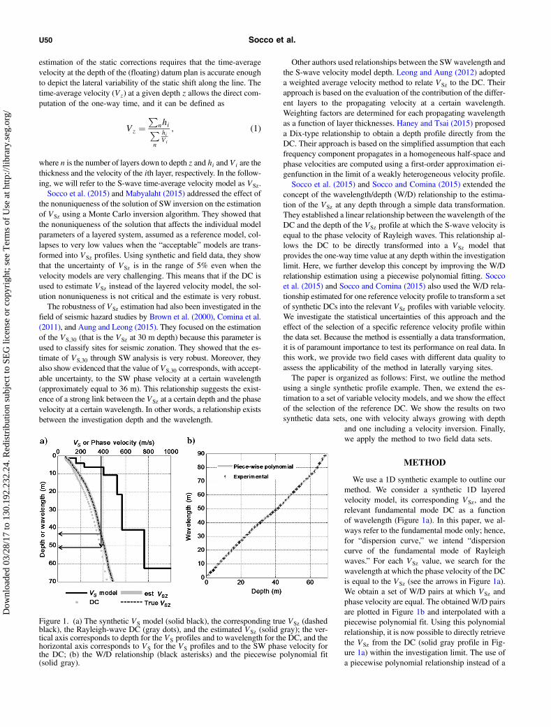
We use a 1D synthetic example to outline ourmethod. We consider a synthetic 1D layeredvelocity model, its corresponding VSz, and therelevant fundamental mode DC as a functionof wavelength (Figure 1a). In this paper, we al-ways refer to the fundamental mode only; hence,for “dispersion curve,” we intend “dispersioncurve of the fundamental mode of Rayleighwaves.” For each VSz value, we search for thewavelength at which the phase velocity of the DCis equal to the VSz (see the arrows in Figure 1a).We obtain a set of W/D pairs at which VSz andphase velocity are equal. The obtained W/D pairsare plotted in Figure 1b and interpolated with apiecewise polynomial fit. Using this polynomialrelationship, it is now possible to directly retrievethe VSz from the DC (solid gray profile in Fig-ure 1a) within the investigation limit. The use ofa piecewise polynomial relationship instead of a

Figure 1. (a) The synthetic VS model (solid black), the corresponding true VSz (dashedblack), the Rayleigh-wave DC (gray dots), and the estimated VSz (solid gray); the ver-tical axis corresponds to depth for the VS profiles and to wavelength for the DC, and thehorizontal axis corresponds to VS for the VS profiles and to the SW phase velocity forthe DC; (b) the W/D relationship (black asterisks) and the piecewise polynomial fit(solid gray).

U50 Socco et al.

Dow

nloa

ded

03/2

8/17

to 1

30.1

92.2

32.2

4. R

edis

trib

utio

n su

bjec

t to

SEG

lice

nse

or c

opyr

ight

; see

Ter

ms

of U

se a

t http

://lib

rary

.seg

.org

/

linear regression is thoroughly addressed by Khosro Anjom (2016),and it is discussed in the “Discussion” section.The W/D relationship has a strong physical link with SW propa-

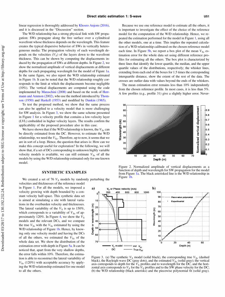
gation: SWs propagate along the free surface over a cylindricalwavefront whose thickness depends on the wavelength. This featurecreates the typical dispersive behavior of SWs in vertically hetero-geneous media: The propagation velocity of each wavelength de-pends on the velocities (VS) of the layers down to the wavefrontthickness. This can be shown by computing the displacements in-duced by the propagation of SWs at different depths. In Figure 2, weshow the normalized amplitude of vertical displacements at differentdepths for each propagating wavelength for the model of Figure 1a.In the same figure, we also report the W/D relationship estimatedin Figure 1b. It can be noted that the W/D relationship roughly cor-responds to the limit at which the displacements become negligible(10%). The vertical displacements are computed using the codeimplemented by Maraschini (2008) and based on the work of Herr-mann and Ammon (2002), who use the method introduced by Thom-son (1950) and Haskell (1953) and modified by Dunkin (1965).To test the proposed method, we show that the same process

can also be applied to a velocity model that is more challengingfor SW analysis. In Figure 3, we show the same scheme presentedin Figure 1 for a velocity profile that contains a low-velocity layer(LVL) embedded in higher velocity layers. The results confirm theapplicability of the proposed procedure also in this case.We have shown that if theW/D relationship is known, the VSz can

be directly estimated from the DC. However, to estimate the W/Drelationship, we need the VSz. Therefore, up to now, it seems that weare in sort of a loop. Hence, the question that arises is: How can wemake this concept useful for exploration? In the following, we willshow that, if a set of DCs corresponding to unknown highly variablevelocity models is available, we can still estimate VSz of all themodels by using theW/D relationship estimated only for one knownmodel.

SYNTHETIC EXAMPLES

We created a set of 76 VS models by randomly perturbing thevelocities and thicknesses of the reference modelin Figure 1. For all the models, we imposed avelocity growing with depth bounded by a con-stant velocity half-space. This synthetic data setis aimed at simulating a site with lateral varia-tions in the overburden velocity and thicknesses.The lateral variability of the VS is up to 150%,which corresponds to a variability of VSz of ap-proximately 120%. In Figure 4, we show the VS

models and the relevant DCs, and we comparethe true VSz with the VSz estimated by using theW/D relationship of Figure 1b. Hence, by know-ing only one velocity model and having the DCsof all the others, we estimated the VSz of thewhole data set. We show the distribution of theestimation error with depth in Figure 5a. It can benoticed that, apart from the very shallow depths,the error falls within 10%. Therefore, the estima-tion is able to reconstruct the lateral variability ofVSz (120%) with acceptable accuracy by apply-ing theW/D relationship estimated for one modelto all the others.

Because we use one reference model to estimate all the others, itis important to investigate the effect of the choice of the referencemodel for the computation of the W/D relationship. Hence, we re-peated the estimation performed for the model in Figure 1, using allthe other models, one at a time. This implies the repeated calcula-tion of a W/D relationship calibrated on the chosen reference modeleach time. In Figure 5b, we report a box plot of the mean VSz es-timation error for the whole data set using different reference pro-files for estimating all the others. The box plot is characterized bythree lines that identify the lower quartile, the median, and the upperquartile values of the distributions, respectively; the whisker lines,extending from each end of the boxes for 1.5 times the correspondinginterquartile distance, show the extent of the rest of the data. Thecrosses are outlier data with values beyond the ends of the whiskers.The mean estimation error remains less than 10% independently

from the chosen reference profile. In most cases, it is less than 5%.A few profiles (e.g., profile 31) give a slightly higher error. Never-

Figure 2. Normalized amplitude of vertical displacements as afunction of depth and wavelength for SW propagation for the modelfrom Figure 1a. The black asterisked line is the W/D relationship inFigure 1b.

Figure 3. (a) The synthetic VS model (solid black), the corresponding true VSz (dashedblack), the Rayleigh-wave DC (gray dots), and the estimated VSz (solid gray); the verticalaxis corresponds to depth for the VS profiles and to wavelength for the DC, and the hori-zontal axis corresponds to VS for the VS profiles and to the SW phase velocity for the DC;(b) the W/D relationship (black asterisks) and the piecewise polynomial fit (solid gray).

Direct static estimation 1: S-wave U51

Dow

nloa

ded

03/2

8/17

to 1

30.1

92.2

32.2

4. R

edis

trib

utio

n su

bjec

t to

SEG

lice

nse

or c

opyr

ight

; see

Ter

ms

of U

se a

t http

://lib

rary

.seg

.org

/

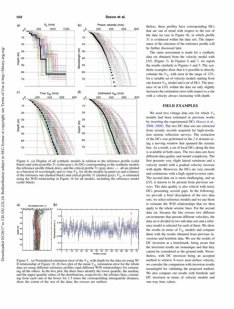
theless, these profiles have corresponding DCsthat are out of trend with respect to the rest ofthe data set (see in Figure 4b, in which profile31 is evidenced within the data set). The impor-tance of the selection of the reference profile willbe further discussed later.The same assessment is made for a synthetic

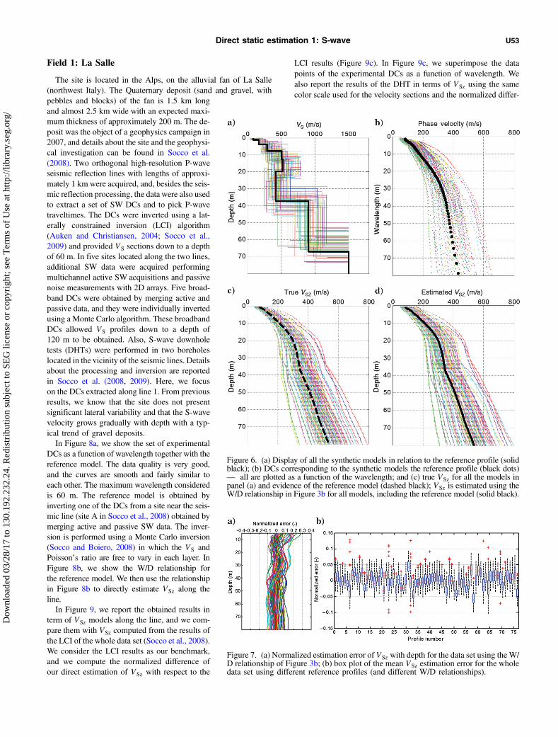
data set obtained from the velocity model withLVL (Figure 3). In Figures 6 and 7, we reportthe results similarly to Figures 4 and 5. The syn-thetic examples show that it is possible to directlyestimate the VSz with error in the range of 12%,for a variable set of velocity models starting fromone known VSz model and a set of DCs. The pres-ence of an LVL within the data set only slightlyincreases the estimation error with respect to a sitewith a velocity always increasing with depth.

FIELD EXAMPLES

We used two vintage data sets for which VS

models had been estimated in previous worksby inverting the experimental DCs (Socco et al.,2008, 2009). The two DC data sets are extractedfrom seismic records acquired for high-resolu-tion seismic reflection surveys. The extractionof the DCs was performed in the f-k domain us-ing a moving window that spanned the seismicline. As a result, a set of local DCs along the lineis available in both cases. The two data sets havedifferent data quality and model complexity. Thefirst presents very slight lateral variations and avelocity model with a gradual velocity increasewith depth. Moreover, the DCs are very smoothand continuous with a high signal-to-noise ratio.The second data set is more challenging, and anLVL is known to be present from previous sur-veys. The data quality is also critical with noisyDCs presenting several gaps. In the following,we provide a brief description of the two datasets, we select reference models and we use themto estimate the W/D relationships that we thenapply to the whole seismic lines. For the seconddata set, because the line crosses two differentenvironments that present different velocities, thedata set is divided in two sub-data sets and a refer-ence model is selected for each of them. We showthe results in terms of VSz models and comparethem with the results obtained from previous in-versions and borehole data. We use the results ofDC inversion as a benchmark, being aware thatthe inversion results are nonunique and that theycannot be considered as the ground truth. Never-theless, with DC inversion being an acceptedmethod to retrieve S-wave near-surface velocity,we consider the comparison with inversion resultsmeaningful for validating the proposed method.We also compare our results with borehole andDC inversion in terms of velocity models andone-way time values.

Figure 4. (a) Display of all synthetic models in relation to the reference profile (solidblack) and critical profile 31 (solid gray); (b) DCs corresponding to the synthetic modelsthe reference profile (black dots), and the critical profile 31 (gray dots) — all are plottedas a function of wavelength; and (c) true VSz for all the models in panel (a) and evidenceof the reference one (dashed black) and critical profile 31 (dashed gray); VSz is estimatedusing the W/D relationship in Figure 1b for all models, including the reference model(solid black).

Figure 5. (a) Normalized estimation error of the VSz with depth for the data set using W/D relationship of Figure 1b; (b) box plot of the mean VSz estimation error for the wholedata set using different reference profiles (and different W/D relationships) for estimat-ing all the others. In the box plot, the three lines identify the lower quartile, the median,and the upper quartile values of the distributions, respectively; the whisker lines, extend-ing from each end of the boxes for 1.5 times the corresponding interquartile distance,show the extent of the rest of the data; the crosses are outliers.

U52 Socco et al.

Dow

nloa

ded

03/2

8/17

to 1

30.1

92.2

32.2

4. R

edis

trib

utio

n su

bjec

t to

SEG

lice

nse

or c

opyr

ight

; see

Ter

ms

of U

se a

t http

://lib

rary

.seg

.org

/

Field 1: La Salle

The site is located in the Alps, on the alluvial fan of La Salle(northwest Italy). The Quaternary deposit (sand and gravel, withpebbles and blocks) of the fan is 1.5 km longand almost 2.5 km wide with an expected maxi-mum thickness of approximately 200 m. The de-posit was the object of a geophysics campaign in2007, and details about the site and the geophysi-cal investigation can be found in Socco et al.(2008). Two orthogonal high-resolution P-waveseismic reflection lines with lengths of approxi-mately 1 km were acquired, and, besides the seis-mic reflection processing, the data were also usedto extract a set of SW DCs and to pick P-wavetraveltimes. The DCs were inverted using a lat-erally constrained inversion (LCI) algorithm(Auken and Christiansen, 2004; Socco et al.,2009) and provided VS sections down to a depthof 60 m. In five sites located along the two lines,additional SW data were acquired performingmultichannel active SW acquisitions and passivenoise measurements with 2D arrays. Five broad-band DCs were obtained by merging active andpassive data, and they were individually invertedusing a Monte Carlo algorithm. These broadbandDCs allowed VS profiles down to a depth of120 m to be obtained. Also, S-wave downholetests (DHTs) were performed in two boreholeslocated in the vicinity of the seismic lines. Detailsabout the processing and inversion are reportedin Socco et al. (2008, 2009). Here, we focuson the DCs extracted along line 1. From previousresults, we know that the site does not presentsignificant lateral variability and that the S-wavevelocity grows gradually with depth with a typ-ical trend of gravel deposits.In Figure 8a, we show the set of experimental

DCs as a function of wavelength together with thereference model. The data quality is very good,and the curves are smooth and fairly similar toeach other. The maximum wavelength consideredis 60 m. The reference model is obtained byinverting one of the DCs from a site near the seis-mic line (site A in Socco et al., 2008) obtained bymerging active and passive SW data. The inver-sion is performed using a Monte Carlo inversion(Socco and Boiero, 2008) in which the VS andPoisson’s ratio are free to vary in each layer. InFigure 8b, we show the W/D relationship forthe reference model. We then use the relationshipin Figure 8b to directly estimate VSz along theline.In Figure 9, we report the obtained results in

term of VSz models along the line, and we com-pare them with VSz computed from the results ofthe LCI of the whole data set (Socco et al., 2008).We consider the LCI results as our benchmark,and we compute the normalized difference ofour direct estimation of VSz with respect to the

LCI results (Figure 9c). In Figure 9c, we superimpose the datapoints of the experimental DCs as a function of wavelength. Wealso report the results of the DHT in terms of VSz using the samecolor scale used for the velocity sections and the normalized differ-

Figure 6. (a) Display of all the synthetic models in relation to the reference profile (solidblack); (b) DCs corresponding to the synthetic models the reference profile (black dots)— all are plotted as a function of the wavelength; and (c) true VSz for all the models inpanel (a) and evidence of the reference model (dashed black); VSz is estimated using theW/D relationship in Figure 3b for all models, including the reference model (solid black).

Figure 7. (a) Normalized estimation error of VSz with depth for the data set using the W/D relationship of Figure 3b; (b) box plot of the mean VSz estimation error for the wholedata set using different reference profiles (and different W/D relationships).

Direct static estimation 1: S-wave U53

Dow

nloa

ded

03/2

8/17

to 1

30.1

92.2

32.2

4. R

edis

trib

utio

n su

bjec

t to

SEG

lice

nse

or c

opyr

ight

; see

Ter

ms

of U

se a

t http

://lib

rary

.seg

.org

/

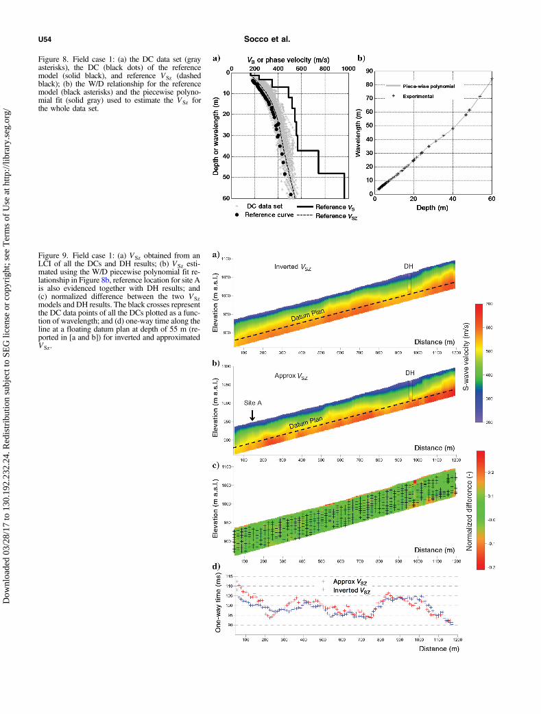
Figure 8. Field case 1: (a) the DC data set (grayasterisks), the DC (black dots) of the referencemodel (solid black), and reference VSz (dashedblack); (b) the W/D relationship for the referencemodel (black asterisks) and the piecewise polyno-mial fit (solid gray) used to estimate the VSz forthe whole data set.

Figure 9. Field case 1: (a) VSz obtained from anLCI of all the DCs and DH results; (b) VSz esti-mated using the W/D piecewise polynomial fit re-lationship in Figure 8b, reference location for site Ais also evidenced together with DH results; and(c) normalized difference between the two VSzmodels and DH results. The black crosses representthe DC data points of all the DCs plotted as a func-tion of wavelength; and (d) one-way time along theline at a floating datum plan at depth of 55 m (re-ported in [a and b]) for inverted and approximatedVSz.

U54 Socco et al.

Dow

nloa

ded

03/2

8/17

to 1

30.1

92.2

32.2

4. R

edis

trib

utio

n su

bjec

t to

SEG

lice

nse

or c

opyr

ight

; see

Ter

ms

of U

se a

t http

://lib

rary

.seg

.org

/

ence of our results with respect to the DHT. InFigure 9d, we report the one-way time (staticshift) at a floating datum at a 55 m depth com-puted along the line using the LCI results and ourapproximated results.Apart from very few zones within the section,

the VSz is estimated with a mean difference withrespect to inverted data of less than 5% along thewhole line. The site presents a very slight lateralvariability, which is very well reconstructed bythe direct estimation (see the comparison betweenFigure 9a and 9b). The data are also in good agree-ment with the DHT except in the first 5 m, inwhich the DHT provides lower velocity than theLCI and our direct estimation. Nevertheless, thiserror is recovered below 5 m, where the differenceremains in the range of 10% or lower. The staticshifts computed at a depth of 55 m (below the topof the first high-velocity layer) show maximumdifference of the order of 5 ms and provide verysimilar trends. The LCI results are slightlysmoother, and this can be due to the use of lateralconstraints among neighboring models during in-version.

Field 2: Torre Pellice

The site is located in an alpine valley in thetown of Torre Pellice (northwest Italy). It presentsa sequence characterized by the fringe of an allu-vial fan with coarse and irregularly shaped sedi-ments, fluvial sediments with variable thickness(10–50 m), lacustrine sediments, and the bedrock,which is expected at more than a 100 m depth inthe central part of the valley. In 2007, a high-res-olution reflection survey was performed along a800 m line across the valley in the frameworkof a seismic hazard study (for details about dataacquisition and processing, see Socco et al. [2009]and Boiero and Socco [2014]). Data from the seis-mic line were also used to extract a set of SWDCsand to pick P-wave traveltimes. The DCs werethen inverted using a joint P- and S-wave inver-sion algorithm (Boiero and Socco, 2014), and theyprovided the VS sections down to a depth of ap-proximately 50 m. The seismic line crosses twodifferent geologic environments: the zone closeto the river (from zero to approximately 250 m)on the south, in which nine DCs are available,and the zone on the north that overlies an alluvialfan (from 250 m to the end of the line), in which27 DCs are available. The maximum wavelengthobtained ranges from 30 to 50 m in the south zoneand from 60 to 100 m in the north zone. The mini-mum values of the wavelength are approximately4 m, thus providing rough information on theuppermost layer.On this data set, we performed the same analy-

sis as for field case 1. However, the two sets ofDCs present two different trends and well-sepa-

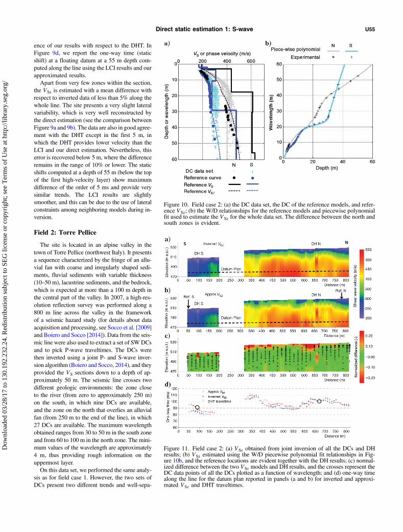
Figure 10. Field case 2: (a) the DC data set, the DC of the reference models, and refer-ence VSz; (b) the W/D relationships for the reference models and piecewise polynomialfit used to estimate the VSz for the whole data set. The difference between the north andsouth zones is evident.

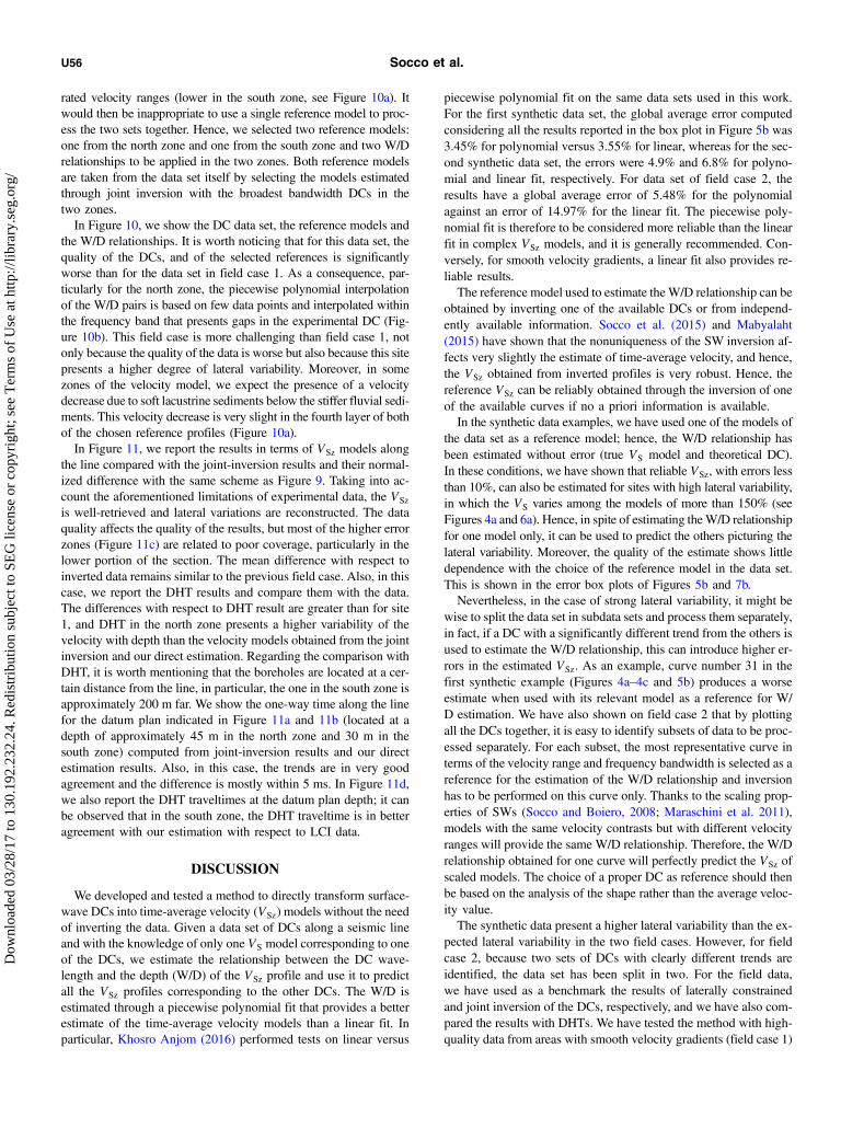
Figure 11. Field case 2: (a) VSz obtained from joint inversion of all the DCs and DHresults; (b) VSz estimated using the W/D piecewise polynomial fit relationships in Fig-ure 10b, and the reference locations are evident together with the DH results; (c) normal-ized difference between the two VSz models and DH results, and the crosses represent theDC data points of all the DCs plotted as a function of wavelength; and (d) one-way timealong the line for the datum plan reported in panels (a and b) for inverted and approxi-mated VSz and DHT traveltimes.

Direct static estimation 1: S-wave U55

Dow

nloa

ded

03/2

8/17

to 1

30.1

92.2

32.2

4. R

edis

trib

utio

n su

bjec

t to

SEG

lice

nse

or c

opyr

ight

; see

Ter

ms

of U

se a

t http

://lib

rary

.seg

.org

/

rated velocity ranges (lower in the south zone, see Figure 10a). Itwould then be inappropriate to use a single reference model to proc-ess the two sets together. Hence, we selected two reference models:one from the north zone and one from the south zone and two W/Drelationships to be applied in the two zones. Both reference modelsare taken from the data set itself by selecting the models estimatedthrough joint inversion with the broadest bandwidth DCs in thetwo zones.In Figure 10, we show the DC data set, the reference models and

the W/D relationships. It is worth noticing that for this data set, thequality of the DCs, and of the selected references is significantlyworse than for the data set in field case 1. As a consequence, par-ticularly for the north zone, the piecewise polynomial interpolationof the W/D pairs is based on few data points and interpolated withinthe frequency band that presents gaps in the experimental DC (Fig-ure 10b). This field case is more challenging than field case 1, notonly because the quality of the data is worse but also because this sitepresents a higher degree of lateral variability. Moreover, in somezones of the velocity model, we expect the presence of a velocitydecrease due to soft lacustrine sediments below the stiffer fluvial sedi-ments. This velocity decrease is very slight in the fourth layer of bothof the chosen reference profiles (Figure 10a).In Figure 11, we report the results in terms of VSz models along

the line compared with the joint-inversion results and their normal-ized difference with the same scheme as Figure 9. Taking into ac-count the aforementioned limitations of experimental data, the VSz

is well-retrieved and lateral variations are reconstructed. The dataquality affects the quality of the results, but most of the higher errorzones (Figure 11c) are related to poor coverage, particularly in thelower portion of the section. The mean difference with respect toinverted data remains similar to the previous field case. Also, in thiscase, we report the DHT results and compare them with the data.The differences with respect to DHT result are greater than for site1, and DHT in the north zone presents a higher variability of thevelocity with depth than the velocity models obtained from the jointinversion and our direct estimation. Regarding the comparison withDHT, it is worth mentioning that the boreholes are located at a cer-tain distance from the line, in particular, the one in the south zone isapproximately 200 m far. We show the one-way time along the linefor the datum plan indicated in Figure 11a and 11b (located at adepth of approximately 45 m in the north zone and 30 m in thesouth zone) computed from joint-inversion results and our directestimation results. Also, in this case, the trends are in very goodagreement and the difference is mostly within 5 ms. In Figure 11d,we also report the DHT traveltimes at the datum plan depth; it canbe observed that in the south zone, the DHT traveltime is in betteragreement with our estimation with respect to LCI data.

DISCUSSION

We developed and tested a method to directly transform surface-wave DCs into time-average velocity (VSz) models without the needof inverting the data. Given a data set of DCs along a seismic lineand with the knowledge of only one VS model corresponding to oneof the DCs, we estimate the relationship between the DC wave-length and the depth (W/D) of the VSz profile and use it to predictall the VSz profiles corresponding to the other DCs. The W/D isestimated through a piecewise polynomial fit that provides a betterestimate of the time-average velocity models than a linear fit. Inparticular, Khosro Anjom (2016) performed tests on linear versus

piecewise polynomial fit on the same data sets used in this work.For the first synthetic data set, the global average error computedconsidering all the results reported in the box plot in Figure 5b was3.45% for polynomial versus 3.55% for linear, whereas for the sec-ond synthetic data set, the errors were 4.9% and 6.8% for polyno-mial and linear fit, respectively. For data set of field case 2, theresults have a global average error of 5.48% for the polynomialagainst an error of 14.97% for the linear fit. The piecewise poly-nomial fit is therefore to be considered more reliable than the linearfit in complex VSz models, and it is generally recommended. Con-versely, for smooth velocity gradients, a linear fit also provides re-liable results.The reference model used to estimate theW/D relationship can be

obtained by inverting one of the available DCs or from independ-ently available information. Socco et al. (2015) and Mabyalaht(2015) have shown that the nonuniqueness of the SW inversion af-fects very slightly the estimate of time-average velocity, and hence,the VSz obtained from inverted profiles is very robust. Hence, thereference VSz can be reliably obtained through the inversion of oneof the available curves if no a priori information is available.In the synthetic data examples, we have used one of the models of

the data set as a reference model; hence, the W/D relationship hasbeen estimated without error (true VS model and theoretical DC).In these conditions, we have shown that reliable VSz, with errors lessthan 10%, can also be estimated for sites with high lateral variability,in which the VS varies among the models of more than 150% (seeFigures 4a and 6a). Hence, in spite of estimating theW/D relationshipfor one model only, it can be used to predict the others picturing thelateral variability. Moreover, the quality of the estimate shows littledependence with the choice of the reference model in the data set.This is shown in the error box plots of Figures 5b and 7b.Nevertheless, in the case of strong lateral variability, it might be

wise to split the data set in subdata sets and process them separately,in fact, if a DC with a significantly different trend from the others isused to estimate the W/D relationship, this can introduce higher er-rors in the estimated VSz. As an example, curve number 31 in thefirst synthetic example (Figures 4a–4c and 5b) produces a worseestimate when used with its relevant model as a reference for W/D estimation. We have also shown on field case 2 that by plottingall the DCs together, it is easy to identify subsets of data to be proc-essed separately. For each subset, the most representative curve interms of the velocity range and frequency bandwidth is selected as areference for the estimation of the W/D relationship and inversionhas to be performed on this curve only. Thanks to the scaling prop-erties of SWs (Socco and Boiero, 2008; Maraschini et al. 2011),models with the same velocity contrasts but with different velocityranges will provide the same W/D relationship. Therefore, the W/Drelationship obtained for one curve will perfectly predict the VSz ofscaled models. The choice of a proper DC as reference should thenbe based on the analysis of the shape rather than the average veloc-ity value.The synthetic data present a higher lateral variability than the ex-

pected lateral variability in the two field cases. However, for fieldcase 2, because two sets of DCs with clearly different trends areidentified, the data set has been split in two. For the field data,we have used as a benchmark the results of laterally constrainedand joint inversion of the DCs, respectively, and we have also com-pared the results with DHTs. We have tested the method with high-quality data from areas with smooth velocity gradients (field case 1)

U56 Socco et al.

Dow

nloa

ded

03/2

8/17

to 1

30.1

92.2

32.2

4. R

edis

trib

utio

n su

bjec

t to

SEG

lice

nse

or c

opyr

ight

; see

Ter

ms

of U

se a

t http

://lib

rary

.seg

.org

/

and with poor-quality data from areas with velocity inversions andcontrasts (field case 2). For both sites, the estimated VSz has errorsmostly less than 5% (Figures 9c and 11c).The synthetic and field examples show that the errors in the es-

timation of VSz tend to be larger at shallow depths, whereas theestimate is more reliable and stable at greater depths (Figures 5aand 7a). This is due to the lack of data points and poor resolutionin the first few meters from the ground surface. In fact, because themethod is based on a data transform, the quality of the estimationdepends on the quality of the DC and on the availability of datapoints at different wavelengths. This can also be seen on the resultsof field data in which the higher errors are in the zones of poor datacoverage, particularly in the very shallow subsurface (Figures 9cand 11c). All the synthetic results underline, however, that the errorreduces and remains stable with increasing depth, particularly be-low the bedrock. This leads to reliable estimates of the one-waytime below the bedrock for statics.In Figure 12, we show the error distributions

on one-way time in milliseconds for the two syn-thetic data sets. We use box plots with the samescheme used for Figures 5b and 7b, and we re-port the distribution of errors of all the profiles atall depths obtained using different referencemodels to estimate the W/D. Most of the valuesfall within 5 ms except for few outliers and a cou-ple of cases already evidenced in the normalizederror for the velocities (Figures 5b and 7b).In Figures 9d and 11d, we compare the static

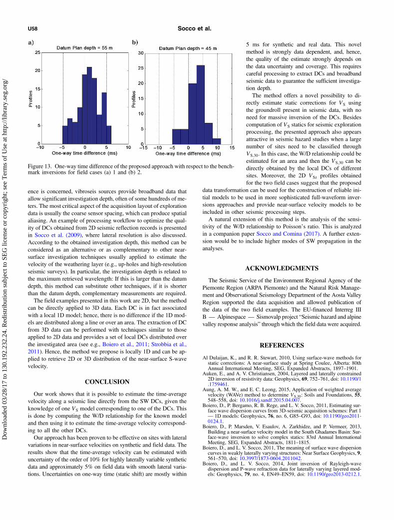
shift computed from the velocity models ob-tained through inversion and those obtained fromthe direct estimation and showed that the spatialtrends are very well-reconstructed. In Figure 13,we report the distribution of the time differencesin Figures 9d and 11d in the form of histograms.In both situations, the difference with respect tothe inversion results remains less than 5 ms ex-cept for a few outliers. The distribution of theone-way traveltime differences is centered atzero for field case 1, and it shows a very slightglobal overestimation for field case 2. In this re-spect, it is useful to remark that the two bench-marks used are different from each other. In fieldcase 1, LCI was performed with a verticalsmoothness constraint and a high number oflayers; hence, the resulting models are verticallysmooth. In field case 2, on the contrary, joint in-version was performed using a limited number oflayers that led to higher contrast within thebenchmark velocity models. Moreover, compar-ing the one-way time obtained with our approachwith the available traveltimes obtained directlyfrom borehole data (Figure 11d), it can be notedthat our estimate is in better agreement with theDHTs and that both are slightly higher than thetime obtained from LCI, particularly in the southzone.The field data confirm the possibility of repli-

cating the results of the inversion in terms of VSz,without the need of inverting the whole data set.

Removing extensive inversion from the workflow reduces the needfor arbitrary choices from the operator (model parameterization)and avoids a possible source of error. Moreover, it makes the proc-ess very fast. The fact that the results are mainly data driven makesthe uncertainty in the results directly related to data coverage andexperimental uncertainties. It is hence of paramount importance toassess that the DCs obtained from the seismic records guarantee thesufficient investigation depth and lateral resolution. The possibilityof extracting broadband and high-quality DC depends on acquisi-tion parameters and on site characteristics. If the DCs are retrievedfrom seismic reflection records acquired for hydrocarbon explora-tion, countermeasures taken to filter ground roll during acquisition,such as geophone groups or high-pass filters, can affect the dataquality. A practical guideline for the acquisition parameters canbe found in Socco et al. (2010), and a discussion about the extrac-tion of dispersion data from hydrocarbon exploration seismicrecords is provided in Strobbia et al. (2011). As far as our experi-

Figure 12. Box plots of the mean one-way time error for the two synthetic data setsusing different reference profiles (and different W/D relationships): (a) synthetic dataset 1 and (b) synthetic data set 2.

Direct static estimation 1: S-wave U57

Dow

nloa

ded

03/2

8/17

to 1

30.1

92.2

32.2

4. R

edis

trib

utio

n su

bjec

t to

SEG

lice

nse

or c

opyr

ight

; see

Ter

ms

of U

se a

t http

://lib

rary

.seg

.org

/

ence is concerned, vibroseis sources provide broadband data thatallow significant investigation depth, often of some hundreds of me-ters. The most critical aspect of the acquisition layout of explorationdata is usually the coarse sensor spacing, which can produce spatialaliasing. An example of processing workflow to optimize the qual-ity of DCs obtained from 2D seismic reflection records is presentedin Socco et al. (2009), where lateral resolution is also discussed.According to the obtained investigation depth, this method can beconsidered as an alternative or as complementary to other near-surface investigation techniques usually applied to estimate thevelocity of the weathering layer (e.g., up-holes and high-resolutionseismic surveys). In particular, the investigation depth is related tothe maximum retrieved wavelength: If this is larger than the datumdepth, this method can substitute other techniques, if it is shorterthan the datum depth, complementary measurements are required.The field examples presented in this work are 2D, but the method

can be directly applied to 3D data. Each DC is in fact associatedwith a local 1D model; hence, there is no difference if the 1D mod-els are distributed along a line or over an area. The extraction of DCfrom 3D data can be performed with techniques similar to thoseapplied to 2D data and provides a set of local DCs distributed overthe investigated area (see e.g., Boiero et al., 2011; Strobbia et al.,2011). Hence, the method we propose is locally 1D and can be ap-plied to retrieve 2D or 3D distribution of the near-surface S-wavevelocity.

CONCLUSION

Our work shows that it is possible to estimate the time-averagevelocity along a seismic line directly from the SW DCs, given theknowledge of one VS model corresponding to one of the DCs. Thisis done by computing the W/D relationship for the known modeland then using it to estimate the time-average velocity correspond-ing to all the other DCs.Our approach has been proven to be effective on sites with lateral

variations in near-surface velocities on synthetic and field data. Theresults show that the time-average velocity can be estimated withuncertainty of the order of 10% for highly laterally variable syntheticdata and approximately 5% on field data with smooth lateral varia-tions. Uncertainties on one-way time (static shift) are mostly within

5 ms for synthetic and real data. This novelmethod is strongly data dependent, and, hence,the quality of the estimate strongly depends onthe data uncertainty and coverage. This requirescareful processing to extract DCs and broadbandseismic data to guarantee the sufficient investiga-tion depth.The method offers a novel possibility to di-

rectly estimate static corrections for VS usingthe groundroll present in seismic data, with noneed for massive inversion of the DCs. Besidescomputation of VS statics for seismic explorationprocessing, the presented approach also appearsattractive in seismic hazard studies when a largenumber of sites need to be classified throughVS;30. In this case, the W/D relationship could beestimated for an area and then the VS;30 can bedirectly obtained by the local DCs of differentsites. Moreover, the 2D VSz profiles obtainedfor the two field cases suggest that the proposed

data transformation can be used for the construction of reliable ini-tial models to be used in more sophisticated full-waveform inver-sions approaches and provide near-surface velocity models to beincluded in other seismic processing steps.A natural extension of this method is the analysis of the sensi-

tivity of the W/D relationship to Poisson’s ratio. This is analyzedin a companion paper Socco and Comina (2017). A further exten-sion would be to include higher modes of SW propagation in theanalyses.

ACKNOWLEDGMENTS

The Seismic Service of the Environment Regional Agency of thePiemonte Region (ARPA Piemonte) and the Natural Risk Manage-ment and Observational Seismology Department of the Aosta ValleyRegion supported the data acquisition and allowed publication ofthe data of the two field examples. The EU-financed Interreg IIIB — Alpinespace — Sismovalp project “Seismic hazard and alpinevalley response analysis” through which the field data were acquired.

REFERENCES

Al Dulaijan, K., and R. R. Stewart, 2010, Using surface‐wave methods forstatic corrections: A near‐surface study at Spring Coulee, Alberta: 80thAnnual International Meeting, SEG, Expanded Abstracts, 1897–1901.

Auken, E., and A. V. Christiansen, 2004, Layered and laterally constrained2D inversion of resistivity data: Geophysics, 69, 752–761, doi: 10.1190/1.1759461.

Aung, A. M. W., and E. C. Leong, 2015, Application of weighted averagevelocity (WAVe) method to determine VS;30: Soils and Foundations, 55,548–558, doi: 10.1016/j.sandf.2015.04.007.

Boiero, D., P. Bergamo, R. B. Rege, and L. V. Socco, 2011, Estimating sur-face wave dispersion curves from 3D-seismic acquisition schemes: Part 1— 1D models: Geophysics, 76, no. 6, G85–G93, doi: 10.1190/geo2011-0124.1.

Boiero, D., P. Marsden, V. Esaulov, A. Zarkhidze, and P. Vermeer, 2013,Building a near-surface velocity model in the South Ghadames Basin: Sur-face-wave inversion to solve complex statics: 83rd Annual InternationalMeeting, SEG, Expanded Abstracts, 1811–1815.

Boiero, D., and L. V. Socco, 2011, The meaning of surface wave dispersioncurves in weakly laterally varying structures: Near Surface Geophysics, 9,561–570, doi: 10.3997/1873-0604.2011042.

Boiero, D., and L. V. Socco, 2014, Joint inversion of Rayleigh-wavedispersion and P-wave refraction data for laterally varying layered mod-els: Geophysics, 79, no. 4, EN49–EN59, doi: 10.1190/geo2013-0212.1.

Figure 13. One-way time difference of the proposed approach with respect to the bench-mark inversions for field cases (a) 1 and (b) 2.

U58 Socco et al.

Dow

nloa

ded

03/2

8/17

to 1

30.1

92.2

32.2

4. R

edis

trib

utio

n su

bjec

t to

SEG

lice

nse

or c

opyr

ight

; see

Ter

ms

of U

se a

t http

://lib

rary

.seg

.org

/

Brown, L. T., J. G. Diehl, and R. L. Nigbor, 2000, A simplified procedure tomeasure average shear-wave velocity to a depth of 30 meters (VS;30): Pre-sented at the 12th World Conference on Earthquake Engineering.

Comina, C., S. Foti, D. Boiero, and L. V. Socco, 2011, Reliability of VS;30evaluation from surface waves tests: Journal of Geotechnical and Geoen-vironmental Engineering, 137, 579–586, doi: 10.1061/(ASCE)GT.1943-5606.0000452.

Douma, H., and M. Haney, 2011, Surface‐wave inversion for near‐surfaceshear‐wave velocity estimation at Coronation field: 81st Annual Interna-tional Meeting, SEG, Expanded Abstracts, 1411–1415.

Dunkin, J., 1965, Computation of modal solutions in layered, elastic mediaat high frequencies: Bulletin of Seismological Society of America, 55,335–358.

Ernst, F., 2007, Long-wavelength statics estimation from guided waves: 69thAnnual International Conference and Exhibition, EAGE, Extended Ab-stracts, E033.

Haney, M., and R. Miller, 2013, Introduction to this special section: Nonreflection seismic and inversion of surface waves and guided waves:The Leading Edge, 32, 610–611, doi: 10.1190/tle32060610.1.

Haney, M. M., and V. C. Tsai, 2015, Non perturbational surface-wave in-version: A Dix-type relation for surface waves: Geophysics, 80, no. 6,EN167–EN177, doi: 10.1190/geo2014-0612.1.

Haskell, N., 1953, The dispersion of surface waves on multilayered media:Bulletin of the Seismological Society of America, 43, 17–34.

Herrmann, R. B., and C. J. Ammon, 2002, Computer programs in seismol-ogy: Surface waves, receiver functions and crustal structure, version 3.20:Saint Louis University.

Khosro Anjom, F., 2016, Direct estimation of S-wave velocity from ground-roll (Rayleigh waves) towards static corrections: M.S. thesis, Politecnicodi Torino.

Leong, E. C., and A. M. W. Aung, 2012, Weighted average velocity forwardmodelling of Rayleigh surface waves: Soil Dynamics and Earthquake En-gineering, 43, 218–228, doi: 10.1016/j.soildyn.2012.07.030.

Mabyalaht, G. S., 2015, Consequences of surface wave non uniqueness onstatic corrections: M.S. thesis, Politecnico di Torino.

Maraschini, M., 2008, A new approach for the inversion of Rayleigh andScholte waves in site characterization: Ph.D. dissertation, Politecnicodi Torino.

Maraschini, M., D. Boiero, S. Foti, and L. V. Socco, 2011, Scale propertiesof the seismic wavefield: Perspectives for full waveform matching: Geo-physics, 76, no. 5, A37–A44, doi: 10.1190/geo2010-0213.1.

Roy, R., R. R. Stewart, and K. Al Dulaijan, 2010, S-wave velocity and staticsfrom ground-roll inversion: The Leading Edge, 29, 1250–1257, doi: 10.1190/1.3496915.

Socco, L. V., and D. Boiero, 2008, Improved Monte Carlo inversion of sur-face wave data: Geophysical Prospecting, 56, 357–371, doi: 10.1111/j.1365-2478.2007.00678.x.

Socco, L. V., D. Boiero, C. Comina, S. Foti, and R. Wisén, 2008, Seismiccharacterization of an Alpine Site: Near Surface Geophysics, 6, 255–267,doi: 10.3997/1873-0604.2008020.

Socco, L. V., D. Boiero, S. Foti, and R. Wisén, 2009, Laterally constrainedinversion of ground roll from seismic reflection records: Geophysics, 74,no. 6, G35–G45, doi: 10.1190/1.3223636.

Socco, L. V., and C. Comina, 2015, Approximate direct estimate ofS-wave velocity model from surface wave dispersion curves: 21st AnnualInternational Conference and Exhibition, EAGE, Extended Abstracts,A09.

Socco, L. V., and C. Comina, 2017, Time-average velocity estimation throughsurface-wave analysis: Part 2: P-wave velocity: Geophysics, 82, this issue,doi: 10.1190/geo2016-0368.1.

Socco, L. V., S. Foti, and D. Boiero, 2010, Surface wave analysis for buildingnear surface velocity models: Established approaches and new perspectives:Geophysics, 75, no. 5, 75A83–75A102, doi: 10.1190/1.3479491.

Socco, L. V., G. Mabyalaht, and C. Comina, 2015, Robust static estimationfrom surface wave data: 85th Annual International Meeting, SEG, Ex-panded Abstracts, 5222–5227.

Strobbia, C., A. Laake, P. Vermeer, and A. Glushchenko, 2011, Surfacewaves: Use them then lose them. Surface-wave analysis, inversion andattenuation in land reflection seismic surveying: Near Surface Geophys-ics, 9, 503–513, doi: 10.3997/1873-0604.2011022.

Thomson, W. T., 1950, Transmission of elastic waves through a stratifiedsolid medium: Journal of Applied Physics, 21, 89–93, doi: 10.1063/1.1699629.

Direct static estimation 1: S-wave U59

Dow

nloa

ded

03/2

8/17

to 1

30.1

92.2

32.2

4. R

edis

trib

utio

n su

bjec

t to

SEG

lice

nse

or c

opyr

ight

; see

Ter

ms

of U

se a

t http

://lib

rary

.seg

.org

/