Tikhonov and Iterative Regularization Methods for Embedded Inverse Problems

Tikhonov and Iterative Regularization Methods for

Embedded Inverse Problems

M. Haltmeier1, O. Scherzer1, A. Leitao2.

1 Department of Computer Science, University of Innsbruck, Technikerstrasse 21a, A-6020 Innsbruck, Austria.E-mail: Markus.Haltmeier,[email protected] Department of Mathematics, Federal University of St. Catarina, P.O. Box 476, 88040-900 Florianopolis, Brazil.E-mail: [email protected]

Abstract

In this paper we suggest two novel classes of regularization techniques for sys-tems of nonlinear ill–posed tomographic problems. We analyze variational regular-ization method as well as iterative regularization techniques analytically. The laterturns out to be of Landweber-Kaczmarz type. We discuss new stopping criteriafor such iterative methods and present a subtle convergence analysis. The stop-ping criterion is favourable (both analytically and practically) to existing stoppingstratgies.

1 Introduction

In this paper we investigate a new concept of regularization methods for solving non-linear ill–posed operator equations of the form

(1) a(p, u) = g(p) , p ∈ S

where a(p, ·) : D ⊆ X → Y are operators between separable Hilbert spaces X and Y ,which are parameterized on the one dimensional sphere S := R/(2πZ). Many inverseproblems, such as impedance tomography [4] and computerized tomography [17, 7] canbe formulated in such a way.

The basic idea of this paper is to rewrite (1) into a system of equations on the spaceof Bochner integrable periodic functions H s(S, X), s > 0

(2) a(p, u(p)) = g(p) , p ∈ S ,

(3)

√

λ1

2π

∫

S

∥

∥

∥

∥

∂su

∂ps

∥

∥

∥

∥

2

X

dp = 0 with some fixed λ > 0 .

If u is a solution of (1) then p 7→ u(p) ≡ u is a solution of (2), (3), respectively, andvice versa. That means that the systems of equations (1) and (2), (3) are equivalent.

1

In this paper we develop and analyze Tikhonov and iterative regularization methodsfor the solution of embedded equations (2), (3).

In Section 2 we derive and motivate variational and iterative regularization tech-niques for solving (2), (3). Since the equation (1) is embedded into a system of equationson a larger function space we call the resulting regularization techniques embedded reg-ularization methods.

In Section 3 we analyze variational embedded regularization techniques. In partic-ular, we show that the corresponding regularization techniques are well posed, conver-gent and stable. In Section 4 we show that the iterative regularization techniques are ofLandweber-Kacmarcz form (cf. [12]) and present convergence results for these modifiedLandweber-Kaczmarz iterations.

Here, the Kacmarcz iteration schemes are combined with a reliable and efficientdiscrepancy principle which consists in enforcing the residual of each experiment (i.e. foreach p) to be below a certain threshold. This termination criteria has several advantages(both analytically and numerically) over stopping criteria previously proposed in theliterature. We remark that this stopping criterion also applies to already analyzedmethods, like the Landweber-Kacmarcz iteration.

2 Embedded Regularization Methods

There are at least two basic concepts for solving systems of equations of the form(1): iterative regularization methods (cf. e.g. [13, 1, 5, 10, 6, 2]) and Tikhonov typeregularization methods [20, 19, 18, 6].

In order to motivate our approach and indicate differences to existing methods weintroduce the function valued operator

A : D ⊆ X → S(S, Y ) ,

u 7→ p 7→ a(p, u)

and the data set G = p 7→ g(p), where S(S, Y ) is a space of Bochner measurablefunctions.

We can state that u ∈ X is a solution of (1) if it is a minimizer of

(4) ‖A(u) − G‖2S(S,Y ) ,

where ‖ · ‖S(S,Y ) is a norm on the space S(S, Y ), which in the the sequel (for the clarityof presentation) we always take the space L2(S, Y ) with the associated norm

(5) ‖G‖2L2(S,Y ) :=

1

2π

∫

S

‖g(p)‖2Y dp .

Then, standard Tikhonov regularization consists in approximating a minimizer of (4)by a minimizer of the functional

(6) ‖A(u) − G‖2L2(S,Y ) + α‖u− u∗‖2

X ,

2

where u∗ ∈ D is some initial guess of the solution to be recovered and α is a regular-ization parameter.

Gradient type regularization methods aim to approximate the minimizer of (4) viaan iterative procedure. Exemplarily we consider the Landweber iteration, which readsas follows:

(7) un+1 = un −A′(un)∗(A(un) − G) ,

where A′(u)∗ denotes the adjoint of the Frechet-derivative of the operator A with respectto the spaces L2(S, Y ) and X.

Standard Tikhonov regularization for solving (2), (3) consists in calculating a min-imizer of

(8)

∫

S

‖a(p, u(p)) − g(p)‖2Y dp+ λ

∫

S

∥

∥

∥

∥

∂su

∂ps

∥

∥

∥

∥

2

X

dp+ α

∫

S

‖u(p) − u∗‖2X ,

with a regularization parameter α > 0 .In practical applications one is committed to a finite number of experiments (rep-

resented mathematically by one equation of the system) instead of an infinitesimaluncountable number as used in the above motivation. However, mostly it is possible toidentify each experiment with a position on the sphere in a straight foward manner.

For instance in tomography one could identify the position on the sphere with theangle of emmitted X-rays. In this situation we use the operator

A(u) :=(

ai(u))N−1

i=0:=(

a(pi, u))N−1

i=0,

where pi denotes the index of the measurement. Standard iterative methods for thesolution of the operator equation

(9) A(u) = G := (g(pi))N−1i=0

become inefficient if the evaluations of ai(u) and a′i(u)∗ are expensive or if N is large.

In this case typically Kaczmarz-type iterative methods are used. For instance, theLandweber-Kaczmarz method (cf. [12]) is defined by

(10) un+1 = un − a′i(un)

∗(ai(u

n) − g(pi)) ,

with i satisfying n = bn/NcN + i (here bxc is the largest integer less or equal x).In this paper we also investigate an embedded Landweber-Kaczmarz type iteration

for the solution of (2) and (3), which we define by:

(11) U (n+1/2) = U (n) −(

a′i(u(n)i )∗(ai(u

(n)i )) − g(pi))

)

i=0,...,N−1

(12) U (n+1) = U (n+1/2) − L(U (n+1/2)) ,

whereU := (ui)i=0,...,N−1 , with ui ∈ X .

3

and L corresponds to a discretized steepest descent direction of the continuous func-tional

(13) p 7→ u(p) 7→ λ1

2π

∫

S

∥

∥

∥

∥

∂su

∂ps

∥

∥

∥

∥

2

X

dp

onHs(S, X). This scheme is called of Kacmarcz type since the two “blocks” of equationsare considered successively.

In the following we first analyze the embedded Tikhonov regularization and lateron we provide a convergence analysis of the Landweber-Kacmarcz type iteration.

3 Embedded Tikhonov Regularization

A common approach for a stable solution of (1) is to minimize the functional (6) overD. As mentioned in the introduction we apply Tikhonov regularization to the operator-equations (3), (2), that is we minimize the functional (8) over Ds := u ∈ Hs(S, X) :u(p) ∈ D, p ∈ S.

Convergence and stability of Tikhonov regularization for the solution of (1) is onthe hand if A is continuous and weakly sequentially closed. We show that we can applystandard Tikhonov regularization as well as embedded Tikhonov regularization for astable solution of (1) if the following assumptions hold true:

T1. The mapping a : S × D → Y is continuous and weakly continuous on boundedsubsets.

T2. The domain D of the operators a(p, ·) is weakly closed.

T3. The (exact) data G is in L2(S, Y ) and (1) has a solution u† in D.

Here a is called weakly continuous on bounded subsets, if a|S×BXis continuous for

all bounded BX ⊆ X, when S × BX is considered with the product topology of theusual metric topology on S and the weak topology on X restricted to BX , and Y isconsidered with the weak topology.

3.1 Notations and technical results

First we introduce some notations and general results on equi-continuity and BochnerSpaces (see, e.g., Yosida [22, Sections V.4, V.5]).

Equi-continuity

Let E and F be locally convex spaces, BE ⊆ E and M ⊆ C(BE , F ).M is called equi-continuous on BE if for every e0 ∈ BE and every zero neighborhood

V ⊆ F there is a zero neighborhood U ⊆ E such that A(e0) −A(e) ∈ V for all A ∈ Mand all e ∈ BE with e− e0 ∈ U . M is called uniformly equi-continuous if for every zeroneighborhood V ⊆ F there is a zero neighborhood U ⊆ E such that A(e) − A(f) ∈ Vfor all A ∈ M and all e, f ∈ BE with e− f ∈ U . If BE is compact, then equi-continuity

4

PSfrag replacements

(p0, e0) (p, e0)

(p, f)

UE = UE(e0)

α = α(p0, e0)S

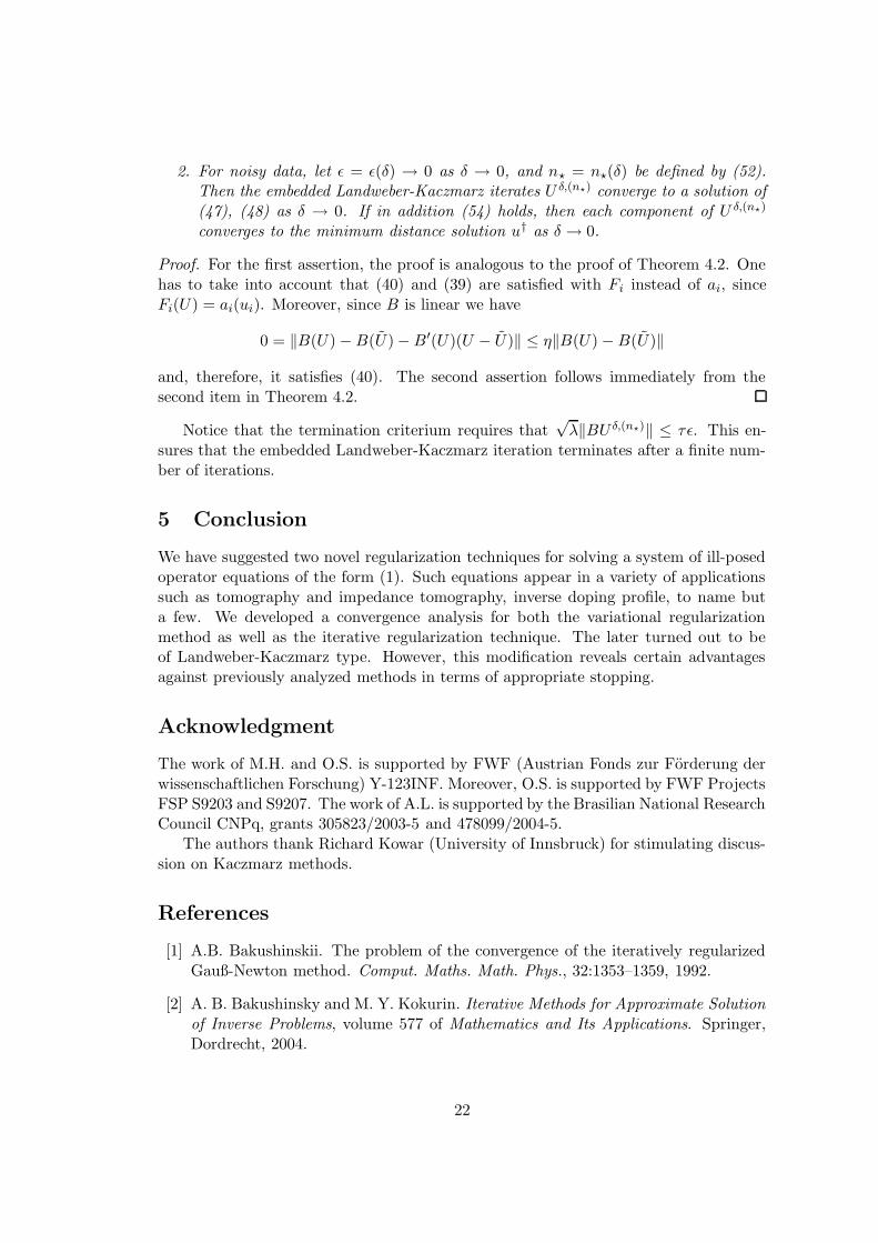
Figure 1: The equi-continuity of a(p, ·) : p ∈ S in e0, the continuity of A(·, e0) in p0

and the triangle inequality imply the continuity of A in (p0, u0).

and uniform equi-continuity are equivalent. If E and F are Hilbert spaces then Mis called strongly (resp. weakly) equi-continuous if E and F are considered with thestrong (resp. weak) topology. Finally, a family (resp. sequence) (Aλ)λ∈Λ ⊆ C(BE , F )Λ

is called (uniformly) equi-continuous if the set Aλ : λ ∈ Λ ⊆ C(E,F ) is (uniformly)equi-continuous.

If (E, dE) is a metric space, analogous definitions hold where statements like e−e0 ∈U have to be replaced by statements like dE(e, e0) < α.

Proposition 3.1. Let BE ⊆ E and a : S × BE → F . If M1 := a(p, ·) : p ∈ S ⊆C(E,F ), M2 := a(·, e) : e ∈ E ⊆ C(S, F ) and M1 (resp. M2) is equi-continuous,then a is continuous.

Conversely, if a is continuous then M1 is equi-continuous and if additionally BE iscompact then M2 is equi-continuous, too.

Proof. Let (ϕλ)λ∈α be a family of semi-norms generating the topology of F . AssumeM1 being equi-continuous and let (p0, e0) ∈ S × BE , λ ∈ Λ and ε > 0. Since M1

is equi-continuous in e0 there is a zero neighborhood UE such that e − e0 ∈ UE andp ∈ S implies ϕλ(a(p, e) − a(p, e0)) < ε/2. Since a(·, e0) is continuous in p0 there isη > 0 such that |p − p0| < η implies ϕλ(a(p, e0) − a(p0, e0)) < ε/2. Hence for all(p, e) ∈ Bη(p0) × (e0 + UE)

ϕλ(a(p, e) − a(p0, e0)) ≤ ϕλ(a(p, e) − a(p, e0)) + ϕλ(a(p, e0) − a(p0, e0)) < ε .

This shows that a is continuous in (e0, b0). To proof that a is continuous when M2 isequi-continuous is analogous.

Now assume that a is continuous and let e0 ∈ E, λ ∈ Λ and ε > 0. Since a(·, e0) iscontinuous there exist α(p) > 0 and zero neighborhoods UE(p) such that ϕλ(a(q, e) −a(p, e0)) < ε/2 for all (q, e) ∈ Bα(p)(p) × (e0 + UE(p)). Hence

(14) ϕλ(a(q, e) − a(q, e0)) ≤ ϕλ(a(q, e) − a(p, e0)) + ϕλ(a(p, e0) − a(q, e0)) < ε

for all q ∈ Bα(p)(p) and all e ∈ e0 + U(p). Since (Bα(p)(p))p∈S is an open covering of S

and S is compact there is a finite subcovering Bα(p1)(p1), . . . , Bα(pK )(pK) of S. Define

UE :=⋂K

k=1 UE(pk), let e ∈ e0 + UE and q ∈ S. Then there exists k ∈ 1, . . . ,K

5

with q ∈ Bα(pk)(pk) and from (14) it follows that ϕλ(a(q, e) − a(q, e0)) < ε. This showsthat M1 is equi-continuous in e0. The proof for the equi-continuity of M2 can be doneanalogously.

Spaces of Bochner integrable functions

Let H be a separabel Hilbert space.A step function U : S → H is called measurable if U−1(x) is measurable for all

x ∈ H. A function U : S → H, which we will often write in the form U = p 7→ u(p), iscalled measurable if there is a sequence Un of step functions such that un(p) → u(p) inH for a.e. p ∈ S. It is called (Bochner-)integrable, if additionally limn→∞

∫

S‖un(p) −

u(p)‖H dp = 0, in which case∫

S

u(p) dp := limn→∞

∫

S

un(p) dp := limn→∞

∑

x∈H

λ(U−1n (x))x

is called the integral of U .A Function U is measurable if and only if it is weakly measurable, i.e., p 7→ 〈u(p), ξ〉

is measurable for all ξ ∈ H (Pettis 1938). If U ,U ′ : S → H are measurable thenp 7→ ‖u(p)‖H and p 7→ 〈u(p), u(p)′〉H are measurable. A measurable function U isintegrable if and only if p 7→ ‖u(p)‖H is integrable (Bochner 1933). Finally L2(S,H)denotes the space of (equivalence classes of) measurable functions U with

‖U‖2L2(S,H) :=

1

2π

∫

S

‖u(p)‖2H dp < ∞ .

Here and in the following two functions are identified if they differ only on a set ofmeasure zero.

The space L2(S,H) with the scalar product

〈U ,U ′〉L2(S,H) :=1

2π

∫

S

〈u(p), u′(p)〉H dp

is a Hilbert space with the associated norm ‖U‖L2(S,H) =√

〈U ,U ′〉L2(S,H).

For U ∈ L2(S,H) we define the Fourier transform U := (u(k))k∈Z of U by

(15) u(k) :=1

2π

∫

S

exp(−ikp)u(p) dp .

Since p 7→ exp(−ikp)u(p) is weakly measurable and L2(S,R) ⊆ L1(S,R) theFourier coefficients in (15) are well defined. It is easy to see, that 〈U ,U ′〉L2(S,H) =∑

k∈Z〈u(k), u′(k)〉HC

. Here HC := H ⊕ iH denotes the complexification of H and〈·, ·〉HC

the associated inner product. Finally H s(S,H) is defined as the space of all(equivalence classes of) Bochner measurable functions U ∈ L2(S,H) with ‖U‖2

s :=∑

k∈Z(1 + |k|s)2‖u(k)‖2

HC< ∞. Note that Hs(S,H) is a Hilbert space with the scalar

product

(16) 〈U ,U ′〉s :=∑

k∈Z

(1 + |k|s)2〈u(k), v(k)〉HC

and the associated norm ‖ · ‖s.

6

Lemma 3.2. Let s > 1/2. Each element U ∈ H s(S,H) has a continuous representativeand the mapping is : Hs(S,H) → C(S,H) is continuous. Let U ∈ H s(S,H), x ∈ Hand define 〈U , x〉H := p 7→ 〈u(p), x〉H. Then 〈U , x〉H ∈ Hs(S) and ‖〈U , x〉‖Hs(S) ≤‖U‖s‖x‖H .

Proof. Let n < m ∈ N. The Cauchy-Schwartz inequality shows∥

∥

∥

∥

∥

∥

m∑

|k|=n

u(k) exp(ikp)

∥

∥

∥

∥

∥

∥

H

≤m∑

|k|=n

‖u(k)‖HC(1 + ks)/(1 + ks)

≤ ‖U‖s

(

2

∞∑

k=n

1/(1 + ks)2

)1/2

.

Since s > 1/2 the series∑∞

k=0 1/(1+ks)2 is convergent and hence∑

|k|≤n u(k) exp(ikp)is uniformly convergent with limit

∑

k∈Zu(k) exp(ikp). Since U 7→ (u(k))k∈Z in one to

one it follows that u(p) =∑

k∈Zu(k) exp(ikp) and that u is continuous. Using (17) for

n = 0 and taking the limit m → ∞ shows that is is bounded. Now let U ∈ Hs(S,H)and x ∈ H. Then the Fourier coefficients of 〈U , x〉H are given by

1

2π

∫

S

〈u(p), x〉He−ikp dp = 〈 1

2π

∫

S

e−ikxu(p) dp, x〉HC= 〈u(k), x〉HC

.

From the Cauchy-Schwartz inequality it follows

‖〈U , x〉‖2Hs(S) =

∑

k∈Z

(1 + ks)2|〈u(k), x〉HC|

≤∑

k∈Z

(1 + ks)2‖u(k)‖2HC

‖x‖2H

= ‖U‖2s‖x‖2

H <∞ .

This shows 〈U , x〉H ∈ Hs(S) and ‖〈U , x〉‖Hs(S) ≤ ‖U‖s‖x‖H .

3.2 Tikhonov Regularization for the solution of A(u) = GAssumption T1 implies that a(·, u) is continuous for all u ∈ D, therefore a(·, u) ∈L2(S, Y ) and hence

(17)A : D ⊆ X → L2(S, Y ) ,

u 7→ p 7→ a(p, u)

is well defined. By assumption T3 we have G ∈ L2(S, Y ) and hence (1) is equivalent tothe single operator-equation

(18) A(u) = G .

In order to apply Tikhonov regularization to (18) we use proposition 3.1 to provethe following lemma:

7

Lemma 3.3. The mapping A : D → L2(S, Y ) is continuous and the restricted mappingA|BX

: D ∩BX → L2(S, Y ) is weakly continuous for all bounded BX ⊆ X.

Proof. Let u0 ∈ D and ε > 0. By assumption T1 a is continuous and from Proposi-tion 3.1 it follows that M1 = a(p, ·) : p ∈ S is strongly equi-continuous in u0. Hencethere is α > 0 such that sup‖a(p, u) − a(p, u0)‖Y : p ∈ S < ε for all u ∈ D ∩ Bα(u0).Hence

‖A(u0) −A(u)‖2L2(S,Y ) =

1

2π

∫

S

‖a(p, u0) − a(p, u)‖2Y dp < ε2

for all u ∈ D ∩Bα(u0). This shows that A is continuous at u0.Now let BX ⊆ X be bounded. Since a|S×BX

is weakly continuous and D is weaklyclosed the image a|S×BX

is bounded. This implies that

∫

S

‖a(p, u)‖2Y dp ≤ R2

for u ∈ BX ∩D. Hence Im(A|BX) is bounded and the weak topology on Im(A|BX

) isgenerated by the semi-norms |〈·, g ⊗ f〉| with g ∈ Y , f ∈ L2(S). To verify that A|BX

isweakly continuous it is sufficient to show that for all u0 ∈ D∩BX , g ∈ Y , f ∈ L2(S) andε > 0 there is a weak neighborhood U of u0 such that 〈A(u) −A(u0), g ⊗ f〉L2(S,Y ) < εfor all u ∈ U .

Since a(p, ·) : p ∈ S is weakly equi-continuous on BX there is a weak zero neigh-borhood U such that |〈a(p, u) − a(p, u0), g〉Y | < ε/‖f‖L2(S) for all u ∈ D ∩ BX andp ∈ S1. Hence, from the Cauchy inequality on L2(S), it follows that

4π2∣

∣〈A(u) −A(u0), g ⊗ f〉L2(S,Y )

∣

∣

2

=

∣

∣

∣

∣

∫

S

〈a(p, u) − a(p, u0), (g ⊗ f)(p)〉Y dp∣

∣

∣

∣

2

=

∣

∣

∣

∣

∫

S

f(p) · 〈a(p, u) − a(p, u0), g〉Y dp∣

∣

∣

∣

2

≤2π‖f‖2L2(S)

∫

S

|〈a(p, u) − a(p, u0), g〉Y |2dp < 4π2ε2 .

This shows that A|BXis weakly continuous in u0.

If we have only noisy data Gδ := p 7→ gδ(p) with ‖G −Gδ‖ < δ and (1) is ill posedthen

(19) a(p, u) = gδ(p) , for p ∈ S

may not have a solution, and even if a solution uδ of (19) exists ‖u∗ − uδ‖X can bearbitrary large (see, e.g., [6, Chapter 3]). Therefore (1) has to be regularized. Henceinstead of trying to solve (19), one minimizes the Tikhonov functional

(20) Jα,Gδ(u) := ‖A(u) − Gδ‖2L2(S,Y ) + α‖u− u∗‖2

X

over D, where u∗ ∈ D is some initial guess and α > 0 is a regularization parameter.

8

Since X is separable, the weak topology on bounded subsets of X is metrizable.Therefore weak sequential-continuity and sequential-continuity on bounded subsets areequivalent. Hence Lemma 3.3 guaranties that the following results for Tikhonov regu-larization hold true (cf. [6, Chapter 10]):

1. Well-posedness. Let α > 0 and Gδ ∈ L2(S, Y ). Then the functional Kα,Gδ attainsa minimizer over Ds.

2. Stability. Let Gn be a sequence in L2(S, Y ) with Gn → Gδ and let un be aminimizer of Jα,Gn

. Then there is a convergent subsequence of un and the limitof any convergent subsequence of un is a minimizer of Jα,Gδ .

3. Convergence. Let α(δ) satisfy

limδ→0

α(δ) = limδ→0

δ2/α(δ) = 0 .

Assume that (δn)n∈N is a sequence converging to zero and assume that (Gn)n∈N

is a sequence in L2(S, Y ) satisfying ‖Gn − G‖L2(S,Y ) < δn. Let un be a minimizerof Jαn ,Gn

with αn := α(δn).

Then, (un)n∈N has a weakly convergent subsequence. Moreover, each weaklyconvergent subsequence is strongly convergent and the limit is an u∗-minimalnorm solution of (18). If (18) has a unique u∗-minimal norm solution u†, thenun → u†.

Convergence Rates

Convergence rates for Tikhonov Regularization can be derived if the solution satisfies asource wise representation (cf. [6]). are obtained under the so called source conditions.Let us assume for the rest of this Section that the following additional condition holdstrue:

T4. D is convex, a(p, ·) : p ∈ S is Frechet equi-differentiable and D2a : S × D →B(X,Y ) is continuous.

Here a(p, ·) : p ∈ S is called Frechet equi-differentiable if, for all u0 ∈ D, all ε > 0,there is η > 0 such that

(21) supp∈S

‖a(p, u0 + h) − a(p, u0) −D2a(p, u0)(h)‖Y < ε‖h‖X ,

for ‖h‖X < η, where D2a(p, u0) ∈ B(X,Y ) denotes the Frechet derivative of a(p, ·) atu0.

Lemma 3.4. The operator A is Frechet differentiable and the Frechet derivative A ′(u0) ∈B(X,L2(S, Y )) at u0 ∈ D is given by

(22) A′(u0)(h)(p) = D2a(p, u0)(h) .

9

Proof. Let u0 ∈ D, define A′(u0) by (22), and let h ∈ X. Since D2a(·, u0) : S →B(X,Y ) is continuous and S is compact, we have supp∈S ‖D2a(p, u0)‖B(X,Y ) =: C <∞.Hence

2π‖A′(u0)(h)‖L2(S,Y ) =

∫

S

‖D2a(p, u0)(h)‖2Y dp ≤ 2πC‖h‖s ,

and consequently A′(u0) : X → L2(S, Y ) is a bounded linear operator.Now let ε > 0. Since a(p, ·) : p ∈ S is Frechet equi-differentiable, there exists

η > 0 such that

(23) supp∈S

‖a(p, u0 + h) − a(p, u0) −D2a(p, u0)(h)‖Y < ε‖h‖X ,

for ‖h‖X < η. Hence

2π‖A(u0 + h) −A(u0) −A′(u0)(h)‖2L2(S,Y )

=

∫

S

‖a(p, u0 + h) − a(p, u0) −D2a(p, u0)(h)‖2Y dp

≤∫

S

ε2‖h‖2X dp < 2πε2‖h‖2

X .

This shows, that A is Frechet differentiable at u0 and its derivative is given by A′(u0).

From Lemma 3.4 it follows that (see, e.g., [6, Theorem 10.7])

Theorem 3.5. Let u† be an u∗-minimum norm solution of (1) and let µ ∈ [1/2, 1].Assume that there exist γ > 0 and ρ > 2‖u∗ − u†‖ such that

‖A′(u†) −A′(u)‖ ≤ γ‖u† − u‖ , u ∈ Bρ(u†)

If there exits w ∈ X satisfying γ‖w‖ < 1 and

u† − u∗ = (A′(u†)∗A′(u†))µw ,

and if α ∼ δ2/(2µ+1), then ‖uδα − u†‖ = O(δ2µ/(2µ+1)).

In Section 3.4 we prove similar statements for the embedding approach. Note, thatthe continuity in p is not needed for Tikhonov regularization, where it would be sufficientto assume that A(·, u) is measurable for all u ∈ D and a(p, ·) : p ∈ S is equi-continuousand weakly equi-continuous on bounded sets (cf. proof of Lemma 3.3). Neverthelessthis continuity is necessary for the embedding approach (cf. proof of Proposition 3.10).However the continuity in p seems to be a natural assumption and hold true for manypractical problems.

10

3.3 Examples

Example 3.6 (Computerized Tomography). Let Ω := B1(0) ⊆ R2 denote the unit ball

in R2 and let p ∈ S. For ϕ ∈ C∞

0 (Ω) and s in (−1, 1) we define

(24) r(p, ϕ)(s) :=

∫

L(p,s)ϕ(g) dy :=

∫ 1

−1ϕ(sp+ tp⊥) dt ,

i.e., the integral of ϕ over the line L(s, p) := sp + Rp⊥ (see, e.g., [17]). By applyingthe Cauchy Schwartz inequality one can see that ‖r(p, ϕ)‖2

L2(−1,1) ≤ 2‖ϕ‖2L2(Ω). Since

C∞0 (Ω) is dense in L2(Ω) there is a unique linear mapping

r(p, ·) : L2(Ω) → L2(−1, 1) : u 7→ g(p) = r(p, u) ,

such that r(p, ϕ) is given by (24) for all ϕ ∈ C∞0 (Ω) and ‖r(p, ·)‖2 ≤ 2. It is easy to

see that this estimate is sharp, i.e., ‖r(p, ·)‖2 = 2. The function r(p, u) is called theprojection of u in direction p. The Radon transform R : L2(Ω) → L2(S, L2(−1, 1)) ≡L2(S × (−1, 1),R) is defined by G = R(u) = p 7→ r(p, u).

The aim in Computerized Tomography is to reconstruct u ∈ L2(Ω) from the mea-sured noisy projections Gδ = gδ

pp∈S with ‖Gδ−G‖L2(S,L2(−1,1)) < δ. Due to Lemma 3.1Computerized Tomography fits in our general framework with D = X = L2(Ω),Y = L2(−1, 1) and a(p, ·) = r(p, ·) if we can show that r(p, ·) : p ∈ S1 is equi-continuous, r(p, ·)|BX

is weakly continuous on bounded sets and r(·, ϕ) : ϕ ∈ BX isweakly equi-continuous for all bounded sets BX ⊆ X.

Since r(p, ·) is bounded and linear it is weakly continuous for all p ∈ S. Sincer(p, ·) : p ∈ S1 is equi-bounded there is a constant c > 0 such that ‖r(p, ·)‖Y ≤ C forall p ∈ S. If ε > 0 and ‖u− u0‖X < ε/C then

‖r(p, u0) − r(p, u)‖Y ≤ ‖r(p, ·)‖‖u0 − u‖X < ε ,

for all p ∈ S. This shows, that r(p, ·) is equi-continuous. Finally we show thatr(·, ϕ) : ϕ ∈ BX is uniformly weakly equi-continuous. Let ψ ∈ C∞

0 (−1, 1) and ε > 0and d := max‖ϕ‖X : x ∈ BX. Then there is α > 0 such that |s − t| < α implies|ψ(s)−ψ(t)|2 < ε2/(d2π). If |p− q| ≤ α, then |〈p, x〉 − 〈q, x〉| < α for all x ∈ B1(0) andtherefore

|〈ϕ, r(p, ·)∗ψ−r(q, ·)∗ψ〉X |2 ≤ ‖ϕ‖2X

∫

B1(0)(ψ(〈p, x〉)−ψ(〈q, x〉))2 dx < d2πε2/(d2π) = ε2

for all ϕ ∈ X. This shows that r(·, ϕ) : ϕ ∈ BX is uniformly weakly equi-continuous.

Example 3.7 (Electrical Impedance Tomography (EIT)). Let Ω ⊆ R2 be a bounded

simply connected domain in R2 with Lipschitz boundary ∂Ω and outer normal ν and

m > 0 a positive real number. Further let L∞m (Ω) := u ∈ L∞(Ω) : ess infΩ(u) ≥ m,

L2(∂Ω) := f ∈ L2(∂Ω) :

∫

∂Ω f(s) ds = 0, u ∈ L∞m (Ω) and f ∈ L2

(∂Ω). In EIT thefunction u is interpreted as the conductivity inside some body Ω and f as the appliedboundary current (see [4, 3, 9, 16]).

11

Using standard techniques for second order elliptic differential equations (see, e.g.,[21]) it can be shown that the Neumann problem

∇ · (u∇ϕ) = 0 , in Ω ,(25)

u∇∂ϕ

∂ν= f , on ∂Ω(26)

attains an unique (weak) solution ϕ = L(f, u) in

H1 (Ω) := ϕ ∈ H1(Ω) : T (u) ∈ L2

(∂Ω) ,

which can be interpreted as the attuning electrical potential. Here T : H 1(Ω) → L2(∂Ω)denotes the trace operator (which is bounded linear with norm ‖T‖ < ∞). Notethat H1

(Ω) is a closed subspace of H1(Ω) and from the Poincare inequality followsthat 〈ϕ,ψ〉 :=

∫

Ω ∇ϕ · ∇ψ dx defines a inner product on H1 (Ω) with associated norm

‖ϕ‖ :=√

〈ϕ,ψ〉 and ‖ · ‖ ∼ ‖ · ‖H1(Ω). The stability estimates

‖L(f, u) − L(f ′, u)‖ ≤ ‖T‖m

‖f − f ′‖L2(∂Ω) ,(27)

‖L(f, u) − L(f, u′)‖ ≤ ‖T‖m2

‖f‖L2(Ω)‖u− u′‖L∞(Ω) ,(28)

hold for all u, u′ ∈ L∞m (Ω) and f, f ′ ∈ L2

(∂Ω).Now let p 7→ f(p) be a family of applied boundary currents uniformly bounded

in L2(∂Ω) and depending smoothly on p.

(29) H2m(Ω) := u ∈ H2(Ω) : inf

Ωu ≥ m ⊆ H2(Ω)

is closed and convex and thus weakly closed. Since i : H 2(Ω) → L∞(Ω) is linear andcompact (and thus bounded with norm ‖i‖) the mappings

a(p, ·) : H2m(Ω) → L2

(∂Ω) : u 7→ a(p, u) := g(p) := (T L)(f(p), i(u))

are continuous and weakly continuous on bounded sets. The aim in EIT is to reconstructu ∈ L2(Ω) from the measured noisy boundary voltages p 7→ gδ(p). Hence EIT fits inour general framework with X = H2(Ω), D = H2

m(Ω) and Y = L2(S) if we can show

that a(p, ·) : p ∈ S1 is equi-continuous, a(p, ·)|BX: p ∈ S is weakly equi-continuous

and a(·, ϕ) is continuous for all ϕ ∈ D. From (27) and (29) follows immediately thata(·, ϕ) is continuous. If we introduce the mappings

a(p, ·) : L∞m (Ω) → L2

(∂Ω) : u 7→ a(p, u) := g(p) := (T L)(f(p), u)

then we have a(p, ·) = a(p, ·) i. Since p 7→ f(p) is uniformly bounded it followsimmediately from (28) that a(p, ·) : p ∈ S and hence a(p, ·) : p ∈ S is stronglyequi-continuous. The weak equi-continuity of a(p, ·)|BX

: p ∈ S for bounded BX ⊆ Xwill be a consequence of the following lemma.

12

Lemma 3.8. Let (E, ‖ · ‖E) be a Banach space, K : X → E linear and compact,BX ⊆ X bounded, BE ⊆ E and K(BX) ⊆ BE. If M ⊆ C(BE, Y ) is strongly equi-continuous, then M := a K|BX

: a ∈ M is weakly equi-continuous.

Proof. Since K is linear and compact it is completely sequentially continuous. Sincethe weak topology on BX is metrizable the restriction K|BX

is completely continuous.Let u0 ∈ BX and ε > 0. Since M is equi-continuous in K(u0) there is α > 0 suchthat ‖e − K(u0)‖E < α implies ‖a(e) − a(K(u0))‖Y < ε for all a ∈ M. Since K|BX

is completely continuous in u0 there is a weak neighborhood U ⊆ D ∩ BX of u0 suchthat u ∈ U implies ‖K(u) − K(u0)‖B < α and hence ‖a(u) − a(u0)‖Y = ‖a(Ku) −a(K(u0))‖Y < ε. This shows that M|BX

is weakly equi-continuous in u0.

Remark 3.9 (Inverse Doping Profile). An application closely related to Example 3.7is the identification of doping profiles in semiconductor devices. The main differencebetween this identification problem and EIT is the fact that the boundary conditionin (26) is substituted by mixed boundary conditions: ϕ = f on ∂Ω0, ϕ = 0 on ∂Ω1,u∇∂ϕ

∂ν = 0 on ∂Ω\(∂Ω0∪∂Ω1), i.e. the input corresponds to dirichlet data (voltage). The

output is the Neumann trace measured at ∂Ω1 and corresponds to u∇ ∂ϕ∂ν (current). Here

∂Ω0 and ∂Ω1 represent the Ohmic contacts of the semiconductor, and ∂Ω−(∂Ω0∪∂Ω1)are the insulating surfaces.

The unknown coefficient u models the doping concentration, which is produced bydiffusion of different materials into the silicon crystal and by implantation with an ionbeam. For a detailed exposition of this inverse problem we refer the reader to [15] andalso to the review paper [14] and the references therein.

3.4 Analysis of Embedded Tikhonov Regularization

Here we consider the solution of (2) and (3) with a Tikhonov regularization method.For the analysis of this methods we require that s > 1/2, which we assume in the sequelto hold.

We define

(30)F : Ds ⊆ Hs(S, X) → L2(S, Y ) ,

p 7→ u(p) 7→ p 7→ a(p, u(p))

Note that F now plays the role of A but acts on a family of elements U = p 7→ u(p)(pointwise). For a function in Hs(S, X) which is not dependent on p we do not usecaligraphic letters.

Proposition 3.10. The operator F is well defined, continuous and (uniformly) weaklycontinuous on bounded sets B ⊆ Ds.

Proof. Lemma 3.2 states that the embedding H s(S, X) → C(S, X) is well defined andcontinuous. Hence, for the continuity of F , it is sufficient to show that F maps C(S, X)continuously into L2(S, Y ). Let U ∈ C(S, X). Since a is continuous (assumption T1) weconclude that F(U) = p 7→ a(p, u(p)) is continuous, hence it is weakly measurable,p 7→ ‖F(U)(p)‖2

Y is bounded, and thus F(U) ∈ L2(S, Y ), proving the first statement.

13

Now let ε > 0. Since a(p, ·) : p ∈ S is uniformly equi-continuous, there is η > 0such that for all u, u′ ∈ D with ‖u − u′‖X < η, and all p ∈ S, we have ‖a(p, u) −a(p, u′)‖2

Y < ε2. Hence

‖F(U) −F(U ′)‖2 =1

2π

∫

S

‖a(p, u(p)) − a(p, u′(p))‖2Y dp < ε2 .

for all U ,U ′ ∈ C(S, X) with sup‖u(p) − u′(p)‖X : p ∈ S < η. This shows that F iscontinuous.

Now assume B ⊆ Ds being bounded.

1. Since Hs(S, X) → C(S, X) is bounded, U ∈ B implies that u(p) : p ∈ S isuniformly bounded. Let ρ ≥ sup‖u(p)‖X : p ∈ S, f ∈ L2(S), g ∈ Y and ε > 0.Since a(p, ·) : p ∈ S ⊆ C(D,Y ) is uniformly weakly equi-continuous on Bρ(0),there are x1, . . . , xN ∈ X and η > 0 such that |〈a(p, u)−a(p, u′), g〉Y | < ε/‖f‖L2(S)

for all p ∈ S and u, u′ ∈ Bρ(0) with max|〈u− u′, xn〉X | : n = 1, . . . , N < η.

2. Since 〈U , xn〉X ∈ Hs(S) and ‖〈U , xn〉‖Hs(S) ≤ ‖U‖s‖xn‖X (cf. Lemma 3.2) thereis a closed bounded ball B ⊆ Hs(S) with 〈U , xn〉X ∈ B for all n ∈ 1, . . . , Nand U ∈ B. Since Hs(S) is compactly embedded in C(S) and B is compact in theweak topology of Hs(S) there are fn,1, . . . , fn,M(n) ∈ Hs(S) and ζn > 0 such that‖f‖C(S) < η for all f ∈ B with max|〈f, fn,m〉Hs(S)| : m = 1, . . . ,M(n) < ζn.

3. Define the weak zero neighborhood U :=⋂N

n=1 Un with

Un := U ∈ Hs(S, X) : |〈U , xn ⊗ fn,m〉s| ≤ ζn , m = 1, . . . ,M(n) .

Let U ,U ′ ∈ B and U − U ′ ∈ U . Hence for all n = 1, . . . , N and m = 1, . . . ,M(n)

|〈〈U − U ′, xn〉X , fn,m〉Hs(S)| =

∣

∣

∣

∣

∣

∑

k∈Z

(1 − ks)2〈u(k) − u′(k), xn〉X fn,m(k)

∣

∣

∣

∣

∣

= |〈U − U ′, xn ⊗ fn,m〉s| < ζn .

Hence U ,U ′ ∈ B, U −U ′ ∈ U implies (cf. step 2) ‖〈U −U ′, xn〉X‖C(S) < η and from theCauchy Schwartz inequality on L2(S) and step 1 it follows that

4π2|〈F(U) −F(U ′), g ⊗ f〉L2(S,Y )|2 =

∣

∣

∣

∣

∫

S

f(p) · 〈a(p, u(p)) − a(p, u′(p)), g〉Y dp∣

∣

∣

∣

2

≤ 2π‖f‖2L2(S)

∫

S

|〈a(p, u(p)) − a(p, u′(p)), g〉Y |2 dp < 4π2ε2.

The last inequality shows that F|B is uniformly weakly continuous.

In the following we consider the case where we have only perturbed data G δ with‖G−Gδ‖L2(S,Y ) < δ. As discussed in the introduction we apply Tikhonov regularizationto the system of equations (3) and (2). Hence we minimize the functional

(31) Kα,Gδ(U) :=(

‖F(U) − G‖2L2(S,Y ) + λ|U|2s

)

+ α‖U − u∗‖2s ,

14

over D, where u∗ ∈ D is some initial guess and α a regularization parameter. Since‖ · ‖2

s = | · |2s + ‖ · ‖2L2(S,X) and |u∗|2s = 0 we have

(32) Kα,Gδ(U) := ‖F(U) − G‖2L2(S,Y ) + (λ+ α)|U|2s + α‖U − u∗‖2

L2(S,X) ,

We call the corresponding regularization technique embedded Tikhonov regulariza-tion for solving (1). The following theorem states that embedded Tikhonov regulariza-tion is in fact a regularization technique for the solution of (1):

Theorem 3.11. Let s > 1/2.

1. (Well-posedness of embedded Tikhonov regularization) For α > 0 and G δ ∈L2(S, Y ), the functional Kα,Gδ attains a minimizer on Ds.

2. (Stability of embedded Tikhonov regularization) Assume that Gn is a sequence inL2(S, Y ) with Gn → Gδ and let Un be a minimizer of Kα,Gn

. Then there exists aconvergent subsequence of Un and the limit of any convergent subsequence of Un

is a minimizer of Kα,Gδ .

3. (Convergence of embedded Tikhonov regularization) Let α(δ) satisfy

limδ→0

α(δ) = limδ→0

δ2/α(δ) = 0 .

Assume that (δn)n∈N is a sequence converging to zero. Moreover, we assume that(Gn)n∈N is a sequence in L2(S, Y ) satisfying ‖Gn − G‖L2(S,Y ) < δn. Let Un bea minimizer of Kαn,Gn

with αn := α(δn). Then, (Un)n∈N has a weakly conver-gent subsequence and each weakly convergent subsequence is strongly convergentto U† = u† which is an u∗-minimal norm solution of (1) (and therefore constantwith respect to p). If u† is unique, then Un → u†.

Proof. From Proposition 3.10 it follows that the operator

(F ,√λ| · |s)T : Ds ⊆ Hs(S, X) → L2(S, Y ) × R

is continuous and weakly continuous on bounded sets. Hence, it follows that minimizingKα,Gδ is well posed and stable. Moreover, under the requirements of 3, the sequence(Un)n∈N has a weak convergent subsequence, and each weak convergent subsequence of(Un)n∈N is strong convergent with limit U †, where U † is a u∗-minimum norm solutionof F(U) = g, λ|U|2s = 0. Therefore U † = u†, where u† is a u∗-minimal norm solution of(1). If u† is unique then U † is unique, and consequently Un → u†.

Convergence Rates

Let us assume for the rest of this Section that condition T4 holds true.

Lemma 3.12. The operator F is Frechet differentiable and the Frechet derivativeF ′(u0) ∈ B(Hs(S, X), L2(S, Y )) at p 7→ u0(p) =: U0 ∈ Ds in direction p 7→ v(p) =:V ∈ Hs(S, X) is given by

(33) F ′(U0)(V)(p) = D2a(p, u0(p))(v(p)) .

15

Proof. Let U0 ∈ Ds and V ∈ Hs(S, X). Define Θ(U0) : V 7→ D2a(p, u0(·))(v(·)). SinceD2a is continuous and is : Hs(S, X) → C(S, X) is bounded linear, Θ(U0)(V) is continu-ous and hence measurable. Since S is compact andD2a is continuous, p 7→ D2a(p, u0(p))is bounded, say ‖D2a(p, u0(p))‖ ≤M , for all p ∈ S. Hence

2π‖Θ(U0)(V)‖L2(S,Y ) ≤∫

S

‖D2a(p, u0(p))(v(p))‖2Y dp ≤ 2πM‖is‖‖V‖s .

This shows that Θ(U0) ∈ B(Hs(S, X), L2(S, Y )). Now let ε > 0. Since A(p, ·) : p ∈ Sis Frechet equi-differentiable, there is α > 0 such that

‖A(p, u0(p)) −A(p, u0(p) + v(p)) −D2a(p, u0(p))(v(p))‖2Y < ε2‖v(p)‖2

X ,

for all p ∈ S and ‖v(p)‖X < α. Since Hs(S, X) → C(S, X) there exists β > 0 such that‖V‖s < β implies ‖v(p)‖X < α for all p ∈ S. Thus, for all ‖V‖s < β

2π‖F(U0) −F(U0 + V) − Θ(U0)V‖2L2(S,Y ) =

∫

S

‖a(p, u0(p)) − a(p, u0(p) + v(p)) −D2a(p, u0(p))(v(p))‖2Y dp ≤

∫

S

ε2‖v(p)‖2X dp < ε2‖V‖2

s .

This shows, that F is Frechet differentiable at U0, and that F ′(U0)(V) = Θ(U0)(V).

Analogous to Theorem 3.5 we can prove the following result.

Theorem 3.13. Assume that u† is an u∗-minimum norm solution of (1) in the interiorof Ds and let µ ∈ [1/2, 1]. Assume that there exists γ > 0 and ρ > 2‖u† −u∗‖ such that

‖F ′(u†) −F ′(U)‖2L2(S,Y ) + λ|u† − U|2s ≤ γ2‖u† − U‖2

s , U ∈ Bsρ(u

†) ⊆ Hs(S, X) .

If there exists W ∈ Hs(S, X) satisfying γ‖W‖s < 1 and

(34) u† − u∗ =(

F ′(u†)∗F ′(u†) + λΛ2s)µ

W ,

where Λ is the square root of (minus) Laplace-Beltrami operator. Then, for a parameterchoice α = α(δ) ∼ δ2/(2µ+1),

‖Uδα(δ) − u†‖s = O(δ2µ/(2µ+1)) .

Remark 3.14. For s = 1 and µ = 1 condition (34) reads as

u† − u∗ =

(

F ′(u†)∗F ′(u†) − λ∂2

∂p2

)

W .

From this equation we conclude that u† − u∗ satisfies the averaged source condition

u† − u∗ =1

2π

∫ 2π

0D2a(p, u

†)∗D2a(p, u†)w(p) dp ,

where W = p 7→ w(p). For W constant in p this condition is the same as in The-orem 3.5, and is therefore weaker. However, it should be taken into account that thecloseness condition γ‖W‖s is more restrictive for the embedded Tikhonov regulariza-tion.

16

4 Embedded Landweber-Kaczmarz Iteration

In this Section we review and addend the convergence analysis of the Landweber-Kaczmarz method, and apply it to the embedding approach discussed in the intro-duction.

4.1 A Survey and Addendum on the Convergence Analysis of the

Landweber-Kaczmarz Method

For given iteration index n, let us denote by i = i(n) ∈ 0, . . . , N − 1 the integer valuesatisfying

n =⌊ n

N

⌋

N + i .

With this notation we define the Landweber-Kaczmarz iteration for approximating thesolution u ∈ X of a system

(35) ai(u) = g(pi) i = 0, 1, . . . , N − 1 ,

using available noisy data gδ(pi) satisfying

‖gδ(pi) − g(pi)‖ ≤ δi ,

by

(36)

uδ,n+1 = uδ,n − ωna′i(u

δ,n)∗(ai(u

δ,n) − gδ(pi)) ,

with

ωn =

1 if ‖ai(uδ,n) − gδ(pi)‖ > τδi ,

0 else .

The positive number τ is chosen in dependence of properties of ai (cf. condition (40)below) such that

(37) τ > 21 + η

1 − 2η> 2 .

Note, that for noise free data we have ωn ≡ 1, and hence the iteration (36) reduces tothe familiar Landweber-Kaczmarz iteration (10). From (37) it follows that

(38) 2(1 + η)δi − (1 − 2η)‖gδ(pi) − ai(uδn)‖ ≥ 0 =⇒ wn = 0 .

The following assumptions are standard in the convergence analysis of iterativeregularization methods (cf., e.g., [11]):

1. We assume that for fixed i ∈ 0, 1, . . . , N − 1

(39) ‖ai(u)‖ ≤ 1 , ∀u ∈ B2ρ(u∗) ⊂ D ,

where B2ρ(u∗) denotes a closed ball of radius 2ρ around the starting value u∗.

17

2. Moreover, we assume that the (local) tangential cone condition hold. This is acentral assumption in the analysis of iterative methods for the solution on non-linear ill–posed problems (cf., e.g., [6, 11]):

(40)‖ai(u) − ai(u) − a′i(u)(u− u)‖ ≤ η‖ai(u) − ai(u)‖ , η <

1

2,

u, u ∈ B2ρ(u∗) ⊂ D .

3. In the case of noisy data, iterative regularization methods require early termina-tion, which is enforced by an appropriate stopping criterion: The termninationindex is denoted by n? := n?(δ) and is the smallest integer multiple of N suchthat

(41) uδ,n? = uδ,n?+1 = · · · = uδ,n?+N−1 .

Here we adopt the notation δ := (δ0, δ1, . . . , δN−1).

Before stating the main result of this Section we prove an auxiliary lemma whichguarantees the existence of a finite n?.

Lemma 4.1. For any solution u of (9) the following estimate holds true(42)

‖uδ,n+1−u‖−‖uδ,n−u‖ ≤ ωn‖gδ(pi)−ai(uδ,n)‖

(

2(1 + η)δi − (1 − 2η)‖gδ(pi) − ai(uδ,n)‖

)

,

for all n. Moreover, the stoping rule (41) and (42) imply ωn?+i = 0 for all i ∈0, . . . , N − 1, i.e.

(43) ‖ai(uδ,(n?)) − gδ(pi)‖ ≤ τδi , i = 0, . . . , N − 1 .

Furthermore,

(44)n?

N(τ min(δ))2 ≤

n?−1∑

n=0

ωn‖gδ(pi) − ai(uδ,n)‖2 ≤ τ

(1 − 2η)τ − 2(1 + η)‖u− u∗‖2 .

Proof. Let us prove (42). For n ≤ n? we shall consider two cases: If ωn = 1, then thisinequality is analog to [6, Inequality (11.11)]; for ωn = 0 the inequality is trivial. Forn > n? (42) follows from ωn = 0.

To prove the second assertion note that for n = n? we have

0 ≤ ωn‖gδ(pi) − ai(uδ,n)‖

(

2(1 + η)δi − (1 − 2η)‖gδ(pi) − ai(uδ,n)‖

)

.

If ωn 6= 0, we would have 2(1+η)δi − (1−2η)‖gδ (pi)−ai(uδ,n)‖ ≥ 0, contradicting (38).

To prove (44) we add up (42) from 0 through n? and obtain

‖u− u∗‖ − ‖u− uδ,n∗‖ ≥ (1 − 2η)τ − 2(1 + η)

τ

n?∑

n=0

ωn‖gδ(pi) − ai(uδ,n)‖2 .

18

This implies the second inequality in (44). The first inequality follows from

n?∑

n=0

ωn‖gδ(pi) − ai(uδ,n)‖2 =

n?

N∑

l=0

N−1∑

i=0

ωn‖gδ(pi) − ai(uδ,n)‖2

≥n?

N∑

l=0

‖gδ(pi) − ai(uδ,n)‖2 ≥ n?

N(τ min(δ))2 .

For the Landweber-Kaczmarz algorithm we have the following results:

Theorem 4.2. Assume that the operators ai are Frechet-differentiable in the open ballB2ρ(u

∗) ⊆ ⋂N−1i=0 D(ai) and satisfy conditions (39) and (40). Moreover, we assume that

the system ai(u) = g(pi), i = 0, 1, . . . , N − 1 has a solution in Bρ(u∗). Then

1. If δ = 0 (exact data), the Landweber-Kaczmarz iteration converges to a solutionof (35). Additionally, if for all i = 0, . . . , N − 1 we have

(45) N (a′i(u†)) ⊆ N (a′i(u)) for all u ∈ Bρ(u

†) ,

then un → u†, the solution of (35) with minimal distance to u∗.

2. For noisy data, we assume that δi > 0. The Landweber-Kaczmarz iterates uδ,(n?)

converge to a solution of (35) as δ → 0. If in addition (45) holds, then uδ,(n?)

converges to u† as δ → 0.

Proof. The proof of the first item is analogous to the proof in [12, Proposition 4.3] (seealso [11]). We emphasize that, for exact data, the variants (10) and (36) are identical,which allows to apply the results of the above papers.

The proof of the second item is analogous to the proof of the corresponding resultfor the Landweber iteration as in [10, Theorem 2.9]. For the first case within this proof,(43) is required. For the second case we need the monotony result from Lemma 4.1.

In the case of noisy data (i.e. the second item of Theorem 4.2), it has been shownin [12] that the Landweber-Kaczmarz iteration (36) with ωn ≡ 1 is convergent if theiteration is terminated after the n?-th step, where n? is the smallest iteration indexsuch that one component of the residual vector

(

ai(uδ,(n?)) − gδ(pi)

)

i=1,...,N−1satisfies

(46) ‖ai(uδ,(n?)) − gδ(pi)‖ ≤ τδi .

4.2 Application to the Embedded Landweber-Kaczmarz Algorithm

Here, we apply the general results of the previous subsection to the embedded Landweber-Kaczmarz method (11) and (12) (in the case of exact data) and to a variant taking intoaccount appropriate termination in the presence of noisy data. For the sake of simplicitywe present the case s = 1.

19

We use the following notation: For ui ∈ X, i = 0, 1, . . . , N − 1 let

U := (ui)i=0,...,N−1 .

We define the diagonal operator

F :=

F0...

FN−1

:=

a0

. . .

aN−1

: XN → Y N

and introduce the functional

B(U) :=N−1∑

i=0

‖ui − ui−1‖2X

over XN such that λB(U) replaces the functional (13) in the case s = 1.We consider the problem of approximating a solution of the following system con-

sisting of N + 1 equations

Fi(U) = g(pi) , i = 0, . . . , N − 1 ,(47)√

λB(U) = 0 ,(48)

from noisy data Gδ = (gδ(pi))i=0,...,N−1 satisfying

(49) ‖gδ(pi) − g(pi)‖ ≤ δi .

Note that (47), (48) and (35) are equivalent for exact data in the sense that eachsolution u of (35) provides a solution U = (u, . . . , u) of (47), (48) and vice-versa.

Since Fi acts on the i-th component of U ∈ XN only, one cycle of the Landweber-Kaczmarz iteration applied to the system (47), (48) with initial value U ∗ = (u∗, . . . , u∗)reads as follows:

(50) U δ,(n+1/2) = U δ,(n) − ΩnF′(U δ,(n))∗

(

F (U δ,(n)) − gδ)

,

(51) U δ,(n+1) = U δ,(n+1/2) − ωλB∗B(

U δ,(n+1/2))

,

were Ωn = diag(ω0n, . . . , ω

N−1n ) is the diagonal matrix with

ωin =

1 if ‖ai(uδ,n) − gδ(pi)‖ > τδi ,

0 else ,for i = 1, . . . , N − 1 .

The additional parameter ωn ensures a finite stopping index n? for noisy data and isdefined by

ω=

1 if ‖B(U δ,(n+1/2))‖ > τε ,0 else ,

20

where ε = ε(δ) → 0 as δ := (δ0, . . . , δN−1) → 0. According to (41) the iteration isterminated if

(52) U δ,(n+1) = U δ,(n+1/2) = U δ,(n)

for the first time. We call (50), (51) the embedded Landweber-Kaczmarz iteration forthe solution of (1)

Note, that in order to determine U δ,(n+1/2) each component can be updated inde-pendently. Indeed,

uδ,(n+1/2)i = u

δ,(n)i − ωi

na′i(u

δ,(n)i )∗

(

ai(uδ,(n)i ) − gδ(pi)

)

, i = 0, . . . , N − 1 .

In the second half-step the U δ,(n+1) is determined from U δ,(n+1/2) by a matrix vectormultiplication with the sparse matrix

2 − ωnλ −1 0 −1

−1 2 − ωnλ. . .

. . .

0. . .

. . .. . . 0

. . .. . . 2 − ωnλ −1

−1 0 −1 2 − ωnλ

⊗ IdX .

What concerns the computational effort, we consider the case where X and Y areapproximated by finite dimensional spaces Xh and Yh of dimensions NX and 1. Note,that in contrast to Kaczmarz and ART (algebraic reconstruction technique, cf. [8, 17, 7]),for the embedded Landweber-Kaczmarz algorithm 4N · NX additional operations arerequired for each cycle.

In order to prove convergence and stability of the Landweber-Kaczmarz iterationwe follow the lines of the proof of Theorem 4.2.

Theorem 4.3. Assume that the operators ai are Frechet-differentiable in B2ρ(u∗) ⊆

⋂N−1i=0 D(ai) and satisfy the conditions (40) and (39). Moreover, assume that system

(1) has a solution in Bρ(u∗), and

(53) ‖√λB‖ < 1 .

Then we have:

1. If δ = 0 (exact data), the embedded Landweber-Kaczmarz iteration (50), (51)converges to a solution of (47), (48). Additionaly, if for all i = 0, . . . , N − 1 wehave

(54) N (a′i(u†)) ⊆ N (a′i(u)) for all u ∈ Bρ(u

†) ,

then U (n) → U †, the solution of (47), (48) with minimal distance to U ∗. Further-more, U † = (u†, . . . , u†), where u† is a solution of (35) with minimal distance tou∗.

21

2. For noisy data, let ε = ε(δ) → 0 as δ → 0, and n? = n?(δ) be defined by (52).Then the embedded Landweber-Kaczmarz iterates U δ,(n?) converge to a solution of(47), (48) as δ → 0. If in addition (54) holds, then each component of U δ,(n?)

converges to the minimum distance solution u† as δ → 0.

Proof. For the first assertion, the proof is analogous to the proof of Theorem 4.2. Onehas to take into account that (40) and (39) are satisfied with Fi instead of ai, sinceFi(U) = ai(ui). Moreover, since B is linear we have

0 = ‖B(U) −B(U) −B′(U)(U − U)‖ ≤ η‖B(U) −B(U)‖

and, therefore, it satisfies (40). The second assertion follows immediately from thesecond item in Theorem 4.2.

Notice that the termination criterium requires that√λ‖BU δ,(n?)‖ ≤ τε. This en-

sures that the embedded Landweber-Kaczmarz iteration terminates after a finite num-ber of iterations.

5 Conclusion

We have suggested two novel regularization techniques for solving a system of ill-posedoperator equations of the form (1). Such equations appear in a variety of applicationssuch as tomography and impedance tomography, inverse doping profile, to name buta few. We developed a convergence analysis for both the variational regularizationmethod as well as the iterative regularization technique. The later turned out to beof Landweber-Kaczmarz type. However, this modification reveals certain advantagesagainst previously analyzed methods in terms of appropriate stopping.

Acknowledgment

The work of M.H. and O.S. is supported by FWF (Austrian Fonds zur Forderung derwissenschaftlichen Forschung) Y-123INF. Moreover, O.S. is supported by FWF ProjectsFSP S9203 and S9207. The work of A.L. is supported by the Brasilian National ResearchCouncil CNPq, grants 305823/2003-5 and 478099/2004-5.

The authors thank Richard Kowar (University of Innsbruck) for stimulating discus-sion on Kaczmarz methods.

References

[1] A.B. Bakushinskii. The problem of the convergence of the iteratively regularizedGauß-Newton method. Comput. Maths. Math. Phys., 32:1353–1359, 1992.

[2] A. B. Bakushinsky and M. Y. Kokurin. Iterative Methods for Approximate Solutionof Inverse Problems, volume 577 of Mathematics and Its Applications. Springer,Dordrecht, 2004.

22

[3] L. Borcea. Addendum to: “Electrical impedance tomography” [Inverse Problems18 (2002), no. 6, R99–R136]. Inverse Problems, 19(4):997–998, 2003.

[4] L. Borcera. Electrical impedance tomography. Inverse Problems, 18(6):R99–R136,2002.

[5] P. Deuflhard, H.W. Engl, and O. Scherzer. A convergence analysis of iterativemethods for the solution of nonlinear ill–posed problems under affinely invariantconditions. Inverse Probl., 14:1081–1106, 1998.

[6] H.W. Engl, M. Hanke, and A. Neubauer. Regularization of Inverse Problems.Kluwer Academic Publishers, Dordrecht, 1996.

[7] C. L. Epstein. Introduction to the Mathematics of Medical Imaging. PearsonPrentice Hall, Upper Saddle River, NJ, 2003.

[8] C. Hamaker and D. C. Solmon. The angles between the null spaces of Xrays. J.Math. Anal. Appl., 62(1):1–23, 1978.

[9] M. Hanke and M. Bruhl. Recent progress in electrical impedance tomography.Inverse Problems, 19(6):S65–S90, 2003. Special section on imaging.

[10] M. Hanke, A. Neubauer, and O. Scherzer. A convergence analysis of Landweberiteration for nonlinear ill-posed problems. Numer. Math., 72:21–37, 1995.

[11] B. Kaltenbacher, A. Neubauer, and O. Scherzer. Iterative Regularization Methodsfor Nonlinear Ill–Posed Problems. 2005. in preparation.

[12] R. Kowar and O. Scherzer. Convergence analysis of a Landweber-Kaczmarz methodfor solving nonlinear ill-posed problems. Ill posed and inverse problems (book se-ries), 23:69–90, 2002.

[13] L. Landweber. An iteration formula for Fredholm integral equations of the firstkind. Amer. J. Math., 73:615–624, 1951.

[14] A. Leitao M. Burger, H. W. Engl and P. A. Markowich. On inverse problems forsemiconductor equations. Milan J. Math., 72:273–313, 2004.

[15] P. A. Markowich M. Burger, H. W. Engl and P. Pietra. Identification of dopingprofiles in semiconductor devices. Inverse Problems, 17(6):1765–1795, 2001.

[16] D. Isaacson M. Cheney and J. C. Newell. Electrical impedance tomography. SIAMRev., 41(1):85–101 (electronic), 1999.

[17] F. Natterer. The Mathematics of Computerized Tomography. SIAM, Philadelphia,2001.

[18] T.I. Seidman and C.R. Vogel. Well posedness and convergence of some regularisa-tion methods for non–linear ill posed problems. Inverse Probl., 5:227–238, 1989.

23

[19] A. N. Tikhonov and V. Y. Arsenin. Solutions of Ill-Posed Problems. John Wiley& Sons, Washington, D.C., 1977. Translation editor: Fritz John.

[20] A.N. Tikhonov. Regularization of incorrectly posed problems. Soviet Math. Dokl.,4:1624–1627, 1963.

[21] J. Wloka. Partial differential equations. Cambridge University Press, 1987. Trans-lated from the German by C. B. Thomas and M. J. Thomas.

[22] K. Yosida. Functional analysis. Springer-Verlag, Berlin, Heidelberg, New York,1995. 5th edition.

24