Tight-binding approach to uniaxial strain in graphene

A tight-binding approach to uniaxial strain in graphene

Vitor M. Pereira and A. H. Castro NetoDepartment of Physics, Boston University, 590 Commonwealth Avenue, Boston, MA 02215, USA

N. M. R. PeresCentro de Fısica e Departamento de Fısica, Universidade do Minho, P-4710-057, Braga, Portugal

(Dated: July 15, 2009)

We analyze the effect of tensional strain in the electronic structure of graphene. In the absenceof electron-electron interactions, within linear elasticity theory, and a tight-binding approach, weobserve that strain can generate a bulk spectral gap. However this gap is critical, requiring thresholddeformations in excess of 20%, and only along preferred directions with respect to the underlyinglattice. The gapless Dirac spectrum is robust for small and moderate deformations, and the gapappears as a consequence of the merging of the two inequivalent Dirac points, only under considerabledeformations of the lattice. We discuss how strain-induced anisotropy and local deformations canbe used as a means to affect transport characteristics and pinch off current flow in graphene devices.

PACS numbers: 81.05.Uw,62.20.-x,73.90.+fKeywords: graphene, strain, elasticity, electronic structure, tight-binding

It is now well established that sp2 bonded carbon sys-tems feature record-breaking mechanical strength andstiffness. Investigations in the context of carbon nan-otubes reveal intrinsic strengths1 that make these sys-tems the strongest in nature, Recently, graphene — themother of all sp2 carbon structures — has been confirmedas the strongest material ever to be measured2, beingable to sustain reversible elastic deformations in excessof 20%3.

These mechanical measurements arise at a time wheregraphene draws considerable attention on account ofits unusual and rich electronic properties. Besides thegreat crystalline quality, high mobility and resilienceto high current densities4, they include a strong fieldeffect5, absence of backscattering6 and a minimum metal-lic conductivity7. While many such properties mightprove instrumental if graphene is to be used in futuretechnological applications in the ever pressing demandfor miniaturization in electronics, the latter is actuallya strong deterrent: it hinders the pinching off of thecharge flow and the creation of quantum point contacts.In addition, graphene has a gapless spectrum with lin-early dispersing, Dirac-like, excitations8,9. Although agap can be induced by means of quantum confinementin the form of nanoribbons10 and quantum dots11, these“paper-cutting” techniques are prone to edge roughness,which has detrimental effects on the electronic properties.Hence, a route to induce a robust, clean, bulk spectralgap in graphene is still much in wanting.

In this paper we inquire whether the seemingly inde-pendent aspects of mechanical response and electronicproperties can be brought together with profit in the con-text of a tunable electronic structure. Motivated by re-cent experiments showing that reversible and controlledstrain can be produced in graphene with measurableeffects12,13, we theoretically explore the effect of strainin the electronic structure of graphene within a tight-binding approach. Our calculations show that, in the

absence of electron-electron interactions, a gap can beopened in a pure tight binding model of graphene fordeformations beyond 20%. This gap opening is not aconsequence of a broken sublattice symmetry but due tolevel crossing. The magnitude of this effect depends onthe direction of applied tension, so that strain along azig-zag direction is most effective in overcoming the gapthreshold, whereas deformations along an armchair di-rection do not induce a gap. Unfortunately, such largethreshold deformations render strain an ineffective meansto achieve a bulk gapped spectrum in graphene. We dis-cuss alternate means to impact transport and electronicstructure using local strain profiles.

I. MODEL

We consider that electron dynamics of electrons hop-ping in the honeycomb lattice is governed by the nearest

(a)

FIG. 1: (Color online) (a) Tension geometry considered inthe text. The zig-zag direction of the honeycomb lattice isalways parallel to the axis Ox.

arX

iv:0

811.

4396

v4 [

cond

-mat

.mtr

l-sc

i] 1

5 Ju

l 200

9

2

(a) (b)

FIG. 2: (Color online) (a) Honeycomb lattice geometry. The

vectors δ1 = a(√

32,− 1

2), δ2 = a(0, 1) δ3 = a(−

√3

2,− 1

2) con-

nect A-sites (red/dark) to their B-site (blue/light) neighbors.(b) The first Brillouin zone of undeformed graphene, with itspoints of high symmetry.

neighbor tight-binding Hamiltonian

H =∑R,δ

t(R, δ)a†(R)b(R+ δ) + H. c. . (1)

Here R denotes a position on the Bravais lattice, and δconnects the site R to its neighbors; a(R) and b(R) arethe field operators in sublattices A and B. The first thingto emphasize is that, under general stress conditions, thehopping t(R, δ) will be generally different among differ-ent neighbors. We are interested in the elastic response,for which deformations are affine. This means that eventhough the hoppings from a given atom to its neighborscan be all different, they will be the same for every atom.Therefore, as depicted in Fig. 2(a), we need only to con-sider three distinct hoppings: t1 = t(δ1), t2 = t(δ2), andt3 = t(δ3). The relaxed equilibrium value for ti = t(δi)is t0 ≈ 2.7 eV9. Our goal is to investigate the changesthat strain induces in these hoppings, and what impactthey have in the resulting electronic structure.

Throughout this paper we shall use the C–C equilib-rium distance, a0 = 1.42 A, as unit of length, and willfrequently use t0 as unit of energy.

II. ANALYSIS OF STRAIN

We are interested in uniform planar tension situations,like the one illustrated in Fig. 1(a): the graphene sheet isuniformly stretched (or compressed) along a prescribeddirection. The fixed Cartesian system is chosen in a waythat Ox always coincides with the zig-zag direction ofthe lattice. In these coordinates the tension, T , readsT = T cos(θ) ex + T sin(θ) ey.

As for any solid, the generalized Hooke’s law relatingstress, τij and strain εij has the form

τij = Cijkl εkl , εij = Sijkl τkl (2)

where Cijkl (Sijkl) are the components of the stiffness(compliance) tensor. Since we address only states of pla-nar stress, we resort to the 2-dimensional reduction of

the stress and strain tensors. In general the componentsCijkl depend on the particular choice of the Cartesianaxes. Incidentally, for an hexagonal system under pla-nar stress in the basal plane, the elastic components areindependent of the coordinate system. This means thatgraphene is elastically isotropic14.

The analysis of strain is straightforward in the princi-pal system Ox′y′ where we simply have T = Tex′ :

ε′ij = Sijklτ′kl = T Sijklδkxδlx = T Sijxx (3)

Given that only five compliances are independent ingraphite (viz., Sxxyy, Sxxyy, Sxxzz, Szzzz, Syzyz)15, itfollows that the only non-zero deformations are

ε′xx = T Sxxxx , ε′yy = T Sxxyy , (4)

which represent the longitudinal deformation and Pois-son’s transverse contraction. If we designate the tensilestrain by ε = T Sxxxx, the strain tensor can be writtenin terms of Poisson’s ratio, σ = −Sxxxy/Sxxxx:

ε′ = ε

(1 00 −σ

). (5)

This form shows that graphene responds as an isotropicelastic medium. For Poisson’s ratio we use the valueknown for graphite: σ = 0.16515. It should be mentionedthat when stress is induced in graphene by mechanicallyacting on the substrate (i.e. when graphene is adheringto the top of a substrate and the latter is put under ten-sion, as is done in Ref. 12), the relevant parameter is infact the tensile strain, ε, rather than the tension T 16. Forthis reason, we treat ε as the tunable parameter. Sincethe lattice is oriented with respect to the axes Oxy, thestress tensor needs to be rotated to extract informationabout bond deformations. The strain tensor in the latticecoordinate system reads

ε = ε

(cos2 θ − σ sin2 θ (1 + σ) cos θ sin θ(1 + σ) cos θ sin θ sin2 θ − σ cos2 θ

). (6)

III. BOND DEFORMATIONS

If v0 represents a general vector in the undeformedgraphene plane, its deformed counterpart is given, toleading order, by the transformation

v = (1 + ε) · v0 . (7)

Especially important are the deformations of the nearest-neighbor bond distances. Knowing εij one readily ob-tains the deformed bond vectors using (7). The new bondlengths are then given by

|δ1| = 1 + 34ε11 −

√3

2 ε12 + 14ε22 (8a)

|δ2| = 1 + ε22 (8b)

|δ3| = 1 + 34ε11 +

√3

2 ε12 + 14ε22 (8c)

3

(a) (b)

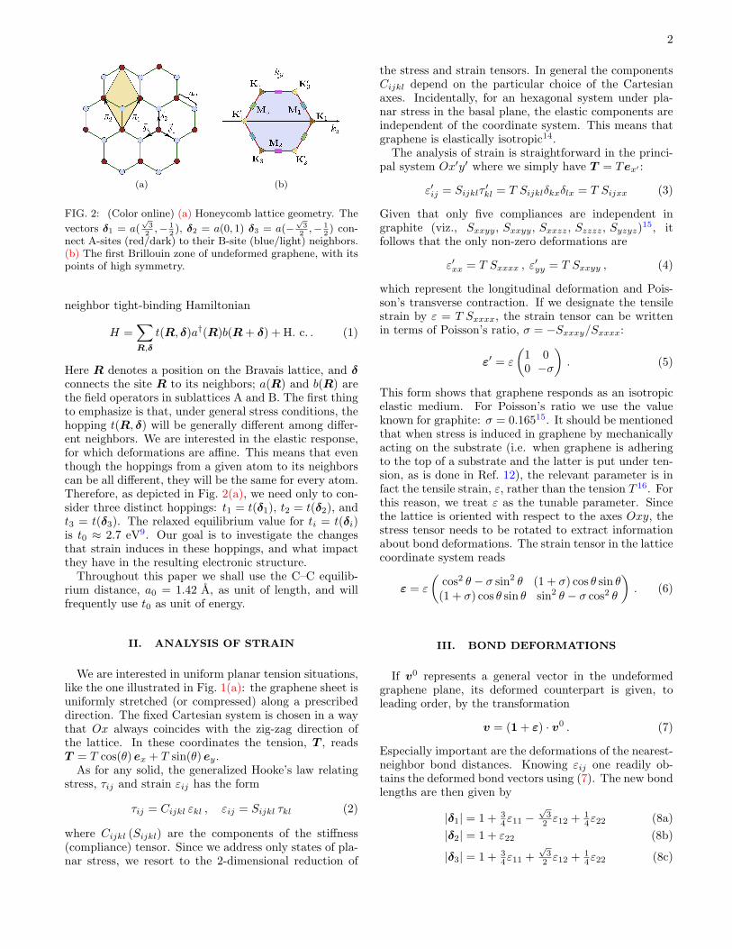
FIG. 3: (Color online) (a) Plot of t1/t2 vs t3/t2 as a func-tion of strain, ε, and θ. Closed lines are iso-strain curves,and arrowed lines correspond to the trajectory of the point(t1/t2, t3/t2) as ε increases, calculated at constant angle. Thegraph is symmetric under reflection on both axes. In theshaded area the spectrum is gapless. The blue iso-strain line(ε ≈ 0.23) corresponds to the gap threshold. In panel (b)we show the angular dependence of t1,2,3 for ε = 0.05 andε = 0.23.

Of particular interest are the cases θ = 0 and θ = π/2since they correspond to tension along the zig-zag (Z)and armchair (A) directions:

Z : |δ1| = |δ3| = 1 + 34ε−

14εσ , |δ2| = 1− εσ (9a)

A : |δ1| = |δ3| = 1 + 14ε−

34εσ , |δ2| = 1 + ε (9b)

The modification of these distances distorts the re-ciprocal lattice as well, and the positions of the high-symmetry points shown in Fig. 2(b) are shifted. Theprimitive vectors of the reciprocal space are denoted byb1,2, and, in leading order, change according to

b1 ≈2π√

3

(1− ε11 −

ε12√3

;1√3− ε12 −

ε22√3

), (10a)

b2 ≈2π√

3

(−1 + ε11 −

ε12√3

;1√3

+ ε12 −ε22√

3

). (10b)

Most importantly, the symmetry point K = ( 4π3√

3, 0)

(that coincides with the Fermi point in the undoped,equilibrium situation, and chosen here for definiteness)moves to the new position

K ≈ 4π3√

3

(1− ε11

2− ε22

2; −2ε12

)(11)

for a general deformation, and in leading order in strain.For uniaxial tension this reduces to

K ≈ 4π3√

3

(1− ε(1− σ)

2; −ε(1 + σ) sin[2θ]

). (12)

The factor of 2θ means that the shift is the same forthe A and Z directions, in leading order. These generalresults will be important for our subsequent discussion.

IV. HOPPING RENORMALIZATION

The change in bond lengths (8) leads to different hop-ping amplitudes among neighboring sites. In the Slater-Koster scheme17, the new hoppings can be obtained fromthe dependence of the integral Vppπ on the inter-orbitaldistance. Unfortunately determining such dependencewith accuracy is not a trivial matter. Many authors re-sort to Harrison’s flyleaf expression which suggests thatVppπ(l) ∝ 1/l218. However this is questionable, inso-far as such dependence is meaningful only in matchingthe tight-binding and free electron dispersions of simplesystems in equilibrium (beyond the equilibrium distancesuch dependence is unwarranted18). It is indeed knownthat such functional form fails away from the equilibriumdistance19, and a more reasonable assumption is an ex-ponential decay20. In line with this we assume that, ingraphene

Vppπ(l) = t0e−3.37(l/a0−1) , (13)

where the rate of decay is extracted from the experi-mental result dVppπ/dl = −6.4 eV/A21. As a consis-tency check, we point out that, according to Eq. (13),the next-nearest neighbor hopping (t′) would have thevalue Vppπ(

√3a0) = 0.23 eV, which tallies with existing

estimates of t′ in graphene9.

V. GAP THRESHOLD

The bandstructure of Eq. (1) with arbitrary hoppingst1, t2, t3 is given by

E(kx, ky) = ±∣∣t2 + t3 e

−ik.a1 + t1 e−ik.a2

∣∣ . (14)

Here both tα and the primitive vectors aα (see Fig. 2(a)for the definition of the vectors aα) change under strain:the hoppings change as per Eqs. (13,8), and the primitivevectors as per Eq. (7). This generalized dispersion hasbeen previously discussed in Refs. 22,23, under the as-sumption that only the hopping elements change, with-out lattice deformation. It was found that the gaplessspectrum is robust, and that a gap can only appear un-der anisotropy in excess of 100% in one of the hoppings.More specifically, the spectrum remains gapless as longas the condition∣∣∣ |t1||t2| − 1

∣∣∣ ≤ |t3||t2| ≤ ∣∣∣ |t1||t2| + 1∣∣∣ (15)

is in effect. This condition corresponds to the shadedarea in Fig. 3(a). Using the results in eqs. (6, 8, 13) wehave mapped the evolution of the hoppings with ε and θ.This allows us to identify the range of parameters thatviolate (15), and to obtain the threshold for gap open-ing. For a given θ, we follow the trajectory of the point(t1/t2, t3/t2) as strain grows, starting from the isotropicpoint at ε = 0. The result is one of the arrowed curves inFig. 3(a). The value of ε at which this curve leaves the

4

(a) (b) (c)

(d) (e)

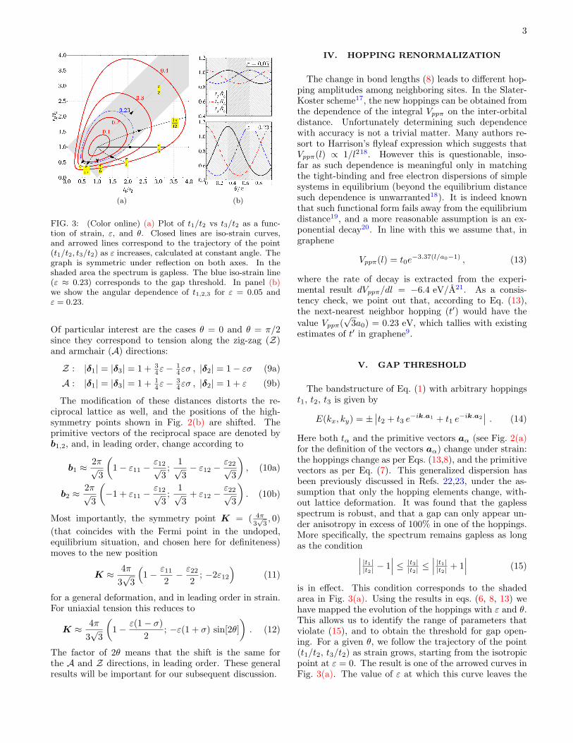
FIG. 4: (Color online) Top row shows density plots of theenergy dispersion, E(kx, ky), for {ε = 0, θ = 0} (a), {ε =0.2, θ = π/2} (b), and {ε = 0.2, θ = 0} (c). In these plots,the central white dashed lines represent the boundary of thefirst BZ of the undeformed lattice, while the solid white linesmark the boundaries of the BZ for the deformed lattice. In (d)we have a cut of (c) along ky = 0, showing the merging of theDirac cones as strain increases, and the ultimate appearanceof the gap. In panel (e) we compare the gap given by Eq. (18)(line) with the result obtained from direct minimization of theenergy in the full BZ (dots).

shaded area corresponds to the gap threshold for thatparticular angle. From such procedure, summarized inFig. 3(a), we conclude that: (i) the gap threshold is atε ≈ 0.23 (∼ 20%); (ii) the behavior of the system isperiodic in θ with period π/3, in accord with the symme-try of the lattice; (iii) tension along the zig-zag direction(θ = 0, π/3, . . . ) is more effective in overcoming the gapthreshold; (iv) tension along the armchair direction nevergenerates a gap.

The two panels of Fig. 3(b) contain plots of the indi-vidual tα for two particular values of strain. It is clearthat, for deformations along the Z direction, the highestrelative change occurs along the zig-zag bonds (t1,3), andconversely for deformations along the A direction. Thiscould have also been anticipated from Eqs. (9) and thesmallness of σ.

VI. CRITICAL GAP

The fact that the isotropic point (1, 1) in Fig. 3(a) issurrounded by an appreciable shaded area, means thatthe gapless situation is robust, and the emergence of thegap requires a critical strain. The physical effect be-hind such critical gap lies in the fact that, under strain,the Dirac cones drift away from the points K, K ′ in the

Brillouin zone (BZ). Before we proceed, it is pertinent toadvance a crucial detail: in a deformed lattice, the Diracpoints (i.e. the positions in the BZ where conduction andvalence bands touch conically) and the symmetry pointsKi do not coincide. In what follows we shall distinguishthem explicitly.

To be more definite, we examine the position of theminimum energy24 for the bands obtained from Eq. (14),which can be done exactly if we assume that the latticeremains undeformed. Due to the particle-hole symmetry,we minimize E(k)2. Let us assume that t1 = t3 6= t2,which applies for tension along either zig-zag or arm-chair directions. In that case the spectrum has minimaat exactly

kmin =

(± 2√

3arccos

[− t2

2t1

]; 0

), (16)

and all symmetry related points. The ± sign refers toone possible choice for the two inequivalent valleys. Inaddition to these local minima, that correspond to theDirac points, the dispersion has saddle points at

k =(π√3

;π

3

), k =

(0;

2π3

), k =

(π√3

; −π3

)(17)

(and all symmetry related points). These are just thepoints M1,M2,M3 shown in Fig. 2(b) and their posi-tion is independent of ti25. The values of energy at thesepoints are E(M1) = |t1+t2−t3|, E(M2) = |−t1+t2+t3|and E(M3) = |t1 − t2 + t3|.

The result in Eq. (16) shows that the Dirac points driftaway from the K point, and the direction of that driftis dictated by the relative variations in ti. For example,for uniaxial tension along the Z we have t2 > t1 = t3,and therefore the minimum of energy moves to the right(left) of K1 (K′

1) [cfr. Fig. 2(b)]. This means that theinequivalent Dirac points move toward each other, andwill clearly meet when 2t1 = t2. They meet precisely atthe position of the saddle point M2. Throughout thisprocess, the dispersion remains linear along the two or-thogonal directions, albeit with different Fermi veloci-ties. If the hoppings change further so that 2t1 > t2,the solution (16) is no longer valid, and the minimumlies always at M2. Since the energy at this saddle pointis given exactly by E(M2) = |2t1 − t2|, the system be-comes gapped, with a gap ∆ = 2|2t1 − t2|. Moreover,the dispersion becomes peculiar in that it remains linearalong one direction (the y direction in this example) andquadratic along the other. The topological structure isalso modified since the two inequivalent Dirac cones havemerged26.

These considerations assume that the hoppings canchange but the lattice remains undeformed. Under a realdeformation both lattice and hoppings are affected. Thelattice deformation will distort the BZ but will not af-fect the aspects discussed above. This can be clearlyseen from inspection of the energy dispersions plotted in

5

(a) (b)

(c)

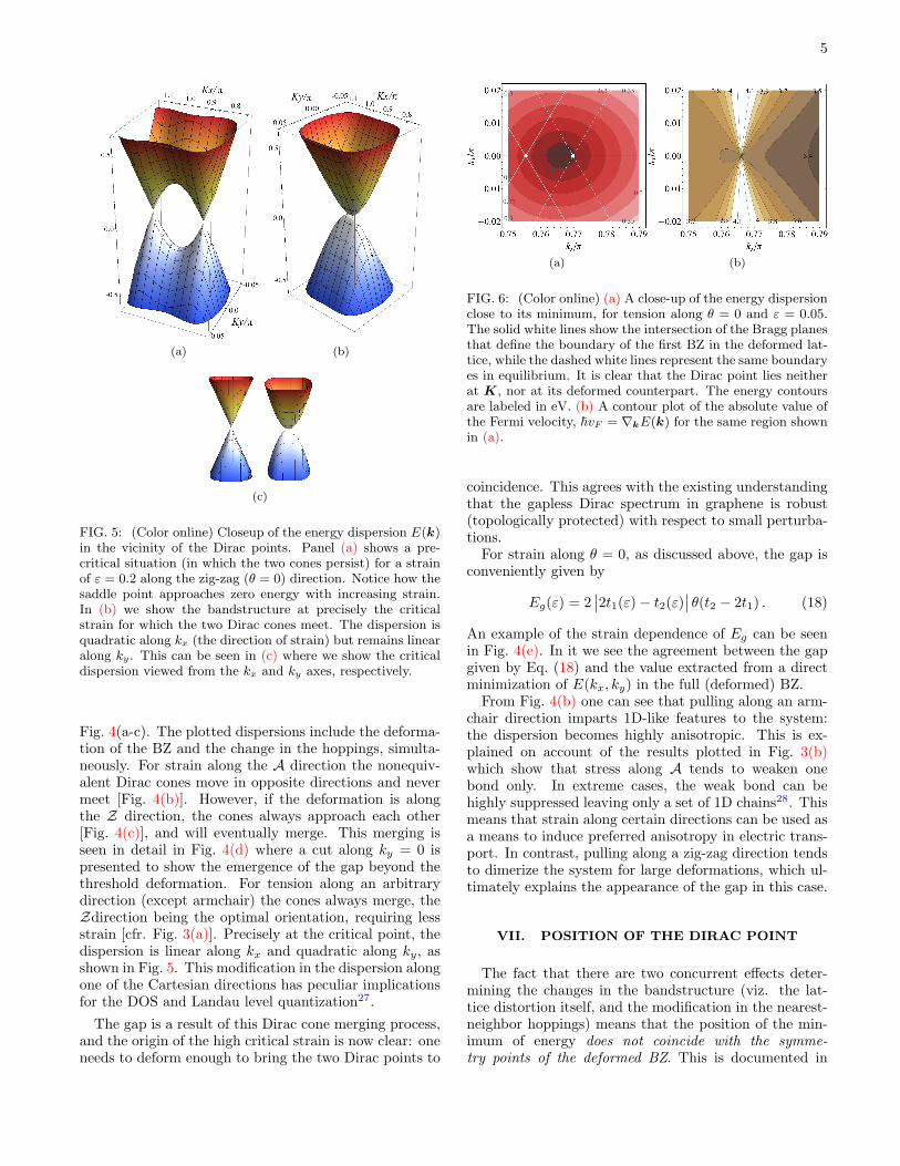
FIG. 5: (Color online) Closeup of the energy dispersion E(k)in the vicinity of the Dirac points. Panel (a) shows a pre-critical situation (in which the two cones persist) for a strainof ε = 0.2 along the zig-zag (θ = 0) direction. Notice how thesaddle point approaches zero energy with increasing strain.In (b) we show the bandstructure at precisely the criticalstrain for which the two Dirac cones meet. The dispersion isquadratic along kx (the direction of strain) but remains linearalong ky. This can be seen in (c) where we show the criticaldispersion viewed from the kx and ky axes, respectively.

Fig. 4(a-c). The plotted dispersions include the deforma-tion of the BZ and the change in the hoppings, simulta-neously. For strain along the A direction the nonequiv-alent Dirac cones move in opposite directions and nevermeet [Fig. 4(b)]. However, if the deformation is alongthe Z direction, the cones always approach each other[Fig. 4(c)], and will eventually merge. This merging isseen in detail in Fig. 4(d) where a cut along ky = 0 ispresented to show the emergence of the gap beyond thethreshold deformation. For tension along an arbitrarydirection (except armchair) the cones always merge, theZdirection being the optimal orientation, requiring lessstrain [cfr. Fig. 3(a)]. Precisely at the critical point, thedispersion is linear along kx and quadratic along ky, asshown in Fig. 5. This modification in the dispersion alongone of the Cartesian directions has peculiar implicationsfor the DOS and Landau level quantization27.

The gap is a result of this Dirac cone merging process,and the origin of the high critical strain is now clear: oneneeds to deform enough to bring the two Dirac points to

(a) (b)

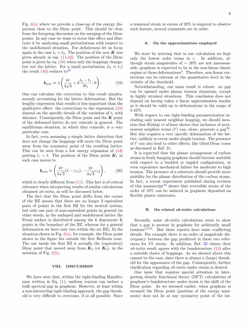
FIG. 6: (Color online) (a) A close-up of the energy dispersionclose to its minimum, for tension along θ = 0 and ε = 0.05.The solid white lines show the intersection of the Bragg planesthat define the boundary of the first BZ in the deformed lat-tice, while the dashed white lines represent the same boundaryes in equilibrium. It is clear that the Dirac point lies neitherat K, nor at its deformed counterpart. The energy contoursare labeled in eV. (b) A contour plot of the absolute value ofthe Fermi velocity, ~vF = ∇kE(k) for the same region shownin (a).

coincidence. This agrees with the existing understandingthat the gapless Dirac spectrum in graphene is robust(topologically protected) with respect to small perturba-tions.

For strain along θ = 0, as discussed above, the gap isconveniently given by

Eg(ε) = 2∣∣2t1(ε)− t2(ε)

∣∣ θ(t2 − 2t1) . (18)

An example of the strain dependence of Eg can be seenin Fig. 4(e). In it we see the agreement between the gapgiven by Eq. (18) and the value extracted from a directminimization of E(kx, ky) in the full (deformed) BZ.

From Fig. 4(b) one can see that pulling along an arm-chair direction imparts 1D-like features to the system:the dispersion becomes highly anisotropic. This is ex-plained on account of the results plotted in Fig. 3(b)which show that stress along A tends to weaken onebond only. In extreme cases, the weak bond can behighly suppressed leaving only a set of 1D chains28. Thismeans that strain along certain directions can be used asa means to induce preferred anisotropy in electric trans-port. In contrast, pulling along a zig-zag direction tendsto dimerize the system for large deformations, which ul-timately explains the appearance of the gap in this case.

VII. POSITION OF THE DIRAC POINT

The fact that there are two concurrent effects deter-mining the changes in the bandstructure (viz. the lat-tice distortion itself, and the modification in the nearest-neighbor hoppings) means that the position of the min-imum of energy does not coincide with the symme-try points of the deformed BZ. This is documented in

6

Fig. 6(a) where we provide a close-up of the energy dis-persion close to the Dirac point. This should be clearfrom the foregoing discussion on the merging of the Diracpoints. In any case we want to stress this effect and illus-trate it by analyzing small perturbations with respect tothe undeformed situation. For definiteness let us focusagain in the case t1 = t3. The position of the new K wasgiven already in eqs. (11,12). The position of the Diracpoint is given by eq. (16) when only the hoppings change,but not the lattice. For a small perturbation (t2 ≈ t1)the result (16) reduces to29

kmin ≈ ±

(4π

3√

3+ 2

t2 − t13t1

; 0

). (19)

One can calculate the correction to this result simulta-neously accounting for the lattice deformation. But thelengthy expression that results is less important than thequalitative effect: the corrections to the expression (19)depend on the specific details of the variation of ti withdistance. Consequently, the Dirac point and the K pointof the deformed lattice do not coincide in general. Theequilibrium situation, in which they coincide, is a veryparticular case.

In fact, even assuming a simple lattice distortion thatdoes not change the hoppings will move the Dirac pointaway from the symmetry point of the resulting lattice.This can be seen from a low energy expansion of (14)putting ti = t. The position of the Dirac point K1 insuch case moves to

kmin ≈

(4π

3√

3(1− ε11); − 4π

3√

3ε12

), (20)

which is clearly different from (11). This fact is of criticalrelevance when interpreting results of similar calculationsobtained ab-initio, as will be discussed below.

The fact that the Dirac point drifts from the cornerof the BZ means that there are no longer 3 equivalentpairs of points in the first BZ for the neutral system,but only one pair of non-equivalent points in general (inother words, in the undoped and undeformed lattice theFermi surface is distributed among the 6 degenerate Kpoints in the boundary of the BZ, whereas for a generaldeformation we have only two within the rst BZ). In thesituation shown in Fig. 6(a), for example, the Dirac pointshown in the figure lies outside the first Brillouin zone.The one inside the first BZ is actually the (equivalent)Dirac point that moved away from K2 (or K3), in thenotation of Fig. 2(b).

VIII. DISCUSSION

We have seen that, within the tight-binding Hamilto-nian written in Eq. (1), uniform tension can induce abulk spectral gap in graphene. However, at least withina non-interacting tight-binding approach, the gap thresh-old is very difficult to overcome, if at all possible. Since

a tensional strain in excess of 20% is required to observesuch feature, several comments are in order.

A. On the approximations employed

We start by noticing that in our calculation we keptonly the lowest order terms in ε. In addition, al-though strain magnitudes of ∼ 20% are not unreason-able, graphene is expected to be in the non-linear elasticregime at those deformations3. Therefore, non-linear cor-rections can be relevant at the quantitative level in thevicinity of the threshold.

Notwithstanding, our main result is robust: no gapcan be opened under planar tension situations, exceptin highly strained situations. This conclusion does notdepend on having taken a linear approximation insofaras it should be valid up to deformations in the range of5-10%.

With respect to our tight-binding parametrization in-cluding only nearest neighbor hopping, we should men-tion that Kishigi et al.have shown that inclusion of next-nearest neighbor terms (t′) can, alone, generate a gap30.But this requires a very specific deformation of the lat-tice, unlikely to occur under simple tension. The presenceof t′ can also lead to other effects, like tilted Dirac conesas discussed in Ref. 31.

It is expected that the planar arrangement of carbonatoms in freely hanging graphene should become unstablewith respect to a buckled or rippled configuration, oreven experience mechanical failure for moderate to hightension. The presence of a substrate should provide morestability for the planar distribution of the carbon atoms.In fact, a recent experiment published during revisionof this manuscript32 shows that reversible strain of theorder of 18% can be induced in graphene deposited onflexible plastic substrates.

B. On related ab-initio calculations

Secondly, some ab-initio calculations seem to showthat a gap is present in graphene for arbitrarily smalltensions12,33. But these reports have some conflictingdetails. For example there is an order of magnitude dis-crepancy between the gap predicted in these two refer-ences for 1% strain. In addition, Ref. 33 claims theirab-initio result agrees with the bandstructure (14) aftera suitable choice of hoppings. As we showed above thiscannot be the case, since there is always a (large) thresh-old for the appearance of the gap. Consequently, furtherclarification regarding ab-initio under strain is desired.

One issue that requires special attention in inter-preting density functional theory (DFT) calculations ofgraphene’s bandstructure under strain is the shift of theDirac point. As we stressed earlier, when graphene isstrained the Dirac point (position of the energy mini-mum) does not lie at any symmetry point of the lat-

7

tice. This is paramount because DFT calculations ofthe bandstructure rely on a preexisting mesh in recipro-cal space, at whose points the bandstructure is sampled.These meshes normally include points along high sym-metry lines of the BZ. But in the current problem, theuse of such a traditional mesh will not be particularlyuseful to distinguish between a gapped and gappless sit-uation. Since the Fermi surface of undoped graphene is asingle point, unless the sampling mesh includes that pre-cise point, one will always obtain a gap in the resultingbandstructure.

Most recently, we became aware of two new devel-opments from the ab-initio front, that shed the lightneeded to interpret the earlier calculations mentionedabove. One of them34 is a revision of the DFT calcu-lations presented in Ref. 12. In this latter work it isshown that, upon careful analysis, the DFT calculationshows no gap under uniaxial deformations up to ∼ 20%.In fact the authors mention explicitly that the shift ofthe Dirac point from the high symmetry point misleadthe authors in their initial interpretation of the band-structure. In another preprint35, independent authorsshow that their DFT calculations reveal, again, no gapfor deformations of the order of 10% in either the Z or Adirections. These subsequent developments confirm ourprediction that only excessive planar deformations areable to engender a bulk spectral gap in graphene.

C. Anisotropic Transport

Several effects of tensional strain are clear from our re-sults. Tension leads to one-dimensionalization of trans-port in graphene by weakening preferential bonds: trans-port should certainly be anisotropic, even for small ten-sions. One example of that is seen in Fig. 6(a) where astrain of 5% visibly deforms the Fermi surface. Fig. 6(b),where the Fermi velocity is plotted for the same region inthe BZ, further shows that, for the chosen tension direc-tion, the Fermi surface is not quite elliptical but slightlyoval, in a reminiscence of the trigonal warping effects.

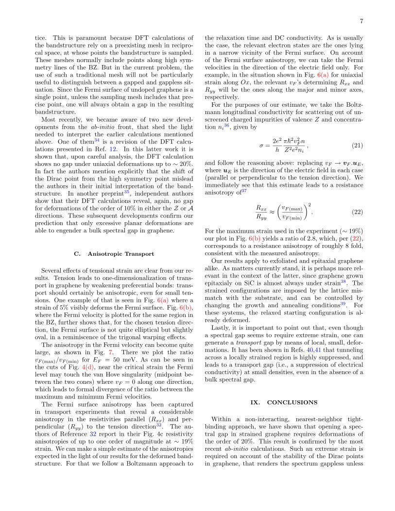
The anisotropy in the Fermi velocity can become quitelarge, as shown in Fig. 7. There we plot the ratiovF (max)/vF (min) for EF = 50 meV. As can be seen inthe cuts of Fig. 4(d), near the critical strain the Fermilevel may touch the van Hove singularity (midpoint be-tween the two cones) where vF = 0 along one direction,which leads to formal divergence of the ratio between themaximum and minimum Fermi velocities.

The Fermi surface anisotropy has been capturedin transport experiments that reveal a considerableanisotropy in the resistivities parallel (Rxx) and per-pendicular (Ryy) to the tension direction32. The au-thors of Reference 32 report in their Fig. 4c resistivityanisotropies of up to one order of magnitude at ∼ 19%strain. We can make a simple estimate of the anisotropiesexpected in the light of our results for the deformed band-structure. For that we follow a Boltzmann approach to

the relaxation time and DC conductivity. As is usuallythe case, the relevant electron states are the ones lyingin a narrow vicinity of the Fermi surface. On accountof the Fermi surface anisotropy, we can take the Fermivelocities in the direction of the electric field only. Forexample, in the situation shown in Fig. 6(a) for uniaxialstrain along Ox, the relevant vF ’s determining Rxx andRyy will be the ones along the major and minor axes,respectively.

For the purposes of our estimate, we take the Boltz-mann longitudinal conductivity for scattering out of un-screened charged impurities of valence Z and concentra-tion ni

36, given by

σ =2e2

h

π~2v2Fn

Z2e2ni, (21)

and follow the reasoning above: replacing vF → vF .uE ,where uE is the direction of the electric field in each case(parallel or perpendicular to the tension direction). Weimmediately see that this estimate leads to a resistanceanisotropy of37

RxxRyy

≈(vF (max)

vF (min)

)2

. (22)

For the maximum strain used in the experiment (∼ 19%)our plot in Fig. 6(b) yields a ratio of 2.8, which, per (22),corresponds to a resistance anisotropy of roughly 8 fold,consistent with the measured anisotropy.

Our results apply to exfoliated and epitaxial graphenealike. As matters currently stand, it is perhaps more rel-evant in the context of the latter, since graphene grownepitaxialy on SiC is almost always under strain38. Thestrained configurations are imposed by the lattice mis-match with the substrate, and can be controlled bychanging the growth and annealing conditions39. Forthese systems, the relaxed starting configuration is al-ready deformed.

Lastly, it is important to point out that, even thougha spectral gap seems to require extreme strain, one cangenerate a transport gap by means of local, small, defor-mations. It has been shown in Refs. 40,41 that tunnelingacross a locally strained region is highly suppressed, andleads to a transport gap (i.e., a suppression of electricalconductivity) at small densities, even in the absence of abulk spectral gap.

IX. CONCLUSIONS

Within a non-interacting, nearest-neighbor tight-binding approach, we have shown that opening a spec-tral gap in strained graphene requires deformations ofthe order of 20%. This result is confirmed by the mostrecent ab-initio calculations. Such an extreme strain isrequired on account of the stability of the Dirac pointsin graphene, that renders the spectrum gappless unless

8

FIG. 7: (Color online) Anisotropy in the Fermi velocity, as afunction of strain for a Fermi energy of 50meV. The verticalaxis shows the ratio of the maximum to the minimum valuesof vF in the entire Fermi surface.

the two inequivalent Dirac points merge. The merg-ing requires substantial anisotropy in the hopping inte-

grals, only achieved under high strain. General featuresof strained graphene are an anisotropic Fermi surface,anisotropic Fermi velocities, and the drift of the Diracpoints away from the high symmetry points of the lat-tice.

Uniform planar stain appears to be an unlikely can-didate to induce a bulk gap in graphene. Nevertheless,strain (local or uniform) can be an effective means of tun-ing the electronic structure and transport characteristicsof graphene devices. Even if the bulk gap turns out tobe challenging in practice, local strain could be used asa way to mechanically pinch off current flow.

Acknowledgments

We thank enlightening discussions with Y. P. Feng,A. K. Geim, A. Heinz, Y. Lu, Z. Ni, Z. X. Shen,and T. Yu. AHCN acknowledges the partial supportof the U.S. Department of Energy under the grantDE-FG02-08ER46512. VMP is supported by FCT viaSFRH/BPD/27182/2006 and PTDC/FIS/64404/2006.

1 M.-F. Yu, O. Lourie, M. J. Dyer, K. Moloni, T. F. Kelly,and R. S. Ruoff, Science 287, 637 (2000).

2 C. Lee, X. Wei, J. W. Kysar, and J. Hone, Science 321,385 (2008).

3 F. Liu, P. Ming, and J. Li, Phys. Rev. B 76, 064120 (2007).4 A. K. Geim and K. S. Novoselov, Nat. Mat. 6, 183 (2007).5 K. S. Novoselov, A. K. Geim, S. V. Morozov, D. Jiang,

Y. Zhang, S. V. Dubonos, I. V. Grigorieva, and A. A.Firsov, Science 306, 666 (2004).

6 T. Ando and T. Nakanishi, J. Phys. Soc. Jpn. 67, 1704(1998).

7 K. S. Novoselov, A. K. Geim, S. V. Morozov, D. Jiang,M. I. Katsnelson, I. V. Grigorieva, S. V. Dubonos, andA. A. Firsov, Nature 438, 197 (2005).

8 P. R. Wallace, Phys. Rev. Lett. 71, 622 (1949).9 A. H. Castro Neto, F. Guinea, N. M. R. Peres, K. S.

Novoselov, and A. K. Geim, Rev. Mod. Phys. 81, 109(2009).

10 M. Y. Han, B. Ozyilmaz, Y. Zhang, and P. Kim, Phys.Rev. Lett. 98, 206805 (2007).

11 L. A. Ponomarenko, F. Schedin, M. I. Katsnelson, R. Yang,E. W. Hill, K. S. Novoselov, and A. K. Geim, Science 320,356 (2008).

12 Z. Ni, T. Yu, Y. H. Lu, Y. Y. Wang, Y. P. Feng, and Z. X.Shen, ACS Nano 2, 2301 (2008).

13 Z. Ni, H. M. Wang, Y. Ma, J. Kasim, Y. H. Wu, and Z. X.Shen, ACS Nano 2, 1033 (2008).

14 L. D. Landau and E. M. Lifshitz, Theory of Elasticity(Pergamon, 1986), 3rd ed.

15 L. Blakslee, D. G. Proctor, E. J. Seldin, G. B. Stence, andT. Wen, J. Appl. Phys. 41, 3373 (1970).

16 In this case the relation between strain and stress is givenby the material parameters of the substrate, rather thanthe intrinsic elastic parameters for graphene.

17 J. C. Slater and G. F. Koster, Phys. Rev. 94, 1498 (1954).18 W. A. Harrison, Elementary Electronic Structure (World

Scientific, 1999), ISBN 981–023895-9.19 G. Grosso and C. Piermarocchi, Phys. Rev. B 51, 16772

(1995).20 D. A. Papaconstantopoulos, M. J. Mehl, S. C. Erwin, and

M. R. Pederson, in Tight-Binding Approach to Computa-tional Materials Science, edited by P. Turchi, A. Gonis,and L. Colombo (Materials Research Society, Pittsburgh,1998), p. 221.

21 A. H. Castro Neto and F. Guinea, Phys. Rev. B 75, 045404(2007).

22 B. Wunsch, F. Guinea, and F. Sols, New J. Phys. 10,103027 (2008).

23 Y. Hasegawa, R. Konno, H. Nakano, and M. Kohmoto,Phys. Rev. B 74, 033413 (2006).

24 By “position of the minimum energy” we mean the positionof the Dirac points (or valleys). They are local extrema,with the abolute minimum of energy lying at the Γ pointin the BZ.

25 The position of the saddle points does not depend explicitlyupon the hoppings ti, and their position is constant onlyif the lattice remains undeformed.

26 G. Montambaux, F. Piechon, J.-N. Fuchs, and M. O. Go-erbig, arXiv:0904.2117 (2009).

27 P. Dietl, F. Piechon, and G. Montambaux, Phys. Rev. Lett.100, 236405 (2008).

28 This is another way to see why strain along A can neverlead to a gap.

29 This is, of course, the same shift that one obtains using aperturbative Hamiltonian in the hoppings from the outset,in which case one generates the widely discussed effectivegauge fields in the low energy description40.

30 K. Kishigi, H. Hanada, and Y. Hasegawa, J. Phys. Soc.

9

Jpn. 77, 074707 (2008).31 M. O. Goerbig, J.-N. Fuchs, G. Montambaux, and

F. Piechon, Phys. Rev. B 78, 045415 (2008).32 K. S. Kim, Y. Zhao, H. Jang, S. Y. Lee, J. M. Kim, K. S.

Kim, J.-H. Ahn, P. Kim, J.-Y. Choi, and B. H. Hong,Nature 457, 706 (2009).

33 G. Gui, J. Li, and J. Zhong, Phys. Rev. B 78, 075435(2008).

34 Z. Ni, T. Yu, Y. H. Lu, Y. Y. Wang, Y. P. Feng, and Z. X.Shen, ACS Nano 3, 483 (2009).

35 M. Farjam and H. Rafii-Tabar (2009), arXiv:0903.1702.36 N. M. R. Peres, J. M. B. Lopes dos Santos, and T. Stauber,

Phys. Rev. B 76, 073412 (2007).37 Notice that in Ref. 32 the directions x and y are inter-

changed with respect to our notation.38 Although in this case the most common situation is biaxial

strain.39 N. Ferralis, R. Maboudian, and C. Carraro, Phys. Rev.

Lett. 101, 156801 (2008).40 V. M. Pereira and A. H. Castro Neto, arXiv:0810.4539

(2008).41 M. M. Fogler, F. Guinea, and M. I. Katsnelson, Phys. Rev.

Lett. 101, 226804 (2009).