Thuener Armando da Silva Optimization Under Uncertainty for Asset Allocation TESE DE DOUTORADO Thesis presented to the Programa de P´ os–Graduac ¸˜ ao em Inform ´ atica of the Departamento de Inform ´ atica da PUC- Rio as partial fulfillment of the requirements for the degree of Doutor. Advisor : Prof. Marcus Vinicius Soledade Poggi de Arag˜ ao Co–Advisor: Prof. Davi Michel Vallad˜ ao Rio de Janeiro April 2015

Welcome message from author
This document is posted to help you gain knowledge. Please leave a comment to let me know what you think about it! Share it to your friends and learn new things together.
Transcript
Thuener Armando da Silva
Optimization Under Uncertainty for AssetAllocation
TESE DE DOUTORADO
Thesis presented to the Programa de Pos–Graduacao emInformatica of the Departamento de Informatica da PUC-Rio as partial fulfillment of the requirements for the degreeof Doutor.
Advisor : Prof. Marcus Vinicius Soledade Poggi de AragaoCo–Advisor: Prof. Davi Michel Valladao
Rio de JaneiroApril 2015
DBD
PUC-Rio - Certificação Digital Nº 1021809/CB

Thuener Armando da Silva
Optimization Under Uncertainty for AssetAllocation
Thesis presented to the Programa de Pos–Graduacao emInformatica of the Departamento de Informatica of CentroTecnico Cientıfico da PUC-Rio, as partial fulfillment of therequirements for the degree of Doutor.
Prof. Marcus Vinicius Soledade Poggi de AragaoAdvisor
Departamento de Informatica – PUC-Rio
Prof. Davi Michel ValladaoCo–Advisor
Departamento de Engenharia Industrial – PUC-Rio
Prof. Helio Cortes Vieira LopesDepartamento de Informatica – PUC-Rio
Prof. Alexandre Street de AguiarDepartamento de Engenharia Eletrica – PUC-Rio
Prof. Vitor Luiz de MatosPLAN4
Prof. Geraldo Gil VeigaRN Tecnologia
Prof. Bruno da Costa FlachIBM
Prof. Jose Eugenio LealCoordinator of the Centro Tecnico Cientıfico da PUC-Rio
Rio de Janeiro, April 06, 2015
DBD
PUC-Rio - Certificação Digital Nº 1021809/CB

All rights reserved.
Thuener Armando da SilvaThuener Silva graduated as Bachelor in Computer Science atPUCRio in 2007. During graduate developed a project thatused machine learning techniques for sentiment analysis withRaul Renteria. In 2010, completed his Master in ComputerScience in Optimization and Automatic Reasoning area. De-veloped the thesis about the portfolio selection applied tothe Brazilian financial market entitled Experimental Studyof Techniques for Portfolio Optimization with his advisorEduardo Laber. During the Master received the scholarshipfrom CNPq and maintained an excellent academic perform-ance. His experience in Computer Science has an emphasis inAlgorithms, Machine Learning, Information Retrieval, Port-folio Selection and Quantitative Methods.
Bibliographic DataSilva, Thuener
Optimization Under Uncertainty for Asset Allocation/ Thuener Armando da Silva; Advisor: Marcus ViniciusSoledade Poggi de Aragao; Co–advisor: Davi MichelValladao. – 2015.
99 f: il. (color.) ; 30 cm
Tese (Doutorado em Informatica) – Pontifıcia Univer-sidade Catolica do Rio de Janeiro, Departamento de In-formatica, 2015.
Inclui bibliografia
1. Informatica – Teses. 2. Selecao de Carteiras. 3.Alocacao de Ativos em multi-estagio. 4. Analise de In-vestimentos. 5. Metodo de Apoio a Tomada de Decisao.6. Black Litterman. 7. Programacao Dinamica Dual Es-tocastica. I. Poggi, Marcus Vinicius. II. Valladao, DaviMichel. III. Pontifıcia Universidade Catolica do Rio deJaneiro. Departamento de Informatica. IV. Tıtulo.
CDD: 004
DBD
PUC-Rio - Certificação Digital Nº 1021809/CB

To my wife, my daughter and my family.
DBD
PUC-Rio - Certificação Digital Nº 1021809/CB

Acknowledgments
I would like first to thank my wife Luana, for your unconditional support
throughout this long journey. This work was only possible thanks to your help,
patience and understanding. During all these years by your side your kindness
and affection shown me the amazing person you are and how wonderful is our
love, you make my life better every day.
Family is the most important thing in my life, thanks to my family for
making me who I’ am, especially to my parents, Fernando and Katia, my
sisters and my brothers-in-law. Also, thank to my father-In-law, Gerson, for
the guidance and revision on this work.
Thanks to my advisor Marcus Poggi for the support over these years,
without your help this work would be impossible, you inspired me to be better
every day. Also, thanks to my co-supervisor David Valladao, for your patience
and dedication during this work, you believed in me even when I was very
skeptical, it is a great pleasure to work with you. I also want to thank the
professors Placido Pinheiro, Alexandre Street for their involvement in this
research.
Friends and colleagues make this difficult journey much easier, a special
thanks to my friends from Galgos laboratory and WhileTrue for the thoughts
and jokes.
Finally, I would like to thank all the teachers and staff at PUC-Rio and
the Department of Informatics for being part of this amazing institution that
supports my intellectual and personal growth and the PUC-Rio and CNPq for
the financial support.
In times we need the most is when we can clearly perceive that everything
we do comes back to us. I counted with the help of many people on things that
I thought would be impossible to do. I thank everyone who helped me in this
incredible journey.
DBD
PUC-Rio - Certificação Digital Nº 1021809/CB

AbstractSilva, Thuener; Poggi, Marcus Vinicius(Advisor); Valladao, Davi Michel.Optimization Under Uncertainty for Asset Allocation. Rio deJaneiro, 2015. 99p. DSc Thesis – Departamento de Informatica, PontifıciaUniversidade Catolica do Rio de Janeiro.
Asset allocation is one of the most important financial decisions made
by investors. However, human decisions are not fully rational, and people
make several systematic mistakes due to overconfidence, irrational loss aversion
and misuse of information, among others. In this thesis, we developed two
distinct methodologies to tackle this problem. The first approach has a more
qualitative view, trying to map the investor’s vision of the market. It tries to
mitigate irrationality in decision-making by making it easier for an investor to
demonstrate his/her preferences for specific assets. This first research uses the
Black-Litterman model to construct portfolios. Black and Litterman developed
a method for portfolio optimization as an improvement over the Markowitz
model. They suggested the construction of views to represent an investor’s
opinion about future stocks’ returns. However, constructing these views has
proven difficult, as it requires the investor to quantify several subjective
parameters. This work investigates a new way of creating these views by using
Verbal Decision Analysis. The second research focuses on quantitative methods
to solve the multistage asset allocation problem. More specifically, it modifies
the Stochastic Dynamic Dual Programming (SDDP) method to consider real
asset allocation models. Although SDDP is a consolidated solution technique
for large-scale problems, it is not suitable for asset allocation problems due
to the temporal dependence of returns. Indeed, SDDP assumes a stagewise
independence of the random process assuring a unique cost-to-go function
for each time stage. For the asset allocation problem, time dependency is
typically nonlinear and on the left-hand side, which makes traditional SDDP
inapplicable. This thesis proposes an SDDP variation to solve real asset
allocation problems for multiple periods, by modeling time dependence as a
Hidden Markov Model with concealed discrete states. Both approaches were
tested in real data and empirically analyzed. The contributions of this thesis
are the methodology to simplify portfolio construction and the methods to
solve real multistage stochastic asset allocation problems.
KeywordsPortfolio Selection; Multistage Asset Allocation; Investments Analysis;
Decision support systems; Black Litterman; Stochastic Dual Dynamic Pro-
gramming.
DBD
PUC-Rio - Certificação Digital Nº 1021809/CB

Resumo
Silva, Thuener; Poggi, Marcus Vinicius; Valladao, Davi Michel. Otimi-zacao Sob Incerteza para Alocacao de Ativos. Rio de Janeiro,2015. 99p. Tese de Doutorado – Departamento de Informatica, PontifıciaUniversidade Catolica do Rio de Janeiro.
A alocacao de ativos e uma das mais importantes decisoes financeiras
para investidores. No entanto, as decisoes humanas nao sao totalmente racion-
ais. Sabemos que as pessoas cometem muitos erros sistematicos como, excesso
de confianca, aversao a perda irracional e mau uso da informacao entre outros.
Nesta tese desenvolvemos duas metodologias distintas para enfrentar esse prob-
lema. A primeira abordagem e qualitativa, utiliza o modelo de Black-Litterman
e tenta mapear a visao que o investidor tem do mercado. Esse metodo tenta
mitigar a irracionalidade na tomada de decisao tornando mais facil para um in-
vestidor demonstrar suas preferencias em relacao aos ativos. Black e Litterman
desenvolveram um metodo para otimizacao de carteiras com a proposta de mel-
horar o modelo Markowitz, utilizando a construcao de visoes para representar
a opiniao do investidor sobre o futuro. No entanto, a forma de construir essas
visoes e bastante confusa e exige que o investidor estime varios parametros
que sao subjetivos. Assim, propomos uma nova forma de criar essas visoes,
utilizando Analise Verbal de Decisao. A segunda pesquisa envolve metodos
quantitativos para resolver o problema de alocacao de ativos com multiplos
estagios com premissas mais realistas. Embora a Programacao Dinamica Dual
Estocastica (PDDE) seja uma tecnica promissora para a solucao de problemas
de grande porte, nao e adequada para o problema de alocacao de ativos devido
a dependencia temporal associada aos retornos dos ativos. PDDE assume que
o processo estocastico tem independencia por estagio assegurando uma funcao
unica de custo futuro para cada estagio. No problema de alocacao de ativos, a
dependencia do tempo e tipicamente nao-linear e no lado esquerdo, o que torna
PDDE tradicional nao aplicavel. Propomos uma variacao do PDDE usando
modelo oculto de Markov com estados discretos para resolver problemas reais
de alocacao de ativos com multiplos perıodos e dependencia no tempo. Ambas
as abordagens foram testadas em dados reais e empiricamente analisadas. As
principais contribuicoes sao as metodologia desenvolvidas para simplificar a
construcao de portfolios e para resolver o problema de alocacao de ativos com
multiplos estagios.
Palavras–chaveSelecao de Carteiras; Alocacao de Ativos em multi-estagio; Analise
de Investimentos; Metodo de Apoio a Tomada de Decisao; Black Litterman;
Programacao Dinamica Dual Estocastica.
DBD
PUC-Rio - Certificação Digital Nº 1021809/CB
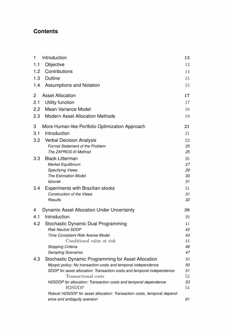
Contents
1 Introduction 13
1.1 Objective 13
1.2 Contributions 14
1.3 Outline 15
1.4 Assumptions and Notation 15
2 Asset Allocation 17
2.1 Utility function 17
2.2 Mean-Variance Model 18
2.3 Modern Asset Allocation Methods 19
3 More Human-like Portfolio Optimization Approach 21
3.1 Introduction 21
3.2 Verbal Decision Analysis 23Formal Statement of the Problem 25The ZAPROS-III Method 25
3.3 Black-Litterman 26Market Equilibrium 27Specifying Views 29The Estimation Model 30Idzorek 31
3.4 Experiments with Brazilian stocks 31Construction of the Views 31Results 32
4 Dynamic Asset Allocation Under Uncertainty 39
4.1 Introduction 39
4.2 Stochastic Dynamic Dual Programming 41Risk Neutral SDDP 42Time Consistent Risk Averse Model 43
Conditional value at risk 44Stopping Criteria 46Sampling Scenarios 47
4.3 Stochastic Dynamic Programming for Asset Allocation 49Myopic policy: No transaction costs and temporal independence 50SDDP for asset allocation: Transaction costs and temporal independence 51
Transactional costs 52H2SDDP for allocation: Transaction costs and temporal dependence 53
H2SDDP 54Robust H2SDDP for asset allocation: Transaction costs, temporal depend-ence and ambiguity aversion 61
DBD
PUC-Rio - Certificação Digital Nº 1021809/CB

H2SDDP for asset allocation: Transaction costs, temporal dependence andsell short 63
4.4 Computational Experiments 64Data analysis 64Sampling Methods 67Sensitivity Analysis 68
HMM 69Impact of the Risk Aversion 69Convergence and trials 70Transactional costs 71
Models Evaluation 73Experiment with Monthly Data Set 2012 to 2014 74Experiment with Monthly Data 2007 to 2014 76Experiment with Daily Data Set 80
5 Conclusions and Future Works 82
Bibliography 86
A Appendix 95
A.1 Questionnaires 95
A.2 Myopic prove 96
DBD
PUC-Rio - Certificação Digital Nº 1021809/CB

List of Figures
3.1 Procedure to apply ZAPROS-III methodology 263.2 Flowchart of Black-Litterman method [19] 273.3 The Black-Litterman portfolio with our views 353.4 Equilibrium portfolio 353.5 Result of the increase in the qualification of Sid. Nacional 363.6 Result of the increase in the qualification of Oi 363.7 Result of right scenario, where the investor guess is right 383.8 Result of wrong scenario, where the investor guess is wrong 38
4.1 -CVaR and -VaR for gain distribution 454.2 Example of Latin Hypercube Sampling for uniform distribu-
tion with two dimensions 484.3 Sampling with Monte Carlo 494.4 Sampling with Latin Hypercube Sampling 494.5 LHS interval for a normal distribution N ∼ (0, 1) 494.6 An example of HMM for stock market 564.7 An example of a Gaussian mixture model. 564.8 Decision tree of the generic problem with return dependence 604.9 Decision tree of the problem with return dependence
modeled with HMM 604.10 Decision tree of the problem of our proposal 614.11 Metrics for historical monthly return series of the five indus-
trial portfolios 654.12 Metrics for historical daily return series of the ten industrial
portfolios 664.13 Cumulative performance for monthly data set of the five
industrial portfolios 664.14 Cumulative performance for daily data set of the ten indus-
trial portfolios 674.15 Comparison between Latin Hypercube Sampling (LHS) and
Monte Carlo (MC) 684.16 States likelihood for train data 694.17 Impact of the risk aversion coefficient (λ) on the upper bound
for monthly returns and daily returns, respectively on the leftand right 70
4.18 Convergence of the Upper Bound for monthly data set 714.19 Impact of the transactional costs on the upper bound 724.20 Portfolio allocation without transactional costs 734.21 Portfolio allocation with transactional costs 734.22 Comparing the different methods for asset allocation data
form 2012 to 2014 754.23 Cumulative returns series from January 2012 to December
2014 754.24 Returns series from January 2007 to December 2014 76
DBD
PUC-Rio - Certificação Digital Nº 1021809/CB

4.25 Comparing the different methods for asset allocation dataform 2007 to 2014 77
4.26 Comparing the market states with the performance of theH2SDDP for data form 2007 to 2014 78
4.27 Trailing returns for asset allocation methods with monthlydata form 2007 to 2014 78
4.28 Comparing the performance of H2SDDP with sell short sellshort with other methods, monthly data form 2007 to 2014 79
4.29 Trailing returns of H2SDDP with sell short sell and othermethods, monthly data form 2007 to 2014 80
4.30 Cumulative performance for asset allocation methods withdaily data set form 2007 to 2014 81
4.31 Trailing returns for asset allocation methods with daily dataset form 2007 to 2014 81
DBD
PUC-Rio - Certificação Digital Nº 1021809/CB

List of Tables
1.1 Set and stochastic process notation 151.2 State and decision variable notation 16
2.1 Some properties of the utility function 18
3.1 FIQ and sector of the stocks 333.2 FIQ of the sectors 333.3 The expected return of the stocks 343.4 A summary of the views data 343.5 stocks returns for the period 373.6 Sectors returns for the period 373.7 Return for the different scenarios and the Market Portfolio 38
4.1 Monthly data series for 5 industrial portfolios 654.2 Daily data series for 10 industrial portfolios 654.3 Number of stages and the computational time 704.4 CVaR and return values of the simulated polices for different
risk coefficients, results in percentage 74
A.1 Questionnaire about the stocks 95A.2 Questionnaire about the sectors 96
DBD
PUC-Rio - Certificação Digital Nº 1021809/CB

1Introduction
Asset allocation is one of the most important financial decisions made
by investors. The asset allocation problem consist in finding a portfolio (for
example stocks, bonds, cash and gold) that better suits the investor’s needs.
Selecting good portfolios represents a competitive advantage, and to make
good decisions in this regard it is necessary to leave emotions aside.
Emotions often affect investment decisions. In most cases, human de-
cisions are not fully rational and people often make systematic mistakes due
to overconfidence, irrational loss aversion and misuse of information. Such mis-
takes, made frequently by investors, can lead to big financial losses, which is
one of the reasons why the behavioral finance field is dedicated to analyzing the
psychology of financial decision making. Hence the need for tools that support
the investors’ financial decisions and prevent pitfalls.
Investment analysis techniques can be used as a tool or as automated
optimization models to minimize, as much as possible, irrational intervention
in decision making. In the last decades, there has been a remarkable increase
in the use of financial models and optimization techniques for asset allocation.
One of the main reasons for this is the attractive assumption that it is possible
to forecast the conditional moments of the return distributions [1]. Another
reason is the growth in processing power and the development of methods and
optimization solutions that can handle a large volume of data. The field hardly
existed in 1980, but has experienced a rapid surge ever since. Every day more
tools are used to support the creation of investment strategies, and currently
there is a large variety of approaches to the problem; Robust Optimization,
Stochastic Programming and Machine Learning being only a few of the many
fields in which we can encounter solutions to assist in financial decision making.
1.1 ObjectiveThe main objective of this thesis is to help investors solve real asset
allocation problems. In this regard, it presents two alternatives that aim at
helping financial decision making.
The first approach has a qualitative perspective, trying to map the
investor’s vision of the market. It is an attempt to mitigate irrationality
DBD
PUC-Rio - Certificação Digital Nº 1021809/CB

Chapter 1. Introduction 14
in decision making, making it easier for investors to demonstrate reasoned
preferences concerning assets. For this purpose, the method combines the
Black-Litterman portfolio optimization method with verbal decision analyses.
However, even when using decision-support methods, we are not safe
from irrational decisions. That is why this work proposes quantitative methods
using stochastic models to evaluate and solve the multistage asset allocation
problem. More specifically, it suggests modifying the Stochastic Dynamic Dual
Programming method to consider real asset allocation models.
1.2 ContributionsThe major contributions of this work are derived from the two proposed
methodologies. The first part of this thesis contributes by developing a simple
new methodology that fits the investor’s needs based on verbal decision
analyses and Black-Litterman. This work has shown that it is possible to
optimize portfolios even when the investor is not an expert on the subject. In
addition, this approach makes it easier for the investors to manifest their own
opinion, in an organized fashion, and allows them to change their portfolios
more frequently. Finally, a case study based on Brazilian stocks demonstrates
that this methodology creates more intuitive and diversified portfolios.
The second part of this thesis proposes a new approach to solve
multistage stochastic asset allocation problems with time dependency. The
method maps the temporal dependence as hidden Markovian states, trans-
forming them into a convex problem that can be solved by adapting the SDDP.
In addition, it presents a more general model that consider the ambiguity
on the states’ probabilities of the optimization problem. As our experiments
demonstrate, the proposed model performs very well and shows promising
results.
Main contributions:
– Proposes a new way to generate the Black-Litterman views using VDA,
enabling the investor to construct personalized portfolio based on the
his/her opinion.
– Model the multistage stochastic portfolio optimization problem with
hidden Markovian temporal dependence and transactional cost.
– Create a more general model for the multistage stochastic portfolio op-
timization problem with ambiguity aversion, with the intent to mitigate
returns estimation errors.
DBD
PUC-Rio - Certificação Digital Nº 1021809/CB

Chapter 1. Introduction 15
1.3 OutlineThis work is organized as follows: Chapter 2 introduces asset allocation
and gives an overview of the methods that have been used to approach this
problem. Chapter 3 is dedicated to the first proposed methodology, providing
an overview of the Verbal Decision Analysis and Black-Litterman, and of how
these two methods are combined. It also presents experiments conducted in the
Brazilian stock market and some remarks about the proposed methodology.
Chapter 4 describes the second, more quantitative, methodology proposed
in this work. Its first part introduces the concept of SDDP and explains
how this method may be adapted for asset allocation, while its final part
proposes alternative models and shows various computational experiments.
Chapter 5 brings this thesis’ final conclusion and debate regarding future
works, presenting the main contributions of the two proposed methodologies
and suggestions for future works.
1.4 Assumptions and NotationIn this section, we present some assumptions and notation used through
this thesis. It will be used bold-faced upper (Σ, Π, Q, P, . . .) and lowercase (µ,
p, r, . . .) letters to denote, respectively matrices and vectors [2]. To simplify
the formulations it will be use a vector with all elements equal one with proper
dimension 1 = [1, . . . , 1]>.
The multistage problem has a finite planning horizon T ; the probability
space is (Ω,F ,P) with filtration F , where F = ∅,Ω and F = FT . A specific
notation for the portfolio selection application was created and is shown in
Table 1.1 and Table 1.2.
Sets
A = 1, . . . , A: Index set of the A ≥ 1 assets.
H = 0, . . . , T − 1: Set of stages.
Stochastic Process
rti (s): Excess return of asset i ∈ A, between stages t ∈1, . . . , T and t − 1, under scenario s ∈ Ω, where
rt (s) = (r1,t (s) , . . . , rA,t (s))> and r[t′,t] (s) =
(rt′ (s) , . . . , rt (s))> for t′ ≤ t .
r[t′,t] = (rt′ , . . . , rt)>: Realization sequence of the asset returns for t′ ≤ t.
r[t] = r[0,t]: Realization sequence of the asset returns for 0 to t.
Table 1.1: Set and stochastic process notation
DBD
PUC-Rio - Certificação Digital Nº 1021809/CB

Chapter 1. Introduction 16
State Variables
Wt (s): Wealth at stage t ∈ H ∪ T under scenario s ∈ Ω
Decision Variables
xti (s): Amount invested in asset i ∈ A, at stage t ∈ H under scenario
s ∈ Ω, where xt (s) = (x1,t (s) , . . . , xA,t (s))> and x[t′,t] (s) =
(xt′ (s) , . . . ,xt (s))> for t′ ≤ t
Table 1.2: State and decision variable notation
Without loss of generality, the risk-free asset is represented as the first
asset of the portfolio without excess return, i.e., for each scenario r1,t (s) = 0,
for all t ∈ H ∪ T and all s ∈ Ω.
DBD
PUC-Rio - Certificação Digital Nº 1021809/CB

2Asset Allocation
Before Markowitz’s work [3] the concept of diversification was greatly
simplified. People had an intuition that putting everything in one asset lead
to largely different results, while distributing their money among many assets
greatly reduced the chance of all having bad returns simultaneously.
The essence of portfolio optimization theory is based on diversification,
as by combining different assets it is possible to obtain a lower risk than the
offered by any of the assets individually. As the number of the assets increase,
the variance of the portfolio decreases towards zero [1].
The Asset Allocation consists in finding the most appropriate group of
assets while considering the individual properties of each asset. The optimal
portfolio varies according to the profile of each investor, and there isn’t a single
portfolio that is recommended for every type of investor. This is due to the
specific characteristics of each individual, institution or group. An investor
averse to risk may prefer to invest in assets with low risk and low return, while
another investor, who is more open to risk, might prefer assets with more risk
when it is possible to achieve higher returns.
2.1 Utility functionTo provide the most suitable portfolio for a given investor, it is necessary
to understand its preference among the set of possible investments. A way
to accomplish this is to map the utility function U that captures investor’s
satisfaction or happiness at a given level of wealth. For a given level of
wealth W , the usefulness U(W ) is the investor’s satisfaction achieved with
this wealth. Assuming that an investor with utility function U attempts to
make an investment portfolio and that P (ws) is the probability of this portfolio
generating a wealth ws for a scenario s, we can calculate the expected utility
for the portfolio as being:
E[C] =∑s
U(ws)P (ws)
Utility functions have some important properties. First, the utility func-
tion should prefer more to less wealth, and therefore the utility of X + 1 units
DBD
PUC-Rio - Certificação Digital Nº 1021809/CB

Chapter 2. Asset Allocation 18
is greater than that of X units. This implies a positive first derivative of the
utility function. The investor’s attitude towards risk is also related to the util-
ity function. Considering that when it comes to risk, an investor can be averse
to it, neutral or like it.
The investor’s classification can be defined by considering a fair bet, i.e.
an investment where the value is equal to the expected cost. The investor
that rejects a fair bet is risk averse, and thus its dissatisfaction with a loss is
greater than its satisfaction with a gain for the same value. Functions with this
behavior have a negative second derivative. The opposite occurs in the case
of an investor who accepts a fair bet, a case in which the second derivative
is positive. For an investor who is indifferent to risk, the utility of these two
investments, with the same expected value, is the same, meaning the second
derivative of this function is zero. Table 2.1 presents the characteristics of the
second derivative according to investors’ profiles.
Profile Behavior Implication
Risk aversion Rejects fair bet U′′(W ) < 0
Risk neutral Indifferent to fair bet U′′(W ) = 0
Taste for Risk accepted the fair bet U′′(W ) > 0
Table 2.1: Some properties of the utility function
2.2 Mean-Variance ModelIn his pioneering work “Portfolio Selection” [3], Markowitz developed a
model that allows the selection of portfolios considering the relation between
return and risk. This became known as the mean-variance model, which uses
the expected return as a measure of performance of the portfolio and the
variance as a risk measure.
A portfolio with n assets can be represented by the amount invested
on each asset x = (x1, . . . , xA). Assuming that future returns are random
variables and using each individual expected return, the portfolio return can
be estimated by the equation
E[Rp] =A∑i=1
xiE[Ri]
In order to evaluate the variance of portfolio σ2c , it is used the covariance
of the return series between all pairs of assets that make up the portfolio
σij, ∀i, j ∈ 1, . . . , A.
DBD
PUC-Rio - Certificação Digital Nº 1021809/CB
Chapter 2. Asset Allocation 19
σ2p =
A∑i=1
A∑j=1
(xixjσij)
Using the mean-variance approach, one can create an efficient frontier.
That is the set of portfolios in which a given risk level has the highest possible
return, or a certain level of return has the lowest possible risk. These are
efficient portfolios. All other portfolios can be considered inefficient, because
they have either lower return or higher risk.
Formally, the two minimization (2.1) and maximization (2.2) formula-
tions are described below
minx
A∑i=1
x2iσ
2i +
A∑i=1
A∑j=1,j 6=i
xixjσij (2.1)
s. t.A∑i=1
µixi ≥ rp
A∑i=1
xi = 1
xi ≥ 0, ∀i
maxx
A∑i=1
µixi (2.2)
s. t.A∑i=1
x2iσ
2i +
A∑i=1
A∑j=1,j 6=i
xixjσij ≤ vp
A∑i=1
xi = 1
xi ≥ 0, ∀i
where the number of assets that may be part of the portfolio is N , and xi is
the percentage of the portfolio that will be granted to asset i. The covariance
between assets i and j is represented by σij, and σ2i is the variance of asset i.
Finally, µi is the expected return of asset i, and rp and vp are the minimum
return and the maximum risk for the desired portfolio, respectively.
2.3 Modern Asset Allocation MethodsEven with several tools available to help investors create mean-variance
optimized portfolios, they are still very skeptical about the mean-variance
theory and its practical implications. Albeit revolutionary, Markowitz’s work
DBD
PUC-Rio - Certificação Digital Nº 1021809/CB

Chapter 2. Asset Allocation 20
has shown major drawbacks in practical applications, yielding portfolios that
can be counter-intuitive [4, 5], that tend to concentrate on a small subset
of available assets and that do not seem well diversified [6, 7]. The optimal
portfolio is also extremely sensitive to small variations in the input data [5,6,8].
This does not mean, however, that the mean-variance theory is flawed,
but only that the idea needs to be remodeled or adapted in order to achieve
better results. Hence, several new methodologies for portfolio optimization,
and consequently for asset allocation, have been developed.
For instance: regarding the mean-variance’s hypersensitivity to changes
on the estimated inputs, which suggests that those parameters need to be
estimated in an extremely precise way, several attempts to reduce the impact
of estimation errors have been made. In fact, there are several ways to
create portfolios that are less sensitive to these variations, such as shrinkage
estimators, Bayesian and resampling methods and robust optimization [4, 5,
9, 10]. Frost and Savarino [11] have demonstrated that these optimization
constraints stabilize the portfolio and generally improve performance. As
mentioned by Jagannathan and Ma [12], these constrains can be interpreted
as a posteriori regularization.
In this thesis, we will focus on two different approaches, presented in
the following chapters. Considering the instability problems and parameter-
estimation method of the Markowitz model, we will propose a methodology to
construct a portfolio based on the investors’ opinion. Another approach is to
focus on solving the asset allocation problem in a quantitative way. This will
be modeled as a multistage stochastic problem with temporal dependence.
DBD
PUC-Rio - Certificação Digital Nº 1021809/CB
3More Human-like Portfolio OptimizationApproach
3.1 IntroductionThe practical disadvantages of the Markowitz model motivated Fisher
Black and Robert Litterman to develop a new approach. Thus the Black-
Litterman approach [13], which combines the expected equilibrium between
returns estimated through the Capital Asset Pricing Model (CAPM) and views
to optimize the portfolio. The views represent the investor’s opinion about the
stocks’ future returns. This model yields more stable and diversified portfolios
than the mean-variance standard model [14].
Black and Litterman’s original paper [4] only explained the core aspects
of their idea, leaving it to others to better explain the implication of their
model. Satchell and Scowcroft [15], Walters [14], He and Litterman [16] explain
the Black-Litterman solution in further detail. Walters [14] also constructed
a framework1 to use the model and other portfolio optimization techniques.
Mankert [17] sheds more light on the practical implications of the Black-
Litterman approach. Other studies focus on extensions of the original model,
like Herold [18], Idzorek [19], Fernandes et al. [20], and Meucci [21].
Also, Bertisimas et al. [2] proposed a more general extension of the ori-
ginal Black-Litterman model that can incorporate investor opinion about volat-
ility and construct estimators for more general notions of risk. Reinterpreting
the problem through inverse optimization Bertisimas et al. [2] extends the
traditional model creating a approach that can combine a greater variety of
views.
The expression of the investor’s preferences can be seen as a decision
making process. Traditionally, decision making scenarios involve the analysis
of objects from several points of view and can be assisted by multi-criteria
methodologies. These help generating knowledge about the decision context
and, as a consequence, increase the confidence of those making decisions [22].
There are multi-criteria methods based either on quantitative or qualitative
1That is available in www.blacklitterman.org
DBD
PUC-Rio - Certificação Digital Nº 1021809/CB
Chapter 3. More Human-like Portfolio Optimization Approach 22
analysis of the problem, and choosing the best approach is a great challenge.
Examples of problem-solving using quantitative methods can be found in
Castro et al. [23], Toncovich et al. [24], and Pinheiro et al. [25]. Among those
who apply qualitative methods, we have Mendes et al. [26], Tamanini et al. [27],
Tamanini et al. [28], Tamanini et al. [29] and Castro et al. [30].
The Verbal Decision Analysis is based on multi-criteria problem-solving
through qualitative analysis methods. One of the advantages of qualitative
methods is that all the questioning in the process of eliciting preferences is
made in the decision maker’s native language. Moreover, verbal descriptions
are used to measure preference levels. This procedure is psychologically valid,
respecting the limitations of the human information processing system. This
characteristic makes the incomparability cases [31] become almost unavoidable
since the scale of preferences is purely verbal and consequently not an accurate
way of estimating values. Therefore, the method may not be capable of
achieving satisfactory results in some situations, presenting an incomplete
solution to the problem.
Establishing views in the traditional quantitative way is not an easy task
and an investor would need help from an expert in the process. That is why we
chose a method to setting views using Verbal Decision Analysis (VDA). For this
propose, we developed questionnaires that are intuitive and can be answered
by anyone with basic knowledge of investment options without needing any
further special training.
The purpose of this chapter is to develop a methodology that constructs
a personalized portfolio based on the investor’s opinions. Our problem is not a
typical multi-criteria problem, being actually very different from normal VDA
applications. This is one of the major difficulties that have to be overcome in
order to create the Black-Litterman views. For this purpose, in the final part of
Section 3.4 we compare the return of investing on the investor most preferred
asset with our proposed approach.
Moreover, the objective pursued is a technique to support the creation
of a personal portfolio based on an individual’s opinion, preferences or view.
Therefore, a comparison among performances of portfolios, in the present case,
should only consider portfolios that are aligned with the considered individual
preference. The technique proposed here follows the mean-variance balance of
Markowitz generated portfolios.
In Section 3.2 we present a brief explanation of the Verbal Decision
Analysis (VDA) framework used in this work. Section 3.3 brings a review
of the Black-Litterman methodology. Finally, in Section 3.4 we report about
the experiments made with Brazilian stocks.
DBD
PUC-Rio - Certificação Digital Nº 1021809/CB

Chapter 3. More Human-like Portfolio Optimization Approach 23
3.2 Verbal Decision AnalysisA decision may be defined as the result of a process of choice when
someone is confronted with a problem or with an opportunity for creation,
optimization or improvement of a given situation. On the other hand, decision
making is a special activity of human behavior, aimed at the achievement of
a given goal. It takes place in every activity of the human world, from simple
daily problems to complex situations inside an organization. The conclusion of
a decision making process can be an ordination of alternatives or the selection
of a single alternative from a list of possible solutions for the problem.
Establishing its preferences and interests is usually enough to allow an
individual to make decisions that solve simple problems. However, individuals
often find it hard to separate emotions from reason. As a result, emotions
often influence the decision making process [32,33]. The decision also involves
several factors, some of which may not be measurable. Thus, when a decision
maker needs to solve complex problems, covering many alternatives and a large
volume of information that may not be measurable nor easily comparable, some
methodologies exist to support the decision making process.
In order to solve a given problem, alternative solutions are taken into
consideration. Such alternatives are defined and characterized according to a
set of criteria, structured around its verbal and qualitative nature. There are
a huge number of practical problems which is necessary to generate an ordinal
scale of alternatives [34]. The construction of such an ordinal scale is helpful
in many situations, for example, to reject less preferable alternatives from a
given set.
The Verbal Decision Analysis (VDA) framework is a set of methods
defined to support the decision making process through the verbal representa-
tion of problems. Some methods that constitute the Verbal Decision Analysis
framework are: ZAPROS-III, ZAPROS-LM, PACOM, and ORCLASS Larichev
and Moshkovich [34]. According to Gomes et al. [35], in the majority of multi-
criteria problems there is a set of alternatives that can be evaluated against the
same set of characteristics (called criteria or attributes). The VDA framework
is structured on the supposition that most decision making processes can be
qualitatively described [36]. Although the decision maker’s ability to choose is
very dependent on the occasion and the stakeholders’ interest, the methods to
support decision making are universal.
Moreover, in Ustinovich and Kochin [37] the analysis of a large amount of
data-processing performed by human beings has shown that the psychologically
correct operations are:
DBD
PUC-Rio - Certificação Digital Nº 1021809/CB

Chapter 3. More Human-like Portfolio Optimization Approach 24
– Comparison of two assessments in verbal scale by two criteria;
– Assignment of multi-criteria alternatives to decision classes;
– Comparative verbal assessment of alternatives according to separate
criteria.
This last operation is the only classification methodology within the VDA
framework. The goal of the Verbal Decision Analysis framework is to establish
a ranking of alternatives in order of preference.
The methods belonging to the Verbal Decision Analysis framework may
be evaluated in light of their objectives:
– As a tool for ordinary classification, ORCLASS was one of the first
methods designed to tackle classification problems. There are several
other widely known methods for solving classification problems that can
be applied and analyzed for future applications [38–40], but that does
not belong to Ustinovich and Kochin’s [37] VDA framework;
– The other objective is to organize the solutions alternatives for the
problem in a rank, from the most preferable to the least preferable one.
Three methods are proposed within the VDA framework: ZAPROS-LM,
ZAPROS-III, and PACOM. Although they have the same final goal, they
have different purposes:
– PACOM is exclusively created to be applied according to pair com-
pensation and consists in comparing the advantages and disadvant-
ages of multi-attribute alternatives.
– The ZAPROS method was created to be applied by pair comparison
and consists in comparing a pair of alternatives with the advantage
of reaching a decision by using simple and understandable dialogue.
It is also divided in two alternative methods:
∗ ZAPROS-III differs from ZAPROS-LM in its level of treatment
of inconsistence. ZAPROS-III can be considered an evolution
of ZAPROS-LM in this concept.
DBD
PUC-Rio - Certificação Digital Nº 1021809/CB

Chapter 3. More Human-like Portfolio Optimization Approach 25
(a) Formal Statement of the Problem
The methodology follows the same problem formulation proposed by [34],
where:
1. K = c1, c2, . . . , cN, representing a set of N criteria;
2. nq represents the number of possible values on the scale of q-th criterion,
(q ∈ K); For the ill-structured problems, as in this case, usually nq ≤ 4;
3. Xq = x1, x2, . . . , xnq represents a set of values to the q-th criterion,
which is this criterion scale; |Xq| = nq; The values of the scale are ranked
from best to worst, and this order does not depend on the values of other
scales;
4. Y = X1×X2×· · ·×XN represents a set of vectors yi, in such a way that:
yi = yi1, yi2, . . . , yiN> and yi ∈ Y , yiq ∈ Xq, where |Y| =∏N
q=1 nq;
5. Z = zij1 and zi ∈ Y , where the set of j vectors represents the
description of the real alternatives.
The order of the multi-criteria alternatives on set A is defined based on the
decision maker’s preferences.
(b) The ZAPROS-III Method
According to Ustinovich and Kochin [37], one of the most important
features of ZAPROS methods is the use of psychologically grounded procedures
for identifying the preferences. This method evaluates personal abilities and
limitations of human information processing system. The disadvantages of the
method also include the limited amount of attributes and difficulties in using
quantitative criteria.
Furthermore, ZAPROS-III [33] considers values known as Quality Vari-
ations (QV) or Quality Changing (QC) [36] and Formal Index of Quality (FIQ).
The QV represents the distance between the evaluations of two criteria. The
FIQ mainly aims at minimizing the number of comparable pairs of alternatives.
The FIQ is used in the ranking of the alternatives.
Figure 3.1 [31] presents a flowchart with steps for the application of
the VDA method ZAPROS-III. As described in the Figure 3.1, the method’s
application can be divided into four stages: Problem Formulation, Elicitation
of Preferences/Comparison of Alternatives, Validation of the Decision maker’s
preferences, and Comparison of Alternatives.
DBD
PUC-Rio - Certificação Digital Nº 1021809/CB
Chapter 3. More Human-like Portfolio Optimization Approach 26
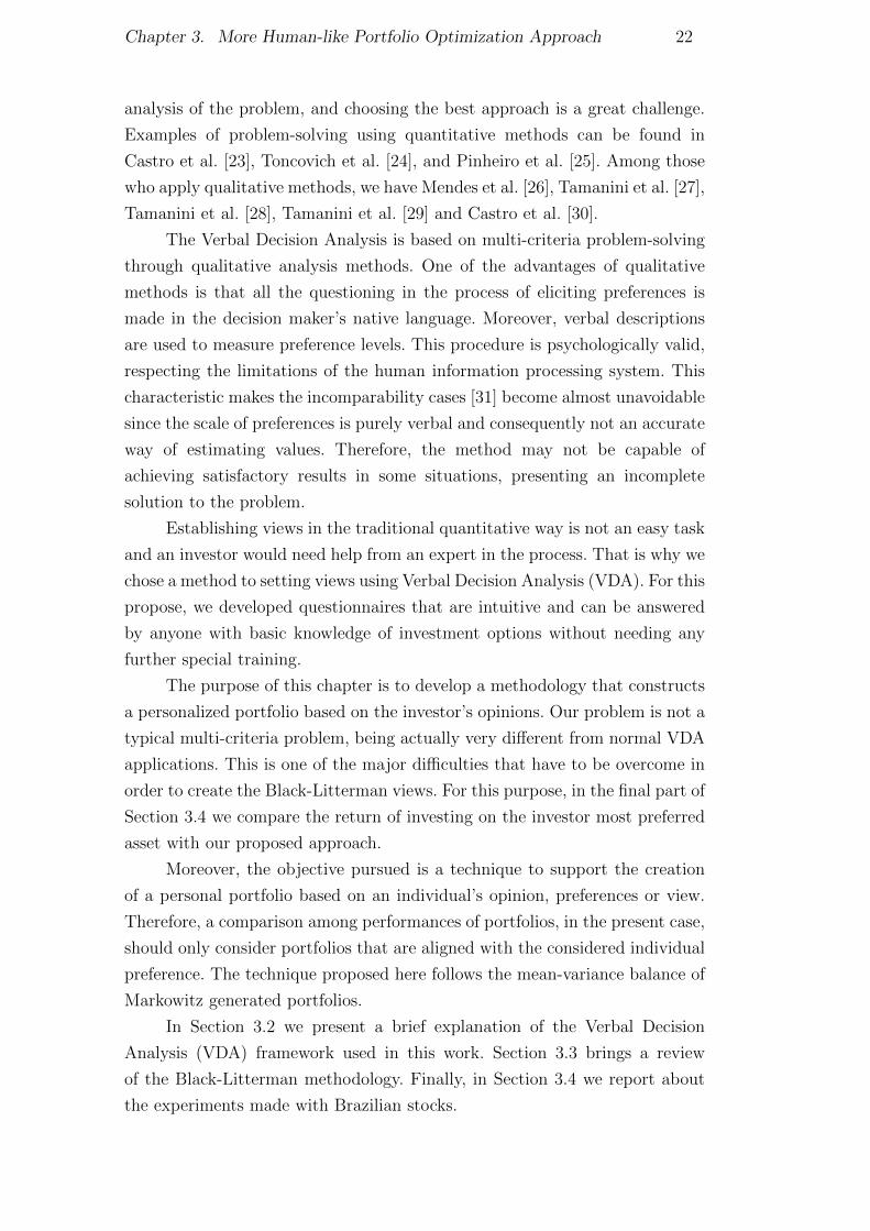
Figure 3.1: Procedure to apply ZAPROS-III methodology
A disadvantage of the method is that the number and values of criteria
that can be handled are limited, in order to keep complexity under control.
Tamanini [31] defends that although ZAPROS-III-i follows a procedure
similar to its predecessor’s to extract preferences, it also implements modifica-
tions that make it more efficient and more accurate regarding inconsistencies.
The number of incomparable alternatives is essentially smaller than in previous
ZAPROS [36].
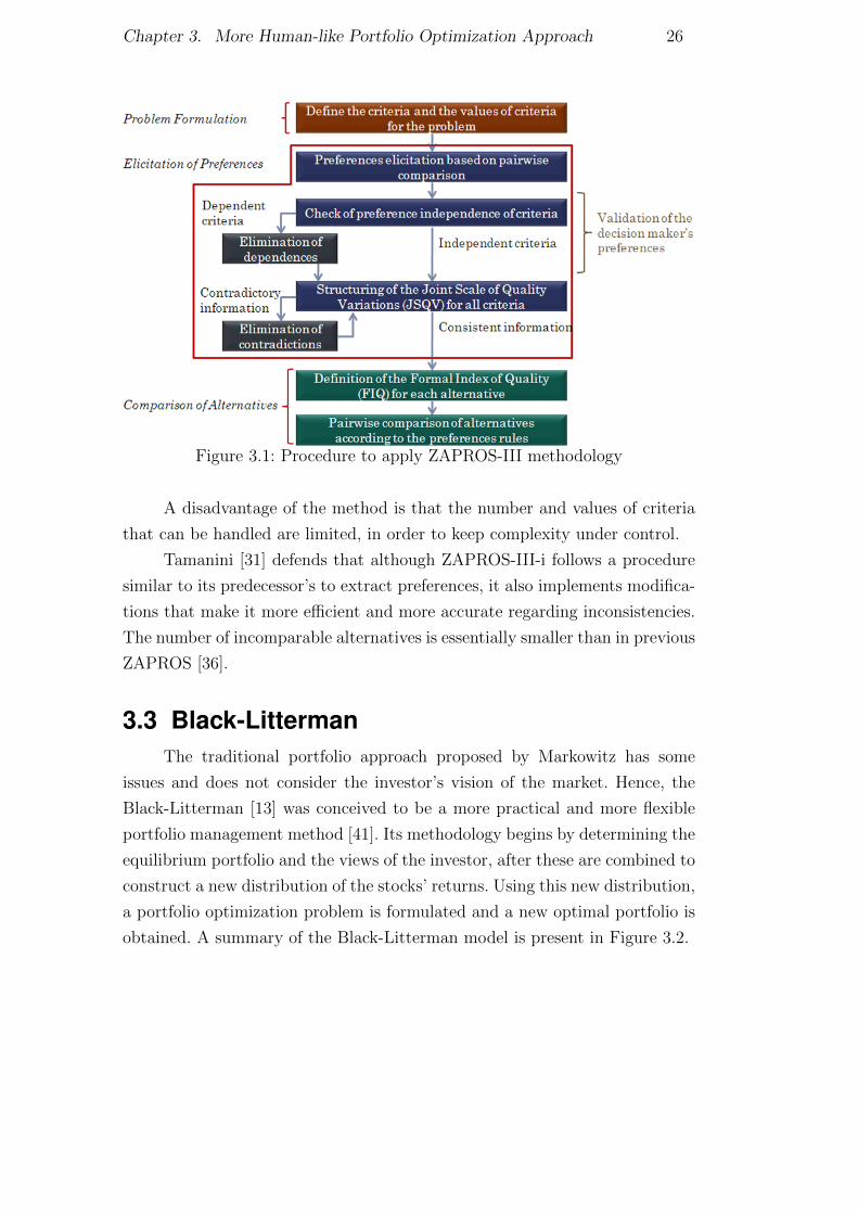
3.3 Black-LittermanThe traditional portfolio approach proposed by Markowitz has some
issues and does not consider the investor’s vision of the market. Hence, the
Black-Litterman [13] was conceived to be a more practical and more flexible
portfolio management method [41]. Its methodology begins by determining the
equilibrium portfolio and the views of the investor, after these are combined to
construct a new distribution of the stocks’ returns. Using this new distribution,
a portfolio optimization problem is formulated and a new optimal portfolio is
obtained. A summary of the Black-Litterman model is present in Figure 3.2.
DBD
PUC-Rio - Certificação Digital Nº 1021809/CB

Chapter 3. More Human-like Portfolio Optimization Approach 27
Covariance
Matrix (Σ)
Market
capitalization
Weights (xm)
Risk Aversion
Coefficient
(δ)
Implied Equilib-
rium Return Vector
Π = δΣxm
Prior Equilibrium Distribution
N ∼ (Π, τΣ)
Views (Q)
Uncertainty
of Views
(Ω)
View Distribution
N ∼ (Q,Ω)
New Expected Return
Distribution N ∼ (µ,M)
New Return Distri-
bution N ∼ (µ, Σ)
Figure 3.2: Flowchart of Black-Litterman method [19]
The model proposed by Black and Litterman can be seen, in a rather
simplistic way, as an adjustment in the prior distribution of the assets’ returns
to adapt it to the investor’s vision. Essentially, however, it combines the
investor’s views with the CAPM notion of market equilibrium [4,13].
(a) Market Equilibrium
The Black-Litterman assumption is that the a priori distributions of
returns are consistent with market equilibrium. Considering that all investors’
utility functions are the same, the CAPM theory shows that everyone should
hold the same portfolio, the market portfolio xm. The market portfolio is the
portfolio where the amount of assets is proportional to its market value.
First we have to assume that the returns of the stocks r are normally
distributed with mean E(r) and covariance matrix Σ i.e. r ∼ N(E(r),Σ).
When the market is efficient, the expected return for any asset has the following
propertyE(ri)− rf = βi(E(rm)− rf ) (3.1)
DBD
PUC-Rio - Certificação Digital Nº 1021809/CB
Chapter 3. More Human-like Portfolio Optimization Approach 28
The E(ri) and E(rm) are the asset i and market portfolio’s expected returns,
while rf is the risk free asset return. Coefficient βi is the covariance between
asset i and the market portfolio returns, divided by the market portfolio
varianceβi =
σimσ2m
(3.2)
Also, the market portfolio return is
rm =n∑j=1
rjxmj (3.3)
The risk equilibrium premium Π is the expected excess of return yielded
by the risky stocks, which should perform better than the risk free stock. It
is properly defined as the difference between the asset returns and risk free
returns Πi = E(ri)− rf . Using the fact that
σim =n∑j=1
xmjσji (3.4)
and (3.1) we have
Πi = βi(E[rm]− rf ) (3.5)
=σimσ2m
(E[rm]− rf )
=E[rm]− rf
σ2m
(n∑j=1
xmjσji)
With the risk aversion parameter δ
δ =E[rm]− rf
σ2m
(3.6)
the final result can be expressed in matrix form as
Π = δΣxm (3.7)
A more detailed demonstration of these equations and more about the
CAPM theory can be found in [42] and [43]. The result above can also be
obtained by deriving the traditional quadratic utility function of the mean-
variance model, assuming that all investors solve this problem.
Finally, we can define the prior distribution as the real µ return distri-
bution with mean Π and variance τΣ
µ = Π + επ
επ ∼ N(0, τΣ) (3.8)
DBD
PUC-Rio - Certificação Digital Nº 1021809/CB

Chapter 3. More Human-like Portfolio Optimization Approach 29
The τ is a small number that reflects the investor’s uncertainty about prior
return estimations [44]. It is the most confusing parameter of the model and
has several different calibration approaches. Further ahead we shall present
Idzorek’s technique to eliminate τ .
(b) Specifying Views
The views are the investor’s vision regarding future market behavior.
These views can be relative or absolute and need to be “fully invested”. Hence,
the sum of weights is zero for the relative view, and one for the absolute. An
example of absolute view is “Stock i will return q1%” and of a relative view is
“International stock will outperform domestic stock by q2%”. Furthermore, the
confidence has to be defined by the investor, and this will change how much
the view will affect the portfolio weights. The investor’s view can be expressed
asPµ = Q + εq (3.9)
Where P is the perspective of the investor and Q specifies the expected
return of each view. The εq is an non-observable random and normally
distributed vector with mean zero and a diagonal covariance matrix Ω that
expresses the uncertainty of the views (εq ∼ N(0,Ω)).
Considering v as the number of views and n the number of stocks, P
will be a matrix v × n with pi (i ∈ 1, . . . , v) representing a vector with n
elements, Q a vector with v elements and Ω a v × v diagonal matrix
PT = [p1,p2,p3, . . . ,pv]
QT = [q1, q2, q3, . . . , qv]
Ω =
ω1 0 . . . 0
0 ω2 . . . 0...
.... . .
...
0 0 . . . ωv
To better understand how to describe these views in matrix form, two
views were created: one relative and other absolute. In the first view, stock one
will outperform stock two by 1% and in the second view, stock three will have
return 2%. [1 −1 0
0 0 1
]µ =
[0.01
0.02
]+ εq
DBD
PUC-Rio - Certificação Digital Nº 1021809/CB

Chapter 3. More Human-like Portfolio Optimization Approach 30
(c) The Estimation Model
With the expected excess return and the views of the investor, it is
possible to proceed to the next step of the Black-Litterman approach, which
combines these two items. There are two ways to estimate the final model. The
original Black-Litterman paper [13] references the Theil’s Mixed Estimation
model [45], but there is also a Bayesian approach. The first method was
chosen because it is easy to understand. By applying the identity matrix I,
the problem can be seen in the matrix form[I
P
]µ =
[Π
Q
]+
[επ
εq
](3.10)
Constructing the auxiliary matrices D =
[I
P
], C =
[Π
Q
]and ε =
[επ
εq
]we can reformulate the problem as
Dµ = C + ε (3.11)
ε ∼ N(0,W), W =
[τΣ 0
0 Ω
](3.12)
Solving this system of equations using least squares, we have
µ = (DTW−1D)−1DTW−1C
= [(τΣ)−1 + PTΩ−1P]−1[(τΣ)−1 + PTΩ−1Q] (3.13)
The variance can also be adjusted to reflect the change in the return
data. Hence, the variance of the returns relative to the new data is
M = (DTW−1D)−1
= [(τΣ)−1 + PTΩ−1P]−1 (3.14)
With this value M, the actual new variance (Σ) can be evaluated as [16]
Σ = Σ + M (3.15)
The final step in this process is to solve the mean-variance model by
using the posterior distribution of the Black-Litterman. Having the new vector
of expected returns and the covariance matrix, the new optimal portfolio can
be estimated using the standard mean-variance method
max xTµ− δ
2xTΣx (3.16)
The solution obtained using the first-order conditional is
DBD
PUC-Rio - Certificação Digital Nº 1021809/CB

Chapter 3. More Human-like Portfolio Optimization Approach 31
x∗ =1
δΣ−1µ (3.17)
(d) Idzorek
Idzorek describes an easy way to determine the level of trust by specifying
the confidence level of each view as a percentage [19]. This method is deemed
to be much more intuitive [14].
Another problem commonly found in the Black-Litterman model is the
determination of τ [44]. Idzorek calibrates the confidence of a view so that x/τ
ratio is equal to the variance of the portfolio view (pTΣp) [46], rendering the
scalar value of τ irrelevant. Idzorek still presents his formulas with τ , but it
can be removed in order to simplify the equations [14].
3.4 Experiments with Brazilian stocksOur process of composing a portfolio is divided in two stages: VDA and
Black-Litterman. In the first step, the investor must answer a series of questions
which will be used to create the views which, in turn, will be used in the Black-
Litterman to build the new portfolio. We created a methodology to construct
the view of the Black-Litterman model by using these questionnaires.
(a) Construction of the Views
Two different sets of questions were prepared. One of them is used to
identify what are the investor’s preferences regarding specific sectors of the
financial market, while the other aims at mapping the investor’s perspective
regarding the companies he/she intends to invest in.
The questionnaire about the sectors contains 3 questions. The first one
on how the domestic scenario is favorable to that sector, the second essentially
the same as the first but regarding the external scenario, and the last one on
the growth expectation for that sector. It was conceived simple, so it can be
answered by most people.
The other questionnaire, about the stocks, has 7 questions regarding risk,
reliability, expected growth, innovation, profitability, management, and com-
pany employees. It was also conceived to be as simple as possible, comprising
only a few questions.
In order to construct the views based on the answers given in the
questionnaires, we use the FIQ of the ZAPROS-III method. We consider the
FIQ as a rating through which we can quantify not only the classification of
stocks, but also how much one stock is better than another one. The FIQ has
DBD
PUC-Rio - Certificação Digital Nº 1021809/CB
Chapter 3. More Human-like Portfolio Optimization Approach 32
to be transformed into a standard for the views, and the values are normalized
between 0 and 1 to create an absolute view that represents the investor’s
perspective.
For questionnaires such as the one about sectors, in which an alternative
represents multiple stocks, we chose to equally divide the value attributed to
the sector among the stocks. For example, if the value of the sector is considered
to be 0.5 and we have two stocks, each one will have a value of 0.25.
Because confidence is a parameter that is somewhat complicated to
determine – even as a percentage –, we decided to insert one more question
in the questionnaires, in order to gauge how confident the participant is with
his/her answers, thus obtaining the confidence of the view. To discretize the
values, this question has four possible answers (very little confidence, little
confidence, reasonably confident and very confident), which are associated with
25, 50, 75, and 100 percent of confidence, respectively.
The last parameter of the view is the expected return. To have sufficient
impact on the portfolio, we chose 0.5% as its value. This value was chosen
based on the expected return of the assets and would be better calculated
automatically, but it was not possible to conceive a general formula which was
appropriate for any case.
(b) Results
To better understand how this methodology would behave in practice,
a test program was conceived to work with the Aranau [31] and Akutan
[14] frameworks. After the questionnaires have been filled out, the program
generates a graphical report showing the optimal portfolio and its details.
The Black-Litterman analytical resolution of the optimal portfolio has
some limitations: even while using a Lagrangian decomposition, like in Silva
et al. [47], the resulted formulation still cannot assure that the stocks’s
percentages are positive. Because of this limitation, the Jay Walters framework
has to be extended to solve the problems using the CPLEX2 solver.
We chose the 10 major companies negotiated in the Brazilian market3:
Petrobras, ItauUnibanco, Bradesco, Banco do Brasil, Vale, Itausa, Eletrobras,
Sid. Nacional, Cemig and Oi. For each of these companies, we chose the
stock with the highest negotiated volume to construct our portfolio and define
the corresponding sector. These companies operate in the following sectors:
electricity, financial, mining, oil, gas and biofuels, steel mill and metallurgy
and telecommunications.
2Version 12.4.0.03In 2012 according to Forbes
DBD
PUC-Rio - Certificação Digital Nº 1021809/CB

Chapter 3. More Human-like Portfolio Optimization Approach 33
After answering the questions, we obtained the FIQ values for the stocks
Table 3.1 and for the sectors Table 3.2. The lower the FIQ, the better
the alternative. Therefore, these values were normalized using the difference
between the maximum values of the companies.
Stock Sector FIQ Stock
Petrobras Oil, gas and biofuels 19
ItauUnibanco Financial 15
Bradesco Financial 26
Banco do Brasil Financial 19
Vale Mining 11
Itausa Financial 31
Eletrobras Electricity 39
Sid. Nacional Steel mill and Metallurgy 31
Cemig Electricity 31
Oi Telecommunications 46
Table 3.1: FIQ and sector of the stocks
The same normalization is done with the sector FIQ, but with the values
being distributed for all the stocks in the sector.
Sector FIQ Sector
Oil, gas and biofuels 12
Financial 1
Mining 7
Electricity 3
Steel mill and Metallurgy 8
Telecommunications 6
Table 3.2: FIQ of the sectors
The expected return were estimated as the mean of the daily returns
for February 2013, and these values are shown in Table 3.3. The returns vary
greatly, but this was not specifically for this month, as the Brazilian market
was experiencing some instability.
DBD
PUC-Rio - Certificação Digital Nº 1021809/CB

Chapter 3. More Human-like Portfolio Optimization Approach 34
Stock Exp. Ret.
Petrobras -0.6107
ItauUnibanco 0.1759
Bradesco -0.145
Banco do Brasil 0.4877
Vale -0.3962
Itausa 0.1924
Eletrobras -0.1139
Sid. Nacional -0.6274
Cemig 0.3786
Oi -0.5714
Table 3.3: The expected return of the stocks
Considering a confidence level of 75% for both the stocks and sector
questionnaires. Finally the views are composed by the confidence level, the
return and the normalized FIQ values for both the assets and the sectors,
which can be seen summarized in Table 3.4.
Stock View sector View stocks
Petrobras 0.14 0.00
ItauUnibanco 0.16 0.08
Bradesco 0.10 0.08
Banco do Brasil 0.14 0.08
Vale 0.18 0.14
Itausa 0.08 0.08
Eletrobras 0.04 0.13
Sid. Nacional 0.08 0.11
Cemig 0.08 0.13
Oi 0.00 0.17
Confidence 75% 75%
Return -0.0013 -0.00083
Table 3.4: A summary of the views data
Inputting the calculated views into the Black-Litterman, we obtain the
optimal portfolio of the Figure 3.3. To analyze how the portfolio changes, the
equilibrium portfolio is presented in Figure 3.4.
DBD
PUC-Rio - Certificação Digital Nº 1021809/CB

Chapter 3. More Human-like Portfolio Optimization Approach 35
Figure 3.3: The Black-Litterman portfolio with our views
Figure 3.4: Equilibrium portfolio
To analyze the sensibility of our method, we conducted some experiments,
as we shall see. However, we must emphasize that an improvement in the
qualification of an asset does not necessarily mean an increase of its percentage
in the optimal portfolio, as this variation also depends on the correlation and
on the assets’ return rates.
Answering the questionnaires with better expectations regarding the
growth, the risk, the innovation, the profitability and the employees of Sid.
Nacional, we obtained the portfolio in Figure 3.5. The participation of Sid.
Nacional’s stocks in the portfolio increased from 0.9% to 8.6%. The increment
was small because of the stock’s equilibrium return and high correlation with
Eletrobras.
DBD
PUC-Rio - Certificação Digital Nº 1021809/CB

Chapter 3. More Human-like Portfolio Optimization Approach 36
Figure 3.5: Result of the increase in the qualification of Sid. Nacional
The same thing happens if we increase the qualification of Oi, as seen in
Figure 3.6. In this case, the correlation between Oi and Bradesco is negative,
which explains why Bradesco’s percentage also increases.
Figure 3.6: Result of the increase in the qualification of Oi
We have similar behavior when we increase the qualifications of the
sectors, but in this case the change is less significant due to the return of
the sectors’ view and because the increase is distributed among all the sector’s
stocks.
To analyze how the resultant portfolio would perform in different situ-
ations it was simulated two different views considering the future return of the
stocks. It is assumed that the investor answers the questionnaires knowing the
asset that will have the highest return and that is the only asset that he/she
DBD
PUC-Rio - Certificação Digital Nº 1021809/CB

Chapter 3. More Human-like Portfolio Optimization Approach 37
wants to invest. In the first scenario we have the best possible outcome, i.e.
the investor guess was right and he/she invested on asset with highest return.
In the second scenario the asset behavior contrary of what the investor was
expecting, resulting on the worst portfolio return among all.
The performance was evaluated for a period of 6 months from February
to September of 2013. In Table 3.5 it is presented the returns of the stocks for
this period and Table 3.6 the returns for the sectors.
Table 3.5: stocks returns for the period
Asset Ret. (%)
Petrobras 4ItauUnibanco -6
Bradesco -13Banco do Brasil -7
Vale -7Itausa -7
Eletrobras -18Sid. Nacional -2
Cemig -3Oi -44
Table 3.6: Sectors returns for the period
Sector Ret. (%)
Oil, gas and biofuels 4Financial -8Mining -7
Electricity -10Steel mill and Metallurgy -2
Telecommunications -44
Considering these values for the first scenario the highest asset return
is Petrobras and the sector with the highest return is Oil, gas and biofuels.
For the second scenario the worst asset return is Oi and the sector with the
worst return is Telecommunications. Resultant portfolios obtain by answering
the questionnaires considering those scenarios are presented in Figure 3.7 and
3.8.
In Table 3.7 also compare these two portfolios with the Market Portfolio
(optimized portfolio with the best Sharpe Ratio) and the portfolio generated
before (Previous).
Analyzing the worst scenario it is evident the problem of allocating the
portfolio entirely in an active disregarding the risk. If the investor had invested
everything on Oi he/she would have lost 44% of its initial investment, using
DBD
PUC-Rio - Certificação Digital Nº 1021809/CB

Chapter 3. More Human-like Portfolio Optimization Approach 38
Figure 3.7: Result of right scenario, where the investor guess is right
Figure 3.8: Result of wrong scenario, where the investor guess is wrong
Table 3.7: Return for the different scenarios and the Market Portfolio
Portfolio Ret. (%)
Previous 93.04Market Portfolio 95.19Right Scenario 97.46Wrong Scenario 82.35
the methodology proposed in this article that loss would decrease to 18%.
However, a gain that would have invested in investor Petrobras decreases from
4% to -3%. These results indicate a decreased risk of the portfolio.
DBD
PUC-Rio - Certificação Digital Nº 1021809/CB
4Dynamic Asset Allocation Under Uncer-tainty
In real life applications, we deal with decision-making processes marked
by uncertainty, i.e., with choices having to be made considering future realiza-
tions of risk factors. Stochastic Programming aims at finding optimal solutions
for such cases involving uncertain data. These decisions also have to be con-
tinuously and periodically re-evaluated, which is why real life applications are
often modeled as multistage stochastic problems.
However, there are many challenges in modeling and solving this type of
application in order to avoid the curse of dimensionality, which is the major
obstacle for multistage stochastic decisions. In fact, in several cases analysts
have to deal with a very large number of possible outcomes at each stage and
the scenario trees grow exponentially with the number of stages. Thus, as the
problems grow, the number of scenarios can easily become enormous.
4.1 IntroductionThere are two common types of methods that can be implemented to
solve multistage stochastic problems. Methods for scenario decomposition, like
progressive hedging and L-shaped (nested Benders); and sampling-based de-
composition methods, such as Stochastic Dynamic Dual Programming (SDDP)
[48], Abridged Nested Decomposition (AND) [49] and Convergent Cutting-
Plane and Partial-Sampling Algorithm (CUPPS) [50].
It is important to highlight that in most cases only sampling-based
methods can efficiently solve problems with a large number of stages, as even
for modern processing power other methods still require a huge computational
effort. Hence, when dealing with large instances, sampling-based algorithmis
are the most appropriate approach.
Pereira and Pinto [48] introduces the SDDP method, through a scenario
sampling process it adds new constraints on the problem using the dual
optimal solution. To overcome the curse of dimensionality, it assumes temporal
independence to separate cost-to-go functions by stage. Sometimes, however, it
is not reasonable to assume stagewise independence for some kind of problems.
DBD
PUC-Rio - Certificação Digital Nº 1021809/CB

Chapter 4. Dynamic Asset Allocation Under Uncertainty 40
Therefore, if the problem presents some level of temporal dependence, the
challenge is to modify the SDDP methodology keeping the cost-to-go function
independent by stage.
Some problems with temporal dependence in the right-hand side, such as
the hydrothermal scheduling, are treatable augmenting the state space [51]. In
the hydrothermal model, for example, the rivers’ inflows are time-dependent
and, in order to create the independence between stages, the proposed solution
is to use the inflow as state variable [52] [53]. To represent this linear
correlation, it is also necessary to change the right-hand side accordingly.
However, this approach is specific for problems with right-hand side linear
dependence.
Mo et al. [54] and Philpott and Matos [55] have shown that when the
relationships between stages are nonlinear, the problem can also be modified
to maintain stagewise independence. Using the Markov chains to model
the nonlinear temporal dependence, it is also possible to preserve stagewise
independence between cost-to-go functions. As in the other methods mentioned
above, the downside of these approaches is to increase the state space, thus
raising the computational effort needed.
Furthermore, it is well-known that in financial time series returns also
have a nonlinear dependence [56, 57]. Portfolio optimization problems can be
modeled as multistage stochastic problems in which for each stage a decision
has to be made regarding where to invest. Therefore, multistage problems
concerning asset allocation have temporal dependence on the left-hand side
and are usually solved using scenario trees like in Valladao et al. [58]. However,
not all the uncertainty regarding a problem can be represented using scenario
trees, because it would become computationally untreatable.
When Dantzig and Infanger [59] researched this problem in 1993, they
used classical Benders decomposition to solve the multistage portfolio problem.
Nonetheless, their method relied on multidimensional integration, and the issue
of dependence between stages was stated but not resolved.
Assuming temporal independence and no transactional cost, the optimal
multistage asset allocation solution is obtained by a myopic policy [60],
allowing such problems to be easily solved by solving a 2-stage problem.
However, when confronted with the reality of transaction costs and temporal
dependence, the proof of optimal myopic policy is not valid.
Our proposal in this chapter is to solve practical multistage asset alloca-
tion problems with realistic assumptions. Modeling the temporal dependence
as a Hidden Markov Model (HMM), using Gaussian mixture, where the state
likelihood depends on historical returns.
DBD
PUC-Rio - Certificação Digital Nº 1021809/CB

Chapter 4. Dynamic Asset Allocation Under Uncertainty 41
In SDDP, we will create a worth function for each Markov state and
stage, with the states probabilities at each stage depending on past returns.
The downside of this approach is that it increases the size of the state
space. Normally, for financial series the states of the Markovian process are
concealed. Consequently, the HMM – a well-established technique – has been
used to predict returns and determine the states probabilities. Using the worth
functions for each Markovian states this proposed methodology will solve an
approximation of real problem.
Similar approach was used in Mo et al. [54] Philpott and Matos [55],
although their approach are different, the dependence is on the right-hand
side, while in the asset allocation problem it is on the left-hand side, and they
have observable states.
In these dynamic decision problems, like multistage asset allocation,
there are much uncertainty about the future realizations making necessary
to incorporate some form of risk aversion in the optimization model. Several
risk measures have been used for portfolio optimization [42], the Conditional
Value at Risk (CVaR) has recently become widely used because it is a coherent
risk measure [61,62] [63] [51].
It is very important to use a time consistency model with a clear
interpretation of the objective function. To overcome skepticism and earn
the investors’ trust, it is necessary that they understand what is the main
objective of the optimized portfolio. Time consistency is also a concern, since
inconsistency may not take risk aversion into account. Therefore, we are going
to adopt a recursive model based on convex combination of the expected
value and CVaR, as it ensures temporal consistency and can be interpreted
as certainty equivalent of the fund.
Section 4.2 describes a brief review of the SDDP with risk neutral and risk
averse proposals, in Section 4.3 we present the SDDP methodology modified
to asset allocation, with different assumptions, our proposal the H2SDDP and
the ambiguity aversion approach. Finally, Section 4.4 brings the experiments
in portfolio selection to analyze how the methods will perform.
4.2 Stochastic Dynamic Dual ProgrammingStochastic Dynamic Dual Programming (SDDP) is an extension of
the Benders decomposition [64] that overcomes the curse of dimensionality,
common in multistage stochastic problems, by creating for each stage an
approximation of the cost-to-go function using a set of linear functions (cutting
planes) [48].
DBD
PUC-Rio - Certificação Digital Nº 1021809/CB
Chapter 4. Dynamic Asset Allocation Under Uncertainty 42
In the literature we can find other multistage stochastic programming
methods that also uses sample average approximation [50] [49], all these meth-
ods successively sample the distribution, constructing better approximations of
the cost-to-go function. What distinguishes SDDP from the other methods is
how the cutting planes are evaluated, using the dual solution, making possible
to share cuts between solution of the same stage.
SDDP, and most of the sampling-based methods, assumes stagewise
independence to avoid having multiple cuts by stage. Considering stagewise
independence, the cutting planes can be shared between solutions from the
same stage. Thus only one approximation of the cost-to-go function has to be
constructed at each stage.
The SDDP algorithm is divide into two main parts, a simulation forward
in time and a backward in time recursion. It generates trials solutions xtj in
forward step and in backward step uses this solutions to compute the cutting
planes for cost-to-go functions.
More specifically, forward step sample m ∈ 1, . . . ,M scenarios to
construct trial solutions xmt chosen from Nt random realizations for every stage
t. For each of these scenarios and stages it is evaluated the optimal solution
using the current approximation of the cost-to-go functions. This procedure
has this name because it goes forward in time taking samples from 1 to T
stages.
Backward step goes in the opposite time direction, from T to 1, taking
advantage of subsequent evaluated cuts. In backward step, the trial solutions
obtained in forward step are used as the solution for previous stage xt−1. For
each stage and sample it solves a problem to find the optimal value xt. These
results are used to calculate the cutting plane of the stages and then added to
the corresponding stage’s set of cutting planes.
(a) Risk Neutral SDDP
The following section is dedicated to present the dynamic programming
equations for the original SDDP, keeping in mind the assumption of stagewise
independence. The notation adopted herein is similar to that of Shapiro in
[60]. SDDP constructs a Sample Average Approximation (SAA) of the “true”
problem by sampling scenarios, typically using Monte Carlo. The generic risk
neutral formulation for multistage stochastic problems is
maxA1x1=b1
x1≥0
c>1 x1+E
[max
A2x2=b2−B2x1x2≥0
c>2 x2+...+E
[max
ATxT =bT−BTxT−1xT≥0
c>T xT
∣∣∣ξT−1
]...
∣∣∣∣ξ1]
(4.1)
DBD
PUC-Rio - Certificação Digital Nº 1021809/CB

Chapter 4. Dynamic Asset Allocation Under Uncertainty 43
The number of stages is T and the number of conditional discrete
realization in each stages is Nt. In this problem, a realization is
ξt(s) = ct(s),At(s),Bt(s),bt(s) (4.2)
To reduce notation, in this formula and throughout the text ξt(s) has
been simplify, leaving ξts = cts,Ats,Bts,bts. Assuming independent samples
with ξt ∈ ξt,1, . . . , ξt,Nt, ∀t ∈ 2, . . . , T, that means ξt does not depend on
ξ1, . . . , ξt−1 and that the cost-to-go functions Qt+1(xt, ξt+1) is independent
from past data. The multistage stochastic dynamic programming equation is
Qt(xt−1, ξts) = maxxt
c>tsxt +Qt+1(xt) (4.3)
s.t. Atsxt = bts −Btsxt−1 : πts
xt ≥ 0
where πts is the vector of dual variables.
In this case, the cost-to-go function is
Qt+1(xt) =1
Nt
Nt∑s=1
Qt+1(xt, ξt+1,s), ∀t ∈ H (4.4)
In the last stage QT (·) ≡ 0. The cost-to-go function Qt+1(xt) shall be
approximated by a set of cutting planes It
Qt(xt−1) = maxl∈ItQt(xt−1,l) + g>tl (xt−1 − xt−1,l), ∀t ∈ H (4.5)
where Qt(xt−1,l) = 1Nt
∑Nt
s=1 Qt(xt−1,l, ξts) and gtl = − 1Nt
∑Nt
s=1 πtslBts.
Using the dynamic programming equations, the SDDP algorithm can
be explained in further detail. In forward step, it uses Qt+1(xt) with current
collections of cutting planes, to find the trials xm1 , · · · ,xmT for backward step.
Backward part goes from T to 1, using the trial solutions as xt−1 to add new
cuts by evaluating Qt(xt−1,l) and gtl. The number of scenarios sampled in
forward will determine how many cuts will be added for iteration.
An estimate of an lower bound is evaluated during the forward procedure
by multiplying the trial solutions by the cost. The upper bound is obtained by
solving the first stages’ problem, using the sets of cutting planes Q2(·).
(b) Time Consistent Risk Averse Model
This section presents the formulation for the risk averse model for
multistage asset allocation problems, using CVaR as risk measure and assum-
ing independence between stages. It is important to notice that the definition
DBD
PUC-Rio - Certificação Digital Nº 1021809/CB

Chapter 4. Dynamic Asset Allocation Under Uncertainty 44
of Value-at-risk for gain distributions [63] differs from the original [65], when
the domain is the final net worth(gain). To differentiate both definitions, we
will call the Value-at-risk for gain distributions VaR and the traditional Value-
at-risk for net worth VaR, analogously for CVaR and CVaR. As this section
will cover gain distributions, it will use CVaR, as in [63].
Conditional value at risk
Standard deviation is the most commonly used measure of dispersion
for asset allocation, however, there are other popular risk measures, such
as Absolute Deviation and Mean-Absolute Moment, as well as downside
measures like semivariance, Value at Risk (VaR) and Conditional Value at
Risk (CVaR), [1]. While dispersion measures attribute an equal weight to the
deviations below and above the mean, for downside risk measure the most
important part is on realizations worse than the portfolio mean return. The
downside risk measure suggests that the left-hand side of a return distribution
gives information about risk, while the right-hand side contains investment
opportunities [66].
One of the preferred downside measures is VaR, vastly used by financial
institutions to report on the exposure of their portfolios to risk. VaR is the
maximum portfolio loss within a certain confidence level α, normally 95% or
99% 1. The popularity of this measure is due to its simple interpretation as the
maximum reasonable loss for a given portfolio. Formally, for a random variable
Z VaR is defined as2
V aRα(Z) = infl : P(ω ∈ Ω | −Z(ω) ≥ l) ≤ (1− α) (4.6)
Despite the popularity of VaR, this risk measure has several undesirable
properties. For one, it does not consider extreme events, changes on the tail
distribution will not have any impact on VaR. It is not subadditive, and more
diversification may lead to an increase in the portfolio risk, what also creates a
non convex function, making it unattractive for optimization. These issues with
VaR motivated the creation of a set of desired properties for risk measures, i.e.
what properties they should have to become coherent risk measures [65].
Therefore, using Z as the set of possible gains, for a risk measure
ρ : Z → R to be coherent it must satisfy the following axioms (for Z and
Z ′ ∈ Z):
1. Convexity, ρ(lZ + (1− l)Z ′) ≤ lρ(Z) + (1− l)ρ(Z ′) l ∈ [0, 1];
1This definition differs from [63], where the (1 − α) is the confidence level and α is asmall number
2As we are using gains Wt, we will use the original definition of VaR [65] when the domainis gain and not loss.
DBD
PUC-Rio - Certificação Digital Nº 1021809/CB
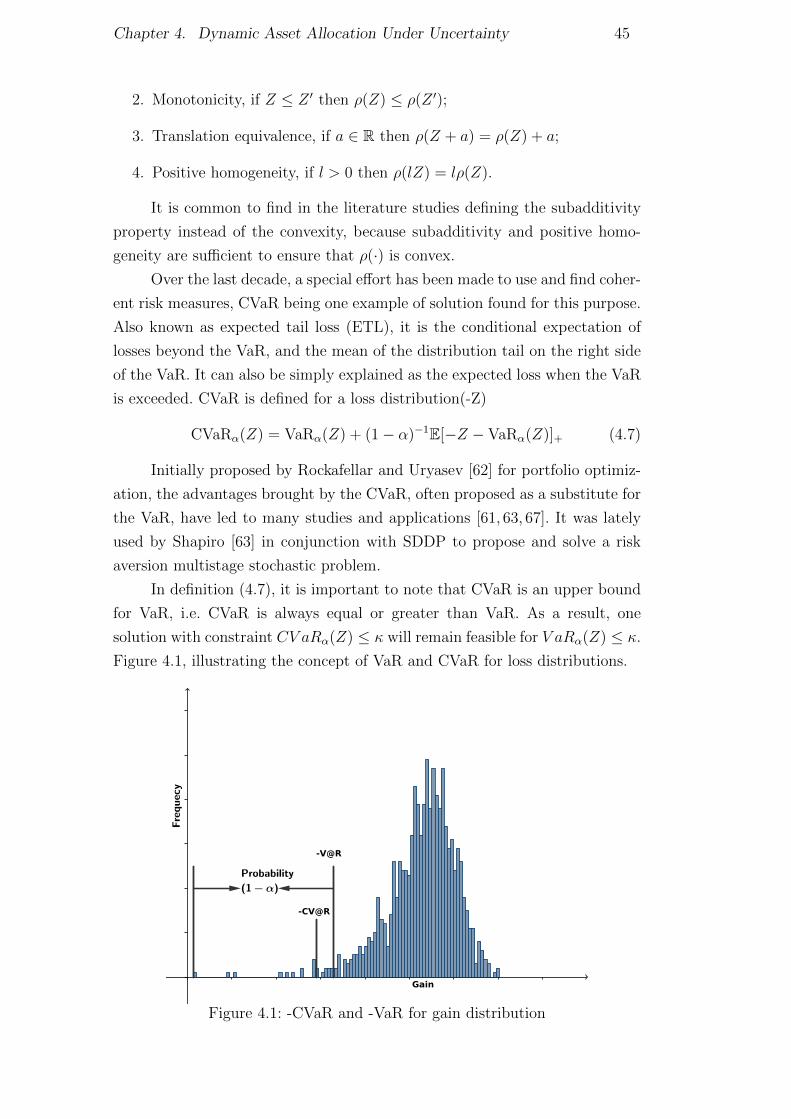
Chapter 4. Dynamic Asset Allocation Under Uncertainty 45
2. Monotonicity, if Z ≤ Z ′ then ρ(Z) ≤ ρ(Z ′);
3. Translation equivalence, if a ∈ R then ρ(Z + a) = ρ(Z) + a;
4. Positive homogeneity, if l > 0 then ρ(lZ) = lρ(Z).
It is common to find in the literature studies defining the subadditivity
property instead of the convexity, because subadditivity and positive homo-
geneity are sufficient to ensure that ρ(·) is convex.
Over the last decade, a special effort has been made to use and find coher-
ent risk measures, CVaR being one example of solution found for this purpose.
Also known as expected tail loss (ETL), it is the conditional expectation of
losses beyond the VaR, and the mean of the distribution tail on the right side
of the VaR. It can also be simply explained as the expected loss when the VaR
is exceeded. CVaR is defined for a loss distribution(-Z)
CVaRα(Z) = VaRα(Z) + (1− α)−1E[−Z − VaRα(Z)]+ (4.7)
Initially proposed by Rockafellar and Uryasev [62] for portfolio optimiz-
ation, the advantages brought by the CVaR, often proposed as a substitute for
the VaR, have led to many studies and applications [61, 63, 67]. It was lately
used by Shapiro [63] in conjunction with SDDP to propose and solve a risk
aversion multistage stochastic problem.
In definition (4.7), it is important to note that CVaR is an upper bound
for VaR, i.e. CVaR is always equal or greater than VaR. As a result, one
solution with constraint CV aRα(Z) ≤ κ will remain feasible for V aRα(Z) ≤ κ.
Figure 4.1, illustrating the concept of VaR and CVaR for loss distributions.
Figure 4.1: -CVaR and -VaR for gain distribution
DBD
PUC-Rio - Certificação Digital Nº 1021809/CB

Chapter 4. Dynamic Asset Allocation Under Uncertainty 46
As a coherent risk measure, the CVaR should be an appropriate way
to assess the risk. However, we want to stress the fact that if one chooses a
dynamic model, time consistency should be a concern since an inconsistent
policy may not consider aversion risk [68].
In a maximization problem it can also be used an alternative definition
using -CVaR to evaluate the equation above, as follows
−CVaRα(Z) = supu∈R
u− E[(Z − u)−]
1− α
(4.8)
where x− = −min(x, 0).
(c) Stopping Criteria
For general deterministic problems, as well as for deterministic Benders
decomposition, the optimal solution is achieved when the lower bound and
the upper bound are the same. However, the SDDP problem is SAA of the
“true” problem, thus the lower and upper bound are an approximation of the
actual value for the real “true” problem, and one has to consider the confidence
interval of this values to compare them.
Although the finite convergence of SDDP and other sampling-based
methods has been proven [63, 69], the computational time required for the
algorithm to actually converge could be considerable. The traditional stopping
criterion proposed by Pereira e Pinto [53] consists in stopping SDDP when
the upper bound get into the lower bound’s confidence interval. As exposed
by Shapiro 2011 [63], this criterion does not seem to make much sense and
it would be more logical if the algorithm stopped when the gap between the
upper limit of the lower bound and the upper bound became small enough
(< ε). However, this gap can be very large and normally does not get narrow
enough within a reasonable computation time [70].
There has been debate around what should be the stopping criteria
of SDDP. Several other different stopping criteria have been proposed in
the literature, but to this date none has been widely accepted as being the
best one. Additionally, finding the lower bound for the multistage stochastic
maximization problems that uses nested CVaR [63] is not easy. In spite of
some promising attempts [71], as seen above, there is no guarantee that by
using a stopping criteria with lower bound the solution of SDDP will converge.
Actually, in practical problems, achieving convergence is very time-consuming,
thus most of the time the SDDP has to be stopped before finding the optimal
solution. Further debate on the convergence of SDDP can be found in [63,72].
Despite all the discussion around the convergence of SDDP, the most
DBD
PUC-Rio - Certificação Digital Nº 1021809/CB

Chapter 4. Dynamic Asset Allocation Under Uncertainty 47
straightforward method to stop SDDP with nested CVaR is the stabilization
of the upper bound. As pointed out by Shapiro [63], the stabilization of the
upper bound does not mean that SDDP is close to the optimal solution.
However, during this thesis, when stabilization was achieved, even by changing
the number of trials and leaving the algorithm running for many days, the
upper bound could not be changed. Thus, given the fact that none of the
methods has guaranteed convergence, we think that the stabilization of the
upper bound represents the better trade off between the computational time
and proximity to the optimal solution.
(d) Sampling Scenarios
The idea to represent the random process through samples was used
by different authors over the years. Sample Average Approximation (SAA)
consists in representing a distribution by random realizations sampled from
“true” distributions. Therefore, the “true” optimization problem is replaced
by its SAA version. The method traditionally used in SAA is the Monte Carlo,
that randomly selects independent and identically distributed (i.i.d.) samples,
all realizations having an equal probability of being selected.
In practical situations, sampling the scenarios with Monte Carlo requires
a large number of samples in order to keep deviations small. Nonetheless,
there are techniques that can be used to reduce the variance, like Importance
Sampling and Latin Hypercube Sampling.
Importance sampling having been created to be a variance reduction
technique [73], but is also particularly useful when it is impossible to sample
from the real distribution, it allows to study and analyze a distribution using
samples taken from another distribution.
Assuming that the likelihood ratio function f(xi)g(xi)
is well defined, if there
is some z ∈ Rd where f(z) = 0, then g(x) = 0, the expected value of a random
variable X ∼ h can be calculated as
E(h(X)) =
∫Dh(x)f(x)dx =
∫D
h(x)f(x)
g(x)g(x)dx = Eg
(h(X)f(X)
g(X)
)(4.9)
For a given set of i.i.d. samples xi drawn according to a probability
density g(X) the importance sampling estimator of µ = Eg(h(X)) is
µg =1
n
n∑i=1
h(xi)f(xi)
g(xi), xi ∼ g (4.10)
The importance sampling estimator µg is an unbiased estimator of µ. By
sampling from distribution probability density function g(·) and making an
DBD
PUC-Rio - Certificação Digital Nº 1021809/CB

Chapter 4. Dynamic Asset Allocation Under Uncertainty 48
adjustment using the likelihood ratio f(xi)g(xi)
, it is also possible to obtain samples
from the original or nominal distribution h.
This approach in SDDP may be used, for example, for a cost-to-go func-
tion Qt(xt−1, ξts), while an importance sampling estimator can be evaluated
given realizations different form ξ. However, as indicated by Shapiro in [60],
the importance sampling method has some issues, it is very sensitive to the
choice of p.d.f., for example, and its instability is notorious, even for small
perturbations in g(·).Latin Hypercube Sampling, another variance reduction technique, uses
probability dense inverse function to sample the distribution more evenly.
Initially proposed by Mckay et al. 1979 [74], it is a stratified sampling method, a
K-dimensional extension of Latin square sampling. Latin Hypercube Sampling
divide the p.d.f. in intervals with the same probability and collect one sample
from each interval. Controlling how random samples are generated, the method
spreads the samples more evenly throughout the distribution.
It is possible to observe on Figure 4.2 how Latin Hypercube Sampling
method performs on two uniform distributions X ∼ U(0, 1) and Y ∼ U(0, 1).
0 0.2 0.4 0.6 0.8 10
0.2
0.4
0.6
0.8
1
X
Y
Figure 4.2: Example of Latin Hypercube Sampling for uniform distributionwith two dimensions
To illustrate how Latin Hypercube Sampling and Monte Carlo behave,
two examples were designed, which can be seen in Figure 4.3 and Figure 4.4. For
the first example, five hundred iterations were performed, sampling 30 points of
normal distribution N ∼ (0, 1) by using Monte Carlo and also Latin Hypercube
Sampling. The resulting figures present the estimated normal distribution for
each one of the five hundred iterations.
DBD
PUC-Rio - Certificação Digital Nº 1021809/CB

Chapter 4. Dynamic Asset Allocation Under Uncertainty 49
−3 −2 −1 0 1 2 30
0.05
0.1
0.15
0.2
0.25
0.3
0.35
0.4
x
f(x)
Figure 4.3: Sampling withMonte Carlo
−3 −2 −1 0 1 2 30
0.05
0.1
0.15
0.2
0.25
0.3
0.35
0.4
x
f(x)
Figure 4.4: Sampling withLatin Hypercube Sampling
On the figure it is clear that the variance of the Monte Carlo is larger
than the Latin Hypercube Sampling. Latin Hypercube Sampling also requires
a reasonable number of examples, mainly to better represent the distribution
tails. The intervals on the tails are bigger, as we can see in Figure 4.5, thus more
samples would be necessary to better represent this part of the distribution.
−3 −2 −1 0 1 2 30
0.05
0.1
0.15
0.2
0.25
0.3
0.35
0.4
Figure 4.5: LHS interval for a normal distribution N ∼ (0, 1)
4.3 Stochastic Dynamic Programming for AssetAllocation
In this section we will explain how to adapt SDDP for multistage asset
allocation. First, we will begin with the risk-neutral formulation and risk averse
DBD
PUC-Rio - Certificação Digital Nº 1021809/CB

Chapter 4. Dynamic Asset Allocation Under Uncertainty 50
formulation, followed by the time independent model, transactional costs with
SDDP and, finally, by our proposal to treat temporal dependence.
Supposing an investor wishes to construct a portfolio dividing a given
amount of cash among the assets xti, ∀i ∈ A each of which has an uncertain
return rti(s) for time t. Each stage brings the need to reallocate the portfolio,
considering the profits obtained in the previous stage Wt = (1 + rt)>xt−1.
Considering an initial capital W1, and not allowing a short sell (i.e. x ≥ 0),
the risk-neutral portfolio multistage stochastic problem is stated as
max1>x1=W1
x1≥0
E
[max
1>x2=W2x2≥0
E[
max1>xt−1=WT−2
xt−1≥0
E[WT
∣∣r[T−1]
]. . .
∣∣∣r1
]](4.11)
The realization of the investment made in t is accounted for in the following
stage t + 1. The optimal solution for this risk-neutral formulation would be
to allocate everything in the asset with the highest expected profit. However,
it is a known fact that investing everything in a single asset is not very wise.
Neglecting risk in the optimization problem can lead to big losses, especially
in fall trends.
Using ψ(·)t function it is possible to add risk aversion formulation for
asset allocation
max1>x1=W1
x1≥0
ψ1
[max
1>x2=W2x2≥0
ψ2
[max
1>xt−1=WT−2xt−1≥0
ψT−2
[WT
∣∣r[T−1]
]. . .
∣∣∣r1
]](4.12)
The function ψ(·)t is the convex combination combination of the expect value
and the CVaR, as it is a maximization problem. Formally, the function ψt(·)is
ψt(Z|ξt) = (1− λ)E[Z|ξt] + λ(−CVaRα[Z|ξt]) (4.13)
(a) Myopic policy: No transaction costs and temporal in-dependence
For the special case when the multistage portfolio selection does not
have transactional cost and no temporal dependence the optimal solution can
be easily found using a myopic policy. In the appendix A.2 it is presented the
myopic prove for a coherent risk measure [60].
The myopic policy, that aims on maximizing one-step reward ignoring
the impact on future rewards, is optimal. However, this policy is optimal in a
very specify situation. In a more realist situation, with transactional costs, the
myopic policy is not optimal.
DBD
PUC-Rio - Certificação Digital Nº 1021809/CB

Chapter 4. Dynamic Asset Allocation Under Uncertainty 51
(b) SDDP for asset allocation: Transaction costs and tem-poral independence
In this section, the asset allocation problem will be formulated with xt
in the state space and risk aversion with CVaR, in order to be used in SDDP
and to later include transactional costs. However, this model still disregards
the temporal dependence.
According to Rudloff et al. [68], the nested CVaR is the certainty
equivalent of the portfolio and, consequently, the worth of the portfolio.
Therefore, for the multistage asset allocation problem the cost-to-go is actually
the worth function. The dynamic programming equation can be defined using
the risk averse multistage formulation for asset allocation (4.12) and the
function ψ(·)(4.13). The worth function is
Qt(xt−1, rt) = maxxt
r>t xt−1 +Qt+1(xt) (4.14)
s.t. 1xt = (rt + 1)>xt−1
xt ≥ 0
and the expected recourse function, in this case, the portfolio expected worth
function is
Qt+1(xt) = (1− λ)1
Nt
Nt∑s=1
Qt+1(xt, rt+1(s))+ (4.15)
λ
(Qt+1(xt, rt+1(τ))− 1
(1− α)Nt
Nt∑s=1
[Qt+1(xt, rt+1(s))−Qt+1(xt, rt+1(τ))]−
)
Is important to emphasize that the Qt+1(xt, rt+1(τ)) is the -VaR of
Qt+1(xt, rt+1(1)), . . . , Qt+1(xt, rt+1(Nt)), i.e the right or positive α quantile.
Herein the -CVaR, and consequently -VaR, will be evaluated using the dual
representation of the CVaR that is a fractional knapsack problem [61,65].
−CV aR(X) = minvs
Nt∑s=1
Qt+1(xt, rt+1(s))× vs (4.16)
s.t.Nt∑s=1
vs = 1
vs ≤1
(1− α)Nt
∀s ∈ 1, . . . , Nt
vs ≥ 0 ∀s ∈ 1, . . . , Nt
To determine the cut, it is necessary to evaluate the subgradient of the
DBD
PUC-Rio - Certificação Digital Nº 1021809/CB

Chapter 4. Dynamic Asset Allocation Under Uncertainty 52
worth function Qt(xt−1), it was used -CVaR. With γts being the subgradient
of Qt(x∗t−1) at point x∗t−1, the subgradient of the expected recourse function is
gt = ∇Qt(x∗t−1) = (1− λ)1
Nt
Nt∑s=1
γts + λ
(γtτ −
Nt∑s=1
ηts
)(4.17)
where using the weights vs of (4.16) we have ηts∀s ∈ 1, . . . , Nt
ηts =
0 if Qt(xt−1, rt(s)) > Qt(xt−1, rt(τ))
−(γt+1,s − γt+1,τ )vs if Qt(xt−1, rt(s)) ≤ Qt(xt−1, rt(τ))(4.18)
and the subgradient of Qt(xt) changes to
γt = rt + (1+ rt)>π∗ (4.19)
It must be kept in mind that traditional SDDP is a minimization problem,
however, this work maximizes the objective function, thus the solution of
Qt(xt−1, rt) is an upper bound to the model presented here.
Transactional costs
Most of the early asset allocation methods did not consider the transac-
tional costs on purchases or sales of assets. When the costs of each transaction
are neglected, the gain apparently obtained can be misleading. Depending on
the frequency of the transactions and costs, an estimated positive return could,
in reality, became loss. Moreover, costs stimulate the maintenance of the se-
lected portfolio in the previous period, because it is an explicit regularization
of portfolio movements. It is a L1 regularization [75], since the sum of the
absolute differences, the changes on the portfolio, is penalized on the object-
ive function. It will be seen later in the experiments section this behavior in
practice.
Introducing d+ti and d−ti to represent how much from each asset i is bought
and sold. Also, the variable c that is the proportional cost, selling will bring
an income (1− c)d−ti , and buying will mean a cost (1 + c)d+ti to current wealth
(1+ rt)>xt−1. The problem with transactional cost can be formulated as
Qt(xt−1, rt) =
maxxt,d
+t ,d−t
r>t xt−1 −∑i∈A
c(d+ti + d−ti) +Qt+1(xt) (4.20)
s. t. 1>xt + c∑i∈A
(d+ti + d−ti) = (1+ rt)
>xt−1 (4.21)
xti − d+ti + d−ti = (1 + rti)xt−1,i, ∀i ∈ A \ 1 (4.22)
d+t ,d
−t ,xt ≥ 0 (4.23)
DBD
PUC-Rio - Certificação Digital Nº 1021809/CB

Chapter 4. Dynamic Asset Allocation Under Uncertainty 53
Notice that there is no transactional cost in the purchase or sale of risk-
free asset. Furthermore, in this model the complementarity of the simultaneous
purchase and sale of a given asset is guaranteed, i.e. d+tid−ti = 0. If there
were simultaneous purchase and sale operations of an asset, that could not
be the best solution as it would be possible to obtain a better return without
interfering with xti.
The subgradient of the worth function for SDDP also changes. In this
context there are additionally A dual variables, represented by the vector
π2 ∈ RA associated with constraint (4.22), then the subgradient of Qt(xt)
becomeγt = rt + (1+ rt)
>π∗1 + (1+ rt)>π∗2 (4.24)
with π1 representing the dual variables of constraint (4.21). Furthermore, the
optimal solution of this new problem cannot be found using myopic policy,
now it cannot ignore future implications caused by the current decision.
(c) H2SDDP for allocation: Transaction costs and temporaldependence
In previous sections it was shown that when the multistage asset alloc-
ation problem has no time dependency the optimal solution can be achieved
using a myopic policy. When transactional costs are added to the model this
myopic optimal behavior does not hold, under these circumstances the tradi-
tional SDDP can be used to find the optimal solution. However, the stagewise
assumption of traditional SDDP is an issue when modeling temporal depend-
ence problems. In this section we will discuss some approaches to model time
dependency and how to modify SDDP for this purpose.
In many applications a more general problem has to be considered, when
there is time dependency between the stages. The worth function becomes
dependent on the historical achievements of the random variable Qt+1(xt, r[t]).
Thus, we have a worth function (future cost function on original SDDP) for
each node in the stochastic tree, and therefore is so common to use L-shaped
methods. The hydrothermal scheduling is one of the problems that typically
has time dependency. This dependence usually occurs in inflows, on the right-
hand side of the problem. The inflows are modeled as an AR(1) autoregressive
of order one, that isbt = φtbt−1 + εt (4.25)
Changing the stochastic process to ξt = (ct,Bt,At, εt) and increasing
the state space to (xt,bt), we can define the generic problem as well as solving
it using the similar SDDP method used by independent case, problem (4.3),
DBD
PUC-Rio - Certificação Digital Nº 1021809/CB

Chapter 4. Dynamic Asset Allocation Under Uncertainty 54
with the cost-to-go function as
Q(xt−1,bt−1, ξt) = maxxt
c>t xt +Qt+1(xt) (4.26)
s. t. Atxt = −Btxt−1 + φtbt−1 + εt
xt ≥ 0
Furthermore, in hydrothermal scheduling there are situations where the
inflows are best mapped as nonlinear functions, for example, as a Markov
process. There are some advantages in mapping the time dependency as a
Markov process, in addition to encapsulate all the historical information it
also incorporate autocorrelated dependency, this is extremely important since
seasonality is present in the inflows data [76].
Using Markovian process to represent the inflows probability distribution,
it is also possible to preserve stagewise independence between cost-to-go
functions. This approach was first develop in [54], and later adapted in [55]
for the New Zealand electricity system and similar methodolodgy was applied
to Energy contracts management of Liquefied Natural Gas in [77]. All these
approaches use deterministic states and has dependency on the right-hand side.
H2SDDP
Undoubtedly, the methodology developed by Pereira and Pinto [48],
SDDP, has great advantages, however, the assumption of stagewise independ-
ence is not realistic for some problems. When dealing with with temporal
dependence, the methodology must go through some adaptation in order to
be able to solve this type of problem.
In the alternative L-shaped method, there is one worth function for every
node of the scenario tree, each node has a unique history and the worth
function depends on the historical return. Therefore, this technique has greater
computational complexity since the expected worth function has to consider
the whole previous realization of the scenario.
The solution proposed here for multistage asset allocation is the Hidden
States Stochastic Dynamic Programming (H2SDDP), that can be described as
a combination of SDDP and L-shaped procedures. In the H2SDDP method,
the market is classified and separated by states, so only the probability of each
state depends on the past returns. The method can be seen as a generalization
of SDDP and L-Shaped, if the number of states is equal to the number of nodes
in the stochastic tree, the model will behave like L-Shaped; otherwise, if the
number of states is one, it will act similarly to SDDP.
DBD
PUC-Rio - Certificação Digital Nº 1021809/CB

Chapter 4. Dynamic Asset Allocation Under Uncertainty 55
The foremost difference between the three methods (SDDP, L-Shaped
and H2SDDP) is the trade-off between how historical information is considered
in each node of the stochastic tree and the computational complexity involved.
With H2SDDP method we expected to achieve the best compromise in this
regard, as it creates a small increase in complexity while being able to deal
with problems with temporal dependence within a reasonable computational
time.
In this work the temporal dependence will be expressed as states of hid-
den Markovian process and the asset return will be modeled as a multivariate
mixture of Gaussians. There are other ways to separate financial time series
in states, the HMM was chosen because it is more suitable for necessities in-
volved in this circumstances. Indeed, the method is especially appropriate for
this application because it can be used to estimate the states likelihood and
to sample the return distributions given the states.
Many traditional financial applications used the normal distributions
with stationary parameters to model the log-returns distributions. Nowadays,
it is well known that this does not reproduce some important stylized facts or
well known properties of the financial time series.
Fama [78] study analyses the behavior of stock market prices and presen-
ted some evidences that contradicts the assumption of normality. Granger and
Ding [79] presented some of the stylized facts of properties for a variety of
log return series. Ryden et al. [80] shown that modeling the financial time
series as a Gaussian mixture according to the states of an unobserved Markov
chain, the HMM model, reproduces most of the stylized facts for daily return
series demonstrated by Granger and Ding [79].Thus, HMM is frequently used
to model return series [80–83].
Figure 4.6 is an example of a simple a HMM for stock market, which
uses, for the sake of simplicity, discrete emission distributions. The objective
is to determine the market state Bull, Bear, Neutral given the return status
of the current day stable, down, up. Observe that, given an emission, it is not
possible to determine, with certainty, what is the state; and given a state and
using the state emission distribution, we can obtain a realization.
DBD
PUC-Rio - Certificação Digital Nº 1021809/CB

Chapter 4. Dynamic Asset Allocation Under Uncertainty 56
Neutral
Bull Bear
downstableup downstable up
down
stable
up
0.10.2
0.7 0.60.30.1
0.2
0.6
0.2
0.2 0.2
0.2
0.1
0.10.1
0.6
0.7 0.8
Figure 4.6: An example of HMM for stock market
But in this application the return of each asset will depend on the state
of the HMM, Figure 4.7 is an example on how return can be represented by
HMM as a mixture of Gaussians.
Figure 4.7: An example of a Gaussian mixture model.
Since temporal dependence of the return series will be modeled as a
HMM, the SDDP’s worth function will be separated by state, creating a
stagewise independence. Therefore, there is only one worth function for each
DBD
PUC-Rio - Certificação Digital Nº 1021809/CB

Chapter 4. Dynamic Asset Allocation Under Uncertainty 57
stage that depends on a specific market state. These functions do not depend on
the previous returns, only the probability of the Markov states is conditional to
historical returns. The downside of this approach is increasing computational
effort, since it has more worth functions, one per state.
Let us first assume that at time t the market state k is known, then we
solve the following problem
Ut(xt|k) = ψt[utk(xt, rt+1)|k] (4.27)
utk(xt, rt+1(s)) = rt+1(s)>xt + maxxt+1∈X(xt,rt+1(s))
K∑j=1
Ut+1(xt+1|j)P (j|k)
where Ut(xt|k) is the worth function given the state k and the transition
probability from state k to j is P (j|k).
In practice, since the state k is unknown, we need to solve problem (4.27)
using the past observed returns r[t] to estimate the states probabilities. To
simulate the system and find the optimal policy we solve the following problem
RPt (xt−1, r[t]) = r>t xt−1 + max
xt∈X(xt−1,rt)
K∑k=1
Ut(xt|k)P (k|r[t]) (4.28)
where P (k|r[t]) is the likelihood of the state k estimated by the forward-
backward algorithm [84] given the past returns r[t].
The worth function Qt+1(xt) is approximated by a set of cutting planes
ItUt(xt|k) = max
l∈Itutk(xt−1,l) + g>tl (xt−1 − xt−1,l), ∀t ∈ H (4.29)
where utk(xt−1,l) = 1Nt
∑Nt
s=1 utk(xt−1,l, rt(s)) and gtl analogously to
equation 4.17 with the subgradient equal to 4.24.
To solve the problem (4.28), it is necessary to know each state’s prob-
ability, in order to weigh the worth function of the next stage. Our approach
with HMM uses past returns to estimate the present probability of each mar-
ket state in forward step. With the states’ probabilities, the objective function
can be evaluate by combining the state probability with the respective worth
function. Also, the states’ probabilities of each stage determine the joint dis-
tributions that are used to establish the sequence of observed returns.
In backward step, each state emission distribution is considered and
one or more cuts are added to each respective state. In other words, when
realizations from a given state are used, the cut will be added to the set of
cuts of that same state. Also, as in problem (4.28), the worth function is
conditional on the state, meaning there will be K functions per stage. Using
the dynamic programming equations above, the models used in forward and
DBD
PUC-Rio - Certificação Digital Nº 1021809/CB

Chapter 4. Dynamic Asset Allocation Under Uncertainty 58
backward steps are (4.30) and (4.31), respectively, with transactional costs.
xt = arg maxxt,d
+t ,d−t
−∑i
c(d+ti + d−ti) +
K∑k=1
Ut(xt|k)P (k|r[1,t]) (4.30)
s. t. 1>xt +∑i
c(d+ti + d−ti) = (1+ rt)
>xt−1
xti − d+ti + d−ti = (1 + rti)xt−1,i, ∀i ∈ A \ 1
xt,d+t ,d
−t ≥ 0
utk(xt, rt+1(s)) =rt+1(s)>xt+ (4.31)
maxxt+1,d
+t+1,d
−t+1
−∑i∈A
c(d+ti + d−ti) +
K∑j=1
Ut+2(xt+1|j)P (j|k)
s. t. 1>xt+1 +∑i∈A
c(d+ti + d−ti) = (1+ rt+1(s))>xt
xt+1,i − d+ti + d−ti = (1 + rt+1,i(s))xti, ∀i ∈ A \ 1
xt+1,d+t+1,d
−t+1 ≥ 0
In the backward step the decision at t are conditional to the state at
time t for every t and for every state. In the forward step only the current
first stage is treated differently, i.e., the state is assumed unknown. Note that,
for the forward step the recourse or future decision are also conditioned to
the states. Separating the worth functions for each state makes this approach
an approximation for the SAA problem. The entire proposed algorithm for
H2SDDP approach is presented below.
DBD
PUC-Rio - Certificação Digital Nº 1021809/CB

Chapter 4. Dynamic Asset Allocation Under Uncertainty 59
Algorithm 1 H2SDDP
Require: Q0tt=2,...,T+1(Init. Upper approx.) and ε = 0.0001 (accuracy)
Initialize: i← 0, z = −∞ (Upper Bound)
while stb count < 5 and i < max do
Sample M scenarios:rt(s)1≤s≤Nt
1≤t≤T
[Foward step]
for m = 1→M do
selects scenario Sm = r0, . . . , rTfor t = 1→ T do
xmt ← argmaxxt
K∑k=1
Ut(xt|k)P (k|r[1,t]) :
1>xt = (1+ rt)>xmt−1,xt ≥ 0
end for
end for
[Backward step]
for m = 1→M , t = T → 2 do
for k = 1→ K do
for s = 1→ Nt(k) do
[utk(xmt−1, rt(s)), π
mt (rt(s))]← max
xt
rt(s)>xmt−1 +
K∑j=1
Ut+1(xt|j)P (j|k) :
1>xt = (1+ rt(s))>xmt−1,xt ≥ 0
end for
utk(xmt−1)← (1− λ) 1
Nt(k)
Nt(k)∑s=1
[utk(x
mt−1, rt(s))
]+
λ
uτtk(xt−1, rt) − 1
(1−α)Nt(k)
Nt(k)∑s=1
[utk(x
mt−1, rt(s)) −
uτtk(xt−1, rt)]−
gmt ← (1− λ) 1Nt
Nt∑s=1
γts + λ
(γt,τ + 1
(1−α)N
Nt∑s=1
ζt(rt(s))
)Ui+1tk ← xt−1 ∈ Uitk : −gmt xt−1 ≥ utk(x
mt−1)− gmt xmt−1)
end for
end for
[Upper bound update]
z ← maxx1
K∑k=1
Ui+12 (x1|k)P (k|r[T ]) : 1>x1 = (1+ r1)>x0,x1 ≥ 0
if |(z/lagr(z)− 1| < ε then
stb count ← stb count + 1
else
stb count ← 0
end if
i← i+ 1
end while
DBD
PUC-Rio - Certificação Digital Nº 1021809/CB

Chapter 4. Dynamic Asset Allocation Under Uncertainty 60
The dynamic asset allocation process under uncertainty embeds a se-
quence of decision at each time succeeded by the asset return realization of
the following period. In Figure 4.8, an illustrative decision tree depicts the
described process. This example represent a generic time dependence of asset
returns, since it is possible to consider different conditional probability distri-
butions of rt+1 for each given rt.
Figure 4.8: Decision tree of the generic problem with return dependence
In particular, when the return time dependence is modeled using HMM
the decision process can be represented as in Figure 4.9.
Figure 4.9: Decision tree of the problem with return dependence modeled withHMM
Note that, in Figure 4.9 the conditional allocation at a given time would
depend on the whole history of asset returns, which would lead to an intractable
optimization problem where the full tree must be represented. In Figure 4.10,
represents an computationally tractable approximation of Figure 4.9, that can
be solved by SDDP.
DBD
PUC-Rio - Certificação Digital Nº 1021809/CB
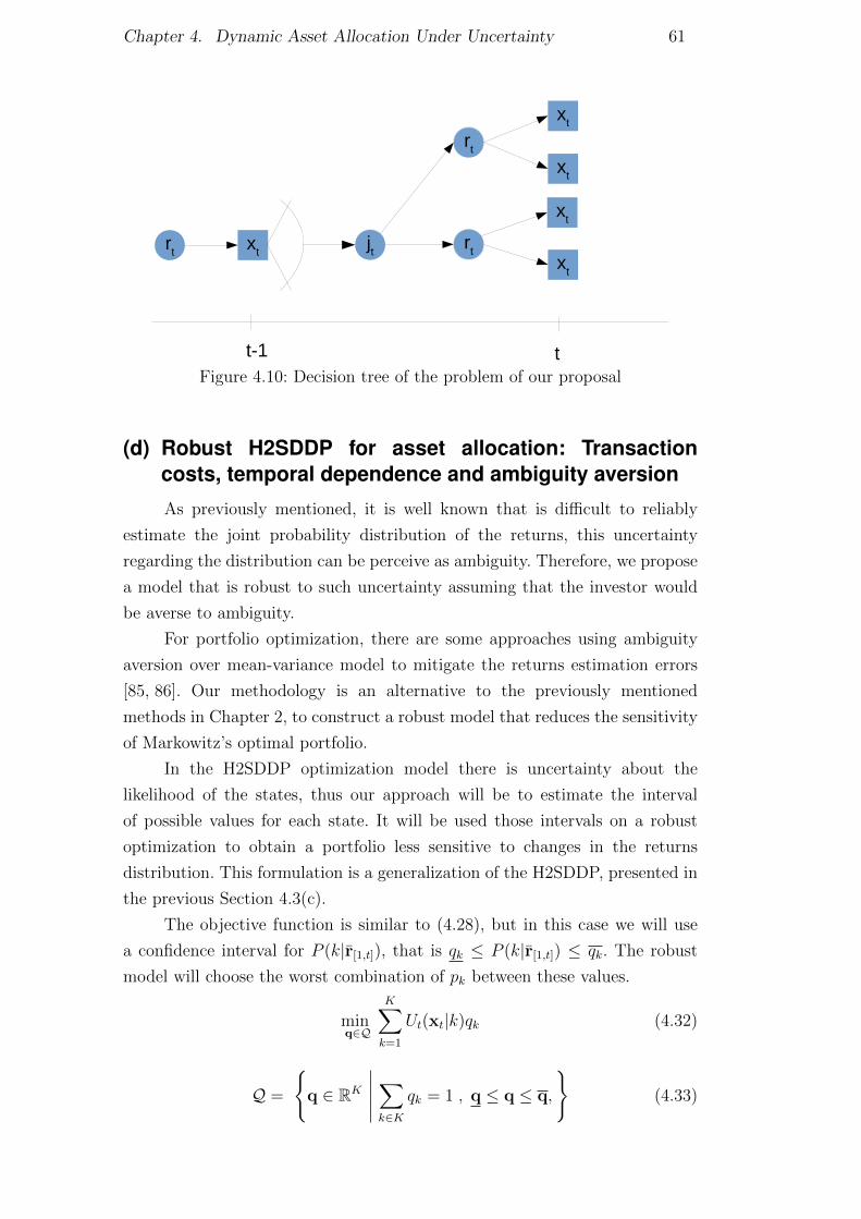
Chapter 4. Dynamic Asset Allocation Under Uncertainty 61
Figure 4.10: Decision tree of the problem of our proposal
(d) Robust H2SDDP for asset allocation: Transactioncosts, temporal dependence and ambiguity aversion
As previously mentioned, it is well known that is difficult to reliably
estimate the joint probability distribution of the returns, this uncertainty
regarding the distribution can be perceive as ambiguity. Therefore, we propose
a model that is robust to such uncertainty assuming that the investor would
be averse to ambiguity.
For portfolio optimization, there are some approaches using ambiguity
aversion over mean-variance model to mitigate the returns estimation errors
[85, 86]. Our methodology is an alternative to the previously mentioned
methods in Chapter 2, to construct a robust model that reduces the sensitivity
of Markowitz’s optimal portfolio.
In the H2SDDP optimization model there is uncertainty about the
likelihood of the states, thus our approach will be to estimate the interval
of possible values for each state. It will be used those intervals on a robust
optimization to obtain a portfolio less sensitive to changes in the returns
distribution. This formulation is a generalization of the H2SDDP, presented in
the previous Section 4.3(c).
The objective function is similar to (4.28), but in this case we will use
a confidence interval for P (k|r[1,t]), that is qk ≤ P (k|r[1,t]) ≤ qk. The robust
model will choose the worst combination of pk between these values.
minq∈Q
K∑k=1
Ut(xt|k)qk (4.32)
Q =
q ∈ RK
∣∣∣∣∣ ∑k∈K
qk = 1 , q ≤ q ≤ q,
(4.33)
DBD
PUC-Rio - Certificação Digital Nº 1021809/CB

Chapter 4. Dynamic Asset Allocation Under Uncertainty 62
Using (4.32) and (4.33) we can define our 2-stage robust problem as
maxxt∈X(xt−1,rt)
minq
K∑k=1
Ut(xt|k)qk (4.34)
s. t.∑k
qk = 1 : z
− qk ≥ −qk ∀k ∈ 1, . . . , K : yk
qk ≥ qk ∀k ∈ 1, . . . , K : wk
x ≥ 0
The objective function has a nonlinearity due to the product of first
and second stage variables Ut(xt|k) qk. To solve the two-stage problem (4.34),
first we have to formulate the dual problem of (4.32), using the dual variables
(z, wk, yk) we have
maxz,y,w
z +K∑k=1
(qkwk − qkyk
)(4.35)
s. t. wk − yk + z ≤ Ut(xt|k) ∀k ∈ 1, . . . , K
w,y ≥ 0, z ∈ R
Adding the restrictions from the original problem and transactional costs,
we have
RPt (xt−1, r[t]) = r>t xt−1 (4.36)
maxxt,y,w,d
+t ,d−t ,z−∑i∈A
c(d+ti + d−ti) + z +
K∑k=1
(qkwk − qkyk
)s. t. 1>xt +
∑i∈A
c(d+ti + d−ti) = (1+ rt)
>xt−1
xti − d+ti + d−ti = (1 + rti)xt−1,i, ∀i ∈ A \ 1
wk − yk + z ≤ Ut(xt|k) ∀k ∈ 1, . . . , K
d+t ,d
−t ,xt,w,y ≥ 0, z ∈ R
This robust model is used only in forward procedure, since the state is
unknown, it is necessary to estimate the likelihood of the states. In backward
procedure the states are known, thus there is no uncertainty associated with
it.
DBD
PUC-Rio - Certificação Digital Nº 1021809/CB

Chapter 4. Dynamic Asset Allocation Under Uncertainty 63
(e) H2SDDP for asset allocation: Transaction costs, tem-poral dependence and sell short
Sell short consist in selling an asset that is not owned by the seller,
betting on the fall in the asset price, to later buy the asset with a lower value,
thus earning the difference between the sell price and the bought price. Sell
short(selling and later purchasing) has the opposite properties of purchasing
and later selling, in which the loss is limited and gain unlimited, in short selling
the gain becomes limited but the loss is unlimited, since there is not an upper
limit for the asset price.
However, in practice it know that asset price will not rise indefinitely,
there is a reasonably limit for this value that can be evaluate, for example,
using the CVaR. Allowing sell short in asset allocation optimization models
enable the portfolio to allocate negative values for the assets, making possible
to better exploit market opportunities. In many markets the sell short involves
renting the asset until the asset is purchase and returned for who bought.
Sell short is very important for quantitative models, as with it is possible
to succeed even when the market has downward trend. For example, short
sell allows the model to obtain a positive expect value for the portfolio even
in situations when all assets have negative expected returns. Actually, using
short sell the model can take advantage of these situations, and without it the
only reasonable alternative is to invest on risk-free asset, a downward trend is
useful as upward trend when using sell short. It also allows a some leverage
behavior, by short selling an asset in order to obtain cash to invest in other
assets. With x−ti being the negative allocation of asset i, the short sell, and
x+ti the positive, also we consider the rent of sell short with penalization in
objective function costing cs
utk(xt, rt+1(s)) =r>t xt−1+ (4.37)
maxx+t ,x−t ,d
+t ,d−t
− cs∑i∈A
x−ti −∑i∈A
c(d+ti + d−ti) +
K∑j=1
Ut+2(xt+1|j)P (j|k)
s. t. 1>xt +∑i∈A
c(d+ti + d−ti) = (1+ rt)
>xt−1∑i∈A
x−ti ≤ (1+ rt)>xt−1 (4.38)
x+ti − x−ti = xti ∀i ∈ A (4.39)
xti − d+ti + d−ti = (1 + rti)xt−1,i, ∀i ∈ A \ 1
d+t ,d
−t ,x
+t ,x
−t ≥ 0
Analogous, using the constrains (4.38), (4.39) and the rent on the
DBD
PUC-Rio - Certificação Digital Nº 1021809/CB
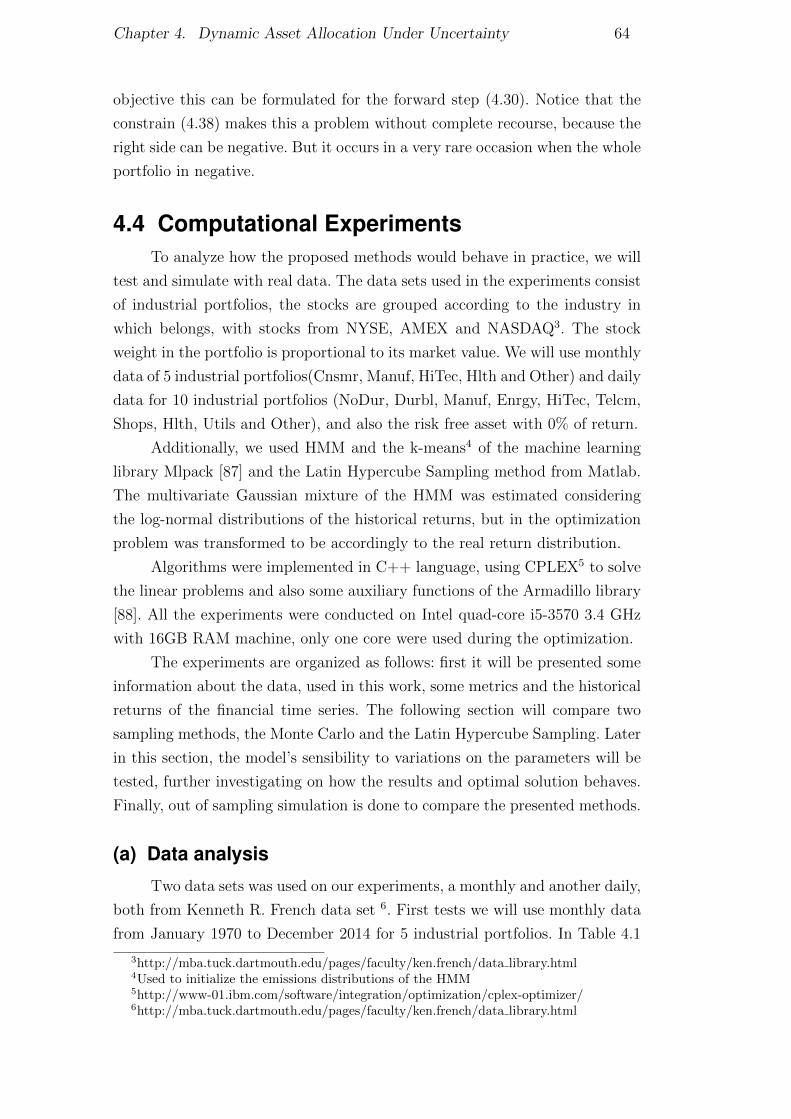
Chapter 4. Dynamic Asset Allocation Under Uncertainty 64
objective this can be formulated for the forward step (4.30). Notice that the
constrain (4.38) makes this a problem without complete recourse, because the
right side can be negative. But it occurs in a very rare occasion when the whole
portfolio in negative.
4.4 Computational ExperimentsTo analyze how the proposed methods would behave in practice, we will
test and simulate with real data. The data sets used in the experiments consist
of industrial portfolios, the stocks are grouped according to the industry in
which belongs, with stocks from NYSE, AMEX and NASDAQ3. The stock
weight in the portfolio is proportional to its market value. We will use monthly
data of 5 industrial portfolios(Cnsmr, Manuf, HiTec, Hlth and Other) and daily
data for 10 industrial portfolios (NoDur, Durbl, Manuf, Enrgy, HiTec, Telcm,
Shops, Hlth, Utils and Other), and also the risk free asset with 0% of return.
Additionally, we used HMM and the k-means4 of the machine learning
library Mlpack [87] and the Latin Hypercube Sampling method from Matlab.
The multivariate Gaussian mixture of the HMM was estimated considering
the log-normal distributions of the historical returns, but in the optimization
problem was transformed to be accordingly to the real return distribution.
Algorithms were implemented in C++ language, using CPLEX5 to solve
the linear problems and also some auxiliary functions of the Armadillo library
[88]. All the experiments were conducted on Intel quad-core i5-3570 3.4 GHz
with 16GB RAM machine, only one core were used during the optimization.
The experiments are organized as follows: first it will be presented some
information about the data, used in this work, some metrics and the historical
returns of the financial time series. The following section will compare two
sampling methods, the Monte Carlo and the Latin Hypercube Sampling. Later
in this section, the model’s sensibility to variations on the parameters will be
tested, further investigating on how the results and optimal solution behaves.
Finally, out of sampling simulation is done to compare the presented methods.
(a) Data analysis
Two data sets was used on our experiments, a monthly and another daily,
both from Kenneth R. French data set 6. First tests we will use monthly data
from January 1970 to December 2014 for 5 industrial portfolios. In Table 4.1
3http://mba.tuck.dartmouth.edu/pages/faculty/ken.french/data library.html4Used to initialize the emissions distributions of the HMM5http://www-01.ibm.com/software/integration/optimization/cplex-optimizer/6http://mba.tuck.dartmouth.edu/pages/faculty/ken.french/data library.html
DBD
PUC-Rio - Certificação Digital Nº 1021809/CB
Chapter 4. Dynamic Asset Allocation Under Uncertainty 65
we exhibit some metrics about the return series of the data set industrial
portfolios. The second data set consists in daily returns for 10 industrial
portfolio, and Table 4.2 contains a summary of the data.
Measure Cnsmr Manuf HiTec Hlth Other
Max 21.73 17.28 19.98 29.52 20.22Min -25.03 -20.80 -22.65 -20.46 -23.60Mean 1.04 1.00 0.93 1.06 0.94StdDev 4.66 4.44 5.71 4.96 5.39VaR 4.22 4.22 5.67 4.90 5.45CvaR 7.64 7.45 10.04 8.02 9.28
Table 4.1: Monthly data series for 5 industrial portfolios
Measure NoDur Durbl Manuf Enrgy HiTec Telcm Shops Hlth Utils Other
Max 10.26 9.73 10.75 19.33 16.06 14.51 10.99 11.09 14.43 11.27Min -17.03 -18.35 -20.00 -19.43 -19.98 -16.68 -16.74 -17.89 -12.86 -15.24Mean 0.05 0.04 0.05 0.05 0.04 0.05 0.05 0.05 0.04 0.04StdDev 0.91 1.37 1.09 1.36 1.48 1.14 1.10 1.12 0.88 1.19VaR 0.93 1.42 1.11 1.38 1.58 1.13 1.16 1.19 0.80 1.15CVaR 1.58 2.40 1.91 2.34 2.62 1.97 1.93 1.97 1.52 2.08
Table 4.2: Daily data series for 10 industrial portfolios
To make it easier to visualize and compare the measures, we presented
data as bar charts on Figure 4.11 and Figure 4.12.
Max Min Mean StdDev VaR CvaR
-30%
-20%
-10%
0%
10%
20%
30%
40%
Cnsmr
Manuf
HiTec
Hlth
Other
Figure 4.11: Metrics for historical monthly return series of the five industrialportfolios
DBD
PUC-Rio - Certificação Digital Nº 1021809/CB

Chapter 4. Dynamic Asset Allocation Under Uncertainty 66
Max Min Mean StdDev VaR CvaR
-25%
-20%
-15%
-10%
-5%
0%
5%
10%
15%
20%
25%
NoDur
Durbl
Manuf
Enrgy
HiTec
Telcm
Shops
Hlth
Utils
Other
Figure 4.12: Metrics for historical daily return series of the ten industrialportfolios
It is also important to present the financial time series of these data sets,
where Figure 4.13 and Figure 4.14 show the monthly and daily cumulative
performance from 1970 to 2014 for 5 and 10 industrial portfolio, respectively.
Date
Figure 4.13: Cumulative performance for monthly data set of the five industrialportfolios
Ret
urn
(%)
DBD
PUC-Rio - Certificação Digital Nº 1021809/CB

Chapter 4. Dynamic Asset Allocation Under Uncertainty 67
Date
Figure 4.14: Cumulative performance for daily data set of the ten industrialportfolios
Ret
urn
(%)
(b) Sampling Methods
As discussed before, Latin Hypercube Sampling is a promising technique
to substitute the Monte Carlo sampling in SAA techniques. Latin Hypercube
Sampling is especially important for this optimization problem, because it is
crucial to represent the distributions with least samples as possible, otherwise
it will lead to a heavy computational burden.
To compare the results of the different sampling methods, we prepared
an experiment that consists in running the optimization multiple times,
comparing the average and standard deviations of the final upper bound. It was
used the monthly data set (from 1970 to 2011), with six stages, three states,
λ 0.1, α 0.9 and no transaction cost. The test was done for Monte Carlo and
Latin Hypercube Sampling, it gradually increase number of the samples per
state 20, 100, 1000, 2500, 3000, 3500, 4000, 4500, 5000, 7000 repeating 5 times,
for each one of this values, but with different random seeds. Notice, that the
final total number of samples depends on the number of states, for example,
with 2500 samples per state and three states the problem will have a total of
7500 samples.
We did an extensive amount of tests using Monte Carlo. However,
even with 5,000 samples per stage, the standard deviation was still high. In
Figure 4.15 we compare, using the average of the upper bound for the wealth
DBD
PUC-Rio - Certificação Digital Nº 1021809/CB

Chapter 4. Dynamic Asset Allocation Under Uncertainty 68
and the standard deviation of it, the two sampling selection techniques for
different numbers of samples.
0 2,000 4,000 6,000
4
4.2
4.4
4.6
4.8
5
5.2·10−2
Samples
Ave
rage
UB
(wea
lth
)
MCLHS
0 2,000 4,000 6,000
0
1
2
3
4
·10−2
SamplesσUB
Figure 4.15: Comparison between Latin Hypercube Sampling (LHS) and MonteCarlo (MC)
It seems that with more samples, Monte Carlo gets a better average.
However, running with 10,000 samples it reaches 0.0407858, which is much
closer to the Latin Hypercube Sampling value with 5,000 samples, and even
with 10,000 samples the standard deviation still was very high.
As the solution of the problem is very stable using Latin Hypercube
Sampling, to get the same stability with Mote Carlo it would require much
more samples, this would increase the convergence time of the SDDP. Rep-
resenting the distribution with last realizations, as possible, can substantially
reduce computational times. Thus, we find the Latin Hypercube Sampling
more adequate sampling method to be used for this model and choose to use
2500 samples per state as it seems that using more samples does not improve
significantly the upper bound.
(c) Sensitivity Analysis
In addition to choosing the sampling method, there are many parameters
that need to be selected to be able to implement the proposed methods. We
need to select SDDP parameters such as number of stages, samples number,
number of trials, risk aversion coefficient and many others. It is also necessary
to analyze the model sensibility to variations, and if the model will behave as
expected on this tests.
The number of samples Nt can be different for each stage, but for the
sake of simplicity, the same number of sample has been considered for all
stages in this work, i.e |Nt| is the same for t ∈ H. Also, for all tests it was used
the monthly data set (from 1970 to 2011), with the default parameters as six
DBD
PUC-Rio - Certificação Digital Nº 1021809/CB

Chapter 4. Dynamic Asset Allocation Under Uncertainty 69
stages, three states, 2500 samples per state, λ 0.1, α 0.9 and no transaction
cost.
HMM
Moreover, there are other parameters from HMM that have to have some
initial good guessing of the states emission probabilities. We employ k-means
method to pick some centroids for every state and adopt these distributions as
the initial guess for HMM. To determine the number of states, we did a sliding
window validation for every number of states between 1 and 8, selecting the
best log-likelihood.
Figure 4.16 shows the likelihood of each state for the monthly historical
train data set.
Jan 70 Jan 73 Jan 76 Jan 79 Jan 82 Jan 85 Jan 88 Jan 91 Jan 94 Jan 97 Jan 00 Jan 03 Jan 06 Jan 090%
10%
20%
30%
40%
50%
60%
70%
80%
90%
100%
3
2
1
Date
Figure 4.16: States likelihood for train data
Lik
elih
ood
We can see that the state transitions are not smooth, it seems to be
because we are using k-means as our initial emissions distributions for the
HMM, since k-means tries to minimize the number of intersections in the
clusters. We should expect more diversified results if the samples were classify
instead of using clusters.
Impact of the Risk Aversion
The risk aversion coefficient (λ) also has big impact in the upper bound,
that is the certainty equivalent of the portfolio, which can be interpreted as the
fund worth. In Figure 4.17 we present the upper bound for different λ values,
for monthly returns on left and on right for daily returns. This results shows
how the value of the portfolio changes for investors with different aversion to
risk.
DBD
PUC-Rio - Certificação Digital Nº 1021809/CB
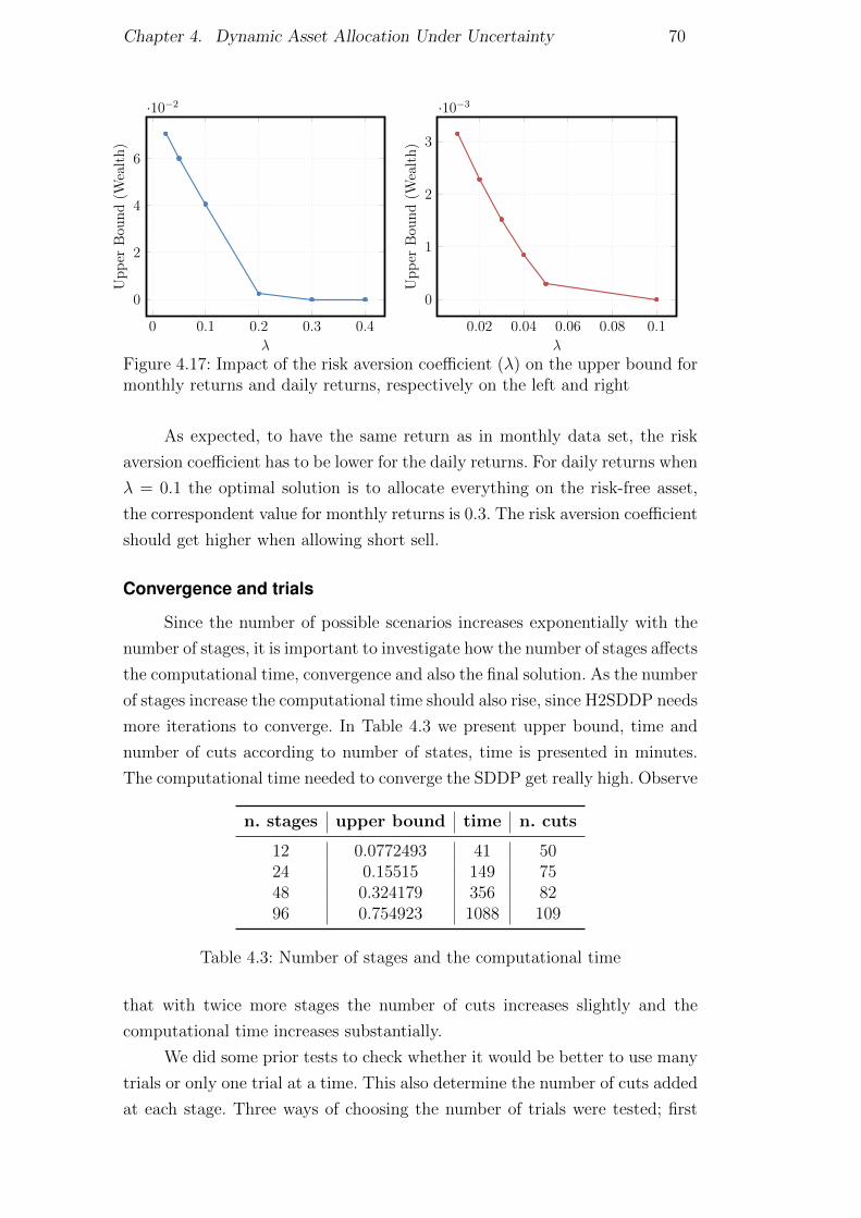
Chapter 4. Dynamic Asset Allocation Under Uncertainty 70
0 0.1 0.2 0.3 0.4
0
2
4
6
·10−2
λ
Up
per
Bou
nd
(Wea
lth
)
0.02 0.04 0.06 0.08 0.1
0
1
2
3
·10−3
λ
Up
per
Bou
nd
(Wea
lth
)
Figure 4.17: Impact of the risk aversion coefficient (λ) on the upper bound formonthly returns and daily returns, respectively on the left and right
As expected, to have the same return as in monthly data set, the risk
aversion coefficient has to be lower for the daily returns. For daily returns when
λ = 0.1 the optimal solution is to allocate everything on the risk-free asset,
the correspondent value for monthly returns is 0.3. The risk aversion coefficient
should get higher when allowing short sell.
Convergence and trials
Since the number of possible scenarios increases exponentially with the
number of stages, it is important to investigate how the number of stages affects
the computational time, convergence and also the final solution. As the number
of stages increase the computational time should also rise, since H2SDDP needs
more iterations to converge. In Table 4.3 we present upper bound, time and
number of cuts according to number of states, time is presented in minutes.
The computational time needed to converge the SDDP get really high. Observe
n. stages upper bound time n. cuts
12 0.0772493 41 5024 0.15515 149 7548 0.324179 356 8296 0.754923 1088 109
Table 4.3: Number of stages and the computational time
that with twice more stages the number of cuts increases slightly and the
computational time increases substantially.
We did some prior tests to check whether it would be better to use many
trials or only one trial at a time. This also determine the number of cuts added
at each stage. Three ways of choosing the number of trials were tested; first
DBD
PUC-Rio - Certificação Digital Nº 1021809/CB

Chapter 4. Dynamic Asset Allocation Under Uncertainty 71
using only one trial, second using 5 trials and, finally, using 5 trials as the upper
bound becomes stable for 10 iterations. From our limit experiments, using more
than one trial, i.e., adding multiple cuts, increase the convergence time even
with the alternative approach using dynamic number of trials. It seems better
to do C iterations adding one cut per iteration than to add C cuts on one
iteration, for the convergence of the algorithm. The real advantage of adding
multiple cuts could be on the quality of the worth function approximation,
this could enhance stability of primal solutions.
The used method to test the convergence of SDDP was the stabilization
of the upper bound. Whether, the upper bound of 10 iterations ago zi−10
is stable for 5 iterations, i.e., 15 iterations without change greater than ε.
Notice that the upper bound of the iteration i − 10 is compared with the
current i upper bound value. We opted for a tighter convergence criteria with
ε = 0.0001 than do more tries. To illustrate the convergence of the H2SDDP,
Figure 4.18 exhibits the upper bound changes, in percentage, for optimization
of the H2SDDP with 96 periods.
Figure 4.18: Convergence of the Upper Bound for monthly data set
Transactional costs
Another interesting subject is the impact of the transactional costs. First,
we present how of the upper bound is sensible to variations of the transactional
costs on Figure 4.19. Later we will discuss further implications of taking the
transactional costs into account. It was used the monthly data set (from 1970
DBD
PUC-Rio - Certificação Digital Nº 1021809/CB

Chapter 4. Dynamic Asset Allocation Under Uncertainty 72
to 2011), with six stages, three states, 2500 samples per state, λ 0.1, α 0.9 and
no transaction cost.
0 0.5 1 1.5 2 2.5 32.5
3
3.5
4
·10−2
Transactional cost(%)
Upp
erB
ound
(Wea
lth)
Figure 4.19: Impact of the transactional costs on the upper bound
It is evidently that the transactional costs can really impact the optimal
solution. Since the return is uncertain but the transactional cost is not,
higher transactional cost makes not worth to do some small changes on the
investments, thus the model only invest when the expect return is higher
enough to mitigate the costs involved.
Further analyzing how the transactional costs will affect the optimal solu-
tion. The portfolio allocation can be seen on Figure 4.20 with no transaction
costs, and in Figure 4.21 with transactional cost equal to 0.1 %. Even at a
cost of 0.1 %, smaller deviations are avoided when the model does not expect
a significant gain with changing the portfolio. In Figure 4.20 and Figure 4.21
we can clearly see the portfolio stabilization effect caused by transaction costs,
it is evident the resemblance to a regularization L1.
DBD
PUC-Rio - Certificação Digital Nº 1021809/CB

Chapter 4. Dynamic Asset Allocation Under Uncertainty 73
Jan 12 Apr 12 Jul 12 Oct 12 Jan 13 Apr 13 Jul 13 Oct 13 Jan 14 Apr 14 Jul 14 Oct 140%
10%
20%
30%
40%
50%
60%
70%
80%
90%
100%
Other
Hlth
HiTec
Manuf
Cnsmr
Risk Free
Date
Figure 4.20: Portfolio allocation without transactional costs
Por
tfoli
oP
erce
nta
ge
Jan 12 Apr 12 Jul 12 Oct 12 Jan 13 Apr 13 Jul 13 Oct 13 Jan 14 Apr 14 Jul 14 Oct 140%
10%
20%
30%
40%
50%
60%
70%
80%
90%
100%
Other
Hlth
HiTec
Manuf
Cnsmr
Risk Free
Date
Figure 4.21: Portfolio allocation with transactional costs
Por
tfol
ioP
erce
nta
ge
(d) Models Evaluation
This section present the final results of simulations on out of sample
data, in order to do evaluate the performance of the models. We will compare
H2SDDP with different approaches and present the results for ambiguity
aversion model. The parameters for the experiments on this sections are: 2500
DBD
PUC-Rio - Certificação Digital Nº 1021809/CB

Chapter 4. Dynamic Asset Allocation Under Uncertainty 74
samples per stage, three states form the HMM, lambda 0.1, alpha 0.9 and
transactional cost 0.1%, it will be mentioned if there is any changes on this
parameters. As the initial wealth is one, this value can also be interpreted as
the return of the policy in percentage.
Experiment with Monthly Data Set 2012 to 2014
On the first tests we are going to use the monthly data set, training with
dates from 1970 to 2011 and simulating with 2012 to 2014 (36 months). In
H2SDDP simulations the train data set(1970 to 2011) was used to evaluate
the policy, then the policy was used to evaluate the performance on test data
set(2012 to 2014).
To compare the performance of the policy accordingly to the risk aversion
coefficient, we alternate the λ value to evaluate what would be the behavior
in out of samples data, the result is presented in Table 4.4.
λ CVaR Ret.0.2 4.16 155.720.1 4.14 158.340.09 4.18 160.790.08 4.04 162.290.07 4.06 166.350.06 4.12 165.040.05 4.31 170.450.025 4.75 171.36
Table 4.4: CVaR and return values of the simulated polices for different riskcoefficients, results in percentage
In order to analyze and compare the proposed approaches, besides of
simulating the previous presented models we also evaluate the results for the
equally weight portfolio and the myopic strategy. One can easily underestimate
the value of the equally weighted portfolio but in practical situations they
outperform most of the traditional optimization approaches [89]. Important to
mention, since we are considering equal distribution of returns for each stage,
the myopic method has the same portfolio in percentage for the entire period,
then the myopic portfolio was establish with a 2-stage optimization.
Figure 4.22 show the result of the simulations. This is an experiment
using the monthly data set comparing H2SDDP with λ 0.1 and 0.05 with the
myopic and equally weight policies.
DBD
PUC-Rio - Certificação Digital Nº 1021809/CB

Chapter 4. Dynamic Asset Allocation Under Uncertainty 75
Date
Figure 4.22: Comparing the different methods for asset allocation data form2012 to 2014
Wea
lth
Further investigation is required to interpret the results of Figure 4.22.
Inspecting the assets cumulative returns on Figure 4.23 for the same time
period we can observe that this was an interval of strong upward trend and,
furthermore, all assets has also very similar behavior for this period. This
hypothesis also is sustained by results presented on Table 4.4, where the
greatest return is obtained with λ = 0.025. In this scenario, it is expected
to have similar results for all the presented methods.
Date
Figure 4.23: Cumulative returns series from January 2012 to December 2014
Wea
lth
DBD
PUC-Rio - Certificação Digital Nº 1021809/CB

Chapter 4. Dynamic Asset Allocation Under Uncertainty 76
Experiment with Monthly Data 2007 to 2014
To test this interpretation we develop a new test case now simulating on
data from 2007 to 2014, as in this period there is more volatility, and changes in
trends, the dynamic policy should be capable of changing the portfolio to adapt
to this variations. The models uses samples from 1970 to 2006 and 96 stages,
after finding the optimal solution the approximations of the expected worth
functions are used on the test with 96 months, January 2007 to December
2014. The cumulative performance for the industrial portfolio from this period
is exhibit in Figure 4.24. The transactional costs was account to all the models,
for those that do not consider in the optimization model it was discounted the
costs after the optimization.
Date
Wea
lth
Figure 4.24: Returns series from January 2007 to December 2014
In this experiment, on Figure 4.25 beside the H2SDDP, Equally weighted
and Myopic models, it is also presented the performance of the Robust model,
using and interval of 10%, i.e. 0.9 × P (k|r[1,t]) ≤ qk ≤ 1.1 × P (k|r[1,t]), ∀k ∈1, . . . , K.
DBD
PUC-Rio - Certificação Digital Nº 1021809/CB
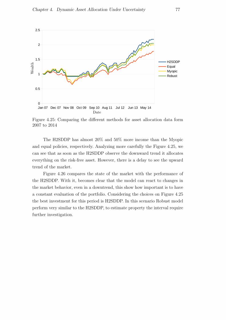
Chapter 4. Dynamic Asset Allocation Under Uncertainty 77
Date
Figure 4.25: Comparing the different methods for asset allocation data form2007 to 2014
Wea
lth
The H2SDDP has almost 20% and 50% more income than the Myopic
and equal policies, respectively. Analyzing more carefully the Figure 4.25, we
can see that as soon as the H2SDDP observe the downward trend it allocates
everything on the risk-free asset. However, there is a delay to see the upward
trend of the market.
Figure 4.26 compares the state of the market with the performance of
the H2SDDP. With it, becomes clear that the model can react to changes in
the market behavior, even in a downtrend, this show how important is to have
a constant evaluation of the portfolio. Considering the choices on Figure 4.25
the best investment for this period is H2SDDP. In this scenario Robust model
perform very similar to the H2SDDP, to estimate property the interval require
further investigation.
DBD
PUC-Rio - Certificação Digital Nº 1021809/CB

Chapter 4. Dynamic Asset Allocation Under Uncertainty 78
Date
Figure 4.26: Comparing the market states with the performance of theH2SDDP for data form 2007 to 2014
Wea
lth
Moreover, to better judge the performance of the models over different
periods, we simulate the investment for 6 consecutively months in each strategy
as if it was a fund. Figure 4.27 presents the semiannual cumulative performance
for every month.
Date
Figure 4.27: Trailing returns for asset allocation methods with monthly dataform 2007 to 2014
Wea
lth
Using short sell the model can take advantage of these situations, and
without it the only reasonable action is to invest on risk-free asset. Therefore,
DBD
PUC-Rio - Certificação Digital Nº 1021809/CB

Chapter 4. Dynamic Asset Allocation Under Uncertainty 79
we want to verify if the use of short selling can help the model improve the
policy return. In order to test how H2SDDP will perform with short sell, we
implement a model that allow short selling but limit it on the total wealth of
the portfolio in the last period. On Figure 4.28 we compare the performance
of H2SDDP, allowing short selling, with other methods for the same period.
Date
Figure 4.28: Comparing the performance of H2SDDP with sell short sell shortwith other methods, monthly data form 2007 to 2014
Wea
lth
The sell short model has by far the highest cumulative return of the
models and also perform similar to the H2SDDP, without short sell, in the
downward trend, investing most of the portfolio on the risk free asset. However,
the sell short took longer to identify the downward trend it also react very fast
when the trend changed.
It seems that allowing short sell makes the model enhance the high
returns, short selling the more stable assets to invest more on asset with high
expected returns. The final cumulative return with sell short(527%) was more
than twice the value of the second best model H2SDDP (218%).
In the trailing returns on Figure 4.29 we can observe that Sell Short
H2SDDP has the higher return for most of the period, but this is also a more
risk model than the H2SDDP without short selling. Although, the model has
it lowest’ possible return at the end of the year 2011 the Myopic and Equal
models reaches lower returns than this, in the begin of 2009. Is is also possible
to decrease the λ, that was 0.1, to obtain more stable performance.
DBD
PUC-Rio - Certificação Digital Nº 1021809/CB

Chapter 4. Dynamic Asset Allocation Under Uncertainty 80
Date
Figure 4.29: Trailing returns of H2SDDP with sell short sell and other methods,monthly data form 2007 to 2014
Wea
lth
Experiment with Daily Data Set
To be able to observe how the model will behavior with more assets and
more volatility, we perform an experiment with daily returns from 10 industrial
portfolios. It was used data from 2007 to 2014, it not possible to create cuts
for 2012 days, thus the daily data set was divide in intervals of 22 days, so the
optimization has 22 cuts and every 22 day the model will be retrained. The
only difference in the parameters was the λ = 0.03.
Figure 4.30 shows the results for the H2SSP and, Equal weight and
Myopic, the figure emphasizes the importance of a dynamic allocation, in
which the model can change allocation when facing critical events, without
it the portfolio depends on the tendency of the market to get good results. By
the end of 2008 the cumulative return for the period was 113.16%, 71.16% and
73.98%, for the H2SSP, Equal weight and Myopic, respectively. Figure 4.31 is
trailing returns for this experiment.
DBD
PUC-Rio - Certificação Digital Nº 1021809/CB

Chapter 4. Dynamic Asset Allocation Under Uncertainty 81
Date
Figure 4.30: Cumulative performance for asset allocation methods with dailydata set form 2007 to 2014
Wea
lth
Date
Figure 4.31: Trailing returns for asset allocation methods with daily data setform 2007 to 2014
Wea
lth
Although, H2SDDP strategy fails to predict the upward tendency after
2008, it has clearly a more controlled risk than the other strategies; it has
lower CVaR and standard deviation for this period (2008 to 2014). This can
be evidence that the model should be retrained more frequently than 22 days.
Besides that, some further investigation is necessary to better compare these
strategies using different data sets with more diversity.
DBD
PUC-Rio - Certificação Digital Nº 1021809/CB

5Conclusions and Future Works
This thesis aims at contributing for the optimization of models for asset
allocation under uncertainty. Different techniques are proposed herein to assist
in the asset allocation problem. Experiments were performed to evaluate the
behavior of ours approaches and they turn down to be very promising for both
of the presented cases.
It is a challenge to find the portfolio that best suit the investor’s needs.
The uncertainty surrounding future returns and the behavior of the assets is a
delicate issue in its own, but when the irrationality caused by human emotions
is added to the equation, the problem becomes even more difficult.
In the traditional asset allocation model, the investor has to choose the
return or the risk of the portfolio. Such mean-variance model has several issues,
however and, as a consequence, we have some proposals for improving the
mean-variance model by making it less sensitive to such issues. One of these
proposals is the Black-Litterman, which combines the investor’s vision with
the mean-variance model and the CAPM theory.
Although it is undeniable that the Black-Litterman technique is able
to mitigate most of the shortcomings of the traditional method proposed by
Markowitz, the construction of views can be a confusing process and depends
largely on the investor’s ability to quantify something extremely subjective.
We propose a new way to solve this problem by using questionnaires
and the ZAPROS-III method to construct the views. Techniques like the VDA
enable us to transform the answers provided in the sets of questions into views
of the Black-Litterman model. A case study based on Brazilian stocks was
conducted as a demonstration of how to use the methodology, and the results
were as expected.
The most important advantage of the proposed solution is that it allows
an investor to create his own portfolio, based on his own opinion, and without
the help of an expert. The final allocation will be optimized considering the
investor vision about the future, this typically will create a more diversified
and less risk portfolio. It also makes it easier for the investor to manifest his
own opinion and facilitates the process, allowing the investor to modify his
portfolio more frequently.
DBD
PUC-Rio - Certificação Digital Nº 1021809/CB

Chapter 5. Conclusions and Future Works 83
While we believe that this approach presents a lot of advantages, it also
has its limitations. The ZAPROS method is not adequate for a larger number of
alternatives or criteria, rendering this method applicable only to cases involving
a few stocks and questions. This shortcoming is a relative one, as the focus of
this proposal has always been to create a simple method, we believe it is not
reasonable to ask an investor too many questions. Besides, even though only
two views were constructed in the scope of this work, a larger number of views
may be constructed in order to represent other visions.
It would be interesting to have further work done in the sense of proposing
or developing new ways to improve the acquisition of the necessary parameters
for the Black-Litterman views, like the expected return. Future work could also
put other risk functions to the test and analyze the model’s behavior. Also the
construction of the views can be done in multilevel using ORCLASS, or some
other similar method, to select the assets of each view and then use ZAPROS
to determine the weight of the assets in the views.
Aiming at a multistage solution that also analyzes the assets in a more
qualitative way, this work proposes the use of stochastic programming for assets
allocation. Most of the proposed solutions in the literature cannot handle a
large number of stages, but the SDDP method has been efficiently used for
large-scale problems for several years now, and was thus chosen in this work
for the multistage asset allocation.
Largely used for hydrothermal scheduling problems, SDDP is specially
suited for large-scale problems. In it, the algorithm implicitly represent the
scenarios tree, building at each iteration better approximations for the worth
function for each stage. The time independence hypothesis of the original
proposed SDDP makes it non-applicable to some types of problems. While
some proposals to adapt the SDDP to consider the time dependence already
exist, none of these can be directly applied to the asset allocation problem.
Hence the methodology in this work, which models this dependency by using
hidden Markovian states. In addition, as there is some ambiguity in the joint
probability of the returns’ distribution, a more general method with ambiguity
aversion has also been developed.
In the experiments section we present the metrics for the data sets, com-
parison between Monte Carlo and Latin Hypercube Sampling, the sensitivity
analyses of the model, showing how H2SDDP performs with different para-
meters, and the final simulations of the proposed methods with out of sample
data. Besides showing how the optimization models would perform as an actual
fund, the experiments emphasizes the importance continuous re-evaluation of
the portfolio.
DBD
PUC-Rio - Certificação Digital Nº 1021809/CB

Chapter 5. Conclusions and Future Works 84
As the use of multistage stochastic techniques for portfolio optimization
becomes more and more widespread, both fields experience constant changes
and new ideas and methods are often proposed. Therefore, several ideas for
possible future work arose during the development of this thesis. One of them
would be to constraint the CVaR, aiming at maximizing the expected value
of the portfolio. The advantage in this case would be to have an easy way
to calculate the lower bound, as well as an easier way of interpreting the
model’s characteristics, risk constraint and objective function. Also, choosing
a maximum value for the CVaR makes interpretation easier and is a more
natural choice than the risk aversion index.
The multistage CVaR constraint has been suggested for the hydrothermal
scheduling problem [90], but adding this constraint to such model my render
it unfeasible. Thus, the normal approach for such cases is to use Lagrangian
relaxation to penalize violations, of the constraint, in the objective function.
In asset allocation problems, however, such feasibility issue is not expected
because allocating everything in the risk free asset is always feasible (just has to
have γ bigger than the transactional cost). This makes the model significantly
more straightforward and not imposing any changes to the objective function.
The main difference in this model is that the optimization needs to be
done in two-stages. The variables yti must be created, representing a vector
with the amount invested in each asset in t. Adding these ideas with H2SDDP,
we acquire
Qt(yt|k) =
maxxt,d
+t ,d−t ,δ,z− c
A∑i=1
(d+ti + d−ti
)+
K∑j=1
P (j|k)Nt∑s=1
P (s|j)
r>t+1(s)xt +Qt+1((1 + rt+1(s))>xt|j)
s. t.A∑i=1
xti + cA∑i=1
(d+ti + d−ti
)=
A∑i=1
yti
xti − d+ti + d−ti = yti ∀ i ∈ A \ 1
z +
K∑j=1
Nt∑s=1
P (j|k)P (s|j)δjs
(1−α)+ c
A∑i=1
(d+ti + d−ti
)≤ γ
(A∑i=1
yti
)δjs ≥ −z − r>t+1(s)xt ∀j ∈ 1, . . . , K, s ∈ 1, . . . , Ntδ,xt,d
+t ,d
−t ≥ 0
where P (s|j) = 1Nt
. Further experimentation will be made with this model in
near future, in order to compare it with the other models developed in this
thesis.
The estimation of the joint distributions of the returns is especially
DBD
PUC-Rio - Certificação Digital Nº 1021809/CB

Chapter 5. Conclusions and Future Works 85
problematic in asset allocation problems, but there are some approaches that
may be used in order to minimize this issue. One of them is to incorporate
robust approaches to the models proposed here by using the Bertsimas ideas
on the probability states of the Markov model. Such proposal is an extension
of the ambiguity aversion model presented in Section 4.3(d).
In addition, it must be said that some of the concepts proposed here
could not be computed due to the long computational time needed to run the
experiments, which is why it would be interesting to have some proposal to
reduce the algorithms’ execution time. In this regard, our research indicates
that a first and straightforward possible solution would be to design parallel
algorithms, making better use of modern computers that currently have
multiple cores. Another alternative would be to create heuristics to remove
some of the cutting planes’ cuts, a solution that has already shown some
improvements in other researches.
There is also the need to better understand the behavior of the HMM in
practice, and how to better estimate the initial probabilities. The method k-
means is a suitable method for this situation, but may have unwanted collateral
effects. We could not find a better alternative in literature, but it is possible
to test with manual classification.
DBD
PUC-Rio - Certificação Digital Nº 1021809/CB
Bibliography
[1] FABOZZI, F. J.; KOLM, P. N.; PACHAMANOVA, D.; FOCARDI, S. M..Robust portfolio optimization and management. John Wiley &Sons, 2007. 1, 2, 4.2(b)
[2] BERTSIMAS, D.; GUPTA, V.; PASCHALIDIS, I. C.. Inverse optimiza-
tion: a new perspective on the black-litterman model. Operationsresearch, 60(6):1389–1403, 2012. 1.4, 3.1
[3] MARKOWITZ, H.. Portfolio selection. The Journal of Finance,7(1):77–91, Marco 1952. 2, 2.2
[4] BLACK, F.; LITTERMAN, R.. Global Portfolio Optimization. Finan-cial Analysts Journal, 48(5), 1992. 2.3, 3.1, 3.3
[5] MICHAUD, R. O.. The markowitz optimization enigma: is’ optim-
ized’optimal? Financial Analysts Journal, 45(1):31–42, 1989. 2.3
[6] TUTUNCU, R. H.; KOENIG, M.. Robust asset allocation. Annals ofOperations Research, 132(1):157–187, 2004. 2.3
[7] BERA, A.; PARK, S.. Optimal portfolio diversification using the
maximum entropy principle. Econometric Reviews, 27(4-6):484–512, 2008. 2.3
[8] ERDOGAN, E.; GOLDFARB, D.; IYENGAR, G.. Robust portfolio
management. Technical report, 2004. 2.3
[9] BEST, M. J.; GRAUER, R. R.. Sensitivity analysis for mean-variance
portfolio problems. Management Science, 37(8):980–989, 1991. 2.3
[10] CHOPRA, V. K.; ZIEMBA, W. T.. The effect of errors in means,
variances, and covariances on optimal portfolio choice. 1993. 2.3
[11] FROST, P. A.; SAVARINO, J. E.. For better performance: Constrain
portfolio weights. 1988. 2.3
[12] JAGANNATHAN, R.; MA, T.. Risk reduction in large portfolios:
Why imposing the wrong constraints helps. The Journal ofFinance, 58(4):1651–1684, 2003. 2.3
DBD
PUC-Rio - Certificação Digital Nº 1021809/CB

Bibliography 87
[13] BLACK, F.; LITTERMAN, R.. Asset Allocation: Combining Investor
Views with Market Equilibrium. The Journal of Fixed Income,1990. 3.1, 3.3, 3.3, 3.3(c)
[14] WALTERS, J.. The black-litterman model in detail. Available atSSRN 1314585, 2011. 3.1, 3.3(d), 3.4(b)
[15] SATCHELL, S.; SCOWCROFT, A.. A demystification of the Black-
Litterman model: Managing quantitative and traditional portfo-
lio construction. Journal of Asset Management, 1(2):138–150, Sept.2000. 3.1
[16] HE, G.; LITTERMAN, R.. The intuition behind black-litterman
model portfolios. Available at SSRN 334304, 2002. 3.1, 3.3(c)
[17] MANKERT, C.. The Black-Litterman Model : Towards its use in
practice. PhD thesis, KTH, Management Control, 2010. QC 20101202.3.1
[18] HEROLD, U.. Computing implied returns in a meaningful way.Journal of Asset Management, 6(1):53 – 64, June 2005. 3.1
[19] IDZOREK, T.. A step-by-step guide to the black-litterman model.Forecasting Expected Returns in the Financial Markets, p. 17, 2002.(document), 3.1, 3.2, 3.3(d)
[20] FERNANDES, B.; FERNANDES, C.; STREET, A.. An asset alloca-
tion model with inequalities constraints and coherent risk meas-
ure: an application to Brazilian equities. Revista de Financas Ap-licadas, p. 1 – 27, 2013. 3.1
[21] MEUCCI, A.. The Black-Litterman Approach: Original Model
and Extensions. Social Science Research Network Working PaperSeries, Apr. 2008. 3.1
[22] EVANGELOU, C. E.; KARACAPILIDIS, N. I.; KHALED, O. A.. Inter-
weaving knowledge management, argumentation and decision
making in a collaborative setting: the kad ontology model. In-ternational Journal of Knowledge and Learning, 1(1/2):130–145, 2005.3.1
[23] CASTRO, A.; PINHEIRO, P.; PINHEIRO, M.. An approach for the
neuropsychological diagnosis of alzheimer’s disease: A hybrid
model in decision making. In: Wen, P.; Li, Y.; Polkowski, L.; Yao,
DBD
PUC-Rio - Certificação Digital Nº 1021809/CB

Bibliography 88
Y.; Tsumoto, S.; Wang, G., editors, ROUGH SETS AND KNOWLEDGETECHNOLOGY, v. 5589 of Lecture Notes in Computer Science, p.216–223. Springer Berlin / Heidelberg, 2009. 3.1
[24] TONCOVICH, A.; TURON, A.; ESCOBAR, M. T.; MORENO-JIMENEZ,J. M.. A quantitative approach to identify the arguments that
support decisions in e-cognocracy. IJKSR, 2(3):36–48, 2011. 3.1
[25] PINHEIRO, P.; SOUZA, G.; CASTRO, A.. Structuring of the mul-
ticriteria problem for production of newspaper. Operational re-search. Rio de Janeiro, 28(2):203–216, 2008. 3.1
[26] MENDES, M.; CARVALHO, A. L.; FURTADO, E.; PINHEIRO, P. R..A co-evolutionary interaction design of digital tv applications
based on verbal decision analysis of user experiences. In: WSKS(2), p. 702–711, 2008. 3.1
[27] TAMANINI, I.; CARVALHO, A. L.; CASTRO, A. K. A.; PINHEIRO,P. R.. A novel multicriteria model applied to cashew chestnut
industrialization process. v. 58 of Advances in Intelligent and
Soft Computing, p. 243–252. Springer Berlin Heidelberg, 2009. 3.1
[28] TAMANINI, I.; CASTRO, A. K. A.; PINHEIRO, P. R.; PINHEIRO, M.C. D.. Verbal decision analysis applied on the optimization of
alzheimer’s disease diagnosis: A case study based on neuroima-
ging. In: SOFTWARE TOOLS AND ALGORITHMS FOR BIOLOGICALSYSTEMS, v. 696 of Advances in Experimental Medicine and Bio-
logy, p. 555–564. Springer New York, 2011. 3.1
[29] TAMANINI, I.; PINHEIRO, P. R.; PINHEIRO, M. C. D.. The choice
of neuropathological questionnaires to diagnose the alzheimer’s
disease based on verbal decision analysis methods. In: INFORM-ATION COMPUTING AND APPLICATIONS, v. 6377 of Lecture Notes
in Computer Science, p. 549–556. Springer Berlin Heidelberg, 2010.3.1
[30] CASTRO, A. K. A. D.; PINHEIRO, P. R.; DANTAS PINHEIRO, M. C.;TAMANINI, I.. Towards the applied hybrid model in decision
making: A neuropsychological diagnosis of alzheimer’s disease
study case. International Journal of Computational Intelligence Sys-tems, 4(1):89–99, 2011. 3.1
DBD
PUC-Rio - Certificação Digital Nº 1021809/CB

Bibliography 89
[31] TAMANINI, I.. Improving the ZAPROS method considering the
incomparability cases. Master’s thesis, University of Fortaleza, Ap-plied Informatics, Ceara, Brazil, 2010. 3.1, 3.2(b), 3.2(b), 3.4(b)
[32] MACHADO, T.; MENEZES, A.; TAMANINI, I.; PINHEIRO, P.. A hybrid
model in the selection of prototypes for educational tools: An
applicability in verbal decision analysis. In: SYMPOSIUM ONCOMPUTATIONAL INTELLIGENCE IN MULTICRITERIA DECISION-MAKING, p. 135–142. IEEE, 2011. 3.2
[33] LARICHEV, O. I.. Ranking multicriteria alternatives: The
method ZAPROS III. European Journal of Operational Research,131(3):550–558, June 2001. 3.2, 3.2(b)
[34] LARICHEV, O.; MOSHKOVICH, H.. Verbal Decision Analysis for
Unstructured Problems. Theory and decision library: Series C,Game theory, mathematical programming, and operations research.Springer, 1997. 3.2, 3.2(a)
[35] GOMES, L.; MOSHKOVICH, H.; TORRES, A.. Marketing decisions
in small businesses: how verbal decision analysis can help. In-ternational Journal of Management and Decision Making, 11(1):19–36,2010. 3.2
[36] CHRISSIS, M.; KONRAD, M.; SHRUM, S.. Cmmi: Guidelines for
Process Integration and Product Improvement. Series in SoftwareEngineering. Prentice Hall, second edition, 2007. 3.2, 3.2(b), 3.2(b)
[37] USTINOVICH, L.; KOCHIN, D.. Verbal decision analysis methods
for determining the efficiency of investments in construction.Foundations of Civil and Environmental Engineering, 5(1):35–46, 2004.3.2, 3.2(b)
[38] BRASIL, A.. A novel approach based on multiple criteria decision
aiding methods to cope with classification problems. Master’sthesis, University of Fortaleza, Applied Informatics, Ceara, Brazil, 2010.3.2
[39] BRASIL, A.; PINHEIRO, P. R.; COELHO, A. L. V.. The impact of the
prototype selection on a multicriteria decision aid classification
algorithm. In: Sobh, T., editor, INNOVATIONS AND ADVANCES INCOMPUTER SCIENCES AND ENGINEERING, p. 379–382. SpringerNetherlands, 2010. 3.2
DBD
PUC-Rio - Certificação Digital Nº 1021809/CB

Bibliography 90
[40] BRASIL, A.; PINHEIRO, P. R.; COELHO, A. L. V.. Towards the Early
Diagnosis of Alzheimer’s Disease through the Application of
a Multicriteria Classification Model, v. 1. Rijeka: Intech - OpenAccess Publisher, 2012. 3.2
[41] MANKERT, C.. The Black-Litterman Model: mathematical and
behavioral finance approaches towards its use in practice. PhDthesis, KTH, 2006. 3.3
[42] ELTON, E. J.; GRUBER, M. J.; BROWN, S. J.; GOETZMANN, W. N..Modern portfolio theory and investment analysis. John Wiley &Sons, 2009. 3.3(a), 4.1
[43] SHARPE, W. F.. Capital asset prices: A theory of market equilib-
rium under conditions of risk*. The journal of finance, 19(3):425–442, 1964. 3.3(a)
[44] WALTERS, J.. The factor tau in the black-litterman model.Available at SSRN 1701467, 2010. 3.3(a), 3.3(d)
[45] THEIL, H.. Principles of econometrics. 1971. 3.3(c)
[46] HE, G.; LITTERMAN, R.. The intuition behind black-litterman
model portfolios. Goldman Sachs Asset Management Working paper,1999. 3.3(d)
[47] SILVA, A. S.; LEE, W.; PORNROJNANGKOOL, B.. The black–
litterman model for active portfolio management. The Journalof Portfolio Management, 35(2):61–70, 2009. 3.4(b)
[48] PEREIRA, M. V. F.; PINTO, L. M. V. G.. Multi-stage stochastic op-
timization applied to energy planning. Math. Program., 52(2):359–375, Oct. 1991. 4.1, 4.2, 4.3(c)
[49] DONOHUE, C. J.; BIRGE, J. R.. The abridged nested decomposi-
tion method for multistage stochastic linear programs with re-
latively complete recourse. Algorithmic Operations Research, 1(1),2006. 4.1, 4.2
[50] CHEN, Z.-L.; POWELL, W. B.. Convergent cutting-plane and
partial-sampling algorithm for multistage stochastic linear pro-
grams with recourse. Journal of Optimization Theory and Applica-tions, 102(3):497–524, 1999. 4.1, 4.2
DBD
PUC-Rio - Certificação Digital Nº 1021809/CB

Bibliography 91
[51] SHAPIRO, A.; TEKAYA, W.; DA COSTA, J. P.; SOARES, M. P.. Risk
neutral and risk averse stochastic dual dynamic programming
method. European journal of operational research, 224(2):375–391,2013. 4.1
[52] INFANGER, G.; MORTON, D. P.. Cut sharing for multistage
stochastic linear programs with interstage dependency. Math-ematical Programming, 75(2):241–256, 1996. 4.1
[53] PEREIRA, M.; PINTO, L.. Stochastic optimization of a multireser-
voir hydroelectric system: a decomposition approach. Water re-sources research, 21(6):779–792, 1985. 4.1, 4.2(c)
[54] MO, B.; GJELSVIK, A.; GRUNDT, A.. Integrated risk management
of hydro power scheduling and contract management. PowerSystems, IEEE Transactions on, 16(2):216–221, 2001. 4.1, 4.3(c)
[55] PHILPOTT, A. B.; DE MATOS, V. L.. Dynamic sampling algorithms
for multi-stage stochastic programs with risk aversion. EuropeanJournal of Operational Research, 218(2):470–483, 2012. 4.1, 4.3(c)
[56] CONT, R.. Empirical properties of asset returns: stylized facts
and statistical issues. 2001. 4.1
[57] MORETTIN, P. A.; TOLOI, C.. Analise de series temporais. Blucher,2006. 4.1
[58] VALLADAO, D. M.; VEIGA, A.; VEIGA, G.. A multistage linear
stochastic programming model for optimal corporate debt man-
agement. European Journal of Operational Research, 237(1):303–311, 2014. 4.1
[59] DANTZIG, G. B.; INFANGER, G.. Multi-stage stochastic linear pro-
grams for portfolio optimization. Annals of Operations Research,45(1):59–76, 1993. 4.1
[60] SHAPIRO, A.; DENTCHEVA, D.; RUSZCZYNSKI, A.. Lectures on
stochastic programming: modeling and theory, v. 16. SIAM, 2014.4.1, 4.2(a), 4.2(d), 4.3(a)
[61] ROCKAFELLAR, R. T.; URYASEV, S.. Conditional value-at-risk
for general loss distributions. Journal of Banking and Finance,26(7):1443–1471, July 2002. 4.1, 4.2(b), 4.3(b)
DBD
PUC-Rio - Certificação Digital Nº 1021809/CB

Bibliography 92
[62] ROCKAFELLAR, R. T.; URYASEV, S.. Optimization of conditional
value-at-risk. Journal of Risk, 2:21–41, 2000. 4.1, 4.2(b)
[63] SHAPIRO, A.. Analysis of stochastic dual dynamic programming
method. European Journal of Operational Research, 209(1):63–72,2011. 4.1, 4.2(b), 1, 4.2(b), 4.2(c)
[64] BENDERS, J.. Partitioning procedures for solving mixed-
variables programming problems. Numerische Mathematik,4(1):238–252, 1962. 4.2
[65] ARTZNER, P.; DELBAEN, F.; EBER, J.-M.; HEATH, D.. Coherent
measures of risk. Mathematical finance, 9(3):203–228, 1999. 4.2(b),4.2(b), 2, 4.3(b)
[66] GROOTVELD, H.; HALLERBACH, W.. Variance vs downside risk: Is
there really that much difference? European Journal of operationalresearch, 114(2):304–319, 1999. 4.2(b)
[67] KROKHMAL, P.; PALMQUIST, J.; URYASEV, S.. Portfolio optimiz-
ation with conditional value-at-risk objective and constraints.JOURNAL OF RISK, 4:11–27, 2002. 4.2(b)
[68] RUDLOFF, B.; STREET, A.; VALLADAO, D. M.. Time consistency
and risk averse dynamic decision models: Definition, interpret-
ation and practical consequences. European Journal of OperationalResearch, 234(3):743–750, 2014. 4.2(b), 4.3(b)
[69] LINOWSKY, K.; PHILPOTT, A. B.. On the convergence of sampling-
based decomposition algorithms for multistage stochastic pro-
grams. Journal of optimization theory and applications, 125(2):349–366, 2005. 4.2(c)
[70] SHAPIRO, A.; TEKAYA, W.. Report for technical cooperation
between georgia institute of technology and ons–operador
nacional do sistema eletrico–risk averse approach. Technical re-port, Citeseer, 2011. 4.2(c)
[71] KOZMIK, V.; MORTON, D. P.. Evaluating policies in risk-averse
multi-stage stochastic programming. Mathematical Programming,p. 1–26, 2014. 4.2(c)
DBD
PUC-Rio - Certificação Digital Nº 1021809/CB

Bibliography 93
[72] HINDSBERGER, M.; PHILPOTT, A.. Stopping criteria in sampling
strategies for multistage slp-problems. In: CONFERENCE “AP-PLIED MATHEMATICAL PROGRAMMING AND MODELLING”, VAR-ENNA, ITALY, 2002. 4.2(c)
[73] RUBINSTEIN, R. Y.; KROESE, D. P.. Simulation and the Monte
Carlo method, v. 707. John Wiley & Sons, 2011. 4.2(d)
[74] MCKAY, M. D.; BECKMAN, R. J.; CONOVER, W. J.. Comparison
of three methods for selecting values of input variables in
the analysis of output from a computer code. Technometrics,21(2):239–245, 1979. 4.2(d)
[75] KIM, S.-J.; KOH, K.; LUSTIG, M.; BOYD, S.; GORINEVSKY, D.. An
interior-point method for large-scale l1-regularized least squares.Selected Topics in Signal Processing, IEEE Journal of, 1(4):606–617,Dec 2007. 4.3(b)
[76] HARTE, D.; PICKUP, M.; THOMSON, P.. Hidden markov models for
new zealand hydro catchment inflows: a preliminary analysis.New Zealand Electricity Commission, 2007. 4.3(c)
[77] BONNANS, J. F.; CEN, Z.; CHRISTEL, T.. Energy contracts manage-
ment by stochastic programming techniques. Annals of OperationsResearch, 200(1):199–222, 2012. 4.3(c)
[78] FAMA, E. F.. The behaviour of stock market prices. Journal ofBusiness, p. 34–105, 1965. 4.3(c)
[79] GRANGER, C. W.; DING, Z.. Stylized facts on the temporal and
distributional properties of daily data from speculative markets.UCSD Department of Economics Discussion Paper, p. 94–19, 1994.4.3(c)
[80] RYDEN, T.; TERASVIRTA, T.; ASBRINK, S.. Stylized facts of daily
return series and the hidden markov model. Journal of appliedeconometrics, 13(3):217–244, 1998. 4.3(c)
[81] HASSAN, M. R.; NATH, B.. Stock market forecasting using hidden
markov model: a new approach. In: INTELLIGENT SYSTEMSDESIGN AND APPLICATIONS, 2005. ISDA’05. PROCEEDINGS. 5THINTERNATIONAL CONFERENCE ON, p. 192–196. IEEE, 2005. 4.3(c)
DBD
PUC-Rio - Certificação Digital Nº 1021809/CB

Bibliography 94
[82] ELLIOTT, R. J.; SIU, T. K.. Strategic asset allocation under a
fractional hidden markov model. Methodology and Computing inApplied Probability, 16(3):609–626, 2014. 4.3(c)
[83] ELLIOTT, R. J.; VAN DER HOEK, J.. An application of hid-
den markov models to asset allocation problems. Finance andStochastics, 1(3):229–238, 1997. 4.3(c)
[84] BISHOP, C. M.; OTHERS. Pattern recognition and machine learn-
ing, v. 4. springer New York, 2006. 4.3(c)
[85] MACCHERONI, F.; MARINACCI, M.; RUFFINO, D.. Alpha as am-
biguity: Robust mean-variance portfolio analysis. Econometrica,81(3):1075–1113, 2013. 4.3(d)
[86] GARLAPPI, L.; UPPAL, R.; WANG, T.. Portfolio selection with para-
meter and model uncertainty: A multi-prior approach. Review ofFinancial Studies, 20(1):41–81, 2007. 4.3(d)
[87] CURTIN, R. R.; CLINE, J. R.; SLAGLE, N. P.; MARCH, W. B.; RAM, P.;MEHTA, N. A.; GRAY, A. G.. MLPACK: A scalable C++ machine
learning library. Journal of Machine Learning Research, 14:801–805,2013. 4.4
[88] SANDERSON, C.; OTHERS. Armadillo: An open source c++
linear algebra library for fast prototyping and computationally
intensive experiments. Report Version, 2, 2010. 4.4
[89] DEMIGUEL, V.; GARLAPPI, L.; UPPAL, R.. Optimal versus naive
diversification: How inefficient is the 1/n portfolio strategy?
Review of Financial Studies, 22(5):1915–1953, 2009. 4.4(d)
[90] COSTA JUNIOR, L. C.. Representing CVaR Risk Aversion Con-
straint on Stochastic Dual Dynamic Programming with Applica-
tion in the Hydrothermal Operation Planning. PhD thesis, FederalUniversity of Rio de Janeiro, COPPE, 2013. 5
DBD
PUC-Rio - Certificação Digital Nº 1021809/CB
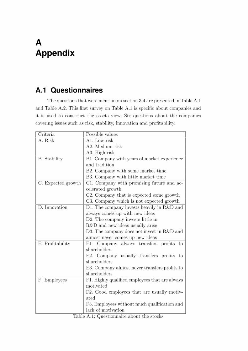
AAppendix
A.1 QuestionnairesThe questions that were mention on section 3.4 are presented in Table A.1
and Table A.2. This first survey on Table A.1 is specific about companies and
it is used to construct the assets view. Six questions about the companies
covering issues such as risk, stability, innovation and profitability.
Criteria Possible valuesA. Risk A1. Low risk
A2. Medium riskA3. High risk
B. Stability B1. Company with years of market experienceand traditionB2. Company with some market timeB3. Company with little market time
C. Expected growth C1. Company with promising future and ac-celerated growthC2. Company that is expected some growthC3. Company which is not expected growth
D. Innovation D1. The company invests heavily in R&D andalways comes up with new ideasD2. The company invests little inR&D and new ideas usually ariseD3. The company does not invest in R&D andalmost never comes up new ideas
E. Profitability E1. Company always transfers profits toshareholdersE2. Company usually transfers profits toshareholdersE3. Company almost never transfers profits toshareholders
F. Employees F1. Highly qualified employees that are alwaysmotivatedF2. Good employees that are usually motiv-atedF3. Employees without much qualification andlack of motivation
Table A.1: Questionnaire about the stocks
DBD
PUC-Rio - Certificação Digital Nº 1021809/CB

Appendix A. Appendix 96
Second survey on sectors Table A.2 is more simple and relative to the
sectors of the market.
Criteria Possible values
A. Internal market A1. Very favorable to industry
A2. Favorable to industry
A3. Not favorable to industry
B. External market B1. Very favorable to industry
B2. Favorable to industry
B3. Not favorable to industry
C. Expected growth C1. It is expected a high growth
C2. It is expected some growth
C3. It is expected little or none growth
Table A.2: Questionnaire about the sectors
A.2 Myopic proveProposition 1 For the portfolio selection with no transaction cost and without
temporal dependence the myopic policy is optimal, i.e. Qt(·) is positive homo-
geneous. As a result, in this case one only needs to consider the return of the
next moment to decide on an investment.
Proof : To prove by induction we will first show for the base case that QT−1(·),then assuming that the proposition holds up to Qt+1(·) and deduce Qt(·)
For the base case the optimal value on T depends on WT−1 and r[T−1],it
will be used RT = 1+ rT , thus we have
QT−1(WT−1, r[T−1]) = maxxt−1
ψT−1[R>T xt−1|r[T−1]]
s. t. 1>xt−1 = WT−1
xt−1 ≥ 0
For t = T − 2, . . . , 0
Qt(Wt, r[t]) = maxxt
ψt[Qt+1(Wt, r[t])]
s. t. 1>xt = Wt
rt+1(r[t])>xt = Wt+1
xt ≥ 0
DBD
PUC-Rio - Certificação Digital Nº 1021809/CB
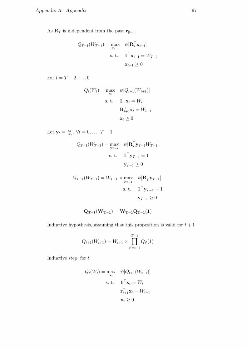
Appendix A. Appendix 97
As RT is independent from the past r[t−1]
QT−1(WT−1) = maxxt−1
ψ[R>T xt−1]
s. t. 1>xt−1 = WT−1
xt−1 ≥ 0
For t = T − 2, . . . , 0
Qt(Wt) = maxxt
ψ[Qt+1(Wt+1)]
s. t. 1>xt = Wt
R>t+1xt = Wt+1
xt ≥ 0
Let yt = xt
Wt, ∀t = 0, . . . , T − 1
QT−1(WT−1) = maxyT−1
ψ[R>T yT−1WT−1]
s. t. 1>yT−1 = 1
yT−1 ≥ 0
QT−1(WT−1) = WT−1 ×maxyT−1
ψ[R>T yT−1]
s. t. 1>yT−1 = 1
yT−1 ≥ 0
QT−1(WT−1) = WT−1QT−1(1)
Inductive hypothesis, assuming that this proposition is valid for t+ 1
Qt+1(Wt+1) = Wt+1 ×T−1∏t′=t+1
Qt′(1)
Inductive step, for t
Qt(Wt) = maxxt
ψ[Qt+1(Wt+1)]
s. t. 1>xt = Wt
r>t+1xt = Wt+1
xt ≥ 0
DBD
PUC-Rio - Certificação Digital Nº 1021809/CB
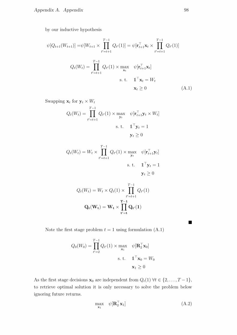
Appendix A. Appendix 98
by our inductive hypothesis
ψ[Qt+1(Wt+1)] =ψ[Wt+1 ×T−1∏t′=t+1
Qt′(1)] = ψ[r>t+1xt ×T−1∏t′=t+1
Qt′(1)]
Qt(Wt) =T−1∏t′=t+1
Qt′(1)×maxxt
ψ[r>t+1xt]
s. t. 1>xt = Wt
xt ≥ 0 (A.1)
Swapping xt for yt ×Wt
Qt(Wt) =T−1∏t′=t+1
Qt′(1)×maxyt
ψ[r>t+1yt ×Wt]
s. t. 1>yt = 1
yt ≥ 0
Qt(Wt) = Wt ×T−1∏t′=t+1
Qt′(1)×maxyt
ψ[r>t+1yt]
s. t. 1>yt = 1
yt ≥ 0
Qt(Wt) = Wt ×Qt(1)×T−1∏t′=t+1
Qt′(1)
Qt(Wt) = Wt ×T−1∏t′=t
Qt′(1)
Note the first stage problem t = 1 using formulation (A.1)
Q0(W0) =T−1∏t′=2
Qt′(1)×maxx1
ψ[R>2 x0]
s. t. 1>x0 = W0
x1 ≥ 0
As the first stage decisions x0 are independent from Qt(1) ∀t ∈ 2, . . . , T − 1,to retrieve optimal solution it is only necessary to solve the problem below
ignoring future returns.
maxx1
ψ[R>2 x1] (A.2)
DBD
PUC-Rio - Certificação Digital Nº 1021809/CB

Appendix A. Appendix 99
s. t. 1>x1 = W1
x0 ≥ 0
Likewise, it is possible to obtain optimal solution for Qt(Wt) ∀t ∈ T .
DBD
PUC-Rio - Certificação Digital Nº 1021809/CB
Related Documents