Throughput analysis in wireless networks with multiple users and multiple channels

Noname manuscript No.(will be inserted by the editor)

Amrinder Arora · Fanchun Jin ·Gokhan Sahin · Hosam Mahmoud ·Hyeong-Ah Choi

Throughput Analysis in Wireless Networks with MultipleUsers and Multiple Channels

April 7, 2005

Abstract We consider the problem of maximizing throughput in a multi-carrier wireless network that em-ploys predictive link adaptation. We explicitly consider the time-penalty incurred due to link adaptation. Thecontributions of this paper are two-fold. Firstly, several high performance algorithms (offline and online) aredeveloped for efficient performance in multiple user and multiple channel environment under the practicablelookahead prediction of one time slot. Secondly, the presented algorithms and heuristics are shown to be com-petitive by deterministic and probabilistic analyses. Our results show that a modest consumption of resourcesfor channel prediction and link adaptation may result in a significant throughput improvement.

Keywords Wireless networks· heuristic· competitive algorithm

1 Introduction

Wireless connections often experience sudden changes in the quality of transmission. Transmission occurs inunits called packets, where a packet carries a certain amount of information to be transmitted in unit time. Achannel, which may be a combination of frequency and code or a combination of frequency and time slot, hasa certain (time-varying) capacity, that may be alloted to a user either in part or in full. When the quality oftransmission degrades over a channel, the network provider may adjust the channel transmission parametersor resume the connection over a different channel. The change in the channel or the transmission parametersis calledlink adaptation. The change, however, may not be instantaneous, and the penalty for switching is theloss of the alloted capacity for a certain time, during which the protocols for the switch (authorization andacknowledgment) are communicated in lieu of data. Predicting the future channel quality may also consumea significant amount of system resources (e.g., time, bandwidth and power), since it may involve transmissionof training-sequences, pilot tones, or feedback messages carrying the channel state information, see [5].

In this investigation we assume, as is practicable, that we have only one predictable lookahead slot ofcapacity, during which time a decision must be made as to whether lose the slot (dedicate it to switchingprotocols) or continue to transmit data. There is a trade-off—we may continue data transmission, losing a

A. AroraDepartment of Computer Science, George Washington University, Washington, DC 20052

Fanchun JinDepartment of Computer Science, George Washington University, Washington, DC 20052

Gokhan SahinElectrical and Computer Engineering, Miami University, Oxford, OH 45056

Hosam MahmoudDepartment of Statistics, George Washington University, Washington, DC 20052

Hyeong-Ah ChoiDepartment of Computer Science, George Washington University, Washington, DC 20052

2

suddenly improved capacity on this or another channel, or use the next time slot to prepare for switching, butending up squandering too many slots on computing the switching protocols, and incurring other associatedoverhead.

Our goal is to maximize the throughput of the entire network of multiple users and multiple channels. Inthe absence of the complete knowledge of the future of the process, as is the practice in reality, it is desirableto find efficient online algorithms, operating under the practicable assumption of admitting the prediction ofonly one time slot lookahead capacity. Efficient offline algorithms provide a good basis.

Previous research work in this field has focused on maintaining system stability with by bounding thequeue sizes (see, for example, [1] and [2]), and on providing fairness within throughput (see [9]). Gener-ally, the penalty incurred by link adaptation has not been considered. We augment these investigations byconsidering the cost associated with the changes.

The rest of this paper is organized as follows. The system model and a precise statement of both offline andonline versions of the problem are presented in Section 2, together with some background. The offline versionof the problem is studied in Section 3, where we prove the inherent difficulty of the problem by showing itis NP complete in Subsection 3.1. In Subsection 3.2, we present a2-approximation algorithm for the offlineversion. The algorithm and its analysis appear in three subsubsections therein. In Section 4 we consider theonline version of the problem for the single user and single channel case (single-single henceforth), andpresent a competitive family of algorithms in Subsection 4.1. We also consider a probabilistic analysis of ourfamily in Subsection 4.2. We extend the algorithm to the multiple user and multiple channel case (multiple-multiple, henceforth) in Subsection 4.3, and extend the probabilistic analysis in Subsection 4.4. Finally, ourconclusions and some ideas for further research are presented in Section 5.

2 System Model and Problem Statement

We consider the channel scheduling problem in a wireless network that consists of one base station,m mobilestations,f channels, over a period ofn (large) time slots. The maximum rate that can be used by stationi on channelj in time slot t is denoted byc(i, j, t), and the rate assigned (theusage) by the scheduler touseri on channelj in time slott is denoted byx(i, j, t), which does not exceedc(i, j, t). For 1 ≤ i ≤ m,1 ≤ j ≤ f and1 ≤ t ≤ n, the matrix of capacitiesc(i, j, t) will be calledC and the schedulex(i, j, t) will becalledX. Regardless of the scheduling algorithm, the system operates under the following additional set ofnatural assumptions:

– A mobile station can receive data on at most one channel at a given time slot.– To prevent interference, a channel can be used for transmission from one base station to at most one

mobile station at a given time slot.– While changing the usage, or the intended mobile station, the next time slot is utilized for completing the

switching protocol, not for data transmission.

All thesenatural constraintssymbolically translate into:

1. x(i, j, t) ≤ c(i, j, t), for each1 ≤ i ≤ m, 1 ≤ j ≤ f , and1 ≤ t ≤ n.2. If x(i, j, t) > 0, then for anyj′ 6= j, x(i, j′, t) = 0.3. If x(i, j, t) > 0, then for anyi′ 6= i, x(i′, j, t) = 0.4. For anyj, if x(i, j, t) > 0 andx(i′, j, t + 1) > 0, theni = i′ andx(i, j, t) = x(i, j, t + 1).5. For anyi, if x(i, j, t) > 0 andx(i, j′, t + 1) > 0, thenj = j′ andx(i, j, t) = x(i, j, t + 1).

For example, considerm = f = 1 (i.e., single-single environment),n = 7, and the channel capacitymatrix C = [1, 3, 7, 8, 7, 15, 14]. An algorithm may produce the feasible scheduleX1 = [0, 0, 7, 7, 7, 0, 14],with throughput 35; a better algorithm may give the feasible scheduleX2 = [1, 0, 7, 7, 0, 14, 14] with thehigher throughput 43. In factX2 is optimal. Note that in these feasible solutions a change of usage is alwayspreceeded by 0, as required by the switching protocols.

If a change is required in the receiving station or the usage, the next downlink transmission (in time slott+1) is used to notify the receiver of the new usage, which is confirmed by the recipient via an acknowledgmentin the next uplink transmission. Transmission at the new usage (possibly to a new user) starts only after adelay of a full duplex transmission cycle. The earliest time a new usage can come into effect after time slottis t + 2. The same penalty is assumed to be applied when a user is changed on the same channel.

3

Let the throughput of useri on channelj be

Rij(n) =n∑

t=1

x(i, j, t).

The goal is to maximize the total network throughput, that is, maximize∑mi=1

∑fj=1 Rij(n) under the natural constraints. We shall compare the network throughput against the total

capacity available

Cap(n) =n∑

t=1

m∑

i=1

f∑

j=1

c(i, j, t).

We formally state the problem as follows.

Offline Scheduling Problem (SP1)Given:A channel status matrixC = [c(i, j, t)] for 1 ≤ i ≤ m, 1 ≤ j ≤ f , and1 ≤ t ≤ n.Objective:Find a scheduleX = [x(i, j, t)] that maximizes

∑mi=1

∑fj=1 Rij(n) under the natural constraints.

Next, we consider the online version of this problem. In the online version, the decision about channel allo-cation needs to be made at each time slot. We assume that, at the beginning of time slott, the base station hasperfect knowledge of the channel state in time slotst andt + 1. The base station decides to which station, onwhat channel, and at what data rate it is going to transmit during time slott.

Online Scheduling Problem (SP2)Given: A channel allocation matrix[x(i, j, t′)], a channel capacity matrix[c(i, j, t′ + 1)] for 1 ≤ i ≤ m,

1 ≤ j ≤ f , for somet ≥ 1, and∀ t′ < t.Objective:Find the channel allocation for time slott, i.e., [x(i, j, t)] that maximizes

∑mi=1

∑fj=1 Rij(n)

subject to the set of natural constraints.

Simpler single-single versions of these scheduling problems were considered in the earlier work of [3].The results presented in this paper are an extension of some results presented there, which are summarizedas:

– The single-single version of the offline problemSP1can be solved inO(n3) time using a dynamic pro-gramming algorithm.

– For the online problemSP2, for every finite size lookahead online algorithm, there exists a sequence ofcapacities that makes the algorithm suboptimal. (This result is noteworthy, because the penalty is fixed toone time slot.)

– There exist two 4-competitive11-lookahead online algorithms forSP2for the single-single version: One,called WD algorithm, can be extended to the multiple-multiple environment as discussed in Section 4, andthe other, called WDH algorithm, works only for the single-single environment.

– For SP2, for the single-single case, the WDH algorithm provides an average performance of about 96%of the optimal as noted in a simulation study.

3 Offline Problem Analysis

In this section, we consider the decision version of SP1, and establish its NP-completeness. In the decisionversion, we are given a value in addition to an instance of SP1, and we need to decide if the problem instancehas a solution that has throughput matching or exceeding the specified value. Clearly, the decision version ofSP1 is in NP, since anO(n) time non-deterministic algorithm can find a solution, and given a solution, wecan easily verify if it is a feasible solution and if its value exceeds the specified value.

1 An online algorithm is said to beδ-competitive if the performance of the algorithm isδ-times “worse” than the performanceof an optimal offline algorithm.

4

3.1 NP-completeness of SP1

To show that SP1 is NP complete, we present a polynomial time reduction from a well-known NP-completeproblem, the3-Dimensional Matching Problem, to SP1.

3-Dimensional Matching Problem:(For details see [6].)Given:Disjoint setsT1, T2 andT3 of sizeq, and a setS ⊆ T1 × T2 × T3, where|S| = p > q.Objective:Determine whether there existsS0, such thatS0 ⊆ S, andS0 contains each element of

T1, T2, T3 exactly once.

Note that if such a subsetS0 exists,|S0| must be equal toq. Consider an instance of 3DM:

T1 = {α1, . . . , αq},T2 = {β1, . . . , βq},T3 = {γ1, . . . , γq},S ⊆ T1 × T2 × T3.

We now construct an instance of SP1 such that 3DM is solvable if and only if total throughput for SP1matches or exceeds a certain value. The instance of SP1 hasm = 2q users,f = 2q channels andn = 3q − 2time slots. The sets of users, channels and time slots are given as follows:

U = {u1, . . . , uq, w1, . . . , wq},C = {c1, . . . , cq, d1, . . . , dq},T = {t1, t′1, t′′1 , . . . , tq−1, t

′q−1, t

′′q−1, tq}.

Note thattk = 3k−2, t′k = 3k−1, andt′′k = 3k for 1 ≤ k < q. We use the notationu-type user to indicatea ui user, andw-type user to indicate awi user. Similarly,c-type channel indicates acj channel, andd-typechannel indicates adj channel. For time slots, there aret-type,t′-type andt′′-type timeslots. Let us introducethe notationI(ui, cj , tk).

I(ui, cj , tk) =

1, if (αi, βj , γk) ∈ S;

0, otherwise.

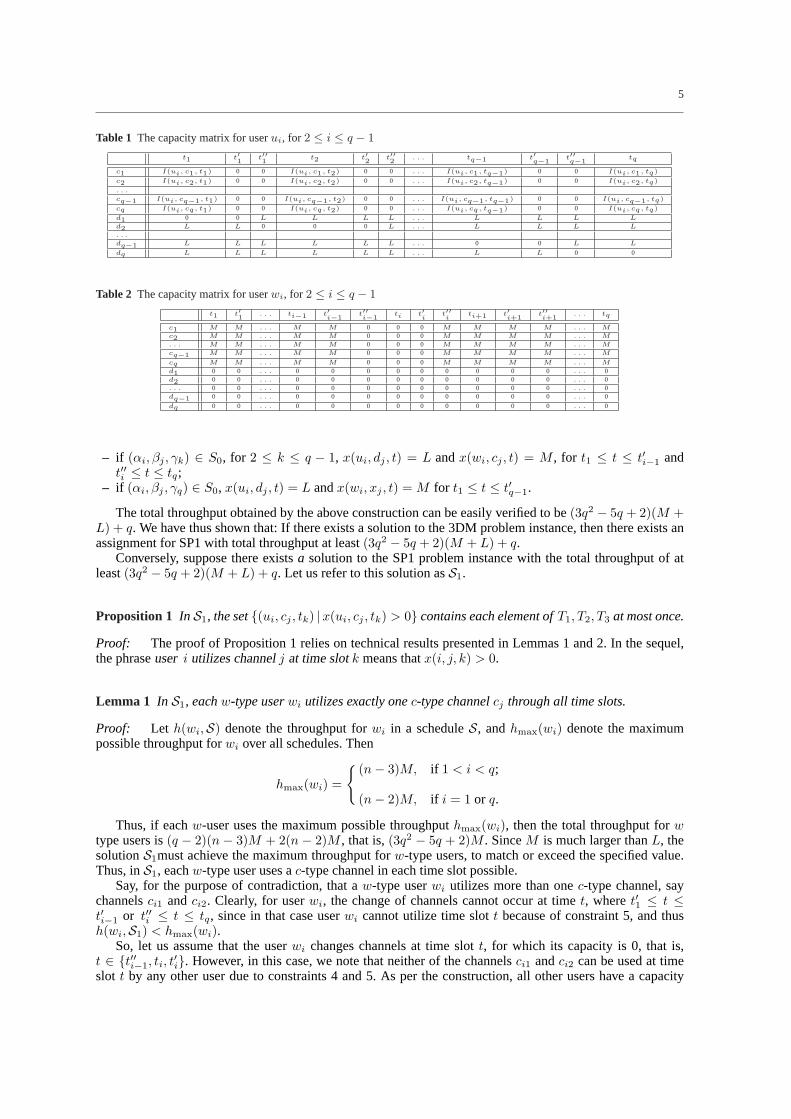
Next, we choose two constantsL andM such that1 ¿ L ¿ M (e.g.,L > n andM > nL). Weconstruct capacity values foru-type andw-type users as shown in Tables 1 and 2, where the tables are shownfor generici values,2 ≤ i ≤ q − 1.

The capacity matrix of eachu-type user is defined as:

(i) m(ui, cj , tk) = I(ui, cj , tk), for 1 ≤ j, t ≤ q,(ii) m(ui, cj , t

′k) = m(ui, cj , t

′′k) = 0, for 1 ≤ j, t ≤ q − 1,

(iii) m(ui, d1, t1) = m(ui, d1, t′1) = 0,

(iv) m(ui, dj , t′′j−1) = m(ui, dj , tj) = m(ui, dj , t

′j) = 0, for 2 ≤ j ≤ q − 1,

(v) m(ui, dq, t′′q−1) = m(ui, dq, tq) = 0, and

(vi) for all otherd-type channels, userui has capacityL.

The capacity matrix of eachw-type user is defined as follows:

(i) m(w1, cj , t1) = m(w1, cj , t′1) = 0, for 1 ≤ j ≤ q,

(ii) m(wi, cj , t′′i−1) = m(wi, cj , ti) = m(wi, cj , t

′i) = 0, for 1 ≤ j ≤ q and2 ≤ i ≤ q − 1,

(iii) m(wq, cj , t′′q−1) = m(wq, cj , tq) = 0, for 1 ≤ j ≤ q,

(iv) for all otherc-type channels, userwi has capacityM , and(v) for all d-type channels and all time slots, userwi has capacity0.

We next proceed to show that there exists a subsetS0 ⊆ S solving the 3DM problem if and only if themaximum throughput of SP1 is at least(3q2 − 5q + 2)(M + L) + q.

Suppose the 3DM is solved usingS0. We then construct channel allocation as follows:

– if (αi, βj , γk) ∈ S0, x(ui, cj , tk) = 1;– if (αi, βj , γ1) ∈ S0, x(ui, dj , t) = L andx(wi, cj , t) = M , for t′′1 ≤ t ≤ tq;

5

Table 1 The capacity matrix for userui, for 2 ≤ i ≤ q − 1

t1 t′1 t′′1 t2 t′2 t′′2 . . . tq−1 t′q−1 t′′

q−1 tq

c1 I(ui, c1, t1) 0 0 I(ui, c1, t2) 0 0 . . . I(ui, c1, tq−1) 0 0 I(ui, c1, tq)c2 I(ui, c2, t1) 0 0 I(ui, c2, t2) 0 0 . . . I(ui, c2, tq−1) 0 0 I(ui, c2, tq). . .

cq−1 I(ui, cq−1, t1) 0 0 I(ui, cq−1, t2) 0 0 . . . I(ui, cq−1, tq−1) 0 0 I(ui, cq−1, tq)cq I(ui, cq, t1) 0 0 I(ui, cq, t2) 0 0 . . . I(ui, cq, tq−1) 0 0 I(ui, cq, tq)d1 0 0 L L L L . . . L L L L

d2 L L 0 0 0 L . . . L L L L

. . .

dq−1 L L L L L L . . . 0 0 L L

dq L L L L L L . . . L L 0 0

Table 2 The capacity matrix for userwi, for 2 ≤ i ≤ q − 1

t1 t′1 . . . ti−1 t′i−1 t′′

i−1 ti t′i

t′′i

ti+1 t′i+1 t′′

i+1 . . . tq

c1 M M . . . M M 0 0 0 M M M M . . . M

c2 M M . . . M M 0 0 0 M M M M . . . M

. . . M M . . . M M 0 0 0 M M M M . . . M

cq−1 M M . . . M M 0 0 0 M M M M . . . M

cq M M . . . M M 0 0 0 M M M M . . . M

d1 0 0 . . . 0 0 0 0 0 0 0 0 0 . . . 0d2 0 0 . . . 0 0 0 0 0 0 0 0 0 . . . 0. . . 0 0 . . . 0 0 0 0 0 0 0 0 0 . . . 0dq−1 0 0 . . . 0 0 0 0 0 0 0 0 0 . . . 0

dq 0 0 . . . 0 0 0 0 0 0 0 0 0 . . . 0

– if (αi, βj , γk) ∈ S0, for 2 ≤ k ≤ q − 1, x(ui, dj , t) = L andx(wi, cj , t) = M , for t1 ≤ t ≤ t′i−1 andt′′i ≤ t ≤ tq;

– if (αi, βj , γq) ∈ S0, x(ui, dj , t) = L andx(wi, xj , t) = M for t1 ≤ t ≤ t′q−1.

The total throughput obtained by the above construction can be easily verified to be(3q2 − 5q + 2)(M +L) + q. We have thus shown that: If there exists a solution to the 3DM problem instance, then there exists anassignment for SP1 with total throughput at least(3q2 − 5q + 2)(M + L) + q.

Conversely, suppose there existsa solution to the SP1 problem instance with the total throughput of atleast(3q2 − 5q + 2)(M + L) + q. Let us refer to this solution asS1.

Proposition 1 In S1, the set{(ui, cj , tk) |x(ui, cj , tk) > 0} contains each element ofT1, T2, T3 at most once.

Proof: The proof of Proposition 1 relies on technical results presented in Lemmas 1 and 2. In the sequel,the phraseuser i utilizes channelj at time slotk means thatx(i, j, k) > 0.

Lemma 1 In S1, eachw-type userwi utilizes exactly onec-type channelcj through all time slots.

Proof: Let h(wi,S) denote the throughput forwi in a scheduleS, andhmax(wi) denote the maximumpossible throughput forwi over all schedules. Then

hmax(wi) =

{ (n− 3)M, if 1 < i < q;

(n− 2)M, if i = 1 or q.

Thus, if eachw-user uses the maximum possible throughputhmax(wi), then the total throughput forwtype users is(q − 2)(n − 3)M + 2(n − 2)M , that is,(3q2 − 5q + 2)M . SinceM is much larger thanL, thesolutionS1must achieve the maximum throughput forw-type users, to match or exceed the specified value.Thus, inS1, eachw-type user uses ac-type channel in each time slot possible.

Say, for the purpose of contradiction, that aw-type userwi utilizes more than onec-type channel, saychannelsci1 andci2. Clearly, for userwi, the change of channels cannot occur at timet, wheret′1 ≤ t ≤t′i−1 or t′′i ≤ t ≤ tq, since in that case userwi cannot utilize time slott because of constraint 5, and thush(wi,S1) < hmax(wi).

So, let us assume that the userwi changes channels at time slott, for which its capacity is 0, that is,t ∈ {t′′i−1, ti, t

′i}. However, in this case, we note that neither of the channelsci1 andci2 can be used at time

slot t by any other user due to constraints 4 and 5. As per the construction, all other users have a capacity

6

of M for all c-type channels during time slott. Observing that there areq − 1 users (besideswi), andq − 2availablec-type channels (besidesci1 andci2), we conclude that at least one other user must “miss” the timeslot t, and thusS1cannot achieve a throughput of(3q2 − 5q + 2)M . [Contradiction.]

Therefore, inS1, eachw-type userwi utilizes exactly onec-type channelcj through all time slots. ut

Lemma 1 indicates that, after assigningw-type users toc-type channels, there is exactly one time slotti available foru-type users to utilize on eachc-type channel and for each pair of channelscj andck, theavailable time slot is different. This implies that, in the solution of SP1, if the set of users{(ui, cj , tk)} utilizeall of the available time slots onc-type channels, then that set contains each element ofT2 andT3 exactlyonce.

Lemma 2 In any solution of SP1, eachu-type userui utilizes exactly oned-type channeldj through all timeslots.

Proof: The proof is similar to that of Lemma 2. ut

From Lemma 2, we know that if userui utilizes channeldj , then userui can only utilizes time slottj onc-type channels. This implies that each user can utilizec-type channels at no more than one time slot. Theimplication of Lemmas 1 and 2 proves Proposition 1. If allu-type users have a chance to utilize in the solutionof SP1, then, from Proposition 1, the set{(ui, cj , tk) |x(ui, cj , tk) > 0} is the solution of 3DM. In this case,the throughput of SP1 should be(3q2 − 5q + 2)(M + L) + q. The following result has been established.

Theorem 1 3DM is solvable if and only if the maximum throughput of SP1 is(3q2 − 5q + 2)(M + L) + q.

Theorem 1 indicates that 3DM is transformed to SP1 in polynomial time, which establishes the NP-completeness of the latter.

3.2 Offline Approximation Solution

Having proved that SP1 is NP-complete in Section 3.1, it is justified to seek an approximation algorithm for it.Before presenting it, we consider the special case when there is only one time slot. This case provides a basestep that is used in the approximation algorithm, as well as in the forthcoming family of online algorithms.

3.2.1 Maximum Throughput for One Time slot

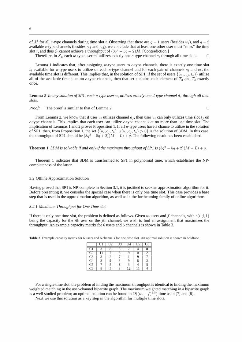
If there is only one time slot, the problem is defined as follows. Givenm users andf channels, withc(i, j, 1)being the capacity for theith user on thejth channel, we wish to find an assignment that maximizes thethroughput. An example capacity matrix for6 users and6 channels is shown in Table 3.

Table 3 Example capacity matrix for 6 users and 6 channels for one time slot. An optimal solution is shown in boldface.

U1 U2 U3 U4 U5 U6C1 3 8 3 7 4 8C2 11 7 3 9 0 2C3 3 2 7 1 9 7C4 3 9 3 9 8 2C5 7 5 8 3 4 8C6 8 5 3 12 11 4

For a single time slot, the problem of finding the maximum throughput is identical to finding the maximumweighted matching in the user-channel bipartite graph. The maximum weighted matching in a bipartite graphis a well studied problem; an optimal solution can be found inO((m + f)2.5) time as in [7] and [8].

Next we use this solution as a key step in the algorithm for multiple time slots.

7

3.2.22-Approximation Algorithm for Multiple Time slots

We propose the following algorithmMUMC-2 for the multiple-multiple offline version of the problem. Thealgorithm works in two stages:

– Step 1:Use the maximum matching to calculate the optimal user-channel assignment for each time slot,independent of preceeding and succeeding time slot. Let us store the output of this step in an array, sayα = [α(1), α(2), α(3), . . . , α(n)]. We callα(t) theeffective capacity at timet.

– Step 2:Assigneffective usagesuch that the total value is maximized. This can be done using a single passdynamic programming algorithm, that is based upon the recurrenceβ(k) = max{β(k− 2) + α(k), β(k−1)}. The boundary conditions may be specified asβ(1) = α(1) andβ(2) = max{α(1), α(2)}.

Lemma 3 β(n) is at least half of the sum of the sequenceα(t), i.e.,β(n) ≥ 12

∑nt=1 α(i).

Proof: Consider two specific feasible solutions:

– The feasible solution in which only odd time slots are chosen.– The feasible solution in which only even time slots are chosen.

Sinceβ(n) is optimal solution, it must be greater than both these feasible solutions. That is,

β(n) ≥∑

i is odd

α(i) and β(n) ≥∑

i is even

α(i)

⇒ 2 β(n) ≥∑

i is odd

α(i) +∑

i is even

α(i)

⇒ β(n) ≥ 12

n∑

i=1

α(i).

ut

Theorem 2 AlgorithmMUMC-2 is 2-Approximation.

Proof: Let us call the optimum throughput for the multiple user multiple channelOPT . In that case,OPTmust be less than the sum of the optimum solutions obtained for each time slot. That is,OPT ≤ ∑n

i=1 α(i).Using Lemma 3,β(n) ≥ 1

2

∑ni=1 α(i) ≥ 1

2OPT . ut

Remarks: We show below two simple examples, one that is the worst case forMUMC-2 , i.e., β(n) =12OPT , and one that is the best case forMUMC-2 , i.e.,β(n) = OPT .

1. An example for worst case forMUMC-2Setc(i, j, t) = M . The capacity for all channels, time slots and users is the same. Any trivial solution keptconstant atM for all time slots achieves the optimal result, butMUMC-2 only achieves half of optimalthroughput.

2. An example for best case forMUMC-2Set

c(i, j, t) =

M, if t is odd;

0, if t is even.

3.2.3 Time Complexity Analysis

In the first stage, we use maximum weighted matching algorithm which runs inO((m + f)2.5) time, for eachtime slot. Thus, the total time of execution for the first stage isO(n(m + f)2.5). The second stage runs inO(n), resulting in an overall time complexity ofO(n(m + f)2.5).

8

4 Competitive Online Algorithm

In this section we present a family of competitive online algorithms. In [3], it was shown that no online algo-rithm can achieve a constant bound on the competitive ratio if no lookahead algorithm is available. However,in the following section, we show that even one lookahead information can be very useful and lead to a4-competitive algorithm.

The algorithms presented in this section are a generalization of an earlier algorithm for the single-singlecase presented in [3]. It is remarkable that the competitive ratio remains the same for the much more generalmultiple-multiple problem.

4.1 Wait-Dominate Heuristic for Single User Single Channel

This family of heuristics, which we call WD(γ), takes into account the usage of the previous time slotx(t−1),the current capacityc(t), and the next capacityc(t+1). The parameterγ that defines a member of this familyis assumed to exceed 1. We first present and analyze the single-single version (f = m = 1), which willbe used as a basis for the multiple-multiple case heuristic, both in construction and analysis. To make thepresentation of the single-single case transparent, we use only a time-indexed notation for it. For examplec(i, j, t) will be denoted simply byc(t), while the suppressedi andj are both understood to be 1.

The intuition behind the heuristic is:

Wait: If the next capacity is “high” (more thanγ of the maximum possible current usage), set the currentusage to0 (that is, dedicate the present time slot to the communication of the switching protocols so thatthe next (high) capacity can be used fully). We observe that the conditionγ > 1 implies that the nextcapacity is strictly larger than the maximum possible usage for the current time slot.

Dominate:Else, set the current usage to the maximum possible current capacity. Set the usage for next timeslot to0.

For the usage in the time slots1 ≤ t < n, the algorithm goes according to the following precise set ofrules. For boundary cases, it assumes thatx(0) = 0 andc(n + 1) = 0. Formally, the algorithm is:

if x(t− 1) > 0 then setx(t) = 0else ifc(t + 1) > γc(t) then setx(t) = 0

elsesetx(t) = c(t)

The second line of this algorithm corresponds toWaitand the third corresponds toDominate. Note that ifat timet aDominatestep is executed, the next step necessarily assigns 0 forx(t + 1).

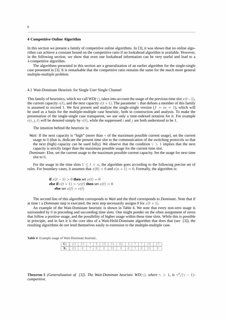
An example of the Wait-Dominate heuristic is shown in Table 4. We note that every non-zero usage issurrounded by0 in preceding and succeeding time slots. One might ponder on the often assignment of zerosthat follow a positive usage, and the possibility of higher usage within these time slots. While this is possiblein principle, and in fact it is the core idea of a Wait-Hold-Dominate algorithm that does that (see [3]), theresulting algorithms do not lend themselves easily to extension to the multiple-multiple case.

Table 4 Example usage of Wait-Dominate heuristic.

C: 23 23 7 5 15 31 62 3 7 7 15 17

X: 23 0 7 0 0 31 0 0 7 0 15 0

Theorem 3 (Generalization of [3]). The Wait-Dominate heuristic WD(γ), whereγ > 1, is γ2/(γ − 1)-competitive.

9

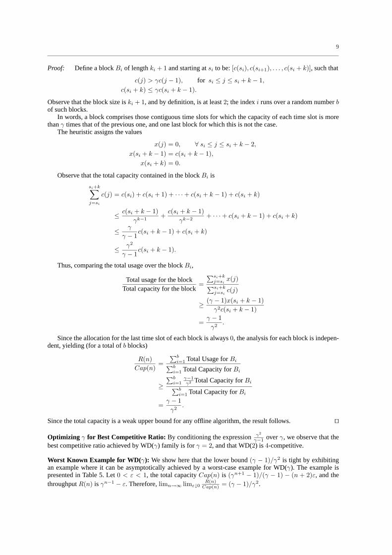
Proof: Define a blockBi of lengthki + 1 and starting atsi to be:[c(si), c(si+1), . . . , c(si + k)], such that

c(j) > γc(j − 1), for si ≤ j ≤ si + k − 1,

c(si + k) ≤ γc(si + k − 1).

Observe that the block size iski + 1, and by definition, is at least2; the indexi runs over a random numberbof such blocks.

In words, a block comprises those contiguous time slots for which the capacity of each time slot is morethanγ times that of the previous one, and one last block for which this is not the case.

The heuristic assigns the values

x(j) = 0, ∀ si ≤ j ≤ si + k − 2,

x(si + k − 1) = c(si + k − 1),x(si + k) = 0.

Observe that the total capacity contained in the blockBi is

si+k∑

j=si

c(j) = c(si) + c(si + 1) + · · ·+ c(si + k − 1) + c(si + k)

≤ c(si + k − 1)γk−1

+c(si + k − 1)

γk−2+ · · ·+ c(si + k − 1) + c(si + k)

≤ γ

γ − 1c(si + k − 1) + c(si + k)

≤ γ2

γ − 1c(si + k − 1).

Thus, comparing the total usage over the blockBi,

Total usage for the blockTotal capacity for the block

=

∑si+kj=si

x(j)∑si+k

j=sic(j)

≥ (γ − 1)x(si + k − 1)γ2c(si + k − 1)

=γ − 1γ2

.

Since the allocation for the last time slot of each block is always0, the analysis for each block is indepen-dent, yielding (for a total ofb blocks)

R(n)Cap(n)

=∑b

i=1 Total Usage forBi∑bi=1 Total Capacity forBi

≥∑b

i=1γ−1γ2 Total Capacity forBi

∑bi=1 Total Capacity forBi

=γ − 1γ2

.

Since the total capacity is a weak upper bound for any offline algorithm, the result follows. ut

Optimizing γ for Best Competitive Ratio: By conditioning the expressionγ2

γ−1 overγ, we observe that thebest competitive ratio achieved by WD(γ) family is for γ = 2, and that WD(2) is 4-competitive.

Worst Known Example for WD( γ): We show here that the lower bound(γ − 1)/γ2 is tight by exhibitingan example where it can be asymptotically achieved by a worst-case example for WD(γ). The example ispresented in Table 5. Let0 < ε < 1, the total capacityCap(n) is (γn+1 − 1)/(γ − 1) − (n + 2)ε, and thethroughputR(n) is γn−1 − ε. Therefore,limn→∞ limε↓0

R(n)Cap(n) = (γ − 1)/γ2.

10

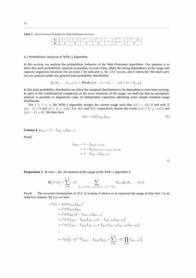
Table 5 Worst Known Example for Wait-Dominate heuristic.

C: 1− ε γ − ε γ2 − ε γ3 − ε . . . γn−1 − ε γn − 3εX: 0 0 0 0 . . . γn−1 − ε 0

4.2 Probabilistic Analysis of WD(γ) Algorithm

In this section, we analyze the probabilistic behavior of the Wait-Dominate algorithms. Our purpose is toshow that such probabilistic analysis is possible, in exact form, albeit the strong dependency in the usage andcapacity sequences involved. For an eventE let indicatorIE be1 if E occurs, and 0 otherwise. We shall carryout our analysis under any general joint probability distribution

Qr(k1, . . . , kr+2; t) := Prob {c(t− r) = k1, . . . , c(t + 1) = kr+2} .

In this joint probability distribution we allow the marginal distributions to be dependent or even time-varying.In spite of the combinatorial complexity of the exact moments of the usage, we shall see that an asymptoticanalysis is possible in degenerate cases of independent capacities admitting some simple standard usagedistribution.

For 1 ≤ t < n, the WD(γ) algorithm assigns the current usage such thatx(t) = c(t) if and only ifx(t− 1) = 0 andc(t + 1) ≤ γc(t). Let A(t) andB(t) respectively denote the events{c(t + 1) ≤ γc(t)} and{x(t− 1) = 0}. We then have

x(t) = c(t)IA(t)IB(t). (1)

Lemma 4 IB(t) = 1− IA(t−1)IB(t−1)

Proof:

IB(t) = 1− I{x(t−1)>0}= 1− I{c(t)≤γc(t−1),x(t−2)=0}= 1− IA(t−1)IB(t−1).

ut

Proposition 2 At timet, thesth moment of the usage of the WD(γ) algorithm is

E[xs(t)

]=

t−1∑r=0

(−1)r∑

kr+2≤γkr+1≤γ2kr≤...≤γr+1k1

ksr+1Qr(k1, . . . , k; t).

Proof: The recursive formulation ofB(t) in Lemma 4 allows us to represent the usage at time slott in aninductive manner. By (1), we have

xs(t) =(c(t)IA(t)IB(t)

)s

= cs(t)IA(t)IB(t)

= cs(t)IA(t)

[1− IA(t−1)IB(t−1)

]

= cs(t)[IA(t) − IA(t)IA(t−1)(1− IA(t−2)IB(t−2))

]

= cs(t)[IA(t) − IA(t)IA(t−1) + IA(t)IA(t−1)IA(t−2)IB(t−2))

]

...

= cs(t)((−1)t−2IA(t) . . . IA(2)IB(2) +

t−3∑r=0

(−1)rr∏

j=0

IA(t−j))).

11

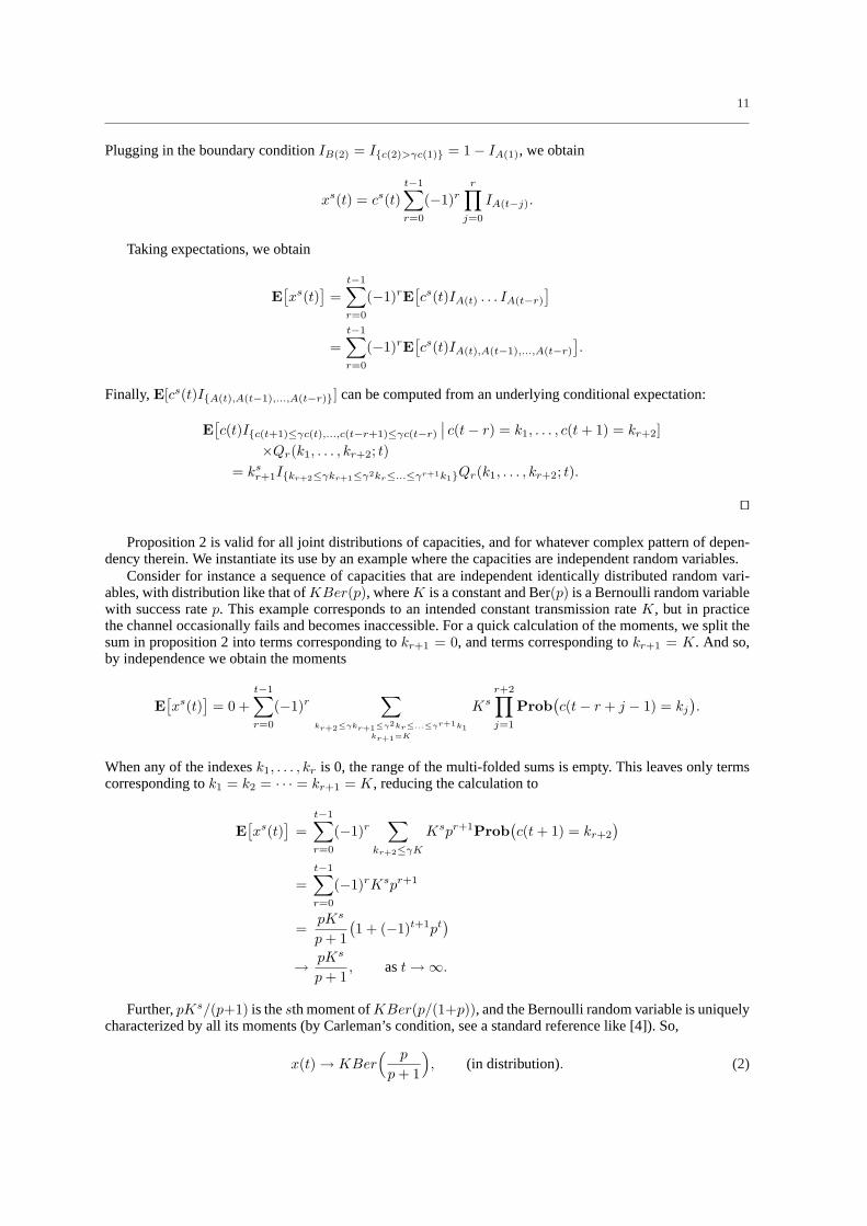
Plugging in the boundary conditionIB(2) = I{c(2)>γc(1)} = 1− IA(1), we obtain

xs(t) = cs(t)t−1∑r=0

(−1)rr∏

j=0

IA(t−j).

Taking expectations, we obtain

E[xs(t)

]=

t−1∑r=0

(−1)rE[cs(t)IA(t) . . . IA(t−r)

]

=t−1∑r=0

(−1)rE[cs(t)IA(t),A(t−1),...,A(t−r)

].

Finally, E[cs(t)I{A(t),A(t−1),...,A(t−r)}] can be computed from an underlying conditional expectation:

E[c(t)I{c(t+1)≤γc(t),...,c(t−r+1)≤γc(t−r)

∣∣ c(t− r) = k1, . . . , c(t + 1) = kr+2]×Qr(k1, . . . , kr+2; t)

= ksr+1I{kr+2≤γkr+1≤γ2kr≤...≤γr+1k1}Qr(k1, . . . , kr+2; t).

ut

Proposition 2 is valid for all joint distributions of capacities, and for whatever complex pattern of depen-dency therein. We instantiate its use by an example where the capacities are independent random variables.

Consider for instance a sequence of capacities that are independent identically distributed random vari-ables, with distribution like that ofKBer(p), whereK is a constant and Ber(p) is a Bernoulli random variablewith success ratep. This example corresponds to an intended constant transmission rateK, but in practicethe channel occasionally fails and becomes inaccessible. For a quick calculation of the moments, we split thesum in proposition 2 into terms corresponding tokr+1 = 0, and terms corresponding tokr+1 = K. And so,by independence we obtain the moments

E[xs(t)

]= 0 +

t−1∑r=0

(−1)r∑

kr+2≤γkr+1≤γ2kr≤...≤γr+1k1kr+1=K

Ksr+2∏

j=1

Prob(c(t− r + j − 1) = kj

).

When any of the indexesk1, . . . , kr is 0, the range of the multi-folded sums is empty. This leaves only termscorresponding tok1 = k2 = · · · = kr+1 = K, reducing the calculation to

E[xs(t)

]=

t−1∑r=0

(−1)r∑

kr+2≤γK

Kspr+1Prob(c(t + 1) = kr+2

)

=t−1∑r=0

(−1)rKspr+1

=pKs

p + 1(1 + (−1)t+1pt

)

→ pKs

p + 1, ast →∞.

Further,pKs/(p+1) is thesth moment ofKBer(p/(1+p)), and the Bernoulli random variable is uniquelycharacterized by all its moments (by Carleman’s condition, see a standard reference like [4]). So,

x(t) → KBer( p

p + 1

), (in distribution). (2)

12

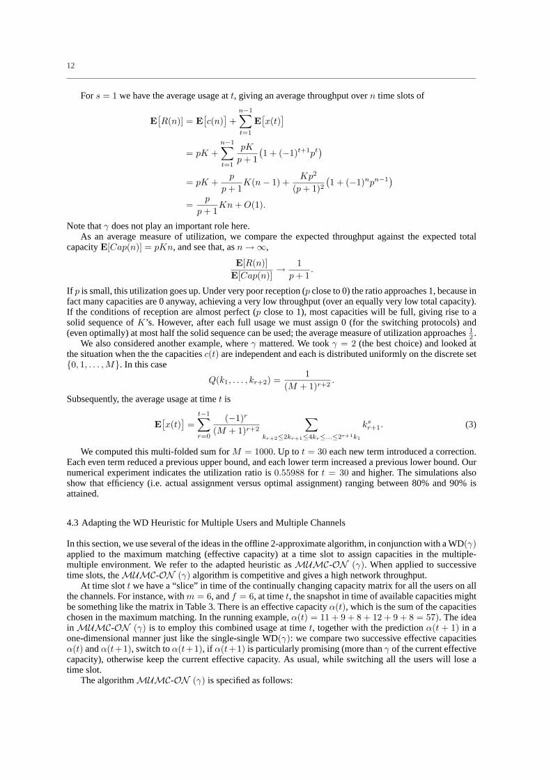
For s = 1 we have the average usage att, giving an average throughput overn time slots of

E[R(n)] = E

[c(n)

]+

n−1∑t=1

E[x(t)

]

= pK +n−1∑t=1

pK

p + 1(1 + (−1)t+1pt

)

= pK +p

p + 1K(n− 1) +

Kp2

(p + 1)2(1 + (−1)npn−1

)

=p

p + 1Kn + O(1).

Note thatγ does not play an important role here.As an average measure of utilization, we compare the expected throughput against the expected total

capacityE[Cap(n)] = pKn, and see that, asn →∞,

E[R(n)]E[Cap(n)]

→ 1p + 1

.

If p is small, this utilization goes up. Under very poor reception (p close to 0) the ratio approaches 1, because infact many capacities are 0 anyway, achieving a very low throughput (over an equally very low total capacity).If the conditions of reception are almost perfect (p close to 1), most capacities will be full, giving rise to asolid sequence ofK ’s. However, after each full usage we must assign 0 (for the switching protocols) and(even optimally) at most half the solid sequence can be used; the average measure of utilization approaches1

2 .We also considered another example, whereγ mattered. We tookγ = 2 (the best choice) and looked at

the situation when the the capacitiesc(t) are independent and each is distributed uniformly on the discrete set{0, 1, . . . ,M}. In this case

Q(k1, . . . , kr+2) =1

(M + 1)r+2.

Subsequently, the average usage at timet is

E[x(t)

]=

t−1∑r=0

(−1)r

(M + 1)r+2

∑

kr+2≤2kr+1≤4kr≤...≤2r+1k1

ksr+1. (3)

We computed this multi-folded sum forM = 1000. Up to t = 30 each new term introduced a correction.Each even term reduced a previous upper bound, and each lower term increased a previous lower bound. Ournumerical experiment indicates the utilization ratio is0.55988 for t = 30 and higher. The simulations alsoshow that efficiency (i.e. actual assignment versus optimal assignment) ranging between 80% and 90% isattained.

4.3 Adapting the WD Heuristic for Multiple Users and Multiple Channels

In this section, we use several of the ideas in the offline 2-approximate algorithm, in conjunction with a WD(γ)applied to the maximum matching (effective capacity) at a time slot to assign capacities in the multiple-multiple environment. We refer to the adapted heuristic asMUMC-ON (γ). When applied to successivetime slots, theMUMC-ON (γ) algorithm is competitive and gives a high network throughput.

At time slott we have a “slice” in time of the continually changing capacity matrix for all the users on allthe channels. For instance, withm = 6, andf = 6, at timet, the snapshot in time of available capacities mightbe something like the matrix in Table 3. There is an effective capacityα(t), which is the sum of the capacitieschosen in the maximum matching. In the running example,α(t) = 11 + 9 + 8 + 12 + 9 + 8 = 57). The ideain MUMC-ON (γ) is to employ this combined usage at timet, together with the predictionα(t + 1) in aone-dimensional manner just like the single-single WD(γ): we compare two successive effective capacitiesα(t) andα(t+1), switch toα(t+1), if α(t+1) is particularly promising (more thanγ of the current effectivecapacity), otherwise keep the current effective capacity. As usual, while switching all the users will lose atime slot.

The algorithmMUMC-ON (γ) is specified as follows:

13

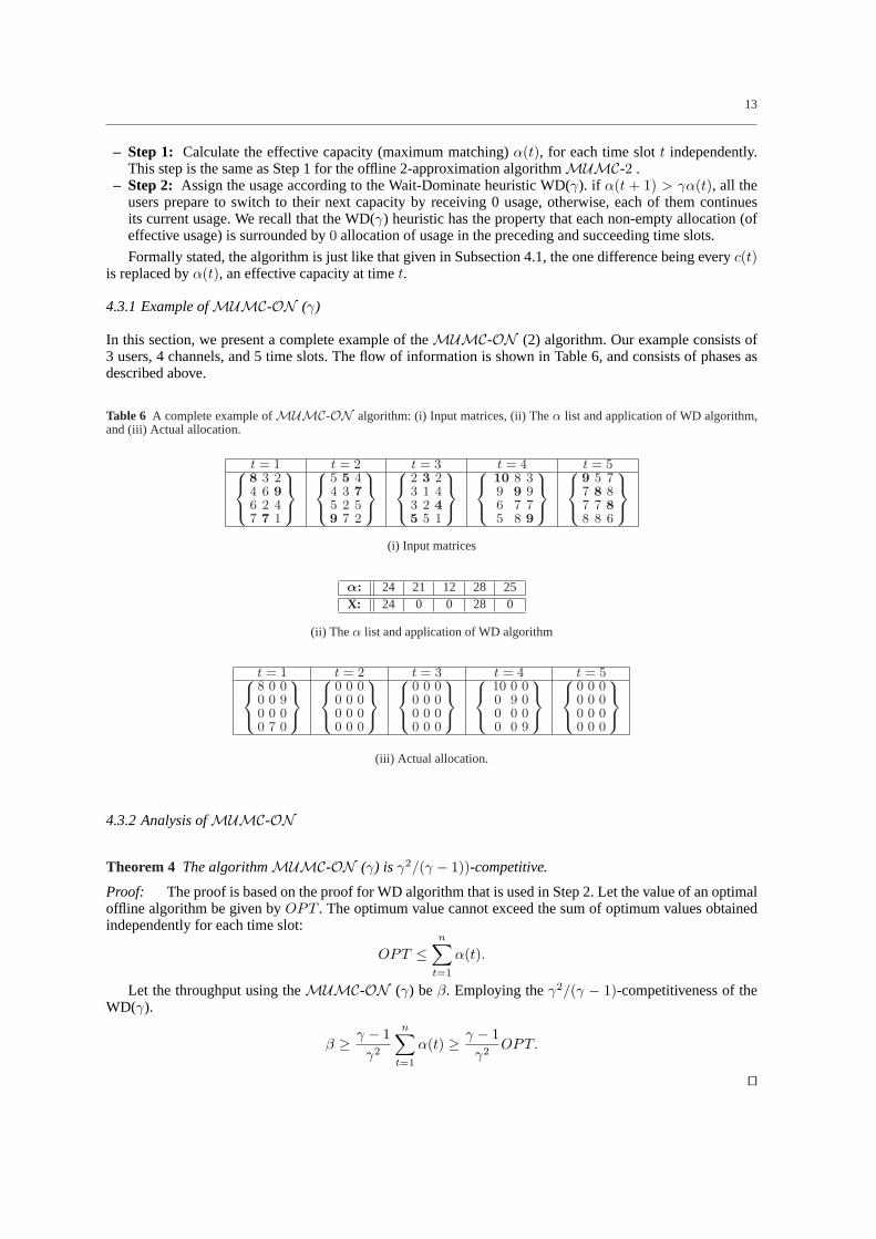
– Step 1: Calculate the effective capacity (maximum matching)α(t), for each time slott independently.This step is the same as Step 1 for the offline 2-approximation algorithmMUMC-2 .

– Step 2: Assign the usage according to the Wait-Dominate heuristic WD(γ). if α(t + 1) > γα(t), all theusers prepare to switch to their next capacity by receiving 0 usage, otherwise, each of them continuesits current usage. We recall that the WD(γ) heuristic has the property that each non-empty allocation (ofeffective usage) is surrounded by0 allocation of usage in the preceding and succeeding time slots.

Formally stated, the algorithm is just like that given in Subsection 4.1, the one difference being everyc(t)is replaced byα(t), an effective capacity at timet.

4.3.1 Example ofMUMC-ON (γ)

In this section, we present a complete example of theMUMC-ON (2) algorithm. Our example consists of3 users, 4 channels, and 5 time slots. The flow of information is shown in Table 6, and consists of phases asdescribed above.

Table 6 A complete example ofMUMC-ON algorithm: (i) Input matrices, (ii) Theα list and application of WD algorithm,and (iii) Actual allocation.

t = 1 t = 2 t = 3 t = 4 t = 5

8 3 24 6 96 2 47 7 1

5 5 44 3 75 2 59 7 2

2 3 23 1 43 2 45 5 1

10 8 39 9 96 7 75 8 9

9 5 77 8 87 7 88 8 6

(i) Input matrices

α: 24 21 12 28 25X: 24 0 0 28 0

(ii) The α list and application of WD algorithm

t = 1 t = 2 t = 3 t = 4 t = 5

8 0 00 0 90 0 00 7 0

0 0 00 0 00 0 00 0 0

0 0 00 0 00 0 00 0 0

10 0 00 9 00 0 00 0 9

0 0 00 0 00 0 00 0 0

(iii) Actual allocation.

4.3.2 Analysis ofMUMC-ON

Theorem 4 The algorithmMUMC-ON (γ) is γ2/(γ − 1))-competitive.

Proof: The proof is based on the proof for WD algorithm that is used in Step 2. Let the value of an optimaloffline algorithm be given byOPT . The optimum value cannot exceed the sum of optimum values obtainedindependently for each time slot:

OPT ≤n∑

t=1

α(t).

Let the throughput using theMUMC-ON (γ) beβ. Employing theγ2/(γ − 1)-competitiveness of theWD(γ).

β ≥ γ − 1γ2

n∑t=1

α(t) ≥ γ − 1γ2

OPT.

ut

14

4.4 Analysis of Multiple User Multiple Channel Version

As already mentioned, theMUMC-ON (γ) algorithm is just like its one dimensional counterpart WD(γ),except that the effective capacity is used at each stage. Therefore, the probabilistic analysis carries over mutatismutandis (only a change ofc(t) to α(t) is required).

Proposition 3 Letα(t) be the effective capacity at timet in a network using theMUMC-ON (γ) algorithm.Thesth moment of the usage at this time slot is

E[xs(t)

]=

t−1∑r=0

(−1)r∑

kr+2≤γkr+1≤γ2kr≤...≤γr+1k1

ksr+1Q̃r(k1, . . . , k; t),

where

Q̃r(k1, . . . , kr+2; t) := Prob {α(t− r) = k1, . . . , α(t + 1) = kr+2} .

We illustrate Proposition 3 by a simple example. Suppose we have only two users, competing at each timeslot for the same channel under theMUMC-ON (2) algorithm. The time slice here isY(t) = (Y1(t), Y2(t)),a pair of independentBer(p) random variables, and allY(t), t = 0, 1, . . . , n, are independent. Clearly, Theeffective capacities come across asK times one combined Bernoulli random variable, because the effectivecapacity is either 0, whenY1(t) = Y2(t) = 0, or it is K when either or bothY1(t), andY2(t) areK (in thecase of both beingK we still get an effective capacityK, owing to the constraint that no two users can sharea channel). In other words, the maximum matching isα(t) = max{Y1(t), Y2(t)}, which is distributed likeBer(p′) random variable, withp′ = 2pq+p2 = 1−q2. The analysis has been reduced to that of a single-singleWD(2) algorithm, with the capacitiesc(t) being an independent BernoulliBer(p′) sequence. For this lattersystem we obtained a result. Whence, form = 2, andf = 1 we have

E[R̃(n)]E[C̃ap(n)]

→ p′

2p(p′ + 1)=

1− q2

2p(2− q2);

hereR̃(n) is interpreted as the effective throughput for the entire network, i.e.

R̃(n) =2∑

i=1

n∑t=1

x(i, 1, t),

andC̃ap(n) is interpreted as the total available capacity, i.e.

C̃ap(n) =n∑

t=1

c̃(t),

where

c̃(t) =

{0, with probabilityq2,K, with probability2pq,2K, with probabilityp2,

and across time the variablesc̃(t) are independent.

15

5 Conclusion and Future Work

Channel-aware scheduling and link adaptation will play an important role in achieving the high data ratesrequired by emerging mobile applications. In this paper, we considered the problem of maximizing throughputin a multi-carrier wireless network that employs link adaptation.

We first analyzed the concept of link adaptation and based on that, we formulated a combinatorial problemto model the scheduling problem in a multi-carrier wireless network with multiple users. We considered theoffline version of the problem and proved the inherent complexity of the problem by presenting a reductionfrom a known NP-complete problem. We presented a2-approximation algorithm for the offline version. Wealso formulated the more practical online version of the problem and generalized a known algorithm for thesingle user single channel case. We extended the algorithm for multiple user multiple channel environmentand proved that the modified algorithm is4-competitive, and also presented an average case analysis of ouralgorithm.

Our results show that a modest lookahead capability of one time slot allows us to provide a4-competitivealgorithm for multiple user and multiple channel environment.

We have not considered the quality of service requirements for different users in the scheduling problem.A natural extension of this work would be to study the scheduling algorithm considering the quality of service.

References

1. Andrews, M., Zhang, L.: Scheduling over a time-varying user-dependent channel with applications to high speed wirelessdata. In: Proceedings of the 43rd Symposium on Foundations of Computer Science, pp. 293–302. IEEE Computer Society(2002)

2. Andrews, M., Zhang, L.: Scheduling over non-stationary wireless channels with finite rate sets. In: IEEE INFOCOM 2004 -The Conference on Computer Communications, vol. 23:1, pp. 1695 – 1705 (2004)

3. Arora, A., Choi, H.: Channel aware scheduling for throughput maximization. Submitted. Also available athttp://www.seas.gwu.edu/˜hchoi/publication/wireless.htm

4. Billingsley, P.: Probability and Measure. Wiley, New York (1986)5. Catreux, S., Erceg, V., Gesbert, D., Heath, R.: Adaptive modulation and MIMO coding for broadband wireless data networks.

IEEE Communications Magazine40, 108–115 (2002)6. Garey, M., Johnson, D.: Computers and Intractability - A Guide to the Theory of NP-completeness. Freeman (1979)7. Goldberg, A.V., Tarjan, R.E.: A new approach to the maximum flow problem. J. Assoc. Comput. Mach.35, 921–940 (1988)8. Hopcroft, J.E., Karp., R.M.: An n 5/2 algorithm for maximum matchings in bipartite graphs. SIAM Journal on Computing

2(4), 225–231 (1973)9. Tsibonis, V., Georgiadis, L., Tassiulas, L.: Exploiting wireless channel state information for throughput maximization. In:

Proceedings of IEEE Infocom ’03, pp. 301–310 (2003)