Technical University at Kosice Faculty of Electrical Engineering and Informatics Department of Electronics and Multimedia Communications Ing. Michal Aftanas Through Wall Imaging Using M-sequence UWB Radar System Thesis to the dissertation examination Supervisor: doc. Ing. Miloˇ s Drutarovsk´ y, CSc. Program of PhD study: Infoelectronic Field of PhD study: 5.2.13 Electronic Form of PhD study: Daily Koˇ sice December 2007

Welcome message from author
This document is posted to help you gain knowledge. Please leave a comment to let me know what you think about it! Share it to your friends and learn new things together.
Transcript
Technical University at KosiceFaculty of Electrical Engineering and Informatics
Department of Electronics and Multimedia Communications
Ing. Michal Aftanas
Through Wall Imaging Using M-sequenceUWB Radar System
Thesis to the dissertation examination
Supervisor: doc. Ing. Milos Drutarovsky, CSc.Program of PhD study: InfoelectronicField of PhD study: 5.2.13 Electronic
Form of PhD study: Daily
Kosice December 2007
Contents
Head Page i
Contents iii
List of Abbreviations iv
List of Symbols v
Introduction 6
1 UWB Radar Systems 71.1 History of Radar . . . . . . . . . . . . . . . . . . . . . . . . . . . . . 71.2 Radars Fundamentals and Applications . . . . . . . . . . . . . . . . . 71.3 UWB and M-sequence Advantages . . . . . . . . . . . . . . . . . . . 81.4 M-sequence UWB Radar System . . . . . . . . . . . . . . . . . . . . 9
2 Data Preprocessing 132.1 Through Wall Radar Basic Model . . . . . . . . . . . . . . . . . . . . 132.2 Through Wall Penetrating . . . . . . . . . . . . . . . . . . . . . . . . 142.3 Through Wall Radar Data Representation . . . . . . . . . . . . . . . 162.4 Data Calibration and Preprocessing . . . . . . . . . . . . . . . . . . . 18
3 Basic Radar Imaging Methods 233.1 Backprojection vs. Backpropagation . . . . . . . . . . . . . . . . . . 233.2 SAR Imaging . . . . . . . . . . . . . . . . . . . . . . . . . . . . . . . 243.3 Kirchhoff Migration . . . . . . . . . . . . . . . . . . . . . . . . . . . . 263.4 f-k Migration . . . . . . . . . . . . . . . . . . . . . . . . . . . . . . . 313.5 Multiple Signal Classification . . . . . . . . . . . . . . . . . . . . . . 363.6 The Inverse Problem . . . . . . . . . . . . . . . . . . . . . . . . . . . 37
4 Improvements in Radar Imaging 404.1 Cross-correlated Back Projection . . . . . . . . . . . . . . . . . . . . 404.2 Fast Back Projection . . . . . . . . . . . . . . . . . . . . . . . . . . . 414.3 Migration by Deconvolution . . . . . . . . . . . . . . . . . . . . . . . 424.4 SEABED and IBBST . . . . . . . . . . . . . . . . . . . . . . . . . . . 434.5 f-k Migration Improvements . . . . . . . . . . . . . . . . . . . . . . . 44
4.5.1 Nonuniform FFT . . . . . . . . . . . . . . . . . . . . . . . . . 444.5.2 f-k Migration in Cylindrical Coordinations . . . . . . . . . . . 454.5.3 f-k Migration with Motion Compensation . . . . . . . . . . . . 454.5.4 f-k Migration with Surface and Loss Compensation . . . . . . 464.5.5 Prestack Residual f-k Migration . . . . . . . . . . . . . . . . . 464.5.6 f-k Migration with Anti-Leakage Fourier Transform . . . . . . 464.5.7 Lagrange’s Interpolation in f-k Migration . . . . . . . . . . . . 47
ii

CONTENTS iii
4.6 Migrations with Antenna Beam Compensation . . . . . . . . . . . . . 47
5 Experiments with Through Wall Imaging 495.1 Review of Experiments . . . . . . . . . . . . . . . . . . . . . . . . . . 495.2 First Experiments with TWI . . . . . . . . . . . . . . . . . . . . . . . 51
Conclusion 55
Thesis for dissertation work 56
References 63
List of Abbreviations
1D – One dimension2D – Two dimensions3D – Three dimensionsADC – Analog to Digital ConverterART – Algebraic Reconstruction TechniqueAWGN – Additive White Gaussian NoiseBHDI – Beamspace High Definition ImagingBST – Boundary Scattering TransformECS – Extended Chirp ScalingEOK – Extended Omega KFFT – Fast Fourier TransformGPR – Ground Penetrating RadarHDVI – High Definition Vector ImagingIBST – Inverse Boundary Scattering TransformIFFT – Inverse Fast Fourier TransformIR – Impulse ResponseLAN – Local Area NetworkM-sequence – MLBS – Maximum Length Binary SequenceMUSIC – MUltiple SIgnal CharacterizationNUFFT – NonUniform Fast Fourier TransformationRADAR – RAdio Detection And Ranging systemRAW – Unprocessed dataRX – ReceiverSAR – Synthetic Aperture RadarSEABED – Shape Estimation Algorithm based on Boundary Scattering Transform
and Extraction of Directly scattered wavesSMA – SubMiniature version A connectorTWI – Through the Wall ImagingSNR – Signal to Noise RatioTCP/IP – Transmission Control Protocol/Internet ProtocolTOA – Time Of ArrivalTWR – Through Wall RadarTX – TransmitterT&H – Track And HoldUWB – Ultra Wide Band
iv

List of Symbols
∗ – Convolutionα – Attenuation constantc – Speed of light in the vacuum~CA – CrosstalkdTXRX – Distance between Tx and Rxdinwall – Thickness of the wallδ – Dirac delta functionεr – Permitivity~Erad – Radiated Electric field~Emeas – Measured Electric fieldf – FrequencyG(x0;x) – Greens function, x0: source point , x: observation point~hA – Measurement system transfer function~hC – Clutter transfer function~hT – Target transfer functionk – WavenumberK – Multiple response matrixλ – EigenvalueΛ – Impulse responseLair−wall – Loss due to air-wall interfaceLwall – Loss inside the wallε – Permeability−→∇ – Divergence∇2 – Laplacianω – Angular frequencyφ – Scalar wavefield in frequency domainψ – Scalar wavefieldr – Distance from the antennaσ – ConductivityT – Time reversal matrixtTXRX – Wave travel time between Tx and Rxtinwall – Wave travel time inside the walltan δ – Loss tangent of the wallv – Velocity of wave propagationvn – Eigenvectorvwall – Velocity of wave propagation inside the wallVS(t) – Voltage time evolution applied to the TX antennaVR(t) – Received voltage from RX antennaw – Point spread function~xo – Source point position~x – Observation point positionZc – Impedances of the feed cableZ0 – Impedances of the free space[xtr, ztr] – Transmitter coordinates[xre, zre] – Receiver coordinates[xT , zT ] – Target coordinates
v

Introduction
Nowadays, rescue and security of people is very serious problem. Persons buriedunder ruins caused by earthquake or under snow after avalanche can be find veryhard with present technique. Lots of firemen died inside building full of smoke withzero visibility. In all of these scenes through wall radar can help on a large scale.”Seeing” through the wall and clothes can help rapidly also in field of airport se-curity, police raid actions and lots of another. In this work I am focused on theimaging algorithms in order to image interior of room including walls and objectsinside of the room. The field of algorithms for through wall imaging is really poor,most of algorithms for this purpose were derived from aircraft radars imaging, seis-mology, ground penetrating radars imaging, sonars etc. There is a huge number ofmodifications and improvements in imaging algorithms in all fields.
In January 2007 started project ultra wideband radio application for localisa-tion of hidden people and detection of unauthorized objects with acronym RADIO-TECT, COOP-CT-2006 co-funded by the European Commission within the SixthFramework Programme with duration of two years. Our department is one of theresearch team in this project. My contribution in this project should be to developenew, or implement some already existing methods that allow to image the interiorof room behind wall. One of the most promising radar device used in this project isM-sequence UWB radar developed at Technische Universitat in Ilmenau (the coor-dinator of this project). I made through wall measurements with this radar and usedthem for processing. That is the reason why I describe main features of M-sequenceUWB radar device in chapter 1. In chapter 2 basic through wall radar model, datarepresentation and preprocessing is described. Three basic imaging methods fromwhich most another methods are derived and they are described in section 3. Inthe next section 4, review of some improved imaging methods that can be used forthrough wall imaging are described. Simulated and real experiments with throughwall imaging are reviewed in section 5. My first experience with through wall imag-ing measurements and processing are shown in section 5.2. At the end of workconclusion and proposed thesis are presented.
This thesis originated within the support of the project Ultra Wideband Radioapplication for localisation of hidden people and detection of unauthorised objects(Acronym: RADIOTECT) and project Digital Processing of UWB Radar Signals(Acronym: DSP-UWB-RAD).
6

1 UWB Radar Systems 7
1 UWB Radar Systems
1.1 History of Radar
In 1904 Christian Huelsmeyer gave public demonstrations in Germany and theNetherlands of the use of radio echoes to detect ships so that collisions could beavoided, which consisted of a simple spark gap aimed using a multipole antenna.When a reflection was picked up by the two straight antennas attached to the sepa-rate receiver, a bell sounded. The system detected presence of ships up to 3 km. Itdid not provide range information, only warning of a nearby metal object, and wouldbe periodically ”spun” to check for ships in bad weather. He patented the device,called the telemobiloscope, but due to lack of interest by the naval authorities theinvention was not put into production [9]. Nikola Tesla, in August 1917, proposedprinciples regarding frequency and power levels for primitive radar units. Tesla pro-posed the use of standing electromagnetic waves along with pulsed reflected surfacewaves to determine the relative position, speed, and course of a moving object andother modern concepts of radar [71]. The world war two moved forward developingof airborne radars [16]. The next major development in the history of radars was theinvention of the cavity magnetron by John Randall and Harry Boot of BirminghamUniversity in early 1940’s. This was a small device which generated microwave fre-quencies much more efficiently. The UWB (Ultra WideBand) term was at first usedin the late 1960’s Harmuth at Catholic University of America, Ross and Robbins atSperry Rand Corporation and Paul van Etten at the USAF’s Rome Air DevelopmentCenter [7]. Till the end of 20th century there were lot of radar types for differentapplications like airborne radars, ground penetrating radars, sonars and one whichwill be discussed detailed in this paper - the through wall penetrating radar.
1.2 Radars Fundamentals and Applications
The term RADAR is derived from the description of its first primary role as a RAdioDetection And Ranging system. Most natural and man-made objects reflect radiofrequency waves and, depending on the radars purpose, information can be obtainedfrom objects such as aircraft, ships, ground vehicles, terrain features, weather phe-nomenon, and even insects. The determination of the objects position, velocity andother characteristics, or the obtaining of information relating to these parameters bythe transmission of radio waves and reception of their return is sometimes referredto radio determination. In most cases, a basic radar operates by generating pulsesof radio frequency energy and transmitting these pulses via a directional antenna.When a pulse fall on object in its path, a small portion of the energy is reflectedback to the antenna. The radar is in the receive mode in between the transmittedpulses, and receives the reflected pulse if it is strong enough. The radar indicatesthe range to the object as a function of the elapsed time of the pulse traveling to

1.3 UWB and M-sequence Advantages 8
the object and returning. The radar indicates the direction of the object by thedirection of the antenna at the time the reflected pulse was received [18].
Radar is an important tool in the safe and efficient management of the airspacesystem. Safe and efficient air travel involves radars for short-range surveillance ofair traffic and weather in the vicinity of airports, the long-range surveillance andtracking of aircraft and weather on routes between airports, and the surveillanceof aircraft and ground vehicles on the airport surface and runways. The aircraftheight above ground is determined by radar altimeters that assist in safe and efficientflight. Airborne Doppler navigation radars measure the vector velocity of the aircraftand determines the distance traveled. Weather avoidance radars identify dangerousweather phenomena and assist the pilot to avoid them. Some military pilots, whotrain at low altitudes, use terrain-following and terrain-avoidance radars that allowthe pilot to closely fly over the ground and fly over or around other obstacles in hispath. Navy and coast guard ships employ navigation radars to assist in avoidingcollisions, assisting in making landfall, and piloting in restricted waters. Radarsare also used on shore for harbor surveillance supporting the vessel traffic system.Spaceborne radars have also been used for altimetry, ocean observation, remotesensing, mapping, navigation, and weather forecasting. The familiar police speed-gun radars are a well-known applications of radar for law enforcement.
Another big category of radar systems are ground penetrating and thorough wallradar system. In general, they use shorter range but better resolution like airborneradars. Ground Penetrating Radar (GPR) can by used e.g. for geological survey orlandmines detection. GPR allow the construction of subsurface 3D seismic images.Detection of landmines is very serious problem in all over the world. One hundredmillion uncleared landmines lie in the fields and alongside the roads and footpathsof one-third of the countries in the developing world and leave over 500 victims aweek [26]. Through Wall Radar (TWR) system is in general used for rescue andsecurity activity. It offers ability to detect criminals including terrorists obscuredfrom view e.g. behind walls, to detect and locate trapped people after accidents orcatastrophes like burred building, earthquake, avalanche, etc. and to detect unlawfulobjects hidden under clothes, including non-metallic objects. Another opportunityof utilize the TWR is imaging interior of room and inside walls, this work will presentreview of methods for this purpose.
1.3 UWB and M-sequence Advantages
We use UWB Maximum Length Binary Sequence (MLBS or M-sequence) radar sys-tem, because it has many advantages in comparison with classical pulse, or contin-uous wave radar. The main advantages of UWB radar are: The UWB signal can betransmitted with no carrier, producing transmit signal require less power, improvedrange measurement accuracy and object identification (greater resolution), reducedradar effects due to passive interference (rain, mist, aerosols, metalized strips, ...),

1.4 M-sequence UWB Radar System 9
decreased detectability by hostile interceptor, availability of low cost transceiversand many others [56], [84], [54].
The first idea to use a very well known M-sequence in UWB radar was proposedin 1996 by Jurgen Sachs from Technical University in Ilmenau and Peter Peyerl fromMEODAT GmbH Ilmenau, US patent No. 6272441 [93], [90]. The main advantagesof using M-sequence are: The use of periodic signals avoids bias errors, allows linearaveraging for noise suppression, M-sequence has low crest factor what allow to usethe limited dynamics of real systems and the signal acquisition may be carried outby undersampling. Thus signals of an extreme bandwidth may be sampled using lowcost, commercial Analog to Digital Converters (ADC) in combination with samplinggates.
1.4 M-sequence UWB Radar System
For illustration how M-sequence looks and what are its property, 3 shift stages forgenerate M-sequence with period 7 chips will be used. It is given from (1.1), wheren is number of chips and N is number of generator shift stages [104].
n = 2N − 1 (1.1)
Then generated M-sequence in time domain is shown on Figure 1.1. Length of one
Period T
Clock period tc
Time
1
-1
Am
plitu
de
Figure 1.1: M-sequence with 7 chips in period T
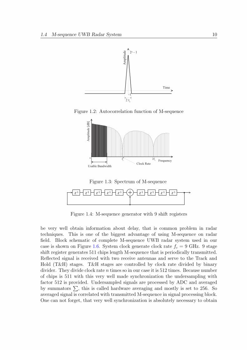
chip is tc that is clock period and M-sequence acquire amplitude values -1 and 1.Autocorrelation function of this M-sequence is shown on Figure 1.2. It can be seenthat maximum amplitude is 2N − 1 so increasing number of chips will increase alsocorrelation gain. On Figure 1.3 spectrum of M-sequence can be seen.
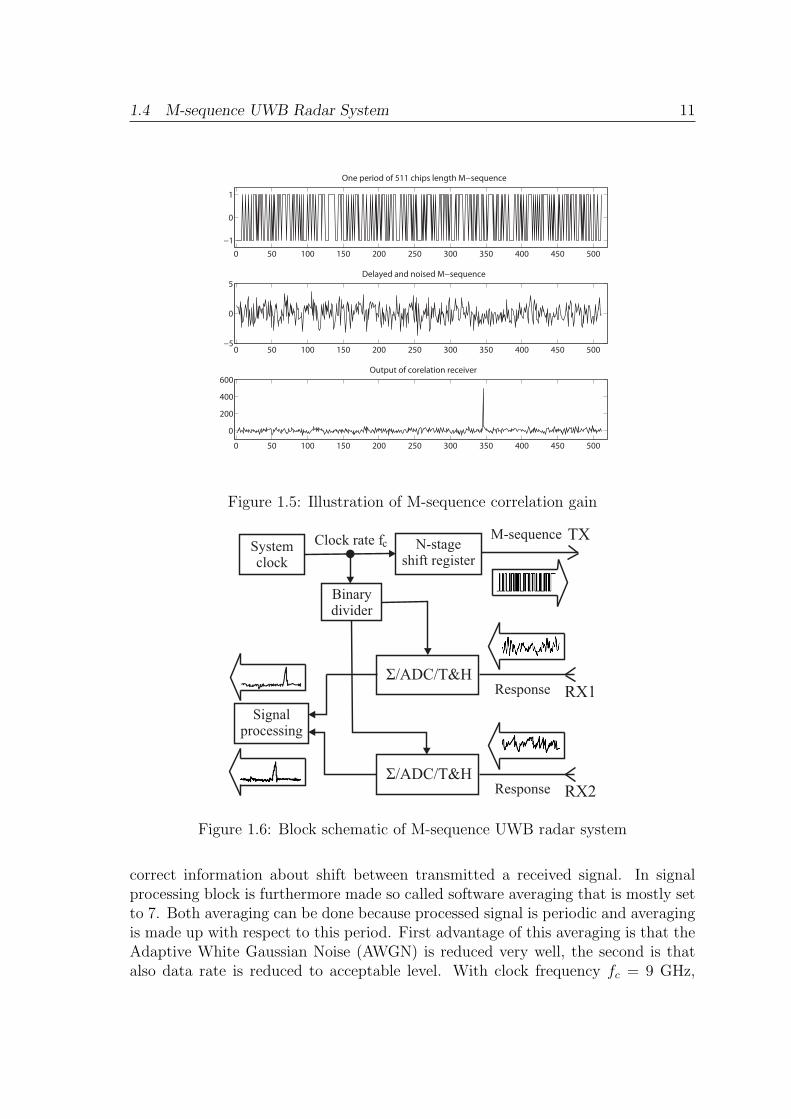
UWB radar system with M-sequence generator [87], [123], [29], [93], [90], [92],[94], [120], [91], [121], [119], [1], [86] is made up from 9 shift registers and 511 chips.From Figure 1.4 can be seen that only 2 feedback connections and one summationare needed. For illustration one period of ideal 511 chips length M-sequence isshown on Figure 1.5 (top), the same but delayed and noised M-sequence with 6dBSNR (middle) and output after correlation of these two signal (top and middle)is shown in bootom of Figure 1.5. From so noised signal (Figure 1.5 middle) can
1.4 M-sequence UWB Radar System 10
Time
-1
2n - 1
2 tc
Am
plitu
de
Figure 1.2: Autocorrelation function of M-sequence
fc 2fc0
Usable Bandwidth
FrequencyClock Rate
Am
plitu
de [d
B]
Figure 1.3: Spectrum of M-sequence
z-1 z-1 z-1 z-1 z-1 z-1 z-1 z-1 z-1
Figure 1.4: M-sequence generator with 9 shift registers
be very well obtain information about delay, that is common problem in radartechniques. This is one of the biggest advantage of using M-sequence on radarfield. Block schematic of complete M-sequence UWB radar system used in ourcase is shown on Figure 1.6. System clock generate clock rate fc = 9 GHz. 9 stageshift register generates 511 chips length M-sequence that is periodically transmitted.Reflected signal is received with two receive antennas and serve to the Track andHold (T&H) stages. T&H stages are controlled by clock rate divided by binarydivider. They divide clock rate n times so in our case it is 512 times. Because numberof chips is 511 with this very well made synchronization the undersampling withfactor 512 is provided. Undersampled signals are processed by ADC and averagedby summators
∑, this is called hardware averaging and mostly is set to 256. So
averaged signal is correlated with transmitted M-sequence in signal processing block.One can not forget, that very well synchronization is absolutely necessary to obtain
1.4 M-sequence UWB Radar System 11
0 50 100 150 200 250 300 350 400 450 500−1
0
1
One period of 511 chips length M−sequence
0 50 100 150 200 250 300 350 400 450 500−5
0
5Delayed and noised M−sequence
0 50 100 150 200 250 300 350 400 450 500
0
200
400
600Output of corelation receiver
Figure 1.5: Illustration of M-sequence correlation gain
Systemclock
N-stageshift register
Binarydivider
Signalprocessing
Σ/ADC/T&H
Clock rate fc M-sequence
Response
TX
RX1
RX2ResponseΣ/ADC/T&H
Figure 1.6: Block schematic of M-sequence UWB radar system
correct information about shift between transmitted a received signal. In signalprocessing block is furthermore made so called software averaging that is mostly setto 7. Both averaging can be done because processed signal is periodic and averagingis made up with respect to this period. First advantage of this averaging is that theAdaptive White Gaussian Noise (AWGN) is reduced very well, the second is thatalso data rate is reduced to acceptable level. With clock frequency fc = 9 GHz,
1.4 M-sequence UWB Radar System 12
number of chips 511, undersampling factor 512, hardware averaging factor 256 andsoftware averaging factor 7 the output frequency is approximately 9809 chips persecond. It means that we practically receive approximately 19 impulse responsesper second. This is enough for detecting of moving people, or for capturing datafrom man made moving radar measurements.
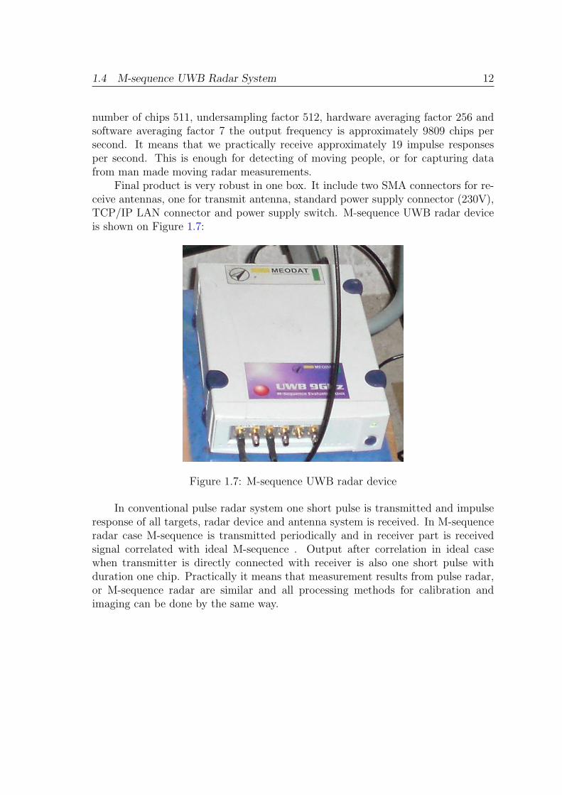
Final product is very robust in one box. It include two SMA connectors for re-ceive antennas, one for transmit antenna, standard power supply connector (230V),TCP/IP LAN connector and power supply switch. M-sequence UWB radar deviceis shown on Figure 1.7:
Figure 1.7: M-sequence UWB radar device
In conventional pulse radar system one short pulse is transmitted and impulseresponse of all targets, radar device and antenna system is received. In M-sequenceradar case M-sequence is transmitted periodically and in receiver part is receivedsignal correlated with ideal M-sequence . Output after correlation in ideal casewhen transmitter is directly connected with receiver is also one short pulse withduration one chip. Practically it means that measurement results from pulse radar,or M-sequence radar are similar and all processing methods for calibration andimaging can be done by the same way.

2 Data Preprocessing 13
2 Data Preprocessing
Before any imaging methods can be applied to the measured data they have to bepreprocessed. There are many special unwanted effects and unknowns that shouldbe reduced as much as possible. The main of these effects and methods to reducedthem will be described in next sections right after TWR basic model and datarepresentation will be described. Moreover one part of this section will be focusedon wave penetrating through the wall.
2.1 Through Wall Radar Basic Model
TWR basic model specify all processes which contribute to the measured data.These processes are caused mainly by the measurement system, the measurementenvironment and in small part also by measured objects. This model will be de-scribed on TWR system with one RX and one TX stationary antenna.
Antenna signal effects will be shown for both RX and TX antennas. The electricfield which is generated by the TX antenna is called ~Erad and can be modeled by[59], [100]:
~Erad(r, θ, ϕ, t) =1
2πrc~hTX(θ, ϕ, t) ∗
√Z0√Zc
dVs(t)
dt(2.1)
where r, θ, ϕ are spatial coordinates and t is time, Zc and Z0 the impedances of thefeed cable and free space resp., and c the vacuum speed of light. The voltage timeevolution applied to the TX antenna is denoted VS(t), ~hTX is the vectorial transferfunction for the emitting antenna and ∗ represents the convolution. The receivedvoltage from RX antenna VR is then:
VR(t) =
√Zc√Z0
~hRX(θ, ϕ, t) ∗ ~Emeas(t) (2.2)
where ~hRX is the transfer function of the receiving antenna, and ~Emeas(t) is the fieldat the RX antenna. VS(t) and VR(t) are scalars due to the fact that the antenna
integrates all spatial components into one signal. The process that transforms ~Erad
into ~Emeas depends on the different travel signal paths and is denoted temporarilyas the unknown impulse response ~X(r, θ, ϕ, t). The received voltage thus becomes:
VR(t) =
√Zc√Z0
~hRX(θ, ϕ, t) ∗ ~X(r, θ, ϕ, t) ∗ ~Erad(r, θ, ϕ, t) (2.3)
If we take the 1/r dependency out of the definition of ~Erad we can combine all
antenna terms into one term ~hA:
VR(t) =1
r~hA(θ, ϕ, t) ∗ ~X(r, θ, ϕ, t) (2.4)
2.2 Through Wall Penetrating 14
~hA contains the contributions of the measurement system to the signal. It can beaccurately measured in lab conditions but it is very difficult and exacting challenge,that require very precise measurements.
Antenna crosstalk effects means signal traveling directly from the transmitterto the receiver. This signal is thus constantly present in all measurements and shallremain constant for a fixed antenna setup. The impulse response of the direct pathbetween both antennas will be expressed as ~CA. The expression of he received fieldbecomes:
VR(t) =1
dTXRX~hA(θ, ϕ, t) ∗ ~CA +
1
r~hA(θ, ϕ, t) ∗ ~X1 (2.5)
where ~X1 represents the other (non-direct) paths between the antennas, and dTXRXis the direct distance between TX and RX. The first term can be measured (cali-
brated) by pointing the antenna to the sky or to an absorber, so that ~X1 becomeszero. It can thus be easily subtracted out of any measured data. The second termcontains the information about eventual target presence, and is thus the most in-teresting one.
~X1 contains a combination of the impulse responses of target ~hT and clutter~hC .
~X1 = ~hT + ~hC (2.6)
Here targets are behind wall scatterers we want to detect, while clutter is anythingelse which adds misinformation to the signal. A typical clutter examples, presentsin most measurements are the multiple reflections inside wall, multiple reflectionsbetween walls inside room, not constant permitivity in wave propagation, movingtrees in outside measurements, false objects received from behind antennas etc. Themodel of the received signal (2.5) becomes:
VR(t) =1
dTXRX~hA(θ, ϕ, t) ∗ ~CA(t) +
1
r~hA(t) ∗ (~hT (t) + ~hC(t)) + n (2.7)
The last term n is added to represent measurement noise which is not added to thesignal due to a reflection, but due to the measurement system itself.
Even if most variables in (2.7) can be measured, it is very difficult to measurethem precisely. In practical measurements only VR(t) is measured what is summationof all this variables, this is the first source of systematic error.
2.2 Through Wall Penetrating
Through wall imaging require wave penetrating through specific building materialssuch as concrete blocks, clay brick, drywall, asphalt shingle, fibreglass insulation etc.The transmitted signal is attenuated due to free space loss, scattering from air-wallinterface, loss in the wall, and the scattering from objects. The loss due to air-wallinterface Lair−wall depends on orientation of the electric field with respect to the
2.2 Through Wall Penetrating 15
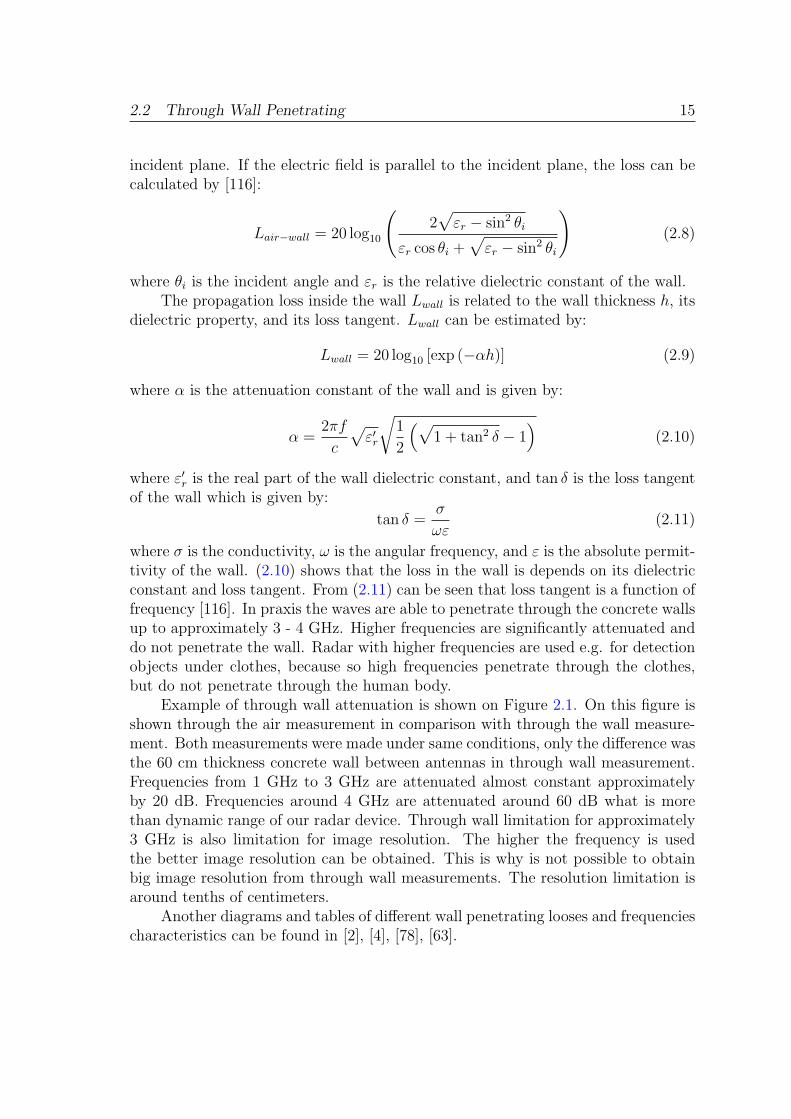
incident plane. If the electric field is parallel to the incident plane, the loss can becalculated by [116]:
Lair−wall = 20 log10
(2√εr − sin2 θi
εr cos θi +√εr − sin2 θi
)(2.8)
where θi is the incident angle and εr is the relative dielectric constant of the wall.The propagation loss inside the wall Lwall is related to the wall thickness h, its
dielectric property, and its loss tangent. Lwall can be estimated by:
Lwall = 20 log10 [exp (−αh)] (2.9)
where α is the attenuation constant of the wall and is given by:
α =2πf
c
√ε′r
√1
2
(√1 + tan2 δ − 1
)(2.10)
where ε′r is the real part of the wall dielectric constant, and tan δ is the loss tangentof the wall which is given by:
tan δ =σ
ωε(2.11)
where σ is the conductivity, ω is the angular frequency, and ε is the absolute permit-tivity of the wall. (2.10) shows that the loss in the wall is depends on its dielectricconstant and loss tangent. From (2.11) can be seen that loss tangent is a function offrequency [116]. In praxis the waves are able to penetrate through the concrete wallsup to approximately 3 - 4 GHz. Higher frequencies are significantly attenuated anddo not penetrate the wall. Radar with higher frequencies are used e.g. for detectionobjects under clothes, because so high frequencies penetrate through the clothes,but do not penetrate through the human body.
Example of through wall attenuation is shown on Figure 2.1. On this figure isshown through the air measurement in comparison with through the wall measure-ment. Both measurements were made under same conditions, only the difference wasthe 60 cm thickness concrete wall between antennas in through wall measurement.Frequencies from 1 GHz to 3 GHz are attenuated almost constant approximatelyby 20 dB. Frequencies around 4 GHz are attenuated around 60 dB what is morethan dynamic range of our radar device. Through wall limitation for approximately3 GHz is also limitation for image resolution. The higher the frequency is usedthe better image resolution can be obtained. This is why is not possible to obtainbig image resolution from through wall measurements. The resolution limitation isaround tenths of centimeters.
Another diagrams and tables of different wall penetrating looses and frequenciescharacteristics can be found in [2], [4], [78], [63].

2.3 Through Wall Radar Data Representation 16
0 1 2 3 4 5 6−60
−50
−40
−30
−20
−10
0
Through the Air and Wall Measurements
Frequency [GHz]
Am
plit
ud
e [d
B]
Through the Air MeasurementThrough the Wall Measurement
Figure 2.1: Through the air and through the wall measurement
2.3 Through Wall Radar Data Representation
3 types of data representation are used in most bistatic radar measurements, A-scan,B-scan and C-scan [28], [59], [29]. Bistatic means that one antenna is transmittingand another antenna is receiving, so not only one antenna is used for transmittingand receiving like in monostatic case.
A-scan is obtained during the acquisition of one TWR time signal (one impulseresponse), in our case it is 511 chips. It is assumed that radar system is stationary,or moves very slowly. In reality all signals, arriving at the antenna at the same timeare superposed with a weight which is dependent on the direction of arrival (theantenna pattern). An A-Scan thus contains for each time t all signals arriving fromall directions at that time. Figure 2.2 shows example of unprocessed A-scan. It ismeasurement of metal plate(1m × 0.5m) 1 meter behind wall. X-axis represents timepropagation of one impulse response expressed in number of chips, Y-axis representsamplitude of received signal.
One A-Scan provides only a very limited amount of information, therefore theinformation in more than one A-Scan has to be combined. In order to have a morecomplete view of the area under study, the TWR system shall be moved e. g. alongthe wall. This movement is said to be part of a scanning, i.e. movement on a more orless regular grid. If the movement is quasi linear, with a near constant velocity, thena number of A-scans are acquired at positions of the measurement system whichare almost equidistant. This set of 1D A-Scans, can thus be assembled togetherin a two dimensional (2D) structure, and visualized as an image. This 2D datasetis called a B-scan. Usually it is visualized with the scanning direction (distance)horizontally, and the time vertically. Figure 2.3 shows example of two the sameunprocessed B-scans. They differ only in colormap chosen in Matlab. It can be seen

2.3 Through Wall Radar Data Representation 17
0 50 100 150 200 250 300 350 400 450 500−1
−0.5
0
0.5
1
Am
plitu
de
Time [Chips]
A−scan example
Wall
Metal plateCrosstalk
Figure 2.2: Example of A-scan, metal plate behind wall
Impulse responses in scaning points
Tim
e [C
hips
]
B−scan example
0 50 100 150
100
200
300
400
500−0.06
−0.04
−0.02
0
0.02
0.04
0.06
Impulse responses in scaning points
Tim
e [C
hips
]
B−scan example
0 50 100 150
100
200
300
400
500−0.06
−0.04
−0.02
0
0.02
0.04
0.06Front wall
Rear wall
Metal plate
Crosstalk Front wall
Rear wall
Metal plate
Crosstalk
a) Colormap - Jet b) Colormap - HSV
Figure 2.3: Example of B-scan, metal plate behind wall, a) Colormap Jet, b) Col-ormap HSV
that different colormap can be little beat confusing and can emphasize or attenuatesmall amplitudes, therefore have to be chosen carefully. From this point of viewsometimes is better to show A-Scans step by step in points of interest or use 3Dimage. Measurement system was moved 1 meter before front wall along 2 meters.150 impulse responses was collected during movements.
B-scan can be represented also by 3D image, X-axis represents time propagationof one impulse response expressed in number of chips, Y-axis represent movementdirection and Z-axis represents amplitude of received signal. Example of this imageis shown on Figure 2.4.
C-scan method can add one more dimension to the measured data. Finally, itis possible to acquire a set of A-Scans, where for each acquisition the radar systemis placed at a well known position in a regular grid. This way a three dimensionaldata set is obtained, with the scanning coordinates in X and Y direction, and the

2.4 Data Calibration and Preprocessing 18
Time [Chips] Impu
lse re
spon
ses
Am
plitu
de
Crosstalk
Front wall
Metal plate
Rear wall
Figure 2.4: Example of B-scan, metal plate behind wall, 3D image
time/depth coordinate in the Z direction. The problem is that there is one moredimension to show (also in A-scan and B-scan), the amplitude of received signal.Imagine 4 dimensions in one image is not so easy, so in praxis only one X-Y planein specific depth Z is shown.
2.4 Data Calibration and Preprocessing
There are several types of calibrations and preprocessing methods that help us toremove some unwanted artifacts from measured data like finding time zero, crosstalkremoving, oversampling, deconvolution techniques, multiply echoes removing, tar-get resonances etc. Most of these calibrations and preprocessing operations areextremely important and affects the imaging results on a large scale. For examplecrosstalk do not contain any information about scanned object, but mostly representbiggest part of signal. Time zero estimation is very important for correct focusingmeasured hyperbolas back to the one point, what will be described in section 3, iftime zero estimation will be incorrect even in a few chips, artifacts after imagingwill be considerable.
One have to mentioned that through wall imaging is much more problematiclike detection or localization of moving objects. Whereas in moving objects detec-tion background subtraction can be applied what solve lot of problems, in imagingantenna system is moving and all what is measured is background and it can notbe subtracted. Background subtraction eliminates influence of antennas, radar elec-tronics, walls etc. on measured objects. Therefore the calibration in imaging haveto be done with great precision and it significantly manipulates the results.
Time zero is the time instant (or corresponding digitized sample) where theactual signal starts. TX antenna transmit M-sequence periodically around. The

2.4 Data Calibration and Preprocessing 19
exact time at which the TX antenna starts emitting the first chip from M-sequenceis time zero (t0) [59]. This time depends on antennas cables lengths and in ourcase moreover from one unpredictable value, because M-sequence generator startsgenerating every time on another chip position after power supply is reconnected.Finding time zero in our case means rotate all received impulse responses so theywill have first chip corresponded with spatial position of TX antenna. There areseveral methods how to find number of chips to rotate all impulse responses. Mostoften used method is with using crosstalk signal, that is very well described in[117]. Principle is very simple, whichever measured object can be used, positionin data that corresponded to well known spatial position of object have to be find.Alternatively, since the geometry of antenna system is known, and the transmissionmedium of the cross talk is air, the time needed for the signal to arrive at RX canbe easily estimated as:
tTXRX = dTXRX/c (2.12)
with tTXRX the estimated travel time, dTXRX the known distance between the an-tennas and c the velocity of propagation in air. As can be seen in Figure 2.2 thecrosstalk has both a negative and a positive peak. The study [117] has shown thatthe best and most reliable part of the crosstalk response to estimate its position isthe first peak.
After the cross talk has been used to determine time zero, it may be removed outfrom the data. The cross talk is the part of the signal that travels directly betweenthe emitting and receiving antennas, it is the first and often the largest peak in theA-Scan signal. The removal of this cross talk is thus important. The cross talk canbe obtained by measuring with radar at the free space, or with absorbers around.This reference measurement can be then subtracted out from the data. In praxis itis very difficult to made a good quality cross talk measurements. It can be madein anechoic chamber room like it is shown on Figure 2.5 a), then the result is veryclose to ideal, but is not usable, because the whole system is positioned differentlythan during normal measurements. Due to this change in positioning it is possiblethat the alignment of the antennas changes slightly due to mechanical relaxation ofthe system. Better results are obtained often when crosstalk measurement is doneduring normal measurements with absolutely same arrangement of whole system.However, in this case it is very difficult to made measurement in ”free space”. Thecrosstalk measurement inside building is shown on Figure 2.5 b), it can be seen thatlots of another artifacts like floor, roof, near walls etc. are present. In this case onlya few chips are used like reference for crosstalk removing, e.g. from chip 80 to 150.Cutting in time domain will cause unwanted effects in frequency domain, so somewindowing function should be used. On Figure 2.6 examples of data (metal platebehind front wall) before a) and after b) crosstalk removing can be seen.
Effort to remove influence of antenna and whole system impulse response tothe measured data is the most complex calibration process. There are lots of less ormore complicated methods how to do it, described here [98], [28], [100], [101], [89],[5], [39]. However, the main principle is every time the same. Long impulse response

2.4 Data Calibration and Preprocessing 20
50 100 150 200 250 300 350 400 450 500−1
−0.5
0
0.5
1Crosstalk mesured in anechoic chamber room
Time [Chips]
Am
plitu
de
50 100 150 200 250 300 350 400 450 500−1
−0.5
0
0.5
1Crosstalk mesured inside building
Time [Chips]
Am
plitu
de
Crosstalk
Another artifacts
a) b)
Figure 2.5: a) Example of crosstalk measured in anechoic chamber room with hornantennas b) Example of crosstalk measured inside building with double horn anten-nas
50 100 150 200 250 300 350 400 450 500−1
−0.5
0
0.5
1Before crosstalk removing
Time [Chips]
Am
plitu
de
50 100 150 200 250 300 350 400 450 500−1
−0.5
0
0.5
1After crosstalk removing
Time [Chips]
Am
plitu
de
Front wall Front wall
Metal plate Metal plateCrosstalk
a) b)
Figure 2.6: Metal plate behind front wall a) Before crosstalk removing b) Aftercrosstalk removing
of antenna causing that every subject that reflect the wave and is received by thisantenna is presented in data also in long area. Influence of antenna impulse responseto the received signal can be reduced by deconvolving whole data with this impulseresponse in frequency domain. This is time consuming process and require lotsof experience for adjusting lots of parameters when is made manually. Therefore,there were made some automatic optimization processes [98], [28] pages 298 - 310,[39], that reduce manually adjusting parameters and improve deconvolution quality.Example of manually made antenna deconvolution is shown on Figure 2.7. It canbe seen that after deconvolution main energy form front wall and metal plate isconcentrated in one peak, that will improve imaging results.
When the target is known (e. g. land mine problem), the impulse responseof this target can by measured and then used for deconvolution. There are severalmethods [28] like optimum or least squares filtering, wiener filtering, matched filter-ing, minimatched filtering etc. which performances are compared by Robinson and

2.4 Data Calibration and Preprocessing 21
50 100 150 200 250 300 350 400 450 500−1
−0.5
0
0.5
1Before deconvolution
Time [Chips]
Am
plitu
de
50 100 150 200 250 300 350 400 450 500−0.4
−0.2
0
0.2
0.4
0.6
0.8
1After deconvolution
Time [Chips]
Am
plitu
de
a) b)
Front wall Front wallMetal plate
Metal plate
Figure 2.7: Metal plate behind front wall a) Before deconvolution b) After decon-volution
Treitel [88]. The selection of a suitable filter depends on the characteristics of thesignal. As the sample data set is composed of signal, noise and clutter, the questionof the stability of the filter must be considered. There are lots of mathematicaloptimization methods how to propose a good solution described in [28].
Multiple echoes or reverberations are very often produced in through wallradars. These can occur as a result of reflections between the antenna and thewall or within cables connecting the antennas to either the receiver or transmitter.The effect of these echoes can be considerably increased as a result of the applica-tion of time varying gain. This can be easily appreciated by considering the case ofan antenna spaced at distance d from the wall. Multiple reflections occur every 2d(twice the separation) and will decrease at a rate equal to the product of the wallreflection coefficient and the antenna reflection coefficient. This problem may bepartially overcome by suitable signal processing algorithms which can be applied tothe sampled time series output from either time domain or frequency domain radars.The general expectation is that all the individual reflections will be minimum delay.This expectation is generally reliable because most reflection coefficients are lessthan unity, hence the more the impulse is reflected and re-reflected the more it isattenuated and delayed [28]. As a result, the energy is concentrated at the beginningof the train of wavelets. The simplest method of removing multiple reflections is bymeans of a filter of the form:
F (z) =1
1 + αzn(2.13)
In essence, this filter subtracts a delayed (by n) and attenuated (by α) value ofthe primary wavelet from the multiple wavelet train at a time corresponding to thearrival of the first reflection. An alternative method of resolving overlapping echoesis based on the use of the MUltiple SIgnal Characterization (MUSIC) algorithm[102], [21]. It is a high resolution spectral estimation method and is used to es-timate the received signals covariance and then perform a spectral decomposition.

2.4 Data Calibration and Preprocessing 22
Although computationally intensive, evaluation of the technique by Schmidt [102]gave promising results.
The application of analytical methods of target discrimination started with theapplication of Prony’s method [82] to target recognition. The basis of the techniqueis that every object will possess a unique resonant characteristic. Hence every targetcan be identified in terms of its resonant characteristic. In its basic form Prony’smethod is inherently an ill conditioned algorithm and is highly sensitive to noise. Itcan, therefore, be understood that for targets behind the wall what is lossy medium,the high frequency signal information is low and hence the signal to noise ratio issuch as to make Prony processing very vulnerable. Indeed, Dudley [36] points outthat since all real data are truncated only approximations to the resonances are everavailable even in the limit of vanishing noise. Recent developments have improvedthe robustness of the method and is very often used in praxis. There are tworealizations of the Prony method, the classical or the eigenvalue method and detailsof these methods are discussed in [20].
All of these preprocessing methods are applied individual on A-scan. There areseveral B-scan or C-scan processing methods mostly based on migration of the dataand will be described in the next chapter.
3 Basic Radar Imaging Methods 23
3 Basic Radar Imaging Methods
In this chapter I will try to mention some basic methods in so big field like radarimaging is. Most of basic imaging methods like Synthetic Aperture Radar (SAR)or lot of migration methods were developed for airborne radar system, ground pen-etrating radar, tomography, seismology or even for sound waves. They passed along way of successive changes, improvements and adapting for specific uses. Thiscaused that many times they changed their names but not fundamental or theyacquired new names but not the base, what can lead to confusing situation. Like agood example the concept ”SAR” can be mentioned: In airborne the SAR imagingprocess is mostly refereed with synthesize a very long antenna by combining signalsreceived by the radar as it moves along its flight track and compensating Dopplereffects [27], on the other hand, in GPR is SAR imaging process mostly mentioned asconvolving the observed data set with the inverse of the point target response [48].What don’t have to look like the same from first point of view.
To obtain corrected image from preprocessed radar data most often some mi-gration techniques are used. The task of imaging algorithms is to transform timedomain in to the depth domain, where depth means the coordination from antennato the target direction, in order to reduce unfocused nature of data before imaging.The migration algorithms perform spatial positioning, focusing and amplitude andphase adjustments to correct the effects of the spreading or convergence of raypathsas waves propagates. All migration algorithms are based on a linearisation of thewave scattering problem. This means that the interaction of the field inside thescatterer and between different scatterers present in the scene is neglected. Thisapproximation is known from optics as the Born approximation [38], [19].
3.1 Backprojection vs. Backpropagation
This approach is not observed in all publications, but most often backprojection isassociate with geometrically based methods. On the other hand, backpropagationis associated with wave equations based methods. Very good subdivide of basicimaging methods into these two categories is shown in [59].
• Backprojection Algorithms: This class of algorithms contains the conventionalSAR algorithm as well as simple migration algorithms as diffraction summationmigration.
• Backpropagation Algorithms: This class of algorithms contains most migrationalgorithms (including the well known Kirchoff migration) as well as the waveequation based, non-conventional SAR.
The first migration methods were geometric approaches. After the introductionof the computer, more complex techniques, based on the scalar wave equation wereintroduced. A good overview of these techniques is given in [118] and [11].
3.2 SAR Imaging 24
3.2 SAR Imaging
In this chapter conventional geometrically based bistatic synthetic aperture radarimaging will be described. Synthetic aperture radar means that antenna system ismoving during data acquisition.
All geometrically based imaging methods perform only spatial positioning andfocusing, the amplitude and phase adjustments can not be done, because the waveequation is not regarded.
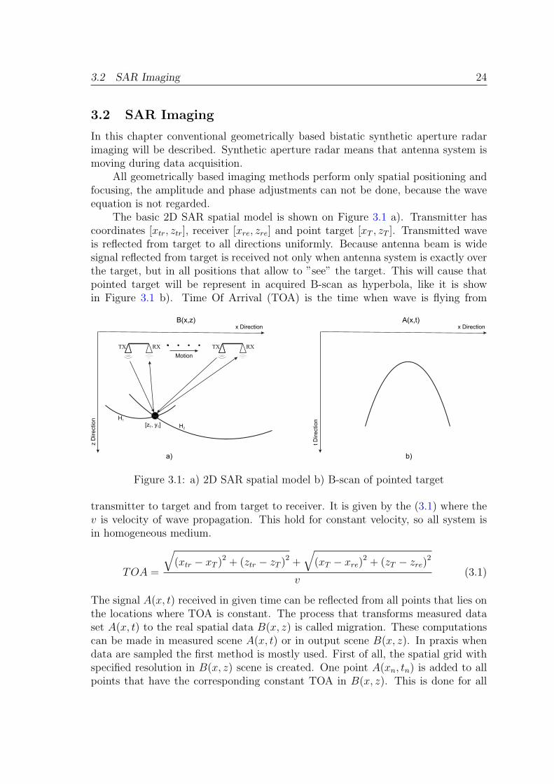
The basic 2D SAR spatial model is shown on Figure 3.1 a). Transmitter hascoordinates [xtr, ztr], receiver [xre, zre] and point target [xT , zT ]. Transmitted waveis reflected from target to all directions uniformly. Because antenna beam is widesignal reflected from target is received not only when antenna system is exactly overthe target, but in all positions that allow to ”see” the target. This will cause thatpointed target will be represent in acquired B-scan as hyperbola, like it is showin Figure 3.1 b). Time Of Arrival (TOA) is the time when wave is flying from
RXTX RXTX
x Direction
zD
ire
ctio
n
[z , yT T]H1
H2
Motion
x Direction
tD
ire
ctio
nA(x,t)B(x,z)
a) b)
Figure 3.1: a) 2D SAR spatial model b) B-scan of pointed target
transmitter to target and from target to receiver. It is given by the (3.1) where thev is velocity of wave propagation. This hold for constant velocity, so all system isin homogeneous medium.
TOA =
√(xtr − xT )2 + (ztr − zT )2 +
√(xT − xre)2 + (zT − zre)2
v(3.1)
The signal A(x, t) received in given time can be reflected from all points that lies onthe locations where TOA is constant. The process that transforms measured dataset A(x, t) to the real spatial data B(x, z) is called migration. These computationscan be made in measured scene A(x, t) or in output scene B(x, z). In praxis whendata are sampled the first method is mostly used. First of all, the spatial grid withspecified resolution in B(x, z) scene is created. One point A(xn, tn) is added to allpoints that have the corresponding constant TOA in B(x, z). This is done for all

3.2 SAR Imaging 25
points from A(x, t). The points that have the same TOA are on hyperbola H withfocuses at transmitter and receiver position (Figure 3.1 a)). Mathematically thisprocess can be written like:
B (xi, zi) =1
N
N∑n=1
A(xn, TOAn) (3.2)
where A(xn, TOAn) are all points that have the same TOA, that is computed by(3.1) for target position [xi, zi].
This method geometrically focus hyperbolas from A(x, t) in to the one pointin B(x, z). Of course this is not ideal approach and this methods produce a lot ofartifacts.
Conflict in names of basic imaging methods become evident in simple geomet-rical approach. This method is often called also back projection [109], [51], [58], [31][66] or diffraction summation [75], [88], [73], [83], [76]. Moreover this geometricalapproach is often incorrectly called Kirchhoff migration [30], [23], [22] [122], [125].
Though the topic is through wall imaging so at least some wall has to beconsidered. Because the wall has another permitivity and permeability like freespace the wave inside the wall will changed the velocity. Wave traveling throughmedium with another permitivity or permeability will cause wave diffraction andrefraction. On Figure 3.2 SAR model with wall is shown.
RXTX
x Direction
zD
ire
ctio
n
[x , zT T]
Wall
�rd 1inwall
d 2inwall
Figure 3.2: Spatial SAR model with wall
The accurate calculation of the total flight time is a critical step. The velocityof the signal inside wall is slower than in free space and this will cause the longerflight time. How to correct the velocity changing inside wall is described by DefenceResearch and Development Canada in [44] and [43]. The time for wave to travel agiven distance dinwall inside a wall is given by:
tinwall =dinwallvwall
(3.3)
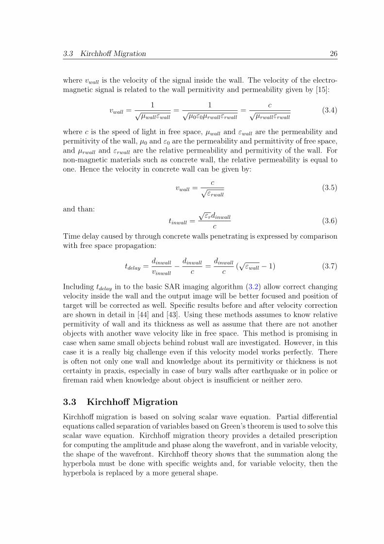
3.3 Kirchhoff Migration 26
where vwall is the velocity of the signal inside the wall. The velocity of the electro-magnetic signal is related to the wall permitivity and permeability given by [15]:
vwall =1
√µwallεwall
=1
√µ0ε0µrwallεrwall
=c
√µrwallεrwall
(3.4)
where c is the speed of light in free space, µwall and εwall are the permeability andpermitivity of the wall, µ0 and ε0 are the permeability and permittivity of free space,and µrwall and εrwall are the relative permeability and permitivity of the wall. Fornon-magnetic materials such as concrete wall, the relative permeability is equal toone. Hence the velocity in concrete wall can be given by:
vwall =c
√εrwall
(3.5)
and than:
tinwall =
√εrdinwallc
(3.6)
Time delay caused by through concrete walls penetrating is expressed by comparisonwith free space propagation:
tdelay =dinwallvinwall
− dinwallc
=dinwallc
(√εwall − 1) (3.7)
Including tdelay in to the basic SAR imaging algorithm (3.2) allow correct changingvelocity inside the wall and the output image will be better focused and position oftarget will be corrected as well. Specific results before and after velocity correctionare shown in detail in [44] and [43]. Using these methods assumes to know relativepermitivity of wall and its thickness as well as assume that there are not anotherobjects with another wave velocity like in free space. This method is promising incase when same small objects behind robust wall are investigated. However, in thiscase it is a really big challenge even if this velocity model works perfectly. Thereis often not only one wall and knowledge about its permitivity or thickness is notcertainty in praxis, especially in case of bury walls after earthquake or in police orfireman raid when knowledge about object is insufficient or neither zero.
3.3 Kirchhoff Migration
Kirchhoff migration is based on solving scalar wave equation. Partial differentialequations called separation of variables based on Green’s theorem is used to solve thisscalar wave equation. Kirchhoff migration theory provides a detailed prescriptionfor computing the amplitude and phase along the wavefront, and in variable velocity,the shape of the wavefront. Kirchhoff theory shows that the summation along thehyperbola must be done with specific weights and, for variable velocity, then thehyperbola is replaced by a more general shape.
3.3 Kirchhoff Migration 27
Kirchhoff migration is mathematically complicated algorithm and is deeply sub-scribed e. g. in [73] and [118] and applied for landmine detection in [40]. In thischapter only short overview of mathematical description will be provided with fo-cusing on physical interpretation of method.
Gauss’s theorem [42] and Green’s theorem [17] is used for Kirchhoff migrationdescription. Gauss’s theorem generalizes the basic integral result (3.8) in to themore dimensions (3.9).
b∫a
φ′(x)dx = φ(x)∣∣ba = φ(b)− φ(a) (3.8)
∫V
−→∇ .−→Advol =
∮∂V
−→A.−→n dsurf (3.9)
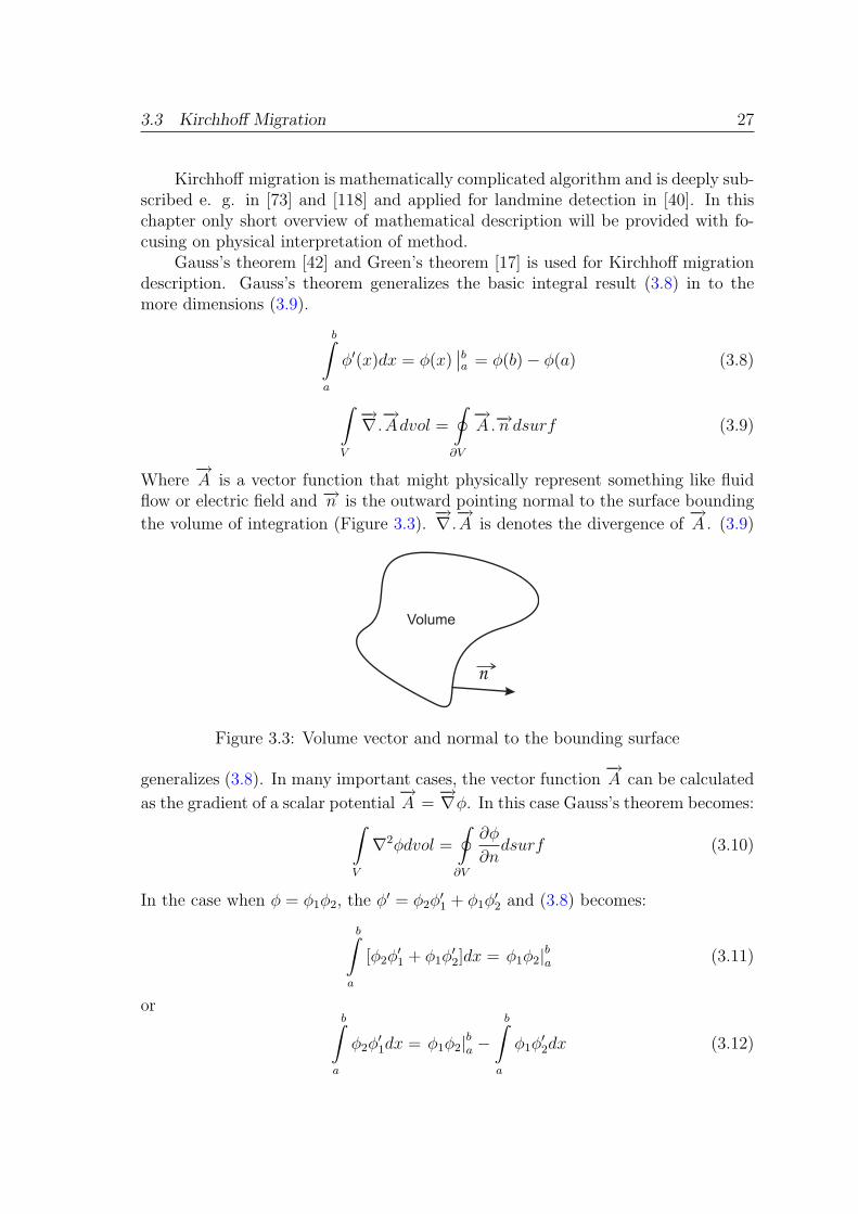
Where−→A is a vector function that might physically represent something like fluid
flow or electric field and −→n is the outward pointing normal to the surface bounding
the volume of integration (Figure 3.3).−→∇ .−→A is denotes the divergence of
−→A . (3.9)
n
Volume
Figure 3.3: Volume vector and normal to the bounding surface
generalizes (3.8). In many important cases, the vector function−→A can be calculated
as the gradient of a scalar potential−→A =
−→∇φ. In this case Gauss’s theorem becomes:∫
V
∇2φdvol =
∮∂V
∂φ
∂ndsurf (3.10)
In the case when φ = φ1φ2, the φ′ = φ2φ′1 + φ1φ
′2 and (3.8) becomes:
b∫a
[φ2φ′1 + φ1φ
′2]dx = φ1φ2|ba (3.11)
orb∫
a
φ2φ′1dx = φ1φ2|ba −
b∫a
φ1φ′2dx (3.12)

3.3 Kirchhoff Migration 28
An analogous formula in higher dimensions arises by substituting A = φ2~∇φ1 into
(3.9). Using the identity ~∇.a~∇b = ~∇a.~∇b+ a∇2b leads to:∫V
[~∇φ2.~∇φ1 + φ2∇2φ1
]dvol =
∮∂V
φ2∂φ1
∂ndsurf (3.13)
Similar result can be obtained when A = φ1~∇2φ2:∫
V
[~∇φ1.~∇φ2 + φ1∇2φ2
]dvol =
∮∂V
φ1∂φ2
∂ndsurf (3.14)
Finally, subtracting (3.14) from (3.13) yields to:∫V
[φ2∇2φ1 − φ1∇2φ2
]dvol =
∮∂V
[φ2∂φ1
∂n− φ1
∂φ2
∂n
]dsurf (3.15)
(3.15) is known as Green’s theorem. It is a fundamental to the derivation of Kirch-hoff migration theory. It is a multidimensional generalization of the integrationby formula from elementary calculus and is valuable for its ability to solve certainpartial differential equation. φ1 and φ1 in (3.15) may be chosen as desired to conve-niently express solutions to a given problem. Typically, in the solution to a partialdifferential equation like the wave equation, one function is chosen to be the solutionto the problem at hand and the other is chosen to be the solution to a simpler ref-erence problem. The reference problem is usually selected to have a known analyticsolution and that solution is called a Greens function [73].
In general, the scalar wavefield ψ is a solution to the Helmholtz scalar waveequation: (
∇2 + k2)ψ = 0 (3.16)
where ∇2 is the Laplacian and k is the wavevector. When the wave travels throughthe medium from point x0 to the point x this Helmholtz scalar wave equation canbe expressed with the aid of Greens function G (x0, x) by:(
∇2 + k2)G (x0, x) = δ (x0 − x) (3.17)
where the δ (x0 − x) is a Dirac delta function. Greens function describes how thewave changes during travel from point x0 to the point x.
Now the Kirchhoff diffraction integral will be described. Let the ψ be a solutionto the scalar wave equation:
∇2ψ (~x, t) =1
v2
∂2ψ (~x, t)
∂2t(3.18)
where v is the wave velocity and don’t have to be a constant. When Green’s theoremfrom (3.15) is applied to the (3.18) with the aid of Helmholtz equation, Hankel
3.3 Kirchhoff Migration 29
functions, piece of luck and good mathematical skill (the complete process can befind in [73]) the Kirchhoff’s diffraction integral can be obtained:
ψ(~x0, t) =
∮∂V
[1
r
[∂ψ
∂n
]t+r/v0
− 1
v0r
∂r
∂n
[∂ψ
∂t
]t+r/v0
+1
r2
∂r
∂n[ψ]t+r/v0
]dsurf (3.19)
where r = |~x− ~x0|, ~x0 is the source position and v0 is a constant velocity. In manycases this integral is derived for forward modeling with the result that all of theterms are evaluated at the retarded time t − r/v0 instead of the advanced time.This Kirchhoff diffraction integral expresses the wavefield at the observation point~xo at time t in terms of the wavefield on the boundary ∂V at the advanced timet + r/v0. It is known from Fourier theory that knowledge of both ψ and ∂nψ arenecessary to reconstruct the wavefield at any internal point.
In order to obtain practical migration formula two essential task are required forconvert (3.19). First, the apparent need to know ∂nψ must be addressed. Second,the requirement that the integration surface must extend all the way around thevolume containing the observation point must be dropped. There are various waysto make both of these arguments. Schneider [103] solved the requirement of ∂nψ byusing a dipole Green’s function with an image source above the recording place, thatvanished at z = 0 and cancelled the ∂nψ term in (3.19). Wiggins in [111] adaptedSchneider’s technique to rough topography. Docherty in [35] showed that a monopoleGreen’s can also lead to the accepted result and once again challenged Schneider’sargument that the integral over the infinite hemisphere can be neglected. After all,migration by summation along diffraction curves or by wavefront superposition hasbeen done for many years. Though Schneider’s derivation has been criticized, hisfinal expressions are considered correct.
As a first step in adapting (3.19) it is usually considered appropriate to discardthe term 1 1
r2∂r∂n
[ψ(~x)]t+r/v0 . This is called the near-field term and decays morestrongly with r than the other two terms. Then, the surface S = ∂V will be takenas the z = 0 plane, S0, plus the surface infinitesimally below the reflector, Sz, andfinally these surfaces will be joined at infinity by vertical cylindrical walls, S∞, Figure3.4. On Figure 3.4 the geometry for Kirchhoff migration is shown. The integrationsurface is S0 + Sz + S∞, only S0 contributes meaningfully to the estimation of thebackscattered field at vx0. Though the integration over S∞ may contribute, but itcan never be realized due to finite aperture limitations and its neglect may introduceunavoidable artifacts. With these considerations, (3.19) becomes:
ψ(~x0, t) =
∮S0
[−1
r
[∂ψ
∂z
]t+r/v0
+1
v0r
∂r
∂z
[∂ψ
∂t
]t+r/v0
]dsurf (3.20)
where the signs on the terms arise because ~n is the outward normal and z is increasingdownward so that ∂n = −∂z.
3.3 Kirchhoff Migration 30
SourceS0
Xs X
X0
Sz
r
Scatterpoint
Image source
SS∞ ∞
θ
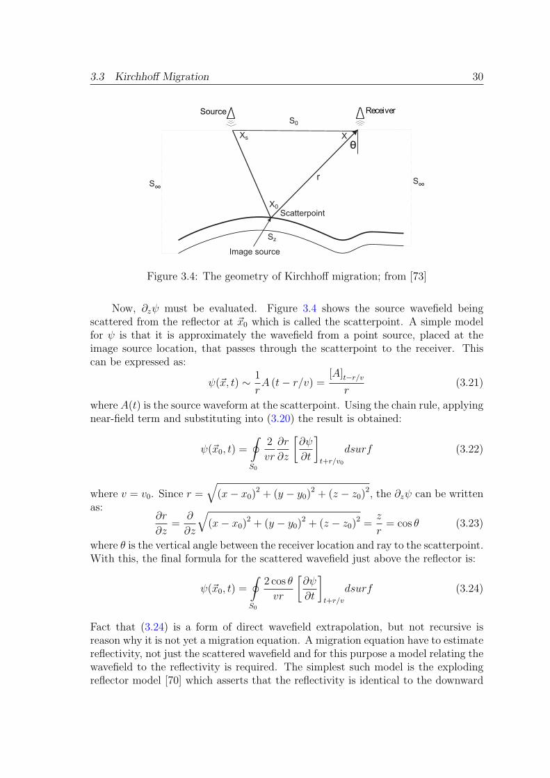
Figure 3.4: The geometry of Kirchhoff migration; from [73]
Now, ∂zψ must be evaluated. Figure 3.4 shows the source wavefield beingscattered from the reflector at ~x0 which is called the scatterpoint. A simple modelfor ψ is that it is approximately the wavefield from a point source, placed at theimage source location, that passes through the scatterpoint to the receiver. Thiscan be expressed as:
ψ(~x, t) ∼ 1
rA (t− r/v) =
[A]t−r/vr
(3.21)
where A(t) is the source waveform at the scatterpoint. Using the chain rule, applyingnear-field term and substituting into (3.20) the result is obtained:
ψ(~x0, t) =
∮S0
2
vr
∂r
∂z
[∂ψ
∂t
]t+r/v0
dsurf (3.22)
where v = v0. Since r =√
(x− x0)2 + (y − y0)2 + (z − z0)2, the ∂zψ can be writtenas:
∂r
∂z=
∂
∂z
√(x− x0)2 + (y − y0)2 + (z − z0)2 =
z
r= cos θ (3.23)
where θ is the vertical angle between the receiver location and ray to the scatterpoint.With this, the final formula for the scattered wavefield just above the reflector is:
ψ(~x0, t) =
∮S0
2 cos θ
vr
[∂ψ
∂t
]t+r/v
dsurf (3.24)
Fact that (3.24) is a form of direct wavefield extrapolation, but not recursive isreason why it is not yet a migration equation. A migration equation have to estimatereflectivity, not just the scattered wavefield and for this purpose a model relating thewavefield to the reflectivity is required. The simplest such model is the explodingreflector model [70] which asserts that the reflectivity is identical to the downward

3.4 f-k Migration 31
continued scattered wavefield at t = 0 provided that the downward continuation isdone with ~v = v/2. Thus, an wave migration equation follows immediately fromequation (3.24) as:
ψ(~x0, 0) =
∮S0
2 cos θ
~vr
[∂ψ
∂t
]r/~v
dsurf =
∮S0
4 cos θ
vr
[∂ψ
∂t
]2r/v
dsurf (3.25)
Finally this is a Kirchhoff migration equation. This result was derived by manyauthors including Schneider [103] and Scales [99]. It expresses migration by sum-mation along hyperbolic travelpaths through the input data space. The hyperbolicsummation don’t have to be seen at the first point of view, but it can be indicatedby [∂tψ]2r/v, notation means that partial derivation is to be evaluated at the time2r/v. ∂tψ (~x, t) is integrated over the z = 0 plane, only those specific traveltimesvalues are selected by:
t =2r
v=
2√
(x− x0)2 + (y − y0)2 + (z − z0)2
v(3.26)
which is the equation of a zero-offset diffraction hyperbola.In addition to diffraction summation, (3.25) requires that the data be scaled by
4cosθ/(vr) and that the time derivative be taken before summation. These addi-tional details were not indicated by the simple geometric theory of section 3.2 and aremajor benefits of Kirchhoff theory. It is these sort of corrections that are necessaryto move towards the goal of creating bandlimited reflectivity. The same correctionprocedures are contained implicitly in f-k migration that will be described in section3.4. Kirchhoff migration is one of the most adaptable migration schemes available.It can be easily modified to account for such difficulties as topography, irregularrecording geometry, pre-stack migration, converted wave imaging etc. Computationcost is one of the few disadvantages of this method.
3.4 f-k Migration
Wave equation based migration can be done also in frequency domain. Mr. Stoltin 1978 showed that migration problem can be solved by Fourier transform [106].The basic principle will be described for 2D problem. Completely mathematicallysolution is very precisely shown in [106] or in [73], so only the basic relations andprinciple of the method will be shown in this work.
Scalar wavefield ψ (x, z, t) is a solution to:
∇2ψ − 1
v2
∂2ψ
∂t2= 0 (3.27)
where v is the constant wave velocity. It is desired to compute ψ (x, z, t = 0) whatis wave in time zero - time when doted point with coordinates [x, y] start radiating.

3.4 f-k Migration 32
While ψ (x, z = 0, t) is given by measuring and it expressing wave in position z = 0where the antennas are positioned. Wavefield can be expressed also in frequency(kx, f) domain, than ψ (x, z, t) is computing from inverse Fourier transform:
ψ(x, z, t) =
∫∫φ (kx, z, f) e2πi(kxx−ft)dkxdf (3.28)
where cyclical wavenumbers and frequencies are used and the Fourier transformconvention uses a + sign in the complex exponential for spatial components (kxx)and a − sign for temporal components (ft). If (3.28) is substituted into (3.27), somemathematical trick can be done and the result is:∫∫ {
∂2φ(z)
∂z2+ 4π2
[f 2
v2− k2
x
]φ(z)
}e2πi(kxx−ft)dkxdf = 0 (3.29)
If v is constant, then the left-hand-side of (3.29) is the inverse Fourier transformof the term in curly brackets. From Fourier theory is known that if signal in onedomain is zero than also in another domain will be zero. This results to:
∂2φ(z)
∂z2+ 4π2k2
zφ(z) = 0 (3.30)
where the wavenumber kz is defined by
k2z =
f 2
v2− k2
x (3.31)
(3.30) and (3.31) are a complete reformulation of the problem in the (kx, f) domain.The boundary condition is now φ (x, z = 0, t) which is the Fourier transform, over(x, t), of ψ (x, z, t). (3.30) is a second-order differential equation with exact solutione±2πikzz, Thus the unique solution can be written by substitution:
φ (kx, z, f) = A (kx, f) e2πikzz +B (kx, f) e−2πikzz (3.32)
where A (kx, f) and B (kx, f) are arbitrary functions of (kx, f) to be determinedfrom the boundary condition(s). The two terms on the right-hand-side of (3.32)have the interpretation of a downgoing wavefield, A (kx, f) e2πikzz, and an upgoingwavefield, B (kx, f) e−2πikzz. Downgoing is mean like in z direction and upgoing in−z direction.
It is now apparent that only one boundary condition φ (x, z = 0, t) is not enoughand the solution will be not unambiguous. To remove this ambiguity the two bound-ary condition are needed for example ψ and ∂zψ, but this is not known in our caseso the migration problem is said to be ill-posed and another trick have to be used.If both conditions were available, A and B could be found as the solutions to φ forz = 0 and it will be specified as φ0 as well as ∂φ/∂z will be specified as φz0:
φ(z = 0) ≡ φ0 = A+B (3.33)
3.4 f-k Migration 33
and∂φ
∂z(z = 0) ≡ φz0 = 2πikzA− 2πikzB (3.34)
The solution for this ill-posed problem and ambiguity removing will be done byassumption the one-way waves. In the receiver position the wave can not be down-going, only upgoing. This allows the solution:
A(kx, f) = 0 and B(kx, f) = φ0(kx, f) ≡ φ(kx, z = 0, f) (3.35)
Then, the wavefield can be expressed as the inverse Fourier transform of φ0:
ψ(x, z, t) =
∫∫φ0(kx, f)e2πi(kxx−kzz−ft)dkxdf (3.36)
and the migrated solution is:
ψ(x, z, t = 0) =
∫∫φ0(kx, f)e2πi(kxx−kzz)dkxdf (3.37)
(3.37) gives a migration process as a double integration of φ0(kx, f) over f andkx. Even if it looks like the solution is complete, it has the disadvantage thatonly one of the integrations, that over kx, is a Fourier transform that can be doneby a fast numerical FFT. The f integration is not a Fourier transform becausethe Fourier kernel e−2πft was lost when the imaging condition (setting t = 0) wasinvoked. However another complex exponential e−2πikzz show up in (3.37). Stoltsuggested a change of variables from (kx, f) to (kx, kz) to obtain a result in whichboth integrations are Fourier transforms. The change of variables is defined by (3.31)and can be solved for f to give:
f = v√k2x + k2
z (3.38)
Performing the change of variables from f to kz according to the rules of calculustransforms (3.37) will yield into:
ψ(x, z, t = 0) =
∫∫φm(kx, kz)e
2πi(kxx−kzz)dkxdkz (3.39)
where
φm(kx, kz) ≡∂f(kz)
∂kzφ0(kx, f(kz)) =
vkz√k2xk
2z
φ0(kx, f(kz)) (3.40)
(3.39) is Stolts expression for the migrated section and forms the basis for the f-kmigration algorithm. The change of variables has reform the algorithm into onethat can be accomplished with FFTs doing all of the integrations. (3.40) resultsfrom the change of variables and is a prescription for the construction of the (kx, kz)spectrum of the migrated section from the (kx, f) spectrum of the measured data.
On Figure 3.5 same examples of transformation from (kx, kz) to (kx, f/v) spaceand vice versa are shown. The v is constant wave velocity. This geometric relation-

3.4 f-k Migration 34
0
0.02
0.04
0.06
0.08
0.1
f/v
-0.06 -0.02 0 0.02 0.06kx
k =.04z
k =.06z
k =.02z
wavelike
0
0.02
0.04
0.06f/v=.06
kz
-0.06 -0.02 0 0.02 0.06kx
f/v=.04
f/v=.02
(k ,f/v)x
(k , )x kz
Figure 3.5: Comparison images in (kx, f/v) space - left side, with (kx, kz) space -right side; from [73]
ships between (kx, kz) and (kx, f/v) can be explained as follows: In (kx, f/v) space,the lines of constant kz are hyperbolas that are asymptotic to the dashed boundary,they are transform in to the (kx, kz) space like curves of constant f/v - semi-circleand vice versa. At kx = 0 and kz = f/v these hyperbolas and semi-circles intersect,when the plots are superimposed. Conceptually, it can also be viewed as a conse-quence of the fact that the (kx, f) and the migrated section must agree at z = 0 andt = 0.
On a numerical dataset, this spectral mapping is the major complexity of theStolt algorithm. Generally, it requires an interpolation in the (kx, f) domain sincethe spectral values that map to grid nodes in (kx, kz) space cannot be expected tocome from grid nodes in (kx, f) space. In order to achieve significant computationspeed that is considered the strength of the Stolt algorithm, it turns out that theinterpolation must always be approximate. This causes artifacts in the final result.The creation of the migrated spectrum also requires that the spectrum be scaled byvkz/
√k2x + k2
z like it is shown in (3.40).The f-k migration algorithm just described is limited to constant velocity. Its
use of Fourier transforms for all of the numerical integrations means that it is com-putationally very efficient.
Stolt provided an approximate technique to adapt f-k migration to non constantwave velocity v(z). This method used a pre-migration step called the Stolt stretch,after this step classical f-k migration has followed. The idea was to perform a one-dimensional time-to-depth conversion with v(z) and then convert back to a pseudotime with a constant reference velocity. The f-k migration is then performed withthis reference velocity. Stolt developed the time-to-depth conversion to be donewith a special velocity function derived from v(z) called the Stolt velocity. Thismethod is now known to progressively lose accuracy with increasing dip and haslost favor. A technique that can handle this problem more precisely is the phase-shift method of Gazdag and is described here [45]. Unlike the direct f-k migration,
3.4 f-k Migration 35
phase shift is a recursive algorithm that process v(z) as a system of constant velocitylayers. In the limit when layer thickness is going to be infinity small, any v(z)variation can be modeled. This method has quite complicated geometrically andlong mathematically representation that is very precisely described in [45] and reallyuserfriendly described in [73]. Hove does it work for one layer will be described inthis work.
The method can be derived starting from (3.36). Considering the first velocitylayer only, this result is valid for any depth within that layer provided that v isreplaced by the first layer velocity, v1. If the thickness of the first layer is ∆z1, thenthe wavefield just above the interface between layers 1 and 2 can be written as
ψ(x, z = ∆z1, t) =
∫∫φ0(kx, f)e2πi(kxx−kz1∆z1−ft)dkxdf (3.41)
where
kz1 =
√f 2
v21
− k2k (3.42)
(3.41) is an expression for downward continuation or extrapolation of the wavefieldto the depth ∆z1. The wavefield extrapolation expression in (3.41) is more simplywritten in the Fourier domain to suppress the integration that performs the inverseFourier transform:
φ(kx, z = ∆z1, f) =
∫∫φ0(kx, f)e2πikz1∆z1 (3.43)
Now consider a further extrapolation to estimate the wavefield at the bottom oflayer 2 (z = ∆z1 + ∆z2). This can be written as:
φ(kx, z = ∆z1 + ∆z2, f) = φ(kx, z = ∆z1, f)T (kx, f)e2πikz2∆z2 (3.44)
where T (kx, f) is a correction factor for the transmission loss endured by the waveas it crossed from layer 2 into layer 1.
If this method want to be applied in praxis, phase shift algorithm [73] haveto be under study more deeply in order to prevent many of unwanted effects andcorrect implementation.
The Fourier method discussed in this section is based upon the solution of thescalar wave equation using Fourier transforms. Though Kirchhoff methods seemsuperficially quite different from Fourier methods, the uniqueness theorems frompartial differential equation theory guarantee that they are equivalent [73]. However,this equivalence only applies to the problem for which both approaches are exactsolutions to the wave equation and that is the case of a constant velocity medium,with regular wavefield sampling. In all other cases, both methods are implementedwith differing approximations and can give very distinct results. Furthermore, evenin the exact case, the methods have different computational artifacts [73].

3.5 Multiple Signal Classification 36
3.5 Multiple Signal Classification
MUltiple SIgnal Classification (MUSIC) is generally used in signal processing prob-lems and was firstly introduce by Therrien in 1992 [108]. It is a method for estimat-ing individual frequencies of multiple time harmonic signals. The use of MUSIC inimaging was first proposed by Devaney in 2000 [32]. He applied the algorithm to theproblem of estimating the locations of a number of point-like scatterers. Detaileddescription is in [32], [21] and [62].
MUSIC for image processing has been developed for multistatic radar systems.It is the way equations based method. The basic idea of MUSIC is the formulationof the so called multistatic response matrix which is then used to compute thetime reversal matrix whose eigenvalues and eigenvectors are shown to correspondto different point-like targets. The multistatic response matrix is formulated usingfrequency domain data, which is obtained by applying the Fourier transform to thetime domain data.
N antennas are centered at the space points Rn, n = 1, 2, ..., N . The positionsof the antennas are not necessarily restricted to be in the same plane or regularlyspaced. The n-th antenna radiate a scalar field ψn (r, ω) into a half space in which areembedded one or more scatterers (targets). M (M ≤ N) is the number of scatterersand Xm is the location of the m-th target in the space. Born approximation is againconsidered [38], [19]. The waveform radiated by the n-th antenna, scattered by thetargets and received by the j-th antenna is given by:
ψn (Rj, ω) =M∑m=1
G (Rj, Xm) τm (ω)G (Xm, Rn) en (ω) (3.45)
where G (Rj, Xm) and G (Xm, Rn) are the Green’s functions of the Helmholtz equa-tion in the medium in which the targets are embedded in direction from transmitterantenna to the target and from the target to the receiving antenna respectively.τm (ω) represents the strength of the m-th target and en (ω) is the voltage appliedat the n-th antenna. In this formula, the signal is only considered for a singlefrequency ω. However, the extension for multiple frequencies is obviously. Themultistatic response matrix K is defined by:
Knj =M∑m=1
G (Rj, Xm) τm (ω)G (Xm, Rn) (3.46)
The scattered waveform emitted at each antenna is measured by all the antennas,so the elements of the multiple response matrix K can be calculated by:
Knj =ψn (Rj, ω)
en (ω)(3.47)
The main idea of MUSIC is to decompose a selfadjoint matrix into two or-thogonal subspaces which represent the signal space and the noise space. Since the
3.6 The Inverse Problem 37
multistatic response matrix is complex, symmetric but not Hermitian (i.e. it is notself-adjoint), the time reversal matrix T is defined from the multistatic responsematrix:
T = Knj ∗Knj (3.48)
where ∗ means the complex conjugation. The time reversal matrix has the samerange as the multistatic response matrix. Moreover, it is selfadjoint. The timereversal matrix T can be represented as the direct sum of two orthogonal subspaces.The first one is spanned by the eigenvectors of T with respect to non-zero eigenvalues.If noise is presence, this subspace is spanned by the eigenvectors with respect toeigenvalues that greater than a certain value, which is specified by the noise level.This space is referred to as the signal space. Note that its dimension is equal tothe number of the point-like targets. The other subspace, which is spanned bythe eigenvectors with respect to zero eigenvalues (or the eigenvalues smaller than acertain value in the case of noisy data), is referred to as noise subspace. That is,denote by the eigenvalues:
λ1 ≥ λ2 ≥ ... ≥ λM ≥ λM+1 ≥ ... ≥ λN ≥ 0 (3.49)
of the time-reversal matrix T and vn, n = 1, 2, ..., N are the corresponding eigen-vectors. Then the signal subspace is spanned by v1, , vM and the noise subspace isspanned by the remaining eigenvectors. For detection of the target the vector gp iscalculated from form the vector of the Greens functions:
gp = (G (R1, p) , G (R2, p) , ..., G (RN , p))′ (3.50)
The point P is at the location of one of the point-like targets if and only if thevector gp is perpendicular to all the eigenvectors vn, n = M + 1, , N . In practice,the following pseudo spectrum is usually calculated by:
D (P ) =1
N∑n=M+1
|(vn, gp)|2(3.51)
The point P belongs to the locations of the targets if its pseudo spectrum is verylarge (theoretically, in the case of exact data, this value will be infinity).
Take in to the account wall in this case can be done by applying Greens functionthat consider wall, what is a big challenge.
3.6 The Inverse Problem
Radar devices generally produce an image which requires considerable skill, abilityand experience in interpretation of data to detect and localise multiple targets.Mathematical methods that can provide this has to allow detection and localisationof the objects as well as the ability to retrieve information about its shape, dielectricpermittivity and conductivity.
3.6 The Inverse Problem 38
Inverse problem is method that estimate both the location and the physicalparameters of the targets like permittivity and conductivity. The main idea is to usesome basic imaging method that estimate initial conditions for inverse problem andthen solve inverse problem what leads to estimate location and physical parametersof the targets. There are many various mathematically more or less complicatedmodels how to solve inverse problem and in the last time this topic becomes anindividual science discipline. In conjunction with radar imaging some of good workscan be find in [28] - chapter 7.9, [59] - chapter 6, or [79], [6], [12], [14], [25]. In thiswork only basic principle will be introduced.
From this point of view, migration can be mean as an approximate solutionto the general elastic wavefield inversion problem [46]. Full elastic inversion usesthe entire measured wavefield as input into a mathematical process that seeks toestimate the elastic parameters of the device under test. This is called an inverseproblem because it is opposite to the classical forward modeling problem (subsection3.3) of predicting the measured wavefield response of a known elastic device undertest model. Generally, a forward problem can be reduced to find the solution to apartial differential equation, in this case the elastic wave equation, given specifica-tions of the coefficients of the equation as functions of position and given appropriateboundary conditions. Though often this is a very difficult process, it is usually moreeasily accomplished than the corresponding inverse problem. The inverse problemusually involve estimating the coefficients of a partial differential equation given itsresponse to a known source. Often, these inverse problems are ill-posed which is amathematical term for a problem whose inputs are insufficient to determine all ofits expected outputs. In addition, to being ill-posed, inversion problems are gener-ally nonlinear and practical schemes are typically linearized approximations. Theneed to find approximate solutions has lead to a large number of different migrationalgorithms that are generally distinguished by the kind of approximations made. Atrue inversion technique would derive the velocity model from the data as part ofthe inversion. Migration requires the velocity model as input to focus, and adjustamplitudes. In order to be a useful process, it should be true that migration requiresonly an approximate, or background, velocity model and that more detailed velocityinformation can be extracted from a successful migration than was input to it [73].
The possibility of ”looking” at the interior of an object is based on the factthat the incident wave penetrates inside the object itself, collects information aboutits interior and finally is scattered, delivering such information to the receivers. Al-though the capability of penetrating objects is part of the features of microwaves,there exists, however, a class of ’impenetrable’ objects. Rigorously speaking, ’im-penetrable’ are objects made up of perfect conductors, whereas objects made upof ’strong conductors’ are ’almost impenetrable’, in the sense that the impingingwave penetrates inside the object only to a shallow depth [55]. For such a class ofobjects, it is thus possible to reconstruct only the objects shape but not to ’look’inside them. This is what happens at optical frequencies, when the impinging elec-tromagnetic radiation does not significantly penetrate inside objects of which our

3.6 The Inverse Problem 39
eyes are capable of seeing only the shape but not the interior [28]. Nevertheless, theinverse problem methods refer only with penetrable objects.
A practical implementation of inverse problem can be find e.g. in [59]. In thiscase it is used for landmine detection. At the first step, the position and overallshapes of the objects is computed in a fast manner. For this purpose the MUSICalgorithm [102], [21] is used. After this first step the method chosen to solve thelinearized problem is the Algebraic Reconstruction Technique (ART) [64], [57] whichis a widely accepted fast linear solution method. ART is used to determine theparameters of the objects, e.g. the parameter values of trinitrotoluene in landmine.Both MUSIC and ART algorithms was developed for a monofrequency method andin [59] Kempen introduced these algorithms with multifrequency approach. Theresults from practical example of landmine detection are showed in [59]. It canbe seen that results obtained by inverse problem are better than by conventionalKirchhoff migration.
Short review of using MUSIC and ART algorithm for diffraction tomographycan be found in [60].
Anyway, one has to mention that inverse problem require huge computationcost which make impossible to use this method real time with present computingtechnique.
4 Improvements in Radar Imaging 40
4 Improvements in Radar Imaging
In previous chapter four basic imaging approaches were described. In this chaptersome improved methods, that increase image quality, decrease computational cost,or are better in something else are shown. Though the topic of radar imaging is veryextensive, and spread in many branch, only some of the improvements with focuson the methods that are most relates to through wall imaging are shown.
4.1 Cross-correlated Back Projection
Senglee Foo and Satish Kashyap from Defence Research & Development Canadacame with first idea to use cross-correlation in back projection [41] in 2004. Theprinciple is the same like classical geometrical approach described in chapter 3.2, butwith one improvement. N receive antennas and one transmit antenna are movingduring measurement like one antenna array. In addition, one more receive antennais stationary during measurement and is used like a reference antenna. The classicalback projection can be described by:
o(x, z) =1
N
N∑n=1
Rn
(dTX + dRXn
v
)(4.1)
where dTX is distance from TX to the examined point, dRXn is distance from exam-ined point to the n-th receiver, v is propagation velocity, Rn is the amplitude of n-threceiver and o(x, z) is migrated image in examined point. These summations willlead to creating unwanted effect in points where point of scatterer are not present.Cross-correlated back projection can be described by:
o(x, z) =1
N
N∑n=1
Rn
(dTX + dRXn
v
)Rref
(dTX + dRXref
v
)(4.2)
where Rref is amplitude from reference receiver. Since two different delay termsin conjunction have to match the actual scattering scenario, the probability to add”wrong” energy to an image pixel, which does not coincide with the point scatterer,will be drastically reduced. Rudolf Zetik et al. in [124] in 2005 showed the modifi-cation of Foo’s method in two steps. First, he didn’t use signal from receiver at allpositions, but only at antenna positions in which can antenna receive signal fromexamined point. By another words it can be said that he took to the account theantenna pattern beam by integration only over the duration T (e.g. effective widthof the impulse):
o(x, z) =1
N
N∑n=1
T/2∫−T/2
Rn
(dTX + dRXn
v+ ξ
)Rref
(dTX + dRXn
v+ ξ
)dξ (4.3)

4.2 Fast Back Projection 41
While Foo used reference antenna the stationary one, Zetik used like referenceantenna the same antenna, but with signal received some time before in SAR mea-surement. This will provide same purpose, but with one less antenna necessity.Even more Zetik came with idea to use one more reference receiver e.g. in sometime after actual measurement. The final modified cross-correlated back projectioncan be expressed by [124]:
o(x, z) =1
N
N∑n=1
T/2∫−T/2
Rn
(dTX + dRXn
v+ ξ
)Rref1
(dTX + dRXn
v+ ξ
)
Rref2
(dTX + dRXn
v+ ξ
)dξ
(4.4)
This modified cross-correlated back projection reduce the unwanted artifacts betterthan classical cross-correlated back projection and shows better results on experi-mental examples that can be seen in [124].
4.2 Fast Back Projection
Fast back projection algorithm was firstly developed for tomography by Amir Boaget al. [15] and later modified for airplane SAR imaging by Shu Xiao et al. in[112]. The main advantage of this method is the smaller computation complexityin comparison with classical back-projection described in chapter 3.2. Classicalback projection require O(N3) operations to generate N projections for N × Nimage whereas fast back projection requires only O (N2 logN) operations. The fastback projection algorithm is performed in two parts. First, the received data arerecursively factorised into a number of decimated data-sets for subimages of thereconstructed image. An example of factorisation is shown on Figure 4.1 (upperside), the resultant hierarchy of data-sets is shown on lower side.
Figure 4.1: An example of factorisation (upper side) and the resultant hierarchy ofdata-sets (lower side)

4.3 Migration by Deconvolution 42
Second, each data-set is back-projected to the corresponding subimage. Acomputational gain is achieved through decimating the data in the factorisationstep. However, doing so introduces an error that degrades the image quality [53].There were made lot of modifications in fast projection algorithm, like filtered back-projection [8], fast factorised back-projection [34], [109], quadtree back projection[74], omega-k quadtree back projection [24], etc. However none of these methodshas better accuracy like classical back projection, or faster computations like f-kmigration.
4.3 Migration Technique Based on Deconvolution
This method is described by Bert Scheers and Marc Acheroy (ELTE Department,Royal Military Academy) and Andre Vander Vorst (Hyperfrequences UCL, Belgium)in David Daniels book [28] chapter 7.5.1 and in Bart Scheers PhD thesis [100]. It isapplied for landmine detection. None of methods mentioned above include systemaspects of the radar like the waveform of the excitation source, the impulse responseof the antennas, the antenna pattern, etc. Furthermore, most of the migrationmethods consider the ground as being loss-less and without dispersion. It can beexpected that a migration technique that takes into account the characteristics of theradar system and possibly the characteristics of the ground would perform betterand this is the case of this method. Bert Scheers described this method on the”radar-ground-target” model, however, it can be also used for ”radar-wall-target”model.
A time-domain model of the radar system is used for the forward modeling.The time-domain model is obtained by considering the total system ”radar-ground-target” as a cascade of linear responses, resulting in a time-domain radar rangeequation. The time-domain radar range equation allows to calculate the receivedvoltage at the output of the receiving antenna in terms of excitation voltage, radarcharacteristics and target. Radar range equation involves the pulse generator, theantennas modeled by their normalized impulse response, the 1/R spreading losses,the transmission coefficients on the airground interface, the propagation through theground and the scattering on the target in the ground. Mathematically the timedomain radar range equation is expressed as [100]:
Vrec(t) =Ta−gTg−a8π2dtdrc
gd(t) ∗ hN,Tx(~ai, t) ∗ Λ1,1(~ai,~as, t) ∗ hN,Rx(−~as, t) ∗dVs(t)
dt(4.5)
where Vs(t) is the excitation voltage applied at the transmitting antenna, ~ai is thedirection of radiation of the transmitting antenna towards the target, ~as is the direc-tion of the scattered field from the target towards the receiving antenna, hN,Tx(~ai, t)is the normalised Impulse Response (IR) of the transmitting antenna in the direction~ai, hN,Rx(−~as, t) is the normalised IR of the transmitting antenna in the direction−~as, gd(t) is the impulse response representing the two-way path length loss and thedispersion in the ground, Λ1,1(~ai,~as, t) is the IR of the target (the time equivalent
4.4 SEABED and IBBST 43
of the square root of the target radar cross-section), dt is the total path length fromthe transmitting antenna to the target, dr is the total path length from the receivingantenna to the target, Ta−g is the transmission coefficient at the air-ground inter-face (air to ground), Tg−a is the transmission coefficient at the air-ground interface(ground to air).
Antennas IR can by obtained by precisely antenna measurements in free spaceor anechoic chamber room and ground IR can be modeled as a lowpass filter [100].The migration method is based on the deconvolution of the recorded data with thepoint-spread function of the radar system, calculated using the time-domain model:
Λ(x, y, t) = b(x, y, t) ∗x,y,t w(x, y, z0, t)−1 (4.6)
where Λ(x, y, t) denotes the spatial image of Λ(x, y, t) at point z0 i.e. the migratedimage, b(x, y, t) is the recorded C-scan that is migrated and w(x, y, zo, t) is the pointspread function for a fixed depth z = zo. Solving (4.6) is a classical ill-posed problemand solution is provided by the same way like in f-k migration in section 3.4 but inthree dimensions. The migrated image is given by the inverse 3D Fourier transform:
Λ(x, y, t) =1
2π
∫∫∫Λ(kx, ky, ω)e−i(kxx+kyy−ωt)dkxdkydω (4.7)
The aim of migration is to focus reflections on objects back into the true physicalshape of the object but also into its true position. From results shown in [59] can beseen that this method reconstructs object position much closer to the true positionlike classical f-k migration. Moreover, from image obtained by this method can beclearly seen that the object is oblique.
4.4 SEABED and IBBST
Shape Estimation Algorithm based on Boundary Scattering Transform (BST) andExtraction of Directly scattered waves (SEABED) algorithm was introduced byTakuya Sakamoto et al. [95] in 2004. Algorithm uses very simple geometrical ap-proach without velocity compensation based on Inverse Bistatic Boundary Scatter-ing Transform (IBST) [96]. First, from measured raw data (B-scan) the image ofthe wave front is derived. This means to find peaks, so the image of front wavecontains only 2 amplitudes, amplitude zero where is nothing and amplitude 1 whereis front wave. When this image is obtained correct, then transformation from thisf(X, Y, Z) space (before imaging) to the real f(x, y, z) space (after imaging) can bedone by simple geometrical approach [95]:
x = X − Z dZdX
y = Y − Z dZdY
z = Z
√1−
(dZ
dX
)2
(4.8)
4.5 f-k Migration Improvements 44
SEABED was developed for monostatic approach. Shouhei Kidera et al. in [61] in2006 introduce IBBST what is bistatic modification of SEABED. Transformationfrom f(X, Y, Z) space to the real f(x, y, z) space can be done by:
x = X − 2Z3Zx
Z2 − d2 +√
(Z2 − d2)2 + 4d2Z2Z2X
y = Y + ZY{d2 (x−X)2 − Z4
}/Z3
z =
√Z2 − d2 − (y − Y )2 − (Z2 − d2) (x−X)2 /Z2
(4.9)
where d is distance between transmitter and receiver.SEABED method was used for detecting the contours of objects behind wall
by Sebastian Hantscher et al. in [49] in 2006. The results are compared withkirchhoff migration and f-k migration on very simple scenario, the cylinder waspositioned behind a wall with a smooth surface [49]. Really great improvement incomputational time, even ten times faster than f-k migration was obtained. It isbecause number of points with nonzero amplitude in f(xw, zw) space is very small.Also the shape of cylinder is very similar to the true one. But this was very simpleand idealized experiment, processing with real and practical data will probablybrings problems, due to non ideal wave front estimation.
4.5 f-k Migration Improvements
f-k migration obtained title of most often used migration method in praxis due toits fast computation and very precise image results. This is the main reason whyf-k migration has lots of improvements and modifications. Some of them will bedescribed in this section.
4.5.1 Nonuniform FFT
Important contributions to this method are from Dutt and Rokhlin [37], G. Beylkin[13] and Qing H. Liu and N. Nguyen in [69]. NonUniform Fast Fourier Transfor-mation (NUFFT) is based on classical Stolt migration with some improvements.Stolt migration require for using FFT algorithms equally spaced input data. Inmany practical situations, however, the input data is nonuniform (i.e., not equallyspaced), that is why the regular FFT can not be applied. NUFFT propose an ap-proach to achieve the fast Fourier transform for nonuniform data by using an anotherclass of matrices, the regular Fourier matrices [80]. This algorithm, with the samecomplexity like Stolt migration O (N2 logN) where N is the number of data points,is more accurate, because approximation error is minimized in the leastsquare sense.Stolt migration require so called stolt interpolation which is cumbersome and reducesthe computational efficiency of the Stolt algorithm. NUFFT does not require Stoltinterpolation. Simply, NUFFT firstly compute Fourier coefficients with using the

4.5 f-k Migration Improvements 45
regular Fourier matrices, with this coefficients compute uniform FFT and than scaleresults back in to the nonuniform space. However, from mathematical point of viewit is not so simple and it is detailed described in [69].
Very nice review of more NUFFT’s methods in comparison with classical f-kmigration tested on simulated data were done by B. Subiza et al. in [107].
4.5.2 f-k Migration in Cylindrical Coordinations
f-k migration transformed in to the cylindrical coordinate system was described byMark A. Haun et al. in [50] in 2000. He obtain a three-dimensional, frequency-domain imaging algorithm for cylindrical geometry by making suitable approxima-tions to the point spread function for wave propagation in cylindrical coordinates andobtaining its Fourier transform by analogy with the equivalent problem in Cartesiancoordinates. The focus is treated as a diverging source by the imaging algorithm,which then forms images on deeper cylindrical shells. Computer simulations andexperimental results using wire targets show that this imaging technique attainsthe resolution limit dictated by the operating wavelength and the transducer char-acteristics. Simulations were done with microprobe rotating around own axle andfive point reflectors. Measurements were done with three 100 µm thick wire targetslocated beyond the transducer focus.
4.5.3 f-k Migration with Motion Compensation
f-k migration with integrated motion compensation for airborne measuring was de-scribed by A. Reigber et al. in [85] in 2006. In the case of airborne measurements,wavenumber-domain processing is limited because of its inability to perform high-precision motion compensation. Extended Chirp Scaling (ECS) [77] algorithm hasproven to be very powerful, although it has certain limitations concerning longaperture syntheses and highly squinted geometries. Reigber in this paper analyti-cally derived a new stripmap SAR data-processing algorithm, called Extended ωk(EOK). The EOK algorithm aims to combine the high focusing accuracy of thewavenumber-domain algorithm with the high-precision motion compensation of theECS algorithm. The EOK algorithm integrates a three-step motion compensationcorrection in the general formulation of the wavenumber-domain algorithm, leadingto a new airborne SAR processing scheme, which is also very robust in the cases oflong synthetic apertures and high squint angles. It offers the possibility of processingwide-band, low-frequency airborne SAR data up to near wavelength resolution. Theperformance and accuracy of the EOK SAR data-processing algorithm were demon-strated using simulated data in different data collection scenarios and geometriesas well as using interferometric data acquired by the airborne experimental SARsystem of DLR at L-band.
4.5 f-k Migration Improvements 46
4.5.4 f-k Migration with Ground Surface and Non Loss-Free Compen-sation
Standard f-k migration assumes that the ground surface is flat and the medium isloss-free which are not true in reality. Xiaoyin Xu and Eric L. Miller in [114] adaptit to rough ground surface and lossy medium. When implemented in the Fourierdomain, the wave equation becomes the Helmholtz equation. It is then straight-forward to incorporate a complex index of refraction in the Helmholtz equation todescribe wave phenomenon in lossy medium [33]. Here the f-k migration is gener-alized to the case of rough ground surface and lossy medium. In the framework ofTikhonov regularization [39], [65], an algorithm was developed that optimally altersthe wave propagation velocity and the complex index of refraction to take into ac-count of the ground roughness and lossy medium. In the process of searching theoptimal velocity and complex index of refraction, the algorithm is constrained toproduce an image of minimum entropy. By minimizing the entropy of the result-ing image, better results are obtained in terms of enhanced mainlobe, suppressedsidelobes, and reduced noise.
4.5.5 Prestack Residual f-k Migration
Prestack residual migration in the frequency domain introduced Paul C. Sava in[97] in 2003. This method has advantages over classical f-k migration that estimateinterval velocity functions for depth migration. It is more accurate than methodsthat are based on focusing the stack of migrated images, so it provides a more accu-rate estimate of the correct migration velocities. Although the theory is developedassuming constant velocity, the method can be used for depth-migrated images pro-duced with smoothly varying velocity models, since the residually migrated imagesdepend only on the ratio of the reference and updated velocities.
4.5.6 f-k Migration with Anti-Leakage Fourier Transform
This method was introduced by Sheng Xu and Don Pham in [113] in 2004. Its aimis to estimate the spatial frequency content on an irregularly sampled grid. Afterobtaining the Fourier coefficients, the data can be reconstructed on any desired grid.For this type of transform, difficulties arise from the non-orthogonality of the globalbasis functions on an irregular grid. As a consequence, energy from one Fourier coef-ficient leaks onto other coefficients. This well-known phenomenon is called spectralleakage. Anti-leakage Fourier transform, for seismic data reconstruction from an ir-regularly sampled grid to a regular grid that overcomes these difficulties. The key toresolving the spectral leakage is to reduce the leakages among Fourier coefficients inthe original data before the calculation of subsequent components. The robustnessand effectiveness of this technique with both synthetic and real data examples canbe seen in [113].

4.6 Migrations with Antenna Beam Compensation 47
4.5.7 Lagrange’s Interpolation in f-k Migration
Aining Li in [67] demonstrate that Stolt interpolation can by done also with La-grange’s and sampling interpolation. The Stolt interpolation is carried out by chang-ing of frequency variables. The selection and implementation of the interpolator iscritical for the final image quality. If the interpolation algorithm is not correctlychosen, it can cause shading and multiple images in the focused data. On the otherhand interpolation algorithms are implemented by means of numerical calculation sothat they give rise to truncation or rounding errors etc. Therefore the interpolatormust be carefully designed in order to obtain good final image quality. Interpola-tions works so that new values can be obtained between sampled values. There aremany polynomial interpolation algorithms which approximate the function utilizing1th order, 2nd order or nth order differences. The higher the polynomial is, thebetter the approximation is. Comparison of calculation the Stolt interpolation byLagrange’s and sampling interpolation have been presented and analyzed as well asthe problem of the extrapolation in the SAR signal processing has been explainedand discussed in [67].
4.6 Migrations with Antenna Beam Compensation
Kun Liu and John C. Bancroft in [68] in 2002 made research how the considerationof antenna angle beam will change computations and results in wave equation basedalgorithms like Kirchhoff migration and f-k migration. They called it the effects ofdip-limited Kirchhoff migration and f-k migration. In praxis most measurements aredone with wide beam antennas, however not with omni-directional, but with somespecific angel beam, that can be precisely measured. This is the reason why thecontribution to the measured data will be only from objects that are inside antennaflaring angle like it is shown on Figure 4.2.
RXTX
FlaringAngleTarget 1
Target 2
Target 3
Moving Direction
Figure 4.2: Effect of antennas flaring angle
Taking in to the account this fact in computations can provide some improve-ments. It can be seen that it can decreasing the computational cost in Kirchhoff

4.6 Migrations with Antenna Beam Compensation 48
migration or suppressing noise in both Kirchhoff and f-k migration. Dip-limited f-kmigration is a common f-k migration with an embedded dip filter, while the dip-limited Kirchhoff migration is implemented by limiting the aperture of migrationoperators. The dip-limited Kirchhoff migration generates additional artifacts whenthe dip limit is less than the maximum dip on the desired output section. Theseartifacts are caused by the endpoints of the migration operators and become moreobvious as the dip limit is decreased. A geometric explanation as well as a syntheticexperiment are described in [68].
With the same idea, however, with much more mathematical approach cameMurthy N. Guddati and A. Homayoun Heidari in [47] in 2005.
5 Experiments with Through Wall Imaging 49
5 Experiments with Through Wall Imaging
In this section, I made a short review of latest through wall imaging experiments.
5.1 Review of Experiments
Fauzia Ahmad et al. in [3] in January 2005 presented aperture synthesis schemeusing subarrays and postdata acquisition beamforming for through-the-wall wide-band microwave imaging applications. She mentioned that coherent combining ofthe pulse waveforms emitted by the different transmitters and incident at the re-ceivers through reflections from targets and clutter requires incorporation of walleffects into the beamformer design. This work contains simulation results verifyingthe proposed synthetic aperture technique for a Through the Wall Imaging (TWI)system. The impact of the wall ambiguities or incorrect estimates of the wall pa-rameters, such as thickness and dielectric constant, on performance is considered.The hybrid ”subarray postdata acquisition processing” design of the proposed beam-former is also presented. In this work only simulated data were used, without realmeasurements.
Hany E. Yacoub and Tapan K. Sarkar in [115] in July 2005 presented monostaticthrough-wall detection of a metallic sphere with time domain and a homomorphic(cepstrum - domain) technique. The metallic sphere was placed behind a lossy di-electric wall. The performance of the two approaches was compared for monostaticapproach at various distances from the wall. To excite the normally incident per-pendicularly polarized Gaussian pulse was used. It can be seen that results for bothmethods are almost the same. Once again algorithms were compared in simulateddata, no measurements were done.
Anthony T. S. Ho et al. in [52] in July 2005 presented investigation of theclassification and identification of objects of different material behind the wall. Thedifferent materials were defined based on their permittivity, permeability and con-ductivity and include concrete, wood, glass and metal. The simulations used finitedifference time domain method and objects behind wall were analyzed using Prony’smethod [81]. Prony’s method decomposes the transient signal into a sum of decay-ing sinusoids. These sinusoids are represented by their poles and residues. Detailedanalysis of the poles and residues was then carried out with the aim of classifyingthem based on the material medium of the object. The pole positions tend to be-come unstable and will shift when there is noise. Therefore, an investigation was alsocarried out on the effect of noise on the pole positions. Singular value decompositionwas also used to enhance the pole stability in the presence of noise. Results showsthat at noise levels of 20, 30 and 40 dB, there were still a number of poles dominantthat remain stable at their respective locations. Simulated data were used.
Lin-Ping Song, Chun Yu and Qing Huo Liu in [105] in December 2005 devel-oped two-dimensional nonlinear inverse scattering technique for imaging objects ina multilayered medium that simulates the effects of building walls in the context
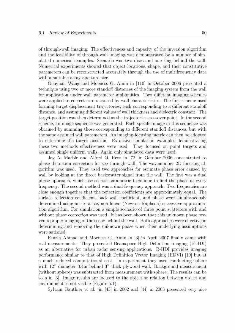
5.1 Review of Experiments 50
of through-wall imaging. The effectiveness and capacity of the inversion algorithmand the feasibility of through-wall imaging was demonstrated by a number of sim-ulated numerical examples. Scenario was two discs and one ring behind the wall.Numerical experiments showed that object locations, shape, and their constitutiveparameters can be reconstructed accurately through the use of multifrequency datawith a suitable array aperture size.
Genyuan Wang and Moeness G. Amin in [110] in October 2006 presented atechnique using two or more standoff distances of the imaging system from the wallfor application under wall parameter ambiguities. Two different imaging schemeswere applied to correct errors caused by wall characteristics. The first scheme usedforming target displacement trajectories, each corresponding to a different standoffdistance, and assuming different values of wall thickness and dielectric constant. Thetarget position was then determined as the trajectories crossover point. In the secondscheme, an image sequence was generated. Each specific image in this sequence wasobtained by summing those corresponding to different standoff distances, but withthe same assumed wall parameters. An imaging-focusing metric can then be adoptedto determine the target position. Extensive simulation examples demonstratingthese two methods effectiveness were used. They focused on point targets andassumed single uniform walls. Again only simulated data were used.
Jay A. Marble and Alfred O. Hero in [72] in October 2006 concentrated tophase distortion correction for see through wall. The wavenumber 2D focusing al-gorithm was used. They used two approaches for estimate phase error caused bywall by looking at the direct backscatter signal from the wall. The first was a dualphase approach, which uses a non-parametric technique to find the phase at everyfrequency. The second method was a dual frequency approach. Two frequencies areclose enough together that the reflection coefficients are approximately equal. Thesurface reflection coefficient, back wall coefficient, and phase were simultaneouslydetermined using an iterative, non-linear (Newton-Raphson) successive approxima-tion algorithm. For simulation a simple scenario of three point scatterers with andwithout phase correction was used. It has been shown that this unknown phase pre-vents proper imaging of the scene behind the wall. Both approaches were effective indetermining and removing the unknown phase when their underlying assumptionswere satisfied.
Fauzia Ahmad and Moeness G. Amin in [3] in April 2007 finally came withreal measurements. They presented Beamspace High Definition Imaging (B-HDI)as an alternative for urban radar sensing applications. B-HDI provides imagingperformance similar to that of High Definition Vector Imaging (HDVI) [10] but ata much reduced computational cost. In experiment they used conducting spherewith 12” diameter 3.4m behind 3” thick plywood wall. Background measurement(without sphere) was subtracted from measurement with sphere. The results can beseen in [3]. Image results are focused to the object so relation between object andenvironment is not visible (Figure 5.1).
Sylvain Gauthier et al. in [43] in 2002 and [44] in 2003 presented very nice
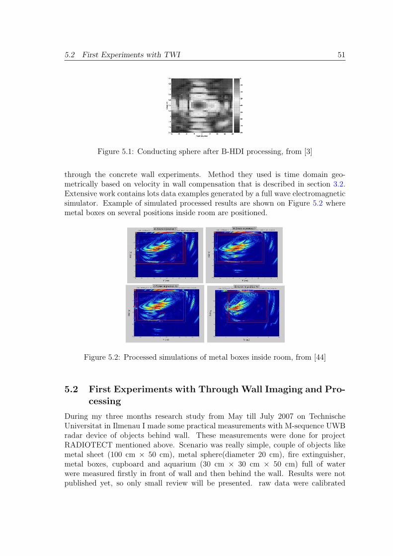
5.2 First Experiments with TWI 51
Figure 5.1: Conducting sphere after B-HDI processing, from [3]
through the concrete wall experiments. Method they used is time domain geo-metrically based on velocity in wall compensation that is described in section 3.2.Extensive work contains lots data examples generated by a full wave electromagneticsimulator. Example of simulated processed results are shown on Figure 5.2 wheremetal boxes on several positions inside room are positioned.
Figure 5.2: Processed simulations of metal boxes inside room, from [44]
5.2 First Experiments with Through Wall Imaging and Pro-cessing
During my three months research study from May till July 2007 on TechnischeUniversitat in Ilmenau I made some practical measurements with M-sequence UWBradar device of objects behind wall. These measurements were done for projectRADIOTECT mentioned above. Scenario was really simple, couple of objects likemetal sheet (100 cm × 50 cm), metal sphere(diameter 20 cm), fire extinguisher,metal boxes, cupboard and aquarium (30 cm × 30 cm × 50 cm) full of waterwere measured firstly in front of wall and then behind the wall. Results were notpublished yet, so only small review will be presented. raw data were calibrated
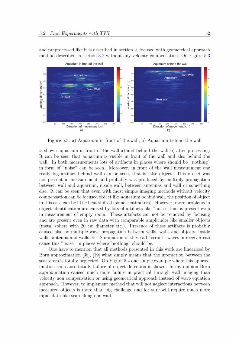
5.2 First Experiments with TWI 52
and preprocessed like it is described in section 2, focused with geometrical approachmethod described in section 3.2 without any velocity compensation. On Figure 5.3
Direction of movement [cm]
Look
ing
dire
ctio
n [c
m]
50 100 150 200 250 300 350 400
100
200
300
400
500
600
700
800 0
10
20
30
40
50
60
Direction of movement [cm]Lo
okin
g di
rect
ion
[cm
]
50 100 150 200 250 300 350 400
100
200
300
400
500
600
700
800 0
10
20
30
40
50
60
Aquarium in front of the wall Aquarium behind the wall
Aquarium
Artifact
Front Wall
AquariumFront Wall
Rear Wall
a) b)
Figure 5.3: a) Aquarium in front of the wall, b) Aquarium behind the wall
is shown aquarium in front of the wall a) and behind the wall b) after processing.It can be seen that aquarium is visible in front of the wall and also behind thewall. In both measurements lots of artifacts in places where should be ”nothing”in form of ”noise” can be seen. Moreover, in front of the wall measurement onereally big artifact behind wall can be seen, that is false object. This object wasnot present in measurement and probably was produced by multiply propagationbetween wall and aquarium, inside wall, between antennas and wall or somethingelse. It can be seen that even with most simple imaging methods without velocitycompensation can be focused object like aquarium behind wall, the position of objectin this case can be little beat shifted (some centimeters). However, more problems inobject identification are caused by lots of artifacts like ”noise” that is present evenin measurement of empty room. These artifacts can not be removed by focusingand are present even in raw data with comparable amplitudes like smaller objects(metal sphere with 20 cm diameter etc.). Presence of these artifacts is probablycaused also by multiple wave propagation between walls, walls and objects, insidewalls, antenna and walls etc. Summation of these all ”errant” waves in receiver cancause this ”noise” in places where ”nothing” should be.
One have to mention that all methods presented in this work are linearized byBorn approximation [38], [19] what simply means that the interaction between thescatterers is totally neglected. On Figure 5.4 one simple example where this approx-imation can cause totally failure of object detection is shown. In my opinion Bornapproximation caused much more failure in practical through wall imaging thanvelocity non compensation or using geometrical approach instead of wave equationapproach. However, to implement method that will not neglect interactions betweenmeasured objects is more than big challenge and for sure will require much moreinput data like scan along one wall.

5.2 First Experiments with TWI 53
RX1 RX2 RX3 TX
Walls
Scattere
r
Figure 5.4: Failure of object detection caused by Born approximation.
From practical point of view system calibration is also extremely important,during research study in Ilmenau I made antenna measurements in anechoic cham-ber room. I measured characteristic of double ridge horn antennas used for throughwall measurements. Measurements were done with two identical antennas in frontto front position, rear to rear, side to side and side to side against big metal plate(Figure 5.5). From theory, measurements front to front and side to side against
Radar
TX RX
Radar
TX RX
Radar
TX RXRadar
TX RX
Metal Plate
Frotn to Front Rear to Rear Side to SideSide to SideAgainst Plate
a) b) c) d)
Figure 5.5: Antennas positions during measurements in anechoic chamber room.
big metal plate in ideal conditions should be the same. On Figure 5.6 examples ofthese measurements in frequency domain with various distances are shown. It canbe seen that they are not the same, but nearly the same. During practical throughwall measurements position of antennas were not the same, cables were with dif-ferent lengths and antennas were placed on metal positioning trolley. Thereforebetter result were obtained with calibration measurements measured during prac-tical through wall measurements. Anyway, this calibration is not satisfactory forthrough wall imaging and should be improved.
During measurements in anechoic chamber room we encounter a problem withcable and connector mishmatch even if cables and connector were very high-class.These mishmatch cause multiple reflections inside cables that can be seen on Figure
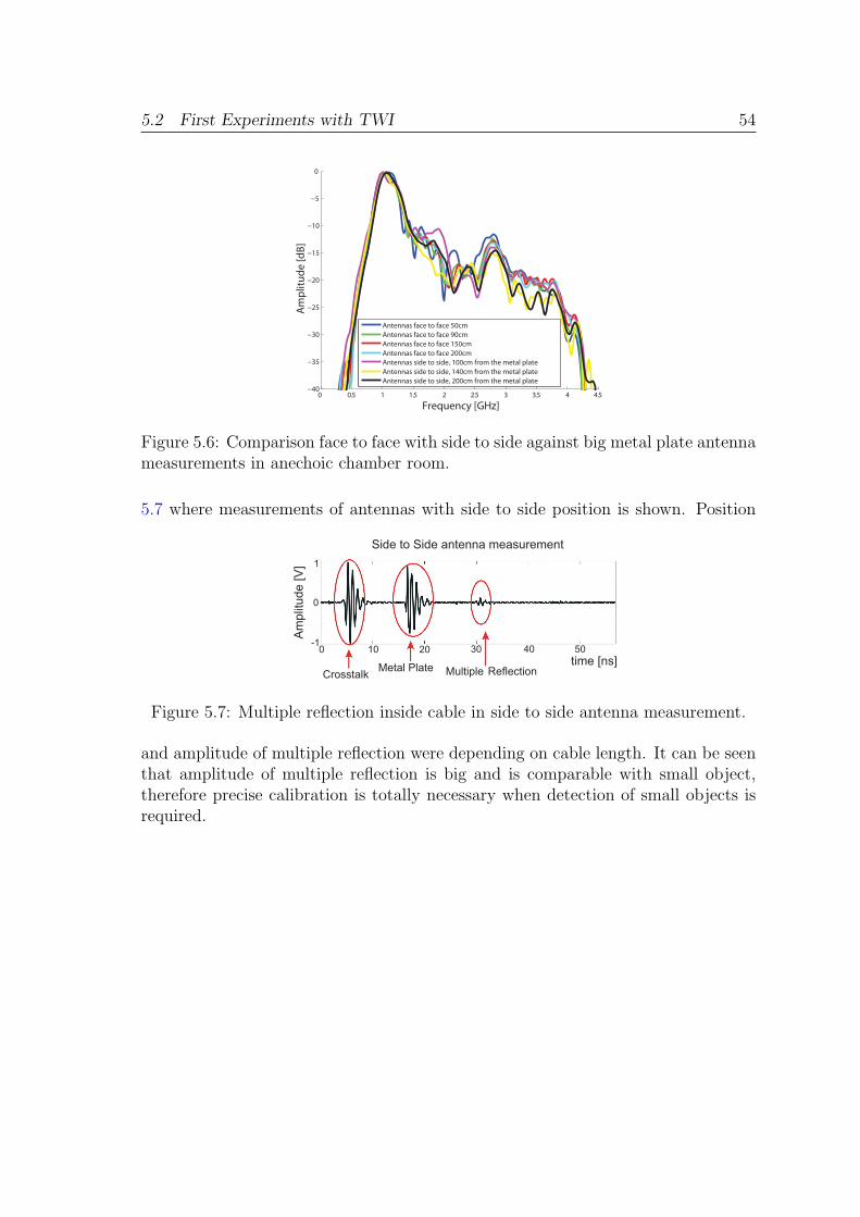
5.2 First Experiments with TWI 54
0 0.5 1 1.5 2 2.5 3 3.5 4 4.5−40
−35
−30
−25
−20
−15
−10
−5
0
Frequency [GHz]
Am
plitu
de [d
B]
Antennas face to face 50cmAntennas face to face 90cmAntennas face to face 150cmAntennas face to face 200cmAntennas side to side, 100cm from the metal plateAntennas side to side, 140cm from the metal plateAntennas side to side, 200cm from the metal plate
Figure 5.6: Comparison face to face with side to side against big metal plate antennameasurements in anechoic chamber room.
5.7 where measurements of antennas with side to side position is shown. Position
Amplitude[V]
time [ns]
0
1
-10 10 20 30 40 50
Crosstalk Metal Plate Multiple Reflection
Side to Side antenna measurement
Figure 5.7: Multiple reflection inside cable in side to side antenna measurement.
and amplitude of multiple reflection were depending on cable length. It can be seenthat amplitude of multiple reflection is big and is comparable with small object,therefore precise calibration is totally necessary when detection of small objects isrequired.
Conclusion
In this thesis to the dissertation examination methods for through wall imaging werereviewed. Firstly, basic properties of M-sequence UWB radar device were describedin chapter 1. Through wall radar basic model, data representation, preprocessingand calibration is shown in chapter 2. In chapter 3 three basic imaging approacheswere described, than lot of improvements for them were summarized in chapter 4.Through wall imaging experiments were reviewed in chapter 5 including my ownexperiments with through wall measurements and imaging. Finally, conclusion andthesis for dissertation work are presented. This document contain through wall radarimaging method overview, what I didn’t find yet in any another article or book.
Through wall imaging is very perspective field that has very wide utilization likethrough wall imaging during security situations such as with terrorists and hostagesto locate people and weapons, through rubble imaging following an emergency e.g.earthquake, explosion etc, through wall imaging during fire to locate people, throughsnow imaging to locate people after avalanche, border control for the detection ofillegal immigrants, substances or contraband e.g. cigarettes in trucks and many an-other applications. This technologies can save many lives during rescue and securityactions because work will be more safely and location of the victims will be faster.
Methods that can handle with practical wave scattering are still at the beginningand new methods with new approaches have to be developed. However this is a bigchallenge and will require lot of research and developing work. During my next PhDstudy I want to contribute to the through wall imaging research. I will concentrateon implementation these methods for real data and practical scenarios.
55

Thesis for dissertation work
PhD dissertation work will be concentrated on development and implementationimaging methods that will allow to reconstruct interior of room including walls frommeasured data set. Thesis for dissertation work can be defined as follows:
• To develop imaging methods with new approaches, or modify some already ex-isting approach that will produce better results with real data in room interiorimaging.
• To find new measurement scenario or antennas configuration that will allowto use imaging method with better results with real data.
• To improve calibration or preprocessing methods, that will improve imageresolution or object detection capabilities.
• To analyze and implement calibration algorithm in order to reduce linear andnonlinear systematic error of radar device.
• To propose and test some image processing method like shape highlighting,noise removing, median filtering, highlighting of knowing perpendicular wallsor another method optimized for specific scenario to improve final image qual-ity.
• To optimize data visualization method, which will leads to better visibility ofsmall objects with focus to the different types of colormap chosen for visual-ization.
56

REFERENCES 57
References
[1] M. Aftanas, J. Rovnakova, M. Riskova, D. Kocur, , and M. Drutarovsky, “An Analysis of 2DTarget Positioning Accuracy for M-sequence UWB Radar System under Ideal Conditions,”Proceedings of 17th International Conference Radioelektronika, Brno, Czech Republic, pp.189–194, Apr. 2007.
[2] A. Agrawal, B. Fougere, M. Oravakandy, and G. Siemens, “Design, construction, and testingof a microwave radar system for through-wall surveillance,” Master’s thesis, Electrical andComputer Engineering in the Faculty of Engineering of the University of Manitoba, 2004.
[3] F. Ahmad and M. G. Amin, “High-Resolution Imaging using Capon Beamformers for UrbanSensing Applications,” Acoustics, Speech and Signal Processing, ICASSP, IEEE, vol. 2, pp.985–988, Apr. 2007.
[4] B. Allen, M. Dohler, E. Okon, W. Malik, A. Brown, and D. Edwards, Ultra-wideband An-tennas and Propagation. John Wiley, Oct. 2006.
[5] L. Y. Astanin and A. A. Kostylev, Ultrawideband Radar Measurements - Analysis and Pro-cessing. Institution of Engineering and Technology, 1997.
[6] G. Backus and F. Gilbert, “Numerical applications of a formalism for geophysical inverseproblems,” Geophysical Journal International, vol. 13, pp. 247–276, July 1967.
[7] T. W. Barrett, “History of UltraWideBand (UWB) Radar & Communications,” Progress InElectromagnetics Symposium, July 2000.
[8] S. Basu and Y. Bresler, “O(N2log2N) Filtered Backprojection Reconstruction Algorithm forTomography,” IEEE Transactions on Image Processing, vol. 9, pp. 1760–1773, Oct. 2000.
[9] A. O. Bauer, “Centre for German Communication and related technology,” The history ofa German mobile radar direction finder, Dec. 2004.
[10] G. R. Benitz, “High-Definition Vector Imaging,” Lincoln Lab Journal, vol. 10, pp. 147–170,Nov. 1997.
[11] A. J. Berkhout, “Wave field extrapolation techniques in seismic migration, a tutorial,” Geo-physics, vol. 46, pp. 1638–1656, Dec. 1981.
[12] M. Bertero and P. Boccacci, “Introduction to Inverse Problems in Imaging,” Inst. of PhysicsPubl., Bristol, Jan. 1998.
[13] G. Beylkin, “On the fast Fourier transform of functions with singularities,” Applied andComputational Harmonic Analysis, vol. 2, pp. 363–381, 1995.
[14] A. Binder, H. W. Engl, C. W. Groetsch, A. Neubauer, and O. Scherzer, “Weakly closednonlinear operators and parameter identification in parabolic equations by Tikhonov regu-larization,” Appl. Anal., vol. 55, pp. 215–234, Dec. 1994.
[15] A. Boag, Y. Bresler, and E. Michielssen, “A multilevel domain decomposition algorithm forfast O(N2logN) reprojection of tomographic images,” Image Processing, Proceedings Inter-national Conference, vol. 2, pp. 633–636, Dec. 1999.
[16] M. Bragg, The Location of Aircraft by Radar Methods 1935-1945. Hawkhead Publishing,May 2002.
[17] S. Brlek, G. Labelle, and A. Lacasse, “The discrete green theorem and some applications indiscrete geometry,” Theor. Comput. Sci., vol. 346, pp. 200–225, Nov. 2005.
[18] J. P. Camacho, Federal Radar Spectrum Requirements. U.S. Dept. of Commerce, NationalTelecommunications and Information Administration, May 2000.
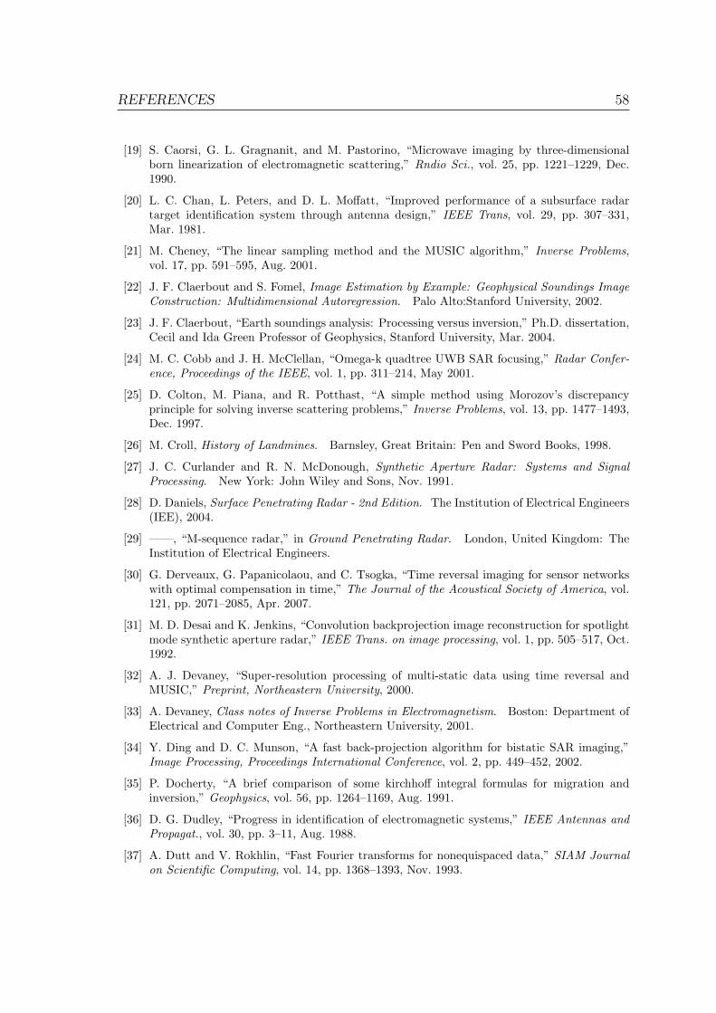
REFERENCES 58
[19] S. Caorsi, G. L. Gragnanit, and M. Pastorino, “Microwave imaging by three-dimensionalborn linearization of electromagnetic scattering,” Rndio Sci., vol. 25, pp. 1221–1229, Dec.1990.
[20] L. C. Chan, L. Peters, and D. L. Moffatt, “Improved performance of a subsurface radartarget identification system through antenna design,” IEEE Trans, vol. 29, pp. 307–331,Mar. 1981.
[21] M. Cheney, “The linear sampling method and the MUSIC algorithm,” Inverse Problems,vol. 17, pp. 591–595, Aug. 2001.
[22] J. F. Claerbout and S. Fomel, Image Estimation by Example: Geophysical Soundings ImageConstruction: Multidimensional Autoregression. Palo Alto:Stanford University, 2002.
[23] J. F. Claerbout, “Earth soundings analysis: Processing versus inversion,” Ph.D. dissertation,Cecil and Ida Green Professor of Geophysics, Stanford University, Mar. 2004.
[24] M. C. Cobb and J. H. McClellan, “Omega-k quadtree UWB SAR focusing,” Radar Confer-ence, Proceedings of the IEEE, vol. 1, pp. 311–214, May 2001.
[25] D. Colton, M. Piana, and R. Potthast, “A simple method using Morozov’s discrepancyprinciple for solving inverse scattering problems,” Inverse Problems, vol. 13, pp. 1477–1493,Dec. 1997.
[26] M. Croll, History of Landmines. Barnsley, Great Britain: Pen and Sword Books, 1998.
[27] J. C. Curlander and R. N. McDonough, Synthetic Aperture Radar: Systems and SignalProcessing. New York: John Wiley and Sons, Nov. 1991.
[28] D. Daniels, Surface Penetrating Radar - 2nd Edition. The Institution of Electrical Engineers(IEE), 2004.
[29] ——, “M-sequence radar,” in Ground Penetrating Radar. London, United Kingdom: TheInstitution of Electrical Engineers.
[30] G. Derveaux, G. Papanicolaou, and C. Tsogka, “Time reversal imaging for sensor networkswith optimal compensation in time,” The Journal of the Acoustical Society of America, vol.121, pp. 2071–2085, Apr. 2007.
[31] M. D. Desai and K. Jenkins, “Convolution backprojection image reconstruction for spotlightmode synthetic aperture radar,” IEEE Trans. on image processing, vol. 1, pp. 505–517, Oct.1992.
[32] A. J. Devaney, “Super-resolution processing of multi-static data using time reversal andMUSIC,” Preprint, Northeastern University, 2000.
[33] A. Devaney, Class notes of Inverse Problems in Electromagnetism. Boston: Department ofElectrical and Computer Eng., Northeastern University, 2001.
[34] Y. Ding and D. C. Munson, “A fast back-projection algorithm for bistatic SAR imaging,”Image Processing, Proceedings International Conference, vol. 2, pp. 449–452, 2002.
[35] P. Docherty, “A brief comparison of some kirchhoff integral formulas for migration andinversion,” Geophysics, vol. 56, pp. 1264–1169, Aug. 1991.
[36] D. G. Dudley, “Progress in identification of electromagnetic systems,” IEEE Antennas andPropagat., vol. 30, pp. 3–11, Aug. 1988.
[37] A. Dutt and V. Rokhlin, “Fast Fourier transforms for nonequispaced data,” SIAM Journalon Scientific Computing, vol. 14, pp. 1368–1393, Nov. 1993.

REFERENCES 59
[38] E. Eide, “Radar imaging of small objects closely below the earth surface,” Ph.D. dissertation,Norwegian University of Science and Technology, Norway, Aug. 2000.
[39] H. W. Engl, M. Hanke, and A. Neubauer, Regularization of Inverse Problems. New York:Springer, July 1996.
[40] X. Feng and M. Sato, “Pre-stack migration applied to GPR for landmine detection,” InverseProblems, vol. 20, pp. 1–17, Nov. 2004.
[41] S. Foo and S. Kashyap, “Cross-correlated back projection for UWB radar imaging,” Antennasand Propagation Society International Symposium. IEEE, vol. 2, pp. 1275–1278, June 2004.
[42] C. Gauss, “Allgemeine Flachentheorie,” W. Engelmann , Leipzig, (Translated from Latin),1900.
[43] S. Gauthier and W. Chamma, “Through-The-Wall Surveillance,” Technical MemorandumDRDC, Ottawa, Oct. 2002.
[44] S. Gauthier, E. Hung, and W. Chamma, “Surveillance Through Concrete Walls,” Proceedingsof SPIE 5403, pp. 597–608, Dec. 2004.
[45] J. Gazdag, “Wave-equation migration with the phase-shift method,” Geophysics, vol. 43, pp.1342–1351, Dec. 1978.
[46] S. H. Gray, “Efficient traveltime calculations for kirchhoff migration,” Geophysics, vol. 51,pp. 1685–1688, Aug. 1986.
[47] M. N. Guddati and A. H. Heidari, “Migration with arbitrarily wide-angle wave equations,”Geophysic, vol. 70, pp. 61–70, May 2005.
[48] A. Gunawardena and D. Longstaff, “Wave equation formulation of Synthetic Aperture Radar(SAR) algorithms in the time-space domain,” IEEE Transactions on Geoscience and RemoteSensing, vol. 36, pp. 1995–1999, Nov. 1999.
[49] S. Hantscher, B. Praher, A. Reisenzahn, and C. G. Diskus, “Analysis of Imaging Radar Algo-rithms for the Identifcation of Targets by Their Surface Shape,” Antennen und Messverfahrenfr Ultra-Wide-Band (UWB)-Systeme, Dec. 2006.
[50] M. A. Haun, D. L. Jones, and W. D. O’Brien, “Efficient three-dimensional imaging from asmall cylindrical aperture,” Ultrasonics Symposium, IEEE Transactions, vol. 2, pp. 1589–1592, Oct. 2000.
[51] G. T. Herman, Image reconstruction from projections. Berlin, Germany: Spriner-Verlag.
[52] A. Ho, W. H. Tham, and K. S. Low, “Improving classification accuracy in through-wallradar imaging using hybrid prony’s and singular value decomposition method,” Geoscienceand Remote Sensing Symposium, IGARSS, Proceedings IEEE, vol. 6, pp. 4267–4270, July2005.
[53] A. J. Hunter, M. P. Hayes, and P. T. Gough, “A Comparison Of Fast Factorised Back-Projection And Wavenumber Algorithms for SAS image reconstruction,” WCU 2003, Paris,pp. 527–530, Sep. 20003.
[54] I. Immoreev and Fedotov, “Ultra wideband radar systems: advantages and disadvantages,”Ultra Wideband Systems and Technologies, pp. 201–205, 2002.
[55] J. D. Jackson, Classical electrodynamics. New York: J. Wiley and Sons, Aug. 1998.
[56] H. Jeongwoo, “Development of an electronically tunable ultra-wideband radar imaging sensorand its components,” Ph.D. dissertation, Texas A&M University, May 2005.
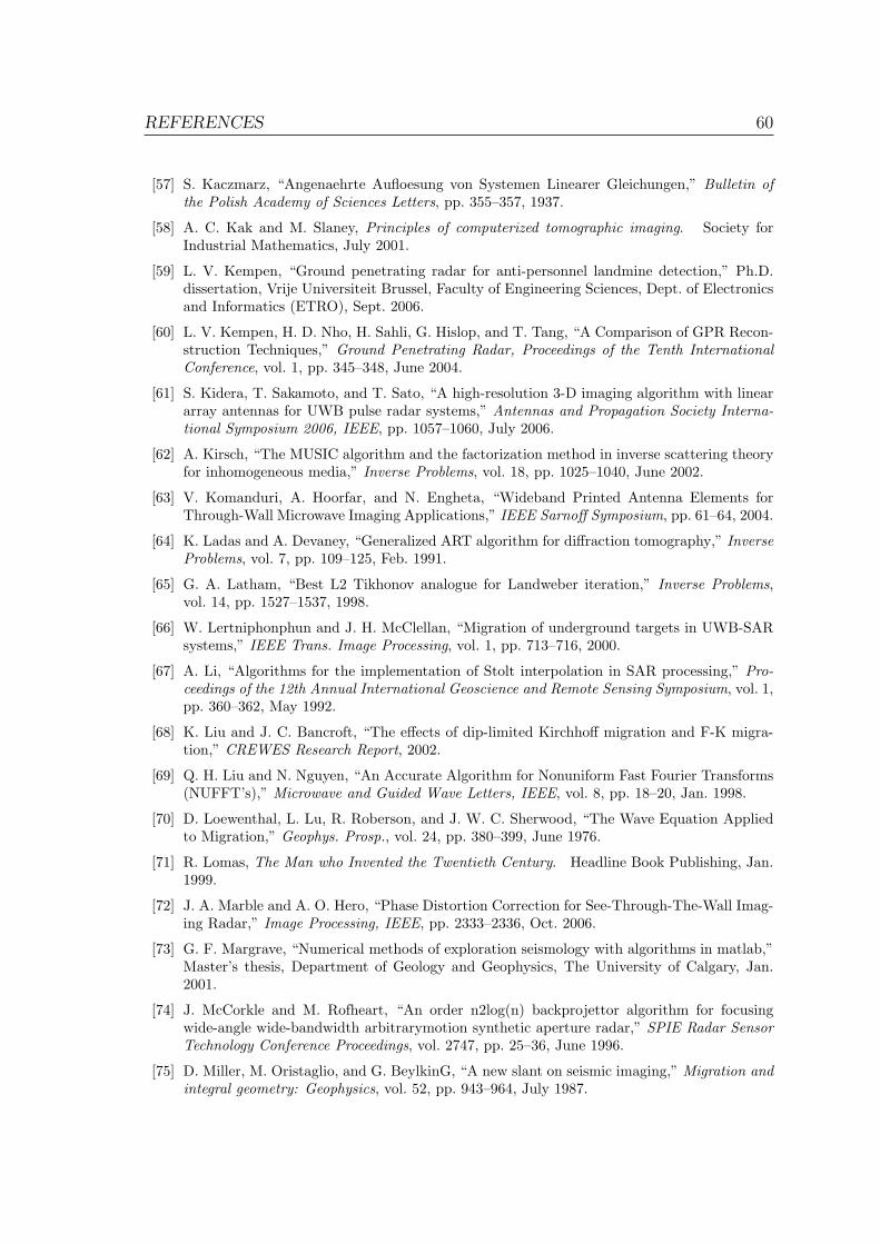
REFERENCES 60
[57] S. Kaczmarz, “Angenaehrte Aufloesung von Systemen Linearer Gleichungen,” Bulletin ofthe Polish Academy of Sciences Letters, pp. 355–357, 1937.
[58] A. C. Kak and M. Slaney, Principles of computerized tomographic imaging. Society forIndustrial Mathematics, July 2001.
[59] L. V. Kempen, “Ground penetrating radar for anti-personnel landmine detection,” Ph.D.dissertation, Vrije Universiteit Brussel, Faculty of Engineering Sciences, Dept. of Electronicsand Informatics (ETRO), Sept. 2006.
[60] L. V. Kempen, H. D. Nho, H. Sahli, G. Hislop, and T. Tang, “A Comparison of GPR Recon-struction Techniques,” Ground Penetrating Radar, Proceedings of the Tenth InternationalConference, vol. 1, pp. 345–348, June 2004.
[61] S. Kidera, T. Sakamoto, and T. Sato, “A high-resolution 3-D imaging algorithm with lineararray antennas for UWB pulse radar systems,” Antennas and Propagation Society Interna-tional Symposium 2006, IEEE, pp. 1057–1060, July 2006.
[62] A. Kirsch, “The MUSIC algorithm and the factorization method in inverse scattering theoryfor inhomogeneous media,” Inverse Problems, vol. 18, pp. 1025–1040, June 2002.
[63] V. Komanduri, A. Hoorfar, and N. Engheta, “Wideband Printed Antenna Elements forThrough-Wall Microwave Imaging Applications,” IEEE Sarnoff Symposium, pp. 61–64, 2004.
[64] K. Ladas and A. Devaney, “Generalized ART algorithm for diffraction tomography,” InverseProblems, vol. 7, pp. 109–125, Feb. 1991.
[65] G. A. Latham, “Best L2 Tikhonov analogue for Landweber iteration,” Inverse Problems,vol. 14, pp. 1527–1537, 1998.
[66] W. Lertniphonphun and J. H. McClellan, “Migration of underground targets in UWB-SARsystems,” IEEE Trans. Image Processing, vol. 1, pp. 713–716, 2000.
[67] A. Li, “Algorithms for the implementation of Stolt interpolation in SAR processing,” Pro-ceedings of the 12th Annual International Geoscience and Remote Sensing Symposium, vol. 1,pp. 360–362, May 1992.
[68] K. Liu and J. C. Bancroft, “The effects of dip-limited Kirchhoff migration and F-K migra-tion,” CREWES Research Report, 2002.
[69] Q. H. Liu and N. Nguyen, “An Accurate Algorithm for Nonuniform Fast Fourier Transforms(NUFFT’s),” Microwave and Guided Wave Letters, IEEE, vol. 8, pp. 18–20, Jan. 1998.
[70] D. Loewenthal, L. Lu, R. Roberson, and J. W. C. Sherwood, “The Wave Equation Appliedto Migration,” Geophys. Prosp., vol. 24, pp. 380–399, June 1976.
[71] R. Lomas, The Man who Invented the Twentieth Century. Headline Book Publishing, Jan.1999.
[72] J. A. Marble and A. O. Hero, “Phase Distortion Correction for See-Through-The-Wall Imag-ing Radar,” Image Processing, IEEE, pp. 2333–2336, Oct. 2006.
[73] G. F. Margrave, “Numerical methods of exploration seismology with algorithms in matlab,”Master’s thesis, Department of Geology and Geophysics, The University of Calgary, Jan.2001.
[74] J. McCorkle and M. Rofheart, “An order n2log(n) backprojettor algorithm for focusingwide-angle wide-bandwidth arbitrarymotion synthetic aperture radar,” SPIE Radar SensorTechnology Conference Proceedings, vol. 2747, pp. 25–36, June 1996.
[75] D. Miller, M. Oristaglio, and G. BeylkinG, “A new slant on seismic imaging,” Migration andintegral geometry: Geophysics, vol. 52, pp. 943–964, July 1987.
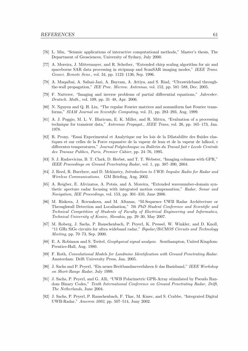
REFERENCES 61
[76] L. Min, “Seismic applications of interactive computational methods,” Master’s thesis, TheDepartment of Geosciences, University of Sydney, July 2000.
[77] A. Moreira, J. Mittermayer, and R. Scheiber, “Extended chirp scaling algorithm for air andspaceborne SAR data processing in stripmap and ScanSAR imaging modes,” IEEE Trans.Geosci. Remote Sens., vol. 34, pp. 1123–1136, Sep. 1996.
[78] A. Muqaibai, A. Safaai-Jazi, A. Bayram, A. Attiya, and S. Riad, “Ultrawideband through-the-wall propagation,” IEE Proc. Microw. Antennas, vol. 152, pp. 581–588, Dec. 2005.
[79] F. Natterer, “Imaging and inverse problems of partial differential equations,” Jahresber.Deutsch. Math., vol. 109, pp. 31–48, Apr. 2006.
[80] N. Nguyen and Q. H. Liu, “The regular Fourier matrices and nonuniform fast Fourier trans-forms,” SIAM Journal on Scientific Computing, vol. 21, pp. 283–293, Aug. 1999.
[81] A. J. Poggio, M. L. V. Blaricum, E. K. Miller, and R. Mittra, “Evaluation of a processingtechnique for transient data,” Antennas Propagat., IEEE Trans, vol. 26, pp. 165–173, Jan.1978.
[82] R. Prony, “Essai Experimental et Analytique sur les lois de la Dilatabilite des fluides elas-tiques et sur celles de la Force expansive de la vapeur de leau et de la vapeur de lalkool, rdifferentes temperatures,” Journal Polytechnique ou Bulletin du Travail fait r Lecole Centraledes Travaux Publics, Paris, Premier Cahier, pp. 24–76, 1995.
[83] S. J. Radzevicius, B. T. Clark, D. Herbst, and T. T. Webster, “Imaging columns with GPR,”IEEE Proceedings on Ground Penetrating Radar, vol. 1, pp. 387–390, 2004.
[84] J. Reed, R. Buerhrer, and D. Mckinstry, Introduction to UWB: Impulse Radio for Radar andWireless Communications. GM Briefing, Aug. 2002.
[85] A. Reigber, E. Alivizatos, A. Potsis, and A. Moreira, “Extended wavenumber-domain syn-thetic aperture radar focusing with integrated motion compensation,” Radar, Sonar andNavigation, IEE Proceedings, vol. 153, pp. 301–310, June 2006.
[86] M. Riskova, J. Rovnakova, and M. Aftanas, “M-Sequence UWB Radar Architecture orThroughwall Detection and Localisation,” 7th PhD Student Conference and Scientific andTechnical Competition of Students of Faculty of Electrical Engineering and Informatics,Technical University of Kosice, Slovakia, pp. 29–30, May 2007.
[87] M. Roberg, J. Sachs, P. Rauschenbach, P. Peyerl, K. Pressel, W. Winkler, and D. Knoll,“11 GHz SiGe circuits for ultra wideband radar,” Bipolar/BiCMOS Circuits and TechnologyMeeting, pp. 70–73, Sep. 2000.
[88] E. A. Robinson and S. Treitel, Geophysical signal analysis. Southampton, United Kingdom:Prentice-Hall, Aug. 1980.
[89] F. Roth, Convolutional Models for Landmine Identification with Ground Penetrating Radar.Amsterdam: Delft University Press, Jan. 2005.
[90] J. Sachs and P. Peyerl, “Ein neues Breitbandmeverfahren fr das Basisband,” IEEE Workshopon Short-Range Radar, July 1999.
[91] J. Sachs, P. Peyerl, and G. Alli, “UWB Polarimetric GPR-Array stimulated by Pseudo Ran-dom Binary Codes,” Tenth International Conference on Ground Penetrating Radar, Delft,The Netherlands, June 2004.
[92] J. Sachs, P. Peyerl, P. Rauschenbach, F. Tkac, M. Kmec, and S. Crabbe, “Integrated DigitalUWB-Radar,” Amerem 2002, pp. 507–514, Juny 2002.
REFERENCES 62
[93] J. Sachs, P. Peyerl, and M. Rossberg, “A New UWB-Principle for Sensor-Array Application,”IEEE proceedings of IMTC/99, vol. 3, May 1999.
[94] J. Sachs, P. Peyerl, R. Zetik, and S. Crabbe, “M-Sequence Ultra-Wideband-Radar: State ofDevelopment and Applications,” Radar 2003, Adelaide (Australia), pp. 224–229, Sep. 2003.
[95] T. Sakamoto and T. Sato, “A fast algorithm of 3-dimensional imaging for pulse radar sys-tems,” IEEE AP-S International Symposium and USNC/URSI National Radio Science Meet-ing, vol. 3, pp. 2099–2102, June 2004.
[96] ——, “A target shape estimation algorithm for pulse radar systems based on BoundaryScattering Transform,” IEICE Transactions on Communications, vol. 87, pp. 1357–1365,May 2004.
[97] P. C. Sava, “Prestack residual migration in the frequency domain,” Geophysics, vol. 68, pp.634–640, Mar. 2003.
[98] T. Savelyev, L. van Kempen, and H. Sahli, “GPR Antipersonnel Mine Detection: ImprovedDeconvolution and Time-Frequency Feature Extraction,” SPIE, Nondestructive Evaluationand Health Monitoring of Aerospace Materials and Composites II, vol. 5046, pp. 232–241,2003, san Diego, USA.
[99] J. A. Scales, Theory of Seismic Imaging. New York: Springer, Jan. 1995.
[100] B. Scheers, “Ultra-wideband ground penetrating radar, with application to the detection ofanti personnel landmines,” Ph.D. dissertation, Universit Catholique de Louvain, Belgium,2001.
[101] B. Scheers, M. Archeroy, and A. V. Vander, “Time-domain modeling of UWB GPR andits application to land mine detection,” SPIE, Detection and Remediation Technologies forMines and Minelike Targets V, vol. 4038, pp. 1452–1460, Aug. 2000, orlando, FL, USA.
[102] R. O. Schmidt, “Multiple emitter location and signal parameter estimation,” IEEE Trans.,vol. 34, pp. 276–280, Mar. 1986.
[103] W. S. Schneider, “Integral formulation for migration in two or three dimensions,” Geophysics,vol. 43, pp. 49–76, 1978.
[104] P. D. Smith and S. R. Cloude, Ultra-Wideband, Short-Pulse Electromagnetics 5. SpringerUS, Sept. 2002.
[105] L.-P. Song, C. Yu, and Q. H. Liu, “Through-wall imaging (TWI) by radar: 2-D tomographicresults and analyses,” Geoscience and Remote Sensing, IEEE, vol. 43, pp. 2793–2798, Dec.2005.
[106] R. H. Stolt, “Migration by Fourier transform,” Geophysics, vol. 43, pp. 23–48, Feb. 1978.
[107] B. Subiza, E. Gimeno-Nieves, J. M. Lopez-Sanchez, and J. Fortuny-Guasch, “An Approachto SAR Imaging by Means of Non-Uniform FFT’s,” Geoscience and Remote Sensing Sym-posium. IGARSS apos., vol. 6, pp. 4089–4091, July 2003.
[108] C. W. Therrien, Discrete Random Signals and Statistical Signal Processing. Hemel Hemp-stead: Prentice-Hall International.
[109] L. Ulander, H. Hellsten, and Stenstrom, “Synthetic aperture radar processing using fastfactorized back-projection,” Aerospace and Electronic Systems, vol. 39, pp. 760–776, July2003.
[110] G. Wang and M. G. Amin, “Imaging Through Unknown Walls Using Different StandoffDistances,” Signal Processing, IEEE, pp. 4015–4025, Oct. 2006.

REFERENCES 63
[111] J. W. Wiggins, “Kirchhoff integral extrapolation an migration of nonplanar data,” Geo-physics, vol. 49, pp. 1239–1248, Aug. 1984.
[112] S. Xiao, D. C. Munson, S. Basu, and Y. Bresler, “An N2logN back-projection algorithm forSAR image formation,” Signals, Systems and Computers, Conference Record of the Thirty-Fourth Asilomar Conference, vol. 1, pp. 3–7, 2000.
[113] S. Xu and D. Pham, “Seismic Data Regularization with Anti-Leakage Fourier Transform,”66th EAGE Conference and Exhibition, Paris, vol. 66, June 2004.
[114] X. Xu and E. L. Miller, “Optimization of Migration Method to Locate Buried Object in LossyMedium,” Geoscience and Remote Sensing Symposium, IGARSS apos., IEEE International,vol. 1, pp. 337–339, June 2002.
[115] H. Yacoub and T. Sarkar, “Monostatic through-wall detection of a metallic sphere,” Antennasand Propagation Society International Symposium, IEEE, vol. 3B, pp. 326–329, July 2005.
[116] B. Yang, A. Yarovoy, T. Savelyev, and L. Ligthart, “Estimated Path Loss for Through WallImaging,” Internal Radiotect intermediate report on workpackage 2, IRCTRS01807, May2007.
[117] R. Yelf, “Where is true time zero?” Proceedings of the Tenth International Conference onGround Penetrating Radar, vol. 1, pp. 279–282, June 2004.
[118] O. Yilmaz, Seismic Data Processing, volume 2 of Investigations in Geophysics. Tulsa:Society of Exploration Geophysicists, Oct. 1987.
[119] R. Zetik, J. Sachs, and P. Peyerl, “UWB Radar: Distance and Positioning Measurements,”International Conference on Electromagnetics in Advanced Applications, Sep. 2003.
[120] R. Zetik, J. Sachs, and R. Thoma, “The Architecture of a Baseband, Pseudo-Noise UWBRadar Sensor,” IEEE Instrumentation & Measurement Magazine, vol. 10, pp. 39–45, April2007.
[121] R. Zetik, J. Sachs, and R. S. Thoma, “UWB localization - active and passive approach,”Instrumentation and Measurement Technology Conference, vol. 2, pp. 1005–1009, May 2004.
[122] R. Zetik and J. Sachs, “Time-Frequency Signal Representations Applied to Ultra WidebandRadar,” German Radar Symposium GRS, Oct. 2000.
[123] R. Zetik, J. Sachs, and R. Thoma, “From UWB Radar to UWB Radio,” Int. Workshopon Ultra-Wideband Systems (IWUWBS 2003), Center of Wireless Communications (CWC),June 2003.
[124] ——, “Modified cross-correlation back projection for UWB imaging: numerical examples,”Ultra-Wideband, 2005. ICU 2005. 2005 IEEE International Conference, Sep. 2005.
[125] R. Zetik, J. Sachs, and R. Thome, “Imaging of Propagation Environment by UWB ChannelSounding,” XXVIIIth URSI General Assembly, Oct. 2005.
Related Documents