Three Essays on the Economic Impact of Immigration

University of Kentucky University of Kentucky

UKnowledge UKnowledge

Theses and Dissertations--Economics Economics

2015

Three Essays on the Economic Impact of Immigration Three Essays on the Economic Impact of Immigration

James Sharpe University of Kentucky, [email protected]

Right click to open a feedback form in a new tab to let us know how this document benefits you. Right click to open a feedback form in a new tab to let us know how this document benefits you.

Recommended Citation Recommended Citation Sharpe, James, "Three Essays on the Economic Impact of Immigration" (2015). Theses and Dissertations--Economics. 20. https://uknowledge.uky.edu/economics_etds/20

This Doctoral Dissertation is brought to you for free and open access by the Economics at UKnowledge. It has been accepted for inclusion in Theses and Dissertations--Economics by an authorized administrator of UKnowledge. For more information, please contact [email protected].

STUDENT AGREEMENT: STUDENT AGREEMENT:

I represent that my thesis or dissertation and abstract are my original work. Proper attribution

has been given to all outside sources. I understand that I am solely responsible for obtaining

any needed copyright permissions. I have obtained needed written permission statement(s)

from the owner(s) of each third-party copyrighted matter to be included in my work, allowing

electronic distribution (if such use is not permitted by the fair use doctrine) which will be

submitted to UKnowledge as Additional File.

I hereby grant to The University of Kentucky and its agents the irrevocable, non-exclusive, and

royalty-free license to archive and make accessible my work in whole or in part in all forms of

media, now or hereafter known. I agree that the document mentioned above may be made

available immediately for worldwide access unless an embargo applies.

I retain all other ownership rights to the copyright of my work. I also retain the right to use in

future works (such as articles or books) all or part of my work. I understand that I am free to

register the copyright to my work.

REVIEW, APPROVAL AND ACCEPTANCE REVIEW, APPROVAL AND ACCEPTANCE

The document mentioned above has been reviewed and accepted by the student’s advisor, on

behalf of the advisory committee, and by the Director of Graduate Studies (DGS), on behalf of

the program; we verify that this is the final, approved version of the student’s thesis including all

changes required by the advisory committee. The undersigned agree to abide by the statements

above.

James Sharpe, Student

Dr. Christopher R. Bollinger, Major Professor

Dr. Jenny A. Minier, Director of Graduate Studies

THREE ESSAYS ON THE ECONOMIC IMPACT OF IMMIGRATION

____________________________________

DISSERTATION ____________________________________

A dissertation submitted in partial fulfillment of the Requirements for the degree of Doctor of Philosophy in the

College of Business and Economics at the University of Kentucky

By James M. Sharpe Lexington, KY

Director: Dr. Christopher R. Bollinger, Gatton Endowed Professor of Economics and

Director of the Center for Business and Economics Research

Lexington, KY

2015

Copyright © James M. Sharpe 2015

ABSTRACT OF DISSERTATION

THREE ESSAYS ON THE ECONOMIC IMPACT OF IMMIGRATION

With the significant rise in immigration to the U.S. over the last few decades, fully understanding the economic impact of immigration is paramount for policy makers. As such, this dissertation consists of three empirical essays contributing to the literature on the impact of immigration. In my first essay, I re-examine the impact of immigration on housing rents and completely controlling for endogenous location choices of immigrants. I model rents as a function of both contemporaneous and initial economic and housing market conditions. I show that existing estimates of the impact of immigration on rents are biased and the source of the bias is the instrumental variable strategy common in much of the immigration literature. In my second essay, I present a new approach to estimating the effect of immigration on native wages. Noting the imperfect substitutability of immigrants and natives within education groups, I posit an empirical framework where labor markets are stratified by occupations. Using occupation-specific skill to define homogeneous skill groups, I estimate the partial equilibrium (within skill group) effect of immigration. The results suggest that when one defines labor market cohorts that directly compete in the labor market, the effect of immigration on native wages is roughly twice as large as previous estimates in the literature. In my third essay, I return to the housing market and examine the effects of immigration within metropolitan areas. Specifically, I investigate the relationship between immigrant inflows, native outflows, and rents. Taking advantage of the unique settlement patterns of immigrants, I show that the effect of immigration on rents is lower in both high-immigrant neighborhoods and portions of the rent distribution where immigrants cluster. Contrary to the existing belief in the literature, the results suggest that the preferences of natives, not immigrants, bid up rents in response to an immigrant inflow.

KEYWORDS: Immigration, Impact of Immigration, Housing Rents, Substitutability, Occupation-Specific Skill, Quantile Regression.

THREE ESSAYS ON THE ECONOMIC IMPACT OF IMMIGRATION

By

James M. Sharpe

___________Dr. Christopher R. Bollinger Director of Dissertation

Dr. Jenny A. Minier Director of Graduate Studies

July 16, 2015 Date

To my loving wife, Anna, and son, Wyatt.

iii

ACKNOWLEDGEMENTS

Though an individual work, this dissertation benefited from the direction and insight

from several people. First, I would like to thank my dissertation advisor and employer at the

Center for Business and Education Research, Dr. Chris Bollinger, for his guidance and support

through this entire process. In addition to the instructive comments and moral support, I would

like to thank Chris for believing in me from the beginning by admitting me and providing funding

throughout my tenure. I would also like to thank my committee members and outside reader,

respectively: Dr. Bill Hoyt, Dr. John Garen, Dr. Michael Samers, and Dr. Monika Causholli.

Each individual provided invaluable comments and critiques that vastly improved the finished

product.

In addition to the support I received from my advisor and committee, I received equally

important support from my loving family. My wife, Anna, was invaluable throughout this

process. Without your love, support, and proofreading prowess, I would not be where I am today.

My son, Wyatt, not only provided much needed comic relief but gave me the extra push needed

to complete this dissertation in a timely manner. My parents, Steve and Deena, instilled in me the

work ethic and devotion needed to complete a Ph.D. My siblings, Brandon and Kaci, provided

much needed support and perspective when times were tough. Each one of you contributed to

this dissertation in different ways, but all of you were invaluable to me.

iv

TABLE OF CONTENTS

ACKNOWLEDGEMENTS iii LIST OF TABLES vi LIST OF FIGURES vii 1. INTRODUCTION 1

2. RE-EVALUATING THE IMPACT OF IMMIGRATION ON THE U.S. RENTAL HOUSING MARKET 2.1. Introduction 5

2.2. Conceptual Framework 9

2.3. Data 15

2.4. Results 18

2.4.1. Consistency of the Shift-Share Instrument 20

2.4.2. Robustness Checks 23

2.4.2.1. Alternate Proxies for Economic Vibrancy 23

2.4.2.2. Overall Housing Demand Growth and Rents 24

2.5. The Affordability of Rental Housing 26

2.6. Conclusion 30

3. IMMIGRATION AND NATIVE WAGES: A NEW LOOK

3.1. Introduction 44

3.2. Data 51

3.2.1. Occupation Groups 52

3.3. Occupation Groups vs. Education Groups 54

3.3.1. Misplacement of Immigrants in the Labor Market 54

3.3.2. Differences in Immigrant and Native Employment Distributions 56

3.4. Empirical Methodology and Results 58

3.4.1. Empirical Model 58

3.4.2. Robustness Checks 62

3.5. Who Competes With Whom? 63

3.6. Conclusion 66

4. DIFFERENTIAL IMPACTS OF IMMIGRATION WITHIN CITIES

v

4.1. Introduction 80

4.2. Native Out-Migration and Segregation 84

4.3. Differential Impact of Immigration Within Cities 88

4.3.1. Instrumental Variable 90

4.3.2. Estimation and Results 92

4.4. Quantile Regression Framework 94

4.4.1. Empirical Model and Data 95

4.4.2. Two-Stage Quantile Regression 99

4.4.3. Results 100

4.5. Native Out-Migration in New York City 103

4.6. Conclusion 107

5. CONCLUSION 127

6. APPENDIX

6.1. Appendix 1 (Chapter 2) 131

6.2. Appendix 2 (Chapter 3) 137

6.3. Appendix 3 (Chapter 4) 142

7. REFERENCES

7.1. References, Chapter 2 145

7.2. References, Chapter 3 148

7.3. References, Chapter 4 150

8. VITA 152

vi

LIST OF TABLES

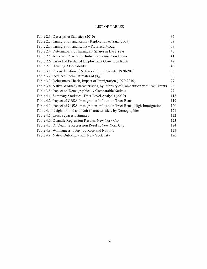
Table 2.1: Descriptive Statistics (2010) 37 Table 2.2: Immigration and Rents - Replication of Saiz (2007) 38 Table 2.3: Immigration and Rents – Preferred Model 39 Table 2.4: Determinants of Immigrant Shares in Base Year 40 Table 2.5: Alternate Proxies for Initial Economic Conditions 41 Table 2.6: Impact of Predicted Employment Growth on Rents 42 Table 2.7: Housing Affordability 43 Table 3.1: Over-education of Natives and Immigrants, 1970-2010 75 Table 3.2: Reduced Form Estimates of (sijt) 76 Table 3.3: Robustness Check, Impact of Immigration (1970-2010) 77 Table 3.4: Native Worker Characteristics, by Intensity of Competition with Immigrants 78 Table 3.5: Impact on Demographically Comparable Natives 79 Table 4.1: Summary Statistics, Tract-Level Analysis (2000) 118 Table 4.2: Impact of CBSA Immigration Inflows on Tract Rents 119 Table 4.3: Impact of CBSA Immigration Inflows on Tract Rents, High-Immigration 120 Table 4.4: Neighborhood and Unit Characteristics, by Demographics 121Table 4.5: Least Squares Estimates 122Table 4.6: Quantile Regression Results, New York City 123Table 4.7: IV Quantile Regression Results, New York City 124Table 4.8: Willingness to Pay, by Race and Nativity 125Table 4.9: Native Out-Migration, New York City 126

vii

LIST OF FIGURES

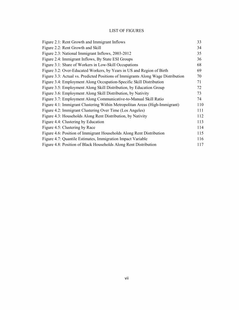
Figure 2.1: Rent Growth and Immigrant Inflows 33 Figure 2.2: Rent Growth and Skill 34 Figure 2.3: National Immigrant Inflows, 2003-2012 35 Figure 2.4: Immigrant Inflows, By State ESI Groups 36 Figure 3.1: Share of Workers in Low-Skill Occupations 68 Figure 3.2: Over-Educated Workers, by Years in US and Region of Birth 69 Figure 3.3: Actual vs. Predicted Positions of Immigrants Along Wage Distribution 70 Figure 3.4: Employment Along Occupation-Specific Skill Distribution 71 Figure 3.5: Employment Along Skill Distribution, by Education Group 72 Figure 3.6: Employment Along Skill Distribution, by Nativity 73 Figure 3.7: Employment Along Communicative-to-Manual Skill Ratio 74 Figure 4.1: Immigrant Clustering Within Metropolitan Areas (High-Immigrant) 110 Figure 4.2: Immigrant Clustering Over Time (Los Angeles) 111 Figure 4.3: Households Along Rent Distribution, by Nativity 112 Figure 4.4: Clustering by Education 113 Figure 4.5: Clustering by Race 114 Figure 4.6: Position of Immigrant Households Along Rent Distribution 115 Figure 4.7: Quantile Estimates, Immigration Impact Variable 116 Figure 4.8: Position of Black Households Along Rent Distribution 117

1

1. Introduction

The topic of immigration is of crucial importance for both academics and policymakers.

The foreign-born population share in the U.S. has risen steadily since 1970 and the current share

stands at roughly 15% of the total population (levels not seen since the early 19th century).

Furthermore, the most recent projections from the PEW research center suggest immigrant shares

of the population are expected to reach 18.8% by 2060.1 In fact, immigrants entering the U.S.

and their descendants will account for 82% of total U.S. population growth. This projection is

staggering compared to recent decades. From 1960-2005, immigrants and their descendants only

accounted for 51% of overall population growth. As a result of this increased growth due to

immigration, projected immigration will also have important implications for the overall

demographic landscape of the U.S. Due to the projected immigration discussed above, the non-

Hispanic white population share will fall from 67% to 47% while the Hispanic population share

will more than double from 14% to 29%.2 As such, the high current level of immigration and the

projected rise in immigrant population shares makes understanding the effects of immigration all

the more important to policymakers.

This dissertation works to reexamine and challenge commonly used methodologies in

estimating the effects of immigration on the U.S. economy. In this dissertation, I examine the

impact of immigration on two important markets: the rental housing market (chapters 2 and 4)

and the labor market (chapter 3). The effects of immigration on both housing prices and the

wages of native workers have motivated much of the discourse regarding immigration reform.

Why should we care about the impact of immigration on rents? From an equity

standpoint, any immigrant-induced rent increase would be concentrated on the poorest

Americans. The most recent data from the American Community Survey suggests that nearly

half of all renter households are “house poor”, as defined by the Federal government. That is, 1 http://www.pewresearch.org/fact-tank/2015/03/09/u-s-immigrant-population-projected-to-rise-even-as-share-falls-among-hispanics-asians/ 2 http://www.pewhispanic.org/2008/02/11/us-population-projections-2005-2050/

2

these households spend more than 30% of their income on housing. Furthermore, nearly a

quarter of all renter households spend more than 50% of their income on rents. While this may

seem to have merit, from a social welfare point-of-view, whether immigrants raise prices should

not matter. I would argue that there are two sides to every market and while rising prices may

cause some tenants to lose welfare upon an immigrant inflow, the owners of these properties

surely gain from these increases in prices. Put bluntly, there are no losses of efficiency when

prices increase.

As such, the policy relevance of this topic may not be immediately clear. The problem is

that policymakers do not seem to consider total social welfare when discussing immigration

reform. Policymakers in the U.S. and abroad have used scholarly evidence that immigrant

inflows cause higher housing prices to argue against immigration. In a speech to discuss the

economic costs of immigration, Theresa May, the Home Secretary in the U.K., said3: “One area

in which we can be certain mass immigration has an effect is housing...More than one third of all

new housing demand in Britain his caused by immigration. And there is evidence that without

the demand caused by mass immigration, house prices could be 10% lower over a 20 year

period.” Similar statistics and research have been used by the Labour Leader in New Zealand4

and many other national news outlets in the U.S. to argue against immigration. On the other side

of the aisle, many proponents of immigration reform have argued the economic benefit of

immigration via the housing market. With homeownership rates and housing values in decline,

immigrant inflows can “bring back” the housing market through demand shocks. This point-of-

view is shared by many U.S. politicians like former New York Mayor Michael Bloomberg and

former Governor of Utah and presidential nominee Jon Huntsman, among many others.5 As both

proponents and opponents of immigration reform use the same general result to argue both sides 3 http://www.telegraph.co.uk/news/uknews/immigration/9739590/Curbing-mass-immigration-could-bring-down-house-prices-Theresa-May-says.html 4 http://www.3news.co.nz/politics/david-cunliffe-blames-migrants-for-housing-crisis-2014052617#axzz3gjvE9eno 5 Several news outlets have published pieces to this affect. Miriam Jordan (2013) published “Immigrants Buoy the Housing Market” in the Wall Street Journal, Jason Gold (2013) published “Killing Immigration Reform Hurts the Housing Recovery” in the U.S. News and World Report, among many others.

3

of immigration policy, identifying the true effect of immigration on housing is important for the

national dialogue on immigration reform.

Chapters 2 and 4 of this dissertation examine the impact of immigration on the rental

housing market. The general consensus in the literature is that immigration significantly

increases housing rents: an inflow of international immigrants equal to 1% of the total population

increases average rents within a metropolitan area by 1% (Saiz, 2007; Ottaviano and Peri, 2012).

This result is the motivation for both chapters 2 and 4.

In chapter 2, I address the magnitude of this result. Specifically, I argue that this estimate

is implausibly large as it does not fit with our knowledge of the urban housing market. The

estimated effect of immigration on rent growth is significantly larger than most estimates of the

effect of total population growth on rents. In fact, the existing literature examines the impact of

an immigrant inflow equal to 1% of the total population, which is an increase in total population

of 1%. Why would population growth attributed solely to immigration have a different impact on

rents than an equal sized population flow of immigrants and natives? Furthermore, Saiz (2007)

analyzes the short-run impact of immigration. How can immigration have a larger effect on rents

than overall population growth when other houses are assumed to be immobile? These two

questions motivate the research in Chapter 2 and the results show that the true effect of

immigration on rents is much smaller than the estimates in the existing literature and

quantitatively similar to the estimates of overall population growth on rents.

In chapter 4, I challenge the use of metropolitan areas as a single housing market in the

previous literature. It is commonly argued that metropolitan areas are segmented into different

submarkets and the implicit price of housing unit characteristics and neighborhood amenities

differ across these submarkets. If submarkets exist because immigrants and natives have different

locational preferences, then we would anticipate a differential impact of immigration on rents

within a metropolitan area. There are two competing dynamics in play. Immigrants tend to

cluster within metropolitan areas forming ethnic enclaves. These ethnic enclaves provide cultural

4

amenities, access to employment, and ease the assimilation process. If the desire to live among

immigrants is strong enough, then this increased willingness to pay for housing in a given

location will bid up rents in these areas. However, when native households are mobile, white

flight out of high-immigrant neighborhoods may diffuse the effects on rent. In this chapter, I

analyze these two dynamics and assess the impact of immigration within metropolitan areas. My

results support the white flight hypothesis and suggest that it is the increased willingness to pay of

natives to live near other natives that drives the average effects found in the existing literature.

Chapter 3 diverges from the housing market and focuses on the impact of immigration in

the labor market. Though I assess a different market, the underlying focus is still on the

methodology used in the existing literature. When assessing the impact of immigration on native

wages, researchers first group immigrants and with “demographically comparable” natives and

assess the impact of relative labor supply on relative wages within skill groups (for example, see

Borjas, 2003 or Ottaviano and Peri, 2012). The fundamental question in this literature then is

who competes with whom in the labor market. In almost all cases, researchers stratify the labor

market based on educational attainment and work experience. In this chapter, I argue that

immigrants and natives with the same level of education and work experience do not necessarily

compete in the labor market -- immigrants and natives are imperfect substitutes within education-

experience groups. Instead, I suggest stratifying labor markets by occupation groups defined by

occupation-specific skills, which will be more homogeneous with respect to skill. In doing so,

the results suggest that the existing literature understates the impact of immigration on native

wages. If we assess the impact of an immigrant supply shock on the wages of natives with whom

immigrants directly compete for jobs, the estimated impact is twice as large.

5

2. Re-Evaluating the Impact of Immigration on the U.S. Rental Housing Market 2.1 Introduction

The union of the immigration and urban literatures is an emerging area of research.

Work in this area was pioneered by Saiz (2003), who analyzes the impact of the 1980 Mariel

Boatlift on the Miami housing market, and formalized by Saiz (2007). Using a difference-in-

difference approach and the natural experiment that occurred in Miami, Saiz (2003) finds that

rental prices in Miami increased by 8 – 11% more than comparable housing markets during this

time; thus, Saiz (2003) concludes that immigrants cause a short-run increase in rental prices.

Following the work of Saiz (2003), the literature on the impact of immigration on housing has

evolved and two themes have emerged as a general consensus. First, subsequent research turned

to a national setting for the analysis: Saiz (2007) and Ottaviano and Peri (2012) analyze the US

housing market, Gonzalez and Ortega (2013) in Spain, Accetturo et al. (2012) in Italy, Degen and

Fischer (2009) in Switzerland, and van der Vlist et al. (2011) in Israel. Second, regardless of the

country of analysis, researchers typically find a significant, positive short-run impact on housing

rents and housing values. Results from studies on the US are consistent: Saiz (2007) finds an

inflow of new legal immigrants equal to 1% of the total population causes an increase of around

1% for both rents and housing values and Ottaviano and Peri (2012) find an increase in housing

prices between 1.1 – 1.6%. In other countries, the estimates tend to be even larger: Gonzalez and

Ortega (2012) find an increase in housing values of 3.4% in Spain and Degen and Fischer (2009)

find an increase in housing values of 2.7% in Switzerland.

The general result found in the literature is not debatable; a one-time increase in

population should have some positive impact on short-run housing prices, ceteris paribus.

However, the estimates above seem implausibly large. There are sizeable discrepancies between

the estimates in the studies above and previous estimates of immigration impacts in other markets

6

and the impact of overall population growth in the urban literature. In the labor market, sizeable

impacts of immigration on labor market outcomes are rare. In fact, Saiz (2007) suggests that

“from the labor literature, a 1% increase in the relative share of a skill group depresses the

relative wages of that group by 0.03%”. However, if one accepts that an increase in the

immigrant population equal to 1% of the total population of a city leads to a 1% increase in rents,

then, according to Saiz (2007), this increase in rent amounts to 0.28% of the initial income of the

typical rent-occupied household. The modest effects in the labor literature are not unique.

Existing research assessing the fiscal effects of immigration (Borjas and Trejo, 1991; Gustman

and Steinmeier, 2000; among others) and the effect of immigration on overall prices (Cortes,

2008) all find modest effects of immigration. Thus, the housing market is the only market for

which large impacts are found.

Further discrepancies arise when one compares the estimates to results in the existing

urban literature. As stated above, Saiz (2007) estimates the impact of an immigrant inflow equal

to 1% of the total population, which is a 1% increase in population. Unless we believe

immigrants have a differential impact on housing prices than native population growth, then the

impact of an inflow of immigrants equal to 1% of the population on rents should be equivalent to

the impact of overall population growth. Estimates of total population growth or employment

growth are often included as controls in the typical housing price determination equation

(Poterba, 1991; Abraham and Hendershott, 1996; Malpezzi et al., 1998; among others). The

evidence of the impact of population growth on housing prices is mixed. Poterba (1991) uses

age-adjusted population growth and finds negative and statistically insignificant impacts on

housing prices. Similarly, Malpezzi et al. (1998) find wrong-signed and insignificant impacts of

overall population growth on both housing values and rent. Abraham and Hendershott (1996) do

find a positive and statistically significant impact of employment growth on housing, but the

7

magnitude is much smaller (around 0.3% increase in housing for a 1% increase in employment),

which is significantly larger than the elasticity of 1 estimated by Saiz (2007).

Thus, in order for the results in the existing literature to be taken as causal, one must

believe that 1) housing markets respond differently than any other market to immigrant-induced

changes in demand and 2) immigrant-inflows have a differential impact on housing prices than

overall population growth. While it is fair to assume that the housing market adjusts more slowly

than say, the labor market, there is no clear theoretical perspective that suggests immigrants

should have a differential impact on housing dynamics than overall population growth.

As such, it is difficult to ascertain causality from the model specification used in much of

the literature. Specifically, the model omits variables that are correlated with both immigrant

location decisions and rent growth, causing estimates to be biased upwards. To see this, note that

a commonly cited fact in the immigration literature is that immigrants tend to cluster in specific

cities in the US (Bartel, 1989). These high-immigration cities tend to be the largest U.S. cities

with thriving economies. If overall economic activity and productivity is higher in high-

immigration cities, then we would expect wages and housing prices to be grow more quickly in

these cities, irrespective of immigration. Saiz (2007) acknowledges the potential harm of this

omitted relationship: “Omitted variables that are differentially present in cities with high

immigration inflows, and that might account for the growth in rents in these cities (such as

economic shocks), are a potential threat to my interpretation of the result.6

To this end, I account for this relationship and make three contributions to the existing

literature. First, the use of a more recent dataset will supply evidence to whether the findings of

past research were simply a one-time occurrence. Second, I improve upon the existing model

specification and posit a more robust empirical model that includes initial city-specific 6 Borjas (2003) further anticipates this fact: “If immigrants endogenously cluster in cities with thriving economies, there would be a spurious positive correlation between immigration and wages.” Thus, it is likely this fact holds true with housing prices as well.

8

characteristics and a more robust treatment of housing supply. These initial conditions, described

in detail later, control for initial city characteristics that impact the future evolution of rents,

namely factors that predispose cities to increased future growth. In doing so, four important

results emerge. First, the use of more recent data and a model specification similar to that in Saiz

(2007) yield comparable results to those found in the existing literature: an immigrant inflow

equal to 1% of the total population leads to an increase in rental prices of 1.3%. Second, when

using the more robust empirical model, the coefficient of interest decreases by around 80% and is

not statistically different from zero. This result suggests that past estimates were biased due to

the spurious correlation discussed above. Third, I provide evidence that, due to the nature of the

omitted variable bias, the shift-share instrumental variable strategy employed in the much of the

existing literature fails to identify a causal impact of immigration on housing prices. Specifically,

I show that past immigrant location choices and future rent growth are both positively correlated

with the initial economic characteristics of cities. Omission of this relationship in the model leads

to biased (upward) and inconsistent estimates as the instrument is correlated with the error term.

Fourth, once I control for initial city characteristics, the magnitude of the impact is similar in

magnitude to the estimated impact of overall changes in housing demand. Overall, I conclude

that it is incorrect to assert that immigrants and natives have a differential impact on housing

prices.

Last I address a more policy relevant question of how immigrants impact the rent-to-

income ratio within cities. Taking the rent-to-income ratio as a proxy for housing affordability,

the use of this housing market outcome allows one to speak to the overall impact of immigrants

on natives as this ratio accounts for changes in both the housing and labor market. While the

results do not allow for definitive statements on the impact of immigrants on housing

affordability, the results do provide further evidence that the omission of city-specific effects lead

to bias in previous studies. Using several measures of income in the dependent variable, a

9

negative correlation is consistently found. Most notably, this result holds for both low-skilled and

high-skilled industries. Thus, if one believes that immigration has a small positive impact on

housing prices, then this result suggests that average wages are growing more quickly, relative to

rents, in high-immigration cities, regardless of the relative skill mix of the industry. As this result

is not supported in the labor literature, I take this as evidence that immigrants are simply settling

in cities with flourishing economies where both rents and average wages are increasing.

The rest of the paper is structured as follows. Section 2.2 outlines a conceptual

framework of rental housing demand and its relationship to prior empirical specifications and the

present empirical model. Section 2.3 describes the data sources used in this analysis. A full

description of each variable used can be found in the Data Appendix and summary statistics are

provided in Table 2.1. Section 2.4 discusses the results of the preferred specification and the bias

introduced by the shift-share instrument. Section 2.5 provides the methodology and results when

using rent-to-income ratios as the dependent variable. Section 2.6 concludes.

2.2 Conceptual Framework

The motivation for this paper is derived from Figures 2.1 and 2.2. Figure 2.1 is a

scatterplot of average rent growth and average immigrant inflows (as a percent of lagged total

population) from 1999-2011 in U.S. metropolitan areas. Consistent with Saiz (2007), there is a

statistically significant positive relationship between rent growth and immigrant inflows. Absent

from past models, however, is a discussion regarding where immigrants are locating. Note the

cities in the NE region and those in the SW region of Figure 2.1. Immigrants are locating in the

largest cities in the U.S. These cities have more overall economic activity that attracts both firms

and workers in the future. As shown below, these cities have a more inelastic supply of housing.

Thus, one would assume that these cities, for reasons beyond changes in demographics, will have

differential housing price growth.

10

To demonstrate this, consider a comparison of Miami, FL and Muskegon, MI in the prior

period. From 1990-1998, the Miami, FL (Muskegon, MI) Core Based Statistical Area (CBSA)

experienced overall population growth of 17.05% (5.32%) and real wage growth of 21.4%

(14.3%).7 Comparing high-immigration cities to low-immigration cities tells a similar story:

high-immigration (low-immigration) cities experienced, on average, total population growth of

11.14% (2.17%) and real wage growth of 21.12% (13.34%).8 Similarly, new construction in

high-immigration cities is more regulated according to the Wharton Residential Land Use

Regulatory Index (WRLURI). Higher values of this index suggest a less elastic supply. High-

immigration cities have an average WRLURI that is about 75% of one standard deviation above

the sample average, while the average WRLURI in low-immigration cities is about 75% of one

standard deviation below the sample average. Thus, because of favorable economic conditions

and relatively more inelastic supply, one would expect high-immigration cities to face increased

growth in housing prices relative to low-immigration cities irrespective of immigration.

Saiz (2007) does attempt to control for fundamental city differences by including the

initial share of the population holding at least bachelor’s degree, a proxy for overall skill in a city.

Glaeser and Saiz (2004) show that cities with more education (skill) experienced increased

growth relative to less-skilled cities and this growth led to increases in wages and housing prices.

Figure 2.2 plots this relationship from 1999-2011. Specifically, Figure 2.2 plots average rent

growth from 1999-2011 against the share of the population holding at least a bachelor’s degree in

1990. The data suggest that this proxy for future growth is not correlated with future rent growth.

Though slightly positive, the correlation is not statistically different from zero. As this seems to

be a weak indicator of future economic success9, the model estimated by Saiz (2007) fails to

7 Glaeser et al. (1995) suggests these as measures of city success. 8 The 25 CBSA’s that received the highest share of immigrants from 1999-2011 are classified as high-immigration cities. Low-immigration cities are the bottom 25 CBSA’s. 9 Similar graphs showing the relationship between the share holding a bachelor’s and employment growth, wage growth, and population growth (available upon request) reveal the same pattern. There is no discernible relationship between economic success and this proxy for skill from 1999-2011.

11

control for these inherent differences between cities. The preferred empirical model herein

accounts for such factors.

The empirical model follows directly from Saiz (2007). The theory underlying the

empirical model is a simple framework of demand and supply of housing. Specifically, I regress

rent growth on immigration inflows and a host of other explanatory variables controlling for both

contemporaneous economic conditions and initial city conditions. One obvious omission from

the model of Saiz (2007), however, is native population flows. In an equilibrium model of the

housing market, we would expect both immigrant and native population flows to influence the

evolution of rents. By omitting native population flows, one can think of the empirical model as

a partial reduced-form model. Formally, the preferred model is written as:

(1) ∆ln (𝑟𝑘𝑘) = 𝛽 �𝐼𝐼𝐼𝐼𝐼𝐼𝐼𝐼𝑘𝐼𝑘,𝑡−1𝑃𝑃𝑃𝑃𝑃𝐼𝑘𝐼𝑃𝐼𝑘,𝑡−2

� + 𝛼𝑋𝑘,𝑘 + 𝜋𝑊𝑘,𝑘−1 + 𝜇∆𝑍𝑘,𝑘−1 + 𝛿𝑀𝑘,𝑘∗ + 𝜃𝑗𝑘 + ∆𝜀𝑘,𝑘.

Consistent with Saiz (2007), the dependent variable is the annual change in the log of FMR in

city k at time t and the main explanatory variable is the lagged annual inflow of legal immigrants

admitted to city k at time t-1 as a percent of the total population in period t-2, making β the

coefficient of interest. The vector 𝑋𝑘,𝑘 includes city-specific attributes, such as climate, crime,

and land area, and the initial share of the population holding at least a bachelor’s degree. 𝑊𝑘,𝑘−1

is the lagged unemployment rate in the CBSA.

The model diverges from that of Saiz (2007), however, with the inclusion of 𝑀𝑘,𝑘∗ and a

more robust treatment of housing supply. Following Glaeser et al. (1995), among others10, 𝑀𝑘,𝑘∗

is a vector of initial CBSA-specific, time invariant variables in some year 𝑡∗ < 𝑡. The intuition

here is that past economic and housing market conditions may have a persistent long-run impact

10 Several papers, mainly in the growth literature, use initial city conditions to explain differential growth rates among cities or metropolitan areas (Glaeser et al., 1995; Drennan et al., 1996). However, a few studies use this technique in other literatures; namely, the housing market (Engberg and Greenbaum, 1999) and the labor market (Beeson and Montgomery, 1993).

12

on future growth. Cities who attracted migrants in the past (both native and foreign-born) will

continue to do so in the future (Blanchard and Katz, 1992; Glaeser et al., 1995). As such, these

cities will experience increased future overall growth in economic activity and growth in housing

demand. The vector 𝑀𝑘,𝑘∗ includes rent growth from 1980-1990, the initial Fair Market Rent

(FMR) level in 1990, the share of the housing stock built before 1939 in 1990, the percent of total

earnings coming from farms in 1990, per capita property tax revenues in 1997, and per capita

spending in retail and service establishments in 1992. Rent growth in CBSA k from 1980-1990

and the FMR level in 1990 are the main inclusions in the preferred model. The intuition behind

these two variables is described in detail below; however, it should be noted that both of these

variables essentially serve the same purpose: to control for the fact that certain cities are

predisposed to increased future rent growth. As such, these two variables do not enter into the

specification together. I estimate two variants of (1) where the initial rent growth and initial rent

levels enter separately.

Rent growth from 1980-1990 controls for the possibility that immigrants are locating in

“superstar” cities. Gyourko, Mayer, and Sinai (2013) show that housing price appreciation in

some cities is persistent and superstar cities that experience increased past price growth will face

higher future appreciation. The authors show that high housing price growth in superstar cities

occurs even if the inherent value of a location, the elasticity of housing supply, and the

willingness to pay to live in each location is held constant. The initial FMR level in 1990 is a

proxy for overall economic vibrancy in a city. Cities with higher rents in 1990 were those with

thriving economies experiencing positive economic shocks. When rents are higher, the values of

local amenities must be higher in order to compensate for this increase in housing expenditures

(Roback, 1982). As such, these cities are attractive to in-migrants, both native and foreign-born.

Furthermore, population tends to flow to area with higher housing prices and higher rents and

these population flows are persistent over several decades (Rappaport, 2004). Thus, cities with

13

high rents in period t* will face higher future growth in housing demand (relative to those cities

with lower housing prices) in period t> t*. If immigrants are inherently attracted to these same

cities yet the model ignores this relationship, then one might falsely attribute accelerated future

rent growth to immigrant inflows.

Per capita property tax revenue is expected to have a positive impact on future housing

prices. Note that this is property tax revenues, not property tax rates. Thus, this variable is not

meant to control for property taxes in the user cost of owning a home; rather, this measure is a

proxy for the initial amenity level of a CBSA relative to others. Higher per capita property tax

revenue suggests increased spending on public goods, namely education and police/protection. In

cities with higher property tax revenue, we expect higher amenity values of public goods and

these amenity values should be capitalized into rents. The impact of the share of the housing

stock built prior to 1939 is, a priori, ambiguous. On one hand, an older housing stock may

depress growth in housing prices. Brueckner (1982) suggests that an inverse relationship exists

between the age of the housing stock and future population growth. If so, a lack of population

growth will slow housing demand and, ceteris paribus, slow the growth of rents in the city. On

the other hand, an older housing stock could have a positive impact on future housing prices if

there is an incentive to revitalize the city (i.e. gentrification). The percent of total earnings

coming from farms in 1990 is included as a proxy for the opportunity cost of converting

agricultural land to residential land and is expected to have a positive impact on future housing

price growth. Per capita consumer spending serves as a proxy for the overall economic activity in

a city and should be positively correlated with future housing price growth.

The last addition to the preferred model is a more rigorous treatment of housing supply. I

include controls for the stringency of land use regulations and the cost of construction. In Saiz

(2007), land area of the CBSA is the lone control for housing supply. However, it has been

consistently shown that a strong positive relationship exists between housing prices and the

14

stringency of land use regulations (Pollakowski and Wachter, 1990; Malpezzi et al., 1996;

Ihlanfeldt, 2007; Gyourko et al., 2008; among others). A city with more stringent land use

regulations (i.e. zoning laws, local government interventions, etc.) will face higher future housing

prices. To control for the degree of land use regulations, the vector 𝑋𝑘,𝑘 now includes the

Wharton Residential Land Use Regulatory Index (WRLURI) (Gyourko, et al., 2008). The use of

the WRLURI as a control for housing supply has advantages and disadvantages. The WRLURI is

superior to the use of land area in that it encompasses a wide range and a large number of land

use regulations. Pollakowski and Wachter (1990) suggest that analyzing the effect of land use

regulations individually (i.e. land area), as opposed to collectively (i.e. WRLURI), will understate

the impact of these controls on housing prices. The disadvantage, however, is that the WRLURI

is time-invariant. Therefore, it must be assumed that land use regulations within a city are

constant throughout the sample period. Similarly, to proxy for cost of new construction I include

the one period lag of the change in average construction wages.

Equation (1) is estimated using both OLS and 2SLS using the same shift-share

instrumental variable strategy used in the existing literature.11 Aside from the additional controls,

two differences exist between the model in (1) and that of Saiz (2007). First, 1995 is used as the

base year of the instrument, while Saiz (2007) uses 1983. I chose 1995 because it is a central date

for which data on initial conditions are available. 12 As discussed below, these initial conditions

also serve as controls for the location choices of the immigrants in the base year. Second, I

include region fixed effects interacted year fixed effects (𝜃𝑗𝑘) to control for regional differences in

rent appreciation. Thus, 𝛽 is estimated from changes in the number of newly arriving immigrants

within a CBSA over time, compared to other CBSA’s in the region.

11 This instrument, described in detail later, is the shift-share instrument similar to that first introduced by Altonji and Card (1991). The instrumental variable strategy uses predicted immigrant inflows, derived from historical settlement patterns of immigrants, as an instrument for actual immigrant inflows. 12 Ultimately, the choice of 1995 as the base year was an arbitrary one as all results hold when different base years are used. Results using alternate base years for the instrument are available upon request.

15

2.3 Data

The data used in this paper are a panel of 325 Core Based Statistical Areas (CBSA’s)

over the period 1999-2011.13 I use the 2013 Core Based Statistical Area (CBSA) definitions

based on population estimates from the 2010 U.S. Census. The advantage of using current CBSA

definitions is that metropolitan areas are no longer defined using partial counties. Thus, county-

level data is easily aggregated to the CBSA-level.

Following Saiz (2007), data on immigrant inflows comes from the “Immigrants Admitted

to the United States” data series of the Department of Homeland Security (DHS).14 Following

the discussion of Saiz (2007), these data should be considered a “noisy indicator” of recent

immigrant inflows for three reasons. First, I am unable to identify the actual timing of arrival to

the U.S. There may be lags from the time a person is granted admission and actually arrives in

the U.S. While the timing of arrival may be off for some, the data suggest the error is minimal.

In 1995 (the year chosen for the base year of the instrument described below), 76% of all

immigrants were admitted and arrived in the same year and more than 99% of the immigrants

arrived within 1 year of admission.15 Second, immigrant inflows are calculated using data on the

zip code of intended residence. If an immigrant settles in a different location than stated in the

data, then I overstate the immigrant inflow to certain CBSA’s, while understate the inflow in the

actual CBSA of residence. Third, as noted above, I do not observe illegal immigrant inflows to

the U.S.

13 There are 377 CBSA’s defined in the 2013 definitions (less CBSA’s in AK and HI); however, I only have complete data for 325 of these CBSA’s. This will not impact the analysis as it compares to Saiz (2007) because most (if not all) of the 52 omitted CBSA’s were not included in Saiz’s sample. 14 During the sample period analyzed in Saiz (2007), this data series was under the control of the Immigration and Naturalization Service (INS). While these data (1999 – 2012) are now managed by the Department of Homeland Security, the structure of the data is the same. While these data are from the same source as used in Saiz ( 2007), one difference should be noted. Due to increased security measures, the DHS does not provide the micro-data files of these data. These data are publicly available on the DHL website, but MSA definitions are not constant across years. Thus, the custom data I received were aggregated using the most current CBSA definitions (2013). 15 I am unable to make use of these admission data because I do not have access to the micro-data for the years 1999-2011.

16

Though data issues exist, these data have the advantage of being the only available source

of annual immigrant inflows to the US. The concern over illegal immigrant flows is most

relevant to this study and one that must be addressed. One concern is that illegal immigrants may

cluster differently than legal immigrants. This could occur if illegal immigrants are more heavily

concentrated in border cities due to higher transportation costs. While accurate counts of the

illegal immigrant population at the CBSA level do not exist, the state-level estimates are

consistent with the legal immigrant population. Passel et al (2004) estimate that roughly two-

thirds of all illegal immigrants live in just 6 states: California, Florida, Illinois, New York, New

Jersey, and Texas. These 6 states are also the main hubs for legal immigration. From the data,

66% of all legal immigrants settled in these 6 states from 1999-2011. While illegal immigrant

populations may cluster in the same state as legal immigrants, it is possible that illegal

immigrants cluster in different parts of a CBSA or the willingness to pay to live near other

immigrants may be stronger for illegal immigrants as the benefits from ethnic enclaves are larger.

Again, I do not have data at finer geographic levels and cannot account for this in the current

model. One may to alleviate this concern is to use decennial Census data that presumably counts

all immigrants, both legal and undocumented. I re-estimate all models herein using decennial US

Census data and the results, reported in Table A2.4 of the Appendix, suggest that the impact of

undocumented immigrants is minimal as the results are quantitatively similar to those found in

the main text.

The main source for rental price data is the Fair Market Rent (FMR) series from the

Department of Housing and Urban Development (HUD). The FMR in a particular area

corresponds to the market value of a vacant two-bedroom unit. HUD reports FMR’s at the

county-level for each county in the U.S. For most counties in the sample, the FMR is the price

of this unit at the 40th percentile of the rent distribution; however, starting in 2005, the FMR for a

small sample of counties are reported as the 50 percentile of the rent distribution. Thus, I

normalize the rental housing price measure throughout the sample, by adjusting 50th percentile

17

estimates to 40th percentile estimates. To do this, I use 40th percentile FMR data for years prior to

2005 to predict the 40th percentile estimate in 2005 �𝐹𝑀𝐹�2005� and take the ratio of the true and

predicted values in 2005, �𝐹𝐹𝐹�40%,2005𝐹𝐹𝐹40%,2005

�. Next, I use the 50th percentile FMR data for the

subsequent years to predict the 50th percentile rent estimate in 2004 �𝐹𝑀𝐹�2004� and take the ratio

of the true and predicted values in 2004, �𝐹𝐹𝐹�50%,2004𝐹𝐹𝐹50%,2004

�. Last, I construct an adjustment factor

equal to the average of the previous ratios to deflate 50% FMR estimates to reflect 40% FMR

estimates.16

Income and wage data are derived from several sources. Per capita personal income and

average wages per job are from the BEA Regional Information Systems (REIS). Other

definitions of income are used in the rent-to-income analysis. Average wages of all industries

and average wages of all good-producing industries are derived from the Quarterly Census of

Employment and Wages (QCEW). All income measures are converted into real 2010 dollars

using the CPI-U. Other explanatory variables come from a variety of sources and follow directly

from Saiz (2007). Civilian labor force and unemployment figures are from the Bureau of Labor

Statistics (BLS). Climate data are from the United States Department of Agriculture Economic

Research Service Natural Amenities Scale Database. Violent Crime and murder data are (mostly)

from the FBI Uniform Crime Reports (UCR).17 Initial MSA-specific conditions come from the

1994 County and City Data Book and the 1990 Economic Census. Full definitions of these

variables used can be found in the Data Appendix, while summary statistics are reported in Table

2.1.

16 In 1995, HUD began to report FMR as a 40% estimate. Thus, Saiz (2007) had to adjust FMR to reflect 45% rent estimates for the years 1996-1998. The difference, however, is that both 40th and 45th percentile estimates were reported in 1995 and the ratio of these two estimates were used to adjust 45th percentile FMRs to 40th percentile FMRs. While this may seem like a crude treatment of the data, the results are not sensitive to this adjustment. Results using unadjusted FMR as the dependent variable are available upon request. 17 Some states did not consistently report crimes to the FBI. For these states (i.e. FL, IL, KS, MN, etc.), individual state Uniform Crime Reports were used.

18

2.4 Results

The discussion in section 2.2 suggests that past results may have suffered from

specification error as they omitted fundamental factors that impact rent growth, independent of

immigration. The impact of these omitted factors is seen in the results in Tables 2.2 and 2.3.

Table 2.2 presents OLS and 2SLS estimates of the model posited by Saiz (2007). These

estimates, which serve as a replication of Saiz (2007), are reported in columns (1) and (2),

respectively. The replication results in columns (1) and (2) serve as an appropriate and

comparable baseline even with different CBSA definitions and more recent data, which include

the Great Recession. These results are very similar to those found in the literature.18 The point

estimate in column (2) suggests that an immigrant inflow equal to 1% of the total population will

cause rents to increase by 1.43%.

I then estimate several variants of the preferred specification and report the estimates in

Table 2.3. I first estimate (1) with the controls discussed above, but omitting region effects.

Column (1) includes the initial FMR in 1990 while Column (2) includes rent growth from 1980-

1990. The reason for estimating the model with and without region fixed effects is the concern

that region fixed effects may “soak up” too much of the variation in the independent variable of

interest. Using this instrumental variable strategy, identification of 𝛽 comes from cross-sectional

variation, not variation within a CBSA. Last, I estimate the full preferred model implied by (1)

which includes the additional controls and region fixed effects. Again, column (3) uses initial

FMR in 1990 and column (4) uses rent growth from 1980-1990.

As is shown in Table 2.3, the coefficient of interest, though imprecisely estimated,

consistently decreases as I control for omitted factors. When initial city conditions are included,

the difference in the coefficients from the baseline estimates is roughly the same. Furthermore,

the consistency across all four specifications suggests that the estimates are not sensitive to the 18 Saiz (2007) reports a point estimate on the immigration impact variable of 1.028 (0.995) for OLS (2SLS) estimation

19

inclusion of region fixed effects, which alleviates any concern that the reduction in the estimated

impact of immigration is due to a lack of identification. When initial city conditions are included,

the impact of immigration falls by around 80% and this effect is similar when using either the

proxy for superstar city status or the proxy for initial economic vibrancy. While the point

estimates in columns (1) – (4) are not statistically significant, they are statistically different from

the replication estimates in column (2) at the 5% level.

The performance of the other controls is mixed. The two proxies for supply conditions

have little impact on rent growth. Both the regulation index and changes in construction wages

have neither statistical nor economic significance. Consistent with Saiz (2007), changes in per

capita income seem to have no impact on rent growth and the share of the population with a

bachelor’s degree has a significant negative impact on rent growth. The latter fact is at odds with

the literature analyzing differential city growth and skill levels. The purpose of including this

variable is to control for fundamental differences between cities that will lead to increased future

overall growth and growth of wages and housing prices. The point estimate of the property tax

revenue variable indicates a zero impact, which is unsurprising. In equilibrium, property tax

revenue should not have an impact on prices because it also represents expenditures. While the

marginal utility with respect to property taxes will be negative (decrease demand), the marginal

utility of the expenditures that stem from property tax revenue will be positive. So, on net, the

impact should be zero. This negative correlation points to the specification error in Saiz (2007).

The proxies for superstar cities and overall economic vibrancy perform as expected. Cities with

larger past rent growth and those with higher initial levels of rent experienced increased future

price appreciation.

Again, though not statistically different from zero, the point estimates are more in line

with what we would expect given the discussion above. The result found by Saiz (2007) is

consistent with the standard perfectly competitive, closed city model, where migration-induced

20

rent growth occurs due to the model assumption that, in the short-run, there is no out-migration.

In the short-run, this assumption is not overly restrictive, especially in the rental housing market.

In the short-run, renter households may be “tied” to their current dwelling due to moving and

search costs, contracts/leases, etc. However, if one considers the role of vacancy rates in rental

housing demand, then one would not expect the one-for-one impact found in the existing

literature. Rental prices do not clear instantaneously. In fact, changes in demand are first

reflected in vacancies, then prices (Blank and Winnick, 1953; Smith, 1974; Eubank and Sirmans,

1979; Rosen and Smith, 1983).

A simple back-of-the-envelope calculation, similar to the one presented in Saiz (2007),

shows that the present results are more in line with what is seen in the labor literature. Assuming

the impact of immigration on rents is around 0.25%, as is implied in Table 2.3, then the impact of

an immigrant inflow equal to 1% of the total population amounts to a reduction in initial income

of 0.0735% for the typical renting household.19 However, a more straightforward interpretation

suggests that, as in the labor market, the impact of immigration is negligible. Immigrants are not

causing a substantial increase in rental prices; rather, immigrants are locating in growing

superstar cities where rents are predisposed to housing price growth.

2.4.1 Consistency of the Shift-Share Instrument

The results in Table 2.3 suggest that current period rent growth is positively correlated

with initial economic conditions in the city. Once we account for these characteristics, the impact

of immigration on rent decreases significantly and is no long statistically different from zero.

One possible explanation for the above is that the shift-share instrument introduces bias. The

instrument is defined as:

19 In 2010, the population-weighted average share of foreign-born population in the US was 14.5%. In order to increase the each cities foreign-born population by 1%, the total population in each city would have to increase by 1.18%. Thus, an immigrant inflow of 1.18% yields an increase in rental prices of 0.295%. Assuming the typical renting household spends 25% of its income on shelter, increase in rent amounts to a 0.0735% decrease in income.

21

(2) 𝐼𝐼𝐼𝐼𝐼𝑟𝐼𝐼𝑡𝐼𝑘,𝑘� = 𝜃𝑘,𝑘∗ ∗ 𝐼𝑈𝑈,𝑘.

The first term on the right-hand side is the share of newly arriving immigrants that migrated to

city k in some base year t*. The second term is the total number of immigrants admitted to the US

in year t. The intuition behind this instrument is that while current location decisions are

endogenous to current economic and housing market conditions in the city, settlement decisions

of previous immigrant waves (𝜃𝑘,𝑘∗) are uncorrelated with current economic conditions. This

follows from the standard result that the only significant determinant of immigrant location

decisions is the existing share of foreign born in a city. In fact, it has been shown that other

factors, such as labor market conditions, do not have a discernible effect on location decisions of

immigrants (Bartel, 1989). Thus, one can use imputed immigrant inflows, based on historical

migration patterns, to instrument for current period immigrant inflows.

Concern would arise, however, if either 𝜃𝑘,𝑘∗ or 𝐼𝑈𝑈,𝑘 are, in fact, correlated with initial

economic conditions that are positively correlated with future rent growth. If either is the case,

then past estimates relying on the shift-share instrument are biased and inconsistent. To test the

exogeneity of the first term, I estimate the determinants of this initial immigrant share via the

following model:

(3) 𝜃𝑘,𝑘∗ = 𝛽𝑀𝑘,𝑡∗ + 𝜀𝑘,𝑡.

The dependent variable is the share of total immigrants that entered CBSA k at base year t*. The

vector 𝑀𝑘,𝑘∗ includes the initial CBSA-level variables used above. I estimate (3) using several

different base years as a robustness check and report the results in Table 2.4. Panel A includes

initial rent levels in 1990 as a control, while Panel B includes initial rent growth.

The results in Table 2.4 confirm the bias introduced by the shift-share instrument. Initial

FMR level and past rent growth are both positively correlated with immigrant shares, regardless

22

of the choice in base year. Newly-arriving immigrants in t* were attracted to large, vibrant

superstar cities with high rent levels that were predisposed to increased future rent growth. As

past both of these variables were shown to have an independent positive impact on future rent

growth in Table 2.3, this result suggests instrument is, in fact, correlated with the error term. The

omission of this relationship explains the large estimates in previous models.

Similarly, the exogeneity of annual inflow of immigrants to the US as a whole ( 𝐼𝑈𝑈,𝑘) is

taken as exogenous. However, if one considers immigrant inflows over the past 10 years, it is

clear that immigrant inflows are somewhat cyclical. To see this, Figure 2.3 plots inflows of

legally admitted immigrants to the U.S as a percentage of lagged total population from 2003-

2012.20 The data suggest that immigrants do respond to overall economic conditions in the U.S.

Legal immigration steadily increased through 2006; however, after the start of the Great

Recession in 2008, immigration stagnated and has actually decreased in recent years. This trend

is not unique to legal immigrants. Passel et al. (2013) show that, during the Great Recession, the

growth of the illegal immigrant population also slowed considerably.

These national trends, however, are only important insomuch as the immigrants who do

immigrate to the U.S. display similar preferences when choosing their final destination within the

U.S. To see this, Figure 2.4 plots weighted average immigrant inflows as a percent of total

population for a) the 10 states most adversely affected by the Great Recession, b) the 10 states

that were least affected by the Great Recession and c) all other states from 2006-2011.21 From

Figure 2.4, we see that immigrant inflows slowed in states that were most affected by the

recession and this decline was much more pronounced than in the other two groups. Perhaps

more importantly, California and Nevada are two states included in the group that were most

harmed by the recession. As both also have high shares of foreign-born populations (in 2000,

20 Specifically, each data point is the annual immigrant inflow at time t divided by the total population in t-1. 21 I use the 10 states with the highest Economic Security Index (ESI) (Hacker et al., 2012). The ESI is defined as “an integrated measure of insecurity that captures the prevalence of large economic losses among households”.

23

California was ranked first and Nevada fifth), the data contradict the theory that the lone

determinant of immigrant locations is the existing share of foreign-born populations.

The above analysis suggests that the widely-used shift-share instrumental variable

strategy introduces bias unless one controls for initial city characteristics. Immigrants in the base

year were choosing cities that provided them the best economic opportunities, but these same

cities were predisposed to higher future rent growth. If we believe that the lone determinant of

immigrant location choices is the share of existing population that is foreign-born, then new

immigrants settle in these same cities in search of the cultural amenities. Without explicitly

controlling for this relationship, we would falsely attribute this increased rent growth to

immigration. However, the results in Figure 2.4 suggest immigrants’ preferences may be

influenced by overall economic climate. As such, a more likely explanation is that all

immigrants, both past and present, choose final destinations that afford them the best economic

opportunities.

2.4.2 Robustness Checks

2.4.2.1 Alternate Proxies for Economic Vibrancy

The results in Table 2.3 suggest that past results were driven by specification error. Once

one controls for initial city characteristics that are correlated with future rent growth and

immigrant location choices, the impact of immigration on rents is significantly lower. To lend

credence to this result, several robustness checks are performed. First, as the controls for initial

city conditions are the primary additions to the model, it must be the case that the results from

Tables 2.3 and 2.4 hold when using alternate proxies. Superstar cities can be thought of,

generally, as large cities that possess certain characteristics that lead to future growth and

prosperity. Thus, the alternate proxies used are variables that describe the initial level of

economic vibrancy of the city. Specifically, I re-estimate (1) using the following proxies in place

of initial rent level and initial rent growth: FMR growth from 1983-90, initial median gross rent

24

in 1990, the average commute in 1990, and the price-to-rent ratio in 1990. The first three proxies

follow directly from the discussion in section 2.2. The price-to-rent ratio is included as it has

been shown to be positively correlated with future capital gains (Capozza and Seguin, 1996) and

future rent growth (Clark, 1995; Gallin, 2008). The intuition is that when the price-to-rent ratio is

high in year t-k, owner-occupied housing is overvalued. As such, rents increase in future periods

as the market works to correct itself.

The 2SLS results, presented in Table 2.5, reaffirm the results in Table 2.3, with the

exception of column (1). The difference between column (1) and columns (2) – (4) is that our

proxy for initial economic conditions in (1) is not correlated with future rent growth. While this

is a somewhat disconcerting, it does allow for comparison that validates the discussion regarding

the shift-share instrument above. Table A2.1 of the Appendix provides results similar to those in

Table 2.4. Specifically, I estimate equation (3) using these alternate proxies. The results suggest

that immigrant shares in the base year are positively correlated with the proxies in columns (2) –

(4), but not past FMR growth in column (1). Because immigrant shares are not correlated with

the initial condition in (1), the estimate remains artificially high. As FMR growth from 1983-90

is an imperfect proxy for economic vibrancy, the instrument remains correlated with the error

term.

2.4.2.2 Overall Housing Demand Growth and Rents

A second test for robustness analyzes the impact of overall housing demand on rent

growth. As total population growth to a city is likely endogenous (and there is no clear cut

instrumental variable strategy), I use an oft-used proxy; the Bartik-style predicted labor demand

shocks to a city (Bartik, 1991). The predicted employment growth rate is derived from the

industrial mix of a CBSA and national employment growth.22 In using national employment

trends, I predict employment growth in each CBSA that would have occurred had the industrial

22 A full discussion of the calculation of this variable can be found in the data appendix.

25

mix remained constant. The idea is that while actual employment growth is likely correlated with

local conditions, a national shock to employment levels is likely exogenous with regards to these

unobserved city conditions. Though typically used in the labor literature, this measure of

predicted employment growth has been used in the housing literature as a proxy for changes in

housing demand (Quigley and Raphael, 2005; Saks, 2008). The intuition is that when a city

experiences a positive labor demand shock, migrants enter the city in search of employment;

which, in turn, increases housing demand.

To address this question I estimate the following model:

(4) ∆ln (𝑟𝑘𝑘) = 𝛽𝐸�𝑘𝑘−1 + 𝛼𝑋𝑘𝑘 + 𝜋𝑊𝑘𝑘−1 + 𝜇∆𝑍𝑘,𝑘−1 + 𝛿𝑀𝑘𝑘∗ + 𝜏𝑘 + 𝜃𝑗 + 𝜃𝑗 ∗ 𝜏𝑘 + ∆𝜀𝑘𝑘.

The lone difference of (4) relative to the preferred specification (1) is that the independent

variable of interest is the predicted employment growth in period t-1 (𝐸�𝑘𝑘−1). This model is

estimated using OLS as this measure of population growth is a plausibly exogenous source of

population inflows into a city. The results are reported in Table 2.6. Column (1) provides

estimates without initial city conditions, while columns (2) and (3) use the additional variables

from the preferred model. The results provide further evidence that previous estimates of the

impact of immigration were biased upward. A 1% increase in housing demand leads to an

increase in rents around 0.4 – 0.5%, or about 63% less than the estimates implied by column (2)

of Table 2.2. The inclusion of initial city conditions, though significant determinants of rental

price growth, do not impact the point estimate of interest. This provides support for this measure

of housing demand growth as it seems to be uncorrelated with local market conditions.23

Similarly, the estimates provide further evidence to the bias of previous estimates. It seems

unreasonable that immigrant inflows alone would have an impact on rents that is more than twice

as large as overall growth in housing demand. Lastly, the coefficient of interest in all 23 Table A2.2 of the appendix provides results similar to those in Table 2.4 when using predicted employment growth. Indeed, the results show that this measure of labor demand growth is uncorrelated with the initial conditions in the full model.

26

specifications in Table 2.6 is similar in magnitude to those found in columns (3) and (4) of Table

2.3. Though direct comparison is difficult as the results in Table 2.3 are not statistically

significant, the results provide further evidence that previous estimates were significantly biased.

2.5 The Affordability of Rental Housing

The above analysis has shown that the actual impact of immigration on housing rents is

significantly less than past research suggests. However, the housing market is simply one avenue

through which immigrants may impact the well-being of the native population. While

immigration-induced housing price growth is certainly a concern of policymakers, it may not tell

the entire story. Of greater concern, perhaps, is if immigrant inflows cause housing prices to

increase faster relative to income; in which case, this increase in rents leads to a higher incidence

of “housing-induced poverty” (Thalmann, 1999; Kutty, 2005). Furthermore, by using the rent-to-

income ratio as a measure of housing affordability, one improves upon earlier specifications as

rents are now normalized across cities controlling for city differences in purchasing power.

I contribute to the immigration literature by formally addressing this issue. To my

knowledge, Greulich et al. (2004) is the only existing study to address the impact of immigration

on the affordability of housing. However, the present model diverges from the model of Greulich

et al., (2004) in two key ways. First, Greulich et al. (2004) does not account for the endogeneity

of immigrant location choices. Second, I use a larger more representative sample and a more

extensive set of controls for economic conditions in the city.

Using the same data as in previous sections, I posit the following model to assess the

impact of immigration on housing affordability:

(5) ∆ ln �𝐼𝑘,𝑡𝐼𝑘,𝑡� = 𝛽 �𝐼𝐼𝐼𝐼𝐼𝐼𝐼𝐼𝑘𝐼𝑘,𝑡−1

𝑃𝑃𝑃𝑃𝑃𝐼𝑘𝐼𝑃𝐼𝑘,𝑡−2� + 𝛼𝑋𝑘,𝑘 + 𝜋𝑊𝑘,𝑘−1 + 𝜇∆𝑍𝑘,𝑘−1 + 𝛿𝑀𝑘,𝑘∗ + 𝜏𝑘 + 𝜃𝑗 + 𝜃𝑗 ∗ 𝜏𝑘 +

∆𝜀𝑘,𝑘.

27

Here, the dependent variable is the annual change in log of the rent-to-income ratio. The

numerator is the FMR in city k and the denominator is a measure of average monthly wages in

city k. The explanatory variables are the same, making β the coefficient of interest. In keeping

the same explanatory variables, I implicitly assume any additional factors impacting average

wages are captured by year-by-region fixed effects. As before, the model is estimated by 2SLS

using the shift-share instrument.

Before I proceed to the results, I first discuss the expected sign of 𝛽. Given the results

and discussion in the previous sections, we should expect immigration to have a slight positive

impact on rents. As such, the impact on average wages will determine the sign of 𝛽. A simple

demand and supply model of the labor market suggests a clear cut answer – a positive shock to

labor supply should depress average wage, ceteris paribus. Here, one would expect an immigrant

inflow to have a positive impact on the rent-to-income ratio. Though straightforward

theoretically, the empirical evidence is mixed. The majority of studies using the “area approach”

– where one uses a CBSA (or MSA in the previous literature) to define a local labor market – find

that an immigrant inflow is associated with increases in average wages (Card, 2001; Card, 2007;

Ottaviano and Peri, 2008). The explanation for this seemingly counterintuitive result is that

immigrants and natives are complements in production. Thus, an immigrant-induced labor

supply shock will have a net positive effect on average wages. If so, the sign of 𝛽 is ambiguous,

depending on the relative impact on rents and wages.

I estimate three variants of (5) using different measures of income in the dependent

variable. The results from the preferred specification, including region effects and CBSA-

specific variables, are reported in Table 2.7. For the sake of brevity, I report baseline estimates

(those estimated without initial CBSA controls) in the final row of Table 2.7. First, I use the

measure of average wages per job provided by the BEA as the income measure. The use of the

CBSA-specific average FMR and average wages will allow for inferences about the typical

28

resident in the city. In column (1), we see a similar pattern as was shown in Tables 2.2 and 2.3.

The estimates from the baseline model suggest that immigrants cause housing to become more

expensive relative to income; however, once one adds the controls of the preferred model, the

results suggest that immigrant inflows are negatively correlated with housing affordability. This

negative correlation suggests that housing is becoming less expensive, relative to income, in high-

immigration cities.

Though negative, the estimate is not statistically significant. Thus, a more

straightforward interpretation of these results is that immigrant inflows have a zero effect on the

rent-to-income ratio. One feasible explanation for this result is that the model suffers from

specification error. In particular, contrary to the assumption above, region-by-year fixed effects

and initial city characteristics are not sufficient in controlling for factors that differentially affect

wages but not rents. This assumption was necessary as data limitations prevent me from

controlling for annual CBSA demographics and the instrumental variable strategy prevents the

use of CBSA-fixed effects.

While I acknowledge that specification error could contribute to the results in Table 2.7, I

argue that the effect is likely minimal and does not impact the qualitative interpretation. On the

demand side of the labor market, region-by-year fixed effects pick up regional shifts in labor over

time. One plausible explanation for the increase in average wages is changes in labor demand. If

firms move to cities with high immigrant populations increasing overall demand or there are

changes in the industrial mix of a CBSA (i.e. low-wage jobs are replaced with high-wage jobs),

then average wages would increase, ceteris paribus. While this would certainly explain an

increase in average wages, region-by-year fixed effects should control for this as I use 8 narrow

BEA-defined regions. To mitigate the concern over specification error driving the differences in

wage growth, I have also estimated the above model using 1) state-level fixed effects to control

for more local trends in labor demand and 2) the Bartik-style imputed employment growth,

29

discussed above, as a control for labor supply shifts. In both cases, the results, reported in Table

A2.4 in the Appendix, are quantitatively similar to those in Table 2.7. Furthermore, the initial

city characteristics pick up any inherent differences in wage growth across CBSA’s. Lastly, I

suggest that specification error is not driving the results as they are consistent with the labor

literature using the area approach to estimate the impact of immigration on average native wages.

As I implicitly adopt the area approach here by defining a CBSA as the housing market, a

positive impact on average wages is expected. As such, I interpret the results in Table 2.7 as

evidence that immigrant inflows are positively correlated with both rents and wages and the net

effect is zero.

To check the robustness of the estimate in column (1), I re-estimate (5) using alternate

sources of average wages. Column (2) uses average wages of all individuals derived from the

Quarterly Census of Employment and Wages (QCEW). Using these alternate data confirms the

results in column (1): once one controls for initial city characteristics, the positive statistically

significant impact of immigration on rent-to-income ratios disappears.

While columns (1) and (2) analyzed the wages for the average worker, one might expect

that immigration would have differential impacts based on the skill level of workers. From the

immigration literature, it is expected that, because immigrants are typically less skilled than the

average native, a large proportion of immigrants will enter low-skill occupations and average

wages in these industries will fall. If so, we would expect a more pronounced positive impact on

the rent-to-income ratio when using average wages in these industries, ceteris paribus. Thus,

column (3) uses the average wages of goods-producing industries reported in the QCEW as the

measure of income in the rent-to-income ratio24. The results, however, do not support the theory

above. Comparing the immigration impact in columns (2) and (3), we see that immigration is

more negatively correlated with the rent-to-income ratio when we consider the average lower-

24 Goods-producing industries include construction, manufacturing, and natural resources and mining (BLS).

30

skilled worker. In other words, immigrants are locating in cities where average low-skilled wages

are rising faster than average total wages in high-immigration cities. As such, I take this as

further evidence that immigrants are locating in cities that provide them the best economic

opportunities, which happen to be large urban “superstar” cities where both wages (regardless of

skill level) and housing prices are increasing.25

2.6 Conclusion

While one would expect a one-time population shift to increase housing prices,

specification error in previous models makes causal inference difficult. Rents growth is larger in

high-immigrant cities, but this relationship is not causal; rather, I show that previous estimates of

the impact of immigration on housing prices are biased upward. The upward bias is due to a lack

of controls for city-specific characteristics that 1) attract immigrants and 2) predispose these cities

for higher rent growth. This result further compels one to question the validity of the shift-share

instrumental variable when these city-specific factors are omitted. Recall, the main identifying

assumption of the shift-share instrument was that immigrant inflows in the base year are not

driven by omitted variables that are correlated with future rent growth. However, the positive

correlation between the initial economic conditions and immigrant location choices in the base

year suggests that past immigrants were also attracted to large, growing cities. Omitting these

city characteristics leads the shift-share instrument to be correlated with the error term and the

impact of immigration to be inconsistently estimated.

Once one controls for initial conditions, the impact of immigration decreases significantly

and is no longer statistically significant from zero. Although point estimates are imprecisely

estimated, it is clear that the true impact of immigration on rents is significantly less than the 1%

25 This fact is confirmed using several other definitions of income measuring average wages of different demographic groups. In this analysis, which is available upon request, both low-skilled and high-skilled wage measures were used. The results suggest that a negative correlation between the rent-to-income ratio regardless of the wage measure, which is further evidence that high-immigration cities were predisposed to larger (relative) rent and wage growth.

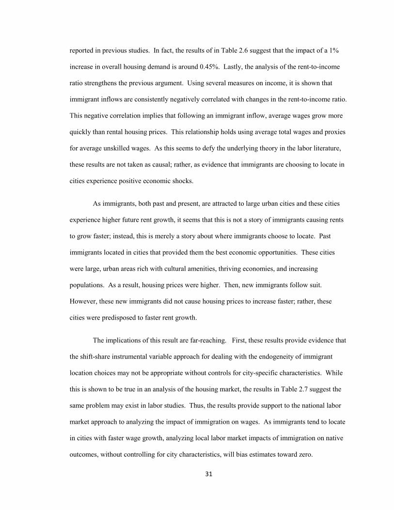
31

reported in previous studies. In fact, the results of in Table 2.6 suggest that the impact of a 1%

increase in overall housing demand is around 0.45%. Lastly, the analysis of the rent-to-income

ratio strengthens the previous argument. Using several measures on income, it is shown that

immigrant inflows are consistently negatively correlated with changes in the rent-to-income ratio.

This negative correlation implies that following an immigrant inflow, average wages grow more

quickly than rental housing prices. This relationship holds using average total wages and proxies

for average unskilled wages. As this seems to defy the underlying theory in the labor literature,

these results are not taken as causal; rather, as evidence that immigrants are choosing to locate in

cities experience positive economic shocks.

As immigrants, both past and present, are attracted to large urban cities and these cities

experience higher future rent growth, it seems that this is not a story of immigrants causing rents

to grow faster; instead, this is merely a story about where immigrants choose to locate. Past

immigrants located in cities that provided them the best economic opportunities. These cities

were large, urban areas rich with cultural amenities, thriving economies, and increasing

populations. As a result, housing prices were higher. Then, new immigrants follow suit.

However, these new immigrants did not cause housing prices to increase faster; rather, these

cities were predisposed to faster rent growth.

The implications of this result are far-reaching. First, these results provide evidence that

the shift-share instrumental variable approach for dealing with the endogeneity of immigrant

location choices may not be appropriate without controls for city-specific characteristics. While

this is shown to be true in an analysis of the housing market, the results in Table 2.7 suggest the

same problem may exist in labor studies. Thus, the results provide support to the national labor

market approach to analyzing the impact of immigration on wages. As immigrants tend to locate

in cities with faster wage growth, analyzing local labor market impacts of immigration on native

outcomes, without controlling for city characteristics, will bias estimates toward zero.

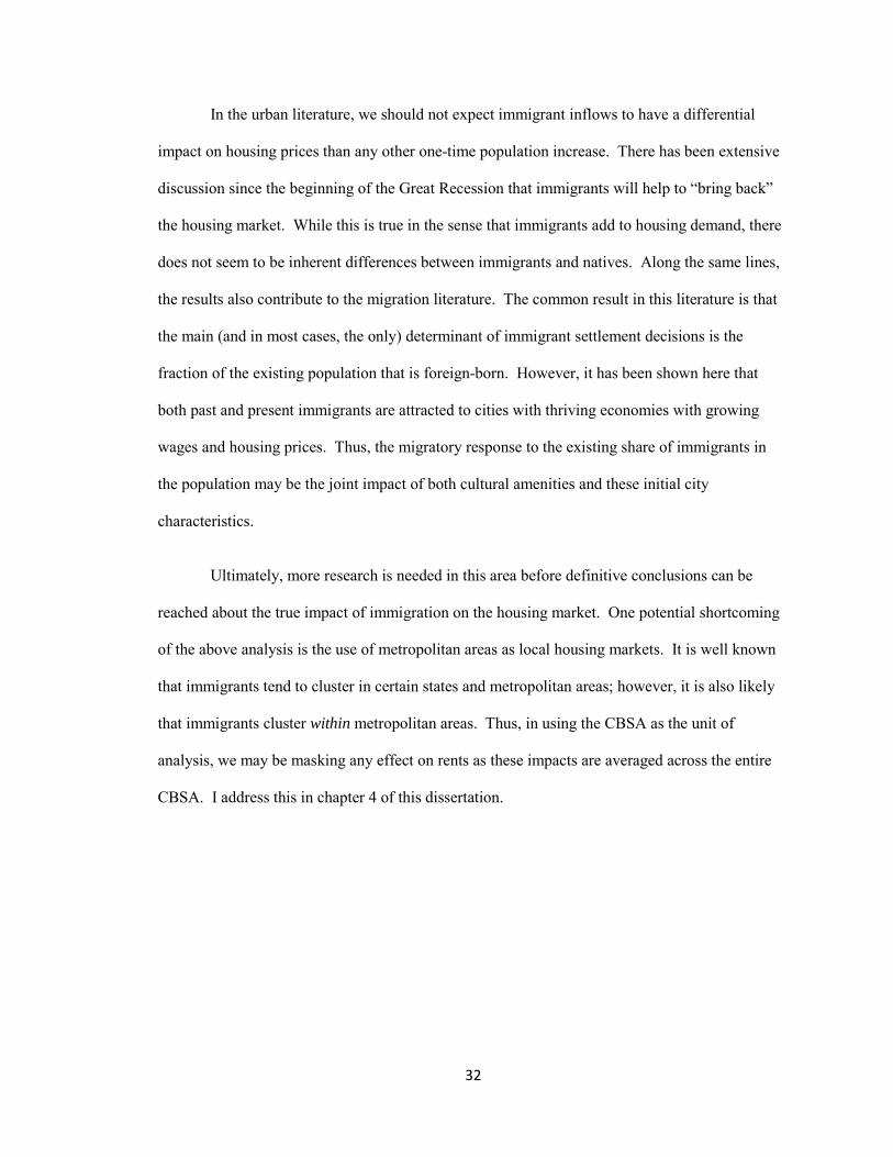
32

In the urban literature, we should not expect immigrant inflows to have a differential

impact on housing prices than any other one-time population increase. There has been extensive

discussion since the beginning of the Great Recession that immigrants will help to “bring back”

the housing market. While this is true in the sense that immigrants add to housing demand, there

does not seem to be inherent differences between immigrants and natives. Along the same lines,

the results also contribute to the migration literature. The common result in this literature is that

the main (and in most cases, the only) determinant of immigrant settlement decisions is the

fraction of the existing population that is foreign-born. However, it has been shown here that

both past and present immigrants are attracted to cities with thriving economies with growing

wages and housing prices. Thus, the migratory response to the existing share of immigrants in

the population may be the joint impact of both cultural amenities and these initial city

characteristics.

Ultimately, more research is needed in this area before definitive conclusions can be

reached about the true impact of immigration on the housing market. One potential shortcoming

of the above analysis is the use of metropolitan areas as local housing markets. It is well known

that immigrants tend to cluster in certain states and metropolitan areas; however, it is also likely

that immigrants cluster within metropolitan areas. Thus, in using the CBSA as the unit of

analysis, we may be masking any effect on rents as these impacts are averaged across the entire

CBSA. I address this in chapter 4 of this dissertation.

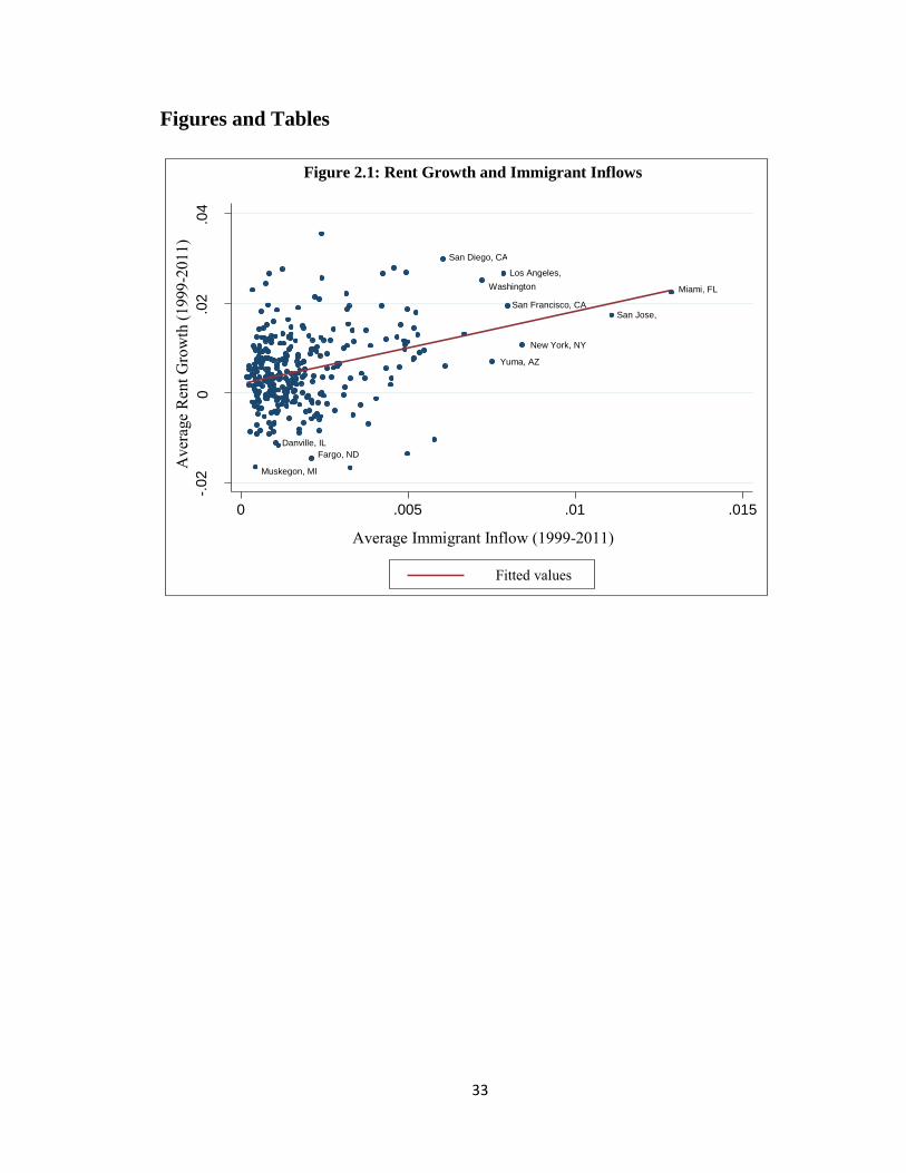
33

Figures and Tables

Miami, FL San Jose,

Los Angeles, Washington

San Francisco, CA

San Diego, CA

Fargo, ND Muskegon, MI

New York, NY Yuma, AZ

Danville, IL

-.02

0 .0

2 .0

4 A

vera

ge R

ent G

row

th (1

999-

2011

)

0 .005 .01 .015

Average Immigrant Inflow (1999-2011)

Fitted values

Figure 2.1: Rent Growth and Immigrant Inflows

34

-.02

0 .0

2 .0

4 A

vera

ge R

ent G

row

th (1

999-

2011

)

.1 .2 .3 .4 % of Population Holding a Bachelor's Degree (1990)

Fitted values

Figure 2.2: Rent Growth and Skill

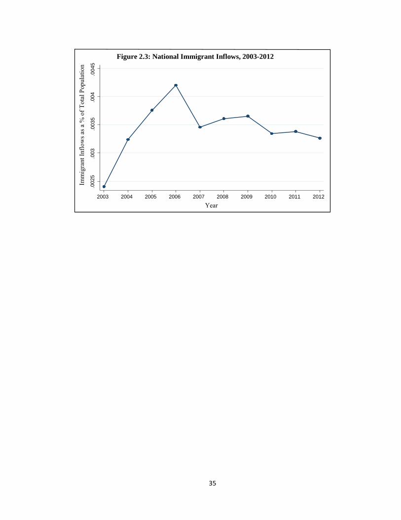
35

.002

5 .0

03

.003

5 .0

04

.004

5 Im

mig

rant

Inflo

ws a

s a %

of T

otal

Pop

ulat

ion

2003 2004 2005 2006 2007 2008 2009 2010 2011 2012 Year

Figure 2.3: National Immigrant Inflows, 2003-2012

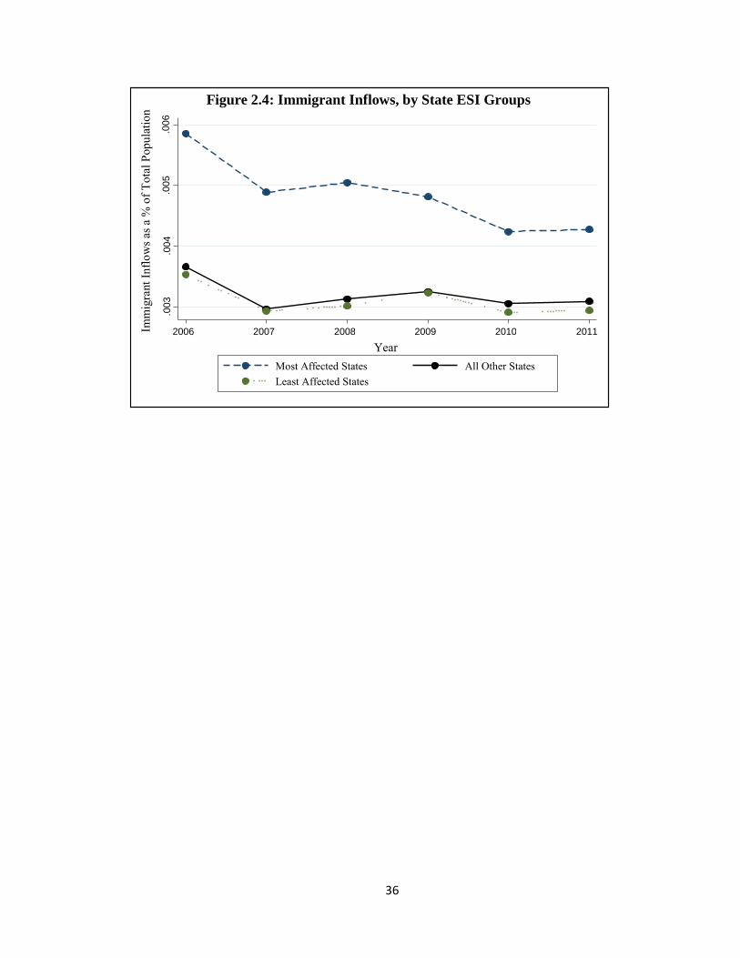
36

.003

.0

04

.005

.0

06

Imm

igra

nt In

flow

s as a

% o

f Tot

al P

opul

atio

n

2006 2007 2008 2009 2010 2011 Year

Most Affected States All Other States Least Affected States

Figure 2.4: Immigrant Inflows, by State ESI Groups

37

Table 2.1: Descriptive Statistics (2010) Variable Obs Mean Std. Dev. Min Max Total Population 325 777,053.50 1,691,680 55,212 19,567,410 Real FMR (Constant 40th Percentile) 325 784.97 202.55 546.16 1656 Real FMR (Unadjusted) 325 781.90 197.50 546.16 1656 Immigrants 325 3,005.59 12,889.28 22 186,086 Immigration Impact 325 0.0021 0.0018 0.00017 0.0154 Immigrant Share (1995) 325 0.0027 0.0134 0 0.2144 % of Pop with Bachelor's (1990) 325 0.1905 0.0621 0.0896 0.4214 Murder Rate, per 1000 population 325 4.3391 3.1873 0 20.8321 Land Area 325 2700.79 2880.46 145.59 27278.47 Average January Temperature 325 35.9846 12.1993 4.4 66.8 Average July Humidity 325 56.8031 16.1934 14 80 Unemployment Rate 325 0.0946 0.0272 0.0380 0.2616 Per Capita Income 325 36,340.77 6,205.52 20,946 71,768 Real Monthly Wages, BEA 325 3398.96 571.63 2439.30 7449.18 Real Monthly Wages, QCEW 324 3232.56 634.80 2168.30 7592.69 Real Monthly Wages, Good Prod 324 4121.75 929.07 2026.33 10478.82 Rent-to-Income Ratio, BEA 325 0.2294 0.0417 0.1563 0.4666 Rent-to-Income Ratio, QCEW 324 0.2432 0.0499 0.1525 0.5089 Rent-to-Income Ratio, Good Prod 324 0.1956 0.0575 0.1066 0.5175 % Housing Stock Built Pre-39 (1990) 325 0.1639 0.1044 0.0072 0.4993 % Total Earnings from Farms (1990) 325 0.0248 0.0321 0.0005 0.2256 Rent Growth (1980-90) 325 0.0386 0.1290 -0.5517 0.3693 Log Per Capita Prop Tax Rev (1997) 325 6.6783 0.4648 5.1394 7.8753 Log Per Capita Sales (1992) 325 10.9068 0.3051 9.4086 12.0878 FMR (1990) 325 795.36 179.01 454.43 1640.88 Price-to-Rent Ratio (1990) 325 166.52 42.08 104.06 348.93 Change Real Average Constr Wages 325 -0.0070 0.0504 -0.3243 0.3412 Predicted Employment Growth 325 -0.0062 0.0033 -0.0222 0.0080 WRLURI 325 -0.2169 0.7507 -1.7647 4.3353

1. All dollar values are 2010-constant dollars, adjusted using the CPI-U.

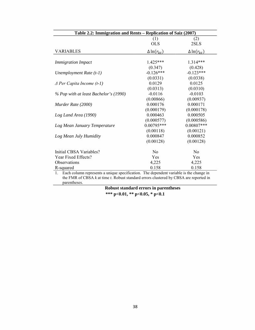
38

Table 2.2: Immigration and Rents – Replication of Saiz (2007) (1) (2) OLS 2SLS VARIABLES ∆ ln(𝑟𝑘𝑘) ∆ ln(𝑟𝑘𝑘) Immigration Impact 1.425*** 1.314*** (0.347) (0.428) Unemployment Rate (t-1) -0.126*** -0.123*** (0.0331) (0.0338) Δ Per Capita Income (t-1) 0.0129 0.0125 (0.0313) (0.0310) % Pop with at least Bachelor’s (1990) -0.0116 -0.0103 (0.00866) (0.00937) Murder Rate (2000) 0.000176 0.000171 (0.000179) (0.000178) Log Land Area (1990) 0.000463 0.000505 (0.000577) (0.000586) Log Mean January Temperature 0.00795*** 0.00807*** (0.00118) (0.00121) Log Mean July Humidity 0.000847 0.000852 (0.00128) (0.00128) Initial CBSA Variables? No No Year Fixed Effects? Yes Yes Observations 4,225 4,225 R-squared 0.158 0.158 1. Each column represents a unique specification. The dependent variable is the change in

the FMR of CBSA k at time t. Robust standard errors clustered by CBSA are reported in parentheses.

Robust standard errors in parentheses *** p<0.01, ** p<0.05, * p<0.1

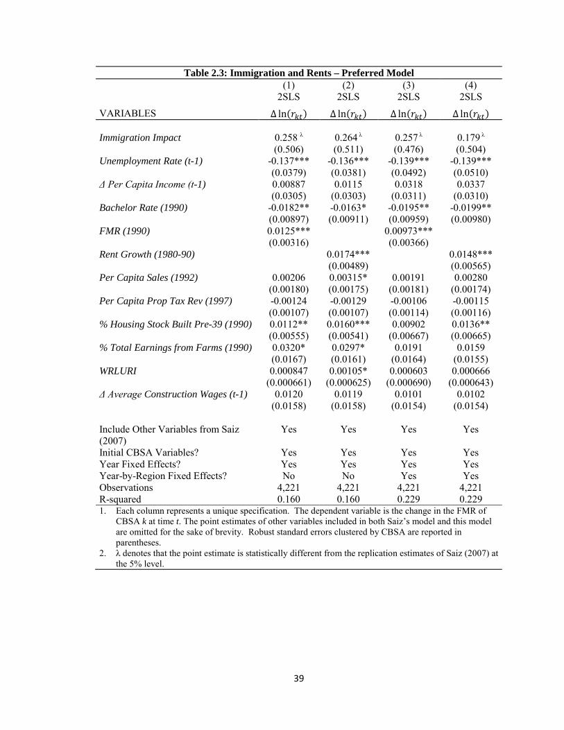
39

Table 2.3: Immigration and Rents – Preferred Model (1) (2) (3) (4) 2SLS 2SLS 2SLS 2SLS VARIABLES ∆ ln(𝑟𝑘𝑘) ∆ ln(𝑟𝑘𝑘) ∆ ln(𝑟𝑘𝑘) ∆ ln(𝑟𝑘𝑘) Immigration Impact 0.258 λ 0.264 λ 0.257 λ 0.179 λ (0.506) (0.511) (0.476) (0.504) Unemployment Rate (t-1) -0.137*** -0.136*** -0.139*** -0.139*** (0.0379) (0.0381) (0.0492) (0.0510) Δ Per Capita Income (t-1) 0.00887 0.0115 0.0318 0.0337 (0.0305) (0.0303) (0.0311) (0.0310) Bachelor Rate (1990) -0.0182** -0.0163* -0.0195** -0.0199** (0.00897) (0.00911) (0.00959) (0.00980) FMR (1990) 0.0125*** 0.00973*** (0.00316) (0.00366) Rent Growth (1980-90) 0.0174*** 0.0148*** (0.00489) (0.00565) Per Capita Sales (1992) 0.00206 0.00315* 0.00191 0.00280 (0.00180) (0.00175) (0.00181) (0.00174) Per Capita Prop Tax Rev (1997) -0.00124 -0.00129 -0.00106 -0.00115 (0.00107) (0.00107) (0.00114) (0.00116) % Housing Stock Built Pre-39 (1990) 0.0112** 0.0160*** 0.00902 0.0136** (0.00555) (0.00541) (0.00667) (0.00665) % Total Earnings from Farms (1990) 0.0320* 0.0297* 0.0191 0.0159 (0.0167) (0.0161) (0.0164) (0.0155) WRLURI 0.000847 0.00105* 0.000603 0.000666 (0.000661) (0.000625) (0.000690) (0.000643) Δ Average Construction Wages (t-1) 0.0120 0.0119 0.0101 0.0102 (0.0158) (0.0158) (0.0154) (0.0154) Include Other Variables from Saiz (2007)

Yes Yes Yes Yes

Initial CBSA Variables? Yes Yes Yes Yes Year Fixed Effects? Yes Yes Yes Yes Year-by-Region Fixed Effects? No No Yes Yes Observations 4,221 4,221 4,221 4,221 R-squared 0.160 0.160 0.229 0.229 1. Each column represents a unique specification. The dependent variable is the change in the FMR of

CBSA k at time t. The point estimates of other variables included in both Saiz’s model and this model are omitted for the sake of brevity. Robust standard errors clustered by CBSA are reported in parentheses.

2. λ denotes that the point estimate is statistically different from the replication estimates of Saiz (2007) at the 5% level.

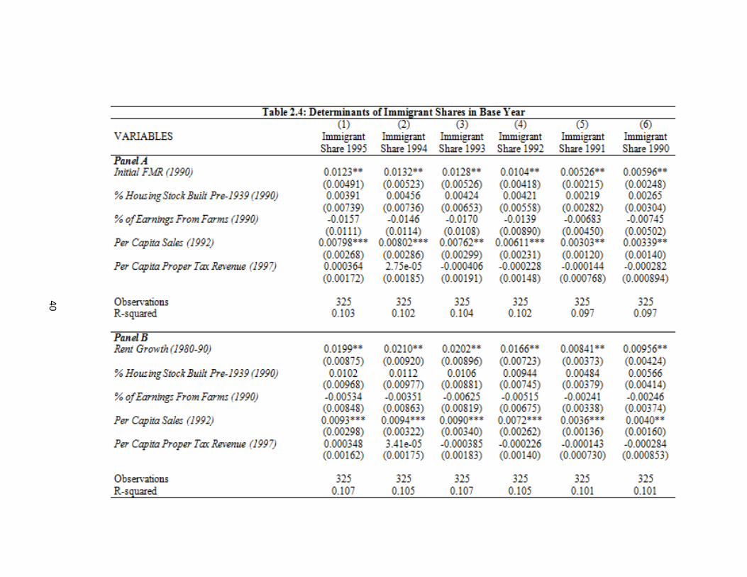
40

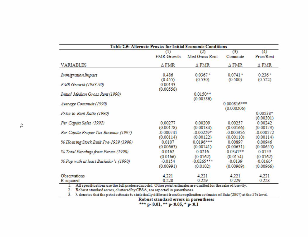
41

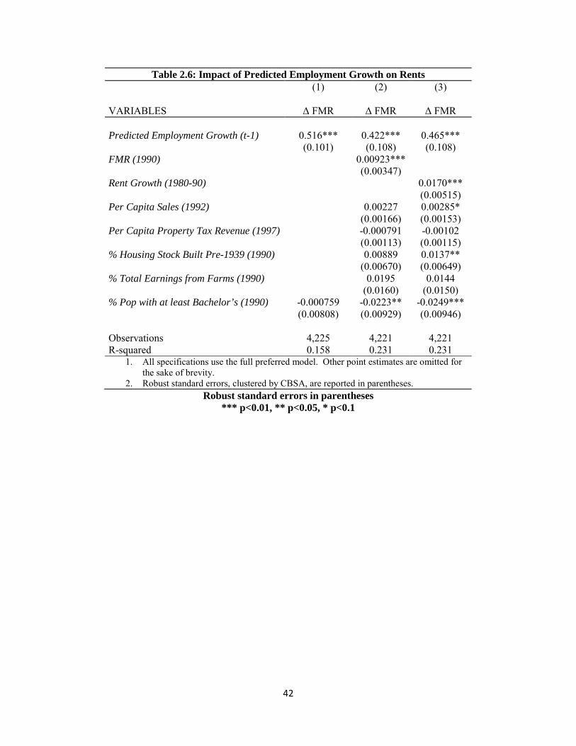
42

Table 2.6: Impact of Predicted Employment Growth on Rents (1) (2) (3) VARIABLES Δ FMR Δ FMR Δ FMR Predicted Employment Growth (t-1) 0.516*** 0.422*** 0.465*** (0.101) (0.108) (0.108) FMR (1990) 0.00923*** (0.00347) Rent Growth (1980-90) 0.0170*** (0.00515) Per Capita Sales (1992) 0.00227 0.00285* (0.00166) (0.00153) Per Capita Property Tax Revenue (1997) -0.000791 -0.00102 (0.00113) (0.00115) % Housing Stock Built Pre-1939 (1990) 0.00889 0.0137** (0.00670) (0.00649) % Total Earnings from Farms (1990) 0.0195 0.0144 (0.0160) (0.0150) % Pop with at least Bachelor’s (1990) -0.000759 -0.0223** -0.0249*** (0.00808) (0.00929) (0.00946) Observations 4,225 4,221 4,221 R-squared 0.158 0.231 0.231

1. All specifications use the full preferred model. Other point estimates are omitted for the sake of brevity.

2. Robust standard errors, clustered by CBSA, are reported in parentheses. Robust standard errors in parentheses

*** p<0.01, ** p<0.05, * p<0.1

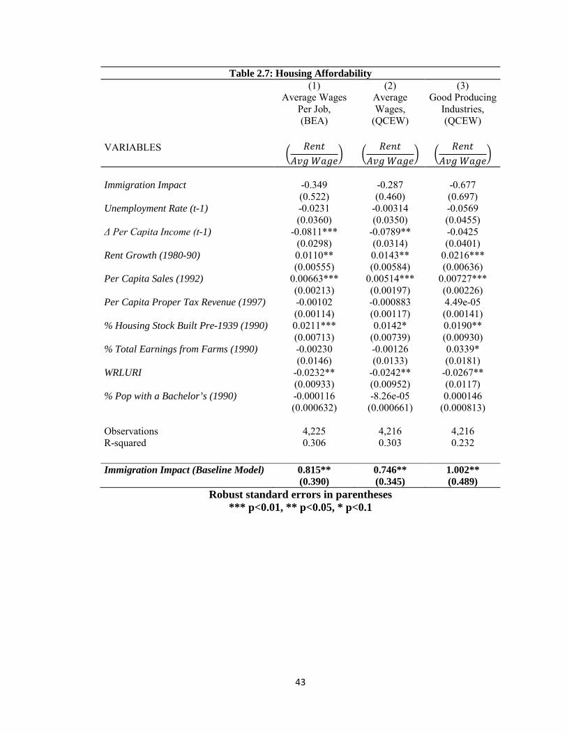
43

Table 2.7: Housing Affordability (1) (2) (3) Average Wages

Per Job, (BEA)

Average Wages,

(QCEW)

Good Producing Industries, (QCEW)

VARIABLES �𝐹𝑅𝐼𝑡

𝐴𝐴𝐼 𝑊𝐼𝐼𝑅� �

𝐹𝑅𝐼𝑡𝐴𝐴𝐼 𝑊𝐼𝐼𝑅

� �𝐹𝑅𝐼𝑡

𝐴𝐴𝐼 𝑊𝐼𝐼𝑅�

Immigration Impact -0.349 -0.287 -0.677 (0.522) (0.460) (0.697) Unemployment Rate (t-1) -0.0231 -0.00314 -0.0569 (0.0360) (0.0350) (0.0455) Δ Per Capita Income (t-1) -0.0811*** -0.0789** -0.0425 (0.0298) (0.0314) (0.0401) Rent Growth (1980-90) 0.0110** 0.0143** 0.0216*** (0.00555) (0.00584) (0.00636) Per Capita Sales (1992) 0.00663*** 0.00514*** 0.00727*** (0.00213) (0.00197) (0.00226) Per Capita Proper Tax Revenue (1997) -0.00102 -0.000883 4.49e-05 (0.00114) (0.00117) (0.00141) % Housing Stock Built Pre-1939 (1990) 0.0211*** 0.0142* 0.0190** (0.00713) (0.00739) (0.00930) % Total Earnings from Farms (1990) -0.00230 -0.00126 0.0339* (0.0146) (0.0133) (0.0181) WRLURI -0.0232** -0.0242** -0.0267** (0.00933) (0.00952) (0.0117) % Pop with a Bachelor’s (1990) -0.000116 -8.26e-05 0.000146 (0.000632) (0.000661) (0.000813) Observations 4,225 4,216 4,216 R-squared 0.306 0.303 0.232 Immigration Impact (Baseline Model) 0.815** 0.746** 1.002** (0.390) (0.345) (0.489)

Robust standard errors in parentheses *** p<0.01, ** p<0.05, * p<0.1

44

3. Immigration and Native Wages: A New Look

3.1 Introduction

According to labor theory, the question of how immigration impacts native wages seems

like a straightforward one. Using a simple labor market model of supply and demand it is easy to

show that as labor supply increases, the average market wages will fall, ceteris paribus. While

economic theory suggests a clear cut answer, empirical evidence rarely supports the theory. In

fact, most empirical work suggests immigration has a negligible negative impact, or even a slight

positive impact, on the wages of demographically comparable natives.26 Several arguments can

be made as to why the empirics fail to match the economic theory. First, immigrant location

decisions are endogenous, such that characteristics of local labor markets may be driving

immigrant location decisions. This endogeneity may take several forms. Immigrants may choose

to locate in high wage cities, natives may respond to immigrant inflows by moving, or firms may

reallocate capital to high-immigrant cities in order to take advantage of the abundance of cheaper

labor. To alleviate this concern, Borjas et al. (1997) suggested that the analysis move away from

analyzing local labor markets; rather, researchers should use national-level data and treat the

entire US as one labor market. Second, Aydemir and Borjas (2011) suggest that sampling error

leads to attenuation bias. Due to the nature of the model, even small levels of measurement error

can have large impacts on the estimated coefficients.

Even when one treats the US as a single labor market, past studies fail to compare

immigrants to demographically comparable natives that will directly compete in the labor market.

It is in this area that the present paper will contribute to the existing literature. It has become

standard in the literature to analyze the impact of immigration on similarly skilled natives within

cohorts defined by education and work experience. This approach, pioneered in the immigration

literature by Borjas (2003), implicitly assumes that within these cohorts, immigrants and natives

26 Borjas (1994) and Kerr and Kerr (2011) provide comprehensive reviews of this literature.

45

are perfect substitutes. Recently, however, the assumption of perfect substitutability has been

challenged, and estimates suggest that a degree of imperfect substitutability exists between

immigrants and natives within these cohorts (Card, 2009; Ottaviano and Peri, 2012; Manacorda

et. al, 2012). As pointed out by Ottaviano and Peri (2012), this fact is nontrivial. If immigrants

and natives are imperfect substitutes, then any wage effect of immigration would be concentrated

on existing immigrants, not natives.

We claim that the incidence of imperfect substitutability arises due to the empirical

model employed in previous studies – education is an imperfect proxy for overall skill level. To

see this, consider three empirical regularities. First, there is a small literature examining the

differential impacts of immigration on natives by race. In this literature, researchers stratify labor

markets by education and race and find that immigration has a differential impact on black wages

relative to white wages, but the evidence is mixed. Using the national labor market approach,

Borjas et al. (2010) find that the impact of immigration is 33% lower on black men relative to

white men. Altonji and Card (1991), who examine the impact of immigration on the wages of

less-skilled (educated) workers using the area approach, find the opposite. Their first-differenced

results (row 4 of Tables 7.8 and 7.9) suggest that a 10% immigration shock has a (roughly) 70%

larger (more negative) effect on the average wage of less-skilled blacks than less-skilled whites.

Though the results differ in the direction of the differential impact (which is likely due to

differences in methodology and/or sample selection), it is clear that the impact of immigration is

not constant across races within education groups. If education is a good proxy for overall skill,

then one would expect the impact of immigration to be constant across all workers within an

education group. The differential effects on black wages estimated in this literature, however,

suggest whites and blacks are not perfect substitutes within education groups; thus, calling into

question the use of education to stratify labor markets.

46

Second, there is significant wage dispersion within education groups (Levy and Murnane,

1992; Murnane, Willett, and Levy, 1995; Ingram and Neumann, 2006). This suggests that skills

other than educational attainment are being rewarded in the labor market. Third, immigrants earn

less than similarly educated natives (Bratsberg and Terrell, 2002; Bratsberg and Ragan, 2002;

Ferrer and Riddell, 2008; Friedberg, 2000). This fact has been attributed to differing employment

distributions across occupations and a lower return to education for immigrant workers. A

similar argument is found in the geography literature when discussing the disparate value of

“credentialized cultural capital” in determining immigrant/native wage gaps in Canada (Bourdieu,

1977; Reza, 2006). In this literature, credentialized cultural capital refers to the level of

educational attainment. Although immigrants may have more credentialized cultural capital

(higher educational attainment), domestic employers do not value education earned abroad as

highly as education earned domestically.

Several feasible scenarios exist for the above differentials in returns to education. First,

US employers may be simply discriminating against immigrants and either underpaying for their

skills or refusing to hire immigrant workers (Borjas, 1990). While feasible, Bucci and Tenorio

(1997) decompose the wage gaps between white natives and immigrants and find that the

majority of the wage differential is simply US employers overvaluing native skills, not

undervaluing immigrant skills. Similarly, Reimers (1983) documents that while discrimination

may play a minor role in the wage gaps of Hispanic immigrants; differences in observable

characteristics (i.e. language proficiency) explain the majority of the wage differences. Second,

immigrants face differential returns to education because they are being “misplaced” in the labor

market. That is, immigrants enter the US and are pushed toward jobs in which they possess too

much education than the average worker. One reason for under-placement is that educational

attainment is a subjective measure between countries and over time within countries. Peracchi

(2006) notes that years of schooling or the schooling level may reflect varying levels of literacy in

47

different countries. As researchers are interested in the effects of immigration on

demographically comparable natives and many immigrants receive the entirety of their education

abroad, stratifying labor markets by education may not identify immigrants and natives that

directly compete in the labor market.

Because of differences in education standards across countries, immigrants may be

misplaced because skills learned in the host country are not transferrable to the US labor market.

While many cases of skilled immigrants taking unskilled jobs are reported in the national media,

this fact is supported by the data (Mattoo et al., 2008; Neagu, 2009). Figure 3.1 confirms this

phenomenon for low-skill occupations. The figure plots the percentage of native and immigrant

workers with a high school degree or some college that work in low-skill occupations. Holding

educational attainment constant, immigrants are more concentrated in less-skilled occupations

and the gap is widening over time. Thus, it seems reasonable to assume that these workers will

not directly compete in the labor market.

Further evidence of this phenomenon can be seen in Table 3.1 below. Table 3.1 presents

the percent of workers that are classified as over-educated for their current job. Here, we define

over-educated as having significantly more education relative to others working in the same

occupation (more detail below). Table 3.1 uses occupation-specific education requirements from

the ONET and matches these data to US Census micro-data from 1970-2010. Specifically, we

use O*NET data for the required level of education needed to adequately perform the job. These

data give a value of 1-100 for 12 education groups, which map directly to the percentage of the

total employment in each occupation that holds said level of education. We collapse these 12

education groups into 7 categories: less than high school, high school graduate (or equivalent),

some college – no degree, Associate’s Degree, Bachelor’s Degree, Master’s Degree, and

Doctorate/Professional Degree. We are interested in the share of the population who possess

above average education for their current job. That is, they work in an occupation for which they

48

hold significantly more education than the rest of the labor force in the given occupation. Using

the data on required education, we group occupations based on the level at which the worker

would be considered over-educated: over-educated if holding at least a bachelor’s degree, over-

educated if holding at least a master’s degree, over-educated if holding a doctorate/professional

degree, or never over-educated. We do not consider the case in which someone is over-educated

for a job if they hold an associate’s degree or some college but no degree. This follows from the

wage structure literature which suggests that high school dropouts and high school graduates are

perfect substitutes (Katz and Murphy, 1992).27 The table presents over-education rates for

natives, all immigrants, and immigrants who have been in the US for less than 5 years.

The differences in over-education rates by nativity are significant, especially for those

persons holding advanced degrees. For all occupations, immigrants are nearly twice as likely to

be over-educated for their job compared to natives. In occupations that generally require a

bachelor’s degree, 15.18% of the immigrant workers hold an advanced degree compared to

6.18% of natives. Column (3) displays over-education rates for newly arriving immigrants.

Unsurprisingly, new immigrants have higher over-education rates than the entire immigrant

population, which likely reflects the lack of transferability in immigrant skills upon entry (i.e.

language skills). From the immigrant assimilation literature however, we would expect this rate

to decline significantly as immigrants remain in the US. Figure 3.2 plots the over-education rates

for immigrants across all occupations by length of time in the US and region of birth. Contrary to

the assimilation hypothesis, the over-education rate for the entire immigrant population (solid

line) is relatively constant over tenure in the US, around 10%. Because assimilation is affected

by English proficiency and cultural similarities, we also plot over-education rates by region of

birth. The constant over-education rate persists for immigrants from Central and South America

27Similarly, when grouping workers into high- and low-education groups, the authors allocate a share of the “some college, no degree” group to the low-education group. Thus, we follow this reasoning and assume that workers with less than a bachelor degree are not over-educated if they work in lower-skill jobs that typically do not require any college education.

49

(dotted line) and Asia (dashed line). Though the magnitudes are different, the underlying trend is

the same. For European immigrants (dash-dot line) however, over-education rates are decreasing

over time, consistent with positive occupational mobility associated with assimilation. While

decreasing, the over-education rate for the longest tenured immigrants is still roughly 9%.

If it is the case that many immigrants are being “misplaced” in the labor market on the

basis of education, then previous studies analyzing wage impacts within education-experience

cells may not tell the whole story. That is, immigrants and natives with the same education-

experience profile may not be directly competing in the labor market, which would explain the

negligible impacts found in the existing literature. While the under-placement scenario is the

main focus, the discrimination scenario is not without merit. As Reimers (1983) indicated,

discrimination plays a minor role in the immigrant-native wage gap. Thus, if this discrimination

is in the form of employers preferring to hire native workers, this may force more immigrants into

occupations for which they are over-educated.

For these reasons, we argue a better measure of labor market competition is to stratify the

labor market by occupation. While this seems like a logical empirical test, existing studies

incorporating occupations as a proxy for skill are relatively sparse. To my knowledge, only three

such studies exist. Camarota (1997) uses one CPS cross-section to estimate the impact of

immigration on wages within occupations and finds that a 1% increase in immigration will

decrease the wages of the average native worker by 0.5%. However, the use of a single cross-

section and small within-occupation sample sizes, make causal inference difficult. Card (2001)

estimates city-specific impacts of immigration on occupational wages for 175 cities using 1990

US Census data and finds that the immigration inflows of the 1980’s decreased wages in low-

skilled occupations in high-immigration cities by no more than 3%. Orrenius and Zavodny

(2007) use CPS data from 1994 – 2000 and INS immigration data to estimate the impact of

immigration on native wages in 3 broad occupation categories. The authors estimate that the

50

change in immigrants over the data period decreased wages in low-skilled, manual occupations

0.8% and had no impact for medium-skilled and high-skilled occupations.

The present study improves upon past research in several ways. First, following Borjas

and Katz (1997) and Borjas (2003), we move away from the area studies of Card (2001) and

Orrenius and Zavodny (2007) and treat the U.S. as one national labor market. Area studies have

been criticized because they implicitly assume that native labor and capital do not adjust across

labor markets in response to immigration. If the existing population relocates inputs to areas (or

occupations) less affected by immigration, then the impact of immigration will be

underestimated. Second, we construct occupation groups defined using skill data from the

O*NET. Previous studies using occupations have relied on broad Census-defined occupation

groups. The advantage of using the O*NET data is that we are able to construct occupation

groups with a greater degree of homogeneity in overall skill level, regardless of nationality and

citizenship status, than those using either education groups or broad occupation classifications.

The rest of the paper is structured as follows. Section 3.2 outlines the data and the

methodology used to define occupation groups. Section 3.3 outlines the potential problems with

stratifying labor markets by education when analyzing the impact of immigration on native

wages. We first analyze differences in employment shares of immigrants and natives along skill

distributions. The results suggest that immigrants are underrepresented (overrepresented) in

communicative (manual/physical) task intensive occupations. This result holds for the entire

population and within education groups. Next, we analyze the differences in the rate of return to

education paid to natives and immigrants. We show that immigrants are paid a lower rate of

return than natives and this leads to a heavier concentration of immigrants in low-wage jobs. As

discrimination has been shown to play only a minor role in immigrant-native wage gaps, this

suggests that similarly educated immigrants and natives work in different jobs. Section 3.4

presents the empirical methodology and results similar to those in Borjas (2003). The results

51

confirm the intuition above. When we stratify labor markets by occupations, the impact of

immigration is nearly twice as large as those found in the existing literature. This result is robust

to several different definitions of occupation groups and when we control for selection problems

associated with occupations. In section 3.5, we address the concern that the use of occupation-

defined skill groups may introduce bias. Using the traditional education-experience skill cohorts,

we show that the impact of immigration on the wages of demographically comparable natives

within education groups is quantitatively similar to the estimated impact when using cohorts

defined by occupational skill. As such, the impact on wages is muted because immigrants and

natives are imperfectly substitutable within education groups. Section 3.6 concludes.

3.2 Data

We draw from several data sources in this paper. Labor supply and wage data are from

the 1960, 1970, 1980, 1990, and 2000 PUMS of the U.S. Census, and the 2009, 2010, and 2011

PUMS of the ACS. The ACS data are pooled together to form a single 2010 cross-section.

Following the work of Borjas (2003), we restrict our sample to men, aged 18-64, who earned

positive wage income. A full description of both the employment and wage samples can be

found in the Data Appendix.

We sort workers into skill groups based on potential experience and occupation. As is

customary in this literature, we calculate potential experience based on educational attainment. It

is assumed that workers with less than a high school diploma enter the labor market at 17 years

old, workers with a high school diploma or GED enter the labor market at 19, workers with some

college enter the labor market at 21, and those with a college degree enter the labor market at 23.

Following Borjas (2003), we limit the sample to men who have 1-40 years of potential experience

and group workers into 5-year potential experience groups (i.e. 1-5 years of potential experience,

6-10 years, etc.).

52

3.2.1 Occupation Groups

The occupation groups constructed in this paper follow generally from a recent paper by

Peri and Sparber (2009). We assume that occupations are distinguished by two occupation-

specific indices of task intensity: manual task intensity and communicative task intensity.

Individual occupations are then grouped based on their relative communicative-to-manual task

intensity.

Occupation-specific task indices are constructed using the Department of Labor’s

O*NET survey, which provides comprehensive data on characteristics of occupations. The

O*NET content model is partitioned into several different domains, each providing different

worker-specific and occupation-specific data. Unlike Peri and Sparber (2009), we make use of

both worker-specific data on abilities, knowledge, and skills and occupation-specific data on

work activities to generate these task intensity indices (throughout the rest of the paper, we will

refer to all four of these measures as “skill groups”).28 Table A1 of the Appendix lists each skill

used in constructing the task intensity indices.

One challenge when working with occupations over this many Census years is that

occupation classifications change over time. Additionally, O*NET data are assigned to 2000

SOC (standard occupation classification) occupations. To remedy this problem, we use a

modified occupation classification developed by Autor and Dorn (2013) (AD classification,

hereafter). This occupation classification system creates a consistent, balanced panel of

occupations across all years. To construct the occupation groups used in this paper, we merge

skill data from the O*NET survey to the AD classification and group occupations on the basis of

their occupation-specific skills.

28 Peri and Sparber (2009) rely solely on “abilities” from the O*NET survey.

53

The O*NET data assigns each skill a score for importance (I) with a range of 0-5 and a

score for level (L) with a range of 0-7 for each occupation.29 To create the occupation-specific

skill index, we first standardize the importance and level scores such that each has a range of 0-

100. Then, we create a normalized “task-intensity score” (TS) for each skill by multiplying the

standardized importance score and standardized level score – a higher task-intensity score

suggests a given task is more important to performing a given occupation. We then calculate the

average manual and communicative task-intensity score for each skill group and occupation. For

example, within the worker ability domain, both physical abilities and psychomotor abilities are

classified as manual abilities. Thus, for each occupation, we calculate the average manual task-

intensity score by averaging the task-intensity of physical and psychomotor abilities. Lastly, the

final manual (communicative) task-intensity score is the average of all skill group specific

manual (communicative) task-intensity scores. Analytically, the manual task intensity index for

each occupation (j) is calculated as30:

(1) ( )∑=i

ijj TSn

M 1 ∀ 𝑖 = (𝐴𝐴𝑖𝐴𝑖𝑡𝐴,𝐾𝐼𝐾𝐾𝐴𝑅𝐾𝐼𝑅, 𝑆𝑘𝑖𝐴𝐴,𝑊𝐾𝑟𝑘 𝐴𝐴𝑡𝑖𝐴𝑖𝑡𝐴).

For each occupation in the AD classification, we create the ratio of communicative task

intensity to manual task intensity, which is the basis for defining our occupation groups. From

this ratio, we construct three occupation classifications based on the distribution of this skill ratio

across occupations: 1) a four occupation group classification where each group is a quartile of the

distribution, 2) a five occupation group classification where each group is a quintile of the

distribution, and 3) a six occupation group classification where each group is a sextile of the

distribution.

29 Importance and Level scores measure different aspects. There are occupations in which a given skill is equally important; however, one occupation needs to use the skill at a much higher level. An example from the O*NET is speaking ability for lawyers and paralegals. Speaking is important in both occupations; however, lawyers need a high level of speaking skills to argue cases, while paralegals simply need an average level of speaking skill (https://www.onetonline.org/help/online/scales). 30 Construction of the communicative task intensity index is constructed analogously.

54

As the above classifications are rather crude treatments of the data, we construct a fourth

occupation classification that allows the data to determine the optimal cutoffs. One concern with

the above classifications is the definition of manual skills. There are obvious occupations that

require significant manual tasks relative to communicative tasks (i.e. construction laborers,

miners, etc.); however, there are other occupations (i.e. dancers and performers) that have similar

values of manual task intensity that are clearly not competing with construction laborers for jobs.

While we attempt to control for this by using both the importance score and level score above,

another feasible way to alleviate this problem is to first classify occupations into blue-collar and

white-collar occupations. Then, we use cluster analysis to determine the optimal number of

occupation groups.31

3.3 Occupation Groups vs. Education Groups

The concern of the present research is that by stratifying labor markets by education,

researchers do not compare immigrants and natives that will directly compete in the labor market

because 1) immigrants are under placed in the labor market and 2) immigrants and natives work

in different occupations. Below, we present two empirical exercises that illustrate this point.

3.3.1 Misplacement of Immigrants in the Labor Market

To illustrate the first point, we provide an empirical analysis in the spirit of Dustmann et

al. (2012). Specifically, we compare across the native wage distribution the actual immigrant

earnings distribution to a counterfactual immigrant earnings distribution. The counterfactual

distribution is the share of immigrants along the native wage distribution if immigrants were paid

the same rates of return to observable characteristics as natives.

31 It is determined that a five group occupation classification is optimal (based on maximizing the Bayesian Information Criterion (BIC)): two clusters in the blue-collar sector and three clusters in the white-collar sector. We also use several other methods and in almost all cases, the methods agree on the optimal number of clusters. These results are available upon request.

55

We construct the employment distributions using micro-data from the 2000 U.S. Census

(IPUMS). Sample criteria are discussed in the Data Appendix. First, we estimate the rates of

return to observable characteristics for native workers via a typical log wage model32:

(2) 𝐾𝐼 = 𝑋𝐼𝛽 + 𝜃𝑘 + 𝜀𝐼;

where 𝐾𝐼 is the log hourly wage for individual i; 𝑋𝐼 is a vector of demographic variables

including categorical variables for education and experience, an interaction of education and

experience, race, and marital status; and 𝜃𝑘 is a vector of state fixed effects controlling for wage

differentials across states. Next, the estimated coefficients are used to predict the wage for each

immigrant in the sample. In other words, we predict the wage an immigrant would have earned

had they received the same rates of return as a native worker. Once we have obtained the

predicted wage, each immigrant in the sample is ranked according to their actual and predicted

wage in the native wage distribution in year t.

Figure 3.6 below plots the kernel estimates of the relative density of the log odds ratio

along the native wage distribution.33 As we plot relative densities, the horizontal line at one

represents the actual native density; thus, if the immigrant density is above one, immigrants are

overrepresented in this portion of the native wage distribution (and vice versa). The dashed line

represents the observed relative density for immigrant wages. The plot of observed wages

suggests that immigrants are overrepresented below the 35th percentile of the native wage

distribution. The dotted line represents the plot of the counterfactual relative density. The plot

illustrates the potential problems with defining skill cohorts based on demographics. The

differences in the actual density and the predicted density are significant and confirm the 32 The model is estimated on male workers only. The regression is weighted by the person weight from the Census and robust standard errors are clustered by education and potential experience. Also, hourly wage is “Winsorized” such that the lower bound of hourly wage is 75% of the federal minimum wage in year t and the upper bound is 50 times the minimum wage in year t (Card, 2009). 33 Because the variable of interest, the position of immigrants along the native wage distribution, is bounded between 0 and 1, kernel estimates on the untransformed variable would give misleading estimates at the extreme (Dustmann et al., 2012). To mitigate this concern we 1) estimate the kernel on the log odds ratio and 2) report the kernel estimates for the 10th-90th percentiles only.

56

discussion on misplacement of immigrants in the labor market with regards to educational

attainment. First, based on observable demographics, too many immigrants reside in the lower

tail of the native wage distribution. Second, while we actually observe immigrants in the bottom

35% of the native wage distribution, the counterfactual distribution suggests immigrants should

be clustered from roughly the 20th to 60th percentiles.

Two plausible scenarios exist for the differences in the distributions in Figure 3.3. First,

either U.S. employers undervalue foreign education or overvalue domestic education. While

Figure 3.3 does not allow differentiation between these two scenarios, either one would lead to

under-placement of immigrants in the labor market. Second, omitted variables are driving the

differences. Namely, we are unable to control for English speaking ability in (2). Because we

estimate (2) on the native population, English proficiency cannot be included as it does not vary

within the native sample. While omitted variables are a threat to the interpretation of the

differences in the distributions above, they would not alter the interpretation that stratifying the

labor market via educational attainment is problematic in the context of immigration. To see this,

consider two workers. One is a U.S. native who recently graduated with a bachelor’s degree

while the other is an immigrant with a recent bachelor’s degree but limited English proficiency.

It is not hard to imagine a scenario in which these two workers accept drastically different

occupations although they have similar education and work experience. This fact would explain

their relative positions along the native wage distribution, but it would not change the fact they do

not compete in the labor market despite equal educational attainment and work experience. As

such, we take Figure 3.3 as support for our claim that education-specific skill groups are

problematic in the context of immigration.

3.3.2 Differences in Immigrant and Native Employment Distributions

Peri and Sparber (2009) suggest that immigrants have comparative advantage in

manual/physical tasks while natives have comparative advantage in communicative tasks. As

57

such, immigrants and natives sort into and specialize in occupations intensive in the task for

which they have comparative advantage. If this occupational sorting exists within education

groups, it may explain the negligible impacts of immigration estimated in previous models.

To test this, we examine the employment distribution of immigrants and natives along the

distribution of occupation-specific skills. Figure 3.4 plots the percentage of total hours worked

by immigrants and natives from 1970-2010 along the distribution of the ratio of the

communicative task intensity index to the manual task intensity. The differences in employment

are striking and make clear that immigrants and natives are distributed differently across

occupation-specific skills. Relative to natives, immigrants are overrepresented in jobs that

require more manual tasks and underrepresented in those jobs that require more communicative

tasks.

While informative, this fact is only important in the context of this analysis insomuch as

these differences persist within education groups. Figure 3.5 shows the distribution of

employment shares for each of the four education groups typically found in the immigration

literature (less than high school, high school graduate or equivalent, some college, college

graduate with at least a bachelor’s degree). For all four education groups, the result is the same:

immigrants are overrepresented in manual task intensive occupations relative to natives while

underrepresented in communicative task intensive occupations.

While the same general result holds within education groups, the differences between

immigrant and native employment shares are modest. This result is unsurprising as the

immigrant population is significantly more heterogeneous than the native population with respect

to educational attainment and education quality. Countries differ in terms of school quality,

curriculum, resources available to schools, and teacher standards (Peracchi, 2006). As such, one

would expect the transferability of general education skills to differ based on an immigrant’s

58

country of origin. Figure 3.6, which plots employment shares along the skill distribution by

region of birth, confirms this phenomenon.34 Employment outcomes differ widely by region of

birth and these differences are likely attributable to the English proficiency. European

immigrants (dashed line) face similar labor market experiences as the native population (solid

line); however, Asian and Central and South American immigrants face significantly different

employment outcomes and are driving the differences in Figures 4 and 5. Asian immigrants

(dotted line) are clustered around the median of the distribution (e.g. occupations within the

service industry), while Central and South American immigrants (dash-dot) are concentrated at

the lower tail of the distribution (e.g. manual task intensive occupations).

Ultimately, the results in this section complement the findings in the previous section.

Education is a subjective measure of skill. Simply stratifying labor markets by education does

not necessarily compare immigrants and natives who will directly compete in the labor market.

Immigrants and natives cluster in occupations in which they have the comparative advantage.

This holds within education groups and across the immigrant population. Stratifying labor

markets by occupation will form labor market cohorts with a greater degree of homogeneity with

respect to skill in which immigrants and natives are perfect substitutes.

3.4 Empirical Methodology and Results

3.4.1 Empirical Model

As we are estimating the impact of relative labor supply of different skill groups on the

structure of wages, the empirical model is derived from a theoretical framework of the demand

side of the labor market. Assuming output is produced using a CES production function where

labor and capital are separable, the relative wage of a given skill group is a function of 1) the

34 For the sake of brevity, we only display the high school graduate and some college education groups. However, the general result holds for the other two groups as well. These figures are available upon request.

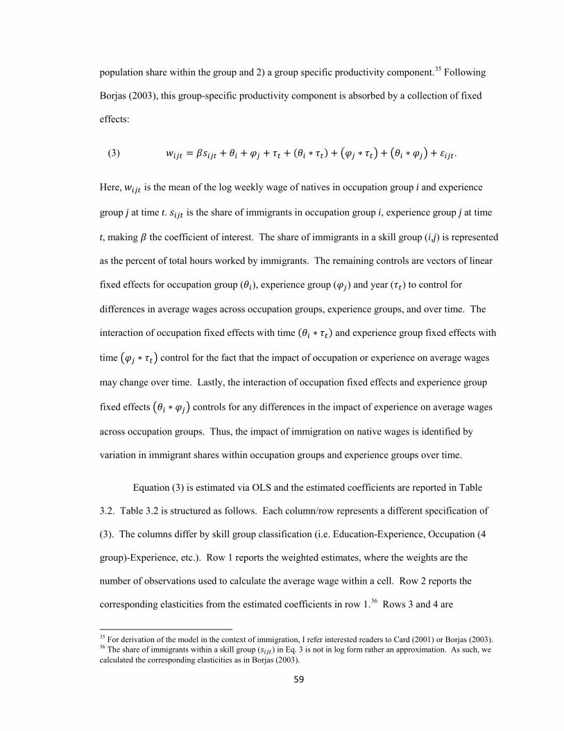
59

population share within the group and 2) a group specific productivity component.35 Following

Borjas (2003), this group-specific productivity component is absorbed by a collection of fixed

effects:

(3) 𝐾𝐼𝑗𝑘 = 𝛽𝐼𝐼𝑗𝑘 + 𝜃𝐼 + 𝜑𝑗 + 𝜏𝑘 + (𝜃𝐼 ∗ 𝜏𝑘) + �𝜑𝑗 ∗ 𝜏𝑘� + �𝜃𝐼 ∗ 𝜑𝑗� + 𝜀𝐼𝑗𝑘.

Here, 𝐾𝐼𝑗𝑘 is the mean of the log weekly wage of natives in occupation group i and experience

group j at time t. 𝐼𝐼𝑗𝑘 is the share of immigrants in occupation group i, experience group j at time

t, making 𝛽 the coefficient of interest. The share of immigrants in a skill group (i,j) is represented

as the percent of total hours worked by immigrants. The remaining controls are vectors of linear

fixed effects for occupation group (𝜃𝐼), experience group (𝜑𝑗) and year (𝜏𝑘) to control for

differences in average wages across occupation groups, experience groups, and over time. The

interaction of occupation fixed effects with time (𝜃𝐼 ∗ 𝜏𝑘) and experience group fixed effects with

time �𝜑𝑗 ∗ 𝜏𝑘� control for the fact that the impact of occupation or experience on average wages

may change over time. Lastly, the interaction of occupation fixed effects and experience group

fixed effects �𝜃𝐼 ∗ 𝜑𝑗� controls for any differences in the impact of experience on average wages

across occupation groups. Thus, the impact of immigration on native wages is identified by

variation in immigrant shares within occupation groups and experience groups over time.

Equation (3) is estimated via OLS and the estimated coefficients are reported in Table

3.2. Table 3.2 is structured as follows. Each column/row represents a different specification of

(3). The columns differ by skill group classification (i.e. Education-Experience, Occupation (4

group)-Experience, etc.). Row 1 reports the weighted estimates, where the weights are the

number of observations used to calculate the average wage within a cell. Row 2 reports the

corresponding elasticities from the estimated coefficients in row 1.36 Rows 3 and 4 are

35 For derivation of the model in the context of immigration, I refer interested readers to Card (2001) or Borjas (2003). 36 The share of immigrants within a skill group (𝐼𝐼𝑗𝑘) in Eq. 3 is not in log form rather an approximation. As such, we calculated the corresponding elasticities as in Borjas (2003).

60

specification checks. Row 3 presents unweighted estimates, while row 4 reports estimates when

we include native labor force as an explanatory variable. Because the key explanatory variable is

simply the immigrant share of total hours worked within a skill group, an increase in 𝐼𝐼𝑗𝑘 would

occur from either an increase in immigrant labor supply or a decrease in native labor supply. As

such, the estimates in row 4 report the impact of 𝐼𝐼𝑗𝑘 holding native labor supply constant.

First, column (1) reports estimates of (3) using the traditional education-experience

classification found in the existing literature.37 The baseline results are slightly lower than those

found by Borjas (2003).38 Focusing on the estimated elasticity in row 2, the results suggest that a

10% supply shock (an inflow of immigrants that increases total hours worked within an

education-experience cohort by 10%) will reduce native wages by a modest 1.9%. Columns (2) –

(6) use different occupation classifications in the estimation of (3). Columns (2) – (4) use

occupation groups defined by the distribution of the communicative-to-manual task intensity

ratio. When we group workers based on occupation-specific skills, the estimated impact of

immigration is much larger. Again, focusing on the elasticities in row 2, the results suggest a

10% supply shock within a given occupation-experience cohort will decrease native wages by

7.2%, 5.6%, and 6.1%, respectively. Column (5) uses the clustered classification that first

separates workers by white-collar/blue-collar status then groups workers based on occupation-

specific skill. In this specification, the estimated impact of immigration is similar to those above

and suggests that a 10% increase in the number of immigrants within a cohort will decrease the

average native wage by 5.4%.

The results support the hypothesis that defining skill groups on the basis of education

may attenuate the effects of immigration. By grouping workers into skill groups defined by

37 In this specification, we use the four-group classification described above (Less than HS, HS grad, some college, college grad). 38 Borjas (2003) estimates a point estimate of -0.572; however, this estimate does not use data from 2010 and uses CPS data for 2000. We used the methodology above and the same data described in Borjas (2003) and produced a very similar result. Thus, the methodology used above is consistent with the past literature.

61

occupation, the estimated impact on native wages is 2-3 times larger depending on specification.

From rows 3 and 4, the results are not sensitive to using weights or controlling for native labor

supply. What is not clear from the estimates in columns (2)-(5) is why the results are larger when

using the occupation-defined skill groups. Is it the fact that skill groups are defined on the basis

of occupation-specific skills or are the estimates driven by the use of occupation-defined skill

groups in general?

To test this, we estimate (3) using the occupation classification system developed by

Autor and Dorn (2013). The results are reported in column (6). Recall that these occupation

groups mirror the typical occupation classifications used in the U.S. Census and are not defined

based on occupation-specific skills.39 If the results are biased downward simply because we use

occupations to define skill groups, we would expect the impact of immigration to be similar to

columns (2)-(5). When using this skill group classification however, the impact of immigration is

significantly lower and similar in magnitude to the estimates when using education-based skill

groups. This is unsurprising as AD rely on average educational attainment when constructing

these groups, not occupation-specific skills.40 To see this in the data, Figure 3.7 plots the share of

total hours worked along the distribution of our skill ratio within AD occupation groups. Panels A

and B are white-collar jobs (i.e. management occupations, etc.) and panels C and D are low-wage

blue-collar jobs (i.e. construction). Though labor supply is skewed in the expected direction for

each occupation group (white-collar occupations are skewed to the right hand side of the

distribution, and vice versa), the variance is quite high. Because of this variability, it is

reasonable to assume that, similar to skill groups defined by educational attainment, not all

workers will directly compete in the labor market. Thus, we take the result in column (6) as

39 The occupation groups are as follows: 1) Management/Professional/Technical/Financial/Public Security, 2) Administrative Support and Retail Sales, 3) Low-Skill Services, 4) Precision Production and Craft Occupations, 5) Machine Operators, Assemblers, and Inspectors, and 6) Transportation/Construction/Mechanics/Mining/Agricultural. 40 In describing one of the occupation groups, the authors claim: “Technical, sales, and administrative support occupations cover a workforce that is on average better educated than any other occupation group apart from managers and professionals”.

62

support for the claim that occupation-specific skills, not occupations themselves, are the

important component in constructing skill groups for which labor market competition is high.

3.4.2 Robustness Checks

While the estimates in column (6) of Table 3.2 suggest that occupation-specific skills are

what are important when defining skill groups, at least two concerns arise when stratifying labor

markets by occupation. First, we only observe those individuals who are presently working in a

given occupation, not all workers who could work in these occupations given a change in local

labor market conditions. Second, as occupational choice is conditional on labor market

conditions, we would expect natives to switch occupations in response to an immigrant inflow.

In both cases, these selection issues would cause us to overstate the impact of immigration on

wages. Following Card (2001), one can alleviate these two concerns by treating a worker’s

occupation as a probabilistic outcome that depends on observable characteristics. In other words,

each worker has some probability (𝜋𝑗), based on observable characteristics, of working in

occupation group 1,..., J. Then, total labor supply in a given occupation group is simply the sum

of these probabilities.

To incorporate this idea into the above analysis, we first estimate the probability that an

individual would work in a given occupation group using a flexible multinomial logit model for

each year and for immigrants and natives separately. For both the native and immigrant

specification, we control for potential experience, race, marital status, education, an indicator for

living in a high-immigration state, and region fixed effects in all models. In the immigrant

specification, we also control for country of birth and years in the U.S.41 Next, we calculate the

average log weekly wage of all workers who could work in a given occupation group, which is a

weighted average using the predicted probabilities (𝜋�𝑗) as weights. We then re-estimate (3) using

41 A full description of these models and methodology can be found in the Data Appendix.

63

this measure of labor supply and wages and data from 1970-2010. The results are reported in

Table 3.3.

Again, the estimated coefficients from the weighted regression are reported in row 1 and

the corresponding elasticities in row 2. Column (1) of Table 3.3 reports estimates using the

education-experience classification as a benchmark42. The benchmark elasticity is around -0.25.

As expected, the estimated wage effect is lower (less negative) in columns (2) – (4) relative to the

estimates in Table 3.2. While selection did bias the estimates in Table 3.2, the bias is small as the

estimated impact of immigration is quantitatively similar to those in Table 3.2. Thus, when we

account for the selection issues of occupational choice, we still conclude that a 10% immigrant

supply shock will reduce average native wages by around 5%.

3.5 Who Competes With Whom?

The question of “who competes with whom?” in the labor market is the motivation for

this paper. The motivation for stratifying the labor market into skill cohorts is to estimate the

impact of immigration on the wages of demographically comparable natives. To this point, we

have argued that occupation-experience cohorts are superior to education-experience cohorts

because we define skill groups for which immigrants and natives directly compete in the labor

market. That is, immigrants and natives with similar work experience are perfect substitutes

within occupations while imperfect substitutes within education groups. While this has been

shown to be true above, two additional concerns arise from the above methodology. First, there

may be some concern regarding the seeming arbitrariness with which we define the number

occupation groups.43 Second, occupational choice of immigrants is likely endogenous. On one

hand, immigrants may choose occupations based on favorable labor market conditions. If so, the

42 The slight differences in the point estimates in Tables 2 and 3 stem from the loss of 1960 data. 43 While this is a legitimate concern, we have estimated the above model using occupation classifications with as many as 10 occupation groups (dividing the skill distribution by centiles) and the underlying result does not change. These results are available upon request.

64

estimates in Table 3.2 would be biased upward. On the other hand, if immigrants are

systemically under placed in the labor market and forced into lower wage jobs, then the estimates

in Table 3.2 would be biased downward. It is this last concern that influenced the use of

education-experience cohorts in the early literature.

An alternate way to approach the question of “who competes with whom?” is to let the

data determine which native workers are demographically comparable to immigrants. In this

section, we return to the standard education-experience skill cohort. The use of education-based

skill cohorts in this section is advantageous for two reasons. First, switching occupations is

significantly easier than switching education groups. As discussed above, there may be doubt as

to whether the estimates in Table 3.2 result from defining more homogeneous skill groups or bias

introduced by using occupations. Second, this analysis provides a test to our claim that imperfect

substitutability within education groups is the primary force behind the counterintuitive results

seen in the previous literature.

To identify demographically comparable natives, we begin by modeling the relationship

between observable characteristics and the nativity of the worker. We first estimate, using the

same data as above less the 1960 census44, the following probit model on male workers for each

year separately:

(4) Pr(𝐼𝐼 = 1) = 𝛷(𝛽𝑋𝐼 + 𝛾𝑂𝑂𝑂𝐼 + 𝛿𝐺𝐸𝑂𝐺𝐼)

where 𝐼𝐼 is a dummy variable equal to 1 if the worker is an immigrant; 𝑋𝐼 is a vector of worker

demographics including education, marital status, race, disability status, and a quadratic in

potential experience; 𝑂𝑂𝑂𝐼 is a vector of occupation-specific controls including AD occupation

group fixed effects and industry fixed effects; 𝐺𝐸𝑂𝐺𝐼 is a vector of geographic location controls

44 The 1960 Census data does not have as rich of a set of demographics as the later Census’

65

including metropolitan status, state fixed effects, and a state-by-metro interaction.45 We use the

estimated coefficients to predict the probability of being an immigrant for all natives in the

sample. We assume that native workers who more closely resemble immigrants in the data are

also more likely to compete with immigrants in the labor market.

Table 3.4 below reports the average labor market and demographic characteristics of

native workers in each of the four quartiles that reflect the intensity with which they will compete

with immigrants in the labor market (i.e. Quartile 1 are the native workers least like immigrants in

the data). Hours worked, weeks worked, potential experience, and the percentage of workers who

are part-time are all fairly constant across quartiles. Perhaps counterintuitively, average weekly

wages are higher among natives that are more likely to compete with immigrants in the data.

However, this confounding result can be explained by the fact that those in quartiles 3 and 4 are

much more likely to reside in metropolitan areas where wages are higher. In addition, native

minorities are much more likely to compete with immigrants—the proportion of white workers

decreases uniformly across the quartiles. Lastly, the differences across education, occupation,

and industry groups are as expected. Native workers who are more likely to compete with

immigrants are those with less education and work in low-skill occupations that require less

communicative skills.

To estimate the impact of immigration on the native wages, we estimate the same

reduced-form model in equation (3). The lone difference is the dependent variable is now the

average log weekly wage of demographically comparable immigrants within a given education-

experience cohort. The results are presented in Table 3.5 below. As a baseline, column (1)

reports the estimates from above using education-experience cohorts. Again, the estimated

elasticity is around -2. Columns (2) – (5) report the estimated impact on the wages of each

45 I also estimated a more flexible specification of this model including a quartic in potential experience and a full set of education-by-demographic interactions and the results are quantitatively similar. These results are available upon request.

66

intensity quartile. For example, the dependent variable in column (2) is the average log weekly

wage of natives in the lowest competition intensity quartile. Recall that by modeling skill groups

on the basis of education and experience, the implicit assumption is that all workers within these

skill groups are perfect substitutes. In theory, we would expect the impact of immigration on the

wages to be the same across all columns because all natives should compete equally with

immigrants in the labor market. From the estimates in Table 3.5, we see that the theory does not

hold. The impact of immigration is increasing uniformly across intensity quartiles. The impact

of immigration is strongest on the wages of quartile 4 – the native workers most likely to compete

with immigrants in the labor market. The elasticity suggests that a 10% immigration shock

would decrease the wages of these natives by 4.3%. The estimated elasticity is quantitatively

similar to the estimates using occupation-experience groups in section 3.4. Therefore, it is not

endogeneity of occupational choice that is driving the estimates in section 3.4; rather, it is the

construction of a more homogeneous group of perfectly substitutable workers that directly

compete in the labor market.

3.6 Conclusion

“Who competes with whom?” is an important question when trying to understand the

impact of immigration on native wages. The existing literature assessing the impact of

immigration on native wages has yielded contradictory results. The majority of these studies find

little evidence that immigration has adversely affected labor market outcomes of natives. In this

paper, we attribute these counterintuitive results to the fact that previous attempts have failed to

compare immigrants and (demographically comparable) natives who directly compete in the

labor market. We show that education is an imperfect proxy for skill in the labor market.

Because immigrants and natives specialize in different skills and immigrants are often under

placed in the labor market, immigrants and natives tend to cluster in different occupations.

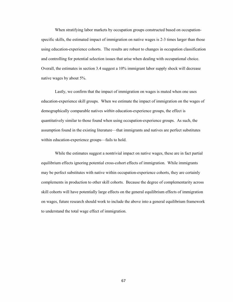
67

When stratifying labor markets by occupation groups constructed based on occupation-

specific skills, the estimated impact of immigration on native wages is 2-3 times larger than those

using education-experience cohorts. The results are robust to changes in occupation classification

and controlling for potential selection issues that arise when dealing with occupational choice.

Overall, the estimates in section 3.4 suggest a 10% immigrant labor supply shock will decrease

native wages by about 5%.

Lastly, we confirm that the impact of immigration on wages is muted when one uses

education-experience skill groups. When we estimate the impact of immigration on the wages of

demographically comparable natives within education-experience groups, the effect is

quantitatively similar to those found when using occupation-experience groups. As such, the

assumption found in the existing literature—that immigrants and natives are perfect substitutes

within education-experience groups—fails to hold.

While the estimates suggest a nontrivial impact on native wages, these are in fact partial

equilibrium effects ignoring potential cross-cohort effects of immigration. While immigrants

may be perfect substitutes with native within occupation-experience cohorts, they are certainly

complements in production to other skill cohorts. Because the degree of complementarity across

skill cohorts will have potentially large effects on the general equilibrium effects of immigration

on wages, future research should work to include the above into a general equilibrium framework

to understand the total wage effect of immigration.

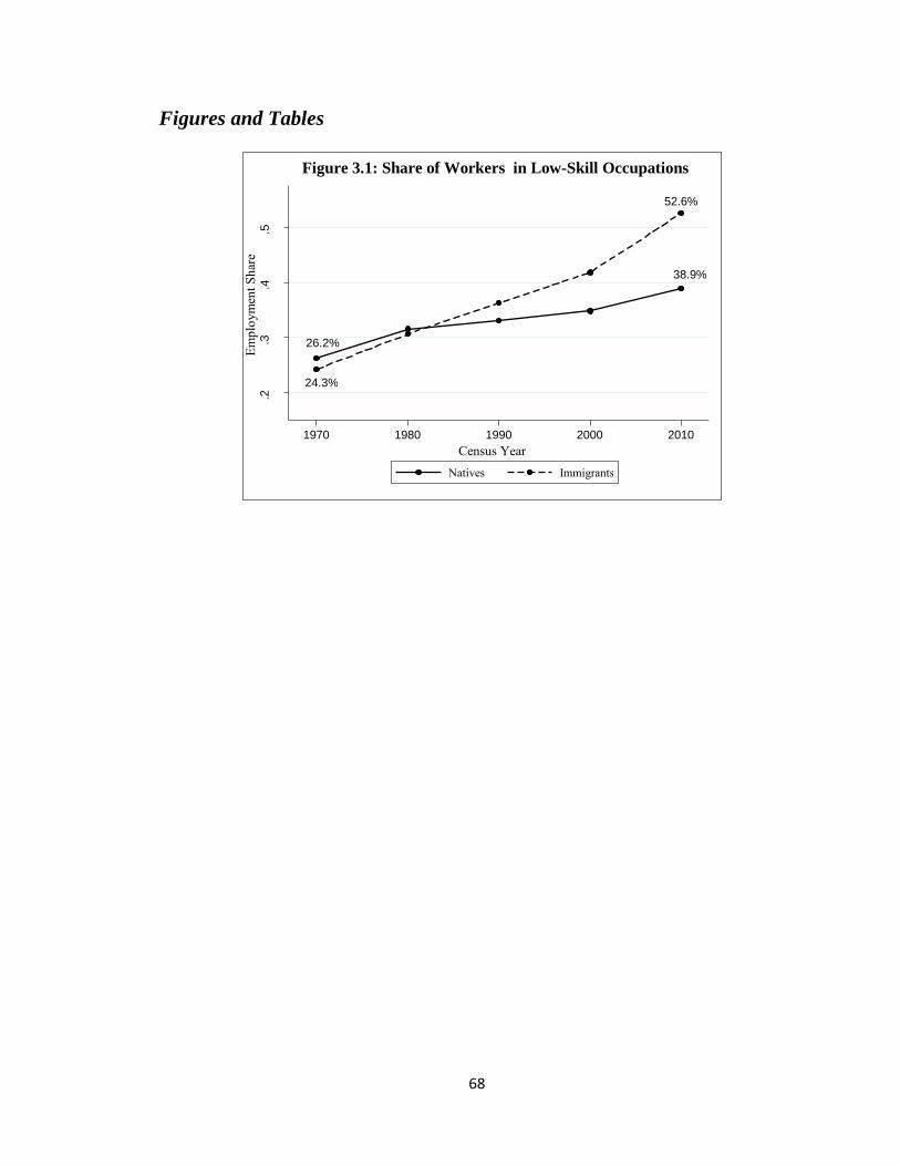
68

Figures and Tables

26.2%

24.3%

52.6%

38.9% .2

.3

.4

.5

Em

ploy

men

t Sha

re

1970 1980 1990 2000 2010 Census Year

Natives Immigrants

Figure 3.1: Share of Workers in Low-Skill Occupations

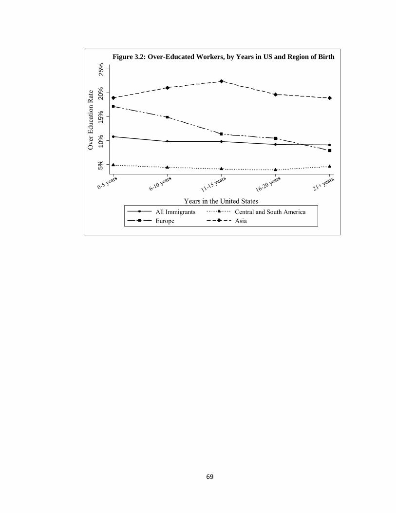
69

5%

10%

15

%

20%

25

%

Ove

r Edu

catio

n R

ate

Years in the United States All Immigrants Central and South America Europe Asia

Figure 3.2: Over-Educated Workers, by Years in US and Region of Birth

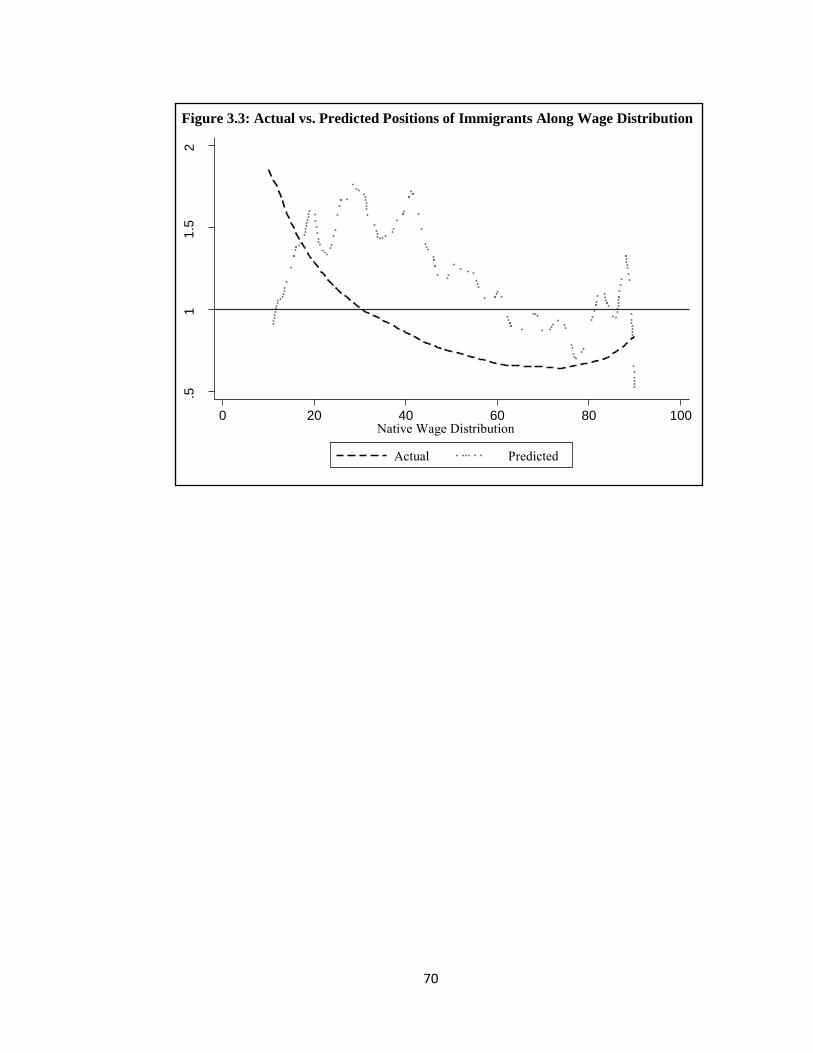
70

.5

1 1.

5 2

0 20 40 60 80 100 Native Wage Distribution

Actual Predicted

Figure 3.3: Actual vs. Predicted Positions of Immigrants Along Wage Distribution

71

.006

.0

08

.01

.012

.0

14

0 20 40 60 80 100 Occupation Skill Distribution

Immigrants Natives

Figure 3.4: Employment Along Occupation-Specific Skill Distribution

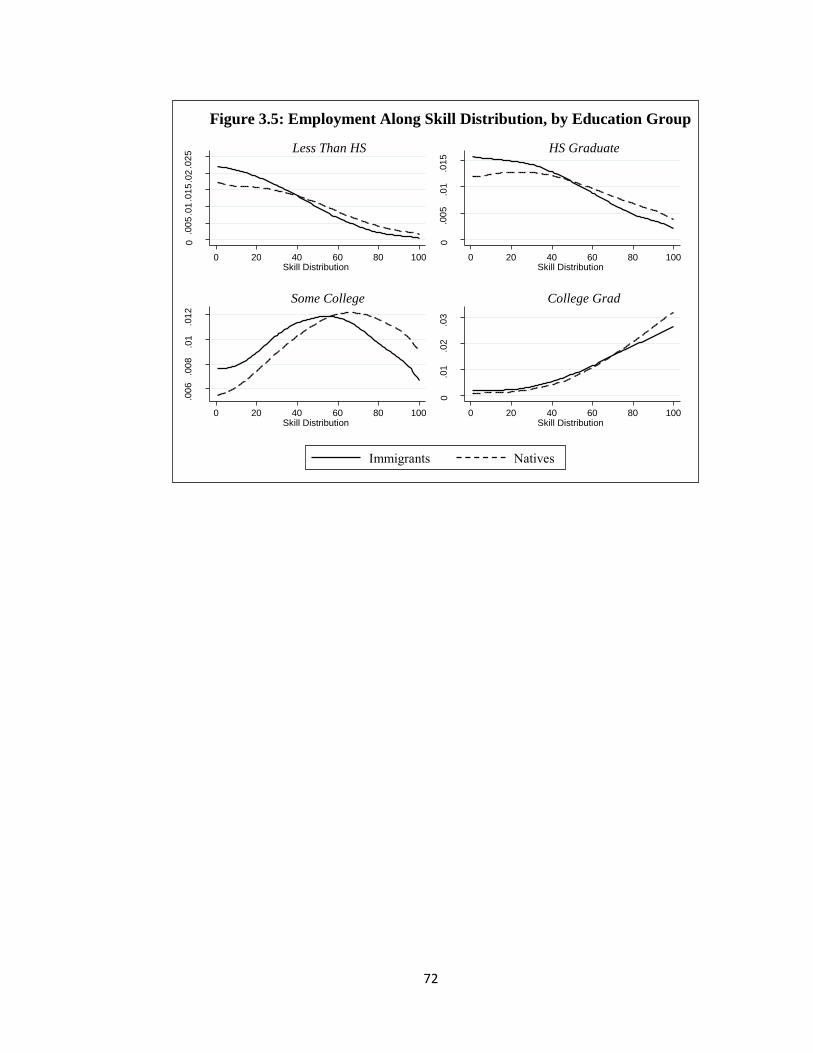
72

0 .0

05 .01

.015 .0

2 .025

0 20 40 60 80 100 Skill Distribution

Less Than HS

0 .0

05

.01

.015

0 20 40 60 80 100 Skill Distribution

HS Graduate

.006

.00

8 .0

1 .0

12

0 20 40 60 80 100 Skill Distribution

Some College

0 .0

1 .0

2 .0

3

0 20 40 60 80 100 Skill Distribution

College Grad

Figure 3.5: Employment Along Skill Distribution, by Education Group

Immigrants Natives

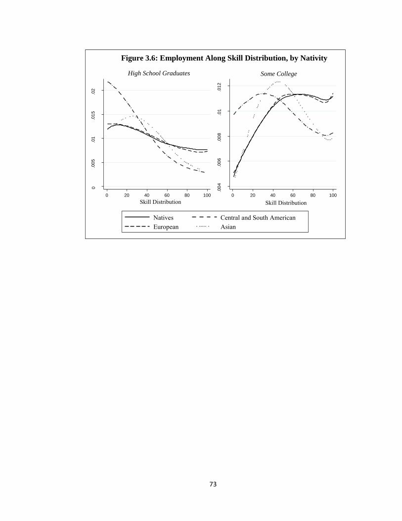
73

0 .0

05

.01

.015

.0

2

0 20 40 60 80 100 Skill Distribution

High School Graduates

.004

.0

06

.008

.0

1 .0

12

0 20 40 60 80 100 Skill Distribution

Some College

Figure 3.6: Employment Along Skill Distribution, by Nativity

Natives Central and South American European Asian

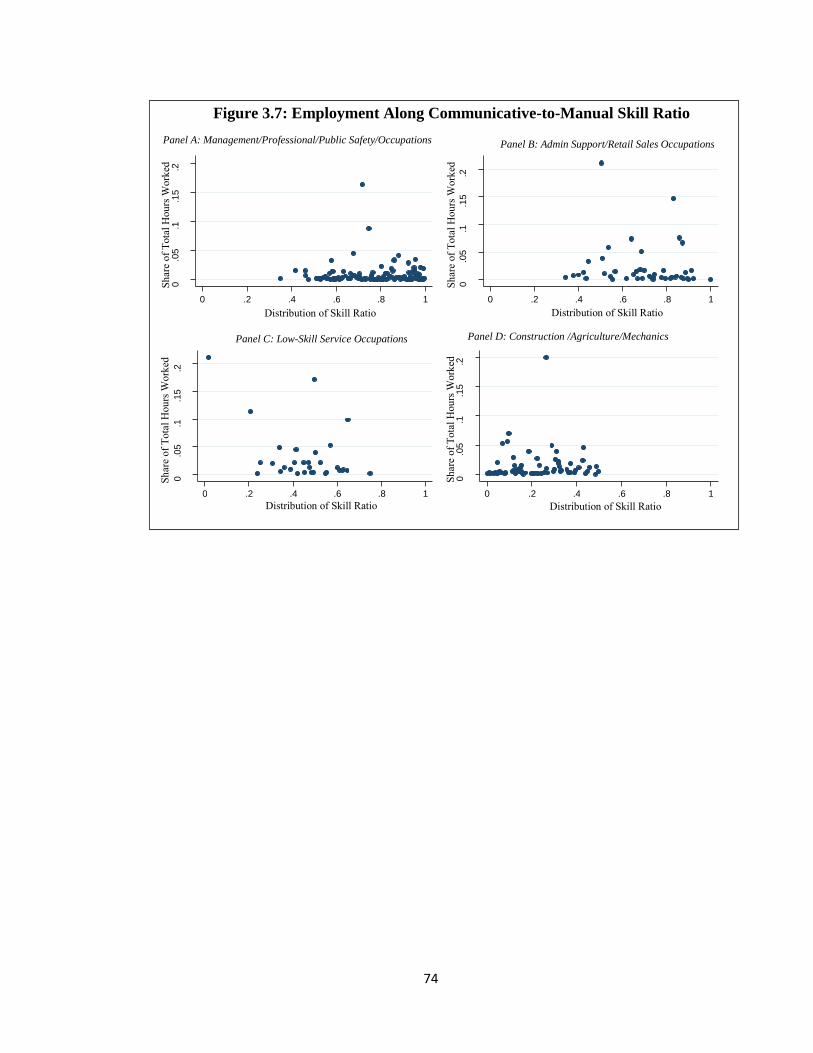
74

0 .0

5 .1

.1

5 .2

Sh

are

of T

otal

Hou

rs W

orke

d

0 .2 .4 .6 .8 1 Distribution of Skill Ratio

Panel A: Management/Professional/Public Safety/Occupations

0 .0

5 .1

.1

5 .2

Sh

are

of T

otal

Hou

rs W

orke

d

0 .2 .4 .6 .8 1 Distribution of Skill Ratio

Panel B: Admin Support/Retail Sales Occupations

0 .0

5 .1

.1

5 .2

Sh

are

of T

otal

Hou

rs W

orke

d

0 .2 .4 .6 .8 1 Distribution of Skill Ratio

Panel C: Low-Skill Service Occupations

0 .0

5 .1

.1

5 .2

Sh

are

of T

otal

Hou

rs W

orke

d

0 .2 .4 .6 .8 1 Distribution of Skill Ratio

Panel D: Construction /Agriculture/Mechanics

Figure 3.7: Employment Along Communicative-to-Manual Skill Ratio

75

Table 3.1: Over-Educated of Natives and Immigrants, 1970-2010 Occupation Group (1)

% Over-Educated Natives

(2) % Over-Educated

Immigrants

(3) % Over-Educated

Immigrants (in US for less than or equal to 5 years)

All Occupations 5.36% (6.33%)

9.25% (10.89%)

9.59% (11.06%)

Occupations where one is over-educated when holding at least a Bachelor’s Degree

5.17% (6.67%)

7.55% (9.37%)

7.91% (10.02%)

Occupations where one is over-educated when holding at least a Master’s Degree

6.70% (7.04%)

15.86% (17.81%)

18.95% (22.86%)

Occupations where one is over-educated when holding at least a Doctoral/Professional Degree

4.28% (4.43%)

12.74% (13.43%)

13.98% (14.75%)

Occupations where one is over-educated when holding at least a Masters or a Doctoral/Professional Degree

6.18% (6.48%)

15.18% (16.81%)

17.78% (20.74%)

1) Hours weighted averages reported in parentheses.

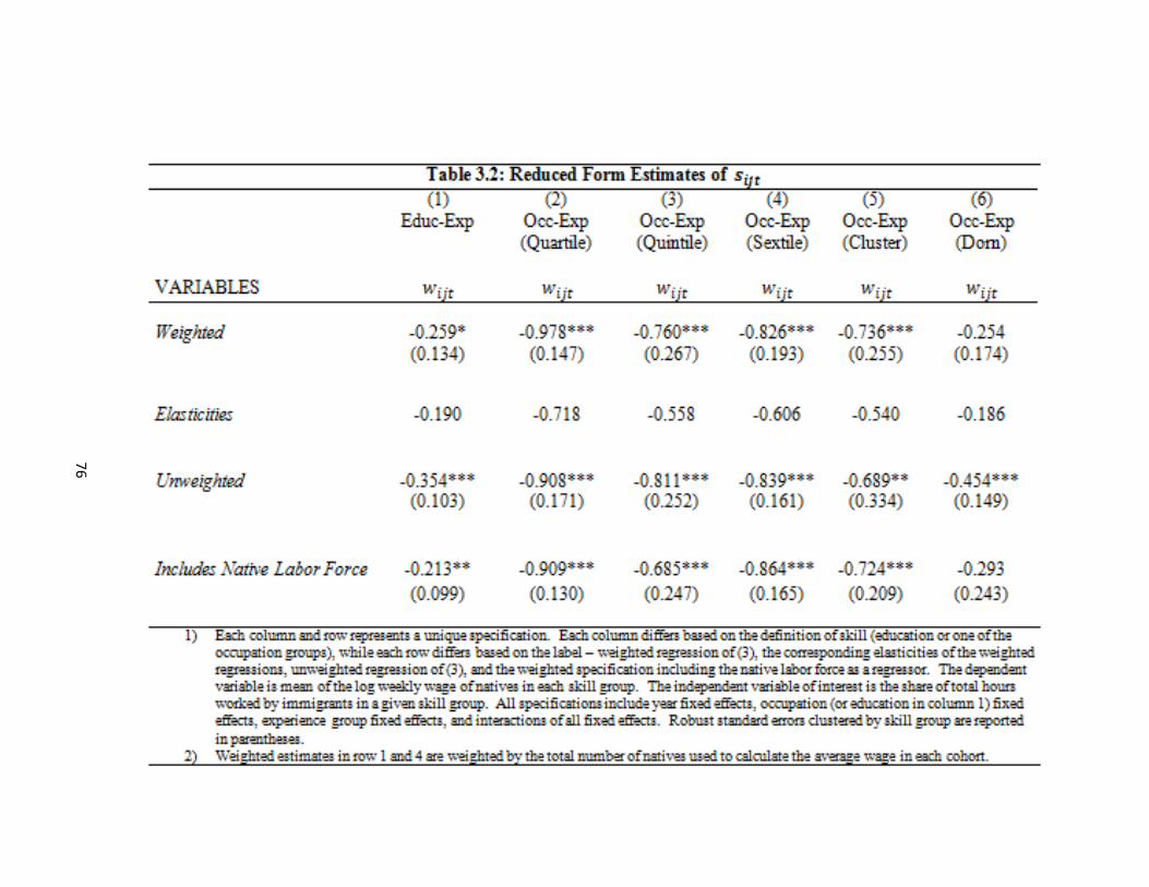
76

77

Table 3.3: Robustness Check, Impact of Immigration (1970-2010) (1) (2) (3) (4) Educ-Exp Occ-Exp

(Quartile) Occ-Exp (Quintile)

Occ-Exp (Cluster)

VARIABLES 𝐾𝐼𝑗𝑘 𝐾𝐼𝑗𝑘 𝐾𝐼𝑗𝑘 𝐾𝐼𝑗𝑘 Immigrant Share (𝐼𝐼𝑗𝑘) -0.307** -0.741*** -0.681*** -0.623** (0.126) (0.1105) (0.1621) (0.2661) Elasticity -0.255 -0.544 -0.500 -0.457 Observations 160 192 240 240 R-squared 0.997 0.999 0.998 0.999

1) Each column represents a unique specification. Each column differs based on the definition of skill (education or one of the occupation groups). The dependent variable is mean of the log weekly wage of natives that could work in a given skill group. The independent variable of interest is the share of total hours worked by immigrants that could work in a given skill group. All specifications include year fixed effects, occupation (or education in column 1) fixed effects, experience group fixed effects, and interactions of all fixed effects. Robust standard errors clustered by skill group are reported in parentheses.

2) All specifications are weighted using the total number of natives used to calculate the average wage in each cohort as weights.

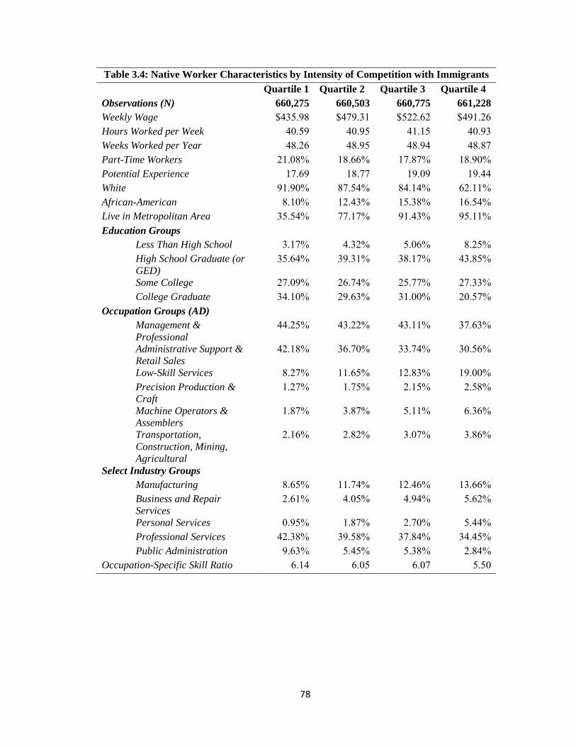
78

Table 3.4: Native Worker Characteristics by Intensity of Competition with Immigrants Quartile 1 Quartile 2 Quartile 3 Quartile 4 Observations (N) 660,275 660,503 660,775 661,228 Weekly Wage $435.98 $479.31 $522.62 $491.26 Hours Worked per Week 40.59 40.95 41.15 40.93 Weeks Worked per Year 48.26 48.95 48.94 48.87 Part-Time Workers 21.08% 18.66% 17.87% 18.90% Potential Experience 17.69 18.77 19.09 19.44 White 91.90% 87.54% 84.14% 62.11% African-American 8.10% 12.43% 15.38% 16.54% Live in Metropolitan Area 35.54% 77.17% 91.43% 95.11% Education Groups

Less Than High School 3.17% 4.32% 5.06% 8.25% High School Graduate (or GED)

35.64% 39.31% 38.17% 43.85%

Some College 27.09% 26.74% 25.77% 27.33% College Graduate 34.10% 29.63% 31.00% 20.57%

Occupation Groups (AD) Management & Professional

44.25% 43.22% 43.11% 37.63%

Administrative Support & Retail Sales

42.18% 36.70% 33.74% 30.56%

Low-Skill Services 8.27% 11.65% 12.83% 19.00% Precision Production & Craft

1.27% 1.75% 2.15% 2.58%

Machine Operators & Assemblers

1.87% 3.87% 5.11% 6.36%

Transportation, Construction, Mining, Agricultural

2.16% 2.82% 3.07% 3.86%

Select Industry Groups Manufacturing 8.65% 11.74% 12.46% 13.66% Business and Repair Services

2.61% 4.05% 4.94% 5.62%

Personal Services 0.95% 1.87% 2.70% 5.44% Professional Services 42.38% 39.58% 37.84% 34.45% Public Administration 9.63% 5.45% 5.38% 2.84%

Occupation-Specific Skill Ratio 6.14 6.05 6.07 5.50

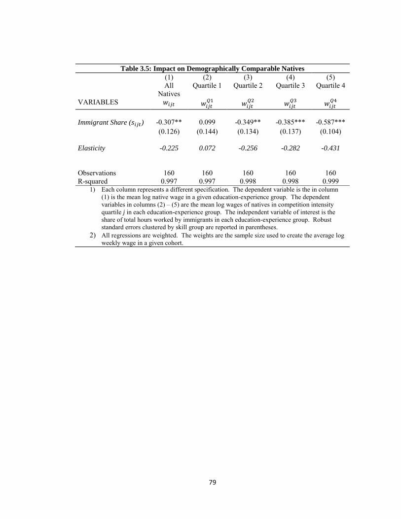
79

Table 3.5: Impact on Demographically Comparable Natives (1) (2) (3) (4) (5) All

Natives Quartile 1 Quartile 2 Quartile 3 Quartile 4

VARIABLES 𝐾𝐼𝑗𝑘 𝐾𝐼𝑗𝑘𝑄1 𝐾𝐼𝑗𝑘

𝑄2 𝐾𝐼𝑗𝑘𝑄3 𝐾𝐼𝑗𝑘

𝑄4 Immigrant Share (𝐼𝐼𝑗𝑘) -0.307** 0.099 -0.349** -0.385*** -0.587*** (0.126) (0.144) (0.134) (0.137) (0.104) Elasticity -0.225 0.072 -0.256 -0.282 -0.431 Observations 160 160 160 160 160 R-squared 0.997 0.997 0.998 0.998 0.999

1) Each column represents a different specification. The dependent variable is the in column (1) is the mean log native wage in a given education-experience group. The dependent variables in columns (2) – (5) are the mean log wages of natives in competition intensity quartile j in each education-experience group. The independent variable of interest is the share of total hours worked by immigrants in each education-experience group. Robust standard errors clustered by skill group are reported in parentheses.

2) All regressions are weighted. The weights are the sample size used to create the average log weekly wage in a given cohort.

80

4. Differential Impacts of Immigration Within Cities 4.1 Introduction The impact of immigration on the housing market is an important one because housing

expenditures are a large portion of the budget for most Americans. Even a modest increase in

prices due to immigration can have significant impacts on the native population. Much of the

existing literature analyzing immigration and the housing market has identified the impact of

immigration on rents using metropolitan statistical area (MSA) median gross rents, treating the

entire MSA as one homogenous “city” (Saiz 2003, 2007).46 Ignoring the heterogeneity of

neighborhoods within a MSA has led to an unsurprising consensus in the literature: immigrant

inflows into an MSA lead to an increase in housing prices and rents. Because an inflow of

immigrants is a positive shock to housing demand and we assume an upward sloping supply

curve, one would expect increases in housing prices in the short-run. The present research

expands on the existing literature and analyzes the impact of immigration within a metropolitan

area.

The motivation for examining the more local effect of immigration on rents is two-fold.

First, settlement patterns of immigrants in the U.S. are unique. We know that immigrants cluster

in only a handful of states and certain cities within these states (Bartel, 1989). This clustering

behavior has been explained as immigrants forming ethnic enclaves that provide cultural

amenities to its residents. The explanation in the literature cited above is that it is this clustering

behavior that bids up rents in high-immigration cities. Assuming the desire to reside in these

ethnic enclaves is strong enough, the increased willingness to pay of immigrants leads to higher

rents in the city. What is typically ignored, however, is that immigrants also cluster within cities.

Immigrant clustering within cities is illustrated in Figures 4.1 and 4.2. Figure 4.1 depicts

census tract-level immigrant population shares for the Los Angeles and New York City CBSA’s. 46 This is also the methodology used in Chapter 2 of this dissertation.

81

The darker areas are tracts with higher shares of immigrants. In both Los Angeles and New York

City, pronounced immigrant clustering is exhibited around the central cities and decreasing

immigrant density in the suburbs.47 Similarly, Figure 4.2 demonstrates immigrant clustering is

consistent over time. Figure 4.2 illustrates tract-level immigrant shares for the years 2000 and

2010 for the Los Angeles CBSA. Again, the same pattern emerges: immigrants cluster near the

city-center, and high-immigrant neighborhoods in 2000 were still high-immigrant neighborhoods

in 2010. If increases in rents are driven by the preferences of immigrants to reside near ethnically

similar households, Figures 4.1 and 4.2 suggest that the impact of immigration should not be

uniform across cities. Instead, the increase in rents should be concentrated on these high-

immigrant neighborhoods as new immigrants enter the housing market and bid up rents in these

areas.

A second omission from the existing literature is the acknowledgement that households

are mobile. As immigrants cluster within cities, natives may have incentives (which are

discussed in more detail below) to move away from high-immigration areas of the city. Schelling

(1972) was among the first to document the “tipping point” at which white populations abandon

neighborhoods with growing black populations for the suburbs. This tipping point is measured as

the share of the population which is black. If white populations feel similarly about immigrant

neighborhoods, then the clustering of immigrants in the same neighborhoods may spur mass out-

migration of white populations as these neighborhoods exceed this tipping point. If natives

migrate from high-immigrant areas to other non-immigrant neighborhoods within the same city,

we ignore an important dynamic when treating a metropolitan area as one homogenous unit. If

this out-migration from high-immigration neighborhoods is severe enough, it is possible that the

47 As Los Angeles and New York City are 1) the two CBSA’s that receive the greatest annual immigrant inflows and 2) two of the largest cities in the US, one may be concerned that immigrant settlement behavior is different in these cities relative to other small CBSA’s. To reconcile this, I also provide illustrations of immigrant clustering in two smaller, lower-immigration CBSA’s (Lexington, KY and Louisville, KY) in Figure 4A.1 of the Appendix. The clustering of immigrants is equally pronounced in these cities as well.

82

impact of immigration on housing rents is lower in high-immigration neighborhoods relative to

other low-immigrant neighborhoods.

The primary focus of this paper is to disentangle the impact of immigration on CBSA-

level rents found in the existing literature. Because of the unique clustering of immigrants,

differential preferences of natives and newly arriving immigrants for living in high-immigrant

neighborhoods may segment the housing market within a CBSA. The presence of unique

housing submarkets within a metropolitan area is well documented in the literature. Submarkets

within metropolitan areas may occur due to either supply or demand-related factors (Goodman

and Thibodeau, 1998). Across these unique submarkets, the implicit price of housing market

characteristics or neighborhood amenities may not be constant (Goodman, 1978; Goodman,

1981). Metropolitan housing markets may be segmented along several different dimensions.

King and Mieszkowski (1973) show that housing submarkets exist along racial lines. Schnare

and Struyk (1976) argue that submarkets occur when household demand for a particular

neighborhood characteristic (i.e. proximity to immigrants) is highly inelastic and these

preferences are common among a large number of households within a metropolitan area. I argue

that the inelastic demand of newly arriving immigrants to live near other immigrants will segment

the housing market within CBSA’s and the impact of immigration on prices will differ across

these submarkets.

In this paper, I document the differential impact of immigration within a metropolitan

(CBSA) housing market in two ways. First, I assume that markets are segmented by different

characteristics of high-immigrant neighborhoods: high shares of foreign-born populations, low

income, and low rent neighborhoods. Using census tract-level data, I show that an immigrant

inflow into a city has a nonlinear effect within a CBSA. Specifically, the impact of immigration

on rents is, on average, negative in high-immigration tracts. This differential effect is even more

negative if I focus on high-immigration CBSA’s.

83

Second, using a quantile regression framework, I analyze the impact of immigration

along the rent distribution within a CBSA. The use of quantile regression is appropriate here due

the settlement patterns of immigrants. Due to the clustering of immigrants in certain

neighborhoods within cities, we also observe clustering along the distribution of housing rents.

To see this, Figure 4.3 plots the share of immigrant households and the share of native households

along the distribution of rents in 2000.48 Relative to native households, immigrants are

overrepresented from roughly the 10th percentile to the 60th percentile. With no out-migration of

native households, one would expect the impact of immigration to be larger in this area of the rent

distribution. If natives do respond by moving, however, the increase in housing demand

associated with immigration (and corresponding increase in rents) would also be seen in the low-

immigrant areas of the rent distribution. The results suggest the latter and confirm the findings

using tract-level data. Immigration has a smaller effect on rents in portions of the rent

distribution where immigrants cluster. While immigrant inflows are shown to have a positive

impact on rents across the distribution, the impact of immigration on rents takes a U-shape. In

fact, the quantile graph of the effect of immigration is roughly the inverse of the immigrant curve

in Figure 4.3, which suggests that the impact is largest in areas with more native households.

Lastly, I show that decreased impact on rents in high-immigration portions of the rent

distribution is due to out-migration of native households. Using census tract-level data for NYC,

I show that immigrant inflows into NYC cause out-migration of white households from tracts

with rents below the median, while higher-rent tracts experience growth in white households.

Just as economists have been concerned with the formation of the “black ghetto” over the

last century, white flight out of high-immigration areas may suggest the formation of an

“immigrant ghetto”. Segregation among immigrants into ethnic enclaves can have positive short 48 This plot uses household data from the 2000 decennial Census for all observations living in a CBSA. To construct this figure, I first generate a cumulative rent distribution within each CBSA. Then, I aggregate all immigrant and native households in each percentile of the rent distribution. The plot illustrates the share of total households in each percentile, by nativity.

84

term economic impacts on immigrants (Cutler et al., 2007). As the authors note, ethnic enclaves

decrease the needed assimilation time by offering job opportunities and transportation. On the

other hand, increased segregation of immigrants may have harmful economic effects in both the

short and long term, especially for low-skill or less educated immigrants. These negative

consequences include lower earnings (Cutler et al., 2007; Sousa, 2013), decreased human capital

accumulation for immigrant children (Cascio and Lewis, 2012), and decreased English

proficiency and decreased access to jobs and quality public services (Cutler et al., 2007). As each

successive immigration wave has become less and less skilled, increased segregation due to white

flight may have tremendous effects on overall economic outcomes for these immigrants.

The rest of the paper is structured as follows. Section 4.2 outlines the conceptual

framework underlying the empirical analysis. This discussion is framed within the context of a

residential segregation model in the spirit of Yinger (1976) and Boustan (2010). Section 4.3

provides supporting evidence into the differential impact of immigration within metropolitan

areas. Specifically, I show that the impact of immigration within a CBSA is smaller in census

tracts that had higher initial immigrant populations, lower incomes, and lower rents. Section 4.4

presents the quantile regression analysis, discusses potential data issues, and presents the results.

Section 4.5 relates the quantile regression results to the out-migration of native households.

Section 4.6 concludes.

4.2 Native Out-Migration and Segregation White flight and urban segregation has been heavily researched area in economics,

sociology, and demography. In the majority of this work, researchers examine the incidence of

white flight in response to black migration and the segregation of black and white residents

within an urban community.49 Recently, however, a growing literature has emerged discussing

49 This literature is far too large to cite all of the relevant papers. Schelling (1971), Yinger (1976), and Courant and Yinger (1977) provide seminal work in the area of racial segregation within an urban community. Bradford and

85

the incidence of white flight in response to immigration. As discussed above, immigrants display

a unique and predictable settlement pattern across cities in the U.S. Because immigrants cluster

within cities, the growing concentration of immigrants within neighborhoods has been shown to

spur white (or native) flight.

To see how immigration may spur native out-migration and its impact on housing prices,

I apply a simple residential segregation model (Yinger, 1976; Boustan, 2010).50 To start,

consider a city with a fixed number of native households. The city has both a city center and a

suburban outer ring. Due to free mobility, utility of a native household cannot fall below 𝑢�, the

utility of a native household living in the suburbs. Native household utility is written as:

(1) 𝑈𝑁(𝑝, 𝑖, 𝑧) = 𝑢�.

Utility is a decreasing function of both housing prices (p) and weakly decreasing in the share of

the city population that is foreign-born (i). I do not specify the nature of the disutility associated

with i, but discuss potential sources in more detail later in the paper. z is a demand shifter that

represents local amenities. Housing prices in the city are a function of the total number of

households in the city (N) and the sensitivity of housing prices to changes in N is determined by

the elasticity of housing supply. Utility for immigrant households is defined as in (1) except

immigrant household utility is increasing in (i). This follows from the discussion above regarding

the clustering of immigrants to achieve cultural amenities. Spatial equilibrium is achieved when

all native and immigrant households weakly prefer their present location to all other locations in

the city and construction firms earn zero profits. The equilibrium housing price is denoted 𝑝∗ and

the equilibrium share of immigrants in the city is 𝑖∗.

Kelejian (1973) model white flight. In sociology, a good overview of the white flight hypothesis, I direct interested readers to Crowder (2000). 50 Yinger (1976) defines a complete model of residential segregation. So as to not be redundant, the following model follows a more short-hand model similar to that found in Boustan (2010).

86

When new immigrants move into the city, the impact on housing prices and the number

of native households that move out of the city will depend on the marginal utility with respect to i

for native households. First, consider the case where native households do not receive disutility

from immigrant households (𝑈𝐼′ = 0). Assuming supply is not perfectly elastic, an immigrant

inflow will increase prices in the short-run to 𝑝�. This increase in prices will induce some native

households to flee to the suburbs and they will continue to do so until housing prices in the city

return to 𝑝∗. Because p is solely a function of N, in order to maintain equilibrium it must be the

case that each immigrant household into the city displaces exactly one native household. Thus, if

natives do not show distaste for living near immigrants, immigrant inflows will displace native

households at a rate of one-for-one and the long-run impact on housing prices in the city will be

zero.

Now, consider the case where native households show distaste for living near immigrants

(𝑈𝐼′ < 0). As before, the new immigrant inflow to the city will increase housing prices to 𝑝� > 𝑝

and increase the share of immigrants in the city to 𝐼̃ > 𝑖. Again, native households will respond

to the increase in price and move to the suburbs until spatial equilibrium is restored

(𝑈𝑁(𝑝∗, 𝑖, 𝑧) = 𝑢�). When natives receive disutility from increased prices and disutility from

living near immigrants, the marginal native would still prefer the suburbs to living in the city

even at equilibrium price levels as 𝑈𝑁(𝑝∗, 𝐼̃, 𝑧) < 𝑢� . In this scenario, native householders will

continue to move out of the city and total population falls below equilibrium. Thus, assuming

housing supply is not perfectly elastic, native distaste for immigration, white flight will cause

housing prices in the city will fall below equilibrium in the short-run.

In the discussion above, I do not specify the nature of the distaste associated with

immigrants and how it may spur out-migration of native households. Crowder et al. (2011)

outlines three main theories to explain the out-migration of natives in response to growing

immigrant concentration. While each theory describes a different mechanism through which

87

native out-migration is achieved, the underlying results are the same: large immigrant

concentrations spur out-migration on native populations. The first theory, referred to as the

ethnic flight theory, suggests immigrant inflows induce out-migration because immigrant inflows

change the ethnic composition of a neighborhood (Clark and Blue, 2004; Saiz and Wachter,

2011). The premise behind this theory is purely racial and can be thought of as traditional “white

flight”. If native households prefer to live near culturally and racially similar households, the

response of natives to immigrant inflows is purely racial.

The second theory is called the socioeconomic context theory. Like the ethic flight

theory above, white flight occurs because of the proximity to large immigrant populations.

Contrary to the ethnic flight theory, however, the social context theory suggests natives respond

to changes in socioeconomic conditions of neighborhoods brought on by a large immigrant

inflow, not the racial sentiment toward immigrants themselves. As pointed out by the authors,

immigrants tend to be less educated with a higher incidence of poverty. As such, an increased

concentration of immigrants in a neighborhood would lead to lower average income and if this

decrease in income is correlated with neighborhood conditions (i.e. school quality, crime, etc.),

then native populations flee high immigrant neighborhoods.

The last theory of white flight, the housing competition model, is related to the

willingness to pay story told in the previous section. Upon entering a neighborhood, immigrants

may change local housing market conditions. In the short-run, immigrant inflows into a

neighborhood will cause an increase in prices which, in turn, may push natives out of the

neighborhood in search for more affordable housing. Similarly, immigrant inflows may affect

other aspects of the local housing market. It is widely known that homeownership rates are far

lower for immigrants relative to natives. If immigrant inflows have an effect on rental/owner-

occupied mix within a neighborhood and this is a source of disutility for native homeowners,

natives may flee the neighborhood.

88

It should be noted that I do not differentiate between these theories in the analysis below.

The data do not allow one to speak to the exact mechanism that spurs out-migration of native

households. While identifying the motive for out-migration is not possible, the above discussion

does provide ample support for the prior that immigrant inflows should have some effect on the

migration decisions of native households in a neighborhood. Furthermore, the above theories

have different implications for the impact of immigration on rents. If the housing competition

model is the main mechanism that spurs out migration, then the impact on rents should be near

zero in high-immigrant tracts. This corresponds directly to the case where natives show no

distaste for living near immigrants discussed above (𝑈𝐼′ = 0). If out-migration is racially

motivated or due to changes in socioeconomic conditions, then the impact of rents will be

negative (𝑈𝐼′ < 0).

4.3 Differential Impact of Immigration Within Cities

This section examines the average impact on rent at the census tract level and finds that

the impact is non-linear, supporting a model where there is negative utility for native households

living near immigrants. The empirical model follows loosely from the model of Saiz and

Wachter (2011). I estimate the impact of a CBSA-level immigrant inflow when accounting for

the heterogeneity of neighborhoods. Here, as is customary in the literature, I use census tracts as

a proxy for neighborhoods. Specifically, the model is:

(2) ∆ ln�𝐹𝑗,𝑘,𝑘� = 𝛼𝐼𝑘,𝑘 + 𝛽(𝐼𝑘,𝑘 ∗ 𝑋𝑗,𝑘,𝑘−1) + 𝛿𝐻𝑗,𝑘,𝑘 + 𝛾𝑍𝑗,𝑘,𝑘−1 + 𝜃𝑘 + 𝜀𝑗𝑘𝑘

𝐹𝑗,𝑘,𝑘 is the average gross rent in a given tract (neighborhood) j within a CBSA k at time t. 𝐼𝑘,𝑘

denotes the CBSA-level immigration impact variable, which is defined as the change in foreign-

born population in year t divided by the CBSA population in year t-10. The interaction term

(𝐼𝑘,𝑘 ∗ 𝑋𝑗,𝑘,𝑘−1) represents the interaction of the CBSA-level immigration impact and an initial

neighborhood level characteristic that differentiates between high and low-immigrant tracts. I

89

estimate four variants of the model with different definitions for 𝑋𝑗,𝑘,𝑘−1: two specifications

include a measure of immigrant concentration, a third is an indicator equal while the third is an

indicator for below average rents. As such, 𝛽 is the coefficient of interest. Because 𝑋𝑗,𝑘,𝑘−1 are

characteristics of high-immigrant neighborhoods, 𝛽 < 0 would suggest the impact of immigration

is lower in high-immigration neighborhoods (and vice versa).

𝐻𝑗,𝑘,𝑘 is a vector of tract-level rental housing market characteristics including controls for

age of structures, units in structures, rental vacancy rate, initial rent level in 1980, and other

physical characteristics of the housing unit. Following Saiz and Wachter (2011), I include both

lagged levels and changes in average housing characteristics. 𝑍𝑗,𝑘,𝑘−1 is a vector of lagged

neighborhood socioeconomic characteristics including the share of the population that is black,

the share of the population with at least a bachelor’s degree, among others. 𝜃𝑘 are year fixed

effects.

Summary statistics are presented in Table 4.1 for all tracts, high-immigrant tracts, and

low-immigrant tracts. High-immigrant tracts differ widely along housing unit characteristics,

neighborhood characteristics, and demographics. High-immigrant tracts have significantly fewer

single family units, housing units tend to be smaller, and average rents are lower. Similarly, the

high-immigrant neighborhoods tend to be less desirable as there is less new construction and

above average values of the neighborhood disadvantage index (NDI). The NDI is comprised of

four individual parts: the unemployment rate among working-aged males in the neighborhood,

the percent of total households that are female heads of household with children under 18 years

old, the inverse of median household income, and the poverty rate (Hannon, 2005).51 Less

desirable neighborhoods have higher values of NDI. Lastly, high-immigrant tracts differ

significantly along demographic lines. Households in these neighborhoods tend to be more

51 To calculate this measure, each of the four components is standardized to mean 0 with a standard deviation of 1. Then, the NDI is simply the average of these 4 standardized components.

90

mobile. Larger shares of renter-occupied households, younger householders, and a smaller share

of households with tenure greater than 10 years in their current dwelling are all characteristics of

more mobile households (Quigley and Weinberg, 1977; Weinberg, 1979). The relative mobility

of the households in high-immigrant neighborhoods lends credence to the white flight hypothesis

in the previous section. Because newly arriving immigrants cluster in existing high-immigrant

neighborhoods (Figures 4.1 and 4.2), these inflows will be concentrated on a more mobile

population, increasing the likelihood of significant out-migration of native households.

4.3.1 Instrumental Variable

Estimating Eq. (2) via OLS will produce biased and inconsistent estimates because

immigrant inflows into cities and neighborhoods are endogenous. As shown by Chapter 2 of this

dissertation, immigrants locate in CBSA’s that provide them the best economic opportunities.

Because immigrants are locating in thriving cities rich in amenities and public goods, housing

prices will increase irrespective of immigration. In this case, OLS estimates will be biased

upwards. To deal with this endogeneity, I use an instrumental variable strategy based on country-

of-origin similar to the one presented in Saiz (2007). I use INS data on newly arriving

immigrants and source country-level data that are exogenous to CBSA-specific amenities to

predict the number of new immigrants to the U.S. from each country in each year. To predict

immigrant inflows from country i in year t, I estimate the following panel random effects model:

(3) 𝐼𝐼𝑘 = 𝛼𝑋𝐼,𝑘−1 + 𝛽𝑍𝐼,𝑘−2 + 𝛾𝑉𝑘 + 𝜃𝐼 + 𝜇𝐼𝑘.

Here, 𝐼𝐼𝑘 is the migration rate from country i to the U.S. in time t. 𝑋𝐼,𝑘−1 is a vector of

lagged source country-level characteristics including real GDP (relative to U.S. GDP), a measure

of poverty defined as the inverse of per capita income, the share of the population that is between

15-19 years old, and the average annual immigrants sent to the U.S. over the previous 5 years.

𝑍𝐼,𝑘−2 is a vector of country-specific variables describing the political instability of the source

91

country and military conflicts. Specifically, I include a dummy variable equal to 1 if the country

underwent a regime change, a dummy variable equal to 1 if the country was involved in a major

military conflict in year t-2, and a dummy variable equal to 1 if there was genocide in year t-2.

While similar to the instrument defined in Saiz (2007), the advantage of the present

instrument is that Eq. (3) is more grounded in migration theory. Following Clark et al. (2007), I

also control for changes in U.S. immigration policy that would directly affect the number of

immigrants arriving from a given source country through the vector 𝑉𝑘. Specifically, I account

for the number of refugee visas and diversity visas allotted to a given source region and the mass

legalization of immigrants in the early 1990’s that stemmed from the Immigration Reform and

Control Act.

I present the estimates of the panel random effects model in Table 4A.1 of the Appendix

and variable descriptions in Table 4A.2. All of the variables have the expected impact on

migration rates. Countries with higher shares of young population, who are war torn, or

experiencing a regime change all experience increased migration. The variables describing

migration policy also have significant effects on migration. Eligibility for diversity and refugee

visas has significant positive impacts on migration. This is important because some countries do

not have complete data throughout the panel. For these countries, Saiz (2007) estimates the panel

random effects model on country random effects and lagged migration. Here, with the addition

of the immigration policy variables, I am able to include these variables in addition to lagged

migration for these counties.

To construct the predicted migration rate from country i, I exclude the estimated random

effects. As Saiz (2007) explains, these random effects may be correlated with factors that made it

attractive to locate in cities where immigrants of that nationality clustered in previous years.

Next, I convert the predicted migration rate into prediction immigration inflows.

92

Once I have backed out the number of imputed immigrants from each country and year (

tUSiM ,,ˆ ), I follow the traditional shift-share approach found in the literature to construct imputed

immigrant inflows into each CBSA that are exogenous to local market conditions. To do this, I

first calculate the number of newly arriving immigrants from each country i that located in each

CBSA k in 1980 ( 1980,kiω ). Because immigrants cluster in a predictable manner, I assume that

CBSA k will receive the same share of total (imputed) immigrants from country i in every year

after 1980. Using this initial share ( 1980,kiω ) and the imputed immigrants ( tUSiM ,,

ˆ ), I calculate the

number of imputed immigrants from each source country i to CBSA k for every year after 1980.

Then, the total imputed inflow of immigrants into a CBSA is simply the sum of the inflows from

each country. Analytically, the annual imputed total immigrant inflow into CBSA k is calculated

as:

(4) ( )∑=

=N

itUSikitk MM

1,,

1980,,

ˆ*ˆ ω

4.3.2 Estimation and Results I estimate (2) using tract-level data from the U.S. Census, Summary Tape 3 from 1990-

2010. Because tract definitions change over time, I use a publicly available crosswalk file from

the US2010 Project to construct consistent 2010-defined tract-level data over time. Due to data

limitations, I focus on the 1990-2010 period.52

As a baseline, I first estimate Eq. (2) without the interaction term via OLS and report the

estimates in Column (1) of Table 4.2. The OLS estimates suggest that an immigrant inflow into

CBSA equal to 1% of the total population will increase neighborhood rents by 0.58%, on average.

52 While the crosswalk files match the data reasonable well in 1990 and 2000, these files do not perform as well for the earlier data There are roughly 30,000 more tracts in 2010 than in 1980 and before. The crosswalk file uses weights to aggregate the earlier tracts to the 2010 definitions. However, in 1980, I routinely calculate tracts with populations of 10 or less when using these weights. As such, the 1980 tracts are not comparable and cannot be used in the national setting. I do however use these 1980 data later in the paper when the analysis is restricted to only a few CBSA’s. For these select CBSA’s, I am able to match all of the tracts throughout the sample period.

93

Next, I estimate (2) via 2SLS (again, without the interaction) using the instrument described

above and report the estimates in column (2). As expected, the OLS estimates were biased

upward. Once I instrument for endogenous location choices of immigrants, the estimated impact

of an immigrant inflow equal to 1% of the population is roughly half, around 0.27%. It is worth

pointing out that this estimate is similar in magnitude to the estimates in Chapter 2 of this

dissertation using CBSA-average rents and a similar time period. Columns (3) – (5) of Table 2

report the 2SLS estimates of the interaction specifications. Columns (3) and (4) report the

estimates when CBSA-level immigrant inflows are interacted with indicators for above average

immigrant concentration. In column (3), 𝑋𝑗,𝑘,𝑘−1 is a dummy variable equal to 1 if the tract share

of linguistically isolated households is greater than the CBSA average. In column (4), 𝑋𝑗,𝑘,𝑘−1 is

a dummy variable equal to 1 if the lagged foreign-born share of the neighborhood exceeds 10%.53

I use two definitions of high-immigration tract because the share of foreign-born population may

be confounded by the fact that children of immigrants are classified as natives in the data. The

use of linguistically isolated households should mitigate this problem. Lastly, in column (5),

𝑋𝑗,𝑘,𝑘−1 is a dummy variable equal to 1 if the average tract rent is below the CBSA average in the

previous period.

The results suggest that the impact of immigration on rents is nonlinear. In all four

columns, the coefficient on the interaction term is negative and in most cases highly significant at

the 1% level. In fact, in columns (3) and (4), the total impact of immigration in high-immigration

tracts is negative. The negative effect of immigration is exacerbated if I limit the sample of tracts

to those in the 100 CBSA’s that received the largest share of immigrants over the sample

period.54 Table 4.3 presents estimates when I limit the sample to these CBSA’s. For these high-

53 This definition of immigration concentration follows from the tipping point models a la Schelling (1972). Specifically, Card et al (2008) show that for the majority of cities, the tipping point that will spur native out-migration is a minority share between 5-20%. 54 This approach is common in the literature (see Saiz and Watcher, 2011). Because immigrants cluster in very few CBSA’s, the variation in immigrant flows is much smaller in CBSA’s that receive few immigrants.

94

immigrant CBSA’s, the 2SLS estimates in column (2) suggests a negative impact on rents, on

average. Though the average effect is negative, columns (3) – (6) again suggest this negative

impact is driven by large negative effects in high-immigration tracts. The interaction term is

highly statistically significant and negative when I use the foreign-born share of the population

variables and the low-rent variable as characteristics for high-immigrant tracts.

The estimates in Tables 4.2 and 4.3 are in line with Saiz and Watcher (2011), who

estimate the impact of a change in the neighborhood-level immigrant share of the population on

the evolution of housing prices. The authors find that increasing the share of immigrants in a

neighborhood by 1% is associated with a decrease in housing prices of around 0.25 log points.

Because we know that new immigrants will locate in already high-immigrant tracts, the negative

effect on rents is suggestive of native out-migration brought on, in part, by racial or

socioeconomic factors.

4.4 Quantile Regression Framework

The estimates in section 4.3 suggest that immigrant inflows have a differential effect on

rents within cities and the effect is actually negative (or marginally positive in one specification)

in high-immigration neighborhoods. An alternate method for assessing the differential impact of

immigration within a city is to use quantile regression, which estimates the impact of immigration

along the distribution of rents. This approach has several advantages over the previous analysis.

First, because I use micro-data from the U.S. census, I am able to better control for the quality of

individual housing units. Although census tracts are fairly homogenous by definition, it is likely

that rental units differ by quality within these tracts. If immigrant inflows are negatively

correlated with housing quality, then the previous estimates will be biased downward. Second,

and most importantly, the results in the previous section use arbitrary cutoff points to denote

high-immigration tracts. Though many specifications suggested a negative effect of immigration

in high-immigrant tracts, the results were inconclusive in other tracts because of insignificant

95

main effects and/or interaction effects. In the quantile regression framework I do not have to use

proxies for high-immigrant neighborhoods.

4.4.1 Empirical Model and Data I start by modelling the rental price of housing similar to hedonic studies of the housing

market. Rents are assumed to be a function of physical housing characteristics and neighborhood

characteristics. Additionally, the neighborhood characteristics are decomposed into immigration

inflows and other neighborhood characteristics. A linear model of this relationship is:

(5) 𝑟𝑗𝑘𝑘 = 𝛼𝑊𝑗𝑘 + 𝛽𝑍𝑘𝑘 + 𝛾𝐼𝑘𝑘 + 𝜃𝑘 + 𝜀𝑗𝑘𝑘;

where 𝑟𝑗𝑘𝑘 is the log of reported gross rent of housing unit j in neighborhood k, 𝑊𝑗𝑘 is a vector of

physical unit characteristics of the jth unit, 𝐼𝑘𝑘 is the immigrant inflows into neighborhood k, 𝑍𝑘𝑘

are all other neighborhood characteristics, and 𝜃𝑘 are year fixed effects.

Before I discuss the individual components in (5), I first discuss the data and potential

problems that may arise. I use micro-data from the 1990 and 2000 from the U.S. Census (5%

sample files ) for the New York City CBSA only (described in more detail below). There are

advantages and disadvantages to using Census micro-data in this analysis. While these data have

the benefit of large sample sizes and more localized geographic data, the controls for housing unit

characteristics and neighborhood amenities are limited. This concern could be alleviated by using

the American Housing Survey (AHS); however, the sample size of the AHS is significantly

smaller and the lowest level of identifiable geography is the MSA. Because I analyze a single

CBSA, the use of AHS data is not feasible as there would be no variation in immigrant inflows.

I define neighborhoods as the state/county of residence. In a traditional hedonic

framework, a neighborhood is typically defined as a census tract or census block group. In the

more recent versions of the Census micro-data however, more local geographic data are omitted.

96

In these data, the lowest level of geography available is either the county of residence or PUMA.

Because this analysis focuses on the New York City CBSA (NYC, hereafter), I choose to define

neighborhoods at the county level as there are more identifiable counties than PUMA’s. I am

able to identify 24 individual counties within NYC, which provides sufficient variation in 𝐼𝑘𝑘.55

A second related problem in using these data are omitted variables due to a lack of data on unit

quality and the broad definition of neighborhood.

Because of these issues, it should be noted that the model in (5) is not a traditional

hedonic regression. In the traditional hedonic framework, the researcher is interested in

estimating the implicit prices of housing market characteristics presumably to estimate either a

constant-quality price index or consumer demand for housing (Sheppard, 2003). As such,

parameter estimates for individual neighborhood effects are crucial. The primary concern of the

model herein, however, is to effectively isolate the causal impact of immigration on rents that is

independent of housing unit characteristics or quality and other neighborhood effects. From (5),

if one believes that 𝑍𝑘𝑘 sufficiently describes neighborhood conditions, then γ should indicate the

pure neighborhood effect of immigration on rents. However, if key explanatory variables are

omitted from 𝑊𝑗𝑘 or 𝑍𝑘𝑘 and these are reflected in γ, then the estimated impact of immigration on

rents is biased (Rubin, 1993). Due to the broad definition of a neighborhood, the main concern

for the present analysis is disentangling the effect of immigration from other neighborhood

effects. In a typical hedonic model, one controls for neighborhood effects by including control

variables such as crime, proximity to parks, school quality, or other amenities of the

neighborhood; however, I cannot explicitly control for such neighborhood amenities as census-

tracts are not identifiable in the data. While county-level “neighborhood” characteristics are

included, these are averages of tract-level characteristics and will disguise the variation in

neighborhood amenities at the tract-level. Additionally, from the analysis in section 4.3, these

55 The next highest count for a CBSA was 5 individual counties.

97

tract-level neighborhood effects are important. Because high-immigrant neighborhoods are less

desirable on average (Table 4.1), omitting these variables from the above model will bias γ

downward. As the vector 𝑍𝑘𝑘 of county-level variables alone will not adequately control for the

heterogeneity of census tracts within these counties, I make use of the within-county variation in

individual demographics (detailed below) to control for these omitted variables.

To this end, the available controls are as follows. Immigrant inflows (𝐼𝑘𝑘) are defined as

the change in the foreign-born population in the neighborhood from year t-10 to year t divided by

the total population in year t-10. Thus, 𝛾 is interpreted as: an immigrant inflow over the prior 10

years equal to 1% of the total population in the prior period causes rents to increase by 𝛾%. The

vector 𝑊𝑗𝑘 includes all physical unit characteristics available in the IPUMS. These variables

include the age of the dwelling, the number of bedrooms, a dummy variable equal to 1 if the unit

is a single family detached home, a dummy variable equal to 1 if the unit is in a building with 10

or more units, and indicator variables for lacking complete plumbing or kitchen facilities.

The vector 𝑍𝑘𝑘 includes four county-level variables that control for economic and

socioeconomic conditions of the county. First, I include for the neighborhood disadvantage index

(NDI). Because the NDI describes the economic climate within a city and is shown to be

correlated with crime, poverty, and unemployment, higher values of NDI should lead to lower

rents. Second, I include the lagged share of the population that is black. Third, I include the

lagged percent of the population with at least a bachelor’s degree. Glaeser and Saiz (2004) show

that cities with a more educated population experience increased growth over time due to

productivity shocks. Last, I include a dummy variable equal to 1 if the county resides in the city

center. This variable is included to pick up any omitted cross-county differences in housing

prices such as average housing unit characteristics, proximity to public transportation, and lower

commuting costs, among others.

98

In order to alleviate the concern of omitted neighborhood characteristics, I use

householder demographics as a proxy for unobserved differences in neighborhood and housing

unit quality. Because households of similar demographic characteristics tend to cluster within

cities, any unobserved across-tract differences in neighborhood characteristics will be picked up

by these demographic variables. These demographics include marital status, an indicator for

being black, an indicator for being Hispanic, and a categorical variable for education attainment

(less than HS, HS graduate, some college, and college graduate).

Figures 4.4 and 4.5 provide evidence that people cluster by education and race within

New York City, supporting the inclusion of these demographics as proxies for unit and

neighborhood quality. Figure 4.4 plots the share of total population with less than a high school

diploma in Panel A and the share of total population with at least a bachelor’s degree for census

tracts in the 4 largest counties in NYC.56 Similarly, Figure 4.5 plots these population shares by

race. Both figures provide initial support for the use of demographics as proxies for unobservable

differences in neighborhoods. Within counties, the population is very much segregated on both

racial and educational lines.

In order for these controls to mitigate the effects of omitted variables, however, these

demographics must also proxy for differences in housing quality. To see this, I make use of the

rich data provided in the AHS. Table 4.4 reports average neighborhood and unit characteristics

by educational attainment (columns 1-4) and race (columns 5-7). Each cell represents the

average response for a given characteristic for all renter-occupied housing units residing in a

metropolitan area. Prior to calculating the average response, I standardize the responses within

metropolitan areas to be mean 0 and have a standard deviation of 1. Table 4.4, demonstrates that

both neighborhood and unit characteristics differ in expected ways across both education and

56 These counties include Bronx County, Kings County, New York County, and Queens County. I originally plotted the 5 main boroughs of NYC, but the inclusion of Richmond County (Staten Island) made the graphs illegible as they were too big to adequately see the sorting.

99

race. In most cases, respondents with low educational attainment and black respondents report

significantly larger incidents of both neighborhood disamenities and unit attributes associated

with low quality.57

As these demographic variables seem to be sufficiently correlated with differences in unit

quality and neighborhood amenities within counties, I rewrite the linear model including the

vector of householder characteristics of unit j (𝑋𝑗𝑘) as:

(6) 𝑟𝑗𝑘𝑘 = 𝛼𝑊𝑗𝑘 + 𝜃𝑋𝑗𝑘 + 𝛽𝑍𝑘𝑘 + 𝛾𝐼𝑘𝑘 + 𝜃𝑘 + 𝜀𝑗𝑘𝑘.

Least squares estimates the conditional mean of 𝑟𝑗𝑘 in (6); however, I am interested in the

effect of an immigrant inflow at different points along the rental distribution. Quantile

regressions –which minimize weighted absolute loss instead of squared loss—estimate the

condition quantiles (i.e. median or 25th percentile) of 𝑟𝑗𝑘 given the explanatory variables. Using

the same relationship described above, the quantile regression model is written as below and the

coefficient of interest is 𝛾(𝜏). Here, the impact of immigration on rents (𝛾) is allowed to vary

across quantiles (𝜏).

(7) 𝑟𝑗𝑘𝑘 = 𝛼(𝜏)𝑊𝑗𝑘 + 𝜃(𝜏)𝑋𝑗𝑘 + 𝛽(𝜏)𝑍𝑘𝑘 + 𝛾(𝜏)𝐼𝑘𝑘 + 𝜃𝑘 + 𝜀𝑗𝑘𝑘(𝜏).

4.4.2 Two-Stage Quantile Regression As discussed previously, immigrant inflows into a neighborhood are endogenous to

housing prices. This is particularly important as the dependent variable is housing rent levels, not

changes. The primary concern here is that immigrants may be attracted to areas with lower

housing prices (or less desirable neighborhoods and/or lower housing unit quality). If so, γ will

be biased downward. To correct for the endogeneity, I use the same instrument described in

section 4.3. Recall that this instrument used source country-level variables that are exogenous to

57 If I cut the sample by marital status or Hispanic origin, the results are similar.

100

local market conditions in the U.S. to predict inflows to CBSA’s. In this section, I use the same

model and estimating strategy but predict inflows to counties instead of CBSA’s.

Several methods have been adopted for estimating quantile regressions with endogenous

explanatory variables.58 The estimator most appropriate for this analysis is a two-stage estimator

as in Kim and Muller (2004).59 In the first stage, I estimate a quantile regression of the

endogenous immigration impact variable (𝐼𝑘𝑘) on the exogenous covariates included in (6) and

the imputed immigration inflow instrument (𝑀𝑘𝑘):

(8) 𝐼𝑘𝑘 = 𝛼1(𝜏)𝑊𝑗𝑘 + 𝛼2(𝜏)𝑋𝑗𝑘 + 𝛼3(𝜏)𝑍𝑘𝑘 + 𝛼4(𝜏)𝑀𝑘𝑘 + 𝜃𝑘 + 𝜀𝑗𝑘𝑘(𝜏);

I then estimate the impact of immigration on rents using the fitted values of the dependent

variable in (8), kI

, as the independent variable of interest:

(9) )()()()()( τεθτγτβτθτα jkttktktjtjtjkt IZXWr +++++=

.

4.4.3 Results I start by estimating the least squares model (6) via OLS and 2SLS. The results are

reported in columns (1) and (2) of Table 4.5, respectively. The OLS estimates suggest that an

immigrant inflow equal to 1% of the lagged population leads to an increase in rents of 0.48%.

The 2SLS estimates are nearly twice as high as the OLS estimates and suggest that the same

immigrant inflow will increase rents by 0.90%. An increase in the point estimate after

instrumenting for immigrant inflows is in stark contrast to the previous section (and Chapter 2 of

this dissertation). Though different, this is not unexpected, as I address a very different question

in this section. In both section 4.3 above and chapter 2 of this dissertation, the variation in

immigrant inflows is across CBSA’s. Here, the variation in immigrant inflows is within a CBSA.

In chapter 2, I showed that immigrants cluster in the largest metropolitan areas that are rich in

58 See Lee (2007) for a comprehensive overview of these methods. 59 Also described as the “fitted values” approach by Blundell and Powell (2003).

101

amenities and provide the best economic opportunities. In the case of national data, immigration

inflows are spuriously positively correlated with rent growth. Here, when focusing within a

single metropolitan area, one should expect immigration to be negatively spuriously correlated

with rent levels. This stems from the fact that immigrants tend to live in less desirable

neighborhoods with smaller housing units and units of lesser quality (Table 4.1). Thus, if

immigrants are locating in areas with otherwise lower rents, controlling for this spurious

correlation should lead to an increase in the estimated impact of immigration on rents.

Taken at face value, the 2SLS estimates in Table 4.5 would lead one to conclude that

immigration increases rents within a city. However, as noted above, immigrants tend to cluster

along the rent distribution. To see this, I plot kernel density estimates of the relative position of

immigrant households along the rent distribution (similar to Chapter 3 of this dissertation) in

Figure 4.6. Again, because the horizontal line at 1 represents the location of native households,

the plot will be above 1 when immigrants are more concentrated than natives (and vice versa).

Figure 4.6 shows that immigrants cluster in the middle of the rent distribution with the largest

relative share from about the 30th – 60th percentiles. This figure will provide a nice comparison

when relationship between immigration inflows, rents, and native mobility. If the estimated

impact of immigration along the rent distribution is shaped similarly to Figure 4.6, then the

willingness to pay story holds. If the impact of immigration is lower in this portion of the rent

distribution, then the results suggest the willingness to pay of native households for living away

from high-immigrant neighborhoods is greater than the willingness to pay of immigrants to live in

high-immigrant neighborhoods. In other words, native households respond to immigrant inflows

by moving away from high-immigrant areas.

I present the quantile regression results for all covariates in the quantile regression

specification and the IV quantile regression specifications in Tables 5.6 and 5.7, respectively. For

the sake of brevity, I report the estimates of the full model for select quantiles. To see the impact

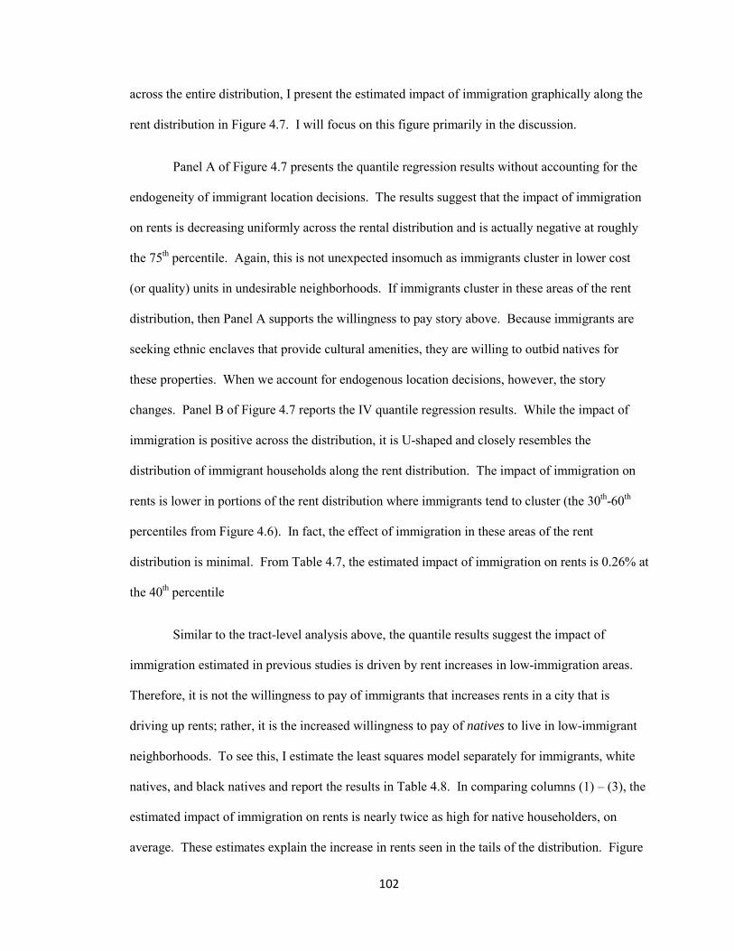
102

across the entire distribution, I present the estimated impact of immigration graphically along the

rent distribution in Figure 4.7. I will focus on this figure primarily in the discussion.

Panel A of Figure 4.7 presents the quantile regression results without accounting for the

endogeneity of immigrant location decisions. The results suggest that the impact of immigration

on rents is decreasing uniformly across the rental distribution and is actually negative at roughly

the 75th percentile. Again, this is not unexpected insomuch as immigrants cluster in lower cost

(or quality) units in undesirable neighborhoods. If immigrants cluster in these areas of the rent

distribution, then Panel A supports the willingness to pay story above. Because immigrants are

seeking ethnic enclaves that provide cultural amenities, they are willing to outbid natives for

these properties. When we account for endogenous location decisions, however, the story

changes. Panel B of Figure 4.7 reports the IV quantile regression results. While the impact of

immigration is positive across the distribution, it is U-shaped and closely resembles the

distribution of immigrant households along the rent distribution. The impact of immigration on

rents is lower in portions of the rent distribution where immigrants tend to cluster (the 30th-60th

percentiles from Figure 4.6). In fact, the effect of immigration in these areas of the rent

distribution is minimal. From Table 4.7, the estimated impact of immigration on rents is 0.26% at

the 40th percentile

Similar to the tract-level analysis above, the quantile results suggest the impact of

immigration estimated in previous studies is driven by rent increases in low-immigration areas.

Therefore, it is not the willingness to pay of immigrants that increases rents in a city that is

driving up rents; rather, it is the increased willingness to pay of natives to live in low-immigrant

neighborhoods. To see this, I estimate the least squares model separately for immigrants, white

natives, and black natives and report the results in Table 4.8. In comparing columns (1) – (3), the

estimated impact of immigration on rents is nearly twice as high for native householders, on

average. These estimates explain the increase in rents seen in the tails of the distribution. Figure

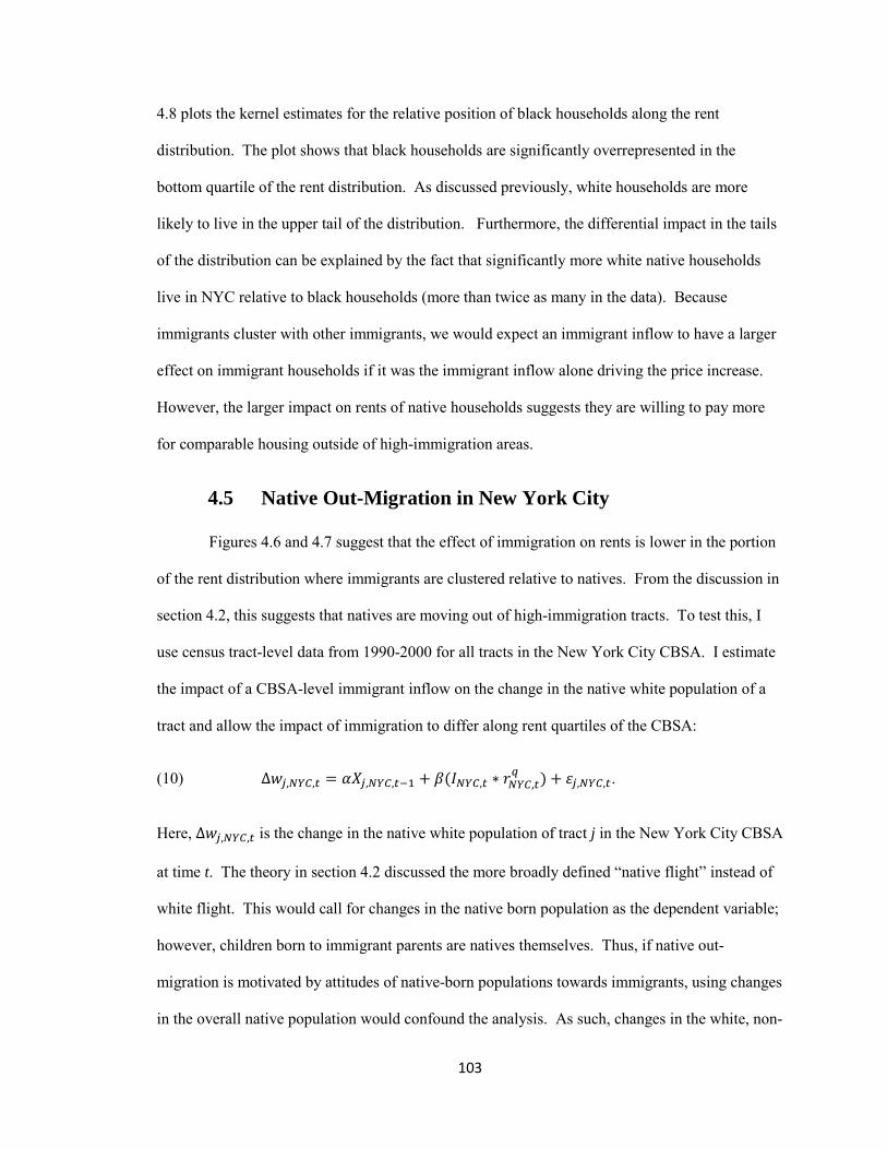
103

4.8 plots the kernel estimates for the relative position of black households along the rent

distribution. The plot shows that black households are significantly overrepresented in the

bottom quartile of the rent distribution. As discussed previously, white households are more

likely to live in the upper tail of the distribution. Furthermore, the differential impact in the tails

of the distribution can be explained by the fact that significantly more white native households

live in NYC relative to black households (more than twice as many in the data). Because

immigrants cluster with other immigrants, we would expect an immigrant inflow to have a larger

effect on immigrant households if it was the immigrant inflow alone driving the price increase.

However, the larger impact on rents of native households suggests they are willing to pay more

for comparable housing outside of high-immigration areas.

4.5 Native Out-Migration in New York City

Figures 4.6 and 4.7 suggest that the effect of immigration on rents is lower in the portion

of the rent distribution where immigrants are clustered relative to natives. From the discussion in

section 4.2, this suggests that natives are moving out of high-immigration tracts. To test this, I

use census tract-level data from 1990-2000 for all tracts in the New York City CBSA. I estimate

the impact of a CBSA-level immigrant inflow on the change in the native white population of a

tract and allow the impact of immigration to differ along rent quartiles of the CBSA:

(10) ∆𝐾𝑗,𝑁𝑁𝑁,𝑘 = 𝛼𝑋𝑗,𝑁𝑁𝑁,𝑘−1 + 𝛽(𝐼𝑁𝑁𝑁,𝑘 ∗ 𝑟𝑁𝑁𝑁,𝑘𝑞 ) + 𝜀𝑗,𝑁𝑁𝑁,𝑘.

Here, ∆𝐾𝑗,𝑁𝑁𝑁,𝑘 is the change in the native white population of tract j in the New York City CBSA

at time t. The theory in section 4.2 discussed the more broadly defined “native flight” instead of

white flight. This would call for changes in the native born population as the dependent variable;

however, children born to immigrant parents are natives themselves. Thus, if native out-

migration is motivated by attitudes of native-born populations towards immigrants, using changes

in the overall native population would confound the analysis. As such, changes in the white, non-

104

immigrant population serve as a proxy for changes in the native born population. 𝑋𝑗,𝑁𝑁𝑁,𝑘−1 is a

vector of lagged tract-level variables that control for other factors that may cause population

changes within a tract. First, to control for neighborhood conditions, I include the neighborhood

disadvantage index (as described earlier), the share of the population with at least a bachelor’s

degree, vacancy rates, and population density. As described above, higher shares of college

graduates are correlated with future growth of a city (Glaeser and Saiz, 2004). As such, I expect

this to positively influence migration rates. Lagged vacancy rates are expected to have a positive

impact on future migration rates as vacant units act as a pull factor that attracts in-migrants.

Population density is a proxy for housing supply constraints and is expected to have a negative

impact on changes in white population. Next, I control for characteristics of the population

residing in the tract at time T-10 that may describe future migration decisions. These variables

include the share of the population that is married, the share of households that have resided in

their current dwelling for at least 10 years, the share of the population that is black, and the share

of occupied units that are renter-occupied. Higher shares of married households and households

with 10 years of tenure are expected to be negatively correlated with future migration rates, while

the share of renter-occupied units is expected to positively impact future migration rates. These

expected impacts follow from the migration literature (Quigley and Weinberg, 1977; Weinberg,

1979). Married households and households with longer tenure in their current home are less

mobile, ceteris paribus; however, renter households are more mobile, ceteris paribus.

The main explanatory variable is the interaction of 𝐼𝑁𝑁𝑁,𝑘 and 𝑟𝑁𝑁𝑁,𝑘𝑞 . 𝐼𝑁𝑁𝑁,𝑘 is the

immigrant inflow (as described in section 4.3) into NYC at time t. 𝑟𝑁𝑁𝑁,𝑘𝑞 is a dummy variable

equal to 1 if the tract-level average rent at time t falls in the qth quartile of the CBSA rent

distribution. For each year, I calculate the 25th, 50th, and 75th percentiles of CBSA rent from tract-

105

level rent data.60 Then, I assign each tract into the relevant quartile of the rent distribution based

on current period average rents.

Given the quantile results, how should 𝛽 differ across the CBSA rent distribution? Panel

B of Figure 4.7 shows that the least squares estimates are driven by the impact in the upper tail of

the distribution. The impact of immigration is decreasing along the rent distribution up to

(roughly) the median rent level, then the increasing thereafter. If native out-migration is the

motivating factor, we would expect an immigrant inflow into NYC to cause white populations to

flow from high-immigration tracts to low-immigration tracts. Thus, 𝛽 should be negative in the

1st and 2nd quartiles and positive in 3rd and 4th quartiles.

I first estimate (10) via OLS and 2SLS without the interaction terms and report the results

in columns (1) and (2) of Table 4.9, respectively. The OLS estimates suggest that an immigrant

inflow equal to 1% of the total population leads to an increase in the white population by roughly

0.4%. If immigrant location choices are correlated with local economic conditions, then the OLS

estimate is biased. In Chapter 2 of this dissertation, I argue that immigrants are locating in areas

that provide them with the best economic opportunities and these same areas are rich in amenities

that attract both new immigrants and natives. If so, the impact on white population flows is

biased upward. To remedy this, I again use predicted immigrant flows based on country of origin

push factors as an instrument for actual immigration inflows.61 The 2SLS estimates are

significantly lower than the OLS estimates and show that immigrant inflows have zero impact on

white population flows, on average. This result is remarkably consistent with the theory derived

in section 4.2 when natives do not have distaste for living near immigrants (𝑈𝐼′ = 0). When

natives do not receive disutility from living near immigrants and the out-migration is purely for

60 Using the number of rental housing units in a tract as weights. 61 Because the independent variable of interest in this analysis is at the tract-level, the instrument is also calculated at the tract-level. In this case, I assume that each tract receives the same fraction of immigrants as it did in 1980. This seems like a reasonable assumption given Figure 2 which shows the clustering of immigrants over time by tract is relatively constant.

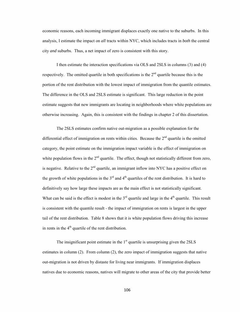
106

economic reasons, each incoming immigrant displaces exactly one native to the suburbs. In this

analysis, I estimate the impact on all tracts within NYC, which includes tracts in both the central

city and suburbs. Thus, a net impact of zero is consistent with this story.

I then estimate the interaction specifications via OLS and 2SLS in columns (3) and (4)

respectively. The omitted quartile in both specifications is the 2nd quartile because this is the

portion of the rent distribution with the lowest impact of immigration from the quantile estimates.

The difference in the OLS and 2SLS estimate is significant. This large reduction in the point

estimate suggests that new immigrants are locating in neighborhoods where white populations are

otherwise increasing. Again, this is consistent with the findings in chapter 2 of this dissertation.

The 2SLS estimates confirm native out-migration as a possible explanation for the

differential effect of immigration on rents within cities. Because the 2nd quartile is the omitted

category, the point estimate on the immigration impact variable is the effect of immigration on

white population flows in the 2nd quartile. The effect, though not statistically different from zero,

is negative. Relative to the 2nd quartile, an immigrant inflow into NYC has a positive effect on

the growth of white populations in the 3rd and 4th quartiles of the rent distribution. It is hard to

definitively say how large these impacts are as the main effect is not statistically significant.

What can be said is the effect is modest in the 3rd quartile and large in the 4th quartile. This result

is consistent with the quantile result - the impact of immigration on rents is largest in the upper

tail of the rent distribution. Table 8 shows that it is white population flows driving this increase

in rents in the 4th quartile of the rent distribution.

The insignificant point estimate in the 1st quartile is unsurprising given the 2SLS

estimates in column (2). From column (2), the zero impact of immigration suggests that native

out-migration is not driven by distaste for living near immigrants. If immigration displaces

natives due to economic reasons, natives will migrate to other areas of the city that provide better

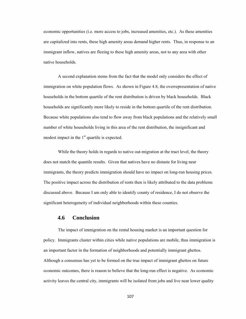
107

economic opportunities (i.e. more access to jobs, increased amenities, etc.). As these amenities

are capitalized into rents, these high amenity areas demand higher rents. Thus, in response to an

immigrant inflow, natives are fleeing to these high amenity areas, not to any area with other

native households.

A second explanation stems from the fact that the model only considers the effect of

immigration on white population flows. As shown in Figure 4.8, the overrepresentation of native

households in the bottom quartile of the rent distribution is driven by black households. Black

households are significantly more likely to reside in the bottom quartile of the rent distribution.

Because white populations also tend to flow away from black populations and the relatively small

number of white households living in this area of the rent distribution, the insignificant and

modest impact in the 1st quartile is expected.

While the theory holds in regards to native out-migration at the tract level, the theory

does not match the quantile results. Given that natives have no distaste for living near

immigrants, the theory predicts immigration should have no impact on long-run housing prices.

The positive impact across the distribution of rents then is likely attributed to the data problems

discussed above. Because I am only able to identify county of residence, I do not observe the

significant heterogeneity of individual neighborhoods within these counties.

4.6 Conclusion

The impact of immigration on the rental housing market is an important question for

policy. Immigrants cluster within cities while native populations are mobile, thus immigration is

an important factor in the formation of neighborhoods and potentially immigrant ghettos.

Although a consensus has yet to be formed on the true impact of immigrant ghettos on future

economic outcomes, there is reason to believe that the long-run effect is negative. As economic

activity leaves the central city, immigrants will be isolated from jobs and live near lower quality

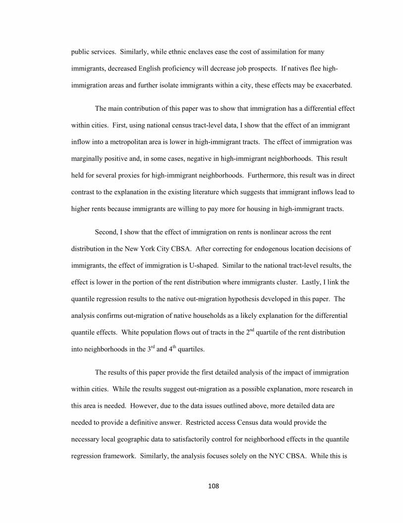
108

public services. Similarly, while ethnic enclaves ease the cost of assimilation for many

immigrants, decreased English proficiency will decrease job prospects. If natives flee high-

immigration areas and further isolate immigrants within a city, these effects may be exacerbated.

The main contribution of this paper was to show that immigration has a differential effect

within cities. First, using national census tract-level data, I show that the effect of an immigrant

inflow into a metropolitan area is lower in high-immigrant tracts. The effect of immigration was

marginally positive and, in some cases, negative in high-immigrant neighborhoods. This result

held for several proxies for high-immigrant neighborhoods. Furthermore, this result was in direct

contrast to the explanation in the existing literature which suggests that immigrant inflows lead to

higher rents because immigrants are willing to pay more for housing in high-immigrant tracts.

Second, I show that the effect of immigration on rents is nonlinear across the rent

distribution in the New York City CBSA. After correcting for endogenous location decisions of

immigrants, the effect of immigration is U-shaped. Similar to the national tract-level results, the

effect is lower in the portion of the rent distribution where immigrants cluster. Lastly, I link the

quantile regression results to the native out-migration hypothesis developed in this paper. The

analysis confirms out-migration of native households as a likely explanation for the differential

quantile effects. White population flows out of tracts in the 2nd quartile of the rent distribution

into neighborhoods in the 3rd and 4th quartiles.

The results of this paper provide the first detailed analysis of the impact of immigration

within cities. While the results suggest out-migration as a possible explanation, more research in

this area is needed. However, due to the data issues outlined above, more detailed data are

needed to provide a definitive answer. Restricted access Census data would provide the

necessary local geographic data to satisfactorily control for neighborhood effects in the quantile

regression framework. Similarly, the analysis focuses solely on the NYC CBSA. While this is

109

one of the major immigrant gateways, the results are not generalizable. Future research should

look to expand the present analysis to other immigrant gateway cities.

110 Figures and T

ables

Figure 4.1: Immigrant Clustering Within Metropolitan Areas High-Immigrant Metropolitan Areas

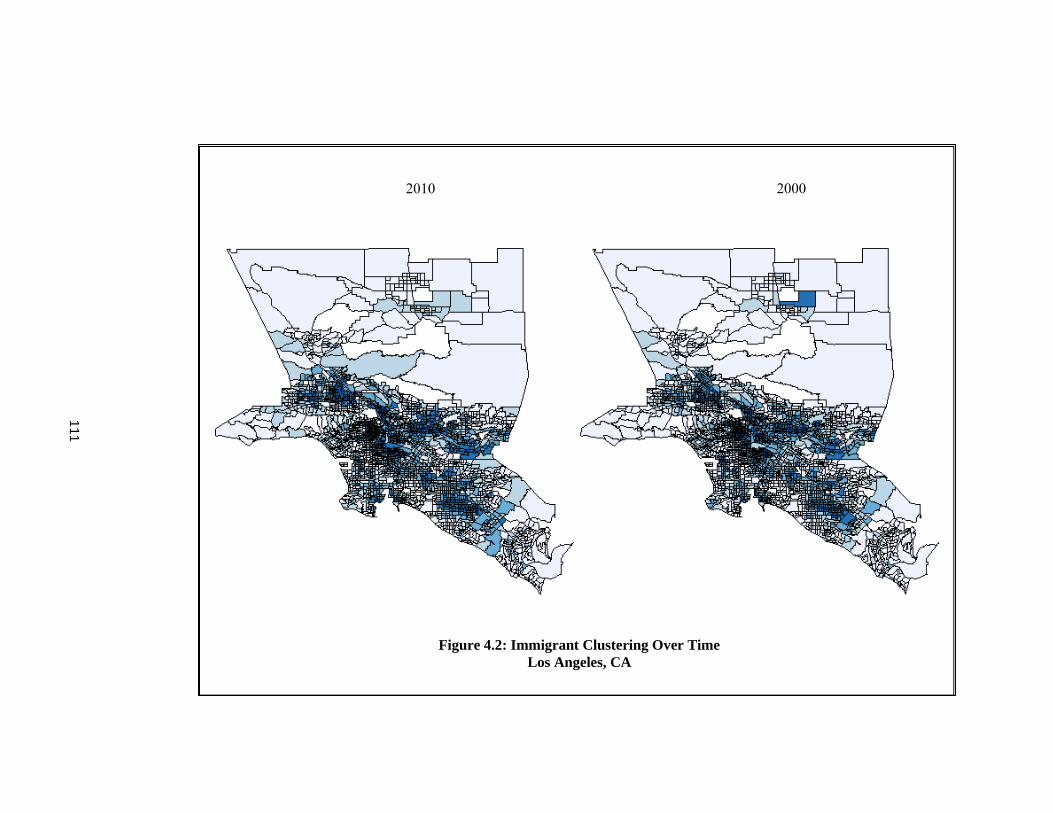
111

Figure 4.2: Immigrant Clustering Over Time Los Angeles, CA

2010 2000

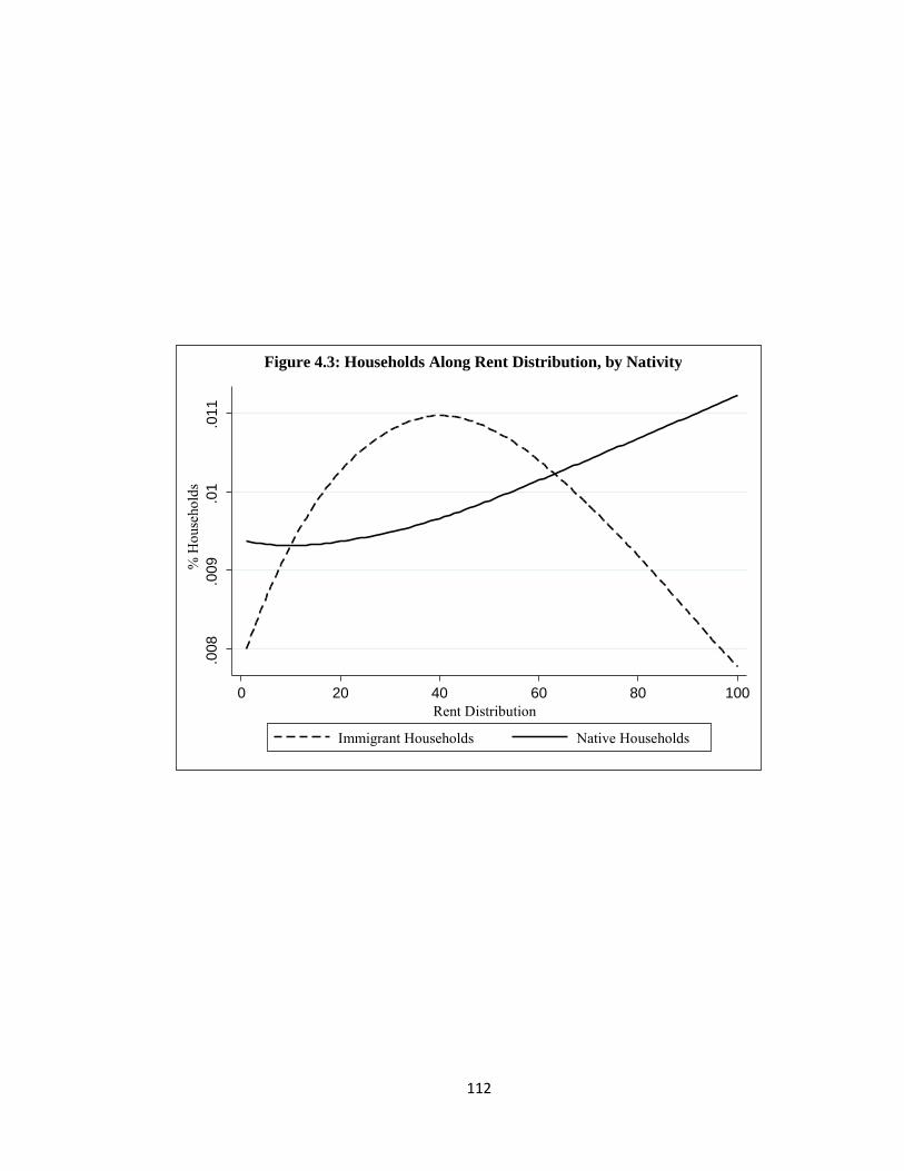
112

.008

.0

09

.01

.011

%

Hou

seho

lds

0 20 40 60 80 100 Rent Distribution

Immigrant Households Native Households

Figure 4.3: Households Along Rent Distribution, by Nativity

113

114

115

.7

.8

.9

1 1.

1 1.

2 R

elat

ive

Den

sity

0 20 40 60 80 100 Rent Distribution

Figure 4.6: Position of Immigrant Households Along Rent Distribution

116

117

0

1 2

3 R

elat

ive

Den

sity

0 20 40 60 80 100 Rent Distribution

Figure 4.8: Position of Black Households Along Rent Distribution

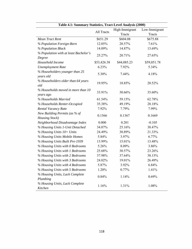
118

Table 4.1: Summary Statistics, Tract-Level Analysis (2000)

All Tracts

High-Immigrant Tracts

Low-Immigrant Tracts

Mean Tract Rent $651.29 $604.08 $675.88 % Population Foreign-Born 12.05% 20.57% 7.61% % Population Black 14.09% 14.87% 13.69% % Population with at least Bachelor’s Degree 25.27% 20.71% 27.65%

Household Income $53,426.38 $44,085.23 $59,051.78 Unemployment Rate 6.23% 7.92% 5.34% % Householders younger than 25 years old

5.30% 7.44% 4.18%

% Householders older than 64 years old

19.95% 18.85% 20.52%

% Households moved in more than 10 years ago 33.91% 30.66% 35.60%

% Households Married 61.54% 59.15% 62.78% % Households Renter-Occupied 35.38% 49.19% 28.18% Rental Vacancy Rate 7.92% 7.79% 7.99% New Building Permits (as % of Housing Stock)

0.1566 0.1367 0.1669

Neighborhood Disadvantage Index 0.000 0.201 -0.105 % Housing Units 1-Unit Detached 34.07% 25.16% 38.47% % Housing Units 10+ Units 24.49% 30.89% 21.33% % Housing Units Mobile Homes 5.84% 3.97% 6.77% % Housing Units Built Pre-1939 13.99% 15.01% 13.48% % Housing Units with 0 Bedrooms 5.26% 8.09% 3.86% % Housing Units with 1 Bedrooms 25.68% 30.57% 23.26% % Housing Units with 2 Bedrooms 37.98% 37.64% 38.15% % Housing Units with 3 Bedrooms 24.02% 19.01% 26.49% % Housing Units with 4 Bedrooms 5.87% 3.92% 6.84% % Housing Units with 5 Bedrooms 1.20% 0.77% 1.41% % Housing Units, Lack Complete Plumbing 0.84% 1.14% 0.69%

% Housing Units, Lack Complete Kitchen

1.16% 1.31% 1.08%

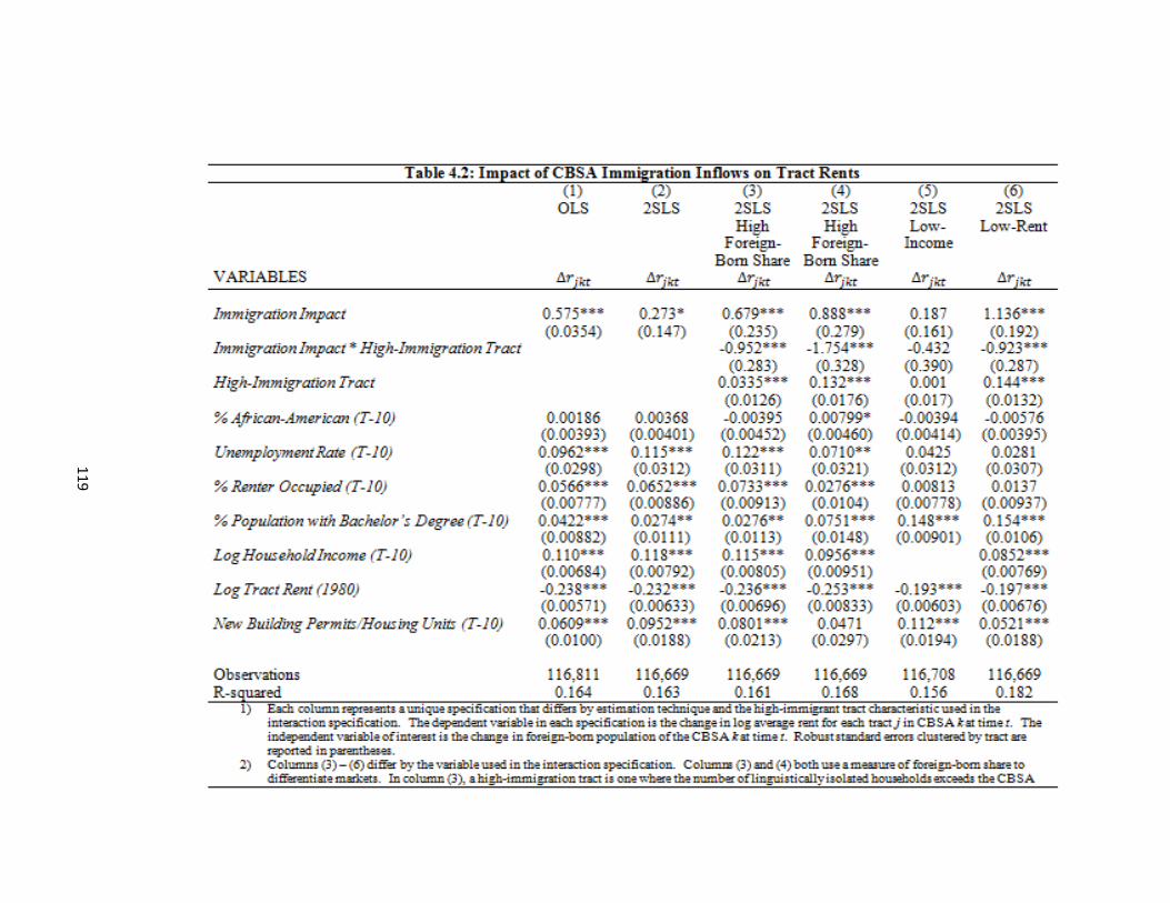
119

120

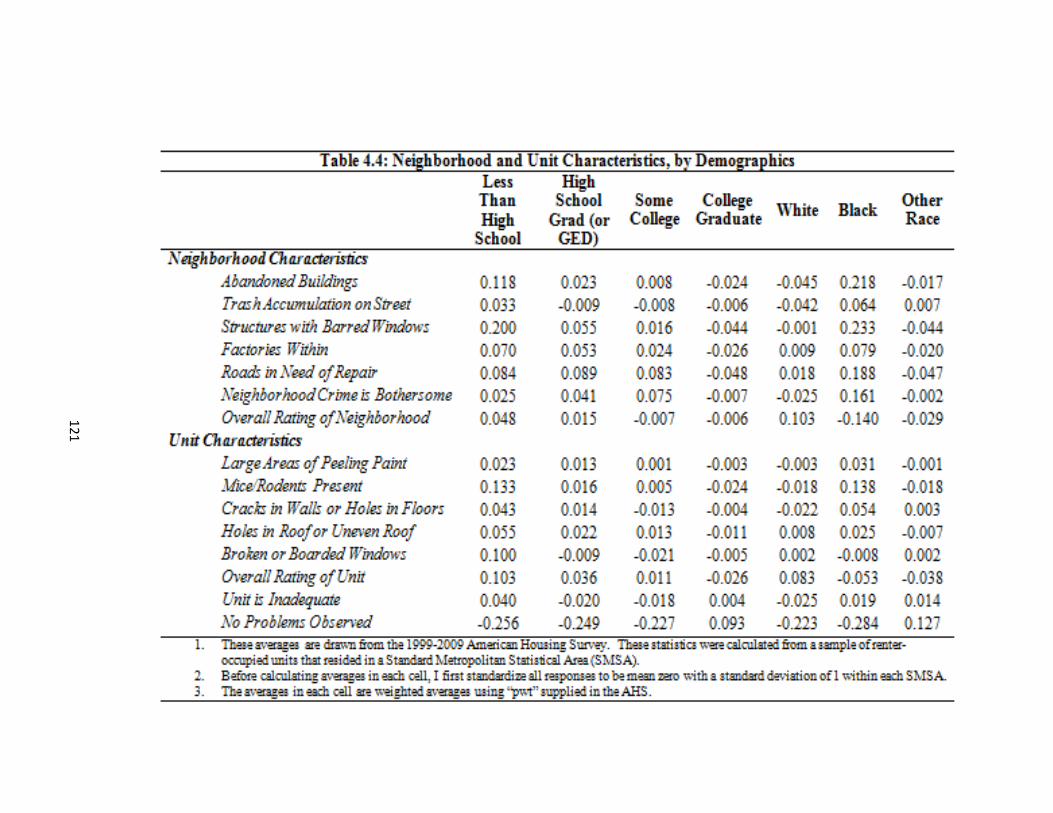
121

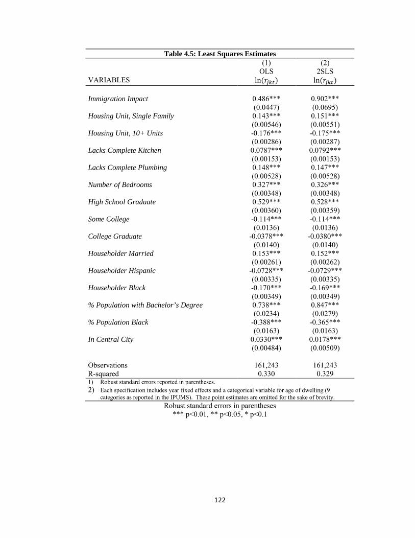
122

Table 4.5: Least Squares Estimates (1) (2) OLS 2SLS VARIABLES ln (𝑟𝑗𝑘𝑘) ln (𝑟𝑗𝑘𝑘) Immigration Impact 0.486*** 0.902*** (0.0447) (0.0695) Housing Unit, Single Family 0.143*** 0.151*** (0.00546) (0.00551) Housing Unit, 10+ Units -0.176*** -0.175*** (0.00286) (0.00287) Lacks Complete Kitchen 0.0787*** 0.0792*** (0.00153) (0.00153) Lacks Complete Plumbing 0.148*** 0.147*** (0.00528) (0.00528) Number of Bedrooms 0.327*** 0.326*** (0.00348) (0.00348) High School Graduate 0.529*** 0.528*** (0.00360) (0.00359) Some College -0.114*** -0.114*** (0.0136) (0.0136) College Graduate -0.0378*** -0.0380*** (0.0140) (0.0140) Householder Married 0.153*** 0.152*** (0.00261) (0.00262) Householder Hispanic -0.0728*** -0.0729*** (0.00335) (0.00335) Householder Black -0.170*** -0.169*** (0.00349) (0.00349) % Population with Bachelor’s Degree 0.738*** 0.847*** (0.0234) (0.0279) % Population Black -0.388*** -0.365*** (0.0163) (0.0163) In Central City 0.0330*** 0.0178*** (0.00484) (0.00509) Observations 161,243 161,243 R-squared 0.330 0.329 1) Robust standard errors reported in parentheses. 2) Each specification includes year fixed effects and a categorical variable for age of dwelling (9

categories as reported in the IPUMS). These point estimates are omitted for the sake of brevity. Robust standard errors in parentheses

*** p<0.01, ** p<0.05, * p<0.1

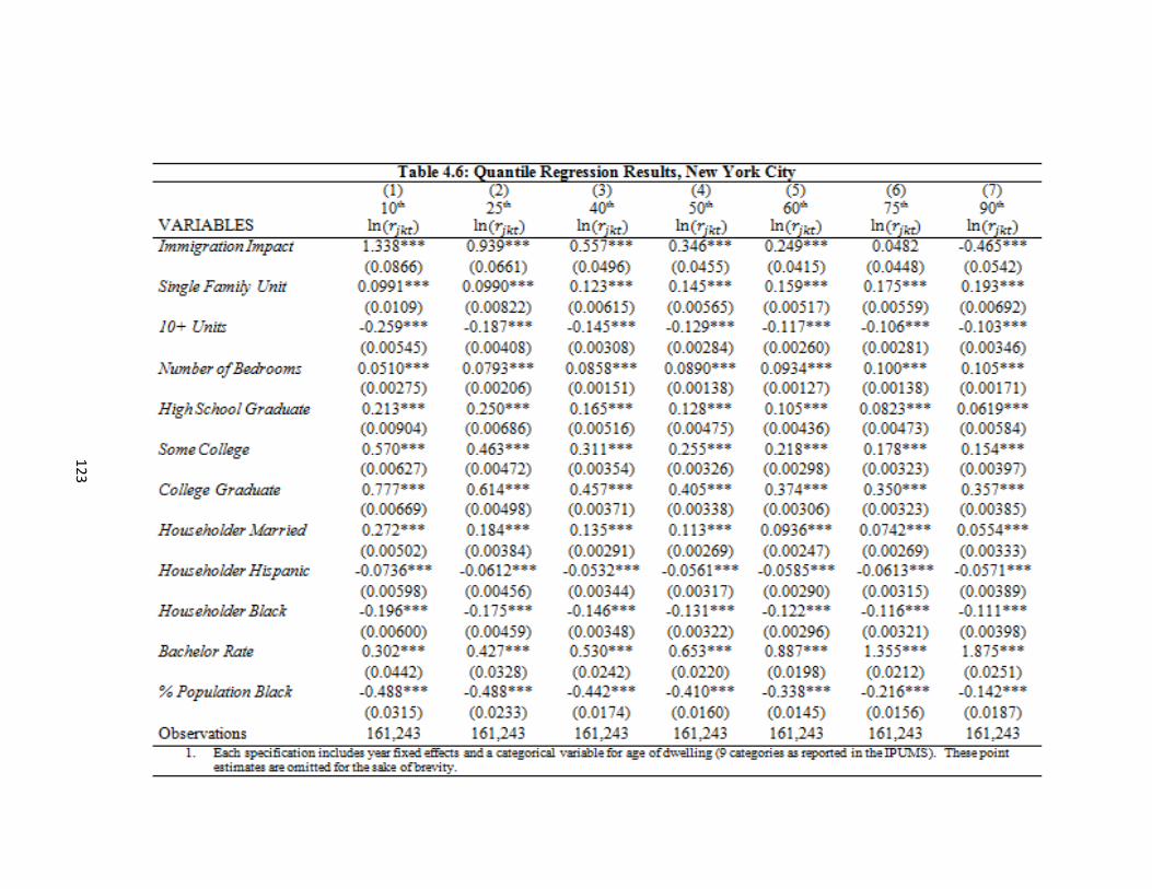
123

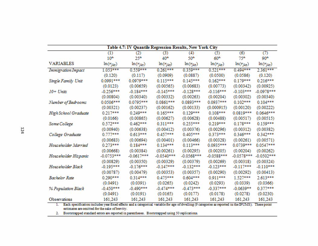
124

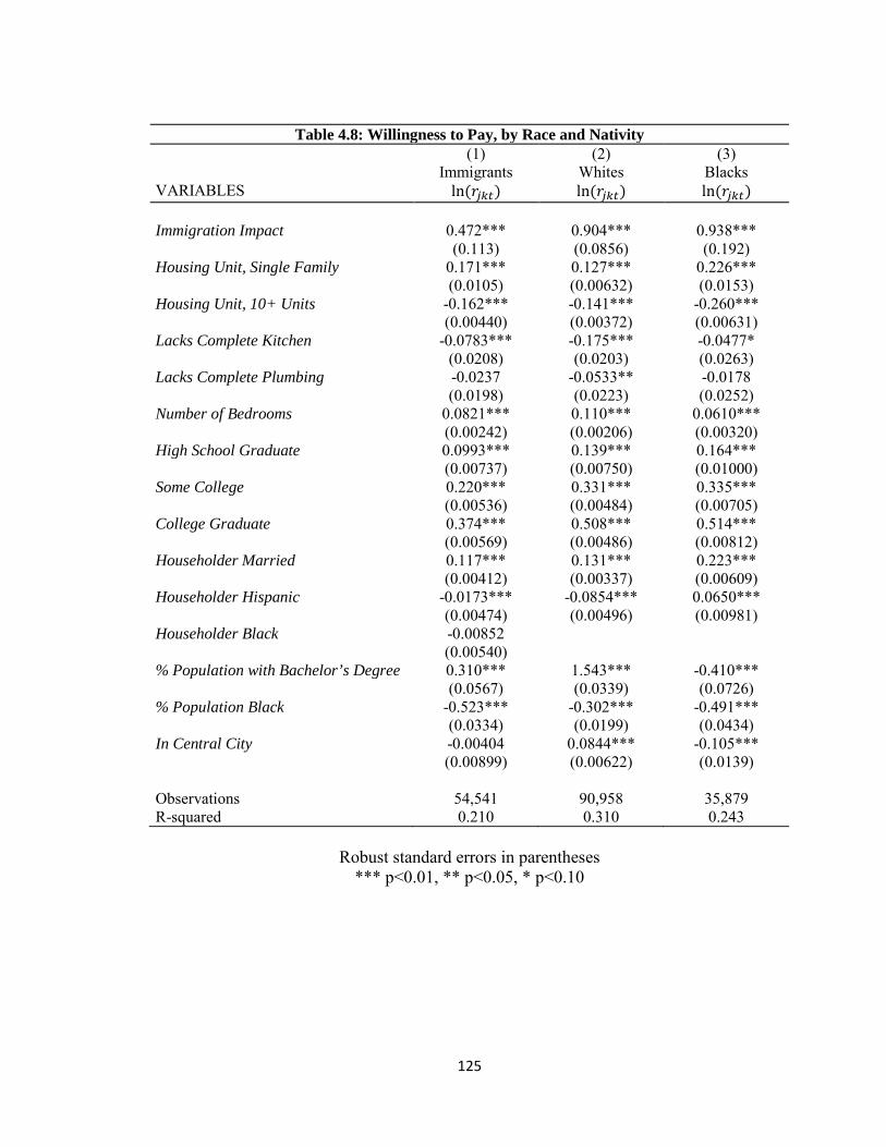
125

Table 4.8: Willingness to Pay, by Race and Nativity

(1) (2) (3) Immigrants Whites Blacks VARIABLES ln (𝑟𝑗𝑘𝑘) ln (𝑟𝑗𝑘𝑘) ln (𝑟𝑗𝑘𝑘) Immigration Impact 0.472*** 0.904*** 0.938*** (0.113) (0.0856) (0.192) Housing Unit, Single Family 0.171*** 0.127*** 0.226*** (0.0105) (0.00632) (0.0153) Housing Unit, 10+ Units -0.162*** -0.141*** -0.260*** (0.00440) (0.00372) (0.00631) Lacks Complete Kitchen -0.0783*** -0.175*** -0.0477* (0.0208) (0.0203) (0.0263) Lacks Complete Plumbing -0.0237 -0.0533** -0.0178 (0.0198) (0.0223) (0.0252) Number of Bedrooms 0.0821*** 0.110*** 0.0610*** (0.00242) (0.00206) (0.00320) High School Graduate 0.0993*** 0.139*** 0.164*** (0.00737) (0.00750) (0.01000) Some College 0.220*** 0.331*** 0.335*** (0.00536) (0.00484) (0.00705) College Graduate 0.374*** 0.508*** 0.514*** (0.00569) (0.00486) (0.00812) Householder Married 0.117*** 0.131*** 0.223*** (0.00412) (0.00337) (0.00609) Householder Hispanic -0.0173*** -0.0854*** 0.0650*** (0.00474) (0.00496) (0.00981) Householder Black -0.00852 (0.00540) % Population with Bachelor’s Degree 0.310*** 1.543*** -0.410*** (0.0567) (0.0339) (0.0726) % Population Black -0.523*** -0.302*** -0.491*** (0.0334) (0.0199) (0.0434) In Central City -0.00404 0.0844*** -0.105*** (0.00899) (0.00622) (0.0139) Observations 54,541 90,958 35,879 R-squared 0.210 0.310 0.243

Robust standard errors in parentheses

*** p<0.01, ** p<0.05, * p<0.10

126

Table 4.9: Native Out-Migration, New York City (1) (2) (3) (4) OLS 2SLS OLS 2SLS VARIABLES ∆𝐾𝑗𝑘𝑘 ∆𝐾𝑗𝑘𝑘 ∆𝐾𝑗𝑘𝑘 ∆𝐾𝑗𝑘𝑘 Immigration Impact 0.389*** -0.000439 1.560*** -0.309 (0.0227) (0.0419) (0.0456) (0.361) Immigration Impact*Rent Quantile 1 -1.573*** 0.273 (0.0525) (0.361) Rent Quantile 1 0.224*** -0.00572 (0.0175) (0.0486) Immigration Impact*Rent Quantile 3 -1.279*** 0.848** (0.0970) (0.391) Rent Quantile 3 0.127*** -0.121** (0.0198) (0.0490) Immigration Impact*Rent Quantile 4 -0.698*** 2.189*** (0.104) (0.481) Rent Quantile 4 0.0835*** -0.196*** (0.0191) (0.0487) % Population with Bachelor’s (T-10) 0.139*** 0.0864** 0.194*** 0.152*** (0.0328) (0.0337) (0.0338) (0.0412) % Population Black (T-10) 0.0662*** 0.0517** 0.0685*** 0.0309 (0.0203) (0.0207) (0.0194) (0.0221) Log Population Density (T-10) -0.0731*** -0.0760*** -0.0771*** -0.0724*** (0.00407) (0.00414) (0.00392) (0.00442) % Households Married (T-10) 0.00422 -0.0258 -0.0583 0.00765 (0.0504) (0.0513) (0.0482) (0.0543) % Renter Occupied Units (T-10) 0.0336 0.0561* -0.0167 0.0464 (0.0334) (0.0340) (0.0323) (0.0381) % Households, Tenure>10 years (T-10) -0.298*** -0.344*** -0.233*** -0.321*** (0.0386) (0.0394) (0.0369) (0.0471) NDI (T-10) 0.0114 0.00395 0.00461 0.0135 (0.0110) (0.0112) (0.0107) (0.0120) Vacancy Rate (T-10) 0.418*** 0.349*** 0.382*** 0.374*** (0.0768) (0.0783) (0.0732) (0.0807) Observations 8,682 8,682 8,682 8,682 R-squared 0.125 --- 0.210 ---

Standard errors in parentheses *** p<0.01, ** p<0.05, * p<0.1

127

5. Conclusion

The essays of this dissertation provided useful contributions for both academics and

policymakers. The underlying theme of this dissertation was inherently methodological. In

chapters 2 and 3, I identified two widely accepted results within the immigration literature and

showed the fragility of some of the underlying theoretical and methodological underpinnings of

past research. In chapter 2, using a more robust empirical model that more readily controls for

the endogeneity of immigrant locations, I provide evidence that we should not expect immigrant

inflows to have a differential impact on rents than any other one-time population increase. In this

essay, the main contribution to the field is the evidence that the widely used shift-share

instrumental variable introduces bias when one does not account for the location choices of past

immigrants. The evidence in chapter 2 suggests that all immigrants, both past and present, are

locating in cities that afford them the best economic opportunities.

While the model used in Chapter 2 is an improvement over past studies, it should be

noted that this is partial reduced form model. In an equilibrium model of population growth and

wages, we expect all population growth to impact prices; however, native population flows are

omitted from the model. Thus, the model in Chapter 2 suggests a much broader model, which is

a logical extension of the present paper. The partial reduced form model was used for two

reasons. First, the main goal of the paper was to address the fragility of the estimates in the

existing literature and the possible bias of the shift share instrument. As such, I utilized a model

that most closely resembled the existing literature. Second, while native population flows are

integral to the evolution of rents, these native populations are more sensitive to economic

conditions within cities – they do not display clustering behavior like immigrants. Thus, a valid

instrument for these population flows is not readily apparent.

A second modeling consideration, which is briefly mentioned in the text, is the idea of

partial adjustment of rents from one period to the next. The literature analyzing the adjustment of

128

rents suggests that significant lags may exist in the response of rents to changes in demand.

Several factors are in play here. First, tenants are likely “tied” to their units by lease contracts,

making moving more difficult. Second, vacancy rates play a fundamental role in the evolution of

rents. Because rental markets are in constant disequilibrium, these inefficiencies may hinder

market clearing. In the context of Chapter 2, this implies that the effect of immigration on rents

may be muted in the short-run. A partial adjustment model of the following general form was

considered and estimated:

𝑟𝑘𝑘 = (1 − 𝜆)𝑟𝑘𝑘−1 + 𝜆𝐼𝑘𝑘 + 𝜆𝑢𝑘𝑘.

Here, λ is the adjustment coefficient. If λ=1, then rents fully adjust between each period. If λ<1,

then rents partially adjust from one period to the next. The results of the partial adjustment model

suggest that rent (or at least FMR) fully adjust from one year to the next as λ was essentially 1.

As such, the static model is appropriate. One concern, however, stems from the above – the

existing literature suggests that the rental market does not clear instantaneously. The full

adjustment result is likely due, in part, to the way the FMR for a city is calculated. To calculate

the FMR for each year, the HUD uses the most recent data from the decennial Census or

American Community Survey to update the value of FMR from the previous year, not estimate

the new value. Thus, the adjustment process is more predictable and the slow, partial adjustment

expected in the rental market is not picked up in the model.

From a policy perspective, the results are potentially more important. Over the last 5

years, some policymakers have considered immigration as a policy tool to help “bring back” the

housing market. On the other hand, the results of Saiz (2007) and similar studies have been

widely cited in the national media and by policymakers to argue against immigration reform. The

results of chapter 2 however, cast doubt on the arguments of either side. Immigrant inflows are

not inherently different from native population flows. The difference is that the majority of

immigrant inflows are into the largest metropolitan areas that face increased housing prices

irrespective of immigration.

129

In chapter 3, I again challenge the consensus in the existing literature and propose a new

framework with which to analyze the wage effects of immigration. Because immigrants are often

misplaced in the labor market with respect to educational attainment and immigrants and natives

specialize in different skills, I propose stratifying the labor market by occupation instead of

education. To my knowledge, I am the first to use occupation-specific skills to define

homogenous labor groups (with respect to skill) within the context of immigration. When

stratifying the labor market across occupations, I estimate a nontrivial impact of immigration on

average native wages. I also provide ample evidence to support the claim that larger wage effect

is due to increased substitutability between workers within skill groups, not endogeneity of

occupation choice. Furthermore, Chapter 3 leads to a rather obvious extension for future

research. While the estimates are significant, both statistically and economically, I should

reemphasize that these effects are partial equilibrium effects. In order to inform national policy,

one must also speak to the total wage effect of immigration on wages – accounting for within-

occupation and across-occupation effects on native wages.

In chapter 4, I return to the rental housing market and assess the impact of immigration

within metropolitan areas. Specifically, I show that immigration has a differential impact within

cities at both the national level and with a single metropolitan area and can provide initial

evidence that differences across the rent distribution is driven by native out-migration. Overall,

because the impact of immigration on rents is lower in high-immigrant neighborhoods, I conclude

that it is not the willingness to pay of immigrants that bid up rents in the city; rather, it is the

willingness to pay of natives to not live in these high-immigration areas.

In Chapter 4, I outline three widely accepted theories in the sociology literature that

explain why native households leave high-immigrant tracts. While the results show that native

mobility is an important factor in determining the evolution of rents in a city, I am unable to

identify the mechanism driving this out-migration. While I cannot speak definitively to the

mechanism, certain specifications allow for conjecture. The tract-level analysis suggests

130

immigrant inflows are associated with decreases in rents. According to the conceptual framework

established in section 4.2, this is consistent with a scenario where native receive disutility from

living near immigrants. Thus, these negative point estimates are consistent with either the ethnic

flight hypothesis or the socioeconomic context hypothesis.

In addition to the extensions mentioned above, these papers provide solid footing for

related research and extensions of the ideas therein. I envision several extensions from Chapter 4.

Ultimately, I see chapter 4 as two standalone papers: the tract-level analysis and the quantile

regression. The tract-level analysis provides the perfect setup for a spatial analysis of

immigration. In order to accurately identify white flight out of neighborhoods, one must consider

the effects of immigrant inflows into neighboring tracts on the mobility decisions of native

households. For the quantile analysis section, restricted-access micro-data of the Census or AHS

would provide the necessary geographic data to completely isolate true neighborhood effects.

Additionally, I foresee myself moving beyond the case study of NYC to a more representative

sample of cities.

131

Appendix 1 (Chapter 2)

Table A2.1: Determinants of Immigrant Share, Alternate Proxies (1) (2) (3) (4) VARIABLES Share 1995 Share 1995 Share 1995 Share 1995 FMR Growth (1983-90) 0.00703 (0.00740) Log Med Gross Rent (1990) 0.0190** (0.00736) Average Commute (1990) 0.00220** (0.00104) Price-to-Rent Ratio (1990) 0.0152** (0.00751) Per Capita Sales (1992) 0.0110*** 0.00661*** 0.00526* 0.00655*** (0.00368) (0.00216) (0.00269) (0.00235) Per Capita Prop Tax Rev (1997) 0.00165 -0.00194 0.00182 0.00116 (0.00173) (0.00182) (0.00173) (0.00170) % Housing Stock Built Pre-39 (1990) 0.00455 0.0162 0.0137 0.00410 (0.00753) (0.0112) (0.0108) (0.00739) % Total Earnings from Farms (1990) -0.00502 -0.0116 0.0333* -0.0199 (0.0106) (0.00937) (0.0181) (0.0137) Observations 325 325 325 325 R-squared 0.083 0.117 0.232 0.122 1. All specifications use the full preferred model. Other point estimates are omitted for the sake of

brevity. 2. Robust standard errors, clustered by CBSA, are reported in parentheses.

Robust standard errors in parentheses *** p<0.01, ** p<0.05, * p<0.1

132

Table A2.2: Determinants of Predicted Employment Growth (1) (2) VARIABLES 𝐸�𝑘𝑘 𝐸�𝑘𝑘 Rent Growth (1980-90) -8.31e-05 (0.00268) FMR (1990) 0.00345* (0.00179) % Housing Stock Built Pre-1939 (1990) -0.00479 -0.00502 (0.00350) (0.00342) Per Capita Sales (1992) 0.00159 0.000638 (0.00127) (0.00133) Per Capita Proper Tax Revenue (1997) 0.000256 -0.000174 (0.000861) (0.000864) % Total Earnings from Farms (1990) 0.00272 -0.00118 (0.0103) (0.0104) Observations 4,225 4,225 R-squared 0.001 0.002

133

Table A2.3: Variable Descriptions and Sources

Variable Description Table

FMR The FMR is reported at the county-level by the HUD. The CBSA-level data are population-weighted averages of the corresponding county data. Prior to aggregating to the CBSA-level, all county-level data are adjusted (as described in section 2.3) to 40% FMR estimates.

T2-A2

Rent-to-Income Ratio The change in the log of rent-to-income ratio from time t-1 to time t. Here, the FMR in city k is divided by one of three income measures.

T6

Immigrants (1999-2011) Customized data from the Department of Homeland Security. These data were aggregated to 2013 CBSA definitions.

T2 – T4, T6, A1

Per Capita Personal Income County-level data from the Bureau of Economic Analysis’ (BEA) Regional Economic Information System (REIS).

T2 – T4, T6

Average Wages (BEA) County-level data from the Bureau of Economic Analysis’ (BEA) Regional Economic Information System (REIS).

T6

Average Wages (QCEW) County-level data from the Quarterly Census of Employment and Wages (QCEW). Aggregated to 2013 CBSA definitions.

T6

Average Wages (Goods-Producing) County-level data from the Quarterly Census of Employment and Wages (QCEW). Aggregated to 2013 CBSA definitions.

T6

Unemployment Rate County-level employment data from the Bureau of Labor Statistics (BLS) aggregated to 2013 CBSA definitions.

T2, T4-T6, A1

January Average Temperature The average temperature (measured in Fahrenheit degrees) over the years 1941–1970. From the United States Department of Agriculture (USDA) Economic Research Service (ERS) Natural Amenities Scale Database. County-level data is aggregated to CBSA.

T2, T4-T6, A1

July Average Humidity The average relative humidity over the years 1941–1970. From the United States Department of Agriculture (USDA) Economic Research Service (ERS) Natural Amenities Scale Database. County-level data is aggregated to CBSA.

T2, T4-T6, A1

CBSA Land Area County-level data derived from the US Census Bureau Censtats database, aggregated to 2013 CBSA definitions.

T2, T4-T6, A1

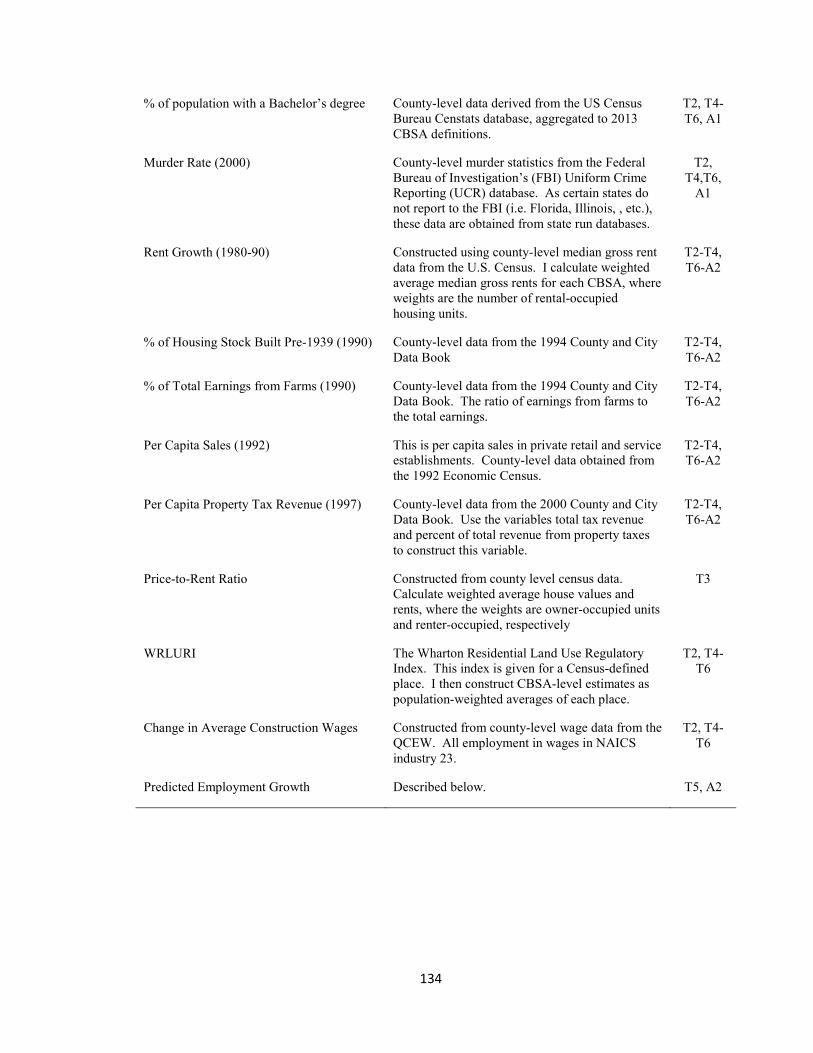
134

% of population with a Bachelor’s degree County-level data derived from the US Census Bureau Censtats database, aggregated to 2013 CBSA definitions.

T2, T4-T6, A1

Murder Rate (2000) County-level murder statistics from the Federal Bureau of Investigation’s (FBI) Uniform Crime Reporting (UCR) database. As certain states do not report to the FBI (i.e. Florida, Illinois, , etc.), these data are obtained from state run databases.

T2, T4,T6,

A1

Rent Growth (1980-90) Constructed using county-level median gross rent data from the U.S. Census. I calculate weighted average median gross rents for each CBSA, where weights are the number of rental-occupied housing units.

T2-T4, T6-A2

% of Housing Stock Built Pre-1939 (1990) County-level data from the 1994 County and City Data Book

T2-T4, T6-A2

% of Total Earnings from Farms (1990) County-level data from the 1994 County and City Data Book. The ratio of earnings from farms to the total earnings.

T2-T4, T6-A2

Per Capita Sales (1992) This is per capita sales in private retail and service establishments. County-level data obtained from the 1992 Economic Census.

T2-T4, T6-A2

Per Capita Property Tax Revenue (1997) County-level data from the 2000 County and City Data Book. Use the variables total tax revenue and percent of total revenue from property taxes to construct this variable.

T2-T4, T6-A2

Price-to-Rent Ratio Constructed from county level census data. Calculate weighted average house values and rents, where the weights are owner-occupied units and renter-occupied, respectively

T3

WRLURI The Wharton Residential Land Use Regulatory Index. This index is given for a Census-defined place. I then construct CBSA-level estimates as population-weighted averages of each place.

T2, T4-T6

Change in Average Construction Wages Constructed from county-level wage data from the QCEW. All employment in wages in NAICS industry 23.

T2, T4-T6

Predicted Employment Growth Described below. T5, A2

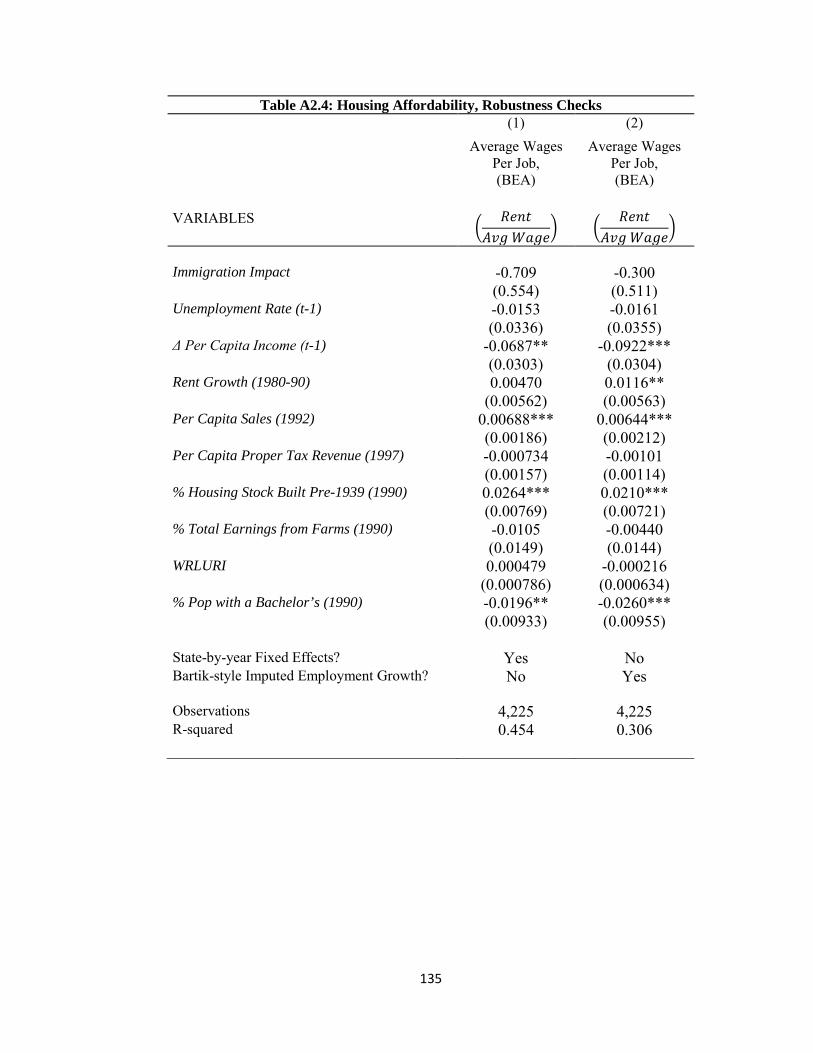
135

Table A2.4: Housing Affordability, Robustness Checks (1) (2) Average Wages

Per Job, (BEA)

Average Wages Per Job, (BEA)

VARIABLES �𝐹𝑅𝐼𝑡

𝐴𝐴𝐼 𝑊𝐼𝐼𝑅� �

𝐹𝑅𝐼𝑡𝐴𝐴𝐼 𝑊𝐼𝐼𝑅

�

Immigration Impact -0.709 -0.300 (0.554) (0.511) Unemployment Rate (t-1) -0.0153 -0.0161 (0.0336) (0.0355) Δ Per Capita Income (t-1) -0.0687** -0.0922*** (0.0303) (0.0304) Rent Growth (1980-90) 0.00470 0.0116** (0.00562) (0.00563) Per Capita Sales (1992) 0.00688*** 0.00644*** (0.00186) (0.00212) Per Capita Proper Tax Revenue (1997) -0.000734 -0.00101 (0.00157) (0.00114) % Housing Stock Built Pre-1939 (1990) 0.0264*** 0.0210*** (0.00769) (0.00721) % Total Earnings from Farms (1990) -0.0105 -0.00440 (0.0149) (0.0144) WRLURI 0.000479 -0.000216 (0.000786) (0.000634) % Pop with a Bachelor’s (1990) -0.0196** -0.0260*** (0.00933) (0.00955) State-by-year Fixed Effects? Yes No Bartik-style Imputed Employment Growth? No Yes Observations 4,225 4,225 R-squared 0.454 0.306

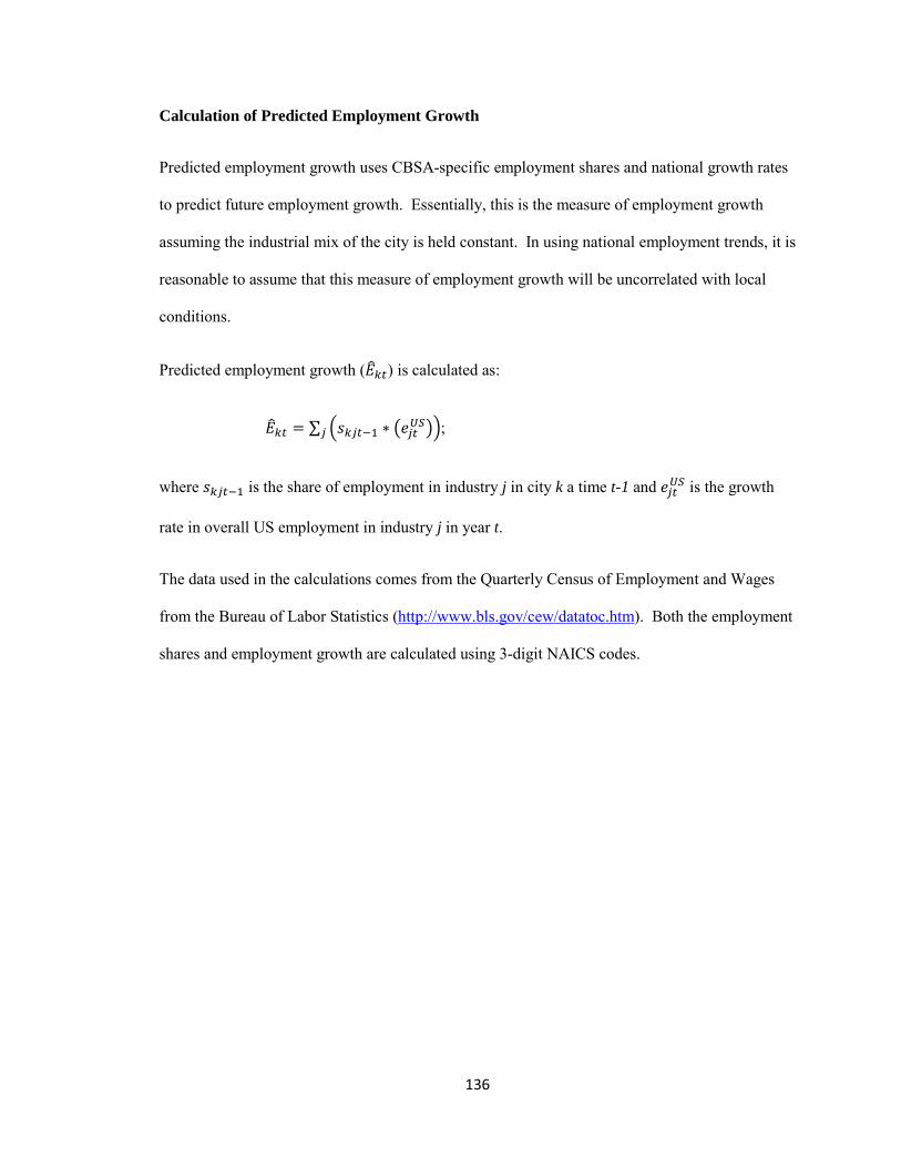
136

Calculation of Predicted Employment Growth

Predicted employment growth uses CBSA-specific employment shares and national growth rates

to predict future employment growth. Essentially, this is the measure of employment growth

assuming the industrial mix of the city is held constant. In using national employment trends, it is

reasonable to assume that this measure of employment growth will be uncorrelated with local

conditions.

Predicted employment growth (𝐸�𝑘𝑘) is calculated as:

𝐸�𝑘𝑘 = ∑ �𝐼𝑘𝑗𝑘−1 ∗ �𝑅𝑗𝑘𝑈𝑈��𝑗 ;

where 𝐼𝑘𝑗𝑘−1 is the share of employment in industry j in city k a time t-1 and 𝑅𝑗𝑘𝑈𝑈 is the growth

rate in overall US employment in industry j in year t.

The data used in the calculations comes from the Quarterly Census of Employment and Wages

from the Bureau of Labor Statistics (http://www.bls.gov/cew/datatoc.htm). Both the employment

shares and employment growth are calculated using 3-digit NAICS codes.

137

Appendix 2 ( Chapter 3)

A. Creating Manual-to-Communicative Task Index

We use the O*NET database (version 18) to construct the manual-to-communicative task ratio.

First, we use select attributes from Ability, Work Activity, Skill, and Knowledge descriptors from

the O*NET to create a communicative task-intensity index and a manual task-intensity index.

Abilities, Skills, and Knowledge data describe the attributes of workers, while Work Activity

describes occupation attributes. For the communicative task-intensity index, we use worker and

occupation attributes related to communicating information, social skills, and listening. The

manual task-intensity index uses attributes related to basic strength and related characteristics. A

full list of attributes for each descriptor used in these calculations (along with their

manual/communicative designation) can be found in Table A1 below.

We first compute a measure of overall intensity for each attribute in a given O*NET occupation.

The O*NET provides two ratings for the attributes: Importance and Level. The importance rating

indicates the importance of a particular attribute to a given occupation, while the level rating

indicates the degree to which an attribute is needed to perform a job. We create an overall

intensity measure by multiplying Importance (scale 1-5) and Level (scale 1-7). We then

normalize each intensity measure to be in the range of 0-1 by dividing by 35.

One limitation of the O*NET is that occupations do not change over time. In order to use these

data for my entire sample, we match the occupation groups defined in the ONET (i.e. 11-1011) to

the occupation classification (occ1990dd) of Autor and Dorn (2013). The advantage of the

occupation classification of Autor and Dorn (2013) is that occupations are a consistent panel from

1960-2010. To do this, we first match O*NET occupations to occupations defined by the U.S.

Census (using the standard crosswalk file and OCC codes from the 2000 Census), then we match

the Census OCC codes to the occ1990dd codes (using the files provide by the authors on their

website). It should be noted that there are significantly more O*NET occupation groups than

138

occ1990dd occupation groups (841 O*NET vs. 330 occ199dd); thus, there are multiple O*NET

occupation groups for each occ1990dd code.

As such, the manual (communicative) task-intensity index for each occ1990dd code is simply the

weighted average of all manual (communicative) attribute-specific intensity measures within a

given occ1990dd code (weighted by total employment). Then, the manual-to-communicative

ratio is calculated by dividing the manual task-intensity index by the communicative task-

intensity index.

139

Table A3.1: O*NET Components Used in Communicative-to-Manual Skill Ratio Abilities

Verbal (All) Idea Generation and Reasoning (Fluency of Ideas, Originality, Deductive Reasoning, Inductive Reasoning) Perceptual (Perceptual Speed)

Communicative Communicative Communicative

Sensory (Speech Recognition, Speech Clarity) Communicative Psychomotor (All) Manual Physical (All) Manual

Work Activities Interpreting the Meaning of Information for Others Communicative Communicating with Supervisors, Peers, or Subordinates Communicative Communicating with Persons Outside Organization Communicative Establishing and Maintaining Interpersonal Relationships Communicative Assisting and Caring for Others Communicative Selling or Influencing Others Communicative Resolving Conflicts and Negotiating with Others Communicative Performing for or Working Directly with the Public Communicative Performing General Physical Activities Manual Handling and Moving Objects Manual Controlling Machines and Processes Manual Operating Vehicles, Mechanized Devices, or Equipment Manual

Skills Reading Comprehension Communicative Active Listening Communicative Writing Communicative Speaking Communicative Installation Manual Operation Monitoring Manual Equipment Maintenance Manual

Knowledge English Language Communicative Communications Communicative Building and Construction Manual Mechanical Manual

1) Abilities, Work Activities, Skills, and Knowledge are the descriptors 2) Within each descriptor, we list all of the “attributes” used in the calculation of the task

intensity indices.

140

B. Sample Description

B.1 Wage Sample

We calculate mean log wages for male workers in each year. Following Borjas (2003), we

restrict the sample to include non-self-employed males, aged 18-64, who have positive weeks

worked, valid earnings data, and that did not live in group quarters. Mean log wages are

represented as constant 2010-dollars and we used hours worked (perwt*weeks*hours/2000) as

weights in the calculation. As in Borjas (2003), we use potential experience as a proxy for actual

experience. To calculate potential experience, we assume that workers with less than a high

school diploma enter the labor force at 17; workers with a high school diploma or GED enter the

labor force at 19; workers with some college (less than a bachelor’s degree) enter the labor force

at age 21; and workers with a college degree enter the labor force at 23. We drop those who

report potential experience less than 0 or greater than 40.

B.2 Employment Sample

To calculate labor supply in each occupation-experience cohort, we limit the sample to males

aged 18-64 who have positive weeks worked that did not reside in group quarters. Here, self-

employed workers are included in the calculations. Labor supply in an occupation-experience

cohort is the sum of all hours worked. Potential experience is defined as above.

141

C. Logit Models

C.1 Labor Supply

The multinomial logit specifications resemble those in Card (2001). However, to remain

consistent with the above, we restrict the sample to males only. We pool the data from 1970,

1980, 1990, 2000, and 2010 and estimate flexible specifications for natives and immigrants

separately. The native specification includes the following controls: education, a quartic in

potential experience, an indicator variable for being married, a set of race dummies (include

Black, Asian, and other non-white), an interaction of education and race dummies, an interaction

of education with linear potential experience and quadratic potential experience, and state and

year fixed effects. The immigrant specification includes the following controls: education, a

quartic in potential experience, a quadratic of years in the U.S, an interaction of education and the

quadratic of years in the U.S., 17 country of origin dummies, an interaction of education with

three main origin groups (Mexico, Canada/Australia/Europe, and Asia), a set of race dummies

(Black, Asian, and other non-white), and state and year fixed effects. We estimate the predicted

probabilities of working in occupation j for each individual. The predicted labor supply for each

occupation is simply the sum of these predicted probabilities.

142 A

ppendix 3 (Chapter 4)

143

Table A4.1: Estimation Results for Imputed Immigrant Calculations (1)

Countries With Complete Data

(2) Countries With Incomplete Data

VARIABLES 𝐼𝐼𝑘 𝐼𝐼𝑘 Relative Real GDP (t-1) -0.409*** (0.113) Poverty Rate (t-1) -0.0517*** (0.0112) % Young Population (t-1) 0.606*** (0.103) Regime Change (t-2) 0.0340** (0.0166) Revolutionary War (t-2) 0.0593*** 0.0298 (0.0137) (0.0811) Genocide (t-2) 0.0845*** 0.0537 (0.0195) (0.2301) Allotted Refugee Visas 0.345* 0.1758* (0.194) (0.0956) Eligible for Diversity Visas 0.0630*** 0.1500*** (0.0191) (0.0431) IRCA 66.64*** 63.18*** (6.818) (20.258) Average Migration Rate Last 5 Years 0.818*** 0.812*** (0.0114) (0.0256) Observations 4,562 527 Number of Countries 154 18

1. Column (1) reports estimates from the full model described by Eq. (2). Column (2) is a modified model estimated for countries with inconsistent data availability over the time period.

2. Country random effects are included, but these estimated effects are omitted when predicting migration rates from a given source country.

Standard errors in parentheses *** p<0.01, ** p<0.05, * p<0.1

144

Table A4.2: Variable Descriptions, Instrument Variable Source Definition

Real GDP Penn World Tables The log of real GDP in international dollars for source country i divided by the real GDP in international dollars for the U.S.

Poverty rate Penn World Tables The log of the inverse of per capita income squared.

Young Population WIDER Institute The share of the total population aged 15-19.

Regime Change The Integrated Network for Societal Conflict Research (INSCR) – The Political Instability Task Force (PITF) State Failure Problem Set.

The data set identifies incidences of each type of conflict by country. I only use conflicts that occurred within a countries border.

Revolutionary War

Genocide

Refugee Visas62

Pre 1992: INS Statistical Yearbooks.

Post-2002: DHS Yearbook of Immigrant

Statistics

The refugee visa quota for a given region divided by the country’s population.

Diversity Visas Defined for eligible countries only – all other countries take a value of 0. The variable is calculated as the total number of diversity visas divided by the country’s population.

IRCA The number of illegal immigrants living in the U.S. in 1980 divided by the country’s population in 1990.

Average Migration Rate The 5 year moving average of migration rates.

62 For detailed explanations of the methodology and theory underlying the visa variables, I direct interested readers to Clark et al. (2007).

145

References (Chapter 2) Abraham, J. M., & Hendershott, P. H. (1996). Bubbles in Metropolitan Housing Markets. Journal

of Housing Research, 191. Accetturo, A., Manaresi, F., Mocetti, S., & Olivieri, E. (2012). Don't stand so close to me: the

urban impact of immigration. Bank of Italy Temi di Discussione (Working Paper) No, 866.

Altonji, J. G., & Card, D. (1991). The effects of immigration on the labor market outcomes of less-skilled natives. In Immigration, trade and the labor market(pp. 201-234). University of Chicago Press.

Bartel, A. P. (1989). Where do the new US immigrants live?. Journal of Labor Economics, 371-391.

Bartik, T. J. (1991). Who benefits from state and local economic development policies?. Books from Upjohn Press.

Beeson, P., & Montgomery, E. (1993). The Effects of Colleges and Universities on Local Labor Markets. The Review of Economics and Statistics, 753-761.

Blanchard, O. J., Katz, L. F., Hall, R. E., & Eichengreen, B. (1992). Regional evolutions. Brookings papers on economic activity, 1-75.

Blank, D. M. & Winnick, L. (1953). The Structure of the Housing Market. The Quarterly Journal of Economics, 67(2), 181-208.

Borjas, G. J. (2003). The labor demand curve is downward sloping: reexamining the impact of immigration on the labor market. The quarterly journal of economics, 118(4), 1335-1374.

Borjas, G. J., & Trejo, S. J. (1991). Immigrant participation in the welfare system. Industrial & labor relations review, 44(2), 195-211.

Brueckner, J. K. (1982). Building ages and urban growth. Regional Science and Urban Economics, 12(2), 197-210.Card (2005)

Capozza, D. R., Hendershott, P. H., Mack, C., & Mayer, C. J. (2002).Determinants of real house price dynamics (No. w9262). National Bureau of Economic Research.

Capozza, D. R., & Seguin, P. J. (1996). Expectations, efficiency, and euphoria in the housing market. Regional Science and Urban Economics, 26(3), 369-386.

Chiswick, B.R., & Miller, P.W. (2004). Where Immigrants Settle in the United States, IZA Discussion Paper Series, No. 1231.

Clark, T. E. (1995). Rents and prices of housing across areas of the United States. A cross-section examination of the present value model. Regional Science and Urban Economics, 25(2), 237-247.

Cortes, P. (2008). The effect of low‐skilled immigration on US prices: evidence from CPI data. Journal of political Economy, 116(3), 381-422.

Degen, K., & Fischer, A. (2009). Immigration and Swiss house prices. Unpublished Working Paper

Drennan, M. P., Tobier, E., & Lewis, J. (1996). The interruption of income convergence and income growth in large cities in the 1980s. Urban Studies,33(1), 63-82.

Engberg, J., & Greenbaum, R. (1999). State enterprise zones and local housing markets. Journal of Housing Research, 10(2), 163-187.

Eubanks Jr., A. A. & Sirmans, C. R. (1979). The Price Adjustment Mechanism for Rental Housing in the United States. The Quarterly Journal of Economics, 93(1), 163-168.

Gallin, J. (2008). The Long‐Run Relationship Between House Prices and Rents.Real Estate Economics, 36(4), 635-658.

Glaeser, E. L., & Saiz, A. (2004). The rise of the skilled city. Brookings-Wharton Papers on Urban Affairs, 2004(1), 47-105.

Glaeser, E. L., Scheinkman, J., & Shleifer, A. (1995). Economic growth in a cross-section of cities. Journal of monetary economics, 36(1), 117-143.

146

Gonzalez, L., & Ortega, F. (2013). Immigration and housing booms: Evidence from Spain. Journal of Regional Science, 53(1), 37-59.

Greulich, E., Quigley, J. M., Raphael, S., Tracy, J., & Jasso, G. (2004). The Anatomy of Rent Burdens: Immigration, Growth, and Rental Housing [with Comments]. Brookings-Wharton Papers on Urban Affairs, 149-205.

Gustman, A. L., & Steinmeier, T. L. (2000). Social Security Benefits of Immigrants and US Born. In Issues in the Economics of Immigration (pp. 309-350). University of Chicago Press.

Gyourko, J. & Mayer, C. & Sinai, T. (2013). Superstar Cities. American Economic Journal: Economic Policy, 5(4), 167-199(33).

Gyourko, J. & Saiz, A. & Summers, A. (2008). A New Measure of the Local Regulatory Environment for Housing Markets: The Wharton Residential Land Use Regulatory Index. Urban Studies, 45(3), 693-729.

Hacker, J. S., Huber, G. A., Nichols, A., Rehm, P., Schlesinger, M., Valletta, R., & Craig, S. (2014). The Economic Security Index: a new measure for research and policy analysis. Review of Income and Wealth, 60(S1), S5-S32.

Ihlanfeldt, K. R. (2007). The Effect of Land Use Regulations on Housing and Land Prices. Journal of Urban Economics, 61(3), 420-435.

Kutty, N. K. (2005). A new measure of housing affordability: Estimates and analytical results. Housing policy debate, 16(1), 113-142.

Mankiw, N. G., & Weil, D. N. (1989). The baby boom, the baby bust, and the housing market. Regional science and urban economics, 19(2), 235-258.

Maplpezzi, S. (1996). Housing Prices, Externalities, and Regulation in U.S. Metropolitan Areas. Journal of Housing Research, 7(2), 209-241.

Malpezzi, S., Chun, G. H., & Green, R. K. (1998). New Place‐to‐Place Housing Price Indexes for US Metropolitan Areas, and Their Determinants. Real Estate Economics, 26(2), 235-274.

Ottaviano, G. I., & Peri, G. (2012). The effects of immigration on US wages and rents: A general equilibrium approach (pp. 107-146). Edward Elgar Publishing Limited.

Passel, J.S., Capps, R., & Fix, M. (2004). Undocumented Immigrants: Facts and Figures. Urban Institute Immigrations Studies Program.

Passel, J. S., Cohn, D., & Gonzalez-Barrera, A. (2013). Population decline of unauthorized immigrants stalls, may have reversed. Washington, DC: Pew Hispanic Center. http://www. pewhispanic. org/files/2013/09/Unauthorized-Sept-2013-FINAL. pdf.

Pollakowski, O. & Wachter, S. M. (1990). The Effects of Land-Use Constraints on Housing Prices. Land Economics, 66(3), 315-324.

Potepan, M. J. (1996). Explaining Intermetropolitan Variation in Housing Prices, Rents, and Land Prices. Real Estate Economics, 24(2), 219-245.

Poterba, J. M. (1991). House Price Dynamics: The Role of Tax Policy and Demography. Brookings Papers on Economic Activity, 143-203.

Quigley, J. M., & Raphael, S. (2005). Regulation and the high cost of housing in California. American Economic Review, 323-328.

Rappaport, J. (2004). Why are population flows so persistent?. Journal of Urban Economics, 56(3), 554-580.

Roback, J. (1982). Wages, rents, and the quality of life. The Journal of Political Economy, 1257-1278.

Rosen, K. T. & Smith, L. B. (1983). The Price-Adjustment Process for Rental Housing and the Natural Vacancy Rate. The American Economic Review, 73(4), 779-786.

Saiz, A. (2003). Room in the kitchen for the melting pot: Immigration and rental prices. Review of Economics and Statistics, 85(3), 502-521.

Saiz, A. (2007). Immigration and housing rents in American cities. Journal of Urban Economics, 61(2), 345-371.

147

Saks, R. E. (2008). Job creation and housing construction: Constraints on metropolitan area employment growth. Journal of Urban Economics, 64(1), 178-195.

Smith, L. B. (1974). A Note on the Price Adjustment Mechanism for Rental Housing. The American Economic Review, 64(3), 478-481.

Thalmann, P. (2003). ‘House poor’or simply ‘poor’?. Journal of Housing Economics, 12(4), 291-317.

van der Vlist, A. J., Czamanski, D., & Folmer, H. (2011). Immigration and urban housing market dynamics: the case of Haifa. The Annals of Regional Science,47(3), 585-598.

148

References (Chapter 3) Altonji, J. G., & Card, D. (1991). The effects of immigration on the labor market outcomes of

less-skilled natives. In Immigration, trade, and the labor market(pp. 201-234). University of Chicago Press.

Autor, D. & Dorn, D. (2013). The growth of low-skill service jobs and the polarization of the US labor market. The American Economic Review, 103(5), 1553-1597.

Aydemir, A. B., & Borjas, G. J. (2011). Attenuation bias in measuring the wage impact of immigration. Journal of Labor Economics, 29(1), 69-112.

Borjas, G. J. (1994). The economics of immigration. Journal of economic literature, 32(4), 1667-1717.

Borjas, G. J. (2003). The labor demand curve is downward sloping: reexamining the impact of immigration on the labor market. The quarterly journal of economics, 118(4), 1335-1374.

Borjas, G. J., Freeman, R. B., Katz, L. F., DiNardo, J., & Abowd, J. M. (1997). How much do immigration and trade affect labor market outcomes?. Brookings papers on economic activity, 1-90.

Borjas, G. J., Grogger, J., & Hanson, G. H. (2010). Immigration and the Economic Status of African‐American Men. Economica, 77(306), 255-282.

Bourdieu, P. (1977). Cultural Reproduction and Social Reproduction. In Power and Ideology in Education, ed. J. Karabel and A. Halsey, 487-511. New York: Oxford University Press.

Bratsberg, B., & Terrell, D. (2002). School quality and returns to education of US immigrants. Economic Inquiry, 40(2), 177-198.

Bratsberg, B., & Ragan Jr, J. F. (2002). The impact of host-country schooling on earnings: a study of male immigrants in the United States. Journal of Human resources, 63-105.

Bucci, G. A., & Tenorio, R. (1997). Immigrant‐Native Wage Differentials and Immigration Reform. Review of Development Economics, 1(3), 305-323.

Camarota, S. (2005). Immigrants at Mid-Decade: A Snapshot of America’s Foreign-Born Population in 2005. Center for Immigration Studies Backgrounder.

Card, D. (2001). Immigrant Inflows, Native Outflows, and the Local Labor Market Impacts of Higher Immigration. Journal of Labor Economics, 19(1), 22-64.

Card, D. (2009). Immigration and inequality (No. w14683). National Bureau of Economic Research.

Card, D., & Lemieux, T. (2001). Going to college to avoid the draft: The unintended legacy of the Vietnam War. American Economic Review, 97-102.

Dustmann, C., & Preston, I. (2012). Comment: Estimating the effect of immigration on wages. Journal of the European Economic Association, 10(1), 216-223.

Ferrer, A., & Riddell, W. C. (2008). Education, credentials, and immigrant earnings. Canadian Journal of Economics/Revue canadienne d'économique,41(1), 186-216.

Friedberg, R. M. (2000). You can't take it with you? Immigrant assimilation and the portability of human capital. Journal of Labor Economics, 18(2), 221-251.

Greulich, E., Quigley, J. M., Raphael, S., Tracy, J., & Jasso, G. (2004). The Anatomy of Rent Burdens: Immigration, Growth, and Rental Housing [with Comments]. Brookings-Wharton Papers on Urban Affairs, 149-205.

Ingram, B. F., & Neumann, G. R. (2006). The returns to skill. Labour Economics, 13(1), 35-59. Kerr, S. P., & Kerr, W. R. (2011). Economic impacts of immigration: A survey(No. w16736).

National Bureau of Economic Research. Katz, L. F., & Murphy, K. M. (1992). Changes in Relative Wages, 1963-1987: Supply and

Demand Factors. The Quarterly Journal of Economics, 107(1), 35-78. Levy, F., & Murnane, R. J. (1992). US earnings levels and earnings inequality: A review of

recent trends and proposed explanations. Journal of Economic Literature, 1333-1381.

149

Manacorda, M., Manning, A., & Wadsworth, J. (2012). The impact of immigration on the structure of wages: Theory and evidence from Britain.Journal of the European Economic Association, 10(1), 120-151.

Mattoo, A., Neagu, I. C., & Özden, Ç. (2008). Brain waste? Educated immigrants in the US labor market. Journal of Development Economics, 87(2), 255-269.

Murnane, R. J., Willett, J. B., & Levy, F. (1995). The growing importance of cognitive skills in wage determination (No. w5076). National Bureau of Economic Research.

Neagu, I. C. (2009). Career Placement of Skilled Migrants in the US Labor Market. Research Working papers, 1(1), 1-50.

Orrenius, P. M., & Zavodny, M. (2007). Does immigration affect wages? A look at occupation-level evidence. Labour Economics, 14(5), 757-773.

Ottaviano, G. I., & Peri, G. (2012). Rethinking the effect of immigration on wages. Journal of the European Economic Association, 10(1), 152-197.

Peri, G., & Sparber, C. (2009). Task specialization, immigration, and wages.American Economic Journal: Applied Economics, 1(3), 135-169.

Reimers, C. W. (1983). Labor market discrimination against Hispanic and black men. The review of economics and statistics, 570-579.

Nakhaie, M. R. (2006). A comparison of the earnings of the Canadian native-born and immigrants, 2001. Canadian Ethnic Studies, 38(2), 19.

150

References (Chapter 4) Bartel, A. P. (1989). Where do the new US immigrants live?. Journal of Labor Economics, 371-

391. Blundell, R., & Powell, J. L. (2003). Endogeneity in nonparametric and semiparametric

regression models. Econometric Society Monographs, 36, 312-357. Boustan, L. P. (2010). Was Postwar Suburbanization ‘White Flight’? Evidence from the Black

Migration. Quarterly Journal of Economics, 125 (1), 417-443. Bradford, D. F., & Kelejian, H. H. (1973). An econometric model of the flight to the suburbs. The

Journal of Political Economy, 566-589. Card, D., Mas, A., & Rothstein, J. (2008). Tipping and the Dynamics of Segregation. The

Quarterly Journal of Economics, 177-218. Cascio, E. U., & Lewis, E. G. (2012). Cracks in the melting pot: immigration, school choice, and

segregation. American Economic Journal: Economic Policy, 91-117. Clark, W. A., & Blue, S. A. (2004). Race, class, and segregation patterns in US immigrant

gateway cities. Urban Affairs Review, 39(6), 667-688. Clark, X., Hatton, T. J., & Williamson, J. G. (2007). Explaining US immigration, 1971-1998. The

Review of Economics and Statistics, 89(2), 359-373. Courant, P. N., & Yinger, J. (1977). On models of racial prejudice and urban residential

structure. Journal of Urban Economics, 4(3), 272-291. Crowder, K. (2000). The racial context of white mobility: An individual-level assessment of the

white flight hypothesis. Social Science Research, 29(2), 223-257. Crowder, K., Hall, M., & Tolnay, S. E. (2011). Neighborhood immigration and native out-

migration. American Sociological Review, 76(1), 25-47. Cutler, D. M., Glaeser, E. L., & Vigdor, J. L. (2008). When are ghettos bad? Lessons from

immigrant segregation in the United States. Journal of Urban Economics, 63(3), 759-774.

Galster, G. C. (1990). White flight from racially integrated neighbourhoods in the 1970s: the Cleveland experience. Urban Studies, 27(3), 385-399.

Glaeser, E. L., & Saiz, A. (2004). The rise of the skilled city. Brookings-Wharton Papers on Urban Affairs, 2004(1), 47-105.

Goodman, A. C., & Thibodeau, T. G. (1998). Housing market segmentation.Journal of housing economics, 7(2), 121-143.

Goodman, A. C. (1978). Hedonic prices, price indices and housing markets.Journal of Urban Economics, 5(4), 471-484.

Goodman, A. C. (1981). Housing Submarkets Within Urban Areas: Definitions and Evidence. Journal of Regional Science, 21(2), 175-185.

Hannon, L. E. (2005). Extremely Poor Neighborhoods and Homicide*. Social Science Quarterly, 86(s1), 1418-1434.

Kim, T. H., & Muller, C. (2004). Two‐stage quantile regression when the first stage is based on quantile regression. The Econometrics Journal, 7(1), 218-231.

King, A. T., & Mieszkowski, P. (1973). Racial discrimination, segregation, and the price of housing. The journal of political economy, 590-606.

Lee, S. (2007). Endogeneity in quantile regression models: A control function approach. Journal of Econometrics, 141(2), 1131-1158.

Quigley, J. M., & Weinberg, D. H. (1977). Intra-urban residential mobility: a review and synthesis. International Regional Science Review, 2(1), 41-66.

Rubin, G. M. (1993). Is housing age a commodity? Hedonic price estimates of unit age. Journal of Housing Research, 4(1), 165-184.

Saiz, A. (2003). Room in the kitchen for the melting pot: Immigration and rental prices. Review of Economics and Statistics, 85(3), 502-521.

151

Saiz, A. (2007). Immigration and housing rents in American cities. Journal of Urban Economics, 61(2), 345-371

Saiz, A., & Wachter, S. (2011). Immigration and the Neighborhood. American Economic Journal: Economic Policy, 169-188.

Schelling, T. C. (1972). A process of residential segregation: neighborhood tipping. Racial discrimination in economic life, 157, 174.

Schnare, A. B., & Struyk, R. J. (1976). Segmentation in urban housing markets. Journal of Urban Economics, 3(2), 146-166.

Sheppard, S. (2003). Hedonic Analysis in Real Estate Market. Handbook of Regional and Urban Economics, 3.

Sousa, L. D. (2013). Human capital traps? enclave effects using linked employer-household data. US Census Bureau Center for Economic Studies Paper No. CES-WP-13-29.

Weinberg, D. H. (1979). The determinants of intra-urban household mobility.Regional Science and Urban Economics, 9(2), 219-246.

Yinger, J. (1976). Racial prejudice and racial residential segregation in an urban model. Journal of urban economics, 3(4), 383-396.

152

Vita

James Michael Sharpe

Place of Birth: Saint Simons Island, GA

Education

Masters of Science, Economics, University of Kentucky, May 2012

Bachelor of Arts, Economics, Valdosta State University, December 2009

Bachelor of Arts, Finance, Valdosta State University, December 2009

Professional Experience

Research Assistant, University of Kentucky Center of Business and Economic Research (CBER),

August 2013-May 2015

Instructor, University of Kentucky, Summer 2011 – Summer 2013