Three Essays on International Trade and Migration

Florida International UniversityFIU Digital Commons

FIU Electronic Theses and Dissertations University Graduate School

6-6-2018

Three Essays on International Trade and MigrationYun [email protected]

DOI: 10.25148/etd.FIDC006830Follow this and additional works at: https://digitalcommons.fiu.edu/etd

Part of the International Economics Commons

This work is brought to you for free and open access by the University Graduate School at FIU Digital Commons. It has been accepted for inclusion inFIU Electronic Theses and Dissertations by an authorized administrator of FIU Digital Commons. For more information, please contact [email protected].

Recommended CitationWang, Yun, "Three Essays on International Trade and Migration" (2018). FIU Electronic Theses and Dissertations. 3803.https://digitalcommons.fiu.edu/etd/3803

FLORIDA INTERNATIONAL UNIVERSITY

Miami, Florida

THREE ESSAYS ON INTERNATIONAL TRADE AND MIGRATION

A dissertation submitted in partial fulfillment of the

requirements for the degree of

DOCTOR OF PHILOSOPHY

in

ECONOMICS

by

Yun Wang

2018

To: Dean John F. Stack, Jr.School of International and Public Affairs

This dissertation, written by Yun Wang, and entitled Three Essays on InternationalTrade and Migration, having been approved in respect to style and intellectualcontent, is referred to you for judgment.

We have read this dissertation and recommend that it be approved.

Cem Karayalcin

Mihaela Pintea

Sneh Gulati

Hakan Yilmazkuday, Major Professor

Date of Defense: June 6, 2018

The dissertation of Yun Wang is approved.

Dean John F. Stack, Jr.

School of International and Public Affairs

Andres G. Gil

Vice President for Research and Economic Developmentand Dean of the University Graduate School

Florida International University, 2018

ii

c© Copyright 2018 by Yun Wang

All rights reserved.

iii

DEDICATION

To my parents.

iv

ACKNOWLEDGMENTS

I would like to express my sincere gratitude to my advisor Dr. Hakan Yilmazkuday

for his guidance. I want to thank the other committee members (Dr. Cem

Karayalcin, Dr. Mihaela Pintea and Dr. Sneh Gulati) for their suggestions. I also

wish to acknowledge Dr. Mihaela Pintea and Mrs. Mayte Rodriguez for their

administrative support. Finally, I am indebted to my family and friends.

v

ABSTRACT OF THE DISSERTATION

THREE ESSAYS ON INTERNATIONAL TRADE AND MIGRATION

by

Yun Wang

Florida International University, 2018

Miami, Florida

Professor Hakan Yilmazkuday, Major Professor

This dissertation encompasses three different topics on international trade and mi-

gration. The first chapter is the introduction. The second chapter investigates the

short run effects of regional trade agreements on trade costs. It is widely accepted

that the reinforcement of Regional Trade Agreements (RTAs) aiming at trade costs

reduction among trade partners requires time. This paper investigates the effects

of RTAs on trade costs over time by using unique micro-price data. As a key factor

compared to the literature, excluding the local distribution costs, the trade costs we

calculated are based on the arbitrage condition to equalize traded input prices across

international cities. We confirm that having an RTA on average lowers trade costs

significantly. Furthermore, data shows significant and negative effects of RTAs on

trade costs over time. Specifically, besides the initial impact on trade costs, having

an RTA continuously lower trade costs every year after the commencement of the

RTA.

Gravity variables such as distance, common language, colonial ties, free trade

agreements, and adjacency are used to capture the effects of trade costs in empir-

ical studies. The third chapter decomposes the overall effects of gravity variables

on trade through three gravity channels: duties/tariffs (DC), transportation-costs

(TC), and dyadic-preferences (PC). When PC is ignored as is typical in the lit-

erature, it is shown that nearly all gravity effects are trough distance; 29 percent

vi

through DC and 71 percent through TC. However, the additional channel of PC

is introduced and shown to dominate other channels, with adjacency contributing

about 45 percent, distance about 32 percent, colonial ties about 14 percent, free

trade agreements about 7 percent, and common language about 2 percent. These

results imply that gravity variables mainly capture the effects of demand shifters

rather than supply shifters (as implied by the existing literature). The results are

further connected to several existing discussions in the literature, such as welfare

gains from trade and the distance puzzle.

The fourth chapter utilizes an immigration inflow data set from OECD countries

during the period of 1984 to 2015 to shed lights on how institutional quality affects

the immigration rate. With the analysis in the fixed-effects framework, we construct

a set of country-time specific institutional quality indexes to examine their effects

on the immigration rate. The paper shows that other than the network effects,

GDP difference, and migration costs, institutional qualities in both destination and

source countries matter when it comes to potential migration decisions. Specifically,

better socioeconomic conditions in the destination countries, and worse foreign debt,

budget balance, government stability, internal conflicts, and corruption conditions

in the source countries increase the immigration inflow.

vii

TABLE OF CONTENTS

CHAPTER PAGE

1. INTRODUCTION . . . . . . . . . . . . . . . . . . . . . . . . . . . . . . . 1

2. ON REGIONAL TRADE AGREEMENTS AND TRADE COSTS . . . . 82.1 Introduction . . . . . . . . . . . . . . . . . . . . . . . . . . . . . . . . . . 82.2 Trade Costs Measurement and Specification . . . . . . . . . . . . . . . . 142.2.1 Trade-input Price Acquisition . . . . . . . . . . . . . . . . . . . . . . 152.2.2 Trade Costs Approximation . . . . . . . . . . . . . . . . . . . . . . . . 182.3 Empirical Methodology . . . . . . . . . . . . . . . . . . . . . . . . . . . 202.4 Data . . . . . . . . . . . . . . . . . . . . . . . . . . . . . . . . . . . . . . 252.5 Empirical Results . . . . . . . . . . . . . . . . . . . . . . . . . . . . . . . 272.5.1 Benchmark Case . . . . . . . . . . . . . . . . . . . . . . . . . . . . . . 272.5.2 Robustness Checks . . . . . . . . . . . . . . . . . . . . . . . . . . . . . 292.6 Conclusion . . . . . . . . . . . . . . . . . . . . . . . . . . . . . . . . . . . 37

3. GRAVITY CHANNELS IN TRADE . . . . . . . . . . . . . . . . . . . . . 483.1 Introduction . . . . . . . . . . . . . . . . . . . . . . . . . . . . . . . . . . 483.2 The Model and Empirical Methodology . . . . . . . . . . . . . . . . . . . 533.2.1 Individuals and Firms . . . . . . . . . . . . . . . . . . . . . . . . . . . 533.2.2 Implications for Trade: The Case of Random Taste Parameters . . . . 553.2.3 Implications for Trade: The Case of Dyadic Taste Parameters . . . . . 573.3 Data . . . . . . . . . . . . . . . . . . . . . . . . . . . . . . . . . . . . . . 583.4 Estimation Results . . . . . . . . . . . . . . . . . . . . . . . . . . . . . . 603.4.1 Trade Elasticity of the Gravity Variables . . . . . . . . . . . . . . . . . 613.4.2 Decomposition of Gravity Channels . . . . . . . . . . . . . . . . . . . . 653.5 Conclusions . . . . . . . . . . . . . . . . . . . . . . . . . . . . . . . . . . 69

4. INSTITUTIONAL QUALITY AND MIGRATION FLOWS . . . . . . . . 854.1 Introduction . . . . . . . . . . . . . . . . . . . . . . . . . . . . . . . . . . 854.2 Empirical Methodology . . . . . . . . . . . . . . . . . . . . . . . . . . . 894.3 Data . . . . . . . . . . . . . . . . . . . . . . . . . . . . . . . . . . . . . . 924.4 Empirical Results . . . . . . . . . . . . . . . . . . . . . . . . . . . . . . . 954.4.1 Benchmark . . . . . . . . . . . . . . . . . . . . . . . . . . . . . . . . . 954.4.2 Robustness . . . . . . . . . . . . . . . . . . . . . . . . . . . . . . . . . 984.4.3 Further Robustness . . . . . . . . . . . . . . . . . . . . . . . . . . . . . 1024.5 Conclusion . . . . . . . . . . . . . . . . . . . . . . . . . . . . . . . . . . . 106

viii

REFERENCES 6. . . . . . . . . . . . . . . . . . . . . . . . . . . . . . . . . .

. . . . . . . . . . . . . . . . . . . . . . . . . . . . . . . . . . 38REFERENCES

. . . . . . . . . . . . . . . . . . . . . . . . . . . . . . . . . . 70REFERENCES

REFERENCES . . . . . . . . . . . . . . . . . . . . . . . . . . . . . . . . . . 107

VITA . . . . . . . . . . . . . . . . . . . . . . . . . . . . . . . . . . . . . . . . 120

ix

LIST OF TABLES

TABLE PAGE

2.1 Benchmark Estimation Results for Trade Costs . . . . . . . . . . . . . . 43

2.2 Estimation Results for Trade Costs: Nonlinearities in Distance Measures 44

2.3 Estimation Results for Trade Costs: City-pair Fixed Effects . . . . . . . 45

2.4 Estimation Results for Trade Costs: City-time and City-pair Fixed Effects 45

2.5 Estimation Results for Trade Costs: A Time-differenced Approach withCity-time Fixed Effects . . . . . . . . . . . . . . . . . . . . . . . . . 46

2.6 Phased-in Estimation Results for Trade Costs: with City-time and City-pair Fixed Effects . . . . . . . . . . . . . . . . . . . . . . . . . . . . 47

3.1 Contribution of Each Gravity Channel to Overall Gravity Effects . . . . 74

3.2 Contribution of Individual Variables to Overall Gravity Effects . . . . . 74

4.1 Summary statistics and data sources . . . . . . . . . . . . . . . . . . . . 110

4.2 List of OECD countries: . . . . . . . . . . . . . . . . . . . . . . . . . . . 110

4.3 List of non-OECD source countries: . . . . . . . . . . . . . . . . . . . . 111

4.4 Benchmark: The determines of inflow foreign population (pooled sample)112

4.5 Robustness 1: The determines of inflow foreign population with fixedeffects . . . . . . . . . . . . . . . . . . . . . . . . . . . . . . . . . . . 113

4.6 Robustness 2: The determines of inflow foreign population at t− 1 . . . 114

4.7 Further Robustness 1: The determines of inflow foreign workers withfixed effects . . . . . . . . . . . . . . . . . . . . . . . . . . . . . . . . 115

4.8 Further Robustness 2: The determines of inflow seasonal foreign workerswith fixed effects . . . . . . . . . . . . . . . . . . . . . . . . . . . . . 116

4.9 Further Robustness 3: The determines of inflow foreign students withfixed effects . . . . . . . . . . . . . . . . . . . . . . . . . . . . . . . . 117

4.10 Further Robustness 4: Non-linearity in stock foreign population withrandom vce . . . . . . . . . . . . . . . . . . . . . . . . . . . . . . . . 118

4.11 Further Robustness 5: The determines of inflow foreign population fromOECD origin, and non-OECD origin. . . . . . . . . . . . . . . . . . . 119

x

LIST OF FIGURES

FIGURE PAGE

3.1 Descriptive Statistics: Effects of Distance . . . . . . . . . . . . . . . . . 75

3.2 Descriptive Statistics: Effects of Having a Common Border (NAFTA) . 76

3.3 Descriptive Statistics: Effects of Having a Colonial Relationship . . . . . 77

3.4 Descriptive Statistics: Effects of Having a Free Trade Agreement . . . . 78

3.5 Descriptive Statistics: Effects of Having a Common Language . . . . . . 79

3.6 Estimates of Distance Elasticity between 1996-2013 . . . . . . . . . . . . 80

3.7 Common-Border Coefficient Estimates between 1996-2013 . . . . . . . . 81

3.8 Colonial-Relationship Coefficient Estimates between 1996-2013 . . . . . 82

3.9 Regional/Free-Trade-Agreement Coefficient Estimates between 1996-2013 83

3.10 Common-Language Coefficient Estimates between 1996-2013 . . . . . . . 84

xi

CHAPTER 1

INTRODUCTION

The gravity model has been introduced into numerous empirical international

trade and migration studies for decades. Gravity variables share bilateral informa-

tion such as distance, common language, border, colonial ties, and regional trade

agreements. They have been employed to connect trade and migration through

a number of economic activities at source and destination countries. Specifically,

gravity variables have been mainly used as proxies for trade costs and migration

costs (Anderson and van Wincoop, 2004).

Trade costs include both observable and unobservable elements such as trans-

portation costs, tariffs, duties, searching costs and information/language barriers.

Migration costs represent physical and cultural barriers occurred when migrants re-

allocate. This dissertation mainly focuses on the gravity model and how well the

gravity variables can explain trade and migration. Therefore, three questions have

been asked in the following chapters: (i) how regional trade agreements affect trade

costs, especially when there is evidence that time is required for a trade agreement

to come into force, (ii) what are the gravity channels on trade, especially concerning

the preferences factors, and (iii) do institutional quality of both destination and

source countries matter when potential migrants decide to reallocate. I use theory

and data to provide quantitative answers to these questions.

Regional Trade Agreements (RTAs) are one of the most important gravity vari-

ables in international trade literature. The second chapter explores the effects of

RTAs on trade costs. The literature shows different results of the elasticity on trade

due to the specialized data sets, sample sizes and methodologies. Cipollina and

Salvatici (2010) used meta-analysis to summarize the existing empirical results.

1

The results support the hypothesis that having an RTA increase trade flows between

two countries significantly.

Understanding the gravity effects is the key for economists to figure out how

elastic trade is with respect to changes in trade frictions. However, the gravity vari-

ables regarding bilateral attributes are mainly used for trade frictions approximation

instead of trade flows, it is best to choose trade costs as the main focus in our study.

Due to the limitation of the trade costs data, existing literature transfers to use

micro-level price data and the arbitrage condition as a measurement of trade costs

(Eaton and Kortum, 2002; Simonovska and Waugh, 2014; Yilmazkuday, 2016). This

method to proxy trade costs has the advantage of covering the widest range of def-

inition of trade frictions from the observable (direct) costs, such as transportation

costs and duties/tariffs, to the unobservable (indirect) costs, such as information

costs, search costs, and potentially the preferences from the demand side.

This measurement of trade costs also gets improved when we use it in this chap-

ter. We distinguish the sources of the price differentials in two locations from in-

ternational trade frictions and local distribution costs. Crucini and Yilmazkuday

(2014) suggests to distinguish retail prices in the data by both trade and non-traded

input prices. Therefore, the trade costs acquired through the arbitrage condition

only come from the trade-input prices other than the non-traded inputs, where the

latter is mainly treated as local distribution costs.

Using the arbitrage condition and the prices of 22 tradable goods recorded from

102 major cities in 58 countries, the second chapter investigates the effects of RTAs

on trade costs in the fixed effects framework. We examine the robustness of the ex-

isting conclusion of negative effect of the RTA dummy variable on trade costs. One

step further to investigate phased-in effect of RTAs, we create a new time-related

variable to indicate the year after an RTA entered into force. The empirical model

2

contains the log term of trade costs on the left-hand side, gravity variable, time-

related RTA variable, and fixed effect for unobserved heterogeneity on the right-hand

side. We also consider the endogeneity problem and different robustness tests. The

results show that the average regional trade agreements have significant anticipatory

effects on trade costs and continue to affect trade costs after the trade deals begin.

The third chapter tries to distinguish the effect of the gravity variables between

trade costs and dyadic-preferences. Head and Mayer (2013) point out that only 30%

of the trade flow variations can be explained by observable trade costs data, such as

transportation costs and duties/tariffs. Almost 70% of the variations of trade flows

come from unobservable dark costs that consist of the information barriers, con-

sumers preferences and producers pricing to market, etc. It is understandable that

the gravity/dyadic variables may also capture the demand-side preferences. Ander-

son (2011) also addressed this concern as the difficulty to distinguish demand-side

home bias from the effect of trade cost, since the dyadic variables pick up both the

demand and the supply side.

Although the existing literature has used these gravity variables extensively,

there have not been sufficient attempts to decompose the overall gravity effects on

trade (across time and space) into those through direct versus indirect trade costs.

This has been mostly due to data limitations on trade costs, especially indirect trade

costs. Thanks to the detailed data on U.S. imports and the corresponding measured

trade costs, our study has achieved to identify the effects of gravity channel on direct

costs and preferences, and externalized the indirect costs.

We first develop a simple theoretical model considering the imports of the U.S. at

the individual goods level, optimization problems of individuals in the U.S, and the

firms profit maximization problem in the source countries. We follow the standard

approach as our consumer utility function has constant elasticity of substitution,

3

the iceberg trade cost is introduced at destination prices and the cost function is

linear. To differentiate the effects of gravity/dyadic variables on preferences and

trade cost, two types of preferences will be considered. The first type is random

preferences, which implies that gravity/dyadic variables only capture the effects of

measured trade costs. The second type is dyadic preferences, which implies that

gravity variables not only capture the effects of measured trade costs but also those

of preferences treated as error term in a typical gravity regression.

In this study, overall effects of gravity variables on trade are mostly shown to be

through dyadic preferences rather than the measured trade costs of transportation

costs or duties/tariffs. This additional channel of dyadic preferences has not been

given enough importance in the existing literature, mostly due to the lack of avail-

able data on the subject.

Similar to international trade, international migration is also a key component

of modern globalization. The fourth chapter focus on the other side of the story

by using gravity models in the analysis on international migration. It seems that

the institutional quality of a country affects the human capital flow and introduces

different effects in the destination and source countries. Much of the migration lit-

erature (Docquier and Rapoport, 2012; Dreher et al., 2011; Dimant et al., 2013;

Fitzgerald et al., 2014; Hatton and Williamson, 2003; Mayda, 2010) focuses on only

one or some aspects of the institutional quality of a country, such as political insta-

bility, social and economic issues, conflicts, and corruption. This paper contributes

to the existing literature by constructing a set of institutional quality indexes to

consider all the possible socioeconomic and political conditions.

We use an updated source-country specific immigration inflow data set from 33

OECD destination countries between 1984 and 2015 to examine the gravity model

in migration. Combining institutional quality indexes from the International Coun-

4

try Risk Guide (ICRG), this paper shows the importance of institutional quality in

both destination and source countries in determining the migration flow.

The modified empirical model summarizes the findings in the previous studies.

The common gravity variables as proxies for the migration costs affect migration flow

negatively, such as geographic distance, common border, colonial ties, and common

language. The results of the estimations also show that one of the most important

factors is network effects from existing immigration stocks in the destination coun-

try. These network effects provide information to potential immigrants from family

and friends who reside in the destination countries. As predicted, network effects

reduce the migration costs, and increase the chance for potential immigrants to land

jobs and settle after reallocation.

Last but not least, the innovation of this paper is to incorporate the unique

institutional quality measurements into explaining the pull and push effects in the

model. This is the first study to fully integrate both economic and political, pull

and push effects with institutional quality indexes to explain the patterns of migra-

tion flow. The results are aligned with the literature, where institutional quality

matters for the determination of migration. Better socioeconomic condition in the

destination countries, worse debt and budget conditions, lower stability of the gov-

ernment, more internal conflicts and corruption in the source countries yield larger

immigration inflows from source to destination countries.

The policy implications are important for developing and underdeveloped coun-

tries specifically. These countries should create related policies to retain their labor

force and citizens, and prevent brain-drain effects which could potentially impact

the labor market and economic growth of those countries in the long run.

5

REFERENCES

[1] James E Anderson. The gravity model. Annu. Rev. Econ., 3(1):133-160, 2011.

[2] James E Anderson and Eric Van Wincoop. Trade costs. Journal of Economicliterature, 42(3):691-751, 2004.

[3] Maria Cipollina and Luca Salvatici. Reciprocal trade agreements in gravitymodels: A meta-analysis. Review of International Economics, 18(1):63-80, 2010.

[4] Mario J Crucini and Hakan Yilmazkuday. Understanding long-run price dis-persion. Journal of Monetary Economics, 66:226-240, 2014.

[5] Eugen Dimant, Tim Krieger, and Daniel Meierrieks. The effect of corruptionon migration, 1985-2000. Applied Economics Letters, 20(13):1270-1274, 2013.

[6] Frederic Docquier and Hillel Rapoport. Globalization, brain drain, and devel-opment. Journal of Economic Literature, 50(3):681-730, 2012.

[7] Axel Dreher, Tim Krieger, and Daniel Meierrieks. Hit and (they will) run: Theimpact of terrorism on migration. Economics Letters, 113(1):42-46, 2011.

[8] Jonathan Eaton and Samuel Kortum. Technology, geography, and trade. Econo-metrica, 70(5):1741-1779, 2002.

[9] Jennifer Fitzgerald, David Leblang, and Jessica C Teets. Defying the law ofgravity: The political economy of international migration. World Politics, 66:406-445, 2014.

[10] Timothy J Hatton and Jeffrey G Williamson. Demographic and economic pres-sure on emigration out of africa. The Scandinavian Journal of Economics, 105(3):465-486, 2003.

[11] Keith Head and Thierry Mayer. What separates us? sources of resistance toglobalization. Canadian Journal of Economics/Revue canadienne d’conomique,46(4):1196-1231, 2013.

[12] Anna Maria Mayda. International migration: A panel data analysis of thedeterminants of bilateral flows. Journal of Population Economics, 23(4):1249-1274, 2010.

6

[13] Ina Simonovska and Michael E Waugh. The elasticity of trade: Estimates andevidence. Journal of international Economics, 92(1):34-50, 2014.

[14] Demet Yilmazkuday and Hakan Yilmazkuday. The role of direct fights in tradecosts. Review of World Economics, 153(2):249-270, 2017.

7

CHAPTER 2

ON REGIONAL TRADE AGREEMENTS AND TRADE COSTS

2.1 Introduction

The gravity model has been the empirical workhorse for studying bilateral trade.

Regional Trade Agreements (RTAs) are one of the most important gravity variables

in the international trade literature. Even though not all of the motivations to form

RTAs are based on economic considerations (WTO, 2011), it is the case that when

forming an RTA, trade partners aim at the promotion of trade and the reduction of

trade barriers. Therefore, we would expect RTAs to reduce trade costs and create

additional trade flows among trade partners.

In this paper, we mainly focus on the effects of RTAs on trade costs, since the

benefits of negotiating RTAs are twofold (RTAs potentially lead to the decreasing

of trade costs and increasing of bilateral trade flows). There are a few studies that

attempt to emphasize how policies impact the changes of trade costs. The topic

is gaining more attention due to the rapid increase in the number of RTAs during

the past few decades. The contents and the scope of the RTAs have consider-

ably expanded at the same time. Recently, signed RTAs tend to be categorized as

”deep integration” agreements, due to the fact that the new agreements go beyond

conventional market access issues. They are not limited to only the promotion of

preferential tariffs and their elimination, but recently formed RTAs encompass a

broad range of trade-related issues, in particular, trade facilitation issues. RTAs

deal more with ”behind-the-border” policies and domestic regulations that aim at

increasing the efficiency of entire trade procedures. Therefore, trade facilitation, as

an important element, is now systematically included in most newly formed RTAs

8

From the perspective of trade costs, we can also see the impact from the trans-

formation of the RTAs with respect to trade facilitation. As tariffs and all the

other quantitative restrictions on trade, such as freight rate, have fallen over recent

decades, attention has shifted towards the reduction to the other forms of trade

barriers in RTA negotiations. Through the wide acceptance of the broad trade costs

definition in Anderson and Wincoop (2004), we recognize that tariffs only account

for less than 5% of the overall ad valorem equivalent trade costs. Trade facilitation

has the potential to have a greater impact on trade costs by potentially changing the

poor trade infrastructure and logistic service markets, both of which contribute to

larger trade barriers between partners. Nevertheless, given the obvious motivations

for the promotion of trade facilitation in RTA negotiation, does having an RTA truly

help trade partners in reducing their trade costs with each other? We attempt to

answer this question in this paper. Most importantly, we are seeking to understand

how to quantify the effects of RTAs on trade costs, since there is a lack of literature

addressing this issue in a more general form.

Several recent studies explore the effects of RTAs on trade costs. Emphasizing

the significant impact of trade facilitation provisions in RTAs, Duval et al. (2016)

ask whether including trade facilitation in RTAs truly helps trade partners reduce

their trade costs. They create a variable that denotes the number of trade facilitation

provisions in all the RTAs to which both trade partners belong. As a replacement

of the standard RTA dummy variable, this main explanatory variable helps the

authors find that each additional trade facilitation provision in an RTA cuts the

trade costs of both trade partners by 1%. By differentiating between the types

of RTAs, Miroudot and Shepherd (2012) address the question of whether services

RTAs have any impact on trade costs. In the case of services, they find a modest

6.5% decrease in trade costs if trade partners have service RTAs. By focusing on

9

the regionalization of trade in East Asia, Pomfret and Sourdin (2009) define trade

costs as the difference between free-on-boat (fob) values when a good reaches the

port in the exporting country and import values that include the cost, insurance and

freight (cif). Additionally, they argue that the trade costs of East Asian countries

dropped over the whole regionalization period. However, they do not include the

RTA variable as an explanatory variable in the regression analysis. Therefore, there

is potential exogeneity bias in their results, as they cannot explain whether it is the

trade agreement that reduces the trade costs.

Studies in the field of Economics focusing on RTAs and trade costs seemingly

lack a formal analysis of the structured gravity model. On the other hand, more

standard gravity studies mainly focus on the effects of RTAs on bilateral trade flows.

Studies show different results of RTA elasticity of trade volume (after treatment

effects of RTAs) due to the specialized data sets, sample sizes and methodologies.

Cipollina and Salvatici (2010) use meta-analysis to summarize the empirical results

of 1,827 estimates gathered from a set of 85 studies. The random effects estimate

demonstrated a 65% increase in trade with RTAs. After filtering biases and impacts,

the meta-analysis confirmed the robust and positive impact of RTAs on trade flows,

which contribute to an increase of approximately 40%. As a comparison to the

random effects estimator, the more modest fixed effects estimate, which drops the

after treatment effects of the RTAs to approximately 10%, is demonstrated to be

unreliable because of the undermined obvious heterogeneity when authors try to

compare different RTAs. Moreover, due to the limitations of cross-sectional analysis,

comparing the estimates in different time frames with different RTAs shows the

upper trending results over the time, which undermines the “consequence of the

evolution from shallow to deep trade agreements,” as the author describes in the

study.

10

However, we still can not accurately quantify the effects of RTAs with concrete

support, due to the endogeneity problem of the RTA dummy variable. This problem

has been documented in many studies. Wonnacott and Lutz (1989) propose a ”nat-

ural trading partner” hypothesis, which states that two countries tend to form an

RTA if they already have significant international trade between them, and form-

ing of an RTA will create additional trade. Magee (2003) considers the question

of whether a higher level of trade flows will cause the formation of RTAs. Using

a simultaneous model, he confirms the higher likelihood of forming RTAs due to

high trade flow level. As formally addressed in Baier and Bergstrand (2007), trade

policy is not an exogenous variable. RTAs could be one of the reasons for trade

expansion. It is also plausible that there is tendency for countries to form more

RTAs for further integration when their bilateral trade is already larger than with

countries that have comparatively small trade flows. Baier and Bergstrand (2007)

suggest the panel approach with different fixed effects: adding bilateral fixed and

county-time effects yields almost a quintupled effect of RTA in the literature on

trade flows, which means the existence of an RTA doubles the trade flow of both

countries.

Along with the many challenges introduced by the endogeneity problem, the

gravity model estimates of RTA effects are also sensitive to the sample size, sample

selection for country pairs, types of RTAs, and the differences in the time periods.

Cipollina and Salvatici (2010) cite multiple ”implausible results” in their MATA

study and find the evidence in the studies of RTAs using the gravity model to be

sensitive. Haveman and Hummels (1998) show that changing the sample of countries

results in a different predictions of trade flows, which results in very different RTA

effects in their study. Additionally, Ghosh and Yamarik (2004) point out that the

11

estimation results in the gravity model are very sensitive to the variables included

in the regression and to the prior beliefs of the researchers.

The panel approach and time-series data bring up another question. Intuitively,

the effects of an RTA are time-related, which makes it impossible to capture all the

effects by the time the agreement enters into force. Are there phased-in effects of

RTAs on trade flows and how can they be captured? Baier and Bergstrand (2007)

use lagged terms of RTA to show that the effects of RTAs can be extended up to

10 years, with an overall 114% increase in the trade level. With a similar approach,

Magee (2008) concludes that, on average, RTAs would affect trade for up to 11 years

after the initial impact.

Most of the literature uses macro data on trade flows or measures trade costs

derived from different theoretical models using observable trade data (Novy, 2011;

Jacks, Meissner and Novy, 2007). We try to use micro price data in this study to

obtain trade costs through the arbitrage condition. This strategy is commonly used

in the literature, such as in the studies of D. Yilmazkuday and H. Yilmazkuday

(2016), Eaton and Kortum (2002), and Simonovska and Waugh (2014). Due to the

lack of a direct measurement, studies find an alternative way to measure trade costs

through the retail price data. In Eaton and Kortum (2002), the model indicates

that the relative trade shares of two trade partners is a product of the relative price

and the geographic barriers, which are regulated by the elasticity θ (also known

as the comparative advantage in the study). To obtain θ, they use the standard

trade flows data, and proxy geographic barriers from country n to country i ”dni”

by the relative price. In detail, they assume that for any given commodity, the

log term of the relative price in two locations is bounded above log ”dni”. They

take the highest value of these relative price terms across commodities to obtain

the measurement of log ”dni”. These trade costs capture much broader definitions,

12

which include direct and indirect trade costs, the price to marking and potential

preferences from the demand side. In D. Yilmazkuday and H. Yilmazkuday (2017),

the authors obtain trade costs in a similar way, but the specification of trade costs

in their study is more precise. Their definition of trade costs obtained through

the arbitrage condition is narrowed by excluding the local distribution costs. The

purpose of our study requires us to adopt the trade costs with the narrowed the

definition.

Can we examine the phased-in effect of RTAs through micro-level disaggregated

price data? We want to know the effects of RTAs on trade over time. With the

standard approach, the exchange rate captures the short-run price volatility, and the

trade costs contribute to the long-run price divergence, which causes most gravity

model estimations to focus on the long-run effects rather than the short-run fluctua-

tions. Would this short-run trade costs volatility caused by RTA statues change over

time? By using micro-price data at the city level, this paper investigates the effects

of the RTA variable on trade costs. With the advantage of the data set, prices of 39

goods recorded from 102 major cities in 58 countries are separated by non-traded

goods (local retail cost) and traded goods (traded input price). The updated RTA

dummy variables are incorporated with a group of gravity variables such as distance,

common language and boarder, etc. from Reuven and Rose (2016). The entire time

span is from 2010 to 2016. The methodology to determine trade costs is through the

arbitrage condition by the measurement of the traded input price differential across

cities (intranational and international). Our trade costs, calculated by traded input

prices, cover the direct and indirect trade costs (duties/tariffs, transportation costs,

information and language barriers) but do not include distribution costs at the des-

tination. We examine the robustness of the existing conclusion of the negative effect

of the RTA dummy variable on trade costs. We go one step further to investigate

13

the phased-in effect of RTAs. We created a new variable to indicate the year after

an RTA entered into force. The empirical model contains the log term of trade costs

on the left-hand side, the RTA dummy variable, a time-related RTA variable, other

gravity variables and a fixed effect for unobserved heterogeneity. We also consider

the endogeneity problem of the gravity variable RTA with different robustness tests

at the end as a comparison. As a conclusion, the random effects estimator has the

most consistent and negative after-treatment effects for RTAs on trade costs. The

after-treatment effects for the time-related RTA variable are inconsistent when we

switch form the random effects estimator to different fixed effects estimators.

The rest of the paper is organized as follows. Section 2 presents the method for

obtaining our trade costs, excluding the local distribution costs. Section 3 provides

the empirical estimation methodologies with mixed random effects and fixed effects

estimators, considering multilateral resistant terms or not. Section 4 summarizes

the empirical results together with many robustness checks. Section 5 concludes.

2.2 Trade Costs Measurement and Specification

In this section, we present a specific way to determine the after-treatment effects

of RTAs on trade costs by proxying trade costs in a novel way through micro-price

data and the arbitrage condition. Most of the literature conducts a gravity study

on trade by using the bilateral trade flows or trade flows with a specific direction

as the independent variable. There are many reasons that the gravity studies on

trade costs are limited. One of the main reasons is the easy access to the trade

flows data from a wide range of goods and services categories, country selections

and year spans. The other reason is that the trade costs data are difficult to acquire

in practice. In most cases, the trade costs we can get from the existing data are

14

very limited to specific time frames and selections1, which would cause problems,

especially when we are using panel data instead of long-run analysis with the cross-

sectional data. The other concern is indirect (dark) costs. Head and Mayer (2013)

point out that only 30% of the trade flow variations can be explained by observable

trade costs data, such as transportation costs and duties/tariffs. Almost 70% of the

variations of trade flows come from unobservable costs that consist of information

barriers, consumers preferences and producers pricing to market, etc.

2.2.1 Trade-input Price Acquisition

Due to the limitation of the trade costs data, many existing studies use micro-

level price data and the arbitrage condition as a measurement of trade costs2. This

method to proxy trade costs has the advantage of covering the widest range of

definitions of trade barriers from the observable (direct) costs, such as transportation

costs and duties/tariffs, to the unobservable (indirect) costs3, such as information

costs, search costs, and potentially the preferences from the demand side. The

difference in this paper is that the trade costs we use are international trade costs.

This can distinguish the sources of the price differentials of two locations (in this

paper, we analyze city pairs) from international barriers and local distribution costs.

Crucini and Yilmazkuday (2014) suggest that we should distinguish retail prices in

1For example, we have the most detailed international trade data from USITC(http://dataweb.usitc.gov/), including the detailed information of the calculated duties,the costs of all freight, insurance, and other charges incurred. However, it only covers thedata between trading partners of US. and US. itself.

2Andrews, Berry and Jia (2004), Andrews and Guggenberger (2009), Andrews andSoares (2010), Eaton and Kortum (2002), Ponomareva and Tamer (2011), Rosen (2008)and Simonovska and Waugh (2014).

3In Head and Mayer (2013), they describe the whole bundle of these unobservabletrade barrier as ”dark costs”.

15

the data by both trade and non-traded input prices. Therefore, the trade costs

we obtain through the arbitrage condition should only come from the trade-input

prices rather than the non-traded inputs, where the latter is mainly treated as

local distribution costs. The other reason that we use this specification of trade

costs, excluding the local distribution costs, is that the purpose of this paper is

to analyze the after treatment effects of RTAs, currency unions and other bilateral

gravity variables. We do not want to add any elements of trade barriers outside

of the costs occurring during crossing the boarders. Thus, the changes of local

retailer/distribution costs are not affected by the after-treatment effects of RTAs,

CUs and other gravity variables. To control the retail prices of traded goods from

the local distribution costs, we follow the methodology in the studies to untangle

the trade costs in this paper.

We know that the retail prices of traded goods reflect the optimum resources

reallocation decisions among technologies, production inputs etc. Based on the

model introduced in Crucini and Yilmazkuday (2014), the definition of the retail

prices of any tradeable good is in a Cobb-Douglas form, as shown below:

Pij =Wαii Q

1−αiij

Aj(2.1)

where Pij is the retail price of a traded good i in location j, Wi is the local wage

or local input price in location i, Qij is the good specific trade-input price of good i

in location j, Aj is a location specific total-factor-productivity in location j. In the

model, αi is good specific local wage input share for good i that is universal across

all locations. The pattern obviously shows that the retail price of good i in location

j increases whenever the total-factor-Productivity at location j Aj drops, and the

local wage Wj, and traded-input price Qij increase.

16

Additionally, using the equation above, we can obtain the relative retail price of

good i between location j and k as follows:

PijPik

=AkAj

(Wj

Wk

)αi (Qij

Qik

)1−αi(2.2)

After linearizing equation (2.2) with logs, we have the following:

pijk = −ajk + αiwjk + (1− αi)qijk (2.3)

where pijk = log(Pij/Pik),ajk = log(Aj/Ak),wjk = log(Wj/Wk), and qijk = log(Qij/Qik).

The relative retail price for a specific good pijk is available from the data, and

the relative price of traded inputs qijk for a particular good is used to calculate the

trade costs through the arbitrage condition. For the identification process of Qijk,

we follow the two-stage approach to control for the local distribution/retail costs.

In line with Crucini and Yilmazkuday (2014), we use the geometric mean regres-

sion (GMR) in equation (2.3) with some modification in the retail prices and wage

data , so the estimation take the following form:

pijk︸︷︷︸Relative retail price

= αi wjk︸︷︷︸Wage

+ θijk︸︷︷︸Relative prices controlled for wages

(2.4)

according to the model above, the residual term θijk from the regression takes the

form of −ajk + (1 − αi)qijk, which is the combination of the relative total-factor-

productivities and the relative traded-input prices. The GMR estimator provides

the consistent estimation of value αi and the residual. To be precise, the wage in

the model is assumed to be orthogonal to the trade-input prices and total-factor-

productivities. Therefore, the effects of ajk on relative retail prices are not correlated

with the effects of wage wjk on relative retail prices.

17

In the second stage of the estimation, we use the relative prices controlled for

wages to estimate the following:

θijk︸︷︷︸Relative prices controlled for wages

= −ajk︸︷︷︸Goods and source location fixed effects

+ (1− αi) qijk︸︷︷︸Relative traded−input prices

where the fixed effects (total-factor-productivities) are also orthogonal to the relative

trade-input prices. The last part of this equation (relative trade-input prices qijk))

is the residuals term. After calculating the fitted value of the estimation, we obtain

the residuals term (1 − αi)qijk as the value calculated and combine with the value

of αi obtained from stage one, and we can finally identify the relative traded-input

prices term qijk.

2.2.2 Trade Costs Approximation

After we obtain the relative trade-input prices qijk, they are subject to the arbi-

trage condition for trade costs. We follow the strategy in Eaton and Kortum (2002)

to approximate trade costs by using traded-input prices. To elaborate, the maxi-

mum traded-input price difference across goods between two locations bounds the

trade costs.

Specifically, we observe the traded-input prices of good i across different loca-

tions. Since we do not know which location it is that the particular price is provided,

We assume that the traded-input price of good i from location j relative to location

k needs to satisfy the following:

Qij

Qik

≤ τkj (2.5)

where τkj stand for the trade costs from location k to location j. That is to say, the

relative traded-input price of good i must be less than or equal to the trade/arbitrage

18

costs τkj from location k to location j. This inequality must hold. Otherwise, the

case would be Qij > τkjQik, in which situation, a producer in location j could

import this trade-input for good i at a lower price from location j, since the trade

costs would not make up the price difference. Therefore, the inequality in equation

(2.5) places a lower bound on the trade friction. We can rewrite the inequality in

log term as follows:

qijk = qij − qik ≤ logτkj (2.6)

This inequality will hold all the time as long as trade costs exist. Because the

arbitrage can happen from any location to another location, and trade costs can

be distinguished from different directions too, this bilateral inequality also holds for

the potential arbitrage from location i to location k, as follows:

qikj = qik − qij ≤ logτjk (2.7)

Since the trade costs are symmetric in the model, that is, τkj = τjk, the last two

arbitrage conditions can be combined as follows:

|qij − qik| ≤ logτjk (2.8)

We can see this bound is possible from both directions.

Improvements on this bound are possible if we observe a relatively large sample

of L goods across locations. This follows by noting that the maximum relative price

must satisfy the same inequality:

logτjk = maxi∈L{|qij − qik|} (2.9)

notice the inequality becomes an equality when it is at the upper bound. This is

the measurement that we use as trade costs in this paper. Here, τjk stands for the

19

approximated value of trade costs, and L indicates the sample size of the trade-input

prices.

As for the importance of defining trade costs, it is crucial to understand the dif-

ference in the trade costs in this paper from that in the literature. Our trade costs

cover a wider range of costs than those studies using observable data, such as trans-

portation costs, international boarder related costs, duties/tariffs etc. On the other

hand, comparing it with the studies using a similar method to approximate trade

costs, such as in Simonovska and Waugh (2014), their trade costs have a boarder

definition due to the presence of local distribution/retail costs. Our trade costs

cover all trade barriers incurred when crossing the border, such as transportation

costs and policy related costs, excluding the local distribution/retail costs. Since

our interest is to examine the after treatment of an RTA, CU and other gravity

variables on international trade barriers, we prefer to use this definition of trade

costs in the analysis.

2.3 Empirical Methodology

In the previous section, we obtained the trade costs through trade-input prices

and arbitrage condition. The next step is to investigate the effect of RTA on trade

costs. The gravity model and gravity equation are introduced first by Tinbergen

(1962), and it is used prominently in international trade studies. Interestingly,

Anderson and Wincoop (2003) address the concerns that how gravity variables ap-

proximate trade costs lack a theoretical foundation, despite the development of the

gravity model itself. Most empirical studies use bilateral gravity variables, such as

distance between locations, whether they share a common border and many other

bilateral variables. Accordingly, we consider the following regression, as our main

20

interest is to investigate the effect of RTAs on trade costs between city i and city j:

logτijt = β0 + β1 rtaijt + β2 RTAijt + β3 log dij + β4 bij +∑k

β5+k xkijt + εijt (2.10)

where our dependent variable is the log term of the trade costs between two interna-

tional locations i and j (we can obtain it by using the methodology in the previous

section), rtaijt is a dummy variable taking a value of 1 if the countries where two

international cities i and k belong to are involved in any regional trade agreement.

Notice that this dummy variable is time-related, since the panel data with time in-

formation4 are given. RTAijt is a time-related variable that reflects the years of the

RTA being formed, which is related to the previous rtaijt dummy variable5. dij is

the great circle distance in miles between city i and city j, which is time irrelevant.

bij is also a dummy variable that takes a value of 1 when there is an international

border between city i and city j; notice that it is also time-irrelevant. Finally, the

vector xkijt represents a set of other control variables which potentially can determine

the trade costs, including the Currency Union (CU) dummy variable, time-related

CU variable, and bilateral gravity variables, such as common language, colonial ties,

colonial ties, etc.

One might be concerned about the problems with the equation above. The first

obvious problem is the multilateral resistant terms. It is common to include both

national incomes and price levels of source country and destination country in the

4The statue of two countries regarding RTA can change at any time available. Forexample, assume two international cities i and j that coming from two countries that werenot involved in any RTA before 2013, but these two countries form an RTA in 2013. Thevalue of the dummy variable rtaij 2012 and all beyond year 2012 should be 0, and startingfrom year 2013, the dummy for rtaijt should take the value 1.

5This time-related RTA variable takes value that is greater and equal to 0. Forexample, when two countries the international cities i and j belong to just form an RTAin year 2013, the time-related RTA variable RTAij 2013 takes the value of 0, and a year afterthat in 2014, the time-related RTA variable RTAij 2014 takes the value of 1. In summary,the value of RTAijt reflects the years an RTA has been formed or went through.

21

estimation, as follows:

logτijt = β0 + β1 log Yit + β2 log Yjt + β3 rtaijt + β4 RTAijt + β5 log dij

+ β6 bij +∑k

β6+k xkijt − log P 1−σ

it − log P 1−σjt + εijt

(2.11)

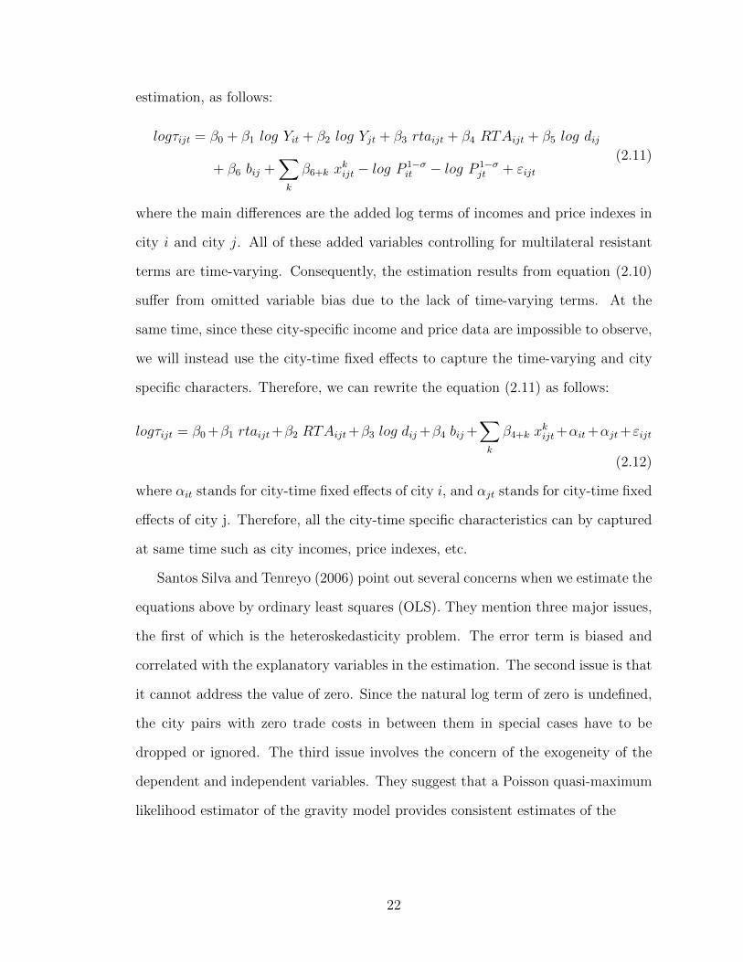
where the main differences are the added log terms of incomes and price indexes in

city i and city j. All of these added variables controlling for multilateral resistant

terms are time-varying. Consequently, the estimation results from equation (2.10)

suffer from omitted variable bias due to the lack of time-varying terms. At the

same time, since these city-specific income and price data are impossible to observe,

we will instead use the city-time fixed effects to capture the time-varying and city

specific characters. Therefore, we can rewrite the equation (2.11) as follows:

logτijt = β0 +β1 rtaijt+β2 RTAijt+β3 log dij +β4 bij +∑k

β4+k xkijt+αit+αjt+εijt

(2.12)

where αit stands for city-time fixed effects of city i, and αjt stands for city-time fixed

effects of city j. Therefore, all the city-time specific characteristics can by captured

at same time such as city incomes, price indexes, etc.

Santos Silva and Tenreyo (2006) point out several concerns when we estimate the

equations above by ordinary least squares (OLS). They mention three major issues,

the first of which is the heteroskedasticity problem. The error term is biased and

correlated with the explanatory variables in the estimation. The second issue is that

it cannot address the value of zero. Since the natural log term of zero is undefined,

the city pairs with zero trade costs in between them in special cases have to be

dropped or ignored. The third issue involves the concern of the exogeneity of the

dependent and independent variables. They suggest that a Poisson quasi-maximum

likelihood estimator of the gravity model provides consistent estimates of the

22

parameters even with heteroskedasticity errors and solves all the issues mentioned

above.

As a robustness check for the after-treatment effects of RTA, the biggest concern

is the endogeneity problem following equations (2.10) or (2.12). Particularly, we

need to address the omitted variables issue, since there is no way to list all the

factors that could potentially affect trade costs. Another issue with the regressions

so far is the correlation of independent variables. For example, we are interested

in the after-treatment effects of RTAs on trade costs, so suppose that a city pair

belongs to countries that share the same common language. Of course, intuitively,

this strong cultural tie would lead to smaller trade costs between the city pair,

and at the same time, it would be more likely for their countries to form an RTA.

Therefore, the error term of the estimation is correlated with the RTAs and the

common language dummy variable, and the coefficients estimated are biased.

We want to find a method to solve the issue mentioned above that captures all

the time-irrelevant unobserved city-pair characteristics that would affect the trade

costs, and this term should also not be correlated with the RTA variable that we

mainly focus on. The bilateral-pair (city-pair) fixed effects seems to solve the issue;

this added term would capture all the time-irrelevant city-pair-specific factors, such

as all the bilateral gravity variables. Thus, we can rewrite equations (2.10) and

(2.12) as follows:

logτijt = β0+β1 rtaijt+β2 RTAijt+∑k

β2+k xkijt+ αit + αjt︸ ︷︷ ︸

Multilateral Resistant Terms

+αij+εijt

(2.13)

where αij stands for this bilateral pair fixed effects. Since this term captures all

the time-irrelevant country pair features, all the city (country) pair -specific dummy

23

variables, such as distance, common border, etc., are omitted. The vector xkijt con-

tains only the CU dummy variable and the time-related CU variables. They are

both time-varying and are not omitted due to the fact that they still capture the

time-sensitive characteristics that affect the trade costs.

There are many other ways to solve this endogeneity issue. To summarize, Baier

and Bergstrand (2007) point out the modern solutions to address the endogeneity is-

sue when we estimate the gravity model are to take advantage of the panel approach

instead of cross-sectional data analysis, where studies use traditional methods. The

instrumental-variable techniques and control-function techniques do not adjust for

the endogeneity issue well, and they are subject to changes in data selection and

sample sizes.

As mentioned, the bilateral city fixed effects should capture all the time-irrelevant

unobserved bilateral pair characteristics. Many studies also use the first-differencing

method. Wooldridge (2002) concludes that when the time periods in the panel data

that are available exceeds two, the fixed-effects estimator is more efficient than the

first-differencing estimator under the assumption that the error terms are serially

uncorrelated. If the assumption changes the error term of the first-differenced esti-

mation following a random walk, the first-differencing estimator is going to be more

efficient. We consider the time-differencing estimator as our further robustness check

considering the potential endogeneity issue. Therefore, we estimate as follows:

4logτij,t−(t−1) = β0 + β14 rtaij,t−(t−1) + β24RTAij,t−(t−1)

+ αit + αjt︸ ︷︷ ︸Multilateral Resistant Terms

+νij,t−(t−1)

(2.14)

where νij,t−(t−1) = εijt− εij,t−1 is white noise. Since this is a replacement of bilateral

fixed effects approach, we do not have the bilateral fixed effects term αij in equation

24

(2.13). We consider both the scenarios with or without the multilateral resistant

terms (αit + αjt).

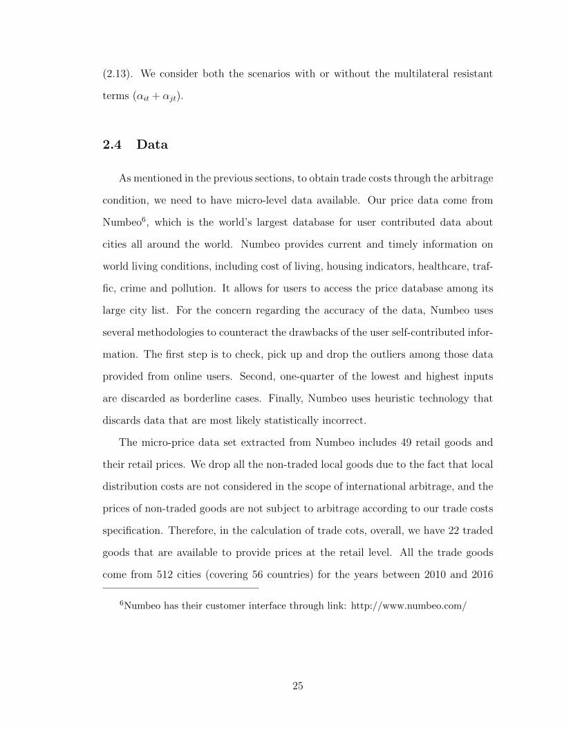
2.4 Data

As mentioned in the previous sections, to obtain trade costs through the arbitrage

condition, we need to have micro-level data available. Our price data come from

Numbeo6, which is the world’s largest database for user contributed data about

cities all around the world. Numbeo provides current and timely information on

world living conditions, including cost of living, housing indicators, healthcare, traf-

fic, crime and pollution. It allows for users to access the price database among its

large city list. For the concern regarding the accuracy of the data, Numbeo uses

several methodologies to counteract the drawbacks of the user self-contributed infor-

mation. The first step is to check, pick up and drop the outliers among those data

provided from online users. Second, one-quarter of the lowest and highest inputs

are discarded as borderline cases. Finally, Numbeo uses heuristic technology that

discards data that are most likely statistically incorrect.

The micro-price data set extracted from Numbeo includes 49 retail goods and

their retail prices. We drop all the non-traded local goods due to the fact that local

distribution costs are not considered in the scope of international arbitrage, and the

prices of non-traded goods are not subject to arbitrage according to our trade costs

specification. Therefore, in the calculation of trade cots, overall, we have 22 traded

goods that are available to provide prices at the retail level. All the trade goods

come from 512 cities (covering 56 countries) for the years between 2010 and 2016

6Numbeo has their customer interface through link: http://www.numbeo.com/

25

7. The 22 traded good prices are all available for 478 cities, so we pair every city

with all other cities that have all the price data available in that particular year.

Doing so results in the generation of 215,134 observations, overall, for city pairs

that have price data available for all year spans. In all the city pairs, the number of

international city pairs is 2,230 (116 city pairs are intranational pairs in which both

cities are from the same country). Since all city pairs have data available for all the

years from 2010 to 2016, this data set we created is balanced.

We use the model-implied traded input prices that were acquired from traded

good prices data and wage data. Since the price data and wage data are all year-

specific, we can get the short-run trade costs for city pairs in the year when price

data are available. On average, the trade costs in between all the city pairs are

approximately 1.39, while the trade costs between international city pairs are 1.44,

on average, and 0.74 for intranational city pairs. These measurements of trade costs

are significantly smaller compared to the literature. The well-defined ad-valorem

equivalent (ice-berg) trade costs in Eaton and Kortum (2002) are approximately

1.90, and they are approximately 1.70 in Anderson and Wincoop (2004). As men-

tioned above, the definition of our trade costs is slightly different from the literature.

First, the trade costs we obtained are at the city level instead of the country level,

as most of the studies use. Second, the trade costs in the literature do not control

for retail/local distribution costs, but to serve the purpose of our interests, they are

calculated without considering the retail costs.

Other gravity variables are collected during the same time from Reuven and

Rose (2016). For the bilateral-specific gravity variables, we exploit the World Fact-

book from the CIA for a number of country-specific variables, such as island status,

language, and colonizers. We create the dummy variables, such as ”border”, which

7See the complete goods list in Table section below.

26

indicate whether two countries have an international border; ”colony”, which deter-

mines whether two countries were ever in a colonial relationship; ”comlang”, which

shows whether two countries share the same common language; and ”island”, which

is a three way dummy variable that takes the values of 0/1/2, which indicates if

either (neither or both) country in the pair is (are) an island country (countries).

However, these bilateral variables are all at the country level, and our trade costs

are at the city level. Since the international trade from international cities does not

account for local distribution costs, all the effects of these country-level bilateral

gravity variables capture these effects on trade costs. Finally, we obtain distances

in the measurement of miles between city pairs through the latitude and longitude

acquired through the Google Map API.

2.5 Empirical Results

2.5.1 Benchmark Case

The benchmark regressions using OLS and the random effects estimator are

given in Table 2.1. Column 1 uses only binary dummy variables for regional trade

agreements and currency unions to explain trade costs. When two nations have an

RTA, the trade costs between two cities in each country decreased by 27.6%. When

we include all the control variables to avoid any omitted variable bias, as shown in

column 4, the existence of an RTA between two countries reduces the trade costs

between two cities from those two countries by 12.3%. This result is smaller com-

pared to 23% in D. Yilmazkuday and H. Yilmazkuday (2016), who include an RTA

dummy in their random effects regression of the trade costs on direct fly between

cities. However, their study focuses on the analysis of long-run effects by calculating

27

the average trade costs through the entire time period. It smooths out the volatility

and hides the details that come from our trade costs calculated on yearly bases.

Accordingly, the trade costs used in our study are time-related, which means that

the trade costs calculated in our study give a unique number every year, instead

of taking the mean of all the values across the whole year span. Currency union

also affects trade costs negatively and significantly. Specifically, according to the

estimation in column 1, when two countries are in a currency union, the trade costs

between two cities in each country will decrease on average by 33% compared with

other cities, and after adding other control variables, according to column 4, the

effect of having a currency union dropped the trade costs from 33% to 52.9%.

After adding the time-related RTA and currency union variables to the binary

dummies without other control variables, as the case shown in column 3, the exis-

tence of an RTA reduces the trade costs by 12.3% immediately, and the phased-in

effect reduces the trade costs by 1.29% each year after the RTA is introduced. On

the other hand, even though the currency union has a significant and negative effect

on trade costs instantly, it has the phased-out effect to cause the trade costs to in-

crease 2.48% each year after two countries join a currency union. This finding means

that even though a currency union causes a decrease in the trade costs between two

cities, it will offset the effect by causing the trade costs to rise to the original level in

approximately 15 years. Similarly, for the RTA, the initial impact and phased-in ef-

fect on trade costs diminished when all the control variables are included. In column

6, it shows that the RTA has a negative impact on trade costs immediately after the

forming of the RTA (coefficient of -12.3%), and the phased-in effect is 0.815% each

year after the initial impact of the RTA. Currency union, on the other hand, causes

the trade costs to decrease by 52.9% immediately but increase by approximately 3%

each year after. The phased-out effect of the currency union is still prominent.

28

In addition to RTAs and currency union, having a common border between the

countries where two cities are located also has a negative influence on trade costs.

Specifically, a common border reduces the trade costs by 49.3%. A colonial relation-

ship between two countries reduces the trade costs of city pairs by approximately

34.6%. However, if the city pairs are in countries that share a common language,

the trade costs increase by 8.78%. This result contradicts our prediction. If there

is only one city in a city pair categorized as an island country, the trade costs are

reduced by 7.5%. As the dummy variable for landlocked and island indicators takes

3 values (0/1/2), the case of both cities belong to two island countries will reduce the

trade costs by almost 15%. Finally, the effect of distance on trade costs is negative

but insignificant, according to column 6, where we include all the control variables.

However, in the model in column 5 without RTA and currency union dummies, the

distance affects trade costs positively and significantly. This result causes concern

regarding the nonlinearity of distance effects, which we will also discuss more in the

following subsection.

2.5.2 Robustness Checks

Nonlinearity in Distance Measures

Up to this point, we have evaluated the distance effects using the log term of the

distances between cities. Now, we consider nonlinearities in the effects of distance on

trade costs. The results are given in Table 2.2. For all the estimations, we include the

four most important variables we are focusing on (RTA dummy, CU dummy, time-

related RTA variable and time-related CU variable) and all other time-irrelevant

control variables. Column 1 replicates column 6 in Table 2.1, with consideration of

all the control variables and the random estimator. The second column considers

29

an extra log distance squared variable. The third column includes five distance-

interval dummy variables in the replacement of the log distance variable in the first

column. Each distance interval represents a 20 percentile of the distance between

cities, compared to all the distances in the data.8 As the results show, in column 2,

the coefficient of the log distance square is negative and significant. The coefficient of

the log distance is positive and significant. This indicates the potential nonlinearity

in the distance effect on trade costs. Column 4 also supports this assumption by

presenting different and significant coefficients of different distance interval dummies.

Therefore, this provides evidence for nonlinearity in distance effects on trade costs.

We can also observe that the treatment effects of the RTA dummy and time-related

variable are both negative and significant in random-effect estimators. From column

4 to column 6, we consider the nonlinearity of distance effects with city fixed effects.

Column 4 shows that a longer distance between two cities causes higher trade costs.

Column 5 yields similar results compared with column 2. Specifically, the coefficient

of the log distance square is negative and significant. The coefficients of all distance

intervals in column 6 are significant and different from each other. Therefore, we

can conclude that there is strong evidence of nonlinearity in the effect of distance

on trade costs. For the RTA effects on trade costs, which we mainly focus on, we

still observe a negative and significant immediate impact and phased-in effect.

Endogeneity of RTA and CU

In the early gravity studies, the drawback of the cross-sectional data is not

able to explain the unobserved time-invariant heterogeneity or provide estimations

of enough treatment effects to solve the endogeneity problem. In our study, this

8A city pair’s distance can only allocated in one of the five distance intervals, and thedummy for that interval has the value equals 1

30

concern is the multilateral resistant term in the gravity model. Ghosh and Yamarik

(2004) address the issue of the insignificance of the effects of RTAs on either trade

or trade costs by using cross-sectional data and extreme-bounds analysis to test the

robustness of the RTA dummy coefficients. The results show that the effects of most

RTAs on trade are not reliable. Instead, Baier and Bergstrand (2007) suggest using

the panel approach combined with fixed effects. We combine city and time fixed

effects in our analysis to eliminate the unobserved city-time-related heterogeneity.

In addition to the unobserved city-time related heterogeneity, there are more

concerns regarding the endogeneity bias in estimating the treatment effects on the

RTA dummy. Since the RTA dummy is possibly correlated with the unobserved

variables and even potentially has the causality problem with trade costs (LHS

variable), the literature has begun using the panel approach to solve the issue. The

earliest literature, such as Magee (2003) and Baier and Bergstrand (2002), uses

IV or control-function techniques to solve the issue. Later, Baier and Bergstrand

(2004) demonstrate the after-treatment effects of the gravity model using IV, or

control-function techniques are unstable and lead to fragile conclusions. Baier and

Bergstrand (2007) take a step forward to include bilateral fixed effects (country-pair

fixed effects) and the first difference method to eliminate the endogeneity problem

of the RTA dummy. This requires balanced panel data with all the years’ data

available for the city pairs.9 Thereafter, we also include city-pair fixed effects in our

estimations.

First, we only include bilateral fixed effects (city-pair fixed effects) to the random

effects estimator without considering the multilateral resistant terms in Table 2.3.

9Next step is for us to analyze RTA effects with the alternative way beside of fixedeffects estimators, such as using first difference, city-pair fixed effects, and consideringtime lag effects of RTA dummy.

31

Due to the fact that there are unobserved time-invariant heterogeneity, we can not

capture in the regression besides the distance, border, common language, colonial

ties, etc., bilateral fixed effects is used in literature, such as Cheng and Wall (2005),

Tomz, Goldenstein and Rivers (2007), and Magee (2008). They all conduct similar

studies using panel data to estimate the effects of RTA on trade flow. Column

1 to column 3 use the OLS estimator. The results are consistent with the after

treatment effects on CU dummy, time-related RTA and CU variables. Accordingly,

after considering the city-pair fixed effects, having an RTA causes city pairs to have

an overall 120% decrease in trade costs compared to the city pairs belong to countries

without an RTA at the point when the RTA forms. Every year after that, the RTA

reduce trad costs by approximately 34%. These results are amplified compared with

the analysis in Table 1. However, it is still aligned with the finding in literature. For

example, Magee (2008) confirms that the cumulative RTA effect on trade is 1.01,

which means having an RTA dubble the trade volume between two countries. On

the other hand, the after treatment effect on CU dummy remains negative on trade

costs, a 128% drop of the trade costs on average if city pairs belong to countries that

join in a CU. The effect of the time-related CU variable is small and insignificant.

From column 4 to column 6, we introduce the PQML estimator with city-pair

fixed effects as comparison. The results turn out to be consistent with the OLS

estimator. However, the magnitude of the immediate impact and phased-in effect

are smaller. For the after-treatment effect of the RTA, city pairs belonging to

countries in an RTA have 41.3% less trade costs, on average, by the time the RTA

is introduced, and every year after that, the RTA will reduce the trade costs by

12.1%. Similarly, there are significant after-treatment effects of CUs. City pairs

belong to countries in a currency union have 26% less trade costs than those city

pairs that do not belong to a currency union by the time the CU is introduced.

32

However, there is no significant effect of currency unions on trade costs every year

thereafter. Regarding the sensitivity of the RTA after treatment effects, we can see

minor differences when we switch the estimator from OLS to PQML. The signs for

the two dummy variables and the two time-related variables remain the same. The

coefficients are considerably smaller in the PQML estimator compared with the OLS

estimator.

Table 2.4 investigates the bilateral fixed effects in the case of considering the

multilateral resistant terms. Therefore, the entire estimation includes city-time fixed

effects (the multilateral resistant terms) and city-pair fixed effects (bilateral fixed

effect). Similarly, the first three columns present the OLS estimator and columns 4

to 6 preset the results using the PQML estimator. Comparing the OLS and PQML

horizontally, the signs in front of the significant coefficients do not change, and the

values are consistent with minor differences, which again examine the insensitivity

of the after treatment effects of the RTA and CU in regard to OLS and PQML.

Comparing Table 2.4 with Table 2.3, we still see consistency regarding the signs and

values of the coefficients. For CU, considering the multilateral resistant terms (city-

time fixed effects) in Table 2.4, the initial impact of CUs on trade costs decreases

from -127.7% to -103.8% in OLS and from -26% to insignificant in PQML; the time-

related CU variable does not have a significant effect on trade costs for both cases.

Large changes come from the after-treatment effects on RTA, considering that the

multilateral resistant terms push down the initial impact of the RTA on trade costs

from -120% to -54.3% with OLS and -41.3% to -20.6% with PQML. It also decreases

the after-treatment effects of the time-related RTA variable on trade costs from -

34% to -5.5% in OLS and -12.1% to -2.59% in PQML.

Table 2.5 provides another method to address the endogeneity issue. We expect

the first-differencing method to more accurately describe the after treatment effects

33

of the RTA and CU or at least to evaluate the robustness of the bilateral pair

fixed effects estimator, since both are aimed to solve the issue of potential omitted

variables bias created by time-irrelevant city-pair specific barriers. We also consider

the multilateral resistant terms (time-related multilateral price terms) by using city-

time fixed effects. Columns 1, 4 and 7 investigate the concurrent changes in RTAs

and CUs with only the first-differencing of the RTA and CU dummy variables and

the time-related variables. As a comparison to Table 2.4, in columns 1 to 3 with

the OLS estimator, the first-differencing method should be consistent with using the

bilateral fixed effects. The after-treatment effects of the RTA and CU maintain the

same signs as the RTA dummy, which has a positive effect on trade costs, while the

CU dummy has a negative effect. Changing from not being in an RTA to joining

in an RTA, on average, increases the change of trade costs by 8.59%. Because

the first-differencing allows for all other constant time-irrelevant factors to remove

the impact themselves, the 8.59% increase in trade costs is due to the joining in an

RTA. For the bilateral fixed effects method, the after-treatment effects of an RTA are

11.3%. The results are also consistent when comparing the after-treatment effects

of a CU and the first-differencing method. An 18.3% decrease of trade costs, on

average, is due to the formation of a CU with the first-differencing method, and the

after-treatment effect is 14% in regard to using the bilateral fixed effects method.

For the first-differenced time-related variables, the coefficients of both RTA and CU

are insignificant compared to the bilateral fixed effects method, where we have a

time-related RTA variable that is significant but small. In columns 2, 5 and 8, we

include an extra second-differencing lag term for both the RTA and CU dummies

and time-related variables. The purpose of using second-differencing is to examine

the phased-in (time) effect along with our time-related variables. In this sense, in

the model of column 8, the second-differencing of the RTA and CU dummies should

34

have the mirror effects of the first-differencing time-related RTA and CU variables.

We can observe the mirror effects from columns 2 and 5, where the coefficient in front

of the second-differenced RTA dummy is 0.037, and the coefficient in front of the

first-differenced RTA time-related variable is -0.040. They are both significant, and

the difference between them is negligible. Then, regarding CUs, the coefficient in

front of the second-differenced CU dummy and the first-differenced CU time-related

variable are also similar to each other with the values of 0.0725 and 0.0752, even

though one of them is insignificant. The other evidence comes from column 8. The

second-differenced CU dummy and the second-differenced time-related RTA variable

are omitted in this model due to the collinearity problem, which means that these

two variables can be linearly explained by the other two variables in the model (the

first-differenced time-related CU variable and the first-differenced RTA dummy).

We also include the future-change terms for both the RTA and CU dummies and

the time-related variables in columns 3, 6 and 9. This method is used to detect the

exogeneity of the explaining variable to the independent variable. As we can see,

due to the insignificant coefficients in front of all the CU future change terms, the

future change in the status of CU has no significant effect on trade costs, which

indicates that trade costs are not the reason for the future change in the status of

CUs. On the other hand, the future change of the RTA dummy and time-related

RTA variable all have significant impacts on the change of trade costs. Recall the

results from Table 4 with the bilateral fixed effects and the case considering the

multilateral resistant terms, having an RTA means that, on average, city pairs have

larger trade costs between them, and the phased-in effect has a negative impact

on trade costs after joining in the RTA throughout the years. This high level of

trade costs might be the reason to form the RTA. Again, due to the collinearity

issue, both the first-differenced and the second-differenced RTA and CU dummies

35

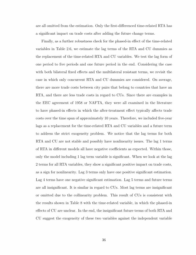
are all omitted from the estimation. Only the first-differenced time-related RTA has

a significant impact on trade costs after adding the future change terms.

Finally, as a further robustness check for the phased-in effect of the time-related

variables in Table 2.6, we estimate the lag terms of the RTA and CU dummies as

the replacement of the time-related RTA and CU variables. We test the lag form of

one period to five periods and one future period in the end. Considering the case

with both bilateral fixed effects and the multilateral resistant terms, we revisit the

case in which only concurrent RTA and CU dummies are considered. On average,

there are more trade costs between city pairs that belong to countries that have an

RTA, and there are less trade costs in regard to CUs. Since there are examples in

the EEC agreement of 1958 or NAFTA, they were all examined in the literature

to have phased-in effects in which the after-treatment effect typically affects trade

costs over the time span of approximately 10 years. Therefore, we included five-year

lags as a replacement for the time-related RTA and CU variables and a future term

to address the strict exogeneity problem. We notice that the lag terms for both

RTA and CU are not stable and possibly have nonlinearity issues. The lag 1 terms

of RTA in different models all have negative coefficients as expected. Within those,

only the model including 1 lag term variable is significant. When we look at the lag

2 terms for all RTA variables, they show a significant positive impact on trade costs,

as a sign for nonlinearity. Lag 3 terms only have one positive significant estimation.

Lag 4 terms have one negative significant estimation. Lag 5 terms and future terms

are all insignificant. It is similar in regard to CUs. Most lag terms are insignificant

or omitted due to the collinearity problem. This result of CUs is consistent with

the results shown in Table 8 with the time-related variable, in which the phased-in

effects of CU are unclear. In the end, the insignificant future terms of both RTA and

CU suggest the exogeneity of these two variables against the independent variable

36

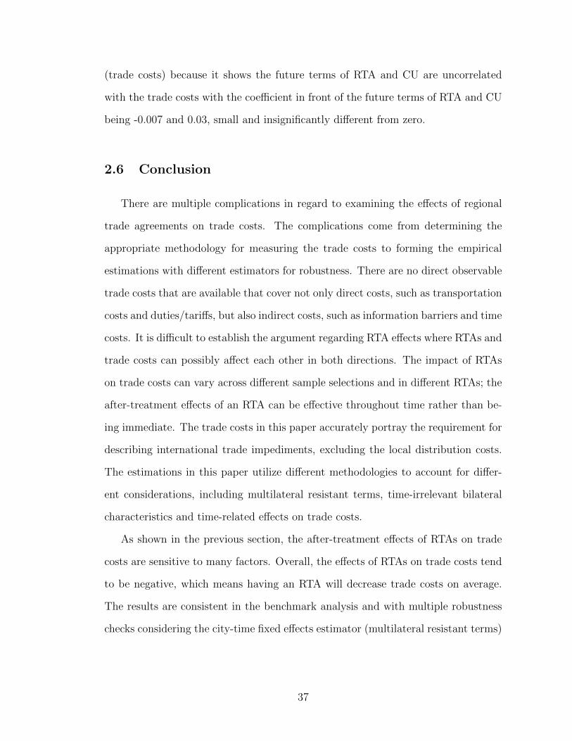
(trade costs) because it shows the future terms of RTA and CU are uncorrelated

with the trade costs with the coefficient in front of the future terms of RTA and CU

being -0.007 and 0.03, small and insignificantly different from zero.

2.6 Conclusion

There are multiple complications in regard to examining the effects of regional

trade agreements on trade costs. The complications come from determining the

appropriate methodology for measuring the trade costs to forming the empirical

estimations with different estimators for robustness. There are no direct observable

trade costs that are available that cover not only direct costs, such as transportation

costs and duties/tariffs, but also indirect costs, such as information barriers and time

costs. It is difficult to establish the argument regarding RTA effects where RTAs and

trade costs can possibly affect each other in both directions. The impact of RTAs

on trade costs can vary across different sample selections and in different RTAs; the

after-treatment effects of an RTA can be effective throughout time rather than be-

ing immediate. The trade costs in this paper accurately portray the requirement for

describing international trade impediments, excluding the local distribution costs.

The estimations in this paper utilize different methodologies to account for differ-

ent considerations, including multilateral resistant terms, time-irrelevant bilateral

characteristics and time-related effects on trade costs.

As shown in the previous section, the after-treatment effects of RTAs on trade

costs are sensitive to many factors. Overall, the effects of RTAs on trade costs tend

to be negative, which means having an RTA will decrease trade costs on average.

The results are consistent in the benchmark analysis and with multiple robustness

checks considering the city-time fixed effects estimator (multilateral resistant terms)

37

and city-pair fixed effects (time-irrelevant bilateral characteristics). When we add

more related gravity variables into the estimations, the negative impacts of RTAs

remain significant. Moreover, the effects of the standard gravity variables on trade

costs are consistent with the literature.

The estimations also reveal more interesting results when we included a time-

related RTA variable. Specifically, in both the benchmark analysis and the robust-

ness checks, this new added variable has a negative impact on trade costs, which

means that the trade costs keep decreasing throughout time after the RTAs has

been introduced. These phased-in effects of RTAs have been caught in all random

and fixed effects estimators, which confirms the results found in the literature, such

as Baier and Bergstrand (2007) and Magee (2003), that RTAs will continue to effect

trade for almost a decade after the trade deal begins. Finally, the results indicate

that it is still a puzzle as to how we can explain the causality of forming RTAs and

trade costs reduction. The study shows mixed results regarding the exogeneity of

the RTA dummy variable. With positive effects on trade costs when forming an

RTA one period in the future, this study suggests that relatively higher trade costs

could be related to the forming of an RTA. There are numerous questions in this

area that need answers, and it is interesting to see more disaggregate analysis re-

garding different specific RTAs and what caused these phased-in effects for different

RTAs.

REFERENCES

[Anderson and Van Wincoop(2003)] James E Anderson and Eric Van Wincoop.Gravity with gravitas: a solution to the border puzzle. the american economicreview, 93(1):170–192, 2003.

[Anderson and Van Wincoop(2004)] James E Anderson and Eric Van Wincoop.Trade costs. Journal of Economic literature, 42(3):691–751, 2004.

38

[Andrews and Guggenberger(2009)] Donald WK Andrews and Patrik Guggen-berger. Validity of subsampling and plug-in asymptotic inference for parametersdefined by moment inequalities. Econometric Theory, 25(3):669–709, 2009.

[Andrews and Soares(2010)] Donald WK Andrews and Gustavo Soares. Inferencefor parameters defined by moment inequalities using generalized moment selec-tion. Econometrica, 78(1):119–157, 2010.

[Andrews et al.(2004)Andrews, Berry, and Jia] Donald WK Andrews, StevenBerry, and Panle Jia. Confidence regions for parameters in discrete gameswith multiple equilibria, with an application to discount chain store location.manuscript, Yale University, 2004.

[Arvis et al.(2016)Arvis, Duval, Shepherd, Utoktham, and Raj] Jean-FrancoisArvis, Yann Duval, Ben Shepherd, Chorthip Utoktham, and Anasuya Raj.Trade costs in the developing world: 1996–2010. World Trade Review, 15(3):451–474, 2016.

[Azapmo(2017)] Jean Bertrand Azapmo. Regional trade agreements and cross-border trade costs: The case of pacific island countries. Technical report,ARTNeT Working Paper Series, 2017.

[Bacchetta et al.(2011)Bacchetta, Beverelli, Hancock, Keck, Nayyar, Nee, Piermartini, Rocha, Roy, Ruta, et al.]Marc Bacchetta, Cosimo Beverelli, John Hancock, Alexander Keck, GauravNayyar, Coleman Nee, Roberta Piermartini, Nadia Rocha, Martin Roy, MicheleRuta, et al. The wto and preferential trade agreements: From co-existence tocoherence. 2011.

[Baier and Bergstrand(2002)] Scott L Baier and Jeffrey H Bergstrand. On the en-dogeneity of international trade flows and free trade agreements, 2002.

[Baier and Bergstrand(2004)] Scott L Baier and Jeffrey H Bergstrand. Economicdeterminants of free trade agreements. Journal of international Economics, 64(1):29–63, 2004.

[Baier and Bergstrand(2007)] Scott L Baier and Jeffrey H Bergstrand. Do free tradeagreements actually increase members’ international trade? Journal of inter-national Economics, 71(1):72–95, 2007.

[Cheng et al.(2005)Cheng, Wall, et al.] I-Hui Cheng, Howard J Wall, et al. Con-trolling for heterogeneity in gravity models of trade and integration. 2005.

39

[Cipollina and Salvatici(2010)] Maria Cipollina and Luca Salvatici. Reciprocaltrade agreements in gravity models: A meta-analysis. Review of InternationalEconomics, 18(1):63–80, 2010.

[Crucini and Yilmazkuday(2014)] Mario J Crucini and Hakan Yilmazkuday. Un-derstanding long-run price dispersion. Journal of Monetary Economics, 66:226–240, 2014.

[Duval et al.(2016)Duval, Neufeld, and Utoktham] Yann Duval, Nora Neufeld, andChorthip Utoktham. Do trade facilitation provisions in regional trade agree-ments matter? impact on trade costs and multilateral spillovers. Technicalreport, ARTNeT Working Paper Series, 2016.

[Eaton and Kortum(2002)] Jonathan Eaton and Samuel Kortum. Technology, ge-ography, and trade. Econometrica, 70(5):1741–1779, 2002.

[Ghosh and Yamarik(2004)] Sucharita Ghosh and Steven Yamarik. Are regionaltrading arrangements trade creating?: An application of extreme bounds anal-ysis. Journal of International Economics, 63(2):369–395, 2004.

[Glick and Rose(2016)] Reuven Glick and Andrew K Rose. Currency unions andtrade: a post-emu reassessment. European Economic Review, 87:78–91, 2016.

[Goldstein et al.(2007)Goldstein, Rivers, and Tomz] Judith L Goldstein, DouglasRivers, and Michael Tomz. Institutions in international relations: Understand-ing the effects of the gatt and the wto on world trade. International Organiza-tion, 61(1):37–67, 2007.

[Haveman and Hummels(2004)] Jon Haveman and David Hummels. Alternative hy-potheses and the volume of trade: the gravity equation and the extent of spe-cialization. Canadian Journal of Economics/Revue canadienne d’economique,37(1):199–218, 2004.

[Head and Mayer(2013)] Keith Head and Thierry Mayer. Gravity equations:Workhorse, toolkit, and cookbook. 2013.

[Jacks et al.(2008)Jacks, Meissner, and Novy] David S Jacks, Christopher M Meiss-ner, and Dennis Novy. Trade costs, 1870-2000. The American Economic Review,98(2):529–534, 2008.

40

[Jacks et al.(2011)Jacks, Meissner, and Novy] David S Jacks, Christopher M Meiss-ner, and Dennis Novy. Trade booms, trade busts, and trade costs. Journal ofInternational Economics, 83(2):185–201, 2011.

[Magee(2003)] Christopher S Magee. Endogenous preferential trade agreements: Anempirical analysis. Contributions in Economic Analysis & Policy, 2(1), 2003.

[Magee(2008)] Christopher SP Magee. New measures of trade creation and tradediversion. Journal of International Economics, 75(2):349–362, 2008.

[Miroudot and Shepherd(2014)] Sebastien Miroudot and Ben Shepherd. The para-dox of preferences: regional trade agreements and trade costs in services. TheWorld Economy, 37(12):1751–1772, 2014.

[Novy(2013)] Dennis Novy. Gravity redux: measuring international trade costs withpanel data. Economic inquiry, 51(1):101–121, 2013.

[Pomfret and Sourdin(2009)] Richard Pomfret and Patricia Sourdin. Have asiantrade agreements reduced trade costs? Journal of Asian Economics, 20(3):255–268, 2009.

[Ponomareva and Tamer(2011)] Maria Ponomareva and Elie Tamer. Misspecifica-tion in moment inequality models: Back to moment equalities? The Econo-metrics Journal, 14(2):186–203, 2011.

[Rosen(2008)] Adam M Rosen. Confidence sets for partially identified parametersthat satisfy a finite number of moment inequalities. Journal of Econometrics,146(1):107–117, 2008.

[Silva and Tenreyro(2006)] JMC Santos Silva and Silvana Tenreyro. The log ofgravity. The Review of Economics and statistics, 88(4):641–658, 2006.

[Simonovska and Waugh(2014)] Ina Simonovska and Michael E Waugh. The elas-ticity of trade: Estimates and evidence. Journal of international Economics,92(1):34–50, 2014.

[Tinbergen(1962)] Jan Tinbergen. Shaping the world economy; suggestions for aninternational economic policy. Books (Jan Tinbergen), 1962.

[Wonnacott and Lutz(1989)] Paul Wonnacott and Mark Lutz. Is there a case forfree trade areas? Free trade areas and US trade policy, 59:84, 1989.

41

[Wooldridge(2002)] Jeffrey M Wooldridge. Inverse probability weighted m-estimators for sample selection, attrition, and stratification. Portuguese Eco-nomic Journal, 1(2):117–139, 2002.

[Yamarik and Ghosh(2005)] Steven Yamarik and Sucharita Ghosh. A sensitivityanalysis of the gravity model. The International Trade Journal, 19(1):83–126,2005.

[Yilmazkuday and Yilmazkuday(2017)] Demet Yilmazkuday and Hakan Yilmazku-day. The role of direct flights in trade costs. Review of World Economics, 153(2):249–270, 2017.

42

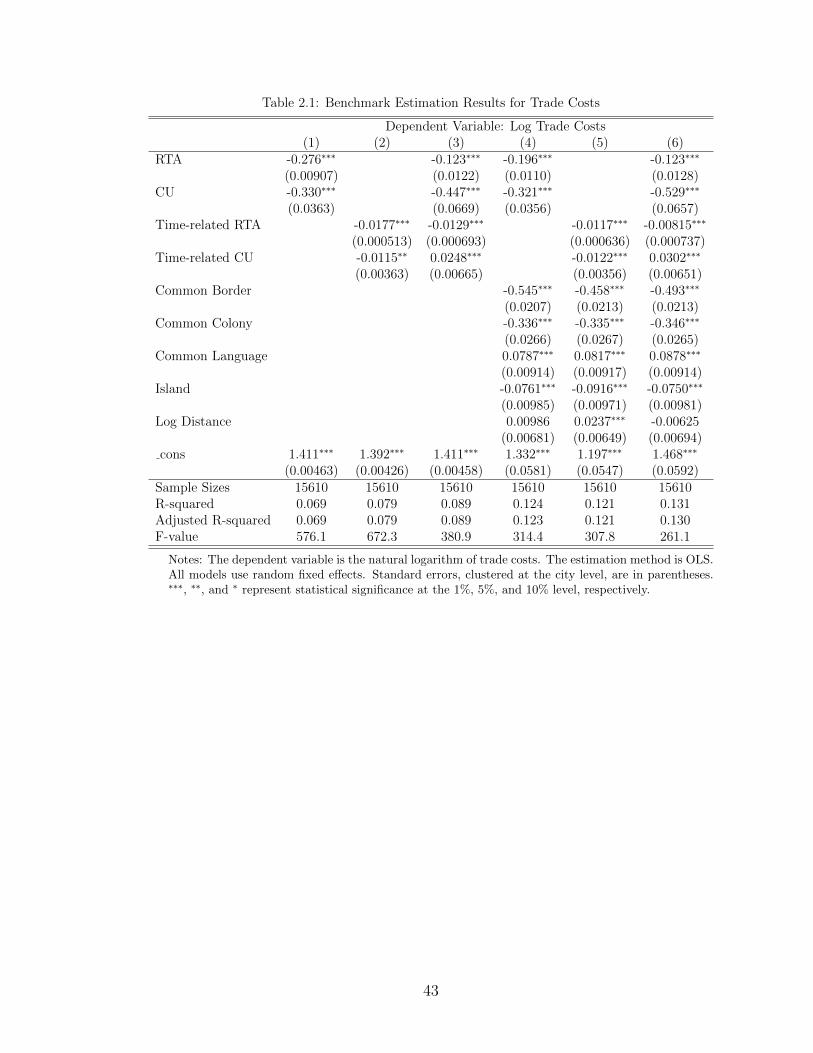
Table 2.1: Benchmark Estimation Results for Trade Costs

Dependent Variable: Log Trade Costs(1) (2) (3) (4) (5) (6)

RTA -0.276∗∗∗ -0.123∗∗∗ -0.196∗∗∗ -0.123∗∗∗

(0.00907) (0.0122) (0.0110) (0.0128)CU -0.330∗∗∗ -0.447∗∗∗ -0.321∗∗∗ -0.529∗∗∗

(0.0363) (0.0669) (0.0356) (0.0657)Time-related RTA -0.0177∗∗∗ -0.0129∗∗∗ -0.0117∗∗∗ -0.00815∗∗∗

(0.000513) (0.000693) (0.000636) (0.000737)Time-related CU -0.0115∗∗ 0.0248∗∗∗ -0.0122∗∗∗ 0.0302∗∗∗

(0.00363) (0.00665) (0.00356) (0.00651)Common Border -0.545∗∗∗ -0.458∗∗∗ -0.493∗∗∗

(0.0207) (0.0213) (0.0213)Common Colony -0.336∗∗∗ -0.335∗∗∗ -0.346∗∗∗

(0.0266) (0.0267) (0.0265)Common Language 0.0787∗∗∗ 0.0817∗∗∗ 0.0878∗∗∗

(0.00914) (0.00917) (0.00914)Island -0.0761∗∗∗ -0.0916∗∗∗ -0.0750∗∗∗

(0.00985) (0.00971) (0.00981)Log Distance 0.00986 0.0237∗∗∗ -0.00625

(0.00681) (0.00649) (0.00694)cons 1.411∗∗∗ 1.392∗∗∗ 1.411∗∗∗ 1.332∗∗∗ 1.197∗∗∗ 1.468∗∗∗

(0.00463) (0.00426) (0.00458) (0.0581) (0.0547) (0.0592)Sample Sizes 15610 15610 15610 15610 15610 15610R-squared 0.069 0.079 0.089 0.124 0.121 0.131Adjusted R-squared 0.069 0.079 0.089 0.123 0.121 0.130F-value 576.1 672.3 380.9 314.4 307.8 261.1

Notes: The dependent variable is the natural logarithm of trade costs. The estimation method is OLS.All models use random fixed effects. Standard errors, clustered at the city level, are in parentheses.∗∗∗, ∗∗, and ∗ represent statistical significance at the 1%, 5%, and 10% level, respectively.

43

Table 2.2: Estimation Results for Trade Costs: Nonlinearities in Distance Measures

Dependent Variable: Log Trade Costs(1) (2) (3) (4) (5) (6)

RTA -0.123∗∗∗ -0.123∗∗∗ -0.150∗∗∗ -0.0465∗∗∗ -0.0495∗∗∗ -0.0373∗∗

(0.0128) (0.0127) (0.0132) (0.0116) (0.0117) (0.0118)CU -0.529∗∗∗ -0.537∗∗∗ -0.561∗∗∗ -0.116∗ -0.122∗ -0.112∗

(0.0657) (0.0656) (0.0658) (0.0545) (0.0545) (0.0542)Time-related RTA -0.00815∗∗∗ -0.00787∗∗∗ -0.00873∗∗∗ -0.00835∗∗∗ -0.00810∗∗∗ -0.00885∗∗∗

(0.000737) (0.000737) (0.000733) (0.000650) (0.000652) (0.000645)Time-related CU 0.0302∗∗∗ 0.0310∗∗∗ 0.0321∗∗∗ 0.0108∗ 0.0116∗ 0.0120∗

(0.00651) (0.00650) (0.00651) (0.00535) (0.00535) (0.00530)Common Border -0.493∗∗∗ -0.469∗∗∗ -0.522∗∗∗ -0.211∗∗∗ -0.198∗∗∗ -0.248∗∗∗

(0.0213) (0.0216) (0.0213) (0.0197) (0.0200) (0.0191)Common Colony -0.346∗∗∗ -0.344∗∗∗ -0.360∗∗∗ -0.187∗∗∗ -0.191∗∗∗ -0.148∗∗∗

(0.0265) (0.0265) (0.0267) (0.0283) (0.0283) (0.0286)Common Language 0.0878∗∗∗ 0.0880∗∗∗ 0.0970∗∗∗ -0.159∗∗∗ -0.151∗∗∗ -0.165∗∗∗

(0.00914) (0.00913) (0.00914) (0.0123) (0.0125) (0.0127)Island -0.0750∗∗∗ -0.0606∗∗∗ -0.0614∗∗∗ -0.467∗∗∗ -0.462∗∗∗ -0.483∗∗∗

(0.00981) (0.0100) (0.00983) (0.0671) (0.0670) (0.0665)Log Distance -0.00625 0.487∗∗∗ 0.0230∗∗ 0.296∗∗∗

(0.00694) (0.0725) (0.00727) (0.0621)Log Distance Squared -0.0316∗∗∗ -0.0175∗∗∗

(0.00463) (0.00395)Log Distance Interval #1 0.0978∗∗∗ 0.0887∗∗∗

(0.0164) (0.0153)Log Distance Interval #2 0.0501∗∗∗ 0.0359∗∗

(0.0130) (0.0116)Log Distance Interval #3 0.0151 0.153∗∗∗

(0.0128) (0.0109)Log Distance Interval #4 0.0119 0.160∗∗∗

(0.0124) (0.0108)Log Distance Interval #5 0 0

(.) (.)cons 1.468∗∗∗ -0.428 1.386∗∗∗ 1.146∗∗∗ 0.102 1.208∗∗∗

(0.0592) (0.284) (0.0106) (0.153) (0.281) (0.142)City Fixed Effects No No No Yes Yes YesSample size 15610 15610 15610 15610 15610 15610R-squared 0.131 0.134 0.133 0.463 0.463 0.474Adjusted R-squared 0.130 0.133 0.133 0.458 0.459 0.469F-value 261.1 240.4 200.2 93.84 93.43 96.24

Notes: The dependent variable is the natural logarithm of trade costs. The estimation method is OLS. logDistance Intervals refer to the first to fifth 20th percentile of the log distance measures. Standard errors,clustered at the city level, are in parentheses. ∗∗∗, ∗∗, and ∗ represent statistical significance at the 1%, 5%, and10% level, respectively.

44

Table 2.3: Estimation Results for Trade Costs: City-pair Fixed Effects

Dependent Variable: Log Trade CostsOLS OLS OLS PQML PQML PQML

RTA -1.748∗∗∗ -1.198∗∗∗ -0.613∗∗∗ -0.413∗∗∗

(0.204) (0.203) (0.0493) (0.0487)CU -2.355∗∗∗ -1.277∗ -0.651∗∗∗ -0.260∗

(0.590) (0.594) (0.113) (0.129)Time-related RTA -0.357∗∗∗ -0.339∗∗∗ -0.127∗∗∗ -0.121∗∗∗

(0.0179) (0.0181) (0.00524) (0.00540)Time-related CU 0.0665 0.0818 0.0107 0.0160

(0.0847) (0.0858) (0.0174) (0.0216)cons 3.576∗∗∗ 4.256∗∗∗ 4.537∗∗∗

(0.0590) (0.0614) (0.0773)City-pair Fixed Effects Yes Yes Yes Yes Yes YesSample Size 15354 15354 15354 15354 15354 15354R-squared 0.007 0.030 0.033Adjusted R-squared -0.162 -0.135 -0.131F-value 44.85 204.9 112.5

Notes: The dependent variable is the natural logarithm of trade costs. The estimation method incolumn 1-3 is OLS. The estimation method in column 4-6 is PQML (quasi-maximum likelihoodestimation). Standard errors, clustered at the city level, are in parentheses. ∗∗∗, ∗∗, and ∗

represent statistical significance at the 1%, 5%, and 10% level, respectively.

Table 2.4: Estimation Results for Trade Costs: City-time and City-pair Fixed Effects

Dependent Variable: Log Trade CostsOLS OLS OLS PQML PQML PQML

RTA -0.586∗∗∗ -0.543∗∗∗ -0.231∗∗∗ -0.206∗∗∗

(0.184) (0.185) (0.0489) (0.0489)CU -1.078∗∗ -1.038∗ -0.202 -0.144

(0.527) (0.537) (0.126) (0.130)Time-related RTA -0.0612∗∗∗ -0.0547∗∗∗ -0.0282∗∗∗ -0.0259∗∗∗

(0.0190) (0.0190) (0.00557) (0.00560)Time-related CU 0.0598 0.0780 0.00505 0.00874

(0.0764) (0.0776) (0.0139) (0.0157)cons 5.496∗∗∗ 5.488∗∗∗ 5.617∗∗∗

(0.0648) (0.0649) (0.0779)City-time Fixed Effects Yes Yes Yes Yes Yes YesCity-pair Fixed Effects Yes Yes Yes Yes Yes YesSample Sizes 15354 15354 15354 15354 15354 15354R-squared 0.210 0.210 0.211Adjusted R-squared 0.075 0.075 0.076F-value 436.1 435.5 349.9

Notes: The dependent variable is the natural logarithm of trade costs. The estimation method incolumn 1-3 is OLS. The estimation method in column 4-6 is PQML (quasi-maximum likelihoodestimation). Standard errors, clustered at the city level, are in parentheses. ∗∗∗, ∗∗, and ∗ representstatistical significance at the 1%, 5%, and 10% level, respectively.

45

Table 2.5: Estimation Results for Trade Costs: A Time-differenced Approach with City-time Fixed Effects

Log Trade Costs - First Differenced(1) (2) (3) (4) (5) (6) (7) (8) (9)

dRTA -0.555∗∗ -0.465∗ -0.630∗∗ -0.541+

(0.278) (0.275) (0.283) (0.279)dCU -1.659∗∗ -0.889 -0.943 -1.652∗

(0.741) (0.932) (0.953) (0.743)ddRTA 0.369 0.181

(0.229) (0.246)ddCU 1.267∗∗ 2.832∗∗∗ 3.750∗∗∗ 3.750∗∗

(0.635) (0.883) (1.296) (1.296)fRTA -0.691∗∗

(0.322)fCU -1.166

(0.953)dTime-related RTA 0.0413 0.400∗ 0.806∗∗ 0.0393 0.806∗∗ 0.806∗∗

(0.0602) (0.229) (0.359) (0.0605) (0.359) (0.359)dTime-related CU 0.220 1.287∗∗ 3.750∗∗∗ 0.197

(0.235) (0.637) (1.296) (0.235)ddTime-related RTA -0.379 -0.154 -0.154 -0.154

(0.232) (0.249) (0.249) (0.249)ddTime-related CU -1.156∗ -2.798∗∗∗ 0.951 0.951

(0.664) (0.908) (0.981) (0.981)fTime-related RTA -0.549+ -0.549+ -0.549+

(0.283) (0.283) (0.283)fTime-related CU -0.958 -0.958 -0.958

(0.954) (0.954) (0.954)cons -0.800 -1.089 -0.465 -0.839 -1.110 0.339 -0.838 0.339 0.339

(1.076) (1.007) (1.146) (1.078) (1.008) (1.148) (1.078) (1.148) (1.148)City-time Fixed Effects Yes Yes Yes Yes Yes YesSample Size 13070 11093 8863 13070 11093 8863 13070 8863 8863R-squared 0.120 0.074 0.085 0.119 0.074 0.084 0.120 0.084 0.084Adjusted R-squared 0.110 0.062 0.070 0.110 0.062 0.069 0.110 0.069 0.069F-value 12.46 6.205 5.636 12.40 6.181 5.609 12.30 5.609 5.609

Notes: The dependent variable is the natural logarithm of trade costs difference from period t to t + 1. The estimationmethod is OLS. Standard errors, clustered at the city level, are in parentheses. ∗∗∗, ∗∗, and ∗ represent statistical significanceat the 1%, 5%, and 10% level, respectively.

46

Table 2.6: Phased-in Estimation Results for Trade Costs: with City-time and City-pairFixed Effects

Dependent Variable: Log Trade Costs(1) (2) (3) (4) (5) (6)

RTA -0.374∗∗∗ -0.599∗∗∗ -0.918∗∗∗ -0.888∗∗∗ -1.276∗∗ -1.089∗∗∗

(0.0435) (0.190) (0.214) (0.247) (0.558) (0.472)CU -0.397∗∗ -0.484 -0.436 -0.424 -0.371 -0.245

(0.174) (0.536) (0.744) (0.745) (0.756) (0.640)RTAlag1 0.220 0.155 0.242 0.274 0.335

(0.192) (0.278) (0.325) (0.611) (0.524)CUlag1 0.309 0.925 -0.0159 -0.0159 0.211

(0.556) (0.898) (1.052) (1.067) (0.870)RTAlag2 0.420∗ 0.303 0.864∗∗ 0.840∗∗∗

(0.182) (0.283) (0.339) (0.303)CUlag2 -0.726 3.850∗∗∗ 0.227

(0.530) (1.013) (1.029)RTAlag3 -0.0149 -0.183 0.447

(0.190) (0.299) (0.299)CUlag3 -3.764∗∗∗

(0.712)RTAlag4 -0.150 -0.944∗∗∗

(0.197) (0.229)CUlag4 -0.293 -0.694

(0.731) (0.634)RTA forward1 -0.313

(0.554)CU forward1 0.213

(0.640)cons 3.175∗∗∗ 2.829∗∗∗ 2.685∗∗∗ 2.687∗∗∗ 2.749∗∗∗ 2.562∗∗∗

(0.0224) (0.0196) (0.0203) (0.0228) (0.0267) (0.0277)City-time Fixed Effects Yes Yes Yes Yes Yes YesCity-pair Fixed Effects Yes Yes Yes Yes Yes YesSample Size 15354 13323 11150 8920 6690 4460R-squared 0.006 0.009 0.010 0.013 0.016 0.021Adjusted R-squared 0.006 0.008 0.009 0.012 0.015 0.019F-value 44.76 28.62 18.81 14.43 12.40 9.711

Notes: The dependent variable is the natural logarithm of trade costs. The estimation methodis OLS. Standard errors, clustered at the city level, are in parentheses. ∗∗∗, ∗∗, and ∗ representstatistical significance at the 1%, 5%, and 10% level, respectively.

47

CHAPTER 3

GRAVITY CHANNELS IN TRADE

3.1 Introduction

Since the seminal studies of Ravenstein (1889) and Tinbergen (1962), a wide

range of studies have utilized a gravity model to explain international trade and

migration activities. The literature uses gravity variables to explain bilateral char-

acteristics between two countries, such as distance, a common language, a common

border, colonial ties, and regional trade agreements. The theoretical framework of

the gravity model builds on studies such as Anderson (1979) and Anderson and van

Wincoop (2003) within the context of homogeneous firms. In recent years, studies

have focused on building a gravity model within the heterogeneous firms framework

(Eaton and Kortum, 2002; Chaney, 2008; Arkolakis et al.,2012; Arkolakis et al.,

2015). Arkolakis et al. (2010) conclude that even though theories use different

frameworks, the estimated gravity equation can be expressed in a log-linear for-

mat, where log trade enters as the dependent variable, and source and destination

country-specific effects and gravity variables explaining the trade costs enter as the

independent variables.

Specific studies also use gravity variables as a direct approach to proxy trade costs

instead of trade flows. Eaton and Kortum (2002) and Yilmazkuday (2012) introduce

gravity variables, especially distance, to explain trade costs (mainly transportation

costs). In a study regarding measuring trade costs with gravity variables, Dovy

(2011) includes a complete list of the gravity variables mentioned in the literature,

such as distance, colonial ties, common boarders, common languages, regional trade

agreements, and currency unions.

48

A survey study by Anderson and van Wincoop (2004) puts together the re-

sults and implications of current studies based on the effects of gravity variables

on trade. According to their investigation, the tax equivalent of international trade

costs is approximately 74 percent, including transportation costs of approximately

12 percent, language barrier costs of approximately 7 percent, and duties/tariffs

of approximately 3 percent (for the U.S.), among others, such as information or

security barriers.

The economic models in these surveys imply that gravity variables explain trade

volume through trade costs, mostly corresponding to the difference between source

and destination prices. Home bias or the preferences of consumers can affect trade

volume, too. However, the standard assumption for the demand-side preferences

in the structural models are homogeneous. Anderson (2011), Anderson and Van

Wincoop (2004) both mention this problem, suggesting that these gravity variables

may also capture the consumer preferences in the destination country. In particular,

as Anderson (2011) writes,

”In practice it is very difficult to distinguish demand-side home bias

from the effect of trade costs, since the proxies used in the literature

(common language, former colonial ties, or internal trade dummies, etc.)

plausibly pick up both demand and cost differences. Henceforth trade

cost is used without qualification but is understood to potentially reflect

demand-side home bias.”

Anderson (2011) mainly emphasizes the difficulty of distinguishing between the ef-

fects of preferences and trade costs on international trade when gravity variables

are employed in the gravity model.

49

In recent studies, gravity variables are mainly used as proxies for both direct and

indirect trade costs. The former costs refer to measurable costs, such as transporta-

tion costs and duties/tariffs. The latter costs correspond to abstract/dark costs

such as information barriers, language barriers, and search costs. Although the ex-

isting literature has used these gravity variables extensively, there are insufficient

attempts to decompose the overall gravity effects on trade (across time and space)

through the channels of direct and indirect trade costs. This is mostly due to data

limitations concerning trade costs, especially indirect ones.

By constructing a simple demand-side model, we differentiate the effects of grav-

ity variables on preferences and trade costs. Including both duties/tariffs and trans-

portation costs while excluding local distribution costs, the trade costs of U.S. im-

ports are defined as the difference between source and destination prices. Having

data about trade costs directly allows us to calculate the effects of gravity variables

on the measured data that we have.

To demonstrate the contribution of this paper in a clear manner, we consider

two types of preferences. The first type of preferences is assigned to be random

(we call it the case of ”random preferences”), which is mostly the case in the liter-

ature, as we show in detail below. Based on these random preferences, the model

implies that gravity variables only capture the effects of measured trade costs (i.e.,

duties/tariffs and transportation costs), as in a typical gravity regression. A post-

estimation decomposition further shows that approximately one third of the effects

on international trade (of gravity variables) are through the channel of duties/tariffs,

whereas the rest are through the channel of transportation costs.

Another type of preferences that we consider depends on gravity variables (we

call it the case of ”dyadic preferences”), which correspond to the quote by An-

derson (2011) above. Based on dyadic preferences, the model implies that gravity

50

variables not only capture the effects of measured trade costs (duties/tariffs and

transportation costs) but also those of preferences in a typical gravity regression. A

post-estimation decomposition further shows that virtually all the effects of grav-

ity variables on U.S. imports are due to preferences, whereas the effects through

duties/tariffs and transportation costs are very small. Therefore, it is essential to

consider the effects of gravity variables on preferences.

When considering the specific contribution of each gravity variable to each grav-

ity channel, we find that distance is the dominant gravity variable for the channels

of duties/tariffs and transportation costs with random preferences. However, for the

channel of dyadic preferences, which captures virtually all the effects of gravity vari-

ables on U.S. imports, having a common border contributes approximately 45.12%,

followed by distance (approximately 32.23%), colonial relationships (approximately

13.98%), free trade agreements (FTAs; approximately 6.91%), and language (ap-

proximately 1.76%).

Finally, we also investigate the contribution of each given gravity variable through

alternative gravity channels. In the case of random variables, the effects of distance,

common borders, colonial relationships, and common language are shown to be

mostly through transportation costs, whereas the effects of FTAs are through du-

ties/tariffs. In the case of dyadic preferences, however, all gravity variables are shown

to be effective through the channel of dyadic preferences rather than duties/tariffs

or transportation costs.

As a conclusion, the effects of gravity variables on trade can be both through

measured trade costs (of duties/tariffs or transportation costs) and dyadic prefer-

ences. Accordingly, when dyadic preferences are ignored, as in the existing liter-

ature, we show that the effects of gravity variables on trade are mostly through

transportation costs, except for the effects of regional trade agreements that are

51

through duties/tariffs (as predicted). When we consider dyadic preferences, how-

ever, we show that the effects of gravity variables on trade are now through the

preferences that dominate the channels of duties/tariffs and transportation costs.

Since all destination-price effects are already captured by the available data in this

study, it is implied that gravity variables mostly work as demand shifters rather

than supply shifters, as implied by the existing literature. This is important from

a policy perspective because policy tools such as duties/tariffs or investment on

transportation technologies are implied as simply not enough to have any impact

on trade; it is rather globalization itself that should be promoted to shift the pref-

erences of destination countries toward partner country products. Therefore, the

consideration of dyadic preferences is essential to understand the effect of gravity

effects on trade.

In summary, the overall effects of gravity variables on trade are mostly shown to

be through dyadic preferences rather than the measured trade costs of transportation

costs or duties/tariffs. This additional channel of dyadic preferences has not been

given sufficient importance in the existing literature, mostly due to the lack of

available data on the subject. Thanks to the detailed data on U.S. imports and the

corresponding measured trade costs, this paper identifies the effects of each gravity

channel by using the implications of a simple model, which is introduced next.

The rest of the paper is organized as follows. Section 2 introduces a simple trade

model. The subsection distinguishes the implications of the model for trade in the

case of random taste parameters and in the case of dyadic preferences. Section 3

introduces the data and the corresponding descriptive statistics. Section describes

the results of the analysis. The subsections depict the estimation results by carefully

connecting the effects of gravity variables on trade, and conduct two types of variance

decomposition analyses. Section 5 concludes.

52

3.2 The Model and Empirical Methodology

We model the imports of the U.S. at the good level considering the optimization

problems of individuals in the U.S. and the firms in the source countries.

3.2.1 Individuals and Firms

The individual in the U.S. maximizes the utility of a composite index of goods

at time t:

Ct ≡∏(

Cjt

)γjt (3.1)

where Cjt represents the composite index of the varieties of good j at time t given

by:

Cjt ≡

(∑i

(θjt,i) 1ηt(Cjt,i

) ηt−1ηt

) ηtηt−1

(3.2)

where Cjt,i is the variety i of good j imported from source country i; ηt > 1 is the

elasticity of substitution across varieties; γjt and θjt,i are taste parameters.

The optimal allocation of any given expenditure within each variety of goods

yields the following demand functions:

Cjt,i = θjt,i

(P jt,i

P jt

)−ηtCjt (3.3)

and

P jt C

jt = γjtPtCt (3.4)

where

P jt ≡

(∑i

θjt,i(P jt,i

)1−ηt

) 11−ηt

(3.5)

is the price index of good j (which is composed of the prices of different varieties),

and

Pt ≡∏j

(P jt

γjt

)γjt

(3.6)

53

is the cost of living index (which is composed of the prices of different goods) at

time t. The previous four equations imply that the total value of imports at time t

in terms of good j can be written as follows:

P jt C

jt =

∑i

P jt,iC

jt,i (3.7)

and the total expenditure at time t for all goods can be written as follows:

PtCt =∑j

P jt C

jt

The unique firm in source country i specialized in the production of good j

maximizes its profits by producing variety i of good j to be exported to the U.S.

according to the following profit maximization problem using its pricing to market

strategy:

maxP jt,i

Y jt,i

[P jt,i − Z

jt,i

]subject to

Y jt,i = Cj

t,i

where Y jt,i is the level of output, and Zj

t,i is the marginal cost of production that is

given by:

Zjt,i =

Wt,iτjt,i

Ajt

where Wt,i represents the time and source-country specific input costs, Ajt is time

and good specific productivity, and τ jt,i representing trade costs between the source

country i and the U.S. for good j at time t is further given by:

τ jt,i = τ j,Dt,i τj,Tt,i (3.8)

where τ j,Dt,i represents trade costs of duties/tariffs, and τ j,Tt,i represents transportation

costs.

54

The first order condition for the profit maximization problem implies that:

P jt,i =

(ηt

ηt − 1

)Zjt,i (3.9)

where ηtηt−1

represents (gross) markups. The source prices (excluding trade costs)

P j∗t,i are implied as follows:

P j∗t,i =

P jt,i

τ jt,i=

(ηt

ηt − 1

)Wt,i

Ajt(3.10)

3.2.2 Implications for Trade: The Case of Random Taste

Parameters

According to Equation (3.3), the value of U.S. imports is implied as follows:

M jt,i = P j

t,iCjt,i = P j

t,iθjt,i

(P jt,i

P jt

)−ηtCjt (3.11)

which can be estimated in its log format according to:

logM jt,i︸ ︷︷ ︸

Trade Data

= (1− ηt)(logP j

t,i

)︸ ︷︷ ︸Destination-Price Data

+ log(Cjt

(P jt

)ηt)︸ ︷︷ ︸Time and Good Fixed Effects

+ log θjt,i︸ ︷︷ ︸Taste Parameters as Residuals

(3.12)

where (log) taste parameters log θjt,i are assumed to be i.i.d. random variables, and

thus they are considered as the residuals. Considering the definition of destination

prices P jt,i = P j∗

t,i τj,Dt,i τ

j,Tt,i due to Equations (3.8) and (3.9), this expression can be

rewritten as follows:

logM jt,i︸ ︷︷ ︸

Trade Data

= (1− ηt)(

logP j∗t,i + log τ j,Dt,i + log τ j,Tt,i

)︸ ︷︷ ︸

Destination Prices

+ log(Cjt

(P jt

)ηt)︸ ︷︷ ︸Time and Good Fixed Effects

+ log θjt,i︸ ︷︷ ︸Taste Parameters as Residuals

(3.13)

where source prices P j∗t,i , together with trade costs of τ j,Dt,i and τ j,Tt,i , are simultane-

ously determined in equilibrium. Accordingly, following Zellner and Theil (1962),

55

we employ the estimation methodology of Three-Stage Least Squares (3SLS) that

simultaneously estimates Equation (3.13) (under the restriction that logP j∗t,i , log τ j,Dt,i

and log τ j,Tt,i have the same coefficient of 1−ηt representing trade elasticity) together

with the following three expressions representing source prices P j∗t,i , trade costs due

to duties/tariffs τ j,Dt,i , and transportation costs τ j,Tt,i , respectively:

logP j∗t,i = log

(ηt

ηt − 1

)︸ ︷︷ ︸Time Fixed Effects

+ logWt,i︸ ︷︷ ︸Time and Source-Country Fixed Effects

− logAjt︸ ︷︷ ︸Time and Good Fixed Effects

+ vj,Pt,i︸︷︷︸Residuals

and

log τ j,Dt,i = δj,Dt +GDt,i + vj,Dt,i (3.14)

and

log τ j,Tt,i = δj,Tt +GTt,i + vj,Tt,i (3.15)

where δj,At (for A ∈ {D,T}) represents time and good fixed effects, vj,Dt,i and vj,Tt,i rep-

resent the random components (as residuals), and GAt,i (for A ∈ {D,T}) represents

the effects of basic gravity variables according to the following specification:

GAt,i = dt,i + bot,i + lat,i + cot,i + ftat,i (3.16)

where dt,i is the effect of (log) distance between the source country i and the U.S.,

bot,i is the effect of sharing a land border (i.e., adjacency), lat,i is the effect of sharing

a language, cot,i is the effect of any colonial relationship, and ftat,i is the effect of

country i and the U.S. having a free trade agreement. It is important to emphasize

that the gravity variables that we consider have time-varying effects as suggested

by Bergstrand et al. (2015) who have shown that ignoring the changes in gravity

variables over time may lead into biased estimates.

In order to see the effects of gravity variables on trade in a better way, once the

estimation is achieved, we can rewrite the fitted value of Equation (3.13) as follows:

log M jt,i = Gt,i + (1− ηt)

(log P j∗

t,i + δj,Dt + δj,Tt

)+

log(Cjt

(P jt

)ηt)+ δj,Ut

56

where Gt,i represents the combined fitted effects of gravity variables according to:

Gt,i = (1− ηt)(GDt,i + GT

t,i

)(3.17)

which can easily be decomposed into effects due to duties/tariffs and transportation

costs, as we will achieve below.

3.2.3 Implications for Trade: The Case of Dyadic Taste Pa-

rameters

If (log) taste parameters are not just i.i.d. random variables (as in Equation

(3.13)) but also functions of gravity variables (i.e., if they are dyadic), they can be

written as follows:

log θjt,i = δj,Ut +GUt,i + vj,Ut,i (3.18)

where δj,Ut represents time and good fixed effects, GUt,i represents the effects of very

same gravity variables (as described in Equation (3.16)) on taste parameters, and

vj,Ut,i represents the i.i.d. random component of taste parameters. When this expres-

sion is substituted into Equation (3.13), we can obtain:

logM jt,i = (1− ηt)

(logP j∗

t,i + log τ j,Dt,i + log τ j,Tt,i

)︸ ︷︷ ︸

Destination Prices

+ log(Cjt

(P jt

)ηt)+ δj,Ut︸ ︷︷ ︸

Time and Good Fixed Effects

(3.19)

+ GUt,i︸︷︷︸

Taste Parameters as Gravity Variables

+ vj,Ut,i︸︷︷︸Residuals

which can be estimated with the same methodology introduced above. Compared to

Equation (3.13) that considers gravity variables affecting trade through duties/tariffs

τ j,Dt,i ’s and transportation costs τ j,Tt,i ’s, Equation (3.19) is a more general framework

where gravity variables can affect trade also through taste parameters θjt,i’s. There-

57

fore, it is very useful to investigate the channels through which gravity variables

affect trade.

In order to see the effects of gravity variables on trade in a better way, we can

rewrite the fitted value of this expression as follows:

log M jt,i = Gt,i + (1− ηt)

(log P j∗

t,i + δj,Dt + δj,Tt

)+

log(Cjt

(P jt

)ηt)+ δj,Ut

where Gt,i again represents the combined fitted effects of gravity variables, this time

according to:

Gt,i = (1− ηt)(GDt,i + GT

t,i

)+GU

t,i (3.20)

which can also be decomposed into effects due to duties/tariffs, transportation costs,

and taste parameters, as we show in details, below.

3.3 Data

The U.S. import data is derived from the U.S. International Trade Commission.1

The data covers 224 countries at the SITC 4-digit good level for the period from 1996

to 2013. The detailed variables include the following: (1) customs value (defined as

the total price actually paid or payable for merchandise, excluding U.S. import du-

ties, freight, insurance, and other charges),(2) unit of quantity, (3) calculated duties

in values (i.e., the estimated duties are calculated based on the applicable rates of

duty as shown in the Harmonized Tariff Schedule), and (4) import charges (i.e., the

aggregate cost of all freight, insurance, and other charges incurred, excluding U.S.

import duties).

Total trade costs are decomposed into duty/tariff costs and transportation costs;

ad valorem duties/tariffs are calculated by dividing the calculated duties by the cus-

1https : //dataweb.usitc.gov/

58

toms value, whereas ad valorem transportation costs are calculated by dividing the

general import charges by the customs value. Import prices (measured at the source)

are calculated by dividing the customs value by the quantity traded. Ignoring miss-

ing observations, the remaining data set constitutes 425,812 observations, consisting

of 822 goods and 177 countries between 1996 and 2013.

We combine the trade data set with the gravity variable data borrowed from

Glick and Rose (2016). In particular, Glick and Rose (2016) obtain data regarding

distance, common borders, colonial relationships and common languages from the

CIA’s World Factbook, whereas they obtain data about regional/free trade agree-

ments (FTAs) from the World Trade Organization. It is important to emphasize

that the data about FTAs change across years, also; e.g., the dummy variable of

FTA takes a value of one after the U.S. starts having an FTA with Australia in

2005, whereas the same dummy takes a value of zero before 2005.

Before continuing with the estimation results, we would like to provide some

descriptive statistics about the combined version of our data sets. The effects of

distance are shown in Figure 3.1, where we distinguish between distant and nearby

countries. As is evident, the shares of U.S. imports are pretty much the same, and

they are stable over time. However, the duties/tariffs decrease significantly over

time for both nearby and distant countries. Although transportation costs have

also been steady up until 2010 or so, they have decreased in recent years, for both

nearby and distant countries.

The effects of having a land border are shown in Figure 3.2, where they also rep-

resent the North American Free Trade Agreement (NAFTA) countries (i.e., Canada

and Mexico) for the U.S. Although the shares of trade are stable over time, both

duties and transportation costs have been reduced, for both NAFTA countries (for

which such trade costs were already low in 1996) and other trade partners (for which

59

the reduction in percentage terms has been greater). Having a colonial relationship

does not seem to have a large impact on U.S. imports due to the low trade shares,

as shown in Figure 3.3, where both duties/tariffs and transportation costs follow

similar patterns across the trade partners over time.

FTAs of the U.S. correspond to higher shares of trade over time according to Fig-

ure 3.4, where both duties/tariffs and transportation costs have increased between

the U.S. and its FTA partner countries. Although such trends may seem puzzling,

there is nothing interesting about them, since they are mostly due to new FTAs

established in the early 2000s. Since the new FTA partner countries are either far

away (e.g., Singapore and Australia) or initially have high duties/tariffs, we observe

such increasing trends in trade costs starting from early 2000s.

Finally, as shown in Figure 3.5, the U.S. has imported relatively less over time

from the countries with which it shares a language. Although there is evidence for

decreasing duties/tariffs, independent of having a common language, duties/tariffs

has always been lower in magnitude for the countries that share a language with the

U.S. during our sample period. There is no significant effect of sharing a language

on transportation costs, however.

3.4 Estimation Results

This section interprets the estimation results of our model using a 3SLS esti-

mator. We mainly focus on the effects of trade elasticity of the gravity variables:

common borders, common languages, colonial ties, free trade agreements, and (log)

distance. Each gravity variable will consider the cases in both random and dyadic

preferences. We depict the estimation results in figures to show their pattern over

time. Thereafter, we also connect the estimation results to the relevant discussions

60

in the existing literature. Finally, the gravity channel decomposition is provided for

both random and dyadic preferences.

3.4.1 Trade Elasticity of the Gravity Variables

As one of the most important gravity variables in gravity studies, distance and

distance elasticity are discussed first. The estimations for the coefficient of log

distance are available for the regressions based on log duties/tariffs (as shown in

Equation (3.14)) and log transportation costs (as shown in Equation (3.15)) for the

case of random variables, whereas they are also available for the regressions based

on preferences (as shown in Equation (3.18)) for the case of dyadic preferences. The

coefficient estimates over the years are given in Figure 3.6, with the corresponding

details. Specifically, for both cases of random and dyadic preferences, the effects of

distance on transportation costs and duties/tariffs are consistent with the expecta-

tions based on their positive signs (since trade costs are expected to increase with

distance) and magnitude; e.g., the average distance elasticity of observed trade costs,

which is about 0.005, corresponds to distance effects on trade of approximately 7%

(≈ 10000.005×2) for a distance of approximately one thousand miles (when multiplied

by a trade elasticity of about 2), which is consistent with our expectations based on

the actual data on duties/tariffs and transportation costs. Moreover, we consider

the estimations for the distance elasticity of dyadic preferences in Figure 3.6. As is

evident, after controlling for distance effects due to duties/tariffs and transportation

costs, the effects of distance on trade due to preferences is positive during the 1990s,

which is against most of the studies in the literature using distance as a proxy for

such observed trade costs. However, this result is consistent with some other studies

in the literature such as by Yilmazkuday (2016b) who also focus on the effects of

61

distance through the preference of consumers toward exotic products coming from

distant countries. The distance elasticity estimates become mostly insignificant over

time (starting from 2005), potentially due to free trade agreements such as NAFTA

showing its effects (gradually starting from 1994) when the U.S. might have started

importing more products from nearby NAFTA countries. And the comparative

trade volume to other remote countries outside NAFTA become insignificant in the

estimation.

For the U.S., the effects of having a common border can also be considered

as investigating the pure effects of NAFTA over time. The coefficient estimates of

having a common border are given in Figure 3.7, where we again distinguish between

the two cases of preferences. Independent of the preference type, as is evident,

the effects of having a common border on transportation costs are significant and

negative starting from the early 2000s, suggesting that transportation costs have

become cheaper over the years, potentially due to the introduction of NAFTA back

in 1994 after which transportation networks might have improved (as consistent with

studies such as by Woudsma, 1999, and Hesse and Rodrigue, 2004). In terms of the

magnitude, since we have log transportation costs on the estimated Equation (3.15),

the average coefficient of about −0.05 corresponds to the U.S. having about 5%

lower transportation costs with NAFTA countries compared to other trade partners,

after controlling for all other factors. Moreover, there is evidence for decreasing

common-border effects on duties/tariffs with NAFTA countries until 2004 (after

which the effects become insignificant). This is exactly what one would expect

due to the details of NAFTA that eliminate duties/tariffs starting in 1994 and

continuing for ten years (with a few tariffs continuing to 15 years) as discussed by

many studies (e.g., Romalis, 2007, and Hakobyan and McLaren, 2016). Regarding

the magnitude of the effects, NAFTA has reduced duties/tariffs from about 3% to

62

nothing during our sample period. The effects through dyadic preferences dominate

one more time in terms of their magnitude (compared to the effects on observed

trade costs) in Figure 7. As is evident, the U.S. has strengthened its already-existing

preference toward NAFTA products over time, even after controlling for all other

factors (captured by other gravity variables). In particular, back in 1996, the U.S.

used to have a preference for NAFTA products by about 2, which has increased to

about 2.5 over the years. Regarding the intuition of these numbers, they suggest

that the U.S. has imported about double the amount of products coming from

NAFTA countries compared to other trade partners, after controlling for all other

factors. This result, which can be called adjacency bias or common-border bias, acts

just like the home-bias in trade as discussed in several studies such as by Obstfeld

and Rogoff (2001) as a puzzle that has been shown to be solved by considering the

existence of trade costs. Compared to these studies, this paper shows that such

trade costs mostly manifest through dyadic preferences (rather than transportation

costs or duties/tariffs) when one considers the broader definition of trade costs by

Anderson and van Wincoop (2004), which we introduced above.

Strong historical trade ties are important to understand the reasons behind cer-

tain trade patterns (see Anderson and van Wincoop, 2004). The empirical literature

based on gravity studies has attempted to capture such effects partly by considering

the historical colonial relationships between countries. As we show in Figure 8, the

effects of having a colonial relationship on transportation costs and duties/tariffs are

considered stable over time, although there are some evidences for increasing trade

costs. It is implied that trade costs between the U.S. and the countries with which it

has historical ties have increased compared to the trade costs between the U.S. and

other trade partners. Nevertheless, the essential part of the picture appears when

the effects of having a colonial relationship on dyadic preferences are investigated.

63

In particular, such effects were captured by a coefficient of 1.98 back in 1996, and

this coefficient has decreased to 1.24 in 2012, suggesting that, after controlling for

other factors, the U.S. has preferred importing more from countries with which it

has historical colonial relationships with. However, these effects have been reduced

significantly in recent years. In other words, after controlling for all other factors,

colonial ties have lost some of their importance for U.S. imports.

Although we covered the effects of NAFTA above, the U.S. has regional/free

trade agreements (FTAs) with 20 different countries in total. From a policy per-

spective, it is essential to understand the pure effects of these FTAs to shape the

future global trade policy of the U.S. Since we have only one dummy variable for

FTAs in our regressions (as standard in empirical gravity studies), the results here

should be considered as the effects of FTAs on average across trade partners of the

U.S. The estimation results presented in Figure 9 for transportation costs and du-

ties/tariffs mostly reflect the descriptive statistics regarding FTAs (shown in Figure

3.4). In particular, since the U.S. started having FTAs in the early 2000s with either

distant countries (e.g., Singapore and Australia) or FTA partner countries that ini-

tially had high duties/tariffs, the effects of having an FTA on both transportation

costs and duties/tariffs started increasing in the early 2000s. Our results in Figure

3.9 also show that the effects of FTAs on transportation costs and duties/tariffs

are almost entirely the mirror image of the results on common-border (NAFTA)

effects (in Figure 3.3) along the horizontal axis. Therefore, while transportation

costs and duties/tariffs have decreased over time between the U.S. and Canada and

between the U.S. and Mexico in relative terms, the same measured trade costs have

increased over time between the U.S. and other trade partners with FTAs, again in

relative terms. This result implies that NAFTA has dominated all other FTAs due

to its effect of decreasing both transportation costs and duties/tariffs. When we

64

consider the dyadic preferences of the U.S. for products coming from FTA partner

countries, it is evident that such preferences have been weakened dramatically dur-

ing our sample period. This is again the mirror image of the results regarding the

effects of NAFTA along the horizontal axis, suggesting that NAFTA has dominated

all other FTAs not only due to its reducing impact on measured trade costs but also

due to the shifts that it has created in the U.S. imports demand through preferences

(e.g., adjacency bias or common-border bias ).

Having a common language can facilitate communication between trade part-

ners by reducing language barriers for trade. Our corresponding results are given

in Figure 3.10, where the effects of language are stable over time. While having

a common language coincides with slightly positive (and sometimes insignificant)

effects on transportation costs, it coincides with negative and significant effects on

duties/tariffs. Therefore, having a common language reduces trade costs mostly

through duties/tariffs rather than transportation costs, where negotiation of tariff

rates might have been affected historically or recently through FTAs. In terms of the

magnitude, the higher effects of having a common language appear again when we

consider the effects on dyadic preferences of the U.S. In particular, after controlling

for all other factors, the U.S. has preferred importing relatively more products from

the countries that it shares a language with, and these effects are fairly stable over

time, as also shown in Figure 3.6.

3.4.2 Decomposition of Gravity Channels

Although we covered the magnitude of the effects through each gravity variable

in the previous section, we did not discuss the sources of variation across chan-

nels, in particular, among the three gravity channels, namely, duties/tariffs (DC),

65

transportation-costs (TC), and dyadic-preferences (PC). Which gravity channel con-

tributes most to the overall effects of gravity variables on trade? What is the contri-

bution of each gravity variable to a given gravity channel? What is the contribution

of each gravity channel for a given gravity variable? We attempt to answer these

questions by employing variance decomposition analyses across time and space (i.e.,

by pooling all source countries and years) and also by distinguishing between the

cases of random and dyadic preferences.

Random Preferences

In the case of random preferences, we start with investigating the contribution of

each gravity channel to the overall effects of gravity variables on trade. We achieve

this through a variance decomposition analysis by taking the covariance of both

sides in Equation (3.17) (i.e., the fitted values of estimated gravity effects) with

respect to the left hand side variable of Gt,i as follows:

cov(Gt,i, Gt,i

)= cov

((1− ηt) GD

t,i, Gt,i

)+ cov

((1− ηt) GT

t,i, Gt,i

)which can be rewritten in percentage terms as follows by using cov

(Gt,i, Gt,i

)=

var(Gt,i

):

100% =cov(

(1− ηt) GDt,i, Gt,i

)var

(Gt,i

)︸ ︷︷ ︸

Gravity Effects (%) through Duties/Tariffs (DC)

+cov(

(1− ηt) GTt,i, Gt,i

)var

(Gt,i

)︸ ︷︷ ︸

Gravity Effects (%) through Transportation Costs (TC)

where cov (·) and var (·) are the operators of covariance and variance, respectively,

and all variables are pooled across source countries i and time t. The corresponding

results are given in Table 1, where duties/tariffs contribute about 30.55%, whereas

transportation costs contribute about 69.45% to the overall effects of gravity vari-

ables on trade. Therefore, when we ignore dyadic preferences, gravity variables are

mostly effective through transportation costs rather than duties/tariffs.

66

Next, we investigate the contribution of each gravity variable to these gravity

channels (in the absence of dyadic preferences). Such results, which are also re-

ported in Table 3.1, are obtained by using the very same variance decomposition

analysis, this time by considering the fitted values of all gravity variables within each

gravity channel. As is evident, distance is the dominant gravity variable for both

duties/tariffs and transportation costs; the contributions of other variables are rela-

tively insignificant, except for the (expected) contribution of FTAs to duties/tariffs,

which is approximately 7.19%.

In the case of random preferences, we also investigate the contribution of each

given gravity variable through alternative gravity channels; the corresponding results

are reported in Table 3.2. As is evident, the effects of distance, common borders,

colonial relationships, and common languages are mostly through transportation

costs, whereas only the effects of FTAs are through duties/tariffs.

Next, we investigate whether these results hold in the case of dyadic preferences,

also.

Dyadic Preferences

In the case of dyadic preferences, for the purpose of investigating the contribution

of each gravity channel to the overall effects of gravity variables on trade, we perform

a variance decomposition analysis by using the very same methodology as above to

67

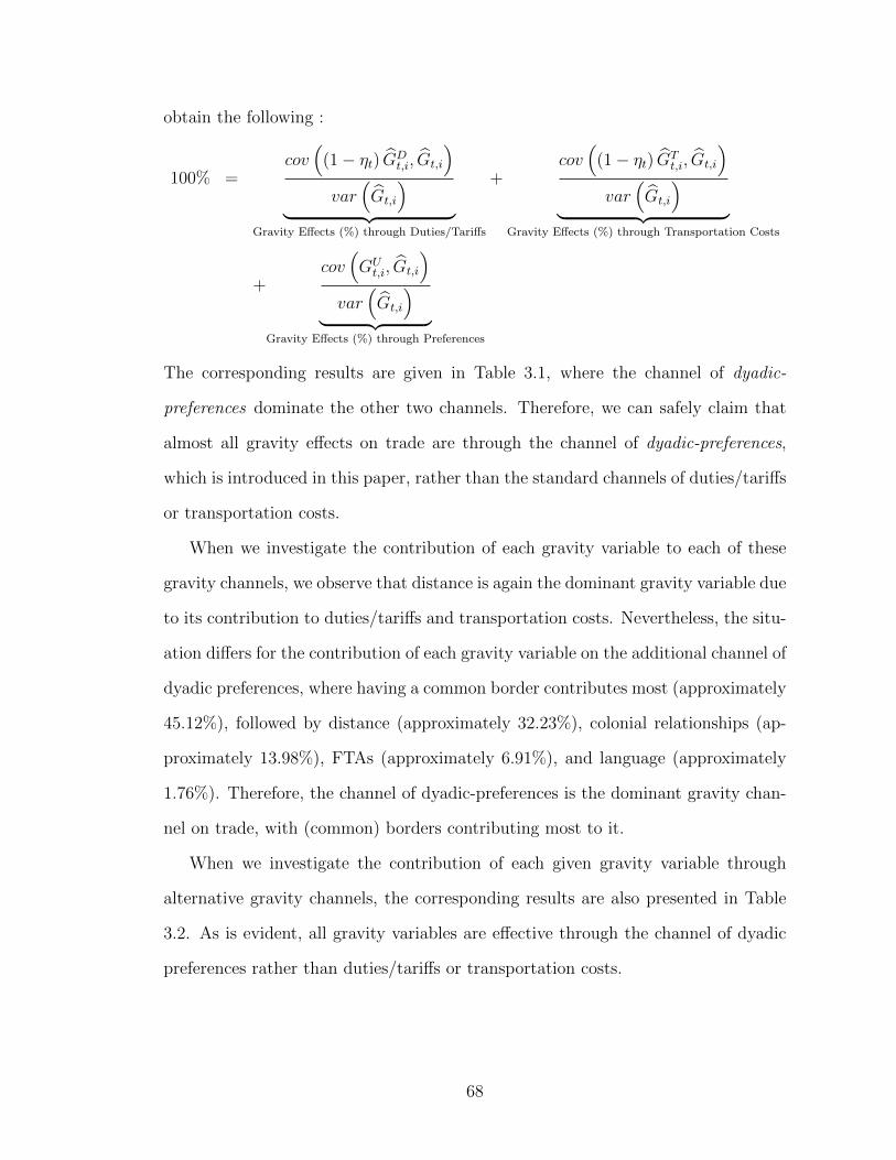
obtain the following :

100% =cov(

(1− ηt) GDt,i, Gt,i

)var

(Gt,i

)︸ ︷︷ ︸

Gravity Effects (%) through Duties/Tariffs

+cov(

(1− ηt) GTt,i, Gt,i

)var

(Gt,i

)︸ ︷︷ ︸

Gravity Effects (%) through Transportation Costs

+cov(GUt,i, Gt,i

)var

(Gt,i

)︸ ︷︷ ︸

Gravity Effects (%) through Preferences

The corresponding results are given in Table 3.1, where the channel of dyadic-

preferences dominate the other two channels. Therefore, we can safely claim that

almost all gravity effects on trade are through the channel of dyadic-preferences,

which is introduced in this paper, rather than the standard channels of duties/tariffs

or transportation costs.

When we investigate the contribution of each gravity variable to each of these

gravity channels, we observe that distance is again the dominant gravity variable due

to its contribution to duties/tariffs and transportation costs. Nevertheless, the situ-

ation differs for the contribution of each gravity variable on the additional channel of

dyadic preferences, where having a common border contributes most (approximately

45.12%), followed by distance (approximately 32.23%), colonial relationships (ap-

proximately 13.98%), FTAs (approximately 6.91%), and language (approximately

1.76%). Therefore, the channel of dyadic-preferences is the dominant gravity chan-

nel on trade, with (common) borders contributing most to it.

When we investigate the contribution of each given gravity variable through

alternative gravity channels, the corresponding results are also presented in Table

3.2. As is evident, all gravity variables are effective through the channel of dyadic

preferences rather than duties/tariffs or transportation costs.

68

In summary, if one ignores the existence of dyadic preferences, s/he may easily

think that the effects of gravity variables are through the measured trade costs; how-

ever, as we show in this paper, the consideration of dyadic preferences dramatically

changes the decomposition of gravity effects into their components.

3.5 Conclusions

Gravity variables such as distance, common borders, colonial ties, free trade

agreements, and language have been extensively used in empirical studies to cap-

ture the effects of trade costs. By using actual data on transportation costs and

duties/tariffs obtained from U.S. imports, this paper decomposes the overall effects

of gravity variables on trade through three gravity channels: duties/tariffs (DC),

transportation-costs (TC), and dyadic preferences (PC). When PC is ignored, as is

typical in the literature, we show that nearly all gravity effects are due to distance,

in which 29 percent are through DC and 71 percent through TC. However, the ad-

ditional channel of PC is introduced and shown to dominate other channels, with

common borders contributing approximately 45 percent, distance approximately 32

percent, colonial ties approximately percent, free trade agreements approximately 7

percent, and common language approximately 2 percent.

The results are robust to the specification of trade costs (e.g., multiplicative

versus additive trade costs) since we use actual data on transportation costs and

duties/tariffs to construct multiplicative trade costs. The results are also robust to

the consideration of any local distribution costs (that are shown to account for ap-

proximately half of overall trade costs in Anderson and van Wincoop, 2004), since we

already use trade data measured at both the source and destination docks. Accord-

ingly, whenever we proxy dyadic preferences by gravity variables in our regressions,

69

it is implied that they capture all other indirect costs of trade, such as time to ship

(as in Hummels and Schaur, 2013), search costs (as in Rauch, 1999), and infor-

mation barriers (as in Portes and Rey, 2005), although the source-country related

costs (such as contracting costs as in Evans, (2001) or insecurity as in Anderson and

Marcouiller, (2002)) are supposedly captured through data on source prices.

Significant policy implications follow. In particular, policy tools such as du-

ties/tariffs or investment in transportation technologies are implied to have an in-

sufficient impact on trade, as advocated in studies such as Harley (1988) and Irwin

and ORourke (2011). It is rather globalization itself that should be promoted to

shift the preferences of destination countries toward partner country products. Ul-

timately, consumers determine their preferences based on their perceptions of the

products rather than pure evidence of quality.

REFERENCES

[1] Anderson, J. E. (1979). A theoretical foundation for the gravity equation. TheAmerican Economic Review, 69(1), 106-116.

[2] Anderson, J. E. (2011) The Gravity Model. Annual Review of Economics, 3:133 -160.

[3] Anderson, J. E., & Marcouiller, D. (2002). Insecurity and the pattern of trade:An empirical investigation. Review of Economics and statistics, 84(2), 342-352.

[4] Anderson, J. E., & Van Wincoop, E. (2003). Gravity with gravitas: a solutionto the border puzzle. the american economic review, 93(1), 170-192.

[5] Anderson, J. E., & Van Wincoop, E. (2004). Trade costs. Journal of Economicliterature, 42(3), 691-751.

[6] Arkolakis, C., Costinot, A., & Rodrıguez-Clare, A. (2012). New trade models,same old gains?. The American Economic Review, 102(1), 94-130.

70

[7] Arkolakis, C., Costinot, A., Donaldson, D., & Rodrıguez-Clare, A. (2015). Theelusive pro-competitive effects of trade (No. w21370). National Bureau of Eco-nomic Research.

[8] Bagwell, K. and R. W. Staiger (1998) Regionalism and Multilateral Tariff Co-operation (with Kyle Bagwell), in John Piggott and Alan Woodland (eds.),International Trade Policy and the Pacific Rim, Macmillan, London.

[9] Baier, S.L., Bergstrand, J.H., 2001. The growth of world trade: tariffs, trans-port costs and income similarity. Journal of International Economics 53 (1),1–27.

[10] Baier, S. L., & Bergstrand, J. H. (2004). Economic determinants of free tradeagreements. Journal of international Economics, 64(1), 29-63.

[11] Bergstrand, J. H., Larch, M., & Yotov, Y. V. (2015). Economic integrationagreements, border effects, and distance elasticities in the gravity equation.European Economic Review, 78, 307-327.

[12] Berthelon, M., & Freund, C. (2008). On the conservation of distance in inter-national trade. Journal of International Economics, 75(2), 310-320.

[13] Broda, C., Weinstein, D.E., (2006). Globalization and the gains from variety.Quarterly Journal of Economics 121 (2), 541–585.

[14] Carrere, C., & Schiff, M. (2005). On the geography of trade. Revue economique,56(6), 1249-1274.

[15] Chaney, T. (2008). Distorted gravity: the intensive and extensive margins ofinternational trade. The American Economic Review, 98(4), 1707-1721.

[16] Disdier, A. C., & Head, K. (2008). The puzzling persistence of the distanceeffect on bilateral trade. The Review of Economics and statistics, 90(1), 37-48.

[17] Eaton, J., & Kortum, S. (2002). Technology, geography, and trade. Economet-rica, 70(5), 1741-1779.

[18] Evans, C. L. (2001). The costs of outsourcing. work. pap. 2001b. Board Gov.Fed. Reserve System.

71

[19] Feenstra, R.C., (1994). New product varieties and the measurement of interna-tional prices. The American Economic Review 84 (1), 157–177.

[20] Glick, R., & Rose, A. K. (2016). Currency unions and trade: A post-EMUreassessment. European Economic Review, 87, 78-91.

[21] Hakobyan, S., & McLaren, J. (2016). Looking for Local Labor-Market Effectsof NAFTA. Review of Economics and Statistics, forthcoming.

[22] Harrigan, J., (1996). Openness to trade in manufactures in the OECD. Journalof International Economics 40, 23–39.

[23] Head, K., & Mayer, T. (2014). Gravity Equations: Workhorse, Toolkit, andCookbook, Ch. 3 in Handbook of International Economics, Gopinath, G, E.Helpman and K. Rogoff (Eds), Vol. 4, 131-95.

[24] Head, K., Ries, J., (2001). Increasing returns versus national product differen-tiation as an explanation for the pattern of U.S.–Canada trade. The AmericanEconomic Review 91 (4), 858–876.

[25] Hesse, M., & Rodrigue, J. P. (2004). The transport geography of logistics andfreight distribution. Journal of transport geography, 12(3), 171-184.

[26] Hummels, D., (2001) Toward a geography of trade costs. mimeo.

[27] Hummels, D. L., & Schaur, G. (2013). Time as a trade barrier. The AmericanEconomic Review, 103(7), 2935-2959.

[28] McCallum, J. (1995). National borders matter: Canada-US regional trade pat-terns. The American Economic Review, 85(3), 615-623.

[29] Obstfeld, M., & Rogoff, K. (2001). The six major puzzles in internationalmacroeconomics: is there a common cause?. In NBER Macroeconomics An-nual 2000, Volume 15 (pp. 339-412). MIT press.

[30] Odell, R. M. (1911). Cotton goods in Spain and Portugal (No. 46). Govt. print.off..

[31] Portes, R., & Rey, H. (2005). The determinants of cross-border equity flows.Journal of international Economics, 65(2), 269-296.

72

[32] Rauch, J. E. (1999). Networks versus markets in international trade. Journalof international Economics, 48(1), 7-35.

[33] Ravenstein, E. G. (1889). The laws of migration. Journal of the royal statisticalsociety, 52(2), 241-305.

[34] Romalis, J. (2007). NAFTA’s and CUSFTA’s Impact on International Trade.The Review of Economics and Statistics, 89(3), 416-435.

[35] Rose, A. and Spiegel, M. 2011. The Olympic Effect. The Economic Journal121(553): 652–677.

[36] Simonovska, I., & Waugh, M. E. (2014). The elasticity of trade: Estimates andevidence. Journal of international Economics, 92(1), 34-50.

[37] Tinbergen, J. (1962). Shaping the world economy; suggestions for an interna-tional economic policy. Books (Jan Tinbergen).

[38] Woudsma, C. (1999). NAFTA and Canada–US cross-border freight transporta-tion. Journal of Transport Geography, 7(2), 105-119.

[39] Yilmazkuday, H. (2014). Mismeasurement of Distance Effects: The Role ofInternal Location of Production. Review of International Economics, 22(5),992-1015.

[40] Yilmazkuday, H. (2016a). A solution to the missing globalization puzzle bynon-ces preferences. Available at SSRN 2258804.

[41] Yilmazkuday, H. (2016b). Constant versus variable markups: Implications forthe Law of one price. International Review of Economics & Finance, 44, 154-168.

[42] Yilmazkuday, D., & Yilmazkuday, H. (2014). Bilateral versus Multilateral FreeTrade Agreements: A Welfare Analysis. Review of International Economics,22(3), 513-535.

[43] Zellner, A., & Theil, H. (1962). Three-stage least squares: simultaneous esti-

mation of simultaneous equations. Econometrica: Journal of the Econometric

Society, 54-78.

73

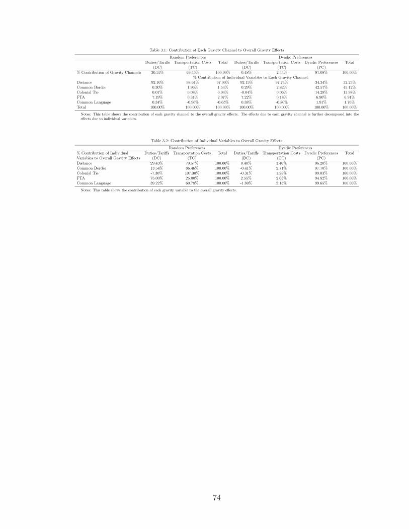
Table 3.1: Contribution of Each Gravity Channel to Overall Gravity Effects

Random Preferences Dyadic PreferencesDuties/Tariffs Transportation Costs Total Duties/Tariffs Transportation Costs Dyadic Preferences Total

(DC) (TC) (DC) (TC) (PC)% Contribution of Gravity Channels 30.55% 69.45% 100.00% 0.48% 2.44% 97.08% 100.00%

% Contribution of Individual Variables to Each Gravity Channel:Distance 92.16% 98.61% 97.00% 92.15% 97.74% 34.34% 32.23%Common Border 0.30% 1.96% 1.54% 0.29% 2.82% 42.57% 45.12%Colonial Tie 0.01% 0.08% 0.04% -0.04% 0.06% 14.28% 13.98%FTA 7.19% 0.31% 2.07% 7.22% 0.18% 6.90% 6.91%Common Language 0.34% -0.96% -0.65% 0.38% -0.80% 1.91% 1.76%Total 100.00% 100.00% 100.00% 100.00% 100.00% 100.00% 100.00%

Notes: This table shows the contribution of each gravity channel to the overall gravity effects. The effects due to each gravity channel is further decomposed into theeffects due to individual variables.

Table 3.2: Contribution of Individual Variables to Overall Gravity Effects

Random Preferences Dyadic Preferences% Contribution of Individual Duties/Tariffs Transportation Costs Total Duties/Tariffs Transportation Costs Dyadic Preferences TotalVariables to Overall Gravity Effects (DC) (TC) (DC) (TC) (PC)Distance 29.43% 70.57% 100.00% 0.40% 3.40% 96.20% 100.00%Common Border 13.54% 86.46% 100.00% -0.41% 2.71% 97.70% 100.00%Colonial Tie -7.30% 107.30% 100.00% -0.31% 1.28% 99.03% 100.00%FTA 75.00% 25.00% 100.00% 2.55% 2.63% 94.82% 100.00%Common Language 39.22% 60.78% 100.00% -1.80% 2.15% 99.65% 100.00%

Notes: This table shows the contribution of each gravity variable to the overall gravity effects.

74

Figure 3.1: Descriptive Statistics: Effects of Distance

75

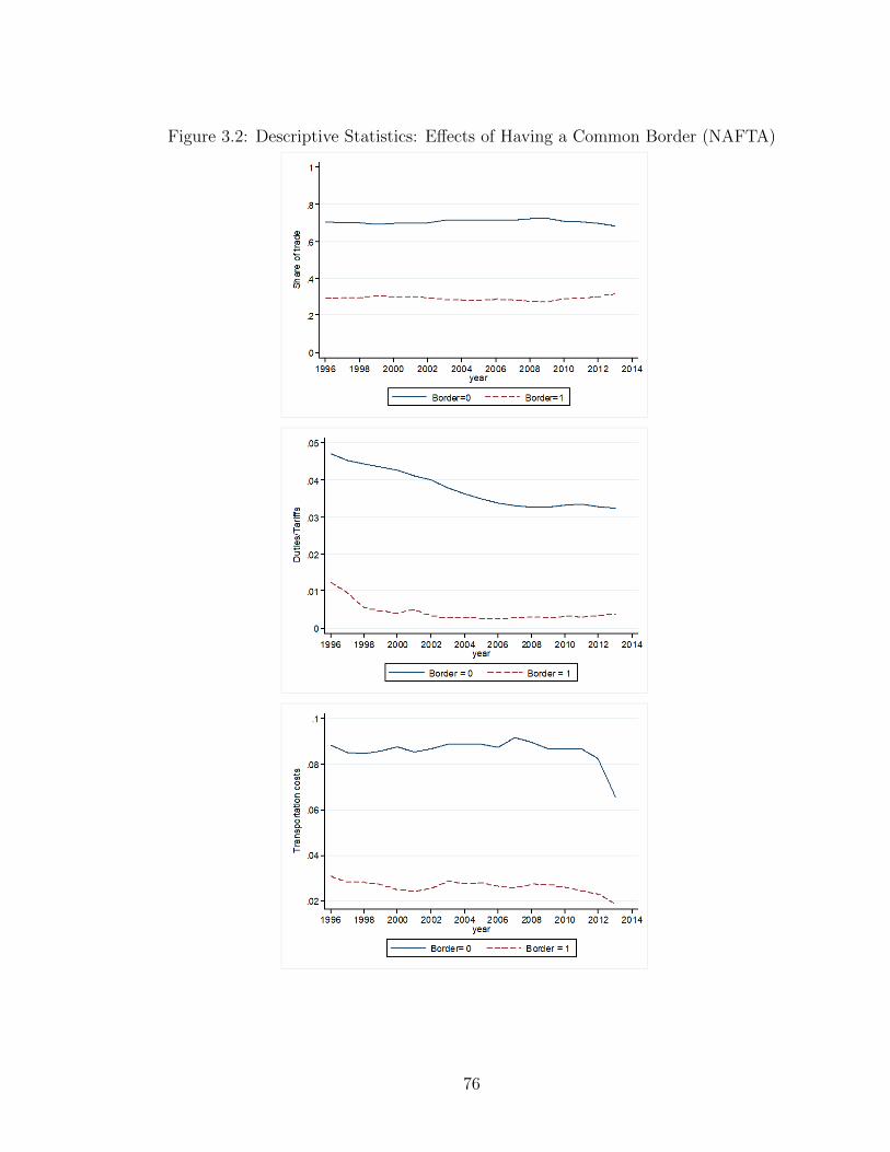
Figure 3.2: Descriptive Statistics: Effects of Having a Common Border (NAFTA)

76

Figure 3.3: Descriptive Statistics: Effects of Having a Colonial Relationship

77

Figure 3.4: Descriptive Statistics: Effects of Having a Free Trade Agreement

78

Figure 3.5: Descriptive Statistics: Effects of Having a Common Language

79

Figure 3.6: Estimates of Distance Elasticity between 1996-2013

80

Figure 3.7: Common-Border Coefficient Estimates between 1996-2013

81

Figure 3.8: Colonial-Relationship Coefficient Estimates between 1996-2013

82

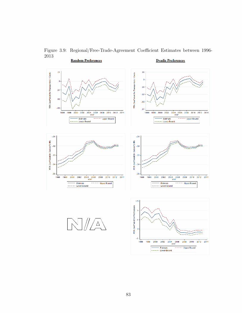
Figure 3.9: Regional/Free-Trade-Agreement Coefficient Estimates between 1996-2013

83

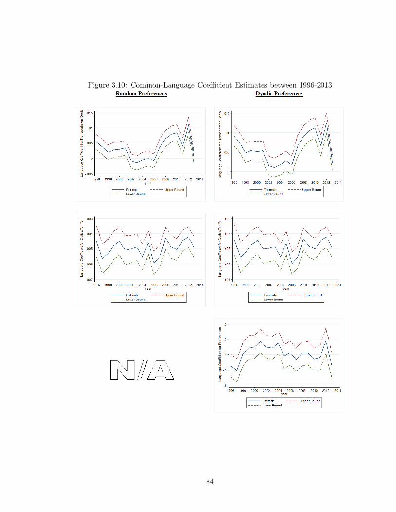
Figure 3.10: Common-Language Coefficient Estimates between 1996-2013

84

CHAPTER 4

INSTITUTIONAL QUALITY AND MIGRATION FLOWS

4.1 Introduction

Similar to international trade, international migration is also a key component of

modern globalization. The number of international migrants worldwide has reached

258 million in 2017. It was 220 million in 2010, and 173 million in 2000 according to

the United Nations International Migration Report (2017). As documented by the

OECD International Migration Outlook (2017), 4.7 million permanent immigrants

resided in the OECD countries in 2015. The number is expected to grow rapidly in

the next few years. United States, Germany, United Kingdom, Canada, and France

have been the top five OECD countries with permanent inflow of foreigners in recent

years. Meanwhile, the migration inflow pattern in the OECD countries has changed

drastically. Before the 1980s, labor-intensive migration took over the majority of

the migration inflow. In recent years, family-based immigrants and asylum-seekers

from developing and underdeveloped countries have become the main source of the

overall migration inflow (Chiswick and Hatton, 2003).

International migration and globalization have become unavoidable trends. Stud-

ies suggest that the patterns and reasons for global migration have changed in recent

years (Karemera et al., 2000). What exactly power the migration movement? Tradi-

tional gravity analysis is able to explain the initiation of migration by highlighting

migration costs and demographic factors. However, in the era in which we live,

migration is driven by complicated social and economic motivations. Docquier and

Rapoport (2012) express a concern that migration mainly flows from developing and

underdeveloped countries to developed countries and thus causes brain-drain effects

on the human capital stock of underdeveloped countries.

85

It seems that the institutional quality of a country affects the human capital flow

and has different effects in the destination and source countries. Different migration

studies (Docquier and Rapoport, 2012; Dreher et al., 2011; Dimant et al., 2013;

Fitzgerald et al., 2014; Hatton and Williamson, 2003; Mayda, 2010) focus on only

one or some aspects of the institutional quality for a country, such as political insta-

bility, social and economic issues, conflicts, and corruption. This paper contributes

to the existing literature by constructing a set of institutional quality indexes to

consider all the possible socioeconomic and political conditions.

Governments need to provide guidance as to about how the migration decision is

made, and how to understand migration and use it for the country’s own advantage.

Immigration policies can highly impact the labor markets, economic development,

and domestic markets on in both destination OECD countries and source countries.

To explain the determinants of migration flows, the literature emphasizes that tra-

ditional gravity variables, such as the distance between destination and source coun-

tries, are key factors that determine the migration flows. Geographical distance is

the most common proxy for migration costs in studies such as Borjas (2000), Hat-

ton and Williamson (2003), and Fitzgerald et al. (2014). Other common gravity

variables are also used in the most migration studies as proxies for cultural barriers

in migration, such as common borders, common languages, and colonial ties.

In addition to the common proxies for migration costs, the literature emphasizes

that wage differences between the destination and source countries may determine

the migration decisions, also (Borjas, 1994; Borjas, 2000; Chiswick, 1986; Chiswick,

2000; Massey et al., 1999). Most recent studies pay attention to social networks that

potentially connect family and friends. Therefore, immigration stocks are one of the

most important explanatory variables in studies such as Fitzgerald et al. (2014),

Karemera et al. (2000), Mayda (2009), and Pedersen et al. (2008).

86

In recent years, migration studies have focused on the specific factors that af-

fect migration decisions in the destination or source countries. Pull factors are

those destination-specific characteristics that attract potential emigrants from cer-

tain source countries. These studies concern socioeconomic and demographic factors

and political institutional conditions in destination countries that affect the migra-

tion decisions of potential immigrants. Push factors are those source-country-specific

characteristics that dissuade citizens residing in source countries from migrate out.

Mainly political conditions, especially political instabilities in source countries, are

main pushing factors that drive migration flows (Fitzgerald et al., 2014; Mayda,

2009; Pedersen et al., 2008).

This paper is motivated by recent advanced studies emphasizing pull and push

factors of migration flows. By using an updated OECD immigration inflow data

from 1984 to 2015, and a set of novel institutional quality indexes, this paper ex-

plores the effects of institutional quality on the immigration rate. The indexes come

from The International Country Risk Guide (ICRG), which comprises 22 factors

in political, economic, and financial categories to portray the overall risk of an in-

stitution. Among these indexes, we mainly focus on pull effects of socioeconomic

conditions, which come from destination countries, and pushing effects from source

countries, including foreign debt, government stability, budget, internal conflicts,

and corruption conditions.

These institutional quality indexes describe both the destination and source

country characteristics in details. The existing literature suggests that main pulling

effects come from income advantages and employment conditions in the destination

country. Specifically, Pedersen et al. (2008) conclude that they find an effect of em-

ployment on migration inflow in destination countries but no such impact in source

countries. However, regarding the push factors, Karemera et al. (2010) suggest

87

that domestic political conditions are the main factors that determine emigration

outflows. Mayda (2009) also notes the existence of the asymmetrical pull and push

factors, where income level and employment conditions in source countries have in-

significant effects on emigration outflows. On the other hand, political issues and

potential government risks will drive potential emigration outflows. Therefore, this

paper mainly uses the destination country socioeconomic condition index to proxi-

mate the pulling effects and uses five other institutional quality indexes to describe

political and government risks to proxy push factors from source countries.

The estimation results in this paper are in conformity with previous studies.

Higher institutional quality in the destination countries increases the immigra-

tion rate. Specifically, higher employment rate and market confidence and a lower

poverty level (socioeconomic condition) draw attention from potential immigrants.

On the other hand, lower institutional quality in source countries decreases potential

emigration outflows. The results provide the governments some guidance regarding

their immigration policies and economic development. The most important thing for

developing and underdeveloped countries is to retain their labor forces and citizens.

For example, corruption risks affect the potential emigration outflow. As noted by

Dimant et al. (2013), corruption control would be an important policy tool to pre-

vent domestic brain drain, where the country in need for development can keep the

talents. Nevertheless, institutional quality is important for countries to maintain

their populations and labor forces. The key goals to prevent emigration outflows

are to keep the government and political structure stable, cease domestic conflicts,

control corruption, and manage the budget and debt for economic development.

The rest of the paper is organized as follows. Section 2 provides the empiri-

cal estimation methodologies with random effects and fixed effects estimators. The

variable selection is also described in this section. Section 3 introduces the data

88

source and constructs data according to the empirical model. Section 4 summarizes

the empirical results, together with many robustness checks. Section 5 concludes.

4.2 Empirical Methodology

The common framework of the migration models is motivated by the idea that

individuals will maximize their utility by choosing which country to live in. Their

behaviors regarding where to move depend on three key components: the char-

acteristics of the potential migrants, source-country-specific pushing effects, and

destination-country-specific pulling effects (Borjas, 1987; Borjas, 1989; Karemera et

al., 2000; Mayda, 2010; Zavodny, 1997).

The standard theoretical migration models, however, do not restrain or define

the proxy variables for the three components. Therefore, the generalized migration

model has the following form:

mijt = β1Iijt + β2Sit + β3Djt + uijt (4.1)

where mijt is the number of immigrants moving from the source country i to the

destination country j at time t. Iijt is a vector of factors that describe the net gain

of migrants if they decide to move from source country i to destination country j

at time t. Pedersen et al. (2008) also separate Iijt into two parts. One denotes

the network effects of the potential immigrants from the destination country. The

obvious proxy variable is the immigration stocks from the source county to the

destination country. The other one represents the migration costs incurred when

moving from source country i to destination country j. Sit and Djt are vectors of

pushing and pulling factors in the source country i and destination country j that

affect the decisions of potential migrants whether to choose to move or stay. uijt is

a white noise with zero mean and variance σ.

89

For the empirical analysis, the literature proposes different variables to indicate

the three components of the migration function (see Borjas, 1989; Fitzgerald et al.,

2014; Gastil, 1978; Greenwood, 1975; Hatton and Williamson, 2003; Mayda, 2010).

As summarized by Karemera et al. (2000), a complete migration gravity model

contains three groups of variables: traditional gravity variables, such as distance,

common languages, common borders, and colonial ties, which account for the costs

of migration. Variables related to the economic and political conditions in the

source country push the potential emigrants to leave, whereas variables related to

the economic and political conditions in the destination country pull the potential

immigrants to arrive. In this paper, we try to examine the effects of institutional

quality on migration flows. Accordingly, our empirical specification of the migration

model has the following form:

mijt

Pit= β0 + β1

STOCKijt

Pit+ β2

GDPperCapitajtGDPperCapitait

+ β3ldistij + β4borderij + β5colonyij

+ β6comlangij + β7SocioeconomicConditionsjt + β8ForeignDebtit

+ β9BudgetBalanceit + β10GovernmentStabilityit + β11InternalConflictsit

+ β12Corruptionit + uijt

(4.2)

where the new dependent variablemijtPit

is the emigration rate. We normalize the

migration flows by the population of the source country i. This is consistent with

the model derived by Borjas (1999), and Clark et al. (2007), in which the emigration

rate is used to compare the relative sizes of the migration flows with the existence

of heterogeneous source country sizes. The immigration stock variable to proxy the

existing network effects is also divided by the population size of the source country.

GDPperCapitajtGDPperCapitait

shows the inequality in GDP per capita from the destination country j

and source country i. ldistij is the natural logarithm of the great circle distance be-

tween the source and destination countries. borderij is a dummy variable that takes

90

the value of 1 if the source and destination countries share a land border. colonyij

is a dummy variable that equals 1 when the source and destination countries had

colonial ties in the past. comlangij is also a dummy variable that takes the value of

1 if the source and destination countries use a common language. All four standard

dummy variables approximate the migration costs to move from source country i

to destination country j. SocioeconomicConditionsjt is an institution quality in-

dex showing the socioeconomic condition of destination country j. ForeignDebtit,

BudgetBalanceit, GovernmentStabilityit, InternalConflictsit, and Corruptionit

are a vector of institutional quality to show the foreign debt condition, government

budget availability, internal conflicts, and the corruption level of the government in

source country i. uijt is an error term with zero mean and a constant variance σ.

In this paper, we use the country-time specific institutional quality indexes in

equation (4.1) to explain the push and pull effects from the source country and

destination country. It is unavoidable for us to solve the endogeneity issue of the

regression, since there are reverse-causality concerns, where not only the difference

of the GDP per capita in two countries affects the decision of potential immigrants

and draws immigrants to the destination country but also more immigrants flow can

impact labor market structural and GDP in the destination country. Another plau-

sible problem is over/underestimating the model with too many/few independent

variables. To solve the endogeneity issue, we include multiple fixed effects, combined

with lagging one year for all time-varying independent variables to account for the

time lag when the immigrants make decisions.

91

4.3 Data

In this section, we will construct the data by combining immigration flow, immi-

gration stock, itemized population inflows, institutional quality indexes, and other

country-pair specific variables from different sources. All the immigration data

comes from the International Migration Statistics (IMS) database for the OECD

countries. This data is the extension of the widely used OECD immigration data

used in some recent studies 1. This paper uses data of immigrants inflow from 134

source countries to 33 OECD countries in the period from 1984 to 2015. It is im-

portant to note that the data collection is conducted by each county separately, and

the definition of migrants is different across countries 2, thus, the immigration inflow

data are not perfectly comparable across OECD countries. Therefore, by controlling

the heterogeneity at the destination-country level, the effects of institution quality

can still be compared with our data over time. The collections of immigration inflow

data from each OECD country are also different with respect to the availability of

the time periods and the source countries. For example, the United States started

to document the immigration inflow from the United Kingdom in 1984. Meanwhile,

it only has immigration inflow data for Austria and Denmark available starting in

1997. Some OECD countries have already started to document immigration data

specifying the country of origin since the 1960s, whereas many small-sized traditional

1Pedersen et al. (2008) use immigration inflow and stock data obtained from 26destination OECD countries during the period 1989-2000. Mayda (2010) uses a similardata that provides bilateral immigration inflow into 14 core OECD countries in the period1980-1995. While Fitzgerald et al. (2014) specifically include labor inflow into 18 OECDcountries from over 170 source countries from the period 1980-2006.

2Majority of the OECD countries categorize and define immigrants by their countryof birth. Some define it based on the nationality and citizenship of the immigrants (suchas France and Austria).

92

low migration-impacted OECD countries have only started it since 1995, such as

Austria.

Compared to existing studies using OECD immigration inflow, our data has sev-

eral extensions and advantages. As mentioned above with more destination OECD

countries included in the data, and extending the available years to 2015, our data

set contains 54,722 observations on immigration inflow. The majority of the studies

use the immigration inflow data even though there are concerns about comparability

due to the complicity of definitions. Fitzgerald et al. (2014) use labor migrants data

to exam the political considerations in shaping migration decisions of the potential

labor migrants. We provide extra variables to allow us to entirely understand the

migration behaviors. In addition to the immigration inflow and immigration stock

yearly data, we also include worker inflow, seasonal worker inflow, and foreign stu-

dent inflow yearly data. Within the discussion of the institution quality, it not only

affects the general immigration inflows, but also impacts certain groups of immi-

grants, such as workers who see financial security of an institution more important

than the political openness.

Our data also includes a set of standard independent variables commonly used

in migration studies. The population and GDP per capita values for the destina-

tion country j and source country i come from World Bank Open Data Catalog3.

Four standard gravity variables (ldistij, borderij, colonyij, and comlangij) are from

Reuven and Rose (2016).

To explain the immigration rate from institutional quality, we apply the country

risk data obtained from the International Country Risk Guide (ICRG). The specific

variable that we use to explain the pulling effects from the destination countries is

SocioeconomicConditions. The reason is that majority of the OECD destination

3https://data.worldbank.org/

93

countries share similar political and economic attributes, where they tend to have

low external and internal conflicts, low military impact in politics, and low religion

tensions. On the economic side, OECD countries have stable financial systems and

mature economic growth rates. The attributes that set all the OECD countries

apart are their different domestic unemployment rates and working conditions, con-

sumer market structures and poverty levels. The socioeconomic conditions calculate

the risk of a country exactly with these three sub-components: unemployment, con-

sumer confidence, and property.

The institutional quality used to explain the pushing effects from the original

countries are considered in terms of both political risks and economic risks. The

ForeignDebt variable indicates the foreign debt as a percentage of GDP in destina-

tion countries, the variable BudgetBalance calculates the estimated central govern-

ment budget balance and grants for a given year as a percentage of the estimated

GDP in destination countries. These two indexes indicate the economic risks of a

country where the potential emigrants worry about the domestic economical condi-

tions and the capability that their government can improve the living and working

conditions of its citizens. The variables GovernmentStability, Internalconflicts,

and Corruption indicate political risks for the potential institute to loose its po-

tential emigrants. Specifically, GovernmentStability assesses the unity, legislative

strength, and the popularity among citizens of the government. Internalconflicts

assesses whether an country is dealing with civil war/coup threat, terrorism/political

violence, and civil disorders. Corruption measures the degree of corruption within

the political system of the country.

As we introduced the institutional quality variables above, it is obvious to con-

sider that potential emigrants will change their decisions of whether to stay or leave

their home countries since the variables reflect a country’s economic and political

94

conditions, where less stabilized and more corrupt governments tend to encour-

age potential emigrants to move outside of their home countries. Moreover, when

potential immigrants make the decision of where to relocate, they look for better

socioeconomic conditions of a potential destination country, where the labor market

thrives and the consumers are confident.

4.4 Empirical Results

4.4.1 Benchmark

Table 4.4 reports the benchmark results. With the dependent variable being

the natural logarithm of the emigration rate (inflow foreign population from source

country i to destination country j divided by the population of source country i) and

using the random effects Generalized Least Squares (GLS) estimator, the estimates

are shown to be consistent with the predictions and previous literature.

First, the control variables of the baseline models in column 1 and column 2

consist of the rate of immigration stock, GDP per capita ratio, and common grav-

ity variables that are widely used in the immigration literature, such as the log

geographic distance, land borders, colonial ties, and common languages. The re-

sults show that the immigration rate is positively related to the (log) percentage

of existing immigration stocks at destination country to the source country popula-

tion. Specifically, every 1 percent increase in the immigration stock rate increases

by approximately 0.8 percent the immigration rate to the destination country. This

denotes the network effects of the immigration rate, where the existing immigration

stock in the destination country provides useful information and helps potential im-

migrants overcome language barriers, asymmetric information on the labor market.

95

All of these are reasonable to draw attentions from the potential immigrants and

cause increases in the immigration rate. Moreover, even though the network effects

from the existing immigration stock are prominent and positive, the increasing rate

of immigration (0.8 percent) is still smaller than the increasing rate of immigration

stock (1 percent).

The model also obtains similar results where the (log) GDP per capita differ-

ences between destination and source countries affect the immigration rate posi-

tively. Specifically, every 1 percent increase in GDP per capita ratio between desti-

nation country and source country will lead to an approximately 1 percent increase

in immigration rate. Considering the case that GDP per capita in the destination

country increases by 1 percent, whereas the GDP per capita in the source country

is unchanged, there will be a 1 percent increase in the immigration rate. The bigger

the GDP per capita gap between destination and source countries is, the higher

income the destination country generally has, or the lower the income the source

country has. In either case, potential immigrants have incentives to move to the

destination country. Comparing columns 3 and 6, the coefficients in front of the

control variables do not have significant changes, except for lnGDPperHeadRatio.

As the evidence in column 6, in which case all control variables are included to avoid

any omitted variables bias, the coefficient value of lnGDPperHeadRatio remains

significant but decreases to 0.632 from 1.067.

For the common gravity variables, we explore the effects of the geographic (dis-

tance and common borders) and cultural (colonial ties and common language) vari-

ables on the costs incurred during the migration. As expected, the geographical

distance has a negative relationship with the immigration rate, and both colonial

ties and common language have positive effects on the immigration rate. Com-

mon borders do not have significant effects on the immigration rate in any baseline

96

model. More specifically, a 1 percent increase in the geographical distance between

the destination and source country causes a decrease in the immigration rate of ap-

proximately 0.075 percent. Keeping all other factors equal, by doubling the distance

between the destination and source country, there will be a 7.5 percent increase in

potential emigrants from the source country who choose to move to the destination

country. Colonial ties and common language between the source country and the

destination country will improve the immigration rate by approximately 20 percent

and 14.5 percent. Moreover, the significant effects of colonial ties and common lan-

guage on immigration rate in Table 1 are consistent with different models. This

result is inconsistent with the findings of Mayda (2010), where common language

and colonial ties do not appear to play any significant role in determining the im-

migration rate.

In columns 3 through 6, one destination-country institution quality index and

five source-country institutional quality indexes are added one by one to the base-

line model. These coefficients of added independent variables are aligned with

the expectation. Specifically, the coefficient of SocioeconomicConditions is 0.0898

and statistically significant at the 1% level. Since the institutional quality in-

dex describes the socioeconomic pressures in the destination country measured in

the scale from 0 to 12, this estimation result implies that a 1 point increase in

SocioeconomicConditions in the destination country is associated with an almost

9 percent increase in the immigration rate.

All the five source-country institutional quality indexes have negative effects on

the immigration rate. Due to the fact that these push factors from the source

country should affect the decision-making of potential emigrants, higher institu-

tional quality in the source country would decrease the emigration rate. As shown

in column 6, with all control variables, the coefficient of ForeignDebt is approx-

97

imately -0.02, which means a 1 point increase in ForeignDebt index 4 from the

source country is associated with around 2 percent decrease in immigration rate.

Similarly, 1 point increase in BudgetBalance index5 from the source country is as-

sociated with around 0.9 percent decrease in the immigration rate. 1 point increase

in GovernmentStability index6 from the source country is associated with around

1.4 percent decrease in the immigration rate. 1 point increase in InternalConflicts

index7 is associated with around 2.2 percent decrease in the immigration rate. Last

but not least, 1 point increase in Corruption index8 is associated with around 2.3

percent decrease in the immigration rate.

4.4.2 Robustness

Generally, endogeneity is the first problem in panel analyses. Especially in

three-dimensional data, both unobserved destination-country and source-country

4ForeignDebt measures the foreign debt services as a percentage of GDP. The valueof the ForeignDebt index is on a scale from 0 to 10. The bigger the index, the higher theinstitutional quality the country has.

5BudgetBalance measures the central government budget balance (including grants)for a given year as the percentage of the estimates GDP. The value for the BudgetBalanceindex ranges from 0 to 10. The bigger the index the higher the institutional quality thecountry has.

6GovernmentStability measures the ability of the government to carry out declaredprograms and stay in office. It also consists of three assessment: government unity, leg-islative strength, and popularity. The value for the GovernmentStability index rangesfrom 0 to 12. The bigger the index, the higher the institutional quality a country has.

7InternalConflicts measures political violence in the country and the potential impactof it on governance. The value for the InternalConflicts index ranges from 0 to 12. Thebigger the index, the higher the institutional quality the country has.

8Corruption measures financial corruption within country’s political system. Thevalue for the Corruption index ranges from 0 to 6. The bigger the index, the higher theinstitutional quality the country has.

98

specific effects could cause a biased estimation. There are several concerns regard-

ing the omitted variable problem. First, to determine the cause of migration (im-

migration rate), we look at the potential pull factors from the destination country.

SocioeconomicConditions may have a positive effect on the immigration rate. How-

ever, it is unclear whether a potential immigrant would be more willing to relocate

to a destination country with better socioeconomic conditions or whether they are

attracted by some other attributes that a destination country has because of good

socioeconomic conditions. For the same reason, the push factors of institutional

quality from source country might be a possible reason to push potential emigrants

to relocate to other countries. It is also possible that other unobserved push factors

lead to relocation of potential emigrants. To solve the omitted variables issue, Table

5 introduces several groups of dummy variables to control for different combinations

of fixed effects.

Table 4.5 is based on the model in column 6 of Table 4.4 which includes all

control variables. The destination-country fixed effects and source-country fixed

effects are introduced in column 1 to account for the unobserved destination and

source country specific effects. Compared with the random effects model in the

column 6 of Table 4.4, there is no sign change in the coefficients, and all the co-

efficients are significant except for border and BudgetBalance. The coefficients

of ln(immigration stock/source population), ldist, colony, and comlang are un-

changed. The coefficient of lnGDPperHeadRatio increases from 0.632 to 0.998,

which means the effect of GDP per capita differences on immigration rate is big-

ger. Regarding the institutional quality indexes, we notice that the pulling effects

are increased with the coefficient changes from 0.0898 to 0.0966. However, source-

country institutional quality indexes have less pushing effects in general after the

fixed effects of destination and source countries are introduced.

99

Column 2 of Table 4.5 introduces another set of dummy variables as time fixed

effects. In addition to the unobserved destination-country and the source-country

specific effects, the time-varying unobserved effects are also considered in this model.

The coefficients in the entire column 2 are unchanged compared to the random ef-

fects model. In the next column, we consider the omitted bias comes from the

unobserved country-pair specific effects. The purpose of this set of dummy vari-

ables is to perfectly replace the gravity/dyadic variables in the model. Therefore,

the gravity variables are omitted in columns 3, 4, and 5, in which country-pair fixed

effects are included. Since country-pair specific attributes that affect the immigra-

tion rate are explained using country-pair fixed effects, the country-time specific

institutional qualities will do a better job at explaining the immigration rate. Col-

umn 4 also includes time fixed effects in addition to the country-pair fixed effects.

Column 5 incorporates time, destination-country, source-country, and country-pair

fixed effects. We can see that the network effects from the immigration stock have

not changed compared with the random effect model with the coefficient of 0.806.

The GDP per capita difference from the destination and source country still has

strong effects on immigration rate, also, with a coefficient of 0.831. For the pull and

push factors, both models in the column 4 and 5 are the same, where socioeconomic

conditions in the destination country affect the immigration rate positively, whereas

the foreign debt rate and the budget balance, government stability, internal conflicts,

and corruption level of the source country have negative effects on the immigration

rate.

Table 4.6 considers the reverse causality issue for this panel analysis. This is

also an unavoidable problem when we consider the estimation results. For example,

the coefficient of the immigration stock rate is expected to be positive in the esti-

mation, because the model predict that positive shocks on immigration stock will

100

increase the network effects between the potential immigrants and the immigration

stocks from the same source country. However, this positive relationship between

immigration stock rate and immigration rate may represent the causation of these

two variables in the opposite direction, where simply more immigration will increase

the immigration stock rate in the destination country. Another example would be

the pull effects of the socioeconomic condition in the destination country. A better

socioeconomic environment means a better labor market and higher market confi-

dence. These attributes all draw immigrants’ attention and bring them in. However,

it is plausible to argue that the incoming immigrants represent a strongly motivated

labor force and high purchasing power, and therefore help to build up the strong

socioeconomic conditions in the destination country.

Due to the reverse causality issue, it is possible for underestimation to occur.

In Table 4.6, we use lagged values for all control variables 9 to explain immigration

rate. It is more realistic to claim that the institutional qualities last period will have

impacts on the migration decision this period, since people make decisions based on

past information and experiences. However, the immigration decision in this period

will have no effect on past institutional qualities.

As shown in columns 1 to 5, we run the regressions from Table 4.5 with the

same fixed effects. The results of the new estimations have unchanged signs for

all coefficients and are significant. border has a significant and negative effect on

the immigration rate, compared with having an insignificant effect in old models.

Specifically, having a land border between destination and source country will lead

to a 15.2 percent decrease in the immigration rate. A plausible explanation is that

most countries that share borders with an OECD country are also developed coun-

9Notice that the lagged value for gravity/dyadic variables such as ldist, border,colonry, and comlang are unchanged because they are not time-related variables.

101

tries or OECD countries themselves. In these cases, the immigration rate would be

higher if the source country were a developing country, where institutional quality

tends to be lower. The effects of colony and comlang are significantly larger than in

Table 4.5. Having a colonial tie increases the immigration rate by 51.3 percent, and

sharing a common language increases the immigration rate by almost 31 percent.

The coefficients of immigration stock rate and GDP per capita differences are

significantly smaller compared with the estimation in Table 5. For the institutional

quality indexes, socioeconomic condition as a pull factor from the destination coun-

try has a larger impact on the immigration rate, with a coefficient change from 0.089

to 0.101. The push effects also have larger effects on the immigration rate for all

source country institutional quality indexes.

4.4.3 Further Robustness

Alternative Migration Data

One of the innovation in this paper is the alternative migration data we use to

explain the importance of institutional quality on migration decision making. After

examining the effects of institutional qualities on immigration rate, we look closely

into how the different institutional qualities will affect migration decisions for dif-

ferent demographics.

Table 4.7 reports the effects of institutional qualities on the inflow of foreign

workers. The most important difference for the inflow of foreign workers is that

they rely less on network effects. However, their decisions about whether to move

to a destination country reply strongly on economic reasons. Specifically, according

to the coefficients of GDP per capita difference, workers are more than twice as

sensitive to GDP per capita differences between the destination and source coun-

102

try. A 1 percent increase in GDP per capita difference leads to an approximately

2 percent increase in the inflow of foreign workers. Moreover, the pull effects from

destination-country socioeconomic conditions are 5 times larger for inflow foreign

workers compared with overall immigrants. On the other hand, push factors from the

source country play lesser roles in emigrants’ decision-making. Only ForeignDebt,

GovernmentStability, and InternalConflicts have weak but significant effects on

foreign workers’ relocation decisions. In addition, the standard gravity variables

affect foreign workers’ reallocation costs more. Having colonial ties and a common

language play larger roles in deciding whether workers choose to relocate.

Table 4.8 introduces the effects of institutional qualities on seasonal foreign work-

ers. The estimation shows that most of the coefficients are insignificant. Pull factors

from destination country have no influence on the seasonal foreign workers’ decision-

making. However, their domestic economic conditions have weak but positive effects

on seasonal workers migrating out for temporary seasonal jobs. Gravity variables

are the only predominant factors that affect seasonal workers. Colonial ties increase

the seasonal worker inflow to the destination country by 140 percent. It is more

than double the size compared to other non-colonial relationship countries. How-

ever, common language decreases the seasonal workers inflow by almost 70 percent

using our data set.

Another group of special categories of immigrants is inflow foreign students.

They migrate to take advantages of the destination-country’s education systems

and future job opportunities. Table 4.9 presents estimations of how institutional

qualities affect inflow foreign students. As expected, the network effects from the

existing immigration stock in the destination country have weak but positive effects

on foreign students’ decision-making regarding whether to obtain their educations

there. The GDP per capita difference does not increase the inflow of foreign stu-

103

dents, since the purpose for the students to move to the destination country is to

consume education. The richer the source country compared with the OECD des-

tination country, the greater the purchasing power the potential outflow students

have. Moreover, the pull effects from destination country play an important role in

the students’ attraction. However, the push effects from the source country have no

significant effects on the students’ decision-making.

Nonlinearity in Network Effects

Social network effects are employed by Fitzgerald et al. (2014) to explain the

gravity of international migration. They argue that by distinguishing whether there

are existing immigration stocks, they can determine the factors that affect original

immigration behaviors and the changes in those factors when there are increasing

immigration stocks. The importance of social networks to reduce the costs and risks

associated with migration depends on the amount of immigration stocks. All the

pulling and pushing factors also behave differently in the effects of migration deci-

sions.

Table 4.10 considers the nonlinear effects of social networks on the immigration

rate. Column 1 shows the estimation with the pooled immigration stock rate. We

compare it with the set of models from columns 2 to 6 using immigration stock rate

in the different percentiles. In column 2, when there are small immigration stocks,

the social network effects are relatively small. The immigration stock rate itself has

weaker effects on the immigration rate compared to the pooled sample. In addition,

the GDP per capita difference is not a concern for the potential immigrants. Mean-

while, geographic distance and common land borders are the most important factors

affecting the immigration rate. This conclusion is consistent with Fitzgerald et al.

(2014). In addition, the pull effects are significant and positive, which means that

104

socioeconomic conditions in the destination country are still important in migrants’

decision-making. Push effects do not affect immigration when the network effects

are small.

While the existing immigration stock increases, the immigration rate is increased.

At the same time, the effects of geographic distance and land border on immigration

rate diminish, which means the social networks can prominently reduce the migra-

tion costs and offset the costs from geographical barriers. Regarding the institutional

quality, the pulling effects of socioeconomic conditions affect the immigration rate

positively and significantly regardless of existing immigration stocks and network

effects. All the pushing effects from institutional quality indexes in source coun-

try have no effect on immigration decisions, especially when there are less existing

immigration stocks and social network effects.

OECD VS. Non-OECD Countries

Table 4.11 compares how the immigration from different source countries would

be affected differently by control variables, especially the network effects and insti-

tutional quality indexes. By splitting source countries into OECD and non-OECD

countries, we run all possible benchmark models, lagged-value models, and fixed

effects models. The first three columns present the immigration rates from the

OECD source countries. The final three columns report the immigration rates from

non-OECD countries.

Due to the similarity among most OECD countries, the potential immigrants

from OECD source countries rely less on the existing network effects from the im-

migration stocks compared to the potential immigrants from non-OECD countries.

Standard gravity variables also affect the immigration rate more strongly for poten-

tial immigrants from non-OECD source countries.

105

Finally, the institutional quality indexes that describe pull and push factors also

affect immigration rate slightly differently. Specifically, socioeconomic conditions in

the destination country affect migration decisions less for potential immigrants from

OECD source countries, also. For push factors, we notice that potential immigrants

from OECD source counties are more affected by their own domestic economic con-

ditions, such as foreign debt conditions and government budget balance conditions.

However, political related institutional qualities affect the immigration rate more in

non-OECD source countries, such as government stability and internal conflicts.

4.5 Conclusion

This paper uses an updated source-country-specific immigration inflow data set

from 33 OECD destination countries between 1984 and 2015 to examine the gravity

model of migration. Combining institutional quality indexes from the International

Country Risk Guide (ICRG), this paper demonstrates the importance of institu-

tional quality in both the destination and source countries for determining migration

flows.

The modified empirical model summarizes the findings of previous studies. The

common gravity variables as proxies for the migration costs affect migration flow

negatively, such as geographic distance, common border, colonial tie, and common

language. The results of the estimations also show that one of the most important

factors is network effects from existing immigration stocks in the destination coun-

try. These network effects provide information to potential immigrants from family

and friends who reside in the destination countries. As predicted, it reduces the

migration costs and increases the chance for potential immigrants to land jobs and

settle after relocation.

106

Finally, the innovation of this paper is to incorporate unique institutional qual-

ity measurements into the explanation of the pull and push factors in the model.

This is the first study to fully integrate both economic and political, pull and push

factors with institutional quality indexes to explain the patterns of migration flow.

The results are aligned with the literature, in which institutional quality matters for

the determination of migration. Better socioeconomic condition in the destination

countries (pull factor), worse debt and budget conditions, lower stability of the gov-

ernment, more internal conflicts and corruption in the source countries yield higher

immigration inflow from source to destination countries.

The policy implications are specifically important for developing and underde-

veloped countries to keep their labor farce and citizens, and prevent brain-drain

effects which could potentially damage the labor market and economic growth of

those countries in the long run.

REFERENCES

[1] George J Borjas. Self-selection and the earnings of immigrants, 1987.

[2] George J Borjas. Economic theory and international migration. Internationalmigration review, pages 457-485, 1989.

[3] George J Borjas. Ethnicity, neighborhoods, and human capital externalities.Technical report, National Bureau of Economic Research, 1994.

[4] George J Borjas. The economic benefit from immigration. Journal of economicperspectives, 9(2):3-22, 1995.

[5] George J Borjas. Foreign-born teaching assistants and the academic perfor-mance of undergraduates. American Economic Review, 90(2):355-359, 2000.

[6] Barry Chiswick and Timothy J Hatton. International migration and the integra-tion of labor markets. In Globalization in historical perspective, pages 65-120.University of Chicago Press, 2003.

107

[7] Barry R Chiswick. Is the new immigration less skilled than the old? Journal ofLabor Economics, 4(2):168-192, 1986.

[8] Barry R Chiswick. The economics of illegal migration for the host economy.EUROSOCIAL REPORTS, 67:165-174, 2000.

[9] Ximena Clark, Timothy J Hatton, and Jeffrey G Williamson. Explaining usimmigration, 1971-1998. The Review of Economics and Statistics, 89(2):359-373, 2007.

[10] Eugen Dimant, Tim Krieger, and Daniel Meierrieks. The effect of corruptionon migration, 1985-2000. Applied Economics Letters, 20(13):1270-1274, 2013.

[11] Frederic Docquier and Hillel Rapoport. Globalization, brain drain, and devel-opment. Journal of Economic Literature, 50(3):681-730, 2012.

[12] Axel Dreher, Tim Krieger, and Daniel Meierrieks. Hit and (they will) run: Theimpact of terrorism on migration. Economics Letters, 113(1):42-46, 2011.

[13] Jennifer Fitzgerald, David Leblang, and Jessica C Teets. Defying the lawof gravity: The political economy of international migration. World Politics,66(3):406-445, 2014.

[14] Michael J Greenwood. Research on internal migration in the united states: asurvey. Journal of Economic Literature, pages 397-433, 1975.

[15] Timothy J Hatton and Jeffrey G Williamson. Demographic and economic pres-sure on emigration out of africa. The Scandinavian Journal of Economics,105(3):465-486, 2003.

[16] David Karemera, Victor Iwuagwu Oguledo, and Bobby Davis. A gravitymodel analysis of international migration to north america. Applied Economics,32(13):1745-1755, 2000.

[17] Douglas S Massey, Joaquin Arango, Graeme Hugo, Ali Kouaouci, and AdelaPellegrino. Worlds in Motion: Understanding International Migration at theEnd of the Millennium: Understanding International Migration at the End ofthe Millennium. Clarendon Press, 1999.

108

[18] Anna Maria Mayda. International migration: A panel data analysis of thedeterminants of bilateral flows. Journal of Population Economics, 23(4):1249-1274, 2010.

[19] United Nations. International Migration Report. United Nations, New York,2017.

[20] Peder J Pedersen, Mariola Pytlikova, and Nina Smith. Selection and networkeffects migration flows into oecd countries 1990-2000. European Economic Re-view, 52(7):1160-1186, 2008.

[21] OECD Publishing. International Migration Outlook: SOPEMI-2017 Edition.Organization for Economic Co-operation and Development, 2017.

[22] Madeline Zavodny. Welfare and the location choices of new immigrants. Eco-

nomic Review-Federal Reserve Bank of Dallas, page 2, 1997.

109

Table 4.1: Summary statistics and data sourcesCount Mean Std.Dev Min Max

lninpopperpop 54722 -11.75264 2.428593 -23.9397 -3.72645lninworkerperpop 24937 -12.89048 2.2603 -19.47161 -4.626491lninseasonworkerperpop 4896 -13.41259 3.140172 -21.03897 -4.87396lnforeignstudentsperpop 6557 -14.08104 2.385284 -21.03389 -4.136038lnstockperpop 42251 -9.933965 2.732961 -22.69102 -1.73629lngdpratio 119630 1.236518 .2511128 .7419261 2.349159Land Border Dummy 135003 .0241476 .1535079 0 1Dummy for pairs ever in Colonial Relationship 135003 .0243698 .1541951 0 11 for Common Language 135003 .1096865 .3124997 0 1Log of Distance 135003 8.076017 .8748306 4.13298 9.416901SocioeconomicConditions 125946 7.638018 1.655893 2 11Debt Service as a % of XGS 118862 8.115373 1.7416 0 13.29167Budget Balance 127606 5.70373 1.797101 0 10GovernmentStability1 127576 7.596499 2.0745 .6666667 12InternalConflicts1 126871 8.82185 2.446831 0 12Corruption1 126871 2.968217 1.326876 0 6

Table 4.2: List of OECD countries:Australia Austria Belgium Canada Chile Czech RepublicDenmark Estonia Finland France Germany GreeceHungary Iceland Ireland Israel Italy JapanLatvia Mexico Netherlands New Zealand Norway PolandPortugal Slovak Republic Slovenia South Korea Spain SwedenSwitzerland Turkey United Kingdom United States

110

Table 4.3: List of non-OECD source countries:Albania Algeria Angola Argentina ArmeniaAzerbaijan Bahamas Bahrain Bangladesh BelarusBolivia Botswana Brazil Brunei BulgariaBurkina Faso Cameroon China Colombia Costa RicaCote d’Ivoire Croatia Cuba Cyprus Dominican RepublicEcuador Egypt El Salvador Ethiopia GabonGhana Guatemala Guinea Guyana HaitiHonduras Hong Kong, China India Indonesia IranIraq Jamaica Jordan Kazakhstan KenyaKuwait Lebanon Liberia Libya LithuaniaMadagascar Malawi Malaysia Mali MaltaMoldova Mongolia Morocco Mozambique MyanmarNamibia Nicaragua Niger Nigeria OmanPakistan Panama Papua New Guinea Paraguay PeruPhilippines Qatar Romania Russia Saudi ArabiaSenegal Serbia Sierra Leone Singapore SomaliaSouth Africa Sri Lanka Sudan Suriname SyriaTanzania Thailand Togo Trinidad and Tobago TunisiaUganda Ukraine United Arab Emirates Uruguay VenezuelaVietnam Yemen Zambia Zimbabwe

111

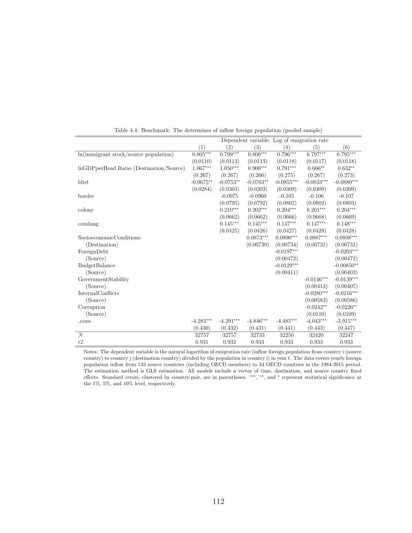
Table 4.4: Benchmark: The determines of inflow foreign population (pooled sample)

Dependent variable: Log of emigration rate(1) (2) (3) (4) (5) (6)

ln(immigrant stock/source population) 0.805∗∗∗ 0.799∗∗∗ 0.800∗∗∗ 0.796∗∗∗ 0.797∗∗∗ 0.795∗∗∗

(0.0110) (0.0113) (0.0113) (0.0118) (0.0117) (0.0118)lnGDPperHead Ratio (Destination/Source) 1.067∗∗∗ 1.050∗∗∗ 0.900∗∗∗ 0.791∗∗∗ 0.666∗∗ 0.632∗∗

(0.267) (0.267) (0.266) (0.275) (0.267) (0.273)ldist -0.0675∗∗ -0.0753∗∗ -0.0763∗∗ -0.0855∗∗∗ -0.0833∗∗∗ -0.0880∗∗∗

(0.0284) (0.0303) (0.0303) (0.0309) (0.0309) (0.0309)border -0.0975 -0.0960 -0.105 -0.106 -0.107

(0.0795) (0.0792) (0.0802) (0.0802) (0.0803)colony 0.210∗∗∗ 0.202∗∗∗ 0.204∗∗∗ 0.201∗∗∗ 0.204∗∗∗

(0.0662) (0.0662) (0.0666) (0.0668) (0.0669)comlang 0.145∗∗∗ 0.145∗∗∗ 0.147∗∗∗ 0.147∗∗∗ 0.148∗∗∗

(0.0425) (0.0426) (0.0427) (0.0428) (0.0428)SocioeconomicConditions 0.0873∗∗∗ 0.0890∗∗∗ 0.0887∗∗∗ 0.0898∗∗∗

(Destination) (0.00739) (0.00734) (0.00731) (0.00731)ForeignDebt -0.0197∗∗∗ -0.0203∗∗∗

(Source) (0.00472) (0.00472)BudgetBalance -0.0129∗∗∗ -0.00850∗∗

(Source) (0.00411) (0.00403)GovernmentStability -0.0146∗∗∗ -0.0139∗∗∗

(Source) (0.00413) (0.00407)InternalConflicts -0.0280∗∗∗ -0.0216∗∗∗

(Source) (0.00583) (0.00586)Corruption -0.0242∗∗ -0.0226∗∗

(Source) (0.0110) (0.0109)cons -4.283∗∗∗ -4.291∗∗∗ -4.846∗∗∗ -4.485∗∗∗ -4.043∗∗∗ -3.915∗∗∗

(0.430) (0.432) (0.431) (0.441) (0.443) (0.447)N 32757 32757 32733 32250 32420 32247r2 0.931 0.932 0.933 0.933 0.933 0.933

Notes: The dependent variable is the natural logarithm of emigration rate (inflow foreign population from country i (sourcecountry) to country j (destination country) divided by the population in country i) in year t. The data covers yearly foreignpopulation inflow from 133 source countries (including OECD members) to 34 OECD countries in the 1984-2015 period.The estimation method is GLS estimation. All models include a vector of time, destination, and source country fixedeffects. Standard errors, clustered by country-pair, are in parentheses. ∗∗∗, ∗∗, and ∗ represent statistical significance atthe 1%, 5%, and 10% level, respectively.

112

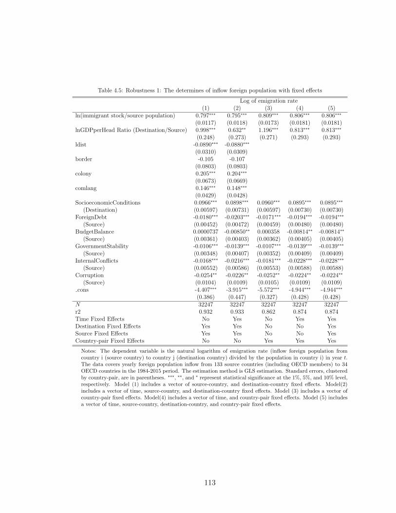
Table 4.5: Robustness 1: The determines of inflow foreign population with fixed effects

Log of emigration rate(1) (2) (3) (4) (5)

ln(immigrant stock/source population) 0.797∗∗∗ 0.795∗∗∗ 0.809∗∗∗ 0.806∗∗∗ 0.806∗∗∗

(0.0117) (0.0118) (0.0173) (0.0181) (0.0181)lnGDPperHead Ratio (Destination/Source) 0.998∗∗∗ 0.632∗∗ 1.196∗∗∗ 0.813∗∗∗ 0.813∗∗∗

(0.248) (0.273) (0.271) (0.293) (0.293)ldist -0.0890∗∗∗ -0.0880∗∗∗

(0.0310) (0.0309)border -0.105 -0.107

(0.0803) (0.0803)colony 0.205∗∗∗ 0.204∗∗∗

(0.0673) (0.0669)comlang 0.146∗∗∗ 0.148∗∗∗

(0.0429) (0.0428)SocioeconomicConditions 0.0966∗∗∗ 0.0898∗∗∗ 0.0960∗∗∗ 0.0895∗∗∗ 0.0895∗∗∗

(Destination) (0.00597) (0.00731) (0.00597) (0.00730) (0.00730)ForeignDebt -0.0180∗∗∗ -0.0203∗∗∗ -0.0171∗∗∗ -0.0194∗∗∗ -0.0194∗∗∗

(Source) (0.00452) (0.00472) (0.00459) (0.00480) (0.00480)BudgetBalance 0.0000737 -0.00850∗∗ 0.000358 -0.00814∗∗ -0.00814∗∗

(Source) (0.00361) (0.00403) (0.00362) (0.00405) (0.00405)GovernmentStability -0.0106∗∗∗ -0.0139∗∗∗ -0.0107∗∗∗ -0.0139∗∗∗ -0.0139∗∗∗

(Source) (0.00348) (0.00407) (0.00352) (0.00409) (0.00409)InternalConflicts -0.0168∗∗∗ -0.0216∗∗∗ -0.0181∗∗∗ -0.0228∗∗∗ -0.0228∗∗∗

(Source) (0.00552) (0.00586) (0.00553) (0.00588) (0.00588)Corruption -0.0254∗∗ -0.0226∗∗ -0.0252∗∗ -0.0224∗∗ -0.0224∗∗

(Source) (0.0104) (0.0109) (0.0105) (0.0109) (0.0109)cons -4.407∗∗∗ -3.915∗∗∗ -5.572∗∗∗ -4.944∗∗∗ -4.944∗∗∗

(0.386) (0.447) (0.327) (0.428) (0.428)N 32247 32247 32247 32247 32247r2 0.932 0.933 0.862 0.874 0.874Time Fixed Effects No Yes No Yes YesDestination Fixed Effects Yes Yes No No YesSource Fixed Effects Yes Yes No No YesCountry-pair Fixed Effects No No Yes Yes Yes

Notes: The dependent variable is the natural logarithm of emigration rate (inflow foreign population fromcountry i (source country) to country j (destination country) divided by the population in country i) in year t.The data covers yearly foreign population inflow from 133 source countries (including OECD members) to 34OECD countries in the 1984-2015 period. The estimation method is GLS estimation. Standard errors, clusteredby country-pair, are in parentheses. ∗∗∗, ∗∗, and ∗ represent statistical significance at the 1%, 5%, and 10% level,respectively. Model (1) includes a vector of source-country, and destination-country fixed effects. Model(2)includes a vector of time, source-country, and destination-country fixed effects. Model (3) includes a vector ofcountry-pair fixed effects. Model(4) includes a vector of time, and country-pair fixed effects. Model (5) includesa vector of time, source-country, destination-country, and country-pair fixed effects.

113

Table 4.6: Robustness 2: The determines of inflow foreign population at t− 1

Log of emigration rate(1) (2) (3) (4) (5)

ln(immigrant stock/source population) (t− 1) 0.616∗∗∗ 0.617∗∗∗ 0.523∗∗∗ 0.511∗∗∗ 0.511∗∗∗

(0.0119) (0.0118) (0.0179) (0.0185) (0.0185)lnGDPperHead Ratio (Destination/Source) (t− 1) 0.838∗∗∗ 0.598∗ 0.405 0.390 0.390

(0.275) (0.309) (0.294) (0.330) (0.330)ldist -0.382∗∗∗ -0.377∗∗∗

(0.0341) (0.0340)border -0.152∗ -0.152∗

(0.0876) (0.0876)colony 0.513∗∗∗ 0.503∗∗∗

(0.0871) (0.0864)comlang 0.308∗∗∗ 0.308∗∗∗

(0.0492) (0.0490)SocioeconomicConditions (t− 1) 0.101∗∗∗ 0.101∗∗∗ 0.105∗∗∗ 0.101∗∗∗ 0.101∗∗∗

(Destination) (0.00632) (0.00795) (0.00637) (0.00788) (0.00788)ForeignDebt (t− 1) -0.0207∗∗∗ -0.0231∗∗∗ -0.0189∗∗∗ -0.0255∗∗∗ -0.0255∗∗∗

(Source) (0.00515) (0.00536) (0.00526) (0.00551) (0.00551)BudgetBalance (t− 1) -0.000516 -0.0110∗∗ -0.000907 -0.0104∗∗ -0.0104∗∗

(Source) (0.00394) (0.00454) (0.00394) (0.00454) (0.00454)GovernmentStability (t− 1) -0.0155∗∗∗ -0.0162∗∗∗ -0.0206∗∗∗ -0.0162∗∗∗ -0.0162∗∗∗

(Source) (0.00377) (0.00464) (0.00377) (0.00465) (0.00465)InternalConflicts (t− 1) -0.0300∗∗∗ -0.0308∗∗∗ -0.0323∗∗∗ -0.0330∗∗∗ -0.0330∗∗∗

(Source) (0.00602) (0.00639) (0.00618) (0.00665) (0.00665)Corruption (t− 1) -0.0442∗∗∗ -0.0415∗∗∗ -0.0530∗∗∗ -0.0474∗∗∗ -0.0474∗∗∗

(Source) (0.0115) (0.0122) (0.0115) (0.0123) (0.0123)cons -2.532∗∗∗ -2.225∗∗∗ -7.099∗∗∗ -7.102∗∗∗ -7.102∗∗∗

(0.429) (0.462) (0.373) (0.464) (0.464)N 30234 30234 30234 30234 30234r2 0.917 0.918 0.848 0.848 0.848Time Fixed Effects No Yes No Yes YesDestination Fixed Effects Yes Yes No No YesSource Fixed Effects Yes Yes No No YesCountry-pair Fixed Effects No No Yes Yes Yes

Notes: The dependent variable is the natural logarithm of emigration rate (inflow foreign population from country i(source country) to country j (destination country) divided by the population in country i) in year t. The values of allthe independent variables are measured in year t − 1. lnstockforeign (t-1) measures the natural logarithm of foreignpopulation stock in year t − 1. The data covers yearly foreign population inflow from 133 source countries (includingOECD members) to 34 OECD countries in the 1984-2015 period. The estimation method is GLS estimation. Standarderrors, clustered by country-pair, are in parentheses. ∗∗∗, ∗∗, and ∗ represent statistical significance at the 1%, 5%, and10% level, respectively. Model (1) includes a vector of source-country, and destination-country fixed effects. Model(2)includes a vector of time, source-country, and destination-country fixed effects. Model (3) includes a vector of country-pair fixed effects. Model(4) includes a vector of time, and country-pair fixed effects. Model (5) includes a vector oftime, source-country, destination-country, and country-pair fixed effects.

114

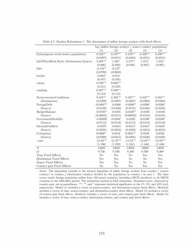
Table 4.7: Further Robustness 1: The determines of inflow foreign workers with fixed effects

log (inflow foreign workers / source country population)(1) (2) (3) (4) (5)

ln(immigrant stock/source population) 0.523∗∗∗ 0.547∗∗∗ 0.419∗∗∗ 0.438∗∗∗ 0.438∗∗∗

(0.0297) (0.0311) (0.0493) (0.0551) (0.0551)lnGDPperHead Ratio (Destination/Source) 2.394∗∗∗ 1.565∗ 2.157∗∗ 1.913∗ 1.913∗

(0.866) (0.920) (0.940) (0.997) (0.997)ldist -0.176∗∗ -0.137∗

(0.0792) (0.0803)border -0.604∗ -0.614∗

(0.347) (0.345)colony 0.700∗∗∗ 0.668∗∗∗

(0.211) (0.210)comlang 0.587∗∗∗ 0.568∗∗∗

(0.112) (0.112)SocioeconomicConditions 0.443∗∗∗ 0.456∗∗∗ 0.435∗∗∗ 0.452∗∗∗ 0.452∗∗∗

(Destination) (0.0299) (0.0307) (0.0297) (0.0308) (0.0308)ForeignDebt -0.0402∗∗∗ -0.0260 -0.0396∗∗ -0.0296∗ -0.0296∗

(Source) (0.0156) (0.0160) (0.0155) (0.0160) (0.0160)BudgetBalance -0.0193∗∗ -0.0105 -0.0228∗∗ -0.0108 -0.0108

(Source) (0.00931) (0.0115) (0.00933) (0.0116) (0.0116)GovernmentStability -0.00299 -0.0204∗ -0.0102 -0.0196∗ -0.0196∗

(Source) (0.0112) (0.0116) (0.0113) (0.0116) (0.0116)InternalConflicts -0.0379 -0.0415 -0.0414∗ -0.0445∗ -0.0445∗

(Source) (0.0238) (0.0253) (0.0239) (0.0254) (0.0254)Corruption 0.0800∗∗ 0.0542 0.0831∗∗ 0.0538 0.0538

(Source) (0.0390) (0.0415) (0.0394) (0.0420) (0.0420)cons -12.40∗∗∗ -11.37∗∗∗ -14.53∗∗∗ -13.92∗∗∗ -13.92∗∗∗

(1.196) (1.259) (1.241) (1.446) (1.446)N 13692 13692 13692 13692 13692r2 0.756 0.760 0.286 0.309 0.309Time Fixed Effects No Yes No Yes YesDestination Fixed Effects Yes Yes No No YesSource Fixed Effects Yes Yes No No YesCountry-pair Fixed Effects No No Yes Yes Yes

Notes: The dependent variable is the natural logarithm of inflow foreign workers from country i (sourcecountry) to country j (destination country) divided by the population in country i in year t. The datacovers yearly foreign population inflow from 133 source countries (including OECD members) to 34 OECDcountries in the 1984-2015 period. The estimation method is GLS estimation. Standard errors, clustered bycountry-pair, are in parentheses. ∗∗∗, ∗∗, and ∗ represent statistical significance at the 1%, 5%, and 10% level,respectively. Model (1) includes a vector of source-country, and destination-country fixed effects. Model(2)includes a vector of time, source-country, and destination-country fixed effects. Model (3) includes a vectorof country-pair fixed effects. Model(4) includes a vector of time, and country-pair fixed effects. Model (5)includes a vector of time, source-country, destination-country, and country-pair fixed effects.

115

Table 4.8: Further Robustness 2: The determines of inflow seasonal foreign workers with fixed effects

log (inflow seasonal foreign workers / source country population)(1) (2) (3) (4) (5)

ln(immigrant stock/source population) 0.270∗∗ 0.248∗∗ 0.0693 -0.0341 -0.0341(0.121) (0.114) (0.242) (0.235) (0.235)

lnGDPperHead Ratio (Destination/Source) 5.433∗ 0.705 5.138 0.161 0.161(2.960) (3.056) (3.120) (3.329) (3.329)

ldist -1.091∗∗∗ -1.125∗∗∗

(0.260) (0.250)border 0.506 0.553

(0.472) (0.480)colony 1.413∗∗∗ 1.489∗∗∗

(0.470) (0.467)comlang -0.683∗ -0.686∗

(0.358) (0.358)SocioeconomicConditions 0.118∗∗ 0.0237 0.141∗∗∗ 0.0402 0.0402

(Destination) (0.0505) (0.0519) (0.0476) (0.0509) (0.0509)ForeignDebt 0.0567 0.0803∗∗ 0.0518 0.0698∗ 0.0698∗

(Source) (0.0382) (0.0406) (0.0366) (0.0378) (0.0378)BudgetBalance 0.0801∗∗∗ 0.0561∗∗ 0.0764∗∗∗ 0.0524∗ 0.0524∗

(Source) (0.0268) (0.0281) (0.0278) (0.0288) (0.0288)GovernmentStability 0.0438∗ -0.00370 0.0408∗ -0.00375 -0.00375

(Source) (0.0240) (0.0252) (0.0237) (0.0253) (0.0253)InternalConflicts 0.0430 -0.0378 0.0527 -0.0379 -0.0379

(Source) (0.0494) (0.0512) (0.0503) (0.0517) (0.0517)Corruption 0.106 0.215∗∗∗ 0.0936 0.211∗∗∗ 0.211∗∗∗

(Source) (0.0758) (0.0818) (0.0735) (0.0800) (0.0800)cons -12.36∗∗∗ -6.033 -22.75∗∗∗ -16.03∗∗∗ -16.03∗∗∗

(3.554) (3.736) (4.411) (4.747) (4.747)N 3211 3211 3211 3211 3211r2 0.737 0.740 0.00000430 0.0176 0.0176Time Fixed Effects No Yes No Yes YesDestination Fixed Effects Yes Yes No No YesSource Fixed Effects Yes Yes No No YesCountry-pair Fixed Effects No No Yes Yes Yes

Notes: The dependent variable is the natural logarithm of inflow seasonal foreign workers from country i (sourcecountry) to country j (destination country divided by the population in country i) in year t. The data covers yearlyforeign population inflow from 133 source countries (including OECD members) to 34 OECD countries in the 1984-2015period. The estimation method is GLS estimation. Standard errors, clustered by country-pair, are in parentheses. ∗∗∗,∗∗, and ∗ represent statistical significance at the 1%, 5%, and 10% level, respectively. Model (1) includes a vectorof source-country, and destination-country fixed effects. Model(2) includes a vector of time, source-country, anddestination-country fixed effects. Model (3) includes a vector of country-pair fixed effects. Model(4) includes a vectorof time, and country-pair fixed effects. Model (5) includes a vector of time, source-country, destination-country, andcountry-pair fixed effects.

116

Table 4.9: Further Robustness 3: The determines of inflow foreign students with fixed effects

log (inflow foreign students / source country population)(1) (2) (3) (4) (5)

ln(immigrant stock/source population) 0.330∗∗∗ 0.300∗∗∗ 0.474∗∗∗ 0.402∗∗∗ 0.402∗∗∗

(0.0348) (0.0328) (0.0966) (0.0973) (0.0973)lnGDPperHead Ratio (Destination/Source) -5.624∗∗∗ -2.406∗∗ -5.544∗∗∗ -2.472∗∗ -2.472∗∗

(0.937) (1.001) (0.995) (1.127) (1.127)ldist -0.389∗∗∗ -0.486∗∗∗

(0.0982) (0.0981)border -0.521 -0.524

(0.423) (0.424)colony 1.874∗∗∗ 1.920∗∗∗

(0.270) (0.271)comlang 0.316 0.355

(0.236) (0.240)SocioeconomicConditions 0.147∗∗∗ 0.117∗∗∗ 0.129∗∗∗ 0.112∗∗∗ 0.112∗∗∗

(Destination) (0.0346) (0.0371) (0.0356) (0.0372) (0.0372)ForeignDebt 0.0206 -0.00467 0.0172 -0.00528 -0.00528

(Source) (0.0167) (0.0171) (0.0170) (0.0173) (0.0173)BudgetBalance 0.0245 0.0111 0.0223 0.00493 0.00493

(Source) (0.0149) (0.0156) (0.0149) (0.0157) (0.0157)GovernmentStability -0.0609∗∗∗ -0.0125 -0.0599∗∗∗ -0.0154 -0.0154

(Source) (0.0173) (0.0186) (0.0180) (0.0186) (0.0186)InternalConflicts -0.0387∗ -0.00000347 -0.0460∗∗ -0.00342 -0.00342

(Source) (0.0223) (0.0198) (0.0229) (0.0199) (0.0199)Corruption 0.0237 0.0148 0.0243 0.0170 0.0170

(Source) (0.0406) (0.0423) (0.0401) (0.0420) (0.0420)cons -4.379∗∗∗ -7.611∗∗∗ -4.241∗∗∗ -9.342∗∗∗ -9.342∗∗∗

(1.200) (1.249) (1.496) (1.710) (1.710)N 2892 2892 2892 2892 2892r2 0.807 0.814 0.212 0.335 0.335Time Fixed Effects No Yes No Yes YesDestination Fixed Effects Yes Yes No No YesSource Fixed Effects Yes Yes No No YesCountry-pair Fixed Effects No No Yes Yes Yes

Notes: The dependent variable is the natural logarithm of inflow foreign students from country i (sourcecountry) to country j (destination country) divided by the population in country i in year t. The data coversyearly foreign population inflow from 133 source countries (including OECD members) to 34 OECD countriesin the 1984-2015 period. The estimation method is GLS estimation. Standard errors, clustered by country-pair,are in parentheses. ∗∗∗, ∗∗, and ∗ represent statistical significance at the 1%, 5%, and 10% level, respectively.Model (1) includes a vector of source-country, and destination-country fixed effects. Model(2) includes a vectorof time, source-country, and destination-country fixed effects. Model (3) includes a vector of country-pair fixedeffects. Model(4) includes a vector of time, and country-pair fixed effects. Model (5) includes a vector of time,source-country, destination-country, and country-pair fixed effects.

117

Table 4.10: Further Robustness 4: Non-linearity in stock foreign population with random vce

Setting ln(immigrant stock/source population) (t− 1) at

Pooled < 20% 20%− 40% 40%− 60% 60%− 80% > 80%ln(immigrant stock/source population) 0.617∗∗∗ 0.244∗∗∗ 0.644∗∗∗ 0.762∗∗∗ 0.708∗∗∗ 0.576∗∗∗

(t− 1) (0.0118) (0.0226) (0.0356) (0.0399) (0.0380) (0.0359)lnGDPperHead Ratio (Destination/Source) 0.598∗ 0.396 0.834 1.626∗∗ 0.546 1.025

(t− 1) (0.309) (0.722) (0.615) (0.642) (0.743) (0.895)ldist -0.377∗∗∗ -0.499∗∗∗ -0.203∗∗∗ -0.161∗∗∗ -0.212∗∗∗ -0.355∗∗∗

(0.0340) (0.113) (0.0674) (0.0604) (0.0563) (0.0629)border -0.152∗ 0.872∗∗∗ -0.835∗∗∗ -0.00783 0.0632 -0.203∗

(0.0876) (0.261) (0.188) (0.191) (0.119) (0.120)colony 0.503∗∗∗ 0.368∗∗∗ 0.825∗∗∗ 0.169∗

(0.0864) (0.115) (0.245) (0.0940)comlang 0.308∗∗∗ -0.148 0.114 -0.00424 0.179∗∗ 0.362∗∗∗

(0.0490) (0.112) (0.0997) (0.0796) (0.0828) (0.0761)SocioeconomicConditions (t− 1) 0.101∗∗∗ 0.0946∗∗∗ 0.114∗∗∗ 0.0882∗∗∗ 0.0462∗∗∗ 0.135∗∗∗

(Destination) (0.00795) (0.0243) (0.0180) (0.0147) (0.0150) (0.0152)ForeignDebt (t− 1) -0.0231∗∗∗ -0.0189 -0.0174 -0.0172∗∗ -0.00165 -0.0319∗∗∗

(Source) (0.00536) (0.0148) (0.0111) (0.00741) (0.0124) (0.0109)BudgetBalance (t− 1) -0.0110∗∗ 0.0109 -0.00530 -0.00298 -0.0174∗∗ -0.0287∗∗

(Source) (0.00454) (0.0117) (0.00898) (0.00706) (0.00857) (0.0112)GovernmentStability (t− 1) -0.0162∗∗∗ -0.0247 -0.00951 0.00152 -0.0211∗∗ -0.0199∗∗∗

(Source) (0.00464) (0.0153) (0.0105) (0.00840) (0.00911) (0.00726)InternalConflicts (t− 1) -0.0308∗∗∗ 0.0250 -0.0116 -0.0470∗∗∗ -0.0161 -0.0417∗∗∗

(Source) (0.00639) (0.0195) (0.0145) (0.0118) (0.0120) (0.0130)Corruption (t− 1) -0.0415∗∗∗ -0.0110 0.0105 -0.0355 -0.0549∗∗ -0.0425∗

(Source) (0.0122) (0.0366) (0.0261) (0.0237) (0.0265) (0.0219)cons -2.225∗∗∗ -5.586∗∗∗ -3.471∗∗∗ -3.184∗∗∗ -3.614∗∗∗

(0.462) (0.927) (1.168) (1.020) (1.054)N 30234 3919 6674 6284 6335 7022r2 0.918 0.825 0.833 0.873 0.892 0.869

Notes: The dependent variable is the natural logarithm of emigration rate (inflow foreign population from country i (sourcecountry) to country j (destination country) divided by the population in country i) in year t. The values of all the independentvariables are measured in year t−1. lnstockforeign (t-1) measures the natural logarithm of foreign population stock in year t−1.The data covers yearly foreign population inflow from 133 source countries (including OECD members) to 34 OECD countries inthe 1984-2015 period. The estimation method is GLS estimation. All models include a vector of time, destination-country, andsource-country fixed effects. Standard errors, clustered by country-pair, are in parentheses. ∗∗∗, ∗∗, and ∗ represent statisticalsignificance at the 1%, 5%, and 10% level, respectively. Model (1) is the replicate of column 2 in the last table. Model (2) - (6)considers non-linearity of stock foreign population, each interval represent a 20 percentile of the stock foreign population.

118

Table 4.11: Further Robustness 5: The determines of inflow foreign population from OECD origin, and non-OECDorigin.

Source: OECD Source: Non-OECD

t t− 1 t− 1 t t− 1 t− 1ln(immigrant stock/source population) 0.798∗∗∗ 0.645∗∗∗ 0.590∗∗∗ 0.789∗∗∗ 0.604∗∗∗ 0.477∗∗∗

(0.0216) (0.0236) (0.0341) (0.0138) (0.0135) (0.0218)lnGDPperHead Ratio (Destination/Source) 1.851 2.141 2.125 0.389 0.235 -0.121

(1.180) (1.360) (1.409) (0.304) (0.342) (0.363)ldist 0.0553 -0.143∗∗∗ -0.122∗∗∗ -0.470∗∗∗

(0.0531) (0.0540) (0.0413) (0.0452)border -0.00829 0.00555 0.0591 0.240

(0.0948) (0.0963) (0.146) (0.162)colony 0.105 0.249 0.246∗∗∗ 0.594∗∗∗

(0.130) (0.162) (0.0737) (0.0994)comlang 0.0798 0.176∗∗ 0.174∗∗∗ 0.360∗∗∗

(0.0736) (0.0783) (0.0472) (0.0560)SocioeconomicConditions 0.0767∗∗∗ 0.0792∗∗∗ 0.0799∗∗∗ 0.0951∗∗∗ 0.112∗∗∗ 0.111∗∗∗

(Destination) (0.0113) (0.0122) (0.0122) (0.00956) (0.0104) (0.0103)ForeignDebt -0.0247∗∗∗ -0.0320∗∗∗ -0.0359∗∗∗ -0.0158∗∗ -0.0184∗∗∗ -0.0180∗∗

(Source) (0.00706) (0.00815) (0.00818) (0.00631) (0.00713) (0.00737)BudgetBalance -0.0217∗∗∗ -0.0309∗∗∗ -0.0303∗∗∗ -0.00244 0.00219 0.00184

(Source) (0.00796) (0.00833) (0.00822) (0.00468) (0.00540) (0.00547)GovernmentStability -0.00832 -0.0135∗ -0.0132∗ -0.0154∗∗∗ -0.0140∗∗ -0.0149∗∗

(Source) (0.00664) (0.00768) (0.00761) (0.00522) (0.00595) (0.00600)InternalConflicts -0.0106 -0.0200 -0.0228∗ -0.0192∗∗∗ -0.0257∗∗∗ -0.0278∗∗∗

(Source) (0.0122) (0.0132) (0.0132) (0.00693) (0.00759) (0.00800)Corruption -0.0614∗∗∗ -0.0900∗∗∗ -0.0976∗∗∗ -0.00635 -0.0221 -0.0255

(Source) (0.0160) (0.0181) (0.0181) (0.0146) (0.0160) (0.0161)cons -7.069∗∗∗ -6.078∗∗∗ -7.176∗∗∗ -3.657∗∗∗ -2.236∗∗∗ -7.235∗∗∗

(1.265) (1.459) (1.515) (0.706) (0.759) (0.554)N 10700 10170 10170 21547 20064 20064r2 0.924 0.915 0.808 0.933 0.916 0.867Time Fixed Effects Yes Yes Yes Yes Yes YesDestination Fixed Effects Yes Yes Yes Yes Yes YesSource Fixed Effects Yes Yes Yes Yes Yes YesCountry-pair Fixed Effects No No Yes No No Yes

Notes: The dependent variable is the natural logarithm of inflow foreign population from country i (source country) tocountry j (destination country) in year t. In model (2) (3) (5) (6), the values of all the independent variables are measuredin year t − 1. lnstockforeign (t-1) measures the natural logarithm of foreign population stock in year t − 1. The datacovers yearly foreign population inflow from 133 source countries (including OECD members) to 34 OECD countries in the1984-2015 period. The estimation method is GLS estimation. Standard errors, clustered by country-pair, are in parentheses.∗∗∗, ∗∗, and ∗ represent statistical significance at the 1%, 5%, and 10% level, respectively. Model (1)-(3) include only OECDsource countries. Model (4)-(6) include only non-OECD source countries.

119

VITA

YUN WANG

August 6, 1991 Born, Nantong, China

2013 B.A., EconomicsShanghai Finance UniversityShanghai, China

2015 M.A., EconomicsFlorida International UniversityMiami, Florida

2015 - 2018 Ph.D candidate, EconomicsFlorida International UniversityMiami, Florida

2013 - 2018 Graduate Teaching AssistantFlorida International UniversityMiami, Florida

120