THREE ESSAYS ON CORPORATE FINANCIAL DISCLOSURES By YINAN YANG A dissertation submitted to the Graduate School – Newark Rutgers, The state University of New Jersey In partial fulfillment of requirements For the degree of Doctor of Philosophy Graduate Program in Management Written under the direction of Dr. Bikki Jaggi and approved by ________________________ ________________________ ________________________ ________________________ Newark, New Jersey May 2018

Welcome message from author
This document is posted to help you gain knowledge. Please leave a comment to let me know what you think about it! Share it to your friends and learn new things together.
Transcript
THREE ESSAYS ON CORPORATE FINANCIAL DISCLOSURES
By YINAN YANG
A dissertation submitted to the
Graduate School – Newark
Rutgers, The state University of New Jersey
In partial fulfillment of requirements
For the degree of
Doctor of Philosophy
Graduate Program in Management
Written under the direction of
Dr. Bikki Jaggi
and approved by
________________________
________________________
________________________
________________________
Newark, New Jersey
May 2018

© [2018]
YINAN YANG
ALL RIGHTS RESERVED

ii
ABSTRACT OF THE DISSERTATION
THREE ESSAYS ON COPRORATE FINANCIAL DISCLOSURES
By YINAN YANG
Dissertation Director: Dr. Bikki Jaggi
This dissertation consists of three papers. In the first paper we identify a new
incentive for managers in determining management forecast (MF) characteristics
stemming from the relative performance evaluation feature of CEO promotion tournaments.
We document higher credibility of MF for firms with stronger tournament incentives (as
proxied for by the CEO pay gap). We posit that the relative performance evaluation feature
of CEO promotion tournaments creates mutual monitoring mechanism within the
management team as well as the incentives for lower-ranked executives to provide high
quality information to gain better evaluation results. We thereby extend previous MF
literature that focuses mainly on equity-based incentives and reports mixed findings. Our
results are robust to using different tournament measures, controlling for other known
determinants of MF characteristics as well as manager skills, and corrections of
endogeneity of all specifications.
In the second paper, we investigate the spill-over effect of customer fraud on non-
fraudulent suppliers’ investment decisions. We posit that suppliers utilize customers’
information to infer future demand and economic prospects, and noisy information distorts
and misguides the investment and productions decisions made by suppliers. The

iii
overinvestment and misrepresented performance of customers signal a high demand and
prosperous economic prospects for suppliers, resulting in overinvestment decisions by
suppliers. We find that suppliers invest more during the fraud periods of customers. The
degree of distortion is less severe when the supplier operates in concentrated industry and
more severe when suppliers have higher sales volatility. In addition, we show that the
overinvestments by suppliers are inefficient as associated future cash flows are
significantly reduced. Our results are robust to different fraud samples, alternative research
methodology, and controlling for other known determinants of investment decisions.
In the third paper, we investigate whether firms engaging in corporate fraud take
advantages of strategic timing of earnings announcements (EA). We document that
misreporting firms strategically time their EA in low attention periods (i.e. after trading
hours) during violation years. In addition, we show that the timing strategy is followed by
a longer detection period and more insider trading. We thereby extend previous corporate
disclosure timing literature that mainly focuses on the content of reported news. We also
extend the corporate fraud literature by showing a low-cost way in which firms can
possibly “hide” the manipulated earnings. Our results are robust to different samples of
fraud, different research methodology, different sample periods, and controlling for other
known determinants of market attention.

iv
ACKNOWLEDGMENTS
The basis for this research originally stemmed from my passion for a better
understanding of firms’ disclosure decisions. Managerial incentives matter in this process
and the consequences of the disclosure choices not only affect the firm itself, but also non-
financial stakeholders such as industry peers and suppliers
I would like to thank my advisor Professor Bikki Jaggi and the other four Professors
in my dissertation committee for their excellent guidance and support during this process. I
also wish to thank all of the respondents, without whose cooperation I would not have been
able to conduct this analysis.
To my other colleagues at Rutgers Business School: I want to thank my best friends
Xin Cheng and Cheng Yin for your wonderful cooperation as well. It was always helpful
to bat ideas about my research around with you. I also benefitted from debating issues with
my friends and family. If I ever lost interest, you kept me motivated. My parents deserve a
particular note of thanks: your wise counsel and kind words have, as always, served me
well.
I hope you enjoy your reading.

v
TABLE OF CONTENTS
ABSTRACT OF THE DISSERTATION ............................................................... ii
ACKNOWLEDGMENTS ..................................................................................... iv
CHAPTER 1: IMPACT OF TOURNAMENT INCENTIVES ON
MANAGEMENT EARNINGS FORECASTS ................................................................... 1
1.1 Introduction ................................................................................................... 1
1.2 Literature Review and Hypothesis Development ......................................... 6
1.2.1 Literature Review................................................................................... 6
1.2.2 Hypotheses ........................................................................................... 10
1.3 Methodology ............................................................................................... 14
1.3.1 Sample Selection .................................................................................. 14
1.3.2 Tournament Incentive Measurements .................................................. 15
1.3.3 Model Specification ............................................................................. 17
1.4 Data Description and Empirical Results ..................................................... 21
1.4.1 Summary Statistics............................................................................... 21
1.4.2 Empirical Results ................................................................................. 21
1.5 Robustness Check Tests .............................................................................. 24
1.5.1 CEO Ability, CEO Fixed Effect, and MEF Quality ............................ 25
1.5.2 Corporate Governance and MEF Quality ............................................ 26

vi
1.5.3 Alternative Tournament Incentive Proxy............................................. 27
1.5.4 Endogeneity Concerns ......................................................................... 27
1.5.5 Economic Consequences ..................................................................... 28
1.6 Conclusion .................................................................................................. 32
CHAPTER 2: DO CORPORATE FRAUDS DISTORT SUPPLIERS’
INVESTMENT DECISIONS? ......................................................................................... 34
2.1 Introduction ................................................................................................. 34
2.2 Literature Review and Hypothesis Development ....................................... 38
2.2.1 Corporate Frauds and Investments....................................................... 38
2.2.2 Supplier-Customer Relationship and Corporate Frauds ...................... 39
2.2.3 Informational Reliance and Suppliers’ Overinvestment ...................... 40
2.3 Research Design.......................................................................................... 42
2.3.1 Data ...................................................................................................... 42
2.3.2 Model Specifications ........................................................................... 44
2.4 Results ......................................................................................................... 46
2.4.1 Descriptive Statistics ............................................................................ 46
2.4.2 Preliminary Results .............................................................................. 47
2.4.3 Main Results ........................................................................................ 48
2.4.4 Cross-sectional Tests ........................................................................... 49
2.5 Additional Tests .......................................................................................... 50

vii
2.6 Robustness Checks...................................................................................... 53
2.7 Conclusion .................................................................................................. 55
CHAPTER 3: STRATEGIC EARNINGS ANNOUNCEMENTS TIMING AND
FINANCIAL MISREPORTING ...................................................................................... 57
3.2 Literature Review and Hypotheses Development ....................................... 62
3.3 Research Design.......................................................................................... 67
3.3.1 Sample.................................................................................................. 67
3.3.2 Measures .............................................................................................. 68
3.3.3 Tests of Hypothesis 1 ........................................................................... 70
3.3.4 Tests of Hypothesis 2 ........................................................................... 74
3.4 Conclusion .................................................................................................. 79
APPENDICIES ..................................................................................................... 80
Appendix A. ...................................................................................................... 80
Appendix B. ...................................................................................................... 83
REFERENCES ..................................................................................................... 85
TABLES ............................................................................................................... 93
Table 1.1 Descriptive Statistics for the Sample of Management Earnings
Forecasts ....................................................................................................................... 93
Figure 1.1. The Time-series Distribution of Executive Pay Gap ...................... 94
Table 1.2 Summary Statistics ........................................................................... 95

viii
Table 1.3 Association between MEF Quality and Tournament Incentives ...... 96
Table 1.4 Moderating Effect of Industry Homogeneity and New CEO on the
Association between Tournament Incentives and MEF Quality .................................. 98
Table 1.5 Robustness Check: CEO Ability, CEO Characteristics and MEF
Quality........................................................................................................................... 99
Table 1.6 Robustness Check: Corporate Governance..................................... 101
Table 1.7 Endogeneity Concerns of Tournament Incentive ........................... 102
Table 1.8 Tournament Incentives and the Economic Consequences of
Management Earnings Forecasts ................................................................................ 103
Table 2.1 Time Series Pattern of Affected Suppliers with Cheating Customers
..................................................................................................................................... 105
Table 2.2 The Customers’ Manipulations During Cheating Periods .............. 106
Table 2.3 Descriptive Statistics ....................................................................... 107
Table 2.4 The Effects of Customers’ Misrepresentations on Suppliers Investment
Decisions ..................................................................................................................... 108
Table 2.5 The Effects of Industry Concentration and Sales Uncertainty on
Suppliers’ Decisions in Response to Customers’ Misconduct ................................... 109
Table 2.6 The Association between Current Investments and Future Cash Flows
..................................................................................................................................... 111
Table 2.7 The Market Reactions to Suppliers’ Investment Decisions After The
Disclosure of Customers’ Frauds ................................................................................ 113

ix
Table 2.8 The Robustness Check: Difference-in-Difference Approach ......... 114
Figure 3.1 Transition Matrix of Before/During/After Trading Hours
Announcement Times ................................................................................................. 115
Figure 3.2 Transition of Matrix of Announcement Weekdays ....................... 116
Table 3.1 Sample Description ......................................................................... 117
Table 3.2 Univariate Test ................................................................................ 118
Table 3.3 Descriptive Statistics ....................................................................... 119
Table 3.4 EA Timings During Periods of Misreporting ................................. 120
Table 3.5 Propensity Score Matching – First Stage ........................................ 121
Table 3.6 Descriptive Statistics ....................................................................... 122
Table 3.7 EA Timings During Periods of Misreporting – Propensity Score
Matching ..................................................................................................................... 123
Table 3.8 Days to Detection with EAs Made in After Trading Hours ........... 124
Table 3.9 Insider Trading with EAs Made in After Trading Hours................ 126
Table 3.10 The Market Reactions Following the Disclosure of Misreporting 128

1
CHAPTER 1: IMPACT OF TOURNAMENT INCENTIVES ON MANAGEMENT
EARNINGS FORECASTS
1.1 Introduction
According to the tournament theory used in the business environment, best performers in
the rank order tournament in a firm receive preference over others for promotion to the
next higher rank ((Lazear and Rosen, 1981).1 Some authors have, however, pointed out
that the rank order tournaments are associated with negative consequences, which are
referred to as dysfunctional consequences, and they include excessive risk taking (Knoeber
and Thurman 1994; and Prendergast 1999), cheating (Cheng 2011), fraud (Haß, Müller,
and Vergauwe 2015), and sabotage of competitors (Harbring and Irlenbusch 2011). Despite
these potential negative consequences, firms are more impressed with the positive aspects
of competitive tournaments and favor organizing rank order tournaments because they
incentivize managers to work harder to win the tournament prize of promotion to the next
higher level, which enhances their pay, and results in improving firms’ overall performance
(e.g. Kale, Reis, and Venkateswaran 2009).
Extending this line of research, we argue that hard work of participants in the rank-order
tournament is also expected to have a significant influence on the quality of information,
including future-oriented information contained in MEFs. In other words, we argue that
1 The concept of firm-specific tournament has been expanded to the industry-wide competitive tournament where
participants from different firms are motivated to compete for a CEO position in a particular firm with tournament
prize, i.e. higher CEO salary in the industry (e.g. Coles, Li, and Wang 2013). Lately, it has also been extended to
geographic level, where participants compete for the CEO position with the highest salary in a particular geographic
region (e.g. Yin 2016)

2
the rank order tournament is likely to result in high quality information, which will enable
CEOs, CFOs, or other managers at the higher levels, to issue MEFs that will also be of
higher quality. Thus, we conjecture in this study that firms with rank order tournament
incentives will issue MEFs that are of higher quality compared to MEFs issued by firms
without tournament incentives, and we measure the MEF quality using the MEF attributes
of accuracy and precision (e.g. Hirst Koonce, and Venkataraman. 2008).
Our expectation of the positive association between tournament incentives and MEF
quality is based on the assumption that information provided by tournament participants,
which will serve as an input to develop the MEFs, is expected to be of high quality
compared to information used by firms without tournament incentives. The higher quality
of information for firms with competitive tournament is supported based on the following
arguments.
First, information provided by managers participating in the rank order tournament to the
Disclosure Committee, consisting of top management and other managers (e.g. Brochet,
Faurel, and McVay 2011), is expected to be of high quality because it will be used for the
purposes of their own performance evaluation. (e.g. Keating 1997). Second, we expect the
competitive tournament environment to result in strict internal monitoring to ensure that
all participating managers follow the rules and regulations to ensure that information
provided by them is not contaminated. The superior managers will ensure that tournament
participating managers are providing unbiased information that will be used to evaluate
them for promotion to the higher rank. If quality of this information is considered
questionable because of massaging of information, such as, earnings manipulations, there
will be heavy penalty, which may even include loss of tournament trophy (Dyck Morse,

3
and Zingales 2010; Fauver and Fuerst 2006). Third, in addition to monitoring by superior
managers, there may also be intra-group monitoring of each other because the participating
members would be concerned about cheating by other members (Li 2014). Thus, it will
motivate all participating members to keep a strict watch over each other’s activities.
Fourth, the quality of information is likely to be positively influenced by the participants’
strong incentives to project their long horizon and it will avoid short-term focus that may
convey negative signals on their capabilities (e.g. Acharya, Myers and Rajan 2011).
Moreover, their focus on the long horizon will especially be desirable when they wish to
be considered for promotion to the rank of CEO because a long-horizon approach is
considered to be an important quality for CEOs to enhance firm value (Dechow and Sloan
1991).
Consistent with Hirst, et al (2008), we measure the quality of MEFs in terms of forecast
accuracy and precision. We conduct analyses based on a sample of 28,337 observations.
Consistent with the existing literature, we measure the tournament prize size as the natural
logarithm of the pay gap between the CEO and other VPs (Kale et al. 2009). The results of
our analyses show that there is a significantly positive association between tournament
incentives and quality of MEFs (i.e. forecast accuracy and precision), confirming our
expectation that firms with rank order tournament incentives issue MEFs that are of higher
quality compared to the firms that do not have such incentives. We also find higher
frequency of MEFs for firms with rank order tournament incentives, suggesting that these
firms are more likely to update their forecasts and keep the market informed when changes
are expected in future performance of the firm.

4
Next, we examine whether industry homogeneity and new CEO will affect the association
between tournament incentives and MEF quality. First, it is argued that industry
homogeneity opens opportunities for tournament participants to look for higher positions
in other firms in the same industry group. We present that the availability of wider
opportunities to the participants is likely to serve as a moderating factor because it will
dampen participants’ motivations to work hard to provide high quality information to
superiors. Moreover, this situation will open up other avenues for firms to hire from outside
the firm, which will send a negative signal to participants for promotion to the higher rank
and thus participants’ enthusiasm to work hard may also be dampened. Similarly, a new
CEO in the firm will convey a negative signal to the tournament participants that promotion
to the rank of CEO may not be available for quite some time and this will have a moderating
effect on the association between tournament incentives and MEF quality. The results of
empirical tests confirm the expectation of a moderating effect of industry homogeneity and
new CEO on the positive association between tournament incentives and MEF quality.
We conduct several tests to confirm that our results are robust. First, we examine the impact
of CEO ability and CEO fixed effects, and the results show that our results still hold and
are not driven by these factors. Second, we examine the impact of corporate governance
effectiveness on our findings. The results show that corporate governance also has an
impact on MEF quality, but our results remain statistically unchanged when these factors
are considered in our analyses. Third, we use alternative measures for tournament
incentives, and our main findings remain unchanged. Finally, we examine whether there
are any endogeneity concerns that would have an influence on our findings. We used the
IV approach and we find that our results are not influenced by endogeneity concerns.

5
We conducted additional analyses to evaluate whether market participants and security
analysts would recognize high quality of MEFs issued by firms with tournaments
incentives. The results on the market reaction have confirmed that market participants
reacted more positively to MEFs issued by firms with tournament incentives, suggesting
that they recognized high quality of MEFs issued by these firms compared to MEFs issued
by firms without tournaments. Similarly, the results based on the security analysts’ reaction
provided additional support to our expectation of high quality of MEFs issued by firms
with tournament incentives.
Our paper makes several contributions to the MEF literature. First, to our knowledge, this
is the first paper that emphasizes the important role of tournament incentives in enhancing
MEF quality. The MEF quality has been examined from different perspectives in the
literature, such as accuracy, precision, frequency, managerial motivation to disclose MEFs,
security analysts’ reaction forecasts, and investors’ reaction to forecasts, etc. Our findings
add to the existing findings that rank order tournaments in firms also have a significant
influence on the disclosure policy of MEFs and they impact frequency, accuracy and
precision of forecasts, and thus enhance the MEF quality. Second, our findings confirm
that MEFs are the outcomes of efforts by several executives, who may contribute in
different ways in developing quality MEFs. This finding implies that coordination among
different executives, reflecting cumulative efforts of the management team associated with
developing MEFs, is also an important factor to enhance the quality of MEFs. Our results
show that properly coordinated efforts of several executives result in high quality of MEFs.
Third, our findings add to the literature on the rank order tournaments in firms. The
existing literature shows that tournaments serve as important tools to improve firm

6
efficiency, deal with management compensation issues, motivate managers to put in their
best effort to achieve company overall objectives, etc. Our findings add to these findings
and show that the tournament objectives can also an important role in improving the quality
of information and especially of future-oriented information contained in MEFs. In this
paper, we especially highlight the role of tournament incentives in enhancing the quality
of MEFs.
These findings provide useful information to investors, regulators, and researchers. While
examining the quality of MEFs, investors can determine whether the firm has tournament
incentives. The MEFs issued by firms with tournament incentives can be expected to have
higher reliability and credibility. The regulators may use this information in developing
regulations to ensure higher quality of disclosures made by firms to the outside users. This
study should encourage researchers to conduct additional research into different issues
related to the usefulness of MEFs and impact of MEFs on decisions by users of the financial
information.
The reminder of the paper proceeds as follows. Section 2 develops the hypotheses based
on prior literature. Section 3 on research methodology describes data, variable
measurements and model specifications. Section 4 presents regression results, whereas
sections 5, 6, and 7 discuss and contain results on robustness checks and additional tests.
Conclusion is presented in Section 8.
1.2 Literature Review and Hypothesis Development
1.2.1 Literature Review
Our research review covers two streams of literature. First, we review the literature on
voluntarily issued MEFs, including incentives for issuing MEFs. Second, we discuss the
7
literature on the rank-order tournament incentives that have an impact on firm-specific
performance, information generation process, and accounting disclosure policies.
Literature on Management Earnings Forecasts
Management earnings forecasts (MEFs) have been examined in the literature from different
perspectives, such as motivation to issue MEFs, different attributes of MEFs (i.e. frequency,
accuracy, precision of forecasts), market reaction to MEFs, etc. In general, managers
voluntarily provide MEFs to achieve different objectives, such as self-serving goals, signal
information to the market on upcoming earnings surprises (Kasznik and Lev 1995), reduce
litigation risk (Skinner 1994), adjust investors’ expectations (Waymire 1986; Cotter Tuna,
and Wysocki 2006), develop reputation for providing transparent information (Graham,
Harvey, and Rajgopal 2005), etc. On an overall basis, managers are likely to provide
forecast information only when benefits outweigh costs.
Among different incentives, CEOs’ are also motivated to issue MEFs that are influenced
by the equity-based compensation and/or personal benefits.2 It is argued that CEOs and
other managers, who have superior information than outsiders, may use private information
for personal benefits. For example, it has been presented in the literature that there is a link
between the timing of MEFs and trading in the company stock (e.g. Penman 1982). Noe
(1999) find that managers engage more in selling activity after issuing a price-increasing
forecast and engage more in buying activity after issuing a price-decreasing forecast.
Similarly, Cheng and Lo (2006) document that CEOs and other top managers strategically
2 Examples include compensations based on stock option grants (Yermack 1997; Aboody and Kasznik 2000), and
insider trading (Cheng and Lo 2006).

8
choose disclosure policy that they can use to make on their stock transactions. Aboody and
Kasznik (2000) find that CEOs voluntarily time their disclosures around the stock option
awards to maximize their stock option compensation. Thus, findings of these studies
demonstrate that the issuance of MEFs may be influenced by personal benefits of top
managers.
Recent studies have pointed out that incentives of non-CEO executives also influence the
quality of information used in developing MEFs, thus influencing the quality of MEFs
(Bamber, Jiang, and Wang 2010). The incentvies of non-CEO executives especially
assume an important role when MEFs are the outcome of a teamwork consisting of CEO
and other managers. A study by Kwak, Ro and Suk (2012) point out that many firms’
disclosure decisions are made by a group of principal managers, in the form of a disclosure
committee, and not just one single individual. Bertrand and Schoar (2003) also argue that
a firm’s policies are made as the outcomes of teamwork by its top executives. Recently,
based on prior research on top management teams (TMTs), Wang (2015) provides evidence
that top executives’ functional diversity can influence management guidance. While the
CEO behavior primarily responds to the performance-based incentives, non-CEO
executives are expected to respond to both performance-based and tournament incentives
(e.g., Baker, Jensen and Murphy 1988; Green and Stokey 1983). Consistent with these
views, we present in this study that tournament incentives may play an important role in
motivating non-CEO top managers to provide higher quality information in developing
MEFs.
Recently, a study by Hirst, et al. (2008) has pointed out that not much attention has been
paid in the literature to the MEFs’ attributes such has frequency, accuracy, and precision

9
of MEFs. They argue that these attributes are important to measure the quality of MEFs,
and managers may also use these attributes to convey a message to investors that is
consistent with their objectives. We expand this line of research and examine whether there
is a link between MEF attributes and competitive tournament incentives.
Literature on Rank Order Tournament Incentives
Rosenbaum (1979) and Lazear and Rosen (1981) originally suggested that the relative
performance evaluation scheme under certain circumstances3 may be used to induce efforts
from agents. In a traditional rank-order tournament, the best performer is promoted to the
next level in hierarchy by passing over others. This provides incentives for tournament
participants to perform well such that their chance of winning the promotion prize is
maximized.
The existing findings on the rank-order tournament also document that tournament
incentives improve corporate policies (e.g. Kini and Williams, 2012) and firm innovation
(e.g. Jia, Tian, and Zhang 2016). Findings of these studies indicate that managerial
compensation structure provides the basis for developing the rank-order tournament
incentives, which incentivize subordinates to compete for a higher position, especially for
the CEO position. The tournament incentives are measured by the difference in the CEO’s
pay and an average of key subordinates’ pay (e.g. Kale et al. 2009; Kini and Williams
2012), whereas the key subordinates are referred to VPs in the literature. It is assumed that
the pay difference is likely to encourage subordinates to work harder and give their best
3 These circumstances include when monitoring is difficult or expensive, when agents are risk averse, and when the
measurement costs of absolute performance are prohibitly high.
10
performance that enhances firm’s overall performance, which in turn would enhance firm
value.
Some studies, on the other hand, have documented that the rank-order tournament is also
likely to enhance firm risk (e.g. Kinni and Williams, 2012) because managers would be
encouraged to undertake risky projects to achieve higher returns that may help them in
winning the trophy. Kubick and Masli (2016) also find that firms with larger pay gap tend
to adopt risky tax policies. In addition, managers may also engage in earnings management
or even frauds to achieve higher targets that could help them increase the chance of
promotion (Chen, Hui, You, and Zhang 2016; Haß et al. 2015). Furthermore, some recent
studies document a decrease in the helping effort and more sabotage activities in firms with
larger pay gaps (Chowdhury and Gurtler 2015; Dechenaux, Kovenock, and Sheremeta
2015).
We extend research on rank-order tournament and examine whether the quality of
information generated by the tournament participating managers will enable superiors, i.e.
CEOs, and/or CFOs to issue MEFs that will be of high quality, i.e. will have higher
accuracy, and precision.
1.2.2 Hypotheses
Tournament Incentives and MEF Quality
The quality of MEF is considered important because it is one of the main sources of
information for investors to develop their market expectations.4 High quality of MEFs
4 It is well documented in the literature that investors find information provided in MEFs more useful for their
investment decisions than forecast information obtained from other sources, such as security analysts’ forecasts, model
forecasts based on historical data, etc. (e.g. Healy and Palepu 2001; Hutton et al., 2012).

11
enhances their value relevance and reduces information asymmetry, especially when they
are reliable and credible (e.g. Jennings 1987; Mercer 2004). However, the Conference
Board (2003) has estimated that only about 40% of investors view MEFs issued by firms
as credible. Several researchers have explored what makes the MEFs more reliable and
creditable. For example, Hirst, et al. (2008), who conducted an analysis to examine
different aspects of MEFs, present that accuracy and precision of MEFs especially play an
important role in enhancing their reliability and thus quality. We examine these attributes
in relation to the rank order tournament with the objective to find out whether the
tournament incentives in a firm would improve the MEF attributes.
Thus the main research question of interest to us is whether tournament incentives improve
MEF accuracy and MEF precision. It is argued in the literature that tournament incentives
motivate participating managers in the competitive tournaments to provide high quality
information to superiors because it is used for evaluation of their capabilities, skills, and
competence for promotion to a higher rank (Keating 1997). We extend this argument and
present that high quality information provided by tournament participants will also improve
the MEF quality, i.e. precision and accuracy of MEFs. If promotion trophy is for the CEO
rank, the Board of Directors will use this information to evaluate which tournament
participant has the capability to serve as CEO. Therefore, participants will make every
effort to provide high quality information to the superiors, including board of directors, to
improve the chances for winning the competitive tournament. This high quality detailed
information would also enable the top management to improve the quality of disclosures
and enable them to issue high quality MEFs.

12
The expectation of high quality of information from tournament participants is supported
by the following arguments. First, tournament participants make every effort to provide
high quality information because their evaluation will be based on this. If the forecast
quality is low, it would raise doubts in the minds to evaluators with regard to the
participants’ capabilities, morale, and their seriousness. Second, superiors will be closely
watching the tournament participants to ensure that there is no cheating in the process (e.g.
Li 2014). Third, participating managers in the tournament will themselves be very cautious
about the quality of information because there will be heavy penalty, including loss of
trophy of promotion if the quality of information is considered questionable as a result of
earnings manipulations, etc. Fourth, tournament participants will be watching each other
to ensure that no one is cheating to gain some advantage. Fifth, Archaya et al. (2011) argues
that VPs in general have longer investment horizons and if they are participants in the
tournaments, tournament incentives will encourage them to generate information that is
more suitable for long-term planning.
The arguments suggest that higher trophy will discourage participants to engage in myopic
behavior. Thus, overall, we expect both accuracy and precision of MEFs to be positively
associated with the level of trophy, and we develop the following hypotheses to test our
expectation.
H1(a): There is a positive association between tournament incentives and MEF accuracy
H1(b): There is a positive association between tournament incentives and MEF precision.
13
The Moderating Effect of Homogeneity among Industry Groups and Appointment of
New CEOs
Both homogeneity in industry groups and appointment of new CEOs are expected to reduce
the perceived probability of promotion, especially to the rank CEO (e.g. Kales et al. 2009).
Thus, we argue that the reduced probability of promotion will have a moderating impact
on the association between the tournament incentives and MEF quality.
We argue that homogeneity among industry groups is likely to have a moderating effect on
managerial motivation to work harder and provide high quality information because
industry homogeneity, i.e. similarity in production technologies and also in products across
firms (e.g. Parrino 1997, Chen et al., 2016), will broaden horizons for hiring by a firm and
also broaden horizons for a job for the tournament participants. This argument suggests
that if the potential for promotion also exists outside the firm and competition for
promotion is stronger, participating managers’ their enthusiasm may be dampened because
promotion chances will be reduced. Consequently, participants’ incentives to work harder
in the firm and to provide high quality information will be moderated. Consequently, we
expect the positive association between internal tournament incentives and MEF attributes
to be less pronounced in homogeneous industries. We empirically test this on the following
hypothesis:
H2(a): Industry homogeneity moderates the positive association between tournament
incentives and MEF attributes of accuracy and precision.
The appointment of a new CEO could work as another moderating factor on the association
between tournament incentives and MEF attributes. Appointment of a new CEO will
reduce managers’ motivation for harder work because promotion to the rank of CEO will
14
not be available for quite some time. The appointment of a new CEO may in fact end the
current promotion tournament and it will start again when there is an expected vacancy for
this position (e.g. Kale et al., 2009).
The non-availability of the CEO position will negative affect tournament incentives, which
means participants’ motivation to compete will be lower. This will have a moderating
effect on the association between tournament incentives and MEF quality. We develop the
following hypothesis to test this expectation:
H2(b): The appointment of a new CEO moderates the positive association between
tournament incentives and MEF attributes of accuracy and precision.
1.3 Methodology
1.3.1 Sample Selection
We obtain our compensation-based tournament sample from Compustat ExecuComp for
the period from year 2002 to 2015. Following Kale, Reis, and Venkateswaran (2009), we
define a CEO as the person who is identified as the chief executive officer of the firm in
ExecuComp (data item CEOANN = CEO), and classify all other executives as subordinate
managers/VPs.5 6 Following Kini and Williams (2012), we include the observation in our
sample when there are with at least three VPs in addition to the CEO.7 We exclude utilities
and financial firms (Standard Industrial Classification (SIC) codes between 4900-4999 and
6000-6999, respectively) because firms in the regulated industries have different financial
5 We manually correct 104 observations for the CEO annual title in the Compustat ExecuComp. For firm-years with
duplicates CEOs, we consider the one with the highest total compensation (data item TDC1) as the CEO and the
remaining duplicates as VPs. 6 Titles of subordinate managers include: chief operating officer, chief finance/accounting officer, chief marketing
officer, VP, president, chairman, and so on so forth. 7 Our results remain qualitatively unchanged when we restrict our sample to firm-years with at least one VP in addition
to the CEO.

15
reporting incentives from those in other industries. We obtain management annual earnings
forecasts from I/B/E/S Guidance during 2002 and 2015. To compare the consistency
between the management forecasts and actual earnings per share, we also combine the
forecast data with the actual reported earnings from I/B/E/S actual files. We collect firms’
financial data and institutional shareholdings from Compustat and Thomson Reuters s34
Master File. We obtain data on firm and market returns from CRSP. The corporate board
and governance data are collected from ISS (formerly RiskMetrics) database. We combine
data from all sources together and drop observations with missing data of test variables.
Our final sample consists of 28,337 observations for precision and accuracy analyses.
The time pattern of management forecasts over 2002 to 2015 is provided in Table 1.
Though there is a small drop in 2009 and 2015 in the annual sample, there appears to be a
steady increase in the number of forecasts over the sample period. This is consistent with
prior studies that examined management forecasts. Majority of MEFs are expressed as
range forecasts instead of point forecasts: on average, only about 9.7% of management
forecasts are point forecasts.
[Insert Table 1 Here]
1.3.2 Tournament Incentive Measurements
We use two measures for tournament incentives, and the first measure is defined as the
natural logarithm of the pay gap between the CEO and the next level of subordinate
managers. Following Kale, Reis, and Venkateswaran (2009) and Kini, and Williams (2012),
pay gap is defined as the difference between the CEO’s total compensation package
(ExecuComp variable TDC1) and the median subordinate managers’ total compensation

16
package. We label this variable as Log(Gap).8 This variable serves as a proxy for a firm’s
tournament incentive, which reflects the average increase in subordinate manager’s salary
if he/she wins the tournament trophy. The second measure of tournament incentive,
Log(Diff), is defined as the natural logarithm of the difference between the total CEO’s
compensation and the highest paid VP’s compensation. It reckons the minimum salary
increase for VPs if he’s promoted to CEO and it conservatively estimates the tournament
trophy. Next, we exclude former CEOs from our analyses if they are still with the firms’
management team, and we drop their compensation when calculating both measures of
tournament incentives. 9 After this correction, we get 1,095 firm-years with negative
compensation gap; these observations are dropped from our sample for primary tests. The
final tournament sample consists of 18,326 firm-year observations.
In Figure 1, we present the time-series distribution of both tournament measures from 2002
to 2015. The executive pay gap is relatively smooth before 2008 financial crisis and starts
to surge after 2009. As salaries of CEOs get boosted, the pay gap increases, leading to
increasing tournament incentives (see figure 1).10
[Insert Figure 1]
8 The executive compensation data in ExecuComp is recorded in thousands. We further divide it by 1000 to make it in
millions in order to make it comparable with firm size. 9 This procedure corrects for the cases where the subordinate’s compensation is greater than the CEO’s compensation.
Therefore, correct or potential upward bias for median subordinate’s compensation. 1,338 observations are dropped. 10 The rising executive pay gap triggers extensive attention on investigating cost and benefits of well-paid CEO
compensation on corporate performance.

17
1.3.3 Model Specification
Regression Model to Test H1
We first test the association between tournament incentives and MEF quality. As discussed
earlier, we use MEF accuracy and precision, two important attributes of MEF, as proxies
for MEF quality. The following OLS regression model is used to test the association:
𝑀𝐸𝐹_𝑄𝑖,𝑡,𝑚 = 𝛽0 + 𝛽1𝑇𝑜𝑢𝑟𝑛𝑎𝑚𝑒𝑛𝑡 𝐼𝑛𝑐𝑒𝑛𝑡𝑖𝑣𝑒𝑖,𝑡−1 + 𝛽𝐶𝑜𝑛𝑡𝑟𝑜𝑙𝑠𝑖,𝑡 + 𝛽𝑘 ∑ 𝑌𝑒𝑎𝑟 +
𝛽𝑘 ∑ 𝐼𝑛𝑑𝑢𝑠𝑡𝑟𝑦 + 𝜀𝑖,𝑡 (1)
Where i= firm, t= year, and m = MEF attribute, i.e. accuracy or precision.
We follow Rogers and Stocken (2005) to measure the variables of Accuracy and Precision
of MEF. Precision is defined as the difference between the forecast upper and lower bounds,
deflated by the beginning stock price and multiplied by -1. Precision takes a value of 0 if
a point forecast is given. We exclude qualitative and open-ended forecasts in our analysis
since we cannot estimate the precision of these forecasts reliably. Accuracy is defined as
the absolute difference between the forecast EPS and the actual reported EPS, deflated by
the beginning stock price and multiplied by -1.11 It measures the extent to which the actual
earnings deviate from management earnings forecast. 12 We use lagged value of the
executive pay gap to proxy tournament incentives to alleviate the possible endogeneity
issues.
Following the existing literature, we use a set of control variables associated with voluntary
disclosures decisions. We include firm size, defined as the natural logarithm of lagged total
11 For a range forecast, we use the midpoint as the forecast value. 12 We multiply both Accuracy and Precision with -1 to make them positive measures of MEF quality.

18
book assets (Lang and Lundholm 1996; Bhojraj, Libby, and Yang 2010). We control for
institutional shareholdings because firms with higher institutional ownership are more
likely to issue MEFs and they are likely to be more accurate and precise (Ajinkya et al.
2005). Prior literature has documented that firms with more volatile earnings are less (more)
likely to issue (stop) forecasts and their forecasts are less likely to be precise nor accurate
due to inherent uncertainty (Waymire 1986; Chen, Matsumoto, and Rajgopal 2011). We
measure earnings volatility as the standard deviation of income before extraordinary items
scaled by total assets over five years ending in year t. We include an indicator variable
Litigation to control for litigation risk. Litigation equals to 1 for firms in following
industries: Drugs (SIC codes 2833-2836), R&D services (8731-8734), Programming
(7371-7379), Computers (3570-3577), and Electronics (2674-3600) (Skinner 1994; Kaznik
and Lev 1995; Sengupta 2004). We do not have an expected sign for Litigation since the
empirical results are mixed.13 We control for firm performance by including ROA, and an
indicator variable Loss for negative net income as firms with poor performance are less
likely to provide high quality forecasts (Miller 2002). We include the market-to-book ratio
MTB and R&D to control for growth and proprietary costs (Bamber and Cheon 1998). We
include internal control effectiveness by using an indicator Weak, which takes the value of
1 if the firm disclosed a material internal control weakness during the sample period. Feng,
Li, and Mcvay (2009) find that forecasts issued by firms with material internal control
13 Skinner (1994) argued that the threat of lawsuits arising from large negative earnings surprises provide
managers with incentives to pre-disclose the information in order to reduce litigation costs. In addition,
Cheng and Lo (2006) showed that litigation risk is not preventing managers from voluntarily disclosing bad
news and purchasing afterwards. On the other hand, litigation fears serve as an important obstacle to
providing forward-looking information (AICPA1994; SEC 1994; Breeden 1995).

19
weaknesses are less accurate. Firms may provide more biased information when
undergoing significant events or accessing capital markets. Thus, M&A and Equity Issue
are included to control merger-related activities and equity offerings. We also control
equity-based incentives for the executive management team, including shares of stocks as
well as vested options owned by CEO and VPs (Malmendier and Tate 2005; Hribar and
Yang 2016). We also control for the horizon of the forecast and the forecast news. Horizon
is defined as the natural logarithm of days between the forecast period end date and the
forecast announcement date. Longer the forecast horizon, lower the forecast accuracy and
precision (Bamber and Cheon 1998). News is the difference between management forecast
EPS and analyst consensus forecast (median) before management forecast, deflated by
beginning stock price and multiplied by 100. Prior research shows that altering the market
expectation is one of the most important factors that influence the quality of the forecast
(Williams 1996). We include performance-matched discretionary accruals (DA) as a
control variable as firms may engage in earnings management in order to meet their own
forecasts (Dutta and Gigler, 2002). We also control for industry concentration, as firms in
high-concentrated industries are more likely to issue pessimistic forecasts when it is
difficult for potential competitors to detect misrepresentation in the forward looking
information (Rogers and Stocken 2005). Finally, we control for tenure of the CEO and VPs
because tenure is likely to be associated with both compensation structure and financial
reporting incentives. We include year and industry fixed-effects in all regression models.
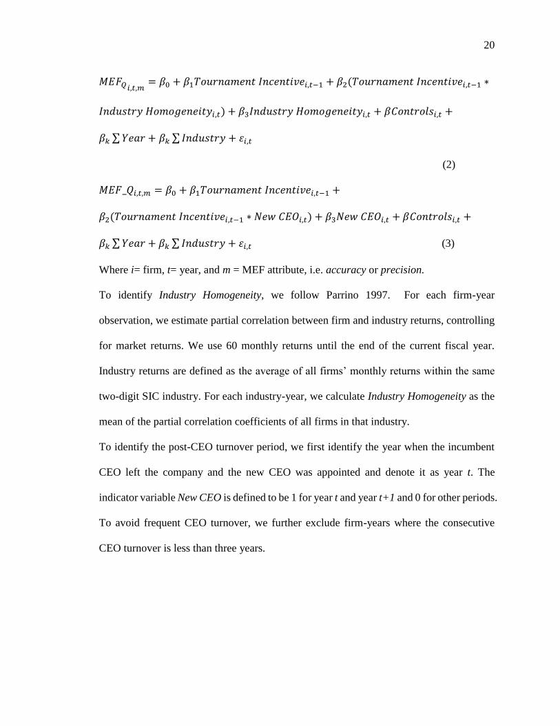
Development of Regression Test for H2
We refine regression model (1) by adding two interaction terms, i.e. Tournament
Incentive*Industry Homogeneity and Tournament Incentive*New CEO in the equation:
20
𝑀𝐸𝐹𝑄𝑖,𝑡,𝑚= 𝛽0 + 𝛽1𝑇𝑜𝑢𝑟𝑛𝑎𝑚𝑒𝑛𝑡 𝐼𝑛𝑐𝑒𝑛𝑡𝑖𝑣𝑒𝑖,𝑡−1 + 𝛽2(𝑇𝑜𝑢𝑟𝑛𝑎𝑚𝑒𝑛𝑡 𝐼𝑛𝑐𝑒𝑛𝑡𝑖𝑣𝑒𝑖,𝑡−1 ∗
𝐼𝑛𝑑𝑢𝑠𝑡𝑟𝑦 𝐻𝑜𝑚𝑜𝑔𝑒𝑛𝑒𝑖𝑡𝑦𝑖,𝑡) + 𝛽3𝐼𝑛𝑑𝑢𝑠𝑡𝑟𝑦 𝐻𝑜𝑚𝑜𝑔𝑒𝑛𝑒𝑖𝑡𝑦𝑖,𝑡 + 𝛽𝐶𝑜𝑛𝑡𝑟𝑜𝑙𝑠𝑖,𝑡 +
𝛽𝑘 ∑ 𝑌𝑒𝑎𝑟 + 𝛽𝑘 ∑ 𝐼𝑛𝑑𝑢𝑠𝑡𝑟𝑦 + 𝜀𝑖,𝑡
(2)
𝑀𝐸𝐹_𝑄𝑖,𝑡,𝑚 = 𝛽0 + 𝛽1𝑇𝑜𝑢𝑟𝑛𝑎𝑚𝑒𝑛𝑡 𝐼𝑛𝑐𝑒𝑛𝑡𝑖𝑣𝑒𝑖,𝑡−1 +
𝛽2(𝑇𝑜𝑢𝑟𝑛𝑎𝑚𝑒𝑛𝑡 𝐼𝑛𝑐𝑒𝑛𝑡𝑖𝑣𝑒𝑖,𝑡−1 ∗ 𝑁𝑒𝑤 𝐶𝐸𝑂𝑖,𝑡) + 𝛽3𝑁𝑒𝑤 𝐶𝐸𝑂𝑖,𝑡 + 𝛽𝐶𝑜𝑛𝑡𝑟𝑜𝑙𝑠𝑖,𝑡 +
𝛽𝑘 ∑ 𝑌𝑒𝑎𝑟 + 𝛽𝑘 ∑ 𝐼𝑛𝑑𝑢𝑠𝑡𝑟𝑦 + 𝜀𝑖,𝑡 (3)
Where i= firm, t= year, and m = MEF attribute, i.e. accuracy or precision.
To identify Industry Homogeneity, we follow Parrino 1997. For each firm-year
observation, we estimate partial correlation between firm and industry returns, controlling
for market returns. We use 60 monthly returns until the end of the current fiscal year.
Industry returns are defined as the average of all firms’ monthly returns within the same
two-digit SIC industry. For each industry-year, we calculate Industry Homogeneity as the
mean of the partial correlation coefficients of all firms in that industry.
To identify the post-CEO turnover period, we first identify the year when the incumbent
CEO left the company and the new CEO was appointed and denote it as year t. The
indicator variable New CEO is defined to be 1 for year t and year t+1 and 0 for other periods.
To avoid frequent CEO turnover, we further exclude firm-years where the consecutive
CEO turnover is less than three years.

21
1.4 Data Description and Empirical Results
1.4.1 Summary Statistics
In Table 2 we report summary statistics for our sample. There is no big difference in
distribution of our two measures of tournament incentives i.e. Log(Gap) and Log(Diff). The
mean (median) value of the executive pay gap is 2.960(3.334) million. It is comparable to
the statistics reported in Kale et al. (2009). The mean value of the forecast range is on
average 0.366 percent of the share price. The mean value of forecast error is about 0.826,
which indicates that the forecast in general deviates from the actual EPS around 0.826
percent of the share price. Distribution of control variables is in general consistent with the
existing literature.
[Insert Table 2 Here]
1.4.2 Empirical Results
Association between MEF Quality and Tournament Incentives
First, we evaluate the association between MEF quality and tournament incentives based
on regression model (1). We conduct two separate tests, one based on the precision
dependent variable, and other based on the accuracy dependent variable. The results of
these regression tests are contained in Table 3.
[Insert Table 3 Here]
The results in columns 1 and 2 on Precision show that coefficients of tournament incentives,
measured by Log(Gap) (coefficient = 0.030) and Log (Diff) (coefficient = 0.017) are
positive and statistically significant at the 0.01 level. Similarly, the results in columns in
3 and 4 on Accuracy show that coefficients of Log(Gap) (coefficient = 0.064) and Log (Diff)
(coefficient = 0.042) are positive and statistically significant. The economic significance

22
of precision shows that one standard deviation increase in Log(Gap) is associated with
8.525 percent increase in forecast precision. The coefficient 0.064 for accuracy indicates
that one standard deviation increase in Log(Gap) is associated with 8.058 percent increase
in forecast accuracy. These results confirm our hypotheses H1a and H1b that firms with
tournament incentives are associated with higher MEF quality, as proxied by MEF
precision and MEF accuracy.
The results on the control variables are overall consistent with prior literature. We find in
our sample that MEF quality is positively associated with firm size, institutional ownership,
growth opportunities, and firm performance, while forecast quality is negatively associated
with earnings volatility, forecast horizons, and internal control weakness.
Additional Evidence supporting H1
Additionally, we investigate whether the MEF attribute frequency is also affected by
tournament incentives. We conjecture that tournament incentives would provide strong
motivation for managers to issue MEFs more often to keep investors and board of directors
informed about expected changes in the future performance of the firm. We examined in
this study whether there is difference in MEF frequency of firms with and without
tournament incentives. We refine the regression model (1) by replacing the dependent
variable with forecast frequency, where MEF_Frequency is defined as the number of MEFs
issued by a firm during a year:
𝑀𝐸𝐹_𝐹𝑟𝑒𝑞𝑢𝑒𝑛𝑐𝑦𝑖,𝑡 = 𝛽0 + 𝛽1𝑇𝑜𝑢𝑟𝑛𝑎𝑚𝑒𝑛𝑡 𝐼𝑛𝑐𝑒𝑛𝑡𝑖𝑣𝑒𝑡−1 + 𝛽𝐶𝑜𝑛𝑡𝑟𝑜𝑙𝑠𝑡−1 +
𝛽𝑘 ∑ 𝑌𝑒𝑎𝑟 + 𝛽𝑘 ∑ 𝐼𝑛𝑑𝑢𝑠𝑡𝑟𝑦 + +𝜀𝑖,𝑡 (4)
The results (untabulated) show that coefficients of Log(Gap) (coefficient = 0.103) and
Log(Diff) (coefficient = 0.101) are positive and statistically significant at 0.01 level. These

23
results provide additional support to our H1and suggest that firms are more willing to
provide MEFs when the forecast quality is higher.14
Moderating Effect of Industry Homogeneity and New CEO on the Association
between Tournament Incentives and MEF Quality
We expect he association between tournament incentives and MEF quality to be moderated
by certain factors, including industry homogeneity and new CEO. Higher industry
homogeneity is associated with higher likelihood that the firm will hire an outsider as CEO
and reduces the possibility of winning tournament inside the firm. Similarly, the
appointment of new CEOs will reduce the possibility of getting promoted to CEO position.
Thus, both factors will take away the strong incentive of tournament participants to work
hard. We evaluate the moderating effect of these factors by including an interaction
variable between tournament incentive measures and the moderating factor. The results are
contained in Table 4.
[Insert Table 4 Here]
The results in the Panel A of Table 4 show that coefficient of the Tournament Incentive
remains positive and statistically significant for both tournament measures, whereas the
coefficient of Industry Homogeneity is negative and statistically significant. The
coefficient of the interaction term (Tournament Incentive*Industry Homogeneity) is
negative and statistically significant both for MEF precision and MEF accuracy (Column
1-4). The negative coefficient confirms that industry homogeneity has a moderating effect
14 We also examine whether firms with tournament incentives are associated with more long-term MEFs. Archaya et al.
(2011) argue that VPs focus more on long-term performance of the firm than CEOs. If VPs are actively involved in the
formation and discussion of MEF, we expect them to provide more long-term forecasts. The results are consistent with
our expectations. Both our tournament measures are positively associated with the frequency of long-term MEFs.

24
on the association between tournament incentives and MEF quality characteristics. This
finding thus suggests that the impact of tournament incentives is moderated with high
industry homogeneity, which may provide an opportunity to hire CEOs and other managers
from outside the firm.
In Panel B, we examine the impact of the moderating factor on the association between
MEF quality and tournament incentives, i.e. when the CEO in the firm is newly hired. The
results show that coefficients of both tournament incentive measures are positive and
statistically significant and the coefficient of New CEO is also positive. The coefficient of
the interaction term (Tournament Incentive* New CEO) is negative and statistically
significant for both proxies of higher quality of MEF, i.e. precision and accuracy. These
findings confirm our expectation that the newly hired CEO has a moderating effect on the
positive association of MEF quality and tournament incentive.
The above results support our hypotheses H2a and H2b that the association between MEF
quality, proxied by accuracy and precision of MEF, is moderated when the tournament
participants perceive the promotion probability to be slim.
1.5 Robustness Check Tests
It is possible that our findings are driven by CEO specific characteristics, some corporate
governance mechanisms, and/or mismeasurement of tournament incentives. In the
robustness tests, we control for the impact of CEO characteristics and certain aspects of
corporate governance on MEF quality, and we use alternative proxies to address the
measurement errors of tournament incentives.

25
1.5.1 CEO Ability, CEO Fixed Effect, and MEF Quality
Baik et al. 2009 show that CEO ability has a positive impact on the likelihood, frequency,
and quality of MEF. In this section, we first examine whether our results are driven by
CEOs’ personal characteristic. We first evaluate the influence of CEO ability on MEF
quality. We construct the Ability measure following Rajgopal et al. (2006) and Baik et al.
(2011). We compute cumulative distribution function (CDF) of industry adjusted ROA for
each CEO-firm-year by industry and take the mean of the CDF ranks of ROA for the first
three years when a new CEO is appointed. We include it as a control variable in our
regression model (1). The regression results are contained in Table 5, Panel A.
Similar to Baik et al. (2011), our results show that CEO ability (Ability) is positively
associated with forecast quality, i.e. accuracy and precision. Additionally, our tournament
incentive measures remain positive and statistically significant. These results support our
main finding and indicate the positive association between tournament incentives and
MEFs is not driven by CEO ability.
Bamber et al. (2010) argue that managers exert unique and significant influence on their
firms’ voluntary disclosure policies, which may be influenced by their style that is affected
by many demographic characteristics and their personal background. To isolate the effect
of CEO style, we include CEO fixed-effects in our regression models. The results are
contained in Panel B of table 5. There are in total 2,361 unique CEOs for our sample period.
The results show that the positive association between tournament incentives and MEF
quality is robust even when CEO fixed effects is included in the regression.
[Insert Table 5 Here]

26
1.5.2 Corporate Governance and MEF Quality
It is well documented in the literature that effective corporate governance is associated with
higher forecast quality (Eng and Mak 2003). Consistent with this line of reasoning, we
present that effective corporate governance would encourage CEOs and other senior
management to issue high quality MEFs. Therefore, it needs to be examined whether the
positive association between tournament incentives and MEF quality is driven by corporate
governance. We add three well-known corporate governance variables as control variables
in our equation (1), including G-Index15, CEO duality, and board independence. We follow
Gompers et al. (2003) and use G Index, which is an inverse measure of shareholder rights,
an indicator variable for CEO Duality, and a variable for Board independence. The CEO
duality indicator is equal to 1 if the CEO is also the chairman of the board. The board
independence is proxied by the percentage of independent outside directors on the board
(%IO Directors). The results are provided in Table 6.
[Insert Table 6 Here]
The results show that the tournament incentives measures remain positive and statistically
significant for all regression tests even after including additional control variables on
corporate governance. Therefore, the results confirm our expectation that tournament
incentives contribute to a better internal monitoring environment in additional to other
corporate governance mechanisms. The results also show that MEFs quality is associated
with stronger shareholder rights (lower G Index), positively associated with independent
15 For G Index after 2007, we use their IRRC values in 2006 and assume these values will carry forward for the
remaining sample periods.

27
board leadership, but board independence, proxied by the percentage of outside directors
serving on the board, is negatively associated with MEF quality.
1.5.3 Alternative Tournament Incentive Proxy
The subordinate managers may be more concerned about the relative increase in their
salaries rather than absolute tournament prize. One million pay differences will be less
attractive for an executive who earns five million per year compared to manager who earns
two million. Besides, the compensation packages of VPs and CEO are probably determined
by common unobserved factors, which may correlate with issuance of MEFs. The use of
relative proxy may mitigate this concern, as the effect of common factors will be canceled
out. We use the logarithm of the ratio of the CEO compensation to the median VP’s
compensation minus 1, to capture the percentage increase in salary if the VP gets promoted.
We re-estimate our models and the results (untabulated) remain unchanged.
Another concern may be that as opposed to other senior executives, CFOs may have more
control over disclosures, including MEF disclosures (Chang, Chen, Liao, and Mishra 2006).
We therefore test the effect of tournament incentives on CFOs. We construct the gap
between CEO and CFO compensation to re-estimate our models. Our results remain
qualitatively unchanged. In addition, the significant effect of pay gap between CEOs and
CFOs confirms the role of tournament incentives for CFOs in making decision on MEFs.
1.5.4 Endogeneity Concerns
It could be argued that tournament incentives and MEF quality are endogenously
determined. It is possible that tournament incentives induce high quality MEF, whereas
high quality MEF results in better firm performance, which results in higher CEO
compensation and tournament incentives. We use IV methodology to address the

28
endogeneity concerns. Following previous literature, our two instruments are the executive
pay gap lagged by two years and the industry median pay gap (Kale et al., 2009; Chen et
al., 2016). The validity of these two instruments is supported on the ground that the lagged
executive pay gap is less likely to be affected by voluntary disclosure decisions two years
later and the industry median pay gap is not likely to affect the firm-level disclosure policy
when industry fixed effects are included.
We present the second stage regression results in Table 7. The Shea R-square is 0.185
(0.144) (Column 1 and Column 2), which provides evidence that our instruments are
relevant. The test results show that our main fidings still hold. Specifically, for the
precisions regression, the coefficients of Log(Gap) and Log (Diff) are 0.039 and 0.025
respectively and are significantly significant at 0.01 level. Similarly, the coefficients of the
accuracy regression for Log (Gap) and Log (Diff) are 0.094 and 0.090 respectively and are
also statistically significant at 0.01 level. Thus, these results show that our main findings
are not influenced by the endogeneity concerns.
[Insert Table 7 Here]
1.5.5 Economic Consequences
Market Reaction to MEFs issued by Firms with Tournament Incentives
Another way to assess whether MEFs issued by firms with tournament incentives are of
higher quality is to evaluate market response to disclosure of MEFs. If market participants
perceive that internal tournaments attest to the higher quality of MEFs, their response to
MEFs issued by firms with tournaments incentvies will be stronger compared to MEFs
issued by firms such incentives.

29
To test the market reaction to MEFs, we use cumulative abnormal returns (CARs) and
abnormal trading volume around the disclosure date of MEFs as dependent variables and
control for other factors that have an influence on investors’ reaction. We use the following
models to evaluate investors’ reaction, where the interaction variable between Tournament
Incentive and News will indicate whether investors take into consideration tournament
incentives in responding to MEFs.
𝐶𝐴𝑅𝑖,[−1,1] = 𝛾0 + 𝛾1𝑇𝑜𝑢𝑟𝑛𝑎𝑚𝑒𝑛𝑡 𝐼𝑛𝑐𝑒𝑛𝑡𝑖𝑣𝑒𝑖,𝑡−1 ∗ 𝑁𝑒𝑤𝑠𝑖,𝑡 +
𝛾2𝑇𝑜𝑢𝑟𝑛𝑎𝑚𝑒𝑛𝑡 𝐼𝑛𝑐𝑒𝑛𝑡𝑖𝑣𝑒𝑖,𝑡−1 + 𝛾3𝑁𝑒𝑤𝑠𝑖,𝑡 + 𝛾𝐶𝑜𝑛𝑡𝑟𝑜𝑙𝑠𝑖,𝑡 + 𝛾𝐶𝑜𝑛𝑡𝑟𝑜𝑙𝑠𝑖,𝑡 ∗ 𝑁𝑒𝑤𝑠𝑖,𝑡 +
𝛾𝑘 ∑ 𝑌𝑒𝑎𝑟 + 𝛾𝑘 ∑ 𝐼𝑛𝑑𝑢𝑠𝑡𝑟𝑦 + 𝜀𝑖,𝑡 (5)
𝐴𝑏𝑛𝑉𝑜𝑙𝑖,[−1,1] = 𝛾0 + 𝛾1𝑇𝑜𝑢𝑟𝑛𝑎𝑚𝑒𝑛𝑡 𝐼𝑛𝑐𝑒𝑛𝑡𝑖𝑣𝑒𝑖,𝑡−1 ∗ |𝑁𝑒𝑤𝑠𝑖,𝑡| +
𝛾2𝑇𝑜𝑢𝑟𝑛𝑎𝑚𝑒𝑛𝑡 𝐼𝑛𝑐𝑒𝑛𝑡𝑖𝑣𝑒𝑖,𝑡−1 + 𝛾3|𝑁𝑒𝑤𝑠𝑖,𝑡| + 𝛾𝐶𝑜𝑛𝑡𝑟𝑜𝑙𝑠𝑖,𝑡 + 𝛾𝐶𝑜𝑛𝑡𝑟𝑜𝑙𝑠𝑖,𝑡 ∗
|𝑁𝑒𝑤𝑠𝑖,𝑡| + 𝛾𝑘 ∑ 𝑌𝑒𝑎𝑟 + 𝛾𝑘 ∑ 𝐼𝑛𝑑𝑢𝑠𝑡𝑟𝑦 + 𝜀𝑖,𝑡 (6)
We measure CAR as abnormal returns adjusted by the size-decile-matched market return
in [-1,1] window around the announcement date of MEFs. AbnVol is the average trading
volume from three trading days around the management forecast announcement date,
scaled by the median trading volume in prior 60 days. To reduce noises, we require the gap
between any two consecutive announcement dates to be greater than 30 days, and we
further delete forecasts announced within 30 days of annual earnings announcements. News,
as defined early, is the difference between management forecast EPS and analyst consensus
forecast (median) before management forecast, deflated by beginning stock price and
multiplied by 100. If firms with tournament incentives are associated with more reliable
forecasts, investors would be more responsive to those forecast news conditional on

30
information content of forecasts. Thus, we expect the coefficient of interaction term
Tournament Incentive*News, 𝛾1 to be significantly positive. Following Libby, Tan, and
Hunton (2006), we control the form of the forecasts (Point) and the timeless of
forecasts(Timeliness), since the market may rely more on point and timely forecasts. We
also use several control firm characteristics that may impact the market reaction, including
firm size, and earnings volatility (EanVol). All variables are interacted with News to
disentangle different reactions to the magnitude of news. Industry and year fixed effects
are also included.
The results are contained in Panel A of Table 8. In column 1-2, the coefficients of
Tournament Incentive* News are positive and significant at 0.01 level for both tournament
measures. These results support the argument that tournament incentives are associated
with stronger investor reaction to information contained in forecasts because of investors’
better perception of reliability of MEF quality when forecasts are issued by firms with
tournament incentives. In Column 3 and 4, we replace News with its absolute value, since
the dependent variable Abn_Vol should be associated with the information content in
forecasts regardless of the sign of news. Again, we find that coefficients of the interaction
term are significantly positive (0.082(0.051)) with a t-stat (3.16 (2.72)), respectively for
accuracy and precision analyses, suggesting that investors are more likely to trade on
information in forecasts issued by firms with tournament incentives.
[Insert Table 8 Here]
Analysts’ Reactions to MEFs issued by Firms with Tournament Incentives
We also examine how analysts react to MEFs issued by firms with tournament incentives.
We first examine the likelihood of analyst revising their forecasts in response to MEFs in

31
general, and then we examine the speed of analysts’ revisions following MEFs. 16 Overall,
we expect a higher number of analyst revisions following MEFs issued by firms with
tournament incentives in place since MEFs issued by these firms will be perceived by
security analysts to be more reliable and credible. We also examine the speed of analyst
revisions following the issuance of MEFs. It can be argued that analysts are likely to revise
their forecasts in a timely manner if the information contained in MEFs is more valuable
and accurate. Thus, we postulate that analysts take shorter time to revise their forecasts
following MEFs issued by firms with tournament incentives.
Panel B in Table 8 reports the results for analyst revisions. We investigate two aspects of
analyst reactions, i.e. fraction of analysts that revise their own forecasts and their speed of
revisions. Fraction is defined as the ratio of analysts who revise forecasts within 90 days
following the announcement dates of MEFs to the total number of analysts following the
firm.17 We refine regression model (6) by replacing the dependent variable with Fraction
and we use absolute value of News to proxy for the difference in information content. As
expected, Column 5 and 6 in Table 8 show that analysts are more likely to revise their
forecasts following management forecasts issued by firms with tournament incentives
(t=1.79 and 2.41 for Log(Gap)* |News| and Log(Diff)*|News|, respectively). Column 7 and
8 display the results for the speed of revisions. Log(Days) is defined as the natural
16 We also do not examine the magnitude of revisions because we cannot determine the quality of analyst forecasts ex
ante. We, however, recognize that there is link between the quality of analyst forecasts and revisions after issuance of
MEFs. If analyst forecasts issued before MEFs are of high quality due to the good information environment for high
tournament firms, the number of analysts revising their forecasts after the issuance of MEF will be significantly lower
because their revision will not add any value in terms of quality of their forecasts. On the other hand, if preceding
analyst forecasts are of poor quality, analysts will be motivated to revise their forecasts after issuance of MEFs to
improve the quality of their forecasts. 17 We define analyst following as the total number of analysts that issue at least one forecast for the firm during the
year.

32
logarithm of the number of days between MEF date and analyst revision date immediately
following the MEF. We find that analysts are inclined to revise faster for forecasts issued
by firms with tournament incentive. The coefficient of Tournament Incentive*|News| is
negative and significant at 0.01 level.
To summarize the findings on investors’ and analysts’ perception of the reliability of MEF
quality, our finding provide a strong support to our expectation that investors and analyst
are more responsive to MEFs when tournament incentives are in place in the firm. These
findings support our main hypotheses that MEF quality is high when forecasts are issued
by firms with tournament incentives.
1.6 Conclusion
In this paper, we examine the relation between competitive rank order tournament
incentives and MEF quality. We find that MEFs issued by firms with higher tournament
incentives are of higher quality, proxied by MEF accuracy and MEF precisions, compared
to MEFs issued by firms without competitive tournaments. Our test results on the third
attribute of MEF quality (i.e. frequency) are also similar to our main results. The positive
association between MEF quality and tournament incentives is moderated by industry
homogeneity and appointment of new CEO in the firm. Our robustness tests show that
findings are however robust because they are not driven by managerial ability, managerial
style, or effectiveness of corporate governance, and they remain unchanged when
alternative measures for tournament incentives are used.
Additionally, our tests on investors’ and security analysts’ response to MEFs support our
expectation that they also perceive MEF quality to be high when MEFs are issued by firms
with tournament incentives compared to the firms without tournament incentives.

33
Investors’ response is stronger when firms with tournament incentives issue the forecasts.
Similarly, security analysts respond to these MEFs by revising their forecasts and they
revise their forecasts on a timely basis.
Our paper contributes to literature by highlighting the role of tournament incentives in
contributing to MEF quality. Additionally, we show how subordinate contribute to higher
quality of MEFs issued by CEOs or CFOs. Our paper also answers to the debates of the
“overpaid” CEO compensation by unravelling the benefits of tournament incentives on
disclosure quality.

34
CHAPTER 2: DO CORPORATE FRAUDS DISTORT SUPPLIERS’
INVESTMENT DECISIONS?
2.1 Introduction
The real costs of corporate frauds on corporations engaging misconduct have been well-
documented in the literature, such as the reduction in market trust (Giannetti and Wang,
2016), the penalty in labor market for CEOs (Karpoff, Lee and Martin, 2008) and the
reduction in R&D or mistrust in patents. Specially, Kedia and Philippon (2007) show that
misrepresentation in accounting will lead to the distortion of employment and capital in
economy: the firms will hire more employees and invest more to pretend as “good firms”.
However, fraudulent information may also impact other clean firms. For example, Beatty,
Liao and Yu (2013) show that the fraudulent financial reports foster the overinvestment
among industry peers during the fraud period. Li (2016) expands such findings by showing
the distortions occur in the broader definition of frauds (e.g., restatements) and in R&D,
advertising and pricing policies as well.
Recently, researchers start to look at how the disclosure of fraudulent accounting will
impact wealth fare of non-financial stakeholders, such as firms with supplier-customer
economic ties. For instance, Kang and Tham (2012) show there’s a negative spillover effect
of earning restatements on supplier’s market value and more dependent suppliers will be
more likely to be cut off in post-restatement period. Files and Gurn (2014) argue that loan
lenders will charge a higher spread as the response to restatements in supplier’s industry.
However, these studies focus on suppliers’ reactions in the post period of customers’ frauds
35
and there is little understanding on how suppliers react to customer’s misrepresentation
during customers’ cheating periods.
This paper attempts to fill up such research gap and investigate whether the customers’
misrepresentation will lead to the distortion or inefficiency of suppliers’ investment
decisions. Thanks to the economic linkage between supply chain participants, suppliers
make investment or other product market strategies based on the prospective of their
customers (e.g., Subramani, 2004). For example, Lee, Padmanabhan and Whang (2017)
document that the distorted order information can misguide upstream members (e.g.,
suppliers) in their inventory and production decisions. Consistent with the argument that
the misrepresentation of financial performance leads to suboptimal investment decisions
(Maurren and Stephen, 2008), it is reasonable to believe the misrepresented customers’
information may distort suppliers’ investment decisions. Additionally, in line with Kumar
and Langer (2009), who shed lights on the association between frauds and overinvestment,
we expect that if customers pretend to be better firms by engaging corporate frauds, it’s
very likely their suppliers will overinvest in capital and deteriorate their investment
efficiency to keep up with customers’ illusory prosperities. As a result, the sacrificed
investment efficiency turns to be the real cost for suppliers.
In this paper, we adapt Li’s (2016) broader definition of misrepresentation and utilize both
litigation data (1996 - 2013) from the Securities Class Action Clearinghouse (SCAC) and
restatement data (2002 - 2013) from Audit Analytics database (AA). After excluding
financial and utility firms, our final litigation and restatement samples contain 1,502 and
2,129 fraudulent firms, respectively. In addition, we extract supply chain relationship

36
information from COMPUSTAT segment data and use a combination of automatic and
manual methods to identify customers.
With regard to the question that whether customers send out distorted positive demand
signals to suppliers during their cheating periods, we first explicitly show that customers
take real activities to cook their performance during the cheating periods, including hiring
excessive employees, purchasing redundant assets, and boosting their sales. Then, to
explore the main hypothesis, we find that affected suppliers1 with cheating customers tend
to have a higher level of capital expenditures during the cheating periods, comparing to
unaffected suppliers without cheating customers.
Further, to examine the cross-sectional variations of distortion influences, we consider two
factors that may moderate suppliers’ informational reliance on their customers: the industry
concentration and the sales volatility.
As argued in the study by Ali, klasa and Yeung (2014), industry leaders in a more
concentrated industry take a large slice of market shares and thus they can provide more
informative disclosure about future demand than firms in a less concentrated industry. In
such manner, suppliers are able to acquire industry demand information and revise their
investment strategies by observing industry leaders’ behaviors and disclosures with
relatively low costs. The emergence of this new information source attenuates the
informational reliance on their customers. On the other hand, suppliers with less sales
volatilities are more likely to be able to predict future performance based on historical
1 For a clear and concise demonstration, the affected suppliers refer to suppliers who engage with cheating customers
and on the contrary, the unaffected suppliers represent suppliers who have no cheating customers.

37
information and consequently become less relied on customers’ contemporaneous
performance to make strategic decisions (e.g., Yu, Yan and Cheng, 2001, Chen and Lee,
2009). Together, our empirical results present that a higher industry concentration or a
lower sales volatility can mitigate the level of suppliers’ overinvestment when they were
distorted by customers’ rosy perspectives.
In additional analysis, to triangle our main findings, we first confirm that suppliers’
distorted investments during the customers’ cheating period are inefficient by examining
the association between capital expenditures and future cash flows in the following two
years. The results show that the existence of cheating customers indeed hurts the
investment efficiency, reflected by the diminishing future cash flows. Next, we also report
evidence that suppliers bogged down in a higher level of overinvestment during the
cheating period, are likely to have more negative 3 (7) days market reactions when
customers’ frauds are made public, implying that the market is reluctant to believe that
affected suppliers can easily get rid of the headaches of customers’ distortions.
The results are robust to alternative empirical settings. Initially, our hypotheses are tested
in a clean setting by ruling out any potential interference of industrial factors. To further
address the issues arising from the pooled sample, we utilize the dynamic “Difference in
Difference” (DID) model adapted from Kedia and Philippon (2009) to concrete our
findings.
This paper adds to the accounting literature in the following three ways. In related studies,
Beatty, Liao and Yu (2013) and Li (2016) show that the fraudulent financial reports foster
the overinvestment among industry peers during the fraud periods. We expand such

38
findings by illustrating that the influence of corporate frauds can be extended to a broader
scope of victims. Specially, we document that corporate frauds incur the real economic
costs to not only firms within the same industry but also to firms with supplier-customer
economic ties. Second, consistent with prior literature (e.g., Baiman and Rajan, 2002; Choi
and Krause, 2006; Patatoukas, 2012), we emphasize the importance of the credibility of
information transferred over supply chain as well, showing that the inferior quality of
customers’ information erodes their suppliers’ investment efficiency. Third, this paper has
practical significance. To be specific, our findings reveal the nontrivial influence of
principal customers in a certain supply chain network. The firms at the center of supply
chain network may impair a large group of suppliers by distorting their future investment
decisions. Therefore, we suggest regulators to raise attentions on the structure of supply
chain and keep eyes on the suspicious behaviors of the “vital nodes” (principle customers)
in the supply chain network.
The reminder of the paper proceeds as follows. Section 2 develops the hypotheses based
on prior literature. Section 3 describes data, variable measurements and model
specifications. Section 4 presents the results, Section 5 and Section 6 discusses additional
tests and robustness checks. Section 7 concludes.
2.2 Literature Review and Hypothesis Development
2.2.1 Corporate Frauds and Investments
During the misrepresentation period, managers manipulate not only the financial numbers
but also the resource allocation to paint a rosy view of economic prospects. Prior literature
examines the effect of corporate frauds on the firm’s investment decisions. Kedia and

39
Philippon (2009) show that firms engaged in frauds tend to overinvest in order to mimic
good managers and conceal the low productivity. In line with this, Maurren and Stephen
(2008) also show that misrepresentation of financial performance leads to suboptimal
investment decisions. The theoretical model proposed by Kumar and Langberg (2009) also
provides some insights on association between frauds and overinvestment. In their model,
in order to pursue personal benefits from large incomplete commitments of investments,
the manager is likely to misreport the productivity and overinvest in some states.
Along with the direct effect of frauds on investments, the spillover effect on non-fraudulent
competitors is documented in the prior literature as well. Durnev and Claudine (2008)
develop a simple model where firms use competitors’ financial reports to gauge the
unknown payoff of investments. They argue that restatements contain news about the
investment projects of restating firm’s competitors and find that competitors change their
level of investments following restatement announcements. In related studies, Beatty, Liao
and Yu (2013) show that the fraudulent financial reports foster the overinvestment by
industry peers during fraud periods. Li (2016) documents that such distortions could occur
in the broader definition of frauds and in R&D, advertising and pricing policies as well.
2.2.2 Supplier-Customer Relationship and Corporate Frauds
The relations with suppliers may shape the customers’ decisions to opportunistically
manage earnings. For example, Raman and Shahrur (2009) document that firms are more
likely to manage accruals and consequently report higher earnings to encourage suppliers
to invest in relationship specific assets. The disclosures of customers’ frauds also impact
the wealth fare of suppliers. Kang and Tham (2012) show that there’s a negative spillover

40
effect of earning restatement over supplier’s market value and more dependent suppliers
will be more likely to be cut off after restatements are announced. Files and Gurun (2014)
argue that loan lenders will charge a higher spread as the response to restatements in
supplier’s industry. The fraudulent accounting induces reputational sanctions from the
product market. Customers impose significant sanctions on detected cheating firms,
leading to inferior operating performance of suppliers through increasing sell costs
(Johnson, Xie and Yi, 2014). To avoid the relationship disruption and reputational damage,
dependent suppliers being sued are more likely to reveal their good news and strategically
withhold their bad news (Cen et al., 2014).
There’s little understanding of how the misrepresentation will distort the investment
decisions and real costs for non-financial stakeholders especially during the undetected
customers’ cheating periods. As suppliers utilize their customer’s information to infer
future demand and economic prospect, noisy information distorts and misguides their
investment and production decisions (Lee, Padmanabhan and Whang 2017; Ha and Tong
2008). The manipulated charming performance of customers signals a potential high level
of future demand and prosperous economic prospects for suppliers. In order to share the
artificial prosperity, suppliers may overinvest to expand their production capacity to satisfy
the illusory high demand and make overinvestment. Thus, we hypothesize that:
H1: Suppliers will invest more during the fraud periods of customers.
2.2.3 Informational Reliance and Suppliers’ Overinvestment
Based on discussions above, we present the importance and potential effects of customers’
information on suppliers’ investment decisions during the cheating period. However, as we

41
known, the demand signal from the customer side is not the unique information channel
that suppliers can use to foresee the future demand. If suppliers have multiple choices of
information sources, they may less rely on customers’ information and consequently be
less distorted by fictional charming prospects of their customers. Therefore, in this section,
we specially identify two moderating effects that may affect suppliers’ informational
reliance on their customers: the industry concentration and the sales volatility.
First, it is costly for suppliers to aggregate customers’ information and forecast future
demand. However, industry leaders who own large market shares could have better
understanding of industry dynamism and demand. They may be more capable of predicting
future industry demand. As documented in Ali, Klasa, and Yeung (2014), in a concentrated
industry, corporate disclosures may provide more reliable information about future
industry demand than similar disclosures in a less concentrated industry. Therefore,
suppliers are more likely to use the reliable information from observing industry leaders’
behaviors or disclosures to revise their own strategies than simply rely on customers’
information. The emergence of such additional information channel may dilute the value
of customers’ information and attenuate suppliers’ informational reliance on their
customers. Therefore, we expect the investment distortions of suppliers to be less severe in
a highly concentrated industry.
H2(a): The distortion effects of fraudulent customers’ information on suppliers’
investment decisions will be less pronounced when suppliers are operating in a highly
concentrated industry.

42
On the other hand, a stream of literature has documented the importance and benefits of
information sharing in supply chain, especially when firms face greater demand uncertainty
(Yu, Yan, and Cheng 2001, Chen and Lee 2009, Lee, Padmanabhan, and Whang 2017).
When suppliers are operating in a volatile environment, it is hard to predict future demands
solely based on historical firm information and thus the demand signals from customers
become more essential to forecast future demands. Consequently, we expect the distortion
effect to be more severe when suppliers rely more on their customers’ information.
H2(b): The distortion effects of fraudulent customers’ information on suppliers’
investment decisions will be more pronounced when suppliers are operating in volatile
environment.
2.3 Research Design
2.3.1 Data
We first proxy corporate frauds by class action lawsuits obtained from the Securities Class
Action Clearinghouse (SCAC). The initial litigation sample is consisted of 2,055 lawsuits
that can be matched to COMPUSTAT from 1996 to 2013. Then, we create restatement
sample by focusing on firms with income-increasing restatements from 2002 to 2013 from
the Audit Analytics database (AA). The initial restatement sample contains 2,846
restatements that are matched with COMPUSTAT.2 We further exclude financial (SIC
codes between 6000 and 6999) and utility firms (SIC codes between 4900 and 4999) for
both samples. For firms that commit multiple frauds in our sample periods, we only keep
2 We follow prior literature (e.g., Wang and Winton, 2010) and focus on ex post detected frauds.

43
the first case. Our final litigation and restatement sample contain 1,502 and 2,129
fraudulent firms, respectively.
We extract supply chain relationship from COMPUSTAT segment data. In accordance
with the statement of Financial Accounting Standards (SFAS) No. 14 and No.131, public
firms are required to disclose the identity of any customer that contributes at least 10% to
the firm’s revenues. However, only the names of principal customers or the abbreviations
of the customer names are reported in the segment data. Next, we use a combination of
automatic and manual methods to match customer names with company names appeared
in the COMPUSTAT to obtain the GVKEY identifiers. We follow Fee and Thomas (2004)
approach to conduct matching and use industry classification to verify matches. If still
cannot find a match, we manually search S&P capital IQ to identify whether the customer
is a corporate subsidiary. If so, the customer will be matched to its parent company.
In this paper, we define a firm as a dependent supplier if it reported at least one principal
customer in the prior two years.3 In order to identify fraudulent customers, we examine all
disclosed customers in the past two years. We use the litigation and restatement data to
identify the cheating periods of customers. In the litigation sample, we identify 391 unique
cheating customers and 934 related dependent suppliers, resulting in 1,288 firm-years.
Alternatively, in the restatement sample, we find 214 unique cheating customers and 435
unique related suppliers, resulting in 609 firm-years. Table 1 presents the summary of the
time series trend of affected suppliers for both samples. As expected, the number of
3 Following prior literature (Maurren and Stephen 2008), the principal customer is any disclosed customer which has at
least 10% of its suppliers’ total sales.

44
affected suppliers drastically drops after the implementation of Sarbane Oxley Act (2002).
[Insert Table 1 Here]
Finally, we obtain financial data from COMPUSTAT database. To attenuate the potential
difference of firm characteristics between dependent suppliers and firms with no principal
customers, we restrict our sample to firm-years where principal customers are disclosed in
the prior two years. We also exclude all dependent suppliers engaged in fraudulent
reporting for a clean research setting. There are 10,727 and 8,771 firm-years with non-
missing financial information in the litigation sample and restatement sample, respectively.
2.3.2 Model Specifications
Test of H1: Investment Distortions of Affected Suppliers
When cheating customers signal prosperous prospects, we expect that the related suppliers
will increase their investments in order to meet increased demand in the future. To test our
hypothesis, we run the following OLS regression.
𝐶𝐴𝑃𝐸𝑋𝑖,𝑡 = 𝛽0 + 𝛽1𝐶ℎ𝑒𝑎𝑡𝑖𝑛𝑔_𝐶𝑢𝑠𝑡𝑜𝑚𝑒𝑟𝑖,𝑡 + 𝛽2𝐹𝑢𝑛𝑑𝑎𝑚𝑒𝑛𝑡𝑎𝑙_𝐶𝑜𝑛𝑡𝑟𝑜𝑙𝑠𝑖,𝑡 + 𝜀𝑖,𝑡4 (1)
The dependent variable CAPEX is the ratio of capital expenditure to lagged total asset. The
main variable of interest Cheating_Customer is to capture the presence of a cheating
principal customer. Cheating_Customer takes one if the customer is disclosed in either of
the prior two years and the current year is part of its class period. We expect the coefficient
of Cheating_Customer to be positive. Following Li (2016) and Beatty, Liao and Yu (2013),
we include a set of fundamental factors to control for the specific characteristics of
4 In the untabulated test, after controlling customers’ fundamental controls, we still get significant and consistent
empirical findings.

45
suppliers that influence their investment decisions. For instance, we control for firm size,
Tobin’s Q, and sales turnover, as firms with higher growth and investment opportunities
tend to invest more. We also control for cash holdings, ROA, and external financing since
extra cash or external financing facilitates investment, and firms’ investment increases with
profitable operations. We control for firms’ financial leverage as previous literature
document that financial frictions and ownership structure could be linked with corporate
investments (Almelda and Campello 2007, Ozdagli 2012). Finally, we include industry and
year fixed effects to the regression model for both samples.
Test of H2: The Moderating Effects of Suppliers’ Informational Reliance on
Customers
In this section, we investigate how suppliers’ informational reliance on customers moderate
the magnitude of suppliers’ overinvestment during customers’ cheating periods. Our
expectation is that suppliers are less likely to use customers’ information to infer future
demand within a concentrated industry, but more likely to depend on customers’
information when there’s high uncertainty over sales. We construct the Herfindahl-
Hirshman Index (HHI) to proxy for the industry concentration. HHI is defined as HHI𝑖,𝑡 =
∑ ( П𝑖)2𝑛
𝑖=1 , where П𝑖 is the market share of company i within the same 2-digit SIC
industry. Following Tong et al. (2008), we use the standard deviation of the natural
logarithm of sales in the prior three years as the measure of volatility in the operating
environment.
We refine the equation (1) by interacting both the HHI and sales volatility with our main
variable of interest Cheating_Customer. We expect the coefficient of is

46
HHI*Cheating_Customer significantly negative, while the coefficient of
Sales_Vol*Cheating_Customer is significantly positive.
𝐶𝐴𝑃𝐸𝑋𝑖,𝑡 = 𝛽0 + 𝛽1𝐶ℎ𝑒𝑎𝑡𝑖𝑛𝑔_𝐶𝑢𝑠𝑡𝑜𝑚𝑒𝑟𝑠𝑖,𝑡 + 𝛽2𝐶ℎ𝑒𝑎𝑡𝑖𝑛𝑔_𝐶𝑢𝑠𝑡𝑜𝑚𝑒𝑟𝑠𝑖,𝑡 ∗ 𝐻𝐻𝐼𝑖,𝑡 +
𝛽3𝐹𝑢𝑛𝑑𝑎𝑚𝑒𝑛𝑡𝑎𝑙_𝐶𝑜𝑛𝑡𝑟𝑜𝑙𝑠𝑖,𝑡 + 𝜀𝑖,𝑡 (2.1)
𝐶𝐴𝑃𝐸𝑋𝑖𝑡 = 𝛽0 + 𝛽1𝐶ℎ𝑒𝑎𝑡𝑖𝑛𝑔_𝐶𝑢𝑠𝑡𝑜𝑚𝑒𝑟𝑠𝑖,𝑡 + 𝛽2𝐶ℎ𝑒𝑎𝑡𝑖𝑛𝑔_𝐶𝑢𝑠𝑡𝑜𝑚𝑒𝑟𝑠𝑖,𝑡 ∗
𝑆𝑎𝑙𝑒𝑠_𝑉𝑜𝑙𝑖,𝑡 + 𝛽3𝐹𝑢𝑛𝑑𝑎𝑚𝑒𝑛𝑡𝑎𝑙_𝐶𝑜𝑛𝑡𝑟𝑜𝑙𝑠𝑖,𝑡 + 𝜀𝑖,𝑡 (2.2)
2.4 Results
2.4.1 Descriptive Statistics
Table 3 presents summary statistics for our entire sample. In accordance with Li (2016),
we utilize both litigation (Panel A) and restatement (Panel B) in our empirical analyses.
Detailed definitions of variables used in Table 3 are provided in Appendix A. We winsorize
all financial variables at the 1st and 99th percentiles of their distributions to minimize the
influence of outliers.
In panel A, the variable of our interest is the dummy variable “Cheating_Customer”, which
equals to 1 if the supplier has at least one cheating customer during the class period. It
shows that 12% out of 10,727 observations are affected suppliers with cheating customers,
implying that the existence of cheating customers in a supplier-customer relationship is not
rare. Similarly, in Panel B, the main variable “Cheating_Customer” indicates that 6.9% out
of 8,771 observations are affected suppliers with cheating customers in our restatement
sample.
Other fundamental factors documented by prior literature that may impact corporate
investment decisions have been included in our sample as well. In litigation sample, on

47
average, the supplier has a logarithm of total assets value of 5.147, with a leverage ratio of
16.3%, a ROA of -10.5%, a cash holding of 19.5% and Tobin’s Q of 2.101. Consistently,
in restatement sample, an average supplier has a logarithm of total assets value of 5.648,
with a leverage ratio 16.2%, a ROA of -8.9%, a cash holding of 19.6% and Tobin’s Q of
2.042. Overall, the distributions of control variables are consistent in both litigation and
restatement sample.
[Insert Table 3 Here]
2.4.2 Preliminary Results
Customers’ Manipulations During Cheating Periods
Following prior literature (Kedia and Philippon 2007, Beatty et al., 2013, Li 2016), in our
preliminary test, we investigate whether cheating customers are manipulating resource
allocations to paint a rosy view of economic prospects during cheating periods. In line with
Kedia and Philippon (2007), we compare cheating firms’ capital expenditures, employee
growth, property, plant, and equipment growth, growth in size, and sales growth in its
market between cheating and clean periods for both our samples. As predicted, we find that
cheating customers not only sugar up financial numbers, but also distort the overall
resource allocations and investments in order to be viewed as “prosperous”. For example,
we observe that during cheating periods, the fraudulent customers on average overinvest
by 0.4%, hire 3.3% more employees, experience 1.5% more growth in size, and 2.8% more
growth in sales comparing to clean customers in the litigation sample. We also find similar
results in the restatement sample.
[Insert Table 2 Here]

48
2.4.3 Main Results
Table 4 reports the regression results for our first hypothesis (H1) using the model of
Equation (1). The dependent variable is suppliers’ capital expenditures (CAPEX). The
variable of interest is the dummy variable “Cheanting_Customer”, which equals to 1 when
suppliers have a cheating principle customer and 0 otherwise. The column (1) and (2)
present the regression results for the litigation sample from 1996 to 2003. In column (1),
we find a significantly positive association (𝛽1 = 0.01, t=3.51) between the existence of
cheating customers and suppliers capital expenditures, implying that customers’
misrepresentations distort their suppliers’ to make overinvestment during the cheating
period. In column (2), this result holds after controlling for factors known to explain firms’
investment decisions. The significantly positive coefficient (𝛽1 = 0.008, t=2.68) suggests
that affected suppliers tend to invest 11.4% more comparing to unaffected suppliers. The
coefficients for control variables are significant and consistent with our expectations as
well. Specially, during customers’ cheating periods, suppliers who have higher cash
holdings, sales, ROA and financing activities, but lower leverage are likely to be distorted
to overinvest. Additionally, in accordance with Li (2016), we also conduct the same
analysis utilizing the restatement sample, presented in column (3) and (4). Our results are
robust and held. The coefficients of variable of interests are 0.01 (t=2.84) and 0.012 (t=3.08)
in column (3) and (4) respectively. It indicates that affected suppliers are more likely to
invest 21% more than unaffected suppliers during customers’ cheating periods. Overall,
the results in Table 4 suggest that customers’ frauds have a spillover effect on suppliers’
investment decisions and trigger suppliers to make overinvestment during the cheating
period.
49
[Insert Table 4 Here]
2.4.4 Cross-sectional Tests
The second hypothesis aims to investigate the moderating effects of “information reliance”
on the association between customers’ misconduct and suppliers’ overinvestment during
customers’ cheating periods. To explore H2, we estimate models in equation (2.1) and (2.2)
and focus on the interaction term Cheating_Customer * HHI and the Cheating_Custmer *
Sales_Vol.
Table 5 reports the regression results for H2. In column (1), consistent with our expectation,
the coefficient of the interaction term Cheating_Customer*HHI is -0.11 (t=-2.48),
suggesting that within a high concentrated industry, suppliers are less distorted by
customers’ misrepresentations to make overinvestment. Within a high concentrated
industry, suppliers are able forecast future demands by extracting information from
industry leaders’ disclosures or observing leaders’ behaviors with low cost, and thus
suppliers’ informational reliance on their customers is largely shrunk. On the other hand,
in column (2), the coefficient of the interaction term Cheating_Customer * Sales_Vol is
significantly positive (0.041, t=2.98), suggesting that suppliers with a high degree of sales
uncertainty, are more distorted by customers’ frauds. Suppliers with high sales volatilities
are hard to predict their future performance solely based on historical data and thus rely
more on their customers’ information when making investment decisions. The results are
still held in column (3) and (4) utilizing the restatement sample from 2002 to 2013. We
find that the coefficient of the interaction term Cheating_Customer*HHI is -0.136 (t=-2.45)
in column (3) and the coefficient of Cheating_Customer*Sales_Vol is 0.052 (t=2.09) in

50
column (4). All specifications include the year and industry fixed effects to control for
potential omitted variables.
[Insert Table 5 Here]
2.5 Additional Tests
2.5.1 The deteriorated investment decisions during the cheating period
To further triangle our main findings, we first confirm that suppliers’ investment decisions
during customers’ cheating period are distorted and suboptimal, by examining how the
existence of cheating customers impacts the association between capital expenditures and
future two years’ cash flows. We expect that the existence of cheating customers will
mitigate the contribution of the investment to future operating performance.
To empirically test our argument, we only eliminate those firm-year observations when
their following years fall in the post period of detected frauds. We control fundamental
variables that could impact future cash flows, such as firm size, cash holdings, leverage,
ROA, sales, financing and Tobin’s Q. Specially, we utilize the following equation (3):
CFO𝑖,𝑡+𝑚 = 𝛽0 + 𝛽1𝐶𝐴𝑃𝐸𝑋𝑖,𝑡 ∗ 𝐶ℎ𝑒𝑎𝑡𝑖𝑛𝑔_𝐶𝑢𝑠𝑡𝑜𝑚𝑒𝑟𝑖,𝑡 + 𝛽2𝐶𝐴𝑃𝐸𝑋𝑖,𝑡
+ 𝛽3𝐶ℎ𝑒𝑎𝑡𝑖𝑛𝑔_𝐶𝑢𝑠𝑡𝑜𝑚𝑒𝑟𝑖,𝑡 + 𝛽4𝐹𝑢𝑛𝑑𝑎𝑚𝑒𝑛𝑡𝑎𝑙_𝐶𝑜𝑛𝑡𝑟𝑜𝑙𝑠𝑖,𝑡 + 𝜀𝑖,𝑡 (3)
Where the dependent variable is future two years’ cash flows CFO𝑡+1 (m=1) and CFO𝑡+2
(m=2) and the interaction term CAPEX*Cheating_Customer is our variable of interest. We
expect a significant negative sign of the coefficient of the interaction term.
Table 6 reports the regression results by using both litigating sample and restatement
sample.

51
[Insert Table 6 Here]
In the first two columns, we show that the coefficients of the interaction terms are
significantly negative with both CFO𝑡+1(𝛽1 =-0.164, t=-2.50) and CFO𝑡+2 (𝛽1 =-0.198,
t=-2.22), supporting our expectation that during customers’ cheating period, suppliers
make suboptimal investment decisions and suffer from the inferior future operating
performance in the following two years. The results presented in the column (3) and
column (4) are still qualitatively consistent with our expectations, when we replace the
litigation sample with the restatement sample.
2.5.2 The stock market reactions to the distortion on the date of the fraud disclosure
In this section, we aim to investigate whether the market will punish distorted suppliers
after the disclosure of customers’ frauds. If so, despite the investment inefficiency and the
inferior operating cash flows during the cheating period, the negative stock market reaction
from investors sets off a new wave of economic real costs to suppliers in the post period of
detected frauds. To empirically test our expectations, we first select those suppliers who
actually engage in overinvestment. Specially, during the cheating period, we use industry
median of capital expenditures from unaffected suppliers as the benchmark level of
investment and consequently the affected suppliers are classified as overinvestment
suppliers if they have a higher level of capital expenditures than the benchmark in at least
one year during the cheating period. Then, we use the disclosure dates of customers’
misrepresentations as event dates to investigate market reactions to the suppliers’
overinvestment at the end of cheating periods. Our treatment groups are affected suppliers

52
engaged with overinvestments and control groups were unaffected suppliers. The
regression model is conducted as following:
CAR𝑖,[−3,+3] 𝑜𝑟 CAR𝑖,[−1,+1]
= 𝛽0 + 𝛽1𝐻𝑖𝑔ℎ_𝐶𝐴𝑃𝐸𝑋_𝐶𝑢𝑠𝑡𝑜𝑚𝑒𝑟𝑖,𝑡 + 𝛽2𝐹𝑢𝑛𝑑𝑎𝑚𝑒𝑛𝑡𝑎𝑙_𝐶𝑜𝑛𝑡𝑟𝑜𝑙𝑠𝑖,𝑡
+ 𝜀𝑖,𝑡 (4)
Where the dependent variable are 3 days or 7 days cumulative abnormal returns (CAR)
adjusted by the size portfolio, and the variable of interests is the dummy variable
(High_CAPEX_Customer) indicating whether affected suppliers have ever overinvested
during the cheating period.
The results can be found in Table 7. In the first two columns, the significantly negative
coefficients (-0.013, t=-1.77 and -0.019, t=-2.16) of our variable of interests
(High_CAPX_Customer) support our expectation that the market will punish the distorted
suppliers’ overinvestment decisions when their fraudulent major customers are caught and
the negative market reaction is also a kind of real economic costs to suppliers. We find a
qualitative consistent result after we replace our litigation sample with restatement sample.
The results can be found in the last two columns.
Moreover, we further investigate that whether the level of overinvestment may trigger
different magnitude of the negative market reaction for affected suppliers with cheating
customers after the disclosure of customers’ frauds. Specially, we still utilize the industry
median of capital expenditures from unaffected suppliers as the benchmark and calculate
the “abnormal investment level” for affected suppliers. Then, we take the average of the
abnormal investment over the cheating period and classify those suppliers as highly

53
overinvested suppliers if their average abnormal investment falls in the top half of the
sample. Then we follow the same regression design by replacing the dummy variable from
the one indicating whether suppliers engage in overinvestment with the one indicating
whether suppliers have highly overinvested comparing to other affected suppliers. In this
test, our treatment groups are highly overinvested suppliers and control groups were the
rest of affected suppliers.
[Insert Table 7 Here]
In the untabulated table, we find that indeed, the more the suppliers engage in
overinvestment, the more severe market reactions they receive after the frauds were made
public, implying that investors are reluctant to believe suppliers can easily get rid of the
headaches of customers’ distortions. This finding concretes our argument that except the
real costs during the cheating period, suppliers also need to pay off the costs from the stock
market after the disclosure of customers’ frauds.
2.6 Robustness Checks
Initially, our empirical results are tested in a cleaner setting. In prior related studies that
investigate distortion effects among peer firms, the potential omitted industrial common
economic factors and information learning between peers can drive the result. In their
studies, they cannot disentangle these two effects. However, in our study, the “cross-
industries” setting successfully rules out the interference of industrial common economic
factors.

54
To alleviate the issues arising from the pooled matching of control groups (unaffected
suppliers), we adapt the approach from Kedia and Philippon (2009) to compare dynamics
of capital expenditures for affected suppliers around the cheating periods.
Firstly, we create a control group of unaffected suppliers that are matched in size, year and
industry. Specially, for each affected suppliers, we choose all unaffected suppliers appear
in two years before the beginning of customers’ misconduct5. We then select unaffected
suppliers which operate in the same industry, and that are in the same size quantile. To
address survival bias, we also require the control group to survive through the entire
customers’ cheating periods. We adjust the variables of interest (capital expenditure) by
subtracting the mean of this control group.
capex̂𝑖,𝑡 = capex𝑖,𝑡 − capex̅̅ ̅̅ ̅̅ ̅̅𝑐(𝑖),𝑡
Where c(i) is the control group for firm i at year t.
We now turn to a formal empirical test to substantiate our evidence as follows:
capex̂𝑖,𝑡 = 𝛽0 + 𝛽1𝐷𝑢𝑟𝑖𝑛𝑔𝑖,𝑡 + 𝛽2𝐴𝑓𝑡𝑒𝑟𝑖,𝑡 + 𝜀𝑖,𝑡
A positive estimated coefficient β1 implies that the affected suppliers invested more than
comparable unaffected suppliers during customers’ cheating periods. Besides that, we also
compare the coefficient over time to see if the dynamics of affected suppliers will
significantly change after the disclosure of customers’ frauds. After the disclosure of
5 Different from Kedia and Philippon (2009), we create the control group in two years before the fraudulent period not
in the beginning of our sample. Since fraudulent firms are likely to make preparation for misconduct in advance, it is
reasonable to consider longer window to observe the dynamics of performance. However, our paper is to see spillover
effects due to customers’ frauds over supply chain. A shorter window is more proper, the firms selected in the control
group are more similar to each other in fundamentals.

55
customers’ frauds, the manipulated customers’ prospects were corrected and suppliers’
start to adjust the level of investments back to normal. Therefore, it is reasonable to expect
that affected suppliers’ capital expenditures will go down after the fraudulent periods. In
this case, the null hypothesis is that 𝛽1 = 𝛽2.
[Insert Table 8]
The results are presented in table 8. The affected suppliers significantly (t=2.17) invest
more during customers’ fraudulent period in comparison to unaffected suppliers. Consist
with our prediction, we find that the null hypothesis that 𝛽1 is the same as 𝛽2 can be
rejected at less than 1% level, indicating that after the fraudulent periods, affected suppliers’
capital expenditures go down, as we predicted.
2.7 Conclusion
The corporate frauds have attracted much attention from both financial and nonfinancial
stakeholders. Prior literature well-document the real costs of corporate frauds on firms
engaging misconducts (Kedia and Philippon 2009, KarpoffLee and Martin, Giannetti and
Wang, 2014). Recently, researchers start to notice the spillover effects of fraudulent
financial reporting on peer firms (Beatty, Liao and Yu, 2013) and broad the definition of
fraudulent accounting (Li, 2016). In this paper, we expand their work and investigate the
spillover effects of corporate frauds in the broader scope of victims. Specially, we
document that corporate frauds incur the real economic costs to not only firms within the
same industry but also to firms with supplier-customer economic ties.
We find that during customers’ cheating periods, affected suppliers with cheating
customers are more likely to be distorted to overinvest in comparison to unaffected

56
suppliers. Further, in the cross sectional analysis, we test the moderating effects of
suppliers’ informational reliance on the positive association between the existence of
cheating customers and suppliers’ overinvestment. Additionally, we also provide evidence
that after the disclosure of customers’ frauds, suppliers engaged in overinvestment are
going to experience the negative market reaction. Lastly, to triangle our main findings, we
utilize a “difference in difference” (DID) approach to confirm that affected suppliers
elevate the level of capital expenditures during customers’ cheating periods and such high
level of investments will go down after the disclosure of customers’ frauds. Overall, our
paper contributes to the current accounting literature by unraveling the real costs of
corporate frauds over supply chains, emphasizing the importance of the credibility of
information transferred over supply chain, and suggesting regulators to keep eyes on the
customers at the center of the supply chain network.

57
CHAPTER 3: STRATEGIC EARNINGS ANNOUNCEMENTS TIMING AND
FINANCIAL MISREPORTING
In the realm of corporate frauds, prior literature has provided evidence that companies
strategically take activities to “hide” their misconduct and in consequence extend the
detection duration due to the phobia of being punished by the market. For example,
managers attempt to make overinvestment to disguise fraud by introducing valuation
imprecisions and creating inference dispersions for outside information users (e.g. Wang
2004, Kedia and Phillipon 2009). Additionally, they may spend a fair amount of money in
lobbying to lower the rate of being detected in frauds (Yu and Yu 2011). Moreover,
managers are likely to increase the cost of extracting information from disclosures by
strategically reducing the readability of financial reporting (Lo, Ramos and Rogo 2017).
However, these studies neglect a low-cost strategy that may be beneficial for managers to
camouflage their opportunistic behaviors: the timing strategy of Earnings Announcement
(EA). In this paper, we are going to examine whether managers involved in accounting
misreporting are inclined to strategically announce earnings news during the period of low
market attention and further explore the underlying benefits of doing this.
The debate regarding the existence of strategic timing of EAs motivates our study. As
argued in recent studies (e.g. Della Vigna and Pollet 2009; Melessa 2013; DeHaan et al.
2015; Michaely 2016), managers are aware of earnings news before the releasing date and
take information advantage over investors to strategically decide the time of disclosure.
Based on the “investor inattention hypothesis” (Hirshleifer et al. 2009), managers are apt
to disclose bad news in low market attention time slots and benefit from reduced market

58
responses. Prior literature devotes many pages to evaluate the proxy for the low market
attention. For example, the pioneering “Firday” (e.g. DellaVigna and Pollet 2009), the
specified “Friday evening”, the new insightful “after trading hours” and “busy
announcement days” (e.g. DeHaan et al. 2015) and the unpredictable exogenous daily news
pressure index (Israeli, Kasznik and Sridharan 2017). But these studies examine the
existence of strategic announcing with respect to the content of news but overlooks the
importance of the quality of the news. As well documented in the earnings management
and corporate frauds literature, managers usually opportunistically manipulate the content
of earnings in an upward direction to maximize their self-interests even paying additional
costs (e.g. taxes): either inflate bad news to good news or shift the bad news from an
extreme to an average extent (e.g. Burgstahler and Dichev 1997; Healy and Wahlen 1999;
Erikson, Hanlon and Maydew 2004). In this way, the manipulated earnings result in a low
quality and intentionally mislead investors’ expectations on firm value. At the meanwhile,
for the fear of the market punishments after being required to restate or detected s
(Palmrose, Richardson and Scholz 2004; Farber 2005; Ball 2009), managers strategically
take real activities to conceal their misconduct. Following a similar logic, we expect
managers engaged in misreporting may release their manipulated earnings strategically by
picking up low market attention or high distraction time to lower the possibilities of being
caught, such as after trading hours, Friday nights, or busy days with numerous news.
As we discussed above, for managers managing earnings, the primary benefit of strategic
announcing is to lower the detection rate. In the era of information explosion, it seems
impossible for managers to completely hide news from investors. Although the pricing
impact through managing disclosure timing may be a flash in the pan, managers still prefer

59
to drag down the rate of the discovery of opportunistic behaviors and bear with a gradual
price drop in future to avoid a high crash and litigation risk (Donelson et al. 2012).
Consistent with prior literature that find mangers successfully extend the detection period,
we expect that the primary benefit of strategically managing EAs time is to lower the
probability of being caught, resulting in a longer undetected period.
Moreover, insider trading may be an additional benefit to explain why cheating firms
would like to announce manipulated earnings in low market attention time slots. In
Michaely et al. (2016) study, they find that insiders benefit from trading in the direction of
the content of the news soon after the EAs. However, it is not the case when the nature of
the news is manipulated. Insiders take advantage of the information asymmetry over
investors to trade based on the underlying quality of news rather than the reported content
of news. Since firms are able to camouflage bad news to good news, In some cases, even
the content of the news announced is good, insiders may still take a short position in shares
because they can foresee that the faked good news may be discovered in future which
increases their personal wealth risk. On the other hand, insiders may also buy shares during
the cheating period to share the faked prosperity. Therefore, the direction of insider trading
is unclear when the news is good. Contrastingly, if the disclosed news is bad, insiders are
more likely to sell shares and benefit from market inattention and unawareness of
manipulation.
To examine our proposed hypotheses above, we first identify financial manipulation by
using accounting restatements from 2002 to 2015 from the Audit Analytics database. We
only keep those income-increasing restatements to proxy the intentional upward
manipulations (e.g. Archambeault, Dezoort and Hermanson 2010). To capture more severe
60
accounting manipulation, we collect Accounting and Auditing Enforcement
releases(AAER) data from 1999 to 2010, as our alternative sample. Specially, the SEC data
are obtained from the University of Berkeley’s Center for Financial Reporting and
Measurement. After excluding financial firms and merging with the COMPUSTAT, we
obtain 1,344 restatements and 308 SEC enforcements, respectively. Following prior
literature (Bagnoli et al. 2005; Doyle and Magilke 2009; DeHaan et al. 2015; Michaely et
al. 2016), we proxy limited attention period as the period after market closes (AMC) and
the Friday, considering both time of the day and day of the week. To address the concern
whether the annual EAs timing is as flexible as quarterly EAs timing, we compare the
timing distribution of annual EAs to quarterly EAs and suggest that the changes of annual
EAs timing are relatively common.
In the univariate analysis, we find that during the fraudulent period, misreporting firms
make 4.61% more EAs than firms within the control group during the after trading hours
in the restatement sample. We find a similar pattern in the AAER sample, whereas
misreporting firms make 10.35% more EAs during the after trading hours than control
firms. To attenuate the potential sample selection bias, we further restrict our sample to
only misreporting firms and find that misreporting firms in fraudulent years tend to disclose
more in after trading hours than that in non-fraudulent years. However, we are not able to
find a similar result by using Friday as the proxy for low market attention period.
To bolster our univariate inferences, we perform cross-sectional regression analysis.
Following prior literature, we control several firm specific variables. Although we focus
on investigating the effect of the quality of the news, we control the content of the news
proxied by the unexpected earnings surprise (SUE) as prior studies suggest. We find a

61
significant positive association between the existence of fraudulent behaviors and the EAs
announced in low market attention time slots, supporting our first hypothesis. Specifically,
the decision to misreport is associated with 11.92% increase in the likelihood of after
trading hours announcements in restatement sample, and 12.20% increase in AAER sample,
respectively However, we fail to find a significant result if we replace our dependent
variable from after trading hours to Friday, consistent with what is seen in the univariate
analysis. The insignificant result for Friday suggest that intra-day timing strategy may
impose a greater cost as investors may pay more attention to changes in announcement day
and infer suspicious manipulations on earnings news. To further consolidate our result and
mitigate sample selection bias, we conduct propensity score matching and consistently find
that during the misreporting period firms are more likely to announce earnings in lower
market attention period.
Next, we investigate the potential benefits of strategic announcing for firms engaged in
financial misconduct. First, we restrict our sample to detected misconduct and examine
whether disclosing EAs in low market attention time will reduce the detection rate and
increase the length of undetected period. After controlling oversight detection intensity,
industrial litigate risk and other firm fundamentals, we find a significant positive result,
supporting our expectation that fraudulent firms with strategic announcements in low
attention period are likely to enjoy a longer undetected period than other firms. Specifically,
we find that taking the timing strategy during the violation periods generally delay the
detection period by 161 days. In addition, we find some empirical evidence on whether
strategic announcing help firms conceal insiders trading. As expected, we find more trades
in the direction of surprise for only negative news announced in after trading hours by

62
misreporting firms. This finding provides us an additional explanation why cheating firms
prefer to strategically announce earnings during after trading hours.
This paper contributes to the current literature along several dimensions. First, we provide
additional evidence on the existence and the effectiveness of the disclosure timing strategy.
We suggest that managers involved in fraudulent activities are likely to announce
manipulated earnings during a low market attention period: after trading hours period.
Second, our paper contributes to the corporate fraud literature by emphasizing the
importance of EAs timing. Specially, our paper is the first to suggest information users and
regulators should pay attention to the earnings announced in the low attention period, since
these announcements more likely to be associated with financial frauds. Furthermore, our
findings also explain the prevalence of undetected financial misconduct as managers utilize
investors inattention to evade detection. Third, instead of analyzing the managerial
incentives based on the content of the news, our paper broads the scope of the research on
strategic timing by utilizing the outcome-based measures (the restatement or the SEC
enforcement) to examine the impact of the quality of news on the choice of strategical
announcing.
The reminder of this paper is organized as follows. The section 2 summarizes the literature
and develops hypotheses. The section 3 contains the research design and empirical results.
The section 4 concludes.
3.2 Literature Review and Hypotheses Development
Our work is based on prior studies that investigate how the time of corporate
announcements (EA) affects investors’ expectations by examining the magnitude and
timeliness of market responses. Since most firms are aware of earnings news before the

63
dates of releasing, managers are able to strategically control the time of disclosure to attract
or avoid excessive market attentions with a relatively low cost (deHaan, Shevlin and
Thornock 2015; Johnson and So 2017). Thanks to the variation in market attentiveness,
managers are likely to gain the benefits6 from reducing (attracting) attentions to bad (good)
news. The debate of the existence of the strategic announcing becomes an ad hoc topic in
the area of accounting disclosures.
Specially, based on the proposed “Friday Effect” (Penman 1987; Damodaran 1989; and
Bagnoli et al. 2006), a number of literature use the incidence of announcements on Friday
as the proxy for the low market attention. For example, DellaVigna and Pollet (2009)
present a reduced market response and a greater post-earnings-announcement-drift as the
evidence for the limited investors’ attention and argue that the low attention motivates
managers to strategically disclose bad news on Fridays. However, this argument is
challenged by another pool of research. Melessa (2013) contradicts this finding by
attributing the reduced market response to the economic uncertainty. Additionally,
Michaely, Rubin and Vedrashko (2016) conclude that the reduced market response to
Friday announcement is due to the selection bias. Moreover, DeHaan et al. (2015) even
claim that the investor attention is the same or even higher on Fridays. Finally, Doyle and
Magilke (2009) find that the proposed “Friday Effect” is gone after controlling the frim
fixed effect.
The debate regarding Friday announcements motivates researchers to find other proper
6 The benefits may from a delayed (immediate) market response under a lazy (elaborate) market scrutiny,
when firms are handing bad (good) news (Lim and Teoh 2010; Huberman and Regev 2001). In addition,
although the timing strategy may only work in a short-term window, managers still prefer to have a gradual
drop price to lower the crash risk and the litigation risk (Donelson et al. 2012).
64
identifications of low market attention. Hirshleifer et al. (2009) utilize the days with many
EAs as the proxy for the low market attention and support that investors’ limited attention
cause market under-reactions. Further, DeHaan et al. (2015) provide evidence that after
trading hours or on busy reporting days, managers are likely to take advantage of low
market attention to public bad news. Moreover, Michaely et al. (2016) refine DeHaan et al.
(2015)’s findings and show that investors are inattentive only on Friday evenings. In a
recent study, Israeli, Kasznik and Sridharan (2017) utilize an unpredictable proxy (daily
news pressure index: DNP) that exogenously captures the level of investors’ distraction to
further confirm the influence of investor attention on corporate announcements.
However, these studies only examine the existence of strategic announcing based on the
content of the news (e.g. good or bad news), and neglect the importance of the quality of
the news (e.g. fair or manipulated news). As documented in Michaely et al. (2016), firms
that announce earnings within low market attention slots are less visible, implying that
managers from those firms are more likely to strategically announce manipulated
accounting information. Thus, it is necessary to make sure whether managers will
strategically misreport earnings under a lazy market scrutiny to avoid the severe
punishment from the market.
In fact, in the realm of corporate frauds, prior literature has provided plenty of evidence
that companies strategically take activities to “hide” their misconduct. For example,
managers attempt to make overinvestment to disguise frauds by introducing valuation
imprecisions and creating inference dispersions for outside information users (e.g. Wang
2004, Kedia and Phillipon 2009). Additionally, they may spend a fair amount of money in
lobbying to lower the rate of being detected (Yu and Yu 2011). Moreover, managers are

65
likely to increase the cost of extracting information from disclosures by strategically
reducing the readability of financial reporting (Lo, Ramos and Rogo 2017). Therefore,
cheating firms may take the low cost timing strategy to camouflage misconduct well.
On the other hand, as pointed out in DeHaan et al. (2015), in the context of big data, with
the rapid development of information technology, the idea that managers can “hide”
manipulated earnings news is potentially not as feasible as old days. For example, the
emergency of “trading robot” based on pre-programmed trading strategies may mitigate
the investor inattention problem caused by earnings announcements at market low attention
time. In addition, anecdotal evidence from press, interviews and surveys shows that a
number of outside information users including investment bankers, analysts, fund
managers are still working in after trading hours. Similar to the argument that investors
may infer that Friday EAs contain bad news (DeHaan et al. 2015), it is possible that
investors may pay additional attention on the EAs that published in the so-called low
attention time slots. In sum, it is ambiguous to empirically identify whether firms engaged
in financial misconduct strategically manage the timing of EAs. Based on above discussion,
our first hypothesis states as follows (in alternative form):
H1: During the misreporting period, firms are (not) more likely to announce earnings in
the lower market attention time slot.
As argued in prior studies, managers have incentives to limit public attention to bad news
and to benefit from a delayed or reduced market response. Although managers are aware
of the pricing impact exists in a short-term window, they still prefer to drag down the speed
of the discovery of bad news, since a gradual price drop leads to a lower level of crash and
litigation risk (Donelson et al. 2012). Instead of digging the benefits of strategical

66
announcing based on the content of news, we focus on the benefits of doing so on the
quality of news. To be specific, following the same logic, cheating firms are likely to take
advantage of the timing strategy to hide their opportunistic manipulations on earnings and
slow down the detection by the market at a low cost. Prior corporate frauds literature
suggests that firms indeed take real activities (e.g. lobbying, making overinvestment,
reducing report readability) and successfully extend the detection period. Thus, we expect
the primary benefits of strategically managing EAs time is to lower the probability of being
detected, as seen in a longer undetected period. We hypothesize our H2(a) h as follows:
H2 (a): The fraudulent firms with strategic announcing are likely to experience a longer
undetected period than those firms which do not use opportunistic timing strategy to
announce earnings.
In standard asset pricing model, the timing of the arrival of information has no impact on
the market price (Ross 1989). However, considering the existence of information
asymmetry, prior literature shows that the timing and the informativeness of disclosure
have a great impact on investors’ expectations (Coller and Yohn 1997; Lennox and Park
2006; Gong, Qu and Tarrant 2018). In this way, managers who strategically manage the
timing of EAs may utilize the information asymmetry and benefit from insiders trading. In
a related study, Michaely et al. (2016) argues that managers benefit from trading in the
direction of the content of the news just after the EAs. In fact, firms are likely to
opportunistically manipulate earnings information upward to maximize manager’s self-
interests (e.g. compensations and promotions), through either inflating bad news to good
news or manipulating extreme bad news to average ones. Taking advantage of the
information asymmetry, insiders make the investment based on the underlying quality of

67
the news, while investors are trading based on the content of news. Since firms are able to
camouflage bad news to good news, in some cases even the content of the news is good,
insiders still take short positions in shares based on the underlying bad signal. On the other
hand, insiders may buy shares during the cheating period to share the faked prosperity.
Therefore, the direction of insider trading is unclear when the news is good. Contrastingly,
if the content of news is bad, the underlying news is even worse. Insiders are more likely
to sell shares and benefit from market inattention and ignorant of manipulation. The H2(b)
is following
H2 (b): Insiders in firms engaged in financial frauds are more likely to gain the benefits
from taking a short position in shares when firms strategically announce bad news in a low
market attention time slot.
3.3 Research Design
3.3.1 Sample
We first proxy misreporting by restatement obtained from the Audit Analytics database.
We identify 2,083 income-increasing restatements from 2002 to 20157. To capture more
severe accounting manipulation, we collect Accounting and Auditing Enforcement
releases(AAER) data from 1999 to 2010, as our alternative sample. Specially, the SEC data
are obtained from the University of Berkeley’s Center for Financial Reporting and
Measurement. We find 510 enforcement actions with non-missing CIK and violation
7 We focus on income-increasing restatement since it better captures income increasing earnings
management. In addition, there is no consensus requirement of the restatement sample, we also perform our
test using alternative SEC enforcement restatements as well as accounting irregulations. Our results remain
statistically unchanged.

68
period information.8 We exclude financial firms and match both samples to Compustat for
firm-level data. Our final misreporting samples contain 1,344 restatements and 308 SEC
enforcements, respectively.
[Insert Table 1 Here]
3.3.2 Measures
Following deHaan et al. (2015) and Michaely et al. (2016), we define limited attention
periods from two dimensions: time of the day, and day of the week. First, we divide time
of the day into three parts: morning before trading hours (from 12:00 a.m. to 9:00 a.m.),
trading hours (from 9:00 p.m. to 4:00 p.m.) and after trading hours or after the market
closes (from 4:00 p.m. to midnight). Prior literature has documented that investors’
attention is especially is lower after the market closes (AMC) compared to the morning
hours (before trading hours) or during the trading hours (Bagnoli et al, 2005; Doyle and
Magilke, 2009; dehaan et al. 2015; Michaely et al. 2016). Second, though prior research
shows mixed evidence on investors’ limited attention on Friday (DeHaan et al. 2015;
Michaely et al. 2016), it is common for firms to disclose bad news on Friday. Michaely et
al. 2016 further argues that only Friday evening is primarily the rational choice of managers
to disclose bad news. Therefore, following Michaely et al. 2016, we use two variables to
measure low attention periods, i.e. AMC, and Friday. 9 We obtain firms annual EA dates
8 We extend the sample beginning year to 1990 in order to obtain a large sample size. 9 Different from DeHaan 2015, we do not consider day as a low attention period, which s with many
competing earnings announcements as a predicted low attention period for firms. We believe how busy the
day is actually depends on decisions of all the firms, which can’t be determined or significantly affected by
only one firm. Therefore, though investors’ attention is low during busy days, firms are less likely to
determine which day is busy or slow ex-ant to time their announcements.

69
and time from IBES Actual Files for the period from1990. To 2015. AMC equals to 1 when
earnings are released after 4:00 p.m. to indicate for low attention periods and 0 otherwise.
Friday equals to 1 if earnings are released on Friday and 0 otherwise. We further delete
firm-year observations with earnings disclosed on Saturday or Sunday and include in our
analyses the earnings that are disclosed on Monday through Friday.10
Prior literatures mainly use quarterly EAs in their empirical tests, and document that
quarterly EA timings are of high variability with frequent switching by firms. Since our
study focuses on annual EAs, one concern is that the annual EA timing may not be as
flexible as quarterly EA timing, and frequent switching of EA timing by firms may draw
attentions from the market participants. Therefore, we need to first verify whether annual
EAs are similarly variable as quarterly EAs such that firms have the same flexibility in
selecting annual earnings announcement dates and time. Following deHaan et al. (2015),
we first identify EA timing along the time of day, then day of the week. Before trading
hours are from 12:00 a.m. to 9:00 a.m., during trading hours are from 9:00 p.m. to 4:00
p.m., and after trading hours are from 4:00 p.m. to midnight.
[Insert Figure 1 and 2 Here]
As can be observed in Figure 1 and Figure 2, 26% of firms change their before/during/after
trading hours timing and 60.5% of firms change their EA weekday. Over the entire sample
period, 68.8% of our sample firms have at least one change in before/during/after hours
timing and 46.2% firms have at least one Friday EA. These results are comparable to those
reported in deHaan et al. (2015) and indicate that changes in EA timing also happen
10 The analysis of earnings announcements shows that a very small number of firms disclose earnings
forecasts on weekends and this elimination from the sample is not likely to affect our results.

70
frequently enough in annual EAs such that strategic changes likely do not draw the
attention of market participants.
3.3.3 Tests of Hypothesis 1
Univariate Analysis
We test the first hypothesis and investigate whether firms are more likely to announce
earnings in low attention periods when they misreport. Because misreporting firms have
stronger incentives to hide themselves from the investors and reduce the risk of being
detected by the market, we examine the EA timings throughout the entire violation period.
During the violation period, misreporting firms make 51.57% earnings announcements
during after trading hours, which is significantly higher than the 46.96% with respect to
control firms (Table 2, Panel A). We find similar results when using the alternative SEC
enforcement sample, whereas misreporting firms make 10.35%more earnings
announcements during after trading hours than that of control firms (Table 2 Panel B).
However, these differences in EA timings may be driven by firm-specific characteristics.
To address this concern, we restrict our sample to just misreporting firms and assessing
whether these firms make more earnings announcements in low attention periods during
violation years than in non-violation years. We find that misreporting firms only make
46.31% (35.22%) earnings announcements during after trading hours in non-violation
years, which is significantly lower when compared with the EA timings in violation years.
However, we observe opposite results for Friday in both misreporting samples. Our results
show that misreporting firms are less likely to disclose earnings in low attention periods
compared with control firms, and in the SEC enforcement sample, we also find that
misreporting firms disclose more earnings in low attention periods even during non-

71
violation years. This result may indicate that Friday is probably not an “actual” low
attention period and firms are realizing and incorporating this fact in selecting their timing
strategies.
[Insert Table 2 Here]
Multivariate Analysis
To bolster the univariate inferences, we perform the following cross-sectional probit
regression model in both our samples:
𝐼𝑛𝑎𝑡𝑡𝑒𝑛𝑡𝑖𝑜𝑛𝑖,𝑡 = 𝛼0 + 𝛼1𝑀𝑖𝑠𝑟𝑒𝑝𝑜𝑟𝑡𝑖𝑛𝑔𝑖,𝑡 + 𝛼2𝑆𝑖𝑧𝑒𝑖,𝑡 + 𝛼3𝐵𝑇𝑀𝑖,𝑡 + 𝛼4𝐿𝑒𝑣𝑖,𝑡 +
𝛼5𝑁𝑢𝑚𝑒𝑠𝑡𝑖,𝑡 + 𝛼6𝑅𝑒𝑝𝐿𝑎𝑔𝑖,𝑡 + 𝛼7𝑅𝑒𝑝𝐿𝑎𝑔𝑆𝑄𝑖,𝑡+ 𝛼8𝑆𝑈𝐸𝑖,𝑡 + 𝛼9𝐼𝑛𝑠𝑡𝑂𝑤𝑛𝑖,𝑡 + 𝑌𝑒𝑎𝑟 +
𝐼𝑛𝑑𝑢𝑠𝑡𝑟𝑦 + 𝜀𝑖,𝑡 (1)
The dependent variable Inattention is one of the two proxies for low attention period, i.e.
AMC or Friday. AMC takes the value of one if the earnings announcement is made after
4:00 PM through midnight, and zero otherwise. Friday takes the value of one if the earnings
announcement is made on Friday, and zero otherwise. Our main variable of interest is
Misreporting, an indicator variable equal to one for years in which the firm is alleged to
have misreported and all years until the end of the violation periods. We expect 𝛼1 to be
positive and statistically significant.
Following deHaan et al. (2015), we include several control variables that capture non-
stationary firm characteristics that likely correlate with market attention: the natural log of
total book assets (Size); growth opportunities (BTM); financial leverage (Lev); the number
of analysts following the firm; the natural log of number of days between the fiscal year
end and the EA date (RepLag); the reporting lag quadratic; and institutional ownership

72
(InstOwn). We also control for unexpected earnings surprise (SUE) since many studies
have documented that bad (good) news is more (less) likely to be disclosed in after trading
hours and Friday (Patell and Wolfson 1982; Bagnoli et al. 2005; Doyle and magilke 2009;
Michaely et al. 2016). SUE is defined as the difference between the actual EPS and the
consensus analyst forecast prior to the earnings announcement, deflated by the year end
stock price. Industry and year fixed effects are added to the model and they control for
stationary industry characteristics and common macroeconomic trends. We report the
mean values of these variables in Table 3, separately for the misreporting and control
samples.
[Insert Table 3 Here]
In Panel A and Panel B, we observe that firm characteristics are significantly different for
misreporting and control samples. In table 4 we present the results of estimating Eq. (1).
The coefficient of Misreporting is positive and significant at the 1% level in Column (1)
and (2). The results are similar, though weak, in SEC enforcement sample. Consistent with
H1, misreporting firms make more EAs during after trading hours in violation years. The
decision to misreport is associated with 11.92% increase in the likelihood of after trading
hours announcements in restatement sample, and 12.20% increase in SEC enforcement
sample, respectively. We do not find significant results with respect to Friday. As
discussed by Michaely et al. (2016), after correcting for selection bias, the “seemed like”
market inattention disappears, raising a question of whether Friday is an actual low
attention period. Therefore, we leave Friday in our base test while exclude it in all
subsequent tests.

73
The coefficients of other control variables are in line with prior research. The negative and
significant coefficient of Size suggest that larger firms are less likely to announce earnings
when the market is closed. We also find positive effects of analyst following and
institutional ownership on the probability of after trading hours EAs, which is consistent
with the results reported by Doyle and Magilke (2009).
[Insert Table 4 Here]
Propensity Score Matching
The misreporting sample differs from the control sample on many dimensions (Table 3).
Although we control for these firm characteristics in our empirical analysis, we also
compare the firms in the misreporting sample with a propensity score matched sample of
firms, such that the differences in firm characteristics are minimized, and the results are
primarily driven by our variable of interest, i.e. the decision to misreport. In the first stage,
we model misreporting as a function of firm characteristics included in Eq. (1) except the
Inattention proxies, which are used as the dependent variables in the second stage. The first
stage regression results are reported in Table 5.
[Insert Table 5 and 6 Here]
Based on the results of the first stage, we calculate propensity scores and identify one
matched control firm, in the same industry and year, for each firm-year observation in the
violation period in both misreporting samples. The treatment and propensity score matched
control samples have very similar propensity scores. We provide the descriptive statistics
of misreporting and propensity score matched samples in Table 6. In both misreporting
samples, the treatment group and the propensity score matched control group are in general
similar in firm characteristics except the EA timings. Specifically, in restatement sample.

74
misreporting firms make 51.78% EAs in after trading hours, which is significantly higher
than the 45.97% for the control group. We find similar results in SEC enforcement sample
in Panel B of Table 6.
We also perform the multivariate regression model specified in Eq. (1) using these samples.
The results are displayed in Table 7. We continue to find a significantly positive association
between Misreporting and AMC (p-value <0.001). The decision to misreport is associated
with an 17.29% increase in after trading hours EAs in restatement sample, and 15.05%
increase in SEC enforcement sample, respectively. Similarly, we still not find any
significant results for Friday.
[Insert Table 7 Here]
3.3.4 Tests of Hypothesis 2
After trading hours EAs and detection period
One possible reason for misreporting firms to disclose earnings in after trading hours is to
decrease the likelihood of being detected by the market, at least for a short period of time.
Therefore, we restrict our sample to misreporting firms that are being detected and estimate
the following regression model:
𝐷𝑒𝑡𝑒𝑐𝑡𝑖𝑜𝑛𝑃𝑒𝑟𝑖𝑜𝑑𝑖 = 𝛼0 + 𝛼1𝐴𝑀𝐶_𝐻𝑖𝑑𝑒𝑖 + 𝛼2𝐼𝑛𝑑𝑀𝑖𝑠𝑟𝑒𝑝𝑜𝑟𝑡𝑖𝑛𝑔𝑖 +
𝛼3𝑀𝑒𝑎𝑛𝐷𝑒𝑡𝑒𝑐𝑡𝑆𝐼𝐶𝑖 + 𝛼4𝑀𝑒𝑎𝑛𝐷𝑒𝑡𝑒𝑐𝑡𝑂𝑡ℎ𝑒𝑟𝑖 + 𝛼5𝑆𝑖𝑧𝑒𝑖 + 𝛼6𝐿𝑒𝑣𝑖 + 𝛼7𝑁𝑢𝑚𝑒𝑠𝑡𝑖 +
𝛼8𝑅𝑂𝐴𝑖 + 𝛼9𝐺𝑟𝑜𝑤𝑡ℎ𝑖 + 𝛼10𝐼𝑛𝑠𝑡𝑂𝑤𝑛𝑖 + 𝛼11𝐴𝑛𝑛𝑅𝑒𝑡𝑖 + 𝛼12𝑅𝑒𝑡𝑉𝑜𝑙𝑖 +
𝛼13𝑇𝑢𝑟𝑛𝑜𝑣𝑒𝑟𝑖 + 𝐼𝑛𝑑𝑢𝑠𝑡𝑟𝑦 + 𝜀𝑖 (2)

75
The dependent variable DetectionPeriod is the natural log of the number of days between
the starting date of the violation and the discovery date (filing date) of the misconduct.11
Our main variable of interest is AMC_Hide, which is an indicator variable equals to one if
the firm makes at least one EAs in after trading hours during violation years, and zero
otherwise. This variable is intended to capture the strategic timing strategy taken by
misreporting firms. 12 We predict the coefficient of AMC_Hide to be positive and
significant.
We control several factors that might influence the time to detection. First, oversight by
regulators, capital markets, and capital markets can be concentrated in a specific industry.
For example, after the discovery of problems at Enron other firms in the same industry
were also suspected of fraudulent practices and faced greater scrutiny. To capture the
variation in the oversight, we estimate the average time to discovery of all misconducts, in
a specific industry and all other industries that year (See Parsons, Sulaeman, and Titman
(2015) for a similar measure). Specifically, MeanDetectSIC captures the prevailing
oversight intensity for an industry and is defined as the mean value of DetectionPeriod for
all misconducts in the same two-digit SIC industry in a year. MeanDerectOther captures
prevailing oversight intensity for all other firms and is defined in a similar way except that
only firms in other industries are included in the computation.
11 If a firm commit multiple misconducts during the sample period, we keep all of them in our empirical
tests. Our results still hold if we only keep the first misconduct of each firm. 12 To the extent that AMC_Hide may not capture the strategic timing of misreporting firms, we also define
AMC_Hide in an alternative way. It takes the value of one if the firm makes half of its EAs in after trading
hours, and zero otherwise. We repeat the regressions using this variable definition and the results are
similar.

76
We also control for other firm fundamentals that might influence the likelihood of detection
in line with prior work by Yu and Yu (2011). We control for industry litigation risk since
high industry litigation may increase an individual firm’s litigation risk and reduce the time
to detection (Khanna, Kim, and Lu (2015)). We define IndMisreporting as the number of
restatements (lawsuits) in the two-digit SIC industry divided by the total number of firms
in Compustat in that industry in a year. We control for analyst following and institutional
ownership since they are important external monitor as documented in prior research
(Chang, Dasgupta and Hilary (2008); Yu (2008)). We include ROA, sales growth (Growth),
annual stock return (AnnRet), and stock return volatility (RetVOl), since prior research find
that firm performance and growth opportunities are corelated with litigation risk (Johnson,
Nelson, and Pritchard (2007)). We also include stock liquidity (Turnover), as it might be
associated with greater investor harm and faster discovery. All variables are averaged over
the entire violation period (See Appendix A for detailed variable definitions).
Table 8 displays the results of estimating Eq. (2) separately for an OLS model, a COX
Proportional Hazard model, and a parametric Weibull hazard model, with industry fixed
effects.
[Insert Table 8 Here]
In Column (1), the positive and significant coefficient of AMC_Hide in the OLS estimation
implies that taking the timing strategy during the violation periods generally delay the
detection period by161 days. We find similar results when using the COX Proportional
Hazard model and a parametric Weibull hazard model, where the dependent variable is the
hazard rate of being detected. As seen in Column (2) and (3), the negative and significant
coefficient of AMC_Hide suggests that it is associated with lower hazard rate of being

77
detected, implying that announcing earnings after the market is closed decreases the hazard
of being detected by the market. We find weak but similar results when using the SEC
enforcement sample.
The coefficients of our control variables are in line with prior research. As expected,
MeanDetectSIC and MeanDetectOther are significant in general. Higher industry litigation
intensity, disappointing firm performance, and higher analyst coverage are associated with
shorter period of time to discovery.
After trading hours EAs and insider trading
Michaely et al. (2016) argue that managers can benefit from delayed market reaction
through insider trading soon after the EAs, especially for bad news. Therefore, in this
section, we empirically test whether misreporting firms are more likely to engage in insider
purchasing or selling activities following EAs to gain personal benefits and take advantage
of PEAD in violation years. We estimate the following cross-sectional regression model
using a sample of both misreporting and control firms:
𝑉𝑎𝑙𝑢𝑒𝑖,𝑡 = 𝛼0 + 𝛼1𝐴𝑀𝐶𝑖,𝑡 + 𝛼2𝑀𝑖𝑠𝑟𝑒𝑝𝑜𝑟𝑡𝑖𝑛𝑔𝑖,𝑡 + 𝛼3𝐴𝑀𝐶𝑖,𝑡 ∗ 𝑀𝑖𝑠𝑟𝑒𝑝𝑜𝑟𝑡𝑖𝑛𝑔𝑖,𝑡 +
𝛼4𝑆𝑈𝐸𝑖,𝑡 + 𝛼5𝑆𝑖𝑧𝑒𝑖,𝑡 + 𝛼6𝐵𝑇𝑀𝑖,𝑡 + 𝛼7𝐿𝑒𝑣𝑖,𝑡 + 𝛼8𝑁𝑢𝑚𝑒𝑠𝑡𝑖,𝑡 + 𝛼9𝑅𝑒𝑝𝐿𝑎𝑔𝑖,𝑡 +
𝛼10𝑅𝑒𝑝𝐿𝑎𝑔𝑆𝑄𝑖,𝑡+ 𝛼11𝐼𝑛𝑠𝑡𝑂𝑤𝑛𝑖,𝑡 + 𝜀𝑖,𝑡 (3)
Where the dependent variable is the net dollar value of trades by insiders in a given firm
during 90 days following an EA in a year. We normalize this variable by the total absolute
value of transactions by the insiders in the firm during the entire sample period to control
for the variations in insiders’ wealth across firms. The variable of interest is the interaction
of AMC and Misreporting. The control variables are the same as those in Eq. (1). We
perform the regression model separately for positive and negative news based on SUE since

78
insiders are trading in opposite directions regarding the news content. The results are
displayed in Table 9.
[Insert Table 9 Here]
We find more trades in the direction of the surprise for only negative news announced in
after trading hours by misreporting firms. The results provide further support for our main
findings and explain why misreporting firms prefer announcing earnings news during
evening.
Stock market reactions to the EA timing on the discovery of the misreporting
In this section, we investigate whether there are potential costs for misreporting firms of
strategically timing EAs during periods of violation. Specifically, we test whether the stock
market will punish misreporting firms with more EAs made in after trading hours after the
disclosure of the misrepresentation. Is so, investors’ negative reactions set off a wave of
real economic costs for misreporting firms in the period after the misrepresentation is being
detected. To empirically test this hypothesis, we restrict our sample to misreporting firms
only and first identify the EA timings in violation years of these firms. Then we use the
disclosure date of the misrepresentation as the event date to investigate the market reactions
and estimate the following OLS regression model:
𝐶𝐴𝑅𝑖,[−1,1] 𝑜𝑟 𝐶𝐴𝑅𝑖,[−3,3] = α0 + 𝛼1𝐴𝑀𝐶_𝐻𝑖𝑑𝑒𝑖 + 𝛼2𝑆𝑖𝑧𝑒𝑖,𝑡 + 𝛼3𝐵𝑇𝑀𝑖,𝑡 + 𝛼4𝐿𝑒𝑣𝑖,𝑡 +
𝛼5𝑁𝑢𝑚𝑒𝑠𝑡𝑖,𝑡 + 𝛼6𝑅𝑒𝑝𝐿𝑎𝑔𝑖,𝑡 + 𝛼7𝑅𝑒𝑝𝐿𝑎𝑔𝑆𝑄𝑖,𝑡+ 𝛼8𝑆𝑈𝐸𝑖,𝑡 + 𝛼9𝐼𝑛𝑠𝑡𝑂𝑤𝑛𝑖,𝑡 + 𝑌𝑒𝑎𝑟 +
𝐼𝑛𝑑𝑢𝑠𝑡𝑟𝑦 + 𝜀𝑖,𝑡 (4)
Where the dependent variable is either the 3-days or 7-days cumulative abnormal returns
(CAR) adjusted by the size of the portfolio. The variable of interest is AMC_Hide, which

79
is an indicator variable equals to one if the firm makes at least one EAs in after trading
hours during violation years, and zero otherwise. We take the values of all other variables
at the end of the fiscal year of the filing date. The results are displayed in Table 10.
[Insert Table 10 Here]
We only find negative and significant results for the restatement sample (coefficient = -
0.0151, p-value = 0.011 in Column (1) and coefficient = -0.0014, p-value = 0.033 in
Column (2), respectively), implying that the market will penalize misreporting firms for
their timing strategy by reacting negatively on the disclosure date of the misrepresentations.
3.4 Conclusion
This paper provides additional evidence on the debate of the existence of strategic EAs and
bridges the analysis of timing strategy to the research of opportunistic misreporting. We
find that firms engaged with manipulated EAs tend to strategically disclose their earnings
in the low market attention period. These firms take advantage of such announcing
strategies to lower the rate of being detected and to benefit from insider trading. Specially,
firms with strategic announcing are more likely to experience a longer undetected fraud
period, and take a short position in shares soon after announcing bad news, benefiting from
the lazy market scrutiny and the reduced market responses.
Instead of emphasizing the influence of the superficial content of news as prior
studies did, our paper is the first to take opportunistic manipulations into consideration and
investigate that how the underlying quality of news impacts the choice of EAs timing. In
addition, we suggest both investors and regulators to keep eyes on the positive association
between strategic timing and corporate frauds, adding contributions to the studies of
corporate frauds.

80
APPENDICIES
Appendix A.
Variable Definition
Tournament measures
Log(Gap) The natural logarithm of the difference between the CEO total
compensation (ExecuComp data item TDC1) and the median of VPs’
compensation.
Log(Diff) The natural logarithm of the compensation (ExecuComp data item
TDC1) gap between CEO and highest paid VP.
High Tournament A dummy variable equal to 1 if executive pay gap is greater than the
median, 0 otherwise.
Forecast quality characteristics
Precision The difference between the range forecast's upper and lower bounds,
deflated by the beginning stock price and multiplied by -1. Precision
is zero for point forecasts.
Accuracy The absolute difference between the forecast EPS and the actual
reported EPS, deflated by beginning stock price and multiplied by -
1. If the forecast is a range forecast, the midpoint is treated as forecast
value.
Market and analysts responsiveness
CAR (-1,1) The size-decile-adjusted market return for three days centered on the
day of the issuance of the management earnings forecast.
AbnVol (-1,1) The average trading volume from three trading days centering on
the management forecast announcement date, scaled by the median
trading volume in the prior 60 days.
Fraction The ratio of the number of analysts revising their own forecasts
within 90 days following the date of management forecast issuance
to the total number of analysts issuing at least 1 forecast in the year
ending 30 days before the date of management forecast issuance.
Log(Days) The natural logarithm of the number of days between management
forecast date and analyst revision date immediately following
management earnings forecast.
Controls
Log (AT) The natural logarithm of lagged total assets (AT).
R&D The research and development expense deflated by total assets.
Coverage
The number of estimates issued by analyst during 90 days prior to the
fiscal year end.
Institutional
Ownership
The percentage of shares held by institutional investors.
Earnings Volatility The standard deviation of income before extraordinary items (IB)
scaled by total assets over prior five years.
Litigation An indicator variable equals to one if the firm belongs to Drugs (SIC
codes 2833-2836), R&D services (8731-8734), Programming (7371-
7379), Computers (3570-3577), Electronics (2674-3600), and zero

81
otherwise.
ROA Return on assets, defined as the income before extraordinary items
scaled by beginning total assets.
Loss An indicator variable equals to one if the firm reported loss in year t,
and zero otherwise.
MTB The market-to-book ratio, defined as the ratio of the market value of
equity (CSHO*PRCC_F) to book value of equity (CEQ).
Weak An indicator variable, which is equal to one if the firm discloses any
material internal control weakness during the sample period (2002-
2015), and zero otherwise.
M&A An indicator variable which is equal to one if the firm’s annual
acquisition or merger-related costs (AQA) exceed 5 percent of net
income (loss) during the year.
Equity Issue An indicator variable that equals to one if the sum of new equity and
debt issued during the year is greater than 0.05 of average asset, and
zero otherwise.
ShrOwn CEO Total shares owned by the CEO (SHROWN_EXCL_OPTS) deflated
by outstanding shares.
ShrOwn VP Total shares owned by subordinate managers deflated by outstanding
shares.
Vest CEO Total unexercised exercisable options owned by the CEO
(OPT_UNEX_EXER_NUM), deflated by outstanding shares,
multiplied by 10.
Vest VP Total unexercised exercisable options owned by subordinate
managers, deflated by outstanding shares, multiplied by 10.
CEO Tenure The number of years the current CEO has stayed in the firm.
Median VP Tenure The median value of the number of years subordinate managers have
stayed in the firm.
Horizon The natural logarithm of days between the forecast announcement
date and the forecast period end date.
News The difference between management forecast EPS and analyst
consensus forecast (median) before management forecast, deflated
by beginning stock price and multiplied by 100.
|News| The absolute value of News.
DA Kothari’s performance-matched discretionary accruals.
Industry
Concentration
Industry concentration ratio defined as the sum of revenue for the top
five firms in its two-digit SIC industry, scaled by sum of revenue for
all firms in the industry.
Industry
Homogeneity
The mean of the partial correlation coefficients of all firms in the two-
digit SIC industry. The partial correlation is estimated between firm
and industry returns, controlling for market returns. We use the 60
monthly returns until the end of the current fiscal year. Industry
returns are defined as the average of all firms’ monthly returns within
the same two-digit SIC industry.
New CEO
A dummy variable equal to 1 for year t and t+1 if the firm has a new
CEO in year t, and 0 otherwise.
StdRet The standard deviation of the firm’s daily stock return in year t.
AF Dispersion The standard deviation of analyst forecasts 90 days prior to the
management forecast in year t.

82
Complex Geo The sum of the squared sales of each geographic segment divided by
the squared total sales of the firm and subtracted from 1.
Complex Cost The correlation between revenues and net income before
extraordinary items measured over the prior 3 years and multiplied
by -1.
Point An indicator variable equals to one if the management earnings
forecast is a point forecast (Range_desc = 02/09/14)
Timeliness The natural log of days between the earnings announcement dates
and the forecast announcement dates.
Update A dummy variable equal to 1 if the management updated a previous
forecast, and 0 otherwise.
CEO Ability The CEO ability measure followed Rajgopal et al. (2006). We
compute the cumulative distributive function (CDF) of industry
adjusted ROA for each CEO-firm-year by industry and take the mean
of the CDF ranks of ROA for the first three years when a new CEO
is appointed.
G Index Gompers et al. 2003 corporate governance index. For each of the 24
provisions related to takeover defense and shareholder rights, 24
binary variables are used to indicate for the existence of each
provision. G Index is defined as the sum of all binaries. For G Index
after 2007, we use their IRRC values in 2006.
CEO Duality An indicator variable that equals to one if the CEO is also the
chairman of the board.
% IO Directors The percentage of independent outside directors on the board.

83
Appendix B.
Variable Name Definitions
Cheating_Customer A dummy variable that equals to 1 if any of current
customers were engaged in wrongdoing during year t. The
customer is current if the customer is reported in the year t
or year t-1.
CAPEX The ratio of capital expenditure (COMPUSTAT
“capx”) to lagged total assets (COMPUSTAT “at”).
Cash The ratio of cash holdings (COMPUSTAT “ch”) to
lagged total assets (COMPUSTAT “at”).
Leverage Long-term debt (COMPUSTAT “dltt”) divided by
total assets (COMPUSTAT “at”), measured at the beginning
of the year.
ROA Net income (COMPUSTAT “ni”) scaled by total
assets (COMPUSTAT “at”).
Size The natural logarithm of total assets
(COMPUSTAT “at).
Sales Total sales (COMPUSTAT “sales” scaled by lagged
total assets.
Financing Sum of equity issues (COMPUSTAT “sstk”) and
debt issues (COMPUSTAT “dltis”) during the year scaled
by total assets (COMPUSTAT “at”).
Q Tobin’s Q, measured as the ratio of market value of
assets (COMPUSTAT “prcc_f” * “csho” + “lt”) divided by
book value of assets (COMPUSTAT “at”).
HHI Industry concentration index. First calculate sales
ratio by dividing sales of each firm (COMPUSTAT “sales”)
to the total sales in the 2-digit SIC industry. Next, HHI is
computed as the sum of the squares of the ratio for all firms
in the same industry.
Sales_Vol The standard deviation of natural log of Sales
starting from year t-2 and ending at year t.
CFO Net cash flow from operations (COMPUSTAT
“oancf”), deflated by lagged total assets.
CAR The 7-day or 11-day size-adjusted cumulative
abnormal returns for suppliers surround the disclosure date
of customers misreporting.
High_CAPEX_Customer An indicator variable equals to 1 if the supplier’s
average abnormal investment during customers’ scandal
periods is higher than the median investment for all affect
suppliers.
During A dummy variable that equals to 1 during
litigation/restatement period and 0 otherwise.
After A dummy variable that equals to 1 for the three-year
period starting from the first fiscal year following the
litigation/restatement period.

84
capex̂ The difference between supplier’s investment in
treatment group and that in the control group.

85
REFERENCES
Aboody, David, and Ron Kasznik. "CEO stock option awards and the timing of corporate
voluntary disclosures." Journal of accounting and economics 29, no. 1 (2000): 73-
100.
Acharya, Viral V., Stewart C. Myers, and Raghuram G. Rajan. "The internal governance
of firms." The Journal of Finance 66, no. 3 (2011): 689-720.
Ajinkya, Bipin, Sanjeev Bhojraj, and Partha Sengupta. "The association between outside
directors, institutional investors and the properties of management earnings
forecasts." Journal of accounting research 43, no. 3 (2005): 343-376.
Ali, Ashiq, Sandy Klasa, and Eric Yeung. "Industry concentration and corporate disclosure
policy." Journal of Accounting and Economics 58.2-3 (2014): 240-264.
Almeida, Heitor, and Murillo Campello. "Financial constraints, asset tangibility, and
corporate investment." The Review of Financial Studies 20.5 (2007): 1429-1460.
Archambeault, Deborah S., F. Todd DeZoort, and Dana R. Hermanson. "Audit committee
incentive compensation and accounting restatements." Contemporary Accounting
Research 25, no. 4 (2008): 965-992.
Bagnoli, Mark, William Kross, and Susan G. Watts. "The information in management’s
expected earnings report date: A day late, a penny short." Journal of Accounting
Research 40, no. 5 (2002): 1275-1296.
Bagnoli, Mark, Michael B. Clement, and Susan G. Watts. "Around-the-clock media
coverage and the timing of earnings announcements." (2005).
Baik, B. O. K., David B. Farber, and Sam Sunghan Lee. "CEO ability and management
earnings forecasts." Contemporary Accounting Research 28, no. 5 (2011): 1645-1668.
Baiman, Stanley, and Madhav V. Rajan. "Incentive issues in inter-firm relationships."
Accounting, Organizations and Society 27.3 (2002): 213-238.
Baker, George P., Michael C. Jensen, and Kevin J. Murphy. "Compensation and incentives:
Practice vs. theory." The journal of Finance 43, no. 3 (1988): 593-616.
Ball, Ray. "Market and political/regulatory perspectives on the recent accounting
scandals." Journal of accounting research47, no. 2 (2009): 277-323.
Bamber, Linda Smith, John Jiang, and Isabel Yanyan Wang. "What’s my style? The
influence of top managers on voluntary corporate financial disclosure." The
accounting review 85.4 (2010): 1131-1162.
Bamber, Linda Smith, and Youngsoon Susan Cheon. "Discretionary management earnings
forecast disclosures: Antecedents and outcomes associated with forecast venue and

86
forecast specificity choices." Journal of Accounting Research 36, no. 2 (1998): 167-
190.
Beatty, Anne, Scott Liao, and Jeff Jiewei Yu. "The spillover effect of fraudulent financial
reporting on peer firms' investments." Journal of Accounting and Economics 55.2-3
(2013): 183-205.
Bertrand, Marianne, and Antoinette Schoar. "Managing with style: The effect of managers
on firm policies." The Quarterly Journal of Economics 118.4 (2003): 1169-1208.
Brochet, Francois, Lucile Faurel, and Sarah McVay. "Manager‐ specific effects on
earnings guidance: An analysis of top executive turnovers." Journal of Accounting
Research 49, no. 5 (2011): 1123-1162.
Burgstahler, David, and Ilia Dichev. "Earnings management to avoid earnings decreases
and losses." Journal of accounting and economics 24, no. 1 (1997): 99-126.
Cen, Ling, et al. "Customer-supplier relationships and strategic disclosures of litigation
loss contingencies." (2014).
Chang, Hsihui, Jengfang Chen, Woody M. Liao, and Birendra K. Mishra. "CEOs'/CFOs'
swearing by the numbers: Does it impact share price of the firm?" The Accounting
Review 81, no. 1 (2006): 1-27.
Chang, Xin, Sudipto Dasgupta, and Gilles Hilary. "The effect of auditor quality on
financing decisions." The Accounting Review 84, no. 4 (2009): 1085-1117.
Chen, Frank, Jennifer K. Ryan, and David Simchi‐Levi. "The impact of exponential
smoothing forecasts on the bullwhip effect." Naval Research Logistics (NRL) 47.4
(2000): 269-286.
Chen, Li, and Hau L. Lee. "Information sharing and order variability control under a
generalized demand model." Management Science 55.5 (2009): 781-797.
Chen, Shuping, Dawn Matsumoto, and Shiva Rajgopal. "Is silence golden? An empirical
analysis of firms that stop giving quarterly earnings guidance." Journal of Accounting
and Economics 51, no. 1-2 (2011): 134-150.
Chen, Zhihong, Kai Wai Hui, Haifeng You, and Yao Zhang. "Tournament Incentives and
earnings management." (2016).
Cheng, Ing-Haw. "Corporate governance spillovers." (2011).
Cheng, Qiang, and Kin Lo. "Insider trading and voluntary disclosures." Journal of
Accounting Research 44, no. 5 (2006): 815-848.
Choi, Thomas Y., and Daniel R. Krause. "The supply base and its complexity: Implications
for transaction costs, risks, responsiveness, and innovation." Journal of Operations
Management 24.5 (2006): 637-652.
Chowdhury, Subhasish M., and Oliver Gürtler. "Sabotage in contests: a survey." Public
Choice 164, no. 1-2 (2015): 135-155.

87
Coles, Jeffrey L., Zhichuan Frank Li, and Albert Y. Wang. "Industry tournament
incentives." The Review of Financial Studies (2013).
Coller, Maribeth, and Teri Lombardi Yohn. "Management forecasts and information
asymmetry: An examination of bid-ask spreads." Journal of accounting research 35,
no. 2 (1997): 181-191.
Cotter, Julie, Irem Tuna, and Peter D. Wysocki. "Expectations management and beatable
targets: How do analysts react to explicit earnings guidance? " Contemporary
Accounting Research 23, no. 3 (2006): 593-624.
Damodaran, Aswath. "The weekend effect in information releases: A study of earnings and
dividend announcements." The Review of Financial Studies 2, no. 4 (1989): 607-623.
Dechenaux, Emmanuel, Dan Kovenock, and Roman M. Sheremeta. "A survey of
experimental research on contests, all-pay auctions and tournaments." Experimental
Economics 18, no. 4 (2015): 609-669.
Dechow, Patricia M., and Richard G. Sloan. "Executive incentives and the horizon problem:
An empirical investigation." Journal of accounting and Economics 14, no. 1 (1991):
51-89.
DellaVigna, Stefano, and Joshua M. Pollet. "Investor inattention and Friday earnings
announcements." The Journal of Finance 64, no. 2 (2009): 709-749.
Donelson, Dain C., John M. McInnis, Richard D. Mergenthaler, and Yong Yu. "The
timeliness of bad earnings news and litigation risk." The Accounting Review 87, no. 6
(2012): 1967-1991.
Doyle, Jeffrey T., and Matthew J. Magilke. "The timing of earnings announcements: An
examination of the strategic disclosure hypothesis." The Accounting Review 84, no. 1
(2009): 157-182.
Durnev, Art, and Claudine Mangen. "Corporate investments: Learning from restatements."
Journal of Accounting Research47.3 (2009): 679-720.
Dutta, Sunil, and Frank Gigler. "The effect of earnings forecasts on earnings
management." Journal of Accounting Research 40, no. 3 (2002): 631-655.
Dyck, Alexander, Adair Morse, and Luigi Zingales. "Who blows the whistle on corporate
fraud? " The Journal of Finance 65, no. 6 (2010): 2213-2253.
Eng, Li Li, and Yuen Teen Mak. "Corporate governance and voluntary
disclosure." Journal of accounting and public policy22, no. 4 (2003): 325-345.
Erickson, Merle, Michelle Hanlon, and Edward L. Maydew. "How much will firms pay for
earnings that do not exist? Evidence of taxes paid on allegedly fraudulent
earnings." The Accounting Review 79, no. 2 (2004): 387-408.
Farber, David B. "Restoring trust after fraud: Does corporate governance matter?." The
Accounting Review 80, no. 2 (2005): 539-561.
88
Fauver, Larry, and Michael E. Fuerst. "Does good corporate governance include employee
representation? Evidence from German corporate boards." Journal of Financial
Economics 82, no. 3 (2006): 673-710.
Feng, Mei, Chan Li, and Sarah McVay. "Internal control and management
guidance." Journal of Accounting and Economics 48, no. 2-3 (2009): 190-209.
Files, Rebecca, and Umit G. Gurun. "Lenders’ Response to Peer and Customer
Restatements." Contemporary Accounting Research (2016).
Giannetti, Mariassunta, and Tracy Yue Wang. "Corporate scandals and household stock
market participation." The Journal of Finance 71.6 (2016): 2591-2636.
Graham, John R., Campbell R. Harvey, and Shiva Rajgopal. "The economic implications
of corporate financial reporting." Journal of accounting and economics 40, no. 1
(2005): 3-73.
Green, Jerry R., and Nancy L. Stokey. "A comparison of tournaments and
contracts." Journal of Political Economy 91, no. 3 (1983): 349-364.
Ha, Albert Y., and Shilu Tong. "Contracting and information sharing under supply chain
competition." Management science 54.4 (2008): 701-715.
Haß, Lars Helge, Maximilian A. Müller, and Skrålan Vergauwe. "Tournament incentives
and corporate fraud." Journal of Corporate Finance 34 (2015): 251-267.
Harbring, Christine, and Bernd Irlenbusch. "Sabotage in tournaments: Evidence from a
laboratory experiment." Management Science 57, no. 4 (2011): 611-627.
Healy, Paul M., and James M. Wahlen. "A review of the earnings management literature
and its implications for standard setting." Accounting horizons 13, no. 4 (1999): 365-
383.
Healy, Paul M., and Krishna G. Palepu. "Information asymmetry, corporate disclosure, and
the capital markets: A review of the empirical disclosure literature." Journal of
accounting and economics 31, no. 1-3 (2001): 405-440.
Hirshleifer, David, Sonya Seongyeon Lim, and Siew Hong Teoh. "Driven to distraction:
Extraneous events and underreaction to earnings news." The Journal of Finance 64,
no. 5 (2009): 2289-2325.
Hirst, D. Eric, Lisa Koonce, and Shankar Venkataraman. "Management earnings forecasts:
A review and framework." Accounting Horizons 22, no. 3 (2008): 315-338.
Hribar, Paul, and Holly Yang. "CEO overconfidence and management
forecasting." Contemporary Accounting Research 33, no. 1 (2016): 204-227.
Huberman, Gur, and Tomer Regev. "Contagious speculation and a cure for cancer: A
nonevent that made stock prices soar." The Journal of Finance 56, no. 1 (2001): 387-
396.

89
Hutton, Amy P., Lian Fen Lee, and Susan Z. Shu. "Do managers always know better? The
relative accuracy of management and analyst forecasts." Journal of Accounting
Research 50, no. 5 (2012): 1217-1244.
Israeli, Doron, Ron Kasznik, and Suhas A. Sridharan. "Unexpected Distractions and
Investor Attention to Corporate Announcements." (2017).
Jennings, Robert. "Unsystematic security price movements, management earnings
forecasts, and revisions in consensus analyst earnings forecasts." Journal of
Accounting Research(1987): 90-110.
Jia, Ning, Xuan Tian, and Weining Zhang. "The real effects of tournament incentives: The
case of firm innovation." (2016).
Johnson, Marilyn F., Karen K. Nelson, and Adam C. Pritchard. "Do the merits matter more?
The impact of the Private Securities Litigation Reform Act." The Journal of Law,
Economics, & Organization 23, no. 3 (2006): 627-652.
Johnson, Travis L., and Eric C. So. "Time will tell: Information in the timing of scheduled
earnings news." (2017).
Johnson, William C., Wenjuan Xie, and Sangho Yi. "Corporate fraud and the value of
reputations in the product market." Journal of Corporate Finance 25 (2014): 16-39.
Kale, Jayant R., Ebru Reis, and Anand Venkateswaran. "Rank‐order tournaments and
incentive alignment: The effect on firm performance." The Journal of Finance 64, no.
3 (2009): 1479-1512.
Kang, Jun-Koo, Mandy Tham, and Min Zhu. "Spillover Effects of Earnings Restatements
along the Supply Chain." Unpublished working paper. Nanyang Technological
University, Singapore (2012).
Karpoff, Jonathan M., D. Scott Lee, and Gerald S. Martin. "The consequences to managers
for financial misrepresentation." Journal of Financial Economics 88.2 (2008): 193-
215.
Karpoff, Jonathan M., D. Scott Lee, and Gerald S. Martin. "The cost to firms of cooking
the books." Journal of Financial and Quantitative Analysis 43.3 (2008): 581-611.
Kasznik, Ron, and Baruch Lev. "To warn or not to warn: Management disclosures in the
face of an earnings surprise." Accounting review (1995): 113-134.
Keating, A. Scott. "Determinants of divisional performance evaluation practices." Journal
of Accounting and Economics 24, no. 3 (1997): 243-273.
Kedia, Simi, and Thomas Philippon. "The economics of fraudulent accounting." The
Review of Financial Studies 22.6 (2007): 2169-2199.
Khanna, Vikramaditya, E. Kim, and Yao Lu. "CEO connectedness and corporate
fraud." The Journal of Finance70, no. 3 (2015): 1203-1252.

90
Kini, Omesh, and Ryan Williams. "Tournament incentives, firm risk, and corporate
policies." Journal of Financial Economics 103, no. 2 (2012): 350-376.
Knoeber, Charles R., and Walter N. Thurman. "Testing the theory of tournaments: An
empirical analysis of broiler production." Journal of Labor Economics 12, no. 2
(1994): 155-179.
Kubick, Thomas R., and Adi NS Masli. "Firm-level tournament incentives and corporate
tax aggressiveness." Journal of Accounting and Public Policy 35, no. 1 (2016): 66-83.
Kumar, Praveen, and Nisan Langberg. "Corporate fraud and investment distortions in
efficient capital markets." The RAND Journal of Economics 40.1 (2009): 144-172.
Kwak, Byungjin, Byung T. Ro, and Inho Suk. "The composition of top management with
general counsel and voluntary information disclosure." Journal of Accounting and
Economics54.1 (2012): 19-41.
Lang, Mark H., and Russell J. Lundholm. "Corporate disclosure policy and analyst
behavior." Accounting review(1996): 467-492.
Lazear, Edward P., and Sherwin Rosen. "Rank-order tournaments as optimum labor
contracts." Journal of political Economy 89, no. 5 (1981): 841-864.
Lennox, Clive S., and Chul W. Park. "The informativeness of earnings and management's
issuance of earnings forecasts." Journal of Accounting and Economics 42, no. 3
(2006): 439-458.
Li, Valerie. "Do false financial statements distort peer firms' decisions?." The Accounting
Review 91.1 (2015): 251-278.
Li, Zhichuan Frank. "Mutual monitoring and corporate governance." Journal of Banking
& Finance 45 (2014): 255-269.
Lim, S., and S. Teoh. "Limited Attention. Behavioral Finance: Investors, Corporations, and
Markets." (2010).
Lo, Kin, Felipe Ramos, and Rafael Rogo. "Earnings management and annual report
readability." Journal of Accounting and Economics 63, no. 1 (2017): 1-25.
Malmendier, Ulrike, and Geoffrey Tate. "CEO overconfidence and corporate
investment." The journal of finance 60, no. 6 (2005): 2661-2700.
McNichols, Maureen F., and Stephen R. Stubben. "Does earnings management affect firms’
investment decisions?." The accounting review 83.6 (2008): 1571-1603.
Melessa, Sam. "Monthly employment reports and the pricing of firm-level earnings news."
(2013).
Mercer, Molly. "How do investors assess the credibility of management disclosures?
" Accounting Horizons 18, no. 3 (2004): 185-196.

91
Michaely, Roni, Amir Rubin, and Alexander Vedrashko. "Further evidence on the strategic
timing of earnings news: Joint analysis of weekdays and times of day." Journal of
Accounting and Economics 62, no. 1 (2016): 24-45.
Michaely, Roni, Amir Rubin, and Alexander Vedrashko. "Are Friday announcements
special? Overcoming selection bias." Journal of Financial Economics 122, no. 1
(2016): 65-85.
Miller, Gregory S. "Earnings performance and discretionary disclosure." Journal of
accounting research 40, no. 1 (2002): 173-204.
Noe, Christopher F. "Voluntary disclosures and insider transactions." Journal of
Accounting and Economics 27, no. 3 (1999): 305-326.
Ozdagli, Ali K. "Financial leverage, corporate investment, and stock returns." The Review
of Financial Studies 25.4 (2012): 1033-1069.
Palmrose, Zoe-Vonna, Vernon J. Richardson, and Susan Scholz. "Determinants of market
reactions to restatement announcements." Journal of accounting and economics 37,
no. 1 (2004): 59-89.
Parrino, Robert. "CEO turnover and outside succession a cross-sectional analysis." Journal
of financial Economics 46, no. 2 (1997): 165-197.
Parsons, Christopher A., Johan Sulaeman, and Sheridan Titman. The geography of
financial misconduct. No. w20347. National Bureau of Economic Research, 2014.
Patatoukas, Panos N. "Customer-base concentration: Implications for firm performance
and capital markets: 2011 american accounting association competitive manuscript
award winner." The Accounting Review 87.2 (2011): 363-392.
Patell, James M., and Mark A. Wolfson. "Good news, bad news, and the intraday timing of
corporate disclosures." Accounting Review (1982): 509-527.
Penman, Stephen H. "Insider trading and the dissemination of firms' forecast
information." Journal of Business (1982): 479-503.
Penman, Stephen H. "The distribution of earnings news over time and seasonalities in
aggregate stock returns." Journal of financial economics 18, no. 2 (1987): 199-228.
Prendergast, Canice. "The provision of incentives in firms." Journal of economic
literature 37, no. 1 (1999): 7-63.
Raman, Kartik, and Husayn Shahrur. "Relationship-specific investments and earnings
management: Evidence on corporate suppliers and customers." The Accounting
Review83.4 (2008): 1041-1081.
Rogers, Jonathan L., and Phillip C. Stocken. "Credibility of management forecasts." The
Accounting Review 80, no. 4 (2005): 1233-1260.
Rosenbaum, James E. "Tournament mobility: Career patterns in a
corporation." Administrative science quarterly (1979): 220-241.

92
Ross, Stephen A. "Information and volatility: The no‐arbitrage martingale approach to
timing and resolution irrelevancy." The Journal of Finance 44, no. 1 (1989): 1-17.
Sengupta, Partha. "Disclosure timing: Determinants of quarterly earnings release
dates." Journal of Accounting and Public Policy 23, no. 6 (2004): 457-482.
Shevlin, Terry, and Jacob Thornock. "Market (in) attention and the strategic scheduling and
timing of earnings announcements." Journal of Accounting and Economics 60, no. 1
(2015): 36-55.
Skinner, Douglas J. "Why firms voluntarily disclose bad news." Journal of accounting
research 32, no. 1 (1994): 38-60.
Subramani, Mani. "How do suppliers benefit from information technology use in supply
chain relationships?." MIS quarterly(2004): 45-73.
Trueman, Brett. "Why do managers voluntarily release earnings forecasts?." Journal of
accounting and economics 8, no. 1 (1986): 53-71.
Wang, Shan. Top management team functional diversity and management forecast
accuracy. Diss. University of Oregon, 2015.
Wang, Tracy Yue. "Investment, shareholder monitoring and the economics of corporate
securities fraud." Working 0.1(2004).
Waymire, Gregory. "Additional evidence on the accuracy of analyst forecasts before and
after voluntary management earnings forecasts." Accounting Review (1986): 129-142.
Williams, Patricia A. "The relation between a prior earnings forecast by management and
analyst response to a current management forecast." Accounting Review (1996): 103-
115.
Yermack, David. "Good timing: CEO stock option awards and company news
announcements." The journal of Finance 52, no. 2 (1997): 449-476.
Yin, Sirui. "Local Tournament Incentives, Firm Performance, and Firm Risk." Browser
Download This Paper (2016).
Yu, F.F., 2008. Analyst coverage and earnings management. Journal of financial
economics, 88(2), pp.245-271.
Yu, Frank, and Xiaoyun Yu. "Corporate lobbying and fraud detection." Journal of
Financial and Quantitative Analysis 46, no. 6 (2011): 1865-1891.
Yu, Zhenxin, Hong Yan, and T. C. Edwin Cheng. "Benefits of information sharing with
supply chain partnerships." Industrial management & Data systems 101.3 (2001):
114-121.
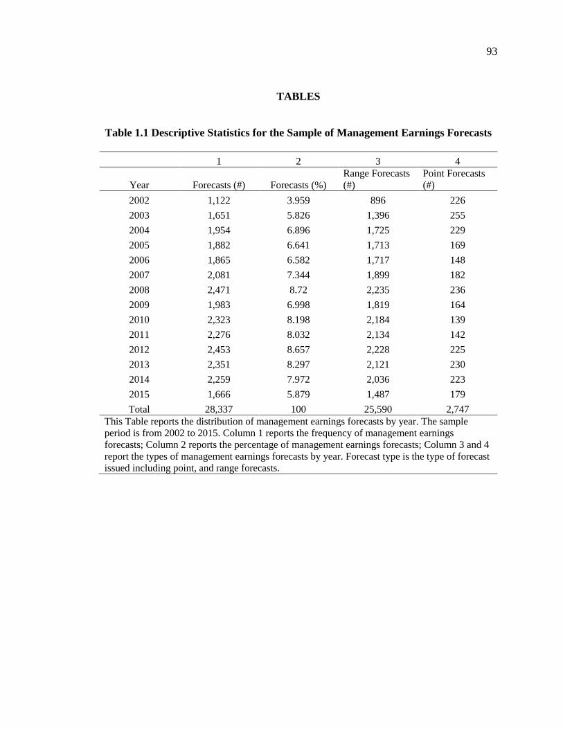
93
TABLES
Table 1.1 Descriptive Statistics for the Sample of Management Earnings Forecasts
1 2 3 4
Year Forecasts (#) Forecasts (%)
Range Forecasts
(#)
Point Forecasts
(#)
2002 1,122 3.959 896 226
2003 1,651 5.826 1,396 255
2004 1,954 6.896 1,725 229
2005 1,882 6.641 1,713 169
2006 1,865 6.582 1,717 148
2007 2,081 7.344 1,899 182
2008 2,471 8.72 2,235 236
2009 1,983 6.998 1,819 164
2010 2,323 8.198 2,184 139
2011 2,276 8.032 2,134 142
2012 2,453 8.657 2,228 225
2013 2,351 8.297 2,121 230
2014 2,259 7.972 2,036 223
2015 1,666 5.879 1,487 179
Total 28,337 100 25,590 2,747
This Table reports the distribution of management earnings forecasts by year. The sample
period is from 2002 to 2015. Column 1 reports the frequency of management earnings
forecasts; Column 2 reports the percentage of management earnings forecasts; Column 3 and 4
report the types of management earnings forecasts by year. Forecast type is the type of forecast
issued including point, and range forecasts.
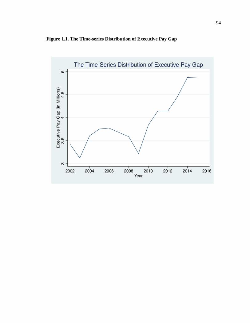
94
Figure 1.1. The Time-series Distribution of Executive Pay Gap

95
Table 1.2 Summary Statistics
Variables N Mean 25% Median 75% SD
Precision(%) 28,337 -0.366 -0.099 -0.218 -0.421 0.503
Accuracy(%) 28,337 -0.826 -0.094 -0.274 -0.740 1.837
Pay Gap(in millions) 28,337 2.960 1.652 3.334 5.943 1.040
Pay Diff(in millions) 28,337 2.065 1.055 2.520 4.764 1.254
InstOwn 28,337 0.790 0.698 0.803 0.900 2.228
Log(AT) 28,337 7.860 6.804 7.809 8.776 1.460
R&D 28,337 0.026 0.000 0.010 0.035 0.040
EarnVol 28,337 0.034 0.011 0.020 0.035 0.044
Litigation 28,337 0.192 0.000 0.000 0.000 0.394
MTB 28,337 3.625 1.803 2.727 4.047 4.508
Equity Issue 28,337 0.446 0.000 0.000 1.000 0.497
M&A 28,337 0.017 0.000 0.000 0.000 0.129
Weak 28,337 0.212 0.000 0.000 0.000 0.409
ROA 28,337 0.067 0.038 0.064 0.096 0.059
Loss 28,337 0.074 0.000 0.000 0.000 0.262
ShrOwn CEO 28,337 0.012 0.001 0.003 0.008 0.029
ShrOwn VP 28,337 0.008 0.001 0.002 0.006 0.019
Vest CEO 28,337 0.076 0.015 0.048 0.103 0.088
Vest VP 28,337 0.068 0.020 0.045 0.091 0.073
CEO Tenure 28,337 6.978 2.000 5.000 9.000 6.585
Median VP Tenure 28,337 3.779 2.000 3.000 5.000 2.637
Horizon 28,337 5.135 4.727 5.412 5.730 0.742
News 28,337 -0.0005 -0.001 -0.0001 0.001 0.005
DA 28,337 0.083 -0.176 -0.010 0.128 3.320
Conc 28,337 0.487 0.363 0.446 0.596 0.161
This table presents summary statistics for the dependent variables, tournament incentive and other
control variables. Panel A reports summary statistics for the regression sample used to test the
accuracy and precision of management earnings forecasts. The sample period is from 2002 to 2015.
All variables are defined in Appendix A and winsorized at 1% and 99%.

96
Table 1.3 Association between MEF Quality and Tournament Incentives
Precision Accuracy
Log(Gap) Log(Diff) Log(Gap) Log(Diff)
Tournament Incentive 0.030*** 0.017*** 0.064*** 0.042***
(7.72) (6.52) (4.69) (4.46)
Institutional 0.227*** 0.235*** 0.632*** 0.645***
Ownership (9.59) (9.95) (6.36) (6.49)
Log (AT) 0.009*** 0.016*** 0.054*** 0.065***
(3.07) (5.82) (4.37) (5.71)
R&D 0.195** 0.216** -0.756** -0.721**
(2.01) (2.22) (-2.19) (-2.09)
Earnings Volatility -1.145*** -1.133*** -2.968*** -2.949***
(-12.42) (-12.29) (-9.44) (-9.39)
Litigation 0.047*** 0.044*** 0.130*** 0.126***
(4.70) (4.47) (3.64) (3.54)
MTB 0.006*** 0.006*** 0.017*** 0.018***
(9.15) (9.36) (8.22) (8.34)
Equity Issue -0.011** -0.012** -0.044** -0.044**
(-2.07) (-2.19) (-2.07) (-2.11)
M&A 0.120*** 0.117*** 0.425*** 0.420***
(4.32) (4.21) (4.29) (4.25)
Weak -0.061*** -0.060*** -0.242*** -0.241***
(-7.58) (-7.52) (-7.45) (-7.44)
ROA 1.558*** 1.572*** 5.332*** 5.349***
(20.79) (20.94) (18.05) (18.12)
Loss -0.201*** -0.200*** -0.517*** -0.517***
(-10.18) (-10.15) (-6.74) (-6.73)
Horizon -0.103*** -0.103*** -0.425*** -0.425***
(-29.58) (-29.56) (-32.63) (-32.64)
News 0.086*** 0.086*** 0.163*** 0.163***
(6.56) (6.56) (3.05) (3.06)
DA -0.002*** -0.002*** 0.001 0.001
(-3.12) (-3.17) (0.32) (0.29)
Conc -0.018 -0.011 0.535* 0.550*
(-0.23) (-0.14) (1.72) (1.77)
ShrOwn CEO 0.049 0.049 -0.364 -0.359
(0.50) (0.51) (-0.85) (-0.84)
ShrOwn VP 0.496*** 0.506*** 1.478** 1.515**

97
(3.34) (3.40) (2.25) (2.31)
Vest CEO -0.193*** -0.183*** -0.663*** -0.650***
(-4.71) (-4.46) (-4.18) (-4.09)
Vest VP 0.018 0.025 0.292 0.305
(0.36) (0.48) (1.34) (1.40)
CEO Tenure 0.004*** 0.004*** 0.004** 0.005***
(8.26) (8.25) (2.50) (2.61)
Median VP Tenure 0.002** 0.002* 0.023*** 0.023***
(1.97) (1.78) (6.18) (6.10)
Industry fixed effect Yes Yes Yes Yes
Year fixed effect Yes Yes Yes Yes
Obs 28,337 28,337 28,337 28,337
R Square 0.2857 0.2849 0.1859 0.1858
This table presents results from regressions of forecast precision and forecast accuracy on the
executive pay gap. Column 1 and 2 display the OLS regression results for the forecast precision.
Precision is the difference between the range forecast's upper and lower bounds, deflated by the
beginning stock price and multiplied by -1. Precision is zero for point forecasts. Column 3 and 4
report the OLS regression results for the forecast accuracy. Accuracy is the absolute difference
between the forecast EPS and the actual reported EPS, deflated by beginning stock price and
multiplied by -1. If the forecast is a range forecast, the midpoint is treated as forecast value.
Coefficients of both Precision and Accuracy are multiplied by 100. Log(Gap) is the natural
logarithm of the difference between the CEO total compensation (ExecuComp data item TDC1)
and the median of VPs compensation. Log(Diff) is the natural logarithm of the compensation
gap between CEO and highest paid VP. All other variables are defined in Appendix A. Industry
and year fixed effects are included. The t-statistics are reported in parentheses. ***, **, and *
indicate 0.01, 0.05, and 0.10 significance levels, respectively.

98
Table 1.4 Moderating Effect of Industry Homogeneity and New CEO on the
Association between Tournament Incentives and MEF Quality
Panel A. Industry Homogeneity
Precision Accuracy
Log(Gap) Log(Diff) Log(Gap) Log(Diff)
Tournament Incentive 0.042*** 0.033*** 0.104*** 0.067***
(6.09) (5.86) (4.40) (3.45)
Industry Homogeneity -0.065*** -0.067*** -0.202*** -0.266***
(-3.82) (-4.67) (-3.20) (-4.91)
Tournament Incentive -0.019** -0.025*** -0.064* -0.039
*Industry Homogeneity (-2.19) (-3.36) (-1.89) (-1.43)
Controls Yes Yes Yes Yes
Industry fixed effect Yes Yes Yes Yes
Year fixed effect Yes Yes Yes Yes
Obs 28,337 28,337 28,337 28,337
R Square 0.2872 0.2866 0.1871 0.1870
Panel B. New CEO
Precision Accuracy
Log(Gap) Log(Diff) Log(Gap) Log(Diff)
Tournament Incentive 0.028*** 0.015*** 0.085*** 0.063***
(6.54) (5.33) (6.10) (6.24)
New CEO 0.035*** 0.020* 0.224*** 0.127***
(2.68) (1.94) (5.47) (3.86)
Tournament Incentive -0.019** -0.009 -0.149*** -0.092***
*New CEO (-2.43) (-1.34) (-5.81) (-4.48)
Controls Yes Yes Yes Yes
Industry fixed effect Yes Yes Yes Yes
Year fixed effect Yes Yes Yes Yes
Obs 25,996 25,996 25,996 25,996
R Square 0.2983 0.2975 0.2056 0.2053 This table presents the regression results of the effect of perceived probability of promotion on the
relation between the forecast characteristics and executive pay gap. Three settings are used where the
perceived probability of promotion matters, including industry homogeneity, CEO turnover, and the
state non-competition agreement enforcement. Results are presented in Panel A, Panel B, and Panel C,
respectively. Precision is the difference between the range forecast's upper and lower bounds, deflated
by the beginning stock price and multiplied by -1. Precision is zero for point forecasts. Accuracy is the
absolute difference between the forecast EPS and the actual reported EPS, deflated by beginning stock
price and multiplied by -1. If the forecast is a range forecast, the midpoint is treated as forecast value.
Coefficients of both Precision and Accuracy are multiplied by 100. Log(Gap) is the natural logarithm of
the difference between the CEO total compensation (ExecuComp data item TDC1) and the median of

99
VPs compensation. Log(Diff) is the natural logarithm of the compensation gap between CEO and
highest paid VP. New CEO is a dummy variable equal to 1 for year t and t+1 if the firm has a new CEO
in year t, and 0 otherwise. Industry Homogeneity is the mean of the partial correlation coefficients of all
firms in the two-digit SIC industry. All other variables are defined in Appendix A. Industry and year
fixed effects are included. The t-statistics are reported in parentheses. ***, **, and * indicate 0.01, 0.05,
and 0.10 significance levels, respectively.
Table 1.5 Robustness Check: CEO Ability, CEO Characteristics and MEF
Quality
Panel A: CEO Ability
Precision Accuracy
Log(Gap) Log(Diff) Log(Gap) Log(Diff)
Tournament Incentive 0.029*** 0.016*** 0.078*** 0.051***
(7.34) (6.26) (5.74) (5.45)
Ability 0.117*** 0.116*** 0.431*** 0.429***
(7.27) (7.21) (6.63) (6.59)
Controls Yes Yes Yes Yes
Industry fixed effect Yes Yes Yes Yes
Year fixed effect Yes Yes Yes Yes
Obs 27,355 27,355 27,355 27,355
R Square 0.282 0.281 0.197 0.197
Panel B: CEO Fixed Effects
Precision Accuracy
Log(Gap) Log(Diff) Log(Gap) Log(Diff)
Tournament Incentive 0.013*** 0.008*** 0.035** 0.024**
(3.16) (2.92) (2.17) (2.19)
Controls Yes Yes Yes Yes
Industry fixed effect Yes Yes Yes Yes
Year fixed effect Yes Yes Yes Yes
CEO Fixed Effect Yes Yes Yes Yes
Obs 28,337 28,337 28,337 28,337
R Square 0.721 0.721 0.621 0.621
This table shows the regression results from robustness checks of CEO attributes. In Panel A we
add the CEO ability variable as an additional control variable. In Panel B we report the main
results by including CEO fixed effects. We compute the cumulative distributive function (CDF)
of industry adjusted ROA for each CEO-firm-year by industry and CEO Ability is defined as the
mean of the CDF rank of ROA for the first three years when a new CEO is appointed. Precision
is the difference between the range forecast's upper and lower bounds, deflated by the beginning
stock price and multiplied by -1. Precision is zero for point forecasts. Accuracy is the absolute
difference between the forecast EPS and the actual reported EPS, deflated by beginning stock
price and multiplied by -1. If the forecast is a range forecast, the midpoint is treated as forecast
value. Coefficients of both Precision and Accuracy are multiplied by 100. Log(Gap) is the natural
logarithm of the difference between the CEO total compensation (ExecuComp data item TDC1)

100
and the median of VPs compensation. Log(Diff) is the natural logarithm of the compensation
gap between CEO and highest paid VP. All other variables are defined in Appendix A. Industry
and year fixed effects are included. The t-statistics are reported in parentheses. ***, **, and *
indicate 0.01, 0.05, and 0.10 significance levels, respectively.

101
Table 1.6 Robustness Check: Corporate Governance
Precision Accuracy
Log(Gap) Log(Diff) Log(Gap) Log(Diff)
Tournament Incentive 0.033*** 0.018*** 0.121*** 0.067***
(7.02) (6.10) (6.57) (5.91)
G Index -0.004** -0.004** -0.003 -0.002
(-2.94) (-2.78) (-0.49) (-0.35)
CEO Duality -0.004 -0.003 -0.116*** -0.112***
(-0.58) (-0.44) (-3.91) (-3.79)
% IO Directors -0.136*** -0.143*** -0.565*** -0.590***
(-4.33) (-4.53) (-4.46) (-4.62)
Controls Yes Yes Yes Yes
Industry fixed effect Yes Yes Yes Yes
Year fixed effect Yes Yes Yes Yes
Obs 18,588 18,588 18,558 18,588
R Square 0.352 0.351 0.210 0.209
This table shows regression results of management earnings forecasts characteristics on
executive pay gaps by including additional corporate governance control variables. G Index is
Gompers et al. 2003 corporate governance index. CEO Duality is a dummy variable equal to 1
if the CEO is also the chairman of the board. % IO Directors is the percentage of independent
outside directors on the board. Precision is the difference between the range forecast's upper and
lower bounds, deflated by the beginning stock price and multiplied by -1. Precision is zero for
point forecasts. Accuracy is the absolute difference between the forecast EPS and the actual
reported EPS, deflated by beginning stock price and multiplied by -1. If the forecast is a range
forecast, the midpoint is treated as forecast value. Coefficients of both Precision and Accuracy
are multiplied by 100. Log(Gap) is the natural logarithm of the difference between the CEO total
compensation (ExecuComp data item TDC1) and the median of VPs compensation. Log(Diff) is
the natural logarithm of the compensation gap between CEO and highest paid VP. All other
variables are defined in Appendix A. Industry and year fixed effects are included. The t-statistics
are reported in parentheses. ***, **, and * indicate 0.01, 0.05, and 0.10 significance levels,
respectively.
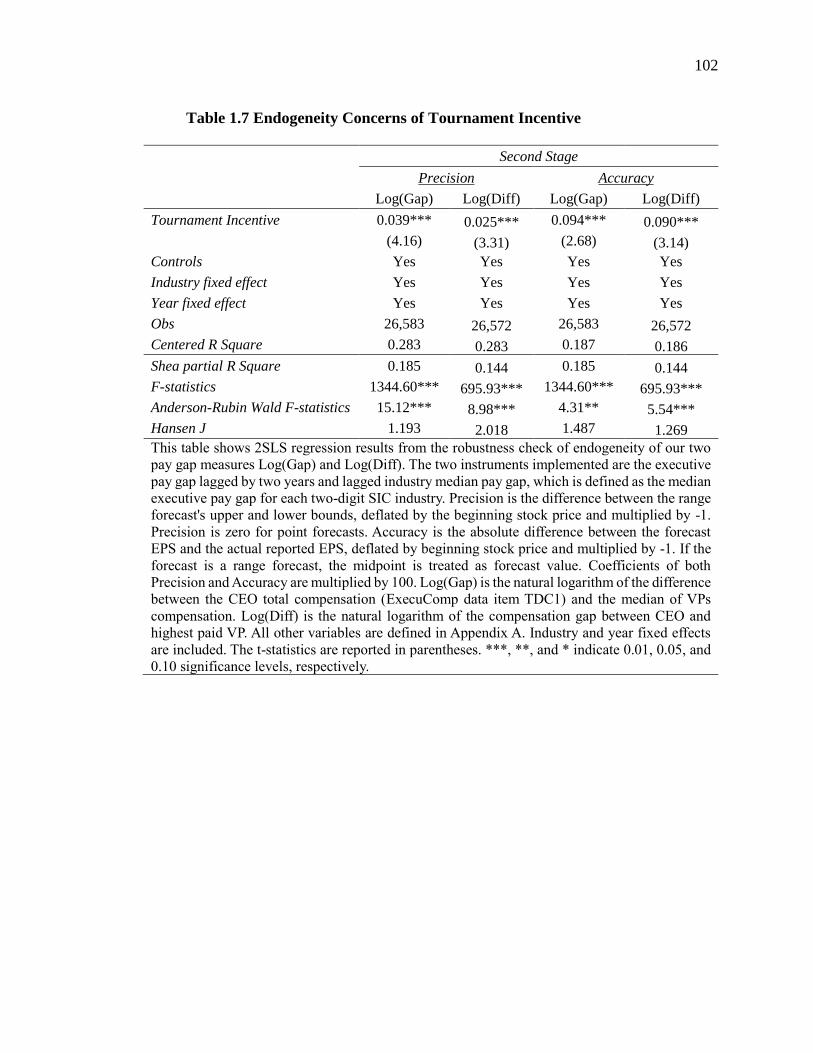
102
Table 1.7 Endogeneity Concerns of Tournament Incentive
Second Stage
Precision Accuracy
Log(Gap) Log(Diff) Log(Gap) Log(Diff)
Tournament Incentive 0.039*** 0.025*** 0.094*** 0.090***
(4.16) (3.31) (2.68) (3.14)
Controls Yes Yes Yes Yes
Industry fixed effect Yes Yes Yes Yes
Year fixed effect Yes Yes Yes Yes
Obs 26,583 26,572 26,583 26,572
Centered R Square 0.283 0.283 0.187 0.186
Shea partial R Square 0.185 0.144 0.185 0.144
F-statistics 1344.60*** 695.93*** 1344.60*** 695.93***
Anderson-Rubin Wald F-statistics 15.12*** 8.98*** 4.31** 5.54***
Hansen J 1.193 2.018 1.487 1.269
This table shows 2SLS regression results from the robustness check of endogeneity of our two
pay gap measures Log(Gap) and Log(Diff). The two instruments implemented are the executive
pay gap lagged by two years and lagged industry median pay gap, which is defined as the median
executive pay gap for each two-digit SIC industry. Precision is the difference between the range
forecast's upper and lower bounds, deflated by the beginning stock price and multiplied by -1.
Precision is zero for point forecasts. Accuracy is the absolute difference between the forecast
EPS and the actual reported EPS, deflated by beginning stock price and multiplied by -1. If the
forecast is a range forecast, the midpoint is treated as forecast value. Coefficients of both
Precision and Accuracy are multiplied by 100. Log(Gap) is the natural logarithm of the difference
between the CEO total compensation (ExecuComp data item TDC1) and the median of VPs
compensation. Log(Diff) is the natural logarithm of the compensation gap between CEO and
highest paid VP. All other variables are defined in Appendix A. Industry and year fixed effects
are included. The t-statistics are reported in parentheses. ***, **, and * indicate 0.01, 0.05, and
0.10 significance levels, respectively.
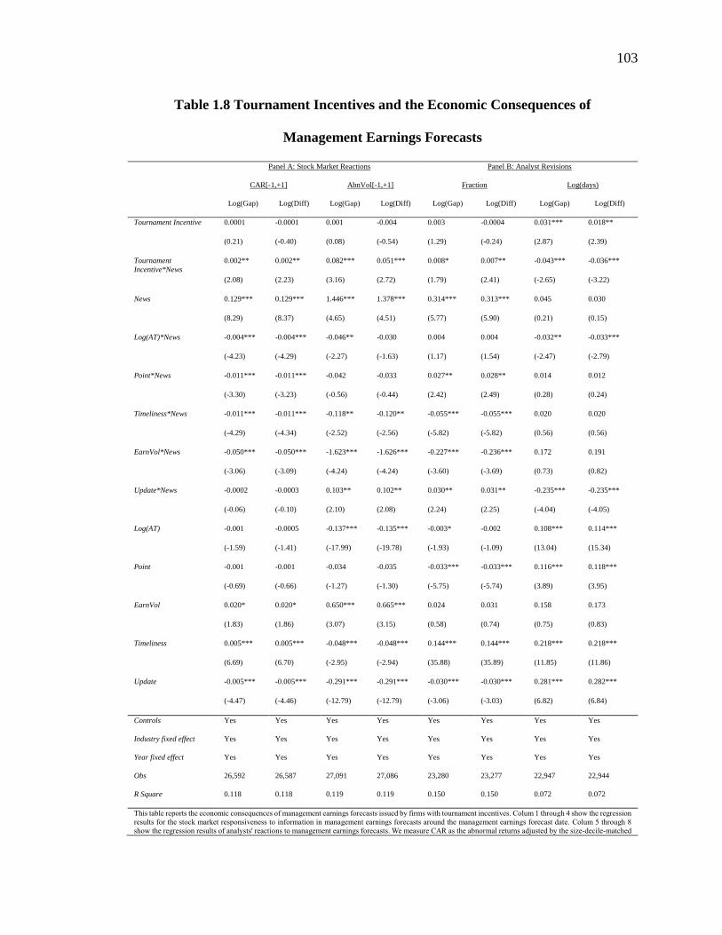
103
Table 1.8 Tournament Incentives and the Economic Consequences of
Management Earnings Forecasts
Panel A: Stock Market Reactions Panel B: Analyst Revisions
CAR[-1,+1] AbnVol[-1,+1] Fraction Log(days)
Log(Gap) Log(Diff) Log(Gap) Log(Diff) Log(Gap) Log(Diff) Log(Gap) Log(Diff)
Tournament Incentive 0.0001 -0.0001 0.001 -0.004 0.003 -0.0004 0.031*** 0.018**
(0.21) (-0.40) (0.08) (-0.54) (1.29) (-0.24) (2.87) (2.39)
Tournament
Incentive*News
0.002** 0.002** 0.082*** 0.051*** 0.008* 0.007** -0.043*** -0.036***
(2.08) (2.23) (3.16) (2.72) (1.79) (2.41) (-2.65) (-3.22)
News 0.129*** 0.129*** 1.446*** 1.378*** 0.314*** 0.313*** 0.045 0.030
(8.29) (8.37) (4.65) (4.51) (5.77) (5.90) (0.21) (0.15)
Log(AT)*News -0.004*** -0.004*** -0.046** -0.030 0.004 0.004 -0.032** -0.033***
(-4.23) (-4.29) (-2.27) (-1.63) (1.17) (1.54) (-2.47) (-2.79)
Point*News -0.011*** -0.011*** -0.042 -0.033 0.027** 0.028** 0.014 0.012
(-3.30) (-3.23) (-0.56) (-0.44) (2.42) (2.49) (0.28) (0.24)
Timeliness*News -0.011*** -0.011*** -0.118** -0.120** -0.055*** -0.055*** 0.020 0.020
(-4.29) (-4.34) (-2.52) (-2.56) (-5.82) (-5.82) (0.56) (0.56)
EarnVol*News -0.050*** -0.050*** -1.623*** -1.626*** -0.227*** -0.236*** 0.172 0.191
(-3.06) (-3.09) (-4.24) (-4.24) (-3.60) (-3.69) (0.73) (0.82)
Update*News -0.0002 -0.0003 0.103** 0.102** 0.030** 0.031** -0.235*** -0.235***
(-0.06) (-0.10) (2.10) (2.08) (2.24) (2.25) (-4.04) (-4.05)
Log(AT) -0.001 -0.0005 -0.137*** -0.135*** -0.003* -0.002 0.108*** 0.114***
(-1.59) (-1.41) (-17.99) (-19.78) (-1.93) (-1.09) (13.04) (15.34)
Point -0.001 -0.001 -0.034 -0.035 -0.033*** -0.033*** 0.116*** 0.118***
(-0.69) (-0.66) (-1.27) (-1.30) (-5.75) (-5.74) (3.89) (3.95)
EarnVol 0.020* 0.020* 0.650*** 0.665*** 0.024 0.031 0.158 0.173
(1.83) (1.86) (3.07) (3.15) (0.58) (0.74) (0.75) (0.83)
Timeliness 0.005*** 0.005*** -0.048*** -0.048*** 0.144*** 0.144*** 0.218*** 0.218***
(6.69) (6.70) (-2.95) (-2.94) (35.88) (35.89) (11.85) (11.86)
Update -0.005*** -0.005*** -0.291*** -0.291*** -0.030*** -0.030*** 0.281*** 0.282***
(-4.47) (-4.46) (-12.79) (-12.79) (-3.06) (-3.03) (6.82) (6.84)
Controls Yes Yes Yes Yes Yes Yes Yes Yes
Industry fixed effect Yes Yes Yes Yes Yes Yes Yes Yes
Year fixed effect Yes Yes Yes Yes Yes Yes Yes Yes
Obs 26,592 26,587 27,091 27,086 23,280 23,277 22,947 22,944
R Square 0.118 0.118 0.119 0.119 0.150 0.150 0.072 0.072
This table reports the economic consequences of management earnings forecasts issued by firms with tournament incentives. Colum 1 through 4 show the regression
results for the stock market responsiveness to information in management earnings forecasts around the management earnings forecast date. Colum 5 through 8
show the regression results of analysts' reactions to management earnings forecasts. We measure CAR as the abnormal returns adjusted by the size-decile-matched

104
market return in [-1,1] window around the day of the announcement of the management earnings forecast. AbnVol is the average trading volume from three trading
days centering on the management forecast announcement date, scaled by the median trading volume in the prior 60 days. Fraction is defined as the ratio of the
number of analysts revising their own forecasts within 90 days following the date of management forecast issuance to the total number of analysts issuing at least
1 forecast in the year ending 30 days before the date of management forecast issuance. Log(Days) is the natural logarithm of the number of days between
management forecast date and analyst revision date. News is the difference between EPS in management earnings forecast and the analyst consensus forecast
(median) before the management forecast, deflated by beginning stock price, and multiplied by 100. |News| is the absolute value of News, Log(Gap) is the natural
logarithm of the difference between the CEO total compensation (ExecuComp data item TDC1) and the median of VPs compensation. Log(Diff) is the natural
logarithm of the compensation gap between CEO and highest paid VP. All other variables are defined in Appendix A. Industry and year fixed effects are included.
The t-statistics are reported in parentheses. ***, **, and * indicate 0.01, 0.05, and 0.10 significance levels, respectively.

105
Table 2.1 Time Series Pattern of Affected Suppliers with Cheating Customers
Year Num. of affected suppliers
litigation sample restatement sample
1996 59 -
1997 64 -
1998 100 -
1999 208 -
2000 252 -
2001 173 -
2002 149 124
2003 147 143
2004 164 177
2005 74 105
2006 63 75
2007 38 29
2008 30 27
2009 51 39
2010 53 43
2011 103 45
2012 78 41
2013 41 25
Num. of unique suppliers 934 435
This table presents the distributions of affected suppliers with cheating customers in both
litigation and restatement sample. The litigation sample covers the period from 1996 to 2013
and the restatement sample covers the period from 2002 to 2013. A supplier is accounted as
“affected” if it has a cheating customer during the current and/or the prior fiscal years.

106
Table 2.2 The Customers’ Manipulations During Cheating Periods
Panel A. Litigation sample for the period of 1996-2013 (N=12,482)
CAPEX
Employee PPE Assets Sales
Growth Growth Growth Growth
Cheating Years 0.0138 0.0620 0.0914 0.0644 0.0629
Non-cheating Years 0.0094 0.0281 0.0305 0.0488 0.0349
Difference 0.0044*** 0.0338*** 0.0609*** 0.0156** 0.0280***
t-statistics (3.19) (5.43) (9.22) (2.07) (3.71)
Panel B. Restatement sample for the period of 2002-2013 (N=11,775)
CAPEX
Employee PPE Assets Sales
Growth Growth Growth Growth
Cheating Years 0.0098 0.0447 0.0435 0.0636 0.0438
Non-cheating Years 0.0061 0.0035 -0.0067 0.0115 -0.0031
Difference 0.0037*** 0.0412*** 0.0501*** 0.0521*** 0.0470***
t-statistics (3.21) (8.35) (9.97) (8.89) (8.15)
This table presents the abnormal operating decisions of misreporting customers during cheating
and non-cheating periods in litigation sample and restatement sample in Panel A and Panel B,
respectively. Litigation sample covers the period from 1996 to2013. Restatement sample covers
the period from 2002 to 2013. Cheating years are defined as the class periods in litigation and
restatement samples and non-cheating years refer to periods with no misreporting. All variables
are winsorized at 1 percent and 99 percent level *, **, and *** indicate significance at the <0.10,
<0.05, and <0.01 levels, respectively based on t-tests.

107
Table 2.3 Descriptive Statistics
Panel A. litigation sample (1996-2013)
Variable Obs Mean Std. Dev. Q1 Median Q3
Cheating_Custom
er 10,727 0.120 0.325 0.000 0.000 0.000
CAPEX 10,727 0.070 0.101 0.016 0.035 0.075
Cash 10,727 0.195 0.299 0.028 0.098 0.239
Leverage 10,727 0.163 0.215 0.000 0.072 0.263
ROA 10,727 -0.105 0.404 -0.114 0.019 0.070
Size 10,727 5.147 2.066 3.732 5.073 6.586
Sales 10,727 1.197 0.942 0.549 1.007 1.545
Financing 10,727 0.190 0.330 0.005 0.040 0.237
Q 10,727 2.101 1.980 1.082 1.477 2.258
HHI 10,727 0.044 0.057 0.020 0.027 0.043
Sales_Vol 10,725 0.260 0.311 0.089 0.169 0.314
Panel B. restatement sample (2002-2013)
Variable Obs Mean Std. Dev. Q1 Median Q3
Cheating_Custom
er 8,771 0.069 0.254 0.000 0.000 0.000
CAPEX 8,771 0.057 0.089 0.014 0.029 0.060
Cash 8,771 0.196 0.266 0.039 0.119 0.250
Leverage 8,771 0.162 0.219 0.000 0.070 0.260
ROA 8,771 -0.089 0.363 -0.108 0.021 0.071
Size 8,771 5.648 2.155 4.204 5.615 7.171
Sales 8,771 1.100 0.875 0.519 0.910 1.431
Financing 8,771 0.172 0.307 0.005 0.033 0.207
Q 8,771 2.042 1.799 1.108 1.503 2.249
HHI 8,771 0.042 0.056 0.018 0.024 0.038
Sales_Vol 8,771 0.240 0.297 0.081 0.157 0.286
This table presents the descriptive statistics of all firm-years in litigation sample and restatement
sample in Panel A and Panel B, respectively. Litigation sample covers the period from 1996 to
2013 and restatement sample is from 2002 to 2013. All variables are winsorized at the 1 percent
and 99 percent level.

108
Table 2.4 The Effects of Customers’ Misrepresentations on Suppliers Investment
Decisions
litigation sample restatement sample
(1996-2013) (2002-2013)
CAPEX Coef. (t-statistic) Coef. (t-statistic)
Cheating_Customer 0.010*** 0.008*** 0.010*** 0.012***
(3.51) (2.68) (2.84) (3.08)
Cash 0.033*** 0.004
(5.85) (0.86)
Leverage -0.015*** -0.013**
(-2.64) (-2.24)
ROA 0.019*** 0.019***
(5.51) (4.90)
Size 0.006*** 0.003***
(7.22) (3.95)
Sales 0.009*** 0.006***
(5.11) (3.02)
Financing 0.047*** 0.036***
(8.68) (6.54)
Q 0.002*** 0.001**
(3.54) (2.11)
Intercept 0.095*** 0.040*** 0.048*** 0.027*
(8.07) (2.66) (4.01) (1.67)
Industry fixed effect Yes Yes Yes Yes
Year fixed effect Yes Yes Yes Yes
R square 0.295 0.361 0.354 0.383
Obs 12,147 10,727 9,759 8,771
This table reports the parameters estimated from the following regression for all suppliers in both
litigation sample and restatement sample:
CAPEX𝑖𝑡 = 𝛽0 + 𝛽1𝐶ℎ𝑒𝑎𝑡𝑖𝑛𝑔_𝐶𝑢𝑠𝑡𝑜𝑚𝑒𝑟𝑖,𝑡 + 𝛽2𝐹𝑢𝑛𝑑𝑎𝑚𝑒𝑛𝑡𝑎𝑙_𝐶𝑜𝑛𝑡𝑟𝑜𝑙𝑠𝑖,𝑡 + 𝜀𝑖,𝑡 (1)
All variables are winsorized at the 1 percent and 99 percent level. Industry and year fixed-effects
are included. The standard errors are clustered by firms. *, **, and *** indicate significance at
the <0.10, <0.05, and <0.01 levels, respectively, based on one-tailed tests if the signs are
predicted, and two-tales tests otherwise.

109
Table 2.5 The Effects of Industry Concentration and Sales Uncertainty on
Suppliers’ Decisions in Response to Customers’ Misconduct
litigation sample restatement sample
(1996-2013) (2002-2013)
HHI Sales_Vol HHI Sales_Vol
CAPEX Coef. (t-statistic) Coef. (t-statistic)
Cheating_Customer*HHI -0.110** -0.136**
(-2.48) (-2.45)
Cheating_Customer*Sales_V
ol 0.041*** 0.052**
(2.98) (2.09)
HHI 0.075 -0.034
(1.52) (-0.93)
Sales_Vol 0.024*** 0.014***
(4.38) (2.61)
Cheating_Customer 0.013*** -0.003 0.017*** -0.002
(3.38) (-0.83) (3.24) (-0.27)
Cash 0.033*** 0.028*** 0.004 0.002
(5.84) (4.88) (0.84) (0.33)
Leverage -0.015*** -0.014** -0.013** -0.013**
(-2.63) (-2.49) (-2.24) (-2.15)
ROA 0.019*** 0.022*** 0.019*** 0.021***
(5.52) (6.38) (4.89) (5.36)
Size 0.006*** 0.006*** 0.003*** 0.003***
(7.24) (7.45) (3.91) (4.12)
Sales 0.009*** 0.010*** 0.006*** 0.006***
(5.11) (5.41) (3.03) (3.33)
Financing 0.047*** 0.044*** 0.036*** 0.035***
(8.69) (8.47) (6.53) (6.36)
Q 0.002*** 0.002*** 0.001** 0.001*
(3.55) (3.19) (2.10) (1.72)
Intercept 0.027 0.039*** 0.038* 0.024
(1.48) (2.68) (1.88) (1.47)
Industry fixed effect Yes Yes Yes Yes
Year fixed effect Yes Yes Yes Yes
R square 0.361 0.368 0.384 0.387
Obs 10,727 10,725 8,771 8,771
This table reports the parameters estimated from the following regressions for all suppliers in

110
both litigation sample and restatement sample:
CAPEX𝑖,𝑡 = 𝛽0 + 𝛽1𝐶ℎ𝑒𝑎𝑡𝑖𝑛𝑔_𝐶𝑢𝑠𝑡𝑜𝑚𝑒𝑟𝑖,𝑡 ∗ 𝐻𝐻𝐼𝑖,𝑡 + 𝛽2𝐶ℎ𝑒𝑎𝑡𝑖𝑛𝑔_𝐶𝑢𝑠𝑡𝑜𝑚𝑒𝑟𝑖,𝑡 +
𝛽3𝐻𝐻𝐼𝑖,𝑡 + 𝛽4𝐹𝑢𝑛𝑑𝑎𝑚𝑒𝑛𝑡𝑎𝑙_𝐶𝑜𝑛𝑡𝑟𝑜𝑙𝑠𝑖,𝑡 + 𝜀𝑖,𝑡 (2.1)
CAPEX𝑖,𝑡 = 𝛽0 + 𝛽1𝐶ℎ𝑒𝑎𝑡𝑖𝑛𝑔𝐶𝑢𝑠𝑡𝑜𝑚𝑒𝑟𝑖,𝑡 ∗ 𝑆𝑎𝑙𝑒𝑠_𝑉𝑜𝑙𝑖,𝑡 + 𝛽2𝐶ℎ𝑒𝑎𝑡𝑖𝑛𝑔_𝐶𝑢𝑠𝑡𝑜𝑚𝑒𝑟𝑖,𝑡 +
𝛽3𝑆𝑎𝑙𝑒𝑠_𝑉𝑜𝑙𝑖,𝑡 + 𝛽4𝐹𝑢𝑛𝑑𝑎𝑚𝑒𝑛𝑡𝑎𝑙_𝐶𝑜𝑛𝑡𝑟𝑜𝑙𝑠𝑖,𝑡 + 𝜀𝑖,𝑡 (2.2)
All variables are winsorized at the 1 percent and 99 percent level. Industry and year fixed-effects
are included. The standard errors are clustered by firms. *, **, and *** indicate significance at
the <0.10, <0.05, and <0.01 levels, respectively, based on one-tailed tests if the signs are
predicted, and two-tales tests otherwise.

111
Table 2.6 The Association between Current Investments and Future Cash Flows
litigation sample restatement sample
(1996-2013) (2002-2013)
CFOt+1 CFOt+2 CFOt+1 CFOt+2
CFOt+i Coef. (t-statistic) Coef. (t-statistic)
CAPEX*Cheating_Customer -0.164** -0.198** -0.044 -0.071
(-2.50) (-2.22) (-0.62) (-0.80)
CAPEX 0.153*** 0.122*** 0.191*** 0.167***
(4.93) (3.62) (5.90) (4.83)
Cheating_Customer 0.008 0.023 -0.002 0.012
(0.87) (1.60) (-0.16) (0.76)
Cash -0.061*** -0.074*** -0.063*** -0.080***
(-5.60) (-5.51) (-4.63) (-5.17)
Leverage 0.019 -0.0002 0.018 0.0005
(1.09) (-0.001) (0.96) (0.02)
ROA 0.334*** 0.257*** 0.367*** 0.285***
(18.79) (13.90) (17.16) (13.65)
Size 0.020*** 0.023*** 0.016*** 0.019***
(9.38) (9.57) (8.57) (9.24)
Sales 0.017*** 0.017*** 0.022*** 0.026***
(4.48) (4.14) (4.56) (5.54)
Financing -0.087*** -0.077*** -0.072*** -0.056***
(-6.90) (-5.87) (-5.65) (-4.02)
Q -0.005* -0.0003 -0.005 0.0001
(-1.81) (-0.10) (-1.43) (0.02)
Intercept -0.045 -0.103** -0.008 -0.083
(-0.99) (-2.16) (-0.14) (-1.39)
Industry fixed effect Yes Yes Yes Yes
Year fixed effect Yes Yes Yes Yes
R square 0.544 0.433 0.561 0.462
Obs 7,377 6,309 6,918 6,192
This table presents the parameters estimated from the following regression for all suppliers in
both litigation sample and restatement sample during customers’ scandal periods:
CFO𝑖,𝑡+𝑚 = 𝛽0 + 𝛽1𝐶𝐴𝑃𝐸𝑋𝑖,𝑡 ∗ 𝐶ℎ𝑒𝑎𝑡𝑖𝑛𝑔_𝐶𝑢𝑠𝑡𝑜𝑚𝑒𝑟𝑖,𝑡 + 𝛽2𝐶𝐴𝑃𝐸𝑋𝑖,𝑡
+ 𝛽3𝐶ℎ𝑒𝑎𝑡𝑖𝑛𝑔_𝐶𝑢𝑠𝑡𝑜𝑚𝑒𝑟𝑖,𝑡 + 𝛽4𝐹𝑢𝑛𝑑𝑎𝑚𝑒𝑛𝑡𝑎𝑙_𝐶𝑜𝑛𝑡𝑟𝑜𝑙𝑠𝑖,𝑡 + 𝜀𝑖,𝑡
Where m=1,2;
All variables are winsorized at the 1 percent and 99 percent level. Industry and year fixed-effects
are included. The standard errors are clustered by firms. *, **, and *** indicate significance at

112
the <0.10, <0.05, and <0.01 levels, respectively, based on one-tailed tests if the signs are
predicted, and two-tales tests otherwise.

113
Table 2.7 The Market Reactions to Suppliers’ Investment Decisions After The
Disclosure of Customers’ Frauds
litigation sample restatement sample
(1996-2013) (2002-2013)
CAR(-3,3) CAR(-5,5) CAR(-3,3) CAR(-5,5)
Coef. (t-statistic) Coef. (t-statistic)
High_CAPX_Customer -0.013* -0.019** -0.016** -0.016
(-1.77) (-2.16) (-2.20) (-1.60)
Cash -0.019 -0.038* 0.030*** 0.010
(-0.80) (-1.67) (2.71) (0.64)
Leverage -0.021 -0.015 0.020 0.031
(-1.49) (-0.83) (1.00) (1.23)
ROA 0.010 0.018 -0.033** 0.018
(0.88) (1.02) (-2.03) (0.82)
Size 0.005** 0.005* -0.001 -0.004
(1.98) (1.85) (-0.56) (-1.32)
Sales 0.006 0.007 0.002 -0.002
(1.06) (1.14) (0.38) (-0.40)
Financing -0.0004 -0.005 -0.064*** -0.038
(-0.03) (-0.31) (-2.82) (-1.26)
Q 0.003 0.005** -0.001 -0.002
(1.56) (2.00) (-0.45) (-0.55)
Intercept -0.028 -0.025 0.009 0.015
(-1.62) (-1.34) (0.65) (0.71)
R square 0.022 0.039 0.083 0.034
Obs 696 696 228 228
This table presents the parameters estimated from the following regression for all suppliers in
both litigation sample and restatement sample:
CAR𝑖,[−3,+3] 𝑜𝑟 CAR𝑖,[−5,+5]
= 𝛽0 + 𝛽1𝐻𝑖𝑔ℎ_𝐶𝐴𝑃𝐸𝑋_𝐶𝑢𝑠𝑡𝑜𝑚𝑒𝑟 + 𝛽2𝐹𝑢𝑛𝑑𝑎𝑚𝑒𝑛𝑡𝑎𝑙_𝐶𝑜𝑛𝑡𝑟𝑜𝑙𝑠𝑖,𝑡 + 𝜀𝑖,𝑡
All variables are winsorized at the 1 percent and 99 percent level. The standard errors are
clustered by firms. *, **, and *** indicate significance at the <0.10, <0.05, and <0.01 levels,
respectively, based on one-tailed tests if the signs are predicted, and two-tales tests otherwise.

114
Table 2.8 The Robustness Check: Difference-in-Difference Approach
litigation sample restatement sample
(1996-2013) (2002-2013)
Capital expenditure Pred. Coef. (t-statistic) Coef. (t-statistic)
During + 0.004** 0.005**
(2.17) (2.26)
After - -0.004*** 0.002
(-2.60) (0.72)
R square 0.003 0.004
Obs 7,049 3,763
During=After (F-statistic) 20.11*** 3.12*
This table presents the parameters estimated from the following DID regression for all suppliers
in both litigation sample and restatement sample:
capx̂𝑖,𝑡 = 𝛽0 + 𝛽1𝐷𝑢𝑟𝑖𝑛𝑔𝑖,𝑡 + 𝛽2𝐴𝑓𝑡𝑒𝑟𝑖,𝑡 + 𝜀𝑖,𝑡
All variables are winsorized at the 1 percent and 99 percent level. *, **, and *** indicate
significance at the <0.10, <0.05, and <0.01 levels, respectively.

115
Figure 3.1 Transition Matrix of Before/During/After Trading Hours
Announcement Times
Previous Year
Current Year Before (%) During (%) AMC (%) Total
Percent before hours 44.6% 3.8% 4.6% 53.0%
Percent during hours 4.2% 4.9% 3.3% 12.4%
Percent after hours 7.0% 3.1% 24.6% 34.7%
Total 55.8% 11.8% 32.5% 100.0%
Sum of shaded green = % that change in any given year 26.0%
Percent of firms with >=1 change in before/during/AMC timing 68.8%
This figure presents the year-over-year transitions matrix of EA during the day from 1990 to 2015. Before
trading hours are from 12:00 AM to 9:00 AM; During trading hours are from 9:00 AM to 4:00 PM; and
after trading hours are from 4:00 PM to midnight.
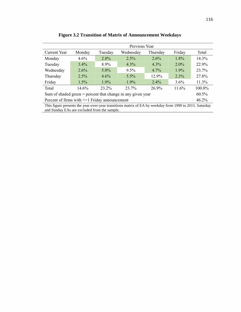
116
Figure 3.2 Transition of Matrix of Announcement Weekdays
Previous Year
Current Year Monday Tuesday Wednesday Thursday Friday Total
Monday 4.6% 2.8% 2.5% 2.6% 1.8% 14.3%
Tuesday 3.4% 8.9% 4.3% 4.3% 2.0% 22.9%
Wednesday 2.6% 5.0% 9.5% 4.7% 1.9% 23.7%
Thursday 2.5% 4.6% 5.5% 12.9% 2.3% 27.8%
Friday 1.5% 1.9% 1.9% 2.4% 3.6% 11.3%
Total 14.6% 23.2% 23.7% 26.9% 11.6% 100.0%
Sum of shaded green = percent that change in any given year 60.5%
Percent of firms with >=1 Friday announcement 46.2%
This figure presents the year-over-year transitions matrix of EA by weekday from 1990 to 2015. Saturday
and Sunday EAs are excluded from the sample.

117
Table 3.1 Sample Description
Sample characteristic Restatements SEC Enforcements
(2002-2015) (1990-2010)
Original events 1,344 308
Unique firms 1,130 304
Firm-years in violation period 3,548 834 The restatement sample consists of all firms that have income-increasing restatements from 2002 to 2015.
The SEC enforcement sample consists of all firms subject to accounting and auditing SEC enforcement
actions from 1990 to 2010. Both samples are required to be matched with Compustat to have necessary
data of firm fundamentals. For purposes of our analyses, the violation period covers the years the firm
misreported.

118
Table 3.2 Univariate Test
Panel A. Restatements (2002-2015)
Mean N
AMC Friday
Misreporting firms – violation years (1) 51.57% 6.45% 3,056
Misreporting firms – other years (2) 46.31% 6.40% 6,324
Control firms – all years (3) 46.96% 7.15% 36,260
Significance test: (1) versus (2) <0.001*** 0.469
Significance test: (1) versus (3) <0.001*** 0.073*
Panel B. SEC Enforcements (1990-2010)
Mean N
AMC Friday
Misreporting firms – violation years (1) 42.49% 7.12% 772
Misreporting firms – other years (2) 35.22% 10.06% 2,256
Control firms – all years (3) 32.14% 10.64% 69,534
Significance test: (1) versus (2) <0.001*** <0.001***
Significance test: (1) versus (3) <0.001*** <0.001*** This table presents the EA timing for misreporting firms relative to control firms that have not had any
misrepresentation event during our sample period. The restatement sample consists of all firms that have
income-increasing restatements from 2002 to 2015. The SEC enforcement sample consists of all firms
subject to accounting and auditing SEC enforcement actions from 1990 to 2010. “Misreporting firms –
violation years” represents years in which the firm misreported. “Misreporting firms – other years”
represents non-violation years of the misreporting firm. “Control firms – all years” represents all years of
control firms. We report the mean value of AMC and Friday, which are indicators for EA made after 4:00
PM and on Friday, respectively.

119
Table 3.3 Descriptive Statistics
Panel A. Restatements Pooled Sample (2002-2015)
Misreporting Control Difference (t-statistic)
AMC 0.5157 0.4759 0.0398*** (4.25)
Friday 0.0645 0.0704 -0.0059 (-1.24)
Size 6.6041 6.6796 -0.0755** (-2.00)
BTM 0.5615 0.5355 0.0260*** (2.61)
Lev 0.2050 0.2201 -0.0150*** (-3.75)
Numest 7.2857 7.1217 0.1639* (1.35)
RepLag 3.8702 3.8459 0.0243*** (3.23)
SUE -0.0367 -0.0350 -0.0017 (-0.28)
InstOwn 0.6032 0.5003 0.1029*** (16.01)
Obs 3,056 42,584 Total 45,640
Panel B. SEC Enforcement Pooled Sample (1990-2010)
Misreporting Control Difference (t-statistic)
AMC 0.4249 0.3224 0.1025*** (6.06)
Friday 0.0712 0.1063 -0.0350***(-3.15)
Size 6.7249 5.9990 0.7258*** (10.08)
BTM 0.4985 0.5486 -0.0500*** (-2.64)
Lev 0.2174 0.2223 -0.0049 (-0.64)
Numest 9.4080 6.2698 3.1382*** (13.96)
RepLag 3.6842 3.7958 -0.1116*** (-6.42)
SUE -0.0059 -0.0691 0.0633*** (3.68)
InstOwn 0.5282 0.3697 0.1585*** (13.18)
Obs 772 71,790 Total 72,562 This table reports firm characteristics for the misreporting sample and control sample that have not had
any misrepresentation event during our sample period. The restatement sample consists of all firms that
have income-increasing restatements from 2002 to 2015. The SEC enforcement sample consists of all
firms subject to accounting and auditing SEC enforcement actions from 1990 to 2010. All variables are
defined in Appendix A. *, **, and *** represent significance at the 10%, 5%, and 1% level, respectively.
Two sided p-values are based on the t-statistic for differences in means.
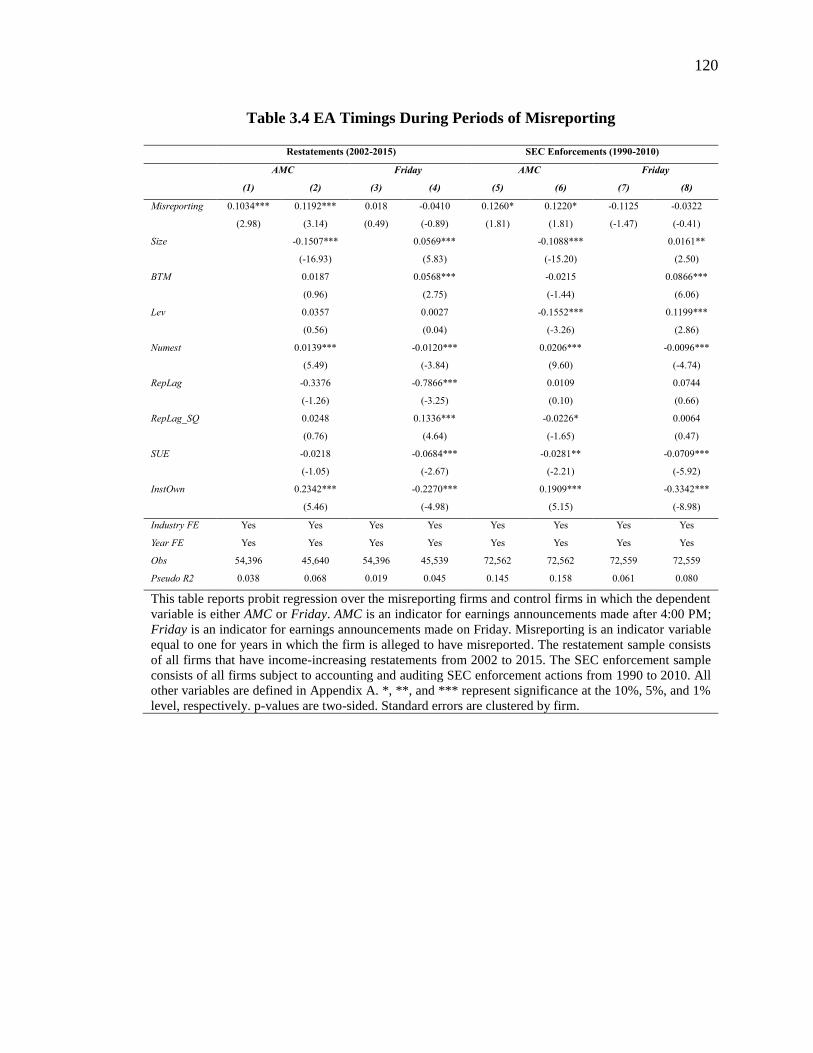
120
Table 3.4 EA Timings During Periods of Misreporting
Restatements (2002-2015) SEC Enforcements (1990-2010)
AMC Friday AMC Friday
(1) (2) (3) (4) (5) (6) (7) (8)
Misreporting 0.1034*** 0.1192*** 0.018 -0.0410 0.1260* 0.1220* -0.1125 -0.0322
(2.98) (3.14) (0.49) (-0.89) (1.81) (1.81) (-1.47) (-0.41)
Size
-0.1507***
0.0569***
-0.1088***
0.0161**
(-16.93)
(5.83)
(-15.20)
(2.50)
BTM
0.0187
0.0568***
-0.0215
0.0866***
(0.96)
(2.75)
(-1.44)
(6.06)
Lev
0.0357
0.0027
-0.1552***
0.1199***
(0.56)
(0.04)
(-3.26)
(2.86)
Numest
0.0139***
-0.0120***
0.0206***
-0.0096***
(5.49)
(-3.84)
(9.60)
(-4.74)
RepLag
-0.3376
-0.7866***
0.0109
0.0744
(-1.26)
(-3.25)
(0.10)
(0.66)
RepLag_SQ
0.0248
0.1336***
-0.0226*
0.0064
(0.76)
(4.64)
(-1.65)
(0.47)
SUE
-0.0218
-0.0684***
-0.0281**
-0.0709***
(-1.05)
(-2.67)
(-2.21)
(-5.92)
InstOwn
0.2342***
-0.2270***
0.1909***
-0.3342***
(5.46)
(-4.98)
(5.15)
(-8.98)
Industry FE Yes Yes Yes Yes Yes Yes Yes Yes
Year FE Yes Yes Yes Yes Yes Yes Yes Yes
Obs 54,396 45,640 54,396 45,539 72,562 72,562 72,559 72,559
Pseudo R2 0.038 0.068 0.019 0.045 0.145 0.158 0.061 0.080
This table reports probit regression over the misreporting firms and control firms in which the dependent
variable is either AMC or Friday. AMC is an indicator for earnings announcements made after 4:00 PM;
Friday is an indicator for earnings announcements made on Friday. Misreporting is an indicator variable
equal to one for years in which the firm is alleged to have misreported. The restatement sample consists
of all firms that have income-increasing restatements from 2002 to 2015. The SEC enforcement sample
consists of all firms subject to accounting and auditing SEC enforcement actions from 1990 to 2010. All
other variables are defined in Appendix A. *, **, and *** represent significance at the 10%, 5%, and 1%
level, respectively. p-values are two-sided. Standard errors are clustered by firm.

121
Table 3.5 Propensity Score Matching – First Stage
Restatements SEC Enforcements
(2002-2015) (1990-2010)
Size 0.0226* 0.0491***
(1.75) (2.65)
BTM 0.0579** -0.0076
(2.03) (-0.19)
Lev -0.0455 0.0849
(-0.50) (0.65)
Numest 0.0015 0.0185***
(0.43) (4.07)
RepLag -1.3501*** 0.0517
(-5.71) (0.19)
RepLag_SQ 0.2218*** 0.0195
(7.73) (0.62)
SUE 0.0032 0.2557***
(0.09) (3.83)
InstOwn 0.4964*** 0.5785***
(8.20) (4.93)
Industry FE Yes Yes
Year FE Yes Yes
Obs 45,622 69,309
Pseudo R2 0.0998 0.1290 This table reports the results of the first stage of propensity score matching in which the dependent variable
Misreporting, is an indicator variable equal to one for years in which the firm is alleged to have
misreported. The restatement sample consists of all firms that have income-increasing restatements from
2002 to 2015. The SEC enforcement sample consists of all firms subject to accounting and auditing SEC
enforcement actions from 1990 to 2010. All other variables are defined in Appendix A. *, **, and ***
represent significance at the 10%, 5%, and 1% level, respectively. p-values are two-sided. Standard errors
are clustered by firm.

122
Table 3.6 Descriptive Statistics
Panel A. Restatements PSM Sample (2002-2015)
Misreporting Control Difference (t-statistic)
AMC 0.5178 0.4597 0.0582*** (4.29)
Friday 0.0649 0.0662 -0.0012 (-0.17)
Size 6.6085 6.5291 0.0794* (1.64)
BTM 0.5642 0.5629 0.0013 (0.09)
Lev 0.2095 0.2080 0.0016 (0.28)
Numest 7.1645 6.9928 0.1717 (1.00)
RepLag 3.8681 3.8679 0.0002 (0.02)
SUE -0.0391 -0.0416 0.0025 (0.32)
InstOwn 0.5969 0.5834 0.0135*(1.56)
Obs 2,632 2,801 Total 5,433
Panel B. SEC Enforcement PSM Sample (1990-2010)
Misreporting Control Difference (t-statistic)
AMC 0.4347 0.3912 0.0435** (1.90)
Friday 0.0674 0.0630 0.0045 (0.39)
Size 6.7716 6.7339 0.0378 (0.40)
BTM 0.5361 0.5003 0.0358* (1.40)
Lev 0.2271 0.2275 -0.0004 (-0.04)
Numest 9.0953 9.3094 -0.2141 (-0.62)
RepLag 3.7554 3.7216 0.0338* (1.35)
SUE -0.0599 -0.0541 -0.0057 (-0.31)
InstOwn 0.5372 0.5285 0.0086 (0.59)
Obs 934 905 Total 1,839 This table reports firm characteristics for the misreporting sample and propensity score matched control
sample that have not had any misrepresentation event during our sample period. The restatement sample
consists of all firms that have income-increasing restatements from 2002 to 2015. The SEC enforcement
sample consists of all firms subject to accounting and auditing SEC enforcement actions from 1990 to
2010. All variables are defined in Appendix A. *, **, and *** represent significance at the 10%, 5%, and
1% level, respectively. Two sided p-values are based on the t-statistic for differences in means.
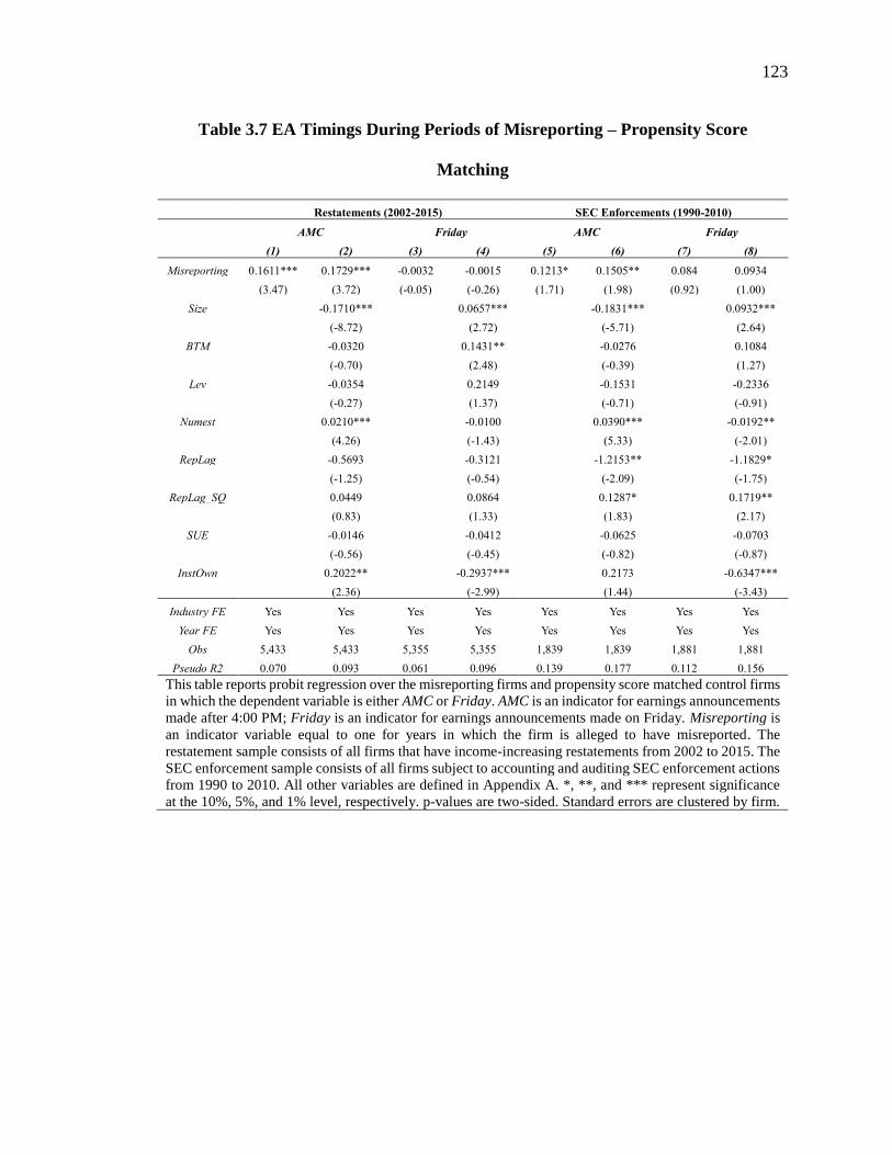
123
Table 3.7 EA Timings During Periods of Misreporting – Propensity Score
Matching
Restatements (2002-2015) SEC Enforcements (1990-2010)
AMC Friday AMC Friday
(1) (2) (3) (4) (5) (6) (7) (8)
Misreporting 0.1611*** 0.1729*** -0.0032 -0.0015 0.1213* 0.1505** 0.084 0.0934
(3.47) (3.72) (-0.05) (-0.26) (1.71) (1.98) (0.92) (1.00)
Size -0.1710*** 0.0657*** -0.1831*** 0.0932***
(-8.72) (2.72) (-5.71) (2.64)
BTM -0.0320 0.1431** -0.0276 0.1084
(-0.70) (2.48) (-0.39) (1.27)
Lev -0.0354 0.2149 -0.1531 -0.2336
(-0.27) (1.37) (-0.71) (-0.91)
Numest 0.0210*** -0.0100 0.0390*** -0.0192**
(4.26) (-1.43) (5.33) (-2.01)
RepLag -0.5693 -0.3121 -1.2153** -1.1829*
(-1.25) (-0.54) (-2.09) (-1.75)
RepLag_SQ 0.0449 0.0864 0.1287* 0.1719**
(0.83) (1.33) (1.83) (2.17)
SUE -0.0146 -0.0412 -0.0625 -0.0703
(-0.56) (-0.45) (-0.82) (-0.87)
InstOwn 0.2022** -0.2937*** 0.2173 -0.6347***
(2.36) (-2.99) (1.44) (-3.43)
Industry FE Yes Yes Yes Yes Yes Yes Yes Yes
Year FE Yes Yes Yes Yes Yes Yes Yes Yes
Obs 5,433 5,433 5,355 5,355 1,839 1,839 1,881 1,881
Pseudo R2 0.070 0.093 0.061 0.096 0.139 0.177 0.112 0.156
This table reports probit regression over the misreporting firms and propensity score matched control firms
in which the dependent variable is either AMC or Friday. AMC is an indicator for earnings announcements
made after 4:00 PM; Friday is an indicator for earnings announcements made on Friday. Misreporting is
an indicator variable equal to one for years in which the firm is alleged to have misreported. The
restatement sample consists of all firms that have income-increasing restatements from 2002 to 2015. The
SEC enforcement sample consists of all firms subject to accounting and auditing SEC enforcement actions
from 1990 to 2010. All other variables are defined in Appendix A. *, **, and *** represent significance
at the 10%, 5%, and 1% level, respectively. p-values are two-sided. Standard errors are clustered by firm.

124
Table 3.8 Days to Detection with EAs Made in After Trading Hours
Restatements (2002-2015) SEC Enforcements (1990-2010)
OLS COX Weibull OLS COX Weibull
(1) (2) (3) (4) (5) (6)
AMC_Hide 0.0981*** -0.2389*** -0.2676*** 0.0363 -0.2317* -0.2574*
(3.65) (-3.87) (-3.90) (0.94) (-1.67) (-1.82)
IndMisreporting -0.1465 0.0439 0.2668 -3.1714*** 11.4886*** 14.4552***
(1.38) (0.19) (0.99) (-3.94) (5.26) (6.38)
MeanDetectSIC 0.0124 -0.0493*** -0.0637*** 0.0137* -0.0534* -0.0541*
(1.61) (-2.72) (-3.54) (1.69) (-1.90) (-1.97)
MeanDetectOther 0.4769*** -1.1678*** -1.6151*** 0.0794 -0.2375*** -0.2249**
(4.15) (-4.75) (-5.69) (1.25) (-2.63) (-2.56)
Size 0.0184* -0.0030 0.0127 -0.0266 0.1060* 0.1232**
(1.72) (-0.13) (0.51) (-1.43) (1.81) (2.18)
Lev 0.0094 -0.1165 -0.0808 0.2987** -1.1821*** -1.1592**
(0.12) (-0.18) (-0.44) (2.35) (-2.67) (-2.52)
Numest -0.0108*** 0.0191** 0.0219*** -0.0105* 0.0391** 0.0429***
(-3.11) (2.52) (2.65) (-1.87) (2.46) (2.65)
ROA 0.1131 -0.3353 -0.3449 0.2623* -1.9102*** -1.7070***
(1.21) (-1.26) (-1.22) (1.84) (-4.15) (-4.07)
Growth -0.1073** 0.4227*** 0.4223*** 0.0962** -0.3508** -0.3443**
(-2.55) (3.31) (3.52) (2.03) (-2.15) (-2.17)
InstOwn 0.0439 -0.1449 -0.2257* 0.0542 -0.2369 -0.3062
(0.86) (-1.29) (-1.86) (0.68) (-0.87) (-1.11)
AnnRet 0.0180 -0.0050 0.0072 -0.0287 0.3361* 0.2889
(0.44) (-0.05) (0.06) (-0.62) (1.88) (1.59)
RetVol -1.5116 5.1511* 6.2959** -6.0752*** 23.8489*** 22.2794***
(-1.19) (1.67) (2.00) (-3.19) (3.94) (3.76)
Turnover -0.0002 0.0146 0.0158 -0.0139 0.0582 0.0376
(-0.03) (0.67) (0.67) (-0.94) (1.00) (0.65)
Industry FE Yes Yes Yes Yes Yes Yes
Obs 1,313 1,313 1,313 308 308 308
R-squared 0.149 0.423
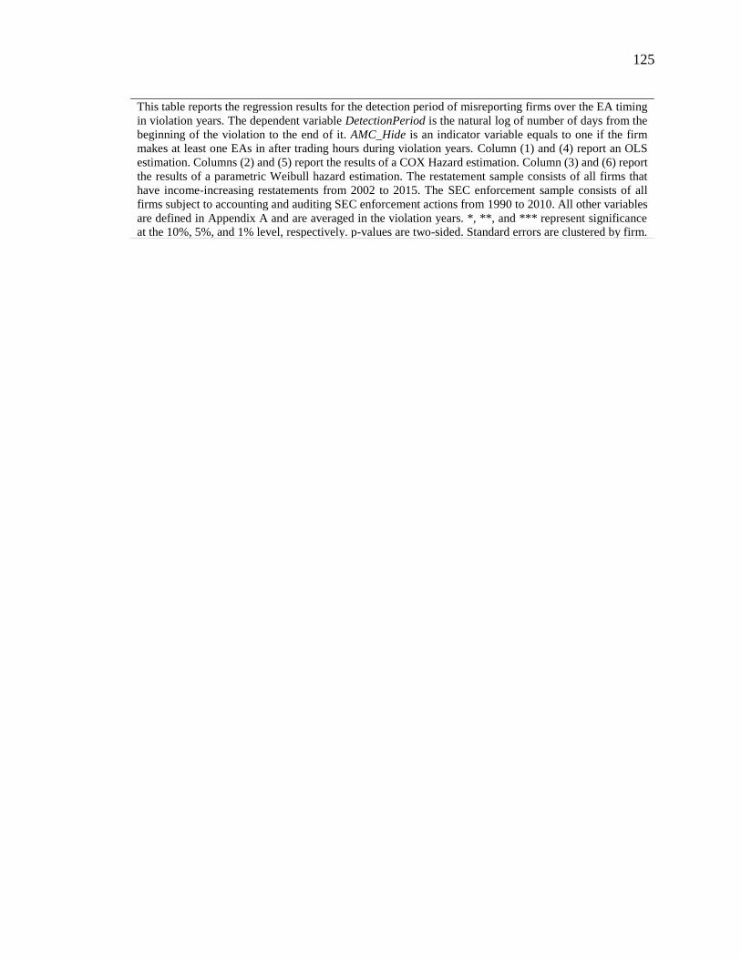
125
This table reports the regression results for the detection period of misreporting firms over the EA timing
in violation years. The dependent variable DetectionPeriod is the natural log of number of days from the
beginning of the violation to the end of it. AMC_Hide is an indicator variable equals to one if the firm
makes at least one EAs in after trading hours during violation years. Column (1) and (4) report an OLS
estimation. Columns (2) and (5) report the results of a COX Hazard estimation. Column (3) and (6) report
the results of a parametric Weibull hazard estimation. The restatement sample consists of all firms that
have income-increasing restatements from 2002 to 2015. The SEC enforcement sample consists of all
firms subject to accounting and auditing SEC enforcement actions from 1990 to 2010. All other variables
are defined in Appendix A and are averaged in the violation years. *, **, and *** represent significance
at the 10%, 5%, and 1% level, respectively. p-values are two-sided. Standard errors are clustered by firm.
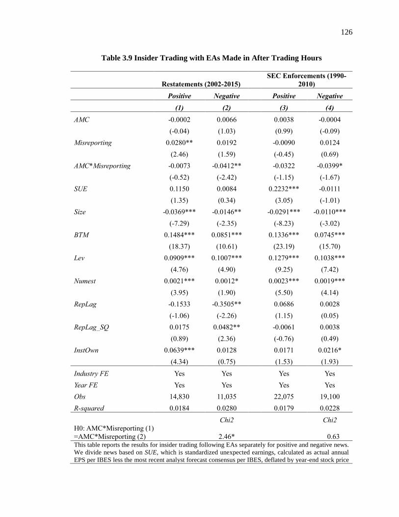
126
Table 3.9 Insider Trading with EAs Made in After Trading Hours
Restatements (2002-2015)
SEC Enforcements (1990-
2010)
Positive Negative Positive Negative
(1) (2) (3) (4)
AMC -0.0002 0.0066 0.0038 -0.0004
(-0.04) (1.03) (0.99) (-0.09)
Misreporting 0.0280** 0.0192 -0.0090 0.0124
(2.46) (1.59) (-0.45) (0.69)
AMC*Misreporting -0.0073 -0.0412** -0.0322 -0.0399*
(-0.52) (-2.42) (-1.15) (-1.67)
SUE 0.1150 0.0084 0.2232*** -0.0111
(1.35) (0.34) (3.05) (-1.01)
Size -0.0369*** -0.0146** -0.0291*** -0.0110***
(-7.29) (-2.35) (-8.23) (-3.02)
BTM 0.1484*** 0.0851*** 0.1336*** 0.0745***
(18.37) (10.61) (23.19) (15.70)
Lev 0.0909*** 0.1007*** 0.1279*** 0.1038***
(4.76) (4.90) (9.25) (7.42)
Numest 0.0021*** 0.0012* 0.0023*** 0.0019***
(3.95) (1.90) (5.50) (4.14)
RepLag -0.1533 -0.3505** 0.0686 0.0028
(-1.06) (-2.26) (1.15) (0.05)
RepLag_SQ 0.0175 0.0482** -0.0061 0.0038
(0.89) (2.36) (-0.76) (0.49)
InstOwn 0.0639*** 0.0128 0.0171 0.0216*
(4.34) (0.75) (1.53) (1.93)
Industry FE Yes Yes Yes Yes
Year FE Yes Yes Yes Yes
Obs 14,830 11,035 22,075 19,100
R-squared 0.0184 0.0280 0.0179 0.0228
Chi2 Chi2
H0: AMC*Misreporting (1)
=AMC*Misreporting (2) 2.46* 0.63 This table reports the results for insider trading following EAs separately for positive and negative news.
We divide news based on SUE, which is standardized unexpected earnings, calculated as actual annual
EPS per IBES less the most recent analyst forecast consensus per IBES, deflated by year-end stock price

127
per Compustat. The dependent variable Value is the net dollar value of trades by insiders in a given firm
during 90 days following an EA in a year. AMC is an indicator for earnings announcements made after
4:00 PM. Misreporting is an indicator variable equal to one for years in which the firm is alleged to have
misreported. The restatement sample consists of all firms that have income-increasing restatements from
2002 to 2015. The SEC enforcement sample consists of all firms subject to accounting and auditing SEC
enforcement actions from 1990 to 2010. All other variables are defined in Appendix A. *, **, and ***
represent significance at the 10%, 5%, and 1% level, respectively. p-values are two-sided. Standard errors
are clustered by firm.

128
Table 3.10 The Market Reactions Following the Disclosure of Misreporting
Restatements
(2002-2015)
SEC Enforcements
(1990-2010)
CAR [-1,1] CAR [-3,3] CAR [-1,1] CAR [-3,3]
(1) (2) (3) (4)
After_Hide -0.0151** -0.0014** 0.0037 -0.0131
(-2.55) (-2.13) (0.31) (-0.74)
Size 0.0058** 0.0060** 0.0047 0.0060
(2.28) (2.14) (0.76) (0.85)
BTM -0.0218*** -0.0323*** -0.0232 -0.0040
(-3.12) (-4.03) (-1.33) (-0.16)
Lev -0.0446*** -0.0506*** -0.0296 -0.0221
(-2.69) (-2.69) (-0.80) (-0.55)
Numest -0.0011* -0.0016** -0.0013 -0.0001
(-1.68) (-2.02) (-0.95) (-0.05)
RepLag -0.0101 -0.0001 0.0929 0.0837
(-0.37) (0.05) (0.81) (0.48)
RepLag_SQ -0.0009 -0.0028 -0.0119 -0.0097
(-0.27) (-0.57) (-0.90) (-0.48)
SUE 0.0296*** 0.0301*** 0.0025 0.0437
(3.42) (2.91) (0.08) (1.47)
InstOwn -0.0026 0.0061 0.0349 0.0548
(-0.24) (0.47) (1.46) (1.39)
Industry FE Yes Yes Yes Yes
Year FE Yes Yes Yes Yes
Obs 1,023 1,023 144 144
R Squared 0.181 0.176 0.439 0.635 This table reports the results for CAR surrounding the discovery date (filing date) of the misreport. The
dependent variable CAR is the 3-day (7-day) size-adjusted abnormal returns surround the filing date of the
restatement or lawsuit. After_Hide is an indicator variable equals to one if the firm makes at least one EAs
in after trading hours during violation years, and zero otherwise. The restatement sample consists of all
firms that have income-increasing restatements from 2002 to 2015. The SEC enforcement sample consists
of all firms subject to accounting and auditing SEC enforcement actions from 1990 to 2010. All other
variables are defined in Appendix A. *, **, and *** represent significance at the 10%, 5%, and 1% level,
respectively. p-values are two-sided. Standard errors are clustered by firm.
Related Documents