Three Essays on Corporate Finance Modelling James Peter Brotchie BEng (AeroAv) GCertSci (FinMaths) A thesis submitted for the degree of Doctor of Philosophy at The University of Queensland in 2015 UQ Business School

Welcome message from author
This document is posted to help you gain knowledge. Please leave a comment to let me know what you think about it! Share it to your friends and learn new things together.
Transcript
Three Essays on Corporate Finance Modelling
James Peter Brotchie
BEng (AeroAv) GCertSci (FinMaths)
A thesis submitted for the degree of Doctor of Philosophy at
The University of Queensland in 2015
UQ Business School

Abstract
In this thesis I use mathematical modelling techniques to further our understanding of
three outstanding corporate finance problems. In each case, I derive a novel model of
agent behaviour, calculate an efficient numerical solution, and then explore how the model
informs theory and practice. I present my contributions to each problem as separate self-
contained essays.
In my first essay I build a novel equity valuation model, based on the fundamental
accounting equation and observable book values, that determines a firm's optimal
voluntary liquidation policy. Voluntary liquidation allows equityholders of a poorly
performing firm to liquidate its assets, repay any creditors, and keep any remaining value.
Empirical evidence suggests that investors react favourably to voluntary liquidation
announcements, suggesting that the liquidation of inefficient firms improves economic
resource allocation. I find that the firm's voluntary liquidation policy is primarily sensitive to
earnings risk, expected asset depreciation, liquidation expenses, leverage, expected
earnings yield, and expected cost-of-debt. My model successfully replicates empirically
observed voluntary liquidation behaviour and suggests that voluntary liquidation aligns
manager and equityholder behaviour with respect to leverage and debt maturity choice
and increased earnings volatility. Manager and equityholder incentives conflict with respect
to asset liquidation costs.
As a supplement to my first essay, I provide a detailed derivation of my model and the
numerical solution of my model's governing partial differential equation. I also provide a
highly optimized implementation of the projected successive overrelaxation algorithm that I
use to solve my model. This implementation exploits CPU cache locality to greatly
accelerate solving two-dimensional stochastic differential equations with early exercise
conditions.
In my second essay I develop a formal economic model of company director decision
making under Australia's past and present insolvent trading laws. A director of an
Australian company who incurs debts while their company is insolvent can be chased by
creditors for compensation if their company fails. I provide the first tractable model that can
determine if this threat of insolvent trading affects director's decisions in a way that is
always advantages creditors. I explore director's decision making and subsequent creditor
outcomes when directors are threatened by insolvent trading, as well as when directors
tactically use Australia's voluntary administration insolvency procedure to avoid insolvent
trading litigation. I show that neither a combination of insolvent trading or voluntary
administration can simultaneously ensure creditors-best outcomes, eliminate insolvent
trading, and reduce director underinvestment.
In my third essay I derive a global asset pricing model with endogenous home preference
that contains a small open economy with a dividend imputation tax system; Dividend
imputation eliminates double taxation by attaching tax credits to distributed dividends for
already paid company tax. Domestic investors can use these credits to reduce their
personal taxes, while credits are useless to foreign investors. The interplay between
imputation eligible domestic investors and ineligible foreign investors makes it difficult to
value imputation credits. My model assumes that home bias arises endogenously from the
status quo and endowment effect behavioural biases. I find that these biases interact with
dividend imputation to drive domestic investors to hold highly concentrated domestic
portfolios. I also find that risk-averse domestic investors cannot fully capture the value of
imputation credits because concentrating their holdings in the domestic market reduces
their diversification.

Declaration by author
This thesis is composed of my original work, and contains no material previously published
or written by another person except where due reference has been made in the text. I
have clearly stated the contribution by others to jointly-authored works that I have included
in my thesis.
I have clearly stated the contribution of others to my thesis as a whole, including statistical
assistance, survey design, data analysis, significant technical procedures, professional
editorial advice, and any other original research work used or reported in my thesis. The
content of my thesis is the result of work I have carried out since the commencement of
my research higher degree candidature and does not include a substantial part of work
that has been submitted to qualify for the award of any other degree or diploma in any
university or other tertiary institution. I have clearly stated which parts of my thesis, if any,
have been submitted to qualify for another award.
I acknowledge that an electronic copy of my thesis must be lodged with the University
Library and, subject to the policy and procedures of The University of Queensland, the
thesis be made available for research and study in accordance with the Copyright Act
1968 unless a period of embargo has been approved by the Dean of the Graduate School.
I acknowledge that copyright of all material contained in my thesis resides with the
copyright holder(s) of that material. Where appropriate I have obtained copyright
permission from the copyright holder to reproduce material in this thesis.

Publications during candidature
Working Papers
1. Alcock J., Brotchie J., Gray S. Optimal Voluntary Liquidation of a Limited Liability
Firm.
2. Brotchie J., Morrison D. Insolvent Trading and Voluntary Administration in Australia:
Winners or Losers?
3. Brotchie J., Gray S. Equilibrium Asset Pricing with Imputation and Home
Preference.
Publications included in this thesis
No publications included.

Contributions by others to the thesis
My working paper co-authors, through the process of reviewing working paper drafts, have
provided the following contributions to my final thesis.
Contributor Statement of contribution
Brotchie J. (Myself)
Conceptualization of Key Ideas (85%)
Technical Calculations (100%)
Drafting and Writing (90%)
Alcock J. Conceptualization of Key Ideas (5%)
Drafting and Writing (5%)
Gray S. Conceptualization of Key Ideas (5%)
Drafting and Writing (5%)
Morrison D. Conceptualization of Key Ideas (5%)
Statement of parts of the thesis submitted to qualify for the award of another degree
None.

Acknowledgements
Firstly I would like to thank my wife Thu for all the encouragement over the past few years
and for answering plenty of questions about accounting. I'd also like to thank my family for
all their support and proof-reading. Special thanks to my supervisors Stephen Gray and
Jamie Alcock for all their guidance and to David Morrison for all the legal advice. I really
appreciate the effort my internal readers Allan Hodgson, Kelvin Tan, and Kam Chan put
into reviewing my work over the PhD process. Finally I'd like to thank Julie Cooper for
managing my PhD life cycle and interfacing with the graduate school. Also thanks to
everybody who has reviewed my work over the past four years.

Keywords
corporate finance, voluntary liquidation, insolvent trading, voluntary administration,
dividend imputation, stochastic differential equations, finite difference methods, numerical
algorithms
Australian and New Zealand Standard Research Classifications (ANZSRC)
ANZSRC code: 150201, Finance, 100%
Fields of Research (FoR) Classification
FoR code: 1502 Banking, Finance and Investment, 100%

Contents
1 Introduction 3
1.1 List of Academic Presentations . . . . . . . . . . . . . . . . . . . . . . . . . 9
1.2 Thesis Structure . . . . . . . . . . . . . . . . . . . . . . . . . . . . . . . . . . 9
2 Essay One – Optimal Voluntary Liquidation of a Limited Liability Firm 10
2.1 Introduction . . . . . . . . . . . . . . . . . . . . . . . . . . . . . . . . . . . . 11
2.2 Prior Literature . . . . . . . . . . . . . . . . . . . . . . . . . . . . . . . . . . 15
2.3 The Model . . . . . . . . . . . . . . . . . . . . . . . . . . . . . . . . . . . . . 31
2.4 Model Results . . . . . . . . . . . . . . . . . . . . . . . . . . . . . . . . . . . 42
2.5 Concluding Remarks . . . . . . . . . . . . . . . . . . . . . . . . . . . . . . . 49
3 Stochastic Earnings Volatility Model Derivation and Solution 59
3.1 Model Derivation . . . . . . . . . . . . . . . . . . . . . . . . . . . . . . . . . 60
3.2 Numerical Solution . . . . . . . . . . . . . . . . . . . . . . . . . . . . . . . . 64
3.3 Selecting our Numerical Solution Method . . . . . . . . . . . . . . . . . . . . 65
3.3.1 Monte-Carlo . . . . . . . . . . . . . . . . . . . . . . . . . . . . . . . . 66
i

Contents ii
3.3.2 Binomial and Multinomial Trees . . . . . . . . . . . . . . . . . . . . . 68
3.3.3 Finite Difference Methods . . . . . . . . . . . . . . . . . . . . . . . . 68
3.4 Coordinate Transformation . . . . . . . . . . . . . . . . . . . . . . . . . . . . 70
3.4.1 Single Dimension Transform . . . . . . . . . . . . . . . . . . . . . . . 70
3.4.2 Two-Dimension Transform . . . . . . . . . . . . . . . . . . . . . . . . 74
3.5 Discretizing the PDE . . . . . . . . . . . . . . . . . . . . . . . . . . . . . . . 76
3.6 Time Stepping . . . . . . . . . . . . . . . . . . . . . . . . . . . . . . . . . . . 79
3.6.1 Operator Splitting . . . . . . . . . . . . . . . . . . . . . . . . . . . . 81
3.6.2 Matrix Representation . . . . . . . . . . . . . . . . . . . . . . . . . . 83
3.6.3 Aθ Elements . . . . . . . . . . . . . . . . . . . . . . . . . . . . . . . . 85
3.6.4 Aφ Elements . . . . . . . . . . . . . . . . . . . . . . . . . . . . . . . 86
3.6.5 Aφθ Elements . . . . . . . . . . . . . . . . . . . . . . . . . . . . . . . 87
3.6.6 Modified Craig-Sneyd Scheme . . . . . . . . . . . . . . . . . . . . . . 90
3.7 Projected Successive Overrelaxation . . . . . . . . . . . . . . . . . . . . . . . 91
3.8 A Cache Optimized PSOR Algorithm . . . . . . . . . . . . . . . . . . . . . . 93
4 Essay Two – Insolvent Trading and Voluntary Administration in Australia:
Economic Winners or Losers? 99
4.1 Introduction . . . . . . . . . . . . . . . . . . . . . . . . . . . . . . . . . . . . 100
4.2 The Model . . . . . . . . . . . . . . . . . . . . . . . . . . . . . . . . . . . . . 107
4.3 Insolvent Trading . . . . . . . . . . . . . . . . . . . . . . . . . . . . . . . . . 113
4.4 Voluntary Administration . . . . . . . . . . . . . . . . . . . . . . . . . . . . 119
4.5 Contracting Options . . . . . . . . . . . . . . . . . . . . . . . . . . . . . . . 128
4.6 Conclusion . . . . . . . . . . . . . . . . . . . . . . . . . . . . . . . . . . . . . 131

Contents iii
5 Essay Three – A Tale of Two Economies: Equilibrium Asset Pricing with
Imputation and Home Preference 133
5.1 Introduction . . . . . . . . . . . . . . . . . . . . . . . . . . . . . . . . . . . . 134
5.2 The Model . . . . . . . . . . . . . . . . . . . . . . . . . . . . . . . . . . . . . 143
5.3 Portfolio Holdings . . . . . . . . . . . . . . . . . . . . . . . . . . . . . . . . . 153
5.4 Equilibrium Value of Franking Credits . . . . . . . . . . . . . . . . . . . . . 161
5.5 Conclusion . . . . . . . . . . . . . . . . . . . . . . . . . . . . . . . . . . . . . 168
6 Thesis Conclusion 170
References 173

Abbreviations
The following list is neither exhaustive nor exclusive, but may be helpful.
AUD Australian Dollar
CAPM Capital Asset Pricing Model
CARA Constant Absolute Risk Aversion
CPU Central Processing Unit
CRRA Constant Relative Risk Aversion
DOCA Deed of Company Arrangement
EBIT Earnings Before Interest and Tax
EBITDA Earnings Before Interest Tax Depreciation and Amortization
GBM Geometric Brownian Motion
GICS Global Industry Classification Standard
GPGPU General Purpose Graphics Processing Unit
LAPACK Linear Algebra Package
1
Contents 2
LCP Linear Complementarity Problem
MABR Maximum Acceptable Burn Rate
MRP Market Risk Premium
NPV Net Present Value
OECD Organisation for Economic Co-operation and Development
OVLB Optimal Voluntary Liquidation Boundary
PDE Partial Differential Equation
PSOR Projected Successive Overrelaxation
RHS Right Hand Side
ROA Return on Assets
SEVM Stochastic Earnings Volatility Model
SOR Successive Overrelaxation
VA Voluntary Administration

1Introduction
Abstract financial theory is valuable, however much can be learned from building a numerical
model, plugging in some real-world values, and examining the results. As long as all the
assumptions are reasonable, any intuition gained from a model can be useful to further
theoretical understanding and inform real-world practice.
In this thesis I aim to address the following three outstanding corporate finance questions:
1. What is a firm’s optimal voluntary liquidation policy?
2. Do Australia insolvent trading laws produce economically optimal outcomes? and,
3

4
3. Are imputation credits fully valued in a small open economy and if not, why not?
Targeting each of these problems I,
1. Build a novel model of the relevant agents, environment, and constraints;
2. Efficiently solve the model, either analytically or numerically, across its parameter
space;
3. Ensure that the model’s outputs are consistent with the underlying theory and capture
empirically observed behaviour;
4. Explore how the model’s outputs extend our knowledge of the problem at hand.
What is a firm’s optimal voluntary liquidation policy?
Liquidating a distressed firm releases capital that may be used more efficiently in other
ventures. Equityholders will rationally choose to voluntarily liquidate their firm when the
value from immediate liquidation is greater than the expected value of continuation. Given
that the observable structural characteristics of a firm are its accounting variables, I build
a model that uses accounting information to calculate equityholder’s optimal liquidation
policy. My model is a continuous time valuation model based on the fundamental accounting
equation and treats equity as a down-and-out Asian-American style option on net earnings. I
model the time evolution of both earnings and assets, allowing me to incorporate book value
based earnings and asset covenants and insolvency laws. Using finite difference techniques, I
derive and solve the partial differential equation governing the firm’s equity value to extract
optimal liquidation policies.
I find that a firm’s optimal voluntary liquidation policy is determined largely by: expected
liquidation costs, earnings volatility, expected earnings, rate of asset depreciation, and the
firm’s cost of debt.

5
Managers control a firm on behalf of its equityholders, but the incentives of managers aren’t
necessarily aligned with the equityholders they represent. I find that voluntary liquidation
aligns manager and equityholder behaviour in some cases, and create conflicts in others.
Understandably, liquidation is a terminal event for managers, who will lose their job, enti-
tlements, and perhaps reputation, thus they will be hesitant to “throw in the towel” and
liquidate a firm under their control. I show that managers who fail to initiate liquidation
when it is optimal for equityholders destroy substantial equityholder wealth, however man-
ager and equityholder behaviour is aligned with respect to increases in earnings, depreciation,
and cost-of-debt volatility as well as maintaining a monotonic relationship between leverage
and debt maturity.
My contributions towards finding firm’s optimal voluntary liquidation policies are: deriving a
novel model of voluntary liquidation based on the fundamental accounting equation, numer-
ically solving this model using my optimization implementation of the projected successive
overrelaxation algorithm that is 5 orders of magnitude faster than a naive implementation,
identifying the key parameters influencing optimal voluntary liquidation policy, and charac-
terizing manager-equityholder conflicts as they relate to voluntary liquidation.
Do Australian insolvent trading laws produce economically optimal outcomes?
Insolvent trading laws make directors and managers personally liable for debts incurred when
their companies are insolvent, or for debts incurred that make their companies insolvent.
Directors who trade while insolvent face civil litigation, and in extreme cases criminal charges.
The insolvent trading laws aim to protect creditors from losses due to directors continuing
to trade when there’s little prospect of debt repayment. Insolvent trading laws weaken
the capitalistic principle of limited liability because incurring debts while simply suspecting
insolvency or simply failing to prevent such a debt being incurred open directors to personal
liability should their company be wound-up.
A defining characteristic of Australia’s insolvency law landscape is the option of Voluntary

6
Administration (VA). VA involves either the company (on behalf of the directors) or liquida-
tors appointing an administrator to take control of, investigate, and make recommendations
for dealing with the property and affairs of an insolvent or near-insolvent company. The
action of entering VA stays all legal proceedings against the company and because the insol-
vent trading laws are only enforceable during a liquidation, VA temporarily stays director’s
personal liability for violating the insolvent trading provisions. It’s typical for directors to
exploit this “feature” of VA as a ”get out of jail free card”, preemptively filing for VA once
they are certain their firm is about to go bankrupt.
There is substantial economic, social, and legal debate regarding the necessity of insolvent
trading laws and voluntary administration, particularly whether they are economically ef-
ficient. As yet nobody has developed a formal mathematical model to analyze Australia’s
insolvent trading laws. A prominent commentator, Whincop (2000), describes the current
situation
Australia has a wealth of doctrinal literature on insolvency and corporate gov-
ernance, and a thriving economic literature of corporate governance, but serious
economic analysis of insolvency remains terra incognita.
To this end I develop an economic model of director behaviour under Australian insolvent
trading laws and voluntary administration. I find that there is no dominant configuration of
insolvent trading and voluntary administration laws that limits insolvent trading while max-
imizing creditor welfare. This is because the goals of simultaneously (a) stopping insolvent
trading, (b) maximizing creditor welfare in default, and (c) minimizing the impact of skittish
directors winding-up too early, are incompatible. The introduction of insolvent trading laws
certainly discourages directors from insolvent trading, however at the expense of extinguish-
ing a company that may have had a better expected payoff by continuing. Creditors in firms
with negative net assets but positive growth expectations are materially worse off under the
insolvent trading laws.
7
My primary contribution here is offering the first tractable economic model of director be-
haviour when subject to Australian insolvent trading laws and voluntary administration. I
numerically demonstrate that insolvent trading laws aren’t necessarily always in the best
interest of creditors and that voluntary administration can generate materially negative out-
comes for creditors in certain feasible scenarios.
Are imputation credits fully valued in a small open economy and if not, why
not?
Domestic Australian companies receive imputation credits for the Australian corporate tax
they pay. When these companies distribute dividends to their shareholders they “frank”
their dividends by attaching imputation credits. Certain domestic shareholders, when they
receive franked dividends, can use the attached credits to reduce their personal taxes. Foreign
investors cannot use the credits and don’t value them. Given that Australia is a small open
economy whose shares are held by a mixture of domestic investors and foreign investors,
each valuing imputation creditors differently, it is not obvious how these credits influence
the market value of Australian shares.
Australia’s equity markets represent 1.7% of world market capitalization, yet Australian’s
allocate 78% of their invested wealth to domestic Australian stocks (Lau, Ng, and Zhang,
2010). Any model ignoring this high level of home bias may come to the wrong conclusion
regarding the demand for imputation paying stocks. In the past, such home bias was of-
ten explain by barriers to cross-country investment. Currency hedging products were less
accessible; information search costs were much higher (pre-internet access), trading costs
were considerable, and there were much explicit barriers to foreign investment. These days,
however, the arrival of discount brokers and the internet dramatically reduced information
search costs within foreign markets and reduced transaction costs across-the-board.
Given that explicit barriers to foreign investment have decreased, yet there hasn’t been
an equivalent decrease in home bias, there must be an alternative explanation. There is

8
plenty of evidence that investors are subject to behavioural biases (Hirshleifer, 2001) and
that these biases can influence investor’s portfolio holdings. Since Australian investors have
been historically accustomed to holding Australian stocks and Australian investors tend to
hold the same portfolio as their peers, it is reasonable to believe that Australian investors
are subject to the status quo and endowment effect behavioural biases. I assume that these
behavioural biases are a prominent factor in the observed home bias of Australian investors.
Given this assumption, I derive a global capital asset pricing model with home bias and
dividend imputation. I then explore the effects of imputation and home bias on investor
holdings, required returns, and the market value of imputation credits. I demonstrate that
domestic investor’s behavioural biases interact with dividend imputation to create a situation
where domestic investors hold highly concentrated domestic asset portfolios. I also identify
that investor risk aversion is the primary determinant of the market value of imputation
credits in an small open economy. In forming their portfolios, domestic investors tradeoff
the positive benefit of imputation credits against the negative effect of further concentrating
their portfolios into domestic assets.
My contribution is a novel asset pricing model for a small open economy interacting with a
larger global economy where the small economy has dividend imputation and all investors ex-
hibit behavioural home biases. I show that behavioural biases magnify the portfolio concen-
tration effect of dividend imputation and that with realistic levels of risk-aversion imputation
credits have negligible market value.
Final Thoughts
Although it is impossible to perfectly solve these corporate finance problems, given they are
largely driven by unpredictable human behaviour, forging ahead with quantitative techniques
at least brings us a step closer to the truth. Just as I have built these three new models
inspired by the works of past authors, I hope that future authors will be able to derive equal
inspiration from my models.

1.1 List of Academic Presentations 9
1.1 List of Academic Presentations
I have presented my work at the following domestic and international conferences and col-
loquia:
• 25th Australasian Finance and Banking Conference (Sydney, Australia, 2012)
• 2013 Midwest Finance Association Annual Conference (Chicago, USA, 2013)
• University of Queensland Business School Annual Research Colloquium (Brisbane,
Australia, 2013). Received the ’Best Presentation’ award.
• 26th Australasian Finance and Banking Conference (Sydney, Australia, 2013)
1.2 Thesis Structure
I have structured this thesis as a compilation of three essays, each in a separate chapter.
I have also included a supplementary chapter detailing the mathematical derivations and
optimized numerical solution of my optimal voluntary liquidation model . Note that apart
from in this introduction, I use the first-person plural personal pronoun we when referring
to myself exclusively and also when collectively referring to myself and my co-authors. I also
readily use his and her interchangeably in a gender-neutral sense, as I feel that replacing his
or her with their can create unnecessary ambiguity.

2Essay One – Optimal Voluntary Liquidation of
a Limited Liability Firm
The decision of whether a firm should attempt to trade out of trouble, rather than volun-
tarily liquidate, is a function of uncertain future earnings, asset depreciation, and the firm’s
cost-of-debt among other things. We develop an equity valuation model derived from the
fundamental accounting equation that treats equity as an Asian-style call option on net
earnings. Using this model we identify the firm’s optimal voluntary liquidation rule and
calculate this rule’s sensitivity to key firm characteristics. While expected rates of EBITDA
10

2.1 Introduction 11
growth, cost-of-debt and accounting depreciation are all important variables, we find that
EBITDA risk is the dominant determinant of the optimal voluntary liquidation rule. Our
model predicts many commonly observed empirical voluntary liquidation behaviours and
also predicts situations where managers interests are misaligned with those of equityholders.
2.1 Introduction
When the liquidation value of a firm is greater than its going-concern value, management
should voluntarily liquidate the firm’s assets and return capital to investors (Berger, Ofek,
and Swary, 1996). Exercising the option to liquidate realizes the current market value of
the firm’s assets net of liquidation costs and forfeits the market value of the earnings stream
that would have been generated using those assets (Myers, 1977; Myers and Majd, 1990;
Robichek and Horne, 1967). Overly-optimistic managers that liquidate too late destroy
shareholder value by allowing unnecessary asset value erosion (Davydenko and Rahaman,
2008; DeAngelo, DeAngelo, and Wruck, 2002). In the worst case, all shareholder value is
destroyed in a compulsory liquidation (i.e. bankruptcy). Overly-pessimistic managers who
liquidate too early may extinguish a firm that would otherwise have continued generating
value for its shareholders.
Intuitively, a mature firm that is losing asset value faster than it produces earnings is moving
closer to bankruptcy and may be “worth more dead than alive”1. However determining
the firm’s optimal voluntary liquidation decision boundary (OVLB) is not straight forward;
future earnings are not deterministic and liquidation is a decision that, if taken, is irreversible.
For example a distressed firm may at some future time experience a substantial positive shock
to its earnings and thus has a non-zero probability of trading out of its current troubles.
Liquidation extinguishes this possibility.
1Eight days before the Dow hit rock-bottom in 1932, Benjamin Graham published a three-part seriestitled “Is American business worth more dead than alive?” in Forbes magazine. Graham suggested thatmany of America’s great corporations were now worth more “dead than alive”.
2.1 Introduction 12
We determine the optimal rule for voluntary liquidation (the OVLB) for the case of a levered
firm holding a single asset with a finite life whose market value is exogenously determined.
We develop a dynamic model of accrual accounting based upon the fundamental accounting
equation where managers use firm assets to generate earnings before interest, taxation, de-
preciation, and amortization (EBITDA). Managers can voluntarily liquidate the firm at any
time unless a debt-covenant or insolvency condition triggers an involuntary liquidation. In
our model, equityholders possess a call option on the value of the firm’s assets, struck at the
face value of debt (c.f. Black and Scholes, 1973). As the firm’s assets are the integral of net
earnings over time, we model equity as a down-and-out American-Asian style Call option on
the firm’s net earnings. Managers should liquidate their firm once earnings falls below the
early exercise boundary of this American-Asian call option. Our modelling approach makes
greater use of the information contained within financial statements compared with existing
structural models.
We find that in many circumstances, the early exercise boundary is significantly below the
profit-making level of earnings. That is, rational equityholders prefer the firm to continue to
trade, even when the firm is making a substantial after-tax loss. For a representative firm,
the maximum acceptable burn rate (MABR), defined as the difference between the liqui-
dation boundary EBITDA yield and the taxable profit-making EBITDA yield, is sensitive
to cost-of-debt, leverage, corporate tax rate,2 accounting depreciation and liquidation costs
however the dominant determinant of the MABR is EBITDA yield risk. The MABR is rela-
tively insensitive to depreciation adjustments representing the difference between economic
(realized) depreciation and accounting depreciation or yield-curve movements. In contrast,
the MABR for a firm in an extreme state of financial distress is highly sensitive to liquidation
costs and yield-curve movements.
The MABR is highly sensitive to EBITDA yield risk because the continuation value of
2We only consider a non-progressive tax rate. Agliardi and Agliardi (2008) investigate voluntary liquida-tion within a progressive tax system.

2.1 Introduction 13
equity is strictly increasing in earnings risk, ceteris paribus. The implicit downside protection
embedded within the option to liquidate a limited liability firm increases the continuation
value of equity (at the expense of debtholders). Accordingly, the OVLB is strictly decreasing
in earnings risk. Equityholders in a firm with riskier utilisation of its assets, cetaris parabis,
are better off with a more optimistic policy with respect to voluntarily winding-up the firm.
The firm’s “liquidate or continue” decision is sensitive to expected liquidation costs. Firms
with highly liquid assets should wind-up earlier than firms holding illiquid assets. The value
of continuation is higher (lower) than the value of the liquidation option when liquidation
costs are large (small). Consequently, firms holding illiquid assets benefit more from at-
tempting to trade-out of trouble.
We find that the optimal voluntary liquidation decision is mostly invariant to levels of re-
strictive asset-based and earnings-based debt covenants. Our model is particularly suited
to modeling such covenants because they are normally expressed in terms of book, rather
than market, values. Restrictive earnings and asset based debt covenants do increase the
optimal voluntary liquidation boundary, but only when the firm is deeply distressed - that
is, when equityholders gain no residual value in liquidating and only hold value from the
continuation option. In this case, restrictive debt covenants reduce the continuation value
to equityholders by enforcing liquidation earlier than is optimal for equity.
We assume that the firm’s investment and financing choices are determined exogenously.
Nevertheless, by exploring the sensitivity of optimal voluntary liquidation to these exogenous
variables we can draw insights into managerial choices of investment and financing that
concur with equityholder preferences. For example, choosing a riskier earnings generation
strategy will both increase equityholder’s value as well as the maximum acceptable burn
rate. To the extent that debtholders will allow such a shift, the interests of equityholders
and managers are aligned. Alternatively, a manager who shifts the firm’s asset base into less
liquid assets will increase the maximum acceptable burn rate, yet is decreasing equityholder

2.1 Introduction 14
value. In this case, the manager’s interests may conflict with those of equityholders. In this
manner, our model provides a benchmark by which these agency costs can be quantified.
Prior literature on voluntary liquidation includes model’s incorporating equityholder’s option
to voluntarily liquidate in the presence of ex-ante customer-imposed bankruptcy costs (Tit-
man, 1984), equityholder–manager agency conflict (Chang and Wang, 1992; White, 1983),
investment intensity (Wong, 2012), progressive taxation (Agliardi and Agliardi, 2008; Wong,
2009) and corporate cash holdings (Anderson and Carverhill, 2011). To date, there is little
understanding as to how, and to what extent, observable accounting variables affect the
optimal liquidation decision, and the associated motivations of various stakeholders. Also,
it is not yet clear the degree of alignment between manager’s and equityholder’s incentives
to voluntarily liquidate.
Our model predicts the results found in many empirical studies into voluntary liquidation.
Firms that exit via voluntarily liquidation, as opposed to bankruptcy or involuntary liqui-
dation, tend to have higher insider ownership (Mehran, Nogler, and Schwartz, 1998), lower
asset productivity (Fleming and Moon, 1995), plentiful slack resources (Balcaen, Buyze, and
Ooghe, 2009), lower leverage (Mata, Antunes, and Portugal, 2011), and are more likely to
be subject to a hostile takeover bid (Ghosh, Owers, and Rogers, 1991). Further, the public
announcement of a voluntary liquidation typically elicits a strong positive market reaction
(Hite, Owers, and Rogers, 1987; Kim and Schatzberg, 1987). Shareholders realize substantial
short-term gains following a voluntary liquidation announcement, implying that voluntary
liquidations net better corporate resource allocation. A liquidation announcement instantly
converts an uncertain future stream of cash flows into a certain terminal dividend. Berger,
Ofek, and Swary (1996) empirically demonstrate that equityholders impute the value of the
option to voluntarily liquidate into equity values.
We present our paper as follows. In Section 2.2 we provide a deeper review of appropriate
literature. In Section 2.3 we introduce our optimal voluntary liquidation model. We explore

2.2 Prior Literature 15
the implications of our model for optimal liquidation policy in Section 2.4. We conclude in
Section 2.5.
2.2 Prior Literature
In this section, we discuss related literature, focusing on extant theoretical models and
empirical explorations of corporate liquidation policy and optimal project abandonment.
Structural Asset Pricing Models
We can classify asset pricing models as either structural or reduced-form. These categories
specify the completeness of the model’s assumed information set. Structural models assume
full and instantaneous knowledge of a firm’s corporate structure, asset value, agent behaviour,
and operating environment. Reduced-form models, in contrast, restrict the information set to
contain only publicly available information. Such classifications are not mutually exclusive—
hybrid models exist where investors can observe some, but not all, inside information.
At a minimum, a structural asset pricing model requires:
• A mathematical definition of a security’s claim over some set of risky underlying value
processes.
• A mathematical characterisation of the time and space evolution of these value pro-
cesses.
• A set of realistic model parameters values, or empirical observations, to calibrate the
model.
An ideal model incorporates all the features of a security and its operating environment. For
example, the indenture contract describing a bond issue defines the magnitude and timing
2.2 Prior Literature 16
of cash flows that the firm must pay debtholders; the allowable sources of funds for these
cash flows; restrictions on firms behaviour and financing activities; and the procedures or
remedies to follow if these conditions are unmet. This contract also sits within a legal system,
which via legislation and case law precedent, establishes certain requirements that the firm
meet to continue operating as a legal going concern. Rulings made in this legal environment
may complement or override provisions in the security contract.
Theoretically, a mathematical model exists that perfectly captures every minute feature of
a security. Generally this goal of complete realism is folly: adding layers of complexity
is unparsimonious and makes a solution computationally intractable3 (Arora, Barak, and
Brunnermeier, 2011). Thus, the general approach in the literature is to only include the
contractual provisions, and aspects of the legal environment that are relevant to the research
question. Even then, authors make simplifying assumptions to aid interpretation, retain
tractability, and increase parsimony.
The primary motivation of Financial Economics is the characterisation and pricing of risk ;
risky underlying processes drive all structural asset pricing models. Selecting an appropriate
underlying processes is key to a successful model. Early pricing models assumed that firm
value was the fundamental value driving process for debt and equity values (Black and
Cox, 1976; Leland, 1994; Merton, 1974). Over time models have incorporated additional
sources of uncertainty such as corporate earnings (Apabhai, Georgikopoulos, Hasnip, Jamie,
Kim, and Wilmott, 1997; Goldstein, Ju, and Leland, 2001; Li, 2003) and interest rates
(Longstaff and Schwartz, 1995). We can differentiate structural models by the author’s
choice of mathematical process; for example, Geometric Brownian Motion (GBM), mean
reverting, or higher order stochastic processes such as stochastic volatility.
An author’s intuition and their review of empirical findings motivates the third aspect of a
3Intractable in the sense that our sun will have exploded in a supernova long before we finish the requirednumerical computations.

2.2 Prior Literature 17
structural model: selecting appropriate parameter values. Authors usually assume reason-
able values for their input parameters; for example, a 5% risk free rate, or bankruptcy costs
of 20%. In general authors establish a reasonable “base case” solution and then perturb this
base case to gauge their model’s response to parameter changes ceteris paribus.
Vanilla Debt and Equity
Black and Scholes (1973) first identified the correspondence between option payoffs and
corporate liabilities. Risky debt is equivalent to buying a riskless bond while writing an
European put on firm assets. Equity is equivalent to buying an European call on firm
assets. Merton (1974) explored this approach, developing closed form solutions for the debt
and equity value of a levered firm. He considered an equity and debt financed firm with a
single discount bond4 in its capital structure. A homogeneous group of creditors own the
bond issue. The bond matures at a known future date. The firm pays no taxes, assets are
infinitely divisible, there are no transaction costs, no agency conflicts, and no bankruptcy or
liquidation costs. The bond indenture requires payment of a fixed face value to creditors at
debt maturity. The firm is bankrupt if it fails to make this payment. During bankruptcy,
creditors receive control of the firm. Note that in Merton’s (1974) model bankruptcy occurs
only at debt maturity, debtholders cannot take preemptive action prior to their face value
payment. Debt covenants restrict the firm’s financing and distribution decisions—the firm
cannot issue additional debt or distribute cash to share holders via dividends or share buy
backs.
At debt maturity bond holders receive
DT (T, VT ) = min(FV, VT ),
= FV −max(FV − VT , 0),
4Zero coupon bond.
2.2 Prior Literature 18
where T is the time of debt maturity, VT is firm value, DT debt fair value, and FV debt
face value. If firm value is greater than face value, debtholders receive their full entitlement,
otherwise they receive whatever asset value remains.
Similarly, at debt maturity, equity holders receive whatever firm asset remain
ET (T, VT ) = max(VT − FV, 0).
Limited liability floors equityholder’s payoff at zero. By assuming that firm value Vt follows
a GBM, the expected payoffs to equity and debt holders are equivalent to vanilla European
call and put options on the firm value process.
Authors have since extended Merton’s (1974) model with all manner of features: strategic
debt service; American, Parisian, and Parasian style exercise; uncertain interest rates; exoge-
nous and endogenous default and liquidation boundaries; upper restructuring boundaries;
non-GBM value and earnings processes; and even game theoretic bargaining among debt
holders, equityholders and bankruptcy judges. Using models extended by these means, au-
thors have explored optimal capital structure, optimal security design, optimal cash holdings,
agency costs, refinancing liquidity, and bankruptcy legislation.
In the remainder of this section we systematically review which firm characteristics, contrac-
tual terms, legislative clauses, and market inefficiencies past authors have modeled as well
as the mathematical techniques used to realise these features. We pay particular attention
to any early exercise rights granted to security holders.
Bankruptcy and Liquidation Triggers
Merton’s (1974) assumption of an European payoff restricts default to the instant of bond
maturity—debtholders are powerless to intervene during financial or economic distress. Even
if a firm’s asset value falls a long way below the face value of its liabilities, bond holders

2.2 Prior Literature 19
must “wait it out” until debt maturity. In this scenario shareholders are free to “shift risk”
onto debtholders by taking on risky projects (Jensen and Meckling, 1976). Equityholder’s
effective call option on asset is deep out of the money, thus increasing asset volatility strictly
increases the value of their claim— they’ve got nothing to loose.
Debt contracts often incorporate financial covenants (Bradley and Roberts, 2004), explicitly
granting debtholders control rights in bad state of the world. Such covenants disincentivise
firm managers from making value destroying decisions, imposing penalties should managers
violate contractual conditions. A common financial covenant regards a firm’s net worth—the
firm must maintain a net asset value above a contractually defined level; usually a multiple
of long term liabilities. Should the firm’s asset value fall below this level, debtholders have
the right to accelerate face value payment, demanding it now, instead of at debt maturity.
Such acceleration effectively forces the firm into liquidation.
Black and Cox (1976) incorporate such a net worth covenant by adding an exogenous default
boundary. Once the firm value process hits this boundary from above, the firm is immediately
liquidated. In the absence of bankruptcy costs, placing this boundary at, or above debt face
value, makes debt principal risk free. At no time between issuance and debt maturity is
the debtholder at risk of loosing their initial capital contribution. Imposing this net worth
condition shifts equity from a vanilla European call to a down-and-out barrier call—once
managers violated the net worth covenant equityholders and managers loose control rights,
and subsequently any claim to firm assets. Subsequent authors follow this approach of
importing exotic option payoffs into structural models.
Leland (1994) derives a closed form solution for debt prices in the presence of debt covenants
were equityholders select a capital structure that maximises firm value. Unlike earlier models,
capital structure choice endogenously determines the bankruptcy barrier. They find that the
coupon demanded for debt protected by a covenant is much less than for unprotected debt.
To achieve a closed form solution the authors assume that when the firm is near bankruptcy

2.2 Prior Literature 20
equityholders continuously inject new capital until it is no longer rational to do so, debt is
perpetual, and equityholders have no right to voluntarily liquidate the firm.
Bankruptcy and liquidation are not synonymous—a firm that is bankrupt is not liquidated
immediately (Orbe, Ferreira, and Nunez-Anton, 2002). Within the US legal system, a firm
in distress can file for Chapter 11 or Chapter 7 bankruptcy. A Chapter 7 filing precipitates
an immediate liquidation, while Chapter 11 starts a court mediated reorganisation process.
During reorganisation, the bankruptcy court grants equityholders an automatic stay, a period
of time when creditors cannot repossess firm assets.
Debt Renegotiation
Roberts and Sufi (2009) analyse a large sample of private credit agreements between US
firms and financial institutions. They find that equityholders renegotiated 90% of long term
debt contracts prior to maturity, with 15% of renegotiations resulting in terms that were
unfavourable compared with the pre-negotiation debt contract. When in distress, equity-
holders sometimes seek a renegotiation of terms instead of immediately defaulting: usually
they ask for a lengthened debt maturity, or a reduced coupon amount.
Strategic Debt Service
Mella-Barral and Perraudin (1997) model such strategic debt service in which equity holders
can reduce their debt service payments by offering creditors a take-it-or-leave-it coupon
reduction. In their model a firm generates GBM cash flows which managers use to cover
operating costs and service debt. Equityholders receive residual earnings as dividends. At
default, equityholders relinquish firm control to debtholders, who continue operations as
an all equity firm. Post default, direct and indirect bankruptcy costs permanently reduce
earnings and increase operating costs. In this environment it is sometime optimal for debt
holders to accept a reduced coupon than force bankruptcy and suffer liquidation costs. The

2.2 Prior Literature 21
authors find that such strategic debt service may account for 30% to 40% of risky credit
spreads.
There may be states of the world, from the creditor’s perspective, where immediate liquida-
tion is optimal. Such liquidation is not always possible, because creditors have no right to
force liquidation until after equityholders default. Mella-Barral (1999) extend their previ-
ous model, allowing creditors to precipitate liquidation by negotiation with equityholders—
creditors offer to reduce their debt contract’s face value and share liquidation proceeds with
equityholders in exchange for an immediate liquidation. The authors find that the rela-
tive bargaining power between debtholders and equityholders strongly affects asset prices,
with departures from absolute priority accounting for as much value destruction as direct
liquidation costs.
Bruche and Naqvi (2010) build a structural model for debt issued in creditor friendly
bankruptcy regimes.5 They allow equityholders to choose the timing of default and debthold-
ers the timing of liquidation. Distributing these rights among agents introduces an agency
cost: once the firm is bankrupt, debtholders liquidate too early in a manner that is not value
maximizing for all claimants. This behaviour induces equityholders to default earlier than
they otherwise would have. When default is costly, such early action erodes value and is not
firm value maximizing.
Creditors–Debtor Negotiation
Anderson and Sundaresan (1996) model the dynamic negotiation between debtholders and
equityholders. Both parties play non-cooperatively in a multi-period game. At the start
of each period, propose a level of debt service, if debtholders accept the proposal the firm
continues operating until the next period, otherwise creditors gain control and immediately
5UK and Australia are generally seen as creditor friendly(Goode, 2011). In both jurisdictions, once afirm is bankrupt equityholders lose all control rights. In contrast the US system is debtor friendly. Afterfiling for Chapter 11 reorganisation the judge’s goal is to maintain the firm as a going concern.
2.2 Prior Literature 22
liquidate the firm. The authors show that allowing for strategic debt service generates signif-
icantly greater credit spreads. Annabi, Breton, and Francois (2010) add more participants to
this game: splitting debtholders into senior and junior classes and adding a bankruptcy judge
overseeing Chapter 11 proceedings. Their model replicates empirically observed Chapter 11
durations and deviations from absolute priority.
Bruche (2011) focus on the cooperative behaviour among a diverse population of creditors
during financial distress. Creditors can either choose to litigate, costing the already distressed
firm additional legal fees and increasing the likelihood of bankruptcy, or not litigate, taking
the risk that they will not receive a share of liquidation proceeds. They argue that Chapter
11 allows equityholders to preempt debtholder action, staying asset liquidation. They find
that the “don’t liquidate” decision of debtholders is weakly dominant.
Temporary Excursions into Bankruptcy
Francois and Morellec (2004) follow a different approach in modeling Chapter 11 reorganisa-
tion, replacing the down-and-out barrier option of Black and Cox (1976) with a down-and-out
Parisian6 option. Firms still enter bankruptcy when they violate their net worth covenant,
however they no longer liquidate immediately. Instead, the bankruptcy court stays liquida-
tion until the firm spends a consecutive number of days in bankruptcy. The authors assume
this “grace period” is exogenous. A failure of this model becomes apparent when we consider
a distressed firm that continuously dips in and out of the default region. Each time its asset
value rises above the net worth covenant the liquidation grace period resets. Thus a firm
may spend the majority of its life in default, only peeking over the default barrier to reset
the grace period.
Moraux (2002) rectifies this flaw by adjusting the knock out condition of the option to
measure the cumulative, instead of the consecutive, number of days spent in bankruptcy.
6A down-and-out Parisian option is knocked out once the underlying remains under some knock outbarrier for a fixed cumulative number of days.

2.2 Prior Literature 23
Galai, Raviv, and Wiener (2007) extends this further by measuring both the cumulative
excursion time and the severity of distress. Thus a firm which plunges into default will
liquidate sooner than a firm which dips into default and flies just below their net worth
covenant. They calibrate their model to empirical credit spreads achieving significantly
smaller deviations than previous models.
Chapter 7 and Chapter 11
Broadie, Chernov, and Sundaresan (2007) ask the question “Is there are place for a Chapter
11 reorganisation process in the presence of costly financial distress and liquidation?” They
focus on how a reorganisation option effects the welfare of debtors and creditors at the differ-
ent stages of financial distress. Both the default and liquidation boundaries are endogenously
determined by the value maximizing behaviour of equity and debt holders. They incorpo-
rate Chapter 11’s automatic stay and grace period. Unpaid coupons and interest accumulate
once in the bankruptcy state, a fraction of the unpaid coupons must be repaid when exiting
bankruptcy on the upside. They find that value maximizing equityholders appropriate value
from debtholders by filing for Chapter 11 early. Granting debtholders the right to choose the
length of the reorganisation grace period, once equityholders file for Chapter 11, eliminates
this agency cost.
Earnings Processes
Early structural debt and equity pricing models (Leland, 1994; Merton, 1974) used firm value
as the fundamental, underlying process. This assumption presents two problems: first, firm
value itself is intrinsically unobservable. There is no public or private resource that enables
instantaneous and precise measurement of true firm value. Second, one of an asset pricing
model’s goals is to, given firm specific characteristics, calculate firm value. Determining
total firm value by summing equity and debt values, whose values themselves are derivatives

2.2 Prior Literature 24
of firm value, presents a recursive definition—a true “chicken or the egg” problem. By
construction, firm value is explicitly indifferent to capital structure and contract design,
precluding investigation of total firm value maximization.
A cash flow test of insolvency, the primary test used in Australia, requires frequent observa-
tions of a firm’s earnings. Models can incorporate the cash flow test and cash flow related
debt covenants once firm earnings are explicitly modeled.
Apabhai, Georgikopoulos, Hasnip, Jamie, Kim, and Wilmott (1997) take a step in this
direction, casting aside the firm value process for an earnings process. They treat earnings
Xt as a GBM
dXt = µXt dt+ σXt dZt,
with all earnings after debt service costs and taxes accumulated in a fixed rate bank account.
The authors derive numerical solutions for debt and equity values by treating the equity and
debt of a leveraged firm as claims on this bank account. They grant firm owners the right
to shut down the firm if its continuation value falls below net asset value. This is the
first attempt to explore such voluntary exit behaviour within a finite maturity framework.
Similarly, Goldstein, Ju, and Leland (2001) models EBIT as a capital structure independent
GBM. Li (2003) replaces the assumption of GBM earnings with the empirical findings of
Chiang, Davidson, and Okunev (1997). They treat earnings as a time-varying mean reverting
process with a long term exponentially growing mean.
dXt = (α exp(kt)− βXt) dt+ σdZt.
Gryglewicz (2011) takes a different approach by assuming a firm generates a cumulative
EBIT process
dEt = µ dt+ σdZt,
whera Et represents EBIT earned since firm incorporation. This is in contrast to previous
2.2 Prior Literature 25
models where the earnings processes represented the instantaneous level of earnings. Treating
shocks as cash flows, as opposed to shocks to the level of earnings, allows earnings to fluctuate
rapidly between positive and negative.
In their mode, instead of all investors knowing the expected growth rate of earnings µ,
it is unobservable and lies uniformly in the interval µ ∈ (µL, µH). As investors observe
Et they adjust their posterior expectations of the mean earnings growth rate. Without an
uncertain mean growth rate, investors know the expect profitability of the firm, predisposing
the firm to either solvency or insolvency. Adding uncertainty to expected growth rate allows
for uncertain future default. Anderson and Carverhill (2011) alter this cumulative EBIT
process, replacing the expected rate of earnings growth µ with a separate mean reverting
stochastic process. They model a firm with fixed assets in place financed with equity, variable
short-term debt, and fixed long-term debt. Managers continuously roll short term debt and
issue infinite maturity long term debt. Managers may use after tax cash flows to either pay
dividends, reduce short term debt, or accumulate as liquid assets. Managers can issue new
equity at a cost, removing the “contribute equity until equity value is zero” nature of the
original Leland (1994) specification.
Assets and Earnings
Simultaneous consideration of the balance sheet and cash flow insolvency tests, net worth,
and interest coverage debt covenants, requires observable earnings and assets processes. In
most earnings driven structural models, profits are either immediately distribute as dividends
or retained in a risk-free bank account.
Goto, Kijima, and Suzuki (2010) define a model with both a tangible assets value process
and an EBIDA process. These processes are correlated GBMs. Assets suffer constant pro-
portional depreciation. This two process setup helps distinguish strategic default, liquidity

2.2 Prior Literature 26
default, and ordinary liquidation. At all times equityholders can choose to strategically de-
fault, liquidate, or renegotiate their debt coupon payments. This generates three endogenous
boundaries: bankruptcy, liquidation, and restructuring. They find that a firm in financial
distress with low earnings and assets will optimally choose liquidity default, a firm with low
earnings but high tangible assets will select voluntary liquidation, otherwise the firm will
choose strategic default.
In a similar manner Realdon (2007) develop a structural asset pricing model with two value
processes. In contrast they restrict their model inputs to publicly observable accounting
variables. Instead of using a dollar value earnings process, they model earnings as a mean-
reverting return on assets. Investors observe accounting book data at quarterly intervals—
default can only occur at these observation points. Managers pay dividends when assets are
above some exogenous level. The authors solve for the market value of perpetual debt and
equity 7 in the presence and absence of voluntary liquidation.
They find that the level of earnings at which voluntary liquidation is optimal increases with
assets and that the probability of voluntary liquidation is sensitive to the rate of change of
earnings. A large negative earnings shock to a firm is much more likely to trigger a voluntary
liquidation than a slow gradual decline. For a firm with lots of assets and dramatically
decreased earnings, it may be optimal for equityholders to realisable whatever firm value
they can via voluntary liquidation. Alternately, if earnings gradually falls, assets value and
the voluntary liquidation boundary drift lower, delaying liquidation and making involuntary
bankruptcy more likely.
Corporate Liquidation and Optimal Project Abandonment
White (1983) analyse the effect of the 1979 change in United States bankruptcy laws on
ex-ante bankruptcy costs. They build a two period model containing a firm with secured
7Approximated by solving the model for debt and equity with 100 years to maturity.

2.2 Prior Literature 27
and unsecured debt generating one know and one stochastic earnings cash flow. At the end
of the first period managers decide between continuation, liquidation, and reorganization.
The authors label a decision inefficient if the manager’s equity value maximizing choice
conflicts with the choice that would maximize firm value. They apply this model to aggregate
bankruptcy statistics and conclude that the 1979 changes reduced ex-ante bankruptcy costs.
Titman (1984) examine how ex-ante bankruptcy costs arise out of the agency relationship
between a firm and its customers. They describe a liquidation policy to be optimal if a firm
is bankrupt in all those state of nature, and only those states of nature, where liquidation
is preferred. If this is not the case they propose that rational customers will impose ex-
ante liquidation costs on the firm by only accepting reduced goods prices. Their model also
implies that a firm following an optimal liquidation policy will liquidate only when the payoff
to equity holders is strictly equal to zero.
Myers and Majd (1990) present a real options model of project abandonment by treating
project value as a geometric Brownian motion with a time-dependent payout ratio. The
total value of a project is then equivalent to an American put option with an optimal
exercise boundary defining the optimal liquidation–continue rule. They subsequently allow
for stochastic salvage values by treating the project abandonment option as a Magrabe option
(a Magrabe option grants the holder the right to swap an asset at expiry).
Chang and Wang (1992) focuses on the principal-agent conflict between managers and eq-
uityholders. They use a two period model where a manager chooses their level of effort,
only observable by themselves, that determines the firm’s output. At time zero an optimal
liquidation policy is defined that aims to induce the manager into maximizing their effort.
They find that a combined issuance of debt and equity is sufficient to enforce the optimal
liquidation policy.
Realdon (2007) models earnings before interest and tax (EBIT) return on assets (ROA) as a
mean-reverting stochastic process, solving for the EBIT boundary were voluntary liquidation

2.2 Prior Literature 28
is optimal. They find that rapid decreases in earnings brings on liquidation much faster than
a slow gradual decline.
Agliardi and Agliardi (2008) construct a real options model of corporate liquidation policy
when a firm operates within a progressive taxation system. They model a firm’s net profits
as a GBM and find that managers and shareholder’s liquidation decision are misaligned only
when they are subject to differing progressive tax regimes. (Find that the optimal liquidation
boundary is decreasing in earnings risk).
Goto, Kijima, and Suzuki (2010) define a model with both a tangible assets value process and
an earnings before interest depreciation and amortization (EBIDA) process. These processes
are correlated GBMs. Assets suffer constant proportional depreciation. This two process
setup helps distinguish strategic default, liquidity default, and ordinary liquidation. At all
times equityholders can choose to strategically default, liquidate, or renegotiate their debt
coupon payments. This generates three endogenous boundaries: bankruptcy, liquidation,
and restructuring. They find that a firm in financial distress with low earnings and assets
will optimally choose liquidity default, a firm with low earnings but high tangible assets will
select voluntary liquidation, otherwise the firm will choose strategic default.
Wong (2012) investigate the presence of an abandonment option on the optimal timing and
intensity of capital investments. They model project cash flows as a GBM. They find that a
project with irreversible capital costs will induce a firm to decrease its investment intensity
and commence the project sooner.
Anderson and Carverhill (2011) investigate cash holding by modeling a firm with fixed assets
in place that generate operating revenues according to a Brownian motion with a drift that
is itself a mean-reverting square-root process. They solve for ”save cash”, issue equity,
distribute dividends, and abandon regions, nothing that in the states where abandonment is
optimal firms have strictly positive levels of cash.

2.2 Prior Literature 29
Empirical Findings
Empirical studies have explored the characteristics which determine firm exit type and like-
lihood. In a small sample of US manufacturing firms Dunne, Roberts, and Samuelson (1988)
find correlated industry entry and exit rates that are persistent over time. They do not
distinguish between voluntary and involuntary exit. Kim and Schatzberg (1987) focus on
voluntary exits via liquidation, finding that shareholders receive substantial gains from suc-
cessful liquidations, implying that voluntary liquidation nets better corporate resource allo-
cation. Mehran, Nogler, and Schwartz (1998) show that CEO insider ownership and stock
option compensation effects liquidation decisions: Greater inside ownership and option com-
pensation makes liquidation more likely, with 41% of downsizing CEOs made better off
by liquidation. They also find that liquidations increase shareholder value. Prantl (2003)
estimate the dependence of voluntary liquidation and court mediated bankruptcy hazard
rates on manager and firm characteristics. They find the bankruptcy hazard rate to be de-
creasing in manager human capital and concave in firm size. Voluntary liquidations are not
significantly related to either human capital or firm size.
Firms that voluntary liquidate typically have low asset productivity, high book-to-market
ratios, and liquid assets (Fleming and Moon, 1995). Aside from insider ownership, any
event that negatively impacts management’s continued employment tends to increase the
likelihood of voluntary liquidation: Fleming and Moon (1995) and Ghosh, Owers, and Rogers
(1991) find that previous takeover bids and proximity to bankruptcy encourage management
to liquidate. This suggests that other ”big stick” mechanism that threaten mangement’s
continuation would also reduce liquidation related agency costs. To this end shareholders
can use our benchmark model to improve monitoring quality: given the public availability of
model parameters, shareholders should be able to compare mangement’s liquidation intention
against our benchmark, pressuring management when they aren’t behaving optimally.
Balcaen, Buyze, and Ooghe (2009) identify the effect of slack resources on the choice between

2.2 Prior Literature 30
bankruptcy and voluntary liquidation for firms experiencing economic distress. High levels
of slack resources allow firms to temporarily absorb operating costs, postponing court medi-
ated bankruptcy. In addition, the authors find that the likelihood of voluntary liquidation
increases in the level of slack resources. Consider two otherwise identical firms, one with
slack resources comprising 10% of assets and the other with a 40% slack resource propor-
tion; slack resources are more liquid than assets-in-place. The latter firm has greater “total”
liquidity and will experience lower liquidation costs, making voluntary liquidation a more
enticing option.
Mata, Antunes, and Portugal (2011) analyse the dependence of exit type on leverage, firm
size, and access to credit lines. They find that highly levered firms are significantly more
likely to become bankrupt, but are significantly less likely to exit voluntarily. This suggests
that once past a certain leverage, voluntary exit is no longer viable—perhaps liquidation
costs are so high that equityholders receive no liquidation proceeds. Thus, at high leverage,
equityholders always “play for time”, risking bankruptcy in the hope of a turnaround.
Using the insight of Myers and Majd (1990) that the abandonment option can be treated as
an American put Berger, Ofek, and Swary (1996) empirically estimate investor’s valuation
of the abandonment option. They do this by estimating the “excess” exit value over and
above analysts expected present value of cash flow using information from “discontinued
operations” footnotes from financial reports. They find that, after controlling for expect
future cash flows, market value and estimated exit value are positively related. They also
find that fungible assets contribute more to expected exit value.
Previous authors (Akhigbe and Madura, 1996; Fleming and Moon, 1995; Hite, Owers, and
Rogers, 1987) have suggested that the substantial stock price increase in liquidating firms
following a liquidation announcement is due to reduced information asymmetry. The an-
nouncement of a liquidation immediately transforms the firm’s asset value from the present
value of the cash flows generated under the firm’s current operating policy into a low risk
2.3 The Model 31
liquidation dividend. In essence, liquidation has replaced many uncertain cash flows with a
terminal almost certain liquidating dividend. Prior to a voluntary liquidation, shareholders
may perceive a firm’s operating policy to be suboptimal, with no change expected in the
future. In calling for a voluntary liquidation, and relinquishing control, managers are implic-
itly admitting their inability to fully utilize firm assets. Shareholders subsequently revalue
their holdings given they no longer face an uncertain future under a poor operating policy.
2.3 The Model
We consider a firm that owns a single asset with a finite life-span. The cash flows of this
asset are determined by the firm’s ability to utilise the asset. The firm should voluntarily
liquidate when its earnings are low relative to its market value. If the firm’s earnings are too
low, then the firm should discontinue trading, sell its assets and return any residual value
(after repaying creditors) to equityholders.
The firm’s continuation value is not the same as the market price of it’s asset. Rather, the
continuation value serves as the firm’s reservation price for the asset. The market value
of the asset is determined by the clearance of an external market where potential buyers
and sellers possess heterogeneous reservation prices. Heterogeneous reservation prices arise
due to various comparative advantages held by each firm, such as greater synergies with
existing assets, better information sets, more talented staff, geopolitical advantage, and
patent protection, among others. Consequently we assume both asset values (and debt
yields) are determined exogenously.
Our objective is to identify the level of earnings at which voluntary liquidation is optimal.8
8We could equally present this as the dual problem; that is, assuming earnings are exogenous thenidentifying the market value of the asset at which liquidation is optimal. However, this alternative approachdoes not enable us to explore the role played by accounting variables in the voluntary liquidation boundary.

2.3 The Model 32
Consider the fundamental accounting equation
Assets = Liabilities + Owner’s Equity.
Net earnings retained by the firm increase the firm’s total asset value; after deducting cost-
of-debt, depreciation, taxes, and dividends from EBITDA, the total asset value of the firm
changes by
∆Assets = ∆Liabilities + ∆Contributed Capital
+ EBITDA−Depreciation− Interest− Tax
−Dividends. (2.1)
We assume the firm’s capital structure contains a single par bond with face value D that
continuously pays a coupon c per annum, and that no further debt or equity is issued. We
further assume net earnings are retained by the firm; that is, the firm pays no dividends.9
Under these assumptions, the change in asset value is given by
∆Assets = EBITDA−Depreciation− Interest− Tax,
which, expressed in continuous time, is
dAt = (Et − γtAt − rd,tD) dt− τ (Et − γtAt − rd,tD) dt,
where At is the firm’s asset value and τ the marginal corporate tax rate. A0 is the current
fair market value of the firm’s assets.
Accounting depreciation is the accrued proxy for expected economic depreciation. Under
9Incorporating continuous dividend payments into the model is initially trivial. However, the incorpora-tion of dividend payments within the context of a distressed firm adds another dimension of complexity, iethe option to adjust dividend payments, which would only serve to obscure the main points of this paper.Accordingly, we restrict our modelling to a ‘no dividends’ model.

2.3 The Model 33
modern accrual accounting practices, recorded depreciation requires an ex-post adjustment
once true economic depreciation is realised. This adjustment is necessary because economic
depreciation is itself a random process. We model instantaneous economic depreciation, γt,
as a random process with mean γ and variance σγ. That is,
γt = γ + σγψγt ,
where ψγt is a normally distributed random variable. By utilizing economic, rather than
accounting, depreciation we can incorporate independent depreciation shocks as well as those
resulting from earnings shocks. Under this framework, accounting depreciation is represented
by the mean (γ) of this process. The variance, σγ, represents the depreciation risk - that is
the difference between the accounting depreciation and the true economic depreciation.
Consistent with modern accrual accounting practices, we assume that the market value of
debt is continuously marked-to-market. Thus, the instantaneous cost-of-debt rd,t incorpo-
rates coupon payments as well as the effect of yield movements, so that,
rd,t = rd + σDψDt ,
where ψDt is a normally distributed random variable. The mean of this process, rd, represents
the expected costs of debt. Given that the firm’s debt is assumed to be a par bond paying
a continuously payable coupon, the expected cost of debt is simply the coupon rate. The
cost-of-debt risk is represented by σD and represents the difference between the expected
cost of debt, and the actual cost of debt. Under the accrual accounting assumption, this is
the risk due to yield curve movements.
The instantaneous change in firm asset value is thus described by the stochastic ordinary

2.3 The Model 34
differential equation
dAt = (1− τ)(Et − γAt − rdD)dt− (1− τ)σγAtdWγt − (1− τ)σDDdW
Dt . (2.2)
Instantaneous EBITDA Et is given by the multiple of EBITDA yield on assets, that follows
an mean-reverting Ornstein-Uhlenbeck process,10,
dµt = θ (µt − µt) dt+ σµdWµt , (2.3)
and the current value of the asset base, At, so that
Et(µt, At, t) = µtAt. (2.4)
We then seek to determine equity value as a function of the asset base, At, and the EBITDA
level, Et. By modelling EBITDA yield as the exogenous variable we can determine EBITDA
with reference to the current asset base, thereby maintaining the link between the earnings
of the firm and the value of the assets generating those earnings. In addition, by maintaining
this link the firm’s future capital expenditure (CAPEX) is now endogenously determined.
Furthermore, by converting EBITDA yield into EBITDA in the value equation, we can incor-
porate restrictive debt covenants (both asset-based and earnings-based covenants) into the
valuation model, and hence into the manager’s decision making process. Finally, insolvency
laws in many jurisdictions are in effect, a mandatory set of asset- and earnings-based debt
covenants. Developing our model in this manner allows us to explore the role of insolvency
laws on equity value and the firm’s liquidation decision.
Let Vt(At, Et) be the value of a claim on the firm’s assets. Applying Ito’s Lemma to Vt yields
10Various empirical studies, such as Fama and French (2000) and Nissim and Penman (2001), concludethat return on assets is best modeled using a mean-reverting process.

2.3 The Model 35
the instantaneous change in value of any claim on the firm’s assets and earnings:11
dVt(Et, At, t) =∂Vt∂t
dt+∂Vt∂Et
(µtdAt + Atdµt + (dAt)(dµt)) +∂Vt∂At
dAt
+1
2
∂2Vt∂E2
t
(µ2t (dAt)
2 + A2t (dµt)
2 + 2µtAt(dAt)(dµt))
+1
2
∂2Vt∂A2
t
(dAt)2
+∂2Vt
∂Et∂At(µt(dAt)
2 + At(dµt)(dAt)). (2.5)
where
(dAt)2 = (1− τ)2
(σ2γA
2 + ρDγσDσγAD + σ2DD
2), (2.6)
(dµt)2 = σ2
µ, (2.7)
(dAt)(dµt) = −(1− τ) (ρµγσµσγA+ ρµDσµσDD) , (2.8)
where ρDγ, ρµγ, and ρµD represent the correlation between cost-of-debt and depreciation
shocks, the correlation between earnings yield and depreciation shock, and the correlation
between earnings and cost-of-debt shocks, respectively.
It is not unreasonable to expect that earnings, depreciation, and cost-of-debt shocks are
correlated. These correlations depend on the nature of the firm’s business model. We expect
the correlation between earnings and depreciation shocks to typically be positive since an
unexpected increase in earnings generated by greater asset utilization will result in increased
depreciation of that asset. For example, consider the case of an aircraft owner: Aircraft
only generate earnings while flying. However, the residual value of an aircraft monotonically
decreases with flight hours. Alternatively, consider a financial services where we treat the
fundamental asset as the firm’s loan book and depreciation as the loan losses due to default.
In this case a positive earnings shock may be negatively or uncorrelated with a positive
11This expression reflects the firms equity value when constrained by appropriate boundary conditions.

2.3 The Model 36
depreciation shock. Similarly, a financial services firm that can borrow at a lower rate
(negative cost-of-debt shock) may be more likely to generate greater carry on their financing
activities (positive earnings shock).
The market for earnings and depreciation risk is incomplete, so we are unable to derive the
claim value equation in a no-arbitrage framework. While we assume investors can trade the
firm’s debt in a liquid secondary market, earnings and depreciation risk cannot be hedged.
In a general equilibrium framework, however,
∂Vt∂t
+∂Vt∂Et
CE +∂Vt∂At
CA +1
2
∂2Vt∂E2
t
CEE +1
2
∂2Vt∂A2
t
CAA +∂2Vt
∂Et∂AtCEA
− (rf + λµσµ + λγσγ)Vt = 0,
where
CA = (1− τ) ((µt − γ)At − rDD) ,
CAA = (1− τ)2(σ2γA
2t + ργµσγσµAtD + σ2
DD2),
CE = (1− τ) ((µt − γ)At − rDD)µt + θ(µt − µt)At
− (1− τ)(ρµγσµσγAt + ρµDσµσDD),
CEE = (1− τ)2(σ2γA
2t + ργµσγσµAtD + σ2
DD2)µ2t + A2
tσ2µ
− 2(1− τ)(ρµγσµσγAt + ρµDσµσDD)µtAt,
CEA = (1− τ)2(σ2γA
2t + ργµσγσµAtD + σ2
DD2)µt
− (1− τ)(ρµγσµσγAt + ρµDσµσDD)At.
where λE and λγ are the market price of earnings and depreciation risk respectively. With
appropriate boundary conditions to model equity as a call option on the firm’s asset, this
Partial Differential Equation (PDE) describes the evolution of the equity claim on this asset.

2.3 The Model 37
When the firm is voluntarily liquidated, equityholders receive the residual of the asset value
less cost of liquidation and the face value of the firm’s debt. Any variations in the market
value of the firm’s debt is captured by continuously marking to market the firm’s cost-of-
debt. Hence the voluntary liquidation condition is given by an early exercise condition, given
by:
Vt(At, Et) ≥ max {At (1− αt)−D, 0} for t < T, (2.9)
where αt is the time dependent liquidation cost12
αt = Lcost
√T − t.
A smooth pasting condition
∂2Vt(A, νt(A))
∂A2=∂2Vt(A, νt(A))
∂E2= 0
ensures continuity at this early exercise boundary. The American style exercise condition
introduces a free boundary νt(A) which represents the earnings, as a function of assets, where
the early liquidation inequality is binding. Equity value behaves linearly for large earnings
and assets; that is,
∂2V
∂E2→ 0 as E →∞, (2.10)
∂2V
∂A2→ 0 as A→∞. (2.11)
The final two boundary conditions reflect exogenous restrictions on the firm’s asset value or
current earnings. The most important of these restrictions represent involuntary liquidation
laws (i.e. insolvency). The option to voluntarily liquidate is extinguished once the firm hits
an insolvency barrier. At this point, the firm is involuntarily liquidated with equityholders
12Our choice of a square root decay ensure continuity at debt maturity.

2.3 The Model 38
receiving little or no net value. Limited liability ensures that equityholders will not have
a negative payoff in this situation. Two principles typically guide the determination of
insolvency in common law countries (Goode, 2011). Cash flow insolvency refers to the case
where a firm is unable to service its debts, that is, where the firm’s EBITDA is less than the
continuous coupon c paid on the firm’s debt. Balance sheet insolvency occurs when a firm’s
asset value falls below the face value of its debts. These insolvency laws are given by the
case where κ1,t = κ2,t = 1 in the final two boundary conditions:
Vt(A,E < κ1,trdD, t) = max {At (1− αt)−D, 0} , (2.12)
and
Vt(A < κ2,tD,E, t) = 0. (2.13)
However these conditions are generalised so as to incorporate all exogenous restrictions on
assets or earnings, such a restrictive debt covenants. An interest coverage ratio of 150% is
included by setting κ1,t = 1.5. An asset coverage ratio of 200% is given by setting κ2,t = 2.
By generalising in this manner, we can incorporate insolvency laws and restrictive earnings-
based and asset-based debt covenants.
Equity is thus an American style down-and-out call option on the value of the firm’s assets
struck at the face value of debt. However, the asset process is given by the integral of
net earnings over time. So, more completely, we identify that equity is an down-and-out
American-Asian13 style call option on the net earnings of the firm, struck at the face value
13An arithmetic Asian option with an integrating “averaging function” η(t) = 1 rather than the stereo-typical η(t) = 1/t.

2.3 The Model 39
of debt. That is,
VT (AT , ET ) = max ((1− αT )AT −D, 0) , (2.14)
= max
((1− αT )
∫ T
0
dAt −D, 0),
= max
((1− αT )
∫ T
0
Net Earningst dt−D, 0).
Arithmetic Asian style options do not yet admit a closed-form solution (Boyle and Potapchik,
2008) so we solve for equity value Vt numerically using a finite-difference method on a
truncated domain At ∈ [Ab, Amax], Et ∈ [Eb, Emax], choosing Amax and Emax such that
upper boundary conditions hold approximately. We incorporate management’s option to
voluntarily liquidate by solving implicit time steps with projected successive over-relaxation
(PSOR) after expressing the early exercise inequality as a linear complementarity problem
(Cryer, 1971).
We present a full derivation of our model’s PDE, details of our numerical solution, and
further information on our optimized PSOR algorithm in the appendix.
Figure 2.1 plots the equity value solution for the case of a “representative firm” with the
model parameters listed in Table 2.1. Our representative firm reflects the median non-
financial firm with 25% leverage (Bates, Kahle, and Stulz, 2009; Custodio, Ferreira, and
Laureano, 2013), A-rated debt, a 5 year debt maturity, and an expected cost-of-debt 130
basis points above the risk-free rate (Bao, Pan, and Wang, 2011; Chen, Lesmond, and Wei,
2007). We estimate cost-of-debt volatility 1.54% as the standard deviation of the Thomson-
Reuters US A-rated Corporate Benchmark yield. We match expected depreciation to project
life (100% / 5 years = 20% p.a.) and our firm faces direct liquidation costs equal to 8% of
pre-liquidation assets (Bris, Welch, and Zhu, 2006).14
We estimate earnings process parameters for the representative firm by applying maximum
14Where we perform sensitivity analyses by adjusting debt maturity, we also adjust the depreciation rateto match.
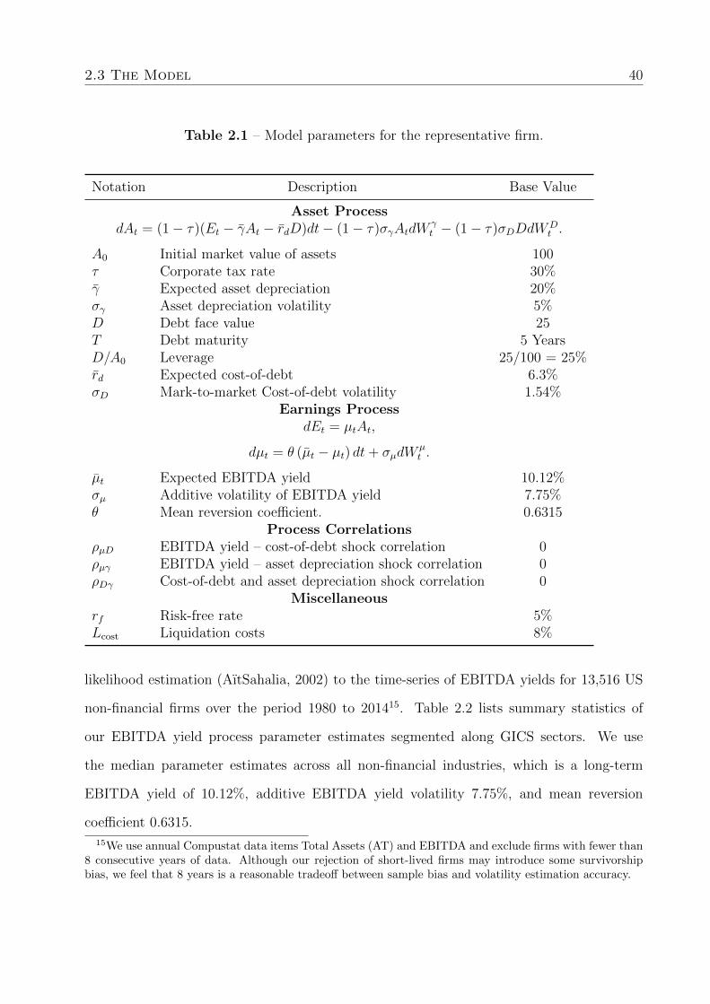
2.3 The Model 40
Table 2.1 – Model parameters for the representative firm.
Notation Description Base Value
Asset ProcessdAt = (1− τ)(Et − γAt − rdD)dt− (1− τ)σγAtdW
γt − (1− τ)σDDdW
Dt .
A0 Initial market value of assets 100τ Corporate tax rate 30%γ Expected asset depreciation 20%σγ Asset depreciation volatility 5%D Debt face value 25T Debt maturity 5 YearsD/A0 Leverage 25/100 = 25%rd Expected cost-of-debt 6.3%σD Mark-to-market Cost-of-debt volatility 1.54%
Earnings ProcessdEt = µtAt,
dµt = θ (µt − µt) dt+ σµdWµt .
µt Expected EBITDA yield 10.12%σµ Additive volatility of EBITDA yield 7.75%θ Mean reversion coefficient. 0.6315
Process CorrelationsρµD EBITDA yield – cost-of-debt shock correlation 0ρµγ EBITDA yield – asset depreciation shock correlation 0ρDγ Cost-of-debt and asset depreciation shock correlation 0
Miscellaneousrf Risk-free rate 5%Lcost Liquidation costs 8%
likelihood estimation (AıtSahalia, 2002) to the time-series of EBITDA yields for 13,516 US
non-financial firms over the period 1980 to 201415. Table 2.2 lists summary statistics of
our EBITDA yield process parameter estimates segmented along GICS sectors. We use
the median parameter estimates across all non-financial industries, which is a long-term
EBITDA yield of 10.12%, additive EBITDA yield volatility 7.75%, and mean reversion
coefficient 0.6315.
15We use annual Compustat data items Total Assets (AT) and EBITDA and exclude firms with fewer than8 consecutive years of data. Although our rejection of short-lived firms may introduce some survivorshipbias, we feel that 8 years is a reasonable tradeoff between sample bias and volatility estimation accuracy.

2.3 The Model 41
Table 2.2 – Median empirical estimates of Ornstein-Uhlenbeck EBITDA yield processparameters. We apply a maximum likelihood estimator to 13,718 non-financial US firmswith at least 8 years of financial data between 1980 and 2014.
MediansGICS Sector Exp’d Yield (%) Yield Vol. (%) Mean-reversion
Energy 10.75 9.60 0.8104Materials 11.12 7.56 0.6134Industrials 10.60 7.01 0.6194Consumer Discr. 10.39 6.68 0.5328Consumer Staples 12.40 5.21 0.5447Health Care 1.79 15.85 0.7480Information Tech. 14.96 4.23 0.4119Telecoms 10.80 1.88 0.3471
All Non-Financials 10.12 7.75 0.6315
These parameters are used as inputs to our model and an equity value surface is generated.
In accordance with natural expectations, equity value increases with EBITDA. Equity value
also increases with asset value and conversely decreases with leverage. The optimal voluntary
liquidation boundary is where the value to equity holders of liquidating is equal to the value
of continuing to trade. This boundary is shown by the red line in Figure 2.1 (a). When
EBITDA falls below the red line for a given asset value then it is optimal for the firm to
liquidate its assets and return capital to equityholders. This boundary is increasing with
assets and hence, decreasing with leverage.
The OVLB can also be presented in terms of earnings yield, defined as EBITDA divided
by Total Assets, versus leverage, defined as Face Value of Debt divided by Asset Value;
see Figure 2.2 (b). This EBITDA boundary is compared with the profitability line (red-
dotted line) defined as the boundary at which Net Earnings is greater than zero, and the
cash flow insolvency line (blue crossed line), defined as the boundary at which EBITDA
is less than the debt-service costs. When a firm’s earnings lie above the profitability line
it is generating positive net earnings, and so the firm’s asset base is growing. Below the
involuntary liquidation line the firms EBITDA is not sufficient to meet debt service costs

2.4 Model Results 42
and so is trading while (cash flow) insolvent. Firms below the OVLB are worth more dead
than alive and should be voluntarily liquidated immediately.
Firms above the OVLB but below the profitability line are slowly losing asset value to depre-
ciation and debt service costs, however the value to equityholders of continuation is greater
than the value of voluntary liquidation. The distance between the OVLB and the profitabil-
ity lines represents the “burn rate” that the firm can sustain while optimally continuing to
trade. For example, in Figure 2.2 (b) a firm with 50% leverage can lose up to 1% of its
asset value per year and still find it optimal to continue; that is, to attempt to trade out of
trouble. We define the difference between the profitability line and the OVLB as the maxi-
mum acceptable burn rate (MABR). Figure 2.2 (c) plots the MABR for the same scenario
as panels (a) and (b). If the firm is burning cash at a rate faster than the MABR then they
should voluntarily liquidate to maximize shareholder value.
2.4 Model Results
The option to voluntarily liquidate the firm’s asset adds significantly to equity value. Figure
2.2 (d) describes the equity value added to the firm by implementing an optimal voluntary
liquidation policy, compared to a static ‘always trade’ policy. We calculate the equity value
added by first solving our model without the voluntary liquidation option, then re-solving
our model with voluntary liquidation, keeping all other parameters the same. The “relative
value of the voluntary liquidation option” is then the percentage increase in value of equity-
with-voluntary-liquidation over equity-without-voluntary-liquidation.
When the firm is highly levered, the firm’s option to cash out before all equity is exhausted
has considerable value to equityholders. The voluntary liquidation option of a highly levered
firm can be worth more than the intrinsic value of the firm’s expected future cash flows.
Even at relatively high EBITDAs (4 × debt service costs / interest expenses) the voluntary

2.4 Model Results 43
liquidation option adds substantial relative value (circa 350%).16
Table 2.3 – Marginal effect of one percentage point increases in primary model pa-rameters on the Maximum Acceptable Burn Rate (MABR). Representative firm pa-rameter values are µt = 10.12%, σµ = 7.75%, γ = 7.75%, σγ = 5%, rf = 5%,rd = 6.3%, σD = 1.54%, τ = 30%, Lcost = 8%, A0 = 100, D = 25, θ = 0.6315,and ρµD = ρµγ = ρDγ = 0.
Parameter 1 Year 5 Year 10 Year
EBITDA Yield Volatility σµ 0.5380 0.5600 0.5572Expected Depreciation γ -0.1297 -0.1462 -0.1457Liquidation Costs Lcost 0.5989 0.2845 0.2284Leverage D/A0 0.0552 0.0545 0.0565Expected Long-Run EBITDA Yield µ 0.1345 0.1526 0.1052Cost-of-debt rd -0.0313 -0.0254 -0.0289Depreciation Volatility σγ 0.0000 0.0000 0.0542Cost-of-debt Volatility σD 0.0000 0.0000 0.0000Earnings Mean Reversion θ 0.0000 0.0000 0.0000Corporate Tax Rate τ -0.0346 -0.0618 -0.0651
We identify the sensitivity of the MABR to firm characteristics (for a variety of firm lifespans)
by comparing the MABR for the representative firm to the MABR determined when we
change each of these variables by 1%. These results are given in Table 2.3. The most
influential characteristics include the liquidation costs, the rate of accounting depreciation,
the expected cost-of-debt, and expected earnings yield. Leverage and corporate tax rate are
also influential, however much less so. Estimates of each of these can easily be extracted
from the firm’s accounts. However the most influential detereminant of the optimal voluntary
liquidation boundary is EBITDA yield volatility. This is also the characteristic that is most
difficult to estimate - especially given that the volitility is an ex-ante measure of EBITDA
risk. Some ex-ante measures of EBITDA yield volatility might be obtained from a sufficient
number of analysts estimates of future earnings although this will only be available for large,
public, firms. The feasibility of extracting model parameters from accounting variables is
16Note, the absolute value of the voluntary liquidation option isn’t particularly large when highly dis-tressed. The substantial relative value increase is a result of the almost zero equity value without thevoluntary liquidation option on the denominator.

2.4 Model Results 44
Table 2.4 – Marginal effect of one percentage point increases in primary model param-eters on the Maximum Acceptable Burn Rate (MABR) for a distressed firm with 0.8leverage. Representative firm parameter values are µt = 10.12%, σµ = 7.75%, γ = 7.75%,σγ = 5%, rf = 5%, rd = 6.3%, σD = 1.54%, τ = 30%, Lcost = 8%, A0 = 100, D = 25,θ = 0.6315, and ρµD = ρµγ = ρDγ = 0.
Parameter 1 Year 5 Year 10 Year
EBITDA Yield Volatility σµ 0.5632 0.5914 0.5914Expected Depreciation γ -0.1326 -0.1455 -0.1455Liquidation Costs Lcost 0.6378 0.3691 0.3691Leverage D/A0 0.0000 0.0000 0.0000Expected Long-Run EBITDA Yield µ 0.1189 0.1305 0.1305Cost-of-debt rd -0.1113 -0.1077 -0.1077Depreciation Volatility σγ 0.0000 0.0000 0.0521Cost-of-debt Volatility σD 0.0000 0.0000 0.0000Earnings Mean Reversion θ 0.0000 0.0000 0.0000Corporate Tax Rate τ 0.0079 0.0000 0.0000
a primary benefit of our model, and makes it applicable in situations outside of analysing
traditional public firms.
Greater earnings risk lowers the OVLB and hence increases the maximum acceptable burn
rate (MABR) at which continuation remains optimal (See Figure 2.3b). The continua-
tion value is strictly increasing in earnings risk because downside risk to equity is reduced
through the option to liquidate or default. The voluntary liquidation value, however remains
unchanged, and consequently the OVLB decreases with earnings risk.
Any shift to greater earnings risk will benefit equityholders because the liquidation boundary
reduction follows directly from the increased continuation value of equity. This increase in
equity is effectively a transfer of wealth from debtholders to equityholders, consistent with
risk-shifting theory of capital management (Myers, 1977). To the extent that debt holders
will accept it, a shift towards riskier asset utilization, simultaneously increases the value of
equity and raises the MABR while reducing the OVLB.17
17Managers can also move their firm into the continuation region by increasing leverage. In this case,however, the value of equity decreases.

2.4 Model Results 45
Empirically, Graham, Harvey, and Rajgopal (2005) find that firm managers exhibit a strong
preference towards smooth (low risk) earnings. Our findings suggest that managers may not
fully appreciate the positive relationship between earnings risk and equity value. However,
the findings of Graham, Harvey, and Rajgopal (2005) suggest that managers are wary of sig-
nalling negative future earnings growth prospects through volatile earnings announcements.
Perhaps managers believe that there is a relationship between earnings volatility and future
earnings growth - a belief that is empirically confirmed by Dichev and Tang (2009). How-
ever, if the firm is distressed, and close to the liquidation boundary, we would expect that
the interests of the manager and equityholders are well aligned - an increase in earnings risk
increases the value of equity and simultaneously moves the firm further into the continuation
region.
The MABR (OVLB) is largely invariant to both depreciation risk and cost-of-debt risk (See
Figures 2.4 and 2.5, respectively), except when the firm is highly levered. Depreciation
risk measures the unexpected deviation of realised economic depreciation from accounting
depreciation. In the same way cost-of-debt risk refers to the difference between the total
cost of debt and the expected cost of debt; that is, the unexpected changes to the cost of
debt arising from marked-to-market yield movements. The point at which each of these risks
becomes significant on the MABR and OVLB is a function of debt maturity and leverage.
When debt maturity is short (1 year) these differences are small, and only effect the OVLB
and MABR at very high leverages (>75%). At longer debt maturities, these risks significantly
effect the OVLB and MABR at a lower leverage.
For highly levered firms (i.e. firms close to financial distress), higher cost-of-debt volatility
and depreciation volatility raise the MABR by increasing the continuation value of equity.
This is primarily through the channel of both volatilities increasing the aggregate asset
value volatility: highly volatile firm assets grant equityholders additional value because they
participate in the upside should the firm favourably recover, while being protected from any
downside by limited liability. While both volatilities are difficult for a manager to change,
2.4 Model Results 46
managers can nevertheless shift the optimal voluntary liquidation decision from ‘liquidate’
to ‘continue’ though strategic capital management; Consider a moderately levered firm with
highly uncertain depreciation and earnings close to the point of optimal liquidation. If
management can increase leverage while keeping other firm characteristics fairly constant,
they can increase the firm’s MABR, thus giving them more opportunity to continue managing
the firm. For example, if we take our representative firm and increase its depreciation
volatility to 15% then shifting from a leverage of 75% to 85% increases the MABR by 5
percentage points. Increases in the MABR induced by high depreciation and cost-of-debt
volatilities are primarily because these parameters increase the continuation value of equity.
Expected depreciation (γ) measures accounting depreciation and expected cost-of-debt (rd)
measures the interest payments on debt (expressed in our model as a continuously paid
coupon). Note that our “profitability line” is the minimum required EBITDA required to
cover the firm’s asset depreciation and debt service costs. Higher accounting depreciation
does not alter the slope of this profitability line, rather it shifts the profitability line upwards.
Increasing expected depreciation also shifts the OVLB higher (see Figure 2.6 (b) and (c)).
This shift in the OVLB is linear in accounting depreciation, but is not influenced by leverage.
The profitability line increases linearly with accounting depreciation, and is influenced by
leverage. In addition, the profitability line is more sensitive than the OVLB to accounting
depreciation. These two effects interact so that the MABR decreases with accounting de-
preciation but increases with leverage (see Figure 2.6 (a)). Note that assets with a longer
lifespan will have lower expected depreciation, while assets with a shorter lifespan will have
higher expected depreciation: Asset lifespan is a negative function of expected depreciation.
Consequently, a manager wishing to keep a firm in the continuation region, irrespective of
the wishes of equityholders, will maintain a monotonic relationship between expected asset
lifespan and leverage. That is, a manager can increase their firm’s MABR by increasing
leverage while decreasing expected depreciation (increasing asset lifespan).
Several authors suggest that a monotonic relationship between leverage and debt maturity

2.4 Model Results 47
is optimal (Alcock, Finn, and Tan, 2012; Leland and Toft, 1996), and the asset-matching
argument of Myers (1977) suggests that debt maturity should optimally match the asset
lifespan. The combination of these arguments suggest that it is optimal for equityholders
to desire a monotonic relationship between asset lifespan and leverage. Our analysis shows
that such a monotonic relationship is also in the interests of rent-seeking managers, because
it allows firm continuation, irrespective of the best interests of equityholders.
In contrast, changes in the expected cost-of-debt affect the slope of both the profitability
line and the OVLB, but do not shift either (see Figure 2.7 (a) and (b)). Because both lines
“rotate” by the same amount and the MABR is the difference between the two, the MABR
is unaffected by cost-of-debt changes.
Consider a distressed firm that has been granted an interest holiday by creditors - we imple-
ment an interest rate holiday in our model by setting the expected cost-of-debt rd to zero.
Reducing the expected cost-of-debt to zero increases the value of equity and decreases the
slope of the OVLB (i.e. reduces it’s first derivatives with respect to leverage). Thus an
interest rate holiday (or reduction) might move the firm from the liquidation region into
the continuation region, however the firm may still be eroding the value of its assets (i.e.
lie below the profitability line). For example, our representative firm with leverage of 50%
and an EBITDA yield of 20% would lie within the voluntary liquidation region under the
OVLB in Figure 2.7 (a). Once granted an interest rate holiday, however, the firm now sits
above the OVLB in the continuation region. With no need to continue paying interest, the
firm is now “treading water”, sitting right on the profitability line. Note that an interest
rate reduction does not change the maximum acceptable burn rate, because the slope of the
OVLB and the profitability line are equally sensitive to the expected cost of debt.
Liquidity costs play a significant role in firm’s voluntary liquidation decision. Intuitively,
we might expect highly liquid assets to serve as a “security” buffer. With a large, liquid
buffer, firms can continue trading with the view of restoring business viability, knowing that

2.4 Model Results 48
if situation gets worse they can liquidate easily without losing value to liquidation costs.
However, our findings support the empirical findings of Jensen and Meckling (1976), Fleming
and Moon (1995), and Mehran, Nogler, and Schwartz (1998) where firms with lower asset
liquidity can endure a higher burn rate and it still be optimal for them to continue trading.
Thus firms with high asset liquidity (low liquidation costs) will actually prefer winding up
to continuation (see Figure 2.8). Firms with a lower asset liquidity (high liquidation costs)
have more to lose from voluntarily liquidating and thus have relatively more to gain from
attempting to trade out of trouble. That is, the hit from liquidation costs are so great that
equityholder’s expected payoff from continuation dominates immediate liquidation.
Unlike earnings, depreciation, and cost-of-debt risks, a reduction in the OLVB (an increase
in the MABR) due to increased liquidation costs does not arise due to an increase in the
continuation value of equity. Rather, increased liquidation costs lowers both the continuation
and liquidation values of equity, however the impact of liquidation costs decreases the firm’s
liquidation value at a faster rate than its continuation value.
Rent-seeking managers may also act to move the firm into the continuation region by reduc-
ing the firm’s asset liquidity, i.e. shifting the firm’s asset base into less liquid assets. The
shift in the MABR/OVLB is due to changes in the relative, not absolute, value of liqui-
dating versus continuing. Shifting the firm’s investment into less liquid assets increases the
MABR and decreases equity value. Thus, any action by the manager to move into less liquid
assets can be considered an owner–manager agency conflict. If the firm is involuntarily liq-
uidated because of balance sheet insolvency, then liquidation costs are borne by debtholders
rather than the residual claimants; the equityholders. As firms increase leverage, the risk
of bearing liquidation costs passes from equityholders to debtholders. And so, at least in
part, the increase (decrease) in the MABR (OVLB) is a wealth transfer from debtholders to
equityholders.

2.5 Concluding Remarks 49
When liquidation costs are substantial (> 30%) the firm is almost always better off attempt-
ing to trade out of trouble; Liquidating such an illiquid asset destroys too much equity value
and so equity holders are better off trading out of trouble, irrespective of the current earnings
yield.
We find that a higher corporate tax rate discourages a firm from attempting to trade out of
trouble because of taxation’s downward drag on retained earnings (see Figure 2.9). Although,
higher levels of corporate tax increase the value of the debt tax shield, this effect is insufficient
to offset the downsides of taxation outflows to the government. Financial distress is the exact
situation where being able to retain the maximum amount of earnings is critical to increase
the firm’s capital base. For all levels of leverage, the MABR is monotonically decreasing
in corporate tax rate. For firms close to insolvency with illiquid asset bases and moderate
leverage, a decrease in the corporate tax rate would encourage continuation. Note that
managers of a firm with large tax loss carry-back offsets will automatically be moved to the
continuation region since the tax offsets lowers their corporate tax rate.
2.5 Concluding Remarks
We develop a model of voluntary liquidation that utilises accounting information to deter-
mine the optimal voluntary liquidation policies for levered, limited liability firms. Our model
treats equity as a down-and-out American-Asian-style call option on the firm’s net earnings,
struck at the face value of debt. We find that misalignment of shareholders and managers
preferences regarding management’s implementation of a voluntary liquidation policy can
significant reduce equity value. That is, managers who fail to implement an optimal vol-
untary liquidation policy will choose continuation in situations where liquidation is value
maximizing for shareholders.
We identify five key variables that largely determine a firm’s optimal voluntary liquidation
policy: expected EBITDA yield volatility, liquidation costs, rate of asset depreciation, the
2.5 Concluding Remarks 50
firm’s expected cost of debt and expected earnings. Potential depreciation adjustments due
to unexpected realised depreciation does not contribute significantly to the optimal vol-
untary liquidation decision, nor does the cost-of-debt risk due to yield curve movements.
Surprisingly, EBITDA risk is the primary determinant of the optimal voluntary liquidation
boundary. As this parameter is the only major determinant of the OVLB that is not com-
monly included in annual statements, we suggest that more focus is placed on the reporting
of a suitable estimate of EBITDA yield volatility. The influence of increased volatility on
the optimal policy is largely due to volatility unconditionally increasing equity value and is
consistent with Myers (1977) risk shifting theory.
Contrary to our prior expectation, we find that firms with a more liquid asset base (lower
liquidation costs) should consider voluntary liquidation sooner. Rather than using liquid
assets as a buffer to trade out of trouble, a firm implementing an optimal liquidation policy
will liquidate to quickly capture remaining asset value. This may present a conflict between
managers and equityholders, whenever managers possess a continuation preference.
We find that restrictive debt covenants, such as an asset-coverage ratio or an interest cov-
erage ratio covenant, do not significantly contribute to the optimal voluntary liquidation
decision unless the firm is extremely highly leveraged (> 80%). By extension, legal solvency
requirements also do not play a significant role in the optimal voluntary liquidation decision
unless the firm is extremely highly leveraged.
We find managerial and equityholder incentives are aligned with respect to leverage and debt
maturity choice. Managers who prefer continuation will maintain a monotonic relationship
between asset lifespan and leverage, and as long as the firm matches their asset-lifespans
with debt maturity, equityholder welfare will be maximized. We also find that these agents
interests are aligned with respect to EBITDA risk, although this is not straight forward due
to managers beliefs about the link between earnings volatility and future earnings growth.
In this paper we have focused largely on the application of the valuation of equity to the

2.5 Concluding Remarks 51
optimal voluntary liquidation boundary and its implications for understanding potential
manager-equityholder conflicts. However our model PDE could be equally applied to pricing
the firm’s debt with appropriately defined boundary conditions. Extending our model in
this manner would allow the full evaluation of the voluntary liquidation decision from both
the management’s, equityholder’s, and debt holder’s perspectives while primarily relying on
empirically observable accounting book values.

2.5 Concluding Remarks 52
Figure 2.1 – Equity value solution for a representative firm. The red line traces theoptimal voluntary liquidation boundary. Given the current fair market value of the firm’sassets this boundary defines the lowest level of EBITDA at which the firm should continueoperating. Equity value maximization is ensured if the firm is liquidated the instantEBITDA hits this boundary. Representative firm parameter values are µt = 10.12%,σµ = 7.75%, γ = 7.75%, σγ = 5%, rf = 5%, rd = 6.3%, σD = 1.54%, τ = 30%,Lcost = 8%, A0 = 100, D = 25, θ = 0.6315, and ρµD = ρµγ = ρDγ = 0.
050
100150
0
20
40
600
20
40
60
80
100
120
Fair Market Value of Assets ($)EBITDA ($)
Equ
ity V
alue
($)

2.5 Concluding Remarks 53
Figure 2.2 – (a) displays the optimal voluntary liquidation boundary (OVLB) as theEBITDA at which voluntary liquidation is optimal for a given starting asset value A0.(b) displays the OVLB expressed as earnings yield (EBITDA/Assets) vs. leverage. Dif-ferent leverages are affected by holding initial market value of asset A0 constant at 100and adjusting the face value of debt D. (c) displays the maximum acceptable burn rate(MABR) calculated as the distance between the treading water line and the OVLB.It describes the maximum amount of value loss, expressed as a proportion of assets, atwhich continuation is preferred over liquidation. (d) displays the relative valute added bythe voluntary liquidation option. We divide the value of equity with optimal voluntaryliquidation by the value of equity without the voluntary liquidation option. Representa-tive firm parameter values are µt = 10.12%, σµ = 7.75%, γ = 7.75%, σγ = 5%, rf = 5%,rd = 6.3%, σD = 1.54%, τ = 30%, Lcost = 8%, A0 = 100, D = 25, θ = 0.6315, andρµD = ρµγ = ρDγ = 0.
Fair Market Value of Assets ($)
EB
ITD
A (
$)
Continuation Region
VoluntaryLiquidation Region
40 60 80 100 120 1405
10
15
20
25
30
35
(a) EBITDA vs. A0
0.2 0.3 0.4 0.5 0.6 0.7 0.8 0.9 10
5
10
15
20
25
30
Ear
ning
s Y
ield
(E
BIT
DA
/ A
sset
s %
)
Leverage (Liabilities / Assets)
Continuation Region(Net Earnings > 0)
Voluntary LiquidationRegion
Involuntary Liquidation RegionInvoluntary Liquidation Region
Continuation Region(Net Earnings < 0)
Maximum AcceptableBurn Rate
(b) Earnings Yield vs. Leverage
0.2 0.3 0.4 0.5 0.6 0.7 0.8−1
0
1
2
3
4
5
6
7
8
Max
imum
Acc
epta
ble
Bur
n R
ate
(MA
BR
)
Leverage (Liabilities / Assets)
VoluntaryLiquidation Region
Continuation Region
(c) Maximum Acceptable Burn Rate
0.1 0.2 0.3 0.4 0.5 0.6 0.7 0.8 0.9 10
50
100
150
200
250
300
350
400
Leverage (Liabilities / Assets)
Rel
ativ
e V
alue
of V
olun
tary
Liq
uida
tion
Opt
ion
(%)
EBITDA = 2 x Interest ExpenseEBITDA = 4 x Interest ExpenseEBITDA = 6 x Interest Expense
(d) Voluntary Liquidation Option Value
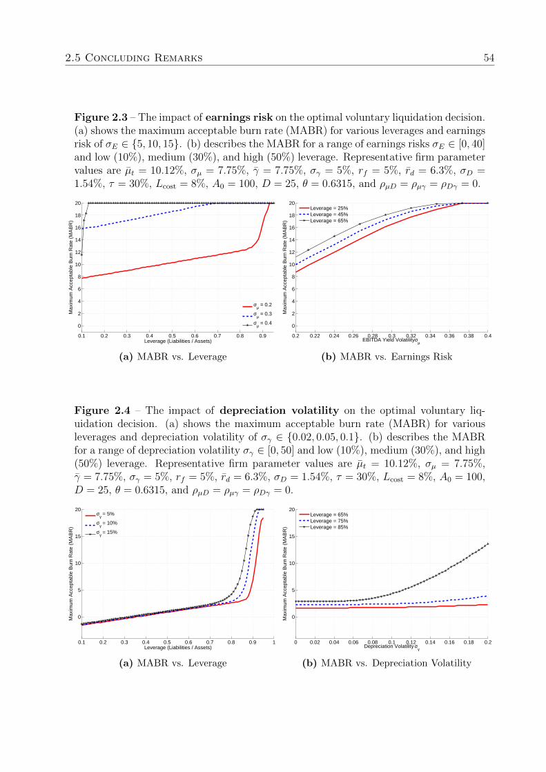
2.5 Concluding Remarks 54
Figure 2.3 – The impact of earnings risk on the optimal voluntary liquidation decision.(a) shows the maximum acceptable burn rate (MABR) for various leverages and earningsrisk of σE ∈ {5, 10, 15}. (b) describes the MABR for a range of earnings risks σE ∈ [0, 40]and low (10%), medium (30%), and high (50%) leverage. Representative firm parametervalues are µt = 10.12%, σµ = 7.75%, γ = 7.75%, σγ = 5%, rf = 5%, rd = 6.3%, σD =1.54%, τ = 30%, Lcost = 8%, A0 = 100, D = 25, θ = 0.6315, and ρµD = ρµγ = ρDγ = 0.
0.1 0.2 0.3 0.4 0.5 0.6 0.7 0.8 0.9
0
2
4
6
8
10
12
14
16
18
20
Max
imum
Acc
epta
ble
Bur
n R
ate
(MA
BR
)
Leverage (Liabilities / Assets)
σµ = 0.2
σµ = 0.3
σµ = 0.4
(a) MABR vs. Leverage
0.2 0.22 0.24 0.26 0.28 0.3 0.32 0.34 0.36 0.38 0.4
0
2
4
6
8
10
12
14
16
18
20
EBITDA Yield Volatility σµ
Max
imum
Acc
epta
ble
Bur
n R
ate
(MA
BR
)
Leverage = 25%Leverage = 45%Leverage = 65%
(b) MABR vs. Earnings Risk
Figure 2.4 – The impact of depreciation volatility on the optimal voluntary liq-uidation decision. (a) shows the maximum acceptable burn rate (MABR) for variousleverages and depreciation volatility of σγ ∈ {0.02, 0.05, 0.1}. (b) describes the MABRfor a range of depreciation volatility σγ ∈ [0, 50] and low (10%), medium (30%), and high(50%) leverage. Representative firm parameter values are µt = 10.12%, σµ = 7.75%,γ = 7.75%, σγ = 5%, rf = 5%, rd = 6.3%, σD = 1.54%, τ = 30%, Lcost = 8%, A0 = 100,D = 25, θ = 0.6315, and ρµD = ρµγ = ρDγ = 0.
0.1 0.2 0.3 0.4 0.5 0.6 0.7 0.8 0.9 1
0
5
10
15
20
Max
imum
Acc
epta
ble
Bur
n R
ate
(MA
BR
)
Leverage (Liabilities / Assets)
σγ = 5%
σγ = 10%
σγ = 15%
(a) MABR vs. Leverage
0 0.02 0.04 0.06 0.08 0.1 0.12 0.14 0.16 0.18 0.2
0
5
10
15
20
Depreciation Volatility σγ
Max
imum
Acc
epta
ble
Bur
n R
ate
(MA
BR
)
Leverage = 65%Leverage = 75%Leverage = 85%
(b) MABR vs. Depreciation Volatility

2.5 Concluding Remarks 55
Figure 2.5 – The impact of mark-to-market cost-of-debt volatility on the optimalvoluntary liquidation decision. (a) shows the maximum acceptable burn rate (MABR)for various leverages and mark-to-market cost-of-debt volatilities of σγ ∈ {0, 0.1, 0.2}. (b)describes the MABR for a range of mark-to-market cost-of-debt volatilities σγ ∈ [0, 0.20]and low (10%), medium (30%), and high (50%) leverage. Representative firm parametervalues are µt = 10.12%, σµ = 7.75%, γ = 7.75%, σγ = 5%, rf = 5%, rd = 6.3%, σD =1.54%, τ = 30%, Lcost = 8%, A0 = 100, D = 25, θ = 0.6315, and ρµD = ρµγ = ρDγ = 0.
0.1 0.2 0.3 0.4 0.5 0.6 0.7 0.8 0.9 1
0
5
10
15
20
Max
imum
Acc
epta
ble
Bur
n R
ate
(MA
BR
)
Leverage (Liabilities / Assets)
σD = 0%
σD = 10%
σD = 20%
(a) MABR vs. Leverage
0 0.02 0.04 0.06 0.08 0.1 0.12 0.14 0.16 0.18 0.2
0
5
10
15
20
Cost−of−debt Volatility σD
Max
imum
Acc
epta
ble
Bur
n R
ate
(MA
BR
)
Leverage = 75%Leverage = 80%Leverage = 85%
(b) MABR vs. Cost-of-Debt Volatility

2.5 Concluding Remarks 56
Figure 2.6 – Effect of expected asset depreciation on the maximum acceptable burnrate (MABR) and the optimal voluntary liquidation boundary (OVLB). (a) describes theMABR for a variety of expected depreciations γ ∈ [0.10.3] and low (10%), medium (30%),and high (50%) leverage. (b) and (c) display the OVLB for various leverages for expecteddepreciations of 10% and 20% respectively. Representative firm parameter values areµt = 10.12%, σµ = 7.75%, γ = 7.75%, σγ = 5%, rf = 5%, rd = 6.3%, σD = 1.54%,τ = 30%, Lcost = 8%, A0 = 100, D = 25, θ = 0.6315, and ρµD = ρµγ = ρDγ = 0.
0.1 0.12 0.14 0.16 0.18 0.2 0.22 0.24 0.26 0.28 0.3−3
−2
−1
0
1
2
3
4
Expected Depreciation γ
Max
imum
Acc
epta
ble
Bur
n R
ate
(MA
BR
)
Leverage = 10%Leverage = 30%Leverage = 50%
(a) MABR vs. Expected Depreciation
0.1 0.2 0.3 0.4 0.5 0.6 0.7 0.8 0.9 10
5
10
15
20
25
30
Ear
ning
s Y
ield
(E
BIT
DA
/ A
sset
s %
)
Leverage (Liabilities / Assets)
Profitability LineCash Flow InsolvencyOVLB
(b) Expected Depreciation γ = 10%
0.1 0.2 0.3 0.4 0.5 0.6 0.7 0.8 0.9 10
5
10
15
20
25
30
Ear
ning
s Y
ield
(E
BIT
DA
/ A
sset
s %
)
Leverage (Liabilities / Assets)
Profitability LineCash Flow InsolvencyOVLB
(c) Expected Depreciation γ = 20%

2.5 Concluding Remarks 57
Figure 2.7 – The optimal voluntary liquidation boundary (OVLB) for the representativefirm and for the same firm with zero interest (expected cost-of-debt). If the firm’sEBITDA yield (EBITDA / Net Assets) lies below the upper dotted profitability linethen the firm is slowly losing asset value to debt service costs and asset depreciation.If the firm lies below the cash flow insolvency line then it is trading while insolvent.Representative firm parameter values are µt = 10.12%, σµ = 7.75%, γ = 7.75%, σγ = 5%,rf = 5%, rd = 6.3%, σD = 1.54%, τ = 30%, Lcost = 8%, A0 = 100, D = 25, θ = 0.6315,and ρµD = ρµγ = ρDγ = 0.
0.2 0.3 0.4 0.5 0.6 0.7 0.8 0.9 10
5
10
15
20
25
30
Ear
ning
s Y
ield
(E
BIT
DA
/ A
sset
s %
)
Leverage (Liabilities / Assets)
Profitability LineCash Flow InsolvencyOVLB
(a) Representative Firm rd = 0.06
0.2 0.3 0.4 0.5 0.6 0.7 0.8 0.9 10
5
10
15
20
25
30
Ear
ning
s Y
ield
(E
BIT
DA
/ A
sset
s %
)
Leverage (Liabilities / Assets)
Profitability LineCash Flow InsolvencyOVLB
(b) Interest Rate Holiday rd = 0
Figure 2.8 – The effect of liquidation costs on the optimal voluntary liquidationdecision. (a) shows the maximum acceptable burn rate (MABR) for various leveragesand liquidation costs of σγ ∈ {0.05, 0.1, 0.2}. (b) describes the MABR for a range ofliquidation costs σγ ∈ [0, 0.25] and low (10%), medium (30%), and high (50%) leverage.Representative firm parameter values are µt = 10.12%, σµ = 7.75%, γ = 7.75%, σγ = 5%,rf = 5%, rd = 6.3%, σD = 1.54%, τ = 30%, Lcost = 8%, A0 = 100, D = 25, θ = 0.6315,and ρµD = ρµγ = ρDγ = 0.
0.1 0.2 0.3 0.4 0.5 0.6 0.7 0.8 0.9 1
0
5
10
15
20
Max
imum
Acc
epta
ble
Bur
n R
ate
(MA
BR
)
Leverage (Liabilities / Assets)
LCost
= 0%
LCost
= 3.5777%
LCost
= 7.1554%
(a) MABR vs. Leverage
0 0.05 0.1 0.15 0.2
0
5
10
15
20
Liquidation Cost
Max
imum
Acc
epta
ble
Bur
n R
ate
(MA
BR
)
Leverage = 10%Leverage = 30%Leverage = 50%
(b) MABR vs. Liquidation Costs

2.5 Concluding Remarks 58
Figure 2.9 – The effect of the corporate tax rate on the optimal voluntary liquidationdecision. (a) shows the maximum acceptable burn rate (MABR) for various leveragesand corporate tax rates of τ ∈ {0, 0.15, 0.3}. (b) describes the MABR for a range ofcorporate tax rates τ ∈ [0, 0.3] and low (10%), medium (30%), and high (50%) leverage.Representative firm parameter values are µt = 10.12%, σµ = 7.75%, γ = 7.75%, σγ = 5%,rf = 5%, rd = 6.3%, σD = 1.54%, τ = 30%, Lcost = 8%, A0 = 100, D = 25, θ = 0.6315,and ρµD = ρµγ = ρDγ = 0.
0.1 0.2 0.3 0.4 0.5 0.6 0.7 0.8 0.9 1
0
5
10
15
20
Max
imum
Acc
epta
ble
Bur
n R
ate
(MA
BR
)
Leverage (Liabilities / Assets)
τ = 0%τ = 15%τ = 30%
(a) MABR vs. Leverage
0 0.05 0.1 0.15 0.2 0.25 0.3
0
5
10
15
20
Corporate Tax Rate τ
Max
imum
Acc
epta
ble
Bur
n R
ate
(MA
BR
)
Leverage = 20%Leverage = 50%Leverage = 80%
(b) MABR vs. Tax Rate

3Stochastic Earnings Volatility Model
Derivation and Solution
This chapter is a supplement to the previous essay ”Throwing in the Towel: A Firm’s
Optimal Voluntary Liquidation Decision”. In this chapter we provide the full derivation
of our stochastic earning volatility model, a detailed explanation of our numerical solution,
and describe an algorithm for efficiently solving finite difference problems with projected
successive overrelaxation (PSOR).
59
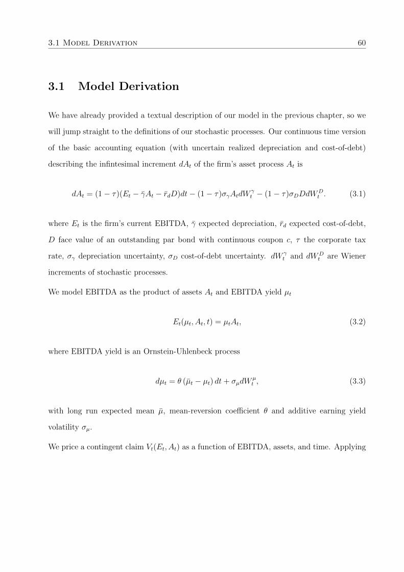
3.1 Model Derivation 60
3.1 Model Derivation
We have already provided a textual description of our model in the previous chapter, so we
will jump straight to the definitions of our stochastic processes. Our continuous time version
of the basic accounting equation (with uncertain realized depreciation and cost-of-debt)
describing the infintesimal increment dAt of the firm’s asset process At is
dAt = (1− τ)(Et − γAt − rdD)dt− (1− τ)σγAtdWγt − (1− τ)σDDdW
Dt . (3.1)
where Et is the firm’s current EBITDA, γ expected depreciation, rd expected cost-of-debt,
D face value of an outstanding par bond with continuous coupon c, τ the corporate tax
rate, σγ depreciation uncertainty, σD cost-of-debt uncertainty. dW γt and dWD
t are Wiener
increments of stochastic processes.
We model EBITDA as the product of assets At and EBITDA yield µt
Et(µt, At, t) = µtAt, (3.2)
where EBITDA yield is an Ornstein-Uhlenbeck process
dµt = θ (µt − µt) dt+ σµdWµt , (3.3)
with long run expected mean µ, mean-reversion coefficient θ and additive earning yield
volatility σµ.
We price a contingent claim Vt(Et, At) as a function of EBITDA, assets, and time. Applying

3.1 Model Derivation 61
Ito’s Lemma to Vt yields
dVt(Et, At) =∂Vt∂t
dt+∂Vt∂Et
dEt +∂Vt∂At
dAt
+1
2
∂2Vt∂E2
t
(dEt)2 +
1
2
∂2Vt∂A2
t
(dAt)2
+∂2Vt
∂Et∂At(dAt)(dEt). (3.4)
Because Et(µt, At) is a function of EBITDA yield µt and assets At, we calculate dEt using
the Ito’s Lemma once again
dEt =∂Et∂t
dt+∂Et∂At
dAt +∂Et∂µt
dµt
+∂2Et∂A2
t
(dAt)2 +
∂2Et∂µ2
t
(dµt)2 +
∂2Et∂At∂µt
(dAt)(dµt), (3.5)
where
∂Et∂t
= 0,∂Et∂At
= µt,∂Et∂µt
= At,
∂2Et∂A2
t
= 0,∂2Et∂µ2
t
= 0,
∂2Et∂At∂µt
= 1.
Substituting these into (3.5) yields the stochastic product rule
dEt = µtdAt + Atdµt + (dAt)(dµt). (3.6)
Expanding the ∂2Et/∂A2t coefficient from (3.4)
(dEt)2 = (µtdAt + Atdµt + (dAt)(dµt))
2,
= µ2t (dAt)
2 + A2t (dµt)
2 + 2µtAt(dAt)(dµt) + 2µt(dAt)2(dµt) + 2At(dAt)(dµt)
2,
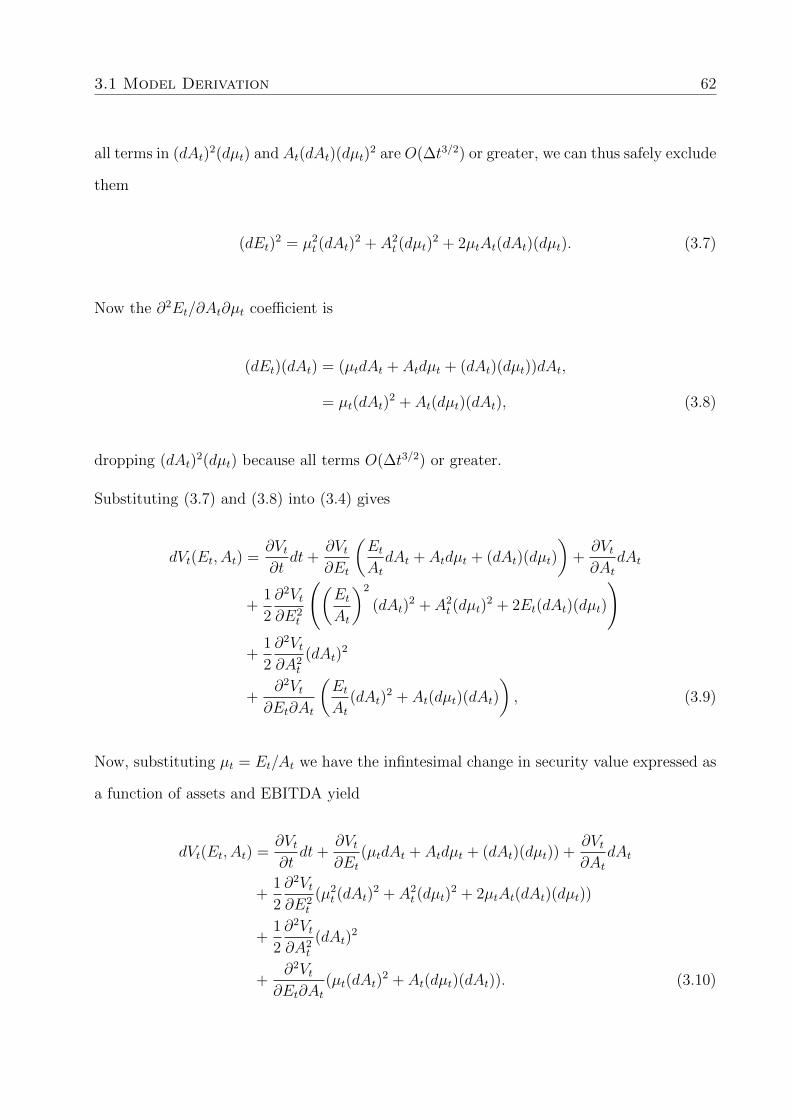
3.1 Model Derivation 62
all terms in (dAt)2(dµt) and At(dAt)(dµt)
2 are O(∆t3/2) or greater, we can thus safely exclude
them
(dEt)2 = µ2
t (dAt)2 + A2
t (dµt)2 + 2µtAt(dAt)(dµt). (3.7)
Now the ∂2Et/∂At∂µt coefficient is
(dEt)(dAt) = (µtdAt + Atdµt + (dAt)(dµt))dAt,
= µt(dAt)2 + At(dµt)(dAt), (3.8)
dropping (dAt)2(dµt) because all terms O(∆t3/2) or greater.
Substituting (3.7) and (3.8) into (3.4) gives
dVt(Et, At) =∂Vt∂t
dt+∂Vt∂Et
(EtAtdAt + Atdµt + (dAt)(dµt)
)+∂Vt∂At
dAt
+1
2
∂2Vt∂E2
t
((EtAt
)2
(dAt)2 + A2
t (dµt)2 + 2Et(dAt)(dµt)
)
+1
2
∂2Vt∂A2
t
(dAt)2
+∂2Vt
∂Et∂At
(EtAt
(dAt)2 + At(dµt)(dAt)
), (3.9)
Now, substituting µt = Et/At we have the infintesimal change in security value expressed as
a function of assets and EBITDA yield
dVt(Et, At) =∂Vt∂t
dt+∂Vt∂Et
(µtdAt + Atdµt + (dAt)(dµt)) +∂Vt∂At
dAt
+1
2
∂2Vt∂E2
t
(µ2t (dAt)
2 + A2t (dµt)
2 + 2µtAt(dAt)(dµt))
+1
2
∂2Vt∂A2
t
(dAt)2
+∂2Vt
∂Et∂At(µt(dAt)
2 + At(dµt)(dAt)). (3.10)

3.1 Model Derivation 63
The expanded coefficients, dropping terms of order O(∆t3/2) or higher, are
(dAt)2 =
((1− τ)(Et − γAt − rdD)dt− (1− τ)σγAtdW
γt − (1− τ)σDDdW
Dt
)2,
= (1− τ)2(σ2γA
2t + ργDσγσDAtD + σ2
DD2)dt, (3.11)
dµt =θ
At(µtAt − Et) dt+ σµdW
µt , (3.12)
(dµt)2 = (θ (µt − µt) dt+ σµdW
µt )2 ,
= σ2µdt, (3.13)
and
(dµt)(dAt) = (θ (µt − µt) dt+ σµdWµt )×(
(1− τ)(Et − γAt − rdD)dt− (1− τ)σγAtdWγt − (1− τ)σDDdW
Dt
), (3.14)
= −(1− τ) (ρµγσµσγAt + ρµDσµσDD) , (3.15)
after substituting in the original processes (3.1) and (3.2).
Under the assumption that the firm’s debt-risk is hedgable while earnings and depreciation
risk are unhedgable and command a risk premium, the governing PDE of any contingent
claim on firm assets and EBITDA is
∂Vt∂t
+∂Vt∂Et
CE +∂Vt∂At
CA
+1
2
∂2Vt∂E2
t
CEE +1
2
∂2Vt∂A2
t
CAA
+∂2Vt
∂Et∂AtCEA − (rf + λµσµ + λγσγ)Vt = 0,

3.2 Numerical Solution 64
where λµ and λγ are the earnings and depreciation risk premia respectively and
CA = (1− τ) ((µt − γ)At − rDD) ,
CAA = (1− τ)2(σ2γA
2t + ργµσγσµAtD + σ2
DD2),
CE = (1− τ) ((µt − γ)At − rDD)µt + θ(µt − µt)At − (1− τ)(ρµγσµσγAt + ρµDσµσDD),
CEE = (1− τ)2(σ2γA
2t + ργµσγσµAtD + σ2
DD2)µ2t + A2
tσ2µ − 2(1− τ)(ρµγσµσγAt + ρµDσµσDD)µtAt,
CEA = (1− τ)2(σ2γA
2t + ργµσγσµAtD + σ2
DD2)µt − (1− τ)(ρµγσµσγAt + ρµDσµσDD)At.
The boundary conditions for the equity claim on the firm are fully detailed in equations in
the previous chapter.
3.2 Numerical Solution
Our model is similar to an American-Asian option in that the asset process is the integral of
the net earnings process. There are no known analytic solutions for down-and-out American-
Asian-style call options. We therefore use numerical methods to solve for equity values
and the optimal voluntary liquidation boundary. Our numerical solution overcomes four
complexities:
• Our governing equation is a two-dimensional PDE, requiring us to find the equity
value solution on a two-dimensional grid. Typical finite difference methods with one
spatial dimension scale in computational complexity O(n2), while in two dimensions
the scaling is O(n4). Given that we need to use a fine grid size to generate smooth
solutions, we must solve the model with a large number of grid points. We develop
a fast and efficient solution method using operator splitting methods and projected
successive overrelaxation (PSOR).

3.3 Selecting our Numerical Solution Method 65
• Equityholder’s option to voluntarily liquidate at any time represents an American-
style early exercise condition. Any finite maturity instrument incorporating American
exercise has a time-dependent “moving” early exercise boundary; where, in our case,
the boundary represents the optimal voluntary liquidation policy. We use projected
successive overrelaxation (PSOR) to ensure the early exercise boundary condition is
always satisfied.
• The cash flow insolvency (interest coverage ratio) boundary introduces a discontinu-
ity in the finite difference solution because equity value dramatically drops when the
firm triggers cash flow insolvency. Ignoring these discontinuities introduces distortions
into the finite-difference solution, either preventing convergence, or producing Gibbs
artefacts. We eliminate the effect of this discontinuity by performing a coordinate
transform on both of our PDE’s spatial dimensions.
• Multiple, correlated, sources of uncertainty (earnings, depreciation, and cost-of-debt
shocks) introduces the cross-term operator ∂2V∂A∂E
in the model PDE. The combination
of a cross-term operator with an early exercise condition and coordinate transforms is
atypical and requires special consideration. We handle these cross-terms in an efficient
manner by using operator splitting and a projector-corrector time stepping scheme.
3.3 Selecting our Numerical Solution Method
We explore the response of equity values and optimal liquidation behaviour to changing
model parameters and need to solve our model over millions of points in a high dimensional
parameter space. Calculating this many solutions requires a fast, optimized, solution process.
Common techniques for solving systems involving stochastic differential equations are Monte-
Carlo methods, binomial and multinomial trees, and finite difference methods. We ultimately
found the only method appropriate for our system is finite difference methods, however we

3.3 Selecting our Numerical Solution Method 66
did consider other solution methods that later proved intractable.
3.3.1 Monte-Carlo
A rational equityholder maximises their discounted expected future cash flows.1 Follow-
ing an optimal voluntary liquidation strategy is concomitant with value maximization—
equityholders selecting a voluntary liquidation boundary that maximizes equity value. The
continuation value of equity is the maximum discounted expected value over all permissible
liquidation times τ ∈ Tt,T
Vt(At, Et) = supτ∈Tt,T
EQt
[e−rf (τ−t)Vτ (Aτ , Eτ )|Ft
], (3.16)
given the current information set Ft. Equityholders choose to liquidate at times where the
value realised by liquidation is greater than firm continuation value
Vτ (Aτ , Eτ ) < max[Aτ (1− α(τ))− FV, 0]. (3.17)
Directly performing this maximization over all stopping times using direct numerical integra-
tion is intractable. Longstaff and Schwartz (2001) describe a method of incorporating early
exercise into a Monte-Carlo framework. Starting at option expiry they time step backwards,
fitting a parametric approximation of continuation value by regressing basis functions of
state variables against discounted next-period continuation values. This procedure provides
an estimate of the SDE’s optimal stopping time. They found American puts priced using
this method, when compared with a finite difference technique, have standard errors ranging
from 0.7 to 2.4 percent.
Our EBITDA and asset SDEs are easily implemented as a quasi Monte-Carlo simulation
using numerical integration techniques (Kloeden and Platen, 2011). We take draws from
1Under the risk neutral measure in our case.
3.3 Selecting our Numerical Solution Method 67
a low discrepancy Sobol sequence to accelerate convergence. Using a deterministic low
discrepancy sequence, instead of pseudo-random numbers, to drive Monto-Carlo simulation
can dramatically accelerate convergence (Glasserman, 2003). Such low discrepancy sequences
aim to consistently “fill” a high dimensional parameter space over a series of draws.
Following Longstaff and Schwartz (2001) we use a constant, A,A2, E, E2, and E×A as basis
functions, randomly generate EBITDA and asset paths, and solve for equity value starting
at debt maturity and moving backwards in time. To generate a full solution surface we
must perform a simulation for each pair of EBITDA and assets across the model parameter
space. Note that with two dimensions and multiple parameters this simulation process is
computationally expensive.
One advantage of Monte-Carlo is that it is “embarrassingly parallel”. That is, the simulation
for each set of parameters can be run independently across a multiplicity of computing
cores. Recent advances in general purpose graphics processing unit (GPGPU) technology
has enabled large accelerations in parallel computing performance. ASCI Red, the fastest
super computer in 1997, had a peak performance of 1.3 teraflops and occupied 104 cabinets.
In comparison, a NVIDIA Tesla GPGPU computing system circa-2012 achieves 2 teraflops
sustained, and can be held in two hands. Gaikwad and Toke (2009) demonstrate an order of
magnitude acceleration, versus a CPU, from using GPGPUs to solve American option prices
with the Longstaff and Schwartz (2001) method.
Althought our implementation of a Monte-Carlo solution produced semi-accurate estimates
of the voluntary liquidation boundary (cross-validated using our finite difference solution),
the number of paths (or quasi-random draws from a Sobol) and time-steps required for full
convergence was computationally prohibitive, even on a modern NVIDIA GPGPU processing
board.

3.3 Selecting our Numerical Solution Method 68
3.3.2 Binomial and Multinomial Trees
A binomial tree model evolves a process across a tree, assuming that over each time step
the process moves an upward step with probability p and a downward step with probability
1−p. The probability p is chosen such that the process is a Martingale under the risk neutral
measure (Shreve, 2004). Binomial trees are memory efficient since calculations can be done
in place. Early exercise conditions are easily incorporated by constraining the solution at
each decision node (Cox, Ross, and Rubinstein, 1979). When solving in more than one
dimensions the number of nodes scales quickly with the number of time steps; O(4n) for a
two dimensional tree. Using trinomial and higher order trees worsens this scaling order.
We wish to solve for equity values and the voluntary liquidation boundary across a wide
range of initial EBITDA–Asset Book Value pairs and parameter values. This requires the
binomial tree solution to be calculated repeatedly for every pair, as well as for varying
parameter values. The memory and processing time requirement to solve our model using
binomial trees is currently not computationally feasible.
3.3.3 Finite Difference Methods
Finite difference methods solve PDEs on a grid. Our equity value PDE (3.15) is a succinct
expression of how equity values evolve in “space” and time. Our model has two spatial
dimensions: EBITDA and assets, and one time dimension: reversed time to debt maturity.
In contrast with Monte-Carlo methods and multinomial tree, finite difference methods al-
low the direct calculation of moving early exercise boundaries for American-style options.
Because one primary output of our model is an accurate optimal voluntary liquidation bound-
ary, we proceed with a finite difference solution.
The sharp drop in equity value at the cash flow insolvency bounday generates a sharp dis-
continuity in our finite difference solution. Solution convergence using naive finite difference

3.3 Selecting our Numerical Solution Method 69
methods requires smooth solution surface. Appropriate finite difference grid spacing and
time step length are necessary to ensure solution stability. Smooth areas of the solution may
be stable with coarse grid spacing, but areas with high first and second order derivatives
require denser grid spacing. To increase “grid fineness” in these unstable areas, we apply a
non-linear, smooth, coordinate transform (Knupp and Steinberg, 1994) to the EBITDA and
asset dimensions to increase grid spacing around the balance sheet and cash flow insolvency
boundaries.
After incorporating this transform we perform a standard spatial discretization, approximat-
ing first, second, and mixed order partial derivatives using central differences. We translate
the spatially discretized system into a band diagonal update matrix, including the spatial
boundary conditions.
There is a menagerie of finite difference time discretization and stepping schemes (Duffy,
2006). Two factors complicate our PDE’s time step: the early exercise condition granting
equityholders voluntary liquidation rights, and the presence of a cross partial derivative.
The cross partial derivative stems from correlations between earnings, depreciation, and
cost-of-debt shocks.
The optimal liquidation boundary is endogenous to the system solution and marks the
boundary between two governing equations; above the moving boundary equity value evolves
according to the primary SEVM PDE, below the boundary, equity value is the residual claim
of equityholders on liquidated assets. This change in “phase” is mathematically equivalent to
the moving boundary layer that forms between a solid (ice) and a liquid (water) as the solid
melts. The Landau transform (Crank, 1987), otherwise known as the front fixing method,
was the original solution to this problem. It involves a coordinate transform of the governing
PDE that translates the moving boundary into a straight line. This explicitly incorporates
the moving boundary into the transformed PDE which can then be solved using non-linear
methods.
3.4 Coordinate Transformation 70
An alternate, and computationally simpler, approach to handling early exercise is projected
successive overrelaxation (PSOR) (Cryer, 1971; Elliott and Ockendon, 1982). American style
early exercise conditions can be reformulated as linear complementarity problems; these
problems consist of finding an equation solution subject to inequality constraints (Wilmott,
Dewynne, and Howison, 1993). When solving the time stepping finite difference equation in
combination with a linear complementarity problem an implicit matrix inversion is required.
PSOR is a form of iterative inversion for diagonal dominant matrices that incrementally
perturbs the inversion solution at each step until convergence. After each iteration step the
solution is constrained to comply with the governing linear complementarity problem.
3.4 Coordinate Transformation
Our model incorporates insolvency and debt covenants as down-and-out boundary conditions
with a rebate, where the rebate is the residual asset value after paying liquidation costs and
debt face value. An interest coverage ratio knocks-out equity holders when earnings falls
below some multiple κ1,t of debt interest payments. An asset coverage ratio knocks out
equity holders when asset value falls below some multiple κ2,t of debt face value.
Both of these boundary conditions introduce large first and second derivatives into our
model solution. If we don’t adjust our solution method to take them into account unwanted
oscillations (Gibbs Phenomena) cause the solution to diverge. To combat these distortions
we perform a two-dimensional coordinate transform increasing the concentration of grid
points around discontinuities?.
3.4.1 Single Dimension Transform
In the general one-dimensional case, we consider transforming V (S) along the S dimensions.
We wish to place grid points in S according to some continuous, monotonically increasing

3.4 Coordinate Transformation 71
Figure 3.1 – Coordinate transforms along the assets axis. The transform focus lies atthe balance sheet insolvency boundary. In this case, the insolvency boundary is set atthe face value of debt D = 60.
20 40 60 80 100 120 140 160 180 200
100
150
200
250
300
EBITDA
Ass
ets
(a) No Transform αA =∞
20 40 60 80 100 120 140 160 180 200
100
150
200
250
300
EBITDAA
sset
s
(b) αA = 20
20 40 60 80 100 120 140 160 180 200
100
150
200
250
EBITDA
Ass
ets
(c) αA = 2
function of another variable (in this case α), whilst solving the PDE with a constant grid
size. We thus define a new function V as a function of α as follows
V(t, α) = V (t, S(α)). (3.18)
Given that V (t, S) is defined by a PDE, we wish to formulate the equivalent PDE for V(t, α).
We first derive the equivalent linear operators for first and second order derivatives when S
is now a function of α. Using the chain rule, the linear operators ∂∂S
and ∂2
∂S2 in terms of ∂∂α

3.4 Coordinate Transformation 72
Figure 3.2 – Coordinate transforms along the earnings axis. The transform focus liesat E = 40.
20 40 60 80 100 120 140 160 180 200
100
150
200
250
EBITDA
Ass
ets
(a) No Transform αE =∞
20 40 60 80 100 120 140 160 180 200
100
150
200
250
EBITDA
Ass
ets
(b) αE = 20
20 40 60 80 100 120 140 160 180 200
100
150
200
250
EBITDA
Ass
ets
(c) αE = 5
and ∂2
∂α2 are
∂
∂S=
(∂S
∂α
)−1∂
∂α(3.19)
∂2
∂S2=
(∂S
∂α
)−1[(
∂S
∂α
)−1∂2
∂α2−(∂S
∂α
)−2∂2S
∂α2
∂
∂α
]. (3.20)
The Jacobian Jα(α) of this transform is the rate of change in our spatial dimension with
respect to our transformed variable
Jα(α) :=∂S(α)
∂α(3.21)

3.4 Coordinate Transformation 73
Figure 3.3 – Combined coordinate transform along both earnings and assets axes.
20 40 60 80 100 120 140 160 180 200
100
150
200
250
300
EBITDA
Ass
ets
(a) No Transform αE =∞, αA =∞
20 40 60 80 100 120 140 160 180 200
100
150
200
250
300
EBITDA
Ass
ets
(b) αE = 20, αA = 20
20 40 60 80 100 120 140 160 180 200
100
150
200
250
EBITDA
Ass
ets
(c) αE = 5, αA = 2
Jα(α) is positive beacuse the co-ordinate transform must be strictly monotically increasing.
Using the result
∂
∂α
[1
Jα
∂
∂α
]=
1
Jα
∂2
∂α2− 1
J2α
∂
∂α
[1
Jα
]∂
∂α(3.22)
and the definition of the Jacobian in (3.21), the first and second order linear operators (3.19)
and (3.20) can be rewritten as
∂
∂S=
1
Jα
∂
∂α(3.23)
∂2
∂S2=
1
Jα
∂
∂α
[1
Jα
∂
∂α
]. (3.24)
3.4 Coordinate Transformation 74
The PDE describing V as a function of S can now be transformed into an equivalent PDE
describing V as a function of α by replacing instances of S with S(α) and the relevant linear
operators with (3.23) and (3.24).
3.4.2 Two-Dimension Transform
Our model is two dimensional and we place EBITDA E on the first axis and assets A
the second. We assume that both earnings E(θ) and assets A(φ) are continuous, strictly
monotonically increasing, functions of transformation variables θ and φ respectively. This
allows us to increase grid fineness around insolvency induced discontinuities and the optimal
voluntary liquidation boundary. We define our new equity value function V as
V(θ, φ, κ) = V (E(θ), A(φ), T − κ). (3.25)
which is a function of time to maturity and the two transform variables.
The Jacobians for the earnings and asset coordinate transforms are
Jθ(θ) =∂E(θ)
∂θ
Jφ(φ) =∂A(φ)
∂φ.
(3.26)
Replacing each linear operator in our original PDE (3.16) with its transformed equivalent

3.4 Coordinate Transformation 75
gives
−∂V∂κ
+ Cθ(θ, φ, κ)1
Jθ
∂V∂θ
+ Cφ(θ, φ, κ)1
Jφ
∂V∂φ
+1
2Cθθ(θ, φ, κ)
1
Jθ
∂
∂θ
(1
Jθ
∂V∂θ
)+
1
2Cφφ(θ, φ, κ)
1
Jφ
∂
∂φ
(1
Jφ
∂V∂φ
)+ Cθφ(θ, φ, κ)
1
Jθ Jφ
∂2V∂θ∂φ
− (rf + λµσµ + λγσγ)Vt = 0,
(3.27)
where
Cφ(θ, φ, κ) = (1− τ) ((E(θ)/A(φ)− γ)A(φ)− rDD) ,
Cφφ(θ, φ, κ) = (1− τ)2(σ2γA(φ)2 + ργµσγσµA(φ)D + σ2
DD2),
Cθ(θ, φ, κ) = (1− τ) ((E(θ)/A(φ)− γ)A(φ)− rDD)E(θ)/A(φ)
+ θ(µT−κ − E(θ)/A(φ))A(φ)− (1− τ)(ρµγσµσγA(φ) + ρµDσµσDD),
Cθθ(θ, φ, κ) = (1− τ)2(σ2γA(φ)2 + ργµσγσµA(φ)D + σ2
DD2)E(θ)2/A(φ)2 + A(φ)2σ2
µ
− 2(1− τ)(ρµγσµσγA(φ) + ρµDσµσDD)E(θ)/A(φ)A(φ),
Cθφ(θ, φ, κ) = (1− τ)2(σ2γA(φ)2 + ργµσγσµA(φ)D + σ2
DD2)E(θ)/A(φ)
− (1− τ)(ρµγσµσγA(φ) + ρµDσµσDD)A(φ).
are the coefficients from the original PDE expressed as functions of the transformed variables.
Note that we’ve used the relationship µ = E/A.

3.5 Discretizing the PDE 76
3.5 Discretizing the PDE
We discretize the transformed solution space (θ, φ, κ) ∈ [0, 1]× [0, 1]× [0, T ] into a uniform
grid with M points in θ, N points in φ, and K time points, such that
∆θ = 1/(M − 1), (3.28)
∆φ = 1/(N − 1), and (3.29)
∆t = T/(K − 1). (3.30)
Our notation for the our transformed discretized solution V on this grid is
V(k)i,j := V ((i− 1)∆θ, (j − 1)∆φ, (k − 1)∆t) , (3.31)
for index variables i ∈ {1, 2, . . . ,M}, j ∈ {1, 2, . . . , N}, and k ∈ {1, 2, . . . , K}. We drop the
superscript (k) from our notation where the time dimension is unimportant.
Let V(θ, φ, κ) be twice differentiable with respect to θ and φ. We approximate the partial
derivative of V with respect to θ using the Taylor series expansion
V(θ + ∆θ, φ, κ) = V(θ, φ, κ) +∂V∂θ
∆E +1
2
∂2V∂θ2
(∆θ)2 +O(∆θ2) (3.32)
and
V(θ −∆θ, φ, κ) = V(θ, φ, κ)− ∂V∂θ
∆E +1
2
∂2V∂θ2
(∆θ)2 +O(∆θ2) (3.33)
Subtracting (3.33) from (3.32) and rearranging yields the central difference approximation
∂V∂θ
=V(θ + ∆θ, φ, κ)− V(θ −∆θ, φ, κ)
2∆θ+O(∆θ2). (3.34)
Using our notation (3.31) for the discretized solution, the finite difference approximation of

3.5 Discretizing the PDE 77
the first order partial derivatives are then
∂V∂θ≈ Vi+1,j − Vi−1,j
2∆θ(3.35)
and
∂V∂φ≈ Vi,j+1 − Vi,j−1
2∆φ. (3.36)
We also discretize our coordinate transform Jacobian. Let
Ei = E ((i− 1) θ) , and
Aj = A ((j − 1)φ) ,
be the values of EBITDA and assets at the discretized grid indices i and j respectively. The
central difference approximation of the discretized EBITDA and asset coordinate transform
Jacobians are then
Jθ,i+1/2 =Ei+1 − Ei
∆θ, (3.37)
Jθ,i =Jθ,i+1/2 + Jθ,i−1/2
2, (3.38)
and
Jφ,j+1/2 =Aj+1 − Aj
∆φ, (3.39)
Jφ,j =Jφ,j+1/2 + Jφ,j−1/2
2. (3.40)
Discretization of the first derivative (3.23) under these transforms using central differences

3.5 Discretizing the PDE 78
gives
1
Jθ
∂V∂θ≈ 1
Jθ,i
Vi+1,j − Vi−1,j
2∆θ(3.41)
1
Jφ
∂V∂φ≈ 1
Jφ,j
Vi,j+1 − Vi,j−1
2∆φ, (3.42)
second derivatives (3.24),
1
Jθ
∂
∂θ
(1
Jθ
∂V∂θ
)≈ 1
Jθ,i∆θ2
(Vi+1,j − Vi,jJθ,i+1/2
− Vi,j − Vi−1,j
Jθ,i−1/2
), and (3.43)
1
Jφ
∂
∂φ
(1
Jφ
∂V∂φ
)≈ 1
Jφ,j∆φ2
(Vi,j+1 − Vi,jJφ,j+1/2
− Vi,j − Vi,j−1
Jφ,j−1/2
), (3.44)
and the mixed derivative
1
JθJφ
∂2
∂θ∂φ≈ 1
Jθ,iJφ,j
(Vi+1,j+1 − Vi+1,j−1 − Vi−1,j+1 + Vi−1,j−1
4∆θ∆φ
). (3.45)
Replacing the continuous space derivatives in (3.27) with their discrete approximations we
have
−∂V∂κ
+ Cθi,j,k1
Jθ,i
Vi+1,j − Vi−1,j
2∆θ
+ Cφi,j,k1
Jφ,j
Vi,j+1 − Vi,j−1
2∆φ
+ Cθθi,j,k1
Jθ,i∆θ2
(Vi+1,j − Vi,jJθ,i+1/2
− Vi,j − Vi−1,j
Jθ,i−1/2
)+ Cφφi,j,k
1
Jφ,j∆φ2
(Vi,j+1 − Vi,jJφ,j+1/2
− Vi,j − Vi,j−1
Jφ,j−1/2
)+ Cθφi,j,k
1
Jθ,iJφ,j
(Vi+1,j+1 − Vi+1,j−1 − Vi−1,j+1 + Vi−1,j−1
4∆θ∆φ
)+ Ci,j,kVi,j = 0,
(3.46)
where
Ci,j,k = − (rf + λµσµ + λγσγ) (3.47)

3.6 Time Stepping 79
and
Cφi,j,k = Cφ ((i− 1)∆θ, (j − 1)∆φ, (k − 1)∆t) ,
Cφφi,j,k =1
2Cφφ ((i− 1)∆θ, (j − 1)∆φ, (k − 1)∆t) ,
Cθi,j,k = Cθ ((i− 1)∆θ, (j − 1)∆φ, (k − 1)∆t) ,
Cθθi,j,k =1
2Cθθ ((i− 1)∆θ, (j − 1)∆φ, (k − 1)∆t) ,
Cθφi,j,k = Cθφ ((i− 1)∆θ, (j − 1)∆φ, (k − 1)∆t) ,
are the discretized transformed PDE’s coefficients.
3.6 Time Stepping
Collecting like terms in our discretized transformed PDE (3.46), we label the finite difference
coefficient at i, j on the transformed solution Vi+m,j+n as A(i,j)m,n . Note that these coefficients
are not time dependent, so we drop the time subscript.
A(i,j)m,n n = −1 n = 0 n = 1
m = −1Cφθi,j
4∆φ∆θ,
Cθθi,j
Jθ,i− 12∆θ2
−Cθi,j
2∆θ, −
Cφθi,j
4∆φ∆θ,
m = 0Cφφi,j
Jφ,j− 12∆φ2
−Cφi,j
2∆φ, Ci,j −
Cθθi,j
∆θ2Jθ,i −
Cφφi,j
∆φ2Jφ,j,
Cφφi,j
Jφ,j+ 12∆φ2
+Cφi,j
2∆φ,
m = 1 −Cφθi,j
4∆φ∆θ,
Cθθi,j
Jθ,i+ 12∆θ2
+Cθi,j
2∆θ,
Cφθi,j
4∆φ∆θ,
(3.48)
3.6 Time Stepping 80
where
Jφ,j =1
Jφ,j+ 12
+1
Jφ,j− 12
, and (3.49)
Jθ,i =1
Jθ,i+ 12
+1
Jθ,i− 12
. (3.50)
Note that the central “cross” of the stencil in (3.48) contains the first and second θ and
φ discretized partial derivatives, while the cross-derivate coefficients lie in the four corners.
For a naive explicit time-stepping scheme, the solution at the next time step is to calculate
by sliding the stencil over the previous solution, multiplying each element of the stencil with
the previous solution value, then summing the results.
The above stencil is only valid in the interior of the finite difference grid i, j ∈ {2, . . . ,M −
1} × {2, . . . , N − 1}. For simplicity in introducing time discretization, we will assume that
this stencil is valid over the entire solution. Later, because we use operator splitting, we
break this stencil into smaller components.
With the assumption of a single stencil our discretized transformed PDE can be expressed
as the element-wise multiplication and sum of the stencil with the solution
∂Vi,j∂κ
=1∑
m=−1
1∑n=−1
A(i,j)m,nVi+m,j+n. (3.51)
Approximating the time partial derivative with a finite forward difference and formulating
the time step implicitly (the right-hand-side includes the solution at the next time step,
before we have calculated it) we have
V(k+1)i,j − V(k)
i,j
∆t=
1∑m=−1
1∑n=−1
A(i,j)m,nV
(k+1)i+m,j+n. (3.52)

3.6 Time Stepping 81
Rearranging so all “next time step” (k + 1) terms are on the RHS
V(k)i,j = V(k+1)
i,j −∆t1∑
m=−1
1∑n=−1
A(i,j)m,nV
(k+1)i+m,j+n. (3.53)
With a suitably defined vector ~V (k) containing all V(k)i,k elements and a matrix A containing
all A(i,j)m,n elements we can rewrite the update equation as
~V (k) = (I−∆tA)~V (k+1) + C, (3.54)
where I is the identity matrix, and C is necessary for boundary conditions.
Our system can then be evolved through time (ignoring the early exercise condition) by
iterating from the initial conditions at k = 1 up to the final time point k = K
~V (k+1) = (I−∆tA)−1(~V (k) −C). (3.55)
3.6.1 Operator Splitting
Standard finite difference time-stepping methods for solving multi-dimensional PDEs are
not good at approximating mixed derivatives (Duffy, 2006). Operating splitting methods
better approximate mixed-derivatives by splitting a PDE into separate operators. Each
operator can be then be treated as a separate sub-problem, where each of these sub-problems
can be solved either explicitly or implicitly over fractional time-steps. In effect a multi-
dimensional problem can be reduced into multiple single dimensional problems. Because
our PDE includes mixed-derivatives (because of the correlation between processes) we use
operator splitting methods.
We split our already discretized PDE (3.46) into three operators

3.6 Time Stepping 82
Lθi,j =1
2Ci,j + Cθ
i,jδθ + Cθθi,jδ
2θ , (3.56)
Lφi,j =1
2Ci,j + Cφ
i,jδφ + Cφφi,j δ
2φ, (3.57)
Lφθi,j = Cφθi,j δφθ, (3.58)
where
δθ =Vi+1,j − Vi−1,j
2∆θ, (3.59)
δ2θ =
1
∆θ2
(Vi+1,j − Vi,jJθi+1/2,j
− Vi,j − Vi−1,j
Jθi−1/2,j
), (3.60)
δφ =Vi,j+1 − Vi,j−1
2∆φ, (3.61)
δ2φ =
1
∆φ2
(Vi,j+1 − Vi,jJφi,j+1/2
− Vi,j − Vi,j−1
Jφi,j−1/2
), (3.62)
and
δφ,θ =Vi+1,j+1 − Vi+1,j−1 − Vi−1,j+1 + Vi−1,j−1
4∆θ∆φ. (3.63)
Note that we evenly distribute the zeroth order term Ci,j between the two directional oper-
ators (3.56) and (3.57).
We label the finite difference matrix forms of each of these operators Aθ, Aφ, and Aθφ.
Because each operator is linear, the combined operator without splitting is A = Aθ + Aφ +
Aθφ.

3.6 Time Stepping 83
3.6.2 Matrix Representation
Our problem is two dimensional and although it may seem that a matrix is an ideal repre-
sentation, using a matrix in this manner is incompatible with finite difference time stepping
schemes. We thus need a method of packing our two dimensional solution space into a one
dimensional representation.
To this end, we build the vector equivalent of our solution ~V k) by translating the two di-
mensional θ, φ grid into a vector. ~V (k+1) is formed using the vec operator. vec(B) stacks
each M × 1 column in a M ×N matrix, creating a MN × 1 vector. For example in the case
where M = 3 and N = 3
~V k = vec
Vk1,1 Vk1,2 Vk1,3
Vk2,1 Vk2,2 Vk2,3
Vk3,1 Vk3,2 Vk3,3
=
Vk1,1
Vk2,1
Vk3,1
Vk1,2
Vk2,2
Vk3,2
Vk1,3
Vk2,3
Vk3,3
In a similar manner, our finite difference update matrices A is a MN×MN matrix comprised
of MN , 1×MN sized row vectors ~A(i,j) in row-major order

3.6 Time Stepping 84
A =
~A(1,1)
~A(2,1)
~A(3,1)
~A(1,2)
~A(2,2)
~A(3,2)
~A(1,3)
~A(2,3)
~A(3,3)
where, for example, the first vector representing the upper left corner of the solution is
~A(1,1) = vec
A(1,1)
0,0 A(1,1)0,1 0
A(1,1)1,0 A(1,1)
1,1 0
0 0 0
T
=
A(1,1)0,0
A(1,1)1,0
0
A(1,1)0,1
A(1,1)1,1
0
0
0
0
T
The complete finite difference update matrix for a toy 3 × 3 solution becomes the 9 × 9
matrix

3.6 Time Stepping 85
A =
A(1,1)0,0 A(1,1)
1,0 0 A(1,1)0,1 A(1,1)
1,1 0 0 0 0
A(2,1)−1,0 A(2,1)
0,0 A(2,1)1,0 A(2,1)
−1,1 A(2,1)0,1 A(2,1)
1,1 0 0 0
0 A(3,1)−1,0 A(3,1)
0,0 0 A(3,1)−1,1 A(3,1)
0,1 0 0 0
A(1,2)0,−1 A(1,2)
1,−1 0 A(1,2)0,0 A(1,2)
1,0 0 A(1,2)0,1 A(1,2)
1,1 0
A(2,2)−1,−1 A(2,2)
0,−1 A(2,2)1,−1 A(2,2)
−1,0 A(2,2)0,0 A(2,2)
1,0 A(2,2)−1,1 A
(2,2)0,1 A(2,2)
1,1
0 A(3,2)−1,−1 A
(3,2)0,−1 0 A(3,2)
−1,0 A(3,2)0,0 0 A(3,2)
−1,1 A(3,2)0,1
0 0 0 A(1,3)0,−1 A(1,3)
1,−1 0 A(1,3)0,0 A(1,3)
1,0 0
0 0 0 A(2,3)−1,−1 A(2,3)
0,−1 A(2,3)1,−1 A
(2,3)−1,0 A
(2,3)0,0 A(2,3)
1,0
0 0 0 0 A(3,3)−1,−1 A
(3,3)0,−1 0 A(3,3)
−1,0 A(3,3)0,0
.
Each pair (m,n) ∈ {−1, 0, 1} × {−1, 0, 1} defines a diagonal of A(i,j)m,n values in A.
The follow sub-sections describe the elements of the finite different matrices for the Lθ,Lφ,
and Lθφ operators we separated as part of the operator splitting procedure above.
3.6.3 Aθ Elements
Within the interior
Vi−1,j Vi,j Vi+1,j
Cθθi,j
Jθi−1/2,j∆θ2−Cθi,j
2∆θ, 1
2Ci,j −
Cθθi,j
∆θ2Jθi,j,
Cθθi,j
Jθi+1/2,j∆θ2
+Cθi,j
2∆θ.
(3.64)

3.6 Time Stepping 86
At E = Eb Boundary
At the lower earnings boundary, the firm is forcibly liquidated by creditors. In this case the
equityholders receive the net asset value after paying off creditors.
Vi−1,j Vi,j Vi+1,j
0, 12Ci,j −
Cθθi,j
∆θ2Jθi,j,
Cθθi,j
Jθi+1/2,j∆θ2
+Cθi,j
2∆θ.
(3.65)
Bi,j =
(Cθθi,j
Jθi−1/2,j∆θ2−Cθi,j
2∆θ
)max[Ai,j − Ab, 0]. (3.66)
At E = Emax Boundary
Vi−1,j Vi,j Vi+1,j
−Cθi,j
2∆θ(1 + J θ
i,j),12Ci,j +
Cθi,j
2∆θ(1 + J θ
i,j), 0.
(3.67)
3.6.4 Aφ Elements
Within the interior
Vi,j−1 Vi,j Vi,j+1
Cφφi,j
Jφi,j−1/2∆φ2−
Cφi,j
2∆φ, 1
2Ci,j −
Cφφi,j
∆φ2Jφi,j,
Cφφi,j
Jφi,j+1/2∆φ2+
Cφi,j
2∆φ.
(3.68)

3.6 Time Stepping 87
At A = Ab Boundary
Vi,j−1 Vi,j Vi,j+1
0, 12Ci,j −
Cφφi,j
∆φ2Jφi,j,
Cφφi,j
Jφi,j+1/2∆φ2+
Cφi,j
2∆φ.
(3.69)
Bi,j = 0. (3.70)
At A = Amax Boundary
Vi,j−1 Vi,j Vi,j+1
−Cφi,j
2∆φ(1 + J φ
i,j),12Ci,j +
Cφi,j
2∆φ(1 + J φ
i,j), 0.
(3.71)
3.6.5 Aφθ Elements
Vi+m,j+n n = −1 n = 0 n = 1
m = −1Cφθi,j
4∆φ∆θ0 −
Cφθi,j
4∆φ∆θ
m = 0 0 0 0
m = 1 −Cφθi,j
4∆φ∆θ0
Cφθi,j
4∆φ∆θ
(3.72)

3.6 Time Stepping 88
At A = Ab Boundary
Vi+m,j+n n = −1 n = 0 n = 1
m = −1 0 0 −Cφθi,j
4∆φ∆θ
m = 0 0 0 0
m = 1 0 0Cφθi,j
4∆φ∆θ
(3.73)
At A = Amax Boundary
Vi+m,j+n n = −1 n = 0 n = 1
m = −1Cφθi,j
4∆φ∆θ(1 + J φ
i,j) −Cφθi,j
4∆φ∆θ(1 + J φ
i,j) 0
m = 0 0 0 0
m = 1 −Cφθi,j
4∆φ∆θ(1 + J φ
i,j)Cφθi,j
4∆φ∆θ(1 + J φ
i,j) 0
(3.74)
At E = Eb Boundary
Vi+m,j+n n = −1 n = 0 n = 1
m = −1 0 0 0
m = 0 0 0 0
m = 1 −Cφθi,j
4∆φ∆θ0
Cφθi,j
4∆φ∆θ
(3.75)
Bi,j =Cφθi,j
4∆φ∆θ(max[Ai,j−1 − Ab, 0]−max[Ai,j+1 − Ab, 0]) . (3.76)
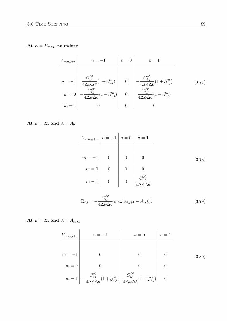
3.6 Time Stepping 89
At E = Emax Boundary
Vi+m,j+n n = −1 n = 0 n = 1
m = −1Cφθi,j
4∆φ∆θ(1 + J θ
i,j) 0 −Cφθi,j
4∆φ∆θ(1 + J θ
i,j)
m = 0 −Cφθi,j
4∆φ∆θ(1 + J θ
i,j) 0Cφθi,j
4∆φ∆θ(1 + J θ
i,j)
m = 1 0 0 0
(3.77)
At E = Eb and A = Ab
Vi+m,j+n n = −1 n = 0 n = 1
m = −1 0 0 0
m = 0 0 0 0
m = 1 0 0Cφθi,j
4∆φ∆θ
(3.78)
Bi,j = −Cφθi,j
4∆φ∆θmax[Ai,j+1 − Ab, 0]. (3.79)
At E = Eb and A = Amax
Vi+m,j+n n = −1 n = 0 n = 1
m = −1 0 0 0
m = 0 0 0 0
m = 1 −Cφθi,j
4∆φ∆θ(1 + J φ
i,j)Cφθi,j
4∆φ∆θ(1 + J φ
i,j) 0
(3.80)

3.6 Time Stepping 90
Bi,j =Cφθi,j
4∆φ∆θ(1 + J φ
i,j) (max[Ai,j−1 − Ab, 0]−max[Ai,j+1 − Ab, 0]) . (3.81)
At E = Emax and A = Ab
Vi+m,j+n n = −1 n = 0 n = 1
m = −1 0 0 −Cφθi,j
4∆φ∆θ(1 + J θ
i,j)
m = 0 0 0Cφθi,j
4∆φ∆θ(1 + J θ
i,j)
m = 1 0 0 0
(3.82)
3.6.6 Modified Craig-Sneyd Scheme
We then use the Modified Craig-Sneyd (MCS) scheme which Hout and Foulon (2010) found
to be good for initial value, two-dimensional convection-diffusion-reaction equations with
mixed derivative terms.
The MCS scheme consists of the following of implicit and explicit steps:
Step 1 : Y0 = (I + ∆tA)~Vk + ∆tB(k)θ ,
2 : Y1 = Y0 + π∆t(AθY1 + B(k+1)θ −Aθ
~Vk −B(k)θ ),
3 : Y2 = Y1 + π∆t(AφY2 −Aφ~Vk),
4 : Y0 = Y0 + π∆t(AθφY2 −Aθφ~Vk),
5 : Y0 = Y0 + (1
2− π)∆t(AY2 −A~Vk),
6 : Y1 = Y0 + π∆t(AθY1 + B(k+1)θ −Aθ
~Vk −B(k)θ ),
7 : Y2 = Y1 + π∆t(AφY2 −Aφ~Vk),
8 : ~Vk+1 = Y2,

3.7 Projected Successive Overrelaxation 91
where π is a parameter that defines the length of the first fractional time-step. For our
solution, we chose the fractional time-step to be half the full time-step; that is, we set
π = 0.5. Note that each step uses the best estimate of the solution from the previous
time-step. Steps 2, 3, 6, and 7 must all be solved implicitly, while all other steps are explicit.
3.7 Projected Successive Overrelaxation
To take into account equityholder’s voluntary liquidation option, we can express the solution
to each implicit MCS fractional time-step as a linear complementarity problem (LCP).
In general, the goal in LCP is to find the solution vector x such that,
Ax ≥ b,
x ≥ c,
and
(x− c)T (Ax− b) = 0,
where A ∈ {Aθ,Aφ} is the update matrix for that step, x is the solution vector for the next
time step, b the solution vector for the current time step, and c is the equityholder’s payoff
should they voluntarily liquidate immediately. The third equality ensures that at least one
of the first two inequalities are binding. Setting up a LCP in this way ensure the solution
x satisfies the finite difference update equation and or satisifes the early exercise boundary
condition.
Each implicit step in the MCS time stepping scheme requires finding the solution of this
LCP, which is a constrained linear system. A common class of algorithms for solving linear
systems are iterative methods. Successive overrelaxation (SOR) (Young, 1971) is a member
of this class of iterative algorithms and is an extention of the Gauss–Seidel method developed

3.7 Projected Successive Overrelaxation 92
by Gauss in 1823.2 PSOR, extends SOR by ensuring an LCP is satisifed at each interation
step. As long as the constraints on the solution vector are a LCP, then PSOR is guaranteed
to converge (Crank, 1987).
Let x(k) be the current best solution vector at iteration k. The PSOR program proceeds as
follows:
1. Start with initial guess x(0), k = 0;
2. Calculate the next unconstrained solution vector for every element i ∈ {1, 2, . . . ,MN}:
x(k+1)i = (1− ω)x
(k)i +
ω
aii
(bi −
∑j<i
aijx(k+1)j −
∑j>i
aijx(k)j
); (3.83)
3. Ensure that the early exercise condition LCP constraint is satisifed:
x(k+1)i = max
(x
(k+1)i , ci
); (3.84)
4. Terminate the iteration if the change between subsequent iterations (as measured by
the L2 norm) is lower than some convergence criteria ε. That is, terminate if the
inequality
(x(k+1) − x(k))T (x(k+1) − x(k)) < ε2, (3.85)
is satisfied, otherwise increment k and repeat from Step 2.
In effect, the PSOR method simply iterates towards a solution using the SOR iterative
procedure (Step 2), but ensures the inequalitites in the LCP are satsified at each iteration
(Step 3).
Its relatively straight forward to implement the PSOR program described by (3.83), (3.84),
and (3.85), however a naive implementation is comutationally inefficient. Being an iterative
2Gauss first mentioned his iterative algorithm in private corresepondence.

3.8 A Cache Optimized PSOR Algorithm 93
procedure, the main PSOR “loop” is run thousands of time per fractional time-step, which
is then run multiple times per full time-step, and so on. Because we solve our model across
a wide range of parameters, there is substantial payoff for us in optimizing the PSOR “hot
loop.”
3.8 A Cache Optimized PSOR Algorithm
The PSOR algorithm, when applied to solve two dimensional finite difference systems, has
order O(n4) computational complexity. That is, the computation time scales with the cube
of problem size. For example, calculating an implicit time step using PSOR on a 512× 512
grid take 16 times (24) longer than on a 256 × 256 grid. Although we cannot improve on
this order of scaling, we can still optimize the PSOR algorithm to speed it up.
We build a custom PSOR implementation and achieve a four order of magnitude decrease in
execution time versus a direct implementation using functions from a standard linear algebra
library3. Our improvements are to:
• Pre-compute the inverted diagonal 1/aii;
• Update the solution vector in-place;
• Exploit the sparseness of the update matrix A by constructing a compact, cache effi-
cient, data structure that enables fast matrix-vector multiplication.
In finite difference problems, the update matrix A is almost always sparse, and in most cases
band diagonal. That is, the vast majority of items in A are zero, expect for the diagonal and
a number of off diagonal bands running from the upper left to the bottom right of the matrix.
Because of this sparsity, it’s more memory efficient to store only the non-zero elements of
the matrix.
3LAPACK sparse matrix functions.
3.8 A Cache Optimized PSOR Algorithm 94
In a computer, there is a “hierarchy of memory”, starting from CPU registers, Level 1, and
Level 2 cache on the CPU, main memory, hard disk, etc. Memory accesses further from
the CPU are slower, and should ideally be avoided. Algorithms that are “cache aware” and
structure their memory accesses to maximize use of on-CPU caches can run much faster than
“cache naive” algorithms. Unfortunately, the in-memory arrangement of sparse matrices and
their associated linear algebra operations are not always cache efficient; the default sparse
matrix memory layout is generally a trade-off betwen flexibility and space efficiency. The
memory accesses required to produce a element in the output vector of a matrix-vector
multiplication are not always contiguous.
In the case of PSOR, because the process is iterative, there’s an advantage in having com-
ponents of the update matrix stored in the CPU cache as long as possible. When executing
Step 2 of the PSOR algorithm, it is advantageous if elements of A required for calculating the
current row index i are contiguous in memory, rather than scattered throughout memory. If
the elements of A are arranged contiguously in the order of access, the CPU can hold them
in cache, and avoid main memory accesses.
For example, in our case, we are left-multiplying a sparse matrix with a vector many times
in succession without changing the left-hand-side matrix. Each element in the output vector
is the inner product of the given row of the matrix and the full input vector. Because the
matrix row is sparse, we only have to do a few multiplicaitons. For each row in the matrix,
we store the elements in that row in contiguous memory, and store an index into the input
vector for each non-zero element in the matrix row.
To perform the matrix multiplication, we can then, for each element of the output vector,
iterate over a contiguous piece of memory reading the matrix row and pulling the relevant
items from the input vector. Because our sparse matrix, after splitting, tends of have a
maximum of 4 elements in a given row, we can store a large numer of matrix ”index rows”
in CPU cache.

3.8 A Cache Optimized PSOR Algorithm 95
Listing 3.1 lists a Matlab MEX function that implements our cache optimized PSOR algo-
rithm.
Listing 3.1 – Optimized PSOR Implementation
1 /∗ Defines the function:2 ∗ cpsor(As, x, b, w, G, err)3 ∗4 ∗ As − NxN sparse matrix.5 ∗ x − Initial guess.6 ∗ b − As∗x = b, solve for x.7 ∗ w − Relaxation parameter.8 ∗ G − Linear complementary constraint.9 ∗ err − Stop iterative once ||x|| < err.
10 ∗/11 #include <string.h>12 #include <math.h>13 #include <time.h>14
15 #include ”mex.h”16 #include ”matrix.h”17
18 #define MAX IN ROW 619 #define MAX ITERATIONS 2000020
21 int getDiagonal(mxArray ∗x, size t ∗nElements, double ∗∗result) {22 mxArray ∗diag;23 if (mexCallMATLAB(1, &diag, 1, &x, ”diag”)) {24 return 1;25 }26 ∗result = mxGetPr(diag);27 ∗nElements = mxGetNumberOfElements(diag);28
29 return 0;30 }31
32 mwIndex getNnz(mxArray ∗x) {33 mwSize columns;34 columns = mxGetN(x);35 return ∗(mxGetJc(x) + columns);36 }37
38 inline void updateIndex(double ∗pr, double ∗value lookup, unsigned long ∗index lookup, unsigned long r, unsigned long c, unsigned long offset) {39 unsigned long i;40 for (i = MAX IN ROW ∗ r; index lookup[i] && i < MAX IN ROW ∗ (r+1); i+=1){};41 value lookup[i] = pr[offset];42 index lookup[i] = c;

3.8 A Cache Optimized PSOR Algorithm 96
43 }44
45 void mexFunction(46 int nlhs, mxArray ∗plhs[],47 int nrhs, const mxArray ∗prhs[])48 {49 /∗ Manual profiling variables. ∗/50 struct timespec begin, end;51 long long cumulative = 0;52
53 size t k, j, i, M;54 double ∗invD, ∗xn, ∗pr;55 unsigned long ∗index lookup;56 double ∗value lookup;57 mwIndex nnz, ∗ir, ∗jc;58
59 mxArray ∗As;60 double w, err;61 double ∗b, ∗x, ∗G;62 As = prhs[0];63 b = mxGetPr(prhs[1]);64 w = mxGetScalar(prhs[3]);65 G = mxGetPr(prhs[4]);66 err = mxGetScalar(prhs[5]);67
68 x = (double∗)mxCalloc(mxGetNumberOfElements(prhs[2]), sizeof(double));69 memcpy(x, mxGetPr(prhs[2]), mxGetNumberOfElements(prhs[2]) ∗ sizeof(double));70
71 if (nrhs != 6 || !mxIsSparse(As)) {72 mexErrMsgTxt(”Single input must be a sparse matrix.”);73 }74
75 /∗ invD = 1 ./ diag(A) ∗/76 getDiagonal(As, &M, &invD);77 for (i = 0; i < M; i++) {78 invD[i] = 1 / invD[i];79 }80
81 /∗ Allocate and construct index lookup array. ∗/82 index lookup = (unsigned long∗)mxCalloc(MAX IN ROW ∗ M, sizeof(unsigned long));83 value lookup = (double∗)mxCalloc(MAX IN ROW ∗ M, sizeof(double));84
85 nnz = getNnz(As);86 ir = mxGetIr(As);87 jc = mxGetJc(As);88 pr = mxGetPr(As);89 int zcount = 0;

3.8 A Cache Optimized PSOR Algorithm 97
90 for (j = 0; j < M; j++) {91 for (k = jc[j]; k < jc[j+1]; k++) {92 if (ir[k] == 0) {93 }94 if (j != ir[k]) {95 updateIndex(pr, value lookup, index lookup, ir[k], j, k);96 zcount++;97 }98 }99 }
100
101 plhs[0] = mxCreateDoubleMatrix(M, 1, mxREAL);102 xn = mxGetPr(plhs[0]);103 memcpy(xn, x, M∗sizeof(double));104
105 for (i = 0; i < MAX ITERATIONS; i++) {106 /∗ xn = x; ∗/107
108 /∗ for jj = 1:length(x)109 xn(jj) = invD(jj)∗(b(jj) − R(jj, :)∗xn);110 end111 ∗/112 for (j = 0; j < M; j++) {113 double ss = 0;114 for (k = j∗MAX IN ROW; index lookup[k] && k < (j+1)∗MAX IN ROW; k+=1) {115 ss += value lookup[k] ∗ xn[index lookup[k]];116 }117 xn[j] = invD[j] ∗ (b[j] − ss);118 }119 /∗ xn = max(G, w∗xn + (1−w)∗x); ∗/120 /∗ if norm(x − xn) < err121 x = xn;122 break123 end124 ∗/125
126 /∗ x = xn; ∗/127
128 double sd = 0;129 for (j = 0; j < M; j++) {130 double new;131 new = fmax(G[j], w∗xn[j] + (1−w)∗x[j]);132 sd += (x[j] − new)∗(x[j] − new);133 x[j] = new;134 xn[j] = x[j];135 }136

3.8 A Cache Optimized PSOR Algorithm 98
137 if (sqrt(sd) < err) {138 goto done;139 }140 }141 mexErrMsgTxt(”Failed to converge.”);142 done:143 plhs[1] = mxCreateDoubleScalar(cumulative);144 return;145 }

4Essay Two – Insolvent Trading and Voluntary
Administration in Australia: Economic
Winners or Losers?
Australian directors who incur debts while their companies are insolvent can be chased by
creditors for compensation when their companies fail. Under the Australian insolvent trad-
ing laws, directors no longer have true limited liability, and they adjust their behaviour as a
result. Identifying director’s rational behaviour in an insolvent trading world is difficult as
99

4.1 Introduction 100
there are no formal economic models of director decision making under Australian current
corporations law. In this paper we develop such a model. We incorporate the threat of insol-
vent trading as well as director’s tactical use of voluntary administration to avoid insolvent
trading litigation. We show that neither a combination of insolvent trading or voluntary ad-
ministration can simultaneously ensure creditors-best outcomes, eliminate insolvent trading,
and reduce director underinvestment.
4.1 Introduction
Insolvent trading laws make directors and managers personally liable for debts incurred when
their companies are insolvent, or for debts incurred that make their companies insolvent.
Directors who trade while insolvent face civil litigation, and in extreme cases criminal charges.
The insolvent trading laws aim to protect creditors from losses due to directors continuing
to trade when there’s little prospect of debt repayment. Insolvent trading laws weaken
the capitalistic principle of limited liability because incurring debts while simply suspecting
insolvency or failing to prevent such a debt being incurred open directors to personal liability
should their company be wound-up.
There is substantial economic, social, and legal debate regarding the necessity of insolvent
trading laws, particularly whether they are economically efficient. Many authors have argued
the merits and disadvantages of insolvent trading laws by drawing upon theories of the firm
(Mannolini, 1996), and other economic tools such as portfolio theory (Morrison, 2003) and
game theory (Whincop, 2000). But, as yet nobody has developed a formal mathematical
model to analyze Australia’s insolvent trading laws. Whincop (2000) description of this
omission in the literature still holds today:
Australia has a wealth of doctrinal literature on insolvency and corporate gov-
ernance, and a thriving economic literature of corporate governance, but serious

4.1 Introduction 101
economic analysis of insolvency remains terra incognita.
The offence of insolvent trading was first introduced in Australia during 1961 in Section
303(3) of the Uniform Companies Act. These laws made it a criminal offence for directors
to contract a debt when there was no reasonable grounds of the firm being able to repay
those debts. This was the first time that insolvent trading was made an offence separate
from outright fraudulent trading. A criminal charge of insolvent trading made the director
personally liable for the amount lent, however none of this recovered money was distributed
to the wronged creditors. Monies “clawed-back” from an insolvent trading director were
effectively a “fine” for acting in a wrongful manner.
In 1964, civil liability for insolvent trading directors was introduced, however creditors could
only pursue civil recovery after a successful criminal prosecution. At the time, these laws
were largely ineffectual with very few successful creditor-lead recoveries (The Law Reform
Commission, 1988). Changes to corporate law in 1971 added broader civil liability, allowing
creditors to pursue civil remedy if a director incurred a debt when there was no reasonable
expectation of repayment.
The Companies Act in 1981 relaxed the requirement of a successful criminal prosecution
for creditor recovery, allowing creditors to bring civil proceedings regardless of whether the
director was convicted criminally. Both directors and managers became personally liable
for incurring debts in circumstances where there was reasonable grounds to expect that the
company would not be able to pay all its debts when they became due.
The current insolvent trading laws were introduced during 1993 in section 588G of the
Corporations Act. These new laws impose explicit duties on directors to prevent a company
from incurring a debt while knowing their company to be insolvent. That is, in addition to
avoiding actions that may constitute insolvent trading, directors must also avoid inaction
that results in insolvent trades being made. A successfully litigated insolvent trading case
requires the plaintiff to:

4.1 Introduction 102
establish that the company is insolvent and is unable to pay its debts as they
become due at the time when it incurs a debt or the company is insolvent because
the debt has been incurred. (Coburn, 2000)
More specifically, the criteria for whether a person has executed an “insolvent trade” are:1
(a) a person is a director of a company at the time when the company incurs a
debt;
(b) the company is insolvent at that time, or becomes insolvent by incurring that
debt, or by incurring at that time debts including that debt;
(c) at that time, there are reasonable grounds for suspecting that the company
is insolvent, or would so become insolvent, as the case may be; and
(d) that time is at or after the commencement of this Part.
Even if the director is not explicitly knowledgeable of his or her firm’s insolvency, there is a
reasonable persons test stating that ignorance doesn’t necessarily diminish director respon-
sibility:2
(a) the person is aware at that time that there are such grounds for so suspecting;
or
(b) a reasonable person in a like position in a company in the company’s circum-
stances would be so aware.
There can be substantial ramifications for a director who violates these insolvent trading
conditions: the director is open to both criminal and civil proceedings. The Australian
Securities & Investments Commission (ASIC) may fine directors up to $200,000, revoke
their right to become a director in the future, and in extreme cases sentence directors to jail.
A recent example:
1Section 588G, Part 1 of the Corporations Act 2001.2Section 588G, Part 2 of the Corporations Act 2001.
4.1 Introduction 103
In August 2011, the former director of International Consulting Group Pty Ltd,
Anula Kumari Kauye, pleaded guilty to insolvent trading, theft, and provid-
ing false information following an investigation by ASIC. Ms Kauye has been
sentenced to a total of three years and two months imprisonment. (Australian
Securities and Investments Commission, 2012)
After the introduction of these new insolvent trading laws in 1993, during a winding-up the
appointed liquidator can bring proceedings against any director believed to have violated
the insolvent trading laws. In general, seeking compensation from the director is a collective
action among all unsecured creditors. Individual creditors can only bring proceedings against
a director with the consent of the liquidator. Even if an individual creditor pursues the
director on their own, any compensation extracted must be paid to the company, and not
to the plaintiff creditor; that is, any unsecured creditor personally pursuing a director must
pass all litigation proceeds through into the shared unsecured creditor pool.
This “sharing” rule, the equal sharing of insolvent trading compensation among all unsecured
creditors, was a dramatic change from the pre-1993 “reservation” rule. Before the Corpo-
rations Act changes, individual creditors were able to pursue insolvent trading directors,
keeping all litigation proceeds to themselves.
Commentators have expressed their concerns that insolvent trading laws may increase di-
rector risk-aversion, causing fearful directors to wind-up firms that otherwise would have
successfully traded out of distress (Oesterle, 2000). The prospect of facing personal liability
for debts incurred in the day-to-day running of a business almost certainly causes stress
for directors. In general, management are optimistic in that they systematically overesti-
mate the probability of good firm performance and underestimate the probability of firm
under-performance. This is a known cognitive bias empirically observed both in psychol-
ogy experiments as well as financial economic analysis (Heaton, 2002; Weinstein, 1980). So
it is not controversial that even a well meaning director would choose to take on further
4.1 Introduction 104
debt to maintain business continuity, however it’s not clear if the threat of insolvent trading
unnecessarily suppresses this optimism.
Accompanying the 1993 changes to the Australian corporations law was the introduction of
Voluntary Administration (VA). The VA procedure is a form of insolvency administration
that aims to3:
• maximize the chances of a company, or as much as possible of its business, continuing
its existence; or
• if continuation isn’t possible, generate a better return for the company’s creditors and
members than would result from an immediate winding up of the company.
VA involves either the company (on behalf of the directors) or liquidators appointing an
administrator to take control of, investigate, and make recommendations for dealing with
the property and affairs of an insolvent or near-insolvent company. The action of entering VA
stays all legal proceedings against the company; that is, once in VA, creditors are barred from
taking legal action until the resolution of administration. Because the insolvent trading laws
are only enforceable during a liquidation, VA temporarily stays director’s personal liability
for violating the insolvent trading provisions.
Once in VA, the appointed administrator either recommends an immediately winding-up of
the company, or proposes a Deed of Company Arrangement (DOCA). A DOCA is a document
describing a plan to ensure business continuity or, failing that, a plan to maximize creditor
returns. Creditors vote on the acceptance of a DOCA, which requires a majority vote to
pass. Hold-out creditors are forced to participate in the DOCA even when voting against it.
In Australia, it is common for directors to appoint an administrator and enter VA the instant
they suspect a creditor initiated winding up is imminent (Fridman, 2003). In effect, directors
use VA as a ”get out of jail free card”, filing for VA once the continued operation of their
3Section 435A, Part 5.3A of the Corporations Act 2001.
4.1 Introduction 105
firm is untenable. It is not clear if it’s always in the best interests of directors to file for VA
as soon as they suspect an adversarial creditor will file for a winding up. Administrators
frequently find evidence of insolvent trading during their initial assessment of companies
entering VA. In the 2013–2014 financial year 57.4% of administrations found evidence of
insolvent trading by directors, an increase from 40.6% in 2008–2009.4
Our primary interest in VA in the context of insolvent trading is that VA is often used by
directors to tactically avoid insolvent trading litigation. In cases of alleged insolvent trading,
as part of a DOCA, directors will contribute personal funds into the company while agreeing
to remove themselves from the unsecured creditor pool; The director effectively says “Ok, I’m
adding some of my personal funds into the DOCA as compensation for the insolvent trades
I may or may not have made. Take what I’m offering in the DOCA, or take me to court.”
As long as the compensation offered by the director is greater than the expected creditor
recovery from a court case, taking into account the costs and inherent risks of litigation,
then the creditors will accept the DOCA and the director avoids insolvent trading charges.
In summary, entering VA and proposing a DOCA grants the director the option of settling
with creditors using their personal funds to avoid insolvent trading litigation.
A recent example of a director using this DOCA “exit hatch” is in the collapse of Retail Ad-
ventures.5 Jan Cameron, also the founder of Kathmandu, agreed to contribute $14 million
into the Retail Adventures unsecured creditors pool as part of a DOCA. Ms Cameron was
being pursued by Deloitte in the NSW supreme court for insolvent trading over more than
$100 million of recklessly incurred debt. In choosing Jan’s substantially reduced offer (re-
turning 14 cents in the dollar) the litigants ”took into account the inherit risks in litigation,
the cost and time it would take to successfully prosecute the claims and the ability of Ms
Cameron and former directors to pay.”
It is not yet clear if Australia’s current insolvent trading and voluntary administration laws
4Series 3: External administrators’ reports. ASIC Australian Insolvency Statistics 2004–2014.5Mitchell, S. (2014, August 5). Kathmandu founder’s Retail Adventures over. The Australian Financial
Review, pp. 20.

4.1 Introduction 106
produce the best outcomes for creditors. Directors operating in a world under the threat of
insolvent trading and with the option of voluntary administration make different decisions
than in a pure limited liability world.
In this paper, we develop a model of directors’ optimal decisions when their firms face finan-
cial distress. First we model a pure limited liability firm when it is in a distressed financial
situation. Next, we model the director’s behaviour subject to the Australian insolvent trad-
ing laws, but exclude the option of entering VA. Finally, we model the behaviour of a director
operating in a world with both insolvent trading and VA. We assume that existing corpo-
rations laws against fraudulent misrepresentation are sufficient to discourage directors from
behaving in a grossly misleading manner. We focus on what characteristic of insolvency
law and under what conditions such provisions change director behaviour. We also model
director decisions and creditor outcomes under alternate “sharing” and “reservation” rules,
particularly if legislation was introduced to allow creditors to voluntarily waive their right
to claim damages from insolvent trading.
Our primary contribution is a tractable economic model of director behaviour incorporating
the main features of Australian insolvent trading and voluntary administration laws. Par-
ticularly, we address Whincop’s annoyance that there has been few attempts to apply true
economic tools to analyze the efficiency of Australia’s insolvent trading laws.
We structure this paper as follows: In Section 4.2 we consider a distressed, pure limited
liability firm, and develop a single period model of optimal director behaviour. In Section
4.3 we extend this model to add the threat of insolvent trading litigation, and explore the
effect of these laws on director behaviour and creditor welfare. In Section 4.4 we include
the option for directors to enter voluntary administration and similarly examine its effect.
In Section 4.5, we use our model to analyze the efficiency of one proposed change to the
insolvent trading laws. We conclude in Section 4.6.

4.2 The Model 107
4.2 The Model
We wish to explore the impact of Australia’s insolvent trading laws on director behaviour
and creditor welfare: Do the current insolvent trading provisions always align director and
creditor incentives?
We build a single period model where debt and equity are contingent claims on the underlying
firm value process. In the most basic case, our model is the single period equivalent to the
continuous time model of Merton (1974). Contingent claims models are a well accepted
approach to explore agent behaviour under various scenarios. Such models have been used to
analyze creditor-equityholder bargaining (Anderson and Sundaresan, 1996; Annabi, Breton,
and Francois, 2010), entrepreneurial decision making (Mcgrath, 1999; O’Brien, Folta, and
Johnson, 2003), and optimal project abandonment (Myers and Majd, 1990), among other
applications.
We assume a discrete, one-period, world. At the start of the period, a director has some
suspicion that his firm is insolvent. For simplicity, we assume that the director wholly owns
the firm (i.e. hold 100% of equity) and makes all managerial decisions6. The director needs
to take on a further debt with face value D to fund business continuation, otherwise the
director must file for a voluntary winding up. For example, these additional funds may be
required to purchase additional equipment, increase stock level, or pay employee salaries.
Figure 4.1 shows the director’s decision tree for this scenario.
We assume a creditor will always be willing to make this new loan; perhaps the new creditor
is a supplier with a positive and long lasting relationship with the distressed firm and has
no reason to suspect insolvency. If the new creditors had perfect visibility into the financial
state of the firm, then they wouldn’t go ahead with the loan. Even with complete knowledge
of the firm’s financial state, the interest rate required by the creditor would be prohibitive
6This simplified environment would also apply to a group of directors with a high equity ownership stakeacting in concert.
4.2 The Model 108
for the borrower.
There must be information asymmetry between the director and providers of credit: If
creditors were completely rational and firms completely transparent, then there would be
no real-world situation where directors could actually trade while insolvent. Clearly this is
not the case, and we make the explicit assumption that insolvent trading directors do have
the ability to take on further debt, either while they are insolvent, or in a manner that will
make their firms insolvent.
At the start of the period, the director decides whether to make an insolvent trade and take
on additional debt or to avoid insolvent trading and commence a voluntary winding up. If
the firm is immediately wound up, then the director nets the residual of the firm’s asset value
after paying back existing creditors: max(A0 − L, 0). The director receives nothing when
total assets are less than total liabilities. During an immediate winding-up, creditors receive
the full face value of debt, or whatever value is remaining in the firm if there is an asset
shortfall: min(A0, L). These option-like payoffs reflect the capital structure split between
debt and equity holders (Merton, 1974). In effect, equityholders (the director in this case)
hold a European call option on firm value, with a strike price equal to the face value of debt.
Creditors hold a portfolio of a risk-free bond and a short position in an equivalent European
put on firm value.
The alternate option for the director is to continue trading, making a bet that the company
can trade out of its current situation by taking on an additional liability with face value D.
If the director continues trading, then there’s a probability pD that by the end of the period,
the firm has performed poorly. In this negative state of the world we assume the firm has
defaulted on one or more of its debts and has been placed into an involuntary winding up by
its creditors. In this default state, the firm’s asset value is AD = A0/(1 + S), where S is the
volatility of the firm’s assets over the period. In the default state, we assume the director
receives zero payoff.

4.2 The Model 109
Note, the firm now has to pay off the original liability as well as the additional liability
incurred by the director to keep the company operating. In the default state, the original
creditors receive a payoff of min(ADL
L+D, L) and the new creditors receive min(AD
DL+D
, D).
These payoffs reflect the typical pari pasu distribution of liquidation proceeds. If the firm
successfully trades out of financial distress (this occurs with probability 1 − pD) then the
firm’s asset value is AT = (1 + S)A0 and the director nets max(AT − (L + D), 0) with the
original and new creditors receiving min(ATL
L+D, L) and min(AT
DL+D
, D) respectively.
We assume the director is risk averse and has a constant absolute risk aversion (CARA)
utility function:
U(c) = 1− exp(−ac), (4.1)
where c is the director’s payoff and a > 0 the director’s risk aversion.
The director’s utility from winding up immediately is
Uwind-up = U [max(A0 − L, 0)] , (4.2)
otherwise their expected utility from continuing in a limited liability (superscript LL) world
is
ULLcontinue = (1− pD)U [vmax(AT − (L+D), 0)] , (4.3)
where v = 11+r
is the discount factor given a required return of r. Although the choice of
discount rate has little impact on director decision making, we include it to break ties when
the payoff from winding-up and continuation are equal.
Directors will chose to wind-up when their expected utility from winding-up is greater or
equal to their expected utility from continuing; that is, when
Uwind-up ≥ ULLcontinue. (4.4)
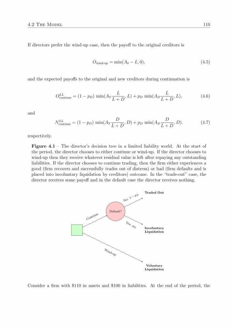
4.2 The Model 110
If directors prefer the wind-up case, then the payoff to the original creditors is
Owind-up = min(A0 − L, 0), (4.5)
and the expected payoffs to the original and new creditors during continuation is
OLLcontinue = (1− pD) min(AT
L
L+D,L) + pD min(AD
L
L+D,L), (4.6)
and
NLLcontinue = (1− pD) min(AT
D
L+D,D) + pD min(AD
D
L+D,D). (4.7)
respectively.
Figure 4.1 – The director’s decision tree in a limited liability world. At the start ofthe period, the director chooses to either continue or wind-up. If the director chooses towind-up then they receive whatever residual value is left after repaying any outstandingliabilities. If the director chooses to continue trading, then the firm either experiences agood (firm recovers and successfully trades out of distress) or bad (firm defaults and isplaced into involuntary liquidation by creditors) outcome. In the “trade-out” case, thedirector receives some payoff and in the default case the director receives nothing.
Default?
VoluntaryLiquidation
InvoluntaryLiquidation
Traded Out
Wind-up
Continue
Yes: pD
No: 1−pD
Consider a firm with $110 in assets and $100 in liabilities. At the end of the period, the

4.2 The Model 111
firm’s assets will either be worth 1.5× 110 = 165 or 110/1.5 = 73.33 (i.e. asset volatility of
S = 0.5). We assume a 50:50 chance between default and successfully trading out of distress.
To continue operating, the firm needs an additional $25 in funding. If the director chooses
to take this debt on, then the firm’s net asset value swings to negative. If the director were
to liquidate immediately, he or she would receive $10 since liquidation would realize $110 in
asset value, of which $100 pays off the original debtholders liability with the director keeping
the remainder.
Table 4.1 – The model parameters for our base case scenario. We model a single periodworld where the firm’s asset value at the period start is A0. At the end of the period,the firms asset value falls to A0/(1 + S) with probability pD or rises to (1 + S)A0 withprobability 1 − pD. In order to continue (not wind up immediately) the director mustmake an insolvent trade to take on additional debt of face value D.
Model Parameter Base Case Value
Asset Volatility S 0.5Initial Asset Value A0 110
Initial Liability L 100New Debt Size D 25
Probability of Default pD 50%Probability of Litigation Success pS 50%
Director Risk Aversion a 0.1Discount Rate 10%
We list the full set of base case scenario parameters in Table 4.1. To gain a stylized under-
standing of our model, before introducing insolvent trading and voluntary administration,
we calculate comparative statics for the pure limited liability case.
Our director winds-up when his or her expected utility from attempting to trade out (contin-
uing) is less than their utility from winding-up straight away: Figure 4.2 shows the director’s
wind-up versus continue decision for the base case scenario as the firm’s initial asset value
and default probabilities vary. When initial assets are less than initial liabilities A0 ≤ L the
director expects no payoff from an immediate winding up and always chooses to “roll-the-
dice” and trade out of trouble.

4.2 The Model 112
When there’s no chance of default (pd = 0), then clearly the director will always choose
to continue. As the probability of default increases, it becomes less and less favourable
to continue, up to the point where default is certain (pd = 1). When default is certain,
the director’s expected payoff is zero both in the wind-up and continue scenario. Thus the
director will wind-up when there’s residual value A0 > L, otherwise they will continue with
nothing to lose.
Figure 4.2 – The director’s optimal wind-up (white) versus continue (black) decisionwhen subject to pure limited liability (no threat of insolvent trading litigation) andvaried initial asset values and default probabilities. The director must make the decisionbetween winding-up immediately, or continuing by incurring a $25 face value debt thatconstitutes an insolvent trade. At the end of the period, the firm’s assets are wortheither 1.5A0 or A0/1.5 (asset volatility of S = 0.5).
Default Probability (%)
Initi
al A
sset
Val
ue (
$)
0 10 20 30 40 50 60 70 80 90 10050
60
70
80
90
100
110
120
130
140
150ContinueWind−Up
A common agency conflict between equityholders and debt holders is risk shifting (Jensen
and Meckling, 1976): Equityholders (in this case the manager / director) in a company close

4.3 Insolvent Trading 113
to insolvency naturally prefer riskier projects because limited liability floors their downside.
When in financial distress, it it rational for the director (whose personal wealth and fu-
ture employment prospect are highly correlated with company outcome) to perfer riskier
behaviour because they participate in the upside, while being shielded from the downside.
Such behaviour is visible in the director’s continue versus wind-up decision when pursuing
risky projects. In Figure 4.3 when the firm has a low probability of default and high asset
volatility directors in a limited liability world preference continuation over an immediate
winding up. Note that for low default probabilities and low asset volatility, the director
chooses winding up over continuation because the expected upside from continuation when
asset volatility is low (< 25%) won’t cover the additional debt needed to keep the company
operating in continuation ($25).
4.3 Insolvent Trading
The Australian government introduced modern insolvent trading laws with the Corporations
Act in 1993. The government’s stated goal in introducing these laws was to protect creditors
from recklessly trading directors. To gauge the impact of these insolvent trading laws on
directors, we extend the limited liability world to allow creditor initiated insolvent trading
litigation.
We assume any action the director takes in making an insolvent trade does not constitute
fraud or gross misrepresentation. The case of a director outright fraudulently misrepresenting
the solvency of their company is covered under existing non-insolvent trading corporations
laws. However, what of the director who may only have a slight suspicious of their firm’s
solvency, or knows that their firm is very close to insolvency? For our purposes, we assume
that the director’s actions, should he or she take on additional debt, constitutes insolvent
trading and not outright fraud. For example, it’s possible that the director has failed to keep
adequate accounts, which would explicitly make them open to insolvent trading litigation,

4.3 Insolvent Trading 114
Figure 4.3 – The director’s optimal wind-up (white) versus continue (black) decisionwhen subject to pure limited liability (no threat of insolvent trading) and varied assetvolatility and default probabilities. The firm has a start-of-period asset value of $110 andoutstanding liabilities of $100. The director must make the decision between winding-up immediately, or continuing by incurring a $25 face value debt that constitutes aninsolvent trade. At the end of the period, the firm’s assets are worth either S × A0 orA0/S where S is the asset volatility.
Default Probability (%)
Ass
et V
olat
ility
(%
)
0 10 20 30 40 50 60 70 80 90 1000
10
20
30
40
50
60
70
ContinueWind−Up
but not to explicit fraud allegations.
We extend the limited liability decision tree in the previous section by adding an additional
decision node in the continuation default state (see Figure 4.4). Now, in the default state,
creditors have the option to bring a case against the director with charges of insolvent
trading. If this litigation is successful, then the director is forced to repay the face value
of insolvent traded debt D. That is, all creditors receive the proceeds from existing assets
plus any compensation payout extracted from the director. If the litigation fails, then the
creditors share only the remaining firm assets. For simplicity, we assume that creditors

4.3 Insolvent Trading 115
always instruct the appointed liquidator to pursue insolvent trading litigation and that the
director has sufficient personal wealth to cover the D compensation payment. We also ignore
litigation expenses; any legal costs would simply reduce the payoff in both the litigation
success and failure states.
Both the wind-up and trade out branches both retain the same expected value in this new
decision tree. The primary change is if the director chooses to continue and the firm defaults:
creditors then commence litigation with certainty. If creditors are successful in their litigation
(with probability pS) then the director experiences a −D payoff (the compensation outflow
to creditors). If litigation fails, then the director pays no compensation, but doesn’t receive
any payoff. The director’s expected utility if the firm defaults after continuing is then
Udefault = pS U [−vD] + (1− pS)U [0] . (4.8)
And the directors prefers winding-up to continuing when
Uwind-up ≥ U ITcontinue, (4.9)
where
U ITcontinue = (1− pD)U [vmax(AT − (L+D), 0)] + pD Udefault. (4.10)
If the firm defaults and the creditors win their litigation, the shared pool of assets for
distribution to unsecured creditors is the terminal asset value plus the amount recovered
from the director AD +D. The expected payoff for the original creditors at the default node
is then
OITdefault = (1− pS) min(AD
L
L+D,L) + pS min((AD +D)
L
L+D,L), (4.11)
4.3 Insolvent Trading 116
and for the new creditors
N ITdefault = (1− pS) min(AD
D
L+D,D) + pS min((AD +D)
D
L+D,D). (4.12)
The expected value for original and new creditors if the director chooses to continue are then
OITcontinue = (1− pD) min(AT
L
L+D,L) + pD O
ITdefault, (4.13)
and
N ITcontinue = (1− pD) min(AT
D
L+D,D) + pDN
ITdefault. (4.14)
respectively.
In contrast to the limited liability scenario, once we include civil insolvent trading litigation,
the director has the potential of suffering a negative payoff. That is, if the director decides
to continue, and then is successfully charged for insolvent trading, he or she will suffer a
negative cashflow −D. This makes the director no longer subject to pure limited liability
and alters their optimal continue versus wind-up decision.
The region of parameter space in which the director chooses continuation over winding-up
is very much diminished once we introduce creditor initiated insolvent trading litigation.
Compare Figure 4.5 (insolvent trading) with the previous Figure 4.2 (limited liability). The
region where the director chooses to continue is substantially smaller in the insolvent trading
world. Again, when there’s no chance of the default, the director always continues.
Note in Figure 4.5, we have fixed the probability of creditors succeeding in insolvent trading
litigation to 50%. Clearly, in this scenario, the director will choose to continue only when
there is a low likelihood of default. In the event of default, the director’s losses from a suc-
cessful insolvent trading litigation could be substantial. This outcome reflects commentator

4.3 Insolvent Trading 117
Figure 4.4 – The director’s decision tree when they are under the threat of insolventtrading without the option to enter voluntary administration. If the director chooses tocontinue and the firm defaults then we assume creditors always start insolvent tradingproceedings. The creditors win their case against the director with probability pS andextract the face value of insolvent traded debt D as compensation. If the creditors failin their case (with probability 1− pS) then they extract no claw-back from the director.In the event of default, the director greatly prefers an unsuccessful litigation to avoidpaying any compensation.
Default?
CreditorLitigation?
Traded Out
InvoluntaryLiquidation
InvoluntaryLiquidation+ Payout
VoluntaryLiquidation
Wind-up
Continue
Failure:1−
pS
Success: pS
Yes: pD
No: 1−pD
concerns that insolvent trading laws encourage directors to be conservative in their con-
tinuation choice (Oesterle, 2000). Introducing insolvent trading causes risk-averse directors
to greatly favour winding-up rather than risking the possibility of future insolvent trading
charges.
The government’s stated motivation in introducing insolvent trading laws is to ensure direc-
tors take greater account of the interests of creditors when their firm is financially distressed
(Oesterle, 2000). A natural questions is then: are creditors now better off in an insolvent

4.3 Insolvent Trading 118
Figure 4.5 – The director’s optimal wind-up (white) versus continue (black) decision forthe base case scenario when the director threatened by creditor initiated insolvent tradinglitigation (no option to enter voluntary administration) across varied initial asset valuesand default probabilities. The area of parameter space (black) covered by the continuedecision is decreased compared with a world without insolvent trading laws.
Default Probability (%)
Initi
al A
sset
Val
ue (
$)
0 10 20 30 40 50 60 70 80 90 10050
60
70
80
90
100
110
120
130
140
150ContinueWind−Up
trading world? We compare the relative expected payoff for original creditors in the limited
liability and insolvent trading worlds in Figure 4.6.
In general, where directors choose to wind-up in the limited liability world, they also choose
to wind up in the insolvent trading world. Thus, there’s no difference in creditor payoff
when there are substantial initial assets and a high probability of default. For most of the
parameter space where insolvent trading changes director behaviour (from continue to wind-
up), creditors are better off in the insolvent trading world. However, this does not hold
universally, for example creditors in a limited liability world are better off when the firm has
lower starting assets and a lower probability of default.
4.4 Voluntary Administration 119
In these scenarios, an immediate winding-up releases insufficient value to cover the original
creditors liability L. With the threat of insolvent trading in this scenario, the director favours
an immediate winding-up. Were he or she to continue, and the company to trade out of
trouble, the original creditors would be “made good” on the full face value of their liability.
Note, however, that the director’s expected payoff is negative, because even if they risk
continuation, and that risk pays off with a company recovery, their eventual payoff doesn’t
out-weight the additional risk of being charged with insolvent trading should the firm default
(even with a slim chance). This is a case of the classic underinvestment problem (Myers,
1977), where equityholders will forego actions with positive NPV expectation when the bulk
of the potential upside goes to creditors rather than themselves.
Note, our discussion of creditor outcomes has focused on the original creditors and not the
new creditors (those creditors that participated in the insolvent trading transaction). In our
base case scenario, new creditors are better off in the insolvent trading world in all cases.
In situations where the director’s behaviour shifts from continue to wind-up in the insolvent
trading world, new creditors are better off because they completely avoid being party to an
insolvent trade in the first place. In situations where the director still chooses the continue,
the expected payoff to new creditors is higher than in the limited liability world because they
share in any compensation clawed back from the direction via a successful insolvent trading
litigation.
4.4 Voluntary Administration
Voluntary Administration (VA) gives directors “breathing space”, granting directors a bit
of “wiggle room” when it comes to insolvent trading.7 Directors often pre-empt attempts
by creditors to wind-up their firms by tactically filing for VA once they suspect creditors of
7Hunt, S., Bruce, E., & Friedlander, D. (2014, July 18). Business judgment rule needed. The AustralianFinancial Review, pp. 28.
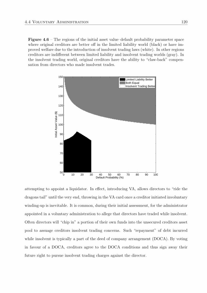
4.4 Voluntary Administration 120
Figure 4.6 – The regions of the initial asset value–default probability parameter spacewhere original creditors are better off in the limited liability world (black) or have im-proved welfare due to the introduction of insolvent trading laws (white). In other regionscreditors are indifferent between limited liability and insolvent trading worlds (gray). Inthe insolvent trading world, original creditors have the ability to “claw-back” compen-sation from directors who made insolvent trades.
Default Probability (%)
Initi
al A
sset
Val
ue (
$)
0 10 20 30 40 50 60 70 80 90 10050
60
70
80
90
100
110
120
130
140
150Limited Liability BetterBoth EqualInsolvent Trading Better
attempting to appoint a liquidator. In effect, introducing VA, allows directors to “ride the
dragons tail” until the very end, throwing in the VA card once a creditor initiated involuntary
winding-up is inevitable. It is common, during their initial assessment, for the administrator
appointed in a voluntary administration to allege that directors have traded while insolvent.
Often directors will “chip in” a portion of their own funds into the unsecured creditors asset
pool to assuage creditors insolvent trading concerns. Such “repayment” of debt incurred
while insolvent is typically a part of the deed of company arrangement (DOCA). By voting
in favour of a DOCA, creditors agree to the DOCA conditions and thus sign away their
future right to pursue insolvent trading charges against the director.

4.4 Voluntary Administration 121
We expect the presence of VA to bias directors’ decisions towards continuation rather than
winding up compared with a world with no VA. Although, encouraging business continuity
may be advantageous for employees, given that insolvency legislation and VAs stated goals
are to maximize creditor recovery, does the behavioural change induced by VA within a
insolvent trading world make creditors better off?
We operationalize VA in our model as an additional decision node in the default state. Once
the director knows their firm is in the default state, they can choose to tactically appoint an
administrator and enter VA, pre-empting creditor calls for a liquidation. We assume that
the director will voluntarily direct some of his or her personal assets into a DOCA. This
amount is equivalent to the expected payoff of creditors under the liquidation branch of the
decision tree. For example, assume that the probability of a successful creditors litigation
for insolvent trading is 25% and the payoff into the unsecured creditor pool from a successful
litigation is $40. Were a litigation to take place, the expected payoff for creditors is
pS ×D + (1− pS)× 0 = 0.25× 40 + 0.75× 0 = 10. (4.15)
$10 is the creditor’s certainty equivalent value for accepting a DOCA versus pursuing litiga-
tion; in other words, creditors are indifferent between accepting a certain payoff of $10 from
the director as part of the DOCA and pursuing litigation. We assume that creditors will
always accept a DOCA when offered the certainty equivalent value of litigation.
In general, the certainty equivalent of VA versus litigation is
CEVA = v pS D. (4.16)
The director’s utility of selecting VA over allowing creditors to wind-up the firm is
UVA = U [−CEVA] = U [−v pS D] . (4.17)

4.4 Voluntary Administration 122
Recall that the director’s utility in a creditor litigated involuntary winding-up is
Udefault = pS U [−vD] , (4.18)
thus the director will chose VA over allowing an involuntary winding-up when
UVA ≥ Udefault. (4.19)
This choice then flows back up the decision tree, effecting the director’s choice of voluntarily
winding-up or continuing such that winding-up immediately is dominant when
Uwind-up ≥ UV Acontinue, (4.20)
where directors utility from continuing is
UV Acontinue = (1− pD)U [ vmax (AT − (L+D), 0) ] + pD max (UVA, Udefault ) . (4.21)
If the choice of VA is dominant, then creditor’s payoffs from the VA are
OVA = min((AD + pS D)L
L+D,L), (4.22)
and for original creditors, and
NVA = min((AD + pS D)D
L+D,D), (4.23)
for new creditors.
Our model results support the argument that VA “pulls back” the effect that insolvent
trading laws have on directors choosing to wind-up too early. The addition of VA expands

4.4 Voluntary Administration 123
Figure 4.7 – The director’s decision tree when voluntary administration is available asan exit option to avoid insolvent trading litigation. If the director chooses to continue andtheir firm defaults, then they have the option of either entering voluntary administration,or letting creditors liquidate the firm and pursue insolvent trading litigation to recoverthe face value of insolvent traded debt. If the director chooses to tactically enter VA toward off creditor legal actions then they must chip in some of their personal wealth aspart of a VA deed of company arrangement (DOCA). The director always contributesenough value to make it no longer worthwhile for creditors to pursue insolvent tradinglitigation.
Default?
CreditorLitigation?
Traded Out
Deed ofCompany
Arrangement
InvoluntaryLiquidation
InvoluntaryLiquidation+ Payout
VoluntaryLiquidation
Wind-up
Continue
Failur
e:1−
pS
Success: pS
VoluntaryAdministr
ation
CreditorWind-up
Yes: pD
No: 1−
pD

4.4 Voluntary Administration 124
the parameter space where continuation is optimal compared with the insolvent trading
only world. Figure 4.8 portrays this change for various initial asset values and default
probabilities. For our base case scenario, in the insolvent trading only world (no VA) with
an initial asset value of $100 and default probability of 20%, the director would optimally
wind-up immediately. At this same point (A0 = 100, pD = 0.2), once VA is available to
directors, it becomes optimal for them to continue.
Were the probability of a successful insolvent trading litigation by creditors is higher than
the 50%, then the difference in director behaviour in the insolvent trading and the voluntary
administration worlds would gradually decrease. At the extremes: with probability of suc-
cessful insolvent trading litigation being either 100% or 0%, the director would experience the
same outcomes regardless of whether they chose to enter VA or not. The director is willing
to pay a certain payoff to the creditors in voluntary administration (the certainty equivalent
value of pursuing litigation) versus taking a probabilistic risk in the insolvent trading-only
world. Once this choice becomes deterministic (pS = 1 or pS = 0), the certainty equivalent
and the expected outcome are identical.
Observed creditor behaviour indicates the frequency of insolvent trading litigation is low,
and even if successful, recovery from a potentially penniless director is often difficult (James,
Ramsay, and Siva, 2004). The power of VA to induce firm continuation is thus greater
when creditor litigation success is unlikely. Note, the expanded “continue in VA world only”
region in Figure 4.9 (a) when the probability of creditor litigation success is 25% compared
with (b) with a high likelihood of litigation success (75%). The change of behaviour from
introducing VA into the insolvent trading world is greater as the probability of successful
insolvent trading litigation decreases.
Clearly, VA alters director behaviour by granting them an insolvent trading avoidance mech-
anism should they end up in a situation where insolvent trading charges are likely. Paying
some amount into a DOCA is the convenient out that causes directors to continue to trade

4.4 Voluntary Administration 125
Figure 4.8 – The directors wind-up versus continue decision in the presence of insolventtrading with and without the ability of for director to enter voluntary administration(VA). Directors can avoid insolvent trading litigation by paying creditors their certaintyequivalent of litigation proceeds. This option to enter VA encourages directors to con-tinue over a large area (gray) of parameter space than in a no-VA insolvent tradingworld.
Default Probability (%)
Initi
al A
sset
Val
ue (
$)
0 10 20 30 40 50 60 70 80 90 10050
60
70
80
90
100
110
120
130
140
150Continue in both Insolvent Trading and VA worldsContinue in VA world onlyWind−Up
when they otherwise wouldn’t have. How do the original creditors fare when they are offered
a DOCA exit instead of being forced to seek civil remedies via the courts?
Original creditors experience different outcomes in VA and non-VA worlds when the prob-
ability of firm default is low. Figure 4.10 describes when creditors are better off in the
insolvent trading only and VA worlds for varied initial asset values and default probabilities.
In regions of parameter space where there is no behavioural difference after the addition
of voluntary administration, then there is no difference in outcome for creditors. That is,
unless the addition of VA induces a change in director behaviour, the outcomes for creditors

4.4 Voluntary Administration 126
Figure 4.9 – A comparison of the continue versus windup-decision for low and highprobabilities of creditor initiated insolvent trading litigation success. Once the option toenter voluntary administration is available to directors, their continuation behaviour issubstantially influenced by the likelihood of them losing an insolvent trading law suite.
Default Probability (%)
Initi
al A
sset
Val
ue (
$)
0 10 20 30 40 50 60 70 80 90 10050
60
70
80
90
100
110
120
130
140
150Continue in both Insolvent Trading and VA worldsContinue in VA world onlyWind−Up
(a) 25% Creditor Litigation Success
Default Probability (%)
Initi
al A
sset
Val
ue (
$)
0 10 20 30 40 50 60 70 80 90 10050
60
70
80
90
100
110
120
130
140
150Continue in both Insolvent Trading and VA worldsContinue in VA world onlyWind−Up
(b) 75% Creditor Litigation Success
are identical to the insolvent trading-only world; Between the VA and non-VA worlds, the
difference in creditors outcome is due to the director’s differential choice of continuation
versus winding-up induced by the VA option.
In our base case scenario, on continuation, the director takes on a further debt of 25, making
the firm’s total liabilities 125. The original creditors are thus better off in an immediate
winding-up when their expected payoff from continuation is worse than the firm’s current
asset value. When the firm’s net asset value is negative (A0 < L) and there’s a high likelihood
of trading out of trouble (low default probability) then VA is a better choice for creditors as
they will likely recover the full amount of their loan (this is the white area in Figure 4.10).
In any other situation where VA induces continuation (the black area in Figure 4.10) then
it would have been better off for creditors if the director wound up immediate, because the
expected losses in default are greater than the expected payoff from an immediate wind-up
and the original creditor’s claim is diluted by the directors taking on further debt.

4.4 Voluntary Administration 127
Figure 4.10 – Original creditor welfare in the presence and absence of director initiatedvoluntary administration. Directors are more likely to continue when they are able touse VA to avoid insolvent trading litigation. For firms already with highly negative netassets and low default probability (white region) original creditors are better off in avoluntary administration world. Firm with some residual assets are better off in a no-VA voluntary administration world. Otherwise original creditors are indifferent betweenthe VA and no-VA worlds (gray).
Default Probability (%)
Initi
al A
sset
Val
ue (
$)
0 10 20 30 40 50 60 70 80 90 10050
60
70
80
90
100
110
120
130
140
150Insolvent Trading Only BetterBoth EqualVoluntary Administration Better
Arguably, insolvent trading protection is more important for trade creditors than larger
lenders. A larger institution lending to many smaller firms is able to minimize its risk by
holding a portfolio of debt assets. Their own business continuation is much less sensitive
to the individual insolvency outcomes of its debt portfolio firms compared with small and
medium enterprises (SMEs). SMEs may only have a few customers, and were one of those
customers to trade with it while insolvent, the SME extending trade credit may itself suffer
financial distress when a borrower defaults. Thus the welfare of new, unsecured creditors,
may be more important than ensuring pari pasu outcomes across all unsecured creditors.

4.5 Contracting Options 128
4.5 Contracting Options
Figure 4.11 – Comparison of original and new creditor (those creditors that were partyto the director’s insolvent trade) welfare in the VA and reserving rule worlds. In thereserving rule world, new creditors can freely waive their right to pursue insolvent tradingcharges. Original creditors are only better off in the reserving world when the companyhas negative net assets and a high likelihood of trading out of trouble. New creditorsare better off in the reserving world over a larger range of parameter space.
Default Probability (%)
Initi
al A
sset
Val
ue (
$)
0 10 20 30 40 50 60 70 80 90 10050
60
70
80
90
100
110
120
130
140
150Reserving Opt−Out BetterBoth EqualVoluntary Administration Better
(a) Original Creditors
Default Probability (%)
Initi
al A
sset
Val
ue (
$)
0 10 20 30 40 50 60 70 80 90 10050
60
70
80
90
100
110
120
130
140
150Both EqualVoluntary Administration Better
(b) New Creditors
In the event of a successful insolvent trading litigation, any residual value from liquidation
is combined with funds recovered from the director and then distributed among unsecured
creditors. This “sharing” rule disadvantages the newest creditor (the “insolvent trading
creditor”); Were the new creditor to pursue insolvent trading litigation against the director,
any compensation won must be shared with all other creditors in the unsecured creditor
pool. Also, if litigation is costly, it may be difficult to convince the entire creditor pool to
collectively pursue litigation. Even if the new creditor funds the legal action themselves, all
the hold-out unsecured creditors still benefit from the distribution of litigation compensation.
Before the Australian Corporations Act changes in 1993, this sharing rule was not enforced.
Rather, the creditor who was party to the insolvent trade could individually pursue litigation

4.5 Contracting Options 129
and then keep the entire recovered compensation amount. In effect, only the new creditors
were protected by the insolvent trading legislation, existing creditors were not able to make
any recovery using the insolvent trading laws. This pre-1993 kind of distribution is called
a “reserving” rule, effectively restricting the interest of insolvent trading compensation to
those creditors extending new credit.
Reverting the corporations act from sharing back to reserving rules would be unlikely to
alter director behaviour. Directors of suspected insolvent companies would not adjust their
wind-up versus continue decision regardless of the presence of voluntary administration. This
is because the director’s payoffs to creditors in all states of the world would be the same
with sharing and reserving rules: the only different would be the relative payoffs of the two
classes of creditor. A change to the reserving rule would simply act as a transfer of wealth
from original creditors to the new creditors. If the insolvent trading laws are primarily in
place to protect trade creditors and SMEs, then this wealth transfer may be justifiable for
the portfolio reasons explained in the previous section.
The ability for directors and creditors to contract around insolvent trading laws are limited
(Whincop, 2000). There is no mechanism for a director and creditor to contractually agree
to waive the creditor’s rights to pursue insolvent trading litigation. This is particularly
important in certain cases where a firm is known to be insolvent, but still has a large enough
upside for a creditor to justify further investment.
For example, consider a start-up firm with a negative net asset position that wishes to
raise further funds by a hybrid debt issue (perhaps a convertible note). Even after being
completely transparent with creditors, the director may not be willing to personally expose
themselves to future liability because their firm is technically insolvent. Thus, we end up
with firm, that may well have been able to trade out or raise additional funds, that is wound
up directly as a result of the insolvent trading laws.
A suggested change to the insolvent trading laws allows directors and creditors to explicitly

4.5 Contracting Options 130
opt-out of insolvent trading protection (Dabner, 1994; Whincop, 2000). That is, creditors
lending to a known insolvent company can choose to selectively waive their right to pursue
insolvent trading charges. This allows creditors to lend to known insolvent companies without
triggering director insolvent trading liability. When subject to the sharing rule, however,
such contracting out of insolvent trading requires all creditors (original and new) to waive
their rights. Achieving such a waiver would prove difficult because original creditors may
be materially worse off after opting-out of insolvent trading laws. If the sharing rule was
reverted back to the pre-1993 reservation rule, however, consent to waive insolvent trading
laws would only be required from the new creditors.
In the scenario of a reservation rule and the ability of creditors to opt-out of insolvent trading
protection, an insolvent firm would be able to legitimately restore solvency by securing debt
from new creditors. If such changes were implemented, then our model simply reduces to
the pure limited liability case: the original creditors have no case for insolvent trading and
the new creditors have waived their rights, so the liquidation payoff in the event of default
is simply split pari pasu with the unsecured creditors.
Original creditors are generally worse off in the reservation worlds while new creditors are
universally worse off. From the director’s point of view, the reservation world is equivalent
to the limited liability world. Moving from the VA world to the reservation world then
makes original creditors better off only where director underinvestment is eliminated. New
creditors are worse off in all circumstances, this is because directors, without the threat of
insolvent trading, are much more likely to continue trading, which makes new creditors more
likely to sustain losses.
We conclude that suggestions to allow contracting around insolvent trading by reverting to
the reserving rule and allowing contractual waivers of the insolvent trading laws are not
efficient. New creditors will be materially worse off and original creditors will benefit in only
extreme cases.

4.6 Conclusion 131
4.6 Conclusion
In this paper we have developed an economic framework of director choice over various
permutations of Australia’s insolvent trading laws. Our model can produce well known
agency conflicts: risk shifting and under investment, replicating the insolvent trading induced
behaviour that is often criticized by commentators.
We find that there is no dominant configuration of insolvent trading and voluntary adminis-
tration laws that limits insolvent trading while maximizing creditor welfare. This is because
the goals of simultaneously (a) stopping insolvent trading, (b) maximizing creditor welfare
in default, and (c) minimizing the impact of skittish directors winding-up too early are in-
compatible. The introduction of insolvent trading laws certainly discourages directors from
insolvent trading, however at the expense of extinguishing a company that may have had a
better expected payoff by continuing. Creditors in firms with negative net assets but positive
growth expectations are materially worse off under the insolvent trading laws.
We hope that our model informs future discussion of the economic trade-off relative to
insolvent trading legislation reform in Australia.
For simplicity we restricted ourselves to a discrete, single period model. Our model can
be extended to continuous time, such that the asset process varies continuously over the
time horizon, so that the insolvency triggers can occur at any time. Our model only con-
siders director decision making and creditor outcomes under director’s choices. We do not
allow creditors any freedom of choice, nor incorporated the negotiation of debt yields by
creditors. The bargaining between creditors and equityholders over debt indenture terms is
complicated, and beyond the scope of our simple model. Other authors have explored sim-
plified bargaining scenarios within continuous time framework (Anderson and Sundaresan,
1996; Annabi, Breton, and Francois, 2010), however it would be difficult to accommodate
directors-creditors bargaining using the entire insolvent trading and voluntary administration

4.6 Conclusion 132
decision tree.

5Essay Three – A Tale of Two Economies:
Equilibrium Asset Pricing with Imputation
and Home Preference
The full effect of a dividend imputation tax system on domestic asset prices is not completely
understood. Dividend imputation eliminates double taxation by attaching tax credits to dis-
tributed dividends for already paid company tax. Domestic investors can use these credits to
133

5.1 Introduction 134
reduce their personal taxes, while credits are useless to foreign investors. The interplay be-
tween imputation eligible domestic investors and ineligible foreign investors makes it difficult
to value imputation credits. We develop a one period, global asset pricing model combining
dividend imputation and home bias. We assume that home biases arises due to the status
quo and endowment behavioural biases. We explore the effects of imputation and home
bias on investor holdings, required returns, and the market value of imputation credits. We
show that risk-averse domestic investors cannot fully capture the value of imputation credits
because concentrating their holdings in the domestic market reduces their diversification.
When given access to imputation credit paying domestic assets, domestic investors load up
on such assets until the marginal gain from extra imputations credits and lowered expected
future regret balances any expected loss from portfolio concentration.
5.1 Introduction
Domestic Australian companies receive imputation credits for the Australian corporate tax
they pay. When these companies distribute dividends to their shareholders they “frank”
their dividends by attaching imputation credits. Certain domestic shareholders, when they
receive franked dividends, can use the attached credits to reduce their personal taxes. Foreign
investors cannot use the credits and don’t value them. Given that Australia is a small open
economy whose shares are held by a mixture of domestic investors and foreign investors,
each valuing imputation creditors differently, it is not obvious how these credits influence
the market value of Australian shares.1
In most countries, income tax applies to both corporations and individuals: A business gen-
erates income and pays taxes on it at the corporate tax rate. The business then distributes
1As yet, there is no consensus in the literature regarding imputation’s value impact on Australian shares(Dempsey and Partington, 2008; Gray and Hall, 2006; Lally, 2008; Truong and Partington, 2008).

5.1 Introduction 135
some of its after-tax income to shareholders as dividends. Shareholders receive these div-
idends and pay personal taxes on them at their marginal tax rate. This combination of
corporate and personal taxes creates a situation where earnings are taxed twice. A system
that behaves in this manner with double taxation is called a “classical” tax system, and can
produce high effective tax rates.
A company’s capital structure and dividend distribution decisions can be biased by their
governing tax regime: A classical taxation system encourages companies to maintain higher
leverage (because interest payment are tax deductible) and encourages share buy-backs by
penalizing dividends (because of double taxation). There are various taxation regimes that
aim to reduce these biases by provide shareholder tax relief. Although, as with any system,
removing one bias can introduce side-effects. The most extreme form of shareholder tax relief
is for income at the corporate level to be passed-through directly to shareholders, ignoring
any corporate tax. The individual investors then simply treat all passed-through earnings as
personal income. Although pass-through taxation is used in many countries for trusts and
other specialty investment vehicles, the administrative overhead of tracking pass-through
income for widely held limited liability corporations with complicated capital structures is
prohibitive.
Dividend imputation is another form of shareholder tax relief that credits shareholders for
tax already paid at the corporate level. Australia and New Zealand are currently the only
two OECD countries with dividend imputation systems, although other countries have re-
cently discontinued dividend imputation.2 Dividend imputation allows eligible domestic
shareholders to gross up their dividend income by adding the value of imputation credits.
Consider a company that makes $115 in operating income and pays $15 in tax deductible
interest expenses. The company’s taxable income is then 115−15 = $100. With a corporate
tax rate of 30%, the company pays $30 to the government and distributes the remaining $70
2UK, Germany, Finland, Norway, Singapore, Malaysia, had and have subsequently disbanded their im-putation taxation systems.
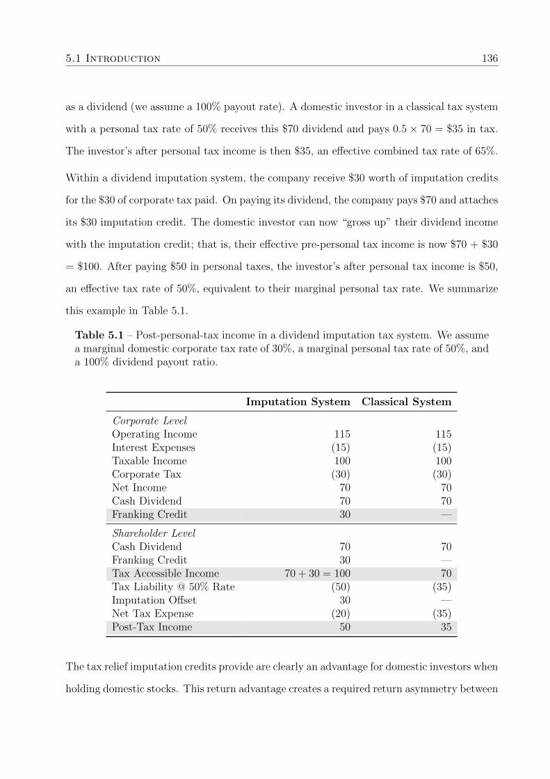
5.1 Introduction 136
as a dividend (we assume a 100% payout rate). A domestic investor in a classical tax system
with a personal tax rate of 50% receives this $70 dividend and pays 0.5 × 70 = $35 in tax.
The investor’s after personal tax income is then $35, an effective combined tax rate of 65%.
Within a dividend imputation system, the company receive $30 worth of imputation credits
for the $30 of corporate tax paid. On paying its dividend, the company pays $70 and attaches
its $30 imputation credit. The domestic investor can now “gross up” their dividend income
with the imputation credit; that is, their effective pre-personal tax income is now $70 + $30
= $100. After paying $50 in personal taxes, the investor’s after personal tax income is $50,
an effective tax rate of 50%, equivalent to their marginal personal tax rate. We summarize
this example in Table 5.1.
Table 5.1 – Post-personal-tax income in a dividend imputation tax system. We assumea marginal domestic corporate tax rate of 30%, a marginal personal tax rate of 50%, anda 100% dividend payout ratio.
Imputation System Classical System
Corporate LevelOperating Income 115 115Interest Expenses (15) (15)Taxable Income 100 100Corporate Tax (30) (30)Net Income 70 70Cash Dividend 70 70Franking Credit 30 —
Shareholder LevelCash Dividend 70 70Franking Credit 30 —Tax Accessible Income 70 + 30 = 100 70Tax Liability @ 50% Rate (50) (35)Imputation Offset 30 —Net Tax Expense (20) (35)Post-Tax Income 50 35
The tax relief imputation credits provide are clearly an advantage for domestic investors when
holding domestic stocks. This return advantage creates a required return asymmetry between

5.1 Introduction 137
domestic stocks distributing imputation credits and otherwise identical foreign stocks in a
classical tax regime. Domestic investors will favour the imputation paying domestic stock,
while foreign investors will be indifferent. How this asymmetry affects asset prices is not
entirely clear.
There are two schools of thought regarding the effect of imputation credits on asset prices.
One school considers Australia to be a small, open economy that is a net importer of capital.
Because foreign capital is required by domestic businesses, and foreign investors receive no
benefit from imputation credits, the equilibrium outcome must be that imputation credits
have a negligible effect on the value of Australian shares. That is, foreign investors will not
rationally pay a premium (in the form of a higher share price) for imputation credits that
are of no value to them.
Cannavan, Finn, and Gray (2004) estimate the market value of imputation credits using
derivative securities on Australian imputation stocks finding that very little of imputation
credit’s value is visible in stock prices. This is consistent with foreign investors being the
marginal price setting investors for Australian firms.
An alternative argument assumes Australia can be treated as a segmented market, with
the majority of Australian shares owned by Australian residents and no overseas investment
opportunities. In this case, imputation credits will have a material effect on Australian
share prices. Under this explanation, the presence of foreign investors is explained in terms
of diversification benefits, the cost of relatively higher share prices is more than offset by
diversification benefits.
In the past there were obvious and explicit barriers to cross-country investment. Cur-
rency hedging products were less accessible; information search costs were much higher
(pre-internet access), trading costs were considerable, and there were much explicit barri-
ers to foreign investment. These days, however, the arrival of discount brokers and the
internet dramatically reduce information search costs within foreign markets and reduced

5.1 Introduction 138
transaction costs(Amihud and Mendelson, 2000). Also, the growing prominence of high-
frequency-trading market makers has also lowered trading costs (Brogaard, Hendershott,
and Riordan, 2014).
Why do Australian investors then still hold the majority of their wealth in Australian stocks?
Australia’s equity markets represent 1.7% of world market capitalization, if Australians were
to hold the world market portfolio, then they would hold nowhere near the currently ob-
served 78% allocation to Australian stocks (Lau, Ng, and Zhang, 2010). Clearly, imputation
benefits incentivize domestic investors to hold domestic stocks, however imputation in itself
is insufficient to create observed concentrations. Also, concentrating holdings in domestic
stocks makes Australian investors miss out on the diversification benefits of holding the
world market portfolio.3
There is plenty of evidence that investors are subject to behavioural biases (Baker and
Nofsinger, 2002; French and Poterba, 1991; Hirshleifer, 2001). One such behavioural bias is
the status quo bias, where investors are unlikely to deviate from their “status quo” portfolio
(Kahneman, Knetsch, and Thaler, 1991). For example, an investor who talks with his family,
colleagues, investment advisor, etc, about his investments is likely to feel comfort in reflecting
the portfolio choices of his confidants. Another behaviour bias is the endowment bias, where
investors, when given an initial portfolio, are hesitant to make choices that move them away
from their default allocation.
The combination of the status quo and endowment biases suggest that a preference for home
economy assets may purely be a result of path-dependent historical baggage. Clearly, in
the past, there were higher barriers to foreign investment than there are today. Informa-
tion search costs may have been considerable given the inaccessibility of information about
firms without either explicitly paying analyst firms or getting days old news via imported
newspapers. If domestic investors have been accustomed to holding Australian stocks and
3See Mishra (2008, 2011); Mishra and Ratti (2013); Warren (2010) for further commentary on Australianhome bias.

5.1 Introduction 139
Australian investors tend to hold the status quo portfolios of their peers, then even a new
investor, observing the portfolio holdings of other investors, will be more likely to hold a
domestic only portfolio.
In contrast to other tax related asset pricing models (Lally, 2000; Lally and van Zijl, 2003;
Monkhouse, 1993; Stulz, 1981; Wood, 1997), we don’t define explicit foreign investment
barriers in our model. Rather, we operationalize the endowment and status quo biases using a
regret based utility function. With a regret based utility function, investors experience regret
when their chosen portfolio’s return deviates from their “home economy only” portfolio. This
home economy only portfolio is, in effect, a status quo and an endowment portfolio.
Consider an investor living in a country where his current portfolio comprises domestic-
only stocks, and his friends, family, colleagues, all hold and discuss domestic stocks.4 Were
he to deviate from the status quo portfolio and choose the world portfolio, which then
subsequently under-performed the portfolio of his colleagues, he would be likely to suffer
considerable decision regret.
Understandably, our investors knows ex-ante that if his chosen portfolio under-performs his
status quo portfolio, he will suffer lower terminal utility. Thus, ex-ante he wants to choose
a portfolio that will maximize his return while minimizing his potential for future regret
should his portfolio under-perform. Bell’s (1983) regret based utility function mathematically
models this behaviour: Investors suffer lower utility when their chosen portfolio deviates from
their status quo portfolio, in our case we set the status quo portfolio to be the mean-variance
optimal portfolio restricted to assets from the investor’s home economy.
There is plenty of experimental evidence that humans exhibit regret aversion: Josephs and
Larrick (1992) and Ritov (1996) observe that individuals are naturally regret averse in their
choices. Investors are not only concerned that certain choices will result in lower realized
returns, but also that the returns on their chosen portfolio will be lower than an alternative
4This strongly agrees with my investment experience and is supported by experimental research (Lin,Huang, and Zeelenberg, 2006).

5.1 Introduction 140
choice. Regret is also stronger for decisions that involve action rather than passivity (Ritov
and Baron, 1990).
Obtaining a reliable estimate of the market value of imputation credits is of considerable
practical importance for two reasons: First, Officer (1994) demonstrates that the value of
imputation tax credits, which he denotes as γ or gamma, is an important component of firm
valuation in dividend imputation tax systems.5 Second, the estimated value of gamma is
one of the key elements of the regulation of monopoly infrastructure assets—an increase in
the value of gamma can result in the allowed revenue for a regulated business to decrease by
tens of millions of dollars per year.
The 2009 Henry tax review into taxation in Australia states that although dividend im-
putation laws should remain unchanged in the short to medium term, the trend towards
greater global market integration suggests we should reconsider the imputation system in
the future.6 If the marginal price setting investor in a highly integrated world is the foreign
investor; that is, if the firms’ true cost of capital is indifferent to the presence or absence
of dividend imputation, then dividend imputation simply becomes a subsidy to Australian
shareholders. This is especially apparent in the Australian system because of tax rebates:
individuals get a tax refund from the government if their marginal tax rate is less than the
corporate tax rate. This is particularly applicable to certain investment vehicles such as
superannuation funds that pay a 15% tax rate.
To this end, we derive a global capital asset pricing model with endogenous home preferences
and dividend imputation. We consider two economies: a large foreign economy and a small,
capital constrained, domestic economy.7 Domestic investors receive imputation credits on
their home economy asset holdings while foreign investors receive no imputation benefits in
5See the Appendix to Officer (1994) for an illustration of how the various cash flows and discount rateexpressions are adjusted for imputation to value a firm under the assumption of a constant stream of cashflows in perpetuity.
6Australia’s future tax system, Report to the Treasurer, December 2009. Updated commentary in Stewart,Moore, Whiteford, and Grafton (2015).
7In our scenario the small, capital constrained economy can be thought of as Australia and the largeforeign economy can be considered “the rest of the world.”

5.1 Introduction 141
either economy. We extend Solnik and Zuo’s (2012) model where investors are risk averse and
exhibit a behavioural preference for home economy assets to include imputation effects. Our
model uses a utility function inspired by regret theory (Bell, 1983; Loomes and Sugden, 1982)
that endogenously replicates the endowment and status quo behavioural biases inducing a
natural home bias among investors.
Consider a scenario where a fully segmented economy contains two assets, neither of which
are currently distributing imputation credits. Also assume that the correlation between these
assets is less than one. Now let’s assume that one of these two assets begins distributing
imputation credits. Domestic investors will wish to take advantage of the newly available
imputation credits by shifting more wealth into the imputation paying asset. However, they
will not entirely abandon the non-imputation paying asset, as doing so will reduce their
portfolio’s diversification benefits. Domestic investors will thus shift some assets into the
domestic asset, but they won’t bid the asset price up by the face value of the distributed
imputation credits.
Because of this effect we find that domestic investors do not fully value imputation credits
at their face value. The only scenario where imputation credits are fully valued are when
investors are risk neutral or all assets are perfectly correlated. In a risk-neutral world, where
investors are indifferent to the level of risk in their portfolio, investors simply allocate their
wealth to maximize returns, regardless of their risk exposure. In this risk neutral case,
domestic investors shift all of their wealth into the imputation paying assets. Contrary to
the discussions of other authors on this topic, even in fully segmented markets case, the
imputed value of imputation credits when investors are risk-averse is always less than unity
and depends on the diversification opportunities available and investor’s risk aversion, among
other things.
We find that regret aversion (home bias) positively interacts with dividend imputation ben-
efits and further drives domestic investors to hold locally concentrated portfolios. Although,
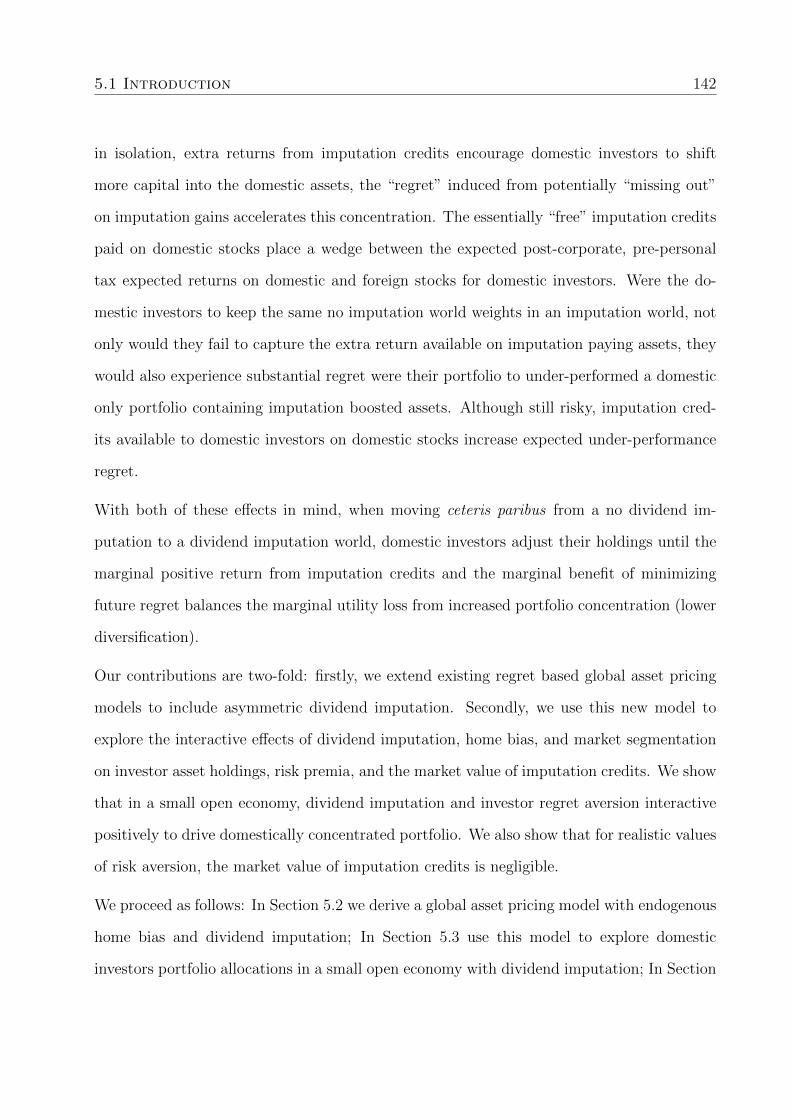
5.1 Introduction 142
in isolation, extra returns from imputation credits encourage domestic investors to shift
more capital into the domestic assets, the “regret” induced from potentially “missing out”
on imputation gains accelerates this concentration. The essentially “free” imputation credits
paid on domestic stocks place a wedge between the expected post-corporate, pre-personal
tax expected returns on domestic and foreign stocks for domestic investors. Were the do-
mestic investors to keep the same no imputation world weights in an imputation world, not
only would they fail to capture the extra return available on imputation paying assets, they
would also experience substantial regret were their portfolio to under-performed a domestic
only portfolio containing imputation boosted assets. Although still risky, imputation cred-
its available to domestic investors on domestic stocks increase expected under-performance
regret.
With both of these effects in mind, when moving ceteris paribus from a no dividend im-
putation to a dividend imputation world, domestic investors adjust their holdings until the
marginal positive return from imputation credits and the marginal benefit of minimizing
future regret balances the marginal utility loss from increased portfolio concentration (lower
diversification).
Our contributions are two-fold: firstly, we extend existing regret based global asset pricing
models to include asymmetric dividend imputation. Secondly, we use this new model to
explore the interactive effects of dividend imputation, home bias, and market segmentation
on investor asset holdings, risk premia, and the market value of imputation credits. We show
that in a small open economy, dividend imputation and investor regret aversion interactive
positively to drive domestically concentrated portfolio. We also show that for realistic values
of risk aversion, the market value of imputation credits is negligible.
We proceed as follows: In Section 5.2 we derive a global asset pricing model with endogenous
home bias and dividend imputation; In Section 5.3 use this model to explore domestic
investors portfolio allocations in a small open economy with dividend imputation; In Section

5.2 The Model 143
5.4 we investigate the equilibrium value of imputation credits in a small open economy; We
conclude in Section 5.5.
5.2 The Model
We consider two economies: a domestic economy D and a foreign economy F .8 Resident
domestic investors receive an imputation benefit in the form of a fixed tax rebate when
they invest in domestic assets. Non-resident foreign investors receive no imputation benefits,
regardless of which assets they hold. Investors are free to short sell any asset with full use
of the proceeds but they must pay the imputation tax rebate when they short imputation
eligible domestic assets.
We assume all investors experience regret when their portfolio’s ex-post return underperforms
a benchmark “status quo” portfolio. Each investor’s status quo portfolio is the mean-variance
optimal portfolio restricted to home economy assets. Investors are “regret averse” and seek
a portfolio that simultaneously maximizes their expected portfolio return while minimizing
their expected future regret. We assume that an investor’s level of expected regret is a
concave function of the difference between the utility of their chosen portfolio and the utility
of their status quo benchmark portfolio. Every investor’s utility function takes the form
(Bell, 1983)
U(cA, cB) = u(cA) + f(u(cA)− u(cB)), (5.1)
where u(c) and f(c) are standard von Neumann-Morgenstern utility functions and U(cA, cB)
is the utility resulting from achieving an end-of-period payoff of cA knowing that a payoff of
cB was otherwise achievable.
The regret portion of each investor’s utility function reflects the “happiness” experienced by
the investor knowing they have minimized expected future regret. Ordinarily, an investor’s
8We consider the domestic economy to be small and capital constrained, and the foreign economy as “therest of the world.”

5.2 The Model 144
expected utility from holding a well diversified portfolio will be greater than that of a portfolio
comprising only assets from that investor’s home economy. With regret utility, however,
investors adjust their portfolio weights to both maximize their direct expected return, but
also the expected difference between their direct expected return and the expected return
on a status quo local-economy-only portfolio. Thus the “regret” component of the utility
function reflects the utility derived from maximizing portfolio returns while simultaneously
minimizing expected future regret from under-performing a local-economy-only portfolio.
We assume investors exhibit constant relative risk aversion, where investor k’s utility function
uk(c):
uk(c) =(c)1−γk
1− γk(5.2)
with investor specific risk aversion γk.
Because the argument to the investor’s regret utility function can be positive or negative,
we assume the regret portion of their utility functions has exponential form:
fk(c) =1− exp(−akc)
ak(5.3)
for ak 6= 0 and fk(c) = c for ak = 0, with regret aversion coefficient ak. There is scant
empirical guidance on the form of equity investor’s regret utility function, however as long
as it’s convex it will have the desired effect. We have solved our model with both exponential
and power utility functions and the difference is negligible.
For example, consider a one period world containing a single investor deciding between
investing in a domestic or a foreign asset. In this case, we assume the assets are indivisible
and the investors is deciding between a 100% investment in the domestic asset or a 100%
investment in the foreign asset. We also assume there are only two possible future states of
the world: A and B. In state A the domestic asset has a payoff of 110 units of utility while
the foreign asset has a payoff of 90. In the B state, the outcomes are reversed: the domestic

5.2 The Model 145
and foreign assets payoff 90 and 110 units respectively. The investor makes an investment at
time zero that maximizes their expected utility. We assume that state A occurs with a 25%
probability and state B with a 75% probability; that is, the state of the world where the
domestic asset pays out more than the foreign asset is less likely compared with the opposite
outcome.
When investors have vanilla utility functions (no consideration of regret), then the investor’s
expected utility for buying and holding the domestic asset is
E[U(domestic asset no regret)] = 0.25× 110 + 0.75× 90 = 95 (5.4)
and the foreign asset
E[U(foreign asset no regret)] = 0.25× 90 + 0.75× 110 = 105. (5.5)
In this case, the investor will preference holding the foreign asset since it offers the higher
expected utility.
Now consider the case where the investor suffers regret if their chosen asset underperforms
their “status quo” asset: in this case, the domestic asset. That is, if the investor buys the
foreign asset and the world ends up in state A, where this foreign asset underperforms, then
they will experience regret for having not chosen the domestic asset instead. Assuming the
investor has regret aversion a = 0.15, then their expected utility from holding the domestic
asset is unchanged (because they won’t suffer any regret) while their expected utility from
holding the foreign asset is
E[U(foreign asset with regret)] = 0.25× (90 + f(90− 110)) + (5.6)
0.75× (110 + f(110− 90)) , (5.7)
= 77.94, (5.8)

5.2 The Model 146
where f(c) is defined in Equation (5.3). Now, once the investor takes into account potential
regret, they preference the domestic asset over the foreign asset. This mechanism of investors
shifting their portfolio allocations to minimize future regret produces a natural home bias.
From this point onwards, we assume that a single risk-free asset and two risky assets trade
within two economies. The first and second risky assets are domiciled in the domestic and
foreign economies respectively. For simplicity, we assume that each asset represents the
entire market portfolio for its economy of domicile, avoiding the need to model a universe
of individual assets. This allows the numerical optimization problem of finding the market
equilibrium to be tractable, with a minimal loss of generality.
Two risk averse investors, one from the domestic and the other from the foreign economy,
make single period investment decision. Each investor k ∈ {D,F} allocates their initial
wealth W 0k among the risk-free and risky assets to maximize their expected end-of-period
utility. We assume investors hold homogeneous expectations regarding the ex-ante distribu-
tion of risky asset returns R; that is, all investors believe expected returns are E [R] = r
with covariance structure E[RTR
]= Σ.
The domestic economy implements an imputation taxation system where domestic investors
receive tax credits for already-paid corporate tax. We model these tax credits as a fixed
additional return received on domestic holdings by domestic investors and a loss suffered by
any investor who shorts imputation paying assets.
Securities lending agreements typically require investors that short sell imputation eligible
shares to make good their security lenders the full value of imputation credits. This compen-
sation is required regardless of whether the lender would have been able to derive value from
the credits had they not lent out their shares. This asymmetry impacts both domestic and
foreign investors who short sell domestic assets. Stulz (1981) demonstrated that not taking
into account such asymmetric tax effects when modeling international asset pricing gener-
ates pathological investor behaviour. Wood (1997) incorporates such an effect into a model
5.2 The Model 147
with imputation credits and finds that an asymmetric tax effect causes foreign investors to
sometimes hold no domestic assets.
To accommodate the asymmetric effect of imputation credits, we split investor’s portfolio
weights into a long component xk and a short component yk, such that an investor k’s net
portfolio weights are xk − yk. These weights must be weakly positive; that is, xk ≥ 0 and
yk ≥ 0. For example if the domestic investor D allocates 150% of his initial wealth to the
domestic asset and shorts the foreign asset equivalent to 50% of his wealth, then
xD = [ 1.5, 0 ]T ,
yD = [ 0, 0.5 ]T ,
(5.9)
where the domestic investors net portfolio weights are xD − xF = [ 1.5,−0.5 ]T .
Dividend imputation generates an additional τ fixed return on domestic assets. We define
two “tax vectors” for each investor: the short tax vector τSk and the long tax vector τLk . The
short tax vector defines the loss each investor suffers from going short in each asset. Because
both domestic D and foreign F investors are penalized for shorting imputation paying assets,
their short tax vectors are identical and equal to
τSD = τSF = [ τ, 0 ]T . (5.10)
The first element of these vectors τSD and τSF is the prevailing imputation tax rate on the
domestic asset, as that’s the penalty for shorting imputation paying assets. Because the
foreign asset doesn’t pay imputation benefits the second element of both vectors is zero.
Only the domestic investor receives a benefit (we consider a benefit a “negative tax”) from
going long domestic assets, so their long tax vector is
τLD = [−τ, 0 ]T , (5.11)

5.2 The Model 148
while foreign investors receive no benefits, therefore their long tax vector is
τLF = [ 0, 0 ]T . (5.12)
Each investor’s after-company tax, but before-personal tax, end-of-period wealth as a func-
tion of long xk and short yk asset holdings is
W 1k (xk,yk) = W 0
k
(1 + (xk − yk)
TR− (xkτLk + ykτ
Sk ) + (1− (xk − yk)
T1)R0
), (5.13)
where R ∼ N(r,Σ) is the vector of asset returns prior to taking the expectation, R0 the
risk-free return and 1 is a column vector of ones. Breaking down (5.13), the
(xk − yk)TR
expression is the return the investor receives from the assets at the end of the period as
terminal dividends,
(xkτLk + ykτ
Sk )
is the gain or loss from imputation on long and short positions,9 and
(1− (xk − yk)T1)R0
is the return from the investor’s remaining wealth invested in the risk-free asset.
The risk-free asset trades with unlimited supply and risky assets are in net positive supply
9We choose the imputation benefit to be independent from realized stock returns (i.e. we don’t multiply(xkτ
Lk +ykτ
Sk ) by R). This assumption is consistent with firms paying stable dividends but returning volatile
capital gains.

5.2 The Model 149
M = [mD,mF ]T . The global market is in equilibrium when supply meets demand
M =∑k∈D,F
W 0kxk. (5.14)
Each investor’s end-of-period utility is then
Uk(W 1k (xk,yk),W
1k (zk, 0)
)= vk(W 1
k (xk,yk)) + fk(vk(W 1
k (xk,yk))− vk(W 1k (zk, 0))
),
(5.15)
where zk is the portfolio weights of investor k’s status quo portfolio. In a simpler formulation,
Solnik and Zuo (2012) set each investor’s status quo portfolio zk to a portfolio containing only
assets domiciled in that investor’s home economy. We take a slightly different approach and
set each investor’s status quo portfolio to the optimal mean-variance portfolio constrained
to the investor’s home economy assets. This means the investor suffers regret when their
investment outcome underperforms an optimal portfolio comprising home economy assets
and the risk-free asset, rather than simply 100% home economy assets.
We use the two moment approximation described by Pratt (1964) and expand vk(W 1k ) around
W 0k and fk(u) around zero using a Taylor series before taking the expectation. We provide
the detailed derivation now.
Rearranging (5.13) slightly
W 1k (xk,yk) = W 0
k (1 +R0) +W 0k
((xk − yk)
T (R− 1R0)− (xkτLk + ykτ
Sk )). (5.16)
Note that W 1k is a random variable (as a function of R); we have not yet taken the expectation
over the asset process.
For our sample scenario in this paper we assume that N = 2 and K = 2 such that for
the domestic investor zD = [1, 0]T and the foreign investor zF = [0, 1]T . Investor k’s utility

5.2 The Model 150
function is then
Uk(xk,yk, zk) = u(W 1k (xk,yk)
)+ fk
(u(W 1
k (xk,yk))− u(W 1k (zk, 0))
), (5.17)
where u(c) and f(c) are the return and regret utility functions defined in equations (5.2)
and (5.3) respectively. We expand u(c) around W 0k and f(c) around 0 to second order using
a Taylor series expansion. That is, from this point on, the implicit argument for u, u′, and
u′′ is W 0k and for f, f ′, and f ′′ is 0. Substituting these expanded utility functions into (5.17)
gives
Uk(xk,yk, zk) ≈ u+ u′W 1k (xk,yk) +
u′′
2W 1k (xk,yk)
2
+ f + f ′[u′(W 1k (xk,yk)−W 1
k (zk, 0))
+u′′
2
(W 1k (xk,yk)
2 −W 1k (zk, 0)2
)]+f ′′
2
[u′(W 1k (xk,yk)−W 1
k (zk, 0))
+u′′
2
(W 1k (xk,yk)
2 −W 1k (zk, 0)2
)]2
.
(5.18)
We assume that investors are sensitive only to the first two moments of portfolio return, thus
when taking the expectation over the realized asset process we ignore terms of order greater
than E[RTR
]. For simplicity we drop the leading W 0
k (1 + R0) term as it doesn’t alter the
investor’s utility maximization. The expectation of each component in (5.18) is then
E[W 1k (xk,yk)
]= W 0
k
[(xk − yk)
T r− (xkτLk + ykτ
Sk )], (5.19)
E[W 1k (xk,yk)
2]
= (W 0k )2[(xk − yk)
TΣ(xk − yk)
− 2(xkτLk + ykτ
Sk )(xk − yk)
T r
+ (xkτLk + ykτ
Sk )2], (5.20)

5.2 The Model 151
E[W 1k (xk,yk)−W 1
k (zk, 0)]
= W 0k
[(xk − zk − yk)
T r
−((xk − zk)τ
Lk + ykτ
Sk
) ], (5.21)
E[(W 1
k (xk,yk)−W 1k (zk, 0))2
]= (W 0
k )2[(xk − zk − yk)
TΣ(xk − zk − yk)
− 2((xk − zk)τ
Lk + ykτ
Sk
)(xk − zk − yk)
T r
+((xk − zk)τ
Lk + ykτ
Sk
)2], (5.22)
E[W 1k (xk,yk)
2 −W 1k (zk, 0)2
]= (W 0
k )2[A− 2BT r + C
], (5.23)
where A = (xk − yk)TΣ(xk − yk) − zTkΣzk, B = (xkτ
Lk + ykτ
Sk )(xk − yk) − (zkτ
Lk )zk, and
C = (xkτLk + ykτ
Sk )2 − (zkτ
Lk )2.
E[(W 1
k (xk,yk)2 −W 1
k (zk, 0)2)2]
= (W 0k )4[2C(A− 2BT r) + 4BTΣB + C2
],
E[(W 1k (xk,yk)−W 1
k (zk, 0))(W 1k (xk,yk)
2 −W 1k (zk, 0)2
)]= (W 0
k )3[C(xk − zk − yk)
T r
− 2(xk − zk − yk)TΣB
−((xk − zk)τ
Lk + ykτ
Sk
) (A− 2BT r + C
) ].
(5.24)
Finding each investor’s portfolio holdings xk,yk that maximize their expected terminal utility
arg maxxk,yk
E [Uk(xk,yk, zk)] (5.25)
maps onto a constrained non-linear programming problem which we solve numerically using
a standard interior point algorithm (Boyd and Vandenberghe, 2004). 10 We find the global
10Given that we’re solving a a convex optimization problem, a global minimum is guaranteed.
5.2 The Model 152
market equilibrium expected returns r using the Levenberg-Marquardt algorithm (Leven-
berg, 1944; Marquardt, 1963).
Finding the market equilibrium involves solving a sequence of nested optimization problems,
where the top-level problem is to find a vector of asset returns that equilibriates supply and
demand. For each prospective vector of asset returns we solve k portfolio optimization sub-
problems; one for each investor. In effect, each investor observes the prevailing asset return
vector and forms an optimal portfolio that maximizes their personal utility function. Each
investor’s optimal portfolio allocation then reveals their demand for each asset. Summing
over all investor’s demands and subtracting asset supply produces a net supply-demand
imbalance. After each iteration we take this imbalance and calculate the direction we have
to “nudge” asset returns to reduce the supply-demand imbalance. We continue doing this
until the imbalance is sufficiently close to zero (less than 10−6). At this point we have
calculated the market equilibrium.
We solve our model over a range of parameter space to generate stylized comparative statics.
We establish a base case scenario in Table 5.2. The two assets are correlated with correlation
coefficient 0.75 and equal volatilities of 20%. The common risk-free rate is 5% and domestic
assets are 10% of world asset supply. Domestic investors holding assets in the domestic
economy receive a 2% imputation benefit. We assume that the domestic market is a net
importer of capital, and thus domestic investors only hold 9% of world wealth (foreign
investors hold 91%).
Recent estimates of relative risk aversion in the USA (Chiappori and Paiella, 2011) find
median CRRA risk aversion in the population to be 1.7. An analysis in Australia using
older data and statistical techniques (Szpiro, 1986) estimates a lower limit of 2.63. Given
the uncertainty in these estimates, we simply choose a risk-aversion coefficient of 2. There
is no empirical guidance on the value of our regret aversion coefficient. We choose a value
of 0.2 so that the proportion of domestic assets held by domestic investors in our model

5.3 Portfolio Holdings 153
equilibrium matches the empirically observed 60%.
Table 5.2 – Parameters for our two economy scenario. The risk characteristics of bothrisky stocks are symmetric, as is the risk-free rate. The domestic, capital constrained,economy supplies only 10% of world assets and domestic investors hold 9% of worldwealth. For the market to reach equilibrium, foreign capital must be invested in thedomestic economy.
Model Parameter EconomyDomestic Foreign
Risk Free Rate 5% 5%Asset Return Volatilities 20% 20%Asset Return Correlation 0.75 –
Proportion of World Asset Supply 10% 90%
Investor Imputation Benefit 2% 0%Investor Risk Aversion 2 2
Investor Regret Aversion 0.2 0.2Investor Initial Wealth Proportion 9% 91%
5.3 Portfolio Holdings
We first find equilibrium asset returns and investor portfolio weights for a simple case with
regret-neutral11 investors and no imputation benefits. That is, we set regret aversion and
imputation benefits to zero in the base case (Table 5.2) and let our model settle at equi-
librium. With this setup, both domestic and foreign investors hold the “world” portfolio:
simply allocating their wealth in proportion to global asset supply: 10% in the domestic
asset and 90% in the foreign asset. Note that although this base case scenario is largely
symmetric (returns and volatilities are the same across both assets) the difference in asset
supply generates asymmetric equilibrium asset returns: the domestic and foreign assets have
expected returns of 11.2% and 12.8% respectively. This is a result of capital import into
11Investors who are indifferent to experiencing regret.
5.3 Portfolio Holdings 154
the domestic economy as foreign investors bid up the domestic asset price because of its
diversification benefit.
When we adjust investor preferences to be regret-averse, keeping imputation benefits at zero,
our model reduces to that of Solnik and Zuo (2012). They find that the expected return
on an economy’s assets are inversely (positively) related to the degree of home bias (regret
aversion) and support this finding with empirical evidence from the International Monetary
Fund data.
One of our primary interests is exploring the combination effect of imputation and decision
regret on domestic asset holdings; that is, what motivates regret averse domestic investor’s
portfolio allocations when they operate in a world with imputation. Figure 5.1 shows the
domestic investor’s utility for various levels of domestic portfolio concentration. We have
labeled prominent points on this figure and subsequent figures A through L and we refer to
these points as (A), (B), etc throughout this section. We calculate the domestic investor’s
utility when they hold a fixed proportion of their initial wealth in the domestic asset, regard-
less of this fixed portfolio’s optimality. To do this, we fix the domestic investor’s domestic
asset weight and then calculate the market equilibrium, keeping the domestic investor’s asset
weighting and the foreign investor’s portfolio weights unconstrained.
We first investigate a domestic investor’s behaviour in our stylized world with no imputa-
tion. In this scenario, the domestic investor maximizes their utility with a 36% domestic
portfolio concentration (A). Note that this point of maximum utility is neither the point
of risk-aversion maximization (which occurs at 10% concentration) (B) or the maximum of
the ”regret avoidance” portion (occurring at 50%) (C) of their utility function. Without
regret aversion, the investor would have maximized their utility at a much lower domestic
asset concentration. This is exactly the effect we would expect when investors experience
regret about possible alternative portfolio choices. Domestic investors’ status-quo portfolios

5.3 Portfolio Holdings 155
Figure 5.1 – Domestic investor’s utility in an imputation and no-imputation world.The solid lines chart the investor’s total utility while the top and bottom dashedlines breakdown the investor’s utility into the return and regret aversion componentsrespectively.
0 10 20 30 40 50 60 70 80 90 100
−0.3
−0.2
−0.1
0
0.1
0.2
0.3
0.4
0.5
Dom
estic
Inve
stor
Util
ity
Domestic Investor Domestic Asset Holdings (%)
A
B
C
D
E
F
G H
ImputationNo ImputationImputation ReturnNo Imputation ReturnImputation RegretNo Imputation Regret
contain only domestic assets, hence the domestic asset concentration that minimizes ex-
pected future regret (equivalent to maximize happiness from avoiding regret) has a domestic
concentrated portfolio. The investor’s total utility maximization is therefore the balance of
these two forces: domestic investors wish to maximize their diversification benefit, however
they naturally hold a concentrated domestic portfolio to avoid underperformance regret.
Now consider the same domestic investor in a world with imputation. What if they main-
tained their portfolio weights as if they remained in a no-imputation world? By keeping their
no-imputation world optimal weights, their total utility decreases in the imputation world,

5.3 Portfolio Holdings 156
and they no longer hold an optimal portfolio (moving down from (A) to (D)).12 At this
suboptimal point, the domestic investor gains return utility from an unconditional increase
in return from imputation credits (E), however their ”regret avoidance” utility decreases
(F): The positive effect of the increased imputation return (E) is dominated by a lowered
regret avoidance (F).
This lowered regret avoidance results from the asymmetric bump in return on the domestic
asset versus the foreign asset. Introducing imputation ceteris paribus increases the sec-
ond component v(W 1k (zk, 0)) of the domestic investor’s regret aversion f(v(W 1
k (xk,yk)) −
v(W 1k (zk, 0))). Thus to minimize their regret aversion, the domestic investor has to shift
their holdings xk,yk closer to the domestic-only status quo portfolio zk. If they don’t fur-
ther concentrate their holdings in the domestic asset, they will experience future regret when
they failed to capture the value of imputation credits. Imputation also shifts the peak of the
risk-aversion component of the domestic investor’s utility function to higher domestic asset
concentration (From 10% in the no-imputation world to 50% in the imputation world in Fig-
ure 5.1) (G). These two effects interact so that in an imputation world, domestic investors
hold a portfolio heavily weighted towards domestic assets (66% domestic asset concentration)
(H).
The greater an investor’s regret aversion, the greater utility they gain from minimizing their
potential future regret. For example, an investor with high regret aversion gain utility when
their chosen portfolio outperforms their “status quo” home-economy only portfolio. Clearly,
this desire to minimize regret results in investors preferring their home economy assets when
forming their portfolios. We show this relationship in Figure 5.2 (a) and (b) where each
investor’s home asset portfolio allocation is a strictly concave function of regret aversion.
With zero regret aversion and no imputation, all investors simply hold the world portfolio of
10% domestic (I), 90% foreign (J) assets (see left hand side of 5.2 (a) and (b)). Increasing
12Moving from the solid “No Imputation” line to the “Imputation” line in Figure 5.1 at 36% domesticasset concentration

5.3 Portfolio Holdings 157
regret aversion causes investors to shift more wealth into their home economies
When we introduce imputation regret-neutral investors marginally maintain a foreign con-
centrated portfolio (K). However, as regret aversion increases, the investor quickly concen-
trates their portfolio into domestic assets. Increased regret aversion then simply increases
domestic portfolio concentration (Figure 5.2 (a)). Note that with regret-neutral investors,
the foreign investor also holds less of the domestic asset when imputation is introduced (L)
(The difference between the solid and dashed lines in Figure 5.2 (b)). Although imputation
does not directly alter the returns expected by international investors, it does effect the
equilibrium required return on the domestic asset: domestic investors bid up the price of the
domestic asset because of the additional imputation return available to them, hence making
it a less favourable asset for the international investors. Although the expected return is
lower, foreign investors won’t divest from the domestic asset completely, because holding
including it in their portfolio offers diversification benefits.
Note that the marginal effect of imputation on investor asset holdings in Figure 5.2(a) and
(b) decreases as regret aversion increases. That is, as the level of regret aversion increases,
the magnitude of the effect of imputation on portfolio asset holdings decreases. In the limit as
regret aversion approaches infinity we have complete market segmentation where investor’s
economy portfolio allocations are totally indifferent to the presence or absence of dividend
imputation.
We now consider how equilibrium asset returns respond to the introduction of imputation.
Clearly, the introduction of imputation, only usable by domestic investors, drives domestic
investors to shift their wealth to home economy assets. Because of simple supply and demand,
this concentration increases domestic asset prices (lowering expected return). Domestic
investors are willing to give up international diversification benefits for the additional gains
from imputation. Looking at domestic investors in isolation, the effect is obvious, however
once we consider the global market equilibrium, it is not as straight forward. Domestic

5.3 Portfolio Holdings 158
Figure 5.2 – (a) Domestic investor’s portfolio allocations for various levels of regretaversion in imputation (dashed lines) and no-imputation worlds. (solid lines) (b) Foreigninvestor’s portfolio allocations for various levels of regret aversion.
0 0.1 0.2 0.3 0.4 0.5 0.6 0.7 0.8 0.9 10
10
20
30
40
50
60
70
80
90
100
Investor Regret Aversion
Por
tfolio
Wei
ght (
%)
I
J
K
Domestic Weight in Domestic AssetDomestic Weight in Foreign AssetDomestic Weight in Domestic Asset (Imp)Domestic Weight in Foreign Asset (Imp)
(a) Domestic Portfolio Allocation vs. Regret Aversion (Imputation and No-Imputation)
0 0.1 0.2 0.3 0.4 0.5 0.6 0.7 0.8 0.9 10
10
20
30
40
50
60
70
80
90
100
Investor Regret Aversion
Por
tfolio
Wei
ght (
%)
L
I
J
Foreign Weight in Domestic AssetForeign Weight in Foreign AssetForeign Weight in Domestic Asset (Imp)Foreign Weight in Foreign Asset (Imp)
(b) Foreign Portfolio Allocation vs. Regret Aversion

5.3 Portfolio Holdings 159
Figure 5.3 – (a) Equilibrium expected asset returns for various levels of regret aversionin imputation (dashed lines) and no-imputation (solid lines) worlds. (b) Marginal effectof increased investor regret aversion on equilibrium asset return.
0 0.1 0.2 0.3 0.4 0.5 0.6 0.7 0.8 0.9 110
10.5
11
11.5
12
12.5
13
13.5
14
Investor Regret Aversion
Equ
ilibr
ium
Exp
ecte
d A
sset
Ret
urn
(%)
Domestic AssetForeign AssetDomestic Asset (Imp)Foreign Asset (Imp)
(a) Equilibrium Asset Return vs. Regret Aversion
0 0.1 0.2 0.3 0.4 0.5 0.6 0.7 0.8 0.9 1−0.1
0
0.1
0.2
0.3
0.4
0.5
0.6
0.7
0.8
Investor Regret Aversion
Mar
gina
l Effe
ct o
f Reg
ret A
vers
ion
on A
sset
Ret
urn
(%)
Domestic AssetForeign AssetDomestic Asset (Imp)Foreign Asset (Imp)
(b) Marginal Asset Return vs. Regret Aversion (partial derivative ∂r∂a)
5.3 Portfolio Holdings 160
capital shifting into domestic stocks and boosting their prices makes them less favourable
for international investors, who can shift capital back into foreign assets to displace the
outflow of domestic investment.
Supporting this intuition, we find that imputation decreases the required return on domestic
economy assets (see Figure 5.3 (a)): In a regret-averse world, introducing imputation ceteris
paribus lowers the required return on domestic assets (more demand for domestic assets)
which raises the required return on foreign assets (lower demand for foreign assets).
We describe the marginal effect of regret aversion on expected asset returns in Figure 5.3 (b).
In the no-imputation world, asset returns are much more sensitive to investor regret aversion.
Consider starting in a no-imputation, regret-neutral world where every investor holds the
world market portfolio (there are no forces acting on the investors to not fully diversify).
Now, slightly increase investors’ regret aversions. This change breaks the model symmetry
and pushes foreign investors to slightly favour foreign stocks, and domestic investors to
slightly favour domestic stocks. Increasing investors’ regret aversion further continues this
trend, yet with a lesser effect. This is why the marginal effect of increasing regret aversion
on asset returns is decreasing in 5.3 (b). Note that once imputation is introduced, domestic
investors have already concentrated their portfolios to capture imputation credits, thus the
marginal effect of increasing regret aversion on asset returns is lower in the imputation world.
Our main finding here is that in a small open economy, dividend imputation and regret
aversion positively interact to drive domestic investors to hold highly concentrated domestic
portfolios. Dividend imputation by itself has an insufficient effect to generate the domestic
concentration we empirically observe in Australia, however the magnification of imputation’s
portfolio effects by regret averse investors scared of “missing out on the tax benefits of
imputation credits” does generate observed levels of domestic portfolio concentration. Under
the assumption that Australian individual and institutional investors are vulnerable to the
status quo and endowment behavioural biases, and that regret aversion is a valid reduced

5.4 Equilibrium Value of Franking Credits 161
form model of these biases, we believe the level of domestic asset concentration in Australia
results from the positive interaction of these behavioural biases with dividend imputation.
5.4 Equilibrium Value of Franking Credits
In an imputation taxation system, a proportion of company tax paid by a firm is rebated by
imputation eligible investors against their personal taxes: In effect, corporate tax rebated
using imputation credits is a pre-collection of personal taxes. Officer (1994) labeled the
proportion of company tax rebated as personal tax by the marginal investor as “gamma”
γ: “γ is the proportion of tax collected from the company that gives rise to the tax credit
associated with a franked dividend.” Note that there is no agreement on who exactly the
“marginal investor” is in the Australian market.
Another measure of franking credits is the imputed market value of one dollar of imputation
credits φ. There is a subtle distinction between γ and φ, but the two are equal γ = φ if and
only if an imputation paying firm distributes 100% of its domestic profits. In our one period
model, we assume that all domestic assets distribute all of their net profits as dividends.
Under these conditions, the value of one dollar of distributed imputation credits and the
proportion of tax giving rise to personal tax rebates are equivalent.
Let rNID be the equilibrium expected return of the domestic stock in a world with no imputa-
tion and rID the domestic stock’s equilibrium expected return when imputation is introduced
ceteris paribus. That is, given a set of model parameters, we solve for the market equilibrium
with no-imputation and record the domestic stock’s expected return. We then re-solve our
model with the same parameters but with dividend imputation and record the new expected
return on the domestic stock.
The debate over the correct value of γ revolves around how much of the face value of
imputation credits incorporated into asset prices. If we assume that domestic investors

5.4 Equilibrium Value of Franking Credits 162
always bid up the domestic stock’s price such that the required return on the domestic stock
reduces to offset the additional return available from franking credits, we would expect
rID = rNID + τD, (5.26)
where τD is the pre-personal tax advantage of imputation credits.
For a small open domestic economy operating in a global environment where domestic in-
vestors can, and foreign investors cannot, utilize the imputation benefit, we would expect
only a fraction of the imputation credit’s face value to be imputed into the stock’s price, and
thus
rID = rNID + γ τD, (5.27)
where γ is the amount, as a proportion of the franking credit, the marginal investor is willing
to pay for a dollar of franking credits. When γ = 1, the entire value of the franking credit is
imputed into stock prices and where γ = 0 the marginal shareholder attributes no value to
franking credits.
For example, consider a world where we can turn imputation on-and-off at will, observing
equilibrium expected asset returns before and after each toggling of imputation. Within
this illustrative example when imputation is turned off, assume that we observe an asset’s
expected return to be 15%. We then introduce an imputation benefit of 2% on this asset,
and let the market reach an equilibrium. Again, assume at equilibrium we observe the asset’s
new expected return is 15.5%, an increase of 50 basis points. Rearranging equation (5.27)
for γ and letting rID = 0.155, rNID = 0.15, and τD = 0.02, we have γ = 0.25. Therefore, in
this example, the equilibrium value of imputation credits is 25% of their face value.
The value of gamma is highly dependent on investor risk aversion. This is because of the
trade-off domestic investors make between capturing additional returns from imputation
credits versus increasing their portfolio concentration (lower portfolio diversification). If the

5.4 Equilibrium Value of Franking Credits 163
investor’s risk aversion is low, then they don’t value diversification benefits as much and
when imputation is introduced ceteris paribus, domestic investors will be more willing to
shift their wealth to imputation paying assets.
At the extreme when investors are risk neutral, the full value of imputation credits are
factored into asset prices (see the far left hand side of Figure 5.4). Being totally indifferent
to risk, risk neutral investors don’t care about portfolio diversification, only about expected
portfolio returns. Thus, in the risk neutral case, domestic investors abandon other stocks
and load up as much as they can in imputation paying stocks, shorting foreign stocks if
necessary.
The only other situation where gamma trends towards one is in the limit as asset correlations
all approach unity. In this case, there’s no benefit from diversification, so domestic investors
bid up domestic stock by the full amount of the imputation benefit.
The shift in slope in Figure 5.4 at the 0.9–1.1 risk aversion mark is the level of risk aversion
where domestic investors bid up the price of domestic assets so much that foreign investors
no longer wish to hold domestic stocks. That is, the marginal benefit from diversification
into foreign stocks is less than the marginal gain over shifting holdings into the foreign
assets. Because all investors must make good on distributed imputation credits when they
short stocks in the imputation paying domestic economy, foreign investors tend to hold no
domestic assets when it’s favourable to do so.13 This effect is visible in Figures 5.5 and 5.6
where foreign investors gradually decrease their wealth allocation in the domestic market
until a risk aversion of 0.9, where it’s better to not hold any imputation paying assets. Note
that in Figure 5.6(a) domestic investors hold 9% of world wealth, but the domestic market
provides 10% of asset supply. In this case, once foreign investors no longer find it viable
to buy domestic stocks, the domestic investor borrows the risk-free asset and loads up on
the domestic asset (hence the domestic investor’s weight in the domestic asset being greater
13In models without this asymmetric feature, the foreign investors tend to pathologically short the domesticasset while the domestic investors go massively long.

5.4 Equilibrium Value of Franking Credits 164
than 110%).
Figure 5.4 – Market value of imputation credits (γ) for various levels of risk aversionand domestic investor wealth proportions.
0 0.2 0.4 0.6 0.8 1 1.2 1.4 1.6 1.8 20
0.1
0.2
0.3
0.4
0.5
0.6
0.7
0.8
0.9
1
Investor Risk Aversion
Gam
ma
Domestic Wealth Proportion = 90%Domestic Wealth Proportion = 50%Domestic Wealth Proportion = 10%
For a fixed level of investor risk aversion, the value of gamma is fairly insensitive to the level
of imputation benefit and regret aversion. Figure 5.7 describes gamma for various levels of
imputation benefit and regret aversion. Interestingly, gamma is negatively related to the
size of the imputation benefit domestic investors receive on domestic assets when investors
are regret-neutral. At higher levels of regret aversion, this effect is reversed, and gamma is
positively related to the level of imputation benefit.
With regret-neutral investors (zero regret aversion) some initial imputation benefit will cause
domestic investors to bid up the price of the domestic stock. Each additional percentage point
of imputation benefit thereafter increases domestic portfolio concentration and increases
domestic stock prices, however the marginal effect is decreasing in level of imputation benefit.
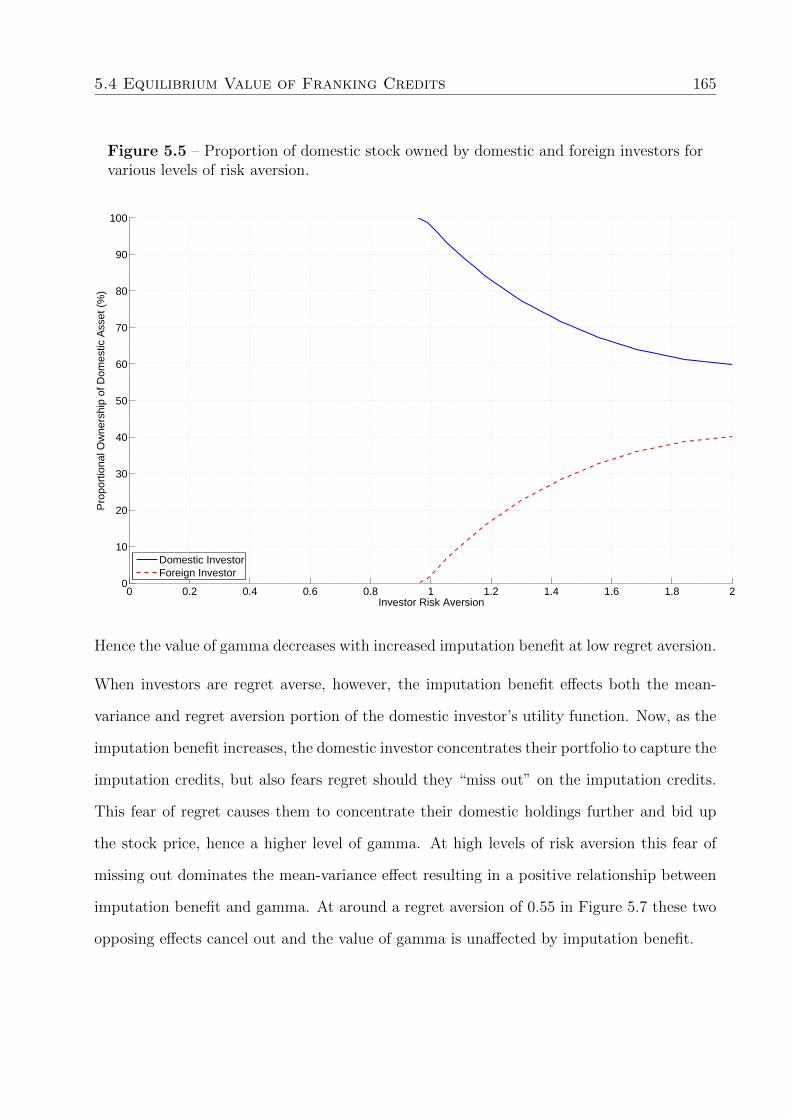
5.4 Equilibrium Value of Franking Credits 165
Figure 5.5 – Proportion of domestic stock owned by domestic and foreign investors forvarious levels of risk aversion.
0 0.2 0.4 0.6 0.8 1 1.2 1.4 1.6 1.8 20
10
20
30
40
50
60
70
80
90
100
Pro
port
iona
l Ow
ners
hip
of D
omes
tic A
sset
(%
)
Investor Risk Aversion
Domestic InvestorForeign Investor
Hence the value of gamma decreases with increased imputation benefit at low regret aversion.
When investors are regret averse, however, the imputation benefit effects both the mean-
variance and regret aversion portion of the domestic investor’s utility function. Now, as the
imputation benefit increases, the domestic investor concentrates their portfolio to capture the
imputation credits, but also fears regret should they “miss out” on the imputation credits.
This fear of regret causes them to concentrate their domestic holdings further and bid up
the stock price, hence a higher level of gamma. At high levels of risk aversion this fear of
missing out dominates the mean-variance effect resulting in a positive relationship between
imputation benefit and gamma. At around a regret aversion of 0.55 in Figure 5.7 these two
opposing effects cancel out and the value of gamma is unaffected by imputation benefit.

5.4 Equilibrium Value of Franking Credits 166
Figure 5.6 – (a) Domestic and (b) Foreign investor’s portfolio weights for varying riskaversion.
0 0.2 0.4 0.6 0.8 1 1.2 1.4 1.6 1.8 20
20
40
60
80
100
120
Investor Risk Aversion
Por
tfolio
Wei
ghts
(%
)
Domestic Investor’s Domestic WeightsDomestic Investor’s Foreign Weights
(a) Domestic Investor’s Portfolio Weights
0 0.2 0.4 0.6 0.8 1 1.2 1.4 1.6 1.8 20
10
20
30
40
50
60
70
80
90
100
Investor Risk Aversion
Por
tfolio
Wei
ghts
(%
)
Foreign Investor’s Domestic WeightsForeign Investor’s Foreign Weights
(b) Foreign Investor’s Portfolio Weights

5.4 Equilibrium Value of Franking Credits 167
Figure 5.7 – Equilibrium value of imputation credits “gamma” for various levels ofregret aversion and imputation benefit.
0 0.1 0.2 0.3 0.4 0.5 0.6 0.7 0.8 0.9 10.03
0.035
0.04
0.045
0.05
0.055
0.06
0.065
0.07
0.075
Investor Regret Aversion
Gam
ma
Imputation Benefit 1%Imputation Benefit 2%Imputation Benefit 3%Imputation Benefit 4%Imputation Benefit 5%

5.5 Conclusion 168
5.5 Conclusion
We develop and solve a new global asset pricing model for a small open economy (Australia)
with dividend imputation and home bias. In our model, domestic investors who buy do-
mestic assets receive an additional return from imputation, foreign investors are imputation
ineligible and receive nothing. Rather than relying on explicit barriers to cross-country in-
vestment, we assume that all investors are subject to the status quo and endowment effect
behavioural biases. There biases drive investors to favour assets from their home economies.
We demonstrate that these behavioural effects interact with dividend imputation to create a
situation where domestic investors hold highly concentrated domestic asset portfolios. This
behaviour is in alignment with observed domestic holdings data, where domestic Australian
investors allocate 70%+ of their equity holdings in Australian stocks.
We also identify that investor risk aversion is the primary determinant of the market value
of imputation credits. In forming their portfolios, domestic investors trade off the positive
benefit of imputation credits against the negative effect of further concentrating their port-
folios into domestic assets. Risk-neutral domestic investors, unconcerned with diversification
benefits, will fully concentrate their portfolios in domestic assets, fully pricing imputation
credits. At more realistic levels of risk aversion, however, the equilibrium value of imputation
credits are negligible.
The Henry tax review14 suggested that as Australia becomes more globally integrated, the
positive benefits of dividend imputation to Australian corporations will become negligible.
We support this view by demonstrating that, although dividend imputation causes domestic
investors to concentrate their holdings in domestic assets, their relative wealth in comparison
with the rest of the world results in foreign investors being the marginal price setters. Thus,
the cost of equity capital in the small open economy that is Australia is primarily set by
14Australia’s future tax system, Report to the Treasurer, December 2009.

5.5 Conclusion 169
foreign investors seeking diversification benefits in the Australian market.

6Thesis Conclusion
In this thesis I have derived and solved three novel financial models in order to address the
following corporate finance questions:
1. What is a limited liability firm’s optimal voluntary liquidation policy?
2. Do Australia insolvent trading laws produce economically optimal outcomes? and,
3. Are imputation credits fully valued in a small open economy?
I conclude this thesis by summarizing my contributions to the literature.
170
171
I have built a novel model of optimal voluntary liquidation for a limited liability firm that
focuses on using observable accounting variables where possible. My model is a continuous
time interpretation of the fundamental accounting equation. Given a set of firm-specific
parameters, my model calculates a firm’s optimal voluntary liquidation policy as well as
its equity value. As far as I am aware, this is the first contingent claim pricing model for
equity values that comprises an Asian-American style down-and-out call on net earnings. I
have identified that earnings volatility, expected liquidation costs, expected earnings, rates
of asset depreciation, and the firm’s cost of debt are the variables that most influence the
voluntary liquidation decision. From an agency cost perspective I have identified scenarios
where equityholder and manager incentives, with respect to voluntary liquidation, both align
and conflict.
My optimal voluntary liquidation model has a number of features that makes it challenging
to solve numerically: it is two-dimensional; the boundary conditions introduce sharp dis-
continuities; it has cross-term operators due to correlations between processes; and it has
an early-exercise condition in the form of voluntary liquidation. This makes the governing
stochastic differential equation and its related partial differential equation unique, with my
solution to it requiring a novel combination of numerical solution techniques. The early
exercise nature of voluntary liquidation requires a computationally intensive specialized ma-
trix inversion method called projected successive overrelaxation (PSOR). By exploiting the
memory hierarchy of modern CPUs, I was able to write a novel algorithm that decreased
the run-time of PSOR by four orders of magnitude: a 10,000 fold decrease in computation
time in comparison with standard sparse matrix linear algebra routines. This reduced the
calculation time for my first essay from 1 year down to 28 minutes.
To explore the optimality of Australia’s insolvent trading laws, I have derived and solved
the first economic model of director behaviour within Australia’s insolvency framework. I
incorporate both insolvent trading laws and voluntary administration. My model addresses
a long standing absence in the literature of quantitative insolvency models targeting the

172
Australian context. I show that my model replicates observed director behaviour. I also
apply my model to analyze a proposed modification to the insolvency laws (a reserving rule
allowing creditors to voluntarily opt out of the right to purse insolvency trading litigation)
demonstrating that the value added for creditors via the rule change is negligible. I hope that
my model can be used as a quantitative tool in upcoming discussions regarding Australian
insolvency law reform.
To value dividend imputation credits, I have extended an existing regret based asset pricing
model to incorporate dividend imputation. Previous models of dividend imputation in Aus-
tralia have either treated Australia as a completely integrated (zero investment barriers) or a
completely segmented economy (infinite investment barriers). The reality is that Australia is
a small open economy that is partially integrated, containing domestic investors who exhibit
a strong home bias. My model is the first to combine endogenous home bias effects (induced
by behavioural biases) with dividend imputation. I find that dividend imputation and be-
havioural biases such as the status quo and endowment biases interact positively to create
the strong home bias observed in Australia. For realistic parameter values I demonstrate
that the equilibrium value of imputation credits is small. This finding has important impli-
cations for regulated Australian companies, whose regulated return on assets is adjusted for
imputation effects.
Although it is impossible to perfectly solve these corporate finance problems, given they are
largely driven by unpredictable human behaviour, forging ahead with quantitative techniques
at least brings us a step closer to the truth. Just as I have built these three new models
inspired by the works of past authors, I hope that future authors will be able to derive equal
inspiration from my models.
References
Agliardi, E., and R. Agliardi (2008): “Progressive taxation and corporate liquidation
policy,” Economic Modelling, 25(3), 532–541.
AıtSahalia, Y. (2002): “Maximum likelihood estimation of discretely sampled diffusions:
A closedform approximation approach,” Econometrica, 70(1), 223–262.
Akhigbe, A., and J. Madura (1996): “Intraindustry effects of voluntary corporate liqui-
dations,” Journal of Business Finance and Accounting, 23(7), 915–930.
Alcock, J., F. Finn, and K. Tan (2012): “The determinants of debt maturity in Aus-
tralian firms,” Accounting and Finance, 52(2), 313–341.
Amihud, Y., and H. Mendelson (2000): “The Liquidity Route to a Lower Cost of
Capital,” Journal of Applied Corporate Finance, 12, 8–26.
Anderson, R., and A. Carverhill (2011): “Corporate liquidity and capital structure,”
Review of Financial Studies, 25(3), 797–837.
Anderson, R., and S. Sundaresan (1996): “Design and valuation of debt contracts,”
Review of Financial Studies, 9(1), 37–68.
173

References 174
Annabi, A., M. Breton, and P. Francois (2010): “Resolution of financial distress
under Chapter 11,” .
Apabhai, M., N. Georgikopoulos, D. Hasnip, R. Jamie, M. Kim, and P. Wilmott
(1997): “A model for the value of a business, some optimization problems in its operating
procedures and the valuation of its debt,” IMA Journal of Applied Mathematics, 59(3),
273–285.
Arora, S., B. Barak, and M. Brunnermeier (2011): “Computational complexity
and information asymmetry in financial products,” Communications of the ACM, 54(5),
101–107.
Australian Securities and Investments Commission (2012): “ASIC enforcement
outcomes: July to December 2011,” Discussion Paper July 2011.
Baker, H. K., and J. R. Nofsinger (2002): “Psychological Biases of Investors,” Finan-
cial Services Review, 11(JANUARY), 97–116.
Balcaen, S., J. Buyze, and H. Ooghe (2009): “Financial distress and firm exit: Deter-
minants of involuntary exits, voluntary liquidations and restructuring exits,” .
Bao, J., J. Pan, and J. Wang (2011): “The illiquidity of corporate bonds,” Journal of
Finance, 66(3), 911–946.
Bates, T., K. Kahle, and R. Stulz (2009): “Why do US firms hold so much more cash
than they used to?,” Journal of Finance, 64(5), 1985–2021.
Bell, D. (1983): “Risk premiums for decision regret,” Management Science, 29(10), 1156–
1166.
Berger, P., E. Ofek, and I. Swary (1996): “Investor valuation of the abandonment
option,” Journal of Financial Economics, 42(2), 257–287.

References 175
Black, F., and J. Cox (1976): “Valuing corporate securities: Some effects of bond inden-
ture provisions,” Journal of Finance, 31(2), 351–367.
Black, F., and M. Scholes (1973): “The pricing of options and corporate liabilities,”
The Journal of Political Economy, 81(3), 637–654.
Boyd, S., and L. Vandenberghe (2004): Convex optimization. Cambridge University
Press, Cambridge.
Boyle, P., and A. Potapchik (2008): “Prices and sensitivities of Asian options: A
survey,” Insurance: Mathematics and Economics, 42(1), 189–211.
Bradley, M., and M. Roberts (2004): “The structure and pricing of corporate debt
covenants,” .
Bris, A., I. Welch, and N. Zhu (2006): “The costs of bankruptcy: Chapter 7 liquidation
versus Chapter 11 reorganization,” The Journal of Finance, 61(3), 1253–1303.
Broadie, M., M. Chernov, and S. Sundaresan (2007): “Optimal debt and equity
values in the presence of Chapter 7 and Chapter 11,” Journal of Finance, 62(3), 1341–
1377.
Brogaard, J., T. Hendershott, and R. Riordan (2014): “High-frequency trading
and price discovery,” Review of Financial Studies, 27(206), 2267–2306.
Bruche, M. (2011): “Creditor coordination, liquidation timing, and debt valuation,” Jour-
nal of Financial and Quantitative Analysis, 46(5), 1407–1436.
Bruche, M., and H. Naqvi (2010): “A structural model of debt pricing with creditor-
determined liquidation,” Journal of Economic Dynamics and Control, 34(5), 951–967.
Cannavan, D., F. Finn, and S. Gray (2004): “The value of dividend imputation tax
credits in Australia,” Journal of Financial Economics, 73(1), 167–197.

References 176
Chang, C., and Y. Wang (1992): “Optimal liquidation rule and debt in the principal-
agent model,” Economics Letters, 40(1), 23–26.
Chen, L., D. Lesmond, and J. Wei (2007): “Corporate yield spreads and bond liquidity,”
Journal of Finance, 62(1), 119–149.
Chiang, R., I. Davidson, and J. Okunev (1997): “Some further theoretical and empiri-
cal implications regarding the relationship between earnings, dividends and stock prices,”
Journal of Banking and Finance, 21(1997), 17–35.
Chiappori, P., and M. Paiella (2011): “Relative risk aversion Is constant: Evidence
from panel data,” Journal of the European Economic Association, 9(6), 1021–1052.
Coburn, N. (2000): “Insolvent trading in Australia: The legal principles,” in Company
Directors’ Liability for Insolvent Trading, ed. by I. M. Ramsay, pp. 73–128.
Cox, J., S. Ross, and M. Rubinstein (1979): “Option pricing: A simplified approach,”
Journal of Financial Economics, 7(3), 229–263.
Crank, J. (1987): Free and Moving Boundary Problems. Oxford University Press, USA.
Cryer, C. (1971): “The solution of a quadratic programming problem using systematic
overrelaxation,” SIAM Journal on Control, 9(3), 385–392.
Custodio, C., M. Ferreira, and L. Laureano (2013): “Why are US firms using more
short-term debt?,” Journal of Financial Economics, 108(1), 182–212.
Dabner, J. (1994): “Trading while insolvent: A case for individual creditor rights,” Uni-
versity of New South Wales Law Journal, 17(2), 546–576.
Davydenko, S., and M. Rahaman (2008): “Excessive continuation and the costs of
flexibility in financial distress,” .
References 177
DeAngelo, H., L. DeAngelo, and K. Wruck (2002): “Asset liquidity, debt covenants,
and managerial discretion in financial distress: The collapse of LA Gear,” Journal of
Financial Economics, 64(1), 3–34.
Dempsey, M., and G. Partington (2008): “Cost of capital equations under the Aus-
tralian imputation tax system,” Accounting and Finance, 48(September 2004), 439–460.
Dichev, I., and V. Tang (2009): “Earnings volatility and earnings predictability,” Journal
of Accounting and Economics, 47(1), 160–181.
Duffy, D. (2006): Finite difference methods in financial engineering: a Partial Differential
Equation approach. Wiley, 1st edn.
Dunne, T., M. Roberts, and L. Samuelson (1988): “Patterns of firm entry and exit
in US manufacturing industries,” The RAND Journal of Economics, 19(4), 495–515.
Elliott, C., and J. Ockendon (1982): Weak and variational methods for moving bound-
ary problems. Pitman, London.
Fama, E., and K. French (2000): “Forecasting profitability and earnings,” The Journal
of Business, 73(2), 161–175.
Fleming, M., and J. Moon (1995): “Preserving firm value through exit: The case of
voluntary liquidations,” .
Francois, P., and E. Morellec (2004): “Capital structure and asset prices: Some effects
of bankruptcy procedures,” The Journal of Business, 77(2), 387–411.
French, K., and J. Poterba (1991): “Investor diversification and international equity
markets,” American Economic Review, 81(2), 222–226.
Fridman, S. (2003): “Voluntary administration: Use and abuse,” Bond Law Review, 15(2),
331–357.

References 178
Gaikwad, A., and I. Toke (2009): “GPU based sparse grid technique for solving multi-
dimensional options pricing PDEs,” in Proceedings of the 2nd Workshop on High Perfor-
mance Computational Finance, pp. 6–15. ACM.
Galai, D., A. Raviv, and Z. Wiener (2007): “Liquidation triggers and the valuation of
equity and debt,” Journal of Banking and Finance Finance, 31(12), 3604–3620.
Ghosh, C., J. Owers, and R. Rogers (1991): “The financial characteristics associated
with voluntary liquidations,” Journal of Business Finance & Accounting, 18(6), 773—-789.
Glasserman, P. (2003): Monte Carlo methods in Financial Engineering. Springer.
Goldstein, R., N. Ju, and H. Leland (2001): “An EBIT-based model of dynamic
capital structure,” The Journal of Business, 74(4), 483–512.
Goode, R. (2011): Principles of corporate insolvency law. Sweet & Maxwell, London, 4th
edn.
Goto, M., M. Kijima, and T. Suzuki (2010): “Optimal default and liquidation with
tangible assets and debt renegotiation,” .
Graham, J., C. Harvey, and S. Rajgopal (2005): “The economic implications of
corporate financial reporting,” Journal of Accounting and Economics, 40(1), 3–73.
Gray, S., and J. Hall (2006): “The Relationship Between Franking Credits and the
Market Risk Premium,” Accounting & Finance, 46(1), 405–428.
Gryglewicz, S. (2011): “A theory of corporate financial decisions with liquidity and
solvency concerns,” Journal of Financial Economics, 99(2), 365–384.
Heaton, J. (2002): “Managerial optimism and corporate finance,” Financial Management,
31(2), 33–45.

References 179
Hirshleifer, D. (2001): “Investor psychology and asset pricing,” Journal of Finance,
56(4), 493–494.
Hite, G., J. Owers, and R. Rogers (1987): “The market for interfirm asset sales:
Partial sell-offs and total liquidations,” Journal of Financial Economics, 18(2), 229–252.
Hout, K., and S. Foulon (2010): “ADI finite difference schemes for option pricing in
the Heston model with correlation,” International Journal of Numerical Analysis and
Modeling, 7(2), 303–320.
James, P., I. Ramsay, and P. Siva (2004): “Insolvent trading: An empirical study,”
Discussion paper, Clayton Utz, Melbourne.
Jensen, M., and W. Meckling (1976): “Theory of the firm: Managerial behavior, agency
costs and ownership structure,” Journal of Financial Economics, 3(4), 305–360.
Josephs, R., and R. Larrick (1992): “Protecting the self from the negative consequences
of risky decisions.,” Journal of Personality and Social Psychology, 62(1), 26–37.
Kahneman, D., J. L. Knetsch, and R. H. Thaler (1991): “Anomalies: The Endow-
ment Effect, Loss Aversion, and Status Quo Bias,” Journal of Economic Perspectives,
5(1), 193–206.
Kim, E., and J. Schatzberg (1987): “Voluntary corporate liquidations,” Journal of Fi-
nancial Economics, 19(2), 311–328.
Kloeden, P., and E. Platen (2011): Numerical solution of stochastic differential equa-
tions. Springer.
Knupp, P., and S. Steinberg (1994): Fundamentals of grid generation. CRC Press.
Lally, M. (2000): “Valuation of companies and projects under differential personal taxa-
tion,” Pacific-Basin Finance Journal, 8(1), 115–133.
References 180
(2008): “Relationship between franking credits and the market risk premium: A
comment,” Accounting and Finance, 48(1), 143–151.
Lally, M., and T. van Zijl (2003): “Capital gains tax and the capital asset pricing
model,” Accounting and Finance, 43(2), 187–210.
Lau, S., L. Ng, and B. Zhang (2010): “The world price of home bias,” Journal of
Financial Economics, 97(2), 191–217.
Leland, H. (1994): “Corporate debt value, bond covenants, and optimal capital structure,”
The Journal of Finance, 49(4), 1213–1252.
Leland, H., and K. Toft (1996): “Optimal capital structure, endogenous bankruptcy,
and the term structure of credit spreads,” Journal of Finance, 51(3), 987–1019.
Levenberg, K. (1944): “A method for the solution of certain non-linear problems in least
squares,” Quarterly of Applied Mathematics, 2(2), 164–168.
Li, S. (2003): “A valuation model for firms with stochastic earnings,” Applied Mathematical
Finance, 10(3), 229–243.
Lin, C., W. Huang, and M. Zeelenberg (2006): “Multiple reference points in investor
regret,” Journal of Economic Psychology, 27(74), 781–792.
Longstaff, F., and E. Schwartz (1995): “A simple approach to valuing risky fixed and
floating rate debt,” Journal of Finance, 50(3), 789–819.
(2001): “Valuing American options by simulation: A simple least-squares ap-
proach,” Review of Financial Studies, 14(1), 113–147.
Loomes, G., and R. Sugden (1982): “Regret theory: An alternative theory of rational
choice under uncertainty,” The Economic Journal, 92(368), 805–824.
References 181
Mannolini, J. (1996): “Creditors’ interests in the corporate contract: A case for the reform
of our insolvent trading provisions,” Australian Journal of Corporate Law, 6(1), 14–33.
Marquardt, D. (1963): “An algorithm for least-squares estimation of nonlinear parame-
ters,” SIAM Journal on Applied Mathematics, 11(2), 431–441.
Mata, J., A. Antunes, and P. Portugal (2011): “Borrowing patterns, bankruptcy and
voluntary liquidation,” .
Mcgrath, R. (1999): “Failing forward: Real options reasoning and entrepreneurial failure,”
The Academy of Management Review, 24(1), 13–30.
Mehran, H., G. Nogler, and K. Schwartz (1998): “CEO incentive plans and corporate
liquidation policy,” Journal of Financial Economics, 50(3), 319–349.
Mella-Barral, P. (1999): “The dynamics of default and debt reorganization,” Review of
Financial Studies, 12(3), 535–578.
Mella-Barral, P., and W. Perraudin (1997): “Strategic debt service,” Journal of
Finance, 52(2), 531–556.
Merton, R. (1974): “On the pricing of corporate debt: The risk structure of interest rates,”
Journal of Finance, 29(2), 449–470.
Mishra, A. (2008): “Australia’s equity home bias,” Australian Economic Papers, 47, 53–73.
(2011): “Australia’s equity home bias and real exchange rate volatility,” Review of
Quantitative Finance and Accounting, 37, 223–244.
Mishra, A., and R. Ratti (2013): “Home bias and cross border taxation,” Journal of
International Money and Finance, 32, 169–193.
Monkhouse, P. (1993): “The cost of equity under the Australian dividend imputation tax
system,” Accounting and Finance, 33(2), 1–18.
References 182
Moraux, F. (2002): “Valuing corporate liabilities when the default threshold is not an
absorbing barrier,” .
Morrison, D. (2003): “The economic necessity for the Australian insolvent trading prohi-
bition,” International Insolvency Review, 12(3), 171–189.
Myers, S. (1977): “Determinants of corporate borrowing,” Journal of Financial Economics,
5(2), 147–175.
Myers, S., and S. Majd (1990): “Abandonment value and project life,” Advances in
Futures and Options Research: A Research Annual, 4(1), 1–21.
Nissim, D., and S. Penman (2001): “Ratio analysis and equity valuation: From research
to practice,” Review of Accounting Studies, 6(1), 109–154.
O’Brien, J., T. Folta, and D. Johnson (2003): “A real options perspective on en-
trepreneurial entry in the face of uncertainty,” Managerial and Decision Economics, 24(8),
515–533.
Oesterle, D. (2000): “Corporate directors personal liability for Insolvent Trading in Aus-
tralia, Reckless Trading in New Zealand and Wrongful Trading in England: A recipe for
timid directors, hamstrung controlling shareholders and skittish lenders,” in Company Di-
rectors’ Liability for Insolvent Trading, ed. by I. M. Ramsay, chap. 2, pp. 19–42. CCH
Australia Limited, Melbourne.
Officer, R. (1994): “The cost of capital of a company under an imputation tax system,”
Accounting and Finance, 34(1), 1–17.
Orbe, J., E. Ferreira, and V. Nunez-Anton (2002): “Length of time spent in Chapter
11 bankruptcy: A censored partial regression model,” Applied Economics, 34(15), 1949–
1957.

References 183
Prantl, S. (2003): “Bankruptcy and voluntary liquidation: Evidence for new firms in East
and West Germany after unification,” .
Pratt, J. (1964): “Risk aversion in the small and in the large,” Econometrica, 32(1/2),
122–136.
Realdon, M. (2007): “Book values and market values of equity and debt,” Quantitative
and Qualitative Analysis in Social Sciences, 1(1), 26–42.
Ritov, I. (1996): “Probability of regret: Anticipation of uncertainty resolution in choice,”
Organizational Behavior and Human Decision Processes, 66(2), 228–236.
Ritov, I., and J. Baron (1990): “Reluctance to vaccinate: Omission bias and ambiguity,”
Journal of Behavioral Decision Making, 3(4), 263–277.
Roberts, M., and A. Sufi (2009): “Renegotiation of financial contracts: Evidence from
private credit agreements,” Journal of Financial Economics, 93(2), 159–184.
Robichek, A., and J. Horne (1967): “Abandonment value and capital budgeting,” Jour-
nal of Finance, 22(4), 577–589.
Shreve, S. (2004): Stochastic calculus for finance I: The binomial asset pricing model.
Springer.
Solnik, B., and L. Zuo (2012): “A global equilibrium asset pricing model with home
preference,” Management Science, 58(2), 273–292.
Stewart, M., A. Moore, P. Whiteford, and R. Q. Grafton (2015): “A stocktake
of the tax system and directions for refirm,” Discussion paper, Tax and Transfer Policy
Institute, Canberra.
Stulz, R. (1981): “On the effects of barriers to international investment,” Journal of
Finance, 36(4), 923–934.

References 184
Szpiro, G. (1986): “Relative risk aversion around the world,” Economics Letters, 20(1),
19–21.
The Law Reform Commission (1988): “Report No 45: General insolvency inquiry,”
Discussion paper.
Titman, S. (1984): “The effect of capital structure on a firm’s liquidation decision,” Journal
of Financial Economics, 13(1), 137–151.
Truong, G., and G. Partington (2008): “Relation between franking credits and the
market risk premium: A comment,” Accounting and Finance, 48(August 2006), 153–158.
Warren, G. (2010): “Equity home bias in Australian superannuation funds,” Australian
Journal of Management, 35, 69–93.
Weinstein, N. (1980): “Unrealistic optimism about future life events,” Journal of Person-
ality and Social Psychology, 39(5), 806–820.
Whincop, M. (2000): “The economic and strategic structure of insolvent trading,” in
Company Directors’ Liability for Insolvent Trading, ed. by I. M. Ramsay, chap. Chapter
3, pp. 43–72. CCH Australia Limited, Melbourne.
White, M. (1983): “Bankruptcy costs and the new bankruptcy code,” Journal of Finance,
3(2), 477–488.
Wilmott, P., J. Dewynne, and S. Howison (1993): Option pricing: Mathematical
models and computation. Oxford Financial Press.
Wong, K. (2009): “Progressive taxation, tax exemption, and corporate liquidation policy,”
Economic Modelling, 26(2), 295–299.
(2012): “The effects of abandonment options on investment timing and intensity,”
Bulletin of Economic Research, 64(3), 305–318.

References 185
Wood, J. (1997): “A simple model for pricing imputation tax credits under Australias
dividend imputation tax system,” Pacific-Basin Finance Journal, 5(4), 465–480.
Young, D. (1971): Iterative solution of large linear systems. Academic Press, Michigan.
Related Documents