Three Essays in Labour Economics and Public Finance by Scott Legree A thesis presented to the University of Waterloo in fulfilment of the thesis requirement for the degree of Doctor of Philosophy in Applied Economics Waterloo, Ontario, Canada, 2016 © Scott Legree 2016

Welcome message from author
This document is posted to help you gain knowledge. Please leave a comment to let me know what you think about it! Share it to your friends and learn new things together.
Transcript

Three Essays in Labour Economics and Public Finance
by
Scott Legree
A thesis
presented to the University of Waterloo
in fulfilment of the
thesis requirement for the degree of
Doctor of Philosophy
in
Applied Economics
Waterloo Ontario Canada 2016
copy Scott Legree 2016
ii
Authorrsquos Declaration
This thesis consists of material all of which I authored or co-authored see Statement of Contributions
included in the thesis This is a true copy of the thesis including any required final revisions as accepted
by my examiners
I understand that my thesis may be made electronically available to the public
iii
Statement of Contributions
Chapter 1 is sole authored Chapter 2 is co-authored with Professor Anindya Sen Professor Sen was
responsible for the original idea of the paper I was responsible for collecting the data the development of
the empirical methodology the data analysis and writing the version of the paper that appears within this
thesis Finally Chapter 3 is co-authored with Professor Mikal Skuterud and Professor Tammy Schirle of
Wilfrid Laurier University I was responsible for collecting preparing and analyzing the data The
chapter that appears in this thesis pulls together two separate articles which are forthcoming in Industrial
Relations and an edited volume on income inequality entitled ldquoIncome Inequality The Canadian Storyrdquo
that will be published by the Institute for Research in Public Policy in 2016
iv
Abstract
This three-chapter thesis evaluates the potential for two major government policy levers to influence
income inequality in Canada the tax and transfer system and the labour relations framework The first
two chapters are concerned with estimating how tax-filers respond to changes in tax rates and the extent
to which governments are limited in raising income tax rates on higher income individuals to fund
transfers to lower income individuals The final chapter examines the possibility that governments can
increase the bargaining power of labour unions through changes in labour legislation and in turn reduce
wage inequality within the labour market
The elasticity of taxable income measures the degree of responsiveness of the tax base to changes in
marginal tax rates Recent Canadian estimates of this elasticity have found moderate elasticities for
earners in the top decile and high elasticities for earners in the top percentile (for example Milligan and
Smart (2015) and Department of Finance (2010)) In Chapter 1 I explore the underlying mechanisms that
generate the relatively higher estimates at the top of the income distribution Using the Longitudinal
Administrative Databank (LAD) I estimate elasticities for several sub-components of taxable income
such as earned employment income and total income In contrast to other research I find modest
elasticities of taxable income even within the top percentile I demonstrate that elasticities estimated
using the Gruber and Saez (2002) specification are sensitive to choices of weights
In Chapter 1 I find small elasticities not only for total and taxable income but also for another very
important income concept employment income Specifically I find employment income elasticites of
less than 007 for all income deciles These elasticities however represent average estimates for
heterogeneous workers who face different constraints and who have different incentives to respond to
changes in tax rates In Chapter 2 therefore I estimate elasticities for different types of workers by
dividing the sample by gender and by attachment to the labour force Using the Survey of Labour and
Income Dynamics (SLID) a survey with detailed information on labour hours and job characteristics I
find higher elasticities for female workers and for workers with a weaker attachment to the labour force I
test for robustness of the estimates by varying the income increment used to calculate the marginal
effective tax rates (METRs) as well as varying the number of years between observations A second-
order benefit of Chapter 2 is it serves as a robustness check on the results of Chapter 1 That is we
reproduce the elasticity estimates for total income and taxable income from Chapter 1 with a different
dataset and find similar results
Chapter 3 turns to the potential role of labour relations reforms to influence Canadian income inequality
Labour relations policy in Canada studied extensively for its impact on unions has not been studied more
generally for its role in income inequality In this chapter I provide evidence on the distributional effects
of labour relationsrsquo reforms by relating an index of the favorableness to unions of Canadian provincial
labour relations laws to changes in industry- occupation- education- and gender-specific provincial
unionization rates between 1981 and 2012 The results suggest that shifting every provincersquos 2012 legal
regime to the most union-favorable possible (a counterfactual environment) would raise the national
union density by no more than 8 percentage points in the steady state I also project the change in union
density rates that would result in the counterfactual situation for several demographic subgroups of the
labour force While there is some evidence of larger gains among blue-collar workers the differences
across these groups are small and in some cases suggest even larger gains among more highly educated
workers The results suggest reforms to labour relations laws would not significantly reduce labour
market inequality in Canada
v
Acknowledgments
This dissertation is the product of over four years immersing myself in the worlds of Canadian labour
relations and income tax policy I am very grateful to several people who have made this work possible I
first thank my supervisor Professor Mikal Skuterud who encouraged me throughout this process to
explore new challenging ideas He allowed me the flexibility to pursue my own avenues and refocused
my attention when I was not making progress I will take away several lessons from my experiences
working with him but three stand out First he has taught me the importance of formalizing my
arguments and convincing myself of my results before I try to convince others Second that writing a
paper in economics is not just about tables of results There are many ways in which a convincing paper
can be written on a given topic and it that sense it is an art as much as a (social) science Third research
is a job Although there are no requirements to work business hours while doing research putting myself
into a daily routine has allowed me to measure my progress throughout this process on a weekly basis
I am also grateful to Professor John Burbidge I really became interested in the idea of studying taxation
issues while taking a graduate class with him on tax policy He is very knowledgeable in the history of
Canadian income taxation and many of its associated institutional details We had many very good
conversations about the progress of my research and how it relates to what we already know from the
literature I particularly liked how he encouraged me to seek out puzzles and contradictions while
completing my research Rather than run away or avoid such inconveniences I came to appreciate that
seeking out these problems is one of the best parts of doing research
I would like to thank Professor Anindya Sen for inviting me to work with him on his research in Canadian
taxation issues I credit him with coming up with the idea to use the Survey of Labour and Income
Dynamics as a data source for estimating tax elasticities in Canada Professor Sen gave me the
opportunity to complete much of my early work on personal income tax elasticities while taking a
graduate class with him on public economics It was also thanks to Professor Senrsquos encouragement that I
decided to pursue a PhD at Waterloo
The first chapter of my thesis is the product of a unique opportunity I had to work with administrative
data at Statistics Canada in Ottawa I thank Brian Murphy and Professor Michael Wolfson of Statistics
Canada and the University of Ottawa respectively for inviting me to be part of research projects using
new linkages of personal and corporate taxation data Brian is a very accommodating host and I value my
time working with such a knowledgeable colleague during the more than 25 weeks I travelled to Ottawa
Professor Wolfson has been a pleasure to work with as a co-author for our research on tax planning using
Canadian Controlled Private Corporations I learned a lot from him while conducting our research
particularly how to identify interesting research questions My travel to Ottawa was funded entirely by a
SSHRC grant held by Professor Wolfson and his co-applicants
Conducting research in tax policy requires a detailed understanding on the institutional details of a
countryrsquos tax system Early on in my research I identified that I needed to invest in my understanding of
these details I am very thankful to Professor Alan Macnaughton from the School of Accounting and
Finance at Waterloo for the two tax classes I took with him More importantly however I appreciate him
reaching out to me regularly to encourage my participation at tax conferences and for introducing me to a
number of people in the tax community in Canada
I am very fortunate that I had the opportunity early on in my second year of studies to work with
Professor Tammy Schirle of Wilfrid Laurier University Tammy who has a very good knowledge of
Canadian public policy issues spent many hours helping me work through the details of computing union
density rates estimating various counterfactuals and tackling econometric puzzles Tammy is a strong
vi
Canadian tax policy researcher and her comments on the other two chapters of this thesis proved to be
very helpful Having Wilfrid Laurier University nearby presents an excellent opportunity for Waterloorsquos
graduate students to learn from other accomplished economic researchers and I am very encouraged that
collaboration between our two departments continues to grow
I would like to thank Pat Shaw for outstanding work as the Administrative Coordinator for our PhD
program Pat was always available to help all of us students get the resources and information that we
required while completing our studies
Finally I would like to thank my wife Shannon for encouraging me to undertake my PhD studies and for
supporting me throughout the process I truly believe that I would not have been able to work through the
challenges of completing a thesis and stay on course without her help
vii
Table of Contents
Authorrsquos Declaration ii Statement of Contributions iii Abstract Iv Acknowledgments v List of Figures ix List of Tables x Dissertation Introduction 1 Chapter 1 1 Introduction 4 2 Income Tax Reforms in Canada 7 21 ldquoTax on Taxable Incomerdquo Reforms in 2000 and 2001 7 22 Timing and Importance 8 3 Data 9 4 Empirical Methodology 11 41 Endogeneity and Identification Issues 12 411 Pooled Models 14 42 Sample restrictions 15 43 Income Definition 16 5 Results 17 51 Baseline Model 17 52 Splitting the sample by income groups 19 53 Decomposing the income definition 19 54 The 90th to 99th Percentile 21 55 Re-introducing the Top 1 Percent 22 56 Robustness Check Different year spacing 25 6 Conclusion 26 7 Tables and Figures 29 Chapter 2 1 Introduction 65 2 Data 66 21 Data Sources 66 22 Sample restrictions 67 23 Trends in data key variables 68 24 Trends in data other covariates 69 3 Empirical Methodology 70 31 Sample Restrictions 72 32 Outliers 73 4 Results 74 41 Baseline Specification and Comparison to Chapter 1 74 42 Paid Employment Income Elasticity 75 43 Hours of labour supply 78
viii
44 Robustness Check Before-after window length 80 45 Robustness Check vary the increment for calculating METR 80 46 Other Canadian estimates of the elasticity of labour supply 82 5 Conclusion 82 6 Appendix 84 61 Decomposition of total income elasticity 84 7 Tables and Figures 85 Chapter 3 1 Introduction 108 2 Methodology 111 3 Data and Trends 114 31 Wage inequality 116 32 Union Density 117 33 The Labour Relations Index 120 34 Control Variables 122 4 The Effect of Labour Relations Reform on Union Density 124 41 Results cutting the sample into 12 groups 126 42 Robustness Check Disaggregated worker types 128 5 Implications for the Wage Distribution 129 51 Results 130 6 Conclusion 133 7 Methodology for Constructing the Counterfactual Wage
Distribution (Appendix A) 134
8 Tables and Figures 136 Dissertation Conclusion 164 References 165
ix
List of Figures
Chapter 1 Figure 1 Distribution of METRs in 1999 (actual) and in 2001
(actual and predicted (IV)) by federal statutory MTR 60
Figure 2Distribution of METRs in 1999 (actual) and in 2001 (actual and predicted (IV)) by province for tax-filers with income in the top decile
61
Figure 3 Marginal effective tax rate (METR) by level of employment income for hypothetical Alberta tax-filer in both 2000 and 2001
62
Figure 4 Percentage point change in METR by level of employment income for hypothetical Alberta tax-filer in both 2000 and 2001
63
Figure 5 Kernel density of total income distribution for years 1999 and 2002
64
Chapter 3 Figure 1 Distribution of log hourly wages (2013 dollars)
among women by union status Canada 1984 and 2012 155
Figure 2 Distribution of log hourly wages (2013 dollars) among men by union status Canada 1984 and 2012
156
Figure 3 Union density rates by gender and by province and labour relations index by province Canada 1981-2012
157
Figure 4 Union density rate in the private and publicparapublic sectors by province Canada 1981 and 2012
158
Figure 5 Union density rate by gender and province Canada 1981 and 2012
159
Figure 6 Change in union density rate by educational attainment and province Canada 1981-2012
160
Figure 7 Union density rate and labour relations index by province 1976-2012
161
Figure 8 Potential effects of union-friendly labour relations (LR) policy on union density rate among men by province Canada 2013
162
Figure 9 Potential effects of union-friendly labour relations (LR) policy on union density rate among women by province Canada 2013
163
Figure 10 Distribution of menrsquos and womenrsquos log hourly wages Canada 2013 and counterfactual
164
x
List of Tables
Chapter 1 Table 1 TONI reform implementation and tax bracket
indexation status by province and year 30
Table 2 Timing of elections tax reform announcements and tax reform events for the four provinces with greatest tax cuts over the sample period
31
Table 3 Mean values of percentage point changes in predicted METR by pairs of observed years and province
32
Table 4 Mean values of percentage point changes in predicted METR by decile and province for the 1999-2001 year pair
33
Table 5 Mapping of LAD variables into CTaCS variables 34 Table 6 Means and standard deviations for key variables in
Table 12 regression 38
Table 7 Real values of key variables over sample period by tax year and tax bracket of last dollar of income
39
Table 8 Income Statistics by Income Group 40 Table 9 Threshold values for total income deciles used in
regression results 41
Table 10 Alternative choices of income deflatorinflator price-based vs income-based
42
Table 11Sample selection assumptions for baseline model 43 Table 12 Elasticity of taxable and total Income baseline
second-stage results 44
Table 13 Elasticity of taxable income By decile of total income
47
Table 14 Elasticity of total income By decile of total income 48 Table 15 Elasticities by income source by decile of total
income 49
Table 16 Elasticity of taxable income of Decile 10 robustness checks
50
Table 17 Elasticities of taxable income for progressively increasing lower thresholds of total income
53
Table 18 Reproduction of Table 1 from Department of Finance (2010)
54
Table 19 Reproduction of Table 1 from Department of Finance (2010) using mutually exclusive income categories
56
Table 20 Mean absolute deviation between predicted and actual METR values
57
Table 21 Elasticity of taxable income robustness of year spacing assumption
58
xi
Chapter 2 Table 1 Sample Selection and Record Inclusion 86 Table 2 Time series of key variables by federal statutory tax
rate on the last dollar of income 87
Table 3 Threshold values for total income deciles used in regression results overall and by gender
88
Table 4 Mean time-series values of binary variables in sample
89
Table 5 Mean values of percentage point changes in predicted METR by tax bracket and province for multiple sets of two-year pairs
90
Table 6 Testing covariates elasticity of total income with various covariates
91
Table 7 Means and standard deviations for key variables 93 Table 8 Baseline Regression Elasticity of income (taxable
and total) by choice of base year income control and by weighting and clustering assumptions
94
Table 9 Elasticity of employment income by degree of dominance of employment income and by attachment to the labour force
96
Table 10 Elasticity of hours on intensive margin overall by gender with and without inclusion of an income effect control
98
Table 11 Elasticity of employment income robustness of year spacing assumption
100
Table 12 Elasticity of employment income robustness of tax variable to METR increment alternative tax measures (ATR)
102
Table 13 Mapping of SLID variables into CTaCS variables 104 Chapter 3 Table 1 Distribution of Menrsquos and Womenrsquos log hourly
wages 1984 and 2012 137
Table 2 Provincial union density rates 1981 and 2012 138 Table 3 Union density rates regressed on linear and
quadratic time trends 140
Table 4 Timing of Laws 141 Table 5 Estimates of the effect of provincial labour relations
index on union density rates 142
Table 6 Robustness analysis of effect of legislative index on union density rates
144
Table 7 Effect of labour legislation on union density rates among men by educational attainment and employment sector Canada
145
Table 8 Effect of labour legislation on union density rates among women by educational attainment and employment sector Canada
146
xii
Table 9 Estimates of legislative effect for 10 largest industry-education-occupation-gender cells
147
Table 10 Distribution of Log Hourly Wages Men and Women by sector
148
Table 11 Mean log hourly wages by education union status sector and gender
150
Table 12 Distribution of log hourly wages and log weekly earnings Canada 2013 and counterfactual
151
Table 13 Household survey descriptions 152 Table 14 Comparability of CALURA and LFS union density
rates 154
1
Dissertation Introduction
The Great Recession of 2008 generated a renewed attention on income inequality issues within the United
States and other advanced economies Most notably discontent with the status quo manifested itself
through various ldquoOccupyrdquo movements aimed at highlighting the relative incomes of the top one percent
of earners
Any debate however about the ldquorightrdquo level of inequality in the United States should start with research
characterizing the level of (and trends in) inequality in that country There are a number of papers that
have thoroughly documented trends in inequality leading up to and following the Great Recession
Atkinson Piketty and Saez (2011) document how the share of national income going to the highest
income earners (eg top 10 top 1) has followed a U-shaped pattern in the US over the last one
hundred years In particular income inequality was high in the 1920rsquos decreased following the Great
Depression and remained relatively stable until the 1980s when it began to rise sharply leading up to
2008
Saez and Veall (2005) do a similar exercise for Canada characterizing the share of national income going
to the highest income earners over the 20th century The authors include comparisons to the US for a
number of inequality measures While income inequality in Canada also followed a U-shaped pattern over
the last century the increases since the 1980rsquos are milder in Canada than in the US For example in 2000
the top 001 of earners in the US earned over 30 of national income in Canada this figure was about
19 By Canadarsquos own standards however the authors show that the 19 value is quadruple its value
from 1978
Looking forward it is natural to ask what governments could do to slow the recent increase in inequality
or even reverse it should they desire to do so With respect to Canada Fortin et al (2012) suggest a
number of policy lsquoleversrsquo available at both the provincial and federal levels for influencing income
inequality The policy levers on which the authors focus are taxes and transfers education minimum
wages and labour relations laws The authors point out however that a number of key gaps still exist in
our understanding of the potential for these policy options to influence inequality in Canada This
dissertation attempts to fill some of these gaps in the Canadian research by providing evidence on
potential for two of the policy options identified in Fortin et al (2012) taxes and transfers and labour
relations laws
The first and second chapters of this thesis explore the role of the tax and transfer system in the inequality
debate arguably the most direct lever for influencing inequality For example suppose a government
wanted to tax high income citizens to fund transfers to lower income citizens The government must keep
in mind that as it raises tax rates on (or reduces tax credits primarily used by) high income earners these
tax-filers may increase their effort to reduce their taxable income It is conceivable that if rates are raised
on high income earners tax revenues could actually fall For example the government of Quebec raised
(federal plus provincial) rates on its highest earners from 482 in 2012 to 499 in 2013 Between these two
years the number of Quebec tax-filers within the top one percent of the national income distribution fell
from 43360 to 408251 If this sharp drop in high income filers were due to the tax hike this would imply
a 58 drop in the number of tax-filers (and their associated incomes) due to a 35 tax increase It is
certainly possible that this tax hike depending on the incomes of these lost tax-filers would result in a
decrease in government revenues In other words the Quebec personal income tax base would be ldquoon the
wrong side of the Laffer curverdquo
1 Source CANSIM table 204-0001 published annually by Statistics Canada
2
Given that this responsiveness to tax reform is important for projecting government revenues many
researchers have attempted to estimate the value of the response in terms of a simple economic statistic
the elasticity of taxable income This value measures the percentage change in taxable income for a given
percentage change in the marginal tax rate τ (or alternatively for a percentage change in the net-of-tax
rate 1- τ) If the elasticity is high governments are limited in their ability to raise additional revenue
through income taxation For countries like the US that collect trillions of dollars in personal income
taxes small increases in the value of this elasticity would imply tens of billions of dollars in lost revenue
Unsurprisingly therefore a number of researchers have estimated the value of this key parameter for the
US personal income tax system
The number of attempts to estimate this parameter for the Canadian personal income tax system
however has been few This is a problem for Canadian policy-making because we should expect the
elasticity to vary across countries as each country has its own taxation system and associated
opportunities for tax-filer response Estimates of the US elasticity therefore are of limited use to
Canadian policymakers Clearly then having some confidence in the value of the taxable income
elasticity in Canada is important for fiscal policy design One way to gain this confidence is to check the
robustness of existing Canadian estimates to different data sources tax reform events identification
strategies and empirical methods The need for additional research on the elasticity of taxable income in
Canada is one of the main arguments in both Bird and Smart (2001) and Milligan (2011) In the spirit of
the need for further Canadian research the goal of Chapter 1 and Chapter 2 of this thesis is to challenge
our existing estimates of the elasticity of taxable income in Canada by introducing new data and methods
In Chapter 1 I estimate elasticities for four definitions of income of employment total net and taxable
income The tax-on-income (TONI) reform implemented by all provinces except Quebec in 2000-2001
serves as a unique opportunity to estimate elasticities in Canada using a quasi-experimental identification
strategy as it allows comparison of observably similar tax-filers who received large tax cuts in Western
Canada with those in Eastern Canada who received relatively smaller tax cuts Specifically I cut the
sample into ten deciles based on the national income distribution and estimate elasticities within each of
these deciles For a data source I use Statistics Canadarsquos Longitudinal Administrative Databank (LAD)
Although the literature has often found large elasticities for high income individuals within the top decile
I do not find elasticities significantly different from zero for all four definitions of income If I restrict the
amount of sample in the right tail of the income distribution to the top 5 or top 1 of earners I continue
to find insignificant elasticities
The estimates from Chapter 1 while useful for understanding the responsiveness of individual tax-filers
on average do not tell us much about the potential for heterogeneity of responses among different types
of workers For example the pooled sample used to estimate the elasticities in Chapter 1 includes full-
time permanent employees such as public sector workers who have few incentives and opportunities to
adjust behaviour in response to tax reform As is often the case in economics however many of the
interesting responses happen on the margin among particular subgroups of the population In Chapter 2 I
divide the sample of employed workers according to gender and job characteristics and find evidence of
higher elasticities among women with a weak attachment to the labour force As married women with
working spouses traditionally have had a weak attachment to the labour force (for example see Keane
(2011 p 1045) these results are consistent with the results in Eissa (1995) which found relatively high
elasticities for married women for the US tax reforms of the 1980s Note that I use the Survey of Labour
and Income Dynamics (SLID) for this study as it contains rich detail on job characteristics that is not
available in the LAD
Finally Chapter 3 of this thesis is also concerned with identifying differential responses to policy among
sub-groups of the working population in Canada As discussed above however in Chapter 3 I move away
from the role of taxation in policy-making and look at the role of labour relations laws for influencing
3
inequality in Canada Labour relations laws dictate the rules of interaction between employers and the
unions that represent their employees Unions tend to reduce wage inequality by among other things
raising wages for unskilled workers It is plausible therefore that adjusting labour relations laws to tilt
the balance of bargaining power in favour of unions would reduce wage inequality in Canada This form
of government-initiated income redistribution is less ldquodirectrdquo than the tax-and-transfer system because it
occurs through the collective bargaining process Politically changes to labour relations laws are
relatively obscure and are much less likely to make headline news in comparison to changes in headline
statutory marginal tax rates such as the federal increase in the top marginal tax rate from 29 to 33 that
occurred in late 2015
To see if there is evidence of union-friendly labour relations laws impacting wage inequality I use a two-
step procedure First I estimate the effect that changes in a set of twelve provincial labour relations laws
would have on the long-run unionization rate of several well-defined subgroups of the labour force in
Canada Second I construct a counterfactual wage distribution that would result if each of these
subgroups were to be paid the prevailing wage premium that is associated with unionization It turns out
that many of the types of workers who would benefit most from changes in labour relations legislation
already have relatively high wages and it is therefore unlikely that these legal changes would reduce
wage inequality
The evaluation of public policy options for influencing inequality in Canada namely tax and labour
relations reforms is the common thread tying together this thesis I provide evidence that although
governments may have additional room to redistribute income using taxes and transfers they are likely
limited in doing so through the use of labour relations laws Conducting policy evaluation of the kind
done within this thesis certainly benefits from the unique subnational variation that exists in Canada The
similarity of both tax and labour relations legal frameworks across most Canadian provinces coupled
with provincial legislative authority to unilaterally change laws permits a quasi-experimental
identification strategy of the kind used in all three chapters of this thesis assuming one accepts that
residents of Canada are sufficiently similar from coast to coast I hope that this thesis serves as evidence
of the policy insights that can arise from reliable national data sources suitable for economic research
4
Chapter 1 Estimating Elasticities of Taxable Income Canadian
Evidence from the Tax on Income (TONI) reform of 200020011
1 Introduction
In December of 2015 the newly-elected majority Government of Canada introduced Bill C-2 in the
House of Commons proposing to increase the marginal tax rate on annual incomes greater than $200000
from 29 to 33 for the 2016 tax year2 This federal tax increase on high earners follows several similar
reforms implemented by provincial governments since 2010 in Nova Scotia New Brunswick Quebec
Ontario Alberta (abandoning its flat tax) and British Columbia (see Milligan and Smart (2016) for all
effective increases) For example for the 2014 tax year Ontario introduced a fifth tax bracket for those
earning between $150000 and $220000 per year and also lowered the threshold for the top tax bracket
from $509000 to $220000 This reform had the effect of increasing the top tax rate by two percentage
points on those earning just over $220000 in 20133As many Canadian provinces struggle with budget
deficits and increasing inequality increasing tax rates on top earners is an attractive policy as it is more
politically feasible than increasing tax rates on the middle class
Raising the statutory marginal tax rates on top earners however does not guarantee a substantial increase
in government revenues Tax-filers can respond to the higher rates by working less or engaging in tax
avoidance strategies to reduce taxable income which shrinks the size of the tax base subject to the higher
rates4 The net effect can lead to realized tax revenues that are only a small fraction of what would be the
case without tax-filer response The deadweight loss that results from income taxation is a further
economic cost of raising tax rates on these tax-filers Ultimately then to understand the potential for
provincial governments to raise taxes we need to estimate how elastic are the incomes of their highest-
earning residents Milligan and Smart (2016) using income elasticities they estimate for the Canadian
provinces generate counterfactual government revenues that would prevail if each province were to
increase its top marginal tax rate by 5 They find that high elasticities would limit several provinces
from raising significant additional revenues that is there is an effective upper bound on how much taxes
can be raised This suggests some provinces may be approaching the peak of the ldquoLaffer Curverdquo for their
high income earners and have less room to manoeuvre than others5
The result in Milligan and Smart (2016) of relatively high elasticities of top earners is consistent with
previous Canadian research (see Sillamaa and Veall (2001) Gagne et al (2004) as well as with research
1 The author wishes to acknowledge Brian Murphy for providing all necessary support on site at Statistics Canada headquarters in
Ottawa Ontario and Paul Roberts and Hung Pham for critical technical assistance with the LAD This research is partially
funded by the 2012 SSHRC grant to Michael Wolfson Michael Veall and Neil Brooks ldquoIncomes of the affluent the role of
private corporationsrdquo 2 See Bill C-2 (2015) in Bibliography This reform was included in the Liberal campaign platform in the fall of 2015 See Liberal
Party of Canada (2000) 3 Note the above references to marginal tax rates exclude surtaxes and the Ontario Health Premium They simply refer to the
headline statutory rates applied to Line 260 taxable income 4 Piketty and Saez (2012) model the net revenue effect of any increase in MTR as the sum of the mechanical effect (the change in
the tax revenue that would result if there were no behavioural response) and the behavioural effect which accounts for the
decrease in the tax base (conceptually) following the mechanical effect 5 Milligan and Smart (2016) Figure 6 shows the ldquonet revenue effectrdquo (see supra footnote 4) that would result from a 5 percentage
point increase on top earners Alberta has the most flexibility to raise rates PEI the least This flexibility is not monotonically
decreasing in the top marginal tax rate
5
from other countries Researchers studying the US UK and France have all found relatively high
elasticities on top earners (see Table 3C7 in Meghir and Phillips (2010) or Chart 1 in Department of
Finance (2010) for a summary by country)6
While it is attractive to summarize all of the income response of the top earners in the form of a single
reduced-form statistic namely the elasticity of taxable income the cost of this reduced-form analysis is
less insight into the data process generating that statistic This is problematic because the elasticity is not a
structural parameter rather it is the aggregate net effect of several possible responses7 Slemrod (2001)
argues that legal responses to taxation can be categorized as one of either real responses or avoidance
responses He defines the former as responses in which the changes in relative prices caused by changes
in taxes cause individuals to choose a different consumption bundle The latter is defined as the activities
that tax-filers engage in to reduce their tax liability without altering their consumption bundle He argues
that these two main categories can be further subdivided and that we can think about all of the possible
responses in terms of a tax elasticity ldquohierarchyrdquo
Understanding the relative importance of each response within such a hierarchical concept can be used to
inform better tax policy For example consider the potential tax-filer response to a ten percent increase in
marginal tax rates If the response is a real drop in labour supply the result is increased deadweight loss
and (potentially) increased government transfer payments If the response is mostly due to one-time
avoidance responses such as owners of private businesses issuing above-average amounts of dividends
from accumulated retained earnings before the tax hike the real impacts to the economy would be
relatively minimal8 Therefore a relevant policy question is how much of the observed elasticity on high
earners is due to such avoidance responses (tax planning responses) including re-timing of income9
Since timing responses cannot be repeated annually if they account for the majority of the estimated
elasticity then provincial governments may be less constrained in raising the top rates than is suggested
by the elasticities estimated in Milligan and Smart (2016)
In this paper I use a large administrative tax dataset ndash the Longitudinal Administrative Databank (LAD) ndash
to explore in more detail the nature of the elasticity of taxable income in Canada The LAD is a 20
random sample of the Canadian tax-filing population which contains variables for over a hundred of the
most commonly-used line items on the T1 General form its associated schedules and provincial tax
forms10
Such a large and detailed dataset contains the disaggregated detail required in order to generate
6 There is no a priori reason to believe that the magnitudes of estimated elasticities should be comparable across countries each
has its own tax legislation and industrial landscape which affect the constraints and income-earning opportunities respectively of
all tax-filers Also two countries may have very similar elasticity values for very different reasons What is notable is the
persistence of the within-country result whatever the tax system that high income tax-filers have higher elasticities than lower
income filers 7 See Slemrod (1996) for more discussion and an early attempt to decompose the aggregate elasticity into finer margins
Characterizing all of these responses is also sometimes referred to as the ldquoanatomyrdquo of the response For a thorough review of the
state of the taxable income elasticity literature see Saez et al (2012) 8 Roughly 80 of dividend income earned in Canada within the top decile comes from private corporations I calculated this
value by dividing total ldquoother than eligiblerdquo net dividends by total net dividends received in 1999 using T5 data at Statistics
Canada As pointed out by Bauer et al (2015) this value is a lower bound (and proxy) for private dividends because private
companies can issue eligible dividends They find a value of 791 over the period 2006-2009 using public data Many of the
individuals in the top decile own majority positions of these corporations and have full control over dividend timing 9 The idea that elasticities can be mostly composed of re-timing responses is not new Slemrod (1995) argues re-timing is the
most responsive among the set of behavioural responses Goolsbee (2000b) finds that 95 of the elasticity among corporate
executives is due to re-timing 10 Quebec is the exception as Revenu Quebec does not send its provincial administrative tax records to Statistics Canada
6
accurate marginal effective tax rates (METRs) in a tax calculator Accuracy of the METR is important as
missing inputs such as RRSP deductions can generate significant measurement error in the actual METR
of the tax-filer With the detailed line-item information I can generate customized definitions of taxable
income such as a version of taxable income in which capital losses and the lifetime capital gains
exemption are excluded Having the ability to make such adjustments is important given that tax-filers
can re-time realizations of capital gains income
As a source of variation in taxes I use unilateral cuts in statutory marginal tax rates implemented by most
provinces upon implementing the ldquotax on incomerdquo (TONI) reform between 2000 and 200111
This reform
granted provinces the discretion to set their own schedule of tax brackets and rates western Canadian
provinces in particular made significant cuts in marginal tax rates at this time This subnational variation
offers a unique opportunity to identify income elasticities using an ldquoexperimentalistrdquo identification
strategy12
namely by comparing the responses of tax-filers in provinces that made relatively large cuts
with observably similar tax-filers in other provinces
In my baseline specification I estimate an elasticity of about 003 for both taxable and total income
Compared to other Canadian US and European studies this value is quite low Restricting the sample
to income earners between the 90thand 99
th percentiles I continue to find a taxable income elasticity of
003 but find a higher total income elasticity of about 013 This total income elasticity is still low but
approaches other estimates for the top decile from the Canadian literature on the TONI reform13
Within the top decile when I progressively increase the lower bound on the sample (estimating elasticities
for the top 10 top 9 top 8 etc) I continue to find relatively low elasticities and do not find evidence that
elasticities rise with income If we expect high income tax-filers to increase tax planning efforts as taxes
increase this result is surprising I argue in this paper that this result may be explained by the fact that I
am estimating elasticities using a reform that implements tax cuts and not tax increases A high observed
elasticity during a period of tax cuts would require a reduction in tax planning efforts in response to these
cuts Given that there are typically high fixed costs of setting up (and taking down) tax planning strategies
and low variable costs of maintaining them there is reason to be skeptical that high income filers would
do less tax planning on the margin as tax rates fall This suggests that tax-filersrsquo overall responses to tax
cuts and hikes are unlikely to be symmetric even if real responses to tax changes in terms of changes in
labour hours are symmetric14
The remainder of this paper is organized as follows The following section describes the relevant aspects
of the TONI reform the third section describes the LAD data the fourth discusses my empirical
approach and the fifth section presents the results The final section concludes and interprets the results
as they relate to tax reform policy and provides some suggestions for future work
11 Quebec did not undergo this reform it collects its own taxes 12 See Chetty (2009) for a contrast of the experimentalist approach vs structural in the context of taxation research 13 For example while Milligan and Smart (2015) estimate a total income elasticity of 042 for the top 10 overall their estimate
for those between the 95th and 99th percentile is only 010 and -003 for the 90th to 95th They present strong evidence that most of
the elasticities they find are driven by the top 1 14 There have been very few notable tax increases on high income earners in Canada (except very recently) and the US over the
past 40 years and therefore minimum opportunity to see if elasticities are greater when identified off of increases One exception
is the Clinton tax increases of 1993 Goolsbee (2000b) estimates elasticities for corporate executives over this period and finds
very large short-term re-timing reductions in taxable income (elasticity greater than 10) but little response over longer periods of
time
7
2 Income Tax Reforms in Canada
21 ldquoTax on Taxable Incomerdquo Reforms in 2000 and 2001
At the turn of the century there was a major reform in the calculation of provincial taxes (with
the exception of Quebec)15
Before the reform the system was known as a ldquotax-on-taxrdquo (TOT) system
because the provincial tax base was based on the amount of federal tax calculated For example Ontario
tax-filers filled out Federal Schedule 1 applied the progressive tax rates to their income subtracted non-
refundable credits and computed their federal tax amount They would then multiply this amount by a
provincial tax rate of 395 as well as a number of additional surtaxes as applicable The reform changed
provincial taxation to a ldquotax on taxable incomerdquo (TONI) system in which each provincersquos tax base
became a function of federal taxable income thus the provincial tax base was no longer explicitly a
function of federally set statutory marginal tax rates (MTRs)16
Rather than make use of surtaxes the
provinces introduced their own set of progressive tax rates to apply on taxable income17
Nova Scotia
New Brunswick Ontario Manitoba and British Columbia implemented the TONI reform in 2000
followed by Newfoundland Prince Edward Island Saskatchewan and Alberta in 2001 (see Table 1 for a
summary)18
Also in 2001 the federal government added an additional tax bracket resulting in tax-filers
with taxable income between approximately $60000 and $100000 facing a lower MTR19
Thus for filers
living in the provinces that implemented the TONI reform in 2001 there were some significant single-
year cuts in the federal-provincial combined MTR (66 percentage points for BC tax-filers in the highest
tax bracket in 2000)20
In theory the switch from TOT to TONI need not have changed the total (federal plus provincial) MTR
paid by tax-filers indeed in some cases it did not21
However most provinces took advantage of the
increased fiscal independence by making at least some minor tax cuts Most notably Alberta switched to
a single-rate MTR or a ldquoflat taxrdquo in the same year it implemented TONI (see McMillan (2000) for
more) Saskatchewan continued to make MTR cuts in 2002 and 2003 in addition to going through the
TONI reform in 2001 and Newfoundland made cuts to MTRs in 2000 a year before it implemented
TONI
In some provinces such as Nova Scotia and PEI ldquobracket creeprdquo counteracted the effect of the tax cuts
for tax-filer near bracket thresholds or kink points Bracket creep described extensively in Saez (2003)
is a term used to describe situations in which tax-filers who have no change in real income move into a
15 See LeBlanc (2004) for a detailed summary of the reform and Hale (2000) for a discussion of the pre-reform planning 16 Implicitly due to behavioural response provincial revenues are still sensitive to federal statutory tax rate changes 17Alberta introduced a flat tax of 10 which is not progressive but this was levied on taxable income and was therefore no
longer a surtax 18 Quebec had been administering its own collection of income tax since the 1950rsquos (see LeBlanc (2004) and was the only
province not to go through this transition Yukon Northwest Territories and Nunavut transitioned in 2001 but are not studied in
this paper 19Determined by consulting federal Schedule 1 for years 1999 through 2001 20 See Department of Finance (2010) Table A21 for a summary of the changes over this period for top marginal tax rates In BC
the combined federal-provincial top marginal tax rate in 1998 was 542 by 2002 it was 437 21 Here is a very simple example Assume an Ontario tax-filer has a taxable income of $x in 1999 If xgt$120000 and she had no
non-refundable credits she would be in the top federal tax bracket with an MTR of 29 and therefore have $(029)x in federal
tax She would have $(0395)(029)x = $(01146)x in Ontario tax upon applying the 395 provincial tax-on-tax rate Under the
TONI system implemented in 2000 in which Ontario could now apply its tax rates directly on taxable income x Ontario could
have simply left the top rate at 1146 to maintain neutrality of the provincial MTR Ontario chose to set it at 1116
8
higher marginal tax bracket due to non- or under-indexation of the tax bracket thresholds Table 1
summarizes provincial tax bracket indexation statuses of all provinces and the federal government over
the sample period22
The implication of un-indexed provincial tax brackets for interpreting the results in
this study is as follows A tax-filer sitting just below a kink point would experience a drop in their tax rate
when tax cuts were implemented but a small increase in their nominal income would then push them
back into their original (higher) tax bracket While this would have very little impact on their tax payable
or average tax rate it does create a technical annoyance for interpreting elasticities since I assume that
tax-filers react to changes in their METR whether the change was generated by reform or by bracket
creep Canada had relatively low inflation in the early 2000s however so the effect of bracket creep on
the results in this paper is likely to be modest
Although minor in any given year in some provinces the effect of unilateral provincial rate cuts at the
same time as or immediately following the TONI reform resulted in some significant cumulative cuts in
MTRs by the end of 2002 This period represents the most significant cuts to MTRs that Canadian tax-
filers have experienced since the federal tax reform that took place in 1988
22 Timing and Importance
With the exception of BC all other provinces announced tax cuts well in advance of their implementation
(see Table 2 for a summary) This timing is important because if a tax-filer were to delay income or ldquore-
timerdquo income around the TONI reform she would require advanced notice to plan income realizations
accordingly Given that BC made its announcement of tax cuts within-year or ldquoex postrdquo many income
re-timing opportunities for tax-filers in that province would be unavailable and any responses that
occurred in this province therefore would most likely be due to real behavioural responses such as
increased hours of work23
The saliency of the tax reforms are also important if we expect to observe tax-filer response through
behaviour or re-timing of income24
The more widely publicized are the reforms the more likely are tax-
filers to optimize in response to the new information Thinking about the provinces that made significant
tax cuts around the time of the TONI reform the tax cuts implemented in BC were a campaign promise
of the Liberals those in Alberta including the well-publicized introduction of a flat tax were announced
in Budget 2000 as recommended by the Alberta Tax Review Committee and finally those in
Saskatchewan and Newfoundland were both announced in their spring 2000 budgets25
The reforms in the
four provinces that made the most substantial cuts therefore should have been covered adequately in the
media and should have been known to the tax-filing population
22 Bracket creep was originally introduced by federal Finance Minister Michael Wilson in 1985 as a way of increasing tax
revenues without increasing tax rates Leslie (1986) notes that this type of tax policy is sometimes referred to as the ldquosilent taxrdquo
Federally bracket creep was not an issue in this study because bracket indexation was restored in 2000 23 Sophisticated tax planning arrangements that allow a tax-filer to adjust returns of previous years to the extent they exist are
beyond the scope of this paper (and also beyond the scope of the data because LAD records are not refreshed when CRA records
are updated) 24 An example of non-salient changes in tax rates is the bracket creep concept discussed in the last section This phenomenon was
the subject of the Saez (2003) paper The advantage of this type of variation ndash notwithstanding the lack of saliency ndash is the
treatment is applied and not applied to individuals with very similar incomes all along the income distribution 25 Relevant references in Kesselman (2002) McMillan (2000) Alberta Treasury Board (2000) Saskatchewan Department of
Finance (2000) Newfoundland and Labrador (2000)
9
I assume throughout this paper that optimizing tax-filers are only concerned with their marginal effective
tax rate (METR) regardless of the source of the variation in that rate That is they do not care if a change
in their METR is due to federal tax reform or provincial tax reform Furthermore they do not care if their
marginal income is reduced due to a claw-back of a means-tested benefit or due to the application of a
statutory marginal tax rate to their taxable income26
Of course it could be argued that tax-filers respond
to federal vs provincial variation in METR differently but to estimate this I would have challenges
identifying the federal elasticity estimate Specifically the primary source of federal tax reform over the
TONI period is due to the addition of a tax bracket for those earning between $61509 and $100000 and
the elimination of the federal surtax both taking place in 2001 The problem with estimating an elasticity
due to a federal reform in general is that tax-filers in all provinces receive the same federal ldquotreatmentrdquo
In order to generate enough variation in the data I would be forced to compare those with low income
and high income which is precisely what I am trying to avoid in this paper by taking advantage of the
subnational variation offered by the provincial reforms
3 Data
I use the Longitudinal Administrative Databank (LAD) a longitudinal panel representing 20 of the
Canadian tax-filing population running from 1982 to the present The LAD is a randomly-sampled subset
of the T1 Family File (T1FF) which is the population file of tax-filers provided by the Canada Revenue
Agency to Statistics Canada annually27
Note that although the LAD is derived from a ldquofamily filerdquo it is a
random sample of individuals not families Once an individual tax-filer is sampled for the LAD this tax-
filer is sampled annually to maintain the longitudinal nature of the data As the tax-filing population
grows more T1FF records are randomly sampled to maintain 20 coverage28
The LAD augments the
raw T1FF data with a number of derived variables such as the ages of children industry of employment
and the structure of families by using Social Insurance Numbers (SINs) and mailing addresses to merge
the T1FF with other administrative datasets29
In addition because the LAD is used by researchers to
study public policy issues it is subject to quality and consistency checks beyond those performed on the
raw T1FF data My baseline specification uses the years 1999 to 2004 to cover the period of the TONI
reform The LAD contains 45 million observations in 1999 growing along with the tax-filing population
to 48 million in 2004
The primary independent variable of interest in this paper the METR is not an administrative data
concept and must be derived through simulation This is because METRs are generated by considering the
ldquogeneral equilibriumrdquo effect of a change in income on tax payable while MTRs are simply fixed rates
applied on that income that ignores other elements of the tax system that are affected by the marginal
change in income To simulate the METR I calculate individual income tax payable then add a small
26 That tax-filers only care about the ldquobottom linerdquo METR is a standard assumption in the tax literature Of course it is possible
that tax-filers suffer from ldquotax illusionrdquo In the retail sales tax setting Chetty et al (2009) show that consumers respond
differentially to a price depending on whether the tax is more or less visible for the same net price 27 For more detail see Statistics Canada (2012) 28 The tax-filing population grows not only due to population growth but also due to increases in the percentage of filers which
may be due to increased incentives to file such as eligibility of the Canada Child Tax Benefit If individuals stop filing taxes for
whatever reason such as leaving the country permanently or death new records are sampled from the T1FF to maintain the 20
coverage 29 Other administrative datasets include but are not limited to the T4 slip file Child Tax Benefit File and BC Family Allowance
Benefits file
10
(marginal) amount of employment income and recalculate individual income tax payable The ratio of
additional taxes paid to the additional labour income represents the METR30
To do this simulation I use
the Canadian Tax and Credit Simulator [CTaCS] by Milligan (2012) a program that calculates the tax
liability of any tax-filer in any province or territory31
METRs can diverge quite substantially from MTRs
over some ranges of income depending on the situation of individual tax-filers Macnaughton et al
(1998) document 19 tax measures that create this divergence between METRs and MTRs The biggest
one by far is the income testing of the Guaranteed Income Supplement (GIS) which is a reduction of
benefit income This benefit reduction can generate METRs of well above 50 Another item causing
outlier METR values is the medical expense tax credit which applies based on a threshold test if income
changes marginally across this threshold METRs in excess of 100 result32
Table 3 summarizes the mean changes in METR by province for four sets of two-year pairs It is clear
from this table that tax cuts were in general greater in the western Canadian provinces Table 4 shows
these mean changes in METR again specifically for the two year period from 1999 to 2001 in which the
majority of tax cuts took place In this table however the sample is cut by the deciles of the income
distribution By looking at these changes within income deciles it is clear that there are some large
differences between provinces within the higher deciles For example within the ninth decile the mean
percentage point decrease in the METR between 1999 and 2001 in BC was 91 while in Nova Scotia it
was only 48 representing a difference of 43 percentage points Within the tenth decile the same
percentage point difference of 43 separates Alberta and Nova Scotia Differences of this magnitude are
not apparent for the lower deciles in the same table nor are they apparent for the pooled sample shown in
Table 3 This is the advantage of cutting the sample into income tranches It is these large differences in
tax cuts among individuals with similar incomes particularly within the top deciles that I will use as the
primary source of identifying variation to estimate income elasticities
A phenomenon not shown by the mean values of the changes in METRs is that there can be substantial
heterogeneity in the level of METRs among similar tax-filers due to the heterogeneity in lines itemized by
tax-filers Using a box-and-whisker plot Figure 1 highlights this variation in the levels of METRs across
the four major federal tax brackets There is much more variation between the 25th and 75
th percentile
within the bottom tax bracket (15 MTR) in comparison with the top bracket (29 MTR) due to the
greater number of benefits and their associated claw-backs facing the former group
Concentrating on tax-filers within the top decile where this variability is lower Figure 2 presents a
similar box-and-whisker plot except the comparison is between provincial distributions The figure
reveals a fact about the TONI reform that is not picked up by the mean changes in METRs listed in Table
4 namely that the pre-reform variability in METRs was very small but then increased greatly following
the reform This phenomenon is explained by the increased provincial autonomy to set tax legislation
following TONI
30 I use a $100 marginal increment instead of $1 to avoid issues such as rounding within the tax calculator Note that unlike
Chapter 2 where I use the change in spousal tax payable I am forced to use the change in individual tax payable because the
LAD unlike the SLID does not contain tax variables for both spouses 31 Program developed by Kevin Milligan available at httpfacultyartsubccakmilliganctacs See Table 5 for details of
variables used in this analysis 32 Such extreme values show up in the CTaCS simulations and I drop these observations as they represent a non-trivial departure
of the data from the theory underpinning the econometric specification See Table 11 for sample implications
11
As discussed above over some ranges of income there can be severe fluctuations in the METR affecting
what would otherwise be relatively smooth progressivity of taxation To illustrate such income ranges
Figure 3 plots the METR for unmarried Alberta tax-filers with employment income as the only source of
earnings in $100 earnings increments in both 2000 and 200133
To the extent that tax-filers are not
informed about their METR to this degree of precision or think about ldquomarginal incomerdquo in a different
sense than what is proposed in most models of tax elasticity these discontinuities may introduce
measurement error into the results34
In general the average magnitude of fluctuations tends to decrease
as income increases so these issues will be less relevant for high income tax-filers
The primary dependent variable of interest for calculating income elasticities is necessarily some measure
of income I estimate the elasticity for the three major definitions of income used for filing taxes in
Canada total income net income and taxable income Estimating elasticities for these three different
income definitions informs the degree to which tax-filers respond to taxation through the use of
deductions Specifically there are two major blocks of deductions within the tax system one that follows
total income and precedes net income and the other that follows net income and precedes taxable income
If tax-filers adjust deductions in response to the tax reform these changes would be picked up in net
income for the first block and taxable income for the second block35
Due to its importance as the major
source of income I also estimate elasticities for employment income the definition of income which is
the focus of Chapter 2 of this thesis
4 Empirical Methodology
My empirical approach follows the first-differences specification used in Gruber and Saez (2002) First-
differencing removes any time-invariant unobservable characteristics such as gender36
Using six years of
the LAD panel from 1999 to 2004 the baseline empirical model (using log ratios instead of subtraction)
takes the form
ln (Ii(t) Ii(t-1))= β0 + β1ln [(1 ndashτij(t)) (1 ndashτij(t-1))] + β2lnIi(t-1)+ β3t + β4age(t-1) + β5age
2(t-1)+ β6self(t-
1)+ β7kids(t-1) +β8married(t-1)+ β9male(t-1)+ +(εij(t)ndashεij(t-1)) [1]
The subscript i denotes the individual and j represents the province of residence I use t to represent the
current year and t-1 to represent the previous year The variable Ii(t) represents the income of person i in
33 Source authorrsquos calculations by increasing employment income in $100 increments using CTaCS Milligan (2012) Figure 4
plots the difference between these two years to show the substantial year-over-year change in METR for tax-filers near
discontinuous points 34 In other words we may be incorrectly modelling the data-generating process of tax-filer response In practice tax-filers may
think about ldquomarginal incomerdquo in increments of $5000 or $10000 For tax-filers who respond to taxes through labour market
decisions they may only consider marginal income as the extra income that would be realized in three states of the world no job
a part-time job or a full-time job 35 In principle I could estimate elasticities of the aggregate value of these deductions for each tax-filer This would yield an
elasticity of deductions as a whole Practically however there are many tax-filers who claim no deductions or who only claim
union dues which are expected to be non-responsive Under this approach I would be estimating elasticities where the majority
of the observations have a zero value of the dependent variable and this would require a substantially different econometric
approach 36 The reader will notice that gender is in fact included in the specification This is to control for gender-specific changes in year-
over-year income to reflect the fact that labour supply elasticities have been shown to be different between men and women (see
Keane (2011) Any true fixed effect for gender disappears in the first-differences specification
12
year t The corresponding METR of the individual is represented by τij(t) Therefore (1 ndashτij(t)) is a net-of-tax
rate37
Other independent variables include age age squared self-employment status number of children
marital status and gender The term represents a set of year dummies for all year-pairs in the first-
difference (equal to 1 in year t) which mitigate the potentially confounding effects of macroeconomic
shocks that are common to all provinces at a single point in time such as the well-known stock market
crash over the period of study I also include a set of industry dummy variables to capture year-over-year
industry trends in average incomes For example primary industry can produce sharp changes in income
over short periods due to changing commodity prices This industry is located primarily in Western
Canada where tax cuts were greatest without this control therefore (1 ndashτij(t)) would be correlated with
εij(t) Table 6 provides summary statistics for several of the covariates in [1] above
The error term is given by (εij(t)ndashεij(t-1)) and clustered at the province level38
The advantage of the Gruber-
Saez approach over other specifications such as panel models with fixed-effects is it requires weaker
assumptions on the error term for the estimator to be consistent Specifically if I assume the error term
does not follow a moving-average process ndash that is εij(t-1) has no history and always starts in a steady-state
ndash then the first-differenced error term is only correlated with the modelrsquos current-year independent
variables via τij(t-1) since shocks to income in year t-1 push up the METR in that year Although not stated
the implicit assumption in the Gruber-Saez model therefore is that εij(t-1) is small or the model is starting
close to a steady-state In a fixed effects model however the error term becomes (εij(t)ndash ij) where ij is the
mean error term within the panel unit which implies τij(t-1) is correlated with all past error terms via the
term ij39
The key dependent and independent variables are represented as natural logarithm ratios an
approximation for percentage changes40
As a result of this ln-ln form β1is the (uncompensated) elasticity
of income parameter The first-differences specification implies that all other explanatory variables are
included to the extent that they explain changes in income rather than the level of income
41 Endogeneity and Identification Issues
Given that Canada has progressive marginal tax rates in which individuals who earn more income will
face a higher tax rate τijt is mechanically a function of εijt in [1] and therefore endogenous To address this
issue I follow Gruber and Saez (2002) and create a ldquosynthetic tax raterdquo instrument for τijt and estimate [1]
by 2SLS Specifically the instrument is a counterfactual value of what the τijt would be if the tax-filer had
no change in real income between year t-1 and year t41
This variation in the instrument of τijt therefore is
37 The literature generally uses a net-of-tax rate to avoid dealing with the ln() operator when the effective marginal tax rate is
zero 38 I do not cluster at the tax-filer (individual) level as many tax-filers only satisfy the sample restrictions for one first-differenced
year pairing That is the panel is not balanced 39 For a detailed discussion of the identification issues in this literature see Moffitt and Willhelm (2000) For discussion of fixed
effects versus first-differences models using panel data see Wooldridge (2010) 40 ln( ) ratios are suitable proxies for percentage changes (positive or negative) of up to 30 I restrict most change variables
within this range see Section 42 for more 41 That is I inflate the year t-1 values of all nominal dollar-valued inputs (and the ages of family members) in the tax calculator
by province-specific Consumer Price Index values up to the year t values (see Table 10 for values) For provinces that index
many of the nominal thresholds in their tax forms to this measure of inflation this should maintain a constant tax burden for
those that do not or who use some other proxy for inflation some tax-filers may ldquocreeprdquo into higher tax brackets Note that any
bracket creep caused by this minor difference in inflation proxies is a separate bracket creep issue from the intentional bracket
creep implemented by governments described in Section 21 above
13
only a function of changes in tax legislation and rules out responses by construction This instrument is
not correlated with any shocks to income that occur in year t because it is predetermined by income in
year t-142
Upon removing the mechanical relationship between τijt and εijt that exists in all progressive tax systems
there remain two further potential sources of endogeneity due to omitted variables in the error term The
first potential omitted variable is due to income distribution widening Given that the TONI reform
resulted in relatively greater tax cuts for those in the top deciles of the income distribution if incomes of
top decile tax-filers grew relatively more over the period 1999 to 2004 due to non-tax reasons the model
would attribute the variation to the tax reform due to omitted variable bias For example Table 7 shows
the time-series of real income in Canada over this period The mean total income of earners in the top two
federal tax brackets increased by a greater percentage than those in the bottom two tax brackets and
METR cuts were greater for the former group
The distribution-widening issue was of particular concern to many researchers estimating elasticities for
the US tax reforms in the 1980rsquos High-income individuals in the US saw their proportion of total
income increase relatively faster than other income groups between 1984 and 1989 25 and 20 point
increases for the top 1 and 05 respectively43
As with the 1980rsquos cuts in the US Table 4
demonstrates that the METR cuts following TONI were relatively greater for the richest third of the
population However unlike the US in the 1980s the Canadian surge in top incomes between 1999 and
2004 was not as pronounced Table 8 shows that over this period the proportion of total income going to
the top 1 and top 01 increased by 07 and 03 points respectively Additionally Figure 5 plots the real
income distribution for the years 1999 and 2001 and is consistent with very little widening of the income
distribution in the upper tail Although the increase in Canadian top incomes across the TONI reform
period were only about a third the size of the increases in the US I use year t-1 capital income as a
proxy for location in the income distribution to account for the correlation between the magnitude of cuts
and the magnitude of income increases among top earners44
The second omitted variable is due to mean-reversion Empirically a large percentage of very low income
individuals have higher income in the following year perhaps due to recovering from a job loss
Correspondingly many individuals with high incomes have lower incomes the following year especially
for individuals who have bonus income tied to market performance The natural control for mean-
reversion therefore is the individualrsquos location in the income distribution in year t-1 Given that the
mean-reversion is strongest at the tails of the income distribution I follow Gruber and Saez (2002) and
use a ten-piece spline That is the sample is divided into ten equal groups (knots) where the marginal
impact of the variable is allowed to vary at each knot the first and last segments of the spline capture the
unique dynamics of the lowest and highest deciles of the income distribution45
To summarize I use
42 See Weber (2014) for a discussion of how this assumption can be violated when there is a national (not provincestate) tax
reform where the magnitude of cuts varies by income level 43 Source See Table 65 in Alm and Wallace (2000) 44 Auten and Carroll (1999) argue that capital income more than total income can be used as a proxy for wealth or a permanent
location within the income distribution 45 As noted in Gruber and Saez (2002) if the data only covered a single federal tax reform identification of the tax effects would
be destroyed because location in the top decile would be correlated with the magnitude of the tax cut However our sample
period includes provincial heterogeneity in cuts and some provinces cut taxes in multiple years I maintain the ten-piece spline
used by Gruber and Saez (2002) because inspection of unconditional year-over-year income dynamics revealed that less knots
14
capital income as a control for income distribution widening and total income as a control for mean-
reversion46
As discussed in Section 22 above response to taxation reform is unlikely to be observed if tax changes
are very small47
For it to be worth investing in accounting advice or adjusting labour supply the tax
changes would need to be sufficiently large to get the attention of tax-filers Expanding the ldquospacingrdquo
between years in [1] from one to two years (or changing t-1 to t-2) therefore allows for greater
cumulative changes in taxes given that most Canadian provinces phased in cuts over multiple years In
fact Gruber and Saez (2002) use a spacing of three years in their baseline model arguing that it allows
more years for real tax-filer responses to appear and minimizes the likelihood of short-run re-timing
responses showing up in the elasticity estimate Using a three-year spacing however comes at a cost The
advantage of using adjacent years (t-1 specification) is tax-filers are less likely to switch jobs or have
large changes in income due to non-tax factors such as slowly-changing macroeconomic events48
Furthermore a narrower window ensures that the set of tax planning technologies will not have changed
significantly across the period49
For the baseline specification in this paper I start with a two-year (t-2)
spacing All sample restrictions in the following section are discussed in the context of this two-year
spacing (t-2 t) assumption
Upon making all of the changes to account for income distribution widening mean-reversion and a two-
year spacing assumption the model becomes
ln (Ii(t) Ii(t-2))= β0 + β1 ln [(1 ndash τij(t) ) (1 ndash τij(t-2))] + β2 ln S(Ii(t-2)) + β3 ln Ki(t-2) + β4t + β5 age(t-2)
+ β6 age2
(t-2) + β7 self(t-2) + β8 kids(t-2) + β9 married(t-2)+ β10 male(t-2) + + (εij(t) ndash εij(t-2)) [2]
where Ki(t-2) is year t-2 capital income and S(Ii(t-2)) is a spline function in year t-2 income For high income
earners β2 is expected to be negative and β3 positive All income values have been converted to 2004
dollars using a provincial CPI inflator (see Table 10)50
411 Pooled Models
Most of the US research studying federal tax reforms in the recent tax responsiveness literature use
models similar to [2] except without the j subscript since the reforms have been at the federal not state
level51
Federal reforms imply that tax-filers with similar incomes face the same tax cuts therefore to
have any variation in their dataset with which to identify β1 researchers have pooled high and low income
would not adequately capture the non-linearity of the relationship For the lower threshold values of each knot used in this paper
see Table 9 46 Note that for high income earners distribution widening affects income positively mean-reversion negatively As discussed in
Kopczuk (2005) this is why separate controls are needed for each effect 47 In theory with no adjustment costs tax-filers would adjust to very small changes In practice they are more likely to respond
to substantial changes in taxes 48 We do not observe whether individuals switch jobs in the tax data the SLID has this information and so I address it in Chapter
2 of this thesis 49 For example tax planning technologies that diffused very quickly include the conversion of many large corporations into
income trusts and the incorporation of professionals such as doctors and dentists in Ontario following the 2001 law permitting
incorporations (see Wolfson and Legree (2015)) 50 Gruber and Saez (2002) use an income inflator by taking average growth in incomes I prefer using provincial CPI growth
rather than provincial income growth because the latter may be endogenous to the tax changes 51 For an alternative that uses subnational reform in the US see Long (1999)
15
tax-filers in their estimation sample52
To control for known heterogeneity in income dynamics between
high and low income earners they included splines of total income and capital income Specifications like
[2] are therefore ldquoquasi-pooledrdquo reduced form models because the spline functions allow for some
heterogeneity but β1 is estimated using a pooled sample
Ideally we would observe similar individuals receiving different exogenous changes to their marginal tax
rate53
The TONI reform with variation generated at the provincial level is closer to this type of
experimental setting in that researchers can compare individuals who are very similar according to all
characteristics except province of residence54
For example the subnational variation in tax rates allows
us to compare two individuals one living in Nova Scotia the other in BC who are similar in age
industry of employment and income but who would have received very different tax cuts between 1999
and 2001 (see Table 4 for mean values) For most of the results in this paper I cut my sample into income
tranches estimating each separately meaning that β1 is no longer pooled across various income groups
This results in more of the variation in tax rates being generated by the ldquobetween-provincerdquo effects or
horizontal variation rather than ldquowithin-provincerdquo effects in the context of this panel model55
42 Sample restrictions
Differencing the data requires changing the unit of observation in the raw LAD data from individual-year
(it) to individual year pairs (itt-2) For example a tax-filer present in LAD for all six years from 1999 to
2004 represents six observations To convert the data to a first-differences unit of analysis like in [2] I
create a record for each pair of years 1999-2001 2000-2002 2001-2003 and 2002-2004 resulting in
only four observations from the original six or a 23 decrease in the record count for a fully balanced
panel Upon converting the 28 million LAD records over six years to two-year pairs about 185 million
remain in a ldquomostly-balancedrdquo panel (see Table 11 for a summary)56
Once in year-pair form I make a number of additional restrictions I drop anyone who (1) changed
marital status between t-2 and t as this would likely give rise to changes in income and deductions that
are unrelated to tax reform (2) changed province of residence between t-2 and t as this would invalidate
the tax rate instrument by incorrectly predicting the counterfactual year t tax rate and (3) in either t-2 or t
is not between the ages of 25 and 65 inclusive I restrict to those tax-filers above 25 so that the sample is
comparable with the SLID sample in Chapter 2 (the SLID considers anyone over the age of 25 to be in a
different census family) I drop those over the age of 65 so as to keep the sample limited to those who are
traditionally working age and to minimize the impact of pension income ndash such as the GIS benefit
52 For example an early influential paper in the literature using pooling was Feldstein (1995) Auten and Carroll (1999) and
Gruber and Saez (2002) introduced more control variables to deal with issues associated with pooling low and high income filers
An exception is Saez (2003) in which there is variation within each decile generated by ldquobracket creeprdquo or un-indexed tax
brackets The magnitude of the cuts were small and there are issues of saliency and tax-filer awareness 53 Similar income also means facing similar opportunities and constraints RRSPs and capital gains deductions are used more
often by and typically only feasible for higher income earners Also high income filers have access to more options (including
tax planning advice) for optimizing their taxes 54 Other authors using this reform as a source of variation for identifying income elasticities include Sand (2005) Dostie and
Kromann (2013) and Milligan and Smart (2015) 55 Many Canadian provinces are quite small so the benefit of the subnational provincial variation is confronted with the small
sample sizes available in the most commonly used source of Canadian tax data the Survey or Labour and Income Dynamics
(SLID) This is why using LAD is important for this study 56 Even if there were no data missing for any individuals the panel would remain mildly unbalanced due to births deaths and
new entrants that are sampled to maintain the population coverage rate of 20
16
reduction ndash on contributing to spikes in METR values The sample lost from these additional restrictions
is summarized in Table 11 For the remaining sample to be an unbiased one we cannot have tax-filers
optimally changing marital status or province of residence in response to the tax reform In the case of
marital status this assumption could be challenged in countries such as the US where there is a
ldquomarriage penaltyrdquo from the joint filing system There is no similar justification for an ldquooptimizingrdquo
marriage response in Canada in the late 1990s
The case of interprovincial migration and is less clear Albertarsquos flat tax proposal was well-publicized
and as shown in Figure 2 the resulting top MTR in Alberta in 2001 was substantially lower than rates in
Eastern Canada High income mobile tax-filers living in Eastern Canada in particular could substantially
increase their after-tax income by taking a job in Alberta or by flowing income through Alberta57
Responding in this way has different theoretical underpinnings as it is assumed the tax-filer optimizes not
only with respect to tax rates in his own jurisdiction but also in response to tax rates in all other potential
jurisdictions as is the case in the tax competition literature I avoid modelling tax competition in this
paper (ie τik k j not in objective function of filer in province j) elasticities shown in this paper
therefore should be interpreted as responses to own-province legislative changes for individuals who did
not move provinces
For the baseline estimation of [2] I follow Gruber and Saez (2002) by setting a minimum total income
cut-off Specifically I restrict the sample to those who earned at least $20000 (2004 C$) in total income
in either year t-2 or t In addition I use a similar restriction to that in Sillamaa and Veall (2001) and drop
those who paid less than $1000 in federal-provincial combined taxes in year t-258
Making all sample
restrictions just described about 61 million differenced observations remain to estimate [2]59
Looking at
Table 11 after making all of these restrictions the starting sample of differenced observations has fallen
by about two-thirds which is substantial However many of these restrictions were made to reduce the
sample to one that represents that target population of interest namely working-age tax-paying
individuals Very few of the observations lost were due to ldquotechnicalrdquo and data-quality issues such as
values of the METR that are less than zero or greater than one
43 Income Definition
I exclude capital gains from total income due to their fundamentally different nature from other
components of total income60
Previous research on US income elasticities has excluded capital gains
primarily due to their ldquolumpyrdquo realization patterns While I also appreciate this concern my primary
reason for excluding capital gains is to exclude sharp increases and decreases in income around the time
57 Well-advised tax-filers can find ways to shift non-labour income into Alberta such as setting up an inter vivos trust and pay
the lower tax rate (see Milligan and Smart (2014) LAD data does not include trusts (T3) data as it is a database of T1 filers For
treatment of inter-state migration due to changes in tax rates on high income earners see Young et al (2014) 58 Note $1000 (2004 dollars) is the CPI-adjusted equivalent of the $625 (1988 dollars) used in Sillamaa and Veall (2001) I use
total payable instead of basic federal tax as my cut-off They do this restriction for both years I only use it for year t-2 so that the
sample (through use of deductions) will not be endogenous to the reform However I restrict the total income in year t to be
above $20000 as it is less likely for income at these levels to decrease due to income effects following tax cuts along the
intensive margin (I am not modelling the extensive margin for low-income individuals or secondary earners in this study) 59
See Table 11 for a summary of the magnitudes of dropped sample Observations are dropped in step-wise fashion in the order
they are mentioned 60 Specifically I exclude taxable capital gains from income ex post that is they are included for the purpose of calculating an
METR so that we know where the tax-filer lies on her budget set but are subtracted from the definition of total and taxable
income for the purpose of generating an elasticity I also add back capital losses that are matched with the capital gains
17
of the stock market crash that occurred at the same time as the TONI reform in Canada as well as the
change in the inclusion rate in 2000 Indeed study of the pattern of capital gains throughout this period
likely warrants a separate analysis61
Given that many tax reforms change simultaneously the statutory marginal tax rates and the definition of
the income tax base it is challenging to separately identify the elasticity solely due to the change in rates
To do so requires fixing a constant definition of the tax base or ldquoconstant-lawrdquo definition an approach
adopted by many researchers to date62
The major 1988 tax reform studied by Sillamaa and Veall (2001)
is an example of a reform in which both the tax base and tax rates were changed simultaneously creating
problems for identification In that reform the federal government converted a number of deductions to
non-refundable credits resulting in a mechanical increase in taxable incomes Although non-refundable
credits and statutory marginal tax rates were adjusted to minimize changes in the tax burden it is clear
that the original definition of taxable income did not remain constant Fortunately the TONI reform
studied in this paper involved fewer changes to the tax base The most significant change was the
reduction in the capital gains inclusion rate in 2000 but I address this by removing taxable capital gains
amounts from the definition of total income Minor changes to the tax base over this period included the
introduction of the Canadian forces and police deduction in 2004 but I do not modify the tax calculator
to account for such minor changes in this paper63
I also calculate elasticities for the federal definitions of net income and taxable income Variation in these
values that is not present in total income is due to the existence of various deductions that a tax-filer can
report such as union dues RRSPRPP contributions or capital losses from other years For example in
anticipation of the tax cuts announced far in advance in Alberta and Saskatchewan a tax-filer in one of
these provinces could have made an RRSP contribution while taxes were high and subsequently make a
withdrawal when tax rates dropped64
An annual summary of the major income items deductions and
credits by income group can be found in the annual T1 Final Statistics report produced by the Canada
Revenue Agency
5 Results
51 Baseline Model
For the baseline specification defined in equation [2] I estimate elasticities for the two most common
definitions of income in the literature namely total income and taxable income65
It is taxable income that
is most relevant to policy-makers as this is the tax base on which progressive statutory tax rates are
61 For a thorough discussion the role of capital gains income in estimating income elasticities see Saez et al (2012) Section III
Note that I include employee stock options which are similar to capital gains due to partial inclusion in taxable income I include
stock options because they are treated as employment income and therefore are a potential source of income that would be
responsive to tax reform that an employee could negotiate receiving The taxation of stock options like capital gains is very
complex Future research would likely involve separate analyses of the elasticities of these forms of income 62 Kopczuk (2005) addresses the issue of simultaneous changes in tax bases and rates with a unique empirical specification that
controls for changes in the base 63 See Table 5 for identification of ldquoconstant-lawrdquo variables that changed definition between 1999 and 2004 64 This is a crude example for illustration of how deductions could be used to pay less tax other considerations such as residual
RRSP contribution room may make this particular tax planning example less appealing 65 In the US literature the comparable definition of total income most commonly used is Adjusted Gross Income (AGI)
18
applied Note that I truncate all values of taxable income at zero where removal of taxable capital gains
would yield negative values of taxable income66
The Gruber and Saez (2002) specification was originally motivated by marginal changes in income in
response to tax rates In practice however some tax-filers experience changes in income between a pair
of observed years that can exceed several factors of magnitude in either direction For large positive
changes and large negative changes in the data values of the ln (Ii(t) Ii(t-2)) term are greater than 20 and
less than ndash4 respectively By way of comparison for tax-filers who experience changes in income of a
factor of 2 or a factor of frac12 ndash large changes in their own right ndash the value of ln (Ii(t) Ii(t-2)) is only 069 and
ndash069 respectively Therefore to remove these outlier observations from the sample I make a few
additional sample restrictions beyond those described in Section 42 Consistent with the mean-reversion
discussion in Section 41 above most of the tax-filers who experience large changes of income are found
within the tails Therefore I first drop all tax-filers with income greater than $250000 in year t-2 a cut-
off which is between the 99th and 999
th percentile of the income distribution The average change in
income among this group between 1999 and 2001 is several thousand dollars and negative reflecting the
role of mean-reversion This restriction does not capture all of the outliers so I also drop individuals who
have increases in taxable income of greater than 100 or income losses of greater than 5067
The model is not only sensitive to large changes in the dependent variable but also to large
changes in the primary independent variable of interest ln [(1 ndash τij(t) ) (1 ndash τij(t-2) )] Therefore I also drop
any observations for which the predicted log-change in the net-of-tax rate (the instrument) is greater than
03 or less than -01 The instrument is intended to represent changes in tax law and changes outside this
range were not legislated Such observations likely show up in the data where the tax-filer is near
discontinuities in the METR across some income ranges I also drop observations where the actual log-
change in the net-of-tax rate is greater than 03 or less than -03 Such large changes generally can again
be due to proximity to discontinuities but since these are actual changes in rates these changes can also
be due to major changes in income As a result of these additional restrictions I lose 461000 observations
in addition to those restrictions already identified in Table 1168
The baseline elasticity estimates from specification [2] are presented in Table 12 There are eight columns
in the table the first four for taxable income the latter four for total income For each income type I add
progressively more controls moving from left to right first I use the simplest specification then a ten-
piece spline of income then industry controls and finally clustered standard errors at the province level
66 Removing taxable capital gains from total income is straight-forward However deducting taxable capital gains from taxable
income can yield negative values of taxable income if other deductions are present I also add back elected capital losses to the
definition of taxable income since losses can only be applied if gains are claimed in the tax year The truncation results in just
over 12000 observations that have a taxable elasticity of exactly zero The cost of this truncation is that the dependent variable
the log-ratio of incomes tends to be very large when one of the values in either year t-2 or t is zero I therefore drop all
observations in which taxable income is less than $100 in all regressions Adding these observations back into the sample
changes the elasticity in column 1 of Table 17 to a value of less than -200 a huge change for a loss of about 02 of the sample
reflecting the hugely volatile elasticity estimates when these very small incomes are not dropped from the estimation sample 67 The reader may wonder why I did not just implement this more targeted restriction in the first place and eschew the restriction
on those with income over $250000 Dropping these very high earners serves another purpose however I provide evidence in
Section 55 that pooling very high income earners with tax-filers in the 90th to 99th percentile may be inappropriate Specifically
in Table 18 I provide evidence that the top 1 percent has a dominating effect on the rest of the top decile for weighted
regressions 68 The sample of 106 million observations in row 10 of Table 11 (the sample representing the target population of interest)
represents about $108B of total tax payable in 1999 upon making the sample restrictions in rows 11 12 and 13 of that table and
those in this section the remaining sample accounts for $83B or 77 of the value of total tax payable
19
The differences in elasticities are significant between the first two columns for each income type This
difference is explained by the fact that the first column uses a single variable to control for mean-
reversion while the second column in each case uses a ten-piece spline Looking at the point estimates of
the splines of year tndash2 taxable income column (2) the values in the first five deciles are in the range of
ndash016 to ndash041 which is suggestive of much stronger mean-reversion than is captured by the single
estimate of ndash0095 in column (1) Thus at least for the bottom half of the income distribution the spline
function seems to appropriately capture year-over-year income dynamics69
Adding the industry controls
(in columns 3 and 7) has very little impact in each case By clustering standard errors at the province
level the significance of the estimates vanishes in both cases
The elasticity of taxable income is greater than that of total income although not significantly One
reason for this is mechanical since taxable income is simply total income minus deductions percentage
(or log) changes in taxable income will be larger because its denominator is smaller70
A second possible
reason for greater values of taxable income elasticities is that tax-filers may reduce RRSP deductions in
response to the cuts in tax rates
52 Splitting the sample by income groups
As discussed in Section 411 above equation [2] pools individuals with very different incomes to
identify the elasticity In Table 13 and most of the following tables in this paper I cut the sample into ten
distinct income deciles and estimate equation [2] on each separately In this setting relatively more of the
variation in the tax rates will reflect the province of residence of tax-filers as opposed to different lagged
incomes I should again emphasize that the advantage of exploiting subnational rather than national
variation in tax rates is we do not have to pool individuals who have very different incomes in order to
generate identifying variation Table 13 therefore repeats the specification in column (4) from Table 12
but now split into ten separate samples by year t-2 income Threshold values for entry into each decile are
shown in the third last row of each column
The results indicate substantial variation in elasticities ranging from ndash015 within the fifth decile to 011
within the eighth decile The two negative (and significant) elasticities within the fifth and sixth deciles
are unexpected One possible explanation is that there is insufficient tax rate variation within these
income tranches Inspection of Table 4 reveals that the difference in terms of percentage points between
the province with the greatest cut and that with the smallest cut were only 24 and 27 in the fifth and sixth
deciles respectively By way of comparison this difference is 43 in the ninth and tenth deciles Given
that the identification strategy I use works best with rich interprovincial variation in tax rate changes
estimates in the middle and lower deciles should be interpreted with more caution than those for the
higher deciles
53 Decomposing the income definition
69 Where the single variable does not capture heterogeneity it will bias elasticity estimates down Also note the very large mean-
reversion for the first decile this effect is likely mechanical since I restrict year t income to be greater than $20000 That is if a
tax-filer starts in the bottom decile just above $20000 they will only be kept in the sample if their income goes up This sample
restriction therefore biases downward the elasticity estimate of the bottom decile 70 For example if a tax-filer has $50000 of total income and $5000 of deductions and he ldquoincreasesrdquo his total income by $5000
in response to a tax cut (with deductions staying at $5000) his total income goes up by 10 and his taxable income goes up by
111 ($50000-$45000)$45000
20
Taxable income is simply total income minus a set of deductions A first step in decomposing the taxable
elasticity from Table 13 therefore is to reproduce the same table except using total income rather than
taxable income This removes any component of the taxable income elasticity that is due to the use of
deductions I do this in Table 14 and find that the total income elasticities in the fourth through tenth
deciles are the larger than those for taxable income Notably unlike for some of the deciles of taxable
income none of the total income elasticities is negative and significant
This process of decomposing the taxable income can be taken even further Similar to what is done in
Sillamaa and Veall (2001) and in Milligan and Smart (2015) using aggregated data I run separate
regressions within each decile for net income and employment income which are other subtotals of
taxable income Table 15 summarizes the elasticity estimates for each of these regressions where I repeat
the elasticities for taxable and total income from the first rows of Table 13 and Table 14 respectively to
aid in comparison
In Table 15 in almost all cases among the top five deciles ndash which comprise the tax-filers who pay nearly
three-quarters71
of taxes ndash the total income elasticity is greater than the net and taxable income elasticities
This is somewhat of a puzzle because theoretically the taxable income elasticity should be greater for a
given percentage change in total income the given percentage change in taxable income should be greater
in the presence of a constant positive amount of deductions72
If deductions decrease following a tax cut
(for example RRSP contributions could decrease as the tax deferral benefit falls) then the taxable income
elasticity should be greater still than the total income elasticity One possible explanation for higher total
income elasticities would be if deductions were to increase rather than decrease in response to a tax cut
If a tax-filer only needs a fixed real amount of after-tax income for consumption each year then the filer
may respond to having ldquoexcessrdquo after-tax income by contributing to an RRSP in that year and therefore
decreasing taxable income73
Looking at the data RRSP contributions in the top decile jumped from
$129B in 1999 to $148B in 200074
To the extent that those with greater tax cuts (typically high income
earners) made greater RRSP contributions this is unconditional evidence that RRSP contributions could
partly explain the difference between total and taxable elasticities Of course this period is further
complicated by a volatile stock market environment that certainly could have affected RRSP contribution
decisions Interestingly Sillamaa and Veall (2001) also estimated a higher elasticity of total income in
comparison to taxable income values of 026 and 014 respectively for their baseline model
Another consideration affecting the interpretation of the elasticity of total income is the inclusion of
dividend income Because net dividends are ldquogrossed uprdquo within the Canadian income tax system to
reflect their pre-corporate-tax values a tax-filer such as the owner-manager of a CCPC who substitutes
71 According to the T1 Income Statistics report of 2006 (for tax year 2004) those earning $50000 paid 724 of total (federal
plus provincial) taxes payable Per Table 9 $50000 is slightly higher than the cut-off for the top five deciles as defined in this
paper so the actual percentage paid by the top five is even greater 72 See supra footnote 70 73 A second possible explanation is a change in the inclusion rate of employee stock option benefits In 2000 the effective
inclusion rate was reduced from frac34 to frac12 to match the corresponding changes in capital gains This has the effect of mechanically
reducing taxable income due to a change in the definition of the tax base The 2005 Tax Expenditure Report produced by the
Department of Finance shows that the tax expenditure increased by about $300 to $400 million due to the change (if we assume
no behavioural response) If this income were added back to the taxable incomes of filers it could have a material impact on the
elasticity This is a potential issue that could be addressed in future work 74 Here top decile refers to the full LAD 10 sample with no restrictions applied The CRA Tax Statistics on Individuals
publication (the ldquoGreenbookrdquo) is unavailable online prior to the 2004 tax year and is unavailable in print following the 1997 tax
year Therefore I could not consult this data source as a test against the LAD 10 file
21
dollar-for-dollar away from salary income in favour of dividend income will report an ldquoinflatedrdquo value of
total income That is the resulting increase in total income for tax purposes would not reflect a real
increase in total (net) income Given the TONI reform introduced provincial dividend tax credits for
corporate taxes paid the degree of double-taxation on dividend income in some provinces was likely
reduced and this may have led to such a shift towards dividend income for owner-managers of CCPCs I
did not explicitly test for this income adjustment in the data but its effect would be to bias upward the
elasticity estimates given the introduction of the provincial dividend tax credits would not affect the
METR on employment income Therefore the already low elasticity estimates of total income presented
in Table 14 may be over-stated75
There is a second issue associated with the inclusion of gross dividends in aggregate measures of income
Because of the dividend tax credit marginal amounts of dividend income are subject to a lower METR
than is employment income For this reason if a tax-filer earns a high proportion of her income in the
form of dividends the employment income METR used in the regressions presented is possibly
inappropriate Given the nature of the empirical specification in differences form however the impact of
any mis-specification is minimized76
Furthermore the appropriate METR to use in a regression depends
on what source of income is the ldquomarginal incomerdquo of the tax-filer which is unknown to the researcher
For all of the above reasons future work would likely involve separate analysis of the responsiveness of
dividend income to tax reform77
54 The 90th to 99th Percentile
Much of the recent Canadian research on elasticities of taxable income has focused on earners above the
90th
percentileThis focus is warranted as these earners paid 53 of combined provincial and federal taxes
in 2004 (see Table 8) and arguably have the most opportunity to make adjustments in response to tax
changes High income earners however tend to have different constraints and opportunities to adjust
income in comparison to those in the middle of the income distribution For this reason it may be more
appropriate to modify the empirical specification to capture the year-over-year income dynamics of these
tax-filers (see Goolsbee (2000a) In Table 16 I test the robustness of the estimates for the top decile from
Table 13 by varying some of the sample restrictions and specification assumptions The first column of
Table 16 is the same specification as column 10 of Table 13 The subsequent variations I test are as
follows
75 As described in Section 3 I create the METR by simulating an increase in employment income This increase would not
trigger dividend tax credits The upward bias on the elasticity is due to the fact that we would observe increased dividend (and
therefore total) income for a given change in METR Because high earners tend to have more dividend income this would create
a correlation between greater METR cuts (that went to high earners) and total income In future work I would consider changing
the definition of dividends included in total net and taxable income to ldquonet dividendsrdquo which are dividends before the gross-up
factor is applied 76 Because I model the change in tax rates based upon an underlying linear model the degree of mis-specification is likely minor
For example if the METR on employment income falls by 5 percentage points and the corporate tax rate gross-up rate and
dividend tax credit rate do not change then the METR on dividend income will also fall by 5 percentage points The only
difference is the starting value of the employment income METR could be 48 vs 33 for dividend income With a smaller
denominator this implies the percentage change (or log-change) in the METR would be biased downward and as a result the
elasticity estimate could be biased downward 77 Generally all income that receives special treatment such as capital gains and employee stock options should be analysed
separately in recognition of the different incentives and constraints associated with these sources of income
22
Add additional ten-piece spline Inspection of mean year-over-year changes in income within vigintiles of
the top 10 percent sample (cuts of 05 of the top decile) reveal that those in the 90th to 91
st percentile
tend to have greater increases in income than those in the 99th percentile Adding an additional spline will
better capture the heterogeneity within the top ten percent
Dummies for major source of income Those earning income primarily through paid employment are
likely to have different year-over-year income dynamics from those who earn primarily investment
income Department of Finance (2010) includes dummies for those who earn income primarily from paid
employment self-employment passive investment income or capital gains income to capture these
differences I try this same approach here
Drop filers with capital gains income in either year In all models I subtracted taxable capital gains from
the total and taxable income values However I had included capital gains in the tax calculator for the
purposes of calculating a filerrsquos METR To test how much these filers impact the overall elasticity I drop
them here
Drop Quebec Provincial deductions and tax credits are not made available to Statistics Canada for
inclusion in the LAD This creates the possibility of greater measurement error in the METRs for Quebec
filers I drop Quebec records here to test if this has a significant impact on the overall estimates
Drop British Columbia Among the four provinces that made the most substantial cuts between 1999 and
2001 BC was the only one that did not announce its cuts in advance (see Table 2) which would
significantly reduce tax planning opportunities such as delaying income realization Dropping this
province would therefore allow more of the variation to be identified off Alberta Saskatchewan and
Newfoundland where tax cuts would have been known to tax-filers in advance
The six columns of Table 16 present the results for each of these cases The most substantial change in
elasticity is found between column (3) and column (6) the only difference between these being the
exclusion of BC The point estimate goes from positive and insignificant to negative and insignificant
Given that BC had the second-most substantial tax cuts of all of the provinces within the top decile (see
Table 4) and likely most newsworthy it could be the case that small real responses were induced on the
workforce within the top ten percent By excluding this province I could be losing one of the only
provinces in which responses (real or otherwise) generated a response among tax-filers perhaps
explaining the drop in the elasticity78
55 Re-introducing the Top 1 Percent
Up until this point I have excluded those in the top one percent (more specifically those with total
income greater than $250000 which is between the 99th and 999
th percentile) from the sample for
several reasons First this group of tax-filers is different from the other groups in that they have greater
access to tax planning opportunities than do others Second mean income changes between year t-2 and
year t revealed very strong mean-reversion within this group that was not present within the 98th to 99
th
78 Eissa (1995) studying the elasticity among married women in response to the major US federal reform of 1986 only
considers tax-filers with cuts of greater than 10 to be ldquotreatedrdquo with the cut By these standards the entire sample I study on
average would be considered untreated If a 10 cut is in fact required to get the attention of tax filers it is understandable that
dropping high-cut provinces like BC would negatively impact identification
23
percentile Finally there is a trade-off between homogeneity of individuals and sample size when doing
pooled regression analysis on tax-filers the differences between the 90th percentile filer and 99
th
percentile and above filers are arguably too great to warrant the inclusion of the additional sample
In Table 17 I relax the constraint of dropping the top 1 percent within the top decile Instead starting
with the full sample of the top decile I incrementally restrict the lower cut-off of the sample by one
percent at a time culminating in an elasticity estimate for the top 1 percent in the tenth column As the
lower cut-off is increased from the 90th to the 94
th percentile the elasticity progressively increases which
is consistent with the theory of elasticities monotonically increasing in income79
standard errors fall over
this range Starting at the 95th (or the ldquotop 5rdquo) percentile the elasticity decreases and standard errors
increase
This increase in standard errors between P95+ and P99+ may be explained by the fact that one-fifth of the
remaining sample in the top 5 percent is comprised of those in the top 1 percent These tax-filers are very
different from those in the 95th to 99
th percentiles and outlier effects may be strong The smaller elasticity
estimates however are more in contrast with the theory of elasticities monotonically increasing in
income due to increased opportunities for tax planning I think it is worth noting however that none of
the elasticity estimates is statistically significant from zero with the exception of P94+ which is
significant at the 5 level
In a model of reported income in which a tax-filer has access to ldquotax avoidance technologyrdquo such as
accounting advice a tax-filer will increase tax avoidance as the opportunity cost of doing no tax planning
increases (or as taxes increase) However this theory is often presented in the context of a tax increase
not a tax cut such as the TONI reform For example the theory posits that if the marginal tax rate
increases from τ1 to τ2 tax-filers will increase tax planning activity on the margin to reduce the value of
taxable income In a model where there are no fixed costs of tax planning if the tax rate returns to τ1 the
tax-filer would reduce tax planning efforts so as to return taxable income to its original level if this were
not the case the tax-filer was not optimizing in the first place In such a model therefore we expect
symmetry of the response over tax cuts and tax hikes
If we introduce fixed costs however the symmetry is challenged Much of the cost of tax advice is up-
front such as setting up a corporation to use for tax deferral or income splitting Once this structure is in
place annual maintenance costs for such a tax structure are low If taxes were to then fall and the cost of
doing no tax planning decreases there is little incentive for the tax-filer to dismantle an existing tax
avoidance structure especially given such a dismantling would likely involve additional legal and
accounting fees This line of reasoning suggests it may be warranted to model this asymmetry in the tax-
planning decision that arises in the case of tax hikes versus tax cuts The corollary of this is that it may be
inappropriate empirically to assume the tax-filer is only concerned with the level of the METR and will
respond symmetrically to tax cuts and tax hikes
It is puzzling therefore that other studies have found high elasticities within the top one percent while
using the TONI reform (a period of tax cuts) as the source of identifying variation The only study of
which I am aware that uses a microeconometric approach is a white paper by the Department of Finance
79 In particular Goolsbee (2000a) provides evidence that ldquotime-shiftable compensationrdquo rises dramatically with income in the
US
24
(2010) They find an elasticity of 019 for the top 10 percent and 072 for the top 1 percent However the
regressions that produced these elasticities were weighted by taxable income implying that the estimates
are meant to be interpreted as elasticities of the tax base rather than the individual elasticity of all tax-
filers in these income groupings80
While the former is useful as a guidepost for informing how responsive
overall government revenues are to tax changes it does not tell us where the responsiveness is occurring
The distinction is important For example if the tax-filers who are in the top one percent of the top one
percent (or who are above the 9999th percentile overall) have much higher elasticities than those in the
rest of the top decile weighting a pooled regression by real incomes will cause these very high income
observations to have a dominating influence on the overall elasticity of the top decile
To make the results of that Department of Finance (2010) paper comparable to the results presented in
this paper I would need the unweighted results unfortunately I was not able to obtain access to these
estimates from the authors However given that I have access to the same data and use much of the same
variation I attempt to reproduce their tax base (weighted) elasticity estimates using their specification
approach The results of this attempt are shown in Table 18 I find a similar pattern of increasing
elasticities of taxable income as the sample is restricted to the top ten five two and one percent The
estimates I obtain are not exactly the same as those from their paper as there are a number of minor
elements in that paper which I am unable to reproduce81
I find a tax base elasticity of taxable income of
057 for the top one percent which I consider reasonably close their estimate of 072 This estimate is also
close to the macro-share estimates of 062 and 066 in Department of Finance (2010) and Milligan and
Smart (2016) respectively
To make the attempted replication of the Department of Finance (2010) elasticities comparable to mine
in the final four columns of the table I re-run the regressions except that I replace the real income weights
with log-income weights to reduce the influence of those above the 9999th percentile Given that log-
values of high incomes do not discriminate as severely as the real incomes I argue that the new set of
results can again be interpreted as elasticities of individual incomes instead of elasticities of the tax base
Upon making this change elasticities remain small and significant for the top 10 and top 5 groups but the
elasticities for the top 2 and top 1 are not significantly different from zero This zero-elasticity result
provides suggestive evidence that the income weights among the top 001 in the tax base regressions
may have a dominating effect on the elasticities within the top 2 and top 1 Given that the elasticity
weighted by log-income is a better representation of the mean individual elasticity (as opposed to the tax
base elasticity) the results suggests that my results in this paper are not very different from those in
Department of Finance (2010)
To test if the elasticity in the top 001 (and its corresponding weights) may have dominated the result
for the top 1 in Department of Finance (2010) I remove the overlapping definitions of the ldquotoprdquo
80 Gruber and Saez (2002) discuss the idea of weighting regressions to convert mean individual elasticities to tax base elasticities
For example a tax-filer with income above the 9999th percentile increasing income by 10 in response to a cut would have the
same effect on government revenues as adjustments of the same magnitude by many ldquolower incomerdquo earners just above the 90th
percentile 81 I could not exactly reproduce their results as I use the period 1999-2004 while they use 1994 to 2006 These missing years
however have very little variation in tax rates I also add back capital losses in addition to subtracting capital gains I also
included capital gains and losses in the tax calculator only for the purpose of calculating the METR They use a one-year spacing
between years but this is not the source of the difference as I get very similar elasticities when using this assumption (see Table
21) Their paper uses a T1 calculator internal to the Department of Finance and therefore does not use CTaCS Finally I do not
include some province-year interaction terms identified in their paper as they are not listed in the published version
25
groupings in favour of mutually exclusive income categories In addition I add two more categories of
income namely the top 01 and the top 001 The results are presented in Table 19 Due to
confidentiality issues around these very high income groups I provide only the key covariates and round
sample sizes to the nearest 50 The elasticity is highest for the P95-P98 group and decreases for
subsequent income groups with the exception of the top 001 For this highest group the point estimate
is 173 a very large elasticity by the standards of the literature It is possible therefore that this income
group is responsible for the high elasticities of the top 2 and top 1 percent in Table 18 This elasticity is
not significant however and therefore does not imply that this top income group on average reduced tax
planning efforts in response to the tax cuts delivered by the TONI reform82
The results in Table 18 and Table 19 highlight the sensitivity of elasticities to assumptions about
weighting and pooling different income levels This is problematic because the different sets of results
can have very different policy implications Looking at the weighted result of 057 from Table 18 can
give the impression that if the government were to for example increase marginal tax rates on the top 1
percent that this would imply large revenue leakage from this entire group Removing the weights and
splitting the sample into mutually-exclusive groups however shows that although the very highest
earners may be driving the high elasticity for the whole group the response among this group is
imprecisely estimated
56 Robustness Check Different year spacing
In the baseline model equation [2] I assume a two-year spacing between pairs of years in the first-
differences model Expanding the spacing will tend to pick up more long-run effects whereas contracting
it more will pick up short-run tax planning effects To generalise the year spacing we can write the model
as
ln (Ii(t) Ii(t-s))= β0 + β1 ln [(1 ndash τij(t) ) (1 ndash τij(t-s))] + β2 lnS(Ii(t-s)) + β3 lnKi(t-s) +β4t + β5 age(t-s) +
β6 age2
(t-s) + β7 self(t-s) + β8 kids(t-s) + β9 married(t-s)+ β10 male(t-s) + + (εij(t) ndash εij(t-s)) [3]
where t-2 has been replaced with t-s to represent the spacing between years The accuracy of the
instrument for ln [(1 - τijt ) (1 - τij(t-s) )] however tends to decrease in the spacing s For example
consider the last row in Table 20 The mean absolute deviation between the instrument value and the
actual value for all tax-filers for a one-year spacing is 18 while for a three-year spacing it is 25 This
means that the instrument will tend to better explain the actual tax rate change when pairs of observed
years are closer together
Table 21 presents the results of the estimation of equation [3] repeating the baseline specifications from
column (4) and column (8) of Table 12 for taxable and total income respectively For both types of
income the elasticity is increasing in the year spacing assumption In all cases the point estimate is
insignificant so while there may be weak evidence of longer-run responses it is not conclusive The
82 Cross-province variation in taxes is the key to my identification strategy Although not presented here for confidentiality
reasons I verified that tax-filers from Alberta and British Columbia the two provinces with the greatest tax cuts represent just
over 25 of the top 001 the same proportion as for the top 1 as a whole Therefore it is not the loss of cross-province
variation that is driving the high standard errors
26
three-year spacing estimate of 0078 for taxable income is small in comparison to other estimates in the
literature
6 Conclusion
Taxable income elasticities depend critically on the unique features of the tax environment within each
tax jurisdiction For this reason elasticities estimated from other countries such as the US are not
appropriate for use in models projecting deadweight loss or revenue sensitivity to tax reform in Canada
As such more ldquomade in Canadardquo research is needed to increase confidence in our understanding of the
responsiveness of the Canadian tax base to tax reforms (see Milligan (2011) for a discussion)
Furthermore many models that use an elasticity parameter as an ldquoinputrdquo for projecting some policy
counterfactual are very sensitive to the elasticity value For example Milligan and Smart (2016) show
that at an elasticity value of 0664 PEI would retain only 64 cents of every additional dollar raised if it
were to increase its statutory rate on the top 1 of its earners by 5 percentage points This result is due to
the size of the behavioural response term in the marginal revenue formula83
If this elasticity were half the
magnitude (0332) PEI would retain 0532 cents which is over eight times greater With the policy
implications under these two scenarios being so different it is easy to make the case that Canadian
research should continue in an effort to get elasticity estimates ldquorightrdquo
One of the key insights from this chapter is that unweighted elasticities or the mean elasticities of
individuals (rather than the elasticity of the tax base as a whole) may be very low I cannot compare my
unweighted results with Milligan and Smart (2016) because these authors used aggregated income data
and therefore could not produce unweighted elasticities84
It is likely therefore that much of the elasticity
of high income earners is driven by the very highest earners Comparing columns 4 and 8 in Table 18
shows that simply weighting the regression for the top one percent sample by income increases the
elasticity from near zero to 057 The elasticity estimate for the top 001 of 172 in Table 19 provides
further evidence that high income dominance could be very significant Given the difference in estimates
between the top 1 and top 001 samples pooling of the tax-filers in the top 1 is likely inappropriate
Future estimation of the elasticities of top earners in Canada should likely focus on cutting the sample of
the top 1 into finer groups and perhaps also by major source of income to recognize the unique nature
of these tax-filers Furthermore econometric specifications such as those used in this paper may be
inappropriate for such higher earners To look for the existence of behavioural response researchers may
want to consider turning to more descriptive methods and testing more narrowly-defined hypotheses to
uncover the existence of tax-planning For example using aggregated data Bauer et al (2015) focus
specifically on income splitting to minor children through the use of CCPCs If micro data are to be used
many research questions would require population datasets (such as the T1 Family File) due to the smaller
sample sizes for top earners
What are possible explanations for the low individual elasticities found in this paper The top one percent
of earners is mostly comprised of individuals who work full-time and who on average work well in
83 The formula is not shown explicitly in their paper However given the other formulas in the paper I have determined it to be
dRdM = [(1-ɛaτp)(1-τ)] where ɛ is the elasticity a is the Pareto parameter τp is the top provincial rate and τ is the top
combined provincial-federal rate 84 In principle the authors of Department of Finance (2010) would have likely generated unweighted results but these were not
shown in the published version of the paper
27
excess of 2000 hours per year85
That these individuals cannot increase their labour supply is not
surprising This is why most of the discussion of the elasticity of income among top earners focuses on
the tax planning response margin Tax planning theory predicts that high income tax-filers will reduce tax
avoidance effort when tax rates are cut as the marginal benefit of avoidance falls (tax rates are reduced)
The low taxable income elasticities found within this paper however imply that even tax planning
responses are negligible This is a puzzle because the very existence of the personal income tax planning
industry in Canada implies that individuals do respond to taxation by seeking tax planning advice and the
aggregate financial benefits of doing so in terms of tax-savings are arguably at least as great as the
revenues of personal tax advisory practices86
There is a possible explanation that reconciles these two
conflicting observations The fact that I find very small elasticities does not negate the existence of this
industry but rather suggests we do not find evidence of a substantial response on the margin over the
range of tax rate reductions observed during the TONI reform This outcome may be explained by the
high initial set-up fees associated with some tax planning strategies There is little reason to believe why
tax-filers would dismantle a tax planning strategy such as income splitting through the use of
corporations when rates become marginally lower87
The existence of such frictions implies that tax planning would not decrease unless cuts in statutory rates
were much more substantial such as the federal US cuts in the 1980s and may not occur through tax-
filers exiting tax planning but rather by reducing the flow of non-planners into tax planning For example
this could be the case for entrepreneurs and start-up firms With lower tax rates these firms could spend
more of their time running their business and less of their time on tax planning If this dynamic is in
operation my identification strategy would not pick up this effect as it involves a counterfactual which is
unobservable using micro-level tax data and would take years to unfold88
The frictions in tax planning
efforts caused by the high setup costs may also imply asymmetric elasticities For example one could
imagine that if the TONI reform involved a series of tax hikes rather than cuts forward-looking tax-filers
may decide to make the investment in tax planning advice on the margin if they expected these hikes to
persist indefinitely
I should make a few cautionary notes about the elasticities found within this study First due to the
potential asymmetric response just discussed the elasticities within this paper may not be appropriate for
forecasting the potential response of a tax increase Second some of the response margins tax-filers use in
response to tax reform are outside the scope of this paper These include migration patterns
85 Moffitt and Willhelm (2000) show 60 of those in the highest tax bracket in the US work more than 2500 hours per year
compared with about 20 for everyone else I reproduced a similar statistic using SLID (not shown) and found Canadarsquos highest
earners to be approaching the possible upper limit of labour supply measured in annual hours paid 86 Without loss of generality by tax-planning advice I am really concerned with more sophisticated advice beyond the use of tax-
preparation services 87 Furthermore even in the case of a tax increase new tax planning technologies do not necessarily arise instantaneously due to
an increase in demand These technologies may arise on the supply side of the market as they are ldquoinventedrdquo by individuals
Some tax planning technologies may diffuse throughout the market quickly eg corporate income trusts while others may be
adopted more slowly For all of these reasons we should not necessarily expect a rapid tax planning response to occur within the
two-year window on which the elasticities in this paper are based 88 Tax-filer age and income trajectory may provide one way to test the hypothesis of reduced flows into tax planning in the
presence of lower METRs For example future research could compare the response of younger and older high income taxpayers
in the presence of tax cuts to see if the former who are likely less established tax-planners are more likely to substitute away
from tax planning efforts on the margin Furthermore one could use the identification strategy of Chapter 3 contained within this
thesis and estimate a rate of incorporation (a flow) and see if this rate decreases when METRs fall
28
(interprovincial or international)89
labour market entry decisions on the extensive margin and tax evasion
(because I rely on reported income to represent real income) Third the reform period used to estimate
these elasticities took place fifteen years ago and since then both the Income Tax Act and labour force
have changed Applying these tax elasticities to forecasts today while more appropriate than using US
elasticities nonetheless represents an out-of-sample prediction and ought to be done with caution Finally
the definition of income in this paper is of income reported on the T1 form As shown in Wolfson et al
(2016) among controlling owners of a Canadian-controlled private corporation (CCPC) income that
flows into a corporation that is not paid out as dividends would be real economic income for that
individual which does not show up in the T1 records (LAD) For such individuals I would understate
their income and overstate their METR because the tax rate they effectively face on the retained income
in a given year is much lower than the METR they would pay on that income if it were paid out as
dividends Furthermore TONI would have no impact on the METR of income earned within a
corporation that is not paid out with a zero change in tax rate we should of course expect no tax-planning
or behavioural response90
Rather than pose the problem facing the government as one in which it chooses statutory tax rates
optimally in response to some exogenously given elasticity we could think of the government as
influencing the proportion of the elasticity that is within its span of control (eg non-real responses) We
can do this because the elasticity itself is a function of the tax legislation the government writes and
enforces This could include eliminating sophisticated tax-planning technologies such as earning business
income through trusts Such measures would refine the set of opportunities to save on taxes to fewer
response margins such as real labour supply responses reporting income outside of Canada or even tax
evasion While it is arguable that the government may not want to raise the relative profile of tax evasion
within the tax planning toolkit eliminating well-known loopholes would have the benefit of simplifying
the tax code and removing the grey area between what constitutes avoidance versus evasion Under these
conditions we would expect headline statutory rates to have a greater meaning or more ldquobiterdquo in the
budget decisions of tax-filers and would therefore expect the public debate surrounding elasticities to
have greater meaning as well
89 I assume tax-filers optimize with respect to their own-jurisdiction tax rate and the tax rates of other jurisdictions are not
included in the tax-filers objective function In other words I am not estimating a model of tax competition 90 A more comprehensive model of tax-filer behaviour would calculate a combined personal-corporate METR to account for the
effective incentives faced by individuals with access to CCPCs
29
7 Tables and Figures
30
Table 1 TONI reform implementation and tax bracket indexation status by province and year
Year CAN NL PE NS NB QCb ON MB SK AB
d BC
2000 indexeda TOT TOT TONI TONI indexed TONI TONI TOT TOT TONI
2001 indexed TONI TONI constant indexed constant indexed indexed TONI TONI indexed
2002 indexed constant constant constant indexed indexed indexed constant constant no brackets indexed
2003 indexed constant constant constant indexed indexed indxed constant constantc no brackets indexed
2004 indexed constant constant constant indexed indexed indexed constant indexed no brackets indexed
2005 indexed constant constant constant indexed indexed indexed constant indexed no brackets indexed
Notes The purpose of this table is twofold First to indicate the year in which each province implemented TONI second to indicate whether tax bracket thresholds were indexed
thereafter The constantindexed status is determined by comparing the nominal value of the bracket threshold in the reference year to the previous year Any modest increase in
the threshold is considered to be ldquoindexingrdquo even if it does not follow a formal rule TOT indicates last year province used tax-on-tax system TONI indicates year province
implemented TONI reform Source of province-year provincial bracket thresholds CTaCS parameter database v2012-1 Milligan (2012)a The federal government reintroduced
indexation of tax brackets in 2000 inspection of archived federal Schedule 1 forms reveals that the threshold for entry into the second tax bracket had been fixed at a value of
$29590 since 1992 b QC did not complete the TONI reform as it was already applying its own tax rates to a definition of incomec There was a major reform of the bracket
thresholds in SK this year dAB used a flat tax upon implementing TONI in 2001 therefore AB did not have progressive tax brackets
31
Table 2 Timing of elections tax reform announcements and tax reform events for the four provinces with greatest tax cuts over the sample period
Province Government status before
and after announcement(s)
Announcement month Major cuts (gt4 pp)
apply in tax year
TONI implementation
BC 1996 (NDP-maj) 2001(LIB-maj) April 2001 (Liberal campaign document) 2001 2000
AB 1997(PC-maj) 2001(PC-maj) March 1999 Budget 2001 2001
SK 1999(NDP-min) 2003 (NDP-maj) March 2000 Budget 2001 2001
NL 1999(LIB-maj) 2003(PC-maj) November 16 1999 Press Release 2000 2001 2001 Notes The Election Years column provides the timing of all provincial elections around the time of the TONI reform for the four provinces selected ldquomajrdquo indicates party winning
election won a majority ldquominrdquo indicates minority The cuts in tax year 2001 in BC were announced mid-year as the election took place in late spring 2001 Sources for the
information in the above table are from Kesselman (2002) McMillan (2000) Alberta Treasury Board (2000) Saskatchewan Department of Finance (2000) Newfoundland and
Labrador (2000)
32
Table 3 Mean values of percentage point changes in predicted METR by pairs of observed years and province
Spacing Year Pair NL PE NS NB QC ON MB SK AB BC
1 1999-2000 -20 -13 -08 -12 -17 -16 -12 -20 -16 -15
2000-2001 -29 -21 -18 -23 -33 -28 -24 -29 -34 -44
2001-2002 00 00 01 -02 -14 -06 -07 -03 10 -18
2002-2003 -01 02 03 01 -01 -03 -06 -10 00 00
2003-2004 -06 -05 -09 -05 -07 -02 -12 -07 -06 -05
2 1999-2001 -44 -36 -31 -38 -49 -45 -33 -48 -49 -59
2000-2002 -25 -24 -18 -28 -45 -34 -27 -35 -25 -62
2001-2003 -02 00 02 -01 -12 -03 -11 -13 09 -18
2002-2004 -04 -04 -09 -04 -08 -03 -15 -15 -07 -06
3 1999-2002 -44 -36 -31 -40 -62 -49 -37 -53 -38 -75
2000-2003 -25 -24 -22 -29 -45 -35 -29 -44 -26 -63
2001-2004 -06 -06 -08 -08 -18 -06 -18 -19 03 -23
Notes Values represent the mean percentage point change in the predicted METRs between various pairs of years for each province lsquoPredictedrsquo refers to the variation in METRs
generated by the instrument described in Section 41 The predicted METR is the METR that would result if the tax-filer had no change in real income ldquoSpacingrdquo refers to the
number of years separating observations used in the first-differences specification The baseline specification in [2] uses a two-year spacing ie (t-2 and t)The statistics apply to a
sample that is subjected to all of the sample restrictions in Table 11 For the two-year spacing this sample is therefore about 61 million observations
33
Table 4 Mean values of percentage point changes in predicted METR by decile and province for the 1999-2001 year pair
Decile NL PE NS NB QC ON MB SK AB BC
1 -20 -10 -09 -14 -42 -14 -04 -08 -01 -20
2 -18 -08 -07 -12 -39 -13 -02 02 08 -18
3 -39 -28 -21 -34 -45 -37 -28 -14 -04 -49
4 -55 -57 -40 -55 -53 -50 -42 -47 -46 -61
5 -55 -54 -37 -47 -49 -47 -41 -54 -53 -61
6 -60 -57 -42 -51 -54 -53 -47 -69 -61 -66
7 -60 -57 -43 -51 -57 -54 -48 -82 -64 -67
8 -61 -62 -44 -52 -58 -61 -49 -88 -70 -75
9 -68 -61 -48 -59 -58 -67 -56 -90 -83 -91
10 -61 -40 -37 -48 -49 -43 -44 -77 -80 -79 Notes The values represent the mean percentage point change in predicted METRs between 1999 and 2001 for each province and total income decile lsquoPredictedrsquo refers to the
variation in METRs generated by the instrument described in section 41 Deciles are calculated based on the same sample as in the 1999-2001 row in Table 3 about 61 million
observations Deciles are defined by the national (Canada-wide) thresholds listed in Table 9
34
Table 5 Mapping of LAD variables into CTaCS variables
CTaCS
Variable
Description 2012 Line LAD Variable Year Available Exact CL
addded COMPOSITE VARIABLE ndash SEE DETAIL BELOW 256 See below
adoptex Adoption expenses 313 adexp 2005- yes
age age 301 age__ 1982- yes
caregiver Caregiver claim Reported line 236 income 315 careg 1998- yes
cginc Capital gains income 127 clkgx 1982- yes
chartex Qualifying children art and culture expenses 370 none 2011-
chfitex Qualifying children sport expenses 365 cfa__ 2007- yes
cqpinc CPPQPP income 114 cqpp_ 1982- yes
dcexp daycare expenses 214 ccexd 1982- yes
disabled disability status 316 215 disdn 1983- no yes
dmedexp dependent medical expenses 331 mdexc grsmd 1984- 1984- no yes
dongift charitable donations and gifts 349 cdonc 1983- yes
dues Union dues or professional association fees 212 dues_ 1982- yes
dvdinc Dividend income (Eligible Dividend Income from 2006 on) 120 xdiv_ 1982- yes
dvdincne Not Eligible Dividend income (Matters 2006 on) 180 2006-
earn Earned income 101 t4e__ oei__ 1982- 1982- yes
equivsp Spousal equivalent dependant Reported line 236 income 305 eqmar spsnic neticp 1993- - yes
fullstu Number of months full time student 322 edudc 1995- no
gisspainc GIS and SPA income 146 235 250 nfsl_ 1992- no
id identification variable lin__ 1982- yes
infdep Infirm dependant age 18+ Reported line 236 income 306 5820 apxmp eqmar neticp 1982- 1993- no
intinc interest income 121 invi_ 1982- yes
kidage1 Age of the youngest child 306 kid1_ 1982- yes
kidage2 Age of the 2nd youngest child 306 kid2_ 1982- yes
kidage3 Age of the 3rd youngest child 306 kid3_ 1982- Yes
kidage4 Age of the 4th youngest child 306 kid4_ 1982- Yes
kidage5 Age of the 5th youngest child 306 kid5_ 1982- Yes
kidage6 Age of the 6th youngest child 306 kid6_ 1982- Yes
kidcred Credits transferred from childs return 327 edudt disdo 1995- 1986- No
male Reference person is male sxco_ 1982- Yes
mard marital status mstco 1982- Yes
medexp medical expenses 330 grsmd 1984- Yes
north Proportion of the year resided in area eligible for Northern Deduction 255 nrdn_ 1987- No
northadd Proportion of the year eligible for additional residency amount of
Northern Deduction
256 nrdn_ 1987- No
oasinc OAS income 113 oasp_ 1982- Yes
othcredf Other non-refundable credits federal 313
othcredp Other non-refundable credits provincial 5833
othded COMPOSITE VARIABLE ndash SEE DETAIL BELOW 256 See below 1988- Yes
othinc COMPOSITE VARIABLE ndash SEE DETAIL BELOW 130 See below
35
CTaCS
Variable
Description 2012 Line LAD Variable Year Available Exact CL
partstu Number of months part time student 321 edupt 1999- No
peninc Pension RPP income 115 sop4a 1982- Yes
political political contributions 409 fplcg 1982- Yes
politicalp political contributions - provincial 6310 pplc_ 1982-1997 Yes
proptax Property tax payments for provincial credit none
province province of residence prco_ 1982- Yes
pubtrex Qualifying public transit expenses 364 ptpa_ 2006- Yes
qmisded Quebec miscellaneous deductions before Taxable Income [ ] Yes
qothded Quebec other deductions before Net Income [ ] Yes
rent Rent payments for property tax credits 6110 none
rppcon RPP contributions 207 t4rp_ 1986- Yes
rrspcon RRSP contributions 208 rrspc Yes
rrspinc RRSP income 129 t4rsp rrspo 1988- No
sainc social assistance income 145 250 saspy 1992- Yes
schinc Scholarship income 130 none
self self-employment income 135 sei__ 1982- Yes
spaddded Additional deductions before Taxable Income 256
spage age 301 age__ 1982- Yes
spcginc Capital gains income 127 Clkgx 1982- Yes
spcqpinc CPPQPP income 114 cqpp_ 1982- Yes
spdisabled disability status 316 215 Disdn 1983- No Yes
spdues Union dues or professional association fees 212 dues_ 1982- Yes
spdvdinc Dividend income (post 2006 eligible only) 120 xdiv_ 1982- Yes
spdvdincne Dividend income - not eligible 180 2006-
spearn Earned income 101 t4e__ oei__ 1982- 1982- yes
spfullstu Number of months full time student 322 edudc 1995- no
spgisspainc GIS and SPA income 146 235 250 nfsl_ 1992- no
spintinc interest income 121 invi_ 1982- yes
spmale spouse person is female 0 sxco_ 1982- yes
spoasinc OAS income 113 oasp_ 1982- yes
spothcredf Other non-refundable credits federal 313
spothcredp Other non-refundable credits provincial 5833
spothded Other deductions before Net Income 256 1988- yes
spothinc all other sources of income 130
sppartstu Number of months part time student 321 edupt 1999- No
sppeninc RPP other pension income 115 sop4a 1982- Yes
sppolitical political contributions 409 fplcg 1982- Yes
sppoliticalp political contributions - provincial 6310 pplc_ 1982-1997 Yes
spqmisded Quebec miscellaneous deductions before Taxable Income [ ] Yes
spqothded Quebec other deductions before Net Income [ ] Yes
sprppcon RPP contributions 207 t4rp_ 1986- Yes
sprrspcon RRSP contributions 208 rrspc Yes
36
CTaCS
Variable
Description 2012 Line LAD Variable Year Available Exact CL
sprrspinc RRSP income 129 t4rsp rrspo 1988- No
spsainc social assistance income 145 250 saspy 1992- Yes
spschinc Scholarship income 130 none
spself self-employment income 135 sei__ 1982- Yes
spstuloan Interest on student loan 319 loanc 1999- Yes
spteachex Teaching supply expenditures (for PEI credit) 0 none
sptuition Tuition paid 320 tutdn 1982- Yes
spuiinc Unemployment insurance income 119 eins_ 1982- Yes
spvolfire Volunteer firefighter etc 362 none
spwcinc Workers compensation income 144 250 wkcpy 1992- yes
stuloan Interest on student loan 319 loanc 1999- yes
teachex Teaching supply expenditures (for PEI credit) none
tuition Tuition paid 320 tutdn 1982- yes
Uiinc Unemployment insurance income 119 eins_ 1982- yes
volfire Volunteer firefighter etc 362 none
Wcinc Workers compensation income 144 250 wkcpy 1992- Yes
COMPOSITE VARIABLES
addded Additional deductions before Taxable Income 256
addded Non capital losses of other years 252 nklpy 1984- yes
addded Stock option benefit deduction 249 stkdn 1984- yes
addded Capital gains exemption 254 ggex_ 1986- yes
addded Employee home relocation 248 hrldn 1986- yes
addded Social benefits repayment 235 rsbcl 1989- yes
addded Other payments deduction 250 DERIVE na no
addded Net federal supplements 146 nfsl_ 1992- yes
addded Canadian forces personnel and police 244 cfpdn 2004- yes Yes
addded Net capital losses of other years 253 klpyc 1983- yes
addded Universal child care benefit 117 uccb_ 2006- yes
addded Universal child care benefit repayment 213 uccbr 2007- yes
addded Registered Disability savings plan 125 rdsp_ 2008- yes
addded Additional deductions before Taxable Income 256 odnni 1988-
addded Limited partnership losses of other years 251 ltplp 1991- yes
othded Other deductions before Net Income 232
othded Moving expenses 219 mvexp 1986- yes
othded Clergy residence deduction 231 clrgy 1999- yes
othded Attendant care expenses disability supports 215 acexp 1989- yes
othded Universal child care benefit repayment 213 uccbr 2007- yes
othded Exploration and development expense 224 cedex 1988- yes
othded Carrying charges and interest expenses 221 cycgi 1986- yes
37
CTaCS
Variable
Description 2012 Line LAD Variable Year Available Exact CL
othded Other deductions before Net Income 232 odn
othded Deduction for elected split pension amount 210 espad 2007- yes
othded Allowable business investment loss (ABIL) 217 klcbc 1988- yes
othded Support payments made 220 230 almdc talip 1997-1998- yes
othded CPP paid on self-employment income 222 cppse ppip_ 2002-2006- yes yes
othded All other expenses 229 alexp 1982- yes
othinc all other sources of income 130
othinc Universal child care benefit 117 uccb_ 2006- yes
othinc Registered Disability savings plan 125 rdsp_ 2008- yes
othinc Taxable Support payments received 128 156 almi_ talir 1986- 1998- yes
othinc Other income 130 oi___ 1982- yes
othinc Limited net partnership income 122 ltpi 1988- yes
othinc Rental income 126 rnet_ 1982- yes
othinc Taxable capital gains 127 clkgl 1982- yes yes
Notes Not all variables provided for in CTaCS could be computed using the available information in LAD The detailed Stata code file in which all LAD variables were converted
into CTaCS variables with assumptions is available upon request Composite variables refer to ldquocatch-allrdquo or subtotalled CTaCS variables into which more detailed administrative
variables can be included The headings in the above table are as follows
CL a variable that affects the constant-law assumption That is legislation changed the definition within the sample period 1999-2004 resulting in artificial bias of the tax base
definition
Exact indicates whether or not the LAD variable can be entered into CTaCS ldquoas-isrdquo or if it requires some modification to meet the CTaCS definition
Year available indicates years that each variable is available in the LAD database
2012 line as a frame of reference refers to the line number of the item within the 2012 T1 General forms
LAD variable administrative name of LAD variable See Statistics Canada (2012) for the data dictionary
CTaCSvariable administrative name of tax calculator variable See Milligan (2012) for tax calculator documentation
38
Table 6 Means and standard deviations for key variables in Table 12 regression
Variable Mean Standard Deviation
Year 1 total income $ 58400 $ 104500
Year 1 taxable income $ 52400 $ 94800
Year 1 wage amp salary income $ 49200 $ 85500
Absolute change in total income $ 1800 $ 96900
Absolute change in taxable income $ 1800 $ 87600
Absolute change in wage and salary incomes $ 660 $ 78900
Percentage point tax cut - 0019 0062
Percentage point tax cut (IV) - 0024 0037
Year 1 age 43 939
Flag Self-employment income in Year 1 008 028
Number of kids 112 110
Married or Common Law 073 044
Notes Summary statistics based on the sample described in the last row of Table 11 a set of differenced observations with two years between each year The self-employment flag
indicates tax-filers with self-employment income of at least $100 in the tax year The mean tax cut is around 2 because the sample includes pairs of years in which there were
few significant tax cuts such as the period between 2002 and 2004 All dollar values are in 2004 Canadian dollars All dollar values are rounded in accordance with the LAD
confidentiality rules
39
Table 7 Real values of key variables over sample period by tax year and tax bracket of last dollar of income
Variable Year MTR 29 amp 26 MTR 22 MTR 15
Total Income 1999 129600 50700 15200
2000 130300 50500 15000
2001 132500 50400 15300
2002 130600 50600 15200
2003 128200 50200 15100
2004 140300 52900 15900
Taxable Income 1999 116100 45700 12300
2000 116500 45700 12200
2001 119900 45900 12500
2002 118800 46200 12500
2003 116400 45900 12500
2004 126300 48200 13200
Employment Income 1999 92200 39700 8300
2000 94500 39600 8300
2001 96500 39400 8400
2002 95700 39600 8300
2003 94900 39300 8300
2004 101800 41600 9000
METR 1999 494 426 187
2000 480 407 181
2001 440 368 174
2002 435 364 171
2003 434 364 172
2004 438 362 179
Notes The mean values in the table are drawn from the full sample of about 28m shown in row 2 of Table 11 The only restriction is that tax-filers living in one of the three
territories are excluded Thus the category MTR15 includes individuals who paid no tax The 29 MTR did not exist in 1999 and 2000 it is imputed by back-casting and
deflating the 2001 cut-off All income values have been converted into 2004 dollars using a CPI deflator Tax brackets used are the federal statutory brackets and are used as an
indicator of place within the taxable income distribution Both total and taxable income values shown are those that are produced by the tax calculator minus taxable capital gains
The METR shown is the actual METR in each cell not the predicted value using the instrument Employment income does not include self-employment
40
Table 8 Income Statistics by Income Group
Income group Statistic 1999 2000 2001 2002 2003 2004
Top 001 Percentage in the same quantile last year 456 428 397 439 511 484
Top 01 Percentage in the same quantile last year 610 580 567 603 634 633
Top 1 Percentage in the same quantile last year 719 711 708 721 735 742
Top 5 Percentage in the same quantile last year 772 762 765 775 784 790
Top 10 Percentage in the same quantile last year 813 801 805 817 823 826
Top 50 Percentage in the same quantile last year 897 897 900 904 906 906
Top 001 Share of federal and provincial or territorial income taxes paid 27 31 29 28 28 29
Top 01 Share of federal and provincial or territorial income taxes paid 79 88 86 83 82 84
Top 1 Share of federal and provincial or territorial income taxes paid 202 215 215 211 209 214
Top 5 Share of federal and provincial or territorial income taxes paid 384 397 398 395 393 398
Top 10 Share of federal and provincial or territorial income taxes paid 519 530 530 530 529 531
Top 50 Share of federal and provincial or territorial income taxes paid 954 957 957 959 960 959
Top 001 Share of income 14 16 15 13 14 14
Top 01 Share of income 38 43 42 39 39 41
Top 1 Share of income 104 112 111 108 108 111
Top 5 Share of income 231 239 240 237 237 241
Top 10 Share of income 342 350 350 348 348 352
Top 50 Share of income 829 832 830 831 832 832
Top 001 Threshold value (thousands of current dollars) $ 1881 $ 2401 $ 2288 $ 2232 $ 2197 $ 2418
Top 01 Threshold value (thousands of current dollars) $ 469 $ 532 $ 557 $ 548 $ 555 $ 598
Top 1 Threshold value (thousands of current dollars) $ 137 $ 146 $ 154 $ 156 $ 160 $ 168
Top 5 Threshold value (thousands of current dollars) $ 73 $ 77 $ 79 $ 81 $ 83 $ 86
Top 10 Threshold value (thousands of current dollars) $ 58 $ 60 $ 62 $ 64 $ 65 $ 68
Top 50 Threshold value (thousands of current dollars) $ 21 $ 21 $ 22 $ 23 $ 23 $ 24
Notes Source of table is CANSIM 204-0001 (accessed Nov 6 2015) All dollar values are in current dollars ldquoToprdquo categories are based on Statistics Canada definition of total
income as defined in CANSIM 204-0001 notes and do not align with income groupings deciles used in this paper
41
Table 9 Threshold values for total income deciles used in regression results
Decile CAN NL PE NS NB QC ON MB SK AB BC
1 $ 20000 $ 20000 $ 20000 $ 20000 $ 20000 $ 20000 $ 20000 $ 20000 $ 20000 $ 20000 $ 20000
2 $ 26400 $ 24300 $ 23800 $ 25000 $ 24600 $ 25400 $ 27500 $ 25100 $ 25700 $ 27300 $ 27100
3 $ 31400 $ 27900 $ 27200 $ 28900 $ 28100 $ 29700 $ 33100 $ 29100 $ 30100 $ 33200 $ 32500
4 $ 35900 $ 31200 $ 30200 $ 32900 $ 31600 $ 33500 $ 38100 $ 32900 $ 34000 $ 38400 $ 37400
5 $ 40800 $ 34900 $ 33500 $ 37300 $ 35500 $ 37700 $ 43300 $ 36900 $ 38400 $ 44000 $ 42100
6 $ 46100 $ 39400 $ 37100 $ 42300 $ 40000 $ 42500 $ 49000 $ 41400 $ 43200 $ 50200 $ 47300
7 $ 52400 $ 44700 $ 41600 $ 48000 $ 45500 $ 47900 $ 55900 $ 46600 $ 49000 $ 57500 $ 53300
8 $ 60200 $ 51200 $ 47400 $ 54600 $ 51700 $ 54800 $ 64400 $ 53300 $ 56300 $ 66800 $ 60700
9 $ 70500 $ 59400 $ 55100 $ 62900 $ 59900 $ 64200 $ 75000 $ 61600 $ 64100 $ 79000 $ 69800
10 $ 89300 $ 74700 $ 68900 $ 79000 $ 75500 $ 79900 $ 95900 $ 76000 $ 79500 $ 103200 $ 86900
Notes Cut-off values are generated from the baseline sample in the final row of Table 11thusthe lower bound of the first decile is $20000 For regression results involving
deciles and splines in this paper I use the ldquoCANrdquo values as the threshold values Provincial values are shown for comparison These ldquodecilesrdquo are different from familiar national
definitions to divide the population such as those found in CANSIM Table 204-0001 (see Table 8) which include low-income observations All values have been rounded to the
nearest $100 in accordance with the confidentiality rules of the LAD All dollars values are in 2004 Canadian dollars
42
Table 10 Alternative choices of income deflatorinflator price-based vs income-based
Year CPI index INCOME index Δ[deflydefl(y+1)] Δ[deflydefl(y+2)] Δ[deflydefl(y+3)]
1999 089 084 0023 0034 0034
2000 09 087 0012 0012 0022
2001 093 091 0000 0011 0020
2002 095 093 0011 0020 -
2003 097 096 0010 - -
2004 1 1 - - -
Notes The national CPI deflator values presented above are from CANSIM Table 326-0021 using the ldquoall-items CPIrdquo The income deflator is generated using the Income
Statistics Division (ISD) definition of total income (xtirc) which is equal to Line 150 total income minus ndash dividend gross-up ndash capital gains + refundable tax credits + other non-
taxable income The Δ variables demonstrate the difference in deflator value that would result from using an income rather than CPI deflator for the year-spacing possibilities of
1 2 and 3 represented with subscripts y+1 y+2 and y+3 respectively For example by using an income deflator to compare real values between 1999 and 2001 the formula
yields (084091)= 0923 For a CPI deflator the formula yields (089093)=0957 The difference between the two values is 0034 as shown in the highlighted box in the table
above The larger value of the CPI deflator in all cases implies that it reduces nominal incomes by less than would an income inflator Nominal values in the paper are calculated
using provincial CPI deflators to account for regional movements in nominal values not the national CPI shown above
43
Table 11Sample selection assumptions for baseline model
Item
Change Remaining Sample Row ID
Individuals
Starting Sample - 28190948 1
Less Territory missing province 156331 28034617 2
Differenced - 18420226 3
Less Missing data in year t or year t-2 992011 17428215 4
Less MTR in year t-2 or t not in (01) 26142 17402073 5
Less MTR instrument not in (01) 19268 17382805 6
Less Moved province 284854 17097951 7
Less Changed marital status 1251313 15846638 8
Less Age less than 25 1974680 13871958 9
Less Age greater than 61 3252794 10619164 10
Less Pays tax less than $1000 in year t-2 3267382 7351782 11
Less Total income less than $20000 in year t-2 756749 6595033 12
Less Total income less than $20000 in year t 517057 6077976 13 Notes All frequencies are raw unweighted LAD sample counts over the years 1999 to 2004 inclusive ldquoDifferencedrdquo refers to converting the data from individual-year
observations to all possible combinations of first-difference observations with two calendar years between years For example for an individual present in the LAD in all six years
from 1999 to 2004 six individual records become four records one in each of 1999-2001 2000-2002 2001-2003 and 2002-2004 Note that multiplying the value in row 2 by
(64) is only slightly less than the value in row 3 indicating an almost perfectly-balanced panel All ldquochangerdquo values reflect step-wise deletion of records Year t-2 and year t refer
to the first and second year in a first-difference specification Starting sample represents six years of LAD data starting with 45m observations in 1999 and increasing to 48m in
2004
44
Table 12 Elasticity of taxable and total Income baseline second-stage results
Taxable Income Total Income
(1) (2) (3) (4) (5) (6) (7) (8)
change in log (1-τ) -01400 00339 00340 00340 -01155 00231 00263 00263
(00029) (00037) (00036) (00410) (00026) (00031) (00031) (00366)
log of base year(t-2) income -00947
-00765
(00002)
(00002)
year t-2 capital income 00004 00001 00002 00002 -00002 -00003 -00002 -00002
(00000) (00000) (00000) (00001) (00000) (00000) (00000) (00001)
year t-2 age 00002 00000 -00025 -00025 -00013 -00013 -00036 -00036
(00001) (00001) (00001) (00005) (00001) (00001) (00001) (00004)
year t-2 age squared -00000 -00000 00000 00000 -00000 -00000 00000 00000
(00000) (00000) (00000) (00000) (00000) (00000) (00000) (00000)
self-employment dummy 00022 -00098 00170 00170 00068 00005 00264 00264
(00003) (00003) (00004) (00027) (00003) (00003) (00004) (00037)
number of kids 00047 00039 00039 00039 00039 00034 00035 00035
(00001) (00001) (00001) (00005) (00001) (00001) (00001) (00004)
married dummy 00001 -00005 -00008 -00008 00001 00004 00002 00002
(00002) (00002) (00002) (00011) (00002) (00002) (00002) (00007)
male 00199 00198 00270 00270 00139 00138 00222 00222
(00002) (00002) (00002) (00023) (00002) (00002) (00002) (00021)
base year 2000 dummy -00196 -00172 -00170 -00170 -00204 -00186 -00184 -00184
(00003) (00003) (00003) (00032) (00002) (00002) (00002) (00028)
base year 2001 dummy -00242 -00129 -00125 -00125 -00205 -00115 -00110 -00110
(00003) (00004) (00003) (00037) (00003) (00003) (00003) (00036)
base year 2002 dummy -00256 -00142 -00135 -00135 -00179 -00090 -00082 -00082
(00003) (00004) (00004) (00039) (00003) (00003) (00003) (00045)
Spline Variables
spline 1
-04100 -04196 -04196
-04138 -04311 -04311
(00022) (00022) (00161)
(00027) (00027) (00187)
spline 2
-02782 -02990 -02990
-02243 -02437 -02437
(00034) (00034) (00222)
(00033) (00032) (00086)
spline 3
-01592 -01741 -01741
-01542 -01737 -01737
(00047) (00046) (00241)
(00044) (00044) (00343)
spline 4
-01606 -01812 -01812
-01149 -01346 -01346
(00055) (00054) (00342)
(00045) (00045) (00120)
45
Taxable Income Total Income
(1) (2) (3) (4) (5) (6) (7) (8)
spline 5
-00706 -00831 -00831
-00143 -00270 -00270
(00055) (00054) (00216)
(00048) (00047) (00125)
spline 6
-00498 -00623 -00623
-00485 -00632 -00632
(00050) (00049) (00080)
(00044) (00044) (00051)
spline 7
-00299 -00490 -00490
-00270 -00435 -00435
(00044) (00044) (00043)
(00040) (00040) (00093)
spline 8
-00469 -00635 -00635
-00212 -00406 -00406
(00038) (00038) (00061)
(00035) (00035) (00046)
spline 9
-00718 -00839 -00839
-00626 -00708 -00708
(00029) (00029) (00140)
(00025) (00025) (00114)
spline 10
00035 00081 00081
-00077 -00016 -00016
(00010) (00010) (00055)
(00009) (00009) (00053)
Industry Dummies
Agriculture Forestry Fishing and Hunting
00208 00208
00166 00166
(00009) (00120)
(00008) (00096)
Mining Quarrying and Oil and Gas Extraction
01139 01139
01039 01039
(00009) (00165)
(00008) (00141)
Utilities
01231 01231
01127 01127
(00009) (00098)
(00008) (00084)
Construction
00635 00635
00583 00583
(00006) (00049)
(00005) (00029)
Manufacturing
00578 00578
00530 00530
(00004) (00069)
(00004) (00041)
Wholesale Trade
00635 00635
00599 00599
(00005) (00061)
(00005) (00037)
Retail Trade
00403 00403
00361 00361
(00005) (00048)
(00005) (00032)
Transportation and Warehousing
00609 00609
00616 00616
(00006) (00058)
(00005) (00039)
Information and Cultural Industries
00868 00868
00823 00823
(00007) (00067)
(00006) (00045)
Finance and Insurance
00885 00885
00854 00854
(00006) (00066)
(00005) (00041)
Real Estate and Rental and Leasing
00684 00684
00643 00643
(00009) (00058)
(00008) (00037)
Professional Scientific and Technical Services
00887 00887
00810 00810
46
Taxable Income Total Income
(1) (2) (3) (4) (5) (6) (7) (8)
(00006) (00056)
(00005) (00034)
Management of Companies and Enterprises
00755 00755
00704 00704
(00012) (00070)
(00011) (00054)
Administrative and Support Waste Management and Remediation Services
00395 00395
00354 00354
(00007) (00046)
(00006) (00025)
Educational Services
00881 00881
00854 00854
(00005) (00050)
(00004) (00044)
Health Care and Social Assistance
00658 00658
00677 00677
(00005) (00063)
(00004) (00055)
Arts Entertainment and Recreation
00438 00438
00413 00413
(00010) (00047)
(00010) (00037)
Accommodation and Food Services
00104 00104
00097 00097
(00008) (00036)
(00007) (00022)
Other Services (except Public Administration)
00444 00444
00442 00442
(00006) (00050)
(00006) (00036)
Public Administration
00886 00886
00877 00877
(00005) (00074)
(00004) (00058)
Not associated to T4 slip
00684 00684
00643 00643
(00007) (00062)
(00006) (00045)
Constant 10943 42960 43751 43751 09415 43846 45419 45419
(00028) (00221) (00220) (01639) (00026) (00277) (00276) (01881)
Spline in year (t-2) income No Yes Yes Yes No Yes Yes Yes
Industry dummies No No Yes Yes No No Yes Yes
Errors Clustered at province level No No No Yes No No No Yes
N 5616976 5616976 5616976 5616976 5568168 5568168 5568168 5568168
First-stage F statistic - - - 282 - - - 254
Notes The first-stage F-statistic is reported in the last row of the table The exclusion restriction is the predicted change in log (1-τ) as described in Section 41 The definition of
year t-2 incomeeither represented as a single variable or as a spline is the same as the dependent variable Deciles used to form the spline function are calculated by dividing the
sample into ten equal groups according to the year t-2 value of the income definition used in the regression (ie either total income or taxable income) In all cases the sample
restrictions applied to the sample are the same as in Table 11 plus those in Section 42 All year t-2 values of taxable income less than $100 have been dropped Such small values
are not appropriate to use in a log-ratio operator to represent approximations in percent change Standard errors in parentheses p lt 010 p lt 005 p lt 001
47
Table 13 Elasticity of taxable income By decile of total income
(1) (2) (3) (4) (5) (6) (7) (8) (9) (10)
change in log (1-τ) -02565 00154 00908 -00192 -01457 -01152 -00419 01054 00553 00236
(01463) (00970) (00303) (00209) (00354) (00359) (00666) (00683) (00426) (01191)
log of base year(t-2) income -04452 -04294 -04645 -04459 -04269 -04157 -03990 -03716 -02769 -00342
(00060) (00124) (00189) (00175) (00223) (00183) (00146) (00147) (00103) (00035)
year t-2 capital income -00004 -00007 -00008 -00009 -00006 -00007 -00007 -00007 -00005 00001
(00002) (00001) (00001) (00001) (00001) (00001) (00001) (00001) (00001) (00003)
year t-2 age -00093 -00087 -00077 -00064 -00052 -00029 -00018 -00002 00037 00075
(00003) (00004) (00008) (00003) (00004) (00006) (00007) (00004) (00005) (00009)
year t-2 age squared 00001 00001 00001 00001 00000 00000 -00000 -00000 -00001 -00001
(00000) (00000) (00000) (00000) (00000) (00000) (00000) (00000) (00000) (00000)
self-employment dummy 00229 00004 -00125 -00138 -00150 -00150 -00049 00102 00271 00499
(00038) (00024) (00027) (00041) (00041) (00028) (00042) (00038) (00057) (00091)
number of kids 00002 00036 00053 00051 00047 00054 00045 00041 00036 00019
(00011) (00008) (00010) (00007) (00004) (00003) (00004) (00005) (00004) (00008)
married dummy -00051 -00037 -00031 -00040 -00035 -00038 -00018 00020 00072 00133
(00012) (00017) (00018) (00017) (00008) (00015) (00003) (00019) (00016) (00016)
male 00319 00271 00251 00257 00237 00216 00214 00183 00221 00222
(00021) (00038) (00047) (00037) (00031) (00022) (00018) (00011) (00020) (00024)
base year 2000 -00096 -00112 -00148 -00141 -00173 -00178 -00140 -00169 -00221 -00376
(00023) (00021) (00025) (00028) (00031) (00031) (00059) (00050) (00042) (00045)
base year 2001 -00164 -00099 -00100 -00113 -00208 -00187 -00132 -00004 -00097 -00441
(00049) (00036) (00028) (00038) (00022) (00032) (00085) (00035) (00042) (00103)
base year 2002 -00153 -00084 -00096 -00130 -00236 -00235 -00165 -00059 -00114 -00361
(00051) (00035) (00031) (00052) (00030) (00044) (00083) (00037) (00034) (00096)
constant 47802 46205 49854 48091 46330 45059 43230 40147 29256 02109
(00579) (01294) (02114) (01915) (02410) (01881) (01500) (01572) (01212) (00325)
Lower threshold of total income value of decile
$20000 $26400 $31400 $35900 $40800 $46100 $52400 $60200 $70500 $89300
N 560545 571425 567605 573605 579925 573170 560710 570635 570200 489165
First-stage F statistic 877097 1308993 6885875 2152227 4816839 1040257 297944 1642371 1008388 2633783
Notes The regression specification [2] is estimated on ten different total income groups (deciles) defined by the lower cut-offs shown in the third last row of the table The
10thdecile has the smallest sample because those with income of $250000 and greater have been excluded (see Section 54) All of the notes in Table 12apply to this table All
estimations in the above table include the full set of industry dummies (not shown) from Table 12 All standard errors are clustered at the province level Standard errors in
parentheses p lt 010 p lt 005 p lt 001
48
Table 14 Elasticity of total income By decile of total income
(1) (2) (3) (4) (5) (6) (7) (8) (9) (10)
change in log (1-τ) -02569 -00544 00130 00297 00935 00614 01105 01142 01475 01295
(01533) (01063) (00334) (00249) (00249) (00360) (00778) (00505) (00405) (01107)
log of base year(t-2) income -04526 -02574 -01681 -01383 -00162 -00593 -00489 -00406 -00675 -00064
(00198) (00229) (00413) (00117) (00040) (00032) (00090) (00052) (00101) (00030)
year t-2 capital income 00005 -00000 -00001 -00002 -00003 -00003 -00004 -00004 -00005 00000
(00002) (00001) (00001) (00000) (00001) (00001) (00001) (00001) (00001) (00003)
year t-2 age -00088 -00079 -00064 -00052 -00039 -00022 -00011 -00000 00029 00064
(00006) (00006) (00007) (00003) (00005) (00008) (00010) (00006) (00008) (00008)
year t-2 age squared 00001 00001 00001 00000 00000 00000 -00000 -00000 -00001 -00001
(00000) (00000) (00000) (00000) (00000) (00000) (00000) (00000) (00000) (00000)
self-employment dummy 00506 00293 00149 00119 00105 00075 00160 00265 00341 00380
(00022) (00021) (00031) (00035) (00040) (00034) (00068) (00057) (00068) (00084)
number of kids 00008 00036 00052 00053 00044 00046 00034 00026 00020 00003
(00012) (00006) (00008) (00006) (00003) (00004) (00004) (00005) (00006) (00004)
married dummy 00018 00003 -00017 -00034 -00023 -00027 -00015 00020 00073 00174
(00009) (00007) (00010) (00011) (00009) (00012) (00004) (00018) (00011) (00015)
male 00291 00240 00232 00224 00215 00187 00180 00143 00178 00207
(00024) (00039) (00046) (00037) (00026) (00019) (00018) (00012) (00020) (00019)
base year 2000 -00109 -00126 -00169 -00163 -00140 -00163 -00135 -00190 -00224 -00343
(00020) (00020) (00024) (00027) (00029) (00037) (00058) (00059) (00040) (00037)
base year 2001 -00165 -00107 -00127 -00081 00002 -00052 -00015 00007 00002 -00257
(00047) (00034) (00028) (00046) (00029) (00051) (00096) (00061) (00048) (00087)
base year 2002 -00148 -00084 -00103 -00076 00035 -00034 -00010 -00008 00045 -00104
(00048) (00037) (00043) (00069) (00049) (00071) (00096) (00059) (00050) (00082)
constant 48922 28786 19155 15650 02258 06600 05050 03765 06048 -00939
(01972) (02290) (04117) (01123) (00467) (00464) (01000) (00687) (01307) (00481)
Lower threshold of total income value of decile
$20000 $26400 $31400 $35900 $40800 $46100 $52400 $60200 $70500 $89300
N 555097 568621 565385 571862 577120 569573 556618 565879 563113 474900
First-stage F statistic 808301 1252021 14677776 2621423 2476361 962710 285802 1759435 1326594 1616617
Notes The regression specification [2] is estimated on ten different total income groups (deciles) defined by the lower cut-offs shown in the third last row of the table The
10thdecile has the smallest sample because those with income of $250000 and greater have been excluded (see Section 54) All of the notes in Table 12 apply to this table All
estimations in the above table include the full set of industry dummies (not shown) from Table 12 All standard errors are clustered at the province level Standard errors in
parentheses p lt 010 p lt 005 p lt 001
49
Table 15 Elasticities by income source by decile of total income
Decile 1 Decile 2 Decile 3 Decile 4 Decile 5 Decile 6 Decile 7 Decile 8 Decile 9 Decile 10
Employment Income -01901 -00843 -00212 -00414 -00709 -00899 -00699 00404 00691 00683
Standard Error (01290) (00485) (00243) (00087) (00337) (00309) (00277) (00223) (00443) (00715)
N 461932 493802 502745 512969 520139 525091 529315 533150 528922 457249
Total Income -02569 -00544 00130 00297 00935 00614 01105 01142 01475 01295
Standard Error (01533) (01063) (00334) (00249) (00249) (00360) (00778) (00505) (00405) (01107)
N 555097 568621 565385 571862 577120 569573 556618 565879 563113 474900
Net income -02337 00089 00966 00066 -01261 -00966 -00306 01160 00659 00387
Standard Error (01419) (01003) (00311) (00204) (00385) (00428) (00794) (00683) (00424) (01210)
N 560095 571180 567395 573435 579685 572885 560435 570335 569765 487505
Taxable Income -02565 00154 00908 -00192 -01457 -01152 -00419 01054 00553 00236
Standard Error (01463) (00970) (00303) (00209) (00354) (00359) (00666) (00683) (00426) (01191)
N 560545 571425 567605 573605 579925 573170 560710 570635 570200 489165
Lower threshold of total
income value of decile $20000 $26400 $31400 $35900 $40800 $46100 $52400 $60200 $70500 $89300
Notes The regression specification [2] is estimated on ten different total income groups (deciles) defined by the lower cut-offs shown in the third last row of the table The
10thdecile has the smallest sample because those with income of $250000 and greater have been excluded (see Section 54) All of the notes in Table 12 apply to this table All
estimations in the above table include the full set of industry dummies (not shown) from Table 12 Total and net income definitions used are net of taxable capital gains Taxable
income is net of capital gains and net (added back) of applicable capital losses First-stage F-statistics are not shown for net income and employment income for other two
definitions see Table 13 and Table 14 All standard errors are clustered at the province level Standard errors in parentheses p lt 010 p lt 005 p lt 001
50
Table 16 Elasticity of taxable income of Decile 10 robustness checks
(1) (2) (3) (4) (5) (6)
change in log (1-τ) 00236 00833 00778 01138 00810 -00630
(01191) (01111) (01149) (01130) (01202) (01839)
log of base year (t-2) income -00342
(00035)
year t-2 capital income 00001
(00003)
year t-2 age 00075 00072 00071 00075 00070 00070
(00009) (00008) (00008) (00009) (00009) (00009)
year t-2 age squared -00001 -00001 -00001 -00001 -00001 -00001
(00000) (00000) (00000) (00000) (00000) (00000)
self-employment dummy 00499 00465 00149 00142 00089 00167
(00091) (00091) (00076) (00067) (00087) (00080)
number of kids 00019 00024 00021 00020 00016 00024
(00008) (00007) (00007) (00008) (00007) (00007)
married dummy 00133 00133 00133 00156 00134 00123
(00016) (00017) (00017) (00018) (00020) (00020)
male 00222 00208 00226 00224 00241 00216
(00024) (00022) (00023) (00023) (00029) (00027)
base year 2000 -00376 -00369 -00366 -00349 -00353 -00412
(00045) (00043) (00044) (00041) (00051) (00042)
base year 2001 -00441 -00386 -00387 -00314 -00386 -00510
(00103) (00098) (00101) (00096) (00108) (00127)
base year 2002 -00361 -00301 -00303 -00260 -00305 -00424
(00096) (00092) (00094) (00090) (00098) (00111)
Spline Variables (total income)
spline 1
-00919 -00991 -00819 -00982 -00830
(00121) (00140) (00177) (00181) (00185)
spline 2
-01186 -01213 -00890 -01386 -01269
(00494) (00487) (00554) (00545) (00537)
spline 3
-02780 -02780 -03103 -02953 -02766
(00267) (00272) (00447) (00243) (00358)
spline 4
00214 00166 -00010 00085 00012
51
(1) (2) (3) (4) (5) (6)
(00220) (00201) (00432) (00250) (00210)
spline 5
-00113 -00135 -00016 -00058 -00447
(00355) (00353) (00401) (00428) (00310)
spline 6
-00230 -00281 -00177 -00406 -00230
(00382) (00383) (00292) (00506) (00282)
spline 7
-00117 -00136 -00451 -00218 00216
(00299) (00297) (00343) (00326) (00240)
spline 8
00022 -00048 00145 00017 -00331
(00244) (00244) (00293) (00288) (00184)
spline 9
00203 00119 00069 00139 00099
(00131) (00133) (00129) (00161) (00195)
spline 10
00137 00070 00135 00104 00065
(00120) (00131) (00150) (00148) (00126)
Spline Variables (capital income)
spline 1-5 (capital income)
00011 00011 00008 00011 00012
(00002) (00002) (00002) (00002) (00002)
spline 6 (capital income)
00004 00002 -00014 00013 -00004
(00013) (00013) (00018) (00009) (00016)
spline 7 (capital income)
00021 00018 00003 00014 00037
(00020) (00020) (00015) (00024) (00006)
spline 8 (capital income)
00086 00082 00130 00084 00063
(00030) (00031) (00033) (00039) (00022)
spline 9 (capital income)
-00161 -00165 -00272 -00152 -00171
(00026) (00029) (00046) (00029) (00037)
spline 10 (capital income)
-00197 -00223 -00201 -00216 -00214
(00016) (00014) (00020) (00018) (00017)
major income source = pension
00927 00971 00926 00881
(00078) (00069) (00097) (00060)
major income source = self-employment
00548 00484 00587 00530
(00122) (00112) (00133) (00146)
major income source = CCPC-source income
00158 00172 00124 00157
(00047) (00049) (00040) (00053)
52
(1) (2) (3) (4) (5) (6)
constant 02109 08688 09214 07090 09102 07606
(00325) (01169) (01350) (01849) (01769) (01731)
Splines of year t-2 total income and capital income within top decile No Yes Yes Yes Yes Yes
Dummies for major source of income No No Yes Yes Yes Yes
Exclude those with capital gains in either t-2 or t No No No Yes No No
Drop Quebec No No No No Yes No
Drop British Columbia No No No No No Yes
N 489165 489165 489165 375858 402037 436934
Notes The sample used in the regressions above is Decile 10 the same sample used in Table 15All estimations in the above table include the full set of industry dummies (not
shown) from Table 12 Total and net income definitions used are net of taxable capital gains Taxable income is net of capital gains and net (added back) of applicable capital
losses The robustness check introduced in column 4 is concerned with tax-filers who have capital gains A tax-filer is considered to have capital gains in either year t-2 or year t if
he or she has at least $100 (as a de minimis rule) Major source of income is calculated by comparing four sources and choosing the greatest value paid worker employment
pension self-employment CCPC-sourced Paid worker employment is the excluded group All standard errors are clustered at the province level Standard errors in parentheses
p lt 010 p lt 005 p lt 001
53
Table 17 Elasticities of taxable income for progressively increasing lower thresholds of total income
P90+ P91+ P92+ P93+ P94+ P95+ P96+ P97+ P98+ P99+
change in log (1-τ) 00663 00788 00945 00991 01096 00868 00051 -00228 00183 00832
(00948) (00823) (00707) (00630) (00556) (00582) (00660) (00815) (00817) (01167)
log of base year (t-2) income -00191 -00179 -00168 -00158 -00143 -00133 -00138 -00130 -00155 -00194
(00019) (00022) (00024) (00019) (00018) (00015) (00015) (00012) (00015) (00028)
year t-2 capital income 00002 00002 00003 00003 00003 00004 00004 00004 00004 00009
(00003) (00002) (00002) (00003) (00002) (00002) (00002) (00002) (00002) (00002)
year t-2 age 00074 00075 00078 00083 00086 00086 00089 00087 00086 00072
(00008) (00006) (00007) (00006) (00006) (00004) (00005) (00006) (00013) (00019)
year t-2 age squared -00001 -00001 -00001 -00001 -00001 -00001 -00001 -00001 -00001 -00001
(00000) (00000) (00000) (00000) (00000) (00000) (00000) (00000) (00000) (00000)
self-employment dummy 00491 00492 00489 00487 00481 00457 00438 00406 00345 00301
(00083) (00083) (00083) (00081) (00080) (00084) (00080) (00080) (00067) (00048)
number of kids 00019 00019 00019 00022 00021 00023 00020 00018 00012 -00005
(00008) (00008) (00008) (00007) (00008) (00007) (00007) (00006) (00007) (00012)
married dummy 00125 00127 00131 00127 00130 00119 00132 00110 00082 00113
(00016) (00017) (00015) (00016) (00014) (00014) (00017) (00018) (00018) (00044)
male 00218 00211 00201 00188 00173 00174 00172 00161 00149 00173
(00022) (00024) (00028) (00030) (00033) (00033) (00030) (00027) (00023) (00018)
Base year 2000 -00382 -00381 -00380 -00376 -00385 -00389 -00412 -00444 -00477 -00522
(00042) (00041) (00042) (00042) (00043) (00047) (00052) (00056) (00046) (00068)
Base year 2001 -00411 -00415 -00425 -00443 -00451 -00473 -00532 -00543 -00521 -00456
(00084) (00076) (00069) (00065) (00060) (00058) (00067) (00080) (00058) (00065)
Base year 2002 -00303 -00296 -00290 -00286 -00277 -00271 -00292 -00255 -00181 -00038
(00073) (00063) (00053) (00048) (00039) (00034) (00037) (00043) (00046) (00066)
Constant 00484 00336 00178 -00009 -00204 -00232 -00145 -00104 00319 01083
(00107) (00137) (00154) (00163) (00157) (00145) (00233) (00186) (00340) (00283)
N 531995 475570 419310 363440 307845 252750 198485 144965 92985 43395
First-stage F statistic 3090738 2580343 2078802 1712450 1390820 1647589 4857570 37086722 67766384 90879283
Notes The regression specification [2] is estimated on ten different total income groups within the top decile These income groups are not mutually exclusive but are defined by
all tax-filers above a given percentile of total income x in year t-2 Moving from left to right x is increased in each column in one percentile increments starting at the value at the
90th percentile (P90+) ending with the 99th percentile (P99+) Those with income of $250000 and greater have been reintroduced in all columns (see Section55) For this reason
the sample size (N) shown for P90+ is greater than the sample size in column 10 of Table 13 All of the notes in Table 12 apply to this table All estimations in the above table
include the full set of industry dummies (not shown) from Table 12 Taxable income is net of capital gains and net (added back) of applicable capital losses All standard errors are
clustered at the province level Standard errors in parentheses p lt 010 p lt 005 p lt 001
54
Table 18 Reproduction of Table 1 from Department of Finance (2010)
Weighted by taxable income Weighted by log (taxable income)
Top 10 Top 5 Top 2 Top 1 Top 10 Top 5 Top 2 Top 1
change in log (1-τ) 00255 00930 02188 05701 00351 00489 -00803 -00501
(00141) (00283) (00603) (01033) (00087) (00190) (00420) (00789)
log of base year (t-1) income -01800 -02026 -02328 -02609 -00870 -01058 -01403 -01707
(00003) (00006) (00010) (00015) (00004) (00008) (00013) (00020)
married dummy 00205 00276 00306 00321 00101 00182 00230 00268
(00007) (00014) (00027) (00046) (00005) (00009) (00018) (00032)
male 00544 00713 00977 01262 00282 00400 00543 00730
(00007) (00013) (00025) (00042) (00004) (00008) (00016) (00029)
age -00003 -00002 -00000 00002 -00011 -00011 -00008 -00004
(00000) (00001) (00001) (00002) (00000) (00000) (00001) (00001)
any children 00093 00089 00094 00080 00110 00131 00173 00202
(00006) (00010) (00020) (00032) (00004) (00007) (00014) (00023)
Major income source
pension -01109 -02108 -03698 -05371 -00591 -01430 -02757 -04335
(00024) (00056) (00140) (00288) (00014) (00033) (00083) (00181)
capital income -03141 -03633 -04250 -04890 -01527 -01945 -02428 -02938
(00026) (00041) (00068) (00104) (00021) (00033) (00054) (00084)
self-employment 01093 01257 01279 01294 -00039 00258 00558 00829
(00011) (00017) (00028) (00044) (00009) (00013) (00020) (00030)
any CCPC-source 00099 00138 00147 00200 -00209 -00280 -00333 -00309
(00008) (00012) (00021) (00033) (00006) (00009) (00016) (00025)
other -00432 -00626 -00908 -01370 -00144 -00146 -00035 -00189
(00010) (00020) (00035) (00056) (00007) (00015) (00026) (00042)
Outlier changes
(TXIM)lt05 -58009 -58371 -58546 -58717 -58498 -59059 -58750 -58546
(00772) (01212) (01996) (03205) (00584) (00871) (01334) (02107)
05lt(TXIM)lt1 -29753 -29658 -29686 -30111 -27811 -27349 -26775 -26891
(00066) (00100) (00159) (00232) (00084) (00122) (00183) (00264)
1lt(TXIM)lt5 -13676 -14070 -14524 -15084 -11810 -12340 -12710 -13336
(00025) (00041) (00070) (00101) (00023) (00040) (00070) (00108)
95lt(TXIM)lt99 05978 06379 06626 06760 04793 05466 05920 06151
(00017) (00026) (00042) (00062) (00016) (00023) (00035) (00051)
99lt(TXIM)lt999 09103 09474 09610 09655 08837 09852 10238 10511
(00052) (00076) (00117) (00167) (00054) (00078) (00112) (00151)
55
Weighted by taxable income Weighted by log (taxable income)
Top 10 Top 5 Top 2 Top 1 Top 10 Top 5 Top 2 Top 1
(TXIM)gt999 08447 09353 09963 10481 06008 08329 10008 11850
(00058) (00085) (00129) (00184) (00065) (00097) (00142) (00202)
Constant 19683 22405 26199 29781 09629 11662 15631 19120
(00036) (00074) (00134) (00217) (00049) (00090) (00155) (00251)
N 2382565 1064135 431605 207995 2382565 1064135 431605 207995
F statistic 1783898401 914490402 360845178 186664679 1806487456 799244792 320760316 157976393
Notes The regression specification [2] has been modified to match the specification described in Department of Finance (2010)The sample size (N) for Decile 10 in this table is
much greater than the corresponding sample size for P90+ in Table 17 because the Department of Finance (2010) uses fewer sample restrictions See Section 55 for a description
of these modifications Income groups are not mutually exclusive but are defined by all tax-filers above a given percentile of total income defined by the column headings in the
table Taxable income is net of capital gains but not net (added back) of applicable capital losses as losses are not discussed in the paper Note that the spacing between years is
only one in this table so the base year is defined as t-1 Standard errors in parentheses p lt 010 p lt 005 p lt 001
56
Table 19 Reproduction of Table 1 from Department of Finance (2010) using mutually exclusive income categories
P90-P95 P95-P98 P98-P99 P99-P999 P999-P9999 P9999+
change in log (1-τ) 00164 02688 01070 00275 -08671 17270
(00086) (00196) (00430) (00798) (03619) (10717)
log of base year (t-1) income -00538 -00224 -00476 -01161 -01990 -06298
(00027) (00040) (00078) (00034) (00118) (00323)
Constant 06085 02343 05083 12693 21238 84604
(00297) (00459) (00902) (00419) (01635) (05169)
N 1318450 632550 223600 183250 22300 2450
First-stage F Statistic 971451796 439392517 169513822 138871627 19572660 6122561
Notes The regression specification [2] has been modified to match the specification described in Department of Finance (2010) See Section 55 for a description of these
modifications Income groups are mutually exclusive in this table defined by the column headings in the table Taxable income is net of capital gains but not net (added back) of
applicable capital losses as losses are not discussed in the paper All covariates used in Table 18 were included in the estimations in this table Only key variables are shown here
Note that the spacing between years is only one in this table so the base year is defined as t-1 Other covariates are suppressed for confidentiality reasons Standard errors in
parentheses p lt 010 p lt 005 p lt 001
57
Table 20 Mean absolute deviation between predicted and actual METR values
Number of years between observations s
Decile Lower threshold value 1 2 3
1 $ 20000 23 30 35
2 $ 26400 27 33 37
3 $ 31400 35 40 43
4 $ 35900 37 43 46
5 $ 40800 26 31 32
6 $ 46100 17 21 24
7 $ 52400 20 25 29
8 $ 60200 26 31 35
9 $ 70500 29 35 37
10 $ 89300 18 24 25 Notes To maintain constancy of the second year for all differenced observations year t is 2002 in all cases For example for a year spacing assumption of three the pair of years
is (19992002) The values in the table represent the mean of the absolute value of the difference between the actual METR in year t and the predicted value As described in
Section 41 the instrument is based on year t-s income where s corresponds to the spacing between years represented in each column
58
Table 21 Elasticity of taxable income robustness of year spacing assumption
Taxable Income Total Income
t-1 t-2 t-3 t-1 t-2 t-3
change in log (1-τ) -00116 00340 00781 -00143 00263 00702
(00261) (00410) (00543) (00244) (00366) (00477)
Spline Variables
spline 1 -03698 -04196 -04373 -03836 -04311 -04519
(00132) (00161) (00145) (00200) (00187) (00166)
spline 2 -02514 -02990 -03324 -01934 -02437 -02755
(00249) (00222) (00157) (00132) (00086) (00106)
spline 3 -01375 -01741 -02102 -01223 -01737 -02193
(00075) (00241) (00377) (00160) (00343) (00517)
spline 4 -01047 -01812 -02209 -00868 -01346 -01679
(00196) (00342) (00496) (00088) (00120) (00136)
spline 5 -00758 -00831 -00874 -00261 -00270 -00118
(00119) (00216) (00302) (00086) (00125) (00175)
spline 6 -00555 -00623 -00610 -00405 -00632 -00737
(00034) (00080) (00096) (00040) (00051) (00083)
spline 7 -00371 -00490 -00592 -00374 -00435 -00546
(00031) (00043) (00123) (00066) (00093) (00170)
spline 8 -00517 -00635 -00912 -00261 -00406 -00668
(00060) (00061) (00080) (00057) (00046) (00104)
spline 9 -00586 -00839 -00940 -00514 -00708 -00768
(00081) (00140) (00222) (00077) (00114) (00199)
spline 10 00027 00081 00129 -00082 -00016 00033
(00045) (00055) (00054) (00042) (00053) (00050)
year 1 capital income 00001 00002 00000 -00001 -00002 -00004
(00000) (00001) (00000) (00001) (00001) (00001)
year 1 age -00008 -00025 -00034 -00020 -00036 -00044
(00002) (00005) (00006) (00002) (00004) (00005)
year 1 age squared -00000 00000 00000 00000 00000 00000
(00000) (00000) (00000) (00000) (00000) (00000)
self-employment dummy 00067 00170 00224 00143 00264 00365
(00016) (00027) (00032) (00022) (00037) (00042)
number of kids 00017 00039 00052 00017 00035 00042
(00004) (00005) (00005) (00003) (00004) (00005)
59
Taxable Income Total Income
t-1 t-2 t-3 t-1 t-2 t-3
married dummy -00003 -00008 -00002 00004 00002 00015
(00008) (00011) (00012) (00005) (00007) (00008)
male 00219 00270 00285 00175 00222 00231
(00018) (00023) (00029) (00017) (00021) (00025)
base year 1999 00190 00135 00101 00175 00082 00039
(00029) (00039) (00042) (00030) (00045) (00048)
base year 2000 -00012 -00035 -00043 -00045 -00102 -00079
(00027) (00029) (00029) (00023) (00039) (00024)
base year 2001 -00006 00009
-00041 -00029
(00019) (00017)
(00024) (00022) base year 2002 00003
-00002
(00019)
(00017) constant 38024 43617 45730 39905 45337 47757
(01292) (01635) (01517) (02046) (01908) (01680)
N 7719151 5616976 3891644 7670257 5568168 3849089
First-stage F statistic 3278839 2821009 3109480 2657270 2535093 2809718
Notes All of the notes in Table 12 apply to this table The results in the t-2 columns of this table are reproductions of the results in the corresponding columns t-2from Table 12
Those with income of $250000 and greater have been excluded in all columns (see Section 54) All estimations in the above table include the full set of industry dummies (not
shown) from Table 12 Taxable income is net of capital gains and net (added back) of applicable capital losses The number of year dummies decreases with the spacing between
years in all cases it is the latest (more recent) year that is the omitted year dummy variable All standard errors are clustered at the province level Standard errors in parentheses
p lt 010 p lt 005 p lt 001
60
Figure 1 Distribution of METRs in 1999 (actual) and in 2001 (actual and predicted (IV)) by federal statutory MTR
Note The bottom and top of the boxes represent the 25th and 75th percentile respectively of the observations within each MTR grouping The horizontal bar through each box
represents the median Federal statutory MTR is determined by comparing each tax-filerrsquos taxable income with the rates in federal Schedule 1 of the T1 General package These
statistics are based on the restricted sample described in Table 11 Only the years 1999 and 2001 are used All ldquooutside valuesrdquo beyond the whiskers in each box-whisker plot are
suppressed for confidentiality reasons
61
Figure 2Distribution of METRs in 1999 (actual) and in 2001 (actual and predicted (IV)) by province for tax-filers with income in the top decile
Note The bottom and top of the boxes represent the 25th and 75th percentile respectively of the observations within each MTR grouping The horizontal bar through each box
represents the median Federal statutory MTR is determined by comparing each tax-filerrsquos taxable income with the rates in federal Schedule 1 of the T1 General package These
statistics are based on the restricted sample described in Table 11 however in this figure only for tax-filers in the top decile The cut-off for the top decile is shown in Table 9
Only the years 1999 and 2001 are used All ldquooutside valuesrdquo beyond the whiskers in each box-whisker plot are suppressed for confidentiality reasons
62
Figure 3 Marginal effective tax rate (METR) by level of employment income for hypothetical Alberta tax-filer in both 2000 and 2001
Notes EMTRMETR simulated using Canadian Tax and Credit Simulator CTaCS Milligan (2012) Simulation based on a single tax-filer with employment income as only source
of income To calculate each EMTRMETR I increment the income by $100 recalculating total tax payable each time All values have been converted to 2001 Canadian dollars
63
Figure 4 Percentage point change in METR by level of employment income for hypothetical Alberta tax-filer in both 2000 and 2001
Notes EMTRMETR simulated using CTaCS Simulation based on a single tax-filer with employment income as only source of income To calculate each EMTRMETR I
increment the income by $100 recalculating total tax payable each time All values have been converted to 2001 Canadian dollars Values in this figure are simply the 2001 value
minus the 2000 value in Figure 3
64
Figure 5 Kernel density of total income distribution for years 1999 and 2002
Notes All values in 2004 Canadian dollars Distribution truncated at $20000 to cover the same sample as is used in the regression in Table 12 There is a three-year gap between
the ldquobeforerdquo and ldquoafterrdquo years as this is the longest spacing between years I estimate in this paper Epanechnikov kernel with bandwidth = 974 Underlying samples are
N(1999)=23m and N(2002)=25m
65
Chapter 2 The Elasticity of Labour Market Earnings Canadian
Evidence from the Tax on Income (TONI) reform of 200020011
1 Introduction
The elasticities of income presented in the previous chapter focused primarily on the aggregate definitions
of total and taxable income which are common in the literature on tax elasticity Running regressions on
such broad aggregated definitions of income has the advantage that these definitions are not sensitive to
changes in the composition of income For example if a tax-filer substitutes between self-employment
and regular employment income while maintaining a very similar total income the dependent variable
will remain relatively stable across time Both forms of income are taxed at the same rate so if the policy
question is to broadly quantify the response of the total income base to changes in tax rates then such
changes in composition are of secondary importance
If however the policy question is to understand which income sources are driving the response to tax rate
reform we should estimate elasticities at the line-item level of detail The most significant of the income
sources that make up total income in Canada is employment income which represents about two-thirds of
total assessed income for tax purposes2 Paid workers change their employment income in response to tax
reform in two primary ways First they can adjust their total hours of work by working more or less
hours Second they can also adjust their level of effort on the job for a given amount of hours In the
previous chapter I estimated elasticities of employment income by each decile of the population The
estimated elasticity of employment income for the top decile was 007 just over half the magnitude of the
corresponding elasticity of 013 for total income within the same decile3 These values suggest that the
employment income elasticity plays an important role in the total income elasticity4
Given that employment income is a product of hours of work and the effective hourly wage rate in any
study estimating employment income elasticities it is natural to inquire how much of the estimated
response is due to changes in hours of work5 The LAD data used in Chapter 1 however do not contain
labour market information on hours of work number of jobs in the year and whether any jobs are full-
time For this reason we are forced to speculate on the relative importance of wages and hours in any
interpretation of employment income elasticities estimated using the LAD
1 This research was conducted under Research Data Centre contract number 12-SSH-SWO-3332 with principal
investigator Anindya Sen 2 Source of two-thirds figure is from the 2004 T1 final statistics report produced by the CRA each year (see Canada
Revenue Agency (2006) exact estimate is $531B$808B = 657 3 Note the cut-offs for dividing the sample into deciles were based on total income Many of the tax-filers in the top
decile may have very little employment income if they have income from other sources 4 A decomposition of the total income elasticity into the elasticity from employment income and that from
everything else requires a more formal characterization that includes the relative weights of each type of income in
total income Such a decomposition is discussed in Section 42 5 Studies estimating the response of labour supply to changes in marginal tax rates number in the hundreds (see
Keane (2011) for a comprehensive summary) Many of these studies are estimations of structural models that
estimate the labour supply response along a particular margin (intensive or extensive) and for particular sub-groups
of the population (such as single mothers with children)
66
Fortunately the Survey of Labour and Income Dynamics (SLID) asks respondents a comprehensive set of
questions on both labour market activity and line item detail from their tax returns The advantage of the
SLID therefore is we can estimate an elasticity of employment income and also estimate the elasticity of
hours worked using the same sample This allows for direct inference of the importance of hours in the
overall employment income elasticity The only US study of which we are aware that does something
similar is Moffitt and Willhelm (2000) using the Survey of Consumer Finances (SCF) in which they
estimate elasticities for both an aggregate measure of income and hours of work using a sample of 406
high income tax-filers They find modest elasticities of total income (Adjusted Gross Income in the US)
but insignificant responses in hours of work and conclude that the response is primarily due to wages
In this paper we further decompose the employment income elasticity results presented in Chapter 1 We
do this by making several adjustments to the empirical specification and sample selection that were not
possible to do with the LAD data First we introduce occupation dummy variables into our specification
that were not available in the LAD Including these data in the empirical specification should reduce bias
in the elasticity estimates to the extent changes in taxes are correlated with year-over-year income
dynamics for some occupations Second we estimate elasticities for tax-filers who have various levels of
attachment to the labour force to see if there are significant differences in response For example we
contrast elasticity estimates for those who have full-time jobs with those who do not Third with the
information available on hours of work we estimate a labour supply model and interpret the results
alongside the employment income elasticities Finally we split our sample by gender and compare our
results with previous studies that have estimated labour supply elasticities for women and men separately
Given the SLIDrsquos relative advantage for studying labour market responses and its relative disadvantage
for studying very high income earners (discussed more in Section 23 below) in this paper we focus
primarily on the response of employment income and labour supply to changes in tax rates Specifically
in comparison to Chapter 1 tax planning responses are not expected to play a major role in our reported
elasticities
This chapter is organized as follows The next section describes the data used Section 3 outlines the
empirical methodology adapted for employment elasticities Section 4 contains the results followed by
concluding remarks in Section 5
2 Data
21 Data Sources
All income and labour market data are from the Survey of Labour and Income Dynamics (SLID) a series
of six-year overlapping longitudinal panels produced by Statistics Canada over the period 1993 to 2011
We use data from Panel 3 of the SLID which runs from 1999 to 2004 and therefore covers the TONI
reform period that we are interested in Representing about 17000 households there are exactly 43683
individuals surveyed per year over six years from 1999 to 2004 The full starting sample of individual-
year observations therefore before any sample restrictions are made is 262100 SLID respondents
complete an annual phone interview between January and March of each year following the reference
year Respondents are asked several questions about their labour market activity and income during the
previous year Respondents have the option to give Statistics Canada permission to access their income
tax records for questions about specific line items in their income tax returns Eighty percent of
67
respondents permit access to their income tax records6 The variables for these records therefore
constitute ldquoadministrativerdquo rather than ldquosurveyrdquo data
The SLID contains rich information on the labour market activity of respondents much of which was not
available in the LAD Quantitative data include hours of work hourly wage number of jobs and months
of continuous employment on the same job Qualitative data that are relevant to the observed income of
tax-filers include labour market participation status class of worker occupation class industry of
employment part-time vs full-time status and highest level of education7
Separate variables for all of the income sources that make up total income are available in the SLID As
with the LAD to generate a value for total income we enter each of the individual income components
into CTaCS (see Milligan (2012) The CTaCS program applies the appropriate inclusion rate for capital
gains income and the appropriate gross-up factor to dividend income to arrive at the accurate definition of
total income for tax purposes8
As in Chapter 1 we also use CTaCS to calculate the marginal effective tax rate (METR) for each filer
which determines the effective tax paid on an additional dollar of income9 Unlike in Chapter 1 however
the METRs in this paper are overstated for some tax-filers This is because the SLID does not ask
respondents to report some deductions and credits Failing to include these line items in the tax calculator
will overstate the values of taxable income and tax payable respectively10
The value of the METR in this
paper therefore can be thought of as a proxy for the true METR that includes some measurement error11
22 Sample restrictions
6 These respondents authorized Statistics Canada to link their survey using their Social Insurance Number (SIN) to
the T1 Family File (T1FF) provided to Statistics Canada every year by the Canada Revenue Agency The 80
figure is from the reference file ldquoSLID Overview Epdfrdquo available to SLID users in the Research Data Centres 7 Most of these labour market variables are available annually for the ldquomain jobrdquo in the individual file but in the job
file many of these variables are available by job (for up to several jobs in the year) and in some cases even by
month 8 The SLID contains a variable for a Statistics Canada definition of total income that is different from the definition
of total income for tax purposes The former definition includes non-taxable government transfers and excludes
capital gains When we adjust this definition to make it comparable to total income for tax purposes we find that it
is an exact match with the total income generated by CTaCS in over 99 of cases validating that we used the tax-
calculator correctly We thank Kevin Milligan of UBC for some Stata code files that got us started linking SLID
with CTaCS 9 Because the SLID surveys a family unit of analysis we make use of the ldquospouserdquo variables in CTaCS and families
are entered into the calculator as a family unit The family unit feature of CTaCS is important for data sources such
as SLID where there are missing tax variables as it will assign items such as non-refundable credits appropriately
to the lower income spouse I do not use spousal information in LAD as the audited records indicate which spouse
claimed each credit Also the LAD is a random sample of individual tax-filers not families so in most cases I only
have data for one spouse To calculate the METR for each spouse we hold the income of the other spouse constant
add an additional $100 of labour income and calculate the marginal tax paid on total family tax payable See Table
12 in which we vary this $100 increment amount 10
Examples of the missing deductions include contributions to personal savings plans (RRSPs) capital losses from
other years employee stock option deductions and the capital gains deduction For a list of all variables which are
available in SLID and used in our CTaCS calculations see Table 13 11
Although I do not quantify the measurement error in principle it could be done by re-running my estimates of the
METR on LAD after excluding the variables that are not available in SLID
68
The SLID is a voluntary survey and in comparison to the LAD there are more issues due to non-response
and data quality that we must address before we can generate an estimation sample12
Table 1
summarizes the sample restrictions we implement to remove respondents from the data for whom there is
insufficient information Beginning with the full sample of 262100 we lose 85100 individuals who
refused to complete all questions in the survey or who provided no income information leaving 177000
observations Following this we drop individuals who are outside of the target population minors and
adult children living at home leaving 124700 observations Next after running some data quality checks
we elected to drop individuals who only provided partial income information as well as those who self-
report their tax-filing data13
Dropping such observations results in an intermediate sample of 109500 tax-
filers for whom income information is complete and accurate While a substantial amount of sample has
been lost compared to the starting sample note that over 50000 of these observations were minors or
adult children living at home which are not part of our target population
23 Trends in data key variables
Based on the above sample in Table 2 we present mean time-series values by federal tax bracket
grouping for a number of key variables employment income total income taxable income annual paid
labour hours and the METR Note that the federal tax bracket in which individuals are grouped is defined
by the statutory marginal tax rate (MTR) of the tax-filerrsquos last dollar of income14
All nominal income
concepts have been converted to real 2004 Canadian dollars The mean value of total income among the
tax-filers in the top two tax-brackets held steady at about $107000 throughout the period in which the
majority of tax cuts took place This mean value is approximately $20000 less or 15 less than the
value for this group that I found in Chapter 1 using the LAD However for the tax-filers in the 22 tax
bracket group the mean value reported in this chapter is only about $2500 less or 5 less than the value
from the LAD sample Finally for the group in the bottom tax bracket the mean value of total income is
about $1000 higher or 5 higher than in the LAD
If the LAD captures the ldquotruerdquo distribution of income across these groups then SLID total income is
understated in the upper tail and overstated in the lower tail This property of the SLID data is thoroughly
documented in Frenette et al (2007) The difference between SLID and LAD is much greater within the
upper tail of the income distribution For example as shown in Table 3 the cut-off for entry into the top
decile in SLID is $80100 the corresponding value using LAD in Chapter 1 was $89300 For this reason
elasticities presented in this paper should not be considered to include the responses of very high income
individuals This is not necessarily a major problem The focus of this paper is on estimating real
economic responses in labour hours and employment income Very high income tax-filers are less likely
12
The LAD is a pure random sample of administrative data and therefore ldquonon-responserdquo issues are less of a
concern Of course some tax-filers can choose not to file their tax return without consequences in some cases but
this typically applies to low income earners who do not owe tax who are excluded from the sample in Chapter 1
anyway 13
About 5900 tax-filers elected to self-report tax information and did not give Statistics Canada permission to use
their SIN number to link with their tax records 14
Note the distinction between MTR and METR The former is simply tax rate applied to the last dollar of income
in federal Schedule 1 and can be determined simply by knowing a tax-filerrsquos taxable income (with some minor
caveats) The METR on the other hand usually requires simulation to calculate as it takes into account clawbacks
of means-tested income sources which are effectively taxes For more on the distinction between the two types of
taxes in the Canadian context see Macnaughton et al (1998)
69
to respond to taxes through these real channels as most of them work full-time hours and many work
well in excess of 2000 hours per year (see Moffitt and Willhelm (2000)
The second panel of Table 2 presents the mean values of taxable income over time For the top tax
bracket group these values are only about $10000 less than with the LAD sample a narrower difference
than is the case with total income Recall from the discussion above on METRs however that this is
likely due to the fact that many high income earners claim deductions that are not provided in SLID and
therefore the computed taxable income using SLID data is biased upward
In the third panel of the same table employment income remains relatively stable over the sample period
at about $92000 for the top tax bracket group and at about $38000 for the middle tax bracket group
Comparing these values to the LAD sample they are almost identical This is encouraging for the validity
of the results in this paper as the form of income that we are interested in studying employment income
may be adequately sampled by the SLID If this is true the severe understatement of income in the upper
tail is caused by other forms of income such as dividends and capital gains
The fourth panel in Table 2 shows mean annual hours paid over time for workers in all jobs Over the six-
year period show mean annual hours decreased by 4 for the top group increased by 24 for the middle
group and increased by 63 for the bottom group For this last group the increase represents about eight
working days which is substantial We will address the possibility that this response is due to tax reform
when we get to the results on hours elasticities in Section 43 The final panel of the table shows the mean
values of the METR over the same period As discussed in Chapter 1 the mean tax cuts were greatest for
the top tax bracket group and lowest for the bottom group If we expect substitution effects to dominate
in models of labour supply and taxes it is interesting that the while the top group received the most
substantial tax cuts it had the smallest increase in hours In the raw data therefore there is no evidence
that the size of the tax cut varies positively with the change in hours worked The empirical challenge
then is to account for other possible factors (discussed below) that may have also affected hours over this
period and see if there is any evidence of a conditional response of hours to changes in tax rates
24 Trends in data other covariates
Apart from the METR there are a number of other factors that likely affect tax-filer income in any given
year Examples of such factors include but are not limited to employment status working in a full-time
job and the presence of children Table 4 presents a number of these characteristics for the adult tax-filers
in our sample Just over a third of the respondents have children living with them The presence of
children has been shown to increase estimated wage elasticities especially for women with children For
example see Blundell et al (1998) The next two rows of Table 4 provide age characteristics of our
sample On average a quarter of adult tax-filers is over the age of 59 and about 5 are under the age of
2515
About 9 of the sample identifies as being a student (at least part-time) at some point in the year
Given that only 5 of our sample is under the age of 25 this implies that a substantial amount of
individuals are still in school beyond this age
15
Note that the proportion of this latter group in the sample is so low because we already dropped adult children
living at home in Section 24 above If we were to add this group back into our sample the proportion under the age
of 25 in the overall sample would be about 13
70
Approximately four-fifths of the sample was employed at some point during the year over the six years
covered by the sample The next line of the table shows that of those who were employed 80 were in
their current job for at least 24 months at the beginning of the sample period falling to 75 by the end of
the sample period Given that the employment rate of individuals in our sample remained stable over the
same period this could suggest that there was increased job turnover starting after the year 2000
Approximately 84 of the employed workers in our sample were paid employees leaving 16 who
identified as self-employed in their main job A slightly higher percentage of workers about 86 of the
employed workers self-reported as full-time in their main job over the same period leaving 14 of the
sample to be part-time workers
3 Empirical Methodology
Recall that the empirical specification used in Chapter 1 for estimating an elasticity of income is as
follows
ln (Ii(t) Ii(t-2))= β0 + β1 ln [(1 ndash τ i(t) ) (1 ndash τ i(t-2) )] + β2 S(ln Ii(t-2)) + β3 ln Ki(t-2) + +
β5 age (t-2) + β6 age2 (t-2) + β7 numkids (t-2) + + (ε i(t) ndash ε i(t-2) )
[1]
where ln Kit-2 is year t-2 capital income and S(Iit-2) is a spline function in year t-2 total income16
Note that the model above is a ldquoquasi-first differencesrdquo model While the dependent variable and some
independent variables17
are first-differenced (or equivalently use log-ratios) age industry of
employment and number of children enter the regression as a levels variable This seemingly inconsistent
specification from Chapter 1 however was not entirely by choice Unfortunately the industry of
employment is only available in the LAD starting in 2000 and therefore missing for the most critical base
year of the study 1999 Therefore in that paper we used the industry in year t as a control variable In this
form the variable captures average changes in incomes within industry groups between pairs of years
We also included the number of children as a levels variable in Chapter 1 due to possible measurement
error in this variable in the LAD Specifically the number of children is not reported on tax forms it is
imputed using other administrative data sources such as applications for child benefits linked to the
Social Insurance Number (SIN) of the parent When a new child is born they are often not captured
immediately in the LAD meaning that a first-differences variable in the number of children will be
inaccurate Second the age at which the first child in a family enters the LAD is often correlated with
each familyrsquos propensity to apply for government-administered child benefits For these reasons I
considered the level of the number of children to contain less measurement error than the change in the
number of children These issues with the industry and number of children variables in Chapter 1 implies
that they serve as second-best proxies for ideal first-differenced forms of these variables
16
Note we maintain the spline assumption for this paper to control for omitted variable bias The source of the bias
is likely due to strong mean reversion at the bottom of the distribution correlated with smaller tax cuts biasing the
elasticity downward 17
Although the variables ln Kij(t-2) and S(ln Iij(t-2)) are level variables recall from the discussion in Chapter 1 that
they are proxies for distribution-widening and mean reversion in the error term (ε ij(t) ndash ε ij(t-2) ) and in that sense they
are capturing first-differenced variation
71
The SLID on the other hand contains more complete and accurate information for many of the
socioeconomic variables missing in the LAD For this paper we are able to include both industry of
employment and number of children in a first-differences form consistent with the dependent variable
and primary independent variable of interest Occupation of employment is also available in SLID so we
include first-differenced occupation terms A potential drawback of including these variables as first-
differences however is they could now be correlated with the error term (ε ij(t) ndashε ij(t-2) ) For the variables
just mentioned however this seems implausible The magnitude of the change in tax rates during the
TONI reform is unlikely to cause the year t values of the demographic variables in the first-differenced
terms to be endogenous to shocks in income Specifically if having children is endogenous to a cut in
marginal tax rates of less than ten percentage points18
we are comfortable assuming that the magnitude of
this endogeneity is negligible
We assume industry of employment has a time-invariant fixed effect on the level of income However the
average wage in an industry can change year-over-year due to market conditions such as in oil and gas
Therefore we also include first-differences of the interactions of industry and year dummy variables For
the sake of completeness we construct similar variables for occupation groupings although we expect
short-term movements in average incomes within broad occupation groupings to be less volatile than
within industries
The new specification with this new set of demographic variables represented as first-differences and
with the terms interacted with year dummies is
ln (Iij(t) Iij(t-2))= β0 + β1 ln [(1 ndash τ ij(t) ) (1 ndash τ ij(t-2) )]] + β2 S(ln Ii(t-2)) + β3 ln Ki(t-2) + β4t
+ β5 Δ age2 + β6 Δ numkids + + +
+
) + (ε ij(t) ndash ε ij(t-2) )
[2]
We conduct a few specification tests on this new model In Table 6 we start with the case where
β5=β6=β7k=β8l=β9mt=β10nt=0 for all k l m n t Then we progressively relax these assumptions
culminating with the full estimation of [2] in the final column of that table The elasticity estimate
remains relatively stable across these multiple specifications with the exception of the inclusion of
occupation dummies after which the estimate drops by almost half I determined that this drop in the
elasticity is due to the large loss of sample that results from adding the occupation dummies (due to
missing occupation data) rather than the occupation dummies themselves19
Given that the inclusion of
occupation result in so much lost sample we elect to avoid the use of occupation dummies in our baseline
regression
18
The province with the greatest tax cut in a two-year period in the sample is BC between 2000 and 2002 at 91
points which is less than 10 percentage points See Table 5 19
Over 4000 observations out of a starting sample of 21883 are lost due to adding occupation After consulting the
questionnaire flow I could not determine any procedural reason for this large number of observations for which
industry data are available but occupation data are not The drop in elasticity is consistent with a sample selection
bias of the responders who are missing occupation Unfortunately I could not identify any characteristics of the
respondents that varied with the missing data
72
31 Sample Restrictions
Converting our current sample of 109500 observations into the two-year differenced structure shown in
[2] above we are left with 76100 differenced observations We make a few additional restrictions on this
sample of differenced year-pairs so that we can estimate [2] First note that the (1 ndash τ ij(t) ) term assumes
that the METR will fall between 0 and 1 In practice however the structure of tax systems can lead to
rare cases where the METR falls outside these bounds we drop 200 such observations from our sample
We drop several observations where there are significant changes in the respondentrsquos situation between
year t-2 and year t First we drop 700 individuals who moved their province of residence between years
Our identification strategy relies on individuals residing in the same province before and after the tax
change With province of residence only reported on December 31st of each year we have incomplete
information on the timing of the tax ldquotreatmentrdquo for individuals who move Of course these individuals
could have moved because of the tax change meaning our sample restriction is endogenous and would
bias our estimate of the population elasticity downward This consideration however is based on the
theory of tax competition which is outside the scope of the research question pursued in this paper In
order to model incentives due to relative changes between provinces we would have to modify the
estimation strategy entirely20
Given the magnitude of relative tax changes between provinces however
endogeneity of province of residence is implausible The relative difference in METR between the
province with the greatest cut BC and that with the smallest cut Nova Scotia was less than five
percentage points between 1999 and 2001 It seems unlikely that individuals would move from one side
of the country to the other with associated moving costs to arbitrage on a relative tax change of this
magnitude The greatest relative changes between neighbouring provinces where moving is less costly
occurred along the border between Manitoba and Saskatchewan the cuts in the latter province were 31
percentage points greater between 1999 and 2001 The number of individuals who moved from Manitoba
to Saskatchewan in the raw data is almost zero providing further evidence that endogeneity of our sample
restriction is unlikely to be a concern With this sample restriction our elasticity estimates represent
elasticities among the Canadian population of ldquonon-moversrdquo or ldquostayersrdquo
Next we drop those who are older than 59 years of age in year t-2 These individuals will be 61 in year t
and when we experiment with a three-year spacing between observations (as we do in one of our
robustness checks in this paper) they will be 62 years of age in year t Statistics Canada defines the
working age population as individuals aged 15 to 64 so our threshold of 59 years of age in the base year
ensures our sample remains strictly within this population21
On the other end of the age distribution we
drop those who are less than 25 years old The labour supply decisions of people under the age of 25 are
likely to be motivated by several factors more important than small tax changes such as paying down
student debt or making a down-payment on a first house Additionally this age restriction removes most
full-time students from our estimation sample
20
We assume and model responses to own-province tax changes We do not assume that the tax-changes of other
provinces are in the objective function of the tax-filer A recent US study Young et al (2014) analyzing inter-state
migration of high income earners due to increased relative marginal tax rates found very little evidence of migration
for tax purposes 21
Dostie and Kromann (2013) use a cut-off of 55 a more restrictive upper bound on the retirement age
73
As described in Chapter 1 we also drop tax-filers who changed marital status between the two observed
periods Although the unit of taxation in Canada is the individual there are several calculations that are a
function of the net income of the spouse In 1999 examples of such items included GSTHST credits
social assistance income and repayments and the spousal amount credit This implies that the definition
of taxable income is a function of marital status ceteris paribus As argued in Gruber and Saez (2002)
ignoring known changes in the definition of taxable income amounts to including measurement error in
the dependent variable Most studies of taxable income elasticities therefore maintain a ldquoconstant-lawrdquo
definition of taxable income across the event period so that any changes in this variable are explained by
the model Rather than ldquoassumerdquo these individuals stay married or stay single (which they do not) to
maintain the constant law definition we choose to drop them from the sample
We drop all respondents who paid less than $1000 tax in year t-2 as well as those who earned less than
$20000 in income in either year t-2 or year t These restrictions remove individuals from our sample who
pay no tax or very little tax Given that we are concerned with estimating the responses to tax reform
among those individuals who pay tax this restriction should not significantly bias the population elasticity
estimate generated from the remaining sample22
Low-income tax-filers are also likely to differ from
medium and higher income tax-filers for a number of relevant unobservable characteristics such as
accumulated savings We have judged that the benefit of the additional sample size that comes with
including low income individuals is outweighed by inappropriateness of assuming pooled regression
parameters for high and low income individuals Summary statistics for our sample after making the
above sample restrictions are shown in Table 7
32 Outliers
Our chosen empirical specification using logarithms which follows closely that of previous researchers
such as Gruber and Saez (2002) is very sensitive to outliers In Chapter 1 I noted that re-including
individuals with taxable income less than $100 in either year (who represented 02 of that sample)
decreased the elasticity of taxable income for the top decile by over 20 an enormous change23
In our
data most individuals with taxable income of less than $100 in year t-2 have taxable income several
hundred percent higher in year t and vice versa representing an extreme form of mean reversion As in
Chapter 1 therefore we drop all individuals with taxable income less than $100 in either year24
Dropping
those with taxable incomes below $100 does not remove all extreme forms of mean reversion As a
second filter we drop all observations where the ratio (Iij(t) Iij(t-2)) is greater than 2 or less than 12
We drop those with predicted log-changes in METR (our exclusion restriction) greater than 03 and less
than -01 as no tax changes of this magnitude were legislated25
Values of this magnitude are rare and are
22
Of course on the extensive margin a lower tax rate can induce some individuals to enter the workforce and begin
to pay tax In this paper however our research question is concerned with the population of individuals who are
already employed and pay tax 23
This was pointed out in footnote 66 of Chapter 1 24
Note that an individual can have total income of $20000 or more and still have a taxable income less than $100
due to the use of deductions 25
When we explored these outliers they were generated by extreme nonlinearities in the relationship between
income and tax payable Fewer outliers are dropped when we modify the income increment used to calculate the
METR in our robustness check in Table 12 ie when we use $1000 instead of $100
74
likely caused by extreme non-linearities in the relationship between income and tax payable at some kink
points such as those identified in Figure 3 in Chapter 1 After removing all outliers discussed so far we
only lose 1100 observations or less than 4 of our sample
Finally we remove those with actual log-changes in METR greater than 03 and less than -03 When
natural logarithm ratios exceed these values in either direction they understate the actual percentage
change in the METR and therefore our coefficient β1 is no longer interpretable as an elasticity This
restriction is costly in terms of sample we lose 4900 observations
4 Results
41 Baseline Specification and Comparison to Chapter 1
We select the specification used in column 4 of Table 6 as our preferred baseline specification26
In Table
8 we test how the significance of the elasticity estimate responds to using weighted least squares and to
clustering of the standard errors For ease of comparison the first column of Table 8 repeats the baseline
result from Table 6 in which we found an elasticity of 0066 We estimate the model using weighted least
squares in column 2 using log income as the weight Recall from Chapter 1 that the use of real income
weights produced much higher elasticities in comparison to log-income weights as the latter weight
dampens somewhat the influence of the very high income earners Including these log weights in this
paper has almost no impact on the estimated elasticity
In column 3 we cluster standard errors at the province level27
We choose the province level as the level
of clustering as there may be province-specific movements in year-to-year income changes The
magnitude of the standard errors increases modestly when clustered suggesting that the original standard
errors may not have been biased downward by very much The original work by Moulton (1990) suggests
that downward bias can occur when one of the right-hand side variables is aggregated at some level above
the microeconometric units like province Our METR variable however is only a quasi-aggregate
variable while the tax reforms do create province-specific variation in the METR the majority of the
variation in this variable is observed within provincial units rather than between provincial units28
In the second half of Table 8 we run the same three regressions except replacing total income with
taxable income Compared to total income the point estimate is slightly lower in our baseline
specification of column 4 Overall there is very little difference in the pattern of results for taxable
26
We choose not to use the model with occupation dummies as we would lose over 4000 observations from missing
occupation data Specifically in reference to the previous section we maintain the restriction β8lt= β9mt =β10nt=0 for
all lm n t 27
Ten clusters one for each province is considered to be a ldquosmall numberrdquo of clusters Unfortunately we have very
few alternatives If we had a fully-balanced panel it would make sense to cluster errors at the individual-level For
each individual the term (ε ij2001 - ε ij1999) will be correlated with (ε ij2002 - ε ij2000) because they are both affected by
the same income shocks in the years 2000 and 2001 However we only have an average of 16 observations per
individual in our restricted sample making it unpractical to cluster at the individual level 28
I regressed the predicted METR (IV) variable on a full set of province dummy variables using the top percentile
of the income distribution in the LAD Only 11 of the variation was explained by province despite all filers being
in the same federal tax bracket
75
income even after adding weights and clustered errors With the elasticities of total and taxable income
being almost identical it suggests that deductions may not have been responsive to the tax changes over
this period29
In comparison to the analogous table from Chapter 1 the elasticity estimate for total income in this paper
is greater by a value of 004 Given the range of elasticities in the literature a difference of this magnitude
should not be considered large In addition by comparing the estimate in both papers we are not
comparing ldquolike with likerdquo for two reasons First our regression specification in this paper includes some
richer controls such as first-differenced industry dummies that were not possible using the LAD data30
Second from the discussion in Section 23 above we know that the SLID sample is less representative of
the tails of the income distribution
Elasticity estimates for taxable income are about 0025 greater than the corresponding estimate in Chapter
1 smaller than the 004 difference between the total income estimates As discussed above however the
taxable income variable is biased upward in this paper for tax-filers who make use of deductions not
captured by the SLID31
For the remainder of this paper we focus on elasticities using dependent variables
that are accurately captured by the SLID total income employment income and hours of labour
supplied
42 Paid Employment Income Elasticity
Two-thirds of total income in Canada is made up of paid employment income (eg not self-employment
income) Unless there are very large elasticities for some of the other types of income in Canada it is
likely that the majority of the total income elasticity is explained by changes in paid employment income
Formally consider the following simple relationship Suppose that for Canada we represent aggregate
total income for tax purposes as y aggregate employment income for tax purposes as y1 and the aggregate
of all other forms of income as y2 Empirically if we look at the T1 Income Statistics Report published by
CRA annually it reveals that y1 and y2 were $531 billion and $273 respectively in 2004 We assume both
of these income sources are sensitive to the METR we can write them as y1(τ) and y2(τ) Writing down
this simple relationship we have
[3]
Taking the derivative with respect to the tax rate and doing some algebraic manipulation (see the
Appendix for all steps) we get
29
These results using taxable income should be interpreted cautiously Recall from the discussion in Section 23
above that the definition of taxable income we use in this paper is likely to be biased upward for individuals who use
deductions and credits not reported in the SLID 30
For example if income in oil and gas decreased sharply between 2000 and 2002 when oil prices declined nearly
20 and tax rates fell for earners in Alberta over this same period this would bias the elasticities downward in the
LAD specification because I did not have year-specific industry controls for such cyclical industries 31
Given that many of these deductions are primarily used by high income filers who are relatively less present in the
SLID sample bias due to measurement error of taxable income should not be severe
76
[4]
From the second expression the greater the share y1 is of total income the more the elasticity of y1
influences the overall elasticity of total income Since y1y is less than one if the elasticity of y1 was to
explain a disproportionate share of then we would expect To see if there is any
evidence of this in the data we estimate the elasticity of paid employment income in Table 932
The first
column in this table adopts the same specification as column 3 of Table 8 The estimate of is only
0003 less than from Table 8 not statistically different From the discussion above this suggests
employment income is not playing a disproportionate role in the overall total income elasticity
If we were now to think of [4] as a microeconomic rather than a macroeconomic relationship we can
think of it as representing the income mix of the tax-filerrsquos budget equation Some filers will have
multiple income types while for others paid employment income will dominate and represent well over
90 of their budget set There are a few reasons why the income mix may affect the elasticity of paid
employment income First it is possible that the elasticity of paid employment income varies positively
with the share of paid employment income in a tax-filerrsquos budget or
For
example for a tax-filer whose budget set is dominated by investment income we may not expect the
METR changes during TONI to induce a significant employment income response Second the amount of
time available for paid employment work is likely a function of the amount of effort put into self-
employment work Elasticities of employment income therefore could be different for individuals who
engage in both paid work and self-employment
Given the expectation of heterogeneous responses in paid employment income depending on its relative
importance in the budget set in the next three columns of Table 9 we progressively restrict the sample to
those tax-filers who rely most on paid employment income as their primary source of income In column
2 we drop workers who have greater self-employment than paid employment incomes in year t-2 (less
than 1 of the sample) The elasticity increases by 004 a substantial jump but the confidence interval
still overlaps with the estimate in the previous column While this increase is not significant a 004
increase from losing a well-defined (and small) segment of the sample suggests that the original model
may have been mis-specified with respect to this segment33
Specifically we could have included a
dummy variable for this segment in column 1 Regardless the elasticity in column 2 can be interpreted as
an elasticity of paid employment income for the population of workers who do not have self-employment
income as their primary source of income
In the third column we drop workers who have any self-employment income to completely remove
workers who face some trade-off between positive amounts of paid work and self-employment work In
32
Note tax-filers with less than $1000 of employment income in either year t or year t-2 are dropped from the
sample Movements across this boundary (ie on the extensive margin of labour supply) and are outside the scope of
the research question of this paper 33
One explanation is those who have an already low income from paid employment were in transition from paid
work to starting their own business When observed in year t their employment income should be expected to drop
substantially and thus the change in the elasticity represents a compositional change in income
77
the fourth column we drop those who have investment income greater than employment income to
remove any workers who face some trade-off between paid work and this type of income In both cases
the changes in the elasticity are small and insignificant Specifically the changes in the point estimate are
less than one-fifth of the magnitude of the standard error34
The specifications in column 2 through 4 explored the impact of heterogeneity in income sources on the
estimated elasticities of paid employment income Now we explore another dimension of heterogeneity
within our sample of workers heterogeneity in the characteristics of their main job35
To do this we reset
our sample restrictions on income source from above and return to our starting sample of 20760 from
column 1 In column 5 we restrict the sample to tax-filers who self-identify as paid workers in their main
job where ldquojobrdquo can be a self-employed job This restriction is very similar to the restriction above where
we confined the sample to workers who had paid employment earnings greater than self-employment
earnings but the current restriction is based on a flag variable that identifies the job with the greatest
number of hours worked as opposed to the greatest income36
Unsurprisingly the point estimate is very
similar in magnitude to that in column 2
In column 6 we further restrict the sample to those workers who have been in the same job for at least 24
months as of year t-2 These workers are more likely to be in ldquostablerdquo jobs with more certainty about
future earnings We may expect the responses on the margin to changes in METRs to be different
between workers with certainty about future income flows compared to those with more uncertainty We
have no prior belief on the sign of this difference Workers who change jobs often may be doing so
because they have bargaining power and are seeking a higher wage On the other hand they may have
changed employers unwillingly due to loss of their previous job We would likely need to include data on
spells of unemployment to distinguish these two worker types When we drop the workers with job tenure
less than 24 months the elasticity falls by 003 to 006 suggesting that the remaining workers in longer-
tenure jobs may have lower elasticities
In the final column of Table 9 we restrict the sample to full-time workers The theoretical underpinnings
of classic labour supply models assume that workers have choice over how much labour to supply on the
margin This assumption is more likely to be true among hourly employees who work less than full-time
hours Full-time workers many of whom are on salary may have less opportunity to adjust paid hours of
work upward When we restrict the sample to these full-time workers the elasticity of paid employment
income falls by 002 to 004 as expected
Note that our sample restriction strategy above is to progressively drop workers who are more likely to
have elastic responses to changes in marginal after-tax income We are left with a sample of full-time paid
workers with relatively long job tenure and we find the sample elasticity drops relative to the baseline
34
The sample size in column 4 of Table 9 is only 1283 observations less than in column 1 This implies that for
959 of the sample paid employment income is the primary source of income 35
Summarized in Keane (2011) the extensive literature on the labour supply response to changes in income taxation
tells us that there is substantial heterogeneity in the response across different subgroups of the population 36
Specifically the flag variable is ldquoclass of workerrdquo This restriction captures many of the same individuals as the
income-based restriction However we use class of worker as our restriction as the subsequent sample restrictions
we make are conditional on value of this flag variable in the flow of the survey questionnaire
78
estimation This suggests that the sample of workers who were dropped just over 3000 observations
have higher elasticities on average37
43 Hours of labour supply
In a simple model of labour supply paid employment income can be thought of as the product of hours of
work and an hourly wage The paid employment income elasticity therefore can be written as the sum of
the elasticity of hours paid and the elasticity of the hourly wage38
Which effect dominates is important
when designing policy For example increased hours of work reduce the amount of time in the workerrsquos
budget set for other activities such as child care and leisure On the other hand if the wage effect
dominates this could be suggestive evidence of increased worker productivity in response to a greater
take-home pay39
To investigate the relative importance of the elasticity of hours of work (versus wages) in the paid
employment elasticity we estimate an elasticity of annual hours of paid work Given that the dependent
variable is now hours of labour supplied we make a few adjustments to the empirical specification in [2]
to align it better with specifications typically used in the literature on the elasticity of hours of labour
supply First we introduce a term for after-tax income to control for income effects Similar to the
discussion on the net-of-tax rate ln [(1 ndash τ ij(t) ) (1 ndash τ ij(t-2) )] this new variable will also be endogenous by
design That is an increase in hours of work will generate a higher statutory tax rate and higher after-tax
income As with the net-of-tax rate we instrument the after-tax income term by ldquocounterfactualrdquo after-tax
income Specifically we take all nominal items reported in year t-2 of each tax-filerrsquos tax return and
inflate them by the provincial CPI We then run all of these tax return variables through the tax calculator
Essentially this instrument amounts to assuming that the real value of all lines in a tax-filerrsquos tax return
did not change between year t-2 and year t Described in another way this counterfactual will generate a
change in the after-tax income that is only a function of the exogenous changes in legislation the same as
for our net-of-tax-rate (1-τ) instrument40
Next we drop the control for capital income from the regression This control was in place in regressions
where the dependent variable was a financial variable to control for the observed relative increases in top
incomes or distribution widening in the upper tail that are unrelated to tax reform For employment
income this could be due to general trends in executive pay pulling away from the pay of the median
worker within firms For total income the widening of the distribution in the upper tail could be to
37
Ideally then we would run a regression on these 3000 observations to test this Unfortunately when we tried this
we found there was insufficient variation across provinces and across time to be confident in our estimates Because
our identification strategy relies on adequate provincial variation we require more sample than do estimations that
rely on federal variation in tax rates 38
This is a simply identity in the calculus of elasticities Namely the elasticity of a product of functions is the sum
of their individual elasticities 39
Previous studies have attempted to distinguish hours and wage elasticities Analyzing the 1986 federal tax reform
in the US Moffitt and Willhelm (2000) conclude that for working age males the elasticity of hours paid is zero
and that the hourly wage response accounts entirely for estimated employment income elasticity They do not
suggest a theoretical mechanism behind this result 40
To the extent that inflation in an individualrsquos income would not have grown at the rate of the provincial CPI (for
example due to a nominal wage freeze) in the absence of tax reform there will be some measurement error in the
counterfactual instrument
79
relative increases in capital income over labour income which occurred in the US in the 1980rsquos and is
described in Goolsbee (2000a) For a dependent variable defined as a first-difference in hours paid where
relatively few respondents in our sample are high income there is no theoretical justification to maintain
this distribution-widening control
Finally we do not use the natural log transformation on the dependent variable The log-transformation is
a reasonable approximation for percentage changes of plus or minus thirty percent As hours can change
by several hundred percent when the value in one of the two years is very small we simply use the first
difference of hours The new specification is as follows
(hij(t) ndash hij(t-2)) = β0 + β1 ln [(1 ndash τ ij(t) ) (1 ndash τ ij(t-2) )]] + β2 ln [(Iij(t) ndash T(Iij(t))) (Iij(t-2) ndash T(Iij(t-2)))] +
β3S(ln Iij(t-2)) + β4t + β5 Δ age2 + β6 Δ numkids + + (ε ij(t) ndash ε ij(t-2) )
[5]
Annual hours of paid labour for person i in year t are represented by hij(t) Correspondingly after-tax
income is represented by (Iij(t) ndash T(Iij(t))) The elasticity for this specification is now computed as
which is simply the point estimate divided by the average hours paid in both year t-2 and
year t41
The estimation results for this new specification are presented in Table 10 As the focus of this
paper is on responses on the intensive margin we drop any tax-filers who have less than 100 hours of
paid work in the year or who have no paid employment income The estimated elasticity of hours reported
in column 1 is about 015 This implies that for a 10 increase in the net-of-tax rate the number of hours
paid on average increases by 15
As described in Keane (2011) researchers have historically found different labour supply responses for
men and women As women traditionally were second earners the theory predicts they would have more
flexibility to respond to changing tax incentives To see if there were substantial differences in elasticities
between men and women during the TONI reform period we split the remaining sets of results in Table
10 by gender Using the same specification as in column 1 we present the results for men in column 2
and for women in column 6 Comparing columns 2 and 6 the hours elasticity for women is higher
although not significantly so as the confidence intervals around the elasticities for men and women
overlap In the second pair of columns (3 and 7) we introduce the income effect control discussed above
In the presence of this new control the estimate of β1 represents now the compensated elasticity of hours
worked In each case introducing this term has negligible impacts on the elasticity suggesting that
income effects are small
In the final two pairs of columns comparing men and women we repeat the exercise from the final two
columns of the previous table Table 9 Specifically we restrict the sample to workers who have been in
their job for at least 24 months and then restrict to those who are full-time workers In both cases the
point estimate for women exceeds that of men but none of the estimates is significant
The income effect coefficient β2 is positive in all cases for men although insignificant It is negative in
all cases for women except for women who are full-time with some job tenure for this case it is not only
41
With no log-transformation on the left-hand side and with a log transformation of the key independent variable
the interpretation is analogous to a semi-elasticity and we have to divide by the mean hours of work to convert β1 to
an elasticity
80
positive but is positive and significant A positive income effect suggests that for this group of women
labour is a normal good or leisure is an inferior good which contradicts one of the most basic
assumptions in the literature on labour supply (for example see Ashenfelter and Heckman (1974) The
estimate however is only significant at the 10 level Given that our model is not a structural model of
labour supply we do not take this as strong evidence of counterintuitive income effects
44 Robustness Check Before-after window length
As discussed in Chapter 1 the choice of the appropriate number of years between the base year and the
final year (year t) in the first-differences specification involves some trade-offs A shorter time-span
reduces the likelihood of there being major non-tax-related changes in a tax-filerrsquos situation whereas a
longer tax span provides more time for a tax-filer to adjust to lower taxes if adjustment frictions are
significant To explore the sensitivity of the results to the year choice Table 11 presents elasticities for
window lengths between years of length one two and three The sample restrictions are the same as those
in column 1 of Table 9 We make an additional restriction that the log-ratio of incomes should be greater
than 12 and less than 2 to eliminate the role of severe outliers in comparing estimates across years42
Looking at Table 11 we find that the two-year window used in all specifications so far produces the
greatest elasticity43
If tax-filers take several years to adjust behaviour we may expect the elasticity on the
three-year window to be greatest like I found in Chapter 1 however we observe that the elasticity for a
three-year spacing is lower than that using two years It could be that the sample of tax-filers who meet
the sample selection criteria in both year t-3 and year t in the three-year case are more likely to be in
stable employment situations Thus the lower elasticity in the three-year case may be driven by sample
selection bias As further evidence of this moving from left to right in Table 11 the first-stage F statistic
is increasing in the number of intervening years Because our instrumental variables strategy relies on
stable incomes for a good first-stage fit this is consistent with a sample selection bias in which the
proportion of workers in stable jobs varies positively with the choice of years between observations
Given that the two-year gap produces the highest point estimate there is some evidence that the elasticity
estimates in all other regression tables presented so far can be thought of as an upper bound
45 Robustness Check vary the increment for calculating METR
The METR can be represented as a partial derivative of the change in tax payable for a small change in
income If y is income and T(y) is tax payable as a function of income the METR is
The
derivative implies we should use the smallest discrete proxy for party possible namely $001 Practically
this would introduce measurement error as CTaCS includes some parameter values and cut-offs that are
rounded To avoid these issues other authors such as Milligan and Smart (2015) have used $100 as the
increment value We have also used $100 so far in this paper
42
Values outside these bounds imply that employment income has increased by over 100 or been cut in half
between years This restriction drops less than 5 of the original sample 43
This is not the same result as in Chapter 1 in which the elasticity was monotonically increasing in the year
spacing for both total and taxable income
81
Measurement errors aside in practice the METR can vary substantially over short ranges of income For
example Figure 3 of Chapter 1 shows that for a low income tax-filer the METR can change from under
01 to 03 after adding only a marginal amount of income Due to claw-backs in the Canadian income tax
system an METR can actually fall as income increases over some ranges of income The non-
monotonicity of the METR as a function of income within the Canadian tax system is in contrast to how
the theoretical models of the economic problem facing a tax-filer are typically presented44
Given that we are interested in modeling behaviour and in particular labour supply behaviour the
relevant METR to model is the one considered by the tax-filer who is optimizing (among other things)
over some labour-leisure choice If an METR were to spike and then crash discontinuously over some
small increment of income such as $375 (or a standard work week at a wage of $10hour) an optimizing
worker may tend to ldquosmooth outrdquo the observed METR and consider the take-home wage rate over a
period longer than a week That is we may not observe the workers bunch at the kink point45
The
relevant question then is does it matter for the elasticity estimates if we use a ldquosharprdquo or ldquosmoothrdquo
definition of METR The first three columns of Table 12 use increment values of $10 $100 and $1000 to
proxy the range from under-smoothing to over-smoothing The difference between the estimates in the
$10 and $100 cases is less than 001 The elasticity using the increment of $1000 however is about 004
less than that using $100 and the standard error is smaller46
None of the elasticities is significant
A fourth option to consider presented in column 4 is taking the average of the METR created by the
three possible increments in the first three columns This generates an elasticity value that falls between
that of the two extremes $10 and $1000 Overall then there is no significant difference in the elasticity
depending on the choice of increment values47
Of the four cases considered the $100 increment produces
the greatest elasticity Given this is the increment used in all previous tables in this paper this is further
suggestive evidence that elasticities estimated in this paper represent the upper bound
Finally we replace the METR with the ATR in [2] to consider the possibility that tax-filers in fact
respond to their average tax rate rather than their marginal tax rate48
In a progressive tax system (ie not
using a pure flat tax) a given change in the METR results in a smaller change in the ATR49
The
44
In theory a plot of after-tax income against gross income would simply be represented as a sequence of positive-
sloped line segments with the slopes decreasing as gross income increases 45
Saez (2010) finds no evidence of bunching at kink points other than at the extensive margin between zero tax
payable and positive tax payable for low income filers 46
Low income filers face volatile METRs over short regions of income which can be thought of as an optimization
problem under uncertainty Filers who are not perfectly informed about their instantaneous METR for each income
level therefore can be considered to respond to their ldquoexpectedrdquo METR The $1000 increment may be a better
proxy for expected METR 47
For high income filers operating beyond the range of claw-backs and other discontinuities in the tax function
there is in general no difference between the four increment cases presented 48
The empirical form of [2] may not be an appropriate representation of an underlying theoretical model of a tax-
filer optimizing with respect to changes in ATR As doing so would require a completely separate analysis the
crude substitution of METR for ATR here should be considered a second-best estimation 49
Formally if income is y and tax is T(y) and the change in METR is partTrsquo(y)party and then the change in ATR is
part(T(y)y)party the change in the METR across a kink point (where T rsquo(y) increases) will be greater than the change in
ATR We can also ask for a given percent change in (1ndash τ) (normalized to one) what would be the equivalent
change in ATR If we use the results of the model in Table 12 and use column 4 as our definition of METR the
empirical answer would be the value of (1ndashATR) that solves εMETR 1= εATR(Δ(1ndashATR)) 00561 =
82
expression for the elasticity as a function of a given marginal change in the ATR therefore will generate
greater elasticity estimates In column 5 the elasticity is 034 implying that a 1 increase in (1ndashATR)
would result in a 034 increase in employment income
46 Other Canadian estimates of the elasticity of labour supply
There have been a number of Canadian studies which have estimated the elasticity of hours of work
using SLID Recently using the SLID over 1996 to 2005 Dostie and Kromann (2013) find elasticities of
labour supply in the range of 003 to 013 for married women While their estimation strategy is
somewhat different they use the same survey and a similar time period to our paper50
We do not have
separate estimates for married women in our paper but our estimates for women in Table 10 range from
010 to 01651
The key difference between the Dostie and Kromann (2013) paper and our paper is they
consider variation in the after-tax earnings due to all possible sources whereas we only consider variation
in this variable due to exogenous tax rate changes Comparability of elasticities from our study with theirs
depends on if workers are indifferent between the sources of variation in their after-tax wage That is
they do not care if it comes from a change in pre-tax wages or from a legislated tax reform52
Another Canadian paper estimating labour supply elasticities using SLID over the period of the TONI
reform is by Sand (2005) Using a grouping estimator and repeated cross-section data from the SLID
public-use file he finds elasticities of labour supply not significantly different from zero for both men and
women over this period Although approaching the question using a different identification strategy the
results in that paper are not very different from the results in this paper Our pooled specifications in
Table 10 do include some estimates which are significantly different from zero but these estimates never
exceed 016 An advantage of our paper over these other two is we use panel data on individuals rather
than repeated cross-section data Rather than comparing groups of similar individuals before and after tax
changes we observe the same individual before and after the changes
5 Conclusion
Estimates of the elasticity of employment income found in this paper are modest in magnitude ranging
from 004 to 014 With employment income elasticities so low it is not surprising that the estimated
hours elasticity the key determinant of the employment income elasticity is also low As has been
demonstrated throughout the literature on labour supply however while the overall elasticities of labour
supply may be low they may be relatively higher for certain well-defined segments of the labour force
For this reason many research papers focus entirely on one of these groups where the elasticities are
expected to be relatively high such as unmarried mothers with children (see Blundell et al (1998)
03431(Δ(1ndashATR)) then Δ(1ndashATR) = 0164 which implies the average change in (1ndashATR) is less than one-
sixth the change of a given change in (1ndash τ) 50
They use a Heckman two-step procedure to estimate their elasticities and also use a Probit specification to
estimate participation elasticities (elasticities on the extensive margin) 51
To explore this unexpected result further we ran a separate regression in which we split the sample from column
9 of Table 10 into married and single women The income effect for married women is positive and significant
while the income effect for single women is negative and insignificant Perhaps time-use data could be used to
explore the underlying mechanics driving the non-normality of leisure among married women This is a topic for
future research 52
Chetty et al (2009) calls into question this common assumption in microeconomic theory providing evidence that
consumers may respond differently to a given price change if they know it is tax-sourced
83
Appreciating the heterogeneity in elasticities we take advantage of some key labour market variables in
the SLID to estimate elasticities for a few identifiable subgroups of the Canadian labour force We find
that dropping the self-employed and those with low job tenure tends to reduce the elasticity of the
remaining sample implying that these dropped workers may in fact have higher elasticities
The structural literature on tax and labour supply has proceeded largely in isolation of the reduced form
or so-called ldquonew tax responsivenessrdquo literature on total income elasticities53
The fact that these
literatures have diverged may have more to do with data sources than anything else Structural labour
supply models are often estimated using survey data that is rich in information on hours worked
education and job characteristics Papers in the new tax responsiveness literature have tended to use
administrative tax data that contains all of the necessary line items necessary to compute an accurate tax
liability and METR The SLID is a unique dataset that contains both of these sets of variables and in this
paper we have attempted to bridge the gap somewhat between these two literatures by estimating
elasticities of both hours of work and employment income for the same set of individuals Although the
elasticity estimates we found are small for both employment income and hours worked we found the
magnitudes to be internally consistent For example when we restricted the sample to full-time workers
with long job tenure the elasticity estimates fell for both employment income and paid hours of work
Apart from insights into heterogeneity in elasticities among workers a second-order benefit of using the
SLID in this paper is it provides a robustness check on the results from the LAD from Chapter 1
Notwithstanding the fact that the SLID is a survey and therefore subject to issues like attrition bias the
tax-filer records in SLID should in general be representative of the LAD sample because for 80 of the
respondents these data are derived from the same database as the LAD54
In Chapter 1 I found elasticities
of employment income in each decile were either negative or zero Although not shown I had estimated a
full-sample regression for employment income using LAD (ie pooling individuals of all income levels)
and found the overall elasticity to be near zero and insignificant Given that we found an insignificant
elasticity of 0067 in this paper using a different sample of tax-filers but a very similar methodology this
suggests that employment income elasticities were likely small in response to the TONI reform
In addition to employment income elasticities we can also compare total income elasticities between the
two chapters In Chapter 1 I find an insignificant elasticity of 0026 for total income in the full-sample
regression In this paper we find an insignificant elasticity of 0065 using a very similar specification
Although the point estimate in the former paper is about 004 lower than in this one this provides
evidence that the response in total income was likewise small in response to the TONI reform
In the conclusion of Chapter 1 I argued that small observed elasticities estimates do not imply that
individuals do not respond to tax changes There are several reasons for this First the estimation strategy
in both papers excludes some margins of response For example we do not cover individuals who are not
participating in the labour force We do not consider workers who move provinces or tax-filers who
engage in tax evasion Second the magnitude of the tax reforms that took place during the TONI reform
may have simply been too small to induce an observable response Third we selected to observe
53
Formally inspection of the bibliography for the most recent survey papers in each literature Keane (2011) and
Meghir and Phillips (2010) reveal almost no common citations 54
This database is the T1 Family File (T1FF) provided to Statistics Canada every year by the Canada Revenue
Agency For more on the comparability of SLID with other tax data see Frenette et al (2007)
84
individuals only up to a maximum of three years apart in our estimation strategy If individuals respond
slowly to tax reform taking longer than three years to fully adjust their behaviour our elasticity estimates
will be understated
What can we say about the results in this paper From a policy perspective low elasticities imply that
when the government cuts statutory tax rates very little of the lost revenue is recaptured Governments
also care about welfare and efficiency Low labour supply elasticities that reflect real responses however
imply that deadweight loss may not be that large to begin with and that Okunrsquos leaky bucket may not be a
major concern We have provided evidence in this paper that for some well-defined groups in the
population elasticities are likely to be higher Future research should focus on estimating the
responsiveness of these well-defined groups If elasticities are found to be very significant this will be
useful for the design of targeted policies
6 Appendix
61 Decomposition of total income elasticity
What follows is the full derivation of expression [4] in the main body of the paper The derivation below
is simply an application of a general result in the calculus of elasticities Namely that the elasticity of a
sum of two functions is the share-weighted average of their individual elasticities
[6]
85
7 Tables and Figures
86
Table 1 Sample Selection and Record Inclusion
Sample Description Observations Row ID
Starting Sample 262100 1
Less out of scope (mostly deceased or hard refusals) 226400 2
Less missing income information 177000 3
Less minors (age less than 18) 134500 4
Less adult children living at home 124700 5
Less missing full labour and income variables 115400 6
Less did not permit access to tax records 109500 7
Change Unit of Analysis to First Differences 76100 8
Less METR not in [01] 75900 9
Less Moved provinces between years 75200 10
Less age in base year less than 25 72200 11
Less age in base year greater than 59 48400 12
Less change in marital status between year t-2 and t 46000 13
Less paid less than $1000 in tax in year t-2 34600 14
Less total income less than $20000 in year t-2 30800 15
Less total income less than $20000 in year t 29200 16
Additional Regression Restrictions - 17
Less total income greater than $250000 in year t-2 29100 18
Less ln [(1 ndash τ ij(predicted) ) (1 ndash τ ij(t-2) )] not in [-0103] 28700 19
Less ln [(1 ndash τ ij(t) ) (1 ndash τ ij(t-2) )] not in [-0303] 23800 20
Less taxable income less than $100 in year 1 or year 2 23800 21
Less ln(taxincttaxinct-2) not in [0520] 23200 22
Notes The starting sample is from Panel 3 of the SLID All values have been rounded to nearest 100 There are
exactly 43683 observations per year over six years from 1999 to 2004 representing about 17000 households (see
2007 SLID Overviewpdf in SLID Documentation files) The above sample restrictions are for our baseline
regression in Table 8 only ndash see notes in other tables for any additional restrictions Where the unit of analysis above
is in first-differences we use a year gap of two years between observations for the purposes of generating the lost
sample counts ie the base year is t-2 This group includes 100 observations for which we are missing marital
status
87
Table 2 Time series of key variables by federal statutory tax rate on the last dollar of income
Federal Tax Bracket
MTR 29 and 26
MTR 22
MTR 15
Variable year
total income 1999
$ 107100
$ 47900
$ 16700
2000
$ 110400
$ 47500
$ 16300
2001
$ 110400
$ 47500
$ 16700
2002
$ 107600
$ 48000
$ 16800
2003
$ 107500
$ 47700
$ 16700
2004
$ 117100
$ 50500
$ 17600
taxable income 1999
$ 105200
$ 46500
$ 15100
2000
$ 108700
$ 46100
$ 14800
2001
$ 108700
$ 46100
$ 15200
2002
$ 105700
$ 46600
$ 15300
2003
$ 105500
$ 46300
$ 15200
2004
$ 114900
$ 48900
$ 16100
employment income 1999
$ 92700
$ 38600
$ 9300
2000
$ 94100
$ 38100
$ 9100
2001
$ 94200
$ 37900
$ 9400
2002
$ 91400
$ 38500
$ 9400
2003
$ 92200
$ 38200
$ 9300
2004
$ 100300
$ 41000
$ 10000
annual hours paid 1999
2082
1845
1070
2000
2038
1835
1079
2001
2083
1841
1092
2002
2079
1848
1074
2003
2099
1846
1086
2004
2078
1869
1133
METR 1999
489
425
234
2000
476
405
233
2001
433
368
220
2002
429
362
215
2003
429
362
214
2004
433
360
220
Notes The mean values in the table are drawn from the full sample of about 109500 shown in row 7 of Table 1
Thus the category MTR15 includes individuals who paid no tax The 29 MTR did not exist in 1999 and 2000 it is
imputed by back-casting and deflating the 2001 cut-off All income values have been converted into 2004 dollars
using a CPI deflator Tax brackets used are the federal statutory brackets and are used as an indicator of place
within the taxable income distribution Both total and taxable income values shown are those that are produced by
the tax calculator minus taxable capital gains The METR shown is the actual METR in each cell not the predicted
value using the instrument All means calculated using panel weights (ilgwt)
88
Table 3 Threshold values for total income deciles used in regression results overall and by gender
Decile All Male Female
1 $ 20000 $ 20000 $ 20000
2 $ 25700 $ 27700 $ 24100
3 $ 30100 $ 33200 $ 27400
4 $ 34400 $ 38500 $ 30600
5 $ 38900 $ 43800 $ 34000
6 $ 43900 $ 49500 $ 37500
7 $ 49900 $ 55400 $ 41900
8 $ 56700 $ 63100 $ 47300
9 $ 66000 $ 72600 $ 55200
10 $ 80100 $ 88200 $ 66800 Notes Cut-off values are generated from the baseline sample in the final row of Table 1 the lower bound of the first
decile is $20000 For regression results in this paper I use the ldquoAllrdquo values as the threshold values even in tables
where regressions are estimated separated by gender Gender values are shown for comparison The deciles in this
table are different from familiar national definitions to divide the population such as those found in CANSIM Table
204-0001 which include low-income observations All values have been rounded to the nearest $100 in accordance
with the confidentiality rules of the RDC All dollars values are in 2004 Canadian dollars The sample is based on
year t-2 values over our entire sample period
89
Table 4 Mean time-series values of binary variables in sample
Values Frequencies
Variable 1999 2000 2001 2002 2003 2004 1999 2000 2001 2002 2003 2004 Total
Any children 036 036 035 034 033 033 16500 17000 19000 18500 19000 19000 109000
Age gt 59 024 024 025 025 026 025 16500 17000 19000 18500 19000 19000 109000
Age lt 25 005 004 004 004 004 004 16500 17000 19000 18500 19000 19000 109000
Student 009 009 009 008 009 008 14000 14500 16000 16000 16000 16000 92500
Employed in year 079 079 080 079 080 080 14000 14500 16000 16000 16000 16000 92500
Same job for 24 months 080 080 078 076 075 074 11500 12500 14000 14000 14000 14000 80000
Employee (paid worker) 084 083 084 085 084 085 11000 11500 13000 12500 12500 12500 73000
Full time worker 085 086 085 085 086 086 11000 11000 12500 12000 12000 12000 70500
Notes Mean values are based on row 7 of Table 1 starting with a total sample size in all years of 109000 All frequencies are rounded to the nearest 500 and
indicate the number of valid (non-missing) values for each cell Student refers to student of any kind Full and part time workers are conditional on employment
Individuals who are not employed were unemployed all year or not in the labour force all year Those who are not paid workers were self-employed in their
main job Those who are not full-time were part-time workers in their main job All means calculated using panel weights (ilgwt)
90
Table 5 Mean values of percentage point changes in predicted METR by tax bracket and province for multiple sets of
two-year pairs
Federal
Statutory Rate Year Pair NL PE NS NB QC ON MB SK AB BC
MTR 29 and
26
1999-2001 -61 -39 -35 -52 -47 -42 -48 -79 -81 -82
2000-2002 -50 -30 -29 -36 -35 -34 -36 -69 -61 -91
2001-2003 01 00 00 01 -05 -01 -01 -26 01 -20
2002-2004 -10 -10 -04 -08 -05 -04 -04 -31 -05 -08
MTR 22
1999-2001 -62 -56 -41 -51 -53 -55 -47 -74 -67 -67
2000-2002 -29 -32 -30 -29 -45 -36 -38 -48 -45 -63
2001-2003 02 02 -01 03 -03 -02 -14 -07 -01 -13
2002-2004 01 -03 -03 -06 -08 -02 -19 -14 -07 -05
MTR 15
1999-2001 -13 -02 06 -10 -20 -06 -02 04 03 -18
2000-2002 -04 -05 03 -10 -21 -08 04 09 12 -26
2001-2003 10 11 10 11 -08 03 05 -04 20 -07
2002-2004 03 07 02 04 -03 10 00 -06 -02 -01
Notes Values represent the mean percentage point change in the predicted METRs between various pairs of years
for each province lsquoPredictedrsquo refers to the variation in METRs generated by the instrument described in Chapter 1
The predicted METR is the METR that would result if the tax-filer had no change in real income The statistics are
based on the same set of sample restrictions as row 16 in Table 1 (N=29200) Federal statutory MTR is determined
by taxable income calculated by CTaCS in year t-2 The 29 MTR did not exist in 1999 and 2000 it is imputed by
back-casting and deflating the 2001 cut-off All means calculated using panel weights (ilgwt)
91
Table 6 Testing covariates elasticity of total income with various covariates
(1) (2) (3) (4) (5) (6)
change in log (1-τ) 00717 00718 00700 00656 00369 00449
(00514) (00510) (00510) (00513) (00524) (00527)
Spline Variables
decile 1 -06094
-05983
-05970
-05896
-06022
-06016
(00471) (00468) (00468) (00479) (00540) (00541)
decile 2 -00737 -00826 -00802 -00852 -00696 -00715
(00557) (00553) (00553) (00563) (00611) (00612)
decile 3 -03436
-03485
-03485
-03437
-03344
-03366
(00751) (00746) (00746) (00756) (00799) (00800)
decile 4 00622 00643 00655 00819 01097 01043
(00752) (00746) (00746) (00755) (00799) (00801)
decile 5 -00987 -00865 -00875 -00825 -00435 -00403
(00775) (00770) (00770) (00779) (00821) (00823)
decile 6 -00285 -00446 -00439 -00613 -00684 -00639
(00702) (00698) (00697) (00700) (00736) (00737)
decile 7 -00671 -00269 -00259 00001 -00437 -00541
(00670) (00666) (00665) (00665) (00690) (00691)
decile 8 -00149 -00295 -00327 -00288 00335 00395
(00571) (00567) (00567) (00565) (00580) (00581)
decile 9 -00922
-00919
-00893
-00778 -00853
-00885
(00443) (00440) (00440) (00436) (00449) (00450)
decile 10 -00013 00057 00051 -00031 00029 00038
(00140) (00139) (00139) (00137) (00139) (00140)
year 1 capital income -00014
-00004 -00004 -00004 -00006
-00006
(00003) (00003) (00003) (00003) (00003) (00003)
base year 1999 00012 -00006 -00006 -00011 00013 -00265
(00051) (00050) (00050) (00051) (00053) (00215)
base year 2000 -00056 -00073 -00073 -00066 -00059 -00182
(00045) (00045) (00045) (00046) (00048) (00204)
base year 2001 -00035 -00044 -00044 -00036 -00051 -00067
(00035) (00035) (00035) (00035) (00037) (00195)
change in age squared
-00007
-00007
-00006
-00005
-00005
(00000) (00000) (00000) (00000) (00000)
change in num kids
-00097
-00086
-00108
-00105
(00025) (00025) (00026) (00026)
Industry
primary
00434
00312 00385
(00138) (00181) (00372)
private goods
00365
00677
00776
(00071) (00099) (00191)
public
00140 00261 00065
(00111) (00134) (00309)
92
(1) (2) (3) (4) (5) (6)
Occupation
mgmt and fin
-00082 -00082
(00097) (00098)
health and science
-00105 -00100
(00116) (00117)
govt
-00254 -00253
(00147) (00147)
Culture
-00329 -00318
(00174) (00175)
sales and service
-00423
-00423
(00110) (00111)
Restrictions
β5=0 Yes
β6=0 Yes Yes
β7k=0 for all k Yes Yes Yes
β8l=0 for all l Yes Yes Yes Yes
Β9m=0 for all m Yes Yes Yes Yes Yes
Β10n=0 for all n Yes Yes Yes Yes Yes
Observations 23183 23183 23183 21883 17765 17765
Notes The exclusion restriction is the predicted change in log (1-τ) as described in Chapter 1 The definition of year
t-2 income represented as a spline is the same as the dependent variable In this table the dependent variable is
defined in terms of total income Deciles used to form the spline function are calculated by dividing the sample into
ten equal groups according to the year t-2 value of total income All estimates are based on the sample in row 22
(last row) of Table 1 All year t-2 values of taxable income less than $100 have been dropped Such small values are
not appropriate to use in a log-ratio operator to represent approximations in percent change All regressions have
been weighted using the panel weight (ilwgt) Weights are not multiplied by income and standard errors are not
clustered in this table Standard errors in parentheses p lt 010 p lt 005 p lt 001
93
Table 7 Means and standard deviations for key variables
Variable N Mean Std Deviation
income and METR
year 1 taxable income 29000 $ 53700 $ 56600
year 1 total income 29000 $ 55200 $ 56800
year 1 wage amp salary income 29000 $ 46500 $ 50900
percentage point change in METR 25000 -18 0064
percentage point change in METR (IV) 29000 -19 0034
Personal -
married dummy 29000 078 0415
number of kids 29000 096 1164
Age 29000 42 9
labour force -
annual hours paid in year t-2 29000 1949 690
self-employment dummy 29000 006 0234
in job for at least 24 months in year t-2 29000 089 0318
in full-time job in year t-2 29000 088 0326
Occupation -
mgmt and fin 24000 031 0464
health and science 24000 016 0368
Govt 24000 009 0288
Culture 24000 002 0145
sales and service 24000 015 0352
blue collar 24000 027 0442
Industry -
Primary 28000 004 0195
private goods 28000 025 0434
private services 28000 063 0483
Public 28000 008 0272
Notes Statistics are based on the sample restrictions applied up to row 16 of Table 1 Sample sizes rounded to
nearest 1000 Dollar values greater than $1000 rounded to nearest $100 All means and standard deviations
calculated using panel weights (ilgwt) The mean tax cut is around 2 because the sample includes pairs of years in
which there were few significant tax cuts such as the period between 2002 and 2004 Frequency values reflect first
difference-year units of analysis not individual-year units of analysis All dollar values are in 2004 Canadian
dollars
94
Table 8 Baseline Regression Elasticity of income (taxable and total) by choice of base year income control and by
weighting and clustering assumptions
Total Income Taxable Income
(1) (2) (3) (4) (5) (6)
change in log (1-τ) 00656 00652 00652 00616 00597 00597
(00513) (00516) (00698) (00539) (00542) (00512)
Spline Variables
decile 1 -05896 -05898 -05898 -06136 -06135 -06135
(00479) (00496) (00480) (00456) (00472) (00429)
decile 2 -00852 -00853 -00853 -01477 -01482 -01482
(00563) (00578) (00331) (00571) (00585) (00400)
decile 3 -03437 -03430 -03430 -02459 -02440 -02440
(00756) (00768) (00664) (00791) (00804) (00514)
decile 4 00819 00813 00813 -00413 -00420 -00420
(00755) (00764) (01469) (00773) (00782) (01158)
decile 5 -00825 -00824 -00824 00059 00058 00058
(00779) (00784) (01094) (00797) (00803) (00621)
decile 6 -00613 -00612 -00612 -01833 -01837 -01837
(00700) (00701) (01431) (00731) (00732) (00784)
decile 7 00001 -00004 -00004 01382 01377 01377
(00665) (00662) (00755) (00664) (00661) (00469)
decile 8 -00288 -00281 -00281 -01119 -01115 -01115
(00565) (00559) (00799) (00591) (00585) (00929)
decile 9 -00778 -00784 -00784 -00633 -00634 -00634
(00436) (00428) (00517) (00435) (00428) (00419)
decile 10 -00031 -00029 -00029 -00001 00001 00001
(00137) (00131) (00273) (00136) (00130) (00269)
year 1 capital income -00004 -00004 -00004 -00003 -00003 -00003
(00003) (00003) (00003) (00003) (00003) (00003)
base year 1999 -00011 -00007 -00007 00040 00045 00045
(00051) (00051) (00057) (00052) (00053) (00058)
base year 2000 -00066 -00066 -00066 -00042 -00041 -00041
(00046) (00046) (00045) (00047) (00047) (00042)
base year 2001 -00036 -00035 -00035 -00037 -00035 -00035
(00035) (00035) (00045) (00036) (00036) (00042)
change in age squared -00006 -00006 -00006 -00005 -00005 -00005
(00000) (00000) (00001) (00000) (00000) (00001)
change in num kids -00086 -00086 -00086 -00096 -00096 -00096
(00025) (00025) (00040) (00025) (00025) (00045)
primary 00434 00443 00443 00482 00493 00493
(00138) (00139) (00192) (00141) (00142) (00186)
private goods 00365 00363 00363 00331 00328 00328
(00071) (00071) (00108) (00072) (00073) (00111)
public 00140 00134 00134 00036 00030 00030
(00111) (00111) (00099) (00114) (00114) (00094)
Spline function Yes Yes Yes Yes Yes Yes
WLS using income No Yes Yes No Yes Yes
Clust std err by prov No No Yes No No Yes
95
Total Income Taxable Income
(1) (2) (3) (4) (5) (6)
Observations 21883 21883 21883 21883 21883 21883
Notes The exclusion restriction is the predicted change in log (1-τ) as described in Chapter 1 The definition of year
t-2 income represented as a spline is the same as the dependent variable Deciles used to form the spline function
are calculated by dividing the sample into ten equal groups according to the year t-2 value of the income definition
used in the regression (ie either total income or taxable income) In all cases the sample restrictions applied to the
sample are the same as in row 22 of Table 1 All year t-2 values of taxable income less than $100 have been
dropped Such small values are not appropriate to use in a log-ratio operator to represent approximations in percent
change In the second-to-last column for each income type estimates are weighted by a product of the sample
weight and log of total income In the final column for each income type standard errors clustered at the province
level Standard errors in parentheses p lt 010 p lt 005 p lt 001
96
Table 9 Elasticity of employment income by degree of dominance of employment income and by attachment to the labour force
(1) (2) (3) (4) (5) (6) (7)
change in log (1-τ) 00677 01187 01371 01262 00940 00627 00413
(01317) (01144) (01255) (01218) (00756) (00765) (00792)
Spline Variables
decile 1 -05413 -06464 -06290 -06079 -05930 -06210 -08607
(00452) (01022) (01180) (01073) (00430) (00492) (00629)
decile 2 -03443 -02372 -03201 -03578 -02965 -02900 -02306
(00934) (01344) (01473) (01492) (00851) (00915) (01003)
decile 3 -01270 -01768 -01494 -01331 -01456 -02025 -02207
(00765) (00725) (00830) (00630) (01137) (01202) (01271)
decile 4 -02729 -02853 -03070 -03047 -02946 -01654 -01632
(01282) (01110) (01199) (01113) (01176) (01233) (01285)
decile 5 00084 00232 -00170 00567 00865 00181 01217
(00907) (00924) (01019) (00758) (01147) (01185) (01225)
decile 6 00504 00541 01157 00344 -00156 00133 -00725
(01310) (01272) (01207) (00761) (01045) (01067) (01102)
decile 7 00295 00325 00913 00962 00636 00350 00632
(00978) (01010) (00620) (00582) (00921) (00935) (00958)
decile 8 00841 00856 00209 00110 00675 00687 00459
(01245) (01259) (01201) (01138) (00763) (00772) (00788)
decile 9 -01597 -01732 -01612 -01484 -01549 -01476 -01309
(01164) (01070) (00787) (00791) (00595) (00599) (00614)
decile 10 -00130 -00114 -00037 00299 00100 00125 00084
(00474) (00463) (00411) (00586) (00147) (00146) (00149)
Year 1 capital income -00013 -00014 -00012 -00008 -00010 -00011 -00010
(00004) (00004) (00003) (00004) (00004) (00004) (00004)
base year 1999 00077 00011 -00005 00007 00059 00050 00065
(00085) (00079) (00067) (00052) (00082) (00084) (00086)
base year 2000 -00087 -00106 -00097 -00072 -00073 -00060 -00053
(00114) (00096) (00074) (00062) (00073) (00075) (00077)
base year 2001 -00031 -00044 -00036 -00006 00023 00023 00013
(00092) (00077) (00059) (00058) (00053) (00055) (00056)
97
(1) (2) (3) (4) (5) (6) (7)
change in age squared -00010 -00009 -00010 -00010 -00009 -00009 -00008
(00001) (00001) (00001) (00001) (00001) (00001) (00001)
change in num kids -00291 -00309 -00281 -00288 -00297 -00271 -00254
(00048) (00047) (00072) (00069) (00038) (00039) (00040)
primary 00556 00530 00691 00629 00388 00457 00595
(00357) (00254) (00212) (00201) (00236) (00263) (00278)
private goods 00696 00718 00759 00723 00565 00608 00650
(00209) (00189) (00195) (00198) (00109) (00120) (00123)
public 00962 00993 00645 00592 01260 01376 01535
(00251) (00268) (00172) (00162) (00173) (00182) (00189)
Income mix restrictions year t-2
employment inc gt self-employment inc - Yes Yes Yes - - -
self-employment inc = 0 - No Yes Yes - - -
employment inc gt investment inc - No No Yes - - -
Worker type restrictions year t-2
are paid workers - - - - Yes Yes Yes
have been in job for 24 months - - - - No Yes Yes
have FT main job - - - - No No Yes
Observations 20760 20607 19624 19477 19726 18022 16661
Notes The specification used in this table is the same as in columns 3 and 6 of Table 8 The definition of year t-2 income represented as a spline is the same as
the dependent variable employment income Deciles used to form the spline function are calculated by dividing the sample into ten equal groups according to the
year t-2 value of employment income In all cases the sample restrictions applied to the sample are the same as in row 22 of Table 1 All year t-2 values of
taxable income less than $100 have been dropped Such small values are not appropriate to use in a log-ratio operator to represent approximations in percent
change We drop those with wage and salary income less than $1000 in either year t or year t-2 Standard errors in parentheses p lt 010 p lt 005 p lt
001
98
Table 10 Elasticity of hours on intensive margin overall by gender with and without inclusion of an income effect control
All Male Female
(1) (2) (3) (4) (5) (6) (7) (8) (9)
Elasticity (compensated) 01497 01104 01002 00145 00447 01587 01609 01076 01002
(00395) (00512) (00514) (00591) (00533) (00708) (00721) (00795) (00878)
change in log (1-τ) 2963637 2293949 2081173 300348 929430 2926748 2968446 1985396 1848948
(781903) (1063690) (1067925) (1228683) (1108091) (1306647) (1330085) (1466043) (1619810)
change in log (I-T(I))
1569945 1403691 1387205
-840941 -541734 8616807
(1536188) (1572771) (1566813)
(4716920) (3956427) (3990372)
base year paid hours -8479422 -10347818 -10253672 -10536127 -11266235 -6915468 -7006454 -6782799 -9644518
(97435) (490959) (601769) (637224) (845070) (320765) (346271) (340375) (914787)
base year 1999 07015 122748 83373 205225 118201 -57023 -38255 -74407 -201649
(73154) (190284) (238123) (296886) (304280) (170254) (194239) (173631) (166444)
base year 2000 -280761 -344618 -363153 -150069 -208050 -117495 -113633 -140076 -179355
(71936) (129387) (156295) (158692) (165069) (124557) (140679) (155414) (157273)
base year 2001 -14771 -44364 -30574 -64543 -118518 51997 62756 10434 -72911
(156005) (203648) (202127) (186643) (177255) (148888) (150590) (136188) (82363)
change in age squared -06399 -07679 -06645 -08237 -07723 -05173 -05671 -04514 00729
(01270) (01708) (01086) (01441) (01610) (01321) (03657) (03297) (03208)
change in num kids -237923 -49417 -51359 -77889 -84866 -546894 -573116 -448034 -258328
(67273) (56434) (61001) (39569) (39045) (108575) (159774) (116740) (153542)
Primary 1631856 1435893 1388248 2048399 1882230 1720792 1776974 2531868 2026335
(768090) (954613) (1038018) (1553794) (1593478) (523195) (441278) (693820) (722389)
private goods 432912 44354 -03981 40517 22375 1733871 1767673 1405900 1012885
(96823) (142415) (121637) (123087) (134020) (416333) (552164) (615427) (628259)
Public 385906 874144 809051 823051 1057798 -280953 -316127 -298398 96178
(247432) (430909) (496419) (597687) (424222) (320252) (253365) (206335) (247043)
Restrict to workers
who
are paid workers Yes Yes Yes Yes Yes Yes Yes Yes Yes
have been in job for 24
months No No No Yes Yes No No Yes Yes
have FT main job No No No No Yes No No No Yes
Observations 18573 10581 10579 9669 9567 7992 7990 7351 6500
99
Notes The dependent variable is the first-difference of hours paid The elasticity and standard error are calculated using the nlcom command by dividing the
point estimate by the average number of hours worked in the regressed sample In all regressions we drop tax-filers with hours paid or hours worked not in (100
5800) inclusive and with wage and salary income less than $1000 Because the dependent variable is now measured in terms of hours we only include year t-2
paid workers (based on clwkr1) and year t-2 tax-filers with some employment income in the year We lose 4500 observations from the baseline sample by
making these restrictions Where income effects are included we run two separate first-stage OLS regressions and use the predicted values in the main
regression We do not use the Stata command reg3 for the two first-stage equations All standard errors clustered at the province level Capital income is
excluded from this regression as it was a control for income-distribution-widening in dollar incomes not for discrete measures such as hours Standard errors in
parentheses p lt 010 p lt 005 p lt 001
100
Table 11 Elasticity of employment income robustness of year spacing assumption
t-1 t-2 t-3
change in log (1-τ) 00001 00976 00352
(00819) (00587) (00412)
Spline Variables
decile 1 -00513 -00757 -00334
(00224) (00292) (00307)
decile 2 -02923 -03938 -03785
(00440) (00594) (01111)
decile 3 -01413 -00671 -02276
(00471) (00342) (00937)
decile 4 00406 -00843 00588
(00707) (00504) (01239)
decile 5 -00846 -00186 -02793
(00699) (00556) (01834)
decile 6 -00255 -00879 01522
(00788) (00336) (01404)
decile 7 00236 00598 00236
(00702) (00800) (00490)
decile 8 00434 -00436 -01265
(00421) (00962) (00864)
decile 9 -01119 -00741 00472
(00357) (00967) (01210)
decile 10 00034 00110 -00076
(00087) (00322) (00273)
year 1 capital income -00000 -00002 -00006
(00001) (00003) (00005)
base year 1999 00006 -00055 -00039
(00076) (00098) (00085)
base year 2000 -00072 -00068 -00105
(00048) (00082) (00057)
base year 2001 -00075 -00008
(00031) (00061)
101
t-1 t-2 t-3
base year 2002 -00102
(00021)
change in age squared -00009 -00007 -00006
(00000) (00001) (00000)
change in num kids -00053 -00095 -00108
(00033) (00042) (00023)
primary 00010 00654 00671
(00220) (00196) (00404)
private goods 00097 00219 00271
(00181) (00081) (00083)
public -00068 -00059 00048
(00188) (00117) (00177)
2091324 6084845 12596376
Observations 28246 19880 13192
First-stage F statistic 2091324 6084845 12596376
Notes The specification used in this table is the same as in column 1 of Table 9 We drop those with wage and salary income less than $1000The number of
year dummies decreases with the spacing between years in all cases it is the latest (more recent) year that is the omitted dummy variable All years 1999 to 2004
are included the longer the number of years between observations the less differenced observations we can construct In addition just for this regression we
restrict those who have a log-change in earnings not in (ln(05) ln(2)) so that outliers do not affect the comparison For this reason the second column of this
table is not comparable to the first column of Table 9 All standard errors are clustered at the province level Standard errors in parentheses p lt 010 p lt
005 p lt 001
102
Table 12 Elasticity of employment income robustness of tax variable to METR increment alternative tax measures (ATR)
(1) (2) (3) (4) (5)
change in log (1-τ) 00587 00677 00280 00561
(01256) (01317) (01030) (01244)
change in log (1-ATR)
03431
(03574)
Spline Variables
decile 1 -05411 -05413 -05416 -05412 -05430
(00452) (00452) (00457) (00453) (00455)
decile 2 -03454 -03443 -03435 -03453 -03648
(00936) (00934) (00954) (00935) (01058)
decile 3 -01255 -01270 -01243 -01264 -01166
(00770) (00765) (00848) (00784) (00832)
decile 4 -02685 -02729 -02511 -02661 -02563
(01277) (01282) (00969) (01199) (00817)
decile 5 00050 00084 -00044 00051 -00372
(00960) (00907) (01049) (00963) (00955)
decile 6 00499 00504 00458 00485 00384
(01312) (01310) (01243) (01283) (01251)
decile 7 00291 00295 00285 00296 00349
(00966) (00978) (00981) (00976) (00951)
decile 8 00840 00841 00818 00832 00820
(01248) (01245) (01247) (01246) (01305)
decile 9 -01574 -01597 -01493 -01566 -01555
(01187) (01164) (01021) (01130) (01119)
decile 10 -00134 -00130 -00145 -00134 -00195
(00470) (00474) (00451) (00467) (00459)
year 1 capital income -00013 -00013 -00013 -00013 -00014
(00004) (00004) (00004) (00004) (00004)
base year 1999 00084 00077 00105 00086 00018
(00099) (00085) (00109) (00092) (00220)
base year 2000 -00082 -00087 -00065 -00081 -00132
(00122) (00114) (00098) (00110) (00194)
103
(1) (2) (3) (4) (5)
base year 2001 -00031 -00031 -00031 -00031 -00030
(00092) (00092) (00091) (00091) (00086)
change in age squared -00010 -00010 -00009 -00010 -00010
(00001) (00001) (00001) (00001) (00001)
change in num kids -00291 -00291 -00291 -00291 -00313
(00048) (00048) (00048) (00048) (00049)
primary 00556 00556 00554 00555 00583
(00356) (00357) (00360) (00357) (00382)
private goods 00695 00696 00694 00695 00715
(00209) (00209) (00211) (00211) (00218)
public 00962 00962 00964 00962 00971
(00250) (00251) (00253) (00252) (00251)
ldquoMarginalrdquo increment value $10 $100 $1000 METR avg ATR
Observations 20759 20760 20760 20759 20760
First-stage F statistic 8759791 6993570 2706540 9988561 7884902
Notes The specification used in this table is the same as in column 1 of Table 9 This table compares the results arising from alternative specifications of the key
independent variable of interest the change in the ldquotax raterdquo The second column with a $100 increment is the method used in all other tables in this paper $10
and $1000 increments are tested here for comparison The tax rate in the fourth column ldquoMETR Averagerdquo is simply the average value of the METR calculated
using the methods in the previous three columns Using an average will attenuate any outlier effects among any one of the options Finally in the fifth column
we use the average tax rate (ATR) The ATR is calculated as the ratio of total tax payable (output from CTaCS) to total income We drop those with wage and
salary income less than $1000 All standard errors clustered at the province level Standard errors in parentheses p lt 010 p lt 005 p lt 001
104
Table 13 Mapping of SLID variables into CTaCS variables
CTaCS Variable Description 2012 Line PR var CF var
addded Additional deductions before Taxable Income 256
adoptex Adoption expenses 313
age Age 301 age26
caregiver Caregiver claim Reported line 236 income 315
cginc Capital gains income 127 capgn42
chartex Qualifying children art and culture expenses 370
chfitex Qualifying children sport expenses 365
cqpinc CPPQPP income 114 cpqpp42
dcexp daycare expenses 214 ccar42
disabled disability status 316 215 disabs26
dmedexp dependent medical expenses 331
dongift charitable donations and gifts 349
dues Union dues or professional association fees 212 udpd42
dvdinc Dividend income (Eligible Dividend Income from 2006 on) 120 inva42
dvdincne Not Eligible Dividend income (Matters 2006 on) 180
earn Earned income 101 wgsal42
equivsp Spousal equivalent dependant Reported line 236 income 303 fslsp26
fullstu Number of months full time student 322 fllprt20
gisspainc GIS and SPA income 146 235 250 gi42
id identification variable
infdep Infirm dependant age 18+ Reported line 236 income 306 5820
intinc interest income 121 inva42
kidage1 Age of the youngest child 306 fmcomp46 fmsz46
kidage2 Age of the 2nd youngest child 306 fmcomp46 fmsz46
kidage3 Age of the 3rd youngest child 306 fmcomp46 fmsz46
kidage4 Age of the 4th youngest child 306 fmcomp46 fmsz46
kidage5 Age of the 5th youngest child 306 fmcomp46 fmsz46
kidage6 Age of the 6th youngest child 306 fmcomp46 fmsz46
kidcred Credits transferred from childs return 327
male Reference person is male sex99
mard marital status marst26 fmcomp46
105
CTaCS Variable Description 2012 Line PR var CF var
medexp medical expenses 330 medx42
north Proportion of the year resided in area eligible for Northern Deduction 255 eir25 postcd25 cmaca25
northadd Proportion of the year eligible for additional residency amount of Northern Deduction 256 eir25 postcd25 cmaca25
oasinc OAS income 113 oas42
othcredf Other non-refundable credits federal 313
othcredp Other non-refundable credits provincial 5833
othded Other deductions before Net Income 256
othinc all other sources of income 130 othinc42
partstu Number of months part time student 321 fllprt20
peninc Pension RPP income 115 pen42
political political contributions 410
politicalp political contributions - provincial 6310
proptax Property tax payments for provincial credit prtxm25
province province of residence pvreg25
pubtrex Qualifying public transit expenses 364
qmisded Quebec miscellaneous deductions before Taxable Income [ ]
qothded Quebec other deductions before Net Income [ ]
rent Rent payments for property tax credits 6110 rentm25
rppcon RPP contributions 207 rppc42
rrspcon RRSP contributions 208
rrspinc RRSP income 129 rspwi42
sainc social assistance income 145 250 sapis42
schinc Scholarship income 130
self self-employment income 135 semp42 incfsee incnfse
spaddded Additional deductions before Taxable Income 256
spage age 301 age26
spcginc Capital gains income 127 capgn42
spcqpinc CPPQPP income 114 cpqpp42
spdisabled disability status 316 215 disabs26
spdues Union dues or professional association fees 212 udpd42
spdvdinc Dividend income (post 2006 eligible only) 120 inva42
spdvdincne Dividend income - not eligible 180
spearn Earned income 101 wgsal42
106
CTaCS Variable Description 2012 Line PR var CF var
spfullstu Number of months full time student 322 fllprt20
spgisspainc GIS and SPA income 146 235 250 gi42
spintinc interest income 121 inva42
spmale spouse person is female sex99
spoasinc OAS income 113 oas42
spothcredf Other non-refundable credits federal 313
spothcredp Other non-refundable credits provincial 5833
spothded Other deductions before Net Income 256
spothinc all other sources of income 130 othinc42
sppartstu Number of months part time student 321 fllprt20
sppeninc RPP other pension income 115 pen42
sppolitical political contributions 410
sppoliticalp political contributions - provincial 6310
spqmisded Quebec miscellaneous deductions before Taxable Income [ ]
spqothded Quebec other deductions before Net Income [ ]
sprppcon RPP contributions 207 rppc42
sprrspcon RRSP contributions 208
sprrspinc RRSP income 129 rspwi42
spsainc social assistance income 145 250 sapis42
spschinc Scholarship income 130
spself self-employment income 135 semp42 incfsee incnfse
spstuloan Interest on student loan 319
spteachex Teaching supply expenditures (for PEI credit) 0
sptuition Tuition paid 320
spuiinc Unemployment insurance income 119 uiben42
spvolfire Volunteer firefighter etc 362
spwcinc Workers compensation income 144 250 wkrcp42
stuloan Interest on student loan 319
teachex Teaching supply expenditures (for PEI credit)
tuition Tuition paid 320
uiinc Unemployment insurance income 119 uiben42
volfire Volunteer firefighter etc 362
wcinc Workers compensation income 144 250 wkrcp42
107
Notes Not all variables provided for in CTaCS could be computed using the available information in SLID In general the LAD is far more comprehensive than
the SLID The detailed Stata code file in which all SLID variables were converted into CTaCS variables with assumptions is available upon request We thank
Kevin Milligan for providing Stata code files that identified many of the above mappings Composite variables refer to ldquocatch-allrdquo or subtotaled CTaCS variables
into which more detailed administrative variables can be included The headings in the above table are as follows
2012 line as a frame of reference refers to the line number of the item within the 2012 T1 General forms
PR CF variable administrative name of SLID variable PR refers to person file CF refers to census family file
CTaCS variable administrative name of tax calculator variable See Milligan (2012) for tax calculator documentation
108
Chapter 3 Can Labour Relations Reform Reduce Wage Inequality
1 Introduction
According to data from the OECD union membership as a proportion of the workforce declined in all but
five OECD countries between 1980 and 20101 In Australia New Zealand the UK and the US the
declines were particularly dramatic While there are sharply diverging views on whether a smaller role for
unions in labour markets is desirable there is little disagreement that it matters On the one hand unions
have been shown to reduce corporate profits investments and dampen employment growth On the other
hand unions have clear beneficial impacts on the wages fringe benefits and working conditions of
unionized workers2 Consistent with this evidence the set of Anglo-Saxon countries that have
experienced the largest declines in unionization internationally have also experienced the largest
increases in inequality These developments are resulting in heightened interest in the potential for
policies aimed at reversing deunionization trends to mitigate growing labour market inequality3
How might greater unionization affect the distribution of earnings As Fortin et al (2012)
explain unions tend to compress the wage distribution by raising wages most among low-wage workers
and less among high-wage workers which reduces inequality At the same time however if they raise the
wages of unionized workers more than the wage gains obtained by nonunionized workers unions can
actually increase inequality Thus greater unionization would reduce wage inequality only if the
equalizing effect of unions were to dominate The literature on income inequality shows that an important
part of rising wage inequality in Canada is due to declining union density rates suggesting that the
equalizing effect dominates For example Card Lemieux and Riddell (2004) attribute about 15 percent of
the growth in Canadian male wage inequality during the 1980s and 1990s to declining union density with
the proportion of Canadian men who were unionized falling from 47 percent in 1984 to 33 percent in
20014 The decline in union density in the United States mdash from 24 percent in 1984 to 15 percent in 2001
mdash is similarly associated with increasing US wage inequality If one takes into account the broader
spillover effects of unions on nonunionized workersrsquo wages the impact of declining union density is
potentially much larger in both countries (Beaudry Green and Sand 2012 Western and Rosenfeld 2011)
Whether unionization can provide a policy lever to affect inequality depends critically on the
extent to which deunionization has been a consequence of government policies (and can therefore
potentially be reversed through policy) as opposed to an inevitable development driven by broad
globalization and deindustrialization trends5 The relative stability of union density rates in Canada
1 Exceptions are Belgium Chile Iceland Norway and Spain The data are from httpstatsoecdorg and measure
the proportion of the workforce that are union members 2 For reviews of the evidence on the economic effects of trade unions see Addison and Hirsch (1989) Kuhn (1998)
and Hirsch (2004a 2004b) 3 For a formal analysis of the link between deunionization and inequality trends across OECD countries see
Jaumotte and Buitron (2015) 4 The sample in Card Lemieux and Riddell (2004) includes paid workers ages 15 to 64 earning wages between
$250 and $44 per hour in 2001 dollars 5 Riddell and Riddell (2004) examine changes over time in the probability of given types of workers being
unionized and suggest that these changes are consistent with the effects of legal changes (as well as with a decline
109
despite its legal political and cultural similarities and close economic ties to the US suggests that the
phenomenon was not inevitable Comparing survey and opinion poll data Riddell (1993) finds that the
vast majority of the Canada-US gap in union density rates cannot be accounted for by structural
economic differences or social attitudes and infers that the gap is most consistent with differences in legal
regimes Following on this evidence there now exists a substantial Canadian empirical literature linking
changes in provincial labour relations laws to administrative data on certification success rates
(Martinello 1996 Martinello 2000 Johnson 2002 Riddell 2004 Bartkiw 2008) applications for
certification (Johnson 2004) as well as successful negotiations of first contracts (Riddell 2013)6 This
research consistently finds a significant effect of the labour relations regime on the ability of unions to
organize new bargaining units Of particular importance appears to be rules for certification and for
insuring that a first contract is successfully negotiated7 Supported by this body of research a frequently
mentioned policy option for reversing the deunionization trend in Canada is enacting labour relations
legislation that is more supportive of unions8
In establishing that labour relations laws matter for union formation the current literature is both
extensive and highly compelling However in informing the potential for legal reforms to not only
reverse deunionization trends but also mitigate inequality trends it falls short in two key respects First
changes in union density rates at the aggregate level depend not only on the rate of organizing new union
members but also on relative changes in employment levels within the union and nonunion sectors
including those resulting from expansions and contractions of existing bargaining units the creation of
new firms and firm closures (Farber and Western 2001) For example if firms shift production to less
union-friendly jurisdictions in response to a more union-friendly legal environment union density and
consequently wage rates are affected but the loss of unionized jobs is not captured in the administrative
data on certification and decertification The current literature has however largely overlooked the effect
that labour relations laws have on employment levels For example in examining the impact of
mandatory certification votes on the Canada-US union density gap Johnson (2004) explicitly assumes
that the law has no impact on employment One would however expect such effects to be important as a
in the demand for unionization as governments improve employment protection and nonwage benefits and
employers introduce mechanisms to manage grievances) 6 Directly relating labour relations laws to unionization is more difficult in the US and UK where labour law
largely falls under the federal jurisdiction and therefore provides little or no cross-sectional variation For example
in the US collective bargaining for all private sector workers is regulated federally by the National Labour
Relations Act (NLRA) and subsequent modifications and interpretative decisions of this Act Consequently one has
to rely on time-series variation to identify the effects of laws This is the approach of Freeman and Pelletier (1990)
and Farber and Western (2002) An exception is for public sector workers at the local and state government levels
within the US where laws vary across occupation groups (eg firefighters police and teachers) This variation is
exploited by Freeman and Valletta (1988) and Farber (2005) Also the 1947 Taft-Hartley amendment of the NLRA
allows states to pass right-to-work laws affecting all private sector workers (and sometimes public employees)
within the state Moore (1993) provides a review of the right-to-work laws For a review of the broader literature
see Godard (2003) 7 For evidence of the alternative view that deunionization trends in Canada and the US are primarily driven by
broader economic factors beyond the influence of public policy and therefore unlikely to be reversed through labour
relations reforms see Troy (2000 2001) 8 Some examples are Fortin et al (2012) Stiglitz (2012) and a number of recent publications from the Canadian
Centre for Policy Alternatives such as Black and Silver (2012) Interestingly a June 2012 White Paper from the
Ontario Progressive Conservative Caucus calls for right-to-work laws in Ontario which almost certainly would have
a dramatic effect on decertification rates in the province although its implications for wage inequality are less
obvious
110
more union-friendly legal environment for example affects employersrsquo perceived threats of unionization
or their relative bargaining power and in turn investment capital utilization scale and locational
decisions To identify the general equilibrium effects of labour relations reforms including employment
effects one has to relate the cross-sectional andor time-series variation in laws directly to union density
rates To do this one needs to look beyond the available administrative data Changes in certification
rules might alter not only the outcomes of certification applications but also the initial decision to begin a
union drive Administrative labour relations data do not capture the latter decision but the overall effect
can be captured by union density rates more generally We are aware of four studies that relate labour
relations to union density rates one using Canadian data (Martinello and Meng 1992) one British
(Freeman and Pelletier 1990) and two from the US (Freeman and Valletta 1988 Farber 2005)
The second key respect in which the current literature falls short is its assumptions regarding the
impact of legislation on different worker types By restricting the effect of legal reforms to be identical
across workers within the labour force the literature tell us nothing about where in the earnings
distribution union density rates are expected to increase most9 However from a standard model of
rational union organizing activity we expect that legal reforms will primarily affect workplaces where the
net marginal benefit of organizing a new bargaining unit is close to zero The reason is that where the net
benefits of unionization are large workers will already have incentive to unionize regardless of small
changes in legislation Where unionization is very costly on the other hand small reductions in the
marginal cost of unionization resulting from legal reforms will be insufficient to alter unionization
decisions It is where the net benefit of unionization is close to zero and becomes more positive as the
result of legal reforms that changes in unionization will occur The question is where are these
workplaces To begin to understand the potential for legal reforms and unionization to address inequality
we need to understand what types of workers are most affected by legislative reform10
In this study we provide evidence of the distributional effects of labour relations reforms by
relating an index of the favorableness to unions of each Canadian provincersquos labour relations regime to its
union density rates estimated within a number of well-defined groups of worker types over the 1981-2012
period To estimate these rates we rely on nationally-representative survey data as opposed to the
administrative data that currently predominates the literature The advantage of the Canadian setting in
doing this analysis is that the legislative jurisdiction primarily lies at the provincial level rather than the
national level as it does in the UK and US thereby allowing us to disentangle policy effects from the
effects of broader unobserved economic fluctuations correlated with the timing of legal changes
Moreover given the contentiousness of these laws changes in governing provincial parties has resulted in
9 There is of course evidence on how rates of deunionization have varied across worker types For example we
know that deunionization has been particularly dramatic among men employed in manufacturing But this does not
necessarily tell us anything about how legal reforms affect workers differentially There is also evidence that the
existence of unions serves to reduce earnings inequality among men but have little impact on and may even raise
inequality among women (Lemieux 1993 Card 1996 Card Lemieux Riddell 2004) But again this does not tell us
anything about the effects of legal reform which are likely to affect the union density rates of some types of workers
more than others 10
The only evidence we have found on distributional effects in the existing literature is from Farber and Western
(2002) who examine the effects of the US air-traffic controllersrsquo strike in 1981 and the Reagan NLRB appointment
of 1983 on the number of certification applications (but not union density rates more generally) separately by
industry and occupation groups
111
significant historical swings across Canadian provinces and over time in the favorableness of provincial
laws to unions thereby providing substantial policy variation to identify effects
To identify the distributional effects of legal reforms we use a dynamic feasible generalized least
squares (FGLS) estimator that conditions on a full set of province and year fixed effects as well as
provincial-level measures of unemployment inflation the manufacturing share of employment and
public opinion of unions The aggregate results suggest that shifting every Canadian provincersquos current
legal regime to the most union-favorable possible (within the set of laws considered) would raise the
national union density rate in the long-run by no more than 8 percentage points from its current value of
30 More specifically we find that legislative changes would have the greatest effect on the union
density rate of more highly educated men mdash particularly those with postsecondary education working in
the public and parapublic sector mdash while the effect would be felt more widely among women but slightly
more among those in the public and parapublic sector
Using our estimates of the effect of legislation on union density we derive the wage distributions
that might exist under a more union-friendly regime Among men we expect reduced wage inequality in a
more union-friendly regime for two reasons First higher union density in the public sector would raise
wages in the lower and middle parts of the menrsquos wage distribution Second we expect some wage
compression at the top of the wage distribution as more men in the private sector with a university degree
would be unionized Among women we find that the wage distribution would be largely unchanged
since although a more union-friendly regime would increase union density among women most women
likely to become unionized already have fairly high wages and thus would gain only a very small wage
premium from unionization Overall a more union-friendly regime would have only a modest effect on
reducing wage inequality
The remainder of the paper is organized as follows In the following section we describe our
empirical methodology for estimating the effects of legal reforms on provincial-level union density rates
In the third section we describe the data we use to estimate the model and in the fourth section we discuss
our findings In the fifth section we discuss the potential for the changes in union density for different
worker types to influence labour market inequality in Canada The paper concludes with a discussion
about the practical policy relevance of our findings
2 Methodology
Modelling the decision of a union to invest the resources necessary to organize a new bargaining unit
involves an optimization problem in which unions compare the relative marginal costs and benefits of
additional membership By influencing these costs and benefits small changes in the legal environment
can potentially alter optimal behaviour thereby initiating organizing activities in a particular workplace
and in turn the per-period flow of workers transitioning from the nonunion to union sector11
Ideally we
11
Similarly legal changes could influence the marginal cost of decertifying an existing bargaining unit which
would instead increase union-to-nonunion transitions However since decertifications are relatively rare we focus
our discussion on certifications Farber (2015) and Dinlersoz Greenwood and Hyatt (2014) are two recent papers
examining how union determine which establishments to target for organizing drives Also related to our approach is
112
could estimate the effect of legal changes directly on these worker-level flows across different types of
workers However this requires large samples of longitudinal microdata with information on workersrsquo
union status and either demographic characteristics or earnings going back to at least the early 1990s
when the key historical variation in laws began Such data for Canada do not exist12
We can however
estimate provincial union density rates for particular types of workers using repeated cross-sections of
nationally-representative household survey data But this requires that we think carefully about how
changes in the per-period flows of workers in and out of the union sector resulting from changes in labour
relations laws affect union density rates in the long-run
Assuming for simplicity a two-state national labour market in which all workers are employed in
either the union or nonunion sector the union density rate in any year t can be expressed as
1 1(1 ) (1 )t un t nu tU p U p U [1]
where pun and pnu are the union-to-nonunion and nonunion-to-union transition probabilities respectively
That is in a world with no possibility of non-employment the union density rate is equal to the
proportion of the previous yearrsquos union members that maintain their union status into the next year plus
the proportion of the previous yearrsquos nonunion members that switch to the union sector Rearranging
terms equation [1] can be rewritten as the first-order Markov process
[2]
Assuming the per-period flows pun and pnu are constant over time and sufficiently small so that 1-
pun - pnu gt 0 this process implies a steady-state union density rate given by
nu
un nu
pU
p p [3]
which is strictly increasing in the nonunion-to-union transition rate pnu and strictly decreasing in the
union-to-nonunion transition rate pun 13
Equation [2] implies that one can recover the underlying transition probabilities by regressing
aggregate union density rates on their own lagged values The intercept in the model identifies the
numerator in equation [3] the coefficient on the lagged dependent variable identifies the denominator
and together this provides two equations to solve for pun and pnu Moreover assuming that legal reforms
favorable to unions raise union density rates by permanently increasing the nonunion-to-union transition
rate pnu one could identify this effect on the long-run union density rate by allowing the legal reform
variable to interact with both the overall intercept and the lagged dependent variable (since pnu appears in
both the intercept and the lagged dependent variable terms in equation [2])
the accounting model of union density by Dickens and Leonard (1985) which provides a framework for determining
future union density given current organizing activity 12
A possible exception is the Longitudinal Administrative Databank (LAD) which links T1 income tax returns of
individuals going back to the early 1980s However unlike the survey data we employ the LAD do not provide any
information on workersrsquo education levels or occupations 13
This can be derived by either solving the infinite geometric series obtained by substituting in for Ut-1 or from
simply equating Ut=Ut-1
1(1 )t un nu t nuU p p U p
113
Of course changes in union density rates over time are driven by numerous factors some of
which may be correlated with the timing of provincial changes to labour relations laws The key empirical
challenge is therefore to separately identify the effects of the laws from other factors To do so we
extend the model implied by equation [2] by controlling for province and year fixed effects as well as a
set of province-level covariates intended to capture province-specific trends in union density rates that
may be correlated with legislative changes Specifically we estimate the linear model
[4]
where Rpt is an index of the favorableness to unions of the provincial labour relations regime that exists in
province p in year t xpt is a vector of control variables intended to capture underlying province-specific
trends in unionization which includes the inflation rate (based on the all-items CPI) the unemployment
rate (age 25 and over) the manufacturing share of employment and an estimate of public opinion of trade
unions based on opinion poll data cp and yt are province and year fixed effects respectively and εpt is an
error term with an expected value of 0 but potentially non-spherical variance-covariance matrix14
Given
variation over time in Rpt within at least one province all the parameters of equation [4] are identified
Equating Upt and Upt-1 the estimates of equation [4] imply an expected steady-state union density rate 119880119901lowast
which depends on all the parameters of the model15
Moreover using union density rates estimated for
different subgroups of the labour force such as more or less educated workers we obtain evidence of the
distributional effects of legal reforms
It turns out that the term containing the interaction of the lagged dependent variable and the legal
index (Upt-1 Rpt) is poorly identified in our data To address this problem we compare our estimates of
the long-run policy effect at the provincial level to those obtained when we impose the restriction θ =0 so
that legislation only affects the intercept through δ16
Having shown that the implied steady-state effects
are similar whether the interaction term effect θ is estimated or not we estimate the effects for subgroups
of the population using the restricted model
It is well known that a consequence of including the lagged union density rate in equation [4] is
that the ordinary least squares (OLS) estimates are biased They are however consistent if the error term
εpt contains no serial correlation Using a Breusch-Godfrey test of autocorrelation based on the OLS fitted
errors from estimating equation [4] we are unable to reject the null hypothesis of no serial correlation17
However efficiency gains can be made using a feasible generalized least squares (FGLS) estimator that
14
See Section 34 for detailed descriptions of each of the control variables 15
Equating and in equation (14) we obtain the expected steady-state union density rate
where Taking the derivative of this term with respect to the legal index R implies an effect on
the steady-state union density rate given by
16 In this case the effect of a marginal change in the legal index on the steady-state union density rate is simply
17
We also performed tests of (i) the poolability of the parameters across provinces (ii) heteroskedasticity and (iii)
stationarity The results are discussed in the notes of Table 5
1 1( )pt p t pt p t pt p p t pt tU U R U R x yc
ptU 1p tU
(1 )p
R WU
R
pt p tW x c y
2
(1
(1
)
)
U W
R R
1U R
114
estimates the structure of the variance-covariance matrix of the error term We therefore begin by
comparing the estimates across four estimators OLS FGLS with province-specific heteroskedasticty
FGLS with province-specific heteroskedasticity and spatial correlation and FGLS with province-specific
heteroskedasticity spatial correlation and province-specific autocorrelation18
Reporting separate results
for the models with and without the interaction term discussed above we obtain eight sets of estimates
As it turns out the estimated steady-state effects of policy reform are remarkably robust across
specifications Given the statistical challenge of identifying these effects for particular subgroups of the
population we take as our preferred specification the estimator with a smallest variance and then examine
the robustness of the estimates to (i) including province-specific linear time trends to capture any
possible remaining latent provincial trends correlated with legal reforms (ii) sample weights based on the
underlying number of observations used to estimate the provincial union density rates and (iii) an
alternative source of data on union density rates based on administrative data on union membership We
conclude our analysis by estimating the distributional effects of legal reform by comparing the magnitude
of the long-run estimated effects for 12 groups defined by educational attainment (high school completion
or less completion of a postsecondary certificate or diploma and completion of a university degree19
)
gender and whether they work in the private or publicparapublic sector
3 Data and Trends
To examine the effect of changes in provincial labour relations legislation on union density and
on the distribution of workersrsquo wages we rely on a number of household surveys conducted by Statistics
Canada to construct union density rates and wages since 1981 Specifically we use the Survey of Work
History for 1981 the Survey of Union Membership for 1984 the Labour Market Activities Survey for the
period from 1986 through 1990 the Survey of Work Arrangements for 1991 and 1995 the Survey of
Labour and Income Dynamics for 1993 1994 and 1996 and the Labour Force Survey for 1997 through
2012 Our approach to constructing union density rates using these data is described below in Section 32
Unless otherwise stated we use samples of paid workers for whom we have complete information on
18
If the variance-covariance matrix of the error term εpt is given by Ω then in the most flexible case we estimate
Not allowing province-specific serial correlation imposes that the diagonal matrices Ωj are all equal to a
identity matrix not allowing spatial correlation imposes that all the off-diagonal elements σij are zero and not
allowing for heteroskedasticity imposes that is a constant equal to This model is similar those in Freeman
and Pelletier (1990) and Nickell et al (2005) 19
Education categories are not entirely consistent across surveys and they change over time Statistics Canada
(2012) offers some guidance with respect to the LFS question design adopted by many surveys In 1989 or earlier
post- secondary certificates and diplomas referred to education that normally requires high school graduation and
resulted in a certificate or diploma but less than a university degree such as a bachelorrsquos degree In 1990 and later
the high school requirement was removed to allow more persons into the post-secondary education category
Postsecondary certificates and diplomas include trades certificates or diplomas from vocational or apprenticeship
training non-university certificates or diplomas from a community college CEGEP school of nursing etc and
university certificates below bachelorrsquos degrees The university degree category normally includes those with a
bachelorrsquos degree or degrees and certificates above a bachelorrsquos degree
2
1 1 12 110
2
21 2 2 210
2
101 102 10 10
I I
I I
I I
T T
2
j 2
115
gender education province of residence industry and union status We should note that all employees
who are covered by a collective agreement are considered unionized not just those who are union
members20
The rules governing the formation operation and destruction of union bargaining units in Canada
are normally specified by the labour relations code of the province in which an employee works
However not all workplaces within a province are governed by these provincial statutes For example
labour relations for employees of the federal government are governed by the Public Service Labour
Relations Act (PSLRA) while employees in federally-regulated industries such as air transportation
banking and uranium mining are regulated by the Canada Labour Code While workers in the banking
sector are governed by federal labour relations legislation most individuals working in finance or
insurance are governed by provincial legislation Provincial civil servants police firefighters teachers
and hospital workers on the other hand are in some cases but not all governed by separate statutes For
the most part provincial exceptions in labour relations legislation affect the management of disputes and
the right to strike and differ from one province to another In Ontario for example hospital workersrsquo
certification procedures are governed by the Ontario Labour Relations Act while dispute resolution in
that sector is governed by the Hospital Labour Disputes Arbitration Act The proportion of workers
governed by such special legislation is small but important for our measurement of union density Ideally
one could separately identify each of these exceptional cases in the data in order to relate the relevant
legislation to union density rates of each employee group However with the exception of the federal
government employees the level of industry and occupation detail provided in the data is inadequate
However as we have emphasized our primary objective is to identify the effect of legal
environment broadly defined When governments change provincial statutes the effects are likely to not
only have spillover effects on workers falling under separate statutes but are also likely to be correlated
with other legal decisions that affect the broad legal environment and in turn the union density rates of
excluded groups For example special statutes typically exist primarily to regulate the right to strike
where employees are providing services deemed essential Consequently key regulations affecting union
density rates such as rules for certifying new bargaining units are taken from the overriding provincial
statutes on which are index is based Moreover in some cases amendments to provincial statues coincide
with comparable changes in the special statutes As well it may be that political swings that result in
legislative changes lead to broad changes in the labour relations environment within a province To take a
particular example a change in government to a relatively labour-friendly administration may lead to
both a more union-friendly legal regime and an increasing reluctance of the government to force through
legislation public sector workers who are in a legal strike back to work which could influence
subsequent employment growth and thereby membership The key point is that in not excluding public-
sector employees (with the exception of federal civil servants) from our analysis we potentially capture
the effect of broader changes in the labour relations climate within a province Given that we are
primarily interested in the distributional effects of the labour relations reforms and changes in labour
relations laws rarely happen in isolation we think that this broad scope is most relevant
20
The difference between union membership and coverage varies by province and over time The 1981 Survey of
Work History identifies only membership We impute the coverage rate for the 1981 Survey of Work History using
the percentage of covered workers by province from the 1984 Survey of Union Membership See Table 13 for more
detail on treatment of inconsistencies across surveys
116
Using the industry information available in the surveys we chose to analyze the private and
publicparapublic sectors separately The public and parapublic sector includes all individuals working at
the provincial and municipal levels in utilities educational services health care social assistance and
public administration We exclude federal employees as they are clearly governed by federal legislation
All other workers are defined as in the private sector In distinguishing between workers employed in the
public and parapublic sector and those employed in the private sector we do not use the surveysrsquo standard
ldquoclass of workerrdquo classification because the Labour Market Activities Survey on which we rely for five
years of our data does not provide it Judging by the Labour Force Surveyrsquos class-of-worker data
however we have found that our categorization based on industry classification captures well industries
that unambiguously fall within the private sector In addition using industry classification to identify
public sector employees also appears to capture well employers that operate privately but are either
publicly funded or heavily regulated and therefore are often thought of as falling within the public
sector21
31 Wage inequality
In determining how changes to provincial labour relations legislation might influence the distribution of
wages and income inequality we first present changes over time in the distribution of hourly wages
(stated in constant 2013 dollars) within groups of workers Specifically we look at the log hourly wages
of unionized and nonunionized men and women in 1984 and 201222
The density of log wages presented in Figure 1 shows the relative frequency of unionized and
nonunionized women with particular (log) hourly wage rates in the two years In 1984 the density of
wages of nonunionized women peaked just above the average provincial minimum wage that year of
$776 (in 2013 dollars) indicated by the grey vertical line at ln(776) = 205 In other words in 1984 it
was most common for nonunionized women to be earning just above the minimum wage (In the figure
the density values on the vertical axis are defined so that the area under the curve sums to 1 In this case
for nonunionized women in 1984 the percentage of women earning wages at or below 209 or $810 per
hour in 2013 dollars was 25 percent) In 2012 the distribution of wages of nonunionized women was
quite similar in shape also peaking just above the average minimum wage that year of $1015 indicated
by the black vertical line at ln(1015) = 223 Over time therefore there was a clear rightward shift in the
distribution of mdash in other words a general increase in mdash hourly wages among nonunionized women
Figure 1 also shows a clear difference in the wage distribution of unionized and nonunionized
women in 1984 and 2012 In both years few unionized women worked for wages close to the minimum
wage instead they were likely to earn wages near the middle and top of the wage distribution In 2012
21
For example in the 2012 Labour Force Survey sample more than 99 percent of workers in manufacturing and
wholesaleretail trade are classified as private sector employees using the class of worker variable Transportation
warehousing is the only industry we classify as private sector that has a significant public sector component (23
percent) Among those classified as in the publicparapublic sector the likelihood of being classified as in the
private sector is typically low 18 percent in utilities 8 percent in education and 0 percent in public administration
The exception is health care and social assistance where 47 percent of employees are classified as in the private
sector 22
It would be preferable to use 1981 but the Survey of Work History does not identify individualsrsquo union coverage
117
the median log wage of nonunionized women was 278 ($16 per hour) while the median log wage of
unionized women was 318 ($24 per hour)
The wage distribution of unionized women was also narrower than that of nonunionized women
in both years as reflected in the lower inequality measures summarized in Table 1 (panel a) For example
the 90-10 differential in log wages shown in the table describes the difference between the wages of the
highest-earning 10 percent (the 90th percentile) and the lowest-earning 10 percent (the 10th percentile) of
workers In 1984 this differential was 0981 for unionized women and 1099 for nonunionized women
indicating greater inequality in wages among nonunionized women By 2012 these inequality measures
had increased for both unionized and nonunionized women they are reflected in Figure 1 in the general
widening of the distribution of wages of both groups of women
The wage distribution of the nonunionized men represented by Figure 2 and Table 1 (panel b)
takes a very different shape than that of nonunionized women In particular in both 1984 and 2012 men
were much less likely than women to be working for wages near the minimum wage (indicated by the
vertical lines in Figure 2) As well more of the mass of the wage densities of both unionized and
nonunionized men overlapped in both years than was the case for women In other words there were
fewer differences between unionized and nonunionized menrsquos wage distributions as more unionized men
fell in the middle of the wage distribution than was the case for women
What is also distinct about menrsquos wages is the way in which their distribution changed between
1984 and 2012 For nonunionized men wages increased the most for those in the lowest part of the wage
distribution (Figure 2) resulting in a slight decrease in most measures of wage inequality among this
group (Table 1 panel b) For example the 90-10 log differential for nonunionized men fell from 1447 in
1984 to 1416 in 2012 In contrast the distribution of wages of unionized men widened between the two
years reflecting relatively stagnant wages in the lower half of the distribution and large increases at the
top end As a result measures of wage inequality increased among unionized men mdash much more so than
among women whether the women were unionized or not
32 Union Density
These wage distributions do not show however the extent to which the composition or size of each
group changed over time In fact there was a substantial decline in union density over the period from
1981 to 2012 which varied in magnitude across different types of workers From the household surveys
referred to earlier we measured union density as the share of employees covered by a collective
agreement within each province sector and demographic group For years in which a household survey
was not available we used a simple linear interpolation of neighbouring yearsrsquo group-specific union
density rates23
23
The only survey year for which we could not clearly identify all workers covered by a collective agreement is
1981 mdash in that year the Survey of Work History identifies only union membership To adjust for this we estimated
a union coverage rate by first calculating union membership in the 1981 Survey of Work History for each
demographic group considered and then added to it a within-group difference between the membership and
coverage rates estimated from the Survey of Union Membership for 1984
118
In Table 2 we consider long-term declines in union density rates across provinces and worker
types by comparing rates in 1981 and 2012 The estimates point to relatively large declines in New
Brunswick British Columbia and Alberta in manufacturing and private services and among men In
most cases the three-decade decline in unionization is more than twice as large for men as women
whether measured in terms of the change in the level of the rate or the proportionate change There
appears relatively little difference in deunionization trends across broad occupation groups although in
the two western-most provinces ndash Alberta and British Columbia ndash the overall declines have clearly been
much larger among blue-collar workers
As Figure 3 shows all provinces experienced a decline in union density rates from 1981 to 2012
especially among men In most provinces the bulk of the decline occurred from the 1980s to the mid-
1990s In British Columbia however the decline continued well into the 2000s and by 2012 the rate had
fallen to only 28 percent among men from 55 percent in 1981 At 20 percent Albertarsquos union density rate
among men in 2012 was the lowest of any province while Quebec at 40 percent among men had the
highest rate
The decline in union density over this period is largely a reflection of falling union coverage in
the private sector as shown in Figure 4 At the national level private sector union density declined by 16
percentage points over the period with the largest decline occurring in British Columbia and the smallest
declines in Alberta and Saskatchewan Union density also declined mdash by 13 percentage points nationally
mdash in the public and parapublic sector but this change was relatively small considering public sector
union density rates ranging from 56 to 70 percent in 2012 It is important to note that the decline in
private sector union density does not reflect merely structural changes in provincial economies we show
in Section 4 (and Table 3) below that the downward trend in union density also exists at the industry and
occupation level
It is also worth emphasizing that the decline in union density occurred chiefly among men as
Figure 5 shows Nationally menrsquos union density rates declined by 20 percentage points between 1981 and
2012 while womenrsquos union density rates declined by only 5 points and in some provinces they barely
changed Looking again at Figure 3 union density among women actually has trended upward in several
provinces in more recent years Saskatchewan is especially noteworthy with union coverage among
women reaching 40 percent in 2012
Finally in all provinces there was a decline in union density rates among all education groups
between 1981 and 2012 as shown in Figure 6 In some provinces such as Ontario and British Columbia
the most-educated appear to have experienced the smallest decline in union density but in Quebec Nova
Scotia Manitoba and Prince Edward Island union density declined the most among university graduates
Nationally however no particular education category is more heavily unionized than others (not shown)
The ubiquity of these trends across provinces as well as the large gender difference emphasizes that an
important part of the deunionization trends are driven by factors beyond labour relations laws The
empirical challenge is to determine to what extent the declines in Table 2 reflect changes in provincial
labour relations laws
There are two significant limitations of the household survey data that we employ (i) missing
years (specifically 1982 1983 1985 and 1992) and (ii) substantial sampling biases in the estimation of
union density rates arising from the limited sample sizes particularly prior to 1997 when the Canadarsquos
119
monthly Labour Force Survey (LFS) first introduced a question identifying union status To provide
ourselves with some confidence in the accuracy of our estimated provincial time-series prior to 1997 we
compare our estimates to those obtained using comparable provincial time-series data based on
mandatory union filings under the Corporations and Labour Unions Returns Act (CALURA)
Specifically prior to 1996 all unions with members in Canada were required to file an annual return in
December of each year reporting the total number of union members within each union local These
counts were then aggregated at the provincial level and published annually by Statistics Canada To
obtain provincial union density rates we divide these membership levels by estimates of provincial
employment from the LFS This provides us with union density rates from 1976 to 1995 which can be
combined with the 1997 to 2012 LFS data to produce a complete series However to make the LFS series
consistent with the CALURA for this comparison series we exclude from the LFS data employees who
are covered by union contracts but not union members24
The resulting provincial time-series of union density rates using both the household survey data
(labeled HS-LFS) and CALURA (labeled CALURA-LFS) are plotted in Figure 725
Consistent with
Table 2 both data sources point to larger declines in New Brunswick Alberta and British Columbia
However in all provinces the long-term declines are smaller in the CALURA-LFS series In fact in
Prince Edward Island Nova Scotia Quebec Manitoba and Saskatchewan there is little or no evidence of
a long-term secular decline in unionization in the administrative data One possible explanation is that
deunionization has occurred primarily through a decline in workers covered by union contracts as
opposed to union membership Indeed to some extent this has been the experience in Australia the
United Kingdom and New Zealand where declines in union coverage rates since the early 1980s have
exceeded declines in union membership rates (Schmitt and Mitukiewicz 2011)26
The key advantage of the survey data is that it allows us to estimate union density rates for
particular subgroups of the population Before considering the role of labour relations laws we examine
to what extent Canadian deunionization trends can be accounted for by compositional shifts in
employment across provinces industries occupations education groups and gender For example union
density rates have always been higher in the manufacturing sector than in private services Consequently
employment shifts away from manufacturing towards services will push aggregate union density rates
downwards for reasons unrelated to labour relations laws
24
There are two significant complications in comparing the LFS and CALURA rates First unions with less than
100 members did not have to provide information in the CALURA This will tend to underestimate union density
rates in the CALURA relative to the LFS On the other hand CALURA membership counts include union members
who are not currently employed such as workers on temporary layoff and are recorded as of December 31 of each
year when seasonal layoffs are typically highest Consequently dividing by December employment levels tends to
overestimate union density rates particularly for the Atlantic Provinces where seasonal layoffs are most prevalent
To limit this measurement error we instead use employment levels estimated using the July LFS files For detailed
information on the comparability of the CALURA and LFS data see Table 14 25
Note that we are missing some years in both time series The CALURA are missing 1996 and with the series
based on survey data are missing 1982 1983 1985 and 1992 To fill in these gaps we use a simple linear
interpolation of the neighbouring years For 1985 1992 and 1996 this is simply an average of the values for the
years on either side of the missing year For 1982 and 1983 we use a weighted average (eg 1982 is two-thirds of the
1981 value and one-third of the 1984 value) 26
Another difference with the CALURA data series is that professional organizations certified as unions such as
teachers federations and nurses associations were not included prior to 1983 (Mainville and Olinek 1999) This will
tend to understate union density rates in the early 1980s resulting in flatter profiles over time
120
To quantify the role of these compositional shifts more generally we compare the estimates from two
different regressions the results of which are reported in Table 3 In the first we pool the aggregate
provincial-level HS-LFS union density rates plotted in Figure 7 and regress them on linear (specification
1) or quadratic (specification 2) time trends In the second we do the same thing using union density rates
estimated at the level of a particular province-industry-occupation-education-gender group With 32 years
of data this gives us 320 observations in the first case (32 x 10 provinces) and 23040 in the second (32 x
10 provinces x 4 industries x 3 occupations x 3 education groups x 2 genders)27
Estimating the union
density rates at this detailed level compromises the precision of the estimates significantly However
since there is no reason to believe that the expected value of this measurement error is correlated with a
trend (although its variance is decreasing due to larger sample sizes beginning with the LFS in 1997) it
should not bias our estimates
The first two columns of Table 3 point to a downward trend in unionization when the rates from
all provinces are pooled The linear specification points to an annual decrease of 037 percentage points
while the quadratic specification suggests that the rate of decline is decreasing such that by the end of our
sample period rates have stabilized (the slope of the time trend is -00065 x 00002time where time is
equal to 32 in 2012) To the extent that this declining trend reflects employment shifts across groups it
should not be evident within groups However the third and fourth columns of Table 3 suggest only
slightly smaller rates of decline when we use the group-specific union density rates The linear
specification now suggests an annual decline of 031 percentage points while the quadratic specification
suggests rates stabilized by 2009 These results imply that something more than structural economic shifts
are responsible for decreasing Canadian union density rates over the past three decades28
33 The Labour Relations Index
The current literature has taken one of three approaches to empirically identifying the effects of labour
relations laws on union density rates The first is to focus on the effects of particular types of regulations
such as automatic certification or first-contract arbitration While focusing on a particular regulation
makes interpreting estimates relatively straightforward new regulations are seldom introduced in
isolation so that the estimates potentially capture the effects of concomitant legal changes To identify the
independent effect of particular regulations other features of the legal regime need to be controlled for
but knowing what these features should be is unclear Moreover because the legal changes are highly
collinear disentangling their independent effects with meaningful statistical precision becomes a
challenge An alternative strategy is to focus on the effects of political regime changes where there has
been a clear and significant shift in the favorableness of legal regime to unions Martinello (2000) using
data from the Canadian province of Ontario and Farber and Western (2002) for the US provide
examples of this strategy Unfortunately these types of regime switches are rare A third approach which
we follow in this paper is to exploit variation across a broad set of regulations but combine the variation
into an overall index capturing the favorableness to unions of the law This is the approach of Freeman
27
The way in which we mapped the detailed survey variables on industry occupation and education to these
aggregated categories is available upon request 28
Hirsch (2008) does a similar compositional analysis by directly decomposing changes in union density into (i)
within-sector changes in union density and (ii) changes in the sector-specific employment shares Using this
approach we find that the entire change in the national union density rate between 1981 and 2012 can be accounted
for by changes in union density rates within either four major industry or three occupation groups These results are
available upon request
121
and Valletta (1988) and Farber (2005) who examine union density rates of US public sector workers
and Freeman and Pelletier (1990) who examine long-term changes in the UK national union density
rate
The advantage for us in employing an index is twofold First the primary objective of our
analysis is to identify the potential for broad shifts in provincial labour relations regime as opposed to
specific types of regulations to differentially affect the union density rates of different groups of workers
By using an index we obtain estimates of a single coefficient the magnitude of which can be compared
in a straightforward way across different samples of workers to obtain evidence on where legal changes
are likely to have their biggest impact Second by pooling all the variation in a single variable we
estimate these effects with greater statistical precision so that differences in the magnitudes of the
estimates across groups are less likely to reflect random sampling error This efficiency gain however
comes at a cost In constructing the index one has to arbitrarily set weights on the relative contributions
of the individual regulations to the index To the extent that the weights chosen are incorrect the resulting
index will provide an inaccurate measure of the favorableness to unions of a provincersquos legal regime
However as Freeman and Pelletier (1990) emphasize the effect of this measurement error should be to
attenuate the estimated effects Since we are primarily concerned with the relative differences in the
magnitude of the estimated effects as opposed to their overall levels this bias is of secondary importance
in our analysis
In constructing our index we restricted our attention to 12 particular aspects of labour relations
addressed in provincial statutes governing labour relations in the private sector as well as municipal
government workers (the timing of these laws in each province is summarized in Table 4) Closely
following the description of legislation in Johnson (2010) the laws we consider are
the secret ballot certification vote whereby certification of new bargaining units requires
majority support in a mandatory secret ballot vote
first-contract arbitration whereby the union or employer can request that a third-party
arbitrator be assigned to impose the terms and conditions of the collective agreement
anti-temporary-replacement laws that prohibit employers from hiring temporary replacement
workers during a work stoppage and that limit the use of existing employees
a ban on permanent replacements whereby employers are prohibited from hiring permanent
replacement workers during a work stoppage
a ban on strikebreakers whereby employers are prohibited from hiring individuals not involved
in a dispute primarily to ldquointerfere with obstruct prevent restrain or disruptrdquo a legal strike
reinstatement rights whereby striking workers are granted the right to reinstatement at the
conclusion of the strike with priority over temporary replacement workers
compulsory dues checkoff whereby a union may request that a clause be included in the
collective agreement that requires employers to deduct union dues automatically from
employeesrsquo pay and remit them to the union
a mandatory strike vote whereby the union must demonstrate through a secret ballot vote
that it has the majority support of the bargaining unit before it can legally strike
an employer-initiated strike vote whereby the employer may request that a secret ballot vote
be held to determine if the bargaining unit is willing to accept the employerrsquos last offer
122
compulsory conciliation which requires some form of third-party intervention to encourage a
contract settlement before a legal work stoppage can occur
a cooling-off period which mandates that a number of days must pass after other legal
requirements have been fulfilled before a legal work stoppage can begin and
a technology ldquoreopenerrdquo which permits at the unionrsquos request that a clause be included in the
collective agreement that allows the contract to be reopened before its expiry in the event that
the union is concerned about the consequences of technological change
With respect to the laws governing these 12 aspects of labour relations we assigned a value of 0
if the law is relatively unsupportive of unions and 1 if it is relatively union friendly In the year a law was
introduced we assigned a fraction representing the portion of the year the law was in place Our final
labour relations index is then simply the unweighted average of the [01] values in each province in each
year Changes to labour legislation are rarely enacted in isolation accordingly changes in the labour
relations index capture instances where several legislative changes are made simultaneously
Again looking back at Figure 3 the labour relations index is plotted alongside union density rates
for each province and important for our analysis displays variation both across provinces and over time
within provinces Some provinces such as Manitoba generally have had labour relations legislation that
is more supportive of unions while legislation in others such as Alberta has been generally less
supportive
Figure 3 also reveals important differences in union density rates across provinces that do not
necessarily align with differences in their labour relations environment For example British Columbiarsquos
1981 union density rate among men at 55 percent was among the highest in the country while Albertarsquos
at 38 percent was among the lowest clearly reflecting the more supportive labour relations environment
in British Columbia than in Alberta In contrast Manitoba and Saskatchewan had similar union density
rates from 1981 to 2012 despite substantial differences in their labour relations environments
Overall there were large declines in union density particularly among men and most
prominently in the private sector There is however no clear pattern across education groups and no
evidence to suggest that positive changes in the legislative environment had clearly positive effects on
union density Moreover the descriptive evidence provides no indication of which workers would be
most affected by legislative changes or the affected workersrsquo likely placement in the wage distribution
Our strategy then is to estimate the changes in gender- and education-specific union density rates that
might result from changes in labour relations legislation while controlling for general differences across
provinces national differences across years and provincial trends in various other factors that could affect
union density in a province29
We then use this information to link legislative changes to potential changes
in the distribution of wages
34 Control Variables
29
In Section 42 below we estimate these effects for further disaggregated groups where the sample sizes from the
household surveys are large enough to generate precise time series estimates of the union density rate in all
provinces
123
To control for the broader trends that are common across provinces we include a full set of year fixed
effects However as is evident in Table 2 and Figure 7 deunionization has clearly been stronger in some
provinces ndash New Brunswick Alberta and British Columbia ndash than in others ndash Newfoundland Manitoba
and Saskatchewan We therefore also include a set of control variables that employ province-specific
data as well as examine the robustness of the estimates to including province-specific linear trends
Below we justify our choice of controls and describe the data we employ
Inflation rate
In periods of high inflation workersrsquo real wages are often eroded An important benefit of unionization is
that unions typically negotiate clauses in collective agreements providing members with automatic cost of
living wage adjustments Since the demand for these COLA clauses and therefore unionization is
expected to be higher in situations where inflation is high and the legal regime itself may be influenced by
levels of inflation we control for provincial-level inflation throughout our analysis To do this we use the
all-items Consumer Price Index (Basket 2009 Year=2002) Note that we use the inflation rate (year-
over-year change in CPI) and not the level of the CPI30
Unemployment rate
Another key benefit of unionization is that it provides its members with increased job security through
seniority rules and restrictions on employersrsquo use of technology to replace workers Therefore we would
expect the demand for unionization to be increasing in provincial unemployment rates In addition job
destruction during a recession may occur differentially in unionized workplaces due primarily to higher
fixed labour costs and therefore greater incentives for labour hoarding Since provincial government
initiatives to augment the labour relations environment may itself be influenced by business cycle
fluctuations it is important to condition on the unemployment rate To do this we include the provincial
unemployment rate among individuals aged 25 and over in all the estimated regressions
Manufacturing share of employment
There is considerable evidence that an important component of the long-term secular decline of unions in
Canada and other OECD countries has been driven by structural economic shifts in particular the shift
from manufacturing to service-producing employment beginning in the 1980s Since these trends are
likely to have occurred differentially across provinces and may be themselves correlated with changes in
labour laws we follow Bartkiw (2008) and Freeman and Pelletier (1990) and control for the
manufacturing share of paid employment These annual shares are estimated using the industry codes in
the 1976 through 2012 Labour Force Survey (LFS) microdata files
Popular preferences for unions
Changes in union density rates are driven by individual preferences for unionization in the population but
these preferences are in turn likely to be correlated with political preferences and the decisions of
politicians to augment labour relations laws To capture changes in preferences that may be correlated
with both union density rates and our legal index we exploit two sources of public opinion poll data ndash the
30
Provincial CPI series begin in 1979 so for the regressions using the CALURA-LFS data series which begins in
1976 we use the national CPI for 1976-1978
124
Canadian Gallup Poll and the Canadian Election Study The Canadian Gallup Poll surveyed individuals
about their perceptions of unions between 1976 and 1989 and again between 1991 and 2000 while the
Canadian Election Study contained questions about perceptions of unions between 1993 and 2008 Given
the changes in the exact wording of poll questions over time and missing years a separate model is
estimated to obtain consistent provincial time-series measuring popular tastes for unions31
4 The Effect of Labour Relations Reform on Union Density
We begin by examining the results from estimating the lagged dependent variable (LDV) model defined
in equation [4] of Section 232
In Table 5 we compare the results with and without the interaction of the
LDV and legal index and across 4 alternative specifications of the error variance-covariance matrix We
then choose our preferred estimator and in Table 6 examine the sensitivity of the estimates to (i) using
the administrative CALURA-LFS data based on union membership counts (ii) including province-
specific quadratic trends33
and (iii) weighting observations by the underlying sample sizes used to
estimate the union density rates
In the absence of the LDV-labour relations index interaction (columns ldquoardquo) the coefficients on
the LDV vary between 064 and 071 In terms of the underlying dynamics defined by equation [2] this
implies considerable annual job flows in and out of the union sector and a gradual adjustment of union
density rates following legal reforms The interaction terms (columns ldquobrdquo) are generally not well
identified although the point estimates are negative in all cases This is consistent with our expectation
that a shift towards a legal environment more favourable to unions will serve to increase the nonunion-to-
union transition rate pnu Similarly the positive and significant coefficients on the legal index itself across
all specifications are in terms of the structure given by equation [2] consistent with more favourable laws
increasing nonunion-to-union transitions To obtain an estimate of the long-run effect of legal reform we
predict the effect of increasing the legal index from average provincial value observed in 2012 (weighted
by the population of each province) to one Given the dynamic structure implied by equation [3] the
estimates in Table 5 imply a long-run increase in the national union density rate ranging from 55 to 76
percentage points Given an actual national rate of 306 in 2012 this represents roughly a 20 percent
increase
31
Specifically we map the categorical responses in each poll regarding support for unions into a binary variable
one for a favorable perception of unions and zero for a neutral or negative opinion We then estimate a probit
regression of this variable on a quadratic time trend a set of province dummies a set of province dummies
interacted with both time and time-squared and survey indicators to control for survey effects (in particular changes
in exact wording of questions) We then use the parameters from the probit to fit the model between 1976 and 2012
by province thereby generating the ldquotastesrdquo variable used to estimate equation [4] 32
Note in Legree Schirle and Skuterud (forthcoming) we use a re-defined weighted definition of our legal index
that puts relatively greater weight on for example card check legislation In addition following the work of Budd
(2000) we take into account the interactions among varies forms of strike legislation In the version of our paper
presented within this thesis chapter the twelve laws we consider are not weighted (or are weighted equally) within
our legal index 33
We restrict the quadratic term across provinces but allow the linear term in the polynomial to vary across
provinces
125
With regard to the control variables the unemployment rate effect estimates imply a
countercyclical relationship with union density rates which is consistent with evidence elsewhere
(Freeman and Pelletier 1990) and the idea that the demand for unionization and the job protection unions
provide increases in recessions All the point estimates also suggest that union density rates are increasing
in inflation consistent with the demand for unionization and COLA clauses rising with inflation although
this effect is estimated much less precisely As for the manufacturing share of employment all the
estimates are positive and in six of the eight cases not statistically different from zero at the 5 level
However to some extent deindustrialization trends have been common across provinces in which case
their influence on unionization will be captured by the year fixed effects Finally and most surprisingly
we find no evidence that popular perceptions of unions captured in opinion poll data have a direct impact
on unionization rates all the estimates are insignificant at the 5 level One interpretation is that public
opinion impacts unionization rates both directly through demand for unionization but also indirectly
through the political process and in turn the legal environment that elected governments impose
Given the similarity of the estimated long-run effects in Table 5 we subsequently restrict our
attention to the estimator with the lowest variance ndash the FGLS estimator allowing for province-specific
heteroskedasticity and autocorrelation as well as contemporaneous spatial correlation In addition we
restrict the interaction effect θ to be zero The results from this case are reported in column (4a) of Table
5 The first column of Table 6 reports these results again to enable comparison with the results using the
same estimator and specification but with the CALURA-LFS union density rates (see fifth column of
Table 6) The additional specifications in Table 6 add province-specific trends (2) or sample weights (3)
or both (4)
The estimated long-run effects of legal reform are remarkably similar using the CALURA-LFS
data based on union membership In three of the four cases the CALURA-LFS point estimates are slightly
larger but the differences are never statistically distinguishable What is more different is the adjustment
process The coefficient on the LDV in the CALURA-LFS is substantially larger in all cases The
structural interpretation of this result based on equation [2] is that transition rates in and out of union
coverage exceed the transitions in and out of union membership as one would expect However it is
likely also the case that the difference reflects greater measurement (sampling) error in the HS-LFS data
The greater noise in the union density rates estimated using survey data is evident in Figure 7 Given that
this measurement error is random we know it will serve to attenuate the estimated LDV effect which in
turn will bias (or ldquosmearrdquo) all the estimates in the model Fortunately the similarity of the long-run
effects provides us with some assurance that the bias using the HS-LFS is modest and if anything tends
underestimate the true effects
Including province-specific trends and sample weights produces larger differences particularly
using the HS-LFS data In both cases the estimates of the long-run legal reform effect are diminished
although including province-specific trends seems to matter more than sampling weights the long-run
estimate declines from 76 percentage points to 45 in the former case but to 66 percentage points in the
latter case The difference appears to primarily reflect a decrease in the coefficient on the LDV which is
now less than 049 suggesting that the sum of the union-to-nonunion and nonunion-to-union annual
transition rates is about one-half which is clearly implausibly large A possible explanation is that
including province trends means that more of the remaining variation in the data to be explained is noise
which once again attenuates the estimated coefficient on the LDV When we include the province trends
126
and the sampling weights in specification (4) the long-run estimate is 31 percentage points less than half
the magnitude of the original estimate but still statistically different from zero
41 Results cutting the sample into 12 groups
Our new specification with θ = 0 becomes
Upt = Upt-1 + Rpt + xrsquopt + cp + yt + pt [5]
We estimated [5] separately for 12 groups defined by educational attainment (high school
completion or less completion of a postsecondary certificate or diploma and completion of a university
degree) gender and whether they work in the private or publicparapublic sector34
Equating Upt and Upt-1 these estimates imply an expected steady-state union density rate which
depends on all the parameters of the model From this we can describe a long-run policy effect on union
density associated with a change in the labour relations environment Using the union density rates
estimated for different subgroups of the labour force we obtained evidence of the differential effects of
legal changes as an indication of the potential for labour laws to reduce wage inequality
Table 7 and Table 8 present our results of the effect of labour relations reform on men and
women respectively by educational attainment and by sector of employment For these estimations we
use the preferred specification from Table 5 (column 4(a)) and do not include provincial trends or
sampling weights We found in Table 5 and Table 6 that this specification produced the greatest long-run
effect These results therefore should be thought of as upper bound estimates although of primary
interest are the relative magnitudes of the estimates across groups in the labour force Before considering
the effects of legislation we consider the coefficients on other covariates
For men the results in the first row clearly demonstrate that current union density rates are
dependent on their prior values (see Table 7) For example for men in the private sector with high school
completion or less a 1 percentage point increase in a provincersquos union density rate at a particular time is
associated with a 063 percentage point increase in the provincersquos union density rate in the following
period This persistence in union density over time is similar across education groups for both men and
women (Table 8 first row) although it is smaller for those with a university degree working in the private
sector
Union density appears to be positively correlated with the unemployment rate but the
relationship is not always statistically significant The relationship with the inflation rate is less clear
Among men with high school or less education there appears to be a statistically significant and positive
relationship between union density and the share of the provincersquos employment in manufacturing in both
the private and publicparapublic sectors (Table 7 columns 1 and 2) For women this relationship is
significant only for those in the private sector (Table 8 column 1) We find very little evidence that
population perceptions of unions captured in opinion poll data have any influence on union density rates
for women in only one of the six cases is the coefficient significantly different from zero at the 5 level
For men this variable is more important in three of the six cases it is negative and significant at the 1
level reflecting an inverse relationship between public opinion of unions and union density rates It may
34
See Section 4 below for results using alternative estimators
127
be that the public opinion variable is itself partially determined by unionization rates in the sense that
more union-friendly laws that lead to a greater union presence and power result in a more negative view
of unions among the general public
Our results show that changes in labour relations legislation have significant effects on union
density among men and women in most education groups and in both the private and publicparapublic
sectors For example the results in the last column of Table 7 suggest that a 1-unit increase (from 0 to 1)
in the labour relations index is associated with a 5 percentage point increase in the union density rate of
men with a university degree employed in the publicparapublic sector In the long run the estimates
imply that increasing the labour relations index from the current national average to a value of 1 (fully
supportive of unions) would increase union density among university-educated men employed in the
publicparapublic sector by almost 67 percentage points (Table 7 column 6 last row)
The effects of legislative changes vary however across groups The effects do not appear to be
statistically significant for men with high school completion or less or for women with a college or trade
diploma They are largest for men in the publicparapublic sector with a college or trades diploma
suggesting that moving to a fully supportive labour relations environment would increase union density
among this group of men by 158 percentage points (Table 7 column 4 last row)
Why are such effects larger in some sectors than others One possible explanation is that legal
changes would primarily affect workplaces where the difference between the benefits of unionization in
terms of improved wages and working conditions and the costs such as the salary costs of union
organizers is small and even close to zero The logic is that where the difference between the benefits
and costs of unionization is large workers are already unionized in workplaces where benefits exceed
costs and nonunionized in workplaces where costs exceed benefits Thus small changes in the costs of
unionization that result from legislative reform are unlikely to alter the decision about whether or not to
be unionized It is where the net benefits of unionization become positive as a result of legal reforms that
changes in union status will occur In the nonunionized private sector where the risks associated with
efforts to unionize a workplace can be quite large a small reduction in the costs of unionization through
legal changes will not be enough to seriously alter union density In the public sector however where
profit incentives are weaker small changes in the costs of union organizing brought about by legislative
reforms are more likely to be sufficient to alter the decision to initiate a union drive
The extent to which a change in policy might change union density in each province relative to
density rates in 2013 is presented in Figure 8 and Figure 935
Here the long-run effect of a switch to
legislation that is fully supportive of unions takes into account that legislation in some provinces is
already more supportive of unions than in others For example Alberta had a labour relations index value
of 0083 in 2012 (see Figure 3) According to our estimates if the value of the index were increased to 1
to be fully supportive of unions union density among men in Alberta would increase by 6 percentage
points (Figure 8) In contrast in Manitoba which had a labour relations index of 083 in 2012 increasing
the index value to 1 would increase union density among men by only 1 percentage point Nationwide
increasing the labour relations index to 1 would increase union density among men by 4 percentage
35
We used the reweighing methods described in Section 7 (Appendix A) to derive the counterfactual union density
rates that would exist if legislation were made fully supportive of unions accounting for differential effects across
education gender and sector
128
points The results for women are quite similar (Figure 9) increasing the labour relations index to 1
would increase union density in Alberta and Nova Scotia by 6 percentage points and nationwide as for
men by 4 percentage points
Overall the results imply that changes in labour relations legislation would not affect all workers
equally Those most likely to become unionized as a result of legislative changes are men with post-
secondary certificates or diplomas working in the publicparapublic sector while those least likely to
become unionized are men with a high school diploma or less working in the private sector
42 Robustness Check Disaggregated worker types
The results discussed above are based on twelve broadly-defined groups of workers six for men
and six for women These six groups for each gender arise from all possible permutations of our industry
(2 groups) and highest education (3 groups) defined in Section 3 above The survey data however allow
us to cut the data into more finely-specified groups of workers which reduces the heterogeneity within
each group In this section therefore we redefine our worker types in a couple of ways First we further
divide the private sector into three sub-groups primary industry manufacturing and private services
Combined with the public sector this now gives us a total of four industry groups Second we introduce
an occupation dimension to our analysis Specifically using the occupation variable from each survey we
classify each of our workers as one of blue collar white collar or administrative With these finer cuts of
our sample we can construct 72 permutations (or 72 cells) of worker types (4 industries x 3 occupations x
3 education groups x 2 genders)
Richer insight into the types of workplaces where legal reforms are expected to be most
influential could be obtained by estimating the effects within the 72 industry-occupation-education-
gender cells For example the long-run effect of legal reforms could be estimated separately for
university-educated women employed in professional (white collar) public-sector jobs Unfortunately in
the vast majority of cases the sample sizes in the survey data are too small to estimate provincial union
density rates at this level of detail with sufficient precision36
Alternatively in Table 9 we report the
results from the largest 10 of these 72 cells in terms of the total provincial sample sizes provided in the
HS-LFS data
The point estimates point to the largest long-run gains in unionization among unskilled (high-
school and blue-collar) women and men employed in private services and manufacturing respectively
(columns 3 and 4) However neither estimate is statistically distinguishable from the long-run effect for
university-educated men or women employed as professionals in public services (columns 6 and 10)
Moreover both estimates are almost identical in magnitude to that of college-educated women employed
as professionals in public services (column 5) The results also continue to suggest small gains among
other unskilled groups such as high-school educated men employed in private services in either blue-
collar (column 1) or administrative (column (9)) jobs as well as high-school educated women employed
as administrators in private services (column 2) Given the rising importance of private services in overall
36
Specifically the most common worker type in our microdata across all years is male blue-collar high-school
educated working in the private service sector The third-most common is the same as the last worker type except
working in manufacturing On the other end of the spectrum the least common worker type in our sample is male
university-educated doing a clericaladministrative job in the primary sector
129
employment these results suggest a limited potential for reforms in labour relations laws to mitigate
rising inequality trends
5 Implications for the Wage Distribution
The results of our analysis in Section 41 suggest that making labour relations legislation more supportive
of unions would have a positive and fairly substantial effect on union density but that the effect would be
larger for some groups in the population than for others What would be the implications for the
distribution of wages
To answer this question we first looked at the wage distribution and union density that prevailed
in 2013 We then constructed a counterfactual wage distribution that might exist if legislation were made
fully supportive of unions in each province With higher union density we expect wages to be slightly
higher given the wage premium generally associated with unionization However we do not expect that
legal changes would raise all groupsrsquo union density rates equally mdash the methods we used which are
described in Section 7 (Appendix A) allowed us to construct a counterfactual scenario in which we raise
the 2013 union density rates more for those most affected by changes in labour relations legislation and
less for those least affected by such changes The extent to which we raise union density rates is based on
the results presented in Table 7 and Table 8 (based on data from the 1981-2012 period) and the extent to
which each provincersquos legislation is already supportive of unions
The share of the population that becomes unionized enjoys the wage gains associated with being
unionized in a particular group as defined by education gender and sector of employment Note that due
to the greater precision of the union density rates for this counterfactual exercise we use the 12 groups of
worker types from Section 41 above and not the 72 groups from Section 42 The resulting
counterfactual wage distribution then reflects what the wage distribution would look like if labour
legislation in each province were made fully supportive of unions and if union density rates increased as
expected in each demographic group We emphasize that our analytical framework is not able to account
for spillover effects such as the potential positive effect of increasing union density on the wages of
nonunionized workers
In what follows we estimate the density of the distribution of both log hourly wages and log
weekly wages of men and women in the private and publicparapublic sectors37
The reason for looking
at the distributions of both hourly and weekly wages is that in unionized work environments wages
work schedules and fringe benefits are negotiated and we expect unionization to result in more stable
work schedules particularly for workers with less than full-time hours This could imply a greater number
of regular hours and higher earnings for those with relatively low wages Furthermore many fringe
benefits such as life insurance pensions and sick leave are more prevalent in unionized environments
and represent fixed costs of hiring an employee Employers of unionized workers thus have an incentive
to increase the hours of existing employees (including overtime) rather than increasing the number of
employees when there is an increase in labour demand Overall then unionization should result in higher
earnings due to both higher wages and more work hours
37
We estimated weekly wages by multiplying the hourly earnings reported in the Labour Force Survey by the actual
total hours reported for the reference week
130
51 Results
We provide our density estimates and statistics describing the distribution of log hourly wages for men
and women in 2013 and under our counterfactual scenario in Table 10 and Figure 10 In Table 10 we also
report separately the results for the private and publicparapublic sectors For reference we present the
2013 mean log hourly wages of unionized and nonunionized workers in each of the demographic groups
shown in Table 11 We should note that the difference in log wages between groups is a good
approximation of the percentage difference in wages between groups
Consider first the observed 2013 distribution of log hourly wages of men in the private sector
(Table 10 panel a) In 2013 10 percent of men in the private sector earned log hourly wages at or below
2398 ($11 per hour) just slightly more than every provincial minimum wage38
This helps to explain the
large mass of workers observed around this wage rate in the 2013 wage density distribution presented in
Figure 10 The median log wage of men in the private sector was 3069 ($22 per hour) and 10 percent of
men in the private sector had log wages of 3732 ($42 per hour) or more represented by the 90th
percentile
The counterfactual distribution mdash that is the distribution that would exist if labour relations
legislation were fully supportive of unions mdash of log hourly wages of men in the private sector is shown in
the second column of Table 10 (panel a) Here higher union density results in a modest increase in the
median hourly wage reflecting the small wage premium that unionized men in the private sector with a
college or trade diploma would enjoy mdash the estimates we show in Table 11 (panel a) indicate that these
men would earn wages 15 log points higher (3259 minus 3113) than those of their nonunionized
counterparts
This wage premium from unionization for college-educated workers is modest however
compared with the 22 log point premium men with high school education or less would be expected to
receive Yet our results in Table 10 show that wages at the lower part of the distribution for men in the
private sector would be largely unaffected by unionization with the 10th percentile unchanged This is
consistent with our estimates in Table 7 that indicate that legislative changes would have no significant
effects on union density among men with high school education or less working in the private sector
Interestingly wages at the 90th percentile would decline even though union-friendly legislation would
increase union density among men in the private sector with a university degree A closer look at the 2013
wage data tells us why In 2013 the average log wage of unionized men in this sector with a university
degree was actually 74 log points lower than that of nonunionized men (see Table 11) As a result
inequality could be reduced in the private sector since wage compression at the top end of the distribution
would reduce the 90-10 log wage differential and result in a lower standard deviation (Table 10)
However the differential effects of union-friendly legislation also imply that wage disparities between
lower- and middle-wage workers would increase as reflected in the higher 50-10 and 75-25 differential in
this grouprsquos counterfactual wage distribution
In Table 10 (panel b) the first two columns describe the distribution of hourly wages for 2013
and our counterfactual among men in the publicparapublic sector The 2013 data in Table 10 and Table
11 reveal that wages are generally higher in this sector than in the private sector and are slightly less
38
For the minimum wage in each province see Canada (2015)
131
dispersed particularly in the upper half of the wage distribution Considering the counterfactual
distribution the greatest effect of legislative changes would be on the 10th percentile of menrsquos wages in
the publicparapublic sector The wage compression that would result from greater unionization would
also reduce measures of inequality mdash in particular the 90-10 log wage differential for men in the
publicparapublic sector would be 54 percent (or 65 log points) lower than that observed in 2013
Looking at the results for both sectors of employment and all education groups combined we see
that union-friendly legislative changes would reduce wage inequality among men (Table 10 panel c)
This is largely because increased union density would raise the wages of the lowest-paid men in the
publicparapublic sector and compress the wages of men in the private sector near the very top of the
wage distribution Making legislation fully supportive of unions would reduce the 90-10 log wage
differential and the 75-25 log differential by about 2 percent (or by 22 and 14 log points respectively)
which would be a fairly substantial reduction in inequality considering that the 90-10 log wage
differential for men increased by 62 percent over the 1984-2012 period39
It is worth emphasizing the importance of accounting for the heterogeneous effects of legislative
changes across sectors and education groups To illustrate this we also estimated a counterfactual wage
distribution for men if union density simply increased by the average effect of legislation in Canada mdash
namely by 4 percentage points thus disregarding heterogeneous effects We then found that the 75-25
log differential would be reduced by 32 percent40
compared with our estimate of a 18 percent (14 log
points) reduction when we account for heterogeneous effects (Table 10 panel c) As such although
union-friendly legislative changes could reduce wage inequality among men other mechanisms that
increased union density more broadly would be required to reduce wage inequality further
The results for the wage distribution of women are quite different from those of men For women
in the private sector (Table 10 panel a column 3) wages tend to be lower than those of men Perhaps
surprisingly our counterfactual wage distribution (Table 10 panel a column 4) suggests that higher
union density resulting from changes to labour legislation would have only minor effects on the
distribution of womenrsquos wages Union density among women in the private sector with a university
degree might rise by 4 percentage points but similar to men in the private sector such women would
have little to gain from unionization in terms of wages mdash the average log wage of unionized women in
the private sector with a university degree is 1 percent more than that of nonunionized women (or 3 log
points see Table 11 panel a) Although there would also be a modest increase in union density among
less-educated women in the private sector as well as a modest wage premium (16 log points for those
with high school education or less) very few unionized women are found in the lowest part of the wage
distribution (recall Figure 1) There would be some changes in the middle of the wage distribution for
women as the 75-25 log differential would be reduced reflecting an increase in the 25th percentile of
wages but no change in the 75th percentile (Table 10 panel a) Overall any increase in union density
39
Authorsrsquo tabulations based on the Survey of Union Membership the Labour Force Survey and the same sample as
represented in Table 1 40
Note that this larger increase aligns well with estimates presented in Card Lemieux and Riddell (2004) They
consider increasing union density rates among men from 0 to 33 percent which results in a 7 to 9 percent reduction
in the variance of wages Using our methods a broad increase in union density by 33 percentage points disregarding
heterogeneous effects would reduce the standard deviation of menrsquos wages by 8 percent
132
among women that might result from changes to labour relations legislation would not be enough to alter
the wage distribution of women in the private sector
Little change would also be expected in their wage distribution as a result of legislative changes
for women in the publicparapublic sector Such changes as did occur likely would have the largest effect
on the median wage (Table 10 panel b) and the 75th percentile41
As a result the increase in unionization
might help to close the gap between highest- and middle-wage women in this sector but might increase
the gap between middle- and lowest-wage women Overall the standard deviation of log wages is slightly
smaller when union density rates are higher as a result of legislative changes
For women then changes to legislation that increased union density rates would not alter the
wage distribution substantially (Table 10 panel c) Over the period from 1984 to 2012 the 90-10 log
differential in womenrsquos wages increased by 9 percent but our estimates in Table 10 suggest that
legislative changes might reduce the 90-10 log differential by less than 01 percent (or less than 005 log
points)
In Table 12 we consider the effects of higher union density on the distribution of log hourly
wages of all individuals The compression of wages that would occur among men would close the gap
between the middle of the wage distribution and the top earners as indicated by a substantial 2 percent (or
21 log points) reduction in the 90-50 log wage differential The 75-25 log differential would be similarly
reduced At the same time however the gap between the lowest-wage and middle-wage workers would
increase as indicated by the increase in the 50-10 log wage differential Why would the gap between the
lowest-wage and middle-wage workers increase Despite raising the wages of the lowest-wage men in
the publicparapublic sector an increase in union density would raise the wages of men more than the
wages of women (see Table 10 panel c) and it is women who are more likely to have the lowest wages
The increase in the 50-10 log wage differential is due to the increase in the gap between menrsquos and
womenrsquos wages that is predicted to result from changes to labour relations legislation
Thus far we have considered only how increased unionization would affect wage rates However
we expect unionization also to affect individualsrsquo work hours In columns 3 and 4 of Table 12 we account
for this by considering the effects of higher union density rates on the distribution of log weekly wages mdash
the product of hourly wages and hours worked The increase in union density would raise weekly
earnings in the middle of the distribution the most largely reflecting the effects on menrsquos wages discussed
above However increased unionization would also result in a modest increase in the 10th percentile of
log weekly wages of both men and women and in both the private and publicparapublic sectors Overall
increased unionization would reduce the gap between the richest and poorest workersrsquo weekly wages
more than it would reduce the gap for hourly wages as represented by the reduction in the 90-10 log
differential for weekly wages
In short the evidence suggests that changes that made provincial labour relations legislation more
supportive of unionization would have only a modest effect on reducing wage inequality As illustrated in
Figure 10 any changes to the overall distribution of wages would not be striking Within certain groups
however the benefits of unionization would be more noticeable in particular for middle-wage men in the
41
The 2013 log hourly wage for women in the publicparapublic sector at the 75th percentile was 3544 the
counterfactualrsquos 75th percentile was 3553
133
private sector and lower-wage men in the publicparapublic sector Broader benefits for lower-wage
individuals might come through union negotiation of work schedules
6 Conclusion
In this chapter we constructed a historical dataset of provincial union density rates and labour relations
legislation and we used a dynamic generalized least-squares estimator to estimate the effect of changes in
labour relations legislation on union density over the period from 1981 to 2012 The results are significant
and substantial the introduction of a fully supportive labour relations regime could increase union density
by as much as 6 percentage points in some provinces for both women and men in the long run For
women such an increase would represent a return to the level of unionization that prevailed in the early
1980s For men a 6 percentage point change in union density is equal to a third of the decline in union
density that occurred between 1981 and 2012
Should we rely on changes to labour relations legislation to reduce income inequality Previous
studies have shown that the decline in unionization in the 1980s and 1990s explains a sizable portion of
the increases in wage inequality that occurred during that period Card Lemieux and Riddell (2004) show
that unionization tends to reduce wage inequality among men and has no effect on wage inequality among
women Our results are similar higher union density resulting from union-friendly legislative changes is
expected to reduce wage inequality among men but to have only a modest effect on wage inequality
among women For men and women combined the effect would still be modest Moreover higher union
density rates likely would increase the gap between the lowest-wage and middle-wage workers mainly by
increasing the wage gap between men and women
In light of these results we conclude that reform to labour relations legislation should not be
pursued in isolation from other policy levers in an attempt to alter income inequality Fortin and Lemieux
(forthcoming) have found that increases in the minimum wage since 2005 are the main reason why wages
at the very bottom of the wage distribution have increased faster than wages in the rest of the distribution
However this effect is concentrated among teenage workers and the impact of the minimum wage is
smaller when teenage workers are excluded from the sample We think this suggests minimum wage
policy may be less effective in reducing income inequality across households than it is in reducing wage
inequality across all workers Frenette Green and Milligan (2009) have shown that the tax-and-transfer
system can directly affect the incomes of lower-wage workers Heisz and Murphy (forthcoming) also
demonstrate the importance of taxes and government transfers (in terms of their size and progressivity)
for redistribution They find that since 1976 changes in average benefit rates have been the main factor
affecting redistribution trends Indeed the progressivity of transfers has been quite stable over time while
the potential negative impact on inequality of income tax rate reductions since the early 2000s has been
offset by increases in the progressivity of tax rates It is our sense therefore that the tax-and-transfer
system would be a much more effective avenue for tackling overall income inequality than changes in
labour relations legislation
134
7 Methodology for Constructing the Counterfactual Wage Distribution (Appendix A)
The procedure for constructing a counterfactual wage distribution follows from the decomposition procedures presented in Dinardo Fortin and
Lemieux (1996)42
Each individual observation can be viewed as a vector (w U E G S P) made up of the individualrsquos wages (w) and a set of
individual attributes including union status (U) education level (E) gender (G) sector (S) and province of residence (P) Each individual
observation belongs to a joint distribution F(w U E G S P) and might depend on characteristics such as the labour relations legislation in place
in the province (R) The density of wages at time t ft(w) can be written as the integral of the density of wages conditional on the set of individual
attributes given the labour relations legislation in place in the province
119891119905(119908) = int 119891119905(119908|119880 119864 119866 119875 119877) 119889119865(119880|119864 119866 119878 119875 119877119905) [6]
The counterfactual density of wages that might exist if labour relations legislation were made fully supportive of unions can be written as
119891119888(119908) = int 119891119905(119908|119880 119864 119866 119875 119877) 119889119865(119880|119864 119866 119878 119875 119877119888) [7]
which can be obtained by multiplying the observed density at time t (equation [6]) by the function
120595119880 = 119889119865(119880|119864 119866 119878 119875 119877119888)
119889119865(119880|119864 119866 119878 119875 119877119905) [8]
As union status takes on values of either 1 or 0 we can restate this function as
120595119880 = 119880 119875119903(119880 = 1|119864 119866 119878 119875 119877119888)
119875119903(119880 = 1|119864 119866 119878 119875 119877119905)+ (1 minus 119880)
119875119903(119880 = 0|119864 119866 119878 119875 119877119888)
119875119903(119880 = 0|119864 119866 119878 119875 119877119905) [9]
We estimated the probabilities represented by the denominator in equation [9] based on observed cell-specific union density rates (for example
university-educated females in the private sector in Ontario) in 2013 The probabilities represented by the numerator are the cell-specific union
density rates that would exist in each province if labour relations legislation were made fully supportive of unions To obtain the latter we
estimated the effect of changing labour relations legislation using a feasible generalized least-squares estimator within each of the 12 education
gender and sector groups presented in Table 7 and Table 8 From this for each province we estimated the extent to which union density rates in
each education and gender group would increase in the long run if the province took the legislative regime that existed in 2012 and made it fully
42
Notation in this section closely follows that in Fortin and Schirle (2006)
135
supportive of unions (an index value R of 1) The result is added to the prevailing union density rate represented by the denominator in equation
[9]
We then multiplied the function represented by equation [9] by the survey weights of each observation in the 2013 Labour Force Survey data to
create a revised weight When estimating the prevailing 2013 wage density and the statistics describing the distribution we used the original
survey weights provided by Statistics Canada When estimating the counterfactual density and associated statistics we used the revised weights In
practice this procedure will increase the sample weights for unionized individuals resulting in the union density rates we would expect under a
new fully supportive labour relations regime
136
8 Tables and Figures
137
Table 1 Distribution of Menrsquos and Womenrsquos log hourly wages 1984 and 2012
(a) Women
1984 2012
Union Non-union Union Non-union
90-10 0981 1099 1087 1234
90-50 0470 0693 0542 0764
50-10 0511 0405 0545 0470
75-25 0486 0693 0588 0723
Std Dev 0385 0462 0418 0475
(b) Men
1984 2012
Union Non-union Union Non-union
90-10 0811 1447 1089 1416
90-50 0325 0754 048 0772
50-10 0486 0693 0610 0644
75-25 0405 0875 0570 0767
Std Dev 0361 0555 0421 0524 Source Authorsrsquo tabulations based on Statistics Canada Survey of Union Membership 1984 and Labour Force Survey 2012 ldquoUnionizedrdquo refers to all
employees covered by a collective agreement not just union members
138
Table 2 Provincial union density rates 1981 and 2012
NL PE NS NB QC ON MB SK AB BC
All Workers 1981 045 040 036 041 049 035 040 040 032 044
2012 038 030 029 028 039 027 035 035 023 030
Industry
primary 1981 051 006 035 037 048 031 034 031 016 060
2012 038 006 019 021 023 017 020 027 011 029
manufacturing 1981 069 039 046 043 057 047 045 042 040 063
2012 043 026 017 024 036 021 031 025 017 025
private services 1981 025 025 022 028 038 022 027 027 023 030
2012 019 010 012 010 026 014 018 018 012 018
public servicesa
1981 073 082 072 078 089 067 077 079 073 078
2012 067 069 064 062 070 059 068 068 056 063
Occupation
blue collar 1981 050 035 041 044 060 046 045 042 038 058
2012 037 023 026 025 044 030 033 031 020 031
administrative 1981 026 028 025 035 040 026 033 032 026 029
2012 025 020 017 017 026 015 023 024 016 020
professionals 1981 062 073 058 057 064 041 053 063 044 051
2012 047 046 041 041 044 031 046 048 031 038
Education
high school or less 1981 046 035 036 04 053 038 04 04 032 046
2012 025 017 018 018 033 022 027 026 017 023
post-secondary degree 1981 046 06 05 056 059 044 052 059 046 055
2012 043 036 034 031 043 03 039 04 025 036
university degree 1981 063 079 058 061 068 041 061 058 042 052
2012 048 046 037 043 041 028 045 045 031 034
Gender
male 1981 051 040 043 046 059 045 047 046 038 055
2012 037 024 025 026 040 026 032 029 020 028
female 1981 043 046 037 043 050 032 039 042 034 038
2012 038 036 032 030 038 027 038 040 026 032
Notes Union density rates are from the HS-LFS series and therefore exclude federal government employees All other relevant sample restrictions are described
in Table 13 The definition of unionization includes those who are covered by a collective agreement but who are not a member of the union Sources SWH
(1981) LFS(2012)
139
a Public services is broadly defined including provincial and municipal government employees education and related services health and welfare services and
utilities
140
Table 3 Union density rates regressed on linear and quadratic time trends
Union density rates
Provincial-level Province-industry-occupation-education-gender-level
Independent variables (1) (2) (1) (2)
Time -00037
-00065
-00031
-00056
(00003) (00006) (00003) (00005)
time squared
00001
00001
(00000)
(00000)
Constant 04011
04150
03924
04052
(00220) (00236) (00188) (00186)
Observations 320 320 23040 23040
R2 0284 0296 0014 0014
Note All linear regressions are weighted by sample sizes of underlying survey data Standard errors are clustered (1) and (2) at province level (3) and (4) at unit
level Standard errors in parentheses p lt 010 p lt 005 p lt 001
141
Table 4 Timing of Laws
Law NL PE NS NB QC ON MB SK AB BC Index First Contract Arbitrationi
8506 1112g 7712 8605 8202 9410 7311 =1
Anti-Temporary Replacement Laws
7802 9301-9511
9301 =1
Ban on Permanent Replacements
8705 8501 =1
Re-instatement Rights
8705 7802 7011-9212
8501 9410 8811 =1
Ban on Strike-breakers
8306 8501 7311 =1
Mandatory Dues Check-off
8507 7804 8007 7211 7205 7709 =1
Mandatory Strike Vote
67 67 7204 7804 9511 8501 67 67 67 =0
Employer-Initiated Strike Vote
9405 0211 8007 9702-0010
8307 8812 8708 =0
Compulsory Conciliation
67 67 67 67 67-7801 678612 6801-8102 8812
=0
Cool off periodh 67 67 67 67 7712 67 8307 67-8811 67 =0 Technology Re-opener
8904 7211 7403 =1
Secret Ballot Certification Votea
9402-1206e
7705 9511f 9702-0009c
0805d 8811 8406-9301 0108b
=0
Notes All dates are from Johnson (2010) unless otherwise noted by a reference Date specifies when law comes into effect (may be different from royal assent date)
a Dates are from Johnson (2002) unless otherwise noted by a reference in this row Changes between 1967 and 1975 inclusive not provided
b Highlights of Major Developments in Labour Legislation HRSDC (2001)
c Highlights of Major Developments in Labour Legislation HRSDC (2000)
d Bill 6 An Act to amend The Trade Union Act Chapter 26 Royal Assent May 14 2008
e Bill 37 An Act to amend The Labour Relations Act Chapter 30 Royal Assent June 27 2012
f Bill 144 An Act to amend certain statutes relating to Labour Relations Royal Assent June 13 2005 Remove mandatory vote below 55 support for construction workers only
Note we do not exclude construction workers in HS-LFS series
g Bill 102 An Act to Prevent Unnecessary Labour Disruptions and Protect the Economy by Amending Chapter 475 of the Revised Statutes 1989 the Trade Union Act Chapter
71 Royal Assent December 15 2011
h We do not specify the number of days of cool-off period in this table ndash see Johnson (2010) for more detail
i Update since Johnson (2002) PEI did not implement first contract arbitration in 9505 never received Royal Assent
142
Table 5 Estimates of the effect of provincial labour relations index on union density rates
Dependent variable HS-LFS union density rates
Independent var (1a) (1b) (2a) (2b) (3a) (3b) (4a) (4b)
lagged density rate 06422
06593
06873
07101
07057
07297
06735
07055
(00450) (00514) (00407) (00469) (00408) (00436) (00383) (00395)
labour relations index 00427
00636 00301
00568
00308
00565
00422
00815
(00124) (00326) (00101) (00287) (00085) (00215) (00060) (00198)
interaction term
-00610
-00764
-00743
-01164
(00883)
(00769)
(00569)
(00559)
unemployment rate 01709
01752
01563
01632
01036 01102
00499 00443
(00742) (00745) (00629) (00634) (00574) (00573) (00526) (00525)
inflation rate 01355 01527 00472 00628 00260 00347 00382 00425
(01281) (01306) (01078) (01100) (00373) (00388) (00792) (00801)
manufacturing share 00975 01032 00934
01035
00753 00781 00752
00797
(00615) (00621) (00501) (00508) (00491) (00487) (00390) (00385)
tastes -00368 -00356 -00312 -00276 -00166 -00120 -00218 -00192
(00242) (00243) (00188) (00191) (00172) (00178) (00226) (00227)
constant 01307
01232
01193
01072
01096
00982
01271
01171
(00274) (00294) (00253) (00284) (00266) (00279) (00269) (00271)
Error Terms
Var[120598119901119905]= 1205902 1205902 1205901199012 120590119901
2 1205901199012 120590119901
2 1205901199012 120590119901
2
Cov[120598119901119905 120598119902119904]= 0 0 0 0 120590119901119902 120590119901119902 120590119901119902 120590119901119902
Cov[120598119901119905 120598119901119905minus1]= 0 0 0 0 0 0 120588119901 120588119901
observations 310 310 310 310 310 310 310 310
R2 0969 0969 - - - - - -
long run effect 00707 00671 00571 00545 00619 00591 00764 00689
(00212) (00193) (00197) (00171) (00176) (00151) (00109) (00103)
Notes Standard errors in parentheses p lt 010
p lt 005
p lt 001 Year dummies and province dummies are included in all regressions The variable
tastes is between (01) with 1 being most supportive of unions The following tests are performed on specification (1) (a) Poolability Using the Baltagi (2008
p57) for full poolability (we need to exclude year dummies to do the test) we reject the null of poolability of all parameters Using the Beck (2001) test for
poolability of a single parameter of interest we fail to reject the null of poolability of the legal index parameter (b) Heteroskedasticity Using the Wald Test
proposed in Greene (2003 p323) we reject the null of no groupwise (panel) heteroskedasticity (c) Serial Correlation Using the Lagrange multiplier test for
143
serial correlation in time-series-cross-section data as described in Beck and Katz (1996) we do not reject the null of no serial correlation (d) Stationarity Using
the Levin Lin Chu (2002) test for stationarity of time-series-cross-section data we reject the null that the panels contain unit roots (cross-sectionally-demeaned
stationary) The ldquolong run effectrdquo is the difference between the long run value of Upt evaluated at Rt=1 and evaluated at Rt=R2012 where R2012 is the average of all
provincial values of R in 2012 weighted by population of the province
144
Table 6 Robustness analysis of effect of legislative index on union density rates
Dependent Variable union density rates
HS-LFS CALURA-LFS
(1) (2) (3) (4) (1) (2) (3) (4)
lagged density rate 06735
06963
04917
04552
08459
07900
06210
05719
(00383) (00350) (00484) (00461) (00233) (00279) (00388) (00412)
labour relations index 00422
00339
00389
00288
00220
00198
00366
00342
(00060) (00066) (00076) (00079) (00046) (00060) (00053) (00071)
unemployment rate 00499 00510 -00348 -00470 00231 -00154 00217 00578
(00526) (00486) (00601) (00610) (00345) (00376) (00412) (00456)
inflation rate 00382 -00161 00076 -00797 00116 -00018 -00497 -00189
(00792) (00753) (00825) (00805) (00618) (00472) (00603) (00498)
manufacturing share 00752 00892
-01117 -00832 00907
00569
-00819 00453
(00390) (00375) (00780) (00642) (00284) (00264) (00519) (00459)
tastes -00218 -00464
00447 00154 00050 00211 -00036 00611
(00226) (00165) (00522) (00457) (00108) (00127) (00190) (00256)
constant 01271
01375
02235
02680
00182
00439
01374
00800
(00269) (00218) (00499) (00445) (00075) (00104) (00234) (00252)
province trends No No Yes Yes No No Yes Yes
sample size weights No Yes No Yes No Yes No Yes
observations 310 310 310 310 360 360 360 360
long run effect 00764 00660 00453 00313 00869 00572 00588 00486
(00109) (00128) (00091) (00088) (00185) (00168) (00088) (00102)
Notes Year dummies and province dummies are included in all regressions The variable tastes is between [01] with 1 being most supportive of unions All
specifications use the same form of GLS as columns 7 and 8 in Table 5 Var[120598119901119905]=1205901199012 Cov[120598119901119905 120598119902119904]=120590119901119902 Cov[120598119901119905 120598119901119905minus1]=120588119901 Sample size weights refer to
total cell counts of micro data underlying the data Standard errors in parentheses p lt 010
p lt 005
p lt 001
145
Table 7 Effect of labour legislation on union density rates among men by educational attainment and employment sector Canada
(1) (2) (3) (4) (5) (6)
High School College University
Private Public Private Public Private Public
Lagged density rate 06304
04396
05342
05023
02238
05504
(00457) (00478) (00447) (00451) (00571) (00373)
Labour relations index 00085 00314 00328 01329
00631
00506
(00113) (00288) (00176) (00340) (00222) (00249)
Unemployment rate 01867
11159
02375 04038 02451 05522
(00920) (01867) (01533) (02068) (01579) (01546)
Inflation rate 02064 08359
00367 03106 -07620
02290
(01540) (03333) (01943) (03481) (02450) (02793)
Manufacturing share 02091
02754 01357 -01170 01970
-00068
(00702) (01478) (01136) (01659) (01184) (01370)
Public opinion 00077 -01085 -01574
-00654 -01716
-00975
(00262) (00803) (00561) (00724) (00602) (00363)
Constant 01113
03079
02413
03443
02199
03336
(00327) (00628) (00530) (00670) (00472) (00614)
Observations 310 310 310 310 310 310
Long run effect 00137 00332 00417 01581 00482 00666
(00179) (00304) (00220) (00369) (00168) (00327) Note Province-fixed and year-fixed effects are included in all regressions The ldquolong-run effectrdquo is defined as the increase in the steady-state density rate that
would result if the weighted average provincial labour relations index (041 in 2012) was assigned a value of 10 (in other words if all provinces had a labour
relations index value of 10) The public opinion measure varies between 0 and 1 with 1 being most supportive of unions (see section 34) p lt 10 p lt 05
p lt 01
146
Table 8 Effect of labour legislation on union density rates among women by educational attainment and employment sector Canada
(1) (2) (3) (4) (5) (6)
High School College University
Private Public Private Public Private Public
Lagged density rate 05422
04961
06143
05461
03842
04071
(00457) (00501) (00417) (00485) (00492) (00498)
Labour relations index 00333
00568
00187 00188 00459 00541
(00112) (00284) (00119) (00284) (00238) (00207)
Unemployment rate 00396 -00132 -00581 02680 02029 02671
(00732) (01502) (01105) (01649) (01521) (01455)
Inflation rate -00336 03301 -04019
01243 03095 03394
(01119) (02620) (01747) (02794) (02338) (02320)
Manufacturing share 01185
02000 00442 -00090 00398 -00933
(00551) (01370) (00768) (01272) (01729) (00907)
Public opinion -00078 -01047 -00620 -01718
-00053 -00700
(00190) (00567) (00430) (00691) (00388) (00388)
Constant 00733
03508
01285
04592
00429 04796
(00204) (00630) (00313) (00670) (00548) (00554)
Observations 310 310 310 310 310 310
Long run effect 00430 00668 00287 00245 00442 00540
(00144) (00328) (00185) (00367) (00229) (00205) Note Province-fixed and year-fixed effects are included in all regressions The ldquolong-run effectrdquo is defined as the increase in the steady-state density rate that
would result if the weighted average provincial labour relations index (041 in 2012) was assigned a value of 10 (in other words if all provinces had a labour
relations index value of 10) The public opinion measure varies between 0 and 1 with 1 being most supportive of unions (see section 34) p lt 10 p lt 05
p lt 01
147
Table 9 Estimates of legislative effect for 10 largest industry-education-occupation-gender cells
(1) (2) (3) (4) (5) (6) (7) (8) (9) (10)
lag un rate 04941
04359
04290
05787
04043
03412
04585
04201
03863
04833
(00486) (00493) (00528) (00443) (00536) (00524) (00531) (00469) (00502) (00455)
LR index -00004 00038
00093 00075
00084
00062
00057
00037
-00008 00055
(00019) (00018) (00051) (00021) (00039) (00025) (00034) (00022) (00031) (00033)
unem rate 00268 -00002 01630 02167
04712
02746 -00039 -01192 00784 04960
(01237) (00973) (02327) (00832) (01830) (01550) (01865) (01301) (01590) (01954)
inflation rate 02729 -02949
04229 02792 00512 -00704 -00651 02361 04467
01612
(01973) (01502) (03635) (01582) (02753) (02511) (03051) (02151) (02204) (03273)
manuf share -01657
-01054 03968
00142 03488
-01376 -09054
-00797 -00668 00303
(00777) (00610) (02209) (00608) (01457) (00969) (01688) (00860) (01431) (01296)
tastes 00313 00363 -00197 -00786
-02023
-00286 -01128 -00430 00010 -01156
(00365) (00210) (00679) (00251) (00771) (00454) (00802) (00347) (00426) (00484)
constant 02562
01241
02869
00770
05151
05425
05779
01640
01939
04104
(00387) (00270) (00817) (00227) (00733) (00620) (00827) (00357) (00511) (00648)
sector services services manuf services public public services services services public
education high school high school high school high school college university college college high school university
occupation blue admin blue blue profes profes blue admin admin profes
gender male female male female female female male female male male
observations 310 310 310 310 310 310 310 310 310 310
long run
effect
-00007 00067 00164 00179 00141 00094 00105 00064 -00013 00107
(00037) (00033) (00088) (00050) (00065) (00039) (00063) (00037) (00051) (00064)
Notes Year dummies and province dummies are included in all regressions The variable tastes is between (01) with 1 being most supportive of unions The
specification used for all 12 regressions above is the same is in Column (4a) of Table 5 Standard errors in parentheses p lt 010 p lt 005 p lt 001
148
Table 10 Distribution of Log Hourly Wages Men and Women by sector
(a) Private Sector
Men Women
2013 Counterfactual 2013 Counterfactual
10th percentile 2398 2398 2327 2327
Median 3069 3074 2773 2773
90th percentile 3732 3724 3496 3496
Log wage differential
90-10 1334 1327 1168 1168
90-50 0662 0650 0723 0723
50-10 0672 0676 0445 0445
75-25 0726 0732 0697 0679
Standard dev 0497 0495 0459 0458
(b) Public and Parapublic Sector
Men Women
2013 Counterfactual 2013 Counterfactual
10th percentile 2708 2773 2639 2639
Median 3401 3401 3178 3180
90th percentile 3912 3912 3767 3767
Log wage differential
90-10 1204 1139 1128 1128
90-50 0511 0511 0589 0588
50-10 0693 0629 0539 0541
75-25 0678 0654 0649 0636
Standard dev 0475 0459 0438 0433
(c) All
Men Women
2013 Counterfactual 2013 Counterfactual
10th percentile 2398 2416 2351 2351
Median 3125 3135 2955 2956
149
90th percentile 3778 3775 3662 3664
Log wage differential
90-10 1381 1359 1311 1312
90-50 0654 0639 0707 0707
50-10 0727 0720 0604 0605
75-25 0763 0749 0748 0756
Standard dev 0504 0500 0483 0482 Authorsrsquo tabulations based on Statistics Canada Labour Force Survey 2013 Note The counterfactual scenario assumes that labour relations legislation is made
fully supportive of unions in all provinces
150
Table 11 Mean log hourly wages by education union status sector and gender
(a) Private Sector Men Women Non-union Union Non-union Union
High School 2859 3077 2655 2816 Postsecondary 3113 3259 2875 2964 University 3326 3252 3096 3129
(b) PublicParapublic Sector
Men Women Non-union Union Non-union Union
High School 2926 3182 2804 3065 Postsecondary 3242 3346 3011 3206 University 3447 3530 3236 3453 Authorsrsquo calculations based on Statistics Canada Labour Force Survey 2013 Refers to all employees covered by a collective agreement not just union
members
151
Table 12 Distribution of log hourly wages and log weekly earnings Canada 2013 and counterfactual
Log Hourly Wages Log Weekly Wages
2013 Counterfactual 2013 Counterfactual
10th Percentile 2375 2374 5478 5481
Median 3021 3041 6625 6633
90th Percentile 3719 3719 7440 7438
Log wage differential
90-10 1344 1344 1962 1958
90-50 0698 0677 0815 0805
50-10 0646 0666 1146 1153
75-25 0761 0744 0932 0933
Standard dev 0499 0496 0804 0799 Source Statistics Canada Labour Force Survey 2013 and authorsrsquo estimates Note The counterfactual scenario assumes that labour relations legislation is fully
supportive of unions in all provinces
152
Table 13 Household survey descriptions
Survey 1981 SWH 1984 SUM 1986-1990 LMAS 1991 SWA 1993 1994
1996 SLID
1995 SWA 1997-2012 LFS
Format Person file Person File Person file Person file Person
(19931996)
Job (1994)
Person file Person file
Frequency One Time
(annual)
One Time
(annual)
Annual Two years Annually Two years Monthly
Union status Monthly Annually Weekly Annually Monthly Annually Monthly
Reference period Week of 15th
of
each month
December 1984 Each week November Monthly November Week of 15th
of
each month
Variable
definitions
Class of worker claswkr paid
worker
clwsker paid
worker
q15cow paid
worker no
distinction of
privatepublic
f05q76 paid
worker
clwkr9
(19931994)
clwkr1
(1996)
cowmain paid
worker
cowmain
public or
private
Labour force status q13 employed lfstatus
employed
q11 lsquopaid worker
last weekrsquo in
reference to
reference week
clfs_ employed in
week 2 of month
lfstatus
employed
q10 lsquopaid
worker last
weekrsquo
mtwrk1
(1993)
mtwr1c
(1994)
mlv28
(1996)
lfsstat employed lfsstat
employed (at
work or absent
from work)
Union membership q26 member only q13_20 q14_21
member or covered q112 q113
member or covered
q29 member
and covered are
combined in
one variable
uncoll1
(1993 1996)
uncol1c
(1994)
swaq29 swaq30
member or
covered
union member or
covered
Industry siccode exclude
fed govrsquot
employees
sic1_ exclude fed
govrsquot employees
sic`irsquo exclude fed
govrsquot employees
f05q7374 no
way to
distinguish
federal
government
employees
sigc3g10
(1993 1994)
nai3g10 no
way to
distinguish
federal
government
employees
(1996)
ind30 exclude fed
govrsquot employees
naics_43
exclude fed
govrsquot
employees
153
Survey 1981 SWH 1984 SUM 1986-1990 LMAS 1991 SWA 1993 1994
1996 SLID
1995 SWA 1997-2012 LFS
Age age lt 70 years
old
age lt 70 years
old
agegrp lt 70 years
old
f03q33 lt 70
years old
yobg21
(1993)
eage26c
(1994 1996)
ageg lt 70 years
old
age_12 lt 70
years old
Main job q21 amp q22
calculated from
data on hours
worked per week
Identified by
Statistics Canada
based on most
weekly hours
worked
hrsday calculated
from data on hours
worked per week
Job information
applies to lsquomain
jobrsquo survey
was supplement
to LFS See
SWA 1995
codebook
awh (1993
1994) refers
to job 1 no
concept of
main job in
public-use
data file
(1996)
Job information
applies to lsquomain
jobrsquo survey was
supplement to
LFS
Identified by
Statistics
Canada based
on most weekly
hours worked
154
Table 14 Comparability of CALURA and LFS union density rates
Issue CALURA LFS COMMENT SOURCE
100+ members Only unions (national or
international) with 100+ members
in Canada reported their union
members
Conditional on being
employed the respondent
can answer whether she is in
a union or not
CALURA understates relative to LFS
numerator is smaller
Mainville and Olinek (1999 p 11 Table 2)
Akyeampong (1998 p 30)
Retired
Unemployed
Seasonally unemployed workers
with recall rights may be included
Retired very unlikely to be
included
Union question asked
conditional on employment
Must be paid worker
CALURA overstates relative to LFS Galarneau (1996 p 4446) Table 1 (1970
CALURA report) Mainville and Olinek
(1999 p14)
Bill Murnighan (CAW) email July 25
2013
Age All union members No age limit Age ranges from 15 to 70+
each of which has union
members in LFS
CALURA overstates relative to LFS Galarneau (1996 p 44)
`Employeesrsquo
denominator
From Dec LFS for each year
conditional on employee
Data are available for all
months of year
CALURA overstates relative to LFS
due to seasonal unemployment in
Atlantic Canada We use July LFS to
correct
Galarneau (1996 p 44)
Multiple jobholders Would be counted twice in
CALURA
LFS only asks about main
job
CALURA overstates relative to LFS
LFS only allows main job per
respondent so will not double-count
Akyeampong (1997 p 45) Historical
CALURA data on CANSIM a note to
users
Union members
numerator ndash report
date
Date unions report is as of Dec 31st Date report is as of Dec 15th No issue Galarneau (1996 p 44) Mainville and
Olinek (1999 p 17 table footnotes)
ldquoHistorical CALURA data on CANSIM a
note to usersrdquo
Union members
numerator ndash new
profession
In 1983 teachers nurses doctors
added based on 1981 legislation
NA ndash these professions
included
CALURA understates relative to LFS
(and itself) for pre-1983 SWH
Mainville and Olinek (1999 p 3-4 9)
Akyeampong (1998 p31)
Self-employed CALURA may include self-
employed in (mostly) construction
industry
LFS identifies self-
employed and we exclude
CALURA overstates relative to LFS ldquoHistorical CALURA data on CANSIM a
note to usersrdquo
155
Figure 1 Distribution of log hourly wages (2013 dollars) among women by union status Canada 1984 and 2012
Source Authorsrsquo tabulations based on Statistics Canada Survey of Union Membership 1984 and Labour Force Survey 2012 Note Vertical lines represent the
average provincial minimum wage (in 2013 dollars) in 1984 and 2012 Union refers to all employees covered by a collective agreement not just union members
156
Figure 2 Distribution of log hourly wages (2013 dollars) among men by union status Canada 1984 and 2012
Source Authorsrsquo tabulations based on Statistics Canada Survey of Union Membership 1984 and Labour Force Survey 2012 Note Vertical lines represent the
average provincial minimum wage (in 2013 dollars) in 1984 and 2012 Union refers to all employees covered by a collective agreement not just union members
157
Figure 3 Union density rates by gender and by province and labour relations index by province Canada 1981-2012
Source Union density rates based on authorsrsquo tabulations see section 32 for details The labour relations index is described in Section 33 and in Table 4 The
index is the unweighted average of the [01] values in each province in each year Union density rate refers to the percentage of employees covered by a
collective agreement not just union members
158
Figure 4 Union density rate in the private and publicparapublic sectors by province Canada 1981 and 2012
Source Authorsrsquo tabulations based on Statistics Canada Survey of Work History 1981 and Labour Force Survey 2012 Union density rates refers to the
percentage of employees covered by a collective agreement not just union members
159
Figure 5 Union density rate by gender and province Canada 1981 and 2012
Source Authorsrsquo tabulations based on Statistics Canada Survey of Work History 1981 and Labour Force Survey 2012 Union density rates refers to the
percentage of employees covered by a collective agreement not just union members
160
Figure 6 Change in union density rate by educational attainment and province Canada 1981-2012
Source Authorsrsquo tabulations based on Statistics Canada Survey of Work History 1981 and Labour Force Survey 2012 Note Union density among those with
a high school diploma or less ranged from 17 percent (PE AB) to 33 percent (QC) in 2012 Union density among those with a postsecondary certificate or
diploma ranged from 25 percent (AB) to 43 percent (QC NL) in 2012 Union density among those with a university degree ranged from 31 percent (AB) to 48
percent (NL) in 2012
161
Figure 7 Union density rate and labour relations index by province 1976-2012
Source Authorrsquos calculations HS-LFS created by combining several Statistics Canada household surveys CALURA-LFS created using CALURA
administrative data See Section 32 and 33 for more details on the construction of these series
01
23
01
23
23
45
23
45
1980 1990 2000 2010 1980 1990 2000 2010 1980 1990 2000 2010 1980 1990 2000 2010 1980 1990 2000 2010
NL PE NS NB QC
ON MB SK AB BC
CALURA-LFS HS-LFS Labor Relations Index
labo
r re
lation
s ind
ex
un
ioniz
atio
n r
ate
162
Figure 8 Potential effects of union-friendly labour relations (LR) policy on union density rate among men by province Canada 2013
Source Statistics Canada Labour Force Survey 2013 and authorsrsquo estimates
163
Figure 9 Potential effects of union-friendly labour relations (LR) policy on union density rate among women by province Canada 2013
Source Statistics Canada Labour Force Survey 2013 and authorsrsquo estimates
164
Dissertation Conclusion
Many important public policy decisions depend critically on understanding how individuals will respond
to reforms and often economic theory does not give us a clear prediction In these situations economists
turn to empirical work to further inform the debate In this dissertation I have attempted to inform our
understanding of how Canadians respond to changes in both personal income tax reforms and labour
relations reforms and in turn what these responses imply for the ability of government policy to
influence income inequality
In the case of cuts in statutory marginal tax rates in contrast to other Canadian research I have found
evidence of small elasticities across a number of income sources income levels and worker types As is
often true in economics however averages can be very misleading and can suppress the role of
interesting results that are occurring on the margin Chapter 1 provided some evidence that there may in
fact be some large responses among very high income individuals (specifically the top 001) Chapter 2
provided some evidence that women with a weak attachment to the labour force may have fairly elastic
labour supply In my other Canadian research found in Wolfson and Legree (2015) we present evidence
that tax planning responses to tax reform may be very important among another narrowly defined
subpopulation namely professionals with corporations For all of the above reasons future tax research in
Canada may benefit from moving away from the analysis of the overall population and instead
identifying particular subsamples of the population that the theory predicts are likely to yield substantial
behavioural responses
In the case of labour relations reforms I have provided evidence that union-friendly legal reforms are
unlikely to translate into reduced labour market inequality The reason for this seems to be that those
workplaces where labour relations reforms are most likely to translate into higher unionization rates on
the margin are not those where unskilled and low-wage workers are located This result similar to the
results of Chapter 2 for different worker types highlights the importance of recognizing heterogeneous
responses to policy of different worker types within Canada
It is my hope that this thesis challenges the ldquoconventional wisdomrdquo on the potential for tax and labour
relations reforms to influence income inequality Well-intentioned policy design that does not account for
many of the unintended consequences that often follow implementation is one of the reasons why analysis
such as that contained within this thesis is necessary For example before undertaking this research I had
not contemplated such issues as asymmetric tax planning responses among high income earners nor had I
considered how little unskilled workers would have to gain on the margin from an improved labour
relations environment Ideally future research will be undertaken to build upon this research and sharpen
our understanding of how individuals respond to incentives within the Canadian tax and labour relations
environments At the current historic levels of inequality public policy proposals within these two arenas
are likely to dominate Canadian political discourse in the coming years and further research is warranted
165
References
Addison J and B Hirsch (1989) ldquoUnion Effects on Productivity Profits and Growth has the Long Run
Arrivedrdquo Journal of Labor Economics 7(1) 72-105
Akyeampong E (1997) ldquoA Statistical Portrait of the Trade Union Movementrdquo Perspectives on Labor
and Income (Statistics Canada Catalogue no 75-001-XPE) 94 (Winter 1997) 45-54
Akyeampong E (1998) ldquoThe rise of unionization among womenrdquo Perspectives on Labor and
Income (Statistics Canada Catalogue no 75-001-XPE) 104 (Winter 1998) 30-43
Alberta Treasury Board (2000) Alberta Treasury Board and Finance ldquoAlberta Tax Advantage New
Century Bold Plans Budget 2000rdquo
Alm J and S Wallace (2000) Are the Rich Different In Does Atlas Shrug The Economic
Consequences of Taxing the Rich pp 165ndash187 Harvard University Press
Ashenfelter O and J Heckman (1974) ldquoThe Estimation of Income and Substitution Effects in a Model of
Family Labor Supplyrdquo Econometrica Journal of the Econometric Society 73ndash85
Atkinson A T Piketty amp E Saez (2011) Top Incomes in the Long Run of Historyrdquo Journal of
Economic Literature American Economic Association 49(1) 3-71
Auten G and R Carroll (1999) ldquoThe Effect of Income Taxes on Household Incomerdquo The Review of
Economics and Statistics 81(4) 681ndash693
Baltagi B (2008) ldquoEconometric Analysis of Panel Data 4th Edrdquo John Wiley amp Sons Canada Ltd 2008
Bartkiw T( 2008) ldquoManufacturing Descent Labor Law and Union Organizing in the Province of
Ontariordquo Canadian Public Policy 34(1) 111-131
Bauer A M A Macnaughton and A Sen (2015) Income Splitting and Anti-Avoidance Legislation
Evidence from the Canadian lsquoKiddie Taxrsquordquo International Tax and Public Finance 22(6) 909ndash931
Beaudry P D Green and B Sand (2012) ldquoDoes Industrial Composition Matter for Wages A Test of
Search and Bargaining Theoryrdquo Econometrica 80(3) 1063-1104
Beck N and J Katz (1996) ldquoNuisance vs substance Specifying and estimating time-series-cross-section
modelsrdquo Political Analysis 6(1) 1-36
Beck N (2001) ldquoTime-series-cross-section data What have we learned in the past few yearsrdquo Annual
Review of Political Science 4(1) 271-293
Bill C-2 (2015) Canada Parliament House of Commons ldquoAn Act to Amend the Income Tax Actrdquo Bill
C-2 42nd
Parliament 1st Session 2015-2016 Ottawa Public Works and Government Services
Canada - Publishing 2016 (1st Reading December 9 2015)
Bird R And M Smart (2001) ldquoTax Policy and Tax Research in Canadardquo In The State of Economics in
Canada Festschrift in Honour of David Slater (pp 59-76) Kingston John Deutsch Institute
166
Black E and J Silver (2012) ldquoInequalities Trade Unions and Virtuous Circles The Scandinavian
Examplerdquo Winnipeg Canadian Centre for Policy Alternatives
Blundell R A Duncan and C Meghir (1998) ldquoEstimating Labor Supply Responses Using Tax
Reformsrdquo Econometrica 827ndash861
Budd J (2000) ldquoThe Effect of Strike Replacement Legislation on Employmentrdquo Labour Economics 7(2)
225-447
Canada (2015) Labour Program ldquoHourly Minimum Wages in Canada for Adult Workersrdquo Accessed June
24 2015 httpsrv116 servicesgccadimt-widsm-mwrpt2 aspxlang=engampdec=5
Canada Revenue Agency (2006) Canada T1 Final Statistics 2006 Edition (2004 Tax Year)
Card D (1996) ldquoThe Effect of Unions on the Structure of Wages A Longitudinal Analysisrdquo
Econometrica 64(4) 957-979
Card D T Lemieux and W C Riddell (2004) ldquoUnions and Wage Inequalityrdquo Journal of Labor
Research 25(4) 519-562
Chetty R (2009) ldquoSufficient Statistics for Welfare Analysis A Bridge between Structural and Reduced-
Form Methodsrdquo Annual Review of Economics 1(1) 451ndash488
Chetty R A Looney and K Kroft (2009) ldquoSalience and Taxation Theory and Evidencerdquo The
American Economic Review 99(4) 1145-1177
Department of Finance (2010) ldquoThe Response of Individuals to Changes in Marginal Income Tax Ratesrdquo
Tax Expenditures and Evaluations 2010
Dickens W and J Leonard (1985) ldquoAccounting for the Decline in Union Membership 1950-1980rdquo
Industrial and Labor Relations Review 38(3) 323-334
DiNardo J N Fortin and T Lemieux (1996) ldquoLabor market institutions and the distribution of wages
1973ndash1992 A semiparametric approachrdquo Econometrica 64(5)1001ndash44
Dinlersoz E J Greenwood and H Hyatt (2014) ldquoWho Do Unions Target Unionization Over The Life-
Cycle of US Businessesrdquo NBER Working Paper No 20151
Dostie B and L Kromann (2013) ldquoNew Estimates of Labour Supply Elasticities for Married Women in
Canada 1996-2005rdquo Applied Economics 45(31) 4355ndash4368
Eissa N (1995) ldquoTaxation and Labour Supply of Married Women The Tax Reform Act of 1986 as a
Natural Experiment (No w5023)rdquo National Bureau of Economic Research
Farber H (2005) ldquoUnion Membership in the United States The Divergence between the Public and
Private Sectorsrdquo Princeton University Industrial Relations Section Working Paper 503
167
Farber H (2015) ldquoUnion Organizing Decisions in a Deteriorating Environment The Composition of
Representation Elections and the Decline in Turnoutrdquo Industrial and Labor Relations Review 68(5)
1126-1156
Farber H and B Western (2001) ldquoAccounting for the Decline of Unions in the Private Sector 1973-
1998rdquo Journal of Labor Research 22(3) 459-485
Farber H and B Western (2002) ldquoRonald Reagan and the Politics of Declining Union Organizationrdquo
British Journal of Industrial Relations 40(3) 385-401
Feldstein M (1995) ldquoThe Effect of Marginal Tax Rates on Taxable Income A Panel Study of the 1986
Tax Reform Actrdquo Journal of Political Economy 103(3) 551ndash572
Fortin N and T Schirle (2006) Gender Dimensions of Changes in Earnings Inequality in Canada in
Dimensions of Inequality in Canada ed David A Green and Jonathan R Kesselman Vancouver
UBC Press
Fortin N and T Lemieux (2015) ldquoChanges in Wage Inequality in Canada An Interprovincial
Perspectiverdquo Canadian Journal of Economics 48(2) 682-713
Fortin N D Green T Lemieux K Milligan and WC Riddell (2012) ldquoCanadian Inequality Recent
Developments and Policy Optionsrdquo Canadian Public Policy 38(2) 121-145
Freeman R and R Valletta (1988) ldquoThe Effects of Public Sector Labor Laws on Labor Market
Institutions and Outcomesrdquo In When Public Sector Workers Unionize Richard B Freeman and
Casey Ichniowski (eds) University of Chicago Press pp 81-106
Freeman Richard B and Jeffrey Pelletier 1990) ldquoThe Impact of Industrial Relations Legislation on
British Union Densityrdquo British Journal of Industrial Relations 28(2) 141-164
Frenette M D A Green and K Milligan (2007) ldquoThe Tale of the Tails Canadian Income Inequality in
the 1980s and 1990srdquo Canadian Journal of Economics 40(3) 734ndash764
Frenette M D Green and K Milligan (2009) ldquoTaxes Transfers and Canadian Income Inequalityrdquo
Canadian Public Policy Vol 35(4) pp 389-411
Gagne R J Nadeau and F Vaillancourt (2004) ldquoReactions des Contribuables aux Variations des Taux
Marginaux drsquoImpot Une Etude Portant sur des Donnees de Panel au Canadardquo Lrsquoactualite
economique Revue drsquoanalyse economique 80(2-3) 383-404
Galarneau D (1996) ldquoUnionized workersrdquo Perspectives on Labor and Income (Statistics Canada
Catalogue no 75-001-XPE) 81 (Spring 1996) 44-52
Godard J (2003) ldquoDo Labor Laws Matter The Density Decline and Convergence Thesis Revisitedrdquo
Industrial Relations 42(3) 458-492
Goolsbee A (2000a) ldquoItrsquos Not About the Money Why Natural Experiments Donrsquot Work on the Richrdquo In
Does Atlas Shrug The Economic Consequences of Taxing the Rich (pp 141ndash158) Harvard
University Press
168
Goolsbee A (2000b) ldquoWhat Happens when you Tax the Rich Evidence from Executive Compensationrdquo
Journal of Political Economy 108(2) 352ndash378
Greene WH (2003) Econometric Analysis (5th ed)rdquo Pearson Education Canada Ltd 2003
Gruber J and E Saez (2002) ldquoThe Elasticity of Taxable Income Evidence and Implicationsrdquo Journal of
Public Economics 84 1ndash32
Hale G (2000) The Tax on Income and the Growing Decentralization of Canadarsquos Personal Income Tax
System In H Lazar (Ed) Towards a New Mission Statement for Fiscal Federalism (pp 235ndash262)
McGill-Queens University Press
Heisz A and B Murphy (forthcoming) ldquoThe Role of Taxes and Transfers in Reducing Income
Inequalityrdquo in eds D Green W C Riddell and F St-Hilaire Income Inequality The Canadian
Story Forthcoming
Hirsch B (2004a) ldquoReconsidering Union Wage Effects Surveying New Evidence on an Old Topicrdquo
Journal of Labor Research 25(2) 233-266
Hirsch B (2004b) ldquoWhat Do Unions Do for Economic Performancerdquo Journal of Labor Research 25(3)
415-455
Hirsch B (2008) ldquoSluggish Institutions in a Dynamic World Can Unions and Industrial Competition
Coexistrdquo Journal of Economic Perspectives 22(1) 153-176
HRSDC (1990-2006) ldquoHighlights of Major Developments in Labour Legislationrdquo [Ottawa] Human
Resources and Social Development Canada
Jaumotte F and C Buitron (2015) ldquoPower from the Peoplerdquo Finance and Development 52(1) 29-31
Johnson S (2002) ldquoCard Check or Mandatory Representation Vote How the Type of Union Recognition
Procedure Affection Union Certification Successrdquo Economic Journal 112 (April) 344-361
Johnson S (2004) ldquoThe Impact of Mandatory Votes on the Canada-US Union Density Gap A Noterdquo
Industrial Relations 43(2) 356-363
Johnson S (2010) ldquoFirst Contract Arbitration Effects on Bargaining and Work Stoppagesrdquo Industrial
and Labor Relations Review 63(4) 585-605
Keane M (2011) ldquoLabour Supply and Taxes A Surveyrdquo Journal of Economic Literature 49(4) 961ndash
1075
Kesselman J R (2002) ldquoFixing BCrsquos Structural Deficit What Why When How And for Whomrdquo
Canadian Tax Journal 50(3) 884ndash932
Kopczuk W (2005) ldquoTax Bases Tax Rates and the Elasticity of Reported Incomerdquo Journal of Public
Economics 89(11) 2093-2119
169
Kuhn P (1998) ldquoUnions and The Economy What We Know What We Should Knowrdquo Canadian
Journal of Economics 31(5) 1033-1056
LeBlanc M (2004) Canada Library of Parliament Tax Collection Agreements and Tax Competition
Among Provinces Ottawa Minister of Public Works and Government Services Canada 2004
Legree S T Schirle and M Skuterud (forthcoming) ldquoThe Effect of Labor Relations Laws on
Unionization Rates within the labor force Evidence from Canadian Provincesrdquo Industrial Relations
Lemieux T (1993) ldquoUnions and Wage Inequality in Canada and the United Statesrdquo In Small Differences
That Matters Labor Markets and Income Maintenance in Canada and the United States David Card
and Richard B Freeman (eds) University of Chicago Press
Leslie P M (1986) Canada The State of the Federation 1986 Institute of Intergovernmental Relations
Queenrsquos University
Levin A C Lin and C Chu (2002) ldquoUnit root tests in panel data asymptotic and finite-sample
propertiesrdquo Journal of econometrics 108(1) 1-24
Liberal Party of Canada (2000) A New Plan for a Strong Middle Class Liberal Party Platform 2015
Long J E (1999) ldquoThe Impact of Marginal Tax Rates on Taxable Income Evidence from State Income
Tax Differentialsrdquo Southern Economic Journal 65(4) 855ndash869
Lu Y R Morissette and T Schirle (2011) ldquoThe Growth of Family Earnings Inequality in Canada 1980-
2005rdquo Review of Income and Wealth 57(1) 23-39
Macnaughton A T Matthews and J Pittman (1998) ldquo lsquoStealth tax ratesrsquo Effective Versus Statutory
Personal Marginal Tax Ratesrdquo Canadian Tax Journal 46(5) 1029ndash1066
Mainville D and C Olinek (1999) ldquoUnionization in Canada A Retrospectiverdquo Perspectives on Labor
and Income Statistics Canada Catalogue no 75-001-SPE (Summer) 3-35
Martinello F (1996) ldquoCorrelates of Certification Application Success in British Columbia Saskatchewan
and Manitobardquo Relations industriellesIndustrial Relations 51(3) 544-562
Martinello F (2000) ldquoMr Harris Mr Rae and Union Activity in Ontariordquo Canadian Public Policy
26(1) 17-33
Martinello F and R Meng (1992) ldquoEffects of Labor Legislation and Industry Characteristics on Union
Coverage in Canadardquo Industrial and Labor Relations Review 46(1) 176-190
McMillan M L (2000) ldquoAlbertarsquos Single-Rate Tax Some Implications and Alternativesrdquo Canadian Tax
Journal 48(4) 1019ndash1052
Meghir C and D Phillips (2010) Labour Supply and Taxes In J Mirrlees S Adam T Besley
R Blundell S Bond R Chote M Gammie P Johnson G Myles and J Poterba (Eds) The
Mirrlees Review Dimensions of Tax Design (Chapter 3 pp 202ndash274) Oxford University Press
170
Milligan K (2011) ldquoThe Design of Tax Policy in Canada Thoughts Prompted by Richard Blundellrsquos
lsquoEmpirical Evidence and Tax Policy Designrsquordquo Canadian Journal of Economics 44(4) 1184-1194
Milligan K (2012) The Canadian Tax and Credit Simulator Database Software and Documentation
Version 2012-1
Milligan K and M Smart (2014) ldquoThe Devolution of the Revolution Taxation of High Incomes in a
Federationrdquo Manuscript Department of Economics University of Toronto
Milligan K and M Smart (2015) ldquoTaxation and Top Incomes in Canadardquo Canadian Journal of
Economics 48(2) 655-681
Milligan K and M Smart (2016) Provincial Taxation of High Incomes What Are the Impacts on Equity
and Tax Revenue In D Green W C Riddell and F St-Hilaire (Eds) Income Inequality The
Canadian Story 5 Institute for Research on Public Policy
Moffitt R and M Willhelm (2000) Taxation and the Labor Supply Decisions of the Affluent In J
Slemrod (Ed) Does Atlas Shrug The Economic Consequences of Taxing the Rich (pp 193-239)
Harvard University Press
Moore W (1993) ldquoThe Determinants and Effects of Right-To-Work Laws A Review of the Recent
Literaturerdquo Journal of Labor Research 19(3) 445-469
Moulton B R (1990) ldquoAn Illustration of a Pitfall in Estimating the Effects of Aggregate Variables on
Micro Unitsrdquo The Review of Economics and Statistics 72(2) 334ndash338
Newfoundland and Labrador (2000) ldquo42 Million in Provincial Income Tax Savings in 2000rdquo [Press
Release] Retrieved from httpwwwreleasesgovnlcareleases2000fin0322n26htm
Nickell S L Nunziata and W Ochel (2005) Unemployment in the OECD Since the 1960s What Do
We Know The Economic Journal 115(500) 1-27
Piketty T and E Saez (2012) ldquoOptimal Labor Income Taxation (No w18521)rdquo National Bureau of
Economic Research
Riddell C (2004) ldquoUnion Certification Success Under Voting Versus Card-Check Procedures Evidence
from British Columbia 1978-1998rdquo Industrial and Labor Relations Review 57(4) 493-517
Riddell C (2013) ldquoLabor Law and Reaching a First Collective Agreement Evidence from a Quasi-
Experimental Set of Reforms in Ontariordquo Industrial Relations 52(3) 702-736
Riddell C and W C Riddell (2004) ldquoChanging Patterns of Unionization The North American
Experiencerdquo in Unions in the 21st Century Anil Verma and Thomas A Kochan (eds) London
Palgrave Macmillan 146-164
Riddell W C (1993) ldquoUnionization in Canada and the United States A Tale of Two Countriesrdquo In
Small Differences That Matter Labor Markets and Income Maintenance in Canada and the United
States David Card and Richard Freeman (eds) (Chicago University of Chicago Press) pp109-148
171
Saez E (2003) ldquoThe Effect of Marginal Tax Rates on Income A Panel Study of Bracket Creeprdquo Journal
of Public Economics 87(5) 1231ndash1258
Saez E (2010) ldquoDo taxpayers bunch at kink pointsrdquo American Economic Journal Economic Policy
2(3) 180ndash212
Saez E M Veall (2005) The Evolution of High Incomes in North America Lessons from Canadian
Evidencerdquo American Econcomic Review 95(1) 831-849
Saez E J Slemrod and S Giertz (2012) ldquoThe Elasticity of Taxable Income with Respect to Marginal
Tax Rates A Critical Reviewrdquo Journal of Economic Literature 50(1) 3ndash50
Sand B M (2005) ldquoEstimating Labour Supply Responses Using Provincial Tax Reformsrdquo University of
British Columbia Working Paper
Saskatchewan Department of Finance (2000) ldquoA Plan for Growth and Opportunity Personal Tax Reform
in Saskatchewan Budget 2000rdquo
Schmitt J and A Mitukiewicz (2011) ldquoPolitics Matter Changes in Unionization Rates in Rich Countries
1960-2012rdquo Center for Economic and Policy Research Working Paper Series
Sillamaa M-A and M R Veall (2001) ldquoThe Effect of Marginal Tax Rates on Taxable Income A Panel
Study of the 1988 Tax Flattening in Canadardquo Journal of Public Economics 80(3) 341ndash356
Slemrod J (1995) ldquoIncome Creation or Income Shifting Behavioral Responses to the Tax Reform Act
of 1986rdquo The American Economic Review 85(2) 175-180
Slemrod J (1996) ldquoHigh-Income Families and the Tax Changes Of The 1980s The Anatomy of
Behavioral Responserdquo In M Feldstein and J Poterba (Eds) Empirical Foundations of Household
Taxation (pp 169ndash192) University of Chicago Press
Slemrod J (2001) ldquoA General Model of the Behavioral Response to Taxationrdquo International Tax and
Public Finance 8(2) 119ndash128
Statistics Canada (1982-2012) Longitudinal Administrative Databank Catalogue Number 12-585-X
Statistics Canada (2012) Guide to the Labour Force Survey Catalogue no 71-543-G Ottawa Statistics
Canada
Stiglitz J (2012) The Price of Inequality WW Norton and Company New York
Troy L (2000) ldquoUS and Canadian Industrial Relations Convergent or Divergentrdquo Industrial Relations
39(4) 695-713
Troy L (2001) ldquoTwilight for Organized Laborrdquo Journal of Labor Research 22(2) 245-259
Weber C E (2014) ldquoToward Obtaining a Consistent Estimate of the Elasticity of Taxable Income Using
Difference-In-Differencesrdquo Journal of Public Economics 117 90ndash103
172
Western B and J Rosenfeld (2011) ldquoUnions Norms and the Rise in US Wage Inequalityrdquo American
Sociological Review 76(4) 513-537
Wolfson M and S Legree (2015) ldquoPrivate Companies Professionals and Income Splitting--Recent
Canadian Experiencerdquo Canadian Tax Journal 63(3) 717-738
Wolfson M M Veall N Brooks and B Murphy (2016) ldquoPiercing the Veil ndash Private Corporations and
the Incomes of the Affluentrdquo Canadian Tax Journal 64(1) 1-30
Wooldridge J M (2010) Econometric Analysis of Cross Section and Panel Data MIT press
Young C C Varner I Lurie and R Prisinzano (2014) Millionaire Migration and the Taxation of the
Elite Evidence from Administrative Data Working Paper


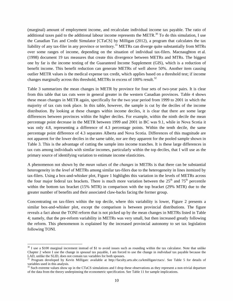


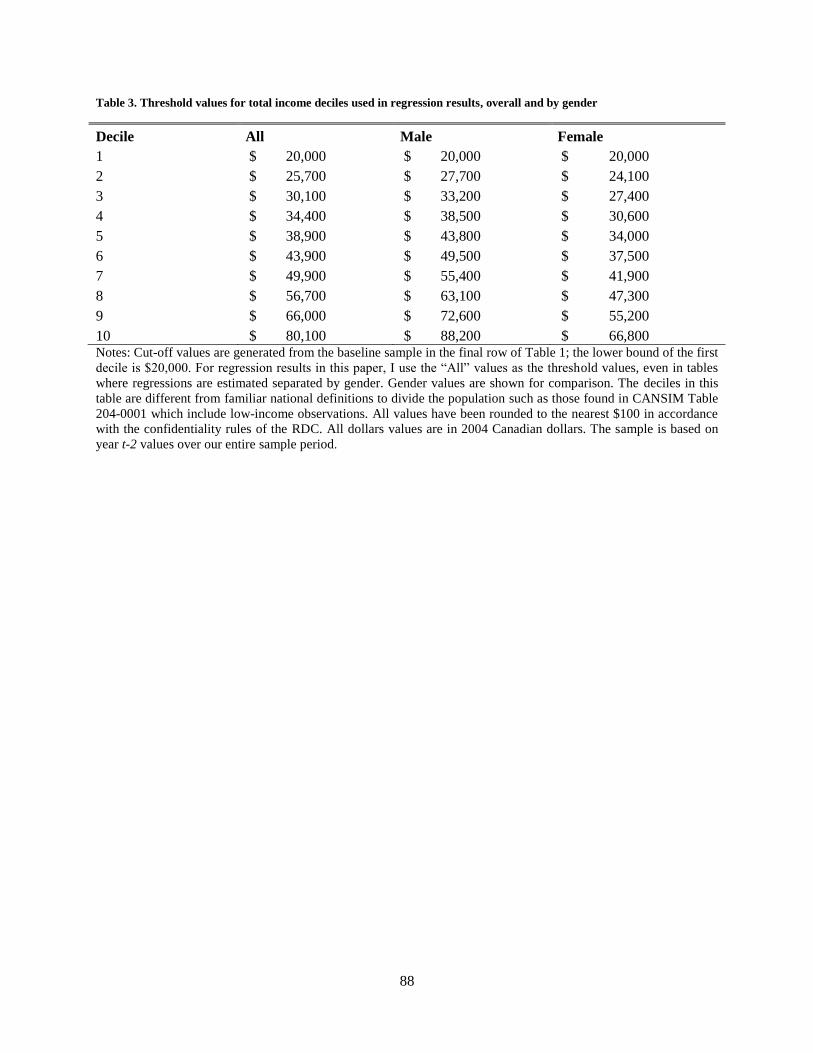


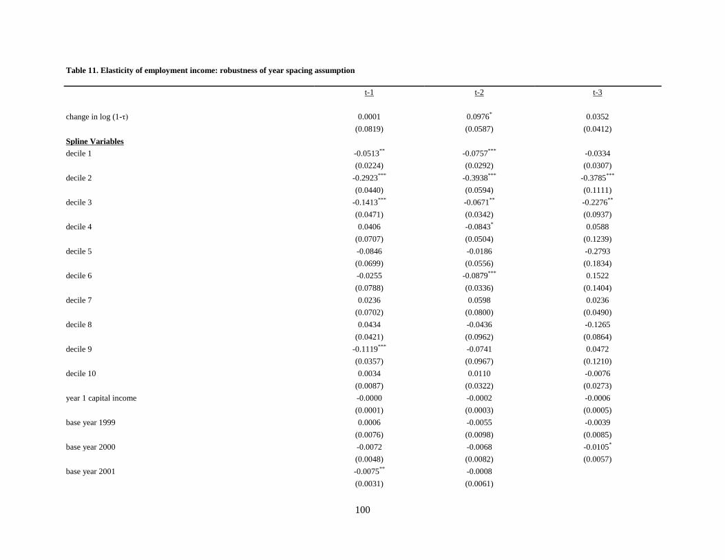


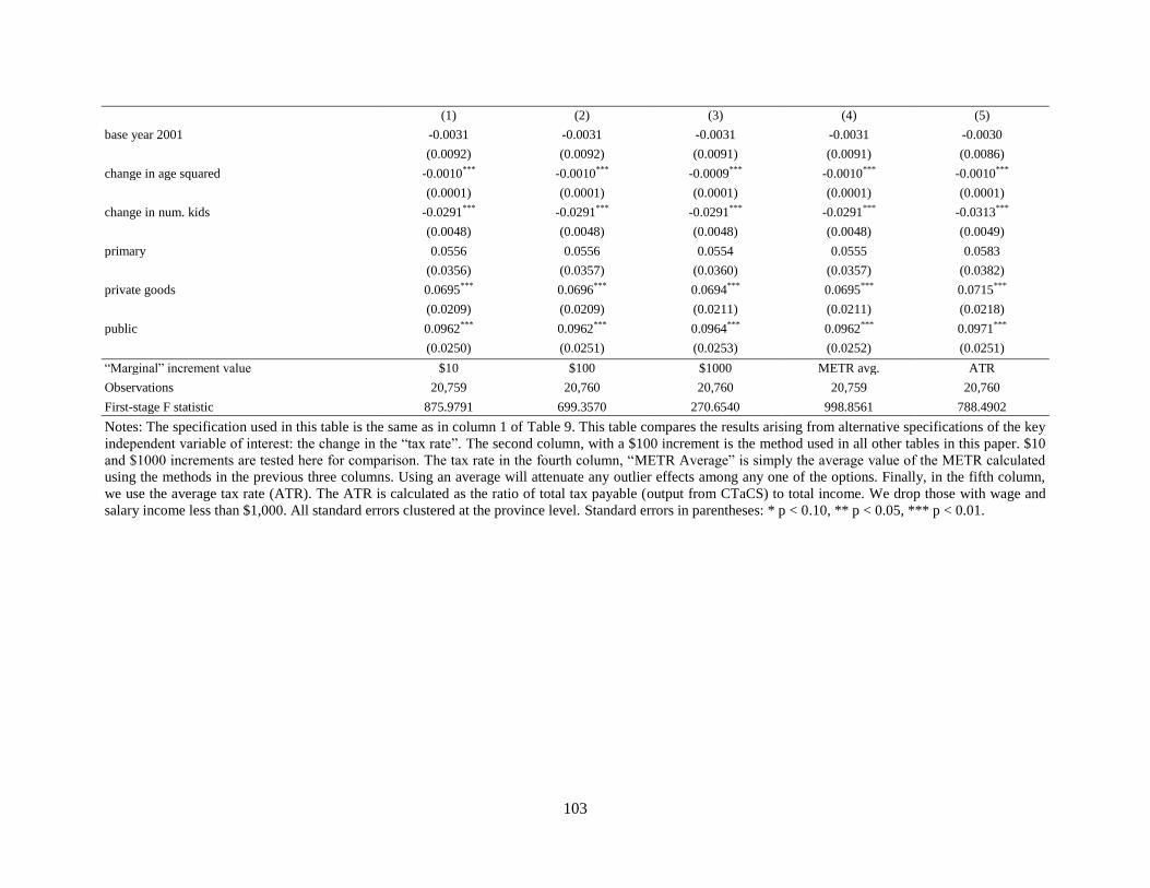


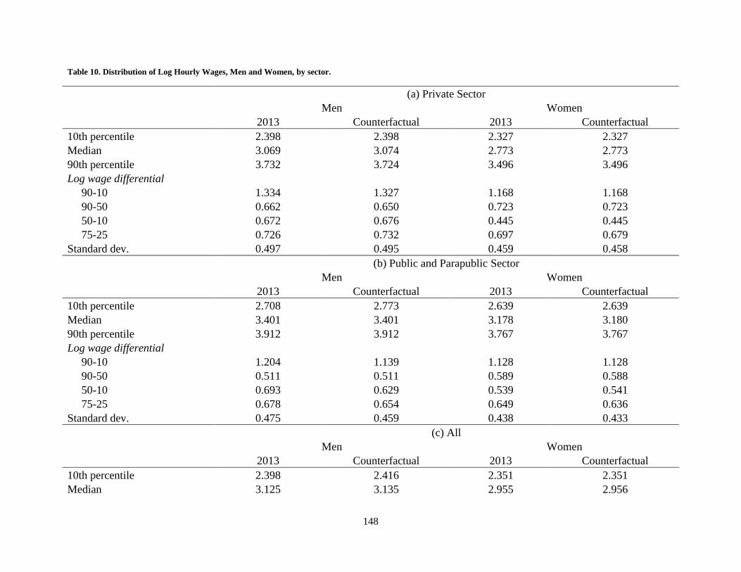


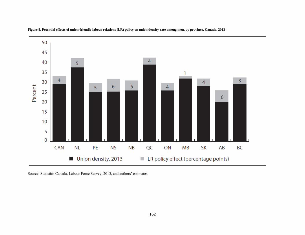


Related Documents