Three Essays in Financial Econometrics Jianxun Li The Department of Finance Imperial College Business School Imperial College London A thesis submitted for the degree of Doctor of Philosophy in Financial Econometrics of Imperial College London and the Diploma of Imperial College London June 29, 2016

Welcome message from author
This document is posted to help you gain knowledge. Please leave a comment to let me know what you think about it! Share it to your friends and learn new things together.
Transcript

Three Essays in
Financial Econometrics
Jianxun Li
The Department of Finance
Imperial College Business School
Imperial College London
A thesis submitted for the degree of
Doctor of Philosophy in Financial Econometrics of Imperial College London
and the Diploma of Imperial College London
June 29, 2016

Declaration
I, Jianxun Li, declare that the work presented in this thesis is entirely my own
except otherwise indicated, in which case I have clearly referenced the original
sources and acknowledged appropriately any assistance provided to me.
2

Copyright Declaration
The copyright of this thesis rests with the author and is made available under
a Creative Commons Attribution Non-Commercial No Derivatives licence. Re-
searchers are free to copy, distribute or transmit the thesis on the condition that
they attribute it, that they do not use it for commercial purposes and that they do
not alter, transform or build upon it. For any reuse or redistribution, researchers
must make clear to others the licence terms of this work.
3

Abstract
This thesis consists of three essays on applying state space models to tackle inter-
esting problems in finance and economics. Simulation-based model estimation
techniques are used extensively to draw statistical inference on latent state vari-
ables.
In the first essay, I develop a new type of Bivariate Mixture model to describe
the empirical dynamics between return volatility and trading volume. The pro-
posed semi-structural model allows the common and idiosyncratic components
in traders’ reservation price to interact in a multiplicative way rather than an addi-
tive way which is typically adopted by previous researches. The resulting Revised
Bivariate Mixture (RBM) model has desirable properties that are fully consistent
with empirical stylized facts, and the model also provides additional insights on
price discovery process from a behavioural perspective. A multi-block Bayesian
MCMC algorithm is proposed to estimate the model. The empirical results based
on a sample of 8 stocks listed in the US stock market are summarized as fol-
lows. First, I find the existence of a common latent information flow process that
drives the bivariate dynamics of return volatility and trading volume simultane-
ously, thus the empirical evidence is in favour of the Mixture of Distribution Hy-
pothesis (MDH) of Clark [1973]. Second, the investors’ sentiment process is near
unit root but the information flow process is much less persistent; this embed-
ded two-factor structure is able to replicate the empirically observed autocorre-
lation functions of absolute return and trading volume. Third, the proportion of
liquidity-driven trading volume is much higher in large-cap stocks than in small-
cap tickers. Fourth, no statistical evidence is found to support the self-referential
hypothesis in behaviour finance literature. Finally, there is strong evidence sug-
gesting that the investors’ sentiment process might be a market-wide factor as the
4

estimated latent sentiment processes are highly correlated within the sample of
8 stocks.
In the second essay, I use the Stochastic Vector Multiplicative Error model (S-
VMEM) of Hautsch [2008] to investigate on genuine multivariate intraday high-
frequency dynamics between bid-ask spread, average dollar volume per trade,
trade intensity and return volatility by taking into account the presence of se-
rially correlated latent information flow. The simulation-based Maximum Likeli-
hood with Efficient Importance Sampling (ML-EIS) technique is used to estimate
the model. The main findings based on a sample of six heavily traded stocks
listed in the US stock market are summarized as follows. First, the empirical evi-
dence supports the Mixture of Distribution Hypothesis (MDH) even at 5-min fre-
quency by revealing the existence of unobserved serially correlated information
flow. Second, a strong contemporaneous genuine dependence between return
volatility and the other three transaction variables is found. Third, the impact of
information flow is most significant for return volatility and trade intensity. This
finding is in sharp contrast with previous studies like Blume et al. [1994], Xu and
Wu [1999], Huang and Masulis [2003] and Hautsch [2008], where the authors
find that it is the average trade size instead of trade intensity that is most infor-
mative about the quality of news. This changing behaviour reflects that market
impact becomes an increasing important concern when investors execute their
trades, and consequently, they tend to break large order into many small child
orders. Thus the number of trades carries more informative content about hid-
den market event than the average trade size does. Finally, impulse response
analysis shows that the dynamics of bid-ask spread is little affected by a positive
shock in the underlying news arrival process, and thus provides no evidence to
support the asymmetric information market microstructure theory.
5

In the third essay, motivated by the fact that inflation swap provides a cleaner source
than government-issued inflation-linked bond to analyse inflation dynamics, I fit the
no-arbitrage joint term structure of nominal interest rate and breakeven inflation rate
to zero coupon inflation swap data in US, UK and EU markets. The model is
estimated using the three-step regression technique outlined in Abrahams et al.
[2013]. The empirical evidence suggests that the no-arbitrage joint term structure
is able to describe the dynamics of breakeven inflation rate very well in all three
developed markets, indicated by small pricing errors observed in nominal yield
curve and inflation swap curve. What’s more, most variation in long-term for-
ward BEI is attributed to the time-varying risk premium whereas the forward in-
flation expectation remains stable over time. Finally, the model-implied inflation
expectation outperforms the unadjusted BEI in terms of forecasting short-term
realized inflation. Thus the no-arbitrage joint term structure model is potentially
of considerable interest to investors and policy markers to help them make more
informative macro decisions.
6

Acknowledgements
First and foremost, I would like to thank my supervisor, Professor Walter Distaso,
for his endless support, patient discussion and ongoing guidance. I also want to
thank Dr. Roberto Dacco for his insightful suggestion on the inflation risk pre-
mium project. I gratefully thank all my friends, in particular, Dr. Yining Shi, for
sharing her invaluable experience and giving great help.
Many thanks also go in particular to my beloved wife, Lin Yang, who has so much
understanding and patience during the hard times, and so much fun and love
every minute.
7

Notations and Conventions
Throughout this thesis, the following notations and conventions are adopted:
• Scalar variable is denoted by plain Greek/English letter.
• Vector/matrix variables are denoted by bold Greek/English letters.
• Phrases printed in italics are particularly important in the context of the
respective section.
8

Abbreviations and Symbols
A large number of mathematical symbols are introduced in this thesis, and they
are based on the standard Greek and English alphabets. As a consequence, the
same symbol might have different meanings under different contexts. Here are a
list of symbols and abbreviations used throughout this thesis.
Abbreviations Description
ACD Autoregressive Conditional Duration model
ACF Autocorrelation Function
AR(1) Auto-Regressive Process of Order 1
ARMA Autoregressive Moving Average model
BIC (Schwarz) Bayesian Information Criterion
CACF Cross Autocorrelation Function
C.I. Confidence Interval
CRN Common Random Numbers
DBM Dynamic Bivariate Mixture model
DGP Data Generating Process
GARCH Generalized Autoregressive Conditional Heteroskedasticity model
GBM Generalized Bivariate Mixture model
GIRF Generalized Impulse Response Function
GMM Generalized Method of Moment
IRF Impulse Response Function
ILB Inflation-linked Bond
IS Importance Sampling
JB Jarque-Bera normality test
LB Ljung-Box test
MC Monte Carlo
9

MCMC Markov Chain Monte Carlo
MDH Mixture of Distribution Hypothesis
MEM Multiplicative Error model
ML-EIS Maximum Likelihood with Efficient Importance Sampling
MM Modified Mixture model
MAE Mean Absolute Error
MSE Mean Squared Error
NSE Mante Carlo Numerical Standard Error
NI MCMC Numerical Inefficiency metric
NYSE New York Stock Exchange
OLS Ordinary Least Square
RBM Revised Bivariate Mixture model
SBM Standard Bivariate Mixture model
SML Simulated Maximum Likelihood
SCD Stochastic Conditional Duration model
SV Stochastic Volatility model
S-VMEM Stochastic Vector Multiplicative Error model
VMEM Vector Multiplicative Error model
WRDS Wharton Research Data Services
10

Symbol Description
θ collection of model parameters θ = {θ1,θ2, ...,θn}
A′ transpose of matrixA
N(·) Gaussian distribution
Pois(·) Poisson distribution
D(·) a generic (any) distribution
∆ difference operator
E[·] expectation operator
var[·] variance operator x
H0 null hypothesis
L(θ,y) Likelihood function
U(·) Uniform distribution
Variables in Chapter 2 Description
Pk asset price at kth temporary equilibrium
P∗k,j the reservation price of j th trader
φi component in ∆P∗i,j that is common to all traders
ψi,j component in ∆P∗i,j that is specific to jth trader
Rt logarithmic of asset return at date t
Vt trading volume at date t
Kt number of information arrivals at date t
m percentage of informed traders who trade via off-exchange venues
σ2φ time-independent variance of fundamental signal
µγ,t time-dependent investors’ systematic sentiment
µw unconditional mean of trading volume attributed
to kth intraday event
σ2w unconditional variance of trading volume attributed
to kth intraday event
11

Variables in Chapter 3 Description
BASt average bid-ask spread
T It trade intensity (number of trades per fixed time interval)
TSt average trade size (in dollar)
Rt intraday return
κt conditional expectation of BASt
φt conditional expectation of T It
ψt conditional expectation of TSt
σ2t conditional variance of Rt
xi,t conditional moment process of variable i in S-VMEM model
si,t seasonality pattern of variable i in S-VMEM model
Variables in Chapter 4 Description
log(P(m)t ) log price of m-month nominal zero coupon bond
log(P(m)t,R ) log price of m-month real zero coupon bond
ω(m)t log price of m-month breakeven inflation rate
Xt pricing factors (principal components)
λt market price of risk
Am andBm coefficients of m-month log bond price onXt
12

Contents
1 Introduction 1
2 Dynamic Bivariate Mixture Model of Return and Trading Volume 3
2.1 Introduction and Motivation . . . . . . . . . . . . . . . . . . . . . . 3
2.2 The Structural Bivariate Mixture Model: Theoretical and Empiri-
cal Aspects . . . . . . . . . . . . . . . . . . . . . . . . . . . . . . . . 6
2.2.1 The Standard Bivariate Mixture Model . . . . . . . . . . . . 6
2.2.2 The Modified Mixture Model . . . . . . . . . . . . . . . . . 10
2.2.3 The Generalized Bivariate Mixture Model . . . . . . . . . . 12
2.2.4 The Revised Bivariate Mixture Model . . . . . . . . . . . . . 14
2.3 The Estimation Procedure . . . . . . . . . . . . . . . . . . . . . . . 21
2.3.1 Why Monte Carlo Markov Chain (MCMC)? . . . . . . . . . 21
2.3.2 The Bayesian MCMC Procedure . . . . . . . . . . . . . . . . 23
2.4 A Monte Carlo Simulation Study . . . . . . . . . . . . . . . . . . . 25
2.5 Empirical Analysis . . . . . . . . . . . . . . . . . . . . . . . . . . . 32
2.5.1 Dataset Description . . . . . . . . . . . . . . . . . . . . . . . 32
2.5.2 Empirical Results . . . . . . . . . . . . . . . . . . . . . . . . 36
2.6 Concluding Remarks . . . . . . . . . . . . . . . . . . . . . . . . . . 47
2.7 Appendix 1: Derivations of unconditional moments . . . . . . . . 49
2.8 Appendix 2: MCMC algorithm . . . . . . . . . . . . . . . . . . . . . 51
i

Contents
3 Multivariate Dynamics of High-Frequency Transaction-level Variables 56
3.1 Introduction and Motivation . . . . . . . . . . . . . . . . . . . . . . 56
3.2 Model Specification . . . . . . . . . . . . . . . . . . . . . . . . . . . 60
3.2.1 The Autoregressive Conditional Duration Model . . . . . . 61
3.2.2 The Vector Multiplicative Error Model . . . . . . . . . . . . 63
3.2.3 The Stochastic Vector Multiplicative Error Model . . . . . . 67
3.3 The Estimation Technique . . . . . . . . . . . . . . . . . . . . . . . 70
3.3.1 Maximum Likelihood with Efficient Importance Sampling 71
3.3.2 Bayesian Predicting and Updating . . . . . . . . . . . . . . 78
3.4 A Monte Carlo Simulation Study . . . . . . . . . . . . . . . . . . . 81
3.5 Empirical Analysis . . . . . . . . . . . . . . . . . . . . . . . . . . . 86
3.5.1 Dataset Overviews . . . . . . . . . . . . . . . . . . . . . . . 86
3.5.2 Univariate Results . . . . . . . . . . . . . . . . . . . . . . . . 97
3.5.3 Multivariate Results . . . . . . . . . . . . . . . . . . . . . . 107
3.6 Concluding Remarks . . . . . . . . . . . . . . . . . . . . . . . . . . 122
4 Analysing Inflation Dynamics Using Inflation Swap Data 124
4.1 Introduction and Motivation . . . . . . . . . . . . . . . . . . . . . . 124
4.2 Market Overviews . . . . . . . . . . . . . . . . . . . . . . . . . . . . 128
4.3 The No-Arbitrage Affine Joint Term Structure Model . . . . . . . . 132
4.3.1 The Nominal Yield Curve . . . . . . . . . . . . . . . . . . . 134
4.3.2 The Real Yield Curve . . . . . . . . . . . . . . . . . . . . . . 135
4.3.3 The Breakeven Inflation Curve . . . . . . . . . . . . . . . . 137
4.3.4 The Decomposition of Term Structure . . . . . . . . . . . . 137
4.4 The Estimation Technique . . . . . . . . . . . . . . . . . . . . . . . 138
4.5 Empirical Analysis . . . . . . . . . . . . . . . . . . . . . . . . . . . 142
4.5.1 Dataset Description . . . . . . . . . . . . . . . . . . . . . . . 142
4.5.2 Constructing Orthogonal Pricing Factors . . . . . . . . . . . 144
4.5.3 Empirical Results . . . . . . . . . . . . . . . . . . . . . . . . 147
ii

Contents
4.6 Concluding Remarks . . . . . . . . . . . . . . . . . . . . . . . . . . 159
5 Conclusion and Outlook 161
iii
List of Figures
2.1 Cross Correlation Plot of Absolute Return on Trading Volume . . . 4
2.2 Visualization of Simulated Dataset . . . . . . . . . . . . . . . . . . 27
2.3 Plots of MCMC draws: Simulated Dataset . . . . . . . . . . . . . . 30
2.4 Estimates of Latent State Variables: Simulated Dataset . . . . . . . 31
2.5 Autocorrelation Function of Absolute Return . . . . . . . . . . . . 39
2.6 Autocorrelation Function of Detrended Volume . . . . . . . . . . . 40
2.7 Latent Market Sentiment Process and Consumer Confidence Index 46
3.1 ML-EIS Estimates of Latent and Observation-driven Processes . . . 84
3.2 ML-EIS Estimates: Residuals Diagnostics . . . . . . . . . . . . . . . 85
3.3 Intraday Seasonality Cubic Splines . . . . . . . . . . . . . . . . . . 92
3.4 Cross-Autocorrelation Functions: Seasonally-unadjusted . . . . . . 95
3.5 Cross-Autocorrelation Functions: Seasonally-adjusted . . . . . . . 96
3.6 Generalized Impulse Response Function . . . . . . . . . . . . . . . 121
4.1 Time Series Plots of Pricing Factors . . . . . . . . . . . . . . . . . . 146
4.2 Time Series Model Fit: US market . . . . . . . . . . . . . . . . . . . 148
4.3 Time Series Model Fit: UK market . . . . . . . . . . . . . . . . . . . 149
4.4 Time Series Model Fit: EU market . . . . . . . . . . . . . . . . . . . 150
4.5 Nominal Yield Loadings . . . . . . . . . . . . . . . . . . . . . . . . 152
iv

List of Figures
4.6 Breakeven Inflation Loadings . . . . . . . . . . . . . . . . . . . . . 153
4.7 Decomposition of Breakeven Inflation Rate (10yr) . . . . . . . . . . 155
4.8 5-10yr Forward BEI Decomposition . . . . . . . . . . . . . . . . . . 156
4.9 Inflation Forecast . . . . . . . . . . . . . . . . . . . . . . . . . . . . 158
v

List of Tables
2.1 Estimation Results of the Monte Carlo Experiement . . . . . . . . . 28
2.2 Parameter Estimation Result for Simulated Dataset . . . . . . . . . 29
2.3 Stocks Used in the Empirical Analysis . . . . . . . . . . . . . . . . 33
2.4 Summary Statistics for Sample Stock Dataset . . . . . . . . . . . . 35
2.5 Posterior Estimation Results of the Revised Bivariate Mixture Model 37
2.6 Variations of Latent Processes . . . . . . . . . . . . . . . . . . . . . 41
2.7 Explanatory Power of Sentiment and News Arrival Processes . . . 42
2.8 Correlation matrix and PCA results of latent processes . . . . . . . 45
2.9 Univariate Regression Results . . . . . . . . . . . . . . . . . . . . . 47
3.1 ML-EIS Estimation Results: A Simulation Study . . . . . . . . . . . 82
3.2 Sample Stocks included in the Analysis . . . . . . . . . . . . . . . . 86
3.3 Descriptive statistics of Sample Dataset . . . . . . . . . . . . . . . . 88
3.3 Descriptive statistics of Sample Dataset . . . . . . . . . . . . . . . . 89
3.3 Descriptive statistics of Sample Dataset . . . . . . . . . . . . . . . . 90
3.4 Estimation Results of (S)-GARCH Model for Intraday Return . . . 99
3.4 Estimation of (S)-GARCH Model for Intraday Return . . . . . . . . 100
3.5 Estimation Results of (S)-ACD Model for Number of Trades . . . . 101
3.5 Estimation of (S)-ACD Model for Number of Trades . . . . . . . . . 102
3.6 Estimation Results of (S)-ACD Model for Average Trade Size . . . . 103
vi

List of Tables
3.6 Estimation of (S)-ACD Model for Average Trade Size . . . . . . . . 104
3.7 Estimation Results of (S)-ACD Model for Bid-Ask Spread . . . . . 105
3.7 Estimation of (S)-ACD Model for Bid-Ask Spread . . . . . . . . . . 106
3.8 Estimation Results of (S)-VMEM Models (CVX and IBM) . . . . . . 111
3.8 Estimation Results of (S)-VMEM Models (CVX and IBM) . . . . . . 112
3.8 Estimation Results of (S)-VMEM Models (CVX and IBM) . . . . . . 113
3.9 Estimation Results of (S)-VMEM Models (JPM and PEP) . . . . . . 114
3.9 Estimation Results of (S)-VMEM Models (JPM and PEP) . . . . . . 115
3.9 Estimation Results of (S)-VMEM Models (JPM and PEP) . . . . . . 116
3.10 Estimation Results of (S)-VMEM Models (WMT and XOM) . . . . . 117
3.10 Estimation Results of (S)-VMEM Models (WMT and XOM) . . . . . 118
3.10 Estimation Results of (S)-VMEM Models (WMT and XOM) . . . . . 119
4.1 Contractual Terms of Inflation-linked Instruments . . . . . . . . . 130
4.2 Zero Coupon Inflation Swap Dataset (End-of-Month) . . . . . . . . 143
4.3 Goodness of Fit: Mean Abosolute Errors (in bps) . . . . . . . . . . 147
4.4 Inflation Forecast Error (2-year) . . . . . . . . . . . . . . . . . . . . 159
vii

1 Introduction
State space model is a powerful tool to analyse dynamical system, especially when
the underlying state variables cannot be observed directly. In particular, the
model uses the dynamics of the state variables and their linkages with the ob-
served system outputs to draw statistical inference on the unobserved system
states. State space models have been widely applied to study the mechanics of
macroeconomic development and financial market over the last decade, and they
recently have been receiving special attention as central banks and other financial
institutions are placingmore andmore emphasis on real time assessment about the
state of the economy.
The standard state space framework consists of two equations, namely, a mea-
surement equation and a state equation. The former describes how the observed
economic variables are related to latent state variables, and the latter character-
izes how state variables themselves change over time. To express the state space
model mathematically, let yt beN×1 observed economic variables and xt be K×1
underlying state variables at time t, then a generic form of a state-space model
can be written as
yt = f (xt ,θ,εt)
1

1 Introduction
xt = g(xt−1,θ,ut)
where εt and ut are independently and identically distributed innovation terms,
θ is a collection of all model parameters, and finally, f (·) and g(·) denote respec-
tively generic functions that characterize how the state variables xt translate into
those actual economic variables yt and how the state variables xt themselves
evolve over time. In many applications, it is often important to draw efficient
and reliable statistical inference on the unobserved state variables xt, because
they are considered as the main driving forces of financial dynamics yt.
In this thesis, I apply state space models to tackle a few interesting problems in
finance and economics. The rest of the thesis is organized as follows. In chap-
ter 2, I examine the empirical bivariate dynamics between return volatility and
trading volume at daily frequency. Chapter 3 studies the genuine lead-lag causal-
ity among several high-frequency transaction level variables, including bid-ask
spread, average dollar volume per trade, trade intensity, and return volatility.
The third essay, which is presented in chapter 4, aims to solve the problem of
estimating market-based measure of inflation expectation based on zero coupon
inflation swap data, which is of considerable interest to policy makers. Finally,
chapter 5 summarizes what I’ve learned from this thesis and also presents several
potential fruitful areas for further researches.
2

2 Dynamic Bivariate Mixture Model
of Return and Trading Volume
2.1 Introduction and Motivation
Modelling the volatility of financial asset return plays an critical role in numer-
ous financial applications, with examples ranging from pricing complex finan-
cial derivative products to managing portfolio risk. Until recently, most empir-
ical works on volatility modelling are devoted to univariate time series models,
where the Autoregressive Conditional Heteroskedasticity (ARCH) model of En-
gle [1982] and its extension into GARCH by Bollerslev [1986] have been very
successful. However, research objective has grown increasingly ambitious. Mul-
tivariate semi-structural models focusing on the causal relations among various
trading variables are now commonplace. Unlike the traditional pure statistical
model which keep silent about the economic reasons causing the variations in volatil-
ity, an important motivation driving the development of multivariate semi-structural
model is the attempt to capture and interpret the underlying source of volatility dy-
namics. To this end, a family of Dynamic Bivariate Mixture (DBM) models have
been developed which focus on describing the joint behaviours of return volatil-
3

2 Dynamic Bivariate Mixture Model of Return and Trading Volume
ity and trading volume. The underlying idea is that according to market mi-
crostructure theory, various trading variables (such as price movement, bid-ask
spread, market depth, trade duration, trading volume, etc.) are all generated si-
multaneously in the price discovery process in response to the arrival of new in-
formation, and thus this unobserved information flow would be a common factor
driving the mechanics of all these observed trading variables. In fact, as shown in
figure (2.1), absolute asset return displays a strong contemporaneous correlation with
trading volume, and lead-lag correlations are also found to be significant at short lags.
This close relation between return volatility and trading volume motivates us to
add volume dynamics to the traditional univariate volatility modelling, with the
aim to refine the estimates of return volatility and to get a deeper understanding
on the whole picture of price formation process. Being a model that incorpo-
rates such structural information, DBM models expect to be more accurate and
robust in explaining and predicting return volatility than traditional pure statis-
tical models.
Figure 2.1: Cross Correlation Plot of Absolute Return on Trading Volume
This figure plots the cross correlation function of absolute daily return on detrended tradingvolume for stock GE over the period January 3, 2002 - December 23, 2014. Observations betweenDecember 24 and January 1 (inclusive) are omitted due to distinct holiday seasonality. The sampleconsists of 2,964 observations in total.
4

2 Dynamic Bivariate Mixture Model of Return and Trading Volume
There are several remarkable developments in DBM literature, including the pi-
oneered Mixture of Distribution Hypothesis (MDH) of Clark [1973], the Stan-
dard Bivariate Mixture (SBM) model of Tauchen and Pitts [1987], the Modified
Mixture (MM) model of Andersen [1996], and the Generalized Bivariate Mix-
ture (GBM) model of Liesenfeld [2001]. All these previous works implicitly as-
sume that the Efficient Market Hypothesis (EMH) holds, which implies that asset
price fully reflects all available information and the change in market equilib-
rium price is a rational and unbiased estimate of the newly received fundamental
signal. However, one major puzzle to EMH is the widely observed excess volatil-
ity. If EMH is true, then the source of stock price volatility can be traced to the
volatility of stock dividends. However, as reported by Shiller [1981], the actual
stock price volatility is far greater than the volatility of dividends. Furthermore,
the anomaly here is not only that the level of stock market volatility is too high,
but also that this volatility level itself display a strong persistence and tends to
cluster over time.
In this paper, inspired by the empirical results of Liesenfeld [2001] and Tauchen
and Pitts [1987], I develop a structural framework to model the price discov-
ery process which allows investors to overreact or underreact to the arrival of
new fundamentals. With this behavioural element embedded, the excess level of
volatility and its variation can be explained by a time-varying market sentiment
process, and thus the model is able to reconcile the excess volatility puzzle from
a behavioural finance prospective.
The rest of the paper is organized as follows. In section 2.2, I review the literature
of DBM models and show how previous empirical results motivate me to come
up with the Revised Bivariate Mixture (RBM) model in this paper. The Bayesian
MCMC method is used to estimate the model, and its procedure is outlined in
5

2 Dynamic Bivariate Mixture Model of Return and Trading Volume
section 2.3, followed by a simulation study in section 2.4 to demonstrate the reli-
ability of the estimation technique. I fit the model to a sample of 8 stocks listed in
the US stock market and the empirical results are reported in section 2.5. Finally,
section 2.6 concludes the paper.
2.2 The Structural Bivariate Mixture Model:
Theoretical and Empirical Aspects
In this section, I review several related theoretical and empirical works in the lit-
erature and explain how the proposed specification leads to a more parsimonious
and adaptive model to better characterize the bivariate dynamics between return
volatility and trading volume.
2.2.1 The Standard Bivariate Mixture Model
The research inmodelling bivariate relation between return volatility and trading
volume is pioneered by Clark [1973] who proposes the well known Mixture of
Distribution Hypothesis (MDH). In particular, the MDH claims that stock return
and trading volume are jointly dependent on an unobservable information flow,
and thus each series can be modelled as a mixture of distributions where the
number of news arrivals acts as the mixing variable.
A subsequent influential work in this field is Glosten and Milgrom [1985] where
they enrich the bivariate dynamics by incorporating the information asymme-
try market microstructure theory into the modelling framework. More specifi-
6

2 Dynamic Bivariate Mixture Model of Return and Trading Volume
cally, they analyse a hypothetical market where there is an asset with a random
liquidation or terminal value. Information on the terminal value is assumed to
be asymmetrically distributed among market participants, and there are totally
three types of traders active in the market. Traders who possess private signals on
the fundamental value of this asset (possibly due to their superior ability of pro-
cessing and analysing information) are called informed traders; they buy and sell
this asset for speculative motives. Another group of traders, called uninformed
traders, participate in the market for exogenous liquidity motives (for examples,
portfolio rebalancing, hedging for the underlying asset, etc.), and thus they are
treated as uninformed. The final third group, called market makers, hold inven-
tory and pose bid and offer quotes to facilitate trade on this asset; they try to
maximize transaction flow and make profits from the bid-ask spread but con-
sume price risk (represented by average loss to informed traders due to adverse
selection). The authors further assume that informed traders receive private sig-
nals at random time and trade accordingly, whereas uninformed traders arrive at
market at a constant exogenous rate. They show that the realizations of private
signals possessed by informed traders lead to a dynamic price discovery process
that eventually moves the asset price to an equilibrium level which fully reflects
its fundamental value.
To formulate this idea as an empirical model, I assume that the market for this
asset passes through a sequence of temporary equilibriums within a trading day,
and the price movement from the k − 1th to the kth equilibrium is caused by a
piece of new information (private signals) arriving at the market. Let P(k) denote
the logarithmic of asset price at kth equilibrium. Suppose that there are totally
N informed traders active in market at any time, and each informed trader i
(i = 1,2, ...,N ) processes and analyses the received information in a different way
and thus possesses heterogeneous belief on the fundamental value of the asset.
7

2 Dynamic Bivariate Mixture Model of Return and Trading Volume
Let P∗(k),i denote the logarithmic of reservation price of informed trader i. Under
the equilibrium condition that market clears, and asset price P(k) is determined
by the average of reservation prices across all N traders, reflecting the average
belief of all informed traders on fundamental asset value.
In Tauchen and Pitts [1987], the authors suggest that the change in trader i’s
reservation price between k − 1th and kth equilibriums, i.e. ∆P∗(k),i = P∗(k),i −P
∗(k−1),i ,
can be modelled as an additive two-component process:
∆P∗(k),i = φ(k) +ψ(k),i (2.1)
φ(k) ∼ i.i.d. N(0,σ2φ) (2.2)
ψ(k),i ∼ i.i.d. N(0,σ2ψ) (2.3)
where φ(k) represents the portion of the signal that is common to all traders and
ψ(k),i describes the heterogeneous component which is specific to trader i. Both
φ(k) and ψ(k),i are assumed to be mutually independent and normally distributed
with zero mean and constant variance, so that the equilibrium asset price, as the
average of reservation prices of individual traders, is ex-ante unpredictable and
follows a random walk. The variance parameters σ2φ and σ2
ψ in (2.2) and (2.3)
measure the sensitivity of traders’ reservation prices in response to the arrivals of
informational events.
Since the asset price at kth intraday equilibrium reflects the average belief of all
informed traders, i.e. P(k) =1N
∑Ni=1P
∗(k),i , the logarithmic return dynamics can
thus be written as
∆P(k) = P(k) −P(k−1) =1N
N∑i=1
∆P∗(k),i = φ(k) +1N
N∑i=1
ψ(k),i (2.4)
8

2 Dynamic Bivariate Mixture Model of Return and Trading Volume
which implies that
r(k) = ∆P(k) ∼N(0,σ2φ +
σ2ψ
N) (2.5)
where the last part follows because both φ(k) and ψ(k),i are mutually independent
and normally distributed according to (2.2) and (2.3).
Tomodel trading volume associatedwith the arrival of informational event, Tauchen
and Pitts [1987] assume that informed trader i ’s desired net position Q∗(k),i , given
her private signal P∗(k),i , is proportional to the difference between her reservation
price and the current market price, i.e.
Q∗(k),i = c ·(P∗(k),i −P(k)
)(2.6)
Assume further that m (in percentage, 0 < m < 1) of informed traders trade with
each others directly via off-exchange venues like dark pools and Electronic Cross-
ing Networks (ECNs), while the rest 1−m portion of informed traders make trans-
actions with market maker (intermediate). Then the informed trading volume,
denoted by v(k),informed, can be written as the total change in traders’ desired
positions, i.e.
v(k),informed = (1− m2) ·
N∑i=1
|∆Q∗(k),i | = c · (1−m2) ·
N∑i=1
|∆P∗(k),i −∆P(k)| (2.7)
Substituting (2.1) and (2.4) into the above equation, one can obtain
v(k),informed = c · (1− m2) ·
N∑i=1
|ψ(k),i −1N
N∑j=1
ψ(k),j | (2.8)
which implies that informed trading volume is solely determined by the varia-
tion of ψ(k),i measuring the degree of heterogeneity or diversity among informed
9

2 Dynamic Bivariate Mixture Model of Return and Trading Volume
traders’ private signals, and it is not affected by the common component φ(k) at
all. Applying the Central Limit Theorem for large N → ∞, one can show that
v(k),informed is approximately normally distributed with the following asymp-
totic mean and variance
µv = c · (1−m2) ·
(2(N − 1)N
π
)1/2(2.9)
σ2v = c2 · (1− m
2)2 ·
(1− 2
π
)·N ·σ2
ψ (2.10)
Finally, suppose that the market passes through a number of Kt temporary equi-
libriums on date t, then daily logarithmic return Rt and trading volume Vt are
the sum of intraday inter-equilibrium returns and trading volumes respectively
where Kt acts as the mixing variable. We now obtain the specifications for the
Standard Bivariate Mixture (SBM) model of Tauchen and Pitts [1987]:
Rt |Kt ∼ i.i.d. N(0, (σ2
φ +σ2ψ
N)Kt
)(2.11)
Vt |Kt ∼ i.i.d. N(µvKt ,σ
2vKt
)(2.12)
2.2.2 The Modified Mixture Model
Andersen [1996] proposes a so-called Modified Mixture (MM) model which ex-
tends the SBM specification (2.11) and (2.12) along several directions. Motivated
by the information asymmetry framework of Glosten and Milgrom [1985], he
takes into account the impact of uninformed traders on trading volume and
develops an empirically testable version of Glosten and Milgrom’s theoretical
model. By assuming uninformed traders arrive at market at a constant rate µ0
and trade one share each time, Andersen describes marginal distribution of trad-
10

2 Dynamic Bivariate Mixture Model of Return and Trading Volume
ing volume by a Poisson distribution with the aim to explicitly respect the non-
negativity constraint of trading volume:
Vt |Kt ∼ i.i.d. Pois(µ0 +µvKt) (2.13)
Andersen also points out that the conditional return variance is mainly affected
by the common mixing variable Kt in (2.11). In other words, the dynamics of
return volatility process depends heavily on the time series characteristics of un-
derlying information flow Kt . Based on this link, he argues that the empirically
observed volatility clustering might imply that the information arrival process
{Kt}Tt=1 is persistent over time. This claim is further supported by the observation
that unexpected informational event often tends to be followed by a sequence of
announcements related to the topic of the initial breaking news. To introduce
serial autocorrelation in the latent information flow process, the author suggests
to use a Gaussian AR(1) process to model the logarithmic of the number of news
arrivals, i.e. λt ≡ lnKt ,
λt = βλλt−1 +σλελ,t with ελ,t ∼ i.i.d.N(0,1) (2.14)
These three equations, namely, (2.11) for the conditional return, (2.13) for the
conditional volume, and (2.14) for the underlying latent information flow pro-
cess, complete the model specification of Andersen [1996]’s MM model.
As reported by Andersen, the inclusion of uninformed trading volume is empir-
ically justified by a statistically significant estimate of µ0, whose magnitude is
also considerably large. Based on the historical IBM stock data over 1973-1991,
Andersen shows that uninformed volume accounts for more than 60% of total
trading volume on average over the full sample period.
11

2 Dynamic Bivariate Mixture Model of Return and Trading Volume
However, it’s worthwhile to note that Possion random variable takes integer val-
ues only. Such property cannot be usually ensured, especially after one per-
forming detrending procedure on raw trading volume data. This doesn’t present
a difficulty in Andersen [1996] as the author adopts a Generalized Method of
Moments (GMM) approach to model estimation. But for other likelihood-based
methods where the evaluation of probability density function of trading volume
is critical, this integer constraint of Poisson variables does pose significant obsta-
cles to drawing statistical inference. As a workaround, one can add a constant
uninformed component to the expected volume expression in (2.12), and thus
model trading volume dynamics as
Vt |Kt ∼N(µ0 +µvKt ,σ2vKt). (2.15)
where the impact of uninformed trading on volume is preserved by µ0.
2.2.3 The Generalized Bivariate Mixture Model
As reported separately by Lamoureux and Lastrapes [1994], Andersen [1996] and
Liesenfeld [1998], empirical estimation results of the standard return-volume bi-
variate mixture model reveal a substantial reduction in persistent parameter βλ
in (2.14) with a typical value less than 0.7, implying that the bivariate model
specification is not adequate to accommodate the observed high persistence in
squared or absolute return, which is a well-known stylized fact of financial as-
set returns and has been successfully captured by the EGARCH model of Nelson
[1991] and the Stochastic Volatility model of Taylor [1986].
To bring back the observed highly persistent volatility clustering to bivariate
12

2 Dynamic Bivariate Mixture Model of Return and Trading Volume
model, Liesenfeld [2001] suggests that the parameters σ2φ and σ2
ψ in Tauchen
and Pitts [1987]’s SBM model specification (2.2) and (2.3) may inherently exhibit
time-varying behaviours, and the source of stock market volatility is thus related
to the degree of uncertainty about current and future state of economic and po-
litical system. From an empirical perspective, modelling this latent economic
uncertainty process as serially correlated time series might be able to decouple
the dynamics between volatility and volume to a certain degree. This setting is
also consistent with the findings of Bollerslev and Jubinski [1999] that return
volatility and trading volume have different degrees of persistence which can-
not be captured by a single latent factor represented by the information arrival
process.
Denote time-dependent variances by σ2φ,t and σ
2ψ,t . Liesenfeld assumes that both
variance processes are driven by a common unobservable process ωt , which mea-
sures the level of uncertainty about the current economic and political system,
i.e.
ln(σ2φ,t) = cφ +αφωt (2.16)
ln(σ2ψ,t) = cψ +αψωt (2.17)
By further introducing asymmetric effect of past return Rt−1 on ωt dynamics,
Liesenfeld [2001] extends Tauchen and Pitts [1987]’s SBM specification (2.11)
and (2.12) and derives the following form for his Generalized Bivariate Mixture
(GBM) model:
Rt |λt ,ωt ∼N(0, [β1 exp(ωt) + β2 exp(αψωt)]exp(λt)
)(2.18)
Vt |λt ,ωt ∼N(µ0 + β3 exp(αψωt/2)exp(λt),β4 exp(αψωt)exp(λt)
)(2.19)
13

2 Dynamic Bivariate Mixture Model of Return and Trading Volume
ωt = δωωt−1 + κRt−1 + νωεω,t (2.20)
λt = δλλt−1 + νλελ,t (2.21)
where αψ = αψ/αφ captures the relative importance of common news variance
σ2φ,t over idiosyncratic news variance σ2
ψ,t in (2.16) and (2.17).
Liesenfeld estimates the GBM model using a Simulated Maximum Likelihood
(SML) method. Based on a historical dataset consisting of IBM and Kodak stock
over 1973-1991, Liesenfeld finds an extremely persistent and nearly unit root
estimate for δω in (2.20). 1 Moreover, the estimate of δλ in latent news arrival
process (2.21) shows only moderate persistence with a typical value between 0.6
and 0.7. These findings imply that the short-run volatility is driven by the in-
formation flow process while long-run volatility is described by the variations of
trader’s sensitivity to news (especially to common news) over time.
2.2.4 The Revised Bivariate Mixture Model
In this section, I discuss how to derive the proposed Revised Bivariate Mixture
(RBM) model with both motivations and implications behind it.
As noted by Liesenfeld [2001], empirical results based on historical IBM and Ko-
dak stock dataset reveal a statistically insignificant estimate of αψ = αψ/αφ in
GBMM (2.18) and (2.19). Liesenfeld further tests the null hypothesis H0 : αψ = 0
by comparing the parameter estimates and the maximized likelihoods for re-
stricted (under null) and unrestricted models and by conducting a Likelihood
Ratio (LR) test, with empirical evidence favouring the null.
1δω = 0.996 for IBM and δω = 0.987 for Kodak.
14

2 Dynamic Bivariate Mixture Model of Return and Trading Volume
Recall that this coefficient αψ measures relative contribution to the variance of
trader i ’s reservation price var[∆Pt,i] due to the trader-specific component ψt,i
over the common component φt . An estimate of αψ = 0 implies that the two-
component additive structure for trader’s reservation price in (2.1) is not supported
by empirical data. Inspired by this finding, I develop a semi-structural model
by allowing common and idiosyncratic components to interact in a multiplicative
way. I’ll show that this multiplicative specification offers us additional insights
on return-volume bivariate system from a behavioural perspective.
Following the conventions and notations I used in section (2.2.1), let P∗(k),i denotes
the reservation price of trader i at kth intraday equilibrium. To allow for a mul-
tiplicative composition, one can write the change in trader i’s reservation price
as
P∗(k),i −P∗(k−1),i = γiφ(k) (2.22)
where φ(k) represents the fundamental true signal contained in the kth informa-
tional event, and γi measures φ(k). In other words, φ(k) measures the rational compo-
nent of the change in trader i ’s reservation price P∗(k),i ; while γi describes the irrational
behavioural bias that is specific to trader i when γi , 1.
The above multiplicative specification is motivated by the Market Sentiment The-
ory which explores how investors’ behavioural biases affect their financial deci-
sion making process. Pioneer works along this line of research include Barberis
et al. [1998], Brown and Cliff [2004], Bergman and Roychowdhury [2008] and
Shefrin [2008]. By definition, market sentiment describes the degree of excessive op-
timism or pessimism in investors’ beliefs on asset price which in general cannot be
justified by fundamentals. Thus the actual market price movement may deviate
15

2 Dynamic Bivariate Mixture Model of Return and Trading Volume
from its rational level, as described in (2.22).
The true fundamental signal assumes to be unpredictable with time-independent
variance, i.e. φ(k) ∼ i.i.d.N(0,σ2φ). As argued by Shefrin [2008], investor sentiment
is non-uniform across the market with heterogeneous beliefs. To address this
issue, the reaction to the true fundamental signal, which is captured by γi , can
vary from trader to trader but generally assumes to be mutually independent
across all traders i = {1,2, ...,N }.
To facilitate further discussion, let µγ denote the mean of γi and σ2γ denote the
variance of γi . The equilibrium price at kth informational event, when market
clears, is the average of reservation prices P∗(k),i of all traders i = {1,2, ...,N },
P(k) =1N
N∑i=1
P∗(k),i (2.23)
and the log asset return in response to this kth news arrival is thus
r(k) = P(k) −P(k−1) =1N
N∑i=1
P∗(k),i −1N
N∑i=1
P∗(k−1),i
=1N
N∑i=1
(P∗(k),i −P
∗(k−1),i
)=
1N
N∑i=1
γiφ(k) (2.24)
Conditional on the realization of a particular fundamental signal φ(k), one can
obtain that
Eφ(k)[r(k)] = E[
1N
N∑i=1
γi]φ(k) = µγφ(k) (2.25)
16

2 Dynamic Bivariate Mixture Model of Return and Trading Volume
from where it becomes clear that the coefficient µγ introduces a potential sys-
tematic bias in asset return. I thus interpret µγ as the systematic investor sentiment
bias for this particular asset.
The unconditional distribution of r(k) is non-normal and has fat-tails. This makes
the RBM model consistent with the empirical evidence that the residual time
series still exhibit heavy tails even after correcting for volatility clustering (e.g.
via GARCH-type model); in contrast, the GBM specification of Liesenfeld [2001]
indicates that r(k) is unconditionally normally distributed and hence is not able
to capture this stylized fact.
The first and second unconditional moments of r(k) are given by
E[r(k)] = 0 (2.26)
var[r(k)] = σ2φ
(σ2γ
N+µ2γ
)(2.27)
Assuming that a large number of traders actively participate in market, i.e. N →
∞, the variance attributed to the diversity of traders’ sentimentsσ2γ
N vanishes, and
thus
var[r(k)] = σ2φµ
2γ (2.28)
Following Tauchen and Pitts [1987], I assume trader i’s desired net position Q∗(k),i
to be described by equation (2.6), which says that trader i holds a strong belief
on her private reservation price P∗(k),i , and thus would like to take a long (short)
position when she believes the asset is currently undervalued (overvalued), i.e.
P(k) < P∗(k),i (P(k) > P
∗(k),i), with the size of her position being proportional to the de-
gree of mispricing in a linear fashion. Given this setup and a further assumption
17

2 Dynamic Bivariate Mixture Model of Return and Trading Volume
that all traders trade with market maker at central exchange, the trading volume
in response to kth information arrival is given by
v(k) = ·N∑i=1
|∆Q∗(k),i | = c ·N∑i=1
|∆P∗(k),i −∆P(k)| (2.29)
Substituting (2.22) and (2.24) into the above equation, one can obtain that
v(k) = c ·N∑i=1
|γiφ(k) −1N
N∑i=1
γiφ(k)| = c ·N∑i=1
|γi − γi | · |φ(k)| (2.30)
where γi =1N
∑Ni=1γi . From (2.30), one can see that trading volume due to kth
information arrival is a function of the spread in γi (mean absolute error) rather
than its location µγ . In the additive setting (2.8) of Tauchen and Pitts [1987]
and Liesenfeld [2001], v(k) follows an asymptotically normal distribution uncon-
ditionally and is independent from the common signal φ(k), which implies that
expected trading volume remains unchanged no matter how large magnitude the
underlying fundamental signal is. However, real world observations reveal that
large-impact news do typically trigger significantly more trading volume than
small-impact ones. The proposed multiplicative composition (2.22) addresses
this issue properly: equation (2.30) shows that trading volume due to kth infor-
mative event is an increasing function of news magnitude |φ(k)|, and thus the
quality of news affects trading volume in a positive way. The dynamic equation
(2.30) is also consistent with the theory that trading volume is a natural conse-
quence of traders disagreeing with each others on fair value of an asset, and thus
an increase in the degree of heterogeneity of traders’ beliefs (reactions) leads to
an increase in trading volume.
Under mild conditions, one can show that v(k) follows an half-normal distribution
asymptotically with the first and second moments being functions of diversity of
18

2 Dynamic Bivariate Mixture Model of Return and Trading Volume
traders’ beliefs σγ and magnitude (quality) of true fundamental signal σφ only,
and being independent from investor systematic sentiment µγ .2 This implies that
the bivariate dynamics of return volatility and trading volume attributed to kth
informative event is driven by two separate forces: return volatility is driven by
the investor systematic sentiment µγ whereas trading volume is driven by the
heterogeneity of investors’ beliefs measured by σγ . In this paper, I allow µγ to
be time dependent, i.e. µγ,t , while let σγ and σφ remain constant. As a conse-
quence, this allows for distinct time series properties between return volatility
and trading volume, which is consistent with the stylized fact that squared/ab-
solute return and trading volume exhibit distinct autocorrelation patterns.
As shown in the appendix, the first and second moments of the unconditional
distribution of v(k), denoted by µw and σ2w, are time-independent and can be writ-
ten as:
µw = E[v(k)] =2cπ
√N (N − 1)σγσφ (2.31)
σ2w = var[v(k)] = c
2[N − 1+ 2(N − 1)2
π− 4N (N − 1)
π2
]σ2φ (2.32)
Let Kt denotes the number of information arrivals at date t. Because each news
assumes to be mutually independent, one can write the daily return and trading
volume as the sum of their intraday counterparts where Kt acting as the mixing
variable. Following the idea of Andersen [1996], I add a non-informed compo-
nent to trading volume to address the role of liquidity traders. When Kt is large,
daily return and trading volume have the following asymptotic distributions
Rt |Kt =Kt∑k=1
r(k) ∼N(0,σ2φµ
2γ,tKt) (2.33)
2See appendix for proof.
19

2 Dynamic Bivariate Mixture Model of Return and Trading Volume
Vt |Kt =Kt∑k=1
v(k) ∼N(µwKt ,σ2wKt) (2.34)
In order to ensure the non-negativity of µ2γ,t and Kt , I focus on modelling the
dynamics of their logarithmic values. To facilitate further discussion, let ht ≡
log(µ2γ,t) and λt ≡ log(Kt). As noted by Liesenfeld [2001], the failure of informa-
tion arrival process λt to accommodate the high persistence in return volatility
implies that there are additional serially correlated variables. Thus the latent sys-
tematic sentiment process ht should exhibit strong serial correlation. Moreover,
an investor may change her mind when she observes a sizeable price movement
or turnover in the market, and this suggests that there might exist causal relation-
ship between investor’s sentiment and market price movement. These considera-
tions motivate the following specification for time-varying systematic sentiment
process:
ht = αh + βhht−1 + qRRt−1 + qVVt−1 +σhηh,t (2.35)
A few considerations are relevant to choose an appropriate dynamics for infor-
mation arrival process λt . First, as argued in Andersen [1996], unexpected in-
formational event often tends to be followed by a sequence of announcements
related to the topic of the initial breaking news, which indicates that the infor-
mation flow are serially correlated. Second, discovering the fundamental value
of the stock is rather difficult. As reported by Trueman [1994] and Guedj and
Bouchaud [2005], even expert financial analysts themselves are known to per-
form really badly at forecasting the next earning of firms. The consequence is
that market participants may be more interested in guessing the opinion of the
market than discovering the rational fundamental value themselves. As empha-
sized by Keynes [1936]’s famous contest, the goal is to anticipate correctly what
20

2 Dynamic Bivariate Mixture Model of Return and Trading Volume
other participants themselves anticipate. To address this issue empirically and keep
the model parsimonious, I add lagged absolute stock return to the serially corre-
lated information arrival process:
λt = βλλt−1 + ρR|Rt−1|+σληλ,t (2.36)
To sum up, I end up with the following testable version for the proposed Re-
vised Bivariate Mixture (RBM) model, which brings behavioural biases to return-
volume bivariate system:
Rt |ht ,λt ∼N(0,exp(ht)exp(λt)
)(2.37)
Vt |λt ∼N(µ0 +µw exp(λt),σ
2w exp(λt)
)(2.38)
ht = αh + βhht−1 + qRRt−1 + qVVt−1 +σhηh,t (2.39)
λt = βλλt−1 + ρR|Rt−1|+σληλ,t (2.40)
2.3 The Estimation Procedure
In this section, I discuss the issues related to estimating the proposed RBMmodel.
2.3.1 Why Monte Carlo Markov Chain (MCMC)?
One can observe that the RBMMhas a state-space representation, where (2.37) and
(2.38) are measurement equations on observations of daily return Rt and trading
volume Vt , while (2.39) and (2.40) describe the dynamics of latent state variables,
21

2 Dynamic Bivariate Mixture Model of Return and Trading Volume
namely, the market sentiment process {ht}Tt=1 and the information flow arrival
process {λt}Tt=1. Denotemodel parameters by θ = {µ0,µw,σw,αh,βh, qR, qV ,σh,βλ,ρR,σλ},
latent state variables byX = {h1:T ,λ1:T } and observations by Y = {R1:T ,V1:T }. The
likelihood function is written as
L(θ|Y ) = f (Y |θ) =∫f (Y ,X |θ)dX =
∫f (Y |X ,θ)f (X |θ)dX (2.41)
Obviously, evaluation of the likelihood (2.41) requires integrating over all latent
state variables with the complexity of such mathematical operation increasing
linearly with the size of the dataset. This makes the standard Maximum Likeli-
hood (ML) method infeasible to draw statistical inference on the model.
A few workarounds are proposed in the literature. Andersen [1996] estimates his
Modified Mixture model using Generalized Method of Moments (GMM), which
aims to capture adequately a selective number of distributional assumptions of
the model. The main advantage of GMM is that it’s fast and robust; however,
it’s a partial information method, and no estimates on the latent variables them-
selves are produced. Liesenfeld [1998] proposes a Simulated Maximum Likeli-
hood (SML) with Importance Sampling (IS) procedure, which is a full information
method, to estimate Andersen [1996]’s Modified Mixture model. That approach
also suffers from the problem of latent process itself being not estimated. To deal
with this issue, Liesenfeld [2001] runs a Kalman Filter in a separate second step
to produce estimates of latent process once model parameters are obtained first
by the SML method.
To address the need for allowing simultaneous estimates of both latent state vari-
ables and unknown model parameters, Mahieu and Bauer [1998] estimates the
ModifiedMixture model using the Bayesian Markov Chain Monte Carlo (MCMC)
22

2 Dynamic Bivariate Mixture Model of Return and Trading Volume
multi-block samplingmethod of Shephard and Pitts [1997]. Interestingly, Mahieu
and Bauer [1998] show that, using the same dataset, the Bayesian MCMC pro-
cedure delivers distinct estimation results from GMM and SML. In particular,
both GMM and SML reveal a sharp reduction in the persistence parameter βλ of
information flow process in Andersen’s Modified Mixture model; while MCMC
still finds a high persistence in volatility. Their findings imply that the choice
of the estimation procedure could affect empirical results significantly. Further-
more, in Andersen et al. [1999], the authors perform a finite sample Monte Carlo
study and compare the results of various estimation methods and conclude that
Bayesian Markov Chain Monte Carlo (MCMC) has the best performance among
other techniques, including Generalized Method of Moments (GMM), Simulated
Method ofMoments (SMM), Quasi-MaximumLikelihood (QML), EfficientMethod
of Moments (EMM), and Simulation-based Maximum Likelihood (SML). There-
fore, in this paper, I adopt a Bayesian MCMC approach to draw statistical infer-
ence of the proposed Revised Bivariate Mixture model.
2.3.2 The Bayesian MCMC Procedure
By employing data augmentation scheme, one is allowed to produce simultaneous
estimates of both model parameters θ and latent processesX. The trick is done
by treating unobserved state variablesX as additional auxiliary unknown model
parameters, and hence estimates of X is a natural by-product of model fitting
procedure. Bayesian estimators θ and X are then calculated as the average (or
mode) from the following joint posterior density
f (θ,X |Y ) ∝ f (Y |X ,θ)f (X ,θ) = f (Y |X ,θ)f (X |θ)f (θ) (2.42)
23

2 Dynamic Bivariate Mixture Model of Return and Trading Volume
Since the resulting posterior density (2.42) is typically non-conjugate and is of
high-dimensional for state-space models, drawing random samples directly from
such posterior distribution is not feasible. Markov Chain Monte Carlo (MCMC)
method is designed to tackle this problem. The idea behind the scene is to care-
fully construct aMarkov chain whose stationary distribution is equal to the target
posterior density (2.42) that we want to draw samples from; then the Bayesian es-
timator, the posterior mean, is obtained as the average of Monte Carlo samples.
To construct the Markov chain with desired stationary distribution, one can use
the Metropolis-Hastings Acceptance-Rejection (MHAR) algorithm, where the tran-
sition probability of a Markov chain from a current state x to a different state x∗,
denoted by π(x→ x∗), is specified as the product of a proposal transition distri-
bution g(x→ x∗) and an acceptance distribution A(x→ x∗). To execute the MHAR
algorithm, given that the current state is x, one can first draw a random state x∗
according to the proposal density g(x→ x∗) and then decide whether to keep or
discard it based on the calculated acceptance probability A(x→ x∗). The price for
this flexibility is that samples drawn based on the MCMC method are no longer
independent; thus a large number of simulated samples are required to ensure
the efficiency and accuracy of Monte Carlo estimates.
Also note that the posterior density (2.42) is of high dimensional, and hence any
attempt to draw samples directly from this high-dimensional joint density suf-
fers from the curse of dimensionality, i.e., the number of draws required to obtain
a high-quality Monte Carlo estimate increases exponentially with the length of
dataset. Gibbs Sampling comes as a handy tool to deal with such problem. In par-
ticular, instead of sampling from the joint distribution directly, Gibbs sampler
generates posterior draws, one random variable at a time, by sweeping through
each variable to sample from its conditional distribution with the remaining vari-
ables being fixed to their current values. It can be shown that the stationary dis-
24

2 Dynamic Bivariate Mixture Model of Return and Trading Volume
tribution of the MCMC draws generated by Gibbs sampler is exactly the target
joint posterior that we are interested in.
One potential drawback of the standard version of single-move Gibbs sampler, i.e.
sampling one variable at a time sequentially, is that the partial posterior density
conditional on the current values of all other parameters (including a large num-
ber latent state variables) brings severe serial correlation to the MCMC draws,
thus destroying the efficiency of the sampling algorithm. To reduce autocorre-
lation between successive MCMC draws and to improve the convergence of the
chain, Shephard and Pitts [1997] develops a multi-block version of Gibbs sam-
pler, and they show that the proposed multi-move block samplers are quicker
and display much less autocorrelation in successive draws from the chain.
In this paper, I develops a Bayesian MCMC procedure by applying the multi-
block sampler of Shephard and Pitts [1997] to estimate the proposed Revised
Bivariate Mixture model. The technical details of the algorithm are placed in the
appendix.
2.4 A Monte Carlo Simulation Study
Before applying the Bayesian MCMC algorithm to real dataset, it would be inter-
esting to firstly assess its sampling performance based on a Monte Carlo simula-
tion study. By presenting estimation results based on simulated dataset, I want
to see whether the proposed Bayesian MCMC procedure can reproduce the true
values of model parameters and latent processes accurately.
25

2 Dynamic Bivariate Mixture Model of Return and Trading Volume
The followingmodel parameter values are used in data generating process (DGP):
αh = 0.005, βh = 0.99, σh = 0.1, βλ = 0.6, σλ = 0.4 and σω = 0.15. All these param-
eter values are meant to be representative of typical results of daily return and
volume series, as shown in Liesenfeld [2001] and also described in later sections
when I apply the model to fit stock market data. More specifically, ht tends to
be close to unit root whereas λt is far less persistent; this two-factor structure
allows the model to mimic the long-memory feature which is typically observed
in real financial return data. Furthermore, according to the empirical results of
Andersen [1996], I set µ0 = 0.6 and µω = 0.4 to allow 60% of daily trading vol-
umes on average are non-informed and driven by liquidity motives. I also set
qR = −0.05 and ρR = 0.05 to include a reasonably large asymmetric effects of past
return on latent processes. Figure (2.2) shows a typical dataset generated by the
above mentioned DGP.
In this Monte Carlo experiment, 50 samples of 3,000 observations each are sim-
ulated. The number of blocks, K , in the multi-move MCMC sampler is set to be
200, so that each block contains roughly 15 latent variables on average. This value
is recommended by Shephard and Pitts [1997], because too few variables in each
block reduces the efficacy of the algorithm whereas too many variables results in
an extremely low acceptance ratio in Metropolis-Hastings step (because it suffers
from the curse of dimensionality). For each sample, I generate 30,000 draws from
the proposed multi-block MCMC algorithm. The first 5,000 draws are discarded
as burn-in sample, Bayesian estimators (posterior mean) are approximated by
the average of the last 25,000 draws. The sample size 3,000 is approximately the
same as our empirical daily dataset used in further analysis.
Table (2.1) contains summaries of the Bayesian MCMC estimates on model pa-
rameters across the 50 simulated samples. Specifically, the sample average of
26

2 Dynamic Bivariate Mixture Model of Return and Trading Volume
Figure 2.2: Visualization of Simulated Dataset
This figure shows empirical features of one simulated series (out of 50 MC samples in total). Thefirst row plots time series of simulated return and trading volume, where the second row presentstheir empirical distributions. The third row generates the Autocorrelation Function (ACF) plotsfor absolute return and trading volume. The last row shows the lead-lag cross correlation betweenabsolute return and trading trading volume.
27

2 Dynamic Bivariate Mixture Model of Return and Trading Volume
Table 2.1: Estimation Results of the Monte Carlo Experiement
Fifty samples of 3,000 observations based on the proposed RBM model are sim-ulated. For each sample, the posteriors are calculated based on the last 25,000draws of the MCMC multi-block sampler, after discarding the first 5,000 drawsin burn-in period. The columns entitled ”MC estimate” and ”MC numericalstdev” report the average and the numerical standard deviation of the 50 pos-terior means.
Parameter true value MC estimate MC numerical stdev
αh 0.0050 0.0022 0.0090βh 0.9900 0.9881 0.0031σh 0.1000 0.1022 0.0135qR -0.0500 -0.0504 0.0064qV 0.0000 0.0029 0.0088βλ 0.6000 0.5990 0.0231σλ 0.4000 0.3951 0.0145ρR 0.0500 0.0500 0.0069µ0 0.6000 0.5917 0.0224µw 0.4000 0.4093 0.0260σw 0.1500 0.1492 0.0056
posterior means and their numerical standard error are reported for each model
parameter. The accuracy of the adopted multi-block algorithm is remarkable for
the proposed RBM model with a modest number of MCMC draws: all model
parameters are estimated very precisely with negligible variations across the 50
simulated samples.
Next, I investigate on the convergence property of MCMC chain. One popular
measure to evaluate the efficacy of MCMC algorithm is the Numerical Inefficiency
(NI) proposed by Geweke [1992], which is derived based on the observed serial
correlation in MCMC sampler. The NI metric is formally defined by
NI = 1+2∞∑k=1
ρ(k) (2.43)
where ρ(k) is the autocorrelation at lag k for the parameter of interest. The
28

2 Dynamic Bivariate Mixture Model of Return and Trading Volume
numerical inefficiency factor can be interpreted as the ratio of the numerical
variance of posterior means from actual MCMC draws to the variance of pos-
terior means from hypothetical independent draws. It measures the relative loss
in computing the posterior mean from using correlated draws instead of hypo-
thetical uncorrelated draws. Another useful measure, also proposed by Geweke
[1992], is the Convergence Diagnostic (CD) statistics. In particular, the author
suggests to assess the convergence of the MCMC chain by comparing values early
in the sequence with those late in the sequence. Let θ(i) denote the ith draw of
a parameter in the recorded 25,000 draws (after discarding the first 5,000 draws
as burn-in period) and let θA = 1nA
∑nAi=1θ
(i) and θB = 1nB
∑25,000i=25,000−nB θ
(i), then the
CD statistics is given by
CD =θA − θB√
σ2A/nA + σ
2B /nB
(2.44)
where σ2A/nA and σ2
B /nB are standard errors of θA and θB.
Table 2.2: Parameter Estimation Result for Simulated Dataset
This table presents parameter estimation result by applying the proposed BayesianMCMC method on a simulation dataset. The true model parameters used for simula-tion are placed in the first column. The first 5,000 MCMC draws are discarded, and thenext 25,000 draws are used to calculate posterior mean, Monte Carlo numerical standarderror (NSE), Numerical Inefficiency (NI), 95% credibility interval (CI), and CD-statistic.
Parameter true value posterior mean NSE NI 95% C.I. CD
αh 0.0050 0.0024 0.0002 37.12 (-0.0094,0.0147) 0.49βh 0.9900 0.9938 0.0001 27.57 (0.9886,0.9980) -0.23σh 0.1000 0.0924 0.0008 108.67 (0.0704,0.1149) 0.23qR -0.0500 -0.0477 0.0003 43.93 (-0.0616,-0.0333) 0.22qV 0.0000 0.0022 0.0002 36.44 (-0.0094,0.0144) -0.49βλ 0.6000 0.5979 0.0013 62.07 (0.5438,0.6487) -1.64σλ 0.4000 0.3799 0.0010 82.96 (0.3470,0.4124) -1.46ρR 0.0500 0.0475 0.0002 18.77 (0.0341,0.0614) -1.72µ0 0.6000 0.6149 0.0023 227.31 (0.5576,0.6565) -1.62µw 0.4000 0.3913 0.0024 210.79 (0.3461,0.4544) 1.54σw 0.1500 0.1584 0.0004 11.03 (0.1472,0.1688) -1.64
29

2 Dynamic Bivariate Mixture Model of Return and Trading Volume
Figure 2.3: Plots of MCMC draws: Simulated Dataset
This figure plots the full chains of 25,000 MCMC draws after an initial 5,000 burn-in sample.
30

2 Dynamic Bivariate Mixture Model of Return and Trading Volume
Figure 2.4: Estimates of Latent State Variables: Simulated Dataset
This figure plots the Bayesian MCMC estimates of latent processes ht and λt (in red dot line)against their true state values (in solid blue line) for the simulated dataset. The magenta shadedarea indicates the 95% confidence intervals on latent process estimates.
31

2 Dynamic Bivariate Mixture Model of Return and Trading Volume
Based on a randomly selected dataset from the 50 simulated MC samples, table
(2.2) reports the Bayesian estimates of model parameters along with their cor-
responding numerical inefficiencies and convergence diagnostic statistics. The
results show that the MCMC chains for σh, µ0 and µω display moderate serial
correlation; the convergence of the chain is satisfied as indicated by small values
of CD statistics. The entire MCMC chains are further visualized in figure (2.3),
from where one can see the MCMC sampler is quite stable and the mixing of the
chains is reasonably good.
As I emphasized in previous section, direct estimation on the unobserved sen-
timent process and information arrival process is one important benefit of the
proposed Bayesian MCMC algorithm. In figure (2.4), posterior means of the la-
tent variables (in red dashed line) are calculated from MCMC output and they
are plotted against their true values (in blue solid line). The shaded area in ma-
genta color highlights the 95% confidence intervals of MCMC estimates on latent
state variables. One can see that the multi-block sampler can recover the true
latent processes very accurately.
2.5 Empirical Analysis
2.5.1 Dataset Description
In this section, I briefly introduce the dataset used in subsequent empirical anal-
ysis and describe general features of the observed return and trading volume
data. The dataset consists of daily return and trading volume series based on a
sample of 8 stocks listed in the US stock market, where four of them are large-
32
2 Dynamic Bivariate Mixture Model of Return and Trading Volume
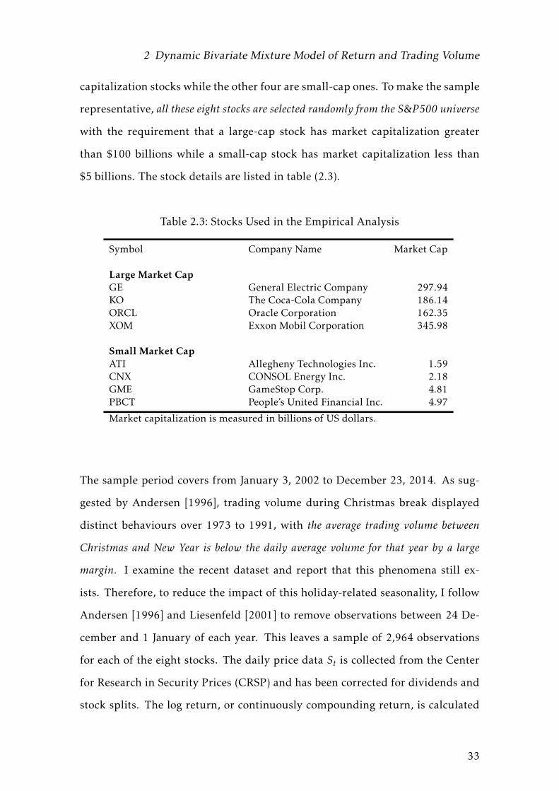
capitalization stocks while the other four are small-cap ones. To make the sample
representative, all these eight stocks are selected randomly from the S&P500 universe
with the requirement that a large-cap stock has market capitalization greater
than $100 billions while a small-cap stock has market capitalization less than
$5 billions. The stock details are listed in table (2.3).
Table 2.3: Stocks Used in the Empirical Analysis
Symbol Company Name Market Cap
Large Market CapGE General Electric Company 297.94KO The Coca-Cola Company 186.14ORCL Oracle Corporation 162.35XOM Exxon Mobil Corporation 345.98
Small Market CapATI Allegheny Technologies Inc. 1.59CNX CONSOL Energy Inc. 2.18GME GameStop Corp. 4.81PBCT People’s United Financial Inc. 4.97
Market capitalization is measured in billions of US dollars.
The sample period covers from January 3, 2002 to December 23, 2014. As sug-
gested by Andersen [1996], trading volume during Christmas break displayed
distinct behaviours over 1973 to 1991, with the average trading volume between
Christmas and New Year is below the daily average volume for that year by a large
margin. I examine the recent dataset and report that this phenomena still ex-
ists. Therefore, to reduce the impact of this holiday-related seasonality, I follow
Andersen [1996] and Liesenfeld [2001] to remove observations between 24 De-
cember and 1 January of each year. This leaves a sample of 2,964 observations
for each of the eight stocks. The daily price data St is collected from the Center
for Research in Security Prices (CRSP) and has been corrected for dividends and
stock splits. The log return, or continuously compounding return, is calculated
33

2 Dynamic Bivariate Mixture Model of Return and Trading Volume
as Rt = 100 × (lnSt − lnSt−1). Also, because trading volume tends to exhibit a
trend and the sample period lasts for more than 10 years, I have to detrend the
series of trading volume in order to make it stationary. To do so, I follow the de-
trending procedure outlined in Andersen [1996]. Specifically, I first calculate the
daily trend component by a centred equally weighted moving median with two-year
window, and then divide each observation of trading volume by the correspond-
ing trend component for that day, which leads to an average detrended volume
approximately being close to one.
Summary statistics of return and detrended volume series for all 8 stocks are
reported in table (2.4). I observe that all the 8 stocks included in the sample
display very similar features. The mean of sample daily return is not signifi-
cantly different from zero and the corresponding standard deviation exceeds the
sample mean by a factor about 100. The return distribution is generally sym-
metric (skewness is typically small) with two notable exceptions, KO and CNX.
These two deviations from zero skewness are mainly caused by a few outliers
in the sample period, as shown in the quantile statistics section. Moreover, the
returns exhibit significant excessive kurtosis with a value far greater than 3. Fur-
thermore, the Ljung-Box statistic (with 20 lags) for absolute daily return and the
autocorrelation coefficients at various lags indicate that the series display signif-
icant serial correlation and it persists for at least 6 months (corresponds to ap-
proximately 120 trading days). Overall, these findings imply that the return data
is clearly not drawn independently from a normal distribution. The detrended
volume series is characterized by underdispersion3 with a significant positive
skewness. The Ljung-Box statistic (with 20 lags) further reveals that the volume
data is serially correlated. However, unlike daily absolute return, trading volume
displays positive autocorrelation only at short lags and the correlation coefficient
3the standard deviation less than the mean
34

2 Dynamic Bivariate Mixture Model of Return and Trading Volume
Table 2.4: Summary Statistics for Sample Stock Dataset
GE KO ORCL XOM ATI CNX GME PBCT
Returnmin -13.684 -9.068 -12.393 -15.027 -21.272 -25.211 -22.166 -16.998q10 -1.167 -1.166 -2.056 1.494 -3.871 -3.310 -2.902 -1.635q25 -0.696 -0.535 -0.928 -0.693 -1.775 -1.545 -1.356 -0.741q50 0.000 0.049 0.030 0.056 0.082 0.065 0.047 0.068q75 0.792 0.588 1.068 0.816 1.939 1.717 1.520 0.819q90 1.716 1.268 2.124 1.563 4.081 3.586 3.005 1.661max 17.986 12.997 12.283 15.863 22.894 17.911 21.460 16.451mean 0.016 0.033 0.050 0.039 0.061 0.052 0.068 0.047stdev 1.862 1.173 1.908 1.526 3.508 3.296 2.760 1.699skewness -0.008 0.287 0.037 -0.003 -0.114 -0.578 -0.051 0.069kurtosis 14.880 14.962 7.878 17.539 6.552 9.277 9.388 15.763LB(R) 146.63 69.20 78.12 192.55 53.91 129.82 47.508 230.44LB(|R|) 8338.1 3419.5 1876.5 4616.5 3147.4 7184.3 1018.9 4738.2Corr(|Rt |, |Rt−1|) 0.350 0.269 0.168 0.292 0.191 0.293 0.145 0.341Corr(|Rt |, |Rt−5|) 0.349 0.223 0.203 0.292 0.228 0.314 0.158 0.243Corr(|Rt |, |Rt−20|) 0.316 0.129 0.138 0.192 0.175 0.303 0.061 0.215Corr(|Rt |, |Rt−60|) 0.265 0.108 0.108 0.114 0.129 0.159 0.064 0.170Corr(|Rt |, |Rt−120|) 0.160 0.037 0.047 0.045 0.078 0.119 0.023 0.110
DetrendedVolumemin 0.301 0.295 0.201 0.292 0.207 0.108 0.186 0.097q10 0.681 0.682 0.668 0.744 0.596 0.590 0.541 0.517q25 0.787 0.785 0.776 0.840 0.733 0.737 0.669 0.662q50 0.924 0.931 0.910 0.961 0.916 0.920 0.869 0.846q75 1.113 1.119 1.101 1.117 1.170 1.179 1.143 1.150q90 1.393 1.385 1.354 1.299 1.537 1.492 1.607 1.570max 5.302 4.790 5.199 3.856 5.536 6.905 10.514 9.771mean 0.999 0.998 0.997 1.006 1.013 1.015 1.011 1.001stdev 0.355 0.349 0.414 0.269 0.452 0.476 0.600 0.637skewness 2.932 2.714 3.705 2.385 2.491 3.462 3.822 4.937LB(V ) 920.8 709.7 771.1 896.1 1300.7 681.4 535.1 596.5Corr(Vt ,Vt−1) 0.424 0.355 0.383 0.383 0.430 0.351 0.334 0.330Corr(Vt ,Vt−5) 0.097 0.084 0.062 0.120 0.162 0.093 0.059 0.059Corr(Vt ,Vt−20) -0.022 0.048 -0.059 -0.029 0.021 0.009 -0.035 -0.011
ContemporaneousCorrelationsCorr(Rt ,Vt) -0.004 -0.024 0.026 -0.055 0.090 0.036 0.052 0.059Corr(|Rt |,Vt) 0.363 0.404 0.485 0.320 0.318 0.219 0.489 0.247
This table shows summary statistics of daily return and dollar trading volume (corrected for stock splitsand dividends) based on a sample of 8 stocks listed in the US market over period January 3, 2002 - De-cember 23, 2014. Observations between December 24 and January 1 (inclusive) are omitted due to distinctholiday seasonality. The sample consists of 2,964 daily observations.
35

2 Dynamic Bivariate Mixture Model of Return and Trading Volume
vanishes to zero in about 2 - 4 weeks (10 - 20 trading days). Finally, there is a sig-
nificant positive contemporaneous correlation between return volatility (absolute
return) and trading volume. All these findings are fully consistent with predic-
tions made by the Mixture of Distribution Hypothesis, as described in Harris
[1987].
2.5.2 Empirical Results
In this section, the proposed Revised Bivariate Mixture (RBM) model is fitted
to each of the 8 stocks individually. Bayesian posterior estimation results are
reported in table (2.5).
The posterior results of the persistent parameter βh in investors’ time-varying
sentiment process {ht}Tt=1 are quite similar across all sample stocks, with the mean
and the 95% credibility interval being approximately 0.990 and [0.980,0.995].
The implication is that the sentiment process displays a very high degree of clus-
tering: large changes in market sentiment tend to be followed by large changes,
and small changes tend to be followed by small changes. The stochastic shock ηh,t
has a long-lasting impact on market sentiment dynamics, with a half-life about
60 trading days (corresponding to 3 calendar months). In contrast, the parameter
βλ, which characterizes the stochastic behaviours of information arrival process
{λt}Tt=1, exhibits much less persistence with a value typically ranging from 0.5 to
0.6. This suggests that the impact of stochastic shock ηλt in the news arrival pro-
cess is short-lived with a half-life about 1 trading day only. These findings are
fully in line with those of Engle and Lee [1996] and Ding and Granger [1996]. In
their works, the authors report that a two-factor stochastic volatility model is
36

2D
ynamic
Bivariate
Mixtu
reM
odelof
Retu
rnand
Trading
Volu
me
Table 2.5: Posterior Estimation Results of the Revised Bivariate Mixture Model
GE KO ORCL XOM ATI CNX GME PBCT
αh 0.004 0.007 0.027 -0.001 0.018 0.009 0.037 -0.005(-0.003,0.013) (-0.009,0.026) (0.009,0.049) (-0.015,0.012) (0.003,0.037) (-0.006,0.028) (0.011,0.072) (-0.019,0.009)
βh 0.995 0.988 0.986 0.989 0.989 0.989 0.981 0.990(0.991,0.997) (0.981,0.993) (0.978,0.993) (0.984,0.993) (0.984,0.994) (0.984,0.994) (0.968,0.989) (0.983,0.996)
σh 0.068 0.089 0.098 0.079 0.088 0.091 0.103 0.112(0.052,0.087) (0.068,0.116) (0.075,0.125) (0.063,0.097) (0.070,0.108) (0.072,0.116) (0.073,0.135) (0.082,0.145)
qR -0.029 -0.056 -0.036 -0.059 -0.023 0-0.022 -0.024 -0.024(-0.039,-0.021) (-0.076,-0.036) (-0.048,-0.025) (-0.075,-0.042) (-0.028,-0.018) (-0.029,-0.015) (-0.032,-0.016) (-0.038,-0.008)
qV -0.002 -0.008 -0.015 0.006 0.005 0.011 -0.008 0.009(-0.011,0.006) (-0.029,0.007) (-0.035,-0.000) (-0.007,0.019) (-0.008,0.016) (-0.004,0.025) (-0.029,0.009) (-0.004,0.025)
βλ 0.593 0.547 0.576 0.605 0.572 0.530 0.546 0.554(0.550,0.635) (0.503,0.591) (0.535,0.617) (0.556,0.652) (0.532,0.612) (0.487,0.573) (0.506,0.586) (0.512,0.596)
σλ 0.488 0.491 0.536 0.431 0.441 0.422 0.613 0.534(0.456,0.520) (0.451,0.531) (0.501,0.572) (0.397,0.465) (0.417,0.464) (0.398,0.447) (0.581,0.646) (0.494,0.555)
ρR -0.008 -0.018 -0.006 -0.039 -0.004 -0.001 0.003 0.007(-0.020,0.003) (-0.042,0.006) (-0.018,0.007) (-0.053,-0.026) (-0.010,0.002) (-0.006,0.004) (-0.006,0.012) (-0.006,0.021)
µ0 0.542 0.541 0.562 0.635 0.295 0.229 0.402 0.303(0.506,0.573) (0.493,0.582) (0.530,0.592) (0.602,0.664) (0.251,0.331) (0.171,0.285) (0.369,0.434) (0.253,0.352)
µw 0.378 0.383 0.345 0.320 0.621 0.671 0.463 0.562(0.341,0.420) (0.337,0.436) (0.308,0.384) (0.283,0.356) (0.573,0.672) (0.631,0.756) (0.421,0.505) (0.505,0.620)
σw 0.132 0.145 0.146 0.133 0.124 0.127 0.173 0.177(0.121,0.142) (0.133,0.156) (0.136,0.155) (0.125,0.141) (0.105,0.141) (0.104,0.148) (0.159,0.187) (0.156,0.196)
This table presents the Bayesian MCMC posterior results of the Revised Bivariate Mixture model based on a sample of 8 stocks listed in theUS market over period January 3, 2002 - December 23, 2014. Observations between December 24 and January 1 (inclusive) are omitted dueto distinct holiday seasonality. The sample consists of 2,964 daily observations. The posterior mean and the 95% credibility interval arereported for each model parameter.
37
2 Dynamic Bivariate Mixture Model of Return and Trading Volume
able to better fit empirical data than a single-factor model, with one component
driving the long-run volatility whereas the other component characterizing the
short-run dynamics. The results stated in table (2.5) further suggest that the
short-run volatility dynamics is related to the information arrival process while
the long-run behaviour is described by investors’ sentiment.
A widely cited stylized fact about stock market returns is that volatility displays
long memory, that is, the autocorrelation function of absolute or squared return
decays at a hyperbolic rate instead of an exponential rate; figure (2.5) presents
empirical evidence to support such statement. In particular, the autocorrelation
function of absolute return shows fast decay at the first few lags but much slower
decay at longer lags. In comparison, long range dependence is not found in vol-
ume series. As shown in figure (2.6), the autocorrelation function of volume re-
veals an exponential decay and its coefficient quickly vanishes toward 0 within 10
lags. The model implied autocorrelation functions in figure (2.5) and (2.6) are cal-
culated as follows: I first simulate a very long series of return and volume with
a sample size of 100,000 observations at the posterior means of model parame-
ters given in table (2.5); and then I calculate the corresponding autocorrelation
function based on simulated data. As one can see, the proposed Revised Bivariate
Mixture model is able to capture empirical autocorrelation function in absolute
return and trading volume reasonably well. This also highlights the importance
of the inclusion of time-varying sentiment process {ht}Tt=1 in reducing the depen-
dence between return volatility and trading volume, and thus allows those two
series displaying distinct time-series properties.
To interpret the parameter σh and σλ, one can calculate the implied variation of
38

2 Dynamic Bivariate Mixture Model of Return and Trading Volume
Figure 2.5: Autocorrelation Function of Absolute Return
This figure plots the empirically observed autocorrelation function v.s. the autocorrelation func-tion implied by the Revised Bivariate Mixture model based on absolute return data. The sampleconsists of 8 stocks over period January 3, 2002 - December 23, 2014. The model-implied auto-correlation function is calculated based a simulated series with 100,000 observations generatedat the parameter estimates given in table (2.5).
39

2 Dynamic Bivariate Mixture Model of Return and Trading Volume
Figure 2.6: Autocorrelation Function of Detrended Volume
This figure plots the empirically observed autocorrelation function v.s. the autocorrelation func-tion implied by the Revised Bivariate Mixture model based on detrended trading volume data.The sample consists of 8 stocks over period January 3, 2002 - December 23, 2014. The model-implied autocorrelation function is calculated based a simulated series with 100,000 observationsgenerated at the parameter estimates given in table (2.5).
40

2 Dynamic Bivariate Mixture Model of Return and Trading Volume
latent state variables exp(ht) and exp(λt) using the following formula:
Var[exp(xt)] = E[{exp(xt)}2]−(E[exp(xt)]
)2= exp
( 2σ2x
1− β2x
)− exp
( σ2x
1− β2x
)(2.45)
where xt is the latent AR(1) process with persistence parameter βx. The implied
variations of latent processes ht and λt are reported in table (2.6), from where
we can see that both the investors’ sentiment process and the information arrival
process show comparable and substantial variations.
Table 2.6: Variations of Latent Processes
GE KO ORCL XOM ATI CNX GME PBCT
var[exp(ht)] 0.937 0.548 0.582 0.439 0.605 0.672 0.432 1.649var[exp(λt)] 0.641 0.579 0.825 0.456 0.447 0.360 1.209 0.768
This table presents the variations of latent processes exp(ht) and exp(λt) calcu-lated using the formula (2.45).
A natural follow-up exercise is to investigate the relative explanatory powers of
market sentiment process and information arrival process on return volatility
and volume. The procedure is similar to that outlined in Liesenfeld [2001]. I
run a regression, in which volatility (volume) is considered as LHS dependent
variable while latent state variable h1:T or λ1:T acts as the single RHS explanatory
variable. Then the R2 statistic tells us how much variations in volatility (vol-
ume) can be explained by each of the latent processes. Since return volatility is
in fact unobservable, I replace it with an observed approximation such like ab-
solute return. The regression results are reported in table (2.7). The variations
in daily trading volume can be largely explained by the variations in informa-
tion arrival process with R2 statistics being greater than 90% for each of the 8
stocks included in the sample. For absolute daily return, I find that both latent
41

2 Dynamic Bivariate Mixture Model of Return and Trading Volume
processes account for a comparably low percent (less than 30%) of total varia-
tions. However, this should not be considered as evidence that those two latent
processes do a bad job in explaining volatility dynamics. As argued in Andersen
and Bollerslev [1998], these low R2 values are due to the fact that the absolute
return is rather a noisy indicator of true volatility. One could expect an improved
R2 when realized volatility is used as a more reliable and accurate proxy to latent
true volatility.
Table 2.7: Explanatory Power of Sentiment and News Arrival Processes
GE KO ORCL XOM ATI CNX GME PBCT
LHS: Absolute Return
RHS: exp(ht) 0.282 0.260 0.185 0.344 0.187 0.256 0.125 0.267RHS: exp(λt) 0.143 0.194 0.229 0.133 0.106 0.051 0.264 0.083
LHS: Detrended Trading Volume
RHS: exp(λt) 0.965 0.956 0.964 0.915 0.991 0.992 0.983 0.983
Analogue to Andersen [1996], the Revised Bivariate Mixture model specification
includes a constant term µ0 to accommodate the presence of non-informed liq-
uidity traders. To test the validity of this hypothesis, one can examine the pos-
terior distribution of the parameter µ0. As shown in table (2.5), posterior means
of parameter µ0 are all positive for all of the 8 stocks and the empirical evidence
overwhelming rejects the null H0 : µ0 = 0, as indicated by the 95% credibility
intervals excluding zero by a significant margin. Another interesting observa-
tion is that the portion of liquidity-based trading volume as a percentage of total
volume is much higher for large-cap stocks than for small-cap tickers. In partic-
ular, for large-cap stocks (GE, KO, ORCL and XOM), the part of trading volume
generated by liquidity traders accounts for about 60% of total turnover on aver-
42

2 Dynamic Bivariate Mixture Model of Return and Trading Volume
age; while this figure is less than 40% for small-cap tickers (ATI, CNX, GME and
PBCT). This can partially explained by the fact that most stock market indices,
such as S&P500, are calculated in a capitalization-weighted fashion, and thus the
blue chip stocks account for a large portion of market index portfolio (for exam-
ples, Exchange Traded Fund). Asset managers who pursue a smart beta strategy
will invest a significant portion of their capital in these market index portfolio
to allow them better track (and possibly outperform) the market index. Thus,
contributions and withdrawals of the funds force asset managers to trade for liq-
uidity motives. Therefore, all else being equal, blue chip stocks tend to have a
higher portion of non-informed trading volume than small-cap stocks.
Next, I look into the posterior estimation results of qR and qV in order to in-
vestigate how market sentiment changes in response to past return and volume.
As reported in table (2.5), past return has an asymmetric impact on investors’
sentiment process. In particular, the posterior mean of qR of all stocks are neg-
ative with the 95% credibility intervals excluding zeros by large margins, which
implies that positive returns tend to clam down investors whereas declines in
stock prices tend tomakemarket participants feel more anxious. This asymmetry
property can be attributed to the so-called loss aversion or prospect theory in the
behavioural finance literature (see Kahneman and Tversky [1979]). More specif-
ically, as argued in Shefrin and Statman [1985], investors exhibit loss-aversed
biases and they tend to sell winners too soon but ride losers too long, hoping
that those losers will eventually coming back and the paper loss will not be re-
alized. This creates a continuous downward pressure on stock price when bad
news is released, introducing excessive price volatility in future and resulting in
the asymmetric impacts typically observed in empirical data. The posterior mean
of qV typically has a small magnitude and is not significantly different from zero.
This suggests that past trading volume has little or no impact on traders’ senti-
43
2 Dynamic Bivariate Mixture Model of Return and Trading Volume
ment, that is, investors tend not to take into account the change in stock turnover
when they make their trading decisions.
Another interesting hypothesis to test is the self-referential theorem proposed in
Wyart and Bouchaud [2007]. As stated in Keynes [1936]’s famous contest, the
goal is to anticipate correctly what other participants themselves anticipate. The im-
plication is that information event is not limited to fundamental news announce-
ment but also includes past market price event itself. In particular, investors
try to predict what other participants themselves anticipate by observing mar-
ket price movements, and thus the changes in market price itself is treated as
an informational event, contributing further to return volatility and volume. A
feedback loop is created in this fashion and it may destabilize the market from
its efficient behaviour. A testable hypothesis to this behavioural statement is the
null H0 : ρR = 0 against the alternative H1 : ρR > 0 with H1 supporting the self-
referential theory. From the posterior results in table (2.5), 7 out of 8 stocks reveal
insignificant estimates of ρR with the 95% credibility intervals including zero.
One notable exception is XOM, where the posterior estimate −0.039 is signifi-
cantly different from zero. However, the sign is opposite to what is expected from
the self-referential hypothesis. Overall, there is no strong empirical evidence to
reveal the presence of self-referential phenomena in the US stock market.
Finally, I examine the cross-sectional relations of the latent processes among 8
stocks. Table (2.8) reports the correlation matrix of market sentiment process
and information arrival process respectively. The results show that there is a
very high and positive correlation for investors’ sentiment processes, while the
connection through information arrival process is not so strong (especially for
those four small-cap tickers). This could suggest that the investors’ sentiment
is a marketwide factor whereas information arrival process is idiosyncratic and
44
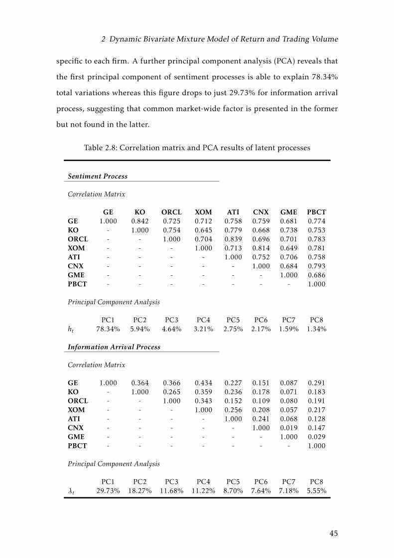
2 Dynamic Bivariate Mixture Model of Return and Trading Volume
specific to each firm. A further principal component analysis (PCA) reveals that
the first principal component of sentiment processes is able to explain 78.34%
total variations whereas this figure drops to just 29.73% for information arrival
process, suggesting that common market-wide factor is presented in the former
but not found in the latter.
Table 2.8: Correlation matrix and PCA results of latent processes
Sentiment Process
Correlation Matrix
GE KO ORCL XOM ATI CNX GME PBCTGE 1.000 0.842 0.725 0.712 0.758 0.759 0.681 0.774KO - 1.000 0.754 0.645 0.779 0.668 0.738 0.753ORCL - - 1.000 0.704 0.839 0.696 0.701 0.783XOM - - - 1.000 0.713 0.814 0.649 0.781ATI - - - - 1.000 0.752 0.706 0.758CNX - - - - - 1.000 0.684 0.793GME - - - - - - 1.000 0.686PBCT - - - - - - - 1.000
Principal Component Analysis
PC1 PC2 PC3 PC4 PC5 PC6 PC7 PC8ht 78.34% 5.94% 4.64% 3.21% 2.75% 2.17% 1.59% 1.34%
Information Arrival Process
Correlation Matrix
GE 1.000 0.364 0.366 0.434 0.227 0.151 0.087 0.291KO - 1.000 0.265 0.359 0.236 0.178 0.071 0.183ORCL - - 1.000 0.343 0.152 0.109 0.080 0.191XOM - - - 1.000 0.256 0.208 0.057 0.217ATI - - - - 1.000 0.241 0.068 0.128CNX - - - - - 1.000 0.019 0.147GME - - - - - - 1.000 0.029PBCT - - - - - - - 1.000
Principal Component Analysis
PC1 PC2 PC3 PC4 PC5 PC6 PC7 PC8λt 29.73% 18.27% 11.68% 11.22% 8.70% 7.64% 7.18% 5.55%
45
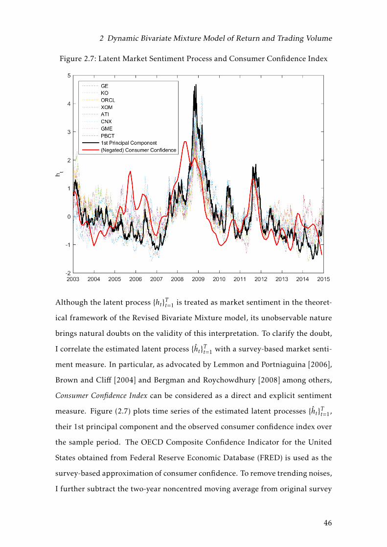
2 Dynamic Bivariate Mixture Model of Return and Trading Volume
Figure 2.7: Latent Market Sentiment Process and Consumer Confidence Index
Although the latent process {ht}Tt=1 is treated as market sentiment in the theoret-
ical framework of the Revised Bivariate Mixture model, its unobservable nature
brings natural doubts on the validity of this interpretation. To clarify the doubt,
I correlate the estimated latent process {ht}Tt=1 with a survey-based market senti-
ment measure. In particular, as advocated by Lemmon and Portniaguina [2006],
Brown and Cliff [2004] and Bergman and Roychowdhury [2008] among others,
Consumer Confidence Index can be considered as a direct and explicit sentiment
measure. Figure (2.7) plots time series of the estimated latent processes {ht}Tt=1,
their 1st principal component and the observed consumer confidence index over
the sample period. The OECD Composite Confidence Indicator for the United
States obtained from Federal Reserve Economic Database (FRED) is used as the
survey-based approximation of consumer confidence. To remove trending noises,
I further subtract the two-year noncentred moving average from original survey
46

2 Dynamic Bivariate Mixture Model of Return and Trading Volume
values, and the resulting series is shown in figure (2.7). As one can see, there is a
strong contemporaneous comovement between {ht}Tt=1 of individual stock and the
observed consumer confidence measure. Table (2.9) provides the estimation re-
sults of univariate regression of the estimated latent process {ht}Tt=1 on observed
consumer confidence. In particular, the regression coefficients are all negative
and significant for 8 stocks, and a good amount of contemporaneous correlation
(about -0.5 on average) is found. All these findings provides supports to inter-
preting {ht}Tt=1 as market sentiment process.
Table 2.9: Univariate Regression Results
GE KO ORCL XOM ATI CNX GME PBCT
Reg Coeff -0.541 -0.367 -0.394 -0.534 -0.434 -0.526 -0.323 -0.629t-ratio -5.214 -4.801 -6.633 -8.901 -5.534 -5.987 -5.293 -8.968Corr Coeff -0.482 -0.465 -0.558 -0.721 -0.489 -0.578 -0.508 -0.672
This table presents the estimation results of univariate regression of the estimatedlatent process {ht}Tt=1 on observed consumer confidence.
2.6 Concluding Remarks
In this paper, I develop a new type of Bivariate Mixture model to describe the
dynamics between return volatility and trading volume. The proposed semi-
structural model allows the common and idiosyncratic components in traders’
reservation price to interact in a multiplicative way rather than an additive way
which is typically adopted by previous researches. The resulting Revised Bivari-
ate Mixture (RBM) model has desirable properties that are fully consistent with
empirical stylized facts and provides additional insights on price discovery pro-
cess from a behavioural perspective.
47

2 Dynamic Bivariate Mixture Model of Return and Trading Volume
The model involves a large number of latent unobservable state variables, and
thus the typical maximum likelihood estimation method is not applicable as
it requires infeasible high-dimension integration. I develop a Bayesian MCMC
multi-block sampler to tackle the statistical inference problem. A Monte Carlo
experiment is studied to show the superior ability of the MCMC algorithm to re-
cover the true model parameters as well as latent state variable very accurately.
The proposed Bayesian estimationmethod is applied to a sample of 8 stocks listed
in the US stock market. The empirical results are summarized as follows. First, I
find the existence of a common latent information flow process that drives the bi-
variate dynamics of return volatility and trading volume simultaneously, thus the
empirical evidence is in favour of the Mixture of Distribution Hypothesis (MDH).
Second, investors’ sentiment process is near unit root but information flow pro-
cess shows much less persistence; overall, this embedded two-factor structure is
able to replicate the observed autocorrelation functions of absolute return and
trading volume. Third, the proportion of liquidity-driven trading volume is
much higher in large-cap stocks than in small-cap tickers. Fourth, no statistical
evidence is found to support the self-referential hypothesis in behaviour finance
literature. Finally, there is strong evidence suggesting that the investors’ sen-
timent process might be a market-wide factor as the estimated latent processes
{ht}Tt=1 are highly correlated within the sample of 8 stocks.
48

2 Dynamic Bivariate Mixture Model of Return and Trading Volume
2.7 Appendix 1: Derivations of unconditional
moments
In this appendix, I show how to derive the unconditional first and second mo-
ments of r(k) and v(k) attributed to the kth intraday informative event.
Since r(k) =1N
∑Ni=1γiφ(k), by mutual independence between γi and φ(k), one can
write
E[r(k)] = E[1N
N∑i=1
γiφ(k)] =1N
N∑i=1
E[γi]E[φ(k)] = 0 (2.46)
where the last equality follows because φ(k) ∼ N (0,σ2φ). The second raw moment
of r(k) is given by
E[r2(k)] = E[1N2
N∑i=1
N∑j=1
γiγjφ2(k)]
=1N2E[φ
2(k)]E[
N∑i=1
N∑j=1
γiγj ]
=1N2σ
2φ
( N∑i=1
E[γ2i ] +
∑i,j
E[γiγj ])
= σ2φ
1N2
[N (σ2
γ +µ2γ ) +N (N − 1)µ2γ
]= σ2
φ
(σ2γ
N+µ2γ
)(2.47)
and its variance is thus
var[r(k)] = E[r2(k)]−(E[r(k)]
)2=σ2γσ
2φ
N+µ2γσ
2φ (2.48)
49

2 Dynamic Bivariate Mixture Model of Return and Trading Volume
The trading volume in response to kth information is given by
v(k) = cN∑i=1
|γi −1N
N∑i=1
γi | · |φ(k)| (2.49)
where both γi − 1N
∑Ni=1γi and φ(k) follow independent normal distributions with
zero means.
The absolute value of a zero-centred normally distributed random variables fol-
low a half-normal distribution, whose mean and variance have closed forms and
are well known in the literature. The expectation, E[v(k)], can be written as
E[v(k)] = c( N∑i=1
E[|γi −1N
N∑i=1
γi |])E[φ(k)]
= c(N ×
√N − 1N
σγ
√2π
)σφ
√2π
=2cπ
√N (N − 1)σγσφ (2.50)
Denote 1N
∑Ni=1γi by γ , one can show the second raw moment of v(k) to be
E[v2(k)] = E
[c2φ2
k
N∑i=1
N∑j=1
|γi − γ | · |γj − γ |]
= c2E[φ2(k)]
( N∑i=1
E[(γi − γ)2] +∑i,j
E[|(γi − γ)(γj − γ)|])
= c2σ2φ
(NN − 1N
σ2γ +N (N − 1)N − 1
N2πσ2γ
)= c2σ2
φ
(N − 1+ 2(N − 1)2
π
)σ2γ (2.51)
and thus the variance is given by
var[v(k)] = E[v2(k)]− (E[v(k)])2 = c2
[N − 1+ 2(N − 1)2
π− 4N (N − 1)
π2
]σ2φσ
2γ (2.52)
50

2 Dynamic Bivariate Mixture Model of Return and Trading Volume
2.8 Appendix 2: MCMC algorithm
In this appendix, I explain details of the multi-block MCMC algorithm to esti-
mate the proposed RBMM model.
To facilitate further discussion, the following conventions and notations are used.
Subscripts denote the time index whereas superscripts with parenthesis indicate
this is a random draw at a particular sweep loop. In addition, I denote the model
parameters by θ = {µ0,µw,σw,αh,βh, qR, qV ,σh,βλ,ρR,σλ}, augmented latent state
variables byX = {h1:T ,λ1:T }, and observations by Y = {R1:T ,V1:T }.
Posterior Density
By dropping irrelevant integrating constants, one can write the joint posterior
density f (θ,X |Y ) of the proposed RBMM model as follows :
∝ f (R1:T ,V1:T |h1:T ,λ1:T ,θ) · f (h1:T ,λ1:T ,θ)
∝ f (R1:T |h1:T ,λ1:T ,θ) · f (V1:T |λ1:T ,θ) · f (h1:T |θ) · f (λ1:T |θ) · f (θ) f (h1:T ,λ1:T ,θ|R1:T ,V1:T )
(2.53)
where
f (R1:T |h1:T ,λ1:T ,θ) =T∏t=1
1√2πexp(ht/2)exp(λt/2)
· exp{− 12
R2t
exp(ht)exp(λt)
}f (V1:T |λ1:T ,θ) =
T∏t=1
1√2πσw exp(λt/2)exp(λt/2)
· exp{− 12
(Vt −µ0 −µw exp(λt)
)2σ2w exp(λt)
}f (h1:T |θ) = f (hT |h1:T−1,θ)f (hT−1|h1:T−2,θ)...f (h2|h1,θ)f (h1|θ)
51

2 Dynamic Bivariate Mixture Model of Return and Trading Volume
=1
√2π σh√
1−β2h
· exp{− 12
[h1 −αh
(1−βh)]2
σ2h
(1−β2h )
}
×T∏t=2
1√2πσh
· exp{− 12(ht −αh − βhht−1 − qrRt−1 − qvVt−1)2
σ2h
}f (λ1:T |θ) = f (λT |λ1:T−1)f (λT−1|λ1:T−2,θ)...f (λ2|λ1,θ)f (λ1|θ)
=1
√2π σλ√
1−β2λ
· exp{− 12λ21σ2λ
1−β2λ
} T∏t=2
1√2πσλ
· exp{− 12(λt − βλλt−1)2
σ2λ
}f (θ) = f (αh)f (βh)f (σh)f (qR)f (qV )f (βλ)f (σλ)f (m1)
The Multi-block Sampler for augmented State Variables
The main ingredient of the algorithm is the multi-block sampler of Shephard
and Pitts [1997], which attempts to draw samples from a multivariate density by
means of importance sampling. In their original paper, the multi-block sampler
is tailored to estimate the univariate Stochastic Volatility (SV) model, which also
possesses a non-Gaussian state-space form as the proposed RBMM model.
I’ll first discuss how to draw samples from investors’ systematic sentiment pro-
cess h1:T . Shephard and Pitts [1997] advocate to use the so-called stochastic knots
approach to divide the entire sequence {h1,h2, ...,hT } into K + 1 blocks in a ran-
dom manner. Set k0 = 0 and kK+1 = T . All K knots, (k1, k2, ..., kK ), are selected
randomly such that
ki = int[T × (i +ui)/(K +2)], (2.54)
where ui for i = 1,2, ...,K are independent uniform random variables onU(0,1).
52

2 Dynamic Bivariate Mixture Model of Return and Trading Volume
Consider a particular block that contains the t th to t + k th elements. It’s easy to
see that sampling from f (h(i+1)t:t+k |h(i+1)t−1 ,h
(i)t+k+1,Rt:t+k ,Vt:t+k ,λ
(i)t:t+k ,θ
(i)) is equivalent
to sampling from its innovation terms f (η(i+1)h,t:t+k |h(i+1)t−1 ,h
(i)t+k+1,Rt:t+k ,Vt:t+k ,λ
(i)t:t+k ,θ
(i)).
The problem of sampling directly on state variables is that its multivariate dis-
tribution f (h(i+1)t:t+k |·) is heavily concentrated on a very small region because of the
high correlation between state variables ht:t+k . In contrast, the distribution of in-
novation terms f (η(i+1)h,t:t+k |·) is highly dispersed and its probability mass spreads much
more evenly throughout the entire domain. The importance sampling, relying on
the proposal density approximating reasonably well to the true target posterior
density, works best when both proposal and target densities are relatively flat.
To sample from f (η(i+1)h,t:t+k |·), suppose that we already got a sequence of h(i)t:t+k that
approximates the true value ht:t+k reasonably well. Then, by taking a second or-
der Taylor expansion of the joint block posterior density around h(i)t:t+k , we obtain
that
log f (η(i+1)h,t:t+k |h(i+1)t−1 ,h
(i)t+k+1,Rt:t+k ,Vt:t+k ,λ
(i)t:t+k ,θ
(i))
∝ log f (η(i+1)h,t:t+k |h(i+1)t−1 ,h
(i)t+k+1,θ
(i)) + log f (Rt:t+k ,Vt:t+k |η(i+1)h,t:t+k ,h
(i+1)t−1 ,h
(i)t+k+1,λ
(i)t:t+k ,θ
(i))
∝ − 12
k+1∑j=1
η(i+1)h,t+j−1
2+t+k∑s=t
log f (Rs,Vs |h(i+1)s ,λ
(i)s ,θ
(i))
≈ − 12
k+1∑j=1
η(i+1)h,t+j−1
2+t+k∑s=t
{log f (Rs,Vs |h
(i)s ,λ
(i)s ,θ
(i))
+∂ log f (Rs,Vs |h
(i)s ,λ
(i)s ,θ(i))
∂hs(i)
(h(i+1)s − h(i)s
)+12∂2 log f (Rs,Vs |h
(i)s ,λ
(i)s ,θ(i))
∂(h(i)s )2
(h(i+1)s − h(i)s
)2}(2.55)
where
log f (Rs,Vs |h(i)s ,λ
(i)s ,θ
(i)) ∝ −12h(i)s −
12R2s exp(−λ
(i)s )exp(−h(i)s ) (2.56)
53

2 Dynamic Bivariate Mixture Model of Return and Trading Volume
∂ log f (Rs,Vs |h(i)s ,λ
(i)s ,θ)
∂hs(i)
∝ −12+12R2s exp(−λ
(i)s )exp(−h(i)s ) (2.57)
∂2 log f (Rs,Vs |h(i)s ,λ
(i)s ,θ)
∂(h(i)s )2∝ −1
2R2s exp(−λ
(i)s )exp(−h(i)s ). (2.58)
One can easily see that the approximation of the likelihood part in (2.55)
log f (Rt:t+k ,Vt:t+k |η(i+1)h,t:t+k ,h
(i+1)t−1 ,h
(i)t+k+1,λ
(i)t:t+k ,θ
(i))
is of quadratic form and thus {h(i+1)s }t+ks=t follows a multivariate normal distribu-
tion. This approximated normal density can be used as the candidate generat-
ing function in Metropolis-Hastings step to draw proposed new samples. More
specifically, h(i+1)s ∼ N(µ(i+1)s , (σ (i+1)
s )2)where µ(i+1)s and (σ (i+1)
s )2 are both known
quantities:
µ(i+1)s = h(i)s − (
∂2 log f (Rs,Vs |h(i)s ,λ
(i)s ,θ(i))
∂(h(i)s )2)−1(
∂ log f (Rs,Vs |h(i)s ,λ
(i)s ,θ(i))
∂hs(i)
)
(σ (i+1)s )2 = −(
∂2 log f (Rs,Vs |h(i)s ,λ
(i)s ,θ(i))
∂(h(i)s )2)−1.
Write hs = µs + σsεs, and along with the original transition equation of hs, we
obtain an auxiliary state space model
µ(i+1)s = h(i+1)s +σ (i+1)
s εs (2.59)
h(i+1)s = α(i)
h + β(i)h h(i+1)s−1 + q(i)r Rt−1 + q
(i)v Vt−1 +σ
(i)h η
(i+1)h,s (2.60)
where we can infer the latent state h(i+1)s from observations on µ(i+1)s . Samples of
η(i+1)h,t:t+k can be generated by first applying the Simulation Smoother of Koopman
[1993] and then passing through the Metropolis-Hastings step to make draws of
true block posterior density.
54

2 Dynamic Bivariate Mixture Model of Return and Trading Volume
The same procedure can be easily applied to information arrival process λ1:T by
changing a handful of density functions as below:
log f (Rs,Vs |λ(i)s ,h
(i)s ,θ
(i)) ∝−λ(i)s −12
[R2s exp(−h
(i)s ) + (σ (i)
v )−2(Vt −µ(i)0 )2
]exp(−λ(i)s )
+ (σ (i)v )−2(Vt −µ
(i)0 )µ(i)v −
12(σ (i)v )−2(µ(i)v )2 exp(λ(i)s )
(2.61)
∂ log f (Rs,Vs |λ(i)s ,h
(i)s ,θ(i))
∂λ(i)s
∝− 1+ 12
[R2s exp(−h
(i)s ) + (σ (i)
v )−2(Vt −µ(i)0 )2
]exp(−λ(i)s )
− 12(σ (i)v )−2(µ(i)v )2 exp(λ(i)s ) (2.62)
∂2 log f (Rs,Vs |λ(i)s ,h
(i)s ,θ(i))
∂(λ(i)s )2∝− 1
2
[R2s exp(−h
(i)s ) + (σ (i)
v )−2(Vt −µ(i)0 )2
]exp(−λ(i)s
− 12(σ (i)v )−2(µ(i)v )2 exp(λ(i)s ) (2.63)
55

3 Multivariate Dynamics of
High-Frequency Transaction-level
Variables
3.1 Introduction and Motivation
Market microstructure theory studies the trading mechanisms used for financial
securities with the aim to help both academic scholars and market practitioners
better understanding the price discovery process in financial markets. By its very
nature, trading is a truly high-dimensional process and generates many observed
variables during the course, including price change, trade duration, trade vol-
ume, bid-ask spread, market depth, order imbalance, etc. Analysing the intraday
multivariate dynamics among these observed transaction variables has been one
of most popular topics in market microstructure research.
Most of previous studies (for examples, see Xu and Wu [1999], Huang and Ma-
sulis [2003], Manganelli [2005] and Hautsch [2008] among others) focus on mod-
elling the multivariate dynamics among transaction variables (such as return
56

3 Multivariate Dynamics of High-Frequency Transaction-level Variables
volatility, trading duration and trading volume), but rare of them include liquidity-
related variables (such as bid-ask spread, market depth and order imbalance) into
their analysis. However, the importance of liquidity in price formation process
cannot be overstated. Therefore, in this paper, I fill this gap in the literature by
adding bid-ask spread into the multivariate dynamics modelling framework.
Two market microstructure frictions deserve special attentions: (1) traders ar-
rive and trade at the market place asynchronously and (2) market participants possess
asymmetric information. Consequently, two main strands of theoretical frame-
works have been proposed in the market microstructure literature to deal with
these two frictions: the inventory-based framework and the information-based frame-
work.
The inventory-based model addresses the inventory problem of market makers
that buyers and sellers do not arrive simultaneously. In Garman [1976], the ar-
rivals of buyers and sellers are modelled as separate Poisson processes; as long as
their arrival rates are equal, the market maker is on average buying and selling
securities at the same pace, and she is able to consistently profit from bid-ask
spread (assuming no price risk). Whenever the inventory of market maker ap-
proaches the alerted boundaries, she needs to update her quotes in order to bring
back the inventory to a normal level by encouraging or discouraging arrivals of
buyers or sellers. The implication is that in a one-side market, where asset price is
under large positive (negative) movement and the market is dominated either by
buyers (sellers), the market maker is more likely to approach her inventory lower
bound (upper bound), and thus she will be likely to publish a higher ask price
(lower bid price) to discourage further buying (selling) activities. Consequently,
the bid-ask spread expects to be positively correlated to return volatility.
57

3 Multivariate Dynamics of High-Frequency Transaction-level Variables
The asymmetric information-based model (see Copeland and Galai [1983] and
Glosten and Milgrom [1985]) approaches the problem from a different perspec-
tive. In particular, market participants are assumed to be divided into three
groups with distinct characteristics: informed traders are those who possess some
private information on fundamental value of assets and thus trade accordingly;
uninformed or liquidity traders are those who trade because of some exogenous
reasons like portfolio rebalances or adjustments; and market makers/dealers are
those who publish a continuous stream of bid-and-ask quotes at which they are
willing to buy and sell a particular security to facilitate trading. It is typically as-
sumed that market maker is uninformed, and on average, and she is able to profit
from trading with uninformed traders by taking the spread of bid-ask quotes as
a compensation for her liquidity providing service; however, trading with in-
formed traders could lead to severe loss due to price risk and adverse selection.
Although market maker is generally uninformed, she is able to compute the con-
ditional expectation of true asset payoff based on her observations on trade and
order flow history. Accordingly, the market maker sets bid/ask quotes so that the
loss to informed traders is offset by the expected gain from uninformed traders.
Market maker continuously do such Bayesian-style updates on her belief of true
asset value. The resulting bid-ask spread is thus positively correlated to the magni-
tude of potential asset price movement. Seminal papers along this line of research
include Easley and O’Hara [1992], Easley et al. [2002] and Easley et al. [2008].
More specifically, in Easley and O’Hara [1992], the authors assume that unin-
formed traders do not necessarily always buy or sell but can also stop trading
and quit the market temporarily. Thus the observation of no trading activities is
also informative. One important implication is that the degree of trading activity,
measured by trade duration or average trade size, also carries out essential in-
formation on potential price movement and hence return volatility. Easley et al.
[2002] extends the original model by allowing informed traders and uninformed
58

3 Multivariate Dynamics of High-Frequency Transaction-level Variables
traders have different Poisson arrival rates, and consequently, the number of daily
trading activities follows a mixture of Poisson distributions. What’s more, Easley
et al. [2008] adds more flexibility to the model by further allowing a time-varying
Poisson arrival intensity, and the Probability of Informed Trading (PIN), defined
as the probability that a randomly chosen trader is informed, can be calculated
in a straightforward manner.
Another popular theory that sheds lights on on how transaction variables might
be interacted with each other is the so-called Mixture of Distribution Hypothe-
sis (MDH). The MDH claims that asset returns follow a mixture of distribution
where a serially correlated but unobservable information flow acts as themixing vari-
able. Its development can be traced back to the seminal work of Clark [1973], and
several subsequent extensions include Epps and Epps [1976], Tauchen and Pitts
[1987], Andersen [1996] and Liesenfeld [2001].
Traditional econometric framework to model the intraday multivariate dynam-
ics is typically the family of Vector Autoregressive Regression with explanatory
variables (VAR-X) and its variations (such as Vector Autoregressive Conditional
Duration model and Vector Multiplicative Error model), where the key focus is
placed on examining the serial correlation as well as the lead-lag causality be-
tween various variables. As pointed by Hautsch [2008], this approach is subject
to potential model misspecification bias because it fails to take into account the
presence of common latent information flow. In fact, the subordination nature of
MDH implies that any investigation on casual relationship among intraday trad-
ing variables without controlling for the effect of latent information flow process
could give misleading statistical results. To better recover the genuine casual re-
lations, Hautsch [2008] proposes a novel Stochastic Vector Multiplicative Error
model (S-VMEM) to tackle this issue.
59

3 Multivariate Dynamics of High-Frequency Transaction-level Variables
In this paper, I extend the S-VMEM model of Hautsch [2008] by adding bid-ask
spread into multivariate dynamics and by allowing positive and negative returns
having asymmetric impacts on return volatility, trade intensity, trade volume and
bid-ask spread. By fitting a sample of six heavily traded stocks listed in NYSE,
I thus want to analyse the genuine causal relations among these four trading
variables after taking into account the presence of latent information flow.
The rest of the chapter is organized as follows. Section 3.2 reviews the economet-
ric framework of Stochastic Vector Multiplicative Error model (S-VMEM). The
model is in state-space form and the Maximum Likelihood with Efficient Im-
portance Sampling (ML-EIS) technique is used to conduct statistical inference.
Details of ML-EIS procedure is documented in section 3.3 and its accuracy is ex-
amined by a Monte Carlo simulation study presented in section 3.4. Overviews
on the empirical dataset and the data cleaning procedures are provided in section
3.5, followed by empirical results reported in the same section. Finally, section
(3.6) concludes the study.
3.2 Model Specification
In this section, I briefly review the development of Stochastic Vector Multiplica-
tive Error model (S-VMEM) in the literature.
60

3 Multivariate Dynamics of High-Frequency Transaction-level Variables
3.2.1 The Autoregressive Conditional Duration Model
The Autoregressive Moving Average (ARMA) model has been a core building
block in univariate time-series modelling. The seminal work of Engle [1982] and
Bollerslev [1986] successfully apply ARMA framework to model the second mo-
ment (volatility) of financial returns and propose the well-known Generalized
Autoregressive Conditional Heteroskedasticity (GARCH) model, i.e.,
Rt = σtεt , εt ∼N(0,1)
σ2t = ω +
p∑i=1
βiσ2t−i +
q∑j=1
αjε2t−j (3.1)
where Rt is observed return and σ2t is the conditional variance of return.
While GARCH-type model is designed to describe the dynamics of financial re-
turn which can take both positive and negative values, the increasing popular
high-frequency data (i.e. duration, volume, bid-ask spread, market depth, etc.) is
typically positive-valued and thus poses great challenges on choosing an appro-
priate econometric framework to model its dynamics. To tackle this problem,
Engle and Russell [1997] and Engle and Russel [1998] develop a novel Autore-
gressive Conditional Duration (ACD) framework to model the dynamics of trade
duration sampled at high-frequency real event time. As the name suggests, the
ACD framework focuses on modelling the conditional first moment (expectation)
of observed trade duration and possesses the following form:
Ψt = E[Yt |Ft−1;θ], εt ≡YtΨt
Ψt = ω +p∑i=1
βiΨt−i +q∑i=1
αqYt−q (3.2)
61

3 Multivariate Dynamics of High-Frequency Transaction-level Variables
where Yt is a generic positive-valued time series (trade duration in the context
of duration modelling); Ft−1 represents a natural filtration containing all infor-
mation up to time t − 1; θ denotes the collection of model parameters; Ψt is the
conditional expectation of Yt given information up to time t − 1 and it follows
an ARMA-type process; and finally, εt ≡YtΨt
follows a positive-valued distribution
with mean equals to 1. Some popular parametric distributional forms of positive-
valued innovation term εt in ACD models include Weibull, Generalized Gamma,
Log-Normal and Burr distributions, as they are flexible enough to accommodate
both underdispersed and overdispersed 1 positive-valued random variables.
Because the observation Yt is positive-valued, it must have a positive conditional
expectation, i.e. Ψt > 0. A sufficient condition for this is that ω > 0, α ≥ 0 and
β ≥ 0. An alternative way to respect this positivity constraint of Ψt is to adopt a
log-linear parametrization, for example, see Bauwens and Giot [2000] for Loga-
rithmic ACD (log-ACD) model,
Ψt = E[Yt |Ft−1;θ]
lnΨt = ω +p∑i=1
βi lnΨt−i +q∑i=1
αq lnYt−q (3.3)
The ACD framework has also been successfully applied to model some positive-
valued transaction variables other than trade duration, see, for examples, the
Autoregressive Conditional Volume (ACV) model applied to trading volume by
Manganelli [2005], and the log-ACDmodel applied to bid-ask spread by Bauwens
and Giot [2000].
Both GARCH models and ACD models belong to a boarder family of Multiplica-
1underdispersed: standard deviation is less than mean.overdispersed: standard deviation is greater than mean.
62

3 Multivariate Dynamics of High-Frequency Transaction-level Variables
tive Error model (MEM). This name comes from the fact that the conditional mo-
ment interacts with error term in a multiplicative way, i.e. Rt = σtεt in GARCH
specification and Yt =Ψtεt in ACD specification.
In ACD-type models, the innovation terms in conditional mean equation is re-
stricted to be the past realized values of Yt , so thatΨt is essentially a deterministic
process given information up to time t − 1. One way to relax this assumption is
to model the conditional mean Ψt as a stochastic process. This leads to the so-
called Stochastic Conditional Duration (SCD) model, first introduced by Bauwens
and Veredas [2004], which can be viewed as a analogue of Stochastic Volatility
(SV) model of Taylor [1982] applied to positive-valued process. The SCD model
is configured as follows:
Yt =Φtεt (3.4)
logΦt = ω + β logΦt−1 + et (3.5)
where et |Ft−1 ∼ i.i.d.N(0,σ2) and is independent of εt . The SCD specification
poses a challenge on how to interpret and justify the existence of the latent pro-
cess {Φt}Tt=1. One popular explanation is to treat the latent factor as informa-
tion flow (or the state of the market), which cannot be observed directly but cer-
tainly play an important role in determining the multivariate dynamics of vari-
ous trading-related variables.
3.2.2 The Vector Multiplicative Error Model
The Vector Multiplicative Error Model (VMEM) of Manganelli [2005] is a powerful
econometric framework to model multivariate dynamics of high-frequency data.
63

3 Multivariate Dynamics of High-Frequency Transaction-level Variables
To facilitate further discussion, I use the following conventions and notations.
Denote the intraday return by Rt , the number of trades (trade intensity) by T I t ,
the average dollar volume per trade (trade size) by TS t , and the average bid-ask
spread as a percentage of current stock price by BAS t . These four quantities
{Rt ,T I t ,T S t ,BAS t} are key interests in this study. Without loss of generality, one
can write their Data Generating Process (DGP) as
Rt ,T I t ,T S t ,BAS t ∼ f(Rt ,T I t ,T S t ,BAS t |Ft−1;θ
)(3.6)
where Ft−1 denotes the full information set up to time t and θ is the complete set
of model parameters. Following the suggestions of Engle [2000] and Manganelli
[2005], one can decompose the joint density (3.6) as a series of conditional densities
(or marginal density), and thus rewrite the DGP as
Rt ,T I t ,T S t ,BAS t ∼ f(BAS t |Ft−1;θ
)(3.7)
× f(TS t |BAS t ,Ft−1;θ
)(3.8)
× f(T I t |TS t ,BAS t ,Ft−1;θ
)(3.9)
× f(Rt |T I t ,T S t ,BAS t ,Ft−1;θ
)(3.10)
Themain benefit of the abovemultiplicative decomposition structure is to allow one
to model each conditional density separately. For examples, to model positive-
valued dynamic process, such like T I t ,T S t or BAS t , one can borrow the idea from
the ACD framework discussed in previous section. In particular, the marginal
density (3.7) and conditional densities (3.8) and (3.9) can be written as
BAS t = κtξBAS,t , ξBAS,t ∼ i.i.d.D(1,νξ,BAS ) (3.11)
TS t = φtξTS,t , ξTS,t ∼ i.i.d.D(1,νξ,TS ) (3.12)
T I t = ψtξT I,t , ξT I,t ∼ i.i.d.D(1,νξ,T I ) (3.13)
64

3 Multivariate Dynamics of High-Frequency Transaction-level Variables
where ξBAS,t , ξTS,t and ξT I,t are positive-valued i.i.d. random variables following
a generic distribution D(·). The other three terms, namely, κt ,φt ,ψt , are con-
ditional expectations of time-varying bid-ask spread, trade size and number of
trades respectively. They can be formally defined as
κt ≡ E[BAS t |Ft−1;θ] (3.14)
φt ≡ E[TS t |BAS t ,Ft−1;θ] (3.15)
ψt ≡ E[T I t |TS t ,BAS t ,Ft−1;θ] (3.16)
For return DGP (3.10), the well-known (E)GARCH framework comes as a handy
tool to model the dynamics of return volatility, i.e.
Rt = σtηR,t , ηR,t ∼ i.i.d.N (0,1) (3.17)
σ2t ≡ E[R2
t |T I t ,T S t ,BAS t ,Ft−1;θ] (3.18)
where σ2t is the conditional variance of return Rt .
The main ingredient of Manganelli [2005]’s VMEM framework is to allow mul-
tivariate causality among the conditional mean processes κt ,φt ,ψt and the con-
ditional variance process σ2t . This can be easily achieved by imposing a Vector
Autoregressive Moving Average with Explanatory variables (vector-ARMA-X) struc-
ture, where the cross-dependence (3.7) - (3.10) is captured linearly by some additional
contemporaneous explanatory variables. To further enrich themodel dynamics, I al-
low past return Rt−1 to have asymmetric impacts on those conditional moments.
Putting all these elements together, one can come up with the following generic
ARMA-X(P, Q) specification:
κt = a0 +P∑i=1
(a1,iκt−i + a2,iφt−i + a3,iψt−i + a4,iσ
2t−i
)
65
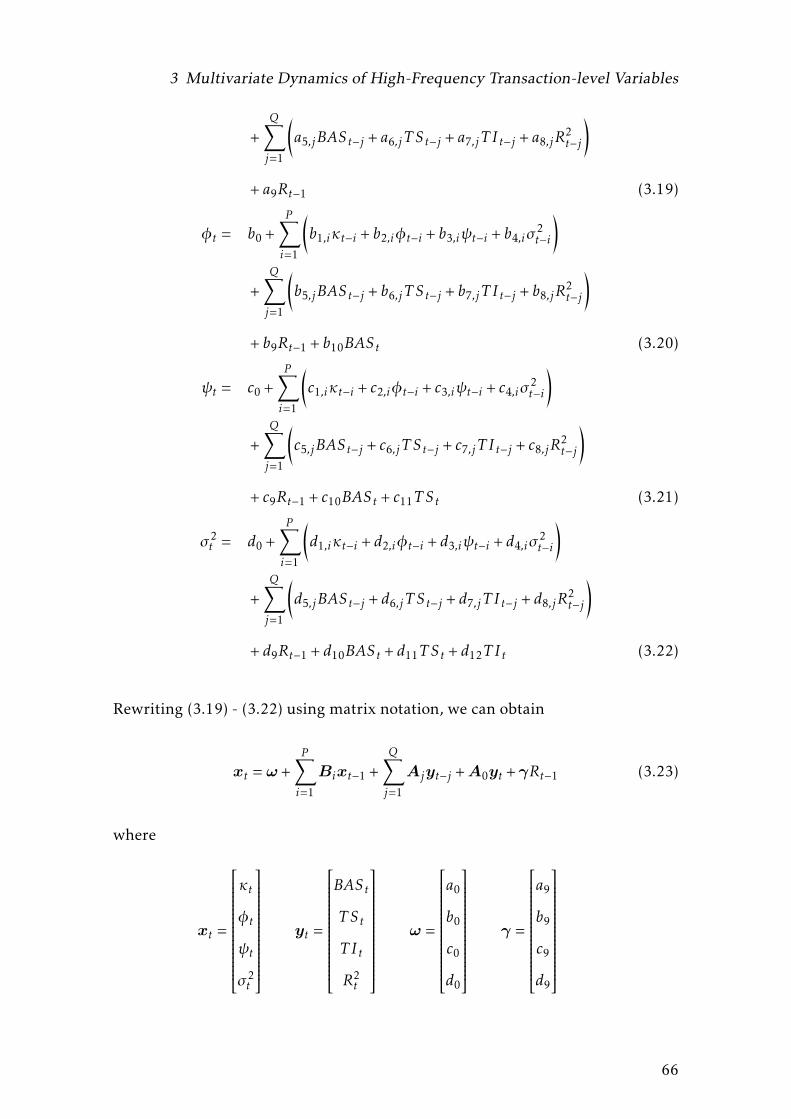
3 Multivariate Dynamics of High-Frequency Transaction-level Variables
+Q∑j=1
(a5,jBAS t−j + a6,jTS t−j + a7,jT I t−j + a8,jR
2t−j
)+ a9Rt−1 (3.19)
φt = b0 +P∑i=1
(b1,iκt−i + b2,iφt−i + b3,iψt−i + b4,iσ
2t−i
)
+Q∑j=1
(b5,jBAS t−j + b6,jTS t−j + b7,jT I t−j + b8,jR
2t−j
)+ b9Rt−1 + b10BAS t (3.20)
ψt = c0 +P∑i=1
(c1,iκt−i + c2,iφt−i + c3,iψt−i + c4,iσ
2t−i
)
+Q∑j=1
(c5,jBAS t−j + c6,jTS t−j + c7,jT I t−j + c8,jR
2t−j
)+ c9Rt−1 + c10BAS t + c11TS t (3.21)
σ2t = d0 +
P∑i=1
(d1,iκt−i + d2,iφt−i + d3,iψt−i + d4,iσ
2t−i
)
+Q∑j=1
(d5,jBAS t−j + d6,jTS t−j + d7,jT I t−j + d8,jR
2t−j
)+ d9Rt−1 + d10BAS t + d11TS t + d12T I t (3.22)
Rewriting (3.19) - (3.22) using matrix notation, we can obtain
xt = ω +P∑i=1
Bixt−1 +Q∑j=1
Ajyt−j +A0yt +γRt−1 (3.23)
where
xt =
κt
φt
ψt
σ2t
yt =
BAS t
TS t
T I t
R2t
ω =
a0
b0
c0
d0
γ =
a9
b9
c9
d9
66

3 Multivariate Dynamics of High-Frequency Transaction-level Variables
Bi =
a1,i a2,i a3,i a4,i
b1,i b2,i b3,i b4,i
c1,i c2,i c3,i c4,i
d1,i d2,i d3,i d4,i
Aj =
a5,i a6,i a7,i a8,i
b5,i b6,i b7,i b8,i
c5,i c6,i c7,i c8,i
d5,i d6,i d7,i d8,i
A0 =
0 0 0 0
b10 0 0 0
c10 c11 0 0
d10 d11 d12 0
(3.24)
The parameter Bi characterizes the persistence of the conditional moments pro-
cesses {xt}Tt=1; the coefficient Aj describes how most recent observations yt−j af-
fect the conditional moments xt ; the lower-diagonal matrixA0 with all elements
on diagonal equal to zero imposes the cross-dependence structure implied by the
DGP decomposition structure in (3.7) - (3.10); and finally, the asymmetric impact
of latest return Rt−1 on the conditional moments xt is captured by γ.
In order to keep the model parsimonious, the vector-ARMA-X(1,1) specification
is generally preferred. Furthermore, I follow Manganelli [2005] to impose the
weak exogeneity by restricting the persistence coefficient B1 to be diagonal. This
also eases the model estimation by simplifying the stationarity constraint on the
conditional moment process xt .
3.2.3 The Stochastic Vector Multiplicative Error Model
As pointed by Hautsch [2008], the standard VMEM specification is subject to
model misspecification bias because it fails to take into account the presence of the
latent serially correlated information flowwhich is common to all trading-related
67

3 Multivariate Dynamics of High-Frequency Transaction-level Variables
variables. In fact, theMixture of Distribution Hypothesis (MDH) implies that any
investigation on casual relationship among intraday trading variables without
controlling for the effect of serially correlated information flow process could give
misleading statistical results: the seemingly lead-lag causality between two variables
may be due to the fact that both variables have latent autocorrelated information flow
as the common component rather than that any true causality exists between these
two variables. To better estimate the genuine casual relationship, Hautsch [2008]
proposes the Stochastic Vector Multiplicative Error model (S-VMEM) to tackle
this issue. Borrowing the idea from S-VMEM framework, I specify the following
dynamics for the four observed intraday trading related variables:
BASt = s1,t exp(x1,t)exp(δ1λt) · ξ1,t , ξ1,t ∼ LN(ν1) (3.25)
TSt = s2,t exp(x2,t)exp(δ2λt) · ξ2,t , ξ2,t ∼ LN(ν2) (3.26)
T It = s3,t exp(x3,t)exp(δ3λt) · ξ3,t , ξ3,t ∼ LN(ν3) (3.27)
Rt =√s4,t exp(x4,t)exp(δ4λt) · ηt , ηt ∼N(0,1) (3.28)
where the latent state variable {λt}Tt=1 describes the underlying information flow
process; si,t characterizes intraday deterministic seasonality patterns; xi,t refers
to the logarithmic of conditional moment process after controlling for the im-
pact of latent information flow λt ; and finally, ηt and ξi,t are normally and log-
normally distributed independent and identical innovation terms. I assume the
Log-Normal (LN) innovation terms for positive-valued process because the LN-
ACD specification allows for a humped-shaped hazard function2 with one free shape
parameter only, which poses a computational advantage compared to other ex-
isting ACD specifications in the literature, like Generalized Gamma- and Burr-
ACDmodels. In fact, the empirical study of Xu [2013] shows that LN-ACDmodel
is always superior to Exponential- andWeibull- ACDmodels and its performance
2typically found in trade duration
68

3 Multivariate Dynamics of High-Frequency Transaction-level Variables
is similar to Burr- and Generalized Gamma- specifications.
The latent state variable λt is assumed to be serially correlated and follow an
AR(1) process:
λt = ρλt−1 + εt , where εt ∼N(0,1) (3.29)
where the variance of error terms εt is set to be unity. This is because when
multiplied with their impact coefficients δi , the combined latent dynamics λi,t :=
δiλt becomes
λi,t = ρλi,t + εi,t where εi,t ∼ i.i.d.N(0,δ2i ) (3.30)
and it’s clear that the model would be unidentifiable if one allows additional
parameter to describe the variance of εt .
As mentioned above, xi,t is the logarithmic of conditional moment process after
controlling for the impact of latent information flow λt , and it is assumed to
follow a VMEM-type dynamics:
xt = ω +Bxt−1 +Aut−1 +A0u0,t +γRt−1√
s4,t exp(x4,t−1)(3.31)
where
u0,t =(ln(BASt), ln(TSt), ln(T It),0
)′ut−1 =
(BASt−1
s1,t−1 exp(x1,t−1),
T St−1s2,t−1 exp(x2,t−1)
,T It−1
s3,t−1 exp(x3,t−1),
|Rt−1|√s4,t−1 exp(x4,t−1)
)′
Note that I standardize ut−1 only by the seasonality pattern si,t−1 and the dynam-
ics of xi,t−1, because this ensures that xi,t can be calculated without integrating the
69

3 Multivariate Dynamics of High-Frequency Transaction-level Variables
latent information flow, which can greatly reduce the computational burden in-
troduced by the inclusion of unobserved state variable λt . The model parameters
ω,B,A,A0 and γ are similar to the ones defined in (3.24).
3.3 The Estimation Technique
Since innovation terms in the S-VMEM specification (3.25) - (3.27) follow stan-
dardized log-normal distributions3, one can write the likelihood function condi-
tional on latent process ΛT ≡ {λt}Tt=1 as
L(YT |θ,ΛT )
=T∏t=1
g(yt |λt ,Yt−1)
=T∏t=1
1√2πσ4BASt
exp{−(logBASt − logs1,t − x1,t − δ1λt +σ2
1 /2)2
2σ21
}1
√2πσ2TSt
exp{−(logTSt − logs2,t − x2,t − δ2λt +σ2
2 /2)2
2σ22
}1
√2πσ3T It
exp{−(logT It − logs3,t − x3,t − δ3λt +σ2
3 /2)2
2σ23
}1√
2πs4,t exp(x4,t)exp(δ4λt)exp
{−
R2t
2s4,t exp(x4,t)exp(δ4λt)
}(3.32)
where yt = {BASt ,T St ,T It ,Rt} are observations of trading variables at time t, and
YT ≡ {BASt ,T St ,T It ,Rt}Tt=1 denote observations up to time T .
Integrating the conditional likelihood function (3.32) with respect to latent state
3standardization: mean equals one
70

3 Multivariate Dynamics of High-Frequency Transaction-level Variables
variables ΛT , one can write the unconditional likelihood function as follows:
L(YT |θ) =∫ΛT
L(YT |θ,ΛT )p(ΛT |θ)dΛT
=∫ΛT
T∏t=1
g(yt |λt ,Yt−1)T∏t=1
p(λt |θ,Λt−1)dΛT (3.33)
The high dimensional density (3.33) poses great challenges on drawing efficient
and effective likelihood-based statistical inference. To tackle this problem, Richard
and Zhang [2007] proposes a novel simulation-based Maximum Likelihood with
Efficient Importance Sampling (ML-EIS). Following Richard and Zhang [2007]
and Hautsch [2008], I apply the ML-EIS method to the S-VMEM model, and the
estimation procedure is outlined in the rest of this section.
3.3.1 Maximum Likelihood with Efficient Importance Sampling
Monte Carlo method has been widely applied to evaluate analytically intractable
integral like the one in (3.33), i.e. L(YT |θ) = EΛT[L(YT |θ,ΛT )]. By simulating
the latent process ΛT R times, the sample average of L(YT |θ,Λ(r)T ) evaluated at
simulated series Λ(r)T would produce a good approximation to EΛT
[L(YT |θ,ΛT )]
as it will eventually converge to the true unconditional density asymptotically.
To simulate ΛT , a straightforward choice is to use the so-called natural sampler
p(λt |θ,Λt−1) and thus
L(YT |θ) = LR(Yt |θ) =1R
R∑r=1
T∏t=1
g(yt |λ(r)t ,Yt−1) (3.34)
However, the MC sampling variance of∏Tt=1 g(yt |λ
(r)t ,Yt−1) based on the natural
71

3 Multivariate Dynamics of High-Frequency Transaction-level Variables
sampler p(λt |θ,Λt−1) is typically massive especially when T is large, and conse-
quently, the MC method is highly inefficient as it requires a prohibitively large
number of simulated paths. Important Sampling (IS) method is developed to
tackle this problem, and its idea is to use a carefully chosen auxiliary sampler,
i.e. m(λt |θ,Λt−1,γt), where the additional parameter γt aims to provide much
more informative content than the original natural sampler so that the integral
has a much smaller sampling variance. Formally,
L(YT |θ) =∫ΛT
T∏t=1
g(yt |λt ,Yt−1)T∏t=1
p(λt |θ,Λt−1)dΛT (3.35)
=∫ΛT
T∏t=1
g(yt |λt ,Yt−1)T∏t=1
p(λt |θ,Λt−1)m(λt |θ,Λt−1,γt)m(λt |θ,Λt−1,γt)
dΛT
=∫ΛT
T∏t=1
g(yt |λt ,Yt−1)p(λt |θ,Λt−1)m(λt |θ,Λt−1,γt)
T∏t=1
m(λt |θ,Λt−1,γt)dΛT
and the corresponding Monte Carlo estimator is given by
L(YT |θ) ≈ LR(Yt |θ) =1R
R∑r=1
T∏t=1
g(yt |λ(r)t ,Yt−1)p(λ
(r)t |θ,Λ
(r)t−1)
m(λ(r)t |θ,Λ(r)t−1,γt)
(3.36)
Obviously, the key ingredient of the IS estimator (3.36) is to choose an appro-
priate auxiliary sampler m(λt |θ,Λt−1,γt) so that the MC sampling variance is
minimized. One popular way proposed by Geweke [1989] is to break down∏Tt=1 g(yt |λ
(r)t ,Yt−1)p(λ
(r)t |θ,Λ
(r)t−1) into T separate elements g(yt |λ
(r)t ,Yt−1)p(λ
(r)t |θ,Λ
(r)t−1)
for t = 1, ...,T and to tailor the auxiliary samplerm(λ(r)t |θ,Λ(r)t−1,γt) to approximate
each elements locally for each t. For example, one can use a second-order Taylor
expansion of g(yt |λ(r)t ,Yt−1)p(λ
(r)t |θ,Λ
(r)t−1) around its local modal value, and the
auxiliary sampler thus follows Gaussian distribution which is easy to simulate
from. This algorithm expects to work reasonably well when T is moderate; how-
ever, it might still impose a large MC sampling variance when T is large, because
72
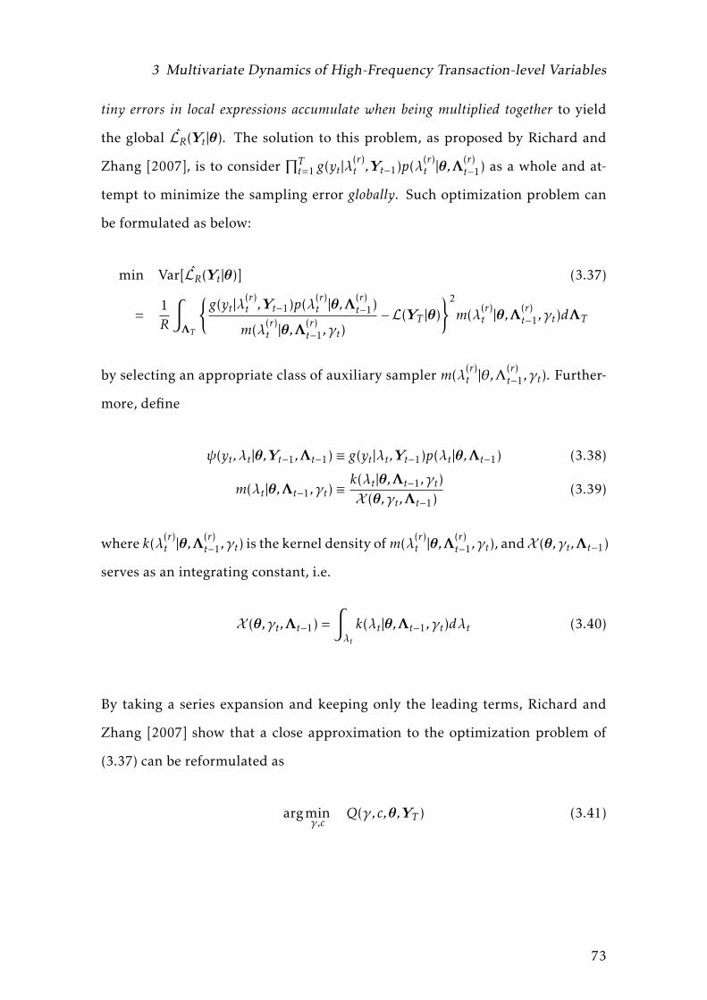
3 Multivariate Dynamics of High-Frequency Transaction-level Variables
tiny errors in local expressions accumulate when being multiplied together to yield
the global LR(Yt |θ). The solution to this problem, as proposed by Richard and
Zhang [2007], is to consider∏Tt=1 g(yt |λ
(r)t ,Yt−1)p(λ
(r)t |θ,Λ
(r)t−1) as a whole and at-
tempt to minimize the sampling error globally. Such optimization problem can
be formulated as below:
min Var[LR(Yt |θ)] (3.37)
=1R
∫ΛT
{g(yt |λ
(r)t ,Yt−1)p(λ
(r)t |θ,Λ
(r)t−1)
m(λ(r)t |θ,Λ(r)t−1,γt)
−L(YT |θ)}2
m(λ(r)t |θ,Λ(r)t−1,γt)dΛT
by selecting an appropriate class of auxiliary sampler m(λ(r)t |θ,Λ(r)t−1,γt). Further-
more, define
ψ(yt ,λt |θ,Yt−1,Λt−1) ≡ g(yt |λt ,Yt−1)p(λt |θ,Λt−1) (3.38)
m(λt |θ,Λt−1,γt) ≡k(λt |θ,Λt−1,γt)X (θ,γt ,Λt−1)
(3.39)
where k(λ(r)t |θ,Λ(r)t−1,γt) is the kernel density ofm(λ(r)t |θ,Λ
(r)t−1,γt), andX (θ,γt ,Λt−1)
serves as an integrating constant, i.e.
X (θ,γt ,Λt−1) =∫λt
k(λt |θ,Λt−1,γt)dλt (3.40)
By taking a series expansion and keeping only the leading terms, Richard and
Zhang [2007] show that a close approximation to the optimization problem of
(3.37) can be reformulated as
argminγ,c
Q(γ,c,θ,YT ) (3.41)
73

3 Multivariate Dynamics of High-Frequency Transaction-level Variables
where
Q(γ,c,θ,YT ) =∫ΛT
d(γ,c,ΛT ,θ,YT )2 ·
T∏t=1
ψ(yt ,λt |θ,Yt−1,Λt−1)dΛT (3.42)
d(γ,c,ΛT ,θ,YT ) = log[ T∏t=1
ψ(yt ,λt |θ,Yt−1,Λt−1)]− c − log
[ T∏t=1
m(λt |θ,Λt−1,γt)]
(3.43)
which says that we are going to minimize a weighted average of quadratic dis-
tances of d(·)2, where d(·) is given by (3.43) as a form of global logarithmic dis-
tance (up to a constant c) between the target conditional likelihood function∏Tt=1ψ(yt ,λt |θ,Yt−1,Λt−1) and its approximation
∏Tt=1m(λ(r)t |θ,Λ
(r)t−1,γt). To eval-
uate the quadratic distance Q(·) in (3.42), one can use the auxiliary sampler by
first rewriting
Q(γ,c,θ,YT ) =∫ΛT
d(γ,c,ΛT ,θ,YT )2 ·
T∏t=1
ψ(yt ,λt |θ,Yt−1,Λt−1)m(λt |θ,Λt−1,γt)
m(λt |θ,Λt−1,γt)dΛT
then simulatingΛT according to the auxiliary samplerm(λ(r)t |θ,Λ(r)t−1,γt) and eval-
uate the expression by MC sample average
Q(γ,c,θ,YT ) =1R
R∑r=1
d(γ,c,Λ(r)T ,θ,YT )
2 ·T∏t=1
ψ(yt ,λ(r)t |θ,Yt−1,Λ
(r)t−1)
m(λ(r)t |θ,Λ(r)t−1,γt)
(3.44)
It’s now clear that to minimize Q(·) is essentially an Generalized Least Square (GLS)
problem where one tries to minimize the sum of quadratic distance d(·)2 with
GLS weights given by∏Tt=1ψ(·)/m(·). One potential drawback is that it may lead
numerical instability of IS approximation if the GLS weights have high variance.
As shown in Richard and Zhang [2007], for most practical problems, the standard
OLS version of (3.44) would fix this issue by setting all weights equal, and the authors
demonstrate that OLS is as efficient as GLS counterpart. So now, the optimization
74
3 Multivariate Dynamics of High-Frequency Transaction-level Variables
problem has been reduced to
argminγ,c
Q(γ,c,θ,YT) =1R
R∑r=1
d(γ,c,Λ(r)T ,θ,YT)
2 (3.45)
where d(·) is given by (3.43), or equivalently,
d(γ,c,ΛT ,θ,YT ) (3.46)
=T∑t=1
[logψ(yt ,λt |θ,Yt−1,Λt−1) + c + logX (θ,γt ,Λt−1)− logk(λt |θ,Λt−1,γt)
]
The challenge is that the latent process ΛT (γ) has a dimension of T and it thus
becomes infeasible to do the optimization with respect to γ (and hence ΛT (γ))
in one single block when T is large. To tackle this problem, Richard and Zhang
[2007] suggest to break down the distance (3.46) in a backward sequential fash-
ion into T smaller pieces of sub Least Square problems and iterate this proce-
dure a few times to ensure the convergence of local minimum to the global mini-
mum. More specifically, let ψt(·) ≡ ψ(yt ,λt |θ,Yt−1,Λt−1), Xt(·) ≡ X (θ,γt ,Λt−1) and
kt(·) ≡ k(λt |θ,Λt−1,γt), one can see that ψt(·) and kt(·) are functions of Λt but the
integrating constant Xt is a function of Λt−1, and thus can rewrite the distance
d(·) as
d(γ,c,ΛT ,θ,YT ) =T∑t=1
[logψt(·) + c + logXt(·)− logkt(·)
]+ logXT+1(·) (3.47)
where logXT+1(·) := 0. A rearrangement gives
d(γ,c,ΛT ,θ,YT ) = logX1(·) +T∑t=1
[logψt(·) + c + logXt+1(·)− logkt(·)
](3.48)
Noticing that λT (γ) is included only in logψT (·) + c + logXT+1(·) − logkT (·), so
75

3 Multivariate Dynamics of High-Frequency Transaction-level Variables
conditional on ΛT−1 is given, this sub optimization problem reduces to
argminγ
[logψT (·) + c + logXT+1(·)− logkT (·)
]2(3.49)
=1R
R∑r=1
[logψ(r)
T (·) + c + logX (r)T+1(·)− logk
(r)T (·)
]2(3.50)
which is simply again a Least Square problem. Therefore, γT can be solved by
formulating a linear regression
logψ(r)T (·) + logX (r)
T+1(·) = −c + logk(r)T (·) + ε(r)T (3.51)
For t = T − 1,T − 2, ...,1, similarly, γt can be estimated by solving a backward
sequence of linear regressions
logψ(r)t (·) + logX (r)
t+1(·) = −c + logk(r)t (·) + ε(r)t (3.52)
Richard and Zhang [2007] suggest that iterating the above procedure for just 3
to 5 times would yield a reasonably good result, and they also advise that setting
R = 30 would be sufficient for most applications.
To apply the ML-EIS algorithm to the S-VMEM model, one need to specify the
form of the kernel density k(λ(r)t |θ,Λ(r)t−1,γt). Motivated by the fact that the con-
ditional likelihood function (3.32) belongs to exponential family, I thus intend
to use a Gaussian-type kernel to approximate the conditional likelihood. More
specifically, keeping only λt related terms, and set γt = {γ1,t ,γ2,t}
k(λt |θ,Λt−1,γt) = p(λt |θ,Λt−1)exp(γ1,tλt +γ2,tλ2t ) (3.53)
∝ exp[− 12(λ(r)t − ρλ
(r)t−1)
2]exp
[γ1,tλt +γ2,tλ
2t )]
∝ exp[(γ1,t + ρλ
(r)t−1)λ
(r)t + (γ2,t −
12)(λ(r)t )2
]
76

3 Multivariate Dynamics of High-Frequency Transaction-level Variables
so k(λt |θ,Λt−1,γt) is a Gaussian kernel with
σ2k,t =
11− 2γ2,t
(3.54)
µ(r)k,t = (γ1,t + ρλ
(r)t−1)σ
2k,t (3.55)
Deriving the integrating constant of k(λt |θ,Λt−1,γt) yields
X (θ,γt ,Λ(r)t−1) = exp
[(µ(r)k )2
2σ2k
− 12ρ2(λ(r)t−1)
2]
(3.56)
Substituting (3.53), (3.56) and (3.38) into the recursive regression (3.52), one can
obtain
logg(yt |λ(r)t ,Yt−1) + logp(λt |θ,Λt−1) + logX (θ,γt+1,Λ
(r)t )
= −c + logp(λt |θ,Λt−1) +γ1,tλ(r)t +γ2,t(λ
(r)t )2 + ε(r)t (3.57)
Cancelling out logp(λt |θ,Λt−1) on both sides gives
logg(yt |λ(r)t ,Yt−1) + logX (θ,γt+1,Λ
(r)t ) = −c +γ1,tλ
(r)t +γ2,t(λ
(r)t )2 + ε(r)t (3.58)
To summarize, details of the implementation steps are given as follows:
1. Compute the observed components xT = {x1,t ,x2,t ,x3,t ,x4,t}Tt=1 in (3.31).
2. Simulate R = 30 trajectories of latent information flow process Λ(r)T accord-
ing to the natural sampler∏Tt=1p(λ
(r)t |θ,Λ
(r)t−1).
3. Drop irrelevant terms with respect to ΛT in (3.58) and solve the following
resulting recursive linear regression sequentially from t = T to t = 1 with
initial condition Z5,T = logXT+1(·) = 0,
Z1,t +Z2,t +Z3,t +Z4,t +Z5,t = γ0,t +γ1,tλ(r)t +γ2,t(λ
(r)t )2 + ε(r)t
77

3 Multivariate Dynamics of High-Frequency Transaction-level Variables
where
Z1,t = −
[logBASt − logs1,t − x1,t − δ1λ
(r)t +σ2
1 /2]2
2σ21
Z2,t = −
[logTSt − logs2,t − x2,t − δ2λ
(r)t +σ2
2 /2]2
2σ22
Z3,t = −
[logT It − logs3,t − x3,t − δ3λ
(r)t +σ2
3 /2]2
2σ23
Z4,t = −12δ4λ
(r)t −
12
R2t
s4,t exp(x4,t + δ4λ(r)t )
Z5,t =
(γ1,t + ρλ
(r)t−1
)21− 2γ2,t
−ρ2(λ(r)t−1)
2
2
one thus obtain a series of OLS coefficients {γ1,t ,γ2,t}Tt=1.
4. Delete previous draws of Λ(r)T . Simulate R = 30 new trajectories according
to the sequential Gaussian kernel density k(λ(r)t |θ,Λ(r)t−1) with
σ2k,t =
11− 2γ2,t
µ(r)k,t = (γ1,t + ρλ
(r)t−1)σ
2k,t
5. Go back to step 3, and repeat the procedure (step 3 to step 5) n = 5 times.
6. Compute the Monte Carlo EIS estimator of Likelihood function by
LR(Yt|θ) =1R
R∑r=1
T∏t=1
g(yt |λ(r)t ,Yt−1)p(λ
(r)t |θ,Λ
(r)t−1)
m(λ(r)t |θ,Λ(r)t−1,γ1,t ,γ2,t)
.
3.3.2 Bayesian Predicting and Updating
Once obtaining theML-EIS estimates onmodel parameters θ, one key application
of S-VMEM model is to allow one to produce filtered estimates and one-step-
78
3 Multivariate Dynamics of High-Frequency Transaction-level Variables
ahead predictions on the unobservable underlying information flow.
Bayesian Prediction
The one-step-ahead prediction problem can be expressed as follows: given ob-
servations Yt up to time t, one tries to calculate the conditional expectation of a
generic function of E[G(Λt+1)|Yt ,θ]:
E[G(Λt+1)|Yt ,θ] =∫G(Λt+1)P(Λt+1|Yt ,θ)dΛt+1
=∫G(Λt+1)
P(Yt |Λt+1,θ)P(Λt+1|θ)P(Yt |θ)
dΛt+1
Because the only channel that information flow enters into Yτ for any τ = 1,2, ..., t
is through λτ , so λτ+1 provides no additional information given λτ . Thus one can
easily rewrite the joint density as a multiplication of single-period density,
E[G(Λt+1)|Yt ,θ]
=∫G(Λt+1)
p(λτ+1|λτ ,θ)∏tτ=1 g(Yτ |λτ ,θ)p(λτ |λτ−1,θ)∫P(Yt ,Λt |θ)dΛt
dΛt+1
=
∫G(Λt+1)p(λτ+1|λτ ,θ)
∏tτ=1 g(Yτ |λτ ,θ)p(λτ |λτ−1,θ)dΛt+1∫
P(Yt ,Λt |θ)dΛt
(3.59)
Based on equation (3.59), one can use EIS technique to evaluate the integrals in
numerator and denominator separately. The denominator is just the likelihood
function and can be calculated in the same manner as stated in previous section.
For numerator, one can use the auxiliary samplermτ(λτ |θ,Λτ−1,γ) for τ = 1,2, ..., t
and the natural sampler p(λt+1|λt ,θ) for time t +1. The detailed implementation
steps are given as follows:
1. Set θ = θML-EIS which are the ML-EIS estimates of model parameters.
79

3 Multivariate Dynamics of High-Frequency Transaction-level Variables
2. Follow the ML-EIS instructions in last section, set R = 30 with n = 5 iter-
ations. Use observations up to time t, Yt , to draw R = 30 trajectories of
Λ(r)t and calculate the by-product likelihood function L(Yt |θ) which is es-
sentially the denominator in equation (3.59).
3. Use the natural sampler p(λ(r)t+1|λ(r)t ,θ) to draw λ
(r)t+1.
4. Evaluate the numerator in (3.59) by
1R
R∑r=1
{G(Λ(r)
t+1)t∏
τ=1
[g(Yτ |λ
(r)τ ,θ)p(λ
(r)τ |λ
(r)τ−1,θ)
mτ(λ(r)τ |θ,Λ
(r)τ−1,γ)
]}(3.60)
Bayesian Updating
To calculate the filtered estimates in Bayesian updating step, one can write
E[G(Λt+1)|Yt+1,θ] =∫G(Λt+1)P(Λt+1|Yt+1,θ)dΛt+1
=∫G(Λt+1)
P(Yt+1|Λt+1,θ)P(Λt+1|θ)P(Yt+1|θ)
dΛt+1
=
∫G(Λt+1)
∏t+1τ=1 g(Yτ |λτ ,θ)p(λτ |λτ−1,θ)dΛt+1∫
P(Yt ,Λt |θ)dΛt
(3.61)
To evaluate the above integral, one can following the steps listed below:
1. Set θ = θML-EIS which are the ML-EIS estimates of model parameters.
2. Follow the ML-EIS instructions in last section, set R = 30 with 5 iterations.
Use observations up to time t + 1, Yt+1, to draw R = 30 trajectories of Λ(r)t+1
and calculate the by-product likelihood function L(Yt+1|θ) which is essen-
tially the denominator in equation (3.61).
80

3 Multivariate Dynamics of High-Frequency Transaction-level Variables
3. Use L(Yt+1|θ) to further evaluate the numerator of equation (3.61) by
1R
R∑r=1
{G(Λ(r)
t+1)t+1∏τ=1
[g(Yτ |λ
(r)τ ,θ)p(λ
(r)τ |λ
(r)τ−1,θ)
mτ(λ(r)τ |θ,Λ
(r)τ−1,γ)
]}(3.62)
3.4 A Monte Carlo Simulation Study
In this section, I run a Monte Carlo simulation study to examine the accuracy of
ML-EIS algorithm to estimate the S-VMEM model and its ability to recover the
true latent information flow process.
The true model parameters θ used in data generating process (DGP) are given in
table (3.1). All these parameter values are meant to be representative of typical
values of actually observed high-frequency data as shown in later sections when
I estimate the S-VMEM model empirically. In particular, latent information flow
tends to be highly persistent and it has moderate impacts on trade intensity as
well as return volatility; regarding the genuine multivariate causality between
trading variables after controlling for the existence of serially correlated unob-
servable information flow, the bid-ask spread and the average dollar volume per
trade are still highly persistent whereas the other two are not; there are strong
cross dependences between return volatility and the other three trading vari-
ables.
In this Monte Carlo experiment, 100 samples of 2,000 observations each are sim-
ulated. For each sample, I apply the ML-EIS algorithm with R = 30 trajectories
with n = 5 iterations to fit the S-VMEM model to the simulated dataset. The
simulated likelihood function is maximized using Broyden-Fletcher-Goldfarb-Shanno
81

3 Multivariate Dynamics of High-Frequency Transaction-level Variables
(BFGS) algorithm with various different starting values to avoid local optima. In or-
der to ensure stationarity, the absolute value of ρ in information flow process and
the absolute values of all diagonal elements in diagonal persistence matrix B in
the observed VMEM process are constrained to be less than one.
Table 3.1: ML-EIS Estimation Results: A Simulation Study
True ML-EIS NSE ASE True ML-EIS NSE ASE
Observation-driven VMEM dynamics
ω1 -0.100 -0.099 0.026 0.076 ω2 -0.100 -0.098 0.035 0.025ω3 -0.200 -0.198 0.094 0.073 ω4 -4.000 -4.129 0.619 0.348α1,1 0.100 0.098 0.018 0.047 α1,2 0.000 0.001 0.025 0.058α1,3 0.000 0.005 0.033 0.037 α1,4 0.000 0.081 0.256 0.122α2,1 0.000 0.001 0.013 0.026 α2,2 0.100 0.094 0.024 0.028α2,3 0.000 -0.002 0.038 0.033 α2,4 0.000 0.007 0.155 0.126α3,1 0.000 0.000 0.008 0.023 α3,2 0.000 0.003 0.011 0.049α3,3 0.300 0.294 0.029 0.054 α3,4 0.000 0.027 0.109 0.115α4,1 0.000 0.000 0.004 0.046 α4,2 0.000 0.001 0.005 0.020α4,3 0.000 0.002 0.009 0.011 α4,4 0.100 0.104 0.054 0.050β1,1 0.900 0.896 0.030 0.042 β2,2 0.900 0.897 0.028 0.036β3,3 0.250 0.219 0.101 0.063 β4,4 0.250 0.222 0.129 0.062γ1 0.000 0.000 0.002 0.004 γ2 0.000 -0.000 0.003 0.028γ3 0.000 0.000 0.007 0.006 γ4 0.000 -0.004 0.033 0.050α(0),2,1 0.000 0.000 0.019 0.089 α(0),3,1 0.000 0.003 0.032 0.040α(0),3,2 0.000 -0.002 0.035 0.039 α(0),4,1 1.500 1.507 0.156 0.124α(0),4,2 0.250 0.191 0.185 0.112 α(0),4,3 0.500 0.504 0.076 0.076
Latent Dynamics
ρ 0.950 0.945 0.015 0.007δ1 0.010 0.010 0.004 0.002 δ2 0.025 0.027 0.005 0.063δ3 0.050 0.052 0.009 0.095 δ4 0.100 0.105 0.029 0.019
Distributional Parameters
σ1 0.200 0.199 0.003 0.051 σ2 0.200 0.200 0.005 0.003σ3 0.300 0.298 0.005 0.011
A hundred of Monte Carlo samples with 2,000 observations each are simulated. ML-EISmethod with R = 30 trajectories with n = 5 iterations is applied to each simulated sample.This table presents the comparison of ML-EIS estimates against their corresponding true val-ues used for simulated dataset. Monte Carlo numerical standard errors (NSE) and statistical(asymptotic) standard errors (ASE) are also reported.
82

3 Multivariate Dynamics of High-Frequency Transaction-level Variables
Table (3.1) summarizes the estimation results of model parameters across the 100
simulated Monte Carlo samples. More specifically, the ML-EIS estimate and its
numerical standard error (NSE) are reported for each model parameter. I also cal-
culate asymptotic standard errors (ASE) based on the inverse of Hessian matrix
evaluated at ML-EIS estimates, and the results are reported in table (3.1) as well.
As one can see, the ML-EIS algorithm is able to reproduce the true model param-
eter values very accurately. In particular, standard errors of ML-EIS estimates
are typically small, and the 95% confidence interval contains true value for each
model parameter. Also, the Monte Carlo numerical standard error and the statis-
tical asymptotic standard error are quite close to each other for most parameters;
a few noticeable exceptions are δ2, δ3, σ1 and γ2 where ASE are typically 10 times
larger than corresponding NSE.
In addition, I calculate the Monte Carlo estimate of latent process, which is a
by-product of Efficient Importance Sampling procedure. The estimated informa-
tion flow is plotted against its true value in figure (3.1), from where one can see
that the EIS method is able to recover the true latent dynamics remarkably well.
The estimated observation-driven dynamics {x1,t ,x2,t ,x3,t ,x4,t} are also compared
with their corresponding true values of the simulated sample, and the result is
also shown in figure (3.1). Furthermore, model diagnostics is done by showing
the quantile-to-quantile plot of fitted residuals to their theoretical probability
density functions, and the results are presented in figure (3.2).
83

3 Multivariate Dynamics of High-Frequency Transaction-level Variables
Figure 3.1: ML-EIS Estimates of Latent and Observation-driven Processes
A small artificial dataset with 2,000 observations is simulated. The ML-EIS method is used to fitthe S-VMEM model to this simulated dataset. The estimated latent information flow process λt(red dash line) and conditional moment processes {x1,t ,x2,t ,x3,t ,x4,t} (green dot line) are plottedagainst their true values (blue solid line).
84

3 Multivariate Dynamics of High-Frequency Transaction-level Variables
Figure 3.2: ML-EIS Estimates: Residuals Diagnostics
Overall, given that the sample size used in empirical high-frequency analysis is
typically even larger than the one I used here in the simulation study 4, I expect
the ML-EIS method to be very reliable to estimate the true dynamics of the S-
VMEM model.
4the empirical dataset used in this paper includes 13,026 observations, which is much largerthan the sample size 2,000 I used here in the simulation study.
85

3 Multivariate Dynamics of High-Frequency Transaction-level Variables
3.5 Empirical Analysis
3.5.1 Dataset Overviews
In this paper, I study a high-frequency dataset sampled at 5-minute interval
based on six heavily-traded popular stocks listed on the New York Stock Ex-
change (NYSE). Sample period covers 8months, from 02/Jan/2014 to 29/Aug/2014,
with 13026 intraday observations in total. The dataset is retrieved from the NYSE
TAQ5 database which is available on Wharton Research Data Services (WRDS)
website. Company names and trading symbols are presented in the table (3.2).
All these 6 selected stocks are blue chip stocks, and I further require that their
average prices over sample period should be greater than $50. The reason is that
a low level of trading price would introduce significant market microstructure
noise to bid-ask price and distort its dynamics, as the spread tends to stay at
minimum tick value ($0.01) for most of time. Table (3.2) also presents the aver-
age number of transactions for each of the 6 stocks over the sample period. It
is clear that all of the 6 stocks are heavily traded with over 4000 trades per day,
implying that asset prices are refreshed very frequently and are subject to much
less stale price bias.
Table 3.2: Sample Stocks included in the Analysis
Symbol Company Name Average DailyNumber of Trades
CVX Chevron 5883.54IBM International Business Machines Corp. 4364.11JPM JPMorgan Chase 6511.44PEP PepsiCo, Inc. 4645.68WMT Wal-Mart Stores, Inc. 5341.44XOM Exxon Mobil Corporation 7645.56
5Trades And Quotes
86

3 Multivariate Dynamics of High-Frequency Transaction-level Variables
TAQ Dataset Cleaning Procedure
To clean the raw TAQ dataset, I follow the procedures recommended in Barndorff-
Nielsen et al. [2009] (see also NYSE TAQ documentations for further details):
• Remove TAQ records with a time stamp outside normal trading hours (09:30am
- 16:00pm)
• Remove TAQ records with non-positive bid/ask/transaction price, bid/ask/-
transaction size and bid-ask spread
• Keep trade records with good correction indicators: CORR in (0, 1, 2) only
• Remove trade records with irregular sale conditions: COND NOT in (”O”,
”Z”, ”B”, ”T”, ”L”, ”G”, ”W”, ”J”, ”K”)
• Remove quote records with irregular quote condition: MODE NOT in (4, 7,
8, 11, 13, 14, 15, 19, 20, 27, 28)
• Remove quote records with bid-ask spread more than 50 times the median
spread of that day
• Remove quote records with mid-quote deviated by more than 10 mean ab-
solute deviations from a local rolling centred median of 50 observations
• Formultiple TAQ records with the same time stamp, keep themedian bid/ask/-
transaction price.
87

3 Multivariate Dynamics of High-Frequency Transaction-level Variables
Table 3.3: Descriptive statistics of Sample Dataset
This table presents the descriptive statistics of log return, squared log return, numberof trade, average dollar volume per trade and average bid-ask spread (as percentage ofmid quote, stated in basis points) based on intraday 5-min sampling frequency for stocksCVX, IBM, JPM, PEP, WMT, XOM. The dataset is extracted from NYSE ConsolidatedTAQ database. Sample period covers from 02/Jan/2014 to 29/Aug/2014, with 13026observations included. The following statistics are presented: mean, standard deviation,skewness, kurtosis, minimum value, maximum value, 1%-, 5%-, 10%-, 25%-, 50%-, 75%-, 90%-, 95%-, 99%-quantiles, and Ljung-Box statistics with 20 lags.
Chevron (CVX)
Ret. Sq. ret. No. of trades Avg. vol.($) B.A.S. (bps)
Mean 0.000 0.007 75.428 16075.8 1.990St. Dev. 0.085 0.022 64.252 4363.3 1.093Skewness -0.381 13.297 4.433 1.943 4.415Kurtosis 10.664 - - - -Min -0.864 0.000 6 4821.8 0.770q01 -0.239 0.000 17 8755.1 0.891q05 -0.129 0.000 25 10619.4 1.032q10 -0.089 0.000 30 11628.6 1.152q25 -0.041 0.000 41 13298.4 1.396q50 0.000 0.002 59 15334.7 1.739q75 0.042 0.006 88 17988.2 2.222q90 0.090 0.017 131 21308.6 2.952q95 0.128 0.029 174 23862.6 3.658q99 0.234 0.082 364 31048.5 6.803Max 0.592 0.747 1125 92027.4 24.009LB(20) 60.08 1548.17 22685.44 13687.35 12811.55
International Business Machines Corp. (IBM)
Ret. (%) Sq. ret. No. of trades Avg. vol.($) B.A.S. (bps)
Mean 0.001 0.008 55.954 20656.4 3.572St. Dev. 0.092 0.025 55.163 5569.2 1.741Skewness 0.288 11.922 4.781 4.383 2.283Kurtosis 9.812 - - - -Min -0.687 0.000 1 1 0.580q01 -0.250 0.000 7 11369.6 1.138q05 -0.139 0.000 13 13880.3 1.572q10 -0.097 0.000 17 15275.6 1.898q25 -0.043 0.000 27 17443.8 2.489q50 0.000 0.002 42 19984.7 3.223q75 0.044 0.007 66 22888.0 4.210
Continued on next page ...
88

3 Multivariate Dynamics of High-Frequency Transaction-level Variables
Table 3.3: Descriptive statistics of Sample Dataset
q90 0.100 0.020 104 26363.9 5.508q95 0.131 0.034 140 29314.3 6.620q99 0.252 0.098 292 39221.0 10.330Max 0.875 0.765 975 186712.0 20.515LB(20) 40.645 1172.12 25464.6 5910.1 21238.4
J.P. Morgan Chase (JPM)
Ret. (%) Sq. ret. No. of trades Avg. vol.($) B.A.S. (bps)
Mean 0.000 0.011 83.484 15538.6 2.014St. Dev. 0.106 0.033 70.268 5832.689 0.373Skewness 0.109 12.433 3.844 1.933 5.862Kurtosis 9.951 - - - -Min -0.809 0.000 5 4649.2 1.640q01 -0.293 0.000 17 7658.8 1.691q05 -0.162 0.000 25 9104.4 1.730q10 -0.109 0.000 31 9946.0 1.760q25 -0.052 0.000 43 11631.3 1.824q50 0.000 0.003 64 14211.2 1.928q75 0.052 0.010 99 17819.7 2.085q90 0.111 0.026 156 22587.1 2.303q95 0.159 0.046 208 26735.4 2.518q99 0.287 0.130 362 36556.7 3.628Max 1.082 1.172 1089 67418.1 10.893LB(20) 40.918 1805.408 28032.769 8328.967 6117.004
PepsiCo, Inc. (PEP)
Ret. (%) Sq. ret. No. of trades Avg. vol.($) B.A.S. (bps)
Mean 0.001 0.007 59.564 15637.2 1.849St. Dev. 0.084 0.039 47.592 5070.8 1.008Skewness 0.446 51.320 5.188 1.668 4.985Kurtosis 32.611 - - - -Min -1.478 0.000 1 1 1.079q01 -0.213 0.000 12 8355.8 1.123q05 -0.120 0.000 19 9665.2 1.176q10 -0.084 0.000 24 10450.5 1.224q25 -0.038 0.000 33 12156.3 1.349q50 0.000 0.001 48 14581.7 1.575q75 0.037 0.005 71 17954.8 1.949q90 0.085 0.015 105 22072.0 2.612q95 0.122 0.025 133 25220.7 3.376q99 0.230 0.086 252 32823.1 6.458Max 1.754 3.075 1365 61474.3 18.121LB(20) 63.309 207.505 21997.142 19613.833 10805.265
Continued on next page ...
89
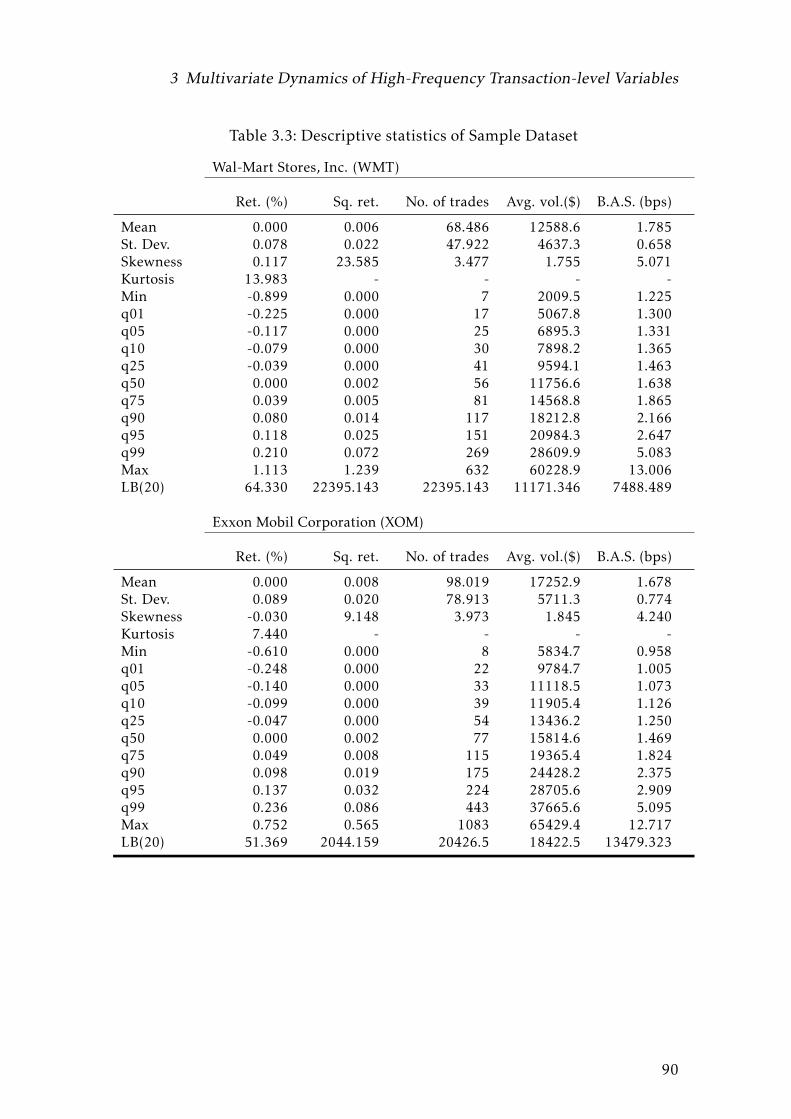
3 Multivariate Dynamics of High-Frequency Transaction-level Variables
Table 3.3: Descriptive statistics of Sample Dataset
Wal-Mart Stores, Inc. (WMT)
Ret. (%) Sq. ret. No. of trades Avg. vol.($) B.A.S. (bps)
Mean 0.000 0.006 68.486 12588.6 1.785St. Dev. 0.078 0.022 47.922 4637.3 0.658Skewness 0.117 23.585 3.477 1.755 5.071Kurtosis 13.983 - - - -Min -0.899 0.000 7 2009.5 1.225q01 -0.225 0.000 17 5067.8 1.300q05 -0.117 0.000 25 6895.3 1.331q10 -0.079 0.000 30 7898.2 1.365q25 -0.039 0.000 41 9594.1 1.463q50 0.000 0.002 56 11756.6 1.638q75 0.039 0.005 81 14568.8 1.865q90 0.080 0.014 117 18212.8 2.166q95 0.118 0.025 151 20984.3 2.647q99 0.210 0.072 269 28609.9 5.083Max 1.113 1.239 632 60228.9 13.006LB(20) 64.330 22395.143 22395.143 11171.346 7488.489
Exxon Mobil Corporation (XOM)
Ret. (%) Sq. ret. No. of trades Avg. vol.($) B.A.S. (bps)
Mean 0.000 0.008 98.019 17252.9 1.678St. Dev. 0.089 0.020 78.913 5711.3 0.774Skewness -0.030 9.148 3.973 1.845 4.240Kurtosis 7.440 - - - -Min -0.610 0.000 8 5834.7 0.958q01 -0.248 0.000 22 9784.7 1.005q05 -0.140 0.000 33 11118.5 1.073q10 -0.099 0.000 39 11905.4 1.126q25 -0.047 0.000 54 13436.2 1.250q50 0.000 0.002 77 15814.6 1.469q75 0.049 0.008 115 19365.4 1.824q90 0.098 0.019 175 24428.2 2.375q95 0.137 0.032 224 28705.6 2.909q99 0.236 0.086 443 37665.6 5.095Max 0.752 0.565 1083 65429.4 12.717LB(20) 51.369 2044.159 20426.5 18422.5 13479.323
90

3 Multivariate Dynamics of High-Frequency Transaction-level Variables
Descriptive Statistics
Once cleaning up the TAQ dataset, I calculate the log return (multiplied by 100),
the number of trades, the average dollar volume per trade, and the time-weighted
average bid-ask spread as a percentage of mid-price at 5-minute frequency. Table
(3.3) presents the descriptive statistics of these four transaction-level variables
for each of the six stocks. A few remarks are listed as below:
• The percentiles of high-frequency return tend to be symmetric and the
skewness is typically small; intraday return reveals empirical evidence of
heavy tails, as indicated by a value of kurtosis far greater than 3. Overall,
5-min return is clearly not normally distributed.
• The other three transaction variables, namely, the number of trades, the av-
erage volume per trade and the average bid-ask spread are positively skewed
and underdispersed, i.e., the skewness is far greater than zero and the stan-
dard deviation exceeds the mean. Sample stocks are traded very frequently
as indicated by the average number of trades per 5-min fixed time inter-
val is typically greater than 50. Bid-ask spread shows a moderate level of
variation and does not stay at the minimum tick size for most of time.
• Time series of all these four transaction variables show significant serial cor-
relations, suggested by the Ljung-Box statistics massively exceeding their
critical values.
91
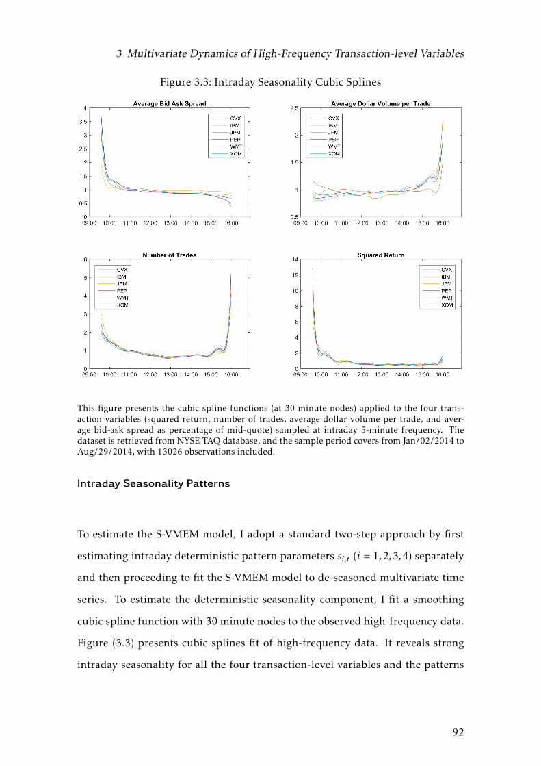
3 Multivariate Dynamics of High-Frequency Transaction-level Variables
Figure 3.3: Intraday Seasonality Cubic Splines
This figure presents the cubic spline functions (at 30 minute nodes) applied to the four trans-action variables (squared return, number of trades, average dollar volume per trade, and aver-age bid-ask spread as percentage of mid-quote) sampled at intraday 5-minute frequency. Thedataset is retrieved from NYSE TAQ database, and the sample period covers from Jan/02/2014 toAug/29/2014, with 13026 observations included.
Intraday Seasonality Patterns
To estimate the S-VMEM model, I adopt a standard two-step approach by first
estimating intraday deterministic pattern parameters si,t (i = 1,2,3,4) separately
and then proceeding to fit the S-VMEM model to de-seasoned multivariate time
series. To estimate the deterministic seasonality component, I fit a smoothing
cubic spline function with 30 minute nodes to the observed high-frequency data.
Figure (3.3) presents cubic splines fit of high-frequency data. It reveals strong
intraday seasonality for all the four transaction-level variables and the patterns
92

3 Multivariate Dynamics of High-Frequency Transaction-level Variables
are quite similar across the sample of the six stocks. In particular, the return
and the bid-ask spread display L-shape with a high-peak around opening and
staying low for the rest of day, while the average dollar volume per trade exhibits
a completely opposite pattern. For the number of trades, a typical U-shape is
noted with trading activities becoming significantly more active during market
open and close phases.
Cross-Autocorrelation Functions
To show how the multivariate trading variables are related to each other em-
pirically, figure (3.4) and (3.5) display their corresponding cross-autocorrelation
functions before and after controlling for the intraday seasonality patterns. In par-
ticular, the correlation coefficient between variable y(i)t and lagged variable y(j)t−l is
calculated for each lag order l = 0,1,2, ...,400 where i, j = 1,2,3,4 refer to the four
trading variables analysed in this paper. Based on the resulting cross-correlation
function, some major features are summarized as follows:
• A significant amount of periodic cross-autocorrelation has been removed
by controlling for intraday patterns, and the behaviours of the resulting
de-seasoned time series look much more smooth and regularized.
• From the diagonals of figure (3.5), one can easily see that all autocorrelation
coefficients do not vanish towards zero at 100 lags, revealing evidence of a
hyperbolic decay instead of an exponential decay in the empirical autocor-
relation function. This implies the existence of long-range dependence for all
of these four trading variables analysed in this paper. The two-factor6 struc-
6one is observation-driven dynamics xt and the other is latent information flow process λt
93

3 Multivariate Dynamics of High-Frequency Transaction-level Variables
ture embedded in the S-VMEM model expects to be able to accommodate
this empirical feature reasonably well, where one factor is responsible for
the short-run dynamics while the other factor drives the long-run dynam-
ics.
• By looking at contemporaneous correlations (the first value of cross-correlation
function) of the de-seasoned absolute return with the other three trading
variables presented in the last row of figure (3.5), one can see that absolute
return typically has a positive correlation with trade intensity between 0.2
and 0.4, a close-to-zero or even negative correlation with average trade size,
and a positive correlation ranging from 0.1 to 0.3 with bid-ask spread. Al-
though absolute return is indeed positively associated with average trade size on
a raw basis, that association is primarily due to deterministic intraday seasonal-
ity rather than genuine stochastic behaviours. This observation contrasts the
main findings of Hautsch [2008], where the author analyses a 2001 TAQ
dataset and concludes that it is the average trade size rather than the num-
ber of trades that is very informative about the latent information flow (and
hence return volatility). This empirical observation implies a recent shift in
market behaviours that traders nowadays are much more concerned with
market impact of a single transaction in large size, so that they split this
single large order into many small child orders with the aim to hide their
footprints in the market. Consequently, the informative content has tran-
sited from the average trade size to the number of trades.
94

3M
ultivariate
Dynam
icsof
High-Frequ
encyTransaction-levelV
ariables
Figure 3.4: Cross-Autocorrelation Functions: Seasonally-unadjusted
This figure presents the cross-autocorrelation functions of the four seasonally-unadjusted transaction variables (absolute return, number of trades, averagedollar volume per trade, and average bid-ask spread as percentage of mid-quote) sampled at intraday 5 minute frequency for six heavily traded blue chipstocks (CVX, IBM, JPM, PEP, WMT, XOM) listed in NYSE. The dataset is retrieved from NYSE TAQ database. Sample period covers from Jan/02/2014 toAug/29/2014, with 13026 observations included.
95

3M
ultivariate
Dynam
icsof
High-Frequ
encyTransaction-levelV
ariables
Figure 3.5: Cross-Autocorrelation Functions: Seasonally-adjusted
This figure presents the cross-autocorrelation functions of the four seasonally-adjusted transaction variables (absolute return, number of trades, averagedollar volume per trade, and average bid-ask spread as percentage of mid-quote) sampled at intraday 5 minute frequency for six heavily traded blue chipstocks (CVX, IBM, JPM, PEP, WMT, XOM) listed in NYSE. The dataset is retrieved from NYSE TAQ database. Sample period covers from Jan/02/2014 toAug/29/2014, with 13026 observations included.
96

3 Multivariate Dynamics of High-Frequency Transaction-level Variables
3.5.2 Univariate Results
I first look at each trading variable individually and examine their univariate
dynamics. More specifically, I use the ML-EIS method to estimate univariate S-
GARCH and S-ACD models based on the high frequency dataset consisting of
seasonality-adjusted intraday return, number of trades, average trade size and
average bid-ask spread based on 5-minute fixed time interval. The estimation
results are reported in table (3.4), (3.5), (3.6) and (3.7), with some main findings
summarized as follows:
• In line with the existing literature, I find that there is a very strong clus-
tering effect in the return volatility and the time-dependent conditional ex-
pectation of the other three positive-valued trading variables. In particular,
the estimated persistence parameter, either β in observation-driven dynam-
ics or ρ in latent dynamics, is typically greater than 0.9, and the results are
quite similar across different stocks.
• The empirical results confirm the existence of latent serially correlated state
variables, as revealed by significant positive estimates of persistence param-
eter ρ in the latent process.
• Comparing S-GARCH and S-ACDmodels with their pure observation-driven
counterparts, i.e. GARCH and ACDmodels, one can see that the innovation
parameter α in observation-driven components declines when the latent
state variable λt is included in the model. As argued by Hautsch [2008], this
suggests that news enters the model primarily through the latent process,
which justifies the interpretation of λt as an proxy for the latent information
97

3 Multivariate Dynamics of High-Frequency Transaction-level Variables
flow process.
• The pure latent specifications (such as SV and SCD) improve overall goodness-
of-fit and is generally preferred by empirical data when compared with the
pure observation-driven models such as GARCH and ACD. In all cases, the
former deliver a much higher log likelihood with lower BIC test statistics.
• Considering S-GARCH/S-ACD as nested models, neither GARCH/ACD or
SV/SCD specification should be rejected, as suggested by the fact that all
model parameters are statistically different from zero. In general, S-GARCH/S-
ACD is preferred by empirical data as it offers highest log likelihood with
lowest BIC statistic. Consequently, the empirical dynamics in these four
trading variables are in favour of a two-factor specification rather than a
single-factor structure.
• To runmodel diagnostics, I calculate the Ljung-Box (LB) test statistics based
on fitted residuals for each of the four univariate models. The reported LB
test statistics are reasonably low for S-GARCH and S-ACD specifications,
suggesting that most time-varying dynamics has been successfully captured
by these models.
98

3 Multivariate Dynamics of High-Frequency Transaction-level Variables
Table 3.4: Estimation Results of (S)-GARCH Model for Intraday Return
This table presents the estimation results of fitting (S)-GARCH models to the log returnsampled at 5-min frequency. ML-EIS method is applied to estimate the models with la-tent components. The dataset consists of six heavily traded stocks (CVX, IBM, JPM, PEP,WMT, XOM) listed in NYSE. Sample period covers from 02/Jan/2014 to 29/Aug/2014,with 13026 observations included. The following diagnostics are calculated: log like-lihood (logL), Bayesian Information Criterion (BIC), Ljung-Box statistics on return (LB)and squared return (LB2) with 20 lags, the mean and the standard deviation (stdev) offitted residuals.
CVX IBM
GARCH SV S-GARCH GARCH SV S-GARCH
Observation-driven Dynamics
w -0.077*** -0.213*** -0.022*** -0.078*** -0.180*** -0.060***α 0.099*** - 0.027*** 0.100*** - 0.071***β 0.990*** - 0.998*** 0.987*** - 0.991***
Latent SV Dynamics
δ - 0.165*** 0.333*** - 0.137*** 0.467***ρ - 0.968*** 0.804*** - 0.976*** 0.512***
Diagnostics
logL -17634 -17448 -17391 -17784 -17621 -17568BIC 35296 34924 34830 35596 35271 35183LB(20) 27.97 44.66 39.23 31.32 37.56 34.70LB2(20) 46.73 21.69 23.78 52.19 28.31 20.02mean 0.006 0.009 0.009 0.000 0.004 0.003stdev 1.000 0.989 0.993 1.000 0.998 0.999
JPM PEP
GARCH SV S-GARCH GARCH SV S-GARCH
Observation-driven Dynamics
w -0.108 -0.251*** -0.089*** -0.101*** -0.195*** -0.052***α 0.140** - 0.103*** 0.130* - 0.061***β 0.982*** - 0.986*** 0.981*** - 0.992***
Continued on next page ...
99

3 Multivariate Dynamics of High-Frequency Transaction-level Variables
Table 3.4: Estimation of (S)-GARCH Model for Intraday Return
Latent SV Dynamics
δ - 0.160*** 0.562*** - 0.199*** 0.464***ρ - 0.976*** 0.360*** - 0.952*** 0.591***
Diagnostics
logL -17518 -17313 -17257 -17806 -17612 -17566BIC 35063 34654 34561 35640 35253 35160LB(20) 23.94 36.39 29.54 23.50 32.08 27.77LB2(20) 47.76 33.15 17.30 45.04 20.30 12.12mean -0.002 0.005 0.002 0.001 0.002 0.001stdev 1.000 0.998 0.995 1.000 0.993 0.994
WMT XOM
GARCH SV S-GARCH GARCH SV S-GARCH
Observation-driven Dynamics
w -0.077*** -0.229*** -0.028 -0.082*** -0.176*** -0.056**α 0.099** - 0.033*** 0.105*** - 0.066***β 0.990*** - 0.997*** 0.989*** - 0.993***
Latent SV Dynamics
δ - 0.243*** 0.464*** - 0.115*** 0.402***ρ - 0.937*** 0.688*** - 0.983*** 0.559***
Diagnostics
logL -17634 -17596 -17524 -17636 -17472 -17429BIC 35296 35221 35095 35300 34972 34906LB(20) 27.97 50.58 48.33 37.25 43.99 39.31LB2(20) 46.73 32.94 21.65 100.18 26.53 19.51mean 0.006 0.005 0.005 0.000 0.004 0.003stdev 1.000 0.996 0.999 1.000 0.990 1.001
100

3 Multivariate Dynamics of High-Frequency Transaction-level Variables
Table 3.5: Estimation Results of (S)-ACD Model for Number of Trades
This table presents the estimation results of fitting (S)-ACD models to the number oftrades sampled at 5-min frequency. ML-EIS method is applied to estimate the mod-els with latent components. The dataset consists of six heavily traded stocks (CVX,IBM, JPM, PEP, WMT, XOM) listed in NYSE. Sample period covers from 02/Jan/2014to 29/Aug/2014, with 13026 observations included. The following diagnostics are calcu-lated: log likelihood (logL), Bayesian Information Criterion (BIC), Ljung-Box statistics onreturn (LB) and squared return (LB2) with 20 lags, the mean and the standard deviation(stdev) of fitted residuals.
CVX IBM
ACD SV S-ACD ACD SV S-ACD
Observation-driven Dynamics
w -0.254*** 0.037* -0.157*** -0.209*** 0.038 -0.180***α 0.254*** - 0.167*** 0.210*** - 0.206***β 0.953*** - 0.507*** 0.983*** - 0.628***
Latent SV Dynamics
δ - 0.114*** 0.301*** - 0.108*** 0.036***ρ - 0.950*** 0.978*** - 0.976*** 0.993***
Distributional Parameters
σ 0.332*** 0.114*** 0.052*** 0.397*** 0.336*** 0.370***
Diagnostics
logL -4151 -3939 -3882 -6069 -5871 -5747BIC 8339 7916 7821 12176 11780 11551LB(20) 136.89 53.11 25.91 302.82 121.63 31.91mean 1.001 0.999 1.007 0.998 1.005 1.001stdev 0.355 0.285 0.330 0.427 0.358 0.406
JPM PEP
ACD SV S-ACD ACD SV S-ACD
Observation-driven Dynamics
w -0.235*** 0.070** -0.048*** -0.217*** 0.034*** -0.165***α 0.240*** - 0.047*** 0.219*** - 0.174***β 0.943*** - 0.989*** 0.959*** - 0.584***
Continued on next page ...
101
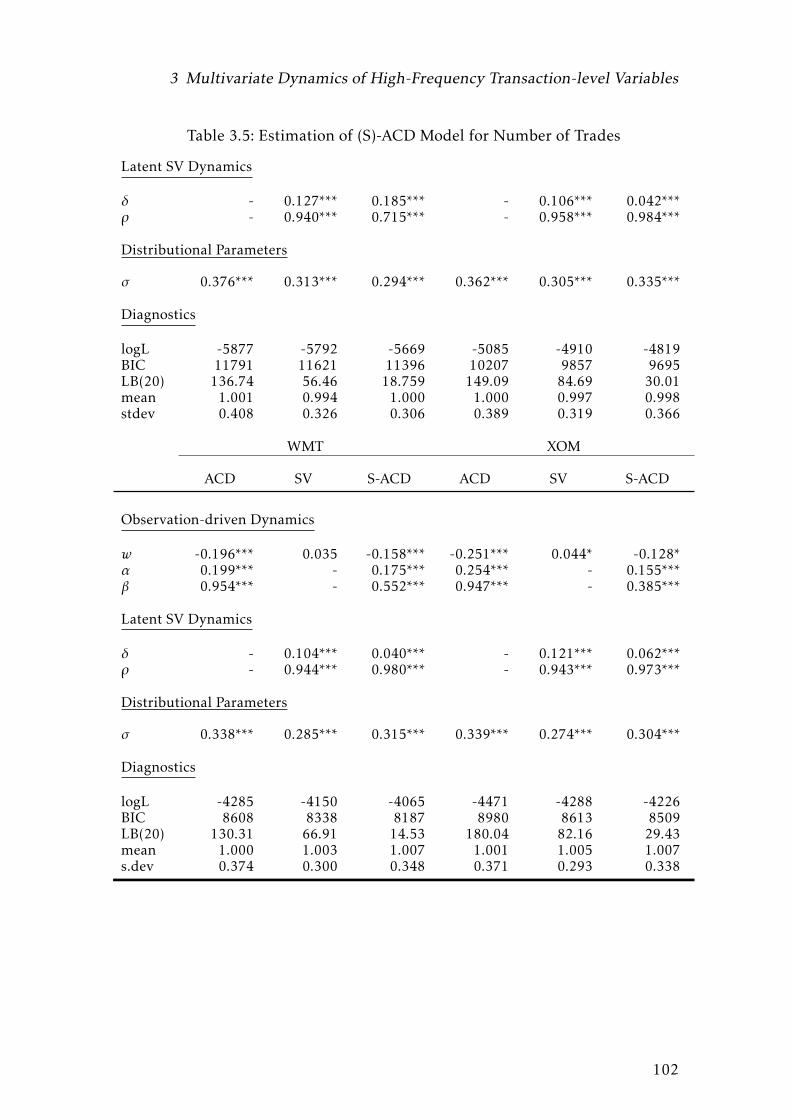
3 Multivariate Dynamics of High-Frequency Transaction-level Variables
Table 3.5: Estimation of (S)-ACD Model for Number of Trades
Latent SV Dynamics
δ - 0.127*** 0.185*** - 0.106*** 0.042***ρ - 0.940*** 0.715*** - 0.958*** 0.984***
Distributional Parameters
σ 0.376*** 0.313*** 0.294*** 0.362*** 0.305*** 0.335***
Diagnostics
logL -5877 -5792 -5669 -5085 -4910 -4819BIC 11791 11621 11396 10207 9857 9695LB(20) 136.74 56.46 18.759 149.09 84.69 30.01mean 1.001 0.994 1.000 1.000 0.997 0.998stdev 0.408 0.326 0.306 0.389 0.319 0.366
WMT XOM
ACD SV S-ACD ACD SV S-ACD
Observation-driven Dynamics
w -0.196*** 0.035 -0.158*** -0.251*** 0.044* -0.128*α 0.199*** - 0.175*** 0.254*** - 0.155***β 0.954*** - 0.552*** 0.947*** - 0.385***
Latent SV Dynamics
δ - 0.104*** 0.040*** - 0.121*** 0.062***ρ - 0.944*** 0.980*** - 0.943*** 0.973***
Distributional Parameters
σ 0.338*** 0.285*** 0.315*** 0.339*** 0.274*** 0.304***
Diagnostics
logL -4285 -4150 -4065 -4471 -4288 -4226BIC 8608 8338 8187 8980 8613 8509LB(20) 130.31 66.91 14.53 180.04 82.16 29.43mean 1.000 1.003 1.007 1.001 1.005 1.007s.dev 0.374 0.300 0.348 0.371 0.293 0.338
102

3 Multivariate Dynamics of High-Frequency Transaction-level Variables
Table 3.6: Estimation Results of (S)-ACD Model for Average Trade Size
This table presents the estimation results of fitting (S)-ACD models to the average dollarvolume per trade sampled at 5-min frequency. ML-EIS method is applied to estimate themodels with latent components. The dataset consists of six heavily traded stocks (CVX,IBM, JPM, PEP, WMT, XOM) listed in NYSE. Sample period covers from 02/Jan/2014to 29/Aug/2014, with 13026 observations included. The following diagnostics are calcu-lated: log likelihood (logL), Bayesian Information Criterion (BIC), Ljung-Box statistics onreturn (LB) and squared return (LB2) with 20 lags, the mean and the standard deviation(stdev) of fitted residuals.
CVX IBM
ACD SV S-ACD ACD SV S-ACD
Observation-driven Dynamics
w -0.175*** 0.022* -0.077*** -0.107*** 0.027** -0.073***α 0.176*** - 0.093*** 0.107*** - 0.097***β 0.952*** - 0.274*** 0.959*** - 0.225***
Latent SV Dynamics
δ - 0.045*** 0.030*** - 0.037*** 0.024***ρ - 0.952*** 0.969*** - 0.957*** 0.975***
Distributional Parameters
σ 0.190*** 0.168*** 0.175*** 0.229*** 0.212*** 0.216***
Diagnostics
logL 3077 3149 3179 713 809 856BIC -6117 -6261 -6301 -1388 -1579 -1655LB(20) 69.37 45.65 23.66 100.98 99.76 23.99mean 1.000 0.998 0.998 0.998 0.997 0.995stdev 0.200 0.176 0.185 0.246 0.225 0.232
JPM PEP
ACD SV S-ACD ACD SV S-ACD
Observation-driven Dynamics
w -0.147*** 0.038*** -0.023 -0.175*** -0.079*** -0.070***α 0.150*** - 0.022 0.177*** - 0.070***β 0.937*** - 0.991*** 0.956*** - 0.985***
Continued on next page ...
103
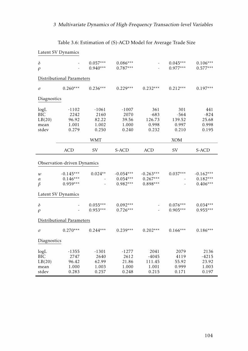
3 Multivariate Dynamics of High-Frequency Transaction-level Variables
Table 3.6: Estimation of (S)-ACD Model for Average Trade Size
Latent SV Dynamics
δ - 0.057*** 0.086*** - 0.045*** 0.106***ρ - 0.940*** 0.787*** - 0.977*** 0.577***
Distributional Parameters
σ 0.260*** 0.236*** 0.229*** 0.232*** 0.212*** 0.197***
Diagnostics
logL -1102 -1061 -1007 361 301 441BIC 2242 2160 2070 -683 -564 -824LB(20) 96.92 82.22 39.56 126.73 139.52 25.68mean 1.001 1.002 1.000 0.998 0.997 0.998stdev 0.279 0.250 0.240 0.232 0.210 0.195
WMT XOM
ACD SV S-ACD ACD SV S-ACD
Observation-driven Dynamics
w -0.145*** 0.024** -0.054*** -0.263*** 0.037*** -0.162***α 0.146*** - 0.054*** 0.267*** - 0.182***β 0.959*** - 0.982*** 0.898*** - 0.406***
Latent SV Dynamics
δ - 0.055*** 0.092*** - 0.076*** 0.034***ρ - 0.953*** 0.726*** - 0.905*** 0.955***
Distributional Parameters
σ 0.270*** 0.244*** 0.239*** 0.202*** 0.166*** 0.186***
Diagnostics
logL -1355 -1301 -1277 2041 2079 2136BIC 2747 2640 2612 -4045 4119 -4215LB(20) 96.42 62.99 21.86 111.45 55.92 23.92mean 1.000 1.003 1.000 1.001 0.999 1.003stdev 0.283 0.257 0.248 0.215 0.171 0.197
104

3 Multivariate Dynamics of High-Frequency Transaction-level Variables
Table 3.7: Estimation Results of (S)-ACD Model for Bid-Ask Spread
This table presents the estimation results of fitting (S)-ACDmodels to the average bid-askspread sampled at 5-min frequency. ML-EIS method is applied to estimate the mod-els with latent components. The dataset consists of six heavily traded stocks (CVX,IBM, JPM, PEP, WMT, XOM) listed in NYSE. Sample period covers from 02/Jan/2014to 29/Aug/2014, with 13026 observations included. The following diagnostics are calcu-lated: log likelihood (logL), Bayesian Information Criterion (BIC), Ljung-Box statistics onreturn (LB) and squared return (LB2) with 20 lags, the mean and the standard deviation(stdev) of fitted residuals.
CVX IBM
ACD SV S-ACD ACD SV S-ACD
Observation-driven Dynamics
w -0.438*** 0.020* -0.082*** -0.426*** -0.001 -0.366***α 0.440*** - 0.081*** 0.426*** - 0.367***β 0.933*** - 0.985** 0.938*** - 0.621***
Latent SV Dynamics
δ - 0.082*** 0.115*** - 0.103*** 0.025***ρ - 0.937*** 0.643*** - 0.931*** 0.980***
Distributional Parameters
σ 0.159*** 0.113*** 0.095*** 0.201*** 0.144** 0.187***
Diagnostics
logL 5326 5350 5517 2591 2637 2759BIC -10615 -10662 -10977 -5144 -5236 -5461LB(20) 228.8 95.40 22.50 218.82 75.42 30.38mean 1.000 1.001 1.002 0.999 0.996 0.998stdev 0.163 0.114 0.096 0.203 0.144 0.190
JPM PEP
ACD SV S-ACD ACD SV S-ACD
Observation-driven Dynamics
w -0.293*** 0.016* -0.263*** -0.445*** 0.037*** -0.065***α 0.295*** - 0.272*** 0.448*** - 0.066***β 0.894*** - 0.397*** 0.901*** - 0.984***
Latent SV DynamicsContinued on next page ...
105

3 Multivariate Dynamics of High-Frequency Transaction-level Variables
Table 3.7: Estimation of (S)-ACD Model for Bid-Ask Spread
δ - 0.032*** 0.008*** - 0.082*** 0.106***ρ - 0.901*** 0.980*** - 0.909*** 0.649***
Distributional Parameters
σ 0.078*** 0.063*** 0.074*** 0.142*** 0.097*** 0.080***
Diagnostics
logL 14443 14470 14664 6565 6607 6782BIC -28848 -28902 -29272 -13092 -13176 -13507LB(20) 304.85 149.24 24.61 229.632 66.66 14.06mean 1.000 1.000 1.000 1.000 0.997 1.000stdev 0.084 0.064 0.078 0.152 0.097 0.081
WMT XOM
ACD SV S-ACD ACD SV S-ACD
Observation-driven Dynamics
w -0.383*** 0.012*** -0.078*** -0.476*** 0.027*** -0.103***α 0.386*** - 0.079*** 0.479*** - 0.104***β 0.856*** - 0.971*** 0.901*** - 0.974***
Latent SV Dynamics
δ - 0.057*** 0.082*** - 0.084*** 0.115***ρ - 0.865*** 0.534*** - 0.909*** 0.575***
Distributional Parameters
σ 0.108*** 0.079*** 0.063*** 0.141*** 0.093*** 0.010***
Diagnostics
logL 10323 10343 10484 6738 6769 6930BIC -20608 -20649 -20911 -13439 -13500 -13804LB(20) 222.43 59.73 18.41 233.08 68.82 20.79mean 1.000 1.001 1.000 1.001 1.000 1.000st.dev. 0.113 0.080 0.063 0.149 0.093 0.070
106

3 Multivariate Dynamics of High-Frequency Transaction-level Variables
3.5.3 Multivariate Results
In this section, I estimate four variations of the S-VMEMmodel corresponding to
different restrictions on the multivariate dynamical system. More specifically,
(1) the pure observation-driven VMEMmodel without any latent state variable
(2) the single latent information flowmodel without any additional observation-
driven VMEM component
(3) the S-VMEM model restricting the parameter A0 = 0 to explicitly not in-
clude the contemporaneous cross-dependence between trading variables
into the modelling framework
(4) the full S-VMEM model without any restriction
In addition, to keep the model parsimonious, I restrict the lag order in VMEM
dynamics to be P = Q = 1. Furthermore, I restrict the news impact parameter δ1
to be positive in order to make the signs of parameter δi (i = 1,2,3,4) identifiable.
All these four specifications (1) - (4) are estimated using the ML-EIS method.
The simulated likelihood function is maximized by the BFGS algorithm, which
is an iterative quasi-Newton optimization technique. It’s well known that quasi-
Newtonmethod is essentially a local optimization routine. Thus, in order to yield
satisfied estimation results, it is required that starting values to be close enough to
the true but unknownmodel parameters. To obtain reasonably good starting values,
I use a bottom-up approach to take the advantage of the nested structure of the model. I
use the univariate estimates presented in the previous section to get a good sense
of what the plausible parameters look like. I then start to estimate multivariate
time series from the most general form (i.e. specification [1]) gradually to the
most specific form (i.e. specification [4]) with the estimates of the former serving
as one of the possible sets of starting values for the latter. At the meantime,
107

3 Multivariate Dynamics of High-Frequency Transaction-level Variables
various sets of different starting values have also been tested to ensure the global
optimum has been selected.
The estimation results are reported in table (3.8), (3.9) and (3.10), with the major
findings being summarized as follows:
• Based on the estimation results of the pure VMEM specification (1), con-
ditional expectations of the average bid-ask spread, the average trade size,
and the number of trades are all highly persistent with their βs being close
to or above 0.9; however, the volatility clustering effect disappears as the
persistence parameter is fairly small or become even insignificant, which is
much lower when compared with the univariate results listed in previous
section. Consequently, massive contemporaneous dependence of the re-
turn volatility on the bid-ask spread, the trade size and the number trades
are found in α(0)4,1,α
(0)4,2,α
(0)4,3. This finding suggests that the source of high-
frequency return volatility clustering can be explained by the contempora-
neous mutual relation between return volatility and the other three trading
variables.
• Comparing the estimation results of specification (3) with (4), one can see
that the magnitudes of news impacts on trading dynamics (which are cap-
tured by the parameter δs) drop significantly for the return volatility and
the number of trades when contemporaneous cross-dependence is included
in the model, while the impacts of latent news on the bid-ask spread and
the trade size remain small for both specifications. The implication is that
the source of contemporaneousmutual correlation is attributed to the latent
information flow process.
108
3 Multivariate Dynamics of High-Frequency Transaction-level Variables
• The empirical results for all the six stocks reveal significant evidence for
the existence of a latent serially correlated state variable λt with an strong
persistence parameter about ρ ≈ 0.98 on average. This strong autocorre-
lation can be explained by the fact that market news tend to be clustered,
with major market event followed by many small subsequent announce-
ments. Based on the reported results for the S-VMEM specification (4), the
estimated parameters δ3 and δ4 are both positively significant for all the
six stocks, indicating that information shocks increase return volatility and
triggermore trades simultaneously. The impacts of news are relatively weak
for the bid-ask spread and the average trading volume though. This obser-
vation is in sharp contrast with previous findings in the literature that it
is the size of transaction rather than trading intensity that carries essential
information about the quality of the news. For example, see Blume et al.
[1994] based on daily data, and Xu and Wu [1999], Huang and Masulis
[2003] andHautsch [2008] based on intraday high frequency data. As I ar-
gued earlier, one explanation is that traders nowadays have a great concern
on potential market impacts of their transactions so that they tend to split
up large order into many small child orders. In fact, due to the increas-
ing popularity of algorithmic trading in recent years, more and more asset
managers have been switching to algorithmic execution strategies where it
is common to spread large order over time to minimize market impacts. As
a result, the number of trades increases whereas the average trade size falls,
and consequently, informative content about hidden market information
flow has transited from the average trading size into the trading intensity.
• Minimal evidence is found for the existence of asymmetric impacts of re-
turns on volatility, bid-ask spread, average trading volume and number of
trades. The coefficients γs are typically small in magnitude and even in-
109

3 Multivariate Dynamics of High-Frequency Transaction-level Variables
significant for several stocks.
• The specification (2) delivers the worst goodness-of-fit universally across
the six stocks. The Ljung-Box statistics on fitted residuals reveal that a
massive amount of dynamics are left unmodelled. This finding is in line
with Andersen [1996] and Liesenfeld [1998], where the authors claim that
a single serially correlated latent process is not sufficient to characterize the
full dynamics of the multivariate system.
• The full S-VMEM model gives the best goodness-of-fit, as suggested by the
highest log likelihood (LL) and lowest Bayesian Information Criterion (BIC)
observed for the full S-VMEM specification (4). Comparing the Ljung-Box
statistics on raw high-frequency data with the ones on fitted residuals by the
S-VMEM model, one can see that the statistics have been reduced sharply,
implying that most dynamics have been successfully captured by the ex-
isting model. However, there are still some hidden and unmodelled serial
dependence left in fitted residuals, as indicated by the observation that the
Ljung-Box statistics on fitted residuals display fairly large values for the
bid-ask spread and the average trade size, while the numbers are reason-
ably small for the return volatility and the number of trades. This finding
suggests that the S-VMEM model with lag order of one may not be ade-
quate to describe the full trading dynamics; introducing more lags could
potentially improve the model diagnostics performance.
110

3M
ultivariate
Dynam
icsof
High-Frequ
encyTransaction-levelV
ariables
Table 3.8: Estimation Results of (S)-VMEM Models (CVX and IBM)
This table presents the model estimation results for stock CVX and IBM. Four models are compared here: (1) Vector MultiplicativeError Model (VMEM) without Latent Process, (2) Single Latent Process Model, (3) Stochastic VMEM without contemporaneousdependence and (4) full Stochastic VMEM with contemporaneous dependence. ML-EIS method is applied to models with la-tent components. The dataset is extracted from NYSE Consolidated TAQ database. Sample period covers from 02/Jan/2014 to29/Aug/2014, with 13026 observations included.
CVX IBM
(1) (2) (3) (4) (1) (2) (3) (4)
VARMA Dynamics
ω1 -0.442*** 0.044** -0.438*** -0.448*** -0.410*** 0.028 -0.425*** -0.422***ω2 -0.083*** 0.029* -0.025** -0.083*** -0.058*** 0.031 -0.025*** -0.058***ω3 -0.129*** 0.034*** 0.101*** -0.118*** -0.121*** 0.039 0.151*** 0.058***ω4 -2.263*** -0.173*** -0.326*** -2.068*** -2.145*** -0.098 -0.398*** -2.421***α1,1 0.435*** - 0.418*** 0.434*** 0.422*** - 0.406*** 0.419***α1,2 -0.066*** - -0.075*** -0.062*** -0.044*** - -0.044*** -0.034***α1,3 -0.139*** - -0.041*** -0.035*** -0.106*** - 0.077*** -0.048***α1,4 -0.209*** - 0.482*** -0.166*** -0.087 - 0.361*** 0.091α2,1 -0.017* - -0.013** -0.011*** -0.021 - -0.019*** -0.018**α2,2 0.168*** - 0.133*** 0.170*** 0.087*** - 0.091*** 0.108**α2,3 -0.059*** - -0.086*** -0.019*** -0.065*** - -0.072*** -0.030**α2,4 0.016*** - -0.203*** 0.114*** 0.021 - 0.021 0.109**α3,1 0.013*** - 0.016*** 0.012*** 0.001 - 0.021*** 0.009α3,2 -0.020*** - -0.021*** -0.006*** 0.017 - -0.019*** -0.003α3,3 0.259*** - 0.048*** 0.143*** 0.228*** - 0.030*** 0.156***α3,4 -0.110*** - -0.033** -0.188*** -0.156*** - -0.052*** -0.078***α4,1 0.016*** - 0.021*** 0.017*** 0.011 - 0.016** 0.013α4,2 -0.003 - -0.011*** -0.004*** 0.007 - -0.008 0.006α4,3 0.004 - -0.028*** 0.009** 0.015* - -0.008** 0.022***α4,4 0.095*** - 0.076*** 0.092*** 0.118*** - 0.078*** 0.078***
Continued on next page ...
111
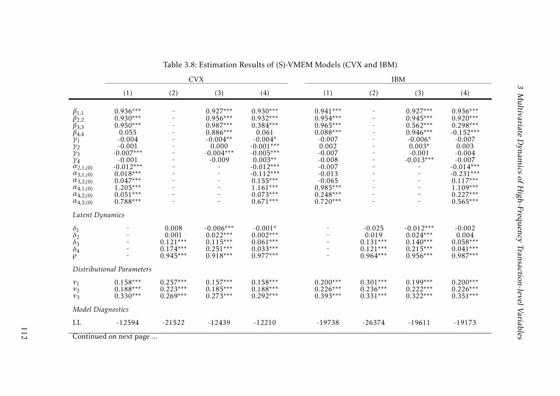
3M
ultivariate
Dynam
icsof
High-Frequ
encyTransaction-levelV
ariables
Table 3.8: Estimation Results of (S)-VMEM Models (CVX and IBM)
CVX IBM
(1) (2) (3) (4) (1) (2) (3) (4)
β1,1 0.936*** - 0.927*** 0.930*** 0.941*** - 0.927*** 0.936***β2,2 0.930*** - 0.956*** 0.932*** 0.954*** - 0.945*** 0.920***β3,3 0.950*** - 0.987*** 0.384*** 0.965*** - 0.562*** 0.298***β4,4 0.055 - 0.886*** 0.061 0.088*** - 0.946*** -0.152***γ1 -0.004 - -0.004** -0.004* -0.007 - -0.006* -0.007γ2 -0.001 - 0.000 -0.001*** 0.002 - 0.003* 0.003γ3 -0.007*** - -0.004*** -0.005*** -0.007 - -0.001 -0.004γ4 -0.001 - -0.009 0.003** -0.008 - -0.013*** -0.007α2,1,(0) -0.012*** - - -0.012*** -0.007 - - -0.014***α3,1,(0) 0.018*** - - -0.112*** -0.013 - - -0.231***α3,2,(0) 0.047*** - - 0.155*** -0.065 - - 0.117***α4,1,(0) 1.205*** - - 1.161*** 0.985*** - - 1.109***α4,2,(0) 0.051*** - - 0.073*** 0.248*** - - 0.227***α4,3,(0) 0.788*** - - 0.671*** 0.720*** - - 0.565***
Latent Dynamics
δ1 - 0.008 -0.006*** -0.001* - -0.025 -0.012*** -0.002δ2 - 0.001 0.022*** 0.002*** - 0.019 0.024*** 0.004δ3 - 0.121*** 0.115*** 0.061*** - 0.131*** 0.140*** 0.058***δ4 - 0.174*** 0.251*** 0.033*** - 0.121*** 0.215*** 0.041***ρ - 0.945*** 0.918*** 0.977*** - 0.964*** 0.956*** 0.987***
Distributional Parameters
ν1 0.158*** 0.257*** 0.157*** 0.158*** 0.200*** 0.301*** 0.199*** 0.200***ν2 0.188*** 0.223*** 0.185*** 0.188*** 0.226*** 0.236*** 0.222*** 0.226***ν3 0.330*** 0.269*** 0.273*** 0.292*** 0.393*** 0.331*** 0.322*** 0.351***
Model Diagnostics
LL -12594 -21522 -12439 -12210 -19738 -26374 -19611 -19173
Continued on next page ...
112
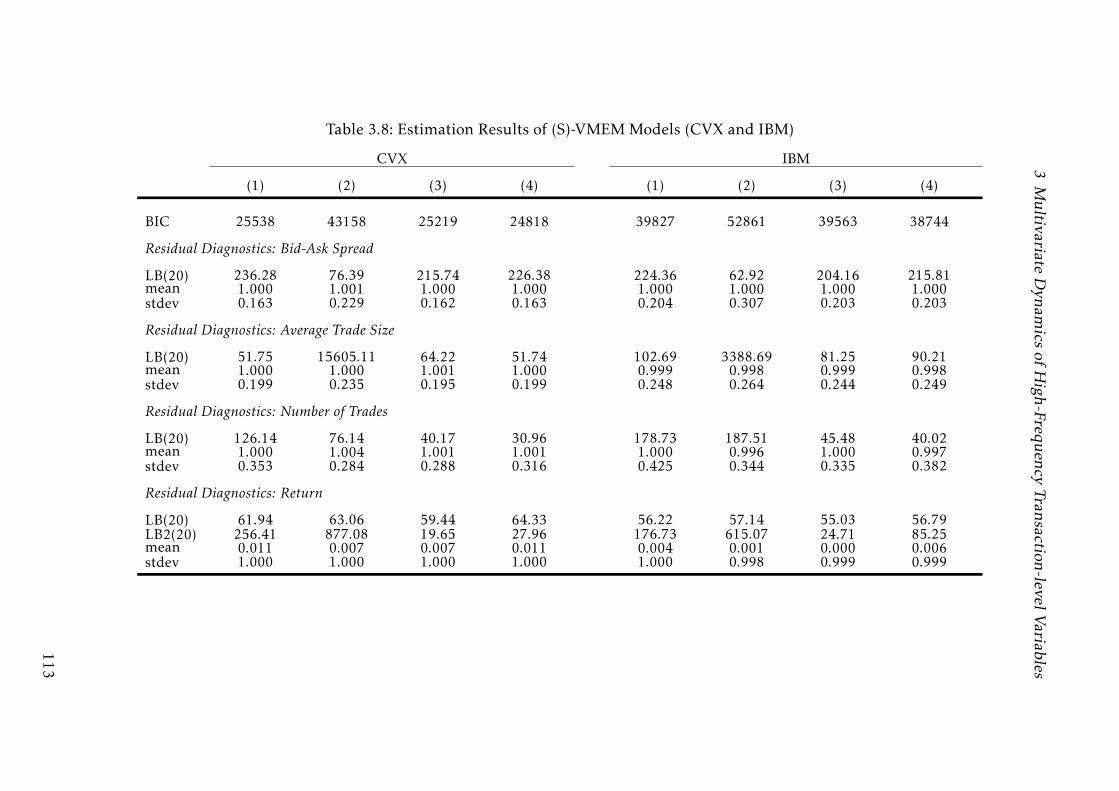
3M
ultivariate
Dynam
icsof
High-Frequ
encyTransaction-levelV
ariables
Table 3.8: Estimation Results of (S)-VMEM Models (CVX and IBM)
CVX IBM
(1) (2) (3) (4) (1) (2) (3) (4)
BIC 25538 43158 25219 24818 39827 52861 39563 38744
Residual Diagnostics: Bid-Ask Spread
LB(20) 236.28 76.39 215.74 226.38 224.36 62.92 204.16 215.81mean 1.000 1.001 1.000 1.000 1.000 1.000 1.000 1.000stdev 0.163 0.229 0.162 0.163 0.204 0.307 0.203 0.203
Residual Diagnostics: Average Trade Size
LB(20) 51.75 15605.11 64.22 51.74 102.69 3388.69 81.25 90.21mean 1.000 1.000 1.001 1.000 0.999 0.998 0.999 0.998stdev 0.199 0.235 0.195 0.199 0.248 0.264 0.244 0.249
Residual Diagnostics: Number of Trades
LB(20) 126.14 76.14 40.17 30.96 178.73 187.51 45.48 40.02mean 1.000 1.004 1.001 1.001 1.000 0.996 1.000 0.997stdev 0.353 0.284 0.288 0.316 0.425 0.344 0.335 0.382
Residual Diagnostics: Return
LB(20) 61.94 63.06 59.44 64.33 56.22 57.14 55.03 56.79LB2(20) 256.41 877.08 19.65 27.96 176.73 615.07 24.71 85.25mean 0.011 0.007 0.007 0.011 0.004 0.001 0.000 0.006stdev 1.000 1.000 1.000 1.000 1.000 0.998 0.999 0.999
113
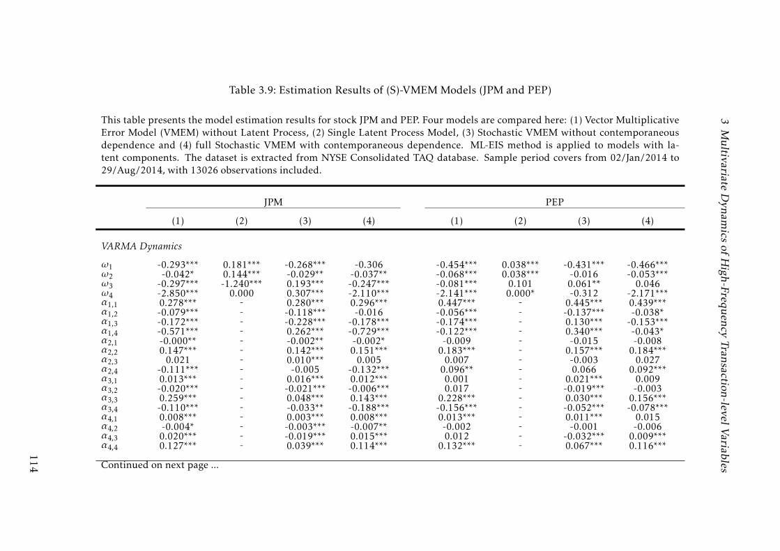
3M
ultivariate
Dynam
icsof
High-Frequ
encyTransaction-levelV
ariables
Table 3.9: Estimation Results of (S)-VMEM Models (JPM and PEP)
This table presents the model estimation results for stock JPM and PEP. Four models are compared here: (1) Vector MultiplicativeError Model (VMEM) without Latent Process, (2) Single Latent Process Model, (3) Stochastic VMEM without contemporaneousdependence and (4) full Stochastic VMEM with contemporaneous dependence. ML-EIS method is applied to models with la-tent components. The dataset is extracted from NYSE Consolidated TAQ database. Sample period covers from 02/Jan/2014 to29/Aug/2014, with 13026 observations included.
JPM PEP
(1) (2) (3) (4) (1) (2) (3) (4)
VARMA Dynamics
ω1 -0.293*** 0.181*** -0.268*** -0.306 -0.454*** 0.038*** -0.431*** -0.466***ω2 -0.042* 0.144*** -0.029** -0.037** -0.068*** 0.038*** -0.016 -0.053***ω3 -0.297*** -1.240*** 0.193*** -0.247*** -0.081*** 0.101 0.061** 0.046ω4 -2.850*** 0.000 0.307*** -2.110*** -2.141*** 0.000* -0.312 -2.171***α1,1 0.278*** - 0.280*** 0.296*** 0.447*** - 0.445*** 0.439***α1,2 -0.079*** - -0.118*** -0.016 -0.056*** - -0.137*** -0.038*α1,3 -0.172*** - -0.228*** -0.178*** -0.174*** - 0.130*** -0.153***α1,4 -0.571*** - 0.262*** -0.729*** -0.122*** - 0.340*** -0.043*α2,1 -0.000** - -0.002** -0.002* -0.009 - -0.015 -0.008α2,2 0.147*** - 0.142*** 0.151*** 0.183*** - 0.157*** 0.184***α2,3 0.021 - 0.010*** 0.005 0.007 - -0.003 0.027α2,4 -0.111*** - -0.005 -0.132*** 0.096** - 0.066 0.092***α3,1 0.013*** - 0.016*** 0.012*** 0.001 - 0.021*** 0.009α3,2 -0.020*** - -0.021*** -0.006*** 0.017 - -0.019*** -0.003α3,3 0.259*** - 0.048*** 0.143*** 0.228*** - 0.030*** 0.156***α3,4 -0.110*** - -0.033** -0.188*** -0.156*** - -0.052*** -0.078***α4,1 0.008*** - 0.003*** 0.008*** 0.013*** - 0.011*** 0.015α4,2 -0.004* - -0.003*** -0.007** -0.002 - -0.001 -0.006α4,3 0.020*** - -0.019*** 0.015*** 0.012 - -0.032*** 0.009***α4,4 0.127*** - 0.039*** 0.114*** 0.132*** - 0.067*** 0.116***
Continued on next page ...
114
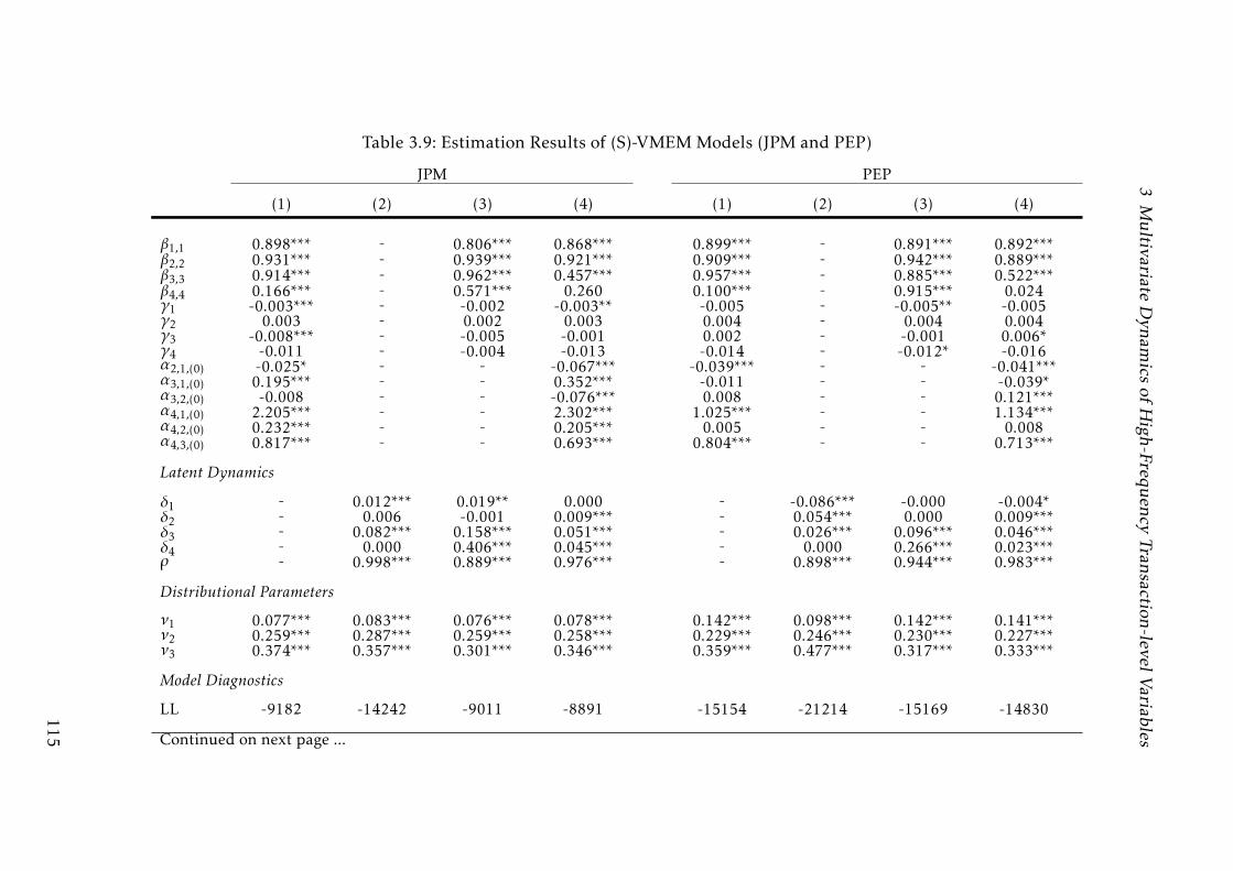
3M
ultivariate
Dynam
icsof
High-Frequ
encyTransaction-levelV
ariables
Table 3.9: Estimation Results of (S)-VMEM Models (JPM and PEP)
JPM PEP
(1) (2) (3) (4) (1) (2) (3) (4)
β1,1 0.898*** - 0.806*** 0.868*** 0.899*** - 0.891*** 0.892***β2,2 0.931*** - 0.939*** 0.921*** 0.909*** - 0.942*** 0.889***β3,3 0.914*** - 0.962*** 0.457*** 0.957*** - 0.885*** 0.522***β4,4 0.166*** - 0.571*** 0.260 0.100*** - 0.915*** 0.024γ1 -0.003*** - -0.002 -0.003** -0.005 - -0.005** -0.005γ2 0.003 - 0.002 0.003 0.004 - 0.004 0.004γ3 -0.008*** - -0.005 -0.001 0.002 - -0.001 0.006*γ4 -0.011 - -0.004 -0.013 -0.014 - -0.012* -0.016α2,1,(0) -0.025* - - -0.067*** -0.039*** - - -0.041***α3,1,(0) 0.195*** - - 0.352*** -0.011 - - -0.039*α3,2,(0) -0.008 - - -0.076*** 0.008 - - 0.121***α4,1,(0) 2.205*** - - 2.302*** 1.025*** - - 1.134***α4,2,(0) 0.232*** - - 0.205*** 0.005 - - 0.008α4,3,(0) 0.817*** - - 0.693*** 0.804*** - - 0.713***
Latent Dynamics
δ1 - 0.012*** 0.019** 0.000 - -0.086*** -0.000 -0.004*δ2 - 0.006 -0.001 0.009*** - 0.054*** 0.000 0.009***δ3 - 0.082*** 0.158*** 0.051*** - 0.026*** 0.096*** 0.046***δ4 - 0.000 0.406*** 0.045*** - 0.000 0.266*** 0.023***ρ - 0.998*** 0.889*** 0.976*** - 0.898*** 0.944*** 0.983***
Distributional Parameters
ν1 0.077*** 0.083*** 0.076*** 0.078*** 0.142*** 0.098*** 0.142*** 0.141***ν2 0.259*** 0.287*** 0.259*** 0.258*** 0.229*** 0.246*** 0.230*** 0.227***ν3 0.374*** 0.357*** 0.301*** 0.346*** 0.359*** 0.477*** 0.317*** 0.333***
Model Diagnostics
LL -9182 -14242 -9011 -8891 -15154 -21214 -15169 -14830
Continued on next page ...
115

3M
ultivariate
Dynam
icsof
High-Frequ
encyTransaction-levelV
ariables
Table 3.9: Estimation Results of (S)-VMEM Models (JPM and PEP)
JPM PEP
(1) (2) (3) (4) (1) (2) (3) (4)
BIC 18715 28598 18362 18180 30658 42542 30680 30058
Residual Diagnostics: Bid-Ask Spread
LB(20) 312.74 7397.58 232.49 287.34 226.42 149.25 237.95 218.19mean 1.000 1.000 1.000 1.000 1.000 1.001 1.000 1.001stdev 0.083 0.088 0.081 0.083 0.152 0.100 0.152 0.151
Residual Diagnostics: Average Trade Size
LB(20) 95.40 9251.19 99.19 95.34 80.31 8241.10 101.49 85.55mean 1.001 1.001 1.001 1.001 0.998 0.998 0.998 0.998stdev 0.278 0.310 0.278 0.277 0.229 0.248 0.230 0.228
Residual Diagnostics: Number of Trades
LB(20) 103.54 2034.91 23.51 26.22 148.55 37471.10 94.27 25.71mean 1.001 0.998 1.002 1.002 1.000 1.001 1.001 0.999stdev 0.405 0.384 0.317 0.376 0.387 0.530 0.332 0.365
Residual Diagnostics: Return
LB(20) 58.15 28.06 60.53 59.55 44.24 41.49 44.53 46.02LB2(20) 200.961 2314.29 42.69 57.10 248.11 1361.13 33.39 40.02mean -0.004 -0.002 -0.001 -0.002 0.000 -0.002 0.000 0.000stdev 1.000 1.000 0.999 1.000 1.000 1.000 1.003 1.000
116

3M
ultivariate
Dynam
icsof
High-Frequ
encyTransaction-levelV
ariables
Table 3.10: Estimation Results of (S)-VMEM Models (WMT and XOM)
This table presents the model estimation results for stock WMT and XOM. Four models are compared here: (1) Vector Multiplica-tive Error Model (VMEM) without Latent Process, (2) Single Latent Process Model, (3) Stochastic VMEM without contempora-neous dependence and (4) full Stochastic VMEM with contemporaneous dependence. ML-EIS method is applied to models withlatent components. The dataset is extracted from NYSE Consolidated TAQ database. Sample period covers from 02/Jan/2014 to29/Aug/2014, with 13026 observations included.
WMT XOM
(1) (2) (3) (4) (1) (2) (3) (4)
VARMA Dynamics
ω1 -0.386*** 0.012*** -0.336*** -0.388*** -0.465*** 0.046 -0.439*** -0.470***ω2 -0.043** 0.042* -0.024* -0.017 -0.153*** 0.051 -0.043*** -0.150***ω3 -0.108*** 0.082** 0.106*** -0.229*** -0.129*** 0.047 0.152*** -0.118***ω4 -2.276*** -0.000 0.045 -1.683*** -2.001*** -0.154* -0.328 -1.961***α1,1 0.375*** - 0.357*** 0.371*** 0.469*** - 0.455*** 0.468***α1,2 -0.130*** - -0.105*** -0.109*** -0.028* - -0.137*** -0.010α1,3 -0.234*** - -0.142*** -0.158*** -0.200*** - 0.121*** -0.087***α1,4 -0.581*** - 0.043 -0.660*** -0.371*** - 0.377*** -0.235***α2,1 -0.005 - -0.009*** -0.005*** -0.026*** - -0.032*** -0.023***α2,2 0.142*** - 0.144*** 0.137*** 0.273*** - 0.221*** 0.277***α2,3 -0.022* - -0.019*** -0.026 -0.054 - -0.006 -0.017α2,4 -0.062 - 0.039 -0.125 0.034 - 0.065*** 0.037**α3,1 0.006* - -0.016*** 0.011 0.011 - 0.004 0.012***α3,2 0.003 - -0.015*** -0.029*** 0.005 - -0.024*** -0.003α3,3 0.217*** - 0.069*** 0.125*** 0.258*** - -0.011*** 0.184***α3,4 -0.247*** - -0.237*** -0.412*** -0.196*** - -0.062*** -0.211***α4,1 0.016*** - 0.009*** 0.018*** 0.018*** - 0.020*** 0.019***α4,2 0.003 - 0.002 0.002 -0.007 - -0.012*** -0.008**α4,3 0.009* - -0.019*** 0.008 0.021 - -0.008*** 0.017***α4,4 0.201*** - 0.111*** 0.194*** 0.078*** - 0.083*** 0.059***
Continued on next page ...
117
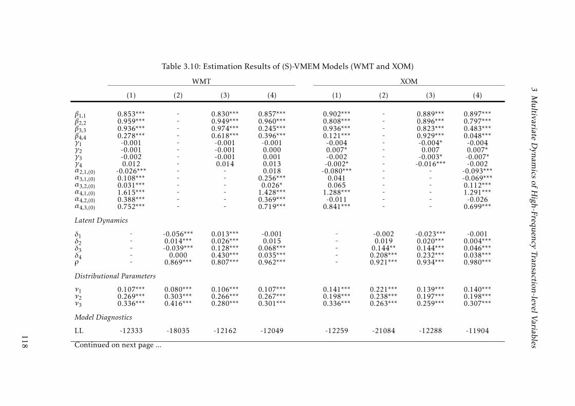
3M
ultivariate
Dynam
icsof
High-Frequ
encyTransaction-levelV
ariables
Table 3.10: Estimation Results of (S)-VMEM Models (WMT and XOM)
WMT XOM
(1) (2) (3) (4) (1) (2) (3) (4)
β1,1 0.853*** - 0.830*** 0.857*** 0.902*** - 0.889*** 0.897***β2,2 0.959*** - 0.949*** 0.960*** 0.808*** - 0.896*** 0.797***β3,3 0.936*** - 0.974*** 0.245*** 0.936*** - 0.823*** 0.483***β4,4 0.278*** - 0.618*** 0.396*** 0.121*** - 0.929*** 0.048***γ1 -0.001 - -0.001 -0.001 -0.004 - -0.004* -0.004γ2 -0.001 - -0.001 0.000 0.007* - 0.007 0.007*γ3 -0.002 - -0.001 0.001 -0.002 - -0.003* -0.007*γ4 0.012 - 0.014 0.013 -0.002* - -0.016*** -0.002α2,1,(0) -0.026*** - - 0.018 -0.080*** - - -0.093***α3,1,(0) 0.108*** - - 0.256*** 0.041 - - -0.069***α3,2,(0) 0.031*** - - 0.026* 0.065 - - 0.112***α4,1,(0) 1.615*** - - 1.428*** 1.288*** - - 1.291***α4,2,(0) 0.388*** - - 0.369*** -0.011 - - -0.026α4,3,(0) 0.752*** - - 0.719*** 0.841*** - - 0.699***
Latent Dynamics
δ1 - -0.056*** 0.013*** -0.001 - -0.002 -0.023*** -0.001δ2 - 0.014*** 0.026*** 0.015 - 0.019 0.020*** 0.004***δ3 - -0.039*** 0.128*** 0.068*** - 0.144** 0.144*** 0.046***δ4 - 0.000 0.430*** 0.035*** - 0.208*** 0.232*** 0.038***ρ - 0.869*** 0.807*** 0.962*** - 0.921*** 0.934*** 0.980***
Distributional Parameters
ν1 0.107*** 0.080*** 0.106*** 0.107*** 0.141*** 0.221*** 0.139*** 0.140***ν2 0.269*** 0.303*** 0.266*** 0.267*** 0.198*** 0.238*** 0.197*** 0.198***ν3 0.336*** 0.416*** 0.280*** 0.301*** 0.336*** 0.263*** 0.259*** 0.307***
Model Diagnostics
LL -12333 -18035 -12162 -12049 -12259 -21084 -12288 -11904
Continued on next page ...
118

3M
ultivariate
Dynam
icsof
High-Frequ
encyTransaction-levelV
ariables
Table 3.10: Estimation Results of (S)-VMEM Models (WMT and XOM)
WMT XOM
(1) (2) (3) (4) (1) (2) (3) (4)
BIC 25017 36184 24665 24496 24869 42301 24917 24207
Residual Diagnostics: Bid-Ask Spread
LB(20) 214.29 80.40 158.48 199.97 227.62 57757.78 227.21 228.38mean 1.000 1.000 1.000 1.000 1.000 1.001 1.000 1.000stdev 0.113 0.081 0.111 0.113 0.148 0.248 0.148 0.148
Residual Diagnostics: Average Trade Size
LB(20) 91.06 10895.28 68.15 83.50 188.58 17805.32 97.57 196.94mean 1.000 1.000 1.001 1.002 1.001 1.001 1.001 1.000stdev 0.282 0.312 0.281 0.282 0.211 0.262 0.210 0.212
Residual Diagnostics: Number of Trades
LB(20) 102.32 24851.78 22.13 15.81 161.57 45.35 41.25 27.12mean 1.000 0.999 1.003 1.007 1.001 0.996 1.006 1.008stdev 0.367 0.442 0.288 0.321 0.365 0.273 0.271 0.340
Residual Diagnostics: Return
LB(20) 59.16 46.76 68.03 63.73 58.12 69.79 62.48 61.47LB2(20) 93.02 1242.65 27.92 73.13 89.48 903.87 26.23 69.37mean 0.005 0.007 0.001 0.004 0.009 0.006 0.004 0.009stdev 1.000 1.000 1.002 1.002 1.000 0.996 1.004 1.003
119
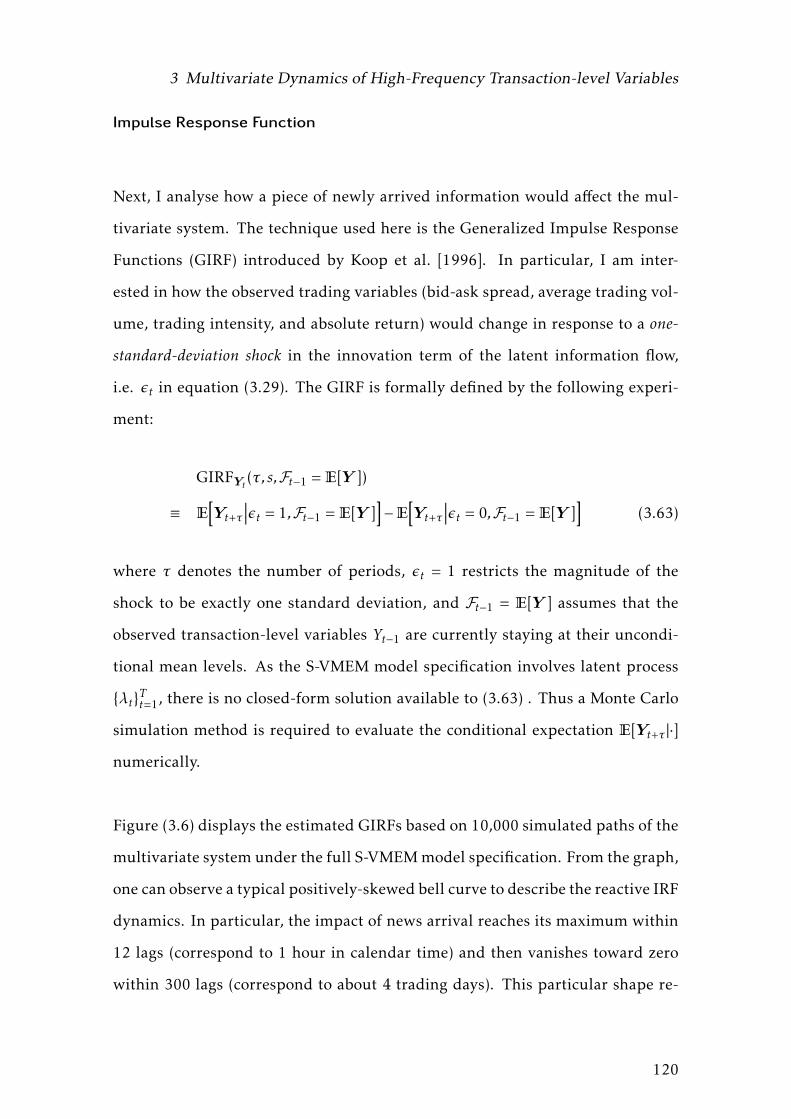
3 Multivariate Dynamics of High-Frequency Transaction-level Variables
Impulse Response Function
Next, I analyse how a piece of newly arrived information would affect the mul-
tivariate system. The technique used here is the Generalized Impulse Response
Functions (GIRF) introduced by Koop et al. [1996]. In particular, I am inter-
ested in how the observed trading variables (bid-ask spread, average trading vol-
ume, trading intensity, and absolute return) would change in response to a one-
standard-deviation shock in the innovation term of the latent information flow,
i.e. εt in equation (3.29). The GIRF is formally defined by the following experi-
ment:
GIRFYt (τ,s,Ft−1 = E[Y ])
≡ E
[Yt+τ
∣∣∣εt = 1,Ft−1 = E[Y ]]−E
[Yt+τ
∣∣∣εt = 0,Ft−1 = E[Y ]]
(3.63)
where τ denotes the number of periods, εt = 1 restricts the magnitude of the
shock to be exactly one standard deviation, and Ft−1 = E[Y ] assumes that the
observed transaction-level variables Yt−1 are currently staying at their uncondi-
tional mean levels. As the S-VMEM model specification involves latent process
{λt}Tt=1, there is no closed-form solution available to (3.63) . Thus a Monte Carlo
simulation method is required to evaluate the conditional expectation E[Yt+τ |·]
numerically.
Figure (3.6) displays the estimated GIRFs based on 10,000 simulated paths of the
multivariate system under the full S-VMEMmodel specification. From the graph,
one can observe a typical positively-skewed bell curve to describe the reactive IRF
dynamics. In particular, the impact of news arrival reaches its maximum within
12 lags (correspond to 1 hour in calendar time) and then vanishes toward zero
within 300 lags (correspond to about 4 trading days). This particular shape re-
120

3 Multivariate Dynamics of High-Frequency Transaction-level Variables
Figure 3.6: Generalized Impulse Response Function
This figure shows the Generalized Impulse Response Function (GIRF) of how the fourtransaction-level variables (bid-ask spread, average trade size, trade intensity, and return volatil-ity) response to a one-standard-derivation shock in unobserved information flow.
121

3 Multivariate Dynamics of High-Frequency Transaction-level Variables
flects that the IRF dynamics is driven by two competing forces: the contribution
by the persistence of news which gradually declines over time and the contribu-
tion by the feedback loop among trading variables which amplifies the impact.
In terms of the size of news impact, one can observe that news arrival has pos-
itive impacts on average trade size, trade intensity and return volatility. This is
consistent with the perception that newly received fundamental signal motivates
investors to more actively participate in the market, resulting in more trades and
bigger size per trade, and consequently, the price exhibits larger volatility. How-
ever, Monte Carlo stimulation delivers mixed results on how the average bid-ask
spread changes in response to market news, and the magnitude of such change
is typically very small. Overall, the empirical GIRF does not support the infor-
mation asymmetric microstructure hypothesis, which claims that market makers
will enlarge bid-ask spread in response to an anticipated underlying information
flow in order to protect themselves from the price risk due to adverse selection.
3.6 Concluding Remarks
In this paper, I use the Stochastic Vector Multiplicative Error model (S-VMEM) of
Hautsch [2008] to study genuine multivariate dynamics between bid-ask spread,
average dollar volume per trade, trade intensity and return volatility by taking
into account the presence of latent information flow. The ML-EIS method is used
to estimate the model. A Monte Carlo experiment is conducted to show the su-
perior ability of the ML-EIS algorithm to recover the true model parameters.
I fit the S-VMEMmodel to six heavily traded stocks listed in the US stock market
and the main empirical results are summarized as follows. First, the empiri-
122

3 Multivariate Dynamics of High-Frequency Transaction-level Variables
cal evidence supports the Mixture of Distribution Hypothesis (MDH) of Clark
[1973] by revealing the existence of unobserved serially correlated information
flow. Second, a strong contemporaneous genuine dependence between return
volatility and the other three transaction variables is found. Third, the impact
of information flow is most significantly positive for return volatility and trade
intensity. This finding is in sharp contrast with previous studies like Blume et al.
[1994], Xu andWu [1999], Huang and Masulis [2003] and Hautsch [2008], where
the authors find that it is the average trade size instead of trade intensity that
is most informative about the quality of news. This changing behaviour reflects
that market impact becomes an increasing important concern when investors ex-
ecute their trades, and consequently, they tend to break large order into many
small child orders. Thus the number of trades carries more informative content
about hidden market event than the average trade size does. Finally, the impulse
response analysis shows that the dynamics of bid-ask spread is little affected by a
positive shock in the underlying information flow, and thus provides no evidence
to support the asymmetric information market microstructure theory.
123

4 Analysing Inflation Dynamics
Using Inflation Swap Data
4.1 Introduction and Motivation
Maintaining a low and anchored 1 inflation expectation is crucial for central bank
to achieve its mandates such as ensuring price stability and steady economic
growth. However, measuring inflation expectation poses a great challenge for
both policy makers and economic researchers because of its unobservable na-
ture. One common approach to obtain an indication on future inflation is to
conduct surveys on a group of people by simply asking what they expect. Some
popular survey-based measures include Consumer Confidence Survey2 and Survey
of Professional Forecasters3. In addition to the survey-based approach, sovereign
inflation-linked bond 4 has now also been used by central banks to infer the mar-
ket expectation on future rate of inflation. More specifically, one can calculate the
1the term anchored means relatively insensitive to incoming macroeconomic data2Consumer Confidence Survey asks 5400 households across 6 metro cities on one-year aheadinflation expectation. The survey is conducted at a quarterly basis.
3Survey of Professional Forecasters asks about 30 professional forecasters for the inflation ex-pectation over each of the next four quarters, next 5 years, and next 10 years. The survey isconducted at a quarterly basis.
4linker for short; in US, it is termed Treasury Inflation Protection Securities, TIPS thereafter
124
4 Analysing Inflation Dynamics Using Inflation Swap Data
so-called Break-Even Inflation (BEI) which is defined as the yield spread between
nominal and inflation-linked bond with similar maturities. The advantage of us-
ing market-based measures over survey-based measure is that the former can provide
a real-time assessment on investors’ inflationary beliefs whereas the latter are updated
only on a quarterly basis. What’s more, market-based measures are believed to be
more reliable in the sense that investors are willing to put money to back up their
views.
However, one should interpret the BEI with cautions because this breakeven rate in-
cludes not just inflation expectation but also various risk premium components that
compensate investors for bearing risks such as that future realized inflation could
potentially deviate from its expected value. Several methods have been proposed
in the literature to separate the inflation expectation from the associated risk pre-
miums, see Haubrich et al. [2011] and Abrahams et al. [2013] among others. The
main idea is to model the joint dynamics of BEI and nominal interest rate within
a no-arbitrage Gaussian affine term structure framework. Then, calibrating model
parameters under pricing measureQ and comparing with their counterparts un-
der physical measure P would allow one to calculate themarket prices of risks and
to decompose BEI into inflation expectation and associated term premiums.
While inflation linkers have remained to be the primary source for central banks
to gauge market-based expectations, the rapid development of inflation swap
market worldwide is receiving increasing attentions because this financial deriva-
tive product trades inflation directly and thus provides an alternative source to
assess investors’ beliefs. In fact, in our opinions, inflation swap is actually a much
cleaner data source than sovereign inflation linkers to analyse inflation expectation for
several reasons:
125

4 Analysing Inflation Dynamics Using Inflation Swap Data
• First of all, the bond BEI, which is calculated as the spread between nomi-
nal yield and real yield with same maturity, contains a significant liquidity
risk premium component. This is because that in order to achieve the bond
BEI, one is required to take a long position in nominal bond and a short po-
sition in inflation linker simultaneously, but nominal sovereign bonds are
generally much more liquid than inflation linkers (more trading volumes
and numbers of transactions per day) and such liquidity risk premium would
understate the bond BEI from its fair value. Moreover, one can obtain lower
financing rates when putting nominal government bond (especially those
on-the-run issuance) rather than inflation linker as collateral in moneymar-
ket, because nominal sovereign bonds are more liquid than inflation link-
ers. This also creates unbalanced strong demand for nominal government bonds
which further drives the bond BEI down.
• Second, sovereign inflation linkers might be priced inefficiently. For exam-
ple, by studying the US market, Haubrich et al. [2011] show that TIPS were
significantly underpriced prior to 2004 and also during the 2008 financial
turmoil.
• Third, inflation swaps allow one to estimate the BEI curve more accurately
because it provides a wider range and more evenly spread terms to maturi-
ties than inflation linkers. More importantly, government inflation linkers
are issued less frequently, and consequently, only a very small number of
inflation linkers are available for BEI curve fitting and interpolation at early
years. For example, in US, TIPS are only issued several times a year at 5-,
10- and 30-years maturities, and thus the interpolated BEI curve over all
maturities based on just a handful of data points are unreliable. In con-
trast, inflation swaps data are abundant, as the swap rates are daily quotes
126

4 Analysing Inflation Dynamics Using Inflation Swap Data
from OTC contracts that have an exact year-to-maturity of 1- to 10-years
and then 15-, 20- , 25- and 30-years.
• Fourth, having maturities which are exact multiples of a whole year, infla-
tion swaps are not subject to any seasonality bias, which could however be
a severe issue for inflation linkers.
• Fifth, inflation linkers are subject to auction effect and they are usually
cheaper ahead of new on-the-run issuance. Also, FED’s Permanent Open
Market Operations (POMO) or European Central Bank’s Long-Term Refi-
nancing Operations (LTRO) could affect price of inflation linkers signifi-
cantly. While for inflation swaps, the swap rates are fully left for the market
to determine and there is much less noises from central bank interventions.
• Sixth, inflation linkers with long maturities (i.e. 30-year) often have very
large redemption values (exceed twice of the par value), and this raises con-
sideration about credit risk of sovereign inflation linkers. This might be
less a problem for US but a severe issue for other countries. In contrast,
inflation swaps are fully collateralized, i.e., counterparties follow mark-to-
market procedure at a daily basis by exchanging the difference in NPVs of
swap and posting collaterals such as government bonds, so the counterparty
credit risk is minimal.
• Finally, there typically exists an embedded floor for inflation linker, which
means the final principal payment won’t shrink if realized inflation goes
negative. This additional option-alike feature further complicates the anal-
ysis of bond BEI. In contrast, there is no embedded caps or floors in inflation
swaps.
127
4 Analysing Inflation Dynamics Using Inflation Swap Data
In this paper, we decompose the term structure of breakeven inflation rates and
further analyse the dynamics of implied inflation expectation by fitting no-arbitrage
affine term structure model to the observed zero coupon inflation swap data. The
rest of paper is organized as follows. First, section (4.2) provides overviews on
inflation-indexed bond market and inflation swap market, and describes their
key structural features. Second, we show how to formulate the no-arbitrage affine
term structure model to characterize the joint dynamics of nominal interest rate
and BEI in section (4.3). Next, section (4.4) is devoted to describe how we pro-
ceed to estimate the model using the three-step regression technique proposed
by Adrian et al. [2013], followed by empirical results reported in section (4.5).
The final section summarizes and concludes.
4.2 Market Overviews
During the last several decades, governments in many countries have started to
issue inflation-linked bonds (ILB) with the aim to reduce their sovereign financ-
ing cost by an amount of inflation risk premium. Such ILB is called index-linked
Gilts in UK, and Treasury Inflation Protection Securities (TIPS) in US. Compared
to nominal government bonds, these real rate products are designed to cancel
the capital eroding effects of inflation. The interest rate of ILB remains the same
as its nominal counterpart, but the principal is adjusted to match the inflation
rate based on a price index, such as Consumer Price Index (CPI) in US and Retail
Price Index (RPI) in UK.
Unlike real rate bond, inflation swap is a pure inflation product. It is a highly
liquid financial derivative instrument designed to transfer inflation risk from
128

4 Analysing Inflation Dynamics Using Inflation Swap Data
one party to another by means of exchanging cash flows. In an inflation swap,
one party (inflation receiver) pays pre-agreed fixed-rate payments, in exchange
for floating-rate payments from a second party where the amount of payment is
linked to an inflation index. For example, one party may pay a fixed rate of 3%
on a two year inflation swap, and in return receive the actual inflation.
Inflation swap contracts are traded in a dealer-based over-the-counter (OTC)mar-
ket so that the pay-off structure can be tailored to address the specific needs of the
counterparty. However, the zero-coupon inflation swap has become the standard
contract for which rates are quoted in wholesale market by brokers, and it is also
the data source we use here. The zero-coupon inflation swap has the most ba-
sic structure with payments exchanged only at maturity date. More specifically,
let st,N denote the swap rate of a zero-coupon inflation swap at time t with re-
maining time to maturity N , and Qt be the realized reference price index at time
t. Then, at maturity date t +N , the inflation receiver would pay the difference
of cumulative actual rate of inflation over the cumulative annually compounded
fixed rate, i.e.,
Notional Amount×(Qt+NQt− (1 + st,N )N
). (4.1)
The growth of international inflation swap market resembles that of the interest
rate swap market in the early 1980s, and there now exists an increasingly highly
liquid global market for inflation derivatives. On the demand side, both ILBs and
inflation swaps are extremely popular among pension funds or other entities,
who have long-term liabilities linked to inflation rate and thus are willing to
hedge such inflation risk exposure. Inflation derivatives are also used by market
participants to speculate the course of inflation. On the supply side, governments
129

4 Analysing Inflation Dynamics Using Inflation Swap Data
are the natural sellers of ILBs because ILBs can lower their financing cost. Major
investment banks are the largest derivative dealers and they make markets for
inflation swap and other derivative products.
Table 4.1: Contractual Terms of Inflation-linked Instruments
ReferenceIndex (RI)
Lag Length(months)
Calculationsof RI
EmbeddedFloors
Inflation-Linked Bonds
US (TIPS) US CPI-U 3 Interpolated Yes
Zero-coupon Inf Swaps
US US CPI-U 3 Interpolated NoUK UK RPI 3 Interpolated NoEuro Euro HICP 3 Interpolated No
In practice, both inflation-linked government bonds and inflation swap contracts
have indexation lags, which means a contract is referenced to the inflation over
a period that begins before the date on which the contract is priced and ends
before the contract matures. Table (4.1) presents the detailed contractual terms
of ILBs and inflation swaps that are discussed in this paper. Note that the in-
dexation lag of ILBs and inflation swaps to inflation index introduces a perfectly
predictable component in the changes of BEIs, as both bond BEIs and swap BEIs
contain some amount of realized inflation. The BEI that is more relevant to market
participants and policy markers is the one that is completely forward-looking and takes
out this realized inflation. The following few paragraphs discuss how to calculate
the implied forward-looking BEI from the raw data.
The specified indexation lag means that a contract of maturity N years traded
at time t will be referenced to inflation over a period t − L to t +N − L, where L
130
4 Analysing Inflation Dynamics Using Inflation Swap Data
is the indexation lag expressed as a fraction of year. The annually compounded
inflation swap rate st,N can therefore be expressed as
(1 + st,N )N = (1+ It−L,t+N−L)
N (4.2)
where Ii,j represents the inflation compensation required by investors for the pe-
riod between date i and date j , stated in annual percentage rate (APR). To strip
out the part of inflation that has already accrued, i.e., It−L,t , we can decompose
the cumulative fixed rate as
(1 + st,N )N = (1+ It−L,t+N−L)
N = (1+ It−L,t)L(1 + It,t+N−L)
T−L. (4.3)
From equations (4.2) and (4.3), we can calculate the implied forward-looking
inflation swap rate from today t to a future date t+N−L, i.e. It,t+N−L, as follows:
(1 + It,t+N−L)N−L =
(1+ st,N )N
(1 + It−L,t)L(4.4)
and this spot BEI rate is now completely forward-looking. Having these carry-
adjusted BEI rates together with nominal yield curve, we can use cubic spline
method to interpolate the term structure of inflation swap rates. By doing so, we
remove the ”carry” noises at input stage. One thing worth mentioning is that as
inflation swap rates are quoted in an annual compounding fashion, one need to
convert them to continuous compounding rates before doing the interpolation.
131

4 Analysing Inflation Dynamics Using Inflation Swap Data
4.3 The No-Arbitrage Affine Joint Term Structure
Model
In this section, I review the no-arbitrage affine term structure model which is
used to describe the joint dynamics of BEI rates and nominal yields. Suppose
that the joint term structure of BEI and nominal interest rates can be explained
by a set of pricing factorsXt , which contain K elements and are assume to follow
a Vector Autoregressive of Order 1 process:
Xt =αP+β
PXt−1 +uP,t (4.5)
Xt =αQ+β
QXt−1 +uQ,t (4.6)
where ut ∼ N(0,ΣX ) and the subscripts P and Q indicate that the parameters
θ and the pricing factors Xt are under real world probability measure and risk
neutral pricing measure respectively.
Let P(m)t denote the price of a zero-coupon bond at time t that pays 1 dollar at
maturity date t +m, then the stochastic discount factor (SDF) 5 St satisfies the
following equation:
P(m)t = E
P
t [St+1P(m−1)t+1 ] (4.7)
Together with the risk neutral pricing formula
P(m)t = exp(−rt)E
Q
t [P(m−1)t+1 ] (4.8)
5it is also called pricing kernel or deflator
132

4 Analysing Inflation Dynamics Using Inflation Swap Data
we have
EP
t [exp(rt)St+1P(m−1)t+1 ] = E
Q
t [P(m−1)t+1 ] (4.9)
where rt = − log(P(1)t ) is the short rate6 process. One can easily show that exp(rt)St+1 =
dQ/dP is the Radon-Nikodym derivative that characterizes the equivalence be-
tween measures P and Q. To derive the formula for St+1, one can write equation
(4.5) in differential form, i.e.
∆Xt =αP+ (β
P− 1)Xt−1 +uP,t
=αQ+ (β
Q− 1)Xt−1 + (α
P+β
PXt−1 −αQ
−βQXt−1) +uP,t
=αQ+ (β
Q− 1)Xt−1 +Σ
12X
[Σ− 12
X
(α
P−α
Q+ (β
P−β
Q)Xt
)+Σ− 12
X uP,t
]=α
Q+ (β
Q− 1)Xt−1 +Σ
12XΣ− 12
X uQ,t . (4.10)
Therefore, the market price of risks, denoted by λt , can be written as
λ′t = Σ− 12
X
(λ0 +λ1Xt
)(4.11)
where
λ0 =αP−α
Q(4.12)
λ1 = βP−β
Q. (4.13)
Furthermore, the corresponding Radon-Nikodym derivative is
dQdP
= exp(−λ′tΣ
− 12
X uP,t+1 −12λ′tλt
), (4.14)
6one-month nominal interest rate
133

4 Analysing Inflation Dynamics Using Inflation Swap Data
making the SDF possess the following form:
St+1 = exp(− rt −λ′tΣ
− 12
X uP,t+1 −12λ′tλt
). (4.15)
4.3.1 The Nominal Yield Curve
The affine term structure framework assumes that the log price of riskless zero
coupon bond log(P(m)t ) is an affine (linear) function of underlying pricing factors
Xt , i.e.
log(P(m)t ) = Am +B′mXt . (4.16)
To derive the no-arbitrage conditions, one can plug the equation (4.16) into the
risk neutral pricing formula (4.8) and thus obtain:
exp(Am +B′mXt) = exp(A1 +B′1Xt)E
Q
t [exp(Am−1 +B′m−1Xt+1)]
exp(Am +B′mXt) = exp(A1 +B′1Xt)E
Q
t [exp(Am−1 +B′m−1αQ
+B′m−1βQXt +B
′m−1uQ,t)]
exp(Am +B′mXt) = exp(A1 +B′1Xt)exp(Am−1 +B
′m−1αQ
+B′m−1βQXt +
12B′m−1ΣXBm−1)
By matching the coefficients for constant term and Xt in the above equation, one
can derive the so-called no-arbitrage recursive equations:
Am = A1 +Am−1 +B′m−1αQ
+12B′m−1ΣXBm−1 (4.17)
Bm =B′1 +B′m−1βQ
(4.18)
where the starting parameters A1 andB1 can be obtained from
log(P(1)t ) ≡ −rt = A1 +B
′1Xt . (4.19)
134

4 Analysing Inflation Dynamics Using Inflation Swap Data
Setting ρ0 = −A1 and ρ1 = −B1, one can rewrite the recursive equations as
Am = −ρ0 +Am−1 +B′m−1αQ+12B′m−1ΣXBm−1
Bm = −ρ′1 +B′m−1βQ
(4.20)
with the initial values A0 = 0 andB0 = 0.
4.3.2 The Real Yield Curve
For a zero coupon bondwhose price is linked to an inflation indexCt , its principal
payment at maturity date is Ct+m/Ct . One can thus write the discounted bond
price as
P(m)t,R = E
Q
t [exp(−rt − rt+1 − · · · − rt+m−1)Ct+mCt
] (4.21)
To allow the price dynamics of real-yield bond stay within the affine term struc-
ture framework, we need to make a key assumption that the logarithm of inflation
index changes ct = log(Ct/Ct−1) is an affine function of the underlying pricing factors
Xt , i.e.
ct = π0 +π′1Xt (4.22)
which implies that the logarithm price of a zero coupon inflation-linked bond is also
an affine function ofXt , i.e.
log(P(m)t,R ) = Am,R +B
′m,RXt . (4.23)
135

4 Analysing Inflation Dynamics Using Inflation Swap Data
This is actually quite a reasonable assumption since the market will take the dy-
namics of inflation into account when they price an inflation linker, so one could
expect the movement in inflation rate to be well explained by a set of pricing
factors extracted from the observed real yields.
Note that the equation (4.21) indicates that
P(m)t,R = E
Q
t [exp(−rt + ct+1)P(m−1)t+1,R ] (4.24)
fromwhich we can derive the no-arbitrage recursive equations for the term struc-
ture of real interest rates:
exp(Am,R +B′m,RXt) = exp(−ρ0 −ρ′1Xt)E
Q
t [exp(π0 +π′1Xt+1)exp(Am−1,R +B
′m−1,RXt+1)]
exp(Am,R +B′m,RXt) = exp(−ρ0 −ρ′1Xt)exp
(Am−1,R +π0 + (Bm−1,R +π1)
′αQ
+ (Bm−1,R +π1)′β
QXt +
12(Bm−1,R +π1)
′ΣX(Bm−1,R +π1))
Similarly, by matching coefficients for constant terms and Xt , one can obtain the
no-arbitrage recursive equations:
Am,R = −ρ0 +π0 + (Bm−1,R +π1)′α
Q+12(Bm−1,R +π1)
′ΣX(Bm−1,R +π1)
B′m,R = −ρ′1 + (Bm−1,R +π1)′β
Q(4.25)
with the starting values A0,R = 0 andB0,R = 0.
136
4 Analysing Inflation Dynamics Using Inflation Swap Data
4.3.3 The Breakeven Inflation Curve
Let ω(m)t denotes the BEI rate between time t and t+m. Having both nominal and
real yield pricing formulas enables us to derive the following pricing formula for
breakeven inflation rate:
ω(m)t = y(m)
t − y(m)t,R
=1m
(logP(m)
t,R − logP(m)t
)=
1m
((Am,R −Am) + (Bm,R −Bm)
′Xt
)=
1m
(Am,ω +B′m,ωXt
)(4.26)
where the recursive parameters are given by
Am,ω = π0 +Am−1,ω + (Bm−1,ω +π1)′α
Q− 12(Bm−1,ω +π1)
′ΣX(Bm−1,ω +π1)
B′m,ω = (Bm−1,ω +π1)′β
Q(4.27)
with the initial values given by A0,ω = 0 andB0,ω = 0.
4.3.4 The Decomposition of Term Structure
Obtaining the market expectation requires removing the risk premium compo-
nent from the observed market price, which is equivalent to changing from risk-
neutral pricing measure Q to real-world probability measure P. To calculate the
model-implied market expectation, we can simply replace the risk-neutral parameters
in pricing formulas with their counterparts under physical measures. Consequently,
the associated risk premium is given by the difference between market price and
137

4 Analysing Inflation Dynamics Using Inflation Swap Data
the implied market expectation.
4.4 The Estimation Technique
To estimate the no-arbitrage affine term structure model, we adopt the three-step
regression technique introduced by Abrahams et al. [2013]. The following nota-
tions and conventions are used to facilitate further discussion. The model pa-
rameter set, denoted by θ, include ρ0, ρ1, π0, π1, αQ, β
Q, α
P, β
Pand ΣX . Once
these nine parameters are obtained, we can calculate model-implied expectation
and risk premium based on the no-arbitrage recursive equations (4.20), (4.25)
and (4.27).
Among these nine parameters of interest, αP, β
Pand ΣX can be estimated in a
straightforward manner by running VAR(1) regression on the observed pricing
factors Xt under the real-world probability measure P. One can easily obtain
the OLS estimates of αP, β
Pand residuals u
P,t . Consequently, the estimate of
variance-covariance matrix ΣX can be constructed as ΣX = uP,tu
′P,t
/T , where T is
the sample size.
Regarding the risk neutral parameters αQ
and βQ, Abrahams et al. [2013] and
Adrian et al. [2013] suggest that these two can be naturally estimated based
on excess holding period returns of nominal and real bonds. In particular, let
ehpr(m−1)t+1 denote the logarithmic of one-period return of holding a nominal bond
138

4 Analysing Inflation Dynamics Using Inflation Swap Data
P(m)t in excessive of one-period short interest rate rt , i.e.
ehpr(m−1)t+1 = logP(m−1)t+1 − logP(m)
t − rt (4.28)
By substituting the recursive parameters Am andBm in (4.20, one can rewrite the
above excess holding period return as
ehprm−1t+1 = Am−1 +B′m−1Xt+1 −Am −B′mXt − ρ0 −ρ′1Xt
= (Am−1 −Am − ρ0)− (Bm +ρ1)′Xt +B
′m−1(αP
+βPXt +uP,t)
=B′m−1(αP−α
Q)− 1
2B′m−1ΣXBm−1 +B
′m−1(βP
−βQ)Xt +B
′m−1uP,t
=(B′m−1λ0 −
12B′m−1ΣXBm−1
)+B′m−1λ1Xt +B
′m−1uP,t (4.29)
Similarly, we can express the excess holding period return of real yield bond
ehpr(m−1)t+1,R as
ehprm−1t+1,R = logP(m−1)t+1,R − logP
(m)t,R − rt (4.30)
Adding inflation ct+1 on both sides and substituting the recursive equations (4.25),
we can obtain
ehprm−1t+1,R + ct+1 =((Bm−1,R +π1)
′λ0 −12(Bm−1,R +π1)
′ΣX(Bm−1,R +π1))
+ (Bm−1,R +π1)′λ1Xt + (Bm−1,R +π1)
′uP,t (4.31)
Let’s further define
Ψ ≡(B1,B2, ...,BM ,B1,R +π1,B2,R +π1, ..,BM,R +π1
)′(4.32)
Φ ≡(B′1ΣXB1,B
′2ΣXB2, ...,B
′MΣXBM , (B1,R +π1)
′ΣX(B1,R +π1)
139
4 Analysing Inflation Dynamics Using Inflation Swap Data
, (B2,R +π1)′ΣX(B2,R +π1), ..., (BM,R +π1)
′ΣX(BM,R +π1))′
(4.33)
Then stacking equations (4.29) and (4.31) gives us
Rstackt+1 =
(Ψλ0 −
12Φ
)+Ψλ1Xt +Ψu
P,t (4.34)
As the observed excess holding period returns are typically subject to measure-
ment errors, one can write the the observed returns Rstack,obst+1 as
Rstack,obst+1 =Rstack
t+1 +Et+1 =A∗ +B∗Xt +C
∗uP,t +Et+1 (4.35)
where
A∗ =Ψλ0 −12Φ (4.36)
B∗ =Ψλ1 (4.37)
C∗ =Ψ (4.38)
and Et+1 is assumed to be serially uncorrelated measurement error with zero
mean.
An appealing feature of regression (4.35) is that all the RHS regressors are or-
thogonal to each other: uP,t are i.i.d. innovation terms in (4.5) and the pric-
ing factorsXt themselves are extracted by Principal Component Analysis (PCA)
method which ensures the orthogonality property as well. The implication is that
multicollinearity bias is minimal, and consequently, all the regression coefficients
could be estimated very accurately with fairly small standard errors. Therefore,
to estimate βQ, we can first obtain the OLS estimates of regression (4.35) as A∗,
140

4 Analysing Inflation Dynamics Using Inflation Swap Data
B∗, C∗ as well as the residuals E. A natural estimate of variance-covariance ma-
trix of the return pricing error Et+1 is obtained by ΣE = EE′/T .
Note that knowing Ψ = C∗ and the covariance matrix of pricing factor innova-
tions ΣX would allow us to construct Φ according to equations (4.32) and (4.33).
Furthermore, equations (4.36) and (4.37) can be rearranged as
A∗ +12Φ =Ψλ0
B∗ =Ψλ1
which leads to the following estimators for λ0 and λ1 with analytically tractable
asymptotic variances:
λ0 = (Ψ′Ψ)−1Ψ
′(A∗ +
12Φ) (4.39)
λ1 = (Ψ′Ψ)−1Ψ
′B∗ (4.40)
The estimators for αQand β
Qare straightforward to obtain by
αQ= α
P− λ0 (4.41)
βQ= β
P− λ1 (4.42)
Next, since the one-period short rate can be directly observed, ρ0 and ρ1 can be
obtained by regressing the observed short rate rt on the pricing factorsXt .
Regarding the inflation dynamic parameters π0 and π1, Abrahams et al. [2013]
suggest to estimate them by calibrating the observed real yield bonds or observed
BEI. The advantage of this approach is that it ensures the recursive dynamics are
141

4 Analysing Inflation Dynamics Using Inflation Swap Data
incorporated in the estimation procedure, so the model-implied yields are con-
sistent with cross-maturity no-arbitrage constraints. The idea is to use a two-step
estimation procedure: till now, all parameters but π0 andπ1 have been estimated,
so the BEI no-arbitrage recursive equations (4.27) can be reduced to a systemwith
only π0 and π1 remain unknown. By recursive substitution, one can write Am,ω
as a quadratic function of π0 and π1, and expressBm,ω as a linear function of π1.
The BEI rate ω(m)t can be expressed in the affine form
ω(m)t =
1m(Am,ω +B′m,ωXt) (4.43)
which implies that the observed real yields ω(m)t is also quadratic in π0 and π1 as
well. Therefore, running a quadratic regression would give us the estimates for
π0 and π1.
4.5 Empirical Analysis
In this section, we fit the no-arbitrage affine joint term structure model to histor-
ical inflation swap dataset in US, UK and Europe.
4.5.1 Dataset Description
The sample size of inflation swap data used in this study varies from country to
country, with detailed information listed in table (4.2). The zero coupon infla-
tion swap rates with 1- to 10- year maturities are obtained from Barclays Live7,
7www.barcaplive.com
142
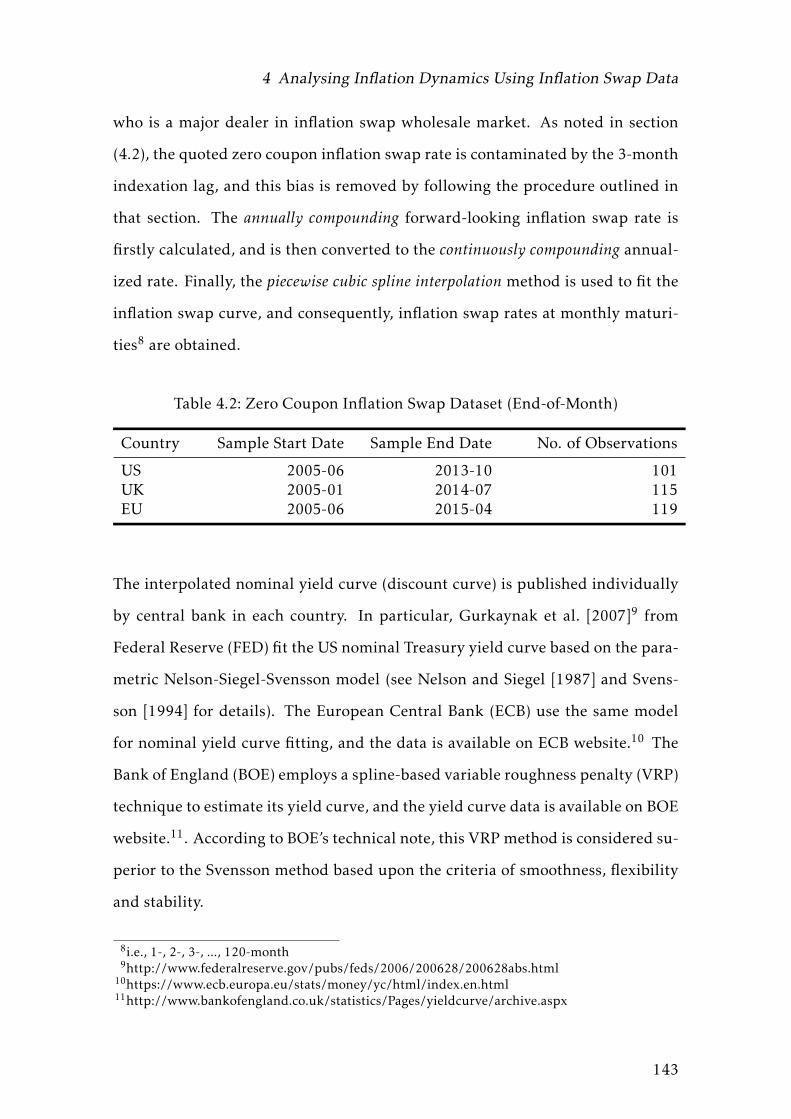
4 Analysing Inflation Dynamics Using Inflation Swap Data
who is a major dealer in inflation swap wholesale market. As noted in section
(4.2), the quoted zero coupon inflation swap rate is contaminated by the 3-month
indexation lag, and this bias is removed by following the procedure outlined in
that section. The annually compounding forward-looking inflation swap rate is
firstly calculated, and is then converted to the continuously compounding annual-
ized rate. Finally, the piecewise cubic spline interpolation method is used to fit the
inflation swap curve, and consequently, inflation swap rates at monthly maturi-
ties8 are obtained.
Table 4.2: Zero Coupon Inflation Swap Dataset (End-of-Month)
Country Sample Start Date Sample End Date No. of Observations
US 2005-06 2013-10 101UK 2005-01 2014-07 115EU 2005-06 2015-04 119
The interpolated nominal yield curve (discount curve) is published individually
by central bank in each country. In particular, Gurkaynak et al. [2007]9 from
Federal Reserve (FED) fit the US nominal Treasury yield curve based on the para-
metric Nelson-Siegel-Svensson model (see Nelson and Siegel [1987] and Svens-
son [1994] for details). The European Central Bank (ECB) use the same model
for nominal yield curve fitting, and the data is available on ECB website.10 The
Bank of England (BOE) employs a spline-based variable roughness penalty (VRP)
technique to estimate its yield curve, and the yield curve data is available on BOE
website.11. According to BOE’s technical note, this VRP method is considered su-
perior to the Svensson method based upon the criteria of smoothness, flexibility
and stability.
8i.e., 1-, 2-, 3-, ..., 120-month9http://www.federalreserve.gov/pubs/feds/2006/200628/200628abs.html
10https://www.ecb.europa.eu/stats/money/yc/html/index.en.html11http://www.bankofengland.co.uk/statistics/Pages/yieldcurve/archive.aspx
143

4 Analysing Inflation Dynamics Using Inflation Swap Data
The seasonally unadjusted price index is used as the reference price index to price
zero coupon inflation swap. In particular, the Consumer Price Index for All Ur-
ban Consumers (CPI-U) is used for US inflation swap; the Retail Price Index (RPI)
is used in UK; and the Harmonized Index of Consumer Prices Excluding Tabacco is
used in Euro area. All these price index data are available from Economic Re-
search Database at Federal Reserve Bank of St. Louis (FRED).12
4.5.2 Constructing Orthogonal Pricing Factors
The pricing factors Xt are constructed by applying the Principal Component
Analysis (PCA) technique to a cross-section of nominal yield curve and inflation
swap curve.
The first Nnom principal components based on nominal yield curve are selected.
Next, to construct the pricing factors for inflation swap, we first realize that in-
flation and nominal interest rates usually have a very positive correlation since
central banks’ monetary policies would affect aggregate demand which further
lead to changes in aggregate price level in future. Therefore, with the aim to
minimize duplication and promote orthogonality among pricing factors, we fol-
low Abrahams et al. [2013] to first regress inflation swap rates on on the Nnom
principle components from nominal yields, and obtain the residuals of the result-
ing regression. Then we pick the first Ninf l principle components extracted from
these orthogonal residuals as additional pricing factors. This gives usNnom+Ninf l
number of pricing (or risk) factors in total.
12https://research.stlouisfed.org/fred2/
144

4 Analysing Inflation Dynamics Using Inflation Swap Data
To choose appropriate values for Nnom and Ninf l , we adopt a forward stepwise
method with starting values Nnom = 3 and Ninf l = 2. The initial values are chosen
as so because these 5 principal components are able to explain over 99% of total
variations in nominal yield curve and inflation swap curve. Then the number
of factors are incremented gradually, and the model-implied curve fitting error,
which is themean squared error between fitted and observed prices, is calculated.
The final choice of Nnom and Ninf l reflects the trade-off between goodness-of-fit
and the degree of model parsimony. As a result, both US and UK data are in
favour of 3 nominal factors with 3 residual BEI factors, whereas 5 nominal and
3 residual BEI factors are preferred by EU data. The EU result is in line with
Adrian et al. [2013], where the authors find including the 4th and 5th nominal
principal components could potentially improve the no-arbitrage affine nominal
term structure curve fitting significantly.
The time series of pricing factors over the sample period are plotted in figure
(4.1). From the graph, we can see that there are strong comovements of pricing
factors among these three developed markets. In particular, as a result of ex-
pansionary monetary policy adopted by central banks globally, the first nominal
principal component, also known as the level factor, drop sharply and stay low
since the 2008 financial crisis. While the other pricing factors are typically fea-
tured by mean-reversion behaviour with a spike during the collapse of Lehman
Brothers in 2008.
145

4 Analysing Inflation Dynamics Using Inflation Swap Data
Figure 4.1: Time Series Plots of Pricing Factors
This figure presents the time-series plots of pricing factors based on nominal yield curve andinflation swap curve for US, UK and EU markets.
146

4 Analysing Inflation Dynamics Using Inflation Swap Data
4.5.3 Empirical Results
We estimate the no-arbitrage joint nominal and BEI term structure model based
on the choice of pricing factors discussed in previous section. Themodel goodness-
of-fit is presented in table (4.3) where the mean absolute term structure fitting
errors are reported at 2-, 5- and 10-year maturities. From the result, we can see
that the model is able to describe the term structure dynamics very well, as in-
dicated by both nominal pricing errors and BEI pricing errors being very small
with the former less than 5 basis points and the latter less than 10 basis points.
Table 4.3: Goodness of Fit: Mean Abosolute Errors (in bps)
2-year 5-year 10-yearNominal Yield
US 3.611 4.334 4.052UK 4.619 3.603 4.333EU 0.775 2.767 1.314
Breakeven Inflation
US 5.927 3.925 5.549UK 5.308 4.447 4.953EU 9.854 6.032 3.743
Figure (4.2), (4.3) and (4.4) further provide graphical evidence on time series fit
of the model to the three developed markets over the sample period. In particu-
lar, the model-implied nominal yields and breakeven inflation rates are plotted
against their observed values at various maturities. In line with the results re-
ported in table (4.3), the no-arbitrage joint term structure model is able to recover
the observed nominal interest rate and inflation swap rate very accurately with
visually indistinguished pricing errors.
147

4 Analysing Inflation Dynamics Using Inflation Swap Data
Figure 4.2: Time Series Model Fit: US market
This figure visualizes the time-series fit of the no-arbitrage joint term structure model of nomi-nal yields and breakeven inflation rates in US market. The blue solid lines are observed nominalyields and breakeven inflation rate, whereas the green dashed lines are their model-implied esti-mates.
148
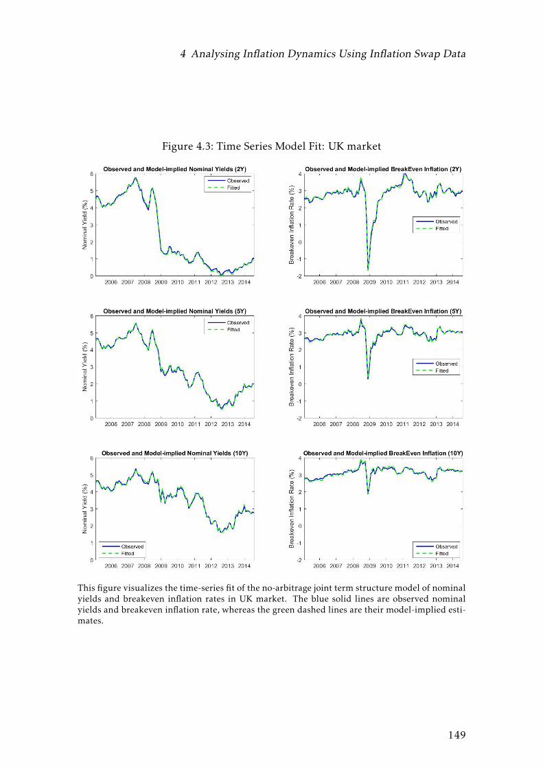
4 Analysing Inflation Dynamics Using Inflation Swap Data
Figure 4.3: Time Series Model Fit: UK market
This figure visualizes the time-series fit of the no-arbitrage joint term structure model of nominalyields and breakeven inflation rates in UK market. The blue solid lines are observed nominalyields and breakeven inflation rate, whereas the green dashed lines are their model-implied esti-mates.
149
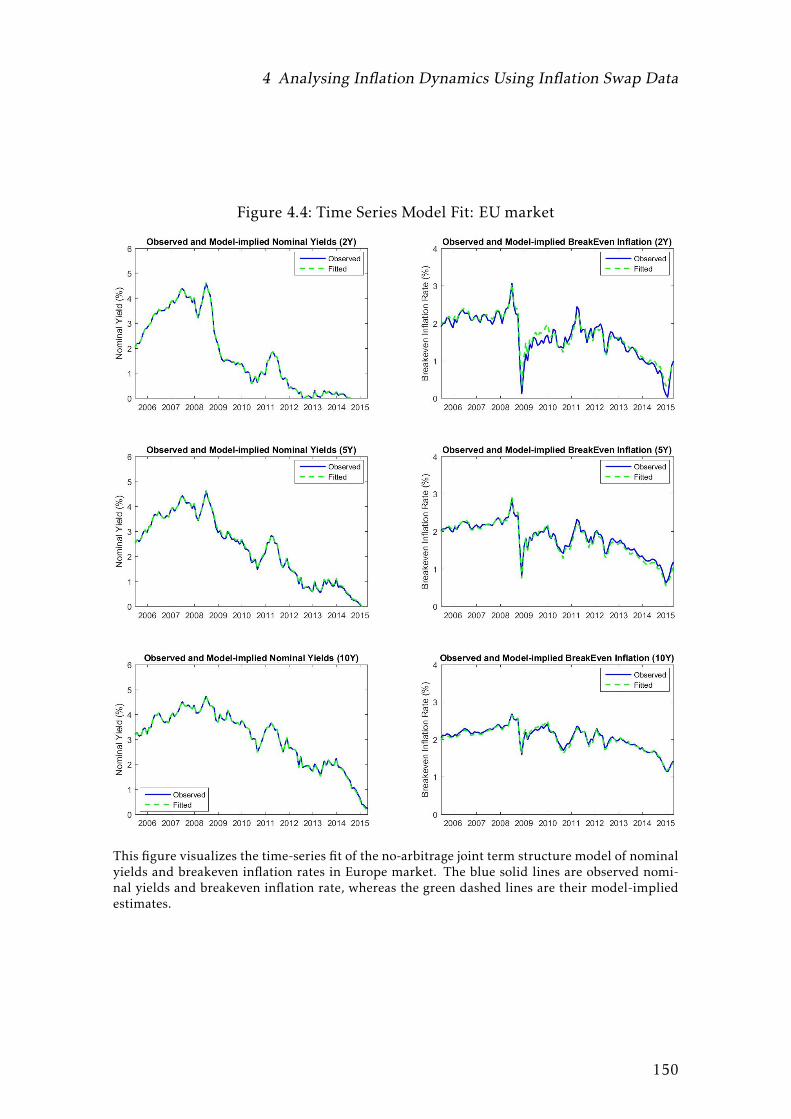
4 Analysing Inflation Dynamics Using Inflation Swap Data
Figure 4.4: Time Series Model Fit: EU market
This figure visualizes the time-series fit of the no-arbitrage joint term structure model of nominalyields and breakeven inflation rates in Europe market. The blue solid lines are observed nomi-nal yields and breakeven inflation rate, whereas the green dashed lines are their model-impliedestimates.
150

4 Analysing Inflation Dynamics Using Inflation Swap Data
Next we examine how the nominal yield curve and the BEI curve respond to
contemporaneous shocks in the chosen pricing factors. Recall that the nominal
yield and breakeven inflation rate can be expressed as
y(m)t = − 1
mAm −
1mB′m,QXt (4.44)
ω(m)t =
1mAm,ω +
1mB′m,ω,QXt (4.45)
where − 1mB
′m,Q and 1
mB′m,ω,Q are implied nominal yield loadings and BEI load-
ings, which measures the sensitivities of nominal yields y(m)t and BEI rate ω(m)
t
with respect to the underlying pricing factorsXt .
Figure (4.5) plots the implied nominal yield loadings − 1mB
′m,Q against maturi-
ties for the three developed markets. From the graph, we make the following
observations: A unity increase (decrease) in the first nominal factor results in
a simultaneous increase (decrease) of nominal yields on all maturities, which is
consistent with the interpretation as the level factor since it shift the entire curve
up (down). For the second nominal factor, it has completely opposite impacts
on short-end and long-end of the curve: as its name slope suggests, an increase
(decrease) in this factor would reduce (raise) short term interest rate while raise
(reduce) long term interest rate at the same time, resulting in a steeper (flatter)
yield curve. The third curvature factor has strong influences on mid-range and
front-end of the curve while leaving long-end untouched. For the rest of pric-
ing factors, the model suggests that they have little impact on the dynamics of
nominal yields.
The model-implied BEI loadings 1mBm,ω,Q are plotted in figure (4.6). The graph
reveals a common observation for all three developed markets that the first nom-
inal factor (level of current nominal interest rate) has positive impact on the ob-
151

4 Analysing Inflation Dynamics Using Inflation Swap Data
Figure 4.5: Nominal Yield Loadings
This figure plots the implied nominal yield loadings −1/m ×B′m,Q for each pricing factor in thethree developed markets.
152

4 Analysing Inflation Dynamics Using Inflation Swap Data
Figure 4.6: Breakeven Inflation Loadings
This figure plots the implied BEI yield loadings 1/m ×B′m,ω,Q for each pricing factor in the threedeveloped markets.
153
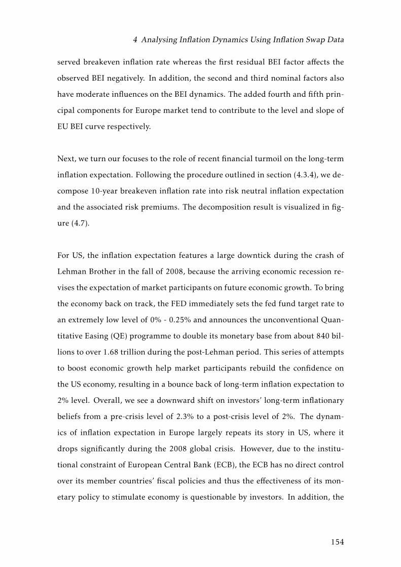
4 Analysing Inflation Dynamics Using Inflation Swap Data
served breakeven inflation rate whereas the first residual BEI factor affects the
observed BEI negatively. In addition, the second and third nominal factors also
have moderate influences on the BEI dynamics. The added fourth and fifth prin-
cipal components for Europe market tend to contribute to the level and slope of
EU BEI curve respectively.
Next, we turn our focuses to the role of recent financial turmoil on the long-term
inflation expectation. Following the procedure outlined in section (4.3.4), we de-
compose 10-year breakeven inflation rate into risk neutral inflation expectation
and the associated risk premiums. The decomposition result is visualized in fig-
ure (4.7).
For US, the inflation expectation features a large downtick during the crash of
Lehman Brother in the fall of 2008, because the arriving economic recession re-
vises the expectation of market participants on future economic growth. To bring
the economy back on track, the FED immediately sets the fed fund target rate to
an extremely low level of 0% - 0.25% and announces the unconventional Quan-
titative Easing (QE) programme to double its monetary base from about 840 bil-
lions to over 1.68 trillion during the post-Lehman period. This series of attempts
to boost economic growth help market participants rebuild the confidence on
the US economy, resulting in a bounce back of long-term inflation expectation to
2% level. Overall, we see a downward shift on investors’ long-term inflationary
beliefs from a pre-crisis level of 2.3% to a post-crisis level of 2%. The dynam-
ics of inflation expectation in Europe largely repeats its story in US, where it
drops significantly during the 2008 global crisis. However, due to the institu-
tional constraint of European Central Bank (ECB), the ECB has no direct control
over its member countries’ fiscal policies and thus the effectiveness of its mon-
etary policy to stimulate economy is questionable by investors. In addition, the
154

4 Analysing Inflation Dynamics Using Inflation Swap Data
Figure 4.7: Decomposition of Breakeven Inflation Rate (10yr)
This figure shows the decomposition of 10-year breakeven inflation rates in three developed mar-kets, namely, US, UK and Europe. Model-implied breakeven inflation rate is in blue, the inflationexpectation is represented by green dashed line, and the associated risk premium is in red dashedline.
155
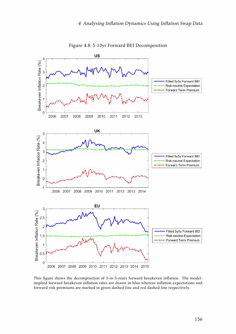
4 Analysing Inflation Dynamics Using Inflation Swap Data
Figure 4.8: 5-10yr Forward BEI Decomposition
This figure shows the decomposition of 5-in-5-years forward breakeven inflation. The model-implied forward breakeven inflation rates are drawn in blue whereas inflation expectations andforward risk premiums are marked in green dashed line and red dashed line respectively.
156

4 Analysing Inflation Dynamics Using Inflation Swap Data
loomy economic outlook on European countries, including Greece, Italy, Spain,
etc., further destroys investors’ confidence on future economic growth in Euro-
zone. Therefore, unlike what happens in US, investors’ inflationary beliefs in
EU haven’t recovered yet since 2008. Interestingly, the inflation expectation in
UK behaves quite differently, with a smooth rising instead of a decline during
the 2008 financial turmoil. This abnormal behaviour is largely explained by the
sharp depreciation of British Pound around 2009 which creates a strong infla-
tionary expectation in UK.
Figure (4.8) further shows the decomposition of far-in-the-future 5-10 year BEI
rate into expected inflation and term premium. We observe that model-implied
5-10 year forward inflation expectation is fairly stable at about 2% in US, 3.2% in
UK and 1.5% in EU. What’s more, in line with the findings of Adrian et al. [2013],
we find most variation in long-term forward BEI is captured by term premiums.
From an economic perspective, this observation reflects that central bank’s in-
flation target policy helps to anchor investors’ long-term inflationary belief and
makes it relatively insensitive to incoming economic data. Furthermore, we ob-
serve that the estimated risk premium has been consistently positive for US and
EU, whereas the term premium in UK has been negative at times. However, the
fact that its sample average is still positive is in line with the perception that in-
vestors require compensation for bearing uncertainty in future inflation rate.
Finally, we evaluate the short-term inflation forecasting performance of the no-
arbitrage joint affine term structure model. More specifically, we compare the
2-year model-implied inflation expectation with the realized inflation rate, i.e.
the change of CPI over the next 2 years, and then calculate the mean absolute
forecasting error. The observed 2-year inflation swap rate is used as the bench-
mark. The forecasting errors in absolute percentage rate are reported in table
157
4 Analysing Inflation Dynamics Using Inflation Swap Data
Figure 4.9: Inflation Forecast
This figure shows the 2-year inflation forecasting performance. The observed actual inflationrates are drawn in blue whereas forecasts generated by the model-implied risk-neutral inflationexpectation and the unadjusted breakeven inflation are marked in red dashed line and greendashed line respectively.
158
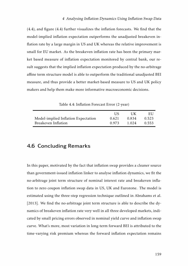
4 Analysing Inflation Dynamics Using Inflation Swap Data
(4.4), and figure (4.4) further visualizes the inflation forecasts. We find that the
model-implied inflation expectation outperforms the unadjusted breakeven in-
flation rate by a large margin in US and UK whereas the relative improvement is
small for EU market. As the breakeven inflation rate has been the primary mar-
ket based measure of inflation expectation monitored by central bank, our re-
sult suggests that the implied inflation expectation produced by the no-arbitrage
affine term structure model is able to outperform the traditional unadjusted BEI
measure, and thus provide a better market-based measure to US and UK policy
makers and help them make more informative macroeconomic decisions.
Table 4.4: Inflation Forecast Error (2-year)
US UK EUModel-implied Inflation Expectation 0.621 0.834 0.523Breakeven Inflation 0.973 1.024 0.553
4.6 Concluding Remarks
In this paper, motivated by the fact that inflation swap provides a cleaner source
than government-issued inflation linker to analyse inflation dynamics, we fit the
no-arbitrage joint term structure of nominal interest rate and breakeven infla-
tion to zero coupon inflation swap data in US, UK and Eurozone. The model is
estimated using the three-step regression technique outlined in Abrahams et al.
[2013]. We find the no-arbitrage joint term structure is able to describe the dy-
namics of breakeven inflation rate very well in all three developed markets, indi-
cated by small pricing errors observed in nominal yield curve and inflation swap
curve. What’s more, most variation in long-term forward BEI is attributed to the
time-varying risk premium whereas the forward inflation expectation remains
159

4 Analysing Inflation Dynamics Using Inflation Swap Data
stable over time. Finally, the model-implied inflation expectation outperforms
the unadjusted BEI in terms of forecasting short-term realized inflation. Thus
the no-arbitrage joint term structure model is potentially of considerable inter-
est to investors and policy markers to help them make more informative macro
decisions.
160

5 Conclusion and Outlook
In this thesis, I study three applications of state-space model to analyse interest-
ing financial dynamics.
In chapter 2, I develop a semi-structural model to describe the empirical bivari-
ate dynamics between return volatility and trading volume. The proposed model
is featured with a multiplicative relation between the common and idiosyncratic
components in traders’ reservation price, where the common component can be
interpreted as market sentiment process. I fit the model to daily data of 8 stocks
listed in the US equity market. The empirical results reveal the existence of a
common latent information flow and thus provide supporting evidence to the
Mixture of Distribution Hypothesis (MDH) of Clark [1973]. The market sen-
timent process is found to be highly persistent whereas the latent information
flow reverts to its unconditional mean fairly frequently. Furthermore, a higher
proportion of liquidity-driven trading volume is revealed in large-cap stocks than
in small-cap stocks.
In chapter 3, I use the Stochastic Vector Multiplicative Error model (S-VMEM)
of Hautsch [2008] to study the genuine multivariate dynamics between bid-ask
spread, average dollar volume per trade, trade intensity and return volatility by
161

5 Conclusion and Outlook
taking into account the presence of serially correlated latent information flow.
The S-VMEM model is fitted to a sample of high-frequency dataset based on six
heavily traded stocks listed in the US stock market. The empirical results con-
firm the existence of unobserved serially correlated information flow at 5-min
frequency. The impact of information flow is most significant for return volatil-
ity and trade intensity. This finding is in sharp contrast with previous studies like
Blume et al. [1994], Xu and Wu [1999], Huang and Masulis [2003] and Hautsch
[2008], where the authors find that it is the average trade size instead of trade
intensity that is most informative about the quality of news. In addition, impulse
response analysis shows that the dynamics of bid-ask spread is little affected by
a positive shock in underlying information flow, and thus provide no evidence to
support the asymmetric information market microstructure theory.
In chapter 4, motivated by the fact that inflation swap provides a cleaner source
than government-issued inflation linker to analyse inflation dynamics, I fit the
no-arbitrage joint term structure of nominal interest rate and breakeven infla-
tion rate to zero coupon inflation swap data in US, UK and Eurozone. I find the
no-arbitrage joint term structure is able to describe the dynamics of breakeven
inflation rate very well in US, UK and Europe. In addition, most variation in
long-term forward BEI is characterized by risk premium factors whereas the for-
ward inflation expectation remains stable over time. Furthermore, the model-
implied inflation expectation outperforms the unadjusted BEI in terms of fore-
casting short-term realized inflation. Thus the no-arbitrage joint term structure
model is potentially of considerable interest to investors and policy markers to
help them make more informative macroeconomic decisions.
There are a few potentially fruitful areas for further researches. First, as shown in
chapters 2, the latent information flows exhibit strong association among differ-
162

5 Conclusion and Outlook
ent stocks at daily frequency, and this might form the basis to build a factor model
which simultaneously characterizes multi-asset dynamics using a market-wide
common factor. Second, to further refine the multivariate S-VMEM framework
to model high-frequency dynamics, one can use a Possion point process to de-
scribe the time-series evolution of bid-ask spread to explicitly respect its discrete
nature due to the minimum tick value constraint. Third, in modelling inflation
expectation dynamics, one can use a Bayesian approach to combine the survey-
based measures with the empirical no-arbitrage affine term structure model pre-
sented in chapter 4, where the observed survey-based measure is factored into
the joint term structure model as prior belief on inflation expectation. With such
additional structural information, one can expect the model to generate even
more reliable and accurate estimates on the actual inflationary beliefs. Finally,
as shown in figure (4.1), pricing factors display strong comovement between US,
UK and EU. Therefore, a global term structure model with the focus on analysing
international spillover effect could be an interesting project to work on.
163

Bibliography
Michael Abrahams, Tobias Adrian, Richard K. Crump, and EmanuelMoench. De-
composing real and nominal yield curves. Staff Report No. 570, Federal Reserve
Bank of New York, 2013.
Tobias Adrian, Richard K. Crump, and Emanuel Moench. Pricing the term struc-
ture with linear regressions. Staff Report No.340, Federal Reserve Bank of New
York, 2013.
T.G. Andersen. Return volatility and trading volume: an information flow inter-
pretation of stochastic volatility. Journal of Finance, 1996.
T.G. Andersen and T. Bollerslev. Answering the skeptics: yes, standard volatility
models do provide accurate forecasts. International Economic Review, 1998.
T.G. Andersen, H.J. Chung, and B.E. Sorensen. Efficient method of moments
estimation of a stochastic volatility model: A monte carlo study. Journal of
Econometrics, 1999.
N. Barberis, A. Shleifer, and R. Vishny. A model of investor sentiment. Journal of
164

Bibliography
Financial Economics, 1998.
O.E. Barndorff-Nielsen, P.R. Hansen, A. Lunde, and N. Shephard. Realized ker-
nels in practice: trades and quotes. Econometrics Journal, 2009.
L. Bauwens and P. Giot. The logarithmic acd model: an application to the bid-ask
quote process of three nyse stocks. Financial Market Microstructure, 2000.
L. Bauwens and D. Veredas. The stochastic duration model: a latent factor model
for the analysis of financial durations. Journal of Econometrics, 2004.
N.K. Bergman and S. Roychowdhury. Investor sentiment and corporate disclo-
sure. Working Paper, 2008.
L. Blume, D. Easley, and M. O’Hara. Market statistics and technical analysis.
Journal of Finance, 1994.
T. Bollerslev. Generalized autoregressive conditional heterskedasticity. Journal of
Econometrics, 1986.
T. Bollerslev and D. Jubinski. Equity trading volume and volatility: latent infor-
mation arrivals and common long-run dependencies. Journal of Business and
Economic Statistics, 1999.
G.W. Brown and M.T. Cliff. Investor sentiment and the near-term stock market.
Journal of Empirical Finance, 2004.
165

Bibliography
P.K. Clark. A subordinated stochastic process model with finite variance for spec-
ulative prices. Econometrica, 1973.
T.E. Copeland and D. Galai. Information effects and bid-ask spread. Journal of
Finance, 1983.
Z. Ding and C.W.J. Granger. Modling volatility persistence of speculative returns:
a new approach. Journal of Econometrics, 1996.
D. Easley and M. O’Hara. Time and process of security price adjustment. Journal
of Finance, 1992.
D. Easley, S. Hvidkjaer, and M. O’Hara. Is information risk a determinant of asset
returns? Journal of Finance, 2002.
D. Easley, R.F. Engle, M. O’Hara, and L. Wu. Time-varying arrival rates of in-
formed and uninformed traders. Journal of Financial Economics, 2008.
R. Engle. Autoregressive conditional heteroskedasticity with estiamtes of united
kingdom inflation. Econometrica, 1982.
R.F. Engle. The econometrics of ultra-high-frequency data. Econometrica, 2000.
R.F. Engle and G.J. Lee. Estimating diffusion models of stochastic volatility. Mod-
elling stock market volatility: bridging the gap to continuous time, Academic Press,
Sandiego, 1996.
166

Bibliography
R.F. Engle and J.R. Russel. Autoregressive conditional duration: A newmodel for
irregularly spaced transaction data. Econometrica, 1998.
R.F. Engle and J.R. Russell. Forecasting the frequency of changes in quoted for-
eign exchange prices with the autoregressive conditional duration model. Jour-
nal of Empirical Finance, 1997.
W. Epps and M. Epps. The stochastic dependence of security price changes and
transaction voloumes: implications for the mixture of distributions hypothesis.
Econometrica, 1976.
M. Garman. Market microstructure. Journal of Financial Eonomics, 1976.
J. Geweke. Bayesian inference in econometric models using monte carlo integra-
tion. Econometrica, 1989.
J. Geweke. Evaluating the accuracy of sampling-base approaches to the calcu-
lation of posterior moments. Berger, J.O., Bernardo, J.M., Dawid, A.P., Smith,
A.F.M. (Eds), Bayesian Statistics, 1992.
L.R. Glosten and P.R. Milgrom. Bid, ask, and transaction prices in a specialist
market with heterogeneously informed traders. Journal of Financial Economics,
1985.
O. Guedj and J.P. Bouchaud. Experts earning forecasts: bias, herding and gos-
samer information. International Journal of Theoretical and Applied Finance,
2005.
167

Bibliography
R.S. Gurkaynak, B. Sack, and Wright J.H. The us treasury yield curve: 1961 to
the present. Journal of Monetary Economics, 2007.
L. Harris. Transaction data tests of the mixture of distribution hypothesis. Journal
of Financial and Quantitative Analysis, 1987.
J.G. Haubrich, G. Pennacchi, and Ritchken P. Inflation expectations, real rates,
and risk premia: Evidence from inflation swaps. Working Paper, Federal Reserve
Bank of Cleverland, 2011.
N. Hautsch. Capturing common components in high frequency finanial time se-
ries: A multivariate stochastic multiplicative error model. Journal of Economics
& Control, 2008.
R.D. Huang and R.W. Masulis. Trading activity and stock price volatility: evi-
dence from london stock exchange. Journal of Empirical Finance, 2003.
D. Kahneman and A. Tversky. Availability: A heuristic for judging frequency and
probability. Cognitive Psychology, 1979.
J.M. Keynes. The general theory of employment, interest and money. McMillan,
London, 1936.
G. Koop, M.H. Pesaran, and S.M. Potter. Impulse response analysis in nonlinear
multivariate models. Journal of Econometrics, 1996.
S.J. Koopman. Disturbance smoother for state space models. Biometrika, 1993.
168

Bibliography
C. Lamoureux andW. Lastrapes. Endogenous trading volume and momentum in
stock-return volatility. Journal of Business and Economics Satistics, 1994.
M. Lemmon and E. Portniaguina. Consumer confidence and asset prices: Some
empirical evidence. Reviews of Financial Studies, 2006.
R. Liesenfeld. A generalized bivariate mixture model for stock price volatility
and trading volume. Journal of Econometrics, 2001.
Roman Liesenfeld. Dynamic bivariate mixture models: Modeling the behavior of
prices and trading volume. Working Paper, 1998.
R. Mahieu and R. Bauer. A bayesian analysis of stock return volatility and trading
volume. Applied Financial Economics, 1998.
S. Manganelli. Duration, volume and volatility impacts of trades. Journal of Fi-
nancial Markets, 2005.
C.R. Nelson and A.F. Siegel. Parsimonious modeling of yield curves. Journal of
Business, 1987.
D.B. Nelson. Conditional heteroskedasticity in asset returns: A new approach.
Econometrica, 1991.
J.F. Richard andW. Zhang. Efficient high dimensional importance sampling. Jour-
nal of Econometrics, 2007.
169

Bibliography
H. Shefrin. A behavioral approach to asset pricing. Academic Press Advanced
Finance, 2008.
H. Shefrin and M. Statman. The disposition to sell winners too early and ride
losers too long: Theory and evidence. The Journal of Finance, 1985.
N. Shephard and M.K. Pitts. Likelihood analysis of non-gaussian measurement
time series. Biometrika, 1997.
R.J. Shiller. Do stock prices move too much to be justified by subsequent changes
in dividends? American Economic Review, 1981.
L. Svensson. Estimating and intepreting forward interest rates: Sweden 1992-
1994. Institute for International Economic Studies, 1994.
G. Tauchen and M. Pitts. The price variability-volume relationship in speculative
markets. Econometrica, 1987.
S.J. Taylor. Financial returns modelled by the product of two stochastic processes
- a study of daily sugar prices. Time Series Analysis, 1982.
S.J. Taylor. Modelling financial time series. John Wiley and Sons, Chichester, 1986.
B. Trueman. Analyst forecasts and hearding behavior. Review of Financial Studies,
1994.
M.Wyart and J.P. Bouchaud. Self-referential behaviour, overreaction and conven-
tions in financial markets. Journal of Economic Behavior & Organization, 2007.
170

Bibliography
X. Xu and C. Wu. The intraday relation between return voaltility, transactions,
and volume. International Reviews of Economics and Finance, 1999.
Y.D. Xu. The lognormal autoregressive conditional duration model and a com-
parasion with an alternative acd models. Working Paper, 2013.
171
Related Documents