Three Essays in Empirical Finance and Corporate Governance

Western University Western University

Scholarship@Western Scholarship@Western

Electronic Thesis and Dissertation Repository

6-23-2016 12:00 AM

Three Essays in Empirical Finance and Corporate Governance Three Essays in Empirical Finance and Corporate Governance

Chongyu Dang, The University of Western Ontario

Supervisor: Stephen Foerster, The University of Western Ontario

Co-Supervisor: Zhichuan Li, The University of Western Ontario

A thesis submitted in partial fulfillment of the requirements for the Doctor of Philosophy degree

in Business

© Chongyu Dang 2016

Follow this and additional works at: https://ir.lib.uwo.ca/etd

Part of the Finance and Financial Management Commons

Recommended Citation Recommended Citation Dang, Chongyu, "Three Essays in Empirical Finance and Corporate Governance" (2016). Electronic Thesis and Dissertation Repository. 3809. https://ir.lib.uwo.ca/etd/3809

This Dissertation/Thesis is brought to you for free and open access by Scholarship@Western. It has been accepted for inclusion in Electronic Thesis and Dissertation Repository by an authorized administrator of Scholarship@Western. For more information, please contact [email protected].

Abstract

This thesis includes three integrated articles in empirical finance and corporate governance.

The first article studies the effects of sell-side financial analysts’ innate ability on corporate

insider trading prior to annual earnings announcements from the perspective of information

asymmetry. The empirical results show that analysts with higher innate ability are associated

with lower level of net buys when insiders have “good” inside information about earnings,

but this relation does not hold for net sells when insiders have “bad” inside information. The

effects of analysts’ innate ability mostly reside in opportunistic trading rather than routine

trading. The tests of analysts’ initial coverage provide stronger effects of analysts’ ability.

This article suggests higher analyst ability can restrict insider trading.

The second article explores a broad picture about how different measures of firm size (total

assets, total sales, and market capitalization) affect the empirical analysis in 20 prominent

areas in corporate finance. This article documents empirical evidence for “measurement

effect” in “size effect”. The results show that in most areas of corporate finance, the

coefficients of firm size measures are robust in sign and statistical significance. However, the

coefficients of regressors other than firm size often change sign and significance when

different size measures are employed. In addition, the goodness of fit measured by R-squared

also varies with different size measures. As different proxies capture different aspects of

“firm size”, the choice of size measures needs both theoretical and empirical justification.

The third article further studies the impact drivers of dissemination of financial research. The

empirical results show that the universalist perspective (quality and domain), the social

constructivist perspective (visibility and personal promotion), and the presentation

perspective (first-page attention and expositional clarity) all provide explanatory power for

the impact of papers in the top three finance journals. Specifically, paper quality, research

methods, journal placement, and paper age are the most important drivers for the number of

citations. In addition, different drivers play different roles for the papers in JF, JFE, and RFS.

This article provides evidence for finance scholars, university administrators, and finance

journal management who care about research impact.

ii

Keywords

Financial Analysts; Innate Ability; Insider Trading; Firm Size; Empirical Corporate Finance;

Dissemination of Financial Research

iii

Co-Authorship Statement (by Zhichuan Li)

For chapter 3 (Measuring Firm Size in Empirical Corporate Finance) and chapter 4 (Impact:

Evidence from Top Journals), the Ph.D. student contributed to defining the research

questions and proposed the empirical designs to study them. The Ph.D. student wrote the

entire draft versions of chapter 3 and chapter 4, and revised them according to comments

from co-author, seminar participants, and conference participants.

Co-author defined the overall research topics together with the Ph.D. student. Co-author

carefully reviewed the drafts and provided various refinements. In addition, co-author helped

explain the empirical results.

iv

Acknowledgments

I am grateful to many people for their support and kind help along my way of my

Ph.D. studies. I am indebted to my supervisor, Dr. Stephen Foerster and my co-supervisor,

Dr. Zhichuan (Frank) Li for their guidance and support. Special thanks to Dr. Craig Dunbar

for serving as my supervisory committee member. Besides, I would like to express my

gratitude to my thesis examination committee: Dr. Stephen Sapp, Dr. Craig Dunbar, Dr.

Shahbaz Sheikh, and Dr. Stephannie Larocque.

For helpful comments and suggestions in my research, I also thank Dr. Simi Kedia,

Dr. Zhenyang Tang, Dr. Saurin Patel, Dr. Michael King, Dr. Jeffrey Coles, Dr. Michael

Schill, Dr. Susan Christoffersen, Dr. Francesca Cornelli, Dr. Pedro Matos, Dr. Heitor

Almeida, Dr. Patrick Akey, Dr. Philip Strahan, Dr. Walid Busaba, Dr. George Athanassakos,

Dr. Franklin Allen, Dr. Andrew Karolyi, Dr. Lee Pinkowitz, Dr. Martin Schmalz, participants

in the annual meeting of the International Finance and Banking Society (IFABS) 2015,

Hangzhou, China, and participants in the annual meeting of Canadian Law and Economics

Association (CLEA) 2015, University of Toronto, Canada. In addition, I thank Michelle

Cheung, Kathleen Chiu, Connor Fraser, David Gil, Tish Lewis, Blossom Lin, and Jennifer

Tin for excellent research assistance in data collection.

I truly appreciate the help from Dr. June Cotte and Dr. Matt Thomson in directing and

supporting my Ph.D. program. I am also grateful for Carly Vanderheyden in the Ph.D. office

for her kind help.

Last but not least, I thank my parents for their love and support. Thanks to my friends

for bringing me happiness into an interesting life.

v

Table of Contents

Abstract ................................................................................................................................ i

Acknowledgments.............................................................................................................. iv

Table of Contents ................................................................................................................ v

List of Tables ................................................................................................................... viii

List of Figures .................................................................................................................... xi

List of Appendices ............................................................................................................ xii

Chapter 1 ............................................................................................................................. 1

1 Introduction .................................................................................................................... 1

References for Chapter 1 ................................................................................................ 6

Chapter 2 ............................................................................................................................. 8

2 Do Not Cover Me: Financial Analysts’ Innate Ability and Insider Trading ................. 8

2.1 Introduction ............................................................................................................. 8

2.2 The Data ................................................................................................................ 13

2.3 Analysts’ Innate Ability and Insider Trading Intensity ........................................ 24

2.3.1 Main Results ............................................................................................. 24

2.3.2 Opportunistic Trading and Routine Trading ............................................. 35

2.3.3 Initial Coverage: The Incremental Effect on Increased Insider Trading .. 40

2.3.4 Regressions at Firm-Year Level and Analyst-Firm-Year Level ............... 49

2.4 Analysts’ Innate Ability and Insider Trading Informativeness............................. 56

2.5 Discussion about Endogeneity .............................................................................. 65

2.6 Conclusion ............................................................................................................ 66

References for Chapter 2 .............................................................................................. 68

Chapter 3 ........................................................................................................................... 73

3 Measuring Firm Size in Empirical Corporate Finance ................................................ 73

vi

3.1 Introduction ........................................................................................................... 73

3.2 Framework for Analysis and Literature Review ................................................... 77

3.3 The Data ................................................................................................................ 82

3.4 Methodology and Empirical Results ..................................................................... 93

3.4.1 Firm Performance ..................................................................................... 94

3.4.2 Board Structure ....................................................................................... 101

3.4.3 Dividend Policy ...................................................................................... 111

3.4.4 Financial Policy ...................................................................................... 113

3.4.5 Compensation Policy .............................................................................. 122

3.4.6 Investment Policy.................................................................................... 131

3.4.7 Diversification......................................................................................... 140

3.4.8 Corporate Control ................................................................................... 146

3.5 Summary, Guidelines, and Limitations .............................................................. 155

References for Chapter 3 ............................................................................................ 163

Appendix for Chapter 3 .............................................................................................. 167

Chapter 4 ......................................................................................................................... 168

4 Impact: Evidence from Top Journals ......................................................................... 168

4.1 Introduction ......................................................................................................... 168

4.2 Theory and Hypothesis ....................................................................................... 172

4.3 The Data .............................................................................................................. 179

4.4 Multivariate Analysis and Results ...................................................................... 201

4.5 Robustness .......................................................................................................... 208

4.6 The Marginal Effects of Negative Binomial Models .......................................... 216

4.7 Conclusion .......................................................................................................... 218

References for Chapter 4 ............................................................................................ 221

Appendices for Chapter 4........................................................................................... 223

vii

Chapter 5 ......................................................................................................................... 226

5 Conclusions ................................................................................................................ 226

Curriculum Vitae ............................................................................................................ 229

viii

List of Tables

Table 2.1: The Measure of Analysts’ Innate Ability from Coles et al. (2013) ...................... 18

Table 2.2: Sample Summary Statistics .................................................................................. 22

Table 2.3: Correlation Matrix ................................................................................................. 23

Table 2.4: Analysts’ Innate Ability and Insiders’ Net Buys ................................................... 30

Table 2.5: Robustness Check- Alternative Measure of Information Type ............................. 33

Table 2.6: Opportunistic Trading and Routine Trading .......................................................... 37

Table 2.7: Initial Coverage: the Incremental Impact of Analyst Ability ................................ 42

Table 2.8: Initial Coverage by an Analyst with Highest Ability ............................................ 47

Table 2.9: Analysts’ Average Innate Ability at Firm-Year Level .......................................... 51

Table 2.10: Analysts’ Innate Ability at Analyst-Firm-Year Level ......................................... 54

Table 2.11: Ability Difference and Market Reactions to Insider Trading .............................. 62

Table 2.12: Analyst’s Innate Ability and Market Reactions to Insider Trading ..................... 64

Table 3.1: Summary Statistics ................................................................................................ 84

Table 3.2: Firm Size Measures for Firm Performance Regression ......................................... 89

Table 3.3: Firm Performance-Tobin’s Q ................................................................................ 96

Table 3.4: Firm Performance-ROA (Return on Assets) ......................................................... 99

Table 3.5: Board of Directors-Board Independence ............................................................. 103

Table 3.6: Board of Directors-Board Size ............................................................................ 106

Table 3.7: Board of Directors-Board Leadership ................................................................. 109

ix

Table 3.8: Payout Policy-Dividend Dummy ......................................................................... 112

Table 3.9: Book Leverage ..................................................................................................... 114

Table 3.10: Market Leverage ................................................................................................ 117

Table 3.11: Cash Holdings .................................................................................................... 120

Table 3.12: Vega ................................................................................................................... 123

Table 3.13: Delta ................................................................................................................... 126

Table 3.14: Executive Pay Level .......................................................................................... 129

Table 3.15: R&D ................................................................................................................... 132

Table 3.16: CAPEX .............................................................................................................. 135

Table 3.17: Firm Risk ........................................................................................................... 138

Table 3.18: Herfindahl Index ................................................................................................ 141

Table 3.19: Business Segments............................................................................................. 144

Table 3.20: Bidder Dummy .................................................................................................. 147

Table 3.21: Target Dummy ................................................................................................... 150

Table 3.22: Poison Pill .......................................................................................................... 153

Table 3.23: Summary of Results ........................................................................................... 156

Table 4.1: The Top 50 Most-Cited Papers in the Top Three Finance Journals: 2000-2013 . 182

Table 4.2: Summary Statistics for the Whole Sample .......................................................... 190

Table 4.3: Comparison of Summary Statistics for JF, JFE, and RFS ................................... 194

Table 4.4: Frequency of Citations ......................................................................................... 196

x

Table 4.5: Comparison of Averages between Top 10% and Bottom 10% Citations ............ 198

Table 4.6: Pearson Correlation Coefficients for the Whole Sample ..................................... 200

Table 4.7: The Impact Drivers of Google Scholar Citations ................................................ 205

Table 4.8: The Impact Drivers of Web of Science Citations ................................................ 207

Table 4.9: Robustness Check-Redefined Citations (per Year) ............................................. 209

Table 4.10: Robustness Check-The Log-Transformed OLS Results.................................... 211

Table 4.11: Robustness Check-Adjustment for Heteroskedasticity ..................................... 213

Table 4.12: Robustness Check-Winsorized Citations ........................................................... 215

Table 4.13: Average Marginal Effects .................................................................................. 217

xi

List of Figures

Figure 2.1: The Distribution of Estimated Analysts’ Innate Ability ..................................... 20

Figure 2.2: Ability Quantiles and Market Reactions to Insider Trading ................................ 59

Figure 3.1: Bivariate Scattergrams of Alternative Firm Size Measures for Firm Performance

................................................................................................................................................. 90

Figure 3.2: Time Series of Alternative Firm Size Measures .................................................. 92

Figure 3.3: Maximum Change of R Squared for Alternative Firm Size Measures .............. 159

Figure 4.1: Trends of Paper Characteristics: 2000-2013 ...................................................... 192

xii

List of Appendices

Appendix 3.1: A survey of 100 empirical corporate finance papers that use firm size

measures ................................................................................................................................ 167

Appendix 4.1: Top 20 World Ranking of Finance Departments: 2009-2013....................... 223

Appendix 4.2: Descriptions of Variables .............................................................................. 224

1

Chapter 1

1 Introduction

This thesis includes three articles (from Chapter 2 to Chapter 4) in empirical

finance and corporate governance.

Chapter 2 explores the effects of analysts’ innate ability on corporate insider

trading. Although some firms impose restrictions on insider trading, insiders continue to

take advantage of positive inside information to obtain profits, but insiders are more

cautious in benefiting from negative inside information (Lee, Lemmon, and Sequeira,

2014). Thus, it is important to think about any alternative channel that can play a role in

restraining insider trading. Financial analysts may be a possible candidate because

analysts provide information through forecasts of future earnings and returns, and can

thus affect a firm’s information environment (Mikhail et al., 2003; Piotroski and

Roulstone, 2004; Loh and Mian, 2006): an improved information environment leaves

little room for insiders to trade profitably and thus discourages insider trading (Frankel

and Li, 2004; Huddart and Ke, 2007; Wu, 2014). However, analysts’ heterogeneity is

ignored in the existing literature. We postulate that analysts with higher ability, defined

as analysts’ fixed effects in Coles et al. (2013), can better mitigate insider trading

intensity.

The empirical results in Chapter 2 show significantly less net buys by insiders

prior to “good” earnings announcements (measured by positive earnings surprise) when

firms are followed by analysts with higher ability, and we do not observe the same effect

prior to “bad” earnings announcements. These asymmetric results are largely consistent

2

with the findings of Cheng and Lo (2006), Agrawal and Nasser (2012), and Agrawal and

Cooper (2015) that insiders tend to avoid trading right before negative corporate events

because of litigation risk. When we further divide insiders into opportunistic traders and

routine traders, following Cohen et al. (2012), we find that the results are primarily

present for opportunistic insiders but largely disappear for routine insiders. We also

document stronger effects of analysts’ ability on insider trading for initial coverage.

Chapter 2 suggests that high-ability analysts may serve in restricting excessive

corporate insider trading. Chapter 2 also sheds light on the nature of analyst information.

On the one hand, analysts are believed to specialize in providing industry-level

information (Clement, 1999; Jacob et al., 1999; Gilson et al., 2001; Piotroski and

Roulstone, 2004). On the other hand, many studies argue that analyst forecasts actually

contain firm-specific information (Mikhail et al., 2003; Park and Stice, 2000; Liu 2011).

This chapter suggests that the degree of firm-specific information an analyst can provide

(e.g. earnings forecasts in this paper) may be determined by her innate ability. Firm-

specific information is more difficult to collect and analyze; thus, analysts with low

ability may not be able to include firm-specific information in their forecasts.

In Chapter 3, we study firm size, which is commonly used as an important,

fundamental firm characteristic in both academic and practical financial analysis. In

many situations, corporate finance researchers observe the “size effect” - firm size

matters in determining the dependent variables. For example, in capital structure, Frank

and Goyal (2003) show that pecking order is only found in large firms; Rajan and

Zingales (1995) discover that leverage increases with firm size. In mergers and

acquisitions, Moeller, Schlingemann, and Stulz (2004) find that small firms have larger

3

abnormal announcement returns; Vijh and Yang (2013) document that for cash offers,

targetiveness (probability of being targeted) decreases with firm size, but for stock offers

they find an inverted-U relation. In executive compensation, Jensen and Murphy (1990)

and Core et al. (1999) find that top-management compensation level increases with firm

size.

Although firm size matters in empirical corporate finance, no paper provides a

comprehensive assessment of the sensitivity of empirical results in corporate finance to

different measures of firm size. We use 20 representative specifications in 9 benchmark

papers in top finance journals (Coles and Li, 2012), and study the influences (sign

sensitivity, significance sensitivity, and R-squared sensitivity) of employing different

measures of firm size (total assets, total sales, and market value of equity).

The results in Chapter 3 confirm the “measurement effect” in “size effect” in

empirical corporate finance. The coefficients on regressors other than firm size often

change sign and significance when we use difference firm size measures. Unfortunately,

this suggests that, when using different firm size proxies, some previous studies are not

robust. Researchers should either use all the important proxies as robustness checks, or

provide rationale of using any specific proxy. Additionally, the goodness of fit measured

by R-squared varies significantly with different firm size measures. Some size measures

appear more “relevant” than others in different areas, implying that they are better control

variables to reduce omitted variable bias and improve the estimation of the main

coefficients of interest. Different size proxies capture different aspects of “firm size”, and

thus have different implications. The choice of these firm size measures can be a

theoretical and empirical question.

4

The empirical results in Chapter 3 not only provides guidance for researchers who

must use firm size proxies in empirical corporate finance research, but also sheds light on

future research that might incorporate measurement effect into other research fields, such

as empirical asset pricing and empirical accounting.

In Chapter 4, we explore a broad picture by studying which factors affect the

impact of financial research. It is known that the top 1% (10%) papers in the leading

finance journals have received 1/3 (3/4) of the total number of citations (Chung, Cox, and

Mitchell, 2001). This phenomenon indicates the value of a paper depends on both journal

placement and research impact. To our knowledge, the literature has not fully answered

the questions of how paper characteristics change over time, how paper characteristics

differ between more influential papers and less influential papers, and what are the

impact drivers of the published papers in top finance journals. We aim to fill these holes

in the literature in Chapter 4.

In addition, all of previous studies in citations in finance literature only cover a

few independent variables, with the lack of a comprehensive construction of impact

drivers of financial research. Following the framework of Stremersch, Verniers, and

Verhoef (2007), we use the most extensive set of paper characteristics as determinants of

citations to explore the roles of three theoretical perspectives: the universalist perspective

(what is said), the social constructivist perspective (who says it), and the presentation

perspective (how it is said).

We have several empirical findings. First, we find that most of the measures of

paper characteristics in the social constructivist perspective (visibility and personal

promotion) and the presentation perspective (first-page attention and expositional clarity)

5

increase over time, while most of the paper characteristics in the universalist perspective

(quality and domain) remain constant. Second, most of the paper characteristics are

significantly different between the top 10% and the bottom 10% groups based on the

number of citations per year. Third, the regression results by negative binomial models

show that the universalist perspective, the social constructivist perspective, and the

presentation perspective all provide impact drivers of published papers in the top three

finance journals. Specifically, paper quality, research methods, journal placement, and

paper age are the most important (in economic significance) drivers for the number of

citations. Furthermore, the results of average marginal results document exact evidence in

how many additional citations are increased with one more unit of a certain paper

characteristics. Last, different drivers play different roles for the papers in Journal of

Finance, Journal of Financial Economics, and Review of Financial Studies.

Chapter 4 provides useful empirical evidence for finance scholars, university

administrators, and finance journal management who care about research impact.

6

References for Chapter 1

Agrawal, A. and Cooper, T., 2015. Insider trading before accounting scandals. Journal of

Corporate Finance, 34, pp.169-190.

Agrawal, A. and Nasser, T., 2012. Insider trading in takeover targets. Journal of

Corporate Finance, 18(3), pp.598-625.

Cheng, Q. and Lo, K., 2006. Insider trading and voluntary disclosures. Journal of

Accounting Research, 44(5), pp.815-848.

Chung, K.H., Cox, R.A. and Mitchell, J.B., 2001. Citation patterns in the finance

literature. Financial Management, pp.99-118.

Clement, M.B., 1999. Analyst forecast accuracy: Do ability, resources, and portfolio

complexity matter? Journal of Accounting and Economics, 27(3), pp.285-303.

Cohen, L., Malloy, C. and Pomorski, L., 2012. Decoding inside information. The Journal

of Finance, 67(3), pp.1009-1043.

Coles, J., and Li, F., 2012. An empirical assessment of empirical corporate finance.

Working paper.

Coles, J., Li, F., and Mola, S., 2013. Is talent wasted on the young? Natural ability vs.

experience-based ability in analyst research. Working Paper.

Core, J. and Guay, W., 1999. The use of equity grants to manage optimal equity incentive

levels. Journal of Accounting and Economics, 28(2), pp.151-184.

Frank, M.Z. and Goyal, V.K., 2003. Testing the pecking order theory of capital

structure. Journal of Financial Economics, 67(2), pp.217-248.

Frankel, R. and Li, X., 2004. Characteristics of a firm's information environment and the

information asymmetry between insiders and outsiders. Journal of Accounting

and Economics, 37(2), pp.229-259.

Gilson, S.C., Healy, P.M., Noe, C.F. and Palepu, K.G., 2001. Analyst specialization and

conglomerate stock breakups. Journal of Accounting Research, 39(3), pp.565-

582.

Huddart, S.J. and Ke, B., 2007. Information asymmetry and cross‐sectional variation in

insider trading. Contemporary Accounting Research, 24(1), pp.195-232.

Jacob, J., Lys, T.Z. and Neale, M.A., 1999. Expertise in forecasting performance of

security analysts. Journal of Accounting and Economics,28(1), pp.51-82.

Jensen, M.C. and Murphy, K.J., 1990. Performance pay and top-management

incentives. Journal of Political Economy, pp.225-264.

7

Lee, I., Lemmon, M., Li, Y. and Sequeira, J.M., 2014. Do voluntary corporate restrictions

on insider trading eliminate informed insider trading? Journal of Corporate

Finance, 29, pp.158-178.

Liu, M.H., 2011. Analysts’ incentives to produce industry-level versus firm-specific

information. Journal of Financial and Quantitative Analysis, 46(03), pp.757-784.

Loh, R.K. and Mian, G.M., 2006. Do accurate earnings forecasts facilitate superior

investment recommendations? Journal of Financial Economics, 80(2), pp.455-

483.

Mikhail, M.B., Walther, B.R. and Willis, R.H., 2003. The effect of experience on security

analyst underreaction. Journal of Accounting and Economics,35(1), pp.101-116.

Moeller, S.B., Schlingemann, F.P. and Stulz, R.M., 2004. Firm size and the gains from

acquisitions. Journal of Financial Economics, 73(2), pp.201-228.

Park, C.W. and Stice, E.K., 2000. Analyst forecasting ability and the stock price reaction

to forecast revisions. Review of Accounting Studies, 5(3), pp.259-272.

Piotroski, J.D. and Roulstone, D.T., 2004. The influence of analysts, institutional

investors, and insiders on the incorporation of market, industry, and firm-specific

information into stock prices. The Accounting Review,79(4), pp.1119-1151.

Rajan, R.G. and Zingales, L., 1995. What do we know about capital structure? Some

evidence from international data. The Journal of Finance,50(5), pp.1421-1460.

Stremersch, S., Verniers, I. and Verhoef, P.C., 2007. The quest for citations: Drivers of

article impact. Journal of Marketing, 71(3), pp.171-193.

Vijh, A.M. and Yang, K., 2013. Are small firms less vulnerable to overpriced stock

offers? Journal of Financial Economics, 110(1), pp.61-86.

Wu, W., 2014. Information Asymmetry and Insider Trading. Fama-Miller Working

Paper, pp.13-67.

8

Chapter 2

2 Do Not Cover Me: Financial Analysts’ Innate Ability and Insider Trading

2.1 Introduction

Corporate insider trading is important in several aspects such as asset prices,

corporate investment policies, and corporate governance. First, it is well documented in

the literature that insider trading is informative in predicting stock returns (Seyhun, 1986;

Seyhun, 1992; Lakonishok and Lee, 2001; Agrawal and Nasser, 2012; Agrawal and

Cooper, 2015). Second, insider trading leads insiders to choose riskier investment

projects (Bebchuk and Fershtman, 1994) and insider trading restrictions can reduce

corporate risk-taking (Kusnadi, 2015). Third, insider trading restrictions are associated

with higher total pay and more use of equity incentives (Roulstone, 2003; Denis and Xu,

2013), implying insider trading serves as a tool in rewarding executives.

Although some firms impose restrictions on insider trading, insiders continue to

take advantage of positive inside information to obtain profits, but insiders are more

cautious in benefiting from negative inside information (Lee, Lemmon, and Sequeira,

2014). Thus, it is important to think about any alternative channels that can play a role in

restraining insider trading1. Financial analysts may be a possible candidate for two

reasons. First, analysts provide information through forecasts of future earnings and

returns, and can thus affect a firm’s information environment (Mikhail et al., 2003;

1 Restrictions of corporate insider trading are in the spirit of better corporate governance as corporate inside

information can crowd out investors, but we are aware about the debate that inside information can improve

market efficiency.

9

Piotroski and Roulstone, 2004; Loh and Mian, 2006): an improved information

environment leaves little room for insiders to trade profitably and thus discourages

insider trading (Frankel and Li, 2004; Huddart and Ke, 2007). Second, analysts also

matter in corporate governance by mitigating corporate insiders’ expropriation of outside

shareholders (Chen et al., 2015), and better internal governance may also help restrict

insider trading (Jagolinzer et al., 2011; Dai et al., 2015). Empirical findings are largely

consistent with analysts restraining insider trading. For example, Frankel and Li (2004)

show that the number of analysts following is negatively associated with insider trading

intensity and profitability, and Wu (2014) documents higher insider trading profitability

following decreases in analyst coverage caused by exogenous brokerage closures.

Alternatively, some studies cast doubt on the association between analysts and insiders

because they may have different information sets. For example, Piotroski and Roulstone

(2004) show that analysts are better at providing industry-specific information, while

insiders primarily trade on firm-specific information. Hsieh et al (2005) find that insider

trades and analyst recommendations usually contradict each other.

In this article, we aim to further extend the question by studying whether financial

analysts with higher ability contribute more in restricting corporate insider trading. We

argue that the inconsistency in empirical studies is a result of ignoring analyst

heterogeneity. Sell-side financial analysts form heterogeneous earnings forecasts and

stock recommendations: Sinha et al. (1997) find that some analysts are able to provide

more accurate annual earnings per share (EPS) forecasts than other analysts, and Loh and

Mian (2006) find that analysts who provide more accurate forecasts also provide more

profitable stock recommendations. Although some previous studies of financial analysts

10

find that experience2 may sometimes be a good proxy for analyst ability (Mikhail et al.

1997; Akyol et al. 2015), Coles et al. (2013) show that an analyst’s innate ability can be

well measured by her fixed effect on forecasting accuracy, and that ability measure

perform better than other ability measures, such as experience. We postulate that analysts

with higher ability, defined as in Coles et al. (2013), can better influence a firm’s

information environment by providing more accurate forecasts. Also, analysts with

higher ability are more likely to effectively monitor insiders because of their superior

abilities in information collection and firm evaluation. Thus, we expect that analysts with

higher ability can better restrain insider trading profitability and mitigate insider trading

intensity. Since corporate insiders are sophisticated investors with inside firm-specific

information, and their trades are on average very profitable (Seyhun, 1986; Lakonishok

and Lee, 2001), it is natural to imagine how difficult it is for an average analyst to crowd

out inside information. However, it is plausible that only a small percentage of high-

ability insiders can compete with insiders in information, which explains why insiders

and analysts may appear to have different information sets but the existence of analysts

(or rather, of high-ability analysts) mitigates insider trading activities.

2 Other alternative ability proxies suggested in the existing literature include industry specialization (Jacob

et al., 1999), reputation (Stickel, 1995) and job complexity (Clement, 1999). Analyst reputation usually

refers to the rankings of all-star analyst (Clarke et al., 2007), but this proxy only provides annual lists of top

analysts and the rankings are mainly based on returns an investor would have achieved following stock

recommendations. However, in this chapter we quantify analysts’ innate ability for all analysts in I/B/E/S,

and for our research purposes, the estimations are based on analysts’ forecast accuracy of earnings rather

than stock recommendations due to the fact that earnings are more relevant to inside information prior to

disclosure but stock prices are more complicatedly determined by market behavior. In addition, Emery and

Li (2009) use data from 1993 to 2005 based on analyst rankings of Institutional Investor (I/I) and The Wall

Street Journal (WSI) and find that earnings forecasts of stars are not significantly different from those of

non-stars and they conclude that analyst rankings are “popularity contests” to a large degree. Thus it is

necessary to investigate in the effects of alternative measure of analysts’ ability, as what we do in this

chapter.

11

Using a sample of US firms from 1986 to 2008, we find that analyst ability indeed

matters for insider trading. Specifically, we show significantly less net buys by insiders

prior to good earnings announcements (measured by positive earnings surprise) when

firms are followed by analysts with higher ability, and we do not observe the same effect

prior to bad earnings announcements. These asymmetric results are largely consistent

with the findings of Cheng and Lo (2006), Agrawal and Nasser (2012), and Agrawal and

Cooper (2015) that insiders tend to avoid trading right before negative corporate events

because of litigation risk. When we further divide insiders into opportunistic traders and

routine traders, following Cohen et al. (2012), we find that the results are primarily

present for opportunistic insiders but largely disappear for routine insiders. We also

document reduced insider trading profitability when firms are covered by high-ability

analysts.

We note that there might be a problem of reverse causality in the results described

above. We try to mitigate this problem by keeping all insider trading data in our sample

in the 30-day window3 prior to annual earnings announcement by firms, and all forecasts

of annual earnings by analysts in our sample are restricted to at least one month before

earnings announcements, thus all forecasts precede insider trading. It is unlikely that

insider trading attracts analyst coverage in the same fiscal year and further changes

analysts’ innate ability. However, we are aware that this setting cannot completely rule

out the possibility of endogeneity. Analyst forecasting accuracy has been documented to

3 Other window length (14-day event window) is also examined. The window length should be neither too

long (noisy information) nor too short (blackout restrictions). We believe one-month window is an

appropriate choice.

12

be higher in firms with relatively higher transparency (see for instance, Brown et al.,

1987, Lang and Lundhold, 1996). If an analyst always picks high-transparency firms to

follow, she may constantly have more accurate forecasts and be deemed a high-ability

analyst in our test, even if she is no better than other analysts. Suppose there is a life

cycle of transparency that corporate insiders would naturally trade less when the

transparency level is high, thus the negative relation between analyst ability and insider

trading may be due to endogeneity, even if we use the setting of initial coverage.

Some researchers view insider trading as a channel to incorporate information

into prices, and thus believe insider trading should be allowed because it promotes market

efficiency (Manne, 1966; Leland, 1992). On the other hand, more and more people view

insider trading as a problem because it may discourage outsiders (Ausubel, 1990), and

many public firms in the US have adopted firm-level insider trading restrictions (Bettis et

al., 2000; Roulstone, 2003). While we do not take a stand in this debate, our study does

suggest high-ability analysts may serve in restricting excessive corporate insider trading.

This study also sheds light on the nature of analyst information. Unlike other

information providers, such as corporate insiders and institutional investors, analysts are

believed to specialize in providing industry-level information (Clement, 1999; Jacob et

al., 1999; Gilson et al., 2001). Piotroski and Roulstone (2004) found that stock return

synchronicity is positively associated with analyst forecast activities, suggesting that

information from analysts is more industry-specific and less firm-specific. Contrarily,

many studies argue that analyst forecasts actually contain firm-specific information

(Mikhail et al., 2003; Park and Stice., 2000). Liu (2011) brings a new perspective,

suggesting that whether information from analysts is more industry-specific or firm-

13

specific depends on the beta and idiosyncratic return volatility of the firm. In this study,

we add a new angle to the debate. Our results suggest that the degree of firm-specific

information an analyst can provide (e.g. earnings forecasts in this paper) may be

determined by her innate ability. Firm-specific information is more difficult to collect and

analyze; thus, analysts with low or average ability may not be able to include firm-

specific information in their forecasts. Difference in analyst ability reconciles the

seemingly contradictory findings that analyst forecasts on average increase stock return

synchronicity and that the presence of analysts affects insider trading activities: though

the number of analysts or the number of analyst forecasts may not be directly associated

with firm-specific information, it increases the likelihood of including high-ability

analysts who provide firm-specific information and affect insider trading.

The rest of this chapter is organized as follows. Section 2.2 describes the data,

Section 2.3 presents empirical design and results for the effects of analysts’ innate ability

on the insider trading intensity, Section 2.4 provides the analysis for the effects of

analysts’ innate ability on insider trading informativeness, Section 2.5 discusses the

endogeneity problem, and Section 2.6 concludes.

2.2 The Data

Insider trading data in this paper are from Thomson Reuters Insider Filing Data

Feed (IFDF). The SEC defines corporate insiders as those who have access to non-public,

material, and inside information, and those people include board directors, corporate

executives, and beneficiary owners with more than 10% ownership of shares outstanding.

The Section 16a of the Securities and Exchange Act of 1934 requires that insider trading

should be reported to the SEC within 10 days after the trades are executed, and the

14

deadline was later changed to two days in 2002 due to the Sarbanes-Oxley Act. The

reported insider trades are mostly legal, and our sample includes the open-market trades

only from 1986 to 2008.

If an insider trades multiple times on the same trading day, then a single daily buy

or sell trade is cumulated for her because trades on the same day are probably on the

same information and separate observations can harm the accurate relationship between

explanatory variables and insider trading measures. Furthermore, we restrict insider

trading to the 30-day window prior to earnings announcements by firms for two reasons.

First, if the window is too long, noise can become a problem as information asymmetry

may be at a low level and other major corporate events might twist the results. Second,

the window being too short can also be a problem as many firms have different blackout

windows that restrict insider trading, and thus the number of observations is not

sufficient. Alternatively, we also use the 14-day window for robustness checks. As for the

insider trading measures, we use net buys and net sells (the opposite numbers of net buys)

for all insiders at firm-year level in multivariate regressions because some sophisticated

insiders can trade in different directions in our event window. For example, an insider

might sell stock first for liquidity and buy stock some days later at lower prices according

to her inside information. In addition, one insider might trade stocks for many other

reasons rather than establishing a long or short position according to inside information,

so insider trading based on all insiders in a firm can be more representative and thus

convey more accurate information than trading by a single insider. As for the

construction of insider trading measures, we provide the formula for the number of

trades, trading volumes, adjusted trading volumes, and trading value in section 2.3.

15

Again, insider trading might not be informative about firms’ futures, although

corporate insiders have favored access to private information about firm events.

Specifically, for insider buys, an insider might purchase stock of her firm due to discount

plans after receiving a bonus; for insider sells, an insider might sell stock of his firm for

liquidity and portfolio rebalancing purposes. To differentiate between informative trades

and non-informative trades, we follow Cohen, Malloy, and Pomorski (2012) who

distinguish opportunistic insider trading and routine trading. They define a routine trader

as an insider who traded in the same calendar month for at least three consecutive years

in the past and define an opportunistic trader as everyone else4. Then all trades are

classified into two categories: routine trades by routine traders and opportunistic trades

by opportunistic traders. We follow this method but we are aware that this method has

the limitation that an insider might change his conventional trading timing in different

years so we only apply this method as comparison with the main empirical results.

For the data of analysts’ innate ability or natural talent, we use the data from

1984 to 20085 in Coles, Li and Mola (2013) who isolate the analyst fixed effects

6 from

the three-way fixed effects (analyst fixed effects, broker fixed effects, and year fixed

4 Cohen, Malloy, and Pomorski (2012) conduct a variety of robustness checks to support their conclusions

that are based on their novel measures of “opportunistic” traders and “routine” traders.

5 This implies the estimated innate ability exhibits a look-ahead bias given that fact that the data of forecast

accuracy are from 1984 to 2008.

6 Equation (1) of Coles, Li, and Mola (2013): �̂�𝑖𝑗𝑡 = 𝐴𝑖𝑡�̂� + 𝐶𝑖𝑗𝑡𝛾 + �̂�𝑖 + �̂�𝑗 + �̂�𝑡 + 휀�̂�𝑗𝑡, with �̂�𝑖𝑡 as the

forecast accuracy for analyst i and brokerage house j at fiscal year t. 𝐴𝑖𝑡�̂� refers to analyst characteristics,

𝐶𝑖𝑗𝑡𝛾 refers to control variables, �̂�𝑖 refers to analyst fixed effects, �̂�𝑗 refers to broker fixed effects, �̂�𝑡 refers

to year fixed effects, and 휀�̂�𝑗𝑡 refers to residuals or “pure luck”.

16

effects) in the regressions on forecast accuracy7 and we employ the analyst fixed effects

as a measure of innate ability or natural talent. They find innate ability (4% in

explanatory power) serves as a more significant role than experience (less than 1.4% in

explanatory power) and affiliation (1% in explanatory power). Following the connected-

group method in Abowd, Kramarz, and Margolis (1999), Coles, Li, and Mola (2013) first

apply it in the analysis of analyst accuracy8. And this method is also well documented in

the studies of managerial compensation (Graham, Li and Qiu, 2012), managerial

incentives (Coles and Li, 2013), mutual fund (Huang and Wang, 2014), and insider

trading (Hillier et al. 2015). We denote the measure as innate ability or natural talent

rather than general analyst heterogeneity because it stems from the regression on forecast

accuracy which mostly depends on ability, although we cannot identify what traits the

“innate ability” comprises9. We assume ability measured by analyst fixed effect is static

for each analyst based on our testing periods. For the data that generate the ability

measure, we report the summary statistics for analyst data in Table 2.1, Panel A and the

regression on forecast accuracy and explanatory power decomposition in Table 2.1, Panel

B, both of which are adapted from Coles, Li, and Simona (2013). Specifically, Table 2.1,

Panel A provides the definitions, means, and demeans of forecast accuracy and analysts’

observable time-variant characteristics and control variables; Table 2.1, Panel B shows

7 Forecast accuracy by financial analysts is based on annual earnings per share (EPS). The exact definition

of forecast accuracy is provided in Table 1. Earnings releases are more related to inside information, while

stock prices are complicatedly determined by market behavior. Thus analysts’ earnings forecasts rather

than analysts’ target prices matter for the research purpose of this paper.

8 A summary of the econometrics of this method is in the Appendix 2 (page 179-page 184) in Graham, Li

and Qiu (2012). In order to save space for this complicated method, we do not summarize again.

9 Since the “innate ability” measure is “comprehensive”, it may incorporate efforts. However, it is hard to

separate efforts from ability as part of efforts is associated with ability, such as in time management.

17

the comparison of empirical results among the specifications with or without analyst

fixed effects - the estimated analyst fixed effects increase the goodness of fit by 2% (0.18

in Column 1 vs. 0.20 in Column 3, and 0.19 in Column 2 vs. 0.21 in Column 4). Also, the

percent explanatory power (calculated as the ratio of covariance between forecast

accuracy and analyst fixed effects to the variance of forecast accuracy) is about 4.01%,

implying a relatively more important role than broker fixed effects and year fixed effects.

We also show the distribution of estimated analysts’ innate ability in Figure 2.1 and this

measure is a “quasi” normal distribution.

18

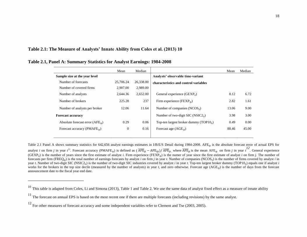
Table 2.1: The Measure of Analysts’ Innate Ability from Coles et al. (2013) 10

Table 2.1, Panel A: Summary Statistics for Analyst Earnings: 1984-2008

Mean Median

Mean Median

Sample size at the year level

Analysts’ observable time-variant

Number of forecasts 25,706.24 26,338.00 characteristics and control variables

Number of covered firms 2,907.00 2,989.00

Number of analysts 2,644.36 2,652.00 General experience (GEXPit) 8.12 6.72

Number of brokers 225.28 237 Firm experience (FEXPijt) 2.82 1.61

Number of analysts per broker 12.06 11.64 Number of companies (NCOSit) 13.06 9.00

Forecast accuracy

Number of two-digit SIC (NSIC2it) 3.98 3.00

Absolute forecast error (AFEijt) 0.29 0.06 Top-ten largest broker dummy (TOP10it) 0.49 0.00

Forecast accuracy (PMAFEijt) 0 0.16 Forecast age (AGEijt) 88.46 45.00

Table 2.1 Panel A shows summary statistics for 642,656 analyst earnings estimates in I/B/E/S Detail during 1984-2008. AFEijt is the absolute forecast error of actual EPS for

analyst i on firm j in year t11. Forecast accuracy (PMAFEijt) is defined as ( AFE̅̅ ̅̅ ̅jt − AFEijt)/ AFE̅̅ ̅̅ ̅

jt , where AFE̅̅ ̅̅ ̅jt is the mean AFEijt on firm j in year t

12. General experience

(GEXPit) is the number of years since the first estimate of analyst i. Firm experience (FEXPijt) is the numer of year since the first estimate of analyst i on firm j. The number of

forecasts per firm (FREQijt) is the total number of earnings forecasts by analyst i on firm j in year t. Number of companies (NCOSit) is the number of firms covered by analyst i in

year t. Number of two-digit SIC (NSIC2it) is the number of two-digit SIC industries covered by analyst i in year t. Top-ten largest broker dummy (TOP10it) equals one if analyst i

works for the brokers in the top size decile (measured by the number of analysts) in year t, and zero otherwise. Forecast age (AGEijt) is the number of days from the forecast

announcement date to the fiscal year end date.

10 This table is adapted from Coles, Li and Simona (2013), Table 1 and Table 2. We use the same data of analyst fixed effect as a measure of innate ability

11 The forecast on annual EPS is based on the most recent one if there are multiple forecasts (including revisions) by the same analyst.

12 For other measures of forecast accuracy and some independent variables refer to Clement and Tse (2003, 2005).

19

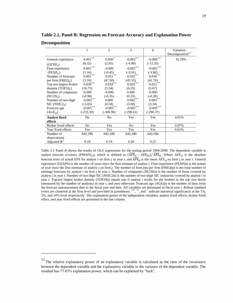
Table 2.1, Panel B: Regression on Forecast Accuracy and Explanation Power

Decomposition

1 2 3 4 Variation

Decomposition13

General experience

(GEXPit)

0.001***

(6.32)

0.000**

(2.05)

-0.002***

(-4.90)

-0.006***

(-12.35)

16.78%

Firm experience

(FEXPijt)

0.001***

(3.16)

-0.000

(-0.45)

-0.002***

(-3.91)

-0.002***

(-3.80)

Number of forecasts

per firm (FREQijt)

0.001***

(3.16)

0.031***

(47.50)

0.032***

(45.55)

0.030***

(41.76)

Top-ten largest broker

dummy (TOP10it)

0.039***

(16.73)

0.018***

(5.54)

0.020***

(6.29)

0.021***

(5.67)

Number of companies

(NCOSit)

-0.000

(-0.98)

-0.000

(-0.35)

0.000

(0.33)

-0.000

(-0.20)

Number of two-digit

SIC (NSIC2it)

-0.003***

(-5.83)

0.000

(0.58)

0.002***

(3.08)

0.003***

(3.34)

Forecast age

(AGEijt)

-0.005***

(-233.30)

-0.005***

(-306.90)

-0.005***

(-298.61)

-0.005***

(-290.37)

Analyst fixed

effects

No No Yes Yes 4.01%

Broker fixed effects No Yes No Yes 0.97%

Year fixed effects Yes Yes Yes Yes 0.61%

Number of

observations

642,186 642,186 642,186 642,186

Adjusted R2 0.18 0.19 0.20 0.21

Table 2.1 Panel B shows the results of OLS regressions for the testing period 1984-2008. The dependent variable is

analyst forecast accuracy (PMAFEijt), which is defined as (AFE̅̅ ̅̅ ̅jt − AFEijt)/ AFE̅̅ ̅̅ ̅

jt , Where AFEijt is the absolute

forecast error of actual EPS for analyst i on firm j in year t, and AFE̅̅ ̅̅ ̅jt is the mean AFEijt on firm j in year t. General

experience (GEXPit) is the number of years since the first estimate of analyst i. Firm experience (FEXPijt) is the numer

of year since the first estimate of analyst i on firm j. The number of forecasts per firm (FREQijt) is the total number of

earnings forecasts by analyst i on firm j in year t. Number of companies (NCOSit) is the number of firms covered by

analyst i in year t. Number of two-digit SIC (NSIC2it) is the number of two-digit SIC industries covered by analyst i in

year t. Top-ten largest broker dummy (TOP10it) equals one if analyst i works for the brokers in the top size decile

(measured by the number of analysts) in year t, and zero otherwise. Forecast age (AGEijt) is the number of days from

the forecast announcement date to the fiscal year end date. All variables are demeaned in fiscal year t. Robust standard

errors are clustered at the firm level and provided in parenthesis. ***, **, and * indicate statistical significance at the 1%,

5%, and 10% level respectively. The explanation power of the independent variables, analyst fixed effects, broker fixed

effect, and year fixed effects are presented in the last column.

13 The relative explanatory power of an explanatory variable is calculated as the ratio of the covariance

between the dependent variable and the explanatory variable to the variance of the dependent variable. The

residual has 77.65% explanation power, which can be explained by “luck”.

20

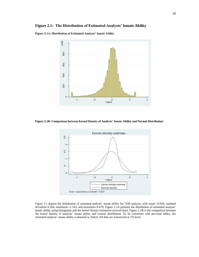
Figure 2.1: The Distribution of Estimated Analysts’ Innate Ability

Figure 2.1A: Distribution of Estimated Analysts’ Innate Ability

Figure 2.1B: Comparison between Kernel Density of Analysts’ Innate Ability and Normal Distribution

Figure 2.1 depicts the distribution of estimated analysts’ innate ability for 7540 analysts, with mean=-0.028, standard

deviation=0.264, minimum=-1.163, and maximum=0.679. Figure 2.1A presents the distribution of estimated analysts’

innate ability using histograms and the kernel density estimation (curved line). Figure 2.1B is the comparison between

the kernel density of analysts’ innate ability and normal distribution. To be consistent with previous tables, the

estimated analysts’ innate ability is denoted as Talent. All data are winsorized at 1% level.

0

20

040

060

080

010

00

Fre

qu

en

cy

-1 -.5 0 .5 1Talent

0.5

11.5

22.5

De

nsity

-1 -.5 0 .5 1Talent

Kernel density estimate

Normal density

kernel = epanechnikov, bandwidth = 0.0247

Kernel density estimate

21

The data for construction of control variables and other measures are from

multiple sources. The stock prices that are used to calculate insider trading value,

earnings surprise, and cumulative abnormal returns (CARs) are from CRSP. The analyst

data that are used to calculate the number of analysts coving a firm, the EPS forecast

timing, and earnings surprise are from I/B/E/S. For other control variables, the data of

market capitalization, total assets, B/M (book to market) ratio, R&D (the research and

development expenses), and PP&E (the property, plant and equipment) are from

COMPUSTAT. All of the variables that are used in this study are summarized in Table

2.2 and the Pearson correlation matrix for the major variables is shown in Table 2.3.

22

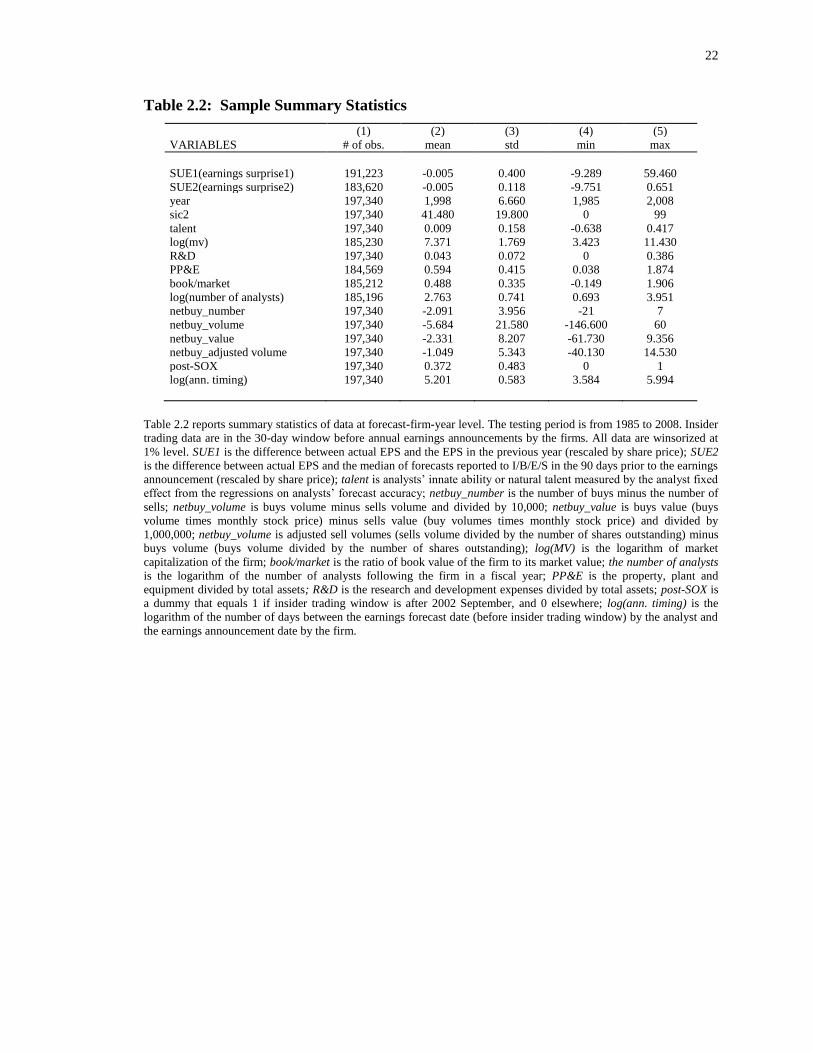
Table 2.2: Sample Summary Statistics

(1) (2) (3) (4) (5)

VARIABLES # of obs. mean std min max

SUE1(earnings surprise1) 191,223 -0.005 0.400 -9.289 59.460

SUE2(earnings surprise2) 183,620 -0.005 0.118 -9.751 0.651

year 197,340 1,998 6.660 1,985 2,008

sic2 197,340 41.480 19.800 0 99

talent 197,340 0.009 0.158 -0.638 0.417

log(mv) 185,230 7.371 1.769 3.423 11.430

R&D 197,340 0.043 0.072 0 0.386

PP&E 184,569 0.594 0.415 0.038 1.874

book/market 185,212 0.488 0.335 -0.149 1.906

log(number of analysts) 185,196 2.763 0.741 0.693 3.951

netbuy_number 197,340 -2.091 3.956 -21 7

netbuy_volume 197,340 -5.684 21.580 -146.600 60

netbuy_value 197,340 -2.331 8.207 -61.730 9.356

netbuy_adjusted volume 197,340 -1.049 5.343 -40.130 14.530

post-SOX 197,340 0.372 0.483 0 1

log(ann. timing) 197,340 5.201 0.583 3.584 5.994

Table 2.2 reports summary statistics of data at forecast-firm-year level. The testing period is from 1985 to 2008. Insider

trading data are in the 30-day window before annual earnings announcements by the firms. All data are winsorized at

1% level. SUE1 is the difference between actual EPS and the EPS in the previous year (rescaled by share price); SUE2

is the difference between actual EPS and the median of forecasts reported to I/B/E/S in the 90 days prior to the earnings

announcement (rescaled by share price); talent is analysts’ innate ability or natural talent measured by the analyst fixed

effect from the regressions on analysts’ forecast accuracy; netbuy_number is the number of buys minus the number of

sells; netbuy_volume is buys volume minus sells volume and divided by 10,000; netbuy_value is buys value (buys

volume times monthly stock price) minus sells value (buy volumes times monthly stock price) and divided by

1,000,000; netbuy_volume is adjusted sell volumes (sells volume divided by the number of shares outstanding) minus

buys volume (buys volume divided by the number of shares outstanding); log(MV) is the logarithm of market

capitalization of the firm; book/market is the ratio of book value of the firm to its market value; the number of analysts

is the logarithm of the number of analysts following the firm in a fiscal year; PP&E is the property, plant and

equipment divided by total assets; R&D is the research and development expenses divided by total assets; post-SOX is

a dummy that equals 1 if insider trading window is after 2002 September, and 0 elsewhere; log(ann. timing) is the

logarithm of the number of days between the earnings forecast date (before insider trading window) by the analyst and

the earnings announcement date by the firm.

23

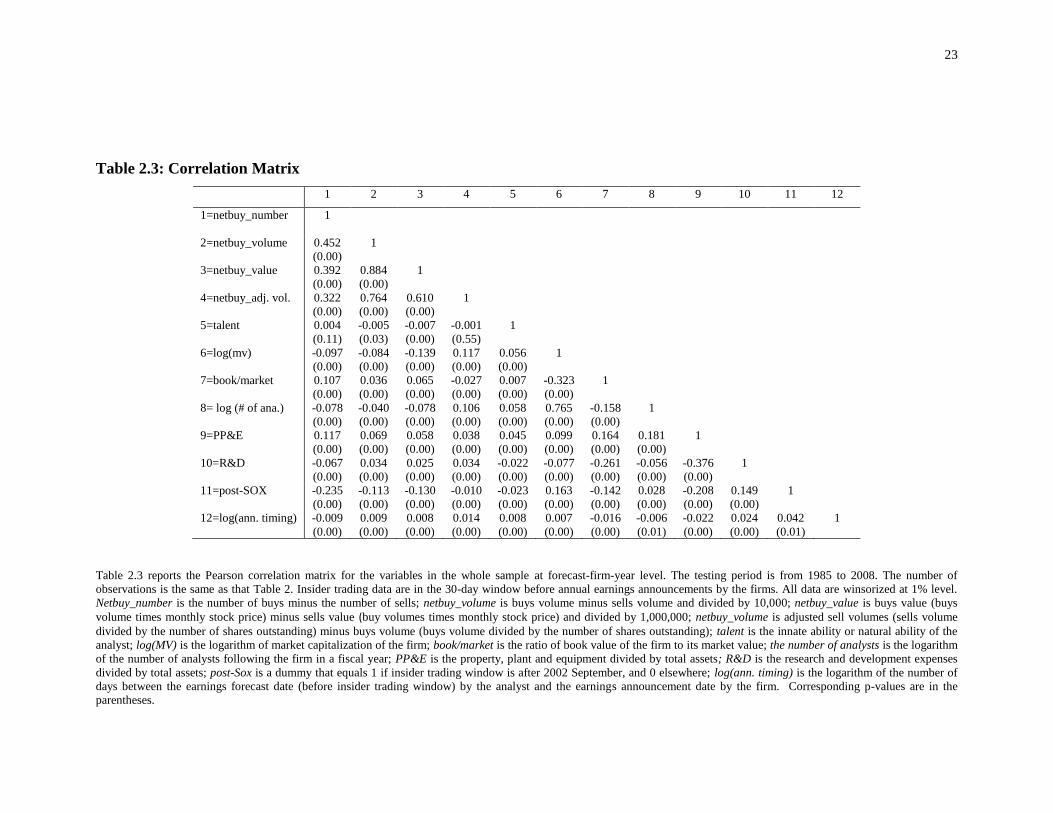
Table 2.3: Correlation Matrix

1 2 3 4 5 6 7 8 9 10 11 12

1=netbuy_number 1

2=netbuy_volume 0.452

(0.00)

1

3=netbuy_value 0.392

(0.00)

0.884

(0.00)

1

4=netbuy_adj. vol. 0.322

(0.00)

0.764

(0.00)

0.610

(0.00)

1

5=talent 0.004

(0.11)

-0.005

(0.03)

-0.007

(0.00)

-0.001

(0.55)

1

6=log(mv) -0.097

(0.00)

-0.084

(0.00)

-0.139

(0.00)

0.117

(0.00)

0.056

(0.00)

1

7=book/market 0.107

(0.00)

0.036

(0.00)

0.065

(0.00)

-0.027

(0.00)

0.007

(0.00)

-0.323

(0.00)

1

8= log (# of ana.) -0.078

(0.00)

-0.040

(0.00)

-0.078

(0.00)

0.106

(0.00)

0.058

(0.00)

0.765

(0.00)

-0.158

(0.00)

1

9=PP&E 0.117

(0.00)

0.069

(0.00)

0.058

(0.00)

0.038

(0.00)

0.045

(0.00)

0.099

(0.00)

0.164

(0.00)

0.181

(0.00)

1

10=R&D -0.067

(0.00)

0.034

(0.00)

0.025

(0.00)

0.034

(0.00)

-0.022

(0.00)

-0.077

(0.00)

-0.261

(0.00)

-0.056

(0.00)

-0.376

(0.00)

1

11=post-SOX

-0.235

(0.00)

-0.113

(0.00)

-0.130

(0.00)

-0.010

(0.00)

-0.023

(0.00)

0.163

(0.00)

-0.142

(0.00)

0.028

(0.00)

-0.208

(0.00)

0.149

(0.00)

1

12=log(ann. timing)

-0.009

(0.00)

0.009

(0.00)

0.008

(0.00)

0.014

(0.00)

0.008

(0.00)

0.007

(0.00)

-0.016

(0.00)

-0.006

(0.01)

-0.022

(0.00)

0.024

(0.00)

0.042

(0.01)

1

Table 2.3 reports the Pearson correlation matrix for the variables in the whole sample at forecast-firm-year level. The testing period is from 1985 to 2008. The number of

observations is the same as that Table 2. Insider trading data are in the 30-day window before annual earnings announcements by the firms. All data are winsorized at 1% level.

Netbuy_number is the number of buys minus the number of sells; netbuy_volume is buys volume minus sells volume and divided by 10,000; netbuy_value is buys value (buys

volume times monthly stock price) minus sells value (buy volumes times monthly stock price) and divided by 1,000,000; netbuy_volume is adjusted sell volumes (sells volume

divided by the number of shares outstanding) minus buys volume (buys volume divided by the number of shares outstanding); talent is the innate ability or natural ability of the

analyst; log(MV) is the logarithm of market capitalization of the firm; book/market is the ratio of book value of the firm to its market value; the number of analysts is the logarithm

of the number of analysts following the firm in a fiscal year; PP&E is the property, plant and equipment divided by total assets; R&D is the research and development expenses

divided by total assets; post-Sox is a dummy that equals 1 if insider trading window is after 2002 September, and 0 elsewhere; log(ann. timing) is the logarithm of the number of

days between the earnings forecast date (before insider trading window) by the analyst and the earnings announcement date by the firm. Corresponding p-values are in the

parentheses.

24

In Table 2.2, it is worth noting that on average all measures about net buys are

negative since there are more insider sells than insider buys. This is because insiders can

obtain shares through grant, bonus and exercising options, but these transactions are not

filed as buys in SEC Form 4. However, if such stocks are sold, they are recorded as sales.

Thus net buys are mechanically negative on average. As for the nature of the earnings

forecasts, the mean earnings surprise is -0.5% for both measures (SUE1 and SUE2), and

37.2% of the earnings forecasts in our sample are announced in the post-SOX period.

In Table 2.3, we find that among the paired insider trading measures,

netbuy_number generates relatively lower Pearson correlation coefficients; this suggests

the frequency of insider trading has a different nature from insider trading volume and

insider trading value and thus can generate different empirical results. In addition,

analysts’ innate ability (variable name as “Talent”) is negatively correlated with

netbuy_volume and netbuy_value at 5% and 1% significance level respectively,

consistent with our intuition that high-ability analysts help restrict insider trading.

2.3 Analysts’ Innate Ability and Insider Trading Intensity

2.3.1 Main Results

First, we examine the effects of analysts’ innate ability (or natural talent) on open

market insider trading before annual earnings announcements at forecast-analyst-firm-

year level. We believe forecast level is more accurate than other considerations. For our

research purposes, analysts’ innate ability only works through earnings forecasts; two

analysts with similar innate ability might have different effects on insider trading if their

number of forecasts is different due to different frequency of information transformation.

25

Each forecast represents specific information flow given different forecast timing,

thereby implying different information asymmetry levels. While controlling for the

frequency of forecasts cannot identify the exact forecast timing, we control the number of

days between earnings forecasts by analysts and earnings announcements by companies.

We use the following specification to explore the effects of analysts’ innate ability on

corporate insider trading:

𝐼𝑛𝑠𝑖𝑑𝑒𝑟 𝑇𝑟𝑎𝑑𝑖𝑛𝑔𝑖𝑗 = 𝛼 + 𝛽1𝑇𝑎𝑙𝑒𝑛𝑡𝑖𝑗𝑘 + 𝛽2𝐿𝑜𝑔(𝑀𝑉)𝑖𝑗 + 𝛽3(𝐵𝑜𝑜𝑘

𝑀𝑎𝑟𝑘𝑒𝑡)𝑖𝑗 + 𝛽4𝑛𝑢𝑚𝑏𝑒𝑟 𝑜𝑓 𝑎𝑛𝑎𝑙𝑦𝑠𝑡𝑖𝑗 +

𝛽5𝑃𝑃&𝐸𝑖𝑗 + 𝛽6 𝑅&𝐷𝑖𝑗 + 𝛽7𝑃𝑜𝑠𝑡 ̶𝑆𝑂𝑋𝑖𝑗 + 𝛽8𝐿𝑜𝑔(𝐴𝑛𝑛. 𝑇𝑖𝑚𝑖𝑛𝑔)𝑖𝑗𝑘𝑚 + 휀𝑖𝑗 (2.1)

where 𝐼𝑛𝑠𝑖𝑑𝑒𝑟 𝑇𝑟𝑎𝑑𝑖𝑛𝑔𝑖𝑗 is net buy or net sell of corporate insider trading in the

30-day window prior to earnings announcement by firm 𝑖 for fiscal year j; 𝑇𝑎𝑙𝑒𝑛𝑡𝑖𝑗𝑘 is

analyst k’ innate ability (measured by estimated analyst fixed effects) if analyst k covers

firm 𝑖 in fiscal year j; 𝐿𝑜𝑔(𝑀𝑉)𝑖𝑗 is the logarithm of market capitalization of firm 𝑖 in

fiscal year j; (𝐵𝑜𝑜𝑘

𝑀𝑎𝑟𝑘𝑒𝑡)𝑖𝑗 is the ratio of book value of firm 𝑖 to its market value in fiscal

year j; 𝑛𝑢𝑚𝑏𝑒𝑟 𝑜𝑓 𝑎𝑛𝑎𝑙𝑦𝑠𝑡𝑖𝑗 is the logarithm of the number of analysts following firm 𝑖

in fiscal year j; 𝑃𝑃&𝐸𝑖𝑗 is the property, plant and equipment divided by total assets of

firm 𝑖 in fiscal year j; 𝑅&𝐷𝑖𝑗 is the research and development expenses divided by total

assets of firm 𝑖 in fiscal year j; 𝑃𝑜𝑠𝑡 ̶𝑆𝑂𝑋𝑖𝑗 is a dummy that equals 1 if insider trading

window of firm 𝑖 in fiscal year j is after 2002 September, and 0 elsewhere;

𝐿𝑜𝑔(𝐴𝑛𝑛. 𝑇𝑖𝑚𝑖𝑛𝑔)𝑖𝑗𝑘𝑚 is the logarithm of the number of days between the date of EPS

forecast m (before insider trading window) by analyst k and the date of earnings

26

announcement by the firm 𝑖 for fiscal year j. We also add year fixed effect and industry

(2-digit SIC) fixed effect for each regression.

For the insider net buys as 𝐼𝑛𝑠𝑖𝑑𝑒𝑟 𝑇𝑟𝑎𝑑𝑖𝑛𝑔𝑖𝑗 , we construct four different

measures. And all measures of insiders’ net sells are the opposite numbers of the

corresponding net buy measures. These fours measures are defined as:

netbuy_number= the number of buys-the number of sells (2.2)

netbuy_volume= buys volume – sells volume (2.3)

netbuy_value= buys volume *stock price-sells volume* stock price (2.4)

netbuy_adjustedvolume= (buys volume-sells volume)/ # shares outstanding (2.5)

The expected signs of the independent variables are: 𝛽1 < 0, 𝛽2 < 0, 𝛽3 < 0 ,

𝛽4 < 0, 𝛽5 < 0, 𝛽6 > 0, 𝛽7 < 0, 𝛽8 ambiguous.

If insiders have good (bad) inside information14

about EPS, we expect 𝛽1 < 0

for net buys (sells) by corporate insiders according to our hypotheses since analysts with

high innate ability can mitigate information asymmetry. As for all the other control

variables, they are almost all related to information asymmetry. 𝛽2 represents the effect

of firm size. Elliot at al. (1984) hypothesize that corporate insiders have more inside

information because smaller firms are followed by fewer analysts. In addition, the results

of Finnerty (1976), Seyhun (1986), Lakonishok and Lee (2001), and Frankel and Li

(2004) all indicate smaller firms are associated with higher insider trading profits. 𝛽3

captures the informativeness of financial statements in the sense that firms with higher

14 The definitions of information type are denoted in Equation (2.6) and (2.7).

27

book-to-market ratio have relatively less unrecorded assets, thus they have lower level of

information asymmetry. 𝛽4 measures the effects of the intensity of analyst activities.

Bhushan (1989) uses analyst following as a measure of private information collection,

and Frankel and Li (2004) find that increased analyst following is related to reduced

insider trading profits and reduced insider buys. 𝛽5 reveals the effects of the proportion

of vital assets than cannot be readily liquidated and larger proportion of tangible assets

implies lower level of information asymmetry. 𝛽6 indicates the effects of information

asymmetry induced by R&D investment. Aboody and Lev (2000) provide evidence that

insider trading profits are higher for firms with R&D investment. 𝛽7 reflects the effects of

changed insider trading rules about accelerated filing deadlines issued by the SEC as

required by the 2002 Sarbanes-Oxley Act. Effective August 29, 2002, Form 4

transactions must be reported to the SEC by the end of the second business day following

the trading day. Thus, this policy should confine insider trading as accelerated filing

deadlines help mitigate information asymmetry. 𝛽8 corresponds to the timing effect of

the earnings forecasts by analysts. However, the effect is mixed by two conflicting

effects. On the one hand, the earlier the forecast is announced, the lower the level of

information asymmetry of earnings is handled with insiders. On the other hand, it is quite

possible that insiders obtain private information very early in the event windows and aim

to trade early to avoid the blackout windows required by firms.

To distinguish the information type, we follow Livnat and Mendenhall (2006) and

employ the following measures of earnings surprise (SUE1 and SUE2):

𝑆𝑈𝐸1 =𝑋𝑖𝑗−𝑋𝑖𝑗−1

𝑃𝑖𝑗 (2.6)

28

𝑆𝑈𝐸2 =𝑋𝑖𝑗−𝑀𝐹𝑋𝑖𝑗

𝑃𝑖𝑗 (2.7)

In Equation (2.6), 𝑋𝑖𝑗 is the actual EPS announced by firm i for fiscal year j,

𝑋𝑖𝑗−1 is the actual EPS announced by firm i for fiscal year j-1, 𝑃𝑖𝑗 is the stock price of

firm i at the end of fiscal year j. In equation (2.7), 𝑋𝑖𝑗 is the actual EPS announced by

firm i for fiscal year j, 𝑀𝐹𝑋𝑖𝑗 is the median of forecasts reported to I/B/E/S in the 90 days

prior to the earnings announcement by firm i in fiscal year j, 𝑃𝑖𝑗 is the stock price of firm

i at the end of fiscal year j. We denote that inside information is “good” if SUE is positive

and that inside information is “bad” if SUE is negative.

In a word, SUE2 uses forecast consensus among analysts as expected earnings,

while SUE1 uses previous actual earnings as expected earnings. Both of them can serve

as measures of earnings surprise, but we believe SUE2 is more accurate since information

is updated, as compared with accounting numbers in the previous year, so we use SUE2

as the main measure and SUE1 as robustness check. As Livnat and Mendenhall (2006)

imply, SUE1 is also reasonable since many shareholders do not bother to investigate in

analyst consensus; they just use the earnings in the previous year for simplicity as the

expectation. Thus, we also consider SUE1 for comparable comparisons.

Table 2.4 provides the main empirical results based on the 30-day window before

earnings announcement by firms. We use positive earnings surprise (SUE2>0) to measure

good inside information in Columns 1-4, and correspondingly the results for bad inside

information (SUE2<0) are reported in Columns 5-8. We find that higher analysts’ innate

ability is associated with lower volumes of net buys, lower value of net buys, and lower

adjusted volume of net buys when insiders have “good” inside information about

earnings (positive SUE2). The economic significance is substantial: one standard

29

deviation increase of analysts’ innate ability is associated with 1.24% decrease in

netbuy_volume, 1.33% decrease in netbuy_value, and 1.50% decrease in

netbuy_adjustedvolume. As for the results for SUE2<0, we find that no measures of

insiders’ net sells can significantly affect insiders’ net sells when insiders have bad

information. This is not surprising because insiders are more cautious in exploiting

negative information for lower litigation risk (Cheng and Lo(2006) etc.). Investors suffer

from actual losses when stock prices decrease following insiders’ sells, but it is less likely

for corporate insiders to be involved in legal troubles if stock prices decrease following

insiders’ buys. It is worth noting that the forecast timing has positive effects on insiders’

net buys, this implies corporate insiders obtain private information of positive earnings

surprise early and aim to trade early to avoid the blackout windows required by their

firms. For other independent variables, we have mixed evidence for the signs and

statistical significance of their coefficients. Most of them have expected signs except

PP&E. In addition, netbuy_number has opposite signs in control variables compared with

the other three measures in terms of volumes and values.

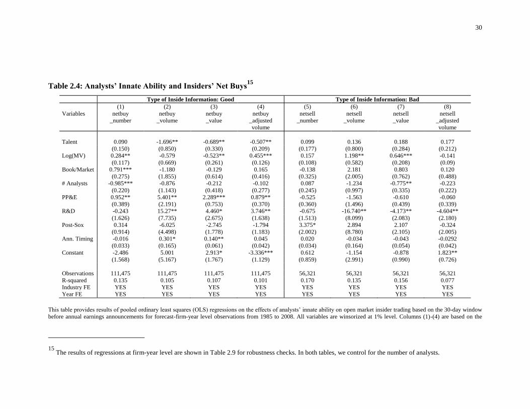
30

Table 2.4: Analysts’ Innate Ability and Insiders’ Net Buys15

Type of Inside Information: Good Type of Inside Information: Bad

(1) (2) (3) (4) (5) (6) (7) (8)

Variables

netbuy

_number

netbuy

_volume

netbuy

_value

netbuy

_adjusted

volume

netsell

_number

netsell

_volume

netsell

_value

netsell

_adjusted

volume

Talent 0.090 -1.696** -0.689** -0.507** 0.099 0.136 0.188 0.177

(0.150) (0.850) (0.330) (0.209) (0.177) (0.800) (0.284) (0.212)

Log(MV) 0.284** -0.579 -0.523** 0.455*** 0.157 1.198** 0.646*** -0.141

(0.117) (0.669) (0.261) (0.126) (0.108) (0.582) (0.208) (0.09)

Book/Market 0.791*** -1.180 -0.129 0.165 -0.138 2.181 0.803 0.120

(0.275) (1.855) (0.614) (0.416) (0.325) (2.005) (0.762) (0.488)

# Analysts -0.985*** -0.876 -0.212 -0.102 0.087 -1.234 -0.775** -0.223

(0.220) (1.143) (0.418) (0.277) (0.245) (0.997) (0.335) (0.222)

PP&E 0.952** 5.401** 2.289*** 0.879** -0.525 -1.563 -0.610 -0.060

(0.389) (2.191) (0.753) (0.370) (0.360) (1.496) (0.439) (0.339)

R&D -0.243 15.27** 4.460* 3.746** -0.675 -16.740** -4.173** -4.604**

(1.626) (7.735) (2.675) (1.638) (1.513) (8.099) (2.083) (2.180)

Post-Sox 0.314 -6.025 -2.745 -1.794 3.375* 2.894 2.107 -0.324

(0.914) (4.498) (1.778) (1.183) (2.002) (8.780) (2.105) (2.005)

Ann. Timing -0.016 0.301* 0.140** 0.045 0.020 -0.034 -0.043 -0.0292

(0.033) (0.165) (0.061) (0.042) (0.034) (0.164) (0.054) (0.042)

Constant -2.486 5.001 2.913* -3.336*** 0.612 -1.154 -0.878 1.823**

(1.568) (5.167) (1.767) (1.129) (0.859) (2.991) (0.990) (0.726)

Observations 111,475 111,475 111,475 111,475 56,321 56,321 56,321 56,321

R-squared 0.135 0.105 0.107 0.101 0.170 0.135 0.156 0.077

Industry FE YES YES YES YES YES YES YES YES

Year FE YES YES YES YES YES YES YES YES

This table provides results of pooled ordinary least squares (OLS) regressions on the effects of analysts’ innate ability on open market insider trading based on the 30-day window

before annual earnings announcements for forecast-firm-year level observations from 1985 to 2008. All variables are winsorized at 1% level. Columns (1)-(4) are based on the

15 The results of regressions at firm-year level are shown in Table 2.9 for robustness checks. In both tables, we control for the number of analysts.

31

sample of good insider information which is measured by positive earnings surprise (SUE2>0), i.e. positive difference between actual EPS and the median of forecasts reported to

I/B/E/S in the 90 days prior to the earnings announcement (rescaled by share prices), and columns (5)-(8) are based on the sample of bad insider information corresponding to

negative earnings surprise. Eight dependent variables are employed: netbuy_number is the number of buys minus the number of sells; netbuy_volume is buys volume minus sells

volume and divided by 10,000; netbuy_value is buys value (buys volume times monthly stock price) minus sells value (buy volumes times monthly stock price) and divided by

1,000,000; netbuy_volume is adjusted sell volumes (sells volume divided by the number of shares outstanding) minus buys volume (buys volume divided by the number of shares

outstanding). All measures of insiders’ net sells are the opposite numbers of the corresponding net buy measures. The key independent variable is analysts’ innate ability or natural

talent, hereinafter referred to as “Talent” in the regressions. The control variables are: Log(MV), the logarithm of market capitalization of the firm; Book/Market, the ratio of book

value of the firm to its market value; The Number of Analysts, the logarithm of the number of analysts following the firm in a fiscal year; PP&E, the property, plant and equipment

divided by total assets; R&D, the research and development expenses divided by total assets. Post-Sox, the dummy that equals 1 if insider trading window is after 2002 September,

and 0 elsewhere; Log(Ann. Timing) is the logarithm of the number of days between the earnings forecast date (before insider trading window) by the analyst and the earnings

announcement date by the firm. All regressions include year fixed effect and industry (2-digit SIC) fixed effect. Robust standard errors in parentheses are clustered at firm level,

and ***, ** and * stand for statistical significance at 0.01, 0.05 and 0.1 level respectively.

32

In Table 2.5, we use SUE1 to measure information type as a robustness check.

The results of insider trading measures in Table 2.5 have the same signs with those in

Table 2.4. Although in Table 2.5 netbuy_volume in Column 2 is not significant anymore,

netbuy_value in Column 3 and netbuy_adjustedvolume in Column 4 are still significant.

Again, higher innate ability is associated with lower value of net buys and lower adjusted

volume of net buys when insiders have “good” inside information about earnings

(positive SUE1). In addition, analysts’ innate ability has no significant effects on

insiders’ net sells when insiders have “bad” information (negative SUE1). The sign,

magnitude, and significance of control variables are quite similar with those in Table 2.4.

In addition, the goodness of fit measured by R squared is very close to corresponding

regressions in Table 2.4 and Table 2.5. The comparison between Table 2.4 and Table 2.5

justifies that both measures (SUE1 and SUE2) of insiders’ information type generate

congruent results, but the absolute values of coefficients are larger when SUE2 is

employed. Thus the effects of analysts’ innate ability on insider buys are amplified if the

consensus among analysts’ forecasts of earnings rather than lagged earnings is used as

the measure of insiders’ information type.

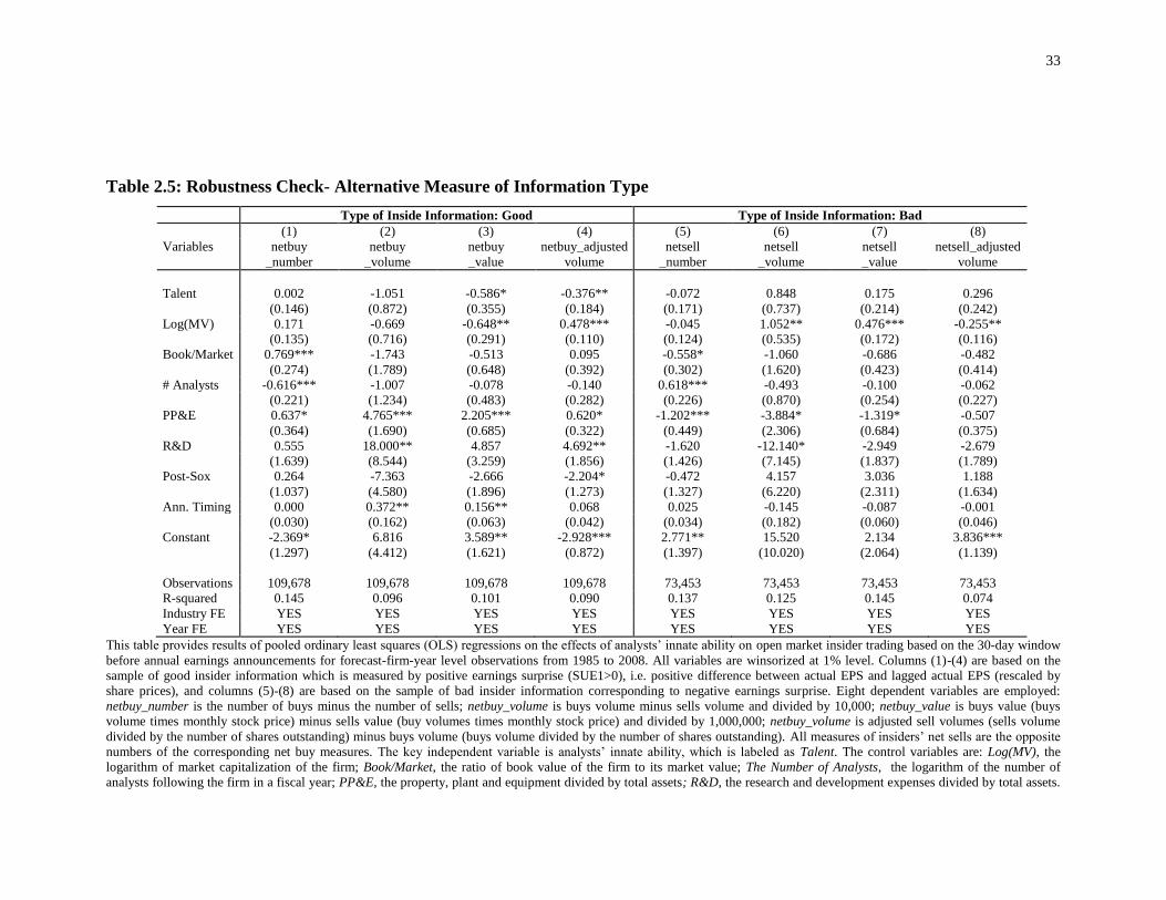
33

Table 2.5: Robustness Check- Alternative Measure of Information Type

Type of Inside Information: Good Type of Inside Information: Bad

(1) (2) (3) (4) (5) (6) (7) (8)

Variables

netbuy

_number

netbuy

_volume

netbuy

_value

netbuy_adjusted

volume

netsell

_number

netsell

_volume

netsell

_value

netsell_adjusted

volume

Talent 0.002 -1.051 -0.586* -0.376** -0.072 0.848 0.175 0.296

(0.146) (0.872) (0.355) (0.184) (0.171) (0.737) (0.214) (0.242)

Log(MV) 0.171 -0.669 -0.648** 0.478*** -0.045 1.052** 0.476*** -0.255**

(0.135) (0.716) (0.291) (0.110) (0.124) (0.535) (0.172) (0.116)

Book/Market 0.769*** -1.743 -0.513 0.095 -0.558* -1.060 -0.686 -0.482

(0.274) (1.789) (0.648) (0.392) (0.302) (1.620) (0.423) (0.414)

# Analysts -0.616*** -1.007 -0.078 -0.140 0.618*** -0.493 -0.100 -0.062

(0.221) (1.234) (0.483) (0.282) (0.226) (0.870) (0.254) (0.227)

PP&E 0.637* 4.765*** 2.205*** 0.620* -1.202*** -3.884* -1.319* -0.507

(0.364) (1.690) (0.685) (0.322) (0.449) (2.306) (0.684) (0.375)

R&D 0.555 18.000** 4.857 4.692** -1.620 -12.140* -2.949 -2.679

(1.639) (8.544) (3.259) (1.856) (1.426) (7.145) (1.837) (1.789)

Post-Sox 0.264 -7.363 -2.666 -2.204* -0.472 4.157 3.036 1.188

(1.037) (4.580) (1.896) (1.273) (1.327) (6.220) (2.311) (1.634)

Ann. Timing 0.000 0.372** 0.156** 0.068 0.025 -0.145 -0.087 -0.001

(0.030) (0.162) (0.063) (0.042) (0.034) (0.182) (0.060) (0.046)

Constant -2.369* 6.816 3.589** -2.928*** 2.771** 15.520 2.134 3.836***

(1.297) (4.412) (1.621) (0.872) (1.397) (10.020) (2.064) (1.139)

Observations 109,678 109,678 109,678 109,678 73,453 73,453 73,453 73,453

R-squared 0.145 0.096 0.101 0.090 0.137 0.125 0.145 0.074

Industry FE YES YES YES YES YES YES YES YES

Year FE YES YES YES YES YES YES YES YES

This table provides results of pooled ordinary least squares (OLS) regressions on the effects of analysts’ innate ability on open market insider trading based on the 30-day window

before annual earnings announcements for forecast-firm-year level observations from 1985 to 2008. All variables are winsorized at 1% level. Columns (1)-(4) are based on the

sample of good insider information which is measured by positive earnings surprise (SUE1>0), i.e. positive difference between actual EPS and lagged actual EPS (rescaled by

share prices), and columns (5)-(8) are based on the sample of bad insider information corresponding to negative earnings surprise. Eight dependent variables are employed:

netbuy_number is the number of buys minus the number of sells; netbuy_volume is buys volume minus sells volume and divided by 10,000; netbuy_value is buys value (buys

volume times monthly stock price) minus sells value (buy volumes times monthly stock price) and divided by 1,000,000; netbuy_volume is adjusted sell volumes (sells volume

divided by the number of shares outstanding) minus buys volume (buys volume divided by the number of shares outstanding). All measures of insiders’ net sells are the opposite

numbers of the corresponding net buy measures. The key independent variable is analysts’ innate ability, which is labeled as Talent. The control variables are: Log(MV), the

logarithm of market capitalization of the firm; Book/Market, the ratio of book value of the firm to its market value; The Number of Analysts, the logarithm of the number of

analysts following the firm in a fiscal year; PP&E, the property, plant and equipment divided by total assets; R&D, the research and development expenses divided by total assets.

34

Post-Sox, the dummy that equals 1 if insider trading window is after 2002 September, and 0 elsewhere; Log(Ann. Timing) is the logarithm of the number of days between the

earnings forecast date (before insider trading window) by the analyst and the earnings announcement date by the firm. All regressions include year fixed effect and industry (2-

digit SIC) fixed effect. Robust standard errors in parentheses are clustered at firm level, and ***, ** and * stand for statistical significance at 0.01, 0.05 and 0.1 level respectively.

35

2.3.2 Opportunistic Trading and Routine Trading

We postulate in general that insiders’ net buys are driven by good inside

information and insiders’ net sells are driven by bad inside information. However, it is

possible that buys or sells are not informative about firms’ futures, even though corporate

insiders have favored access to private information about firm events. For insider buys,

an insider might purchase stock of his firm due to discount plans after receiving a bonus;

for insider sells, an insider might sell stock of his firm for liquidity and portfolio

rebalancing purposes. In either case, a given insider trade is not related to inside

information. Thus, we follow Cohen et al. (2012) who distinguish opportunistic insider

trading and routine trading. They define a routine trader as an insider who traded in the

same calendar month for at least three consecutive years in the past and define an

opportunistic trader as everyone else. Then, all trades are classified into two categories:

routine trades by routine traders and opportunistic trades by opportunistic traders. We

use the same method to identify routine trades and opportunistic trades.

We report the results of opportunistic trades in Panel A, Table 2.6 and the results

of routine trades in Panel B, Table 2.6. In the sample of good inside information, about

64.81% of total trades are opportunistic trades; in the sample of bad inside information,

about 72.24% of total trades are opportunistic trades; in the whole sample of which inside

information type can be identified, about 67.27% of total trades are opportunistic trades.

In Table 2.6, Panel A, the absolute values of the coefficients of volume and adjusted

volume of net buys for opportunistic traders are larger than those in Table 2.4, Panel A

for the whole sample. However, these two coefficients are not statistically significant in

Table 2.6, Panel B for routine traders. In both of Panel A and Panel B in Table 2.6, the

36

coefficient of net buy values is significant, but the coefficient is less significant for

routine traders.

These results suggest that the results in Table 2.4 mainly stem from opportunistic

trades rather than routine trades, or in other words, the true relationship in Table 2.4 is

mixed with noise compared with Table 2.6 - this difference is consistent with our

hypothesis that insider trading prior to earnings announcements is driven by inside

information to a large degree. Besides, post-SOX is significant for opportunistic trades,

while it is insignificant in Table 2.4 for the sample of all trades, this also supports the

importance of distinguishing information-driven trades from routine trades as stricter

regulations are mainly against information-driven trades.

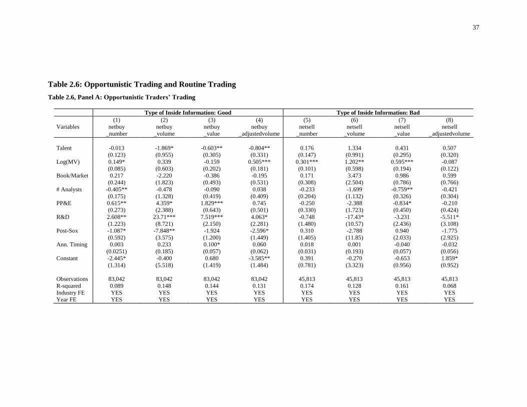
37

Table 2.6: Opportunistic Trading and Routine Trading

Table 2.6, Panel A: Opportunistic Traders’ Trading

Type of Inside Information: Good Type of Inside Information: Bad

(1) (2) (3) (4) (5) (6) (7) (8)

Variables

netbuy

_number

netbuy

_volume

netbuy

_value

netbuy

_adjustedvolume

netsell

_number

netsell

_volume

netsell

_value

netsell

_adjustedvolume

Talent -0.013 -1.869* -0.603** -0.804** 0.176 1.334 0.431 0.507

(0.123) (0.955) (0.305) (0.331) (0.147) (0.991) (0.295) (0.320)

Log(MV) 0.149* 0.339 -0.159 0.505*** 0.301*** 1.202** 0.595*** -0.087

(0.085) (0.603) (0.202) (0.181) (0.101) (0.598) (0.194) (0.122)

Book/Market 0.217 -2.220 -0.386 -0.195 0.171 3.473 0.986 0.599

(0.244) (1.823) (0.493) (0.531) (0.308) (2.504) (0.786) (0.766)

# Analysts -0.405** -0.478 -0.090 0.038 -0.233 -1.699 -0.759** -0.421

(0.175) (1.328) (0.419) (0.409) (0.204) (1.132) (0.326) (0.304)

PP&E 0.615** 4.359* 1.829*** 0.745 -0.250 -2.388 -0.834* -0.210

(0.273) (2.388) (0.643) (0.501) (0.330) (1.723) (0.450) (0.424)

R&D 2.608** 23.71*** 7.519*** 4.063* -0.748 -17.43* -3.231 -5.511*

(1.223) (8.721) (2.150) (2.281) (1.480) (10.57) (2.436) (3.108)

Post-Sox -1.087* -7.848** -1.924 -2.596* 0.310 -2.788 0.940 -1.775

(0.592) (3.575) (1.200) (1.449) (1.405) (11.85) (2.033) (2.925)

Ann. Timing 0.003 0.233 0.100* 0.060 0.018 0.001 -0.040 -0.032

(0.0251) (0.185) (0.057) (0.062) (0.031) (0.193) (0.057) (0.056)

Constant -2.445* -0.400 0.680 -3.585** 0.391 -0.270 -0.653 1.859*

(1.314) (5.518) (1.419) (1.484) (0.781) (3.323) (0.956) (0.952)

Observations 83,042 83,042 83,042 83,042 45,813 45,813 45,813 45,813

R-squared 0.089 0.148 0.144 0.131 0.174 0.128 0.161 0.068

Industry FE YES YES YES YES YES YES YES YES

Year FE YES YES YES YES YES YES YES YES

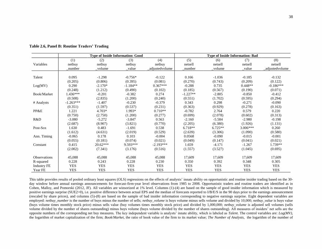
38

Table 2.6, Panel B: Routine Traders’ Trading

Type of Inside Information: Good Type of Inside Information: Bad

(1) (2) (3) (4) (5) (6) (7) (8)

Variables

netbuy

_number

netbuy

_volume

netbuy

_value

netbuy

_adjustedvolume

netsell

_number

netsell

_volume

netsell

_value

netsell

_adjustedvolume

Talent 0.095 -1.298 -0.756* -0.122 0.166 -1.036 -0.185 -0.132

(0.205) (0.806) (0.395) (0.081) (0.270) (0.743) (0.209) (0.122)

Log(MV) 0.290 -2.170* -1.184** 0.367*** -0.288 0.735 0.448** -0.186***

(0.248) (1.212) (0.490) (0.102) (0.185) (0.567) (0.190) (0.071)

Book/Market 1.436*** -0.201 -0.382 0.274 -1.227** -2.805 -0.850 -0.412

(0.508) (2.835) (1.200) (0.240) (0.551) (1.702) (0.595) (0.294)

# Analysts -1.263*** -1.407 -0.230 -0.379 0.343 0.298 -0.271 -0.090

(0.351) (1.597) (0.537) (0.231) (0.363) (0.929) (0.278) (0.163)

PP&E 1.221 4.703* 1.993* 0.710** -0.782 2.764 0.579 0.220

(0.750) (2.750) (1.200) (0.277) (0.699) (2.078) (0.602) (0.313)

R&D -3.080 -5.272 -3.847 0.563 -2.160 -5.584 -2.980 -0.198

(2.687) (8.907) (3.821) (0.770) (2.205) (6.380) (1.926) (1.131)

Post-Sox 1.630 0.483 -1.691 0.538 6.718** 6.725** 3.006*** 0.260

(1.612) (4.631) (2.019) (0.529) (2.639) (3.306) (1.090) (0.580)

Ann. Timing -0.065 0.178 0.103 -0.004 0.0568 -0.090 -0.015 -0.001

(0.055) (0.181) (0.074) (0.021) (0.049) (0.147) (0.041) (0.021)

Constant 0.415 20.62*** 9.593*** -2.193*** 1.659 -4.171 -1.267 1.739**

(2.002) (7.341) (3.176) (0.516) (1.557) (3.527) (1.045) (0.695)

Observations 45,088 45,088 45,088 45,088 17,609 17,609 17,609 17,609

R-squared 0.228 0.243 0.228 0.230 0.350 0.392 0.348 0.305

Industry FE YES YES YES YES YES YES YES YES

Year FE YES YES YES YES YES YES YES YES

This table provides results of pooled ordinary least squares (OLS) regressions on the effects of analysts’ innate ability on opportunistic and routine insider trading based on the 30-

day window before annual earnings announcements for forecast-firm-year level observations from 1985 to 2008. Opportunistic traders and routine traders are identified as in

Cohen, Malloy, and Pomorski (2012, JF). All variables are winsorized at 1% level. Columns (1)-(4) are based on the sample of good insider information which is measured by

positive earnings surprise (SUE2>0), i.e. positive difference between actual EPS and the median of forecasts reported to I/B/E/S in the 90 days prior to the earnings announcement

(rescaled by share prices), and columns (5)-(8) are based on the sample of bad insider information corresponding to negative earnings surprise. Eight dependent variables are

employed: netbuy_number is the number of buys minus the number of sells; netbuy_volume is buys volume minus sells volume and divided by 10,000; netbuy_value is buys value

(buys volume times monthly stock price) minus sells value (buy volumes times monthly stock price) and divided by 1,000,000; netbuy_volume is adjusted sell volumes (sells

volume divided by the number of shares outstanding) minus buys volume (buys volume divided by the number of shares outstanding). All measures of insiders’ net sells are the

opposite numbers of the corresponding net buy measures. The key independent variable is analysts’ innate ability, which is labeled as Talent. The control variables are: Log(MV),

the logarithm of market capitalization of the firm; Book/Market, the ratio of book value of the firm to its market value; The Number of Analysts, the logarithm of the number of

39

analysts following the firm in a fiscal year; PP&E, the property, plant and equipment divided by total assets; R&D, the research and development expenses divided by total assets.

Post-Sox, the dummy that equals 1 if insider trading window is after 2002 September, and 0 elsewhere; Log(Ann. Timing) is the logarithm of the number of days between the

earnings forecast date (before insider trading window) by the analyst and the earnings announcement date by the firm. All regressions include year fixed effect and industry (2-

digit SIC) fixed effect. Panel A is for opportunistic trading, and Panel B is for routine trading. Robust standard errors in parentheses are clustered at firm level, and ***, ** and *

stand for statistical significance at 0.01, 0.05 and 0.1 level respectively.

40

2.3.3 Initial Coverage: The Incremental Effect on Increased Insider Trading

In previous sections, we did not specify which traits the innate ability or natural

talent comprises. It might include an extraordinary economic sense of firm policies, wide

social networks in professional connections (Cohen, Frazzini, and Malloy, 2010), or any

other valuable behavioral traits (Easterwood and Nutt, 1999) for better forecasts. So even

if we use “innate ability” or “natural talent” to name our measure, probably analysts’

innate ability or natural talent can function through learning to trigger or strengthen itself,

but such learning can be comprehensive and is not subject to work experience. We want

to justify that analysts’ innate ability can work without learning. For this purpose, we

follow Irvine (2003), Irvine et al. (2007), and Crawford et al. (2012) by constructing

initial-coverage setting in the spirit of the difference-in-differences method. We define

initial coverage as the first time that an analyst covers a firm on the I/B/E/S tape. To

isolate innate ability from firm-specific experience, our sample is limited to analysts

covering a firm for the first time. To isolate general experience based on this step, we

then confine the sample to analysts covering a firm for the first time in their careers on

the I/B/E/S tape16

.

As for the dependent variables, we use increased insider trading intensity

measured as net buys (sells) minus lagged net buys (sells). In detail, we employ the

following specification:

16 This setting causes a substantial drop in sample size.

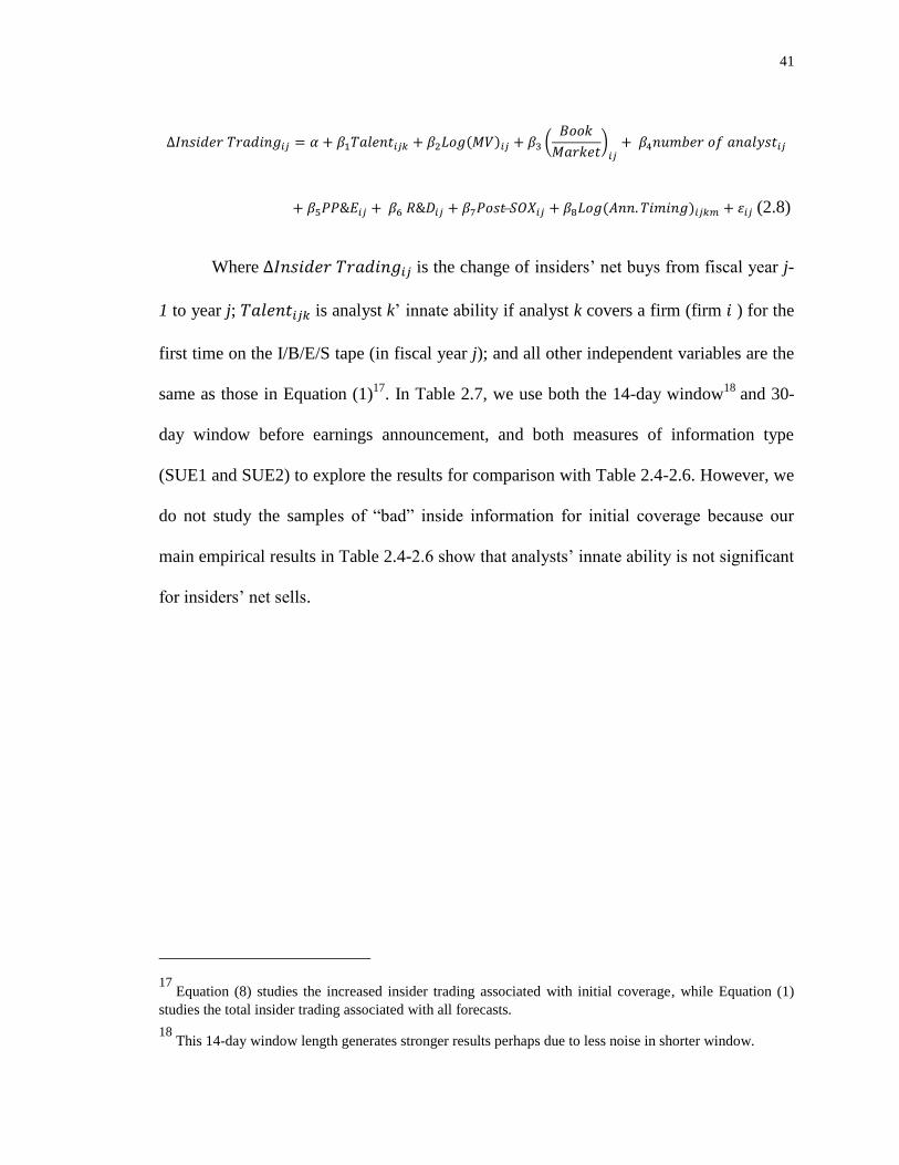
41

∆𝐼𝑛𝑠𝑖𝑑𝑒𝑟 𝑇𝑟𝑎𝑑𝑖𝑛𝑔𝑖𝑗 = 𝛼 + 𝛽1𝑇𝑎𝑙𝑒𝑛𝑡𝑖𝑗𝑘 + 𝛽2𝐿𝑜𝑔(𝑀𝑉)𝑖𝑗 + 𝛽3 (𝐵𝑜𝑜𝑘

𝑀𝑎𝑟𝑘𝑒𝑡)

𝑖𝑗+ 𝛽4𝑛𝑢𝑚𝑏𝑒𝑟 𝑜𝑓 𝑎𝑛𝑎𝑙𝑦𝑠𝑡𝑖𝑗

+ 𝛽5𝑃𝑃&𝐸𝑖𝑗 + 𝛽6 𝑅&𝐷𝑖𝑗 + 𝛽7𝑃𝑜𝑠𝑡 ̶𝑆𝑂𝑋𝑖𝑗 + 𝛽8𝐿𝑜𝑔(𝐴𝑛𝑛. 𝑇𝑖𝑚𝑖𝑛𝑔)𝑖𝑗𝑘𝑚 + 휀𝑖𝑗 (2.8)

Where ∆𝐼𝑛𝑠𝑖𝑑𝑒𝑟 𝑇𝑟𝑎𝑑𝑖𝑛𝑔𝑖𝑗 is the change of insiders’ net buys from fiscal year j-

1 to year j; 𝑇𝑎𝑙𝑒𝑛𝑡𝑖𝑗𝑘 is analyst k’ innate ability if analyst k covers a firm (firm 𝑖 ) for the

first time on the I/B/E/S tape (in fiscal year j); and all other independent variables are the

same as those in Equation (1)17

. In Table 2.7, we use both the 14-day window18

and 30-

day window before earnings announcement, and both measures of information type

(SUE1 and SUE2) to explore the results for comparison with Table 2.4-2.6. However, we

do not study the samples of “bad” inside information for initial coverage because our

main empirical results in Table 2.4-2.6 show that analysts’ innate ability is not significant

for insiders’ net sells.

17 Equation (8) studies the increased insider trading associated with initial coverage, while Equation (1)

studies the total insider trading associated with all forecasts.

18 This 14-day window length generates stronger results perhaps due to less noise in shorter window.

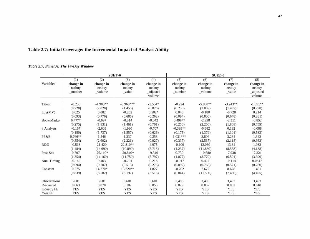
42

Table 2.7: Initial Coverage: the Incremental Impact of Analyst Ability

Table 2.7, Panel A: The 14-Day Window

SUE1>0 SUE2>0

(1) (2) (3) (4) (5) (6) (7) (8)

Variables

change in

netbuy

_number

change in

netbuy

_volume

change in

netbuy

_value

change in

netbuy

_adjusted

volume

change in

netbuy

_number

change in

netbuy

_volume

change in netbuy

_value

change in netbuy

_adjusted

volume

Talent -0.233 -4.909** -3.968*** -1.564* -0.224 -5.090** -3.243** -1.851**

(0.220) (2.020) (1.455) (0.826) (0.230) (2.069) (1.437) (0.798)

Log(MV) 0.025 0.082 -0.252 0.502* 0.040 -0.180 -0.728 0.214

(0.093) (0.776) (0.685) (0.262) (0.094) (0.800) (0.648) (0.261)

Book/Market 0.477* -0.097 -0.314 -0.042 0.498** -2.358 -2.511 -0.852

(0.275) (1.831) (1.461) (0.701) (0.250) (2.266) (1.808) (0.759)

# Analysts -0.167 -2.609 -1.930 -0.707 -0.399** -0.682 0.192 -0.088

(0.180) (1.737) (1.557) (0.626) (0.175) (1.379) (1.101) (0.532)

PP&E 0.766** 1.546 1.337 0.258 1.031*** 3.806 3.284 1.343

(0.354) (2.602) (2.221) (0.927) (0.337) (2.587) (2.118) (0.933)

R&D -0.513 21.420 22.810** 4.975 -0.100 12.060 13.64 1.983

(1.484) (14.690) (10.890) (5.713) (1.237) (11.830) (8.558) (4.138)

Post-Sox 0.707 -26.110* -20.840* -9.340 0.730 -10.680 -7.938 -2.221

(1.354) (14.160) (11.750) (5.797) (1.077) (8.779) (6.501) (3.399)

Ann. Timing -0.142 0.463 -0.201 0.218 -0.017 0.427 -0.114 0.0347

(0.094) (0.707) (0.513) (0.276) (0.092) (0.768) (0.521) (0.280)

Constant 0.275 14.270* 13.720** 1.827 -0.202 7.672 8.628 1.401

(0.839) (8.582) (6.192) (3.513) (0.844) (11.500) (7.430) (4.495)

Observations 3,601 3,601 3,601 3,601 3,493 3,493 3,493 3,493

R-squared 0.063 0.070 0.102 0.053 0.079 0.057 0.082 0.048

Industry FE YES YES YES YES YES YES YES YES

Year FE YES YES YES YES YES YES YES YES

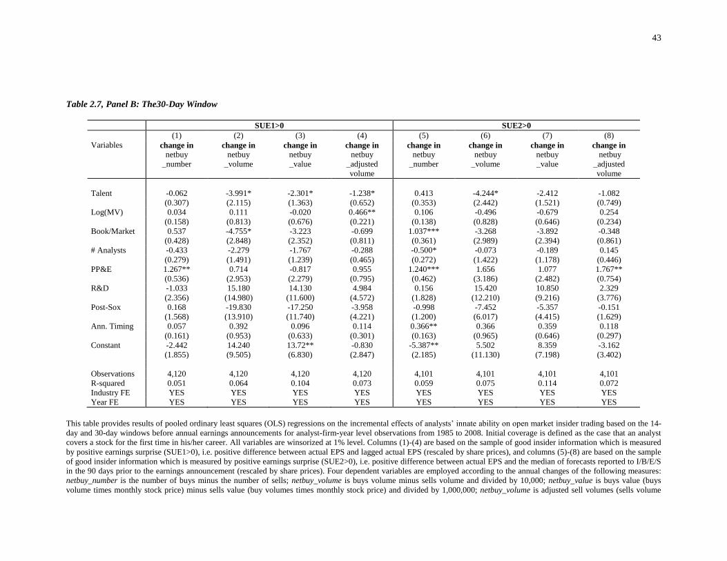
43

Table 2.7, Panel B: The30-Day Window

SUE1>0 SUE2>0

(1) (2) (3) (4) (5) (6) (7) (8)

Variables

change in

netbuy

_number

change in netbuy

_volume

change in netbuy

_value

change in netbuy

_adjusted

volume

change in netbuy

_number

change in netbuy

_volume

change in netbuy

_value

change in

netbuy

_adjusted

volume

Talent -0.062 -3.991* -2.301* -1.238* 0.413 -4.244* -2.412 -1.082

(0.307) (2.115) (1.363) (0.652) (0.353) (2.442) (1.521) (0.749)

Log(MV) 0.034 0.111 -0.020 0.466** 0.106 -0.496 -0.679 0.254

(0.158) (0.813) (0.676) (0.221) (0.138) (0.828) (0.646) (0.234)

Book/Market 0.537 -4.755* -3.223 -0.699 1.037*** -3.268 -3.892 -0.348

(0.428) (2.848) (2.352) (0.811) (0.361) (2.989) (2.394) (0.861)

# Analysts -0.433 -2.279 -1.767 -0.288 -0.500* -0.073 -0.189 0.145

(0.279) (1.491) (1.239) (0.465) (0.272) (1.422) (1.178) (0.446)

PP&E 1.267** 0.714 -0.817 0.955 1.240*** 1.656 1.077 1.767**

(0.536) (2.953) (2.279) (0.795) (0.462) (3.186) (2.482) (0.754)

R&D -1.033 15.180 14.130 4.984 0.156 15.420 10.850 2.329

(2.356) (14.980) (11.600) (4.572) (1.828) (12.210) (9.216) (3.776)

Post-Sox 0.168 -19.830 -17.250 -3.958 -0.998 -7.452 -5.357 -0.151

(1.568) (13.910) (11.740) (4.221) (1.200) (6.017) (4.415) (1.629)

Ann. Timing 0.057 0.392 0.096 0.114 0.366** 0.366 0.359 0.118

(0.161) (0.953) (0.633) (0.301) (0.163) (0.965) (0.646) (0.297)

Constant -2.442 14.240 13.72** -0.830 -5.387** 5.502 8.359 -3.162

(1.855) (9.505) (6.830) (2.847) (2.185) (11.130) (7.198) (3.402)

Observations 4,120 4,120 4,120 4,120 4,101 4,101 4,101 4,101

R-squared 0.051 0.064 0.104 0.073 0.059 0.075 0.114 0.072

Industry FE YES YES YES YES YES YES YES YES

Year FE YES YES YES YES YES YES YES YES

This table provides results of pooled ordinary least squares (OLS) regressions on the incremental effects of analysts’ innate ability on open market insider trading based on the 14-

day and 30-day windows before annual earnings announcements for analyst-firm-year level observations from 1985 to 2008. Initial coverage is defined as the case that an analyst

covers a stock for the first time in his/her career. All variables are winsorized at 1% level. Columns (1)-(4) are based on the sample of good insider information which is measured

by positive earnings surprise (SUE1>0), i.e. positive difference between actual EPS and lagged actual EPS (rescaled by share prices), and columns (5)-(8) are based on the sample

of good insider information which is measured by positive earnings surprise (SUE2>0), i.e. positive difference between actual EPS and the median of forecasts reported to I/B/E/S

in the 90 days prior to the earnings announcement (rescaled by share prices). Four dependent variables are employed according to the annual changes of the following measures:

netbuy_number is the number of buys minus the number of sells; netbuy_volume is buys volume minus sells volume and divided by 10,000; netbuy_value is buys value (buys

volume times monthly stock price) minus sells value (buy volumes times monthly stock price) and divided by 1,000,000; netbuy_volume is adjusted sell volumes (sells volume

44

divided by the number of shares outstanding) minus buys volume (buys volume divided by the number of shares outstanding). The results of insiders’ net sells based on bad inside

information are not significant and are not reported here. The key independent variable is analysts’ innate ability, which is labeled as Talent. The control variables are: Log(MV),

the logarithm of market capitalization of the firm; Book/Market, the ratio of book value of the firm to its market value; The Number of Analysts, the logarithm of the number of

analysts following the firm in a fiscal year; PP&E, the property, plant and equipment divided by total assets; R&D, the research and development expenses divided by total assets.

Post-Sox, the dummy that equals 1 if insider trading window is after 2002 September, and 0 elsewhere; Log (Ann. Timing) is the logarithm of the number of days between the

initial earnings forecast date (before insider trading window) by the analyst and the earnings announcement date by the firm. All regressions include year fixed effect and industry

(2-digit SIC) fixed effect. Robust standard errors in parentheses are clustered at firm level, and ***, ** and * stand for statistical significance at 0.01, 0.05 and 0.1 level

respectively.

45

The results in Panel A of Table 2.7 are more significant than the results in Panel B

of Table 2.7, implying the effects of analysts’ innate ability on corporate insiders’ net

buys through initial coverage are concentrated in the 14-day window19

prior to an

earnings announcement, although as many as 87.40 % observations are overlapped in the

two windows. Another obvious phenomenon is that the effects of innate ability from

initial coverage are stronger compared with those based on the whole sample of all

forecasts in Table 2.4-2.6; this might imply that analysts’ initial coverage is considered

important by both analysts and corporate insiders. For example, in the 30-day event

window, the coefficient of innate ability in the regression on net-buy volumes for initial

coverage is 2.5 (=4.244/1.696) times larger than that for the whole sample if SUE2 is

used.

We also investigate the influences of initial coverage by the analysts of the

highest ability among those who cover the same firm in the same fiscal year because

high-talent analysts are supposed to be more capable of collecting firm-specific

information. The specification is the same as equation (8) and the results are provided in

Table 2.8. We find that in this case only SUE1 rather than SUE2 works if insiders have

“good” inside information. In the 14-day window, the change in the number of net buys,

the change in the volume of net buys, and the change in the value of net buys are all

significant, while in the 30-day window only the change in the volume of net buys is

significant. If we compare Table 2.7 and Table 2.8, we find the absolute values of the

coefficients of innate ability, as based on the sample of initial coverage by the highest-

19 It is still marginally significant in the 30-day window in Table 7, Panel B.

46

ability analysts, are stronger than those based on the whole sample of initial coverage.

Combined with the results in Tables 2.4-2.6, the sequence of relative economic

significance is: initial coverage by the analyst with the highest ability>initial coverage by

all analysts> all coverage.

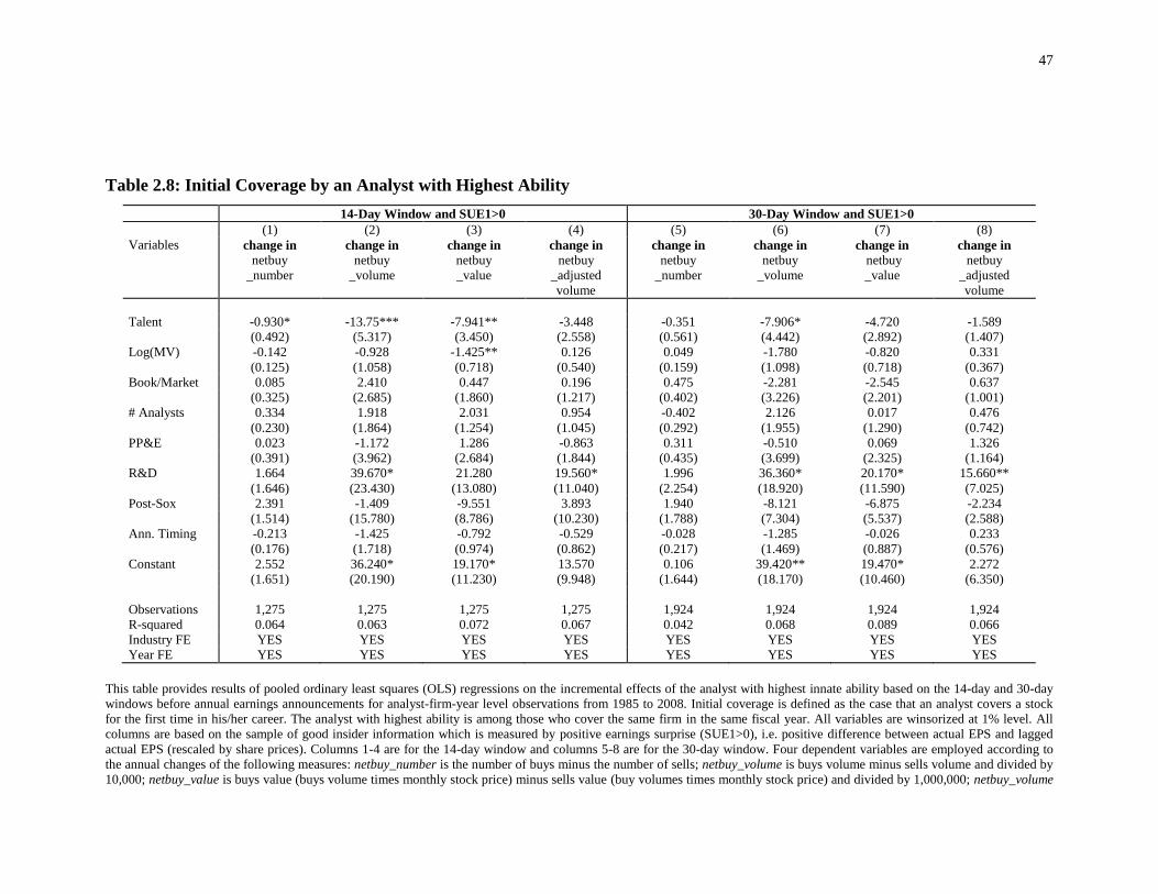
47

Table 2.8: Initial Coverage by an Analyst with Highest Ability

14-Day Window and SUE1>0 30-Day Window and SUE1>0

(1) (2) (3) (4) (5) (6) (7) (8)

Variables

change in

netbuy

_number

change in netbuy

_volume

change in netbuy

_value

change in netbuy

_adjusted

volume

change in netbuy

_number

change in netbuy

_volume

change in

netbuy

_value

change in netbuy

_adjusted

volume

Talent -0.930* -13.75*** -7.941** -3.448 -0.351 -7.906* -4.720 -1.589

(0.492) (5.317) (3.450) (2.558) (0.561) (4.442) (2.892) (1.407)

Log(MV) -0.142 -0.928 -1.425** 0.126 0.049 -1.780 -0.820 0.331

(0.125) (1.058) (0.718) (0.540) (0.159) (1.098) (0.718) (0.367)

Book/Market 0.085 2.410 0.447 0.196 0.475 -2.281 -2.545 0.637

(0.325) (2.685) (1.860) (1.217) (0.402) (3.226) (2.201) (1.001)

# Analysts 0.334 1.918 2.031 0.954 -0.402 2.126 0.017 0.476

(0.230) (1.864) (1.254) (1.045) (0.292) (1.955) (1.290) (0.742)

PP&E 0.023 -1.172 1.286 -0.863 0.311 -0.510 0.069 1.326

(0.391) (3.962) (2.684) (1.844) (0.435) (3.699) (2.325) (1.164)

R&D 1.664 39.670* 21.280 19.560* 1.996 36.360* 20.170* 15.660**

(1.646) (23.430) (13.080) (11.040) (2.254) (18.920) (11.590) (7.025)

Post-Sox 2.391 -1.409 -9.551 3.893 1.940 -8.121 -6.875 -2.234

(1.514) (15.780) (8.786) (10.230) (1.788) (7.304) (5.537) (2.588)

Ann. Timing -0.213 -1.425 -0.792 -0.529 -0.028 -1.285 -0.026 0.233

(0.176) (1.718) (0.974) (0.862) (0.217) (1.469) (0.887) (0.576)

Constant 2.552 36.240* 19.170* 13.570 0.106 39.420** 19.470* 2.272

(1.651) (20.190) (11.230) (9.948) (1.644) (18.170) (10.460) (6.350)

Observations 1,275 1,275 1,275 1,275 1,924 1,924 1,924 1,924

R-squared 0.064 0.063 0.072 0.067 0.042 0.068 0.089 0.066

Industry FE YES YES YES YES YES YES YES YES

Year FE YES YES YES YES YES YES YES YES

This table provides results of pooled ordinary least squares (OLS) regressions on the incremental effects of the analyst with highest innate ability based on the 14-day and 30-day

windows before annual earnings announcements for analyst-firm-year level observations from 1985 to 2008. Initial coverage is defined as the case that an analyst covers a stock

for the first time in his/her career. The analyst with highest ability is among those who cover the same firm in the same fiscal year. All variables are winsorized at 1% level. All

columns are based on the sample of good insider information which is measured by positive earnings surprise (SUE1>0), i.e. positive difference between actual EPS and lagged

actual EPS (rescaled by share prices). Columns 1-4 are for the 14-day window and columns 5-8 are for the 30-day window. Four dependent variables are employed according to

the annual changes of the following measures: netbuy_number is the number of buys minus the number of sells; netbuy_volume is buys volume minus sells volume and divided by

10,000; netbuy_value is buys value (buys volume times monthly stock price) minus sells value (buy volumes times monthly stock price) and divided by 1,000,000; netbuy_volume

48

is adjusted sell volumes (sells volume divided by the number of shares outstanding) minus buys volume (buys volume divided by the number of shares outstanding). The key

independent variable is analysts’ innate ability, which is labeled as Talent. The control variables are: Log(MV), the logarithm of market capitalization of the firm; Book/Market, the

ratio of book value of the firm to its market value; The Number of Analysts, the logarithm of the number of analysts following the firm in a fiscal year; PP&E, the property, plant

and equipment divided by total assets; R&D, the research and development expenses divided by total assets. Post-Sox, the dummy that equals 1 if insider trading window is after

2002 September, and 0 elsewhere; Log(Ann. Timing) is the logarithm of the number of days between the initial earnings forecast date (before insider trading window) by the

analyst and the earnings announcement date by the firm. All regressions include year fixed effect and industry (2-digit SIC) fixed effect. Robust standard errors in parentheses are

clustered at firm level, and ***, ** and * stand for statistical significance at 0.01, 0.05 and 0.1 level respectively.

49

In addition, in Column 1 of Table 2.8, we find highest ability is negatively

associated with the change in the number of transactions of net buys. Frankel and Li

(2004) argue that the frequency of insider trades can be used as a measure of insider

trading profits because more trades are expected when insiders’ private information is

more valuable given the same trading costs. In this economic sense, our results suggest

that analysts with the highest innate ability can serve to confine insider trading profits.

The empirical results of initial coverage imply that analysts’ innate ability can

affect insider trading intensity without any general experience or firm-specific

experience; this is consistent with the “innate” nature of our novel measure. In addition,

the stronger effects of initial coverage on insider trading do not mean analysts’ innate

ability deteriorates with time, likely because analysts are more cautious and put more

efforts to utilize their innate ability on their “first show”, or because innate ability is

initially less twisted by other factors since analysts want to build their reputation through

initial coverage.

2.3.4 Regressions at Firm-Year Level and Analyst-Firm-Year Level

This section is also dedicated to robustness checks. In section 2.3.1 to 2.3.3, we

focus on regressions on the forecast level which conveys accurate information of forecast

timing and frequency; in this section, we also test firm-year level and analyst-firm-year

level to explore whether the relationship between analysts’ innate ability and insiders’ net

buys still holds. However, we expect firm-year level and analyst-firm-year level to

provide weaker results. Each forecast represents specific information flow given different

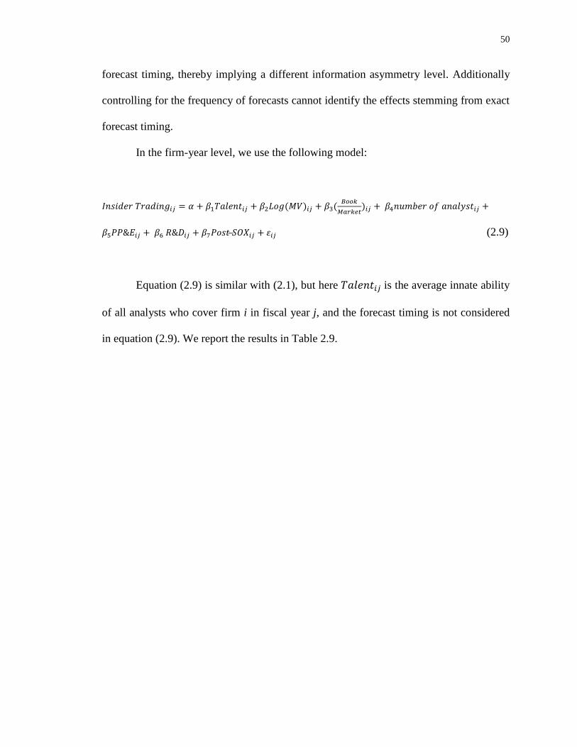
50

forecast timing, thereby implying a different information asymmetry level. Additionally

controlling for the frequency of forecasts cannot identify the effects stemming from exact

forecast timing.

In the firm-year level, we use the following model:

𝐼𝑛𝑠𝑖𝑑𝑒𝑟 𝑇𝑟𝑎𝑑𝑖𝑛𝑔𝑖𝑗 = 𝛼 + 𝛽1𝑇𝑎𝑙𝑒𝑛𝑡𝑖𝑗 + 𝛽2𝐿𝑜𝑔(𝑀𝑉)𝑖𝑗 + 𝛽3(𝐵𝑜𝑜𝑘

𝑀𝑎𝑟𝑘𝑒𝑡)𝑖𝑗 + 𝛽4𝑛𝑢𝑚𝑏𝑒𝑟 𝑜𝑓 𝑎𝑛𝑎𝑙𝑦𝑠𝑡𝑖𝑗 +

𝛽5𝑃𝑃&𝐸𝑖𝑗 + 𝛽6 𝑅&𝐷𝑖𝑗 + 𝛽7𝑃𝑜𝑠𝑡 ̶𝑆𝑂𝑋𝑖𝑗 + 휀𝑖𝑗 (2.9)

Equation (2.9) is similar with (2.1), but here 𝑇𝑎𝑙𝑒𝑛𝑡𝑖𝑗 is the average innate ability

of all analysts who cover firm i in fiscal year j, and the forecast timing is not considered

in equation (2.9). We report the results in Table 2.9.

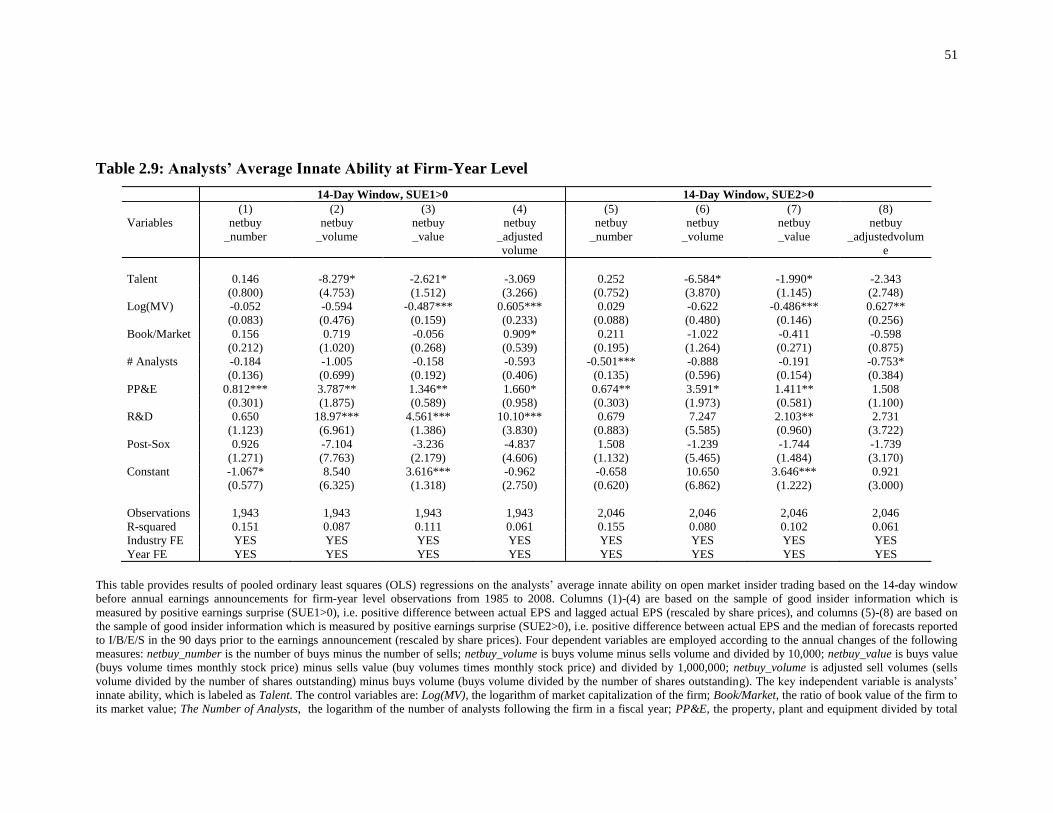
51

Table 2.9: Analysts’ Average Innate Ability at Firm-Year Level

14-Day Window, SUE1>0 14-Day Window, SUE2>0

(1) (2) (3) (4) (5) (6) (7) (8)

Variables

netbuy

_number

netbuy

_volume

netbuy

_value

netbuy

_adjusted

volume

netbuy

_number

netbuy

_volume

netbuy

_value

netbuy

_adjustedvolum

e

Talent 0.146 -8.279* -2.621* -3.069 0.252 -6.584* -1.990* -2.343

(0.800) (4.753) (1.512) (3.266) (0.752) (3.870) (1.145) (2.748)

Log(MV) -0.052 -0.594 -0.487*** 0.605*** 0.029 -0.622 -0.486*** 0.627**

(0.083) (0.476) (0.159) (0.233) (0.088) (0.480) (0.146) (0.256)

Book/Market 0.156 0.719 -0.056 0.909* 0.211 -1.022 -0.411 -0.598

(0.212) (1.020) (0.268) (0.539) (0.195) (1.264) (0.271) (0.875)

# Analysts -0.184 -1.005 -0.158 -0.593 -0.501*** -0.888 -0.191 -0.753*

(0.136) (0.699) (0.192) (0.406) (0.135) (0.596) (0.154) (0.384)

PP&E 0.812*** 3.787** 1.346** 1.660* 0.674** 3.591* 1.411** 1.508

(0.301) (1.875) (0.589) (0.958) (0.303) (1.973) (0.581) (1.100)

R&D 0.650 18.97*** 4.561*** 10.10*** 0.679 7.247 2.103** 2.731

(1.123) (6.961) (1.386) (3.830) (0.883) (5.585) (0.960) (3.722)

Post-Sox 0.926 -7.104 -3.236 -4.837 1.508 -1.239 -1.744 -1.739

(1.271) (7.763) (2.179) (4.606) (1.132) (5.465) (1.484) (3.170)

Constant -1.067* 8.540 3.616*** -0.962 -0.658 10.650 3.646*** 0.921

(0.577) (6.325) (1.318) (2.750) (0.620) (6.862) (1.222) (3.000)

Observations 1,943 1,943 1,943 1,943 2,046 2,046 2,046 2,046

R-squared 0.151 0.087 0.111 0.061 0.155 0.080 0.102 0.061

Industry FE YES YES YES YES YES YES YES YES

Year FE YES YES YES YES YES YES YES YES

This table provides results of pooled ordinary least squares (OLS) regressions on the analysts’ average innate ability on open market insider trading based on the 14-day window

before annual earnings announcements for firm-year level observations from 1985 to 2008. Columns (1)-(4) are based on the sample of good insider information which is

measured by positive earnings surprise (SUE1>0), i.e. positive difference between actual EPS and lagged actual EPS (rescaled by share prices), and columns (5)-(8) are based on

the sample of good insider information which is measured by positive earnings surprise (SUE2>0), i.e. positive difference between actual EPS and the median of forecasts reported

to I/B/E/S in the 90 days prior to the earnings announcement (rescaled by share prices). Four dependent variables are employed according to the annual changes of the following

measures: netbuy_number is the number of buys minus the number of sells; netbuy_volume is buys volume minus sells volume and divided by 10,000; netbuy_value is buys value

(buys volume times monthly stock price) minus sells value (buy volumes times monthly stock price) and divided by 1,000,000; netbuy_volume is adjusted sell volumes (sells

volume divided by the number of shares outstanding) minus buys volume (buys volume divided by the number of shares outstanding). The key independent variable is analysts’

innate ability, which is labeled as Talent. The control variables are: Log(MV), the logarithm of market capitalization of the firm; Book/Market, the ratio of book value of the firm to

its market value; The Number of Analysts, the logarithm of the number of analysts following the firm in a fiscal year; PP&E, the property, plant and equipment divided by total

52

assets; R&D, the research and development expenses divided by total assets. Post-Sox, the dummy that equals 1 if insider trading window is after 2002 September, and 0

elsewhere; Log(Ann. Timing) is the logarithm of the number of days between the initial earnings forecast date (before insider trading window) by the analyst and the earnings

announcement date by the firm. All regressions include year fixed effect and industry (2-digit SIC) fixed effect. Robust standard errors in parentheses are clustered at firm level,

and ***, ** and * stand for statistical significance at 0.01, 0.05 and 0.1 level respectively.

53

In Table 2.9, innate ability is only significant in the 14-day window prior to

earnings announcements, which may be due to the fact that the longer window (30-day)

has more noise. For both SUE1 and SUE2, innate ability is negatively associated with the

volume of net buys and the value of net buys when insiders have “good” information

about earnings. These results are consistent with the results in Table 2.4-Table 2.6,

although Table 2.9 provides less significant results. The possible reason is that we ignore

forecast timing and frequency in Table 2.9 so the role of analysts’ innate ability cannot be

examined accurately.

In the analyst-firm-year level, we add the frequency of forecasts as a control

variable, which is defined as the number of forecasts by an analyst for a covered firm in a

fiscal year. The specification at analyst-firm-year level is:

𝐼𝑛𝑠𝑖𝑑𝑒𝑟 𝑇𝑟𝑎𝑑𝑖𝑛𝑔𝑖𝑗 = 𝛼 + 𝛽1𝑇𝑎𝑙𝑒𝑛𝑡𝑖𝑗𝑘 + 𝛽2𝐿𝑜𝑔(𝑀𝑉)𝑖𝑗 + 𝛽3(𝐵𝑜𝑜𝑘

𝑀𝑎𝑟𝑘𝑒𝑡)𝑖𝑗 + 𝛽4𝑛𝑢𝑚𝑏𝑒𝑟 𝑜𝑓 𝑎𝑛𝑎𝑙𝑦𝑠𝑡𝑖𝑗 +

𝛽5𝑃𝑃&𝐸𝑖𝑗 + 𝛽6 𝑅&𝐷𝑖𝑗 + 𝛽7𝑃𝑜𝑠𝑡 ̶𝑆𝑂𝑋𝑖𝑗 + 𝛽8𝐹𝑟𝑒𝑞𝑢𝑒𝑛𝑐𝑦𝑖𝑗𝑘 + 휀𝑖𝑗 (2.10)

Where 𝐹𝑟𝑒𝑞𝑢𝑒𝑛𝑐𝑦𝑖𝑗𝑘 is the number of forecasts by analyst k covering firm i for

fiscal year j, and all other variables are the same as the setting in equation (2.1). We

expect 𝐹𝑟𝑒𝑞𝑢𝑒𝑛𝑐𝑦𝑖𝑗𝑘 has a negative sign since more forecasts help reduce information

asymmetry. However, we are aware that frequency cannot identify the information that

the timing of each forecast conveys. If an analyst forecasts the EPS of a firm one year

beforehand, intuitively it will have weaker effects than a forecast which is announced just

a few months beforehand. We report the results at analyst-firm-year level in Table 2.10.

54

Table 2.10: Analysts’ Innate Ability at Analyst-Firm-Year Level

14-Day Window, SUE1>0 30-Day Window, SUE1>0

(1) (2) (3) (4) (5) (6) (7) (8)

Variables

netbuy

_number

netbuy

_volume

netbuy

_value

netbuy

_adjusted

volume

netbuy

_number

netbuy

_volume

netbuy

_value

netbuy

_adjusted

volume

Talent 0.079 -1.226* -0.550 -0.350* 0.101 -1.094 -0.472 -0.318*

(0.107) (0.720) (0.340) (0.183) (0.112) (0.751) (0.357) (0.188)

Log(MV) 0.024 -1.104* -0.629** 0.393*** 0.027 -1.141* -0.636** 0.378***

(0.099) (0.638) (0.288) (0.119) (0.098) (0.636) (0.285) (0.117)

Book/Market 0.837*** -0.044 0.001 0.467 0.863*** 0.091 0.028 0.475

(0.255) (1.328) (0.554) (0.362) (0.257) (1.346) (0.552) (0.366)

# Analysts -0.131 -0.234 0.023 -0.234 -0.136 -0.163 0.040 -0.204

(0.161) (1.114) (0.485) (0.313) (0.160) (1.109) (0.481) (0.308)

PP&E 0.832*** 4.099** 1.747** 0.524 0.846*** 4.032** 1.715** 0.525

(0.312) (1.839) (0.831) (0.426) (0.310) (1.821) (0.817) (0.420)

R&D 1.496 15.65*** 7.202*** 4.761*** 1.577 16.39*** 7.374*** 4.880***

(1.147) (5.901) (2.624) (1.680) (1.212) (6.152) (2.717) (1.723)

Post-Sox 0.787 -7.258 -4.731 -2.104 0.745 -7.092 -4.574 -2.070

(1.071) (5.761) (3.143) (1.742) (0.952) (5.490) (3.041) (1.695)

Frequency -0.054** -0.242 -0.083 -0.043 -0.056** -0.252 -0.088 -0.039

(0.022) (0.149) (0.070) (0.037) (0.023) (0.155) (0.072) (0.039)

Constant -1.682** 9.914* 4.496** -0.911 -1.742*** 9.974* 4.489** -1.000

(0.667) (5.565) (1.871) (1.380) (0.668) (5.671) (1.869) (1.352)

Observations 18,036 18,036 18,036 18,036 17,845 17,845 17,845 17,845

R-squared 0.176 0.113 0.103 0.091 0.174 0.113 0.103 0.090

Industry FE YES YES YES YES YES YES YES YES

Year FE YES YES YES YES YES YES YES YES

This table provides results of pooled ordinary least squares (OLS) regressions on the analysts’ innate ability based on the 14-day and 30-day windows before annual earnings

announcements for analyst-firm-year level observations from 1985 to 2008. All variables are winsorized at 1% level. All columns are based on the sample of good insider

information which is measured by positive earnings surprise (SUE1>0), i.e. positive difference between actual EPS and lagged actual EPS (rescaled by share prices). Columns 1-4

are for the 14-day window and columns 5-8 are for the 30-day window. Four dependent variables are employed according to the annual changes of the following measures:

netbuy_number is the number of buys minus the number of sells; netbuy_volume is buys volume minus sells volume and divided by 10,000; netbuy_value is buys value (buys

volume times monthly stock price) minus sells value (buy volumes times monthly stock price) and divided by 1,000,000; netbuy_volume is adjusted sell volumes (sells volume

divided by the number of shares outstanding) minus buys volume (buys volume divided by the number of shares outstanding). The key independent variable is analysts’ innate

ability, which is labeled as Talent. The control variables are: Log(MV), the logarithm of market capitalization of the firm; Book/Market, the ratio of book value of the firm to its

55

market value; The Number of Analysts, the logarithm of the number of analysts following the firm in a fiscal year; PP&E, the property, plant and equipment divided by total

assets; R&D, the research and development expenses divided by total assets. Post-Sox, the dummy that equals 1 if insider trading window is after 2002 September, and 0

elsewhere; Log(Ann. Timing) is the logarithm of the number of days between the initial earnings forecast date (before insider trading window) by the analyst and the earnings

announcement date by the firm. Frequency is the number of forecasts by an analyst for a covered firm in a fiscal year. All regressions include year fixed effect and industry (2-digit

SIC) fixed effect. Robust standard errors in parentheses are clustered at firm level, and ***, ** and * stand for statistical significance at 0.01, 0.05 and 0.1 level respectively.

56

In Table 2.10, Only SUE1 generates significant results for analysts’ innate ability

if corporate insiders have “good” inside information about annual EPS. In the 14-day

event window, analysts with higher innate ability are associated with smaller volumes

and smaller adjusted volumes of insiders’ net buys. In the 30-day event window, the

negative relation only resides in adjusted volumes of insiders’ net buys. Compared with

Table 2.4, Table 2.10 has less statistically significant results and the effects of analysts’

innate ability on insider trading are weaker in economic significance. Thus we should not

ignore the exact timing of forecasts even if we consider the frequency of forecasts.

2.4 Analysts’ Innate Ability and Insider Trading Informativeness

The informativeness of insider trading is well documented in the literature

although the SEC requires that no trading by corporate insiders be based on non-public

and material information. For example, Finnerty(1976), Seyhun(1986), Rozeff and

Zaman(1988), and Lakonishok and Lee(2001), all find that corporate insider can earn

abnormal returns. For our research purpose, we care about how analysts’ innate ability

can affect insider trading informativeness. Piotroski and Roulstone (2004), and Chan and

Hameed (2006) find that analyst following positively affects the relative amount of

market- and industry-level information in stock prices, while Liu (2011) and Crawford,

Roulstone, and So (2012) suggest analysts can provide firm-specific information in stock

prices. We assume analysts with higher ability are more capable of collecting firm-

specific information and postulate that analysts can reduce the magnitude of insider

trading informativeness around earnings announcements through earnings forecasts.

57

We measure insider trading informativeness by post-trade cumulated abnormal

return (CAR). This measure is widely used to measure informativeness in the existing

literature such as Lakonishok and Lee (2001) and Frankel and Li (2004). To generate

CARs, we employ the market model and sum up daily abnormal returns. Consistent with

the window used in the main regressions, we restrict the insider trading sample at the

forecast-analyst-firm-year level within one month prior to annual earnings

announcements by firms. In addition, to guarantee the commonly used one-week event

window is prior to earnings announcements by firms, the sample includes all insider

trades in the -30 to -7 trading day window prior to earnings announcements. However,

this consideration is only for accuracy in the regressions on CAR [0,i] for 𝑖 ≤ 5. For

CARs in the longer periods such as the 3-month and 6-month window, as we have a large

data sample, the effects of announcements of good earnings and bad earnings can

basically cancel out.

First, we investigate the insider trading informativeness for different quantiles of

analysts’ innate ability in long, post-trading periods. We divide the ability data into 9

quantiles20

where quantile 1 refers to low ability, quantile 5 refers to median ability, and

quantile 9 refers to high ability. Then, we calculate the mean CAR for each trading day

surrounding earnings announcement dates by the firms and generate the time-series of the

mean CARs in the days of [-20, 120] window (day 0 is the trading day) for different

ability quantiles in Figure 2.2. In Figure 2.2A and Figure 2.2B, we find analysts with

higher ability are mapped into lower level of insider trading informativeness for insider

20 It is convenient to identify the median quantile in odd quantiles. We also conduct sensitivity analysis for

5 quantiles, 7quantiles, and 11 quantiles. The results are quite similar for the time series of mean CARs.

58

sells and higher levels of insider trading informative for insider buys. But when we

distinguish the insiders’ information type, we see some differences. In Figure 2.2C, we

find higher ability is related to smaller positive CARs when insiders have good

information about earnings, while this relation does not hold when insiders have bad

information about earnings. In Figure 2.2D, higher ability is related to smaller absolute

values of CARs no matter what the information type is, which is consistent with Figure

2.2A.

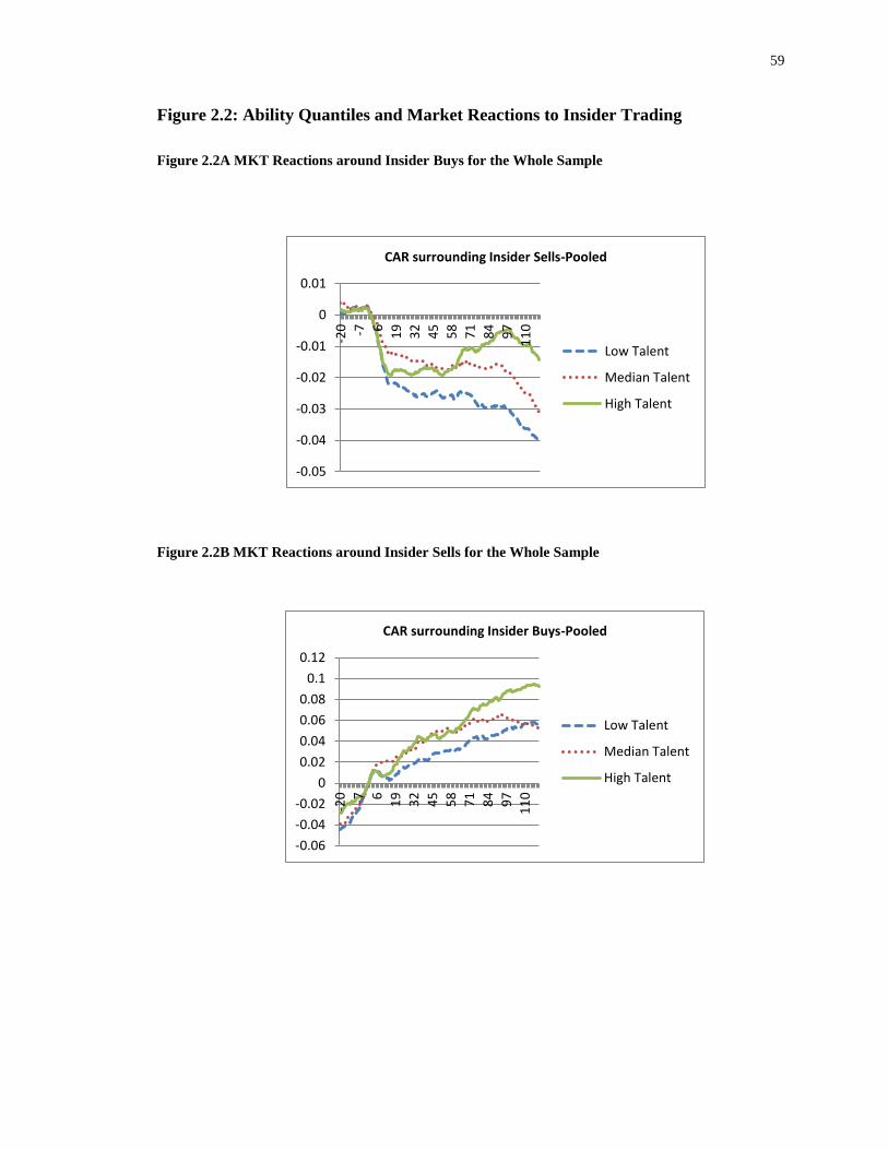
59

Figure 2.2: Ability Quantiles and Market Reactions to Insider Trading

Figure 2.2A MKT Reactions around Insider Buys for the Whole Sample

Figure 2.2B MKT Reactions around Insider Sells for the Whole Sample

-0.05

-0.04

-0.03

-0.02

-0.01

0

0.01

-20 -7 6

19

32

45

58

71

84

97

11

0

CAR surrounding Insider Sells-Pooled

Low Talent

Median Talent

High Talent

-0.06

-0.04

-0.02

0

0.02

0.04

0.06

0.08

0.1

0.12

-20 -7 6

19

32

45

58

71

84

97

11

0

CAR surrounding Insider Buys-Pooled

Low Talent

Median Talent

High Talent

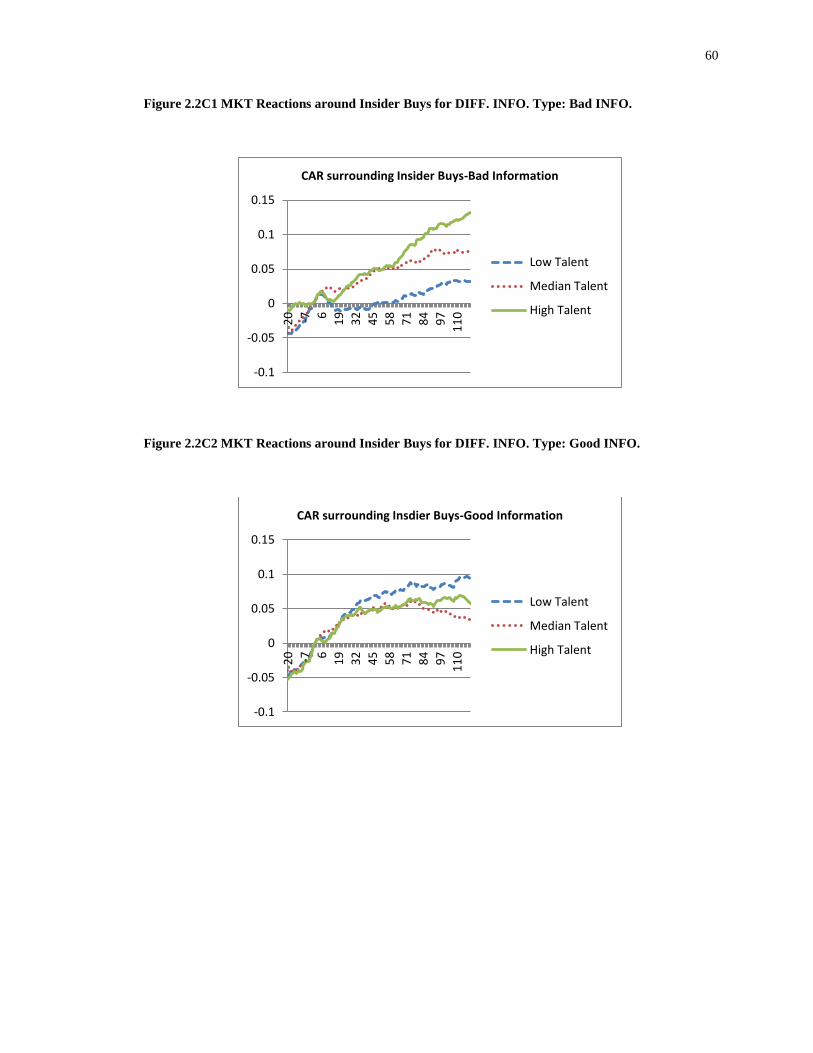
60

Figure 2.2C1 MKT Reactions around Insider Buys for DIFF. INFO. Type: Bad INFO.

Figure 2.2C2 MKT Reactions around Insider Buys for DIFF. INFO. Type: Good INFO.

-0.1

-0.05

0

0.05

0.1

0.15

-20 -7 6

19

32

45

58

71

84

97

11

0

CAR surrounding Insider Buys-Bad Information

Low Talent

Median Talent

High Talent

-0.1

-0.05

0

0.05

0.1

0.15

-20 -7 6

19

32

45

58

71

84

97

11

0

CAR surrounding Insdier Buys-Good Information

Low Talent

Median Talent

High Talent

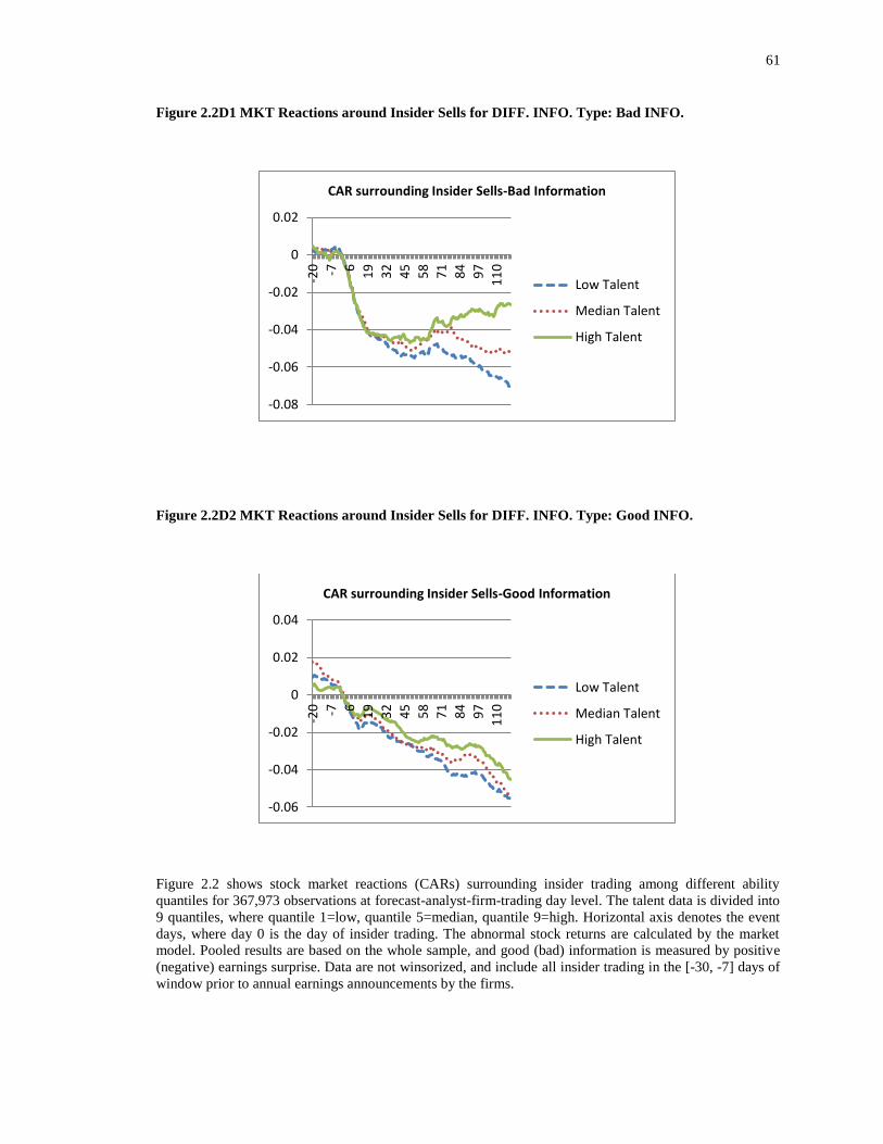
61

Figure 2.2D1 MKT Reactions around Insider Sells for DIFF. INFO. Type: Bad INFO.

Figure 2.2D2 MKT Reactions around Insider Sells for DIFF. INFO. Type: Good INFO.

Figure 2.2 shows stock market reactions (CARs) surrounding insider trading among different ability

quantiles for 367,973 observations at forecast-analyst-firm-trading day level. The talent data is divided into

9 quantiles, where quantile 1=low, quantile 5=median, quantile 9=high. Horizontal axis denotes the event

days, where day 0 is the day of insider trading. The abnormal stock returns are calculated by the market

model. Pooled results are based on the whole sample, and good (bad) information is measured by positive

(negative) earnings surprise. Data are not winsorized, and include all insider trading in the [-30, -7] days of

window prior to annual earnings announcements by the firms.

-0.08

-0.06

-0.04

-0.02

0

0.02

-20 -7 6

19

32

45

58

71

84

97

11

0

CAR surrounding Insider Sells-Bad Information

Low Talent

Median Talent

High Talent

-0.06

-0.04

-0.02

0

0.02

0.04

-20 -7 6

19

32

45

58

71

84

97

11

0

CAR surrounding Insider Sells-Good Information

Low Talent

Median Talent

High Talent

62

To explain Figure 2.2, we conduct the t-statistics for the comparisons of paired

sample in the time-series means of stock market reactions between the high ability group

and the low ability group. We test the difference for four time-series CARs: one and a

half months(from CAR[0,0] to CAR[0,30]), three months (from CAR[0,0] to

CAR[0,60]), four and a half months (from CAR[0,0] to CAR[0,90]), and half a year(from

CAR[0,0] to CAR[0,120]). In Table 2.11, Panel A, we find all of the differences are

statistically significant at the 1% level, and the signs are consistent with the Figure 2.2.

Higher ability is related to lower level of insider trading informativeness for insider sells,

but this relation only applies for insider buys if insiders have “good” information about

earnings. This is consistent with our results in insider trading intensity that analysts’

annual forecasts mainly help restrict insider trading when insiders have “good”

information. In Table 2.11, Panel B, we find the differences of means between the high-

ability group and the low-ability group are larger as the time-series expands, for example,

in the half a year window, if insiders have good information about earnings, the mean

difference of mean CARs is 0.95% for insider sells and -1.65% for insider buys.

Table 2.11: Ability Difference and Market Reactions to Insider Trading

Table 2.11, Panel A: T Statistics for Means of Paired Samples

High Ability minus Low Ability

all sells all buys sells+good sells+bad buys+good buys+bad

CAR[0,0]~CAR[0,120] -15.92*** -20.77*** -22.94*** -12.01*** 19.20*** -21.08***

CAR[0,0]~CAR[0,90] -13.50*** -16.88*** -18.16*** -10.52*** 14.44*** -16.92***

CAR[0,0]~CAR[0,60] -13.20*** -12.78*** -17.82*** -7.79*** 9.00*** -12.55***

CAR[0,0]~CAR[0,30] -6.54*** -5.76*** -10.24*** -2.00* 5.75*** -6.27***

63

Table 2.11, Panel B: Differences of Means

High Ability minus Low Ability

all sells all buys sells+good sells+bad buys+good buys+bad

Expected Sign

(Mean Diff.)

+ - + + - -

Actual Sign

(Mean Diff.)

+ + + + - +

CAR[0,0]~CAR[0,120] 0.01320 0.02193 0.00947 0.01436 -0.01652 0.05576

CAR[0,0]~CAR[0,90] 0.00907 0.01743 0.00800 0.00792 -0.01404 0.04490

CAR[0,0]~CAR[0,60] 0.00527 0.01251 0.00553 0.00387 -0.00980 0.03206

CAR[0,0]~CAR[0,30] 0.00280 0.00677 0.00493 0.00049 -0.00238 0.01509

Table 2.11 provides the t-statistics for the comparisons of paired samples in the time-series means of stock

market reactions (CARs) between high ability group and low ability group surrounding insider trading (day

0 is the day of insider trading) corresponding to Figure 2.2 for 367,973 observations at forecast-analyst-

firm-trading day level. The abnormal returns are calculated by the market model. The ability data is divided

into 9 quantiles, where quantile 1=low, quantile 5=median, quantile 9=high. The abnormal stock returns are

calculated by the market model. Pooled results are based on the whole sample in Columns 1-2, and good

(bad) information is measured by positive (negative) earnings surprise (SUE2) in Columns 3-6. Data are

not winsorized, and include insider trading in the [-30, -7] days of window before annual earnings

announcements by the firms. The t-statistics are reported in Panel A, and ***, ** and * stand for statistical

significance at 0.01, 0.05 and 0.1 level respectively. The differences of means are reported in Panel B.

In addition, for each point in the time series of Figure 2.2, we want to know in the

regressions whether analysts’ innate ability is negatively associated with insider trading

informativeness. One potential concern is the proper window length for this purpose.

Since insider trading might precede major corporate events, such as dividend

announcements and mergers and acquisitions, longer window length can generate more

noise and destroy the true information. As the SEC requires that insider trades be

reported within two days after the trades are executed, one-day CAR might be the most

informative. We focus on the one-day post-trade window and report the results in Table

2.12. We find analysts’ innate ability negatively affects positive CARs for both insider

buys and insider sells at the 10% significance level with the same magnitude. However,

these results are not robust if we try other longer windows rather than CAR [0,1] (the

results are not reported here for simplicity).

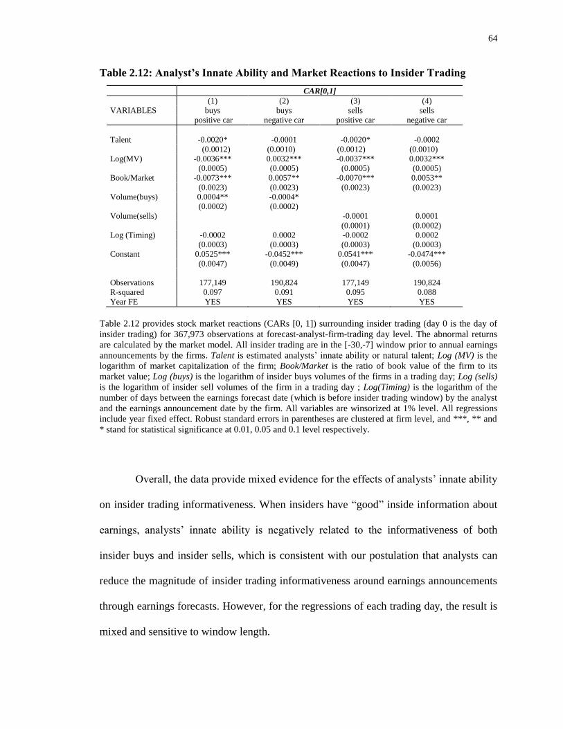
64

Table 2.12: Analyst’s Innate Ability and Market Reactions to Insider Trading

CAR[0,1]

(1) (2) (3) (4)

VARIABLES buys buys sells sells

positive car negative car positive car negative car

Talent -0.0020* -0.0001 -0.0020* -0.0002

(0.0012) (0.0010) (0.0012) (0.0010)

Log(MV) -0.0036*** 0.0032*** -0.0037*** 0.0032***

(0.0005) (0.0005) (0.0005) (0.0005)

Book/Market -0.0073*** 0.0057** -0.0070*** 0.0053**

(0.0023) (0.0023) (0.0023) (0.0023)

Volume(buys) 0.0004** -0.0004*

(0.0002) (0.0002)

Volume(sells) -0.0001 0.0001

(0.0001) (0.0002)

Log (Timing) -0.0002 0.0002 -0.0002 0.0002

(0.0003) (0.0003) (0.0003) (0.0003)

Constant 0.0525*** -0.0452*** 0.0541*** -0.0474***

(0.0047) (0.0049) (0.0047) (0.0056)

Observations 177,149 190,824 177,149 190,824

R-squared 0.097 0.091 0.095 0.088

Year FE YES YES YES YES

Table 2.12 provides stock market reactions (CARs [0, 1]) surrounding insider trading (day 0 is the day of

insider trading) for 367,973 observations at forecast-analyst-firm-trading day level. The abnormal returns

are calculated by the market model. All insider trading are in the [-30,-7] window prior to annual earnings

announcements by the firms. Talent is estimated analysts’ innate ability or natural talent; Log (MV) is the

logarithm of market capitalization of the firm; Book/Market is the ratio of book value of the firm to its

market value; Log (buys) is the logarithm of insider buys volumes of the firms in a trading day; Log (sells)

is the logarithm of insider sell volumes of the firm in a trading day ; Log(Timing) is the logarithm of the

number of days between the earnings forecast date (which is before insider trading window) by the analyst

and the earnings announcement date by the firm. All variables are winsorized at 1% level. All regressions

include year fixed effect. Robust standard errors in parentheses are clustered at firm level, and ***, ** and

* stand for statistical significance at 0.01, 0.05 and 0.1 level respectively.

Overall, the data provide mixed evidence for the effects of analysts’ innate ability

on insider trading informativeness. When insiders have “good” inside information about

earnings, analysts’ innate ability is negatively related to the informativeness of both

insider buys and insider sells, which is consistent with our postulation that analysts can

reduce the magnitude of insider trading informativeness around earnings announcements

through earnings forecasts. However, for the regressions of each trading day, the result is

mixed and sensitive to window length.

65

2.5 Discussion about Endogeneity

Endogeneity is highlighted in the studies of the effect of analyst coverage on

corporate governance outcomes. By convention we discuss three cases of endogeneity, of

which reverse causality should be the most important consideration in this study.

First, we try to exclude the possibility of reverse causality that insider trading

causes analyst forecasts. We use insider trading data in the 30-day window prior to

annual earnings announcements by the firms, and all analysts’ forecasts in our sample are

restricted to at least one month prior to earnings announcements, thus all forecasts

precede insider trading; given this, it is unlikely that insider trading with large volumes

attracts analyst coverage and further affect analysts’ innate ability due to the changes in

the number of analysts covering a firm. However, we are aware that this setting cannot

completely rule out the possibility of reverse causality. Analyst forecasting accuracy has

been shown to be higher in firms with a relatively higher transparency level (Brown et al.

1987, Lang and Lundhold 1996, etc). If an analyst always picks high-transparency firms

to follow, she may constantly have more accurate forecasts and be considered as a high-

ability analyst, even if she is no better than other analysts. Suppose there is a life cycle of

transparency then corporate insiders may naturally trade less when transparency level is

higher, thus we would observe a negative relation which is caused by endogeneity, even

if we use the setting of initial coverage.

Second, we try to avoid measurement error for both dependent variable and

independent variables. For the measures of insider trading intensity, we use trading

frequency (the number of trades, which can also measure trading profitability), trading

volume, trading value (volume*price), and adjusted trading volume (volume/number of

66

shares outstanding) for comparison of empirical results. For analysts’ unobservable

innate ability or natural talent, our measure, the isolated analyst fixed effect, is novel and

its “quasi” normal distribution is consistent with reality. No measures in the existing

literature can serve as alternative proxies for our research purpose.

Third, we try to overcome the problem of omitted variables. There are always

endless explanatory variables for consideration, and the existing literature of insider

trading does not provide a consensus of necessary explanatory variables. Most

importantly, information asymmetry is the prior concern according to our research

purpose. Previous studies show that analysts tend to cover firms with a lower level of

information asymmetry (Lang and Lundholm, 1996; Bhushan, 1989; Hshman, Piotroski,

and Smith, 2005 etc.), so in order to avoid the situation that omitted variables of

information asymmetry are correlated with both analysts’ innate ability and insider

trading, we use as many measures of information asymmetry as we can to mitigate the

problem of omitted variables for information asymmetry.

2.6 Conclusion

Financial analysts can affect insider trading through the information channel. This

paper employs a novel measure of sell-side financial analysts’ innate ability or natural

talent and explores its effects on reported corporate insider trading. We postulate that

analysts with high innate ability can reduce information asymmetry between corporate

insiders and outside investors through earnings forecasts, thereby negatively affecting

insider trading intensity and informativeness.

67

The empirical results show that analysts with higher innate ability are associated

with less net buys measured by trading volume, adjusted trading volume, and trading

value when insiders have “good” inside information about annual EPS, but this relation

does not hold for net sells when insiders have “bad” information. In addition, we conduct

tests of initial coverage and find the effects of analysts’ ability on insider trading are

stronger for these incremental impacts and the results are much stronger for high-ability

analysts in the sample of initial coverage. Additionally, we examine the time-series of

mean post-trading CARs and find that insider sells better predict future stock returns of

the companies that are covered by analysts with lower innate ability, but the evidence is

mixed for insider buys of which the results depends on information type. Overall, this

paper suggests a negative relation between analysts’ innate ability and insider trading

intensity and informativeness.

Our research confirms the role of analyst ability in insider trading and suggests

that high-ability analysts may serve in restricting excessive corporate insider trading.

Additionally, our study sheds light on the nature of analyst information. Our results imply

that the degree of firm-specific information an analyst can provide may be determined by

her innate ability. Compared with market-specific and industry-specific information,

firm-specific information is more difficult to collect and analyze; thus, analysts with low

ability may not be able to include firm-specific information in their forecasts.

68

References for Chapter 2

Aboody, D. and Lev, B., 2000. Information asymmetry, R&D, and insider gains. Journal

of Finance, pp.2747-2766.

Abowd, J.M., Kramarz, F. and Margolis, D.N., 1999. High wage workers and high wage

firms. Econometrica, 67(2), pp.251-333.

Agrawal, A. and Cooper, T., 2015. Insider trading before accounting scandals. Journal of

Corporate Finance, 34, pp.169-190.

Agrawal, A. and Nasser, T., 2012. Insider trading in takeover targets. Journal of

Corporate Finance, 18(3), pp.598-625.

Akyol, A.C., Qian, Y. and Yu, F., 2015. How Do Experienced Analysts Improve Price

Efficiency? Available at SSRN 2448041.

Ausubel, L.M., 1990. Insider trading in a rational expectations economy. The American

Economic Review, pp.1022-1041.

Bebchuk, L.A. and Fershtman, C., 1994. Insider trading and the managerial choice

among risky projects. Journal of Financial and Quantitative Analysis, 29(01),

pp.1-14.

Bettis, J.C., Coles, J.L. and Lemmon, M.L., 2000. Corporate policies restricting trading

by insiders. Journal of Financial Economics, 57(2), pp.191-220.

Bhushan, R., 1989. Collection of information about publicly traded firms: Theory and

evidence. Journal of Accounting and Economics, 11(2), pp.183-206.

Bhushan, R., 1989. Firm characteristics and analyst following. Journal of Accounting and

Economics, 11(2), pp.255-274.

Brown, L.D., Richardson, G.D. and Schwager, S.J., 1987. An information interpretation

of financial analyst superiority in forecasting earnings. Journal of Accounting

Research, pp.49-67.

Bushman, R.M., Piotroski, J.D. and Smith, A.J., 2005. Insider trading restrictions and

analysts' incentives to follow firms. The Journal of Finance,60(1), pp.35-66.

Chan, K. and Hameed, A., 2006. Stock price synchronicity and analyst coverage in

emerging markets. Journal of Financial Economics, 80(1), pp.115-147.

Chen, T., Harford, J. and Lin, C., 2015. Do analysts matter for governance? Evidence

from natural experiments. Journal of Financial Economics, 115(2), pp.383-410.

Cheng, Q. and Lo, K., 2006. Insider trading and voluntary disclosures. Journal of

Accounting Research, 44(5), pp.815-848.

69

Clarke, J., Khorana, A., Patel, A. and Rau, P.R., 2007. The impact of all-star analyst job

changes on their coverage choices and investment banking deal flow. Journal of

Financial Economics, 84(3), pp.713-737.

Clement, M.B., 1999. Analyst forecast accuracy: Do ability, resources, and portfolio

complexity matter?. Journal of Accounting and Economics, 27(3), pp.285-303.

Clement, M.B. and Tse, S.Y., 2003. Do investors respond to analysts' forecast revisions

as if forecast accuracy is all that matters? The Accounting Review, 78(1), pp.227-

249.

Clement, M.B. and Tse, S.Y., 2005. Financial analyst characteristics and herding

behavior in forecasting. The Journal of Finance, 60(1), pp.307-341.

Cohen, L., Frazzini, A. and Malloy, C., 2010. Sell‐side school ties. The Journal of

Finance, 65(4), pp.1409-1437.

Cohen, L., Malloy, C. and Pomorski, L., 2012. Decoding inside information. The Journal

of Finance, 67(3), pp.1009-1043.

Coles, J., Li, F., and Mola, S., 2013. Is talent wasted on the young? Natural ability vs.

experience-based ability in analyst research. Working Paper.

Coles, J. and Li, F., 2013. Managerial attributes, incentives, and performance. Incentives,

and Performance (January 31, 2013).

Crawford, S.S., Roulstone, D.T. and So, E.C., 2012. Analyst initiations of coverage and

stock return synchronicity. The Accounting Review, 87(5), pp.1527-1553.

Dai, L., Fu, R., Kang, J.K. and Lee, I., 2015. Internal corporate governance and the

profitability of insider trading. Available at SSRN 2103523.

Denis, D.J. and Xu, J., 2013. Insider trading restrictions and top executive

compensation. Journal of Accounting and Economics, 56(1), pp.91-112.

Easterwood, J.C. and Nutt, S.R., 1999. Inefficiency in analysts' earnings forecasts:

Systematic misreaction or systematic optimism?. Journal of Finance, pp.1777-

1797.

Elliott, J., Morse, D. and Richardson, G., 1984. The association between insider trading

and information announcements. The Rand Journal of Economics, pp.521-536.

Emery, D.R. and Li, X., 2009. Are the Wall Street analyst rankings popularity

contests? Journal of Financial and Quantitative Analysis, 44(02), pp.411-437.

70

Finnerty, J.E., 1976. Insiders and market efficiency. The Journal of Finance, 31(4),

pp.1141-1148.

Frankel, R. and Li, X., 2004. Characteristics of a firm's information environment and the

information asymmetry between insiders and outsiders. Journal of Accounting

and Economics, 37(2), pp.229-259.

Gilson, S.C., Healy, P.M., Noe, C.F. and Palepu, K.G., 2001. Analyst specialization and

conglomerate stock breakups. Journal of Accounting Research, 39(3), pp.565-

582.

Graham, J.R., Li, S. and Qiu, J., 2012. Managerial attributes and executive

compensation. Review of Financial Studies, 25(1), pp.144-186.

Hillier, D., Korczak, A. and Korczak, P., 2015. The impact of personal attributes on

corporate insider trading. Journal of Corporate Finance, 30, pp.150-167.

Hsieh, J., Ng, L.K. and Wang, Q., 2005, April. How informative are analyst

recommendations and insider trades? In AFA 2006 Boston Meetings Paper.

Huang, J. and Wang, A.Y., 2015. The predictability of managerial heterogeneities in

mutual funds. Financial Management, 44(4), pp.947-979.

Huddart, S.J. and Ke, B., 2007. Information asymmetry and cross‐sectional variation in

insider trading. Contemporary Accounting Research, 24(1), pp.195-232.

Irvine, P., Lipson, M. and Puckett, A., 2007. Tipping. Review of Financial Studies, 20(3),

pp.741-768.

Irvine, P.J., 2003. The incremental impact of analyst initiation of coverage.Journal of

Corporate Finance, 9(4), pp.431-451.

Jacob, J., Lys, T.Z. and Neale, M.A., 1999. Expertise in forecasting performance of

security analysts. Journal of Accounting and Economics, 28(1), pp.51-82.

Jagolinzer, A.D., Larcker, D.F. and Taylor, D.J., 2011. Corporate governance and the

information content of insider trades. Journal of Accounting Research, 49(5),

pp.1249-1274.

Kothari, S.P., 2001. Capital markets research in accounting. Journal of Accounting and

Economics, 31(1), pp.105-231.

Kusnadi, Y., 2015. Insider trading restrictions and corporate risk-taking. Pacific-Basin

Finance Journal, 35, pp.125-142.

Lakonishok, J. and Lee, I., 2001. Are insider trades informative? Review of Financial

Studies, 14(1), pp.79-11.

71

Lang, M.H. and Lundholm, R.J., 1996. Corporate disclosure policy and analyst

behavior. Accounting Review, pp.467-492.

Lee, I., Lemmon, M., Li, Y. and Sequeira, J.M., 2014. Do voluntary corporate restrictions

on insider trading eliminate informed insider trading? Journal of Corporate

Finance, 29, pp.158-178.

Leland, H.E., 1992. Insider trading: Should it be prohibited? Journal of Political

Economy, pp.859-887.

Liu, M.H., 2011. Analysts’ incentives to produce industry-level versus firm-specific

information. Journal of Financial and Quantitative Analysis, 46(03), pp.757-784.

Livnat, J. and Mendenhall, R.R., 2006. Comparing the post–earnings announcement drift

for surprises calculated from analyst and time series forecasts. Journal of

Accounting Research, 44(1), pp.177-205.

Loh, R.K. and Mian, G.M., 2006. Do accurate earnings forecasts facilitate superior

investment recommendations? Journal of Financial Economics, 80(2), pp.455-

483.

Manne, H. G. 1966. Insider trading and the stock market. New York: The Free Press.

Mikhail, M.B., Walther, B.R. and Willis, R.H., 1997. Do security analysts improve their

performance with experience? Journal of Accounting Research, 35, pp.131-157.

Mikhail, M.B., Walther, B.R. and Willis, R.H., 2003. The effect of experience on security

analyst underreaction. Journal of Accounting and Economics, 35(1), pp.101-116.

Park, C.W. and Stice, E.K., 2000. Analyst forecasting ability and the stock price reaction

to forecast revisions. Review of Accounting Studies, 5(3), pp.259-272.

Piotroski, J.D. and Roulstone, D.T., 2004. The influence of analysts, institutional

investors, and insiders on the incorporation of market, industry, and firm-specific

information into stock prices. The Accounting Review, 79(4), pp.1119-1151.

Piotroski, J.D. and Roulstone, D.T., 2005. Do insider trades reflect both contrarian beliefs

and superior knowledge about future cash flow realizations? Journal of

Accounting and Economics, 39(1), pp.55-81.

Roulstone, D.T., 2003. The relation between insider‐trading restrictions and executive

compensation. Journal of Accounting Research, 41(3), pp.525-551.

Rozeff, M.S. and Zaman, M.A., 1988. Market efficiency and insider trading: New

evidence. Journal of Business, pp.25-44.

Seyhun, H.N., 1986. Insiders' profits, costs of trading, and market efficiency. Journal of

Financial Economics, 16(2), pp.189-212.

72

Seyhun, H.N., 1992. Why does aggregate insider trading predict future stock returns? The

Quarterly Journal of Economics, pp.1303-1331.

Sinha, P., Brown, L.D. and Das, S., 1997. A Re‐Examination of Financial Analysts'

Differential Earnings Forecast Accuracy. Contemporary Accounting

Research, 14(1), pp.1-42.

Stickel, S.E., 1995. The anatomy of the performance of buy and sell

recommendations. Financial Analysts Journal, 51(5), pp.25-39.

Wu, W., 2014. Information Asymmetry and Insider Trading. Fama-Miller Working

Paper, pp.13-67.

73

Chapter 3

3 Measuring Firm Size in Empirical Corporate Finance

3.1 Introduction

The studies of firm size date back to a seminal article, Coase (1937), which raises

the questions of how firm boundaries affect the allocation of resources and what

determines firm boundaries. A large body of research follows the topic, and both

questions have received much attention in theoretical studies in economics and finance

(e.g., Williamson (1975, 1986), Klein, Crawford, and Alchian (1978), and Grossman and

Hart (1986)). Empirical researchers in corporate finance also consider firm size an

important and fundamental firm characteristic, and in many situations, observe the “size

effect” – and firm size matters in determining the dependent variables. For example, in

capital structure, Frank and Goyal (2003) show that pecking order is only found in large

firms; Rajan and Zingales (1995) discover that leverage increases with firm size. In

mergers and acquisitions, Moeller, Schlingemann, and Stulz (2004) find that small firms

have larger abnormal announcement returns; Vijh and Yang (2013) document that for

cash offers, targetiveness (probability of being targeted) decreases with firm size, but for

stock offers they find an inverted-U relation.

Although firm size matters in empirical corporate finance, the existing literature is

silent on the rationale of using a certain measure of firm size, and no paper provides a

comprehensive assessment of the sensitivity of empirical results in corporate finance to

different measures of firm size. To the best of our knowledge, Vijh and Yang (2013)

provide a list of firm size proxies and corresponding coefficients of firm size proxies in

74

the literature of takeover likelihood models. Their study indicates that the sign and

significance of the coefficients of firm size in different papers are sensitive to firm size

measures. While Vijh and Yang (2013) suggest that firm size measures should receive

more attention, they do not compare the results based on the same regression, or conduct

the assessment of firm size measures in broad corporate finance literature.

We use 20 representative specifications, in the areas of executive compensation,

board of directors, corporate control, financial policy, payout policy, investment policy,

diversification, firm performance, and study the influences (sign sensitivity, significance

sensitivity, and R-squared sensitivity) of employing different measures of firm size. For

each specification we employ the natural logarithm forms of three firm size measures:

total assets, total sales, and market value of equity. We choose these three measures

because, according to our survey of 100 research papers, they are the most popular firm

size proxies in corporate finance. However, other measures, such as number of

employees and net assets, also appear in empirical work.

We choose the 20 representative specifications from Coles, Daniel, and Naveen

(2006), Comment and Schwert (1995), Core and Guay (1999), DeAngelo, DeAngelo, and

Stulz (2006), Graham, Li, and Qiu (2012), Harford (1999), Harford, Mansi, and Maxwell

(2008), Lemmon, Roberts, and Zender (2008), Linck, Netter, and Yang (2008) and

Mehran (1995). For brevity and data availability, we select the same papers as those in

Coles and Li (2012). With a different goal, Coles and Li (2012) assess firm, manager, and

time fixed effects in these 20 prominent areas in empirical corporate finance. On one

hand, our project is modest. Using our data sample with year fixed effect and industry

fixed effect, our empirical models resemble the corresponding benchmark specifications

75

in these papers.21

This allows an even-handed comparison between our results and those

in the original papers and the results based on different firm size measures. On the other

hand, our research thrust is ambitious in data collection and analysis for a large number

of regression specifications across a wide spectrum of subfields in corporate finance.

Although all firm size measures are significantly correlated, they are theoretically

and empirically different.22

Because size is a firm fundamental variable, any subtle

differences may have critical impact on the dependent variable and other independent

variables in empirical study.23

Our results indeed confirm this “measurement effect” in

“size effect” in empirical corporate finance. First, the coefficients on regressors often

change sign and significance when we use difference firm size measures. We observe

sign changes and significance changes in almost all the areas except dividend policy and

executive compensation. Unfortunately, this suggests that, when using different firm size

proxies, some previous studies are not robust.24

Researchers should either use all the

21 We introduce industry fixed effect because some benchmark papers employ 2-digit SIC controls (e.g.

Coles, Daniel, and Naveen (2006)) and others include industrial firms (e.g. DeAngelo, DeAngelo, and Stulz

(2006)) or manufacturing firms (e.g. Mehran (1995)). Broadly speaking, the industry fixed effects are

widely documented in the empirical corporate finance research. We also tried firm fixed effects and

obtained qualitatively similar results, although the implications, by looking at within-firm variations, are

different from those of the original papers.

22 The correlation coefficients range from 0.64 to 0.81 in our sample.

23 According to our results, the firm size measures are consistently one of the most significant independent

variables in all the subfields of corporate finance. In 18 out of 20 subfields, size proxy is statistically

significant at 1% level.

24 In order to provide even-handed comparisons, we attempted to use exactly the same methodology and

variable definitions in our experiments; we also tried the subsamples in the same time periods as in the

original papers. The results are not qualitatively different, giving us some confidence that our data and

estimation are not so different from those papers. More importantly, we are not trying to argue against the

results in these papers. Instead, we test the sensitivity and robustness of the size measures in our larger,

more comprehensive, and more recent data to raise awareness. For comparisons of the testing periods

between our sample and the samples in the benchmark papers, please refer to footnote 26.

76

important proxies as robustness checks, or provide rationale of using any specific proxy.

Second, the goodness of fit measured by R-squared varies significantly with different

firm size measures. Some size measures appear more “relevant” than others in different

areas, implying that they are better control variables to reduce omitted variable bias and

improve the estimation of the main coefficients of interest. Different size proxies capture

different aspects of “firm size”, and thus have different implications. The choice of these

firm size measures can be a theoretical and empirical question. Finally, based on all our

results, we attempt to provide guidelines on the choice of size measure in different areas

and situations. The sensitivity of empirical results to different size measures not only

provides guidance for researchers who must use firm size proxies in empirical corporate

finance research, but also sheds light on future research that might incorporate

measurement effect into other research fields, such as empirical asset pricing and

empirical accounting.

We have some guidelines for future research. First, we do not employ all possible

measures of firm size; we only study the most popular three measures. Researchers can

use some alternative size proxies such as enterprise value (market capitalization plus net

debt), the number of employees, total profits, or net assets (total assets minus total

liabilities) when the main measures are not available or irrelevant (e.g., market cap for

private firms and total sales for start-up firms). Second, we might omit some important

representative papers in specific sub-fields due to data and time constraints. Third, some

linear models may lose power if the true relation between firm size and the dependent

variable is non-linear (such as quadratic form). Fourth, most of our empirical results are

based on year fixed effects and/or industry fixed effects, while introducing other

77

considerations, such as firm fixed effects (for consideration of with-in firm variations of

interest rather than cross-sectional variations) or manager fixed effects (for emphasis on

corporate governance issues such as managerial compensation), might change our results,

and result in different implications. In a word, for future research, on the one hand

explicit theories should be refined for the proper usage of different measures of firm size;

on the other hand, a general role should be developed for empirical justification given

specific econometric methods.

The outline of this chapter is as follows. Section 3.2 discusses research

motivation, literature review, and the measures of firm size. Section 3.3 describes our

data and the sample. Section 3.4 provides discussion of empirical results. Section 3.5

concludes.

3.2 Framework for Analysis and Literature Review

Coase (1937) states that firms are formed with boundaries to substitute markets to

save transaction costs such as contracting and monitoring fees. For the effects of firm

boundaries on firm behavior, Williamson (1975, 1986), Klein, Crawford, and Alchian

(1978), and Grossman and Hart (1986) provide theoretical insights, while some recent

works such as Holmstrom and Kaplan (2001), Robinson (2008), and Seru (2010) present

empirical evidence that links the theory of firm and corporate finance to firm activities

such as capital allocation. Specifically, Bolton and Scharfstein (1998) review the

relationship between corporate finance and the theory of firm and organizations.

As for the determinants of firm size, Kumar, Rajan, and Zingales (1999)

comprehensively review the literature and classify the theories into four categories:

78

technological theories (Lucas (1978), Rosen (1982), Kremer (1993), etc.), organizational

theories (Williamson (1975, 1986), Klein, Crawford and Alchian (1978), Grossman and

Hart (1986), Rajan and Zingales (1998b, 2001), Holmstrom (1999), Holmstrom and

Roberts (1998), etc.), regulatory theories (Ringleb and Wiggins (1990), Hopenhayn

(1992), etc.), and financial theories (Rajan and Zingales (1998a), etc.). Kumar, Rajan,

and Zingales (1999) provide empirical evidence that the utility sector, R&D intensive

industries, capital intensive industries, high wage industries, and industries that need little

external financing all feature large firms.25

Several papers also investigate whether the measures of firm size are

interchangeable in microeconomics and industrial organization, and these works are more

associated with our goal to evaluate the effects of employing different firm size measures

in empirical research. Smyth, Boyes, and Peseau (1975) first demonstrate that measures

of firm size are only interchangeable when more rigorous technical conditions than

correlation are met. Smyth, Boyes, and Peseau (1975) show that economies of scale are

sensitive to different firm size measures. Jackson and Dunlevy (1982) employ an

asymptotically valid procedure to test the null hypothesis of orthogonal least squares

suggested by Smyth, Boyes, and Peseau (1975). However, these works play little role in

the existing corporate finance literature. Financial researchers usually use firm size

measures without examining correlations and other interrelationships among different

firm size measures. The empirical results in this paper support that the measures of firm

size are indeed not interchangeable.

25 Such evidence also motivates us to use industry fixed effect in our empirical investigations.

79

From the review above, we find that the overall assessment of firm size measures

in empirical corporate finance has largely been ignored in the existing literature.

However, this topic deserves attention. In most prominent areas of empirical corporate

finance research, finance scholars employ firm size as an important firm characteristic,

and, in many situations, finance scholars have observed the “size effect” - firm size

matters in determining the dependent variables. For example, it is well recognized that

top-management compensation level increases with firm size (Jensen and Murphy

(1990), Core, Holthausen, and Larcker (1999), etc.). Baker and Hall (2004) find that CEO

marginal products increase substantially with firm size. Gabaix and Landier (2008, 2014)

show that small differences in CEO talent can result in substantial differences in CEO

pay through the effect of firm size, and, in particular, larger firms usually have more

skilled managers (Himmelberg and Hubbard (2000)).

Although the majority of the literature takes for granted that the choice of firm

size measures is not a vital concern, we doubt the existence of selection bias of empirical

results in some papers. Recent works (e.g. Vijh and Yang (2013, Appendix 2)) find that

the sign and significance of the coefficients of size proxies in the literature of mergers

and acquisitions are sensitive to different firm size measures. While Vijh and Yang

(2013) indicate that firm size measures should receive more attention, they are silent on

the assessment of firm size measures based on the same regression and the

comprehensive assessment in broad corporate finance literature. In addition, Vijh and

Yang (2013) have little to say on the sensitivity of the coefficients of regressors other

than firm size when different firm size measures are employed. These limitations in the

80

existing literature motivate us to investigate the effects of different size measures

comprehensively.

For the purpose of conducting a comprehensive empirical assessment of firm size

measures in different sub-fields of empirical corporate finance, we follow Coles and Li

(2012), covering 20 prominent research areas in corporate finance: financial policy

(book leverage, market leverage, and cash holdings), payout policy (dividend dummy),

investment policy (CAPEX, R&D, and firm risk), diversification (Herfindahl index and

business segments), firm performance (Tobin’s Q, which is the sum of market

capitalization of equity plus liabilities divided by total book assets, and ROA, which is

the ratio of net income to total assets), mergers and acquisitions and corporate control

(bidder, target, and poison pills), managerial compensation and incentives (delta, vega,

and pay level), and board of directors (board size, board independence, and CEO duality).

We employ three firm size measures: total assets, total sales, and market value of

equity. These measures are the most popular firm size proxies in empirical corporate

finance research, according to our survey in which we investigate 100 empirical papers

from top finance, accounting, and economics journals that use firm size measures on the

topics of empirical corporate finance. We collect a total of 100 papers through Google

Scholar by searching subfield key words, and the results are listed by descending number

of citations. We only choose the papers that appear in top journals and use firm size

measures in empirical studies. The papers are distributed across extensive areas in

corporate finance, including capital structure, debt policy, payout policy, cash holdings,

corporate investment and financial constraints, cross listings, CEO turnover, CEO

compensation, board of directors, law and finance, ownership structure, mergers and

81

acquisitions and corporate control (see the Appendix 3.1 for the detailed information of

these papers.). We find that these three firm size proxies are used in 85 papers out of the

87 papers that use single measures, and the remaining 13 papers use multiple measures

for robustness checks. Among these 87 papers, 49 papers use total assets, 20 papers use

market capitalization, 16 papers use sales, and 2 papers use number of employees. We are

aware that other measures, such as number of employees and net assets, also appear,

though infrequently, in empirical finance works, but for conciseness we only use these

three measures. In addition, most papers in empirical corporate finance use the logarithm

form of firm size measures. In the 100 papers we surveyed, only 3 papers use the original

form of the three size measures. This suggests the rule of thumb in corporate finance is to

use log form to mitigate the high skewness of firm size data.

It is interesting that Forbes Global 2000 uses four measures (assets, sales, profits,

and market cap) to rank all the large companies in the world, and Fortune 500 uses two

measures (sales and profits). Both of them employ sales and profits, but profits seldom

appear as a proxy for firm size in academic research.

Every firm size measure exhibits advantages and disadvantages, and no measure

can capture all characteristics of “firm size”. Generally speaking, total assets measures

total firm resources; market capitalization involves firm growth opportunities and equity

market condition; total sales measures product market competition and is not forward

looking. In addition, researchers can use the number of employees, total profits, and net

assets when the main measures are not available or irrelevant (e.g., market cap for private

firms and total sales for start-up firms). Moreover, Hart and Oulton (1996) argue that net

assets can be negative but sales are always positive. They also point out that the number

82

of employees does not include the number of part-time workers, but these days part-time

workers play an important role. Because every measure has pros and cons, Hart and

Oulton (1996) suggest that in practice choosing which measure to use depends on data

availability. In addition, we think the choice of firm size measures also depends on the

purpose of the specific study. For example, Prowse (1992) applies different firm size

measures as the research purpose changes from the ownership of equity to the ownership

of asset.

In sum, we find that the existing literature has little to say about the rationale of

using a certain measure of firm size for specific corporate finance research, and no paper

provides a comprehensive assessment of the sensitivity of empirical results in corporate

finance to different measures of firm size. This hole in the literature motivates us to find

evidence for “measurement effect” in “size effect”, and to provide a general guideline to

researchers who must use firm size, whether as key variable or control variable, in their

empirical corporate finance studies.

3.3 The Data

We extract the data from multiple sources. Corporate governance data are from

RiskMetrics Governance, director data are from RiskMetrics Directors, stock daily

returns and prices are from CRSP, company diversification data are from Compustat

Segment, corporate bond data are from Compustat Ratings, institutional holdings data are

from Thomson Reuters, Executive data, up to five top executives per firm, are from

ExecuComp, M&A deals and corporate control data are from SDC, and all other financial

items are from Compustat Fundamentals. We restrict the observations to only those

which match North American data from CRSP and Compustat for firms with fiscal years

83

1993-200626

. In line with conventional tradition, we exclude data from the financial and

utility sectors. See Table 3.1 for summary statistics for all the variables featured in our

representative specifications from corresponding benchmark papers.

26 This is different from the testing periods in the benchmark papers. Mehran (1995) uses a sample from

1979 to 1980; Linck, Netter, and Yang (2008) use a sample from 1990 to 2004; DeAngelo, DeAngelo, and

Stulz (2006) use a sample from 1973 to 2002; Comment and Schwert (1995) use a sample from 1977 to

1991; Harford (1999) uses a sample from 1977 to 1993; Lemon, Roberts, and Zender (2008) use a sample

from 1965 to 2003; Coles, Daniel, and Naveen (2006) use a sample from 1992 to 2002; Graham, Li, and

Qiu (2012) use a sample from 1992 to 2006; Harford, Mansi, and Maxwell (2008) use a sample from 1993

to 2004.

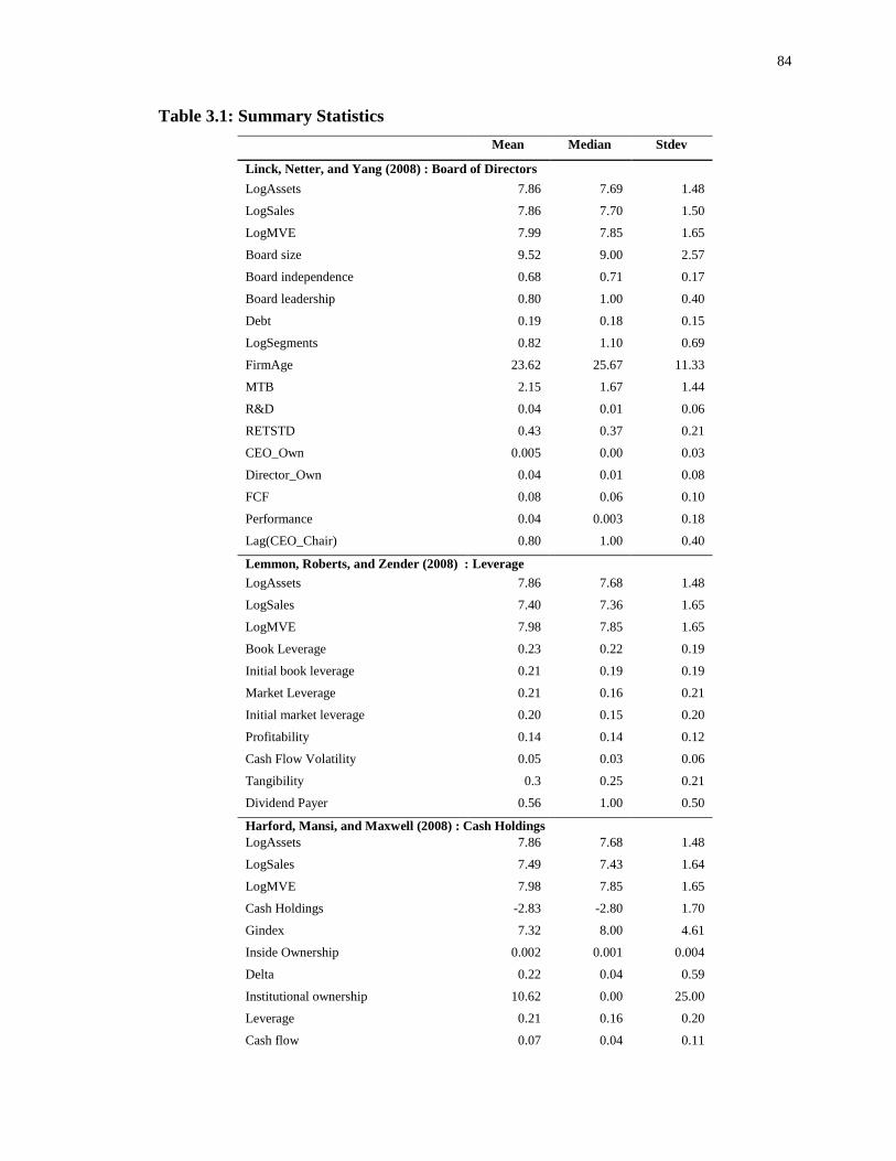
84

Table 3.1: Summary Statistics

Mean Median Stdev

Linck, Netter, and Yang (2008) : Board of Directors

LogAssets 7.86 7.69 1.48

LogSales 7.86 7.70 1.50

LogMVE 7.99 7.85 1.65

Board size 9.52 9.00 2.57

Board independence 0.68 0.71 0.17

Board leadership 0.80 1.00 0.40

Debt 0.19 0.18 0.15

LogSegments 0.82 1.10 0.69

FirmAge 23.62 25.67 11.33

MTB 2.15 1.67 1.44

R&D 0.04 0.01 0.06

RETSTD 0.43 0.37 0.21

CEO_Own 0.005 0.00 0.03

Director_Own 0.04 0.01 0.08

FCF 0.08 0.06 0.10

Performance 0.04 0.003 0.18

Lag(CEO_Chair) 0.80 1.00 0.40

Lemmon, Roberts, and Zender (2008) : Leverage

LogAssets 7.86 7.68 1.48

LogSales 7.40 7.36 1.65

LogMVE 7.98 7.85 1.65

Book Leverage 0.23 0.22 0.19

Initial book leverage 0.21 0.19 0.19

Market Leverage 0.21 0.16 0.21

Initial market leverage 0.20 0.15 0.20

Profitability 0.14 0.14 0.12

Cash Flow Volatility 0.05 0.03 0.06

Tangibility 0.3 0.25 0.21

Dividend Payer 0.56 1.00 0.50

Harford, Mansi, and Maxwell (2008) : Cash Holdings

LogAssets 7.86 7.68 1.48

LogSales 7.49 7.43 1.64

LogMVE 7.98 7.85 1.65

Cash Holdings -2.83 -2.80 1.70

Gindex 7.32 8.00 4.61

Inside Ownership 0.002 0.001 0.004

Delta 0.22 0.04 0.59

Institutional ownership 10.62 0.00 25.00

Leverage 0.21 0.16 0.20

Cash flow 0.07 0.04 0.11

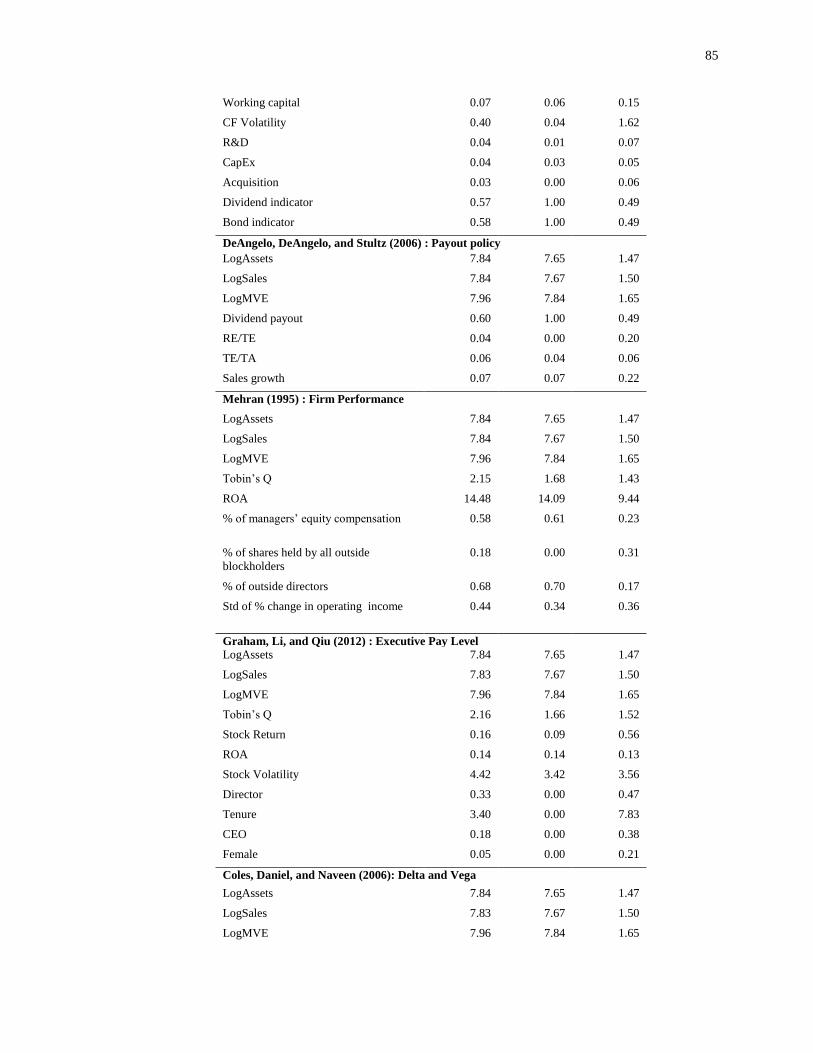
85

Working capital 0.07 0.06 0.15

CF Volatility 0.40 0.04 1.62

R&D 0.04 0.01 0.07

CapEx 0.04 0.03 0.05

Acquisition 0.03 0.00 0.06

Dividend indicator 0.57 1.00 0.49

Bond indicator 0.58 1.00 0.49

DeAngelo, DeAngelo, and Stultz (2006) : Payout policy

LogAssets 7.84 7.65 1.47

LogSales 7.84 7.67 1.50

LogMVE 7.96 7.84 1.65

Dividend payout 0.60 1.00 0.49

RE/TE 0.04 0.00 0.20

TE/TA 0.06 0.04 0.06

Sales growth 0.07 0.07 0.22

Mehran (1995) : Firm Performance

LogAssets 7.84 7.65 1.47

LogSales 7.84 7.67 1.50

LogMVE 7.96 7.84 1.65

Tobin’s Q 2.15 1.68 1.43

ROA 14.48 14.09 9.44

% of managers’ equity compensation 0.58 0.61 0.23

% of shares held by all outside

blockholders

0.18 0.00 0.31

% of outside directors 0.68 0.70 0.17

Std of % change in operating income 0.44 0.34 0.36

Graham, Li, and Qiu (2012) : Executive Pay Level LogAssets 7.84 7.65 1.47

LogSales 7.83 7.67 1.50

LogMVE 7.96 7.84 1.65

Tobin’s Q 2.16 1.66 1.52

Stock Return 0.16 0.09 0.56

ROA 0.14 0.14 0.13

Stock Volatility 4.42 3.42 3.56

Director 0.33 0.00 0.47

Tenure 3.40 0.00 7.83

CEO 0.18 0.00 0.38

Female 0.05 0.00 0.21

Coles, Daniel, and Naveen (2006): Delta and Vega

LogAssets 7.84 7.65 1.47

LogSales 7.83 7.67 1.50

LogMVE 7.96 7.84 1.65

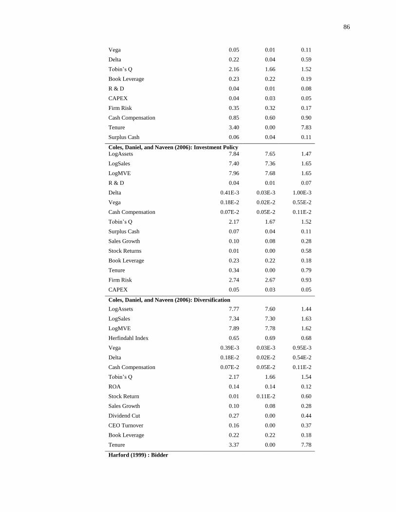
86

Vega 0.05 0.01 0.11

Delta 0.22 0.04 0.59

Tobin’s Q 2.16 1.66 1.52

Book Leverage 0.23 0.22 0.19

R & D 0.04 0.01 0.08

CAPEX 0.04 0.03 0.05

Firm Risk 0.35 0.32 0.17

Cash Compensation 0.85 0.60 0.90

Tenure 3.40 0.00 7.83

Surplus Cash 0.06 0.04 0.11

Coles, Daniel, and Naveen (2006): Investment Policy LogAssets 7.84 7.65 1.47

LogSales 7.40 7.36 1.65

LogMVE 7.96 7.68 1.65

R & D 0.04 0.01 0.07

Delta 0.41E-3 0.03E-3 1.00E-3

Vega 0.18E-2 0.02E-2 0.55E-2

Cash Compensation 0.07E-2 0.05E-2 0.11E-2

Tobin’s Q 2.17 1.67 1.52

Surplus Cash 0.07 0.04 0.11

Sales Growth 0.10 0.08 0.28

Stock Returns 0.01 0.00 0.58

Book Leverage 0.23 0.22 0.18

Tenure 0.34 0.00 0.79

Firm Risk 2.74 2.67 0.93

CAPEX 0.05 0.03 0.05

Coles, Daniel, and Naveen (2006): Diversification

LogAssets 7.77 7.60 1.44

LogSales 7.34 7.30 1.63

LogMVE 7.89 7.78 1.62

Herfindahl Index 0.65 0.69 0.68

Vega 0.39E-3 0.03E-3 0.95E-3

Delta 0.18E-2 0.02E-2 0.54E-2

Cash Compensation 0.07E-2 0.05E-2 0.11E-2

Tobin’s Q 2.17 1.66 1.54

ROA 0.14 0.14 0.12

Stock Return 0.01 0.11E-2 0.60

Sales Growth 0.10 0.08 0.28

Dividend Cut 0.27 0.00 0.44

CEO Turnover 0.16 0.00 0.37

Book Leverage 0.22 0.22 0.18

Tenure 3.37 0.00 7.78

Harford (1999) : Bidder

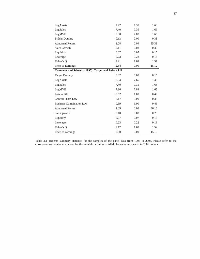
87

LogAssets 7.42 7.35 1.60

LogSales 7.40 7.36 1.66

LogMVE 8.00 7.87 1.66

Bidder Dummy 0.12 0.00 0.33

Abnormal Return 1.08 0.09 55.38

Sales Growth 0.11 0.08 0.30

Liquidity 0.07 0.07 0.15

Leverage 0.23 0.22 0.18

Tobin’s Q 2.21 1.69 1.57

Price-to-Earnings -2.84 0.00 15.12

Comment and Schwert (1995): Target and Poison Pill

Target Dummy 0.02 0.00 0.15

LogAssets 7.84 7.65 1.48

LogSales 7.40 7.35 1.65

LogMVE 7.96 7.84 1.65

Poison Pill 0.62 1.00 0.49

Control Share Law 0.17 0.00 0.38

Business Combination Law 0.69 1.00 0.46

Abnormal Return 1.09 0.08 56.15

Sales growth 0.10 0.08 0.28

Liquidity 0.07 0.07 0.15

Leverage 0.23 0.22 0.18

Tobin’s Q 2.17 1.67 1.52

Price-to-earnings -2.80 0.00 15.19

Table 3.1 presents summary statistics for the samples of the panel data from 1993 to 2006. Please refer to the

corresponding benchmark papers for the variable definitions. All dollar values are stated in 2006 dollars.

88

Specifically, we report data properties and bivariate scattergrams of the

alternative firm size measures in logarithm numbers for the regressions of firm

performance (Tobin’s Q and ROA) as an example. Table 3.2 Panel A reports summary

statistics of firm size measures for both raw numbers and logarithm numbers. Panel B

presents the Pearson correlation coefficients of firm size measures across raw numbers

and logarithm numbers. Figure 3.1 shows bivariate scattergrams of alternative firm sizes

measured in logarithm numbers, which we employ in the regressions. We find that the

correlation coefficients among log (assets), log (sales), and log (market value of equity)

are between 0.77 and 0.92, and those among raw numbers are between 0.64 and 0.81.

The highest correlation coefficient is between log (assets) and log (sales) (0.92), and the

lowest correlation coefficient is between sales and log (market value of equity) (0.50).

These correlations indicate that although all the size measures are significantly correlated,

they are different and some are more correlated than others.

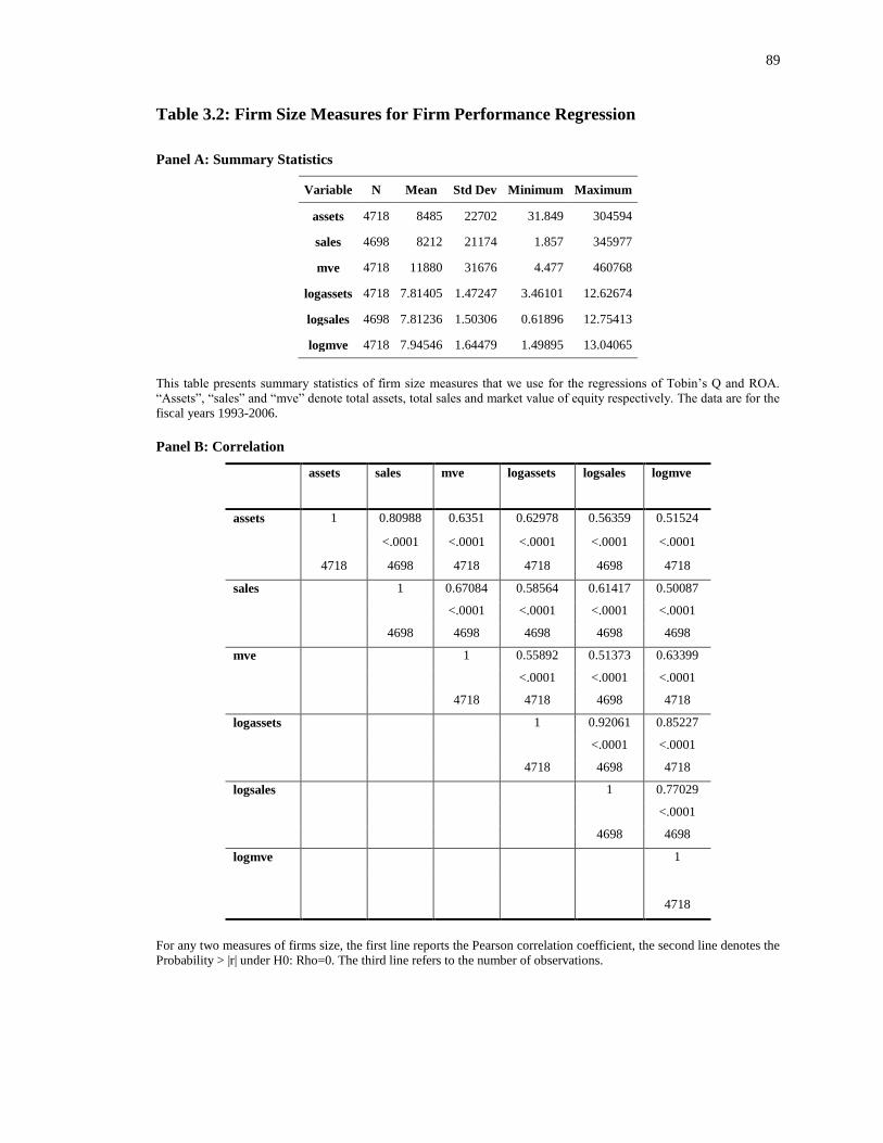
89

Table 3.2: Firm Size Measures for Firm Performance Regression

Panel A: Summary Statistics

Variable N Mean Std Dev Minimum Maximum

assets 4718 8485 22702 31.849 304594

sales 4698 8212 21174 1.857 345977

mve 4718 11880 31676 4.477 460768

logassets 4718 7.81405 1.47247 3.46101 12.62674

logsales 4698 7.81236 1.50306 0.61896 12.75413

logmve 4718 7.94546 1.64479 1.49895 13.04065

This table presents summary statistics of firm size measures that we use for the regressions of Tobin’s Q and ROA.

“Assets”, “sales” and “mve” denote total assets, total sales and market value of equity respectively. The data are for the

fiscal years 1993-2006.

Panel B: Correlation

assets sales mve logassets logsales logmve

assets 1 0.80988 0.6351 0.62978 0.56359 0.51524

<.0001 <.0001 <.0001 <.0001 <.0001

4718 4698 4718 4718 4698 4718

sales 1 0.67084 0.58564 0.61417 0.50087

<.0001 <.0001 <.0001 <.0001

4698 4698 4698 4698 4698

mve 1 0.55892 0.51373 0.63399

<.0001 <.0001 <.0001

4718 4718 4698 4718

logassets 1 0.92061 0.85227

<.0001 <.0001

4718 4698 4718

logsales 1 0.77029

<.0001

4698 4698

logmve 1

4718

For any two measures of firms size, the first line reports the Pearson correlation coefficient, the second line denotes the

Probability > |r| under H0: Rho=0. The third line refers to the number of observations.

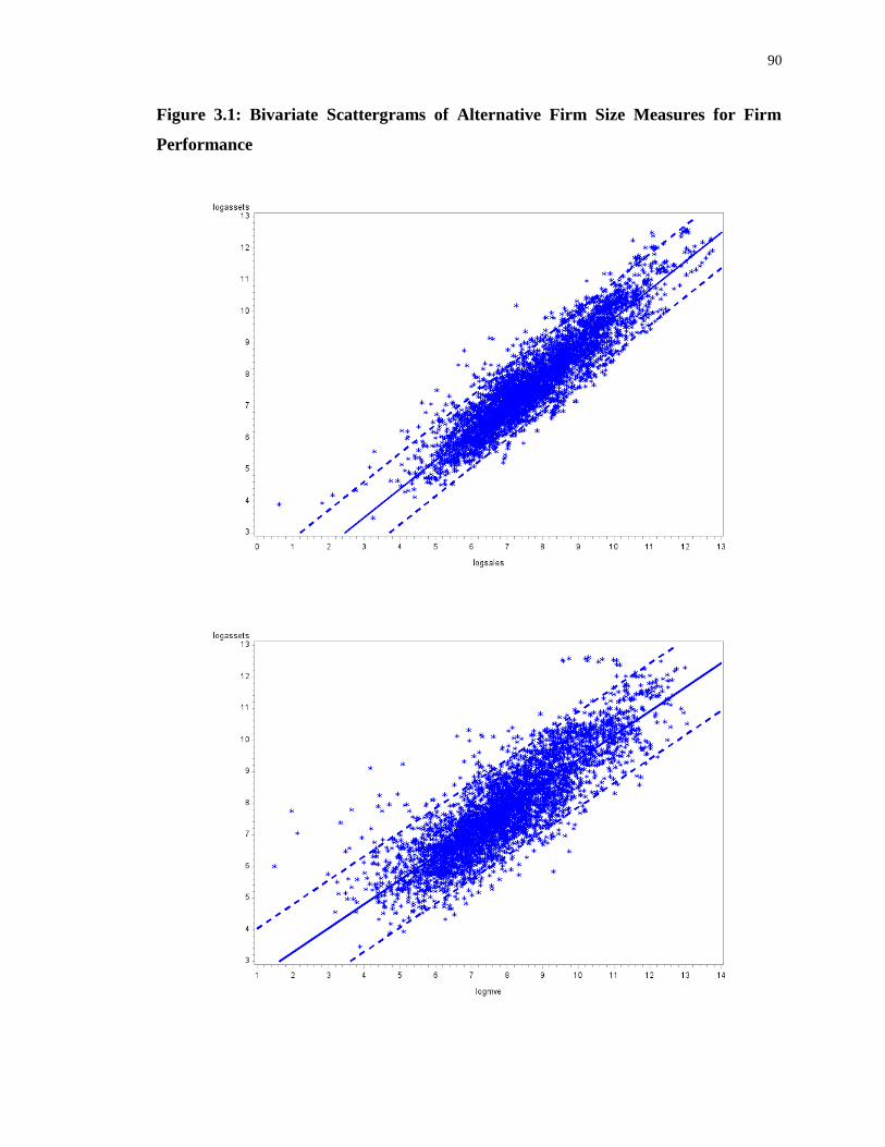
90

Figure 3.1: Bivariate Scattergrams of Alternative Firm Size Measures for Firm

Performance

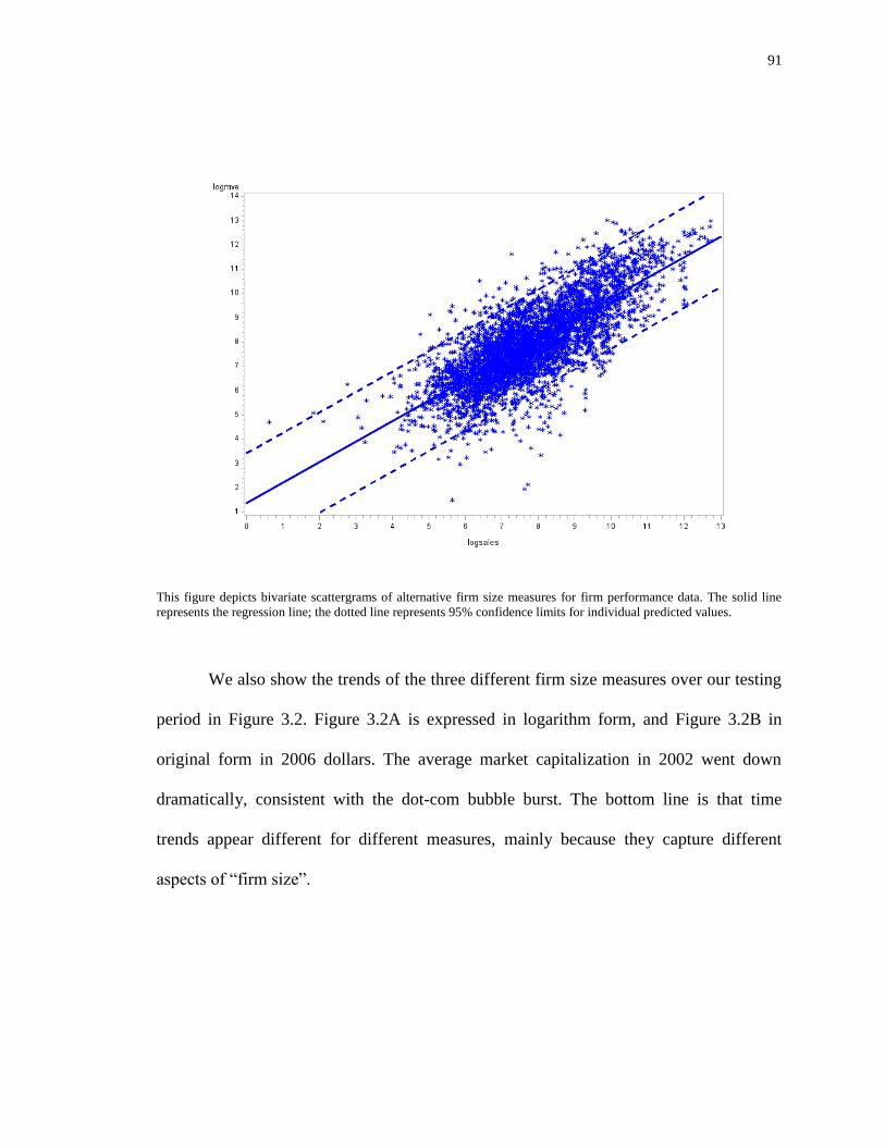
91

This figure depicts bivariate scattergrams of alternative firm size measures for firm performance data. The solid line

represents the regression line; the dotted line represents 95% confidence limits for individual predicted values.

We also show the trends of the three different firm size measures over our testing

period in Figure 3.2. Figure 3.2A is expressed in logarithm form, and Figure 3.2B in

original form in 2006 dollars. The average market capitalization in 2002 went down

dramatically, consistent with the dot-com bubble burst. The bottom line is that time

trends appear different for different measures, mainly because they capture different

aspects of “firm size”.

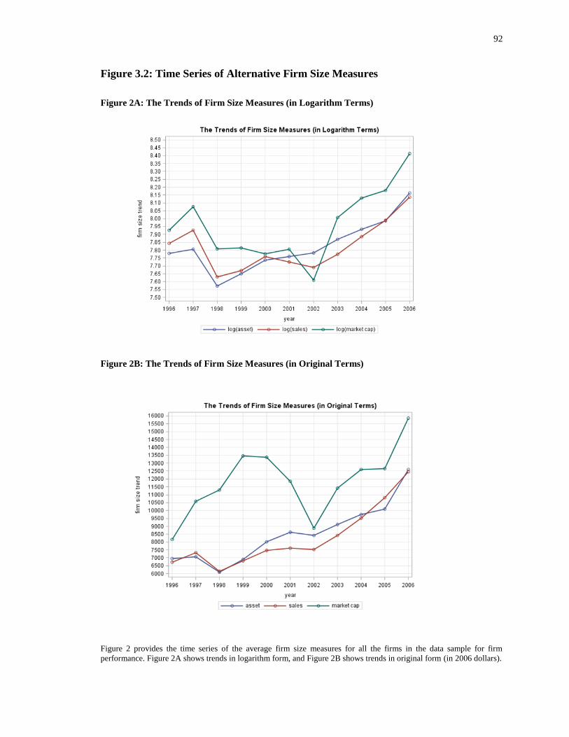
92

Figure 3.2: Time Series of Alternative Firm Size Measures

Figure 2A: The Trends of Firm Size Measures (in Logarithm Terms)

Figure 2B: The Trends of Firm Size Measures (in Original Terms)

Figure 2 provides the time series of the average firm size measures for all the firms in the data sample for firm

performance. Figure 2A shows trends in logarithm form, and Figure 2B shows trends in original form (in 2006 dollars).

93

3.4 Methodology and Empirical Results

We adopt the empirical methodologies in the benchmark papers by employing

conventional short-panel techniques for basic empirical analysis. For each specification,

we apply both basic OLS regressions and industry fixed effect regressions. Time fixed

effects are included in every regression. We use industry fixed effect because some

benchmark papers employ 2-digit SIC controls (e.g. Coles, Daniel, and Naveen (2006)),

and others only include industrial firms (e.g. DeAngelo, DeAngelo, and Stulz (2006)) or

manufacturing firms (e.g. Mehran (1995)). The industry fixed effects and time fixed

effects are widely used in the empirical corporate finance research.

We only use the benchmark papers for comparison, not to replicate their results,

given the fact that some papers use old data that are hard to track, some papers do not

employ year fixed effect and industry fixed effect, some papers conduct different

econometric specifications (cross-sectional vs. panel), and the databases are adjusted over

long periods. Fortunately, our results are by and large consistent with those in the

benchmark papers.

As we follow the benchmark papers, we are implicitly assuming that the

explanatory variables do not affect both dependent variable and firm size. We believe that

firm size is a more important fundamental firm characteristic than other control variables,

based on the theoretical and empirical works in the corporate finance literature and our

experiments in this paper. Therefore, it is more likely that the causality runs from the firm

size to corporate policies. We follow the literature and the seminal papers that we

replicate in treating the firm size as exogenous. Additionally, since we cannot rule out

collinearity, researchers should be cautious about the “bad control” problem.

94

It is possible that some relationships that we study are not static. For robustness,

we used GMM to estimate dynamic models, although none of the benchmark papers

mention that dynamic models should be used. For many tests, the Arellano-Bond test of

auto-correlation can’t reject H0: no auto-correlation in error terms. Although the GMM

may not be a good model for many corporate finance subfields, the (unreported) results

are still robust and the sensitivity to different size measures still exists.

Note also that although different size proxies, if with measurement errors or

random noise, might affect the coefficients in the regressions by chance, we believe that

the three size proxies have different economic meanings that are far beyond random

noise. The size proxies have different economic meanings and therefore we cannot regard

the difference between the size proxies as random noise. In addition, the firm size proxies

we use and the whole literature employs, namely total assets, sales, and market cap, are

generally measured and reported accurately for all public corporations. The literature

implicitly assumes that there are no measurement errors or random noise in these

variables, although researchers might need to deal with this problem in their specific data

samples.

We report our results in Table 3.3 through Table 3.22 for 20 separate fields and

summarize the results in Table 3.23 and Figure 3.3. We discuss the results in each field as

follows.

3.4.1 Firm Performance

We use Tobin’s Q and ROA (return on assets) as measures of firm performance.

For Tobin’s Q, the representative specification is based on Mehran (1995, Table 4, Panel

95

A, Column 4), which applies the log of total assets as the measure of firm size. Table 3.3

reports the results when we use Tobin’s Q as the dependent variable. Industry fixed effect

models are employed to be consistent with Mehran (1995), whose sample includes only

manufacturing firms. When we use the log of market value of equity, we observe higher

𝑅2 because market capitalization is in the nominator of Tobin’s Q; thus, these results

suffer from mechanical correlation. Total assets and sales have the same 𝑅2: 0.22 for

OLS and 0.28 for industry fixed effect respectively. The coefficients of all size measures

are positive and significant at 1% level, while the coefficient of firm size in Mehran

(1995) is negative. This is not surprising. Although the negative relation reflects that

small firms have high growth opportunities, this only happens beyond some point as the

true relation between firm size and performance can be curvilinear, which suggests

quadratic functional form. Neither too small nor too big is optimal, and this is one of the

reasons why we observe firm growth and firm divesture in reality. Another reason might

stem from the time trends of Tobin’s Q and ROA in our data sample (1993-2006), while

the benchmark paper uses cross-sectional data (the averages of 1979-1980). We also find

that for Tobin’s Q, the sign of business risk (measured by standard deviation of

percentage change in operating income) is sensitive to different firm size measures. In

addition, the coefficient of the percentage of managers’ equity compensation turns

insignificant when we use the log of market value of equity.

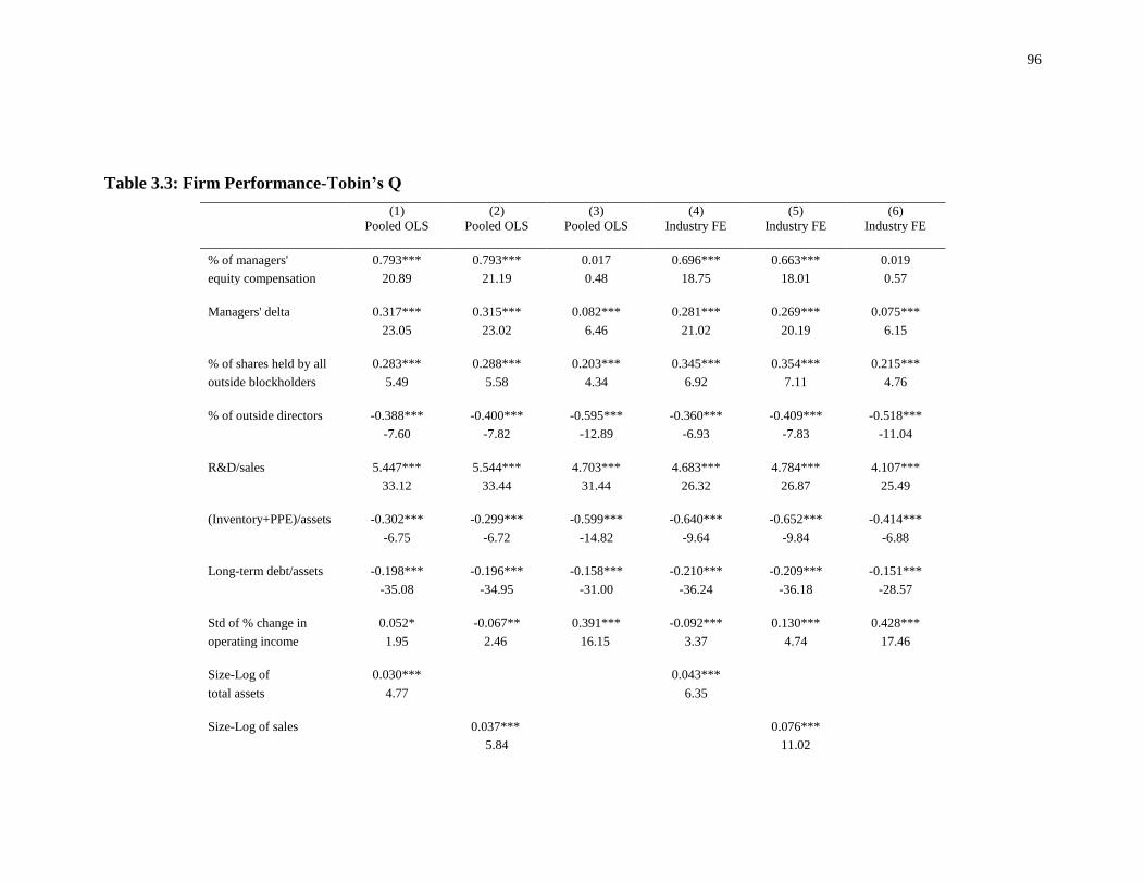
96

Table 3.3: Firm Performance-Tobin’s Q

(1)

Pooled OLS

(2)

Pooled OLS

(3)

Pooled OLS

(4)

Industry FE

(5)

Industry FE

(6)

Industry FE

% of managers' 0.793*** 0.793*** 0.017 0.696*** 0.663*** 0.019

equity compensation 20.89 21.19 0.48 18.75 18.01 0.57

Managers' delta 0.317*** 0.315*** 0.082*** 0.281*** 0.269*** 0.075***

23.05 23.02 6.46 21.02 20.19 6.15

% of shares held by all 0.283*** 0.288*** 0.203*** 0.345*** 0.354*** 0.215***

outside blockholders 5.49 5.58 4.34 6.92 7.11 4.76

% of outside directors -0.388*** -0.400*** -0.595*** -0.360*** -0.409*** -0.518***

-7.60 -7.82 -12.89 -6.93 -7.83 -11.04

R&D/sales 5.447*** 5.544*** 4.703*** 4.683*** 4.784*** 4.107***

33.12 33.44 31.44 26.32 26.87 25.49

(Inventory+PPE)/assets -0.302*** -0.299*** -0.599*** -0.640*** -0.652*** -0.414***

-6.75 -6.72 -14.82 -9.64 -9.84 -6.88

Long-term debt/assets -0.198*** -0.196*** -0.158*** -0.210*** -0.209*** -0.151***

-35.08 -34.95 -31.00 -36.24 -36.18 -28.57

Std of % change in 0.052* -0.067** 0.391*** -0.092*** 0.130*** 0.428***

operating income 1.95 2.46 16.15 3.37 4.74 17.46

Size-Log of 0.030*** 0.043***

total assets 4.77 6.35

Size-Log of sales 0.037*** 0.076***

5.84 11.02

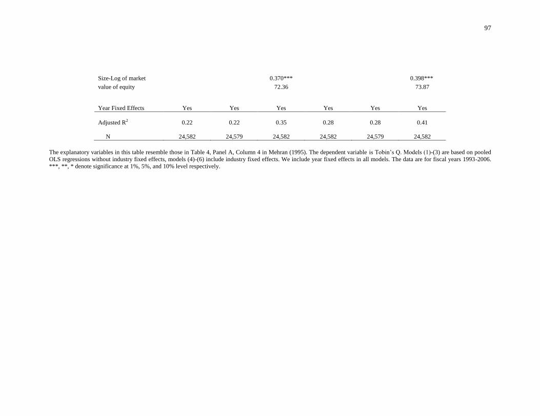
97

Size-Log of market 0.370*** 0.398***

value of equity 72.36 73.87

Year Fixed Effects Yes Yes Yes Yes

Yes

Yes

Adjusted R2 0.22 0.22 0.35 0.28

0.28

0.41

N 24,582 24,579 24,582 24,582

24,579

24,582

The explanatory variables in this table resemble those in Table 4, Panel A, Column 4 in Mehran (1995). The dependent variable is Tobin’s Q. Models (1)-(3) are based on pooled

OLS regressions without industry fixed effects, models (4)-(6) include industry fixed effects. We include year fixed effects in all models. The data are for fiscal years 1993-2006.

***, **, * denote significance at 1%, 5%, and 10% level respectively.

98

For ROA as the dependent variable, the representative specification refers to

Mehran (1995, Table 4, Panel B, Column 4), which also applies the log of total assets as

the measure of firm size. In Table 3.4, we find that when market value of equity is used

as firm size, 𝑅2 increases sharply (Figure 3.3) for both OLS and industry fixed effect

regressions, while the 𝑅2s are similar if we use total assets or sales. We further find that

the size proxy log of assets is not significant in the industry fixed effect regression. In

addition, unlike the results for Tobin’s Q, the sign and significance of the coefficients of

business risk are robust. However, the sign of the percentage of managers’ equity

compensation and managers’ delta both change to negative when firm size is market

value of equity, which suggests scholars should be especially careful about the firm size

measured by market value of equity for studies of firm performance.

It is worth noting that market value of equity is in the numerator Tobin’s Q, so it

is possible that they are mechanically correlated and thus affect empirical sensitivity such

as goodness-of-fit. Therefore, a high R-squared does not necessarily suggest a good

proxy of firm size. In Table 3.23 and Figure 3.3, we find the goodness-of-fit exhibits

substantial changes when market capitalization is used as a firm size proxy.

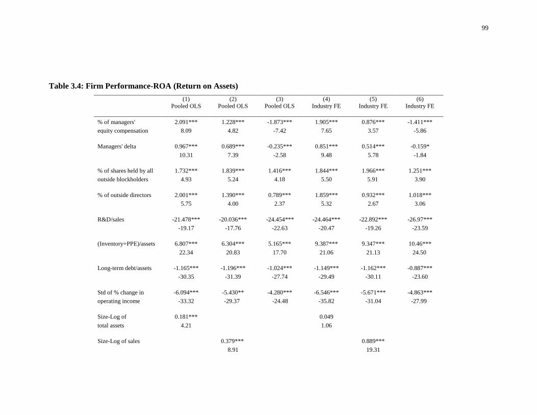
99

Table 3.4: Firm Performance-ROA (Return on Assets)

(1)

Pooled OLS

(2)

Pooled OLS

(3)

Pooled OLS

(4)

Industry FE

(5)

Industry FE

(6)

Industry FE

% of managers' 2.091*** 1.228*** -1.873*** 1.905*** 0.876*** -1.411***

equity compensation 8.09 4.82 -7.42 7.65 3.57 -5.86

Managers' delta 0.967*** 0.689*** -0.235*** 0.851*** 0.514*** -0.159*

10.31 7.39 -2.58 9.48 5.78 -1.84

% of shares held by all 1.732*** 1.839*** 1.416*** 1.844*** 1.966*** 1.251***

outside blockholders 4.93 5.24 4.18 5.50 5.91 3.90

% of outside directors 2.001*** 1.390*** 0.789*** 1.859*** 0.932*** 1.018***

5.75 4.00 2.37 5.32 2.67 3.06

R&D/sales -21.478*** -20.036*** -24.454*** -24.464*** -22.892*** -26.97***

-19.17 -17.76 -22.63 -20.47 -19.26 -23.59

(Inventory+PPE)/assets 6.807*** 6.304*** 5.165*** 9.387*** 9.347*** 10.46***

22.34 20.83 17.70 21.06 21.13 24.50

Long-term debt/assets -1.165*** -1.196*** -1.024*** -1.149*** -1.162*** -0.887***

-30.35 -31.39 -27.74 -29.49 -30.11 -23.60

Std of % change in -6.094*** -5.430** -4.280*** -6.546*** -5.671*** -4.863***

operating income -33.32 -29.37 -24.48 -35.82 -31.04 -27.99

Size-Log of 0.181*** 0.049

total assets 4.21 1.06

Size-Log of sales 0.379*** 0.889***

8.91 19.31

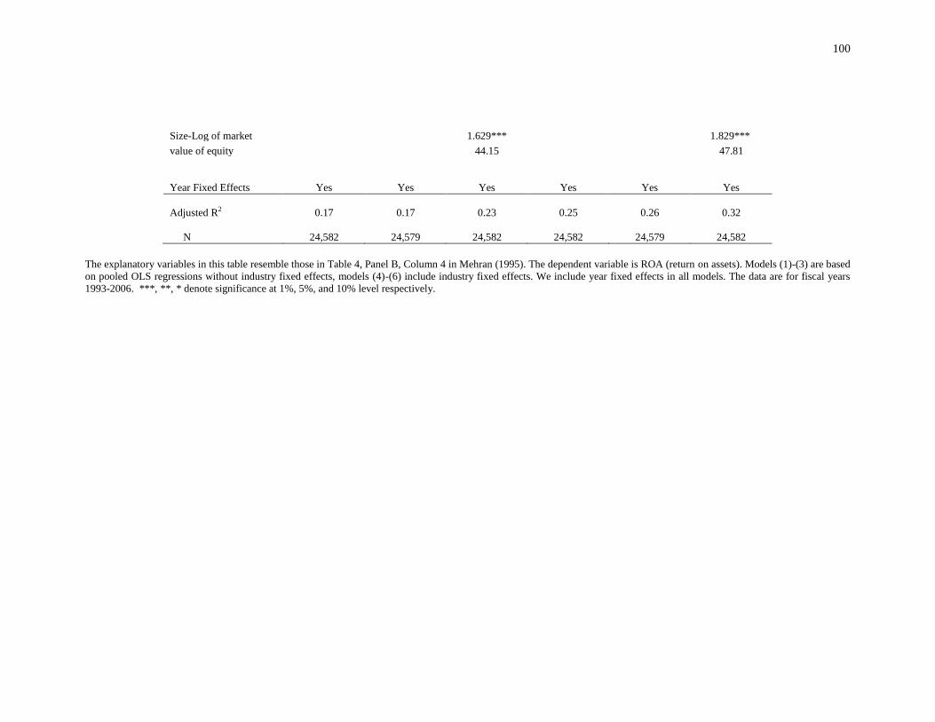
100

Size-Log of market 1.629*** 1.829***

value of equity 44.15 47.81

Year Fixed Effects Yes Yes Yes Yes

Yes

Yes

Adjusted R2 0.17 0.17 0.23 0.25

0.26

0.32

N 24,582 24,579 24,582 24,582

24,579

24,582

The explanatory variables in this table resemble those in Table 4, Panel B, Column 4 in Mehran (1995). The dependent variable is ROA (return on assets). Models (1)-(3) are based

on pooled OLS regressions without industry fixed effects, models (4)-(6) include industry fixed effects. We include year fixed effects in all models. The data are for fiscal years

1993-2006. ***, **, * denote significance at 1%, 5%, and 10% level respectively.

101

3.4.2 Board Structure

Board structure has received much attention as an important topic in corporate

governance; the existing literature covers three prominent board characteristics:

independence, i.e. the proportion of outside directors (Weisbach (1988), Byrd and

Hickman (1992), Brickley, Coles and Terry (1994), etc.); size (Jensen (1993), Yermack

(1996), Coles, Daniel, and Naveen (2008), etc.); and leadership, i.e. separation of CEO

and Chairman of the Board (COB) (Baliga, Moyer, and Rao (1996) and Brickley, Coles,

and Jarrel (1997), etc.).

We use Linck, Netter, and Yang (2008) for the examination of board structure,

more specifically, board independence as in Linck, Netter, and Yang (2008, Table 4,

Column 2). This benchmark paper uses the market value of equity as the firm size

measure. We denote the proportion of non-executive board members as the dependent

variable and report the results in Table 3.5. The positive sign of firm size indicates that

big firms tend to have more outside directors. The sign and significance of coefficients of

firm size are robust for both OLS and industry fixed effect models to different firm size

measures. While the 𝑅2𝑠 are similar, we observe that the sign and significance are

sensitive for debt (total long term debt divided by total assets) and R&D (R&D

expenditures divided by total assets) when we employ different firm size proxies. Fama

and Jensen (1983) suggest that outside directors who bring valuable expertise and

connections are beneficial to firms with complex operating or financial structures,

thereby leading to larger and more independent boards, and the pros of effective

monitoring should dominate the monitoring costs that go hand in hand with firm

complexity. Thus, Linck, Netter, and Yang (2008) predict that, as a proxy for growth

102

opportunities, R&D expenditures, which increase monitoring and advising costs, are

negatively related to board size and independence. However, debt proportion should be

positively related to board size and independence since debt proportion is a proxy for

firm complexity and advising benefits. In our results, the coefficient of debt is positive, as

predicted, but only significant when log of market value of equity is used. The coefficient

for R&D is positive for OLS regression but negative for industry fixed effect regression,

suggesting the results of industry fixed effect regressions are consistent with the

prediction. However, the significance is sensitive when we apply different firm size

measures in the industry fixed regressions.

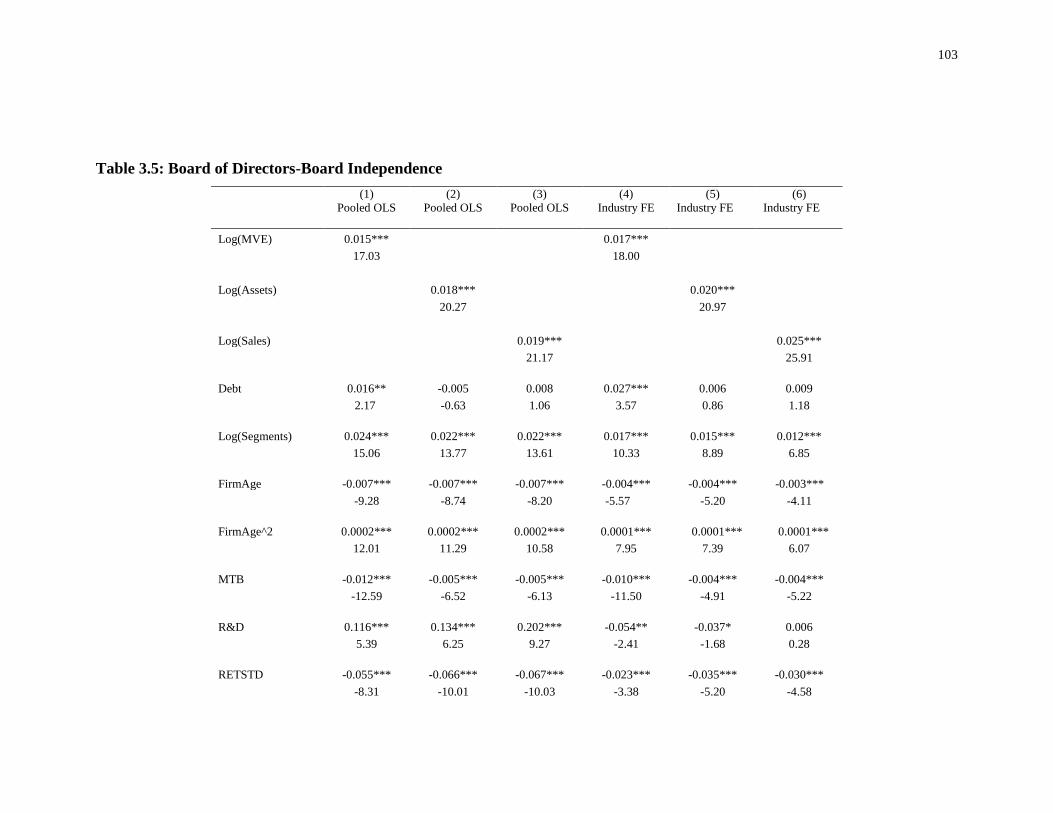
103

Table 3.5: Board of Directors-Board Independence

(1)

Pooled OLS

(2)

Pooled OLS

(3)

Pooled OLS

(4)

Industry FE

(5)

Industry FE

(6)

Industry FE

Log(MVE) 0.015*** 0.017***

17.03 18.00

Log(Assets) 0.018*** 0.020***

20.27 20.97

Log(Sales) 0.019*** 0.025***

21.17 25.91

Debt 0.016** -0.005 0.008 0.027*** 0.006 0.009

2.17 -0.63 1.06 3.57 0.86 1.18

Log(Segments) 0.024*** 0.022*** 0.022*** 0.017*** 0.015*** 0.012***

15.06 13.77 13.61 10.33 8.89 6.85

FirmAge -0.007*** -0.007*** -0.007*** -0.004*** -0.004*** -0.003***

-9.28 -8.74 -8.20 -5.57 -5.20 -4.11

FirmAge^2 0.0002*** 0.0002*** 0.0002*** 0.0001*** 0.0001*** 0.0001***

12.01 11.29 10.58 7.95 7.39 6.07

MTB -0.012*** -0.005*** -0.005*** -0.010*** -0.004*** -0.004***

-12.59 -6.52 -6.13 -11.50 -4.91 -5.22

R&D 0.116*** 0.134*** 0.202*** -0.054** -0.037* 0.006

5.39 6.25 9.27 -2.41 -1.68 0.28

RETSTD -0.055*** -0.066*** -0.067*** -0.023*** -0.035*** -0.030***

-8.31 -10.01 -10.03 -3.38 -5.20 -4.58

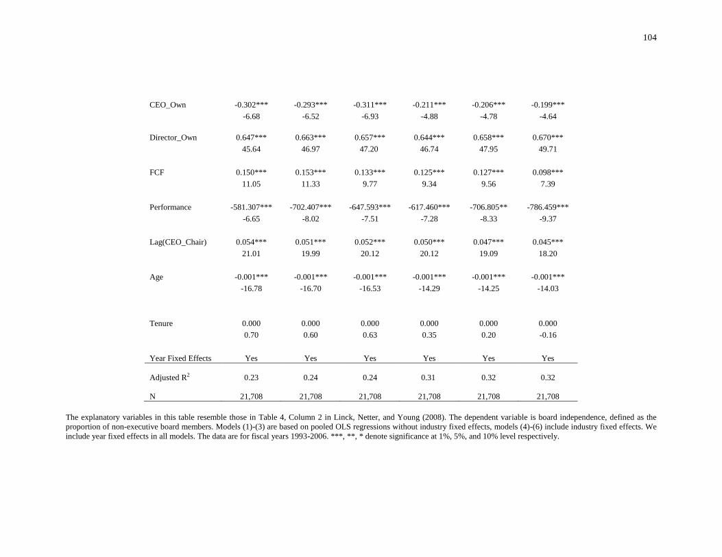
104

CEO_Own -0.302*** -0.293*** -0.311*** -0.211*** -0.206*** -0.199***

-6.68 -6.52 -6.93 -4.88 -4.78 -4.64

Director_Own 0.647*** 0.663*** 0.657*** 0.644*** 0.658*** 0.670***

45.64 46.97 47.20 46.74 47.95 49.71

FCF 0.150*** 0.153*** 0.133*** 0.125*** 0.127*** 0.098***

11.05 11.33 9.77 9.34 9.56 7.39

Performance -581.307*** -702.407*** -647.593*** -617.460*** -706.805** -786.459***

-6.65 -8.02 -7.51 -7.28 -8.33 -9.37

Lag(CEO_Chair) 0.054*** 0.051*** 0.052*** 0.050*** 0.047*** 0.045***

21.01 19.99 20.12 20.12 19.09 18.20

Age -0.001*** -0.001*** -0.001*** -0.001*** -0.001*** -0.001***

-16.78 -16.70 -16.53 -14.29 -14.25 -14.03

Tenure 0.000 0.000 0.000 0.000 0.000 0.000

0.70 0.60 0.63 0.35 0.20 -0.16

Year Fixed Effects Yes Yes Yes Yes Yes Yes

Adjusted R2 0.23 0.24 0.24 0.31

0.32

0.32

N 21,708 21,708 21,708 21,708

21,708

21,708

The explanatory variables in this table resemble those in Table 4, Column 2 in Linck, Netter, and Young (2008). The dependent variable is board independence, defined as the

proportion of non-executive board members. Models (1)-(3) are based on pooled OLS regressions without industry fixed effects, models (4)-(6) include industry fixed effects. We

include year fixed effects in all models. The data are for fiscal years 1993-2006. ***, **, * denote significance at 1%, 5%, and 10% level respectively.

105

The representative specification of board size refers to Linck, Netter, and Yang

(2008, Table 4, Column 1), and we report the results in Table 3.6. The dependent variable

is the number of directors on the board. The positive sign of firm size is also consistent

with Linck, Netter, and Yang (2008), indicating that board size increases with firm size.

The sign and significance of coefficients of firm size are robust to different size measures

in both OLS and industry fixed effect regressions. The 𝑅2𝑠 are quite similar. Once again,

the abnormal results reside in the sign and significance of the coefficients on debt and

R&D if different firm size measures are used.

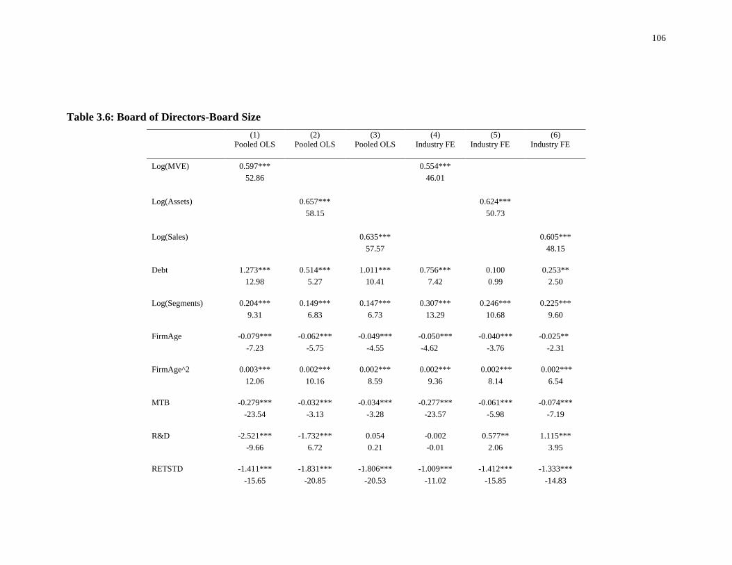
106

Table 3.6: Board of Directors-Board Size

(1)

Pooled OLS

(2)

Pooled OLS

(3)

Pooled OLS

(4)

Industry FE

(5)

Industry FE

(6)

Industry FE

Log(MVE) 0.597*** 0.554***

52.86 46.01

Log(Assets) 0.657*** 0.624***

58.15 50.73

Log(Sales) 0.635*** 0.605***

57.57 48.15

Debt 1.273*** 0.514*** 1.011*** 0.756*** 0.100 0.253**

12.98 5.27 10.41 7.42 0.99 2.50

Log(Segments) 0.204*** 0.149*** 0.147*** 0.307*** 0.246*** 0.225***

9.31 6.83 6.73 13.29 10.68 9.60

FirmAge -0.079*** -0.062*** -0.049*** -0.050*** -0.040*** -0.025**

-7.23 -5.75 -4.55 -4.62 -3.76 -2.31

FirmAge^2 0.003*** 0.002*** 0.002*** 0.002*** 0.002*** 0.002***

12.06 10.16 8.59 9.36 8.14 6.54

MTB -0.279*** -0.032*** -0.034*** -0.277*** -0.061*** -0.074***

-23.54 -3.13 -3.28 -23.57 -5.98 -7.19

R&D -2.521*** -1.732*** 0.054 -0.002 0.577** 1.115***

-9.66 6.72 0.21 -0.01 2.06 3.95

RETSTD -1.411*** -1.831*** -1.806*** -1.009*** -1.412*** -1.333***

-15.65 -20.85 -20.53 -11.02 -15.85 -14.83

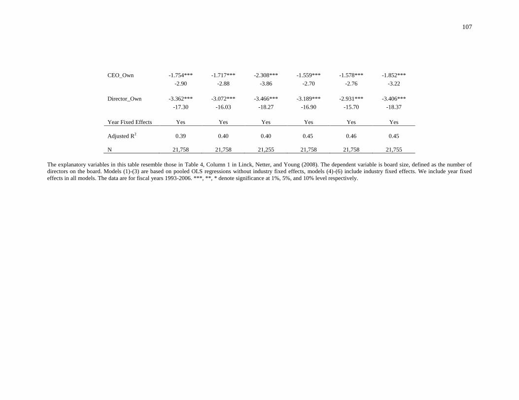
107

CEO_Own -1.754*** -1.717*** -2.308*** -1.559*** -1.578*** -1.852***

-2.90 -2.88 -3.86 -2.70 -2.76 -3.22

Director_Own -3.362*** -3.072*** -3.466*** -3.189*** -2.931*** -3.406***

-17.30 -16.03 -18.27 -16.90 -15.70 -18.37

Year Fixed Effects Yes Yes Yes Yes Yes Yes

Adjusted R2 0.39 0.40 0.40 0.45

0.46

0.45

N 21,758 21,758 21,255 21,758

21,758

21,755

The explanatory variables in this table resemble those in Table 4, Column 1 in Linck, Netter, and Young (2008). The dependent variable is board size, defined as the number of

directors on the board. Models (1)-(3) are based on pooled OLS regressions without industry fixed effects, models (4)-(6) include industry fixed effects. We include year fixed

effects in all models. The data are for fiscal years 1993-2006. ***, **, * denote significance at 1%, 5%, and 10% level respectively.

108

We refer to Linck, Netter, and Yang (2008, Table 4, Column 3) for the study of

board leadership (CEO duality). The dependent variable is the logit-transformed dummy

variable that equals 1 if the CEO and COB positions are combined and 0 otherwise. The

regressions are based on logistic models with and without industry fixed effects. Table

3.7 shows that the 𝑅2𝑠 are quite similar. The positive sign of firm size suggests CEO

duality increases with firm size. Different firm size measures do not change the sign and

significance of firm size coefficients. The sensitivity of R&D still exists in our results of

board leadership, suggesting scholars should pay special attention to this issue in the

extensive study of board governance. Standard deviation of stock returns, which is a

proxy for information asymmetry that increases monitoring and advising costs, also has

sensitive significance for different firm size measures.

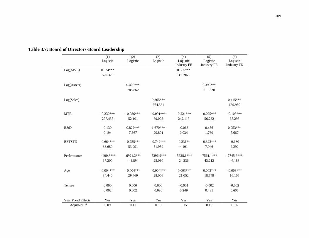
109

Table 3.7: Board of Directors-Board Leadership

(1)

Logistic

(2)

Logistic

(3)

Logistic

(4)

Logistic

Industry FE

(5)

Logistic

Industry FE

(6)

Logistic

Industry FE

Log(MVE) 0.324*** 0.305***

520.326 390.963

Log(Assets) 0.406*** 0.396***

785.862 611.320

Log(Sales) 0.365*** 0.415***

664.551 659.980

MTB -0.230*** -0.086*** -0.091*** -0.221*** -0.095*** -0.105***

297.455 52.101 59.008 242.113 56.232 68.293

R&D 0.130 0.822*** 1.670*** -0.063 0.456 0.953***

0.194 7.667 29.891 0.034 1.760 7.667

RETSTD -0.664*** -0.755*** -0.742*** -0.231** -0.323*** -0.180

38.689 53.991 51.959 4.101 7.946 2.292

Performance -4490.8*** -6921.2*** -5396.9*** -5628.1*** -7561.1*** -7745.6***

17.200 -41.894 25.010 24.236 43.212 46.183

Age -0.004*** -0.004*** -0.004*** -0.003*** -0.003*** -0.003***

34.440 29.469 28.006 21.052 18.749 16.106

Tenure 0.000 0.000 0.000 -0.001 -0.002 -0.002

0.002 0.002 0.030 0.249 0.481 0.606

Year Fixed Effects Yes Yes Yes Yes Yes Yes

Adjusted R2 0.09 0.11 0.10 0.15 0.16 0.16

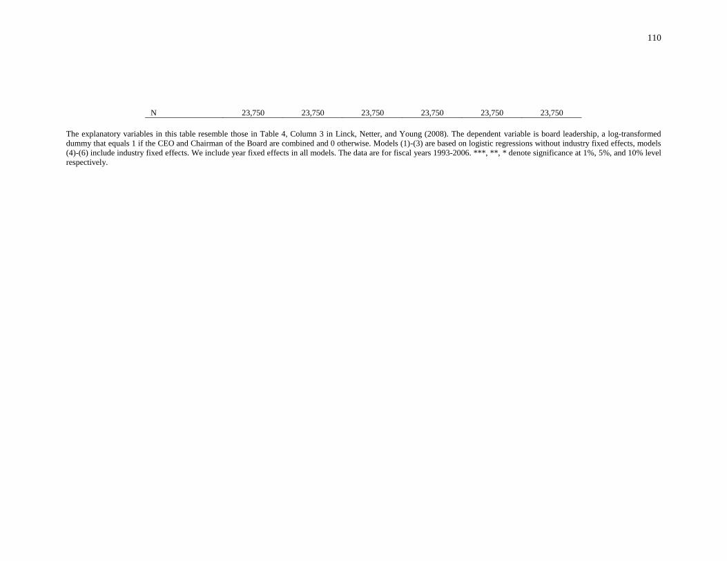
110

N 23,750 23,750 23,750 23,750

23,750

23,750

The explanatory variables in this table resemble those in Table 4, Column 3 in Linck, Netter, and Young (2008). The dependent variable is board leadership, a log-transformed

dummy that equals 1 if the CEO and Chairman of the Board are combined and 0 otherwise. Models (1)-(3) are based on logistic regressions without industry fixed effects, models

(4)-(6) include industry fixed effects. We include year fixed effects in all models. The data are for fiscal years 1993-2006. ***, **, * denote significance at 1%, 5%, and 10% level

respectively.

111

3.4.3 Dividend Policy

We choose DeAngelo, DeAngelo, and Stulz（2006, Table 3, Column 1） as the

benchmark paper for our analysis of payout policy. DeAngelo, DeAngelo, and Stulz（

2006）apply the market value of equity as the size proxy. The dependent variable is a

dummy variable that equals 1 if the firm pays out dividends and 0 otherwise. The

regressions are based on logistic models with and without industry fixed effect. We report

the results in Table 3.8. All results are robust: there were no changes in sign and

significance of the regressors when different size proxies were used.

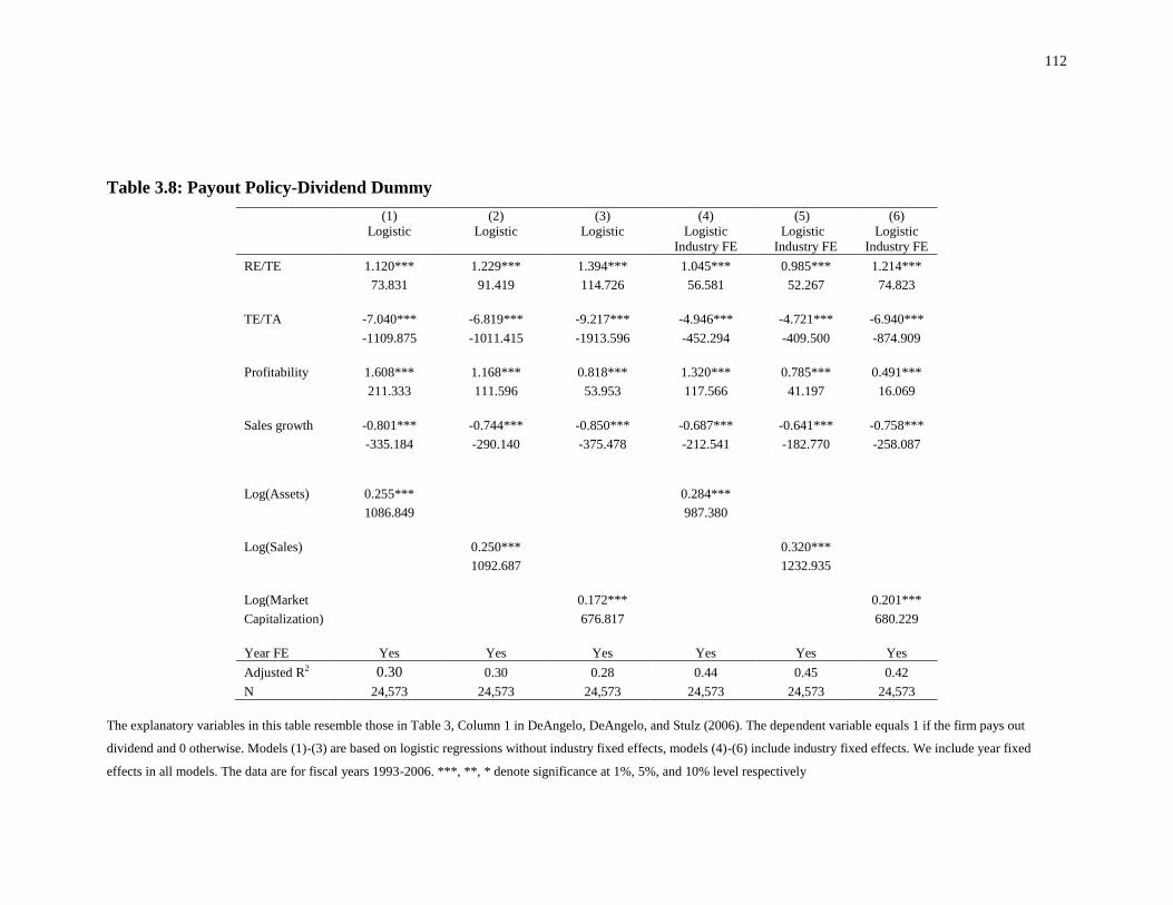
112

Table 3.8: Payout Policy-Dividend Dummy

(1)

Logistic

(2)

Logistic

(3)

Logistic

(4)

Logistic

Industry FE

(5)

Logistic

Industry FE

(6)

Logistic

Industry FE

RE/TE 1.120*** 1.229*** 1.394*** 1.045*** 0.985*** 1.214***

73.831 91.419 114.726 56.581 52.267 74.823

TE/TA -7.040*** -6.819*** -9.217*** -4.946*** -4.721*** -6.940***

-1109.875 -1011.415 -1913.596 -452.294 -409.500 -874.909

Profitability 1.608*** 1.168*** 0.818*** 1.320*** 0.785*** 0.491***

211.333 111.596 53.953 117.566 41.197 16.069

Sales growth -0.801*** -0.744*** -0.850*** -0.687*** -0.641*** -0.758***

-335.184 -290.140 -375.478 -212.541 -182.770 -258.087

Log(Assets) 0.255*** 0.284***

1086.849 987.380

Log(Sales) 0.250*** 0.320***

1092.687 1232.935

Log(Market 0.172*** 0.201***

Capitalization) 676.817 680.229

Year FE Yes Yes Yes Yes Yes Yes

Adjusted R2 0.30 0.30 0.28 0.44 0.45 0.42

N 24,573 24,573 24,573 24,573 24,573 24,573

The explanatory variables in this table resemble those in Table 3, Column 1 in DeAngelo, DeAngelo, and Stulz (2006). The dependent variable equals 1 if the firm pays out

dividend and 0 otherwise. Models (1)-(3) are based on logistic regressions without industry fixed effects, models (4)-(6) include industry fixed effects. We include year fixed

effects in all models. The data are for fiscal years 1993-2006. ***, **, * denote significance at 1%, 5%, and 10% level respectively

113

3.4.4 Financial Policy

We examine capital structure (book leverage and market leverage) and cash

holdings in this section. We investigate both book leverage and market leverage because

Frank and Goyal (2009) find firm size has different effects on book leverage and market

leverage. The benchmark paper we select for capital structure is Lemmon, Roberts, and

Zender (2008), which uses the log of sales as the measure of firm size. The benchmark

specification for book leverage refers to Lemmon, Roberts, and Zender (2008, Table II,

Panel A, Column3). We report the results for book leverage in Table 3.9. All firm size

measures are significant, and the sign is positive when we use total assets and sales, but

the sign turns out to be negative when we use market value of equity. This change might

be due to mechanical correlation, as leverage is one minus equity ratio. The other obvious

change is that the sign and significance of the cash flow volatilities is sensitive if we

apply different firm size measures. The 𝑅2 is lower for the log of sales in the industry

fixed effect regressions.

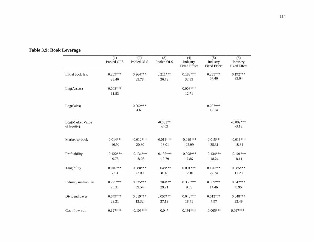
114

Table 3.9: Book Leverage

(1)

Pooled OLS

(2)

Pooled OLS

(3)

Pooled OLS

(4)

Industry

Fixed Effect

(5)

Industry

Fixed Effect

(6)

Industry

Fixed Effect

Initial book lev. 0.209*** 0.264*** 0.211*** 0.188***

0.235***

0.192***

36.46 65.78 36.78 32.95 57.40 33.64

Log(Assets) 0.008*** 0.009***

11.83 12.71

Log(Sales) 0.002*** 0.007***

4.61 12.14

Log(Market Value -0.001** -0.002***

of Equity) -2.02 -3.18

Market-to-book -0.014*** -0.012*** -0.012*** -0.019*** -0.015*** -0.016***

-16.92 -20.80 -13.01 -22.99 -25.31 -18.64

Profitability -0.122*** -0.134*** -0.135*** -0.098*** -0.134*** -0.101***

-9.78 -18.26 -10.79 -7.86 -18.24 -8.11

Tangibility 0.040*** 0.088*** 0.048*** 0.091*** 0.120*** 0.085***

7.53 23.00 8.92 12.10 22.74 11.23

Industry median lev. 0.295*** 0.325*** 0.309*** 0.355*** 0.369*** 0.342***

28.31 39.54 29.71 9.35 14.46 8.96

Dividend payer 0.049*** 0.019*** 0.057*** 0.040*** 0.013*** 0.048***

23.21 12.32 27.13 18.41 7.97 22.49

Cash flow vol. 0.127*** -0.108*** 0.047 0.191*** -0.065*** 0.097***

115

4.18 -7.24 1.56 6.23 -4.46 3.18

Year Fixed Effects Yes Yes Yes Yes Yes Yes

Adjusted R2 0.24 0.23 0.23 0.32 0.27 0.31

N 25,680 56,590 25,680 25,680

56,590

25,680

The explanatory variables in this table resemble those in Table II, Panel A, Column 3 in Lemmon, Roberts, and Zender (2008). The dependent variable is book leverage, defined as

the ratio of total debt to book assets. Models (1)-(3) are based on pooled OLS regressions without industry fixed effects, models (4)-(6) include industry fixed effects. We include

year fixed effects in all models. The data are for fiscal years 1993-2006. ***, **, * denote significance at 1%, 5%, and 10% level respectively.

116

We refer to Lemmon, Roberts, and Zender (2008, Table II, Panel A, Column 6)

for the study of market leverage. Results are in Table 3.10. Similar with the results of

book leverage, the sign of the coefficient of firm size is positive when we use total assets

and sales, but turns negative when we use market value of equity. In addition, the sign

and significance of the cash flow volatilities is also sensitive to different size measures.

The goodness of fit is lower, with a difference of about 0.03-0.04 for the log of sales in

the industry fixed effect regressions. The coefficient of dividend payer is not significant if

we use the log of total assets in the pooled OLS regression.

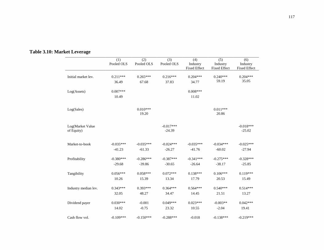
117

Table 3.10: Market Leverage

(1)

Pooled OLS

(2)

Pooled OLS

(3)

Pooled OLS

(4)

Industry

Fixed Effect

(5)

Industry

Fixed Effect

(6)

Industry

Fixed Effect

Initial market lev. 0.211*** 0.265*** 0.216*** 0.204***

0.240***

0.204***

36.49 67.68 37.83 34.77 59.19 35.05

Log(Assets) 0.007*** 0.008***

10.49 11.02

Log(Sales) 0.010*** 0.011***

19.20 20.86

Log(Market Value -0.017*** -0.018***

of Equity) -24.39 -25.02

Market-to-book -0.035*** -0.035*** -0.024*** -0.035*** -0.034*** -0.025***

-41.23 -61.33 -26.27 -41.76 -60.02 -27.94

Profitability -0.380*** -0.286*** -0.387*** -0.341*** -0.275*** -0.328***

-29.68 -39.86 -30.65 -26.64 -38.17 -25.85

Tangibility 0.056*** 0.058*** 0.072*** 0.138*** 0.106*** 0.119***

10.26 15.39 13.34 17.79 20.53 15.49

Industry median lev. 0.343*** 0.393*** 0.364*** 0.564*** 0.540*** 0.514***

32.05 48.27 34.47 14.45 21.51 13.27

Dividend payer 0.030*** -0.001 0.049*** 0.023*** -0.003** 0.042***

14.02 -0.75 23.32 10.55 -2.04 19.41

Cash flow vol. -0.109*** -0.150*** -0.288*** -0.018 -0.138*** -0.219***

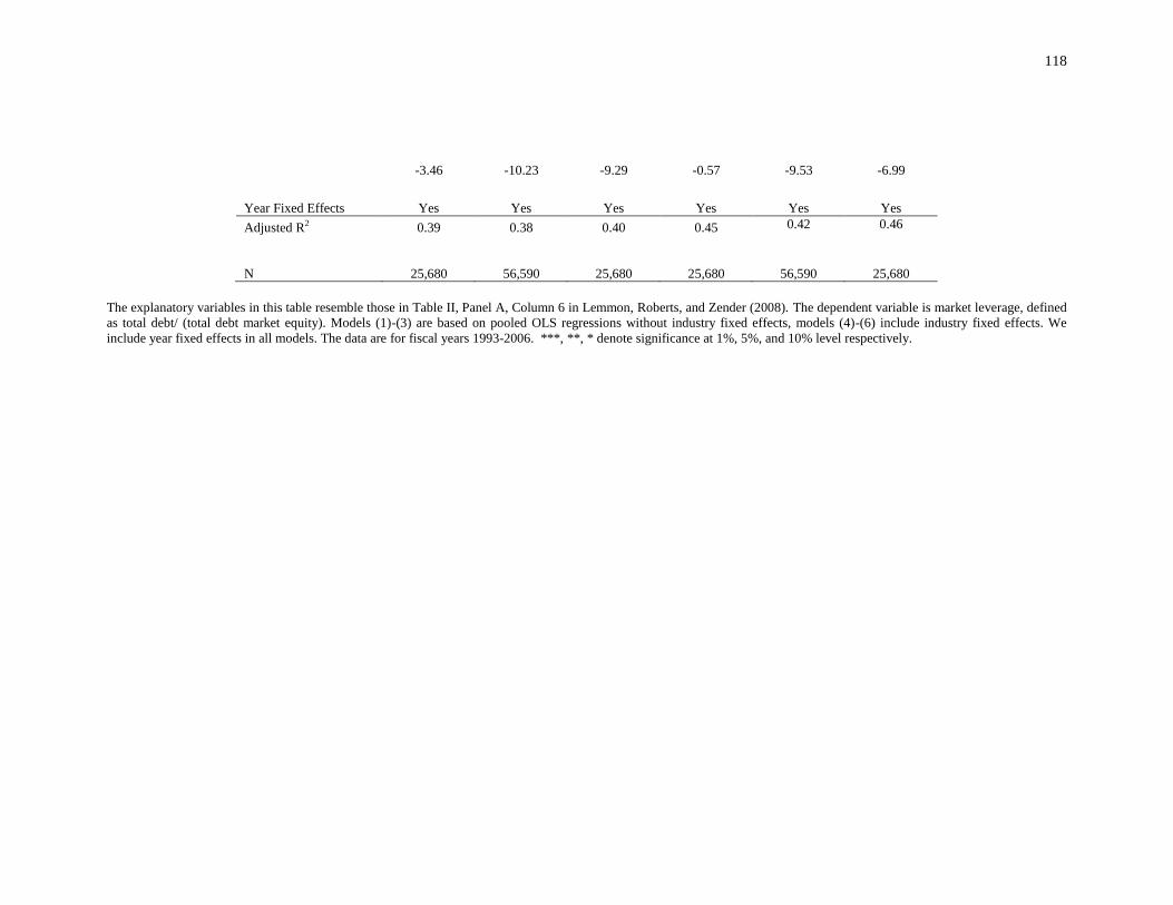
118

-3.46 -10.23 -9.29 -0.57 -9.53 -6.99

Year Fixed Effects Yes Yes Yes Yes Yes Yes

Adjusted R2 0.39 0.38 0.40 0.45 0.42 0.46

N 25,680 56,590 25,680 25,680

56,590

25,680

The explanatory variables in this table resemble those in Table II, Panel A, Column 6 in Lemmon, Roberts, and Zender (2008). The dependent variable is market leverage, defined

as total debt/ (total debt market equity). Models (1)-(3) are based on pooled OLS regressions without industry fixed effects, models (4)-(6) include industry fixed effects. We

include year fixed effects in all models. The data are for fiscal years 1993-2006. ***, **, * denote significance at 1%, 5%, and 10% level respectively.

119

The analysis for cash holdings is based on Harford, Mansi, and Maxwell (2008,

Table 3, Column 1), which applies the natural log of total assets as firm size measure and

the natural log of cash/sales ratio as the dependent variable. We report the results in Table

3.11. In pooled OLS regressions, only the coefficient of firm size measured by the log of

sales is significant, while all firm size coefficients are significant in the industry fixed

effect model. The sign of firm size is negative if the log of sales is used, consistent with

the conventional wisdom that small firms have financial constraints, limited access to

external financing, and higher marginal probability of bankruptcy. But when we use the

log of assets and the log of market value of equity, the signs are positive in the industry

fixed effect regressions. The significance of inside ownership, pay sensitivity, and

institutional ownership is sensitive, especially in the industry fixed effect model. In

addition, both the sign and the significance of cash flow are sensitive to different size

measures. We do not observe obvious differences of goodness of fit across the

regressions.

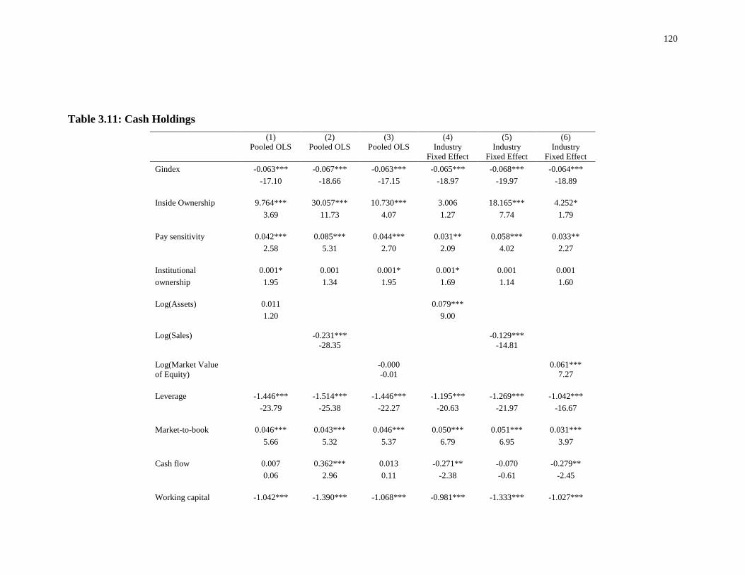
120

Table 3.11: Cash Holdings

(1)

Pooled OLS

(2)

Pooled OLS

(3)

Pooled OLS

(4)

Industry

Fixed Effect

(5)

Industry

Fixed Effect

(6)

Industry

Fixed Effect

Gindex -0.063*** -0.067*** -0.063*** -0.065*** -0.068*** -0.064***

-17.10 -18.66 -17.15 -18.97 -19.97 -18.89

Inside Ownership 9.764*** 30.057*** 10.730*** 3.006 18.165*** 4.252*

3.69 11.73 4.07 1.27 7.74 1.79

Pay sensitivity 0.042*** 0.085*** 0.044*** 0.031** 0.058*** 0.033**

2.58 5.31 2.70 2.09 4.02 2.27

Institutional 0.001* 0.001 0.001* 0.001* 0.001 0.001

ownership 1.95 1.34 1.95 1.69 1.14 1.60

Log(Assets) 0.011 0.079***

1.20 9.00

Log(Sales) -0.231*** -0.129***

-28.35 -14.81

Log(Market Value -0.000 0.061***

of Equity) -0.01 7.27

Leverage -1.446*** -1.514*** -1.446*** -1.195*** -1.269*** -1.042***

-23.79 -25.38 -22.27 -20.63 -21.97 -16.67

Market-to-book 0.046*** 0.043*** 0.046*** 0.050*** 0.051*** 0.031***

5.66 5.32 5.37 6.79 6.95 3.97

Cash flow 0.007 0.362*** 0.013 -0.271** -0.070 -0.279**

0.06 2.96 0.11 -2.38 -0.61 -2.45

Working capital -1.042*** -1.390*** -1.068*** -0.981*** -1.333*** -1.027***

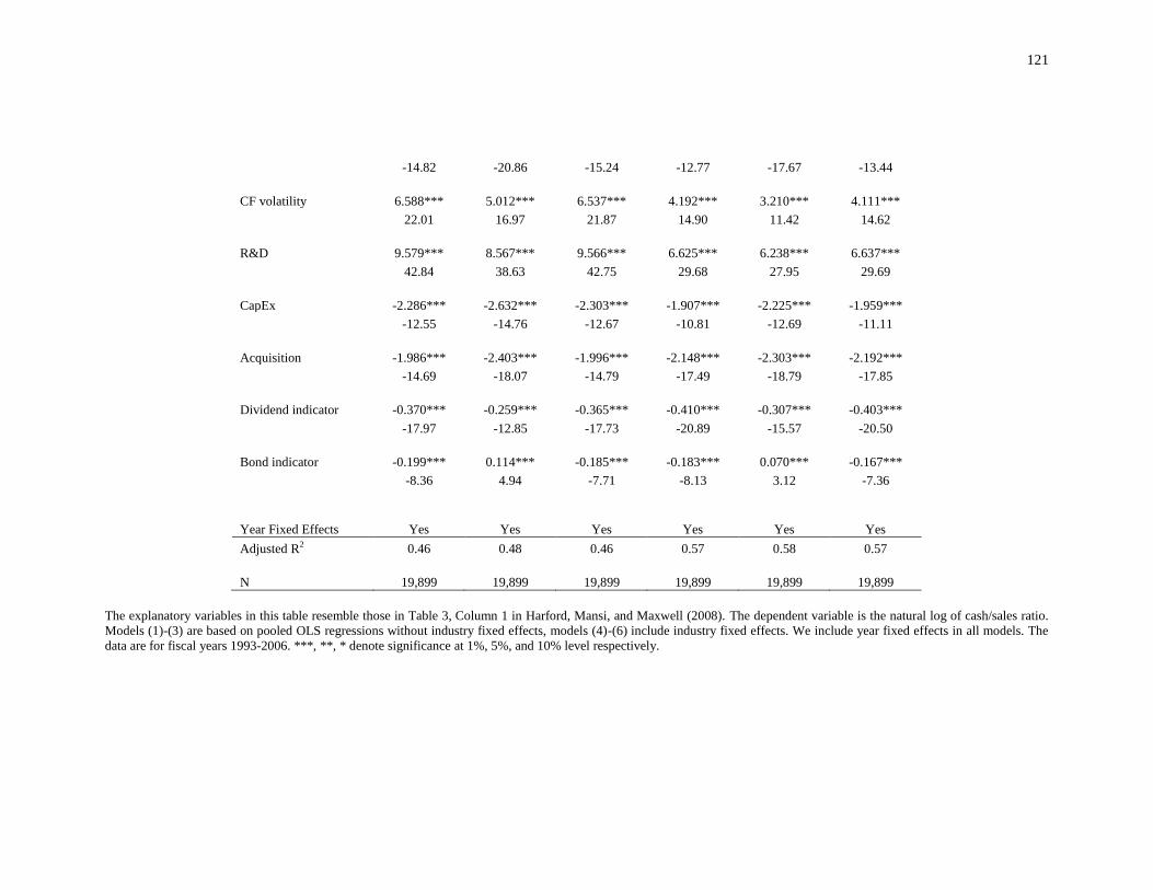
121

-14.82 -20.86 -15.24 -12.77 -17.67 -13.44

CF volatility 6.588*** 5.012*** 6.537*** 4.192*** 3.210*** 4.111***

22.01 16.97 21.87 14.90 11.42 14.62

R&D 9.579*** 8.567*** 9.566*** 6.625*** 6.238*** 6.637***

42.84 38.63 42.75 29.68 27.95 29.69

CapEx -2.286*** -2.632*** -2.303*** -1.907*** -2.225*** -1.959***

-12.55 -14.76 -12.67 -10.81 -12.69 -11.11

Acquisition -1.986*** -2.403*** -1.996*** -2.148*** -2.303*** -2.192***

-14.69 -18.07 -14.79 -17.49 -18.79 -17.85

Dividend indicator -0.370*** -0.259*** -0.365*** -0.410*** -0.307*** -0.403***

-17.97 -12.85 -17.73 -20.89 -15.57 -20.50

Bond indicator -0.199*** 0.114*** -0.185*** -0.183*** 0.070*** -0.167***

-8.36 4.94 -7.71 -8.13 3.12 -7.36

Year Fixed Effects Yes Yes Yes Yes Yes Yes

Adjusted R2 0.46 0.48 0.46 0.57 0.58 0.57

N 19,899 19,899 19,899 19,899 19,899 19,899

The explanatory variables in this table resemble those in Table 3, Column 1 in Harford, Mansi, and Maxwell (2008). The dependent variable is the natural log of cash/sales ratio.

Models (1)-(3) are based on pooled OLS regressions without industry fixed effects, models (4)-(6) include industry fixed effects. We include year fixed effects in all models. The

data are for fiscal years 1993-2006. ***, **, * denote significance at 1%, 5%, and 10% level respectively.

122

3.4.5 Compensation Policy

We build on Coles, Daniel, and Naveen (2006) for vega (the sensitivity of

managerial compensation to stock volatility) and delta (the sensitivity of managerial

compensation to stock price, i.e. the pay-performance sensitivity). For vega we use the

same independent variables as in Coles, Daniel, and Naveen (2006, Table 3, Panel A,

Column 2), who apply the log of sales as firm size. We consider industry fixed effect

because Coles, Daniel, and Naveen (2006) employ 2-digit SIC control. The empirical

results are reported in Table 3.12. The sign is positive for different firm size proxies,

consistent with Coles, Daniel, and Naveen (2006). The sign and sensitivity are not robust

for the coefficients of market-to-book ratio and book leverage level. The R-squared does

not change.

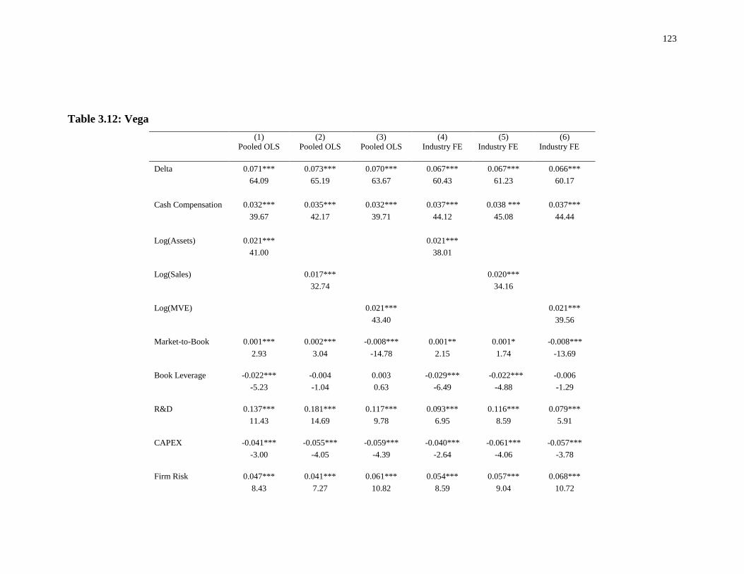
123

Table 3.12: Vega

(1)

Pooled OLS

(2)

Pooled OLS

(3)

Pooled OLS

(4)

Industry FE

(5)

Industry FE

(6)

Industry FE

Delta 0.071*** 0.073*** 0.070*** 0.067*** 0.067*** 0.066***

64.09 65.19 63.67 60.43 61.23 60.17

Cash Compensation 0.032*** 0.035*** 0.032*** 0.037*** 0.038 *** 0.037***

39.67 42.17 39.71 44.12 45.08 44.44

Log(Assets) 0.021*** 0.021***

41.00 38.01

Log(Sales) 0.017*** 0.020***

32.74 34.16

Log(MVE) 0.021*** 0.021***

43.40 39.56

Market-to-Book 0.001*** 0.002*** -0.008*** 0.001** 0.001* -0.008***

2.93 3.04 -14.78 2.15 1.74 -13.69

Book Leverage -0.022*** -0.004 0.003 -0.029*** -0.022*** -0.006

-5.23 -1.04 0.63 -6.49 -4.88 -1.29

R&D 0.137*** 0.181*** 0.117*** 0.093*** 0.116*** 0.079***

11.43 14.69 9.78 6.95 8.59 5.91

CAPEX -0.041*** -0.055*** -0.059*** -0.040*** -0.061*** -0.057***

-3.00 -4.05 -4.39 -2.64 -4.06 -3.78

Firm Risk 0.047*** 0.041*** 0.061*** 0.054*** 0.057*** 0.068***

8.43 7.27 10.82 8.59 9.04 10.72

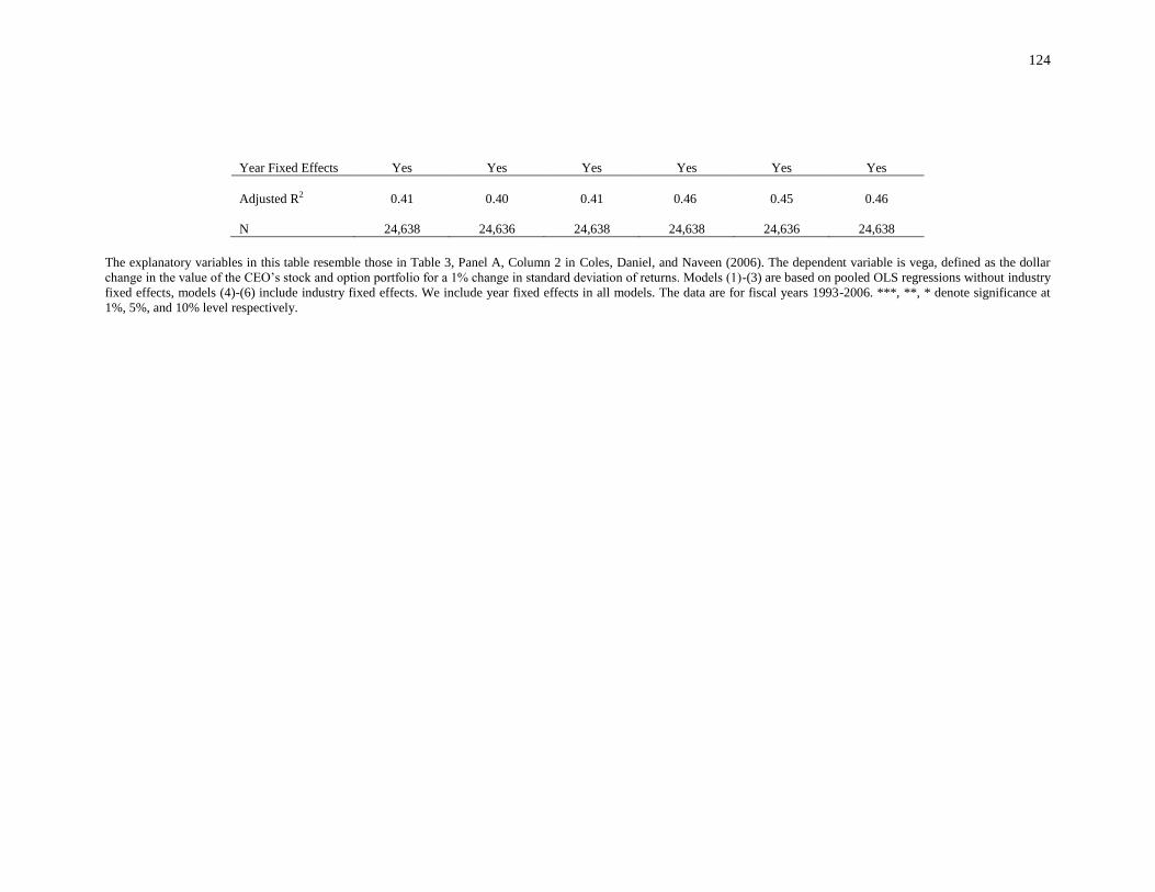
124

Year Fixed Effects Yes Yes Yes Yes Yes Yes

Adjusted R2 0.41 0.40 0.41 0.46

0.45

0.46

N 24,638 24,636 24,638 24,638

24,636

24,638

The explanatory variables in this table resemble those in Table 3, Panel A, Column 2 in Coles, Daniel, and Naveen (2006). The dependent variable is vega, defined as the dollar

change in the value of the CEO’s stock and option portfolio for a 1% change in standard deviation of returns. Models (1)-(3) are based on pooled OLS regressions without industry

fixed effects, models (4)-(6) include industry fixed effects. We include year fixed effects in all models. The data are for fiscal years 1993-2006. ***, **, * denote significance at

1%, 5%, and 10% level respectively.

125

We refer to Coles, Daniel, and Naveen (2006, Table 3, Panel A, Column 2) for

delta and report the results in Table 3.13. The sign of firm size is positive when we apply

different measures of firm size, indicating that larger firms have larger pay-performance

sensitivity. The results for other regressors are robust, except for the firm risk. We find

that the coefficient of firm risk is significant in the OLS regressions, but when we add

industry fixed effect it is no longer significant, though the sign remains positive. The

goodness of fit remains the same across different regressions.

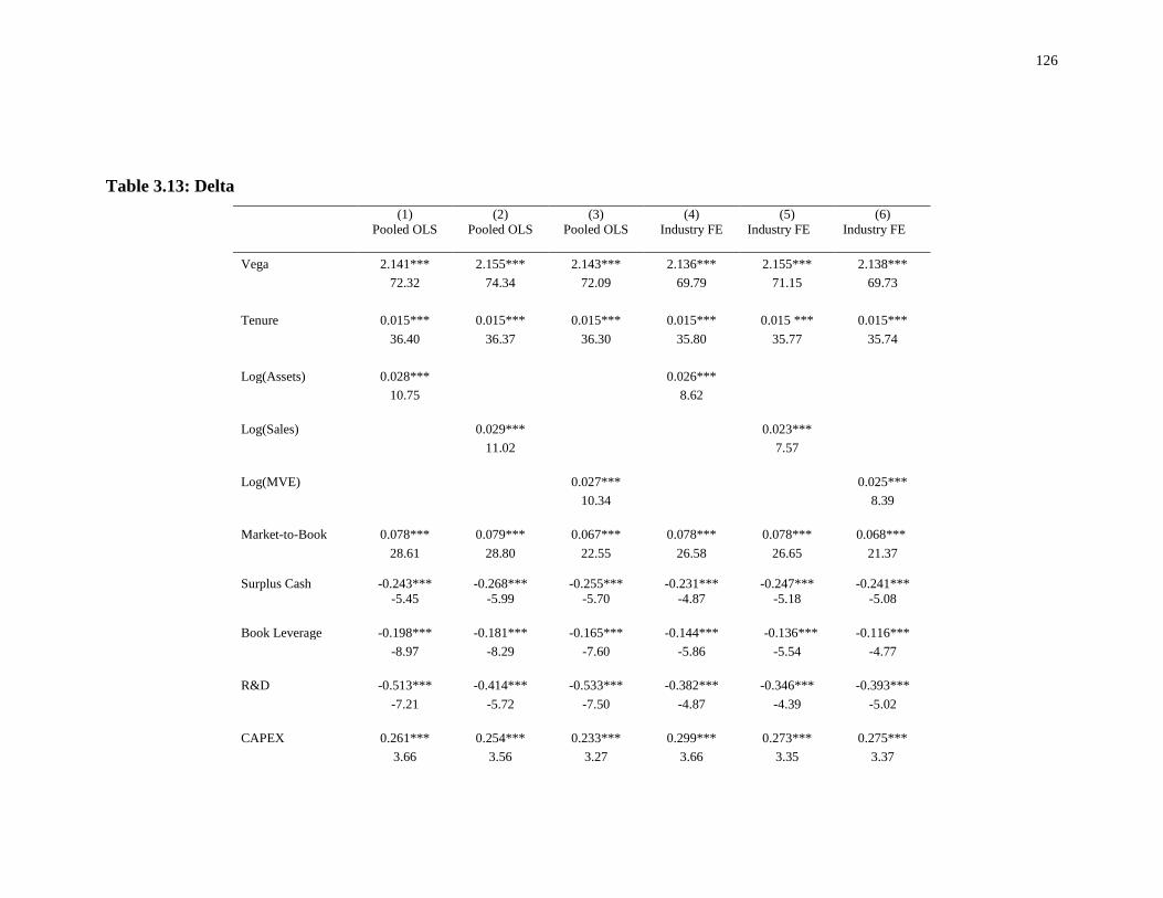
126

Table 3.13: Delta

(1)

Pooled OLS

(2)

Pooled OLS

(3)

Pooled OLS

(4)

Industry FE

(5)

Industry FE

(6)

Industry FE

Vega 2.141*** 2.155*** 2.143*** 2.136*** 2.155*** 2.138***

72.32 74.34 72.09 69.79 71.15 69.73

Tenure 0.015*** 0.015*** 0.015*** 0.015*** 0.015 *** 0.015***

36.40 36.37 36.30 35.80 35.77 35.74

Log(Assets) 0.028*** 0.026***

10.75 8.62

Log(Sales) 0.029*** 0.023***

11.02 7.57

Log(MVE) 0.027*** 0.025***

10.34 8.39

Market-to-Book 0.078*** 0.079*** 0.067*** 0.078*** 0.078*** 0.068***

28.61 28.80 22.55 26.58 26.65 21.37

Surplus Cash -0.243*** -0.268*** -0.255*** -0.231*** -0.247*** -0.241***

-5.45 -5.99 -5.70 -4.87 -5.18 -5.08

Book Leverage -0.198*** -0.181*** -0.165*** -0.144*** -0.136*** -0.116***

-8.97 -8.29 -7.60 -5.86 -5.54 -4.77

R&D -0.513*** -0.414*** -0.533*** -0.382*** -0.346*** -0.393***

-7.21 -5.72 -7.50 -4.87 -4.39 -5.02

CAPEX 0.261*** 0.254*** 0.233*** 0.299*** 0.273*** 0.275***

3.66 3.56 3.27 3.66 3.35 3.37

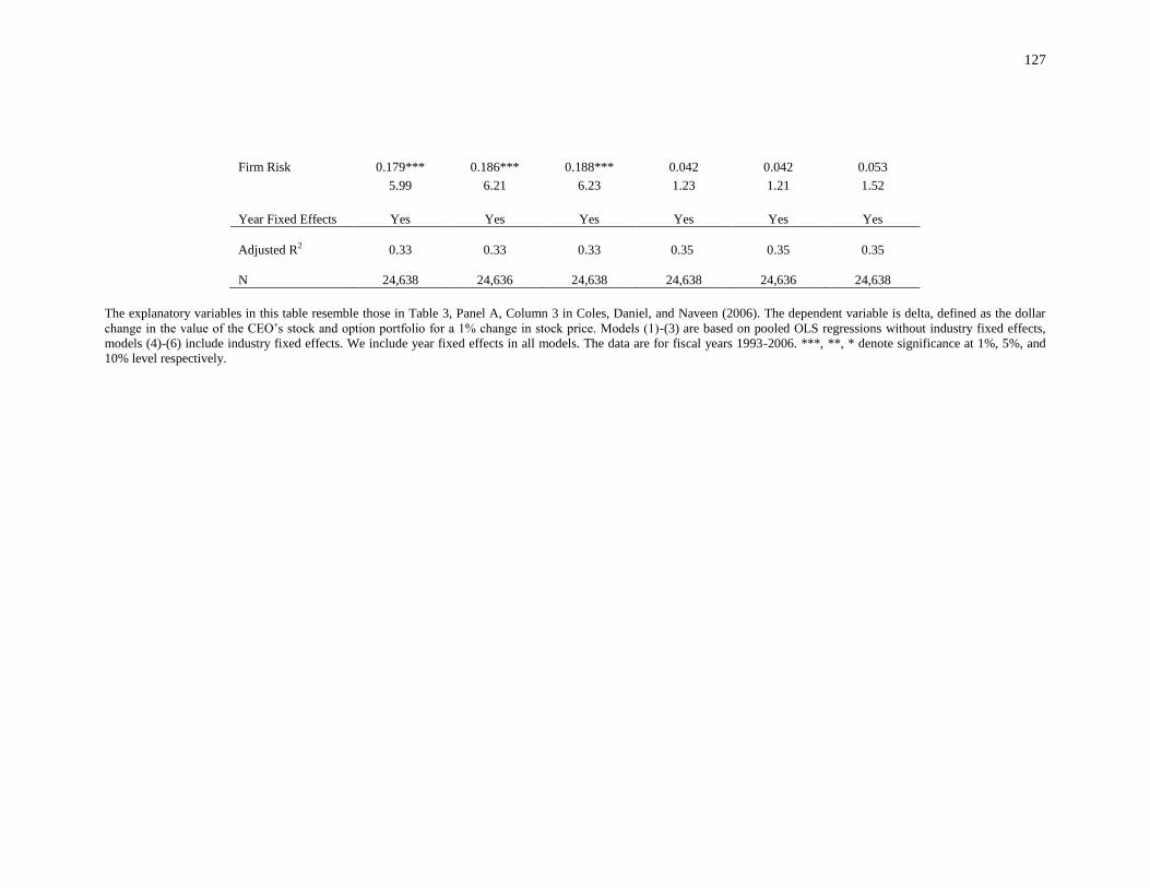
127

Firm Risk 0.179*** 0.186*** 0.188*** 0.042 0.042 0.053

5.99 6.21 6.23 1.23 1.21 1.52

Year Fixed Effects Yes Yes Yes Yes Yes Yes

Adjusted R2 0.33 0.33 0.33 0.35

0.35

0.35

N 24,638 24,636 24,638 24,638

24,636

24,638

The explanatory variables in this table resemble those in Table 3, Panel A, Column 3 in Coles, Daniel, and Naveen (2006). The dependent variable is delta, defined as the dollar

change in the value of the CEO’s stock and option portfolio for a 1% change in stock price. Models (1)-(3) are based on pooled OLS regressions without industry fixed effects,

models (4)-(6) include industry fixed effects. We include year fixed effects in all models. The data are for fiscal years 1993-2006. ***, **, * denote significance at 1%, 5%, and

10% level respectively.

128

For executive pay level (i.e. total compensation), we refer to Graham, Li, and Qiu

(2012, Table 4, Panel A, Column 1). Graham, Li, and Qiu (2012) use the log of assets as

firm size proxy. We report the results in Table 3.14. The sign is positive for different firm

size measures, consistent with the fact that larger firms lead to higher top-management

pay levels. The results are robust for the coefficient of stock return, but not for the lagged

stock return. In addition, the results are robust for lagged ROA, but not for ROA. Thus,

we should pay special attention to whether we should use lagged terms or current terms

as asset performance in determining executive pay level. We also find the significance

for coefficients of stock return volatility and gender changes slightly across different

regressions. We do not observe obvious differences in goodness of fit.

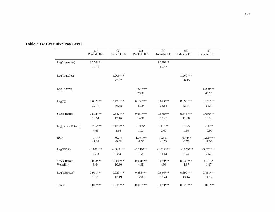
129

Table 3.14: Executive Pay Level

(1)

Pooled OLS

(2)

Pooled OLS

(3)

Pooled OLS

(4)

Industry FE

(5)

Industry FE

(6)

Industry FE

Lag(logassets) 1.276***

1.289***

79.14

69.37

Lag(logsales)

1.209***

1.260***

72.82

66.15

Lag(logmve)

1.275***

1.239***

78.92

68.56

Lag(Q) 0.632*** 0.732*** 0.106*** 0.613*** 0.693*** 0.151***

32.17 36.58 5.00 28.84 32.44 6.58

Stock Return 0.592*** 0.542*** 0.654*** 0.576*** 0.543*** 0.636***

13.51 12.16 14.91 12.29 11.50 13.53

Lag(Stock Return) 0.205*** 0.133*** 0.085* 0.111** 0.075 -0.037

4.65 2.96 1.93 2.40 1.60 -0.80

ROA -0.477 -0.278 -1.064*** -0.651 -0.744* -1.134***

-1.16 -0.66 -2.58 -1.53 -1.73 -2.66

Lag(ROA) -1.708*** -4.549*** -3.119*** -1.819*** -4.609*** -3.323***

-3.98 -10.39 -7.26 -4.13 -10.35 7.52

Stock Return 0.063*** 0.080*** 0.031*** 0.039*** 0.035*** 0.015*

Volatility 8.64 10.60 4.35 4.98 4.37 1.87

Lag(Director) 0.911*** 0.923*** 0.883*** 0.844*** 0.899*** 0.811***

13.26 13.19 12.85 12.44 13.14 11.92

Tenure 0.017*** 0.019*** 0.013*** 0.023*** 0.023*** 0.021***

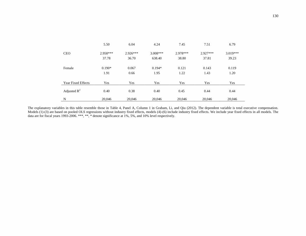
130

5.50 6.04 4.24 7.45 7.51 6.79

CEO 2.958*** 2.926*** 3.008*** 2.978*** 2.927*** 3.019***

37.78 36.70 638.40 38.80 37.81 39.23

Female 0.190* 0.067 0.194* 0.121 0.143 0.119

1.91 0.66 1.95 1.22 1.43 1.20

Year Fixed Effects Yes Yes Yes Yes Yes Yes

Adjusted R2 0.40 0.38 0.40 0.45

0.44

0.44

N 20,046 20,046 20,046 20,046

20,046

20,046

The explanatory variables in this table resemble those in Table 4, Panel A, Column 1 in Graham, Li, and Qiu (2012). The dependent variable is total executive compensation.

Models (1)-(3) are based on pooled OLS regressions without industry fixed effects, models (4)-(6) include industry fixed effects. We include year fixed effects in all models. The

data are for fiscal years 1993-2006. ***, **, * denote significance at 1%, 5%, and 10% level respectively.

131

3.4.6 Investment Policy

We refer to Coles, Daniel, and Naveen (2006) for the studies of investment policy

(CAPEX, R&D, and firm risk). For firm size measures, Coles, Daniel, and Naveen

(2006) use the log of sales. In Table 3.15, we use the R&D (the research and

development expenditures scaled by assets) as the dependent variable, and the

independent variables are based on Coles, Daniel, and Naveen (2006, Table 3, Panel A,

Column 1). The coefficients of different firm size measures are all significantly negative,

which means small firms tend to invest in riskier projects, but large, mature firms are less

involved in risky investments. The results for several regressors are not robust, especially

for cash compensation and stock return. Another obvious change lies in R-squared, which

is sharply lower if we use the log of sales.

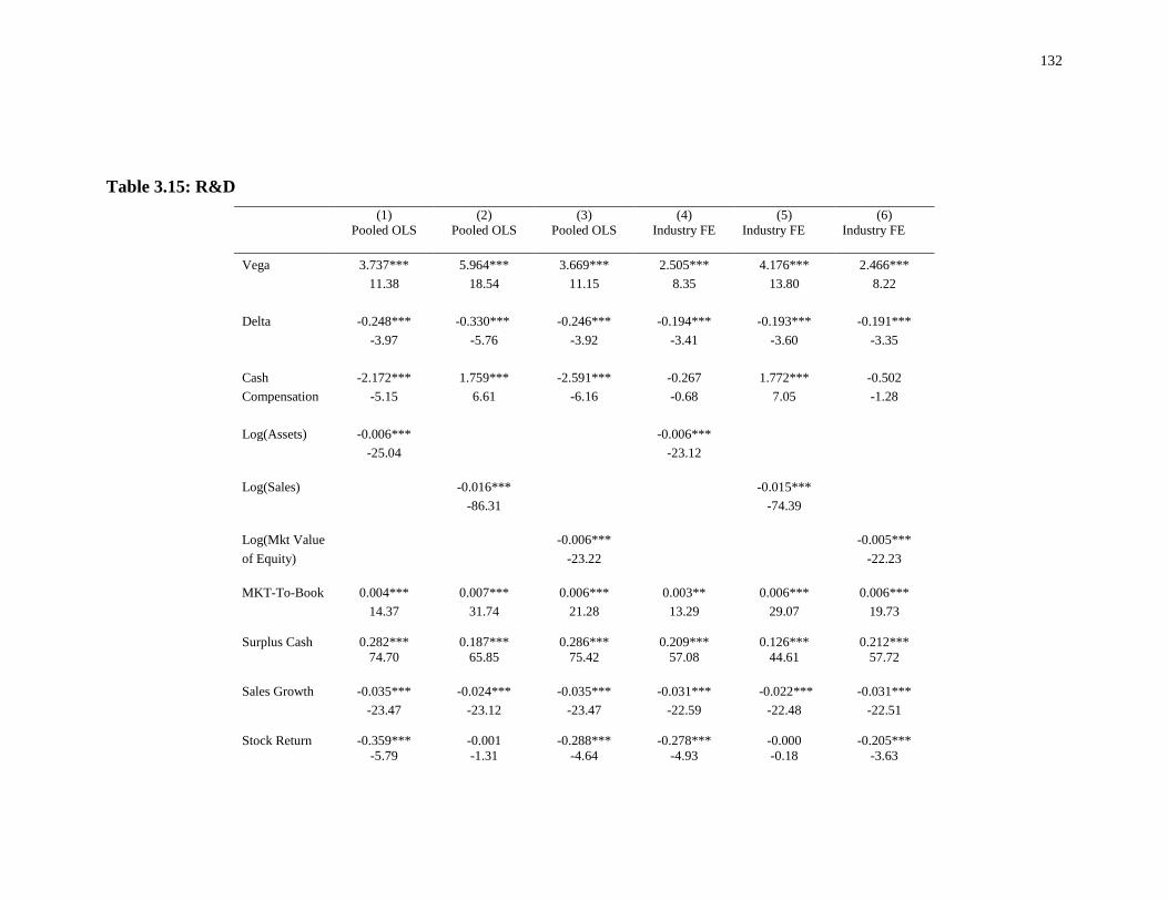
132

Table 3.15: R&D

(1)

Pooled OLS

(2)

Pooled OLS

(3)

Pooled OLS

(4)

Industry FE

(5)

Industry FE

(6)

Industry FE

Vega 3.737*** 5.964*** 3.669*** 2.505*** 4.176*** 2.466***

11.38 18.54 11.15 8.35 13.80 8.22

Delta -0.248*** -0.330*** -0.246*** -0.194*** -0.193*** -0.191***

-3.97 -5.76 -3.92 -3.41 -3.60 -3.35

Cash -2.172*** 1.759*** -2.591*** -0.267 1.772*** -0.502

Compensation -5.15 6.61 -6.16 -0.68 7.05 -1.28

Log(Assets) -0.006***

-0.006***

-25.04

-23.12

Log(Sales)

-0.016***

-0.015***

-86.31

-74.39

Log(Mkt Value

-0.006***

-0.005***

of Equity)

-23.22

-22.23

MKT-To-Book 0.004*** 0.007*** 0.006*** 0.003** 0.006*** 0.006***

14.37 31.74 21.28 13.29 29.07 19.73

Surplus Cash 0.282*** 0.187*** 0.286*** 0.209*** 0.126*** 0.212***

74.70 65.85 75.42 57.08 44.61 57.72

Sales Growth -0.035*** -0.024*** -0.035*** -0.031*** -0.022*** -0.031***

-23.47 -23.12 -23.47 -22.59 -22.48 -22.51

Stock Return -0.359*** -0.001 -0.288*** -0.278*** -0.000 -0.205***

-5.79 -1.31 -4.64 -4.93 -0.18 -3.63

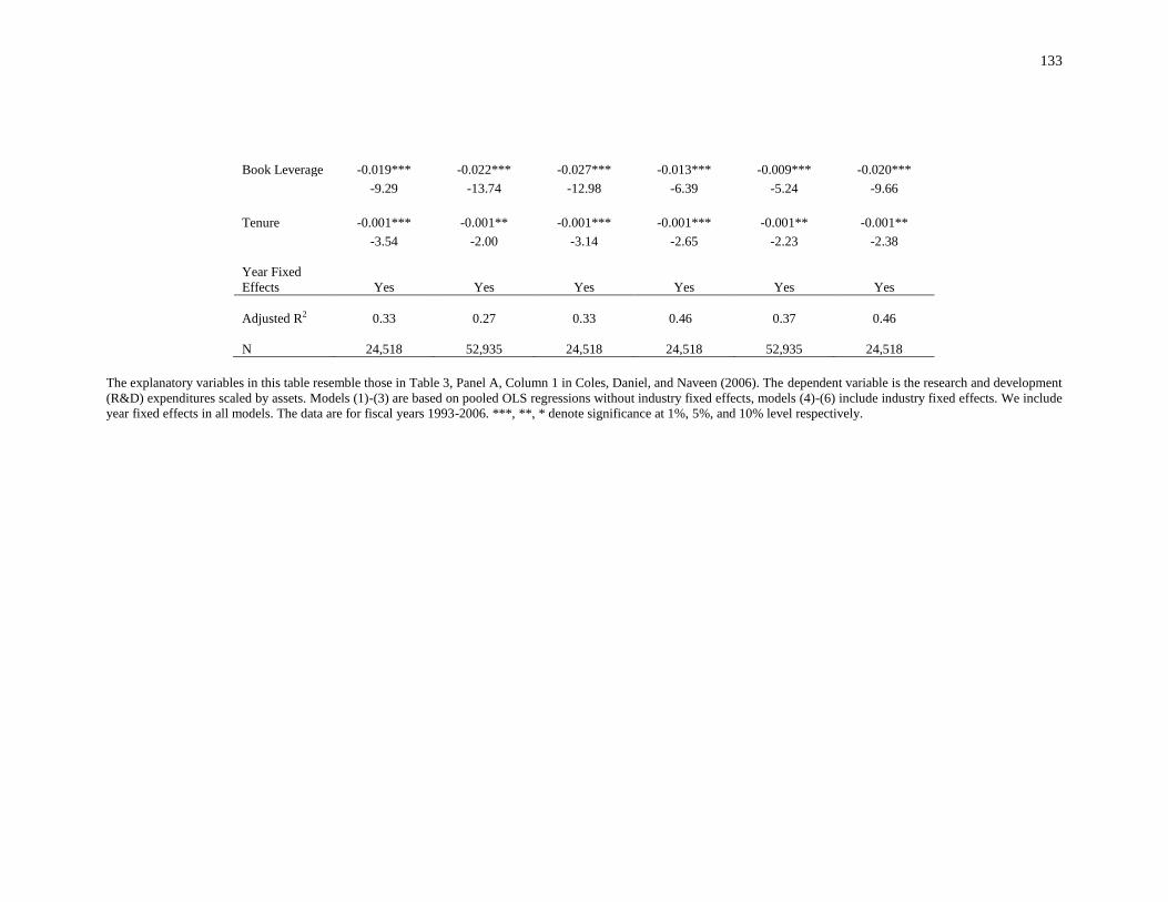
133

Book Leverage -0.019*** -0.022*** -0.027*** -0.013*** -0.009*** -0.020***

-9.29 -13.74 -12.98 -6.39 -5.24 -9.66

Tenure -0.001*** -0.001** -0.001*** -0.001*** -0.001** -0.001**

-3.54 -2.00 -3.14 -2.65 -2.23 -2.38

Year Fixed

Effects Yes Yes Yes Yes Yes Yes

Adjusted R2 0.33 0.27 0.33 0.46

0.37

0.46

N 24,518 52,935 24,518 24,518

52,935

24,518

The explanatory variables in this table resemble those in Table 3, Panel A, Column 1 in Coles, Daniel, and Naveen (2006). The dependent variable is the research and development

(R&D) expenditures scaled by assets. Models (1)-(3) are based on pooled OLS regressions without industry fixed effects, models (4)-(6) include industry fixed effects. We include

year fixed effects in all models. The data are for fiscal years 1993-2006. ***, **, * denote significance at 1%, 5%, and 10% level respectively.

134

For the examination of CAPEX (net capital expenditures scaled by assets), we

refer to Coles, Daniel, and Naveen (2006, Table 3, Panel B, Column 1). We report the

results in Table 3.16. Theoretically, CAPEX corresponds to safer investment policy

when compared with R&D and leverage, so we have significantly positive coefficients

for firm size, except that the coefficient is not significant when we use the log of market

value of equity as the firm size measure in the pooled OLS regressions. In addition, the

coefficient of stock return becomes insignificant when we employ the log of sales as firm

size proxy.

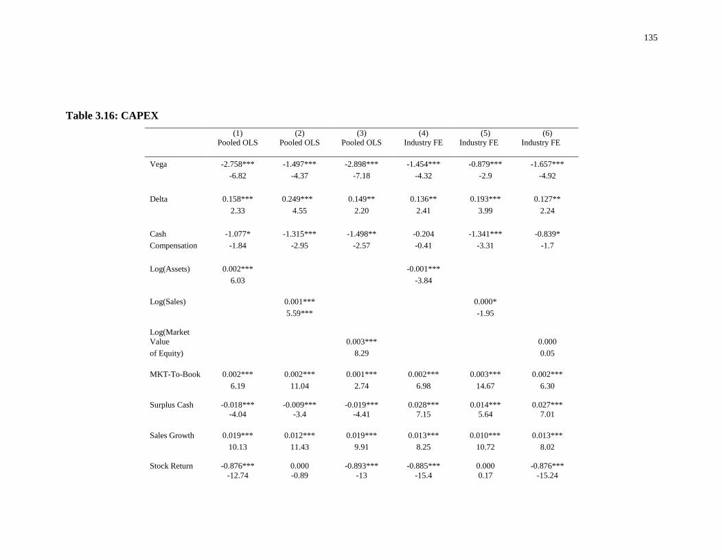
135

Table 3.16: CAPEX

(1)

Pooled OLS

(2)

Pooled OLS

(3)

Pooled OLS

(4)

Industry FE

(5)

Industry FE

(6)

Industry FE

Vega -2.758*** -1.497*** -2.898*** -1.454*** -0.879*** -1.657***

-6.82 -4.37 -7.18 -4.32 -2.9 -4.92

Delta 0.158*** 0.249*** 0.149** 0.136** 0.193*** 0.127**

2.33 4.55 2.20 2.41 3.99 2.24

Cash -1.077* -1.315*** -1.498** -0.204 -1.341*** -0.839*

Compensation -1.84 -2.95 -2.57 -0.41 -3.31 -1.7

Log(Assets) 0.002***

-0.001***

6.03

-3.84

Log(Sales)

0.001***

0.000*

5.59***

-1.95

Log(Market

Value

0.003***

0.000

of Equity)

8.29

0.05

MKT-To-Book 0.002*** 0.002*** 0.001*** 0.002*** 0.003*** 0.002***

6.19 11.04 2.74 6.98 14.67 6.30

Surplus Cash -0.018*** -0.009*** -0.019*** 0.028*** 0.014*** 0.027***

-4.04 -3.4 -4.41 7.15 5.64 7.01

Sales Growth 0.019*** 0.012*** 0.019*** 0.013*** 0.010*** 0.013***

10.13 11.43 9.91 8.25 10.72 8.02

Stock Return -0.876*** 0.000 -0.893*** -0.885*** 0.000 -0.876***

-12.74 -0.89 -13 -15.4 0.17 -15.24

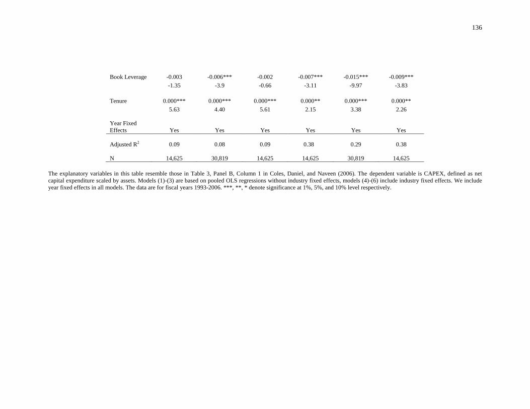
136

Book Leverage -0.003 -0.006*** -0.002 -0.007*** -0.015*** -0.009***

-1.35 -3.9 -0.66 -3.11 -9.97 -3.83

Tenure 0.000*** 0.000*** 0.000*** 0.000** 0.000*** 0.000**

5.63 4.40 5.61 2.15 3.38 2.26

Year Fixed

Effects Yes Yes Yes Yes Yes Yes

Adjusted R2 0.09 0.08 0.09 0.38

0.29

0.38

N 14,625 30,819 14,625 14,625

30,819

14,625

The explanatory variables in this table resemble those in Table 3, Panel B, Column 1 in Coles, Daniel, and Naveen (2006). The dependent variable is CAPEX, defined as net

capital expenditure scaled by assets. Models (1)-(3) are based on pooled OLS regressions without industry fixed effects, models (4)-(6) include industry fixed effects. We include

year fixed effects in all models. The data are for fiscal years 1993-2006. ***, **, * denote significance at 1%, 5%, and 10% level respectively.

137

In Table 3.17, we report the results for firm risk (stock return volatility). We use

the independent variables in Coles, Daniel, and Naveen (2006, Table 9 Column 1). The

coefficients of different firm size measures are all significantly negative, indicating small

firms have high stock return variances. We find that the coefficients are not robust for

vega, cash compensation, market to book ratio, book leverage, and tenure. These results

indicate that the choice of firm size is vital in determining firm risk as measured by stock

return volatility.

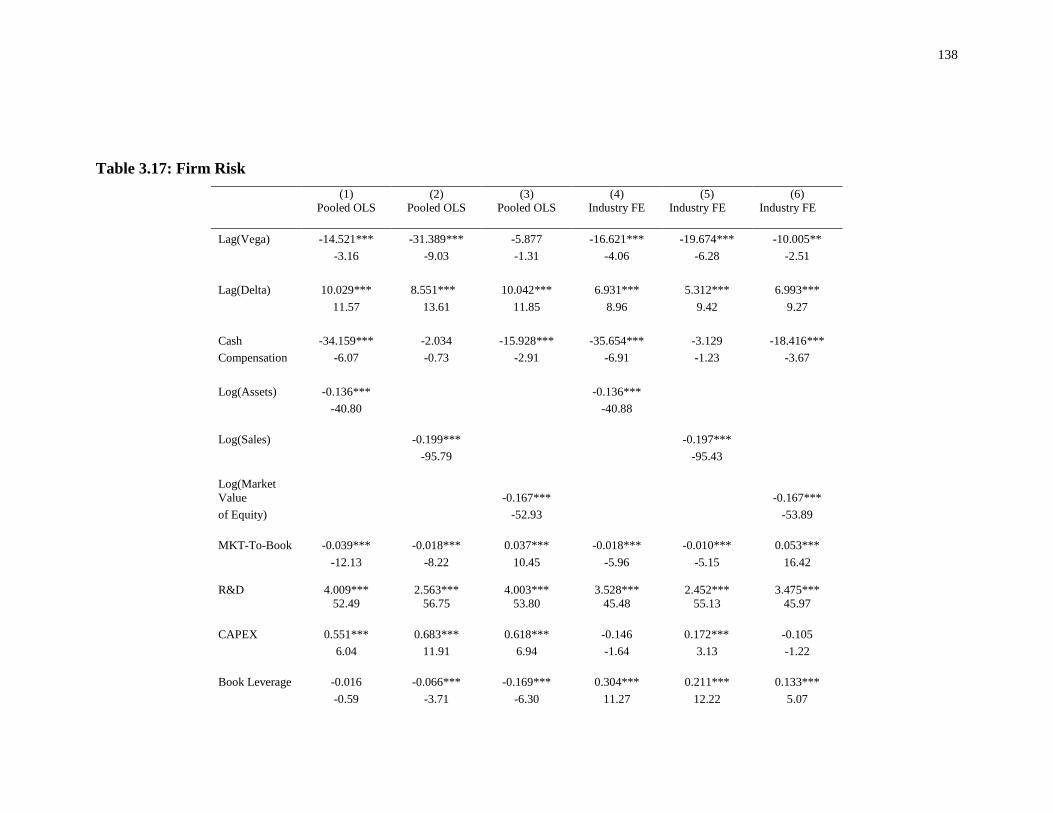
138

Table 3.17: Firm Risk

(1)

Pooled OLS

(2)

Pooled OLS

(3)

Pooled OLS

(4)

Industry FE

(5)

Industry FE

(6)

Industry FE

Lag(Vega) -14.521*** -31.389*** -5.877 -16.621*** -19.674*** -10.005**

-3.16 -9.03 -1.31 -4.06 -6.28 -2.51

Lag(Delta) 10.029*** 8.551*** 10.042*** 6.931*** 5.312*** 6.993***

11.57 13.61 11.85 8.96 9.42 9.27

Cash -34.159*** -2.034 -15.928*** -35.654*** -3.129 -18.416***

Compensation -6.07 -0.73 -2.91 -6.91 -1.23 -3.67

Log(Assets) -0.136***

-0.136***

-40.80

-40.88

Log(Sales)

-0.199***

-0.197***

-95.79

-95.43

Log(Market

Value

-0.167***

-0.167***

of Equity)

-52.93

-53.89

MKT-To-Book -0.039*** -0.018*** 0.037*** -0.018*** -0.010*** 0.053***

-12.13 -8.22 10.45 -5.96 -5.15 16.42

R&D 4.009*** 2.563*** 4.003*** 3.528*** 2.452*** 3.475***

52.49 56.75 53.80 45.48 55.13 45.97

CAPEX 0.551*** 0.683*** 0.618*** -0.146 0.172*** -0.105

6.04 11.91 6.94 -1.64 3.13 -1.22

Book Leverage -0.016 -0.066*** -0.169*** 0.304*** 0.211*** 0.133***

-0.59 -3.71 -6.30 11.27 12.22 5.07

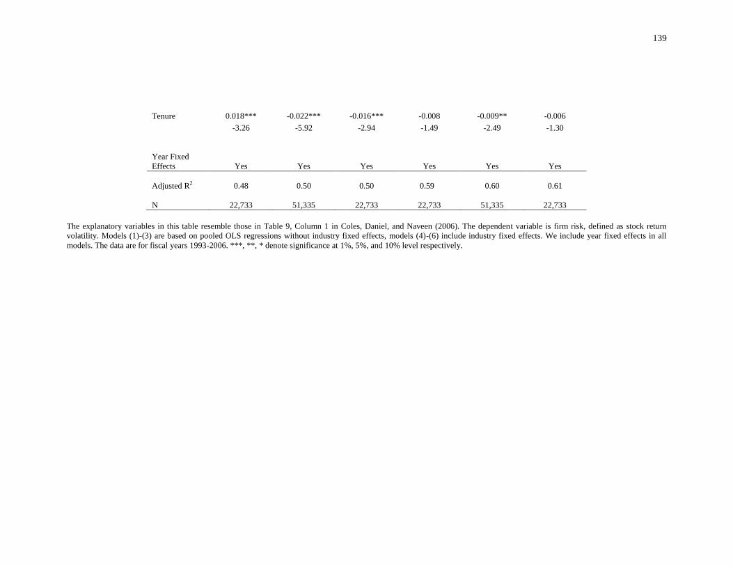
139

Tenure 0.018*** -0.022*** -0.016*** -0.008 -0.009** -0.006

-3.26 -5.92 -2.94 -1.49 -2.49 -1.30

Year Fixed

Effects Yes Yes Yes Yes Yes Yes

Adjusted R2 0.48 0.50 0.50 0.59

0.60

0.61

N 22,733 51,335 22,733 22,733

51,335

22,733

The explanatory variables in this table resemble those in Table 9, Column 1 in Coles, Daniel, and Naveen (2006). The dependent variable is firm risk, defined as stock return

volatility. Models (1)-(3) are based on pooled OLS regressions without industry fixed effects, models (4)-(6) include industry fixed effects. We include year fixed effects in all

models. The data are for fiscal years 1993-2006. ***, **, * denote significance at 1%, 5%, and 10% level respectively.

140

3.4.7 Diversification

We focus on the Herfindahl index and business segments for the studies of

diversification. We refer to Coles, Daniel, and Naveen (2006) as the benchmark paper.

The Herfindahl index is defined as the sum of the square of segment sales divided by the

square of firm sales. Our choices of explanatory variables resemble those in Coles,

Daniel, and Naveen (2006, Table 4, Panel A, Column 1). Table 3.18 reports the results.

The sign of firm size is significantly negative, implying that large firms have high levels

of diversification, which is consistent with the fact that large firms have better capability

to diversify revenue concentration across different business segments. The models with

industry fixed effect produce robust results, with the exceptions that the coefficient of

lagged delta becomes insignificant when we use the log of sales, and the coefficient of

lagged vega becomes significant when we use the log of assets. Besides, the coefficient

of ROA changes sign for different firm size measures. When it comes to the results of

OLS regressions without industry fixed effect, in addition to these sensitive variables, we

find stock return and tenure have changes in the significance of their coefficients.

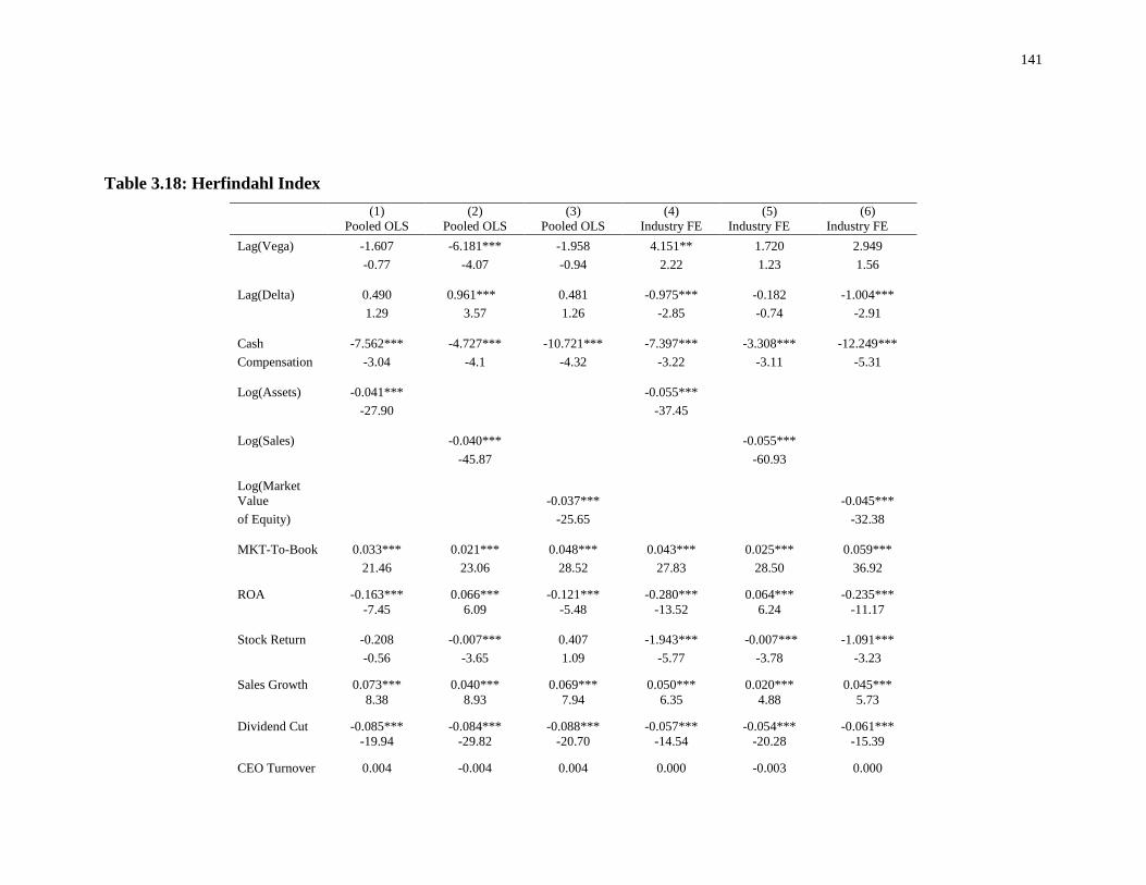
141

Table 3.18: Herfindahl Index

(1)

Pooled OLS

(2)

Pooled OLS

(3)

Pooled OLS

(4)

Industry FE

(5)

Industry FE

(6)

Industry FE

Lag(Vega) -1.607 -6.181*** -1.958 4.151** 1.720 2.949

-0.77 -4.07 -0.94 2.22 1.23 1.56

Lag(Delta) 0.490 0.961*** 0.481 -0.975*** -0.182 -1.004***

1.29 3.57 1.26 -2.85 -0.74 -2.91

Cash -7.562*** -4.727*** -10.721*** -7.397*** -3.308*** -12.249***

Compensation -3.04 -4.1 -4.32 -3.22 -3.11 -5.31

Log(Assets) -0.041***

-0.055***

-27.90

-37.45

Log(Sales)

-0.040***

-0.055***

-45.87

-60.93

Log(Market

Value

-0.037***

-0.045***

of Equity)

-25.65

-32.38

MKT-To-Book 0.033*** 0.021*** 0.048*** 0.043*** 0.025*** 0.059***

21.46 23.06 28.52 27.83 28.50 36.92

ROA -0.163*** 0.066*** -0.121*** -0.280*** 0.064*** -0.235***

-7.45 6.09 -5.48 -13.52 6.24 -11.17

Stock Return -0.208 -0.007*** 0.407 -1.943*** -0.007*** -1.091***

-0.56 -3.65 1.09 -5.77 -3.78 -3.23

Sales Growth 0.073*** 0.040*** 0.069*** 0.050*** 0.020*** 0.045***

8.38 8.93 7.94 6.35 4.88 5.73

Dividend Cut -0.085*** -0.084*** -0.088*** -0.057*** -0.054*** -0.061***

-19.94 -29.82 -20.70 -14.54 -20.28 -15.39

CEO Turnover 0.004 -0.004 0.004 0.000 -0.003 0.000

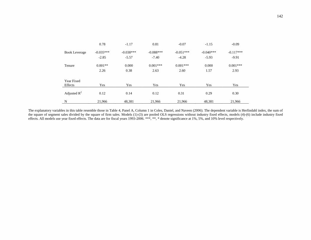
142

0.78 -1.17 0.81 -0.07 -1.15 -0.09

Book Leverage -0.035*** -0.038*** -0.088*** -0.051*** -0.040*** -0.117***

-2.85 -5.57 -7.40 -4.28 -5.93 -9.91

Tenure 0.001** 0.000 0.001*** 0.001*** 0.000 0.001***

2.26 0.38 2.63 2.60 1.57 2.93

Year Fixed

Effects Yes Yes Yes Yes Yes Yes

Adjusted R2 0.12 0.14 0.12 0.31

0.29

0.30

N 21,966 48,381 21,966 21,966

48,381

21,966

The explanatory variables in this table resemble those in Table 4, Panel A, Column 1 in Coles, Daniel, and Naveen (2006). The dependent variable is Herfindahl index, the sum of

the square of segment sales divided by the square of firm sales. Models (1)-(3) are pooled OLS regressions without industry fixed effects, models (4)-(6) include industry fixed

effects. All models use year fixed effects. The data are for fiscal years 1993-2006. ***, **, * denote significance at 1%, 5%, and 10% level respectively.

143

In addition, we examine the number of operating business segments that also

capture the diversification. We use the same explanatory variables as in Coles, Daniel,

and Naveen (2006, Table 4, Panel A, Column 1). The dependent variable is the logarithm

of the number of business segments. We report the results in Table 3.19. As expected, our

results show that firm size has a positive effect on the number of business segments.

When we use different size measures for the regressions with industry fixed effect, the

coefficients of lagged vega and ROA are not robust.

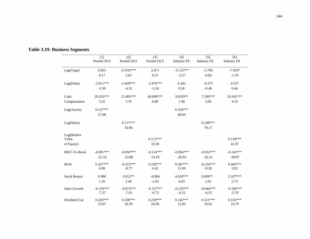
144

Table 3.19: Business Segments

(1)

Pooled OLS

(2)

Pooled OLS

(3)

Pooled OLS

(4)

Industry FE

(5)

Industry FE

(6)

Industry FE

Lag(Vega) 0.823 12.910*** 2.471 -11.257** -2.780 -7.935*

0.17 3.65 0.51 -2.57 -0.85 -1.79

Lag(Delta) -2.911*** -2.669*** -2.870*** 0.442 -0.275 0.527

-3.30 -4.31 -3.24 0.56 -0.48 0.66

Cash 29.203*** 15.485*** 40.089*** 10.659** 7.506*** 24.565***

Compensation 5.02 5.76 6.89 1.98 3.00 4.53

Log(Assets) 0.127***

0.164***

37.08

48.04

Log(Sales)

0.117***

0.148***

56.96

70.17

Log(Market

Value

0.112***

0.138***

of Equity)

33.38

41.87

MKT-To-Book -0.081*** -0.050*** -0.124*** -0.094*** -0.053*** -0.143***

-22.16 -23.86 -31.65 -26.93 -26.31 -38.07

ROA 0.357*** -0.223*** 0.228*** 0.587*** -0.226*** 0.445***

6.98 -8.77 4.42 12.09 -9.30 9.02

Stock Return 0.980 0.012** -0.894 4.620*** 0.009** 2.107***

1.16 2.49 -1.05 6.03 2.05 2.73

Sales Growth -0.150*** -0.073*** -0.137*** -0.120*** -0.044*** -0.106***

-7.37 -7.03 -6.73 -6.52 -4.55 -5.70

Dividend Cut 0.228*** 0.198*** 0.239*** 0.145*** 0.121*** 0.155***

23.07 30.39 24.08 15.85 19.62 16.79

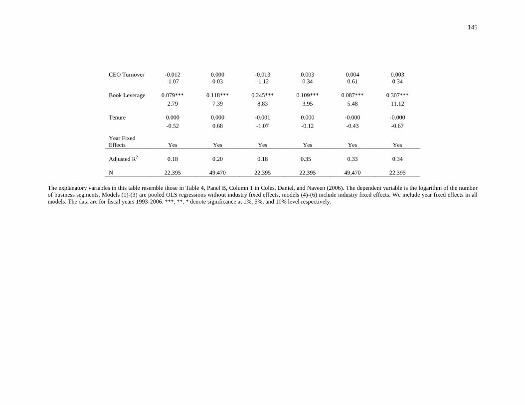
145

CEO Turnover -0.012 0.000 -0.013 0.003 0.004 0.003

-1.07 0.03 -1.12 0.34 0.61 0.34

Book Leverage 0.079*** 0.118*** 0.245*** 0.109*** 0.087*** 0.307***

2.79 7.39 8.83 3.95 5.48 11.12

Tenure 0.000 0.000 -0.001 0.000 -0.000 -0.000

-0.52 0.68 -1.07 -0.12 -0.43 -0.67

Year Fixed

Effects Yes Yes Yes Yes Yes Yes

Adjusted R2 0.18 0.20 0.18 0.35

0.33

0.34

N 22,395 49,470 22,395 22,395 49,470

22,395

The explanatory variables in this table resemble those in Table 4, Panel B, Column 1 in Coles, Daniel, and Naveen (2006). The dependent variable is the logarithm of the number

of business segments. Models (1)-(3) are pooled OLS regressions without industry fixed effects, models (4)-(6) include industry fixed effects. We include year fixed effects in all

models. The data are for fiscal years 1993-2006. ***, **, * denote significance at 1%, 5%, and 10% level respectively.

146

3.4.8 Corporate Control

We use Probit specifications to study the mergers and acquisitions and corporate

control. We cover three topics in this section: propensity to bid, propensity to be a target,

and poison pill adoption as an antitakeover device. For the propensity to bid, we use the

bidder dummy as the dependent variable, which is 1 if a firm announces a bid in a

specific year and 0 otherwise. The explanatory variables resemble those in Harford

(1999, Table III, Column 1). Harford (1999) uses the log of total assets as the measure of

firm size. As shown in Table 3.20, the coefficient is significantly positive for each firm

size measure, which is consistent with the results in Harford (1999). The positive sign of

firm size implies that large firms tend to announce bids, as these firms have higher

absolute levels of cash holdings or market capitalization to participate in mergers and

acquisitions activities. However, we find that the results for other regressors are not

robust whether industry fixed effects are employed or not: the significance and/or sign

changes for abnormal returns, noncash working capital, market-to-book ratio, and price-

to-earnings ratio. The main changes reside in the usage of market value of equity. Also

the R-squared is higher when we employ the market value of equity for the industry fixed

effect regressions.

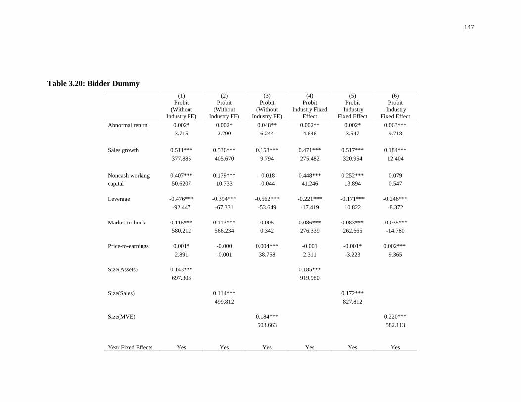
147

Table 3.20: Bidder Dummy

(1)

Probit

(Without

Industry FE)

(2)

Probit

(Without

Industry FE)

(3)

Probit

(Without

Industry FE)

(4)

Probit

Industry Fixed

Effect

(5)

Probit

Industry

Fixed Effect

(6)

Probit

Industry

Fixed Effect

Abnormal return 0.002* 0.002* 0.048** 0.002** 0.002* 0.063***

3.715 2.790 6.244 4.646 3.547 9.718

Sales growth 0.511*** 0.536*** 0.158*** 0.471*** 0.517*** 0.184***

377.885 405.670 9.794 275.482 320.954 12.404

Noncash working 0.407*** 0.179*** -0.018 0.448*** 0.252*** 0.079

capital 50.6207 10.733 -0.044 41.246 13.894 0.547

Leverage -0.476*** -0.394*** -0.562*** -0.221*** -0.171*** -0.246***

-92.447 -67.331 -53.649 -17.419 10.822 -8.372

Market-to-book 0.115*** 0.113*** 0.005 0.086*** 0.083*** -0.035***

580.212 566.234 0.342 276.339 262.665 -14.780

Price-to-earnings 0.001* -0.000 0.004*** -0.001 -0.001* 0.002***

2.891 -0.001 38.758 2.311 -3.223 9.365

Size(Assets) 0.143*** 0.185***

697.303 919.980

Size(Sales) 0.114*** 0.172***

499.812 827.812

Size(MVE) 0.184*** 0.220***

503.663 582.113

Year Fixed Effects Yes Yes Yes Yes Yes Yes

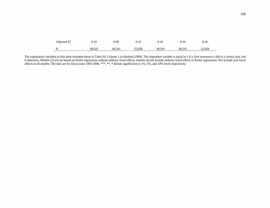
148

Adjusted R2 0.10 0.09 0.10 0.16

0.16

0.18

N 49,541 49,541 22,658 49,541

49,541

22,658

The explanatory variables in this table resemble those in Table III, Column 1 in Harford (1999). The dependent variable is equal to 1 if a firm announces a bid in a certain year and

0 otherwise. Models (1)-(3) are based on Probit regressions without industry fixed effects, models (4)-(6) include industry fixed effects in Probit regressions. We include year fixed

effects in all models. The data are for fiscal years 1993-2006. ***, **, * denote significance at 1%, 5%, and 10% level respectively.

149

For the examination of the propensity to be a target, we use the independent

variables in Comment and Schwert (1995, Table 3, Column 1). The dependent variable is

a target dummy, which is 1 if a company is announced as a target of a successful M&A

deal in a specific year and 0 otherwise. Comment and Schwert (1995) use the log of total

assets as the measure of firm size. In contrast to Comment and Schwert (1995), in our

results (Table 3.21) the coefficient is significantly positive for each firm size measure

across different regressions, suggesting that larger firms are more likely to be targeted in

M&A. The sign and/or significance change for sales growth and leverage when we use

the log of sales, regardless of whether the industry fixed effect is used. In addition, the R-

squared is smaller when we use the log of sales. Furthermore, the market-to-book ratio

becomes insignificant when we use the log of assets.

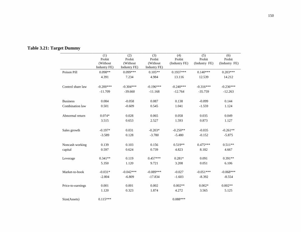
150

Table 3.21: Target Dummy

(1)

Probit

(Without

Industry FE)

(2)

Probit

(Without

Industry FE)

(3)

Probit

(Without

Industry FE)

(4)

Probit

(Industry FE)

(5)

Probit

(Industry FE)

(6)

Probit

(Industry FE)

Poison Pill 0.098** 0.099*** 0.105** 0.1937*** 0.140*** 0.203***

4.391 7.234 4.984 13.116 12.539 14.212

Control share law -0.200*** -0.304*** -0.196*** -0.240*** -0.316*** -0.236***

-11.709 -39.660 -11.168 -12.764 -35.759 -12.263

Business 0.084 -0.058 0.087 0.138 -0.099 0.144

Combination law 0.501 -0.609 0.545 1.041 -1.559 1.124

Abnormal return 0.074* 0.028 0.065 0.058 0.035 0.049

3.515 0.653 2.527 1.593 0.873 1.127

Sales growth -0.197* 0.031 -0.203* -0.250** -0.035 -0.261**

-3.589 0.128 -3.780 -5.480 -0.152 -5.875

Noncash working 0.139 0.103 0.156 0.519** 0.475*** 0.511**

capital 0.597 0.624 0.739 4.823 8.182 4.667

Leverage 0.341** 0.119 0.457*** 0.281* 0.091 0.391**

5.350 1.120 9.721 3.208 0.051 6.106

Market-to-book -0.031* -0.042*** -0.089*** -0.027 -0.051*** -0.068***

-2.804 -6.809 -17.834 -1.603 -8.392 -8.554

Price-to-earnings 0.001 0.001 0.002 0.002** 0.002* 0.002**

1.120 0.323 1.874 4.272 3.565 5.125

Size(Assets) 0.115*** 0.088***

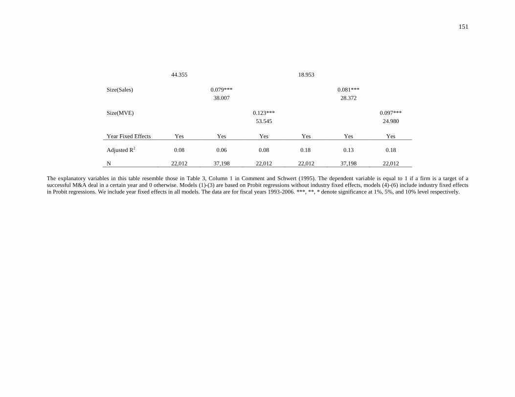
151

44.355 18.953

Size(Sales) 0.079*** 0.081***

38.007 28.372

Size(MVE) 0.123*** 0.097***

53.545 24.980

Year Fixed Effects Yes Yes Yes Yes Yes Yes

Adjusted R2 0.08 0.06 0.08 0.18

0.13

0.18

N 22,012 37,198 22,012 22,012

37,198

22,012

The explanatory variables in this table resemble those in Table 3, Column 1 in Comment and Schwert (1995). The dependent variable is equal to 1 if a firm is a target of a

successful M&A deal in a certain year and 0 otherwise. Models (1)-(3) are based on Probit regressions without industry fixed effects, models (4)-(6) include industry fixed effects

in Probit regressions. We include year fixed effects in all models. The data are for fiscal years 1993-2006. ***, **, * denote significance at 1%, 5%, and 10% level respectively.

152

We also use Comment and Schwert (1995) as the benchmark paper to study

poison pill adoption as an antitakeover device. The dependent variable is equal to 1 if a

firm has the poison pill in place in a specific year and 0 otherwise. The independent

variables resemble those in Comment and Schwert (1995, Table 3, Column 4). In contrast

to Comment and Schwert (1995), in our results (Table 3.22) the coefficient of each firm

size measure is significantly negative, suggesting larger firms are less likely to adopt

poison pill. When the log of sales is used, the sign of the coefficient of share law changes

from negative to positive. The coefficient of leverage level is only significant in the

regressions without industry fixed effect when we use the log of assets, and it is also

significant in the regressions with industry fixed effect when we use the log of sales. The

usage of log of market value of equity leads to insignificant coefficient of leverage. The

goodness of fit is lower when we use the log of sales in the industry fixed effect

regressions.

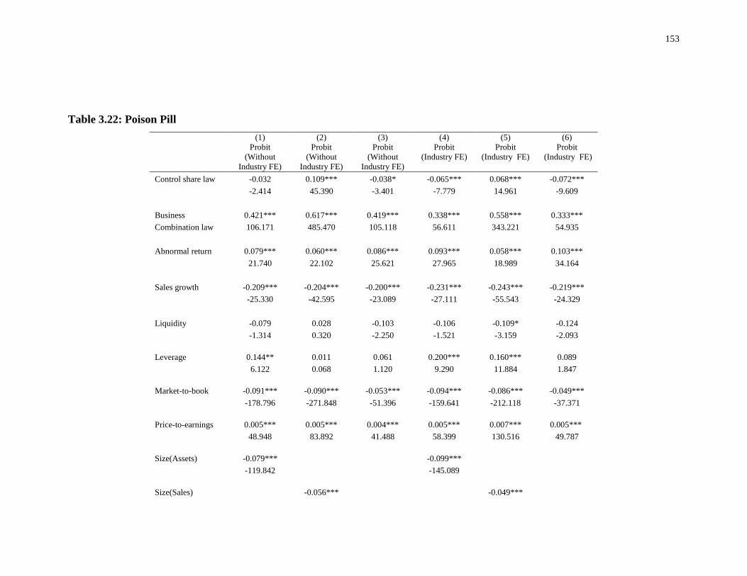
153

Table 3.22: Poison Pill

(1)

Probit

(Without

Industry FE)

(2)

Probit

(Without

Industry FE)

(3)

Probit

(Without

Industry FE)

(4)

Probit

(Industry FE)

(5)

Probit

(Industry FE)

(6)

Probit

(Industry FE)

Control share law -0.032 0.109*** -0.038* -0.065*** 0.068*** -0.072***

-2.414 45.390 -3.401 -7.779 14.961 -9.609

Business 0.421*** 0.617*** 0.419*** 0.338*** 0.558*** 0.333***

Combination law 106.171 485.470 105.118 56.611 343.221 54.935

Abnormal return 0.079*** 0.060*** 0.086*** 0.093*** 0.058*** 0.103***

21.740 22.102 25.621 27.965 18.989 34.164

Sales growth -0.209*** -0.204*** -0.200*** -0.231*** -0.243*** -0.219***

-25.330 -42.595 -23.089 -27.111 -55.543 -24.329

Liquidity -0.079 0.028 -0.103 -0.106 -0.109* -0.124

-1.314 0.320 -2.250 -1.521 -3.159 -2.093

Leverage 0.144** 0.011 0.061 0.200*** 0.160*** 0.089

6.122 0.068 1.120 9.290 11.884 1.847

Market-to-book -0.091*** -0.090*** -0.053*** -0.094*** -0.086*** -0.049***

-178.796 -271.848 -51.396 -159.641 -212.118 -37.371

Price-to-earnings 0.005*** 0.005*** 0.004*** 0.005*** 0.007*** 0.005***

48.948 83.892 41.488 58.399 130.516 49.787

Size(Assets) -0.079*** -0.099***

-119.842 -145.089

Size(Sales) -0.056*** -0.049***

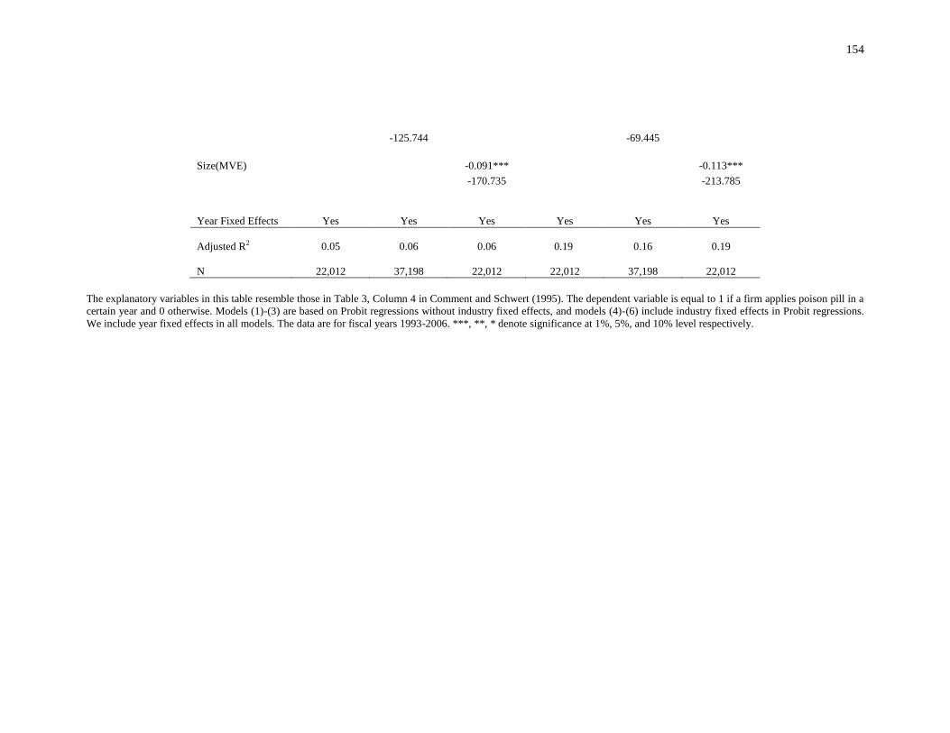
154

-125.744 -69.445

Size(MVE) -0.091*** -0.113***

-170.735 -213.785

Year Fixed Effects Yes Yes Yes Yes Yes Yes

Adjusted R2 0.05 0.06 0.06 0.19

0.16

0.19

N 22,012 37,198 22,012 22,012

37,198

22,012

The explanatory variables in this table resemble those in Table 3, Column 4 in Comment and Schwert (1995). The dependent variable is equal to 1 if a firm applies poison pill in a

certain year and 0 otherwise. Models (1)-(3) are based on Probit regressions without industry fixed effects, and models (4)-(6) include industry fixed effects in Probit regressions.

We include year fixed effects in all models. The data are for fiscal years 1993-2006. ***, **, * denote significance at 1%, 5%, and 10% level respectively.

155

3.5 Summary, Guidelines, and Limitations

We summarize our results in Table 3.23 and Figure 3.3, and hereby provide a

general guideline to researchers who may use firm size, whether as key variable or

control variable, in their empirical corporate finance studies.

156

Table 3.23: Summary of Results

Panel A: Sensitivity of Firm Size Coefficient Based on OLS

measures

field

Sign Significance 𝑅2

Assets Sales Mkt Cap Assets Sales Mkt Cap Assets Sales Mkt Cap

Tobin’s Q + + + <1% <1% <1% 0.22 0.22 0.35

ROA + + + <1% <1% <1% 0.17 0.17 0.23

Board Size + + + <1% <1% <1% 0.40 0.40 0.39

Board Independence + + + <1% <1% <1% 0.24 0.24 0.23

Board Leadership + + + <1% <1% <1% 0.11 0.10 0.09

Dividend Payout + + + <1% <1% <1% 0.30 0.30 0.28

Book Leverage + + - <1% <1% <5% 0.24 0.23 0.23

Market Leverage + + - <1% <1% <1% 0.39 0.38 0.40

Cash Holdings + - - >10% <1% >10% 0.46 0.48 0.46

Vega + + + <1% <1% <1% 0.41 0.40 0.41

Delta + + + <1% <1% <1% 0.33 0.33 0.33

Executive Pay Level + + + <1% <1% <1% 0.40 0.38 0.40

R & D - - - <1% <1% <1% 0.33 0.27 0.33

Capital Expenditure + + + <1% <1% <1% 0.09 0.08 0.09

Herfindahl Index - - - <1% <1% <1% 0.12 0.14 0.12

Business Segments + + + <1% <1% <1% 0.18 0.20 0.18

Firm Risk - - - <1% <1% <1% 0.48 0.50 0.50

Bidder + + + <1% <1% <1% 0.10 0.09 0.10

Target + + + <1% <1% <1% 0.08 0.06 0.08

Poison Pill - - - <1% <1% <1% 0.05 0.06 0.06

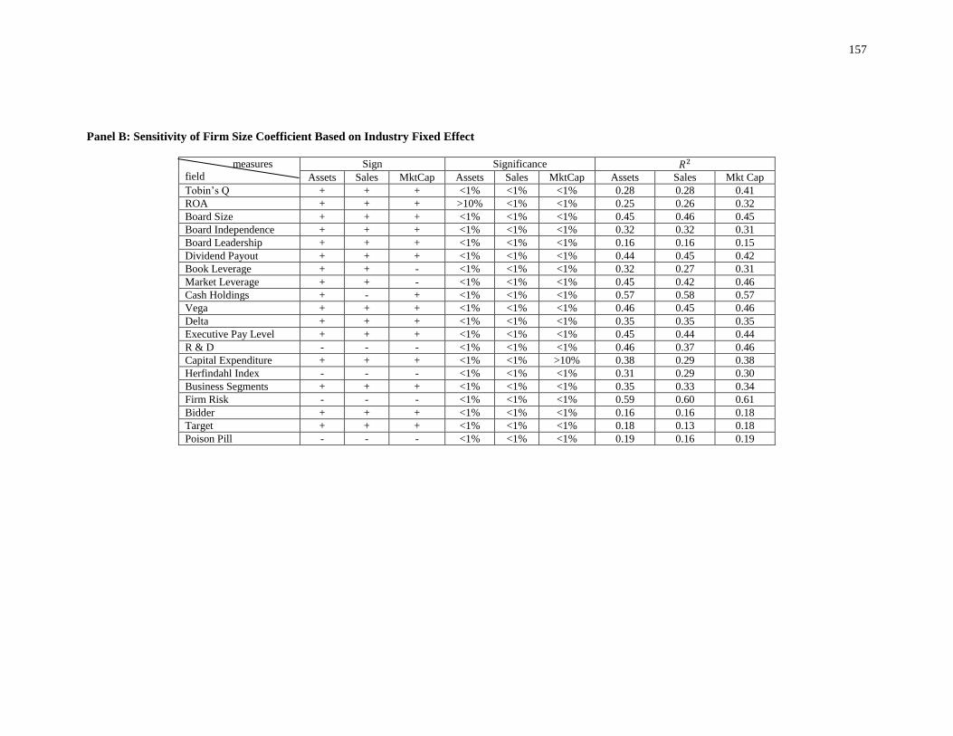
157

Panel B: Sensitivity of Firm Size Coefficient Based on Industry Fixed Effect

measures

field

Sign Significance 𝑅2

Assets Sales MktCap Assets Sales MktCap Assets Sales Mkt Cap

Tobin’s Q + + + <1% <1% <1% 0.28 0.28 0.41

ROA + + + >10% <1% <1% 0.25 0.26 0.32

Board Size + + + <1% <1% <1% 0.45 0.46 0.45

Board Independence + + + <1% <1% <1% 0.32 0.32 0.31

Board Leadership + + + <1% <1% <1% 0.16 0.16 0.15

Dividend Payout + + + <1% <1% <1% 0.44 0.45 0.42

Book Leverage + + - <1% <1% <1% 0.32 0.27 0.31

Market Leverage + + - <1% <1% <1% 0.45 0.42 0.46

Cash Holdings + - + <1% <1% <1% 0.57 0.58 0.57

Vega + + + <1% <1% <1% 0.46 0.45 0.46

Delta + + + <1% <1% <1% 0.35 0.35 0.35

Executive Pay Level + + + <1% <1% <1% 0.45 0.44 0.44

R & D - - - <1% <1% <1% 0.46 0.37 0.46

Capital Expenditure + + + <1% <1% >10% 0.38 0.29 0.38

Herfindahl Index - - - <1% <1% <1% 0.31 0.29 0.30

Business Segments + + + <1% <1% <1% 0.35 0.33 0.34

Firm Risk - - - <1% <1% <1% 0.59 0.60 0.61

Bidder + + + <1% <1% <1% 0.16 0.16 0.18

Target + + + <1% <1% <1% 0.18 0.13 0.18

Poison Pill - - - <1% <1% <1% 0.19 0.16 0.19

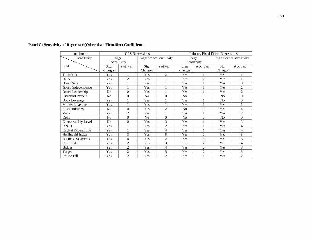
158

Panel C: Sensitivity of Regressor (Other than Firm Size) Coefficient

methods OLS Regressions Industry Fixed Effect Regressions

sensitivity

field

Sign

Sensitivity

Significance sensitivity Sign

Sensitivity

Significance sensitivity

Sign

changes

# of var. Sig.

Changes

# of var. Sign

changes

# of var. Sig.

Changes

# of var.

Tobin’s Q Yes 1 Yes 2 Yes 1 Yes 1

ROA Yes 2 Yes 1 Yes 2 Yes 1

Board Size Yes 1 Yes 1 Yes 1 Yes 3

Board Independence Yes 1 Yes 1 Yes 1 Yes 2

Board Leadership No 0 Yes 1 Yes 1 Yes 2

Dividend Payout No 0 No 0 No 0 No 0

Book Leverage Yes 1 Yes 1 Yes 1 No 0

Market Leverage Yes 1 Yes 1 Yes 1 Yes 1

Cash Holdings No 0 Yes 2 No 0 Yes 4

Vega Yes 2 Yes 1 Yes 1 Yes 2

Delta No 0 No 0 No 0 No 0

Executive Pay Level No 0 Yes 3 Yes 1 Yes 3

R & D Yes 1 Yes 2 Yes 1 Yes 4

Capital Expenditure Yes 1 Yes 4 Yes 1 Yes 4

Herfindahl Index Yes 3 Yes 5 Yes 2 Yes 3

Business Segments Yes 4 Yes 2 Yes 3 Yes 3

Firm Risk Yes 2 Yes 3 Yes 2 Yes 4

Bidder Yes 2 Yes 4 Yes 2 Yes 3

Target Yes 2 Yes 5 Yes 2 Yes 5

Poison Pill Yes 2 Yes 2 Yes 1 Yes 2

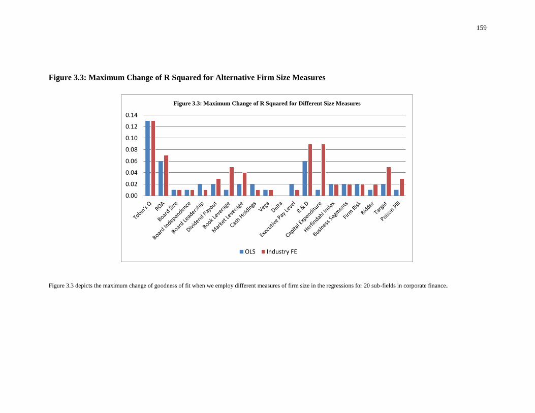
159

Figure 3.3: Maximum Change of R Squared for Alternative Firm Size Measures

Figure 3.3 depicts the maximum change of goodness of fit when we employ different measures of firm size in the regressions for 20 sub-fields in corporate finance.

0.00

0.02

0.04

0.06

0.08

0.10

0.12

0.14

Figure 3.3: Maximum Change of R Squared for Different Size Measures

OLS Industry FE

160

First, in most areas of corporate finance, the coefficients of firm size measures are

robust in sign and statistical significance. However, when studying firm performance and

capital structure, researchers should consider empirical sensitivity because market

capitalization, as a size proxy, can be mechanically correlated with the dependent

variables.

Second, the coefficients on regressors other than firm size often change sign and

significance. We observe sign changes and significance changes (change from significant

to insignificant) in almost all the areas except dividend policy and delta (Table 3.23).

Unfortunately, this suggests that some previous studies are not robust to using different

firm size proxies. Researchers should either use all the important firm size measures as

robustness checks or provide a rationale of using any specific measure.

Third, the goodness of fit measured by R-squared also varies when we use

different firm size measures (Figure 3.3 and Table 3.23, Panel B). The variation indicates

that some size measures are more relevant than others in certain areas. In particular, total

assets seems more relevant for executive compensation, firm diversification, capital

structure, and investment policy, but not for firm performance and risk; total sales matters

more for dividend policy, cash holdings, but not for investment, diversification, and

M&A; market cap increases the goodness of fit more for firm risk, capital structure,

investment, and M&A, but not for corporate governance. Although a size proxy that

delivers a higher goodness-of-fit alone cannot justify a good model specification,

researchers should not ignore abnormal changes in goodness-of-fit.

161

Fourth, in terms of research areas that are robust to size measures, Table 3.23,

Panel C on Sensitivity of Regressor (Other than Firm Size) Coefficient can serve as

guidance. The most robust areas are dividend policy, executive compensation, and then

capital structure, which means the choice of the size measures may not matter much in

those areas. The least robust areas include M&A and firm diversification, suggesting that

researchers should select size proxies with consideration for sensitivity tests.

Fifth, different size proxies capture different aspects of “firm size”, and thus have

different implications in corporate finance. For example, market cap is more market

oriented and forward looking, and reflects the ownership of equity only, while total assets

measures the firm’s total resources. Total sales are more related to product market and

are not forward looking. The choice of these firm size measures can be a theoretical and

empirical question. For example, if researchers want to control for the company’s “size”

in product market, they should use total sales; if they want to control for the size in stock

market, they should use market cap; if the size refers to the total resources that the

company can generate profit from, they should use total assets.

We have some guidelines for future research. . First, we do not employ all

possible measures of firm size; we only study the most popular three measures.

Researchers can use some alternative size proxies such as enterprise value (market

capitalization plus net debt), the number of employees, total profits, or net assets (total

assets minus total liabilities) when the main measures are not available or irrelevant (e.g.,

market cap for private firms and total sales for start-up firms). Second, we might omit

some important representative papers in specific sub-fields due to data and time

constraints. Third, some linear models may lose power if the true relation between firm

162

size and the dependent variable is non-linear (such as quadratic form). Fourth, most of

our empirical results are based on year fixed effects and/or industry fixed effects, while

introducing other considerations, such as firm fixed effects (for consideration of within

firm variations of interest rather than cross-sectional variations) or manager fixed effects

(for emphasis on corporate governance issues such as managerial compensation), might

change our results, and result in different implications. For future research, on the one

hand explicit theories should be refined for the proper usage of different measures of firm

size; on the other hand, a general role should be developed for empirical justification

given specific econometric methods.

163

References for Chapter 3

Angelini, P. and Generale, A., 2008. On the evolution of firm size distributions. The

American Economic Review, 98(1), pp.426-438.

Albuquerque, R. and Hopenhayn, H.A., 2004. Optimal lending contracts and firm

dynamics. The Review of Economic Studies, 71(2), pp.285-315.

Baker, G.P. and Hall, B.J., 2004. CEO Incentives and Firm Size. Journal of Labor

Economics, 22(4), pp.767-798.

Baliga, B.R., Moyer, R.C. and Rao, R.S., 1996. CEO duality and firm performance:

what's the fuss? Strategic Management Journal, 17(1), pp.41-53.

Beck, T., Demirgüç‐Kunt, A.S.L.I. and Maksimovic, V., 2005. Financial and legal

constraints to growth: does firm size matter? The Journal of Finance, 60(1),

pp.137-177.

Bolton, P. and Scharfstein, D.S., 1998. Corporate finance, the theory of the firm, and

organizations. The Journal of Economic Perspectives, 12(4), pp.95-114.

Brickley, J.A., Coles, J.L. and Jarrell, G., 1997. Leadership structure: Separating the CEO

and chairman of the board. Journal of Corporate Finance, 3(3), pp.189-220.

Brickley, J.A., Coles, J.L. and Terry, R.L., 1994. Outside directors and the adoption of

poison pills. Journal of Financial Economics, 35(3), pp.371-390.

Byrd, J.W. and Hickman, K.A., 1992. Do outside directors monitor managers?: Evidence

from tender offer bids. Journal of Financial Economics, 32(2), pp.195-221.

Cabral, L.M. and Mata, J., 2003. On the evolution of the firm size distribution: Facts and

theory. American Economic Review, pp.1075-1090.

Coase, R.H., 1937. The nature of the firm. Economica, 4(16), pp.386-405.

Coles, J.L., Daniel, N.D. and Naveen, L., 2006. Managerial incentives and risk-

taking. Journal of Financial Economics, 79(2), pp.431-468.

Coles, J.L., Daniel, N.D. and Naveen, L., 2008. Boards: Does one size fit all?. Journal of

Financial Economics, 87(2), pp.329-356.

Coles, J.L., Daniel, N.D. and Naveen, L., 2014. Co-opted boards. Review of Financial

Studies, 27(6), pp.1751-1796.

Coles, J., and Z. Li, 2012. An empirical assessment of empirical corporate finance,

Arizona State University working paper.

164

Comment, R. and Schwert, G.W., 1995. Poison or placebo? Evidence on the deterrence

and wealth effects of modern antitakeover measures. Journal of Financial

Economics, 39(1), pp.3-43.

Cooley, T.F. and Quadrini, V., 2001. Financial markets and firm dynamics. American

Economic Review, pp.1286-1310.

Core, J. and Guay, W., 1999. The use of equity grants to manage optimal equity incentive

levels. Journal of Accounting and Economics, 28(2), pp.151-184.

Core, J.E., Holthausen, R.W. and Larcker, D.F., 1999. Corporate governance, chief

executive officer compensation, and firm performance. Journal of Financial

Economics, 51(3), pp.371-406.

DeAngelo, H., DeAngelo, L. and Stulz, R.M., 2006. Dividend policy and the

earned/contributed capital mix: a test of the life-cycle theory. Journal of Financial

Economics, 81(2), pp.227-254.

Fama, E.F. and Jensen, M.C., 1983. Separation of ownership and control.The Journal of

Law & Economics, 26(2), pp.301-325.

Frank, M.Z. and Goyal, V.K., 2003. Testing the pecking order theory of capital

structure. Journal of Financial Economics, 67(2), pp.217-248.

Frank, M.Z. and Goyal, V.K., 2009. Capital structure decisions: which factors are reliably

important? Financial Management, 38(1), pp.1-37.

Gabaix, X. and Landier, A., 2008. Why has CEO pay increased so much? Quarterly

Journal of Economics, 123, pp49-100.

Gabaix, X., Landier, A. and Sauvagnat, J., 2014. CEO pay and firm size: an update after

the crisis. The Economic Journal, 124(574), pp.F40-F59.

Graham, J.R., Li, S. and Qiu, J., 2012. Managerial attributes and executive

compensation. Review of Financial Studies, 25(1), pp.144-186.

Grossman, S.J. and Hart, O.D., 1986. The costs and benefits of ownership: A theory of

vertical and lateral integration. The Journal of Political Economy, pp.691-719.

Harford, J., 1999. Corporate cash reserves and acquisitions. The Journal of

Finance, 54(6), pp.1969-1997.

Harford, J., Mansi, S.A. and Maxwell, W.F., 2008. Corporate governance and firm cash

holdings in the US. Journal of Financial Economics, 87(3), pp.535-555.

Hart, P.E. and Oulton, N., 1996. Growth and size of firms. The Economic Journal,

pp.1242-1252.

165

Himmelberg, C.P., Hubbard, R.G. and Palia, D., 1999. Understanding the determinants of

managerial ownership and the link between ownership and performance. Journal

of Financial Economics, 53(3), pp.353-384.

Holmström, B. and Roberts, J., 1998. The boundaries of the firm revisited.The Journal of

Economic Perspectives, 12(4), pp.73-94.

Holmstrom, B., 1999. The firm as a subeconomy. Journal of Law, Economics, and

organization, 15(1), pp.74-102.

Holmstrom, B. and Kaplan, S.N., 2001. Corporate Governance and Merger Activity in

the United States: Making Sense of the 1980s and 1990s. Journal of Economic

Perspectives, 15(2), pp.121-144.

Jackson, J.D. and Dunlevy, J.A., 1982. Interchanging measures of firm size: an

asymptotic test and further results. Southern Economic Journal, pp.764-768.

Jensen, M.C., 1993. The modern industrial revolution, exit, and the failure of internal

control systems. The Journal of Finance, 48(3), pp.831-880.

Jensen, M.C. and Murphy, K.J., 1990. Performance pay and top-management

incentives. Journal of Political Economy, pp.225-264.

Klein, B., Crawford, R.G. and Alchian, A.A., 1978. Vertical integration, appropriable

rents, and the competitive contracting process. The Journal of Law &

Economics, 21(2), pp.297-326.

Kremer, M., 1993. The O-ring theory of economic development. The Quarterly Journal

of Economics, pp.551-575.

Kumar, K.B., Rajan, R.G. and Zingales, L., 1999. What determines firm size? (No.

w7208). National Bureau of Economic Research.

Lemmon, M.L., Roberts, M.R. and Zender, J.F., 2008. Back to the beginning: persistence

and the cross‐section of corporate capital structure. The Journal of Finance, 63(4),

pp.1575-1608.

Linck, J.S., Netter, J.M. and Yang, T., 2008. The determinants of board structure. Journal

of Financial Economics, 87(2), pp.308-328.

Lucas Jr, R.E., 1978. On the size distribution of business firms. The Bell Journal of

Economics, pp.508-523.

Mehran, H., 1995. Executive compensation structure, ownership, and firm

performance. Journal of Financial Economics, 38(2), pp.163-184.

Moeller, S.B., Schlingemann, F.P. and Stulz, R.M., 2004. Firm size and the gains from

acquisitions. Journal of Financial Economics, 73(2), pp.201-228.

166

Prowse, S.D., 1992. The structure of corporate ownership in Japan. The Journal of

Finance, 47(3), pp.1121-1140.

Rajan, R.G. and Zingales, L., 1995. What do we know about capital structure? Some

evidence from international data. The Journal of Finance, 50(5), pp.1421-1460.

Rajan, R. and Zingales, L., 1998a. Financial development and growth. The American

Economic Review, 88, pp.559-586.

Rajan, R. and Zingales, L., 1998b. Power in a theory of the firm. The Quarterly Journal

of Economics, 113, pp.387-432.

Rajan Raghuram, G., Luigi, Z., Rajan Raghuram, G. and Luigi, Z., 2001. The firm as a

dedicated hierarchy: A theory of the origins and growth of firms.The Quarterly

Journal of Economics, 116, pp.805-851.

Ringleb, A.H. and Wiggins, S.N., 1990. Liability and large-scale, long-term

hazards. Journal of Political Economy, pp.574-595.

Robinson, D.T., 2008. Strategic Alliances and the Boundaries of the Firm. Review of

Financial Studies, 21(2), pp.649-681.

Rosen, S., 1982. Authority, control, and the distribution of earnings. The Bell Journal of

Economics, pp.311-323.

Seru, A., 2014. Firm boundaries matter: Evidence from conglomerates and R&D activity.

Journal of Financial Economics, 111(2), pp.381-405.

Simon, H.A. and Bonini, C.P., 1958. The size distribution of business firms .The

American Economic Review, 48(4), pp.607-617.

Smyth, D.J., Boyes, W.J. and Peseau, D.E., 1975. The measurement of firm size: Theory

and evidence for the United States and the United Kingdom. The Review of

Economics and Statistics, pp.111-114.

Vijh, A.M. and Yang, K., 2013. Are small firms less vulnerable to overpriced stock

offers? Journal of Financial Economics, 110(1), pp.61-86.

Weisbach, M.S., 1988. Outside directors and CEO turnover. Journal of Financial

Economics, 20, pp.431-460.

Williamson, O., 1975. Markets and hierarchies: analysis and antitrust implications. New

York: Free Press.

Williamson, O., 1985. The economic institutions of capitalism. New York: Free Press.

Yermack, D., 1996. Higher market valuation of companies with a small board of

directors. Journal of Financial Economics, 40(2), pp.185-211.

167

Appendix for Chapter 3

Appendix 3.1: A survey of 100 empirical corporate finance papers that use firm size

measures

Paper Sources by journal:

Sources # of Articles

Journal of Financial Economics 50

Journal of Finance 34

Review of Financial Studies 8

Journal of Accounting and Economics 4

Quarterly Journal of Economics 1

Journal of Political Economy 1

Journal of Accounting Research 1

The Accounting Review 1

By field:

Sources # of Articles

Mergers and Acquisitions 13

Cash Holdings 12

Executive Compensation 12

Ownership Structure 11

Capital Structure 9

Board of Directors 8

Law and Finance 7

Dividend Policy 6

Corporate Investment 6

CEO Turnover 6

Debt Policy 5

Cross Listings 5

168

Chapter 4

4 Impact: Evidence from Top Journals

4.1 Introduction

Publishing papers in refereed journals plays a vital role in academia, as the

“publish or perish” rule gives the true portrayal for tenure promotion in this profession.

For finance faculty, publications in the top finance journals are justified to boost annual

salary and promotion, and even full professors continue to obtain returns in thousands of

dollars for publications in the top finance journals (Swidler and Goldreyer, 1998). In

addition to the importance of publication records, the number of citations has received

more and more attention. It is often used, particularly in research universities, to assess

scholars’ research impact, and thus, their career. The increasing focus on research impact

triggers the development of online Google Scholar Citations which can readily keep track

of paper citations. However, the top 1% (10%) papers in the leading finance journals

have received 1/3 (3/4) of the total number of citations (Chung, Cox, and Mitchell, 2001).

This phenomenon indicates the value of a paper depends on both journal placement and

research impact. To our knowledge, the literature has not fully answered the questions of

how paper characteristics change over time, how paper characteristics differ between

more influential papers and less influential papers, and what are the factors that affect the

citations of the published papers in top finance journals. We aim to fill these holes in the

literature and provide evidence for finance scholars, university administrators, and

journal management who care about research impact.

The existing finance literature studies some relevant research topics. Ederington

(1979) investigates how paper length, co-authorship, and top institutions affect the

169

number of citations for 345 papers published in the Journal of Finance and Journal of

Financial Quantitative Analysis for the period 1968-1971. Schwert (1993) sheds light on

the determinants of citations such as paper age, paper length, and paper order in the

journal issue for the papers published in Journal of Financial Economics during 1974-

1991. Borokhovich, Bricker, and Simkins (2000) document evidence that the research

impact of Journal of Finance, Journal of Financial Economics and Review of Financial

Studies 27

does not depend on the “hot” topics or fads. Pinkowitz (2002) studies the

number of downloads of online papers in the Journal of Finance website. Kim, Morse,

and Zingales (2009) examine the effect of being affiliated with a top 25 university on

citations for finance faculty and find that this positive effect weakens with time (from the

1970s to the 1990s) because of the reduced importance of physical access to coauthors.

Brogaard, Engelberg, and Parsons (2014) explore the role of editor rotations and show

evidence that “connected” papers in the top three finance journals receive higher Web of

Science citations, but this effect is less robust with school fixed effects or author fixed

effects. They also find that editorial networks in one of the top three finance journals do

not affect the number of publications in the other two competing journals. Michayluk and

Zurbruegg (2014) highlight the importance of being the lead papers as a signal of higher

quality in the top four finance journals.

However, all of these previous studies in citations in finance literature only cover

a few independent variables, with the lack of a comprehensive construction of impact

27 We denote Journal of Finance, Journal of Financial Economics, and Review of Financial Studies as the

top three finance journals hereinafter. Similarly, we denote Journal of Finance, Journal of Financial

Economics, Review of Financial Studies, and Journal of Financial and Quantitative Analysis as the top four

finance journals hereinafter. Such journal rankings are consistent with Oltheten, Theoharakis, and Travlos

(2005), Chen and Huang (2007), Currie and Pandher (2011), and Chan, Chang, and Chang (2013).

170

drivers of financial research. Following the framework of Stremersch, Verniers, and

Verhoef (2007), who study the research impact in marketing literature, we use the most

extensive set of paper characteristics as determinants of citations to explore the roles of

three theoretical perspectives: the universalist perspective (what is said), the social

constructivist perspective (who says it), and the presentation perspective (how it is said).

For each theoretical perspective, we consider several dimensions - the universalist

perspective includes quality and domain, the social construction perspective includes

visibility and personal promotion, the presentation perspective includes first-page

attention and expositional clarity.28

We study the characteristics of all the published papers in the top three finance

journals during 2000-2013 and how these paper characteristics affect the number of

citations in Google Scholar and Web of Science. First, we find that most of the measures

of paper characteristics in the social constructivist perspective (visibility and personal

promotion) and the presentation perspective (first-page attention and expositional clarity)

increase over time, while most of the paper characteristics in the universalist perspective

(quality and domain) remain constant. Second, most of the paper characteristics are

significantly different between the top 10% and the bottom 10% groups based on the

number of citations per year. Third, the regression results by negative binomial models

show that the universalist perspective, the social constructivist perspective, and the

presentation perspective all provide impact drivers of published papers in the top three

finance journals. Specifically, paper quality, research methods, journal placement, and

28 We modify the dimensions of the three theoretical perspectives in Stremersch, Verniers, and Verhoef

(2007) considering the distinctiveness of the financial research. The measures in these dimensions are

defined in Appendix 1.

171

paper age are the most important (in economic significance) drivers for the number of

citations. These results are robust to redefined citation measures, alternative econometric

specifications, heteroskedasticity adjustment, and winsorized sample. Furthermore, the

results of average marginal results document exact evidence in how many additional

citations are increased with one more unit of a certain paper characteristics.

Last, different drivers play different roles for the papers in Journal of Finance,

Journal of Financial Economics, and Review of Financial Studies. For example,

theoretical papers in Journal of Financial Economics and Review of Financial Studies

receive significantly fewer citations than empirical papers but this relation is insignificant

for papers in Journal of Finance; larger number of pages significantly contributes to the

number of citations of papers in Journal of Finance, but not in Journal of Financial

Economics or Review of Financial Studies (in Table 7 and 8).

This paper provides empirical evidence for finance scholars, university

administrators, and finance journal management who care about research impact. For

example, the results are useful in assessing and supporting financial research. One

possible application is that universities should put more emphasis on travelling

awards/subsidies for conferences than direct research funding in terms of support

according to our empirical analysis.

This chapter is organized as follows: Section 4.2 presents the theory and

hypothesis, Section 4.3 describes the data, Section 4.4 discusses the model and the main

results, Section 4.5 provides robustness checks, Sections 4.6 shows the average marginal

effects of the negative binomial models, and Section 4.7 concludes.

172

4.2 Theory and Hypothesis

We follow the theoretical framework in Stremersch, Verniers, and Verhoef

(2007). They highlight three theoretical perspectives for citations in marketing: the

universalist perspective –quality and domain (what is said), the social constructivist

perspective – visibility and personal promotion (who says it), and the presentation

perspective – title length, attention grabbers, and expositional clarity (how it is said).

Stremersch, Verniers, and Verhoef (2007) provide explanations for the three

perspectives: The universalist perspective is that “what” the authors say drives the

citations of papers. Baldi (1998) argues that the reward structure of research is

determined by cognitive content. Therefore, paper characteristics such as the cognitive

dimension should be strongly related to research impact (Van Dalen and Henkens

(2001)). The social constructivist perspective is that “who” the authors are affect the

citations of papers. For example, Matthew effect in science (Merton (1968)) can promote

visibility and more references can improve reciprocity in citations (Ciadini, 1988). The

presentation perspective claims that “how” the authors present their research also

determines research impact, for instance, the title of a paper matters since it enhances the

informativeness while perhaps it also increases the complexity thereby reducing

attractiveness of the paper (Yitzhaki, 2002).

We discern similar theoretical construction and modify the measures given the

uniqueness of the finance field. The univeralist perspective denotes the influences of

“what” the authors say on the number of citations, and Stremersch, Verniers, and Verhoef

(2007) divide it into two dimensions: quality and domain. We also employ these two

dimensions. Papers of high quality can capture the strength of the contributions, and thus

173

can receive larger number of citations. We use five measures to quantify quality: the

number of authors from the top 20 finance departments29

, the number of pages, paper

order in a journal issue, whether a paper is the lead paper, and working-paper age.

Authors from the top 20 finance departments on average have better publication records,

better resources, and better training, which can represent paper quality to an extent.

Although it is also related to the Matthew effect (Merton (1968)), we believe it is a good

measure of paper quality. The number of pages are managed to be consistent with the

magnitude of research contribution according to potential impact-to-page ratio.. Order

placement and the lead article can be an indicator of contribution judged by an editor, and

a signal of quality, even though electronic journal access may make paper order less

relevant (Michayluk and Zurbruegg, 2014). We expect paper order has negative effect

and lead paper has positive effect on the number of citations. Laband and Piette (1994)

provide evidence that paper length and lead paper positively affect the number of

citations to papers in 28 top economics journals. The working paper age is our novel

measure, defined as the year difference between the first appearance on the web and

publication. First, working paper age measures the quality improvement from R&R

(Revise and Re-submit), which implies a positive effect on the number of citations.

Second, large working paper age might be just the result of pecking order in journal

submission. For example, it may capture the waiting time for the decisions by the top

economics journals such as American Economics Review. Third, lower-quality papers

29 We provide the top 20 world ranking of finance department in Appendix 4.1. Stremersch, Verniers, and

Verhoef (2007) use the business school ranking as a measure of visibility (due to the Matthew effect) in the

social constructivist perspective, while we think the research rankings of finance departments is more

relevant to quality in the universalist perspective.

174

with large working paper age and several rejections from other journals may find lucky

placement in one of the top three finance journals, and thus indicate a negative effect on

the number of citations. Altogether, the net effect of working paper age is an empirical

question. We are aware that many papers were not uploaded to SSRN or linked to

conference/seminar websites until the authors think the papers are ready to be exposed to

others, so the working paper age might not be exactly accurate, however, we can consider

that working papers with very limited access are not finished papers to some degree.

As for domain, we use only one measure: methods30

. If the paper is purely

theoretical, then the methods dummy equals 1; if the paper is purely empirical, then the

methods dummy equals 0; if mixed methods are used, then the methods dummy is 0.5.

Empirical papers may present better readability and may be more realistic and practical.

Theoretical papers are more likely to be milestones as benchmarks and inspirations, and

thus might receive broader citations. Therefore, the net effect of research methods is also

an empirical question.

Hypothesis 1A (The Universalist Perspective): As indicators of quality, the

number of authors from the top 20 finance departments, the number of pages, and

whether the paper is the lead paper positively affect the number of citations; paper order

in a journal issue negatively affects the number of citations;

30 We do not use the subject area in finance as a measure of domain because existing papers show that

subfield topics in finance have no significant impact on the number of citations to the papers in the top

three finance journals. For example, Table 8 in Schwert (1993) documents evidence that the papers in the

capital markets area and the corporate finance and governance area are not significantly different in average

citations per year. Borokhovich, Bricker, and Simkins (2000) find that the impact factors of the top three

finance journals are not affected by the distribution of papers across subfields in finance.

175

Hypothesis 1B (The Universalist Perspective): Working paper age positively

affects the number of citations due to improvement in quality during the R&R process.

Hypothesis 1C (The Universalist Perspective): Working paper age negatively

affects the number of citations due to lucky placement after rejections from other similar

journals.

Hypothesis 1D (The Universalist Perspective): Research methods positively

affect the number of citations because theoretical papers are more likely to be milestones

as benchmarks and inspiration.

Hypothesis 1E (The Universalist Perspective): Research methods negatively

affect the number of citations because empirical papers may present better readability

and may be more realistic and practical.

The second theoretical perspective - the social constructivist perspective refers to

the fact that “who” the authors of the papers are has influence over the research impact.

Following Stremersch, Verniers, and Verhoef (2007), we also explore two dimensions in

this perspective: visibility and personal promotion. For visibility, we use seven measures:

the number of authors; whether the authors are from the same school (internal

collaboration); whether the paper has received financial support; the number of

acknowledgements; the number of conferences; the number of seminars; and the number

of research assistants (RAs). More authors may have different opportunities for paper

presentations. Authors from different schools can promote the dissemination of the idea.

Financial support indicates not only better resources, but also the visibility for expert

reviewers during the evaluation process. The number of acknowledgements presents the

176

constructive feedback for the paper. The number of conferences and the number of

seminars also imply the visibility of a working paper. The RAs can also increase

visibility, as many RAs are doctorate students who are or will be research active in

academia. The number of RAs reflects the author’s resources and networks. All measures

should have positive effects on the number of citations except for internal collaboration

(a variable that equals 1 if all of the authors are from the same school, 0 if none of the

authors are from the same school, and 0.5 if some of the authors are from the same

school). Thus, internal collaboration is a reverse-scored measure for which lower value is

assigned to external collaboration. We postulate that external collaboration can expand

external visibility in different schools and accelerate the marketing of the paper, and thus

may increase the number of citations.

We use the number of references31

to proxy for “personal promotion”. If one

paper is unnoticed, a follow-up paper that cites the original paper can bring renewed

interest in the original topic. In addition, researchers may feel indebted to others who cite

their papers, and perhaps return the citation (Stremersch, Verniers, and Verhoef, 2007).

This reciprocity implies “Others cite me, I cite others.” Thus, the number of references

may have a positive effect on the number of citations.

31 We do not use any measure for editorial networks as the dark side. Laband and Piette (1994) find that

editorial networks serve to enhance efficiency (say identify a good paper as a lead paper) through

professional connections rather than choose low-quality papers. This means the role of editorial networks in

the number of citations can be substituted in the quality dimension. In addition, the authors from top

finance departments are more likely to be selected as editors because of their good publication records: this

effect can also be captured in the quality dimension. In a more recent paper, Brogaard, Engelberg, and

Parsons (2014) show evidence that “connected” papers in the top three finance journals receive higher Web

of Science citations, but this effect is not robust with school fixed effects. They also find that editorial

networks in one of the top three finance journals do not affect the number of publications in the other two

competing journals.

177

Hypothesis 2A (The Social Constructivist Perspective): As indicators of

visibility, the number of authors, whether the paper has received financial support, the

number of acknowledgements, the number of conferences, the number of seminars, and

the number of RAs positively affect the number of citations; whether the authors are from

the same school (internal collaboration) negatively affects the number of citations.

Hypothesis 2B (The Social Constructivist Perspective): As an indicator of

personal promotion, the number of references positively affects the number of citations.

The last theoretical perspective - the presentation perspective is that published

papers receive citations based on “how” the authors write the paper. Stremersch,

Verniers, and Verhoef (2007) explore three dimensions for this perspective: title length,

attention grabbers, and expositional clarity. However, we believe some attention

grabbers (for example, the word “new” in the title) might affect the readers’ interest and

the number of downloads, but cannot affect the number of citations. Moreover, the

hypothesis of attention grabbers is not confirmed by the empirical results in Stremersch,

Verniers, and Verhoef (2007). Thus we extend the title-length dimension to construct the

“first-page attention” dimension and omit the attention-grabbers dimension by

incorporating the number of key words and the number of codes into the “first-page

attention” dimension. We employ five measures to capture the “first-page attention”: the

title length, whether the paper uses a subtitle, the length of abstract, the number of key

words, and the number of codes (JEL classifications), where the number of key words

and the number of codes are only available for papers in Journal of Financial Economics.

The title length has both positive effect (more informative) and negative effect (more

complex) on the number of citations (Yitzhaki, 2002). For current requirements of all of

178

the top three finance journals, an abstract should be 100 words or less. Similarly, whether

the paper uses a subtitle and abstract length also exhibit such pros and cons, and therefore

it is an empirical question. The number of key words and the number of codes are

attention grabbers because they can increase the probability that the paper can be

searched out in the databases through key words and JEL code classifications and can be

cited by papers in different subject areas. Thus, the number of key words and the number

of codes should have positive effects on the number of citations.

In the expositional clarity dimension, we use four measures: the number of

tables32

, the number of pictures, the number of footnotes, and whether the paper has the

appendix part. On the one hand, we think tables, pictures, footnotes, and appendix can

improve the clarity of the paper, and thus we argue that these measures may have positive

influences on the number of citations. On the other hand, too many of these components

may negatively affect the clarity, which is similar to the issue of title length mentioned

previously (Yitzhaki, 2002). For example, we believe too many footnotes may cause

distraction. In addition, Stremersch, Verniers, and Verhoef (2007) argue that the number

of equations or footnotes may be context dependent. For example, more equations may

add more value for mathematicians’ research. So, the net effects of these four measures

are theoretically ambiguous.

32 The number of tables is positively related to the number of pages, and thus the number of tables can also

capture the quality of a paper to some degree as more tables may be allocated in a long paper with

potentially higher impact-to-page ratio. We are aware about this point but considering the presentational

nature of tables, we categorize tables with pictures, footnotes, and appendix together in the expositional

clarity dimension.

179

Hypothesis 3A (The Presentation Perspective): The title length, whether the

paper uses a subtitle, abstract length, the number of tables, the number of pictures, the

number of footnotes, and whether the paper has the appendix part positively affect the

number of citations because these characteristics cause papers to be more informative

with clarity.

Hypothesis 3B (The Presentation Perspective): The title length, whether the

paper uses a subtitle, abstract length, the number of tables, the number of pictures, the

number of footnotes, and whether the paper has the appendix part negatively affect the

number of citations because these characteristics cause papers to be more complex and

scatted details may cause distraction.

Hypothesis 3C (The Presentation Perspective): The number of key words and the

number of codes positively affects the number of citations because they indicate the

number of research areas and can increase the probability that the paper can be

searched out.

4.3 The Data

In previous studies, Keloharju (2008) uses citation data from Google Scholar;

Kim, Morse, and Zingales (2009), and Brogaard, Engelberg, and Parsons (2014) employ

Thomson Reuters’ ISI Web of Science as the data source. While the citations in Web of

Science are more concentrated in peer-reviewed journals and thus are more

180

professional33

, Google Scholar expanded the citation sources to working papers and

forthcoming papers. Since both Google Scholar and Web of Science have pros and cons,

we use both data sources. The citation data were collected in the last quarter of 2014 for

all the published papers in the top three finance journals during 2000-2013. We have

3,365 papers in our sample, of which 1,108 papers are in Journal of Finance, 1,284

papers in Journal of Financial Economics, and 973 papers in Review of Financial

Studies. We manually collected all the characteristics of these papers. All variables are

defined in Appendix 4.2 with detailed descriptions.

To identify the most influential papers in our sample, we generate the ranking for

top 50 most-cited papers in Google Scholar in Table 4.1. In Panel A, we provide the

ranking based on the total number of citations. This ranking is not corrected for time as

we want to find out the influential papers based on cumulative impact. Among these 50

papers, 28 papers (56%) are in Journal of Finance, 17 (34%) papers are Journal of

Financial Economics, and 5 papers (10%) are in Review of Financial Studies. It is

interesting that only 3 papers (6%) in this ranking were published after 2008 in our 2000-

2013 sample period, and all of these three papers are in Review of Financial Studies. 42

papers (84%) in this ranking are also in the ranking of the top 50 most-cited papers in

Web of Science (also shown in Table 4.1 Panel A), and this comparison justifies the

objectiveness and accuracy of the cumulative research impact of “star” papers.

33 The ISI Web of Science database covers more than 12,000 journals. The number of citations is based on

all these journals.

181

Table 4.1 Panel B provides the ranking based on the annualized number of

citations (total number of citations divided by paper age). This can partially remove the

cumulative effects. 22 (44% of 50) papers are in Journal of Finance, 20 Papers (40%) are

in Journal of Financial Economics, and 8 papers (16%) are in Review of Financial

Studies. 36 papers (72%) in this ranking also appear in the comparable ranking for Web of

Science. This proportion is smaller than that in Table 4.1 Panel A because Google

Scholar has broader citation sources; therefore, the total number of citations in Web of

Science to newer papers is much smaller than in Google Scholar. The calculation for

annualized number of citations is more sensitive for Web of Science.

182

Table 4.1: The Top 50 Most-Cited Papers in the Top Three Finance Journals: 2000-2013

Panel A: Ranking Based on the Total Number of Citations

GS

Rank

WOS

Rank

Authors Title Year Journal

1 2 La Porta, R., Lopez-de-Silanes,

F., Shleifer, A. and Vishny, R.

Investor protection and corporate governance 2000 JFE

2 1 Petersen, M.A. Estimating standard errors in finance panel data sets: comparing

approaches

2009 RFS

3 3 Claessens, S., Djankov, S. and

Lang, L.H.

The separation of ownership and control in East Asian corporations 2000 JFE

4 7 Graham, J.R. and Harvey, C.R. The theory and practice of corporate finance: evidence from the field 2001 JFE

5 4 La Porta, R., Lopez-de-Silanes,

F., Shleifer, A. and Vishny, R.

Investor protection and corporate valuation 2002 JF

6 5 Claessens, S., Djankov, S., Fan,

J.P. and Lang, L.H.

Disentangling the incentive and entrenchment effects of large

shareholdings

2002 JF

7 8 Anderson, R.C. and Reeb, D.M. Founding-family ownership and firm performance: evidence from the

S&P 500

2003 JF

8 11 Beck, T., Levine, R. and Loayza,

N.

Finance and the sources of growth 2000 JFE

9 9 Forbes, K.J. and Rigobon, R. No contagion, only Interdependence: measuring stock market

comovements

2002 JF

10 10 Faccio, M. and Lang, L.H. The ultimate ownership of Western European corporations 2002 JFE

11 13 Dyck, A. and Zingales, L. Private benefits of control: an international comparison 2004 JF

12 6 Longstaff, F.A. and Schwartz,

E.S.

Valuing American options by simulation: a simple least-squares

approach

2001 RFS

13 29 Baker, M. and Wurgler, J. Market timing and capital structure 2002 JF

14 14 Leuz, C., Nanda, D. and Wysocki,

P.D.

Earnings management and investor protection: an international

comparison

2003 JFE

15 22 La Porta, R., Lopez‐de‐Silanes,

F., Shleifer, A. and Vishny, R.W.

Agency problems and dividend policies around the world 2000 JF

16 33 Fama, E.F. and French, K.R. Testing trade‐off and pecking order predictions about dividends and

debt

2002 RFS

17 12 Rajan, R.G. and Zingales, L. The great reversals: the politics of financial development in the

twentieth century

2003 JFE

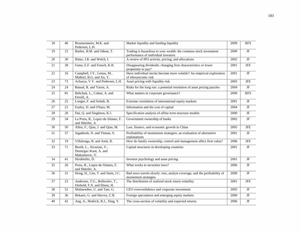
183

18 40 Brunnermeier, M.K. and

Pedersen, L.H.

Market liquidity and funding liquidity 2009 RFS

19 15 Barber, B.M. and Odean, T. Trading is hazardous to your wealth: the common stock investment

performance of individual investors

2000 JF

20 30 Ritter, J.R. and Welch, I. A review of IPO activity, pricing, and allocations 2002 JF

21 38 Fama, E.F. and French, K.R. Disappearing dividends: changing firm characteristics or lower

propensity to pay?

2001 JFE

22 16 Campbell, J.Y., Lettau, M.,

Malkiel, B.G. and Xu, Y.

Have individual stocks become more volatile? An empirical exploration

of idiosyncratic risk

2001 JF

23 73 Acharya, V.V. and Pedersen, L.H. Asset pricing with liquidity risk 2005 JFE

24 24 Bansal, R. and Yaron, A. Risks for the long run: a potential resolution of asset pricing puzzles 2004 JF

25 81 Bebchuk, L., Cohen, A. and

Ferrell, A.

What matters in corporate governance? 2009 RFS

26 25 Longin, F. and Solnik, B. Extreme correlation of international equity markets 2001 JF

27 21 Easley, D. and O'hara, M. Information and the cost of capital 2004 JF

28 20 Dai, Q. and Singleton, K.J. Specification analysis of affine term structure models 2000 JF

29 34 La Porta, R., Lopez‐de‐Silanes, F.

and Shleifer, A.

Government ownership of banks 2002 JF

30 50 Allen, F., Qian, J. and Qian, M. Law, finance, and economic growth in China 2005 JFE

31 37 Jegadeesh, N. and Titman, S. Profitability of momentum strategies: an evaluation of alternative

explanations

2001 JF

32 19 Villalonga, B. and Amit, R. How do family ownership, control and management affect firm value? 2006 JFE

33 71 Booth, L., Aivazian, V.,

Demirguc‐Kunt, A. and

Maksimovic, V.

Capital structures in developing countries 2001 JF

34 41 Hirshleifer, D. Investor psychology and asset pricing 2001 JF

35 26 Porta, R., Lopez‐de‐Silanes, F.

and Shleifer, A.

What works in securities laws? 2006 JF

36 31 Hong, H., Lim, T. and Stein, J.C. Bad news travels slowly: size, analyst coverage, and the profitability of

momentum strategies

2000 JF

37 23 Andersen, T.G., Bollerslev, T.,

Diebold, F.X. and Ebens, H.

The distribution of realized stock return volatility 2001 JFE

38 52 Malmendier, U. and Tate, G. CEO overconfidence and corporate investment 2005 JF

39 36 Bekaert, G. and Harvey, C.R. Foreign speculators and emerging equity markets 2000 JF

40 42 Ang, A., Hodrick, R.J., Xing, Y. The cross‐section of volatility and expected returns 2006 JF

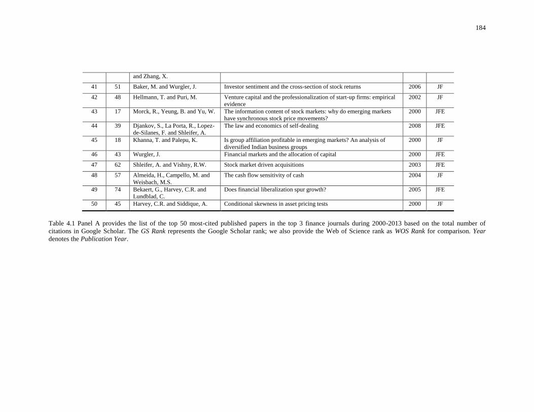
184

and Zhang, X.

41 51 Baker, M. and Wurgler, J. Investor sentiment and the cross-section of stock returns 2006 JF

42 48 Hellmann, T. and Puri, M. Venture capital and the professionalization of start-up firms: empirical

evidence

2002 JF

43 17 Morck, R., Yeung, B. and Yu, W. The information content of stock markets: why do emerging markets

have synchronous stock price movements?

2000 JFE

44 39 Djankov, S., La Porta, R., Lopez-

de-Silanes, F. and Shleifer, A.

The law and economics of self-dealing 2008 JFE

45 18 Khanna, T. and Palepu, K. Is group affiliation profitable in emerging markets? An analysis of

diversified Indian business groups

2000 JF

46 43 Wurgler, J. Financial markets and the allocation of capital 2000 JFE

47 62 Shleifer, A. and Vishny, R.W. Stock market driven acquisitions 2003 JFE

48 57 Almeida, H., Campello, M. and

Weisbach, M.S.

The cash flow sensitivity of cash 2004 JF

49 74 Bekaert, G., Harvey, C.R. and

Lundblad, C.

Does financial liberalization spur growth? 2005 JFE

50 45 Harvey, C.R. and Siddique, A. Conditional skewness in asset pricing tests 2000 JF

Table 4.1 Panel A provides the list of the top 50 most-cited published papers in the top 3 finance journals during 2000-2013 based on the total number of

citations in Google Scholar. The GS Rank represents the Google Scholar rank; we also provide the Web of Science rank as WOS Rank for comparison. Year

denotes the Publication Year.

185

Panel B: Ranking Based on the Number of Citations per Year

GS

p.a.

Rank

WOS

p.a.

Rank

Authors Title Year Journal

1 1 Petersen, M.A. Estimating standard errors in finance panel data sets: comparing

approaches 2009 RFS

2 2 La Porta, R., Lopez-de-Silanes,

F., Shleifer, A. and Vishny, R. Investor protection and corporate governance 2000 JFE

3 3 Brunnermeier, M.K. and

Pedersen, L.H. Market liquidity and funding liquidity 2009 RFS

4 19 Bebchuk, L., Cohen, A. and

Ferrell, A. What matters in corporate governance? 2009 RFS

5 4 Claessens, S., Djankov, S. and

Lang, L.H. The separation of ownership and control in East Asian Corporations 2000 JFE

6 6 La Porta, R., Lopez-de-Silanes,

F., Shleifer, A. and Vishny, R. Investor protection and corporate valuation 2002 JF

7 14 Graham, J.R. and Harvey, C.R. The theory and practice of corporate finance: evidence from the field 2001 JFE

8 109 Gorton, G. and Metrick, A. Securitized banking and the run on repo 2012 JFE

9 8 Anderson, R.C. and Reeb, D.M. Founding-family ownership and firm performance: evidence from the

S&P 500 2003 JF

10 9 Djankov, S., La Porta, R., Lopez-

de-Silanes, F. and Shleifer, A. The law and economics of self-dealing 2008 JFE

11 11 Dyck, A. and Zingales, L. Private benefits of control: an international comparison 2004 JF

12 7 Claessens, S., Djankov, S., Fan,

J.P. and Lang, L.H.

Disentangling the incentive and entrenchment effects of large

shareholdings 2002 JF

13 83 Asness, C.S., Moskowitz, T.J. and

Pedersen, L.H. Value and momentum everywhere 2013 JF

14 16 Forbes, K.J. and Rigobon, R. No contagion, only Interdependence: measuring stock market

comovements 2002 JF

15 124 Demyanyk, Y. and Van Hemert,

O. Understanding the subprime mortgage crisis 2011 RFS

16 18 Faccio, M. and Lang, L.H. The ultimate ownership of Western European corporations 2002 JFE

17 17 Leuz, C., Nanda, D. and Wysocki,

P.D.

Earnings management and investor protection: an international

comparison 2003 JFE

18 36 Barber, B.M. and Odean, T. All that glitters: the effect of attention and news on the buying behavior

of individual and institutional investors 2008 RFS

19 10 Villalonga, B. and Amit, R. How do family ownership, control and management affect firm value? 2006 JFE

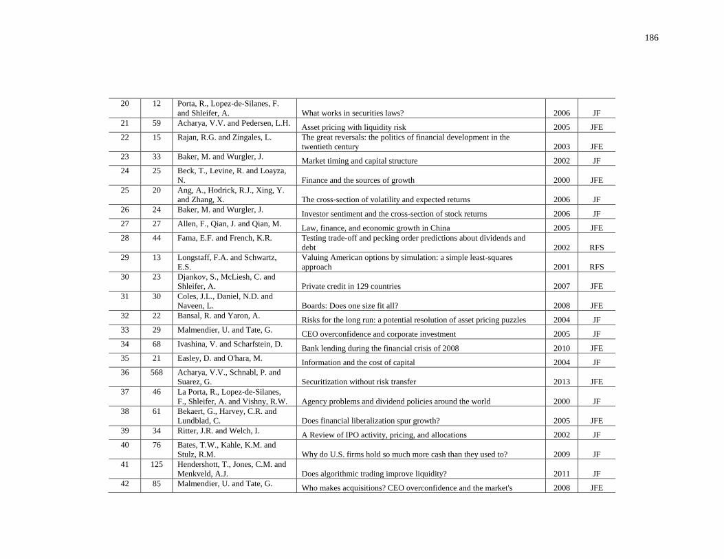
186

20 12 Porta, R., Lopez‐de‐Silanes, F.

and Shleifer, A. What works in securities laws? 2006 JF

21 59 Acharya, V.V. and Pedersen, L.H. Asset pricing with liquidity risk 2005 JFE

22 15 Rajan, R.G. and Zingales, L. The great reversals: the politics of financial development in the

twentieth century 2003 JFE

23 33 Baker, M. and Wurgler, J. Market timing and capital structure 2002 JF

24 25 Beck, T., Levine, R. and Loayza,

N. Finance and the sources of growth 2000 JFE

25 20 Ang, A., Hodrick, R.J., Xing, Y.

and Zhang, X. The cross‐section of volatility and expected returns 2006 JF

26 24 Baker, M. and Wurgler, J. Investor sentiment and the cross-section of stock returns 2006 JF

27 27 Allen, F., Qian, J. and Qian, M. Law, finance, and economic growth in China 2005 JFE

28 44 Fama, E.F. and French, K.R. Testing trade‐off and pecking order predictions about dividends and

debt 2002 RFS

29 13 Longstaff, F.A. and Schwartz,

E.S.

Valuing American options by simulation: a simple least-squares

approach 2001 RFS

30 23 Djankov, S., McLiesh, C. and

Shleifer, A. Private credit in 129 countries 2007 JFE

31 30 Coles, J.L., Daniel, N.D. and

Naveen, L. Boards: Does one size fit all? 2008 JFE

32 22 Bansal, R. and Yaron, A. Risks for the long run: a potential resolution of asset pricing puzzles 2004 JF

33 29 Malmendier, U. and Tate, G. CEO overconfidence and corporate investment 2005 JF

34 68 Ivashina, V. and Scharfstein, D. Bank lending during the financial crisis of 2008 2010 JFE

35 21 Easley, D. and O'hara, M. Information and the cost of capital 2004 JF

36 568 Acharya, V.V., Schnabl, P. and

Suarez, G. Securitization without risk transfer 2013 JFE

37 46 La Porta, R., Lopez‐de‐Silanes,

F., Shleifer, A. and Vishny, R.W. Agency problems and dividend policies around the world 2000 JF

38 61 Bekaert, G., Harvey, C.R. and

Lundblad, C. Does financial liberalization spur growth? 2005 JFE

39 34 Ritter, J.R. and Welch, I. A Review of IPO activity, pricing, and allocations 2002 JF

40 76 Bates, T.W., Kahle, K.M. and

Stulz, R.M. Why do U.S. firms hold so much more cash than they used to? 2009 JF

41 125 Hendershott, T., Jones, C.M. and

Menkveld, A.J. Does algorithmic trading improve liquidity? 2011 JF

42 85 Malmendier, U. and Tate, G. Who makes acquisitions? CEO overconfidence and the market's 2008 JFE

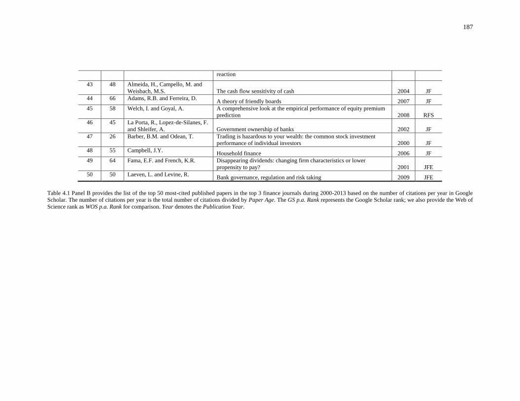
187

reaction

43 48 Almeida, H., Campello, M. and

Weisbach, M.S. The cash flow sensitivity of cash 2004 JF

44 66 Adams, R.B. and Ferreira, D. A theory of friendly boards 2007 JF

45 58 Welch, I. and Goyal, A. A comprehensive look at the empirical performance of equity premium

prediction 2008 RFS

46 45 La Porta, R., Lopez‐de‐Silanes, F.

and Shleifer, A. Government ownership of banks 2002 JF

47 26 Barber, B.M. and Odean, T. Trading is hazardous to your wealth: the common stock investment

performance of individual investors 2000 JF

48 55 Campbell, J.Y. Household finance 2006 JF

49 64 Fama, E.F. and French, K.R. Disappearing dividends: changing firm characteristics or lower

propensity to pay? 2001 JFE

50 50 Laeven, L. and Levine, R. Bank governance, regulation and risk taking 2009 JFE

Table 4.1 Panel B provides the list of the top 50 most-cited published papers in the top 3 finance journals during 2000-2013 based on the number of citations per year in Google

Scholar. The number of citations per year is the total number of citations divided by Paper Age. The GS p.a. Rank represents the Google Scholar rank; we also provide the Web of

Science rank as WOS p.a. Rank for comparison. Year denotes the Publication Year.

188

We present the paper characteristics for the total sample in Table 4.2 and Figure

4.1. The summary statistics in Table 4.2 Panel A show that, on average, lead paper

accounts for 10% of our sample, the paper order is 5.87, the number of authors is 2.27,

internal collaboration is 0.32 (1 if no external collaboration), 0.77 authors are from the

top 20 finance departments, the abstract includes 107.52 words, title length is 8.67 words,

29% of the papers have subtitles, the number of pages is 31.75, the number of footnotes

is 18.63, 42% of the papers have received financial support, the authors acknowledge

11.90 peer scholars, presentations occur at 2.99 conferences and 4.80 seminars, 0.67 RAs

provide research assistance, research methods is 0.49 (1 if purely theoretical), the number

of references is 42.08, the number of tables is 6.73, the number of pictures is 2.52, 59%

of the papers have at least one appendix, and the working paper age is 1.65 years. We

also notice that the standard deviations of all measures of the number of citations are

larger than their means, and this implies the over-dispersion of the citation data and thus

non-normal properties.

In Table 4.2 Panel B, we investigate the trends of paper characteristics over the

recent 14 years during 2000-2013. We find that in the universalist perspective, most of

the measures remain constant except that the working paper age is increasing from 0.79

to 2.06. It takes more time to publish a paper now than before.

In the social constructivist perspective, all measures increase with time: the

number of authors increases from 2.00 to 2.43, internal collaboration increases from 0.18

to 0.33, financial support increases from 0.37 to 0.48, the number of acknowledgements

189

increases from 9.34 to 13.23, the number of conferences34

increases from 1.51 to 4.09,

the number of seminars increases from 2.98 to 5.63, the number of RAs increases from

0.58 to 0.80, the number of references increases from 35.25 to 47.92. These numbers

suggest that finance researchers care more and more about the exposure of their papers to

their peers in recent years. The finance academia seems more and more “liquid” in terms

of opportunities of presentations, co-authorship, and resources.

In the presentation perspective, the abstract length increases from 101.26 to

107.68, the number of tables increases from 5.01 to 7.74, the number of pictures

(graphs/figures) increases from 2.22 to 3.17, the number of footnotes increases from

13.40 to 21.40, the appendix dummy increases from 0.44 to 0.70. These trends may

suggest that the recent papers contain more information or try to do more things in one

project. However, the title length and subtitle dummy does not exhibit stable increase.

We depict the time trends of normalized paper characteristics in Figure 4.1.

34 The number of conferences is a measure in the presentation perspective rather than in the universalist

perspective, so we do not measure conference quality here.

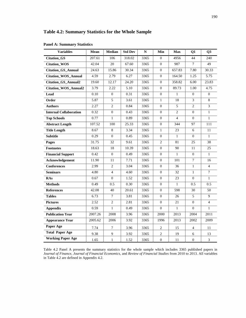
190

Table 4.2: Summary Statistics for the Whole Sample

Panel A: Summary Statistics

Variables Mean Median Std Dev N Min Max Q1 Q3

Citation_GS 207.61 106 318.02 3365 0 4956 44 240

Citation_WOS 42.04 20 67.60 3365 0 987 7 49

Citation_GS_Annual 24.63 15.86 30.34 3365 0 657.83 7.80 30.33

Citation_WOS_Annual 4.59 2.79 6.27 3365 0 164.50 1.25 5.75

Citation_GS_Annual2 19.60 12.17 24.20 3365 0 358.82 6.00 23.83

Citation_WOS_Annual2 3.79 2.22 5.10 3365 0 89.73 1.00 4.75

Lead 0.10 0 0.31 3365 0 1 0 0

Order 5.87 5 3.61 3365 1 18 3 8

Authors 2.27 2 0.84 3365 0 5 2 3

Internal Collaboration 0.32 0 0.43 3365 0 2 0 1

Top Schools 0.77 1 0.89 3365 0 4 0 1

Abstract Length 107.52 100 25.33 3365 0 344 97 111

Title Length 8.67 8 3.34 3365 1 23 6 11

Subtitle 0.29 0 0.45 3365 0 1 0 1

Pages 31.75 32 9.61 3365 2 81 25 38

Footnotes 18.63 18 10.39 3365 0 90 11 25

Financial Support 0.42 0 0.49 3365 0 1 0 1

Acknowledgement 11.90 11 7.71 3365 0 101 7 16

Conferences 2.99 2 3.04 3365 0 36 1 4

Seminars 4.80 4 4.60 3365 0 32 1 7

RAs 0.67 0 1.52 3365 0 23 0 1

Methods 0.49 0.5 0.30 3365 0 1 0.5 0.5

References 42.08 40 20.61 3365 0 598 30 50

Tables 6.73 7 3.81 3365 0 26 5 9

Pictures 2.52 2 2.81 3365 0 21 0 4

Appendix 0.59 1 0.49 3365 0 1 0 1

Publication Year 2007.26 2008 3.96 3365 2000 2013 2004 2011

Appearance Year 2005.62 2006 3.92 3365 1996 2013 2002 2009

Paper Age 7.74 7 3.96 3365 2 15 4 11

Total Paper Age 9.38 9 3.92 3365 2 19 6 13

Working Paper Age 1.65 1 1.52 3365 0 11 0 3

Table 4.2 Panel A presents the summary statistics for the whole sample which includes 3365 published papers in

Journal of Finance, Journal of Financial Economics, and Review of Financial Studies from 2010 to 2013. All variables

in Table 4.2 are defined in Appendix 4.2.

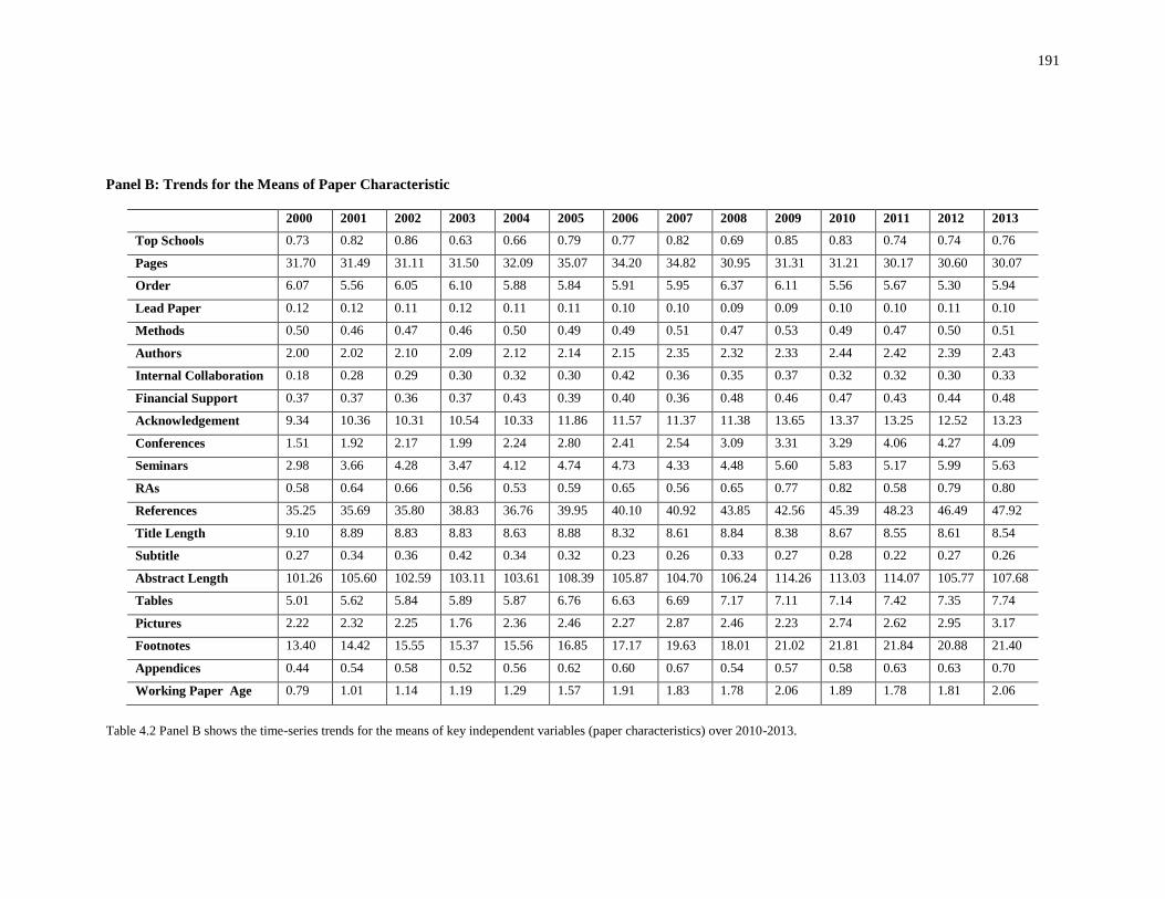
191

Panel B: Trends for the Means of Paper Characteristic

2000 2001 2002 2003 2004 2005 2006 2007 2008 2009 2010 2011 2012 2013

Top Schools 0.73 0.82 0.86 0.63 0.66 0.79 0.77 0.82 0.69 0.85 0.83 0.74 0.74 0.76

Pages 31.70 31.49 31.11 31.50 32.09 35.07 34.20 34.82 30.95 31.31 31.21 30.17 30.60 30.07

Order 6.07 5.56 6.05 6.10 5.88 5.84 5.91 5.95 6.37 6.11 5.56 5.67 5.30 5.94

Lead Paper 0.12 0.12 0.11 0.12 0.11 0.11 0.10 0.10 0.09 0.09 0.10 0.10 0.11 0.10

Methods 0.50 0.46 0.47 0.46 0.50 0.49 0.49 0.51 0.47 0.53 0.49 0.47 0.50 0.51

Authors 2.00 2.02 2.10 2.09 2.12 2.14 2.15 2.35 2.32 2.33 2.44 2.42 2.39 2.43

Internal Collaboration 0.18 0.28 0.29 0.30 0.32 0.30 0.42 0.36 0.35 0.37 0.32 0.32 0.30 0.33

Financial Support 0.37 0.37 0.36 0.37 0.43 0.39 0.40 0.36 0.48 0.46 0.47 0.43 0.44 0.48

Acknowledgement 9.34 10.36 10.31 10.54 10.33 11.86 11.57 11.37 11.38 13.65 13.37 13.25 12.52 13.23

Conferences 1.51 1.92 2.17 1.99 2.24 2.80 2.41 2.54 3.09 3.31 3.29 4.06 4.27 4.09

Seminars 2.98 3.66 4.28 3.47 4.12 4.74 4.73 4.33 4.48 5.60 5.83 5.17 5.99 5.63

RAs 0.58 0.64 0.66 0.56 0.53 0.59 0.65 0.56 0.65 0.77 0.82 0.58 0.79 0.80

References 35.25 35.69 35.80 38.83 36.76 39.95 40.10 40.92 43.85 42.56 45.39 48.23 46.49 47.92

Title Length 9.10 8.89 8.83 8.83 8.63 8.88 8.32 8.61 8.84 8.38 8.67 8.55 8.61 8.54

Subtitle 0.27 0.34 0.36 0.42 0.34 0.32 0.23 0.26 0.33 0.27 0.28 0.22 0.27 0.26

Abstract Length 101.26 105.60 102.59 103.11 103.61 108.39 105.87 104.70 106.24 114.26 113.03 114.07 105.77 107.68

Tables 5.01 5.62 5.84 5.89 5.87 6.76 6.63 6.69 7.17 7.11 7.14 7.42 7.35 7.74

Pictures 2.22 2.32 2.25 1.76 2.36 2.46 2.27 2.87 2.46 2.23 2.74 2.62 2.95 3.17

Footnotes 13.40 14.42 15.55 15.37 15.56 16.85 17.17 19.63 18.01 21.02 21.81 21.84 20.88 21.40

Appendices 0.44 0.54 0.58 0.52 0.56 0.62 0.60 0.67 0.54 0.57 0.58 0.63 0.63 0.70

Working Paper Age 0.79 1.01 1.14 1.19 1.29 1.57 1.91 1.83 1.78 2.06 1.89 1.78 1.81 2.06

Table 4.2 Panel B shows the time-series trends for the means of key independent variables (paper characteristics) over 2010-2013.

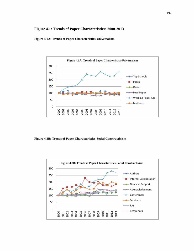
192

Figure 4.1: Trends of Paper Characteristics: 2000-2013

Figure 4.1A: Trends of Paper Characteristics-Universalism

Figure 4.2B: Trends of Paper Characteristics-Social Constructivism

0

50

100

150

200

250

300

20

00

20

01

20

02

20

03

20

04

20

05

20

06

20

07

20

08

20

09

20

10

20

11

20

12

20

13

Figure 4.1A: Trends of Paper Charateristics-Universalism

Top Schools

Pages

Order

Lead Paper

Working Paper Age

Methods

0

50

100

150

200

250

300

20

00

20

01

20

02

20

03

20

04

20

05

20

06

20

07

20

08

20

09

20

10

20

11

20

12

20

13

Figure 4.2B: Trends of Paper Characteristics-Social Constructivism

Authors

Internal Collaboration

Financial Support

Acknowledgement

Conferences

Seminars

RAs

References

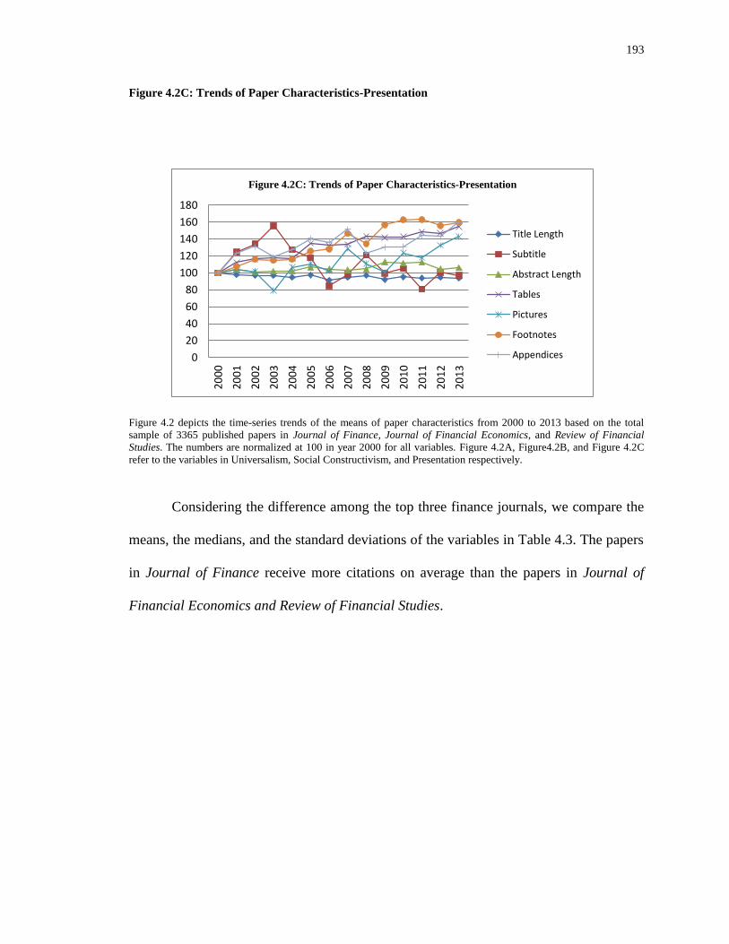
193

Figure 4.2C: Trends of Paper Characteristics-Presentation

Figure 4.2 depicts the time-series trends of the means of paper characteristics from 2000 to 2013 based on the total

sample of 3365 published papers in Journal of Finance, Journal of Financial Economics, and Review of Financial

Studies. The numbers are normalized at 100 in year 2000 for all variables. Figure 4.2A, Figure4.2B, and Figure 4.2C

refer to the variables in Universalism, Social Constructivism, and Presentation respectively.

Considering the difference among the top three finance journals, we compare the

means, the medians, and the standard deviations of the variables in Table 4.3. The papers

in Journal of Finance receive more citations on average than the papers in Journal of

Financial Economics and Review of Financial Studies.

0

20

40

60

80

100

120

140

160

1802

00

0

20

01

20

02

20

03

20

04

20

05

20

06

20

07

20

08

20

09

20

10

20

11

20

12

20

13

Figure 4.2C: Trends of Paper Characteristics-Presentation

Title Length

Subtitle

Abstract Length

Tables

Pictures

Footnotes

Appendices

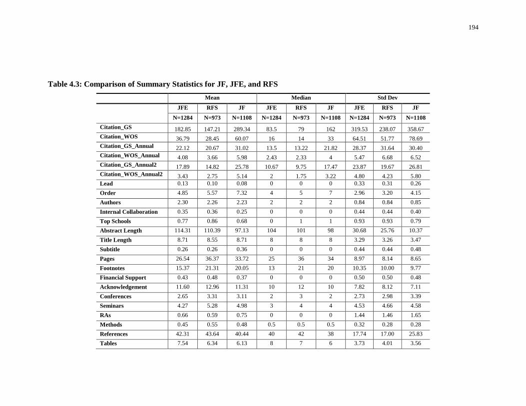
194

Table 4.3: Comparison of Summary Statistics for JF, JFE, and RFS

Mean Median Std Dev

JFE RFS JF JFE RFS JF JFE RFS JF

N=1284 N=973 N=1108 N=1284 N=973 N=1108 N=1284 N=973 N=1108

Citation_GS 182.85 147.21 289.34 83.5 79 162 319.53 238.07 358.67

Citation_WOS 36.79 28.45 60.07 16 14 33 64.51 51.77 78.69

Citation_GS_Annual 22.12 20.67 31.02 13.5 13.22 21.82 28.37 31.64 30.40

Citation_WOS_Annual 4.08 3.66 5.98 2.43 2.33 4 5.47 6.68 6.52

Citation_GS_Annual2 17.89 14.82 25.78 10.67 9.75 17.47 23.87 19.67 26.81

Citation_WOS_Annual2 3.43 2.75 5.14 2 1.75 3.22 4.80 4.23 5.80

Lead 0.13 0.10 0.08 0 0 0 0.33 0.31 0.26

Order 4.85 5.57 7.32 4 5 7 2.96 3.20 4.15

Authors 2.30 2.26 2.23 2 2 2 0.84 0.84 0.85

Internal Collaboration 0.35 0.36 0.25 0 0 0 0.44 0.44 0.40

Top Schools 0.77 0.86 0.68 0 1 1 0.93 0.93 0.79

Abstract Length 114.31 110.39 97.13 104 101 98 30.68 25.76 10.37

Title Length 8.71 8.55 8.71 8 8 8 3.29 3.26 3.47

Subtitle 0.26 0.26 0.36 0 0 0 0.44 0.44 0.48

Pages 26.54 36.37 33.72 25 36 34 8.97 8.14 8.65

Footnotes 15.37 21.31 20.05 13 21 20 10.35 10.00 9.77

Financial Support 0.43 0.48 0.37 0 0 0 0.50 0.50 0.48

Acknowledgement 11.60 12.96 11.31 10 12 10 7.82 8.12 7.11

Conferences 2.65 3.31 3.11 2 3 2 2.73 2.98 3.39

Seminars 4.27 5.28 4.98 3 4 4 4.53 4.66 4.58

RAs 0.66 0.59 0.75 0 0 0 1.44 1.46 1.65

Methods 0.45 0.55 0.48 0.5 0.5 0.5 0.32 0.28 0.28

References 42.31 43.64 40.44 40 42 38 17.74 17.00 25.83

Tables 7.54 6.34 6.13 8 7 6 3.73 4.01 3.56

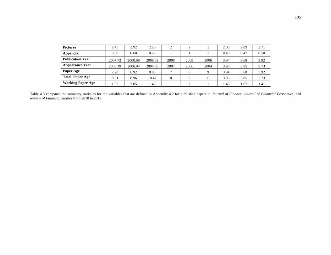
195

Pictures 2.45 2.92 2.26 2 2 1 2.80 2.89 2.71

Appendix 0.60 0.68 0.50 1 1 1 0.49 0.47 0.50

Publication Year 2007.72 2008.08 2006.02 2008 2009 2006 3.94 3.68 3.92

Appearance Year 2006.19 2006.04 2004.58 2007 2006 2004 3.95 3.85 3.73

Paper Age 7.28 6.92 8.98 7 6 9 3.94 3.68 3.92

Total Paper Age 8.81 8.96 10.42 8 9 11 3.95 3.85 3.73

Working Paper Age 1.52 2.05 1.45 1 2 1 1.43 1.67 1.41

Table 4.3 compares the summary statistics for the variables that are defined in Appendix 4.2 for published papers in Journal of Finance, Journal of Financial Economics, and

Review of Financial Studies from 2010 to 2013.

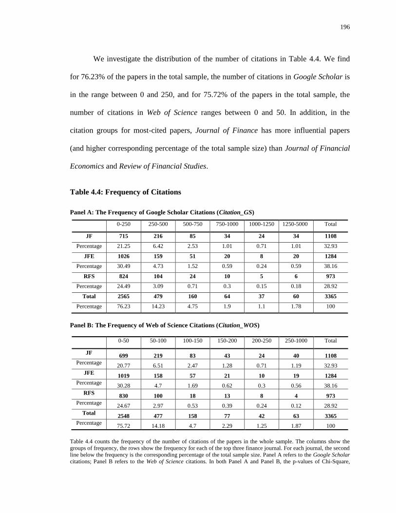
196

We investigate the distribution of the number of citations in Table 4.4. We find

for 76.23% of the papers in the total sample, the number of citations in Google Scholar is

in the range between 0 and 250, and for 75.72% of the papers in the total sample, the

number of citations in Web of Science ranges between 0 and 50. In addition, in the

citation groups for most-cited papers, Journal of Finance has more influential papers

(and higher corresponding percentage of the total sample size) than Journal of Financial

Economics and Review of Financial Studies.

Table 4.4: Frequency of Citations

Panel A: The Frequency of Google Scholar Citations (Citation_GS)

0-250 250-500 500-750 750-1000 1000-1250 1250-5000 Total

JF 715 216 85 34 24 34 1108

Percentage 21.25 6.42 2.53 1.01 0.71 1.01 32.93

JFE 1026 159 51 20 8 20 1284

Percentage 30.49 4.73 1.52 0.59 0.24 0.59 38.16

RFS 824 104 24 10 5 6 973

Percentage 24.49 3.09 0.71 0.3 0.15 0.18 28.92

Total 2565 479 160 64 37 60 3365

Percentage 76.23 14.23 4.75 1.9 1.1 1.78 100

Panel B: The Frequency of Web of Science Citations (Citation_WOS)

0-50 50-100 100-150 150-200 200-250 250-1000 Total

JF 699 219 83 43 24 40 1108

Percentage 20.77 6.51 2.47 1.28 0.71 1.19 32.93

JFE 1019 158 57 21 10 19 1284

Percentage 30.28 4.7 1.69 0.62 0.3 0.56 38.16

RFS 830 100 18 13 8 4 973

Percentage 24.67 2.97 0.53 0.39 0.24 0.12 28.92

Total 2548 477 158 77 42 63 3365

Percentage 75.72 14.18 4.7 2.29 1.25 1.87 100

Table 4.4 counts the frequency of the number of citations of the papers in the whole sample. The columns show the

groups of frequency, the rows show the frequency for each of the top three finance journal. For each journal, the second

line below the frequency is the corresponding percentage of the total sample size. Panel A refers to the Google Scholar

citations; Panel B refers to the Web of Science citations. In both Panel A and Panel B, the p-values of Chi-Square,

197

Likelihood Ratio Chi-Square, and Mantel-Haenszel Chi-Square are all smaller than 0.001 (not reported in Table 4),

which means the distribution of citation groups are significantly different among the top 3 finance journals.

In order to identify how paper characteristics differ between more influential

papers and less influential papers, we compare the means of the paper characteristics

between the top 10% and the bottom 10% annual citations in Table 4.5. For annual

citations in Google Scholar (Citation_GS_Annual1), almost all measures in the three

perspectives are significantly different, with the exceptions of subtitle dummy, abstract

length, and the number of pictures. By large, more influential papers in our sample have

larger number of authors from the top 20 finance departments, larger number of pages,

smaller paper order and higher proportion of lead papers, larger paper age, total paper age

and working paper age, higher empirical orientation, larger number of authors, higher

level of external collaboration and financial support, larger numbers of

acknowledgements, conferences, seminars, and RAs, more references, shorter title length,

larger number of tables and footnotes, and less appendix setting. As for annual citations

in Web of Science (Citation_WOS_Annual1), all the measures in the universalist

perspective, paper age, and total paper age are still significant. Some paper characteristics

in the social constructivist perspective (internal collaboration, financial support, the

number of conferences, seminars, and RAs) and in the presentation perspective (title

length, abstract length, and the number of pictures) become insignificant, but the signs of

the differences are the same as those of Citation_GS_Annual1 except the number of

footnotes. It is not surprising that more measures become insignificant for

Citation_WOS_Annual1 because Citation_WOS is more sensitive for annualized quantile

calculation given the number of citations in Web of Science is always much smaller than

that in Google Scholar. Again, these results highlight the importance of paper quality,

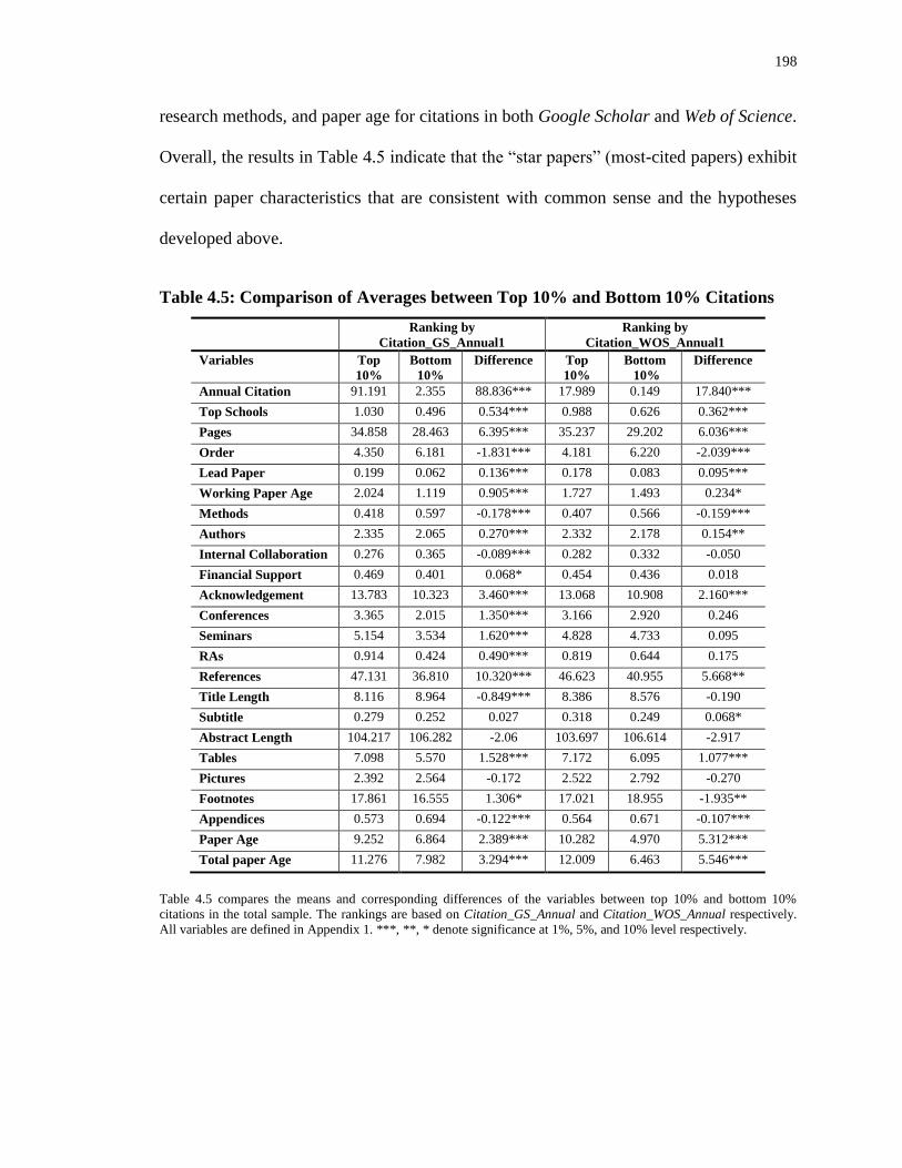
198

research methods, and paper age for citations in both Google Scholar and Web of Science.

Overall, the results in Table 4.5 indicate that the “star papers” (most-cited papers) exhibit

certain paper characteristics that are consistent with common sense and the hypotheses

developed above.

Table 4.5: Comparison of Averages between Top 10% and Bottom 10% Citations

Ranking by

Citation_GS_Annual1

Ranking by

Citation_WOS_Annual1

Variables Top

10%

Bottom

10%

Difference Top

10%

Bottom

10%

Difference

Annual Citation 91.191 2.355 88.836*** 17.989 0.149 17.840***

Top Schools 1.030 0.496 0.534*** 0.988 0.626 0.362***

Pages 34.858 28.463 6.395*** 35.237 29.202 6.036***

Order 4.350 6.181 -1.831*** 4.181 6.220 -2.039***

Lead Paper 0.199 0.062 0.136*** 0.178 0.083 0.095***

Working Paper Age 2.024 1.119 0.905*** 1.727 1.493 0.234*

Methods 0.418 0.597 -0.178*** 0.407 0.566 -0.159***

Authors 2.335 2.065 0.270*** 2.332 2.178 0.154**

Internal Collaboration 0.276 0.365 -0.089*** 0.282 0.332 -0.050

Financial Support 0.469 0.401 0.068* 0.454 0.436 0.018

Acknowledgement 13.783 10.323 3.460*** 13.068 10.908 2.160***

Conferences 3.365 2.015 1.350*** 3.166 2.920 0.246

Seminars 5.154 3.534 1.620*** 4.828 4.733 0.095

RAs 0.914 0.424 0.490*** 0.819 0.644 0.175

References 47.131 36.810 10.320*** 46.623 40.955 5.668**

Title Length 8.116 8.964 -0.849*** 8.386 8.576 -0.190

Subtitle 0.279 0.252 0.027 0.318 0.249 0.068*

Abstract Length 104.217 106.282 -2.06 103.697 106.614 -2.917

Tables 7.098 5.570 1.528*** 7.172 6.095 1.077***

Pictures 2.392 2.564 -0.172 2.522 2.792 -0.270

Footnotes 17.861 16.555 1.306* 17.021 18.955 -1.935**

Appendices 0.573 0.694 -0.122*** 0.564 0.671 -0.107***

Paper Age 9.252 6.864 2.389*** 10.282 4.970 5.312***

Total paper Age 11.276 7.982 3.294*** 12.009 6.463 5.546***

Table 4.5 compares the means and corresponding differences of the variables between top 10% and bottom 10%

citations in the total sample. The rankings are based on Citation_GS_Annual and Citation_WOS_Annual respectively.

All variables are defined in Appendix 1. ***, **, * denote significance at 1%, 5%, and 10% level respectively.

199

Last but not least, we provide the correlation coefficients in Table 4.6. We find all

the dependent variables (the four citation measures) are highly correlated-the correlation

coefficients are between 0.82 and 0.97. However, the independent variables (paper

characteristics) are usually not highly correlated, which indicates we do not suffer from a

multicollinearity problem in the regressions. For the significant correlation coefficients,

the citation measures are positively correlated to Lead, Authors, Top Schools, Subtitle,

Pages, Financial Support, Acknowledgement, Conferences, Seminars, RAs, References,

Tables, Paper Age and Total Paper Age; the citation measures are negatively correlated

with Order, Internal Collaboration, Abstract Length, Title Length, Methods, Appendices.

One exception is that Pictures is not significantly correlated with any of the citation

measures.

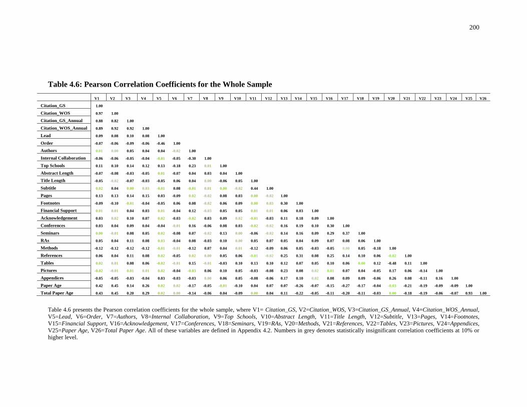
200

Table 4.6: Pearson Correlation Coefficients for the Whole Sample

V1 V2 V3 V4 V5 V6 V7 V8 V9 V10 V11 V12 V13 V14 V15 V16 V17 V18 V19 V20 V21 V22 V23 V24 V25 V26

Citation_GS 1.00

Citation_WOS 0.97 1.00

Citation_GS_Annual 0.88 0.82 1.00

Citation_WOS_Annual 0.89 0.92 0.92 1.00

Lead 0.09 0.08 0.10 0.08 1.00

Order -0.07 -0.06 -0.09 -0.06 -0.46 1.00

Authors 0.01 0.00 0.05 0.04 0.04 -0.02 1.00

Internal Collaboration -0.06 -0.06 -0.05 -0.04 -0.01 -0.05 -0.30 1.00

Top Schools 0.11 0.10 0.14 0.12 0.13 -0.18 0.23 0.01 1.00

Abstract Length -0.07 -0.08 -0.03 -0.05 0.01 -0.07 0.04 0.03 0.04 1.00

Title Length -0.05 -0.02 -0.07 -0.03 -0.05 0.06 0.04 0.00 -0.06 0.05 1.00

Subtitle 0.02 0.04 0.00 0.03 -0.01 0.08 -0.01 0.01 0.00 -0.02 0.44 1.00

Pages 0.13 0.13 0.14 0.15 0.03 -0.09 0.02 -0.02 0.08 0.03 0.00 -0.02 1.00

Footnotes -0.09 -0.10 -0.01 -0.04 -0.05 0.06 0.08 -0.02 0.06 0.09 0.00 0.03 0.30 1.00

Financial Support 0.01 0.01 0.04 0.03 0.01 -0.04 0.12 -0.03 0.05 0.05 0.01 0.01 0.06 0.03 1.00

Acknowledgement 0.03 0.02 0.10 0.07 0.02 -0.03 -0.02 0.03 0.09 0.02 -0.01 -0.03 0.11 0.18 0.09 1.00

Conferences 0.03 0.04 0.09 0.04 -0.04 -0.01 0.16 -0.06 0.08 0.03 -0.02 -0.02 0.16 0.19 0.10 0.30 1.00

Seminars 0.00 -0.01 0.08 0.05 0.02 -0.08 0.07 -0.02 0.13 0.00 -0.06 -0.02 0.14 0.16 0.09 0.29 0.37 1.00

RAs 0.05 0.04 0.11 0.08 0.03 -0.04 0.08 -0.03 0.10 0.00 0.05 0.07 0.05 0.04 0.09 0.07 0.08 0.06 1.00

Methods -0.12 -0.12 -0.12 -0.12 -0.01 -0.01 -0.12 0.07 0.04 0.01 -0.12 -0.09 0.06 0.05 -0.03 -0.05 0.00 0.05 -0.18 1.00

References 0.06 0.04 0.11 0.08 0.02 -0.05 0.02 0.00 0.05 0.06 -0.01 -0.02 0.25 0.31 0.08 0.25 0.14 0.10 0.06 -0.02 1.00

Tables 0.02 0.01 0.08 0.06 -0.02 -0.01 0.15 -0.01 -0.03 0.10 0.13 0.10 0.12 0.07 0.05 0.10 0.06 0.00 0.12 -0.48 0.11 1.00

Pictures -0.02 -0.01 0.01 0.01 0.02 -0.04 -0.03 0.06 0.10 0.05 -0.03 -0.08 0.23 0.08 0.02 0.01 0.07 0.04 -0.05 0.17 0.06 -0.14 1.00

Appendices -0.05 -0.05 -0.03 -0.04 0.03 -0.03 -0.03 0.00 0.06 0.05 -0.08 -0.06 0.17 0.10 0.02 0.08 0.09 0.09 -0.06 0.26 0.08 -0.11 0.16 1.00

Paper Age 0.42 0.45 0.14 0.26 0.02 0.02 -0.17 -0.05 -0.01 -0.10 0.04 0.07 0.07 -0.26 -0.07 -0.15 -0.27 -0.17 -0.04 -0.03 -0.21 -0.19 -0.09 -0.09 1.00

Total Paper Age 0.43 0.45 0.20 0.29 0.02 0.00 -0.14 -0.06 0.04 -0.09 0.00 0.04 0.11 -0.22 -0.05 -0.11 -0.20 -0.11 -0.03 0.00 -0.18 -0.19 -0.06 -0.07 0.93 1.00

Table 4.6 presents the Pearson correlation coefficients for the whole sample, where V1= Citation_GS, V2=Citation_WOS, V3=Citation_GS_Annual, V4=Citation_WOS_Annual,

V5=Lead, V6=Order, V7=Authors, V8=Internal Collaboration, V9=Top Schools, V10=Abstract Length, V11=Title Length, V12=Subtitle, V13=Pages, V14=Footnotes,

V15=Financial Support, V16=Acknowledgement, V17=Conferences, V18=Seminars, V19=RAs, V20=Methods, V21=References, V22=Tables, V23=Pictures, V24=Appendices,

V25=Paper Age, V26=Total Paper Age. All of these variables are defined in Appendix 4.2. Numbers in grey denotes statistically insignificant correlation coefficients at 10% or

higher level.

201

4.4 Multivariate Analysis and Results

We use the following specification to explore the effects of paper characteristics

on the number of citations:

𝐶𝑖𝑡𝑎𝑡𝑖𝑜𝑛𝑖𝑗 = 𝛼 + ∑ 𝛽𝑗2𝑗=1 𝐽𝑜𝑢𝑟𝑛𝑎𝑙𝑗 + 𝛾𝐴𝑔𝑒𝑖𝑗 + 𝛿𝐴𝑔𝑒𝑖𝑗

2 + ∑ 𝜃𝑢6𝑢=1 𝑈𝑛𝑖𝑣𝑒𝑟𝑎𝑠𝑎𝑙𝑖𝑠𝑡𝑢𝑖𝑗 +

+ ∑ 𝜇𝑠8𝑠=1 𝑆𝑜𝑐𝑖𝑎𝑙𝑠𝑖𝑗+ ∑ 𝜑𝑝

9𝑝=1 𝑃𝑟𝑒𝑠𝑒𝑛𝑡𝑎𝑡𝑖𝑜𝑛𝑝𝑖𝑗 + 휀𝑖𝑗 (4.1)

Where 𝐶𝑖𝑡𝑎𝑡𝑖𝑜𝑛𝑖𝑗 is the number of citations for paper 𝑖 in journal j. 𝐽𝑜𝑢𝑟𝑛𝑎𝑙𝑗 is a

dummy that equals 1 if paper 𝑖 is in journal j, and 0 otherwise. 𝐴𝑔𝑒 denotes paper age,

i.e. the number of years since publication. We include the quadratic terms of paper age in

the regressions because Alexander and Mabry (1994) find that for published papers the

curve of cumulative percent of total citations by paper age is concave.

𝑈𝑛𝑖𝑣𝑒𝑟𝑠𝑎𝑙𝑖𝑠𝑡𝑢𝑖𝑗 , 𝑆𝑜𝑐𝑖𝑎𝑙𝑠𝑖𝑗 , and 𝑃𝑟𝑒𝑠𝑒𝑛𝑡𝑎𝑡𝑖𝑜𝑛𝑝𝑖𝑗 are measures in the universalist

perspective, the social constructivist perspective, and the presentation perspective

respectively.

Following Stremersch, Verniers, and Verhoef (2007) and Brogaard, Engelberg,

and Parsons (2014), we estimate the model using negative binomial regressions. The

advantage of negative binomial regression is that it can deal with over-dispersed count

data (the conditional variances of dependent variables are bigger than the conditional

means). It is superior to Poisson regression since it has an extra parameter to capture the

over-dispersion.

We provide the results in Table 4.7 for the regressions on the total number of

citations per paper in Google Scholar (Citation_GS). In Column 1, we find that all of the

202

three perspectives have significant effects on the number of citations based on our total

sample. The signs of the coefficients in the universalist perspective (quality and domain)

are consistent with Hypothesis 1. In the quality dimension, the results show that the

number of authors from top departments, the number of pages, and lead paper dummy

(confirmation of Michayluk and Zurbruegg (2014)) positively affect the number of

citations; the paper order negatively affects the number of citations. The net effect of

working paper age is positive, which implies an indicator of quality improvement. In the

domain dimension, we find empirical papers can attract more citations. Half of the

measures in the social constructivist measure are insignificant, but all of the signs of the

coefficients are consistent with Hypothesis 2. In the visibility dimension, the number of

acknowledgements, the number of conferences, and the number of RAs all positively

affect the number of citations. In the personal promotion dimension, the number of

references has significant positive effect on the number of citations. As for the

presentation perspective, all of the results support Hypothesis 3. In the first-page attention

dimension, the negative coefficient of title length indicates the complexity of title can

destroy citations, and the positive coefficient of abstract length means the

informativeness of the abstract can boost citations. In the expositional dimension, the

number of tables has positive influence on citations, while the numbers of footnotes and

appendices have negative effects on citations, and the latter implies that the complexity in

details may harm research impact.

For independent variables other than the measures for the three perspectives, we

find papers in Journal of Finance receive more citations on average than the papers in the

other two top finance journals. In addition, the number of citations is concave in paper

203

age, consistent with Alexander and Mabry (1994). Papers are generally losing the

momentum of impact over time.

It is worth noting that if we compare the magnitude of the coefficients, the

measures of the universalist perspective, journal dummy, and paper age have bigger

influences compared to the measures in the social constructivist perspective and the

presentation perspective. Paper quality, research methods, journal placement, and paper

age appear to be the most important drivers (based on economic significance) for

research impact.

The evidence in Columns 2, 3, and 4 for the three journals respectively suggests

that the impact drivers play different roles in different journals. For example, lead paper

has no significant effect on citations for papers in Journal of Finance, paper order has no

significant impact in Review of Financial Studies, and the number of authors loses its

effect in Journal of Financial Economics.

When it comes to the goodness of fit35

, we use the Value/DF ratio, where Value is

the doubled difference between the log likelihood of the maximum achievable model and

the log likelihood of the fitted model, and DF is the number of observations minus the

number of parameters. If the model fits the data well, then Value/DF should be around 1.

In our results, this number is also about 1, implying good model fit. We also report the

dispersion parameter. If the dispersion is 0, then the model reduces to a Poisson model

35 Refer to this website for more technical and programming details:

http://www.ats.ucla.edu/stat/sas/output/sas_negbin_output.htm

204

which assumes that the expected value of the dependent variable is equal to its variance;

if the dispersion is bigger than zero the dependent variable is over-dispersed. It is not

surprising that in our model the dispersion is significantly bigger than 0: the small

variance of dispersion implies the lower bound of the Wald 95% confidence limits is

above 0. Thus, our model is more appropriate to the Poisson model.

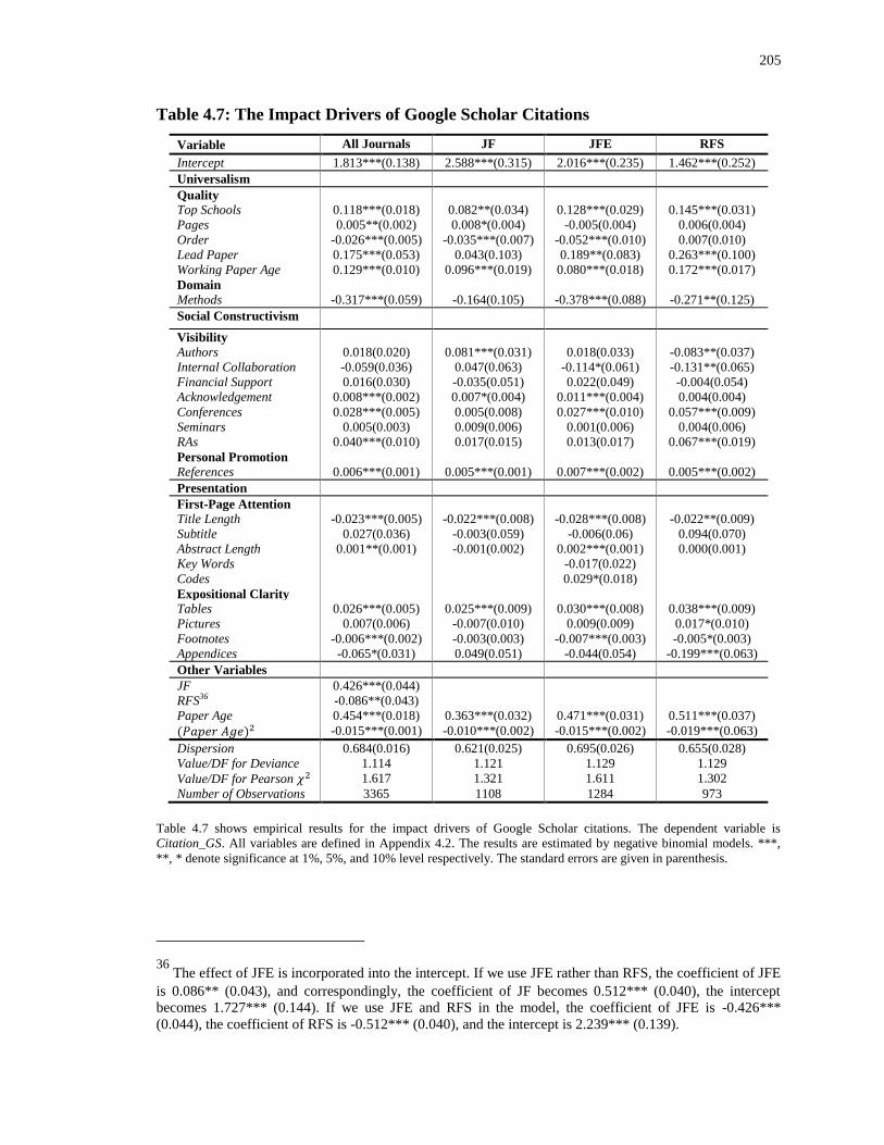
205

Table 4.7: The Impact Drivers of Google Scholar Citations

Variable All Journals JF JFE RFS

Intercept 1.813***(0.138) 2.588***(0.315) 2.016***(0.235) 1.462***(0.252)

Universalism

Quality

Top Schools 0.118***(0.018) 0.082**(0.034) 0.128***(0.029) 0.145***(0.031)

Pages 0.005**(0.002) 0.008*(0.004) -0.005(0.004) 0.006(0.004)

Order -0.026***(0.005) -0.035***(0.007) -0.052***(0.010) 0.007(0.010)

Lead Paper 0.175***(0.053) 0.043(0.103) 0.189**(0.083) 0.263***(0.100)

Working Paper Age 0.129***(0.010) 0.096***(0.019) 0.080***(0.018) 0.172***(0.017)

Domain

Methods -0.317***(0.059) -0.164(0.105) -0.378***(0.088) -0.271**(0.125)

Social Constructivism

Visibility

Authors 0.018(0.020) 0.081***(0.031) 0.018(0.033) -0.083**(0.037)

Internal Collaboration -0.059(0.036) 0.047(0.063) -0.114*(0.061) -0.131**(0.065)

Financial Support 0.016(0.030) -0.035(0.051) 0.022(0.049) -0.004(0.054)

Acknowledgement 0.008***(0.002) 0.007*(0.004) 0.011***(0.004) 0.004(0.004)

Conferences 0.028***(0.005) 0.005(0.008) 0.027***(0.010) 0.057***(0.009)

Seminars 0.005(0.003) 0.009(0.006) 0.001(0.006) 0.004(0.006)

RAs 0.040***(0.010) 0.017(0.015) 0.013(0.017) 0.067***(0.019)

Personal Promotion

References 0.006***(0.001) 0.005***(0.001) 0.007***(0.002) 0.005***(0.002)

Presentation

First-Page Attention

Title Length -0.023***(0.005) -0.022***(0.008) -0.028***(0.008) -0.022**(0.009)

Subtitle 0.027(0.036) -0.003(0.059) -0.006(0.06) 0.094(0.070)

Abstract Length 0.001**(0.001) -0.001(0.002) 0.002***(0.001) 0.000(0.001)

Key Words -0.017(0.022)

Codes 0.029*(0.018)

Expositional Clarity

Tables 0.026***(0.005) 0.025***(0.009) 0.030***(0.008) 0.038***(0.009)

Pictures 0.007(0.006) -0.007(0.010) 0.009(0.009) 0.017*(0.010)

Footnotes -0.006***(0.002) -0.003(0.003) -0.007***(0.003) -0.005*(0.003)

Appendices -0.065*(0.031) 0.049(0.051) -0.044(0.054) -0.199***(0.063)

Other Variables

JF 0.426***(0.044)

RFS36 -0.086**(0.043)

Paper Age 0.454***(0.018) 0.363***(0.032) 0.471***(0.031) 0.511***(0.037)

(𝑃𝑎𝑝𝑒𝑟 𝐴𝑔𝑒)2 -0.015***(0.001) -0.010***(0.002) -0.015***(0.002) -0.019***(0.063)

Dispersion 0.684(0.016) 0.621(0.025) 0.695(0.026) 0.655(0.028)

Value/DF for Deviance 1.114 1.121 1.129 1.129

Value/DF for Pearson 𝜒2 1.617 1.321 1.611 1.302

Number of Observations 3365 1108 1284 973

Table 4.7 shows empirical results for the impact drivers of Google Scholar citations. The dependent variable is

Citation_GS. All variables are defined in Appendix 4.2. The results are estimated by negative binomial models. ***,

**, * denote significance at 1%, 5%, and 10% level respectively. The standard errors are given in parenthesis.

36 The effect of JFE is incorporated into the intercept. If we use JFE rather than RFS, the coefficient of JFE

is 0.086** (0.043), and correspondingly, the coefficient of JF becomes 0.512*** (0.040), the intercept

becomes 1.727*** (0.144). If we use JFE and RFS in the model, the coefficient of JFE is -0.426***

(0.044), the coefficient of RFS is -0.512*** (0.040), and the intercept is 2.239*** (0.139).

206

We conduct similar regressions for the total number of citations per paper in Web

of Science (Citation_WOS) in Table 4.8. We find Web of Science citations generate

congruent results to Google Scholar citations for our total data sample. Some exceptions

reside in the changes of statistical significance of the number of authors, the number of

seminars, and the appendices dummy. Again, paper quality, research methods, journal

placement, and paper age are the most important drivers (in economic significance) of the

number of citations.

As for the regressions for the three different journals, the impact drivers also play

different roles based on the results in Table 4.8. In both of Table 4.7 and Table 4.8,

theoretical papers in Journal of Financial Economics and Review of Financial Studies

significantly receive fewer citations than empirical papers but this relation is insignificant

for papers in Journal of Finance; larger number of pages significantly contributes to the

number of citations of papers in Journal of Finance, but not in Journal of Financial

Economics or Review of Financial Studies. However, the significance changes for several

visibility measures (the number of authors, internal collaboration, the number of

acknowledgements, and the number of conferences) and one first-page attention measure

(title length) if we compare Columns 2-4 between Table 4.7 and Table 4.8.

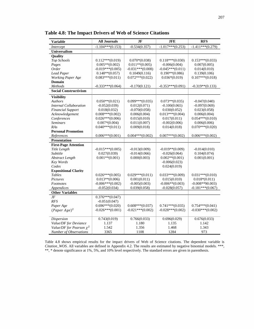
207

Table 4.8: The Impact Drivers of Web of Science Citations

Variable All Journals JF JFE RFS

Intercept -1.104***(0.153) -0.534(0.357) -1.017***(0.253) -1.411***(0.279)

Universalism

Quality

Top Schools 0.112***(0.019) 0.070*(0.038) 0.118***(0.030) 0.153***(0.033)

Pages 0.005**(0.002) 0.011**(0.005) -0.006(0.004) 0.007(0.005)

Order -0.019***(0.005) -0.031***(0.008) -0.045***(0.011) 0.014(0.010)

Lead Paper 0.148**(0.057) 0.1049(0.116) 0.190**(0.086) 0.139(0.106)

Working Paper Age 0.083***(0.011) 0.072***(0.022) 0.036*(0.019) 0.107***(0.018)

Domain

Methods -0.333***(0.064) -0.170(0.121) -0.353***(0.091) -0.319**(0.133)

Social Constructivism

Visibility

Authors 0.050**(0.021) 0.099***(0.035) 0.073**(0.035) -0.047(0.040)

Internal Collaboration -0.052(0.039) 0.012(0.071) -0.100(0.065) -0.097(0.069)

Financial Support 0.018(0.032) -0.070(0.058) 0.030(0.052) 0.023(0.058)

Acknowledgement 0.008***(0.002) 0.006(0.004) 0.013***(0.004) 0.006(0.004)

Conferences 0.026***(0.006) 0.015(0.010) 0.017(0.011) 0.054***(0.010)

Seminars 0.007*(0.004) 0.011(0.007) -0.002(0.006) 0.006(0.006)

RAs 0.040***(0.011) 0.009(0.018) 0.014(0.018) 0.070***(0.020)

Personal Promotion

References 0.006***(0.001) 0.004***(0.002) 0.007***(0.002) 0.006***(0.002)

Presentation

First-Page Attention

Title Length -0.015***(0.005) -0.013(0.009) -0.019**(0.009) -0.014(0.010)

Subtitle 0.027(0.039) -0.014(0.066) -0.026(0.064) 0.104(0.074)

Abstract Length 0.001**(0.001) 0.000(0.003) 0.002**(0.001) 0.001(0.001)

Key Words -0.006(0.023)

Codes 0.024(0.019)

Expositional Clarity

Tables 0.026***(0.005) 0.029***(0.011) 0.033***(0.009) 0.031***(0.010)

Pictures 0.013**(0.006) 0.001(0.011) 0.015(0.010) 0.018*(0.011)

Footnotes -0.006***(0.002) -0.005(0.003) -0.006**(0.003) -0.008**90.003)

Appendices -0.052(0.034) 0.039(0.058) -0.028(0.057) -0.181***(0.067)

Other Variables

JF 0.376***(0.047)

RFS -0.051(0.047)

Paper Age 0.696***(0.020) 0.608***(0.037) 0.741***(0.035) 0.754***(0.041)

(𝑃𝑎𝑝𝑒𝑟 𝐴𝑔𝑒)2 -0.026***(0.001) -0.021***(0.002) -0.028***(0.002) -0.030***(0.002)

Dispersion 0.743(0.019) 0.766(0.033) 0.696(0.029) 0.676(0.033)

Value/DF for Deviance 1.137 1.180 1.135 1.142

Value/DF for Pearson 𝜒2 1.542 1.356 1.468 1.343

Number of Observations 3365 1108 1284 973

Table 4.8 shows empirical results for the impact drivers of Web of Science citations. The dependent variable is

Citation_WOS. All variables are defined in Appendix 4.2. The results are estimated by negative binomial models. ***,

**, * denote significance at 1%, 5%, and 10% level respectively. The standard errors are given in parenthesis.

208

4.5 Robustness

We examine the robustness of our empirical results for the whole sample in five

ways.

First, we use redefined dependent variables for citations. In previous studies,

Keloharju (2009) uses the ratio of the number of Google Scholar citations to the number

of years since publication; Kim, Morse, and Zingales (2009) study Web of Science

citations adjusted for age. We employ both annualized Google Scholar citations

(Citation_GS_Annual1) and annualized Web of Science citations

(Citation_WOS_Annual1) in Table 4.9. Both measures are defined as the total number of

citations scaled by paper age (the age since publication). The sign, significance, and

magnitude (economic significance) of the coefficients are quite similar between Table 4.7

Column 1 (Citation_GS_Annual1) and Table 4.9 Column 1 (Citation_GS). The only

difference is that the magnitude of paper age becomes smaller for annual citations since

citations are partially (given the nonlinear relation) normalized for annual calculation. As

for Web of Science citations, the results are also similar between Table 4.8 Column 1 and

Table 4.9 Column 3, except for the significance of abstract length and the magnitude for

paper age. Alternatively, we use total paper age to rescale the number of citations in

Table 4.9 (Citation_GS_Annual2 in Column 2 and Citation_WOS_Annual2 in Column 4).

Both Citation_GS_Annual2 and Citation_WOS_Annual2 are defined as the total number

of citations divided by total paper age (the age since appearance on the web as a working

paper). Since we consider working paper age in the denominator of annual-citation

calculation of Citation_GS_Annual2 and Citation_WOS_Annual2, the coefficients change

for working paper age and paper age, while all other coefficients remain almost the same.

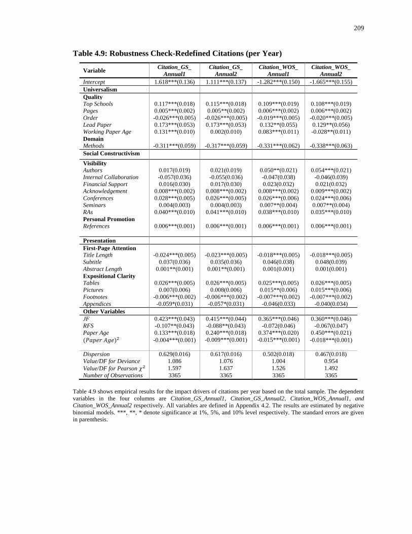
209

Table 4.9: Robustness Check-Redefined Citations (per Year)

Variable Citation_GS_

Annual1

Citation_GS_

Annual2

Citation_WOS_

Annual1

Citation_WOS_

Annual2

Intercept 1.618***(0.136) 1.111***(0.137) -1.282***(0.150) -1.665***(0.155)

Universalism

Quality

Top Schools 0.117***(0.018) 0.115***(0.018) 0.109***(0.019) 0.108***(0.019)

Pages 0.005***(0.002) 0.005**(0.002) 0.006***(0.002) 0.006***(0.002)

Order -0.026***(0.005) -0.026***(0.005) -0.019***(0.005) -0.020***(0.005)

Lead Paper 0.173***(0.053) 0.173***(0.053) 0.132**(0.055) 0.129**(0.056)

Working Paper Age 0.131***(0.010) 0.002(0.010) 0.083***(0.011) -0.028**(0.011)

Domain

Methods -0.311***(0.059) -0.317***(0.059) -0.331***(0.062) -0.338***(0.063)

Social Constructivism

Visibility

Authors 0.017(0.019) 0.021(0.019) 0.050**(0.021) 0.054***(0.021)

Internal Collaboration -0.057(0.036) -0.055(0.036) -0.047(0.038) -0.046(0.039)

Financial Support 0.016(0.030) 0.017(0.030) 0.023(0.032) 0.021(0.032)

Acknowledgement 0.008***(0.002) 0.008***(0.002) 0.008***(0.002) 0.009***(0.002)

Conferences 0.028***(0.005) 0.026***(0.005) 0.026***(0.006) 0.024***(0.006)

Seminars 0.004(0.003) 0.004(0.003) 0.007**(0.004) 0.007**(0.004)

RAs 0.040***(0.010) 0.041***(0.010) 0.038***(0.010) 0.035***(0.010)

Personal Promotion

References 0.006***(0.001) 0.006***(0.001) 0.006***(0.001)

0.006***(0.001)

Presentation

First-Page Attention

Title Length -0.024***(0.005) -0.023***(0.005) -0.018***(0.005) -0.018***(0.005)

Subtitle 0.037(0.036) 0.035(0.036) 0.046(0.038) 0.048(0.039)

Abstract Length 0.001**(0.001) 0.001**(0.001) 0.001(0.001) 0.001(0.001)

Expositional Clarity

Tables 0.026***(0.005) 0.026***(0.005) 0.025***(0.005) 0.026***(0.005)

Pictures 0.007(0.006) 0.008(0.006) 0.015**(0.006) 0.015***(0.006)

Footnotes -0.006***(0.002) -0.006***(0.002) -0.007***(0.002) -0.007***(0.002)

Appendices -0.059*(0.031) -0.057*(0.031) -0.046(0.033) -0.040(0.034)

Other Variables

JF 0.423***(0.043) 0.415***(0.044) 0.365***(0.046) 0.360***(0.046)

RFS -0.107**(0.043) -0.088**(0.043) -0.072(0.046) -0.067(0.047)

Paper Age 0.133***(0.018) 0.240***(0.018) 0.374***(0.020) 0.450***(0.021)

(𝑃𝑎𝑝𝑒𝑟 𝐴𝑔𝑒)2 -0.004***(0.001) -0.009***(0.001) -0.015***(0.001) -0.018***(0.001)

Dispersion 0.629(0.016) 0.617(0.016) 0.502(0.018) 0.467(0.018)

Value/DF for Deviance 1.086 1.076 1.004 0.954

Value/DF for Pearson 𝜒2 1.597 1.637 1.526 1.492

Number of Observations 3365 3365 3365 3365

Table 4.9 shows empirical results for the impact drivers of citations per year based on the total sample. The dependent

variables in the four columns are Citation_GS_Annual1, Citation_GS_Annual2, Citation_WOS_Annual1, and

Citation_WOS_Annual2 respectively. All variables are defined in Appendix 4.2. The results are estimated by negative

binomial models. ***, **, * denote significance at 1%, 5%, and 10% level respectively. The standard errors are given

in parenthesis.

210

Second, we show the empirical results of log-transformed OLS models in Table

4.10 as the comparison with those of negative binomial models. Since neither total

citations nor annual citations are normally distributed, log-transformed number of

citations is widely used as the dependent variables in the literature (e.g., Ederington,

1974; Laband and Piette, 1994; Brogaard, Engelberg, and Parsons, 2014). However, log-

transformed OLS models have disadvantages such as the lack of capability of modeling

the dispersion, as well as the loss of data of uncited articles37

. Given the fact that we use

the log form as the default link function for the negative binomial regressions and the fact

that log-transformed OLS models are popular in previous studies, we still show the

results of log OLS models in Table 4.10. We find that among the 25 independent

variables, 4 variables change significance for Google Scholar citations (for both

log(Citation_GS) and log (Citation_GS_Annual1)), 5 variables change significance for

Web of Science citations (for both log(Citation_WOS) and log (Citation_WOS_Annual1)),

and all other variables have similar results. We allow for such difference to distinguish

between log-transformed OLS model and negative binomial models.

37 To deal with papers without any citations, we also tried log (1+citations) and found similar results.

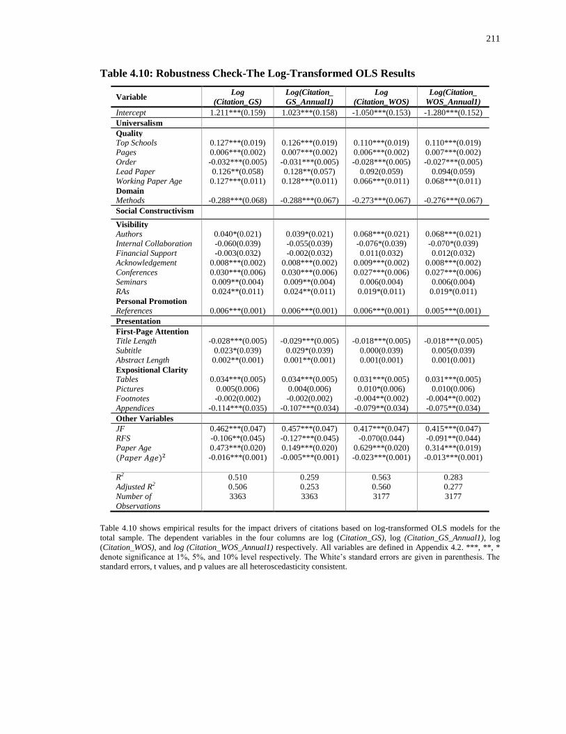
211

Table 4.10: Robustness Check-The Log-Transformed OLS Results

Variable Log

(Citation_GS)

Log(Citation_

GS_Annual1)

Log

(Citation_WOS)

Log(Citation_

WOS_Annual1)

Intercept 1.211***(0.159) 1.023***(0.158) -1.050***(0.153) -1.280***(0.152)

Universalism

Quality

Top Schools 0.127***(0.019) 0.126***(0.019) 0.110***(0.019) 0.110***(0.019)

Pages 0.006***(0.002) 0.007***(0.002) 0.006***(0.002) 0.007***(0.002)

Order -0.032***(0.005) -0.031***(0.005) -0.028***(0.005) -0.027***(0.005)

Lead Paper 0.126**(0.058) 0.128**(0.057) 0.092(0.059) 0.094(0.059)

Working Paper Age 0.127***(0.011) 0.128***(0.011) 0.066***(0.011) 0.068***(0.011)

Domain

Methods -0.288***(0.068) -0.288***(0.067) -0.273***(0.067) -0.276***(0.067)

Social Constructivism

Visibility

Authors 0.040*(0.021) 0.039*(0.021) 0.068***(0.021) 0.068***(0.021)

Internal Collaboration -0.060(0.039) -0.055(0.039) -0.076*(0.039) -0.070*(0.039)

Financial Support -0.003(0.032) -0.002(0.032) 0.011(0.032) 0.012(0.032)

Acknowledgement 0.008***(0.002) 0.008***(0.002) 0.009***(0.002) 0.008***(0.002)

Conferences 0.030***(0.006) 0.030***(0.006) 0.027***(0.006) 0.027***(0.006)

Seminars 0.009**(0.004) 0.009**(0.004) 0.006(0.004) 0.006(0.004)

RAs 0.024**(0.011) 0.024**(0.011) 0.019*(0.011) 0.019*(0.011)

Personal Promotion

References 0.006***(0.001) 0.006***(0.001) 0.006***(0.001) 0.005***(0.001)

Presentation

First-Page Attention

Title Length -0.028***(0.005) -0.029***(0.005) -0.018***(0.005) -0.018***(0.005)

Subtitle 0.023*(0.039) 0.029*(0.039) 0.000(0.039) 0.005(0.039)

Abstract Length 0.002**(0.001) 0.001**(0.001) 0.001(0.001) 0.001(0.001)

Expositional Clarity

Tables 0.034***(0.005) 0.034***(0.005) 0.031***(0.005) 0.031***(0.005)

Pictures 0.005(0.006) 0.004(0.006) 0.010*(0.006) 0.010(0.006)

Footnotes -0.002(0.002) -0.002(0.002) -0.004**(0.002) -0.004**(0.002)

Appendices -0.114***(0.035) -0.107***(0.034) -0.079**(0.034) -0.075**(0.034)

Other Variables

JF 0.462***(0.047) 0.457***(0.047) 0.417***(0.047) 0.415***(0.047)

RFS -0.106**(0.045) -0.127***(0.045) -0.070(0.044) -0.091**(0.044)

Paper Age 0.473***(0.020) 0.149***(0.020) 0.629***(0.020) 0.314***(0.019)

(𝑃𝑎𝑝𝑒𝑟 𝐴𝑔𝑒)2 -0.016***(0.001) -0.005***(0.001) -0.023***(0.001) -0.013***(0.001)

R2 0.510 0.259 0.563 0.283

Adjusted R2 0.506 0.253 0.560 0.277

Number of

Observations

3363 3363 3177 3177

Table 4.10 shows empirical results for the impact drivers of citations based on log-transformed OLS models for the

total sample. The dependent variables in the four columns are log (Citation_GS), log (Citation_GS_Annual1), log

(Citation_WOS), and log (Citation_WOS_Annual1) respectively. All variables are defined in Appendix 4.2. ***, **, *

denote significance at 1%, 5%, and 10% level respectively. The White’s standard errors are given in parenthesis. The

standard errors, t values, and p values are all heteroscedasticity consistent.

212

Third, we conduct adjustment for heterogeneity by reporting robust standard

errors in Table 4.11. The results for Citation_GS in Table 4.11 Column 1 are quite similar

with those in Table 4.7 Column 1, except that the coefficient of the number of authors

becomes significant at 10% level after adjustment of heteroskedasticity. The results for

Citation_WOS in Table 4.11 Column 3 are very similar with those in Table 4.8 Column

1, with the exceptions of the number of seminars, the number of RAs, and the number of

pictures. These three variables become insignificant after the heteroskedasticity

adjustment. The annual numbers of citations (Citation_GS_Annual1 and

Citation_WOS_Annual1) do not exhibit more changes than total number of citations.

Considering the complexity of the research question and the number of independent

variables (25 independent variables), we conclude that heteroskedasticity is not a serious

problem for our empirical examinations.

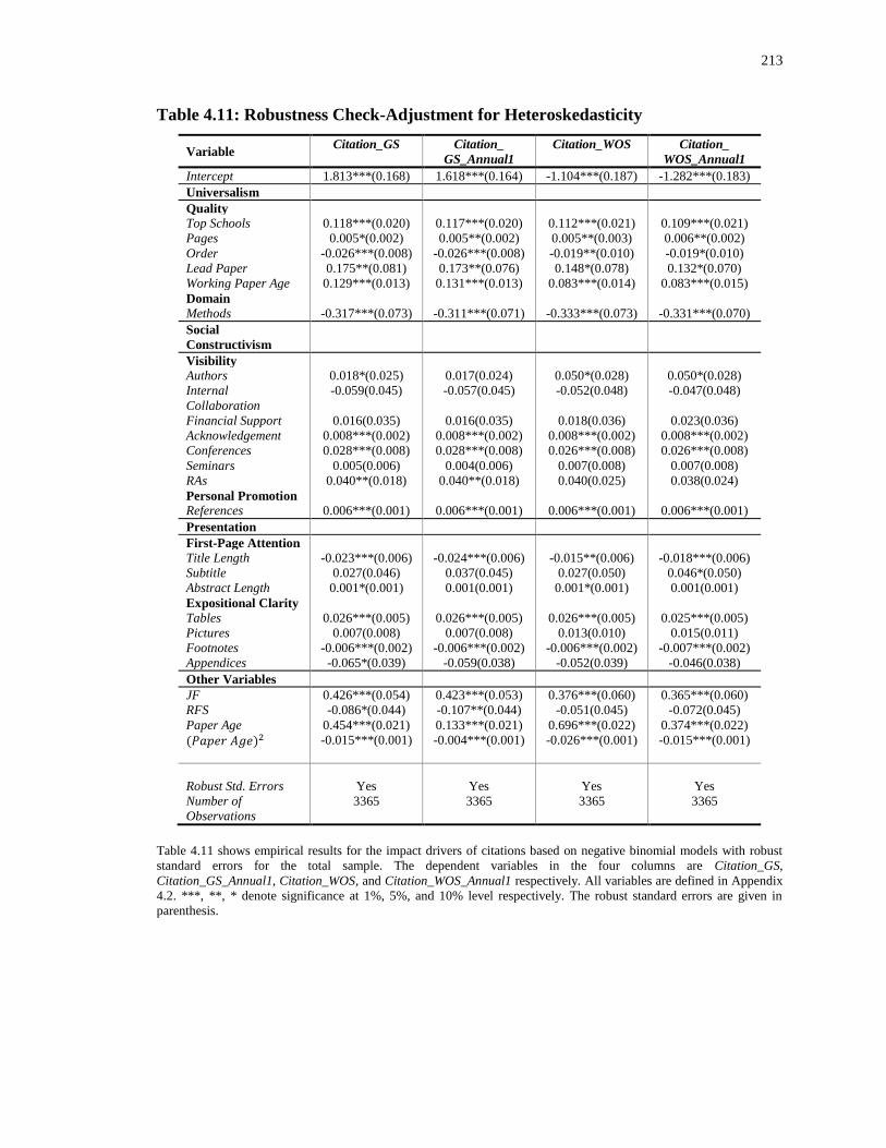
213

Table 4.11: Robustness Check-Adjustment for Heteroskedasticity

Variable Citation_GS Citation_

GS_Annual1

Citation_WOS Citation_

WOS_Annual1

Intercept 1.813***(0.168) 1.618***(0.164) -1.104***(0.187) -1.282***(0.183)

Universalism

Quality

Top Schools 0.118***(0.020) 0.117***(0.020) 0.112***(0.021) 0.109***(0.021)

Pages 0.005*(0.002) 0.005**(0.002) 0.005**(0.003) 0.006**(0.002)

Order -0.026***(0.008) -0.026***(0.008) -0.019**(0.010) -0.019*(0.010)

Lead Paper 0.175**(0.081) 0.173**(0.076) 0.148*(0.078) 0.132*(0.070)

Working Paper Age 0.129***(0.013) 0.131***(0.013) 0.083***(0.014) 0.083***(0.015)

Domain

Methods -0.317***(0.073) -0.311***(0.071) -0.333***(0.073) -0.331***(0.070)

Social

Constructivism

Visibility

Authors 0.018*(0.025) 0.017(0.024) 0.050*(0.028) 0.050*(0.028)

Internal

Collaboration

-0.059(0.045) -0.057(0.045) -0.052(0.048) -0.047(0.048)

Financial Support 0.016(0.035) 0.016(0.035) 0.018(0.036) 0.023(0.036)

Acknowledgement 0.008***(0.002) 0.008***(0.002) 0.008***(0.002) 0.008***(0.002)

Conferences 0.028***(0.008) 0.028***(0.008) 0.026***(0.008) 0.026***(0.008)

Seminars 0.005(0.006) 0.004(0.006) 0.007(0.008) 0.007(0.008)

RAs 0.040**(0.018) 0.040**(0.018) 0.040(0.025) 0.038(0.024)

Personal Promotion

References 0.006***(0.001) 0.006***(0.001) 0.006***(0.001) 0.006***(0.001)

Presentation

First-Page Attention

Title Length -0.023***(0.006) -0.024***(0.006) -0.015**(0.006) -0.018***(0.006)

Subtitle 0.027(0.046) 0.037(0.045) 0.027(0.050) 0.046*(0.050)

Abstract Length 0.001*(0.001) 0.001(0.001) 0.001*(0.001) 0.001(0.001)

Expositional Clarity

Tables 0.026***(0.005) 0.026***(0.005) 0.026***(0.005) 0.025***(0.005)

Pictures 0.007(0.008) 0.007(0.008) 0.013(0.010) 0.015(0.011)

Footnotes -0.006***(0.002) -0.006***(0.002) -0.006***(0.002) -0.007***(0.002)

Appendices -0.065*(0.039) -0.059(0.038) -0.052(0.039) -0.046(0.038)

Other Variables

JF 0.426***(0.054) 0.423***(0.053) 0.376***(0.060) 0.365***(0.060)

RFS -0.086*(0.044) -0.107**(0.044) -0.051(0.045) -0.072(0.045)

Paper Age 0.454***(0.021) 0.133***(0.021) 0.696***(0.022) 0.374***(0.022)

(𝑃𝑎𝑝𝑒𝑟 𝐴𝑔𝑒)2 -0.015***(0.001) -0.004***(0.001) -0.026***(0.001) -0.015***(0.001)

Robust Std. Errors Yes Yes Yes Yes

Number of

Observations

3365 3365 3365 3365

Table 4.11 shows empirical results for the impact drivers of citations based on negative binomial models with robust

standard errors for the total sample. The dependent variables in the four columns are Citation_GS,

Citation_GS_Annual1, Citation_WOS, and Citation_WOS_Annual1 respectively. All variables are defined in Appendix

4.2. ***, **, * denote significance at 1%, 5%, and 10% level respectively. The robust standard errors are given in

parenthesis.

214

Fourth, we conduct regressions on winsorized citations by removing the top 1%

highly cited papers. We follow Brogaard, Engelberg, and Parsons (2014) by using

winsorized data to see whether our empirical results are driven by outliers (i.e., those

super star papers). Specifically we remove the 34 most-cited papers from the total

sample. In Table 4.12 Column 1, the results are robust for Citation_GS as most of the

independent variables exhibit consistent sign, significance, and magnitude compared with

those of the total sample. Only the coefficients of number of pages and internal

collaboration change statistical significance. In Table 4.12 Column 2 for

Citation_GS_Annual1, the results are quite similar with those in Table 4.9 Column 1,

except that internal collaboration and abstract length change significance. As for

Citation_WOS and Citation_WOS_Annual1, the common significance changes reside in

internal collaboration, the number of seminars, pictures, and appendices. Overall, based

on the winsorized sample with the most-cited papers ignored, the results in Table 4.12 are

similar with previous results, especially for Google Scholar citations.

Fifth, we examine the non-linear effects of non-dummy independent variables by

adding the quadratic forms. By and large, we find these quadratic forms generate

insignificant results and extremely small magnitude. We do not report the results of

quadratic terms to make this chapter concise.

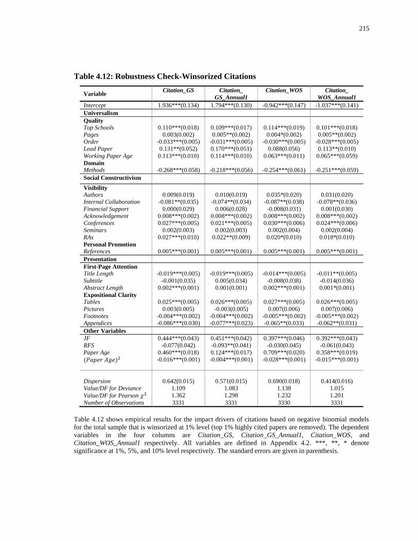
215

Table 4.12: Robustness Check-Winsorized Citations

Variable Citation_GS Citation_

GS_Annual1

Citation_WOS Citation_

WOS_Annual1

Intercept 1.936***(0.134) 1.794***(0.130) -0.942***(0.147) -1.037***(0.141)

Universalism

Quality

Top Schools 0.110***(0.018) 0.109***(0.017) 0.114***(0.019) 0.101***(0.018)

Pages 0.003(0.002) 0.005**(0.002) 0.004*(0.002) 0.005**(0.002)

Order -0.033***(0.005) -0.031***(0.005) -0.030***(0.005) -0.028***(0.005)

Lead Paper 0.131**(0.052) 0.170***(0.051) 0.088(0.056) 0.113**(0.010)

Working Paper Age 0.113***(0.010) 0.114***(0.010) 0.063***(0.011) 0.065***(0.059)

Domain

Methods -0.268***(0.058) -0.218***(0.056) -0.254***(0.061) -0.251***(0.059)

Social Constructivism

Visibility

Authors 0.009(0.019) 0.010(0.019) 0.035*(0.020) 0.031(0.020)

Internal Collaboration -0.081**(0.035) -0.074**(0.034) -0.087**(0.038) -0.078**(0.036)

Financial Support 0.000(0.029) 0.006(0.028) -0.008(0.031) 0.001(0.030)

Acknowledgement 0.008***(0.002) 0.008***(0.002) 0.008***(0.002) 0.008***(0.002)

Conferences 0.027***(0.005) 0.021***(0.005) 0.030***(0.006) 0.024***(0.006)

Seminars 0.002(0.003) 0.002(0.003) 0.002(0.004) 0.002(0.004)

RAs 0.027***(0.010) 0.022**(0.009) 0.020*(0.010) 0.018*(0.010)

Personal Promotion

References 0.005***(0.001) 0.005***(0.001) 0.005***(0.001) 0.005***(0.001)

Presentation

First-Page Attention

Title Length -0.019***(0.005) -0.019***(0.005) -0.014***(0.005) -0.011**(0.005)

Subtitle -0.001(0.035) 0.005(0.034) -0.008(0.038) -0.014(0.036)

Abstract Length 0.002***(0.001) 0.001(0.001) 0.002***(0.001) 0.001*(0.001)

Expositional Clarity

Tables 0.025***(0.005) 0.026***(0.005) 0.027***(0.005) 0.026***(0.005)

Pictures 0.003(0.005) -0.003(0.005) 0.007(0.006) 0.007(0.006)

Footnotes -0.004***(0.002) -0.004***(0.002) -0.005***(0.002) -0.005***(0.002)

Appendices -0.086***(0.030) -0.077***(0.023) -0.065**(0.033) -0.062**(0.031)

Other Variables

JF 0.444***(0.043) 0.451***(0.042) 0.397***(0.046) 0.392***(0.043)

RFS -0.077(0.042) -0.093**(0.041) -0.030(0.045) -0.061(0.043)

Paper Age 0.460***(0.018) 0.124***(0.017) 0.709***(0.020) 0.358***(0.019)

(𝑃𝑎𝑝𝑒𝑟 𝐴𝑔𝑒)2 -0.016***(0.001) -0.004***(0.001) -0.028***(0.001) -0.015***(0.001)

Dispersion 0.642(0.015) 0.571(0.015) 0.690(0.018) 0.414(0.016)

Value/DF for Deviance 1.109 1.083 1.138 1.015

Value/DF for Pearson 𝜒2 1.362 1.298 1.232 1.201

Number of Observations 3331 3331 3330 3331

Table 4.12 shows empirical results for the impact drivers of citations based on negative binomial models

for the total sample that is winsorized at 1% level (top 1% highly cited papers are removed). The dependent

variables in the four columns are Citation_GS, Citation_GS_Annual1, Citation_WOS, and

Citation_WOS_Annual1 respectively. All variables are defined in Appendix 4.2. ***, **, * denote

significance at 1%, 5%, and 10% level respectively. The standard errors are given in parenthesis.

216

4.6 The Marginal Effects of Negative Binomial Models

In previous sections, it is not straightforward to quantify the effects of different

drivers of research impact as the models are non-linear, so we provide the average

marginal effects in Table 4.13. The dependent variables are Citation_GS,

Citation_GS_Annual, Citation_WOS, Citation_WOS_Annual respectively in the four

columns. The sign and significance of the coefficients of paper characteristics are

consistent with the results in previous sections. Among the three perspectives, the

universalist perspective has the largest influences on citations. For example, one more

author from the top 20 finance department in the world is associated with 24.9 additional

total citations and 2.91 additional annual citations in Google Scholar, 4.85 additional

total citations and 0.51 additional annual citations in Web of Science; if a paper is placed

as the lead paper in a journal issue, it is associated with 39.54 additional total citations

and 4.60 additional annual citations in Google Scholar, 6.76 additional total citations and

0.64 additional annual citations in Web of Science. Compared with the universalist

perspective, the other two perspectives have smaller influences in economic significance.

In the constructivist perspective, the number of conferences has the largest magnitude

among the paper characteristics that are statistically significant for all of the four

dependent variables; in the presentation perspective, the number of tables has the largest

magnitude for statistically significant results. For the effects of other variables, journal

placement in Journal of Finance and paper age (i.e. the numbers of years since

publication) have stronger effects than any paper characteristics in all of the three

perspectives. These results provide direct evidence for those who are concerned with the

number of citations of their papers in the top three finance journals.

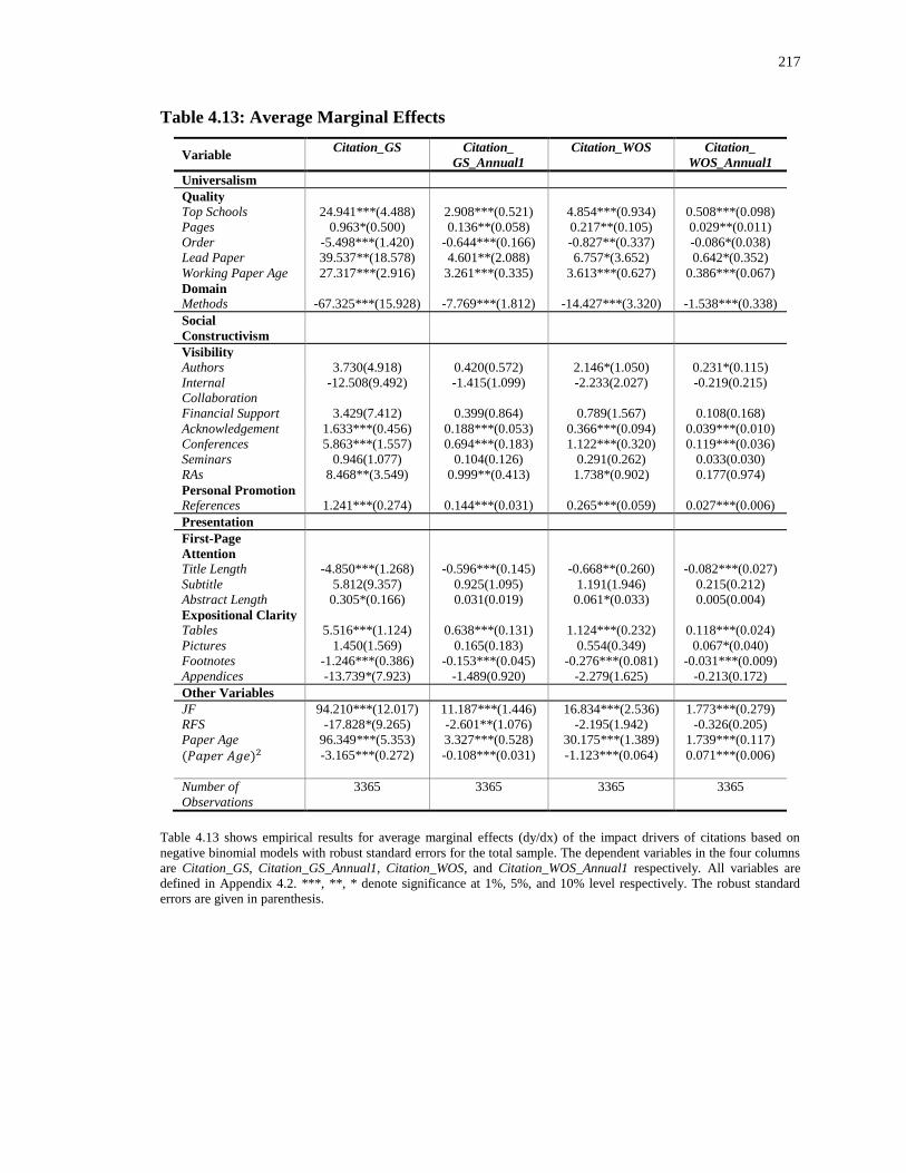
217

Table 4.13: Average Marginal Effects

Variable Citation_GS Citation_

GS_Annual1

Citation_WOS Citation_

WOS_Annual1

Universalism

Quality

Top Schools 24.941***(4.488) 2.908***(0.521) 4.854***(0.934) 0.508***(0.098)

Pages 0.963*(0.500) 0.136**(0.058) 0.217**(0.105) 0.029**(0.011)

Order -5.498***(1.420) -0.644***(0.166) -0.827**(0.337) -0.086*(0.038)

Lead Paper 39.537**(18.578) 4.601**(2.088) 6.757*(3.652) 0.642*(0.352)

Working Paper Age 27.317***(2.916) 3.261***(0.335) 3.613***(0.627) 0.386***(0.067)

Domain

Methods -67.325***(15.928) -7.769***(1.812) -14.427***(3.320) -1.538***(0.338)

Social

Constructivism

Visibility

Authors 3.730(4.918) 0.420(0.572) 2.146*(1.050) 0.231*(0.115)

Internal

Collaboration

-12.508(9.492) -1.415(1.099) -2.233(2.027) -0.219(0.215)

Financial Support 3.429(7.412) 0.399(0.864) 0.789(1.567) 0.108(0.168)

Acknowledgement 1.633***(0.456) 0.188***(0.053) 0.366***(0.094) 0.039***(0.010)

Conferences 5.863***(1.557) 0.694***(0.183) 1.122***(0.320) 0.119***(0.036)

Seminars 0.946(1.077) 0.104(0.126) 0.291(0.262) 0.033(0.030)

RAs 8.468**(3.549) 0.999**(0.413) 1.738*(0.902) 0.177(0.974)

Personal Promotion

References 1.241***(0.274) 0.144***(0.031) 0.265***(0.059) 0.027***(0.006)

Presentation

First-Page

Attention

Title Length -4.850***(1.268) -0.596***(0.145) -0.668**(0.260) -0.082***(0.027)

Subtitle 5.812(9.357) 0.925(1.095) 1.191(1.946) 0.215(0.212)

Abstract Length 0.305*(0.166) 0.031(0.019) 0.061*(0.033) 0.005(0.004)

Expositional Clarity

Tables 5.516***(1.124) 0.638***(0.131) 1.124***(0.232) 0.118***(0.024)

Pictures 1.450(1.569) 0.165(0.183) 0.554(0.349) 0.067*(0.040)

Footnotes -1.246***(0.386) -0.153***(0.045) -0.276***(0.081) -0.031***(0.009)

Appendices -13.739*(7.923) -1.489(0.920) -2.279(1.625) -0.213(0.172)

Other Variables

JF 94.210***(12.017) 11.187***(1.446) 16.834***(2.536) 1.773***(0.279)

RFS -17.828*(9.265) -2.601**(1.076) -2.195(1.942) -0.326(0.205)

Paper Age 96.349***(5.353) 3.327***(0.528) 30.175***(1.389) 1.739***(0.117)

(𝑃𝑎𝑝𝑒𝑟 𝐴𝑔𝑒)2 -3.165***(0.272) -0.108***(0.031) -1.123***(0.064) 0.071***(0.006)

Number of

Observations

3365 3365 3365 3365

Table 4.13 shows empirical results for average marginal effects (dy/dx) of the impact drivers of citations based on

negative binomial models with robust standard errors for the total sample. The dependent variables in the four columns

are Citation_GS, Citation_GS_Annual1, Citation_WOS, and Citation_WOS_Annual1 respectively. All variables are

defined in Appendix 4.2. ***, **, * denote significance at 1%, 5%, and 10% level respectively. The robust standard

errors are given in parenthesis.

218

4.7 Conclusion

Little is known about how paper characteristics change over time, how paper

characteristics differ between more influential papers and less influential papers, and

what are the factors that affect the citations of the published papers in finance literature.

In this chapter, we try to answer these questions based on the hand-collected data for the

published papers in the top three finance journals over the period 2000-2013. We employ

three different theoretical perspectives: the universalist perspective (what is said), the

social constructivist perspective (who says it), and the presentation perspective (how it is

said), and have four main findings:

First, most of the paper characteristics in the social constructivist perspective

(visibility and personal promotion) and the presentation perspective (fist-page attention

and expositional clarity) increase over time, while most of the paper characteristics in the

universalist perspective (quality and domain) remain constant.

Second, most of the paper characteristics are significantly different between the

top 10% and the bottom 10% papers based on the number of citations per year. Generally

speaking, the more influential papers have larger number of authors from the top 20

finance departments, larger number of pages, smaller paper order and higher proportion

of lead papers, longer paper age, working paper age, and total paper age, higher empirical

orientation, larger number of authors, higher level of external collaboration and financial

support, larger numbers of acknowledgements, conferences, seminars, and RAs, more

references, shorter title length, larger number of tables and footnotes, and less appendix

setting.

219

Third, the regression results by negative binomial models show that the

universalist perspective, the social constructivist perspective, and the presentation

perspective all provide drivers of research impact. Specifically, paper quality, research

methods, journal placement, and paper age are the most important (in economic

significance) drivers for the number of citations. In our analysis, Web of Science citations

generate congruent results to Google Scholar citations. Additionally, our results are

robust to redefined citation measures, alternative econometric specifications,

heteroskedasticity adjustment, and winsorized sample. The results of average marginal

results document exact evidence in how many additional citations are increased with one

more unit of a certain paper characteristics.

Last but not least, different drivers play different roles for the papers in Journal of

Finance, Journal of Financial Economics, and Review of Financial Studies. For example,

theoretical papers in Journal of Financial Economics and Review of Financial Studies

receive significantly fewer citations than empirical papers but this relation is insignificant

for papers in Journal of Finance; larger number of pages significantly contributes to the

number of citations of papers in Journal of Finance, but not in Journal of Financial

Economics or Review of Financial Studies (in Table 4.7 and 4.8).

Our main contributions are five-fold. First, we track the characteristics dynamics

for papers in the top three finance journals. Second, we characterize how star papers

differ from less influential papers. Third, we find multiple drivers (and their effects and

relative importance) of research impact in the finance area. Fourth, we justify that both

Web of Science and Google Scholar are objective sources of citations and that they

generate congruent empirical results. Fifth, our results contribute to the literature of

220

scientometrics by documenting evidence in financial research for comparison with other

knowledge areas.

Our results can provide empirical evidence for finance scholars, university

administrators, and finance journal management who care about research impact. For

example, the results are useful in assessing and supporting financial research for

university departments. One possible application is that universities should put more

emphasis on travelling awards/subsidies for conferences than direct research funding in

terms of support according to our analysis. Research impact is not only about career path

for the scholars, the school rankings for the deans, or the journal impact factors for the

editors, but also, much more importantly, about the dissemination and advancement of

knowledge.

221

References for Chapter 4

Alexander, J.C. and Mabry, R.H., 1994. Relative significance of journals, authors, and

articles cited in financial research. The Journal of Finance, 49(2), pp.697-712.

Baldi, S., 1998. Normative versus social constructivist processes in the allocation of

citations: A network-analytic model. American Sociological Review, pp.829-846.

Borokhovich, K.A., Bricker, R.J. and Simkins, B.J., 2000. An analysis of finance journal

impact factors. The Journal of Finance, 55(3), pp.1457-1469.

Brogaard, J., Engelberg, J. and Parsons, C.A., 2014. Networks and productivity: Causal

evidence from editor rotations. Journal of Financial Economics, 111(1), pp.251-

270.

Chan, K.C., Chang, C.H. and Chang, Y., 2013. Ranking of finance journals: Some

Google Scholar citation perspectives. Journal of Empirical Finance, 21, pp.241-

250.

Chan, K.C., Chen, C.R. and Steiner, T.L., 2002. Production in the finance literature,

institutional reputation, and labor mobility in academia: A global

perspective. Financial Management, pp.131-156.

Chen, C.R. and Huang, Y., 2007. Author Affiliation Index, finance journal ranking, and

the pattern of authorship. Journal of Corporate Finance, 13(5), pp.1008-1026.

Chung, K.H., Cox, R.A. and Mitchell, J.B., 2001. Citation Patterns in the Finance

Literature. Financial Management, pp.99-118.

Cialdini, R.B., 2009. Influence: Science and practice (Vol. 4). Boston: Pearson

Education.

Currie, R.R. and Pandher, G.S., 2011. Finance journal rankings and tiers: An active

scholar assessment methodology. Journal of Banking & Finance, 35(1), pp.7-20.

Ederington, L.H., 1979. Aspects of the production of significant financial research. The

Journal of Finance, 34(3), pp.777-786.

Keloharju, M., 2008. What's new in finance? European Financial Management, 14(3),

pp.564-608.

Kim, E.H., Morse, A. and Zingales, L., 2009. Are elite universities losing their

competitive edge? Journal of Financial Economics, 93(3), pp.353-381.

Laband, D.N. and Piette, M.J., 1994. Favoritism versus search for good papers: Empirical

evidence regarding the behavior of journal editors. Journal of Political

Economy, 102(1), pp.194-203.

222

Merton, R.K., 1968. The Matthew effect in science. Science, 159(3810), pp.56-63.

Michayluk, D. and Zurbruegg, R., 2014. Do lead articles signal higher quality in the

digital age? Evidence from finance journals. Scientometrics, 98(2), pp.961-973.

Oltheten, E., Theoharakis, V. and Travlos, N.G., 2005. Faculty perceptions and

readership patterns of finance journals: A global view. Journal of Financial and

Quantitative Analysis, 40(01), pp.223-239.

Pinkowitz, L., 2002. Research dissemination and impact: Evidence from web site

downloads. The Journal of Finance, 57(1), pp.485-499.

Schwert, G.W., 1993. The journal of financial economics: A retrospective evaluation

(1974–1991). Journal of Financial Economics, 33(3), pp.369-424.

Stremersch, S., Verniers, I. and Verhoef, P.C., 2007. The quest for citations: Drivers of

article impact. Journal of Marketing, 71(3), pp.171-193.

Swidler, S. and Goldreyer, E., 1998. The value of a finance journal publication. The

Journal of Finance, 53(1), pp.351-363.

Van Dalen, H. and Henkens, K., 2001. What makes a scientific article influential? The

case of demographers. Scientometrics, 50(3), pp.455-482.

Xu, N., Chan, K.C. and Chang, C.H., 2015. A quality-based global assessment of

financial research. Review of Quantitative Finance and Accounting, pp.1-27.

Yitzhaki, M., 2002. Relation of the title length of a journal article to the length of the

article. Scientometrics, 54(3), pp.435-447.

223

Appendices for Chapter 4

Appendix 4.1: Top 20 World Ranking of Finance Departments: 2009-201338

Rank University (Business School) Articles Score Country

1 University of Pennsylvania (The Wharton School) 82 38.47 USA

2 University of Chicago (Booth School of Business) 88 38.25 USA

3 Harvard University (Harvard Business School) 78 34.23 USA

4 New York University (Leonard N. Stern School of Business) 90 33.54 USA

5 Columbia University (Graduate School of Business) 72 27.79 USA

6 University of North Carolina at Chapel Hill

(Kenan-Flagler Business School)

47 26.30 USA

7 University of California at Los Angeles

(Anderson School of Management)

47 21.39 USA

8 Duke University (The Fuqua School of Business) 51 21.08 USA

9 University of California at Berkeley

(Walter A. Haas School of Business)

44 20.33 USA

10 Ohio State University (Fisher College of Business) 55 19.73 USA

11 Stanford University (Graduate School of Business) 43 18.95 USA

12 Northwestern University (Kellogg School of Management) 45 18.86 USA

13 University of Maryland at College Park

(Robert H. Smith School of Business)

37 18.35 USA

14 University of Texas at Austin (McCombs School of Business) 44 18.26 USA

15 University of Michigan at Ann Arbor (Ross School of Business) 39 18.24 USA

16 University of Southern California (Marshall School of Business) 33 16.83 USA

17 Massachusetts Institute of Technology

(Sloan School of Management)

47 16.78 USA

18 London Business School 49 16.58 UK

19 University of Notre Dame (Mendoza College of Business) 23 15.66 USA

20 Boston College (Carroll School of Management) 34 14.84 USA

Appendix 4.1 is provided by UT Dallas: The UTD Research Rankings of the Top 100 Finance

Departments (Web link: http://jindal.utdallas.edu/the-utd-top-100-business-school-research-rankings/). The

database was still in the process of updating the 2014 articles in our writing period, so we chose the most

recent five years (from 2009 to 2013) for investigation. We only keep the top 20 schools in the list which is

based on research contribution in Journal of Finance, Journal of Financial Economics, and Review of

Financial Studies.

38 We also check other UTD rankings based on different year ranges and the finance rankings provided by

ASU (http://legacy.wpcarey.asu.edu/fin-rankings/rankings/results.cfm). We find that 90% of the schools in

the list in Appendix 4.1 never drop out of the top 20 in any rankings. Also, 80% of the schools in the list in

Appendix 2 are consistent with the rankings based on financial research in Chan, Chen, and Steiner (2002)

and Xu, Chan and Chang (2015).

224

Appendix 4.2: Descriptions of Variables

Variable Definition and Measurement

Dependent Variables

Citation_GS The number of Google Scholar (GS) citations the paper has

received until the last quarter of 2014.

Citation_WOS The number of Web of Science (WOS) citations the paper has

received until the last quarter of 2014.

Citation_GS_Annual Citation_GS divided by Paper Age.

Citation_WOS_Annual Citation_WOS divided by Paper Age.

Citation_GS_Annual2 Citation_GS divided by Total Paper Age.

Citation_WOS_Annual2 Citation_WOS divided by Total Paper Age.

Independent Variables

Universalism

Quality

Top Schools The number of authors who are in the top 20 finance departments

of business schools. The top finance department list provided by

UT Dallas includes top 20 world ranking of finance departments

based on research contribution in Journal of Finance, Journal of

Financial Economics and Review of Financial Studies during

2009-2013. Please refer to Appendix 4.1 for details.

Pages The total number of pages of the paper.

Order Paper order in a journal issue.

Lead Paper A dummy that equals 1 if Order=1 for the paper; Otherwise 0.

Domain

Methods If the paper is purely theoretical, then Methods=1; If the paper is

purely empirical, then Methods=0; If mixed methods are used,

then Methods=0.5.

Social Constructivism

Visibility

Authors The number of authors of the paper.

Internal Collaboration If all of the authors are from the same school, then Internal

Collaboration=1; If some (but not all) of the authors from the

same school, then Internal Collaboration=0.5; if none of the

authors are from the same school, then Internal Collaboration=0.

Financial Support A dummy variable that equals 1 if the paper has received financial

support; Otherwise Financial Support=0.

Acknowledgement The number of persons being acknowledged in the

acknowledgement part in the paper.

Conferences The number of conferences where the paper has been presented.

Seminars The number of department seminars where the paper

has been presented.

RAs The number of research assistants for the paper.

Personal Promotion

References The number of references in the reference part of the paper.

Presentation

First-Page Attention

Title Length The number of words in the title of the paper.

Subtitle If there is a subtitle (separated by: or --) in the paper, then

Subtitle=1; otherwise Subtitle=0.

Abstract Length The number of words in the abstract of the paper.

Key Words The number of key words. This variable is only available for

papers in Journal of Financial Economics.

Codes The number of codes in JEL classification. This variable is only

available for papers in Journal of Financial Economics.

Expositional Clarity

Tables The number of tables in the paper.

Pictures The number of pictures in the paper.

Footnotes The number of footnotes in the paper.

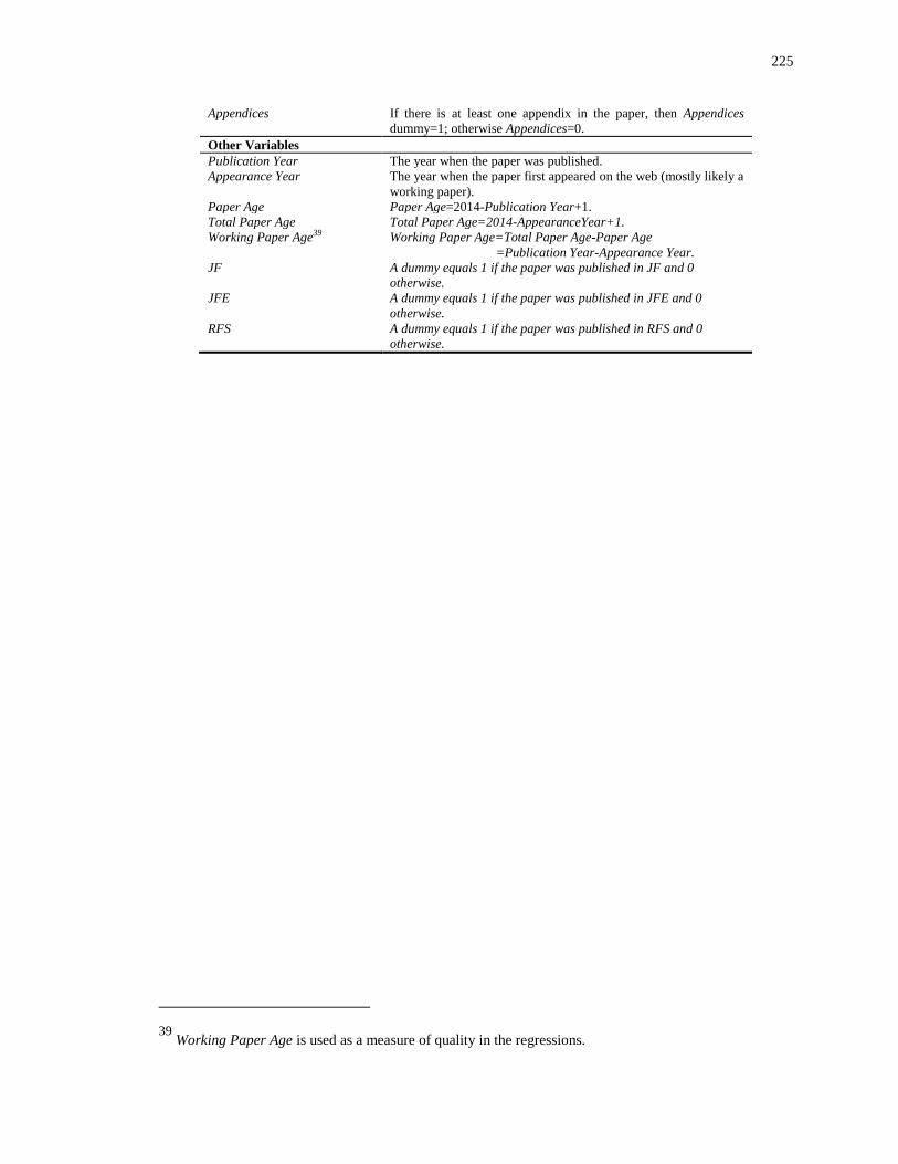
225

Appendices If there is at least one appendix in the paper, then Appendices

dummy=1; otherwise Appendices=0.

Other Variables

Publication Year The year when the paper was published.

Appearance Year The year when the paper first appeared on the web (mostly likely a

working paper).

Paper Age Paper Age=2014-Publication Year+1.

Total Paper Age Total Paper Age=2014-AppearanceYear+1.

Working Paper Age39 Working Paper Age=Total Paper Age-Paper Age

=Publication Year-Appearance Year.

JF A dummy equals 1 if the paper was published in JF and 0

otherwise.

JFE A dummy equals 1 if the paper was published in JFE and 0

otherwise.

RFS A dummy equals 1 if the paper was published in RFS and 0

otherwise.

39 Working Paper Age is used as a measure of quality in the regressions.

226

Chapter 5

5 Conclusions

This thesis contributes to the finance literature in three main aspects.

Chapter 2 employs a novel measure of sell-side financial analysts’ innate ability

or natural talent and explores its effects on reported corporate insider trading. We

postulate that analysts with high innate ability can reduce information asymmetry

between corporate insiders and outside investors through earnings forecasts, thereby

restricting insider trading. The results show that analysts with higher innate ability are

associated with lower level of net buys when insiders have “good” inside information

about earnings, but this relation does not hold for net sells when insiders have “bad”

inside information. The effects of analysts’ ability mostly reside in opportunistic trading

rather than routine trading. The tests of analysts’ initial coverage provide stronger effects

of analysts’ ability and these effects are much stronger for high-ability analysts in the

sample of initial coverage. We also examine the time-series of mean post-trading CARs

and find mixed evidence that also depends on information type. Overall, this study

suggests a negative relation between analyst ability and insider trading intensity and

informativeness. This study suggests that high-ability analysts may serve in restricting

excessive corporate insider trading. Additionally, our study sheds light on the nature of

analyst information. Our results imply that the degree of firm-specific information an

analyst can provide may be determined by her innate ability. Compared with market-

specific and industry-specific information, firm-specific information is more difficult to

227

collect and analyze; thus, analysts with low ability may not be able to include firm-

specific information in their forecasts.

In empirical corporate finance, firm size is commonly used as an important,

fundamental firm characteristic. However, no research comprehensively assesses the

sensitivity of empirical results in corporate finance to different measures of firm size.

Chapter 3 fills this hole by providing empirical evidence for “measurement effect” in

“size effect”. In particular, we examine the influences of employing different proxies

(total assets, total sales, and market capitalization) of firm size in 20 prominent areas in

empirical corporate finance research. We highlight several empirical implications. First,

in most areas of corporate finance, the coefficients of firm size measures are robust in

sign and statistical significance. Second, however, the coefficients on regressors other

than firm size often change sign and significance when we use different size measures.

This may suggest that some previous studies are not robust to different firm size proxies.

Third, the goodness of fit measured by R-squared also varies with different size

measures, suggesting that some measures are more relevant than others in different

situations. Fourth, different proxies capture different aspects of “firm size”, and thus have

different implications in corporate finance. Therefore, the choice of size measures needs

both theoretical and empirical justification. Our empirical assessment provides general

guidance to empirical corporate finance researchers who must use firm size measures in

their work.

In Chapter 4, we explore the factors that affect the impact of financial research.

Specifically, we study the characteristics of all the published papers in the top three

finance journals (JF, JFE, and RFS) during 2000-2013 and how these paper

228

characteristics affect the number of citations in Google Scholar and the ISI Web of

Science database. We investigate three theoretical perspectives: the universalist

perspective (what is said), the social constructivist perspective (who says it), and the

presentation perspective (how it is said). First, we find that most of the paper

characteristics in the social constructivist perspective (visibility and personal promotion)

and the presentation perspective (first-page attention and expositional clarity) increase

over time, while the characteristics in the universalist perspective (quality and domain)

remain constant. Second, most of the paper characteristics are significantly different

between the top 10% (high impact) and the bottom 10% (low impact) groups based on

the number of citations per year. Third, the regression results by negative binomial

models show that the universalist perspective, the social constructivist perspective, and

the presentation perspective all provide explanatory power for the impact of published

papers in the top three finance journals. Specifically, paper quality, research methods,

journal placement, and paper age are the most important (in economic significance)

drivers for the number of citations Last, different drivers play different roles for the

papers in JF, JFE, and RFS. Chapter 4 provides evidence for finance scholars, university

administrators, and finance journal management who care about research impact.

Research impact is not only about career path for the scholars, the school rankings for the

deans, or the journal impact factors for the editors, but also, much more importantly,

about the dissemination and advancement of knowledge.

229

Curriculum Vitae

Name: Chongyu Dang

Post-secondary Dalian University of Technology

Education and Dalian, Liaoning, P.R. China

Degrees: 2005-2009 B.A.

The University of British Columbia

Vancouver, British Columbia, Canada

2009-2010 M.A.

The University of Alberta

Edmonton, Alberta, Canada

2010-2012 M.A.

The University of Western Ontario

London, Ontario, Canada

2012-2016 Ph.D.

Honours and Plan for Excellence Doctoral Scholarship, Ivey Business School

Awards: 2012-2016

Related Work Teaching Assistant and Research Assistant

Experience The University of Alberta and The University of Western Ontario

2011-2016