Three-Dimensional Sensors Lecture 5: Point-Cloud …perception.inrialpes.fr/~Horaud/Courses/pdf/Horaud_3DS_5.pdf · Three-Dimensional Sensors Lecture 5: Point-Cloud Processing Radu

Three-Dimensional SensorsLecture 5: Point-Cloud Processing

Radu HoraudINRIA Grenoble Rhone-Alpes, France

[email protected]://perception.inrialpes.fr/

Radu Horaud Three-Dimensional Sensors: Lecture 5

http://perception.inrialpes.fr/

3D Data

Data representation: PCA and its variants, KD-trees,KNN-graphs.

Data segmentation: K-means, Gaussian mixtures, spectralclustering.

Data registration: Iterative closest point (ICP), soft assignmethods, robust registration.


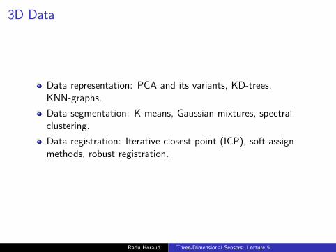
Data Representation

Principal component analysis (PCA): The data arerepresented in an intrinsic coordinate system and projectedonto a lower dimensional space (2D or 1D).

There are many interesting variants of PCA: probabilistic PCA(PPCA), mixture of PPCA, kernel PCA, etc.

KD-trees (K-dimensional trees): The 3D point cloud isrepresented as a binary 3D-tree by recursively splitting thepoint cloud into two subsets. Provides an efficient way tomanipulate the point cloud.

KNN-graph (K nearest neighbor graph): The 3D point cloudis represented as a sparse undirected weighted graph.


Data Segmentation

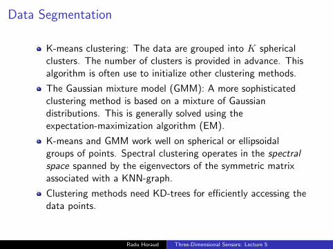
K-means clustering: The data are grouped into K sphericalclusters. The number of clusters is provided in advance. Thisalgorithm is often use to initialize other clustering methods.

The Gaussian mixture model (GMM): A more sophisticatedclustering method is based on a mixture of Gaussiandistributions. This is generally solved using theexpectation-maximization algorithm (EM).

K-means and GMM work well on spherical or ellipsoidalgroups of points. Spectral clustering operates in the spectralspace spanned by the eigenvectors of the symmetric matrixassociated with a KNN-graph.

Clustering methods need KD-trees for efficiently accessing thedata points.


Data Registration

“Fuse” data gathered with several 3D sensors or with amoving 3D sensor.

Each sensor provides a point cloud in a sensor-centeredcoordinate frame.

There is only a partial overlap between the two point clouds.

The two point clouds must be registered or represented in thesame coordinate frame.

The registration process requires point-to-pointcorrespondences which is a difficult problem.


Data Registration Methods

Iterative closest point (ICP) is the most popular rigidregistration method that needs proper initialization of theregistration parameters (rotation and translation).

A number of robust variants of ICP were proposed foreliminating bad points (outliers).

An alternative to ICP is to use a generative probabilisticmodel such as GMM, or EM-based point registration.


Some Notations and Definitions

Let’s start with a few more notations:

The input (observation) space: X = [x1 . . .xi . . .xn],xi ∈ R3

The output (latent) space: Y = [y1 . . .yi . . .yn],yi ∈ Rd, 1 ≤ d ≤ 3Projection: Y = Q>X with Q> a d× 3 matrix.

Q>Q = Id


Computing the Spread of the Data

We start with n scalars x1 . . . xn; the mean and the varianceare given by:

x =1n

∑i

xi σx =1n

∑i

(xi − x)2 =1n

∑i

x2i − x2

More generally, for the data set X:

The mean: x = 1n

∑i xi

The covariance matrix is semi-definite positive symmetric ofdimension 3× 3:

CX =1n

∑i

(xi − x)(xi − x)> =1n

XX> − x x>


Maximum-Variance Formulation of PCA

Let’s center and project the data X onto a line along a unitvector u. The variance along this line writes:

σu =1n

∑i

(u>(xi − x))2

= u>

(1n

∑i

(xi − x)(xi − x)>)u

= u>CXu

Find u maximizing the variance under the constraint that u isa unit vector:

u? = argmaxu

u>CXu+ λ(1− u>u)


Maximum-Variance Solution

First note that the 3× 3 covariance matrix is a symmetricsemi-definite positive matrix. (The associated quadratic formabove is non-negative).

Taking the derivative with respect to u and setting thederivatives equal to 0, yields: CXu = λu

Making use of the fact that u is a unit vector we obtain:σu = λ

Solution: The principal or largest eigenvector–eigenvalue pair(umax,λmax) of the covariance matrix.


Eigendecomposition of the Covariance Matrix

Assume that the data are centred:

nCX = XX> = nUΛU>

Where U is a 3× 3 orthogonal matrix and Λ is the diagonalmatrix of eigenvalues:

Λ = [λ1 λ2 λ3]

If the point-cloud lies on a lower d-dimensional space(collinear or planar points):

d = rank(X) < 3

andΛd = [λ1 λd]

CX = UΛdU>

U = UI3×d is a 3× d column-orthgonal matrix

U> = I>d×3U> is a d× 3 row-orthgonal matrix


Data Representation in the Eigen (Sub)space

Coordinate change: Y = QX; We have

YY> = QXX>Q> = nQUΛdU>Q>

1 The projected data have a diagonal covariance matrix:1nYY> = Λd, by identification we obtain

Q = U>

2 The projected data have an identity covariance matrix, this iscalled whitening the data: 1

nYY> = Id

Q = Λ−12

d U>

Projection of the data points onto principal direction ui:

(y1i . . . yni) = λ−1/2i︸︷︷︸

whitening

u>i (x1 . . .xn)


Summary of PCA

The eigenvector-eigenvalue pairs of the covariance matrixcorrespond to a spectral representation of the point cloud, ora within representation.

This eigendecomposition allows to reduce the dimensionalityof the point cloud to one plane or one line and then to projectthe cloud onto such a linear subspace.

The largest eigenvalue-eigenvector pair defines the direction ofmaximum variance. By projecting the data onto this line onecan order the data (useful for data organization, i.e.,KD-trees).

The eigenvalue-eigenvector pairs can be efficiently computedusing the power method: get a random unit vector x(0) anditerate x(k+1) = Cx(k), normalize x(k+1), etc., until‖x(k+1) − x(k)‖ < ε. Then umax = x(k+1).


KD Trees

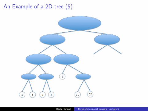
KD-tree (K-dimensional tree) is a data structure that allowsto organize a point cloud under the form of a binary tree.

The basic idea is to recursively and alternatively project thepoints onto the x, y, z, x, y, z, etc., axes, to order the pointsalong each axis and to split the set into two halves.

This point-cloud organization facilitates and accelerates thesearch of nearest neighbors (at the price of kd-treeconstruction).

A more elaborate method (requiring more pre-processingtime) is to search for the principal direction and split the datausing a plane orthogonal to this direction, and apply thisstrategy recursively.


An Example of a 2D-tree (1)










K-means Clustering

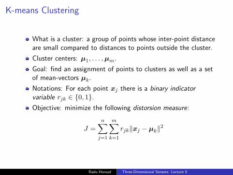
What is a cluster: a group of points whose inter-point distanceare small compared to distances to points outside the cluster.

Cluster centers: µ1, . . . ,µm.

Goal: find an assignment of points to clusters as well as a setof mean-vectors µk.

Notations: For each point xj there is a binary indicatorvariable rjk ∈ 0, 1.Objective: minimize the following distorsion measure:

J =n∑

j=1

m∑k=1

rjk‖xj − µk‖2


The K-means Algorithm

1 Initialization: Choose m and initial values for µ1, . . . ,µm.

2 First step: Assign the j-th point to the closest cluster center:

rjk =

1 if k = arg minl ‖xj − µl‖20 otherwise

3 Second Step: Minimize J to estimate the cluster centers:

µk =

∑nj=1 rjkxj∑n

j=1 rjk

4 Convergence: Repeat until no more change in theassignments.


How to Represent This Point Cloud?


Spherical Clusters


Building a Graph from a Point Cloud

K-nearest neighbor(KNN) rule

ε-radius rule

Other more sophisticatedrules can be found in theliterature, i.e., Lee andVerleysen. NonlinearDimensionality Reduction(Appendix E). Springer.2007.

Remark: The KD-tree data structure can be used to facilitategraph construction when the number of points is large.


The Graph Partitioning Problem

We want to find a partition of the graph such that the edgesbetween different groups have very low weight, while theedges within a group have high weight.

The mincut problem:1 Edges between groups have very low weight, and2 Edges within a group have high weight.3 Choose a partition of the graph into k groups that mimimizes

the following criterion:

mincut(A1, . . . , Ak) :=12

k∑i=1

W (Ai, Ai)

withW (A,B) =

∑i∈A,j∈B

wij


RatioCut and NormalizedCut

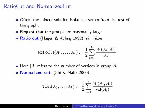
Often, the mincut solution isolates a vertex from the rest ofthe graph.

Request that the groups are reasonably large.

Ratio cut (Hagen & Kahng 1992) minimizes:

RatioCut(A1, . . . , Ak) :=12

k∑i=1

W (Ai, Ai)|Ai|

Here |A| refers to the number of vertices in group A.

Normalized cut: (Shi & Malik 2000)

NCut(A1, . . . , Ak) :=12

k∑i=1

W (Ai, Ai)vol(Ai)


What is Spectral Clustering?

Both ratio-cut and normalized-cut minimizations are NP-hardproblems

Spectral clustering is a way to solve relaxed versions of theseproblems:

1 Build the Laplacian matrix of the graph2 Compute the smallest (non-null) eigenvalue-eigenvector pairs

of this matrix3 Map the graph vertices into the space spanned by these

eigenvectors4 Apply the K-means algorithm to the new point cloud


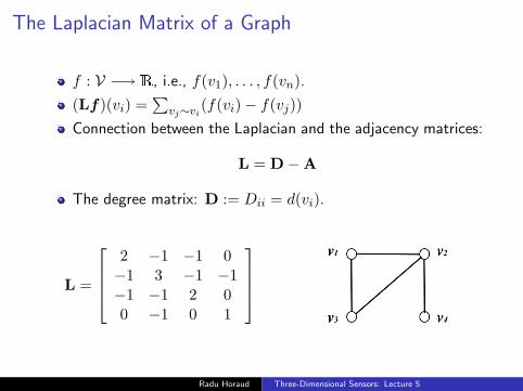
The Laplacian Matrix of a Graph

f : V −→ R, i.e., f(v1), . . . , f(vn).

(Lf)(vi) =∑

vj∼vi(f(vi)− f(vj))

Connection between the Laplacian and the adjacency matrices:

L = D−A

The degree matrix: D := Dii = d(vi).

L =

2 −1 −1 0−1 3 −1 −1−1 −1 2 00 −1 0 1


Case of an Undirected Weighted Graph

We consider undirected weighted graphs; Each edge eij isweighted by wij > 0. We obtain:

Ω :=

Ωij = wij if there is an edge eijΩij = 0 if there is no edgeΩii = 0

The degree matrix: D =∑

i∼j wij


The Laplacian on an Undirected Weighted Graph

Often we will consider:

wij = exp(−‖xi − xj‖2/σ2

)L = D−Ω

L is symmetric and positive semi-definite ↔ wij ≥ 0.

L has n non-negative, real-valued eigenvalues:0 = λ1 ≤ λ2 ≤ . . . ≤ λn.


Laplacian embedding: Mapping a graph on a line

Map a weighted graph onto a line such that connected nodesstay as close as possible, i.e., minimize∑n

i,j=1wij(f(vi)− f(vj))2, or:

arg minff>Lf with: f>f = 1 and f>1 = 0

The solution is the eigenvector associated with the smallestnonzero eigenvalue of the eigenvalue problem: Lf = λf , (theFiedler vector) u2.

Practical computation of the eigenpair λ2,u2): the shiftedinverse power method (see lecture 2).


Mapping the Graph’s Vertices on the Eigenvector


Spectral Embedding using the Laplacian

Compute the eigendecomposition L = D−Ω = UΛU>.

Select the k smallest non-null eigenvalues λ2 ≤ . . . ≤ λk+1

λk+2 − λk+1 = eigengap.

We obtain the n× k column-orthogonal matrixU = [u2 . . .uk+1]:

U =

u2(v1) . . . uk+1(v1)...

...u2(vn) . . . uk+1(vn)

Embedding: The i-row of this matrix correspond to therepresentation of vertex vI in the Rk basis spanned by theorthonormal vector basis u2, . . . ,uk+1.

Therefore: Y = [y1 . . .yi . . .yn] = U>


Laplacian Eigenmap


Next Lecture: Data Registration

“Fuse” data gathered with several 3D sensors or with amoving 3D sensor.

Each sensor provides a point cloud in a sensor-centeredcoordinate frame.

There is only a partial overlap between the two point clouds.

The two point clouds must be registered or represented in thesame coordinate frame.

The registration process requires point-to-pointcorrespondences which is a difficult problem.


Three-Dimensional Sensors Lecture 5: Point-Cloud …perception.inrialpes.fr/~Horaud/Courses/pdf/Horaud_3DS_5.pdf · Three-Dimensional Sensors Lecture 5: Point-Cloud Processing Radu

Documents