Three-Dimensional Roughness Characterization of Rock Joints using Laser Scanning and Wind Diagrams

1. INTRODUCTION

The evaluation of surface roughness is not a new field,

nor is it unique to the world of rock mechanics. Many

other scientific fields have made use of roughness

information, and it can be observed clearly that varying

disciplines investigate roughness at a scale applicable to

their investigation. An integral part to the investigation

of roughness at any scale is the method of data

collection. For obvious reasons, the method must be able

to capture the scale of interest, but beyond that there are

many available techniques and tools for the collection

and description of surface roughness. For this

investigation, the focus was placed on laboratory scale

surface roughness created by the asperities of a given

rock sample. Roughness has a significant influence on

the shear strength of a rock joint, with the asperities

controlling much of the peak shear strength behavior [1].

In the work presented in this paper, evaluations of joint

surface roughness consider both roughness and waviness

together as “surface roughness” with no direct

distinction between the two. The combined asperities in

this investigation would classify as second-order

asperities (wavelength less than approximately 50 to 100

mm) as outlined by Patton [2]. This type of surface can

have roughness angles as high as twenty to thirty

degrees, and as can be seen through the 3D analysis

presented in this paper, some individual facets can

exhibit even higher roughness angle values.

The tools and techniques of interest in this paper include

direct two-dimensional replication of the surface using a

contour duplication gauge, and the creation of a digital

triangulated mesh of the joint surface through 3D laser

scanning technology. Both techniques were deployed on

four different rock types: schist, granite, slate, and

sandstone, all of which were collected in the field in

Montana. The methods investigated demonstrate the

ability to attain a roughness description, though they do

not provide the same output value. The scope of this

investigation was more focused on the data collection

and characterization methodologies available rather than

comparing the merits of the various quantifications of

rock joint roughness as has been done by others (for

instance Hsiung [3], Yu [4], and Propat [5]).

With the vast amount of data produced by these tools

and techniques, a significant challenge is presented in

displaying such a massive dataset. Various visualizations

were attempted but the extreme density of the output

visuals made it difficult to interpret and draw

conclusions. An effective solution was found with the

use of wind diagrams. This allows for a graphical

display which features both magnitude and direction,

which in this scenario translates to dip angle and dip

direction respectively, of each facet on the surface.

ARMA 14-7454

Three-Dimensional Roughness Characterization of

Rock Joints using Laser Scanning and Wind Diagrams

Adams, S.L., MacLaughlin, M.M., Berry, K.G., McCormick, M.L., and Berry, S.M.

Montana Tech of The University of Montana, Butte, Montana, USA

McGough, M. and Hudyma, N.

University of North Florida, Jacksonville, Florida, USA

Copyright 2014 ARMA, American Rock Mechanics Association

This paper was prepared for presentation at the 48th US Rock Mechanics / Geomechanics Symposium held in Minneapolis, MN, USA, 1-4 June

2014.

This paper was selected for presentation at the symposium by an ARMA Technical Program Committee based on a technical and critical review of the paper by a minimum of two technical reviewers. The material, as presented, does not necessarily reflect any position of ARMA, its officers, or members. Electronic reproduction, distribution, or storage of any part of this paper for commercial purposes without the written consent of ARMA is prohibited. Permission to reproduce in print is restricted to an abstract of not more than 200 words; illustrations may not be copied. The abstract must contain conspicuous acknowledgement of where and by whom the paper was presented.

ABSTRACT: This paper presents 3D desktop laser scanning as a tool for roughness characterization of rock joints, in conjunction

with traditional 2D contour gauge profiles. Four specimens representing four different rock types (schist, granite, slate, and

sandstone) and roughness values were characterized. The 2D roughness profiles are presented along with the JRC values assigned

through comparison with standard JRC profiles. The 3D laser scan data are used to generate files containing the strike, dip angle,

and dip direction of thousands of individual facets. The data are presented using traditional histograms of dip angle (irrespective of

direction), and as wind plots that allow effective visualization of both magnitude and direction of the dip of the facets. The wind

plots are used to highlight the similarities and differences of the specimens, and also between scans of the same specimen before

and after being subjected to a direct shear test.

2. BACKGROUND

The significance of rock joint surface roughness has

been demonstrated by Barton and Choubey [6], with

several modifications since development, through the

proposed equation for the estimation of peak joint shear

strength:

10tan logn b

n

JCSJRC

(1)

Where τ = peak shear strength, σn = normal stress

applied to the joint, JRC = joint roughness coefficient,

JCS = joint wall compressive strength, and φb = base

friction angle of the joint.

Roughness is represented through the Joint Roughness

Coefficient (JRC), which can be determined through tilt

test, direct shear, or via comparison to a standard set of

profiles established by Barton and Choubey [6]. These

were developed through extensive laboratory testing,

resulting in a set of ten representative profiles with JRC

values of 0-2, 2-4, and so on through 18-20. This method

of establishing JRC can be seen in the ISRM standards

[7], and has been widely accepted in practice.

The scientific community has since been actively

working towards an effective method of quantification

of the standardized JRC profiles. Prominent examples of

such work include Tse and Cruden [8], Carr and

Warriner [9], Turk et al. [10], Lee et al. [11], and

Wakabayashi and Fukushige [12]. This effort has been

made largely due to the subjective nature of comparing a

sample profile to the standard which can lead to error in

selecting an appropriate JRC value [4]. This is one of the

predominant reasons for continued extensive direct shear

testing in order to accurately determine the peak shear

strength of a rock, rather than using the JRC formula to

calculate the value which would save time and resources.

Despite the lack of confidence within the rock

mechanics community in selecting JRC, there is also the

issue of misuse of the available analysis tools and in

some cases incorrect back calculation of JRC based on

inadequate knowledge of advances which have been

made with regard to joint degradation and behavior

during shear testing [13].

The most prevalent theories regarding the quantification

of the JRC profiles include fractal geometry, statistics

including average deviation, root mean square, and tilt

test. Each has been extensively investigated on various

rock specimens with promising results, but in a

comparison, it was shown by Hsiung [3] that the various

methods repeatedly underestimate the JRC value derived

through an actual direct shear test, some even estimating

the JRC several value brackets below its actual value.

Each of the numerical approaches described above are

dependent on high quality surface data to even have a

hope of eventually capturing a purely objective

methodology of determining JRC. The methodologies

used in this study and described in section 4 are only a

sampling of the available techniques, but were selected

because they are representative of many of the common

approaches for obtaining roughness data from a rock

joint.

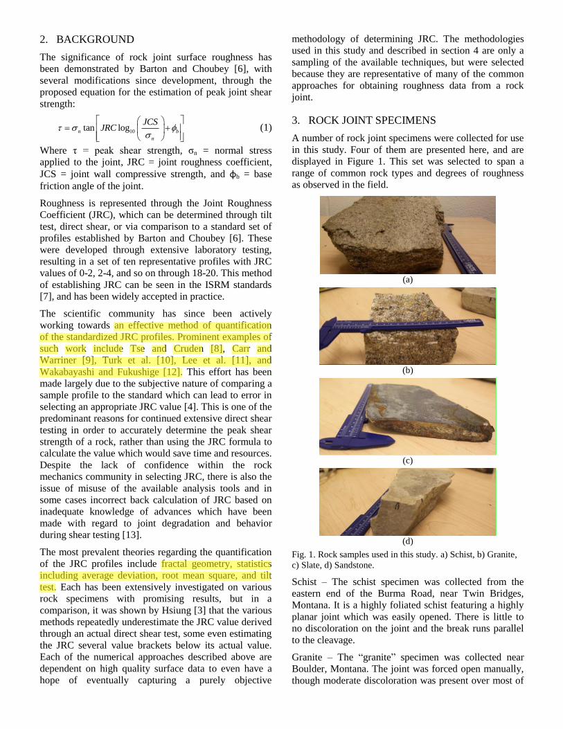
3. ROCK JOINT SPECIMENS

A number of rock joint specimens were collected for use

in this study. Four of them are presented here, and are

displayed in Figure 1. This set was selected to span a

range of common rock types and degrees of roughness

as observed in the field.

(a)

(b)

(c)

(d)

Fig. 1. Rock samples used in this study. a) Schist, b) Granite,

c) Slate, d) Sandstone.

Schist – The schist specimen was collected from the

eastern end of the Burma Road, near Twin Bridges,

Montana. It is a highly foliated schist featuring a highly

planar joint which was easily opened. There is little to

no discoloration on the joint and the break runs parallel

to the cleavage.

Granite – The “granite” specimen was collected near

Boulder, Montana. The joint was forced open manually,

though moderate discoloration was present over most of

the surface, indicating a weathering surface. The rock is

technically a medium to coarse grained porphyritic

granodiorite with feldspar phenocrysts.

Slate – The slate specimen was acquired from the Gates

Slate quarry north of Helena, Montana. The joint was

created by using a chisel and hammer to fracture the

specimen along foliation. The joint surface is comprised

of fresh rock material and shows very little roughness

except for the sections where the rock split along a

different foliation plane. Discoloration is limited to the

outer boundaries of the specimen, likely attributed to

weathering of the outside edges of the initial rock slab.

Sandstone – The sandstone specimen was collected from

an outcrop of the Cut Bank formation near Cut Bank,

Montana. It is a tan colored fine grained sedimentary

rock with a dolomitic cementing matrix.

4. TOOLS AND TECHNIQUES

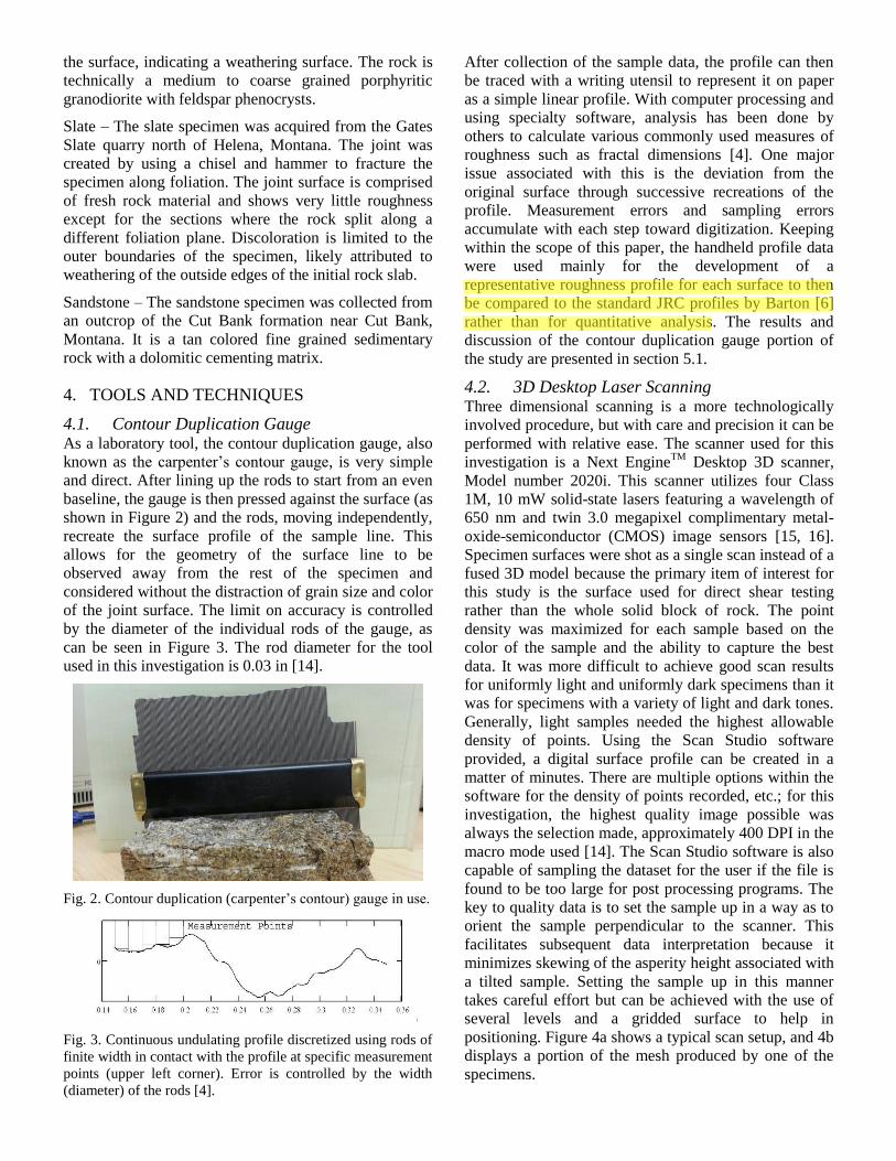
4.1. Contour Duplication Gauge As a laboratory tool, the contour duplication gauge, also

known as the carpenter’s contour gauge, is very simple

and direct. After lining up the rods to start from an even

baseline, the gauge is then pressed against the surface (as

shown in Figure 2) and the rods, moving independently,

recreate the surface profile of the sample line. This

allows for the geometry of the surface line to be

observed away from the rest of the specimen and

considered without the distraction of grain size and color

of the joint surface. The limit on accuracy is controlled

by the diameter of the individual rods of the gauge, as

can be seen in Figure 3. The rod diameter for the tool

used in this investigation is 0.03 in [14].

Fig. 2. Contour duplication (carpenter’s contour) gauge in use.

Fig. 3. Continuous undulating profile discretized using rods of

finite width in contact with the profile at specific measurement

points (upper left corner). Error is controlled by the width

(diameter) of the rods [4].

After collection of the sample data, the profile can then

be traced with a writing utensil to represent it on paper

as a simple linear profile. With computer processing and

using specialty software, analysis has been done by

others to calculate various commonly used measures of

roughness such as fractal dimensions [4]. One major

issue associated with this is the deviation from the

original surface through successive recreations of the

profile. Measurement errors and sampling errors

accumulate with each step toward digitization. Keeping

within the scope of this paper, the handheld profile data

were used mainly for the development of a

representative roughness profile for each surface to then

be compared to the standard JRC profiles by Barton [6]

rather than for quantitative analysis. The results and

discussion of the contour duplication gauge portion of

the study are presented in section 5.1.

4.2. 3D Desktop Laser Scanning Three dimensional scanning is a more technologically

involved procedure, but with care and precision it can be

performed with relative ease. The scanner used for this

investigation is a Next EngineTM

Desktop 3D scanner,

Model number 2020i. This scanner utilizes four Class

1M, 10 mW solid-state lasers featuring a wavelength of

650 nm and twin 3.0 megapixel complimentary metal-

oxide-semiconductor (CMOS) image sensors [15, 16].

Specimen surfaces were shot as a single scan instead of a

fused 3D model because the primary item of interest for

this study is the surface used for direct shear testing

rather than the whole solid block of rock. The point

density was maximized for each sample based on the

color of the sample and the ability to capture the best

data. It was more difficult to achieve good scan results

for uniformly light and uniformly dark specimens than it

was for specimens with a variety of light and dark tones.

Generally, light samples needed the highest allowable

density of points. Using the Scan Studio software

provided, a digital surface profile can be created in a

matter of minutes. There are multiple options within the

software for the density of points recorded, etc.; for this

investigation, the highest quality image possible was

always the selection made, approximately 400 DPI in the

macro mode used [14]. The Scan Studio software is also

capable of sampling the dataset for the user if the file is

found to be too large for post processing programs. The

key to quality data is to set the sample up in a way as to

orient the sample perpendicular to the scanner. This

facilitates subsequent data interpretation because it

minimizes skewing of the asperity height associated with

a tilted sample. Setting the sample up in this manner

takes careful effort but can be achieved with the use of

several levels and a gridded surface to help in

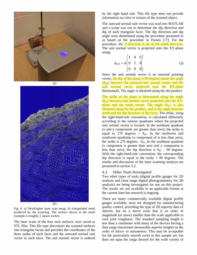
positioning. Figure 4a shows a typical scan setup, and 4b

displays a portion of the mesh produced by one of the

specimens.

(a)

(b)

Fig. 4. a) NextEngine laser scan setup, b) triangulated mesh

produced by the scanning. The surface shown in the mesh

example is roughly 2 square inches.

The laser scans of the four rock surfaces were saved as

STL files. This file type discretizes the scanned surfaces

into triangular facets and provides the coordinates of the

three nodes of each facet and the outward normal unit

vector to each facet. The unit normal vector is ordered

by the right hand rule. This file type does not provide

information on color or texture of the scanned object.

The outward normal unit vector was read into MATLAB

and a script was run to determine the dip direction and

dip of each triangular facet. The dip direction and dip

angle were determined using the procedure presented in

as based on the procedure in Fienen [17]. For the

procedure, the Y-direction is set as the north direction.

The unit normal vector is projected onto the XY-plane

using:

proj

1 0 0

n n 0 1 0

0 0 0

(2)

Since the unit normal vector is an outward pointing

vector, the dip of the plane is 90 degrees minus the angle

(θdip) between the outward unit normal vector and the

unit normal vector projected onto the XY-plane

(horizontal). The angle is obtained using the dot product.

The strike of the plane is determined using the angle

(θdir) between unit normal vector projected onto the XY-

plane and the north vector. The angle (θdir) is also

obtained using the dot product, and is the angle between

north and the dip direction of the facet. The strike, using

the right-hand-rule convention, is calculated differently

according to the various quadrants where the projected

unit normal vector is located. In the northeast quadrant

(x and y components are greater than zero), the strike is

equal to 270 degrees + θdir. In the northwest and

southwest quadrants (x component of is less than zero),

the strike is 270 degrees - θdir. In the southeast quadrant

(x component is greater than zero and y component is

less than zero), the dip direction is θdir – 90 degrees.

With the right-hand-rule convention, the corresponding

dip direction is equal to the strike + 90 degrees. The

results and discussion of the laser scanning analysis are

presented in section 5.2.

4.3. Other Tools Investigated Two other types of tools (digital profile gauges for 2D

analysis and close range digital photogrammetry for 3D

analysis) are being investigated for use on this project.

The results are not available in an applicable format at

the current time but research is ongoing.

There are many commercially available digital profile

gauges available; most are designed for manufacturing

quality control, providing the type of 2D asperity data of

interest, but on a micro scale that is an order of

magnitude (or more) smaller than the scale applicable to

rock joint roughness. The standard sampling length is

less than a centimeter with many of the devices having a

data range (maximum measurable asperity height) on the

order of micro- to nanometers. This may be acceptable

for the particularly smooth rocks in this sample set, but

does not span the range desired for the wide variety of

rock joints. Furthermore, the available instruments are

very expensive, ranging in cost from $1000 to more than

$100,000. The search continues for an instrument with a

larger data range and ideally, a longer sampling length.

This 2D profile technique is also still being pursued

through the development of a setup optimized for

measurement of laboratory scale rock joint roughness

that can be assembled for a reasonable cost. Combining

a sliding machining table with a digital displacement

gauge will allow for control of the sampling along a

surface enabling the user to control x and y values,

requiring only the true z-value (height) to be recorded

with the displacement gauge. The data could be used to

produce profile lines for manual comparison with the

JRC profiles similar to the contour tool described above,

or they could be input into software designed to

calculate the advanced statistics described earlier in this

paper. At this time the components of this setup are

being gathered for future work in this area.

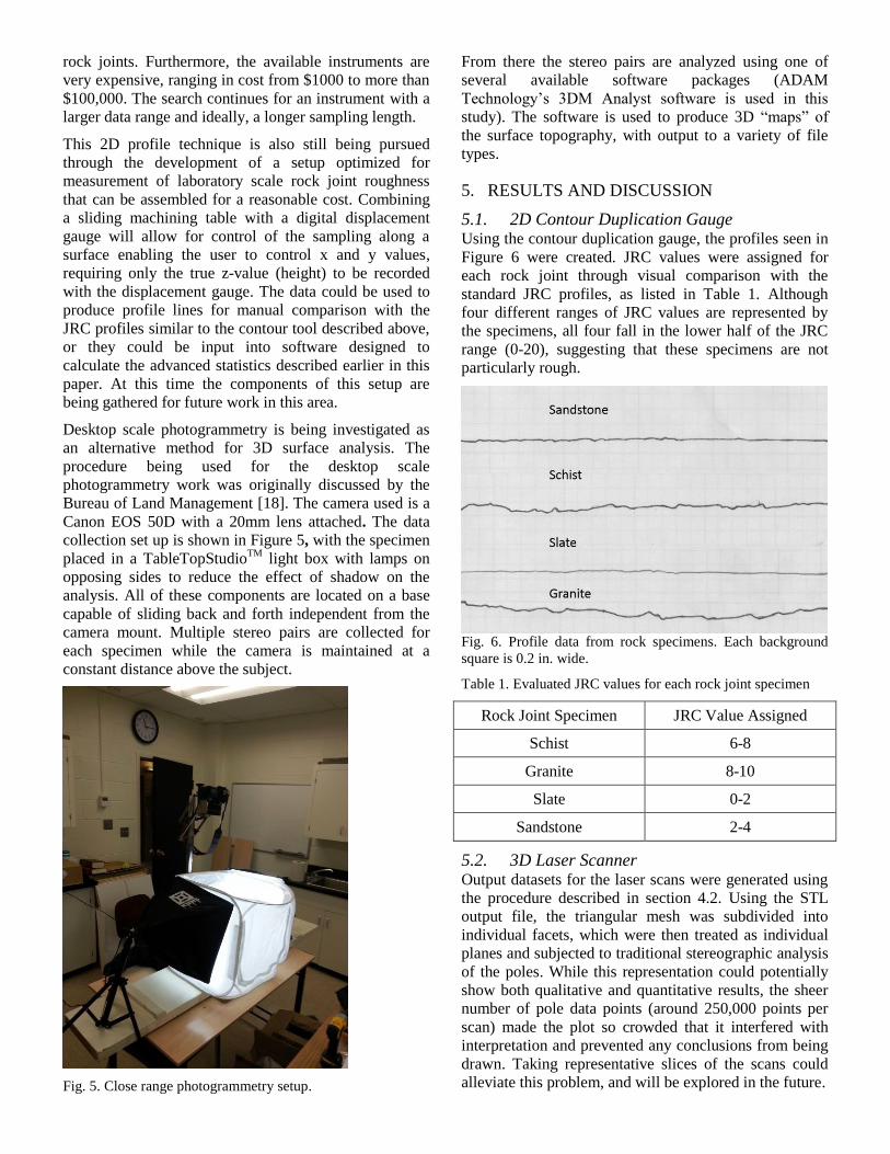
Desktop scale photogrammetry is being investigated as

an alternative method for 3D surface analysis. The

procedure being used for the desktop scale

photogrammetry work was originally discussed by the

Bureau of Land Management [18]. The camera used is a

Canon EOS 50D with a 20mm lens attached. The data

collection set up is shown in Figure 5, with the specimen

placed in a TableTopStudioTM

light box with lamps on

opposing sides to reduce the effect of shadow on the

analysis. All of these components are located on a base

capable of sliding back and forth independent from the

camera mount. Multiple stereo pairs are collected for

each specimen while the camera is maintained at a

constant distance above the subject.

Fig. 5. Close range photogrammetry setup.

From there the stereo pairs are analyzed using one of

several available software packages (ADAM

Technology’s 3DM Analyst software is used in this

study). The software is used to produce 3D “maps” of

the surface topography, with output to a variety of file

types.

5. RESULTS AND DISCUSSION

5.1. 2D Contour Duplication Gauge Using the contour duplication gauge, the profiles seen in

Figure 6 were created. JRC values were assigned for

each rock joint through visual comparison with the

standard JRC profiles, as listed in Table 1. Although

four different ranges of JRC values are represented by

the specimens, all four fall in the lower half of the JRC

range (0-20), suggesting that these specimens are not

particularly rough.

Fig. 6. Profile data from rock specimens. Each background

square is 0.2 in. wide.

Table 1. Evaluated JRC values for each rock joint specimen

Rock Joint Specimen JRC Value Assigned

Schist 6-8

Granite 8-10

Slate 0-2

Sandstone 2-4

5.2. 3D Laser Scanner Output datasets for the laser scans were generated using

the procedure described in section 4.2. Using the STL

output file, the triangular mesh was subdivided into

individual facets, which were then treated as individual

planes and subjected to traditional stereographic analysis

of the poles. While this representation could potentially

show both qualitative and quantitative results, the sheer

number of pole data points (around 250,000 points per

scan) made the plot so crowded that it interfered with

interpretation and prevented any conclusions from being

drawn. Taking representative slices of the scans could

alleviate this problem, and will be explored in the future.

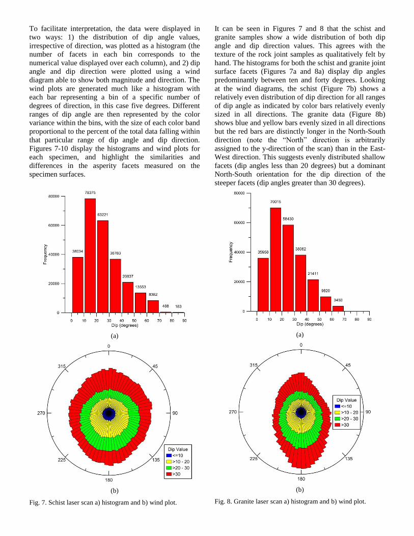
To facilitate interpretation, the data were displayed in

two ways: 1) the distribution of dip angle values,

irrespective of direction, was plotted as a histogram (the

number of facets in each bin corresponds to the

numerical value displayed over each column), and 2) dip

angle and dip direction were plotted using a wind

diagram able to show both magnitude and direction. The

wind plots are generated much like a histogram with

each bar representing a bin of a specific number of

degrees of direction, in this case five degrees. Different

ranges of dip angle are then represented by the color

variance within the bins, with the size of each color band

proportional to the percent of the total data falling within

that particular range of dip angle and dip direction.

Figures 7-10 display the histograms and wind plots for

each specimen, and highlight the similarities and

differences in the asperity facets measured on the

specimen surfaces.

(a)

(b)

Fig. 7. Schist laser scan a) histogram and b) wind plot.

It can be seen in Figures 7 and 8 that the schist and

granite samples show a wide distribution of both dip

angle and dip direction values. This agrees with the

texture of the rock joint samples as qualitatively felt by

hand. The histograms for both the schist and granite joint

surface facets (Figures 7a and 8a) display dip angles

predominantly between ten and forty degrees. Looking

at the wind diagrams, the schist (Figure 7b) shows a

relatively even distribution of dip direction for all ranges

of dip angle as indicated by color bars relatively evenly

sized in all directions. The granite data (Figure 8b)

shows blue and yellow bars evenly sized in all directions

but the red bars are distinctly longer in the North-South

direction (note the “North” direction is arbitrarily

assigned to the y-direction of the scan) than in the East-

West direction. This suggests evenly distributed shallow

facets (dip angles less than 20 degrees) but a dominant

North-South orientation for the dip direction of the

steeper facets (dip angles greater than 30 degrees).

(a)

(b)

Fig. 8. Granite laser scan a) histogram and b) wind plot.

In contrast to the granite and schist samples, the slate

and sandstone datasets display much more shallowly

inclined facets as well as interesting trends in

directionality. The histograms (Figures 9a and 10a) show

that dip angles for both the slate and sandstone surface

facets are predominantly between zero and twenty

degrees, which can be qualitatively validated by hand.

The predominance of shallow dip angles agrees with the

low JRC values assigned to these joint surfaces.

The wind diagrams for each of these rock joint

specimens highlight a pronounced and unexpected

directionality of the surface facets. The slate data shows

a very strong trend with dip direction towards west,

while the sandstone facets generally dip toward the

southwest. This pronounced directionality cannot be

validated from the profile gauge data (Figure 6) or

qualitatively by touch.

(a)

(b)

Fig. 9. Slate laser scan a) histogram and b) wind plot.

These two specimens correspond to the lowest JRC

values associated with this investigation and to the naked

eye appear extremely smooth. These observations

suggest a potential misrepresentation that is believed to

be caused by the flat nature of the surfaces themselves.

The textures of the two joints in question are of a very

small scale even compared to the granite and schist,

which could lead to errors in either calculations using

extremely small values, or errors associated with

stereonet type analysis of near-horizontal slopes. On the

other hand, it is possible that the facet directionality is

real, and that the finer scale of the laser scanning is able

to measure this while the other techniques are not. The

discrepancy between the wind plot analysis and the other

surface roughness results has been noted and is currently

under investigation.

(a)

(b)

Fig. 10. Sandstone laser scan a) histogram and b) wind plot

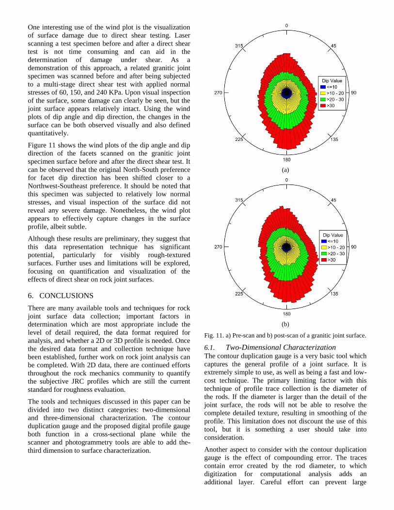
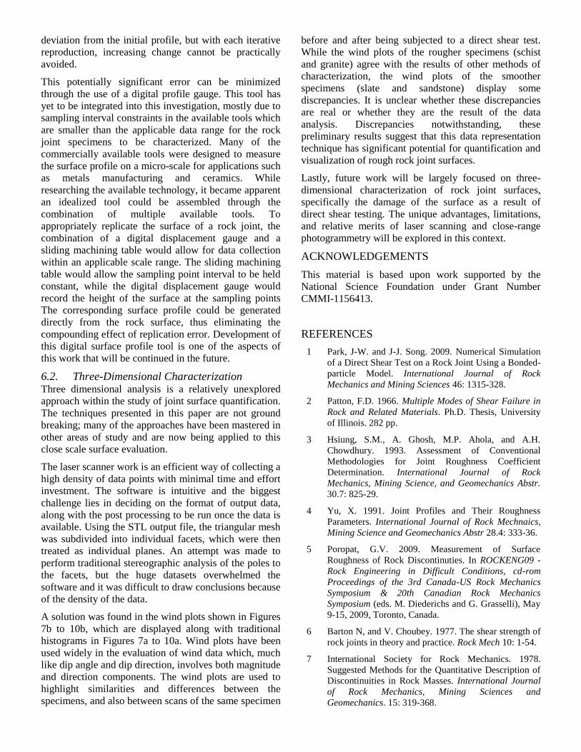
One interesting use of the wind plot is the visualization

of surface damage due to direct shear testing. Laser

scanning a test specimen before and after a direct shear

test is not time consuming and can aid in the

determination of damage under shear. As a

demonstration of this approach, a related granitic joint

specimen was scanned before and after being subjected

to a multi-stage direct shear test with applied normal

stresses of 60, 150, and 240 KPa. Upon visual inspection

of the surface, some damage can clearly be seen, but the

joint surface appears relatively intact. Using the wind

plots of dip angle and dip direction, the changes in the

surface can be both observed visually and also defined

quantitatively.

Figure 11 shows the wind plots of the dip angle and dip

direction of the facets scanned on the granitic joint

specimen surface before and after the direct shear test. It

can be observed that the original North-South preference

for facet dip direction has been shifted closer to a

Northwest-Southeast preference. It should be noted that

this specimen was subjected to relatively low normal

stresses, and visual inspection of the surface did not

reveal any severe damage. Nonetheless, the wind plot

appears to effectively capture changes in the surface

profile, albeit subtle.

Although these results are preliminary, they suggest that

this data representation technique has significant

potential, particularly for visibly rough-textured

surfaces. Further uses and limitations will be explored,

focusing on quantification and visualization of the

effects of direct shear on rock joint surfaces.

6. CONCLUSIONS

There are many available tools and techniques for rock

joint surface data collection; important factors in

determination which are most appropriate include the

level of detail required, the data format required for

analysis, and whether a 2D or 3D profile is needed. Once

the desired data format and collection technique have

been established, further work on rock joint analysis can

be completed. With 2D data, there are continued efforts

throughout the rock mechanics community to quantify

the subjective JRC profiles which are still the current

standard for roughness evaluation.

The tools and techniques discussed in this paper can be

divided into two distinct categories: two-dimensional

and three-dimensional characterization. The contour

duplication gauge and the proposed digital profile gauge

both function in a cross-sectional plane while the

scanner and photogrammetry tools are able to add the-

third dimension to surface characterization.

(a)

(b)

Fig. 11. a) Pre-scan and b) post-scan of a granitic joint surface.

6.1. Two-Dimensional Characterization

The contour duplication gauge is a very basic tool which

captures the general profile of a joint surface. It is

extremely simple to use, as well as being a fast and low-

cost technique. The primary limiting factor with this

technique of profile trace collection is the diameter of

the rods. If the diameter is larger than the detail of the

joint surface, the rods will not be able to resolve the

complete detailed texture, resulting in smoothing of the

profile. This limitation does not discount the use of this

tool, but it is something a user should take into

consideration.

Another aspect to consider with the contour duplication

gauge is the effect of compounding error. The traces

contain error created by the rod diameter, to which

digitization for computational analysis adds an

additional layer. Careful effort can prevent large

deviation from the initial profile, but with each iterative

reproduction, increasing change cannot be practically

avoided.

This potentially significant error can be minimized

through the use of a digital profile gauge. This tool has

yet to be integrated into this investigation, mostly due to

sampling interval constraints in the available tools which

are smaller than the applicable data range for the rock

joint specimens to be characterized. Many of the

commercially available tools were designed to measure

the surface profile on a micro-scale for applications such

as metals manufacturing and ceramics. While

researching the available technology, it became apparent

an idealized tool could be assembled through the

combination of multiple available tools. To

appropriately replicate the surface of a rock joint, the

combination of a digital displacement gauge and a

sliding machining table would allow for data collection

within an applicable scale range. The sliding machining

table would allow the sampling point interval to be held

constant, while the digital displacement gauge would

record the height of the surface at the sampling points

The corresponding surface profile could be generated

directly from the rock surface, thus eliminating the

compounding effect of replication error. Development of

this digital surface profile tool is one of the aspects of

this work that will be continued in the future.

6.2. Three-Dimensional Characterization Three dimensional analysis is a relatively unexplored

approach within the study of joint surface quantification.

The techniques presented in this paper are not ground

breaking; many of the approaches have been mastered in

other areas of study and are now being applied to this

close scale surface evaluation.

The laser scanner work is an efficient way of collecting a

high density of data points with minimal time and effort

investment. The software is intuitive and the biggest

challenge lies in deciding on the format of output data,

along with the post processing to be run once the data is

available. Using the STL output file, the triangular mesh

was subdivided into individual facets, which were then

treated as individual planes. An attempt was made to

perform traditional stereographic analysis of the poles to

the facets, but the huge datasets overwhelmed the

software and it was difficult to draw conclusions because

of the density of the data.

A solution was found in the wind plots shown in Figures

7b to 10b, which are displayed along with traditional

histograms in Figures 7a to 10a. Wind plots have been

used widely in the evaluation of wind data which, much

like dip angle and dip direction, involves both magnitude

and direction components. The wind plots are used to

highlight similarities and differences between the

specimens, and also between scans of the same specimen

before and after being subjected to a direct shear test.

While the wind plots of the rougher specimens (schist

and granite) agree with the results of other methods of

characterization, the wind plots of the smoother

specimens (slate and sandstone) display some

discrepancies. It is unclear whether these discrepancies

are real or whether they are the result of the data

analysis. Discrepancies notwithstanding, these

preliminary results suggest that this data representation

technique has significant potential for quantification and

visualization of rough rock joint surfaces.

Lastly, future work will be largely focused on three-

dimensional characterization of rock joint surfaces,

specifically the damage of the surface as a result of

direct shear testing. The unique advantages, limitations,

and relative merits of laser scanning and close-range

photogrammetry will be explored in this context.

ACKNOWLEDGEMENTS

This material is based upon work supported by the

National Science Foundation under Grant Number

CMMI-1156413.

REFERENCES

1 Park, J-W. and J-J. Song. 2009. Numerical Simulation

of a Direct Shear Test on a Rock Joint Using a Bonded-

particle Model. International Journal of Rock

Mechanics and Mining Sciences 46: 1315-328.

2 Patton, F.D. 1966. Multiple Modes of Shear Failure in

Rock and Related Materials. Ph.D. Thesis, University

of Illinois. 282 pp.

3 Hsiung, S.M., A. Ghosh, M.P. Ahola, and A.H.

Chowdhury. 1993. Assessment of Conventional

Methodologies for Joint Roughness Coefficient

Determination. International Journal of Rock

Mechanics, Mining Science, and Geomechanics Abstr.

30.7: 825-29.

4 Yu, X. 1991. Joint Profiles and Their Roughness

Parameters. International Journal of Rock Mechnaics,

Mining Science and Geomechanics Abstr 28.4: 333-36.

5 Poropat, G.V. 2009. Measurement of Surface

Roughness of Rock Discontinuties. In ROCKENG09 -

Rock Engineering in Difficult Conditions, cd-rom

Proceedings of the 3rd Canada-US Rock Mechanics

Symposium & 20th Canadian Rock Mechanics

Symposium (eds. M. Diederichs and G. Grasselli), May

9-15, 2009, Toronto, Canada.

6 Barton N, and V. Choubey. 1977. The shear strength of

rock joints in theory and practice. Rock Mech 10: 1-54.

7 International Society for Rock Mechanics. 1978.

Suggested Methods for the Quantitative Description of

Discontinuities in Rock Masses. International Journal

of Rock Mechanics, Mining Sciences and

Geomechanics. 15: 319-368.

8 Tse, R. and D.M. Cruden. 1992. Estimating Joint

Roughness Coefficients. International Journal of Rock

Mechanics, Mining Sciences and Geomechanics. 16:

202-207.

9 Carr, J.R. and J.B. Warriner. 1989. Relationship

between the fractal dimension and joint roughness

coefficient. Bulletin of the Association of Engineering

Geologist. XXVI (2): 253-263.

10 Turk N., M.J. Greig, W.R. Dearman, and F.F. Amin.

1987. Characterization of rock joint surfaces by fractal

dimension. In Proceedings of the 28th

U.S. Symposium

on Rock Mechanics, University of Arizona, 1223-1236.

11 Lee Y–H., J.R. Carr, D.J. Barr, and C.J. Hass. 1990.

The fractal dimension as a measure of the roughness of

rock discontinuity profiles. International Journal of

Rock Mechanics, Mining Sciences and Geomechanics.

27: 453-464.

12 Wakabayashi N. and I. Fukushige. 1993. Experimental

study on the relation between fractal dimension and

shear strength. International Journal of Rock

Mechanics and Mining Sciences & Geomechanics

Abstracts, Volume 30, Issue 3, June, Page A152

13 Barton, N. 2013. Shear Strength Criteria for Rock,

Rock Joints, Rockfill and Rock Masses: Problems and

Some Solutions. Journal of Rock Mechanics and

Geotechnical Engineering 5.4: 249-61.

14 General® "837 - 6" Contour Gage." General: Specialty

Tools and Instruments. Web. 2012.

http://www.generaltools.com/837--6-Contour-

Gage_p_246.html.

15 NextEngine, Inc. 2009. NextEngine Desktop 3D

Scanner TechSpecs.

http://www.nextengine.com/HD_DataSheet.pdf.

16 Platt, B.F., S.T. Hasiotis, and D.R. Hirmas. 2010. Use

of Low-Cost Multistripe Laser Triangulation (MLT)

Scanning Technology for Three-Dimensional,

Quantitative Paleoichnological and Neoichnological

Studies. Journal of Sedimentary Research 80.7: 590-

610.

17 Fienen, M.N. 2005. The three-point problem, vector

analysis and extension to the N-point problem, Journal

of Geoscience Education, 53.3 (May 2005)

http://www.nagt.org/nagt/jge/abstracts/may05.html.

18 Matthews, N.A. 2008. Aerial and Close-Range

Photogrammetric Technology: Providing Resource

Documentation, Interpretation, and Preservation.

Technical Note 428. U.S. Department of the Interior,

Bureau of Land Management, National Operations

Center, Denver, Colorado. 42 pp.