Three-Dimensional Linear Elastostatics€¦ · The ﬁeld equations are generally partial differential equations ... Mathematica or Maple, ... THREE-DIMENSIONAL LINEAR ELASTOSTATICS

10Three-Dimensional

LinearElastostatics

10–1

Chapter 10: THREE-DIMENSIONAL LINEAR ELASTOSTATICS

TABLE OF CONTENTS

Page§10.1 Introduction . . . . . . . . . . . . . . . . . . . . . 10–3

§10.2 The Governing Equations . . . . . . . . . . . . . . . . 10–3§10.2.1 Direct Tensor Notation . . . . . . . . . . . . . . 10–4§10.2.2 Matrix Notation . . . . . . . . . . . . . . . . 10–6

§10.3 The Field Equations . . . . . . . . . . . . . . . . . . 10–7§10.3.1 Strain-Displacement Equations . . . . . . . . . . . 10–7§10.3.2 Constitutive Equations . . . . . . . . . . . . . . 10–8§10.3.3 Internal Equilibrium Equations . . . . . . . . . . . 10–9

§10.4 The Boundary Conditions . . . . . . . . . . . . . . . . 10–9§10.4.1 Surface Compatibility Equations . . . . . . . . . . 10–9§10.4.2 Surface Equilibrium Equations . . . . . . . . . . . 10–9

§10.5 Tonti Diagrams . . . . . . . . . . . . . . . . . . . . 10–10

§10.6 Other Notational Conventions . . . . . . . . . . . . . . . 10–12§10.6.1 Grad-Div Direct Tensor Notation . . . . . . . . . . 10–13§10.6.2 Full Notation . . . . . . . . . . . . . . . . . 10–13

§10.7 Solving Elastostatic Problems . . . . . . . . . . . . . . 10–14§10.7.1 Discretization Methods . . . . . . . . . . . . . . 10–14

§10.8 Constructing Variational Forms . . . . . . . . . . . . . . 10–14§10.8.1 Step 1: Select Master Field(s) . . . . . . . . . . . . 10–15§10.8.2 Step 2: Select Weak Connections . . . . . . . . . . 10–16§10.8.3 Step 3: Construct A Weak Form . . . . . . . . . . . 10–16§10.8.4 Step 4: Replace Weights by Alleged Variations and Homogenize 10–17§10.8.5 Step 5: Find Variational Form (VF) . . . . . . . . . . 10–17

§10.9 Derivation of Total Potential Energy Principle . . . . . . . . 10–17§10.9.1 A Long Journey Starts with the First Step . . . . . . . . 10–17§10.9.2 Lagrangian Glue . . . . . . . . . . . . . . . . 10–18§10.9.3 The First-Variation Pieces . . . . . . . . . . . . . 10–19§10.9.4 A Happy Ending . . . . . . . . . . . . . . . . 10–19

§10.10 The Tensor Divergence Theorem and the PVW . . . . . . . . 10–21

§10. Exercises . . . . . . . . . . . . . . . . . . . . . . 10–22

10–2

§10.2 THE GOVERNING EQUATIONS

§10.1. Introduction

We move now from the easy ride of Poisson problems and Bernoulli-Euler beams to the tougherroad of elasticity in three dimensions. This Chapter summarizes the governing equations of linearelastostatics. Various notational systems are covered in sufficient detail to help readers with theliterature of the subject, which is enormous and spans over two centuries. The governing equationsare displayed in a Strong Form Tonti diagram for visualization convenience.

The classical single-field variational principle of Total Potential Energy is derived in this Chapteras prelude to mixed and hybrid variational principles, which are presented in following Chapters.1

Volume V

x3

x2x1

t n^S : σ = t

u^S : u = u

n: exterior normal to S

Figure 10.1. A linear-elastic body of volume V in static equilibrium. The body surface S : St ∪ Su is splitinto St , on which surface tractions are prescribed, and Su , on which surface displacements are prescribed.

§10.2. The Governing Equations

Consider a linearly elastic body of volume V , which is bounded by surface S, as shown in Fig-ure 10.1. The body is referred to a three dimensional, rectangular, right-handed Cartesian coordinatesystem xi ≡ {x1, x2, x3}. The body is in static equilibrium under the action of body forces bi inV , prescribed surface tractions ti on St and prescribed displacements ui on Su , where St ∪ Su ≡ Sare two complementary portions of the boundary S. This separation of boundary conditions andsource data is displayed in more detail in Figure 10.2.

The three unknown internal fields are displacements ui , strains ei j = e ji and stresses σi j = σ j i .All of them are defined in V . In the absence of internal interfaces the three fields may be assumedto be continuous and piecewise differentiable; see, e.g., the expository chapter by Gurtin [353]. Atinternal interfaces (for instance, a change in material) certain strain and stress components may bediscontinuous, but such “jump conditions” are ignored in the present treatment.

The three known or data fields are the body forces bi , prescribed surface tractions ti and prescribeddisplacements ui . These are specified in V , on St , and on Su , respectively.

The equations that link the three volume fields are called the field equations of elasticity. Thoselinking volume fields (evaluated at the surface) to prescribed surface fields are called boundaryconditions. The ensemble of field equations and boundary conditions collectively represents thegoverning equations of elastostatics.

1 The material in this and the next two chapters is mostly taken from a course in variational methods offered in 1991,complemented with additional material on problem-solving.

10–3


n

b

x3

x2x1

n^S : σ = tt

u^S : u = u

u��V

body forces b in volume

t

Figure 10.2. Showing in more detail the separation of the surface S of theelastic body into two complementary regions: St and Su .

Remark 10.1. The field equations are generally partial differential equations (PDEs), although for linear elas-ticity the constitutive equations become algebraic. The classical boundary conditions are algebraic relations.

Remark 10.2. The separation of S into traction-specified St and displacement-specified Su may be morecomplex than the simple surface partition of the Poisson problem. This is because ti and ui are now vectorswith several components. These may be specified at the same surface point in various combinations. Thishappens in many practical problems. For example, one may consider a portion of S where a pressure (normal)force is applied whereas the tangential displacement components are zero. Or a bridge roller support: thedisplacement normal to the rollers is precluded (a displacement condition) but the tangential displacements arefree (a traction condition). This mixture of force and displacement conditions over the same surface elementwould complicate the notation considerably. In this exposition we shall use the “union of” notation S ≡ St ∪Su

for notational simplicity but the possible occurrence of such complications should be kept in mind.

§10.2.1. Direct Tensor Notation

In the foregoing description we used the so-called component notation or indicial notation for fields.More precisely, the notation appropriate to Rectangular Cartesian Coordinates (RCC). For example,the single symbol ui is equivalent to writing the three components u1, u2, u3 of the displacementfield u. We now review the so-called direct tensor notation or compact tensor notation.

Scalars, which are zero-dimensional tensors, are represented by non-boldface Roman or Greeksymbols. Example: ρ for mass density and g for the acceleration of gravity.

Vectors, which are one-dimensional tensors, are represented by boldface symbols. These willbe usually lowercase letters unless common usage dictates the use of uppercase symbols.2 Forexample:

u =[ u1

u2

u3

], b =

[ b1

b2

b3

], t =

[ t1t2t3

], (10.1)

identify the vectors of displacements, body forces and surface tractions, respectively.

2 This happens in electromagnetics: tradition since Maxwell has kept field vectors such as E (electric field) and B (magneticfield) in uppercase.

10–4

§10.2 THE GOVERNING EQUATIONS

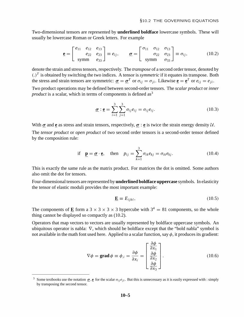
Two-dimensional tensors are represented by underlined boldface lowercase symbols. These willusually be lowercase Roman or Greek letters. For example

e =[ e11 e12 e13

e22 e23

symm e33

]≡ ei j , σ =

[σ11 σ12 σ13

σ22 σ23

symm σ33

]≡ σi j , (10.2)

denote the strain and stress tensors, respectively. The transpose of a second order tensor, denoted by(.)T is obtained by switching the two indices. A tensor is symmetric if it equates its transpose. Boththe stress and strain tensors are symmetric: σ = σT or σi j = σ j i . Likewise e = eT or ei j = e ji .

Two product operations may be defined between second-order tensors. The scalar product or innerproduct is a scalar, which in terms of components is defined as3

σ : e =3∑

i=1

3∑j=1

σi j ei j = σi j ei j . (10.3)

With σ and e as stress and strain tensors, respectively, σ : e is twice the strain energy density U .

The tensor product or open product of two second order tensors is a second-order tensor definedby the composition rule:

if p = σ · e, then pi j =3∑

k=1

σikek j = σikek j . (10.4)

This is exactly the same rule as the matrix product. For matrices the dot is omitted. Some authorsalso omit the dot for tensors.

Four-dimensional tensors are represented by underlined boldface uppercase symbols. In elasticitythe tensor of elastic moduli provides the most important example:

E ≡ Ei jk�, (10.5)

The components of E form a 3 × 3 × 3 × 3 hypercube with 34 = 81 components, so the wholething cannot be displayed so compactly as (10.2).

Operators that map vectors to vectors are usually represented by boldface uppercase symbols. Anubiquitous operator is nabla: ∇, which should be boldface except that the “bold nabla” symbol isnot available in the math font used here. Applied to a scalar function, say φ, it produces its gradient:

∇φ = grad φ ≡ φ,i = ∂φ

∂xi=

∂φ∂x1∂φ∂x2∂φ∂x3

. (10.6)

3 Some textbooks use the notation σ..e for the scalar σi j e ji . But this is unnecessary as it is easily expressed with : simplyby transposing the second tensor.

10–5


Applying nabla to a vector via the dot product yields the divergence of the vector:

∇ · u = div u ≡ ui,i =3∑

i=1

∂ui

∂xi= ∂u1

∂x1+ ∂u2

∂x2+ ∂u3

∂x3. (10.7)

Applying nabla to a second order tensor yields the divergence of a tensor, which is a vector. Forexample:

∇ · σ ≡ div σ = σi j, j =3∑

j=1

∂σi j

∂x j=

∂σ11∂x1

+ ∂σ12∂x2

+ ∂σ13∂x3

∂σ21∂x1

+ ∂σ22∂x2

+ ∂σ23∂x3

∂σ31∂x1

+ ∂σ32∂x2

+ ∂σ33∂x3

(10.8)

Applying ∇ to a vector via the cross product yields the curl or spin operator. This operator is notneeded in classical elasticity but it appears in applications that deal with rotational fields such asfluid dynamics with vorticity, or corotational nonlinear structural mechanics.

§10.2.2. Matrix Notation

Matrix notation is a modification of direct tensor notation in which everything is placed in matrixform, with some trickery used if need be. The main advantages of matrix notation are historicalcompatibility with finite element formulations, and ready computer implementation in symbolic ornumeric form.4

The representation of scalars, which may be viewed as 1 × 1 matrices, does not change. Neitherdoes the representation of vectors because vectors are column (or row) matrices.

Two-dimensional symmetric tensors are converted to one-dimensional arrays that list only theindependent components (six in three dimensions, three in two dimensions). The operation iscalled tensor-to-vector casting, and the result is called a cast vector. Component order in a castvector is a matter of convention, but usually the tensor diagonal components are listed first followedby the off-diagonal ones. A factor of 2 may be applied to the latter, as the strain vector examplebelow shows. The tensor is then represented as if were an actual vector, that is by non-underlinedboldface lowercase Roman or Greek letters.

For the strain and stress tensors the casting process produces the 6-vectors

e ≡ e =

e11

e22

e33

2e23

2e31

2e12

, σ ≡ σ =

σ11

σ22

σ33

σ23

σ31

σ12

, (10.9)

Note that off-diagonal (shearing) components of the strain vector are scaled by 2, but that no suchscaling applies to the off-diagonal (shear) stress components. The idea behind the scaling is to

4 Particularly in high level languages such as Matlab, Mathematica or Maple, which directly support matrix operators.

10–6

§10.3 THE FIELD EQUATIONS

maintain inner product equivalence so that for example, the strain energy density is simply

U = 12σ : e = 1

2

3∑i=1

3∑j=1

σi j ei j = 12σi j ei j = 1

2σT e

= 12

(σ11e11 + σ22e22 + σ33e33 + 2σ31e31 + 2σ23e23 + 2σ12e12

).

(10.10)

Four-dimensional tensors are cast to square matrices and denoted by matrix symbols, that is, non-underlined boldface uppercase Roman or Greek letters. Indices are appropriately collapsed toreflect symmetries and maintain product equivalence. Rather than stating boring rules, the exampleof the elastic moduli tensor is given to illustrate the mapping technique.

The stress-strain relation for linear elasticity in component notation is σi j = Ei jk� ek�, and incompact tensor form σ = E · e. We would of course like to have σ = E e in matrix notation. Thiscan be done by defining the 6 × 6 elastic modulus matrix

E =

E11 E12 E13 E14 E15 E16

E22 E23 E24 E25 E26

E33 E34 E35 E36

E44 E45 E46

E55 E56

symm E66

(10.11)

The components E pq of E are related to the components Ei jk� of E through an appropriate mappingthat preserves the product relation. For example: σ11 = E1111e11+E1122e22+E1133e33+E1112e12+E1121e21 + E1113e13 + E1131e31 + E1123e23 + E1132e32 maps to σ11 = E11e11 + E12e22 + E13e33 +E14 2e23 + E15 2e31 + E16 2e12, whence E11 = E1111, E14 = E1123 + E1132, etc.

Finally, operators that can be put in vector form are usually represented by a vector symbol boldfacelowercase whereas operators that can be put in matrix form are usually represented as matrices.Here is an example:

e =

e11

e22

e33

2e12

2e23

2e31

=

∂u1∂x1∂u2∂x2∂u3∂x3

∂u3∂x2

+ ∂u2∂x3

∂u1∂x3

+ ∂u3∂x1

∂u2∂x1

+ ∂u1∂x2

=

∂∂x1

0 0

0 ∂∂x2

0

0 0 ∂∂x3

0 ∂∂x3

∂∂x2

∂∂x3

0 ∂∂x1

∂∂x2

∂∂x1

0

[ u1

u2

u3

]= D u. (10.12)

Operator D is called the symmetric gradient in the continuum mechanics literature.5 In the matrixnotation defined above it is written as a 6 × 3 matrix. In direct tensor notation D = 1

2 (∇ + ∇T ) isthe tensor that maps u to e, and we write e = D · u. For the indicial form see below.

5 Some books use variants of ∇, such as ∇, ∇, ∇S or ∇S , for this operator.

10–7


§10.3. The Field Equations

Three field equations connect the internal (volume) fields.

§10.3.1. Strain-Displacement Equations

The strain-displacement equations, also called the kinematic equations (KE) or deformation equa-tions, yield the strain field given the displacement field. For linear elasticity the infinitesimal straintensor ei j is given by

ei j = 12 (ui, j + u j,i ) = 1

2

(∂ui

∂x j+ ∂u j

∂xi

)in V . (10.13)

Here a comma denotes differentiation with respect to the space variable whose index follows.

In compact tensor notation, with D as the symmetric gradient operator,

e = 12 (∇ + ∇T ) · u = D · u in V . (10.14)

The matrix form is e = D u. The full form of this is given in (10.12).

The inverse problem: given a strain field, find the displacements, is not generally soluble unlessstrain compatibility conditions are verified. These are complicated second-order PDE given in anybook on elasticity. This strain-to-diaplacement problem will not be considered here.

§10.3.2. Constitutive Equations

The constitutive equations connect the stress and strain fields in V . These equations are intendedto model the behavior of materials as continuum media. Generally they are partial differentialequations (PDEs) or even integrodifferential equations in space and time. In linear elasticity,however, a considerable simplification occurs because the relation becomes algebraic, linear, andhomogeneous. For this case the stress-strain relations may be written in component notation as

σi j = Ei jk� ek� in V . (10.15)

The Ei jk� are called elastic moduli. They are the components of a fourth order tensor E called theelasticity tensor. The elastic moduli satisfy generally the following symmetries

Ei jk� = E jik� = Ei j�k, (10.16)

which reduce their number from 34 = 729 to 62 = 36. Furthermore, if the body admits a strainenergy (that is, the material is not only elastic but hyperelastic) the elastic moduli enjoys additionalsymmetries:

Ei jk� = Ek�i j , (10.17)

which reduce their number to 21. Further symmetries occur if the material is orthotropic or isotropic.In the latter case the elastic moduli may be expressed as function of only two independent materialconstants, for example Young’s modulus E and Poisson ratio ν.

10–8

§10.4 THE BOUNDARY CONDITIONS

In compact tensor notation:

σ = E · e. (10.18)

In matrix form:

σ = E e, (10.19)

in which E is the 6 × 6 matrix listed in (10.11).

If the elasticity tensor is invertible, the relation that connects strains to stresses is written

ei j = Ci jk� σk� in V . (10.20)

The Ci jk� are called elastic compliances. They are also the components of a fourth order tensorcalled the compliance tensor, which satisfies the same symmetries as E. In compact tensor notation

e = C · σ = E−1 · σ, (10.21)

and in matrix form

e = C σ = E−1σ. (10.22)

§10.3.3. Internal Equilibrium Equations

The internal equilibrium equations of elastostatics are

σi j, j + bi = ∂σi j

∂x j+ bi = 0 in V . (10.23)

These follow from the linearized momentum balance equations derived in books on continuummechanics. The compact tensor notation is

∇ · σ + b = 0 in V . (10.24)

The matrix form is

DT σ + b = 0 in V . (10.25)

Here DT is the transpose of the symmetric gradient operator given in (10.12).

10–9


§10.4. The Boundary Conditions

The classical boundary conditions of elastostatics connect displacements and fluxes to given datato satisfy boundary compatibility and equilibrium condistions, respectively.

§10.4.1. Surface Compatibility Equations

The surface compatibility equations, more commonly called displacement boundary conditions,are

ui = ui on Su . (10.26)

or in direct notation (both tensor and matrix)

u = u on Su . (10.27)

The physical meaning is that the displacement components at points of Su must match the prescribedvalues.

§10.4.2. Surface Equilibrium Equations

The surface equilibrium equations, more commonly called stress boundary conditions, and alsotraction boundary conditions, are

σi j n j = ti on St , (10.28)

in which n j are the components of the external unit normal n at points of St where tractions arespecified; see Figure 10.2. Note that

σni = σi j n j = ti , (10.29)

are the components of the internal traction vector t ≡ σn . The physical interpretation of the stressboundary condition is that the internal traction vector must equal the prescribed traction vector. Or:the net flux ti − ti on St vanishes, component by component (a balnce or conservation law). Incompact tensor form

t = σn = σ · n = t. (10.30)

Stating (10.28) in a matrix form that uses the stress cast vector σ defined in (10.9) requires somecare. It would be incorrect to write either t = σT n or t = nT σ because σ is 6 × 1 and n is 3 × 1.Not only are these vectors non-conforming but even augmenting n with 3 zeros those products arescalars. The correct matrix form is a bit contrived:

t =[ t1

t2t3

]=

[ n1 0 0 0 n3 n2

0 n2 0 n3 0 n1

0 0 n3 n2 n1 0

]

σ11

σ22

σ33

σ23

σ31

σ12

= Pn σ, (10.31)

in which Pn is the 3 × 6 normal-projection matrix shown above.

10–10

§10.5 TONTI DIAGRAMS

This "dual" part of the Tonti diagram is not used here

Specifiedflux

variable

Primaryvariable

Specifiedprimaryvariable

Interme-diate

variable

Fluxvariable

Sourcefunction

Kinematicequations

Primaryboundaryconditions

Fluxboundaryconditions

Balance orequilibriumequations

Constitutiveequations

FIELDEQUATIONS

Figure 10.3. The general configuration of the Tonti diagram. Upper portion reproducedfrom Chapter 2. The diagram portion shown in dashed lines, which represents the so-

called dual or potential equations, is not used in this book.

§10.5. Tonti Diagrams

The Tonti diagram was introduced in Chapter 6 to represent the field equations of a mathematicalmodel in graphical form. The general configuration of the expanded form of that diagram (“ex-panded” means that it shows boundary conditions) is repeated in Figure 10.3 for convenience. Thisdiagram lists generic names for the “box occupants” and the connecting links.

Boxes and box-connectors drawn in solid lines are said to constitute the primal formulation of thegoverning equations. Dashed-lines boxes and connectors that appear in the bottom of the figurepertain to the so-called dual formulation in terms of potentials, which will not be used in this book.6

Figure 10.4 shows the primal formulation of the linear elasticity problem represented as a Tontidiagram. For this particular problem the displacements are the primary (or primal) variables, thestrains the intermediate variables, and the stresses the flux variables. The source variables are thebody forces. The prescribed configuration variables are prescribed displacements on Su and theprescribed flux variables are the surface tractions on St .

Tables 10.1 and 10.2 10.3 list generic names for the components of the Tonti diagram, as well asthose specific for the elasticity problem. Table 10.3 summarizes the governing equations of linearelastostatics written down in three notational schemes.

6 In the dual formulation the intermediate and flux variable exchange roles, so that boundary conditions of flux type arelinked to the intermediate variable of the primal formulation. In this way it is possible, for instance, to specify strain BCin elasticity, or velocity BC in fluids: just go for the dual formulation.

10–11


Table 10.1 Abbreviations for Tonti Diagram Box Contents

Acronym Meaning Alternate names in literature

PV Primary variable Primal variable, configuration variable,“across” variable

IV Intermediate variable First intermediate variable,auxiliary variable

FV Flux variable Second intermediate variable,“through” variable

SV Source variable Internal force variable,production variable

PPV Prescribed primary variablePrescribed flux variable

Table 10.2 Abbreviations for Tonti Diagram Box Connectors

Acronym Generic Name(s) given in thename elasticity problem

KE Kinematic equations Strain-displacement equationsCE Constitutive equations Stress-strain equations,

material equationsBE Balance equations Internal equilibrium equationsPBC Primary boundary conditions Displacement BCsFBC Flux boundary conditions Stress BCs, traction BCs

Table 10.3 Summary of Elastostatic Governing Equations

Acr Valid Compact or direct Matrix Component (indicial)tensor form form form

KE in V e = 12 (∇ + ∇T ) · u = D · u e = D u ei j = 1

2 (ui, j + u j,i )

CE in V σ = E · e σ = E e σi j = Ei jk� ek�

BE in V ∇ · σ + b = 0 DT σ + b = 0 σi j, j + bi = 0

PBC on Su u = u u = u ui = ui

FBC on St σ · n = σn = t = t Pn σ = σn = t = t σi j n j = σni = ti = ti

10–12

§10.6 OTHER NOTATIONAL CONVENTIONS

KE: BE:

PBC:

CE: FBC:σi j = Ei jk� ek�

in V

σi j, j + bi = 0in V

eij = 12 (ui, j + uj,i )

in V

ui = ui

on Su

σi j n j = tion St

t

u u

e

b

σ

Figure 10.4. Strong Form Tonti diagram for linear elastostatics. Governing equationsare written near links in indicial form.

§10.6. Other Notational Conventions

To facilitate comparison with older textbooks and papers, the governing equations are restatedbelow in two more alternative forms: in “grad/div” notation, and in full form.

§10.6.1. Grad-Div Direct Tensor Notation

This is a variation of the “nabla” direct tensor notation. Symbols grad and div are used insteadof ∇ and ∇· for gradient and divergence, respectively, whereas symm grad means the symmetricgradient operator D = 1

2 (∇ + ∇T ). The notation is slightly mode readable but takes more room.

KE: e = symm grad u in V,

CE: σ = E e in V,

BE: div σ + b = 0 in V,

PBC: u = u on Su,

FBC: σ · n = σn = t = t, on St .

(10.32)

§10.6.2. Full Notation

In the full-form notation everything is spelled out. No ambiguities of interpretation can arise;consequently this works well as a notation of last resort, and also as a “comparison template” againstone can check out the meaning of more compact notations. It is also useful for programming inlow-order languages.

The full form has, however, two major problems. First, it can become quite voluminous whenhigher order tensors are involved. Notice that most of the equations below are truncated becausethere is no space to state them fully. Second, compactness encourages visualization of essentials:long-windedness can obscure the forest with too many trees. Anyway, here they are:

10–13


KE: e11 = ∂u1

∂x1, e12 = e21 = 1

2

(∂u1

∂x2+ ∂u2

∂x1

), . . . in V,

CE: σ11 = E1111e11 + E1112e12 + . . . (7 more terms), σ12 = . . . in V,

BE:∂σ11

∂x1+ ∂σ12

∂x2+ ∂σ13

∂x3+ b1 = 0, . . . in V,

PBC: u1 = u1, u2 = u2, u3 = u3 on Su,

FBC: σ11 n1 + σ12 n2 + σ13 n3 = t1, . . . on St .

(10.33)

§10.7. Solving Elastostatic Problems

By solving an elastostatic problem we mean meant to find the displacement, strain and stress fields that satisfyall governing equations. That is, the field equations and the boundary conditions.

Under mild assumptions of primary interest to mathematicians, the elastostatic problem has one and only onesolution. There are, however, practical exceptions where the solution is not unique. Two instances:

1. “Free Floating” Structures. The displacement field is not unique but strains and stresses are. Examples:aircraft structures in flight and space structures in orbit.

2. Incompressible Materials. The mean (hydrostatic) stress field is not determined from the displacementsand strains. Determination of the hydrostatic stress field depends on the stress boundary conditions,which may be insufficient in some cases.

An analytical solution of the elastostatic problem is only possible for very simple cases. Most practicalproblems require a numerical solution. Most numerical methods involve a discretization process throughwhich an approximate solution with a finite number of degrees of freedom is constructed.

§10.7.1. Discretization Methods

Discretization methods of highest importance in computational mechanics can be grouped into three classes:finite difference, finite element, and boundary methods.

Finite Difference Method (FDM). The governing differential equations are replaced by difference expressionsbased on the field values at nodes of a finite difference grid. Although FDM remains important in fluidmechanics and in dynamic problems for the time dimension, it has been largely superseded by the finiteelement method in a structural mechanics in general and elastostatics in particular.

Finite Element Method (FEM). This is the most important “volume integral” method. One or more of thegoverning equations are recast to hold in some average sense over subdomains of simple geometry. Thisrecasting is often done in terms of variational forms if variational principles can be readily constructed, as isthe case in elastostatics. The procedure for constructing the simplest class of these principles is outlined inthe next section.

Boundary Methods. Under certain conditions the field equations between volume fields can be eliminated infavor of boundary unknowns. This dimensionality reduction process leads to integro-differential equationstaken over the boundary S. Discretization of these equations through finite element or collocation techniquesleads to the so-called boundary element methods (BEM).

Further discussion on the use of these methods for simulating structural systems can be found in Chapter1 of the Advanced Finite Element methods (AFEM) book [271]. Some more specialized approaches, e.g.,meshfree and spectral discretizations, are desccribed there.

10–14

§10.8 CONSTRUCTING VARIATIONAL FORMS

Step* Operation Description

1 Select master field(s) One or more of the unknown internal fields (displacements, strains and stresses in the elasticity problem) are chosen as masters. 2 Select weak connections Selected strong links are weakened. Slave fields may have to be split if necessary. If so, duplicated slave fields are connected by weak links. 3 Construct Weak Form (WF) A Weak Form is established by choosing weights for the weak links and integrating over their domains (volume or surface). 4 Replace weights by alleged variations WF weight functions are replaced by master field variations propagated through and homogenize the strong links as appropriate. Master field variations are homogenized using integration by parts (the divergence theorem in 2D or 3D) as necessary.

5 Find Variational Form (VF) The VF is obtained as the functional whose first variation reproduces the varied-WF of Step 4. This process may involve trial and error, e.g., playing with alleged variations and their signs. If no VF can be found, one may have to be content with the WF of Step 3 as basis to develop numerical approximations.

* Steps 4-5 are typically the most difficult and time-consuming ones. There is no guarantee that Step 5 will be successful within the Standard Variational Calculus. It becomes possible through nonstandard extensions such a adjoint variational principles, restricted variational principles, or use of noncommutative variations; none of which are considered here.

Figure 10.5. Steps to construct a Variational Form (VF) starting from the field-decomposed Strong Form (SF).

§10.8. Constructing Variational Forms

Finite element methods for the elasticity problem are based on Variational Forms, or VFs, of theforegoing Strong Form (SF) equations. Although the SF is unique, there are many VFs.7 Asexplained in previous Chapters, the search for a VF begins by selecting one or more master fields,and weakening one or more links. This process produces a set of equations called the Weak Form,or WF, which may be viewed as an midway stop between the SF and the VF.

The end result of the process is the construction of a functional � that contains integrals of theknown and unknown fields. Associated with the functional is a variational principle: setting thefirst variation δ� to zero recovers the strong form of the weakened field equations as Euler-Lagrangeequations, and the strong form of the weakened BCs as natural boundary conditions.

Here is a summary of the VF construction steps: (1) select master(s), (2) select weak links, (3)construct the Weak Form (WF), (3) make the WF the variation of an alleged functional, (5) find thefunctional to establish the Variational Form (VF). Those steps are summarized in Figure 10.5, andgenerically described below keeping the elasticity equations in mind.

The steps are illustrated with the construction of the single-field primal elasticity functional, calledthe Total Potential Energy or TPE.

§10.8.1. Step 1: Select Master Field(s)

One or more of the unknown internal fields

ui , ei j , σi j , (10.34)

7 There is in fact an infinite number of functionals, parametrizable by a finite number of parameters, as shown in theexpository survey [246]. Most books and papers give the impression that there is only a finite number. What is true isthat only a finite number of canonical functionals exist; they are listed in the next Chapter for the elasticity problem.

10–15


are chosen as masters. A master (also called primary, varied, or parent) field is one that is subjectedto the δ process of Variational Calculus. Unknown fields that are not masters, i.e. not subject tovariation, are called slave, secondary, or derived. The owner (also called parent or source) of aslave field is the master from which it derives. The master-slave connection must be via stronglinks (see below for specific rule).

If only one master field is chosen, the resulting variational principle (obtained after going throughSteps 2–5) is called single-field, and multifield otherwise.

A known or data field (for example: body forces or surface tractions in elastostatics) cannot be amaster field because it is not subject to variation, and is not a slave field because it does not derivefrom others. Hence we see that fields can only be of three types: master, slave, or data.

§10.8.2. Step 2: Select Weak Connections

Given a master field, consider the equations that link it to other known and unknown fields. Theseare called the connections of that field. Classify these connections into two types:

Strong connection. The connecting relation is enforced point by point in its original form. Forexample if the connection is a PDE or an algebraic equation we use it as such. Also called a priorienforcement. When applied to a boundary condition, a strong connection is also referred to as anessential constraint or essential B.C.

Weak connection. The connection relationship is enforced only in an average or mean sense throughthe use of a weight or test function, or of a distributed Lagrange multiplier. Also called a-posteriorienforcement. When applied to a boundary condition, a weak connection is also referred to as anatural constraint or natural B.C.

A general rule to keep in mind is that a slave field must be reachable from its master owner throughstrong connections.

If there is more than one master field (i.e. we are constructing a multifield principle), the foregoingdefinitions must be applied to each master field in turn. In other words, we must consider theconnections that “emanate” from each of the master fields. The end result is that the same field mayappear more than once. For example in elasticity the strain field e may appear up to three times:(1) as a master field, (2) as a slave field derived from displacements, and (3) as a slave field derivedfrom stresses. If this causes a slave field to have multiple masters, that field must be duplicated insuch a way that each duplicate has one and only one owner. The duplicates are then connected witha weak link. Such a complication cannot occur with single-field principles.

Remark 10.3. There is usually limited freedom as regards the choice of strong vs. weak connections. The keytest comes when one tries to form the total variation in Steps 4-5. If this happens to be the exact variation of afunctional, the choice is admissible. Else is back to the drawing board.

§10.8.3. Step 3: Construct A Weak Form

Establish a Weak Form (WF) by multiplying the weak link residuals by weighting functions andintegrating over the approrpriate domains: volume for field equations, surface for boundary condi-tions.

Once all choices of Steps 1–3 have been made, the remaining manipulations are technical in nature,and essentially consist of applying the tools and techniques of vector, tensor and variational calculus.

10–16

§10.9 DERIVATION OF TOTAL POTENTIAL ENERGY PRINCIPLE

Since the number of operational combinations is huge, the techniques are best illustrated throughspecific examples. The end result of these gyrations should be a variational statement

δ� = 0, (10.35)

where the symbol δ here embodies variations with respect to all master fields. Steps 4–5 aredesigned to get there.

§10.8.4. Step 4: Replace Weights by Alleged Variations and Homogenize

Once all choices of Steps 1–3 have been made, the remaining manipulations are technical innature, and essentially consist of applying the tools and techniques of vector, tensor and variationalcalculus: Lagrange multipliers, integration by parts (called the divergence theorem in 2D or 3D)homogenization of variations, surface integral splitting, and so on. Since the number of operationalcombinations is huge, the techniques are best illustrated through specific examples.

The end result of all these gyrations should be a variational statement

δ� = 0, (10.36)

where the symbol δ here embodies variations with respect to all master fields, and � (if it exist) isthe target functional.

§10.8.5. Step 5: Find Variational Form (VF)

With luck, the variational statement constructed in Step 4 will be recognized as the exact variationof a functional �, such as the one in §10.9.4 below. If one arrives at this happy end, the variationalstatement becomes a true variational principle and the movie fades into the sunset before the creditsroll in. The expression δ� = 0 now states a variational principle. If this is a new principle for animportant problem, your name may perhaps live forever attached to that �.

We now illustrate the foregoing steps with the detailed derivation of the most important single-fieldVF in elastostatics: the principle of Total Potential Energy or TPE.

§10.9. Derivation of Total Potential Energy Principle

§10.9.1. A Long Journey Starts with the First Step

The departure point for deriving the classical TPE principle is the WF diagrammed in Figure 10.6.Such modifications are briefly explained in the figure label and in the text below. The displacementfield ui is the only master. The strain and stress fields are slaves. The slave-provenance notationintroduced in Chapter 3 is used: the owner of a slave field is marked by a superscript. For example,eu = D u means “eu is owned by u” through the strong KE link.

The strong connections are the kinematic equations KE (in elasticity the strain-displacement equa-tions), the constitutive equations CE, and the primary boundary conditions PBC (in elasticity thedisplacement boundary conditions). These are shown in Figure 10.6 as solid box-connecting lines:

Strong : ei j = 12 (ui, j + u j,i ) in V, σi j = Ei jk� ek� in V, ui = ui on Su . (10.37)

10–17


Slave Slave

∫V

(σui j, j + bi ) dV = 0

∫St

(σui j nj − ti ) d S = 0

Master

KE: BE:

PBC:

CE: FBC:σi j = Ei jk� ek�

in V

eij = 12 (ui, j + uj,i )

in V

ui = ui

on Su

t

u u

e

b

σuu

λi

δui

Symbol λ used here for the BE-residual suggests a Lagrange multiplier.That is how some authors constructvariational forms by "relaxing"strong links. Scheme first used by Friedrichs (cf. Courant-Hilbert book)and popularized in mechanics & FEMby Fraeijs de Veubeke

Figure 10.6. Tonti Diagram of the Weak Form (WF) used as departurepoint for deriving the TPE functional of linear elastostatics.

The weak connections are the balance equations BE (in elasticity the stress equilibrium equations),and the flux boundary conditions FBC (in elasticity the traction boundary conditions), These appearin Figure 10.6 as shaded lines:

Weak: σi j, j + bi = 0 in V, σi j n j = ti on St . (10.38)

§10.9.2. Lagrangian Glue

Now we get down to the business of variational calculus. A slight notational variation of theresidual weighting technique of previous Chapters is used. The notation has certain interpretationadvantages that will become apparent later when dealing with hybrid principles.

To treat BE as a weak connection, take the first of (10.38), replace σi j by the slave σ ui j , multiply by

a piecewise differentiable 3-vector field λi and integrate over V :∫V(σ u

i j, j + bi ) λi dV = 0. (10.39)

Apply the divergence theorem to the first term in (10.39):∫V

σ ui j, j λi dV = −

∫V

σ ui jλi, j dV +

∫Sσ u

i j n jλi d S. (10.40)

For a symmetric stress tensor σ ui j = σ u

ji this formula may be transformed8 to

∫V

σ ui j, jλi dV = −

∫V

σ ui j

12 (λi, j + λ j,i ) dV +

∫Sσ u

i j n jλi d S. (10.41)

8 This transformation is stated in §5.5 of Sewell’s book [735]. It may also be verified directly as in Exercise 10.4.

10–18

§10.9 DERIVATION OF TOTAL POTENTIAL ENERGY PRINCIPLE

Assignation of meaning of internal energy to the second term in (10.41) suggests identifying λi

with the variation of the displacement field ui (a “lucky guess” that can be proved rigorously aposteriori): ∫

Vσ u

i j, j δui dV = −∫

Vσ u

i j δeui j dV +

∫Sσ u

i j n j δui d S, (10.42)

in which the strain-variation symbol means

δeui j = 1

2 (δui, j + δu j,i ) in V, (10.43)

because of the strong connection eui j = 1

2 (ui, j + u j,i ), which if varied with respect to ui yields(10.43).

Remark 10.4. Although the essence of the treatment of weak connections is ultimately the same, there is farfrom universal agreement on terminology in the literature. The foregoing scheme is known as the Lagrangemultiplier treatment. It closely follows the work of Fraeijs de Veubeke (a major contributor to variationalmechanics). The technique was originally introduced by Friedrichs (a disciple of Courant and Hilbert) in amathematical context.

Other authors, primarily in fluid mechanics, favor weight functions (as in the treatment of the Poisson equationin previous Chapters) or test functions. If the WF is directly discretized, as often done in fluid mechanics,the former technique leads to weighted-residual subdomain methods (for example the Fluid Volume Method)whereas test functions lead to Galerkin, Petrov-Galerkin, least-square, . . . etc., methods. Some authors, suchas Lanczos [478], multiply directly equilibrium residuals by displacement variations, which are called thenvirtual displacements. Some music but different lyrics.

§10.9.3. The First-Variation Pieces

Substituting (10.42) into (10.39), with λi → δui , we obtain

∫V

σ ui j δeu

i j dV −∫

Vbi δui dV −

∫Sσ u

i j n j δui d S = 0. (10.44)

The surface integral may be split as follows:

∫Sσ u

i j n j δui d S =∫

St

σ ui j n j δui d S +

∫Su

σ ui j n j δui d S =↗0

∫St

σ ui j n j δui d S. (10.45)

where the substitution δui = δui on Su results from the strong connection ui = ui on Su . Butδui = 0 because prescribed (data) fields are not subject to variation, and the Su integral drops out.Treating the FBC weak connection with δui as 3-vector weight function we obtain

∫St

(σ ui j n j − ti ) δui d S = 0, whence

∫St

σ ui j n j δui d S =

∫St

ti δui d S. (10.46)

10–19


§10.9.4. A Happy Ending

Substituting (10.45) and the second of (10.46) into (10.44), we obtain the final form of the variationin the master field ui , which we write (hopefully) as the variation of a functional �TPE:

δ�TPE =∫

Vσ u

i j δeui j dV −

∫V

bi δui dV −∫

St

ti δui d S = 0. (10.47)

And indeed (10.47) can be recognized9 as the exact variation, with respect to ui , of

�TPE[ui ] = 12

∫V

σ ui j eu

i j dV −∫

Vbi ui dV −

∫St

ti ui d S. (10.48)

This �TPE is called the total potential energy functional. It is often written as the difference of thestrain energy and the external work functionals:

�TPE = UTPE − WTPE, in which

UTPE = 12

∫V

σ ui j e

ui j dV, WTPE =

∫V

bi ui dV +∫

St

ti ui d S.(10.49)

Consequently (10.47) is a true variational principle and not just a variational statement.

The physical interpretation is well known: 12σ u

i j eui j is the strain energy density U in terms of

displacements. Integrating this density over the volume V gives the total strain energy stored inthe body. In elasticity this is the only stored energy, and consequently it is also the internal energyU . Likewise, bi ui is the external work density of the body forces, whereas ti ui is the external workdensity of the applied surface tractions. Integrating these densities over V and St , respectively, andadding gives the total external work potential W .

Remark 10.5. What we have just gone through is called the Inverse Problem of Variational Calculus: given thegoverning equations (field equations and boundary conditions), find the functional(s) that have those governingequations as Euler-Lagrange equations and natural boundary conditions, respectively.

The Direct Problem of Variational Calculus is the reverse one: given a functional such as (10.48), how that thevanishing of its first variation is equivalent to the governing equations. These appear as the Euler-Lagrangeequations and natural boundary conditions.

This problem is normally the first one tackled in Variational Calculus instruction in math support courses.10

The Direct Problem is done by carrying out the foregoing steps in reverse order: form a variation such as(10.47), integrate by parts as appropriate to homogenize variations, and use the strong connections to finallyarrive at

δ�TPE =∫

V

(σ ui j, j + bi ) δui dV +

∫St

(σi j n j − ti ) δui d S. (10.50)

Using the fundamental lemma of variational calculus11 one then shows that δ�TPE = 0 yields the weakconnections (10.38) as Euler-Lagrange equations and natural boundary conditions, respectively.

9 See Exercise 10.5 for the variation of the strain energy term.10 For example, Aerospace Math.11 See, e.g., §1.3 of [321].

10–20

§10.10 THE TENSOR DIVERGENCE THEOREM AND THE PVW

§10.10. The Tensor Divergence Theorem and the PVW

Recall from Chapter 7 the canonical form of the divergence theorem, which says that the vectordivergence of a vector a over a volume is equal to the vector flux over the surface:∫

V∇ · a dV =

∫S

a · n d S. (10.51)

Take a = σ · u, where σ = [σi j ] is a symmetric stress tensor and u = [ui ] a displacement vector:∫V(σ : ∇u + ∇σ · u) dV =

∫Sσ · u · n d S. (10.52)

Here ∇u = [∂ui/∂x j ] is an unsymmetric tensor called the deformation gradient. Its transpose isuT ∇T = [∂u j/∂xi ]. Now σ : ∇u = (σ : ∇u)T = σ : uT ∇T = σ : 1

2 (∇ + ∇T ) · u = σ : D · u,where D = 1

2 (∇ + ∇T ). Hence∫V

σ : D · u dV = −∫

V∇σ · u dV +

∫Sσ · u · n d S. (10.53)

In indicial notation this is∫V

σi j12

(∂u j

∂xi+ ∂ui

∂x j

)dV = −

∫V

∂σi j

∂xiu j dV +

∫Sσi j u j ni d S. (10.54)

Recognizing that eui j = 1

2 (∂u j/∂xi + ∂ui/∂x j ) we finally arrive at

∫V

σi j eui j dV = −

∫V

∂σi j

∂xiu j dV +

∫Sσi j u j ni d S. (10.55)

Taking the variation of this equation with respect to the displacements while keeping σi j fixed yieldsthe Principle of Virtual Work (PVW):∫

Vσi j δeu

i j dV = −∫

V

∂σi j

∂xiδu j dV +

∫Sσi j δu j ni d S. (10.56)

So far σi j and eui j are disconnected in (10.56) because no constitutive assumption has been stated in

this derivation. Consequently the PVW is valid for arbitrary materials (for example, in plasticity),which underscores its generality. Setting σi j = σ u

i j provides the form used in §10.9.2.

10–21


Homework Exercises for Chapter 10

Three-Dimensional Linear Elastostatics

EXERCISE 10.1 [A:10] Specialize the elasticity problem to a bar directed along x1. Write down the fieldequations in indicial, tensor and matrix form.

EXERCISE 10.2 [A:10] Justify the matrix form (10.30).

EXERCISE 10.3 [A:20] Suppose that the displacement uP at an internal point P(xP) is known. How canthat condition be accomodated as a boundary condition on Su? Hint: draw a little sphere of radius ε about P ,then . . . oops I almost told the story.

EXERCISE 10.4 [A:20] Justify passing from (10.38) to (10.39) by proving that if σi j is symmetric, that is,σi j = σ j i , then σi jλi, j = σi j

12 (λi, j + λ j,i ). Hint: one (elegant) way is to split λi, j + λ j,i into symmetric and

antisymmetric parts; other approaches are possible.

EXERCISE 10.5 [A:15] Prove that δ( 12 σ u

i j eui j ) = σ u

i j δeui j , where the variation δ is taken with respect to

displacements ui .

10–22

Three-Dimensional Linear Elastostatics€¦ · The ﬁeld equations are generally partial differential equations ... Mathematica or Maple, ... THREE-DIMENSIONAL LINEAR ELASTOSTATICS

Documents