Three-dimensional accelerating electromagnetic waves

arX

iv:1

303.

6320

v1 [

phys

ics.

optic

s] 2

5 M

ar 2

013

Three-dimensional Accelerating Electromagnetic

Waves

Miguel A. Bandres,a,1 Miguel A. Alonso,b Ido Kaminerc and Mordechai Segevc

aInstituto Nacional de Astrofısica, Optica y Electronica,

Tonantzintla, Puebla 72840, MexicobThe Institute of Optics, University of Rochester,

Rochester, NY 14627, USAcPhysics Department and Solid State Institute, Technion,

Haifa 32000, Israel

E-mail: [email protected]

Abstract: We present a general theory of three-dimensional nonparaxial spatially-

accelerating waves of the Maxwell equations. These waves constitute a two-dimensional

structure exhibiting shape-invariant propagation along semicircular trajectories. We pro-

vide classification and characterization of possible shapes of such beams, expressed through

the angular spectra of parabolic, oblate and prolate spheroidal fields. Our results facilitate

the design of accelerating beams with novel structures, broadening scope and potential

applications of accelerating beams.

1http://www.mabandres.com/

Contents

1 Introduction 1

2 Three-dimensional nonparaxial accelerating waves 3

3 Parabolic accelerating waves 6

4 Prolate spheroidal accelerating waves 7

5 Oblate spheroidal accelerating waves 9

5.1 Outer-type 9

5.2 Inner-type 11

6 Vector solutions 11

7 Conclusion 13

8 Acknowledgments 13

1 Introduction

The concept of self-accelerating beam, which was introduced into the domain of optics

in 2007 [1, 2], has generated much follow-up and many new discoveries and applications.

Generally, the term “accelerating beams” is now used in conjunction with wave packets

that preserve their shape while propagating along curved trajectories. The phenomenon

arises from interference: the waves emitted from all points on the accelerating beam in-

terfere in the exact manner that maintains a propagation-invariant structure, bending

along a curved trajectory. This beautiful phenomenon requires no waveguiding structure

or external potential, appearing even in free-space as a result of pure interference. The

first optical accelerating beam, the paraxial Airy beam, was proposed and observed in

2007 [1, 2]. Since then, research on accelerating beams has been growing rapidly, leading

to many intriguing ideas and applications ranging from particle and cell micromanipula-

tion [3], light-induced curved plasma channels [4], self-accelerating nonlinear beams [5],

self-bending electron beams [6] to accelerating plasmons [7] and applications in laser mi-

cromachining [8]. Following the research on spatially-accelerating beams, similar concepts

have been studied also in the temporal domain, where temporal pulses self-accelerate in a

dispersive medium [1, 9–11] up to some critical point determined by causality [11]. Inter-

estingly, shape-preserving accelerating beams were also found in the nonlinear domain [12]

in a variety of nonlinearities ranging from Kerr, saturable and quadratic media [12–15] to

nonlocal nonlinear media [14].

– 1 –

In two-dimensional (2D) paraxial systems (including the propagation direction and

one direction transverse to it), the one-dimensional Airy beams are the only exactly

shape-preserving solution to paraxial wave equation with accelerating properties. How-

ever, in three-dimensional (3D) paraxial systems, two separable solutions are possible:

two-dimensional Airy beams [2] and accelerating parabolic beams [16, 17]. Furthermore,

it has been shown [18] that any function on the real line can be mapped to an acceler-

ating beam with a different transverse shape. This allows creating paraxial accelerating

beams with special properties such as reduced transverse width and beams with a trans-

verse rainbow-like profile having a finite width, instead of a long tail, in the accelerating

direction.

However, until 2012, the concept of accelerating beams was restricted to the paraxial

regime, and the general mindset was that accelerating wave packets are special solutions

for Schrodinger-type equations, as they were originally conceived in 1979 [19]. This means

that the curved beam trajectory was believed to be restricted to small (paraxial) angles.

In a similar vein, paraxiality implies that the transverse structure of paraxial accelerat-

ing beams cannot have small features, on the order of a few wavelengths or less. At the

same time, reaching steep bending angles and having small scale features is fundamental

in areas like nanophotonics and plasmonics, hence searching for shape-preserving accel-

erating nonparaxial wave packets was naturally expected. Indeed, recent work [20] has

overcome the paraxial limit finding shape-preserving accelerating solutions of the Maxwell

equations. These beams propagate along semi-circular trajectories [20, 21] that can reach,

with an initial “tilt”, almost 180 turns [22]. Subsequently, 2D nonparaxial accelerating

wave packets with parabolic [23, 24] and elliptical [24, 25] trajectories were found. Also,

fully 3D nonparaxial accelerating beams were proposed, based on truncations or complex

apodization of spherical, oblate and prolate spheroidal fields [25, 26]. Finally, nonparaxial

accelerating beams were suggested in nonlinear media [27, 28].

All of this recently found plethora of nonparaxial accelerating beams suggest there

might be a broader theory of self-accelerating beams of the three-dimensional Maxwell

equations: a general formulation encompassing all the particular examples of [18, 25], and

generalizing them to a unified representation. Such a theory could once and for all, answer

several questions about the phenomenon of self-accelerating beams. For example, what

kind of beam structures can display shape-preserving bending? What are the fundamental

limits on their feature size and acceleration trajectories? What trajectories would such

beams follow?

Here, we present a theory describing the entire domain of 3D nonparaxial accelerating

waves that propagate in a semicircle. These electromagnetic wave packets are monochro-

matic solutions to the Maxwell equations and they propagate in semicircular trajectories

reaching asymptotically a 90 bending in a quarter of a circle. We show that solutions

exist with the polarization essentially perpendicular to their bending direction towards the

path’s center of curvature. In their scalar form, these waves are exact time-harmonic solu-

tions of the wave equation. As such, they have implications to many linear wave systems

in nature. We propose a classification and characterization of possible shapes of these

accelerating waves, expressed through the angular spectra of parabolic, oblate and prolate

– 2 –

spheroidal fields. We find novel transverse distributions, such as the nonparaxial counter-

part of a 2D paraxial Airy beam, and accelerating beams that instead of a long tail, have a

finite width (of a few wavelengths) in the transverse direction to the propagation direction

that bends in a circle, among others.

2 Three-dimensional nonparaxial accelerating waves

We begin our analysis by considering the 3D Helmholtz equation(∂xx + ∂yy + ∂zz + k2

)ψ =

0 where k is the wave number. In free space, the solution of the Helmholtz equation can

be described in terms of plane waves through its angular spectral function A(θ, φ) as

ψ (r) =

∫A(θ, φ) exp (ikr · u) dΩ, (2.1)

where u = (sin θ sinφ, cos θ, sin θ cosφ) is a unit vector that runs over the unit sphere, and

dΩ = sin θdθdφ is the solid angle measure on the sphere.

To search for wavepackets that are shape-preserving and whose trajectory resides on a

semicircle, it is convenient to start with solutions whose trajectory resides on a full circle,

i.e., solution with rotational symmetry. These solutions have an intensity profile that is

exactly preserved over planes containing the y-axis and therefore they will have defined

angular momentum Jy = −i (xdz − zdx) along this axis. This operator acts on the spectral

function as Jy = −i∂φ; hence, the spectral function of a rotationally symmetric solution

must satisfy −i∂φA = mA. In this way, any rotationally symmetric wave must have a

spectral function of the form A(θ, φ) = g(θ)exp (imφ) , where m is a positive integer and

g (θ) is any complex function in the interval [0, π].

Although these rotationally symmetric fields are shape-invariant and travel in a closed

circle, they are composed of forward- (positive kz, i.e., φ ∈ [−π/2, π/2]) and backward-

(negative kz, i.e., φ ∈ [π/2, 3π/2]) propagating waves. Creating such rotationally-symmetric

beams would require launching two pairs of counter-propagating beams (or two counter-

propagating beams each with an initial tilt of virtually 90 angle). Here, we are interested

in beams that can be launched from a single plane. We therefore limit the integration in

Eq. (2.1) to the forward semicircle φ ∈ [−π/2, π/2] resulting in a forward-propagating wave

with accelerating characteristics that can be created by a standard optical system, i.e.,

ψ (r) =

∫ π

0

sin θdθ

∫ π/2

−π/2dφg(θ)exp (imφ) exp (ikr · u) , (2.2)

where nowm can be any positive real number (not necessarily an integer), because we are no

longer restricted by periodic boundary conditions. In this way, any function g(θ) generates

a nonparaxial accelerating wave with a different transverse distribution. Furthermore,

by construction, all these waves share the same accelerating characteristics: their maxima

propagate along a semicircular path of radius slightly larger thanm/k, while approximately

preserving their 2D transverse shape up to almost 90 bending angles. These characteristics

are reminiscent of broken rotational symmetry. Also, because larger angular momentum

gives better spatial separation of the counterpropagating parts of a rotational field, our

– 3 –

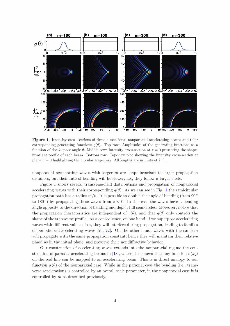
Figure 1. Intensity cross-sections of three-dimensional nonparaxial accelerating beams and their

corresponding generating functions g(θ). Top row: Amplitudes of the generating functions as a

function of the k-space angle θ. Middle row: Intensity cross-section at z = 0 presenting the shape-

invariant profile of each beam. Bottom row: Top-view plot showing the intensity cross-section at

plane y = 0 highlighting the circular trajectory. All lengths are in units of k−1.

nonparaxial accelerating waves with larger m are shape-invariant to larger propagation

distances, but their rate of bending will be slower, i.e., they follow a larger circle.

Figure 1 shows several transverse-field distributions and propagation of nonparaxial

accelerating waves with their corresponding g(θ). As we can see in Fig. 1 the semicircular

propagation path has a radius m/k. It is possible to double the angle of bending (from 90

to 180 ) by propagating these waves from z < 0. In this case the waves have a bending

angle opposite to the direction of bending and depict full semicircles. Moreover, notice that

the propagation characteristics are independent of g(θ), and that g(θ) only controls the

shape of the transverse profile. As a consequence, on one hand, if we superpose accelerating

waves with different values of m, they will interfere during propagation, leading to families

of periodic self-accelerating waves [20, 22]. On the other hand, waves with the same m

will propagate with the same propagation constant, hence they will maintain their relative

phase as in the initial plane, and preserve their nondiffractive behavior.

Our construction of accelerating waves extends into the nonparaxial regime the con-

struction of paraxial accelerating beams in [18], where it is shown that any function ℓ (ky)

on the real line can be mapped to an accelerating beam. This is in direct analogy to our

function g (θ) of the nonparaxial case. While in the paraxial case the bending (i.e., trans-

verse acceleration) is controlled by an overall scale parameter, in the nonparaxial case it is

controlled by m as described previously.

– 4 –

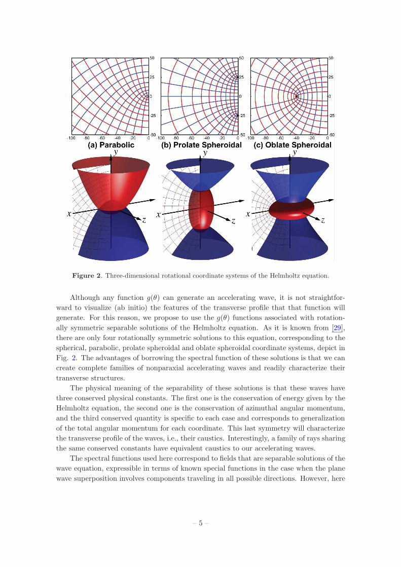
Figure 2. Three-dimensional rotational coordinate systems of the Helmholtz equation.

Although any function g(θ) can generate an accelerating wave, it is not straightfor-

ward to visualize (ab initio) the features of the transverse profile that that function will

generate. For this reason, we propose to use the g(θ) functions associated with rotation-

ally symmetric separable solutions of the Helmholtz equation. As it is known from [29],

there are only four rotationally symmetric solutions to this equation, corresponding to the

spherical, parabolic, prolate spheroidal and oblate spheroidal coordinate systems, depict in

Fig. 2. The advantages of borrowing the spectral function of these solutions is that we can

create complete families of nonparaxial accelerating waves and readily characterize their

transverse structures.

The physical meaning of the separability of these solutions is that these waves have

three conserved physical constants. The first one is the conservation of energy given by the

Helmholtz equation, the second one is the conservation of azimuthal angular momentum,

and the third conserved quantity is specific to each case and corresponds to generalization

of the total angular momentum for each coordinate. This last symmetry will characterize

the transverse profile of the waves, i.e., their caustics. Interestingly, a family of rays sharing

the same conserved constants have equivalent caustics to our accelerating waves.

The spectral functions used here correspond to fields that are separable solutions of the

wave equation, expressible in terms of known special functions in the case when the plane

wave superposition involves components traveling in all possible directions. However, here

– 5 –

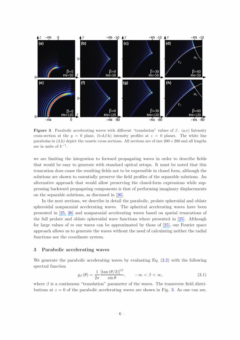
Figure 3. Parabolic accelerating waves with different “translation” values of β. (a,e) Intensity

cross-section at the y = 0 plane, (b-d,f-h) intensity profiles at z = 0 planes. The white line

parabolas in (d,h) depict the caustic cross sections. All sections are of size 200×200 and all lengths

are in units of k−1.

we are limiting the integration to forward propagating waves in order to describe fields

that would be easy to generate with standard optical setups. It must be noted that this

truncation does cause the resulting fields not to be expressible in closed form, although the

solutions are shown to essentially preserve the field profiles of the separable solutions. An

alternative approach that would allow preserving the closed-form expressions while sup-

pressing backward propagating components is that of performing imaginary displacements

on the separable solutions, as discussed in [26].

In the next sections, we describe in detail the parabolic, prolate spheroidal and oblate

spheroidal nonparaxial accelerating waves. The spherical accelerating waves have been

presented in [25, 26] and nonparaxial accelerating waves based on spatial truncations of

the full prolate and oblate spheroidal wave functions where presented in [25]. Although

for large values of m our waves can be approximated by those of [25], our Fourier space

approach allows us to generate the waves without the need of calculating neither the radial

functions nor the coordinate system.

3 Parabolic accelerating waves

We generate the parabolic accelerating waves by evaluating Eq. (2.2) with the following

spectral function

gβ (θ) =1

2π

[tan (θ/2)]iβ

sin θ, −∞ < β <∞, (3.1)

where β is a continuous “translation” parameter of the waves. The transverse field distri-

butions at z = 0 of the parabolic accelerating waves are shown in Fig. 3. As one can see,

– 6 –

these profiles resemble the ones of the 2D paraxial Airy beams [1, 2]; this is because the

parabolic coordinate system looks like a Cartesian coordinate system rotated 45 near a

coordinate patch at y ≈ 0, |x| ≫ 1, as shown in Fig. 2(a). The main lobe of the waves

is located near x = −m/k, y = β/k. The fundamental mode is β = 0 and as β increases

the waves “translate” in the y-axis. This is consistent with the result of [18] where it is

shown that the paraxial 2D Airy beams are orthogonal under translations perpendicular

to the direction of acceleration. Notice that in our case for β 6= 0 there is also a “tilt” in

the caustic accompanied by a change in the spacing of the fringes along the caustic sheets.

Note that this “tilt” does not change the direction of propagation, thus the acceleration

is still horizontal in Fig. 3, and not in the direction to which the intensity pattern points,

as it might seem at first. This resembles a paraxial 2D Airy beam with different scale

parameters for each of the constituent Airy functions. As shown in Figs. 3(a) and 3(e),

the parabolic accelerating waves present a single intensity main lobe that follows a circular

path of radius slightly larger than m/k.

By separation of variables the Helmholtz equation can be broken into ordinary differ-

ential equations [29] with an effective potential for each coordinate. The turning point of

these effective potentials will give the caustics of the solutions. We find that our acceler-

ating waves share these caustics in a form reminiscent of the broken symmetries. In this

way, we find that the caustics of the parabolic accelerating waves are given by

u2C =(−β +

√β2 +m2

)/k, v2C =

(β +

√β2 +m2

)/k, (3.2)

where the parabolic coordinates [u, v, φ] , are defined as

x = uv sinφ, y =1

2

(u2 − v2

), z = uv cosφ, (3.3)

where u ∈ [0,∞], v ∈ [0,∞], φ ∈ [0, 2π). The caustic cross sections are depicted in Fig.

3(d) and 3(h); by rotating these around the y-axis one gets the caustic surfaces which are

two paraboloids, see Fig. 2(a).

4 Prolate spheroidal accelerating waves

We construct the prolate spheroidal accelerating waves by evaluating Eq. (2.2) with the

following spectral function

gmn (θ; γ) = Smm+n (cos θ, γ) , γ ≡ kf, (4.1)

where the foci of the prolate spheroidal coordinate system are at (0,±f, 0), m = 0, 1, 2, . . . ,

n = 0, 1, 2, . . . , and Sml (•) is the spheroidal wave function [30] that satisfies

d

dν

[(1− ν2

) d

dνSml (ν, γ)

]+

(Λml − γ2ν − m2

1− ν2

)Sml (ν, γ) = 0, (4.2)

where Λml (γ) is the eigenvalue of the equation.

Several transverse intensity distributions at y = 0 and z = 0 of the prolate spheroidal

accelerating waves are shown in Fig. 4. The waves have a definite parity with respect to

– 7 –

Figure 4. Prolate spheroidal accelerating beams of different orders n. (a,e) Intensity cross-section

at the y = 0 plane. (b-d,f-h) Intensity profiles at the z = 0 plane. The beam of order n has exactly

n+ 1 stripes. The white line hyperbolas and ellipses in (c,g) depict the caustic cross sections. All

subfigures are for m = 120, of size 200× 200, and all lengths are in units of k−1.

the y-axis, which is given by the parity of n. The order n of the waves corresponds to the

number of hyperbolic nodal lines at the z = 0 plane, and the width of the waves in the

y-axis increases as n increases. As shown in Figs. 4(a) and 4(e), the prolate accelerating

waves have two main lobes (or a single lobe for n = 0) that follow a circular path of

radius slightly larger than m/k, i.e., the degree m of the waves controls their propagation

characteristics.

To understand the behavior of the prolate waves for different f , let us analyze how

the prolate spheroidal coordinate system behaves as a function of f. As f → 0 the foci

coalesce and the prolate spheroidal coordinates tend to the spherical coordinates, while

in the other extreme, as f → ∞ the prolate spheroidal coordinates tend to the circular

cylindrical ones. Irrespective of the value of f , we find that the entire beam is always

restricted to√x2 + z2 > m/k, This limit can be understood as a centrifugal force barrier.

Using this notation, we divide the prolate accelerating beams into three regimes:

• For m & kf, the prolate accelerating waves resemble the spherical accelerating waves

described in [25, 26], cf. Figs. 4(f,h) and Figs. 2(j,l) of [26].

• For m < kf , the waves are located in a coordinate patch that approximates a Carte-

sian system, hence the prolate accelerating waves take the form A(x)H(y), where

A(x) is an accelerating function and H(y) is a function that retains its form upon

propagation and has finite extend.

• For m≪ kf , the prolate spheroidal coordinates tend to the circular cylindrical ones,

and the prolate accelerating waves tend to the product of a “half-Bessel” wave [20]

– 8 –

in the x-coordinate times a sine or cosine in the y-coordinate.

To complete the characterization of the prolate accelerating beams, we find the caustic

surfaces to be a prolate spheroid and two-sheet hyperboloids given by

sin2 η+C =−(Λ− γ2

)+

√(Λ− γ2)2 + 4γ2m2

2γ2, (4.3)

sinh2 ξC =

(Λ− γ2

)+

√(Λ− γ2)2 + 4γ2m2

2γ2, (4.4)

and η−C = π − η+C , where the prolate spheroidal coordinates [ξ, η, φ] , are defined as

x = f sinh ξ sin η sinφ, y = f cosh ξ cos η, z = f sinh ξ sin η cosφ, (4.5)

and ξ ∈ [0,∞], η ∈ [0, π], φ ∈ [0, 2π). The caustic cross sections are depicted in Fig. 4(c)

and 4(g); by rotating this around the y-axis one gets the caustic surfaces, see Fig. 2(b).

5 Oblate spheroidal accelerating waves

The oblate spheroidal accelerating waves are given by evaluating Eq. (2.2) with the follow-

ing spectral function

gmn (θ; iγ) = Smm+n (cos θ, iγ) , γ ≡ kf, (5.1)

where f is the radius of the focal ring in the y = 0 plane,m = 0, 1, 2, . . . , and n = 0, 1, 2, . . . .

Notice that the prolate and oblate spectral functions are related by the transformation

γ2 → −γ2, yet the two families exhibit different physical properties, that resemble each

other only in the spherical limit (m≫ kf).

By studying the caustics of the oblate accelerating waves we find that they have two

types of behavior according to the value of the eigenvalue of Smm+n (cos θ, iγ), Λ

mm+n (iγ).

On the one hand, if Λmm+n (iγ) > m2, the caustic is composed of an oblate spheroid and

a hyperboloid of revolution; we will call these waves outer-type. On the other hand, if

Λmm+n (iγ) < m2, the caustic is composed of two hyperboloids of revolution; we will call

these waves inner-type [see Fig. 5 (f-g,j-k)]. Interestingly, in general this last condition is

only fulfilled if kf > m. Because Λmm+n (iγ) increases as n increases, for any kf > m there

is a maximum value of n for inner-type waves and for higher n values the waves become

outer-type. This transition from inner-type to outer-type as n increases is depicted in

middle and bottom rows of Fig. 5.

5.1 Outer-type

Outer-type oblate accelerating waves are depicted in Fig. 5. The degree m of the waves

controls their propagation characteristics because their two main lobes (or single lobe for

n = 0) follows a circular path of radius slightly larger than m/k [see Fig. 5)(a)]. The order

n gives its parity with respect to the y-axis and corresponds to the number of hyperbolic

– 9 –

Figure 5. Oblate spheroidal accelerating beams of outer-type and inner-type. (a,e,i) Intensity

cross-section at the y = 0 plane. (b-d,f-h,j-l) Intensity profiles at the z = 0 plane. The white line

hyperbolas and ellipses in (g,h,k,l) depict the caustic cross sections. The white dots correspond to

the foci. All subfigures are for m = 100, of size 200× 200, and all lengths are in units of k−1.

nodal lines at the z = 0 plane. One of the two cusps that n > 0 oblate waves have, can

be suppressed by combining three of these field as in [26], i.e., Ψmn − i/2

(Ψm

n+1 −Ψmn−1

).

Notice that n = 0 outer-type waves are very thin (several wavelenghts), even more confined

in the y-axis than the parabolic and prolate accelerating waves, cf. Fig. 5(b) and Fig. 3(b),

Fig. 4(b); this gives these type of waves a potential advantage in applications.

Near a coordinate patch at | x |≈ f and y ≈ 0 the transverse coordinates look like a

parabolic system, see Fig. 2(c). Then for m = f the oblate accelerating waves become the

nonparaxial version of the paraxial accelerating parabolic beams in [16, 17], cf. Fig. 5(a,c,e)

and Fig.1(b,c,d) of [16].

The caustics of the outer-type oblate accelerating waves are given by

sin2 ηOC =

(Λ+ γ2

)−

√(Λ− γ2)2 + 4γ2m2

2γ2, (5.2)

cosh2 ξOC =

(Λ+ γ2

)+

√(Λ + γ2)2 − 4γ2m2

2γ2, (5.3)

– 10 –

where the oblate spheroidal coordinates [ξ, η, φ] , are defined as

x = f cosh ξ cos η sinφ, y = f sinh ξ sin η, z = f cosh ξ cos η cosφ, (5.4)

and ξ ∈ [0,∞], η ∈ [−π/2, π/2], φ ∈ [0, 2π). The caustic cross sections are depicted in Fig.

5(d), 5(h), and 5(l); by rotating this around the y-axis one gets the caustic surfaces, which

are an oblate spheroid and a hyperboloid of revolution, see Fig. 2(c).

5.2 Inner-type

Inner-type oblate accelerating waves form ⌈(n+1)/2⌉ hyperpolic stripes that separate two

regions of darkness [see Fig. 5(f,g,j,k)] and therefore their topological structure is different

than all the other waves presented in this work. First, the caustic of these waves does

not present a cusp. Also, the intensity cross section at the y = 0 plane of the n = 0

inner-type wave only presents a single lobe of several wavelengths width, instead of a long

tail of lobes present in all the other accelerating beams, cf. Fig. 5(e,i) and Fig. 5(a).

Moreover, the position of the maximum is no longer near x = −m but at some x < −m.

The maximum amplitude remains constant during propagation until it decays very close

to 90 of bending; this behavior is completely different than other accelerating waves that

present a small oscillation of their maximum during propagation - compare Fig. 5(e,i) and

Fig. 5(a). Finally, these waves have definite parity with respect to the y-axis, which is

given by the parity of n. For example, the waves with n = 2 [see Fig. 5(g)] and n = 3

both form two parabolic stripes, but have opposite parity. If we combine these waves of

opposite parity, i.e., ψn ± iψn+1, where n is even, we can create continuous stripes of light

that will also carry momentum along the hyperbolic stripes at a given z-plane.

The caustics of inner-type oblate accelerating waves are given by

sin2 ηI+C =

(Λ + γ2

)−

√(Λ− γ2)2 + 4γ2m2

2γ2, (5.5)

sin2 ηI−C =

(Λ + γ2

)+

√(Λ + γ2)2 − 4γ2m2

2γ2. (5.6)

The caustics cross sections are depicted in Fig. 5(g) and 5(k); by rotating this around the

y-axis one gets the caustic surfaces which are two hyperboloids of revolution.

6 Vector solutions

While up to this point our work has dealt with scalar waves, full vector accelerating waves

can be readily constructed from these results by using the Hertz vector potential formalism.

This formalism shows that an electromagnetic field in free-space can be defined in terms of

a single auxiliary vector potential [31]. In this way, if the auxiliary Hertz vector potentials

Πe,m satisfy the vector Helmholtz equations, i.e., ∇2Πe,m + k2Πe,m = 0, one can recover

the electromagnetic field components by

H = iωǫ∇×Πe, E = k2Πe +∇ (∇ ·Πe) , (6.1)

– 11 –

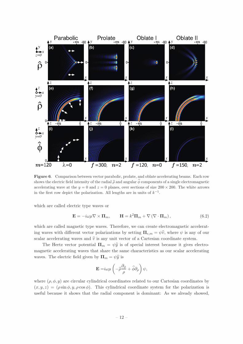
Figure 6. Comparison between vector parabolic, prolate, and oblate accelerating beams. Each row

shows the electric field intensity of the radial ρ and angular φ components of a single electromagnetic

accelerating wave at the y = 0 and z = 0 planes, over sections of size 200× 200. The white arrows

in the first row depict the polarization. All lengths are in units of k−1.

which are called electric type waves or

E = −iωµ∇×Πm, H = k2Πm +∇ (∇ ·Πm) , (6.2)

which are called magnetic type waves. Therefore, we can create electromagnetic accelerat-

ing waves with different vector polarizations by setting Πe,m = ψv, where ψ is any of our

scalar accelerating waves and v is any unit vector of a Cartesian coordinate system.

The Hertz vector potential Πm = ψy is of special interest because it gives electro-

magnetic accelerating waves that share the same characteristics as our scalar accelerating

waves. The electric field given by Πm = ψy is

E =iωµ

(−ρ∂φ

ρ+ φ∂ρ

)ψ,

where (ρ, φ, y) are circular cylindrical coordinates related to our Cartesian coordinates by

(x, y, z) = (ρ sinφ, y, ρ cos φ). This cylindrical coordinate system for the polarization is

useful because it shows that the radial component is dominant: As we already showed,

– 12 –

in the region of interest our scalar waves behave approximately as ψ ∼ F (ρ/k, y/k) eimφ.

Then ρ−1∂φψ ∼ imρ−1ψ, and because the maximum of ψ is around ρ ∼ m/k the amplitude

of the maximum of the radial component is approximately kψ. Now, ∂ρψ ∼ (F ′/F ) kψ and

F ′/F ≪ 1 around the main lobes of ψ. This allows us to show that the radial component ρ

is the dominant one. This behavior was confirmed by comparing both components numer-

ically. Hence, the polarization of the accelerating beams is perpendicular to the direction

of propagation that bends in a circle. Physically, this makes sense, since the polarization

must be perpendicular to the propagation direction of each plane-wave constituent of the

beam, and in the case of our accelerating electromagnetic waves the radial polarization is

always perpendicular to the direction of propagation of the whole wave packet that bends

in a circle. Figure 6 shows the radial and angular components of the electric field of several

accelerating electromagnetic waves at the x = 0 and z = 0 planes; notice that the radial

component preserves the shape and propagation characteristics of the scalar accelerating

waves.

7 Conclusion

To summarize, we presented a general theory of three-dimensional nonparaxial accelerating

electromagnetic waves, displaying a large variety of transverse distributions. These waves

propagate along a semicircular trajectory while maintaining an invariant shape. In their

scalar form, these waves are exact time-harmonic solutions of the wave equation; therefore

they have implications to many linear wave systems in nature such as sound, elastic and

electron waves. Moreover, in their electromagnetic form, these families of waves span

the full vector solutions of the Maxwell equations, in several different representations,

each family presenting a different basis for this span. By using the angular spectrum of

parabolic, oblate and prolate spheroidal fields, we gave a classification and characterization

of the possible transverse shape distributions of these waves. As a final point, because our

accelerating waves are nonparaxial, they can bend to steep angles and have features of

the order of the wavelength; characteristics that are necessary and desirable in areas like

nanophotonics, plasmonics, and micro-particle manipulation.

8 Acknowledgments

MAA acknowledges support from the National Science Foundation (PHY-1068325). MAB

acknowledge useful correspondence with W. Miller Jr.

References

[1] G. A. Siviloglou and D. N. Christodoulides, “Accelerating finite energy Airy beams,” Opt.

Lett. 32, 979–981 (2007).

[2] G. A. Siviloglou, J. Broky, A. Dogariu, and D. N. Christodoulides, “Observation of

accelerating Airy beams,” Phys. Rev. Lett. 99, 213901 (2007).

[3] J. Baumgartl, G. M. Hannappel, D. J. Stevenson, D. Day, M. Gu, and K. Dholakia, “Optical

redistribution of microparticles and cells between microwells,” Lab Chip 9, 1334–1336 (2009).

– 13 –

[4] P. Polynkin, M. Kolesik, J. V. Moloney, G. A. Siviloglou, and D. N. Christodoulides, “Curved

plasma channel generation using ultraintense Airy beams,” Science 324, 229–232 (2009).

[5] T. Ellenbogen, N. Voloch-Bloch, A. Ganany-Padowicz, and A. Arie, “Nonlinear generation

and manipulation of Airy beams,” Nature Photonics 3, 395–398 (2009).

[6] N. Voloch-Bloch, Y. Lereah, Y. Lilach, A. Gover, and A. Arie, “Generation of electron Airy

beams,” Nature 494, 331–335 (2013).

[7] A. Minovich, A. Klein, N. Janunts, T. Pertsch, D. Neshev, and Y. Kivshar, “Generation and

Near-Field imaging of Airy surface plasmons,” Physical Review Letters 107, 116802 (2011).

[8] A. Mathis, F. Courvoisier, L. Froehly, L. Furfaro, M. Jacquot, P. A. Lacourt, and J. M.

Dudley, “Micromachining along a curve: Femtosecond laser micromachining of curved

profiles in diamond and silicon using accelerating beams,” Applied Physics Letters 101,

071110 (2012).

[9] A. Chong, W. H. Renninger, D. N. Christodoulides, and F. W. Wise, “Airy–Bessel wave

packets as versatile linear light bullets,” Nature photonics 4, 103–106 (2010).

[10] D. Abdollahpour, S. Suntsov, D. G. Papazoglou, and S. Tzortzakis, “Spatiotemporal Airy

light bullets in the linear and nonlinear regimes,” Phys. Rev. Lett. 105, 253901 (2010).

[11] I. Kaminer, Y. Lumer, M. Segev, and D. N. Christodoulides, “Causality effects on

accelerating light pulses,” Opt. Express 19, 23132–23139 (2011).

[12] I. Kaminer, M. Segev, and D. N. Christodoulides, “Self-accelerating self-trapped optical

beams,” Phys. Rev. Lett. 106, 213903 (2011).

[13] I. Dolev, I. Kaminer, A. Shapira, M. Segev, and A. Arie, “Experimental observation of

self-accelerating beams in quadratic nonlinear media,” Phys. Rev. Lett. 108, 113903 (2012).

[14] Y. Hu, Z. Sun, D. Bongiovanni, D. Song, C. Lou, J. Xu, Z. Chen, and R. Morandotti,

“Reshaping the trajectory and spectrum of nonlinear Airy beams,” Opt. Lett. 37, 3201–3203

(2012).

[15] R. Bekenstein and M. Segev, “Self-accelerating optical beams in highly nonlocal nonlinear

media,” Opt. Express 19, 23706–23715 (2011).

[16] M. A. Bandres, “Accelerating parabolic beams,” Opt. Lett. 33, 1678–1680 (2008).

[17] J. A. Davis, M. J. Mintry, M. A. Bandres, and D. M. Cottrell, “Observation of accelerating

parabolic beams,” Opt. Express 16, 12866–12871 (2008).

[18] M. A. Bandres, “Accelerating beams,” Opt. Lett. 34, 3791–3793 (2009).

[19] M. V. Berry and N. L. Balazs, “Nonspreading wave packets,” Am. J. Phys. 47, 264–267

(1979).

[20] I. Kaminer, R. Bekenstein, J. Nemirovsky, and M. Segev, “Nondiffracting accelerating wave

packets of Maxwell’s equations,” Phys. Rev. Lett. 108, 163901 (2012).

[21] F. Courvoisier, A. Mathis, L. Froehly, R. Giust, L. Furfaro, P. A. Lacourt, M. Jacquot, and

J. M. Dudley, “Sending femtosecond pulses in circles: highly nonparaxial accelerating

beams,” Opt. Lett. 37, 1736–1738 (2012).

[22] I. Kaminer, E. Greenfield, R. Bekenstein, J. Nemirovsky, M. Segev, A. Mathis, L. Froehly,

F. Courvoisier, and J. M. Dudley, “Accelerating beyond the horizon,” Opt. Photon. News

23, 26–26 (2012).

– 14 –

[23] M. A. Bandres and B. M. Rodrıguez-Lara, “Nondiffracting accelerating waves: Weber waves

and parabolic momentum,” New Journal of Physics 15, 013054 (2013).

[24] P. Zhang, Y. Hu, T. Li, D. Cannan, X. Yin, R. Morandotti, Z. Chen, and X. Zhang,

“Nonparaxial Mathieu and Weber accelerating beams,” Phys. Rev. Lett. 109, 193901 (2012).

[25] P. Aleahmad, M.-A. Miri, M. S. Mills, I. Kaminer, M. Segev, and D. N. Christodoulides,

“Fully vectorial accelerating diffraction-free Helmholtz beams,” Phys. Rev. Lett. 109, 203902

(2012).

[26] M. A. Alonso and M. A. Bandres, “Spherical fields as nonparaxial accelerating waves,” Opt.

Lett. 37, 5175–5177 (2012).

[27] I. Kaminer, J. Nemirovsky, and M. Segev, “Self-accelerating self-trapped nonlinear beams of

Maxwell’s equations,” Opt. Express 20, 18827–18835 (2012).

[28] P. Zhang, Y. Hu, D. Cannan, A. Salandrino, T. Li, R. Morandotti, X. Zhang, and Z. Chen,

“Generation of linear and nonlinear nonparaxial accelerating beams,” Opt. Lett. 37,

2820–2822 (2012).

[29] C. P. Boyer, E. G. Kalnins, and W. Miller Jr, “Symmetry and separation of variables for the

Helmholtz and Laplace equations,” Nagoya Math. J 60, 3580 (1976).

[30] L.-W. Li, M.-S. Leong, T.-S. Yeo, P.-S. Kooi, and K.-Y. Tan, “Computations of spheroidal

harmonics with complex arguments: A review with an algorithm,” Phys. Rev. E 58,

6792–6806 (1998).

[31] J. Stratton, Electromagnetic theory, vol. 33 (Wiley-IEEE Press, 2007).

– 15 –

This figure "FigCoordinates300.jpg" is available in "jpg" format from:

http://de.arxiv.org/ps/1303.6320v1

This figure "FigF300.jpg" is available in "jpg" format from:

http://de.arxiv.org/ps/1303.6320v1

This figure "FigOblate300.jpg" is available in "jpg" format from:

http://de.arxiv.org/ps/1303.6320v1

This figure "FigParabolic300.jpg" is available in "jpg" format from:

http://de.arxiv.org/ps/1303.6320v1

This figure "FigProlate300.jpg" is available in "jpg" format from:

http://de.arxiv.org/ps/1303.6320v1

This figure "FigVector300.jpg" is available in "jpg" format from:

http://de.arxiv.org/ps/1303.6320v1