This thesis has been submitted in fulfilment of the ... - CiteSeerX

This thesis has been submitted in fulfilment of the requirements for a postgraduate degree

(e.g. PhD, MPhil, DClinPsychol) at the University of Edinburgh. Please note the following

terms and conditions of use:

• This work is protected by copyright and other intellectual property rights, which are

retained by the thesis author, unless otherwise stated.

• A copy can be downloaded for personal non-commercial research or study, without

prior permission or charge.

• This thesis cannot be reproduced or quoted extensively from without first obtaining

permission in writing from the author.

• The content must not be changed in any way or sold commercially in any format or

medium without the formal permission of the author.

• When referring to this work, full bibliographic details including the author, title,

awarding institution and date of the thesis must be given.

Engineering Value, Engineering Risk:What Derivatives Quants Know and

What Their Models Do

Taylor C. Spears

Doctor of Philosophy in SociologyThe University of Edinburgh

2014

Abstract

This thesis examines the ‘evaluation culture’ of derivatives ‘quants’ working in the over-the-

counter markets for interest rate derivatives tied to Libor. Drawing on data from interviews

with quants, financial mathematicians, and economists conducted primarily in the United

Kingdom and the United States, combined with fieldwork at derivatives ‘quant’ conferences

and an extensive set of technical sources, this thesis explores the historical development and

contemporary patterning of modelling practices that are used within derivatives dealer banks

to price and hedge Libor-based interest rate derivatives. Moreover, this thesis uses the histor-

ical development of interest-rate modelling techniques, beginning in the late 1970s, as a lens

through which to understand the establishment, differentiation and separation of this ‘deriva-

tives quant’ evaluation culture as a body of knowledge and practice distinct from financial

economics.

The analysis is carried out in nine chapters. The thesis begins with an introductory chap-

ter, a chapter reviewing the relevant sociological and historical literature on economic and

financial modelling, and a chapter covering the research methodology employed in the thesis.

In Chapters 4-5, I provide background on the mathematical techniques used by derivatives

quants and financial economists, the social and institutional structure of the Libor derivatives

markets, and the instruments that are traded in these markets. In Chapter 6, I explore the

organisational patterning of modelling practices in these markets and highlight the tacit and

experiential nature of quant expertise. In Chapters 7-8, I investigate the ‘social shaping’ of

models that are currently used to price so-called ‘exotic’ Libor derivatives. These models orig-

inated within the discipline of economics and were designed for a set of purposes different

from models currently used by derivatives quants. By tracing out how these models were

adapted to serve as derivatives pricing ‘engines’ within banks, I highlight how modelling

practices are shaped by the organisational contexts in which they are used.

Declaration

I declare that this thesis was composed by myself and that the work contained therein is myown, except where explicitly indicated otherwise in the text.

(Taylor C. Spears)

To Cheryl and Ron. In Memory of Doreen.

Most academic training narrows the viewpoint and reinforces the single wayof seeing that is the trademark of the discipline. [...] Sociologists don’t knowanything in quite this way; they only know how it is to know. The sociologistis promiscuous, experiencing many loves without ever falling in love. This isneither a happy nor an endearing state. But while promiscuity is not a recipe forlove, it is for education. A well-educated person is not just a faithful specialistbut one who knows how to take another’s point of view – even to invade another’sworld of knowledge.

Harry Collins and Steven Yearley

in Science as Practice and Culture (1992)

I really must say that you are an ignorant person, friend Greybeard, if you knownothing of this enigmatic business which is at once the fairest and most deceitfulin Europe, the noblest and the most infamous in the world, the finest and themost vulgar on earth. It is a quintessence of academic learning and a paragon offraudulence; it is a touchstone for the intelligent and a tombstone for the auda-cious, a treasury of usefulness and a source of disaster...

Joseph de la Vega

in Confusión de Confusiones (1688)

Acknowledgements

One incurs many debts of gratitude to a variety of individuals and organisations as a doctoral

student. Time and money become scarce resources, and I am grateful to the College of Hu-

manities and Social Sciences of the University of Edinburgh and the Scottish Funding Council

for giving me the resources to focus on my research during these last several years. Many

of the research expenses associated with this thesis were also funded by the UK Economic

and Social Research Council (RES-598-25-0054) and the European Union’s Seventh Framework

Programme (FP7/2007-2013/ERC grant agreement no. 291733), and this type of project would

not have been possible were it not for these sources of support.

I am extremely grateful to Donald MacKenzie and Riccardo Rebonato for supervising this

thesis. Donald oversaw this project from the start and has been an ideal supervisor through-

out. His influence on my intellectual and professional development over these past three years

has been tremendous, and he will continue to serve as a model of scholarship long after this

thesis has been submitted. He gave me the freedom and patience to develop my ideas and

thereby grow more fully into an independent researcher, and his careful feedback has made

me into a more rigorous academic and a better writer. Riccardo’s own work on the history of

interest rate modelling served as initial inspiration for this project, and I am extremely grate-

ful for his willingness to be involved as an external supervisor. As a quant and former trader,

Riccardo pushed me to engage more rigorously with the mathematical content of interest rate

modelling. He is also a keen observer of the social and organisational dynamics surrounding

the use of models within banks and helped me see the financial forest for the binomial trees.

This research project would not have been possible without the willingness of my inter-

viewees to patiently explain their world and the work they do to an outsider such as myself.

Unfortunately, anonymity precludes full recognition of these individuals.

The world of quantitative finance can also be inaccessible to an outsider due to the some-

times prohibitive cost of gaining access to research materials and field sites. I am particularly

indebted to ICBI and Marie Houghton for providing me with access to Global Derivatives

conference series in 2012 and 2013 at reduced cost. I am also grateful to Miklos Rasonyi and

Sotirios Sabanis in Edinburgh’s mathematics department for allowing me to attend their lec-

tures on financial mathematics. A number of friends – namely Charlie Tafoya, Nicole Turcotte,

x Acknowledgements

Val Gueco, Devin Mauney, and Brittany Jordan – graciously hosted me during various research

trips abroad to the U.S., without whom this project would have been cost prohibitive.

I am also fortunate to have made new friends during my time at Edinburgh, who have been

a source of companionship and intellectual camaraderie during these past several years. Alex

Hensby’s weekly salon nights and its regular attendees – Alex himself, Kim Abbott, Fritz Eier-

danz, Bram Mueleman, Mike Slaven, and Chi-Chung Wang – helped me grow intellectually

as a sociologist while also giving me a refuge from my research. Mike and Alex have become

particularly close friends during these past several years, and I’ve enjoyed our numerous con-

versations over drinks and coffee. I am also grateful to Michael Kattirtzi who helped make me

feel at home in the science studies department and who has been a good friend to me as well.

The informal ‘social studies of finance’ research groups in Edinburgh, London, and New York

have also been a source of intellectual stimulation and moral support. I am particularly grate-

ful to Tim Johnson, Martha Poon, Aina Begim for both their friendship and their willingness

to exchange ideas and offer candid feedback about my work during the writing-up stage.

The journey that led to this thesis began long before I arrived in Edinburgh to begin my

PhD, and in that time I have become indebted to a number of individuals who have played an

important role in shaping my intellectual development. My first opportunity to engage deeply

with the social studies of finance came while I was a masters student while on a Fulbright

scholarship at SPRU. I am quite certain that without Janet Burke and Ted Humphrey’s tireless

encouragement and assistance in developing my Fulbright application, my academic career

would likely have taken a very different path. I am indebted to Paul Nightingale and Ed

Steinmueller for supervising me during my time at SPRU, first as an MSc student and later

as a research fellow. Since I have left SPRU, Paul has continued to be fantastically supportive

of my work, and I owe an enormous debt of gratitude to him. While an undergraduate at

ASU, the faculty at CSPO helped me begin developing my current interests. Jamey Wetmore

had the foresight to encourage me to read up on the social studies of finance literature. I

eventually took his advice, several years later and a continent away. Dan Sarewitz’s seminar

on ‘uncertainty and decision making’ first prompted me to think about economic modelling

as a subject for social science research, while Mike Crow and Dave Guston helped make me

attentive to how scientists – both working in public laboratories and private corporations –

continually reshape our world. All of these influences are present in this thesis, and there are

others still.

I feel incredibly lucky to have had Celeste Berteau’s love and support during the last two

years, and am grateful for her constant willingness to talk through and offer feedback on my

ideas and writing. I can’t wait to continue building a life together during this upcoming year.

Lastly, I am forever grateful to my parents, Ron Spears and Cheryl Clancy, who have un-

failingly encouraged and supported my intellectual development and ambitions every step of

the way.

Contents

Abstract i

Acknowledgements ix

I Preliminary Material 3

1 Introduction 5

1.1 Focus and Aims of the Thesis . . . . . . . . . . . . . . . . . . . . . . . . . . . . . 9

1.2 Structure of the Thesis . . . . . . . . . . . . . . . . . . . . . . . . . . . . . . . . . 12

2 Literature Review 15

2.1 Economic Sociology and the Study of Markets . . . . . . . . . . . . . . . . . . . 15

2.2 The ‘Performativity’ of Economics . . . . . . . . . . . . . . . . . . . . . . . . . . 18

2.2.1 Evidence of Performativity . . . . . . . . . . . . . . . . . . . . . . . . . . 18

2.2.2 Critiques of Performativity . . . . . . . . . . . . . . . . . . . . . . . . . . 21

2.2.3 Recent Work on Economics and Economic Modelling . . . . . . . . . . . 24

2.2.4 Evaluation ‘Cultures’ in Finance . . . . . . . . . . . . . . . . . . . . . . . 27

2.3 The ‘Shaping’ of Financial and Economic Models . . . . . . . . . . . . . . . . . . 30

2.3.1 How Economists Use Models . . . . . . . . . . . . . . . . . . . . . . . . . 31

2.3.2 Models as Technological Systems . . . . . . . . . . . . . . . . . . . . . . . 32

2.4 Conclusion . . . . . . . . . . . . . . . . . . . . . . . . . . . . . . . . . . . . . . . . 34

3 Research Design and Methodology 35

3.1 ‘Identical twins separated at birth’ . . . . . . . . . . . . . . . . . . . . . . . . . . 35

3.2 Acquiring Interactional Expertise . . . . . . . . . . . . . . . . . . . . . . . . . . . 38

3.3 Interview Structure and Sampling Strategy . . . . . . . . . . . . . . . . . . . . . 43

3.4 Description of Data . . . . . . . . . . . . . . . . . . . . . . . . . . . . . . . . . . . 46

3.4.1 Interview Data . . . . . . . . . . . . . . . . . . . . . . . . . . . . . . . . . 46

3.4.2 Documentary Sources . . . . . . . . . . . . . . . . . . . . . . . . . . . . . 48

3.4.3 Quant Conferences . . . . . . . . . . . . . . . . . . . . . . . . . . . . . . . 48

xii Contents

4 No-Arbitrage Pricing Theory: An Overview 51

4.1 Arbitrage . . . . . . . . . . . . . . . . . . . . . . . . . . . . . . . . . . . . . . . . . 53

4.2 Martingale Pricing Theory . . . . . . . . . . . . . . . . . . . . . . . . . . . . . . . 54

4.3 A Simplified Explanation . . . . . . . . . . . . . . . . . . . . . . . . . . . . . . . 56

4.4 Replication . . . . . . . . . . . . . . . . . . . . . . . . . . . . . . . . . . . . . . . . 59

4.5 Summary . . . . . . . . . . . . . . . . . . . . . . . . . . . . . . . . . . . . . . . . . 63

4.6 Derivatives Quants vs. Financial Economists . . . . . . . . . . . . . . . . . . . . 64

II The Derivatives Quant ‘Evaluation Culture’ 67

5 Overview of the ‘Over-the-Counter’ Markets for Libor Derivatives 69

5.1 Libor Derivatives and the Financial Markets . . . . . . . . . . . . . . . . . . . . 70

5.2 Overview of Libor Derivatives . . . . . . . . . . . . . . . . . . . . . . . . . . . . 72

5.2.1 Linear Products . . . . . . . . . . . . . . . . . . . . . . . . . . . . . . . . . 73

5.2.2 Vanilla Options . . . . . . . . . . . . . . . . . . . . . . . . . . . . . . . . . 75

5.2.3 Exotic Libor Derivatives . . . . . . . . . . . . . . . . . . . . . . . . . . . . 77

5.3 Market Structure . . . . . . . . . . . . . . . . . . . . . . . . . . . . . . . . . . . . 80

5.4 Why Do Traders at Dealer Banks Use No-Arbitrage Models? . . . . . . . . . . . 83

5.4.1 To Design Hedging Strategies . . . . . . . . . . . . . . . . . . . . . . . . . 83

5.4.2 To Produce Risk Sensitivities, a.k.a. ‘Greeks’ . . . . . . . . . . . . . . . . 84

5.4.3 ‘Marking to Market’ and ‘Marking to Model’ . . . . . . . . . . . . . . . . 86

5.5 Derivatives Quants: The Model Builders and Developers . . . . . . . . . . . . . 93

5.6 Conclusion . . . . . . . . . . . . . . . . . . . . . . . . . . . . . . . . . . . . . . . . 97

6 The Organisational Patterning of Quant Modelling Activities 99

6.1 ‘Model Objects’ and ‘Modelling Practices’ . . . . . . . . . . . . . . . . . . . . . . 101

6.1.1 ‘Model Objects’ . . . . . . . . . . . . . . . . . . . . . . . . . . . . . . . . . 101

6.1.2 ‘Modelling Practices’ . . . . . . . . . . . . . . . . . . . . . . . . . . . . . . 105

6.2 The Linear Products Desk: A ‘Price Maker’ in Rates . . . . . . . . . . . . . . . . 108

6.2.1 Forward Libor and Swap Curves . . . . . . . . . . . . . . . . . . . . . . . 108

6.2.2 The Discount Curve . . . . . . . . . . . . . . . . . . . . . . . . . . . . . . 109

6.2.3 Forward Curves and Discount Curves as Tools for ‘Distributed Cognition’119

6.3 The Vanilla Options Desk: a ‘Price Taker’ in Rates; a ‘Price Maker’ in ‘Volatility’ 120

6.3.1 Historical Path Dependence and the Black Model . . . . . . . . . . . . . 121

6.3.2 ‘Implied Vols’ and the Communicative Practices of Options Traders . . 125

6.3.3 The SABR Model and the lasting influence of the Black Model . . . . . . 128

6.4 The Exotics Desk: a ‘Price Taker’ in Both Rates and Volatility . . . . . . . . . . . 130

6.4.1 Global vs. Local Calibration . . . . . . . . . . . . . . . . . . . . . . . . . . 132

Contents xiii

III The ‘Social Shaping’ of Interest Rate Term Structure Models 137

7 From Explanation to Calculation: The Reshaping of ‘Short Rate’ Models 139

7.1 Equilibrium Term Structure Modelling and the Expectations Hypothesis . . . . 141

7.2 Modelling Interest Rates in Simulated Economies . . . . . . . . . . . . . . . . . 152

7.3 Adapting Term Structure Models for the Derivatives Markets . . . . . . . . . . 155

7.4 From ‘Small Worlds’ to Pricing Infrastructure . . . . . . . . . . . . . . . . . . . . 165

7.5 Conclusion . . . . . . . . . . . . . . . . . . . . . . . . . . . . . . . . . . . . . . . . 172

8 Homology, Path Dependence, and the Reshaping of the HJM Framework 175

8.1 Let’s ‘throw away this whole general equilibrium concept and apply the Black

and Scholes concept to price bonds’ . . . . . . . . . . . . . . . . . . . . . . . . . 176

8.2 A Cultural Break . . . . . . . . . . . . . . . . . . . . . . . . . . . . . . . . . . . . 180

8.3 The ‘HJM Revolution’ . . . . . . . . . . . . . . . . . . . . . . . . . . . . . . . . . 182

8.4 HJM’s Adoption and Impact . . . . . . . . . . . . . . . . . . . . . . . . . . . . . . 187

8.5 HJM’s Incompatibilities with Market Practices . . . . . . . . . . . . . . . . . . . 194

8.6 The Libor and Swap ‘Market Models’ . . . . . . . . . . . . . . . . . . . . . . . . 195

8.7 “It’s quite a nice intuitive idea because that corresponds a lot to the way that

derivatives are priced in practice.” . . . . . . . . . . . . . . . . . . . . . . . . . . 197

8.8 Non-Markovian Modelling Finds its Commercial Niche . . . . . . . . . . . . . . 201

8.9 Conclusion . . . . . . . . . . . . . . . . . . . . . . . . . . . . . . . . . . . . . . . . 206

9 Conclusion 207

9.1 Summary of the Thesis . . . . . . . . . . . . . . . . . . . . . . . . . . . . . . . . . 207

9.2 Intellectual Contribution . . . . . . . . . . . . . . . . . . . . . . . . . . . . . . . . 209

9.3 Limitations and Directions for Future Research . . . . . . . . . . . . . . . . . . . 211

9.3.1 Do Traders Have an Evaluation Culture? . . . . . . . . . . . . . . . . . . 211

9.3.2 The Boundaries of the Derivatives Quant Evaluation Culture . . . . . . 211

A Primer on Continuous-Time Stochastic Processes 215

A.1 A Discrete-Time Introduction . . . . . . . . . . . . . . . . . . . . . . . . . . . . . 216

A.2 Moving to Continuous Time . . . . . . . . . . . . . . . . . . . . . . . . . . . . . . 219

A.3 Defining the Wiener Process . . . . . . . . . . . . . . . . . . . . . . . . . . . . . . 220

A.4 Changing Probability Measures . . . . . . . . . . . . . . . . . . . . . . . . . . . . 222

B List of Interviewees 225

Abbreviations and Mathematical Notation 227

Glossary 229

xiv Contents

Source Material 235

References 243

List of Figures

2.1 Evaluation cultures vs. organisations . . . . . . . . . . . . . . . . . . . . . . . . . 27

3.1 Modelling lineage . . . . . . . . . . . . . . . . . . . . . . . . . . . . . . . . . . . . 37

4.1 No-arbitrage pricing theory . . . . . . . . . . . . . . . . . . . . . . . . . . . . . . 53

4.2 A simple model with two assets . . . . . . . . . . . . . . . . . . . . . . . . . . . . 57

4.3 A simple model with three assets . . . . . . . . . . . . . . . . . . . . . . . . . . . 61

5.1 Libor interest rate calculation . . . . . . . . . . . . . . . . . . . . . . . . . . . . . 72

5.2 Payoff profile: caps and payer swaptions . . . . . . . . . . . . . . . . . . . . . . 78

5.3 Payoff profile: floors and receiver swaptions . . . . . . . . . . . . . . . . . . . . 78

5.4 Payoff profile: straddles . . . . . . . . . . . . . . . . . . . . . . . . . . . . . . . . 78

5.5 Participants in the Libor derivatives market . . . . . . . . . . . . . . . . . . . . . 81

5.6 A P&L Explain report . . . . . . . . . . . . . . . . . . . . . . . . . . . . . . . . . . 88

5.7 A dealer’s swaption book . . . . . . . . . . . . . . . . . . . . . . . . . . . . . . . 91

6.1 Trading floor . . . . . . . . . . . . . . . . . . . . . . . . . . . . . . . . . . . . . . . 102

6.2 ‘Stripping’ a discount curve . . . . . . . . . . . . . . . . . . . . . . . . . . . . . . 112

6.3 Hull-White model calibration . . . . . . . . . . . . . . . . . . . . . . . . . . . . . 134

7.1 Vasicek model applied to U.S. Treasury yields . . . . . . . . . . . . . . . . . . . . 149

7.2 Pricing a callable bond with the Vasicek model . . . . . . . . . . . . . . . . . . . 151

7.3 Black-Derman-Toy model calibration . . . . . . . . . . . . . . . . . . . . . . . . . 160

7.4 A Hull-White trinomial tree . . . . . . . . . . . . . . . . . . . . . . . . . . . . . . 164

8.1 Movement of the discount curve in the Ho-Lee model . . . . . . . . . . . . . . . 179

8.2 Perturbation functions in the Ho-Lee model . . . . . . . . . . . . . . . . . . . . . 179

8.3 Historical forward rate curve movements . . . . . . . . . . . . . . . . . . . . . . 185

8.4 Recombining lattices vs. non-recombining trees . . . . . . . . . . . . . . . . . . 189

A.1 Comparison of historical yields on U.S. Treasuries with a discrete-time stochas-

tic process . . . . . . . . . . . . . . . . . . . . . . . . . . . . . . . . . . . . . . . . 218

xvi List of Figures

A.2 Illustration of conditional expectation . . . . . . . . . . . . . . . . . . . . . . . . 219

List of Tables

5.1 Cashflows of a fixed/floating interest rate swap . . . . . . . . . . . . . . . . . . 75

5.2 Rights and obligations of caps and floors . . . . . . . . . . . . . . . . . . . . . . 76

5.3 Rights and obligations of payer and receiver swaptions . . . . . . . . . . . . . . 77

5.4 Level 2 and Level 3 assets . . . . . . . . . . . . . . . . . . . . . . . . . . . . . . . 90

6.1 A forward swap curve . . . . . . . . . . . . . . . . . . . . . . . . . . . . . . . . . 109

6.2 A discount curve . . . . . . . . . . . . . . . . . . . . . . . . . . . . . . . . . . . . 111

6.3 Implied volatilities for at-the-money swaptions . . . . . . . . . . . . . . . . . . . 127

A.1 Comparison of discrete and continuous-time processes . . . . . . . . . . . . . . 221

B.1 Interviewee Sample A: Derivatives Quants (Non-Attributable) . . . . . . . . . . 225

B.2 Interviewee Sample B: Historical Interviewees (Attributable) . . . . . . . . . . . 226

B.3 Interviewee Sample C: Non-Quant Individuals with Extensive Knowledge of

the OTC Derivatives Markets (Non-Attributable) . . . . . . . . . . . . . . . . . . 226

Part I

Preliminary Material

Chapter 1

Introduction

A rocket scientist in faculty slang is not a scientist who works on rockets. Wernher vonBraun was another kind of rocket scientist all together. “A rocket scientist”, I am informedby Ray Healey, Jr. of Forbes Magazine, “is an academic superstar, especially in math andthe physical sciences, who is lured away from the hallowed halls to work on Wall Street.”By putting their number-crunching to work on less-academic pursuits, these former theo-reticians devise stratagems for making money in great bundles. “Apparently, zero-couponbonds are an example of a new investment vehicle created by a rocket scientist,” Mr.Healey said. Thus quants, or rocket scientists, are great brains drained off campus by thebusiness world.

“On Language” by William Safire (1986) in the New York Times

PRIOR TO THE MID-1980S, a financial institution would have been one of the very last

places an aspiring physicist or mathematician would have sought to build a career after

finishing a PhD. For much of the twentieth century, the world of high finance – particularly

its more prestigious varieties such as securities underwriting – was a relationship-based busi-

ness. Chernow (2001, pg. 519) describes The City of London of the 1950s as a place of “obsolete

splendor” where “self-respecting merchant bankers still wore bowler hats and carried furled

umbrellas; their reading glasses were always crescent-shaped” and where “junior men wore

stiff collars and were considered dangerously uppity if they let them soften.” Education in

this elite world meant attending the right schools, making the right friends, and developing

the habitus necessary to interact with executives from prominent corporations. Academics

were not entirely absent from the financial markets. Indeed, in 1949, a “a rather shy, schol-

arly journalist” with a PhD in sociology from Columbia University created what he called a

‘hedged fund’ (Brooks, 1998, pg. 142), the first of its kind. Moreover, physicists and math-

ematicians have a long history of interaction with private industry (c.f. Freeman and Soete,

1997; Rosenberg and Nelson, 1994), most commonly – but certainly not always1 – in corporate

1See: Bowker (1994) for a prominent example of industrial science performed outside of the laboratory.

6 Chapter 1

research and development labs. But the world of finance provided few, if any, opportunities

for serious scientific or mathematical work.

Although bankers were far from being ‘masters of the universe’ in the years following the

Second World War, research physicists working in academia and at national laboratories such

as Los Alamos in the United States came close. In his history of the physicist community in the

U.S., Kevles writes that the postwar generation “was dominated by physicists who seemed to

wear the ‘tunic of Superman’, in the phrase of a Life reporter, and stood in the spotlight of a

thousand suns” (Kevles, 1978, pg. 334). The Manhattan Project had transformed physicists

like J. Robert Oppenheimer into quasi-celebrities, while the growing spectre of the Cold War

made research in mathematics, nuclear physics and engineering a national priority. Physical

scientists and mathematicians found themselves awash with research funding from the fed-

eral government, even for ‘basic’ research that had no obvious military purpose. Invoking

the imagery of Manifest Destiny, Vannevar Bush – President Roosevelt’s science advisor – de-

clared in 1945 that science was a new, “endless frontier” for the country to explore.2 The U.S.

government, according to Bush, had previously “opened the seas to clipper ships and fur-

nished land for pioneers. Although these frontiers have more or less disappeared, the frontier

of science remains” (Bush, 1945, pg. 234). Broad public support ushered in a new era of ‘Big

Science’: big budgets, big experiments, and perhaps most importantly, big enrolments in PhD

programmes. In 1940, the number of physics PhDs awarded in the United States had never

exceeded more than 200 per year. By the mid 1960s, American research universities were pro-

ducing nearly 1,000 new physicists each year and the rate was growing quickly (Mulvey and

Nicholson, 2011).

Those halcyon days did not last, though. In the U.S., high inflation caused by Vietnam

spending and reduced growth in federal funding in the late 1960s and early 1970s combined

to create a substantial reduction in real funding for research; there was effectively a fifty per-

cent reduction in funding for high energy physics over a four year period beginning in 1970

(Kevles, 1978, pg. 421). Moreover, by the late 1960s, public support for science began to wane

as social and political priorities changed, particularly in the wake of an increasingly unpopu-

lar American war in Vietnam which had shed light on the influence of the ‘military-industrial

complex’ on the practice of academic science. Whereas it was once widely believed that ‘what

is good for science is good for the country’, Alvin Weinberg – then chief administrator of Oak

Ridge National Laboratory – was forced to concede in 1976 that research on “isobaric analog

states in nuclei won’t resolve racial tension in Detroit or religious tension in Belfast” (Kevles,

1978, pg. 425).

Two crucial developments in the 1970s would ultimately turn physicists and mathemati-

cians into prized commodities for banks and drive these individuals into Wall Street and the

City en masse. The first development was the emergence of severe inflation and high and2Dennis (2004) carefully examines the significance of this document and Bush’s intentions in writing it.

Introduction 7

volatile interest rates during the 1970s, the former of which was, coincidentally, one of the

major causes of a reduced federal budget for physics research.3 These forces combined to

make the profitability and status of working as a bond salesman or a trader – “people long

shunned as the rabble of the business” – grow considerably as fixed-income investors shifted

from a ‘buy and hold’ approach to investing to active portfolio management (Chernow, 2001,

pg. 585). With the growth of these markets came the need for more quantitative acumen on

the trading floor, especially as record yields and volatility made the favourite calculative appa-

ratus of bond traders – the ‘yield book’ – increasingly unusable. Salomon Brothers & Hutzler

– the most prominent bond firm in the United States in the late 1960s and one where nearly

half the partners at the time had never attended university (Lewis, 2010, pg. 41), chose to hire

Martin Leibowitz, its first PhD mathematician, after he finished his doctorate at New York

University in 1969 (Homer and Leibowitz, 2004, pg. xvi). Later, firms like Salomon Broth-

ers would create new types of financial instruments that investors, corporations, and banks

could use to protect themselves against – or speculate on – these changes in interest rates.

In the U.K., American investors had been depositing U.S. dollars into British banks at least

since the 1960s in an effort to evade ‘Regulation Q’, which since its enactment in 1933 placed

a cap on the interest paid on money deposited with U.S. banks (Friedman, 1971, pgs. 17-18).

British banks were, in turn, happy to receive deposits in U.S. dollars in part due to the pound’s

weak international position following World War II, especially following the 1957 sterling cri-

sis (MacKenzie, 2008). This market for ‘Eurodollars’ grew quickly in the wake of the 1973-4

oil crisis when many oil producing states chose to deposit significant amounts of their dollar-

denominated profits into London banks (Chisholm, 2009). Over time, the cost of borrowing

money in this market came to be represented by an interest rate known as the London In-

terbank Offered Rate (Libor), and by the early-to-mid 1980s a new set of financial products

emerged called ‘interest rate derivatives’ that were tied to the Libor rate.

The second development was intellectual, and originated in a handful of economics de-

partments and business schools in the United States. In 1973, Fischer Black, Myron Scholes,

and Robert C. Merton jointly developed a model for pricing European call options, a type

of derivative that gives the holder the right, but not the obligation, to buy an asset at a pre-

determined price on a future date (Black and Scholes, 1973; Merton, 1973b). Although the

Black-Scholes model was not the first options pricing model to be developed – indeed, work

on options pricing originated with a French mathematician named Louis Bachelier in 1900 – it

soon became popular on the nascent options exchange in Chicago and would be used to justify

and legitimate the practice of options trading, an activity that was widely regarded as a du-

bious form of gambling at the time (MacKenzie and Millo, 2003). Perhaps more importantly,

though, the Black-Scholes model provided a strategy for ‘synthesising’ options by trading in

the underlying stock, thus making it possible for a bank or trading firm to ‘make markets’ in3I credit Derman’s (2004) memoir for initially drawing my attention to this coincidence.

8 Chapter 1

options to clients in large volumes without, in principle, taking on a large amount of risk. Risk

could now be manufactured or engineered, rather than simply avoided or managed.

Emanuel Derman, a PhD-trained physicist who eventually moved to Wall Street in 1985

after he and his wife were unsuccessful in finding tenure-track academic positions in the same

city, emphasises in a recent memoir how Black-Scholes’ capacity for dynamic replication fun-

damentally altered the business of selling options:

Before the advent of the [Black-Scholes] model, a dealer who sold a call option to a clienthad to take the other side of the trade; the dealer then bore the risk, if the stock price wentup, of having to pay the client out of pocket. After the model’s dawn, a dealer could use itsrecipe to roll his or her own option out of stock and cash, and estimate the cost of doing so.The dealer could then sell the homemade option to the client, ideally being left with no riskat all. Options dealers soon began to use the Black-Scholes model to manufacture optionsout of raw stock and then sell them. Dealers charged a fee for this manufacture, just like anyother value-added reseller. (Derman, 2004, pg. 146)

Within the academy, the work of Black, Scholes and Merton turned options pricing into a hot

area of financial research, as economists sought to generalise their work to new applications

and contexts. Cox and Ross (1976) soon realised that the price of a variety of options could be

calculated by simply taking the discounted expectation of the option’s future payoff under a

special set of ‘risk-neutral’ probabilities. Later, Harrison and Kreps (1979); Harrison and Pliska

(1981) recast the idea of ‘risk-neutral’ pricing in the rigorous mathematical language of prob-

ability theory and martingales. These generalisations of the Black-Scholes model provided

a set of tools for pricing derivatives of many types – even new derivatives that had not yet

been invented – rather than the simple call options. Using these theories, however, required

many of the same mathematical tools that underlie the study of quantum physics. Thus while

Alvin Weinberg may have been correct that research on isobaric analog states in nuclei could

not resolve the major social issues of the day, the same tools and skills that mathematicians

and physicists had developed to study these phenomena became incredibly valuable – and

lucrative – to banks and other financial institutions.

The move of physicists and mathematicians from universities into banks parallels a broader,

century-long transformation in Western societies. On the one hand, ‘risk’ has been trans-

formed from an obscure concept used within the narrow field of marine insurance into an

organising concept of finance and society more broadly (c.f. Levy, 2012; Power, 2007). At

the same time, businesses and corporations in Western economies have become increasingly

‘financialised’, as profits have come to be accrued primarily through financial channels rather

than through trade or commodity production (Krippner, 2005). As the epigraph to this chapter

indicates, by the mid-1980s a new job description was beginning to enter the popular lexicon:

the ‘rocket scientist’ or ‘derivatives quant’. Early quants tended to be “retreads from other dis-

ciplines who could learn quickly, solve equations, and write [their] own programs”, according

to Emanuel Derman. But by the late 1990s this new community of ‘quants’ was “becoming a

discipline, a business, and a profession” of its own, complete with its own canonical textbooks,

Introduction 9

graduate programs, journals, and conferences (Derman, 2004, pg. 224). Today, this new ‘quant

profession’ is a fixture in the world of finance. The models and tools that quants build and

maintain are central not only to the day-to-day activities of traders, but also the governance of

those traders and even the financial institutions in which they work. Quant models are used

to assess the vulnerability of banks to financial shocks, and to levy capital charges on them ac-

cording to the riskiness of the assets and liabilities on their books. Perhaps most importantly,

though, quant models have become a key technology enabling the modern practice of ‘mark-

to-market’ accounting. Moreover, quants increasingly work outside banks, at institutions such

as hedge funds and pension funds, where their quantitative acumen is applied to developing

investment strategies rather than pricing derivatives that are sold to clients.

At the time the above epigraph was written, little was known about these apparently bril-

liant individuals by members of the public and even their former academic colleagues, other

than the fact that what they do is both complicated and well-compensated. Yet despite their

obvious significance within the global financial system in the present day, there has been re-

markably little social science or historical work on the quant community and how its models

are developed and used.4

1.1 Focus and Aims of the Thesis

This thesis builds upon existing work by MacKenzie and Spears (2014a,b) on the derivatives

quant ‘evaluation culture’, a term they use to characterise distinctive communities of evalua-

tion practice that span multiple financial institutions.5 In particular, the concept of ‘evaluation

culture’ is intended to capture the shared sets of beliefs among certain groups of financial mar-

ket practitioners about how financial assets ought to be valued, along with a set of shared con-

ceptual objects (‘an ontology’) around which evaluation practices are organised, and a set of

social processes by which those practices are shared and reproduced. In the case of derivatives

quants, this ‘evaluation culture’ is primarily centred around the practice of articulating, con-

structing, and maintaining mathematical models that, like the original Black-Scholes model,

are used by traders to ‘manufacture’ derivatives that are sold to clients. Moreover, it largely ex-

ists within a small set of financial institutions conventionally called ‘dealer banks’ that ‘make

markets’ in these instruments with client institutions such as corporations. It is these models,

used in this particular institutional context, which constitute the focus of this thesis.

4Notable exceptions include Lépinay’s (2011)’s ethnography of an equity derivatives trading floor at a French bank,which examines the role of quants within this organisation in some detail; however, quants and their models are notthe focus of his book. MacKenzie and Spears (2014a,b), on the other hand, examine the derivatives quant communityand the historical development and use of one model in particular: the Gaussian Copula model, which was originallydeveloped to value complex structured products such as the ABS CDOs that played a significant role in the 2008-2009financial crisis.

5‘Evaluation practice’ in this context means any practice that is concerned with assessing the (not necessarily mon-etary) worth of an object. Unlike Lamont (2012), whose recent review on the sociology of valuation and evaluationtends to differentiate between these two activities, I intend for the term ‘valuation practice’ to refer to a specific typeof evaluation wherein the worth of an object is assigned a price or monetary value.

10 Chapter 1

My focus is on models that derivatives quants build to price and hedge financial instru-

ments that are traded in a particular set of markets: those for ‘over-the-counter’ (OTC) deriva-

tives tied to Libor, a set of markets that are based predominantly in London.6 Since the 1980s,

this market has grown to become a central component of the global financial system, as cor-

porations, government entities, and financial institutions have come to rely on Libor deriva-

tives to both manage – and speculate on – changes in the cost of borrowing money in the

Eurocurrency markets. The markets for Libor derivatives are also some of the largest ‘over-

the-counter’ derivatives markets in existence. According to statistics provided by the Bank for

International Settlements, interest rate derivatives make up approximately eighty-one percent

of total notional issuance of OTC derivatives globally,7 while a recent trade-level analysis of

these markets conducted by Fleming et al. (2012) suggests that Libor derivatives make up the

majority of these contracts. Despite its relative size, as far as I am aware the only existing work

on these markets by a social scientist is Riles’s (2011) ethnographic study of the legal practices

employed in the ‘back office’ of a derivatives dealer operating in Japan. There has not been any

social science research that directly examines the modelling or valuation practices employed

in these markets.

This thesis examines the models and modelling practices employed by derivatives quants

from two distinctive vantage points. Within the first vantage point – which occupies part II of

this thesis – I provide a holistic picture of how modelling practices are employed by quants

who work at dealer banks that ‘make markets’ in the Libor derivatives market in the present

day. By closely examining the ways in which these models are used by various stakeholders

within dealer banks and the relationship between these practices and the organisational struc-

ture of these banks, I shed light on the social and technical processes that underpin trading in

these markets. We will see that modelling activities in these markets are organised around a

particular set of what I call ‘model objects’ which are produced by traders working at distinct

trading desks. I trace out how these ‘model objects’ circulate around the trading room while

reinforcing a cognitive division of labour between different trading desks within banks. I also

highlight a distinct set of practices referred to as ‘implied calibration’ by quants which they

use to connect these abstract models to market data. Finally, I draw attention to the largely

tacit body of knowledge that quants need to perform these practices.

The second vantage point is instead historical and occupies part III of this thesis. I pick

out one class of models that are used by quants to price and hedge so-called ‘exotic’ Libor

derivatives known as ‘interest rate term structure models’, and trace their development from

6I use the term ‘Libor derivative’ to generically refer to any contract that is tied to either one of the currency-specificLibor rates, the Euribor rate, or swaps written on these rates. London-based derivatives quants and traders often referto such contracts generically as ‘interest rate derivatives’. Throughout this thesis – and particularly in part II – I haveused the more specific term ‘Libor derivative’ to acknowledge that there are many interest rate derivatives contractsthat are traded in the financial markets whose practitioners use evaluation practices very different from those that Iexamine here; for instance, mortgage-related securities.

7Bank for International Settlements (June 2013) “Semiannual OTC derivatives statistics”. Retrieved 31 January2014, http://www.bis.org/statistics/dt1920a.csv.

Introduction 11

the late 1970s until the present day. As Galison (1997, pgs. 4-5) notes in his study of the

material culture of physics, as soon as one begins examining the development of the tools that

practitioners in an intellectual community use to produce knowledge, one inevitably traces

a path far outside the original centre of investigation: in his case, that investigation entailed

a journey outside the physics laboratory through fields as diverse as seismology and glass

blowing in sites as varied as Victorian Scotland and England and the Los Alamos National

Laboratory in New Mexico during World War II. Likewise, tracing the historical development

of these ‘interest rate term structure models’ will take us away from the City and Wall Street,

back into a set of economics departments and business schools in the United States. We will see

that these models were originally designed for a very different set of purposes and modelling

practices than are used by present-day derivatives quants.

By tracing how quants and financial mathematicians gradually reshaped these models into

tools that could be employed within the social and technical context described in part II,

the models themselves will serve as a technical microcosm through which to view a much

larger social development that has gone virtually unnoticed by social scientists: the establish-

ment and growth of communities of financial modellers that are distinct and separate from

economists and finance academics working in universities. As Morgan (2012) shows in a re-

cent book, modern academic economists build and use models according to a distinctive set

of rules and conventions that govern their use, and a set of normative criteria of what ‘good’

modelling entails. As she shows, models that are created and used in this community are de-

signed to be “small worlds” that contain “compressed” descriptions of real-world economic

processes. Academic economists are rarely interested in building models that can make accu-

rate predictions or that reflect the richness and complexity of the real world. Instead, models

in economics are used to express, at most, one or several economic processes in a highly car-

icatured manner that elucidates their economic significance. Derivatives pricing models, as I

show in this thesis, are rarely designed to be the ‘small, caricatured worlds’ that economists

prefer, but instead are meant to be tools for calculation. Moreover, they are evaluated by a

comparatively pragmatic set of criteria that is distinctive of the derivatives quant community:

namely, their capacity to produce ‘good hedges’ for a trader in a reasonable amount of time,

and their ability to ‘match’ or ‘reproduce’ a wide variety of observed prices seen in the market.

However, building models that are capable of doing these things requires a distinctive body

of knowledge – what I call ‘quant expertise’ – from that which is possessed by economists and

finance academics working in business schools.

Term structure models, as I demonstrate, have also been ‘shaped’ by factors other than

these explicit normative criteria. An old theme in sociology and structuralist anthropology

is the way in which classification systems come to reflect (be homologous to) the structure of

the society in which they are employed. Durkheim and Mauss famously argued that the cos-

mological beliefs of certain communities are shaped or “moulded, as it were, by the totemic

12 Chapter 1

organisation” (Durkheim et al., 1963, pg. 29). While contemporary social scientists recognise

that there are rather serious methodological problems with Durkheim and Mauss’s particular

case, the notion that the objects and tools used by a community reflect the community itself has

been a major theme in structuralist-influenced anthropology (c.f. Bourdieu, 1977). In chapter 8,

I provide tentative evidence of such a Durkheimian process: the popularity and influence of

the term structure models I examine in that chapter is at least partly due to the fact that the the-

oretical structure of these models is homologous to the market structure of Libor derivatives

trading and the organisational structure of many banks.

This distinction between the modelling ‘cultures’ of economics and derivatives quants can

potentially inform the recent literature on the ‘performativity’ of economics and economic

models. This concept, which was first articulated by Callon (1998a), refers to the capacity of

economic theories and models to not only describe and explain social and economic phenom-

ena, but to actively intervene, reformat and constitute forms of social and economic order.

Much of the subsequent performativity literature has implicitly treated ‘economics’ as a rel-

atively unified and homogeneous set of logics and practices revolving around the enactment

of Homo Economicus. The historical case studies that I provide in part III of this thesis instead

suggests the possibility of multiple epistemic ‘cultures’ – distinct from academic economics –

which engage in economic and financial modelling, along with a potential diversity of logics

and practices that these communities employ in the course of building and using models.

1.2 Structure of the Thesis

Although the subject of this thesis is unavoidably technical in nature, I have attempted to

structure it in such a way that it is possible to follow my line of argument without delving into

the technicalities of interest rate derivatives modelling. On the other hand, I do not completely

banish equations from the text, as the conceptual objects that are invoked in these equations

are central to the argument that I make in this thesis. Moreover, the technical jargon of quan-

titative finance and derivatives cannot be avoided entirely, and thus I have also included a

glossary and a summary of abbreviations and mathematical notation at the end of this thesis.

The reader should also bear in mind that the material I present in chapters 4 through 8 is cu-

mulative, with each chapter introducing a set of technical concepts that are used later in the

thesis.

The thesis consists of nine chapters, including this introduction, which are grouped into

three parts.

Chapter 2 continues part I of the thesis. In this chapter, I review the relevant literature from

economic sociology and science and technology studies on financial models and their relation-

ship to markets. Of particular importance is the recent body of work on the ‘performativity

of economics’ that I mentioned above. I examine this approach to the study of economics and

Introduction 13

markets, along with several prominent critiques and refinements of the performativity con-

cept. I also introduce existing historical and ethnographic work on the use of models within

the economics discipline.

Chapter 3 explains the methodology employed whilst researching this thesis and the data

that this thesis draws upon. This data include interviews, a large corpus of technical docu-

ments on interest rate modelling, and participant observation at derivatives quant conferences.

I also discuss some of the issues that arose during the research phase; in particular, the need

to acquire ‘interactional expertise’ in the area of financial mathematics and how I went about

accomplishing this.

Chapter 4, which concludes part I of the thesis, provides an introduction to the mathemat-

ical concepts that underlie no-arbitrage models, the family of models that includes all of the

models discussed in this thesis. I present the central concepts of these models using simple

mathematics; however, it is not strictly necessary for the reader to understand the material in

this chapter to follow the argument that I make in this thesis.

Chapter 5 begins part II of the thesis, which focusses on the ‘evaluation culture’ of deriva-

tives quants working in the Libor derivatives markets. This chapter introduces this culture by

describing the role and function of the Libor derivatives markets within the broader financial

system, the major types of derivatives that are traded in these markets, the institutional struc-

ture of these markets, and how and why no-arbitrage models are used by banks operating

within them. I also introduce the institutional role of derivatives ‘dealer banks’ within these

markets, and end the chapter by describing the activities of derivatives quants within these

banks.

Chapter 6 engages more deeply with the cognitive world of derivatives quants working

in the Libor derivatives markets, and the models they build and use. I introduce a family of

‘model objects’ and ‘modelling practices’ that organise quants’ modelling activities in these

markets, explain how they map onto the organisation structure of dealer banks, and highlight

how they enable a system of ‘distributed cognition’ between trading desks. This chapter pro-

vides a description of the sociotechnical context to which quants needed to ‘re-shape’ the term

structure models that are the focus of part III of the thesis.

Chapter 7 begins part III of the thesis. In this chapter, I examine the development of the

family of ‘short rate’ interest rate models by economists and financial academics beginning in

the late 1970s. These models, I claim, were initially designed to study the economy, and in

particular, the bond market. This entailed a certain style of modelling that was, unfortunately,

incompatible with the emerging modelling practices in the Libor derivatives markets. This

chapter traces how these models were gradually re-configured to work as tools of calculation

embedded within the information infrastructure of banks, and how this shift corresponded

with the development of a new form of ‘quant expertise’.

Chapter 8 examines the development of another family of interest rate models that were

14 Chapter 1

initially created by a group of academics who identified as mathematicians as much as they

did economists. These models were initially developed to address some of the shortcomings

of those I examine in chapter 7, but were later re-shaped into a set of ‘market models’ that

are deeply homologous both to the ‘model objects’ that I introduce in chapter 6, and to the

organisational division of labour between trading desks within dealer banks. However, a

material shortcoming of these models – their capacity to produce ‘good hedges’ quickly and

reliably – caused certain users to experience considerable losses during the recent financial

crisis.

Chapter 9 summarises the the major findings of the thesis, and discusses its contribution to

the existing sociological literature on economic and financial modelling. I also examine several

limitations of the research design I employed, and offer some directions for future research.

Chapter 2

Literature Review

THIS thesis examines the ‘evaluation culture’ of derivatives quants working in the Libor

derivatives markets, and how a set of models used to price ‘exotic’ Libor derivatives

were ‘reshaped’ to work within this evaluation culture. As such, this thesis makes a number

of contributions to the emerging sociological literatures on the ‘performativity of economics’

and financial modelling practices. The purpose of this chapter is, first, to review the existing

sociological and historical literature on performativity and economic modelling and position

this thesis within this body of existing work. Second, I introduce a number of concepts that

will be employed throughout the empirical portion of this thesis.

2.1 Economic Sociology and the Study of Markets

Sociologists can claim to be some of the earliest academics to take an empirical interest in mod-

ern financial markets; however, the systematic study of financial markets, and financial valua-

tion practices in particular, is a relatively recent development in the discipline’s history. While

Louis Bachelier’s (1900) study of speculation on the Paris Stock Exchange – Théorie de la spécu-

lation – is generally regarded by financial mathematicians as one of the founding documents of

their field (and indeed many of the mathematical techniques that the models discussed in this

thesis draw upon Bachelier’s thesis), Max Weber’s two pamphlets on the German stock and

commodity exchanges were actually published four and six years prior to it (Weber, 2000a,b).

Weber’s interest in these institutions was not merely confined to the broader importance and

effects on society: in addition, the second of these pamphlets contains rich descriptions about

the practice and operations of futures and stock trading, the processes of calculation used by

market participants, and so on.

During much of the twentieth century, however, empirical interest in marketplaces such

as financial exchanges faded within sociology and across the academy in general. Both Weber

and Bachelier’s interest in these institutions reflected their perceived social and political im-

16 Chapter 2

portance at the time: Weber, for instance, penned his two pamphlets on the stock and commod-

ity exchanges in order to contribute to a political debate within Germany over their regulation

(Lestition, 2000). Yet both Bachelier and Weber’s work largely failed to gain interest from each

of their respective disciplines. Bachelier’s thesis was not awarded the mark necessary for him

to attain a prestigious professorial appointment within French mathematics, in part due to its

lack of fit with other work in the discipline (Taqqu, 2001). While some of the mathematicians

who laid the groundwork for the mathematical techniques that underlie derivatives pricing

knew of his work (e.g. Kolmogorov, Doob and Ito), its importance to the study of finance and

economics was only rediscovered by economists such as Paul Samuelson in the 1960s (Jarrow

and Protter, 2004, pgs. 6-7).

For Weber, the use of calculation was an important characteristic of the process of ratio-

nalization, with monetary and financial calculation (e.g. capital budgeting) being associated

most closely with formal, bureaucratic rationality (Weber, 1968, pg. 86). Weber also believed

that modern society’s ability to “master all things by calculation” was an important cause of

society’s “disenchantment” and the elimination of magical thinking (Weber, 2009, pg. 139).

Despite its importance within Weber’s sociology, empirical work on calculation – particu-

larly economic and financial calculation – is notably absent in much of 20th century sociology.

Within sociology, empirical interest in economic calculation withered as the discipline came to

embrace an implicit jurisdictional demarcation between itself and the discipline of economics

that was not yet present in Weber’s time. In particular, many mid-century sociologists came

to implicitly embrace the view that modern economies are embedded within but distinct from

society, and are characterised by a set of distinctive logics and rationalities. Consequently,

economists should have intellectual jurisdiction over the workings of the economy and mar-

kets, whereas sociologists should instead focus on the broader macro-social system in which

economies are embedded.

Stark (2000) attributes this shift to the influence of Talcott Parsons, who tried to carve out a

distinct intellectual niche for sociology. Stark refers to the resulting demarcation as “Parsons’

Pact”. While Parsons’ highly theoretical functionalist sociology became increasingly unpopu-

lar during the 1970s (Joas and Knobl, 2009, pg. 93) and sociologists came to embrace a much

more critical attitude towards the rational-choice approaches used by economists, the implicit

jurisdictional demarcation that he set out between economics and sociology remained influen-

tial for many additional years. Moreover, during much of the 20th century, economics moved

in an increasingly formal and mathematised direction with little interest in real-world mar-

kets, while the study of finance remained a marginalised and low-status field of study within

business schools well into the 1950s (MacKenzie, 2006).

Across the academy, the shift away from interest in finance had a number of broader causes,

including the rise of managerial capitalism and large, hierarchical corporations (Chandler,

1977). For economists such as Coase (1937), the existence of such large forms of social organi-

Literature Review 17

sation was a paradox for economics to answer, and later economists such as Williamson (1973)

created a research programme to address the question of why so much economic activity is or-

ganised through managerial ‘hierarchies’ rather than bilateral trading through ‘markets’. The

theme of ‘markets vs. hierarchies’ came to shape a generation of thinking within sociology and

organisational theory as well: the influence of this perspective can be seen in Granovetter’s

(1985) critique of Williamson’s research programme, and subsequent attempt to find a middle

path between “oversocialised” and “undersocialised” accounts of economic action. However,

focus on the nature and existence of such ‘hierarchies’ among social scientists meant that mar-

ket institutions such as the stock and commodities exchanges that Weber had examined went

unstudied.

Beginning in the early 1980s, a new style of sociology emerged that began to challenge Par-

sons’ disciplinary demarcation, while at the same time the marketplace became a renewed area

of empirical interest. White’s (1981) work on production markets was a crucial development

in this respect. As Stark notes, White “turns the table” on Parsons’ Pact: “Markets, he argues,

are not simply embedded in social relations, they are social relations” (Stark, 2000, pg. 2). Unlike

Parsons who saw sociological theory as being a generalisation of economic theory, Stark notes

that White created the possibility of a sociological approach to the study of markets distinct

from economics. As a consequence, real-world markets came to be seen as legitimate subjects

of empirical sociological inquiry. Two empirical studies particularly exemplify this new ap-

proach to the study of the economic domain. In his study of the prices of options traded on an

options exchange in the United States, Baker (1984) showed that the structural properties of the

networks of traders participating in the market can significantly affect the volatility of options

traded in the market. Likewise, Zuckerman (1999) showed that the existence and organisation

of industry categories can shape the valuation of stocks, particularly those that do not cleanly

fit into established categories. Later, Zuckerman (2004) showed how such categories can also

drive the quantity of trading in particular stocks. Carruthers and Stinchcombe (1999) took this

line of inquiry a step further still. They showed that the existence of ‘liquidity’ in a financial

market – the ability to transact relatively large quantities of a particular instrument without

affecting its price – is a problem in the sociology of knowledge, as buyers and sellers must

possess a shared conviction about what counts as an identical good and must be able to en-

gage in what Espeland and Stevens (1998) call ‘commensuration’ between similar goods: that

is, compare them according to a common metric. Liquid markets are thus not a ‘naturally’

existing entity as economic theory traditionally assumes; instead, they must be constructed.

Doing so entails what Carruthers and Stinchcombe describe as “minting work”, which often

amounts to stripping away the distinctiveness and complexity of a particular object to turn it

into a standardised commodity.

18 Chapter 2

2.2 The ‘Performativity’ of Economics

A subtly different challenge to ‘Parsons’ Pact has come in the form of a research programme

around Michel Callon’s concept of the “performativity of economics”. Like Weber, Callon puts

the study of calculation at the centre of a sociology of markets (Callon, 1998b, pg. 3); however,

there is a crucial difference between Callon’s approach and previous approaches to the study

of markets. The major premise of Callon’s programme is that the models, techniques and the-

ories of economics (broadly interpreted to include related disciplines such as accounting and

management in addition to academic economics) do not merely describe a naturally existing

economy or a set of economic actors with predefined properties, but instead play a role in for-

matting, shaping, and even constructing these entities (Callon, 1998b, pg. 2). For Callon, the

important sociological question is not how economic actors behave “naturally”, but instead

how activities, behaviours and social domains become ‘economised’ and amenable to calcu-

lation and hence transformed into the realities that economic theory assumes to be natural

(Caliskan and Callon, 2009; Callon, 1998b, pg. 33). Economics is thus ‘performative’, accord-

ing to Callon, because it is a discourse that “contributes to the reality that it describes” (Callon,

2007c, pg. 315). Callon argues that with a performative statement – such as an economic model

– it is more appropriate to say that the world it represents or describes “becomes actual” rather

than ‘true’, since its truth value is not independent of its description. This representation or

description is made actual through a “long sequence of trial and error, reconfigurations and

reformulations” of “articulating, experimenting, and observing” (Callon, 2007c, pg. 320).

2.2.1 Evidence of Performativity

Of course, the idea that economics is performative is merely a hypothesis: it is ultimately an

empirical question whether and to what extent such a process of “reconfiguration and reformu-

lation” drives alignment between the social world and the models and theories of economics.

It is also not altogether clear from Callon’s description of the concept what performativity

means in practice. However, there does exist some tentative evidence of the performative ca-

pacity of economics and economic models which also clarifies its meaning. One prominent

example provided in a case study written by Guala (2007) is the use of game theory – a sub-

field of economics concerned with the study of strategic interactions between rational agents

– by economists working in conjunction with the U.S. Federal Communications Commission

(FCC). The FCC hired economists to develop a set of procedures for auctioning ‘wireless spec-

trum’ – contractual rights to broadcast at certain radio frequencies – to private corporations,

such as telecommunications providers. Auctioning wireless spectrum turned out to be incred-

ibly lucrative for the U.S. government, with revenues in the billions of U.S. dollars; however, it

was believed that the willingness of private corporations to pay for wireless spectrum tends to

be highly sensitive to the rules and procedures of the auction itself. As a consequence, the FCC

Literature Review 19

employed economists with expertise in a branch of game theory known as ‘mechanism design’

to design an auction protocol. According to Guala (2007), one of the problems that designers

of the auctions faced was that the efficiency of the auction protocol that the game theorist de-

signed was sensitive to all participants in the auction possessing ‘common knowledge’ of the

rationality of other players: in other words, the situation in which each player is rational, each

player knows that each player is rational, each player knows that each player knows that each

player is rational, and so on out to infinite degrees of such higher order knowledge (Guala,

2007, pg. 146).1 The simplest solution to this problem, it turned out, was to assign a “pet game

theorist” to each participating team in the auction (Guala, 2007, pg. 147).

Perhaps the most well-known evidence of performativity to date is MacKenzie and Millo’s

(2003) case study of the Black-Scholes model for pricing equity (i.e. stock) options. To provide

a brief summary of their argument, MacKenzie and Millo explain that when the Black-Scholes

model was first developed, it did a rather poor job fitting the patterning of market prices for

traded options. In particular, whereas the Black-Scholes model assumes that a single constant

parameter can be used to describe the volatility of the underlying stock, initially this was not

the case. However, as they argue, use of the model by market practitioners (e.g. options

traders at the newly formed Chicago Board Options Exchange, or CBOE) drove patterns of

market prices to coincide with those predicted by the model. MacKenzie and Millo identify

four distinct mechanisms through which this occurred. First, the Black-Scholes model lent le-

gitimacy to the practice of options trading, whereas it had previously been seen as a form of

reckless gambling. Consequently, options exchanges – such as the CBOE – were permitted to

grow and become an institutional fixture within modern finance. Second, as the model and

options markets became prominent, laws and regulations were adjusted to align more closely

to the assumptions of the underlying model (i.e. the fact that short-selling restrictions were

waived for “bona fide hedging by options market makers”) (MacKenzie and Millo, 2003, pg.

123). Third, that by being used as a tool for spotting and exploiting arbitrage opportunities

(that is, opportunities for risk-free profit arising from a divergence in the prices of financially

identical securities), traders helped drive patterns of market prices to align with those pre-

dicted by the Black-Scholes model itself. Finally, and perhaps most importantly, the model

became embedded into the communicative practices of the market itself, as traders came to

quote options in terms of their ‘implied volatility’ (the value for the volatility of the underly-

1This technical formulation of the term ‘common knowledge’ originates with Lewis’s (1969) game-theoretic ap-proach to the study of social conventions. Lewis’s concept was later appropriated by economists, and most gametheoretic models in economics make certain assumptions about the existence of common knowledge of certain typesof information (most notably, common knowledge of the rationality of actors and the structure of the game). Thisidea also underpins many theories and concepts in financial economics, such as the existence of a ‘rational expecta-tions equilibrium’ in an economy. See: Brunnermeier (2001, ch. 2) for a summary of the connection between commonknowledge and finance. Barnes (1995), a sociologist, points to the difficulty in producing and maintaining commonknowledge among rational, atomistic actors as a critique against the ‘rational choice’ tradition in social theory, acriticism that seems to be validated by an increasingly voluminous literature in economics on how the equilibriumoutcomes of certain games can change in the presence of deviations from common knowledge among players (c.f.Rubinstein, 1989; Shin, 1996).

20 Chapter 2

ing stock that must be inputted into the Black-Scholes model so that the model’s price matches

that which is quoted in the market) and continue to do so in the present day. However, inso-

far as the Black-Scholes model shaped market practices and options prices, its performative

capacity was neither total nor permanent. Following a stock market crash in October 1987

which was at least partly caused by the use of the formula as a hedging tool, a “volatility

smile” emerged in the options markets (and indeed eventually spread to the Libor derivatives

markets which I examine in this thesis), thus violating Black-Scholes’ assumption of constant

volatility of the underlying stock.

If models and theories are indeed able to perform markets but in an imperfect manner, then

as MacKenzie (2003, pg. 373) suggests, the “insulation” of the economic sphere from what are

traditionally thought of as social dynamics (e.g. imitation and convention) may – contrary to

Parsons’ conception of the economy/society divide – be limited and imperfect. For example,

MacKenzie (2003) argues that a social process of imitation was the primary causes of the 1998

Long Term Capital Management (LTCM) disaster, in which an unexpected event forced the

then-prominent fixed-income investment firm to unwind its positions at a considerable loss

and threatened the stability of the whole financial system.2 LTCM’s success had attracted

a large number of imitators, who unconsciously imitated the firm’s portfolio of investments.

This, in turn, forced LTCM to increase its leverage, in effect creating an enormous market-wide

“superportfolio” that was highly vulnerable to slight changes in bond yields.

Beunza and Stark’s (2012) ethnographic study of merger arbitrageurs also highlights the

use of models as tools for spotting mispriced securities. They examine how merger arbi-

trageurs reflexively use models to assess whether or not proposed corporate mergers will

ultimately be carried out. As they explain, merger arbitrageurs use spreadsheet-based mod-

els to form probabilistic estimations of a merger between two companies, but they are keenly

aware that their own models are likely to be wrong. Because of this, they reflexively watch for

changes in a stock’s price in the lead-up to a merger announcement in order to ‘back out’ other

traders’ changing beliefs about the likelihood of the merger. If the price of a stock changes in a

way that does not correspond with a trader’s model, she will re-check her model to be sure no

relevant information was left out of her prediction. However, as Beunza and Stark show, this

shared practice of ‘backing out’ other traders’ beliefs from changes in prices can cause traders

to overestimate other traders’ confidence in a particular outcome. Beunza and Stark argue that

this type of reflexive social process created a feedback loop of false confidence that lay at the

heart of $2.9 billion in losses in the lead-up to a proposed merger between Honeywell and GE

in 2001, an incident that they at least partially attribute to “a lack of diversity in the models

and databases of the actors engaged in a deal” (Beunza and Stark, 2012, pg. 43).

The behavioural dynamics Beunza and Stark observed are similar to models of rational2Many of LTCM’s trades were bets on the difference between the yield on government bonds and interest rate

swaps of a given maturity (MacKenzie, 2006, pg. 219). Interest rate swaps are a type of Libor derivative whoseproperties I examine in depth in chapter 6.

Literature Review 21

‘herding’ from the information economics literature (c.f. Bikhchandani et al., 1992; Scharfstein

and Stein, 1990). The important insight of these models is that conformity in beliefs and action

can often be rationalisable for individuals even if it leads to collective decisions that appear

to be irrational. The critical difference between Beunza and Stark’s account and these herding

models is the fact that in Beunza and Stark’s account, agents’ beliefs are shaped by a common

set of valuation practices, tools, and models, whereas the herding literature assumes agents’

private beliefs are independent from each other but can become dependent through a process

of social learning. More generally, Beunza and Stark’s perspective is attentive to how specific

material artefacts – what Callon and Muniesa (2005) call “calculative devices” and Muniesa

et al. (2007) equivalently call “market devices” – constitute and shape the social order of mar-

kets.

2.2.2 Critiques of Performativity

The ‘performativity programme’ has attracted a considerable amount of criticism, both from

within and outside sociology. Some of this criticism pertains specifically to Callon’s particular

approach to the study of performativity, while others relate more to the concept in general. I

will first address some criticisms of Callon’s particular approach to the study of this subject,

and then move on to more general critiques.

Callon’s specific approach to the study of calculation and performativity deviates from

mainstream economic sociology in important ways, some of which have been highly contro-

versial among anthropologists and sociologists. First, along with scholars working within the

French ‘sociology of conventions’ school (c.f. Orléan, 2003), Callon is specifically interested in

‘de-naturalising’ the vision of the economy and of economic actors provided by economics,

and instead showing how the modes of social interaction and behaviour (e.g. competition,

profit-maximising action) that characterise this vision are brought into being. In particular,

Callon (1998a) draws on actor network theory (ANT) (c.f. Callon and Law, 1986; Latour, 2005)

and Hutchins’s (1995) work on ‘distributed cognition’ to argue for a radically non-essentialist

conception of economic actors in which an actor’s ability to make rational decisions is con-

tingent upon her use of calculative ‘prostheses’, such as models, computers, and other such

material tools (Callon, 2007a). Callon suggests that if equipped with a sufficiently advanced

set of calculative tools, the utility-maximising model of strategic behaviour assumed by eco-

nomics could, to borrow his phrase, ‘become actualised’. Consequently, he (2007a) argues that

social science critiques of rational Homo Economicus lose their “relevance”, and that economic

sociologists should instead concern themselves with how such calculative agencies come into

being. For Mirowski and Nik-Khah (2007), Callon’s Transformers-like vision of economic ac-

tors is uncomfortably similar to that within cybernetic disciplines such as operations research

and game theory; they argue that Callon’s approach to the study of markets is far too mechan-

22 Chapter 2

ical and ignores the politics surrounding the adoption of particular economic theories and

models. Mirowski and Nik-Khah focus in particular on Guala’s case of the use of game theory

in developing an auction protocol for the FCC and claim that he fails to highlight the deeply

political ramifications of using game theoretic techniques to design such auctions.

Second, a central concept to Callon’s approach to the study of economization is the notion

of “disentanglement” – the re-formatting of social and material relationships both of goods and

actors (or ‘actants’ in Callon’s ANT-based terminology) which perform calculation. Returning

to Carruthers and Stinchcombe’s work on liquidity, a mortgage must be ‘disentangled’ from

the time and location in which it was originated so that it can be packaged into a mortgage-

backed security and transformed into a good for which there is a liquid market. Thus in the

case of objects, ‘disentanglement’ is less controversial, since it is similar to the ‘minting work’

discussed by Carruthers and Stinchcombe whereby heterogenous objects are transformed into

a set of standardised goods that buyers and sellers can commensurate between. However,

Miller (2002) strongly objects to the notion that rational, socially disentangled actors – i.e. Homo

Economicus from literal interpretations of economic theory – can be created, or that such actors

are a natural component of economization. For Miller, “there are distinct practices in capitalist

societies but these rarely if at all assume the form presumed for them by market theory and

economists. [...] We can theorise such bare bones academically but that is not how economies

or economic agents operate” (Miller, 2002, pg. 232). In a separate paper, Holm (2007) de-

fends Callon’s approach from Miller’s critique. In Holm’s view, Miller’s rejection of Callon’s

programme is reminiscent of the way that Collins and Yearley (1992) rejected Latour and Cal-

lon’s actor-network theory over a decade prior as a “betrayal” of the social studies of science.

Callon, according to Holm, does not believe in the existence of a perfect utility-maximising

rational actor whose existence is natural and universal. “Instead, he insists that markets some-

times can be formatted in such a way that real people achieve some powers of calculation and

rationality” (Holm, 2007, pg. 327).

However, even if we grant to Callon that the rational, self-interested behaviour of Homo

Economicus can be enacted, a market of such agents would still depend on shared knowledge

in order to coordinate their actions in such a way so as to achieve the outcomes predicted

by economic theory, since economic models – particularly those of the game theoretic variety

– generally make strong assumptions about the distribution of knowledge among economic

actors but do not explicitly account for how this shared body of knowledge is produced or

sustained. This is, in fact, born out by the existing empirical work on performativity: in

Guala’s case, the models that were used to inform the design of the spectrum auctions cru-

cially depended on there being ‘common knowledge’ of rationality among the players, which

was most easily achieved by assigning a game theorist to each team. Moreover, if Carruthers

and Stinchcombe are right that liquid markets depend on the existence of shared knowledge,

then market actors must be socially “entangled” at least insofar as they possess a shared body

Literature Review 23

of knowledge for evaluating goods that are traded in the market. Even if each team partici-

pated in the auction in a fully rational and self-interested manner in accordance with auction

theory itself, Guala’s case suggests that the enactment of the auction depended upon each of

the participants in the market belonging to a shared epistemic community: that of academic

economics.

Another line of criticism has focussed on setting boundaries on the extent to which a model

or theory can ‘perform’ a certain social reality. Felin and Foss (2009), for instance, criticise

the social constructivist assumptions underlying the concept of performativity and maintain

that “objective reality” sets a barrier on the extent to which an economic model or theory can

reshape reality in its own image. With reference to MacKenzie and Millo’s study of the Black-

Scholes model, they maintain that “not just any (false or other) prophecies and theoretical

claims about option value could be made by these scholars. Rather, the underlying realities

that the model tapped into better explained a more true value of options” (Felin and Foss,

2009, pgs. 656-7). Felin and Foss claim in a endnote to their paper that much of the research

on the performativity of economics assumes that the content of these theories and models is

essentially arbitrary or conventional in nature:

The nature of economic theories and models themselves, it is argued, then is explicitly(though this remains implicit in most work, see MacKenzie 2006) arbitrary in nature (i.e.,their truth value is not of interest), specifically because it is the social, technological, andpolitical factors, rather than the models themselves, that receive primacy in determiningwhether a theory obtains. In line with this, Callon (2007, pp. 321-323) argues that economicmodels and theories are “arbitrary conventions”. (Felin and Foss, 2009, pg. 664)

Felin and Foss’s criticism of MacKenzie (2006) is puzzling given that MacKenzie explicitly

states that, “[i]t is emphatically not my intention to imply” that the Black-Scholes formula

itself was arbitrary. To say that the Black-Scholes model is performative “is not to make the

crude claim that any arbitrary formula for option prices, if proposed by sufficiently author-

itative people, could have “made itself true” by being adopted” (MacKenzie, 2006, pg. 20).

Moreover, a closer reading of Callon (2007c) reveals that he himself rejects the notion that

models such as Black-Scholes can be “arbitrary” (several paragraphs below the section that

Felin and Foss quote in their article). According to Callon, “the content of the formula mat-

ters” (Callon, 2007c, pg. 323): in the case of the Black-Scholes story that MacKenzie and Millo

provide, this is shown definitively by the fact that the use of the model partly contributed to

the stock market crash of 1987, and that patterning of prices predicted by the model came to

deviate from observed prices following the crash. Felin and Foss nevertheless raise an impor-

tant question: to what extent can models or theories be conventional? While the Black-Scholes

formula was not arbitrary, there is nevertheless a conventional aspect to the formula, insofar

as it is used by traders to this day to quote options prices in terms of their “implied volatility”.

Felin and Foss’s argument is based on the premise of an “objective reality” that ‘pushes

back’ and makes the success or failure of a model or theory contingent upon its capacity to

24 Chapter 2

represent this reality faithfully. The problem with this line of criticism is that it fails to ac-

knowledge the extent to which models and theories can become embedded within such an

‘objective reality’. In doing so, they can change that reality so fundamentally as to render the

concept of objectivity unhelpful or meaningless in this context. A central message of chap-

ters 5 and 6 of this thesis is the degree to which financial models are not only used to spot

discrepancies between prices (in order to engage in arbitrage), but also to produce prices that

are used for accounting purposes. At least in the case of the Libor derivatives markets, models

are being used to create Felin and Foss’s so-called “objective reality”. Indeed, Ayache (2007)

– a former options trader turned philosopher (and hence someone with first-hand knowledge

of how the Black-Scholes model is used) – instead provocatively suggests that MacKenzie and

Millo’s analysis of the Black-Scholes model does not go far enough: rather than merely ‘shap-

ing’ options markets, the Black-Scholes model quite literally constituted them in their current

form, since traders use the formula itself to “dynamically replicate” or synthesise new options

contracts out of shares of stock. Thus because MacKenzie and Millo were primarily focussed

on the model’s capacity to perform arbitrage on the CBOE, they do not sufficiently emphasise

what is perhaps an ultimately more important use of the model: the creation of a high volume

business in stock options. Without the Black-Scholes formula, the volume of options that are

traded in the markets would almost certainly be much lower. Derman and Ayache thus sug-

gest that Black-Scholes is thus not merely a story of a model affecting the patterning of prices

for options; instead, it is a case of performativity in a much deeper sense, in which a model is

used to quite literally constitute the market.

2.2.3 Recent Work on Economics and Economic Modelling

More recent work on economic modelling has begun to address some of the limitations of the

original work on the performativity of economics. First, I mentioned that one of the major

criticisms given by Mirowski and Nik-Khah of research on the performativity of economics

is that it tends to downplay the politics surrounding the adoption and institutionalisation of

economic theories and models. What Callon’s articulation of performativity does not seem

to consider is the possibility that such political factors could influence the types of models or

theories that are performed. Fourcade’s (2011) study of the economic valuation of damaged

natural habitats following oil spills in France and the United States illustrates that the capac-

ity of a set of valuation practices to ‘perform’ in a given context is highly dependent on the

degree to which those practices align with what she calls the “political cosmology” of each

country: a set of beliefs widely shared by citizens of the country about the relevant political

actors, victims, institutions and matters of concern in the context of an oil spill. Moreover,

her cases carefully show how the assumptions and concepts underlying each set of practices

came to reflect the political cosmology of each country. In the United States, for instance, a

Literature Review 25

set of economic techniques known as ‘contingent valuation’ were used to assess the value of

natural habitats that were damaged in the wake of the Exxon Valdez oil spill in Prince William

Sound, Alaska in 1989. Contingent valuation, as it was applied following the Exxon Valdez

disaster, was practiced by surveying members of the American public – and not just the local

inhabitants of Prince William Sound – to determine how much they would be ‘willing to pay’

to prevent a similar oil spill from happening in the future. These survey responses would then

be averaged in order to determine an estimate of the monetary damages to the environment

caused by the oil spill. The principal assumption underlying contingent valuation is that the

environment provides ‘utility’ to the public at large; even members of the public who would

never visit Prince William Sound might be willing to forego some of their income to assure its

safety. According to Fourcade, there is a deep correspondence between the assumptions and

concepts underlying this method and the broad “political cosmology” of the United States:

[B]y representing the value of the Prince William Sound as an aggregation of individualutilities, the contingent valuation method relied heavily on the idea of a putative “public”made up of individual citizens [...] The use of a survey to represent these citizens’ state ofmind in the face of the spill symbolically performed this democratic cosmology, and it was,of course, very much in line with a long tradition of using public opinion to justify publicdecisions. (Fourcade, 2011, pg. 1764)

What Fourcade is alluding to is the notion of a homology between the conceptual objects of a

model or valuation practice and the social context in which it is performed; and moreover,

how the model or practice’s degree of conceptual correspondence with its social context can

potentially inhibit or enhance its capacity to ‘perform’ its intended function within that con-

text. This touches on an old theme in sociology and structuralist anthropology, but one which

is notably absent from Callon’s approach to performativity: the way in which classification

systems come to reflect the structure of the society in which they are employed. Durkheim

and Mauss, as I mentioned in chapter 1, argued that the cosmological beliefs of certain com-

munities are shaped or “moulded, as it were, by the totemic organisation” (Durkheim et al.,

1963, pg. 29). The concept of homology is also prominent in Fourcade’s (2010) comparative

study of how the economics discipline became institutionalised within the academic, public

and private sectors in the United States, Britain and France during the 20th century. Fourcade

shows how the form of economics that is practiced in each of these countries – not their mod-

elling practices per se, but the nature of economists’ professional identity and the ways they

engage with the state and private industry – has come to reflect the broader political culture

in which they are situated.

As noted above, a second important line of criticism of the performativity literature came

from Miller. It instead focussed on Callon’s claim that economization naturally entails a pro-

cess of “disentanglement”. According to Miller, Callon’s view tends to reinforce the overly-

mechanical and asocial view of economic interactions that is claimed by economic theory. One

way that the literature has addressed this criticism is by focussing on the heterogeneity of mod-

26 Chapter 2

elling practices that tends to exist within contemporary finance, many of which deviate in

important ways from those that would be thought of as ‘natural’ by economists. Moreover,

recent work has shown that the development and institutionalisation of these practices tend

to be historically contingent and characterised by a considerable amount of path dependence

and historical lock-in. For example, MacKenzie (2011b) examines the modelling and evalu-

ation practices that were used to rate and value ‘ABS CDOs’, a type of structured financial

product backed by consumer mortgage debt that experienced significant losses during the

credit crisis of 2007-2008. MacKenzie argues that these instruments were valued using two

distinct bodies of “evaluation practice” that were organisationally separate within the ratings

agencies that were responsible for evaluating the credit worthiness of the mortgages contained

in these instruments. This separation created an arbitrage opportunity that banks exploited in

the lead-up to the financial crisis. One of these bodies of practice was rooted in the staid field

of mortgage finance, where a rich body of evaluation practices arose around the evaluation of

‘prepayment risk’ (the risk that a homeowner will refinance their loan and that the owner of the

mortgage will receive a smaller quantity of interest payments than was originally promised)

but not ‘default risk’ (the risk that the homeowner will stop making mortgage payments al-

together). MacKenzie shows that this arrangement is due to a particular set of historical con-

tingencies distinctive to the mortgage markets of the United States. The second body of prac-

tice emerged from the world of derivatives trading, particularly Banker’s Trust’s invention of

credit derivatives and J.P. Morgan’s efforts to build credit derivatives into a full-fledged busi-

ness. This set of practices emphasised the calculation of default risk, and did so with highly

sophisticated mathematical tools, such as the Gaussian Copula model. MacKenzie (2011b) ar-

gues that when ratings agencies combined these two approaches to modelling to evaluate the

risks associated with complex structured products such as ABS CDOs in a two-stage fashion,

they inadvertently created an arbitrage opportunity whose exploitation by large banks funda-

mentally altered the structure of the mortgage issuance market. Poon’s (2009) study of the in-

stitutionalisation of the Fair Issac Company’s proprietary credit scoring system (FICO) within

the American mortgage markets complements MacKenzie’s work on the ABS CDO markets

in that it focuses attention on the institutionalisation of a set of modelling practices that came

to perform the ‘subprime’ mortgage markets. Poon’s work illustrates how FICO was initially

institutionalised within the lending procedures of the American government-sponsored en-

terprises (GSEs) such as Fannie Mae and Freddie Mac as a secondary risk control apparatus,

but eventually came to enable a new pathway of mortgage-financing that ultimately displaced

the GSEs themselves. In telling this story, her case illustrates a very particular feature of the

path dependent nature of economic modelling practices and tools, in that models which are

developed for one set of political, social and economic purposes tend to be incrementally ap-

propriated for another for which they were not initially designed.

Literature Review 27

2.2.4 Evaluation ‘Cultures’ in Finance

Depicting a plurality of modelling and evaluation practices does not, however, constitute a

conception of ‘the social’ that is likely to appease strong critics of performativity, such as Miller.

As I emphasised in section 2.2.2, one way to achieve a richer, more classically sociological un-

derstanding of how these tools and practices are used is to focus on the social communities

which produce and sustain the shared bodies of knowledge that underlie and shape their use

and development. Even if one is willing to grant to Callon that the atomised, hyper-rational

actors from economic theory can be enacted in the social world, that enactment must necessar-

ily depend on a shared body of knowledge, a fact that is not only shown by the assumptions

of economic theory itself but also some of the existing empirical work on performativity, such

as Guala’s study of the FCC’s spectrum auctions. Yet several decades of work on the sociology

of scientific knowledge has shown that knowledge production is rarely, if ever, an atomistic

activity: it always takes place within a shared intellectual community. This is true even within

intellectual domains that at first glance appear to be the straightforward application of logic,

such as pure mathematics. As Bloor (1991), Livingston (1999) and – more recently – Barany

and Mackenzie (2014) have shown, the creation of new mathematical knowledge is a deeply –

and ineluctably – social activity.

Org. #3Org. #1 Org. #2

EvaluationCulture #1

EvaluationCulture #2

Figure 2.1: A schematic illustration of the relationship between evaluation cultures and organ-isations. Source: MacKenzie and Spears (2014b).

This brings me to the last body of work related to the performativity of models that I will

discuss in this chapter, and moreover, the one that this thesis contributes to most substantially:

28 Chapter 2

MacKenzie and Spears’s (2014a; 2014b)’s recent work on the development and use of the Gaus-

sian Copula model, which was used to value and hedge the ABS CDOs discussed previously.

MacKenzie and Spears examine how the model was adapted to perform a set of practices

that lie at the heart of ‘over-the-counter’ derivatives trading and which Ayache has previously

criticised the social studies of finance for ignoring: dynamic replication and hedging within

derivatives dealer banks, whereby models – such as the Gaussian Copula – are used to synthe-

sise new financial products which are sold to clients and then used to ‘hedge’ (i.e. eliminate)

the resulting risks. Thus rather than being merely used as a tool to spot arbitrage opportunities

– a major theme of some of the earlier work on performativity and financial models – models

are shown to constitute markets and economic value in a more fundamental manner. Used in

this capacity, the Gaussian Copula became embedded within the practices of banks in several

important ways. First, consistent with existing work on the performativity of financial models,

the Gaussian Copula came to be used as a communicative tool to quote the prices of ABS CDOs

in terms of the “implied correlation” of the credit derivatives underlying the ABS CDO, much

as the Black-Scholes formula is used to quote stock options in terms of the stock’s “implied

volatility”. Second, the Gaussian Copula came to be used by banks to ‘mark-to-model’ their

financial position in these instruments and calculate their profit and loss (the ‘P&L’ in trader

parlance) on a day-to-day basis. As a consequence of this, the Gaussian Copula became deeply

embedded within the informational infrastructure of banks, and was responsible for not only

measuring the riskiness of these trades, but the bonuses of traders and other personnel as well.

What is most important for the purposes of this thesis – and unlike most previous work

on the performativity of models – MacKenzie and Spears highlight the social community re-

sponsible for building models that are used to replicate and hedge derivative instruments

within banks: that of ‘derivatives quants’. Rather than being a set of atomistic market partici-

pants, derivatives quants work within a distinctive community of practice that spans multiple

banks and other financial institutions, which MacKenzie and Spears refer to as an “evaluation

culture”. (A schematic illustration of the relationship between evaluation cultures and organ-

isations is provided in figure 2.1.) Evaluation cultures provide their members with shared

knowledge, practices, and conventions that enable routine and unproblematic exchange be-

tween market participants (Biggart and Beamish, 2003). MacKenzie and Spears’s use of the

term ‘culture’ parallels existing uses of that term within existing work in both the field of sci-

ence and technology studies (STS) and the broader discipline of sociology. Within STS, Knorr-

Cetina and Barnes et al. (1996), for instance, both emphasise the heterogeneity of the practices,

tools, and conceptual ontologies that are used to produce knowledge across fields and disci-

plines. Moreover, the distribution of these elements is not random, and in most fields there

exist social structures to ensure their reproduction. MacKenzie and Spears’s use of the term

‘culture’ is also broadly consistent with uses within sociology. Swidler, for instance, frames

the concept of culture in terms of a “tool-kit” of symbols, skills, rituals, and styles that mem-

Literature Review 29

bers of that culture use to develop “strategies of action” (Swidler, 1986, pg. 273). According

to Swidler, ‘culture’ should not be seen as defining the end goals of actors, but rather the tech-

niques used to achieve those goals. Likewise, while most financial market participants may

have roughly the same end goals (e.g. maximising risk-adjusted returns), numerous ‘evalua-

tion cultures’ may be drawn upon by different communities of actors to achieve those goals.

Although the derivatives quant evaluation culture is primarily organised around the develop-

ment and use of mathematical models like the Gaussian Copula and the models that I examine

in this thesis, the concept of ‘evaluation culture’ is flexible enough to encompass evaluation

practices that do not involve explicit models. Indeed, to borrow Hacking’s (1992) terminology,

modelling represents just one ‘style of reasoning’ that could characterise an evaluation culture.

By orienting the concept of ‘culture’ primarily around a characteristic ‘ontology’ of deriva-

tives quants, this use of the term is roughly consistent with a recent body of ‘object-oriented’

work in social anthropology (Henare et al., 2007) and science and technology studies (La-

tour, 2005; Law and Singleton, 2005).3 What these bodies of work have in common is an

attempt to move beyond an epistemologically-focussed social science - wherein studying ‘cul-

ture’ amounts to examining how different groups interpret a single universal reality – toward

an ontologically-focussed social science that attempts to take seriously the objects that social

actors themselves use to understand - and even constitute - their reality. In anthropology,

much of this recent work has been concerned with material objects (Miller, 2005); by com-

parison, the derivatives quant ‘culture’ that MacKenzie and Spears examine revolves around

a set of conceptual objects, namely “risk-neutral” or “martingale” probabilities, that organise

modelling activities within the derivatives quant evaluation culture. Given my focus on the

modelling activities that this community uses to price and hedge Libor derivatives specifically,

in chapter 6 I expand this ontology to include a number of ‘model objects’ which are particular

to these markets.

While use of the term ‘culture’ is relatively unproblematic within STS, it has acquired a

negative connotation within some circles of social anthropology in recent years, with some

anthropologists even advocating for outright abandonment of the concept itself. Abu-Lughod

(1991), for instance, argues that the concept of culture is deeply entwined with anthropol-

ogy’s historical relationship with colonialism and its tendency to treat non-Western persons

as ‘Other’. Moreover, she argues that ‘culture’ tends to flatten and essentialise social groups

by ignoring differences that exist within those groups. When applying the concept of ‘culture’

to financial markets in which the researcher is inevitably ‘studying up’ (Nader, 1972), the for-

mer of these concerns does not seem particularly relevant. With respect to the second of these

concerns, Brumann argues contrary to Abu-Lughod that ‘culture’ is fundamentally concerned

with “the set of specific learned routines (and/or their material and immaterial products) that3In anthropology particularly, the relationship between ‘ontology’ and ‘culture’ is complex and controversial, and

I acknowledge that some anthropologists may find my use of the term ‘culture’ alongside ‘ontology’ problematic. SeeCarrithers et al. (2010) for an overview of these debates.

30 Chapter 2

are characteristic of a delineated group of people” and thus does not necessarily imply essen-

tialism or a flattening of internal difference within groups (Brumann, 2005, pg. 6). However,

this issue is potentially worrisome insofar as it might imply a ‘boundedness’ to the practices

and beliefs of the derivatives quant community that is facile or misleading. Fortunately, by

examining the derivatives quant community in relation to financial economists, the account I

present in this thesis does not risk ‘essentialising’ the practices of quants. Indeed, certain prac-

tices that might at first seem characteristic of derivatives quants are, in fact, shared by financial

economists; most notably the use of no-arbitrage models. The fact that both of these commu-

nities share a common approach to modelling is exactly what allows me to trace how these

models were re-shaped by quants as they were appropriated from financial economists. Cul-

ture, Brumann argues, is ultimately “an abstraction” that one imposes on an otherwise distinct

set of practices, beliefs, and objects (Brumann, 2005, pg. 6). To borrow Brumann’s metaphor,

in the same way that one can always debate whether a group of trees really qualifies as a for-

est, one can always contest whether a set of practices, beliefs, and objects together actually

constitute a culture. The concept of culture is thus inherently vague. The proper criterion for

evaluating the concept of culture is not, then, its truth value, but instead its usefulness.

2.3 The ‘Shaping’ of Financial and Economic Models

The literature that I have reviewed thus far has focussed primarily on how economic and fi-

nancial models shape and constitute the social contexts in which they are employed, but little

of this work has explicitly focussed on the obverse issue: how economic and financial models

are shaped and moulded by those social contexts. Yet such a focus on the ‘ shaping’ of models

is wholly consist with Callon’s (2007c)’s formulation of the performativity of economics, for

whom performativity simply implies that there is a “long sequence of trial and error, recon-

figurations and reformulations” between a model or theory and the social context in which it

is applied. Fourcade’s work, both on the economic valuation of damaged coastlines and the

professionalisation of the economics discipline, suggests that modelling practices and social

contexts tend to be homologous to each other: in broad terms, each tends to reflect the other

in some fashion. Yet, to claim that models are shaped by their context amounts to a stronger

claim than the claim that modelling practices differ systematically across different social and

political contexts. Shaping implies that financial models are malleable – that they can undergo

substantial changes in their structure as they are adapted from one context to another and

refashioned for a different purpose. Indeed, from Poon’s work, we know that models are in-

crementally adapted for purposes and contexts beyond those for which they were designed.

By examining how interest rate term structure models were re-shaped as they were adapted

into the derivatives quant ‘evaluation culture’, this thesis thus makes a set of original contri-

butions to the existing literature on the performativity of economics and financial models. To

Literature Review 31

develop this idea further, I will need to draw on two additional bodies of literature outside of

economic sociology.

2.3.1 How Economists Use Models

As I stressed earlier in this chapter, Callon frames economics around its distinctive vision of in-

dividual actors as atomistic, rational, and self-interested Homo Economici. Unfortunately, this

framing of economics says little about the models and modelling practices that economists

use, which is ultimately the interest of this thesis. As a consequence, this thesis also draws

upon existing historical and ethnographic work on the use of models within the economics

discipline. Morgan’s (2012) recent collection of case studies on the history of modelling in eco-

nomics and Yonay and Breslau’s ethnographic work on the modelling practices of economists

are perhaps most relevant to this thesis. These cases make clear that economic models have

taken a variety of forms over the last several centuries, while the practice of modelling eco-

nomic relationships using abstract mathematics represents a rather recent innovation within

the discipline. François Quesnay’s Tableu Économique – developed in 1758 – is an early pre-

decessor to models that would later be developed in economics. Yet it has more in common

with a visual diagram than the mathematical models used by economists in the present day.

Morgan shows that the use of abstract mathematics within economics did not emerge until

the late nineteenth century, and did not begin to flourish within the discipline until the 1930s

(Morgan, 2012, ch. 1). Since then, economists have developed a distinctive ‘style of reasoning’

with which they use models to produce economic phenomena.

Among academic economists, the primary use of models is – according to one economist

that Yonay and Breslau interviewed – to “organise one’s thinking” about how to explain an

economic phenomenon (Yonay and Breslau, 2006, pg. 373). To do so, an economist will strip

that process to its essence through what Morgan calls a “sophisticated process of caricaturi-

sation” (Morgan, 2012, pg. 384). The resulting models function as “small worlds” in which

the interaction between different economic phenomena can be studied and understood by the

economist in order to clarify and validate his or her economic intuition. But crucially, models

in economics are generally not intended to be ‘scale models’ of the phenomenon under in-

vestigation. Indeed, economists will often exaggerate certain features of interest within their

models, while ignoring or minimising the importance of other phenomena that are not needed

to explain the phenomenon under consideration (Morgan, 2012).

Morgan’s account of the style of economic modelling is largely consistent with Yonay and

Breslau’s (2006) ethnographic research on academic economists. They found that the aim of

the style of modelling that is practised by academic economists is not to represent an economic

phenomenon per se, but instead “to isolate one mechanism behind the phenomenon by build-

ing a simplified model of the real-world economy that shows how the (rational) conduct of

32 Chapter 2

maximising agents under specific conditions leads to that phenomenon" (Yonay and Breslau,

2006, pg. 362). Economists thus tend not to evaluate models “based on some standard distance

from reality, but rather on distance from a more refined model” that takes account of some set

of relevant economic processes or phenomena (Breslau and Yonay, 2008, pg. 325).

Consistent with existing work on the importance of non-formal, ‘tacit’ knowledge in sci-

entific practice (c.f. Collins, 1974, 2001), the knowledge that economists need to build a model

according to these criteria is not something that can be easily codified into a set of formal rules

or propositions. As Morgan explains:

Model-making is a skilled job. [...] [L]earning how to portray elements in the economy,learning what will fit together, and how, in order to make the model work, are specialisedtalents using a tacit, craft-based, knowledge as much as an articulated, scientific knowledge.(Morgan, 2012, pg. 25)

In part II of this thesis, we will see that within the derivatives quant evaluation culture, the

explanatory capacity of models plays a secondary role to their capacity to calculate – prices

for various derivatives, ‘risk sensitivities’ that capture the degree to which those prices will

change depending on changes in other market data, and so on. As a consequence, derivatives

quants practice a ‘style’ of modelling that differs in important ways from that of academic

economists. Associated with this style of modelling is a characteristic body of tacit knowledge

about how to produce effective models that can be used to calculate, and a set of largely tacit

criteria for what counts as a ‘good’ model. In part III, we will see that while early interest

rate term structure models were designed to explain the behaviour of bond prices and interest

rates – and hence were developed in accordance with the style of modelling that Morgan and

Breslau and Yonay describe – they were less than capable of calculating the prices of various

derivatives written on interest rates.

2.3.2 Models as Technological Systems

The existing historical, philosophical and social science literature on models has found it dif-

ficult to classify models within standard categories of entities associated with science: they

are neither theories, ‘data’, or scientific instruments per se, yet possess elements of all of these

things. Morgan and Morrison’s (1999) anthology on the subject of modelling frames models

as ‘mediators’ that sit between and connect high-level theories and real-world data, possess-

ing elements of both but remaining distinct from each. Cartwright (1984) articulates a similar

view in her work on the epistemic status of fundamental laws in physics: she sees models as

‘bridging’ between idealised, ceteris paribus laws and observable data. Models also possess el-

ements of both what is ordinarily thought of as ‘science’ and ‘technology’. Derivatives pricing

models embody theoretical concepts from no-arbitrage pricing theory in the form of abstract

mathematical equations, but often can only be solved using sophisticated computer systems.

Literature Review 33

In contrast to the models that academic economists routinely build and use – which can usu-

ally be solved using pencil and paper alone – the models that derivatives quants build and

maintain form some of the essential informational infrastructure within banks and are used

to price and hedge many thousands of trades every day. As a consequence, models are rarely

evaluated by derivatives quants purely in terms of their veracity. Instead, a number of criteria

more typically associated with technological artefacts tend to be more relevant, such as the

speed at which the model can be solved, its reliability, and so on. The stakes in this game for

banks are high, as Nawalkha and Rebonato explain: “[w]henever the computational time re-

quired to extract the risk metrics for a book that may contain thousands of deals exceeds 24 h,

the game is, literally, over” since a trader will not be able to hedge his book in time to mitigate

any risks that arise (Nawalkha and Rebonato, 2011, pg. 6).

Models – particularly derivatives pricing models – thus possess many of the same proper-

ties as technological artefacts. An important finding of this thesis is that the historical develop-

ment of derivatives pricing models has been influenced by several of the dynamics that were

originally observed in the STS literature on the ‘social shaping’ of technology (c.f. MacKen-

zie and Wajcman, 1999; Williams and Edge, 1996). This work begins from the premise that

the path along which technologies develop rarely, if ever, follow an ‘internal logic’ embedded

within the technology itself, but instead are shaped by the social and institutional context in

which they are developed and used. One important theme from this literature is that the de-

velopment of a technological artefact never proceeds according to unambiguous criteria such

as ‘good design’ or ‘efficiency’, for several reasons. First, these ideas are open to interpre-

tation by different users. Bijker’s (1997) study of the evolution of the modern safety bicycle

illustrates this point nicely. While the evolution of the modern bicycle toward a uniform de-

sign (characterised by two wheels of similar diameter) might appear to be natural outcome

of the evolution of the technology, Bijker demonstrates that the modern design was only able

to ‘win out’ over competing designs (such as the big-wheeled ‘penny farthing’) after it had

been able to meet the needs of multiple social groups with different values of what counts as

a ‘good’ bicycle design. Bijker’s case study thus highlights the interpretive flexibility of techno-

logical artefacts: the idea that a single artefact can be simultaneously viewed as a successful or

a failed design by different social groups. Models, likewise, are characterised by interpretive

flexibility, given that different communities of modellers – e.g. economists and derivatives

quants – often possess different criteria of what counts as a ‘good’ model. Another popular

theme in this body of work is historical path dependency or ‘lock in’. Drawing on work by

economists of technological change (Arthur, 2009; David, 1985), this refers to the notion that

minor historical contingencies can create a self-reinforcing pattern that shapes the develop-

ment and use of new technologies. In chapter 6, I will show how the development and use

of a variant of the Black-Scholes model that is used in the Libor derivatives markets to price

vanilla interest rate options has been characterised by a complex dynamic of path-dependency,

34 Chapter 2

whereas in chapter 8 I show how the popularity of this model came to shape the development

of another set of models that are used to price ‘exotic’ Libor derivatives.

2.4 Conclusion

This chapter has positioned this thesis within the existing literature in economic sociology and

STS on the ‘performativity of economics’, and has introduced a number of other useful con-

cepts that I employ throughout the remainder of the thesis. I explained that one of the major

criticisms of Callon’s original formulation of the performativity of economics is that it embod-

ied a rather asocial conception of economic actors. More recent work – such as Fourcade’s

research on the economics profession and the use of contingent valuation – has focussed on

the social communities in which models are built and used. I explained that while this work

has effectively shown that economic modelling practices tend to differ between communities

and in some cases come to reflect the beliefs and practices of those communities, the principal

aim of this thesis is to capture the ways in which models are ‘reshaped’ as they are adopted

from one social context and moved into another.

Chapter 3

Research Design and Methodology

THE purpose of this chapter is to detail the research design, methodology, and data collec-

tion strategy that were used while researching this thesis. The first two sections of this

chapter examine some of the methodological issues that arose whilst researching the subject

matter of this thesis. In section 3.1, I discuss some of the methodological challenges that arise

when drawing historical inferences about how a set of technical artefacts – such as mathemat-

ical models – were ‘shaped’ by the social and organisational context in which they are used.

I explain how a historical contingency associated with the development of interest rate term

structure models alleviates some of these potential problems. In section 3.2, I discuss another

set of challenges that arise specifically in the context of studying a community of scientific

practice: the need to balance one’s status as an ‘outsider’ with the opposing need to build

trust and rapport with members of that community and understand their logics and practices.

In section 3.3, I explain the strategy that was employed to build a sample of interviewees,

while section 3.4 concludes this chapter by summarising the resulting data.

3.1 ‘Identical twins separated at birth’

One of the primary aims of this thesis is to investigate how mathematical models are shaped

by the social contexts in which they are developed and used. Unfortunately, one faces a poten-

tial methodological challenge in researching this topic: ‘social shaping’ arguments essentially

amount to causal claims, albeit weak ones. It is not sufficient to point to a correspondence or

similarity between a model and the social or organisational context in which it is used, as that

correspondence could have arisen due to mere coincidence. Indeed, at least some of the con-

temporary criticism of Durkheim et al.’s work on primitive classification is that they attribute

a causal link between systems of classification and social structure where there is insufficient

evidence of one.1 Alternatively, the direction of causality could instead be flipped: the model

1Durkheim et al. (c.f. 1963, pg. xiv)

36 Chapter 3

itself could be a ‘shaping agent’ in creating a correspondence between the social and organisa-

tional environment and the model rather than the reverse. Indeed, this latter notion is, in very

general terms, the central idea of the “performativity of economics”, as articulated by Callon

(2007c). Thus, any potential claim about the capacity of ‘the social’ to shape the development

of a model must at the very least eliminate the possibility that the causal relationship is not

running in the opposite direction.

According to one line of thinking on the nature of causality, for a social shaping argument

to be at all meaningful, it should satisfy what philosophers call ‘counterfactual dependence’

(Goertz and Mahoney, 2012, ch. 6). In plainer language: had the social or organisational envi-

ronment been different, then the development or use of the model itself would have differed

as well. Of course, counterfactuals can never be observed, so the best one can do is make a

compelling case that were the counterfactual to have occurred, the outcome would have been

significantly different. There are at least two strategies one can adopt to accomplish this. The

first is deep within case historical analysis. In the context of financial modelling, this would

amount to studying the development of a set of models within a single community of practice

and examining how the values and practices of that community came to influence its models.

This has been the approach that STS scholars who contributed to the original ‘social shap-

ing’ literature have adopted almost universally. With this approach, one establishes the ‘social

shaping’ effect using a detailed analysis with rich primary sources of the development of the

technological artefact. For instance, Fallows (1999) examines how a rather idiosyncratic set of

beliefs and values concerning weapon design held by members of the U.S. Army’s ordnance

corps shaped the development of the M-16 rifle, which was the standard issue rifle for U.S.

infantrymen during the Vietnam War. Although this rifle was widely used, it was regarded

as faulty and susceptible to jamming by soldiers at the time. Using a rich analysis of primary

sources, Fallows convincingly shows that “these problems, which loomed so large on the bat-

tlefield, were entirely the result of modifications to the rifle’s original design by the Army’s

own ordnance bureaucracy” which were made primarily to settle “organisational scores” (Fal-

lows, 1999, pg. 382). Fallows’s article is convincing in large part due to the richness of his data:

nearly 600 pages of transcripts from an “exhaustive inquiry” by the Committee on Armed Ser-

vices in the U.S. House of Representatives. Similarly, Armacost (1999) examines how interde-

partmental competition between the U.S. Air Force and the Army and the character of the U.S.

political process came to shape the development of the military’s intermediate-range ballistic

missile systems also by drawing heavily on transcripts of congressional hearings and official

reports written by these branches of the U.S. military.

Unfortunately, the reliability of ‘within case’ analysis of this sort depends crucially on the

existence of this sort-of rich primary source data.2 This is problematic in the context of finan-

2An example of where ‘within case’ social shaping-type analysis can go awry in the absence of reliable primarysources is Winner’s (1980) famous claim that Robert Moses designed the overpasses along the Long Island Expressway

Research Design and Methodology 37

cial modelling given that many of the historical details related to the development of these

models are non-public: they were made behind closed doors by quants working within banks

and many remain closely guarded trade secrets and hence are inherently unknowable to out-

side researchers. While it is often quite straightforward to gather general, non-specific data on

contemporary practices, it is much harder to find data on the historical development of mod-

elling practices that took place within banks. Good interview data can alleviate some of these

problems, but interviewees are subject to hindsight bias. With no written record to corrobo-

rate interviewee accounts, any conclusions drawn from such an analysis must be taken with a

grain of salt.

Origin: Late 1970s

Financial EconomicsEpistemic Culture

Derivative Quant Evaluation Culture

Org. 1 Org. 2 Org. 3

Org. A Org. B Org. C

Figure 3.1: Shared lineage of derivatives quant and financial economics approaches to interestrate term structure modelling

An alternative approach is to examine the development of models across multiple com-

munities. The primary advantage of this approach is that, in most cases, there will be more

reliable, publicly available information on the development of models from which to draw a

set of conclusions. The typical disadvantage of this approach, however, is that if the models

used by the communities are different, then observed differences might arise from intrinsic

technical properties of the models rather than the social or organisational context in which

they are used. Thus, the greater the extent to which the models used by a group of epistemic

communities differ, the harder it is to isolate the ‘shaping’ effect of a particular practice on the

models.

This thesis exploits a historical contingency associated with the class of models that are

used to price and hedge exotic Libor derivatives that alleviates this problem: these mod-

els were originally developed outside the derivatives quant community and were only later

adapted to be used for pricing and hedging Libor derivatives. Moreover, these models are

still used for their original purpose to this day. Thus within a single technical class of mod-

els are two ‘identical twins separated at birth’: two different communities have developed

and modified these models to suit their own purposes, as I illustrate in figure 3.1. To allevi-

ate these problems, this thesis adopts a ‘between case’ analysis by focussing on how models

were developed within the epistemic community of economics and then adapted and modi-

in New York so as to keep buses out of Long Island. Winner attributes this decision to racism on Moses’s part.However, Joerges (1999) points out that Winner’s sources seem to consist only of a biography of Moses written byRobert Caro. There is no reliable first-hand evidence of Moses being racist.

38 Chapter 3

fied by derivatives quants and incorporated into the modelling practices used within this latter

community. As we shall see, adapting this single class of models to this purpose entailed sub-

stantial changes to the technical structure of the models themselves, but also deeper changes

in terms of the objects that are modelled. Before describing the data upon which this thesis

draws, it will be useful to discuss some of the social issues that crop up for social scientists

studying highly technical communities of practice.

3.2 Acquiring Interactional Expertise

In classic anthropological style, I began this research project as an outsider. My undergradu-

ate training was in economics and mathematics, but I came to this project with no particular

knowledge of what derivatives quants do or the mathematical models and techniques they

use. My undergraduate training in economics gave me little substantial insight into the prac-

tices and methods of this community: indeed, a major theme of this thesis is that academic

economists and derivatives quants inhabit relatively distinct intellectual communities with

their own respective modelling practices and theoretical and tacit bodies of knowledge for

using those models.

Approaching a research site as an outsider has distinct advantages and disadvantages.

With little pre-existing knowledge of financial mathematics, it is likely that I had fewer pre-

existing notions of what constitutes a ‘good’ modelling practice for pricing Libor derivatives

than would somebody with a prior background or experiences working in the derivatives

quant community. As Kuhn (1963) noted, in the course of being trained in a scientific disci-

pline, an entrant to a scientific field is usually taught to reproduce a set of exemplary results

or experiments, which come to deeply shape their views on what constitutes good scientific

practice. While this process of ‘indoctrination’ is necessary for producing capable and produc-

tive members of a scientific field, it can get in the way of doing social science research on the

practices of that field or discipline. My outsider status was thus useful as the aim of this project

has been to approach the question of financial modelling from a position of ‘methodological

relativism’, in which one “brackets out” pre-existing and received notions as to what counts

as good modelling practice or a good model (c.f. Collins, 1998, pg. 297). On the other hand,

given my undergraduate training in economics, I did not approach this project from a posi-

tion of neutrality. Economists have their own distinctive practices and styles of mathematical

modelling into which I was once, to an extent, enculturated. Yet as Shapin and Schaffer (1985,

pg. 6) note, one of the primary advantages of being an outsider to an epistemic community is

that one is more likely to be aware of alternatives to the beliefs and practices of the commu-

nity one is studying, as knowledge of such alternatives tends to be forgotten as one becomes

more and more of an insider into the community in question. Unfortunately, when studying a

highly technical topic such as derivatives pricing, true outsiders are unlikely to have any use-

Research Design and Methodology 39

ful knowledge of alternative practices and beliefs. My familiarity with the modelling practices

of economists has thus provided a useful alternative case with which to compare the practices

that I have examined in the derivatives quant community.

There are substantial disadvantages, however, of approaching a highly technical research

site from a position of unfamiliarity. First and most obvious is the problem that one is less

able to converse with members of that community and understand what it is they do. This

is a potentially serious issue given that this thesis is primarily concerned with how the social

context in which derivatives quants work has shaped the technical development of the models

used by this group. To engage with such a topic, one must be relatively proficient with the

mathematical tools and techniques used by the community in question. A second very serious

problem is that one’s perceived outsider status can impinge on one’s ability to collect useful

interview data. For a quant, being asked to participate in a research study on the historical

development of derivatives modelling practices creates professional and reputational risks,

particularly in the wake of the recent financial crisis, as derivatives quants have received a

considerable amount of scrutiny from the media and journalists. Sitting down for an interview

with an outsider to one’s field entails a certain amount of trust: not only trust that the outsider

is coming to the interview with an open mind and without a political ‘axe to grind’, but also

trust that the outsider is technically capable of describing the practices of one’s field in an

accurate and complete manner. For instance, the following is an example of the sort-of probing

question that I was asked at the beginning of several of my interviews in order to assess my

intentions in conducting this research:

Interviewee: And just out of curiosity, the angle that people [in your field] take here, is it ascandalous angle in terms of, “Look the market blew up, let’s try to figure out what all theserocket scientists are doing... that they’re wrong”, or...?

These problems of trust are compounded when using a respondent-driven sampling tech-

nique, as I do in this thesis. Studying the models and modelling practices used by derivatives

quants is an example of what anthropologists refer to as “studying up” (Nader, 1972), in which

case the social scientist is in an inferior position of status and power compared to the people

that she is interviewing. In providing a list of additional insiders for the outsider to speak to,

the insider is – to a certain extent – making a tacit endorsement of the outsider and hence risk-

ing her reputation within the community. There is a known tendency for respondent-driven

samples to be biased by the homophilous tendency of respondents to select participants who

are similar to themselves (c.f. Gile and Handcock, 2010; Heckathorn, 2002). This tendency is

likely to be compounded if the insider perceives that the outsider presents a threat to her rep-

utation, particularly in the highly stratified social context that exists within investment banks

(Godechot, 2008): he will, for instance, be reluctant to encourage the outsider to speak to

quants that are either socially ‘above’ or ‘below’ his position within the community. It is thus

not surprising that some of the prominent examples of approaching the study of scientific

40 Chapter 3

practice as a naive outsider – e.g. Latour and Woolgar (1986, ch. 1) – were done in the context

of observing scientists working in a particular laboratory where the outsider is less dependent

on referrals from members of the community in question.

All of these problems are unavoidable to an extent: the closer one comes to being an ‘in-

sider’ to a particular community, the more certain features and practices of that community

come to be taken for granted. However, there is a balance between insider and outsider status

and knowledge that can ameliorate some of the problems associated with being at either of the

two extremes. One strategy is to develop and cultivate what Collins (2004) refers to as “inter-

actional expertise”. Collins argues that there exists a second – albeit weaker – type of expertise

that one can acquire in which one is able to interact deeply with members of a particular field

while not possessing the tacit and experiential knowledge needed to be a fully competent and

contributing member of that community. In other words, “mastery of an entire form of life

is not necessary for the mastery of the language pertaining to the form of life” (Collins and

Evans, 2007, pg. 77). As he explains:

What I am saying is that it is possible to learn to say everything that can be said aboutbicycle-riding, car-driving or the use of a stick by a blind man, without ever having ridden abike, driven a car, or been blind and used a stick [...] [by] spending enough time talking withthe practitioners of the relevant domains without actually practising the practices. But thatis not the same as being able to make the knowledge explicit or to be able to encode it in acomputer program. Being able to speak a language is a social skill, but the new point is thatit is not the same social skill as being able to practice the corresponding physical activities;crucially, the latter is not necessary for the former. (Collins, 2004)

In developing a body of interactional expertise, the goal for an outsider is to develop enough

of the formalised and tacit knowledge associated with a field so that he or she can converse

with members of that community at a technical level about their work and understand and

follow the conversation, but not enough to perform the day-to-day practices of members of

that community. One can think of the process of acquiring interactional expertise as coming

to know, to use Kuhn’s (1963) terminology, the “disciplinary matrix” of a particular field or

discipline: that is, its symbolic generalisations, values, and its ‘exemplary solutions’ to specific

epistemic problems. In the case of derivatives quants and their models, this means developing

knowledge of the different type of models they use, their logic and structure, and the various

problems that quants face in implementing these models within the context of a bank. What

it does not entail is developing the body of largely tacit knowledge needed to contribute to

the community itself: e.g., develop new models and implement and optimise those models

within a bank’s computer system. Indeed, a major purpose of this thesis is to shed light on the

existence of this body of tacit ‘quant knowledge’ and explain its role within the organisation

of dealer banks.

Possessing interactional expertise has another incidental benefit: it aids the creation of rap-

port and trust with potential interviewees, given that acquiring this body of knowledge is

time-intensive and requires a considerable amount of effort. Coming to an interview “hav-

Research Design and Methodology 41

ing done one’s homework” can serve as what economists refer to as a ‘costly signal’ of a

researcher’s intention to do high-quality academic work on their topic and field, which is

more credible than “cheap talk” to this effect which an interviewee is less inclined to trust (c.f.

Crawford and Sobel, 1982; Farrell and Rabin, 1996). The following quote exemplifies one of

the instances in which an interviewee was put more at ease by the fact that I had come to the

interview with a familiarity of the technical details of his own work on interest rate modelling:

Interviewee: Yeah. You really are into this stuff. Most people don’t know what you know.

Spears: Oh, thanks! Well, I think it’s pretty hard to do anything on the history of this withoutgetting -

Interviewee: I think that’s good. You know, we ought to spend more time here. Would youlike a dessert?

Later in the interview, the interviewee said that he was initially a bit concerned about talking

to me, “but when I looked at what you do on your website, I was not worried. You knew too

much about models.”

The difficulty with developing interactional expertise is finding a place to start. As its

name implies, ‘interactional expertise’ depends on interaction with insiders. Indeed, according

to Collins and Evans, the demarcation between “primary source knowledge” – which an out-

sider can acquire by reading technical papers in a scientific field or discipline – and genuine

“interactional expertise” is the possession of a sufficient amount of specialist tacit knowledge

unique to that field (Collins and Evans, 2007, pg. 14). One of the most effective ways to acquire

specialist tacit knowledge is through intensive participant-observation. In the context of my

research project, this would entail substantial time spent working with quants at derivatives

dealer banks. Unfortunately, this level of access was not possible for me to achieve: banks

rarely permit outsiders to spend extensive periods of time interacting with their employees.

On the other hand, interviews alone generally provide an insufficient amount of exposure

to the tacit knowledge of a field or discipline for a researcher to make the crucial transition

from primary source knowledge to interactional expertise. While it is possible to acquire con-

siderable interactional expertise in many apparently mathematical fields of science without

a familiarity with advanced mathematics (Collins and Evans, 2007, pg. 109), this is unfortu-

nately not the case with derivatives modelling. Indeed, a pre-requisite to being able to speak

and understand the language used by derivatives quants is familiarity with the mathematical

concepts and techniques with which the models developed and used by this community are

expressed. Mathematical knowledge is not merely propositional in nature: there is a substan-

tial tacit component to it and its acquisition is deeply connected with the material practice of

proving theorems and solving problems (Livingston, 1999). Furthermore, acquiring ‘deriva-

tives quant’ interactional expertise goes beyond learning a mathematical language. In the case

of this community, it entails an understanding of the market and organisational context in

which those models are used and the complexities involved in implementing those models

42 Chapter 3

into banks’ computer systems.

How can one begin to acquire this type of tacit knowledge without being ‘on site’? This is a

tricky problem, and at first glance it might appear to be impossible. Indeed, some of Collins’s

most famous work on tacit knowledge explicitly shows how the knowledge needed to per-

form a given scientific practice can only be transmitted person-to-person by participating in an

activity in the same location (Collins, 1974, 2001). For instance, in the case of the TEA-Laser,

Collins showed that this particular laser could not be constructed in a new laboratory without

a researcher who had constructed the laser in another laboratory being present and assisting

with its construction, despite the fact that the original developers of the laser had provided

extensive instructions to the new lab. What I want to suggest, however, is that there is a sub-

stantial amount of “off-site learning” that can be done away from the site of scientific practice

which can dramatically reduce the amount of time it takes for an outsider to acquire interac-

tional expertise once she begins interacting with members of the field. Moreover, this ‘off-site’

learning can be continued after each interview is conducted to fill in, as much as possible, any

gaps in technical understanding that arise during the interviews. In the case of the TEA-Laser,

for instance, it is helpful to imagine two otherwise identical social scientists witnessing the

difficulties that the physicists building the laser are encountering, except one of the social sci-

entists has studied chemistry and optical physics and understands the physical principles of

the laser, whereas the other is a complete outsider. While the first social scientist does not pos-

sess any relevant tacit knowledge in the field of laser physics, having “done her homework”

she will be able to understand the nature of the scientists’ difficulties more quickly than her

colleague. Moreover, it is possible that the second social scientist will never be able to under-

stand the issues at stake without extensive preparatory work, because the scientists will not

only be speaking in terms of an unfamiliar language but concepts she has never encountered.

Before embarking on my interviews, I audited several classes in the University of Edin-

burgh’s School of Mathematics on discrete and continuous-time asset pricing theory in the

Autumn and Spring terms of 2010 and 2011, which are two of the core classes that any new

MSc student in financial mathematics would be required to take as a part of their degree pro-

gramme. (I repeated the classes in 2011 because my first-year coursework in sociology pre-

vented me from immersing myself sufficiently in the material.) To acquire as much of the tacit

knowledge that a quant-in-training would acquire, I approached these courses as if I myself

were an MSc student and attempted to master the material as completely as possible by work-

ing through proofs and problem sets on my own and with other MSc students. Unfortunately,

MSc-level coursework on financial mathematics barely covers the field of interest rate mod-

elling, a rather specific (albeit important) sub-topic of derivatives pricing theory. Thus after

these classes were finished, I engaged in a substantial amount of self-study with textbooks

and papers on interest rate modelling and derivatives pricing theory on my own time. (These

sources are examined in more detail in section 3.4.2.)

Research Design and Methodology 43

I continued this process of ‘off-site’ learning throughout the course of the research project,

alongside the more traditional ‘sociological analysis’ of interview data. As new issues were

brought up by my interviewees, I spent a substantial amount of time learning about these

after the interview had been completed. I would then spend a portion of later interviews cor-

roborating these issues with additional interviewees and confirming my own understanding

of the issues at stake.

3.3 Interview Structure and Sampling Strategy

While many derivatives quants identify as members of a shared ‘quant’ community, member-

ship in this community is not explicitly regulated by the community itself, unlike traditional

professions. On the other hand, admission to the community is informally regulated by the

fact that most quants in the present day possess PhDs in physics, math or a related discipline

and nearly all work or have worked at a major bank or financial institution. Due to the in-

formal nature of this community, however, there is no sampling frame from which to build

a random sample of potential interviewees. In this respect, the community shares something

in common with typical ‘hidden populations’ studied by sociologists in that non-probabilistic

sampling methods must be used to build a sample of interviewees. (The derivatives quant

community differs in a crucial way from ‘hidden’ populations, however, in that membership

in the community itself is not a source of stigma.)

One popular approach to sampling communities such as these is the ‘snowball” or “chain-

referral” sampling approach (c.f. Goodman, 1961). To use this method, a small number of

interviews are initially conducted with ‘visible’ members of the community: in the case of

derivatives quants, individuals who have published in financial mathematics and speciality

quant journals, e.g. Risk Magazine. At the end of these interviews, participants are asked to

connect the researcher to other members of the community of interest. This process is, in turn,

repeated with each new batch of interviews until an appropriately large and diverse sample

has been created. Due to the fact that many quants publish academic articles on a regular

basis, this initial sample ended up making a comparatively large fraction of the final interview

sample.

Snowball sampling has a number of well-known limitations (Erikson, 1979). Estimates pro-

duced by a snowball sample tend to be sensitive to the structure of the network being exam-

ined and the structural properties of the initial interviewees chosen to seed the sample. Highly

connected actors, for instance, tend to be oversampled because there are naturally more paths

between those actors and other actors in the network. In addition, a snowball technique will

be unable to sample actors in a population that belong to a subnetwork that is ‘disconnected’

(in the graph-theoretical sense that there exists no path of social ties between nodes) from the

initial interviewees. Finally, as noted, it is a well-documented fact that individuals tend to be

44 Chapter 3

homophilous (McPherson et al., 2001) in making chain-based referrals; that is, they frequently

choose individuals who are highly similar to themselves. Consequently, even large portions of

densely connected networks of interviewees can be undersampled as a result of this tendency.

In recent years, sociologists have developed a number of solutions to these problems. One

is the “respondent-driven” sampling (RDS) technique developed by Heckathorn (2002) and

Salganik and Heckathorn (2004), which was initially created to study populations of drug

users in an urban setting. RDS can be shown to produce estimates that are asymptotically

unbiased, unlike snowball samples. But similar to a snowball sample, an RDS methodology

begins with a small sample of visible ‘level 0’ participants and fans outwards. After data is

collected from these participants, however, they are given a set of coded ‘coupons’ and in-

structed to distribute these to other members of the population of interest (the ‘level 1’ group),

who can then reimburse a coupon with the researcher for a cash reward for participating in

the study. This process is repeated with each new group of recruits. The fact that interviewees

are given coupons which they can distribute to their peers, rather than being asked to identify

these individuals without their consent, partially addresses the problem of homophily that

arises with snowball samples. Second, the fact that these coupons are coded with a unique

identifying number allows the researcher to then build a graph of the network structure of

the sampled population and make corrections for the sampling bias using a specialised set of

statistical techniques.

While appealing, the RDS method is inappropriate in the context of this project. First, while

RDS is well-suited to quantitative or survey-based data collection, it is not at all straightfor-

ward to apply this technique to semi-structured interview data. I considered surveys and

highly-structured interviews as possible options, but they have their own deficiencies. Sur-

veys, for instance, tend to have extremely low response rates when given to financial market

practitioners – e.g. 8% in the case of Mosley (2003, pg. 132) – and are likely to create compliance

and legal complications for quants working in financial institutions. Structured interviews, on

the other hand, do not allow a sufficient degree of freedom for a researcher like myself to

build a sense of rapport and trust with an interviewee: as I mentioned in section 3.2, trust is

extremely important when conducting interviews with derivatives quants given the increased

scrutiny of this community in the wake of the recent financial crisis. Moreover, given the lack

of existing research on derivatives quant modelling practices, it would be difficult to design a

structured interview protocol that would be able to capture the diversity and nuances of these

practices and how they have shaped the development of models used by quants. A more

serious problem with the RDS method, however, comes with the territory of “studying up”:

due to the market value of their time, derivatives quants are extremely unlikely to respond to

the financial incentives for participation that are required to practice RDS, or alternatively, the

incentives would need to be so large that it would be economically impractical to conduct the

research in the first place. Given their academic orientation, however, I found that quants are

Research Design and Methodology 45

quite willing and happy to engage intellectually with outsiders who are genuinely interested

in their work.

All hope is not lost, however: there are certain social and structural features of the deriva-

tives quant community that make the application of a snowball sampling procedure less prob-

lematic than with many ‘typical’ hidden populations. First, the network of quants is likely to

be much more densely connected than typical ‘hidden’ populations studied by sociologists. In

technical terms, one might expect that the ‘diameter’ or ‘average path length’ between any two

derivatives quants to be lower than in many hidden populations, which means that a snowball

sample is more likely to be representative of the underlying population than is the case with

populations composed of less connected networks. Although there is no formal data on the

structural properties of this network, this is not an unreasonable assumption to make given

the following: first, the fact that a great number of derivatives quants work or have worked at

one of the G16 derivatives dealer banks at some point during their careers (with the remain-

der working at asset management firms, hedge funds, and smaller regional banks); second,

the fact that there tends to be a ‘churn’ of employees between these institutions; and finally,

the fact that quants regularly publish in public venues and meet regularly at conferences and

industry events.

Second, as noted, derivatives quants are not a stigmatised group, unlike many of the typical

‘hidden’ populations studied by sociologists. Thus, there is little risk of negative consequences

that might arise from ‘outing’ the identity of another member in the group, unlike in the con-

text of a community of drug users in an urban setting. My experience was that quants were

generally willing to offer the names of colleagues and peers who they perceived I might benefit

from speaking to, although they were quick to mention that “he may or may not be willing

to speak with you. It’s worth asking, though”. As I mentioned in section 3.2, my perception

is that the quants I interviewed instead perceived a certain risk in associating themselves with

me, which comes with the territory of ‘studying up’. As one senior quant put it to me, “you

just have to be aware that there’s a tendency on that side to be nervous about requests from

outside hierarchies, and misjudging politics. They’re quite paranoid.” In one case, a quant I in-

terviewed gave me a set of names but explicitly instructed me not to mention him if I decided

to contact the names on the list. With that said, I sensed that this perceived risk-of-association

was more common among more junior quants than senior quants, who were more comfort-

able handling and negotiating requests from outside their organisational hierarchy, and who

seemed quite confident in recommending other quants with a similar level of professional sta-

tus, and in some cases, their own employees. Of course, this tendency can create its own type

of homophilic bias, especially given that there tends to be a relatively high degree of social

stratification within banks between different employees (Godechot, 2008). Thus, if one begins

seeding a snowball sample of interviewees with the most prominent and widely published

quants, there is a risk that one may never receive referrals outside of this upper ‘stratum’ of

46 Chapter 3

elite quants. A major risk here is that one may end up with descriptions of modelling prac-

tices that are overly idealised and ‘ungrounded’ from the day-to-day practices of more junior

quants. Moreover, it is well-known among sociologists of science that members of scientific

professions often construct a “public image” of scientific practice that often differs in subtle

(or not subtle) ways from its actual practice (Gieryn, 1983).

To ameliorate these potential problems, I supplemented the interview data with technical

analysis of a large corpus of documents on interest rate derivatives modelling and approxi-

mately 12 days of ethnographic work at derivatives quant conferences. In the next section, I

describe each of these data sources.

3.4 Description of Data

3.4.1 Interview Data

The primary data for this project are a series of 41 semi-structured interviews conducted be-

tween July 2011 and March 2013. Interviews took an average of 81 minutes (the shortest inter-

view was 23 minutes in length, while the longest was 180 minutes long).

A first set (sample A) of interviews was conducted with 20 individuals who range from

mid-to-senior level derivatives quants who currently or previously have worked for at least

one of the G16 derivatives dealer banks. 15 of these interviews took place in London, 3 took

place in New York City, 1 took place in San Francisco. An additional interview took place in

Barcelona, but was conducted at a derivatives quant conference with a quant who is based

in London. (This geographic asymmetry is not a weakness of my sample, but instead re-

flects the fact that London does a much greater volume of business in exotic Libor derivatives

than New York City.) The primary focus of these interviews was to understand, in general

terms, how models are used by quants and traders within dealer banks, how these models

and practices are situated within the organisational structure of the bank, and how they have

changed over the quant’s career in banking. Prior to the interview, I explained to the prospec-

tive interviewees – usually over email – that I was doing a predominately historical project

on the development and shaping of interest rate models and modelling practices. These in-

terviews took a loose oral-history form in order to establish how each quant’s career history

touched on the historical development of modelling practices used within this community;

however, the focus of the interview was to understand the models and practices rather than

the quant’s personal story. Because ‘on the record’ interviews can create legal and compliance

issues for employees of financial institutions, all of the quants interviewed in this sample were

told that their comments would be kept strictly non-attributable and neither they nor their

employers would be identified. In this thesis, these individual and bank names have been

given randomly-assigned code names and are referenced using these code names. 15 of these

Research Design and Methodology 47

interviews were tape recorded, while 2 were documented through extensive note taking.

The second set (sample B) of interviews consisted of primarily oral-history interviews con-

ducted with 13 academics, financial mathematicians, and derivatives quants who have made

what are regarded within the derivatives quant community as historically significant contri-

butions to the development of the field since the late 1970s. Selection of these interviewees was

made after reviewing the technical literature on interest rate modelling, or in some cases after

recommendations made from present day quants interviewed for sample A. These interviews

took place in New York City, Ithaca, Boston, San Francisco, London, and Toronto. Due to the

fact that these interviews focussed on the development of specific models, it is not possible

to keep the identity of these interviewees anonymous. Throughout this thesis, I quote these

interviewees by their last names.

A third set (sample C) of 8 interviews was conducted with individuals with extensive ex-

perience in the OTC derivatives markets but who are not derivatives quants. These included

hedge fund managers, consultants, attorneys, regulators, and members of prominent deriva-

tives industry groups. The purpose of these interviews was to ‘fill in the gaps’ in my knowl-

edge that can arise when interviewing only a specific group of individuals within banks. For

instance, hedge fund managers are especially useful to interview as they have knowledge

of what it is like to trade derivatives with derivative dealer banks, whereas nearly all of the

quants whom I interviewed work within dealer banks. These interviews took place in Wash-

ington, D.C., London, and New York.

Interviews with 35 of these individuals were tape recorded and transcribed, while inter-

views with the remaining 6 were documented through extensive note taking on my part dur-

ing the interview. (In these cases, interviewees were given an opportunity to review my notes

after the interview and correct transcriptional or technical errors I had made.) In two cases,

interviewees explicitly requested that the tape recorder remain off due to confidentiality con-

cerns. On the other hand, the other 4 non-recorded interviews were some of the last inter-

views I conducted: I left the recorder off to see if any new information would be mentioned

in a more relaxed environment. I found that although individuals were willing to speak more

candidly without a recorder present, their descriptions of modelling and valuation practices

were roughly consistent with the previously recorded interviews.

One potential weakness of the resulting samples is a large gender disparity among my

interviewees. Out of the 41 individuals I was able to interview, only one was female, making

up approximately 2.4% of the total sample of interviewees. Although this might first appear

to be a potentially grave weakness in my sampling protocol, it largely reflects the rather severe

gender disparity that exists within the derivatives quant community. What little evidence of

the gender composition of this community that exists suggests that female quants are rare, and

exceedingly so within senior roles at banks and other financial institutions. Unfortunately, I

was not able to find any reliable survey data on the prevalence of women within the quant

48 Chapter 3

community. However, I examined conference brochures for one popular derivatives quant

conference for the years 2004-2013 and found that only two of the total 141 featured speakers

during that time period were women, and exactly zero of these individuals were quants: one

was the CEO of a finance company while the other was a scientist who participated in the

conference as an outside guest speaker. Thus any unrepresentativeness of my resulting sample

likely reflects the snowball sampling strategy I employed, which began with interviewing

senior-level quants and those who have published widely.

3.4.2 Documentary Sources

Interview data were supplemented and corroborated with an analysis of a large corpus of

technical documents on interest rate modelling and derivatives pricing written between 1930

and the present day. (Those of which are cited in this thesis are included in the Sources chap-

ter beginning on page 235.) The first group of documents consists of textbooks, monographs

and articles written by economists on the economics of interest rates from the 1930s until ap-

proximately the late 1970s. These documents combined with interviews from sample B with

several financial economists were used to establish the intellectual context of early work in

the economics discipline on interest rate modelling. The second group of documents consist

of textbooks and papers published on interest rate modelling from the late 1970s until the

present day that were published by financial economists, financial mathematicians, and more

recently derivatives quants working in the financial services industry.3 This set included pa-

pers published in specialist trade publications (e.g. Risk Magazine, Euromoney Magazine), in

addition to more traditional academic journals on economics and mathematics. I used this set

of documents and interviews from sample B to understand how the mathematical structure

of interest rate models changed as these models moved from the academic world and became

institutionalised within the financial markets. These papers were also used to generate an ini-

tial sample of historical interviewees for the project (e.g. sample B). The last set of documents

consists of miscellaneous publications that I used to understand the organisational and market

context of interest rate derivatives modelling and trading.

3.4.3 Quant Conferences

A third and final source of data came in the form of ethnographic work done at derivatives

quant conferences. Because derivatives quants work within a quasi-academic community,

each year there are a number of academically-oriented conferences on technical topics that

are attended and run by members of this community. For the derivatives quant community,

conferences serve as a crucial vehicle by which modelling know-how is exchanged between

3Notably: Andersen (2000); Brace et al. (1997); Cox et al. (1985); Heath et al. (1992); Ho and Lee (1986); Hull andWhite (1990a); Hunt et al. (2000); Jamshidian (1997); Piterbarg (2003); Vasicek (1977).

Research Design and Methodology 49

financial institutions. As von Hippel (1987) observed, the exchange of know-how between

engineers at competing firms can be viewed as a type of cooperative research and develop-

ment. Rebonato (2004b) – a derivatives quant himself – notes that derivatives traders “do not

routinely make money by pitting their intellects against each other in a (zero-sum) war-game

of pricing models”, and so there are times when information sharing can be mutually bene-

ficial between quants working across competing banks. (In chapter 7, I mention one case in

which a bank had a strong incentive to share a proprietary model with its competitors as it

believed that they were underpricing a financial product significantly, which put the bank that

had developed the model at a competitive disadvantage.)

The three conferences that I attended were the week-long ‘ICBI Global Derivatives’ con-

ferences in April 2012 in Barcelona and April 2013 in Amsterdam. According to a presenta-

tion given by Peter Carr, a well-known derivatives quant, the ICBI conferences are the field’s

“equivalent of the academy awards”(Carr, 2006). In addition, I attended a two-day conference

on the “Valuation of Financial Instruments” in London in May 2013. This latter conference was

oriented more towards quants and practitioners working in banks’ product control and model

validation functions, and thus served to understand the issues particular to quants working in

this section of dealer banks.

These conferences were extremely useful for several reasons. First, they allowed me to

develop my “interactional expertise” in a way that is not possible by taking courses, working

through mathematical finance problems on my own, or by interviewing quants. This is partly

due to the fact that these conferences represent one of the few occasions where it is possible

to see how the members of the community interact together, given that quants work across a

variety of financial institutions, many of which are competitors. Drawing on her training as an

anthropologist, Tett notes that financial market conferences “fill a similar structural function

as wedding ceremonies. Both events allow an otherwise disparate tribe of players to unite,

mingle and forge all manner of fresh alliances on the margins of the main event” (Tett, 2009,

pg. xii). Conferences also, according to Tett, serve to re-articulate the dominant beliefs and

narratives of the group. Second, quant conferences provided valuable information to me on

current modelling practices used by quants. Third, they provided an opportunity to meet and

interact with a greater number of quants than would be possible through interviews alone and

hence alleviated some of the biases that tend to arise when drawing inferences from interview

data resulting from a ‘snowball’ sample of interviewees.

Chapter 4

No-Arbitrage Pricing Theory: An

Overview

It seems that the market – the aggregate of speculators – can believe in neithera market rise nor a market fall, since, for each quoted price, there are as manybuyers as sellers. [...] The mathematical expectation of a speculator is zero.

Louis Bachelier (1900)

THIS thesis examines the ‘evaluation culture’ of derivatives quants working in the Libor

derivatives markets and how a set of models that were originally developed by financial

economists were ‘reshaped’ to align with the modelling practices, conventions, and ontology

of this quant ‘culture’. As I explained in chapter 3, the fact that interest rate models were ini-

tially developed within a relatively separate epistemic community – namely, economics – and

were only later appropriated and modified by derivatives quants for their own needs is ex-

tremely useful from a methodological standpoint. This feature allows one to more effectively

isolate the degree to which certain properties of present-day interest rate models are due to

the distinctive practices and social context of the derivatives quant community itself, or can be

better understood as simply ‘technical’ or mathematical properties of the models themselves.

One consequence of this feature is that the interest rate models developed and used within

both of these epistemic communities are based on a shared body of mathematical and finan-

cial theory called ‘no-arbitrage pricing theory’, which is also known as ‘martingale pricing

theory’. As is illustrated in figure 4.1, no-arbitrage pricing theory is employed by members of

both of these communities, despite the fact that the actual models, modelling practices, and

conceptual ‘objects’ that these models describe and act upon vary greatly between these two

communities.

52 Chapter 4

The purpose of this chapter is to provide an overview of this body of theory before exam-

ining the distinctive models and modelling practices of derivatives quants, and the conceptual

objects around which quants organise their modelling activities. While it is unusual for a work

of social science to have a chapter devoted to abstract mathematical theory, there is an impor-

tant reason for doing so in this case: the remaining chapters of this thesis invoke ideas and

concepts that are connected to this body of theory, and so the reader will benefit from under-

standing some of this conceptual and mathematical language. I ask that the reader temporarily

suspend judgment about whether this body of theory is realistic or true, and simply accept that

it constitutes much of the cognitive world of the members of the communities discussed in this

thesis.

If it seems paradoxical that a common body of theory can be used in two distinctive epis-

temic communities, it might be helpful to consider the philosophical view of models artic-

ulated by Morgan and Morrison (1999) that I mentioned in chapter 2, which is that models

‘mediate between’ high-level theories and real-world data. Thus, two very different models

can be used to ‘link’ a single high-level theory to observable data. This distinction between

between arbitrage pricing theory and particular pricing models has been articulated, at least

implicitly, by certain derivatives quants. Hagan et al., for instance, seem to embrace such a

distinction in a paper that introduces a popular stochastic volatility model that I examine in

chapter 6. The paper begins by deriving a number of general results on the price of European

call options using the techniques I describe in this chapter before noting that:

This is as far as the fundamental theory of arbitrage free pricing goes. In particular, onecannot determine the coefficient C(t, ∗) on purely theoretical grounds. Instead one mustpostulate a mathematical model for C(t, ∗). (Hagan et al., 2002, pg. 85)

at which point they introduce the Black-Scholes model, and then later their own stochastic

volatility model.1

While this chapter examines no-arbitrage pricing theory, it does not delve into the math-

ematics of continuous-time stochastic processes, the mathematical objects that constitute the

actual models examined later in this thesis. I have done this to keep the chapter as readable as

possible to non-mathematical audiences, as it is impossible to introduce these models without

delving into university-level calculus and probability theory. Moreover, I believe it is possible

to understand the sociological argument I make about these models without understanding

the meaning of the mathematical equations that define the models. However, I have included a

brief overview of continuous-time stochastic processes for the interested reader in appendix A.

1I acknowledge that other quants dispute the claim that the mathematical concepts I present in this chapter con-stitute a unified mathematical ‘theory’. For instance, Emanuel Derman, the quant I referenced in the introductorychapter of this thesis, states in a recent book on financial modelling that “finance cannot be a branch of mathematics,and therefore should not have a fundamental theorem” (Derman, 2011, pg. 143). Regardless of how one chooses tocategorise the concepts and ideas explained in this chapter, it is difficult to dispute that they are shared between fi-nancial economists and derivatives quants and are important in both of these communities in constructing and usingfinancial models.

No-Arbitrage Pricing Theory: An Overview 53

EconomicsEpistemicCulture

DerivativesQuant

EvaluationCulture

Modelling Practices

Models

ModelObjects

Modelling Practices

Models

ModelObjects

No-ArbitragePricingTheory

Figure 4.1: The relationship between no-arbitrage pricing theory and the models, modellingpractices, and model objects employed by the derivatives quant and economics communities

4.1 Arbitrage

In finance, an ‘arbitrage’ is a trading strategy that involves simultaneously entering into a

series of financial transactions that requires no net capital investment in which there is no

possibility of a loss and some possibility of a gain (c.f. Baxter and Rennie, 2007; Björk, 2009).

As Hardie (2004) observes, what is often called “arbitrage” by financial market practitioners

usually entails a considerable amount of risk.2 Moreover, in real-world markets, arbitrage is

a distinct form of trading activity, and it is typically performed by ‘proprietary traders’ who

seek to exploit inconsistencies between the prices of assets that are traded in the market. In

recent years, arbitrage has attracted a considerable amount of interest from sociologists and

other researchers working in the social studies of finance (c.f. Beunza et al., 2006; Beunza and

Stark, 2004; MacKenzie, 2003). Some of this work has focussed specifically on how financial

models are used to engage in arbitrage activities (Beunza and Stark, 2012).

The models that derivatives quants build and maintain and which are the focus of this

thesis are generally not used to find and exploit arbitrage opportunities. Instead, dealer banks

and the traders they employ are primarily focussed on ‘making markets’ in derivatives to

2Consequently, the exploitation of even seemingly cut-and-dry examples of risk-free arbitrage in the interest ratederivatives market can require an enormous amount of planning, re-engineering of pricing systems, and coordinationacross all levels of a bank. Such was the case when Goldman Sachs attempted to arbitrage other dealers who came tomisvalue interest rate swaps in the wake of the recent financial crisis, as Cameron (2013) highlights in a recent coverstory in Risk Magazine.

54 Chapter 4

clients and earning a profit in doing so rather than finding and exploiting mispricings. As

I mentioned in chapter 3, most Libor derivative traders – with the exception of proprietary

traders – “do not routinely make money by pitting their intellects against each other in a (zero-

sum) war-game of pricing models” (Rebonato, 2004b, pg. 9). Rebonato further explains that:

It is for them much more reliable and profitable to deal with the non-trading community,by providing the end users with the financial payoff they want (e.g. interest-rate protection,principal-protected products, yield ‘enhancement’, cheaper funding costs), and by executinga compensation for the technological, intellectual and risk-management costs involved inproviding this service. (Rebonato, 2004b, pg. 9)

While arbitrage is not a trading activity that interest rate quants and traders engage in on a

day-to-day basis, the concept of arbitrage underlies nearly all of the models that are built and

maintained by quants and the ones which I focus on in this thesis, including those that were

originally developed by financial economists.3 In particular, the basic assumption of these

models is that assets are priced in such a way that opportunities for risk-free arbitrage are

entirely ruled out: or, put another way, it is not possible to earn a profit without taking on

risk. These models are thus referred to as ‘no-arbitrage models’. For financial economists,

no-arbitrage models are theoretically appealing since the presence of arbitrage opportunities

represents a deviation from economic equilibrium. Derivatives quants and traders use no-

arbitrage models for a far more practical reason: since their models are used to ‘produce’ prices

of financial instruments that are sold to clients and other dealer banks, a model that produces

prices that do not admit arbitrage opportunities ensures that the trader selling the product will

not become the target of an arbitrageur seeking to profit from her mispriced securities.

4.2 Martingale Pricing Theory

No-arbitrage models that are built and used in the present day are based on an abstract body of

mathematical theory known as ‘martingale pricing theory’. While earlier models were derived

using alternative techniques – including some that I examine in chapter 7 – martingale pricing

theory has generally supplanted the alternative approaches due to its higher-level of generality

and flexibility. Moreover, these earlier models can be derived using martingale pricing theory,

and so for the sake of consistency and clarity I adopt the ‘modern’ martingale-based notation

throughout this thesis.4

It would be difficult to overstate how deeply the theory of martingale pricing has influ-

enced the language and day-to-day practices used by derivative quants and traders, and the3Kevin, an interest rate quant at AlphaBank, told me that: “The other thing you can do is make baby - not arbitrage

free - models for how the market’s behaving. Quick and dirty models, you can run relative value models, etc etc,to identify trade ideas, etc etc.” However, the development of these ‘baby’ models is an activity that appears to besomewhat peripheral to the day-to-day activities of most derivatives quants.

4I recognise that re-expressing these earlier models using ‘modern’ notation is somewhat ahistorical. I do not in-tend to suggest that the ‘modern’ approach to asset pricing was a ‘natural’ or pre-determined development. However,some notational consistency is needed in order to trace out how the models I examine in this thesis have changed overtime.

No-Arbitrage Pricing Theory: An Overview 55

historical development of the modelling practices considered in this thesis. The theoretical en-

tities tied to this approach (namely, ‘martingale probability measures’) are a core component of

the language that quants use; indeed, MacKenzie and Spears (2014b) argue that ‘risk-neutral

probabilities’ are the fundamental ontology of what they call the “culture of no-arbitrage mod-

elling”, of which the interest rate modelling practices I describe in this thesis are associated.

Moreover, by expressing the prices of derivatives in terms of ‘discounted expectations’ – which

can be converted into partial differential equations, a type of mathematical object that physi-

cists are adept at solving – the theory provided a bridge that allowed physical scientists and

mathematicians to apply their numerical skills within the derivatives industry.

A complete description of the theory of martingale pricing theory lies outside the scope

of this thesis: to provide one would require a serious engagement with several branches of

graduate-level mathematics. My goal is instead the less ambitious one of introducing some of

the language associated with this approach that will make the remainder of this thesis more

readable. I begin with a general statement of the theory. It is likely that this general descrip-

tion of the theory will contain language that is unfamiliar to the reader; however, I elucidate

its meaning using a simple example that involves only high-school level mathematics in the

following section. I have adapted this simplified exposition from Shreve’s (2004) popular fi-

nancial mathematics textbook, but it ultimately derives from a discrete time reformulation of

the Black-Scholes model that was developed by Sharpe (1978) and Cox et al. (1979), and which

became immensely popular among MBA students where these academics worked. The model

has remained popular within certain corners of the financial markets as well, such as the eq-

uity options markets where it is used to price ‘American-style’ options that can be exercised

on multiple dates.

Although the connection between financial markets and what are now called ‘martingales’

has been recognised at least since Louis Bachelier’s work financial mathematics (as indicated

by the epigraph of this chapter), the essence of modern arbitrage pricing theory is a series

of mathematical theorems developed by Harrison and Kreps (1979) and Harrison and Pliska

(1981), and a general equation for pricing financial assets that results from those theorems.

Harrison, Kreps, and Pliska showed that in a certain idealised type of market (e.g. one in

which there are no transaction costs, no restrictions on short selling, where assets are perfectly

divisible, and so on), the current prices of financial assets in that market are compatible with

the assumption of no-arbitrage if-and-only-if their current prices are equal to the expectation of

their possible future prices, where the expectation is taken under a special set of probabilities

(what mathematicians call a ‘probability measure’) known as a ‘risk-neutral’ or ‘equivalent

martingale’ probability measure. A more formal (albeit still paraphrased) statement of the

Harrison and Kreps result is given by the following:

Theorem: Harrison-Kreps

56 Chapter 4

1. A market is free from risk-free arbitrage if and only if there exists an equivalent martingale mea-

sure such that the current prices of assets in that market are discounted expectations of their

future prices under that martingale measure.

2. Every asset in the market has a unique no-arbitrage price if and only if the equivalent martingale

measure is unique.

The meaning of these statements will be made clear shortly. Using the Harrison and Kreps

result, one can then derive a very general equation for pricing financial assets (Brigo and Mer-

curio, 2006, pg. 30). According to this equation, financial assets can be valued by discounting

their expected future prices back to the present day using a ‘numéraire’ asset, an asset – such

as cash in a particular currency – that is used to express the value of all other prices in the

market. Moreover, these expectations are taken using a particular probability measure N that

is associated with that numéraire asset that makes those discounted payoffs into ‘martingales’

(the meaning of this term will be made clear in the next section). The general asset pricing

equation is:X(t)N(t)

= EN

[X(T)N(T)

| Ft

]which can be equivalently expressed in a more convenient manner by multiplying both sides

by Nt:

X(t) = N(t)EN

[X(T)N(T)

| Ft

]In these equations, X(t) denotes the price of an asset today (at time t) while X(T) denotes

the price of an asset at some future date (at time T), whereas N(t) represents the value of the

numéraire asset today, and N(T) represents the value of the numéraire at the same future date.

The resulting equation is very general, since the choice of numéraire and associated mar-

tingale probability measure is independent of the price of the asset. This means that if one

instead switches to a different strictly-positive numéraire N∗(t), then in the absence of arbi-

trage there will exist an equivalent probability measure N∗ that makes the derivative’s payoffs

into martingales. (For this reason I use variations on the letter ‘N’ to express both the value

of the numéraire asset and its associated martingale probabilities.) Moreover, if we take the

expectation of these payoffs discounted under this alternative numéraire, then we will find the

same price for the derivative.

4.3 A Simplified Explanation

These statements and the resulting equation are dauntingly abstract. The easiest way to endow

them with some intuitive meaning is to consider an extremely simple – although admittedly

unrealistic – model of a financial market consisting of only two assets: a risky asset X(t) (e.g.

a stock, a derivative, etc.) and cash deposited into a risk-free bank account, denoted by Q(t),

No-Arbitrage Pricing Theory: An Overview 57

which will serve as a ‘numéraire’ asset in the model. In this hypothetical market, there are

only two possible future prices for the risky asset, while the numéraire asset accrues interest

at a known annualised interest rate of 10% per annum. Although this model is unrealistic, it

will allow us to more easily understand the connection between absence of arbitrage and the

‘martingale probability measures’ mentioned previously.

This admittedly contrived situation is illustrated in figure 4.2, where X(0) denotes the cur-

rent unknown price of the asset while X(1)U and X(1)D denote the only two possible future

prices for the asset in one year’s time. Likewise, Q(1)U and Q(1)D represent the value of a

cash deposit in one year’s time that is made at time t = 0. Because the return on the numéraire

asset is risk-free in this case, both of these values are identical.

Upon some reflection, it becomes clear that in our simple model, for the current price of

the asset – X(0) – to be free from arbitrage, its value should be between the discounted present

value of the two possible future prices for the asset. If not, an investor could buy or short sell

the asset until X adjusts to be within that range and in doing so earn a risk-free profit. (The

current price of the asset must lie between the discounted value of the two future possible prices

to correct for the ‘time value of money’: the fact that the money used to pay for X could be

invested in the numéraire asset and receive a financial return of 10% over the year.)

Thus the current price of the asset – X(0) – must lie between £31.1 and £0

1.1 , or simply £0.

This restriction on the value of X(0) is enforceable via arbitrage: for instance, suppose that

the current price of the asset is £5. Then an investor could short sell the asset in unlimited

quantities and immediately book a risk-free profit of £5− £3/1.1 per share, which could grow

to £5 per share if the asset’s price instead converges to £0 in a year’s time. Likewise, today’s

price of the asset should not be below X(1)D, or else the investor could buy the underpriced

asset and hold it to the future period and likewise earn a risk-free profit.

X(0) = ?Q(0) = £1

X(1)U = £3Q(1)U = £1.1

X(1)D = £0Q(1)D = £1.1

Figure 4.2: A two-period, two-outcome market with only two assets

A more mathematically precise way of stating that X(0) must lie “between” the discounted

value of X(1)U and X(1)D is to say that it must be equal to a linear combination of these values,

58 Chapter 4

or:

X(0)1

= qU3

1.1+ qD

01.1

(4.1)

for some numbers qU and qD. To ensure that X(0) lies between the two discounted possible

future prices – and hence is an arbitrage-free price – qU and qD must sum to one, e.g. qU + qD =

1. But at this point, we cannot say anything more about the value of qU and qD, and multiple

choices of qU and qD satisfy this requirement.

Yet regardless of their actual values, because qU and qD must sum to one to ensure the

absence of risk-free arbitrage, they form a set of probabilities; thus, the ‘linear combination’

in equation 4.1 is in fact the expected value or expectation of the future prices of the asset

calculated using those probabilities. Re-written in probabilistic notation:

X(0)1

= EQ

[X(1)1.1

](4.2)

where EQ[.] signifies that one should take the expectation of the various future outcomes of

X(1) using the (presently unspecified) probabilities qU and qD, which are collectively denoted

by Q. Note that the values of these probabilities are dependent on the fact that we chose Q(t)

– cash deposited in a risk-free bank account with a 10% annual interest rate – as our numéraire

asset. If we had instead chosen a different numéraire with which to express the discounted

values of the stock, then these probabilities would also need to change to properly express the

current value of the stock as an expectation of its discounted future values.

We can make equation 4.2 more general by re-writing the specific values for the numéraire

asset – 1 and 1.1 – with the respective variable names – Q(0) and Q(1):

X(0)Q(0)

= EQ

[X(1)Q(1)

](4.3)

We are now in a position to understand the meaning of the term ‘martingale’ mentioned in the

previous section.5 Informally speaking, a martingale is just a random process (i.e. a sequence

of random variables) in which the expected value of the process in each period is equal to its

value in the previous period, or put another way, the process is neither expected to rise or fall

in value in each moment of time.

Equation 4.3 is a martingale, since its current discounted price is equal to its discounted

future price under the probability measure Q. Of course, in our simple two-outcome example,

the probability that the asset’s price will actually remain constant is zero, since – by assump-

tion – it must either move up to £3 or £0 in one year’s time. However, what is needed for5Formally, a martingale is a stochastic process {Wn}n≥0 such that:1. E[|Wn|] < ∞,

2. E[Wt|Fs] = Ws, for all s < t.

No-Arbitrage Pricing Theory: An Overview 59

a process to be a martingale is that the value of the process in the next time step is expected

to remain constant, not that this outcome be likely, or even possible. (In fact, in a model in

which the asset’s future price is drawn from a continuous interval, the probability that the

asset’s price will remain the same is exactly zero.) The probability measure Q thus transforms

the discounted future price of the asset into a martingale, which can be seen by comparing

equation 4.3 to the definition of a martingale provided in the footnote. For this reason, Q is

known as a “martingale measure” for the asset. Harrison and Kreps showed that at least one

such martingale measure must exist in an idealised economy if-and-only-if the asset is priced

in such a way that there are no arbitrage opportunities.

We must be careful to note that this ‘martingale measure’ Q for the asset is distinct from the

probability measure that describes the ‘real-world’ probability (usually denoted by P) of either

X(1)U or X(1)D being realised at date T. This is a subtle but important point. Were we to know

P, we would generally find that the current price of the asset is not the discounted expectation

of the asset’s future price under this ‘real-world’ probability measure. An additional piece of

information – called the “risk premium” – would need to be added to the expectation before

the current price X(0) could be equated to its possible future prices. This is due to the fact that

investors tend to be “risk-averse”: if presented with the choice, many people would strongly

prefer to be handed a £20 bank note than make a gamble that has a 60% chance of gaining £100

and a 40% of losing £100, despite the fact that this gamble has the same expected outcome

as the £20 payment. Generally, investors tend to place less value on a risky investment than

the expected value of that investment and consequently demand extra compensation – a risk

premium – to be induced to make the investment. Although P and Q are distinct probability

measures, they must share one important thing in common: they must agree on what future

prices for the asset are possible; or, in more precise language, they must share agreement on the

events that have a probability of zero. Mathematicians call such measures ‘equivalent’. Thus,

Q is an “equivalent martingale measure” for the asset.

4.4 Replication

In our simple example, imposing the condition that the asset’s current price must satisfy no-

arbitrage placed a set of bounds on its value: in particular, we saw that in such a simple model,

the current price should lie between the discounted value of the two future possible values of

the asset – £31.1 and £0

1.1 – which is satisfied only if qU and qD sum to one. But this in and of itself is

not particularly useful: an infinite number of choices of qU and qD satisfy this criterion. What

we want is a specific price for X(0), which entails choosing particular values of qU and qD. In

principle, one could determine specific values for qU and qD for any asset if one possessed

knowledge of both the ‘real-world’ probability distribution P that I mentioned previously,

along with information on investors’ ‘risk premia’. However, this information is not freely

60 Chapter 4

available in the financial markets. It is not possible to ‘observe’ the real-world probabilities of

a stock in the same way as one can observe the price of a stock. Instead, these quantities can

only be estimated via statistical analysis of historical data, which has the unfortunate property

of being ‘backward looking’ and do not necessarily represent the properties of the asset going

forward. Fortunately, with certain types of assets, it is possible to determine unique values

for these these martingale probabilities solely using arbitrage-based arguments and the prices

of other assets as modelling inputs. This brings us to the second major concept of martingale

pricing theory: that of replication.

To ‘replicate’ an asset means to construct a portfolio of simpler securities (whose value can

be known with certainty at each moment in time) and which together match the value the asset

one wishes to price. If one can construct such a collection of simpler securities that replicates

the value of the original asset at each moment in time and along every potential future sce-

nario, the replicating portfolio and the derivative itself must have the same price, otherwise

there will be an arbitrage opportunity. Thus if the asset one wishes to price is replicable using

a portfolio of other financial instruments (those that are are usually called ‘derivatives’ or ‘con-

tingent claims’), then in certain circumstances it is possible to determine a unique probability

measure Q that defines the current price of the asset.

The replication approach to asset pricing originated with Merton’s (1973b) derivation of the

Black-Scholes formula; he showed that Black and Scholes’ original result could be derived by

replicating the payoff of a stock option by means of continuous, moment-by-moment trading

in shares of the underlying stock and cash. To develop an intuition for this approach, let

us return to our simple model and apply a simplified version of Merton’s replication-based

derivation of the Black-Scholes model to the valuation of our asset. We will need to expand

the set of financial assets in our model, and will need to place some restrictions on our original

financial instrument, X. Let us instead imagine that our financial asset is a ‘call option’ written

on a share of stock, a financial contract that gives its owner the right, but not the obligation,

to buy that share of stock at some future time at a pre-specified price, which is called the

‘strike price’. Suppose a call option is written on IBM’s stock for one year from today with a

strike price of £100. Thus in one year, the owner of the option will have the right, but not the

obligation to buy a share of IBM stock from the option seller at £100, regardless of what the

stock’s actual price might be at that time.

Replication-based pricing is ideally suited for financial instruments that have a fixed lifes-

pan and whose value at that expiration date can either be known in advance, or can be ex-

pressed in terms of an underlying asset whose value can be modelled. Such is the case for

call options, and indeed nearly all of the Libor derivatives mentioned in this thesis (e.g. caps

and swaptions). For instance, through arbitrage-based reasoning, it is possible to write down

the exact payoff of the call option in terms of the underlying stock: absence of arbitrage dic-

tates that in one year’s time, the payoff of a 1 year call option on IBM stock will be worth

No-Arbitrage Pricing Theory: An Overview 61

max{S(1) − K, 0}, i.e. the maximum of the difference between the stock price in one year’s

time (S(1)) and the strike price of the option (K), and zero. To see why, suppose that in one

year, the stock’s price is less than the strike price. Then the owner of the option would ideally

choose not to exercise the option, since she could purchase the stock in the stock market for

less than the strike price of the option. In this scenario, the option would therefore be worth-

less and hence have a value of £0. On the other hand, suppose that in one year’s time S(1)

is greater than the strike price of the option. Then the owner of the option could exercise the

option and buy the stock at its strike price, and then immediately turn around and sell the

share of stock in the stock market for its current price, thus earning a profit of the difference

between the stock’s price and the strike price of the option.

X(0) = ?S(0) = £7Q(0) = £1

X(1)U = max{£10− £7, 0}= £3

S(1)U = £10Q(1)U = £1.1

X(1)D = max{£4− £7, 0}= £0

S(1)D = £4Q(1)D = £1.1

Figure 4.3: A two-period, two-outcome model with three assets

Because the value of the call option has a known relationship with the underlying stock

on its expiry date, one can – in principle – replicate the option by constructing a ‘replicating

portfolio’ of simpler assets – shares of stock and units of cash – that mimic the value of the

option at every date and across every potential movement of the underlying stock. By absence

of arbitrage, the current value of this portfolio must then have the same value as the call option,

otherwise there will be an opportunity for risk-free profit. We can denote the number of shares

of stock and units of cash held in the replicating portfolio by variations on the greek letter psi:

Ψ = (ψQ, ψS)

where ψQ and ψS denote the units of cash and stock held in the portfolio, while Ψ represents

the portfolio itself. In a more complex model, this portfolio of cash and shares of stock would

be updated dynamically over the lifetime of the option; however, because our example only has

a single time period, the portfolio will only be specified once: at the current date. To keep the

model consistent with our previous example, we will also assume that call option matures one

62 Chapter 4

year from today, that the underlying stock will either be £10 or £4 on the option’s expiry date,

and that strike price of the option is £7, while the cash deposit grows at an annualised interest

rate of 10%. This simple model is illustrated in figure 4.3.

If we let V(1)U and V(1)D denote the value of the replicating portfolio one year from

today in the up and down-state, respectively, then the problem of pricing the option amounts

to choosing ψQ and ψS that solve the following linear system of equations:

V(1)U = ψQ1.1 + ψS10 = 3

V(1)D = ψQ1.1 + ψS4 = 0

This is a system of two linear equations with two unknowns, so a unique solution pair (ψQ, ψS)

is guaranteed to exist. Indeed, one can solve this system of equations using high-school level

algebra. Having done so, one is left with the following solution:

ψQ = −20/11

ψS = 1/2

meaning that to exactly replicate the call option, an investor would need to buy 1/2 a share

of stock and sell short 20/11 units of cash in the current period until the option’s expiry date

in one year’s time. Having solved for the quantities of cash and stock that will replicate the

payoff of the option, one can then calculate the current no-arbitrage price of the call option by

multiplying these quantities by the current price of cash and stock:

V(0) = ψQ1 + ψS7

= −2011· 1 + 1

2· 7

=3722≈ £1.68

This price of £1.68 is, in principle, enforceable by arbitrage. Suppose that the option were

instead priced at £1.75. In that case, an investor could theoretically sell options on the stock in

unlimited quantity while simultaneously buying the replicating portfolio and hence earning a

risk-free profit of £0.07 per option. Likewise, if the option were underpriced, an investor could

buy the option in unlimited quantities while selling short the replicating portfolio, thus also

earning a risk-free profit.

What is more, this arbitrage-enforced price specifies a unique set of martingale probabilities

– namely qU = 3760 and qD = 23

60 – that allow us to calculate a unique, no-arbitrage price for

every asset in our model. For instance, with these probabilities, we can express the price of the

No-Arbitrage Pricing Theory: An Overview 63

option in terms of equation 4.3:

X(0)Q(0)

= EQ

[X(1)Q(1)

]X(0)

1= qU

X(1)UQ(1)U

+ qDX(1)DQ(1)D

X(0) =3760· 3

1.1+

2360· 0

1.1

=3722≈ £1.68

Moreover, these probabilities also give the current price of the stock:

S(0)Q(0)

= EQ

[S(1)Q(1)

]S(0)

1=

3760· 10

1.1+

2360· 4

1.1

S(0) = £7

and, trivially, the numéraire asset itself (i.e cash deposits into a bank account):

Q(0)Q(0)

= EQ

[Q(1)Q(1)

]=

3760· 1.1

1.1+

2360· 1.1

1.1

= £1

4.5 Summary

Let us sum up. In section 4.2, I explained that the primary result of Harrison and Kreps was

that in a certain idealised economy, if an asset’s price does not admit opportunities for risk-

free arbitrage, then there will be at least one martingale probability measure N that allows its

current price to be expressed as the discounted expectation of its future price under those prob-

abilities, where this discounting is done with a numéraire asset chosen by the model builder.

Moreover, we saw that the converse is true: if such a probability measure N can be shown

to exist, then the asset’s price must be free from opportunities for risk-free arbitrage. We saw

this through a simple one period, two state example which is illustrated in figure 4.2. In that

admittedly contrived case, the price of an asset would be free from opportunities for risk-free

arbitrage if and only if its current price lies between the discounted value of the asset’s value

in these two future states, in which case its current price could be connected to these future

possible prices via a set of numbers that sum to one (i.e. a set of probabilities).

We encountered a problem, though. We saw that in our simple example, there were a range

of prices for X(0) that were compatible with risk-free arbitrage when we only considered the

64 Chapter 4

risky and risk-free asset, and when we did not place any restrictions on the type of risky asset

that X is. Indeed, any choices of qU and qD were permissible so long as they were positive

and summed to one. To pin down a specific price for X(0), we resorted to a replication-based

argument. We were able to do so when our original asset was a derivative written on some

other asset, such as a share of stock, in which case, its payoff could be expressed directly in

terms of that underlying asset. We then expanded the set of financial instruments in the model

from our two original assets to three assets (a call option, a stock, and risk-free cash) and

then showed how the payoff of the call option could be replicated (e.g. reproduced) using a

portfolio consisting of shares of stock and cash. This allowed us to pin down a specific price

for the asset that was enforceable by arbitrage, along with a specific martingale probability

measure that connected the current price of all of the assets in the model to their possible

future prices.

Our simple example illustrated that our ability to pin down a specific price for an asset

solely using arbitrage arguments depended crucially on the nature of the relationship between

the asset being valued and the assets used to replicate its value. What was needed was a set of

replicating assets that could together ‘span’ every possible future value of the unpriced asset,

a condition which financial mathematicians and economists refer to as a “complete market”.

In our second example, ‘market completeness’ was satisfied when we assumed X to be a call

option written on a share of stock and allowed the call option to be hedged with shares of

stock and cash. If, on the other hand, X were some other financial asset that could not be

‘replicated’ by trading other assets – as was the case in our first example – the market would

be ‘incomplete’. In ‘incomplete markets’, there are instead multiple martingale measures that

are compatible with the assumption of risk-free arbitrage. In this case, additional information

– about the real-world probabilities for the asset and investors’ risk premia – are needed before

a model can pin down a unique price for the asset.

4.6 Derivatives Quants vs. Financial Economists

The no-arbitrage interest rate models used by derivatives quants and economists that I ex-

amine in this thesis roughly map on to the aforementioned terminology of “complete” and

“incomplete” markets. The interest rate models that are developed and used by derivatives

quants are generally done within a ‘complete markets’ setting. Quants use these models to

price and hedge ‘exotic’ Libor derivatives, whose payoffs can – in principle – be fully repli-

cated using other fixed-income instruments that are traded by derivatives traders: namely

swaps and vanilla interest rate options. (I examine derivatives quant modelling practices in

more detail in chapter 6.) These ‘replicating portfolios’ of swaps, vanilla interest rate options

and other instruments are in turn used to ‘hedge’ the trades executed by a trader. Put another

way, as Martin Baxter – a derivative quant at Normura – explains in one of his papers:

No-Arbitrage Pricing Theory: An Overview 65

Any market practitioner who sells derivatives on his own account will say that hedging isthe key to pricing. If a contract is not hedged, one can sell it at any price, even the right one,and still lose money. The price of the contract must be the cost of the hedge, plus margin,and the profit/loss of the deal will depend crucially on the hedge being effective. (Baxter,1998, pg. 1)

Because the payoffs of these ‘exotic’ derivatives are in principle ‘fully replicable’ using port-

folios of these simpler assets, derivatives quants can, again in principle, use their models to

derive a specific price for the assets they wish to price using the prices of assets in a ‘replicat-

ing portfolio’ as inputs, and hence a unique set of martingale probabilities that describe these

prices. Consistent with this, we will see in chapter 6 that much of what derivatives quants

know and do consists of building models and specific ‘replicating portfolios’ in order to price

and hedge the assets that need to be valued by traders and other bank personnel. Moreover,

a set of distinctive ‘model objects’ that describe the prices of these underlying instruments

constitute the ‘ontology’ of Libor derivatives quants.

By contrast, the models I examine which were developed and used by financial economists

were done so within an “incomplete markets” framework. (In the earliest models, this ter-

minology was not used since early interest rate models were developed independently from

work on options pricing theory; however, these models can be – and were later – recast in

the modern ‘martingale’ approach to asset pricing that I have outlined in this chapter.) These

economists used no-arbitrage models to understand how macroeconomic factors shape the

behaviour of interest rates and the pricing of bonds. Like derivatives quants, their models are

also based on the concept of replication that I have outlined in this chapter. Whereas deriva-

tives quants ‘replicate’ the price of exotic Libor derivatives using combinations of swaps and

interest rate options, economists’ models instead replicate the price of bonds using the theoret-

ical construct of the instantaneous ‘short rate’ earned on cash deposited into a risk-free bank

account. Crucially unlike the models used by derivatives quants, it is generally not possible

to derive a unique price for a bond from the interest rates earned on bank deposits; in mar-

tingale terminology, there are generally multiple martingale measures that describe the prices

of bonds which are compatible with the assumption of no-arbitrage. As we will see in chap-

ter 7, another parameter is needed to pin down a specific price for these assets: the ‘market

price of risk’ or more generally the ‘risk premium’, which economists use to capture the extra

compensation that investors demand to be willing to invest in a risky asset such as a bond.

Only after this parameter is specified can a unique price for a bond be determined with a no-

arbitrage interest rate model. Conversely, by studying the way in which investors price bonds,

an economist can use a no-arbitrage interest rate model to study the nature and behaviour of

investors’ risk premia. Modelling the ‘bond risk premium’ continues a key area of interest for

academic financial economists who study the movement of interest rates (c.f. Cochrane and

Piazzesi, 2005; Piazzesi, 2010). Thus, to be able to accurately predict the future behaviour of

interest rates requires one to develop a measurement of this premium. As a consequence, the

66 Chapter 4

variety of interest rate modelling that was performed by financial economists was primarily

oriented around this conceptual object – the risk premium – one which makes no appearance

in the ‘complete markets’ setting adopted by derivatives quants and traders.

A second major difference between the interest rate models used by derivatives quants

and financial economists concerns which assets are priced by a model and which are taken

‘as given’ within the model. When we expanded the set of assets in our simple model to in-

clude a call option written on a share of stock, the stock itself, and the risk-free bank account,

we implicitly took the current price of the stock (£7) ‘as given’ and did not attempt to derive

a ‘correct’ price of this asset within the model: doing so is what allowed us to derive a no-

arbitrage price for the call option. Likewise, when derivatives quants use interest rate models

to value and hedge exotic interest rate derivatives, they take the prices of the assets in their

replicating portfolios ‘as given’ and do not use their models to derive prices for these instru-

ments. As we will see in chapters 5 and 6, this practice is closely aligned to the organisation

of derivatives trading within dealer banks. By contrast, the models developed by financial

economists which I examine in chapter 7 were instead focussed on pricing what derivatives

quants take as ‘given’ in their models.

Finally, the models that are used by derivatives quants and financial economists differ in

terms of the numéraire assets that are used. The models developed by financial economists

that are examined in chapter 7 use a numéraire known as the ‘money market account’, a

continuous-time analogue of the risk-free bank account that underpinned the simple two pe-

riod, two outcome example I presented in this chapter. Associated with this numéraire is the

Q martingale measure, which makes the discounted future prices of assets into martingales in

the absence of arbitrage when discounting is done with the money market account. On the

other hand, we will see that derivatives quants often prefer to use numéraire assets within

their models which correspond to an informational object – a bank’s ‘discount curve’ – that is

‘produced’ by banks’ swaps traders. Associated with this numéraire asset is a separate mar-

tingale measure: the T-forward measure, denoted by QT , in which discounting is done using

a financial instrument that I will introduce in chapter 6 called a discount bond that matures at

date T.

In the next chapter, I will go into more detail about how no-arbitrage models are used

within banks that ‘make markets’ in Libor derivatives, the place of these markets within the

broader financial system, and the role of derivatives quants within these organisations.

Part II

The Derivatives Quant ‘Evaluation

Culture’

Chapter 5

Overview of the ‘Over-the-Counter’

Markets for Libor Derivatives

IN THE PREVIOUS CHAPTER, I highlighted the major technical features of ‘no-arbitrage’ fi-

nancial models, which were initially developed by financial economists in the late 1970s

and were later appropriated and modified by derivatives quants and traders for the purpose

of pricing and hedging derivative contracts. Before examining that historical episode, this

chapter and the next provide a description of the market and organisational context in which

present-day derivatives quants work, with a particular focus on derivatives quants who build

models that are used to price and hedge ‘over-the-counter’ (OTC) Libor derivatives. Chapter 6

will, by comparison, highlight an important set of modelling practices that are employed by

these quants and Libor derivatives traders. Finally, chapters 7 and 8 will examine how the

models used by derivatives quants were reshaped to match the social context and practices

described in this chapter and the next.

This chapter has the following structure. In section 5.1, I provide a brief overview of the

Libor derivatives markets and their place within the broader financial system. Next, in sec-

tion 5.2, I explain the types of contracts that are traded in these markets. In section 5.3, I

explain the basic institutional structure of these markets, which is characterised by an ‘over-

the-counter’ mode of trading. A set of institutions known as ‘dealer banks’ play a particularly

important role by ‘making markets’ between clients who wish to enter into Libor derivatives

contracts. As I explain in section 5.4, no-arbitrage models are used for several interrelated pur-

poses within dealer banks, including the production of prices and hedging strategies and the

governance of the activities of traders. The chapter ends, in section 5.5, with a brief explanation

of what derivatives quants do within dealer banks.

70 Chapter 5

5.1 Libor Derivatives and the Financial Markets

The economic function of the Libor derivatives markets primarily derives from their connec-

tion to two important sets of financial markets: on the one hand, the interbank money markets

and the so-called ‘Eurocurrency’ market in particular; and on the other hand, the markets for

bonds, and in particular floating rate notes.

An interbank money market consists of banks who borrow and lend unsecured funds (in

other words, money that is not backed by collateral) to other banks. From an economic stand-

point, the existence of interbank money markets is driven by the basic social function of banks

in modern economies. Generally, banks take short-term deposits and invest these deposits

into longer-term loans and investments to businesses and other productive endeavours. As

such, banks fulfil an important social and economic role by channelling short-term deposits

by savers into longer-term loans and thus solving a liquidity mismatch that would otherwise

exist between savers and borrowers (Diamond and Dybvig, 1983). While socially useful, this

model of intermediation is inherently unstable and can lead to bank runs if savers all make

withdrawals simultaneously. Merton (1948) famously observed that a bank run can occur

even when a bank is otherwise fully solvent, which has become the quintessential example

of a ‘self-fulfilling prophecy’. For this reason, modern banks are required to hold reserves –

the quantity of which are, in most countries, set by central banks – against their short-term

liabilities to mitigate the possibility of bank runs. As a consequence, it is often the case that

banks face a short-term funding shortage and need to borrow money from banks that have a

surplus of deposits. Likewise, banks with a surplus of deposits are often interested in lending

these funds to banks that have funding shortages to earn interest on these funds.

Prior to the development of the Eurocurrency markets, most interbank lending activity in

U.S. dollars occurred between banks within the United States through the ‘Fed funds market’

under the supervision of the U.S. central bank, known as the Federal Reserve, or simply ‘the

Fed’ (Chisholm, 2009, pg. 17). As I mentioned in chapter 1, the Eurocurrency market initially

arose out of attempts by American investors and financial institutions in the 1950s and 1960s

to avoid reserve requirements and other rules set by the Fed and the U.S. Congress by deposit-

ing significant quantities of funds into British-based banks (Chisholm, 2009, pgs. 26-7). As

the market for ‘Eurodollars’ grew, it came to include currencies other than U.S. dollars, thus

creating what are now called the ‘Eurocurrency’ markets. Today the Eurocurrency markets

are one of the major focal points of the international money markets and are a major source

of short-term funding for large international institutions such as banks and corporations. Un-

like domestic money markets such as the Fed funds market, which tend to operate under the

supervision of a central bank, the Eurocurrency markets are comparatively less regulated and

supervised.

At least since the late 1970s, the cost of borrowing money in the Eurocurrency markets has

Overview of the ‘Over-the-Counter’ Markets for Libor Derivatives 71

been measured by the London Interbank Offer Rate, also known as Libor.1 Informally, Libor

represents the interest rate at which large banks are willing to lend each other money in a Eu-

rocurrency market for a specific currency for certain intervals of time up to a year. However,

it is arguably more accurate to say that Libor represents an interrelated set of technical and or-

ganisational practices and conventions for producing those rates. Libor rates are constructed

by calculating a trimmed average interest rate from a set of self-reported borrowing rates pro-

vided by a panel of large banks, with the composition of that panel dependent on the currency.

For transactions denominated in U.S. dollars and sterling, each business day just before 11:00

a.m. London time, a panel of nineteen and sixteen banks (respectively) are asked the following

question:

At what rate could you borrow funds, were you to do so by asking for and then acceptinginter-bank offers in a reasonable market size just prior to 11 a.m.? (British Bankers’ Associa-tion, 2013)

which panel panel members must answer with respect to loans in that currency for seven

different maturities.2

Beginning in 1998, a variation of Libor known as Euribor was developed to gauge the cost

of borrowing in euros. To calculate the Euribor rate, a somewhat different question is asked to

a panel of forty-six banks:

At what rate do you believe one prime bank is quoting to another prime bank for interbankterm deposits within the eurozone? (Euribor-EBF, 2013)

Euribor panel members submit their rates for a similar but not identical set of maturities. After

determining their responses to these questions, banks then submit their answers to Thomson

Reuters, which serves as the designated ‘calculation agent’ for both Libor and Euribor, which

then has the responsibility to throw out the highest four and the lowest four responses for each

group of responses, in order to calculate Libor rates for the ten currencies.

The organisations that previously maintained Libor and Euribor prior to the recent Libor

fixing scandal – the British Bankers’ Association and Euribor-EBF, respectively – created a

number of standardised conventions for the calculation of interest using these rates, without

which market participants would be unable to agree on the value of instruments written on

Libor rates. One such convention is known as the ‘day count fraction,’ typically denoted by

τ(D1, D2) which determines how interest is to be accrued for fractions of a year. With the

exception of GBP Libor, all other Libor rates and Euribor use an Actual/360 convention, which

means that the length of the loan to be divided by 360, i.e. D2−D1360 . GBP Libor, on the other

1Although the modern incarnation of Libor was not formulated until 1985, an informal version of Libor was usedas early as the mid-1970s. For instance, the earliest mention of Libor I was able to find is in a 1976 manuscript on “TheDetermination of Eurocurrency Interest Rates” published by the University of Michigan Business School. The authorsnote that even then, Libor had become established as “the fundamental base rate on which actual charges for all butinterbank borrowers – the wholesale market – are computed” (Dufey and Giddy, 1976).

2In the wake of the recent Libor fixing scandal, the number of currencies and tenors was reduced reduced beginning1 November 2013.

72 Chapter 5

hand, uses an Actual/365 convention.3 Figure 5.1 shows the relevant portion of the BBA Libor

website that defines these conventions.

Figure 5.1: Current convention for calculating interest with Libor rates. (Source: BritishBankers’ Association)

The Libor derivatives markets are also crucially important to the markets for loans and

bonds. For nearly as long as Libor has been an accepted measure of the cost of borrowing

money in the Eurocurrency markets, it has been used to underpin many corporate loan agree-

ments, which are often stipulated in terms of a percentage spread over the rate.4 Moreover,

banks and the U.S. government sponsored entities (e.g. Fannie Mae and Freddie Mac) often

issue ‘floating rate notes’ or ‘floaters’, which are bonds that pay a coupon that is tied to Libor.

As private and public organisations throughout the world became increasingly ‘financialised’

during the 1980s and 1990s (Krippner, 2005), it became more common for their treasurers to

actively manage their balance sheets and hedge exposure to interest rate risk, at which point

Libor derivatives became important tools for even non-financial corporations and certain non-

profits.

5.2 Overview of Libor Derivatives

A market for swaps and other derivatives written on Libor emerged in the early 1980s, a time

when both interest rates and the volatility of these rates were at their highest levels in over a

century (Homer and Sylla, 2005, ch. 18). Today, the Libor derivatives markets have become

centrally important to the institutions that participate in the Eurocurrency markets – such as

large financial institutions – by providing them with tools for managing the costs of borrowing

money in these markets. For instance, swaps allow banks to ‘lock-in’ a particular cost of bor-

3Opengamma (2013), “Interest Rate Instruments and Market Conventions Guide,” URL: http://developers.opengamma.com/quantitative-research/Interest-Rate-Instruments-and-Market-Conventions.pdf. Ac-cessed: 28 April 2014.

4Dufey and Giddy (1976) note that even in the late 1970s, many corporate loans were written as a percentagespread over Libor (Dufey and Giddy, 1976, pg. 12).

Overview of the ‘Over-the-Counter’ Markets for Libor Derivatives 73

rowing in the Eurocurrency markets, while options gave them the ability to set a ‘cap’ on their

borrowing costs but allow them to benefit from cheaper funding should interest rates instead

decline.

Today, there are three broad categories of ‘over-the-counter’ Libor derivatives written on

Libor: linear products, vanilla options, and exotic instruments. The purpose of this section is

to highlight the major products that are traded within each of these categories.

5.2.1 Linear Products

The first category of instruments are so-called ‘linear’ Libor derivatives. (These products are

called ‘linear’, as I explain later, because their future payoffs are defined as a linear function

of the future value of the underlying Libor rate.) Two important types of such instruments

are forward rate agreements (FRAs) and fixed/floating interest rate swaps. Both of these

instruments enable a buyer to either ‘lock in’ their borrowing costs for a period of time, or

alternatively, to speculate on changes in interest rates.

A forward rate agreement (FRA; pronounced ‘frah’) is a contract that allows one to ‘lock

in’ an interest rate on the trade date t for a loan that is made at a later date T1 (known as the

‘settlement date’) and is paid back at a third date TE (known as the ‘end date’ or ‘expiry date’).

A FRA is negotiated between a ‘borrower’ and a ‘lender’ where the size and direction of the

cash-flow between the two parties depends upon a chosen notional principal amount (e.g. £1

million) and the realised difference between a standardised reference interest rate (e.g. Libor

in a particular currency) and a fixed rate specified in the contract. (Unlike a bond’s ‘principal’,

the notional principal itself is never exchanged by the counterparties, but is instead used as a

multiplier to determine the final cash flows of the contract.)

At the trade date t of the FRA, the borrower and the lender negotiate the contract’s no-

tional principal N, its fixed rate K and choose a reference Libor rate L(T1, TE) whose value is

unknown at time t. Later, on the settlement date T1, the chosen spot Libor rate L(T1, TE) will

have become observable in the market, and this value determines the net cash flows between

the participants in the FRA agreement, which are typically made two days after date T1. For a

FRA with a notional principal of N, its payoff for the ‘lender’ and ‘borrower’, respectively, on

the settlement date is given by the following formulae:

PayoffLFRA(T1) = N((L(T1, TE)− K)τ(T1, TE)

1 + L(T1, TE)τ(T1, TE)

)(5.1)

PayoffBFRA(T1) = N((K− L(T1, TE))τ(T1, TE)

1 + L(T1, TE)τ(T1, TE)

)

Thus if on the settlement date T1, the relevant Libor rate for a loan between T1 and TE turns

out to be higher than the previously negotiated fixed rate K, then the lender must pay to

the borrower an amount equal to the discounted difference in those rates multiplied by the

74 Chapter 5

notional principal amount. Conversely, if the reference rate is lower than the fixed rate, the

borrower pays the seller this discounted difference to the lender. The value of the FRA is thus

inherently zero-sum in nature: if interest rates change in such a way that the present value of

the contract is reduced to the lender, then its value to the borrower will increase by exactly an

off-setting amount. Through this contract, each party can effectively ‘lock-in’ an interest rate

at time t for a loan over the period T1 to TE.

Another, and much larger, class of linear Libor derivatives are swaps. Today, the most com-

mon type of swap in existence is the fixed/floating Libor swap.5 According to no-arbitrage

pricing theory, interest rate swaps are financially equivalent to a sequence of FRAs, and thus

the defining characteristic of swaps is that payments are made over a sequence of dates rather

than at a single date. For instance, in a typical fixed/floating swap contract, one party - such

as a corporation or a hedge fund - agrees at the trade date t to make floating interest rate pay-

ments to another party - such as a bank - on a specified number of payment dates T0, T1, . . . , TE,

usually spaced at 3 or 6 month intervals. The second party to the swap, in return, agrees at

the trade date t to make payments at a fixed interest rate on a notional principal amount to the

first party (e.g. 2%× £1m = £20, 000) on each of the payment dates. A bank might quote a 10

year semi-annual payer swap with a fixed rate of 2% on 6 month U.S. dollar Libor. A client

who buys this deal agrees to pay 2% every six months in exchange for six month U.S. dollar

Libor. Like FRAs, fixed/floating swaps allow clients to both speculate and protect themselves

against changes in the cost of borrowing money in the financial markets.

The mechanics of a swap usually proceed in the following way: after the trade date t of

the swap, there is a period known as the ‘spot lag’ before the swap’s ‘settlement date’, which

is denoted by T0. In most cases this lag period is two business days, but many swaps are also

forward starting, in which case T0 would be equal to the forward period of the swap plus the

spot lag. Several days before date T0 is the first Libor ‘fixing date’, at which point the relevant

Libor rate L(T0, T1) is observed, which locks-in a set of payments to be made between the

parties at the next payment date, which usually occurs on day T1 or just thereafter. The cycle

is then repeated: several days before T1, the relevant Libor rate L(T1, T2) is observed, which

locks in a set of payments to be made shortly after date T2. This routine is then repeated until

the swap contract terminates on date TE.

The cash flows of a simplified fixed/floating interest rate swap are shown in Table 5.1.

This particular contract has a maturity in thirty-six months time, while the contract specifies

that payments are to be made between the counterparties every six months. One party to the

contract – the ‘fixed rate payer’ – agrees to pay the ‘fixed leg’ of the contract to the other party

5Another increasingly popular class of interest rate swaps are overnight index swaps (OISs), which are tied toa particular overnight borrowing rate, e.g. the Fed Funds rate in the case of U.S. dollar denominated transactions,SONIA in the case of GBP denominated transactions, EONIA in the case of Euro denominated transactions, and soon (c.f. Hull, 2012, 7.8). Because the focus of this thesis is the Libor derivatives markets, I have omitted discussion ofthese from this thesis.

Overview of the ‘Over-the-Counter’ Markets for Libor Derivatives 75

Table 5.1: Future cashflows for a 3 year fixed/floating swap with a notional principal of £1min which the reference rate is GBP Libor, denoted by L(T1, T2). The future spot Libor rates(coloured red) are uncertain at the swap’s initiation but will ultimately determine which partythe swap is profitable for.

Payment Fixed FloatingDate Leg Payments Leg Payments6 months £1m× K× 180

365 £1m× L(0, 6)× 180365

12 months £1m× K× 180365 £1m× L(6, 12)× 180

36518 months £1m× K× 180

365 £1m× L(12, 18)× 180365

24 months £1m× K× 180365 £1m× L(18, 24)× 180

36530 months £1m× K× 180

365 £1m× L(24, 30)× 180365

36 months £1m× K× 180365 £1m× L(30, 36)× 180

365

– the ‘fixed rate receiver’. The cash flows for the fixed leg are determined by multiplying the

fixed rate K specified in the contract by the notional principal amount N, in this case £1 million.

As the name implies, the payments for the fixed leg do not change over the life of the contract.

Meanwhile, the fixed rate receiver agrees to pay the 6 month spot Libor rate prevailing on

those dates multiplied by the same notional principal amount. Like a FRA, a fixed/floating

swap is inherently zero sum. If the spot Libor rates rise, then the net payments to the fixed

rate payer will increase relative to her fixed payments. However, if rates fall, then the size of

the floating leg payments will decrease, and the fixed leg payer will end up paying more than

she receives from her counterparty to the swap.

Swaps and FRAs may appear to be opaque financial instruments, but they are routinely

used by non-financial corporations and even certain non-profit organisations for rather mun-

dane purposes. For example, according to its 2012 consolidated financial statements, the

American Sociological Association entered into a thirty-year, fixed/floating interest rate swap

in 2008 “in order to hedge against the effect of the floating interest rate on its long-term debt”.

The ASA issued approximately $7.2 million in floating rate bonds in order to finance the con-

struction of a new headquarters in Washington, D.C. and used the swap to transform those

variable rate payments into a set of fixed-rate obligations.6

5.2.2 Vanilla Options

The next class of vanilla Libor derivatives are options written on FRAs and swaps. The three

most popular types of interest rate options are called caps and floors, European swaptions,

and CMS options.

Interest rate caps and floors are a series of consecutive call options or put options, respec-

tively, that correspond to a sequence of dates T0, T1, . . . , TE and which are written on a se-

quence of spot Libor rates L(T0, T1), L(T1, T2), etc. Each of these individual options is referred6American Sociological Association (2012). “Financial Statements for the Year Ended December 31, 2012 with Sum-

marized Financial Information for 2011,” URL: http://www.asanet.org/documents/asa/pdfs/ASA_2012_Audit.pdf. Accessed: 20 May 2014.

76 Chapter 5

Instrument Buyer/Holder Seller/WriterCap Right, but not obligation, to pay

fixed (at K) to the cap seller and re-ceive Libor on a sequence of dates.

Contingent obligation to pay Liborto the cap buyer and receive fixed (atK) on a sequence of dates.

Floor Right, but not obligation, to pay Li-bor to the floor seller and receivefixed (at K) on a sequence of dates.

Contingent obligation to to pay fixed(at K) to the floor buyer and receiveLibor on a sequence of dates.

Table 5.2: Caps and Floors: Rights and Obligations

to as a ‘caplet’ or a ‘floorlet’. (I examine the basic structure of a call option in chapter 4.) Ig-

noring certain subtleties regarding the difference between payment, expiry and accrual dates,

the payoff of a caplet at time T2, conditional on a particular realisation of the underlying spot

Libor rate for the accrual period T1 to T2 (denoted by L(T1, T2)) is given by:

Payoffcaplet(T2) = Nτ(T1, T2)(L(T1, T2)− K)+

where N is a chosen notional principal amount, τ(.) is the conventional date count fraction

associated with the Libor rate L(.) and (.)+ denotes max{., 0}. With such a structure, a caplet

will only provide a payment to the cap holder if the underlying Libor rate exceeds the strike

rate K, and the amount of this payment will scale proportionally with the extent to which the

underlying Libor rate exceeds the strike rate. The payoff of a floorlet, by contrast, is given by:

Payoff f loorlet(T2) = Nτ(T1, T2)(K− L(T1, T2))+

Conversely, a floorlet will only provide to its owner if the underlying Libor rate falls below the

strike rate K, while the size of this payment will, again, scale proportionally with the extent to

which the underlying Libor rate falls below K.

With these structures, caps and floors provides their owners with protection against in-

creases or decreases in the cost of borrowing in the interbank money market. Caps are useful

to corporations who issue corporate bonds, many of which are ‘floating rate’ notes whose pay-

ments fluctuate with Libor. Whereas a FRA effectively allows an investor to ‘lock-in’ a future

interest rate, caps establish an upper limit on the cost of financing that its owner will face, but

allows the buyer to exploit cheaper funding options if they become available. For instance, a

five year cap might consist of 20 three-month caplets, which would allow the purchaser to be

certain of never having to pay an interest rate greater than the strike on the cap for five years.

As one might expect, this additional freedom has a price: whereas one can generally enter into

a FRA or a swap with no upfront cost, the buyer of a cap must pay an option premium to the

option seller. Floors, by comparison, can be useful to lenders for whom a decrease in market

interest rates can create financial losses. According to Sadr (2009, pg. 127), it is common for

traders to buy and sell what are known as cap/floor ‘straddles’, which consist of the simul-

Overview of the ‘Over-the-Counter’ Markets for Libor Derivatives 77

Instrument Buyer/Holder Seller/WriterPayer Swaption Right, but not obligation, to en-

ter into a swap with the swaptionseller to pay fixed (at K) and re-ceive Libor.

Contingent obligation to enterinto a swap with the swaptionbuyer to pay Libor and receivefixed (at K).

Receiver Swaption Right, but not obligation, to en-ter into a swap with the swap-tion seller to pay Libor and re-ceive fixed (at K).

Contingent obligation to enterinto a swap with the swaptionbuyer to pay fixed (at K) and re-ceive Libor.

Table 5.3: Payer and Receiver Swaptions: Rights and Obligations

taneous purchase or sale of a cap and floor written on the same underlying Libor rates. The

payoff of a ‘straddle’ is illustrated in figure 5.4.

The second major class of interest rate options are called ‘swaptions’ (a portmanteau of

‘swap’ and ‘option’), an instrument that gives the buyer the right, but not the obligation, to

enter into a swap with a pre-specified fixed rate at a future date. While caps/floors represent

call and put options, respectively, on a future spot Libor rate, ‘payer swaptions’ and ‘receiver

swaptions’ represent call and put options on the future fixed-rate quoted by the market to

enter into a new swap. In particular, the holder of a ‘3 into 7’ payer swaption has the right, but

not the obligation, to enter into a seven year fixed/floating swap with the option seller in three

years time in which she pays at the fixed rate K and receives the spot Libor rate. Conversely,

a ‘4 into 6’ receiver swaption gives one the right, but not the obligation, to enter into a six

year fixed/floating swap after four years in which one pays the spot Libor rate and receives

the pre-specified fixed rate K. Swaptions provide a useful way for corporations to hedge (i.e.

eliminate) the funding disadvantage that comes from the call provisions embedded in the

bonds that they have issued. Moreover, the U.S. Government Sponsored Entities (GSEs) such

as Fannie Mae and Freddie Mac often use swaptions to partially hedge the right that American

homeowners have to refinance their mortgages when interest rates drop.

Whereas a swaption is an option whose payoff depends on the realisation of an underlying

swap rate, constant maturity swap (CMS) spread options are instead options that depend on

the spread between two forward swap rates. These instruments became very popular during

the early-to-mid 2000s, as they allowed investors and other market participants to make bets

on the likelihood that the yield curve would ‘invert’, a situation in which the yield-to-maturity

on shorter term loans is higher than the yield-to-maturity on comparatively longer maturity

loans. (Yield curve ‘inversion’ often precedes an economic recession, which is why such a

phenomenon is of interest to market participants.)

5.2.3 Exotic Libor Derivatives

The last broad category of Libor derivatives are the so-called ‘exotic’ instruments, and it is the

modelling practices associated with these instruments that occupy the central focus of this the-

78 Chapter 5

Buyer’s Payoff

+

+

-

0

Underlying Libor or Swap Rate

Profi

t

Strike Rate

Option Premium

Option

Payoff

Seller’s Payoff

+

+

-

0

Underlying Libor or Swap Rate

Profi

t

Strike Rate

Option Premium

Option Payoff

Figure 5.2: Payoff profiles of caps (written on a forward Libor rate) and payer swaptions (writ-ten on a forward swap rate).

Buyer’s Payoff

+

+

-

0

Underlying Libor or Swap Rate

Profi

t

Strike Rate

Option Premium

Option Payoff

Seller’s Payoff

+

+

-

0

Underlying Libor or Swap Rate

Profi

t

Strike Rate

Option Premium

Optio

n Pa

yoff

Figure 5.3: Payoff profiles of floors (written on a forward Libor rate) and receiver swaptions(written on a forward swap rate)

Buyer’s Payoff

+

+

-

0

Underlying Libor or Swap Rate

Profi

t

Strike Rate

Option Payoff

Seller’s Payoff

+

+

-

0

Underlying Libor or Swap Rate

Profi

t

Strike Rate

Option Payoff

Figure 5.4: Payoff profile of an option ‘straddle’, i.e. the simultaneous purchase of either a capand a floor, or a payer and a receiver swaption

Overview of the ‘Over-the-Counter’ Markets for Libor Derivatives 79

sis. Exotic Libor instruments differ from their vanilla counterparts in several important ways.

First, unlike vanilla instruments such as swaps, caps and swaptions, exotic Libor instruments

usually have some special feature that either adds additional risk, with the benefit of a possi-

bly greater yield to the client purchasing the instrument, or provides a client with a funding

advantage. These advantages come at a cost, and embedded within many of these structures

is a ‘volatility premium’ that is an implicit option sold to the bank itself. Second, exotic in-

struments tend to be highly illiquid; in particular, there tends to be very little if any trading

of exotic instruments between dealer banks, unlike vanilla swaps and options. As I explain

later, this feature has rather profound implications for how these instruments are modelled

and valued. Third, unlike most vanilla instruments, Libor exotics require an interest rate term

structure model – a financial model that describes the simultaneous evolution of the interest

rates for multiple maturities in an arbitrage-free fashion – in order to be valued and hedged.

The term ‘exotic’ has no fixed meaning, and the financial instruments that are considered

‘exotic’ by market participants have evolved considerably over the last two decades. In the

past, what are now considered ‘vanilla’ swaptions and caps were once considered relatively

‘exotic’ (Rebonato, 2002, pg. 9). Today, the term ‘exotic’ encompasses a variety of complex

instruments that are tied to the realisation of Libor rates, many of which have colourful names

(e.g. snowballs, ratchet caps, pathwise accumulators).7

Some exotics are ‘callable’, meaning that they can be exercised at one or more dates prior to

their expiry date. One of the most common and liquid exotic Libor instruments is the ‘Bermu-

dan swaption’, which gives its owner the right, but not the obligation, to enter into an interest

rate swap on a pre-determined set of dates. This instrument is similar to a vanilla swaption,

except that one has the right to enter into a fixed-rate swap on multiple dates instead of a

single date. In trading jargon, the owner of a “10 year no call 3” Bermudan would have the

right, but not the obligation, to enter into a pre-specified fixed rate swap each subsequent year

after the third year. The popularity of Bermudan swaptions is due to the relationship between

the Libor derivatives market and the market for corporate bonds: corporations that issue debt

will often immediately swap their floating-rate payment obligations using interest rate swaps

and then simultaneously purchase Bermudan swaptions to maintain the right to cancel those

swaps at a later date (Longstaff et al., 2001, pg. 40). (One can, in effect, cancel an existing swap

by entering into a new swap in the opposite direction.)

In addition to the corporate bond market, Libor exotics – particularly Bermudan swaptions

– are used by participants in the mortgage markets to partially hedge the possibility of ‘pre-

payment risk’, i.e. the risk that homeowners will refinance their mortgages when interest rates

fall, which can create losses to mortgage lenders. (Unlike the United Kingdom, due to a set of

7For instance, Andersen and Piterbarg (2010, Vol. 3) organise commonly traded Libor derivatives into six cate-gories: single-rate vanilla derivatives (e.g. caps and swaptions), multi-rate vanilla derivatives (e.g. spread options),callable Libor exotics, Bermudan swaptions, TARNs (Target Redemption Notes) and Volatility Swaps. In this cate-gorisation, the latter four categories of instruments would all qualify as definitively ‘exotic’.

80 Chapter 5

historical contingencies in the U.S. mortgage market, American homeowners have tradition-

ally been granted the valuable option to refinance their mortgages without penalty by their

lenders, which is particularly attractive when interest rates fall.) In chapter 8, I mention a par-

ticular type of exotic interest rate derivative, called an ‘indexed principal swap’ (IPS), whose

development intersects with the development of the interest rate models I examine in this the-

sis. While this instrument does not appear to be traded in contemporary markets, it was very

popular in the early 1990s for its promised ability to replicate the prepayment behaviour of

large groups of homeowners and hence was sold as an instrument that could be used to hedge

the risks that arise from lending in the mortgage markets.

Finally, some popular instruments appear to be designed specifically to allow investors

to make bets (or ‘take a view on’) on particular macroeconomic phenomena. One such in-

strument that I examine in chapter 8 and whose development intersects with that of a pop-

ular group of interest rate models are called “callable CMS range accruals”. These products

promise an investor a relatively large coupon so long as the ‘swap curve’ in a particular cur-

rency – the market’s price for fixed/floating swaps across various maturities – remains ‘non-

inverted’. (As I stated previously, yield curve ‘inversion’ refers to a situation in which the

yields of shorter maturity instruments is lower than longer maturity instruments, which his-

torically has preceded an economic recession.)

While trading in vanilla Libor derivatives seems to be truly global, much of the trading in

exotic products is centred in London. (This explains why the vast majority of my interviews

with derivatives quants took place in London as well.) For instance, ‘Stephen’, a quant at

EpsilonBank, explained to me that a large quantity of the bank’s trading in Libor exotics is

done out of its London office:

Stephen: In terms of exotic rates, that’s primarily - in our case - done out of the Londonoffice. We have far bigger volume, far bigger profits in that business, in the London office.[...] What drives it in London? Who are the market participants? I mean, a lot of it has to dowith structured notes. You just package stuff in note form and sell it to retail investors whoare interested in getting exposure to weird payoffs - they have views. [...] in Europe there’sa tradition for that; packaging stuff and selling it out to retail.

5.3 Market Structure

The markets for Libor derivatives are primarily characterised by three types of institutions:

clients, dealers, and interdealer brokers. Clients in these markets tend to be sophisticated mar-

ket participants such as large corporations, governments, and financial institutions such as

banks, hedge funds, and asset management firms. These institutions enter into Libor deriva-

tives contracts for a variety of reasons, some of which I explained in the previous section,

which range from risk protection and hedging to outright speculation.

Unlike more traditional financial markets such as the stock markets, many Libor deriva-

Overview of the ‘Over-the-Counter’ Markets for Libor Derivatives 81

Dealer Bank

Dealer Bank

Dealer Bank

Dealer BankCorp.

Central Bank

Corp.

Pension Fund

HedgeFund Muni.

Corp.HedgeFund

Interdealer Broker

Figure 5.5: Schematic illustration of major participants in the OTC market for Libor derivatives

tives are not traded at a centralised trading venue.8 Exchanges like the Chicago Mercantile

Exchange and the Chicago Board Options Exchange - which are so crucial to enabling price

discovery in the futures and equity option markets - do not fully exist for Libor derivatives.

Since the birth of these markets in the 1980s, most Libor derivatives – particularly those with

longer maturities – have been traded ‘over the counter’ (OTC); however, the role of banks

within these markets has evolved over time.

The earliest swap and derivatives contracts were so-called ‘matched deals’, in which an

investment bank would individually arrange a contract on behalf of two clients who had com-

patible interests. For instance, in 1981 Salomon Brothers famously negotiated the first currency

swap agreement between IBM and the World Bank (Tett, 2009, pg. 13). In the IBM/World Bank

deal, the World Bank issued bonds in U.S. dollars and swapped these payment obligations to

IBM in exchange for taking over IBM’s existing Swiss Franc and Deutsche Mark-backed obli-

gations (Tett, 2009, pgs. 13-14). While not an interest rate swap tied to a standardised reference

rate such as Libor, this deal demonstrated that the derivatives business could be profitable for

both investment banks and their clients. Because matched deals such as the one negotiated

by Salomon Brothers must be individually tailored to meet the needs of clients, in those years

a bank’s primary role was to use its institutional knowledge and connections to find counter-

parties with mutually aligning interests. In exchange, each client would typically pay a fee or

8The primary exception are Eurodollar futures traded on the Chicago Mercantile Exchange and Euribor futurestraded on NYSE Liffe and Eurex, which are roughly analogous to exchange-traded versions of Libor and Euribor-denominated FRAs, respectively. According to Fleming et al. (2012, pg. 10), trading volumes in these instrumentsis much higher than short-maturity FRAs ($3.2 trillion vs. $8 billion in average daily volume in 2010, respectively);however, the volume of trading in longer-maturity swaps and other Libor derivatives is much higher in the OTCmarket than is the case for comparable exchange-traded products. For example, according to Fleming et al. (2012),average daily notional volume in U.S. dollar-denominated swap futures in 2010 was approximately $600 million,while average daily notional volume in dollar-denominated interest rate swaps was approximately $86 billion.

82 Chapter 5

commission to the bank for its work in arranging the deal (Miron and Swannell, 1991, pg. 27).

With the exception of a large volume of trading in Eurodollar and Euribor futures contracts,

most Libor derivatives are still traded ‘over-the-counter’ today, but through a set of ‘dealer

banks’ who ‘make markets’ in these instruments. The largest derivative dealers are members

of an industry group known as the G16, which currently consists of: Bank of America - Mer-

rill Lynch, Barclays, BNP Paribas, Citigroup, Crédit Agricole, Credit Suisse, Deutsche Bank,

Goldman Sachs, HSBC, JPMorgan Chase, Morgan Stanley, Nomura, Royal Bank of Scotland,

Société Générale, UBS, and Wells Fargo (Cameron, 2011; Mengle, 2010).9 Instead of working

to find clients with off-setting interests (akin to IBM and the World Bank in the previous ex-

ample), ‘market making’ traders who are employed by these banks stand ready to enter into

derivatives contracts with clients, such as governments, hedge funds and corporations. In this

capacity, a derivatives dealer plays a role similar to a bookmaker at a horserace, effectively

quoting odds for and against a particular outcome in the hope of making a profit from the

‘spread’ between the ‘odds’ she quotes to her various clients (Baxter and Rennie, 2007, pg. 1-

2). However, unlike a bet at a horserace which concerns an outcome at a particular moment in

time (e.g. the outcome of the race), entering into an interest rate derivative contract entails an

agreement by both parties to make and receive payments over long periods of time. Indeed,

whereas more familiar financial markets are often characterised by a largely anonymous in-

teraction order in which market participants trade with each other at arm’s length, ‘over the

counter’ Libor derivatives often entail a long-term agreement between two counterparties to

exchange payments over many months, years, or even decades. As Riles (2011) eloquently

explains, with instruments such as interest rate swaps, “the fates” of two counterparties “are

intermingled”.

For these reasons, ‘market making’ in OTC Libor derivatives is not a simple task. Due to the

fact that many of these derivatives contracts entail financial obligations for many years, traders

at dealer banks must be able to hedge these risks over similar lengths of time. If a trader mis-

estimates the contracts that she must buy or sell to hedge away the risk that has been created

through a client trade, the bank can stand to lose large amounts of money over a long period of

time. Hedging client trades is also complicated by the fact that there is generally a mismatch

between the number of buyers and sellers for a particular product (Sadr, 2009, pg. 217), and

the dates at which clients enter off-setting trades. In the early days of the interest rate swaps

and derivatives market, this problem was mitigated by a rather low degree of competition in

the market: a trader could simply charge a large premium (through a wide bid/ask spread)

as profit that could also cover any difficulties that might arise in hedging a book of positions.

However, as competition intensified and bid/ask spreads gradually diminished, there came

9In the wake of the recent financial crisis and the passage of the Dodd-Frank Act in the United States, the struc-ture of these markets is evolving considerably. One of the changes mandated by the Dodd-Frank Act is the use of‘swap execution facilities’ for certain instruments, which would create an electronic platform similar to an electronicexchange for swaps and other Libor derivatives.

Overview of the ‘Over-the-Counter’ Markets for Libor Derivatives 83

to be an increasing need to hedge large volumes of swaps and derivatives in the cheapest way

possible with greater speed and precision (Miron and Swannell, 1991, pgs. 27-8). Moreover, in

contemporary times it is usually not economically profitable for a trader to keep a ‘flat book’

in which all instruments are perfectly hedged. Instead, a modern derivatives trader’s job is –

as one recent Risk Magazine article puts it succinctly – “to take and manage basis risk”, that is:

the risk that a set of client trades will be imperfectly hedged by a set of hedging instruments.

As the article further explains, “We [traders] do not go out and hedge client trades one-to-one

- if we did, the business would not make money. We use simple, liquid products to partially

hedge more complex exposures” (Madigan, 2013).

Whereas clients primarily enter into trades with ‘market making’ dealers, there also exists

a robust market in trading between dealer banks in certain simpler products. These trades are

usually orchestrated through a set of ‘interdealer brokers’ who broker trades between dealer

banks. These firms essentially allow dealers to trade with each other anonymously, which

avoids the ‘adverse selection’ problem that arises from the tendency for market participants to

avoid entering into trades with participants seen as knowledgeable.

5.4 Why Do Traders at Dealer Banks Use No-Arbitrage Mod-

els?

The importance of models within dealer banks is connected to the institutional role and posi-

tion of these banks within the OTC markets for Libor derivatives, and contemporary financial

and accounting regulations that govern how the value of derivatives are measured.

5.4.1 To Design Hedging Strategies

First, models are essential tools that allow traders to fulfil their institutional role as market

makers by ‘taking and managing basis risk’; in other words, entering into derivatives contracts

with clients and then hedging those exposures using simple vanilla instruments, such as FRAs,

swaps, caps and swaptions. Surprisingly, in the case of vanilla Libor derivatives there exists

a two-way market for these instruments in the interdealer market, and thus swap and option

market makers do not technically need a model to price new trades, as quotes for many vanilla

options are available from other dealers through interdealer brokers. ‘Kevin’, an interest rate

quant from AlphaBank that I interviewed joked that in these vanilla markets, “nobody cares

about prices that much”:

Kevin: The reason for that is, if I need to price a deal, I can call up John and say “Whatwill you sell it to me for?” and call up Suzie and say “What will you buy it for?” If I putthose two together, I pretty much know the price of the deal. So you say, “Why the heck dowe go through all this effort [of building and maintaining models]?” Well the real reason isbecause of hedging. If I spend £117 million on a deal on January 1st; come a year from now,

84 Chapter 5

the deal plus all the hedges I have better be worth £117 million, or you know - I’m going tobe fired. So it’s to defend the value; it’s to - no matter what happens in the marketplace, youhave to be able to keep the value.

To understand how no-arbitrage models are useful in this capacity, consider the simple

two-period, two-outcome no-arbitrage model I examined in chapter 4. I showed that the pay-

off of a call option written on a share of stock could be ‘replicated’ by assembling a portfolio

of shares of stock and cash that provide the same value to an investor as an option itself. Con-

versely, if an investor were to instead ‘sell short’ the model-prescribed replicating portfolio of

cash and shares of stock (that is, borrow the constituent shares of stock and cash such that one

will profit if their value decreases rather than increases), then one could, in principal, fully

‘hedge’ one’s position in the call option.

The hedging strategy for this call option depended on the chosen mathematical model for

the movement of the underlying asset itself. Our simple example consisted of a toy model in

which the stock price could only take on one of two possible future outcomes. Not surpris-

ingly, a more sophisticated continuous-time model – such as those that I outline in appendix A

– would prescribe a different hedging strategy. Moreover, most derivatives (for instance, op-

tions) require ‘dynamic’ hedging strategies in which the trader changes the composition of

the hedging portfolio throughout the life of the instrument. Models thus play a crucial role in

allowing derivatives traders to hedge the derivatives they have sold to clients by prescribing

a dynamic strategy to the trader with which she can hedge her position in those derivative

instruments using other assets.

5.4.2 To Produce Risk Sensitivities, a.k.a. ‘Greeks’

Derivatives traders and quants tend to think, communicate, and calculate the effectiveness

of hedging strategies using a set of concepts known as ‘risk sensitivities’ or more informally,

‘the Greeks’. As far as I know, their use throughout the community derivatives quants and

traders is universal. These conceptual objects originate with the mathematical equations that

define the Black-Scholes model itself. Central to that model is a partial differential equation

that relates the no-arbitrage value of a call option, denoted by C, that is written on a share of

stock whose current price is S, with the risk-free rate of interest r:

∂C∂t

+ rS∂C∂S

+12

σ2S2 ∂C2

∂S2 = rC

If one solves the above equation for a specific price of C, one can derive the famous Black-

Scholes formula.10

Although the Black-Scholes PDE describes the value of a specific type of derivative, namely

10This formula can also be derived using the ‘modern’ martingale approach to no-arbitrage modelling that I exam-ined in chapter 4.

Overview of the ‘Over-the-Counter’ Markets for Libor Derivatives 85

a call option, the above equation expresses a set of ‘sensitivities’ that derivatives traders –

including traders working in the OTC Libor derivatives markets – have adopted to express and

measure the risk of linear products, options, and even more complicated exotic instruments.

Rewriting the above equation in terms of these risk sensitivities leads to the following:

(Theta) + rS(Delta) +12

σ2S2(Gamma) = rC

‘Theta’, the first term (denoting ∂C∂t ) gives the sensitivity of a derivative’s price to changes in

time, or its ‘time decay’. In other words, theta measures the change in the value of a deriva-

tive that arises merely due to the passage of time as the derivative approaches its expiry date.

(Unlike more familiar financial instruments, the value of many derivatives change as they

approach their maturity dates, most notably option-like instruments such as caps and swap-

tions). The second term is referred to as a derivative’s ‘Delta’ (denoting ∂C∂S ), and it captures the

sensitivity of a derivative to changes in the prices of its underlying instruments, or more gener-

ally the set of instruments that a trader is using to hedge the derivative. For instance, if a trader

is hedging a book of caps using FRAs, ‘delta’ in this case would measure the sensitivity of the

cap’s value to changes in the quoted prices for FRAs. ‘Gamma’ (denoting ∂C2

∂S2 ) instead mea-

sures the sensitivity of a derivative’s value to changes in its ‘delta’. This parameter tends to be

of interest to traders because it provides a measure of how ‘stable’ a delta-hedging strategy is.

Finally, while the volatility parameter σ is assumed to be constant in the Black-Scholes model,

it is common practice, particularly among exotics traders, to assume that it also varies and to

compute a ‘vega’ sensitivity of the option. (This would correspond to a partial derivative of∂C∂σ .) ‘Vega’ is a particularly important risk sensitivity for exotic Libor derivatives traders, as

they often use vanilla options to hedge the exotic Libor instruments they sell to clients.

‘The Greeks’ are not only an important conceptual object to traders and quants, but the

calculation of these sensitivities is a major function of no-arbitrage pricing models that are

built and maintained by derivatives quants. Calculating a set of risk sensitivities for a book

of derivatives is a routine day-to-day practice which in the simplest case involves ‘bumping’,

for each derivative position, the quoted prices of the underlying FRAs and swaps (to calculate

deltas) and caps and swaptions (to calculate vegas) and then revaluing the derivative itself.

Doing this for the many thousands of derivatives positions that a bank accumulates in its

books requires an enormous amount of computing power, much more than is actually required

for the valuation of the derivative itself. ‘Nathan’, a quant at DeltaBank, described this process

to me as “producing risk”; he emphasises the prodigious scale of the computational resources

needed to produce these numbers:

Nathan: Serious institutions use massive, massive farms of computers. Nobody does it ontheir PC. [...] You know, so I’m talking about huge IT infrastructure to support it. I’m notjoking when I say that I would not be surprised if banks right now run the biggest computerclusters on the planet [...] The computing infrastructure is massive - just massive.

86 Chapter 5

Spears: And you’re using that to calculate risk sensitivities?

Nathan: Yes - to revalue books and to produce risk. And then some of it is on-the-fly forcertain products throughout the day. Some of it is on batches overnight.

Producing prices and risk sensitivities for such a portfolio depends upon both extremely large

IT infrastructures and expertise in optimising these models to the material constraints of avail-

able hardware. In chapter 8, I explain how one popular interest rate model known as the Libor

Market Model created problems for certain institutions during the recent financial crisis be-

cause its high dimensionality and complexity caused it to be rather slow in calculating risk

sensitivities. Traders using these models – I am told by my interviewees – were not able to

“get out their risk in time” and thus suffered losses that, in some cases, exceeded those who

used simpler, lower dimensional models.

5.4.3 ‘Marking to Market’ and ‘Marking to Model’

In addition to prescribing a hedging strategy for a book of derivatives, models fulfil a second

important function within dealer banks: they allow banks to measure the current value of a

book of derivatives that a bank has on its balance sheet from the prices that are currently being

quoted in the market – a process that is generally referred to as ‘marking to market’ – and to

‘explain’ changes in these values. Current financial and accounting regulations require that

dealer banks ‘mark to market’ the value of their derivatives positions on a daily basis, along

with any other assets that are contained within the bank’s so-called ‘trading book’.11 Typically,

at the initiation of a trade, a derivatives trader will book what is called “day one P&L” (profit

and loss), which is equal to the price that the trader sold the derivative for less the cost of

any instruments the trader purchases to hedge the trade. International accounting standards

(namely IAS 39) require banks to recognise changes in the mark-to-market value of derivatives

within the profit and loss account of their accounting statements. Consequently, the ‘day one

P&L’ associated with a trade will change and be updated throughout the life of the derivative

contract: an initial profit might either grow larger or it might turn into a loss, depending on

the hedging strategy employed by the trader and how market prices change. Consequently, a

derivative contract must not only be valued at its initiation, but every day it is on the balance

sheet of a dealer bank.

These routine procedures of measuring the ‘P&L’ of derivatives contracts using a small set

of standardised vanilla instruments are embodied in a particular type of reporting procedure

known as a ‘P&L Explain’ (or sometimes a PnL Explain or P&L attribution report), which, I

am told, is used within many dealer banks to ascribe causes to changes in the P&L of a deriva-

11Both modern accounting practice and current regulatory capital rules (i.e. Basel II and Basel III) dictate that banks’assets and liabilities are split between a ‘banking book’ and a ‘trading book’. Whereas the banking book containsassets and liabilities that are expected to be held to maturity (such as loans to customers), the trading book containsinstruments that are traded frequently. While the trading book must be ‘marked to market’, the elements of a bankingbook are permitted to be valued at their historical cost (Butler, 2009).

Overview of the ‘Over-the-Counter’ Markets for Libor Derivatives 87

tive contract (or more realistically, a book of contracts) to factors such as the risk sensitivities

(e.g. ‘Greeks’) of the contract itself.12 Figure 5.6 illustrates the major categories of an admit-

tedly simplified P&L explain report that corresponds to the risk sensitivities that I explained

in section 5.4.2. Such a report, which would be produced using a no-arbitrage model, would

attempt to break down the causes of changes in a book’s P&L into a set of root causes, includ-

ing the model-produced risk sensitivities (deltas, vegas, gammas) associated with that book.

(For instance, if yesterday the Delta of a particular derivatives book was 0.3, this delta would

be multiplied by the difference between today’s and yesterday’s price in order to calculate the

total contribution of Delta on the change in P&L of the book.) In addition to these explana-

tory terms, P&L Explain reports would also include a category for ‘Unexplained’ changes in

P&L which cannot be attributed to factors that have been identified by a model. According to

Shydlo, who wrote an overview of the reporting technique for the popular industry journal

Energy Risk, these reports are used by a number of different actors within the bank, such as

risk managers and traders:

Risk managers use this knowledge of the source of trading profits to act more effectively. Forexample, they will investigate if they discover that an options desk’s profits are primarilydue to commodity price changes instead of volatility changes. Traders use this report as adiagnostic tool to help them reconcile at end-of-day if their hand-calculated P&L estimatedoesn’t match the value produced by their trading system (Shydlo, 2007, pg. 76).

Alan, a former swaps trader I interviewed who now works at a hedge fund, explained to

me that in normal circumstances, when models are functioning properly, the ‘unexplained’

component of P&L “will be mean-reverting”: in other words, everyday “there will be a certain

amount each day that can’t be explained, but it shouldn’t really grow directionally. [...] It will

go up and down, up and down, but generally around some small percentage of your P&L”

(Interview with Alan). Alan told me that a desk whose P&L cannot be explained can indicate

the presence of a faulty model that is failing to capture the risk of a book, or in some cases

can indicate the presence of a rogue trader who is intentionally distorting the P&L of her book

to hide losses. According to Alan, “without a (P&L) explain, there’s no way for a manager

to understand that something has gone wrong, unless the manager knows that book”. Alan

explained to me that while it is possible for managers to ‘know’ a trader’s book within smaller

operations such as hedge funds, these reporting procedures are essential in large banks and

are an important tool for the internal governance of traders’ activities within banks:

Alan: You get into a large bank - not an even international bank - but a large bank, whereyou could be talking about 100 traders across five different locations across lots of differentbooks, you don’t have any way of explaining what’s going on. The risk manager is justsomebody sitting there looking at data, and then trying to make sense of that data. And ifyou are - to make sense of the data without any useful risk system, *at best* you’re going tobe a week behind. At best. And then you’re always going to miss the problems.

12Andersen and Piterbarg (2010, ch. 22.2.2), for instance, examine how models are used to produce ‘P&L Explain’reports in their recent textbook on interest rate modelling.

88 Chapter 5

Total P&L

Explanatory Factors

Profit & Loss

Impact of Changes in Prices

Impact of Changes in Volatilities

Impact of Changes in

TimeNew

Trades

Deltas Gammas Vegas Theta

Unexplained

P&L = Sum of Explanatory Factors + Unexplained

Figure 5.6: A simplified set of categories for a ‘P&L Explain’ report. Source: Shydlo (2007).

Not surprisingly then, among quants it seems that the criteria of what makes a ‘good’ model

for vanilla Libor derivatives is not the model’s ability to produce accurate prices per se, but

instead to hedge the book effectively and allow the trader to maintain a desired P&L profile.

Moreover, while there exist multiple models that are all capable of producing the ‘correct’

prices for caps and swaptions, each of these models can produce different risk sensitivities

(e.g. Greeks), and as a consequence, a very different P&L profile for a trader. Thus, according

to Andersen and Piterbarg:13

It is important to realise that different models, while possibly producing identical swaptionprices, may imply different - sometimes very different - hedging strategies, and ultimatelyP&L (Profit-And-Loss) of a vanilla options desk (Andersen and Piterbarg, 2010, pg. 698).

While there is thus a need to measure and explain the day-to-day changes in the value of

derivatives held by dealer banks, unlike simpler instruments such as stocks, it is generally not

possible to straightforwardly observe the current value of a derivative in the marketplace –

even for ‘vanilla’ instruments such as swaps and caps – due to the distinctive patterning of

liquidity in these markets. As my interviewees have told me, most linear products and vanilla

options are usually traded with standardised maturities (1y, 2y, 5y, 10y, etc.), tenors (in the

case of swaptions) and strikes. Whereas most new swaps and FRAs are sold ‘at par’ (with

fixed rates chosen such that they have zero present value at initiation), most new caps and

swaptions are sold ‘at-the-money’, which means that the strike rate K of the cap or swaption

is equal to the fixed rate being quoted within the swaps market to enter into a swap with the

same set of payment dates as the cap or swaption itself (Brigo and Mercurio, 2006, pgs. 18

and 21).14 Consistent with my own findings, in their recent empirical quantitative study of

13Henrard (2005) makes a similar point. He prices swaptions with four distinct models and shows that while all fourproduce the same price when calibrated to the same market data, however each produces distinct risk sensitivities,e.g. deltas and gammas.

14If this seems unintuitive, it will be helpful to think of stock options, in which case ‘at-the-money’ simply meansthat the strike price of the option is equal to the stock’s current price.

Overview of the ‘Over-the-Counter’ Markets for Libor Derivatives 89

trading in the OTC Libor derivatives markets, Fleming et al. (2012, pg. 7) finds that 92% of

transactions in these markets are for ‘new’ contracts.

In the case of OTC Libor derivatives, the problem from the standpoint of marking-to-

market is that if interest rates change in the coming days or weeks - which they will do al-

most surely - the ‘at-the-money’ fixed rates that will be quoted tomorrow or next week will

have fixed rates that no longer correspond to the instruments being sold today. Moreover,

the value of options such as caps and swaptions will change merely with the passage of time

(due to an option’s ‘Theta’, discussed previously), regardless of the movement of the interest

rates upon which these options are written. Consequently, even a standardised instrument

quickly becomes ‘non-standard’ in the sense that it is no longer regularly quoted by dealers

and brokers in the market. ‘Daniel’, a quant I interviewed who works at a software vendor

that specialises in financial services, explained to me the nature of this problem in the specific

case of swaptions. He explained why, even in the case of a vanilla interest rate derivative, a

model is needed to ‘interpolate’ its value soon after it has been bought or sold:

Daniel: You enter an at-the-money swaption today, and tomorrow it’s not going to be at-the-money. So a standard at-the-money swaption today is going to be a non-standard, out-of-the-money swaption tomorrow. [...] [S]ay that you bought, like, a three month time-to-maturity swaption yesterday. Today, the time-to-maturity is three month minus one day.And that point is not quoted by the market. I need to interpolate that. So I say, "What isthe implied volatility for that point? Is it equal to the three month one?" But in fact, thatthree month maturity will become two month, one month - you still need to give a valuefor that. The strike, which was at-the-money, will become out-of-the-money. So your vanillainstrument, if it is not directly quoted by the market, still has to be marked-to-market.

Likewise, ‘Kevin’, a quant at AlphaBank, emphasised this problem to me as well:

Kevin: If I’m a desk, most options I trade everyday are at-the-money, right? But at night,most of the ones I price are off-market - at some other strike.

Finally, ‘Elliot’, a quant at EpsilonBank emphasised this problem – in addition to the need to

hedge derivatives contracts – as being the major function of models within dealer banks:

Elliot: You should think of derivative pricing in general as, if you wish, a gigantic... or maybenot so gigantic depending on the setting... it’s an exercise in interpolation. So basically, toprice a derivative what you try to do is to compare it to other derivatives which are alreadyquoted in the market. And you try to find some sort of mechanism that will transfer thoseknown prices into the price of the derivative that you are interested in. [...] The other thingis you will also need to have some hedging parameters, which would themselves dependon the model. So it’s a fairly complicated machinery. It’s not entirely straightforward.

This phenomenon is not limited to the Libor derivatives markets. In fact, if one scrutinises

the annual reports of the major derivatives dealer banks, one finds that the vast majority of

their reported assets and liabilities are classified as ‘Level 2’ or ‘Level 3’ assets within the

FASB fair-value hierarchy, which encompass any instruments whose value cannot be directly

observed in the market, such as a stock price.

90 Chapter 5

Table 5.4: Level 2 and Level 3 assets and liabilities, as a percentage of total assets or liabilitiesfor selected G16 derivative dealer banks. Source: 2012-2013 annual reports.

Bank Assets LiabilitiesJ.P. Morgan 91% 97%

Goldman Sachs 99% 99%Citi 90% 96 %

Barclays 87% 96%Credit Suisse 87% 93%BNP Paribas 87% 85%

Deutsche Bank 89% 95%HSBC 51% 62%RBS 87% 96%

Société Générale 70% 93%UBS 78% 94%

Vanilla Libor Derivatives

Figure 5.7 provides an admittedly stylised illustration of the problem that Daniel, Kevin, and

Elliot refer to in the case of a book of vanilla swaptions. The top panel shows a hypothetical

series of quoted prices for swaptions that a ‘market making’ trader might see on her com-

puter screen. (This information would, I am told, normally be provided by an interdealer

broker.) In this top panel, I have only shown a small number of hypothetical ‘at-the-money’

swaption prices, which corresponds to what is generally the most actively traded set of swap-

tions. (To show prices other than at-the-money strikes, I would need to include an additional

matrix of prices for each strike.) Daniel explained to me that during the last fifteen years as

banks became more sophisticated and the market grew in complexity, it became common for

some banks to quote both in-the-money and out-of-the-money swaption prices, which might

include as many as 1,000 or more individual prices; however, very few of these prices are actu-

ally traded on a regular basis.15 Unfortunately, the value of the other swaptions in the trader’s

book cannot be directly imputed from quoted at-the-money market prices: this is because their

features do not directly correspond with those of the instruments being quoted through the

interdealer broker, given in the top panel of figure 5.7. Regardless of how extensive this set

of quoted prices is, a trader will almost certainly have swaptions or caps sitting in her book

whose characteristics do not correspond exactly to the instruments that are quoted in the in-

terdealer market. She will thus need a way of interpolating and extrapolating from these quoted

prices to determine the value of these now ‘non-standard’ instruments sitting in her book.

Unfortunately for our trader, to risk manage her book and for the bank to be able to keep

15Fleming et al. (2012, pg. 7) found that only 182 swaption and 11 caps/floor trades actually occur in the market onan average day. It is possible that the low number of trades that Fleming et al. found for swaptions/caps/floors couldbe due to market dislocations that arose following the recent financial crisis, as their data was collected during a threemonth period in 2010. Yet other sources confirm that actual trades in these markets are infrequent. Sadr (2009, pg.136), for instance, states that “on a typical trading day, only a few (10 to 20) swaptions and cap/floors trade”. Sadr,however, provides no indication of whether this number refers to trades made by a particular bank, or in the marketas a whole.

Overview of the ‘Over-the-Counter’ Markets for Libor Derivatives 91

Dealer's swaption book (with new and old swaptions)

Quoted volatilities for swaptions with 'at-the-money' (ATM) strike rates

Figure 5.7: The top panel shows a hypothetical set of at-the-money swaption volatilities for aparticular currency, taken from Lesniewski (2008, pg. 13). The bottom panel shows a hypo-thetical swaption book owned by a dealer bank. Unfortunately, at each moment in time thevast majority of the swaptions in the book will not correspond to at-the-money instrumentsthat are regularly quoted in the market.

track of its changing value (according to ‘mark-to-market’ accounting rules), she will need to

determine the value of all of these instruments.

Exotic Libor Derivatives: ‘Marking to Model’

‘Marking to market’ is even more challenging for exotic Libor derivatives traders. As I men-

tioned previously, one of the characteristic features of these instruments is that there tends

to be very little trading of these products between dealer banks; instead, any trading in these

products tends to occur in relatively small quantities between clients and dealers. Thus whereas

a trader making markets in swaptions can generally ‘mark to market’ the value of such a

derivative by interpolating and extrapolating from a smaller set of ‘at-the-money’ swaptions

that are actively quoted and traded in the interdealer market, an exotics trader must instead

derive the price of an exotic from a portfolio of vanilla Libor derivatives (e.g. swaps, caps, and

swaptions) that together ‘replicate’ the payoff of the exotic. As Andersen and Piterbarg note

in their textbook on interest rate modelling, this fact “leads to fundamental differences in the

way models are used for valuation of vanillas vs. exotic derivatives”; in particular, the values

of exotics are “fundamentally derived from a model” (Andersen and Piterbarg, 2010, pg. 818).

Another difficulty with modelling interest rate exotics is that many of these instruments

tend to be quite ‘long-dated’ (that is, they mature many years in the future) compared to the

92 Chapter 5

majority of vanilla instruments. These features combine to make the exotics business particu-

larly difficult for dealer banks: not only must quants and traders value what tend to be very

long-dated instruments but they must also do so in the absence of an interdealer market in

these instruments and must therefore derive their value only from the prices of the chosen

hedging instruments for the exotic. Moreover, in the absence of interdealer prices, dealers

engage in a blind bidding process with the client firm. As Rebonato explains:

Given the lack of a publicly visible (‘screen-visible’) price, ultimate users [...] ensure thatthey get a fair deal by pitting several banks against each other, and asking the banks in thechosen panel to submit competitive bids. Each bank prices the structure ‘blindly’ (i.e., with-out access to a screen-visible price for the complex product) and submits a competitive price.Every competing bank observes the (relatively liquid) prices of the hedging instruments –say, swaps, and plain-vanilla, at-the-money European swaptions. Given these market ob-servables, the price for the complex product is arrived at by using a proprietary derivativesmodel, developed by the quants of the bank (Rebonato, 2013, pg. 13).

Daniel, a quant who works at a prominent financial technology vendor, joked to me that “the

only way to win a deal” in this blind bidding process “is to have the wrong price” (Interview

with Daniel). In other words, it is difficult to win a prospective trade with a client institu-

tion if the trader is quoting a price to it that accurately reflects the cost of hedging the exotic.

According to Daniel, the bank that wins a given trade often tends to be one that has either

made a mistake in implementing a given model, has used “the wrong model” entirely, or is

intentionally pricing the instrument in an “aggressive” manner in order to create loyalty or

get additional business from the client, usually in more profitable areas of finance. Surpris-

ingly, careless mathematical mistakes, it turns out, are not entirely absent from the world of

derivatives pricing and trading:

Daniel: So ’mistake’ meaning really that somebody made some mistake in valuation. So, theperson had the right models, the right market data, but did something wrong in the processof... there was some operational risk. So instead of writing down, ‘1’ he wrote ‘2’. I mean,these types of risks are still present. They are overlooked mostly, but people do make thosekinds of mistakes. We always think about complex things: models, using...

Spears: (laughs)

Daniel: No, really. I mean sometimes there’s a guy who has to buy a call and instead hebuys a put. You know, this kind-of risk is still present in the market. Of course, it’s relatedto human beings.

Stephen, a quant at EpsilonBank, made a similar point to me during our interview. He

went as far to say that in general with exotic derivatives, a trade might appear to be prof-

itable upfront but “you typically end up losing in the long end” due to the adverse selection

problems inherent to the business:

Stephen: The exotics business is a little bit like that. You write all these fancy models, andthen you put them on. But because they are so long dated, at some point you figure out,"Boy that wasn’t worth it because it’s so expensive to hedge and now liquidity is drying upand things don’t move the way it used to. Everything has to be recalibrated," and so forth.So generally speaking, long-dated exotics are not, overall, good business in a sense. Because

Overview of the ‘Over-the-Counter’ Markets for Libor Derivatives 93

they are just very expensive to hedge and maintain and they never go away - they just goon and on. You sit on them for such a long time and have to maintain them, and so forth.And you amortise all the profits into the original price; you can get lucky, but most often,adverse selection is such that you end up - you typically end up losing in the long end. Sothe question is, "Was it profitable?" Sometimes it is, sometimes it isn’t. It certainly isn’t aslam dunk. It’s not like the simpler short-dated business where you are shovelling pennies.Instead you get paid more up-front, but you also run risks and hedging costs over a longperiod of time. It’s a completely different style of business.

Spears: Yeah. I heard one person say that it’s pretty impossible to win a deal in the exoticsbusiness if you’re actually capturing the risk correctly, because it’s always going to be thatone bank that mis-modelled the deal –

Stephen: Yeah, that’s sort-of the adverse selection. You tend to win whenever you missedsomething that other people were thinking of. And also because there is a tendency of -for very long dated trades, most people think, "Thirty years - I’m not going to be here forthirty years. So as long as it’s profitable for the first ten". But anyway, I don’t think exoticsbusiness are - not the *truly* exotic businesses - generally speaking, I don’t know if anyonethinks they are fantastic businesses to be in. It’s just one that you kind-of have to be in inorder to do other things that are more profitable.

Nevertheless, according to Stephen, banks generally feel compelled to make markets in ex-

otic instruments in order to remain competitive with other dealer banks. Pricing and hedging

interest rate exotics in a manner that leads to long-term profitability is thus a challenging ex-

ercise, both for traders who price and hedge these instruments and for the derivatives quants

who build the models that are used to do so. In chapter 6, I emphasise that performing these

modelling practices entails a considerable amount of tacit knowledge and judgment on the

part of derivatives quants.

5.5 Derivatives Quants: The Model Builders and Developers

This brings us to the last section of this chapter, which focusses on the role of derivatives

quants within dealer banks and the markets in which they operate. As I have emphasised

throughout this chapter, ‘market making’ traders working at dealer banks play an important

role in allowing derivatives markets to function by standing ready to enter into contracts with

clients and other dealers. The role of derivatives quants within this system of exchange is

primarily to build and maintain no-arbitrage models that these traders use to value their ‘po-

sitions’ in these instruments, and which the bank’s management uses to govern the activities

of traders. As ‘Nathan’, a quant at DeltaBank explained to me, quants work closely with

traders to ensure that the latter have the models and software they need to price and hedge

the derivative instruments they are responsible for trading:

Nathan: They [the quants] do it all. They develop models; they calibrate those models; theypresent what they have done to the traders; they agree with the traders that something ismissing, and then they have to be modified, and so on. It’s a continuous, ongoing dialoguewith the user. And their responsibility ends with a system sitting on the desktop of a trader,doing whatever he or she wants to do.

94 Chapter 5

Derivatives quants work in a number of different locations within dealer banks. Nearly all

of the quants that I interviewed for this project were connected to the so-called ‘front office’,

the portion of a bank where sales and trading occur (in comparison to the ‘middle office’

and ‘back office’). As ‘Kevin’, a quant at AlphaBank put it to me, within the front office “you

directly report with the traders. Most of what you do is you ensure that the software creates the

hedges, you look to make sure the hedges make sense, and you look to make sure everything

is running smoothly” (Interview with Kevin). Quants who build and maintain models for

pricing exotic Libor derivatives also play an instrumental role in redeveloping models when a

bank begins trading a new product. For instance, ‘Robert’, a quant at LambdaBank, explained

to me how quants at a bank might tackle the problem of developing a pricing model for a new

financial product:

Robert: Usually a client calls a salesperson and says, “[GammaBank] is offering us this. Canyou offer us this? And the salesperson goes to the trader and the trader, depending on howhe feels can say “Get lost! I’m not selling this stuff.” Or he can say, “Alright, this may be asort-of important product” and he comes to the quants... You know, quants usually supporttrading. So he comes to the quants and says “We have a new flavour of the product. Whatdo you think? How can we put it in?”

Spears: And then the quant - I imagine that quants at different banks know what each otherare reading...?

Robert: I mean, frankly the products themselves - the client will just send you a descriptionof a product. But then you just have to think, “Can we handle it using existing models?” Soit could be a fairly mechanical thing that you need to change some calculation of the couponsomewhere. Or, it may depend on the risk factors that a model is not particularly goodat, and then you need to think about a different model. And that becomes a sort-of biggerproject.

Robert’s comments illustrate the highly collaborative nature of quant work, especially

when models for new financial products are being developed. While Lépinay (2011) exam-

ines equity instead of Libor derivatives, his ethnography provides key insight into the modes

of interaction that routinely exist between different types of quants. As he observes, creating

a valuation methodology for a new product requires substantial knowledge of both advanced

mathematics and practical financial knowledge. Likewise, many of the derivatives quants I

interviewed highlighted the importance of interaction with front office traders in order to gain

an understanding of the issues they face when pricing and hedging derivatives. According to

‘Oscar’, an interest rate quant who now works at a hedge fund, by working in the front office

“you get a feel for the magnitude of the effects as well. And from that you can tell what’s an

important issue in a model and what’s not” (Interview with Oscar). In his view, it is “almost

impossible” for a quant who does not have significant front office experience to build effec-

tive models, since these individuals tend to focus on “issues that are not even 3rd order, but

really, really tiny compared to the 1st order problems that we [in the front office] still haven’t

solved”. On the other hand, Oscar also told me that quants who spend all of their time in

the front office tend to “solve the problems of this week or this day” and ignore longer term

work on the development of new models. Consequently, the front office can easily “get stuck

Overview of the ‘Over-the-Counter’ Markets for Libor Derivatives 95

in models that are suboptimal”. In his view, the banks that have been most successful in the

Libor derivatives markets are those that have “taken a long-term perspective on model de-

velopment”, in part through the creation of a centralised ‘model research’ quant group that is

to some degree insulated from the day-to-day pressures of the front office. Centralised quant

groups have another advantage: they prevent the duplication of effort between trading desks.

‘John’, a quant at PiBank, explained to me that at his bank “there is a central group, in order

to capture some synergies between the quants. If I build a yield curve, it can be used in credit

and elsewhere. And so you want that. And you wouldn’t really get that if quants were just

attached to a particular desk”. According to Oscar, some banks have quants rotate between

the ‘desk quant’ and ‘research quant’ roles, while others instead encourage specialisation be-

tween these two roles. Crucially, though, for both desk and research-oriented quants, their

compensation is generally tied to the traders they support. As John put it to me:

John: what I get paid every year is much more to do with what the head of rates tradingthinks than what the head quant thinks. [...] It’s very clear where the accountability is.

Spears: You’re accountable to your trader?

John: Yeah, exactly. If he’s happy, then I’m happy. And if he’s not, then I’m not. It’s assimple as that.

In banking, monetary compensation is both a determinant and a signal of one’s status

within the organisation of a bank. However, because derivatives quants work within a quasi-

academic community and the majority of quants possess PhDs, the profit-oriented status sys-

tem that exists within banks interacts in complex ways with the intellectual status system of

the derivatives quant community. For instance, Joshua told me that “there’s always this area

where quants have to distinguish themselves from the kind-of run-of-the-mill quants, the ju-

nior quants, and so on. And if there’s a kind-of body of knowledge that’s arcane and difficult,

it does that for you.” Knowing, or better yet developing, a difficult body of knowledge that is

seen as profitable to the firm is not only essential to keeping one’s job but making a name for

oneself in the derivatives quant community, being invited to give talks at major quant confer-

ences, and so on. Another quant named ‘Eugene’ explained to me that until the recent financial

crisis, the most prestigious quants were those who were involved in developing new models

for pricing exotic derivatives, as opposed to linear products such as swaps and FRAs. Eugene

joked with me that for quants, much of the quant-work associated with linear products – such

as building the ‘discount curves’ that I describe in chapter 6 – is as mundane as janitorial work:

Eugene: It’s like the people who hoover the carpet, or something. That sounds really deroga-tory, but you know what I mean. It’s like the coffee machine; it’s just always working, hope-fully.

Until the financial crisis, the modelling techniques needed to price and hedge vanilla Li-

bor derivatives were widespread and relatively consistent among dealer banks, while the

96 Chapter 5

bid/offer spread for these products was very low, meaning that opportunities for signifi-

cant profits were limited. Consequently, quants who worked on building models for pric-

ing these instruments had few opportunities to make substantial theoretical advances or de-

velop innovative new models. However, during the financial crisis many of the standard,

long-established techniques for pricing vanilla Libor derivatives began to fail, and banks who

quickly realised that these modelling techniques were no longer applicable were able to arbi-

trage traders at other banks who had not yet realised that those older models were no longer

producing correct prices (Cameron, 2013). According to Eugene, “now it’s completely topsy-

turvy, in that the sort-of interest rate exotic group is still important, but not nearly as impor-

tant” (Interview with Eugene). This switch came to be reflected in the content of presentations

given at high-profile quant conferences; at the two quant conferences I attended in 2012 and

2013, talks on pricing interest rate exotics were rare, whereas talks on the intricacies of pricing

vanilla options in the post-crisis markets were plentiful.

In addition to the front office, quants are also hired to work in banks’ model validation

and product control functions, a set of departments whose purpose is to approve the models

that are used by front office traders. (As I explained earlier in this chapter, the choices that

traders and quants make with respect to modelling exotic Libor derivatives can have a signif-

icant effect on how the value of a particular derivative contract is measured and which of its

associated risks are made visible.) Although I was only able to interview two quants who had

experience working in the middle office (in part due to the fact that these quants tend to be

less visible to outsiders than front office quants), there is some tentative evidence to suggest

that quants working within these departments have had an influence on the development and

adoption of no-arbitrage models that are used to price derivatives. For instance, in chapter 7,

I mention that one quant I interviewed told me that during the mid-to-late 1990s, there was a

perception within the middle office of the bank he worked for that ‘low-dimensional’ interest

rate models gave traders too much freedom in marking their books to market. As a conse-

quence, the push to develop higher-dimensional models within his bank (such as those that

I discuss in chapter 8) came in part to constrain traders’ ability to misrepresent the mark-to-

market value of their trades. On the other hand, my admittedly limited interview data on

model validators suggests that the power of this department over model development and

implementation within most banks is quite constrained. ‘Aaron’, a quant I spoke to who had

previously worked at SigmaBank, told me that “everybody knows that the job of a validator

is a thankless one, and subject to enormous pressures” (Interview with Aaron). According

to Aaron, traders are generally interested in having model validators discover what he called

“within-the-model mistakes” that could expose the bank to costly losses if they underbid com-

peting banks and win a trade after quoting a price for a trade that does not accurately reflect

its hedging costs. On the other hand, Aaron told me that model validators generally lack the

political power needed for “stopping the development of a new product for which the Street

Overview of the ‘Over-the-Counter’ Markets for Libor Derivatives 97

is beginning to provide prices because the model proposed is bad”’ or “saying that an estab-

lished model that everybody uses is bad and should not be used”, since doing so will make a

bank less competitive with respect to the product being valued.

5.6 Conclusion

This chapter began with a ‘macro’-level description of the over-the-counter markets for Libor

derivatives and ended with a comparatively ‘micro’-level account of what derivatives quants

do within this market system. In moving from the macro to the micro, I highlighted the major

features of the over-the-counter markets for Libor derivatives, the place of these primarily

London-based markets within the broader financial system, how and why no-arbitrage models

are used within these markets, and the role of derivatives quants in building and maintaining

these models. I explained that the use of no-arbitrage models by traders at dealer banks is

partly due to the institutional role of these banks as ‘market makers’: traders at these banks

stand ready to enter into derivatives contracts with clients, and thus must ‘hedge’ the resulting

exposures much as a book maker at a horserace seeks to enter into off-setting bets and profit

from the ‘spread’ offered between these bets. Traders engage in an admittedly more complex

variant of this activity by using no-arbitrage models to produce ‘risk sensitivities’ (also known

as ‘Greeks’) in order to design trading strategies to hedge derivatives exposures which result

from ‘making markets’ in these products.

I also showed that traders need no-arbitrage models due to the unique patterning of liq-

uidity in the various OTC markets for Libor derivatives, combined with the fact that modern

accounting rules require dealer banks to ‘mark to market’ the value of their derivatives po-

sitions on a daily basis. Because quoted prices are generally only available for a small set of

‘at-the-money’ derivatives contracts, traders – and the dealer banks that employ them – must

use no-arbitrage models to ‘interpolate’ and ‘extrapolate’ the value of their derivatives books

from this comparatively smaller set of prices. By contrast, there is little or no trading between

dealer banks in the case of exotic Libor instruments; instead, nearly all trading in these instru-

ments occurs between dealers and their clients. To value these exotic products, no-arbitrage

models are needed to derive prices of these assets from a set of hedging instruments chosen

by traders and quants.

Because no-arbitrage models are not only used to measure day-to-day changes in the value

of Libor derivatives, but also their risks, no-arbitrage models play an important role in the

governance of traders’ activities by providing information to other stakeholders within banks –

including risk managers – on the causes of profit and loss for a book of derivatives contracts.

As a consequence, in many banks the use of no-arbitrage models is regulated and controlled by

groups such as the model validation and product control functions working within a bank’s

middle office; however, my limited interview data on model validators suggests that these

98 Chapter 5

departments possess limited power over the development and implementation of no-arbitrage

models within banks.

Finally, I described the role of derivatives quants within this system of financial exchange.

Front office quants are generally responsible for building and maintaining no-arbitrage models

that are used by traders and other stakeholders within banks. While some banks appear to

have a centralised quant group to prevent the duplication of model-building efforts across

trading desks, the compensation of front office quants tends to be tied to that of the trading

desks. Moreover, quants generally need to work very closely with traders for two reasons:

first, to understand the intricacies of the products that they trade; second, in order to build

models that are capable of producing “good prices” and “good hedges”.

The next chapter will delve more deeply into the social and cognitive world of derivatives

quants. I focus on two important aspects of this world that bear on the problem of modelling

Libor derivatives: the conceptual objects that derivatives pricing models describe, and the

modelling practices that quants employ.

Chapter 6

The Organisational Patterning of

Quant Modelling Activities

LONDON, late morning, March 2012. I have arrived at a mid-sized office building in

the City for an interview with ‘Kevin’, a derivatives quant at AlphaBank, a prominent

derivatives dealer bank. After exiting the elevator, I walk through a series of glass doors and

realise that I have entered a small trading floor rather than a reception area. Having never met

Kevin before, I had no idea what he looks like or how to find him in this office. Clearly, this is

not the sort-of place visitors to the bank ordinarily encounter.

My eyes dart around the trading room as I hope to find someone who might be able to

direct me to the person I am meant to interview. The room is quiet. The bank’s employees

sit along several rows of desks, and each workstation has several large monitors. Most of the

employees are too engrossed in their work to notice my presence; a few look at me standing in

the doorway, but quickly lose interest. They appear to be focused, yet the mood in the room is

quite relaxed, perhaps because it is late morning and the most stressful part of the trading day

has already passed.

As I try to decide whether to wait for my presence to be acknowledged or to ask for direc-

tions, I am noticed by an employee who is walking around the office.

“Hello... can I help you?”

“Hi, yes - I have an appointment with Kevin. I didn’t see a reception area... am I in the

right place?”

“Okay, hold on a second.”

I wait near the entrance as the man tracks down the quant I hope to interview. While

waiting for him to be located, a couple of men to my left – presumably quants – catch my

attention. They have stood up and have begun having a conversation over the bay of monitors

that separates the row of desks they share.

100 Chapter 6

“We needed a Norwegian krone discount curve. Do you know how much of a pain it is to

try to strip a Norwegian krone OIS curve past the two year maturity point?

“Yeah, there’s not much liquidity out that far. How did you end up doing it? Can you infer

those points using cross-currency basis swaps?”

I soon left for my interview with Kevin, as the conversation continued in my absence. Al-

though I was not able to explore AlphaBank’s trading floor, if I had been permitted to I likely

would have encountered an organisational arrangement similar to that depicted in figure 6.1.

One group of individuals would have comprised a sales team, which would have the respon-

sibility for negotiating trades with the bank’s clients, such as corporations, asset management

firms, and government entities.1 In addition, there likely would have been a number of trad-

ing ‘desks’ composed of traders who are responsible for executing trades on behalf of the sales

team and hedging the resulting exposures from these trades by trading with other dealers in

the so-called ‘interdealer market’.

The term ‘desk’ in this case does not imply that all derivatives traders for a given class

of assets sit in the same physical location; a large bank may have multiple physical ‘desks’

of traders spread around the world who make markets in interest rate swaps, for example. A

trading desk is, rather, an organisational unit: and most importantly for our purposes, one that

engages in a specific set of modelling practices and activities that contribute to the production

of the Libor derivatives markets. If I had been able to stay at the trading floor, it soon would

have become apparent that there is a division of labour between these desks, with one group of

traders focusing on trading and hedging so-called ‘linear’ products such as swaps and FRAs,

another with the responsibility of trading and hedging vanilla options, and a final group with

the responsibility to trade so-called ‘exotic’ Libor instruments with the bank’s clients. What

would have been impossible to see as a mere participant-observer but which became apparent

through my interviews with quants and close reading of the technical literature on interest

rate modelling is that the modelling activities of these trading desks are not independent but

are instead deeply interconnected: modelling ‘objects’ which are produced by one desk are

routinely used as inputs into the modelling practices of another desk in a complex system of

“distributed cognition” (Hutchins, 1995).

Whereas the previous chapter provided a broad overview of the Libor derivatives markets

and the role of derivatives quants within them, the aim of this chapter is to examine the major

types of trading desks that – based on my interviews and analysis of available documentary

evidence on Libor derivatives modelling practices – make markets in Libor derivatives and

the models and modelling practices they employ. My argument in this chapter is that this

organisational structure that exists within dealer banks, along with the models and modelling

practices that quants employ within it, together make up the sociotechnical ‘context’ which the

models that I examine in chapters 7 and 8 had to be re-shaped to be compatible to and homolo-1Rebonato (2013) explains the dynamic between a bank’s sales force and its traders in great detail.

The Organisational Patterning of Quant Modelling Activities 101

gous with. We will travel from trading desk to trading desk around an idealised trading room

and will delve more deeply into the cognitive world of derivatives quants and the largely tacit

body of knowledge that they possess. We will examine the models and modelling practices

they employ within these markets and the financial objects which their models produce. At

each desk, we will see that the models and practices that present-day traders employ – and

which together make up the sociotechnical ‘context’ of the Libor derivatives markets – have

been subject to path-dependent processes of historical change. Only by examining their de-

velopment is it possible to understand how they became fixtures on modern day fixed-income

trading floors and part of the socio-technical ‘context’ that shaped the models that I examine

later in this thesis.

The remainder of this chapter proceeds as follows. In section 6.1, I introduce the concepts

of ‘model objects’ and ‘modelling practices’, which I claim largely define the socio-technical

context that interest rate term structure models were reshaped to be compatible with. Having

introduced these entities, I ‘visit’ each of the three idealised trading desks mentioned previ-

ously in order to examine the modelling practices that each employs, the ‘model objects’ that

are produced, and how these objects are, in turn, used by other desks on the trading floor.

6.1 ‘Model Objects’ and ‘Modelling Practices’

This chapter broadly focuses on three specific types of model-related entities that are em-

ployed by the trading desks that I introduced in the introduction. These are derivatives pricing

models themselves, along with a set of ‘objects’ that these models describe and produce, and

a set of corresponding ‘modelling practices’. The distinction between these three terms is ex-

tremely important for the argument that I make in this thesis, as my central claim is that a set

of models that I examine in chapters 7 and 8 were reshaped to align more closely to both the

model objects and modelling practices employed by derivatives quants. By this point in the

thesis, the reader should be familiar with no-arbitrage financial models, which I introduced

in chapter 4. The concepts of ‘model objects’ and ‘modelling practices’, however, need some

further explanation.

6.1.1 ‘Model Objects’

In this chapter, ‘model objects’ refer to the set of entities which are represented, described, and

produced by a no-arbitrage model. For instance, in the simplified version of the Black-Scholes

model presented in chapter 4, the ‘model objects’ were the prices of the underlying stock, the

numéraire asset, and the option. My focus on the objects that models and describe is roughly

consistent with Suppes’s (1960) highly mathematical, set-theoretical account of modelling, in

which he described a model as an entity “consisting of a set of objects and relations and op-

102 Chapter 6

Interdealer Market

Options DeskMarket Maker in

OptionsPrice Taker in

Rates

Exotics DeskPrice Takers in

Options + Rates

Linears DeskPrice Maker in

Rates

Legend:

Swap/FRA tradingSwaption/Cap tradingExotics trading

Sales TeamArranges/Organises Trades with Clients

Client Market

Figure 6.1: Schematic illustration of the relationship between trading desks that ‘make mar-kets’ in Libor derivatives

The Organisational Patterning of Quant Modelling Activities 103

erations on these objects”. While there are admittedly many entities which are treated and

used as ‘models’ which do not fit this admittedly narrow criteria of models, Suppes’s account

of models does seem to capture many of the features of no-arbitrage pricing models that I

examine in these next several chapters.

The model objects I focus on in this chapter function in many ways like prices, but are

not ‘prices’ in the conventional sense, which can be straightforwardly observed in the mar-

ket. Indeed, the prices that are quoted for specific instruments in the market are generally

not directly useful to derivatives quants; these ‘natural’ prices must first be transformed and

translated into model objects, and it is those purified model objects which are then used as in-

puts into other models that are used to price and hedge other types of derivatives. The ‘model

objects’ that I discuss in this chapter have much in common with the ‘working objects’ stud-

ied by Daston and Galison (1992).2 As they note, all sciences require a set of special ‘working

objects’ whose properties are well-understood by the members of a particular scientific com-

munity and facilitate analysis and comparison, as opposed to the less manageable ‘natural

objects’ that are more readily available:

All sciences must deal with this problem of selecting and constituting “working objects,” asopposed to the too plentiful and too various natural objects. [...] If working objects are notraw nature, they are not yet concepts, much less conjectures or theories; they are the mate-rials from which concepts are formed and to which they are applied. [...] Working objectscan be atlas images, type specimens, or laboratory processes – any manageable, commu-nal representatives of the sector of nature under investigation. No science can do withoutsuch standardised working objects, for unrefined natural objects are too quirkily particularto cooperate in generalisations and comparisons (Daston and Galison, 1992, pg. 85)

Likewise, when derivatives quants model Libor derivatives, they rarely use as an input the

value of any particular derivative that may exist on a bank’s balance sheet, but instead a gen-

eralised ‘curve’ or ‘surface’ of interest rates from which the value of all derivatives in a par-

ticular market can be derived and which is ‘stripped’ or constructed from a set of prices that

are quoted in the market . This is partly explained by the distinctive patterning of liquidity in

these markets: as I explained in chapter 5, in most cases, the prices of most of the swaps and

options that a bank will have on its balance sheet will no longer be directly quoted in the mar-

ket, and it is instead only a smaller number of ‘at-the-money’ instruments for which quoted

prices are available.

When quants build and use the interest rate term structure models whose development I

examine in chapters 7 and 8, their models act upon and describe four basic types of model

objects: ‘forward curves’, ‘discount curves’, ‘volatilities surfaces’, and ‘correlations’. Discount

curves were mentioned in my anecdote in the introduction of this chapter, and the fact that

a quant mentioned this object within moments of me stepping onto a trading floor indicates

their importance within this world. These objects are, moreover, all mathematical objects,

2My use of the term ‘working objects’ differs from that of Morgan (2012), who treats models themselves as ‘workingobjects’ for financial economists.

104 Chapter 6

and each can be represented (e.g. within a model) using a set of mathematical symbols that

I introduce later. However, these objects also have a material existence as well and are thus

examples of what Law and Singleton (2005) call ‘messy objects’ whose ontological properties

are difficult to pin down. The mathematical definition of a discount curve or a forward curve

is not useful to traders or quants; only one that has been ‘stripped’ using a set of computer

algorithms and which is readily accessible via the bank’s IT system can be used to price and

hedge Libor derivatives. I’ll also show that these objects are produced by the modelling efforts

of trading desks within dealer banks and are then re-used as modelling inputs at other trading

desks. The production of these objects is closely linked to the patterns of trading between

trading desks within dealer banks and the institutional function of these trading desks within

the Libor derivatives markets. (An illustration of the organisational relationship between these

trading desks is provided in figure 6.1.)

The ‘model objects’ that I discuss in this chapter are related to but distinct from ‘martin-

gale probabilities’, the class of objects that I introduced in chapter 4 and which MacKenzie and

Spears (2014b) claim plays a central role in organising modelling practices in that community.

Martingale probabilities are similarly ‘derived’ from market information like the objects that

I focus on in this chapter. However, the objects that I discuss in this chapter are more akin to

informational infrastructure, whereas martingale probabilities are closer to being theoretical

constructs that exist primarily within the world of derivatives quants’ models and theories.

My first interview for this project was with a quant named ‘Ryan’, who works at ThetaBank.

One of the questions that I asked him was about the distinction between the so-called ‘real-

world’ and ‘martingale’ probability measures. As he explained to me, the risk-neutral measure

“will tell you everything you want to know. It tells you the forwards, the vols, and the corre-

lations”, three of the four model objects which I focus on in this chapter.

In addition to choosing which objects to model, modellers face a trade-off with respect to

which of those objects will be exogenous (i.e. ‘inputs’) to the model and those which will be

endogenous to (i.e. ‘outputs of’) the model itself. Quants, like all scientific practitioners, must

make trade-offs with respect to the phenomena that their models attempt to explain versus

what it leaves to be determined exogenously, i.e. ‘outside’ the model. To be useful, a model

must ‘black-box’ certain features of the real-world in order to draw attention to other features

that are of interest to the user of the model. As Daniel explained to me, the choice of which

objects derivatives quants choose to be exogenous to their models and which they choose to

model directly is closely connected with the need for traders to fulfil their institutional role as

market makers and hedge the resulting positions that they acquire in their books:

Daniel: If you need to price an option - say, a basket option on two equity stocks - youdirectly model the two stock prices. You don’t think about the fundamental componentsdriving the actual asset pricing. You don’t think, like, “Let me model the balance sheets; thiscompany has some exposure in a different currency. Let me model the exchange rate risk”.No, you don’t do that. You say, “Okay, this is the price I observe in the market. I don’t care -

The Organisational Patterning of Quant Modelling Activities 105

maybe this share is actually overpriced. If I did a model to codify, say, the theoretical valuefor that share maybe I would find a much lower number. But I don’t care, because if I needto hedge my position, then I need to buy that share now in the market. So, I need to buy100 shares. And if I need to buy 100 shares, I have to pay that much". Nobody is going totell me, "Oh yeah, but my model tells me that the price is 95 and you’re trying to sell it tome for 100". They say, “Okay, man - that’s the price. If you want to hedge your position,this is the price”. So, the point is that you may be able – if you’re smart enough – to exploitsome arbitrage opportunities, but in fact if you hedge your position, you’re not necessarilyinterested in doing that.

Indeed, in the simplified Black-Scholes model presented in chapter 4, the price of the stock and

the value of the cash deposit were exogenous to the model; we did not attempt to solve for the

‘correct’ value of these quantities within the model itself by “modelling the balance sheet” of

the company associated with that stock. Instead, its price was simply an input to the model.

On the other hand, the price of the option was endogenous to the model: it was the quantity

that the model was designed to solve for. In this chapter, we will see that there is an important

relationship between the objects that a given derivatives pricing model treats as exogenous

or endogenous and the position of the trader using that model within the organisation of

the bank. Traders sitting at a bank’s linear products desk require models for which forward

curves and discount curves as outputs, whereas options and exotics traders use models that

treat these objects as inputs. Likewise, ‘volatilities’ are an output of a bank’s options desk but

are inputs to the models used on its exotics desk.

6.1.2 ‘Modelling Practices’

The term ‘modelling practice’ is intended to encompass the multiple ways that models can be

(and often are) used by quants and traders within organisations such as dealer banks. A model

is simply a technical artefact, and its use is in no way “determined” by its design. In chapter 7,

we will see that financial economists and derivatives quants, in fact, came to use the same

class of interest rate models in fundamentally different ways. We encountered one example

of a quant modelling practice in chapter 5: the use of no-arbitrage models for calculating risk

sensitivities and building ‘P&L explained’ reports.

While a single model can often be used to perform multiple modelling practices, each of

these practices often requires distinct bodies of knowledge to be performed successfully. For

instance, generating risk sensitivities is extremely computationally intensive, and derivatives

quants must employ a variety of what Robert, a quant at LambdaBank referred to as “a lot

of tricks, and sort of - experience comes in” in order to calculate these risk sensitivities in a

time frame that allows traders to successfully keep their books hedged. Thus the modelling

practices upon which I focus in this chapter share much in common with existing accounts

of practice from sociological and anthropological work on scientific laboratories, which have

largely emphasised the ‘craft’ or ‘tacit’ dimensional of scientific practice (c.f. Collins, 1974;

Latour and Woolgar, 1986; Ravetz, 1971). Indeed, in this chapter we will see that there is a

106 Chapter 6

tremendous amount of tacit knowledge and judgment involved in what quants do on a day-

to-day basis.

This chapter is focussed on one set of modelling practices which largely differentiates the

practices of derivatives quants from the financial economists and mathematicians that I ex-

amine in chapters 7 and 8. These practices are concerned with the distinctive methods and

routines with which quants choose the parameters of their models in order to connect those

models to market data. Quants call this set of practices ‘implied calibration’ and while the use

of these practices appears to be universal among derivatives quants, the ways in which mod-

els are calibrated differ systematically between the submarkets of the OTC Libor derivatives

markets, and in the case of exotics, between dealer banks participating in these markets. As

Kevin, an interest rate quant at AlphaBank, explained to me, the use of a derivatives pricing

model always begins with calibration, which involves setting the parameters of the model so

as to ‘reproduce’ a set of prices in the market.

Kevin: Now, a model right out of the box is completely useless. The reason is because ithas things in it called ‘mathematical parameters’, and until you set those parameters youaren’t going to be able to price anything. So the next step is always calibration. And whenyou calibrate in the interest-rate world, you have to do two things: first is you’ve got to getthe discount curve correct, because you are going to be toast otherwise. The second thingis typically you select a set of vanilla instruments - swaptions, caps, floors - things that youknow moment-by-moment throughout the day what their prices are. And you make surethat your model can reproduce market prices on the calibration set.

While calibration might at first glance appear to be a mundane technical practice that is only of

interest to derivatives quants, it is crucially important to how risk is represented and measured

within dealer banks. As Kevin emphasised a few moments later in our interview, the way in

which quants and traders choose to calibrate models fundamentally determines which risks

are made visible and how they are hedged:

Kevin: But if you think about that, look what’s happened is - whatever I used to calibrateit [the model], those are the risks I see, and so it’s going to be a linear combination of thoseinstruments that are actually going to be the hedge. So you think, oh my God! How do youchoose your hedging instruments?

Spears: That becomes a very crucial decision, then?

Kevin: That becomes an absolutely crucial decision.

The selection of instruments to be included in this ‘calibration set’ is thus a matter of great

importance: the value and risk profile of a particular derivative that the trader and her bank

‘sees’ is contingent upon this choice.

Although Kevin’s previously quoted comment specifically related to how models that are

used to price and hedge exotic instruments are calibrated, his remark highlights an important

feature of ‘calibration’ as it is practiced in the Libor derivatives markets: quants make no at-

tempt for the model to produce the ‘correct’ or ‘fundamental’ value of the vanilla instruments

that they calibrate their models to. Instead, they take these prices ‘as given’, and program

The Organisational Patterning of Quant Modelling Activities 107

their models so that the models produce the currently quoted prices, regardless of whether

or not these prices are correct in any ‘fundamental sense’. An exotics trader might believe

that the price of a vanilla swaption she is using to hedge her exotic might be ‘wrong’ in the

sense that it presents an arbitrage opportunity, but in most cases the exotic trader must still

‘match the market’. Within the trading floor, responsibility for pricing the vanilla instruments

is instead given to vanilla options traders who take the discount curve (produced by the linear

products desk) as given. The practice of model calibration thus reflects a cognitive division

of labour within dealer banks that seems to exist among quants building models for exotics

traders and for traders using those models. Indeed, ‘Ryan’, a derivatives quant ThetaBank,

also highlighted this implicit division of labour. Although our conversation was about pricing

credit derivatives rather than Libor derivatives, it is still representative of this general attitude:

Ryan: As derivatives quants, our job is to take that as a market input and to respect that -make sure that all of our derivatives are priced consistent with the CDS market.

Spears: Your job is not to speculate in the CDS market?

Ryan: Uh, exactly.

Spears: But, if for some reason those numbers aren’t reflecting proper default risk, that is aconcern for you, right?

Ryan: Not for me, no.

Spears: Okay.

Ryan: [slight laughter] I need to match the market. If the market is wrong... that’s not myproblem or opportunity.

As Ryan explained to me, in building an exotic derivatives model, his job is to make sure

that the models he develops ‘match the market’. Implicit in this attitude is the notion that

the responsibility of pricing CDS contracts appropriately is given to the trading desk making

a market in those contracts, rather than the exotics trader herself. This ‘division of labour’ is

not arbitrary, but is instead deeply linked to contemporary accounting practices and an exotic

trader’s practice of keeping a hedged book. Because the hedging instruments themselves are

used to derive the value of the exotic at each moment in time, deviating from this practice

would amount to a breach of the basic philosophy behind ‘fair value’ accounting: as I ex-

plained in chapter 5, current accounting regulations only allow traders to book ‘day one P&L’

(in other words, immediately book the projected difference between the price of the exotic and

the cost of its hedging portfolio as profit) to the extant that the model is calibrated to observ-

able market prices.3 To the extent that the model uses unobservable market data as inputs -

which is almost always the case to a certain extent for an exotic interest-rate derivative - the

trader must keep a portion of the trade’s P&L in a ‘model reserve’, which will only be realised

in a gradual manner over time.

For these reasons, the practice of calibrating models to market data in such a way as to

‘match the market’ is – as far as I have been able to determine – universally practiced among

3See Section AG 76 of IAS 39.

108 Chapter 6

derivatives quants who work for traders that ‘make markets’ in Libor derivatives. On the other

hand, ‘calibration’ is not the only practice by which an interest rate model’s parameters can be

‘connected’ to market data. The financial economists and academics who initially developed

the interest rate term structured models that I examine in chapters 7 and 8 instead designed

these models so that their parameters would be estimated statistically from historical market

data, rather than current market prices. As a consequence, these early term structure models

did a poor job of ‘matching the market’ and had to be re-engineered in order to do so.

The remainder of this chapter will examine the modelling practices and the model objects

that are produced and used by each of the three idealised trading desks that make markets in

the Libor derivatives markets. We will begin with the linear products desk, as the products

that the traders working on this desk traders are most fundamental to the Libor derivatives

markets.

6.2 The Linear Products Desk: A ‘Price Maker’ in Rates

A bank’s linear products desk – sometimes called its ‘rates desk’ or ‘swaps desk’ – is responsi-

ble for ‘making markets’ in swaps, FRAs and other ‘linear’ interest rate derivatives. (Chapter 5

includes a description of both of these financial instruments.) According to several of my in-

terviewees, in some banks this desk is also responsible for making markets in government

bonds. Traders working on this desk must be prepared to quote prices – in the form of a

bid/offer spread – for these instruments to the bank’s clients (e.g. corporations) via its sales

team and to other dealers through the interdealer broker market. Moreover, the linears desk

must stand ready to enter into trades with traders at other trading desks within the bank –

most notably the bank’s interest rate options and exotics desks – who use linear Libor swaps

and FRAs to hedge their own trades. Compared to the options and exotics desks, a bank’s lin-

ear products desk tends to do the greatest volume of trading on a day-to-day basis, reflecting

the comparatively greater amount of liquidity in this class of products compared to options

and exotics.4

6.2.1 Forward Libor and Swap Curves

Traders working on this desk typically quote prices for FRAs and swaps through a set of

model objects that are known as ‘forward Libor curves’ and ‘forward swap curves’. Each of

these ‘curves’ gives the current fixed rate at which the trader is willing to enter into a FRA or

swap with a counterparty that starts and ends on a pair of dates T1 and TE. (In the case of a4Writing in 2003, Remolona and Wooldridge (2003) note that even back then the market for interest rate swaps was

very liquid, with bid/ask spreads for Euro and USD swaps routinely quoted at 1 basis point (1/100 of a percentagepoint). More recently, Fleming et al. (2012) had access to a transaction-level dataset on interest rate derivative trades.They found that trading in interest rate swaps dominated trading in all other OTC interest rate derivatives; on average,there were 1,928 unique transactions per day in this market, with an average daily notional volume of $15.5 trillion.Approximately 78% of these trades were made in U.S. Dollars, Euros, Yen and Sterling.

The Organisational Patterning of Quant Modelling Activities 109

FRA, T1 and TE represent its expiry and maturity date, whereas in the case of a swap T1 and TE

denotes its first and last payment dates.) Forward Libor and swap rates that are quoted in this

manner represent rates at which the trader is willing to enter into FRAs and swaps with no

upfront payment from her counterparty. As a consequence, arbitrage logic dictates that these

rates represent the fixed rate of a FRA or swap which has zero present value at initiation (Brigo

and Mercurio, 2006, pgs. 12-15). Of course, once the trade has been executed and underlying

interest rates change, the value of the contract will either move such that it has positive value

to the client (and thus negative value to the bank’s swaps trader), or vice versa. In this thesis,

I denote the forward Libor and swap curves by F(T1, TE) and S(T1, TE), respectively.

A hypothetical forward swap curve is illustrated in table 6.1. Following the usual conven-

tion, the table only shows mid-market quotes, rather than a bid/offer spread for each set of

dates. The starting date for the swap – denoted by T1 – is shown along the top horizontal

row, while the swap’s termination date – denoted by TE – is listed along the first vertical col-

umn. The case in which T1 corresponds to today’s date is denoted by the first column of rates,

labeled ‘spot’.

Later in this chapter, we will see that forward Libor and swap curves are immensely im-

portant to how quants model the value of vanilla Libor options and Libor exotics using certain

models. We will see, for instance, that vanilla options traders model the future movement of

a single forward Libor or swap rate using a model similar to the Black-Scholes model I ex-

amined in chapter 4, while quants who build models to price exotic Libor instruments often

calibrate their models to a set of forward Libor rates which together represent the payoff of

the exotic instrument. These models are then, in turn, used to simulate the co-movement of

multiple points on the forward Libor and swap curves in order to derive a price for an exotic

Libor instrument.

Table 6.1: Example forward swap curve S(T1, TE)

T1|TE spot 3m 1y 3y 5y 10y1y 0.51 0.56 0.61 1.05 1.82 2.452y 0.56 0.61 0.82 1.43 2.13 2.663y 0.72 0.82 1.15 1.76 2.38 2.825y 0.99 1.10 1.47 2.03 2.56 2.92

10y 1.27 1.39 1.74 2.24 2.69 3.0130y 1.52 1.63 1.96 2.41 2.79 3.07

6.2.2 The Discount Curve

Swaps traders generally ‘produce’ forward Libor and swap curves, in addition to pricing and

risk managing existing swaps and FRAs, using another model object known as a ‘discount

curve’, an object that was mentioned in the introduction of this chapter. A discount curve

110 Chapter 6

gives, for each possible future maturity date T, the price prevailing at time t – denoted by

P(t, T) or more simply P(T) – of a ‘discount bond’, a ‘virtual’ financial instrument that pays

one unit in a particular currency on its maturity date T and nothing before. By ‘virtual’, I

mean that discount bonds are not actual financial instruments that are bought and sold within

the Libor derivatives markets. Instead, the prices of these discount bonds are constructed

or ‘stripped’ from Libor rates and the quoted market prices of money market instruments

that are routinely traded by a bank’s swap desk which are available via interdealer brokers.

Like forward and swap rate curves, discount curves tend to be produced by swaps traders

and are then used as an input into many other pricing models that are developed by quants to

price vanilla options and exotic Libor instruments. A hypothetical discount curve is illustrated

numerically in table 6.2 and visually in figure 6.2. The first entry of table 6.2 corresponds to

the value of a discount bond that matures today, which by definition must be equal to one in

the absence of arbitrage. The ‘curve’ extends out to as many as 30 years to represent the cost

of long-term borrowing and lending in the Eurocurrency markets.

A discount curve is one possible representation of what economists call the ‘term structure

of interest rates’: in other words, the relationship between the maturity date of a loan – in

this case, by borrowing and lending money in the Eurocurrency markets – and its cost to the

borrower. Both discount curves and forward curves are closely related to the ‘yield curves’

examined by Zaloom (2009) in her ethnographic study of bond traders. Indeed, one can trans-

form a discount curve into a yield curve using a simple mathematical relationship.5 However,

unlike the bond traders studied by Zaloom who often ‘read’ the yield curve as a “collective as-

sessment of the future” (Zaloom, 2009), discount curves and forward curves are instead used

in a more algorithmic manner and seem to be treated more as a mundane piece of informa-

tional infrastructure within banks. As I mentioned in chapter 5, one of my interviewees told

me that discount curves are “like the coffee machine; it’s just always working, hopefully”.

Swaps traders use discount curves because the no-arbitrage value of any linear Libor deriva-

tive can, in principle, be calculated using this model object. Given that there exist simple math-

ematical relationships that express forward Libor and swap rates in terms of points along the

discount curve, and vice versa, a trader can use such a curve to build the forward Libor and

swap curves, which can then be quoted to her bank’s clients and to other dealers.6 Moreover, a

5If we let t and T denote the current date and the maturity date of a bond or a loan, respectively, then the currentyield-to-maturity Y(t, T) of a bond or loan maturing at date T is given in terms of the discount curve by:

Y(t, T) =− log P(t, T)

T − t

6Arbitrage pricing theory dictates that the forward rate curve F(T1, TE) is related to the discount curve by thefollowing relationship:

F(T1, TE) =1

τ(T1, TE)

[P(T1)

P(TE)− 1]

while the swap rate curve is related to it by:

S(T0, TE) =P(T0)− P(TE)

∑Ei=1 τ(Ti−1, Ti)P(Ti)

The Organisational Patterning of Quant Modelling Activities 111

discount curve allows a trader to value and hedge a large book of ‘off-market’ swaps and other

linear interest rate derivatives from the smaller set of quoted prices available in the market,

or alternatively from the prices that the trader herself is willing to quote to clients and other

dealers. As I explained in chapter 5, two important uses of models within dealer banks are to

produce prices for derivatives that are no longer being actively quoted in the market and to

develop trading strategies that allow traders to hedge these derivatives positions. Thus one

distinguishing feature of the discount curve illustrated in table 6.2 is its relative continuity: it

not only gives the value of £1 paid at a select number of maturities, but instead represents the

present value of a £1 payment for every possible date up to approximately thirty years. This

feature is needed so that the discount curve can be used to value ‘off-market’ swaps and FRAs

that are contained in a swap trader’s book, but whose value cannot be directly observed in the

market.

Once a complete discount curve has been ‘stripped’ it can then be used to price and hedge

off-market swaps in a trader’s book. Indeed, according to modern no-arbitrage pricing theory

(c.f. Björk, 2009; Brigo and Mercurio, 2006), the value of a FRA or swap can, in principle, be

decomposed into a series of discount bonds.7 Thus according to the body of financial theory

that is widely used by traders and quants, the problem of valuing a book of swaps essentially

boils down to specifying a discount curve and then using this curve to calculate the value all

of the swaps in the trader’s book.

Maturity Date Discount Factortoday 1.0000

tomorrow 0.99922 days 0.99873 days 0.99814 days 0.99795 days 0.9974

......

10,956 days 0.183610,957 days 0.184110,958 days 0.1849

Table 6.2: Example discount curve P(T) for maturities up to 30 years

where τ(Ti , Tj) represents the day-count fraction between the days Ti and Tj using the relevant day-count conventionfor that rate (Brigo and Mercurio, 2006, ch. 1).

7For instance, the current value of a fixed payer swap for the fixed leg payer is given by the following formula:

Price f ixedpayer =E

∑i=1

N[P(Ti−1)− (1 + Kτ(Ti−1, Ti))P(Ti)]

where P(Ti) is the current price of a discount bond for a loan maturing at time Ti , K is the fixed rate of the swap, andτ(Ti−1, Ti) is the day-count fraction for dates Ti−1 and Ti .

112 Chapter 6

0 5 10 15 20 25 30

0.2

0.4

0.6

0.8

1

Maturity (in years)

Dis

coun

t Fa

ctor

Short End

Long End

(a)

0 5 10 15 20 25 30

0.2

0.4

0.6

0.8

1

Maturity (in years)

Dis

coun

t Fa

ctor

Short End

Long End

(b)

Figure 6.2: ‘Stripping’ a continuous discount curve from Libor rates and interdealer brokerquotes for swaps and other ‘linear’ Libor derivatives

The Organisational Patterning of Quant Modelling Activities 113

Hedging, Netting and the Development of ‘Zero-Coupon’ Pricing

Evan, a former swaps trader I interviewed who began trading in the mid-1980s, explained to

me that while using a “discount function for valuing future cashflows is a sort-of blindingly

obvious thing to do” for present-day quants and traders, “it didn’t necessarily seem so” when

he began trading swaps. Indeed, early pricing techniques for swaps and FRAs were based

on bond pricing techniques, such as those that Zaloom (2009) describes in her work on bond

traders, in which discount curves make no appearance. Unlike present-day swaps traders,

bond traders tend to calculate a bond’s price in terms of a single interest rate called the “yield-

to-maturity” or more simply its ‘yield’, rather than a sum of individual cashflows each with a

distinct interest rate as the discount curve-based approach implicitly does. In the early years

of the Libor derivatives markets, this ‘yield-based’ approach was also used for valuing swap

and FRA cash-flows.

Unfortunately, both primary and secondary sources that discuss this older approach to

swaps pricing are limited; as Evan suggests, modern day practitioners and textbooks seem

to take it as a given that a discount curve is the only plausible way to price and risk man-

age swaps, while this earlier approach was largely abandoned by banks when the swaps and

derivatives markets were still relatively small and obscure. As far as I am aware, there are

only two documentary sources that acknowledge the use of these older techniques from that

time. The first is an early swaps pricing textbook written by Miron and Swannell (1991), which

was one of the first textbooks on swaps pricing to be published. The second is a 1987 article in

Euromoney magazine which documents the switch from the yield-based approach beginning

in the mid-to-late 1980s to what was then called the “zero-coupon” approach to pricing, which

largely corresponds to the approach to discount curve-based approach to swaps pricing used

today. (The term ‘zero-coupon curve’ is synonymous with ‘discount curve’.) Moreover, Evan

was the only swaps trader I was able to interview who worked during this time; most have

long since retired.

The limited historical data that do exist, however, suggest that the yield-based approach

was not abandoned in favour of the discount curve approach because the former produced

wrong or incorrect prices for swaps, but instead because this approach only allowed a trader to

hedge swaps on an individual basis, rather than at a portfolio level. Moreover, the yield-based

technique was not able to ‘net’ off-setting derivatives cashflows in a straightforward manner.

This is because each swap had to be valued individually, using a “very ad-hoc” process that

Evan explained to me:

Evan: So suppose you had done, say, a five year swap five months ago, so that now it is a 434 year swap. And you wanted to calculate its PV [present value]. You would [...] observein the market today the five year swap rate and the four year swap rate. Remember thatthe swap you’ve got on your book is 4 3

4 years, so you’ve got some interpolation to do togive you a par rate for a 4 3

4 year swap. And then you value your existing swap by thinkingabout the differences between the cashflows on your existing swap and the cashflows on

114 Chapter 6

this 4 34 year at-the-money swap. So that’s valuing an annuity plus taking care of the first

coupon on the fixed side of the swap, which will be for a whole period rather than for abroken period; and on the Libor leg of the two swaps that you are comparing, you have totake care of the differences in cashflows there. Um, so it was very ad-hoc. It was the sort-ofthing you could calculate on an HP-12C. It was all kind-of HP-12C; anything before the useof reasonably carefully constructed discount function.

Evan ends his explanation by saying that the primary advantage of these techniques were that

they “could be done with a piece of paper and an HP-12C”, a pocket calculator that was widely

popular in the financial markets at that time. A discount curve, by comparison, requires a more

elaborate computer system.

These two features – portfolio-level hedging and netting of trades – became increasingly

important as the market evolved from a structure in which banks played the role of arranging

‘matched deals’ between clients with exactly off-setting interests (such as the IBM-World Bank

swap organised by Salomon Brothers that I mentioned in chapter 5) to its present structure

where a set of dealer banks act as ‘market makers’ in Libor derivatives. To attract clients and

offer a competitive bid/offer spread to them, a bank must be willing and able to perform what

traders and quants call the ‘warehousing of risk’ (Hull, 1993), wherein a trader will collect a

large volume of off-setting swaps in a book and only worry about hedging the residual interest

rate risk that does not net out. Cooper indicates the appeal of the so-called ‘zero-coupon’

approach for swap dealers who first adopted it in the 1980s was that it was able to do exactly

this:

Perhaps the most significant contribution of the portfolio approach is also vital to under-standing the zero coupon method: namely, its ability to focus on all cash flows of similarmaturity instead of focusing on any single cash flow. Each new cash flow is thrown into thehopper with tens, hundreds, perhaps even thousands of cash flows of similar maturity. Theswap house is not concerned with the individual cash flow; rather it wants to net out thewhole basket of cash flows. So the swap house establishes a grid of time frames: say, oneweek, one month, three months, six months, one year, 18 months, and so forth. For eachgrid, it values the net of the cash flows – whether incoming or outgoing – at a particulardiscount rate. (Cooper, 1987)

ISDA and the Legal Enforceability of ‘Netting’

As the above quote suggests, by pricing all of a bank’s linear interest rate derivatives in a

single ‘hopper’, off-setting trades could be partially or in some cases entirely ‘netted’ away.

It is here that the development of swaps valuation techniques intersects with several impor-

tant contractual and institutional innovations that helped establish the legal status of ‘netted’

swap cash flows. Initially, the notion that one could ’net’ a series of swap cashflows made

with even a single counterparty (let alone across an entire swaps book) lacked a firm basis

in English and American contract law, the two legal venues in which most early swaps and

derivatives trading took place. According to American and English bankruptcy law, debtors

to a bankrupt firm must usually still pay their debts to the bankrupt firm, even though the

The Organisational Patterning of Quant Modelling Activities 115

process of bankruptcy enables the insolvent firm to eliminate many of its own debts. How-

ever, this feature of bankruptcy law creates a problem for long-term bilateral contracts such

as interest rate swaps: if one party to an interest rate swap defaults on the swap and declares

bankruptcy, it is quite likely that its counterparty will be required to keep paying their leg of

the swap until its maturity date even though it will likely never receive another payment from

the bankrupt firm. As Riles (2011) notes, this feature of bankruptcy law means that the con-

cept of ‘netting’ cashflows that are made with a single counterparty – assumed to be possible

within the ‘zero-coupon’ approach to swaps pricing – is on rather weak legal footing.

The legal enforceability of ‘netting’ came with the development of the ‘ISDA Master Agree-

ment’ by the International Swap Dealers Association in 1991 and subsequent efforts by this

organisation in lobbying major governments to change their bankruptcy laws to give prior-

ity to such netting agreements during the liquidation of a firm’s assets (Riles, 2011).8 As a

consequence, in the mid-1980s the major swap dealers formed a trade organisation called the

International Swap Dealers Association to develop a set of standardised contracts – most no-

tably the ‘ISDA Master Agreement’ – to standardise the structure of swap contracts and to

reduce uncertainty over the legal treatment of swap obligations for dealers and clients operat-

ing in different legal jurisdictions. The use of a Master Agreement effectively established that

all swaps negotiated between those two parties were part of a single, unified legal contract,

which allowed for the ‘netting’ of opposite swap cash flows. Thus, market participants could

be confident that two swaps struck with the same counterparty with present values of +£10

million and negative −£9 million would net out to a single payment of +£1 million. This ‘net-

ting’ provision significantly reduces the legal risk that the non-defaulting counterparty faces

by preventing a bankrupt firm from “cherry picking” which swap obligations to honour to

its counterparties. Yet, ISDA’s efforts were not limited to the technical legal work of design-

ing standardised contracts. As Riles (2011) notes, the legal enforceability of the ISDA master

agreement crucially depended upon work by ISDA and its constituents in lobbying govern-

ments to change their bankruptcy laws to give priority to such netting agreements during the

liquidation of a firm’s assets.

Discount Curves and Risk Sensitivities

Miron and Swannell (1991, ch. 8), who describe the technicalities of the zero-coupon approach

to pricing in considerable depth, also indicate another attractive feature of the technique: it

could be used to calculate a series of ‘Deltas’ for a portfolio of swaps that capture the sensitivity

of the portfolio’s value to changes in the major maturity points along the discount curve (e.g.

1 year, 3 years, 5 years, etc.), much as an options trader using the Black-Scholes model would

8Riles (2011) examines these developments in her ethnography of ‘back office’ personnel in a Japanese dealerbank, while Flanagan (2001) provides an insider’s perspective on the role of ISDA in the early years of the swaps andderivatives markets.

116 Chapter 6

calculate the Delta for an option. (Recall from chapter 5 that ‘Delta’ measures the sensitivity of

a derivative to changes in the prices of the underlying instruments.) Having calculated these

Deltas, a swaps trader could then straightforwardly hedge her swaps book by entering into

spot-starting FRAs or swaps with notional amounts that are chosen to cancel out these risks

(Miron and Swannell, 1991, pg. 143). By comparison, while the yield-based approach to swaps

pricing allows one to calculate the sensitivity of each individual swap to changes in its yield-

to-maturity (a calculation that bond traders call ‘DV01’ or equivalently ‘PV01’),9 one cannot

calculate a set of ‘risk sensitivities’ for an entire book of swaps.

Curve ‘Stripping’ and the Tacit Knowledge of Quants

The zero-coupon technique gives a set of mathematical relationships that allows one to price

and hedge an entire book of swaps or FRAs using a single discount curve. However, by them-

selves, these relationships do not specify how a discount curve should be constructed, and it

turns out that there are a variety of ways that this discount curve could be specified which are

consistent with no-arbitrage pricing theory itself. A trader could, for instance, develop an inter-

est rate model that estimates the ‘fundamental’ prices of these discount bonds using historical

data on the behaviour of interest rates.10 In practice, I am told, that rarely, if ever, happens.

Instead, the standard practice is to calibrate the discount curve to the market prices of swaps

and other liquid linear instruments.11

This calibration process occurs first by ‘stripping’ a set of discount bond prices from the

prices of instruments that are regularly quoted in the market and then ‘interpolating’ (e.g. ‘fill

in the gaps’) between these discount bond prices to create a curve that can be used to value

any swap in a trader’s swap book. I have illustrated this process in figure 6.2. Evan explained

to me the basic process by which a discount curve is produced or ‘stripped’ by a bank’s linear

products desk. The process begins with a set of ‘par rates’, which is another word for rates

within the ‘spot-starting’ (that is: instruments which take effect immediately rather than at

some future date) column of the forward Libor and swap curves. From there, a swaps trader

will incorporate his own views on the appropriate value of these rates by evaluating informa-

9See: Sadr (2009, pg. 11).10To see what an alternative might look like, we must skip ahead to chapter 7. In that chapter, I mention that the

price of a discount bond can be expressed as the discounted expectation of the ‘short rate’ under the risk-neutralprobability measure Q:

P(t, T) = EQ[e−∫ T

t r(s)ds|Ft

]Consequently, if one were to estimate a model for this short rate process r(s) using econometric techniques applied tohistorical data on the behaviour of interest rates, one could then value a book of swaps. This, in fact, is the approachdeveloped by Duffie and Singleton (1997), who acknowledge that their approach is a “model-based alternative” to thecalibration-based approach used by “many commercial and investment banks” (Duffie and Singleton, 1997, pg. 1288)which I describe here.

11I follow the general usage of the term ‘calibration’ used by Gibbs and Goyder (2012). They note that while theterm ‘calibration’ is usually reserved for the process of setting the parameters of a dynamical model (e.g. those usedto price vanilla and exotic options), building a discount curve amounts to a special case of calibration in the sense thatone is choosing the parameters of a model – in this case, the values of the discount curve at each point in time – sothat it is capable of reproducing the prices of market instruments.

The Organisational Patterning of Quant Modelling Activities 117

tion from quotes providing by interdealer brokers and his own beliefs about the likely future

value of FRAs and swaps. Thus, “his own price for a seven year swap might be shaded to be a

tiny bit higher”. Finally, a computer algorithm that has been developed by a derivatives quant

will take these key par rates and build what Evan calls a ‘curve object’ – that is, a continuous

discount curve – by filling in the gaps between this discrete set of par rates. In Evan’s words:

Evan: The way I’ve seen that work is that the quants will have written C++ code to strip a –which needs to take the inputs of your points on the curve – and will create and be able topublish some sort-of curve object. The rates traders will then write a spreadsheet which usestheir own heuristics to come up with the par curve, and then some cell on that spreadsheetwill be calling the quant’s code to do the publication of the curve – of the ‘built’ curve, ifyou’d like – which other people can subscribe to. So, the rates trader might have a viewabout how he likes to [infer] the par curve. He might be able to see on the broker’s screen orhave his own view. If he’s a market maker, he can see all the brokers’ screens. But his ownprice for a seven year swap might be shaded to be a tiny bit higher because he’s looking topay at that point on the curve. So you might see that the trader has written a spreadsheetincorporating how he likes to infer the par curve. You’ve then got a formula calling an add-in function written by his quant desk which points to all these cells where he’s got his parcurve. And when the spreadsheet recalculates, that will call the C++ code written by thequant which will by some technical process publish that curve, which then other desks cansubscribe to.

The design of a calibration algorithm, however, involves choices that require tacit judgment

and knowledge. As Evan’s quote suggests, the first choice that a trader (or a quant working

for her) must make is to decide on a set of par rates that are used as ‘inputs’ to the curve

building process. The exact choices made for constructing such a curve seem to come down

to personal preference on the part of quants and traders, but there seems to be widespread

consensus among market practitioners that quoted Libor rates should be used for what prac-

titioners call ‘the short end of the curve’ (for maturities between 1 day and anywhere up to 3

months and 1 year), while quoted prices for Eurodollar futures in 3 month increments should

be used for the mid-section of the curve (for maturities up to 5 years). Finally, the quoted fixed

rates for fixed/floating interest rate swaps should be used for the curve’s ‘long end’ (for ma-

turities up to 30 years) (Andersen and Piterbarg, 2010; Brigo and Mercurio, 2006; Ron, 2000).

Second, having ‘stripped’ a discrete set of discount factors, a computer program will need to

use an interpolation algorithm to ‘fill in the gaps’ between individual points on the curve, thus

transforming the discrete set of discount factors given by market data into a smooth discount

curve that could be used to value any vanilla interest rate derivative.

Indeed, later in our interview, Evan explained to me that there are a number of distinct

choices that traders and quants can make in terms of how one interpolates the discount curve,

and in his experience these often differ in subtle ways between banks:

Evan: You did need to have some degree - a decent degree - of correspondence between themodels you had in your systems or your library, and the models they had in theirs. And oneof the important things was, ‘How do you interpolate the discount factor?’ [...]

Spears: How do - how do you turn that into a continuous curve...?

118 Chapter 6

Evan: Yeah. And there are a whole bunch of choices you can make. You could linearly inter-polate the discount factors if you wanted to - that would be quite a bad choice, though. [...]And so the interpolation method matters - and the interpolation of discount factors matters.And that probably was one of the two things that might drive differences between banks’valuations. You know, these differences would never be particularly large, but you know, itmight be equivalent to a basis point or two basis points on the swap yield. Something likethat. And how big those differences would be - how important the choice of discount factorinterpolation probably depends upon how steep the yield curve is at that particular time.And how far off market this swap is.

As Evan suggests, there are a number of different choices that quants and traders can make

in terms of how this interpolation is done. Moreover, these differences can create differences

in terms of how different banks value their swaps. As a consequence, model calibration is

not simply the routine application of formal rules, but instead involves tacit knowledge and

judgment on the part of traders and quants.

For instance, Hagan and West (2006) is a popular technical reference among quants and

traders (Evan mentioned it to me during our interview) that covers many of the possible

curve interpolation techniques that can be used by derivative dealers in building their dis-

count curves. What is especially interesting to note is the criteria that Hagan and West claim

that one should use when “judging a curve construction and interpolation method” (Hagan

and West, 2006, pgs. 90-91). The algorithm should “converge sufficiently rapidly”, reflecting

the importance of speed in derivatives modelling. Another criterion they mention is “stabil-

ity”: traders use the resulting discount curve to hedge swaps and other derivatives, and one

cannot put much faith in the accuracy of a curve that shifts wildly with small changes in the

input par swap and Libor rates. Finally, a desirable feature is that the hedges are “local”: in

other words, does the chosen interpolation technique ensure that one is able to delta hedge the

portfolio with a discrete set of maturity points, or does this risk “leak into other regions of the

curve”. Of course, these criteria of what makes a “good” interpolation scheme are not neces-

sarily universal, and traders and quants often have different preferences. ‘Nathan’, a quant I

interviewed prior to Evan, also emphasised the importance of these choices.

Nathan: The way you construct the [discount] curve has a phenomenal impact on the wayyou see the risk to changes in the level of the [discount] curve [...] So, for instance, if youuse a bootstrap methodology, in which you go to progressively to set different levels ofrates, your discount function representation will produce risk which is very different to therisk produced by differently specified discount functions. [...] So, traders will often ask aquestion: “I traded a ten year swap. Why on earth do I have a sensitivity to a nine year swapin my book?” Well, that’s what it *should* be, because the object is the *curve* - going backto the notion of infinite dimensional diffusions. What moves over time is not one point onthe curve; the entire curve moves. So, it should be sensitive to the entire curve.

However, Nathan’s views seem to reflect his mathematical background, and particularly the

theoretical idea that a discount curve is a continuous object, rather than a discrete collection

of points. From this perspective, an interpolation algorithm that enforces a high degree of

‘localness’ of the hedges might be seen as more of a bug than a feature.

The Organisational Patterning of Quant Modelling Activities 119

In emphasising these different viewpoints, I do not wish to suggest that any of these indi-

viduals are right or wrong. Instead, I wish to emphasise the more fundamental point that these

choices inevitably require tacit judgment, knowledge and experience of traders and quants

alike. Indeed from one point of view, a bank’s linear products desk suffers an analogue to the

classic philosophical problem of underdetermination with respect to building and interpolating

their discount curves (Newton-Smith, 2001, pg. 532). Philosophers have long understood that

empirical data alone is rarely sufficient on its own to decide between rival hypotheses or the-

ories on wholly logical grounds. In fact, on the grounds of logic alone, any finite number of

observations is compatible with an infinite number of distinct hypotheses. Newton-Smith pro-

vides the classic thought experiment that illustrates the problem of underdetermination, and it

is interesting to note the similarity between the logical problem he describes and the problem

of stripping a continuous zero-coupon curve that is illustrated in figure 6.2:

Imagine a finite number of dots on a page of paper representing the available evidence. Itwill always be possible to draw more than one curve connecting the points. How do wedecide which curve or theory to adopt? (Newton-Smith, 2001, pg. 532)

How do scientists decide between rival theories and hypotheses? Such decisions are made, in

part, through a combination of tacit knowledge and personal judgment.

6.2.3 Forward Curves and Discount Curves as Tools for ‘Distributed Cog-

nition’

While swaps traders ‘produce’ forward curves and discount curves in the course of making

markets in FRAs and swaps, these model objects are also important modelling inputs for op-

tions and exotics traders, as I will explain later in this chapter. This is due to the fact that these

objects fundamentally represent the cost of borrowing and lending money in the Eurocurrency

markets, and hence, the price that banks face to finance a ‘hedging portfolio’ that is used to

delta hedge a book of Libor derivatives. Moreover, these costs change over the lifespan of

a derivatives contract, due to the fact that these curves turn, twist, and shift as interest rates

change in response to a variety of factors, such as changing expectations about the health of the

economy or monetary policy actions by central banks. Consequently, in many cases the future

movement of this discount curve – or equivalently, a set of forward Libor or swap rates – must

be modelled explicitly in order to arrive at the price of many exotic Libor derivatives. Indeed,

this is the purpose of the ‘term structure models’ whose development I examine in chapters 7

and 8. Quants who build models for pricing vanilla options and exotic Libor instruments use

the discount curve as a fundamental modelling building block.

As a consequence, these desks can usually ‘subscribe’ to the model objects produced by the

linear products desk.12 Evan explained to me how this typically works:

12Sadr (2009, pg. 124) explains that a Libor discount curve is needed to build the ‘implied volatility surfaces’ that

120 Chapter 6

Evan: Well, I think the typical organisation would be that you have a linear products desk -the rates traders as they might be called today - and they will be responsible for publishingin real-time a discount curve, or just a curve. And then options traders or exotics traderswould be able to, you’d use the phrase ‘subscribe to that curve’. So the curves used by theircomputers would be updated in real time from the curves being published by the rates desk.So, that involves software which operates in real time with some sort-of communicationsprotocol.

Forward curves and discount curves should therefore be understood not merely as important

conceptual objects within the theories and models that Libor derivatives quants use, but key

components to a large and elaborate system of what Hutchins (1995) calls ‘distributed cog-

nition’, which largely corresponds to Callon and Muniesa’s (2005) distributed view of mar-

ket action. This form of coordinated action is also consistent with Stark’s (2009) concept of

“heterarchy”, “an organisational form of distributed intelligence in which units are laterally

accountable according to diverse principles of evaluation”.

In the remainder of this chapter, we will see that this system of distributed cognition ex-

tends further, as vanilla options traders also produce a set of prices (in the form of ‘implied

volatilities’) that are used as inputs for the modelling of exotic Libor instruments. Moreover,

the construction of these implied volatilities depends on the forward and discount curves as

inputs.

6.3 The Vanilla Options Desk: a ‘Price Taker’ in Rates; a ‘Price

Maker’ in ‘Volatility’

Whereas the linear products desk is responsible for making markets in FRAs, swaps and other

linear products, a bank’s vanilla options desk is instead responsible for making markets in

options written on these instruments; most notably caps, swaptions, and CMS spread op-

tions. (Chapter 5 includes a description of these financial instruments.) Traders working on

this desk must be prepared to quote prices for these instruments to the bank’s clients via the

bank’s sales team. And like traders on the linear products desk, vanilla options traders also

trade frequently with other dealer banks via interdealer brokers, in addition to exotics traders

at their own institution who use vanilla options to ‘vega hedge’ their own exotics trades. A

bank’s vanilla options desk occupies an intermediate position on the trading floor insofar as

it trades with at least two other trading desks within the bank itself. First, traders at this desk

often trade ‘downward’ by entering into FRAs and swaps with the bank’s linear products desk

in order to ‘delta hedge’ residual exposures that exist on their books. Second, they trade ‘up-

ward’ with exotics traders who often enter into caps, swaptions, and CMS spread options with

the vanilla options desk in order to ‘vega hedge’ their own sales of exotic Libor instruments to

clients.

are produced and used by vanilla options traders.

The Organisational Patterning of Quant Modelling Activities 121

While FRA and swap traders initially appropriated valuation practices from the bond mar-

kets before developing their own, traders of caps and swaptions were instead deeply influ-

enced by the options pricing model developed by Black and Scholes, despite the presence of

alternative approaches to pricing these instruments, such as the ‘short rate’ models I exam-

ine in chapter 7. According to Rebonato (2002, pgs. 6-7), in the earliest years of the interest

rate derivatives markets there were a number of competing variations of the Black-Scholes

approach that were applied to these instruments,13 but traders in these markets eventually

appropriated and modified a variant of the Black-Scholes model that Fischer Black developed

in 1976 to price options on commodities to price and hedge caps and swaptions. The quants I

interviewed told me that while traders have largely abandoned the Black model as a tool for

pricing and hedging options, the pricing formula produced by the model remains an essen-

tial tool with which options traders quote and communicate prices for options. As ‘Robert’, a

quant at LambdaBank put it to me, “the Black model became kind-of a language [...] it’s not

that they believe in the model; they just use it to translate prices into another parameter, which

is volatility.” Moreover, as I explain later in this chapter, the Black formulae for caps and swap-

tions are used to produce an important set of model objects – ‘implied volatility surfaces’ – to

which exotics traders calibrate their models, and as we will see in chapter 8, has also deeply

influenced the development of models that are used to price these exotic Libor derivatives.

6.3.1 Historical Path Dependence and the Black Model

The development and use of the Black (1976) model in the Libor options markets is socio-

logically interesting in its own right, and echoes a familiar story from the sociology of sci-

entific knowledge about the historical contingency of scientific and technological practices

and how they often proceed prior to theoretical explanation and justification.14 Fischer Black,

co-developer of the famous Black-Scholes model, initially developed the Black (1976) model

to price options on commodities, which have certain characteristics that make the use of the

original Black-Scholes model inappropriate for these instruments. Black’s commodity options

model was later appropriated by Libor options traders in the mid-to-late 1980s, but many

practitioners, particularly academically-oriented quants and financial mathematicians – be-

lieved then that its application to interest rate derivatives was problematic, and even logically

13Rebonato (2002, pgs. 5-6) discusses some early alternative approaches, including the direct use of the originalBlack and Scholes (1973) model for where the underlying asset is a discount bond, and an approach where the yieldof a bond was treated as an underlying asset. In his personal memoir, Derman (2004, pgs. 152-3) also discusses anearly lognormal yield adaptation of the Black-Scholes model that was used at Goldman Sachs in the late 1980s.

14This has been an important theme in the economic history of science and technology. It has also been a promi-nent theme in work written by science and technology policy scholars who criticise the so-called ‘linear model’ ofinnovation, which naively presumes that scientific understanding is a necessary and sufficient pre-requisite to thedevelopment of new technology (c.f. Kline and Rosenberg, 1986; Mowery and Rosenberg, 1979). Mokyr (2002) givesseveral prominent examples in which technological breakthroughs preceded a theoretical understanding of the scien-tific principles involved. These include the development of the Bessemer steelmaking process in 1856, whose inventorlacked anything more than a rudimentary knowledge of chemistry and metallurgy, and the development of the steamengine, which historically preceded Sadi Carnot’s development of thermodynamics in 1824.

122 Chapter 6

contradictory. Its use for these products was only later justified in a manner that quants find

theoretically convincing with the development of the Libor and Swap Market Models in the

late 1990s, which I examine in chapter 8.

The problem with pricing commodity options with the original Black-Scholes model which

Fischer Black sought to address is the following: Unlike stock prices, prices for commodities

(e.g. grain and wheat) tend to behave non-randomly. They are affected, for instance, by sea-

sonal changes in supply that tend to be predictable. According to Black (1976, pg. 167), these

non-random patterns are not indicative of risk-free arbitrage opportunities, since they tend to

arise from the fact that it is costly to store physical commodities, unlike financial instruments.

However, the presence of non-random behaviour is inconsistent with the assumptions of the

original Black and Scholes model, which assumes that the spot price of the underlying asset

follows a lognormal Brownian motion. Black’s solution to this problem was to build an op-

tions pricing model in which the underlying price is the forward price for a commodity, which

he argued is unlikely to be affected by these seasonal factors (Black, 1976, pgs. 167-8).15 Ac-

cording to Black, because the forward price of a commodity must converge to its spot price on

the forward’s expiry date in the absence of risk-free arbitrage (Black, 1976, pg. 169), by mod-

elling the forward price of an asset as a geometric Brownian motion one can price the same

type of options (e.g. calls and puts on a future spot price) using this approach. However, by

modelling a forward price instead of a spot price, one must make some adjustments to the

original Black-Scholes model, since it generally costs nothing to enter into a forward contract,

whereas buying an underlying asset at the spot rate entails a payment in the present period.

After making these adjustments, Black provided the following pricing formula for commodity

options in his paper (Black, 1976, pg. 177):16

W(t) = er(t−T) [X(t, T)Φ(d1)− KΦ(d2)] (6.1)

d1 =1

σ√

T − t

[ln(

X(t, T)K

)+

σ2

2(T − t)

]d2 = d1 − σ

√T − t

where W is the no-arbitrage price of the commodity option, X(t, T) is the forward price at

time t to purchase the commodity at time T, r is the annualised risk-free rate of interest, T

is the maturity date of the option, K is the option’s strike price, and Φ(.) is the cumulative

distribution function for a normally distributed random variable.

Like the Black and Scholes model, the Black (1976) model assumes the existence of a con-

stant risk-free rate of interest denoted by r, which corresponds to the annualised interest

15Confusingly, in his original paper, Black refers to what Libor traders call the ‘forward price’ at any particular pointin time as the ‘futures price’ of a commodity. Instead, Black uses the term ‘forward price’ to refer to the price specifiedin a particular forward contract, which Libor derivatives quants call the ‘fixed rate’, in the case of a FRA.

16I have made some adjustments to Black’s original notation to facilitate comparison to the Black formulae for capsand swaptions given in equations 6.2 and 6.3.

The Organisational Patterning of Quant Modelling Activities 123

earned by making deposits into a risk-free bank account. When cap and swaptions traders

appropriated the Black (1976) model, they essentially replaced the commodity forward price

X(t, T) in equation 6.1 with the forward Libor or swap rate, denoted by F(t, T1, TE) or S(t, T1, TE),

respectively. Moreover, they replaced the non-random discount factor er(t−T) with an equally

non-random quantity: the sum of the prices of a sequence of discount bonds which correspond

to the payment dates of the underlying Libor rates or the underlying swap, scaled by the ap-

propriate day-count fraction and the notional principal of the cap or swaption. This leads to

the so-called Black formulae for caps/floors and swaptions. For example, the Black formula

for caps is given by (Brigo and Mercurio, 2006, pg. 17):

Cap(t) = NE

∑i=2

P(t, Ti)τ(Ti−1, Ti) [F(t, Ti−1, Ti)Φ(d1)− KΦ(d2)] (6.2)

d1 =1

σFi

√Ti−1 − t

[ln(

F(t, Ti−1, Ti)

K

)+

σ2Fi

2(Ti−1 − t)

]d2 = d1 − σFi

√Ti−1 − t

where σFi represents the volatility of each of the forward Libor rates F(t, Ti−1, Ti) underlying

the cap. Thus, according to equation 6.2, the price of an interest rate cap can be determined by

summing together the value of a sequence of individual ‘caplets’, each of which represents an

option on a particular forward Libor rate F(Ti−1, Ti) and which is discounted by the price of

a discount bond that matures on the maturity date of that particular forward Libor rate. This

resulting sum is then multiplied by the notional principal amount to arrive at the price of the

cap.

The Black formula for payer swaptions is, by comparison, given by (Brigo and Mercurio,

2006, pg. 20):

PS(t) = NE

∑i=2

P(t, Ti)τ(Ti, Ti−1) [S(t, T1, TE)Φ(d1)− KΦ(d2)] (6.3)

d1 =1

σS√

T1 − t

[ln(S(t, T1, TE)

K

)+

σ2S2(T1 − t)

]d2 = d1 − σS

√T1 − t

where σS represents the volatility of the single forward swap rate S(t, T1, TE) underlying the

payer swaption.17 The careful reader will note that unlike the Black cap formula, the swaption

formula gives the price of a swaption as being equal to a single option written on a single

forward swap rate, which is then discounted by a series of discount bonds which represent the

payment dates of that underlying swap.

17Similar formulae can be derived for the prices of floors and receiver swaptions as well. See: Brigo and Mercurio(2006, pg. 17) and Brigo and Mercurio (2006, pg. 20).

124 Chapter 6

The apparent logical inconsistency arises from the following issue: In the original model,

Black assumed that the evolution of the forward price of a commodity contract X(t, T) is statis-

tically independent from the numéraire asset, given by the rate of interest r on cash deposited

into a bank account. This assumption leads directly to the further assumption that X(t, T)

follows a lognormal Brownian motion, and is thus crucial to the derivation of the options

pricing formula itself. In the case of commodity options, this is arguably a reasonable assump-

tion given that changes in market interest rates are unlikely to affect commodity prices in any

direct fashion. By contrast, the quantities that cap and swaption traders replaced these origi-

nal values with – namely forward rates for the ‘underlying’ and discount bond prices for the

numéraire – are instead very likely to be correlated with each other: indeed, in section 6.2.2, I

mentioned that forward rates could be explicitly re-written in terms of discount bond prices.

Thus the contradiction: if one wishes to assume that a forward Libor or swap rate follows a

lognormal Brownian motion, then it would seem that one would also need to model the rela-

tionship between the forward rate and the numéraire asset, which the Black formulae for caps

and swaptions assume are independent.18 An early version of John Hull’s popular textbook

Options, Futures and Other Derivatives confirms that this weakness of the Black model has not

arisen merely from hindsight bias on the part of present day quants and traders. Hull consid-

ers the Black model for caps and swaptions as a “simple model” that is “commonly used” by

practitioners but which:

[...] can also be criticised for being inconsistent in its treatment of interest rates. The rate[...] which is used for discounting is assumed to be constant. But the forward rates [...] areassumed to be stochastic (Hull, 1993, pg. 376).

As we will see in chapter 7, by the mid-to-late 1980s, derivative quants and members of

the trading community had produced a number of modelling techniques that could be used

to price caps and swaptions that were theoretically consistent with no-arbitrage pricing theory.

Most notably, the Vasicek (1977) and Cox et al. (1985) short rate models had been published

and by 1989, Jamshidian had derived closed-form solutions for bond options using Vasicek’s

model. Why, then, did Libor options traders standardise around the ‘theoretically inconsis-

tent’ Black formula, rather than adopt one of these alternative theoretically sound models?

The answer to this question is complex and to some degree unknowable, however a partial

answer may lie in the practical issue of hedging. While these short rate models were capable

of calculating prices for instruments such as caps and swaptions, until the 1990s they had not

yet been modified in such a way that they could fit an arbitrary discount/yield curve, which

is what is needed to use these models for the purpose of delta hedging a cap or a swaption. It

is possible, then, that if these developments in short rate modelling had come prior to the de-

velopment of the Black (1976) model, cap and swaption traders may have never coordinated

18Brigo and Mercurio (2006, pgs. 197-8) provides an overview of the informal but inconsistent derivation thatpractitioners used in early years of these markets.

The Organisational Patterning of Quant Modelling Activities 125

on using the Black model as the ‘standard’ approach to pricing caps and swaptions. I address

this question in much more depth in chapter 7.

This decision made by the trading community turned out to be crucial in shaping the de-

velopment of later modelling practices that were used not only in the markets for caps and

swaptions, but also in the exotic interest rate derivatives markets. It is also the clearest ex-

ample of path dependence of financial modelling practices. Piotr Karasinski – a quant who

developed one of the interest rate term structure models I examine in chapter 7 – explained to

me that the Black model (what he refers to as a ‘lognormal’ model below, referring to the fact

that the underlying in the Black (1976) model follows a lognormal Brownian motion) became

deeply embedded within the systems that dealers used to produce prices:

Karasinski: So, since they [vanilla options traders] used the [Black] model, by definitionmarket prices were produced by the model. It’s not that people were actually thinking,‘when the rates are lower, my lognormal volatility should go up’. The market was made bythe systems. And because in the systems there was only the Black model available, marketprices were quoted according to the lognormal model.

As a consequence, an important criteria by which term structure models came to be evaluated

was the degree to which they could be made to ‘match’ the prices of caps and swaptions

that were produced by the Black formula, a fact that Karasinski confirmed to me during my

interview with him. Indeed, according to Brigo and Mercurio (2006, pg. 86) – a popular

interest rate modelling textbook – the model that Karasinski co-developed with Fischer Black

developed in 1991 (Black and Karasinski, 1991) remained popular with traders for many years

precisely because it also modelled interest rates according to a lognormal process, and hence

could more easily fit the quoted prices of caps and swaptions. (I discuss this model in more

detail in chapter 7.)

6.3.2 ‘Implied Vols’ and the Communicative Practices of Options Traders

In addition to being used as a model for pricing and hedging caps and swaptions, the Black

formula also came to be embedded in the communicative practices of traders.19 It became

– and remains – common for traders to quote and communicate option prices in terms of a

‘Black implied volatility’: for a given underlying forward or swap rate, maturity date and

strike price for the option, this refers to the value for the Black model’s volatility parameter –

σFi for Black’s cap formula or σS for the swaption formula – that causes the formula to produce

the intended price for the cap or swaption. According to Sadr (2009, pg. 132), in recent years,

another variant of the Black formula which assumes that the underlying rate follows a normal

– rather than a lognormal – distribution has also become popular as interest rates have fallen

19MacKenzie and Millo (2003) note that this practice also took hold in the equity derivatives markets, where it firstoriginated, while MacKenzie and Spears (2014a,b) explain how the Gaussian Copula model came to be used in asimilar fashion in the credit derivatives markets.

126 Chapter 6

to historically low levels.20 Moreover, both Sadr (2009) and Andersen and Piterbarg (2010, pg.

776) claim that this ‘normal’ variant of the Black formula has also become the market-standard

formula for quoting the prices of CMS spread options.21

Traders find that quoting options prices in terms of implied volatility is useful because it

has a more economically informative meaning than the option price itself, as it is an expression

of the market’s belief about the volatility of the underlying forward Libor rate F(t, Ti−1, Ti) or

forward swap rate S(t, T0, TM). Moreover, as Sadr (2009, pg. 124) explains, it allows a trader

to easily evaluate the “fairness” of an option, in the same way that a bond trader can quickly

assess the ‘fairness’ of a bond’s price by examining its yield-to-maturity. The use of the Black

formula in this capacity, as Brigo and Mercurio note, represents a major shift in thinking about

what options fundamentally are:

When approaching the interest-rate option market from a practical point of view, one im-mediately realised that the volatility is the fundamental quantity one has to deal with. Sucha quantity is so important that it is not just a sheer parameter, as theoretical researchers aretempted to view it, but it becomes an actual asset that can be bought or sold in the market(Brigo and Mercurio, 2006, pg. 86).

The transformation of volatility from a parameter into an asset has shaped how options are

quoted and traded. According to Sadr (2009, pg. 124), options traders most frequently quote

and trade at-the-money ‘straddles’. As I mentioned in chapter 5, buying or selling a ‘straddle’

involves the simultaneous purchase or sale of a cap and floor with the same strike, or alter-

natively, a payer and receiver swaption with the same strike. The payoff profile of straddles

– illustrated in figure 5.4 of chapter 5 – allow vanilla options traders to trade the ‘volatility’

of Libor or swap rates, without taking a position on the direction those rates will move in

the future. This is consistent with the organisational division of labour which exists between

the swaps and options desk: whereas the first takes and manages interest rate risk, the latter

is “in the business of taking and managing volatility risk” (Sadr, 2009, pg. 124). As we will

see in the next section, this communicative practice has also had a significant impact on the

development of models for exotic interest rate derivatives. Most notably, the quoted Black im-

plied volatilities for caplets and swaptions become inputs for the volatility parameters in the

stochastic differential equations of the Libor and Swap Market Models.

This brings us to the set of model objects that are produced by a bank’s options desk: im-

plied volatility ‘surfaces’, with which the prices of options are quoted to clients, interdealer

brokers – and most importantly for the purposes of this thesis – traders working on the bank’s

exotics desk. A hypothetical example of such a ‘surface’ is illustrated in figure 6.3, which is

20A lognormally distributed random variable cannot take negative values. Moreover, lognormal models generallystruggle to model the movement of interest rates that are close to the zero boundary. So-called ‘normal’ models, bycontrast, allow for negative quantities and thus have become more popular in recent years.

21While the difference between two lognormally distributed random variables can take on negative values, using alognormal model with a CMS spread option requires one to model two volatilities (for each of the constituent rates)and the correlation between them. With a normal model, by contrast, one can model the spread of the rates directly,which only requires a single volatility input.

The Organisational Patterning of Quant Modelling Activities 127

how market participants might see the quoted prices for at-the-money swaptions in a given

currency. (Because swaptions are defined by both a tenor and a maturity date, one would need

an additional matrix of prices to show the implied volatilities for swaptions for each additional

strike.) The values in this table would be produced by taking the quoted prices for swaptions

of a certain type and then determining the value for the σS of the Black swaption formula

that causes the formula to produce those prices. Producing a matrix of implied volatilities

mat/tenor 1y 2y 3y 4y 5y 6y1y 6.7 13.3 15.5 15.7 15.6 15.52y 11.9 14.8 16.2 16.2 16.1 15.93y 16.7 17.1 17.2 17.0 16.8 16.64y 18.5 18.2 17.9 17.7 17.4 17.25y 18.9 18.4 18.2 18.0 17.7 17.56y 18.9 18.3 18.1 17.9 17.6 17.5

Table 6.3: Example ‘implied volatilities’ (lognormal %) for at-the-money swaptions. Repro-duced from: Lesniewski (2008, pg. 13).

like one illustrated in table 6.3 however cannot be performed without using both a discount

curve and a forward swap curve as inputs: indeed, Black’s swaption formula given in equa-

tion 6.3 depends on both of these quantities in order to produce a price for a swaption, and

thus, its implied volatility. As a consequence, the numerous choices that quants make with

respect to how they ‘strip’ and interpolate the bank’s discount curve – a set of choices that are

ineluctably tacit in nature – will affect the implied volatilities that are produced by the options

desk. Indeed, Sadr makes this clear in his textbook on Libor derivatives pricing:

The calculated implied vol is then not only a function of the quoted prices, but also of howthe Libor curve is constructed. Every trading shop on the street has their own curve build-ing mechanism, with enough minor variations and nuances so that starting from the sameoption price, each will get a similar – but not exactly identical – implied vol (Sadr, 2009, pg.124).

Because of these differences, traders working at different banks who are trading with each

other can ‘see’ different implied volatilities and at-the-money Libor and swap rates when ne-

gotiating a trade. Indeed, Sadr explains that because of these differences, options traders usu-

ally agree on the price of an option first before negotiating the strike rate of the contract, whose

value depends on the current forward Libor or swap curve:

When quoting ATMF [at-the-money forward] straddles, a price is agreed on, and the nextstep is to agree on the forward swap rate. Due to their curve differences, each side mightsee the ATM rate at slightly different values. [...] Here is a typical transaction... “Okay, I justbought $100m 1y-into-2y ATM straddles for 124 cents ($1,240,000). I see the forward rate as5.256%, is that where you see it too?” “I see it as 5.242%. Let’s set it in the middle: 5.249%.Works for you?” “Okay. Done.” (Sadr, 2009, pgs. 133-4).

While the practice of quoting cap and swaption prices in terms of their ‘Black implied

volatility’ has remained to this day, the Black model itself was, according to my interviewees

128 Chapter 6

and written sources, gradually abandoned during the mid-to-late 1990s after the emergence

of the ‘volatility skew’ in the interest rates markets beginning in around 1994. Like the Black-

Scholes model the Black (1976) model assumes that the volatility of the underlying forward

Libor or swap rate is constant with respect to the strike price K of the option. This prediction

was approximately true in the early years of the interest rate derivatives markets, but follow-

ing the 1987 stock market crash, a distinct volatility emerged first in the equity derivatives

markets – a phenomenon that MacKenzie (2006) examined in his work on the ‘performativity’

of the Black-Scholes model – and then gradually spread to the interest rate derivative markets

by the mid-1990s (Rebonato, 2004a, pgs. 222-6). Unfortunately, as ‘Kevin’, a quant at Alpha-

Bank explained to me, the presence of this skew makes it difficult or even impossible to hedge

a book of caps or swaptions without what is known as a ‘volatility smile model’, as each op-

tion in a trader’s book would essentially be priced using its own ‘model’, represented by the

Black implied volatility for the option’s particular strike. According to Kevin, smile models

are needed to consolidate risks on the option desk’s books: “That’s the only way this business

works, is if I can consolidate hundreds of deals and hedge it with one.” Without such a model,

“it’d be too expensive to hedge each individually; I’d just die” (Interview with Kevin).

As a consequence, few contemporary interest rate options traders seem to ‘believe’ that

the Black model is an accurate description of economic reality, given that it assumes constant

volatility with respect to the option’s strike price. Yet I must stress that the Black formula was

– and still is – used as a convention for quoting interest rate options in terms of their ‘implied

volatility’ long after the Black model was abandoned by traders. While this might at first seem

to be logically inconsistent, ‘Daniel’, another interest rate quant I interviewed, explained to me

why this is not the case:

Daniel: We need to make a distinction between Black’s formula and Black’s model. Black’sformula is a result of Black’s model. [...] A formula is a formula. So, it’s nothing more thana quotation mechanism. Forget about the way you derived the formula. You say, ‘I have aformula. That formula allows me to convert prices into what I call implied vols [volatilities]’.So, I can do that. So for each single strike, I invert the price with the same formula, and I getan implied vol. This is something that can be done, and it’s not inconsistent. [...] You definethis mapping, you know, in a consistent manner. So this is consistent. This is not consistent,however, with the Black model, because the Black model implies that all options for a givenmaturity should be priced with the same implied volatility.

6.3.3 The SABR Model and the lasting influence of the Black Model

The Black model has influenced the vanilla Libor options markets in another way still: through

the development of the so-called ‘smile models’ that are currently used by options desks to

price/hedge these instruments in the presence of a ‘volatility smile. According to my intervie-

wees and a number of written sources (c.f. Andersen and Piterbarg, 2010; Brigo and Mercurio,

The Organisational Patterning of Quant Modelling Activities 129

2006; Sadr, 2009), for much of the last decade,22 most banks operating in the interest rate op-

tions market have used some variant of a model called ‘SABR’ to price and hedge caps and

swaptions, which is an acronym for ‘Stochastic α, β and ρ’ - the Greek letters for ‘alpha, beta

and rho’, the three parameters that are used to calibrate the model.23

The SABR model was developed in the early 2000s by Hagan et al. (2002). According to

one of the model’s developers whom I interviewed, at the time the model was developed

in the late 1990s and early 2000s, banks were struggling to price caps and swaptions in the

presence of the volatility skew. The dominant approach at the time was to construct a large

‘volatility cube’, a piece of computer software that organised all of the in-the-money, out-of-

the-money, and at-the-money caps and swaptions in a trader’s book into a series of ‘buckets’

which would each be hedged separately. The problem was that for a given bank, one would

end up having well-over 1,000 individual ‘buckets’ that had to be separately hedged. As that

person explained to me,

Interviewee: You’d have fourteen hundred different buckets, and you can’t sort-of indi-vidually hedge each bucket - it’s too massive. [...] And so anything that simplified it wasglommed onto immediately.

The fact that SABR was released to the trading community rather than kept as a proprietary

model was, in part, due to a historical contingency: at the time derivative dealers were do-

ing a significant amount of business trading caps and swaptions with high, out-of-the-money

strikes. It just so happened that the model that was widely used at the time - what is called

a ‘constant elasticity of variance’ (CEV) model - produced prices for these options that were

unrealistically low. Consequently, rather than keeping the new model proprietary (as a bank

would otherwise be inclined to do), there was a strong incentive to make SABR public within

the trading community so that other banks would realise that they were pricing these instru-

ments too cheaply. As the co-developer of SABR I interviewed explained to me:

Interviewee: It’s one thing to say, “This deal is worth 50 bps” when everyone else says it’seight. If they still say it’s eight two years later, you’re gonna have to sell it at eight. If you’rethe only person who thinks it’s worth fifty, then guess what? It ain’t worth fifty.

The lasting influence of the Black model is evident in the design of SABR: it prices caps and

swaptions according to their respective versions of the Black formula (given in equations 6.2

and 6.3), but adjusts the volatilities of the Black model in such a way that it can capture the

‘volatility smile’ phenomenon. In the original paper, Hagan et al. did not provide an exact

closed form solution for these implied volatilities, but instead provides a closed-form approx-

22Like all lognormal models, SABR is not well-suited to operate in a low interest rate environment. Thus, several ofmy interviewees told me that in the last five years, banks have been forced to develop adaptations to the SABR model(many of which remains confidential), or in some cases were forced to abandon it outright. See: Carver (2013) for adiscussion of these issues.

23The original paper outlining the SABR model was written by Hagan et al. (2002). Sadr (2009, pg. 138) claims that“The current skew model of choice is the SABR model”. Brigo and Mercurio (2006, pg. 508) state that “the SABRmodel [...] is widely used in practice [...]”

130 Chapter 6

imation which is now referred to as the ‘Hagan Approximation’ among quants. According to

this approximation, at-the-money swaptions are priced according to

σS (K) =α

S (1−β)

{1 +

[(1− β)2

24α2

S2−2β+

14

ρβαVS (1−β)

+2− 3ρ2

24V2]

TE + . . .}

where α, β, ρ are model parameters and S = S(T1, TE) is the at-the-money swap rate. Out-of-

the-money options have their own approximation formula, which I have omitted because it is

rather long.

To understand why the ‘Hagan Approximation’ is useful to options traders, one must keep

in mind the fact that I mentioned previously: vanilla options traders tend to communicate

prices of these instruments to each other via Black implied volatilities. Thus, a trader who

is given - or observes on her computer terminal - a set of implied volatilities for a series of

options can calibrate the Hagan Approximation to those implied volatilities by finding values

for the formula’s parameters (α, β, ρ, ε) so that the Hagan approximation correctly ‘reproduces’

those quoted implied volatilities. These parameters can then be used as modelling inputs to

price or hedge an entire book of swaptions.

The popularity of SABR, and in particular, the Hagan Approximation is consistent with

what has been found in the existing literature on the sociology of financial modelling: deriva-

tive traders tend to strongly prefer using simple, closed-form models in order to communicate

prices, even though they often price and hedge derivatives using models that often are not

as simple and do not admit closed-form solutions. MacKenzie and Millo (2003), for instance,

found that this was much of the appeal of the Black-Scholes model in the equity markets, while

conversely the inability of the semi-analytical Gaussian Copula models to act as an effective

communicative tools in the credit derivative markets MacKenzie and Spears (2014a,b).

6.4 The Exotics Desk: a ‘Price Taker’ in Both Rates and Volatil-

ity

The ‘exotics desk’ is the last trading desk I will examine in this chapter, but it is the one who’s

practices matter most for the material presented in chapters 7 and 8. Exotics traders sell exotic

Libor instruments and structured products to clients, who are often investors and financial

institutions who either wish to make complex bets (e.g. ‘take a position’) on the movement of

the interest rate term structure, or who use exotic Libor instruments as a way of raising money

at below-market rates. As Rebonato (2013) explains, in both cases this requires the client to

take on additional risk, which usually means that these products are structured in such a way

that they effectively involve the client firms ‘selling volatility’ to the issuing bank (Rebonato,

2013, pg. 15).

The Organisational Patterning of Quant Modelling Activities 131

The models which are used to price and hedge exotic Libor derivatives will be introduced

in the historical material presented in chapters 7 and 8, so I will not cover this material here.

However, it is worth examining how these models are calibrated, as these modelling practices

differ in crucial respects from those employed by the swaps and vanilla options desks. As I

stressed in chapter 5, because exotic Libor derivatives are rarely traded within a ‘two-way’

market with which traders can calibrate their models, calibration instead entails selecting a

‘replicating portfolio’ of vanilla options and linear products that will be used by the trader to

both hedge the exotic and derive its value. In simpler terms, exotics desks ‘mark-to-model’

instead of ‘marking-to-market’ as the linear products and vanilla options desks do. As a con-

sequence, exotics traders and the quants who work for them face a different challenge with

respect to exotics: they must decide how best to ‘replicate’ the payoff of the exotic with a set of

vanilla hedging instruments. As Kevin explained to me, in these markets, the use of a model

invariably begins with a trader or quant making a “qualitative assessment” of the risks asso-

ciated with a particular book of exotics, and deciding on a set of vanilla instruments that will

be used to replicate the value of the exotics:

Kevin: [W]hen you take a book of deals, you first sort-of qualitatively examine the risks.What are the risks? Am I at risk for interest rates going up and down? Am I at risk for tiltsin the yield curve? Am I at risk for volatilities going up and down? So, sort-of qualitatively- what are the risks? So once you figure out what the risks are, you have to choose a model.

Unlike the Hagan Approximation for the SABR model, the calibration of most models for

pricing exotic derivatives generally cannot be done ‘manually’ by a trader. Instead, calibra-

tion is invariably done algorithmically by a computer system, at the very least on a nightly

basis when the bank’s computer systems calculate risk sensitivities for the bank’s derivative

positions. This is because for most models, there do not exist ‘closed form’ analytic solutions

for either the prices of the underlying hedging instruments or the exotic itself. As a conse-

quence, a variety of computational techniques must be employed to calibrate the model to a

set of hedging instruments and value and calculate risk sensitivities for the exotic. This in-

variably involves converting the continuous-time stochastic process representing a model into

a discrete-time process, which creates a whole new set of decisions that depend on a deep,

and largely tacit, familiarity with the ‘art’ of building fast and robust numerical approxima-

tions using tools from applied mathematics and computer science. During an interview with

Robert, a quant at LambdaBank, he emphasised that familiarity with this tacit body of knowl-

edge (what he referred to as “a lot of tricks, and sort of - experience”) can make a significant

difference in whether a model is able to value all of the exotics in a trader’s (or a bank’s) book:

Robert: That depends on how good your quants are. [...] So, depending on how good youare with your approximations, your calibration can be very fast - it could be, you know, afew seconds. But the valuation - because you have to run, you know, a lot of paths andso on, it could be minutes. But for some people, they just read some book and implementwhat’s in the book, and calibration takes minutes as well.

132 Chapter 6

6.4.1 Global vs. Local Calibration

Compared to the modelling practices that are employed by linear products and vanilla op-

tions traders, my interviews suggest that there is a greater degree of diversity in modelling

practices between dealer banks in the case of exotic Libor instruments. According to several

of my interviewees (including Kevin) and a number of interest-rate modelling textbooks (c.f.

Andersen and Piterbarg, 2010, 14.5), there are two major approaches (some of my interviewees

called them ‘philosophies’) to model calibration that are popular among traders and quants at

derivative dealer banks: ‘global’ and ‘local’ (or ‘trade level’) calibration. Ryan, from Theta-

Bank, described the difference between these approaches in the following manner:

Ryan: So there’s kind of two extreme schools of thought, and then most banks are in themiddle. One extreme school of thought says you want for consistency, arbitrage-free-ness,you want one model for everything. It usually looks like a big multi-factor model, oftenimplemented using Monte Carlo, and you’re just going to run everything through it. And[EtaBank] do that, [KappaBank] to some extent does that, and probably others as their mainapproach. And you have the advantages of consistency, everything is priced the same way,risk is net-able, and so on. [...] At the other end of the spectrum you get banks who sayevery product is different, it depends on different factors - let’s produce a model for thatproduct that captures the risk factors of that product. So if the product depends on the swaprate, then we model the swap rate. If the product depends on, say, the spread of two CMSrates, then let’s model that. And so, let’s model everything individually, tailored product-by-product, so that we know we are doing the best job we can for each product.

‘Cameron’, a quant from ZetaBank, also highlighted the distinction between ‘global’ and ‘local’

calibration. He told me that for a book of exotics, ‘local’ or ‘trade level’ calibration entails

choosing - on a trade-by-trade basis - the set of vanilla instruments (e.g. specific points on the

cap/swaption implied volatility surface) that best represent the risk of that particular trade, and

then having the model calibrate to those points in order to value the instrument and calculate

risk sensitivities for it.

Cameron: [T]he trader or the quant would pick out the individual instruments that wouldaffect the product [...] The trader or the quant would write an algorithm which would say,‘If I’ve got a Bermudan, then I’m sensitive to the diagonal [of the at-the-money swaptionvolatility matrix] and whatever else’. And then at run-time, the algorithm would say, ‘Hey,this is a Bermudan. Therefore I’m going to calibrate to these and those.

In the ‘global’ approach by contrast, one set of model parameters is used to value all exotic in-

struments in the entire book. This usually entails calibrating to a wider variety of instruments

(e.g. the entire at-the-money swaption matrix) that represents the risk in the entire book. It

is usually neither possible (nor desirable) for the model to match every one of these prices;

instead, the matching will be done in a ‘least squares’ sense, e.g. as if one wanted to plot a line

of best fit through a scatterplot of data. These parameters would be fed back into the model in

order to value the instrument and determine its risk sensitivities. As Cameron put it to me:

Cameron: [With global calibration] you’re not trying to hit everything spot on; you are tryingto come up with the parameter set which represents the broad volatility cube or whatever it

The Organisational Patterning of Quant Modelling Activities 133

is that you are calibrating to across the whole thing in some sort-of balanced way [...] Andusually that’s a sort-of end-of-day, end-of-week, end-of-month calibration procedure whereyou say, ‘Fine, given this set of market data, what are my illiquid model parameters?’ AndI want to calibrate to these things. And then in a sort-of least squares / best fit across thewhole market type approach, and then I’m going to feed those into the model.

Figure 6.3 illustrates a typical term structure model that might be used in accordance with the

local calibration approach. The model illustrated in the figure is a one factor Hull and White

model, which according to Andersen and Piterbarg, ch. 19 and several of my interviewees,

is used at some dealer banks for pricing certain interest-rate exotics, most notably Bermudan

swaptions (As I explained in chapter 5, Bermudan swaptions are swaptions that can be ex-

ercised on multiple dates instead of a single date). Figure 6.3 illustrates what according to

Andersen and Piterbarg (2010, ch. 19) and Hagan (2012) are typical choices for calibration in-

struments when calibrating a Hull-White model to price a five year Bermudan swaption. The

first parameter set in the short rate equation, given by θ(t), would be chosen so that when the

model is solved for the prices of discount bonds, it would output the current prices given by

the discount curve produced by the bank’s linear products desk. Indeed, Kevin explained to

me that “you’ve got to get the discount curve correct, because you are going to be toast oth-

erwise”. Next, the calibration algorithm would choose a parameter set for σ(t) so that when

the model is solved for the prices of a select group of at-the-money swaptions, it would out-

put the correct prices for those instruments. One factor short rate models are not sufficiently

flexible to match all quoted swaption prices, and so a quant or a trader would need to use her

judgment to decide which swaptions to calibrate the model to. Andersen and Piterbarg (2010,

ch. 19) and Hagan (2012) indicate that a popular choice is the triangle-shaped selection shown

in figure 6.3. Of course, using the local calibration approach means that a seven year and a

five year Bermudan swaption will be calibrated to different swaption implied volatilities. By

contrast, in a globally calibrated model, a trader would attempt to have the model match the

prices of a much wider selection of quoted swaption prices, such as the entire matrix of at-

the-money quotes. Finally, a(t) in the model would be chosen based on a set of correlations

between various swap rates. According to Andersen and Piterbarg (2010, ch. 19), these could

either be chosen manually by the exotics trader – based on her own personal judgment – or

could instead be ‘implied’ from the prices of instruments such as CMS spread options, whose

prices are also quoted by the vanilla options desk.

Cameron told me that in his view, global calibration made more sense for banks that do

large volumes of ‘flow’ business (e.g. trading in vanilla options and linear products) and were

thus better able to ‘net’ risk across trades that they did with clients and other dealers. In this

case, netting is made easier by the fact that only a single set of parameters is used to value

every trade in an exotics book, which would leave only a smaller ‘residual’ of risk that had

to be directly hedged by trading in vanilla options and linear products. ‘Global’ calibration

thus allows for easier consolidation of risk for banks that do large volumes of trading. The

134 Chapter 6

r 1y 2y 3y 5y 7y 10y 15y1y 1.002y 0.97 1.003y 0.96 0.97 1.005y 0.95 0.94 0.96 1.007y 0.91 0.92 0.93 0.97 1.00

10y 0.87 0.88 0.90 0.94 0.96 1.0015y 0.83 0.85 0.87 0.91 0.92 0.97 1.00

Correlation Between Swap Rates

m/t 1y 2y 3y 4y 5y 6y1y 6.7 13.3 15.5 15.7 15.6 15.52y 11.9 14.8 16.2 16.2 16.1 15.93y 16.7 17.1 17.2 17.0 16.8 16.64y 18.5 18.2 17.9 17.7 17.4 17.25y 18.9 18.4 18.2 18.0 17.7 17.56y 18.9 18.3 18.1 17.9 17.6 17.5

today 1.0000tomorrow 0.9992

2 days 0.9987...

...10,957 days 0.184110,958 days 0.1849

Implied Volatilities for ATM SwaptionsDiscount Curve

dr(t) = [q(t) + a(t)(b � r)]dt + s(t)dWQ(t)

Figure 6.3: Calibration of a Hull-White (extended Vasicek) model to market data in order toprice and hedge a five year Bermudan swaption. Source: Andersen and Piterbarg (2010, ch.19) and Hagan (2012).

downside of this approach seems to be that because the parameters are only matched in a

‘least squares’ sense, the valuation (and risk sensitivities) of any particular trade might be off

somewhat, since the parameters of the model will only match the intricacies of that trade in an

approximate sense. This approach, thus, makes less sense for banks that do lower volumes of

business, and whose traders will tend to hedge each exotics trade by trading directly in vanilla

options and linear products.

As Stephen told me, different models and procedures are associated with different ‘trading

styles’: a trader who is accustomed to hedging a book that is locally calibrated will often have

difficulty managing a globally calibrated book, because the risk sensitivities (e.g. the deltas

and vegas) will “have more slack” for a globally calibrated book. (Elliot, a quant who works at

the same bank as Stephen, also used the term ‘trading styles’ when discussing these different

calibration practices with me.)

Stephen: There are some banks that have a very idiosyncratic perspective. For instance, afirm like [KappaBank], very early on - and here we are talking about at least ten years back,perhaps even longer than that - decided that they wanted to run their portfolios on somekind of big, globally calibrated - in their case it’s an HJM model [...] So they had this big,ugly Monte Carlo model calibrated running, for a while, on a series of supercomputers, sofast to be fast enough. And then they managed their book in a global fashion. We actuallyhave a trader from [KappaBank] in this institution, and he’s still managing his book thatway. [...] That trading style is something that, generally speaking, he’s the only personwho does in this firm. There are pros and cons. The pros of this are that you have a single

The Organisational Patterning of Quant Modelling Activities 135

consistent setting for everything you do. The cons are that it is slow, and it’s imprecise, andit’s noisy. And the prices you get for simple instruments, when you dump them into themodels, do not match those in the market to any degree of precision. It just can’t - no modelis that accurate that it can match every single vanilla in the world. So you have to acceptthat - “Hey, my vanilla hedges are all - they have a quite a lot of slack here”. And, so thatrequires a lot of experience and a particular mindset in order to be able to operate in a worldthat has a lot of slack and noise. [...] [S]o you’ll see that the hedge information that comesout will be - it won’t be crisp, it won’t tell you, “You have to hedge with *that* option, *that*maturity”. Instead, it’s going to give you sort-of like a fuzzy hedge profile. So usually youhave to eyeball and say, “Okay there’s a lot of noise here, but based on my experience withthese types of models, I’m going to pick these sets of instruments”. So it’s something thatrequires a particular mindset and a particular trading style.

Stephen’s comments indicate that these ‘trading styles’ are also linked to a particular body

of tacit expertise on the part of traders. When risk sensitivities are computed for a locally

calibrated model, deltas, vegas and gammas will only be produced for a relatively small set

of vanilla derivatives that the trader has explicitly designated to use as hedging instruments

for that particular trade. On the other hand, with a globally calibrated model, there will be

a much larger number of risk sensitivities produced by the model (since it will be calibrated

to a larger array of market prices), and the trader must use her judgment in deciding which

instruments she should hedge with. According to my interviewees, while the ‘global’ and

‘local’ approaches have historically been associated with particular institutions, due to the

‘diaspora’ of traders, quants and technical know-how between and among banks (to use a

phrase that Elliot employed during our interview), in the present day both of these approaches

are used simultaneously at many banks depending on the preferences of traders.

As Stephen’s comments indicate, these different approaches to calibration are, moreover,

associated with different interest rate models. My interviewees consistently indicated to me

that when banks use the ‘global’ calibration approach in the present day, they do so with a type

of model called a Libor Market Model, whose development I examine in chapter 8. Chapter 7

is instead concerned with the development of the class of models that are generally used for

‘locally’ calibrated exotics books in the present day: short rate models, and more generally,

low-dimensional Markov interest-rate models.

Short rate models actually originated outside of the derivatives quant world, and were ini-

tially developed by academic financial economists for a rather different purpose: understand-

ing and measuring the empirical behaviour of interest rates, and in particular understanding

the behaviour of the bond risk premium. Thus in these early models, the discount curve con-

stituted an output of the model rather than an input, which meant that it was difficult, if not

impossible, to calibrate these early models to an arbitrary set of discount bond prices observed

in the market. The story of how these models were adapted for the purpose of pricing interest-

rate derivatives sheds light on the ‘sociotechnical shaping’ of financial models and how these

two communities use models in different ways.

Part III

The ‘Social Shaping’ of Interest

Rate Term Structure Models

Chapter 7

From Explanation to Calculation:

The Reshaping of ‘Short Rate’

Models

The desire to price interest-rate options has placed new demands on our mod-elling of interest rates and the term structure...

Philip H. Dybvig (1988)

THE aim of these next two chapters is to examine how models are ‘shaped’ as they are ap-

propriated from one epistemic community and adapted to work within another, namely

the ‘evaluation culture’ of derivatives quants. The models considered in these chapters –

arbitrage-free term structure models – have a feature that makes them particularly well-suited

for an examination of this sort. Unlike the models used by vanilla options traders (e.g. the

Black model and the SABR model), the models used to price and hedge exotic interest-rate

derivatives were initially developed by an outside epistemic community – that of financial

economics – with its own ‘culture’ and style of modelling. Arbitrage-free term structure mod-

els are thus used by multiple epistemic communities, but as we shall see, in distinctive ways.

The generality of this class of models allows us to more effectively isolate the degree to which

the structure and design of models are shaped by social elements (e.g. organisational market

conventions) rather than technical factors intrinsic to the models themselves. Arbitrage-free

term structure models started out as tools used by financial economists to study the economy,

and specifically, the bond markets. However, they have been reshaped into tools of calculation

that are used by derivatives quants. In examining this process, this story further highlights a

140 Chapter 7

broader historical dynamic that has begun to attract attention from social scientists: the devel-

opment of a ‘performative’ mode of economic knowledge production which is distinct from

the more traditional ‘representational’ mode of knowing in economics.

Traditionally, the practice of modelling in economics has been largely concerned with de-

veloping representations of economies and economic actors with the aim of producing knowl-

edge about how these systems do (or should) function, often with the aim of intervening in

their operation through policy. Morgan’s description of “model making as the art of carica-

turing” roughly corresponds to this classical ‘representational’ style of economic modelling.

In this approach, certain elements of the world that are of interest to an economist are exag-

gerated in order to more fully understand their behaviour or significance. In the last several

decades, however, economic models have come to play a more central role in the performance

of markets and economic processes by becoming embedded into the fabric and infrastructure

of markets themselves. In this capacity, models are not merely used to describe or intervene in

economic activities, but instead to directly constitute those activities. The market for so-called

‘exotic’ Libor derivatives represents a useful research site with which to examine this historical

shift, due to the centrality of models to the day-to-day functioning of these markets. As we

will see in this chapter and the next, the re-shaping of models to play this ‘performative’ role

has entailed an incremental shift in the structure and configuration of the models themselves,

and the development of a new body of ‘quant’ expertise that is separate from that which is pos-

sessed by financial economists, the community from which these models originated. Through

a process of social shaping, I trace how interest-rate term structure models were moulded and

reshaped from tools of representation to devices that can be used to help ‘perform’ the exotic

interest-rate derivatives markets.

‘Michael’, a financial economist I interviewed who does contemporary research on term

structure modelling, emphasised that one of the key differences lies in the objects that each

community is interested in describing:

Michael: The big wedge, I think, between the derivatives quants and the academics is [...]academics care a lot about what’s going on with risk premia, and they want to relate thoseback to the macroeconomy. And the Street is using these [interest-rate term structure] mod-els primarily as a kind-of interpolation device. They want to know - given certain mar-ket prices, how would they price something else that’s not exactly like anything else that’spriced out there. And they don’t care about risk premia; they’re doing everything underthe risk neutral distribution. [...] Now, there are a number of hedge funds that *do* want tocalculate risk premia and back them out, because partly the way they trade along the yieldcurve is to form their own judgments as to what a reasonable risk premium is. And if themarkets are far away from that, then they will position themselves based on that. So, thereare practitioners who want more than the risk-neutral distribution. But the typical tradingdesk and quant team that’s doing pricing and managing their book is only looking at therisk-neutral distribution and is calibrating to that. And that’s the big difference. We areentirely... not entirely, to a large degree... the ultimate objective in the academic literature isto understand risk premia: how they move and how they relate to the economy. And that’sexactly the part that everybody on the Street, the quants, are more than happy to not take astand on and throw away. They just care about the risk-neutral distribution.

From Explanation to Calculation: The Reshaping of ‘Short Rate’ Models 141

As Michael indicated to me, the major difference between these two groups concerns not only

the objects that are modelled but also how the models are used. It is here that the social left

its mark on the modelling practices used by each of these groups. I argue that the distinct

focus of each of these epistemic communities came to be reflected in the design and config-

uration of their models; in particular, the theoretical entities invoked by them. Because early

term structure models were developed by financial economists, their models were primarily

designed to examine the real-world behaviour of interest rates under what derivatives quants

call the ‘P measure’. Moreover, these models were explicitly concerned with a theoretical

entity called the ‘market price of risk’ (denoted by λ) which captures the behaviour of the

bond risk premium. Because derivative traders and quants are not primarily interested in

understanding the macroeconomic drivers of market interest rates, this theoretical entity was

gradually stripped out from term structure models, and this group developed its own set of

modelling practices that as my interviewee suggests, are primarily - if not entirely - focussed

on modelling the behaviour of interest rates under various martingale measures, namely the

risk-neutral measure. As Michael’s quote indicates, connected with this focus on the ‘risk-

neutral’ distribution is the modelling practice of implied calibration, which represents another

major point of difference between the way that financial economists and derivatives quants

use term structure models.

The remainder of this chapter proceeds as follows: In section 7.1, I examine the initial de-

velopment of ‘short rate’ models by financial economists working in the United States in the

1970s and highlight the intellectual context in which these models were developed. The story

begins with Oldrich Vasicek, and his work in applying the insights of the Black-Scholes model

to the pricing of bonds. In section 7.3, I examine the effort on the part of early derivatives

quants to adapt these models to the task of pricing interest rate derivatives according to the

calibration practices described in the previous chapter, while section 7.4 examines how these

models were eventually embedded into information infrastructure within dealer banks. Fi-

nally, in section 7.5, I conclude.

7.1 Equilibrium Term Structure Modelling and the Expecta-

tions Hypothesis

In 1968, John McQuown, the head of the Management Sciences division of Wells Fargo bank,

hired Oldrich Vasicek, a twenty-six year old probability theorist who had recently finished a

PhD from Charles University in Prague (Vasicek interview). Vasicek was prompted to immi-

grate with his wife to the United States following the Warsaw Pact invasion of Czechoslovakia

that year. Although Vasicek had no background in finance, he quickly gained exposure to the

new financial economics being developed at the University of Chicago and MIT through his

142 Chapter 7

work at the bank (Vasicek interview).

Under McQuown’s tutelage, the Management Sciences division at Wells Fargo was be-

coming an important conduit by which new intellectual developments in financial economics

found their way into industry. McQuown and the division also cultivated close links with the

network of economists at MIT and Chicago at the centre of these intellectual developments.

Among other people, Fischer Black, Myron Scholes, and William Sharpe served as consultants

to the division in those years (Vasicek Interview), (MacKenzie, 2006, pg. 84). In one such

consulting engagement, Myron Scholes wrote a report for the bank (Scholes, 1998, 353) that

proposed the idea of “passive investment strategies” for the bank’s clients, an idea that origi-

nated with research by Michael Jensen, a former student of Eugene Fama and Merton Miller

and future colleague of Vasicek’s. Jensen’s research showed that active investment managers

did not systematically outperform stock market indices. This idea would eventually become

the world’s first index fund. “When we first mentioned the concept of index portfolios in the

bank at Wells Fargo, people thought we were absolutely nuts!”, said Vasicek (Vasicek inter-

view).

The bank’s close relationship with finance academics also gave Vasicek access to new devel-

opments within financial economics, even before they were published. In the early 1970s, the

bank began funding a series of annual conferences on developments in financial economics.

“They invited all of the rising stars, young kids, in finance academia - to come and talk to

themselves for the price of a few of us being able to sit there” (Vasicek interview). In a July

1970 seminar, Black and Scholes presented their work on option pricing for the first time,

an event that Robert C. Merton, who would eventually develop his own proof of the option

pricing formula, famously overslept (Merton, 1998, pg. 326). At another seminar, Merton pre-

sented for the first time his work on continuous time consumption and investment decision

optimisation using Ito diffusion processes, a branch of probability theory that was, according

to Vasicek, “entirely new to people” within the finance community at the time (Vasicek inter-

view). “So he’s standing there by the board covering three or four blackboards with his tiny

handwriting, and so on, and people are looking at him. And when he finished, it was abso-

lutely quiet; nobody knew what to say.” That is, until Franco Modigliani – co-developer of the

Modigliani-Miller capital structure irrelevance theorem – began to clap. “He saw that this was

going to be something new and big”. With a PhD in probability theory, these mathematical

techniques were not unfamiliar to Vasicek, although until then it had never before occurred to

him to apply them to finance (Vasicek interview).

In 1974, Vasicek left Wells Fargo and joined the faculty of the Graduate School of Manage-

ment of the University of Rochester (Vasicek interview). Vasicek’s exposure to the network of

financial economists working on the forefront of the discipline continued there. The Gradu-

ate School of Management had previously hired Michael Jensen, whose research had formed

the basis of the index funds that Wells Fargo developed during Vasicek’s tenure at the bank

From Explanation to Calculation: The Reshaping of ‘Short Rate’ Models 143

(MacKenzie, 2006, pg. 73). Rochester’s management school had also been the venue of the

1969 Wells Fargo Capital Market Conference, which Vasicek attended. Moreover, Rochester’s

management department enjoyed a particularly strong relationship with the mathematics de-

partment. “They had joint seminars, they were personal friends, they used to go skiing to-

gether, and things like that. You know, writing papers together. There was a very close re-

lationship”, said Vasicek. It was during this time that he began thinking seriously about the

problem of bond pricing.

The emerging financial economics had achieved much in a little more than a decade, but

that work was focussed almost exclusively on equity instruments like stocks. In 1964, Sharpe

published his groundbreaking paper on the Capital Asset Pricing Model. By (1973a), Merton

had extended Sharpe’s single period model to a continuous-time setting. Meanwhile, the Black

and Scholes (1973) and the Merton (1973b) papers on the valuation of stock options had been

circulating for several years previous to Vasicek’s arrival at Rochester. Thus, by 1974, financial

economists associated with the University of Chicago and MIT had produced a stream of im-

portant theoretical work on the valuation of equity instruments but very little research on the

pricing of bonds or other fixed-income instruments. Granted, bonds were not entirely ignored

by financial economists working within the emerging “no arbitrage” paradigm. In 1974, Mer-

ton published another now-influential paper on the pricing of “risky” corporate bonds, which

unlike government bonds denominated in that government’s own currency, are characterised

by a non-negligible risk of default.1 Merton realised that a person who owns stock in a cor-

poration owns the equivalent of a call option written on the firm’s assets. Due to the limited

liability protection afforded to corporate shareholders, and the corporation’s legal right to de-

clare bankruptcy and receive legal protection from its creditors, the payoff to owning the stock

has a floor of zero, even if the value of the corporation’s liabilities come to exceed the value

of its assets. Having viewed a share of stock as a call option, Merton was able to apply the

Black-Scholes model to determine the value of a debt claim on the firm’s assets given the price

of stock for that corporation.

Merton’s extension of the Black-Scholes model to corporate bonds was a clever application

of no-arbitrage reasoning to the pricing of bonds. However, it ignored a more fundamental

question: how should risk-free bonds, such as U.S. Treasuries, be priced in the absence of risk-

free arbitrage? In Merton’s model, the risk-free interest-rate is taken ‘as given’, since r is an

exogenously specified parameter in the Black-Scholes formula. A more fundamental limitation

is that the Black-Scholes model takes as given only a single interest-rate – the continuously

compounded interest-rate on a risk-free bank account. How are the interest rates at each of

these different maturities related? Vasicek believed that there must be some shapes for the

yield curve which are incompatible with the assumption of no arbitrage, regardless of the

1Later, Vasicek would help develop a commercial version of Merton’s model that he helped sell commerciallythrough KMV Associates. See MacKenzie and Spears (2014b).

144 Chapter 7

precise nature of a bond risk premium. “You cannot have, for instance, a fixed-income market

in which the yield curves are always flat and move up and down in some random fashion

through time, because then a barbell portfolio would always outperform a bullet portfolio of

the same duration, so it would be possible to set up a profitable risk-free arbitrage” (Vasicek,

2003, pg. 598).2

To understand Vasicek’s work, it will be useful to cover the intellectual context in which he

was operating. Economics research on the interest-rate term structure during that era largely

revolved around a set of ideas known as the “Expectations Hypothesis”, and the measurement

of risk premia for bonds. The Expectations Hypothesis, which originated with Fisher (1930)

and Lutz (1940), consists of several interrelated predictions about the relationship between

interest rates on loans of different maturities. Stated generally, the Expectations Hypothesis

predicts that the shape of today’s yield curve is determined solely by investors’ expectations

of future interest rates, and that investors are completely indifferent between borrowing or

lending money at various maturities (say, 1 year vs. 10 year loans). In other words, we can

think of the “long-term rate as a sort-of average of the future short-term rates” (Lutz, 1940, pg.

37). The hypothesis implies that the yield of a long maturity bond (e.g. a bond struck today

that matures in ten years) should be equal to the average yield of buying and “rolling over” a

pair of five-year bonds, 5 two-year bonds, 10 one-year bonds, and so on.

While the Expectations Hypothesis did a satisfactory job explaining why the yields of

bonds at different maturities tend to move together, it failed to explain the persistent upward

sloping shape of the yield curve; that is, the fact that longer term bonds regularly trade at

higher yields than can be explained if the Expectations Hypothesis were true. As a conse-

quence, economists following Lutz and Fisher argued that a pure version of the Expectations

Hypothesis ignores key risks and institutional constraints that prevent borrowers and lenders

from easily substituting between loans of different maturities. Each of these theories implies

the existence of a ‘bond risk premium’ that holders of long-term debt demand to compensate

them for these various risks, and each theory entails different predictions about the functional

form of this bond risk premium as a function of a bond’s maturity (Roll, 1970).

John Hicks, a British economist who is most famous for formalising Keynesian macroe-

conomics into the now-famous IS/LM model, proposed one of the first modifications to the

Expectations Hypothesis in his 1946 magnum opus, Value and Capital. Hicks’ idea, which is

called the “liquidity preference hypothesis”, argues that the Expectations Hypothesis ignores

the effects of interest-rate risk on investor behaviour. In particular, he argued that there are

risks that borrowers and investors face in rolling-over, or reinvesting, in short-term bonds –

namely, that the yields on those bonds might change so as to make replicating the longer term

yield impossible. According to this theory, investors tend to demand an extra ‘premium’ to2A ‘barbell portfolio’ is one in which an investor splits his/her investment into bonds with long and short maturi-

ties, but not bonds with intermediate maturities. Such a strategy is most profitable when interest rates are rising. Bycontrast, a ‘bullet portfolio’ is one in which the investor trades only in bonds with intermediate maturity dates.

From Explanation to Calculation: The Reshaping of ‘Short Rate’ Models 145

compensate for this risk when lending long-term, and this extra risk premium explains the

failure of the Expectations Hypothesis to explain the upward sloping shape of the yield curve.

In the decades following Hicks and Lutz’s work, a variety of modifications and changes to this

basic idea emerged, as well as a number of authors who rejected both the “pure” expectations

hypothesis and its variants entirely. For instance, Culbertson (1957) advanced a “market seg-

mentation hypothesis”, which argued that the market for short and long-term loans tends to

be segmented due to various institutional factors which prevent investors from freely substi-

tuting between bonds of different maturities. Later, Modigliani and Sutch (1966) argued for a

“preferred habitat theory” – a combination of the liquidity preference and market segmenta-

tion hypotheses.

Many of these theories were developed in the context of macroeconomic research on the

effectiveness of monetary policy, a field of economics with a largely separate focus than the

emerging financial economics. Concern about the relationship between long and short-term

interest rates had grown as Keynesian macroeconomics gained influence and active monetary

policy became more popular among governments. Effective monetary policy requires that cen-

tral banks’ actions affecting short-term interest rates are channeled into the longer end of the

yield curve as well.3 Hicks, for example, was a prominent Keynesian macroeconomist, while

Modigliani and Sutch wrote their paper on preferred habitat theory in order to explain the

failure of the Federal Reserve’s monetary policy actions during the first year of the Kennedy

Administration. During the 1960s, a large yet inconclusive literature emerged that neither

definitively confirmed nor falsified any of these particular hypotheses, nor had been able to

accurately measure the size of a bond risk premium, assuming that one even exists. For in-

stance, in a book published in 1962, Meiselman produced statistical evidence that the pure

version of the expectations hypothesis best explains the shape of the yield curve, while eight

years later Roll (1970), produced strong evidence to the contrary.

What was missing from this earlier work on the shape and behaviour of the yield curve was

the kind-of arbitrage-based approaches that were being pioneered by Vasicek and his contem-

poraries, the paradigm example of which was at the time the Black-Scholes model. Unfortu-

nately, deep and fundamental differences between stock options and default-free bonds made

extending the Black-Scholes paradigm to this case difficult. It was a problem that “kept me

awake for about a year”, said Vasicek (Vasicek interview). The first is the complexity of a dis-

count or yield curve relative to a stock price. The Black-Scholes model deals with derivatives

that depend on a single price, but a yield curve is formed from the prices of many individual

bonds. Given the complexity of this object, it seemed that some simplification of the dynamics

of the yield curve was needed to make the problem of modelling it more manageable. One

option was to start by defining the dynamic evolution of a single or small number of discount

3See, for instance, Culbertson (1957, pg. 488) for a discussion of the policy significance of long-term rate “sticki-ness”.

146 Chapter 7

bonds, and from those build up a model of the whole, continuous yield curve, in much the

same way as Black-Scholes-Merton had used the price of the stock as the single source of un-

certainty in their model.

Here Vasicek faced another difficulty, though. Recall that the essence of the Black-Scholes-

Merton paradigm lies in the creation of a dynamically adjusted, riskless portfolio containing

tradable instruments, e.g. shares of the stock, the option written on the stock, and cash. More-

over, the heart of the Black-Scholes-Merton approach is a single stochastic differential equation

that defines the uncertain movement of the stock’s price. How could one apply a similar ap-

proach to an entire yield curve, an object defined by the yields on a continuum of financial

instruments rather than the price of a single instrument? One possible solution to the problem

was to find “the smallest common denominator, so to speak, for [bonds of] all maturities”,

and to treat that as a fundamental building block that drives the random movement of bonds

along the whole yield curve (Vasicek interview). An appropriate building block turned out to

be the “short rate”, which represents the continuously compounded interest earned on mak-

ing a risk-free deposit into a bank account and is denoted r(t). The value of bonds with longer

maturities could then be solved relative to this ‘short rate’. Thus, the starting point of the Va-

sicek model is what is now called the ‘money market account’, whose change at each moment

in time is defined by the following differential equation:

dN(t) = N(t)r(t)dt (7.1)

where N(t) is the value of the risk-free loan at time t and r(t) is the short rate prevailing at

that time.

Because Vasicek was interested in the empirical behaviour of the term structure, he con-

sidered the problem of modelling the behaviour of the term structure under the real-world P

measure, rather than a risk-neutral martingale measure Q. Moreover, Vasicek also made what

turned out to be an important assumption about the behaviour of r(t) that would come to

define the approach to interest rate modelling associated with his model: that r(t) follows a

so-called Markov process (Vasicek, 1977, pg. 178). A Markov process is one that is ‘memory-

less’ in the narrow sense that the only information that is needed to make predictions about

the future behaviour of the process is the process’s current value; crucially, what is not needed

is information about the history or path that the process has taken up until that point in time.

These two assumptions lead to a stochastic differential equation for the short rate of the form:

dr(t) = µ(r, t)dt + σ(r, t)dWP(t) (7.2)

which roughly means that the instantaneous change in the short rate will be the sum of the av-

erage movement of the short rate per unit time (µ) and its volatility (σ). (Appendix A includes

From Explanation to Calculation: The Reshaping of ‘Short Rate’ Models 147

an overview of continuous-time models, such as this.) With the short rate and the definition

of the money market account as building blocks, Vasicek was able to solve for the price of a

discount bond in terms of the short rate itself (under the real-world probability measure), and

a factor called the ‘market price of risk’ (denoted by λ), which captures the extra compensation

that bondholders demand per unit of risk of the short rate process. This yields the following

equation for the price of a discount bond under the P measure (Vasicek, 1977, pg. 182):

P(t, T) = EP

[exp

{−∫ T

tr(s)ds− 1

2

∫ T

tλ2(s, r(s))ds +

∫ T

tλ(s, r(s))dW(s)

}| Ft

](7.3)

Thus, if one had empirical data – from historical data on interest rate movements – with which

to estimate µ, σ and λ, then one would be able to find the price of any bond consistent with

absence of arbitrage.

Among present-day derivative traders, quants, and financial economists, the term “Vasicek

model” generally refers to a worked-out example that Vasicek included at the end of his paper

in which the short rate follows a stochastic process of the form:

dr(t) = a(b− r(t))dt + σdWP(t) (7.4)

with a constant market price of risk denoted by λ. He admits that “in the absence of empirical

results on the character of the spot rate process, this specification serves only as an example”

(Vasicek, 1977, pg. 185). In the above equation, a and b are constant parameters that determine

the ‘drift’ (i.e. average movement in each moment) of the short rate, while σ is a constant

parameter that affects its volatility. The choice of a(b − r) captures the tendency for interest

rates to ‘mean-revert’, meaning that they tend to cluster around an average rate in the long-

run, unlike stock prices which generally have no such behaviour. If in a given moment, the

current short rate r is such that r > b, then the rate will, on average, be ‘pulled’ downward in

the next time step by a factor of a, whereas if r is such that r < b then the short rate in the next

moment will be correspondingly ‘pushed’ upward.

Using this specification of the short rate, one can derive the following explicit formula for

a discount bond:4

P(t, T) = eA(t,T)−B(t,T)r(t) (7.5)

where

B(t, T) =1a

{1− e−a(T−t)

}and

A(t, T) =(

b− λσ

a− σ2

2a2

)[B(t, T)− (T − t)]− σ2

4aB2(t, T)

4Here I have chosen not to use the original expression of this solution used in Vasicek’s paper, but instead anexpression provided by Pacati (2012, pgs. 9-10) in order to allow for better comparisons with models that I examinelater in this chapter.

148 Chapter 7

Using the above formula one could build up an entire term structure: to produce a discount

curve (like those discussed in chapter 6), one would simply need to solve the above equation

for different choices of T. (To instead produce a yield curve, one could convert discount bond

prices into yields using the fact that yields are related to discount bond prices by the following

formula: Y(t, T) = − ln P(t,T)T .) And while Vasicek did not explain it in his paper, using the

short rate as a building block, one could derive equations for the prices for a number of other

interest-rate securities in terms of the short rate and the market price of risk. A year following

Vasicek’s 1977 publication, Dothan (1978) published a similar short rate model that had an

alternative expression for the drift of the short rate process, while Brennan and Schwartz (1979)

developed a two-factor extension of these approaches in which the yield curve was not only

driven by the short rate, but by a correlated long-term interest-rate as well. Adding additional

stochastic factors allows for a better ‘fit’ with historical data by permitting the yield curve to

take on more complex shapes than are possible with a single factor model, such as Vasicek’s.

What all of these models have in common is the fact that bond prices are a model output

rather than an input. Unfortunately, this property makes these models awkward, if not im-

possible, to use to price and hedge interest-rate derivatives according to the modelling prac-

tices I described in chapters 5 and 6. In this context, a derivatives trader would ideally have

a model that can match the current price of these underlying instruments exactly, since the

trader would use those underlying instruments to hedge and replicate the options that she

has sold to a client. (If the prices do not match, then there is a good chance that the trader

will not hedge the option appropriately.) In the Black-Scholes model, for instance, the current

price of the underlying stock is an input to the model, and every parameter save for volatility

is strictly observable in the market. Moreover even estimates of volatility can be ‘backed out’

from option prices by inverting the Black-Scholes formula and determining whether the values

of a stock’s volatility are consistent with current prices for options (Hull, 2012, pgs. 318-320).

To price derivatives that depend on the behaviour of interest rates (e.g. caps and swaptions)

using a short rate model, one must match, at the very least, the current prices or yields of the

‘underlying’ discount bonds. Yet this is generally not possible with short rate models in which

bond prices are themselves calculated using an equation that takes as its inputs the drift (a, b)

and volatility (σ) of the short rate (and possibly another rate, if one were using a multi-factor

model) and the market price of risk (λ). One would instead need to estimate these parameters

using statistical methods from historical data on interest-rate behaviour. And while a model

estimated from historical data can potentially fit average bond prices or yields during a partic-

ular time period quite well, it will generally do a very poor job fitting prices that are observed

on any particular date.

To illustrate this fact, figure 7.1 shows a Vasicek model whose parameters have been sta-

tistically ‘fitted’ to monthly data on U.S. Treasury bond yields from 1952 until the mid-1980s,

the approximate timeframe when derivative market practitioners would have first used the

From Explanation to Calculation: The Reshaping of ‘Short Rate’ Models 149

0 2 4 6 8 10 12 14

0.0

50

0.0

60

Average U.S. Treasury Yield curve, 1952-1985

Maturity

Ave

rag

e)Y

ield

Average)yield)curve

Vasicek)model)(fitted)

(a)

0 2 4 6 8 10 12

0.0

50

.07

0.0

90

.11

Observed vs. Predicted Yields

maturities

yie

ld

YieldkcurvekforkDec.k1985

Predictedk(fittedkVasicek)

(b)

Figure 7.1: A Vasicek model fitted to historical data on U.S. Treasury Yields from 1952-1985(Panel A) versus the same fitted model used to predict yields for the last month in the sample(Panel B).

150 Chapter 7

model for pricing interest-rate derivatives.5 The top panel illustrates the correspondence be-

tween average yields over the time period and those predicted by the fitted Vasicek model.

The degree of fit is adequate but not great, and the fit could easily be improved by adding one

or more additional correlated stochastic drivers that would allow the model’s yield curve to

achieve the same level of ‘steepness’ as the observed yield curve. However, the bottom panel

illustrates what happens when one takes those estimated model parameters and uses them

to make predictions about yields in a particular month (I have chosen the last month in the

sample, Dec. 1985). Here, the ‘predicted’ yield curve given by the model no longer matches

the ‘observed’ yield curve except at a single point on the curve’s short end.

In some particular cases, these limitations could be overcome. During my interview with

Vasicek, he explained to me how bond market practitioners used his model in the late 1970s

and early 1980s to price callable bonds. Callable bonds are often issued by corporations; the

call provision within the bond gives the corporation the right, but not the obligation, to re-pay

the remaining value of the bond to its bondholders prior to the bond’s maturity date.6 The

embedded call provision becomes particularly valuable when interest rates fall, as it allows

the corporations to refinance its debt at a lower cost. Because a callable bond gives a poten-

tially valuable option to the issuer, the value of such a bond to a bond buyer must be less than

the value of a ‘straight’ bond with no such call provision; hence, a callable bond will always

have a higher yield than a corresponding ‘straight’ bond. Indeed, the value of a callable bond

is equal to the price of a ‘straight’ bond less a value known as the ‘call premium’. Prior to

the development of arbitrage-free term structure models, simple heuristics were used to value

these provisions. Homer and Leibowitz’s book also describes a number of heuristics that bond

traders and investors used to value these instruments prior to the development of arbitrage-

free term structure models. For example, they recommend that one compute a ‘yield-to-call’,

which measures the yield one would achieve from buying the bond assuming that the bond

were called at the first possible call date. An alternative, described in a ‘Fixed-Income Glos-

sary’ issued by First Boston Corporation in 1977 instructs an investor to calculate the bond’s

‘yield-to-worst’ (First Boston Corporation, 1977, pg. 35). To calculate this measure, one would

determine the yield an investor could achieve prior to each possible call date, instead of just

the first possible call date. The ‘yield-to-worst’ would be the lowest yield of this set (Vasicek

interview). These heuristics, while useful, were limited because they take no account of how

interest rates might evolve in the future. Thus, these methods fail to fully capture the nature

of the ‘optionality’ embedded in the contract. As Vasicek explained to me, if the issuer had to

5The Vasicek bond pricing formula given in Equation 6.4 was used, while its parameters (a, b, λ, and σ) were es-timated using the Broyden-Fletcher-Goldfarb-Shanno (BFGS) method, a widely used technique for solving nonlinearoptimisation problems. Data on U.S. Treasury yields and the R code used to make these calculations and plots areavailable at: http://www.math.ku.dk/ rolf/teaching/mfe04/MiscInfo.html#Code.

6Writing in a popular guide to bond pricing from that era, Homer and Leibowitz (2004, pg. 163) state that eventhen most corporate bonds were callable. Homer and Sylla (2005, pg. 310) also indicate that callable bonds have beentraded at least since the nineteenth century, although their use likely precedes this.

From Explanation to Calculation: The Reshaping of ‘Short Rate’ Models 151

0 1 2 3 4 5 6 7 8 9 10 11 12

5

6

7

8

9

10

Maturity (Years)

Yield

Call premium (model)

Figure 7.2: Pricing a callable bond with the Vasicek model. Source: Vasicek interview.

commit today as to whether or not it should call the bond, and if so on which date, then these

methods would have been sufficient. But they ignore the fact that the value of an option is

precisely that it gives its issuer the ability to act according to future circumstances, rather than

information available today (Vasicek interview).

Despite the fact that a short rate model estimated from historical data generally fits a cur-

rent yield curve rather poorly, practitioners could nevertheless use such a model to produce a

value of the ‘call premium’, based on the assumption that the difference between callable and

non-callable bond prices is likely to remain the same between the model and real-world bond

prices. As figure 7.2 illustrates, to price a five year callable bond where the corresponding

‘straight’ bond is trading with a yield of 8.55%, a bond trader could calculate the value of the

call premium within the model (the difference in yield between the ‘straight’ bond and the

callable bond) and then use this number to calculate the yield on the real-world callable bond.

While this ad-hoc modification could allow a short rate model to calculate a price for certain

derivatives with a reasonable degree of accuracy, the fact that the model generally does not fit

the current yield curve is worrying to to a trader. Wilmott discusses the trader’s dilemma in a

popular introductory textbook on financial engineering: “Do we believe the theoretical yield

curve or do we believe the prices trading in the market? You have to be very brave to ignore

the market prices for such liquid instruments as bonds and swaps” (Wilmott, 2007, pg. 374)

Moreover, a model that is incapable of fitting the current term structure of interest rates is

incapable of providing information to a trader about how to hedge derivatives written on those

rates (Wilmott, 2007, pg. 374). To calculate risk sensitivities for an interest-rate derivative

(e.g. deltas and vegas), one must be able to match the prices of the underlying instruments,

otherwise the hedging strategies prescribed by the model are likely to be wrong and hence

will create losses for the trader using the model.

At this point in our story, it would be tempting to see the early short-rate models devel-

152 Chapter 7

oped by Vasicek, Dothan, and Brennan and Schwartz as being technically inferior to what was

developed later: ‘hopeful monstrosities’ that would pave the way for greater technological

progress in the field of interest-rate modelling down the road. However, this would resort to a

Whiggish view of the development of interest-rate modelling: one must keep the original pur-

pose of these early models in mind and evaluate them within that context. These models were

not primarily designed to be used as derivative pricing ‘engines’, but instead as ‘cameras’, or

in Morgan’s terminology – ‘small worlds’ that aid financial economists in studying the rela-

tionship between interest rates, and how macroeconomic factors shape the term structure. And

if that is one’s goal, the failure of the model to ‘fit’ an existing yield curve is a feature rather

than a bug.

Despite the fact that they were developed by financial economists who were closely in-

volved with the development of derivatives pricing theory, early term structure models were

developed to address a rather distinct set of problems. This fact becomes more apparent if

we examine the history behind the development of another popular short rate model that

was developed in the 1970s: the Cox-Ingersoll-Ross (CIR) model.7 While all three of the co-

developers of this model were closely involved in the development of options pricing theory

at that time, their work on term structure modelling instead drew upon a relatively distinct

intellectual programme separate from derivatives pricing.

7.2 Modelling Interest Rates in Simulated Economies

Two years after Vasicek arrived in the United States, Stephen Ross was finishing a PhD in Eco-

nomics at Harvard. After graduating, Ross took a job as an assistant professor at the Wharton

School of Business at the University of Pennsylvania. However, he quickly became tired of

the field of international trade, his original area of specialisation, and soon moved onto other

topics (Patel, 2003, pg. 578). The mid-1970s were a time of remarkable productivity for Ross.

Within four years of finishing his PhD, Ross published the first paper on the principal/agent

problem, which laid the groundwork for the field of contract theory in microeconomics, and

has also been adopted widely in political science. However, the largest share of Ross’s work

during this period was in the area of financial economics, a field he became interested in after

attending a seminar on the Black-Scholes formula given by Fischer Black, and another seminar

a week later by Richard Roll on the term structure of interest rates (Patel, 2003, pg. 578).

Ross eventually collaborated with John C. Cox, who was then a PhD student in Wharton’s

Applied Economics programme, and the two ended up producing a number of influential

papers on financial economics, including options pricing theory and later interest rate term

structure modelling after they had joined forces with another economist named Jonathan In-7The paper was finally published in 1985 in two parts: Cox et al. (1985) and Cox et al. (1985). According to Cox,

the delay was due to the fact that the authors simply were busy with other projects, rather than facing any substantialproblems during the referee process (Cox interview).

From Explanation to Calculation: The Reshaping of ‘Short Rate’ Models 153

gersoll. (Cox told me that their collaboration with Ingersoll began after the two had met him at

the 1976 meeting of the American Financial Association meeting in Atlantic City and it became

apparent to all three that they had a similar interests, particularly in applying the concept of

arbitrage-free pricing to the study of interest rates). While Cox, Ingersoll and Ross drew on

the tools of options pricing theory to study the behaviour of interest rates, they were specifi-

cally interested in understanding how individuals’ risk preferences in an economy shape the

behaviour of interest rates and the validity of the Expectations Hypothesis. Although the trio

were not aware that Vasicek was also working on the problem at the time, in 1978 they released

a paper that developed a similar short rate based approach to interest-rate modelling, but one

which precluded the possibility of negative interest rates (Interview with Cox). The short rate

equation that they developed was indeed similar to Vasicek’s, with the notable difference of

a√

r within the diffusion term (which eliminated the possibility of the short rate becoming

negative):

dr(t) = a(b− r(t))dt + σ√

rdWP(t) (7.6)

with a market price of risk equal to λ√

r (instead of λ in the Vasicek model). However, the ap-

parent similarity between the CIR short rate equation and Vasicek’s ‘worked example’ for the

short rate obscures the particular ambition of Cox, Ingersoll and Ross’s project. As I mentioned

previously, Vasicek had found a general equation that calculated the ‘no-arbitrage’ price for

bonds given a specification of the short rate and the market price of risk. But Cox, Ingersoll and

Ross went a step further: they derived formulas for these quantities that are consistent with

a ‘general equilibrium’ model of the economy. In other words, Cox, Ingersoll and Ross were

primarily interested in understanding which specifications of the short rate and the market

price of risk were compatible with economic theory, rather than the more practical problem of

pricing derivatives and other real-world securities.

‘General equilibrium’ refers to the study of economic equilibrium at the level of a whole

economy, as opposed to ‘partial equilibrium’, which is concerned with economic equilibrium

within individual markets. By comparison, the Black-Scholes model is a prominent example

of a partial equilibrium model: it is only concerned with there being no arbitrage opportuni-

ties between the market in the underlying stock and options written on that stock. However,

at the level of the whole economy, changes in prices in one market tend to affect the prices

of goods in other markets. An increase in the price of steel is likely to increase the cost of

building an automobile; the extent of this price increase will, however, depend on how eas-

ily automobile manufacturers can substitute away from steel in favour of other metals, and

the extent to which buyers can substitute towards alternative forms of transportation. Can a

whole economy be in a state of equilibrium? Although the study of general equilibrium devel-

oped initially at the end of the nineteenth century, it only became a core element of economics

education and research in the years after World War II following the emergence of a new style

154 Chapter 7

of mathematical economics that was developed by Lionel McKenzie, Kenneth Arrow, Gerard

Debreu, and others associated with the Cowles Commission.8

The abstract general equilibrium model developed by Arrow and Debreu (1954) and McKen-

zie (1954) imagines a world where there is a perfectly competitive market for every traded

commodity (gold, silver, wheat, etc.), and a set of competitive forward markets for every pos-

sible date of delivery for those commodities. Agents in this hypothetical economy consist of

consumers and producers, both of whom adjust their consumption and production activities

to maximise utility with respect to a set of fixed preferences, in the case of consumers, or to

maximise profit with respect to an abstract technological constraint in the case of producers.

McKenzie and Arrow and Debreu were able to prove that a ‘competitive equilibrium’ will exist

in such an economy, contingent on there being certain restrictions on consumers’ preferences.

These preferences must be ‘convex’, which roughly means that consumers prefer to avoid ex-

tremes in their consumption activities (e.g. only buying wheat and nothing else) and prefer

instead to buy a balance of different commodities. Moreover, these economists were able to

prove that under these conditions, such an equilibrium would be ‘optimal’ in the narrowly

defined sense that no set of agents could be made better off without taking away resources

from someone else.

Cox et al. sought to build a general equilibrium that they could ‘solve’ for a particular

specification of the short rate and the market price of risk. To do so, the trio needed to build

up a substantial amount of theoretical machinery. First, one of the obvious weaknesses of

Arrow and Debreu’s model was that only physical commodities are traded, and so there is

no analogue to money or interest rates. Thus, using general equilibrium techniques to derive

useful results about the shape of the yield curve was not a straightforward task and would

require substantial extensions to general equilibrium theory itself. Moreover, up until that

point, general equilibrium models were constructed in such a way that time was treated as

a discrete, rather than continuous process. Thus in Cox et al. (1985), the trio extended Arrow

and Debreu’s universe to a continuous-time setting with Ito diffusion processes, just as Merton

had done with the Capital Asset Pricing Model, as described above.

By building up an interest-rate model in a general equilibrium setting, Cox et al. had, in

effect, developed a ‘small world’ – to borrow Morgan’s (2012) phrase – with which to under-

stand the economic intuition behind the features of their short rate model. For instance, they

were able to show that the particular formula for the short rate given above depends on in-

dividuals in the economy having a particular type of utility function (log utility), while the

‘market price of risk’ is given an economic rationale, as the co-variance between bond returns

and the business cycle. Later, the trio published a paper that would use the model to re-analyse

the classic questions regarding the term structure of interest rates, in which they demonstrated

8An extensive history of the development of Arrow and Debreu (1954) and general equilibrium theory is providedby Mirowski (2002).

From Explanation to Calculation: The Reshaping of ‘Short Rate’ Models 155

that many of the formulations of the Expectations Hypothesis that had been developed since

Fisher (1930) and Lutz (1940)’s were incompatible with a continuous-time general equilibrium

economy in which agents are rational (Cox et al., 1981).

Summing up, early term structure models were largely designed to address a series of aca-

demic questions about the relationship between interest rates and the broader macroeconomy,

and the validity of the Expectations Hypothesis and its variations. These models invoked the-

oretical entities - such as the ‘market price of risk’ - that are unobservable to traders and other

market participants, and can only be measured using statistical analyses on historical price

data. But within the intellectual context in which Vasicek, Cox, Ingersoll and Ross were work-

ing, the fact that the model was expressed in the form of unobservable parameters such as

‘the market price of risk’ was not a serious deficiency: after all, understanding the relationship

between the bond risk premium and market interest rates was exactly the intellectual problem

that Vasicek and his contemporaries were interested in addressing. As Vasicek explained to

me, the focus of the derivatives quant community has a fundamentally different goal:

Vasicek: [That approach] has a different goal. It says, ‘We will not price bonds. Discountbonds are priced however they are priced’. And then it utilises this information in an effi-cient way to price derivatives. In a sense, that’s the thing you want to do if you are tradinginterest-rate derivatives, right? Because bond prices are observable, and so you can use thatand you want to use that. From that kind-of thinking to the underlying economics - it comesa little short. [...] One may want to ask, ‘What are the causal variables that drive interestrates?’ - which must be economic, right? Interest rates are not going up and down becausesomebody like God or somebody on Wall Street rolls dice. I mean, they are driven by eco-nomic factors, and if you are interested in what each of those factors are, then the pricing ofbonds would be the primary objective - not the pricing of interest-rate derivatives.

Even today, modelling bond risk premia and the empirical behaviour of the yield curve con-

tinues to be an active area of research in financial economics (c.f. Cochrane and Piazzesi, 2005;

Dai and Singleton, 2002; Gürkaynak and Wright, 2012; Piazzesi, 2010). Yet during the 1980s

and 1990s, the task of re-engineering term structure models so that they could be ‘calibrated’

to the ‘risk-neutral’ distribution came to be the focus of interest-rate modelling practices used

by traders and quants. This occupies the next part of our story.

7.3 Adapting Term Structure Models for the Derivatives Mar-

kets

Beginning in the 1980s, the growth of markets for bond options and other interest-rate deriva-

tives created a demand among financial institutions for interest-rate models. Within the mar-

ket for U.S. Treasury bonds, falling bond yields caused investors to search for alternative

strategies for making large profits. Bond investors began selling call options on Treasury

bonds that they already owned, hoping that the options would expire ‘out-of-the-money’, in

which case they could keep the revenue from selling customised options as a way to enhance

156 Chapter 7

yield (Derman, 2004, pg. 132). Within these markets, interest-rate models began being used by

dealer banks who bought options from these investors and needed to hedge them with generic

futures contracts or listed bond options (Derman, 2012, pg. 3).

By the mid-1980s, the market for vanilla Libor-based interest-rate derivatives had also

grown into a substantial component of the financial markets (Rebonato, 2002, ch. 1). Swaps

had been traded from the early 1980s; by 1986, caps and floors had become popular enough to

attract attention from Euromoney magazine, which called them a “dangerous new protection

racket” (Shireff, 1986). As I explained in chapter 6, practices in these markets were heav-

ily influenced by the Black-Scholes model and by the mid-to-late 1980s, Black’s (1976) ex-

tension of the Black-Scholes model for the valuation of commodity options had become the

market-standard model for pricing and hedging interest-rate caps and swaptions, despite the

fact that its use was not justifiable on theoretical grounds at that time. (I will explain this in

greater depth in the next chapter, and argue that this convention influenced the development

of interest-rate term structure modelling practices in important ways.) In their 1991 textbook

on swap pricing, Miron and Swannell also include a section on interest-rate options in which

they derive Black’s formula for caps and swaptions and note that it is “the market standard

pricing tool”.

Yet, regardless of the theoretical soundness of applying Black’s model to caplets and swap-

tions, from a practical standpoint it was too limited for many dealer banks making markets in

these products. Miron and Swannell explain that the Black model is “theoretically imperfect”,

for the reason that it only models a single stochastic variable, namely a single interest rate.

“Unfortunately, such a restriction is at odds with the real world - each swap rate, for example,

is, in theory, an independent random variable” (pg. 207). This limitation creates a signifi-

cant problem for a dealer bank when it attempts to hedge its position in caps with swaptions,

and vice versa due to the fact that banks normally face an imbalance of supply and demand

for these derivatives (Rebonato, 2002, pg. 8).9 Although there came to be a strong demand

among clients who wish to buy interest-rate caps (who do so to protect themselves against

interest-rate increases), there came to be very few natural sellers, other than other derivative

dealer banks. Moreover, while there are often many natural swaption ‘sellers’ in the form of

corporations which did so to cancel-out the call provisions embedded within their callable cor-

porate bonds, there are comparatively fewer market participants who wish to ‘buy’ swaptions.

Dealer banks thus often faced a net ‘short’ position in caps and a net ‘long’ position in swap-

tions which they were unable to hedge by trading in each of these categories by themselves.

Unfortunately, Black’s (1976) model provides no way to value a cap in terms of swaptions or

vice versa. In effect, each instrument is valued in isolation from the other.10 To remain com-

9Shireff (1986) also alludes to this problem in a Euromoney article from that time: “the problem facing all writers ofcaps and similar medium-term options is how to hedge with matching financial instruments”.

10As Rebonato (2002, pg. 8) says, “each individual caplet would be perfectly priced by the Black formula withthe ‘correct’ input volatility, but it would inhabit its own universe (in late-to-be-introduced terminology, it would be

From Explanation to Calculation: The Reshaping of ‘Short Rate’ Models 157

petitive – and indeed, to be able to effectively monitor their risk exposures – banks needed

to develop modelling techniques that could be applied across product types. To do so, how-

ever, they would need models that could take a discount curve and the prices of plain vanilla

options as given.

Thus, the demand for a general interest-rate model among financial institutions was com-

ing not only from the market for Treasury bond options, but from the growing market for

Libor-based derivatives as well. Emanuel Derman, a quant at Goldman Sachs who was work-

ing on these issues at the time, wrote in his recent memoir that during the 1980s “you could

sense a rising urgency, almost a race, to solve the problem [of pricing bond options]” (Derman,

2004, pg. 154). While short rate models may have at first appeared to be a natural solution to

this problem, documents written by market practitioners from those years indicate that they

avoided using term structure models for the reasons I discussed previously: without the ability

to closely, if not exactly, match an existing yield curve, short rate models would not produce

accurate prices for derivatives or strategies with which to hedge them. In a section of their

textbook from that era on bond options, Miron and Swannell (1991, pg. 208) note that Brennan

and Schwartz’s two-factor short rate model could be used as an alternative to Black’s model

for caps and swaptions, but that the process of “fine tuning” the parameters of the model to

achieve a “best fit” with the observed discount curve is “not necessarily an easy process”.

One solution to this problem came from within the banking industry, which by the 1980s

had begun to hire PhD-trained mathematicians and physicists more frequently. By the late

1980s, Fischer Black had left academia and was working full-time at Goldman Sachs. Together

with Emanuel Derman and Bill Toy, two former physicists, they built the first extension of the

short rate modelling approach that could be calibrated to not only an arbitrary discount/yield

curve, but to the ‘implied volatility’ surface of various interest rates.11 I interviewed Derman,

who explained the motivation for the development of their model. While he was not familiar

with Vasicek’s model at the time (having trained as a physicist, Derman learned finance ‘on

the job’ at Goldman Sachs rather than in a formal classroom setting), he explained that their

model was suited for a different purpose:

Derman: Vasicek’s [model] specifies the dynamics for interest rates, and calculates the yieldcurve. And then you can calculate options on the yield curve. But what we were interestedin was fitting the yield curve and then calculating options on the yield curve. And if youtook the simple version of Vasicek, you ended up with bond prices which weren’t the bondprices in the market. [. . . ] The aim was: give me a yield curve; I’ll fit it, and then I’ll calculateoption prices. Because it was sort-of pointless to calculate the value of an option on a bondwhen you had already priced the bond incorrectly. So, we were doing something similar toVasicek, in a way, but our aim wasn’t to *predict* the yield curve, but to calibrate to the yieldcurve. [. . . ] So calibration was the main thing, and then no-arbitrage.

priced in its own forward measure). Even more so, there would be no systematic way, within a Black framework,to make a judgment about the mutual consistency between the volatility of a swaption and the volatilities of theunderlying caplets”.

11Derman (2004) provides an extended personal account of the development of the BDT model in his memoir.

158 Chapter 7

Like the Vasicek and Cox et al. models, Black et al.’s model is driven by a single stochas-

tic variable: the short rate. Using this short rate process, the price of bonds and interest-

rate derivatives could then be priced: in modern terminology, one would do so by taking

discounted expectations of the asset’s payoff under an appropriate martingale measure. But

whereas using Vasicek’s or Cox et al.’s model required one to specify the real-world probabilis-

tic behaviour of the short rate process and the market price of risk using statistical techniques

performed on historical data, Black et al. took the inverse approach: in their model, the short

rate process is instead deduced from the current prices and volatilities of discount bonds that

are currently quoted in the market. (These volatility values can be determined by taking the

current prices for interest-rate caplets and then backing out their associated ‘implied volatility’

using the Black (1976) caplet formula.) In this manner, one could thus construct a short rate

model directly from quoted market prices that not only matched the current discount curve

but the caplet volatility surface as well. Moreover, unlike Vasicek and Cox et al.’s models,

Black et al. built a model with a lognormal process for the short rate, which added a degree of

compatibility with the Black model for caps and swaptions.

To build their model, Black et al. drew on a pair of intellectual resources that Cox and Ross

themselves had helped develop in their own work on options pricing theory: the Cox et al.

binomial option pricing model and the concept of ‘risk-neutral’ pricing, which I mentioned

in chapter 4.12 Just as Cox et al. had restricted the movement in the underlying stock to

‘up/down’ movements of a fixed size at discrete time intervals, Black et al. did the same for

the short rate, which in a discrete setting refers to the interest on a discount bond maturing in

one time step (e.g. a 1 year bond). However, rather than deriving a formula for the risk-neutral

probability q that satisfies no-arbitrage, Black et al. took the leap of assuming that the up

and down state are equally likely at each time step (meaning that the risk-neutral probability

q = 1/2). While this appears to be a somewhat arbitrary choice, it is a powerful simplification.

With the risk-neutral probability pre-set to 1/2 and when applied to discount bonds, Cox

et al.’s risk-neutral pricing formula and the formula for the stock’s implied volatility reduces

to a system of two equations with two unknowns in each time-step, which admits a unique

solution. As long as one has a complete yield curve and corresponding set of caplet volatilities,

a modified version of Cox et al.’s risk-neutral valuation formula can then be used to solve

recursively for the ‘market-implied’ values of the short rate process. Having ‘calibrated’ the

model to market data using this procedure, any bond and many interest-rate derivatives could

then be valued using an approach similar to that used by Cox et al. to price a call option on a

share of stock.

By developing their model in Cox et al.’s discrete binomial framework, Black et al. made

a significant break from the existing literature on term structure modelling. First, rather than12While Black et al.’s original paper contains no citations, in his lecture notes, Derman (2012) states that “BDT is

inspired more by the binomial formulation of Black-Scholes than it is by the p.d.e. approach” (the p.d.e. approachreferring to the original continuous-time formula provided by Black and Scholes and Merton (1973b).

From Explanation to Calculation: The Reshaping of ‘Short Rate’ Models 159

using the abstract language of continuous-time Ito processes, their paper was written in the

simpler language of binomial processes, which Cox et al. had in large part developed to teach

to their MBA students who had little or no training in advanced mathematics. In addition

to being simpler, the BDT paper essentially provided a calibration and pricing algorithm that

could be programmed into a computer, a fact that Derman (2004, pg. 161) himself acknowl-

edges as an important reason for the model’s popularity among derivatives traders: “[I]n our

model, the medium was the message: The description and the implementation were almost

one.” Second, by using the same modelling framework as the Cox et al. binomial model,

which like the Black and Scholes and Black models assumes that the price of the underlying

asset follows a lognormal Brownian motion, the BDT model was theoretically in line with

the increasingly market standard Black caplet and swaption formulas. Yet, as is always the

case with models, its simplicity came at a price: the BDT model is a rather restrictive model,

and it implies a rather implausible behaviour for the short rate process in the future (Rebon-

ato, 2004a, pgs. 691-2). Later, Fischer Black and a quant named Piotr Karasinski published

a continuous-time generalisation of the BDT model that addressed some of the limitations of

the BDT model and remained popular among traders in the interest-rate derivative markets

for many years.13

While Black et al.’s binomial model was analytically much more amenable to working as

a derivatives pricing ‘engine’ than many of the short rate models that preceded it, its use of

the ‘risk-neutral’ valuation framework represents a subtle but crucial shift in thinking about

the object of interest-rate modelling. Short rate models developed by financial economists

were oriented towards quantifying the empirical behaviour of the short rate and the bond risk

premium. Of course, after the development of the martingale pricing techniques introduced

by Harrison and Kreps and Harrison and Pliska, a set of techniques existed to modify a Vasicek

or CIR short rate process to describe its evolution under the ‘risk-neutral’ world. Dybvig

(1988) seems to be the first published paper to make this connection: he notes that one does

not actually need to consider the ‘real-world’ behaviour of the short rate in order to price

interest-rate derivatives written on bonds, and thus one can stick with modelling its ‘risk-

neutral’ behaviour. Moreover, by 1989, Artzner and Delbaen had formally extended Harrison

and Kreps’s methods to short rate models. However, these short rate models still suffered from

the problem of not being able to match an existing discount curve, let alone a term structure of

volatilities. In the Black et al. short model, by comparison, the short rate is instead a quantity

that is derived within the model based on current market prices, on the assumption that these

prices are free from arbitrage opportunities, and using this quantity derives the prices of other

derivatives in a way that is economically consistent. This short rate is a model parameter that

turns the model into a useful pricing ‘engine’, rather than the accurate statistical behaviour of13See the “hypothetical conversation between a trader in interest-rate derivatives and a quantitative analyst” offered

by Brigo and Mercurio (2006, pg. 935). They note that the Black-Karasinski and the Hull-White (extended Vasicek)models are popular among traders because they offer “kind of opposite assumptions on the short rate distributions”.

160 Chapter 7

Figure 7.3: Calibrating the short rate process at the first time step (rU1 and rD

1 ) in a Black-Derman-Toy model to the current price P(0, 2) and volatility σP(0,2) of a two-year discountbond via backward induction. This process can be repeated recursively to solve for a completeset of short rates using the rest of the discount curve and volatility surface.

P(0, 2) =

(12 ·

12 ·$1+ 1

2 ·$1

1+rU1

+ 12 ·

12 ·$1+ 1

2 ·$1

1+rD1

)1+r0

P(1, 2) =12 ·$1+ 1

2 ·$11+rD

1

P(1, 2) =12 ·$1+ 1

2 ·$11+rU

1

P(2, 2) = $1

P(2, 2) = $1

P(2, 2) = $1

σP(0,2) =14 ln

(rU

1rD

1

) q = 1/2

q = 1/2

q = 1/2

q = 1/2

q = 1/2

q = 1/2

the real-world short rate.

Figure 7.3 is an illustration of how the possible paths of the short rate for the first two time

steps can be inferred within the BDT model given a set of discount bond prices and Black im-

plied volatilities. Note that rU1 and rD

1 are not strictly related to the ‘real-world’ behaviour of

the term structure (to assume that they are would require one to believe that the model itself

is ‘correct’ in a fundamental sense). Instead, they are risk-neutral parameters. As such, they are

simply model parameters that we solved for that make the current prices and implied volatili-

ties associated with discount bonds internally consistent and free from arbitrage opportunities

within the world of the model. Those risk-neutral interest rates do not necessarily – and in all

likelihood, do not – represent the ‘real-world’ behaviour of the short rate, because their val-

ues are inextricably entwined with the structure and assumptions of the model itself. Yet, as

Cox and Ross had shown, this did not matter: within their intellectual framework, these risk-

neutral values were more useful to a trader for pricing derivatives, because within the model

they defined the ‘no-arbitrage’ price.

This now brings us to the last part of our story in this chapter: the development of exten-

sions to the original short rate models that could be fitted to an arbitrary yield curve and a set

of cap or swaption implied volatilities. John Hull and Alan White, a pair of finance academics

at the University of Toronto’s business school, came to publish an important modification to

the early short rate models developed by Vasicek and Cox et al. that enabled these models

to exactly fit an arbitrary discount curve and volatility surface. Unlike many academics who

worked in the field of interest-rate modelling at the time, Hull and White had built close ties

with industry practitioners and often drew inspiration for their academic work from problems

From Explanation to Calculation: The Reshaping of ‘Short Rate’ Models 161

that the derivatives industry was facing. They had met in the mid-1980s at York University

in Ontario, Canada, where both worked on the finance faculty. Hull had completed his PhD

in 1976 on a topic squarely in the field of corporate finance rather than asset pricing theory.

However, by the early 1980s he was drawn into the emerging field of options pricing. In 1984

he co-authored a paper on the pricing of currency options (Biger and Hull, 1983), and was later

asked by a bank in Toronto to present his work on the topic (Hull interview). Hull and his co-

author derived their model for currency options using continuous-time Ito processes, as Black,

Scholes and Merton had done. However, for the presentation they decided to present it using

Cox et al.’s simpler binomial framework. “I had to learn the Cox/Ross/Rubinstein model in

the three weeks before the presentation”, said Hull (Hull interview). Hull had helped recruit

Alan White, a recent PhD graduate from the University of Toronto who had been hired the

previous year as an assistant professor by York’s finance faculty. Working together, Hull and

White developed a Monte Carlo simulation to illustrate the performance of delta hedging in

the model (Hull, 2003, pg. 549). “One participant in the audience told us that delta hedging

doesn’t work, due to the fact that volatility is non-constant” (Hull interview). The participant

was right: as soon as they adjusted the model to account for a non-constant volatility of the

underlying currency, delta hedging was no longer effective as standard option pricing models

suggest. Based on this observation, the duo ended up publishing one of the first stochastic

volatility models (Hull and White, 1987), a field of modelling that would become extremely

important after the emergence of a “volatility skew” following the stock market crash of 1987.

By 1988, the two had moved to the University of Toronto and became aware of the problem

that banks were facing in aggregating and hedging risks associated with swaptions and caps

(Hull interview).14 However, in comparison to Fischer Black and his colleagues at Goldman

Sachs, they realised that both Vasicek’s and Cox et al.’s models could be straightforwardly

adapted to fit an arbitrary discount curve and even a volatility structure by allowing the pa-

rameters governing the short rate process to change with time rather than being fixed con-

stants (Hull and White, 1990a). Whereas Vasicek and Cox, Ingersoll and Ross had developed

models where the short rate takes the form:

dr(t) = a(b− r(t))dt + σdWP(t)

dr(t) = a(b− r(t))dt + σ√

rdWP(t)

Hull and White replaced the fixed parameters of these models with a set of time-varying func-

tions to create the following ‘extended’ versions of the Vasicek and Cox-Ingersoll-Ross short

14See also Hull and White (1990a, pg. 574): “[I]t is difficult to aggregate exposures across different interest-rate-dependent securities. For example, it is difficult to determine the extent to which the volatility exposure of a swaptioncan be offset by a position in caps”.

162 Chapter 7

rate models:15

dr(t) = [θ(t) + a(t)(b− r(t))]dt + σ(t)dWQ(t) (7.7)

dr(t) = [θ(t) + a(t)(b− r(t))]dt + σ(t)√

rdWQ(t) (7.8)

Following Dybvig (1988), Hull and White note that for the purpose of derivative pricing it is

not necessary to consider the ‘real world’ P evolution of the short rate; instead, one can model

the short rate directly within a ‘risk-neutral’ Q measure:

For the purposes of derivative security pricing, this paper needs only to be concerned withthe risk-neutral process for r(t). This is because derivative securities can be priced by as-suming that r(t) follows its risk-neutral process and by using the risk-free interest-rate fordiscounting. The procedures that will be described in this paper lead directly to a tree rep-resenting the risk-neutral process for r. No assumptions are required about the market priceof risk. (Hull and White, 1993a, pg. 239)

These apparently minor modifications were exactly what was needed to allow the Vasicek

and CIR models to both fit an arbitrary discount curve and volatility surface. This stochastic

differential equation describing the short rate r(t) in the risk-neutral world is then used as a

stochastic ‘building block’ for the entire term structure of interest rates, e.g. the discount curve.

Using a short rate model, the value of most Libor derivatives - both vanilla and exotic - can

then in principle be valued by taking discounted expectations of an asset’s payoff expressed

in terms of this short rate process.

These models can be calibrated to the prices of discount bonds and vanilla interest-rate

options using the calibration procedure outlined in chapter 6: a non-linear optimisation al-

gorithm running on a computer can search for a set of parameters for one of these models

(θ(t), a(t), and σ(t) in the equations above) such that the model produces the appropriate

prices for these instruments, after which the derivative of interest can then be priced. In most

cases, however, it is not possible to derive ‘closed form’ (i.e. analytic) solutions for the prices

of either vanilla interest-rate derivatives or exotics. Thus, a numerical approximation method

must be employed to solve the model. This invariably involves converting the continuous-

time stochastic processes given in Equation 7.7 into a discrete-time process, which creates a

whole new set of decisions for quants to make. No-arbitrage interest-rate theory itself pro-

vides little guidance in selecting between these various choices. Instead, it requires a deep,

and largely tacit, familiarity with the ‘art’ of building fast and robust numerical approxima-

tions using tools from applied mathematics and computer science. As Sadr explains:

15During my interview with Andrew Morton - who co-developed the HJM model that I discuss in the next chapter- he told me that because most rates traders and quants at that time had a background in mathematics or physics, theywere generally comfortable making modifications (such as adding time varying parameters) to ‘off-the-shelf’ interest-rate models on their own. This is not to diminish Hull and White’s contribution, however. As I mentioned previously,the substantial challenge in using these models seems to lie in developing a set of numerical implementations thatcan be used to calibrate the models and price various interest-rate derivatives. Hull and White developed a setof techniques for doing so (via trinomial trees and finite difference methods), and made these techniques publiclyavailable to the trading community.

From Explanation to Calculation: The Reshaping of ‘Short Rate’ Models 163

The process of implementing a discrete-time version of a short rate model introduces a seriesof implementation choices and techniques. The process is more of an art, and involves thejudicious use of a variety of techniques. The desire is to implement a discretised model thatis easy to use, is flexible to handle a variety of instruments, and can recover market pricesfor liquid flow options, and provides quick Greeks to guide the selection of the replicatingportfolio. This is a tall order! (Sadr, 2009, pg. 154)

In implementing these models, interest-rate traders and quants were aided by a convenient

mathematical feature of all of these models beginning with the Vasicek model: the short rate

possesses the so-called ‘Markov property’, which means in a certain precise sense they are

‘memoryless’. Thus, in these models, the future distribution of the short rate only depends on

its current value and not the path that the rate took up until that point in time. For quants,

the appeal of Markovian models - of which short rate models are a subset - is that they can

be efficiently solved with a particular set of numerical tools that are well understood, robust,

and most importantly, quite fast. The most common set of techniques for solving Markovian

models of this sort are recombining trees (also known as lattices) and finite difference methods,

which had been introduced to the world of mathematical finance by Schwartz (1977).

The simplest lattice-based method is the binomial tree technique that Black et al. built

their interest-rate model around. To use a tree-based method with a short rate model, the

movement of the continuous short rate process is discretised and its movement in each time

step is restricted to a small number of possible moves. Next, a tree is constructed that captures

the possible movements of the short rate from the present date up until the derivative’s expiry

date. Finally, a computer algorithm traverses backward along the tree from its end points and

calculates the value of the derivative at each date. An example of a trinomial tree for the Hull

and White model is shown in figure 7.4.

Finite difference methods are another standard set of techniques that can be applied in an

efficient manner to Markovian short rate models. To use this approach, one would begin by

converting the risk-neutral expectation that define the exotic’s no-arbitrage price into a partial

differential equation (similar to the famous Black-Scholes PDE). Next, one would convert this

PDE into a set of discrete difference equations, which could then be solved iteratively using a

number of different computer algorithms. To a great extent, these techniques were a natural

fit with the early short rate models: Vasicek (1977), for instance, initially solved his short rate

model using a PDE-based approach, as martingale pricing theory had not yet been developed.

These techniques also have the advantage of being extremely robust and well-known to physi-

cists and engineers, who were hired as ‘rocket scientists’ (the term ‘quant’ had not yet become

commonplace) in those years.

Again, however, Hull and White’s revision to the Vasicek and CIR models should not be

viewed as inherently superior than Vasicek and Cox et al.’s original models, a fact that Hull

and White themselves hint at, and which other writers confirm: in fitting the parameters of

their model to the market discount curve and volatility surface, their model could achieve a

164 Chapter 7

Figure 7.4: Example of a Hull-White trinomial tree. Source: Hull and White (1993a).

high degree of ‘fit’ with current market prices, but unlike the Vasicek model it becomes highly

likely – and possibly certain – that the fit of the model will quickly break down as time passes

and those prices change.16 Yet, as Hull and White note, while this is potentially a drawback

when one is interested in studying the empirical behaviour of interest rates (as Vasicek and

others were), this is less of a problem for a derivatives pricing model:

If it is found that the functions [...] change significantly over time, it would be temptingto dismiss the model as being a “throw-away” of no practical value. However, this wouldbe a mistake. It is important to distinguish between the goal of developing a model thatadequately describes term-structure movements and the goal of developing a model thatadequately values most of the interest-rate-contingent claims that are encountered in prac-tice. (Hull and White, 1990a, pg. 583)

Like the ‘implied’ short rate process in the Black et al. model, the parameters of the Hull-

White model make no attempt to represent the real-world behaviour of the short rate. Instead,

the short rate is defined by a series of risk-neutral parameters that make the current prices of

discount bonds and interest-rate derivatives consistent within the model so that it can be used

to calculate prices of other derivatives. Thus, while the switch from the Vasicek to the Hull-

White model appears to be a merely cosmetic one, it in fact represents a deeper shift in the

object of interest-rate modelling: from the ‘real-world’ behaviour of the term structure to the

‘risk-neutral’ world.

16See Wilmott (2007, pg. 376) on “Yield Curve Fitting: For and Against”: “If the market prices of simple bonds werecorrectly given by a model, such as Ho & Lee or Hull & White, fitted at time t then, when we come back a week later,t + one week, say, to refit the function η(t), we would find that this function had not changed in the meantime. Thisnever happens in practice. We find that the function η(t) has changed out of all recognition.”

From Explanation to Calculation: The Reshaping of ‘Short Rate’ Models 165

7.4 From ‘Small Worlds’ to Pricing Infrastructure

Derivative dealers - particularly those who entered the market before the mid-1990s - came to

develop sophisticated pricing infrastructure based on Markovian models coupled with low-

dimensional numerical techniques, such as trees and finite-difference methods. In the simplest

cases, these models were ‘textbook’ short rate models, such as those illustrated in Equation 7.7,

some of which appear to still be in use to this day. Dealers, however, came to develop new

low-dimensional interest rate models some of which abandoned the focus on the short rate

altogether. In doing so, interest rate models gradually transformed from Morgan’s economic

models as ‘small worlds’ that economists use as tools for discovery to more instrumental tools

of calculation. At the same time, quants who worked with these models gradually developed

a largely tacit body of expertise in overcoming their weaknesses that is independent from

the knowledge and expertise of the epistemic community that developed the first short rate

models.

Oscar, who worked at a bank which I was told by Joshua “was traditionally a very strong

Markov low-dimensional rates house” (Oscar agreed with this sentiment), described the suc-

cess of this approach to modelling as follows:

Oscar: The approach taken by [Alphabank] in the ’90s was to focus on short rate models.And to be fair, before ’97 there wasn’t really much of an alternative, and they did start veryearly on. And, well... 1, 2, 3 factor versions of those... Well, the advantage of those [...] isthat these models can be made to be extremely fast, they’re easy to calibrate, they’re verystable. They’re a very scalable way to run a business, and that’s what they were doing. Theywere running, in many cases, portfolios that were five to ten times as large as much of theircompetition. So stability, scalability, robustness - could be argued was much more importantthan actually getting the nitty-gritty right of a particular trade.

As Oscar explained to me, compared to the models that I focus on in the next chapter, these

models have the advantage of being quite fast: because the entire term structure of interest

rates is only driven by a single (or at most several) state variables, they can be used to price

and risk manage exotic interest-rate derivatives with a high level of performance. This was of

course an important feature in the 1990s, given that computing power was relatively limited,

even within large investment banks. A number of other quants told me that even now after

computing power has increased, a great advantage of lattice and finite-difference based nu-

merical techniques (and low-dimensional Markov models by extension) is that these methods

tend to produce “crisper” and “cleaner” risk sensitivities for traders. Stephen explained to me

that the methods needed to solve the non-Markov models discussed in the next chapter will

produce risk that:

Stephen: [...] won’t be crisp, it won’t tell you, ‘You have to hedge with *that* option, *that*maturity’. Instead, it’s going to give you sort-of like a fuzzy hedge profile. So usually youhave to eyeball and say, ‘Okay there’s a lot of noise here, but based on my experience withthese types of models, I’m going to pick these sets of instruments’. [...] So if you get stuff into

166 Chapter 7

finite-difference grids, then generally speaking the risk comes out just crisper; everything iscleaner, there’s less confusion and less noise.

Markovian short rate models and their associated numerical techniques do have a number

of weaknesses, though, which became more apparent to market practitioners over time and

with the growing complexity of the rates market. Banks came to develop solutions to these

problems within the paradigm of low-dimensional Markovian modelling. Because there is

only one source of uncertainty in the Hull-White model (a single dW term), the discount curve

can only shift up and down in a parallel fashion: it cannot, therefore, twist or turn as the

‘real-world’ term structure of interest rates often does.

In the mid-to-late 1990s, however, a popular class of exotic interest-rate derivatives emerged

which depended on the ‘spread’ between two interest rates: for instance, the spread between

the 10 year and the 2 year points on the discount curve.17 These products, which were early

predecessors of the CMS spread options discussed in chapter 5, were attractive to certain insti-

tutional investors because they allowed them to make bets on whether the yield curve would

invert over some period of time. For instance, a ‘spread option’ which pays off the maximum

between the spread of the 10 year and 2 year rates and zero will expire ‘in the money’ as long

as the yield curve is not inverted, at least between those points. Writing in a Risk Magazine ar-

ticle from that time, Garman (1992) notes that initially many traders attempted to price spread

options using single factor models (and in some cases, even the Black model) by treating the

‘spread’ itself as a single random variable. The major difficulty that traders encounter in us-

ing a single factor model for a spread option, as Garman observes, is that such a model will

produce a set of risk sensitivities that cannot realistically be used to hedge the option. As Gar-

man wrote, “the one-factor approach to spread option modelling is, to be frank, the ostrich or

“head-in-the-sand,” solution.” To some extent, this weakness can be ameliorated by adding

one or more extra stochastic factors to drive the short rate process. For instance, according

to Brigo and Mercurio (2006) at the time of that textbook’s publication, one popular model

in this class of Markovian short rate models was the G2++ model, which is described by the

following system of equations:

r(t) = θ(t) + x(t) + y(t)

dx(t) = −ax(t)dt + σ1dWQ1 (t)

dy(t) = −by(t)dt + σ2dWQ2 (t)

dWQ1 (t)dWQ

2 (t) = ρdt (7.9)

where θ(t), x(t), y(t), a, b are parameters that describe the degree of mean reversion and the

volatility of the short rate process, while ρ expresses the degree of correlation between the two17This is a point that many of my interviewees - including Joshua and Oscar - brought up, but relevance of spread

options in prompting interest in multi-factor short rate models is also mentioned by Brigo and Mercurio (2006, pg.137).

From Explanation to Calculation: The Reshaping of ‘Short Rate’ Models 167

Brownian motion factors. Because there are two sources of uncertainty in this model, which

are linked by the correlation parameter ρ, such a model could be used, in principle, to price

these spread instruments. However, it quickly became apparent that the capacity of these

models to ‘induce decorrelation’ between two rates (e.g. to have the two rates move out of

lock-step with one another) was actually quite limited.18 Decorrelation could be more easily

accomplished by increasing the number of correlated Brownian motions driving the short rate

(Rebonato, 2004a, pg. 695). Unfortunately, even in the present day it is seems that banks run

into difficulty applying finite difference-based techniques to solve models that have more than

three sources of uncertainty. Stephen explained to me that the weakness of these methods is

that they become infeasible to use when solving interest-rate models that have more than three

sources of uncertainty:

Spears: So really with more than two factors it’s impossible to do finite-differences, or –

Stephen: Yeah. The most we go up to is three. And that’s sort-of scraping against the... -we have prototypes up to four. But the emergence of these graphic processing units, peopleare starting to look at that, and we are looking at that as well. [...] But there’s this curse ofdimensionality that happens with lattice-based methods that - as you go from N to N2 toN3, and at some point it just becomes infeasible.

The ‘curse of dimensionality’ that Stephen mentions arises because in tree and finite difference-

based approaches, one has to account for all of the possible movements of the stochastic quan-

tity up until the derivative’s expiration date. One must do so because these methods are ‘back-

ward looking’ and involve starting from the derivative’s possible future payoffs and working

backward along the possible movements of the short rate to calculate the derivative’s current

price. In the early-to-mid 1990s, however, the general perception seems to have been that no

serious alternatives to these numerical methods yet existed. According to Rebonato (2004a, pg.

697), Monte Carlo based simulation techniques could have handled high dimensional short rate

models. With Monte Carlo-based techniques, instead of building a tree or a discretised PDE

that describes all of the possible discrete movements of the short rate over some period of

time, one relies on the law of large numbers: a smaller set of possible paths of the short rate

would be simulated up until the derivative’s expiry, the derivative’s value along each of these

paths would be calculated, and then the resulting average would (given enough sample paths)

converge to the ‘correct’ price of the derivative. But according to Rebonato, these techniques

were not yet trusted among quants and traders and were instead treated as “a tool of last

resort to be tried when everything else failed”. Monte Carlo-based methods were also inca-

pable, at that time, of handling exotics with so-called ‘early exercise’ features. This amounted

to a serious weakness, given that the market for Bermudan swaptions was (and continues to

be) one of the most popular exotic products in existence, due to the large demand from cor-

porate issuers and mortgage lenders in the United States. Conversely, numerical techniques

such as binomial and trinomial trees are extremely efficient at pricing instruments such as18See Rebonato and Cooper (1994), who analyse this weakness in the case of two-factor short rate models.

168 Chapter 7

Bermudan swaptions. Thus, few banks at that time - particularly those that had already made

considerable investments in tree and finite difference-based approaches - were interested in

abandoning the Markovian short rate / finite differences-based pricing platform in favour of

an untested (and untrusted) alternative, given that such a platform could not even handle the

most common of exotics.

With that said, it appears that decorrelation was not an insurmountable problem for the

banks that had specialised in Markov-based modelling techniques: being filled with smart,

talented quants, these banks muddled through and managed to adapt these models to the

task. Joshua emphasised to me that while the “Markov framework itself is fighting against

you”, some banks managed to get it to work:

Joshua: When you run the analysis, you discover that as you go out in time, the rates allend up correlating with each other again. So you just run out of freedom - you can probablydecorrelate in the short-term, but over the long-term the Markov framework itself is fightingyou. And it’s wanting to push stuff back together [...] So you end up with a bunch ofpeople who are frustrated with the ability to decorrelate but could just about get a two-factor Markov model to work, and they became work horses in banks, and so on. They hadgood numerical properties, they’re very stiff and so on, they struggled with decorrelation.But at least you could just about force them to work.

Oscar and Joshua both hint at another problem with the low dimensional Markovian paradigm:

in addition to having trouble pricing certain ‘spread’ products that were becoming more com-

mon in the market, these models are in general quite ‘rigid’, in part due to the aforementioned

limitation of only having 2-3 stochastic factors to allow for a lattice or finite differences imple-

mentation. This is the primary reason that these models are generally used within the ‘local’

approach to calibration: they are too inflexible to be calibrated to a wide array of market data.

As Joshua said to me, while a Markovian short rate model is numerically advantageous, “it’s

a very stiff model so it struggles to match a complex reality, all the detail” (Interview with

Joshua). What Joshua is referring to here is that low-dimensional models generally have diffi-

culty ‘reproducing’ all of the prices that a trader would usually be interested in calibrating to

for a given product while still making realistic predictions about the future behaviour of those

prices. Typically, the patterning of implied volatilities for caps and swaptions across strikes

and tenors is much more complex than can be accounted for by a low-dimensional short rate

model. As Oscar told me, “in a short rate model, it’s very, very hard to try to match caplets

and swaptions at the same time”. ‘Roger’, a quant who joined AlphaBank in the mid-to-late

1990s, indicated to me that the ‘stiffness’ of these models actually created risk governance

issues within the bank. Specifically, he told me that one disadvantage of low-dimensional

Markov models that were used in the mid-to-late 1990s is that they can give, in his opinion,

too much freedom to traders in terms of the choice of instruments they calibrate to and thus

excessive liberty in marking his/her books. According to Roger, the push within AlphaBank

to develop higher-dimensional, non-Markov models was driven in part to constrain traders’

ability to misrepresent the mark-to-market value of their trades through selective calibration

From Explanation to Calculation: The Reshaping of ‘Short Rate’ Models 169

by using models calibrated to a wider set of market instruments.

Problems arising from the ‘stiffness’ of these models became particularly acute following

the emergence of a “volatility smile” in the interest-rate derivatives markets beginning in 1994

and intensifying by the late 1990s and early 2000s. (As I mentioned in the previous chapter,

the term ‘volatility smile’ refers to the phenomenon in which the Black implied volatility of

a cap or swaption depends on its strike, something that is not predicted to happen by the

Black model itself.) According to Oscar, short rate models “struggle enormously” to match

the smile in a straightforward fashion. Nevertheless, banks came to develop solutions to this

problem that fit within the low-dimensional Markov paradigm: one example of which is the

‘quadratic Gaussian’ short rate model, a model that was first published in 1991 (Beaglehole

and Tenney, 1991). In these models, the short rate is a quadratic function (e.g. of the form y =

ax2 + bx + c) of some other Markov process x(t). This quadratic specification gives the model

greater flexibility in matching the implied volatilities of caplets and swaptions with strikes

that are in or out-of-the-money. In its simplest formulation, such a model can be expressed as

evolving under the ‘risk-neutral’ Q measure by (Andersen and Piterbarg, 2010, pg. 443):

r(t) = α(t)x(t)2 + β(t)x(t) + θ(t)

dx(t) = σ(t)dWQ(t)

where α(t), β(t), θ(t), σ(t) are parameter vectors.

Once an understanding of the martingale pricing techniques outlined in chapter 4 became

widespread among quants by the late 1990s, they developed more general Markov models

that moved away from what until then had been a fixation on using the ‘short rate’ as a mod-

elling building block. Instead, a Markovian interest rate model could be defined in terms of

a number of stochastic processes that define the movement of interest rates, but which do

not necessarily have any economic or financial meaning in and of themselves. These models

had the advantage of being easier to calibrate to cap and swaption prices in the presence of a

volatility smile and were thus a major ‘step forward’ among interest rate quants and traders,

but these developments simultaneously represent a ‘step away’ from the style of modelling

used by economists from which short rate models first originated.

Hagan and Woodward’s Markov modelling framework, for instance, begins from the premise

that the only necessary ingredients for an arbitrage-free interest rate model are (a) a set of

stochastic processes that drive the random movement of interest rates and (b) a numéraire

asset whose price must remain strictly positive at all times; however, the functional form of

these two elements is essentially arbitrary, and one need not choose a set of stochastic pro-

cesses or a numéraire that corresponds to financially or economically meaningful entities. As

one current textbook puts it: “critically, the numéraire does not need to be the money market

account, or any other ‘identifiable’ security such as a discount bond or an annuity - a positive

170 Chapter 7

process is all that is required” (Andersen and Piterbarg, 2010, pg. 466). Hagan and Woodward

realised that by redefining the numéraire asset itself, one could develop a set of Markovian

interest rate models that can “match the implied volatility smiles of swaptions and caplets,

and thus enable one to eliminate smile error” more effectively than short rate models (Hagan

and Woodward, 1999, pg. 233).

As an example, the typical numéraire in a short rate model is the ‘money market account’

(see chapter 4), which is associated with the well-known ‘risk-neutral’ martingale measure Q

and corresponds to the interest earned by depositing cash into a bank account and accruing

interest on a continuous basis at the short rate r(t):

N(t) = e∫ t

0 r(s)ds

This equation is, for instance, what results when one solves Equation 7.1 from the original

Vasicek framework. While abstract, the above equation attempts to represent a real-world

action that an investor could undertake: depositing money into a bank account and receiving

interest on it. In the martingale pricing framework, this equation is, in turn, used to define

the stochastic discount factor that is used to price derivatives using the martingale pricing

equation. Recalling from chapter 4 that the martingale pricing equation is given by:

X(t) = EN

[N(t)

X(T)N(T)

| Ft

]

where N is a probability measure that admits the same set of events as possible outcomes as

the ‘real-world’ measure P and under which discounted asset prices are martingales. When

the money market account is used as numéraire, then:

N(t)N(T)

=e∫ t

0 r(s)ds

e∫ T

0 r(s)ds= e−

∫ Tt r(s)ds

and the martingale pricing equation becomes:

X(t) = EQ[e−∫ T

t r(s)ds · X(T) | Ft

]where the chosen martingale measure is now the ‘risk-neutral’ measure Q, as this measure is

associated with using the money market account as numéraire. Hagan and Woodward argued

that this numéraire could be ‘arbitrary’ as long as it satisfied the relatively weak requirements

of martingale pricing theory. Notably, it need not correspond to an actual financial instrument

or process (e.g. depositing money into a bank account), as long as it could in principle be

synthetically created from existing real-world instruments or processes. In their framework,

From Explanation to Calculation: The Reshaping of ‘Short Rate’ Models 171

they instead choose the following numéraire:

N(t) =1

P(0, t)eh(t,x(t))+a(t)

In the above equation, P(0, t) is the price of a discount bond maturing at t, h(.) and a(t) are

functions that are chosen to calibrate the model to existing cap and swaption prices and x(t)

is a low-dimensional Markov process that evolves according to the following stochastic dif-

ferential equation under a probability measure QN that make asset prices martingales when

discounted using the above numéraire:

dx(t) = α(t)[1 + βx(t)]ηdWQN (t)

where α(t), β and η are parameters.

Rather than being a ‘small world’ that attempts to capture real-world economic processes

in a highly caricatured yet elegant manner, as the Vasicek and Cox et al. models arguably

attempted to do, these models are much more instrumental in their focus and ambition. This

change makes the models much easier to calibrate to caps and swaptions, which is one of the

primary criteria that derivative quants use when evaluating the quality of a model. Hagan

and Woodward’s framework thus represents another step in developing interest rate models

into being ‘derivatives pricing engines’.

In some respects, this gradual move away from the style of modelling that economists gen-

erally practise is best seen with the so-called ‘Markov-functional models’, which were first

introduced by Hunt et al. (2000) as a low-dimensional alternative to the BGM framework that

is discussed in chapter 8. (In mathematics, a ‘functional’ is a generalisation of the concept of

a function: it takes a function as an input and maps it to a specific value.) We can think of

the Markov-functional approach to modelling as being a ‘top down’ approach to modelling

compared to the ‘bottom-up’ approach of short rate modelling and the approach developed

by Hagan and Woodward. In these ‘bottom-up’ approaches, one specifies a stochastic process

and a numéraire and then calibrates the resulting model by adjusting the parameters of these

equations so that the model can match the prices of vanilla instruments as closely as possi-

ble. The Markov-functional approach reverses this strategy. Like the short rate and Hagan

and Woodward approaches, the ‘building block’ of a Markov-functional model is a one or two

factor Markovian process denoted by x(t). However, the functional relationship between this

process and the numéraire is initially left unspecified. Instead, the prices of a small set of dis-

count bonds and a chosen set of vanilla options are expressed in terms of x(t) and then used to

directly imply or ‘back out’ a functional relationship H(.) that connects the numéraire process

N(t) to x(t) and which satisfies the no-arbitrage principle. Because these vanilla instruments

are used to ‘back out’ an arbitrage-free relationship between x(t) and the numéraire (rather

172 Chapter 7

than assuming one a priori, as in other Markov interest rate models), the prices of these instru-

ments are guaranteed to be matched exactly by the model. Having done this, one will have

a complete interest rate model that can be used to value and hedge the exotic via the arbi-

trage pricing equation. Of course, the resulting functional relationship H(.) that connects the

process x(t) to the numéraire will almost certainly not be elegant or particularly meaningful,

but that is not the point. The model’s strength lies in its ability to calibrate to a wide variety

of vanilla derivatives and to compute prices and risk sensitivities for exotics in a rapid and

reliable manner.

According to my interviewees, however, Markov-functional models have their own weak-

nesses, and an important element of what quants who work with these models know is a body

of largely tacit expertise in overcoming those weaknesses when building and maintaining pric-

ing infrastructure for banks and knowing which derivatives can be safely and reliably priced

with these models. Oscar, for instance, told me that whereas short rate models are generally

too “rigid” to match most of the quoted prices for caps and swaptions, Markov-functional

models suffer from the opposite problem: they “are almost too flexible”. As he explained to

me, when you try to match the market using an off-the-shelf Markov-functional model, the

resulting functional H(.) that is backed-out from market prices for vanilla options will imply

“very weird dynamics” for the future behaviour of the yield curve (Interview with Oscar).

The potential danger is that because the price of the exotic will equal to the projected future

costs of hedging it with the vanilla instruments, an off-the-shelf Markov-functional model will

misestimate these hedging costs. As Oscar explained to me, one needs first-hand knowledge

of how these instruments are traded to modify the model in such a way to achieve the right

“balance” between rigidity and flexibility:

Oscar: So, it’s quite a balance to get that right. And I haven’t seen anybody be able to matchall of it [the cap and swaption volatility surface], and in fact I believe that it’s impossible todo so.

Spears: Okay, and this is where the sort-of tacit knowledge of, ‘what do you calibrate to’ -the sort-of knowledge that quants acquire...

Oscar: That’s where it’s *extremely* important to not just have experience from the modeldevelopment side but to actually look at what’s going on in the market and, ideally, speakto people who are trading it. [...]

7.5 Conclusion

The aim of this chapter has been to analyse the ‘social and organisational shaping’ of a class

of interest-rate term structure models to meet the needs of quants who build models that are

used to price exotic Libor derivatives. This chapter has shown that the early ‘short rate’ models

could not be easily incorporated into the modelling practices of derivatives traders and quants

and required significant re-development to be used in this context. These models were orig-

From Explanation to Calculation: The Reshaping of ‘Short Rate’ Models 173

inally developed within a specific epistemic community – that of academic economics. This

community possessed a distinctive ‘ontology’: a set of conceptual objects that the models de-

veloped by this community attempt to describe and explain, namely investors’ risk preferences

or ‘risk premia’. In addition, it was characterised by a distinctive set of modelling practices

and shared beliefs among economists about how models can be used as a source of knowledge

about the economic world. These models were designed as ‘small worlds’ that attempted to

represent the economic processes that drive interest rates, instead of tools of calculation.

The ‘smallness’ of these models, however, made them ill-suited for performing the domi-

nant modelling practice of derivatives traders and quants – ‘implied calibration’ – which in-

volves setting the parameters of a derivatives pricing model so that the model can reproduce

the prices of a chosen set of vanilla derivatives that are used to both hedge and derive the

value of the exotic derivative. The practice of model calibration is not one that is not practiced

arbitrarily by derivatives quants and traders; instead, it is one that is deeply aligned with the

role that derivatives traders play in these markets (as market makers) and contemporary ac-

counting practices, which strongly incentivise - if not require - traders to derive the value of

these instruments from observable market prices.

I have argued in this chapter that the reshaping of short rate models into derivatives pric-

ing tools represents one instance of the emergence of a style of economic modelling that is not

fundamentally oriented towards explaining economic phenomena but to actively constituting

markets. In particular, we saw that the short rate models that were initially developed by

financial economists to explain the behaviour of bond prices and the validity of the Expecta-

tions Hypothesis were ill-suited for this particular modelling practice, and it was a non-trivial

undertaking to reshape these models to suit a context in which a model must calibrate exactly

to a set of vanilla options. Moreover, this re-shaping came to involve a new ontological focus

on the part of model builders – a shift in focus from the ‘real-world’ behaviour of interest rates

and the market price of risk to a focus purely on the ‘risk-neutral’ behaviour of interest rates

– and the development of a body of tacit modelling expertise that is largely distinct from that

of financial economists. While short rate models are typically associated with the practice of

‘local’ or ‘trade-level’ calibration, in chapter 8 I instead examine the ‘social shaping’ of a class

of interest rate models typically associated with the ‘global’ approach to calibration.

Chapter 8

Homology, Path Dependence, and

the Reshaping of the HJM

Framework

IN the previous chapter, we saw that the short rate models developed within financial eco-

nomics were ill-suited to the practices of derivatives quants and traders, in particular the

practice of calibrating a model to the prices of a set of vanilla interest rate derivatives. Financial

economists had instead designed these models to be used as ‘small worlds’ for understanding

the economic behaviour of interest rates, rather than tools for calculating prices. I examined

one particular response that academics and derivatives practitioners made to reshape these

models, which involved making a series of gradual changes to the models themselves to adapt

them to the social context of derivatives trading and risk management.

This gradual approach, however, was not the only path that was taken. This chapter fo-

cusses on another set of approaches to interest rate modelling that were developed to address

the misalignment between the short rate models developed by Vasicek, Cox et al., and others

to the modelling practices of derivatives trading, and which today is closely associated with

the ‘global’ approach to model calibration described in chapter 6. The Ho and Lee model and

Heath-Jarrow-Morton (HJM) framework were developed by a group of academics who iden-

tified as mathematicians as much as they did economists, and consequently brought a distinc-

tively abstract style of modelling from the discipline of mathematics to bear on the problem of

modelling interest rates.

Although these models were explicitly designed for derivatives pricing rather than un-

derstanding the economic drivers of interest rates, they came to be ‘re-shaped’ by derivatives

quants and traders in ways that are perhaps more dramatic than was the case with the short

rate models. Indeed, this chapter provides the most compelling evidence of the ways in which

176 Chapter 8

financial models have been ‘reshaped’ to match the organisational context of derivatives trad-

ing and the distinctive practices that characterise it.

The HJM framework, in particular, was re-engineered into a set of ‘market models’ that

are deeply homologous both to the conceptual objects that derivatives quants and traders

work with on a day-to-day basis and to the organisational structure of modern dealer banks.

Moreover, it provided an ex-post justification for the practice among vanilla options traders of

using the Black model for pricing and hedging caps and swaptions. And while these ‘market

models’ have been deeply influential among traders and quants as a conceptual framework

for thinking about derivatives pricing, a material shortcoming of these models – their inability

to calculate ‘good hedges’ quickly and reliably – has prevented them from becoming a single

dominant approach for valuing and hedging exotic interest rate derivatives.

8.1 Let’s ‘throw away this whole general equilibrium concept

and apply the Black and Scholes concept to price bonds’

In the early 1980s, the limitations of the early short rate models came to interest a young

finance researcher at NYU named Tom Ho. Like Vasicek, Ho had been trained as a mathe-

matician before becoming involved in finance research. After completing an undergraduate

degree in pure mathematics at the University of Warwick, he enrolled as a graduate student

at the University of Pennsylvania and eventually completed a PhD in Mathematics in the field

of tensor analysis. (In mathematics, a ‘tensor’, a generalisation of the concept of a ‘vector’,

is important in certain branches of physics, such as General Relativity.) In his spare time, Ho

took classes on macroeconomics and finance across campus at the University of Pennsylva-

nia’s Wharton School of Business, and gradually became a member of its research community.

(Wharton was where Ross and Cox initially worked when they began their research on term

structure modelling). Finance turned out to be a fairly natural extension of the skillset Ho

had developed studying tensor analysis and differential geometry. Later, when he read Cox

et al.’s binomial option pricing model, he thought, “Wow! These are tensors - that’s what I’m

good at! Conceptually, I can see all these things moving.” (Ho interview). After finishing his

PhD in 1978, he was hired by Wharton to teach a class on Ito’s stochastic calculus, the Black-

Scholes model, and various other developments in the field of financial economics which were

unfamiliar to many of the senior faculty at Wharton at that time.

In the same year, Ho was hired as an assistant professor of finance at New York Univer-

sity (NYU). On his last day at Wharton before moving to Manhattan, one of the senior faculty

in the department encouraged him to do research on term structure modelling, as financial

economists had, at that point, made very little progress in understanding how to price sim-

ple instruments such as government bonds. Indeed, in 1978, the term structure modelling

Homology, Path Dependence, and the Reshaping of the HJM Framework 177

literature was still in its infancy: only the Vasicek and Dothan interest rate models had been

formally published, while the Cox et al. model was still in working paper form. Later, a visit

to the trading floor at Merrill Lynch confirmed to Ho that fixed-income traders were using rel-

atively primitive tools compared to stock traders, among whom the CAPM model was gradu-

ally becoming popular, and options traders, where practitioners used Black-Scholes from the

early days (MacKenzie, 2006, chs. 3 and 6). For a departmental seminar at NYU, Ho decided

to present Cox, Ingersoll and Ross’s general equilibrium model and term structure model.

(Before it was published, the general equilibrium model and the resulting interest rate model

were combined into a single 90+ page working paper.) “I actually studied the whole work-

ing paper back to front and rewrote the whole thing and really understood the whole paper.

And then I made the presentation, talked about it, and then that really started me thinking.”

(Ho interview). With a graduate student named Sang Bin Lee, the two attempted to, as Ho

put it to me, “throw away this whole general equilibrium concept” that had been used by

Cox, Ingersoll and Ross and fully apply the logic of the Black-Scholes model to the pricing of

bonds.

With this goal in mind, Ho and Lee’s project had a similar goal as Fischer Black, Emanuel

Derman, and William Toy who began working on the problem of bond option pricing in 1986

at Goldman Sachs. Like them, Ho and Lee were interested in building a model that could fit an

arbitrary yield curve and could be used to price and hedge interest rate derivatives. However,

unlike Black, Derman and Toy (and indeed, all other financial economists working on term

structure modelling up to that point), Ho and Lee abandoned the use of a single interest rate –

i.e. the short rate – as a building block for the whole yield curve. Instead, they sought to model

the random movement of the whole discount bond curve directly, an approach that felt more

natural to Ho given his training in tensor analysis and differential geometry (Ho interview).

Ho explained to me the advantages of this approach:

Ho: There’s no reason why you should look at only one rate, because we know the wholeyield curve is moving. And surely, a general equilibrium model [such as the CIR model]cannot explain how the shape of a yield curve moves - it’s too complicated. So the only wayto do it, really, is take it [the yield curve] as a given.

Thus, unlike the later developed BDT and Hull-White models (discussed in the previous chap-

ter) in which a short rate is inferred from the current prices of discount bonds and the caplet

volatility surface and then used to price other bonds and derivatives, Ho and Lee sought to

build a model that would simply take the discount bond prices as inputs and then ‘evolve’

the random movement of all of those discount bond prices forward in a manner consistent

with the absence of opportunities for risk-free arbitrage. Their model thus had an advantage

over all short rate models that had been developed previously. (Recall that at that time, Hull

and White had not yet developed their extensions to the Vasicek and CIR short rate models.)

Because the Ho and Lee model takes as ‘input’ the price of long-dated bonds (rather than

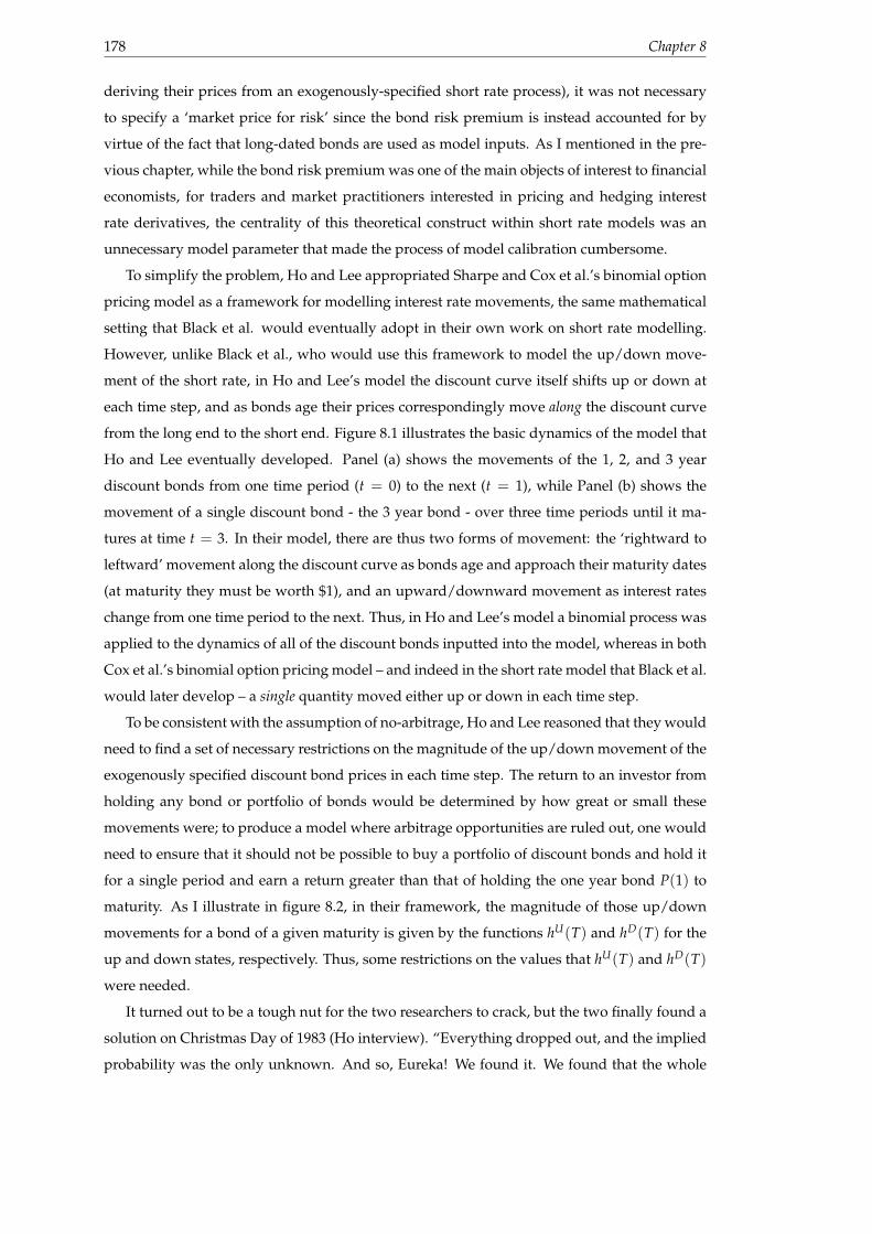
178 Chapter 8

deriving their prices from an exogenously-specified short rate process), it was not necessary

to specify a ‘market price for risk’ since the bond risk premium is instead accounted for by

virtue of the fact that long-dated bonds are used as model inputs. As I mentioned in the pre-

vious chapter, while the bond risk premium was one of the main objects of interest to financial

economists, for traders and market practitioners interested in pricing and hedging interest

rate derivatives, the centrality of this theoretical construct within short rate models was an

unnecessary model parameter that made the process of model calibration cumbersome.

To simplify the problem, Ho and Lee appropriated Sharpe and Cox et al.’s binomial option

pricing model as a framework for modelling interest rate movements, the same mathematical

setting that Black et al. would eventually adopt in their own work on short rate modelling.

However, unlike Black et al., who would use this framework to model the up/down move-

ment of the short rate, in Ho and Lee’s model the discount curve itself shifts up or down at

each time step, and as bonds age their prices correspondingly move along the discount curve

from the long end to the short end. Figure 8.1 illustrates the basic dynamics of the model that

Ho and Lee eventually developed. Panel (a) shows the movements of the 1, 2, and 3 year

discount bonds from one time period (t = 0) to the next (t = 1), while Panel (b) shows the

movement of a single discount bond - the 3 year bond - over three time periods until it ma-

tures at time t = 3. In their model, there are thus two forms of movement: the ‘rightward to

leftward’ movement along the discount curve as bonds age and approach their maturity dates

(at maturity they must be worth $1), and an upward/downward movement as interest rates

change from one time period to the next. Thus, in Ho and Lee’s model a binomial process was

applied to the dynamics of all of the discount bonds inputted into the model, whereas in both

Cox et al.’s binomial option pricing model – and indeed in the short rate model that Black et al.

would later develop – a single quantity moved either up or down in each time step.

To be consistent with the assumption of no-arbitrage, Ho and Lee reasoned that they would

need to find a set of necessary restrictions on the magnitude of the up/down movement of the

exogenously specified discount bond prices in each time step. The return to an investor from

holding any bond or portfolio of bonds would be determined by how great or small these

movements were; to produce a model where arbitrage opportunities are ruled out, one would

need to ensure that it should not be possible to buy a portfolio of discount bonds and hold it

for a single period and earn a return greater than that of holding the one year bond P(1) to

maturity. As I illustrate in figure 8.2, in their framework, the magnitude of those up/down

movements for a bond of a given maturity is given by the functions hU(T) and hD(T) for the

up and down states, respectively. Thus, some restrictions on the values that hU(T) and hD(T)

were needed.

It turned out to be a tough nut for the two researchers to crack, but the two finally found a

solution on Christmas Day of 1983 (Ho interview). “Everything dropped out, and the implied

probability was the only unknown. And so, Eureka! We found it. We found that the whole

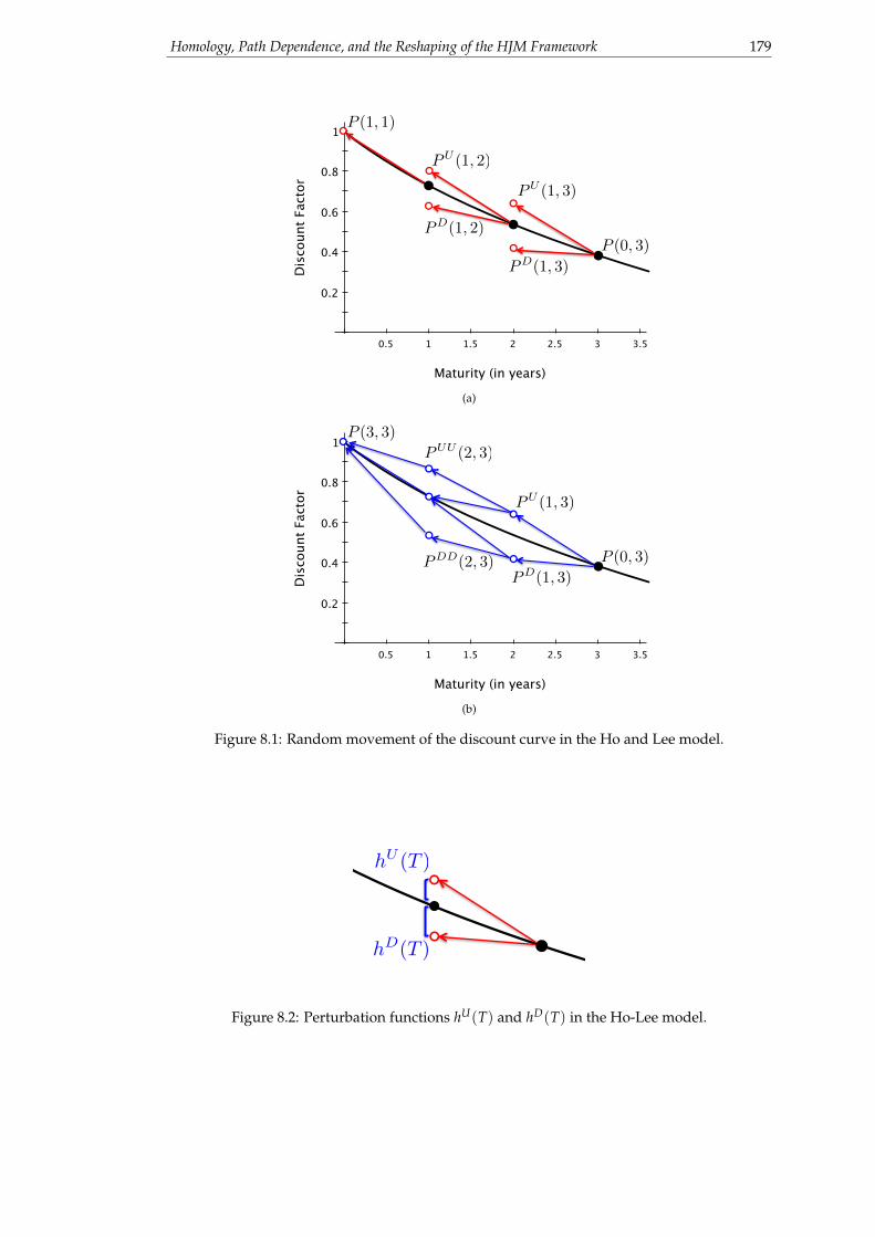
Homology, Path Dependence, and the Reshaping of the HJM Framework 179

0.5 1 1.5 2 2.5 3 3.5

0.2

0.4

0.6

0.8

1

Maturity (in years)

Dis

coun

t Fa

ctor PU (1, 3)

PD(1, 3)

PU (1, 2)

PD(1, 2)

P (1, 1)

P (0, 3)

(a)

0.5 1 1.5 2 2.5 3 3.5

0.2

0.4

0.6

0.8

1

Maturity (in years)

Dis

coun

t Fa

ctor

P (0, 3)

PU (1, 3)

PD(1, 3)

PUU (2, 3)

PDD(2, 3)

P (3, 3)

(b)

Figure 8.1: Random movement of the discount curve in the Ho and Lee model.

0.5 1 1.5 2 2.5 3 3.5

0.2

0.4

0.6

0.8

1

Maturity (in years)

Dis

coun

t Fa

ctor hU (T )

hD(T )

Figure 8.2: Perturbation functions hU(T) and hD(T) in the Ho-Lee model.

180 Chapter 8

model just drops out so beautifully” (Ho interview). What Ho and Lee were left with was an

equation relating the magnitude of the up/down movements of the discount bond prices to a

parameter π that Ho and Lee refer to as the ‘implied binomial probability’, which is analogous

to the risk-neutral probability in the Cox et al. binomial model:

πhD(T) + (1− π)hU(T) = 1 (8.1)

where hD(T) and hU(T) are the ‘perturbation functions’ that shift the value of the discount

bond with maturity date T in the next time period either above or below its value in the current

time period. With a bit of re-arranging, Equation 8.1 can be re-arranged to express the value

of this risk-neutral probability:

π =hU(T)− 1

hU(T)− hD(T)

This quantity is analogous to the risk-neutral probability q of the Cox et al. model, which is

similarly expressed in terms of the up/down movements of the stock and the risk-free rate

of interest. Furthermore, one can pin down unique values for hU(T) and hD(T) by taking

advantage of the fact that the binomial tree in Cox et al.’s framework is Markovian, and hence

recombining: in other words, that an ‘up’ move followed by a ‘down’ move is equivalent to a

‘down’ move followed by an ‘up’ move, as is illustrated in Panel (b) of figure 8.1. Using this

feature, Ho and Lee found the following unique solutions for hU(T) and hD(T) expressed in

terms of a variable δ, which captures the volatility of the discount bonds, and the bond’s time

to maturity T:

hU(T) =δT

π + (1− π)δT , hD(T) =1

π + (1− π)δT

Thus, using the current discount bond prices P(t, T1), . . . , P(t, TN), by specifying π and δ, one

could build a complete model of the future evolution of the term structure. Moreover, with

the risk-neutral probability π, one could recursively price most interest rate derivatives using

the risk-neutral pricing formula provided by Cox et al. (1979).

8.2 A Cultural Break

With its focus on modelling the movement of the entire discount curve rather than the short

rate in order to avoid specifying the market price of risk, the Ho and Lee model constituted

a rather significant break from existing approaches to interest rate modelling, particularly for

academics. (Recall that the as of then undeveloped Black et al. model would be created for

use by derivative traders and quants, rather than academic economists). As I explained in the

previous chapter, in the early-to-mid 1980s, interest rate modelling was a fairly distinct area

of intellectual work from options theory, with the former largely focussed on understanding

the extent to which the Expectations Hypothesis is true and measuring and quantifying the

Homology, Path Dependence, and the Reshaping of the HJM Framework 181

size and behaviour of the bond risk premium. Yet in the Ho and Lee model, many of the

theoretical tools and constructs central to this research programme – such as the notion of

general equilibrium and the market price of risk – are notably absent. Like the Black and

Scholes model, the Ho and Lee model is a partial equilibrium model: it was designed to be

used to value derivatives written on bonds and interest rates, just as the Black and Scholes

model was intended to value options written on shares of stock. As I explained in chapter 4, in

a ‘complete market’ setting where the payoff of the asset being priced can be replicated using

a set of simpler assets, one can calculate a unique price for the asset using arbitrage-based

arguments and no specification of investors’ risk preferences is necessary. Notably, though,

the Black and Scholes model makes no attempt to price the underlying stock itself, a problem

for which understanding those risk preferences is needed, as we also saw in chapter 4. Yet,

insofar as interest rate modelling is concerned, financial economists at that time were explicitly

interested in doing the equivalent of ‘pricing the underlying stock’ for interest rates, rather

than derivatives written on interest rates, a problem that Ho and Lee intentionally ignored

in their approach. In other words, most financial economists were interested in what Vasicek

described to me as the “underlying economics” of interest rates, rather than the more technical

problem of pricing derivatives.

For this reason, it is not altogether surprising that reception of Ho and Lee’s model among

their colleagues within NYU’s finance and economics faculty was less than enthusiastic. As Ho

explained to me, “the senior people didn’t show any interest at all - they almost deliberately

did not show interest” (Ho interview). In one case, one of the senior faculty members even

fell asleep whilst sitting in the front row of a seminar in which he presented the paper to the

department. When I asked him why he thought they showed no interest, Ho said that it came

down to the fact that for the senior faculty, the Ho and Lee model was “not economics”, but

rather a mathematical exercise.1 When I asked him to elaborate on this distinction, Ho said

that the economists in the department kept looking for a set of theoretical constructs that they

were familiar with. He was asked questions like:

Ho: “Why do you have all of these equations?” “What are you actually looking for?”“Where are the supply and demand curves?” “Where are the preferences?” “Where’s therisk aversion?” None of those things were in my equation.

Although Ho identifies as an economist (and indeed has published extensively in the field

of market microstructure), he told me that he approached the problem of term structure mod-

elling as a mathematician would, rather than an economist. In his view, mathematicians use

mathematics as a tool for building intuition: through the manipulation of their equations, they

try to gain understanding of subjects they are interested in but do not yet understand. In the

case of the Ho and Lee model, the fact that in a binomial framework, the relationship between

1In many respects, this episode echoes the response that Harry Markowitz, developer of portfolio theory, receivedfrom the economics faculty at the University of Chicago a generation earlier (MacKenzie, 2006, pg. 50).

182 Chapter 8

the perturbation functions hU(T) and hD(T) is uniquely determined by only two parameters

– π and δ – is not something that Ho sought out to confirm, but was a result that emerged

through the manipulation of the equations in the model:

Ho: I originally didn’t know what I would get. I just keep writing equations; keep doing thealgebra, cancelling things out, getting many wrong calculations and wrong answers, andthen finally all the terms just cancel out, the risk premium disappears, becoming impliedvolatility [the δ parameter], and then saying “Ah, eureka!” But as I said, this whole line ofthinking is totally alien to typical economists.

On the other hand, according to Ho, economists tend to use mathematics to confirm the logical

coherence of their pre-existing intuitions, a view that is roughly consistent with Morgan and

Yonay and Breslau historical and ethnographic work on economists’ modelling practices. In

other words, in Ho’s view economists and mathematicians approach mathematics from differ-

ent directions:

Ho: I spent all this time manipulating equations to discover things. None of the economistsappreciate that part. They use mathematics to confirm their intuition, but that to us - tomathematicians - we do the reverse. Because if I have the insight already, then it’s not a verygreat discovery, right? The big discovery is that I have some equations that drop out andtell you what you really should be looking at. So, my excitement about it [the Ho and Leemodel] couldn’t get through at all [to economists].

Although the Ho and Lee model was released in working paper form by 1984, it was not

published in the Journal of Finance until 1986. According to Ho, during that time the model at-

tracted interest from Wall Street, and its popularity among practitioners ultimately legitimised

it to the referees reviewing his article. As he put it to me, “It’s very hard to reject the paper

when it’s already cited on Wall Street. I kind of believe it was a point of leverage that finally

got the paper published” (Ho interview).

Ho’s explanation of the differences in mathematical practice between mathematicians and

economists does not seem to be universally shared by other members of those disciplines. In-

deed, I asked several other financial economists whether they share this view and they offered

different accounts. However, it turns out that the tension he felt with other members of the fac-

ulty over whether new developments in interest rate modelling were ‘proper’ economics was a

harbinger of social and intellectual developments to come. The style of interest rate modelling

that Ho and Lee were practicing would eventually become a part of the “parallel universe”

that Cox described to me: a subfield of mathematics, rather than economics. The shift of term

structure modelling from economics to mathematics intensified with the development of the

Heath-Jarrow-Morton model, which I examine in the next section.

8.3 The ‘HJM Revolution’

In 1979, a young finance academic named Robert Jarrow had finished a PhD under Robert

Merton and Fischer Black at MIT and had taken a job in the finance department at Cornell

Homology, Path Dependence, and the Reshaping of the HJM Framework 183

University. Although Jarrow’s PhD thesis focussed on the empirical behaviour of the term

structure of interest rates and the expectations hypothesis, he soon became interested in tak-

ing his research on finance in a much more mathematical direction. Jarrow had received some

exposure to stochastic calculus as a graduate student in the finance department at MIT. How-

ever, as he explained to me, Robert C. Merton - his PhD supervisor - engaged with stochastic

calculus from an “engineering perspective” rather than a “mathematical perspective”.

Jarrow: The difference being that you don’t worry about conditions. You just use it as a rotemethod, and you have Ito’s lemma and you apply it. You don’t worry about boundedness,expectations, and existence. You just apply formalisms and follow your nose.

During our interview, Jarrow joked to me that “to a mathematician I’m an economist. To an

economist, I’m a mathematician. So I live in a no-man’s land” (Jarrow interview), an identity

similar to that held by Ho.

In the same year that Jarrow finished his PhD, Harrison and Kreps (1979) published the first

paper on martingale pricing techniques that I outlined in chapter 4. While certain people in the

economics and finance profession thought that martingale methods amounted to mathemati-

cal formalism from which “there were no new economic insights to be gained”, Jarrow became

convinced that these techniques were the shape of things to come within the profession. To get

better acquainted with the underlying mathematics of stochastic processes, he decided to take

classes on probability theory in Cornell’s mathematics department. The instructor of one of

those classes was a probability theorist named David Heath, and the two eventually became

friends. For several years before it was finally published, Ho and Lee’s working paper was

in circulation, and Heath and his graduate student Andrew Morton worked on a consulting

project to implement their model for a firm. According to Jarrow, “David always liked looking

at limiting structures, so he was going to take the limit. And in doing so, he came across some

difficulties in understanding the structure” (Interview with Jarrow). With his knowledge of

both probability and interest rate theory, Jarrow was asked to join the team.

Unlike Ho and Lee who modelled the stochastic movement of the discount curve, Heath,

Jarrow and Morton chose to look at the stochastic movement of the instantaneous forward rate

curve f (t, T). Intuitively, one can think of this as being a continuously compounded version of

the forward Libor rate F(t, T1, TE) where the length of time between T1 and TE is infinitesimally

short and interest is compounded continuously rather than discretely. Put another way, f (t, T)

represents the market price at time t to borrow or lend at the short rate r prevailing at time

T. There are at least two advantages to this approach. First, modelling the forward rate curve

directly allowed for a greater degree of generality than is possible in the Ho and Lee model. In

their model, Ho and Lee chose to keep the volatilities of the discount bonds deterministic, since

these volatilities cannot be chosen arbitrarily while remaining consistent with the absence of

arbitrage. After all, as the maturity date of a discount bond approaches, its volatility must

‘pull to par’, as I mentioned in chapter 7.

184 Chapter 8

Modelling the forward rate curve directly allows for more freedom in specifying the rel-

evant volatilities, since even a constant forward rate volatility is consistent with a discount

bond having a fixed value at maturity. Moreover, bond prices can be mathematically derived

from the instantaneous forward rate curve: the price of a discount bond is equal to the expo-

nential of the integral of the forward rate curve; conversely, the forward rate curve itself is the

partial derivative of the natural logarithm of the discount bond price with respect to maturity.

In equation form:

P(t, T) = e−∫ T

t f (t,s)ds and f (t, T) = − ∂

∂Tln P(t, T) (8.2)

Second, the short rate r(t) at any moment in time is equal to f (t, t) and hence can be derived

from the instantaneous forward rate curve itself. Thus, by modelling the instantaneous for-

ward rate curve, there was no loss of generality compared to the Ho and Lee or short rate

approaches.

In their framework, Heath, Jarrow and Morton assumed that for every maturity date T, the

following stochastic differential equation defines the movement of this curve:

d f (t, T) = α(t, T)dt + σ(t, T)dWQ(t) (8.3)

f (0, T) = f M(0, T) (8.4)

where the initial conditions of this process are given by the current forward rate curve, repre-

sented by f (0, T), and where α(t, T) is the drift of the forward rate curve, WQ = (WQ1 , . . . , WQ

n )

is a vector containing n Q-Wiener processes and σ(t, T) = (σi(t, T), . . . , σn(t, T)) is a vector that

defines what is called the ‘volatility structure’ of the forward rate curve.

Before moving on, let us stop a moment and consider the complexity and generality of

this framework compared to the low-dimensional Markovian models that we examined in the

previous chapter. Although Equation 8.3 may superficially appear to be similar to the equa-

tions that described those models, it is an order of magnitude more complex. Those models

were defined by the movement of either the short rate r(t), or some other process x(t), each of

which is a one-dimensional ‘point’ at each moment in time. When one plots the movement of

that process over time, this one dimensional ‘point’ becomes a jagged two-dimensional line,

similar to those depicted in figure A.1 of appendix A. By comparison, the forward rate curve

f (t, T) at each moment in time is, as its name suggests, a two-dimensional curve. If one were

to plot its evolution over time, one would instead produce a three-dimensional surface, such as

that depicted in figure 8.3. Second, unlike short rate models which are formulated in terms of

one or two correlated Wiener processes, the HJM framework allows for an arbitrary number

of sources of uncertainty. It thus allows one to model the evolution of interest rates in a much

richer and less ‘rigid’ way than is possible with short rate models.

Homology, Path Dependence, and the Reshaping of the HJM Framework 185

Figure 8.3: Historical behaviour of the instantaneous forward rate curve, January 1973-March1997. Source: Jarrow (2002, pg. 58).

Similarly, unlike the short rate and other low-dimensional Markovian models discussed in

chapter 7, σ(t, T) has two inputs and hence captures two aspects of volatility of the forward

rate curve. Holding t fixed, it represents what one might call the ‘cross-sectional’ volatility

of this curve at each moment in time: for instance, the volatility of the one year vs. five year

forward rate prevailing today. Second, holding T fixed, it captures what one might call the

‘time series’ volatility of this curve: e.g. the five year forward rate prevailing in the market

today vs. the five year forward rate that prevailed last year.

The particular limiting case that Heath and Morton examined was the case in which the

instantaneous forward rate curve follows a lognormal Brownian motion (Jarrow interview),

which is the same stochastic process that Black used in his commodity options pricing model

that was becoming the ‘market standard’ approach for valuing interest rate derivatives such as

caps and swaptions. As Jarrow explained to me, the trio were convinced that the limit should

exist (and by extension, the risk-neutral probability measure Q should exist), but they had an

incredibly difficult time finding a proof for it:

Jarrow: We sort-of knew how everything would work out, in principle. But we couldn’tprove the existence of what’s called the ’risk neutral probabilities’, try as we might. And weworked on it for a long time, because we were convinced that it should work!

At various points they came close. At one point, Morton and Jarrow had developed an outline

of a proof that looked promising, and its validity crucially depended on a weaker version

186 Chapter 8

of what probability theorists call ‘Novikov’s condition’, which is a sufficient condition for a

stochastic process to be a martingale in the context of an important mathematical theorem

they invoked in their proof. “If it had been true, we would have been done.” Unfortunately,

they soon saw that the condition was not satisfied, and they were forced to go back to the

drawing board.

Jarrow: And then, I don’t know why - we started thinking, “Jeez, maybe it doesn’t exist”.And we literally said to Andy, “Andy, maybe a solution doesn’t exist.” This was weird,because we were so convinced that it was going to, and we just couldn’t find the proof. Andthen literally a few days later, he had a non-existence proof. He [Andy] could show that itdidn’t exist.

It became clear to the trio that the reason the lognormal case did not work was because the

drift of a lognormal forward rate process failed to satisfy a set of conditions that had to be

met for the stochastic movement of the forward rate curve to be compatible with the absence

of arbitrage. From there, Heath, Jarrow and Morton were able to develop a proof that in the

absence of arbitrage, the drift of this stochastic process - denoted by α(t, T) - cannot be chosen

arbitrarily, compared to, say, the drift in a short rate model. Instead, they were able to show

that the drift of the forward rate curve must be purely a function of the volatility structure,

given by σ(t, T). This leads to what is known as the “HJM drift restriction”, which is given by:

α(t, T) = σ(t, T)∫ T

tσ(t, s)ds

Although it was not immediately clear at the time, economists and financial mathematicians

(c.f. Baxter, 1997) later realised that this drift restriction must apply to all arbitrage-free term

structure models, including existing models such as Vasicek (1977), Cox et al. (1985), and all

of the other models that I introduced in chapter 7. Thus, it became apparent that HJM is not

strictly a model per se, but a quite general framework (a ‘supermodel’ of sorts) for modelling

the term structure of interest rates via its instantaneous forward rate curve.

To use the framework for pricing interest rate derivatives, one would need to specify the

current forward rate curve f (0, T) (which could be ‘translated’ from the discount curve us-

ing Equation 8.2) and a volatility structure of that forward rate curve, given by σ(t, T). With

those two items chosen as inputs, the no-arbitrage evolution of the forward rate curve (and

hence the short rate and the prices of all discount bonds) would be completely determined.

This model could then be used to price and risk manage a wide range of fixed-income instru-

ments, including bonds, vanilla options, and interest rate exotics by expressing their payoffs

as functions of this curve and taking discounted expectations of these final payoffs.

Heath, Jarrow and Morton intended for the HJM model to be used to manage an entire

book of interest rate derivatives. In a 1992 issue of Risk Magazine – which by that time was

growing into one of the primary publishing venues within the derivatives quant community

– Heath et al. (1992) hint at their ambition for the HJM model. Many of the products that are

Homology, Path Dependence, and the Reshaping of the HJM Framework 187

now considered ‘exotic’ largely did not exist at the time, so Heath et al. make this point with

respect to valuing and hedging a book of interest rate caps and swaptions:

To contrast HJM’s approach with a more conventional one, consider how a trader using theBlack model prices and hedges a cap. The constituent caplets are valued separately andindependently, each with its own Black volatility. [...] HJM, on the other hand, offers oneconsistent model which can be used to value and hedge all interest rate options. [...] OneHJM model, with one consistent set of assumptions, prices and hedges an entire book (Heathet al., 1992, pg. 30)

During my interview with Jarrow in 2012, he emphasised the importance of using a single

model approach to valuing and hedging interest rate derivatives, contrary to the way that

interest rate models tend to be used within dealer banks. In his view, there are dangers that

arise when multiple models are used to value instruments within a single asset class:

Jarrow: If I were the research director, that would be the first thing that I’d change in thoseorganisations. Because there’s a real danger. A lot of times groups trade within the firm,and you could create false opportunities between departments. Consistency is always anadvantage. I think conceptually the state of the art of modelling enables one to have aconsistent model.

Spears: Yeah - across all asset classes and...

Jarrow: Yes. Now, if you’re dealing with oil commodities and interest rates, then maybeyou’re going to separate. With equities and interest rates - you still might separate, but notalways. With really long dated equity options, I would separate. But fixed income? Jeez.Within fixed income, I think it would be very dangerous not to.

The HJM model thus planted the seed for the style of modelling that today is associated with

‘global calibration’: namely, the use of high dimensional models that are used to price and

risk manage all of the instruments in a trader or even a bank’s portfolio of exotic interest rate

derivatives.

8.4 HJM’s Adoption and Impact

By 1986, Heath, Jarrow and Morton had written a manuscript based on their work, but like Ho

and Lee, they had difficulty getting the model published, in part due to the fact that knowl-

edge of martingale techniques were not widely understood among members of the finance

community. (I provide a description of these techniques in chapter 4.) The trio first sub-

mitted the paper to The Journal of Finance, where it was rejected, and then the The Journal of

Financial Economics, where it was also rejected (Jarrow Interview). The trio even had difficulty

getting the manuscript accepted at the American Finance Association meetings. Finally, they

decided to submit the paper to Econometrica, a top-ranked economics journal that has a repu-

tation for preferring highly mathematical economics research. Econometrica rejected it as well,

but the referees encouraged re-submission. The paper was finally published in 1992. While the

HJM paper received a lukewarm response from the financial economics community, it soon at-

188 Chapter 8

tracted interest from fixed income traders and early ‘rocket scientists’ working on Wall Street.

As Hughston later wrote of that time,

[The approach to term structure modelling] which was initiated in the well known paperof Ho and Lee (1986), was just what was needed at the time by the investment banks asa basis for their interest rate risk management, and this is perhaps why the ideas in theHJM working paper were accepted more quickly by the practitioners than by the academiccommunity. I remember Farshid Jamshidian once recalling the tremendous impact that HJMresults made at the investment bank where he was working at the time when the first draft ofthe paper arrived, and how its practical implications were appreciated almost immediatelyby the community of modellers and traders (Hughston, 2003, pgs. 12-13)

When I interviewed Andrew Morton, he emphasised to me that part of the HJM frame-

work’s early appeal to traders and quants was that the calibration process became concep-

tually simpler because there is a greater degree of conceptual correspondence between the

quoted at-the-money swaption/caplet volatility surface and the σ(t, T) matrix within HJM.

In comparison, with short-rate models that have time-varying parameters, there is no easy

mapping between quoted implied volatilities and the model parameters. Morton told me that

traders at the time had a habit of reading meaning into the time-varying parameters of short

rate models, such as the Hull and White model. Traders would take the value of these param-

eters to be, for instance, an indicator of exposure, even though such a meaning could not be

mathematically justified (Morton Interview). Unfortunately, beyond being a nice conceptual

framework, the HJM framework initially struggled to be taken seriously as a model that could

compete with the existing short rate paradigm, or alternatively with the much simpler Ho and

Lee (1986) model. For most possible specifications of the HJM’s volatility structure, the result-

ing bond price dynamics are ‘non-Markovian’ in any finite number of state variables, unlike

the short rate models discussed previously. As a consequence, much of numerical model-

solving infrastructure that had been (or were in the process of being) developed within banks

to use short rate models – such as re-combining lattices and finite difference techniques – could

not be used with the general HJM framework. The only way to solve an HJM model to actually

calculate prices and risk sensitivities was through the use of non-recombining (e.g. ‘bushy’)

tree techniques or Monte Carlo simulation. Monte Carlo methods, as I mentioned previously,

were relatively undeveloped in the 1980s and 1990s, and were regarded as ‘tools of last resort’

(Rebonato, 2004a, pg. 697), leaving ‘bushy’ trees as the only viable option. As illustrated in

figure 8.4, in a ‘bushy’ tree, nodes never re-combine: hence, an ‘up’ move of the forward rate

curve followed by a ‘down’ move leads to a different position than a ‘down’ move followed by

an ‘up’ move. Consequently, the number of nodes that a computer must keep track of when

solving the model grows at an exponential - rather than a linear - rate with time, unlike a

recombining lattice. This is a significant issue because after only 30 discrete time steps, the bi-

nomial lattice in Panel (a) will have only thirty nodes while the ‘bushy’ binomial tree in Panel

(b) will have over 500 million!

Homology, Path Dependence, and the Reshaping of the HJM Framework 189

1

1

2

1

2

3

1

2

3

4

1

2

3

4

5

(a)

1

1

2

1

2

4

3

1

2

3

4

5

6

7

8

12345678910111213141516

(b)

Figure 8.4: A recombining lattice (Panel A) vs. a non-recombining ’bushy’ tree (Panel B).

Given its non-Markovian nature, the trio thus faced skepticism both from banks and other

academics as to whether the general HJM model could be used to price interest rate deriva-

tives. As Jarrow put it to me:

Jarrow: So for about five years, David Heath and I and Andy Morton were trying to convinceeveryone that you could compute with this. That if you did six time steps, and it went 26,then your tree expanded so much that you could price accurately. There was a time periodwith some people in industry saying, ‘It’s the perfect model, but you can’t use it becauseyou can’t compute with it”.

Although ‘bushy’ non-recombining trees grow exponentially larger with time, the trio rea-

soned that fewer time steps would generally be needed for the model to converge on the

correct price: since derivatives valuation essentially amounts to computing an expectation, a

‘bushy’ tree would therefore converge on the ‘correct’ value for the derivative with a ‘coarser’

grid of time steps. Thus after writing their paper, David Heath and Andrew Morton developed

software that could be used to price derivatives in an efficient manner using non-recombining

trees (Morton interview) in order “to convince people that you could price with the model

and that it wasn’t impossible to compute with” (Jarrow interview). While Heath and Morton

focussed on the development of the software, Jarrow focussed his attention on marketing the

software to banks. Eventually they partnered with BARRA, an investment technology and

consulting firm that had become well-known within the finance industry since the 1970s for

being one of the first companies to sell stock performance analysis models to buy-side in-

vestors (MacKenzie, 2006, pg. 83). The plan was to build a commercial software package that

BARRA would then license to banks for a fee. Unfortunately, the trio had a difficult time find-

ing interested buyers. “We had a hard time selling it, and it sort-of died a slow death”, Jarrow

told me. A debate that emerged in a 1992 issue of Risk Magazine nicely captures some of the

industry’s concerns over the practicality of HJM. In an October 1992 issue of Risk, Heath et al.

(1992) argued for the practicality of their model, claiming that “even with [a bushy tree of]

seven steps, 200 caps scan be priced in 200 seconds and 200 swaptions in 68 seconds” on a

typical personal computer available at the time. However, in an issue of the same journal two

190 Chapter 8

months later, Leong (1992) argued that Heath et al.’s claim only applied to a one-factor version

of their model. As he explained:

It is only in the multi-factor version that the model’s risk management strength emerges.Experience of using a two-factor HJM model on a Sun Sparc-2 workstation indicates thatpricing the same five-year cap will take 17 seconds, or 17 times as long as for a one-factormodel. This dramatic increase in runtime requirement as the number of factors is increasedmay spell problems when performing other daily routines. A trading book of only 200 five-year caps might take up to an hour to revalue (Leong, 1992).

Fortunately, by 1991 the three had found some interest from Lehman Brothers, which –

Morton told me during our interview – was using short rate models such as the Vasicek and

Black et al. to price non-European options at the time. The bank refused to license the soft-

ware from BARRA, and insisted on having control over the source code for the software. As an

alternative, Lehman proposed that Andy Morton work at the bank for six weeks over the sum-

mer (at the time he was still a full-time academic), after which they purchased the source code

from BARRA itself. In this way, Lehman Brothers became the first commercial user of the non-

Markovian HJM model. Although there is no way to know the precise extent to which Heath

and Morton’s software came to replace the bank’s existing short rate modelling approach,

Morton eventually became the head of fixed-income trading at the bank. In that capacity, he

arranged for the bank to hire a number of other quants who had completed PhDs with David

Heath and who thus felt at home using the HJM framework (Morton Interview). I was also

told independently by two of my interviewees that Lehman Brothers came to widely adopt

HJM, and one said that this was based on a ‘globally calibrated’, Monte Carlo-based approach

to valuation.

With that said, the non-recombining tree technique suffers from some weaknesses. As Jar-

row himself later noted in a 1998 keynote address that he gave describing the history of the

HJM model, the exponential growth of ‘bushy’ trees means that the technique “starts having

difficulties with long dated options of the American type, where there are numerous decision

nodes” (Jarrow, 1998). To price these instruments within a non-Markovian HJM framework,

one must either “use bigger, faster computers (possibly in parallel)” or “use Monte Carlo simu-

lation” (Jarrow, 1998). Computing power, in the early 1990s, remained a precious commodity,

while Monte Carlo techniques were still relatively undeveloped. Moreover, Monte Carlo was

not able to handle Bermudan or American-style derivatives at that time: a 1993 version of John

Hull’s popular textbook Options, Futures and Other Derivatives notes that at that time, “One lim-

itation of the Monte Carlo simulation approach is that it can be used only for European-style

derivatives” (Hull, 1993, pg. 322). Indeed, techniques for handling Bermudan and American-

style instruments were not published at least until the latter part of the decade (c.f. Broadie

and Glasserman, 1997). Moreover, where Monte Carlo had been used by traders and quants

in those early years, the results were at times disastrous.

Homology, Path Dependence, and the Reshaping of the HJM Framework 191

One particular exotic product that caused trouble for those banks was called an indexed

principal swap (IPS), which became popular during the early part of that decade.2 The IPS was

a synthetic instrument that was designed to mimic the phenomenon of mortgage prepayment

in a large portfolio of mortgages. Due to a set of historical contingencies in the U.S. mortgage

market, homeowners have long had the valuable option to refinance their mortgages without

penalty, which is particularly attractive when interest rates fall.3 Unfortunately, mortgage

prepayment behaviour does not follow changes in interest rates in an exact manner, since

many homeowners choose not to exercise their prepayment option in an ‘optimal’ manner.

This phenomenon can create risks for mortgage investors that generally cannot be hedged

with typical interest rate derivatives such as caps and swaptions; hence, the attraction of the

IPS product to mortgage investors and investors in securitised products, such as mortgage-

backed securities. Unfortunately, the IPS is a path-dependent security. While some banks

were able to modify their Markovian modelling techniques to value the product,4 the IPS is

more naturally suited to being valued using a set of numerical methods that are capable of

handling path-dependent products, such as Monte Carlo simulation. Unfortunately, some of

the banks that chose to use this approach suffered considerable losses. As Stephen, a quant at

EpsilonBank explained to me:

Stephen: I think the primary exotic product those days was probably the indexed principalswap, the IPS structure - which is a synthetic mortgage. [...] And that caused losses, yeah. Ithink the one firm I remember was [EtaBank]. They had a model that was set-up to do this,and it was rumoured that they took some massive write downs due to simply the modelbeing unstable. So it was a little bit premature, in a sense. These models clearly depended- they had multifactor dependency in them, because the behaviour was typically associatedwith how a short rate would hit some threshold, and then the notional would move in anamortisation fashion. [...] So you ended up having to do a multi-factor model by MonteCarlo simulation in the early 90s when people didn’t really know what they were doing.[...] A lot of banks just couldn’t hedge it and couldn’t get it right; the models were unstableand so forth. I’m sure a lot of people made a lot of money on it until they realised that theyhadn’t.

Given these limitations, other industry practitioners attacked the non-Markovian beast

from another angle: by finding simplifications of the ‘general’ HJM framework that are Marko-

vian, and hence can be solved using traditional methods. In this way, the influence of the HJM

approach itself looped back around and become incorporated into the Markovian interest rate

modelling tradition that I examined in chapter 7. In the early 1990s, Oren Cheyette, a quant

who worked at BARRA – the firm that Heath and Morton originally partnered with – devel-2An article in the Winter 1993 issue of the Federal Reserve Bank of New York Quarterly Review confirms that this

market was born in 1990 and suggests that most dealers were using either one or two-factor short rate models at thetime to value these products, but faced difficulties in modelling their risks due to the path dependent nature of theirpayoffs. According to the article, “Estimating the true profitability over time of an IAR swap can be difficult. Becauseof the swap’s path dependent behaviour, the instrument cannot be easily broken down into pieces that look exactlylike other instruments whose prices are known. Hence, the product’s valuation depends crucially on interest ratemodels (Galaif, 1993, pgs. 67-68).

3MacKenzie and Spears (2013a) explain the modelling of mortgage prepayment risk in some detail, and how theinstitutional features of the mortgage market shaped modelling practices in these markets.

4Hull and White (1993b), for instance, published an article that provides instructions on how to modify a recom-bining tree to value a path-dependent security such as an IPS.

192 Chapter 8

oped a ‘separable volatility’ version of the HJM model, in which σ(t, T) is the product of a

maturity dependent factor and a time and rate dependent factor (Cheyette, 1992), a devel-

opment that Ritchken and Sankarasubramanian (1995) made simultaneously. Such a model

would capture the path dependency of bond prices and interest rates in HJM with an addi-

tional set of state variables. Thus, for an n factor HJM model, the resulting ‘separable’ HJM

model would be Markovian in n(n + 3)/2 state variables. Notably, for an HJM model where

the forward rate curve is driven by a single Brownian motion term, only two state variables

would be needed to describe the resulting model in a Markovian fashion. Given that three

variables is approximately the upper limit of dimensionality when using finite difference and

lattice-based pricing methods, this development allowed HJM models of the one factor vari-

ety to be used with these traditional numerical techniques. Moreover, Hagan and Woodward’s

Markov models, discussed in the previous chapter, amount to a further refinement of the HJM

models in which an n factor HJM model could be operationalised using only n state variables.

As Hagan and Woodward state, “this greatly reduces their computational complexity, allow-

ing two- and even three-factor models to be used without requiring Monte Carlo simulations.”

More generally, HJM became used within the low-dimensional Markov style of interest

rate modelling as a conceptual tool for reformulating and creating new short rate models, and

appears to be used in this capacity in the present day. In a recent book on interest rate mod-

elling published after the recent financial crisis, Kenyon and Stamm (2012, pg. 94) state that

the HJM approach is “typically used mechanically for constructing short-rate models that are

otherwise difficult to derive”. Kevin touched on this use of the HJM model during our inter-

view. At one point, he talked about a model called the ‘Linear Gauss Markov’ model but told

me that it was just the Hull and White model (introduced in chapter 7) written in terms of

instantaneous forward rates:

Kevin: LGM is the Hull-White written this way - Linear Gauss Markov. And it’s exactlyHull-White written like an HJM model, actually.

Spears: So, instead of the instantaneous short rate you have an instantaneous forward rate?

Kevin: Yeah. And again, it is exactly the same model, because I can solve this one and getthis, or start from here and get that. So, it has exactly the same range, if you know what Imean. It’s just that this one - written this way - it’s just a lot easier to deal with. It’s justtrivial.

In this capacity, the HJM framework can be used as a conceptual tool that allows Markovian

interest rate models to be constructed that are more flexible than those that were first devel-

oped by financial economists. Interest rate quants, however, did not fully crystallise around

this ‘mechanical’ use of the HJM model. For one thing, this approach suffers from all of the

problems that characterise low-dimensional Markovian models that I discussed in chapter 7,

namely “rigidity” and difficulty in matching all of the relevant vanilla options for a given

trade.

Homology, Path Dependence, and the Reshaping of the HJM Framework 193

Like more familiar technological artefacts examined by sociologists and STS scholars, the

HJM framework is characterised by a high degree of interpretive flexibility: the way in which

this model can be used is not strictly determined by its technical design or features and is

instead left open to interpretation by its users. Jarrow, for instance, told me that he is opposed

to the practice of calibrating the volatility structure of an HJM model to the current market

prices of caps and swaptions. Calibration, according to Jarrow, involves taking a particular

model (what he refers to below as an ‘evolution’) and “forcing it to fit” the market prices of

interest rate derivatives. As he explained to me, this practice is dangerous because the hedging

strategies produced by the model are likely to be wrong, which can create risks to banks and

financial institutions and can result in derivatives being mispriced:

Jarrow: So what that means is now you have an estimated evolution which is not the trueone. Hedging is always based on the true evolution. But you’re using a false evolution. Sohow can you hedge with it? You can’t.

Jarrow instead told me that he believes that the volatility structure of an HJM model should be

estimated from historical data on interest rate volatility, rather than picking a particular param-

eterisation of σ(t, T) and fitting its parameters to the quoted prices of options as derivatives

quants usually do. (In the 1992 Risk Magazine article I mentioned previously in which Heath

et al. defend the practicality of HJM, both approaches are presented as options, although the

historical approach is presented first.) As Jarrow explained to me, this was the approach that

he, David Heath, and Andrew Morton originally adopted when they developed their model:

Jarrow: I’ve been saying this for 30 years - since HJM. The first implementation of HJM byDavid Heath and Andy Morton and I was to go to the data, run a principal components anal-ysis, find the parameters that are consistent with historical data, plug them into a numericaltree, and fit the actual prices. I’ve always had this perspective.

Jarrow’s view illustrates that despite the fact that the practice of ‘implied calibration’ is nearly

universal within the derivatives quant community, it is not one that is required or ‘determined’

by technical features of these models, and is thus not the only conceivable way to price and

hedge interest rate derivatives. As I explained in chapter 6, however, the practice among

exotics traders and quants in calibrating their models so as to exactly fit the prices of vanilla

caps and swaptions are deeply embedded within the organisational practices of contemporary

dealer banks, and are entwined with how risk management is performed and profit and loss

are measured. In the following section, I examine how the HJM framework was redeveloped

by traders and quants working in the industry so that its conceptual structure aligned more

closely with their own practices.

194 Chapter 8

8.5 HJM’s Incompatibilities with Market Practices

By the mid-1990s, a non-Markovian alternative had become available in the form of the ‘gen-

eral’ HJM framework, but it suffered from a number of weaknesses and did not yet offer

a substantial advantage over the existing low-dimensional Markovian modelling paradigm.

As I previously mentioned, one problem was that there did not yet exist an associated set

of numerical procedures for this modelling framework that could compete with the reliable,

scalable and understood techniques of recombining lattices and finite differences used with

Markovian models that had become core infrastructure within some banks.

A second problem was that it was not substantially easier to calibrate than existing Marko-

vian models, and moreover appeared to be fundamentally incompatible with the Black model,

which had become the ‘market standard’ model for pricing and quoting interest rate caps and

swaptions in the markets for vanilla options. It is here that the historical path dependence of

the Black model for caps and swaptions left its mark on the evolution of modelling practices

in the exotics market most clearly. Although, as Morton emphasised, HJM was conceptually

appealing to traders and quants, the forward rate curve of the HJM model is a set of instanta-

neous forward rates f (t, T) for which interest is compounded continuously while the market for

linear products deals in either discrete forward Libor rates F(t, T1, TE) or forward swap rates

S(t, T1, TE). Likewise, the volatility structure in an HJM model - denoted by σ(t, T) - consist

of instantaneous volatilities that describe these instantaneous forward rates, and not the dis-

crete forward Libor and swap rates used by linear products traders. They are not, therefore,

directly compatible with the Black implied volatilities that are quoted in the cap and swaption

markets.

HJM also appeared to exhibit more fundamental incompatibilities with the Black formula

used by cap and swaption traders. When instantaneous forward rates are assumed to follow

a lognormal distribution in HJM, the HJM drift restriction causes the forward rate process

to ‘explode’ (that is, go to infinity) in a finite amount of time, thus rendering the framework

unusable. The fact that a lognormal forward rate curve was not admissible was, after all,

the blind alley that Heath, Jarrow and Morton had stumbled down in the course of proving

the general theorem in their paper. However, at first blush, it suggests that there is a deep

and fundamental incompatibility between the HJM framework and the Black formula used

by vanilla options traders, given that forward Libor rates are assumed to be lognormal in

the Black model. Moreover, at that time options traders themselves were unable to provide

a derivation of the model that was logically consistent, as I explained in chapter 6. It was

especially surprising because lognormal short rates did not ‘explode’ in the way that forward

rates did: indeed, Black et al. (1990) and Black and Karasinski (1991) had built lognormal

short rate models that came to be widely used within banks. As I mentioned in chapter 6,

Piotr Karanski – who co-developed a lognormal short rate model along with Fischer Black –

Homology, Path Dependence, and the Reshaping of the HJM Framework 195

explained to me that if you were an exotics trader, you needed your model to match the prices

of caps and swaptions given by the Black model, because that was the model “in the systems”,

a fact that had motivated his own work on term structure modelling.

8.6 The Libor and Swap ‘Market Models’

Soon after the publication of the HJM model, a number of quants and mathematicians became

interested in these problems and would ultimately resolve this paradox. In doing so, they de-

veloped a new set of forward rate models that eventually became the heart of non-Markovian

interest rate modelling. I interviewed one of these mathematicians: Marek Musiela, who had

first met Jarrow while Jarrow was in Australia shortly after he, David Heath and Andrew

Morton had developed the HJM model (Jarrow interview). At the time, Musiela was on the

faculty of New South Wales University and had been teaching financial mathematics classes

to students since the late 1980s. While implementing the model for several banks, it became

apparent to him that there was a discrepancy between the practices used by vanilla option

traders and the HJM model. As Musiela explained to me:

Musiela: I was back then a consultant to a number of banks in Sydney. So when the Heath-Jarrow-Morton paper was published, I worked with two banks and a software companywho tried to implement it. So I knew the details of Heath-Jarrow-Morton. And then Irealised that the natural choices of Heath-Jarrow-Morton lead to valuation formulae forcaplets that the market does not use. And then it started to be an interesting question -‘Why on earth do they do what they do?’ Here is a nice HJM and they don’t like it.

Indeed, academically-oriented quants and financial mathematicians had great difficulty ratio-

nalising the use of the Black model by vanilla options traders, and it appeared to them to be

theoretically dubious. Unfortunately, the ‘correct’ way to value a cap or a swaption within a

short rate framework, as shown by Jamshidian (1989), ended up producing formulas for those

instruments that were different from the Black formulas used by vanilla option traders. Had

traders standardised around the use of a model that was fatally flawed? Was this the case of

an arbitrary pricing formula that had become popular merely as a matter of arbitrary conven-

tion? In the mid-1990s, it was not clear to quants and traders. Vanilla options traders “knew

that people were putting valid arguments on the table; that there is something that does not

add up”, Musiela told me. “But nobody had proven to them that it was really stupid.” As he

explained to me:

Musiela: How could they prove it to them? “Well, show me how you would arbitrage me?”If academics would have come up with strategies to arbitrage the guys that traded caps andfloors, then probably they would have reconsidered.

But academics were not able to make convincing arguments that traders’ use of the Black

model created arbitrage opportunities.

196 Chapter 8

Musiela and a number of other financial mathematicians eventually came to realise that the

market standard practice could be rationalised. Drawing on the ‘forward measure’ concept that

had been initially developed by Jarrow (1987), Musiela, Jamshidian and others realised that

the Black formulas could be rationalised through a change of measure from the risk-neutral

measure Q to the T-forward measure associated with the discount bond P(t, TE) as numéraire.

Thus, rather than taking the discounted expectation of a cap or swaption’s payoff under the

risk-neutral measure Q, this expectation was instead taken under an alternative martingale

measure denoted by QTE under which payoffs that are discounted by discount bonds that

mature at date TE are martingales. One can show that under this probability measure, the

forward Libor rate F(t, T1, TE) is a martingale, and so can reasonably be assumed to evolve

under a lognormal Brownian motion with zero drift:

dF(t, T1, TE) = σF(t, T1, TE)dWQTE (t) (8.5)

From here, the Black formula that cap and swaption traders had been employing since the

1980s could then be derived in a manner consistent with no-arbitrage pricing theory, in effect

providing an ex-post rationalisation of a valuation practice that traders had been using all

along. Musiela emphasised to me that it was a ‘miracle’ of sorts that the market had somehow

figured out that if you assume that forward Libor rates are lognormally distributed, then you

must discount to the forward rate’s maturity date:

Spears: So it’s purely an accident that this happens to produce the correct formula?

Musiela: No, what actually produced to me the correct formula was that the market wastreating forward Libor process as a lognormal process. And miraculously understood thatwhat you need to do is - you need to apply discounting - and where the miracle comes is -to the end of the period; not to the beginning of the period.

Having realised that the use of the Black formula for caps and swaptions could be theoreti-

cally rationalised by assuming that forward Libor rate F(t, S, T) follows a lognormal Brownian

motion under the T-forward measure, it was then possible to build up a modification to the

HJM framework that possesses the same conceptual structure as the Black model for vanilla

options. This resulting model is known as a Libor Market Model, or equivalently a ‘BGM

model’ and was simultaneously published by Brace et al. (1997), Jamshidian (1997), and Mil-

tersen et al. (1997). (A version that models forward swap rates called the Swap Market Model

was also introduced by Jamshidian (1997), but for brevity I will not discuss it.) This model

is similar to a short rate or HJM model, in that it could be used to price exotic interest rate

derivatives that depended on the co-evolution of multiple rates. However, it had a number of

advantages over these previously developed term structure models. First, it provided a ratio-

nalisation of the practice of using Black’s cap and swaption formulas. Musiela explained to

me that using the Black model “kind-of made sense” to traders, but “they didn’t know why it

made sense”. “The BGM helped them to understand why it made sense” (Musiela interview).

Homology, Path Dependence, and the Reshaping of the HJM Framework 197

Second, it had the great advantage of dealing in quantities that exotics traders calibrate their

models to: namely, forward Libor and swap rates and Black-implied volatilities on those rates.

As a consequence, such a model automatically valued caps and swaptions in accordance with

the models used by vanilla option traders. Thus, no longer would it be necessary to engage

in a complex non-linear optimisation exercise to ensure that a pricing model ‘reproduces’ the

prices of the underlying instruments: this would be guaranteed by design.

Although the Libor Market Model was published in 1997, it is difficult to establish when this

approach was actually first developed and implemented. A number of my interviewees told

me that banks had developed the Libor Market Model (or models very similar to it) in the early

1990s within several years of the publication of the HJM paper. Elliot explained to me that

Banker’s Trust – an early pioneer in derivatives trading which no longer exists – developed

an early version of the model which it called ‘Mega’ in around 1994 (Interview with Elliot),

although I have so far been unable to find any documentary evidence to corroborate his claim.

Kevin made a similar point to me: “the funny thing is - the BGM model was... [EpsilonBank]

had it years earlier and so did [KappaBank]; they just called it their ‘discrete HJM model’.

They had no idea they were doing ’BGM’, you know? So [KappaBank] had their four factor

model, and [EpsilonBank] had their six factor model.”

8.7 “It’s quite a nice intuitive idea because that corresponds a

lot to the way that derivatives are priced in practice.”

Let us examine the conceptual structure of the Libor Market Model in detail, as it is striking

how closely the equations that govern the model resemble the equations for the Black model

used by cap and swaption traders. Unlike these earlier term structure models, the Libor Mar-

ket Model does not model a continuous curve but a discrete set of points along it. However,

unlike a short rate or HJM model, a Libor Market Model consists of multiple stochastic differen-

tial equations that describe the movement of a sequence of forward Libor rates, each of which

we can denote by Fi(t). For a model consisting of n forward Libor rates, the Libor Market

Model consists of a sequence of SDEs which describes the evolution of each of these forward

198 Chapter 8

Libor rates that all evolve under a particular T-forward martingale measure:5

dF1(t) = σi(t)F1(t)dWQT11 (t) (8.6)

dF2(t) =τ1F1(t)σ1(t)σ2(t)ρ1,2

1 + τ1F1(t)dt + σ2(t)F2(t)dW

QT12 (t)

... =...

dFn(t) =n−1

∑k=1

τkFk(t)σn(t)σk(t)ρn,k

1 + τ1Fk(t)dt + σn(t)Fn(t)dW

QT1n (t)

One junior quant that I talked to described the Libor Market Model as “essentially a sequence

of Black models strung together”, and this is a helpful way to make sense of it. The first

equation - for the first forward Libor rate - in fact almost exactly matches the stochastic dif-

ferential equation for the Black model, written in modern ‘forward measure’ notation. The

resulting model is defined by a set of n forward Libor (or equivalently, swap) rates denoted by

F1(t), . . . , Fn(t), a series of volatility functions for those rates, denoted by σ1(t), . . . , σn(t), and

a correlation matrix {ρi,j} that defines the correlation between each of the individual Libor

rates. Unlike the parameters of a low-dimensional Markovian model, these objects naturally

map onto prices and rates that an exotics trader can observe and transact in with her bank’s

vanilla options and swaps desks. The forward Libor rates, for example, are directly provided

by the forward Libor curve that is quoted by her bank’s swaps traders. Moreover, because the

volatility parameters in the model refer to the volatility of lognormally distributed forward

Libor rates (and not a short rate), a trader could more easily take the quoted Black implied

volatilities from her bank’s cap volatility surface and use them to specify a volatility structure

in the Libor Market Model without engaging in a complicated translation exercise between

discrete forward Libor rates and short rates. Conversely, she could be confident that her model

would ‘recover’ or produce the quoted prices for these vanilla options. Finally, the correlation

parameters of the model could either be inferred from market prices (e.g. of correlation sen-

sitive instruments, such as CMS spread options), or could be assigned manually by the trader

according to her own judgment and ‘view’ on the market.

Indeed, the degree of conceptual resemblance between Equation 8.6 and Equation 8.5 played

no small part in causing the BGM modelling approach to become widely adopted among

quants and traders at dealer banks. ‘Ryan’, a quant at a dealer bank who began working in

these markets in the mid-to-late 1990s, emphasised to me that the inputs to the HJM and BGM

(e.g. the Libor Market Model) frameworks are conceptually separated in such a way that is

homologous to the organisational demarcation of Libor derivatives trading within banks:

5I have chosen to present these equations under the T-forward measure associated with F1, given by QT1 ; however,the drift terms of each forward rate would change if we instead expressed these equations in terms of the measureassociated with a different discount bond. (One can switch between measures using Girsanov’s theorem, which isoutlined in appendix A.)

Homology, Path Dependence, and the Reshaping of the HJM Framework 199

Ryan: The whole HJM approach was nice conceptually to a lot of us at the time, because ithad the key understanding of separating out the forward curve from the volatility surface.In short-rate modelling those two were all mixed up together. [...] With a short-rate model,the forward curve – you know, where the forward Libors are – is all mixed-up with thevolatility surface and mean-reversion – it’s all tangled. Whereas with the HJM it’s muchcleaner. You’ve kind-of got the forward curve in one place, and you’ve got the volatilitysurface in another. [...] So the idea that your rates model is based on the forwards, thevols, and the correlation as three separate planks. It’s quite a nice intuitive idea because thatcorresponds a lot to the way that derivatives are priced in practice. So, the first thing youask when you price derivatives is: “what’s the forward?” And if you’re doing an option“What’s the vol?” And as soon as two or more things are involved, “What’s the correlationstructure?” And you often risk manage those in different ways, maybe different people arerisk managing them. So the ability to separate them out is very useful. So the HJM wasa good *conceptual* move forward in that respect because it achieved that separation [...]So, the strength of HJM and BGM were the, sort-of, directness in talking about what youcare about, and categorised them into the boxes that you naturally categorised used, i.e.forwards is one, volatility is two, and the third correlation. In a short-rate model – even amulti-factor short-rate model – you’ve only got one short-rate and everything is mixed-uptogether, so it’s slightly conceptually harder to see what’s going on.

The conceptual appeal of the Libor Market Model is also shared among quants who prefer the

style of low-factor modelling, described in chapter 7. For instance, John, a quant at PiBank

who is an advocate for low-factor Markovian modelling techniques, also remarked on the

conceptual appeal of the BGM framework:

John: [Y]ou could think of things more intuitively - you could think in terms of Libors. [...]conceptually people felt comfortable thinking in terms of Libors and how they correlated.That was the real contribution [of BGM], I think - the conceptual framework.

John also told me that in his view, the appeal of BGM among quants was cultural insofar

as many quants come from the discipline of physics where there is a strong desire to find a

universal model or theory to explain a given set of phenomena. He contrasts this to a more

‘statistical approach’, which is more closely associated with the low-dimensional Markovian

models discussed in chapter 7:

John: It’s also cultural. A lot of people in finance come from physics, and they have this ideaof ‘There is the perfect solution if only we knew it.’ They think, the Libor Market Model is abit better, it’s a bit more accurate. Whereas [there is] the more statistical approach of, ‘Wellactually, you don’t know a lot. Keep it simple, and when it breaks at least you’ll know thatit’s broken’.

Another major appeal of the Libor Market Model among traders and quants was its flex-

ibility in modelling a wide range of payoffs, many of which the low dimensional Markovian

approach had a difficult time handling. To give one example, in chapter 7 I explained that a

perceived disadvantage of the low-dimensional Markovian models among quants and traders

during the 1990s was that they had a difficult time modelling spread-based products (e.g. op-

tions whose payoffs depend on the spread between two interest rates). To value and hedge

these instruments accurately, a model would need to ‘induce decorrelation’ between these

rates: that is, model them in such a way that they can move out of lock-step with one another.

200 Chapter 8

This was not possible in a one-factor model, and within the low-dimensional Markovian ap-

proach to interest rate modelling, the only apparent solution to this problem was to add a

greater number of stochastic drivers to the model. A Libor Market Model, by contrast, could

‘induce’ this phenomenon of decorrelation between two rates with a small number of factors

by specifying the volatility structure σ1(t), . . . , σn(t) for the model in a particular way.

This freedom came at a cost, however. Like the HJM framework, the Libor Market Model

is ‘non-Markovian’: this is indicated in Equation 8.6 by the fact that the drift term of the ith

forward Libor rate depends on the level of all of the rates preceding it. Thus, even for a model

only consisting of two or three forward Libor rates, the standard numerical techniques that

banks had built their low-dimensional interest rate models around – namely finite difference

methods and recombining trees – were no longer applicable. As Jamshidian (1997) himself

notes in his original publication on the model, even the ‘bushy trees’ that Heath, Jarrow and

Morton had used for the HJM model have trouble handling the dimensionality of this new

model: by default, a model made of, say, 10 forward Libor or swap rates consists of 10 SDEs

of the form given in Equation 8.6 and hence 10 correlated Brownian motions. Monte Carlo

simulation is, realistically, the only numerical technique that can be used. As a consequence,

banks that developed the BGM framework into their preferred platform for pricing and hedg-

ing exotic interest rate derivatives faced a multitude of ‘engineering challenges’ in making

the model fast, stable and reliable, which was particularly difficult given that Monte Carlo

techniques were in the mid-to-late 1990s much less well-developed and understood than the

more traditional numerical techniques associated with low-dimensional models (c.f. Jackel,

2002). As Robert – a quant at LambdaBank – put it to me, “The devil is in the details, you

know? You can put a BGM together in half an afternoon, but to make it actually process

thousands of derivatives every night - that takes years, frankly”. This plethora of challenges

included: reducing the dimensionality of the model (what mathematicians call ‘factor reduc-

tion’); developing analytical approximations for vanilla instruments so that these instruments

could be valued quickly, allowing the model to be calibrated in a reasonable amount of time

(“seconds, instead of minutes” according to Robert); techniques for producing risk sensitiv-

ities (e.g. Deltas and Vegas) in a way that was computationally efficient but also produced

‘crisp hedges’ that traders could use to understand the risk associated with their exotics books

and hedge their positions effectively; techniques for handling instruments with ‘early exercise’

features (such as Bermudan swaptions), that are ordinarily extremely difficult to value using

Monte Carlo methods (c.f. Broadie and Glasserman, 1997; Longstaff and Schwartz, 2001); and

modifying the models so that they could be made to fit the ‘volatility smile’ in the cap and

swaptions markets (c.f. Andersen, 2000; Piterbarg, 2003; Rebonato et al., 2009). These engi-

neering efforts among quants within banks allowed the BGM model to become a very general

framework for modelling interest rates, one that was so flexible that it could reproduce the in-

Homology, Path Dependence, and the Reshaping of the HJM Framework 201

terest rate dynamics produced by simpler models.6

Joshua, another quant I spoke to, had a more cynical view of the emergence of the BGM

framework as a dominant model in the derivatives quant world. He compared the BGM ap-

proach to what is known among mathematicians as a “pons asinorum” (Latin for ‘bridge of

asses’), which refers to one of the first genuinely difficult propositions in Euclid’s classic text

on geometry. A student’s ability to prove this proposition was once treated as a signal of her

potential as a mathematician, and in Joshua’s view, BGM served a similar purpose within the

derivatives quant community:

Joshua: So it was a sort-of pons asinorum; most quants couldn’t handle the complexities em-bedded in the BGM, so you could earn more money and have more job security if you coulddo it. [...] And there’s always this thing wherein quants have to distinguish themselvesfrom the kind-of run-of-the-mill quants, the junior quants, and so on. And if there’s a kind-of body of knowledge that’s arcane and difficult, it does that for you. So that’s definitely arole that BGM had.

8.8 Non-Markovian Modelling Finds its Commercial Niche

Thus while the conceptual elegance of the BGM approach was certainly appealing to traders

and quants, in all likelihood this feature alone probably does not explain the eventual success

and popularity of the modelling framework, given the costs of implementing it and the engi-

neering complexities involved. As is the case with most new technologies, the popularity of

BGM was likely due to its ability to appeal to multiple interests and actors within banks: this,

in fact, is one of the central themes of the literature on the social shaping of technology (c.f.

Bijker, 1997).

Whatever the reason for its popularity, the quant community’s preference for the BGM

framework over low-factor models was becoming evident by 2004. The Markov-Functional

models outlined in chapter 7, for instance, were increasingly seen as outdated tools, even

though these low-dimensional models had certain desirable technical features that ‘standard’

BGM models did not possess. (BGM models, for instance, required significant adaptations to

fit the volatility smile, whereas Markov-functional models possessed the ability to do this ‘out

of the box’). In that year, Joanne Kennedy – one of the co-developers of the Markov-functional

approach – and her student Michael Bennett submitted a manuscript to Risk Magazine that

compared one factor versions of those models to BGM models with a ‘separable’ volatility

surface (Bennett and Kennedy, 2005a), analogous to the ‘separable’ Cheyette HJM model dis-

cussed previously. A referee that was identified by the editor as a quant practitioner wrote

6For instance, I attended a technical class at a quant conference that was focussed on the Libor Market Model, andone of the quants teaching told the audience that his bank had once seen another dealer quoting prices with whatappeared to be a Hull-White short rate model. (I discussed this model in chapter 7.) Although they had the Hull-White model ‘sitting in code’, the quants had not used it in some time and they found that it was actually easier tochange the parameters of their BGM model to make it match a Hull-White model, rather than switching back to theHull-White model itself.

References

Abu-Lughod, L. (1991). Writing Against Culture. In R. G. Fox (Ed.), Recapturing Anthropology:
Working in the Present, Chapter 43, pp. 137–54. Santa Fe: School of American Research Press.
Armacost, M. H. (1999). The Thor-Jupiter Controversy. In D. MacKenzie and J. Wajcman
(Eds.), The Social Shaping of Technology (2nd ed.)., Chapter 28, pp. 395–405. Maidenhead:
Open University Press.
Arthur, W. B. (2009). The Nature of Technology: What It is and How It Evolves. London: Penguin
Books.
Ayache, E. (2007). The Next Question Concerning Technology - Part 1: The Significance of
Dynamic Replication. Wilmott Magazine, 32–38.
Bachelier, L. (1900). Théorie de la Spéculation. Annales Scientifiques de l’École Normale
Supérieure 3(17), 21–86.
Baker, W. E. (1984, January). The Social Structure of a National Securities Market. American
Journal of Sociology 89(4), 775.
Barany, M. J. and D. Mackenzie (2014). Chalk: Materials and Concepts in Mathematics Chalk
in Hand. In C. Coopmans, M. Lynch, J. Vertesi, and S. Woolgar (Eds.), Representation in
Scientific Practice Revisited, pp. 107–130. Cambridge, MA: MIT Press.
Barnes, B. (1995). The Elements of Social Theory. Princeton University Press.
Barnes, B., D. Bloor, and J. Henry (1996). Scientific Knowledge: a Sociological Analysis. London:
Athlone Press.
Beunza, D., I. Hardie, and D. Mackenzie (2006). A Price is a Social Thing: Towards a Material
Sociology of Arbitrage. Organizational Studies 27, 721–745.
Beunza, D. and D. Stark (2004, April). Tools of the Trade: the Socio-Technology of Arbitrage
in a Wall Street Trading Room. Industrial and Corporate Change 13(2), 369–400.
Beunza, D. and D. Stark (2012). From Dissonance to Resonance: Cognitive Interdependence in
Quantitative Finance. Economy and Society 41(3), 383–417.
244 References
Biggart, N. W. and T. D. Beamish (2003, August). The Economic Sociology of Conventions:
Habit, Custom, Practice, and Routine in Market Order. Annual Review of Sociology 29(1),
443–464.
Bijker, W. (1997). Of Bicycles, Bakelites, and Bulbs: Toward a Theory of Sociotechnical Change. Cam-
bridge, MA: MIT Press.
Bikhchandani, S., D. Hirshleifer, and I. Welch (1992). A Theory of Fads, Fashion, Custom, and
Cultural Change in Informational Cascades. Journal of Political Economy 100(5), 992–1026.
Bloor, D. (1991). Knowledge and Social Imagery. University of Chicago Press.
Bourdieu, P. (1977). Outline of a Theory of Practice.
Bowker, G. C. (1994). Science on the Run: Information Management and Industrial Geophysics at
Schlumberger, 1920-1940. Cambridge, MA: MIT Press.
Brady Commission (1988). Report of the Presidential Task Force on Market Mechanisms. US Gov-
ernment Printing Office.
Breslau, D. and Y. Yonay (2008, September). Beyond Metaphor: Mathematical Models in Eco-
nomics as Empirical Research. Science in Context 12(02).
Brooks, J. (1998). The Go-Go Years: The Drama and Crashing Finale of Wall Street’s Bullish 60s.
John Wiley & Sons.
Brumann, C. (2005). Writing for Culture: why a successful concept should not be discarded. In
A. Miller (Ed.), Concepts of Culture: Art, Politics, and Society, pp. 43–77. Calgary: University
of Calgary Press.
Brunnermeier, M. K. (2001). Asset Pricing Under Asymmetric Information. Oxford University
Press.
Bush, V. (1945, January). Science: The Endless Frontier. Transactions of the Kansas Academy of
Science (1903-), 231–264.
Caliskan, K. and M. Callon (2009, August). Economization, Part 1: Shifting Attention from the
Economy Towards Processes of Economization. Economy and Society 38(3), 369–398.
Callon, M. (1998a). Actor-Network Theory: The Market Test. Sociological Review 46(S), 181–195.
Callon, M. (1998b). Introduction: The Embeddedness of Economic Markets in Economics. In
M. Callon (Ed.), The Laws of the Markets (1st ed.)., pp. 272. Oxford: Blackwell Publishers.
Callon, M. (2007a). An Essay on the Growing Contribution of Economic Markets to the Prolif-
eration of the Social. Theory, Culture & Society 24(7-8), 139–163.
References 245
Callon, M. (2007c). What Does it Mean to Say Economics is Performative? In D. MacKenzie,
F. Muniesa, and L. Siu (Eds.), Do Economists Make Markets?: on the Performativity of Economics,
pp. 311–357. Princeton, NJ: Princeton University Press.
Callon, M. and J. Law (1986). Some elements of a sociology of translation: domestication of
the scallops and the fishermen of St. Brieuc Bay. In J. Law (Ed.), Power, Action and Belief: A
New Sociology of Knowledge? London: Routledge.
Callon, M. and F. Muniesa (2005, August). Economic Markets as Calculative Collective De-
vices. Organization Studies 26(8), 1229–1250.
Carrithers, M., M. Candea, K. Sykes, M. Holbraad, and S. Venkatesan (2010, May). Ontology Is
Just Another Word for Culture: Motion Tabled at the 2008 Meeting of the Group for Debates
in Anthropological Theory, University of Manchester. Critique of Anthropology 30(2), 152–200.
Carruthers, B. G. and A. L. Stinchcombe (1999, June). The Social Structure of Liquidity: Flexi-
bility, Markets, and States. Theory and Society 28(3), 353–382.
Cartwright, N. (1984). How the Laws of Physics Lie. Oxford: Oxford University Press, USA.
Chandler, A. (1977). The Visible Hand. Cambridge, MA: Belnap Press of Harvard University
Chernow, R. (2001). The House of Morgan: An American Banking Dynasty and the Rise of Modern
Finance. New York: Grove Press.
Coase, R. (1937, November). The Nature of the Firm. Economica 4(16), 386–405.
Collins, H. (1998). The Meaning of Data: Open and Closed Evidential Cultures in the Search
for Gravitational Waves. American Journal of Sociology 104(2), 293–338.
Collins, H. (2004). Interactional Expertise as a Third Kind of Knowledge. Phenomenology and
the Cognitive Sciences 3(2), 125–143.
Collins, H. M. (1974). The TEA Set: Tacit Knowledge and Scientific Networks. Science Stud-
ies 4(2), 165–185.
Collins, H. M. (2001). Tacit Knowledge, Trust and the Q of Sapphire. Social Studies of Sci-
ence 31(1), 71–85.
Collins, H. M. and R. Evans (2007). Rethinking Expertise (1st ed.). Princeton, NJ: Princeton
University Press.
Collins, H. M. and S. Yearley (1992). Epistemological Chicken. In A. Pickering (Ed.), Science as
Practice and Culture, pp. 474. University of Chicago Press.
246 References
Crawford, V. and J. Sobel (1982). Strategic Information Transmission. Econometrica 50(6), 1431–
1451.
Daston, L. and P. Galison (1992, October). The Image of Objectivity. Representations 40(1),
81–128.
David, P. (1985). Clio and the Economics of QWERTY. The American Economic Review 75(2),
332–337.
Dennis, M. A. (2004). Reconstructing Sociotechnical Order: Vannevar Bush and US Science
Policy. In States of Knowledge: The co-production of science and social order, pp. 225–253. New
York: Routledge.
Diamond, D. W. and P. H. Dybvig (1983, June). Bank Runs, Deposit Insurance, and Liquidity.
The Journal of Political Economy 91(3), 401–419.
Durkheim, E., M. Mauss, and R. Needham (1963). Primitive Classification. London: Routledge.
Erikson, B. H. (1979). Some Problems of Inference from Chain Data. In K. F. Schuessler (Ed.),
Sociological Methodology, pp. 276–302. San Francisco, CA: Jossey-Bass Publishers.
Espeland, W. and M. Stevens (1998, August). Commensuration as a Social Process. Annual
Review of Sociology 24(1), 313–343.
Fallows, J. (1999). The American Army and the M-16 Rifle. In D. MacKenzie and J. Wajcman
(Eds.), The Social Shaping of Technology (2nd Editio ed.)., Chapter 27, pp. 382–394. Maiden-
head: Open University Press.
Farrell, J. and M. Rabin (1996). Cheap talk. Journal of Economic Perspectives 10(3), 103–118.
Felin, T. and N. J. Foss (2009, April). Social Reality, the Boundaries of Self-Fulfilling Prophecy,
and Economics. Organization Science 20(3), 654–668.
Flanagan, S. M. (2001). The Rise of a Trade Association: Group Interactions Within the Inter-
national Swaps and Derivatives Association. Harvard Negotiation Law Review 6, 211–264.
Fourcade, M. (2010). Economists and Societies: Discipline and Profession in the United States,
Britain, and France, 1890s to 1990s. Princeton, NJ: Princeton University Press.
Fourcade, M. (2011, May). Cents and Sensibility: Economic Valuation and the Nature of “Na-
ture”. American Journal of Sociology 116(6), 1721–77.
Freeman, C. and L. Soete (1997). The Economics of Industrial Innovation (3rd ed.). Oxford: Rout-
ledge.
Galison, P. (1997). Image and Logic: A Material Culture of Microphysics. Chicago, IL: University
of Chicago Press.
References 247
Gieryn, T. (1983). Boundary-Work and the Demarcation of Science From Non-Science: Strains
and Interests in Professional Ideologies of Scientists. American Sociological Review 48(6), 781–
795.
Gile, K. J. and M. S. Handcock (2010, August). Respondent-Driven Sampling: An Assessment
of Current Methodology. Sociological Methodology 40(1), 285–327.
Godechot, O. (2008, April). What do heads of dealing rooms do? The social capital of internal
entrepreneurs. The Sociological Review 56, 145–161.
Goertz, G. and J. Mahoney (2012). A Tale of Two Cultures: Qualitative and Quantitative Research
in the Social Sciences. Princeton, NJ: Princeton University Press.
Goodman, L. A. (1961). Snowball Sampling. Annals of Mathematical Statistics 32(1), 148–170.
Granovetter, M. (1985, November). Economic Action and Social Structure: the Problem of
Embeddedness. American Journal of Sociology 91(3), 481–510.
Guala, F. (2007). How to Do Things with Experimental Economics? pp. 128–162. Princeton,
NJ: Princeton University Press.
Hacking, I. (1992). ‘Style’ for Historians and Philosophers. Studies in History and Philosophy of
Science 23(1), 1–20.
Hardie, I. (2004, May). ’The Sociology of Arbitrage’: a Comment on MacKenzie. Economy and
Society 33(2), 239–254.
Heckathorn, D. D. (2002). Respondent-Driven Sampling II: Deriving Valid Population Esti-
mates from Chain-Referral Samples of Hidden Populations. Social Problems 49(1), 11–34.
Henare, A., M. Holbraad, and S. Wastell (2007). Thinking Through Things: Theorising Artefacts
Ethnographically. New York: Routledge.
Holm, P. (2007). Which Way is Up on Callon? In Do Economists Make Markets?: on the Perfor-
mativity of Economics, pp. 225–243. Princeton University Press.
Hutchins, E. (1995). Cognition in the Wild. MIT Press.
Joas, H. and W. Knobl (2009). Social Theory. Cambridge: Cambridge University Press.
Joerges, B. (1999, June). Do Politics Have Artefacts? Social Studies of Science 29(3), 411–431.
Kevles, D. J. (1978). The Physicists: The History of a Scientific Community in Modern America.
Cambridge, MA: Harvard University Press.
Kline, S. and N. Rosenberg (1986). An Overview of Innovation. In R. Landau and N. Rosenberg
(Eds.), The Positive Sum Strategy, pp. 275–305. Washington, D.C.: National Academies Press.
248 References
Knorr-Cetina, K. (2000). Epistemic Cultures: How the Sciences Make Knowledge. Harvard Univer-
sity Press.
Krippner, G. (2005, May). The financialization of the American economy. Socio-Economic Re-
view 3(2), 173–208.
Kuhn, T. (1963). The Function of Dogma in Scientific Research. In A. C. Crombie (Ed.), Sci-
entific Change: Historical Studies in the Intellectual, Social and Technical Conditions for Scientific
Discovery, pp. 347–369. London: Heinemann.
Lamont, M. (2012, August). Toward a Comparative Sociology of Valuation and Evaluation.
Annual Review of Sociology 38(1), 201–221.
Latour, B. (2005). Reassembling The Social: An Introduction to Actor-Network-Theory. Oxford
Latour, B. and S. Woolgar (1986). Laboratory Life: The Construction of Scientific Facts. Princeton,
Law, J. and M. Callon (1992). A Life and Death of an Aircraft: A Network Analysis of Technical
Change. In W. E. Bijker and J. Law (Eds.), Shaping Technology/Building Society: Studies in
Sociotechnical Change, Chapter 1, pp. 21–52. Cambridge, MA: MIT Press.
Law, J. and V. Singleton (2005, May). Object Lessons. Organization 12(3), 331–355.
Lépinay, V.-A. (2011). Codes of Finance. Princeton University Press.
Lestition, S. (2000). Historical preface to Max Weber, "Stock and Commodity Exchanges". The-
ory and Society 29(3), 289–304.
Levy, J. (2012). Freaks of Fortune: The Emerging World of Capitalism and Risk in America. Cam-
bridge, MA: Harvard University Press.
Lewis, D. K. (1969). Convention: A Philosophical Study. Harvard University Press.
Lewis, M. (2010). Liar’s Poker: Rising Through the Wreckage on Wall Street (2nd ed.). New York:
W. W. Norton Company.
Livingston, E. (1999, December). Cultures of Proving. Social Studies of Science 29(6), 867–888.
MacKenzie, D. (2003). Long-Term Capital Management and the Sociology of Arbitrage. Econ-
omy and Society 32(3), 349.
MacKenzie, D. (2008, September). What’s in a Number? London Review of Books 30(18), 11–12.
MacKenzie, D. (2011b, May). The Credit Crisis as a Problem in the Sociology of Knowledge.
American Journal of Sociology 116(6), 1778–1841.
References 249
MacKenzie, D. and Y. Millo (2003, July). Constructing a Market, Performing Theory: The
Historical Sociology of a Financial Derivatives Exchange. American Journal of Sociology 109(1),
107–145.
MacKenzie, D. and T. Spears (2014a). ‘A Device For Being Able to Book PL’: The Organizational
Embedding of the Gaussian Copula. Social Studies of Science (Forthcoming).
MacKenzie, D. and T. Spears (2014b). ‘The Formula That Killed Wall Street’: The Gaussian
Copula and Modelling Practices in Investment Banking. Social Studies of Science (Forthcom-
ing).
MacKenzie, D. and T. C. Spears (2013a). The Cognitive Sociology of Toxic Assets.
MacKenzie, D. A. (2006). An Engine, Not a Camera: How Financial Models Shape Markets. MIT
MacKenzie, D. A. and J. Wajcman (1999). The Social Shaping of Technology. Open University
McPherson, M., L. Smith-Lovin, and J. M. Cook (2001, August). Birds of a Feather: Homophily
in Social Networks. Annual Review of Sociology 27(1), 415–444.
Merton, R. K. (1948). The Self-Fulfilling Prophecy. The Antioch Review 8(2), 193–210.
Miller, D. (2002). Turning Callon the Right Way Up. Economy and Society 31(2), 218.
Miller, D. (2005). Materiality: An Introduction. In D. Miller (Ed.), Materiality, pp. 1–50.
Durham: Duke University Press.
Mirowski, P. (2002). Machine Dreams: Economics Becomes a Cyborg Science. Cambridge Univer-
Mirowski, P. and E. Nik-Khah (2007). Markets Made Flesh. In D. MacKenzie, F. Muniesa, and
L. Siu (Eds.), Do Economists Make Markets?: on the Performativity of Economics, Chapter 7, pp.
190–224. Princeton, NJ: Princeton University Press.
Mokyr, J. (2002). The Gifts of Athena: Historical Origins of the Knowledge Economy. Princeton, NJ:
Princeton University Press.
Morgan, M. S. (2012). The World in the Model: How Economists Work and Think. New York:
Cambridge University Press.
Morgan, M. S. and M. Morrison (1999). Models as Mediators: Perspectives on Natural and Social
Science. Cambridge University Press.
Mosley, L. (2003). Global Capital and National Governments. Cambridge: Cambridge University
250 References
Mowery, D. and N. Rosenberg (1979, April). The influence of market demand upon innovation:
a critical review of some recent empirical studies. Research Policy 8(2), 102–153.
Mulvey, P. J. and S. Nicholson (2011). Physics Graduate Degrees: Results from the Enrollments
and Degrees and the Degree Recipient Follow-up Surveys. Focus On: The American Institute
of Physics (July).
Muniesa, F., Y. Millo, and M. Callon (2007). An Introduction to Market Devices. Sociological
Review 55(s2), 1–12.
Nader, L. (1972). Up the Anthropologist: Perspectives Gained from Studying Up. In D. H.
Hymes (Ed.), Reinventing Anthropology, pp. 284–311. New York: Pantheon Books.
Newton-Smith, W. H. (2001). Underdetermination of Theory by Data. In A Companion to the
Philosophy of Science, pp. 532–536. Blackwell Publishers.
Orléan, A. (2003). Réflexion sur les fondements institutionnels de l’objectivité marchande.
Cahiers d’economie politique 44, 181–96.
Poon, M. (2009, July). From New Deal Institutions to Capital Markets: Commercial Consumer
Risk Scores and the Making of Subprime Mortgage Finance. Accounting, Organizations and
Society 34(5), 654–674.
Power, M. (2007). Organized Uncertainty: Designing a World of Risk Management. Oxford Uni-
versity Press.
Ravetz, J. R. (1971). Science as Craftman’s Work. In J. R. Ravetz (Ed.), Scientific Knowledge and
its Social Problems, Chapter 3, pp. 449. Oxford: Clarendon Press.
Riles, A. (2011). Collateral Knowledge: Legal Reasoning in the Global Financial Markets. University
Rosenberg, N. and R. Nelson (1994, January). American Universities and Technical Advance
in Industry. Research Policy 23, 323–348.
Rubinstein, A. (1989, June). The Electronic Mail Game: Strategic Behavior Under "Almost
Common Knowledge". The American Economic Review 79(3), 385–391.
Safire, W. (1986, July). Quants Ain’t Quaint. The New York Times July, SM8.
Salganik, M. J. and D. D. Heckathorn (2004, December). Sampling and Estimation in Hidden
Populations Using Respondent-Driven Sampling. Sociological Methodology 34(1), 193–240.
Scharfstein, D. S. and J. C. Stein (1990, June). Herd Behavior and Investment. The American
Economic Review 80(3), 465–479.
References 251
Scholes, M. (1998). Derivatives in a Dynamic Environment. The American Economic Re-
view 88(3), 350–370.
Shapin, S. and S. Schaffer (1985). Leviathan and the Air-Pump: Hobbes, Boyle, and the Experimental
Life. Princeton, NJ: Princeton University Press.
Sharpe, W. (1964). Capital Asset Prices: A Theory of Market Equilibrium Under Conditions of
Risk. Journal of Finance 19(3), 425–442.
Shin, H. S. (1996, January). Comparing the Robustness of Trading Systems to Higher-Order
Uncertainty. The Review of Economic Studies 63(1), 39–59.
Stark, D. (2000). For a Sociology of Worth. Technical Report October, Center on Organizational
Innovation, Columbia University.
Stark, D. (2009). Heterarchy: The Organization of Dissonance. In The Sense of Dissonance:
Accounts of Worth in Economic Life, pp. 245. Princeton University Press.
Suppes, P. (1960). A Comparison of the Meaning and Uses of Models in Mathematics and the
Empirical Sciences. Synthese 12(2-3), 287–301.
Swidler, A. (1986). Culture in Action: Symbols and Strategies. American Sociological Re-
view 51(2), 273–286.
Taqqu, M. S. (2001). Bachelier and his Times : A Conversation with Bernard Bru. Finance and
Stochastics 5(1), 3–32.
Tett, G. (2009). Fool’s Gold: How Unrestrained Greed Corrupted a Dream, Shattered Global Markets
and Unleashed a Catastrophe. Little, Brown and Company.
Vega, J. D. L. (1688). Confusion De Confusiones, 1688. http://babel.hathitrust.org/cgi/
pt?id=uc1.32106019504239.
von Hippel, E. (1987, December). Cooperation Between Rivals: Informal Know-How Trading.
Research Policy 16(6), 291–302.
Weber, M. (1968). Economy and Society: An Outline of Interpretive Sociology (2nd ed.). Berkeley,
CA.: University of California Press.
Weber, M. (2000a). Commerce on the Stock and Commodity Exchanges [Die Borsenverkehr].
Theory and Society 29(3), 339–371.
Weber, M. (2000b). Stock and Commodity Exchanges [Die Borse (1894)]. Theory and Soci-
ety 29(3), 305–338.
Weber, M. (2009). Science as a Vocation. In H. Gerth, C. W. Mills, and B. S. Turner (Eds.), From
Max Weber: Essays in Sociology (2nd ed.)., pp. 129–156. Ablingdon: Routledge.
252 References
White, H. C. (1981). Where Do Markets Come From? The American Journal of Sociology 87(3),
517–547.
Williams, R. and D. Edge (1996, September). The social shaping of technology. Research Pol-
icy 25(6), 865–899.
Williamson, O. E. (1973). Markets and Hierarchies. American Economic Review 63(2), 316–325.
Winner, L. (1980). Do Artifacts Have Politics? Daedalus 109(1), 121.
Yonay, Y. and D. Breslau (2006, December). Marketing Models: The Culture of Mathematical
Economics, Volume 21.
Zaloom, C. (2009, May). How to Read the Future: The Yield Curve, Affect, and Financial
Prediction. Public Culture 21(2), 245.
Zuckerman, E. W. (1999). The Categorical Imperative: Securities Analysts and the Illegitimacy
Discount. American Journal of Sociology 104(5), 1398–1438.
Zuckerman, E. W. (2004). Structural Incoherence and Stock Market Activity. American Socio-
logical Review 69(3), 405–432.
Related Documents