N O T I C E THIS DOCUMENT HAS BEEN REPRODUCED FROM MICROFICHE. ALTHOUGH IT IS RECOGNIZED THAT CERTAIN PORTIONS ARE ILLEGIBLE, IT IS BEING RELEASED IN THE INTEREST OF MAKING AVAILABLE AS MUCH INFORMATION AS POSSIBLE https://ntrs.nasa.gov/search.jsp?R=19820003851 2018-08-13T01:43:22+00:00Z

Welcome message from author
This document is posted to help you gain knowledge. Please leave a comment to let me know what you think about it! Share it to your friends and learn new things together.
Transcript

N O T I C E
THIS DOCUMENT HAS BEEN REPRODUCED FROM MICROFICHE. ALTHOUGH IT IS RECOGNIZED THAT
CERTAIN PORTIONS ARE ILLEGIBLE, IT IS BEING RELEASED IN THE INTEREST OF MAKING AVAILABLE AS MUCH
INFORMATION AS POSSIBLE
https://ntrs.nasa.gov/search.jsp?R=19820003851 2018-08-13T01:43:22+00:00Z

Some Analysis on The Diurnal Var;
of Rainfall Over The Atlantic 0
Tepper Gill, Shien Perng and Arthu
Department of Mathematics
Howard University
Washington, D.C. 20059
(NASA-CH-164937) SUMS ANALYSIS ON THE
DIURNAL VARIATION OF RAINFALL OVE6 THEATLANTIC OCEAN (Howard U"iv.) 55 pHC A04/MF AO1 CSC
t» ^
August, 1981
C' NASA STi FACIUIY. tiAC' ESS DEPT.
2
This research was carried out under a grant from the NASA, Goddard Space

4
Ac)uiowledgement
'Me authors wish to thank Mr. Charles Laughlin and Dr. Raym ml Wexler
of National Aeronautics mid Space Administra Lion, Goddard Space Flight Cer,
for their assistance -md helpful discussions throughout the period of rest
and Mr. Vernon Paterson of National Oceanic and Atmospheric Administratic
for his assistance in data preparation.

Summary
Diurnal variation of rainfalls over the oceans has long been a ,treat concern
of members _in the meteorological communit •In this paper we examined such
Variation using part of data collected from the CARP Atlantic Tropical Experiment
(GATE), which was conducted in 1974 in the North Atlantic ocean. The data were
collected from 10,000 grid points arranged as a 100 x 100 array; each grid covered a
4 square km area. The amount of rainfall was meauured every 15 minutes during tale
experiment periods using c-band radars. We analyzed data collected in Phases I
and II of CATE which were conducted between 1790h and 197th days and between 209th
and 227th days of the year , respectively.
Two types of analyses were performed oil the data: A unlysis of diurnal varia-
tiun wits done on each of grid point y: bared oil rainfall averages at noon and
at midnight, and time series analysis an selected grid points based oil hourly
averages of rainfall.
Since there are no known distribution model which hesc describes the rainfall
amount, nonparnmetric methods were used to examine the diuratil variation. This
kind of methods was selected because of its model free nature. Kolmogorov-
Smirnov test was ised to test if the rainfalls at noon and at midnight have the
same statistical distribution. Wilc.oxon signed-rank test wits used to test If the
noon rainfall is heavier than, equal to, or lighter than the midnight rainfall.
These tests were done oil each of the 10,000 grid points at which the data are
available.
Among 10,000 grid points, data are not available at 1,872; these grid points
are around the boundary of tie square covered by CATE. In addition, there are
1,743 grid points where no conclusion was drawn due to insufficient frequency of
rain at noon or at midnight during the experiment periods. Both Kolmogorov-
Smirnov and Wilcoxon signed-rank tests were conducted at the rest of 6,385 grid
points.
F

11
With Kolmogorov;S...Irnuv test, it was found that at one out of 10 chance of
error, the rainfall distributions at noon and at midnight are same at 5,425 grid
points and different at 960 grid points. In term of percentage, they are 15.0 and
85.02, respectively. This is in contrast to 10 and 90%, respectively, if the as-
sumption of no difference between noon and midnight rainfall distributions had been
true. A chi-tielua re test showed that this split of percentage was not followed.
There are muA more grid points where the assertion of difference was made than
expected. Thus, overall the temporal rainfall distribution at noon and at midnight
are different,
With Wilcoxon signed-rank test it was found that at one out of 10 chance of
error, the numbers of grid points at which the noon rainfall is less than, equal
to, and more than tha midnight rainfall are, respectively, 430, 4,890, and 1,065.
In term of percentage, they are 6.7, 76.6, and 16.7%, respectively. This is in
contrast to 10, 80, and 10%, respectively, if the assumption of no difference had
been true. A chi-square test concluded that the midnight rainfall is not equal
to the noon rainfall; the noon rainfall is convincingly higher than the midnight
rainfall.
Time series analysis was conducted on some selected grid points in both
Phases I and II. This analysis is designated to detect if there is a short term
cycle in the rainfall pattern during the experiment periods and to examine the
temporal correlational behavior of the rainfall.
For Phase I, 20 grid points are randomly selected from 8,128 grid points at
which data are available and-for Phase II, 16 grid points are strategically selec-
ted. For these selected grid points the hourly averages of rainfall are obtained.
For cacti of these grid points, we thus obtained a time series consisting of the
hourly averages of rainfall. There are 36 time series, 20 for Phase I and 16 for
Phase II.
a
Although there were no uniform shape of the autocorrelation functions of
these time series, 9 out of 20 in Phase I and 9 out of 16 in Phase II are basically
negative exponential curves. Tito values for the auto-correlation decrease rapidly
as the values for lag increase. The medians of the auto-correlations for these
series at lags 1, 2, 3 and 4 are 0.46, 0.17, 0.15, and 0.10 for Phase I and 0.41,
0.12, 0.08, and 0.04 for Phase II, respectively. The medians at lags 5 or greater
are not significantly different from 0 for series in both Phases.
There are short term cycles detected in some of the time series. These cycles
are sparae and irregular. For Phase T, a 10-hour cycle is found in one series,
15-hour cycle in another series and 25-hour cycle in another one. A 12.5-hour cycle
is found in two series. For Phase IT, the cycles found are usually longer; 13-hour
cycle in two series, 50-hour cycle in 3 series and u 1.00-hour cycle in one series.
Thus, short term cycles exist in the oreanic rainfall, but they are not prevail.
It is interesting to note that the rainfall distribution in Phase II is very
even among all locations. 'They vary little from location to location. But in
Phase 1, the story is different. The value for the mean ranges from 0.0014 cm/hr
to 0.1320 cm/hr in Phase I; the latter is 94 times of the former. The variation
in the variance is also dramat{c in Phase I. The largest variance is 9,349 times
of the smallest. For Phase IT, it is only 25 times. This phenomenon probably as-
sociates with the heavy thunder storm activities usually happen in June or July
during which Phase I of GA'I'T, was conducted.

Chapter 1. Objectives and Background
1.1 Introduction
1.2 Background
1.3 Approach
Chapter 2. Statistical Methodologies
- 2.1 Kolmogorov-Smirnov
I 2.2 Wilcoxon Signed Rank Test
2.3 Chi-square Test
Chapter 3. Temperal Analysis on :iourly Rainfall Averages
3.1 Objectives of The study
3.2 Sample Design and- Data
3.3 Auti Correlation
3.4 Power Spectrum
3.5 Distribution of Total Power
3.6 Rainfall Average
Chapter 4. Results on niurnal Analysis
4.1 Introduction
4,2 Correlation
4.3 Kolmogorov-Smirnov 'rest
4.4 Wilcoxon Signed Rank Test
4.5 Chi-square Test
4.6 Summary on Diurnal Analyses

Chapter I: 1bjectives and llackgrouna
1.1 Introd•acti.on
Many members of the meteorological community have long been concerned with the
possibility of diurnal rainfall variation over the oceans. A comprehensive study
of the observational evidence for the acceptance of the hypothesis that such a
variation exists was completed by Jacobson (1976). Cray assumes that this is the
case and proceeds to attempt an explanotion based on a radiational cooling pro M c
theory. Much of the observational data used by Jacobson was based on small islane
data in th ,e Pacific ►
It should be noted that the work of Jacobson points to the existence of a
maximum in the morning and a minimum at night; this is in contrast to a recent
paper of Weick ►nan, long and Hoxit (1977), where a maximum appears at night and a
minimum appears in the morning. The Wei.ckman tet al) paper is based on CATE ship
measurements over the mid-Atlantic ocean. Assuming that Cray's theory explains
the variation over the Pacific.; the Weickman (et al) study makes it clear that we
cannot expect the same theory to apply to the Atlantic.
Questions immediately arise, both of P. theoretical and a methodological nature.
On the theoretical level, one i.ants to know if the variation is seasonally depen-
dent and how; is it latitudinally or long1tuLinally dependent and how; are there any
significant fluctuations in the variational distribution from year to year in a
given season; how doL, this affect our current overall estimates of world rainfall
rate; how does this affect current sampling plans to estimh;e the oceanic rainfall
budgrt?
On the methodological level, there have been grumblings concerning the possible
belief in any of the reports on rainfall variations over the oceans. This is due
to many factors: the lack of quality control over data collected from both small
islands and ships; the lack of any reasonable distril,utior, of reliable data col-
lection source; over a given region; the use of unreliable and/or untested data
-z-
manipulation methods and statistical procedures.
ThR_purpose of this report is to present a comprehensive unbiased analysis
of the question of the existence or non-existence of a diurnal rainfall variation
over the Eastern Atlantic,_ Our study is based on use of validated radar data
from a dense network of ships in the Eastern Atlantic during phases I and II of
GATE. In order Lo clearly define the scope of our study, the srecific research
objectives were:
I. To determine if ,iiurnal rainfall variations exist ami determine when
maxima and minima occ ar.
II. To identify and analyze periodic behavior in oceanic rainfall.
III. To develope a map showing those areas where rainfall variations exist.
Because of criticisms of previous efforts, we attempted to constrain our
approach methodologically in such a manner as to minimize tt•chnic:al objections
to our conclusions. This lead us to the following, specific methodological ob-
irctives.
1. To determine if there was any mathemat'.cal difference in the empirical
distributions of rainfall at mo rning verses evening.
II. To determine if there was any statistical difference between the mean
hourly rainfall rates in the mornings verses evenings.
III. To determine if there was any temporal. correlation between rainfall in
morning and evening.
1.2 Background
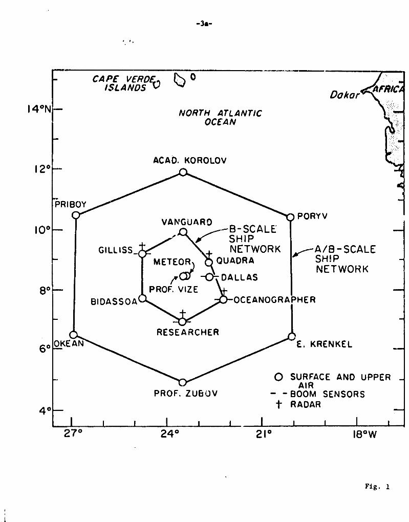
The GARP Atlantic Tropical Experiment (GATT:) was conducted in 1974 using a
total of twelve ships arranged in two hexagonal arrays which were exact for the
first two phases and distorted during the last phase. It is clear from Figure 1,

Acknowledgement
The author wish to thank Mr. Charles Laughlin and Dr. Raymond Wexler
of National Aeronautics and Space Administration, Goddard Space Flight
Center for their assistances and helpful discussions throughout the period
of researe}, and Mr. Vernon Paterson of National Oceanic and Atmospheric
Administration for his assistance in data preparation.
the extent and nature of the distortion. The ships in the inner hexagon were 165
Km apart while those in the outer hexagon •.acre .445 Km apart. This report Is
based only on data from phases I and II.
The ships in the array made standard surfacr, synoptic observations on an
hourly basis and upper air measurements every six hours, such measurements were
increased in frequency during periods of precipitation. Many ships made ocean-
ographic and radiation measurements, collected boundary layer profile data, and
recorded surface meterological data; however, the- data used in this study come
from the use of twos-band radars used to obtain special distributions of rain-
fall not available from ocher sources.
The c-band radars were choosen to minimize attenuation problems and maximize
spatial resolution. The radars were equipped with automatic digital processing
and recording equipment and the anteinian were stabilized to compensate for possible
roll and pitch.
Data was collected at 15 min. intervalP on a 24 hour basis. Antenna tilt
sequences of 360° scans at a series of 12 increasing tilt angles were collected
out to a range of 250 km. The reader is referred to Hft+dl.ow (1975) for details
and further discussion on the radar systems along with further references.
1.3 Approach.
The distribution of rainfall has been studied extensively from many different
vantage points and a number of probability models have been developed. Thom (1968),
Simpson (1972), Johnson and Mielke and Mielke (1973) are among the major workers
In this field. There is no single distribution which best describes rainfall and
any proposed model may be criticized at a number of levels. In particular, the
very nature of the diurnal rainfall variation makes the use of any model problemaric.
i
Doko
-3&-
14°N
12°
PRIBOY
10°
8°
CA PE VER0§0ISLANDS
^ ^)
NORTH ATLANTICOCEAN
ACAD. KOROLOV
VANGUARD B-SCALE
PORY V
/ SH IP
GILL ISS_ NETWORK ,,,--A/B - SCALEMETEOR QUADRA SHIP
DALLASNETWORK
PROF. VIZE
BIDASSOA OCEANOGRAPHER
6° PKEA
4°
E. KRENKEL
0 SURFACE AND UPPERAIR
- -BOOM SENSORSt RADAR
RESEARCHER
PROF. ZU60V
27° 24°
21° 18°W
Fig. 1

-4-
Ilia approach takop '.n this study is based on the use of three powerful methods
in mathematical statistics. The first two methods are used to accomplish the first
research objective and pare f the others. We use two non-parametric statistics,
the Kolmogorov-Smirnov and the Wilcoxon signed rank. Non-parametric statistics
are definition, those statistics that are independent of any particular model
for the distribution which generates the data, and thus, all conclusions drawn
are model indgendent.
This approach only depends on the assumption that the underlying distribution
is of continuous type; that is that measurements take values in a continuous in-
terval or union of intervals and does not take any specific value with positive
probability. It is clear that rainfall measurement is not of continuous type,
and in fact takes the value zero with large probability. For our ntudy, this is
not a major problem since we are only interested in comparisons conditioned on
the event of rainfall, thus our approach uses Coo method of conditional probabi-
lity. The measurement of comparisons conditioned on the event of nonzero rain-
fall is a continuous distribution. For related applications, see McAllister
(1969) and Gringarten (1970).
The third method used in this report is based on the assumption that the
hourly rainfall averages may be viewed as a time series. This approach allows
us to examine the serial correlation of the hourly rainfall, to detect short
term cycles, to measure and compare rainfall at different locations and to
es"ablish confidence intervals for the mean value of hourly rainfall at different
locations. We are thus able to accomplish our last two research objectives with-
in imposed methodological constraints.
In the second chapter we disco~s the Kolmogorov-Smirnov and Wilcoxon signed
Rank statistics and analyze their application to the problem of rainfall variation
between noon and midnight. In the third chapter, we apply time series methods to
the hourly rainfall data and provide a detailed analysis of results. In Chapter 4,
we report results of the diurnal analyses.

Chapter 2: Statistical Methodologies
In this section tw discuss the statistical foundations which ut;derpin our
approach. Since the Wilcoxon test is well documented in the literat-ire and well
known to applied researchers, we denote a major portion of this section to the
explication of the Kolomogorov-Smirnov statistic which is less used and less
known in applied research circles.
2.1 Kolmogorov-Smifrnov.
We would like to compare the distribution -f rainfall and rainfall rate at
noon with that occuring at midnight. We expect that if there is a diurnal varia-
tion then chose two Distributions may be different. It is possible that there
could be a diurnal variation and yet the distributions are the same, so that this
assumption is biased in favor of no variation.
Let (x 11 y l )J... (X no Yn) represent n-observations of rainfall over some
region C. The x's represent the measurement at midnight and the y's at noon. In
order to satisfy our assumption of continuity, we only cons±der those pairs
(x, y) for which either x > 0 or y > 0. Let F 1 (x) by the cumulative distribution
function for midnight and F 2 (y) be the cumulative distribution for noon. These
are the unknown true conditional distribution;. We can now state that if there is
no variation, then we expect that FI (x) - F2 (y); that is, it is desired to test
the statistical hypothesis:
H: F 1 ()') - F2 (Y) (2.1)
verses the al.terrate hypothesis:
A: F 1 (x) f F2 (Y) (2.2)
Under this framework, the basic hypothesis (11) is that the distribution of midnight
rainfall measure is the same as the distribution of noon rainfall measure. Based
on the data, we would like to confirm or reject this hypothesis. In rejecting 11
we would be making the conclusion that the alternate hypothesis (A) is true.

-6-
Since we don't hpve direct access to F 1 (x) and F2 (y) we construct and analyze
the empirical distributions F W and F 2 (y), where n denotes the number of sample
points. Define CM by;
1 if X Z 0
E(A) -
(2.3)
0 if a < 0
and set:n
Fn(x) a - E C(x - x3)1
(2.0
Fn(Y) - E C (Y - Y^)-1
Since the superscript identifies the distribution, we shall let a denote the
independent variable so that equation (2.4) now becomes:
Fn(^) n n C(X - X^) i . 1,2 (2.5)-1
where A= . x^ if i - 1 and a J Q y^ it i - 2. The following theorems s'.iow how the
empirical distributions are related to the true distributions. We interpret
F M to be the proportion of X which are less than X.
Theorem 2.1. The expectation and covariance of F M satisfy:
1) E(Fn(X)) - F i M
2) Cov {F1(X), F J) ) - n {rein (F i (X), Fi (T)) •• Fi ( X ) Fi(Z))
Theorem 2.2
1) (Strong law of large numbers)
Fi (X) -► Fi (with probability 1)
(2.6)
(2.7)
^A
I-s
1^

2) limlog log t
Fi(J1) (1 - Fi 01) an,*m
t^3) sup IF M - x i MI 4 0 (with prubability 1) (Cantilli-Glivenko lemma).
—oo< A<w
Proofs of the above results require very delicate analysis and are presented
in order to provide us with the relationship between true and empirical distributions,
the relevent literature incluues: Githman 195:3, 1954, Glivenko 1933, Gnedenko and
Kolmogory 1933, 1941, and Smirnov 1936, 1937, 1939.
The next two theorei.is are fundamental to our testing procedure, define E
andn
D12 by: (i ® 1, 2)
El a V n sup IF iM - F I M 1 (2.8)
r -CQ<A<«0 n
Dn2z sup IF M- F2 M1
(2.9)D21 - n12
n n
Theorem 2.3
1) Di1 2 is independent of F M
i Q 1, 2
22) 11.", PnI 2 1)n 2 < YJ ^ 1 - e-2r ^ ¢(Y) for 0 < Y <
n-►-
Proof: We shall obtain the proof of theorem 2.3 as a special case of theorem 2.4.
Theorem 2.4. Set c - Q2nYl (greatest integer) then:
( 2n )1 _ n -1 < <
Y 11( 2n) 2

aa
Proof: 1,et us arrange our 2n-observations (xl' y d ... (X no yn ) in increasing
order of magnitude X1 , ... X2n . Consider the r ►ew set of random variable s Y1' ••• Y2n'
defined by:
1 if Xk is a midnight observation
Y a (2.11)
-1 if Xk is a noon observation
kSet SO n 0 and Sk - r Xk . It is easy to see that nD12 a cup S ;.et us note
J u l n 0<k<2i k
that Stn = 0; if we plot the points (k, S k ) for k - 0,1,.-.2n in the (u,v) plane
and connect these points by straight-line segments, the v c-)mponent will increase
by one unit at n points (corresponding to rainfall observation at noon) and will
decrease by one unit at,the cemainir.g n points.
S
(01 0) i
2n k
rig. 2
Figure 2 represents a typical trajectory of the process, the dotted lines
indicate that the curve has been broken. Since there are n increases and n de-
creases, the total number of possible trajectories is (n2n ); furthermore as our
null hypothesis is that both distributions are the same, this means that all
trajectories are equally likely. (Another bias in favor of the null hypothesis)
Hence, the probability of each trajectory is (2nd . In our geometric interpre-
n
tation, the required probability satisfying Q^ n (Y) Pr( Dn2 < c] may be stated
L
J _ ( 2n )/(2n)n-c n
(2.12)
-4-
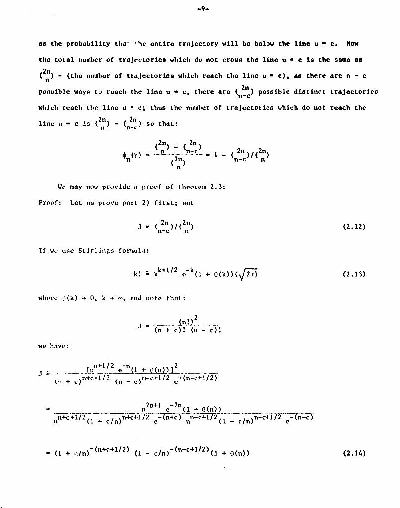
as the probability tha — lie entire trajectory will be below the line u - C. Now
the total number of trajectories which do not cross the line u - c is the same as
2n( n ) - (the number of trajectories which reach the line u - c), as there are n - c
possible ways to reach the line u - c, there are ( 2n ) possible distinct trajectoriesn-c
which reach the line u - c; thus the number of trajectories which do not reach the
line u - c `--o ( 2nl ) (n c) so that:
( 2n) - ( 2n )
Q^(Y) —nn_c- (2n M2n11 2n n )
( n)
We may now provide a proof of theorem 2.3:
Proof: Let us prove part 2) first; set
If we use Stir]ings formula:
k! a kk+1/2 0- (1+ p (k))( 21i) (2.13)
where p(k) -► 0, k -► -, and note that:
J
2
(n + c) (n - c)
we have:
In n+1/2 n 2
+ 0n+r.+l/2 (n - 0nl-c.+1/2 e-(n- c+1/1.)
2n+1 -2n
nn+c^Fl /2(1 + c/n)n+c:+ l%2 a-(n+c) nn-c+l 2U - c/n)n-c -4-l/2 a-(n-c)
(1 + ,t/n)-(n+c+1 /2) (1 - c/n)- (n-c+1/2) ( 1 + O(n)) (2.14)
-10-
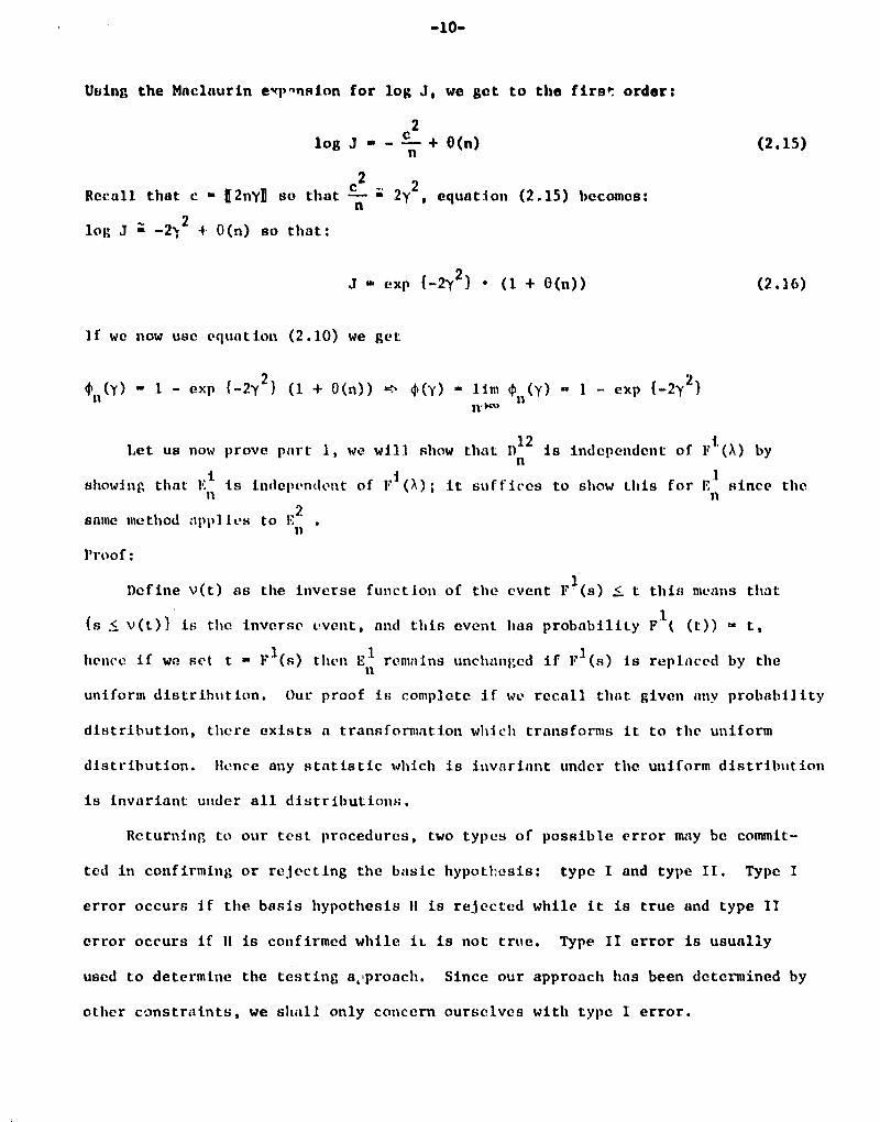
Using the Maclaurin evp-nsion for log J, we get to the firs! order:
2log J - n + 0(n)
2Recall that c - Q2nyJ so that n 2y2 , equation (2.15) becomes:
log J Z -21 2 + 0(n) so that:
J - exp {-2y 2 ) • (1 + 0(n))
(2.15)
(2.16)
If we now use equation (2.10) we got
Q'11 (Y) '° 1 - exp {-2y 2 ) (1 + 061)) 'C' t(Y) - lim 0 1 (Y) - 1 - exp {-2y2}IrKu
Let us now prove part 1, we will show that 1) 12 is independent of F i (a) byn
showing that Fi is independent of F i (X); it suffices to show this for rn since the
same method applies to En
Proof:
Define v(t) as the inverse function of the event F 1 (s) < t this means that
Is _< v(t)) it; the inverse event, and this event has probability F t ( (t)) - t,
hence if we set t - F 1 (s) then Lip remains unchanged if F 1 (s)is repinced by the
uniform distribution. Our proof is complete if we recall that given any probability
distribution, there exists a transformation which transforms it to the uniform
distribution. Hence any statistic which is invariant under the uniform distribution
is invariant under all distributions;.
Returning to our test procedures, two types of possible error may be commit-
ted in confirming or rejecting the basic hypothesis: type I and type II. Type I
error occurs if the basis hypothesis H is rejected while it is true and type II
' error occurs if H is confirmed while iL is not true. Type II error is usually
used to determine the testing a,,proach. Since our approach has been determined by
other constraints, we shall only concern ourselves with type I error.
-11-
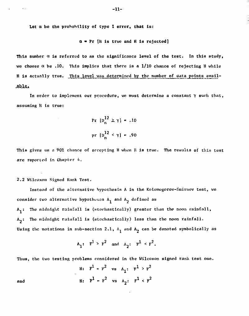
Let a be the probability of type I error, that is:
a - Pr [11 is true and H is rejected]
This number a is referred to as the significance level of the test. In this study,
we choose a be .10. This implies that there is a 1/10 chance of rejecting H while
H is actually true. This level was determined by the number of data _points avail-
Jlug.
In order to implement our procedure, we must determine a constant Y such that,
assuming It is true:
Pr [1) 12 > Y] . .10
pr [D12 < Y] - .90
This gives us a 90% chance of accepting H when 11 is true. The results of this test
are reported in Chapter 4.
2.2 Wilcoxon Signed hank Test.
Instead of the alternative hypothesis A in the Kolomogorov-Smirnov test, we
consider two alternative hypotheses Al and A2 defined as
A1: The midnight rainfall is (stochastically) greater than the noon rainfall,
A2: The midnight rainfall is (stochastically) less than the noon rainfall.
Using the notations in sub-section 2.1, A l and A2 can be denoted symbolically as
Al : F1 > F2 and A2 : Fl < F2.
Thus, the two testing problems considered in the Wilcoxon signed rank test one.
H: F1 = F 2vs A1 : F1 > F2
and H: F1 . F2 vs A2 : F1 < F2

-12-
However, these two to^r+ ,il, problems are statistically equivalent, respectively,
to If F2 < F2 vs A1 : F 1 > F2 and N2 : F1 > F2 vs A2 : F1F2. If Al is not rejected in
the first problem and A2 is not rejected in the-second problem then we conclude
that II: F1 = 1?2 holds.
As in the K - S test, there are two types of possible error in each of these
two problems. Again, we consider only type I errors. To test H vs Al , type I
error is committed if H (or Ii 1 ) is rejected while H: F F` is actually true, i.e.
confirming A 1 : ,'1 < F2 while H: F 1 a F2 is actually true. The significance level 011
is given by
a1 I' 1{ [rejecting III - P 11 [accepting A11.
To test H vs A2 , type I error is committed if A 2 : F 1 > F2 is accepted while
11: F 1 = F2 in actually true. The significance level is given by
a2 = 1 . 11 f rejecting 111 - P H [accepting A 2 1 .
Note that rejecting; H implies accepting A l in the first testing problem If vs Al
and accepting; A2 in the second testing problem H vs A2 . In this study, we adopted
N= a2 = .10.
Let (x1,y1),..., (Xns yn ) be as defined in subsection 2.1. The testing pro-
cedure of Wilcoxon signed test consists of deriving a statistic V based on
(xl'yl)'...' (xn'yn) and choosing constants C 1 and C2 (C2 • C1 ) corresponding to
al and a2 , respectively, such that for testing 11 vs Al
rejecting; 11 (or accepting A1 ) if and only if V > C1
and for testing If A2
rejecting H (or accepting A2 ) if and only if V S C2.
e detail, the reader is referred to Lehmann (1975).
►c above discussion that when If is true, PH [Vn < C2 1 - . 10,

-13-
PH [C
2< VN < C 1 ) _ .LC ind P
IlIV '1 Z C 1 ) - .10. Thus, when H is true, the chance
of concluding that midnight rainfall is (stochastically) greater than, equal to
and less than the noon rainfall are, respectively 10%, 80% and 10%.
The result of this test is reported in Chapter 4.
2.3. Chi-square Test.
The tests describe in subsection 2.1 and 2.2 are applied to the midnight and
noon rainfall measures at each grid of the GATE data. It was seen that when H is
true, the chances of drawing e conclusion that F Q F 2 1 2and F 0 F , are, respectively,
90% and 10% and that F < F 2 , 1- 1 - F2 and F > F2 are, respectively 102, 80% and 10%. We
use X 2-test to test whether these percentages are actually obtained in the result.
Let 1) 1 be the probability of making the jth conclusion, j - 1,2,..., k, where
k is the number of different conclusions (k - 2 in K-S test and k - 3 in Wilcoxon
test). Let: n' be the number grids at which jth conclusion is made, j - 1,2,..., k
and n = n + n2 +...+ nk , the number of grids in the study. Define
2 k ( _ J:_Xk = j°1 np j
If the given percentages of different conclusions are followed, Xk should be
relatively small. Thus, if Xk is large, we may conclude that the percentages do
not hold true and should have been otherwise. For instance, in the Wilcoxon test,
P 1 . .10, P2 - .80 and P 3.10. If X3 is too large, then the percentages of 10,
80 and 10% do not hold and thus the hypothesis H: F 1 - F2 is not true. To determine
"how large" is "too large", a cutoff constant can be ound corresponding to k and
the desired significance level of the X 2-test. With a - .05 (i.e. 5% chance of
making wrong conclusion), C - 3.84 for k - 2 and C - 5.99 for k = 3.
Results of the X2-test are reported in Chapter 4.

►ugh for practical purpose.
Chapter 3
Teml•iral Analysin on Hourly Rainfall Averages
The hourly rainfall averages were considered as observations in a time series.
Analyses on the time series were undertaken for both Phase I and II data in
experiment. Properties of such time series at selected locations in the GATE
experiment were investigated. In the following sections, the objective of the study,
the data and sampling design as well as the analyses and their results are reported.
3.1. Objective of The Study
The objectives of this study are:
• To examine the serial correlation of the hourly rainfall.
• To detect the short term cycles in the rainfall activities.
• To measure and compare the power of rainfall activities at different localities.
• To establiHii a confidence interval for the mean of hourly rainfall averages.
The serial correlation of hourly rainfall averages reveal the linear dependence
of the rainfall on the rainfall of the preceeding hours. These statistics are
closely related to the duration of rainfall activities.
High autocorrelation with large lags implies long duration and vice versa.
The serial correlation is also related to an assumption in the studies in Chapter 2:
The diurnal analysis of rainfall. It was implicitly assumed in thc: study that the
noontime and midnight rainfall rates are independent. Here we consider the corelation
between rainfalls several hours apart. While no correlation between rainfalls in
different hours do not imply independence between them, they may be considered close
-15-
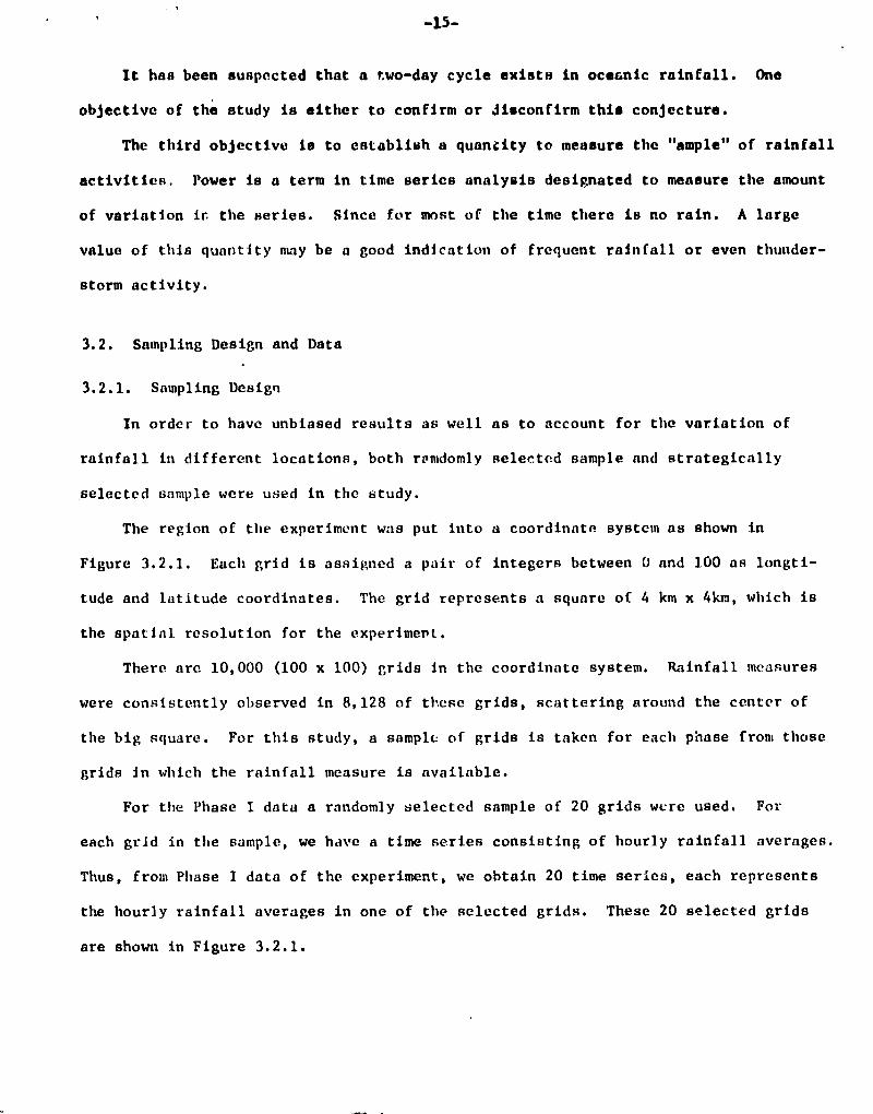
It has been suspected that a two-day cycle exists in oceanic rainfall. One
objective of the study is either to confirm or disconfirm this conjecture.
The third objective is to establish a quantity to measure the "ample" of rainfall
activities. Power is a term in time series analysis designated to measure the amount
of variation it the series. Since for most of the time there is no rain. A large
value of this quantity may be a good indication of frequent rainfall or even thunder-
storm activity.
3.2. Sampling Design and Data
3.2.1. Sampling Design
In order to have unbiased results as well as to account for the variation of
rainfall in different locations, both randomly selected sample and strategically
selected sample were used in the study.
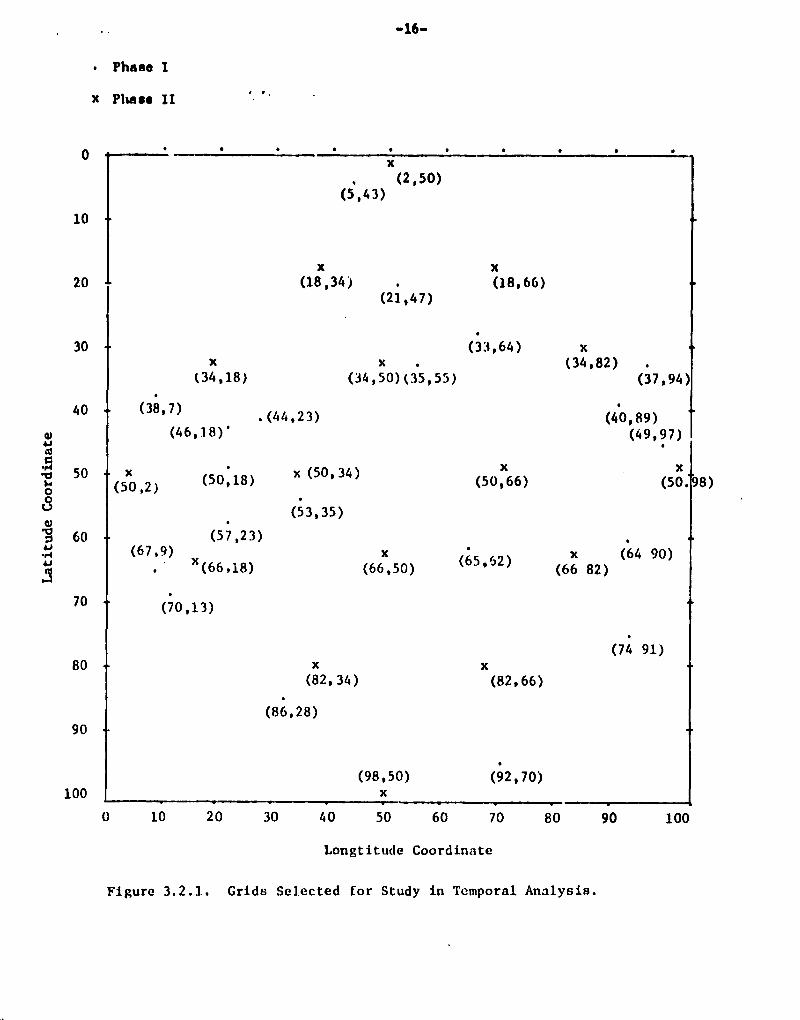
The region of the experiment was put into a coordinate system as shown in
Figure 3.2.1. Each grid is assigned a pair of integers between 0 and 100 as longti-
tude and latitude coordinates. The grid represents a square of 4 km x 4km, which is
the spatial resolution for the experiment.
There are 10,000 (100 x 100) grids in the coordinate system. Rainfall measures
were consistently observed in 8,128 of these grids, scattering around the center of
the big square. For this study, a sample of grids is taken for each phase from those
grids in which the rainfall measure is available.
For the Phase I data a randomly selected sample of 20 grids were used. For
each grid in the sample, we have a time series consisting of hourly rainfall averages.
Thus, from Phase I data of the experiment, we obtain 20 time series, each represents
the hourly rainfall averages in one of the selected grids. These 20 selected grids
are shown in Figure 3.2.1.
L
-16-
• Phase I
x Phase II
x(2,50)
(5,43)10
` x x20 (18034) (18,66)
^ (21,47)
30 (33,64) xx x (34,82)
i (34,18) (34,50)(35,55) (37,94)
40 (38,7). (44,23) (40,89)
(46,18) • (49,97)
50 (50,18)(50 ,2) x (50,34)
(50,66) (50. 8)I 0
(53,35)n^
60 (57,23)•4 (67,9) x x (64 90)
(65,2)x (66.18) (66,50) (66 82)a
I 70 (70,13)
(74 91)4
80 x x(82,34) (82,66)
i (86,28)
90
Ia
(98,50) (92,70)100 x
U 10 20 30 40 50 60 70 80 90 100
Longtitude Coordinate
Figure 3.2.1. Grids Selected for Study in Temporal Analysis.
-17-
For Phase II data. a strategically selected sample of 15 grids were used. The
sampled grids are also shown in Figure 3.2.1.
3.2.2. Data and Missing Values.
Hourly rainfall averages are computed by adding the rainfall measured in the
hour and then dividing by the number of rainfall measurements within the hour. This
Is done for each hour in the duration of Phases I and II in the CATE experiment.
The nature of the study calla for an uninterrupted sequence of hourly rainfall
averages. It was found that there are hours in both Phases I and II which do not
have rainfall measurements. This situation usually occured in the earlier stage of
both pharces. We decided to cut short the time series to accomodate our needs. For
Phase I, the actual duration usCd for this study is from the 12th hour of 182nd day
to the 17th hour of the 197th day. (The Phase I experiment lasts from the 0th hour
of the 179th day to the 17th hour of the 197th day.) (All Julian hours and days).
For Phase II the actual duration used is front 20th hour of the 214th day to the
21st hour of the 227th day. (The Phase II experiment lasts from the 0th hour of the
209th day to the 21st hour of the 227 day.)
In both Phases I and II there still exists an hour without measurement. This is
filled with method of interpolation. It is expected that the effect of this is
negligiM e.
We could have used the original rainfall measure of every quarter hour as the
observati^n (term) of the time series, instead of the hourly rainfall average. However,
there are so many missing values in the quarter-hourly measures throughout the experi-
ment in both Phase I and II that it is not advisable to use them directly.
-18-
3.3. Auto Correlation
It is well known that the hourly rainfall averages of adjacent hours are
positively correlated. That is given that there was an above average rainfall. in
a specific hour, it is very likely that there would be an above average rainfall
in the next hour, and possibly in the hour thereafter, etc. Auto-correlation
measures the correlation of the hourly rainfall of hours apart. The computation
formula are given in subsection 3.3.1 and refults reported in the subsequent sections.
3.3.1. Computation Formulas.
Let xI ' x2,...,xn denote the hourly rainfall averages at a given grid of the study.
Note that n is the number of hourly rainfall averages in the grid. Define the
sample mean and sample variance as
_n nx- 1 Ex S2-1 E (x -x) 2 .nt-1t nt-1 t
Uen the rth auto-correlation of the series is defined to be
n-rRr
n- R(r) - E (xt X) (X- x)/s 2 , r
t-1
The number r in the formula is called 1^ of the auto-correlation, and k is the
maximum number of lags for the auto-correlation to L computed. The auto-correlation
R - R(r) considered as a function of r is called an auto-corre lation func tion.
It should he pointed out that, unlike in a random sample (fro g a population of
rainfalls), xl,x2,...,xn are not independent and identically distributed. The x
denote the t-th hourly rainfall average starting at sc.,ic specific hour. The length
n of time series is 366 for series in Phase I data and 328 for series in Phase II
data.
-19-
3.3.2. Correlograms.
The correlogram of a time series is the plot of its auto-correlation function
R(r) against the lag r. Just as the histogram is studying sampling problems, the
correlogram is descriptive and informat i ve in studying the time series. It is a
visual device which is useful to perceive the linear relationship of rainfalls
several hours apart and to Identify the mechanism generating the rainfall series.
However, it in not an objective of this study for the latter, i.e. to identify the
model of the series.
In the following paragraphs, we make some observations of the correlograms for
time series in both phases I and II.
As said earlier, the length of the time series is 366 for phase I and 328
for phase II. Corresponding to these sample sizes, the approximate 95% confidence
interval for the correlation coefficient of 0 is (- .12, .12). That is, if it is
hypothesized that the correlation coefficient is zero, the chance of having the
computed coefficient to be out of interval (- .12, .12) is 5% or 1 out of 20. The
5% chance of error is a generally accepted level in practice. Thus, if the auto-
correlation of a time series at any given lag is in the interval (- .12, .1.2), we
may safely assume the value 0 (with 5% chance of being wrong.)
Examining the correlogram, it is found that there are no
uniform and specific shape for the correlograms for all time series. The shape
varies greatly from series to series. The length of these time series may be blamed
for the non-uniformity in the correlogram. In general, a timc series of length 366
or 328 should be long enough to obtain a meaningful result. But for the time series
-z0-
on hand, this may not be true, because there are too many zeros (more than 4 out of
5) for most series) for the hourly rainfall average. It is very likely that just a
few hours of heavy or even moderate amount of rainfall at a different time would
change the bhape of the correlogram dramatically.
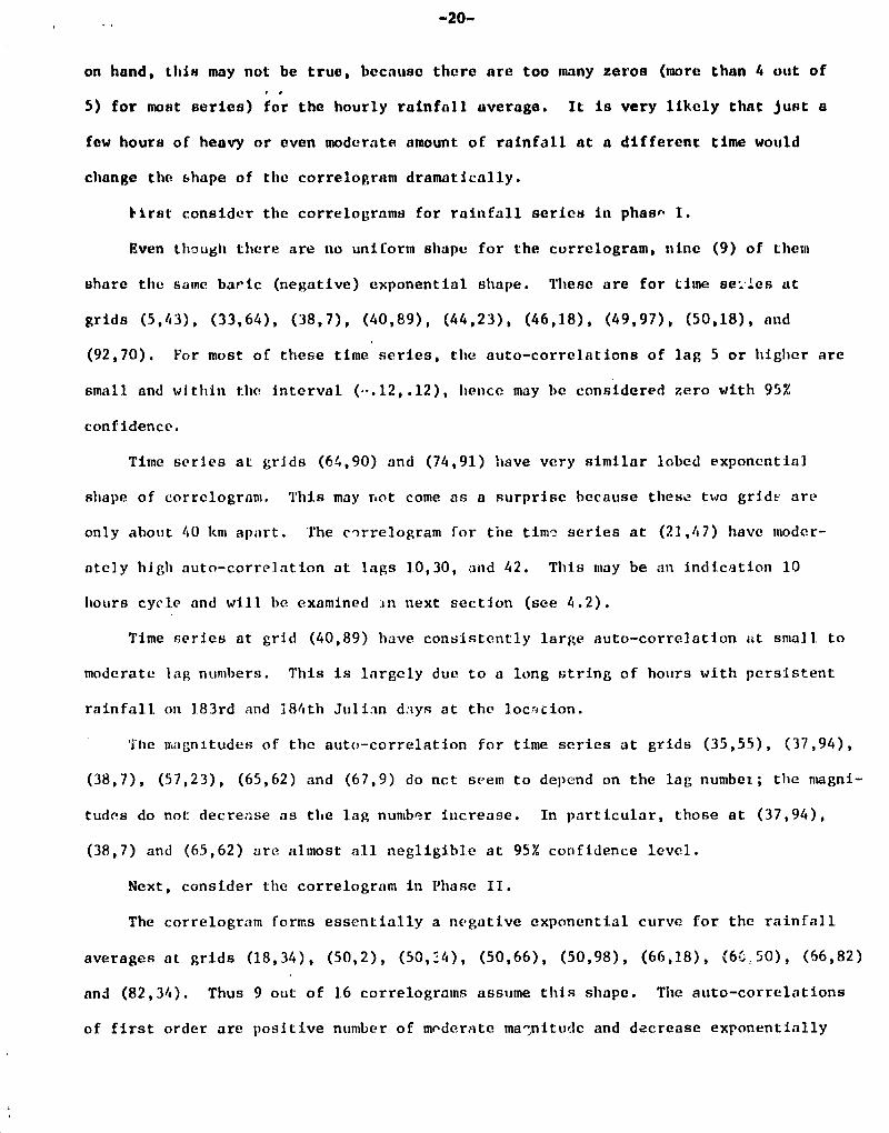
first consider the correlograms for rainfall series in phase I.
Even though there are no uniform shape for the correlogram, nine (9) of them
share the same baric (negative) exponential shape. These are for time series at
grids (5,43), (33,64), (38,7), (40,89), (44,23), (46,18), (49,97), (50,18), and
(92,70). For most of these time series, the auto-correlations of lag 5 or higher are
small and within the interval (••.12,.12), hence may be considered zero with 95%
confidence.
Time series at grids (64,90) and (74,91) have very similar lobed exponential
shape of correlogram. This may not come as a surprise because these two gridF are
only about 40 km apart. The correlogram for the tim^ series at (21,47) have moder-
ately high auto-correlation at lags 1.0,30, and 42. This may be an indication 10
hours cycle and will be examined in next section (see 4.2).
Time series at grid (40,89) have consistently large auto-correlation i;t small to
moderate lag numbers. This is largely due to a long string of hours with persistent
rainfall on 183rd and .184th Julian dayn at the locricion.
'rile magnitudes of the auto-correlation for time series at grids (35,55), (37,94),
(38,7), (57,23), (65,62) and (67,9) do nct seem to depend on the lag numbex; the magni-
tudes do not: decrease as the lag number increase. In particular, those at (37,94),
(38,7) and (65,62) are almost all negligible at 95% confidence level.
Next, consider the correlogram in Phase II.
The correlogram forms essentially a negative exponential curve for the rainfall
averages at grids (18,34), (50,2), (50,24), (50,66), (50,98), (66,18), (66,50), (66,82)
and (82,34). Thus 9 out of 16 correlograms assume this shape. Tile auto-correlations
of first order are positive number of mrderate ma7nitude and decrease exponentially
-21-
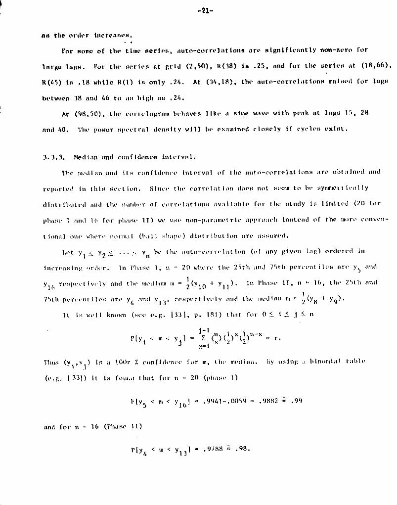
as the order increa»es.
For son ►e of the tln ►e series, auto-correlations are significantly non-zero for
large lagm. Vor th(- series rt grid (2,50), R ( 38) is .25, and for tilt, serteti at (18,66),
R(45) is .18 while R(t) it; only .24. At ('14,18), the auto-correl tit ton-.4 raised for lairs
between 38 and 46 to tit; high as .24.
At (98,50), the correlogram behaves like it wave with peak at ings IS, 28
and 40. The power spectral density will tit , examined closely if cycles exist.
3.3.3. Median and confidence interval.
nit- motlian and its Confidence Interval of the auto-correlations are oi-italned and
reported in this section. Since the correlation does not seem to li t, sYmmett ict ► 11y
distribctted and the number of correlations avallabte for the study is limited (20 for
phc ► sv 1 and lb for pl ► r ► se 1T) we use non-parametric approach instead of the more conven-
t.ional one wbert , normal (1, all s11ape) distribution are assumed.
I.et y l * y 2 < ... vn be the auto-correlation (of tiny given lair) ordered In
increasing m-der. In 1'11aso T, it 20 where , tilt- 25111 :ind 75th percent Iles are y, and
Y16 reslivet ively and the tnedi ►tm m ° I (Y 10 i Yll)'
in p ltnse IT, it 16, the 25th and
175111 percentile:; are y
4 and y 13 1
respect ivt-ly and tit(- med inn to 2
(y 8 + Yy) .
It it; we l knourn (see e. g. 133 1, p. 181 ) that for 0 .<_ i _< 1 ^- n
PIy i < m < y l l G . F. 1 (11 1
) ( ) x ( I)'t-x r.x'i
Thus (y i , v i ) Is it % confidence for n► , the Illectiall. BY using; .^ binomial table
(e. g, ( 331) 1 t is fou ► .kt t hat for it 20 (phase 1)
Ply < m < YlbI
o .9041-.00`)9 - .9882 s .99
and for n - 16 (Phase 11)
P1 Y4 < tit < y 13 1 - .9788 a .98.

-22-
Hence (y 5 , y16) is a 99% confidence interval for the medium of the auto -correlation
with any given lag in Phase I and N' y13 ) a 98% confidence interval in Phase H.
The chances of error are 1% and 22 in Phases I and II, respectively, in saying that
the medium is in the interval.
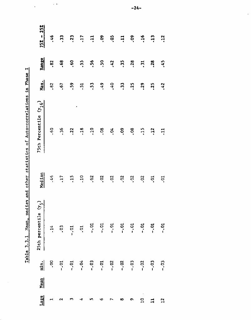
Table 3.3.1 and Table 3.3.2 summarize the means, medians, 25th and 75th percent•
iles, ranges, lengths of confidence intervals of the auto-correlations for lags 1
through 12 in Phases I and II data, respectively. The range is defined to be the
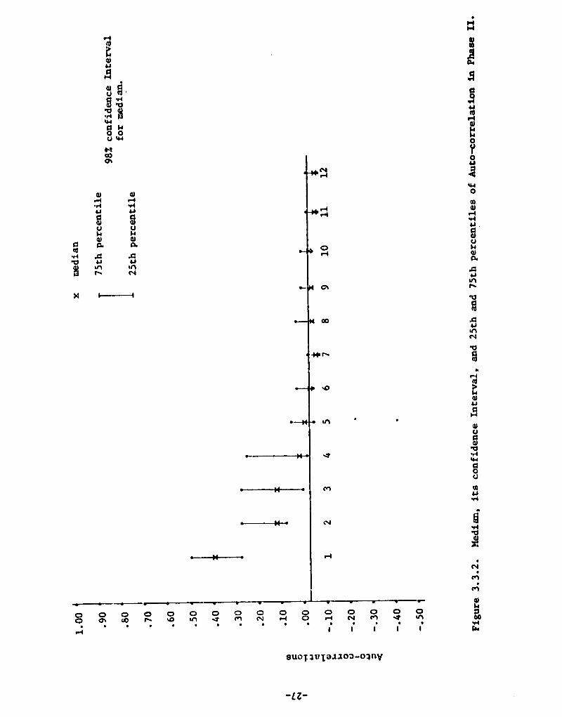
maximum of correlations minus minimum of the same. Figure 3.3.1 and Figure 3.3.2
show the medium, 25th and 75th percentile along with confidence interval for the
medium in Phases I and 11 data respectively.
It is seen that in.hoth Figure 3.3.1 and Figure 3.3.2, the median with lag 1 is
moderate (in 40's) and there is a considerable drop between lags 1 and 2. The mediums
with lags 2 and 3 are about the same magnitude. Those with lag 5 or higher are so
small that they are negligible. In fact, their confidence intervals contain 0 for
most of them. Thus, the hypothesis that meal ian is 0 ,!ould not have been rejected.
3.3.4. Concluding Remarks.
The auto-correlation function for each time series in both Phases 1 and II
were studied. The length of series is 366 in Phase I and 328 in Phase II. Since
most (more than 80%) of the rainfall are 0, the auto-correlation function seem un-
stable in sense that the shape of the function are uite different from series to
series. However, 9 out of 20 in Phase I and 9 out of 16 in Phase ?I are essentially
negative exponential curves. For these series, the auto-correlation with lag 1
ranges from .46 to .82 in Phase I and from .34 to .68 in Phase 11. The value decrease
exponentially as the lag increase. Three of the correlation functions show scme re-
peating peaks and valleys. These series r:ay have short term cycles and will be
examined for such in the next section. At lag 1, the median of the auto-correlation
is .46 for phase I series and .41 for phase II series. At lags 2 and 3, the values
-23-
for the auto-correItit ion drop considerably for both phases I and H. The values
are not significant for lag larger than or equal to S. Thus we may say with caution
that rainfalls of S or more hours apart are uncorrelated. This statement is not
always true. There are occasions that the auto-correlation with larger lag is signs--
ficantly non-zero.
3.4. Power Spectrum
TEe power spectrum is useful tool to detect a cycle in the time series. If the
power at it frequency is large comparing to the powers of neighboring frequencies,
then we may conclude that there Iv it cycle In the time series corresponding to the
frcquvacy.
In this section, we use power spectrum estimate of hourly rainfall averages to
detect short term cycles. We start with a brief review of the methology in subsection
3.4.1. The analysh-, and results are reported i.n subsection 3.4.2.
3.4.1. Power spectrum of the t iaie series.
To farilltate the intei-pretatton of the results of s pectral analysis an over-
simplitied version of time series representation and its analysis; is presented here.
This version is intended for readers who have no background in time series analysis
and want to get hold of some conceptccal meaning of the result to be reported in the
following subsection. Readers with background in spectral analysis of time series
may skip th.Is subsection and proceed to subsection 3.4.2.
We assume that a time series x(t) may be written as
X(t) _ {{
CO
E z eixjt
J'-p0 S
whprc- i _ I a0 0 0, X -1 _ - a1
and z z^, the z's are random variables (with
0 for J # 0). The restrictions on the a 0 and z's imply that x(t) is a real-
random variable for each t, the time. The representation of x(t) says that
v'►N
1Kn
;I
k I N f- O% .-1 M O% O M to 4N Un N
1^Q+ aC ^O u1 n n M N N N. . . . . . . . . . .
n
r-1
v
CI
M
c^SiU O 10 N tlD O 00 11 ON 00 ►n N r--1u N .-r r-4 O p O O r-1 r4 r-A
C!axa^^n
G%.v n Ln O N N N N N N r-1 r-111 r-1 r i r i O O O O O O O O
CI
r-1 r--1 r--1 M r-1 r--4 r-4 r-1^Y M .-r r-1 O O O O O O O Or-1 O O O
• i i 1 i i i i Ii
H^ 0 r-1 r-A d M r-d N N M N M M
O O
1
O
1
O
I
O
1
O
1
O
1
O
1
O
1
O
1
O
1
O
1
tq i
e-1 N M -1 in %O r- co m O r-1 N(ti .-1 .-1 .-d
nrnu
CI
Ma^ANuNofaxuN

Z NCi
ri
dl
Eid+I
i-25-
HHdW
^dd•iii
^p
O•rlRIr-1}GlNOU
dWOMuaNu^or3
HNNOb
CR
6
K
11 N Cl N N O 0 0 0 0 0 0
n
1
en M 1- N 1- 1- N in rl in ^C •-1^7 ^7 cn M N N M N N r4 r-4 •"
•I f^
cn M N N N N r-1 r4 r-1 O
nM
r-i
01 HM M N Q OO m^ 1^ M O vy.i n M N N O O V C O ^ . 1
q IduNOlax^nr
t++ ' r N co 17 H . -1 .-1 N H .-i N NrA O O O O O O O O O O
^^ 1 i 1 1 1 1 I
Jr-1v
d'H !•1 en N N N M M H 00^ M O O O O O O O O O O Oy 1 1 I I 1 1 I I
uwa,auinN
u1 r-i N N N ^t
;
tn
q ! N O O O O O O O O O O O
1 1 1 1 1 1 1 I 1 1
^I
T-A N c9 It 00 O% OH9-4 C4

Fi
MM
0oMW
a
0
SO
N
dw0
w
Mr-1Y'IuuNC!aa^^n
b
Au.nNb
wt"`I
uparbMW
guu
w
ld
b
du
u^^b
u W
eaa
d
-26-
O O O O O O O O O O O O%D Ln -1 Cn N rl O •-1 N M -4
1 1 1 1 1
suoT3t?jajjoo-oany
-LZ-
GI CI.-1 •-1•d 44u u
u u
YI .0 A
Ln tnr` N
O 0 0 O
.••-1
N
ud
OvOa►
WO
041
.-1
u.
uHNa.cu
n
,Cu
N
b
w.-1
01u1^1
0)
uqNbAw
u
u,rw
N
A
M
dH
vlW
a►u
u^bbwq HuwM000

-26-
the series can be decomposed into contribution of harmonic at frequency a^ or that
the series is the superimposed sum of harmonics at frequency AJ.
It can be shown then that the power of the time series can be written as
power of x(t) _ (power of x(t) at frequency a^J.
The power of x(t) at frequency X
measure the amount of variation, or intensity, of
the series at frequency X J . In particular if z a c i , a fixed constant (i.e. not it
chance variable), then the power at X i is c 2 J . Note that lei I is the magnitude of
the term c I e ixjt in.the representation. (i.( , . le I = Ic- i IC i/jtj ). When z is a
chance variable, the power of x(t) at frequency a^ is the variance of z i , E1z21, and
the power of x(t) is the total variance at all frequencies, which is also the variance
of the ensemble x(t), t = 1,2.....N.
The power spectrum of the time series describes the distribution of the total
power of x(t) at different frequencies. Define the bower of x(t) at frequency Xi
as a function of a J . '1'lav function so defined is the power spectrum of the series
x(t). At frequency Xj , the value of this aunction measures the contribution of theis t
harmonic e i to the total power of x(t). if the contribution at the frequency a3
Is large, coanparing to thc• neighboring; frequency, then there is a cycle imbedded in
the time series x(t) at frequency X J . It is understood that the power spectrum, or
spectral analysis in general, is useful in other respects such as model building;,
prediction, filtering; and control simulation and optimization, etc. We shall restrict
our study to explore the short term cycles of the series. For detail discussion,
the Interested readers are referred to Jenkins and Watts 1371 and Koopmans 142).
3.4.2. Power spectrum estimate.
The power spectrum estimate is computed using FT-FREQ subroutine of the Inter-
national Mathematical and Statistical. libraries (IMSI.). Due to the limited accessi-
bility of the 1MSL to the author,;, only preliminary exploratory study of the analysis
-29-
is undertaken. The study is restricted to explore the short term cycles in the
data. it is noted that the length of the time series is short for detecting cycles:
366 for series in Phase I and 328 in Phase II.
In Phase I, the series at grid (21, 41) show strongly a 10 hour-cycle, at grid
(53,35) a 25 hour cycle, at grid (64,90) and (65,62) a 12.5 hour cycle, and at
(74,91) a 15 hour cycle.
In Phase I1, the series at (98,50) shows a 13 hour cycle, and a 5 hour cycle,
at (82,34) a slight 50 hour cycle, at (66,82) a 100 hour cycle, at (66,50) a slight
33 hour cycle,at (50,98) it hour cycle, at (50,2), 14, 7 and 5 hour cycles, at
(34.38) a 50 hour cycle and at (18,34) a 50 hour cycle.
From the obt;ervation in the last two paragraphs, it does not seem to have
dominant cycle prevail to all time scrics. A cycle of 12-13 hours is observed in
two of Phase I Series and one of Phase l.I series. A cycle of 50 hours (or more
likely 2 days) is observed in three series in Phase 1I.
3.5. Distribution of Totnl Power
It was observed in the last section that the power varies wildly among; series.
This is true for bath total power and power at all frequencies. To some extent,
the power measure the "amount" of rainfall activities at a specific frequency. The
total power is in fact the variance of the hourly rainfall averages (the ensemble).
Since most of the hourly rainfall averages are zero, large variance would indicate
a large of rainfall from time to time or maybe frequent thunderstorm activities.
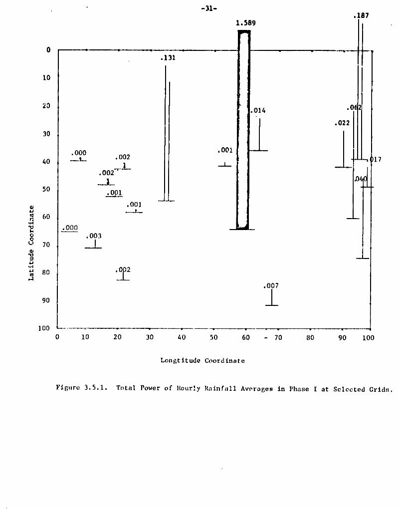
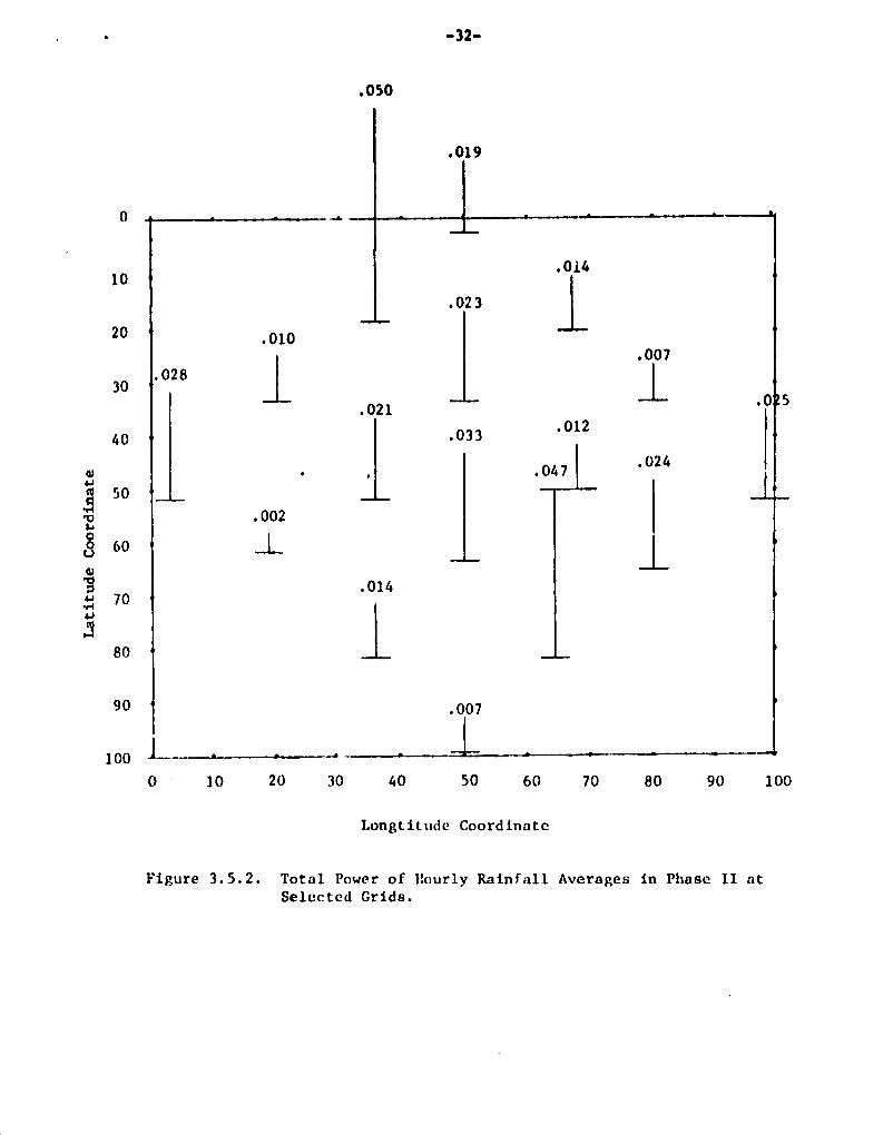
Figures 3.5.1 and 3.5.2 show, the plot of the total powers of times series at
selected grids in Phase I and Phase II, respectively. Tables 3.5.1 and 3.5.2 list
L• he values.
It is observed that the values of the total power of the series in Phase I
vary from .002 to 1.589. This variation is dramatical considering that there are
U.
-30-
366 observations involved. The value of 1.589 occured at grid (65.62). It is
found that at this grid there was e..ceptional.ly largo: amount (23.71 cm/hour) of
rainfall at one time. At grids (37,97) and (53,35) the total powers are .187
and Al, respectively. These values are also considerably large comparing to
the rest.
The total power of series in Phase II ranges from .002 to .050. The largest
value is 25 times of the smallest values. The ratio is moderate if one notes that
the corresponding ratio in Phase I is 9,349. Thus the rainfall activities were
somewhat similar among all localities during Phase II of the experiment while they
were dramaticnlly different during Phase I.
-31-.187
a
r 60vw00
70av0
80.a
1.000
90
40
20
50
10
30
0
117
10 20 30 40 50 60 - 70
Longtitude Coordinate
80
90 100
Figure 3.5.1. Total Power of Hourly Rainfall Averages in Phase I at Selected Grids.
0
10
20
30
40
70 80 90 1001.0 20 30
90
100
0
80
a^
. 50
Hg 60
0^v0
70
40 50 60
Longtitude Coordinate
.050
-32—
Figure 3.5.2. Total Power of Hourly Rainfall Averages in Phase II atSelected Grids.
1u
.04 r.N o3
aui . 02NF .01
.00
10 20 30 40 50 60 70 80 90 100
Longtitude Coordinate
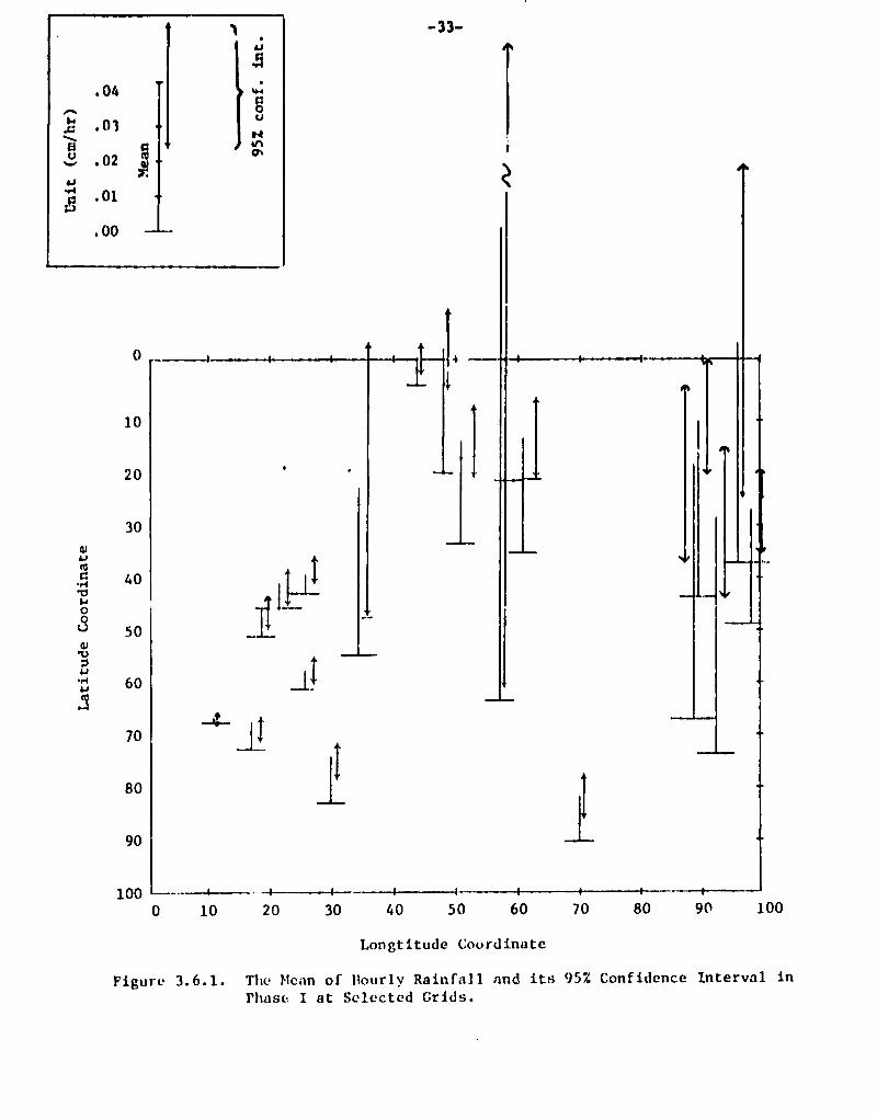
1. The Mean of Hourly Rainfall and its 95% Confidence Interval inPhase I at Selected Grids.
0
10
20
70
80
90
100 --
0
irc
-33-
30
ub
40b00
50a^v
60I

1w
u
0%
-34-
.04
,-^ .03H
.0211
. 01,4a .00
I
1(
2(
3(
4(
0 50uCO.a
N 60
00Ub 70
NM
a 80
90
100 --+— '0 10 20 30 40 50 60 70 80 90 100
Longtitude Coordinate
Figure 3.6 . 2. The Mean of Hourly Rainfall and its 95% Confidence Intervalin Phase II at Selected Grids.
-39-
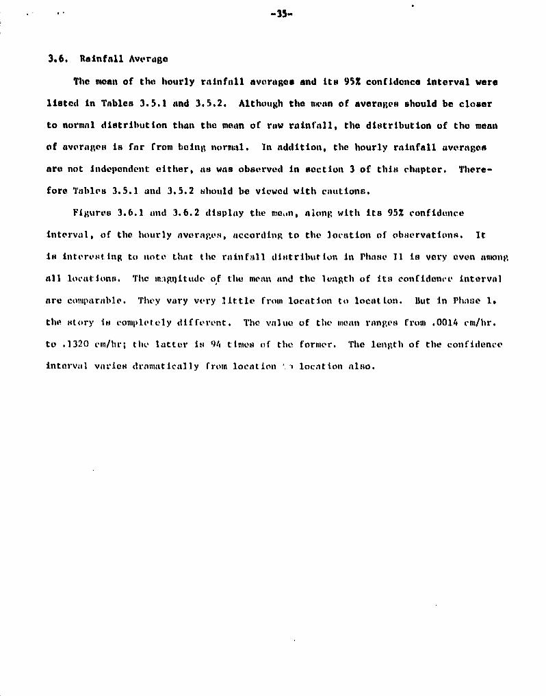
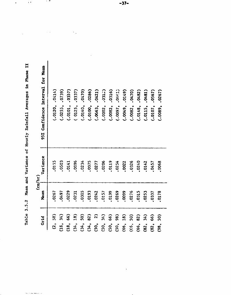
V3.6. Rainfall Average
The mean of the hourly rainfall averages and its 952 confidence interval were
listed in Tables 3.5.1 and 3.5.2. Although the mean of averages should be closer
to normal distribution than the mean of raw rainfall, the distribution of the mean
of averages is far from being normal. In addition, the hourly rainfall averages
are not independent either, as was observed in section 3 of this chapter. There-
fore Tables 3.5.1 and 3.5.2 should be viewed with cautions.
Figures 3.6.1 and 3.6.2 display the mean, along with its 95% confidence
interval, of the hourly nverageK, according to the location of obKervations. It
Is interesting to note that the rainfall dit.tribut.ion in Phase 11 is very even among
all locations. The in.igqitude of the mein and the length of its confidence interval
are comparable. They vary vary little from location to location. But in Phase l•
the Mary is completely different. The value of the mean ranges from .0014 cm/hr.
to .1320 em/hr; the latter iK 94 times of the former. The length of the confidence
interval varies dramatically from location 1,-) location ale:o.

I.
-36-
N
O/
F1+
NQOcoN
r-1td
W
^^1py
PR
D+rl
wO
Olu
N
bcoo
M 00 O ^T ^D ^D ^D M N O %D V1 QT r l% V1 1- 00 %T 00 %nF-1 N C% 0 N rl .-1 1-1 r-1 1- O M9 O r-1 O N m r- 0% %.Dr4 O M M O O 0 r-i r4 .t .-1 00 rl O% 0 O O 00 r-4 NO 0 O O -4 O O O O O O O O O N O O O O O
•w w w w w w w w w w w w w w w w w w w wON in %D 0 -T N N m O -T N QT in m u1 N C\ ^ 00 r-N ^ -4 %D -7 rl r-1 r-1 N O M rl M O M -4 O %D00 ON
00 0 0 0 0 0 0 0 0 0 0 0 0 0 8 0$ 0 00. . . . . . . . . . . . . . . . . . ... v v ^.. v v^ v v v v v v^ v v ^ v v^
v
r^ O% M O r-1 M %T 9-4 N N N n %:r m 00r-1 M ^T 00 ^D O N N N r l- rl r4 r-i N Q\ O N O N %DO .7 r-1 O O O N O O e-1 O M O ^D 00 O O ^' O OO O O O rl O O O O O O r-1 O O L1 O O O O O
rl 0% 00 O L1 'T w %D %^D 1`- m kD O M O U1 0 M M r-41^ 00 %D %0 00 r-4 %D -.D %D M %D 00 1^ %D N r-1 -T %D 'T 00
O O O O V O O O O O O O O O O r-1 O O O O O
NOW
r-'1
O)N
F-1
uI10.r4W
P2MO^
0)uco.NN
P
.-% P► n 0'% 0-^ e% o-% e*% ^ ^ 0-% r- 0-k 0-. 0-% 0-% o-%M 1- -4 u1 -T 1- ON M 00 1- 00 V1 M O J O% M r-1 00 O
b -.T %D v1 m 00 N r-1 O% r4 M N ON . 0 rl a% N n.rjN w w w w w w w w w w w w w w w w w w w wO M 10+1
O^nN M m ^T --T 4 uli QT
tnM ^D %0 %D w 0%
v v v v^^ v v v ^^ v v v v v^^^
M
M
0)r-1
NH
-37—
N
to
H
ydi
fow
r-1N
WO01u
.9N
.d
N
MdAt0H
1+O
W
4p r. r r .^ r r r r r i r ON i-% r r rID+ ^7 O^ 1^ 1^ O kC P-1 ' 4 %O r 1 ON O N r-1 t%% t^e-1 M ,i1 M f- 00 N •-4 r4 v' -1 f- W 00 0 ^D01 ^7 n M M .7 N ^1 M M ^7 r-f ^.7 ^7 .T ►11 N1.^ O O O O O O O O O O O O O O O O
w w w w w w w w w w w w w w w wd O ^n r-1 u1 O O M N N f` O^ N 00 U1 f` O^u N In O N 4 C %O Q w ON .7 00 .7 r-1 O 00r-1 N r-1 •-1 .-1 rl0^ Q O O O O r-1 rl r-1 O0 0 0 0 0 o 0 0 o a o 0 0 0•ow
V
fnON
wuq u'1 M .-1 ^O ^7 ul i^ ^D O^ ^7 N ^D O N f^ 00
v10^ M O ^Y O^ M 1^ f^ O .-1 in N C14r-t in rr O N O N N .-1 N O M N •-1 ^7 OO O O O O O O O O O O O O O O O^ . . . . . . • . . . . . • . . .
rM
vM N h CN O0 O\ rD V4 M f^ 00W O^ N M
0O O% d U1 CN W O% n r-1 «1 M n
N ^7 N N M •-1 N r-1 •-f N p N M N M •-•iO O O O O O O O O O O O O O O Q
r r r r r r r r
.
. r r .^ r r rb w -T %D 00 O N N -7 %O 00 00 O N 17 ^D O^n M CO ►-4 U1 00 M %D m r-f vn 00 M ^p V1
(^ w w w w w w w w w w w w w w wN fa0 00 .7 ^ .7 O O O O W ^U ^D N N 00
r-1 r♦ M M M 1^1 V1 u W W CO 00 OD Q\^3 v v v v ^ v v v v v v ^ ^ v
-38-
Chapter 4: Results on Diurnal Analysis
4.1 Introduction.
In this part of our report, the results of the Kolmogorov-Smirnov, Wileoxon
Signed Rank and the Chi-square Goodness of fit tests are reported as they were
applied to the noon and midnight average rainfall rates at each grid (4 square
Km) of the 160,000 square Km array of GATE.
Special programs were written to perform the analysis utilizing standard
subprograms from S.S.P. One program prints Lite results of both tests in a tabular
form while two other programs were designed to present the output of the results
pictorially as a 100 x 100 cartesian array of alpha-numeric symbols, each repre-
senting the outcome of the statistical procedures indiented above. The graphical.
approach makes it easy to detect clustering; and/or perioetic behavior in any region
of the array.
Data condi oned on the event of rain for noon or midnight were combined
for the first two phases of GATE to produce a temporal resolution of 35 days at
each point of the 100 x 100 array. Noon and midnight rate vectors of length 35
were generated.
Fifteen minute instantaneous radar precipitation data for phases one and two
were used in the study. To minimize the effects of missing data, there was 107
records used from phase one and 188 used from phase two. The noon (12th hour)
and midnight (o th hour) rainfall rates were obtained by taking averages of all
data Moth one hour before and one hour after noon and midnight. Thus the neighbor-
hood about both noon and midnight was a one hour 'r.l.dius.
ri-39-
4.2 Correlation
In Chapter 3. a detailed analysis of Lite time-series approach to the question
of temporal correlations was presented. Recall that a major ( implicit) assumption
of the Kolmogorov-Smirnov and the Wilcoxon Signed Rank tchts is that the noon and
midnight data are independent. A fundamental conclusion from the temporal anal sus
jll. 3.3.1 and 3.3.^Ij__Spames 26 and 27 is that with a 98% confidence level. rainfall
5 or more a ar^ . are uncorrelated.
It is well known that uncorrelated data need not be independent, however from
a practical point of view, this is all that can be expected. In it more technical
vain, there can be no difference between the two concepts unless we are a priori
given Lite joint distribution function, which is a part of the unknown information
In this study.
4.3 Kolmogo -oy-Smirnov 'rest
A major objective was to determine if there is any mathematical difference
in the empirical. distribution of rainfall at noun verses midnight. This is
equivalent to our test of the null hypothesis that noon and midnight distribution~
are the same verses the alternate hyoothesis that they are different.
In this study we surveyed 10,000 grid points; 1,872 were excluded because
they had too few rainfall events for analysis; 1,742 had noon and midnight data
distributed in such a way that we could not reach any conclusion. I n 5,425 g rid
areas, we found that the nu ll hypothesis could tie accep ted and in 960 grid areas;
we found tint the null hypothesis must be rdected and the alterrinte hypothesis
accepted.
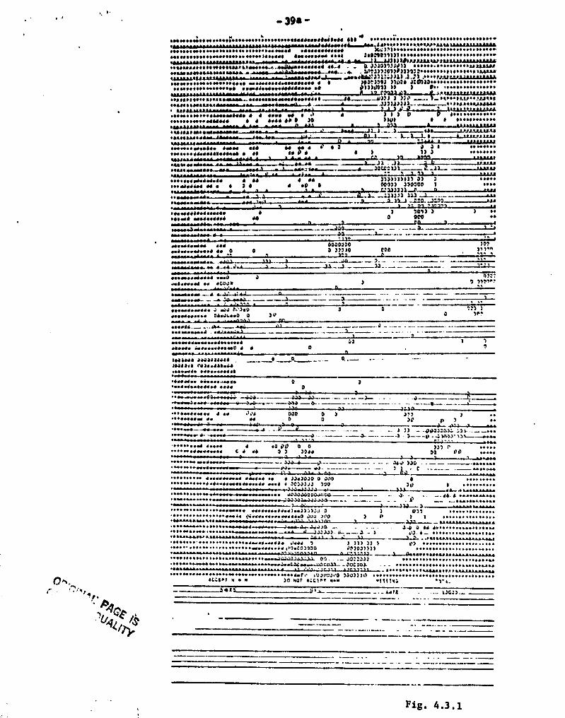
Figure 4.2.1 displays the results pictorially in a 100 x 100 array. The
letter D indicates that there is a significant difference between noon and midnight
data, (reject hull hypothesis) A blank indicates that there is no difference. It
is easy to see that zero rainfall rates in both phases dominate the western border
/law
r^ r
39a -.a•.•a.M♦•.. r.u•i•..•r•..•i....a.aHb1 ♦N.11.•1.11 •/1 ~ ♦••••••i..•••a.♦ a•••••.••..•N•••a.•..ry aN.1.Y...1•J •" 11♦ ra•r •ru•,a.VL11Y•frWLU•r'.=::M.aNNHN.... H•.H.p .Na1 .•N.•••N•.• 7t.,;) ^ 1.r aa•.a..•. *of ••.... HN.w.0 NU.♦....w.aa.0 •r.•.••1•H•N 1N •u.•N .a•a i•OMOl1171•au.••ur.....• ►N NN.••.•.
Y ^_- ^^-^rN.1•y.^• ^3^.3LJJ)!) Il1^.r^uaw ••••••••••••••••r.•uuaa•.. ♦..aaa•au.a.•Naa. ..p.J.u.u••1 ur. 0 PNOY))J/f •••......•...•..wia•wa.u.ruaauNa/aw^.. •a/.._a we1))JO))1)))7.:••r•.•••.r.r ► R.•aziaaua•aa1•a♦L •.1•••-••••--.1aa -•--'^---•' a1•3.i.^..r.IWJ:1.li.:JJli.)..`) J••e!. ►_u s:!121•t•_3.•Nr•a...••...a•.•N.• w•.aN.•hMN1uN • • lOJC7D01 ))Oi• 1:0)iD•.rN•...r.N.•u..•.•r....••w•. a.aa• .ar•IuNN.N•No. d ♦111)1)))! 11 1 I•• •. ••♦.• N•N....
w/1aaa.u•aw ----"'-- ^---./W.^ 3.i.' ^:r_+•"..S?92111^.k..^•Y,a,••••••u.0•.1»s.a1► ♦ ara•sa.a_.•pu.Nr.N.••NI•• __ ^^...^ y1))) )^A .VR. ►s^aatlw•aaa•.aa.aua♦1.....a.../. --1.+/_.rL..h ^ ^^ ^)^)^)Ni.. • R•aeaaataaaalia..♦ r r. •a •r.•NNr••1. • • 4080 N • •) • ) 1 ) p V i.N NN...• ► ••.r•.a...N NNN1 • ♦ 6064 •• O i0 1)D/ • • a••• ♦ ra•...•
. •.- a .n. a . ^^ •..r ♦. ^.. -^- '-^.adab ---- J L1._.1 a1 a wL12•i1..^... L
.•uawa••rJ • --- •.a Ma •: , C1 _1__ __... L L.1 1 ► •••ui uia••'^a3a^r-..-^.. u- ___ .__^ tl i _.. 7R rte- . •.. •. s...
r.a•.•r w..i•. 1MN N1 1• N • ♦ • 0 D i 1 .. 4884••.r•..NMNI•YNMd • i• •1 • • )) i ►.Nrr.•
- 0 -. ♦ P' )D_.JD L2•••••
•♦ua..aN•.- - -a-' -•3 - 'a .- )OCCCIJ7 _.11_. ••
•.•Nr..a.iNd• • " •1 ^ • •• )))1)))))) D) ) 4444•r..w.•1.• u . • i • • •v • 0007) »0000 ) 8.84
.:........a. -- 3 ' ...- ^ _____w.1Z .L +1u)7 . 7aa..•1.__.__._._.
8888 --Otto
.br••IN♦.r..•. • 7 )017 ) ) a••Nr1 rda.•IS• •• D OCO ••^w.a^arr •ma n + ne
a.ra.Mq ..• 0000000 >Cew•r..w•..1 b 0 0 0 ))710 000 )`)+e.Yra-
^...^ ► Y n ,w p n ,2. ,...ra.rr•... ..JJS. ++` .._ i .—.d0._. _.].._ .. 88_88.-^..__^_ ._ .._. '1'u.r•ar^. r..a1...1.•'V.,_..._-.1..x_..7 ..^J____).._ J)---- -_8888 . _ ....^rai+•.i J 6111 1 ' ,•Nr...♦pai urJ J C)7CJd r...a •r IGOJ• ) ^ ), p^.^
..rr.^.r_ ._..^. 1ii-.r♦1.-.._ ^ ? ._..__ .__S.__^_^.._ .___ _.. ._ __ ^___-
u.ru...r ObJwrO 0 7O 0 - )P`W W JL.a - _ -nnn.^
rr.Ji____a►a..__.a.i.. n'+ ^. -888_8 ^—_.J _ .._._ . _._ ^_^..__
Y•rY_.rY ___.._. ,;) r• ) )
Mob i•N •HN•w0 ♦ • 0
U7aNa 3liiai ♦ Ia• „_ 0-^^,,..0.•^^__ - 0•----- -- `- '--)1i1a11 IYia•aaaii•.•a•.1♦. Nr.. •.•Mi.r.•r•♦.•r.• ia.•...wrr 0 ) ^•.w.•Ia.b1.N .d• D•wwN......J..••00«r•rri:-ri0i__..^.....^.OJJ--.iJ___'°___.......,_...__^. _ _. . .J_.^_^_._
•••1.•I.r •. J a• J:1 000 0 ) )?) )•..•wNr r. r♦ 0 0 )^ O ) ••
^_,• _,_^..____.`J..7--_A_-..ln.)J.-))^»8_888.••N•. •.ra ♦.. •. • •0 0/) 0 0 ))) 1+ 4448•..NN.r w ♦.N•. C • ♦a 7 ) ))1♦ )0 00 NN.NN NN.►.♦o••r 8888-JJJ-i--•_LT _. _88__88.___ _ _ _ J{•rr ))D - _.__ _ , u.••u•^••••
+•••^iw.•Mrr.-^ .- 8811 N_. __._____ - - ^I } _ C ._ ._ ►•.•s.•
M...•1.N ♦.ur N.ai• .b1.1 .• '• )11 )OJD 0 JUO • •N... ••.•N.N•.N • I .i..hwp la•a ♦r u.a i JC)J))J 700 )p 1 ••N•NN.4488.. ••NN.Mrr•M...••••.w•.• JO JJJJD ODJt^(W--- - :J. - .. 8888 ♦i. a •wNUa.•u• ►v..wNN•«r«r-o.•..•«•..•.^.%WJJJ.JJ3JJ, --._--_ _ _ .. l) ^. ».•u N.w••••.•........ •.••N.brwrr• N•ru.di. ♦) K))))JJ j D ) OJ7 8884. N•••..•4844 N.•.••.••N•a.•ia D:+r.. p •.. rr••♦.0 JOJ J0p 1 h ) 1 ••.•.•••••••••••• Waw•.Y.wNaaaaY.Wr.•.^y - -JUr" :. `-11nn .^ J.L`_.^_.awaaa..a..uua••N.w...•NN•...rwJr.Mr...-J.r/-J..-3:110 .- - Oy 0 a1 KNr••••.a•.. r•• ►a..•.NU•..-.••.••••..r.••.w...r^.Gl-Jl..->J)1>1-t^__..1-^) - r11. i._ ...... off..au•ur^waa•a... ---------------- - '•'•.1.-' r ^3 ...uaa•.••.......u►•u.N.N•v ••••..•.. N..•.♦•. •r...li• 0.11 1 ) M)) ) y) ••rN ►N•••••••...••••.N••••.N ••...••.'••'•••w.r ♦ r.•r1 PD.JOJ7D0 OD)OJ)))) ..••. ...................•...aw..•.•w WYW ^._.L..paua..UWI-•-' •aa••--.N•.......••.r.•..•auu•.. .wdC3.L)JJ3.:3d. AC. _ 1DJJ3)J _ of ............ ............ w•.N.••••.wa•.••Nw•.u•.•..y..J.•,C.0-410 COJD-_DOC 00)- _. •......•N•........ w.uu•...a.aa• ".)1111)
O 3+ 111.._...•• •.•.•...uuu. ►n.wa..N.NHN....NNM.•N N•H.•... N.• 1. 1'(`
.,.UJDDJ.' )JJN IO
...............................♦C:I.t N • • 30 Not a:C)•t M • . •IS{tal 11'1.
_ 503 ' 1 ^_.._^ -.._Y.._ _.: 1♦ tt. __
^ UC))._
Fig. 4.3.1
-4o-
of the array. Heavy clustering of U's can be detected in the north eastern and
south western region of the array. We expect that thin is duo to the occurance
of heavy rain in these regions throughout the thirty five day period of phase 1
and 2. This also i.mLlies thnt_there t^ hea periodic spatial distribution of
areas where there is a_definit:e diurnal rainfall variation surrounded by regions
where there is no variation.
4.4 The Wilcoxon Signed Rank Test
The Wilcoxon test, allows us to test the null hypothesis that the mean distri-
bution of rainfall rata for noon and midnight are the same verses the alternative
hypothesise that one is greater than the other.
In this study, 1,872 grid areas were excluded because they had too few events for
analysis; for 1,743 we could reach no conclusion. In 4,890 &rid areas we found that
the null IyLc^l'hesis could be accc^Lted while in 1,495 of the gridaic^;ts we found that
the null ji)a^othesis must be rejected and the al ternate hypothesis accepted.
ThIs result it expected since the Wilcoxon test is less conservative than the
Kolmogorov-5mirnov test. It is possible for the distributions of rainfall at noon
and midnight to be the same and yet the means are different.
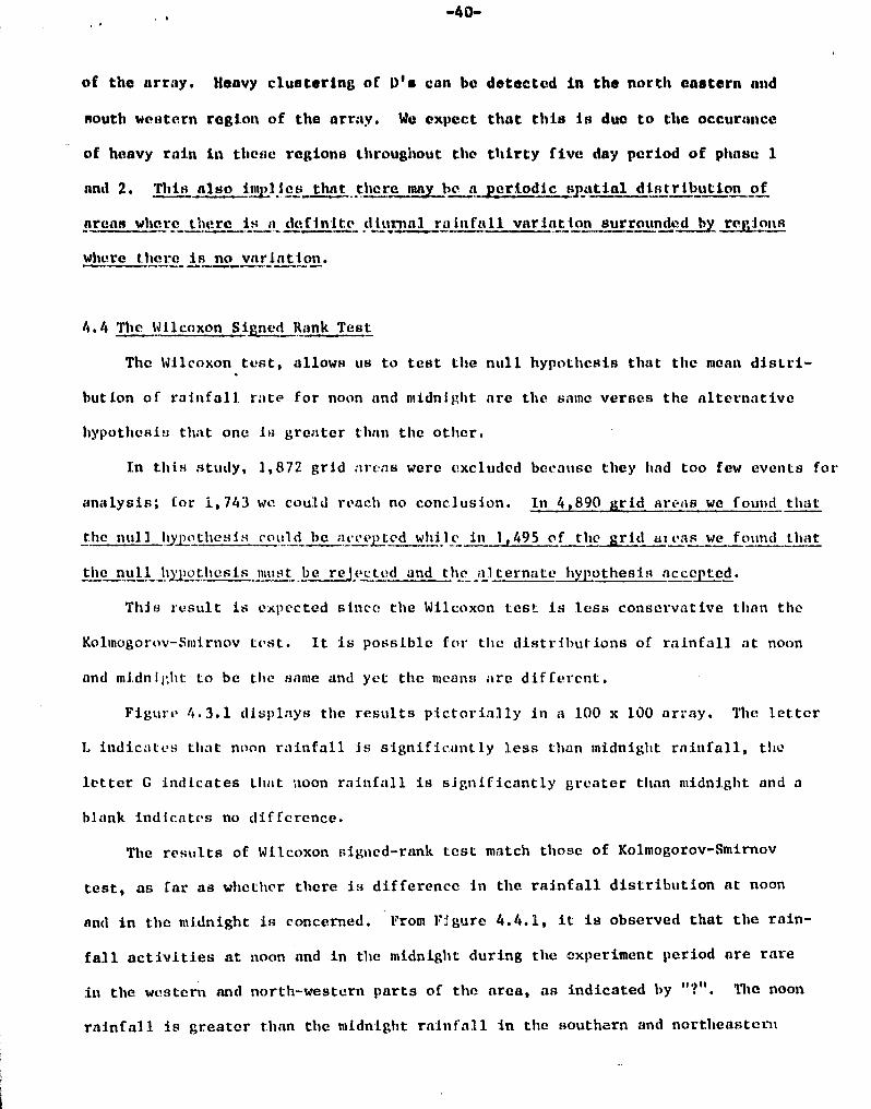
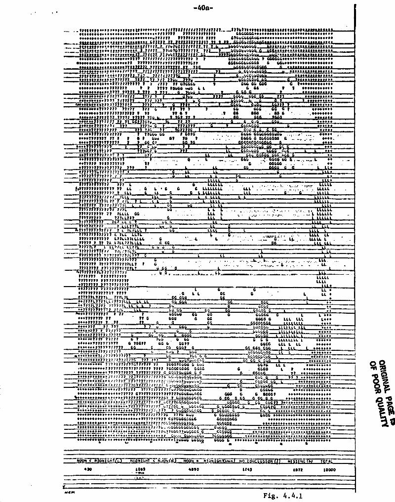
Figure 4.3.1 displays the results pictorially in a 100 x 100 array. The letter
1. indicates that noon rainfall is significantly Less than midnight rainfall, the
letter G indicates that noon rainfall is significantly greater than midnight and a
blank indicates no difference.
The results of Wilcoxon signed-rank test match those of Kolmogorov-Smirnov
test, as far as whether there is difference in the rainfall distribution at noon
and in the midnight is concerned. from Figure 4.4.1, it is observed that the rain-
fall activities at noon and in the midnight during the experiment period are rare
in the western and north-western parts of the area, as indicated by "?". The noon
rainfall is greater than the midnight rainfall in the southern and northeastern
t.
tttttllt •• tttttt o ttM !ll6tttt f t ► t 1/1111111 ItIIIIfII1fiL_.....tifb••••••••••••••6••••••••••66.66.9f1iH1 iTtttlf1tt119•••NN••• ►••••••••••••••••••u7/J71t 1117171 tf1
^-1tit!! ut t t •..ls!!t!1.1.Lltstt.G1lu 1 11Ittu tLT1111Y^__ttlitt!!tt !• tit!!•2iL•SS YtIT11_J_J7w101111 1 1tt_1t
!littti:!t •t!!littttitt -` 1^ t t 7t_ JrGUTG ► y1 1i9t . tt^•t ••••••2!!!t V•.!!dit 111E JTritill
N New •a ••.•••••••919 f7717f111111 ?I11f "11M••••N*0 16•••••••ff 11111119/9)7919fT171TW 7•••••• *••• lsstLtiLiLt1]122t.1.i72t22Lt21Lt T it a
-40a-
tt . »117? at6YG{.6GGU4..61•F161
t L 444G4k4c44G_..Jittt01"1^4G6GYaG4GG
LGY,--2>^GkfrGGruii.GY1.r^.GY••
6666G66GG6b6aa666064GGGa
Ito tot t1 muttedtts"tttun66G66GG•••••••••••••••• w•• ►•••••••6••
GL CjG({f^y l- •nr.••. ••Liflt•_y•!•••.••.••4 cGB••uLli!!dd •••••••••1 GGGGG0*9 •••••••••NG flab.••...••.•••••.••••
G GG4GGG
H •1.•1•••1.1•••1••.
N••••
^tL•ld.L:St••t'.tt tl?79 1 t YY171112 y 17I1L1 .1,L1.LZ.1^^3 JL6G64tcG.c6G ..^1Lt.iLl,•^•.•••e_^••!lLtdlt? !L! • 17211 ^_,.:tZ.c1121z1 ^^- 4GGirseGu^1 ►^^...^lttttttdtittlL!•••••}^,!•• .!?1111 LL ^•6•••••••16661fY771IT1 T J 1411 it a 6666•••••••••• ►r11»714 t 1 1111 tauaa miG L•••sROM# .^ttt..tt yo••6•••1.66r1917?71 y i.Y _y•tw••.!.••till ^z 1 7
^"^ ..••....J7y7fI2C••••a•• 119771 1777 97 G it IT I•••••+••i.1f79fiT1flt991 t 11 11 a T
^4^LnGiLGG1
L
1f
L^ fl. r•y•ttif••••aG6 G6 aaa G 1••••••••••6••
G 66 1 t •••••••.••••
Fy_¢kfr.
y64 GGG
ha G
Oa aae da G
•••••
of IN •.d•••6•.•••••••••••1H•
1!6••6 1 tJ 7 .^33.^L1iL tltL 1 7Y L00!6.6 InVi
l^
Y 700 00 1.!_>3 ?_. ^
••6••fit T1 Gb 66 1 6170
•1N1t1tf1T it t 1 a 1 Gb.i of to 10000 _9}^ 19 ,} 1 CyG1in
_ - _
4_&a'.GGr,Gr
Gisl%.Si^GGGG a66G6GGU 6 ,.4•.GGGG a G6G000GG C
CAG Qg CC GGCXJ C G d
•••••0000•..N•
'^••• T? G Gu••• t^'y^t 6?_^ 1tT^•1 17^^'^1?Y7 3^77
•• Tf{R?^7f?1„_
L TJJ,,•._
G46GGGCJyarGy ^
fG'
^' ,GG GGG GG6G t^ tSl -^i^G
•••••
••••17117 1171771111 t1 _ _ .. G GGa6G ._ ••• 7 11L7 ??
7_ ^ ?' J LL
77?11 LLLO
.'= i1•1 _f 71777_.3_ l: G l•
Uto^1^)fT'ti3 i^17 Lll
j4 M1.• a, Lll(•91117117171111 if LL a L 6 G G LLLLLLLL LLL LLLLL
LyL 6'r 6 LL LLL19it19t19t79 it f lL4 6 LL'f 111_ Ill L L77
1.L LLLLl l'L 111L _ llll LL
1.7094?> Lt U I II1 L {^ l LLtL LLLL L1t1^7177'1 '!'t? iL L t ^ij406
----TffffffVh)71irLL LL
LLLL
71-IL11117/TT71 71 TLLLL aG
LLLLL l
. ., j z,LLLLLLL LLLLLL
1111!/ it 9711 77 G...r_,
77 G919177?77 p 1 1^ 4a G L l ILL, LLL
^^49#3^37ifi7'i 1 l it--i , G Ll 6-"'113771Tfif55T'^?ll LL -hit
1T17711179T9 L77LL17LUZ. G L. L .r•Qa _ 1^,.....LLLLL Lf1171 1 . 19 7L ltLL177LL f. GG
-" 17 i! 7!1'!11111 L LLIIY"T ?177461'141?` Z/11711 ?l Y G
' ^ f374T414f'97?rt9lili79"'1fTT}7111Tf33f333l3Y _L. . .. LL6.
1177111 717771T/7t79111 1 G _ r ".._ ^,....^._ ^ , ... LL.114 1 71 t 1 ?7771'1197, Tt7^ d (,GG ^ 66 ti/L3'7t3'i^tii 4.G• 44..,^,^..^.,..._...,.,,._..____^.._._ _..__ uL_.ttT9197 177171mv _LULL
19111711 147777?1711 LLLL• 171 91?.ji77777 ^it 7 91 777?J/77T79L 6 G ll •
•7177191717?77 ???? .6 L L GG G l LL •0799?f4^ yl .7j41? 1••?9. 19 17 7 9 111, 1'!1?TILL•_,LL LL G4_G4G GG GGG L 6••i1t11L7i9T 777)77 l 7 Gy 4 GGGG Of6. 71 '1'7t1 " '^7 711 4"G ¢ GG Gf. (.(i •.
^6041711119171 it GGGba 6 •GG G GGGG l ••••#011117fl 71 If a GGG a Go GGGG a LLL LLL L6•••66•?fy999 ♦ 7 1 G G CG -M 0.GUkG L"LIILL6••••77^^ 67 ?77 9 u 6 G6' GGGGG4 J JkJU r, 0000•1611917 ?1111711171 ,G G 4G44GG' LLLL UL •6•••61 ••• 7 • 7j i ? G ban L LLLLLLL L 6666•0.000. 799 77711 G 9 740 co 66 G G G LLLLLLLL L 0660••H•••111177?7191 G toot? GG 4 GG11 GGGG LLL L LL 0000••••••••$M 77777? 79 GG G GG,^SjGt G GG GGg QGG L LLL L ♦ N••••
16.1•H 1.•• •• 66Y77f774t 7771771177?7u1?G4G4GGbGG C, •.^••••••••••••••6.11••.1(1•••.•79977 6171lT7ttlT9f9tt?GGGGGGr.G6 GGG G G GGGG? 16116.1.1••666611
t6.6.166^6••^••60••67?17717 ?1777177G7 ^(L@G G GG G 4Cs_ a cc r G •••••••••••••••••••16•••6••11.6ii6•^•77y ??77771>777 uG7i7GGGGG4G4G 4^C GGG fr,SrG ¢(.G 17 9••6•••••6•••••6••••
•_ ,Fie ^••^ i6•. 7?1777777!7!7 y7 G4 G 4GG1•G" ^1 Gam. C^{jf (^,.___*fit-•ii^••6••••ii.•i66ei••'► 9?7?7 r,7 •7^J/7 4a G 4C.G 4 G G G C.G 4 •6.6••6.•••••.•••x•.••NN N 16.1•••••••••16••71 71717i?77G 777E 4au 44{iG6GGG GGGG •666.6••6666• N1••6 H • ♦••••••••••••• • 6••••••••••97997 ► 9799 GGTG6GGGG6G GGGGGGGG ••••••••••••••••••....•••••••l616.61.66••166^• •6N 66 y797j77G ,yGGGGG.G G.._^ CL4^t GG^j •••6.66•••••••••6••••6.6•••••16 66. •6110^ i•• ♦••6 ^6 •• •6•• ^7717b 3,GaGG44GG44G4 G_Y(.GQ^_ •••^1.11• ►••^6^^661066••61••!._..♦166.1i•1•^i• • •6^.•.••^• •_^ 666.777b79GGG77WyGGG_¢ GGt^yGG •6p•••06666•tt^.•666'06.61600i0••••••1. 16 ••e6^o. 6•a 6. 66••7r•••.^. 67 Gu •..0 4Gfti^j§GGG4GG •••••6•••••6•••6.60•••6.66••66•••6 ^,•6NHH:11^••►•s•^; •1.6 N616M •••1 H 6•I^G6YY bGfr4h GG4G G •66.66.6 ►6•.6.61 N•1N H161•N61611.6•
• - •
NUUN < 416T47 70 NIDNI4M ( NJUN(6) NO MTOTAL
•to Lou ^e10 I/1s keys 10000
Fig. 4.4.1
•t!
G
••••••••777777777 {. Guu ? 44u^•as► •aT•f7lJ7i?7 T1 ►7• ^ 4G 744 G• 6i•6i1•it 1 7771111711 •. 77 J71 '1 ot•GG GG••61.16••1 t`i)79rT?7?iG 9 7 77 7GG07M.4 G Ltn;.•••61.6116 T17777T9/171711/9? 7117 ?GGGGGGGG GGGG♦11111.1N• 6777717T17T ??94177777 G G_r-3 q 00^.G....^♦••^.•••.••7i 777J?? 77 77?7717717TG 6GoG4G000aGG6^••••ii••i••!•7J 117 7177?9777TJr7j ^: U7 ua:74 y{rObY:^•i6^Ti•6T6•^^
.iJ 71777?G771'11 )/)711 ( rG V44GyvG^u4,
0600
GGGG l 9 •.•••••.•••

-41-
parts, as indicated by "C". The places where midnight rainfall is greater ere
scattering..
4.5 Chi-Square Test
The c.hi-dquare test is used to provide a further check on the results of
the Kolmogorov-Smirnov and Wilcoxon signed rank tests. This test allows us to
determine whether or not the percentages used for analysis using the other two
statistics were actually preserved in the results of the analysis. In this case
the X2-test is defined by: (see Chapter 2)
2 k (it_nP^ )X k t' nP3-1 J
k
where it F n n is the numlirr of grids for which the J-th conclusion was made;n= l j
. Pi is the probability of making the n-th conclusion.
We use an a - .05 for the level of significance for each experiment.
The X2 test, applied to the K-S experiment.
In the K-S test we have the following, information:
k-2 j-1,2.nl - 5425 P1 - .90 P2 - .10
n3 C 960
n = n + n2 - 6385
c .05,2 - 3.84
So2 - (5425 - 6385 (.90 ) 2 + (960 - 6385 ( .10))2
X2 6385 (.90) 6385 (.10)
- (321.5 ) 2 + (321.5)2 = 17.99 + 161.88 - 179.87 > 3.845746.5 638.5
hence, the percentages of 80 and 20 do not hold at the 5% level of significance
and thus the null hypothesis 11 0 : F1 F2 is not true end must be rejected.
f

-42-
The X 2Teet applied to the Wilcoxon lixreriment.
In the Wilcoxon experiment we have the following information:
k -3 j-1,2,3.3
n 430 n2 - 4890 n3 - 1065 n - E ni - 6385
1
P 1.10 P 2 - .80 P3 - .10
c .05,3 - 5.99
2 - X 430 - 6385).10 2 + 4890 - ( 63851 .80)) 2 + ( 1065 - 6485 (.10)]2X 3 6385 (.10) 6385 (.80) 6385 (.10)
- 208.5 2 + ( - 218jj + ( 426.5 2L - 68.03 + 9.30 + 284.67 - 362.00 > 5.99639 5108 639
Thus, the percentages of 10, 80; and 1.02 do not hold at the 5% level of significance
and hence the null hypothesis H0: F - F2 is not true and must be rejected.
4.6. Summary on Diurnal Analyses.
Two non-pa rametric tests were used to detect if there is a diurnal variation
in oceanic rainfall using CATE data. Nan-parametric methods are choson because of
their model free characteristic.
The test was undertaken at grid points where data are available. Of the 10,000
grid points in the study area, 1872 were excluded because data are not available;
these points are around the boundary of the square. In addition, there are 1743
grid points where no conclusion was obtained due to insufficient frequency of rain
in the midnight and at noon during the experiment period. The analysis was done
at the rest of 6385 grid points.
The Kolmogorov-Smirnov test was used to test whether there is a difference in
the rainfall distributions between noon and midnight. At one out of 10 chance of
error, it was found that out of 6385 grid points, the rainfall distributions at
-43-
noon and at midnight are different in 960 grid points and are same at 5,4125 grid
points, which are 15.0 and 85.0%, respectively. If there were no difference in
the rainfall distributions, these percentages would have been 10 and 90% respec-
tively. A uhi-square teat at one out of 20 chance of error shows that this split of
percentage was not followed. There are more grid points where the assertion of
difference is made than expected. Thus, overall the rainfall distributions at
noon and at midnight are different. This concludion could have been made at
practically any significant level.
The Wilcoxon signed-rank test was used to test if the noon rainfall is less
than, equal to, or greater than the midnight rainfall. It was found that, at one
out of 10 chance of error, the numbers of grid points fall in these three categories
are, respectively, 430, 4,890, and 1,065. In terms of percentage, they are 6.73,
76.5, and 16.68%, as compared to 10, 80, and 1.0%, respectively, which are expected
if the assumption of no difference had been true. At one out of 20 chance of error,
the chi-square test concluded that the midnight rainfall is not equal to the noon
rainfall; the noon rainfall. is convincingly greater than the midnight rainfall.
Thin; conclusion could have been made at practically any significantly level.
From the analysis it was also found that the Wilcoxon signed-rank test is more
sensitive than the Kolmogorov-Smirnov test in detecting the difference in the mid-
night and noon rainfalls. This is to be expected by the nature of these two tests.
s
r_tl
x

BIBLIOGRAPHY
1. Allison, Lewis J., William R. Bandeen, Charles R. Laughlin. and Raymond
Wexler, "Remote Sensing of the Atmosphere iron Environmental Satellitos,"
X-901-77-132 Preprint, Goodard Space Flight Center, Greenbelt, Maryland,
(June, 1977).
2. Arnold, A., E.B. Dobson, J. Goldhirsh, I. Katz, T.G. Konrad, and W.L. Vann,
"Radar. Derived Spatial Statistics of Summer Rain Experiment Description,"
NASA r,,ntractor Re smart, NASA CR-Z59Z (Sel!tember, 1975).
3. Bark, L. Dean, and A.M. Feyerhern, "Probability Models for Simulating
Temperatures and Precipitation", Kansas State University, Manhattan, Kansas.
4. Bark, L. Dean, N.T. Ison, and A.M. Feyerberm, "Wet Period Precipitation and
the Gamma Distribution," JLurnnl of Applied Meteoro1oa, X (1971), 658-665.
5. Bowen, E.C., and Paul T. Schickedanz, "The Computation of Climatological
Power Spectra", The Embassy of Australia and Illinois State Water Survey,
(March, 1977).
6. Bowman, K.O., and L.R. Shenton, "Comments+ on the Gamma Distribution and
Uses in Rainfall Data", Computer Center, University of Georgia and Oak Ridge
National Laboratory, Oak Ridge, Tennessee.
7. Bowman, K.O., and L.R. Shenton, "Further Remarks on Maximum Likelihood
Estimation for the Gamma Distribution", Technometries, XIV (1.972), 725-733.
8. Briprn, Maurice, "Describing and Testing, for Heavy Tailed Distributions",
Colorado State University, Fort Collins, Colorado.
9. Carter, Michael C., Lee W. Falls, and William 0. Williford, "Probaability
Distributions for Thunderstorm Activity at Cape Kennedy, Florida", NASA
Technical Memorandum, NASA TM X-53867 (May, 1970).
10. Chernoff, I{-irman, "The Efficient Estimation of a Parameter Measurable By Two
Instruments of Unknown Precisions", Oltimizing_Methods in Statistics, (1971),
1-27.
,,
11. Clements, Arthur E., and Benjamin M. Herman, "Removal of Seeing and Instru-
mental Blur Effects from Astronomical Scanner Observations", Apn__ lied t ics,
XIII (December, 1 974), 2947-2956.
12. Cohen, A. Clifford, F. Russell Helm, and Merritt Sugg, "Tables of Areas of
the Standardized Pearson Type III Dennity Function", NASA Contractor Report,
NASA CR-61266 (March, 1969).
13. , The Space Applications Board Assembly of Engineering,
National Research Council, Practical Applications of Space Systems: Support-
ing Paper 1. Weather and Climate, Washington, 11.C.
A Note on a Gamma Distribution Computer Program and
Computer Produced Graphs", NOAA Technical Report. EDS 24 (May, 1977).
15. Crosby, D.S., "Estimation of the Mean and Covanance Matrix of Cloud Effect
for Remote Soundings of Atmospheric Temperature Profiles", National Environ-
mental Satellite Service, NOAA and The American University, Washington, D.C.
16. Durand, David, and J. Arthur Greenwood, "Aids for Fitting the Gamma Distri-
bution by Maximum Likelihoods", Technome tries, TI (1960), 55-65.
17. Falcone, V.J., and K. Mano, "Statistical Methods of Indirect Probing of
the Atmosphere" Air Force, Cambridge Research Laboratories, L.C. Hanscom
Field, Bedford, Mass.
18. Falls, Lee W., "The Beta Distribution: A Statistical Model for World Cloud
Cover, "Journal of Geophysl cal Research, 79 (March, 1974), 1261-1264.
19. Falls, Lee W., "A Computer Program for Standard Statistical Distributions",
I Memorandum, NASA TM X-64588 (April, 1971).
"On the empirical distribution function in the case of group-
Doklady Akad, Nauk SSSR (NS). Vol. 82 (1952, pp. 837-840.
"Some results on empirical distribution functions", Mat.
Sborn. Univ. Kiev., Vol. 8 (1954).
NASA Technica
20. Gihman, I.I.,
ing of data",iF
21. Gihman, I.I.,
.
r
22. Ci.hman, I.I., "On the Empirical Distribution Function in the Case of Grouping
of the Data", Trans. by the National Bureau of Standards.
23. Glivenko, V., "Sulla determinazi.one empirica delle leggi di probabilita",
riorn. del 1'Instit. degli att., Vol. 4 (1933), pp. 92-99.
24. Gnedenko, B.V., and V.S. Mihalevic, "Two Theorems on the Behavior of Empirical
Distribution Functions", Trans. by the National Bureau of Standards.
25. Gnedenko, B.V., and V.S. Mihalevic, "On the Distribution of the Number of
Excesses of One Empirical Distribution Function Over Another", Trans. by
The National Bureau of Standards.
26. Gnedenko, B.V. and V.C. Korolyuk, "On the Maximal deviation between two
empirical distributions", Doklady Akad, Nauk SSSR, Vol. g0 (1951), pp. 525-
528.
27. Gnedenko, B.V. and V.S. Mihal0,ic, "Two theorems on the behavior of empirical
distribution functions", Doklady Akad. Nauk SSSR, Vol. 85 (1952), pp. 25-27.
28. Gnedonko, B.V., "Unber die Nachprufung Statisticher Hypothesen mit Hilfe der
Variationsreihe", Bericht uber die Tagung Wahr, and Math. Stat. Berlin, 1954,
pp. 97-107.
29. Grantbam, Donald D., and Iver A. Lund, "Persistense Runs and Recurrence of
Precipitation", Journal o- Applied Met,oLr 122X, XVI (March, 1977), 346-358.
30. Green, Richar N., "Simulation Studies of Wide and Medium Field of View Earth
Radiation Data Analysis", NASA Technical Paper 1182 (1978).
31. Gringor.ten, Irving I., "Modelling Conditional Probability", Journal of
Applied Meterology, (December, 1970), 646-798.
32. Gumbel, E.J., and C.K. Mustafi, Tables of the Probability and Density
Functions for the Bivariate Extremal Distributions, Department of Industrial
Engineering, Columbia University, New York, 1968.
l .
33. Hoff, John D., Michael D. Iludluw, Vernon L. Patterson, :'ete: .1. i'yhowa
Frank 1 1 . Richards, "Cate Radar Rainfall Processing System", NO ,A Techn
Memorandum, (Au^ust 1978).
34. Hogg, Robert V., and Elliot A. Tanis, Probability and Statistical infe
Macmillan New York 1977.
35. Iludlow, Michael D., and Frank Richards, "Use and Abuse of the Cate Dig
Radar Data", Center for Experiment Design and Data Analysis, National
Oceanic and Atmospheric Administration, Washington, D.C.
36. ih►dlow, Michael 1)., "Precipitation Climatology for the Three Phases of
CATE", Center for Experimental Design and Data Analysis, National Ocea
and Atmospheric Administratloit, Washington, D.C.
37. Jacobson, R.N., and W.M. Gray, 1976: Dlurnal. Variation of Oceanic Dee
Comulus Convection, Colorado State Uni.vvi- g ity, At-%-^ylteri.c Sciencr Paper
No. 243, Dort Collins, Colorado.
38. Jenkins, Gwilym M., and Donald G. Watts, Spectral. Analysis and it;; appli-
cations llolden-Day Inc. C 1968.
39. Kaplan, L.D., 1959: Inference of Atmospheric Structure from Remote
Radiation Measur vine nLis journal the Optienn Society of America, P. 49,
10, 1004-1007.
40. Kidder, S.Q., 1976: Tropical Oceanic 1 1 reripitation frequency from Nimbus-
5 Microwave Data, Colorado `;Late University, Atmospheric. Science Paper Nu.
248, fort Collin~, Colorado.
ail. Kolmogorov, A.N., "Confidence limits for an unknown distribution function",
Ann. Meth. Stave., Vol. 12 (1971), pp. 461-463.
42. Kolmogorov, A.N., "Sull y determinazione empiric& di une legge di dist:ribuzione",
'''ern. dell 'Instil. der, att. $ Vol. 4 (1933), pp. 83-91.
opmans,, Lambert Herman, The Spectral analysis of Time Series, Academic
:ss, New York 1974.
44. Kuel.bs, J., "A Counterexample for Bannell Spaca Valued Random vnriable.tt",
The Annals of Probabiliy, IV (1976), 684-689.
45. Mielke, Paul W., "Another Family of Distributions for Describing and Analyzing
Precipitation Data", Journal of A1]a ali^^d Aleteoraln^,Z► , XII (1973), 275-280.
46. Pears, N.W., nad B.L. Welch, "On Formulae of Confidence Paints Based on
Integrals of Weighted Likelihoods", University of l.cteds.
47. Samuel, Ester, "An Empirical Hayes Approach to the Testing, of Certain Para-
metric Hypo Llty Ls 10 , The Hebrew University of Jerus alcum, (lone, 1963) .
48. Sanyo, Yoshio, "On the Probabilistic Analysis of Precipitation Particles;",
M teorological 1%escarch Institute of Japan.
49. Sinap..on, Joanne, "Use of the Ganuna Distribution in Single Cloud Rainf;all
Analysis", Month } Wcrntl^^^r Rvview, 1.00 (1972), 309-312.
50. Smirnov, N.V., "Probabi lit Ivs of L,argc. Values of Not pariamotri c one-Sided
Coodnoss of lit Statistics;", Trans,. by Warasily llocffding.
51. Smirnov, N.V., "Stir la distribution do w 2 ", C.1:. Acad. See. Paris, Vol. 202
( 1`)36 ), pp. 44')-452.
52. Smirnov, N.V., "On the distribution of the w 2 criterion of von Mises", Ree.
Math. (NS), Vol. 2 (1937), pp. 973-993.
53. Smirnov, N.V., "Sur les cearts de in courbe da y distribution emptridue"
(Russian, branch summar) , ), Rec. Math, (NS) (Mat. Shorn.), Vol. G (98) (1939),
pp. 3-26.
54. Smirnov, N.V., "On the es-t imntion of the discrepancy between empirical curves
of distribution for two independent samples", Ilull, Math. Univ. MOSCOW, Vol.
2, No. 2 (1939), pp. 3-14.
55. Smirnov, N.V., "Approximate laws of distribution of random variables from
empirical data", Uspehi I`iatena. Nauk, Vol. 10 (1944), pp. 179-206.
56. Smirnov, N.V., "'.Cable for estimating the goodness of fit of empirical distri-
butions", Ann. Math. Stet., Vol. 19 (1948), pp. 279-281.
v
I"...

57. Smirnov, N.V., 110n
Vol. 4, No. 4 Or
58. Smirnov, N.V., 110n
distributions of r,
the Cramer-von Mises criterion", Uspehi Matem. Nauk (NS),
(1949), pp. 10-197.
the construction of confidence regions for the density of
andom variables", Doklady Akad, Nauk SSSR (NS), Vol. 47
(1950), pp. 189-191.
59. Stnelin, D.A., 1966: "Measurements and Interpretation of the Microwave
Spectrum of the Terrestrial Atmosphere Near 1 Centimeter Wave length", J.
Ceophys. Res., 71, 2875-2881.
60. Staclin, D.A., 1969: Passive remote sensing at microwave wave lengths,
.oc. TEEE, 57, 427-439.
61. Thom, 11.C.S., "Approximate Convolution of the Camma and Mixed Gamma distri-
butlons", Moll th ly jceathc-r RevLrw, 96 (1.968), 883-886.
62. Van Vleck, J.H., 1947: Absorption of Microwaves by water vapor, Phys. Rev.,
71, 425-433.
63. Welch, 11.L., "Tic Significance of the Difference Between Wo Means When
Tlie Population variances are lhicqual", University of Leeds.
64. Wil.hcit, 'T.T., M.S.V. Rao, T.C. Chant;, E.B. Rogers and J.S. 'Theor, 1975:
Tlie Remote Scion ing of Rainfall Rates over the Oceans, Presented at the
Second Conference on Atmospheric Radiation of the American Meterological
Siciet y , Arlington, VA., October 29, 1975.
65. Wilhe i t, T.T. , 1972: The electrically Scanning Mtcrowave Radiometer (ESAll:)
Experiment in Hie Nimbus-5 User's Guide, NASA/Goddard Space Flight C+--nter,
Grecilbe.lt, MD., pp. 59-105.
Related Documents