T/HIS Manual from Oasys Ltd Version 18.0

Welcome message from author
This document is posted to help you gain knowledge. Please leave a comment to let me know what you think about it! Share it to your friends and learn new things together.
Transcript
T/HIS Manual
from Oasys Ltd
Version 18.0
LS-DYNA, LS-OPT and LS-PrePost are registered trademarks of Livermore Software Technology Corporation
For help and support from Oasys Ltd please contact:
UKThe Arup CampusBlythe Valley ParkSolihullUnited KingdomB90 8AETel: +44 121 213 3399Email: [email protected]
ChinaArup China37/F & 39/F Huaihai Plaza1045 Huaihai Road (M)Xuhui District, ShanghaiChina200031Tel: +86 21 3118 8875Email: [email protected]
IndiaArup India Pvt Ltd10th floor, Western Dallas CenterPlot no. 83/1, Knowledge CityRai DurgHyderabad 500032Telangana, IndiaTel: +91 40 69019797 / 98Email: [email protected]
USA WestOasys Ltdc/o 560 Mission Street Suite 700San FranciscoUnited StatesCA 94105Tel: +1 415 940 0959Email: [email protected]
Web:www.arup.com/dyna
or contact your local Oasys Ltd distributor.
0.1Preamble 0.1Text conventions used in this manual 0.2Themes for the Graphical User Interface 0.2Setting the theme 1.11 Introduction 1.11.1 Program Limits 1.21.2 Running T/HIS 1.41.3 Command Line Options 2.12 Using Screen Menus 2.12.1 Basic screen menu layout 2.22.2 Mouse and keyboard usage for screen-menu interface 2.42.3 Dialogue input in the screen menu interface 2.42.4 Window management in the screen interface 2.52.5 Dynamic Viewing (Using the mouse to change views). 2.62.6 "Tool Bar" Options 2.62.7 Colours 3.13 Graphs and Pages 3.13.1 Creating Graphs 3.23.2 Page Size 3.23.3 Page Layouts 3.23.3.1 Automatic Page Layout 3.63.4 Pages 3.63.5 Active Graphs 4.14 Global Commands and Pages 4.14.1 Page Number 4.14.2 PLOT (PL) 4.24.3 POINT (PT) 4.24.4 CLEAR (CL) 4.24.5 ZOOM (ZM) 4.24.6 AUTOSCALE (AU) 4.24.7 CENTRE (CE) 4.24.8 MANUAL 4.24.9 STOP 4.24.10 TIDY 4.34.11 Additional Commands 5.15 Main Menu 5.15.0 Selecting Curves 5.65.1 READ Options
5.335.2 WRITE Options 5.415.3 Curve Manager 5.545.4 Model Manager 5.565.5 EDIT Options 5.625.6 LINE STYLES 5.705.7 Command / Session Files 5.745.8 IMAGE Options 5.795.9 OPERATE Options 5.865.10 MATHS Options 5.875.11 AUTOMOTIVE Options 5.945.12 SEISMIC Options 5.965.13 MACRO Options 5.985.14 FAST-TCF Options
5.1025.15 TITLE/AXES/LEGEND Options 5.1115.16 DISPLAY Options 5.1155.17 SETTINGS 5.1205.18 MEASURE 5.1245.19 Curve Groups 5.1275.20 GRAPHS 5.1285.21 PROPERTIES 5.1335.22 UNITS 5.1385.23 The Javascript Interface 5.1445.24 Datum Lines 5.1495.25 T/HIS Session Save and Retrieve
6.16 Other Options 6.16.1 Tool Bar
6.106.2 Graph Tool Bar 6.126.3 CURVE INFORMATION 6.136.4 Curve Histories ... 6.176.5 Keyboard Shortcuts 6.216.6 Preferences 6.226.7 PRIMER: Synchronising with PRIMER 6.286.8 REPORTER: Integrating with REPORTER
User manual Version 18.0, April 2021 T/HIS
Page i
7.17 FAST-TCF 7.17.0 FAST-TCF OVERVIEW 7.27.1 FAST-TCF INTRODUCTION 7.87.2 PAGE / GRAPH LAYOUT AND SELECTION
7.107.3 INPUT SYNTAX TO LOAD OTHER FILES 7.117.4 INPUT FOR DATA EXTRACTION REQUESTS 7.337.5 UNITS 7.357.6 CURVE TAGS 7.377.7 CURVE GROUPS 7.387.8 PERFORMING FAST-TCF CURVE OPERATIONS 7.427.9 APPLYING EXTRA OPTIONS TO DATA REQUESTS 7.437.10 Setting properties for curves 7.457.11 Defining Datums 7.477.12 FAST-TCF IMAGE OUTPUT OPTIONS 7.557.13 Outputting curve properties to text files, variables and REPORTER 7.597.14 FAST-TCF CURVE OUTPUT 7.607.15 FAST-TCF ADDITIONAL 8.18 Quick Find 8.1Introduction 8.1Fuzzy Matching 8.2Search Terms 8.3Tutorials 8.3Options 9.19 REPORTER INTEGRATION 9.19.1 Linking the Programs 9.19.2 Item Tree 9.29.3 Capture 9.49.4 Reload 9.79.5 Generate 9.79.6 Variables 9.89.7 Exceptions to the Version 17 Method and Existing Templates from Version 16 and Earlier A.1APPENDICES A.2APPENDIX A - LS-DYNA Data Components B.1APPENDIX B - T/HIS CURVE FILE FORMAT C.1APPENDIX C - T/HIS BULK DATA FILE FORMAT D.1APPENDIX D - FILTERING E.1APPENDIX E - INJURY CRITERIA F.1APPENDIX F - Curve Correlation G.1APPENDIX G - The ERROR Calculation H.1APPENDIX H - The "oa_pref" preference file I.1APPENDIX I - Windows File Associations J.1APPENDIX J - T-HIS JavaScript API
K.1APPENDIX K - Typed Commands L.1Installation organisation L.1Version18.0 Installation structure
M.1JaDe: The JavaScript debugger M.1Viewing the script files and functions M.1Adding/removing breakpoints M.2Running the script M.3Printing the value of a variable M.4The call stack M.5Exceptions N.1Licences used in software N.1Apple Public Source N.1Draco N.1Expat N.1FreeType N.3FFmpeg N.4Jpeg N.4Libcurl N.4Libfame N.5Libgif N.5Libpng N.6Libxlsxwriter N.7MPEG-LA N.7Openssl N.9PCRE
N.10PDFHummus N.10POV-Ray N.10SmoothSort N.10Spidermonkey
T/HIS User manual Version 18.0, April 2021
Page ii

N.14Treeview N.15Win-iconv N.15x264 N.15Zlib O.1Fonts on Linux O.1The range of fonts available O.2Plain versus Anti-aliased fonts P.1The JavaScript GUI Builder P.2How to build a GUI P.9How to use the GUI in a script
User manual Version 18.0, April 2021 T/HIS
Page iii

T/HIS User manual Version 18.0, April 2021
Page iv
Preamble
Text conventions used in this manual
Typefaces
Three different typefaces are used in this manual:
Manual text This typeface is used for text in this manual.Computer type
This one is used to show what the computer types. It is also used for equations, keywords (eg *PART) etc.
Operator type
This one is used to show what you must type.
Button text This one is used for screen menu buttons (eg APPLY)
NotationTriangular, round and square brackets have been used as follows:
• Triangular To show generic items, and special keys. For example:<list of integers> <filename> <data component><return> <control Z> <escape>
• Round To show optional items during input, for example:<command> (<optional command>) (<optional number>)
And also to show defaults when the computer prompts you, eg:
Give new value (10) :
Give model number (12) :
• Square To show advisory information at computer prompts, eg
Give filename: [.key] :
THIS >>> [H for Help] :
User manual Version 18.0, April 2021 T/HIS
Page 0.1
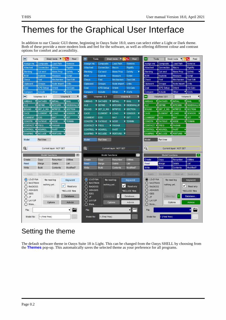
Themes for the Graphical User InterfaceIn addition to our Classic GUI theme, beginning in Oasys Suite 18.0, users can select either a Light or Dark theme. Both of these provide a more modern look and feel for the software, as well as offering different colour and contrast options for comfort and accessibility.
Setting the theme
The default software theme in Oasys Suite 18 is Light. This can be changed from the Oasys SHELL by choosing from the Themes pop-up. This automatically saves the selected theme as your preference for all programs.
T/HIS User manual Version 18.0, April 2021
Page 0.2

The theme can also be set for individual programs from the Display menu in PRIMER, D3PLOT and T/HIS or the Preferences menu (File->Preferences...) in REPORTER. This choice is not automatically retained after exiting the program, so you must select a theme, then select Save pref to ensure a theme is used for all future sessions.
User manual Version 18.0, April 2021 T/HIS
Page 0.3

T/HIS User manual Version 18.0, April 2021
Page 0.4
1 IntroductionT/HIS is an x/y plotting program, specifically written to perform two functions:
1. To produce time-history plots from transient analyses, such as those performed using LS-DYNA.
2. To plot any form of x/y data that is produced either by a program or by directly typing in values.
T/HIS is a graphically driven, interactive program. Input and manipulation of data is through a graphical user interface on systems capable of running X-Windows applications; selections are made through "pressing buttons" using a mouse. On machines not capable of running X-Windows it is also possible to use T/HIS in a "command line" mode of operation; instructions are entered through the keyboard to perform the required operations.
1.1 Program Limits
There are a number of limits in T/HIS of which the user should be aware. These are listed below:
Number of graphs T/HIS can have a maximum of 32 graphs
Number of curves The number of curves is unlimited
Number of points The number of points that can be defined per curve is unlimited.
Time-history blocks In the interface to the LS-DYNA time-history (.thf) file there is a limit of 100,000 items in each of the node, solid, beam, shell and thick shell time-history blocks: thus 500,000 items overall.
In the interface to the LS-DYNA extra time-history (.xtf) file up to 100,000 nodal reactions (or groups of reactions) may be processed.
Number of colours By default, T/HIS curves wrap around the following six colours in order:
WHITE RED GREEN BLUE CYAN MAGENTA
However, a further 24 predefined colours are available if required and 6 user defined ones can be created.
Title The title can contain up to 80 characters.
Labels Labels for axes and lines can contain up to 80 characters.
User manual Version 18.0, April 2021 T/HIS
Page 1.1
1.2 Running T/HIS
1.2.1 Starting the code
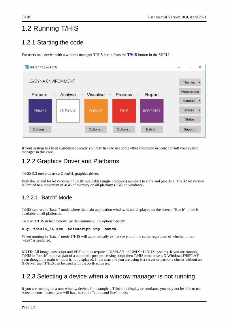
For users on a device with a window manager T/HIS is run from the T/HIS button in the SHELL:
If your system has been customised locally you may have to use some other command or icon: consult your system manager in this case.
1.2.2 Graphics Driver and Platforms
T/HIS 9.3 onwards use a OpenGL graphics driver.
Both the 32 and 64 bit versions of T/HIS use 32bit (single precision) numbers to store and plot data. The 32 bit version is limited to a maximum of 4GB of memory on all platform (3GB on windows).
1.2.2.1 "Batch" Mode
T/HIS can run in "batch" mode where the main application window is not displayed on the screen. "Batch" mode is available on all platforms.
To start T/HIS in batch mode use the command line option "-batch".
e.g. this14_64.exe -tcf=script.inp -batch
When running in "batch" mode T/HIS will automatically exit at the end of the script regardless of whether or not "-exit" is specified.
NOTE: All image, postscript and PDF outputs require a DISPLAY on UNIX / LINUX systems. If you are running T/HIS in "batch" mode as part of a automatic post processing script then T/HIS must have a X Windows DISPLAY even though the main window is not displayed. If the machine you are using is a server or part of a cluster without an X-Server then T/HIS can be used with the Xvfb software.
1.2.3 Selecting a device when a window manager is not running
If you are running on a non-window device, for example a Tektronix display or emulator, you may not be able to use screen menus. Instead you will have to run in "command-line" mode.
T/HIS User manual Version 18.0, April 2021
Page 1.2
It is very unlikely that a user on a modern workstation will see these options, since the machine will have a window manager and will be running in "screen menu" mode. If they do appear it suggests that the machine and/or software are wrongly set up: see 1.2.4 below for suggested remedies.
1.2.4 If T/HIS will not start in “screen-menu” mode
You may be running on a device with a window manager, but still only get the command-line prompt (and probably no menu driven _93 shell either).
This is almost certainly because of one or both of the following setup errors:
(1) The DISPLAY environment variable has not been set up, or has been set incorrectly. This tells the X11 window manager where to place windows, and it must be set to point to your screen. Its generic setup string is:
setenv DISPLAY <hostname>:<display number> (C shell syntax)
Where <hostname> is your machine’s name or internet address, for example:
setenv DISPLAY :0 (Default display :0 on this machine)
setenv DISPLAY tigger:0 (Default display :0 on machine "tigger")
setenv DISPLAY 69.177.15.2:0 (Default display :0, address 69.177.15.2)
You may have to use the raw network address if the machine name has not been added to your /etc/hosts file, or possibly the "yellow pages" server hosts file.
(2) Your machine (strictly the X11 "server") has not been told to accept window manager requests from remote machines. This is usually the case when you are trying to display from a remote machine over a network, and you get the message similar to:
Xlib: connection to "<hostname>" refused by server
Xlib: Client is not authorised to connect to server
In this case go to a window with a Unix prompt on your machine, and type:
xhost +
Which tells your window manager to accept requests from any remote client. It will produce a confirmatory message, which will be something like:
access control disabled, clients can connect from any host
If T/HIS still fails to work then please contact your system manager, or contact Oasys Ltd for advice and help.
1.2.5 Command Line Mode
Command line mode is the main method of data input on non X-Windows devices. Command line mode is also available within the X-Windows screen interface and is accessed through the dialogue window. In command line mode the user will be presented with a prompt which also indicates which level of the menu structure the user is at. For example:
Defaults >
In response to the prompt a valid option must be given. These are usually a two or three letter abbreviation of a command; for example PL is the command to plot a graph. A list of the commands available is provided by typing M (for Menu). In addition to commands specific to one menu there are a number of commands which have the same effect throughout T/HIS.
Q - (Quit) Abort and return to current menu
! - Go up a level in the menu structure
User manual Version 18.0, April 2021 T/HIS
Page 1.3
/ - Return to the top level menu
; - Equivalent to a <carriage return> in a string of commands
M - Lists menu.
Several commands can be strung together on one line, separated by spaces, for example:
/DE GR ON
Numeric data can also be included in the command line if required, for example:
/OP ADX #1 7.2 #
Commands can be in upper or lower case.
As well as menu level commands you will be asked questions such as:
THF file to read (filename_1)?
The default response, if one exists, is given in parentheses.
1.3 Command Line Options
Instead of starting T/HIS using the Command shell it is also possible to start T/HIS from the command line with a number of optional input parameters. Starting T/HIS from the command line offers a number of advantages.
• Faster start-up is possible by pre-selecting the device type.• The input filename can be specified and opened automatically.• Faster start-up is possible by pre-selecting the device type
Argument format:
<application name> (<arg 1>) (<arg n>) (<input filename>)
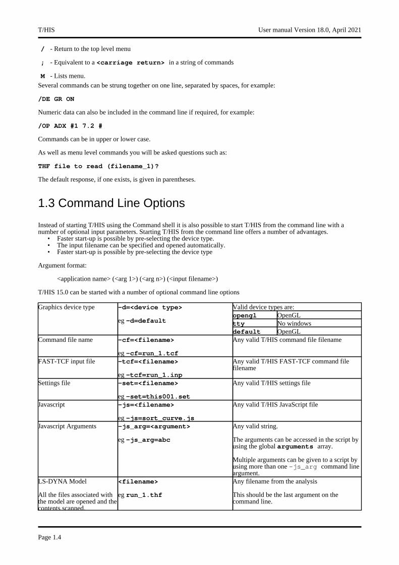
T/HIS 15.0 can be started with a number of optional command line options
Valid device types are: Graphics device type -d=<device type>
eg -d=default opengl OpenGLtty No windowsdefault OpenGL
Command file name -cf=<filename>
eg -cf=run_1.tcf
Any valid T/HIS command file filename
FAST-TCF input file -tcf=<filename>
eg -tcf=run_1.inp
Any valid T/HIS FAST-TCF command file filename
Settings file -set=<filename>
eg -set=this001.set
Any valid T/HIS settings file
Javascript -js=<filename>
eg -js=sort_curve.js
Any valid T/HIS JavaScript file
Javascript Arguments -js_arg=<argument>
eg -js_arg=abc
Any valid string.
The arguments can be accessed in the script by using the global arguments array.
Multiple arguments can be given to a script by using more than one -js_arg command line argument.
LS-DYNA Model
All the files associated with the model are opened and the contents scanned.
<filename>
eg run_1.thf
Any filename from the analysis
This should be the last argument on the command line.
T/HIS User manual Version 18.0, April 2021
Page 1.4
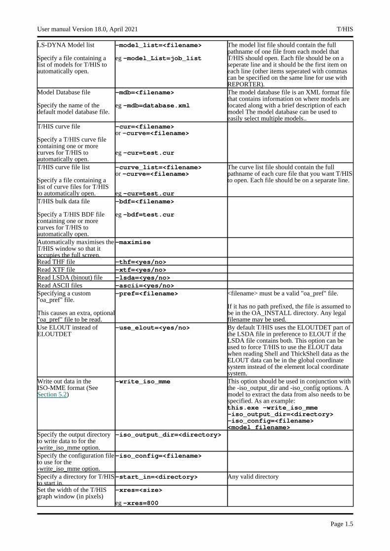
LS-DYNA Model list
Specify a file containing a list of models for T/HIS to automatically open.
-model_list=<filename>
eg -model_List=job_list
The model list file should contain the full pathname of one file from each model that T/HIS should open. Each file should be on a seperate line and it should be the first item on each line (other items seperated with commas can be specified on the same line for use with REPORTER).
Model Database file
Specify the name of the default model database file.
-mdb=<filename>
eg -mdb=database.xml
The model database file is an XML format file that contains information on where models are located along with a brief description of each model The model database can be used to easily select multiple models..
T/HIS curve file
Specify a T/HIS curve file containing one or more curves for T/HIS to automatically open.
-cur=<filename> or -curve=<filename>
eg -cur=test.cur
T/HIS curve file list
Specify a file containing a list of curve files for T/HIS to automatically open.
-curve_list=<filename> or -curve=<filename>
eg -cur=test.cur
The curve list file should contain the full pathname of each cure file that you want T/HIS to open. Each file should be on a separate line.
T/HIS bulk data file
Specify a T/HIS BDF file containing one or more curves for T/HIS to automatically open.
-bdf=<filename>
eg -bdf=test.cur
Automatically maximises the T/HIS window so that it occupies the full screen.
-maximise
Read THF file -thf=<yes/no>Read XTF file -xtf=<yes/no>Read LSDA (binout) file -lsda=<yes/no>Read ASCII files -ascii=<yes/no>Specifying a custom "oa_pref" file.
This causes an extra, optional "oa_pref" file to be read.
-pref=<filename> <filename> must be a valid "oa_pref" file.
If it has no path prefixed, the file is assumed to be in the OA_INSTALL directory. Any legal filename may be used.
Use ELOUT instead of ELOUTDET
-use_elout=<yes/no> By default T/HIS uses the ELOUTDET part of the LSDA file in preference to ELOUT if the LSDA file contains both. This option can be used to force T/HIS to use the ELOUT data when reading Shell and ThickShell data as the ELOUT data can be in the global coordinate system instead of the element local coordinate system.
Write out data in the ISO-MME format (See Section 5.2)
-write_iso_mme This option should be used in conjunction with the -iso_output_dir and -iso_config options. A model to extract the data from also needs to be specified. As an example: this.exe -write_iso_mme -iso_output_dir=<directory> -iso_config=<filename> <model_filename>
Specify the output directory to write data to for the -write_iso_mme option.
-iso_output_dir=<directory>
Specify the configuration file to use for the -write_iso_mme option.
-iso_config=<filename>
Specify a directory for T/HIS to start in.
-start_in=<directory> Any valid directory
Set the width of the T/HIS graph window (in pixels)
-xres=<size>
eg -xres=800
User manual Version 18.0, April 2021 T/HIS
Page 1.5
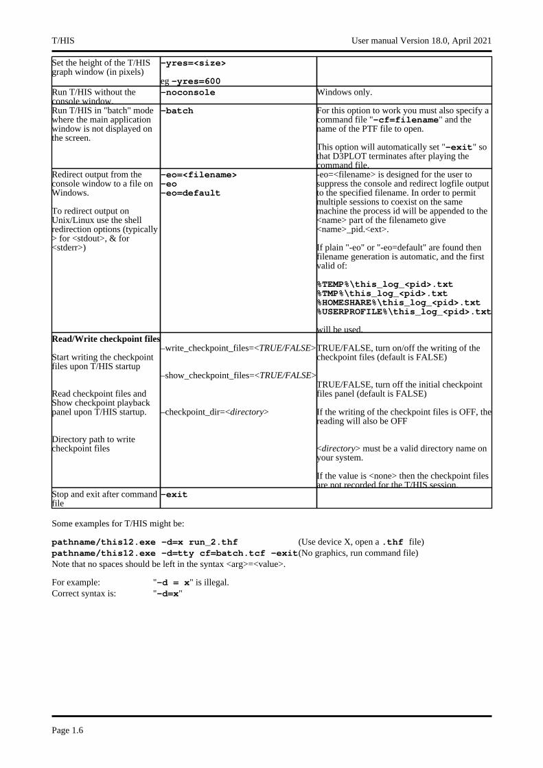
Set the height of the T/HIS graph window (in pixels)
-yres=<size>
eg -yres=600Run T/HIS without the console window.
-noconsole Windows only.
Run T/HIS in "batch" mode where the main application window is not displayed on the screen.
-batch For this option to work you must also specify a command file "-cf=filename" and the name of the PTF file to open.
This option will automatically set "-exit" so that D3PLOT terminates after playing the command file.
Redirect output from the console window to a file on Windows.
To redirect output on Unix/Linux use the shell redirection options (typically > for <stdout>, & for <stderr>)
-eo=<filename>-eo-eo=default
-eo=<filename> is designed for the user to suppress the console and redirect logfile output to the specified filename. In order to permit multiple sessions to coexist on the same machine the process id will be appended to the <name> part of the filenameto give <name>_pid.<ext>.
If plain "-eo" or "-eo=default" are found then filename generation is automatic, and the first valid of:
%TEMP%\this_log_<pid>.txt%TMP%\this_log_<pid>.txt%HOMESHARE%\this_log_<pid>.txt%USERPROFILE%\this_log_<pid>.txt
will be used.Read/Write checkpoint files
Start writing the checkpoint files upon T/HIS startup
Read checkpoint files and Show checkpoint playback panel upon T/HIS startup.
Directory path to write checkpoint files
–write_checkpoint_files=<TRUE/FALSE>
–show_checkpoint_files=<TRUE/FALSE>
–checkpoint_dir=<directory>
TRUE/FALSE, turn on/off the writing of the checkpoint files (default is FALSE)
TRUE/FALSE, turn off the initial checkpoint files panel (default is FALSE)
If the writing of the checkpoint files is OFF, the reading will also be OFF
<directory> must be a valid directory name on your system.
If the value is <none> then the checkpoint files are not recorded for the T/HIS session.
Stop and exit after command file
-exit
Some examples for T/HIS might be:
pathname/this12.exe -d=x run_2.thf (Use device X, open a .thf file)pathname/this12.exe -d=tty cf=batch.tcf -exit(No graphics, run command file)Note that no spaces should be left in the syntax <arg>=<value>.
For example: "-d = x" is illegal.Correct syntax is: "-d=x"
T/HIS User manual Version 18.0, April 2021
Page 1.6
2 Using Screen Menus2.1 Basic screen menu layout2.2 Mouse and keyboard usage2.3 Dialogue input2.4 Window management2.5 Dynamic Viewing (Using the mouse to change views)2.6 Graphics Box Options
Versions of T/HIS prior to release 6.1 only had a "command-line" interface. This has been preserved for backwards compatibility, but a "screen-menu" interface has been added which allows you to drive the program almost entirely with the mouse.
2.1 Basic screen menu layout
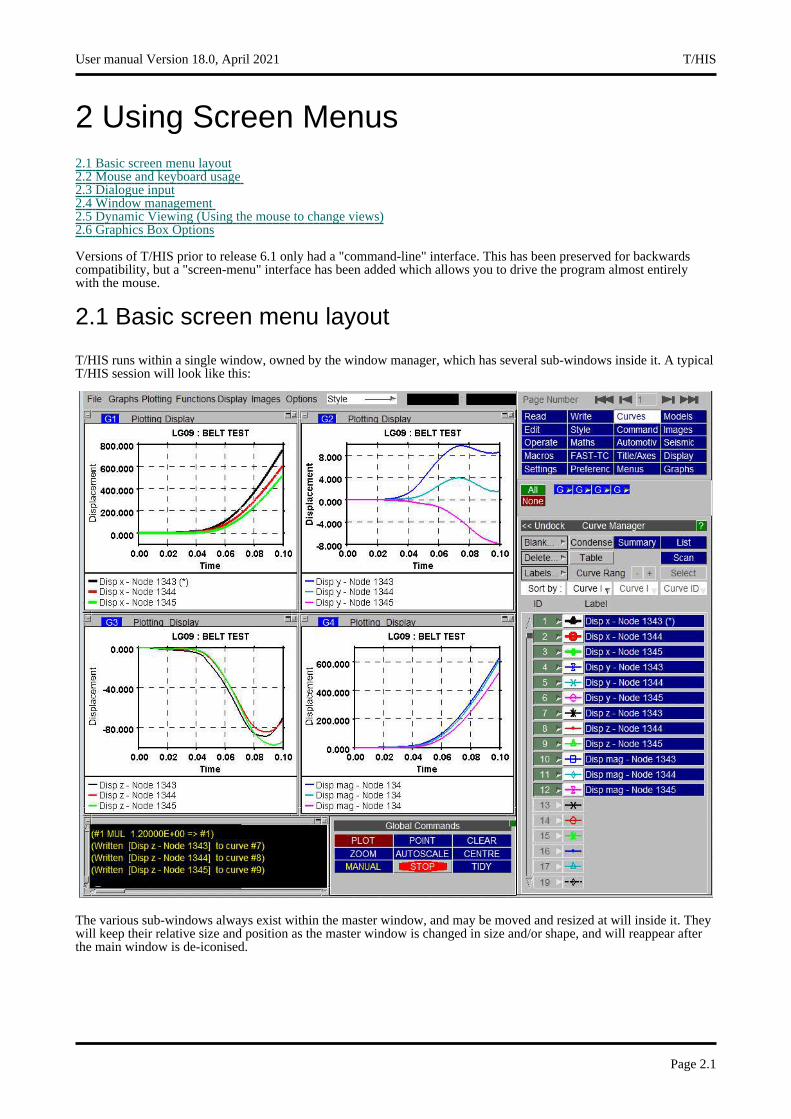
T/HIS runs within a single window, owned by the window manager, which has several sub-windows inside it. A typical T/HIS session will look like this:
The various sub-windows always exist within the master window, and may be moved and resized at will inside it. They will keep their relative size and position as the master window is changed in size and/or shape, and will reappear after the main window is de-iconised.
User manual Version 18.0, April 2021 T/HIS
Page 2.1
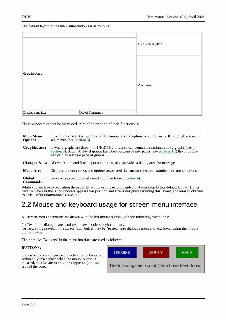
The default layout of the main sub-windows is as follows:
These windows cannot be dismissed. A brief description of their functions is:
Main Menu Options
Provides access to the majority of the commands and options available in T/HIS through a series of sub menus (see Section 5).
Graphics area Is where graphs are drawn. In T/HIS 15.0 this area can contain a maximum of 32 graphs (see Section 3). Alternativley if graphs have been organised into pages (see Section 3.3) then this area will display a single page of graphs.
Dialogue & list Allows "command-line" input and output, also provides a listing area for messages.
Menu Area Displays the commands and options associated the current selection fromthe main menu options.
Global Commands
Gives access to commonly used commands (see Section 4).
While you are free to reposition these master windows it is recommended that you keep to this default layout. This is because when further sub-windows appear their position and size is designed assuming this layout, and aims to obscure as little useful information as possible.
2.2 Mouse and keyboard usage for screen-menu interface
All screen-menu operations are driven with the left mouse button, with the following exceptions:
(a) Text in the dialogue area and text boxes requires keyboard entry.(b) Text strings saved in the cursor "cut" buffer may be "pasted" into dialogue areas and text boxes using the middle mouse button.
The primitive "widgets" in the menu interface are used as follows:
BUTTONS:
Screen buttons are depressed by clicking on them, but action only takes place when the mouse button is released, so it is safe to drag the (depressed) mouse around the screen.
T/HIS User manual Version 18.0, April 2021
Page 2.2
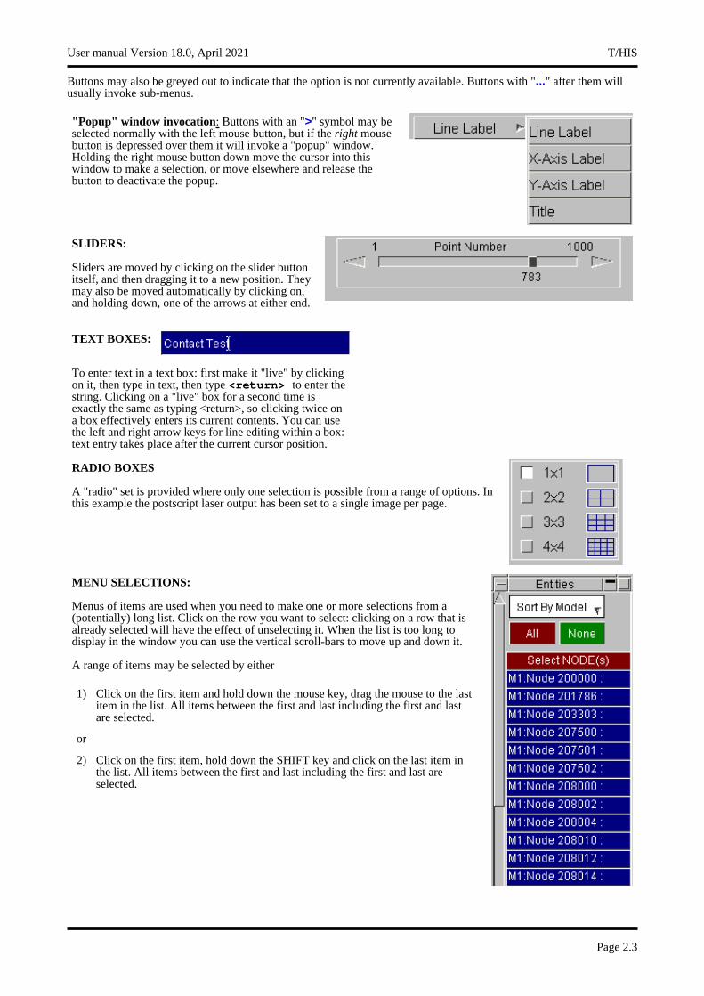
Buttons may also be greyed out to indicate that the option is not currently available. Buttons with "..." after them will usually invoke sub-menus.
"Popup" window invocation: Buttons with an ">" symbol may be selected normally with the left mouse button, but if the right mouse button is depressed over them it will invoke a "popup" window. Holding the right mouse button down move the cursor into this window to make a selection, or move elsewhere and release the button to deactivate the popup.
SLIDERS:
Sliders are moved by clicking on the slider button itself, and then dragging it to a new position. They may also be moved automatically by clicking on, and holding down, one of the arrows at either end.
TEXT BOXES:
To enter text in a text box: first make it "live" by clicking on it, then type in text, then type <return> to enter the string. Clicking on a "live" box for a second time is exactly the same as typing <return>, so clicking twice on a box effectively enters its current contents. You can use the left and right arrow keys for line editing within a box: text entry takes place after the current cursor position.
RADIO BOXES
A "radio" set is provided where only one selection is possible from a range of options. In this example the postscript laser output has been set to a single image per page.
MENU SELECTIONS:
Menus of items are used when you need to make one or more selections from a (potentially) long list. Click on the row you want to select: clicking on a row that is already selected will have the effect of unselecting it. When the list is too long to display in the window you can use the vertical scroll-bars to move up and down it.
A range of items may be selected by either
1) Click on the first item and hold down the mouse key, drag the mouse to the last item in the list. All items between the first and last including the first and last are selected.
or
2) Click on the first item, hold down the SHIFT key and click on the last item in the list. All items between the first and last including the first and last are selected.
User manual Version 18.0, April 2021 T/HIS
Page 2.3
2.3 Dialogue input in the screen menu interface
The full command-line capability is preserved when T/HIS is running in screen-menu mode, and you are free to mix command-line and mouse-driven input at will. There are some situations in which command-line input is more efficient: for example when entering lists of explicit entities.
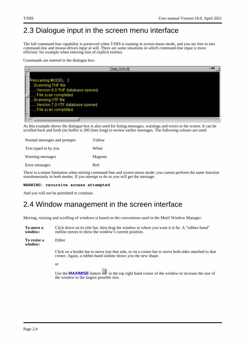
Commands are entered in the dialogue box:
As this example shows the dialogue box is also used for listing messages, warnings and errors to the screen. It can be scrolled back and forth (its buffer is 200 lines long) to review earlier messages. The following colours are used:
Normal messages and prompts Yellow
Text typed in by you White
Warning messages Magenta
Error messages Red
There is a minor limitation when mixing command-line and screen-menu mode: you cannot perform the same function simultaneously in both modes. If you attempt to do so you will get the message:
WARNING: recursive access attempted
And you will not be permitted to continue.
2.4 Window management in the screen interface
Moving, resizing and scrolling of windows is based on the conventions used in the Motif Window Manager.
To move a window:
Click down on its title bar, then drag the window to where you want it to be. A "rubber-band" outline moves to show the window’s current position.
To resize a window:
Either
Click on a border bar to move just that side, or on a corner bar to move both sides attached to that corner. Again, a rubber-band outline shows you the new shape.
or
Use the MAXIMISE button in the top right hand corner of the window to increase the size of the window to the largest possible size.
T/HIS User manual Version 18.0, April 2021
Page 2.4
To scroll a window:
If a window has got too small for its contents then horizontal and/or vertical scrollbars will appear. Click on a scrollbar slider and move it to the desired position, the window contents will scroll as you do so. Alternatively click on the arrows at either end of the scrollbar for timed motion in that direction.
To minimise a window:
Click on the button in the top right hand corner of the window. When a window has been iconised it will appear in the ICON area at the bottom of the screen.
To restore a window:
Iconised windows may be restored by clicking on the icon in the ICON area.
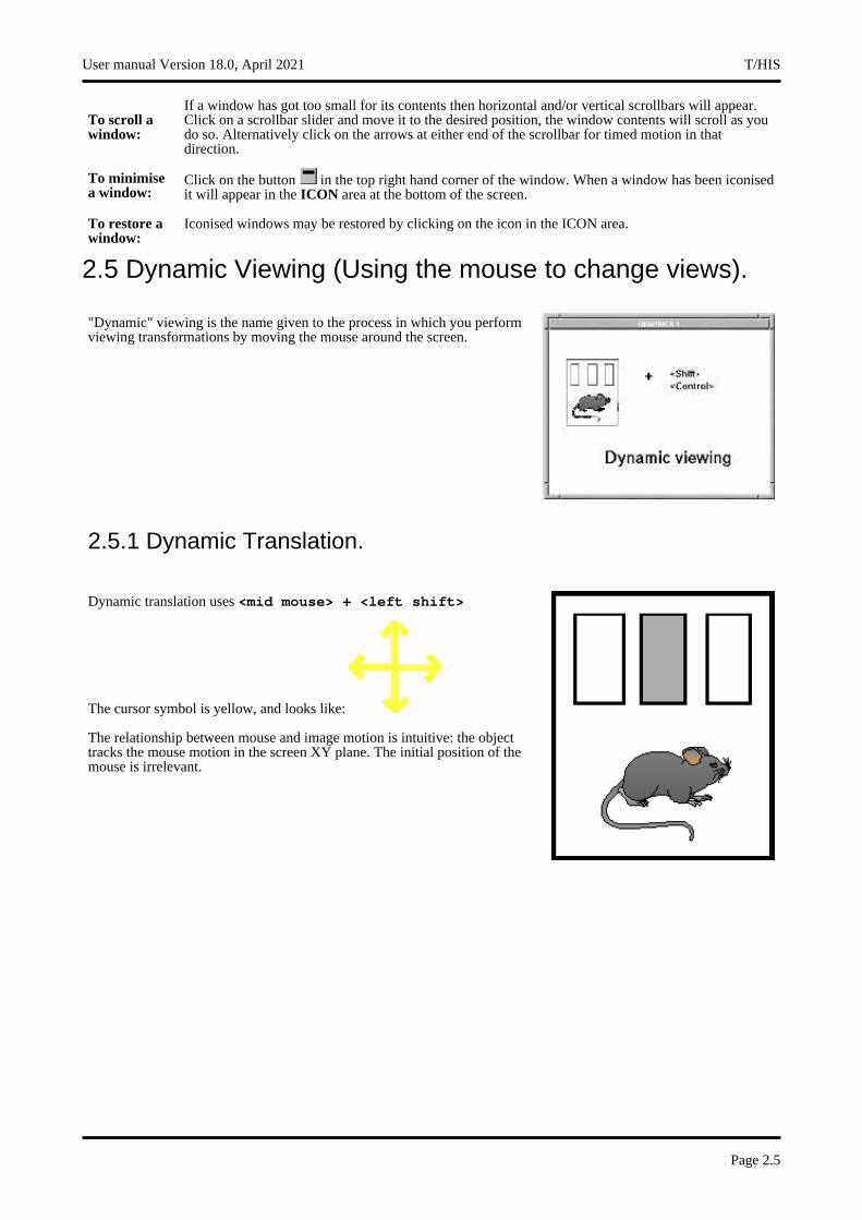
2.5 Dynamic Viewing (Using the mouse to change views).
"Dynamic" viewing is the name given to the process in which you perform viewing transformations by moving the mouse around the screen.
2.5.1 Dynamic Translation.
Dynamic translation uses <mid mouse> + <left shift>
The cursor symbol is yellow, and looks like:
The relationship between mouse and image motion is intuitive: the object tracks the mouse motion in the screen XY plane. The initial position of the mouse is irrelevant.
User manual Version 18.0, April 2021 T/HIS
Page 2.5
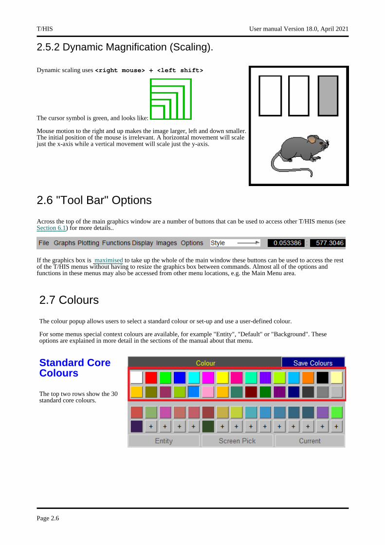
2.5.2 Dynamic Magnification (Scaling).
Dynamic scaling uses <right mouse> + <left shift>
The cursor symbol is green, and looks like:
Mouse motion to the right and up makes the image larger, left and down smaller. The initial position of the mouse is irrelevant. A horizontal movement will scale just the x-axis while a vertical movement will scale just the y-axis.
2.6 "Tool Bar" Options
Across the top of the main graphics window are a number of buttons that can be used to access other T/HIS menus (see Section 6.1) for more details..
If the graphics box is maximised to take up the whole of the main window these buttons can be used to access the rest of the T/HIS menus without having to resize the graphics box between commands. Almost all of the options and functions in these menus may also be accessed from other menu locations, e.g. the Main Menu area.
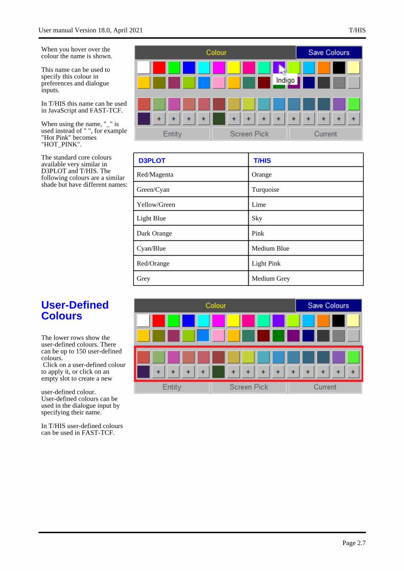
2.7 Colours
The colour popup allows users to select a standard colour or set-up and use a user-defined colour.
For some menus special context colours are available, for example "Entity", "Default" or "Background". These options are explained in more detail in the sections of the manual about that menu.
Standard Core Colours
The top two rows show the 30 standard core colours.
T/HIS User manual Version 18.0, April 2021
Page 2.6
When you hover over the colour the name is shown.
This name can be used to specify this colour in preferences and dialogue inputs.
In T/HIS this name can be used in JavaScript and FAST-TCF.
When using the name, "_" is used instead of " ", for example "Hot Pink" becomes "HOT_PINK".
The standard core colours available very similar in D3PLOT and T/HIS. The following colours are a similar shade but have different names:
D3PLOT T/HIS
Red/Magenta Orange
Green/Cyan Turquoise
Yellow/Green Lime
Light Blue Sky
Dark Orange Pink
Cyan/Blue Medium Blue
Red/Orange Light Pink
Grey Medium Grey
User-Defined Colours
The lower rows show the user-defined colours. There can be up to 150 user-defined colours.Click on a user-defined colour to apply it, or click on an empty slot to create a new
user-defined colour. User-defined colours can be used in the dialogue input by specifying their name.
In T/HIS user-defined colours can be used in FAST-TCF.
User manual Version 18.0, April 2021 T/HIS
Page 2.7
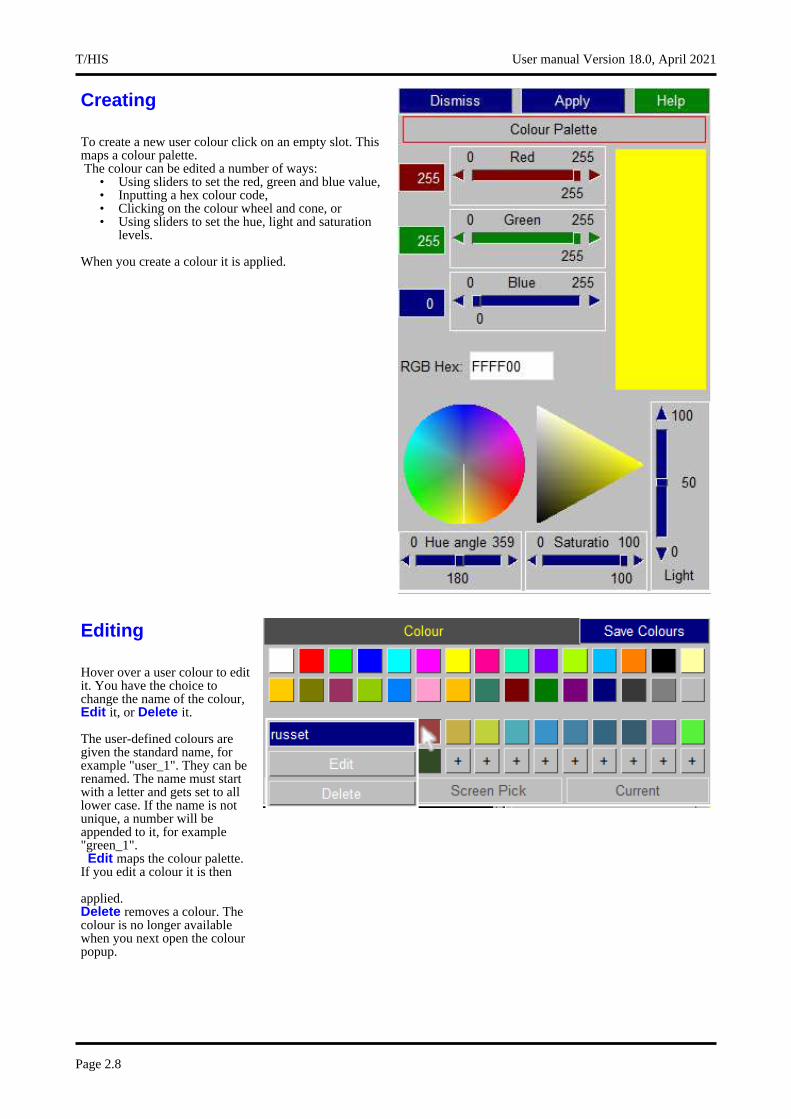
Creating
To create a new user colour click on an empty slot. This maps a colour palette. The colour can be edited a number of ways:
• Using sliders to set the red, green and blue value,• Inputting a hex colour code,• Clicking on the colour wheel and cone, or• Using sliders to set the hue, light and saturation
levels.
When you create a colour it is applied.
Editing
Hover over a user colour to edit it. You have the choice to change the name of the colour, Edit it, or Delete it.
The user-defined colours are given the standard name, for example "user_1". They can be renamed. The name must start with a letter and gets set to all lower case. If the name is not unique, a number will be appended to it, for example "green_1". Edit maps the colour palette.
If you edit a colour it is then
applied. Delete removes a colour. The colour is no longer available when you next open the colour popup.
T/HIS User manual Version 18.0, April 2021
Page 2.8

Saving
The user-defined colours can be saved. The same user-defined colour are then available when you next run D3PLOT or T/HIS.
The user-defined colours are stored in the user_colours.xml file. If the user has permission to modify things in the INSTALL directory, the user is given the option to either save the user colours to the INSTALL directory (which is sometimes visible to multiple users) or their HOME directory.
Alternatively, the preference user_colour_file can be set to specify an .xml file.
When D3PLOT or T/HIS is next started the user_colours.xml file is read in.
If the same colour, for example "user_1", is defined in the user_colours.xml file in both the INSTALL and HOME directory, the HOME directory user_colours.xml file takes precedence.
If the preference user_colour_file has been set, any user_colours.xml file in the HOME directory is ignored. If a colour is also defined in the user_colours.xml file in the INSTALL directory, the user_colour_file .xml file takes precedence.
For T/HIS, if a user colour was previously set-up using a preference, for example this*user_colour1, and that colour slot is also defined in a user_colours.xml file, the user_colours.xml file takes precedence.
T/HIS Link
When running the T/HIS link any user colours created in D3PLOT (or in T/HIS) will be available in the other program. When T/HIS is first opened it sets-up the user colours to match the current D3PLOT session, rather than using a saved user_colours.xml file.
User manual Version 18.0, April 2021 T/HIS
Page 2.9

T/HIS User manual Version 18.0, April 2021
Page 2.10

3 Graphs and Pages3.1 Creating Graphs3.2 Page Size3.3 Page Layouts3.4 Pages3.5 Active / Inactive Graphs
T/HIS 17.0 can display a maximum of 32 graphs. Each graph can have a different appearance and they can display different curves.
Graphs can be laid out using a number of different formats and they can be organised into ’Pages’.
3.1 Creating Graphs
Create Graphs Create a new graph.
The shortcut key ’G’ can also be used to create new graphs.
Number of graphs to create
This option can be used to create multiple graphs.
User manual Version 18.0, April 2021 T/HIS
Page 3.1
When new graphs are created the initial settings for each graph can be copied from 3 different sources.
Create using preference settings
The Display and Axis Settings are copied from the preference file.
Create using current settings
The Display and Axis Settings are copied from the current settings in the Display and Axis menus.
Copy settings from graph n The Display and Axis Settings are copied from the specified graph.
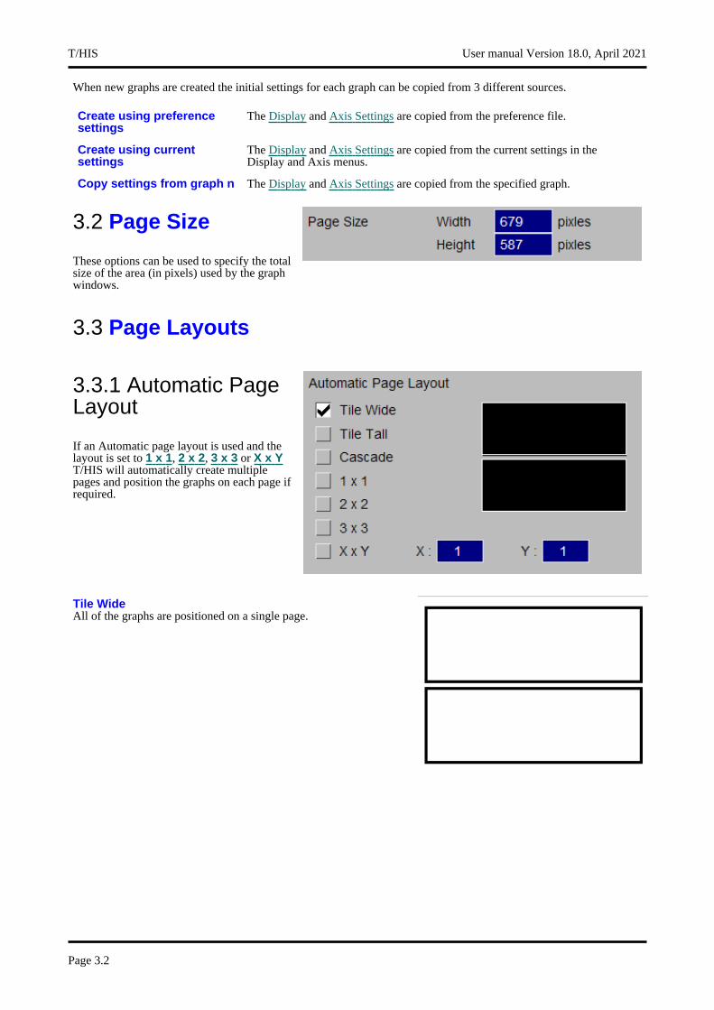
3.2 Page Size
These options can be used to specify the total size of the area (in pixels) used by the graph windows.
3.3 Page Layouts
3.3.1 Automatic Page Layout
If an Automatic page layout is used and the layout is set to 1 x 1, 2 x 2, 3 x 3 or X x YT/HIS will automatically create multiple pages and position the graphs on each page if required.
Tile Wide All of the graphs are positioned on a single page.
T/HIS User manual Version 18.0, April 2021
Page 3.2
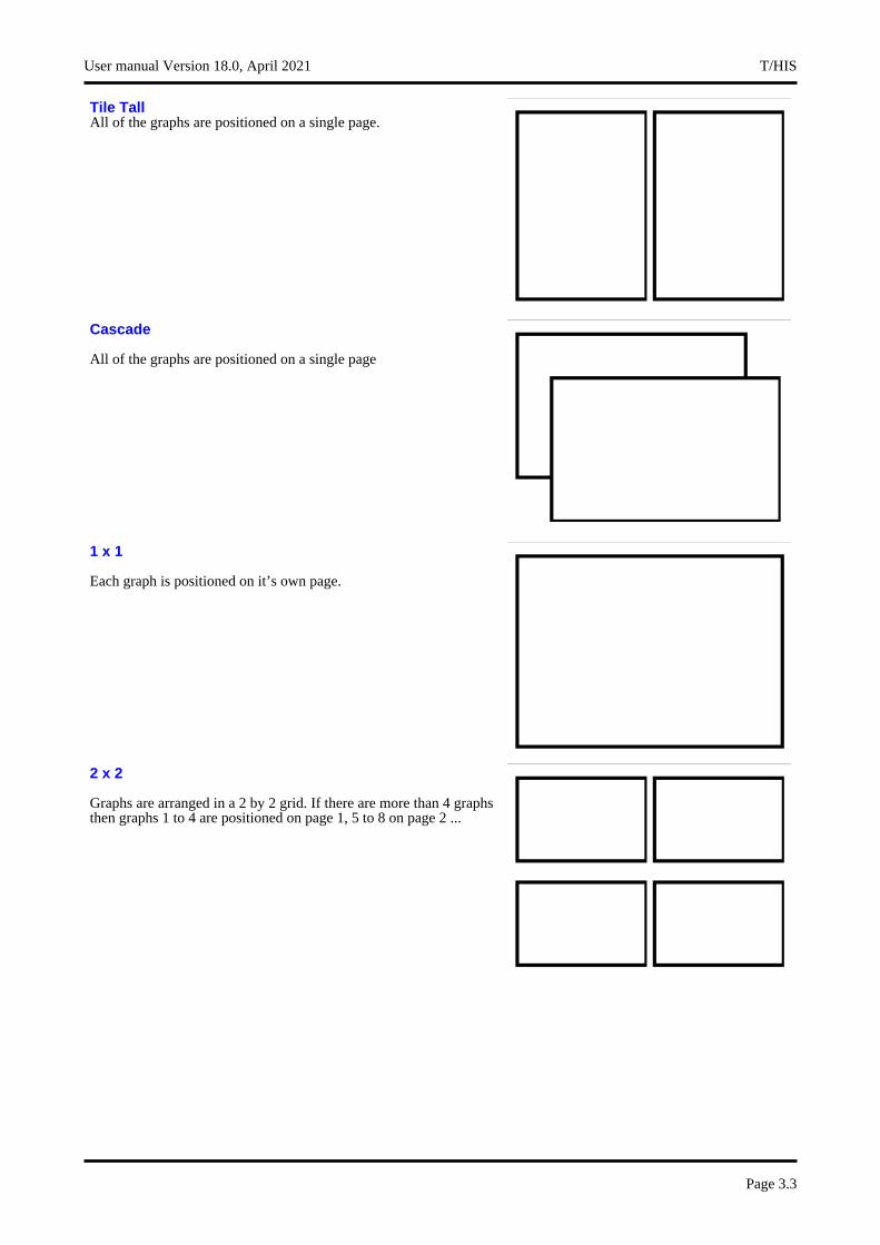
Tile Tall All of the graphs are positioned on a single page.
Cascade
All of the graphs are positioned on a single page
1 x 1
Each graph is positioned on it’s own page.
2 x 2
Graphs are arranged in a 2 by 2 grid. If there are more than 4 graphs then graphs 1 to 4 are positioned on page 1, 5 to 8 on page 2 ...
User manual Version 18.0, April 2021 T/HIS
Page 3.3
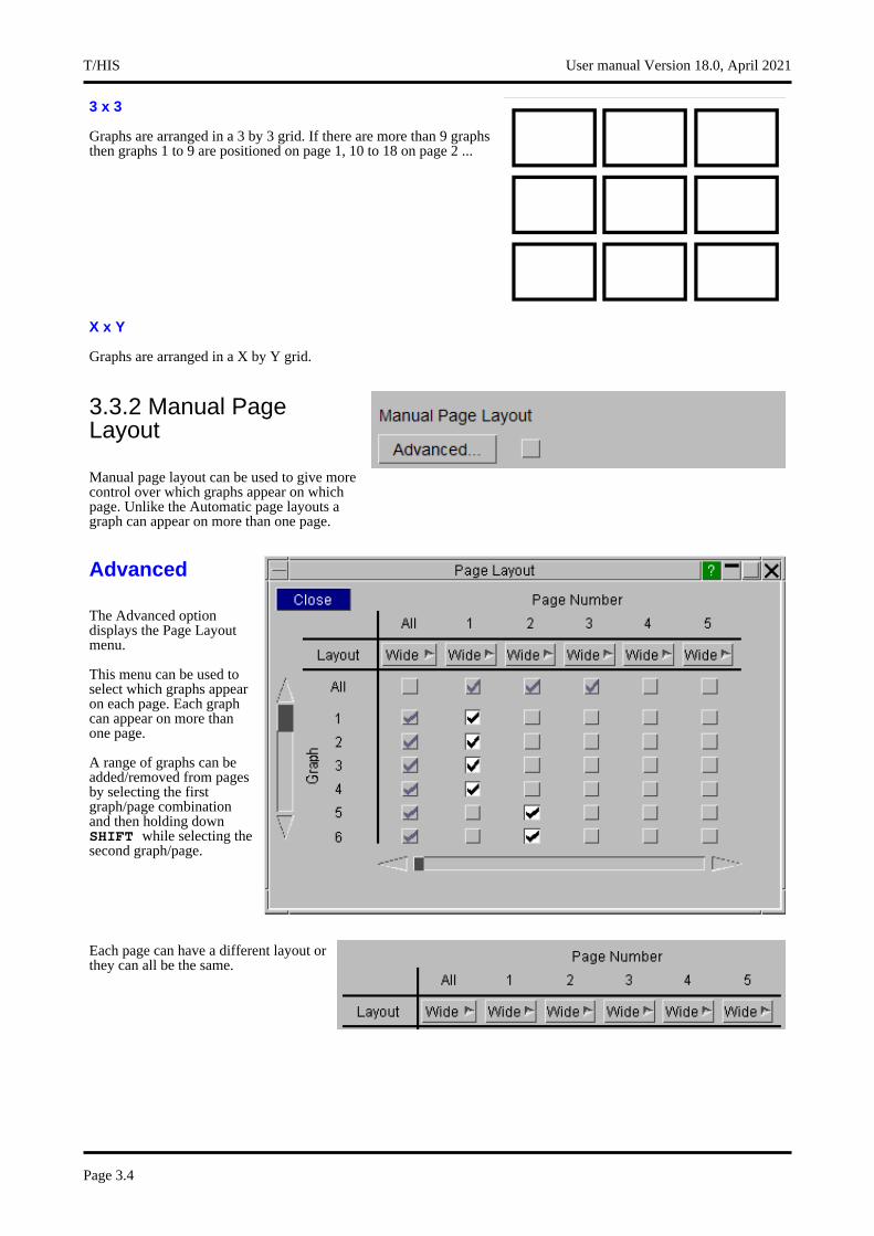
3 x 3
Graphs are arranged in a 3 by 3 grid. If there are more than 9 graphs then graphs 1 to 9 are positioned on page 1, 10 to 18 on page 2 ...
X x Y
Graphs are arranged in a X by Y grid.
3.3.2 Manual Page Layout
Manual page layout can be used to give more control over which graphs appear on which page. Unlike the Automatic page layouts a graph can appear on more than one page.
Advanced
The Advanced option displays the Page Layout menu.
This menu can be used to select which graphs appear on each page. Each graph can appear on more than one page.
A range of graphs can be added/removed from pages by selecting the first graph/page combination and then holding down SHIFT while selecting the second graph/page.
Each page can have a different layout or they can all be the same.
T/HIS User manual Version 18.0, April 2021
Page 3.4

With the Advanced option the Graph Layout options work in exactly the same way as the Automatic Page Layoutoptions, except they only position the graphs defined on each page.
If for example T/HIS has 6 graphs defined and graphs 2,3,4,5 are defined on page 1 and graphs 1 and 6 are on page 2 then the different graph layout options would produce the following.
Page 1 Page 2
Tile Wide
Tile Tall
Cascade
1 x 1
(stacked on top of each other)
User manual Version 18.0, April 2021 T/HIS
Page 3.5
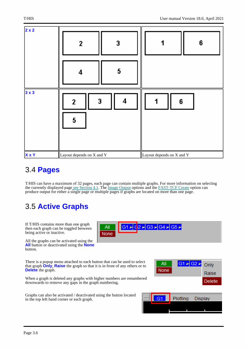
2 x 2
3 x 3
X x Y Layout depends on X and Y Layout depends on X and Y
3.4 Pages
T/HIS can have a maximum of 32 pages, each page can contain multiple graphs. For more information on selecting the currently displayed page see Section 4.1. The Image Output options and the FAST-TCF Create option can produce output for either a single page or multiple pages if graphs are located on more than one page.
3.5 Active Graphs
If T/HIS contains more than one graph then each graph can be toggled between being active or inactive.
All the graphs can be activated using the All button or deactivated using the None button.
There is a popup menu attached to each button that can be used to select that graph Only, Raise the graph so that it is in front of any others or to Delete the graph.
When a graph is deleted any graphs with higher numbers are renumbered downwards to remove any gaps in the graph numbering.
Graphs can also be activated / deactivated using the button located in the top left hand corner or each graph.
T/HIS User manual Version 18.0, April 2021
Page 3.6

The options in the Display and Title/Axes menus that control the appearance of graphs are only applied to active graphs.
When new curves are created by reading in data from files the new curves are automatically unblanked in all of the currently active graphs and blanked in any inactive graphs.
User manual Version 18.0, April 2021 T/HIS
Page 3.7

T/HIS User manual Version 18.0, April 2021
Page 3.8
4 Global Commands and Pages4.1 Page Number4.2 PLOT4.3 POINT4.4 CLEAR4.5 ZOOM4.6 AUTOSCALE4.7 CENTRE4.8 MANUAL4.9 STOP4.10 TIDY4.11 Additional Commands
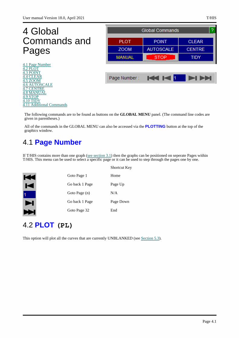
The following commands are to be found as buttons on the GLOBAL MENU panel. (The command line codes are given in parentheses.)
All of the commands in the GLOBAL MENU can also be accessed via the PLOTTING button at the top of the graphics window.
4.1 Page Number
If T/HIS contains more than one graph (see section 3.1) then the graphs can be positioned on seperate Pages within T/HIS. This menu can be used to select a specific page or it can be used to step through the pages one by one.
XXXXXXXXXXXXXXX XXXXXXXXXXXXXXX
Shortcut Key
Goto Page 1 Home
Go back 1 Page Page Up
Goto Page (n) N/A
Go back 1 Page Page Down
Goto Page 32 End
4.2 PLOT (PL)
This option will plot all the curves that are currently UNBLANKED (see Section 5.3).
User manual Version 18.0, April 2021 T/HIS
Page 4.1
4.3 POINT (PT)
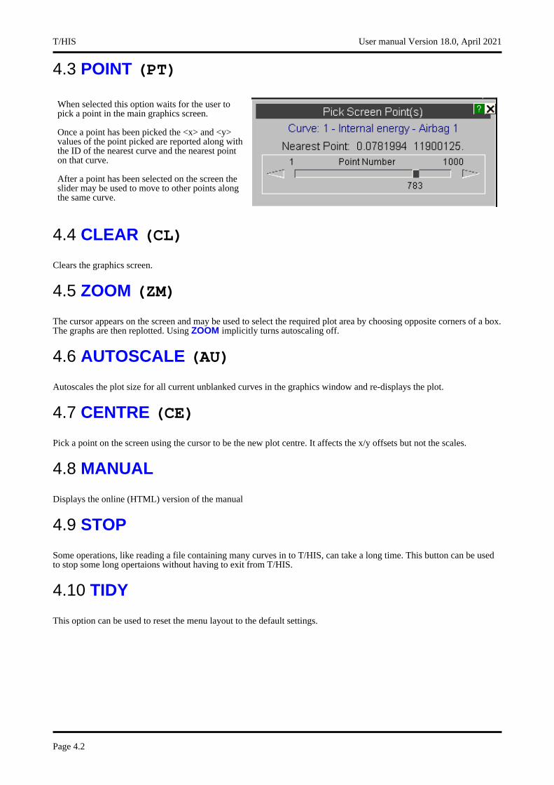
When selected this option waits for the user to pick a point in the main graphics screen.
Once a point has been picked the <x> and <y> values of the point picked are reported along with the ID of the nearest curve and the nearest point on that curve.
After a point has been selected on the screen the slider may be used to move to other points along the same curve.
4.4 CLEAR (CL)
Clears the graphics screen.
4.5 ZOOM (ZM)
The cursor appears on the screen and may be used to select the required plot area by choosing opposite corners of a box. The graphs are then replotted. Using ZOOM implicitly turns autoscaling off.
4.6 AUTOSCALE (AU)
Autoscales the plot size for all current unblanked curves in the graphics window and re-displays the plot.
4.7 CENTRE (CE)
Pick a point on the screen using the cursor to be the new plot centre. It affects the x/y offsets but not the scales.
4.8 MANUAL
Displays the online (HTML) version of the manual
4.9 STOP
Some operations, like reading a file containing many curves in to T/HIS, can take a long time. This button can be used to stop some long opertaions without having to exit from T/HIS.
4.10 TIDY
This option can be used to reset the menu layout to the default settings.
T/HIS User manual Version 18.0, April 2021
Page 4.2
4.11 Additional Commands
A number of additional global commands exist in command line mode. These functions exist in screen menu mode within other menu levels.
(PF) Creates a postscript plot file. Either A4 landscape or A4 portrait formats may be chosen. A title and figure number are also requested. Other plot setting may be made in the command line mode UTILITIES menu.
(BL) Blank a currently displayed curve.
(UB) Unblank a curve that has been blanked.
(RM) Remove (delete) a curve. Once a curve has been removed it is lost from the system.
(ER) Erase (delete) all existing curves from T/HIS. (Equivalent to the command RM *.)
(GS) Global status: displays the current number of curves, their labels and whether they are blanked.
(CO) Condense: renumbers all curves to fill any gaps in curve numbers.
(LM) Gives the current program limits.
(FT) File tracking: lists the 20 files which have been accessed most recently by T/HIS, giving details of the type of file and whether it was read from or written to.
(EX) Exits (leaves) the program.
User manual Version 18.0, April 2021 T/HIS
Page 4.3

T/HIS User manual Version 18.0, April 2021
Page 4.4

5 Main Menu5.1 READ Options5.2 WRITE Options5.3 CURVE Manager5.4 MODEL Manager5.5 EDIT Options5.6 STYLE Menu5.7 Command File5.8 IMAGE Options5.9 OPERATE Options5.10 MATHS Options5.11 AUTOMOTIVE Options5.12 SEISMIC Options5.13 MACRO Options5.14 FAST-TCF Options5.15 TITLE/AXES Options5.16 DISPLAY Options5.17 SETTINGS Menu5.18 MEASURE Menu5.19 GROUPS Menu5.20 GRAPHS Menu5.21 PROPERTIES Menu5.22 UNITS Menu5.23 JavaScript Menu5.24 Datum Menu
5.25 T/HIS Session Save and Retrieve
The MAIN MENU provides access to a number of separate menus that perform most of the operations available within T/HIS from reading in data to producing postscript laser files.
5.0 Selecting Curves
5.0.1 Input Curves
By Curve ID
A number of the menus require a range of curves to be selected. When a range of curves has to be selected a menu containing a list of the available curves will be displayed (see figure, right).
A range or curves may be selected by either1. Click on the first item and hold down
the mouse key, drag the mouse to the last item in the list. All items between the first and last including the first and last are selected.
2. Click on the first item, hold down the SHIFT key and click on the last item in the list. All items between the first and last including the first and last are selected.
User manual Version 18.0, April 2021 T/HIS
Page 5.1
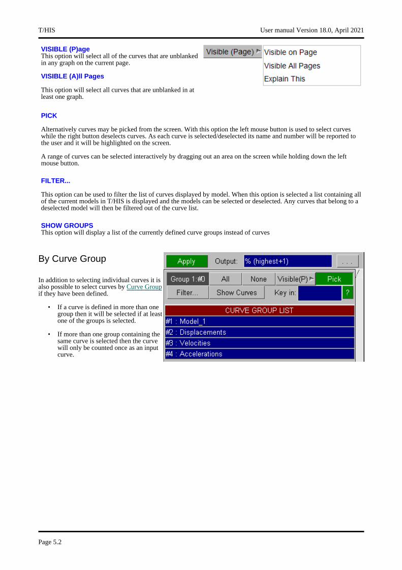
VISIBLE (P)age This option will select all of the curves that are unblanked in any graph on the current page.
VISIBLE (A)ll Pages
This option will select all curves that are unblanked in at least one graph.
PICK
Alternatively curves may be picked from the screen. With this option the left mouse button is used to select curves while the right button deselects curves. As each curve is selected/deselected its name and number will be reported to the user and it will be highlighted on the screen.
A range of curves can be selected interactively by dragging out an area on the screen while holding down the left mouse button.
FILTER...
This option can be used to filter the list of curves displayed by model. When this option is selected a list containing all of the current models in T/HIS is displayed and the models can be selected or deselected. Any curves that belong to a deselected model will then be filtered out of the curve list.
SHOW GROUPS This option will display a list of the currently defined curve groups instead of curves
By Curve Group
In addition to selecting individual curves it is also possible to select curves by Curve Groupif they have been defined.
• If a curve is defined in more than one group then it will be selected if at least one of the groups is selected.
• If more than one group containing the same curve is selected then the curve will only be counted once as an input curve.
T/HIS User manual Version 18.0, April 2021
Page 5.2

By Command Line
In command line mode a single curve may be selected by typing in a range. A valid syntax is:
A single curve number e.g. #27
A "from":"to" range e.g. #10:#30 (no gaps, ":" mandatory)
A compound list in "(..)" e.g. (#1 #2 #10:#30 #3 #97)
In all contexts the order in which a group is defined does NOT influence the order in which it is processed. It is ALWAYS processed in ascending sequential order.
Thus the addition operation
/OP ADD (#30 #20 #10) (#1 #2 #3) #40
will produce the results
#40 = #10 + #1
#41 = #20 + #2
#42 = #30 + #3
5.0.2 Output Curves
All operations that generate new curves must have a target curve defined. This must be one of the following:
#nnn a specific curve number nnn
# meaning "the lowest free curve"
% meaning "the highest free curve"
In all cases output will start at the relevant curve number, however defined, and will rise sequentially with no gaps. This can cause an existing curve to be overwritten, or the output curve number to exceed the limit of 999. Both conditions are checked for: a warning is given if either will occur should the operation go ahead, and an opportunity given to modify or abort the pending operation.
There is a further output option that is only valid for operations where the input is a curve group:
. meaning "overwrite the input curve(s)"
In this case the input curves are overwritten without warning. For example, this option might be used to integrate a set of curves, overwriting the original results with the integrated values.
Any curve number between 1 and 999 may be used as an input or output curve. It is not necessary to use curves sequentially; gaps are permitted in curve number usage. Therefore curves #1 and #10 can be used, for example, without having to use the intervening curves #2 to #9. Likewise, deleting a curve will no longer cause those above it to be renumbered downwards to fill the gap.
User manual Version 18.0, April 2021 T/HIS
Page 5.3
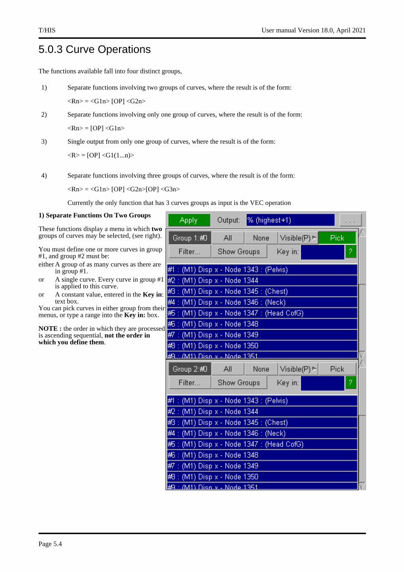
5.0.3 Curve Operations
The functions available fall into four distinct groups,
1) Separate functions involving two groups of curves, where the result is of the form:
<Rn> = <G1n> [OP] <G2n>
2) Separate functions involving only one group of curves, where the result is of the form:
<Rn> = [OP] <G1n>
3) Single output from only one group of curves, where the result is of the form:
<R> = [OP] <G1(1...n)>
4) Separate functions involving three groups of curves, where the result is of the form:
<Rn> = <G1n> [OP] <G2n>[OP] <G3n>
Currently the only function that has 3 curves groups as input is the VEC operation
1) Separate Functions On Two Groups
These functions display a menu in which two groups of curves may be selected, (see right).
You must define one or more curves in group #1, and group #2 must be:either A group of as many curves as there are
in group #1.or A single curve. Every curve in group #1
is applied to this curve.or A constant value, entered in the Key in:
text box.You can pick curves in either group from their menus, or type a range into the Key in: box.
NOTE : the order in which they are processed is ascending sequential, not the order in which you define them.
T/HIS User manual Version 18.0, April 2021
Page 5.4
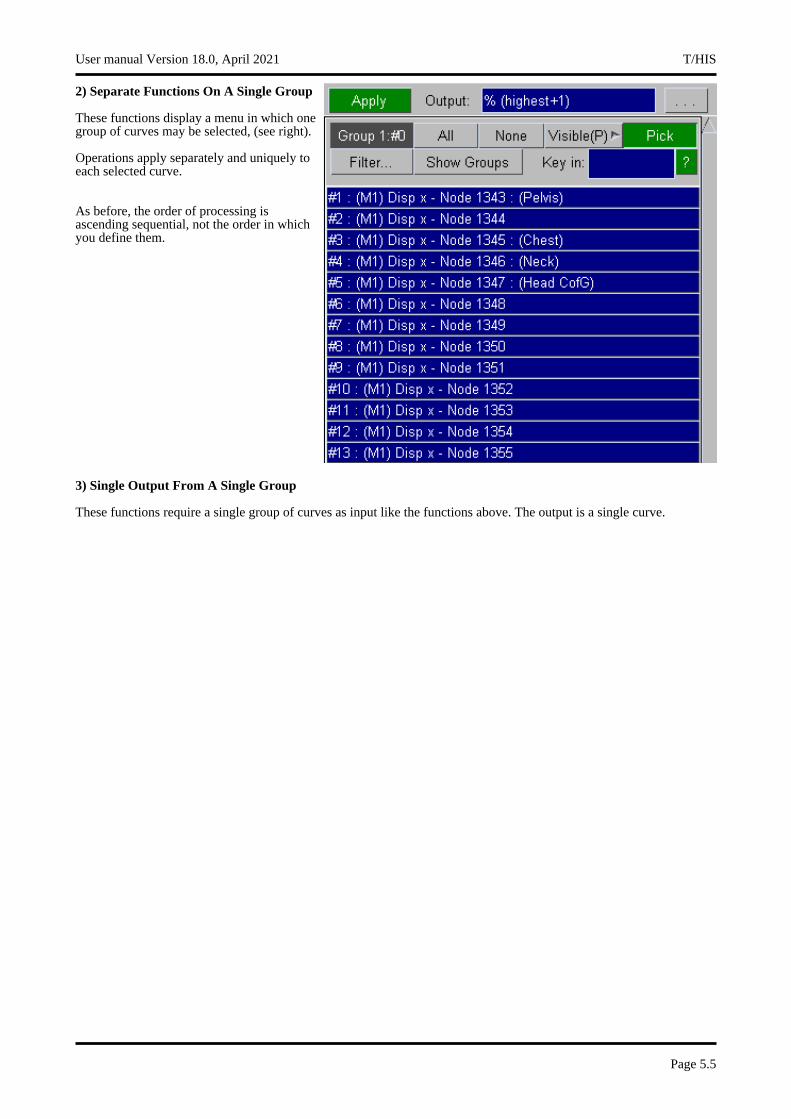
2) Separate Functions On A Single Group
These functions display a menu in which one group of curves may be selected, (see right).
Operations apply separately and uniquely to each selected curve.
As before, the order of processing is ascending sequential, not the order in which you define them.
3) Single Output From A Single Group
These functions require a single group of curves as input like the functions above. The output is a single curve.
User manual Version 18.0, April 2021 T/HIS
Page 5.5

5.1 READ Options
T/HIS can READ data from a number of sources including LS-DYNA binary output files, LS-DYNA ASCII files and tabulated x/y data files. In addition this menu allows data for new curves to be entered directly using the keyboard.
5.1.1 LS-DYNA
Users are strongly advised to run each LS-DYNA analysis in a separate directory. Some of the default names for the files generated by LS-DYNA that T/HIS can read are not unique and T/HIS can not tell which files belong to which model. If you do read multiple models from the same directory T/HIS will generate a warning message if you read the same file for more than 1 model.
5.1.1.1 Selecting Models
There are three ways to select the LS-DYNA models that you want to read into T/HIS
(i) Select a single model (see Section 5.1.1.1.1) (ii) Search directories for results and open open
multiple models (see Section 5.1.1.1.2) (iii)Open a model database and select the models
you want to read ( see Section 5.1.1.1.3)
T/HIS User manual Version 18.0, April 2021
Page 5.6
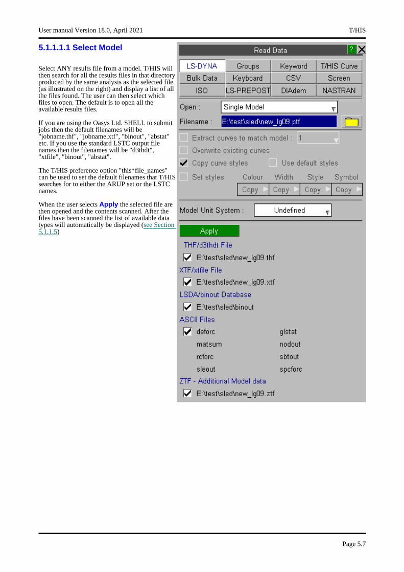
5.1.1.1.1 Select Model
Select ANY results file from a model. T/HIS will then search for all the results files in that directory produced by the same analysis as the selected file (as illustrated on the right) and display a list of all the files found. The user can then select which files to open. The default is to open all the available results files.
If you are using the Oasys Ltd. SHELL to submit jobs then the default filenames will be "jobname.thf", "jobname.xtf", "binout", "abstat" etc. If you use the standard LSTC output file names then the filenames will be "d3thdt", "xtfile", "binout", "abstat".
The T/HIS preference option "this*file_names" can be used to set the default filenames that T/HIS searches for to either the ARUP set or the LSTC names.
When the user selects Apply the selected file are then opened and the contents scanned. After the files have been scanned the list of available data types will automatically be displayed (see Section5.1.1.5)
User manual Version 18.0, April 2021 T/HIS
Page 5.7

5.1.1.1.2 Search Directories Recursively
Multiple models can be opened by using the option to search directories recursively.
After a directory has been specified T/HIS will display a list of all the models it can find in the directory structure and each file can be selected. The order in which the models are read in can be specified by selecting the models in the order required. The selection buttons will display the model number that each model will be read into. The model numbering begins from the next free model number and is then sequential.
T/HIS User manual Version 18.0, April 2021
Page 5.8
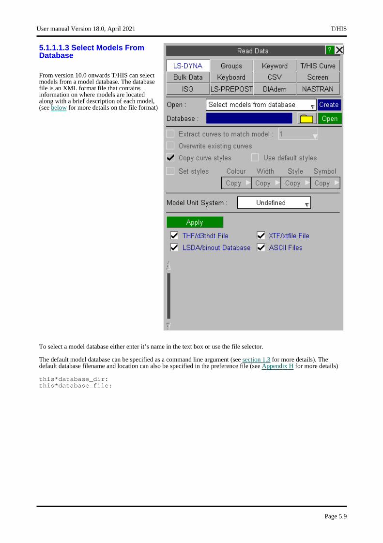
5.1.1.1.3 Select Models From Database
From version 10.0 onwards T/HIS can select models from a model database. The database file is an XML format file that contains information on where models are located along with a brief description of each model, (see below for more details on the file format)
To select a model database either enter it’s name in the text box or use the file selector.
The default model database can be specified as a command line argument (see section 1.3 for more details). The default database filename and location can also be specified in the preference file (see Appendix H for more details)
this*database_dir:this*database_file:
User manual Version 18.0, April 2021 T/HIS
Page 5.9

After a database file has been selected it’s contents will be read and T/HIS will display a Tree Like menu showing the contents of the database.
As each item is displayed T/HIS will check to see if the files that it refers to exist.
If a file does exist then a green tick will be displayed If a file does not exist then a red cross will be displayed The number of levels in the database that are automatically expanded when it is first displayed can be specified in the preference file (see Appendix H for more details)
this*database_expand:
After selecting the required models use Apply to close the database window and return to the main menu where the selected models will be displayed along with the model numbers they will be read in as.
T/HIS User manual Version 18.0, April 2021
Page 5.10
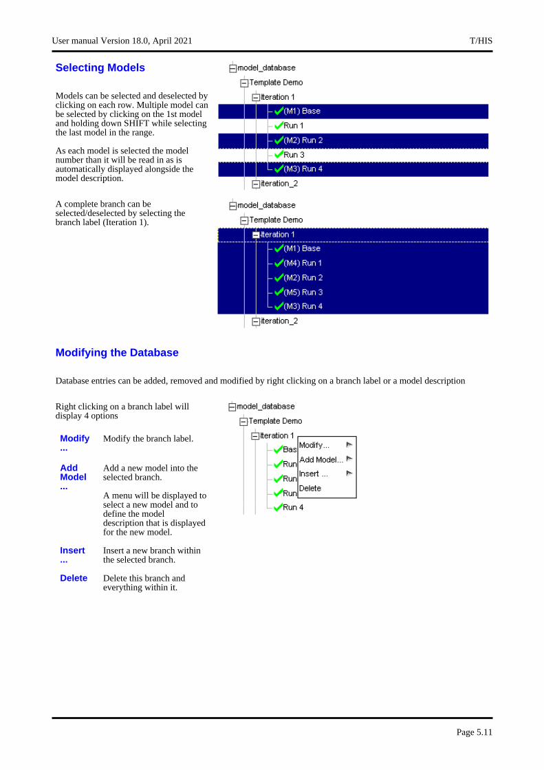
Selecting Models
Models can be selected and deselected by clicking on each row. Multiple model can be selected by clicking on the 1st model and holding down SHIFT while selecting the last model in the range.
As each model is selected the model number than it will be read in as is automatically displayed alongside the model description.
A complete branch can be selected/deselected by selecting the branch label (Iteration 1).
Modifying the Database
Database entries can be added, removed and modified by right clicking on a branch label or a model description
Right clicking on a branch label will display 4 options
Modify ...
Modify the branch label.
Add Model ...
Add a new model into the selected branch.
A menu will be displayed to select a new model and to define the model description that is displayed for the new model.
Insert ...
Insert a new branch within the selected branch.
Delete Delete this branch and everything within it.
User manual Version 18.0, April 2021 T/HIS
Page 5.11

Right clicking on a model description will display 3 options
Modify ...
Modify the model location and description.
Insert ...
Insert a new branch.
The selected model will be moved into the new branch.
Delete Delete the model
Saving the Database
After modifying the database use the Save option to save the changes for future sessions.
Creating a new Database
If you do not have a database or if you want to create a new one then T/HIS can create the new database for you. To create a new database click the CREATE button and simply enter the name of the new database file in the text box that appears, T/HIS will then check that the file does not already exist and if it doesn’t it will create a new empty database.
Alternatively if you type in the name of a file in the main Open Plot File window that does not exist then T/HIS will ask if you want to create a new empty database using that filename.
Once you have done this you can use the Modify options above to add items into the database and then save the file before exiting.
Database Format
The Model Database uses an ASCII XML file format.
All items with the database are either branches or models. Each database entry has an XML name and a LABEL element. Models also contain a model element that contains the full pathname of one of the files belonging to the model.
The XML name should be unique and should obey the following rules• Names can contain letters, numbers, and other characters• Names must not start with a number or punctuation character• Names must not start with the letters xml (or XML, or Xml, etc)• Names cannot contain space
The LABEL is the string used to display an item within the tree view. Unlike the XML name the LABEL can contain any ASCII character.
T/HIS User manual Version 18.0, April 2021
Page 5.12
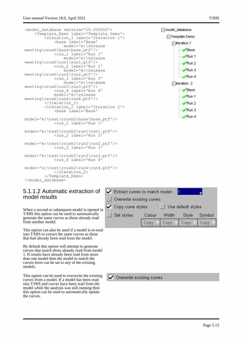
<model_database version="10.000000"><Template_Demo label="Template Demo">
<iteration_1 label="Iteration 1"><base label="Base"
model="e:\release meeting\crush\base\base.ptf"/>
<run_1 label="Run 1"model="e:\release
meeting\crush\run1\run1.ptf"/><run_2 label="Run 2"
model="e:\release meeting\crush\run2\run2.ptf"/>
<run_3 label="Run 3"model="e:\release
meeting\crush\run3\run3.ptf"/><run_4 label="Run 4"model="e:\release
meeting\crush\run4\run4.ptf"/></iteration_1><iteration_2 label="Iteration 2">
<base label="Base"
model="e:\test\crush2\base\base.ptf"/><run_1 label="Run 1"
model="e:\test\crush2\run1\run1.ptf"/><run_2 label="Run 2"
model="e:\test\crush2\run2\run2.ptf"/><run_3 label="Run 3"
model="e:\test\crush2\run3\run3.ptf"/><run_4 label="Run 4"
model="e:\test\crush2\run4\run4.ptf"/></iteration_2>
</Template_Demo></model_database>
5.1.1.2 Automatic extraction of model results
When a second or subsequent model is opened in T/HIS this option can be used to automatically generate the same curves as those already read from another model.
This option can also be used if a model is re-read into T/HIS to extract the same curves as those that had already been read from the model.
By default this option will attempt to generate curves that match those already read from model 1. If results have already been read from more than one model then the model to match the curves form can be set to any of the existing models.
This option can be used to overwrite the existing curves from a model. If a model has been read into T/HIS and curves have been read from the model while the analysis was still running then this option can be used to automatically update the curves.
User manual Version 18.0, April 2021 T/HIS
Page 5.13
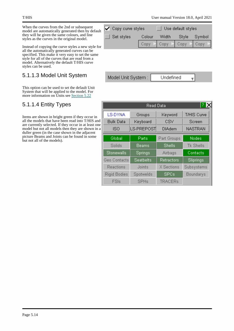
When the curves from the 2nd or subsequent model are automatically generated then by default they will be given the same colours, and line styles as the curves in the original model.
Instead of copying the curve styles a new style for all the automatically generated curves can be specified. This make it very easy to set the same style for all of the curves that are read from a model. Alternatively the default T/HIS curve styles can be used.
5.1.1.3 Model Unit System
This option can be used to set the default Unit System that will be applied to the model. For more information on Units see Section 5.22
5.1.1.4 Entity Types
Items are shown in bright green if they occur in all the models that have been read into T/HIS and are currently selected. If they occur in at least one model but not all models then they are shown in a duller green (in the case shown in the adjacent picture Beams and Joints can be found in some but not all of the models).
T/HIS User manual Version 18.0, April 2021
Page 5.14
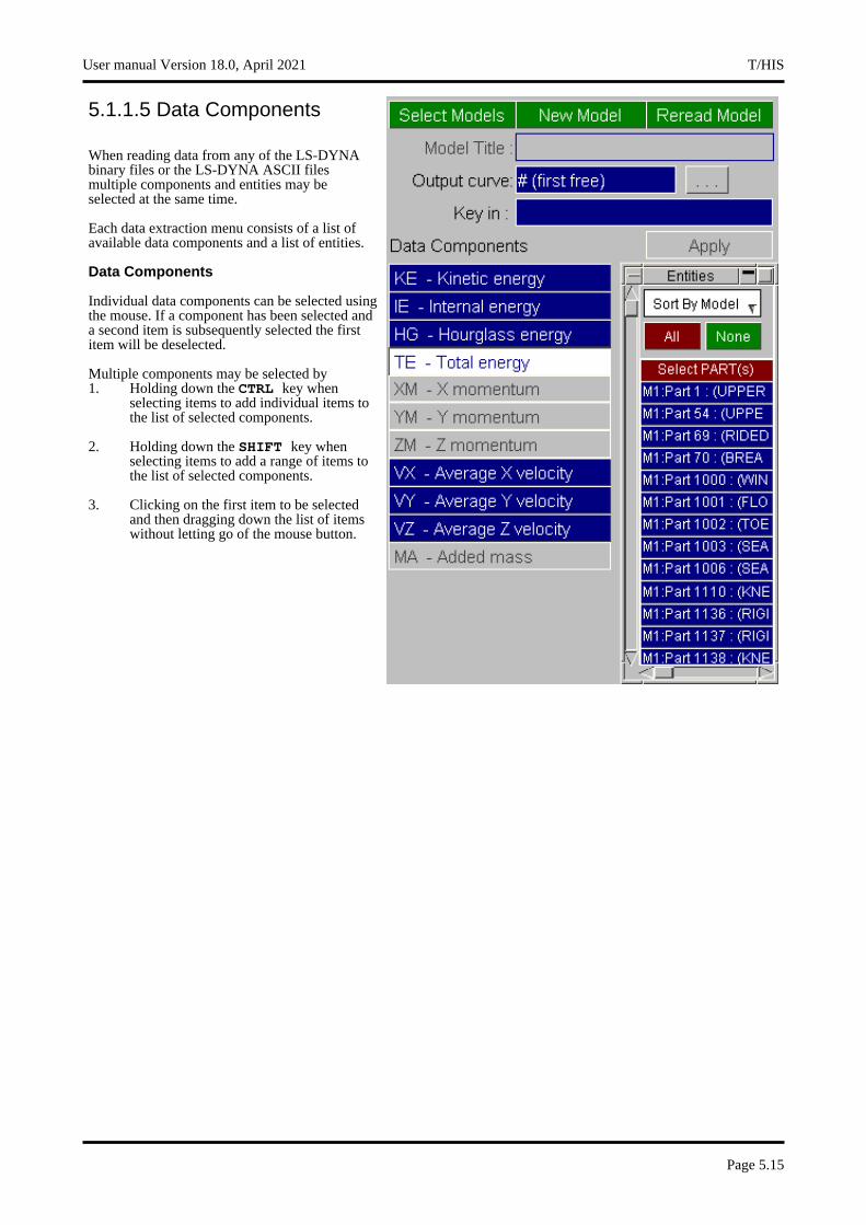
5.1.1.5 Data Components
When reading data from any of the LS-DYNA binary files or the LS-DYNA ASCII files multiple components and entities may be selected at the same time.
Each data extraction menu consists of a list of available data components and a list of entities.
Data Components
Individual data components can be selected using the mouse. If a component has been selected and a second item is subsequently selected the first item will be deselected.
Multiple components may be selected by 1. Holding down the CTRL key when
selecting items to add individual items to the list of selected components.
2. Holding down the SHIFT key when selecting items to add a range of items to the list of selected components.
3. Clicking on the first item to be selected and then dragging down the list of items without letting go of the mouse button.
User manual Version 18.0, April 2021 T/HIS
Page 5.15
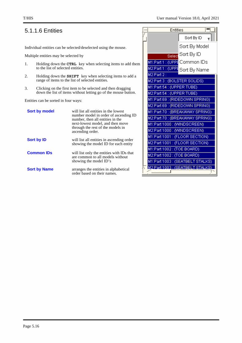
5.1.1.6 Entities
Individual entities can be selected/deselected using the mouse.
Multiple entities may be selected by
1. Holding down the CTRL key when selecting items to add them to the list of selected entities.
2. Holding down the SHIFT key when selecting items to add a range of items to the list of selected entities.
3. Clicking on the first item to be selected and then dragging down the list of items without letting go of the mouse button.
Entities can be sorted in four ways:
Sort by model will list all entities in the lowest number model in order of ascending ID number, then all entities in the next-lowest model, and then move through the rest of the models in ascending order.
Sort by ID will list all entities in ascending order showing the model ID for each entity
Common IDs will list only the entities with IDs that are common to all models without showing the model ID’s
Sort by Name arranges the entities in alphabetical order based on their names.
T/HIS User manual Version 18.0, April 2021
Page 5.16
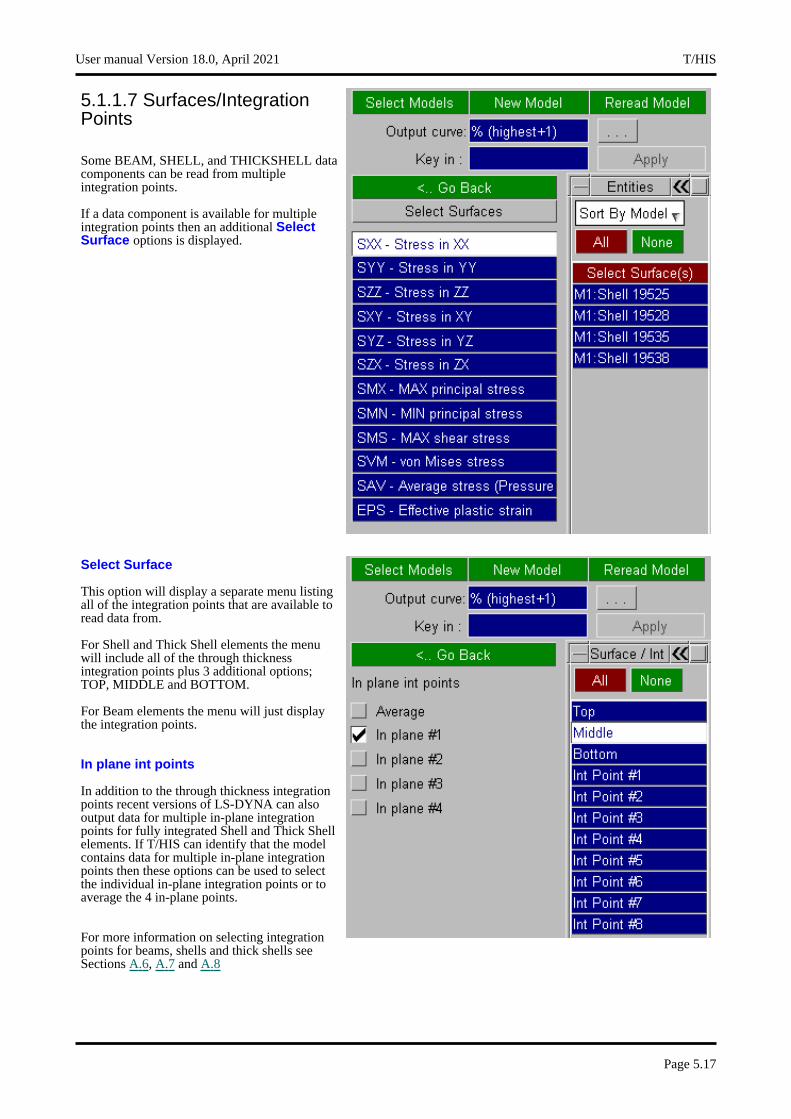
5.1.1.7 Surfaces/Integration Points
Some BEAM, SHELL, and THICKSHELL data components can be read from multiple integration points.
If a data component is available for multiple integration points then an additional Select Surface options is displayed.
Select Surface
This option will display a separate menu listing all of the integration points that are available to read data from.
For Shell and Thick Shell elements the menu will include all of the through thickness integration points plus 3 additional options; TOP, MIDDLE and BOTTOM.
For Beam elements the menu will just display the integration points.
In plane int points
In addition to the through thickness integration points recent versions of LS-DYNA can also output data for multiple in-plane integration points for fully integrated Shell and Thick Shell elements. If T/HIS can identify that the model contains data for multiple in-plane integration points then these options can be used to select the individual in-plane integration points or to average the 4 in-plane points.
For more information on selecting integration points for beams, shells and thick shells see Sections A.6, A.7 and A.8
User manual Version 18.0, April 2021 T/HIS
Page 5.17
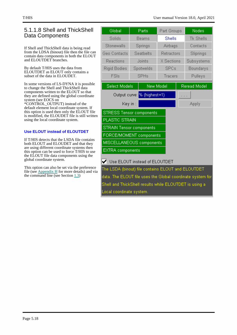
5.1.1.8 Shell and ThickShell Data Components
If Shell and ThickShell data is being read from the LDSA (binout) file then the file can contain data components in both the ELOUT and ELOUTDET branches.
By default T/HIS uses the data from ELOUTDET as ELOUT only contains a subset of the data in ELOUDET.
In some versions of LS-DYNA it is possible to change the Shell and ThickShell data components written to the ELOUT so that they are defined using the global coordinate system (see EOCS on *CONTROL_OUTPUT) instead of the default element local coordinate system. If this option is used then only the ELOUT file is modified, the ELOUDET file is still written using the local coordinate system.
Use ELOUT instead of ELOUTDET
If T/HIS detects that the LSDA file contains both ELOUT and ELOUDET and that they are using different coordinate systems then this option can be used to force T/HIS to use the ELOUT file data components using the global coordinate system.
This option can also be set via the preference file (see Appendix H for more details) and via the command line (see Section 1.3)
T/HIS User manual Version 18.0, April 2021
Page 5.18
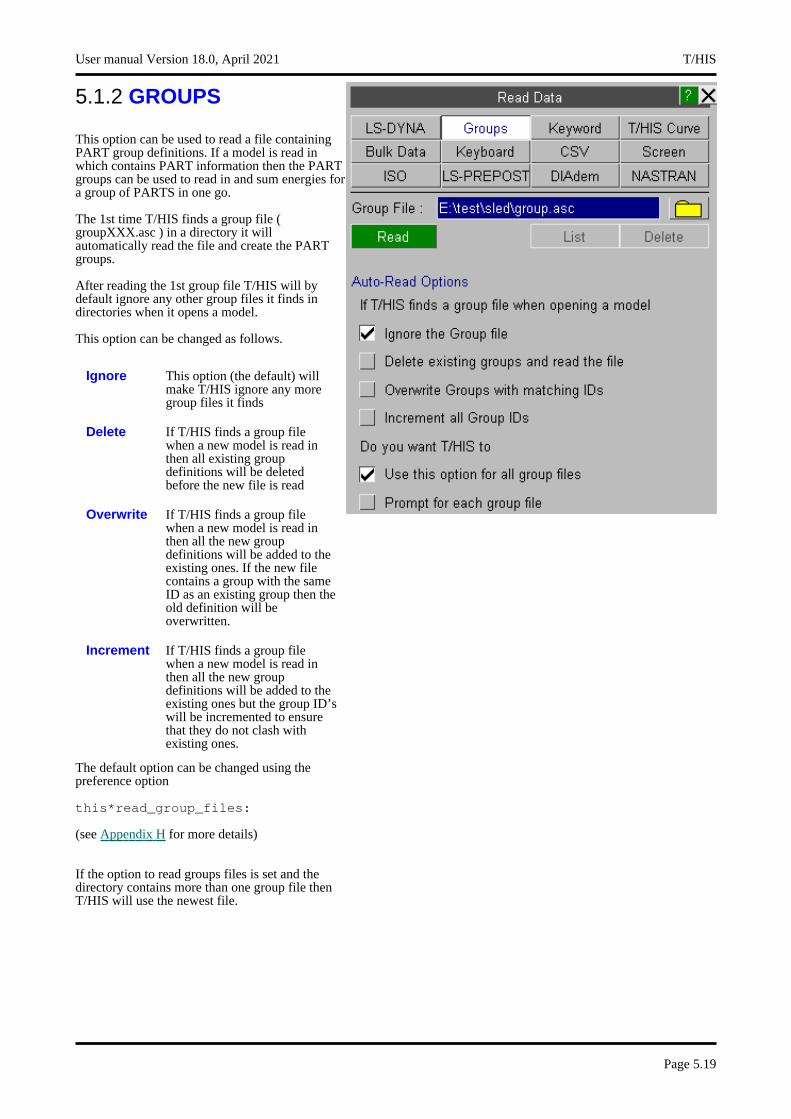
5.1.2 GROUPS
This option can be used to read a file containing PART group definitions. If a model is read in which contains PART information then the PART groups can be used to read in and sum energies for a group of PARTS in one go.
The 1st time T/HIS finds a group file ( groupXXX.asc ) in a directory it will automatically read the file and create the PART groups.
After reading the 1st group file T/HIS will by default ignore any other group files it finds in directories when it opens a model.
This option can be changed as follows.
Ignore This option (the default) will make T/HIS ignore any more group files it finds
Delete If T/HIS finds a group file when a new model is read in then all existing group definitions will be deleted before the new file is read
Overwrite If T/HIS finds a group file when a new model is read in then all the new group definitions will be added to the existing ones. If the new file contains a group with the same ID as an existing group then the old definition will be overwritten.
Increment If T/HIS finds a group file when a new model is read in then all the new group definitions will be added to the existing ones but the group ID’s will be incremented to ensure that they do not clash with existing ones.
The default option can be changed using the preference option
this*read_group_files:
(see Appendix H for more details)
If the option to read groups files is set and the directory contains more than one group file then T/HIS will use the newest file.
User manual Version 18.0, April 2021 T/HIS
Page 5.19
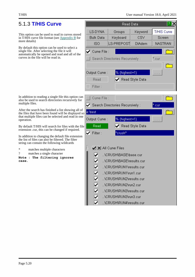
5.1.3 T/HIS Curve
This option can be used to read in curves stored in T/HIS curve file format (see Appendix B for more details)
By default this option can be used to select a single file. After selecting the file it will automatically be opened and read and all of the curves in the file will be read in.
In addition to reading a single file this option can also be used to search directories recursively for multiple files.
After the search has finished a list showing all of the files that have been found will be displayed so that multiple files can be selected and read in one operation.
By default T/HIS will search for files with the file extension .cur, this can be changed if required.
In addition to changing the default file extension the list of files can also be filtered. The filter string can contain the following wildcards
* matches multiple characters? matches a single characterNote : The filtering ignores case.
T/HIS User manual Version 18.0, April 2021
Page 5.20
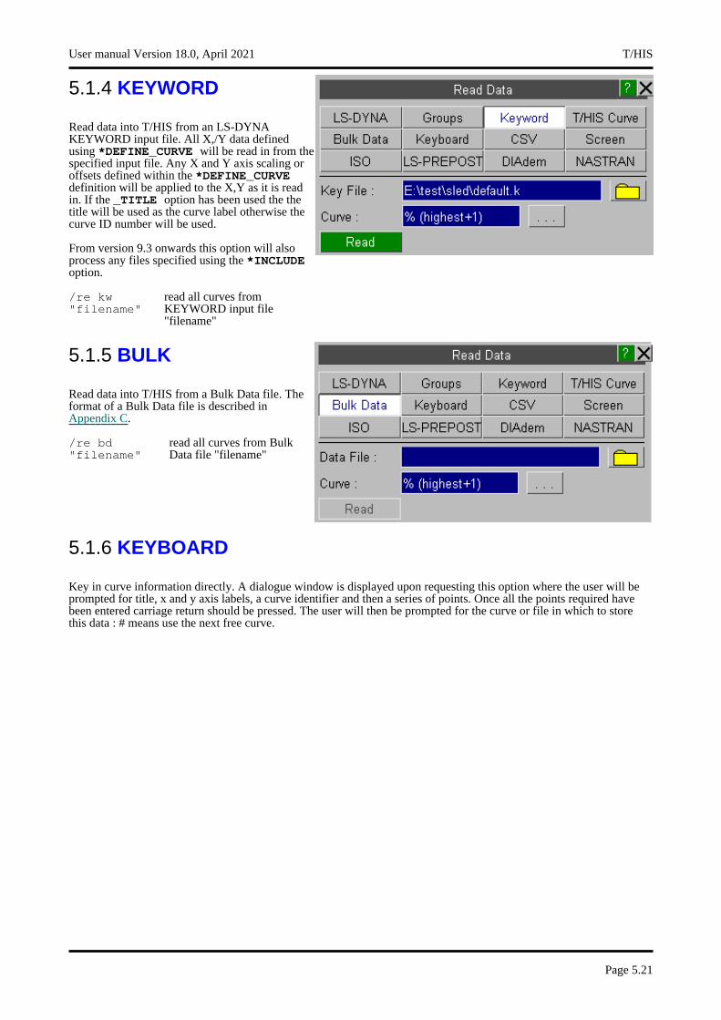
5.1.4 KEYWORD
Read data into T/HIS from an LS-DYNA KEYWORD input file. All X,/Y data defined using *DEFINE_CURVE will be read in from the specified input file. Any X and Y axis scaling or offsets defined within the *DEFINE_CURVE definition will be applied to the X,Y as it is read in. If the _TITLE option has been used the the title will be used as the curve label otherwise the curve ID number will be used.
From version 9.3 onwards this option will also process any files specified using the *INCLUDE option.
/re kw "filename"
read all curves from KEYWORD input file "filename"
5.1.5 BULK
Read data into T/HIS from a Bulk Data file. The format of a Bulk Data file is described in Appendix C.
/re bd "filename"
read all curves from Bulk Data file "filename"
5.1.6 KEYBOARD
Key in curve information directly. A dialogue window is displayed upon requesting this option where the user will be prompted for title, x and y axis labels, a curve identifier and then a series of points. Once all the points required have been entered carriage return should be pressed. The user will then be prompted for the curve or file in which to store this data : # means use the next free curve.
User manual Version 18.0, April 2021 T/HIS
Page 5.21

5.1.7 CSV
The CSV menu (see right) can be used to read comma separated variable file(s) into T/HIS. This menu allows to read single csv file or all the csv files in a selected directory both recursively and non-recursively.
Each file may contain up to 1000 columns of data (separated by commas).
The maximum line length supported by this option is 10240 characters.
CSV files written from the D3PLOT Write Menu are automatically detected by T/HIS and sets the appropriate read options. The options can be changed, but the data may not read in as expected. Both the Write->Entity and Write->Scan formats are supported. The first column of data containing the entity IDs is ignored for both formats. For files written from the Write->Scan menu the third column is ignored as this also contains entity IDs.
The CSV menu can also read in multiple CSV files in a given directory and also all the sub-directories recursively by changing the Open option from CSV File to either CSV Directory or CSV Directory (Recursive).
T/HIS User manual Version 18.0, April 2021
Page 5.22
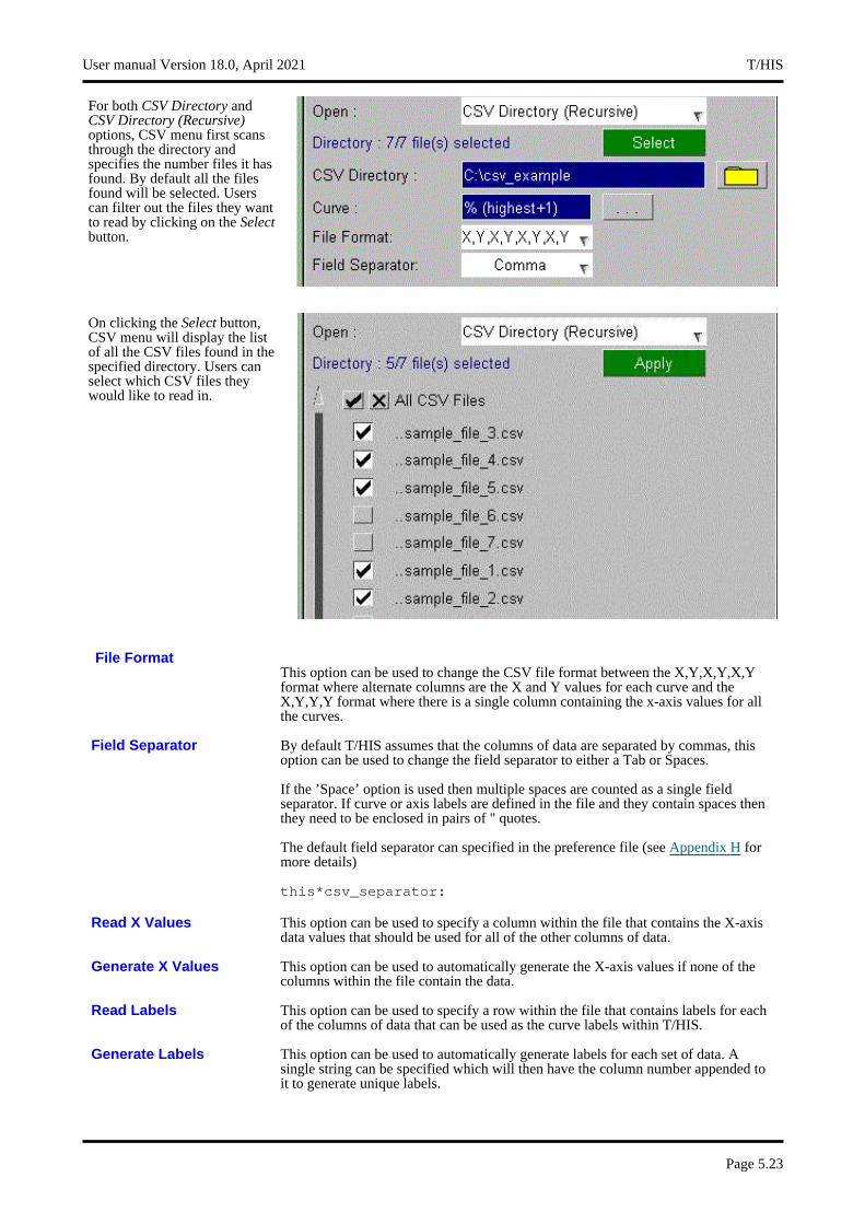
For both CSV Directory and CSV Directory (Recursive) options, CSV menu first scans through the directory and specifies the number files it has found. By default all the files found will be selected. Users can filter out the files they want to read by clicking on the Select button.
On clicking the Select button, CSV menu will display the list of all the CSV files found in the specified directory. Users can select which CSV files they would like to read in.
File FormatThis option can be used to change the CSV file format between the X,Y,X,Y,X,Y format where alternate columns are the X and Y values for each curve and the X,Y,Y,Y format where there is a single column containing the x-axis values for all the curves.
Field Separator By default T/HIS assumes that the columns of data are separated by commas, this option can be used to change the field separator to either a Tab or Spaces.
If the ’Space’ option is used then multiple spaces are counted as a single field separator. If curve or axis labels are defined in the file and they contain spaces then they need to be enclosed in pairs of " quotes.
The default field separator can specified in the preference file (see Appendix H for more details)
this*csv_separator:
Read X Values This option can be used to specify a column within the file that contains the X-axis data values that should be used for all of the other columns of data.
Generate X Values This option can be used to automatically generate the X-axis values if none of the columns within the file contain the data.
Read Labels This option can be used to specify a row within the file that contains labels for each of the columns of data that can be used as the curve labels within T/HIS.
Generate Labels This option can be used to automatically generate labels for each set of data. A single string can be specified which will then have the column number appended to it to generate unique labels.
User manual Version 18.0, April 2021 T/HIS
Page 5.23
Read Axis Labels This option can be used to specify a row within the file that contains the axis labels.
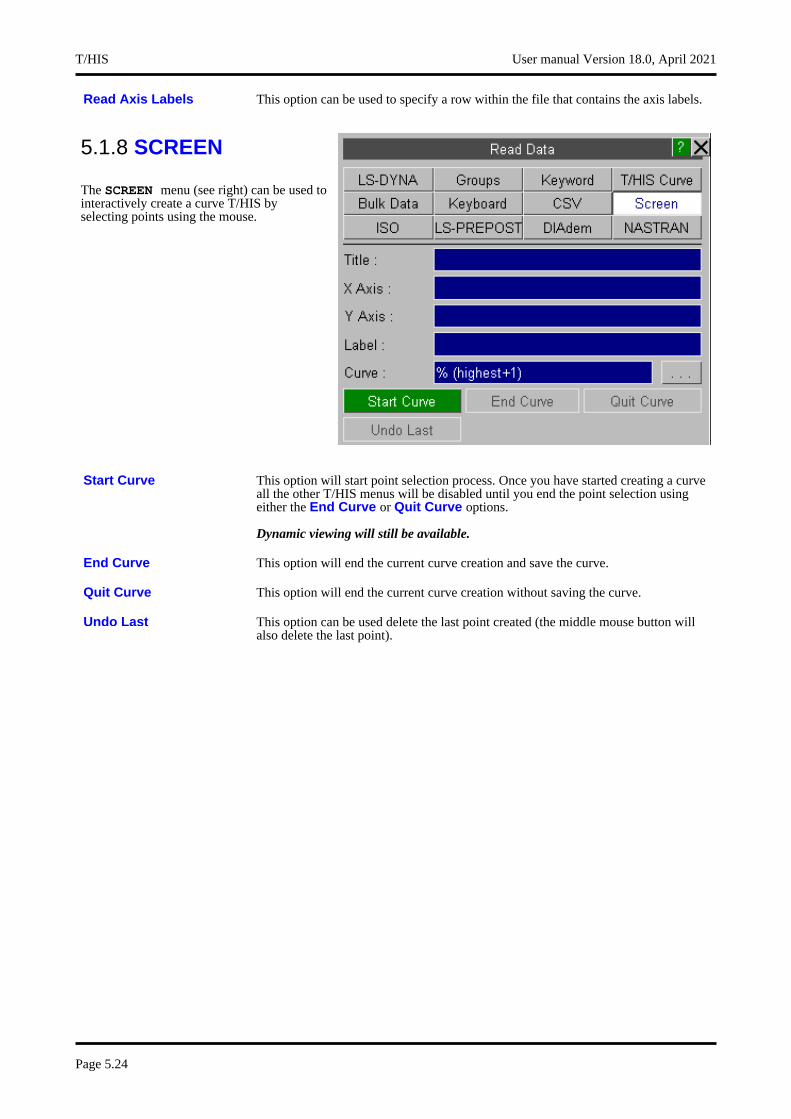
5.1.8 SCREEN
The SCREEN menu (see right) can be used to interactively create a curve T/HIS by selecting points using the mouse.
Start Curve This option will start point selection process. Once you have started creating a curve all the other T/HIS menus will be disabled until you end the point selection using either the End Curve or Quit Curve options.
Dynamic viewing will still be available.
End Curve This option will end the current curve creation and save the curve.
Quit Curve This option will end the current curve creation without saving the curve.
Undo Last This option can be used delete the last point created (the middle mouse button will also delete the last point).
T/HIS User manual Version 18.0, April 2021
Page 5.24
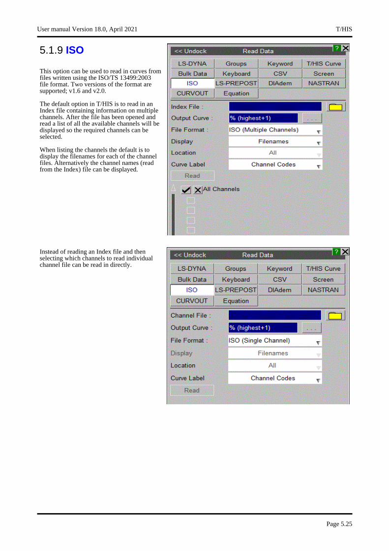
5.1.9 ISO
This option can be used to read in curves from files written using the ISO/TS 13499:2003 file format. Two versions of the format are supported; v1.6 and v2.0.
The default option in T/HIS is to read in an Index file containing information on multiple channels. After the file has been opened and read a list of all the available channels will be displayed so the required channels can be selected.
When listing the channels the default is to display the filenames for each of the channel files. Alternatively the channel names (read from the Index) file can be displayed.
Instead of reading an Index file and then selecting which channels to read individual channel file can be read in directly.
User manual Version 18.0, April 2021 T/HIS
Page 5.25
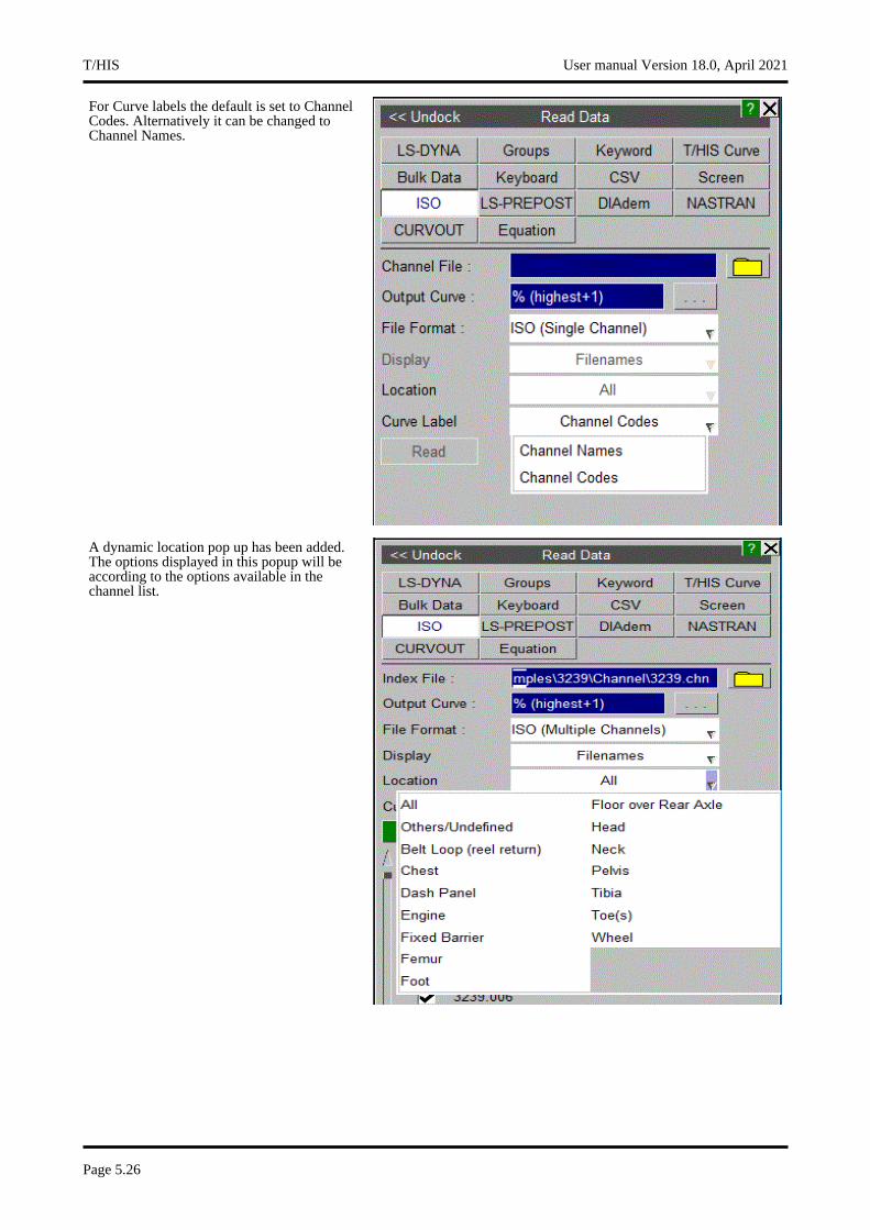
For Curve labels the default is set to Channel Codes. Alternatively it can be changed to Channel Names.
A dynamic location pop up has been added. The options displayed in this popup will be according to the options available in the channel list.
T/HIS User manual Version 18.0, April 2021
Page 5.26
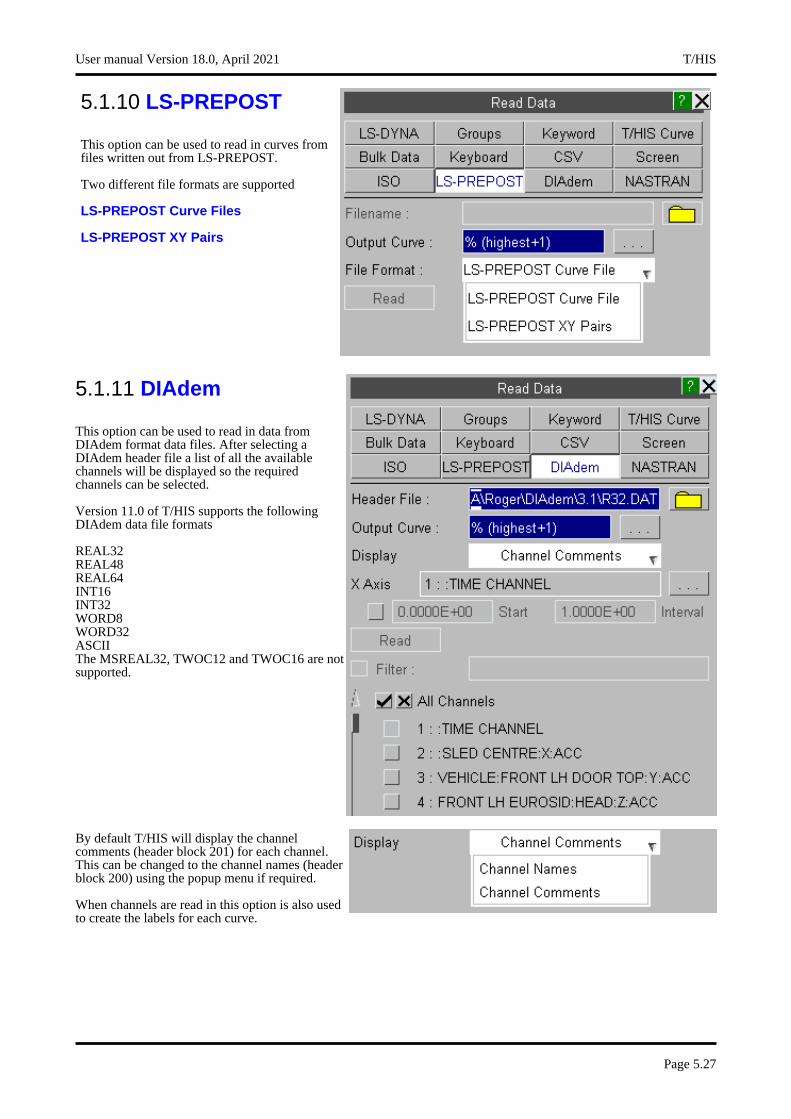
5.1.10 LS-PREPOST
This option can be used to read in curves from files written out from LS-PREPOST.
Two different file formats are supported
LS-PREPOST Curve Files
LS-PREPOST XY Pairs
5.1.11 DIAdem
This option can be used to read in data from DIAdem format data files. After selecting a DIAdem header file a list of all the available channels will be displayed so the required channels can be selected.
Version 11.0 of T/HIS supports the following DIAdem data file formats
REAL32REAL48REAL64INT16INT32WORD8WORD32ASCIIThe MSREAL32, TWOC12 and TWOC16 are not supported.
By default T/HIS will display the channel comments (header block 201) for each channel. This can be changed to the channel names (header block 200) using the popup menu if required.
When channels are read in this option is also used to create the labels for each curve.
User manual Version 18.0, April 2021 T/HIS
Page 5.27
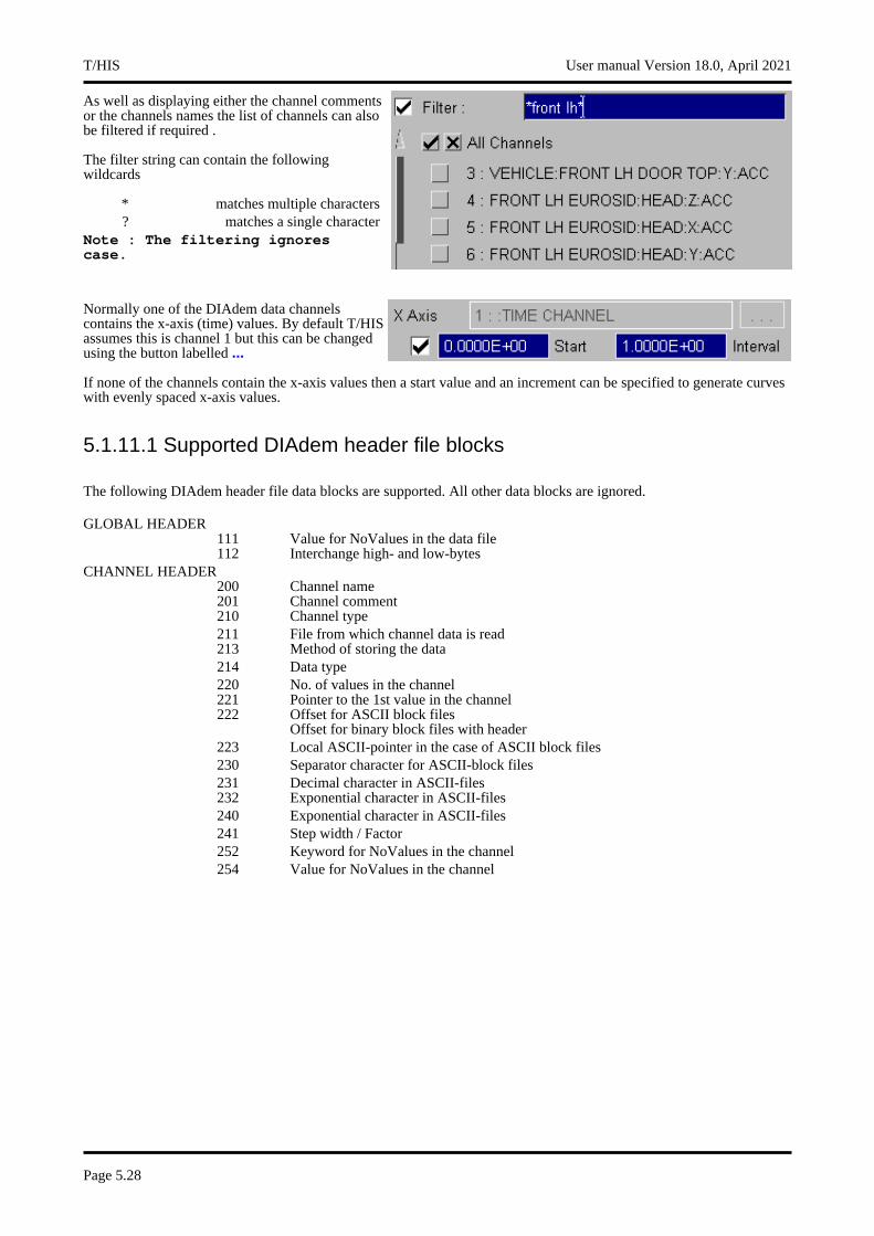
As well as displaying either the channel comments or the channels names the list of channels can also be filtered if required .
The filter string can contain the following wildcards
* matches multiple characters? matches a single character
Note : The filtering ignores case.
Normally one of the DIAdem data channels contains the x-axis (time) values. By default T/HIS assumes this is channel 1 but this can be changed using the button labelled ...
If none of the channels contain the x-axis values then a start value and an increment can be specified to generate curves with evenly spaced x-axis values.
5.1.11.1 Supported DIAdem header file blocks
The following DIAdem header file data blocks are supported. All other data blocks are ignored.
GLOBAL HEADER111 Value for NoValues in the data file112 Interchange high- and low-bytes
CHANNEL HEADER200 Channel name201 Channel comment210 Channel type211 File from which channel data is read213 Method of storing the data214 Data type220 No. of values in the channel221 Pointer to the 1st value in the channel222 Offset for ASCII block files
Offset for binary block files with header223 Local ASCII-pointer in the case of ASCII block files230 Separator character for ASCII-block files231 Decimal character in ASCII-files232 Exponential character in ASCII-files240 Exponential character in ASCII-files241 Step width / Factor252 Keyword for NoValues in the channel254 Value for NoValues in the channel
T/HIS User manual Version 18.0, April 2021
Page 5.28
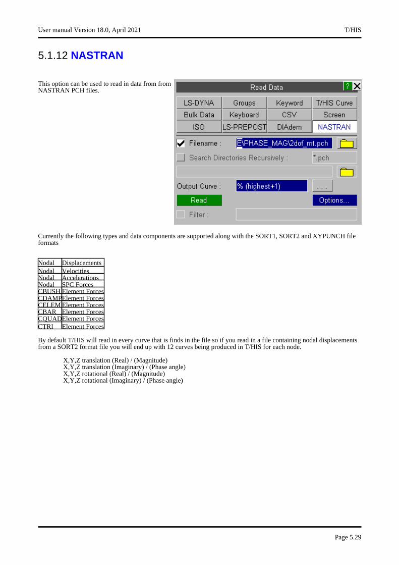
5.1.12 NASTRAN
This option can be used to read in data from from NASTRAN PCH files.
Currently the following types and data components are supported along with the SORT1, SORT2 and XYPUNCH file formats
Nodal DisplacementsNodal VelocitiesNodal AccelerationsNodal SPC ForcesCBUSH Element ForcesCDAMPElement ForcesCELEM Element ForcesCBAR Element ForcesCQUADElement ForcesCTRI Element Forces
By default T/HIS will read in every curve that is finds in the file so if you read in a file containing nodal displacements from a SORT2 format file you will end up with 12 curves being produced in T/HIS for each node.
X,Y,Z translation (Real) / (Magnitude)X,Y,Z translation (Imaginary) / (Phase angle)X,Y,Z rotational (Real) / (Magnitude)X,Y,Z rotational (Imaginary) / (Phase angle)
User manual Version 18.0, April 2021 T/HIS
Page 5.29
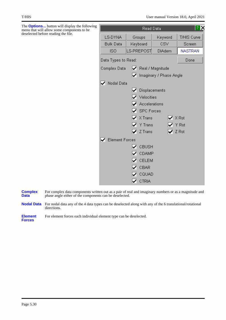
The Options... button will display the following menu that will allow some components to be deselected before reading the file.
Complex Data
For complex data components written out as a pair of real and imaginary numbers or as a magnitude and phase angle either of the components can be deselected.
Nodal Data For nodal data any of the 4 data types can be deselected along with any of the 6 translational/rotational directions.
Element Forces
For element forces each individual element type can be deselected.
T/HIS User manual Version 18.0, April 2021
Page 5.30
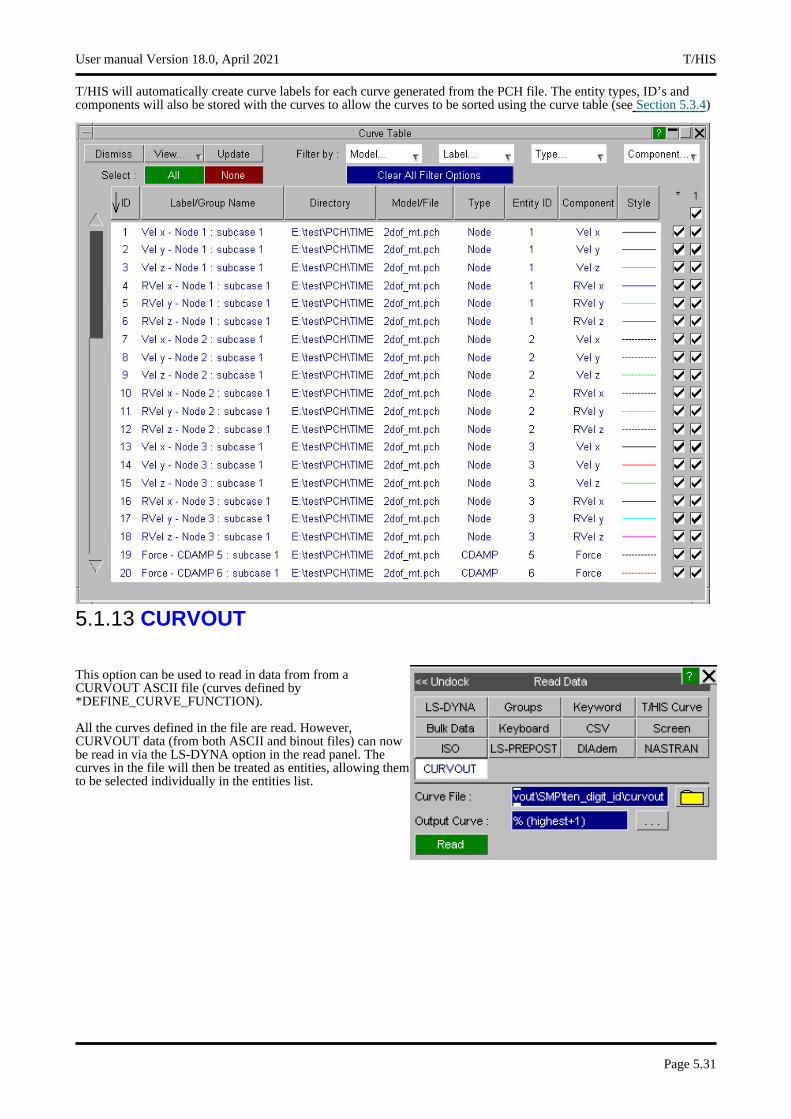
T/HIS will automatically create curve labels for each curve generated from the PCH file. The entity types, ID’s and components will also be stored with the curves to allow the curves to be sorted using the curve table (see Section 5.3.4)
5.1.13 CURVOUT
This option can be used to read in data from from a CURVOUT ASCII file (curves defined by *DEFINE_CURVE_FUNCTION).
All the curves defined in the file are read. However, CURVOUT data (from both ASCII and binout files) can now be read in via the LS-DYNA option in the read panel. The curves in the file will then be treated as entities, allowing them to be selected individually in the entities list.
User manual Version 18.0, April 2021 T/HIS
Page 5.31
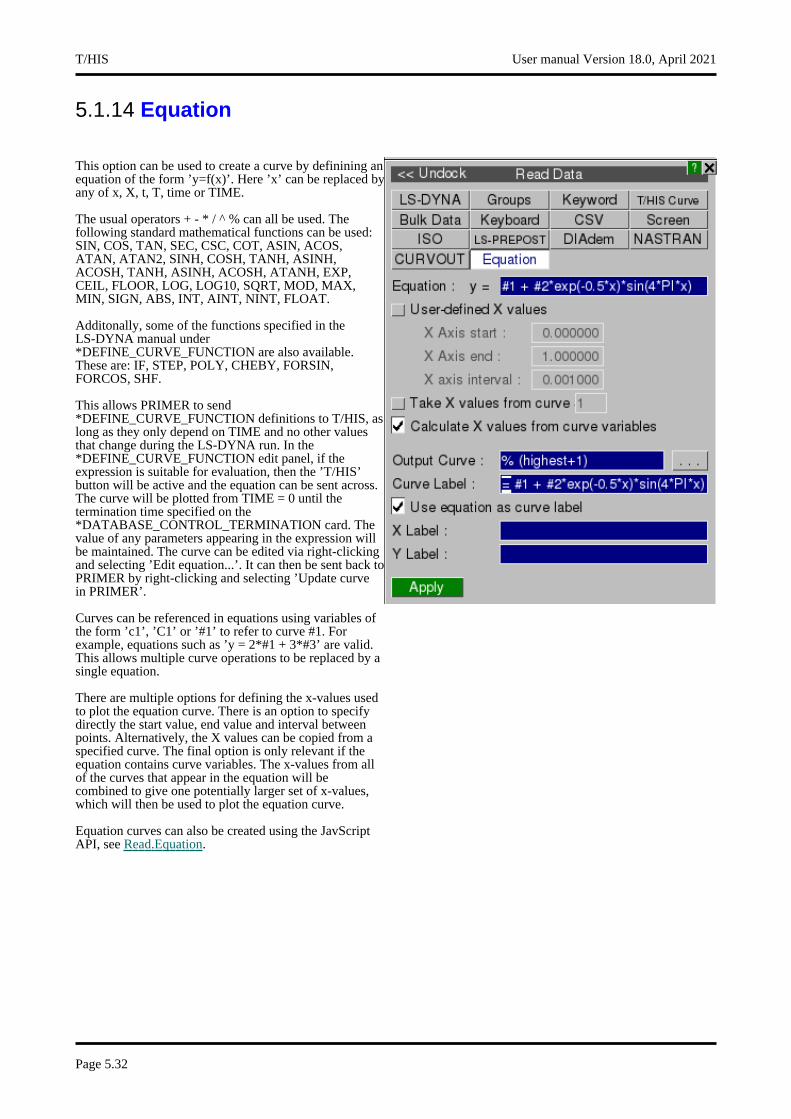
5.1.14 Equation
This option can be used to create a curve by definining an equation of the form ’y=f(x)’. Here ’x’ can be replaced by any of x, X, t, T, time or TIME.
The usual operators + - * / ^ % can all be used. The following standard mathematical functions can be used: SIN, COS, TAN, SEC, CSC, COT, ASIN, ACOS, ATAN, ATAN2, SINH, COSH, TANH, ASINH, ACOSH, TANH, ASINH, ACOSH, ATANH, EXP, CEIL, FLOOR, LOG, LOG10, SQRT, MOD, MAX, MIN, SIGN, ABS, INT, AINT, NINT, FLOAT.
Additonally, some of the functions specified in the LS-DYNA manual under *DEFINE_CURVE_FUNCTION are also available. These are: IF, STEP, POLY, CHEBY, FORSIN, FORCOS, SHF.
This allows PRIMER to send *DEFINE_CURVE_FUNCTION definitions to T/HIS, as long as they only depend on TIME and no other values that change during the LS-DYNA run. In the *DEFINE_CURVE_FUNCTION edit panel, if the expression is suitable for evaluation, then the ’T/HIS’ button will be active and the equation can be sent across. The curve will be plotted from TIME = 0 until the termination time specified on the *DATABASE_CONTROL_TERMINATION card. The value of any parameters appearing in the expression will be maintained. The curve can be edited via right-clicking and selecting ’Edit equation...’. It can then be sent back to PRIMER by right-clicking and selecting ’Update curve in PRIMER’.
Curves can be referenced in equations using variables of the form ’c1’, ’C1’ or ’#1’ to refer to curve #1. For example, equations such as ’y = 2*#1 + 3*#3’ are valid. This allows multiple curve operations to be replaced by a single equation.
There are multiple options for defining the x-values used to plot the equation curve. There is an option to specify directly the start value, end value and interval between points. Alternatively, the X values can be copied from a specified curve. The final option is only relevant if the equation contains curve variables. The x-values from all of the curves that appear in the equation will be combined to give one potentially larger set of x-values, which will then be used to plot the equation curve.
Equation curves can also be created using the JavScript API, see Read.Equation.
T/HIS User manual Version 18.0, April 2021
Page 5.32
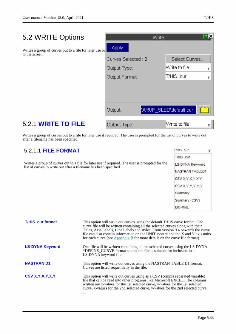
5.2 WRITE Options
Writes a group of curves out to a file for later use or to the screen.
5.2.1 WRITE TO FILE
Writes a group of curves out to a file for later use if required. The user is prompted for the list of curves to write out after a filename has been specified.
5.2.1.1 FILE FORMAT
Writes a group of curves out to a file for later use if required. The user is prompted for the list of curves to write out after a filename has been specified.
T/HIS .cur format This option will write out curves using the default T/HIS curve format. One curve file will be written containing all the selected curves along with their Titles, Axis Labels, Line Labels and styles. From version 9.4 onwards the curve file can also contain information on the UNIT system and the X and Y axis units for each curve (see Appendix B for more details on the curve file format)
LS-DYNA Keyword One file will be written containing all the selected curves using the LS-DYNA *DEFINE_CURVE format so that the file is suitable for inclusion in a LS-DYNA keyword file.
NASTRAN D1 This option will write out curves using the NASTRAN TABLE D1 format. Curves are listed sequentially in the file.
CSV X,Y,X,Y,X,Y This option will write out curves using as a CSV (comma separated variable) file that can be read into other programs like Microsoft EXCEL. The columns written are x-values for the 1st selected curve, y-values for the 1st selected curve, x-values for the 2nd selected curve, y-values for the 2nd selected curve ...
User manual Version 18.0, April 2021 T/HIS
Page 5.33
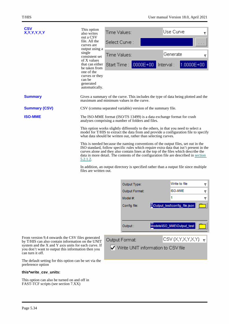
CSV X,Y,Y,Y,Y,Y
This option also writes out a CSV file. All the curves are output using a single consistent set of X values that can either be taken from one of the curves or they can be generated automatically.
Summary Gives a summary of the curve. This includes the type of data being plotted and the maximum and minimum values in the curve.
Summary (CSV) CSV (comma separated variable) version of the summary file.
ISO-MME The ISO-MME format (ISO/TS 13499) is a data exchange format for crash analyses comprising a number of folders and files.
This option works slightly differently to the others, in that you need to select a model for T/HIS to extract the data from and provide a configuration file to specify what data should be written out, rather than selecting curves.
This is needed because the naming conventions of the output files, set out in the ISO standard, follow specific rules which require extra data that isn’t present in the curves alone and they also contain lines at the top of the files which describe the data in more detail. The contents of the configuration file are described in section5.2.1.2.
In addition, an output directory is specified rather than a output file since multiple files are written out.
From version 9.4 onwards the CSV files generated by T/HIS can also contain information on the UNIT system and the X and Y axis units for each curve. If you don’t want to output this information then you can turn it off.
The default setting for this option can be set via the preference option
this*write_csv_units:
This option can also be turned on and off in FAST-TCF scripts (see section 7.XX)
T/HIS User manual Version 18.0, April 2021
Page 5.34
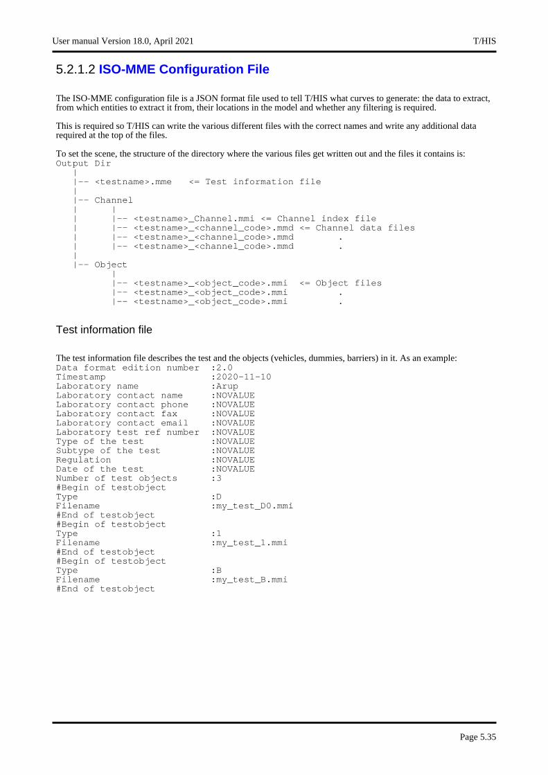
5.2.1.2 ISO-MME Configuration File
The ISO-MME configuration file is a JSON format file used to tell T/HIS what curves to generate: the data to extract, from which entities to extract it from, their locations in the model and whether any filtering is required.
This is required so T/HIS can write the various different files with the correct names and write any additional data required at the top of the files.
To set the scene, the structure of the directory where the various files get written out and the files it contains is: Output Dir
||-- <testname>.mme <= Test information file||-- Channel| || |-- <testname>_Channel.mmi <= Channel index file| |-- <testname>_<channel_code>.mmd <= Channel data files| |-- <testname>_<channel_code>.mmd .| |-- <testname>_<channel_code>.mmd .||-- Object
||-- <testname>_<object_code>.mmi <= Object files|-- <testname>_<object_code>.mmi .|-- <testname>_<object_code>.mmi .
Test information file
The test information file describes the test and the objects (vehicles, dummies, barriers) in it. As an example: Data format edition number :2.0Timestamp :2020-11-10Laboratory name :ArupLaboratory contact name :NOVALUELaboratory contact phone :NOVALUELaboratory contact fax :NOVALUELaboratory contact email :NOVALUELaboratory test ref number :NOVALUEType of the test :NOVALUESubtype of the test :NOVALUERegulation :NOVALUEDate of the test :NOVALUENumber of test objects :3#Begin of testobjectType :DFilename :my_test_D0.mmi#End of testobject#Begin of testobjectType :1Filename :my_test_1.mmi#End of testobject#Begin of testobjectType :BFilename :my_test_B.mmi#End of testobject
User manual Version 18.0, April 2021 T/HIS
Page 5.35

Object files
The object files describe each object in the test, for example: Name :H350Velocity :NOVALUEMass :NOVALUEImpact side :00#Begin of biomechanicalGender :maleAge :21#End of biomechanical
Channel index file
The channel index file lists the channel data files: Number of channels :3Data origin :SData source :simulation#Begin of channelExtended channel code :D0HEADMI0000000B#End of channel#Begin of channelExtended channel code :D0CHSTMI0000000C#End of channel#Begin of channelExtended channel code :D0PELVMI0000000C#End of channel
Channel data files
The channel data files contain the time series data: Data structure :ChannelInstrumentation standard :NOVALUEName of the channel :Accel x - Node 52503304 : (PelvisAccel_INJURY) (Reg 0.100E-03) (C 180)Data source :simulationData status :okCut off frequency :NOVALUEChannel amplitude class :NOVALUESampling interval :0.0001Bit resolution :NOVALUETime of first sample :0Number of samples :1500Reference channel :implicit#Start of data-6.09125e-05-1785.28-3315.55
.
.#End of data
Configuration file
Below is an example configuration file, showing all the available options that can be set. Not all of them are required, the list below shows which ones are optional and what they can be set to.
T/HIS User manual Version 18.0, April 2021
Page 5.36
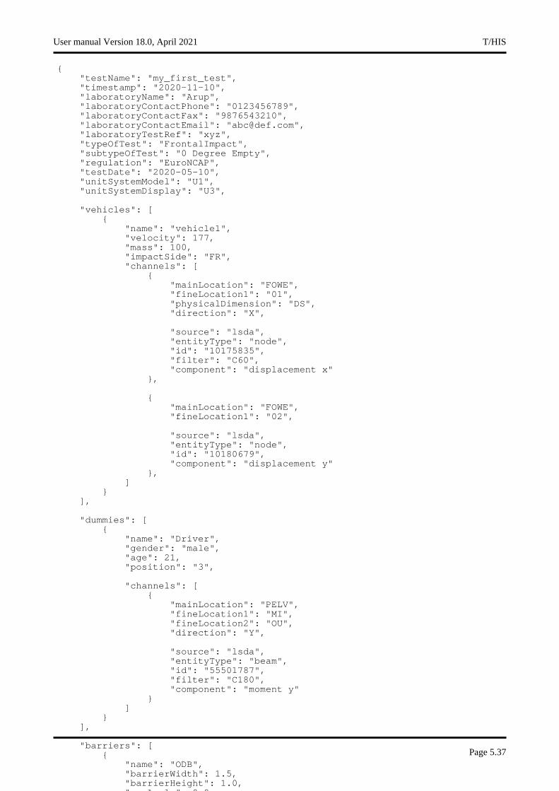
{"testName": "my_first_test","timestamp": "2020-11-10","laboratoryName": "Arup", "laboratoryContactPhone": "0123456789", "laboratoryContactFax": "9876543210", "laboratoryContactEmail": "[email protected]", "laboratoryTestRef": "xyz", "typeOfTest": "FrontalImpact","subtypeOfTest": "0 Degree Empty","regulation": "EuroNCAP","testDate": "2020-05-10","unitSystemModel": "U1","unitSystemDisplay": "U3",
"vehicles": [{
"name": "vehicle1","velocity": 177,"mass": 100,"impactSide": "FR","channels": [
{"mainLocation": "FOWE","fineLocation1": "01","physicalDimension": "DS","direction": "X",
"source": "lsda","entityType": "node","id": "10175835","filter": "C60","component": "displacement x"
},
{"mainLocation": "FOWE","fineLocation1": "02",
"source": "lsda","entityType": "node","id": "10180679","component": "displacement y"
},]
}],
"dummies": [{
"name": "Driver","gender": "male","age": 21,"position": "3",
"channels": [{
"mainLocation": "PELV","fineLocation1": "MI","fineLocation2": "OU","direction": "Y",
"source": "lsda","entityType": "beam","id": "55501787","filter": "C180","component": "moment y"
}]
}],
"barriers": [{
"name": "ODB","barrierWidth": 1.5,"barrierHeight": 1.0,"yawAngle": 0.0,
User manual Version 18.0, April 2021 T/HIS
Page 5.37
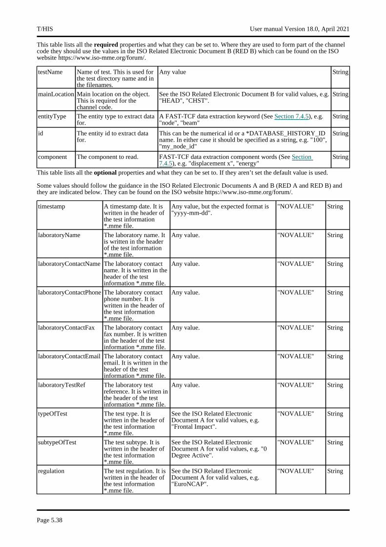
This table lists all the required properties and what they can be set to. Where they are used to form part of the channel code they should use the values in the ISO Related Electronic Document B (RED B) which can be found on the ISO website https://www.iso-mme.org/forum/.
testName Name of test. This is used for the test directory name and in the filenames.
Any value String
mainLocation Main location on the object. This is required for the channel code.
See the ISO Related Electronic Document B for valid values, e.g. "HEAD", "CHST".
String
entityType The entity type to extract data for.
A FAST-TCF data extraction keyword (See Section 7.4.5), e.g. "node", "beam"
String
id The entity id to extract data for.
This can be the numerical id or a *DATABASE_HISTORY_ID name. In either case it should be specified as a string, e.g. "100", "my_node_id"
String
component The component to read. FAST-TCF data extraction component words (See Section7.4.5), e.g. "displacement x", "energy"
String
This table lists all the optional properties and what they can be set to. If they aren’t set the default value is used.
Some values should follow the guidance in the ISO Related Electronic Documents A and B (RED A and RED B) and they are indicated below. They can be found on the ISO website https://www.iso-mme.org/forum/.
timestamp A timestamp date. It is written in the header of the test information *.mme file.
Any value, but the expected format is "yyyy-mm-dd".
"NOVALUE" String
laboratoryName The laboratory name. It is written in the header of the test information *.mme file.
Any value. "NOVALUE" String
laboratoryContactName The laboratory contact name. It is written in the header of the test information *.mme file.
Any value. "NOVALUE" String
laboratoryContactPhone The laboratory contact phone number. It is written in the header of the test information *.mme file.
Any value. "NOVALUE" String
laboratoryContactFax The laboratory contact fax number. It is written in the header of the test information *.mme file.
Any value. "NOVALUE" String
laboratoryContactEmail The laboratory contact email. It is written in the header of the test information *.mme file.
Any value. "NOVALUE" String
laboratoryTestRef The laboratory test reference. It is written in the header of the test information *.mme file.
Any value. "NOVALUE" String
typeOfTest The test type. It is written in the header of the test information *.mme file.
See the ISO Related Electronic Document A for valid values, e.g. "Frontal Impact".
"NOVALUE" String
subtypeOfTest The test subtype. It is written in the header of the test information *.mme file.
See the ISO Related Electronic Document A for valid values, e.g. "0 Degree Active".
"NOVALUE" String
regulation The test regulation. It is written in the header of the test information *.mme file.
See the ISO Related Electronic Document A for valid values, e.g. "EuroNCAP".
"NOVALUE" String
T/HIS User manual Version 18.0, April 2021
Page 5.38
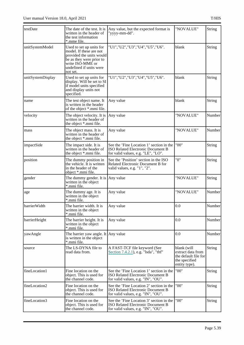
testDate The date of the test. It is written in the header of the test information *.mme file.
Any value, but the expected format is "yyyy-mm-dd".
"NOVALUE" String
unitSystemModel Used to set up units for model. If these are not provided the units would be as they were prior to write ISO-MME or undefined if units were not set.
"U1","U2","U3","U4","U5","U6". blank String
unitSystemDisplay Used to set up units for display. Will be set to SI if model units specified and display units not specified.
"U1","U2","U3","U4","U5","U6". blank String
name The test object name. It is written in the header of the object *.mmi file.
Any value blank String
velocity The object velocity. It is written in the header of the object *.mmi file.
Any value "NOVALUE" Number
mass The object mass. It is written in the header of the object *.mmi file.
Any value "NOVALUE" Number
impactSide The impact side. It is written in the header of the object *.mmi file.
See the ’Fine Location 1’ section in the ISO Related Electronic Document B for valid values, e.g. "LE", "LO".
"00" String
position The dummy position in the vehicle. It is written in the header of the object *.mmi file.
See the ’Position’ section in the ISO Related Electronic Document B for valid values, e.g. "1", "2".
"0" String
gender The dummy gender. It is written in the object *.mmi file.
Any value "NOVALUE" String
age The dummy age. It is written in the object *.mmi file.
Any value "NOVALUE" Number
barrierWidth The barrier width. It is written in the object *.mmi file.
Any value 0.0 Number
barrierHeight The barrier height. It is written in the object *.mmi file.
Any value 0.0 Number
yawAngle The barrier yaw angle. It is written in the object *.mmi file.
Any value 0.0 Number
source The LS-DYNA file to read data from.
A FAST-TCF file keyword (See Section 7.4.2.1), e.g. "lsda", "thf"
blank (will extract data from the default file for the specified entity type).
String
fineLocation1 Fine location on the object. This is used for the channel code.
See the ’Fine Location 1’ section in the ISO Related Electronic Document B for valid values, e.g. "IN", "OU".
"00" String
fineLocation2 Fine location on the object. This is used for the channel code.
See the ’Fine Location 2’ section in the ISO Related Electronic Document B for valid values, e.g. "IN", "OU".
"00" String
fineLocation3 Fine location on the object. This is used for the channel code.
See the ’Fine Location 3’ section in the ISO Related Electronic Document B for valid values, e.g. "IN", "OU".
"00" String
User manual Version 18.0, April 2021 T/HIS
Page 5.39
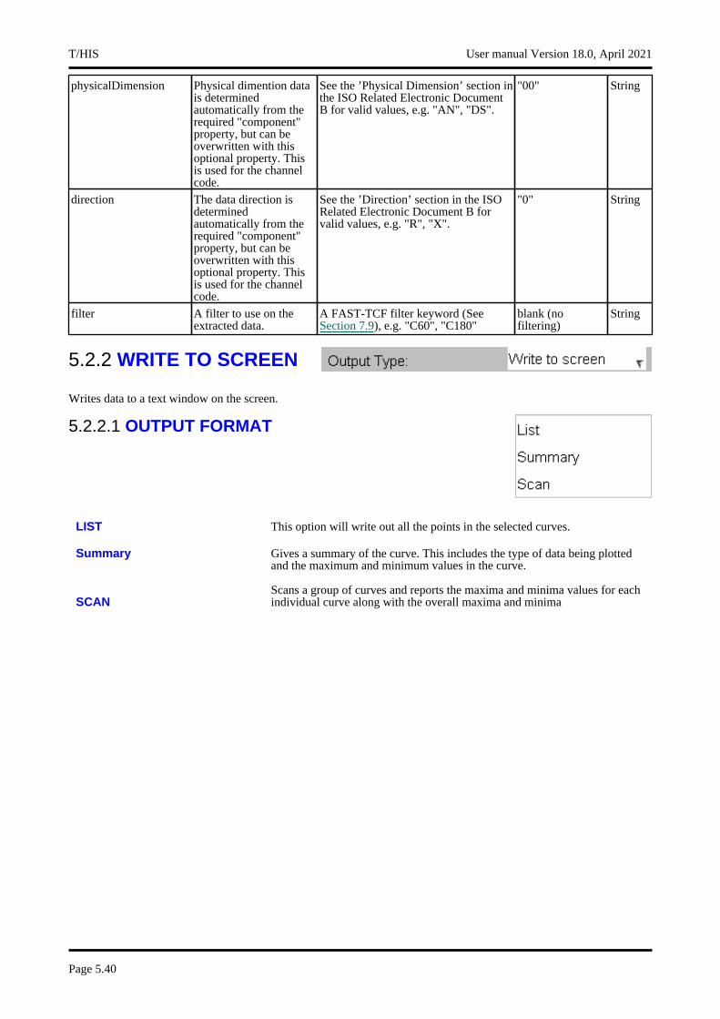
physicalDimension Physical dimention data is determined automatically from the required "component" property, but can be overwritten with this optional property. This is used for the channel code.
See the ’Physical Dimension’ section in the ISO Related Electronic Document B for valid values, e.g. "AN", "DS".
"00" String
direction The data direction is determined automatically from the required "component" property, but can be overwritten with this optional property. This is used for the channel code.
See the ’Direction’ section in the ISO Related Electronic Document B for valid values, e.g. "R", "X".
"0" String
filter A filter to use on the extracted data.
A FAST-TCF filter keyword (See Section 7.9), e.g. "C60", "C180"
blank (no filtering)
String
5.2.2 WRITE TO SCREEN
Writes data to a text window on the screen.
5.2.2.1 OUTPUT FORMAT
LIST This option will write out all the points in the selected curves.
Summary Gives a summary of the curve. This includes the type of data being plotted and the maximum and minimum values in the curve.
SCANScans a group of curves and reports the maxima and minima values for each individual curve along with the overall maxima and minima
T/HIS User manual Version 18.0, April 2021
Page 5.40
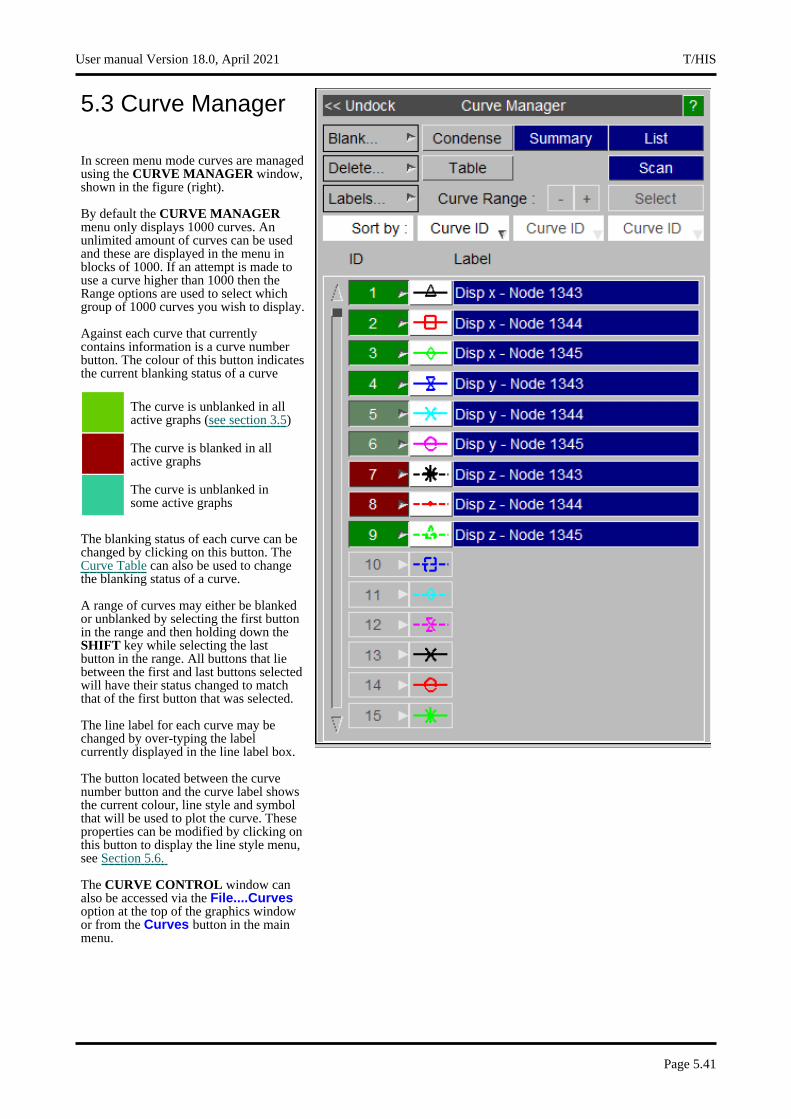
5.3 Curve Manager
In screen menu mode curves are managed using the CURVE MANAGER window, shown in the figure (right).
By default the CURVE MANAGER menu only displays 1000 curves. An unlimited amount of curves can be used and these are displayed in the menu in blocks of 1000. If an attempt is made to use a curve higher than 1000 then the Range options are used to select which group of 1000 curves you wish to display.
Against each curve that currently contains information is a curve number button. The colour of this button indicates the current blanking status of a curve
fffffff The curve is unblanked in all active graphs (see section 3.5)
The curve is blanked in all active graphs
The curve is unblanked in some active graphs
The blanking status of each curve can be changed by clicking on this button. The Curve Table can also be used to change the blanking status of a curve.
A range of curves may either be blanked or unblanked by selecting the first button in the range and then holding down the SHIFT key while selecting the last button in the range. All buttons that lie between the first and last buttons selected will have their status changed to match that of the first button that was selected.
The line label for each curve may be changed by over-typing the label currently displayed in the line label box.
The button located between the curve number button and the curve label shows the current colour, line style and symbol that will be used to plot the curve. These properties can be modified by clicking on this button to display the line style menu, see Section 5.6.
The CURVE CONTROL window can also be accessed via the File....Curves option at the top of the graphics window or from the Curves button in the main menu.
User manual Version 18.0, April 2021 T/HIS
Page 5.41
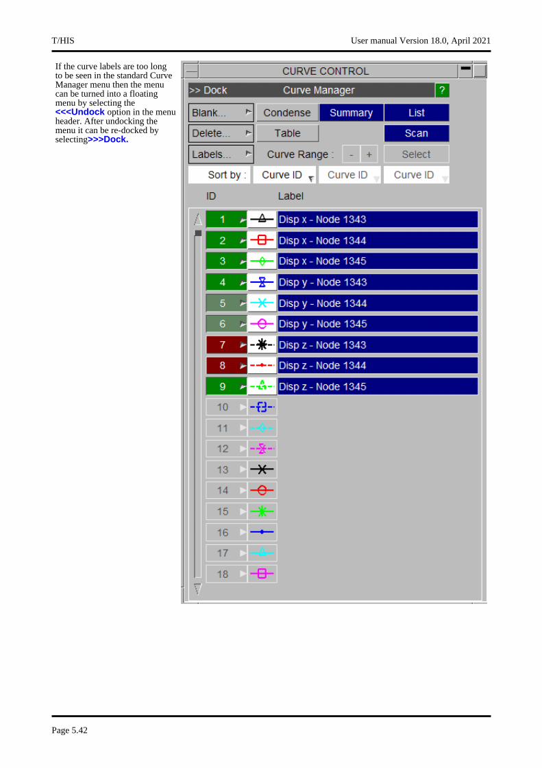
If the curve labels are too long to be seen in the standard Curve Manager menu then the menu can be turned into a floating menu by selecting the <<<Undock option in the menu header. After undocking the menu it can be re-docked by selecting>>>Dock.
T/HIS User manual Version 18.0, April 2021
Page 5.42
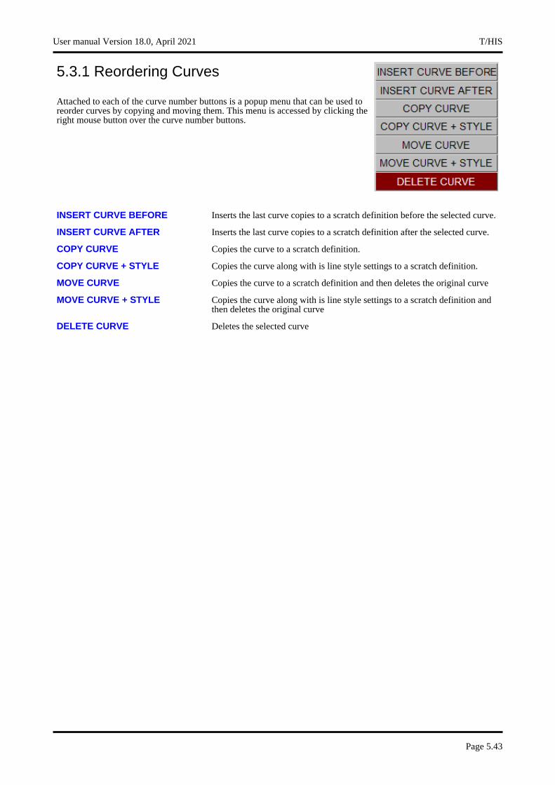
5.3.1 Reordering Curves
Attached to each of the curve number buttons is a popup menu that can be used to reorder curves by copying and moving them. This menu is accessed by clicking the right mouse button over the curve number buttons.
INSERT CURVE BEFORE Inserts the last curve copies to a scratch definition before the selected curve.
INSERT CURVE AFTER Inserts the last curve copies to a scratch definition after the selected curve.
COPY CURVE Copies the curve to a scratch definition.
COPY CURVE + STYLE Copies the curve along with is line style settings to a scratch definition.
MOVE CURVE Copies the curve to a scratch definition and then deletes the original curve
MOVE CURVE + STYLE Copies the curve along with is line style settings to a scratch definition and then deletes the original curve
DELETE CURVE Deletes the selected curve
User manual Version 18.0, April 2021 T/HIS
Page 5.43
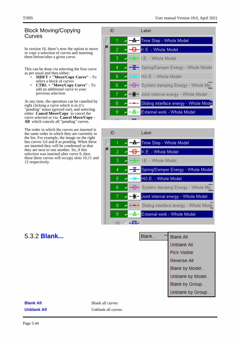
Block Moving/Copying Curves
In version 16, there’s now the option to move or copy a selection of curves and inserting them before/after a given curve.
This can be done via selecting the first curve as per usual and then either:
• SHIFT + "Move/Copy Curve" - To select a block of curves
• CTRL + "Move/Copy Curve" - To add an additional curve to your previous selection
At any time, the operation can be canelled by right clicking a curve which is in it’s "pending" status (greyed out), and selecting either Cancel Move/Copy to cancel the curve selected or via Cancel Move/Copy - All which cancels all "pending" curves.
The order in which the curves are inserted is the same order in which they are currently in the list. For example, the image on the right has curves 3,6 and 8 as pending. When these are inserted they will be condensed so that they are next to one another. So, if this selection was inserted after curve 9, then these three curves will occupy slots 10,11 and 12 respectively.
5.3.2 Blank...
Blank All Blank all curves
Unblank All Unblank all curves
T/HIS User manual Version 18.0, April 2021
Page 5.44
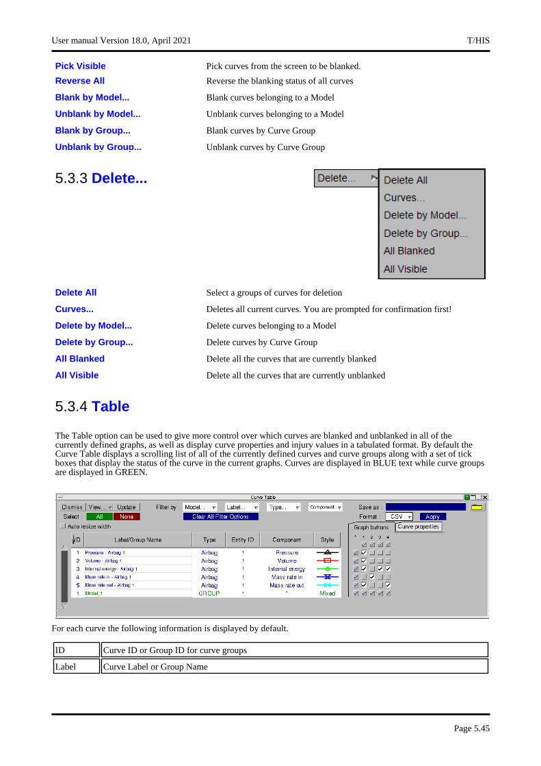
Pick Visible Pick curves from the screen to be blanked.
Reverse All Reverse the blanking status of all curves
Blank by Model... Blank curves belonging to a Model
Unblank by Model... Unblank curves belonging to a Model
Blank by Group... Blank curves by Curve Group
Unblank by Group... Unblank curves by Curve Group
5.3.3 Delete...
Delete All Select a groups of curves for deletion
Curves... Deletes all current curves. You are prompted for confirmation first!
Delete by Model... Delete curves belonging to a Model
Delete by Group... Delete curves by Curve Group
All Blanked Delete all the curves that are currently blanked
All Visible Delete all the curves that are currently unblanked
5.3.4 Table
The Table option can be used to give more control over which curves are blanked and unblanked in all of the currently defined graphs, as well as display curve properties and injury values in a tabulated format. By default the Curve Table displays a scrolling list of all of the currently defined curves and curve groups along with a set of tick boxes that display the status of the curve in the current graphs. Curves are displayed in BLUE text while curve groups are displayed in GREEN.
For each curve the following information is displayed by default.
ID Curve ID or Group ID for curve groups
Label Curve Label or Group Name
User manual Version 18.0, April 2021 T/HIS
Page 5.45
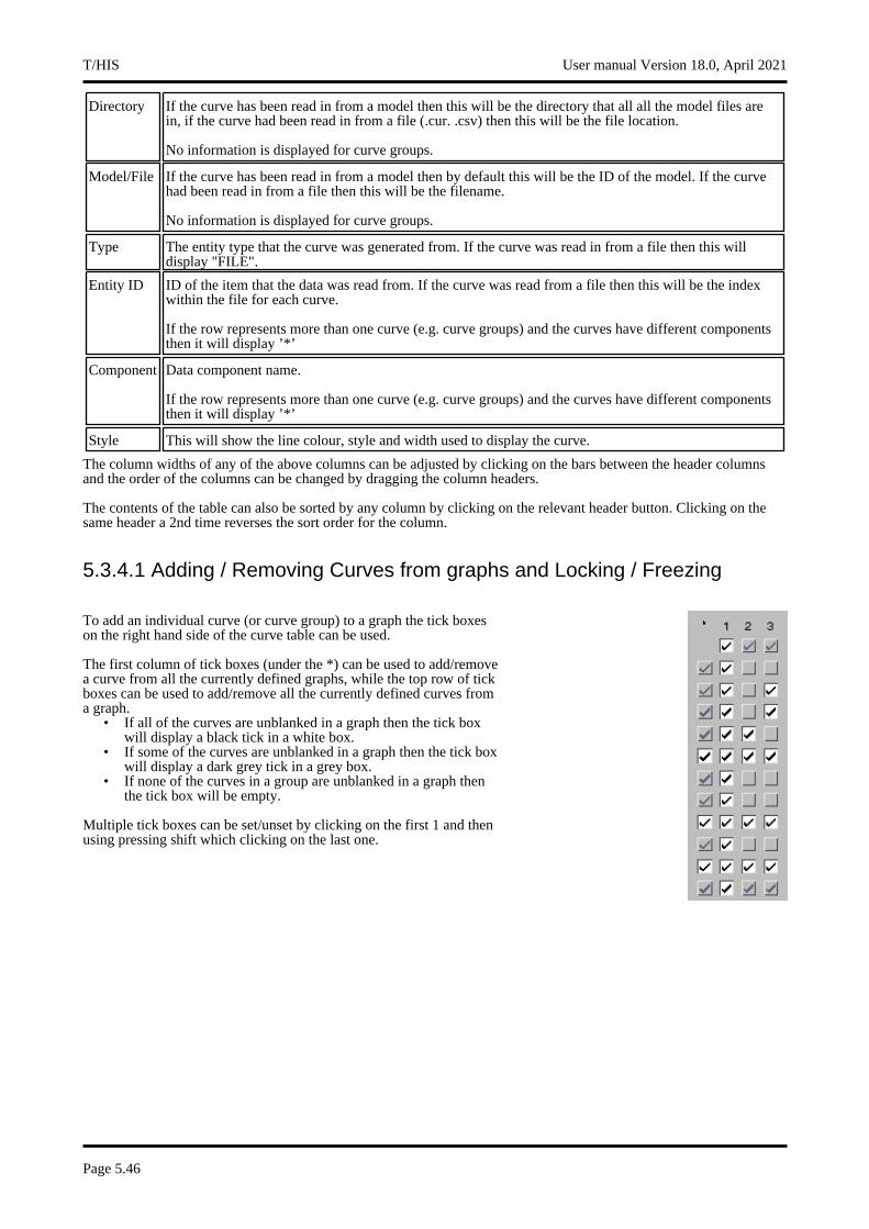
Directory If the curve has been read in from a model then this will be the directory that all all the model files are in, if the curve had been read in from a file (.cur. .csv) then this will be the file location.
No information is displayed for curve groups.
Model/File If the curve has been read in from a model then by default this will be the ID of the model. If the curve had been read in from a file then this will be the filename.
No information is displayed for curve groups.
Type The entity type that the curve was generated from. If the curve was read in from a file then this will display "FILE".
Entity ID ID of the item that the data was read from. If the curve was read from a file then this will be the index within the file for each curve.
If the row represents more than one curve (e.g. curve groups) and the curves have different components then it will display ’*’
Component Data component name.
If the row represents more than one curve (e.g. curve groups) and the curves have different components then it will display ’*’
Style This will show the line colour, style and width used to display the curve.
The column widths of any of the above columns can be adjusted by clicking on the bars between the header columns and the order of the columns can be changed by dragging the column headers.
The contents of the table can also be sorted by any column by clicking on the relevant header button. Clicking on the same header a 2nd time reverses the sort order for the column.
5.3.4.1 Adding / Removing Curves from graphs and Locking / Freezing
To add an individual curve (or curve group) to a graph the tick boxes on the right hand side of the curve table can be used.
The first column of tick boxes (under the *) can be used to add/remove a curve from all the currently defined graphs, while the top row of tick boxes can be used to add/remove all the currently defined curves from a graph.
• If all of the curves are unblanked in a graph then the tick box will display a black tick in a white box.
• If some of the curves are unblanked in a graph then the tick box will display a dark grey tick in a grey box.
• If none of the curves in a group are unblanked in a graph then the tick box will be empty.
Multiple tick boxes can be set/unset by clicking on the first 1 and then using pressing shift which clicking on the last one.
T/HIS User manual Version 18.0, April 2021
Page 5.46
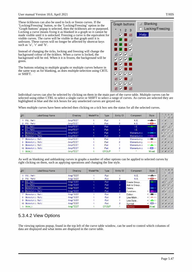
These tickboxes can also be used to lock or freeze curves. If the ’Locking/Freezing’ button, or the ’Locking/Freezing’ option in the ’Graph buttons’ popup is selected, then the tickboxes are re-purposed. Locking a curve means fixing it as blanked in a graph so it cannot be made visible until it is unlocked. Freezing a curve is the equivalent for visible curves. The curve will be visible in that graph until it is unfrozen. These curves will no longer be affected by shortcut keys such as ’u’, ’r’ and ’b’.
Instead of changing the ticks, locking and freezing will change the background colour of the tickbox. When a curve is locked, the background will be red. When it it is frozen, the background will be green.
The buttons relating to multiple graphs or multiple curves behave in the same way as for blanking, as does multiple-selection using CRTL or SHIFT.
Individual curves can also be selected by clicking on them in the main part of the curve table. Multiple curves can be selected using either CTRL to select a single curve or SHIFT to select a range of curves. As curves are selected they are highlighted in blue and the tick boxes for any unselected curves are greyed out.
When multiple curves have been selected then clicking on a tick box sets the status for all the selected curves.
As well as blanking and unblanking curves in graphs a number of other options can be applied to selected curves by right clicking on them, such as applying operations and changing the line style.
5.3.4.2 View Options
The viewing options popup, found in the top left of the curve table window, can be used to control which columns of data are displayed and what items are displayed in the curve table.
User manual Version 18.0, April 2021 T/HIS
Page 5.47

By default all 8 columns of general information about each curve will be displayed, each column can be turned on and off but T/HIS will ensure that at least one column is always displayed. Curve properties and injury values can also be displayed, but this will be discussed further in Section 5.3.4.4.
The columns that are initially displayed can be specified in the preference file (see Appendix H for more details). If the columns are changed then Save to Pref can be used to update the preference file.
Display
This option can be used to control how items are displayed in the curve table.
All Items
By default the curve table will contain one row for each curve and one row for each curve group.
T/HIS User manual Version 18.0, April 2021
Page 5.48
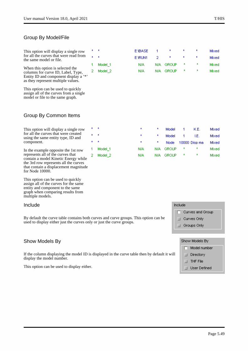
Group By Model/File
This option will display a single row for all the curves that were read from the same model or file.
When this option is selected the columns for curve ID, Label, Type, Entity ID and component display a ’*’ as they represent multiple values.
This option can be used to quickly assign all of the curves from a single model or file to the same graph.
Group By Common Items
This option will display a single row for all the curves that were created using the same entity type, ID and component.
In the example opposite the 1st row represents all of the curves that contain a model Kinetic Energy while the 3rd row represents all the curves that contain a displacement magnitude for Node 10000.
This option can be used to quickly assign all of the curves for the same entity and component to the same graph when comparing results from multiple models.
Include
By default the curve table contains both curves and curve groups. This option can be used to display either just the curves only or just the curve groups.
Show Models By
If the column displaying the model ID is displayed in the curve table then by default it will display the model number.
This option can be used to display either.
User manual Version 18.0, April 2021 T/HIS
Page 5.49
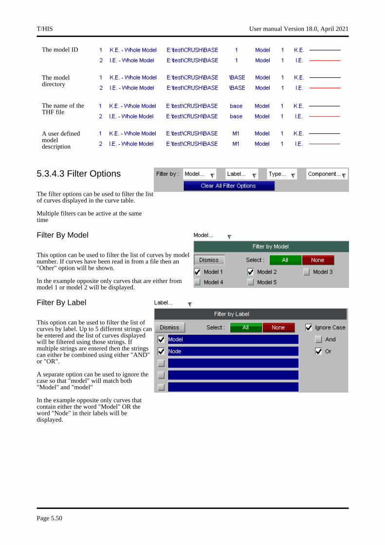
The model ID
The model directory
The name of the THF file
A user defined model description
5.3.4.3 Filter Options
The filter options can be used to filter the list of curves displayed in the curve table.
Multiple filters can be active at the same time
Filter By Model
This option can be used to filter the list of curves by model number. If curves have been read in from a file then an "Other" option will be shown.
In the example opposite only curves that are either from model 1 or model 2 will be displayed.
Filter By Label
This option can be used to filter the list of curves by label. Up to 5 different strings can be entered and the list of curves displayed will be filtered using those strings. If multiple strings are entered then the strings can either be combined using either "AND" or "OR".
A separate option can be used to ignore the case so that "model" will match both "Model" and "model"
In the example opposite only curves that contain either the word "Model" OR the word "Node" in their labels will be displayed.
T/HIS User manual Version 18.0, April 2021
Page 5.50
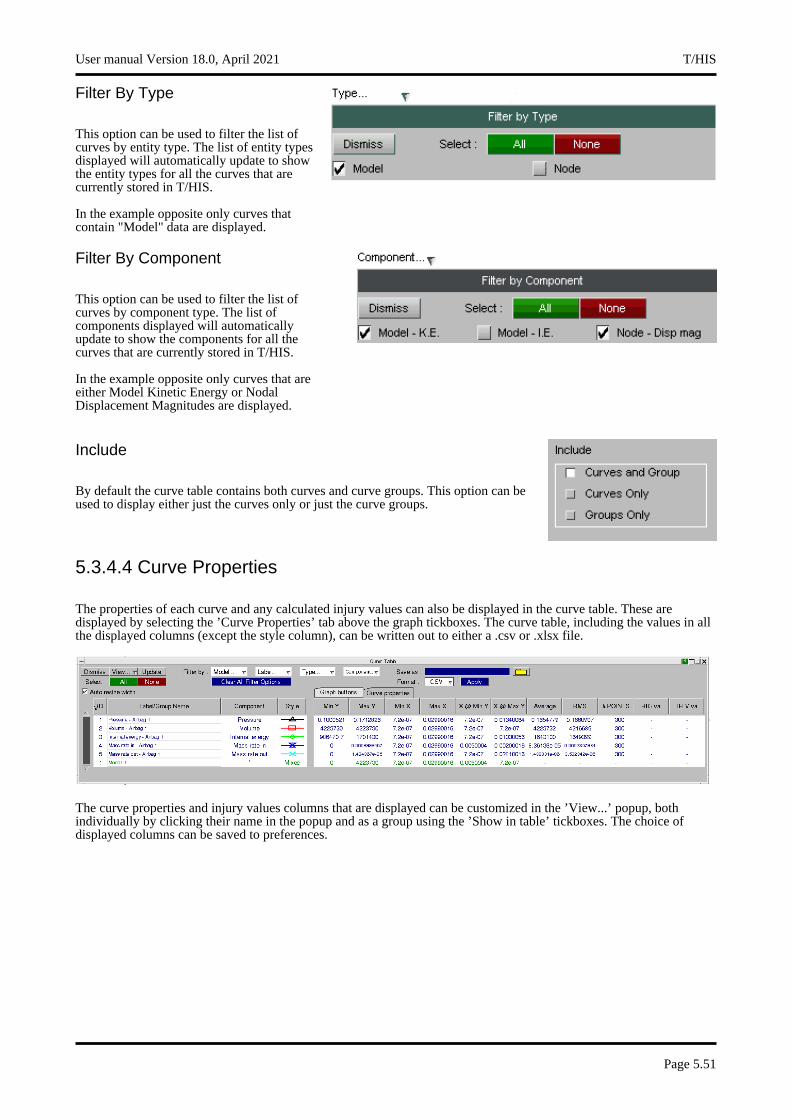
Filter By Type
This option can be used to filter the list of curves by entity type. The list of entity types displayed will automatically update to show the entity types for all the curves that are currently stored in T/HIS.
In the example opposite only curves that contain "Model" data are displayed.
Filter By Component
This option can be used to filter the list of curves by component type. The list of components displayed will automatically update to show the components for all the curves that are currently stored in T/HIS.
In the example opposite only curves that are either Model Kinetic Energy or Nodal Displacement Magnitudes are displayed.
Include
By default the curve table contains both curves and curve groups. This option can be used to display either just the curves only or just the curve groups.
5.3.4.4 Curve Properties
The properties of each curve and any calculated injury values can also be displayed in the curve table. These are displayed by selecting the ’Curve Properties’ tab above the graph tickboxes. The curve table, including the values in all the displayed columns (except the style column), can be written out to either a .csv or .xlsx file.
The curve properties and injury values columns that are displayed can be customized in the ’View...’ popup, both individually by clicking their name in the popup and as a group using the ’Show in table’ tickboxes. The choice of displayed columns can be saved to preferences.
User manual Version 18.0, April 2021 T/HIS
Page 5.51
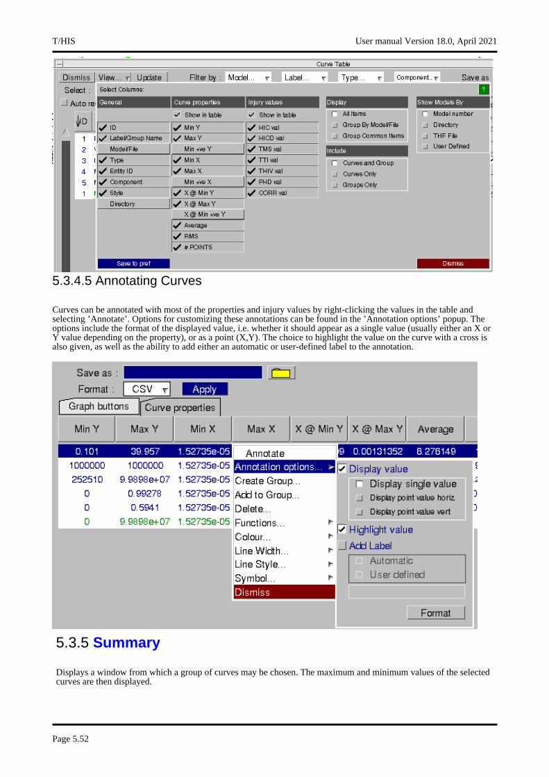
5.3.4.5 Annotating Curves
Curves can be annotated with most of the properties and injury values by right-clicking the values in the table and selecting ’Annotate’. Options for customizing these annotations can be found in the ’Annotation options’ popup. The options include the format of the displayed value, i.e. whether it should appear as a single value (usually either an X or Y value depending on the property), or as a point (X,Y). The choice to highlight the value on the curve with a cross is also given, as well as the ability to add either an automatic or user-defined label to the annotation.
5.3.5 Summary
Displays a window from which a group of curves may be chosen. The maximum and minimum values of the selected curves are then displayed.
T/HIS User manual Version 18.0, April 2021
Page 5.52
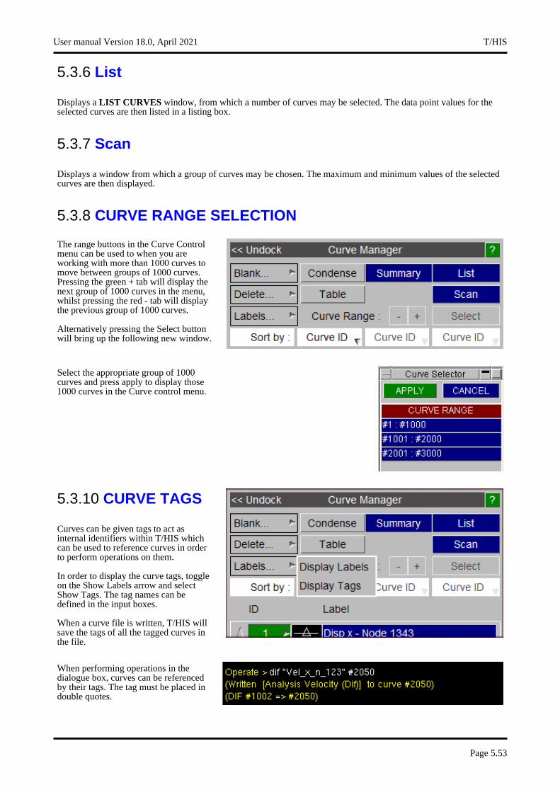
5.3.6 List
Displays a LIST CURVES window, from which a number of curves may be selected. The data point values for the selected curves are then listed in a listing box.
5.3.7 Scan
Displays a window from which a group of curves may be chosen. The maximum and minimum values of the selected curves are then displayed.
5.3.8 CURVE RANGE SELECTION
The range buttons in the Curve Control menu can be used to when you are working with more than 1000 curves to move between groups of 1000 curves. Pressing the green + tab will display the next group of 1000 curves in the menu, whilst pressing the red - tab will display the previous group of 1000 curves.
Alternatively pressing the Select button will bring up the following new window.
Select the appropriate group of 1000 curves and press apply to display those 1000 curves in the Curve control menu.
5.3.10 CURVE TAGS
Curves can be given tags to act as internal identifiers within T/HIS which can be used to reference curves in order to perform operations on them.
In order to display the curve tags, toggle on the Show Labels arrow and select Show Tags. The tag names can be defined in the input boxes.
When a curve file is written, T/HIS will save the tags of all the tagged curves in the file.
When performing operations in the dialogue box, curves can be referenced by their tags. The tag must be placed in double quotes.
User manual Version 18.0, April 2021 T/HIS
Page 5.53
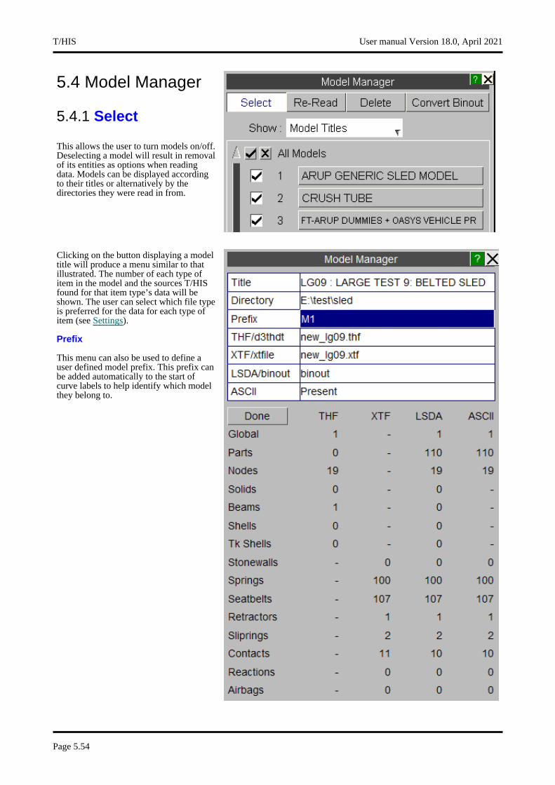
5.4 Model Manager
5.4.1 Select
This allows the user to turn models on/off. Deselecting a model will result in removal of its entities as options when reading data. Models can be displayed according to their titles or alternatively by the directories they were read in from.
Clicking on the button displaying a model title will produce a menu similar to that illustrated. The number of each type of item in the model and the sources T/HIS found for that item type’s data will be shown. The user can select which file type is preferred for the data for each type of item (see Settings).
Prefix
This menu can also be used to define a user defined model prefix. This prefix can be added automatically to the start of curve labels to help identify which model they belong to.
T/HIS User manual Version 18.0, April 2021
Page 5.54

5.4.2 Re-Read
The re-read option can be used to rescan and update the model. This will find any new data written to disk since the file was last read.
5.4.3 Delete
This option allows the user to select and delete models from T/HIS. Any curves that have been read in from a model that is deleted are NOT deleted with the model. Any number of models to be deleted from T/HIS.
5.4.4 Convert Binout
This option can be used to convert LSDA binout files into the older ASCII files. The menu allows a number of models to be selected.
The Select Files button allows the user to specify which ASCII files are to be created.
All of the ASCII files are written into the directory containing the LSDA file.
User manual Version 18.0, April 2021 T/HIS
Page 5.55

5.5 EDIT Options
This menu allows you to examine and make modifications to the curve data points. You are always working on a "scratch" copy of the curve. The permanent curve is only updated when you SAVE it explicitly.
Moving around the curve data is done through the use of scroll bars on the data panel.
SaveSaves the edited curve as either a new curve or overwrites the original.
RestartResets the curve being edited to the values at the start of the edit session.
QuitQuits the curve editor without making any changes to the curve
Labels...Allows the title, axis and line label to be changed (see Section 5.5.3 for more details)
ReplaceAllows curve values to be changed by overtyping the x and y values.
Insert BeforeInserts a new point in the curve before the selected point.
Insert AfterInserts a new point in the curve after the selected point.
DeleteDeletes the selected point.
The Command text-box allows control by command line (see Section 5.5.2 for more details).
T/HIS User manual Version 18.0, April 2021
Page 5.56
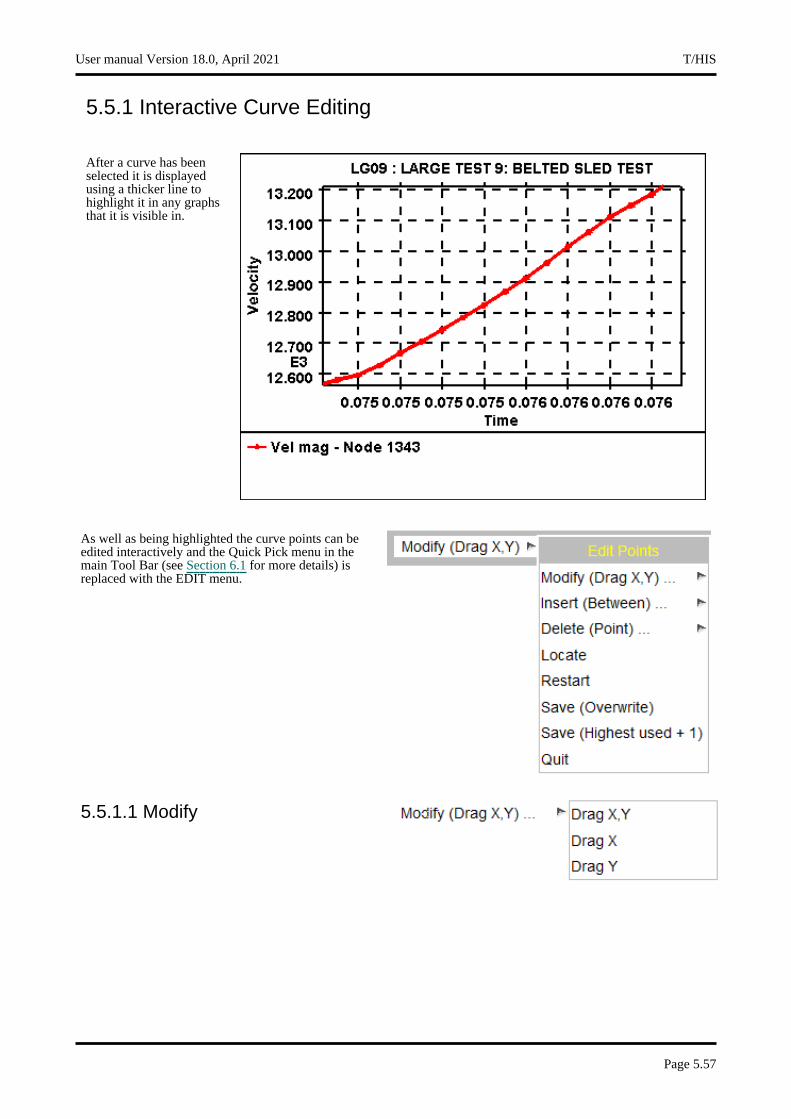
5.5.1 Interactive Curve Editing
After a curve has been selected it is displayed using a thicker line to highlight it in any graphs that it is visible in.
As well as being highlighted the curve points can be edited interactively and the Quick Pick menu in the main Tool Bar (see Section 6.1 for more details) is replaced with the EDIT menu.
5.5.1.1 Modify
User manual Version 18.0, April 2021 T/HIS
Page 5.57
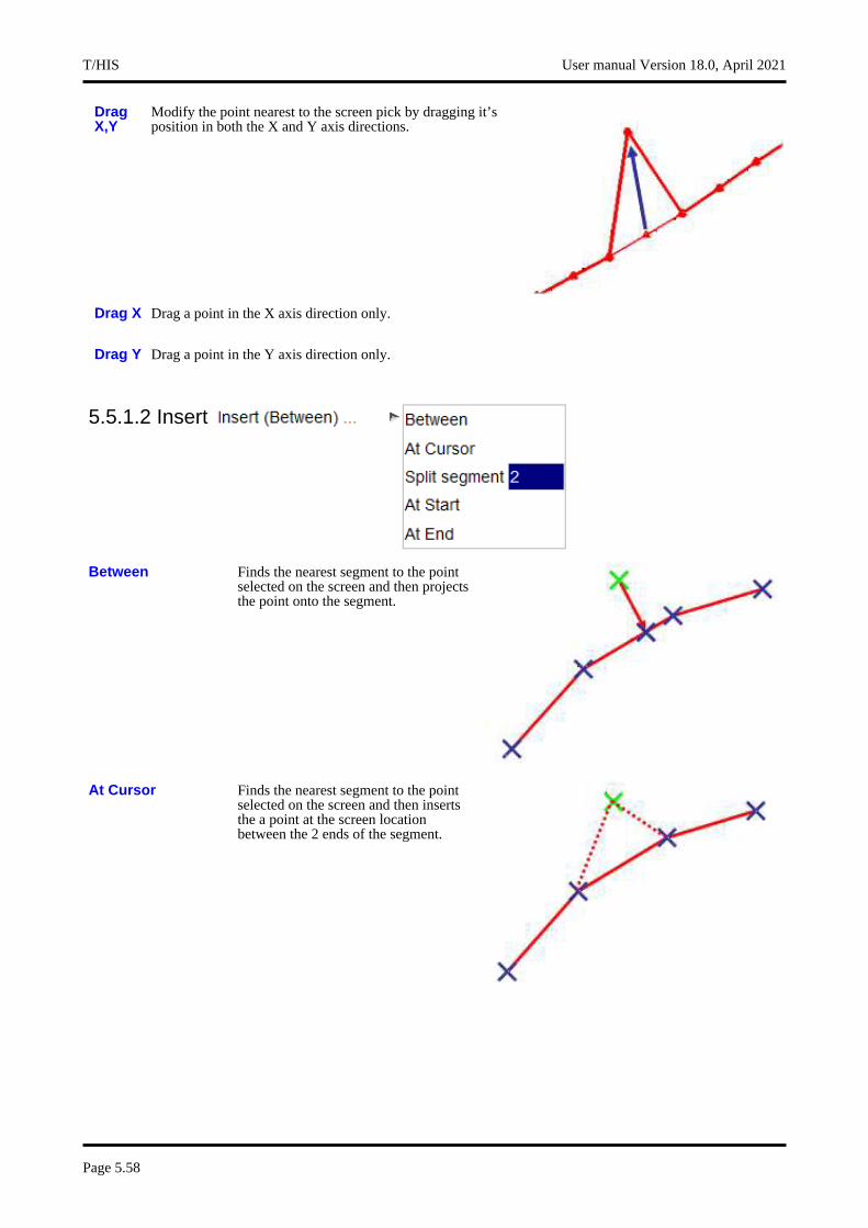
Drag X,Y
Modify the point nearest to the screen pick by dragging it’s position in both the X and Y axis directions.
Drag X Drag a point in the X axis direction only.
Drag Y Drag a point in the Y axis direction only.
5.5.1.2 Insert
Between Finds the nearest segment to the point selected on the screen and then projects the point onto the segment.
At Cursor Finds the nearest segment to the point selected on the screen and then inserts the a point at the screen location between the 2 ends of the segment.
T/HIS User manual Version 18.0, April 2021
Page 5.58
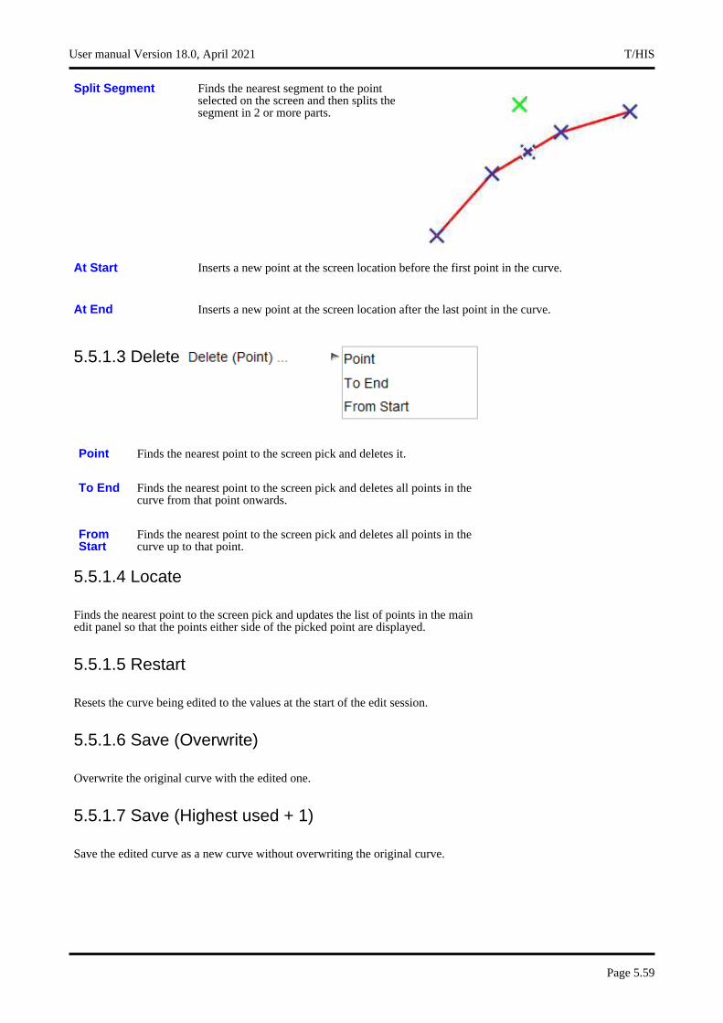
Split Segment Finds the nearest segment to the point selected on the screen and then splits the segment in 2 or more parts.
At Start Inserts a new point at the screen location before the first point in the curve.
At End Inserts a new point at the screen location after the last point in the curve.
5.5.1.3 Delete
Point Finds the nearest point to the screen pick and deletes it.
To End Finds the nearest point to the screen pick and deletes all points in the curve from that point onwards.
From Start
Finds the nearest point to the screen pick and deletes all points in the curve up to that point.
5.5.1.4 Locate
Finds the nearest point to the screen pick and updates the list of points in the main edit panel so that the points either side of the picked point are displayed.
5.5.1.5 Restart
Resets the curve being edited to the values at the start of the edit session.
5.5.1.6 Save (Overwrite)
Overwrite the original curve with the edited one.
5.5.1.7 Save (Highest used + 1)
Save the edited curve as a new curve without overwriting the original curve.
User manual Version 18.0, April 2021 T/HIS
Page 5.59
5.5.1.8 Quit
Quits the curve editor without making any changes to the curve.
5.5.2 Command line mode
In command line mode editing of curves is done in a similar fashion using the following commands.
Moving around the curve: F Forward Move forward 16 lines
B Back Move back 16 lines
T Top Move to the top of the curve
E End Move to the end of the curve
N Number Move to given line number
Modifying the curve: Cn Change Change line n
In Insert Insert points before line n
An Append Append points after line n
D n1 n2 Delete Delete lines n1 to n2
L Label Change the line label
R Reset Reset the curve back to the original curve
Saving and Plotting the curve: W Write Write the curve
S Save As write
PE Plot Edited Plot the edited curve
PA Plot All Plot the edited and original curve
PL Plot Plot the current T/HIS curves
Q Quit Quit the editor
In command line mode the EDIT menu is reached by typing /ED
T/HIS User manual Version 18.0, April 2021
Page 5.60
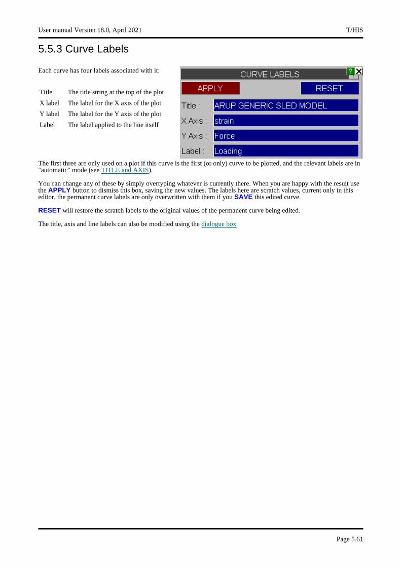
5.5.3 Curve Labels
Each curve has four labels associated with it:
Title The title string at the top of the plot
X label The label for the X axis of the plot
Y label The label for the Y axis of the plot
Label The label applied to the line itself
The first three are only used on a plot if this curve is the first (or only) curve to be plotted, and the relevant labels are in "automatic" mode (see TITLE and AXIS).
You can change any of these by simply overtyping whatever is currently there. When you are happy with the result use the APPLY button to dismiss this box, saving the new values. The labels here are scratch values, current only in this editor, the permanent curve labels are only overwritten with them if you SAVE this edited curve.
RESET will restore the scratch labels to the original values of the permanent curve being edited.
The title, axis and line labels can also be modified using the dialogue box
User manual Version 18.0, April 2021 T/HIS
Page 5.61
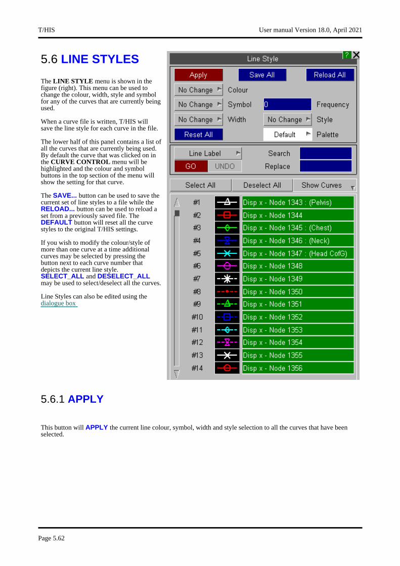
5.6 LINE STYLES
The LINE STYLE menu is shown in the figure (right). This menu can be used to change the colour, width, style and symbol for any of the curves that are currently being used.
When a curve file is written, T/HIS will save the line style for each curve in the file.
The lower half of this panel contains a list of all the curves that are currently being used. By default the curve that was clicked on in the CURVE CONTROL menu will be highlighted and the colour and symbol buttons in the top section of the menu will show the setting for that curve.
The SAVE... button can be used to save the current set of line styles to a file while the RELOAD... button can be used to reload a set from a previously saved file. The DEFAULT button will reset all the curve styles to the original T/HIS settings.
If you wish to modify the colour/style of more than one curve at a time additional curves may be selected by pressing the button next to each curve number that depicts the current line style. SELECT_ALL and DESELECT_ALL may be used to select/deselect all the curves.
Line Styles can also be edited using the dialogue box
5.6.1 APPLY
This button will APPLY the current line colour, symbol, width and style selection to all the curves that have been selected.
T/HIS User manual Version 18.0, April 2021
Page 5.62
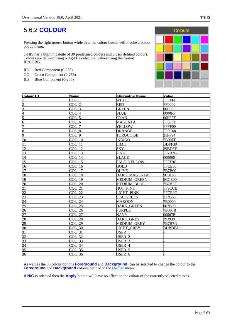
5.6.2 COLOUR
Pressing the right mouse button while over the colour button will invoke a colour popup menu.
T/HIS has a built in palette of 30 predefined colours and 6 user defined colours. Colours are defined using 6 digit Hexadecimal values using the format RRGGBB.
RR Red Component (0-255)GG Green Component (0-255)BB Blue Component (0-255)
Colour ID Name Alternative Name Value 1 COL_1 WHITE FFFFFF 2 COL_2 RED FF0000 3 COL_3 GREEN 00FF00 4 COL_4 BLUE 0000FF 5 COL_5 CYAN 00FFFF 6 COL_6 MAGENTA FF00FF 7 COL_7 YELLOW FFFF00 8 COL_8 ORANGE FF9C00 9 COL_9 TURQUOISE 21FF94 10 COL_10 INDIGO 7B00FF 11 COL_11 LIME BDFF39 12 COL_12 SKY 39BDFF 13 COL_13 PINK FF7B7B 14 COL_14 BLACK 000000 15 COL_15 PALE_YELLOW FFFF9C 16 COL_16 GOLD FFCE00 17 COL_17 OLIVE 7B7B00 18 COL_18 DARK_MAGENTA 9C3163 19 COL_19 MEDIUM_GREEN 9CCE00 20 COL_20 MEDIUM_BLUE 7B7BFF 21 COL_21 HOT_PINK FF9CCE 22 COL_22 LIGHT_PINK FFCE9C 23 COL_23 SEA_GREEN 317B63 24 COL_24 MAROON 7B0000 25 COL_25 DARK_GREEN 007B00 26 COL_26 PURPLE 7B007B 27 COL_27 NAVY 00007B 28 COL_28 DARK_GREY 393939 29 COL_29 MEDIUM_GREY 7B7B7B 30 COL_30 LIGHT_GREY BDBDBD 31 COL_31 USER_1 - 32 COL_32 USER_2 - 33 COL_33 USER_3 - 34 COL_34 USER_4 - 35 COL_35 USER_5 - 36 COL_36 USER_6 -
As well as the 36 colour options Foreground and Background can be selected to change the colour to the Foreground and Background colours defined in the Display menu.
If N/C is selected then the Apply button will have no effect on the colour of the currently selected curves..
User manual Version 18.0, April 2021 T/HIS
Page 5.63
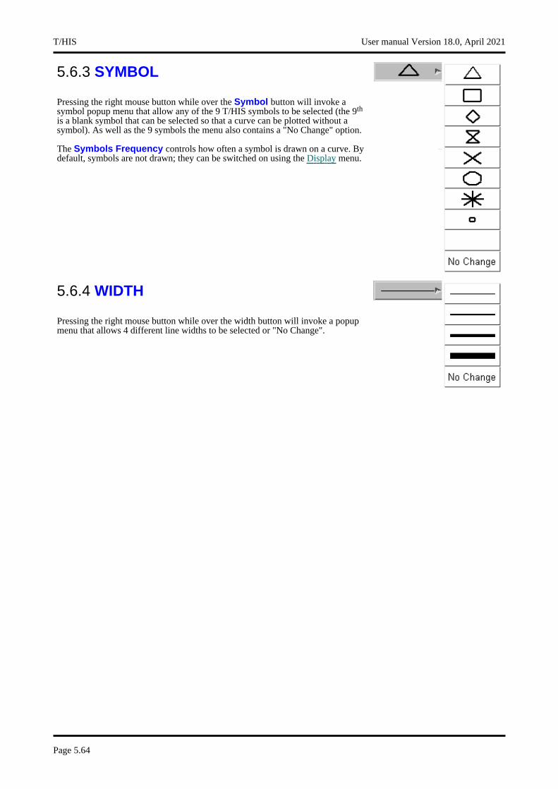
5.6.3 SYMBOL
Pressing the right mouse button while over the Symbol button will invoke a symbol popup menu that allow any of the 9 T/HIS symbols to be selected (the 9th
is a blank symbol that can be selected so that a curve can be plotted without a symbol). As well as the 9 symbols the menu also contains a "No Change" option.
The Symbols Frequency controls how often a symbol is drawn on a curve. By default, symbols are not drawn; they can be switched on using the Display menu.
5.6.4 WIDTH
Pressing the right mouse button while over the width button will invoke a popup menu that allows 4 different line widths to be selected or "No Change".
T/HIS User manual Version 18.0, April 2021
Page 5.64

5.6.5 STYLE
ressing the right mouse button while over the style button will invoke a popup menu that allows 8 different line styles to be selected (the 3rd is actually a blank line that can be selected so that a curve can be plotted without a line).
As well as the 8 line styles the menu also contains a "No Change" option.
5.6.6 CURVE PALETTE
By default T/HIS uses 6 colours (White, Red, Green, Blue, Cyan and Magenta) for any curves that have not had a colour explicitly defined for them. Curves 1,7,13... will be White, 2,8,14... will be Red.
This option can be used to change the default number of colours T/HIS uses.
Default Use the default 6 colours
Extended Use the first 13 colours
No Grey Use all 30 predefined colours except the 3 grey ones
Full Use all 30 predefined colours plus any user defined ones.
The default value for the curve palette can also be specified in the "preferences" file (see Appendix H for more details).
5.6.7 MODIFYING LABELS
Multiple curve labels may be edited using the Search and Replace option to enter the string to search for and the string to replace it with ^ can be used to insert text at the beginning of a label while $ can be used to append to the end of a label. The table below shows the effect of 2 search and replace examples.
Example 1 Example 2
Original Label Displacement N1034 Time
Search String N1 $
Replace String Node 1 (s)
Modified Label Displacement Node 1034 Time(s)
The GO button will initiate the search and replace on all the curves that are currently selected (highlighted in the bottom half of the menu), while the UNDO button can be used to reset the labels to what they were before the search and replace.
User manual Version 18.0, April 2021 T/HIS
Page 5.65
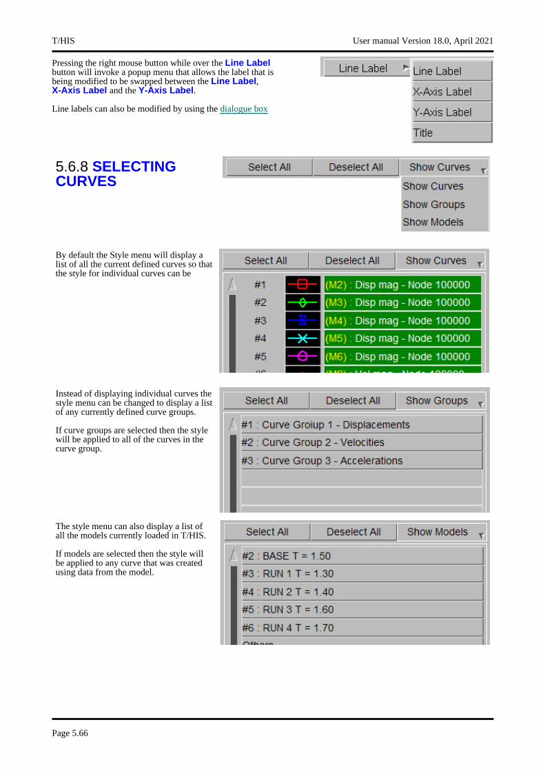
Pressing the right mouse button while over the Line Label button will invoke a popup menu that allows the label that is being modified to be swapped between the Line Label, X-Axis Label and the Y-Axis Label.
Line labels can also be modified by using the dialogue box
5.6.8 SELECTING CURVES
By default the Style menu will display a list of all the current defined curves so that the style for individual curves can be
Instead of displaying individual curves the style menu can be changed to display a list of any currently defined curve groups.
If curve groups are selected then the style will be applied to all of the curves in the curve group.
The style menu can also display a list of all the models currently loaded in T/HIS.
If models are selected then the style will be applied to any curve that was created using data from the model.
T/HIS User manual Version 18.0, April 2021
Page 5.66
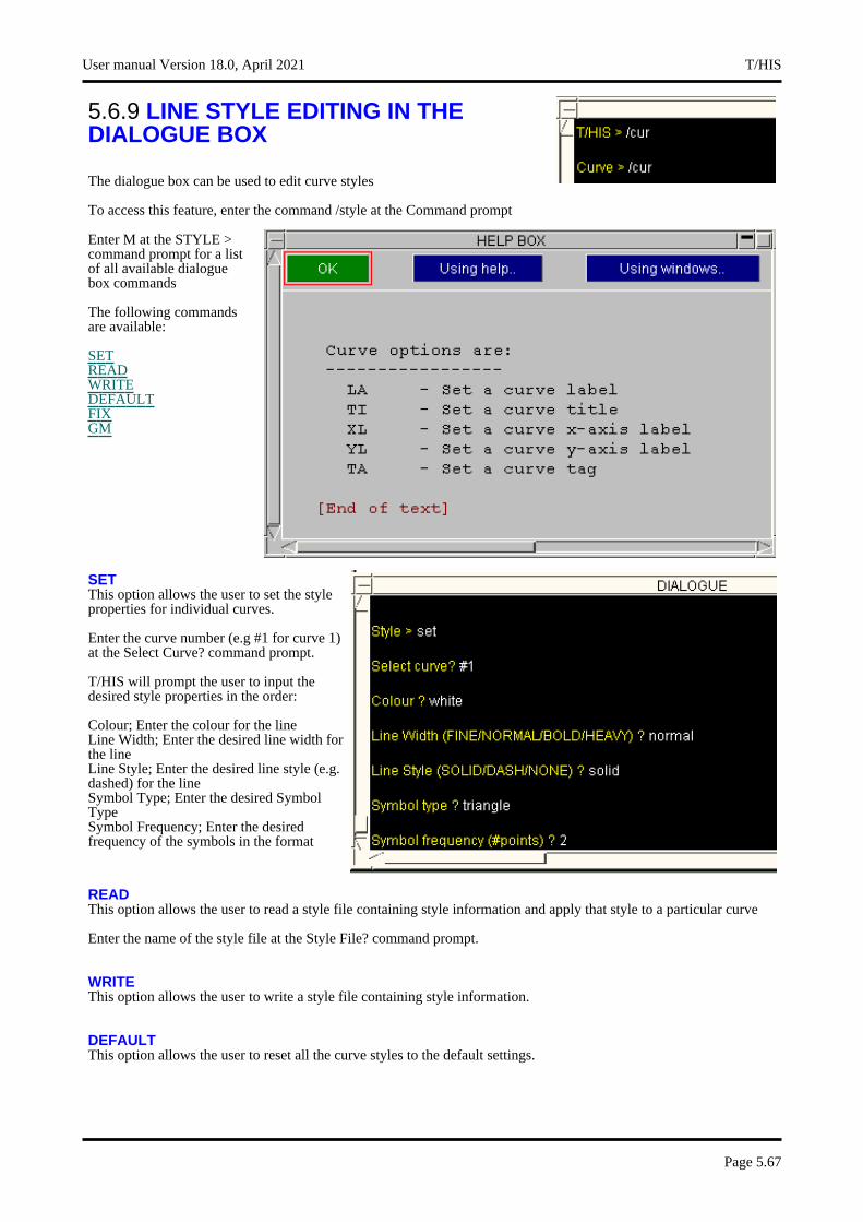
5.6.9 LINE STYLE EDITING IN THE DIALOGUE BOX
The dialogue box can be used to edit curve styles
To access this feature, enter the command /style at the Command prompt
Enter M at the STYLE > command prompt for a list of all available dialogue box commands
The following commands are available:
SETREADWRITEDEFAULTFIXGM
SET This option allows the user to set the style properties for individual curves.
Enter the curve number (e.g #1 for curve 1) at the Select Curve? command prompt.
T/HIS will prompt the user to input the desired style properties in the order:
Colour; Enter the colour for the lineLine Width; Enter the desired line width for the lineLine Style; Enter the desired line style (e.g. dashed) for the lineSymbol Type; Enter the desired Symbol TypeSymbol Frequency; Enter the desired frequency of the symbols in the format
READ This option allows the user to read a style file containing style information and apply that style to a particular curve
Enter the name of the style file at the Style File? command prompt.
WRITE This option allows the user to write a style file containing style information.
DEFAULT This option allows the user to reset all the curve styles to the default settings.
User manual Version 18.0, April 2021 T/HIS
Page 5.67
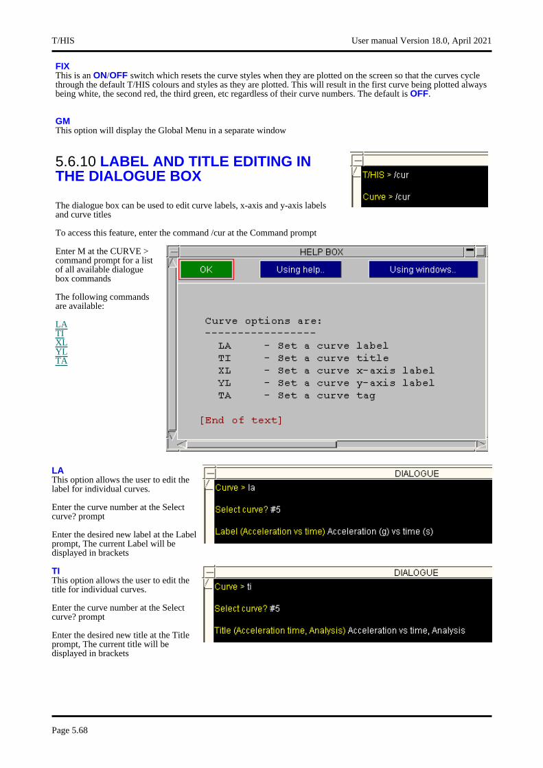
FIX This is an ON/OFF switch which resets the curve styles when they are plotted on the screen so that the curves cycle through the default T/HIS colours and styles as they are plotted. This will result in the first curve being plotted always being white, the second red, the third green, etc regardless of their curve numbers. The default is OFF.
GM This option will display the Global Menu in a separate window
5.6.10 LABEL AND TITLE EDITING IN THE DIALOGUE BOX
The dialogue box can be used to edit curve labels, x-axis and y-axis labels and curve titles
To access this feature, enter the command /cur at the Command prompt
Enter M at the CURVE > command prompt for a list of all available dialogue box commands
The following commands are available:
LATIXLYLTA
LA This option allows the user to edit the label for individual curves.
Enter the curve number at the Select curve? prompt
Enter the desired new label at the Label prompt, The current Label will be displayed in brackets
TI This option allows the user to edit the title for individual curves.
Enter the curve number at the Select curve? prompt
Enter the desired new title at the Title prompt, The current title will be displayed in brackets
T/HIS User manual Version 18.0, April 2021
Page 5.68
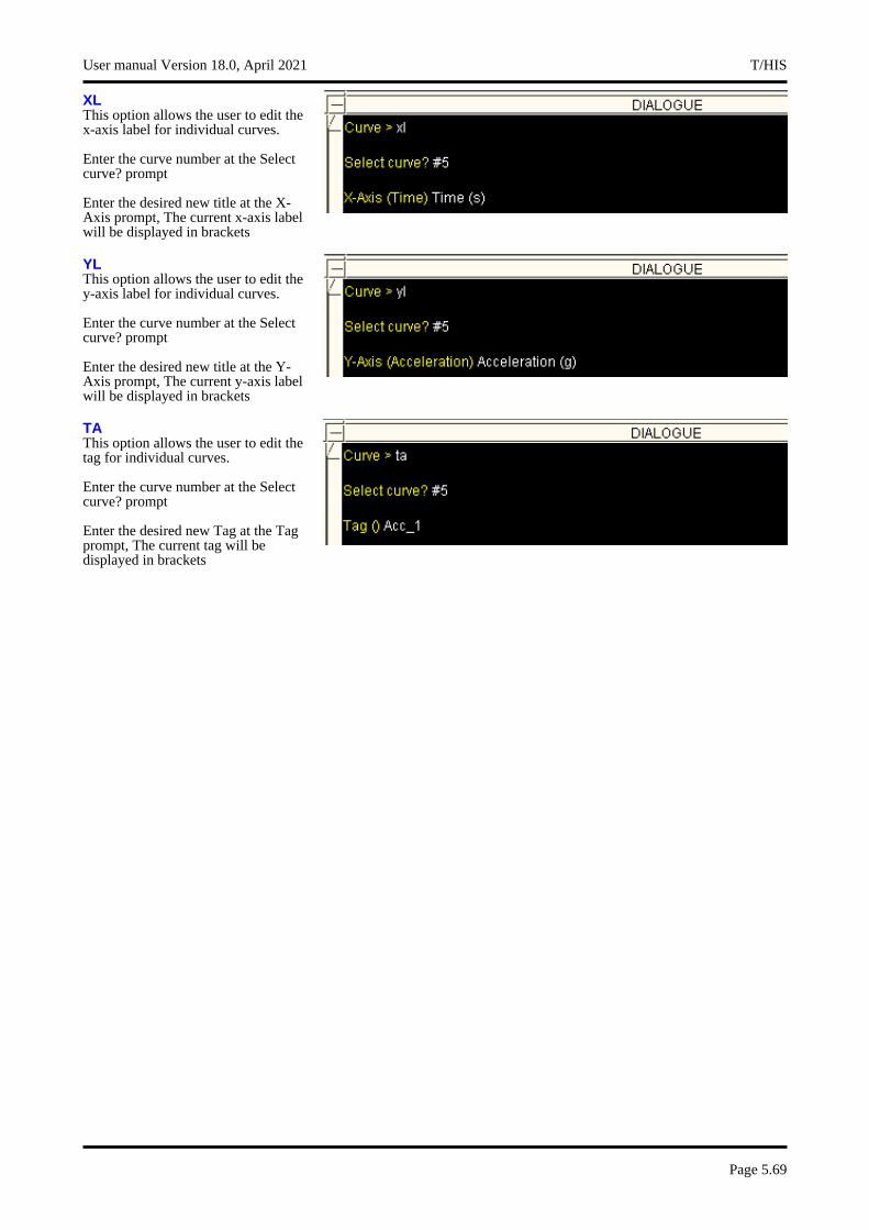
XL This option allows the user to edit the x-axis label for individual curves.
Enter the curve number at the Select curve? prompt
Enter the desired new title at the X- Axis prompt, The current x-axis label will be displayed in brackets
YL This option allows the user to edit the y-axis label for individual curves.
Enter the curve number at the Select curve? prompt
Enter the desired new title at the Y- Axis prompt, The current y-axis label will be displayed in brackets
TA This option allows the user to edit the tag for individual curves.
Enter the curve number at the Select curve? prompt
Enter the desired new Tag at the Tag prompt, The current tag will be displayed in brackets
User manual Version 18.0, April 2021 T/HIS
Page 5.69
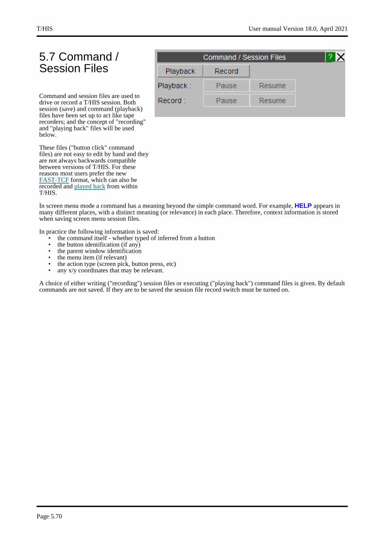
5.7 Command / Session Files
Command and session files are used to drive or record a T/HIS session. Both session (save) and command (playback) files have been set up to act like tape recorders; and the concept of "recording" and "playing back" files will be used below.
These files ("button click" command files) are not easy to edit by hand and they are not always backwards compatible between versions of T/HIS. For these reasons most users prefer the new FAST-TCF format, which can also be recorded and played back from within T/HIS.
In screen menu mode a command has a meaning beyond the simple command word. For example, HELP appears in many different places, with a distinct meaning (or relevance) in each place. Therefore, context information is stored when saving screen menu session files.
In practice the following information is saved:• the command itself - whether typed of inferred from a button• the button identification (if any)• the parent window identification• the menu item (if relevant)• the action type (screen pick, button press, etc)• any x/y coordinates that may be relevant.
A choice of either writing ("recording") session files or executing ("playing back") command files is given. By default commands are not saved. If they are to be saved the session file record switch must be turned on.
T/HIS User manual Version 18.0, April 2021
Page 5.70

5.7.1 Writing ("Recording") Session Files
To write a session file the record CONTROLS... button must be pressed, displaying the RECORD COMMAND FILES menu shown right.
Pressing the RECORD > button will start the session file. Thereafter, all commands (except those in the session/playback windows) are saved in an internal scratch file. In order to save these commands to disk they must be written explicitly using the SAVE TO DISK button. They can then be read back in and replayed
A variety of features are available to help move around the file. These are shown in the FILE POSITION AND CONTROL area of the panel. The file can be indexed at particular user defined points using the INDEX MARKS menu is accessed by pressing the INDEX... button. These may be used as targets of a search and also to control recording.
The scratch file is random access, and can be moved back and forth and reviewed at will. To help with this it is possible to switch between RECORD and REVIEW modes in the session file control box:
RECORD
REVIEW
records all your commands when running
plays back your recorded commands
A command file can be stepped through or run backwards or forwards. It may also be searched for a particular command. As with a real tape recorder, if the pointer is moved backwards and recording continued the commands that were previously stored will be overwritten from that point.
The session file recording and command file playback operations are totally separate: they can be thought of as two separate tape recorders. As a consequence it is possible to record commands that are being played back: in effect it is possible to edit and combine files.
User manual Version 18.0, April 2021 T/HIS
Page 5.71
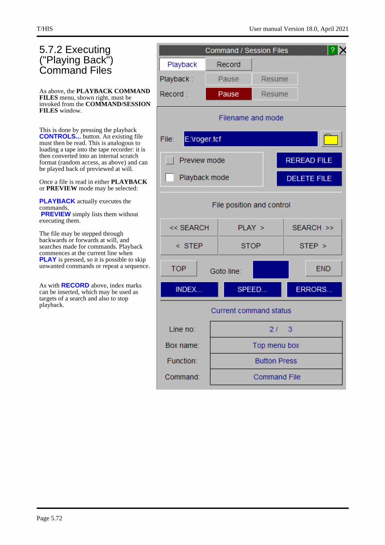
5.7.2 Executing ("Playing Back") Command Files
As above, the PLAYBACK COMMAND FILES menu, shown right, must be invoked from the COMMAND/SESSION FILES window.
This is done by pressing the playback CONTROLS... button. An existing file must then be read. This is analogous to loading a tape into the tape recorder: it is then converted into an internal scratch format (random access, as above) and can be played back of previewed at will.
Once a file is read in either PLAYBACK or PREVIEW mode may be selected:
PLAYBACK actually executes the commands,PREVIEW simply lists them without executing them.
The file may be stepped through backwards or forwards at will, and searches made for commands. Playback commences at the current line when PLAY is pressed, so it is possible to skip unwanted commands or repeat a sequence.
As with RECORD above, index marks can be inserted, which may be used as targets of a search and also to stop playback.
T/HIS User manual Version 18.0, April 2021
Page 5.72
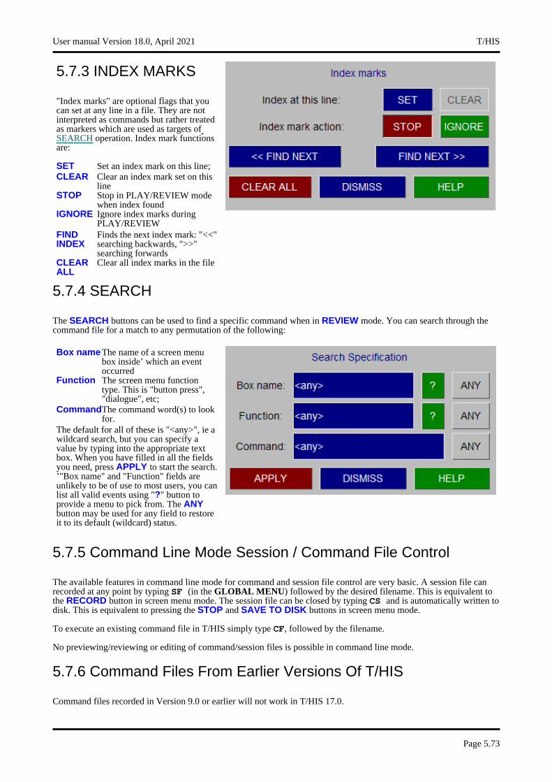
5.7.3 INDEX MARKS
"Index marks" are optional flags that you can set at any line in a file. They are not interpreted as commands but rather treated as markers which are used as targets ofSEARCH operation. Index mark functions are:
SET Set an index mark on this line;CLEAR Clear an index mark set on this
lineSTOP Stop in PLAY/REVIEW mode
when index foundIGNORE Ignore index marks during
PLAY/REVIEWFIND INDEX
Finds the next index mark: "<<" searching backwards, ">>" searching forwards
CLEAR ALL
Clear all index marks in the file
5.7.4 SEARCH
The SEARCH buttons can be used to find a specific command when in REVIEW mode. You can search through the command file for a match to any permutation of the following:
Box nameThe name of a screen menu box inside’ which an event occurred
Function The screen menu function type. This is "button press", "dialogue", etc;
CommandThe command word(s) to look for.
The default for all of these is "<any>", ie a wildcard search, but you can specify a value by typing into the appropriate text box. When you have filled in all the fields you need, press APPLY to start the search. ’"Box name" and "Function" fields are unlikely to be of use to most users, you can list all valid events using "?" button to provide a menu to pick from. The ANY button may be used for any field to restore it to its default (wildcard) status.
5.7.5 Command Line Mode Session / Command File Control
The available features in command line mode for command and session file control are very basic. A session file can recorded at any point by typing SF (in the GLOBAL MENU) followed by the desired filename. This is equivalent to the RECORD button in screen menu mode. The session file can be closed by typing CS and is automatically written to disk. This is equivalent to pressing the STOP and SAVE TO DISK buttons in screen menu mode.
To execute an existing command file in T/HIS simply type CF, followed by the filename.
No previewing/reviewing or editing of command/session files is possible in command line mode.
5.7.6 Command Files From Earlier Versions Of T/HIS
Command files recorded in Version 9.0 or earlier will not work in T/HIS 17.0.
User manual Version 18.0, April 2021 T/HIS
Page 5.73

5.8 IMAGE Options
5.8.1 BMP,JPEG ...
This menu can be used to save an image containing one or more graphs in a number of different formats.
All Pages Each page will be saved as a single image to multiple files. The filenames used will be based on the filename selected by the user..
This option will only be available if T/HIS contains multiple graphs on more than one page (see section 3.2).
Current Page A single image containing currently displayed page will be generated.
This option will only be available if T/HIS contains multiple graphs on more than one page (see section 3.2).
Only Page (n) A single image containing the selected page will be generated.
This option will only be available if T/HIS contains multiple graphs on more than one page (see section 3.2).
All Graphs A single image will be generated containing all of the graphs.
This option will only be available if T/HIS only contains a single page (see Section3.2).
All Active Graphs A single image will be generated containing all of the currently active graphs.
This option will only be available if T/HIS only contains a single page (see Section3.2).
Only Graph (n) A single image containing the selected graph will be generated.
White Background Captures the image with a white background and black foreground. Once the image is captured the colours are reset to their original values.
T/HIS User manual Version 18.0, April 2021
Page 5.74
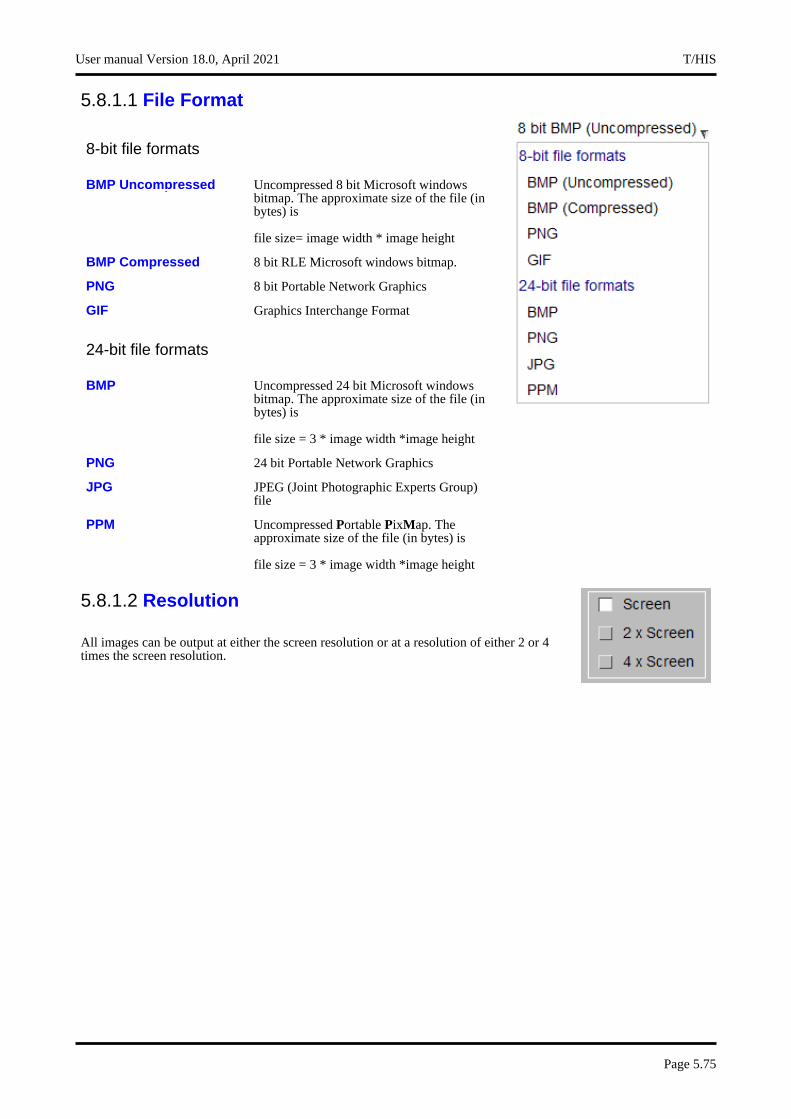
5.8.1.1 File Format
8-bit file formats
BMP Uncompressed Uncompressed 8 bit Microsoft windows bitmap. The approximate size of the file (in bytes) is
file size= image width * image height
BMP Compressed 8 bit RLE Microsoft windows bitmap.
PNG 8 bit Portable Network Graphics
GIF Graphics Interchange Format
24-bit file formats
BMP Uncompressed 24 bit Microsoft windows bitmap. The approximate size of the file (in bytes) is
file size = 3 * image width *image height
PNG 24 bit Portable Network Graphics
JPG JPEG (Joint Photographic Experts Group) file
PPM Uncompressed Portable PixMap. The approximate size of the file (in bytes) is
file size = 3 * image width *image height
5.8.1.2 Resolution
All images can be output at either the screen resolution or at a resolution of either 2 or 4 times the screen resolution.
User manual Version 18.0, April 2021 T/HIS
Page 5.75
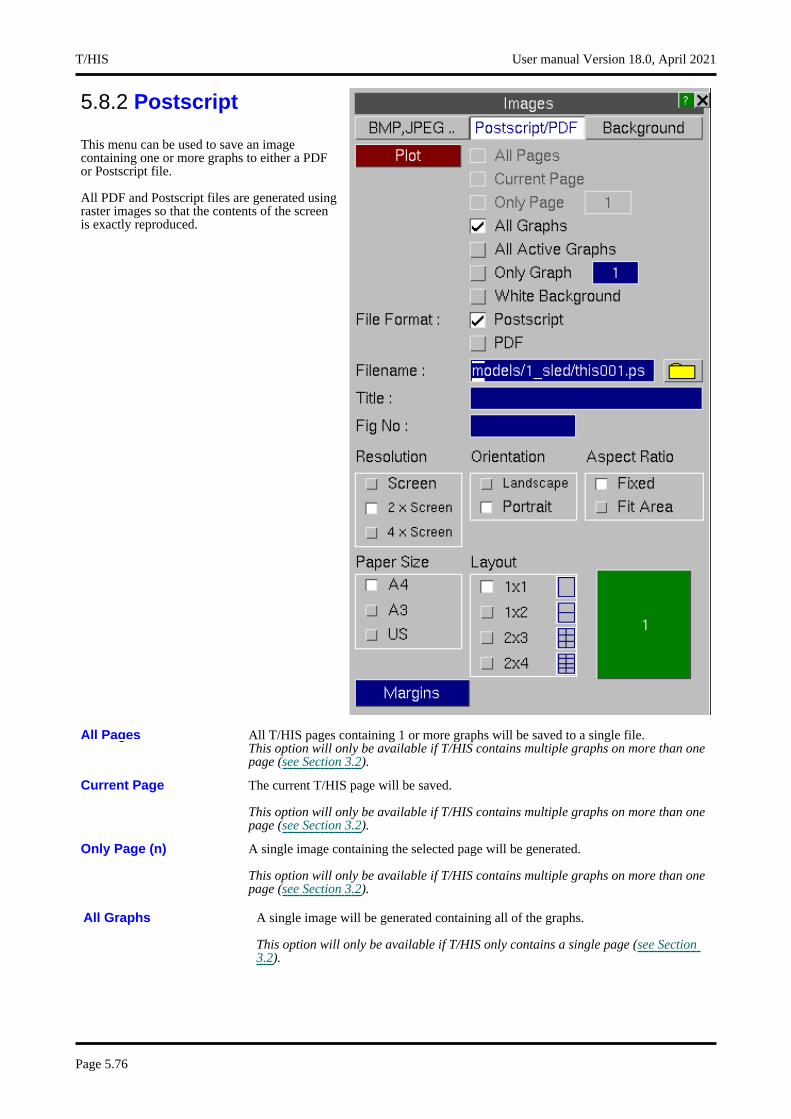
5.8.2 Postscript
This menu can be used to save an image containing one or more graphs to either a PDF or Postscript file.
All PDF and Postscript files are generated using raster images so that the contents of the screen is exactly reproduced.
All Pages All T/HIS pages containing 1 or more graphs will be saved to a single file. This option will only be available if T/HIS contains multiple graphs on more than one page (see Section 3.2).
Current Page The current T/HIS page will be saved.
This option will only be available if T/HIS contains multiple graphs on more than one page (see Section 3.2).
Only Page (n) A single image containing the selected page will be generated.
This option will only be available if T/HIS contains multiple graphs on more than one page (see Section 3.2).
All Graphs A single image will be generated containing all of the graphs.
This option will only be available if T/HIS only contains a single page (see Section3.2).
T/HIS User manual Version 18.0, April 2021
Page 5.76
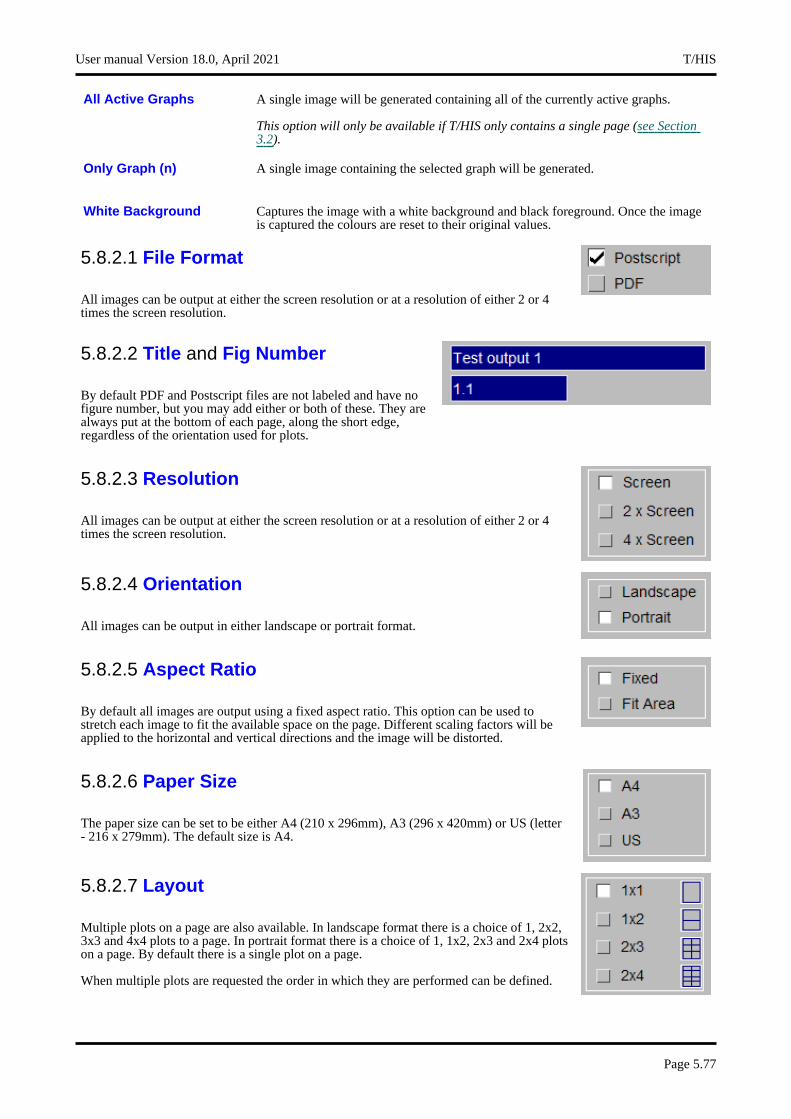
All Active Graphs A single image will be generated containing all of the currently active graphs.
This option will only be available if T/HIS only contains a single page (see Section3.2).
Only Graph (n) A single image containing the selected graph will be generated.
White Background Captures the image with a white background and black foreground. Once the image is captured the colours are reset to their original values.
5.8.2.1 File Format
All images can be output at either the screen resolution or at a resolution of either 2 or 4 times the screen resolution.
5.8.2.2 Title and Fig Number
By default PDF and Postscript files are not labeled and have no figure number, but you may add either or both of these. They are always put at the bottom of each page, along the short edge, regardless of the orientation used for plots.
5.8.2.3 Resolution
All images can be output at either the screen resolution or at a resolution of either 2 or 4 times the screen resolution.
5.8.2.4 Orientation
All images can be output in either landscape or portrait format.
5.8.2.5 Aspect Ratio
By default all images are output using a fixed aspect ratio. This option can be used to stretch each image to fit the available space on the page. Different scaling factors will be applied to the horizontal and vertical directions and the image will be distorted.
5.8.2.6 Paper Size
The paper size can be set to be either A4 (210 x 296mm), A3 (296 x 420mm) or US (letter - 216 x 279mm). The default size is A4.
5.8.2.7 Layout
Multiple plots on a page are also available. In landscape format there is a choice of 1, 2x2, 3x3 and 4x4 plots to a page. In portrait format there is a choice of 1, 1x2, 2x3 and 2x4 plots on a page. By default there is a single plot on a page.
When multiple plots are requested the order in which they are performed can be defined.
User manual Version 18.0, April 2021 T/HIS
Page 5.77

5.8.2.8 Margins
The Margins can be used to change the top, bottom, left and right margins for each page.
5.8.3 Background
This option can be used to add a background image to each graph (see section 5.16.8 for more details).
T/HIS User manual Version 18.0, April 2021
Page 5.78
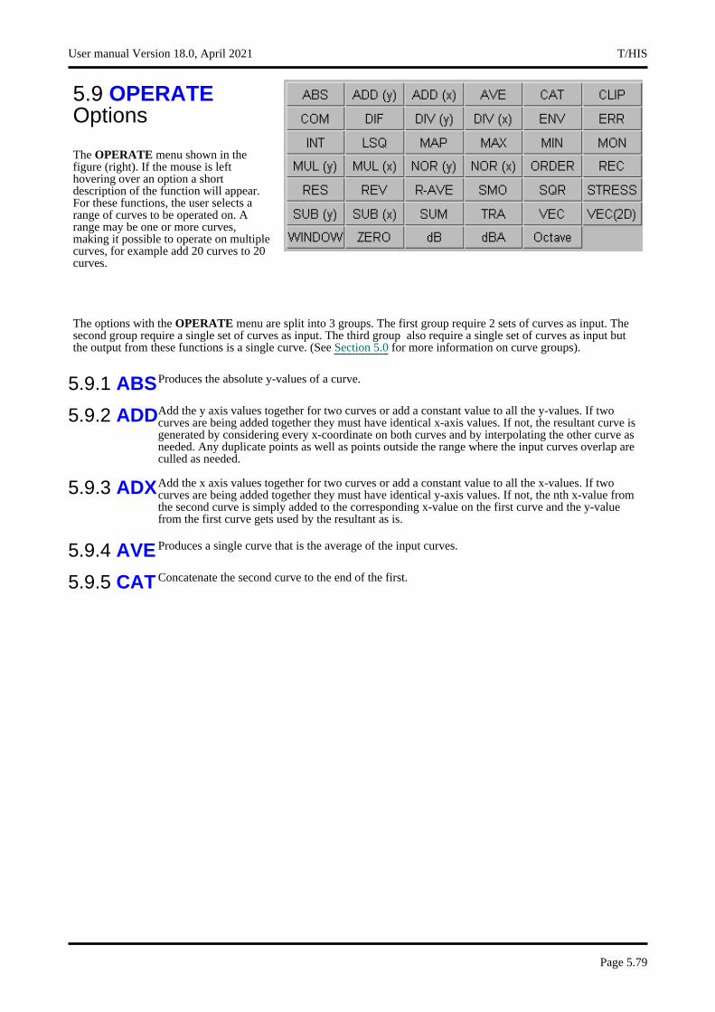
5.9 OPERATE Options
The OPERATE menu shown in the figure (right). If the mouse is left hovering over an option a short description of the function will appear.For these functions, the user selects a range of curves to be operated on. A range may be one or more curves, making it possible to operate on multiple curves, for example add 20 curves to 20 curves.
The options with the OPERATE menu are split into 3 groups. The first group require 2 sets of curves as input. The second group require a single set of curves as input. The third group also require a single set of curves as input but the output from these functions is a single curve. (See Section 5.0 for more information on curve groups).
5.9.1 ABSProduces the absolute y-values of a curve.
5.9.2 ADDAdd the y axis values together for two curves or add a constant value to all the y-values. If two curves are being added together they must have identical x-axis values. If not, the resultant curve is generated by considering every x-coordinate on both curves and by interpolating the other curve as needed. Any duplicate points as well as points outside the range where the input curves overlap are culled as needed.
5.9.3 ADXAdd the x axis values together for two curves or add a constant value to all the x-values. If two curves are being added together they must have identical y-axis values. If not, the nth x-value from the second curve is simply added to the corresponding x-value on the first curve and the y-value from the first curve gets used by the resultant as is.
5.9.4 AVE Produces a single curve that is the average of the input curves.
5.9.5 CAT Concatenate the second curve to the end of the first.
User manual Version 18.0, April 2021 T/HIS
Page 5.79
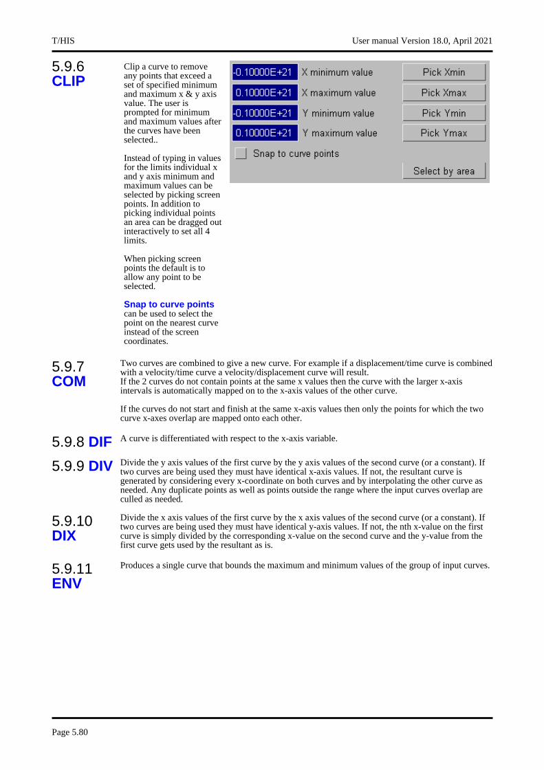
5.9.6 CLIP
Clip a curve to remove any points that exceed a set of specified minimum and maximum x & y axis value. The user is prompted for minimum and maximum values after the curves have been selected..
Instead of typing in values for the limits individual x and y axis minimum and maximum values can be selected by picking screen points. In addition to picking individual points an area can be dragged out interactively to set all 4 limits.
When picking screen points the default is to allow any point to be selected.
Snap to curve points can be used to select the point on the nearest curve instead of the screen coordinates.
5.9.7 COM
Two curves are combined to give a new curve. For example if a displacement/time curve is combined with a velocity/time curve a velocity/displacement curve will result. If the 2 curves do not contain points at the same x values then the curve with the larger x-axis intervals is automatically mapped on to the x-axis values of the other curve.
If the curves do not start and finish at the same x-axis values then only the points for which the two curve x-axes overlap are mapped onto each other.
5.9.8 DIF A curve is differentiated with respect to the x-axis variable.
5.9.9 DIV Divide the y axis values of the first curve by the y axis values of the second curve (or a constant). If two curves are being used they must have identical x-axis values. If not, the resultant curve is generated by considering every x-coordinate on both curves and by interpolating the other curve as needed. Any duplicate points as well as points outside the range where the input curves overlap are culled as needed.
5.9.10 DIX
Divide the x axis values of the first curve by the x axis values of the second curve (or a constant). If two curves are being used they must have identical y-axis values. If not, the nth x-value on the first curve is simply divided by the corresponding x-value on the second curve and the y-value from the first curve gets used by the resultant as is.
5.9.11 ENV
Produces a single curve that bounds the maximum and minimum values of the group of input curves.
T/HIS User manual Version 18.0, April 2021
Page 5.80

5.9.12 ERR
This option reports the degree of correlation between 2 input curves. The first curve selected is used as a reference curve and the following parameters are then reported :
Maximum difference : Value & TimeValue as a %age of reference curveValue as a %age of reference curve peak value.
Average difference - Value %age of reference curve peak value
Area Weighted Difference Correlation Parameter -
0 to 1
For more details on this function please see Appendix G
5.9.13 INTA curve is numerically integrated with respect to the x-axis variable using Simpson’s rule.
5.9.14 LSQ
Fits a straight line through the points using the least squares method.
5.9.15 MAP
The second curve is mapped onto the first curve, the resulting curve has identical x-axis values to the reference (first) curve with y-axis values obtained from the mapped (second) curve.
5.9.16 MAX
Produces a single curve that bounds the maximum values of the group of input curves.
5.9.17 MIN
Produces a single curve that bounds the minimum values of the group of input curves.
5.9.18 MON
Sorts a curve into monotonically increasing x-axis values.
5.9.19 MUL
Multiply the y axis values together for two curves or multiply all the y-values by a constant. If two curves are being multiplied together they must have identical x-axis values. If not, the resultant curve is generated by considering every x-coordinate on both curves and by interpolating the other curve as needed. Any duplicate points as well as points outside the range where the input curves overlap are culled as needed.
5.9.20 MUX
Multiply the x axis values together for two curves or multiply all the x-values by a constant. If two curves are being multiplied together they must have identical y-axis values. If not, the nth x-values on the two curves are simply multiplied together and the y-value from the first curve gets used by the resultant as is.
User manual Version 18.0, April 2021 T/HIS
Page 5.81
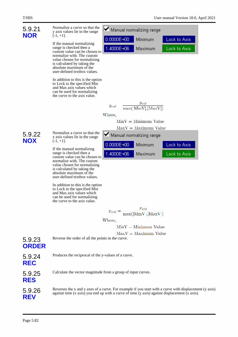
5.9.21 NOR
Normalize a curve so that the y axis values lie in the range [-1, +1].
If the manual normalizing range is checked then a custom value can be chosen to normalize with. The custom value chosen for normalizing is calculated by taking the absolute maximum of the user-defined textbox values.
In addition to this is the option to Lock to the specified Min and Max axis values which can be used for normalizing the curve to the axis value.
5.9.22 NOX
Normalize a curve so that the x axis values lie in the range [-1, +1].
If the manual normalizing range is checked then a custom value can be chosen to normalize with. The custom value chosen for normalizing is calculated by taking the absolute maximum of the user-defined textbox values.
In addition to this is the option to Lock to the specified Min and Max axis values which can be used for normalizing the curve to the axis value.
5.9.23 ORDER
Reverse the order of all the points in the curve.
5.9.24 REC
Produces the reciprocal of the y-values of a curve.
5.9.25 RES
Calculate the vector magnitude from a group of input curves.
5.9.26 REV
Reverses the x and y axes of a curve. For example if you start with a curve with displacement (y axis) against time (x axis) you end up with a curve of time (y axis) against displacement (x axis).
T/HIS User manual Version 18.0, April 2021
Page 5.82

5.9.27 R-AVE
Produces a single curve of the running average on the input curve.
If the time window is set to 0 then the y values for the output curve are the average value of all the point up to that point.
If the time window is non-zero (T) then the y values at each point are calculated by averaging the values between -T/2 and +T/2.
5.9.28 SMO
A moving average technique is used to smooth (filter) a curve. The user will be prompted for a smoothing factor.
The integer refers to the number of points included in the averaging of each point. The value you want will depend on the number of points in the curve and the amount of smoothing required. A certain amount of trial and error is necessary to get the required result.
5.9.29 SQR
Take the square root of the y-values of a curve.
5.9.30 STRESS
Converts a stress / strain curve between True and Engineering Stress /Strain.
5.9.31 SUB
Subtract the y axis value (or constant) of the second curve from the first curve. If two curves are being subtracted they must have identical x-axis values. If not, the resultant curve is generated by considering every x-coordinate on both curves and by interpolating the other curve the other curve as needed. Any duplicate points as well as points outside the range where the input curves overlap are culled as needed.
5.9.32 SUX
Subtract the x axis value (or constant) of the second curve from the first curve. If two curves are being subtracted they must have identical y-axis values. If not, the nth x-value from the second curve is simply subtracted from the corresponding x-value on the first curve and the y-value from the first curve gets used by the resultant as is.
5.9.33 SUM
Calculates the sum of a group of curves. This "sums" up the y-axis values of a group of curves, and maps the result onto the x-axis of the first curve.
5.9.34 TRA
Translate a curve with respect to the x and y axes. The user is prompted for the x and y values.
5.9.35 VEC
Calculate the vector magnitude from three input curves.
5.9.36 VEC(2-D)
Calculate the vector magnitude from two input curves.
User manual Version 18.0, April 2021 T/HIS
Page 5.83
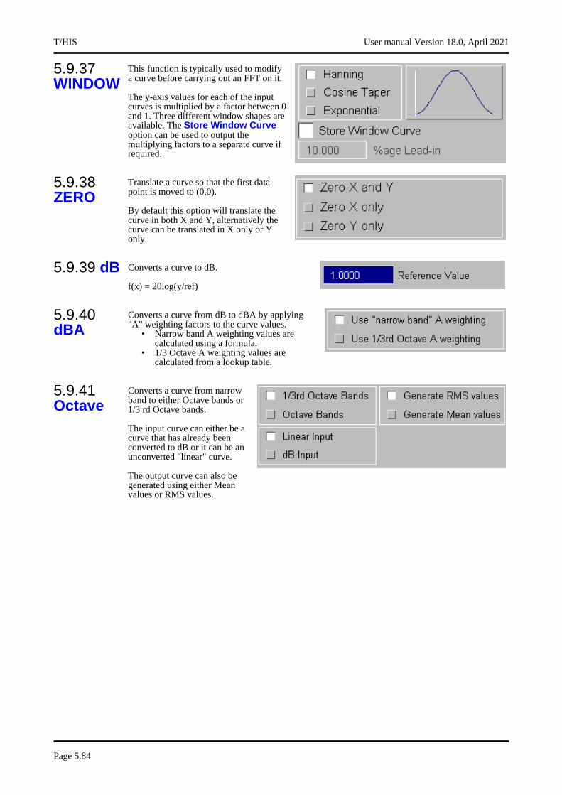
5.9.37 WINDOW
This function is typically used to modify a curve before carrying out an FFT on it.
The y-axis values for each of the input curves is multiplied by a factor between 0 and 1. Three different window shapes are available. The Store Window Curve option can be used to output the multiplying factors to a separate curve if required.
5.9.38 ZERO
Translate a curve so that the first data point is moved to (0,0).
By default this option will translate the curve in both X and Y, alternatively the curve can be translated in X only or Y only.
5.9.39 dB Converts a curve to dB.
f(x) = 20log(y/ref)
5.9.40 dBA
Converts a curve from dB to dBA by applying "A" weighting factors to the curve values.
• Narrow band A weighting values are calculated using a formula.
• 1/3 Octave A weighting values are calculated from a lookup table.
5.9.41 Octave
Converts a curve from narrow band to either Octave bands or 1/3 rd Octave bands.
The input curve can either be a curve that has already been converted to dB or it can be an unconverted "linear" curve.
The output curve can also be generated using either Mean values or RMS values.
T/HIS User manual Version 18.0, April 2021
Page 5.84
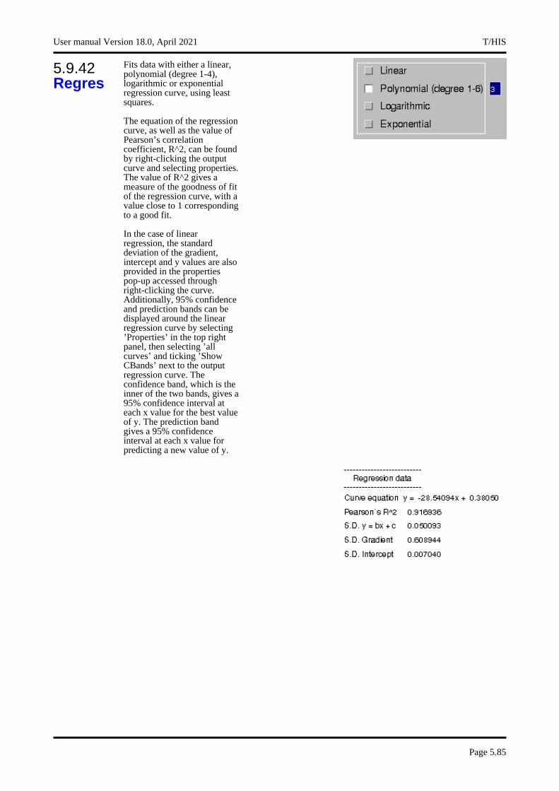
5.9.42 Regres
Fits data with either a linear, polynomial (degree 1-4), logarithmic or exponential regression curve, using least squares.
The equation of the regression curve, as well as the value of Pearson’s correlation coefficient, R^2, can be found by right-clicking the output curve and selecting properties. The value of R^2 gives a measure of the goodness of fit of the regression curve, with a value close to 1 corresponding to a good fit.
In the case of linear regression, the standard deviation of the gradient, intercept and y values are also provided in the properties pop-up accessed through right-clicking the curve. Additionally, 95% confidence and prediction bands can be displayed around the linear regression curve by selecting ’Properties’ in the top right panel, then selecting ’all curves’ and ticking ’Show CBands’ next to the output regression curve. The confidence band, which is the inner of the two bands, gives a 95% confidence interval at each x value for the best value of y. The prediction band gives a 95% confidence interval at each x value for predicting a new value of y.
User manual Version 18.0, April 2021 T/HIS
Page 5.85

5.10 MATHS Options
The MATHS menu is shown in the figure (right). This menu allows mathematical operations to be applied to curves. These options are self explanatory and work on the y-value of the curve (except where explicitly stated).
Note: Trigonometrical functions expect the user to work in radians.
5.10.1 SQRT The square root of a curve.
5.10.2 LOG Natural log (to base e)
5.10.3 EXP e to power of.
5.10.4 LOG10 Log to base 10
5.10.5 **n Raise to power n.
5.10.6 LOG(x) Log to base 10 (x-axis values)
5.10.7 LOG10(x) Log to base 10 (x-axis values)
5.10.8 SIN Sine (radians assumed)
5.10.9 ASIN Arc sine
5.10.10 COS Cosine
5.10.11 ACOS Arc cosine
5.10.12 TAN Tangent
5.10.13 ATAN Arc tangent
5.10.14 ATAN2 Arc tangent using two curves
T/HIS User manual Version 18.0, April 2021
Page 5.86

5.11 AUTOMOTIVE Options
The AUTOMOTIVE menu is shown in the figure (right). The automotive options are a number of operations that can be performed on curves, typically finding their use in the Automotive industry. They consist of filters and injury criteria calculations, along with a number of other useful functions.
All the options in the AUTOMOTIVE menu require a single set of curves as input except the VEC and VEC(2D)options which require groups of 3 or 2 curves respectively as input but only output a single curve. (See Section 5.0 for more information on curve groups).
Notes on using the various filters
When filtering curves the sampling rate of the data should be considered: it should be at least twenty times the filter cutoff frequency if good results are to be obtained.
T/HIS will reject attempts to filter curves for which the sampling rate is too low, if this happens the REG option can be used to increase the number of points. This will allow the filter to function although it is not a good substitute for obtaining data at a higher sampling rate.
For more information on the filters and injury criteria calculations see Appendices D & G.
All of the filters expect the input curve to have a consistent time interval. When using one of the filter options the user can specify a time interval for the curve to be automatically regularised to ( REG ) before filtering if the time interval is not consistent. The user can set a default time interval for regularising the input curves in the PREFERENCE menu. The PREFERENCE menu can also be used to automatically convert the x axis values from milliseconds to seconds before filtering and to convert the curve back to milliseconds afterwards.
5.11.1 C60 Filter a curve using a standard SAE Class 60 filter.
5.11.2 C180 Filter a curve using a standard SAE Class 180 filter.
5.11.3 C600 Filter a curve using a standard SAE Class 600 filter.
5.11.4 C1000 Filter a curve using a standard SAE Class 1000 filter.
5.11.5 BUT The curve is passed through a Butterworth filter. The user is prompted for the cutoff frequency and the order of the filter.
5.11.6 BUT(p) This passes a curve through a Pure Butterworth filter. This is the same as the BUT function above, but the two refinements, described in Appendix D, to minimise end-effects and phase change errors are not included.
5.11.7 FIR Special filter for US "SID" dummy.
User manual Version 18.0, April 2021 T/HIS
Page 5.87

5.11.8 HIC Calculates the Head Impact Criteria from an acceleration time history. The user is prompted for the time window and the acceleration conversion factor.
Normally this option writes the HIC value to the screen. If required the values may also be written out to a file using the WRITE TO FILE option.
The time unit for the input curve should be seconds. T/HIS look at the range of the x-axis values and if the range is >1 then T/HIS will assume the x-axis values are in ms and it will automatically divide the x-axis values by 1000.
If the y-axis values are not in (G) then an optional factor can be specified that T/HIS will DIVIDE the y-axis values by to convert them to (G).
Example factors for different units are :
Unit Factor
m/s2 9.81
mm/s2 9810
mm/ms2 0.00981
In addition to calculating and reporting the HIC value the time window and value can be displayed on the graph using the Show HIC Value option.
See Appendix E for more details on the Head Impact Criteria calculation.
T/HIS User manual Version 18.0, April 2021
Page 5.88
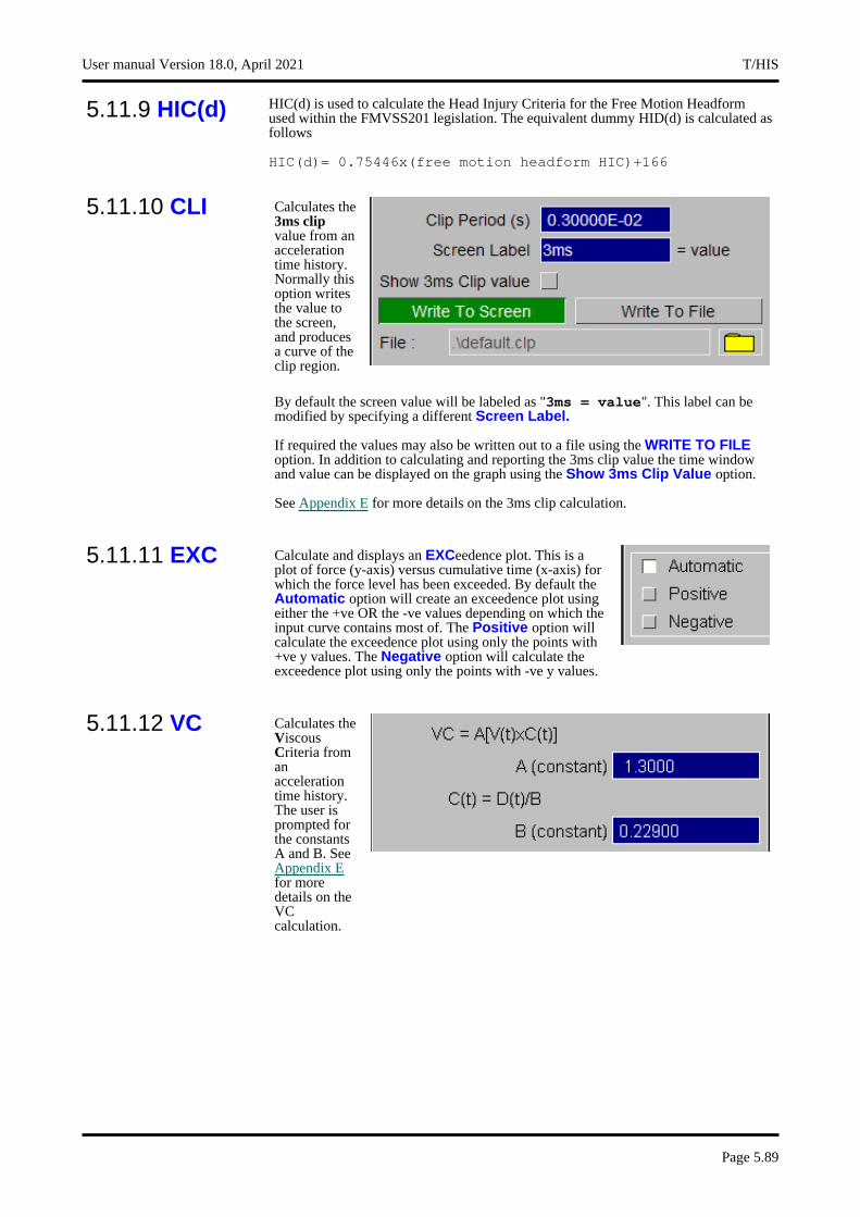
5.11.9 HIC(d) HIC(d) is used to calculate the Head Injury Criteria for the Free Motion Headform used within the FMVSS201 legislation. The equivalent dummy HID(d) is calculated as follows
HIC(d)= 0.75446x(free motion headform HIC)+166
5.11.10 CLI Calculates the 3ms clip value from an acceleration time history. Normally this option writes the value to the screen, and produces a curve of the clip region.
By default the screen value will be labeled as "3ms = value". This label can be modified by specifying a different Screen Label.
If required the values may also be written out to a file using the WRITE TO FILE option. In addition to calculating and reporting the 3ms clip value the time window and value can be displayed on the graph using the Show 3ms Clip Value option.
See Appendix E for more details on the 3ms clip calculation.
5.11.11 EXC Calculate and displays an EXCeedence plot. This is a plot of force (y-axis) versus cumulative time (x-axis) for which the force level has been exceeded. By default the Automatic option will create an exceedence plot using either the +ve OR the -ve values depending on which the input curve contains most of. The Positive option will calculate the exceedence plot using only the points with +ve y values. The Negative option will calculate the exceedence plot using only the points with -ve y values.
5.11.12 VC Calculates the Viscous Criteria from an acceleration time history. The user is prompted for the constants A and B. See Appendix Efor more details on the VC calculation.
User manual Version 18.0, April 2021 T/HIS
Page 5.89
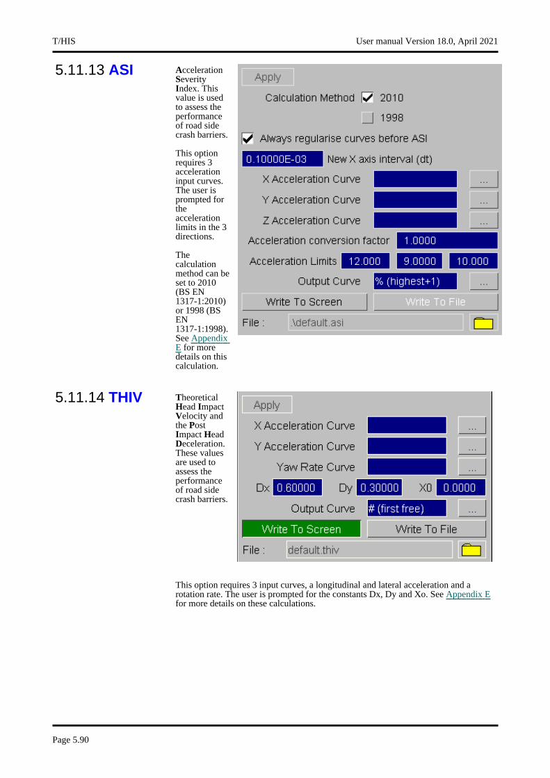
5.11.13 ASI Acceleration Severity Index. This value is used to assess the performance of road side crash barriers.
This option requires 3 acceleration input curves. The user is prompted for the acceleration limits in the 3 directions.
The calculation method can be set to 2010 (BS EN 1317-1:2010) or 1998 (BS EN 1317-1:1998). See AppendixE for more details on this calculation.
5.11.14 THIV Theoretical Head Impact Velocity and the Post Impact Head Deceleration. These values are used to assess the performance of road side crash barriers.
This option requires 3 input curves, a longitudinal and lateral acceleration and a rotation rate. The user is prompted for the constants Dx, Dy and Xo. See Appendix Efor more details on these calculations.
T/HIS User manual Version 18.0, April 2021
Page 5.90
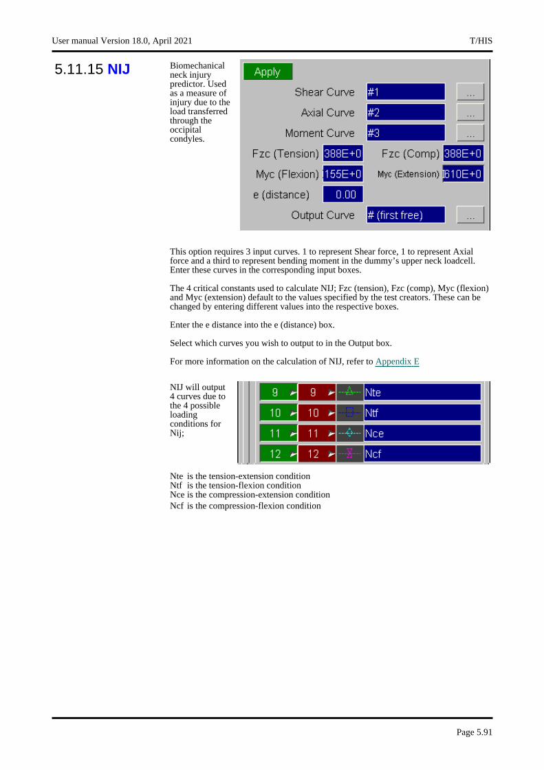
5.11.15 NIJ Biomechanical neck injury predictor. Used as a measure of injury due to the load transferred through the occipital condyles.
This option requires 3 input curves. 1 to represent Shear force, 1 to represent Axial force and a third to represent bending moment in the dummy’s upper neck loadcell. Enter these curves in the corresponding input boxes.
The 4 critical constants used to calculate NIJ; Fzc (tension), Fzc (comp), Myc (flexion) and Myc (extension) default to the values specified by the test creators. These can be changed by entering different values into the respective boxes.
Enter the e distance into the e (distance) box.
Select which curves you wish to output to in the Output box.
For more information on the calculation of NIJ, refer to Appendix E
NIJ will output 4 curves due to the 4 possible loading conditions for Nij;
Nte is the tension-extension conditionNtf is the tension-flexion conditionNce is the compression-extension conditionNcf is the compression-flexion condition
User manual Version 18.0, April 2021 T/HIS
Page 5.91

5.11.16 TTI Thorax Trauma Index:
This option requires 3 input curves. 1 to represent the Upper Rib Acceleration, 1 to represent the Lower Rib Acceleration and a third to represent the Lower Spine Acceleration. Enter these curves in the corresponding input boxes.
The output can either be written to the screen, appearing in a listing box, or written to a file specified in the File: input box, or both. If the write to screen tab is highlighted, the following window will appear:
For more information on the calculation of TTI, refer to Appendix E
5.11.17 NOR(y) Normalise the curve so that the Y values are within the range [ -1, +1].
5.11.18 NOR(x) Normalise the curve so that the X values are within the range [ -1, +1].
5.11.19 REG Make a curve have a constant time step.
It is necessary for a curve to have a constant time step between points for it to be filtered. This option takes an existing curve and prompts the user for a new time step. The points of the output curve are calculated by linear interpolation. Regularising a curve may alter its peak values, and could change filtered output slightly.
5.11.20 VEC Calculate the vector magnitude of three input curves.
5.11.21 VEC2D Calculate the vector magnitude of two input curves.
5.11.22 ACU Airbag Control Unit
This option evaluates the following equation:
T/HIS User manual Version 18.0, April 2021
Page 5.92
Where m = user defined offsetn = time to integrate over
5.11.23 COR1 Curve correlation function.
The Correlation function provides a measure of the degree to which two curves match. When comparing curves by eye, the quality of correlation may be judged on the basis of how well matched are the patterns of peaks, the overall shapes of the curves, etc, and can allow for differences of timing as well as magnitude. Thus a simple function based on the difference of Y-values (such as T/HIS ERR function) does not measure correlation in the same way as the human eye. The T/HIS correlation function attempts to include and quantify the more subtle ways in which the correlation of two curves may be judged.
The input parameters for the COR1 function have been chosen so as to produce a strict judgement of the correlation (see Appendix F for more details).
5.11.24 COR2 The COR2 function is the same as COR1 except the input parameters have been chosen so as to produce a less strict judgement of the correlation (see Appendix F for more details).
5.11.25 COR3 Another curve correlation function.
This function first normalises the curves using two factors either specified by the user or defaults calculated by the program (the maximum absolute X and Y values of both graphs). For each point on the first normalised curve, the shortest distance to the second normalised curve is calculated. The root mean square value of all these distances is subtracted from 1 and then multiplied by 100 to get an index between 0 and 100. The process is repeated along the second curve and the two indices are averaged to get a final index. The higher the index the closer the correlation between the two curves.
Note that the choice of normalising factors is important. Incorrect factors may lead to a correlation index outside the range of 0 to 100 (see Appendix F for more details).
5.11.26 WIF Weighted Integrated Factor (WIFAC) curve correlation function.
Compares curves using the Weighted Integrated Factor method (WIFAC). A value between 0 and 100 is calculated, the higher the index the closer the correlation between the two curves.
See Appendix F for more details.
User manual Version 18.0, April 2021 T/HIS
Page 5.93

5.12 SEISMIC Options
The SEISMIC menu is shown in the figure (right). T/HIS can be used to handle response spectra information. In particular, displacement, velocity or acceleration spectra can be read and converted to another format.
5.12.1 DV Displacement spectrum is converted to a velocity spectrum
5.12.2 DA Displacement spectrum is converted to an acceleration spectrum
5.12.3 VD Velocity spectrum is converted to a displacement spectrum
5.12.4 VA Velocity spectrum is converted to an acceleration spectrum
5.12.5 AD Acceleration spectrum is converted to a displacement spectrum
5.12.6 AV Acceleration spectrum is converted to a velocity spectrum.
5.12.7 DS Produce a design spectrum from a response spectrum through the specification of a broadening factor..
5.12.8 RS Produce a response spectrum from input accelerations. This gives the response of a damped single degree of freedom system, given its damping factor and period, to the input acceleration time-history.
5.12.9 FFT Perform a fast Fourier transform. Convert an input signal from the time to the frequency domain.
There are three options for output;• magnitude only• magnitude and phase• real and imaginary components of the time signal.
The frequency is calculated in Hz NOT radians/s if the time axis is in seconds.
T/HIS automatically adds points with zero y-value to the end of the curve to pad the curve out so that the number of points is increased to the next power of 2.
There are two options for scaling the curves output:• Scaling Option 1 - Consistent with other signal processing software giving a magnitude
independent of any padding. This is the default and recommended for most purposes. Performing an inverse FFT on the resulting curves will NOT get back exactly to the original curve if it did not have a number of points equal to a power of 2.
• Scaling Option 2 - With this option, applying an inverse FFT to the resulting curves will generate a curve the same as the original even if the original curve did not have a number of points equal to a power of 2. This is useful if users wish to create their own filters, where the filter characteristic is defined in the frequency domain.
An option to regularise the curve before performing the function is on by default. The spacing between points on the frequency axis of the resulting curve is determined by the time duration of the padded input curve; dx = 1.0/(time).
The highest frequency in the output curve is determined by the time interval of the input curve; F(max). = (#points)/dt
T/HIS User manual Version 18.0, April 2021
Page 5.94
5.12.10 IFFT Performs an inverse fast Fourier transform. Converts two input signals from the frequency to the time domain. The two input signals can be the magnitude and phase or real and imaginary components of the time signal.
NOTE: If an FFT using scaling option 1 is performed on a curve that does not have a number of points equal to a power of 2 and then an IFFT is performed on the resulting curves you will NOT get back exactly to the original curve. This is because the FFT and IFFT both scale their output curves by the number of points in the curve, which in this case will be different. For the FFT the number of points used to scale the curves is the original number of points before padding. For the IFFT the number of points used is the original number of points plus the points needed to make it a power of 2.
If the number of points in the original curve is a power of 2 and no padding is required, the IFFT of the resulting curves will get back to the original curve.
5.12.11 NCP
dddddddddddddddddddd
By default beam element plastic rotations are always written out by LS-DYNA as being increasing +ve (i.e. cumulative). This option allows a non-cumulative plastic rotation to be calculated by taking two input curves: the moment/time and the cumulative rotation/time histories for the beam in question.
5.12.12 BLC Baseline correction.
User manual Version 18.0, April 2021 T/HIS
Page 5.95
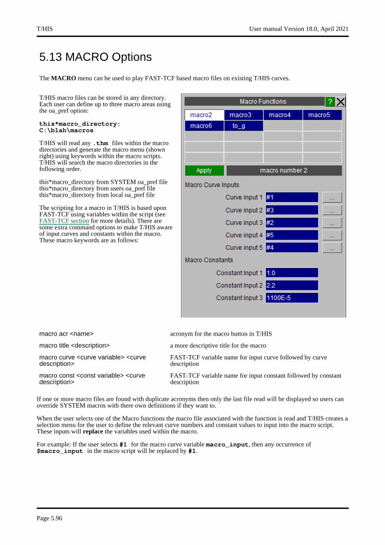
5.13 MACRO Options
The MACRO menu can be used to play FAST-TCF based macro files on existing T/HIS curves.
T/HIS macro files can be stored in any directory. Each user can define up to three macro areas using the oa_pref option:
this*macro_directory: C:\blah\macros
T/HIS will read any .thm files within the macro directories and generate the macro menu (shown right) using keywords within the macro scripts. T/HIS will search the macro directories in the following order.
this*macro_directory from SYSTEM oa_pref filethis*macro_directory from users oa_pref filethis*macro_directory from local oa_pref file
The scripting for a macro in T/HIS is based upon FAST-TCF using variables within the script (see FAST-TCF section for more details). There are some extra command options to make T/HIS aware of input curves and constants within the macro. These macro keywords are as follows:
macro acr <name> acronym for the macro button in T/HIS
macro title <description> a more descriptive title for the macro
macro curve <curve variable> <curve description>
FAST-TCF variable name for input curve followed by curve description
macro const <const variable> <curve description>
FAST-TCF variable name for input constant followed by constant description
If one or more macro files are found with duplicate acronyms then only the last file read will be displayed so users can override SYSTEM macros with there own definitions if they want to.
When the user selects one of the Macro functions the macro file associated with the function is read and T/HIS creates a selection menu for the user to define the relevant curve numbers and constant values to input into the macro script. These inputs will replace the variables used within the macro.
For example: If the user selects #1 for the macro curve variable macro_input, then any occurrence of $macro_input in the macro script will be replaced by #1.
T/HIS User manual Version 18.0, April 2021
Page 5.96

An example macro script follows. This macro asks the user for a filter option (e.g. c60, c600, c1000) and also an input curve number. The macro then filters the input curve and divides by 9810.
# Macro to convert a file to g after filtering#macro acr to_gmacro title filter and convert curve to gmacro curve macro_input input curvemacro const macro_filter filter to use# model none model 1 oper $macro_filter $macro_input tag filteredoper div filtered 9810.0
User manual Version 18.0, April 2021 T/HIS
Page 5.97

5.14 FAST-TCF Options
The FAST-TCF menu can be used to capture and playback FAST-TCF scripts. FAST-TCF is a simple and intuitive scripting language for T/HIS. See FAST-TCF (section 7) for more details and commands.
5.14.1 Create
T/HIS 9.2 onwards has the ability to automatically generate FAST-TCF scripts using the CREATE menu.
The FAST-TCF script will contain all of the commands required to1. Create and position multiple graphs on
pages.2. Extract the data from models or other files3. Carry out any curve operations required to
reproduce the chosen curves 4. Set any curve styles and labels5. Set plot attributes such as titles, axis labels,
colours, fonts and scaling6. Generate the output image and/or curve
file7. Generate curve groups8. Generate variable and tabular output
requests
Before generating the FAST-TCF script the following options can be set
T/HIS User manual Version 18.0, April 2021
Page 5.98
Generate For
All Pages The FAST-TCF script will contain all of the commands required to regenerate all of the pages that contain 1 or more graphs.
If the option to generate images is selected then the FAST-TCF script will contain the commands to generate multiple images with the page number appended to the filename specified.
Current Page The FAST-TCF script will contain all of the commands required to regenerate the currently displayed page.
Only Page (n) The FAST-TCF script will contain all of the commands required to regenerate the selected page.
All Graphs The FAST-TCF script will contain all of the commands required to regenerate all the currently defined graphs.
All of the graphs will be positioned on page 1 using the currently defined layout.
This option will only be available if T/HIS only contains a single page (see Section3.2).
All Active Graphs The FAST-TCF script will contain all of the commands required to regenerate all of the active graphs.
All of the graphs will be positioned on page 1 using the currently defined layout.
This option will only be available if T/HIS only contains a single page (see Section3.2).
Only Graph (n) The FAST-TCF script will contain all of the commands required to regenerate the selected graph.
The graph will be positioned on page 1.
FAST-TCF Script : Image Output
If this option is selected then the FAST-TCF script will contain the commands required to generate an image of each of the pages/graphs selected for output. The Image Format can be set to any of the supported image types (seeSection 5.8).
If the FAST-TCF script generates multiple pages then the Filename specified will be used for the first image. Subsequent images will use the specified filename with "_2", "_3" ... appended.
FAST-TCF Script : Curve Output
By default the FAST-TCF script will only contain the command needed to reproduce the curves that are unblanked in 1 or more of the graphs selected for output. This option can be used to select additional curves for which the commands required to generate them are also added to the FAST-TCF script. If a curve is selected that is also unblanked in one of the graphs the command to regenerate it are only added to the FAST-TCF script once.
In addition to selecting additional curves this option can also be used to add commands to the FAST-TCF script to write the additional curves out to a T/HIS .cur curve file.
FAST-TCF Script : Curve Group Output
This option can be used to select additional curves for output to the FAST-TCF script by curve group. If a curve is selected that is also unblanked in one of the graphs the command to regenerate it are only added to the FAST-TCF script once. This option will also add the commands to regenerate the selected curve groups to the FAST-TCF script.
FAST-TCF Script : Variable Output
This option can be used to define variable and tabular output requests for output to the FAST-TCF script via the menu launched by pressing the button. Variable and tabular output requests defined in a FAST-TCF script that is read in will appear in the menu.
User manual Version 18.0, April 2021 T/HIS
Page 5.99
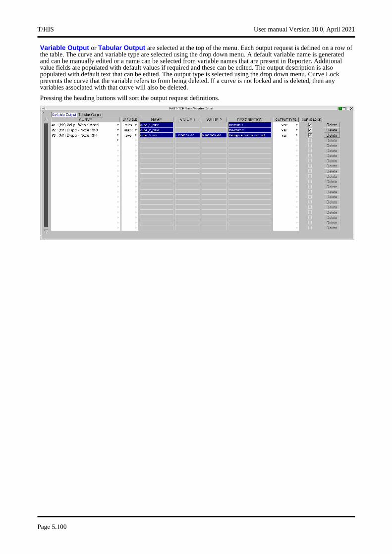
Variable Output or Tabular Output are selected at the top of the menu. Each output request is defined on a row of the table. The curve and variable type are selected using the drop down menu. A default variable name is generated and can be manually edited or a name can be selected from variable names that are present in Reporter. Additional value fields are populated with default values if required and these can be edited. The output description is also populated with default text that can be edited. The output type is selected using the drop down menu. Curve Lock prevents the curve that the variable refers to from being deleted. If a curve is not locked and is deleted, then any variables associated with that curve will also be deleted.
Pressing the heading buttons will sort the output request definitions.
T/HIS User manual Version 18.0, April 2021
Page 5.100
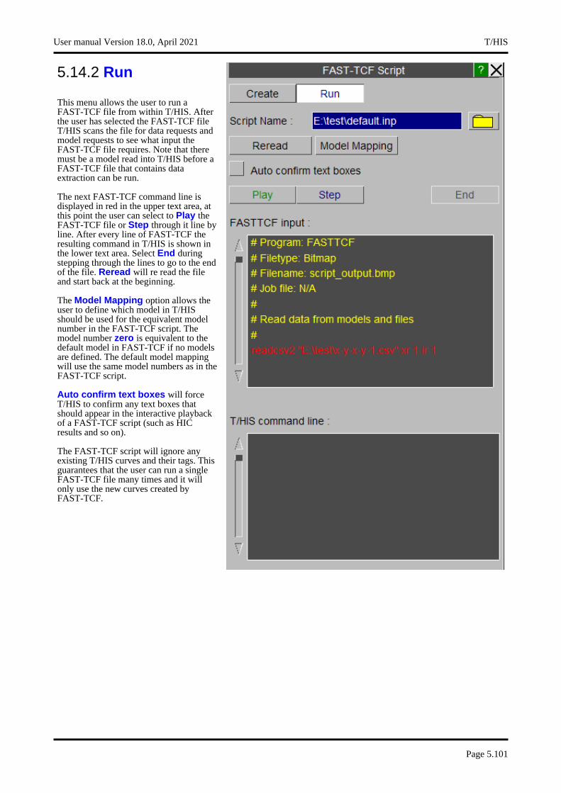
5.14.2 Run
This menu allows the user to run a FAST-TCF file from within T/HIS. After the user has selected the FAST-TCF file T/HIS scans the file for data requests and model requests to see what input the FAST-TCF file requires. Note that there must be a model read into T/HIS before a FAST-TCF file that contains data extraction can be run.
The next FAST-TCF command line is displayed in red in the upper text area, at this point the user can select to Play the FAST-TCF file or Step through it line by line. After every line of FAST-TCF the resulting command in T/HIS is shown in the lower text area. Select End during stepping through the lines to go to the end of the file. Reread will re read the file and start back at the beginning.
The Model Mapping option allows the user to define which model in T/HIS should be used for the equivalent model number in the FAST-TCF script. The model number zero is equivalent to the default model in FAST-TCF if no models are defined. The default model mapping will use the same model numbers as in the FAST-TCF script.
Auto confirm text boxes will force T/HIS to confirm any text boxes that should appear in the interactive playback of a FAST-TCF script (such as HIC results and so on).
The FAST-TCF script will ignore any existing T/HIS curves and their tags. This guarantees that the user can run a single FAST-TCF file many times and it will only use the new curves created by FAST-TCF.
User manual Version 18.0, April 2021 T/HIS
Page 5.101

5.15 TITLE/AXES/LEGEND Options
The TITLE/AXES menu is shown in the figure (right).
This menu controls the contents of the title and axes labels and the axis scaling.
The individual axis, title and legend menus can also be accessed by clicking over the appropriately highlighted area on the graph.
Changes to the TITLE/AXES/LEGEND options are only applied to active graphs (seeSection 3.5).
5.15.1 TITLE
The plot title may be set AUTOmatically or manually. When the AUTO option is selected the text box will display <automatic> and the plot title will be set to the title of the first curve that is currently being plotted. The plot title may be turned on and off by toggling the ON/OFF button.
Save Preferences to File
Launches a popup to quickly save preferences to the oa_pref file. See Section 6.6.1
T/HIS User manual Version 18.0, April 2021
Page 5.102
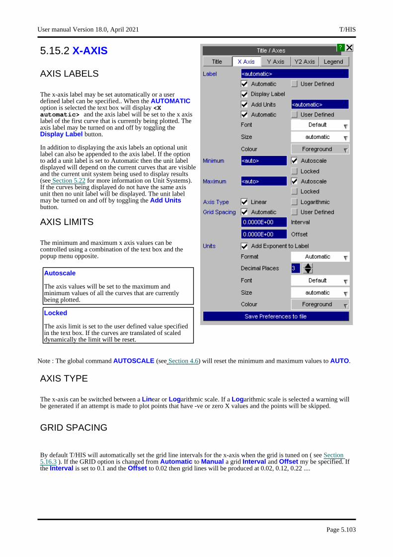
5.15.2 X-AXIS
AXIS LABELS
The x-axis label may be set automatically or a user defined label can be specified.. When the AUTOMATIC option is selected the text box will display <X automatic> and the axis label will be set to the x axis label of the first curve that is currently being plotted. The axis label may be turned on and off by toggling the Display Label button.
In addition to displaying the axis labels an optional unit label can also be appended to the axis label. If the option to add a unit label is set to Automatic then the unit label displayed will depend on the current curves that are visible and the current unit system being used to display results (see Section 5.22 for more information on Unit Systems). If the curves being displayed do not have the same axis unit then no unit label will be displayed. The unit label may be turned on and off by toggling the Add Units button.
AXIS LIMITS
The minimum and maximum x axis values can be controlled using a combination of the text box and the popup menu opposite.
Autoscale
The axis values will be set to the maximum and minimum values of all the curves that are currently being plotted.
Locked
The axis limit is set to the user defined value specified in the text box. If the curves are translated of scaled dynamically the limit will be reset.
Note : The global command AUTOSCALE (see Section 4.6) will reset the minimum and maximum values to AUTO.
AXIS TYPE
The x-axis can be switched between a Linear or Logarithmic scale. If a Logarithmic scale is selected a warning will be generated if an attempt is made to plot points that have -ve or zero X values and the points will be skipped.
GRID SPACING
By default T/HIS will automatically set the grid line intervals for the x-axis when the grid is tuned on ( see Section5.16.3 ). If the GRID option is changed from Automatic to Manual a grid Interval and Offset my be specified. If the Interval is set to 0.1 and the Offset to 0.02 then grid lines will be produced at 0.02, 0.12, 0.22 ....
User manual Version 18.0, April 2021 T/HIS
Page 5.103
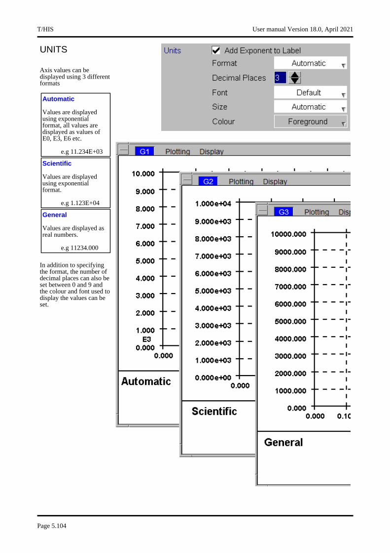
UNITS
Axis values can be displayed using 3 different formats
Automatic
Values are displayed using exponential format, all values are displayed as values of E0, E3, E6 etc.
e.g 11.234E+03
Scientific
Values are displayed using exponential format.
e.g 1.123E+04
General
Values are displayed as real numbers.
e.g 11234.000
In addition to specifying the format, the number of decimal places can also be set between 0 and 9 and the colour and font used to display the values can be set.
T/HIS User manual Version 18.0, April 2021
Page 5.104
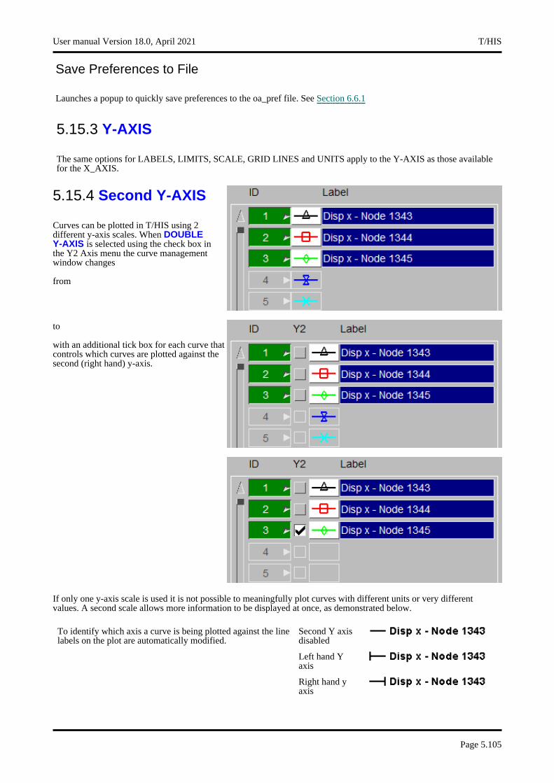
Save Preferences to File
Launches a popup to quickly save preferences to the oa_pref file. See Section 6.6.1
5.15.3 Y-AXIS
The same options for LABELS, LIMITS, SCALE, GRID LINES and UNITS apply to the Y-AXIS as those available for the X_AXIS.
5.15.4 Second Y-AXIS
Curves can be plotted in T/HIS using 2 different y-axis scales. When DOUBLE Y-AXIS is selected using the check box in the Y2 Axis menu the curve management window changes
from
to
with an additional tick box for each curve that controls which curves are plotted against the second (right hand) y-axis.
If only one y-axis scale is used it is not possible to meaningfully plot curves with different units or very different values. A second scale allows more information to be displayed at once, as demonstrated below.
Second Y axis disabled
To identify which axis a curve is being plotted against the line labels on the plot are automatically modified.
Left hand Y axis
Right hand y axis
User manual Version 18.0, April 2021 T/HIS
Page 5.105
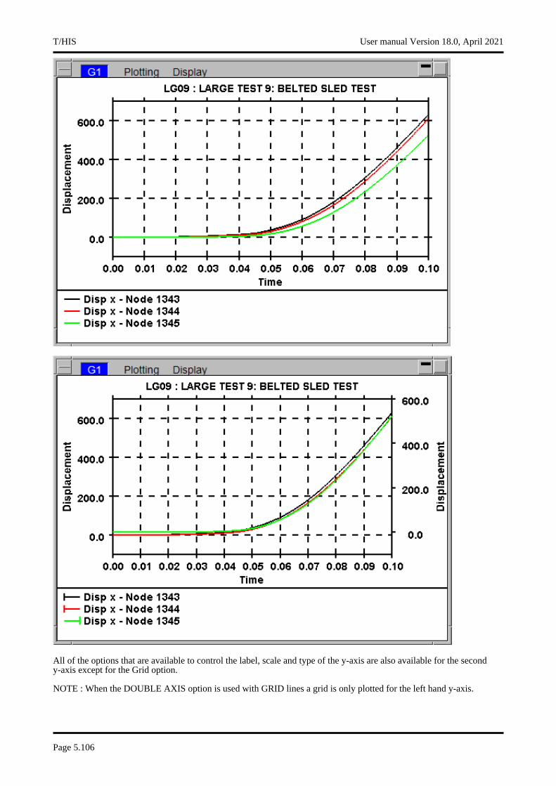
All of the options that are available to control the label, scale and type of the y-axis are also available for the second y-axis except for the Grid option.
NOTE : When the DOUBLE AXIS option is used with GRID lines a grid is only plotted for the left hand y-axis.
T/HIS User manual Version 18.0, April 2021
Page 5.106
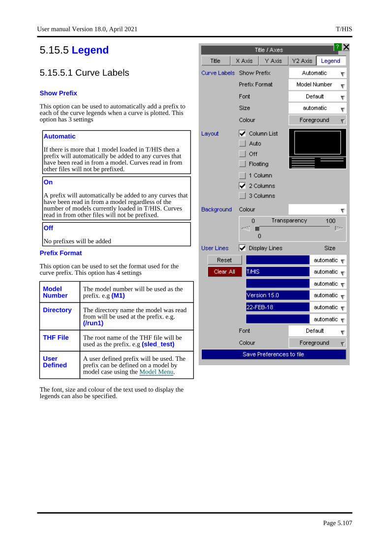
5.15.5 Legend
5.15.5.1 Curve Labels
Show Prefix
This option can be used to automatically add a prefix to each of the curve legends when a curve is plotted. This option has 3 settings
Automatic
If there is more that 1 model loaded in T/HIS then a prefix will automatically be added to any curves that have been read in from a model. Curves read in from other files will not be prefixed.
On
A prefix will automatically be added to any curves that have been read in from a model regardless of the number of models currently loaded in T/HIS. Curves read in from other files will not be prefixed.
Off
No prefixes will be added
Prefix Format
This option can be used to set the format used for the curve prefix. This option has 4 settings
Model Number
The model number will be used as the prefix. e.g (M1)
Directory The directory name the model was read from will be used at the prefix. e.g. (/run1)
THF File The root name of the THF file will be used as the prefix. e.g (sled_test)
User Defined
A user defined prefix will be used. The prefix can be defined on a model by model case using the Model Menu.
The font, size and colour of the text used to display the legends can also be specified.
User manual Version 18.0, April 2021 T/HIS
Page 5.107
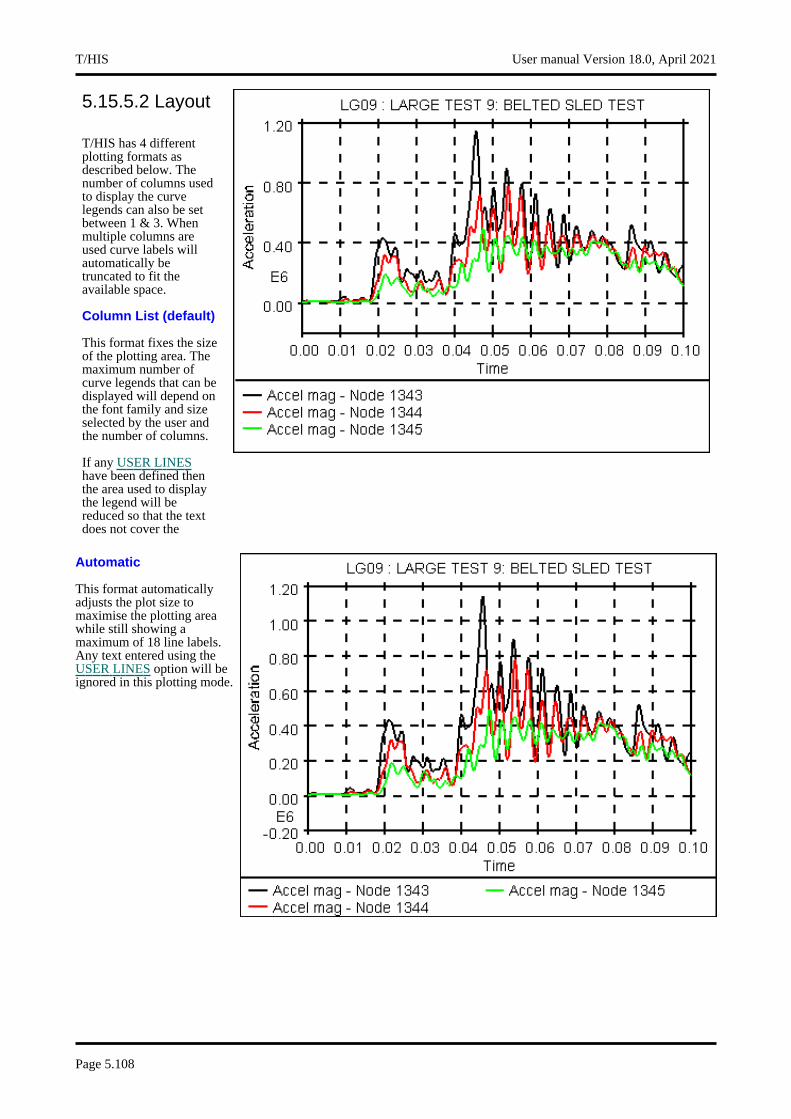
5.15.5.2 Layout
T/HIS has 4 different plotting formats as described below. The number of columns used to display the curve legends can also be set between 1 & 3. When multiple columns are used curve labels will automatically be truncated to fit the available space.
Column List (default)
This format fixes the size of the plotting area. The maximum number of curve legends that can be displayed will depend on the font family and size selected by the user and the number of columns.
If any USER LINEShave been defined then the area used to display the legend will be reduced so that the text does not cover the
Automatic
This format automatically adjusts the plot size to maximise the plotting area while still showing a maximum of 18 line labels. Any text entered using the USER LINES option will be ignored in this plotting mode.
T/HIS User manual Version 18.0, April 2021
Page 5.108
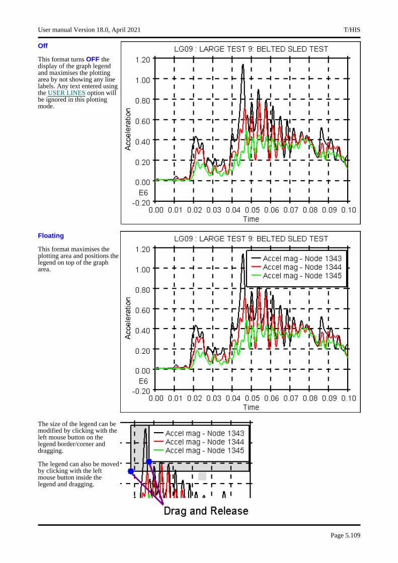
Off
This format turns OFF the display of the graph legend and maximises the plotting area by not showing any line labels. Any text entered using the USER LINES option will be ignored in this plotting mode.
Floating
This format maximises the plotting area and positions the legend on top of the graph area.
The size of the legend can be modified by clicking with the left mouse button on the legend border/corner and dragging.
The legend can also be moved by clicking with the left mouse button inside the legend and dragging.
User manual Version 18.0, April 2021 T/HIS
Page 5.109

5.15.5.3 BACKGROUND
This option can be used to alter the default background colour of the floating legend. By default the colour will be the same as the backgorund colour of the graph. As well as setting a different background colour for the floating legend a %age transparency can also be specified if the legend obscures any curves
5.15.5.4 USER LINES
This option can be used to alter the default text that appears on the bottom right-hand corner of each plot. Text can be typed into any of the panels or they can be left blank. The Size of the text may be altered. If no text is specified the area used by the curve legends will be increased.
The default values are read from the "preferences" file (see Appendix H for more details).
5.15.5.5 Save Preferences to File
Launches a popup to quickly save preferences to the oa_pref file. See Section 6.6.1
T/HIS User manual Version 18.0, April 2021
Page 5.110
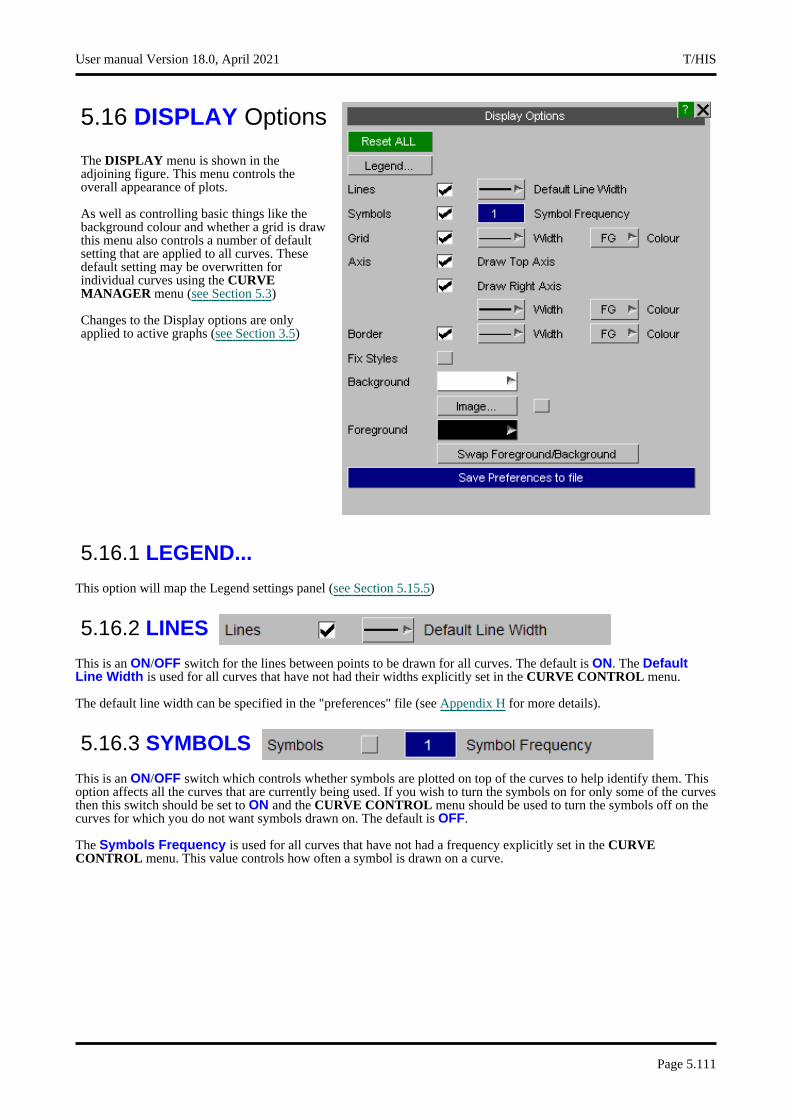
5.16 DISPLAY Options
The DISPLAY menu is shown in the adjoining figure. This menu controls the overall appearance of plots.
As well as controlling basic things like the background colour and whether a grid is draw this menu also controls a number of default setting that are applied to all curves. These default setting may be overwritten for individual curves using the CURVE MANAGER menu (see Section 5.3)
Changes to the Display options are only applied to active graphs (see Section 3.5)
5.16.1 LEGEND...
This option will map the Legend settings panel (see Section 5.15.5)
5.16.2 LINES
This is an ON/OFF switch for the lines between points to be drawn for all curves. The default is ON. The Default Line Width is used for all curves that have not had their widths explicitly set in the CURVE CONTROL menu.
The default line width can be specified in the "preferences" file (see Appendix H for more details).
5.16.3 SYMBOLS
This is an ON/OFF switch which controls whether symbols are plotted on top of the curves to help identify them. This option affects all the curves that are currently being used. If you wish to turn the symbols on for only some of the curves then this switch should be set to ON and the CURVE CONTROL menu should be used to turn the symbols off on the curves for which you do not want symbols drawn on. The default is OFF.
The Symbols Frequency is used for all curves that have not had a frequency explicitly set in the CURVE CONTROL menu. This value controls how often a symbol is drawn on a curve.
User manual Version 18.0, April 2021 T/HIS
Page 5.111
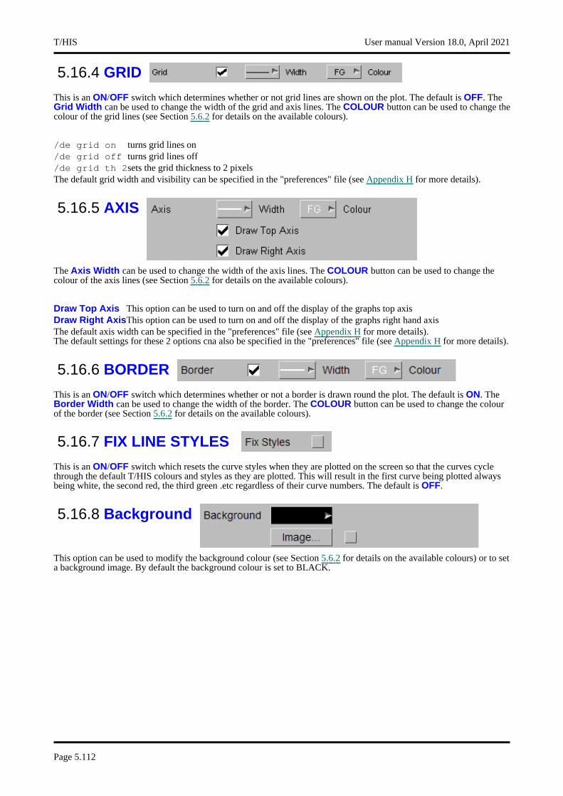
5.16.4 GRID
This is an ON/OFF switch which determines whether or not grid lines are shown on the plot. The default is OFF. The Grid Width can be used to change the width of the grid and axis lines. The COLOUR button can be used to change the colour of the grid lines (see Section 5.6.2 for details on the available colours).
/de grid on turns grid lines on/de grid off turns grid lines off/de grid th 2sets the grid thickness to 2 pixelsThe default grid width and visibility can be specified in the "preferences" file (see Appendix H for more details).
5.16.5 AXIS
The Axis Width can be used to change the width of the axis lines. The COLOUR button can be used to change the colour of the axis lines (see Section 5.6.2 for details on the available colours).
Draw Top Axis This option can be used to turn on and off the display of the graphs top axisDraw Right AxisThis option can be used to turn on and off the display of the graphs right hand axisThe default axis width can be specified in the "preferences" file (see Appendix H for more details). The default settings for these 2 options cna also be specified in the "preferences" file (see Appendix H for more details).
5.16.6 BORDER
This is an ON/OFF switch which determines whether or not a border is drawn round the plot. The default is ON. The Border Width can be used to change the width of the border. The COLOUR button can be used to change the colour of the border (see Section 5.6.2 for details on the available colours).
5.16.7 FIX LINE STYLES
This is an ON/OFF switch which resets the curve styles when they are plotted on the screen so that the curves cycle through the default T/HIS colours and styles as they are plotted. This will result in the first curve being plotted always being white, the second red, the third green .etc regardless of their curve numbers. The default is OFF.
5.16.8 Background
This option can be used to modify the background colour (see Section 5.6.2 for details on the available colours) or to set a background image. By default the background colour is set to BLACK.
T/HIS User manual Version 18.0, April 2021
Page 5.112

Image
The IMAGE option can be used to display a background image behind a graph instead of a solid background colour.
If the image dimensions do not match the graph window dimensions then the image can be scaled to fit or it can be tiled.
User manual Version 18.0, April 2021 T/HIS
Page 5.113
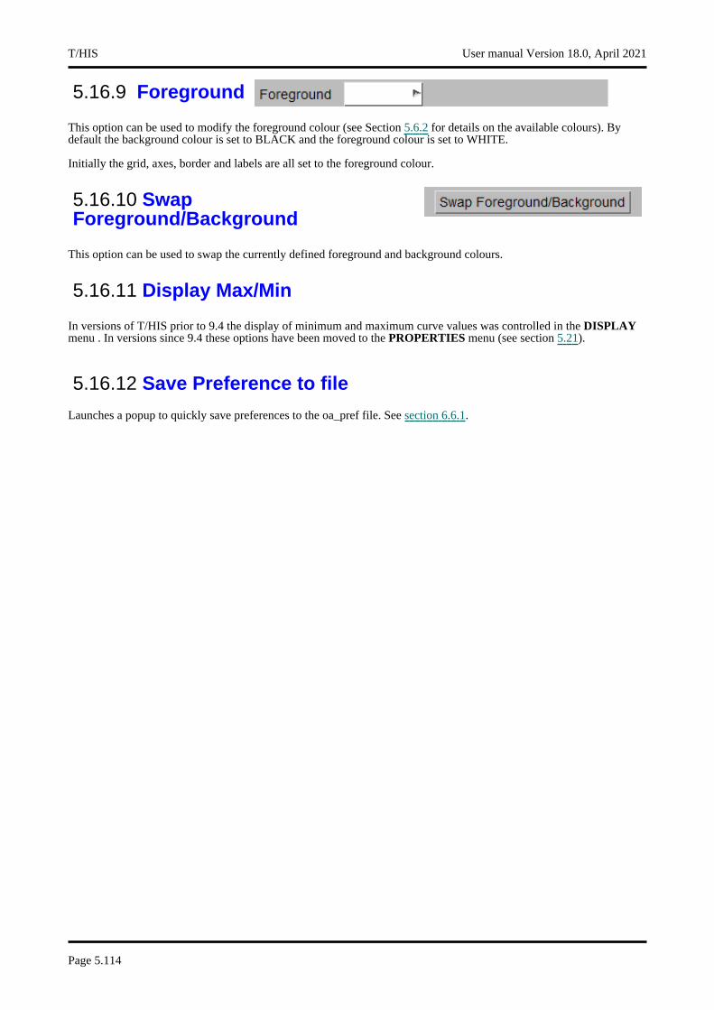
5.16.9 Foreground
This option can be used to modify the foreground colour (see Section 5.6.2 for details on the available colours). By default the background colour is set to BLACK and the foreground colour is set to WHITE.
Initially the grid, axes, border and labels are all set to the foreground colour.
5.16.10 Swap Foreground/Background
This option can be used to swap the currently defined foreground and background colours.
5.16.11 Display Max/Min
In versions of T/HIS prior to 9.4 the display of minimum and maximum curve values was controlled in the DISPLAY menu . In versions since 9.4 these options have been moved to the PROPERTIES menu (see section 5.21).
5.16.12 Save Preference to file
Launches a popup to quickly save preferences to the oa_pref file. See section 6.6.1.
T/HIS User manual Version 18.0, April 2021
Page 5.114
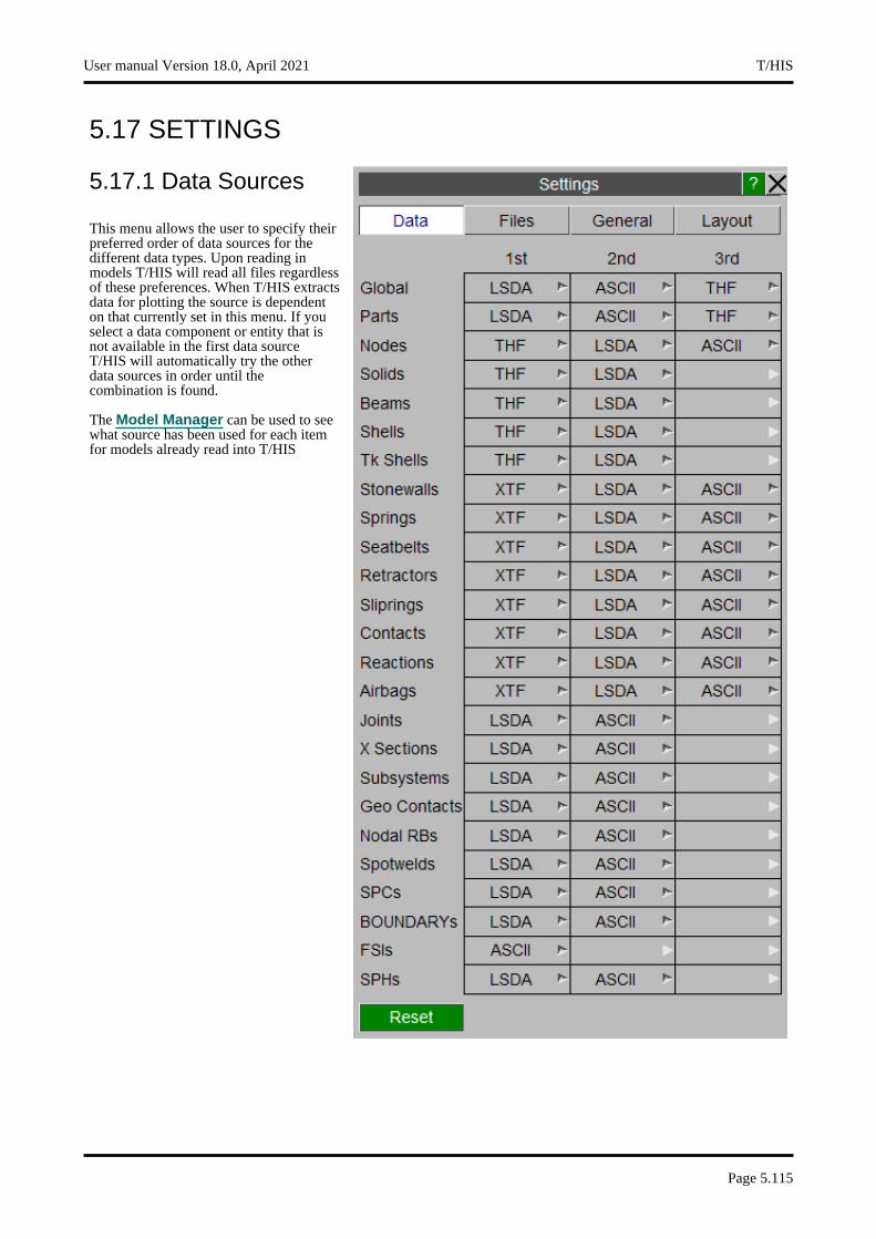
5.17 SETTINGS
5.17.1 Data Sources
This menu allows the user to specify their preferred order of data sources for the different data types. Upon reading in models T/HIS will read all files regardless of these preferences. When T/HIS extracts data for plotting the source is dependent on that currently set in this menu. If you select a data component or entity that is not available in the first data source T/HIS will automatically try the other data sources in order until the combination is found.
The Model Manager can be used to see what source has been used for each item for models already read into T/HIS
User manual Version 18.0, April 2021 T/HIS
Page 5.115

5.17.2 Files
File Names By default the file filters in T/HIS are set to look for the file naming convention set for the LS-DYNA output files by the SHELL. This option can be used to swap the file filters back to the default LSTC naming convention. This option can be set in the Preference File
File type ARUP LSTC
Time history "job".thf d3thdt
Extra Time history "job".xtf xtfile
File Output The HIC, 3ms Clip, ASI,THIV, TTIAutomotive injury criteria functions and ERR operator function can all send their output to a file as well as to the screen. These options can be used to select which functions send output to a file and to specify a Root Filename that is used for all of the output files. The Root Filename can be set in the Preference File
T/HIS User manual Version 18.0, April 2021
Page 5.116
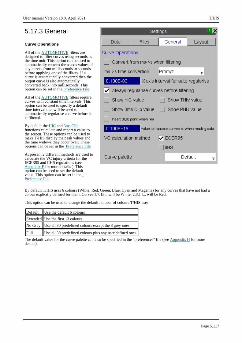
5.17.3 General
Curve Operations
All of the AUTOMOTIVE filters are designed to filter curves using seconds as the time unit. This option can be used to automatically convert the x-axis values of any curves from milliseconds to seconds before applying one of the filters. If a curve is automatically converted then the output curve is also automatically converted back into milliseconds. This option can be set in the Preference File
All of the AUTOMOTIVE filters require curves with constant time intervals. This option can be used to specify a default time interval that will be used to automatically regularise a curve before it is filtered.
By default the HIC and 3ms Clipfunctions calculate and report a value to the screen. These options can be used to make T/HIS display the peak values and the time widows they occur over. These options can be set in the Preference File
At present 2 different methods are used to calculate the VC injury criteria for the ECER95 and IIHS regulations (see Appendix E for more details ). This option can be used to set the default value. This option can be set in the Preference File
By default T/HIS uses 6 colours (White, Red, Green, Blue, Cyan and Magenta) for any curves that have not had a colour explicitly defined for them. Curves 1,7,13... will be White, 2,8,14... will be Red.
This option can be used to change the default number of colours T/HIS uses.
Default Use the default 6 colours
Extended Use the first 13 colours
No Grey Use all 30 predefined colours except the 3 grey ones
Full Use all 30 predefined colours plus any user defined ones.
The default value for the curve palette can also be specified in the "preferences" file (see Appendix H for more details).
User manual Version 18.0, April 2021 T/HIS
Page 5.117
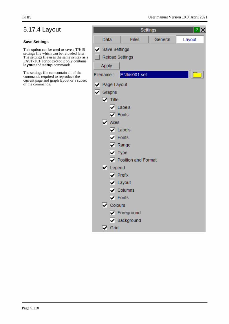
5.17.4 Layout
Save Settings
This option can be used to save a T/HIS settings file which can be reloaded later. The settings file uses the same syntax as a FAST-TCF script except it only contains layout and setup commands.
The settings file can contain all of the commands required to reproduce the current page and graph layout or a subset of the commands.
T/HIS User manual Version 18.0, April 2021
Page 5.118

Reload Settings
This option can be used to reload a previously saved settings file. In addition to reloading a file interactively a settings file can also be specified on the commandline
-set=filename
or via the Preference File
this*settings_file: filename
User manual Version 18.0, April 2021 T/HIS
Page 5.119
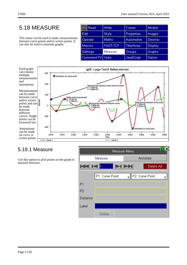
5.18 MEASURE
This menu can be used to make measurements between curve points and/or screen points. It can also be used to annotate graphs.
Each graph can contain multiple measurements and annotations.
Measurements can be made between curve and/or screen points and can be made between different curves. Single points can be measured too.
Annotations can be made on curve or screen points.
5.18.1 Measure
Use this option to pick points on the graph to measure between.
T/HIS User manual Version 18.0, April 2021
Page 5.120
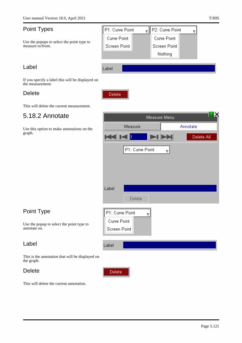
Point Types
Use the popups to select the point type to measure to/from.
Label
If you specify a label this will be displayed on the measurement.
Delete
This will delete the current measurement.
5.18.2 Annotate
Use this option to make annotations on the graph.
Point Type
Use the popup to select the point type to annotate on.
Label
This is the annotation that will be displayed on the graph.
Delete
This will delete the current annotation.
User manual Version 18.0, April 2021 T/HIS
Page 5.121
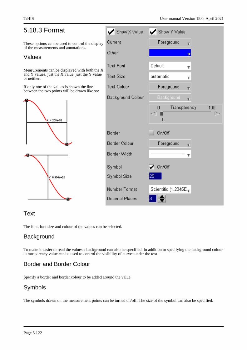
5.18.3 Format
These options can be used to control the display of the measurements and annotations.
Values
Measurements can be displayed with both the X and Y values, just the X value, just the Y value or neither.
If only one of the values is shown the line between the two points will be drawn like so:
Text
The font, font size and colour of the values can be selected.
Background
To make it easier to read the values a background can also be specified. In addition to specifying the background colour a transparency value can be used to control the visibility of curves under the text.
Border and Border Colour
Specify a border and border colour to be added around the value.
Symbols
The symbols drawn on the measurement points can be turned on/off. The size of the symbol can also be specified.
T/HIS User manual Version 18.0, April 2021
Page 5.122

Number Format
Specify the format of the values displayed on the graph.
User manual Version 18.0, April 2021 T/HIS
Page 5.123
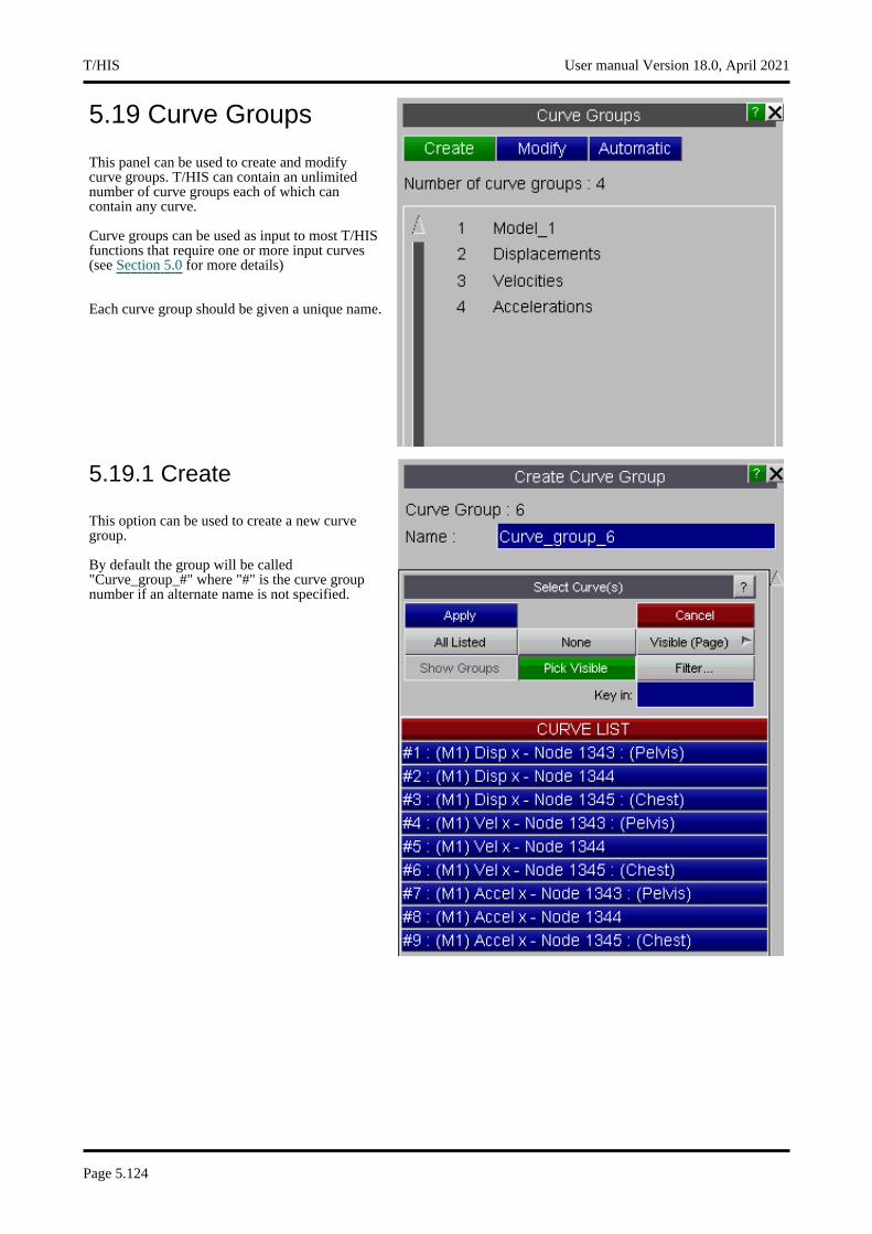
5.19 Curve Groups
This panel can be used to create and modify curve groups. T/HIS can contain an unlimited number of curve groups each of which can contain any curve.
Curve groups can be used as input to most T/HIS functions that require one or more input curves (see Section 5.0 for more details)
Each curve group should be given a unique name.
5.19.1 Create
This option can be used to create a new curve group.
By default the group will be called "Curve_group_#" where "#" is the curve group number if an alternate name is not specified.
T/HIS User manual Version 18.0, April 2021
Page 5.124

5.19.2 Modify
This option can be used to modify the contents of an existing curve group or it’s name.
When a curve group is selected any curves that are already defined in the group are highlighted in the curve list.
The contents of Automatic curves groups can not be modified as T/HIS automatically adds and removes curves from automatic groups.
Curves that belong to an automatic curve group are highlighted in yellow.
The name of an automatic curve group can be changed.
User manual Version 18.0, April 2021 T/HIS
Page 5.125
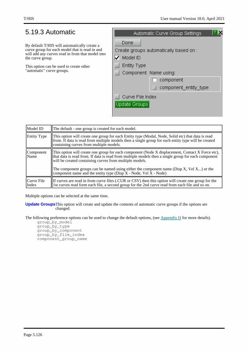
5.19.3 Automatic
By default T/HIS will automatically create a curve group for each model that is read in and will add any curves read in from that model into the curve group.
This option can be used to create other "automatic" curve groups.
Model ID The default - one group is created for each model.
Entity Type This option will create one group for each Entity type (Modal, Node, Solid etc) that data is read from. If data is read from multiple models then a single group for each entity type will be created containing curves from multiple models.
Component Name
This option will create one group for each component (Node X displacement, Contact X Force etc), that data is read from. If data is read from multiple models then a single group for each component will be created containing curves from multiple models.
The component groups can be named using either the component name (Disp X, Vel X...) or the component name and the entity type (Disp X - Node, Vel X - Node)
Curve File Index
If curves are read in from curve files (.CUR or CSV) then this option will create one group for the 1st curves read form each file, a second group for the 2nd curve read from each file and so on.
Multiple options can be selected at the same time.
Update GroupsThis option will create and update the contents of automatic curve groups if the options are changed.
The following preference options can be used to change the default options, (see Appendix H for more details). group_by_modelgroup_by_typegroup_by_componentgroup_by_file_indexcomponent_group_name
T/HIS User manual Version 18.0, April 2021
Page 5.126
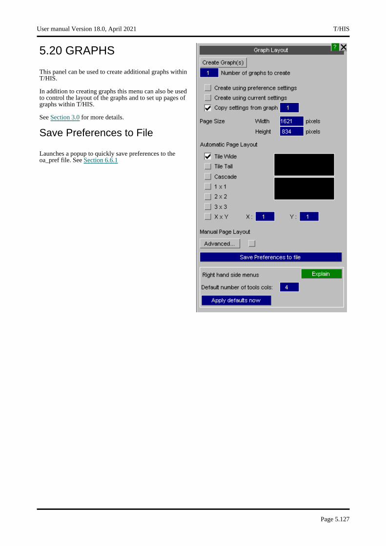
5.20 GRAPHS
This panel can be used to create additional graphs within T/HIS.
In addition to creating graphs this menu can also be used to control the layout of the graphs and to set up pages of graphs within T/HIS.
See Section 3.0 for more details.
Save Preferences to File
Launches a popup to quickly save preferences to the oa_pref file. See Section 6.6.1
User manual Version 18.0, April 2021 T/HIS
Page 5.127

5.21 PROPERTIES
This menu can be used to display additional curves properties.
Minimum and maximum curve values can be highlighted for each curve and the value can also be displayed.
In addition to displaying the value on the curve the values can also be added automatically to the curve label in the graph legend.
5.21.1 Curves
Curves (Off)
This option will turn off the display of all minimum and maximum values.
T/HIS User manual Version 18.0, April 2021
Page 5.128

Curves (Summary)
This option will display a single minimum/maximum value from all curves currently displayed..
The following properties can be displayed
Maximum value
Mark the maximum value with a cross
Display Maximum
Display the maximum value
Minimum value
Mark the minimum value with a cross
Display Minimum
Display the minimum value
Curves (All curves)
This option can be used to select the properties that are displayed for each individual curve.
When this option is selected the display of injury criteria (HIC,HICd etc) for curves can also be selected.
User manual Version 18.0, April 2021 T/HIS
Page 5.129
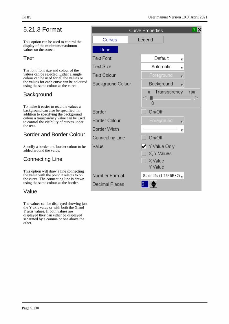
5.21.3 Format
This option can be used to control the display of the minimum/maximum values on the screen.
Text
The font, font size and colour of the values can be selected. Either a single colour can be used for all the values or the values for each curve can be coloured using the same colour as the curve.
Background
To make it easier to read the values a background can also be specified. In addition to specifying the background colour a transparency value can be used to control the visibility of curves under the text.
Border and Border Colour
Specify a border and border colour to be added around the value.
Connecting Line
This option will draw a line connecting the value with the point it relates to on the curve. The connecting line is drawn using the same colour as the border.
Value
The values can be displayed showing just the Y axis value or with both the X and Y axis values. If both values are displayed they can either be displayed separated by a comma or one above the other.
T/HIS User manual Version 18.0, April 2021
Page 5.130

Number Format
The values can be displayed using 3 different formats
Automatic Values are displayed using exponential format, all values are displayed as values of E0, E3, E6 etc.
e.g 11.234E+03
Scientific Values are displayed using exponential format.
e.g 1.123E+04
General Values are displayed as real numbers.
e.g 11234.000
Decimal Places
In addition to specifying the format, the number of decimal places can also be set between 0 and 9.
5.21.3 Legend
This option can be used to automatically added curve properties to the curve labels in the legend area.
The following curve properties can be added to each curve label
Maximum valueMinimum valueAverage valueInjury Criteria (HIC, HICd etc)
Other options
Off Turns off the display of curve properties in the legend
Append Add the values to the same line as the curve labels in the legend
2nd Line
Display the values using a second line for each curve in the legend
The format of the numbers added to the curve labels is the same as that used to display values on the curves.
User manual Version 18.0, April 2021 T/HIS
Page 5.131
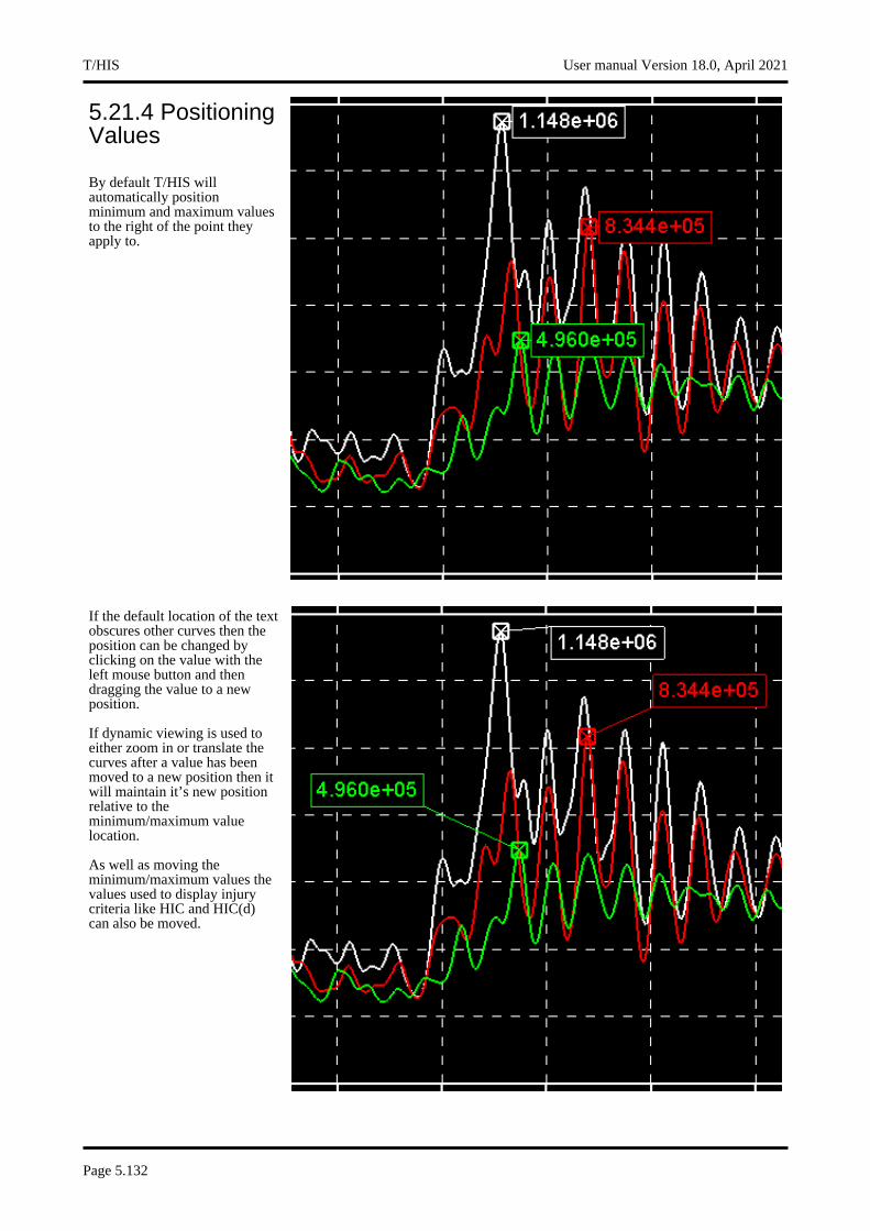
5.21.4 Positioning Values
By default T/HIS will automatically position minimum and maximum values to the right of the point they apply to.
If the default location of the text obscures other curves then the position can be changed by clicking on the value with the left mouse button and then dragging the value to a new position.
If dynamic viewing is used to either zoom in or translate the curves after a value has been moved to a new position then it will maintain it’s new position relative to the minimum/maximum value location.
As well as moving the minimum/maximum values the values used to display injury criteria like HIC and HIC(d) can also be moved.
T/HIS User manual Version 18.0, April 2021
Page 5.132
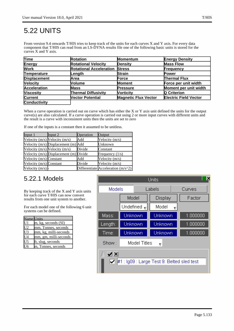
5.22 UNITS
From version 9.4 onwards T/HIS tries to keep track of the units for each curves X and Y axis. For every data component that T/HIS can read from an LS-DYNA results file one of the following basic units is stored for the curves X and Y axis.
Time Rotation Momentum Energy Density Energy Rotational Velocity Density Mass Flow Work Rotational Acceleration Stress Frequency Temperature Length Strain Power Displacement Area Force Thermal Flux Velocity Volume Moment Force per unit width Acceleration Mass Pressure Moment per unit width Viscosity Thermal Diffusivity Vorticity Q Criterion Current Vector Potential Magnetic Flux Vector Electric Field Vector Conductivity
When a curve operation is carried out on curve which has either the X or Y axis unit defined the units for the output curve(s) are also calculated. If a curve operation is carried out using 2 or more input curves with different units and the result is a curve with inconsistent units then the units are set to zero
If one of the inputs is a constant then it assumed to be unitless.
Input 1 Input 2 Operation Output Velocity (m/s) Velocity (m/s) Add Velocity (m/s) Velocity (m/s) Displacement (m) Add Unknown Velocity (m/s) Velocity (m/s) Divide Constant Velocity (m/s) Displacement (m) Divide Frequency (1/s) Velocity (m/s) Constant Add Velocity (m/s) Velocity (m/s) Constant Divide Velocity (m/s) Velocity (m/s) - Differentiate Acceleration (m/s^2)
5.22.1 Models
By keeping track of the X and Y axis units for each curve T/HIS can now convert results from one unit system to another.
For each model one of the following 6 unit systems can be defined.
Name Units U1 m, kg, seconds (SI) U2 mm, Tonnes, seconds U3 mm, kg, milli-seconds U4 mm, gm, milli-seconds U5 ft, slug, seconds U6 m, Tonnes, seconds
User manual Version 18.0, April 2021 T/HIS
Page 5.133
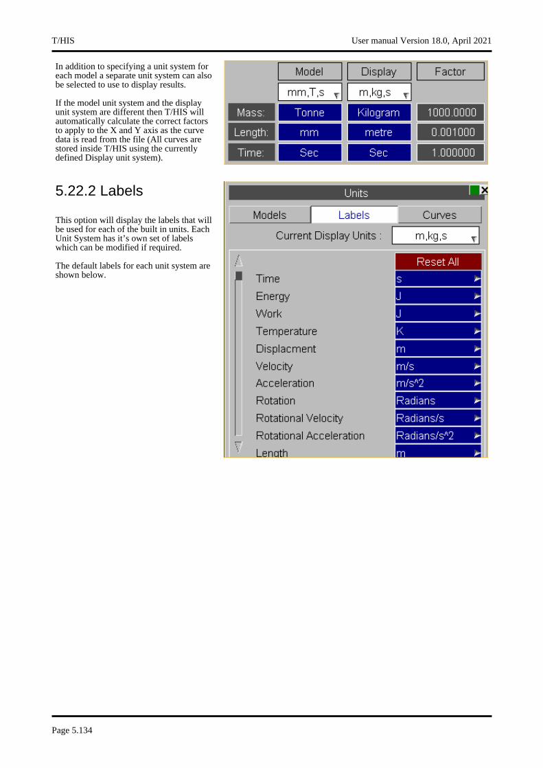
In addition to specifying a unit system for each model a separate unit system can also be selected to use to display results.
If the model unit system and the display unit system are different then T/HIS will automatically calculate the correct factors to apply to the X and Y axis as the curve data is read from the file (All curves are stored inside T/HIS using the currently defined Display unit system).
5.22.2 Labels
This option will display the labels that will be used for each of the built in units. Each Unit System has it’s own set of labels which can be modified if required.
The default labels for each unit system are shown below.
T/HIS User manual Version 18.0, April 2021
Page 5.134
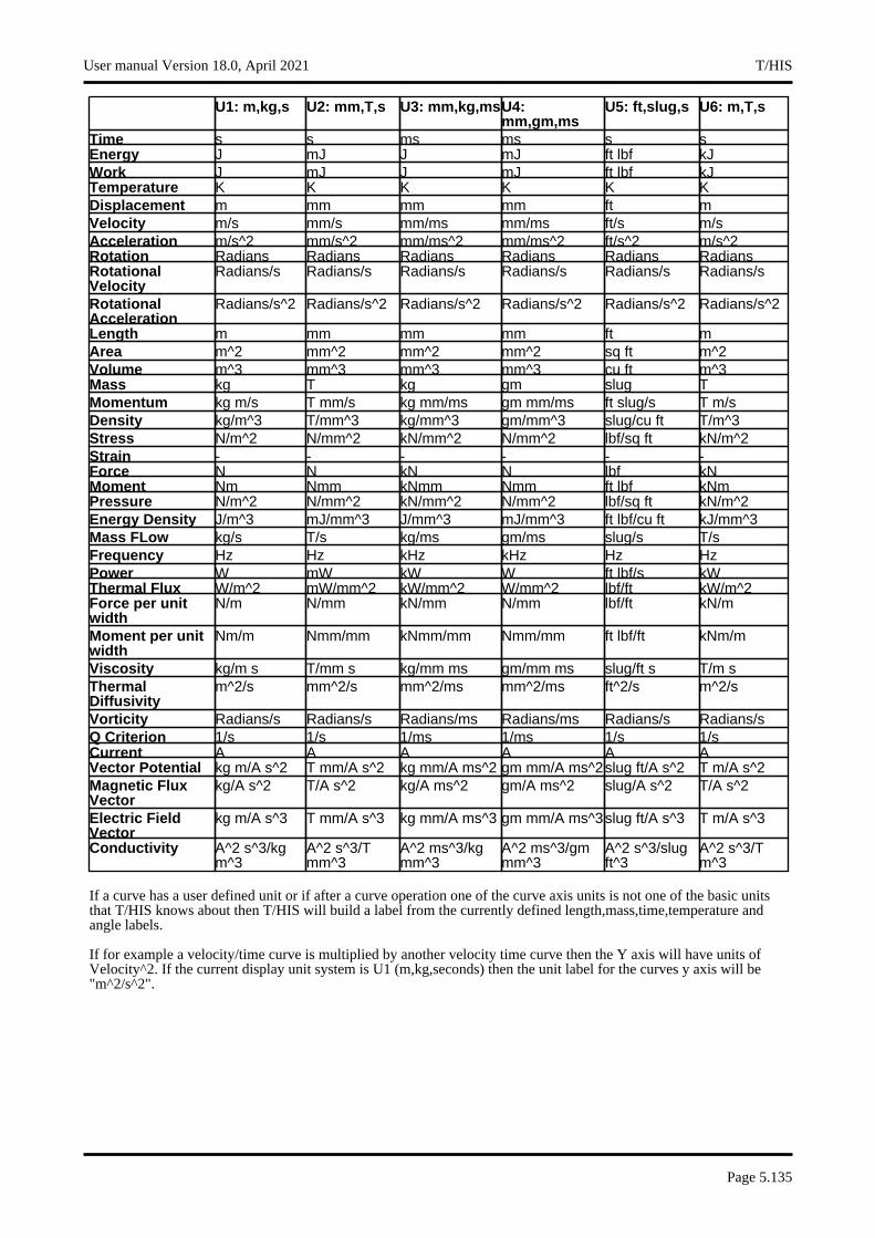
U1: m,kg,s U2: mm,T,s U3: mm,kg,ms U4: mm,gm,ms
U5: ft,slug,s U6: m,T,s
Time s s ms ms s s Energy J mJ J mJ ft lbf kJ Work J mJ J mJ ft lbf kJ Temperature K K K K K K Displacement m mm mm mm ft m Velocity m/s mm/s mm/ms mm/ms ft/s m/s Acceleration m/s^2 mm/s^2 mm/ms^2 mm/ms^2 ft/s^2 m/s^2 Rotation Radians Radians Radians Radians Radians Radians Rotational Velocity
Radians/s Radians/s Radians/s Radians/s Radians/s Radians/s
Rotational Acceleration
Radians/s^2 Radians/s^2 Radians/s^2 Radians/s^2 Radians/s^2 Radians/s^2
Length m mm mm mm ft m Area m^2 mm^2 mm^2 mm^2 sq ft m^2 Volume m^3 mm^3 mm^3 mm^3 cu ft m^3 Mass kg T kg gm slug T Momentum kg m/s T mm/s kg mm/ms gm mm/ms ft slug/s T m/s Density kg/m^3 T/mm^3 kg/mm^3 gm/mm^3 slug/cu ft T/m^3 Stress N/m^2 N/mm^2 kN/mm^2 N/mm^2 lbf/sq ft kN/m^2 Strain - - - - - - Force N N kN N lbf kN Moment Nm Nmm kNmm Nmm ft lbf kNm Pressure N/m^2 N/mm^2 kN/mm^2 N/mm^2 lbf/sq ft kN/m^2 Energy Density J/m^3 mJ/mm^3 J/mm^3 mJ/mm^3 ft lbf/cu ft kJ/mm^3 Mass FLow kg/s T/s kg/ms gm/ms slug/s T/s Frequency Hz Hz kHz kHz Hz Hz Power W mW kW W ft lbf/s kW Thermal Flux W/m^2 mW/mm^2 kW/mm^2 W/mm^2 lbf/ft kW/m^2 Force per unit width
N/m N/mm kN/mm N/mm lbf/ft kN/m
Moment per unit width
Nm/m Nmm/mm kNmm/mm Nmm/mm ft lbf/ft kNm/m
Viscosity kg/m s T/mm s kg/mm ms gm/mm ms slug/ft s T/m s Thermal Diffusivity
m^2/s mm^2/s mm^2/ms mm^2/ms ft^2/s m^2/s
Vorticity Radians/s Radians/s Radians/ms Radians/ms Radians/s Radians/s Q Criterion 1/s 1/s 1/ms 1/ms 1/s 1/s Current A A A A A A Vector Potential kg m/A s^2 T mm/A s^2 kg mm/A ms^2 gm mm/A ms^2 slug ft/A s^2 T m/A s^2 Magnetic Flux Vector
kg/A s^2 T/A s^2 kg/A ms^2 gm/A ms^2 slug/A s^2 T/A s^2
Electric Field Vector
kg m/A s^3 T mm/A s^3 kg mm/A ms^3 gm mm/A ms^3 slug ft/A s^3 T m/A s^3
Conductivity A^2 s^3/kg m^3
A^2 s^3/T mm^3
A^2 ms^3/kg mm^3
A^2 ms^3/gm mm^3
A^2 s^3/slug ft^3
A^2 s^3/T m^3
If a curve has a user defined unit or if after a curve operation one of the curve axis units is not one of the basic units that T/HIS knows about then T/HIS will build a label from the currently defined length,mass,time,temperature and angle labels.
If for example a velocity/time curve is multiplied by another velocity time curve then the Y axis will have units of Velocity^2. If the current display unit system is U1 (m,kg,seconds) then the unit label for the curves y axis will be "m^2/s^2".
User manual Version 18.0, April 2021 T/HIS
Page 5.135
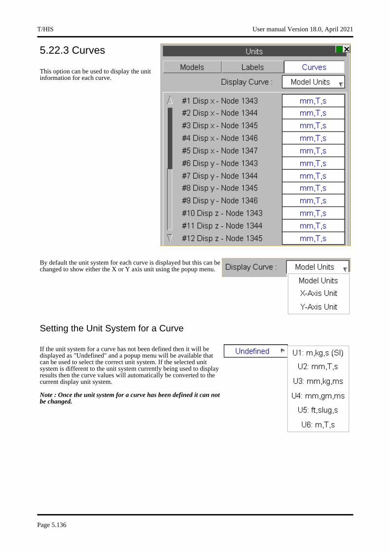
5.22.3 Curves
This option can be used to display the unit information for each curve.
By default the unit system for each curve is displayed but this can be changed to show either the X or Y axis unit using the popup menu.
Setting the Unit System for a Curve
If the unit system for a curve has not been defined then it will be displayed as "Undefined" and a popup menu will be available that can be used to select the correct unit system. If the selected unit system is different to the unit system currently being used to display results then the curve values will automatically be converted to the current display unit system.
Note : Once the unit system for a curve has been defined it can not be changed.
T/HIS User manual Version 18.0, April 2021
Page 5.136
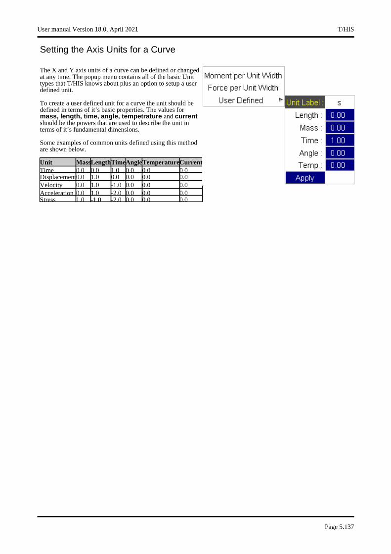
Setting the Axis Units for a Curve
The X and Y axis units of a curve can be defined or changed at any time. The popup menu contains all of the basic Unit types that T/HIS knows about plus an option to setup a user defined unit.
To create a user defined unit for a curve the unit should be defined in terms of it’s basic properties. The values for mass, length, time, angle, tempetrature and current should be the powers that are used to describe the unit in terms of it’s fundamental dimensions.
Some examples of common units defined using this method are shown below.
Unit Mass Length Time Angle TemperatureCurrent Time 0.0 0.0 1.0 0.0 0.0 0.0 Displacement0.0 1.0 0.0 0.0 0.0 0.0 Velocity 0.0 1.0 -1.0 0.0 0.0 0.0 Acceleration 0.0 1.0 -2.0 0.0 0.0 0.0 Stress 1.0 -1.0 -2.0 0.0 0.0 0.0
User manual Version 18.0, April 2021 T/HIS
Page 5.137
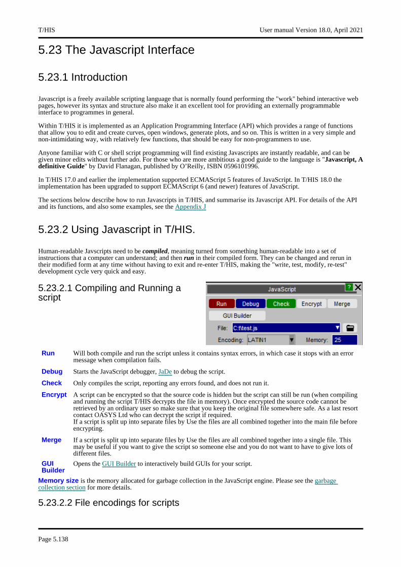
5.23 The Javascript Interface
5.23.1 Introduction
Javascript is a freely available scripting language that is normally found performing the "work" behind interactive web pages, however its syntax and structure also make it an excellent tool for providing an externally programmable interface to programmes in general.
Within T/HIS it is implemented as an Application Programming Interface (API) which provides a range of functions that allow you to edit and create curves, open windows, generate plots, and so on. This is written in a very simple and non-intimidating way, with relatively few functions, that should be easy for non-programmers to use.
Anyone familiar with C or shell script programming will find existing Javascripts are instantly readable, and can be given minor edits without further ado. For those who are more ambitious a good guide to the language is "Javascript, A definitive Guide" by David Flanagan, published by O’Reilly, ISBN 0596101996.
In T/HIS 17.0 and earlier the implementation supported ECMAScript 5 features of JavaScript. In T/HIS 18.0 the implementation has been upgraded to support ECMAScript 6 (and newer) features of JavaScript.
The sections below describe how to run Javascripts in T/HIS, and summarise its Javascript API. For details of the API and its functions, and also some examples, see the Appendix J
5.23.2 Using Javascript in T/HIS.
Human-readable Javscripts need to be compiled, meaning turned from something human-readable into a set of instructions that a computer can understand; and then run in their compiled form. They can be changed and rerun in their modified form at any time without having to exit and re-enter T/HIS, making the "write, test, modify, re-test" development cycle very quick and easy.
5.23.2.1 Compiling and Running a script
Run Will both compile and run the script unless it contains syntax errors, in which case it stops with an error message when compilation fails.
Debug Starts the JavaScript debugger, JaDe to debug the script.
Check Only compiles the script, reporting any errors found, and does not run it.
Encrypt A script can be encrypted so that the source code is hidden but the script can still be run (when compiling and running the script T/HIS decrypts the file in memory). Once encrypted the source code cannot be retrieved by an ordinary user so make sure that you keep the original file somewhere safe. As a last resort contact OASYS Ltd who can decrypt the script if required.If a script is split up into separate files by Use the files are all combined together into the main file before encrypting.
Merge If a script is split up into separate files by Use the files are all combined together into a single file. This may be useful if you want to give the script so someone else and you do not want to have to give lots of different files.
GUI Builder
Opens the GUI Builder to interactively build GUIs for your script.
Memory size is the memory allocated for garbage collection in the JavaScript engine. Please see the garbagecollection section for more details.
5.23.2.2 File encodings for scripts
T/HIS User manual Version 18.0, April 2021
Page 5.138
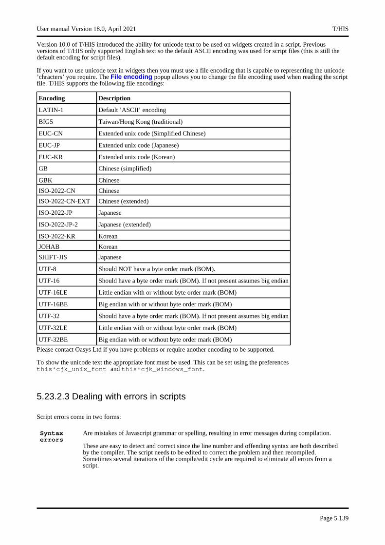
Version 10.0 of T/HIS introduced the ability for unicode text to be used on widgets created in a script. Previous versions of T/HIS only supported English text so the default ASCII encoding was used for script files (this is still the default encoding for script files).
If you want to use unicode text in widgets then you must use a file encoding that is capable to representing the unicode ’chracters’ you require. The File encoding popup allows you to change the file encoding used when reading the script file. T/HIS supports the following file encodings:
Encoding Description
LATIN-1 Default ’ASCII’ encoding
BIG5 Taiwan/Hong Kong (traditional)
EUC-CN Extended unix code (Simplified Chinese)
EUC-JP Extended unix code (Japanese)
EUC-KR Extended unix code (Korean)
GB Chinese (simplified)
GBK Chinese
ISO-2022-CN Chinese
ISO-2022-CN-EXT Chinese (extended)
ISO-2022-JP Japanese
ISO-2022-JP-2 Japanese (extended)
ISO-2022-KR Korean
JOHAB Korean
SHIFT-JIS Japanese
UTF-8 Should NOT have a byte order mark (BOM).
UTF-16 Should have a byte order mark (BOM). If not present assumes big endian
UTF-16LE Little endian with or without byte order mark (BOM)
UTF-16BE Big endian with or without byte order mark (BOM)
UTF-32 Should have a byte order mark (BOM). If not present assumes big endian
UTF-32LE Little endian with or without byte order mark (BOM)
UTF-32BE Big endian with or without byte order mark (BOM)
Please contact Oasys Ltd if you have problems or require another encoding to be supported.
To show the unicode text the appropriate font must be used. This can be set using the preferences this*cjk_unix_font and this*cjk_windows_font.
5.23.2.3 Dealing with errors in scripts
Script errors come in two forms:
Syntax errors
Are mistakes of Javascript grammar or spelling, resulting in error messages during compilation.
These are easy to detect and correct since the line number and offending syntax are both described by the compiler. The script needs to be edited to correct the problem and then recompiled. Sometimes several iterations of the compile/edit cycle are required to eliminate all errors from a script.
User manual Version 18.0, April 2021 T/HIS
Page 5.139
Run-time errors
Are errors of context or logic in scripts that are syntactically correct, and thus have compiled, but which fail at some stage when being run.
A typical example of a run-time error is an attempt to divide a value by zero, yielding the illegal result infinity. More subtle errors involve passing an invalid value to a function, accessing an array subscript that is out of range, and so on.
The T/HIS Javascript API has been written in such a way that it handles "harmless" run-time errors by issuing a warning and continuing execution, but that more serious errors which could result in the wrong answers being generated issue an error message and terminate.
5.23.2.4 Setting the Garbage Collection Threshold Size(This is an advanced topic, and you don’t need to understand it.)
JavaScripts execute inside a memory "arena", allocated dynamically from the operating system, which grows in size as storage is requested within the script. This growth occurs due to requests for "new" variables within the script and also when API functions allocate and return values and objects, and it is limited only by what the operating system can deliver.
The nature of JavaScript means that objects frequently become redundant, and it is wasteful not to reuse the storage that they occupy, therefore there is a "Garbage Collection" process running behind the scenes which periodically checks storage and releases that which is no longer needed. This process is automatic and hidden from the user, it just "happens".
However Garbage Collection is quite a CPU-hungry process, so it is only carried out periodically when a certain threshold is reached. This can sometimes be observed during script execution as a periodic "pause for thought", and if you are monitoring memory usage with a system tool you may see it drop during these pauses.
Clearly this threshold value must be large enough not to trigger excessively frequent (and costly) garbage collections, while at the same time not being so large that scripts build up large amounts of excess memory to the detriment of the rest of the programme.
The Memory size value in the JavaScript panel is the amount of memory allocated for garbage collection. Every time a new object, array, string or double precision number is used a garbage collection ’thing’ is also allocated. The Memory size is the total memory for these ’garbage collection things’, NOT the total memory for the script. The total memory for the script could be significantly higher than this value. e.g the memory required for a Model object could be several kbytes but the memory for the ’garbage collection thing’ for the Model object will something like 10 bytes for a 64bit operating system.
When the memory used for garbage collection ’things’ reaches a significant proportion of Memory Size (normally about 2/3) then garbage collection will take place to try to reclaim memory. If no memory can be reclaimed and the total memory used for garbage collection reaches Memory size then the script will terminate with an error.
If your script has to retain a large number of objects, arrays, strings etc in memory then you may have to increase the value for Memory size. This can also be done using the this*javascript_memory_size preference or adding a special memory comment at the top of the script.
To recap:• This threshold does not limit the memory the script can use, that is limited only by the operating system.• It sets the memory for Garbage Collection ’objects’.• Scripts which allocate a lot of memory, and which exhibit frequent pauses, may run faster with a larger value.
• ... and finally:
If you don’t understand this topic don’t worry. Most scripts will run quite happily with the default value, and you can ignore this setting unless they appear to be struggling, in which case try raising it. (As good an approach as any is to keep on doubling this value until the script works, but don’t use very large sizes unnecessarily.)
T/HIS User manual Version 18.0, April 2021
Page 5.140

5.23.2.5 Assigning Javascripts to Shortcut Keys
If a script is to be run repeatedly it can be convenient to set up a short-cut to it. From within the JavaScript menu ths script can be assigned to one fo the 12 function keys, alternativly the JavaScript can be assigned to any key using the Shortcut menu.
5.23.2.6 Maintaining a library of Javascripts
It is also convenient to have a library of scripts in a defined location.
By default T/HIS looks in $OA_INSTALL/this_library/scripts, but you can define a different directory by setting the preference:
this*script_directory: some_different_directory_name
In the your oa_pref file.
All scripts found in the relevant directory will be listed in the Javascript panel, as shown in this example.
5.23.2.7 Using the "description:" comment at the top of a script to identify its purpose.
To help to identify scripts special comments are searched for in the top 10 lines of each script, and if description:
User manual Version 18.0, April 2021 T/HIS
Page 5.141
is found, for example the comment line:
// description: Some description of the script’s purpose
Then the description line is shown as hover text when the mouse is placed over that filename. In the example above the "princ2d" script has the line
// description: Colour curve by model number
5.23.2.8 Using the "name:" comment at the top of a script to change its name
Normally the name shown for a script will be its filename, stripped of any leading pathname and trailing ".js" extension.
However if the string name: is found in the first ten lines of the script, then the following name will be used instead. For example the line:
// name: Colour By Model
Will result in the script appearing with the name "Colour By Model" in tha Javascript panel. This does not affect the actual name of the script, only the name on its library button.
5.23.2.9 Using the "memory:" comment at the top of a script to change the required memory
Sometimes the memory required for garbage collection needs to be changed.
If the string memory: is found in the first ten lines of the script, then the size given will be used for the memory (unless the size in the memory textbox is larger than this value). For example the line:
// memory: 50
Will result in the script using 50Mb for garbage collection memory.
5.23.3 Running a Javascript in "batch" mode.
All the above assumes that Javascripts will be run interactively from the user interface, however it is also possible to run a script in "batch" mode using the command line interface. The relevant command-line commands are:
/JAVASCRIPT - +- COMPILE Compiles and checks the script, but does not run it.
+- EXECUTE (Re)compiles and runs the script
+- MEMORY <nnn> Resets the Garbage Collection threshold to <nnn> MBytes
To run a Javascript from batch these commands need to be placed in a command file and run using the command line "-cf=command filename" option. For example the command file might be:
... some other commands/JAVA EXEC my_script.js...some further commands
And the command line required to run T/HIS might be something like:
$OASYS/this10.exe -d=default -cf=command_file -exit analysis_name
Obviously multiple script invocations may be placed in a command file. For more information see:
Command and Session files Describes command files, and explains how to create and use them
T/HIS command line arguments Describes the various command line arguments, and how to use them
T/HIS User manual Version 18.0, April 2021
Page 5.142
5.23.4 Running a Javascript from within a FAST-TCF script
JavaScripts can also be run from within a FAST-TCF script using the "javascript" option
javascript "E:\javascripts\new_function.js"
Within a FAST-TCF script curves are usually accessed via curve tags. If a JavaScript is used within a FAST-TCF script it is recommended that the Curve.GetFromTag() function is used to access existing curves. If a new curve is created by a JavaScript within a FAST-TCF script then the new curve can be accessed within the FAST-TCF script using the "tag" parameter of the curve creation function
new_curve = new Curve(id,tag,label,x-axis label,y-axis label);
If a tag is not specified in the curve creation function
new_curve = new Curve(id);
then a curve tag will be generated automatically for the curve. The 1st curve created within the script will be tagged "curve_js_1", the 2nd "curve_js_2" ...
5.23.5 The T/HIS Javascript API
All of the T/HIS JavaScript API functions are described in detail in Appendix J.
5.23.6 Examples
By far the easiest way to learn Javascript is by example and, more specifically by modified existing scripts to do what you want.
The software comes supplied with examples in the $OASYS/programme_library/examples directory (for T/HIS $OASYS/this_library/examples) and you are free to use and modify these files for your own purposes.
User manual Version 18.0, April 2021 T/HIS
Page 5.143
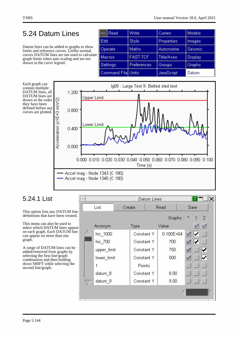
5.24 Datum Lines
Datum lines can be added to graphs to show limits and reference curves. Unlike normal curves DATUM lines are not used to calculate graph limits when auto scaling and are not shown in the curve legend.
Each graph can contain multiple DATUM lines, all DATUM lines are drawn in the order they have been defined before any curves are plotted.
5.24.1 List
This option lists any DATUM line definitions that have been created.
This menu can also be used to select which DATUM lines appear on each graph. Each DATUM line can appear on more than one graph.
A range of DATUM lines can be added/removed from graphs by selecting the first line/graph combination and then holding down SHIFT while selecting the second line/graph.
T/HIS User manual Version 18.0, April 2021
Page 5.144
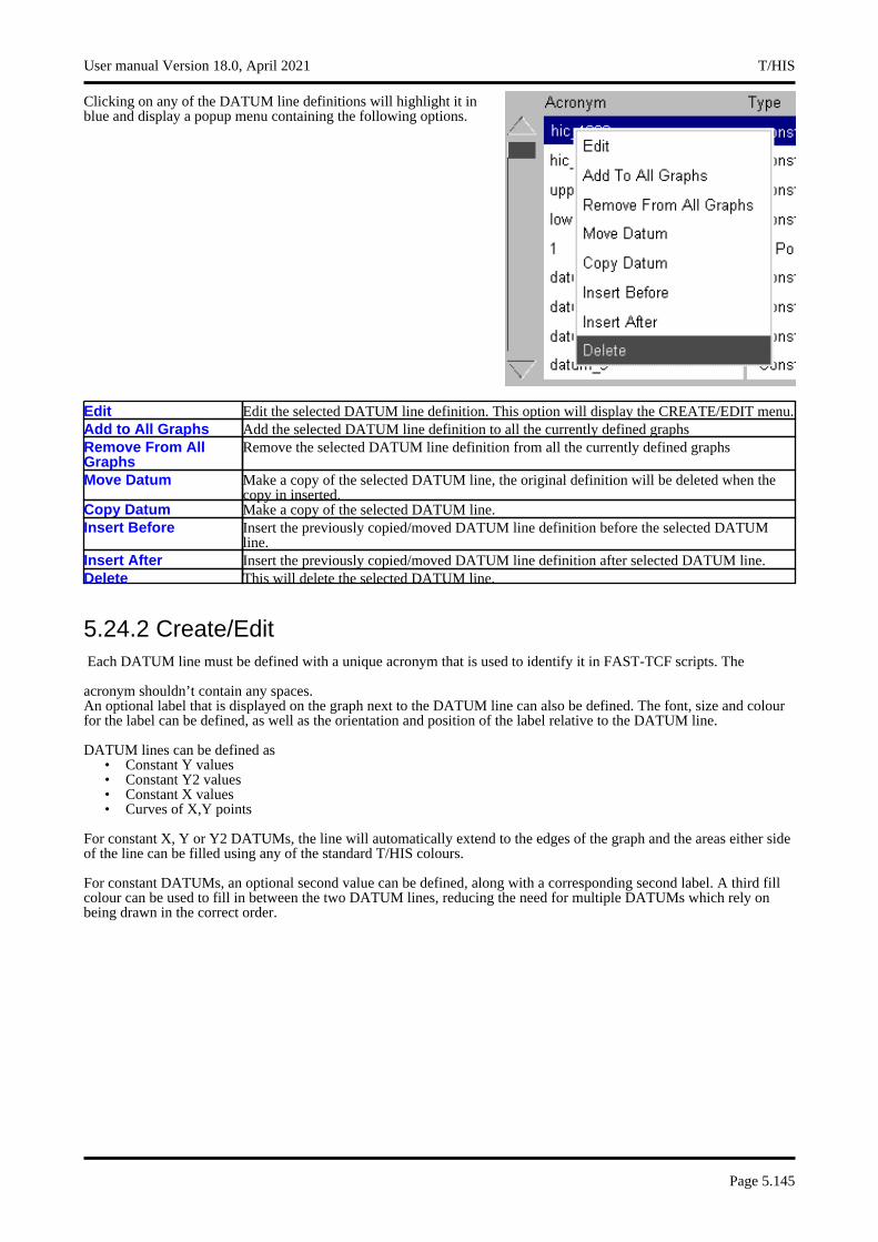
Clicking on any of the DATUM line definitions will highlight it in blue and display a popup menu containing the following options.
Edit Edit the selected DATUM line definition. This option will display the CREATE/EDIT menu.Add to All Graphs Add the selected DATUM line definition to all the currently defined graphsRemove From All Graphs
Remove the selected DATUM line definition from all the currently defined graphs
Move Datum Make a copy of the selected DATUM line, the original definition will be deleted when the copy in inserted.
Copy Datum Make a copy of the selected DATUM line.Insert Before Insert the previously copied/moved DATUM line definition before the selected DATUM
line.Insert After Insert the previously copied/moved DATUM line definition after selected DATUM line.Delete This will delete the selected DATUM line.
5.24.2 Create/EditEach DATUM line must be defined with a unique acronym that is used to identify it in FAST-TCF scripts. The
acronym shouldn’t contain any spaces. An optional label that is displayed on the graph next to the DATUM line can also be defined. The font, size and colour for the label can be defined, as well as the orientation and position of the label relative to the DATUM line.
DATUM lines can be defined as • Constant Y values• Constant Y2 values• Constant X values• Curves of X,Y points
For constant X, Y or Y2 DATUMs, the line will automatically extend to the edges of the graph and the areas either side of the line can be filled using any of the standard T/HIS colours.
For constant DATUMs, an optional second value can be defined, along with a corresponding second label. A third fill colour can be used to fill in between the two DATUM lines, reducing the need for multiple DATUMs which rely on being drawn in the correct order.
User manual Version 18.0, April 2021 T/HIS
Page 5.145

As the DATUM lines are drawn in the order they are defined, care must be taken when applying fill colours. The following example shows the effect of defining the DATUMs in a different order. Using the optional second value, the following example can actually be made into a single DATUM with two values, two labels and three fill colours, as in the above image.
Datum 1
+ +Datum 2
= =
T/HIS User manual Version 18.0, April 2021
Page 5.146
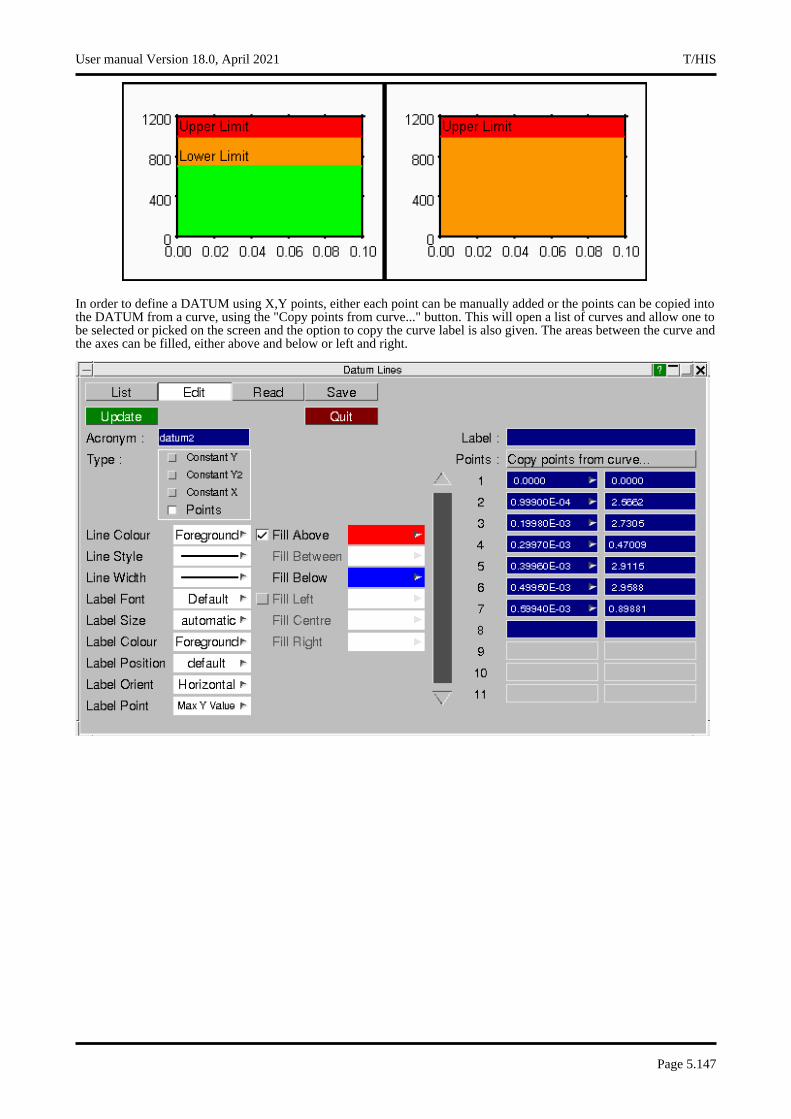
In order to define a DATUM using X,Y points, either each point can be manually added or the points can be copied into the DATUM from a curve, using the "Copy points from curve..." button. This will open a list of curves and allow one to be selected or picked on the screen and the option to copy the curve label is also given. The areas between the curve and the axes can be filled, either above and below or left and right.
User manual Version 18.0, April 2021 T/HIS
Page 5.147
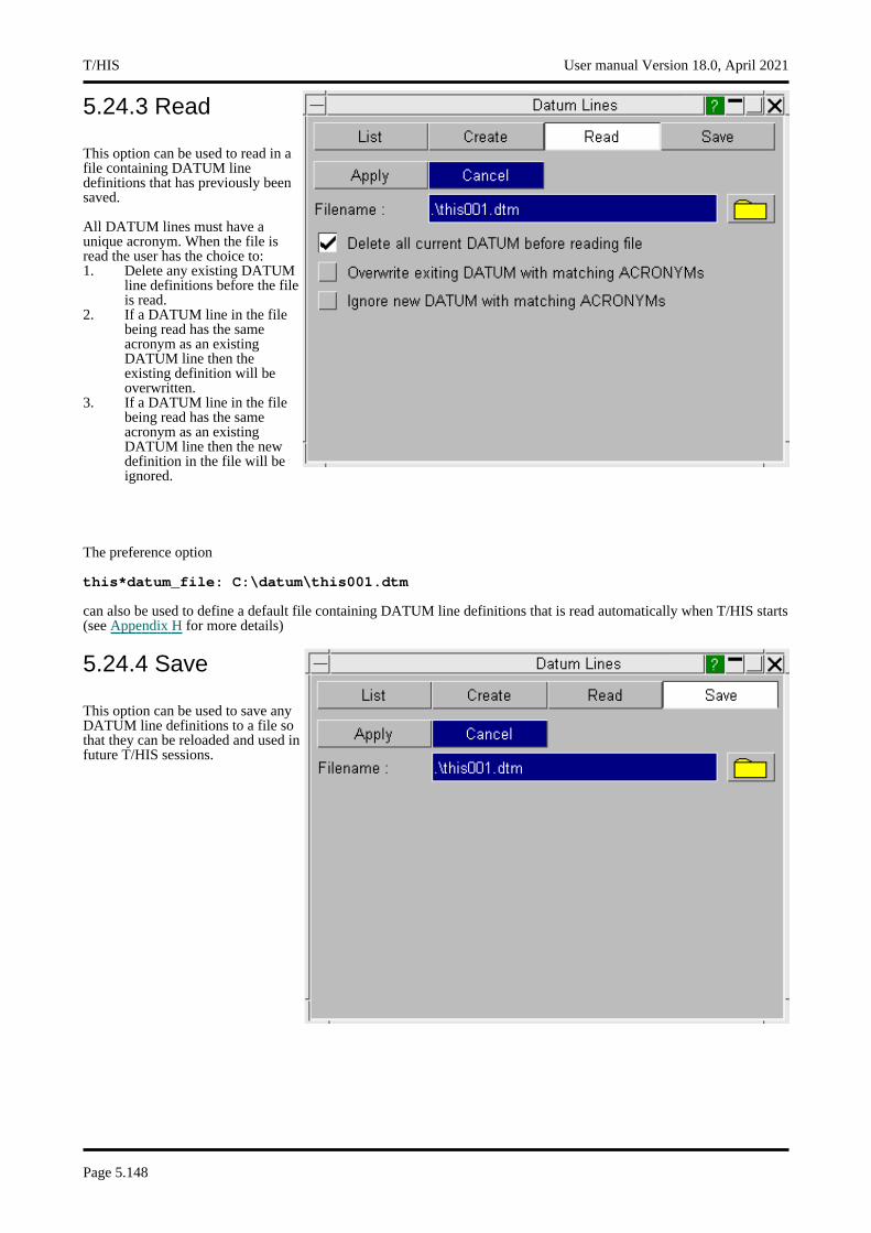
5.24.3 Read
This option can be used to read in a file containing DATUM line definitions that has previously been saved.
All DATUM lines must have a unique acronym. When the file is read the user has the choice to:1. Delete any existing DATUM
line definitions before the file is read.
2. If a DATUM line in the file being read has the same acronym as an existing DATUM line then the existing definition will be overwritten.
3. If a DATUM line in the file being read has the same acronym as an existing DATUM line then the new definition in the file will be ignored.
The preference option
this*datum_file: C:\datum\this001.dtm
can also be used to define a default file containing DATUM line definitions that is read automatically when T/HIS starts (see Appendix H for more details)
5.24.4 Save
This option can be used to save any DATUM line definitions to a file so that they can be reloaded and used in future T/HIS sessions.
T/HIS User manual Version 18.0, April 2021
Page 5.148

5.25 T/HIS Session Save and Retrieve
T/HIS session save and retrieve saves the current T/HIS session as a session file of format (.tsf) onto the disk which can be read back later on to retrieve the saved T/HIS session. A T/HIS session file can also appended to or overlayed on top of an existing session.
5.25.1 Save Session
A T/HIS session can be saved either through Save/Retrieve Session panel or on Exit.
5.25.1.1 Save Session - Save/Retrieve Session PanelTo save a T/HIS session, select File -> Session File -> Save to open Save/Retrieve Session panel in the menu area. Enter a name for the session file in the File Name text-box and click Apply. Filename can also be entered using file
selection browser. It should be noted that T/HIS session file does not directly store either the LS-DYNA model results or any csv/cur files that have been used for generating the curves inside the session file by default. It will only contain the full address path to these files. As a result of this session file do not occupy much space on disk.
If users want they can embed extra information into the session file so that the saved T/HIS session can be retrieved even if LS-DYNA results/csv/cur files are deleted or lost.
Embed cur/csv files into session
This option embeds the cur or csv files that are used for creating the curves. The session file with embedded cur/csv files no longer depend on these files and the session can be retrieved even if these files are deleted or lost. If users want this option to be checked/turned-on always, they can change the preference file (see Appendix H for more details)
this*session_embed_cur_csv_files:
Embed curve data into session
This option embeds the curve xy coordinate data for all curves into the session file. A session file with embedded curve data can be retrieved even if the model files are missing. However, a session retrieved using embedded curve data loses informations such as curve-id and graph properties. If users want this option to checked/turned on always, they can change the preference file (see Appendix H for more details)
this*session_embed_curve_data:
User manual Version 18.0, April 2021 T/HIS
Page 5.149

5.25.1.2 Save Session - On Exit
T/HIS session can be saved on exit from T/HIS by selecting SAVE SESSION button on the exit INFORMATION panel. The session file saved would have a name of the format this__.tsf. The file would be by saved to the location defined in preference file (see Appendix H for more details).
this*session_save_option:
this*session_save_dir:
The session file can also saved automatically every time T/HIS exits by defining in the preference file (see Appendix Hfor more details).
this*session_auto_save:
T/HIS User manual Version 18.0, April 2021
Page 5.150
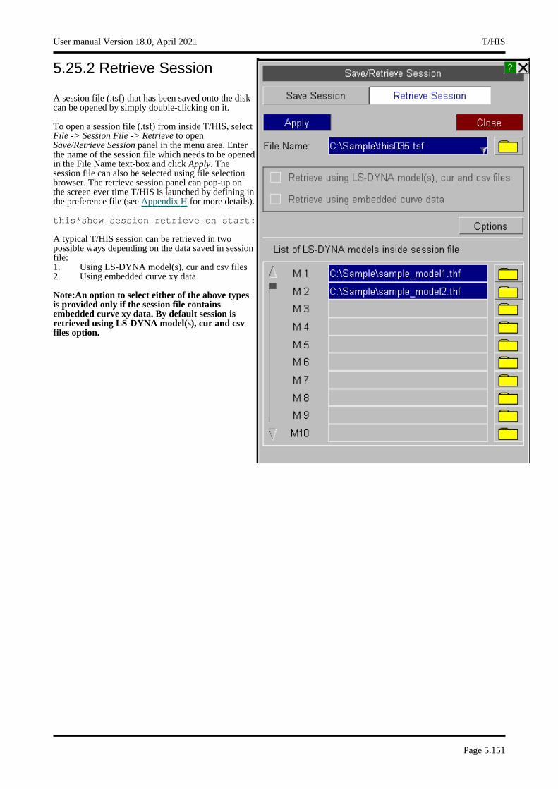
5.25.2 Retrieve Session
A session file (.tsf) that has been saved onto the disk can be opened by simply double-clicking on it.
To open a session file (.tsf) from inside T/HIS, select File -> Session File -> Retrieve to open Save/Retrieve Session panel in the menu area. Enter the name of the session file which needs to be opened in the File Name text-box and click Apply. The session file can also be selected using file selection browser. The retrieve session panel can pop-up on the screen ever time T/HIS is launched by defining in the preference file (see Appendix H for more details).
this*show_session_retrieve_on_start:
A typical T/HIS session can be retrieved in two possible ways depending on the data saved in session file: 1. Using LS-DYNA model(s), cur and csv files 2. Using embedded curve xy data
Note:An option to select either of the above types is provided only if the session file contains embedded curve xy data. By default session is retrieved using LS-DYNA model(s), cur and csv files option.
User manual Version 18.0, April 2021 T/HIS
Page 5.151
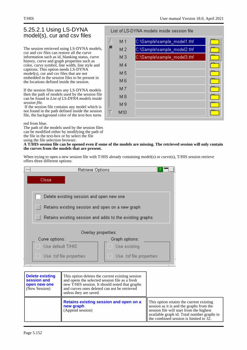
5.25.2.1 Using LS-DYNA model(s), cur and csv files
The session retrieved using LS-DYNA models, cur and csv files can restore all the curve information such as id, blanking status, curve history, curve and graph properties such as color, curve symbol, line width, line style and captions. This option needs LS-DYNA model(s), cur and csv files that are not embedded in the session files to be present in the locations defined inside the session.
If the session files uses any LS-DYNA models then the path of models used by the session file can be found in List of LS-DYNA models inside session file.If the session file contains any model which is not found in the path defined inside the session file, the background color of the text-box turns
red from blue. The path of the models used by the session files can be modified either by modifying the path of the file in the text-box or by select the file using the file selection browser.A T/HIS session file can be opened even if some of the models are missing. The retrieved session will only contain the curves from the models that are present.
When trying to open a new session file with T/HIS already containing model(s) or curve(s), T/HIS session retrieve offers three different options:
Delete existing session and open new one (New Session)
This option deletes the current existing session and opens the selected session file as a fresh new T/HIS session. It should noted that graphs and curves ones deleted can not be retrieved unless they are saved.
Retains existing session and open on a new graph (Append session)
This option retains the current existing session as it is and the graphs from the session file will start from the highest available graph id. Total number graphs in the combined session is limited to 32.
T/HIS User manual Version 18.0, April 2021
Page 5.152
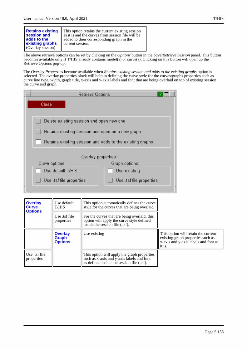
Retains existing session and adds to the existing graphs (Overlay session)
This option retains the current existing session as it is and the curves from session file will be added to their corresponding graph in the current session.
The above retrieve options can be set by clicking on the Options button in the Save/Retrieve Session panel. This button becomes available only if T/HIS already contains model(s) or curve(s). Clicking on this button will open up the Retrieve Options pop-up.
The Overlay Properties become available when Retains existing session and adds to the existing graphs option is selected. The overlay properties block will help in defining the curve style for the curves/graphs properties such as curve line type, width, graph title, x-axis and y-axis labels and font that are being overlaid on top of existing session the curve and graph.
Use default T/HIS
This option automatically defines the curve style for the curves that are being overlaid.
Overlay Curve Options
Use .tsf file properties
For the curves that are being overlaid, this option will apply the curve style defined inside the session file (.tsf).
Use existing This option will retain the current existing graph properties such as x-axis and y-axis labels and font as it is.
Overlay Graph Options
Use .tsf file properties
This option will apply the graph properties such as x-axis and y-axis labels and font as defined inside the session file (.tsf).
User manual Version 18.0, April 2021 T/HIS
Page 5.153
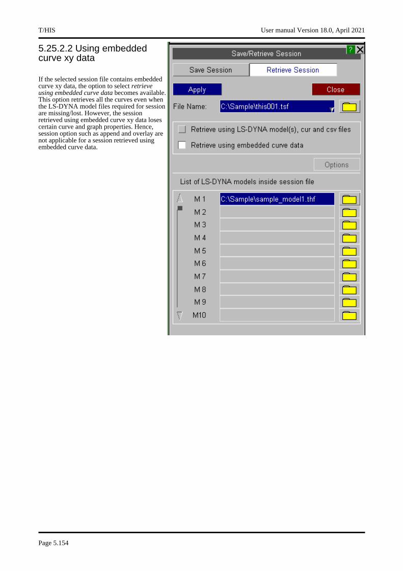
5.25.2.2 Using embedded curve xy data
If the selected session file contains embedded curve xy data, the option to select retrieve using embedded curve data becomes available. This option retrieves all the curves even when the LS-DYNA model files required for session are missing/lost. However, the session retrieved using embedded curve xy data loses certain curve and graph properties. Hence, session option such as append and overlay are not applicable for a session retrieved using embedded curve data.
T/HIS User manual Version 18.0, April 2021
Page 5.154
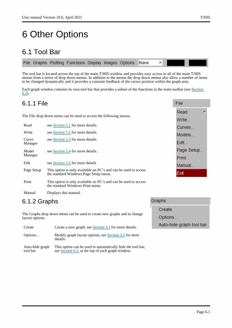
6 Other Options
6.1 Tool Bar
The tool bar is located across the top of the main T/HIS window and provides easy access to all of the main T/HIS menus from a series of drop down menus. In addition to the menus the drop down menus also allow a number of items to be changed dynamically and it provides a constant feedback of the cursor position within the graph area.
Each graph window contains its own tool bar that provides a subset of the functions in the main toolbar (see Section6.2).
6.1.1 File
The File drop down menu can be used to access the following menus.
Read see Section 5.1 for more details.
Write see Section 5.2 for more details.
Curve Manager
see Section 5.3 for more details.
Model Manager
see Section 5.4 for more details.
Edit see Section 5.5 for more details
Page Setup This option is only available on PC’s and can be used to access the standard Windows Page Setup menu.
Print This option is only available on PC’s and can be used to access the standard Windows Print menu.
Manual Displays this manual.
6.1.2 Graphs
The Graphs drop down menu can be used to create new graphs and to change layout options.
Create Create a new graph, see Section 3.1 for more details.
Options... Modify graph layout options, see Section 3.1 for more details.
Auto-hide graph tool bar
This option can be used to automatically hide the tool bar, see Section 6.2, at the top of each graph window.
User manual Version 18.0, April 2021 T/HIS
Page 6.1

6.1.3 Plotting
The Plotting drop down menu can be used to access the following plotting commands.
Plot see Section 4.1 for more details.
Zoom see Section 4.5 for more details.
Point see Section 4.3 for more details.
Autoscale see Section 4.6 for more details.
Centre see Section 4.7 for more details.
6.1.4 Functions
The Functions drop down menu can be used to access all of the curve functions.
Automotive see Section 5.11 for more details.
Operate see Section 5.9 for more details.
Maths see Section 5.10 for more details.
Seismic see Section 5.12 for more details.
6.1.5 Display
The Display drop down menu can be used to access the Title/Axis and Display menus and to dynamically modify the appearance of graphs. This menu changes all of the currently active graphs (see Section 3.5).
Title/Axis see Section 5.15 for more details.
Legend see Section 5.15.5 for more details.
Display see Section 5.16 for more details.
Grid Turns the gird on/off, see Section 5.16.4 for more details.
Symbols Turns graph symbols on/off, see Section 5.16.3 for more details.
Lines Turns graph lines on/off, see Section 5.16.2 for more details.
Border Turns the plot border on/off, see Section 5.16.6 for more details.
Foreground Sets the foreground colour, see Section 5.16.9 for more details.
Background Sets the background colour, see Section 5.16.8 for more details.
Swap Fore/Back
Swaps the current foreground and background colours, see Section 5.16.10 for more details.
Plot Format Set the current plot format, see Section 5.15.5.2 for more details.
T/HIS User manual Version 18.0, April 2021
Page 6.2

6.1.6 Images
The Images drop down menu can be used to save the current displayed graphs as an image in a number of formats. In addition to saving an image this menu can also be used to read in an image that is used as the background for each graph.
BMP, JPEG...
Capture the image as a bitmap or JPEG, see Section 5.8.1 for more details.
Postscript Generate a Postscript or PDF image, see Section 5.8.2 for more details.
Background This option can be used to set an image as the background for each graph, see Section 5.8.3 for more details.
User manual Version 18.0, April 2021 T/HIS
Page 6.3
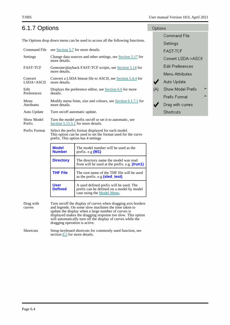
6.1.7 Options
The Options drop down menu can be used to access all the following functions.
Command File see Section 5.7 for more details.
Settings Change data sources and other settings, see Section 5.17 for more details.
FAST-TCF Generate/playback FAST-TCF scripts, see Section 5.14 for more details.
Convert LSDA>ASCII
Convert a LSDA binout file to ASCII, see Section 5.4.4 for more details.
Edit Preferences
Displays the preference editor, see Section 6.6 for more details.
Menu Attributes
Modify menu fonts, size and colours, see Section 6.1.7.1 for more details.
Auto Update Turn on/off automatic update.
Show Model Prefix
Turn the model prefix on/off or set it to automatic, see Section 5.15.5.1 for more details.
Prefix Format Select the prefix format displayed for each model. This option can be used to set the format used for the curve prefix. This option has 4 settings
Model Number
The model number will be used as the prefix. e.g (M1)
Directory The directory name the model was read from will be used at the prefix. e.g. (/run1)
THF File The root name of the THF file will be used as the prefix. e.g (sled_test)
User Defined
A used defined prefix will be used. The prefix can be defined on a model by model case using the Model Menu.
Drag with curves
Turn on/off the display of curves when dragging axis borders and legends. On some slow machines the time taken to update the display when a large number of curves is displayed makes the dragging response too slow. This option will automatically turn off the display of curves while the dragging operation is active.
Shortcuts Setup keyboard shortcuts for commonly used function, see section 6.5 for more details.
T/HIS User manual Version 18.0, April 2021
Page 6.4

6.1.7.1 MENU AttributesThis panel allows you to tune the visual attributes of the screen menus within T/HIS and save them if you wish.
Display Factor
Lies in the range 0.5 to 2.0, default 1.0. Values < 1.0 reduce the apparent size of the screen so that menus and text become larger. Values > 1.0 act in the opposite sense. This is the simplest way of taking into account the display size.
User manual Version 18.0, April 2021 T/HIS
Page 6.5
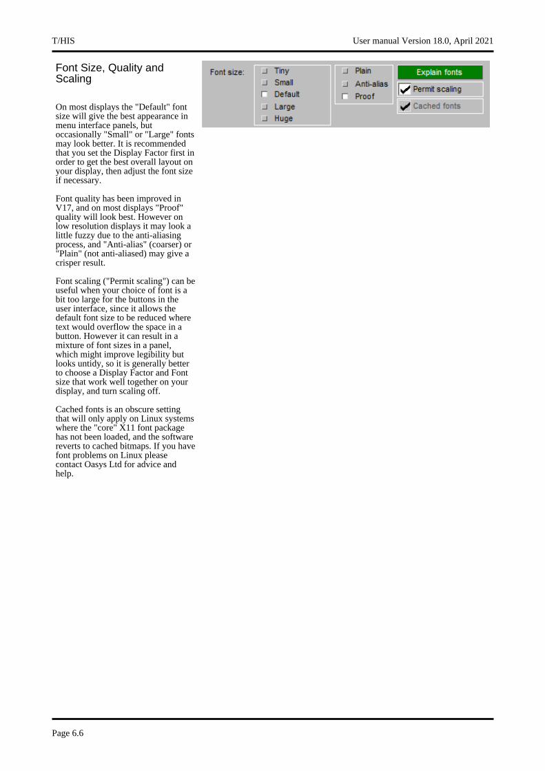
Font Size, Quality and Scaling
On most displays the "Default" font size will give the best appearance in menu interface panels, but occasionally "Small" or "Large" fonts may look better. It is recommended that you set the Display Factor first in order to get the best overall layout on your display, then adjust the font size if necessary.
Font quality has been improved in V17, and on most displays "Proof" quality will look best. However on low resolution displays it may look a little fuzzy due to the anti-aliasing process, and "Anti-alias" (coarser) or "Plain" (not anti-aliased) may give a crisper result.
Font scaling ("Permit scaling") can be useful when your choice of font is a bit too large for the buttons in the user interface, since it allows the default font size to be reduced where text would overflow the space in a button. However it can result in a mixture of font sizes in a panel, which might improve legibility but looks untidy, so it is generally better to choose a Display Factor and Font size that work well together on your display, and turn scaling off.
Cached fonts is an obscure setting that will only apply on Linux systems where the "core" X11 font package has not been loaded, and the software reverts to cached bitmaps. If you have font problems on Linux please contact Oasys Ltd for advice and help.
T/HIS User manual Version 18.0, April 2021
Page 6.6
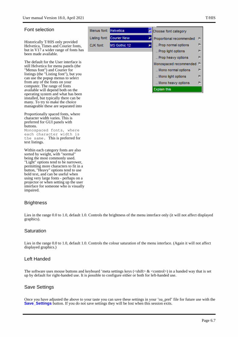
Font selection
Historically T/HIS only provided Helvetica, Times and Courier fonts, but in V17 a wider range of fonts has been made available.
The default for the User interface is still Helvetica for menu panels (the "Menus font") and Courier for listings (the "Listing font"), but you can use the popup menus to select from any of the fonts on your computer. The range of fonts available will depend both on the operating system and what has been installed, but typically there can be many. To try to make the choice manageable these are separated into
Proportionally spaced fonts, where character width varies. This is preferred for GUI panels with buttons.Monospaced fonts, where each character width is the same. This is preferred for text listings.
Within each category fonts are also sorted by weight, with "normal" being the most commonly used. "Light" options tend to be narrower, permitting more characters to fit in a button, "Heavy" options tend to use bold text, and can be useful when using very large fonts - perhaps on a projector or when setting up the user interface for someone who is visually impaired.
Brightness
Lies in the range 0.0 to 1.0, default 1.0. Controls the brightness of the menu interface only (it will not affect displayed graphics).
Saturation
Lies in the range 0.0 to 1.0, default 1.0. Controls the colour saturation of the menu interface. (Again it will not affect displayed graphics.)
Left Handed
The software uses mouse buttons and keyboard ’meta settings keys (<shift> & <control>) in a handed way that is set up by default for right-handed use. It is possible to configure either or both for left-handed use.
Save Settings
Once you have adjusted the above to your taste you can save these settings in your ’oa_pref’ file for future use with the Save_Settings button. If you do not save settings they will be lost when this session exits.
User manual Version 18.0, April 2021 T/HIS
Page 6.7
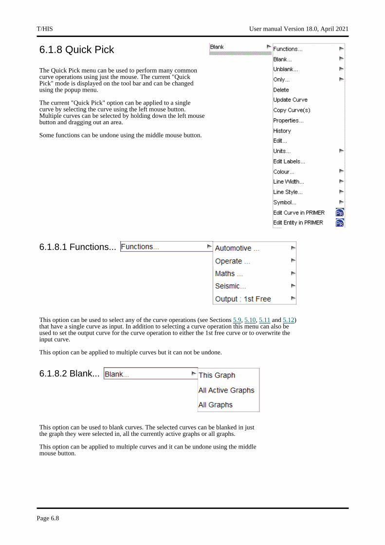
6.1.8 Quick Pick
The Quick Pick menu can be used to perform many common curve operations using just the mouse. The current "Quick Pick" mode is displayed on the tool bar and can be changed using the popup menu.
The current "Quick Pick" option can be applied to a single curve by selecting the curve using the left mouse button. Multiple curves can be selected by holding down the left mouse button and dragging out an area.
Some functions can be undone using the middle mouse button.
6.1.8.1 Functions...
This option can be used to select any of the curve operations (see Sections 5.9, 5.10, 5.11 and 5.12) that have a single curve as input. In addition to selecting a curve operation this menu can also be used to set the output curve for the curve operation to either the 1st free curve or to overwrite the input curve.
This option can be applied to multiple curves but it can not be undone.
6.1.8.2 Blank...
This option can be used to blank curves. The selected curves can be blanked in just the graph they were selected in, all the currently active graphs or all graphs.
This option can be applied to multiple curves and it can be undone using the middle mouse button.
T/HIS User manual Version 18.0, April 2021
Page 6.8
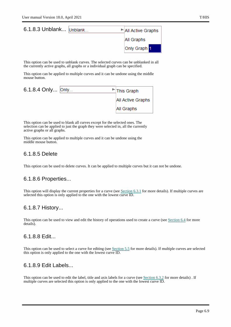
6.1.8.3 Unblank...
This option can be used to unblank curves. The selected curves can be unblanked in all the currently active graphs, all graphs or a individual graph can be specified.
This option can be applied to multiple curves and it can be undone using the middle mouse button.
6.1.8.4 Only...
This option can be used to blank all curves except for the selected ones. The selection can be applied to just the graph they were selected in, all the currently active graphs or all graphs.
This option can be applied to multiple curves and it can be undone using the middle mouse button.
6.1.8.5 Delete
This option can be used to delete curves. It can be applied to multiple curves but it can not be undone.
6.1.8.6 Properties...
This option will display the current properties for a curve (see Section 6.3.1 for more details). If multiple curves are selected this option is only applied to the one with the lowest curve ID.
6.1.8.7 History...
This option can be used to view and edit the history of operations used to create a curve (see Section 6.4 for more details).
6.1.8.8 Edit...
This option can be used to select a curve for editing (see Section 5.5 for more details). If multiple curves are selected this option is only applied to the one with the lowest curve ID.
6.1.8.9 Edit Labels...
This option can be used to edit the label, title and axis labels for a curve (see Section 6.3.2 for more details) . If multiple curves are selected this option is only applied to the one with the lowest curve ID.
User manual Version 18.0, April 2021 T/HIS
Page 6.9
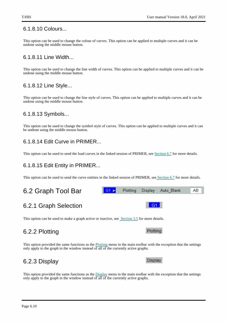
6.1.8.10 Colours...
This option can be used to change the colour of curves. This option can be applied to multiple curves and it can be undone using the middle mouse button.
6.1.8.11 Line Width...
This option can be used to change the line width of curves. This option can be applied to multiple curves and it can be undone using the middle mouse button.
6.1.8.12 Line Style...
This option can be used to change the line style of curves. This option can be applied to multiple curves and it can be undone using the middle mouse button.
6.1.8.13 Symbols...
This option can be used to change the symbol style of curves. This option can be applied to multiple curves and it can be undone using the middle mouse button.
6.1.8.14 Edit Curve in PRIMER...
This option can be used to send the load curves in the linked session of PRIMER, see Section 6.7 for more details.
6.1.8.15 Edit Entity in PRIMER...
This option can be used to send the curve entities in the linked session of PRIMER, see Section 6.7 for more details.
6.2 Graph Tool Bar
6.2.1 Graph Selection
This option can be used to make a graph active or inactive, see Section 3.5 for more details.
6.2.2 Plotting
This option provided the same functions as the Plotting menu in the main toolbar with the exception that the settings only apply to the graph in the window instead of all of the currently active graphs.
6.2.3 Display
This option provided the same functions as the Display menu in the main toolbar with the exception that the settings only apply to the graph in the window instead of all of the currently active graphs.
T/HIS User manual Version 18.0, April 2021
Page 6.10

6.2.4 Auto_Blank
The Auto_Blank function can be used to blank and unblank curves in a graph using either the TAB key or SHIFT+TAB.
By default if you now press the TAB key in a graph T/HIS will automatically blank all the curves except for those belonging to model 1. If you press TAB a 2nd time you will just see the curve belonging to model 2, a third time model 3. When you reach the end of the models you have curves for pressing the TAB key loops back to model 1. If you press SHIFT+TAB then it goes the other way (model 3 > model 2 > model 1 > model 3 ....)
Instead of blanking curves by model the behaviour of the TAB key can be changed.
Models Default. Blanks curves by model ID.
Components Blanks curves by component. e.g Node X Displacement > Node Y Displacement > Node Z Displacement > ...
Entity Types Blanks curves by entity type e.g. Whole Model > Parts > Nodes > Solids > ...
Entity ID Blanks curves by ID. e.g Node 1 and Solid 1 > Node 2 and Solid 2 > ....
Component Types
This is similar to Component except that it lumps all the displacement curves together then velocity so you get x,y,z and magnitudes. You will also get data for different entity types. So Energy would show things like Whole Model KE and Contact Energies.
Surface/Int Point
Blanks curves by surface or through thickness integration point. e.g Top > Middle > Bottom > Layer 1 > ...
Curves ID’s Blanks curves by ID
The default Auto_Blank mode can be modified using the preference file (see Appendix H for more details)
this*auto_blank_mode:
6.2.5 Curve Locking
The ’Lock’ option works in a similar way to locking in PRIMER and D3PLOT. When the ’Lock’ button is pressed at the top of a graph, all currently blanked curves in that graph are locked from becoming visible, until they are unlocked. This allows the remaining unlocked curves to be manipulated without unblanking any of the locked curves. This includes the use of the shortcut keys ’u’, ’r’ and ,’b’. Locking can also be set via the curve table using the graph buttons (see Section 5.3.4.1 for more details)
Once the ’Lock’ button is pressed, a popup is attached, providing the option to either unlock the curves in that graph or ’Unfreeze All’. ’Freezing’ is the equivalent of locking for visible curves, so once a curve is frozen, it will stay visible until unfrozen. This can be set using quick-pick, the curve manager or the curve table.
6.2.6 AB
This option can be used to turn and off the Auto Blank option. The default setting for this option can be modified using the preference file (see Appendix H for more details) this*auto_blank:
User manual Version 18.0, April 2021 T/HIS
Page 6.11
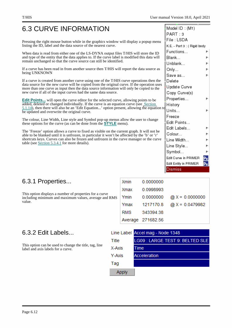
6.3 CURVE INFORMATION
Pressing the right mouse button while in the graphics window will display a popup menu listing the ID, label and the data source of the nearest curve.
When data is read from either one of the LS-DYNA output files T/HIS will store the ID and type of the entity that the data applies to. If the curve label is modified this data will remain unchanged so that the curve source can still be identified.
If a curve has been read in from another source then T/HIS will report the data source as being UNKNOWN
If a curve is created from another curve using one of the T/HIS curve operations then the data source for the new curve will be copied from the original curve. If the operation uses more than one curve as input then the data source information will only be copied to the new curve if all of the input curves had the same data source.
Edit Points... will open the curve editor for the selected curve, allowing points to be added, deleted or changed individually. If the curve is an equation curve (see Section5.1.14), then there will also be an ’Edit Equation...’ option present, allowing the equation to be updated and overwrite the original curve.
The colour, Line Width, Line style and Symbol pop-up menus allow the user to change these options for the curve (as can be done from the STYLE menu).
The ’Freeze’ option allows a curve to fixed as visible on the current graph. It will not be able to be blanked until it is unfrozen, in particular it won’t be affected by the ’b’ or ’r’ shortcuts keys. Curves can also be frozen and unfrozen in the curve manager or the curve table (see Section 5.3.4.1 for more details).
6.3.1 Properties...
This option displays a number of properties for a curve including minimum and maximum values, average and RMS value.
6.3.2 Edit Labels...
This option can be used to change the title, tag, line label and axis labels for a curve.
T/HIS User manual Version 18.0, April 2021
Page 6.12
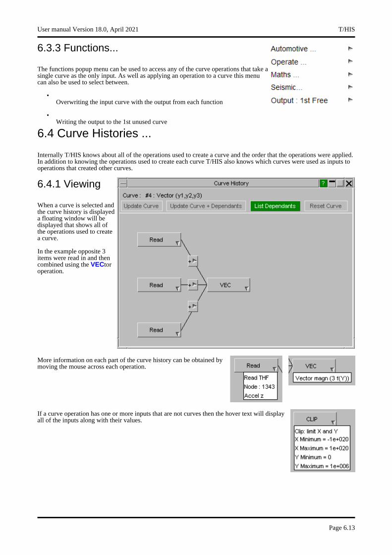
6.3.3 Functions...
The functions popup menu can be used to access any of the curve operations that take a single curve as the only input. As well as applying an operation to a curve this menu can also be used to select between.
•Overwriting the input curve with the output from each function
•Writing the output to the 1st unused curve
6.4 Curve Histories ...
Internally T/HIS knows about all of the operations used to create a curve and the order that the operations were applied. In addition to knowing the operations used to create each curve T/HIS also knows which curves were used as inputs to operations that created other curves.
6.4.1 Viewing
When a curve is selected and the curve history is displayed a floating window will be displayed that shows all of the operations used to create a curve.
In the example opposite 3 items were read in and then combined using the VECtor operation.
More information on each part of the curve history can be obtained by moving the mouse across each operation.
If a curve operation has one or more inputs that are not curves then the hover text will display all of the inputs along with their values.
User manual Version 18.0, April 2021 T/HIS
Page 6.13
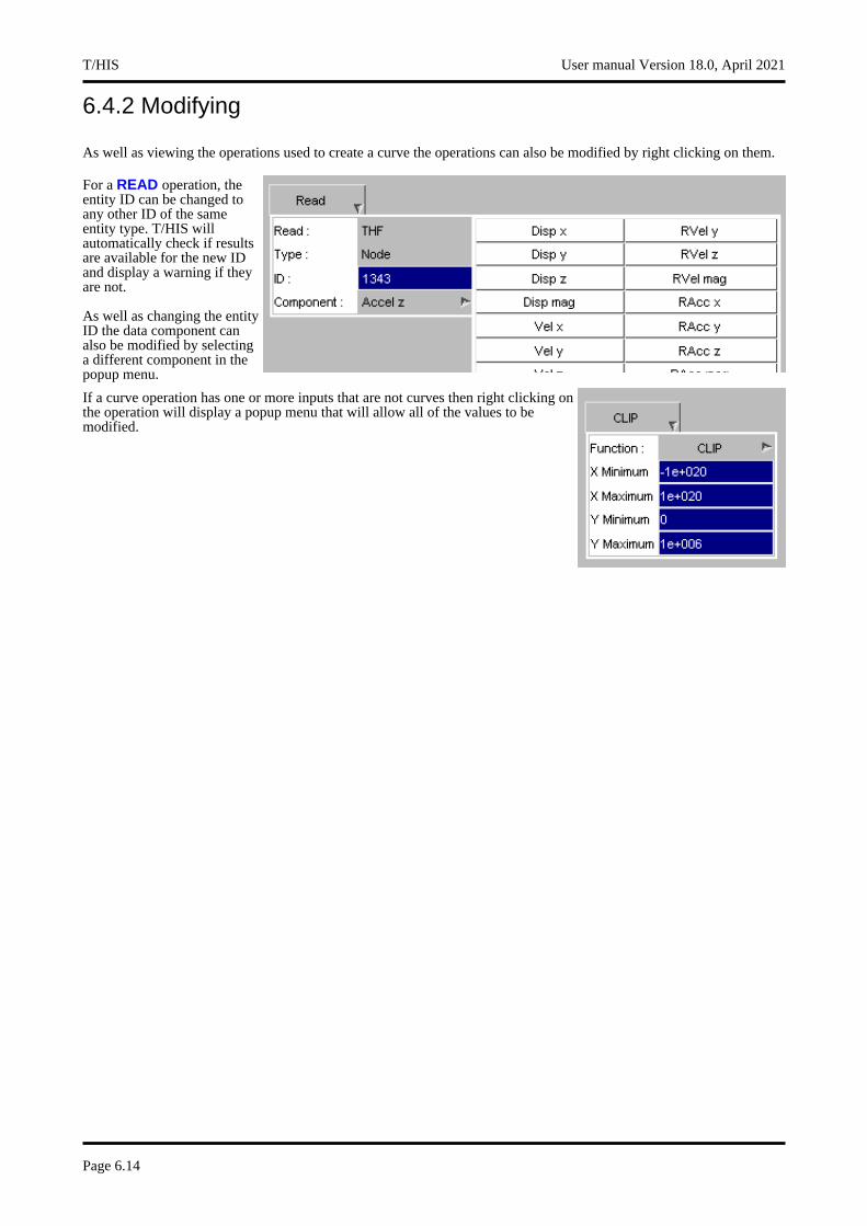
6.4.2 Modifying
As well as viewing the operations used to create a curve the operations can also be modified by right clicking on them.
For a READ operation, the entity ID can be changed to any other ID of the same entity type. T/HIS will automatically check if results are available for the new ID and display a warning if they are not.
As well as changing the entity ID the data component can also be modified by selecting a different component in the popup menu.
If a curve operation has one or more inputs that are not curves then right clicking on the operation will display a popup menu that will allow all of the values to be modified.
T/HIS User manual Version 18.0, April 2021
Page 6.14

As well as changing the inputs to existing curve operations it is also possible to change a curve operation to any other curve operation that has the same number of input curves.
Right clicking on the popup symbol next to the name of the current curve operation will display a menu containing a list of all of the curve operations that are available which have the same number of input curves.
If for example the current curve operation is CLIP then the popup menu of available operations will contain all of the other curve functions that have a single input curve.
User manual Version 18.0, April 2021 T/HIS
Page 6.15

6.4.3 Inserting New Operations
.New operations can be inserted into the chain of curve operations by right-clicking on one of the + symbols between the existing operations.
The popup menu that is displayed will contain all of the curve operations that take a single curve as input and produce a single output curve.
6.4.4 Update Curve
.If any of the operations used to create a curve are modified or if a new operation is inserted then this option can be used to automatically update the curve. T/HIS will automatically rebuild the curve using the updated set of curve operations and will replace the old curve with the new one.
6.4.5 Update Curve + Dependants
This option will update the selected curve and any dependant curves. As T/HIS stores all of the operations used to create every curve it knows if a curve has been used as an input to any other curves.
The selected curve will be automatically rebuilt and replaced with the new curve and then any curves that use the selected curve as an input will also be rebuilt and replaced.
6.4.6 List Dependants
This option will display a list containing any curves that have been created which use the currently selected curve as an input somewhere in their chain of curve operations.
T/HIS User manual Version 18.0, April 2021
Page 6.16
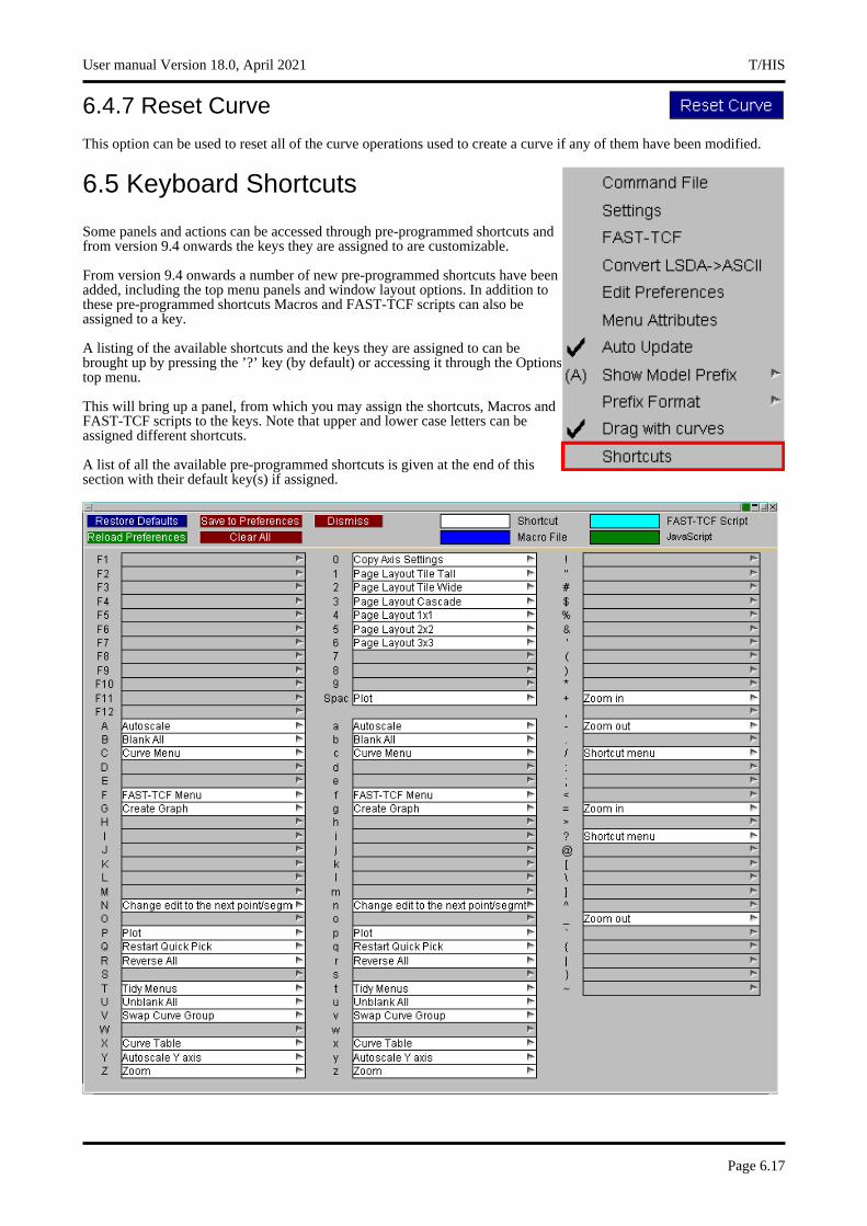
6.4.7 Reset Curve
This option can be used to reset all of the curve operations used to create a curve if any of them have been modified.
6.5 Keyboard Shortcuts
Some panels and actions can be accessed through pre-programmed shortcuts and from version 9.4 onwards the keys they are assigned to are customizable.
From version 9.4 onwards a number of new pre-programmed shortcuts have been added, including the top menu panels and window layout options. In addition to these pre-programmed shortcuts Macros and FAST-TCF scripts can also be assigned to a key.
A listing of the available shortcuts and the keys they are assigned to can be brought up by pressing the ’?’ key (by default) or accessing it through the Options top menu.
This will bring up a panel, from which you may assign the shortcuts, Macros and FAST-TCF scripts to the keys. Note that upper and lower case letters can be assigned different shortcuts.
A list of all the available pre-programmed shortcuts is given at the end of this section with their default key(s) if assigned.
User manual Version 18.0, April 2021 T/HIS
Page 6.17
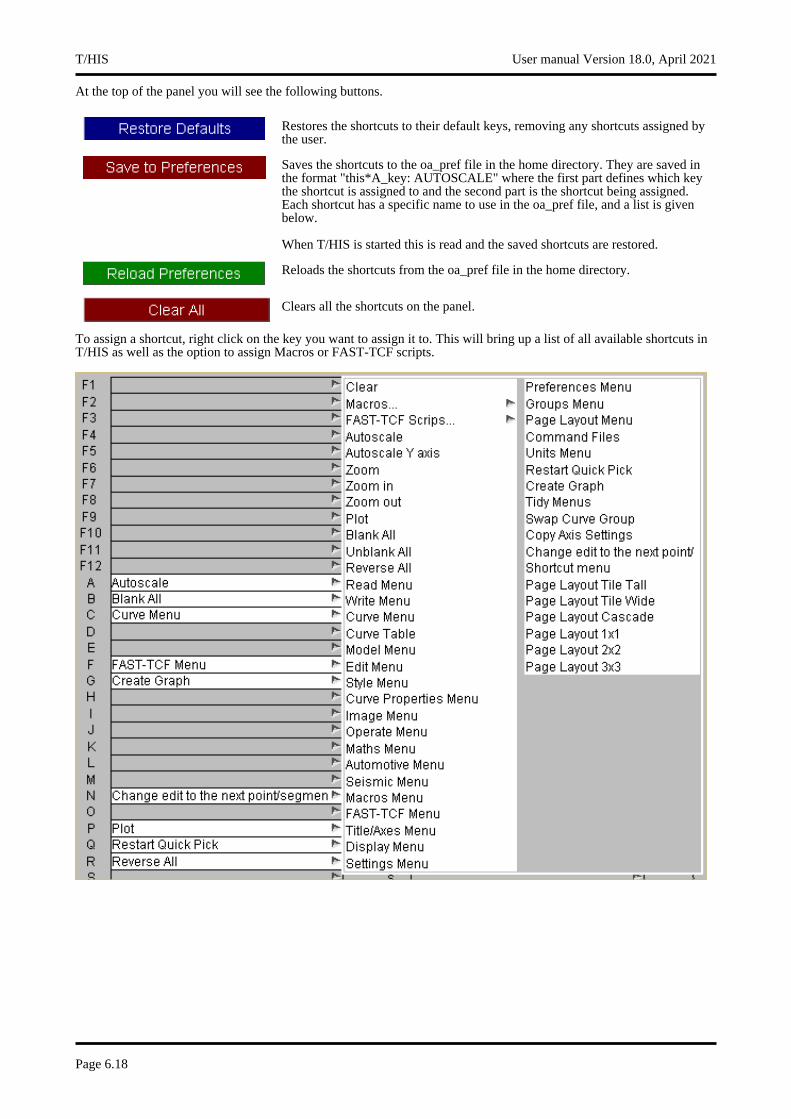
At the top of the panel you will see the following buttons.
Restores the shortcuts to their default keys, removing any shortcuts assigned by the user.
Saves the shortcuts to the oa_pref file in the home directory. They are saved in the format "this*A_key: AUTOSCALE" where the first part defines which key the shortcut is assigned to and the second part is the shortcut being assigned. Each shortcut has a specific name to use in the oa_pref file, and a list is given below.
When T/HIS is started this is read and the saved shortcuts are restored.
Reloads the shortcuts from the oa_pref file in the home directory.
Clears all the shortcuts on the panel.
To assign a shortcut, right click on the key you want to assign it to. This will bring up a list of all available shortcuts in T/HIS as well as the option to assign Macros or FAST-TCF scripts.
T/HIS User manual Version 18.0, April 2021
Page 6.18
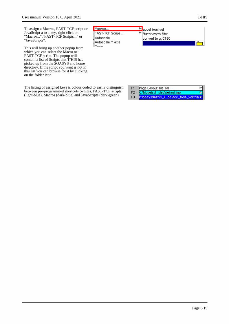
To assign a Macros, FAST-TCF script or JavaScript a to a key, right click on "Macros...","FAST-TCF Scripts..." or "JavaScripts".
This will bring up another popup from which you can select the Macro or FAST-TCF script. The popup will contain a list of Scripts that T/HIS has picked up from the $OASYS and home directory. If the script you want is not in this list you can browse for it by clicking on the folder icon.
The listing of assigned keys is colour coded to easily distinguish between pre-programmed shortcuts (white), FAST-TCF scripts (light-blue), Macros (dark-blue) and JavaScripts (dark-green)
User manual Version 18.0, April 2021 T/HIS
Page 6.19
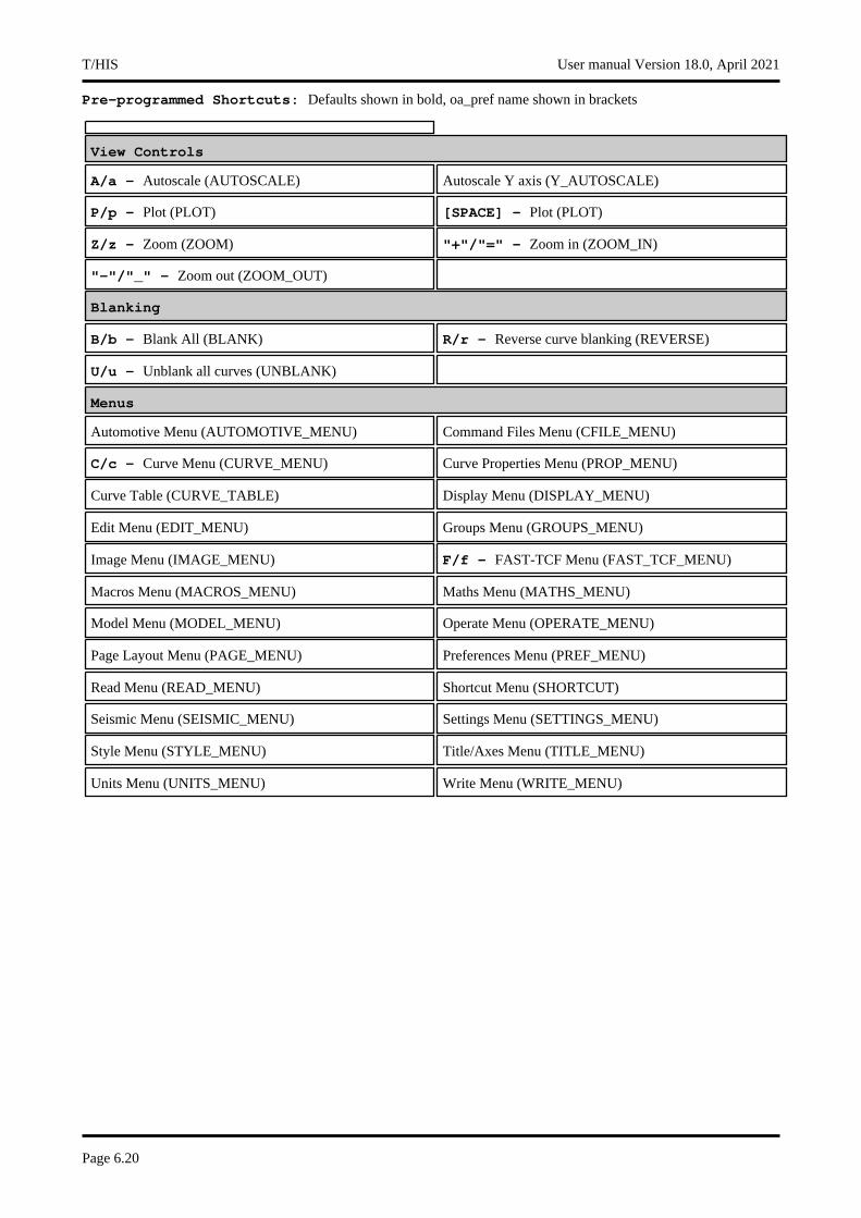
Pre-programmed Shortcuts: Defaults shown in bold, oa_pref name shown in brackets
View Controls
A/a - Autoscale (AUTOSCALE) Autoscale Y axis (Y_AUTOSCALE)
P/p - Plot (PLOT) [SPACE] - Plot (PLOT)
Z/z - Zoom (ZOOM) "+"/"=" - Zoom in (ZOOM_IN)
"-"/"_" - Zoom out (ZOOM_OUT)
Blanking
B/b - Blank All (BLANK) R/r - Reverse curve blanking (REVERSE)
U/u - Unblank all curves (UNBLANK)
Menus
Automotive Menu (AUTOMOTIVE_MENU) Command Files Menu (CFILE_MENU)
C/c - Curve Menu (CURVE_MENU) Curve Properties Menu (PROP_MENU)
Curve Table (CURVE_TABLE) Display Menu (DISPLAY_MENU)
Edit Menu (EDIT_MENU) Groups Menu (GROUPS_MENU)
Image Menu (IMAGE_MENU) F/f - FAST-TCF Menu (FAST_TCF_MENU)
Macros Menu (MACROS_MENU) Maths Menu (MATHS_MENU)
Model Menu (MODEL_MENU) Operate Menu (OPERATE_MENU)
Page Layout Menu (PAGE_MENU) Preferences Menu (PREF_MENU)
Read Menu (READ_MENU) Shortcut Menu (SHORTCUT)
Seismic Menu (SEISMIC_MENU) Settings Menu (SETTINGS_MENU)
Style Menu (STYLE_MENU) Title/Axes Menu (TITLE_MENU)
Units Menu (UNITS_MENU) Write Menu (WRITE_MENU)
T/HIS User manual Version 18.0, April 2021
Page 6.20
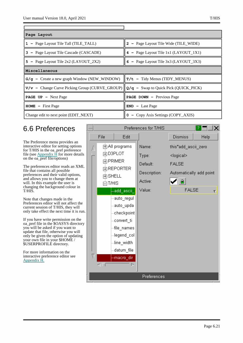
Page Layout
1 - Page Layout Tile Tall (TILE_TALL) 2 - Page Layout Tile Wide (TILE_WIDE)
3 - Page Layout Tile Cascade (CASCADE) 4 - Page Layout Tile 1x1 (LAYOUT_1X1)
5 - Page Layout Tile 2x2 (LAYOUT_2X2) 6 - Page Layout Tile 3x3 (LAYOUT_3X3)
Miscellaneous
G/g - Create a new graph Window (NEW_WINDOW) T/t - Tidy Menus (TIDY_MENUS)
V/v - Change Curve Picking Group (CURVE_GROUP) Q/q - Swap to Quick Pick (QUICK_PICK)
PAGE UP - Next Page PAGE DOWN - Previous Page
HOME - First Page END - Last Page
Change edit to next point (EDIT_NEXT) 0 - Copy Axis Settings (COPY_AXIS)
6.6 Preferences
The Preference menu provides an interactive editor for setting options for T/HIS in the oa_pref preference file (see Appendix H for more details on the oa_pref file/options)
The preferences editor reads an XML file that contains all possible preferences and their valid options, and allows you to change them at will. In this example the user is changing the background colour in T/HIS.
Note that changes made in the Preferences editor will not affect the current session of T/HIS, they will only take effect the next time it is run.
If you have write permission on the oa_pref file in the $OASYS directory you will be asked if you want to update that file, otherwise you will only be given the option of updating your own file in your $HOME / $USERPROFILE directory.
For more information on the interactive preference editor see Appendix H.
User manual Version 18.0, April 2021 T/HIS
Page 6.21
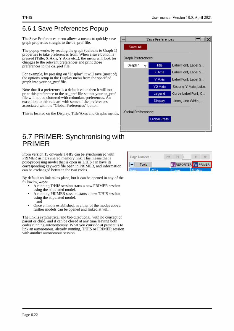
6.6.1 Save Preferences Popup
The Save Preferences menu allows a means to quickly save graph properties straight to the oa_pref file.
The popup works by reading the graph (defaults to Graph 1) properties to take preferences from. When a save button is pressed (Title, X Axis, Y Axis etc..), the menu will look for changes to the relevant preferences and print those preferences to the oa_pref file.
For example, by pressing on "Display" it will save (most of) the options setup in the Display menu from the specified graph into your oa_pref file.
Note that if a preference is a default value then it will not print this preference to the oa_pref file so that your oa_pref file will not be cluttered with redundant preferences. An exception to this rule are with some of the preferences associated with the "Global Preferences" button.
This is located on the Display, Title/Axes and Graphs menus.
6.7 PRIMER: Synchronising with PRIMERFrom version 15 onwards T/HIS can be synchronised with PRIMER using a shared memory link. This means that a post-processing model that is open in T/HIS can have its corresponding keyword file open in PRIMER, and information can be exchanged between the two codes.
By default no link takes place, but it can be opened in any of the following ways:
• A running T/HIS session starts a new PRIMER session using the stipulated model.
• A running PRIMER session starts a new T/HIS session using the stipulated model.
and• Once a link is established, in either of the modes above,
further models can be opened and linked at will.
The link is symmetrical and bid-directional, with no concept of parent or child, and it can be closed at any time leaving both codes running autonomously. What you can’t do at present is to link an autonomous, already running, T/HIS or PRIMER session with another autonomous session.
T/HIS User manual Version 18.0, April 2021
Page 6.22
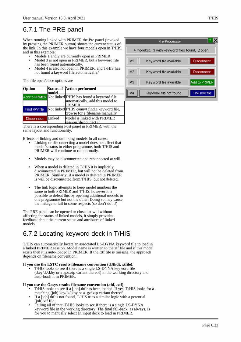
6.7.1 The PRE panel
When running linked with PRIMER the Pre panel (invoked by pressing the PRIMER button) shows the current status of the link. In this example we have four models open in T/HIS, and in this example:
• Models 1 and 2 are currently open in PRIMER• Model 3 is not open in PRIMER, but a keyword file
has been found automatically.• Model 4 is also not open in PRIMER, and T/HIS has
not found a keyword file automatically/
The file open/close options are
Option Status of model
Action performed
Not linkedT/HIS has found a keyword file automatically, add this model to PRIMER
Not linkedT/HIS cannot find a keyword file, browse for a filename manually
Linked Model is linked with PRIMER session, disconnect it
There is a corresponding Post panel in PRIMER, with the same layout and functionality.
Effects of linking and unlinking models:In all cases:• Linking or disconnecting a model does not affect that
model’s status in either programme, both T/HIS and PRIMER will continue to run normally.
• Models may be disconnected and reconnected at will.
• When a model is deleted in T/HIS it is implicitly disconnected in PRIMER, but will not be deleted from PRIMER. Similarly, if a model is deleted in PRIMER is will be disconnected from T/HIS, but not deleted.
• The link logic attempts to keep model numbers the same in both PRIMER and T/HIS, however it is possible to defeat this by opening additional models in one programme but not the other. Doing so may cause the linkage to fail in some respects (so don’t do it!)
The PRE panel can be opened or closed at will without affecting the status of linked models, it simply provides feedback about the current status and attributes of linked models.
6.7.2 Locating keyword deck in T/HIS
T/HIS can automatically locate an associated LS-DYNA keyword file to load in a linked PRIMER session. Model name is written to the ztf file and if this model exists then it is auto-loaded in PRIMER. If the .ztf file is missing, the approach depends on filename convention:
If you use the LSTC results filename convention (d3thdt, xtfile):• T/HIS looks to see if there is a single LS-DYNA keyword file
(.key/.k/.kby or a .gz/.zip variant thereof) in the working directory and auto-loads it in PRIMER.
If you use the Oasys results filename convention (.thf, .xtf):• T/HIS looks to see if a [job].thf has been loaded. If yes, T/HIS looks for a
matching [job].key/.k/.kby or a .gz/.zip variant thereof.• If a [job].thf is not found, T/HIS tries a similar logic with a potential
[job].xtf file.• Failing all of that, T/HIS looks to see if there is a single LS-DYNA
keyword file in the working directory. The final fall-back, as always, is for you to manually select an input deck to load in PRIMER.
User manual Version 18.0, April 2021 T/HIS
Page 6.23
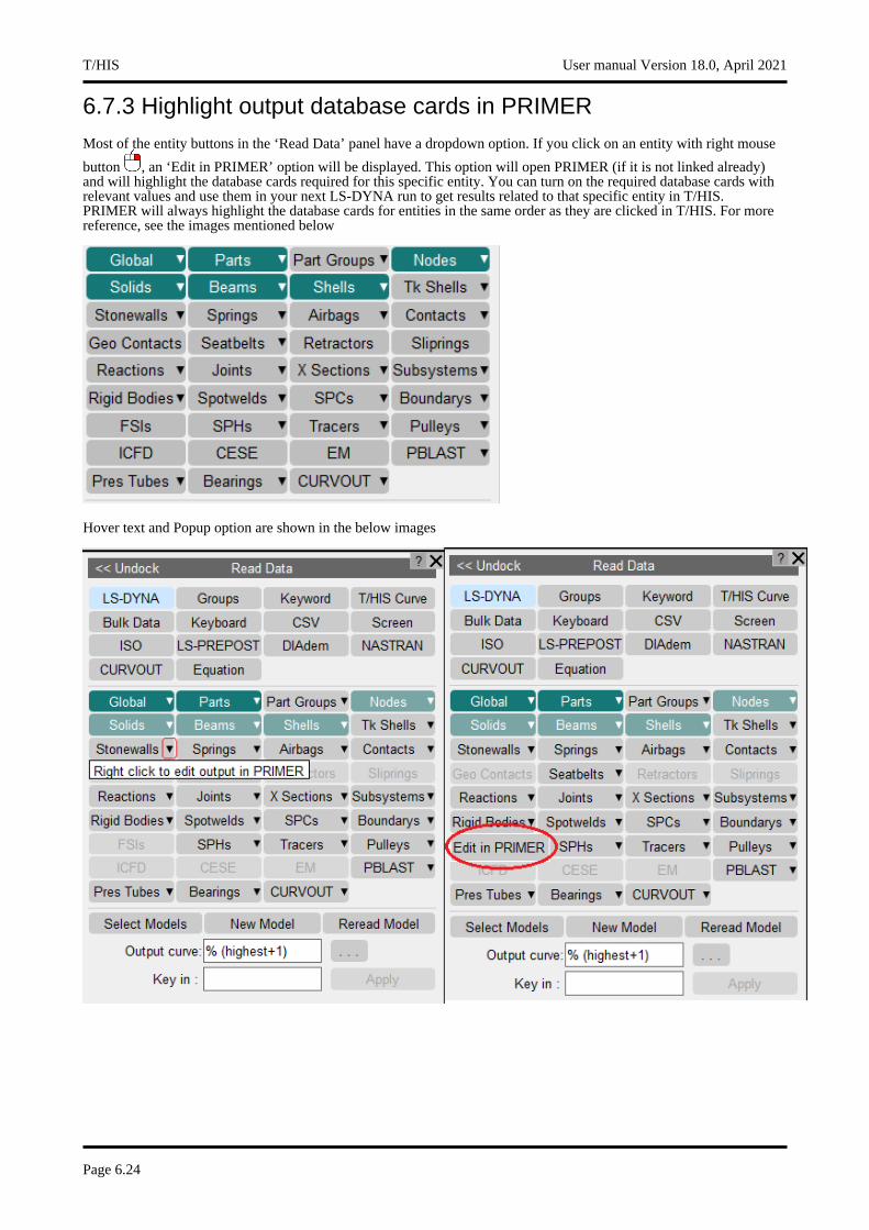
6.7.3 Highlight output database cards in PRIMER
Most of the entity buttons in the ‘Read Data’ panel have a dropdown option. If you click on an entity with right mouse
button , an ‘Edit in PRIMER’ option will be displayed. This option will open PRIMER (if it is not linked already) and will highlight the database cards required for this specific entity. You can turn on the required database cards with relevant values and use them in your next LS-DYNA run to get results related to that specific entity in T/HIS. PRIMER will always highlight the database cards for entities in the same order as they are clicked in T/HIS. For more reference, see the images mentioned below
Hover text and Popup option are shown in the below images
T/HIS User manual Version 18.0, April 2021
Page 6.24
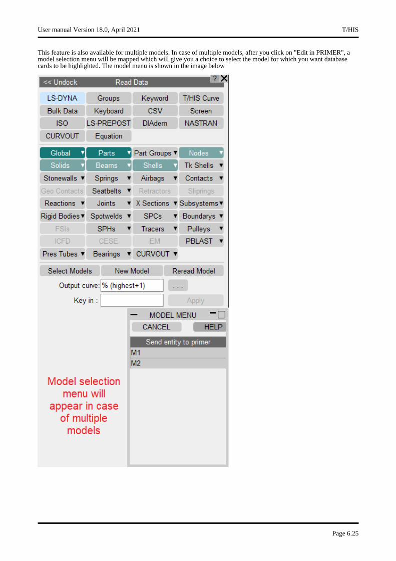
This feature is also available for multiple models. In case of multiple models, after you click on "Edit in PRIMER", a model selection menu will be mapped which will give you a choice to select the model for which you want database cards to be highlighted. The model menu is shown in the image below
User manual Version 18.0, April 2021 T/HIS
Page 6.25
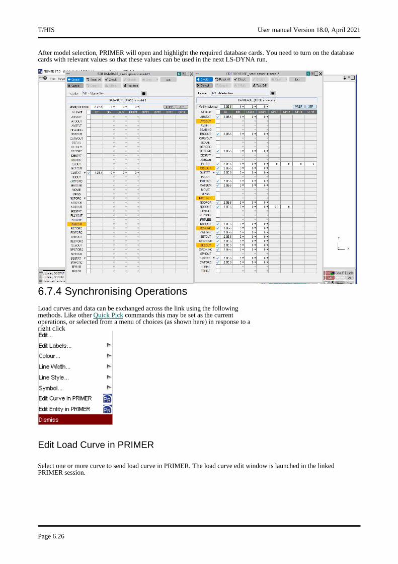
After model selection, PRIMER will open and highlight the required database cards. You need to turn on the database cards with relevant values so that these values can be used in the next LS-DYNA run.
6.7.4 Synchronising Operations
Load curves and data can be exchanged across the link using the following methods. Like other Quick Pick commands this may be set as the current operations, or selected from a menu of choices (as shown here) in response to a right click
Edit Load Curve in PRIMER
Select one or more curve to send load curve in PRIMER. The load curve edit window is launched in the linked PRIMER session.
T/HIS User manual Version 18.0, April 2021
Page 6.26

Edit Curve Entity in PRIMER
Select one or more curves to call up the corresponding EDIT panel in PRIMER, so if for example you clicked on a curve that was an acceleration for a node you would get the node card in PRIMER or if you clicked on a contact force curve you would get the contact card in PRIMER.
User manual Version 18.0, April 2021 T/HIS
Page 6.27
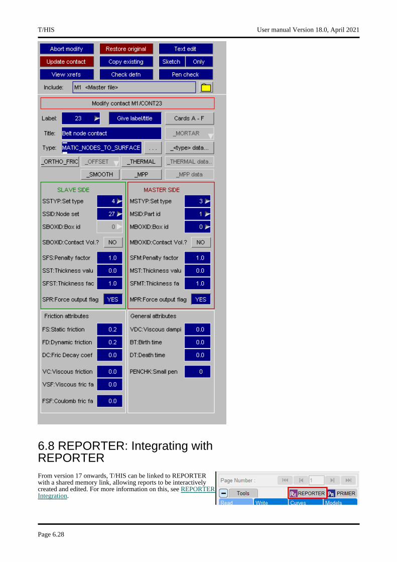
6.8 REPORTER: Integrating with REPORTERFrom version 17 onwards, T/HIS can be linked to REPORTER with a shared memory link, allowing reports to be interactively created and edited. For more information on this, see REPORTERIntegration.
T/HIS User manual Version 18.0, April 2021
Page 6.28
7 FAST-TCF FAST-TCF CONTENTS
7.0 Overview7.1 Introduction7.2 Page / Graph layout and selection7.3 Input syntax to load other files7.4 Input for data extraction requests7.5 Units7.6 Curve Tags7.7 Curve Groups7.8 Performing FAST-TCF curve operations7.9 Applying extra options to data requests7.10 Setting properties for curves7.12 FAST-TCF Image Output options7.13 Outputting curve properties to text files, variables and REPORTER7.14 FAST-TCF Curve Output7.15 FAST-TCF additional
7.0 FAST-TCF OVERVIEW
FAST-TCF is a scripting language for T/HIS. It is designed to be editable and backward-compatible with previous versions of T/HIS. From version 9.2 FAST-TCF scripts can be recorded and played back in T/HIS. The FAST-TCF scripts are plain text files, and are therefore easy to edit and manipulate.
7.0.1 NEW FEATURES
New Features for FAST-TCF version 11.0
Version 11 of T/HIS contains the following new FAST-TCF commands• Support for DISBOUT data component• Support for PLLYOUT data components• "style_m" command for setting curve styles by model
New Features for FAST-TCF version 10.0
Version 10 of T/HIS contains the following new FAST-TCF commands• Support for TRHIST data components• Support for CPM_SENSOR data components• New wildcard options for specifying curve tags• Ouputting a range of curves to curve file
New Features for FAST-TCF version 9.4
Version 9.4 of T/HIS contains the following new FAST-TCF commands• Support for DBFSI data components• Support for TPRINT data components• New "plot setup" commands• New curve style options
New Features for FAST-TCF version 9.3
Because of the multiple graphs and pages available in T/HIS 9.3 additional commands have been added to FAST-TCF 93 to define and position graphs and to generate multiple images containing one or more graphs. Because of these new commands version 9.3 FAST-TCF scripts generated by T/HIS can not be used in previous releases.
• New commands have been added for generating and positioning multiple graphs and pages.• New commands for generating images containing multiple graphs and pages.• New variables have been added for accessing the output values of the ERR command.• New built in variables "$run_nameN", "$run_titleN" and "$run_dirN" for multiple models.
User manual Version 18.0, April 2021 T/HIS
Page 7.1
• New built in variable"$FTCF_PATH"
New Features for FAST-TCF version 9.2
FAST-TCF has been extensively revised to include almost all of the T/HIS commands. The improved functionality does mean that old scripts may have to be changed to meet the new standards.
NOTE: FAST-TCF is not 100% compatible with pre-version 9.1 input scripts:• Variables have changed to allow more flexibility, but the old rule for filenames (word1 + word2) has now been
discontinued, filenames must all be one word• Rigidwall command must now have "n" for the xtf file output (rather than nothing at all)• Shell and Solid effective strain must have the fourth word "eff" to distinguish them from other types of strain
that have been added• No FAST-TCF defaults for plot setup - defaults are now the T/HIS standard ones
New features since version 9.1: • Reading of keyword, csv, csv2, and bulk data files, keyboard entry• Operation commands "order", "cat", "r_ave", "stress", "logx", "logx10", "translate", "vector2D", "window"• Variables are processed on a line by line basis• Variables can be defined using curve properties - for example a variable could be set to equal max of a curve,
and then used to divide another curve• Continuation lines added - defined using a "\" at the very end of a line• Tabulation commands "yatmax" and "yatmin" added for Y values at maximum and minimum X• All extraction commands are supported: Boundary, Geo contacts, FSI, Joints, SPH, Thick shells and so on• All the missing components for previous data types are now supported• Multiple data extraction on one line e.g. "node 100:last acc X"• Multiple generic tagging and labeling of output curves using wildcard "*"• Multiple curves can be operated upon in one line e.g. "oper ADD acc_* 10.0"• Multiple curves can be plotted using wildcards "*" in tag names• Integration point output can be changed• Multiple models supported• Extended plotting syntax for setting up plot defaults (grid colours, offsets, fonts and so on)• "Tabc" command for writing out tabulation data to a csv file• "plot" and "auto" commands added for use in interactive playback mode• macro support for running FAST-TCF files on specific curves
7.1 FAST-TCF INTRODUCTION
7.1.1 General Rules1. Each line in the input file defines one data extraction or plot request2. Long lines can be split into shorter ones using a continuation character "\" at the end of each line3. Space characters are used to divide the line into ’words’4. The input script is NOT case-sensitive.5. Unless detailed elsewhere in this manual, the first few (usually three) characters of the first word on the line
discriminate the request of a particular entity, and the syntax which applies to reading in the remaining words on the line
6. If the first word on the line is not recognised, the program ignores it - it is treated as a comment7. The last words on the data extraction request lines allow options for filtering, Y-axis scaling, HIC, average and a
short reference tag (The tags may be used for operation and plotting requests)8. The last words on the plotting request line allow options for title, line style and axis changes9. A successful data extraction always has a curve outputted, if there is no output (e.g. HIC, ERR) then a duplicate
curve is outputted. This helps with tagging output curves
7.1.2 Running FAST-TCF
7.1.2.1 Automatic running
FAST-TCF is integrated into the T/HIS executable and can be accessed from the command line or the shell.
Command line syntax:
<this executable> -tcf=<FAST-TCF input file> -start_in=<start directory> -exit -batch <thf file name>
T/HIS User manual Version 18.0, April 2021
Page 7.2
e.g. this93.exe -tcf=side_impact.tcf -start_in=e:\side_impact\run1 -exit run1.thf
The <thf file file>, -start_in, -exit and -batch syntax are all optional.
NOTES:• If no THF file is specified then T/HIS will search the directory for the latest one (*.thf). • If no THF file exists, then T/HIS will look for a d3thdt file (xtf file = xtfile). • If this does not exist then no thf or xtf input filename is passed to FAST-TCF, and the input file is defaulted to
ASCII• The program runs in any directory you like (via the -start_in command line option). The FAST-TCF output files
are created in that directory, and files written out are relative to that directory.
Instead of opening a single model multiple models can be read using the command line option
<this executable> -tcf=<FAST-TCF input file> -start_in=<start directory> -exit -batch -model_list=<file name>
The -model_list expects a text file with a list of filenames (1 per line) to read into model slots within T/HIS.
e.g e:\side_imnpact\run1\run1.thf
e:\side_imnpact\run2\run2.thf
e:\side_imnpact\run3\run3.thf
e:\side_imnpact\run4\run4.thf
Shell operation:
Right click on the SHELLS’s T/HIS button, and go to the options menu. Select the FAST-TCF input script and the thf input file if necessary. Return to the main shell menu and press the T/HIS button.
7.1.2.2 Interactive running
In the T/HIS tools menu within T/HIS, select the FAST-TCF option, then click on the "Run" tab in the sub menu that appears. This brings up the following menu:
User manual Version 18.0, April 2021 T/HIS
Page 7.3
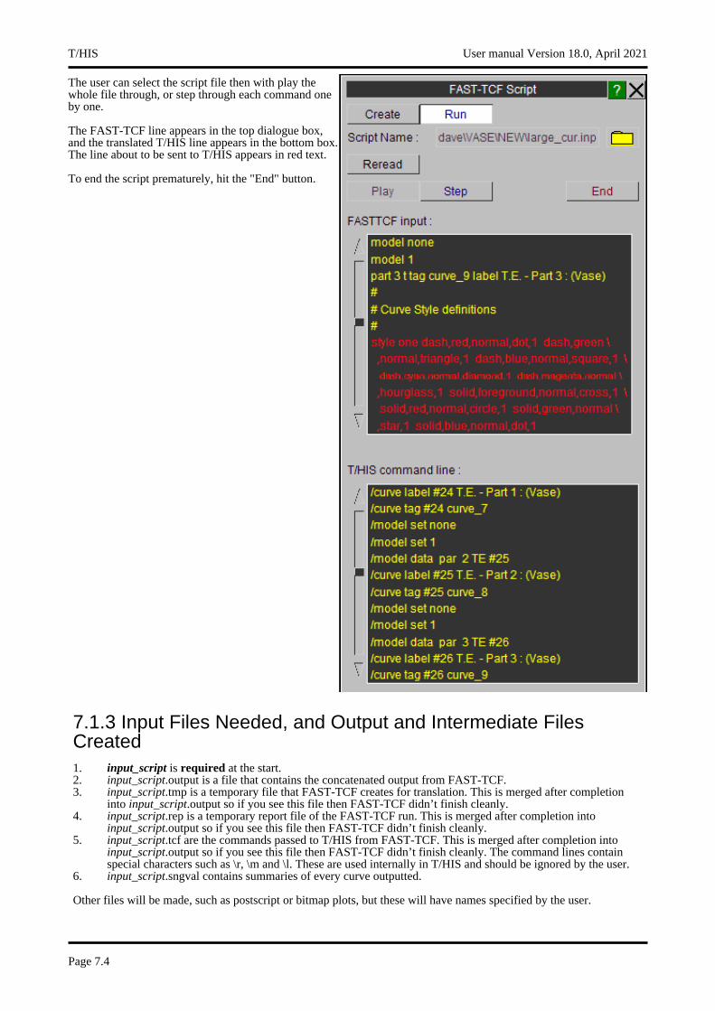
The user can select the script file then with play the whole file through, or step through each command one by one.
The FAST-TCF line appears in the top dialogue box, and the translated T/HIS line appears in the bottom box. The line about to be sent to T/HIS appears in red text.
To end the script prematurely, hit the "End" button.
7.1.3 Input Files Needed, and Output and Intermediate Files Created1. input_script is required at the start.2. input_script.output is a file that contains the concatenated output from FAST-TCF.3. input_script.tmp is a temporary file that FAST-TCF creates for translation. This is merged after completion
into input_script.output so if you see this file then FAST-TCF didn’t finish cleanly.4. input_script.rep is a temporary report file of the FAST-TCF run. This is merged after completion into
input_script.output so if you see this file then FAST-TCF didn’t finish cleanly.5. input_script.tcf are the commands passed to T/HIS from FAST-TCF. This is merged after completion into
input_script.output so if you see this file then FAST-TCF didn’t finish cleanly. The command lines contain special characters such as \r, \m and \l. These are used internally in T/HIS and should be ignored by the user.
6. input_script.sngval contains summaries of every curve outputted.
Other files will be made, such as postscript or bitmap plots, but these will have names specified by the user.
T/HIS User manual Version 18.0, April 2021
Page 7.4
7.1.4 Debugging FAST-TCF files
Complicated FAST-TCF files will inevitably go wrong. There are a number of things the user can do to help identify where it is going wrong. Assuming the command line syntax is correct and the correct files are in the run directory, these typical procedures are as follows:
Identifying errors using the interactive playback option in T/HIS:• Read the model(s) into T/HIS.• Read the FAST-TCF script into T/HIS under the "FAST-TCF > Run" sub menu.• Step through the FAST-TCF script manually, keeping an eye on how FAST-TCF is translating the lines, and
the output T/HIS is producing.
Identifying if FAST-TCF has found an error:• If FAST-TCF finds an error, then it is stored and T/HIS then resets the command line and continues to translate
the input file. If 10 errors are found then T/HIS will stop at this line. You can set this error amount internally within FAST-TCF.
• Once T/HIS has stopped, the errors are summarised in the command line box and the terminal that T/HIS was run from. The number of warnings found is also printed.
• It should be obvious what is wrong, FAST-TCF checks numerous things, including:• Whether T/HIS created the curve from the previous line.• That the syntax is correct for all the data input lines (the data extraction requests have additional checking
to check the combinations of words inputted is right).• If the syntax is correct, whether it applies to the file being requested for output.• The output file exists in the directory for the data extraction.
• Correct the input line error utilising the reference tables in this document if applicable.
Identifying what errors T/HIS is giving:• Identify how many curves were outputted into T/HIS before things went wrong (run T/HIS in graphical mode).• Place an exit keyword after the next input line. This should stop T/HIS just after the line which is causing the
file to fail. • Check what errors T/HIS is giving out. If it’s not obvious what went wrong then try another procedure.
Identifying if there are warnings or errors from FAST-TCF:• The errors are summarised once T/HIS has finished. They are printed in the command line box and the terminal
which T/HIS was run from.• There will be a input_file.rep or input_file.output file in the directory which contains any warnings or errors that
FAST-TCF has detected. Make sure nothing is obviously wrong with the input file using this report file.• The input_file.tmp or input_file.output file contains the actual file inputted into FAST-TCF after includes have
been found and special characters removed. Check this is correct and all the include files have been accounted for.
Identifying if FAST-TCF is processing the line correctly:• It’s possible that FAST-TCF has processed the line incorrectly. If so, open the input_file.tcf or input_file.output
file to investigate what FAST-TCF is asking T/HIS to do.• Identify which line is going wrong using the above procedure, and then find this section in the .tcf file. Input the
entire tcf request for the line into the T/HIS command box to step through what is being asked from T/HIS. This may highlight where things are going wrong. The command lines contain special characters such as \r, \m and \l. These are used internally in T/HIS and should be ignored by the user.
Using Primer to check a FAST-TCF file:• Primer has a FAST-TCF check menu under the main check menu. This can be used to check the FAST-TCF
file data requests against a certain keyword deck. • Read the deck into Primer, and select MODEL > CHECK > CHECK FAST-TCF FILE. Select the FAST-TCF
file and press APPLY. Details can be found in Section 3.9 of the Primer manual.• Primer will highlight any errors that have occurred with the input file with regards to the keyword deck.• The main Primer checks are if the line syntax is valid, whether the correct file is being outputted, whether the
relevant DATABASE_HISTORY is present and whether the id. actually exists. • Any errors will have to be corrected manually in Primer.
NOTE: If FAST-TCF has completed, then it may be necessary to open the input_file.output file which has the all the output files concatenated together in different sections.
User manual Version 18.0, April 2021 T/HIS
Page 7.5
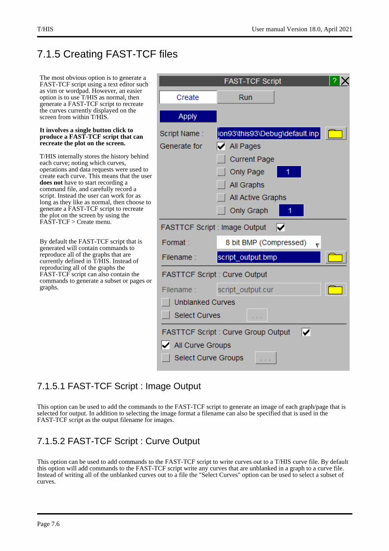
7.1.5 Creating FAST-TCF files
The most obvious option is to generate a FAST-TCF script using a text editor such as vim or wordpad. However, an easier option is to use T/HIS as normal, then generate a FAST-TCF script to recreate the curves currently displayed on the screen from within T/HIS.
It involves a single button click to produce a FAST-TCF script that can recreate the plot on the screen.
T/HIS internally stores the history behind each curve; noting which curves, operations and data requests were used to create each curve. This means that the user does not have to start recording a command file, and carefully record a script. Instead the user can work for as long as they like as normal, then choose to generate a FAST-TCF script to recreate the plot on the screen by using the FAST-TCF > Create menu.
By default the FAST-TCF script that is generated will contain commands to reproduce all of the graphs that are currently defined in T/HIS. Instead of reproducing all of the graphs the FAST-TCF script can also contain the commands to generate a subset or pages or graphs.
7.1.5.1 FAST-TCF Script : Image Output
This option can be used to add the commands to the FAST-TCF script to generate an image of each graph/page that is selected for output. In addition to selecting the image format a filename can also be specified that is used in the FAST-TCF script as the output filename for images.
7.1.5.2 FAST-TCF Script : Curve Output
This option can be used to add commands to the FAST-TCF script to write curves out to a T/HIS curve file. By default this option will add commands to the FAST-TCF script write any curves that are unblanked in a graph to a curve file. Instead of writing all of the unblanked curves out to a file the "Select Curves" option can be used to select a subset of curves.
T/HIS User manual Version 18.0, April 2021
Page 7.6

7.1.5.3 FAST-TCF Script : Curve Group Output
This option can be used to select additional curves for output to the FAST-TCF script by curve group. If a curve is selected that is also unblanked in one of the graphs the command to regenerate it are only added to the FAST-TCF script once. This option will also add the commands to regenerate the selected curve groups to the FAST-TCF script.
User manual Version 18.0, April 2021 T/HIS
Page 7.7

7.2 PAGE / GRAPH LAYOUT AND SELECTION
FAST-TCF scripts can contain commands to create and position multiple graphs. T/HIS Pages can also be created and graphs moved between pages. By default T/HIS will automatically create a single graph on the 1st ’Page’ when it starts. If a single graph is required then the script does not need to contain any of the commands in this section. If additional graphs are required then by default they will be created on the 1st Page unless multiple pages have been selected.
T/HIS User manual Version 18.0, April 2021
Page 7.8
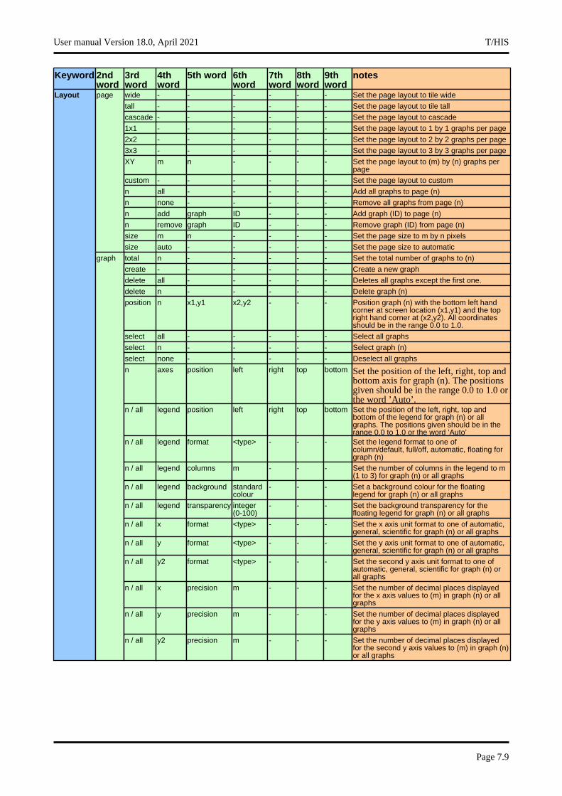
Keyword 2nd word
3rd word
4th word
5th word 6th word
7th word
8th word
9th word
notes
wide - - - - - - Set the page layout to tile wide Layout page
tall - - - - - - Set the page layout to tile tall
cascade - - - - - - Set the page layout to cascade
1x1 - - - - - - Set the page layout to 1 by 1 graphs per page
2x2 - - - - - - Set the page layout to 2 by 2 graphs per page
3x3 - - - - - - Set the page layout to 3 by 3 graphs per page
XY m n - - - - Set the page layout to (m) by (n) graphs per page
custom - - - - - - Set the page layout to custom
n all - - - - - Add all graphs to page (n)
n none - - - - - Remove all graphs from page (n)
n add graph ID - - - Add graph (ID) to page (n)
n remove graph ID - - - Remove graph (ID) from page (n)
size m n - - - - Set the page size to m by n pixels
size auto - - - - - Set the page size to automatic
total n - - - - - Set the total number of graphs to (n)graph
create - - - - - - Create a new graph
delete all - - - - - Deletes all graphs except the first one.
delete n - - - - - Delete graph (n)
position n x1,y1 x2,y2 - - - Position graph (n) with the bottom left hand corner at screen location (x1,y1) and the top right hand corner at (x2,y2). All coordinates should be in the range 0.0 to 1.0.
select all - - - - - Select all graphs
select n - - - - - Select graph (n)
select none - - - - - Deselect all graphs
n axes position left right top bottom Set the position of the left, right, top and bottom axis for graph (n). The positions given should be in the range 0.0 to 1.0 or the word ’Auto’.
n / all legend position left right top bottom Set the position of the left, right, top and bottom of the legend for graph (n) or all graphs. The positions given should be in the range 0.0 to 1.0 or the word ’Auto’
n / all legend format <type> - - - Set the legend format to one of column/default, full/off, automatic, floating for graph (n)
n / all legend columns m - - - Set the number of columns in the legend to m (1 to 3) for graph (n) or all graphs
n / all legend background standard colour
- - - Set a background colour for the floating legend for graph (n) or all graphs
n / all legend transparency integer (0-100)
- - - Set the background transparency for the floating legend for graph (n) or all graphs
n / all x format <type> - - - Set the x axis unit format to one of automatic, general, scientific for graph (n) or all graphs
n / all y format <type> - - - Set the y axis unit format to one of automatic, general, scientific for graph (n) or all graphs
n / all y2 format <type> - - - Set the second y axis unit format to one of automatic, general, scientific for graph (n) or all graphs
n / all x precision m - - - Set the number of decimal places displayed for the x axis values to (m) in graph (n) or all graphs
n / all y precision m - - - Set the number of decimal places displayed for the y axis values to (m) in graph (n) or all graphs
n / all y2 precision m - - - Set the number of decimal places displayed for the second y axis values to (m) in graph (n) or all graphs
User manual Version 18.0, April 2021 T/HIS
Page 7.9
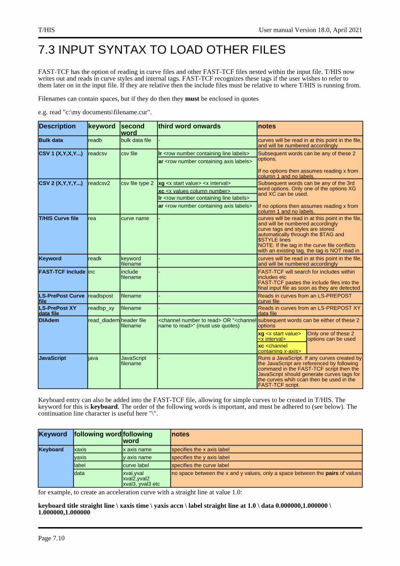
7.3 INPUT SYNTAX TO LOAD OTHER FILES
FAST-TCF has the option of reading in curve files and other FAST-TCF files nested within the input file. T/HIS now writes out and reads in curve styles and internal tags. FAST-TCF recognizes these tags if the user wishes to refer to them later on in the input file. If they are relative then the include files must be relative to where T/HIS is running from.
Filenames can contain spaces, but if they do then they must be enclosed in quotes
e.g. read "c:\my documents\filename.cur".
Description keyword second word
third word onwards notes
Bulk data readb bulk data file - curves will be read in at this point in the file, and will be numbered accordingly
lr <row number containing line labels>CSV 1 (X,Y,X,Y...) readcsv csv file Subsequent words can be any of these 2 options.
If no options then assumes reading x from column 1 and no labels.
ar <row number containing axis labels>
xg <x start value> <x interval>CSV 2 (X,Y,Y,Y...) readcsv2 csv file type 2 Subsequent words can be any of the 3rd word options. Only one of the options XG and XC can be used.
If no options then assumes reading x from column 1 and no labels.
xc <x values column number>lr <row number containing line labels>
ar <row number containing axis labels>
T/HIS Curve file rea curve name - curves will be read in at this point in the file, and will be numbered accordinglycurve tags and styles are stored automatically through the $TAG and $STYLE linesNOTE: If the tag in the curve file conflicts with an existing tag, the tag is NOT read in
Keyword readk keyword filename
- curves will be read in at this point in the file, and will be numbered accordingly
FAST-TCF Include inc include filename
- FAST-TCF will search for includes within includes etcFAST-TCF pastes the include files into the final input file as soon as they are detected
LS-PrePost Curve file
readlspost filename - Reads in curves from an LS-PREPOST curve file
LS-PrePost XY data file
readlsp_xy filename - Reads in curves from an LS-PREPOST XY data filesubsequent words can be either of these 2 options
DIAdem read_diadem header file filename
<channel number to read> OR "<channel name to read>" (must use quotes)
xg <x start value> <x interval>
Only one of these 2 options can be used
xc <channel containing x-axis>
JavaScript java JavaScript filename
- Runs a JavaScript. If any curves created by the JavaScript are referenced by following command in the FAST-TCF script then the JavaScript should generate curves tags for the curves whih ccan then be used in the FAST-TCF script.
Keyboard entry can also be added into the FAST-TCF file, allowing for simple curves to be created in T/HIS. The keyword for this is keyboard. The order of the following words is important, and must be adhered to (see below). The continuation line character is useful here "\".
Keyword following word following word
notes
xaxis x axis name specifies the x axis labelKeyboardyaxis y axis name specifies the y axis label
label curve label specifies the curve label
data xval,yvalxval2,yval2 xval3, yval3 etc
no space between the x and y values, only a space between the pairs of values
for example, to create an acceleration curve with a straight line at value 1.0:
keyboard title straight line \ xaxis time \ yaxis accn \ label straight line at 1.0 \ data 0.000000,1.000000 \ 1.000000,1.000000
T/HIS User manual Version 18.0, April 2021
Page 7.10
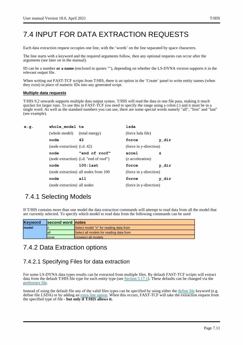
7.4 INPUT FOR DATA EXTRACTION REQUESTS
Each data extraction request occupies one line, with the ’words’ on the line separated by space characters.
The line starts with a keyword and the required arguments follow, then any optional requests can occur after the arguments (see later on in the manual).
ID can be a number or a name (enclosed in quotes ""), depending on whether the LS-DYNA version supports it in the relevant output file.
When writing out FAST-TCF scripts from T/HIS, there is an option in the ’Create’ panel to write entity names (when they exist) in place of numeric IDs into any generated script.
Multiple data requests
T/HIS 9.2 onwards supports multiple data output syntax. T/HIS will read the data in one file pass, making it much quicker for larger runs. To use this in FAST-TCF you need to specify the range using a colon (:) and it must be in a single word. As well as the standard numbers you can use, there are some special words namely "all", "first" and "last" (see example).
e.g. whole_model te lsda
(whole model) (total energy) (force lsda file)
node 42 force y_dir
(node extraction) (i.d. 42) (force in y-direction)
node "end of roof" accel z
(node extraction) (i.d. "end of roof") (z acceleration)
node 100:last force y_dir
(node extraction) all nodes from 100 (force in y-direction)
node all force y_dir
(node extraction) all nodes (force in y-direction)
7.4.1 Selecting Models
If T/HIS contains more than one model the data extraction commands will attempt to read data from all the model that are currently selected. To specify which model to read data from the following commands can be used
Keyword second word notesn Select model "n" for reading data frommodelall Select all models for reading data from
none Unselect all models
7.4.2 Data Extraction options
7.4.2.1 Specifying Files for data extraction
For some LS-DYNA data types results can be extracted from multiple files. By default FAST-TCF scripts will extract data from the default T/HIS file type for each entity type (see Section 5.17.1). These defaults can be changed via the preference file.
Instead of using the default file any of the valid files types can be specified by using either the define file keyword (e.g. define file LSDA) or by adding an extra line option. When this occurs, FAST-TCF will take the extraction request from the specified type of file - but only if T/HIS allows it.
User manual Version 18.0, April 2021 T/HIS
Page 7.11
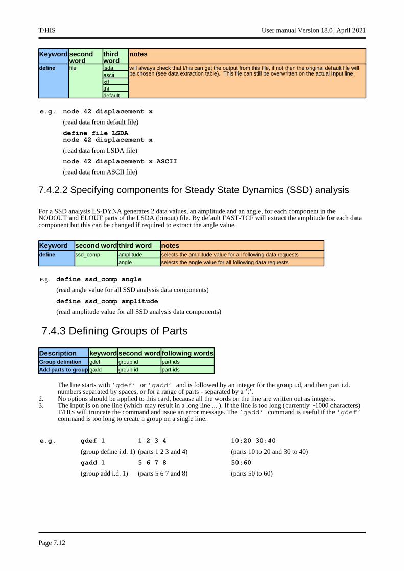
Keyword second word
third word
notes
lsdadefine file will always check that t/his can get the output from this file, if not then the original default file will be chosen (see data extraction table). This file can still be overwritten on the actual input lineascii
xtfthfdefault
e.g. node 42 displacement x
(read data from default file)
define file LSDA node 42 displacement x
(read data from LSDA file)
node 42 displacement x ASCII
(read data from ASCII file)
7.4.2.2 Specifying components for Steady State Dynamics (SSD) analysis
For a SSD analysis LS-DYNA generates 2 data values, an amplitude and an angle, for each component in the NODOUT and ELOUT parts of the LSDA (binout) file. By default FAST-TCF will extract the amplitude for each data component but this can be changed if required to extract the angle value.
Keyword second word third word notesamplitude selects the amplitude value for all following data requestsdefine ssd_comp
angle selects the angle value for all following data requests
e.g. define ssd_comp angle
(read angle value for all SSD analysis data components)
define ssd_comp amplitude
(read amplitude value for all SSD analysis data components)
7.4.3 Defining Groups of Parts
Description keyword second word following wordsGroup definition gdef group id part ids
Add parts to group gadd group id part ids
dd1. The line starts with ’gdef’ or ’gadd’ and is followed by an integer for the group i.d, and then part i.d.
numbers separated by spaces, or for a range of parts - separated by a ’:’.2. No options should be applied to this card, because all the words on the line are written out as integers.3. The input is on one line (which may result in a long line ... ). If the line is too long (currently ~1000 characters)
T/HIS will truncate the command and issue an error message. The ’gadd’ command is useful if the ’gdef’ command is too long to create a group on a single line.
e.g. gdef 1 1 2 3 4 10:20 30:40
(group define i.d. 1) (parts 1 2 3 and 4) (parts 10 to 20 and 30 to 40)
gadd 1 5 6 7 8 50:60
(group add i.d. 1) (parts 5 6 7 and 8) (parts 50 to 60)
T/HIS User manual Version 18.0, April 2021
Page 7.12
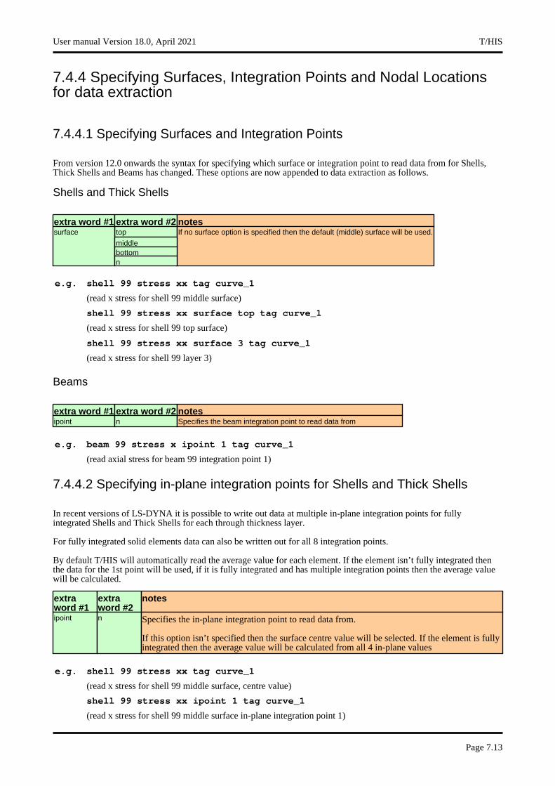
7.4.4 Specifying Surfaces, Integration Points and Nodal Locations for data extraction
7.4.4.1 Specifying Surfaces and Integration Points
From version 12.0 onwards the syntax for specifying which surface or integration point to read data from for Shells, Thick Shells and Beams has changed. These options are now appended to data extraction as follows.
Shells and Thick Shells
extra word #1 extra word #2 notestopsurface If no surface option is specified then the default (middle) surface will be used.
middlebottomn
e.g. shell 99 stress xx tag curve_1
(read x stress for shell 99 middle surface)
shell 99 stress xx surface top tag curve_1
(read x stress for shell 99 top surface)
shell 99 stress xx surface 3 tag curve_1
(read x stress for shell 99 layer 3)
Beams
extra word #1 extra word #2 notesipoint n Specifies the beam integration point to read data from
e.g. beam 99 stress x ipoint 1 tag curve_1
(read axial stress for beam 99 integration point 1)
7.4.4.2 Specifying in-plane integration points for Shells and Thick Shells
In recent versions of LS-DYNA it is possible to write out data at multiple in-plane integration points for fully integrated Shells and Thick Shells for each through thickness layer.
For fully integrated solid elements data can also be written out for all 8 integration points.
By default T/HIS will automatically read the average value for each element. If the element isn’t fully integrated then the data for the 1st point will be used, if it is fully integrated and has multiple integration points then the average value will be calculated.
extra word #1
extra word #2
notes
ipoint n Specifies the in-plane integration point to read data from.
If this option isn’t specified then the surface centre value will be selected. If the element is fully integrated then the average value will be calculated from all 4 in-plane values
e.g. shell 99 stress xx tag curve_1
(read x stress for shell 99 middle surface, centre value)
shell 99 stress xx ipoint 1 tag curve_1
(read x stress for shell 99 middle surface in-plane integration point 1)
User manual Version 18.0, April 2021 T/HIS
Page 7.13
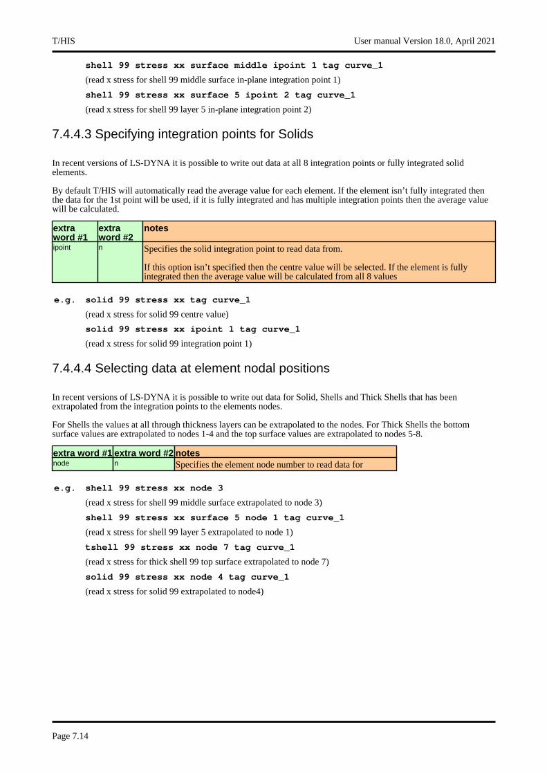
shell 99 stress xx surface middle ipoint 1 tag curve_1
(read x stress for shell 99 middle surface in-plane integration point 1)
shell 99 stress xx surface 5 ipoint 2 tag curve_1
(read x stress for shell 99 layer 5 in-plane integration point 2)
7.4.4.3 Specifying integration points for Solids
In recent versions of LS-DYNA it is possible to write out data at all 8 integration points or fully integrated solid elements.
By default T/HIS will automatically read the average value for each element. If the element isn’t fully integrated then the data for the 1st point will be used, if it is fully integrated and has multiple integration points then the average value will be calculated.
extra word #1
extra word #2
notes
ipoint n Specifies the solid integration point to read data from.
If this option isn’t specified then the centre value will be selected. If the element is fully integrated then the average value will be calculated from all 8 values
e.g. solid 99 stress xx tag curve_1
(read x stress for solid 99 centre value)
solid 99 stress xx ipoint 1 tag curve_1
(read x stress for solid 99 integration point 1)
7.4.4.4 Selecting data at element nodal positions
In recent versions of LS-DYNA it is possible to write out data for Solid, Shells and Thick Shells that has been extrapolated from the integration points to the elements nodes.
For Shells the values at all through thickness layers can be extrapolated to the nodes. For Thick Shells the bottom surface values are extrapolated to nodes 1-4 and the top surface values are extrapolated to nodes 5-8.
extra word #1 extra word #2 notesnode n Specifies the element node number to read data for
e.g. shell 99 stress xx node 3
(read x stress for shell 99 middle surface extrapolated to node 3)
shell 99 stress xx surface 5 node 1 tag curve_1
(read x stress for shell 99 layer 5 extrapolated to node 1)
tshell 99 stress xx node 7 tag curve_1
(read x stress for thick shell 99 top surface extrapolated to node 7)
solid 99 stress xx node 4 tag curve_1
(read x stress for solid 99 extrapolated to node4)
T/HIS User manual Version 18.0, April 2021
Page 7.14
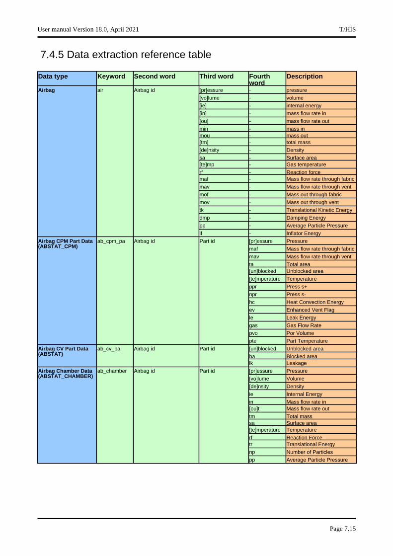
7.4.5 Data extraction reference table
Data type Keyword Second word Third word Fourth word
Description
[pr]essure - pressureAirbag air Airbag id
[vo]lume - volume
[ie] - internal energy
[in] - mass flow rate in
[ou] - mass flow rate out
min - mass inmou - mass out[tm] - total mass
[de]nsity - Density
sa - Surface area[te]mp - Gas temperature
rf - Reaction forcemaf - Mass flow rate through fabric
mav - Mass flow rate through vent
mof - Mass out through fabric
mov - Mass out through vent
tk - Translational Kinetic Energy
dmp - Damping Energy
pp - Average Particle Pressure
if - Inflator Energy
[pr]essure PressureAirbag CPM Part Data(ABSTAT_CPM)
ab_cpm_pa Airbag id Part id
maf Mass flow rate through fabric
mav Mass flow rate through vent
ta Total area[un]blocked Unblocked area
[te]mperature Temperature
ppr Press s+
npr Press s-
hc Heat Convection Energy
ev Enhanced Vent Flag
le Leak Energy
gas Gas Flow Rate
pvo Por Volume
pte Part Temperature
[un]blocked Unblocked areaAirbag CV Part Data(ABSTAT)
ab_cv_pa Airbag id Part id
ba Blocked arealk Leakage
[pr]essure PressureAirbag Chamber Data(ABSTAT_CHAMBER)
ab_chamber Airbag id Part id
[vo]lume Volume
[de]nsity Density
ie Internal Energy
in Mass flow rate in[ou]t Mass flow rate out
tm Total masssa Surface area[te]mperature Temperature
rf Reaction Forcetr Translational Energy
np Number of Particles
pp Average Particle Pressure
User manual Version 18.0, April 2021 T/HIS
Page 7.15
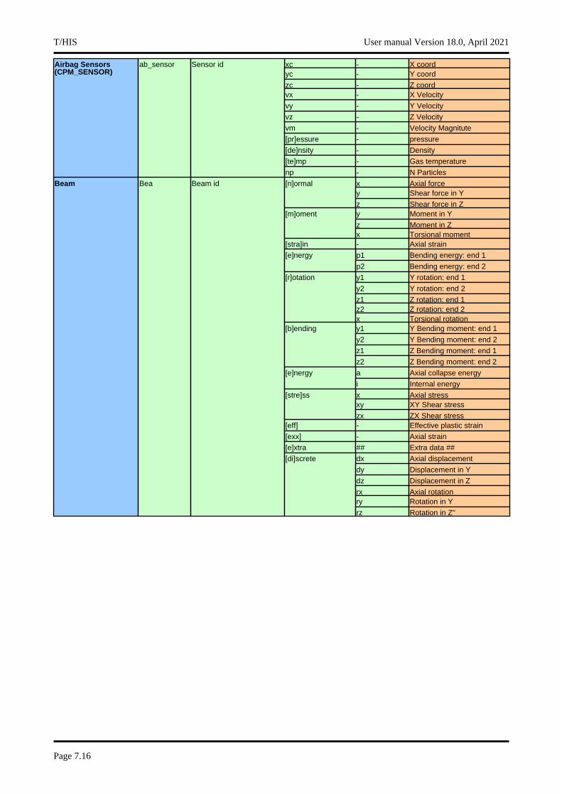
xc - X coordAirbag Sensors(CPM_SENSOR)
ab_sensor Sensor idyc - Y coord
zc - Z coordvx - X Velocity
vy - Y Velocity
vz - Z Velocity
vm - Velocity Magnitute
[pr]essure - pressure
[de]nsity - Density
[te]mp - Gas temperature
np - N Particles
x Axial forceBeam Bea Beam id [n]ormaly Shear force in Y
z Shear force in Zy Moment in Y[m]oment
z Moment in Zx Torsional moment
[stra]in - Axial strain
p1 Bending energy: end 1[e]nergy
p2 Bending energy: end 2
y1 Y rotation: end 1[r]otation
y2 Y rotation: end 2
z1 Z rotation: end 1z2 Z rotation: end 2x Torsional rotationy1 Y Bending moment: end 1[b]ending
y2 Y Bending moment: end 2
z1 Z Bending moment: end 1
z2 Z Bending moment: end 2
a Axial collapse energy[e]nergy
i Internal energy
x Axial stress[stre]ssxy XY Shear stress
zx ZX Shear stress[eff] - Effective plastic strain
[exx] - Axial strain
[e]xtra ## Extra data ##
dx Axial displacement[di]screte
dy Displacement in Y
dz Displacement in Z
rx Axial rotationry Rotation in Y
rz Rotation in Z"
T/HIS User manual Version 18.0, April 2021
Page 7.16
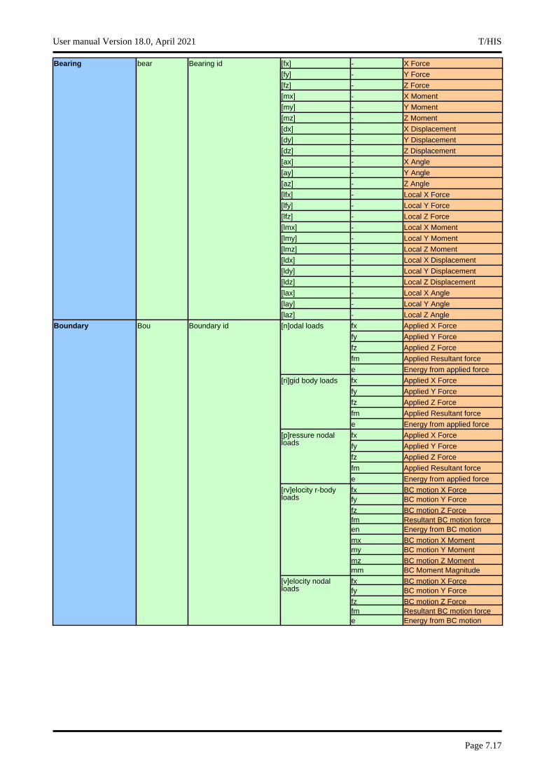
[fx] - X Force Bearing bear Bearing id
[fy] - Y Force
[fz] - Z Force
[mx] - X Moment
[my] - Y Moment
[mz] - Z Moment
[dx] - X Displacement
[dy] - Y Displacement
[dz] - Z Displacement
[ax] - X Angle
[ay] - Y Angle
[az] - Z Angle
[lfx] - Local X Force
[lfy] - Local Y Force
[lfz] - Local Z Force
[lmx] - Local X Moment
[lmy] - Local Y Moment
[lmz] - Local Z Moment
[ldx] - Local X Displacement
[ldy] - Local Y Displacement
[ldz] - Local Z Displacement
[lax] - Local X Angle
[lay] - Local Y Angle
[laz] - Local Z Angle
fx Applied X ForceBoundary Bou Boundary id [n]odal loads
fy Applied Y Force
fz Applied Z Force
fm Applied Resultant force
e Energy from applied force
fx Applied X Force[ri]gid body loads
fy Applied Y Force
fz Applied Z Force
fm Applied Resultant force
e Energy from applied force
fx Applied X Force[p]ressure nodal loads fy Applied Y Force
fz Applied Z Force
fm Applied Resultant force
e Energy from applied force
fx BC motion X Force[rv]elocity r-body loads fy BC motion Y Force
fz BC motion Z Forcefm Resultant BC motion forceen Energy from BC motion
mx BC motion X Momentmy BC motion Y Moment
mz BC motion Z Momentmm BC Moment Magnitude
fx BC motion X Force[v]elocity nodal loads fy BC motion Y Force
fz BC motion Z Forcefm Resultant BC motion forcee Energy from BC motion
User manual Version 18.0, April 2021 T/HIS
Page 7.17
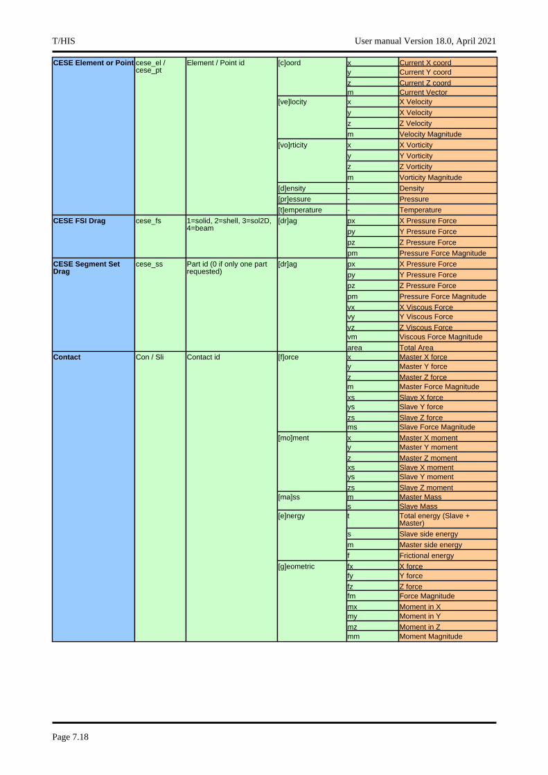
x Current X coordCESE Element or Point cese_el / cese_pt
Element / Point id [c]oordy Current Y coord
z Current Z coordm Current Vectorx X Velocity[ve]locity
y X Velocity
z Z Velocity
m Velocity Magnitude
x X Vorticity[vo]rticity
y Y Vorticity
z Z Vorticity
m Vorticity Magnitude
[d]ensity - Density
[pr]essure - Pressure
[t]emperature - Temperature
px X Pressure ForceCESE FSI Drag cese_fs 1=solid, 2=shell, 3=sol2D, 4=beam
[dr]ag
py Y Pressure Force
pz Z Pressure Force
pm Pressure Force Magnitude
px X Pressure ForceCESE Segment Set Drag
cese_ss Part id (0 if only one part requested)
[dr]ag
py Y Pressure Force
pz Z Pressure Force
pm Pressure Force Magnitude
vx X Viscous Forcevy Y Viscous Force
vz Z Viscous Forcevm Viscous Force Magnitude
area Total Areax Master X forceContact Con / Sli Contact id [f]orcey Master Y force
z Master Z forcem Master Force Magnitude
xs Slave X forceys Slave Y force
zs Slave Z forcems Slave Force Magnitude
x Master X moment[mo]menty Master Y moment
z Master Z momentxs Slave X momentys Slave Y moment
zs Slave Z momentm Master Mass[ma]sss Slave Masst Total energy (Slave +
Master)[e]nergy
s Slave side energy
m Master side energy
f Frictional energy
fx X force[g]eometricfy Y force
fz Z forcefm Force Magnitude
mx Moment in Xmy Moment in Y
mz Moment in Zmm Moment Magnitude
T/HIS User manual Version 18.0, April 2021
Page 7.18
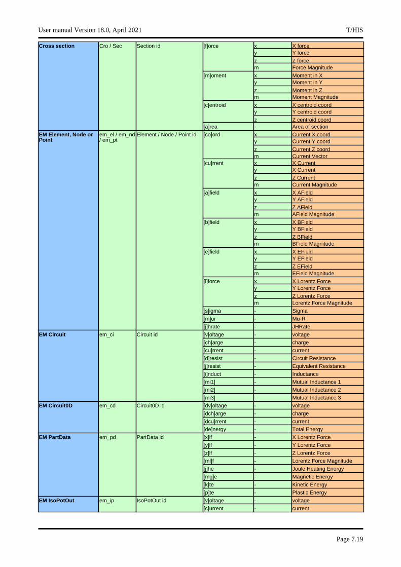
x X forceCross section Cro / Sec Section id [f]orcey Y force
z Z forcem Force Magnitude
x Moment in X[m]omenty Moment in Y
z Moment in Zm Moment Magnitude
x X centroid coord[c]entroidy Y centroid coord
z Z centroid coord[a]rea - Area of section
x Current X coordEM Element, Node or Point
em_el / em_nd / em_pt
Element / Node / Point id [co]ordy Current Y coord
z Current Z coordm Current Vectorx X Current[cu]rrenty X Current
z Z Currentm Current Magnitude
x X AField[a]fieldy Y AField
z Z AFieldm AField Magnitude
x X BField[b]fieldy Y BField
z Z BFieldm BField Magnitude
x X EField[e]fieldy Y EField
z Z EFieldm EField Magnitude
x X Lorentz Force[l]forcey Y Lorentz Force
z Z Lorentz Forcem Lorentz Force Magnitude
[s]igma - Sigma
[m]ur - Mu-R
[j]hrate - JHRate
[v]oltage - voltageEM Circuit em_ci Circuit id
[ch]arge - charge
[cu]rrent - current
[d]resist - Circuit Resistance
[j]resist - Equivalent Resistance
[i]nduct - Inductance
[mi1] - Mutual Inductance 1
[mi2] - Mutual Inductance 2
[mi3] - Mutual Inductance 3
[dv]oltage - voltageEM Circuit0D em_cd Circuit0D id
[dch]arge - charge
[dcu]rrent - current
[de]nergy - Total Energy
[x]lf - X Lorentz ForceEM PartData em_pd PartData id
[y]lf - Y Lorentz Force
[z]lf - Z Lorentz Force
[ml]f - Lorentz Force Magnitude
[j]he - Joule Heating Energy
[mg]e - Magnetic Energy
[k]te - Kinetic Energy
[p]te - Plastic Energy
[v]oltage - voltageEM IsoPotOut em_ip IsoPotOut id
[c]urrent - current
User manual Version 18.0, April 2021 T/HIS
Page 7.19
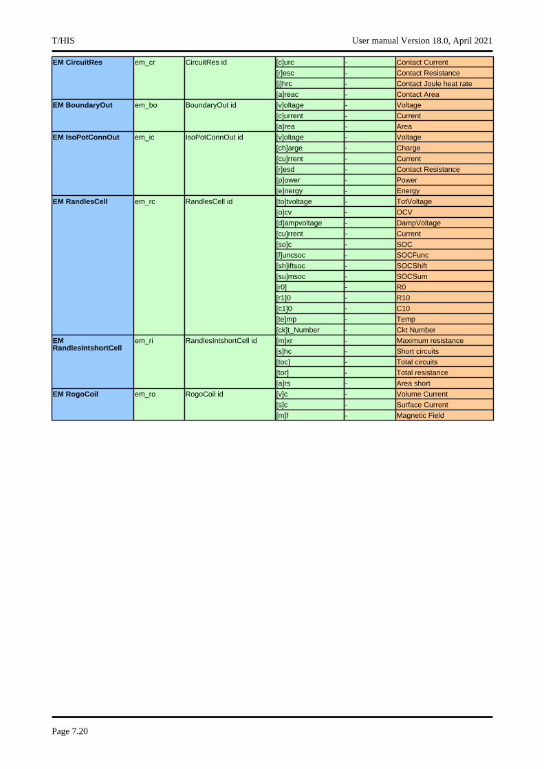
[c]urc - Contact CurrentEM CircuitRes em_cr CircuitRes id
[r]esc - Contact Resistance
[j]hrc - Contact Joule heat rate
[a]reac - Contact Area
[v]oltage - VoltageEM BoundaryOut em_bo BoundaryOut id
[c]urrent - Current
[a]rea - Area
[v]oltage - VoltageEM IsoPotConnOut em_ic IsoPotConnOut id
[ch]arge - Charge
[cu]rrent - Current
[r]esd - Contact Resistance
[p]ower - Power
[e]nergy - Energy
[to]tvoltage - TotVoltageEM RandlesCell em_rc RandlesCell id
[o]cv - OCV
[d]ampvoltage - DampVoltage
[cu]rrent - Current
[so]c - SOC
[f]uncsoc - SOCFunc
[sh]iftsoc - SOCShift
[su]msoc - SOCSum
[r0] - R0
[r1]0 - R10
[c1]0 - C10
[te]mp - Temp
[ck]t_Number - Ckt Number
[m]xr - Maximum resistanceEM RandlesIntshortCell
em_ri RandlesIntshortCell id
[s]hc - Short circuits
[toc] - Total circuits
[tor] - Total resistance
[a]rs - Area short
[v]c - Volume CurrentEM RogoCoil em_ro RogoCoil id
[s]c - Surface Current
[m]f - Magnetic Field
T/HIS User manual Version 18.0, April 2021
Page 7.20
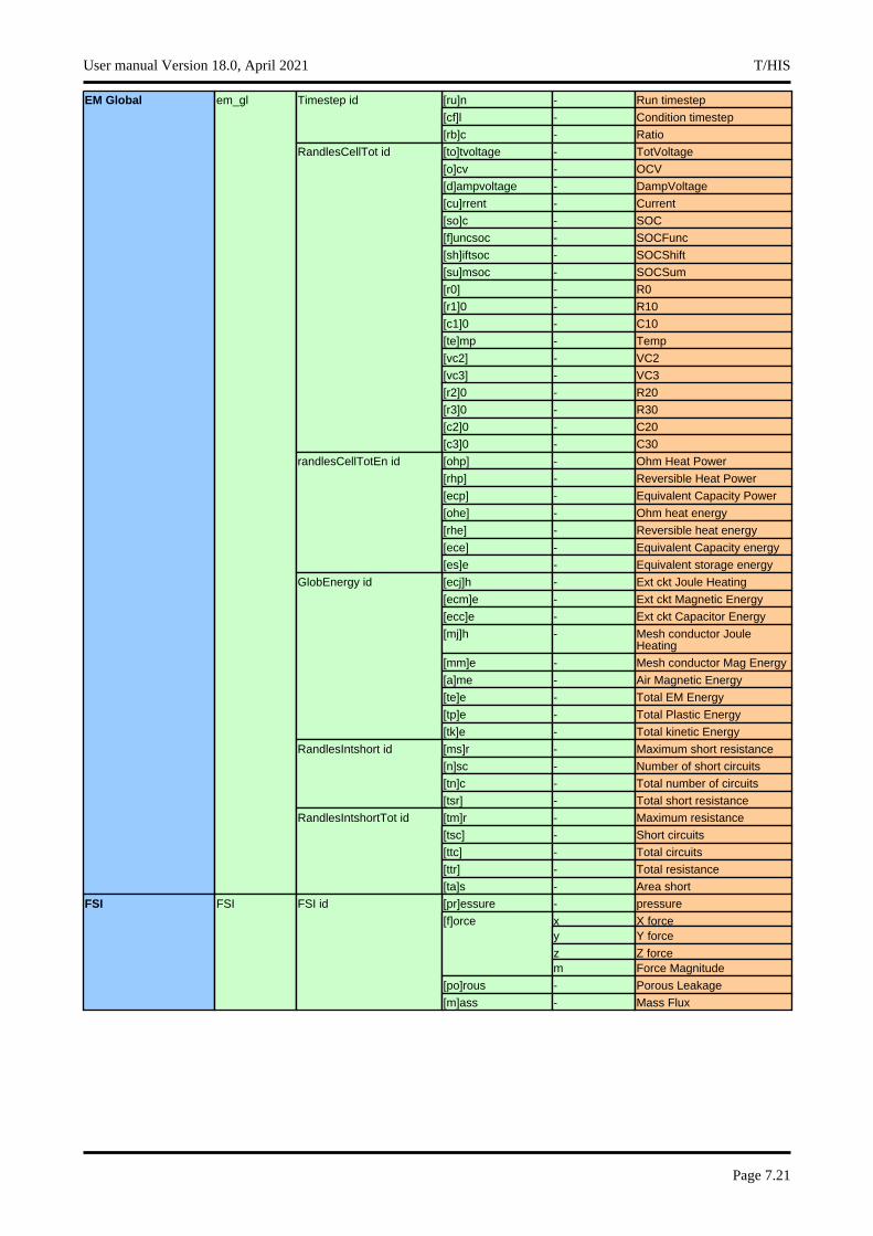
[ru]n - Run timestepEM Global em_gl Timestep id
[cf]l - Condition timestep
[rb]c - Ratio
[to]tvoltage - TotVoltageRandlesCellTot id
[o]cv - OCV
[d]ampvoltage - DampVoltage
[cu]rrent - Current
[so]c - SOC
[f]uncsoc - SOCFunc
[sh]iftsoc - SOCShift
[su]msoc - SOCSum
[r0] - R0
[r1]0 - R10
[c1]0 - C10
[te]mp - Temp
[vc2] - VC2
[vc3] - VC3
[r2]0 - R20
[r3]0 - R30
[c2]0 - C20
[c3]0 - C30
[ohp] - Ohm Heat PowerrandlesCellTotEn id
[rhp] - Reversible Heat Power
[ecp] - Equivalent Capacity Power
[ohe] - Ohm heat energy
[rhe] - Reversible heat energy
[ece] - Equivalent Capacity energy
[es]e - Equivalent storage energy
[ecj]h - Ext ckt Joule HeatingGlobEnergy id
[ecm]e - Ext ckt Magnetic Energy
[ecc]e - Ext ckt Capacitor Energy
[mj]h - Mesh conductor Joule Heating
[mm]e - Mesh conductor Mag Energy
[a]me - Air Magnetic Energy
[te]e - Total EM Energy
[tp]e - Total Plastic Energy
[tk]e - Total kinetic Energy
[ms]r - Maximum short resistanceRandlesIntshort id
[n]sc - Number of short circuits
[tn]c - Total number of circuits
[tsr] - Total short resistance
[tm]r - Maximum resistanceRandlesIntshortTot id
[tsc] - Short circuits
[ttc] - Total circuits
[ttr] - Total resistance
[ta]s - Area short
[pr]essure - pressureFSI FSI FSI id
x X force[f]orcey Y force
z Z forcem Force Magnitude
[po]rous - Porous Leakage
[m]ass - Mass Flux
User manual Version 18.0, April 2021 T/HIS
Page 7.21
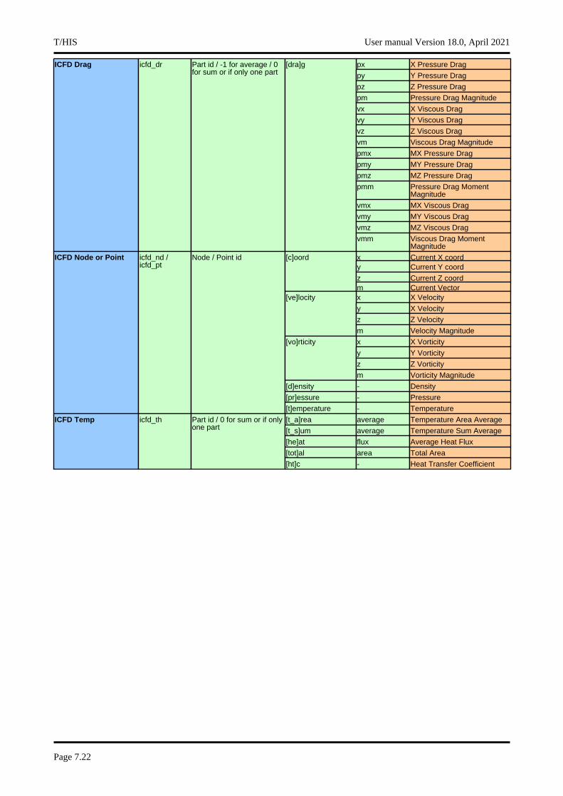
px X Pressure DragICFD Drag icfd_dr Part id / -1 for average / 0 for sum or if only one part
[dra]g
py Y Pressure Drag
pz Z Pressure Drag
pm Pressure Drag Magnitude
vx X Viscous Drag
vy Y Viscous Drag
vz Z Viscous Drag
vm Viscous Drag Magnitude
pmx MX Pressure Drag
pmy MY Pressure Drag
pmz MZ Pressure Drag
pmm Pressure Drag Moment Magnitude
vmx MX Viscous Drag
vmy MY Viscous Drag
vmz MZ Viscous Drag
vmm Viscous Drag Moment Magnitude
x Current X coordICFD Node or Point icfd_nd / icfd_pt
Node / Point id [c]oordy Current Y coord
z Current Z coordm Current Vectorx X Velocity[ve]locity
y X Velocity
z Z Velocity
m Velocity Magnitude
x X Vorticity[vo]rticity
y Y Vorticity
z Z Vorticity
m Vorticity Magnitude
[d]ensity - Density
[pr]essure - Pressure
[t]emperature - Temperature
[t_a]rea average Temperature Area AverageICFD Temp icfd_th Part id / 0 for sum or if only one part [t_s]um average Temperature Sum Average
[he]at flux Average Heat Flux
[tot]al area Total Area
[ht]c - Heat Transfer Coefficient
T/HIS User manual Version 18.0, April 2021
Page 7.22
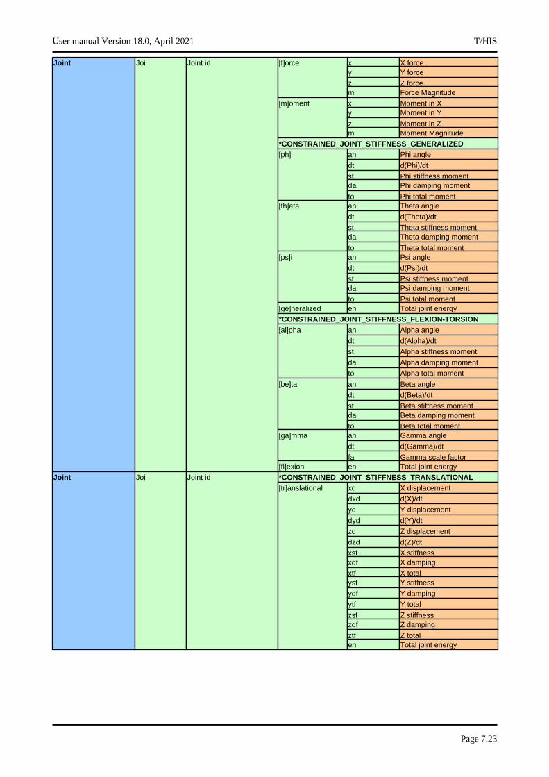
x X forceJoint Joi Joint id [f]orcey Y force
z Z forcem Force Magnitude
x Moment in X[m]omenty Moment in Y
z Moment in Zm Moment Magnitude
*CONSTRAINED_JOINT_STIFFNESS_GENERALIZEDan Phi angle[ph]i
dt d(Phi)/dt
st Phi stiffness momentda Phi damping moment
to Phi total momentan Theta angle[th]eta
dt d(Theta)/dt
st Theta stiffness momentda Theta damping moment
to Theta total momentan Psi angle[ps]i
dt d(Psi)/dt
st Psi stiffness momentda Psi damping moment
to Psi total moment[ge]neralized en Total joint energy
*CONSTRAINED_JOINT_STIFFNESS_FLEXION-TORSIONan Alpha angle[al]pha
dt d(Alpha)/dt
st Alpha stiffness moment
da Alpha damping moment
to Alpha total moment
an Beta angle[be]ta
dt d(Beta)/dt
st Beta stiffness momentda Beta damping moment
to Beta total momentan Gamma angle[ga]mma
dt d(Gamma)/dt
fa Gamma scale factor[fl]exion en Total joint energy
*CONSTRAINED_JOINT_STIFFNESS_TRANSLATIONALJoint Joi Joint idxd X displacement[tr]anslational
dxd d(X)/dt
yd Y displacement
dyd d(Y)/dt
zd Z displacement
dzd d(Z)/dt
xsf X stiffnessxdf X damping
xtf X totalysf Y stiffness
ydf Y damping
ytf Y total
zsf Z stiffnesszdf Z damping
ztf Z totalen Total joint energy
User manual Version 18.0, April 2021 T/HIS
Page 7.23

[te]mperature x TemperatureNode No Node id
[to]p temperature Top Surface Temperature
[bo]ttom temperature Bottom Surface Temperature
x X Displacement[d]isplacement
y Y Displacement
z Z Displacement
m Displacement Magnitute
x X Velocity[v]elocity
y Y Velocity
z Z Velocity
m Velocity Magnitute
x X Acceleration[a]ccelerationy Y Acceleration
z Z Accelerationm Acceleration Magnitude
x Current X coord[c]oordy Current Y coord
z Current Z coordm Current Vectorx Basic X coord[b]asicy Basic Y coord
z Basic Z coordm Basic Vectorx X rotation[r]otationy Y rotation
z Z rotationm Rotation Magnitude
vx X rotational velocity
vy Y rotational velocity
vz Z rotational velocity
vm Rotation Vel Magnitude
ax X rotational accelerationay Y rotational acceleration
az Z rotational accelerationam Rotation Accel Magnitude
x X forceforcey Y force
z Z forcem Force Magnitude
[e]nergy - Energy
x X forceNode Group Ng Group id forcey Y force
z Z forcem Force Magnitude
[k]inetic e - Kinetic energyPart Pa Part id
[i]nternal e - Internal energy
[h]ourglass e - Hourglass energy
[t]otal e - Total energy
[mx] - X momentum
[my] - Y momentum
[mz] - Z momentum
[x] velocity - Average X velocity
[y] velocity - Average Y velocity
[z] velocity - Average Z velocity
[am] - Added mass
[ek] - Eroded Kinetic energy
[ei] - Eroded Internal energy
[k]inetic e - Kinetic energyPart group Gro Group id
[i]nternal e - Internal energy
[h]ourglass e - Hourglass energy
[t]otal e - Total energy
[am] - Added mass
T/HIS User manual Version 18.0, April 2021
Page 7.24
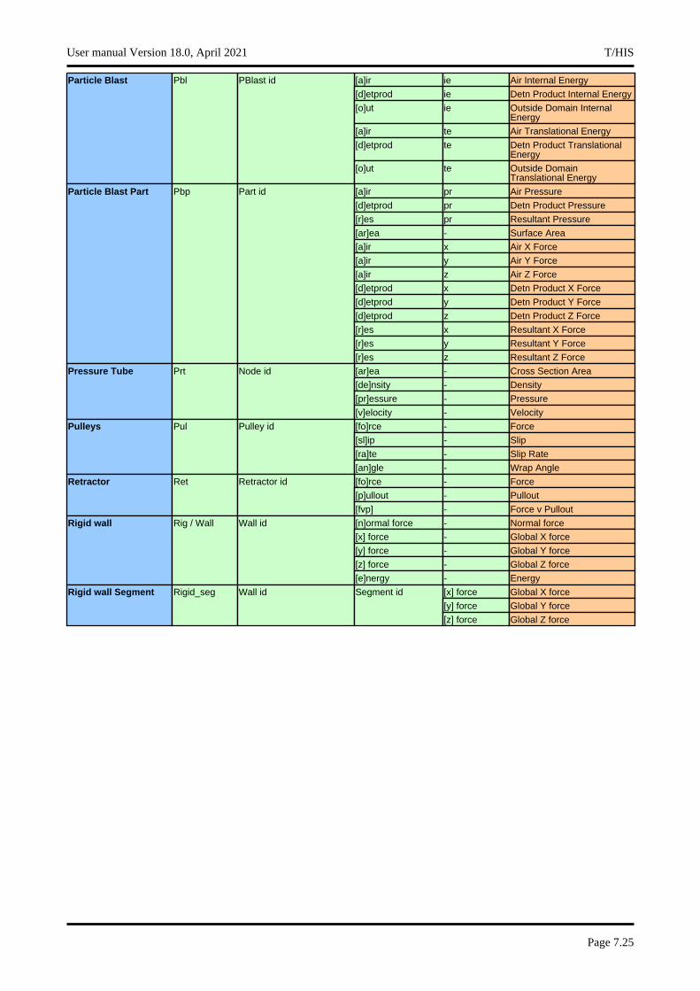
[a]ir ie Air Internal EnergyParticle Blast Pbl PBlast id
[d]etprod ie Detn Product Internal Energy
[o]ut ie Outside Domain Internal Energy
[a]ir te Air Translational Energy
[d]etprod te Detn Product Translational Energy
[o]ut te Outside Domain Translational Energy
[a]ir pr Air PressureParticle Blast Part Pbp Part id
[d]etprod pr Detn Product Pressure
[r]es pr Resultant Pressure
[ar]ea - Surface Area
[a]ir x Air X Force
[a]ir y Air Y Force
[a]ir z Air Z Force
[d]etprod x Detn Product X Force
[d]etprod y Detn Product Y Force
[d]etprod z Detn Product Z Force
[r]es x Resultant X Force
[r]es y Resultant Y Force
[r]es z Resultant Z Force
[ar]ea - Cross Section AreaPressure Tube Prt Node id
[de]nsity - Density
[pr]essure - Pressure
[v]elocity - Velocity
[fo]rce - ForcePulleys Pul Pulley id
[sl]ip - Slip
[ra]te - Slip Rate
[an]gle - Wrap Angle
[fo]rce - ForceRetractor Ret Retractor id
[p]ullout - Pullout
[fvp] - Force v Pullout
[n]ormal force - Normal forceRigid wall Rig / Wall Wall id
[x] force - Global X force
[y] force - Global Y force
[z] force - Global Z force
[e]nergy - Energy
[x] force Global X forceRigid wall Segment Rigid_seg Wall id Segment id
[y] force Global Y force
[z] force Global Z force
User manual Version 18.0, April 2021 T/HIS
Page 7.25
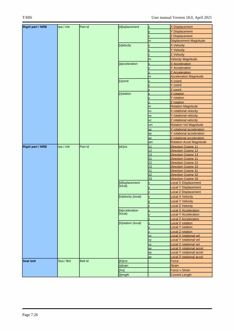
x X DisplacementRigid part / NRB rpa / nrb Part id [d]isplacement
y Y Displacement
z Z Displacement
m Displacement Magnitude
x X Velocity[v]elocity
y Y Velocity
z Z Velocity
m Velocity Magnitude
x X Acceleration[a]ccelerationy Y Acceleration
z Z Accelerationm Acceleration Magnitude
x X coord[c]oordy Y coord
z Z coordx X rotation[r]otationy Y rotation
z Z rotationm Rotation Magnitude
vx X rotational velocity
vy Y rotational velocity
vz Z rotational velocity
vm Rotation Vel Magnitude
ax X rotational accelerationay Y rotational acceleration
az Z rotational accelerationam Rotation Accel Magnitude
11 Direction Cosine 11Rigid part / NRB rpa / nrb Part id [dc]os12 Direction Cosine 1213 Direction Cosine 1321 Direction Cosine 2122 Direction Cosine 2223 Direction Cosine 2331 Direction Cosine 3132 Direction Cosine 3233 Direction Cosine 33x Local X Displacement[ld]isplacement
(local) y Local Y Displacement
z Local Z Displacement
x Local X Velocity[lv]elocity (local)
y Local Y Velocity
z Local Z Velocity
x Local X Acceleration[la]cceleration (local) y Local Y Acceleration
z Local Z Accelerationx Local X rotation[lr]otation (local)y Local Y rotation
z Local Z rotationvx Local X rotational velvy Local Y rotational vel
vz Local Z rotational velax Local X rotational accelay Local Y rotational accel
az Local Z rotational accel[fo]rce - ForceSeat belt Sea / Bel Belt id
[s]train - Strain
[fvs] - Force v Strain
[l]ength - Current Length
T/HIS User manual Version 18.0, April 2021
Page 7.26
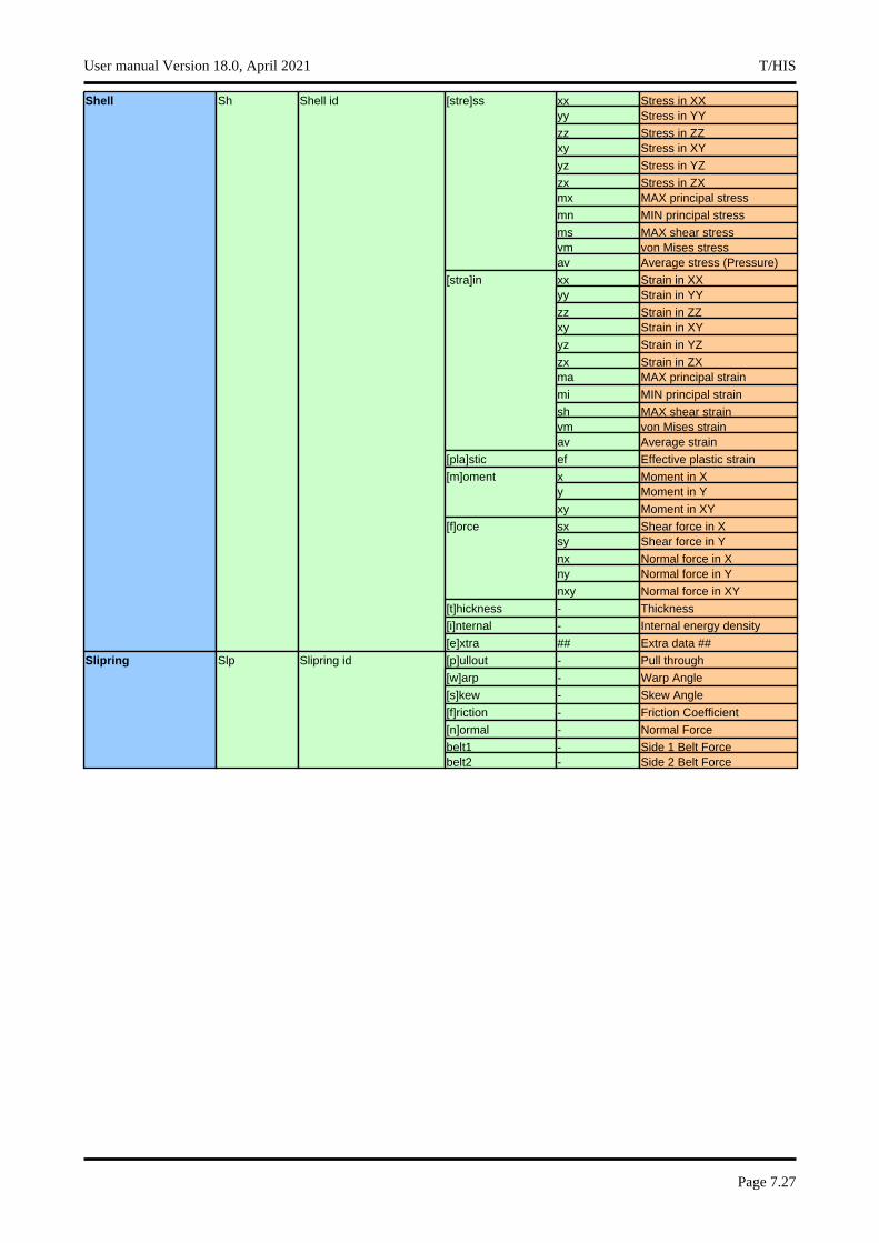
xx Stress in XXShell Sh Shell id [stre]ssyy Stress in YY
zz Stress in ZZxy Stress in XY
yz Stress in YZ
zx Stress in ZXmx MAX principal stress
mn MIN principal stress
ms MAX shear stressvm von Mises stressav Average stress (Pressure)
xx Strain in XX[stra]inyy Strain in YY
zz Strain in ZZxy Strain in XY
yz Strain in YZ
zx Strain in ZXma MAX principal strain
mi MIN principal strain
sh MAX shear strainvm von Mises strainav Average strain
[pla]stic ef Effective plastic strain
x Moment in X[m]omenty Moment in Y
xy Moment in XY
sx Shear force in X[f]orcesy Shear force in Y
nx Normal force in Xny Normal force in Y
nxy Normal force in XY
[t]hickness - Thickness
[i]nternal - Internal energy density
[e]xtra ## Extra data ##
[p]ullout - Pull throughSlipring Slp Slipring id
[w]arp - Warp Angle
[s]kew - Skew Angle
[f]riction - Friction Coefficient
[n]ormal - Normal Force
belt1 - Side 1 Belt Forcebelt2 - Side 2 Belt Force
User manual Version 18.0, April 2021 T/HIS
Page 7.27
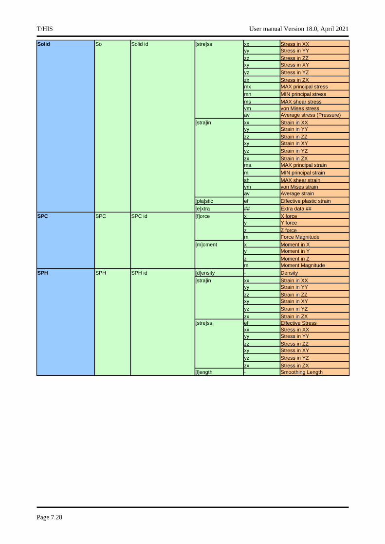
xx Stress in XXSolid So Solid id [stre]ssyy Stress in YY
zz Stress in ZZxy Stress in XY
yz Stress in YZ
zx Stress in ZXmx MAX principal stress
mn MIN principal stress
ms MAX shear stressvm von Mises stressav Average stress (Pressure)
xx Strain in XX[stra]inyy Strain in YY
zz Strain in ZZxy Strain in XY
yz Strain in YZ
zx Strain in ZXma MAX principal strain
mi MIN principal strain
sh MAX shear strainvm von Mises strainav Average strain
[pla]stic ef Effective plastic strain
[e]xtra ## Extra data ##
x X forceSPC SPC SPC id [f]orcey Y force
z Z forcem Force Magnitude
x Moment in X[m]omenty Moment in Y
z Moment in Zm Moment Magnitude
[d]ensity - DensitySPH SPH SPH id
xx Strain in XX[stra]inyy Strain in YY
zz Strain in ZZxy Strain in XY
yz Strain in YZ
zx Strain in ZXef Effective Stress[stre]ssxx Stress in XXyy Stress in YY
zz Stress in ZZxy Stress in XY
yz Stress in YZ
zx Stress in ZX[l]ength - Smoothing Length
T/HIS User manual Version 18.0, April 2021
Page 7.28
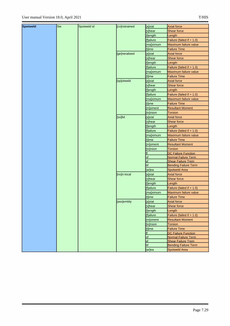
[a]xial Axial forceSpotweld Sw Spotweld id [co]nstrained
[s]hear Shear force
[l]ength Length
[f]ailure Failure (failed if > 1.0)
[ma]ximum Maximum failure value
[t]ime Failure Time
[a]xial Axial force[ge]neralised
[s]hear Shear force
[l]ength Length
[f]ailure Failure (failed if > 1.0)
[ma]ximum Maximum failure value
[t]ime Failure Time
[a]xial Axial force[sp]otweld
[s]hear Shear force
[l]ength Length
[f]ailure Failure (failed if > 1.0)
[ma]ximum Maximum failure value
[t]ime Failure Time
[m]oment Resultant Moment
[to]rsion Torsion
[a]xial Axial force[so]lid
[s]hear Shear force
[l]ength Length
[f]ailure Failure (failed if > 1.0)
[ma]ximum Maximum failure value
[t]ime Failure Time
[m]oment Resultant Moment
[to]rsion Torsion
ff DC Failure Functionnf Normal Failure Termsf Shear Failure Trembf Bending Failure Term
[ar]ea Spotweld Area
[a]xial Axial force[no]n-local
[s]hear Shear force
[l]ength Length
[f]ailure Failure (failed if > 1.0)
[ma]ximum Maximum failure value
[t]ime Failure Time
[a]xial Axial force[ass]embly
[s]hear Shear force
[l]ength Length
[f]ailure Failure (failed if > 1.0)
[m]oment Resultant Moment
[to]rsion Torsion
[t]ime Failure Time
ff DC Failure Functionnf Normal Failure Termsf Shear Failure Trembf Bending Failure Term
[ar]ea Spotweld Area
User manual Version 18.0, April 2021 T/HIS
Page 7.29
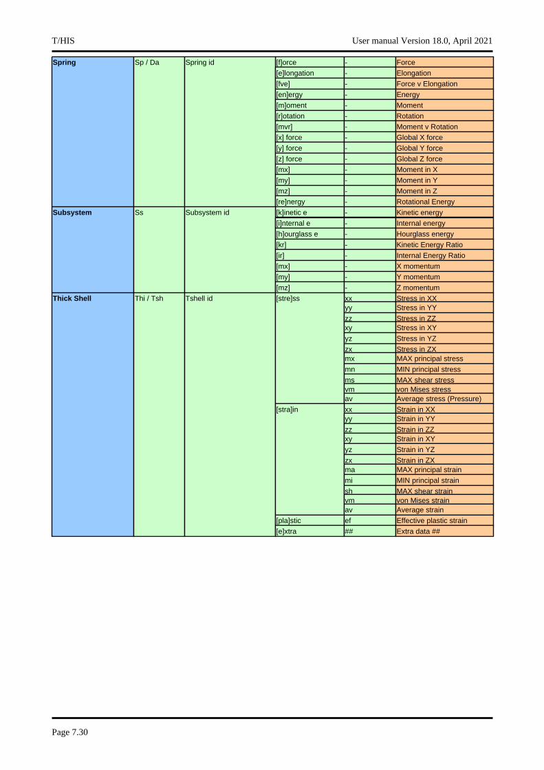
[f]orce - ForceSpring Sp / Da Spring id
[e]longation - Elongation
[fve] - Force v Elongation
[en]ergy - Energy
[m]oment - Moment
[r]otation - Rotation
[mvr] - Moment v Rotation
[x] force - Global X force
[y] force - Global Y force
[z] force - Global Z force
[mx] - Moment in X
[my] - Moment in Y
[mz] - Moment in Z
[re]nergy - Rotational Energy
[k]inetic e - Kinetic energySubsystem Ss Subsystem id
[i]nternal e - Internal energy
[h]ourglass e - Hourglass energy
[kr] - Kinetic Energy Ratio
[ir] - Internal Energy Ratio
[mx] - X momentum
[my] - Y momentum
[mz] - Z momentum
xx Stress in XXThick Shell Thi / Tsh Tshell id [stre]ssyy Stress in YY
zz Stress in ZZxy Stress in XY
yz Stress in YZ
zx Stress in ZXmx MAX principal stress
mn MIN principal stress
ms MAX shear stressvm von Mises stressav Average stress (Pressure)
xx Strain in XX[stra]inyy Strain in YY
zz Strain in ZZxy Strain in XY
yz Strain in YZ
zx Strain in ZXma MAX principal strain
mi MIN principal strain
sh MAX shear strainvm von Mises strainav Average strain
[pla]stic ef Effective plastic strain
[e]xtra ## Extra data ##
T/HIS User manual Version 18.0, April 2021
Page 7.30

x Current X coordTRACERS Tr Tracer ID [d]isplacementy Current Y coord
z Current Z coordm Current Vectorx X Velocity[v]elocity
y Y Velocity
z Z Velocity
m Velocity Magnitute
xx Stress in XX[stre]ssyy Stress in YY
zz Stress in ZZxy Stress in XY
yz Stress in YZ
zx Stress in ZXEFP -(de)nsity - Density
rvol - Relative Volumeac[tive] - Active
[dt] - Time stepWhole model Wh -
[k]inetic e - Kinetic energy
[i]nternal e - Internal energy
[sw] - Stonewall energy
[j]oint e - Joint internal energy
[sp]ring e - Spring and damper energy
[h]ourglass e - Hourglass energy
[sy]stem e - System damping energy
[si] - Sliding interface energy
[ew] - External work
[rb] - Rigid Body stopper energy
[t]otal e - Total energy
[er] - Total/initial energy
[x] velocity - Average X velocity
[y] velocity - Average Y velocity
[z] velocity - Average Z velocity
[cy]cle time - Time per zone cycle
[am] --- Added mass
[pm] - %age Mass increase
[ek] - Eroded Kinetic energy
[ei] - Eroded Internal energy
[eh] - Eroded Hourglass energy
[ewoe] - Energy Ratio w/o Eroded
[m]ass - Mass
7.4.5.1 Defining Surfaces / Integration points for data extraction
Some data components can be written out at multiple locations.
In recent versions of LS-DYNA it is possible for each element to write out multiple values for some data components.
For fully integrated Shells and Thick Shells values can be written out for all 4 in-plane integration points in each through thickness location. In addition to the integration point values it is also possible to write out data that has been extrapolated from the integration points out to the shells nodes.
For fully integrated solid elements data can also be written out for all 8 integration points and values can also be extrapolated to the elements nodes.
To select these additional values the entity ID’s specified in a FAST-TCF scripts can be modified as follows.
User manual Version 18.0, April 2021 T/HIS
Page 7.31
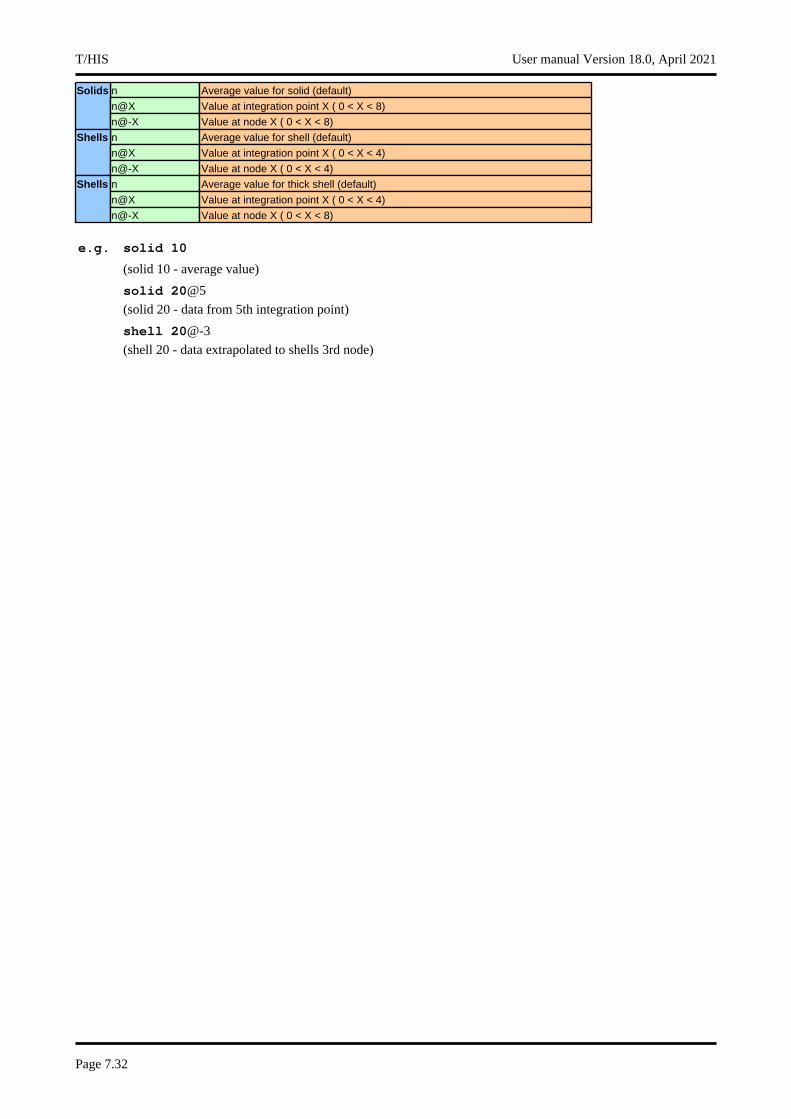
n Average value for solid (default)Solidsn@X Value at integration point X ( 0 < X < 8)
n@-X Value at node X ( 0 < X < 8)
n Average value for shell (default)Shellsn@X Value at integration point X ( 0 < X < 4)
n@-X Value at node X ( 0 < X < 4)
Shells n Average value for thick shell (default)
n@X Value at integration point X ( 0 < X < 4)
n@-X Value at node X ( 0 < X < 8)
e.g. solid 10
(solid 10 - average value)
solid 20@5
(solid 20 - data from 5th integration point)
shell 20@-3
(shell 20 - data extrapolated to shells 3rd node)
T/HIS User manual Version 18.0, April 2021
Page 7.32
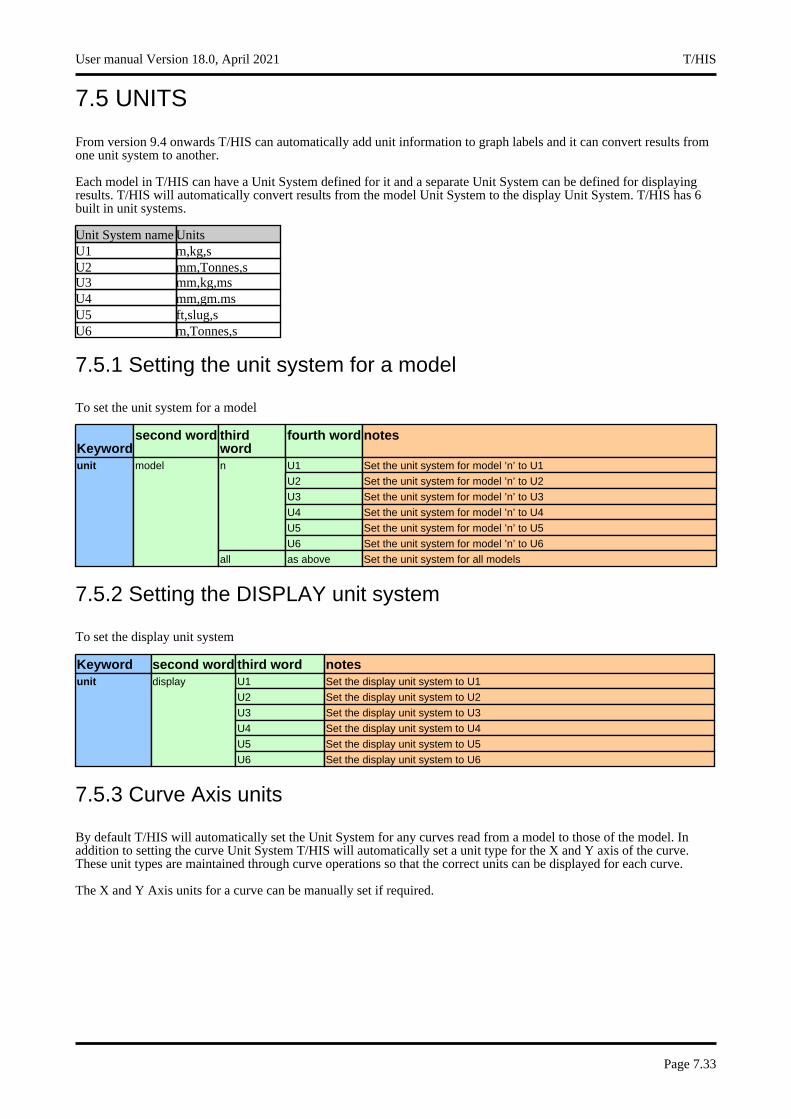
7.5 UNITS
From version 9.4 onwards T/HIS can automatically add unit information to graph labels and it can convert results from one unit system to another.
Each model in T/HIS can have a Unit System defined for it and a separate Unit System can be defined for displaying results. T/HIS will automatically convert results from the model Unit System to the display Unit System. T/HIS has 6 built in unit systems.
Unit System name UnitsU1 m,kg,sU2 mm,Tonnes,sU3 mm,kg,msU4 mm,gm.msU5 ft,slug,sU6 m,Tonnes,s
7.5.1 Setting the unit system for a model
To set the unit system for a model
Keywordsecond word third
wordfourth word notes
U1 Set the unit system for model ’n’ to U1unit model n
U2 Set the unit system for model ’n’ to U2
U3 Set the unit system for model ’n’ to U3
U4 Set the unit system for model ’n’ to U4
U5 Set the unit system for model ’n’ to U5
U6 Set the unit system for model ’n’ to U6
all as above Set the unit system for all models
7.5.2 Setting the DISPLAY unit system
To set the display unit system
Keyword second word third word notesU1 Set the display unit system to U1unit display
U2 Set the display unit system to U2
U3 Set the display unit system to U3
U4 Set the display unit system to U4
U5 Set the display unit system to U5
U6 Set the display unit system to U6
7.5.3 Curve Axis units
By default T/HIS will automatically set the Unit System for any curves read from a model to those of the model. In addition to setting the curve Unit System T/HIS will automatically set a unit type for the X and Y axis of the curve. These unit types are maintained through curve operations so that the correct units can be displayed for each curve.
The X and Y Axis units for a curve can be manually set if required.
User manual Version 18.0, April 2021 T/HIS
Page 7.33
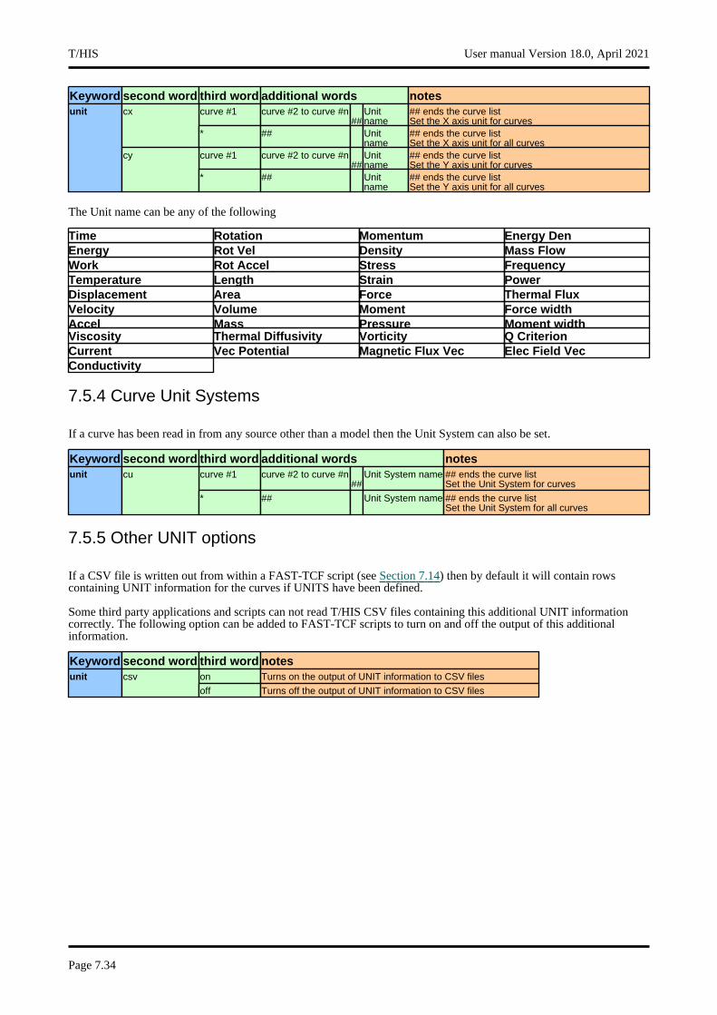
Keyword second word third word additional words notescurve #1 curve #2 to curve #n
##Unit name
## ends the curve listSet the X axis unit for curves
unit cx
* ## Unit name
## ends the curve listSet the X axis unit for all curves
curve #1 curve #2 to curve #n##
Unit name
## ends the curve listSet the Y axis unit for curves
cy
* ## Unit name
## ends the curve listSet the Y axis unit for all curves
The Unit name can be any of the following
Time Rotation Momentum Energy Den Energy Rot Vel Density Mass Flow Work Rot Accel Stress Frequency Temperature Length Strain Power Displacement Area Force Thermal Flux Velocity Volume Moment Force width Accel Mass Pressure Moment width Viscosity Thermal Diffusivity Vorticity Q Criterion Current Vec Potential Magnetic Flux Vec Elec Field Vec Conductivity
7.5.4 Curve Unit Systems
If a curve has been read in from any source other than a model then the Unit System can also be set.
Keyword second word third word additional words notescurve #1 curve #2 to curve #n
##Unit System name ## ends the curve list
Set the Unit System for curvesunit cu
* ## Unit System name ## ends the curve listSet the Unit System for all curves
7.5.5 Other UNIT options
If a CSV file is written out from within a FAST-TCF script (see Section 7.14) then by default it will contain rows containing UNIT information for the curves if UNITS have been defined.
Some third party applications and scripts can not read T/HIS CSV files containing this additional UNIT information correctly. The following option can be added to FAST-TCF scripts to turn on and off the output of this additional information.
Keyword second word third word noteson Turns on the output of UNIT information to CSV filesunit csv
off Turns off the output of UNIT information to CSV files
T/HIS User manual Version 18.0, April 2021
Page 7.34
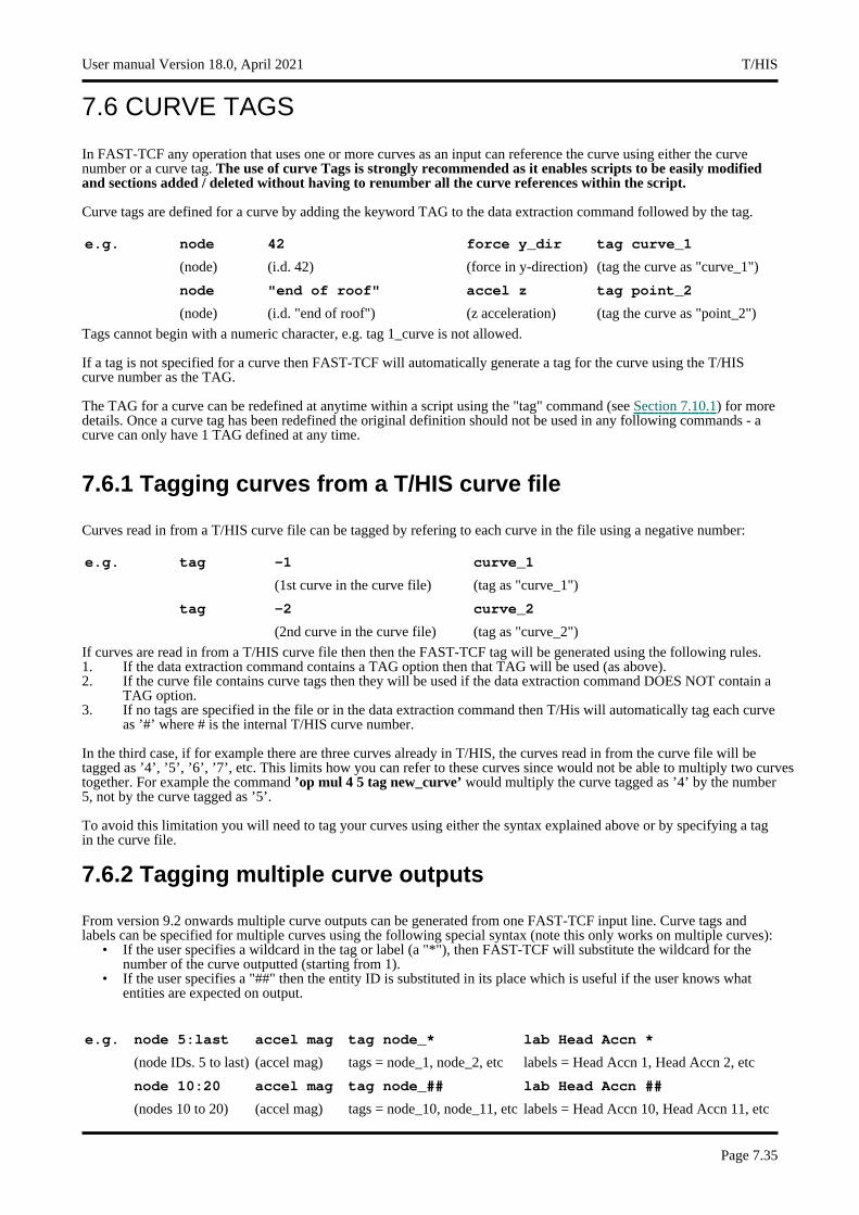
7.6 CURVE TAGS
In FAST-TCF any operation that uses one or more curves as an input can reference the curve using either the curve number or a curve tag. The use of curve Tags is strongly recommended as it enables scripts to be easily modified and sections added / deleted without having to renumber all the curve references within the script.
Curve tags are defined for a curve by adding the keyword TAG to the data extraction command followed by the tag.
e.g. node 42 force y_dir tag curve_1
(node) (i.d. 42) (force in y-direction) (tag the curve as "curve_1")
node "end of roof" accel z tag point_2
(node) (i.d. "end of roof") (z acceleration) (tag the curve as "point_2")
Tags cannot begin with a numeric character, e.g. tag 1_curve is not allowed.
If a tag is not specified for a curve then FAST-TCF will automatically generate a tag for the curve using the T/HIS curve number as the TAG.
The TAG for a curve can be redefined at anytime within a script using the "tag" command (see Section 7.10.1) for more details. Once a curve tag has been redefined the original definition should not be used in any following commands - a curve can only have 1 TAG defined at any time.
7.6.1 Tagging curves from a T/HIS curve file
Curves read in from a T/HIS curve file can be tagged by refering to each curve in the file using a negative number:
e.g. tag -1 curve_1
(1st curve in the curve file) (tag as "curve_1")
tag -2 curve_2
(2nd curve in the curve file) (tag as "curve_2")
If curves are read in from a T/HIS curve file then then the FAST-TCF tag will be generated using the following rules.1. If the data extraction command contains a TAG option then that TAG will be used (as above).2. If the curve file contains curve tags then they will be used if the data extraction command DOES NOT contain a
TAG option.3. If no tags are specified in the file or in the data extraction command then T/His will automatically tag each curve
as ’#’ where # is the internal T/HIS curve number.
In the third case, if for example there are three curves already in T/HIS, the curves read in from the curve file will be tagged as ’4’, ’5’, ’6’, ’7’, etc. This limits how you can refer to these curves since would not be able to multiply two curves together. For example the command ’op mul 4 5 tag new_curve’ would multiply the curve tagged as ’4’ by the number 5, not by the curve tagged as ’5’.
To avoid this limitation you will need to tag your curves using either the syntax explained above or by specifying a tag in the curve file.
7.6.2 Tagging multiple curve outputs
From version 9.2 onwards multiple curve outputs can be generated from one FAST-TCF input line. Curve tags and labels can be specified for multiple curves using the following special syntax (note this only works on multiple curves):
• If the user specifies a wildcard in the tag or label (a "*"), then FAST-TCF will substitute the wildcard for the number of the curve outputted (starting from 1).
• If the user specifies a "##" then the entity ID is substituted in its place which is useful if the user knows what entities are expected on output.
e.g. node 5:last accel mag tag node_* lab Head Accn *
(node IDs. 5 to last) (accel mag) tags = node_1, node_2, etc labels = Head Accn 1, Head Accn 2, etc
node 10:20 accel mag tag node_## lab Head Accn ##
(nodes 10 to 20) (accel mag) tags = node_10, node_11, etc labels = Head Accn 10, Head Accn 11, etc
User manual Version 18.0, April 2021 T/HIS
Page 7.35
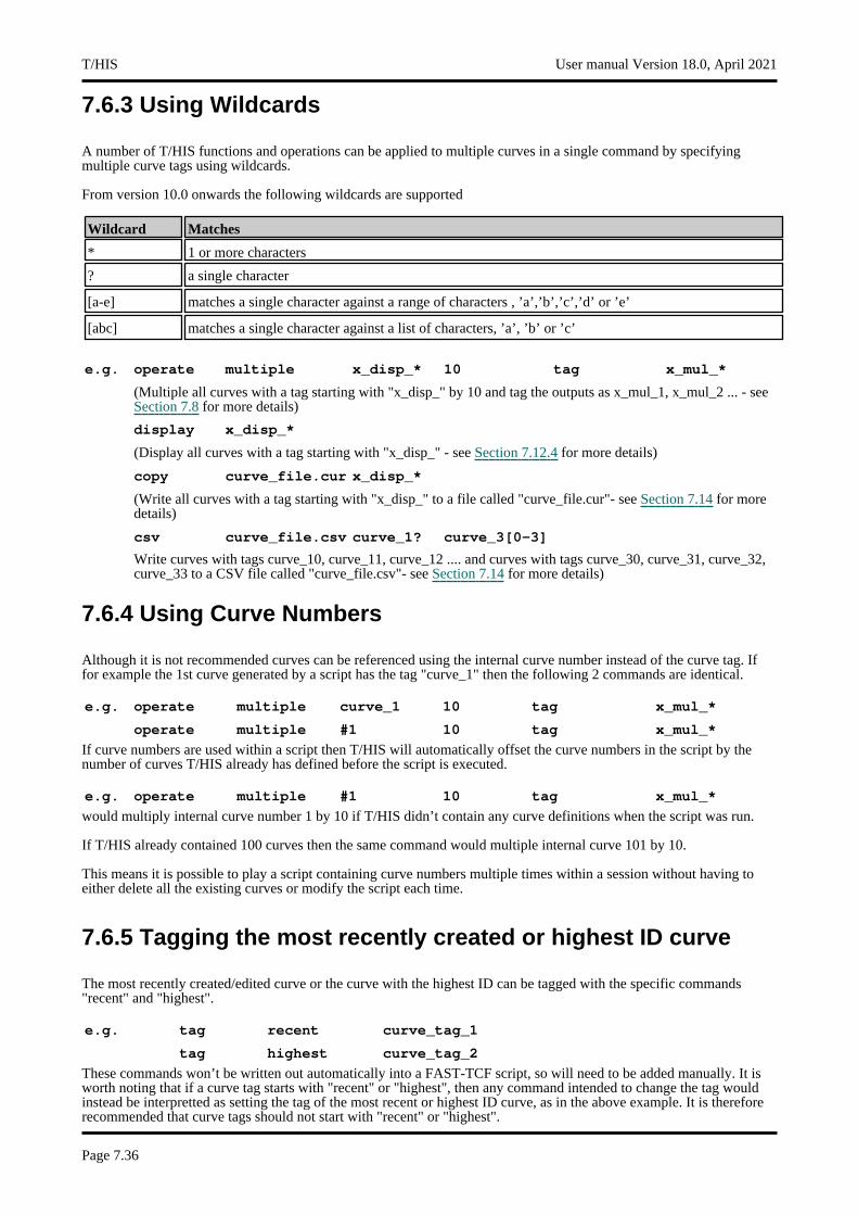
7.6.3 Using Wildcards
A number of T/HIS functions and operations can be applied to multiple curves in a single command by specifying multiple curve tags using wildcards.
From version 10.0 onwards the following wildcards are supported
Wildcard Matches
* 1 or more characters
? a single character
[a-e] matches a single character against a range of characters , ’a’,’b’,’c’,’d’ or ’e’
[abc] matches a single character against a list of characters, ’a’, ’b’ or ’c’
e.g. operate multiple x_disp_* 10 tag x_mul_*
(Multiple all curves with a tag starting with "x_disp_" by 10 and tag the outputs as x_mul_1, x_mul_2 ... - see Section 7.8 for more details)
display x_disp_*
(Display all curves with a tag starting with "x_disp_" - see Section 7.12.4 for more details)
copy curve_file.cur x_disp_*
(Write all curves with a tag starting with "x_disp_" to a file called "curve_file.cur"- see Section 7.14 for more details)
csv curve_file.csv curve_1? curve_3[0-3]
Write curves with tags curve_10, curve_11, curve_12 .... and curves with tags curve_30, curve_31, curve_32, curve_33 to a CSV file called "curve_file.csv"- see Section 7.14 for more details)
7.6.4 Using Curve Numbers
Although it is not recommended curves can be referenced using the internal curve number instead of the curve tag. If for example the 1st curve generated by a script has the tag "curve_1" then the following 2 commands are identical.
e.g. operate multiple curve_1 10 tag x_mul_*
operate multiple #1 10 tag x_mul_*
If curve numbers are used within a script then T/HIS will automatically offset the curve numbers in the script by the number of curves T/HIS already has defined before the script is executed.
e.g. operate multiple #1 10 tag x_mul_*
would multiply internal curve number 1 by 10 if T/HIS didn’t contain any curve definitions when the script was run.
If T/HIS already contained 100 curves then the same command would multiple internal curve 101 by 10.
This means it is possible to play a script containing curve numbers multiple times within a session without having to either delete all the existing curves or modify the script each time.
7.6.5 Tagging the most recently created or highest ID curve
The most recently created/edited curve or the curve with the highest ID can be tagged with the specific commands "recent" and "highest".
e.g. tag recent curve_tag_1
tag highest curve_tag_2
These commands won’t be written out automatically into a FAST-TCF script, so will need to be added manually. It is worth noting that if a curve tag starts with "recent" or "highest", then any command intended to change the tag would instead be interpretted as setting the tag of the most recent or highest ID curve, as in the above example. It is therefore recommended that curve tags should not start with "recent" or "highest".
T/HIS User manual Version 18.0, April 2021
Page 7.36

7.7 CURVE GROUPS
Curve groups can be defined within FAST-TCF scripts using the cgroup keyword. After a curve group has been defined in a FAST-TCF script it can then be used as an input to some FAST-TCF commands. Each curve group should be given a unique name within the FAST-TCF script.
Keyword Second word
Third word
following word
notes
create name - Create a curve group called "name". If the name contains any spaces then it should be enclosed in quotes ("name with space")
cgroup
add name curve list Adds a list of curves to the curve group called "name". If the name contains any spaces then it should be enclosed in quotes ("name with space"). The curve list should be a list of curve tags.
remove name curve list Removes a list of curves from the curve group called "name". If the name contains any spaces then it should be enclosed in quotes ("name with space"). The curve list should be a list of curve tags.
e.g. cgroup create group_1
(Create a curve group called "group_1"
cgroup add group_1 curve_1 curve_2
(Add curves with tags "curve_1" and "curve_2" to group "group_1")
cgroup create "Group 2"
(Create a curve group called "Group 2")
cgroup add "Group 2" curve_1*
Add all curves with a curve tag containing "curve_1" to group "Group 2"
cgroup remove "Group 2" curve_11
Remove curve with tag "curve_11" from group "Group 2"
To use a curve group as the input to another FAST-TCF command the curve group name is preceeded by an &. If a curve group name contains spaces then the name should be enclosed in double quotes and the & should be before the first ".
e.g. operate multiple &group_1 10 tag output_*
(Multiple all curves in curve group "group_1" by 10 and tag the outputs as output_1, output_2 ..._)
operate multiple &"Group 2" 10 tag output_*
(Multiple all curves in curve group "Group 2 " by 10 and tag the outputs as output_1, output_2 ..._)
Curve Groups can currently be used as • The first curve input in all of the operate commands• Within the list of curves specified as input to curve range functions.• To select a group of curves for the display command.• Outputting curves to T/HIS curve files and CSV files.
User manual Version 18.0, April 2021 T/HIS
Page 7.37
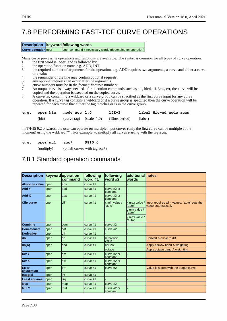
7.8 PERFORMING FAST-TCF CURVE OPERATIONS
Description keyword following wordsCurve operation oper oper command + necessary words (depending on operation)
Many curve processing operations and functions are available. The syntax is common for all types of curve operation:1. the first word is ’oper’ and is followed by:2. the operation/function name e.g. ADD, INT.3. the required number of arguments for the operation, e.g. ADD requires two arguments, a curve and either a curve
or a value.4. the remainder of the line may contain optional requests.5. any optional requests can occur after the arguments.6. curve numbers must be in the format: #<curve number> 7. An output curve is always needed - for operation commands such as hic, hicd, tti, 3ms, err, the curve will be
copied and the operation is executed on the copied curve.8. A curve tag containing a wildcard or a curve group can be specified as the first curve input for any curve
operation. If a curve tag contains a wildcard or if a curve group is specified then the curve operation will be repeated for each curve that either the tag matches or is in the curve group.
e.g. oper hic node_acc 1.0 15E-3 label Hic-ed node accn
(hic) (curve tag) (scale=1.0) (15ms period) (label)
In T/HIS 9.2 onwards, the user can operate on multiple input curves (only the first curve can be multiple at the moment) using the wildcard "*". For example, to multiply all curves starting with the tag acc:
e.g. oper mul acc* 9810.0
(multiply) (on all curves with tag acc*)
7.8.1 Standard operation commands
Description keyword operation command
following word #1
following word #2
additional words
notes
Absolute value oper abs curve #1 - -
Add Y oper add curve #1 curve #2 or constant
-
Add X oper adx curve #1 curve #2 or constant
-
x max value / "auto"
Clip curve oper cli curve #1 x min value / "auto"
Input requires all 4 values, "auto" sets the value automatically
y min value / "auto"
y max value / "auto"
Combine oper com curve #1 curve #2 -
Concatenate oper cat curve #1 curve #2 -
Derivative oper dif curve #1 - -
db oper db curve #1 reference value
Convert a curve to dB
narrow Apply narrow band A weightingdb(A) oper dba curve #1
octave Apply octave band A weighting
Div Y oper div curve #1 curve #2 or constant
-
Div X oper dix curve #1 curve #2 or constant
-
Error calculation
oper err curve #1 curve #2 - Value is stored with the output curve
Integral oper int curve #1 - -
Least squares oper lsq curve #1 - -
Map oper map curve #1 curve #2 -
Mul Y oper mul curve #1 curve #2 or constant
-
T/HIS User manual Version 18.0, April 2021
Page 7.38
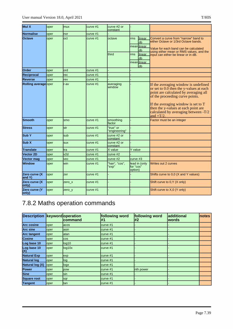
Mul X oper mux curve #1 curve #2 or constant
-
Normalise oper nor curve #1 - -
linearOctave oper oct curve #1 octave rms Convert a curve from "narrow" band to either Octave or 1/3rd Octave bands.
Value for each band can be calculated using either mean or RMS values, and the input can either be linear or in dB.
dblinearmeandblinearthird rmsdblinearmeandb
Order oper ord curve #1 - -
Reciprocal oper rec curve #1 - -
Reverse oper rev curve #1 - -
Rolling average oper r-av curve #1 averaging window
- If the averaging window is undefined or set to 0.0 then the y-values at each point are calculated by averaging all of the proceeding curve points.
If the averaging window is set to T then the y-values at each point are calculated by averaging between -T/2 and +T/2.
Smooth oper smo curve #1 smoothing factor
- Factor must be an integer
Stress oper str curve #1 "true" or "engineering"
-
Sub Y oper sub curve #1 curve #2 or constant
-
Sub X oper sux curve #1 curve #2 or constant
-
Translate oper tra curve #1 X value Y value
Vector 2D oper v2d curve #1 curve #2 -
Vector mag oper vec curve #1 curve #2 curve #3
Window oper win curve #1 "han", "cos", "exp"
lead in (only for "cos" option)
Writes out 2 curves
Zero curve (X and Y)
oper zer curve #1 - - Shifts curve to 0,0 (X and Y values)
Zero curve (X only)
oper zero_x curve #1 - - Shift curve to 0,Y (X only)
Zero curve (Y only)
oper zero_y curve #1 - - Shift curve to X,0 (Y only)
7.8.2 Maths operation commands
Description keyword operation command
following word #1
following word #2
additional words
notes
Arc cosine oper acos curve #1 - -
Arc sine oper asin curve #1 - -
Arc tangent oper atan curve #1 - -
Cosine oper cos curve #1 - -
Log base 10 oper log10 curve #1 - -
Log base 10 (X)
oper log10x curve #1 - -
Natural Exp oper exp curve #1 - -
Natural log oper log curve #1 - -
Natural log (X) oper logx curve #1 - -
Power oper pow curve #1 nth power -
Sine oper sin curve #1 - -
Square root oper sqr curve #1 - -
Tangent oper tan curve #1 - -
User manual Version 18.0, April 2021 T/HIS
Page 7.39

7.8.3 Automotive operation commands
Description keyword operation command
following word #1
following word #2
additional words
notes
Delta V oper acu curve #1 offset time period
word6 = acceleration conversion factor
Acceleration severity index
oper asi Accn x curve # Accn y curve # Accn z curve #
word7 = x limitword8 = y limit
word9 = z limitButterworth filter oper but curve #1 cut off
frequencyorder
C60 filter oper c60 curve #1 - -
C180 filter oper c180 curve #1 - -
C600 filter oper c600 curve #1 - -
C1000 filter oper c1000 curve #1 - -
Clip value oper cva curve #1 time window Label displayed on screen (optional)
Value is stored with the output curve
Exceedence oper exc curve #1 auto / pos / neg -
Fir filter oper fir curve #1 - -
Hic oper hic curve #1 division scale factor
time period Value is stored with the output curve
Hicd oper hicd curve #1 division scale factor
time period Value is stored with the output curve
word6 = Fzc tensionNeck injury criteria oper nij Shear curve # Axial curve # Moment curve #word7 = Fzc compression
word8 = Myc flexion
word9 = Myc extension
word10 = Distance from joint
Regularise oper reg curve #1 new dt value -
word6 = Horizontal distance
THIV oper thi Accn x curve # Accn y curve # Yaw rate curve #
word7 = Lateral distanceword8 = Head to vehicle distance
TTI oper tti Upper rib curve #
Lower rib curve #
Lower spine curve # Value is stored with the output curve
Viscous criteria ECER95 oper vc curve #1 constant A constant B ECER95 method
Viscous criteria IIHS oper vc2 curve #1 constant A constant B IIHS method
Curve Correlation (strict) oper corr strict curve #1 curve #2 Value is stored with the output curves
Curve Correlation (loose) oper corr loose curve #1 curve #2 Value is stored with the output curves
Weighted Integrated Factor Curve Correlation (WIFAC)
oper wif curve #1 curve #2 - Value is stored with the output curve
7.8.4 Seismic operation commands
Description keyword operation command
following word #1
following word #2
additional words
notes
Accn to disp spectra
oper ad curve #1 - -
Accn to vel spectra
oper av curve #1 - -
Disp to vel spectra
oper dv curve #1 - -
Disp to accn spectra
oper da curve #1 - -
Vel to disp spectra
oper vd curve #1 - -
T/HIS User manual Version 18.0, April 2021
Page 7.40

Vel to accn spectra
oper va curve #1 - -
Baseline correction
oper blc curve #1 - -
Design spectrum oper ds curve #1 broadening factor -
FFT oper fft curve #1 - -
Non cumulative P.R.
oper ncp curve #1 curve #2 -
Response spectrum
oper rs curve #1 damping factor sampling factor Sampling must be either 30 or 70
7.8.5 Range of curve operation commands
Description keyword operation command
following word #1
following word #2
additional words
notes
Average oper ave curve #1 curve #2 to curve #n ## "##" ends the curve list
Envelope oper env curve #1 curve #2 to curve #n ## "##" ends the curve list
Minimum oper min curve #1 curve #2 to curve #n ## "##" ends the curve list
Maximum oper max curve #1 curve #2 to curve #n ## "##" ends the curve list
Resultant oper res curve #1 curve #2 to curve #n ## "##" ends the curve list
Sum oper sum curve #1 curve #2 to curve #n ## "##" ends the curve list
Sum oper sum curve #1 curve #2 to curve #n ## "##" ends the curve list
User manual Version 18.0, April 2021 T/HIS
Page 7.41
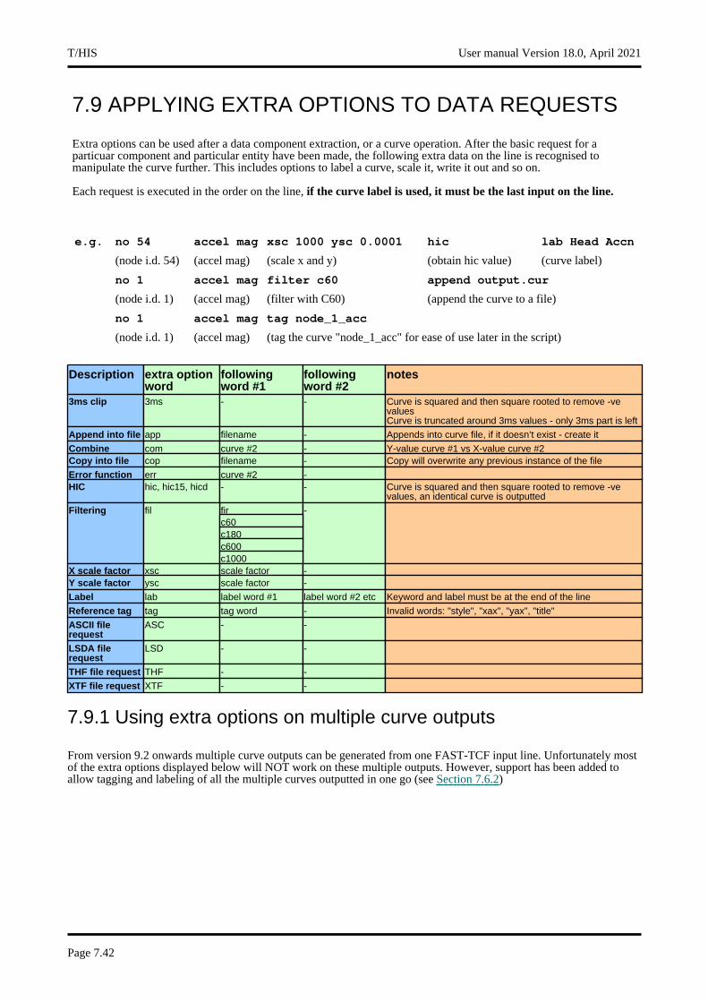
7.9 APPLYING EXTRA OPTIONS TO DATA REQUESTS
Extra options can be used after a data component extraction, or a curve operation. After the basic request for a particuar component and particular entity have been made, the following extra data on the line is recognised to manipulate the curve further. This includes options to label a curve, scale it, write it out and so on.
Each request is executed in the order on the line, if the curve label is used, it must be the last input on the line.
e.g. no 54 accel mag xsc 1000 ysc 0.0001 hic lab Head Accn
(node i.d. 54) (accel mag) (scale x and y) (obtain hic value) (curve label)
no 1 accel mag filter c60 append output.cur
(node i.d. 1) (accel mag) (filter with C60) (append the curve to a file)
no 1 accel mag tag node_1_acc
(node i.d. 1) (accel mag) (tag the curve "node_1_acc" for ease of use later in the script)
Description extra option word
following word #1
following word #2
notes
3ms clip 3ms - - Curve is squared and then square rooted to remove -ve valuesCurve is truncated around 3ms values - only 3ms part is left
Append into file app filename - Appends into curve file, if it doesn’t exist - create it
Combine com curve #2 - Y-value curve #1 vs X-value curve #2Copy into file cop filename - Copy will overwrite any previous instance of the file
Error function err curve #2 -HIC hic, hic15, hicd - - Curve is squared and then square rooted to remove -ve
values, an identical curve is outputted
firFiltering fil -c60c180c600c1000
X scale factor xsc scale factor -Y scale factor ysc scale factor -
Label lab label word #1 label word #2 etc Keyword and label must be at the end of the line
Reference tag tag tag word - Invalid words: "style", "xax", "yax", "title"
ASCII file request
ASC - -
LSDA file request
LSD - -
THF file request THF - -
XTF file request XTF - -
7.9.1 Using extra options on multiple curve outputs
From version 9.2 onwards multiple curve outputs can be generated from one FAST-TCF input line. Unfortunately most of the extra options displayed below will NOT work on these multiple outputs. However, support has been added to allow tagging and labeling of all the multiple curves outputted in one go (see Section 7.6.2)
T/HIS User manual Version 18.0, April 2021
Page 7.42
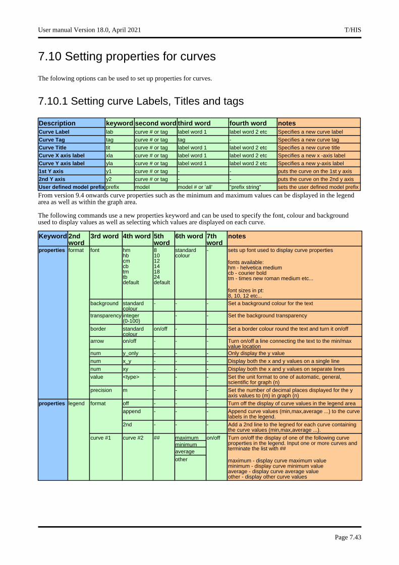
7.10 Setting properties for curves
The folowing options can be used to set up properties for curves.
7.10.1 Setting curve Labels, Titles and tags
Description keyword second word third word fourth word notesCurve Label lab curve # or tag label word 1 label word 2 etc Specifies a new curve label
Curve Tag tag curve # or tag tag - Specifies a new curve tag
Curve Title tit curve # or tag label word 1 label word 2 etc Specifies a new curve title
Curve X axis label xla curve # or tag label word 1 label word 2 etc Specifies a new x -axis label
Curve Y axis label yla curve # or tag label word 1 label word 2 etc Specifies a new y-axis label
1st Y axis y1 curve # or tag - - puts the curve on the 1st y axis
2nd Y axis y2 curve # or tag - - puts the curve on the 2nd y axis
User defined model prefix prefix model model # or ’all’ "prefix string" sets the user defined model prefix
From version 9.4 onwards curve properties such as the minimum and maximum values can be displayed in the legend area as well as within the graph area.
The following commands use a new properties keyword and can be used to specify the font, colour and background used to display values as well as selecting which values are displayed on each curve.
Keyword 2nd word
3rd word 4th word 5th word
6th word 7th word
notes
font hm hb cm cbtmtbdefault
8 1012141824default
standard colour
- sets up font used to display curve properties
fonts available:hm - helvetica mediumcb - courier boldtm - times new roman medium etc...
font sizes in pt:8, 10, 12 etc...
properties format
background standard colour
- - - Set a background colour for the text
transparency integer (0-100)
- - Set the background transparency
border standard colour
on/off - - Set a border colour round the text and turn it on/off
arrow on/off - - - Turn on/off a line connecting the text to the min/max value location
num y_only - - - Only display the y value
num x_y - - - Display both the x and y values on a single line
num xy - - - Display both the x and y values on separate lines
value <type> - - - Set the unit format to one of automatic, general, scientific for graph (n)
precision m - - - Set the number of decimal places displayed for the y axis values to (m) in graph (n)
off - - - Turn off the display of curve values in the legend areaproperties legend format
append - - - Append curve values (min,max,average ...) to the curve labels in the legend.
2nd - - - Add a 2nd line to the legned for each curve containing the curve values (min,max,average ...).
maximum curve #1 curve #2 ## on/off Turn on/off the display of one of the following curve properties in the legend. Input one or more curves and terminate the list with ##
maximum - display curve maximum valueminimum - display curve minimum valueaverage - display curve average valueother - display other curve values
minimum average
other
User manual Version 18.0, April 2021 T/HIS
Page 7.43
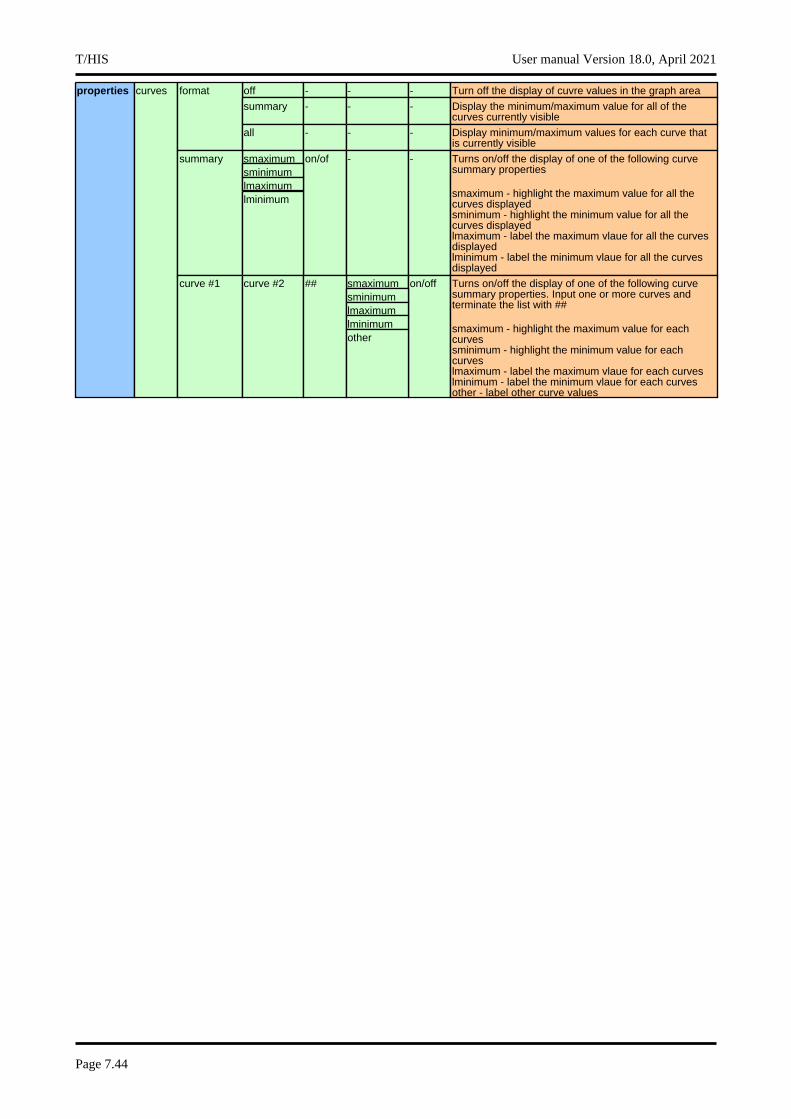
off - - - Turn off the display of cuvre values in the graph areaproperties curves format
summary - - - Display the minimum/maximum value for all of the curves currently visible
all - - - Display minimum/maximum values for each curve that is currently visible
smaximumsummary on/of - - Turns on/off the display of one of the following curve summary properties
smaximum - highlight the maximum value for all the curves displayedsminimum - highlight the minimum value for all the curves displayedlmaximum - label the maximum vlaue for all the curves displayed lminimum - label the minimum vlaue for all the curves displayed
sminimumlmaximumlminimum
smaximumcurve #1 curve #2 ## on/off Turns on/off the display of one of the following curve summary properties. Input one or more curves and terminate the list with ##
smaximum - highlight the maximum value for each curvessminimum - highlight the minimum value for each curveslmaximum - label the maximum vlaue for each curveslminimum - label the minimum vlaue for each curvesother - label other curve values
sminimumlmaximumlminimumother
T/HIS User manual Version 18.0, April 2021
Page 7.44
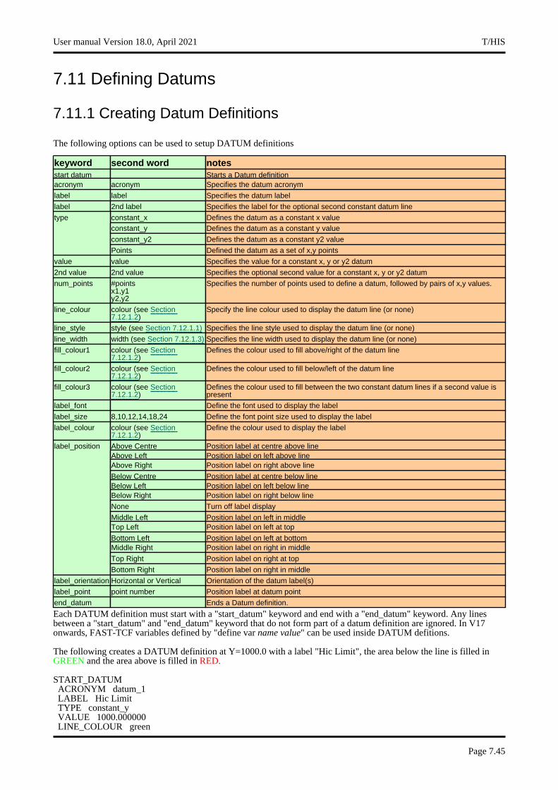
7.11 Defining Datums
7.11.1 Creating Datum Definitions
The following options can be used to setup DATUM definitions
keyword second word notesstart datum Starts a Datum definitionacronym acronym Specifies the datum acronym
label label Specifies the datum label
label 2nd label Specifies the label for the optional second constant datum line
constant_x Defines the datum as a constant x valuetypeconstant_y Defines the datum as a constant y value
constant_y2 Defines the datum as a constant y2 value
Points Defined the datum as a set of x,y points
value value Specifies the value for a constant x, y or y2 datum
2nd value 2nd value Specifies the optional second value for a constant x, y or y2 datum
num_points #pointsx1,y1y2,y2
Specifies the number of points used to define a datum, followed by pairs of x,y values.
line_colour colour (see Section7.12.1.2)
Specify the line colour used to display the datum line (or none)
line_style style (see Section 7.12.1.1) Specifies the line style used to display the datum line (or none)
line_width width (see Section 7.12.1.3) Specifies the line width used to display the datum line (or none)
fill_colour1 colour (see Section7.12.1.2)
Defines the colour used to fill above/right of the datum line
fill_colour2 colour (see Section7.12.1.2)
Defines the colour used to fill below/left of the datum line
fill_colour3 colour (see Section7.12.1.2)
Defines the colour used to fill between the two constant datum lines if a second value is present
label_font Define the font used to display the label
label_size 8,10,12,14,18,24 Define the font point size used to display the label
label_colour colour (see Section7.12.1.2)
Define the colour used to display the label
Above Centre Position label at centre above linelabel_positionAbove Left Position label on left above lineAbove Right Position label on right above line
Below Centre Position label at centre below lineBelow Left Position label on left below lineBelow Right Position label on right below line
None Turn off label display
Middle Left Position label on left in middleTop Left Position label on left at top
Bottom Left Position label on left at bottomMiddle Right Position label on right in middle
Top Right Position label on right at top
Bottom Right Position label on right in middle
label_orientation Horizontal or Vertical Orientation of the datum label(s)
label_point point number Position label at datum point
end_datum Ends a Datum definition.
Each DATUM definition must start with a "start_datum" keyword and end with a "end_datum" keyword. Any lines between a "start_datum" and "end_datum" keyword that do not form part of a datum definition are ignored. In V17 onwards, FAST-TCF variables defined by "define var name value" can be used inside DATUM defitions.
The following creates a DATUM definition at Y=1000.0 with a label "Hic Limit", the area below the line is filled in GREEN and the area above is filled in RED.
START_DATUMACRONYM datum_1LABEL Hic LimitTYPE constant_yVALUE 1000.000000LINE_COLOUR green
User manual Version 18.0, April 2021 T/HIS
Page 7.45
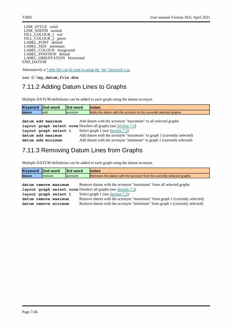
LINE_STYLE solidLINE_WIDTH normalFILL_COLOUR_1 redFILL_COLOUR_2 greenLABEL_FONT defaultLABEL_SIZE automaticLABEL_COLOUR foregroundLABEL_POSITION defaultLABEL_ORIENTATION Horizontal
END_DATUM
Alternatively a *.dtm file can be read in using the ’inc’ keyword, e.g.
inc C:\my_datum_file.dtm
7.11.2 Adding Datum Lines to Graphs
Multiple DATUM definitions can be added to each graph using the datum acronym
Keyword 2nd word 3rd word notesdatum add acronym Adds the datum with the acronym to the currently selected graphs
datum add maximum Add datum with the acronym "maximum" to all selected graphslayout graph select none Deselect all graphs (see Section 7.2)layout graph select 1 Select graph 1 (see Section 7.2)datum add maximum Add datum with the acronym "maximum" to graph 1 (currently selected)datum add minimum Add datum with the acronym "minimum" to graph 1 (currently selected)
7.11.3 Removing Datum Lines from Graphs
Multiple DATUM definitions can be added to each graph using the datum acronym
Keyword 2nd word 3rd word notesdatum remove acronym Removes the datum with the acronym from the currently selected graphs
datum remove maximum Remove datum with the acronym "maximum" from all selected graphslayout graph select none Deselect all graphs (see Section 7.2)layout graph select 1 Select graph 1 (see Section 7.2)datum remove maximum Remove datum with the acronym "maximum" from graph 1 (currently selected)datum remove minimum Remove datum with the acronym "minimum" from graph 1 (currently selected)
T/HIS User manual Version 18.0, April 2021
Page 7.46
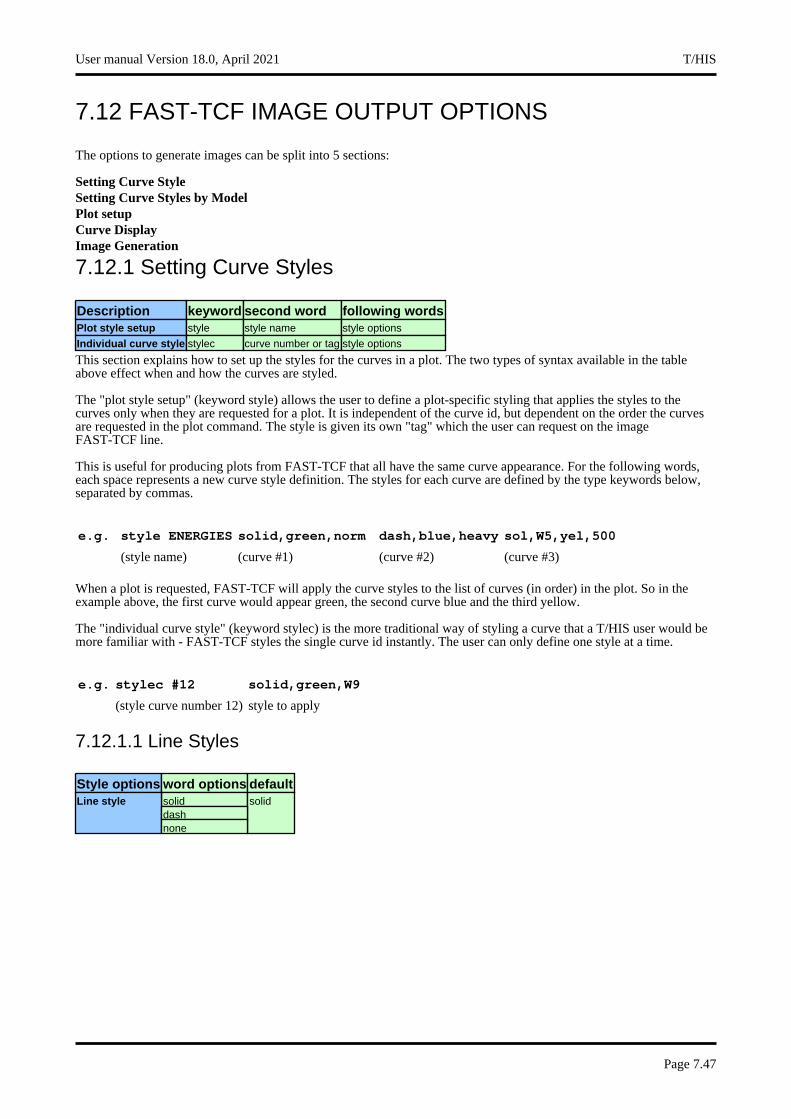
7.12 FAST-TCF IMAGE OUTPUT OPTIONS
The options to generate images can be split into 5 sections:
Setting Curve StyleSetting Curve Styles by ModelPlot setupCurve DisplayImage Generation
7.12.1 Setting Curve Styles
Description keyword second word following wordsPlot style setup style style name style options
Individual curve style stylec curve number or tag style options
This section explains how to set up the styles for the curves in a plot. The two types of syntax available in the table above effect when and how the curves are styled.
The "plot style setup" (keyword style) allows the user to define a plot-specific styling that applies the styles to the curves only when they are requested for a plot. It is independent of the curve id, but dependent on the order the curves are requested in the plot command. The style is given its own "tag" which the user can request on the image FAST-TCF line.
This is useful for producing plots from FAST-TCF that all have the same curve appearance. For the following words, each space represents a new curve style definition. The styles for each curve are defined by the type keywords below, separated by commas.
e.g. style ENERGIES solid,green,norm dash,blue,heavy sol,W5,yel,500
(style name) (curve #1) (curve #2) (curve #3)
When a plot is requested, FAST-TCF will apply the curve styles to the list of curves (in order) in the plot. So in the example above, the first curve would appear green, the second curve blue and the third yellow.
The "individual curve style" (keyword stylec) is the more traditional way of styling a curve that a T/HIS user would be more familiar with - FAST-TCF styles the single curve id instantly. The user can only define one style at a time.
e.g. stylec #12 solid,green,W9
(style curve number 12) style to apply
7.12.1.1 Line Styles
Style options word options defaultsolidLine style soliddashnone
User manual Version 18.0, April 2021 T/HIS
Page 7.47
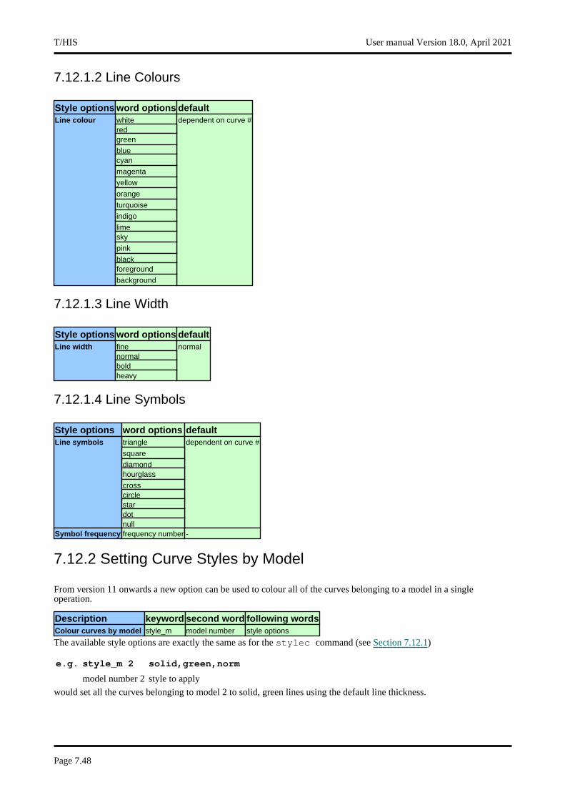
7.12.1.2 Line Colours
Style options word options defaultwhiteLine colour dependent on curve #redgreen
bluecyan
magenta
yellow
orange
turquoise
indigo
limesky
pink
blackforeground
background
7.12.1.3 Line Width
Style options word options defaultfineLine width normalnormalboldheavy
7.12.1.4 Line Symbols
Style options word options defaulttriangleLine symbols dependent on curve #
square
diamondhourglass
crosscirclestardotnull
Symbol frequency frequency number -
7.12.2 Setting Curve Styles by Model
From version 11 onwards a new option can be used to colour all of the curves belonging to a model in a single operation.
Description keyword second word following wordsColour curves by model style_m model number style options
The available style options are exactly the same as for the stylec command (see Section 7.12.1)
e.g. style_m 2 solid,green,norm
model number 2 style to apply
would set all the curves belonging to model 2 to solid, green lines using the default line thickness.
T/HIS User manual Version 18.0, April 2021
Page 7.48
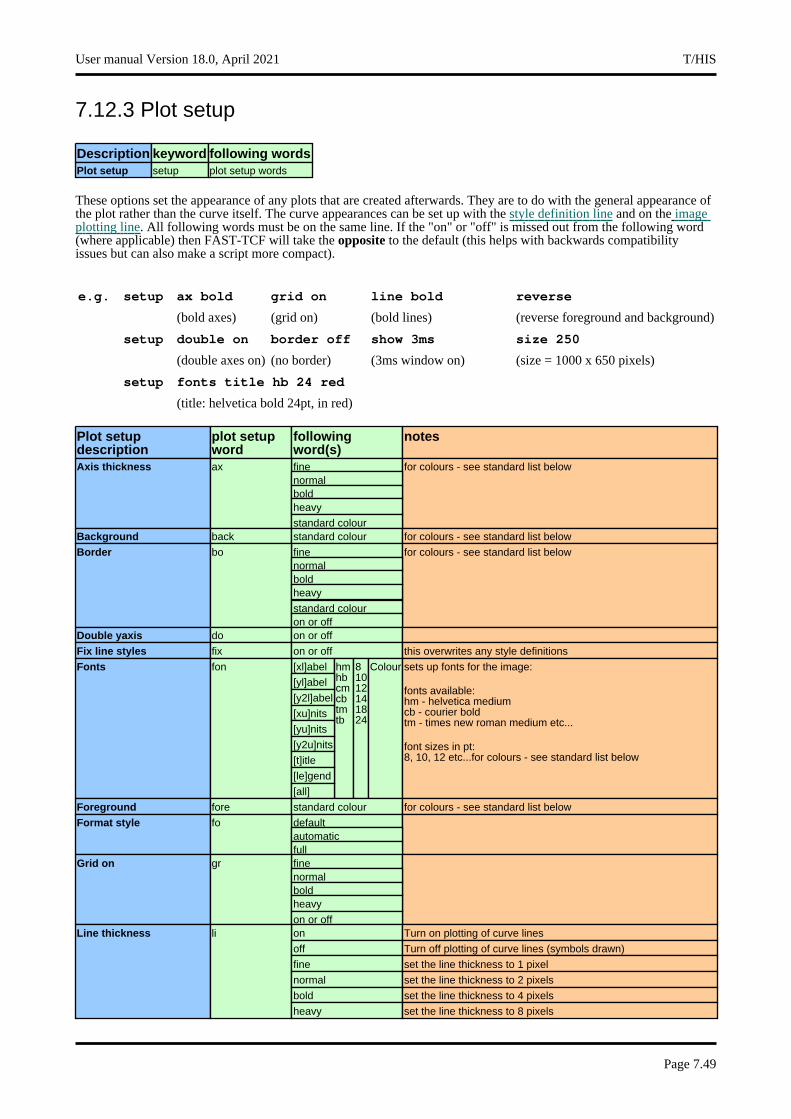
7.12.3 Plot setup
Description keyword following wordsPlot setup setup plot setup words
These options set the appearance of any plots that are created afterwards. They are to do with the general appearance of the plot rather than the curve itself. The curve appearances can be set up with the style definition line and on the imageplotting line. All following words must be on the same line. If the "on" or "off" is missed out from the following word (where applicable) then FAST-TCF will take the opposite to the default (this helps with backwards compatibility issues but can also make a script more compact).
e.g. setup ax bold grid on line bold reverse
(bold axes) (grid on) (bold lines) (reverse foreground and background)
setup double on border off show 3ms size 250
(double axes on) (no border) (3ms window on) (size = 1000 x 650 pixels)
setup fonts title hb 24 red
(title: helvetica bold 24pt, in red)
Plot setup description
plot setup word
following word(s)
notes
fineAxis thickness ax for colours - see standard list belownormalboldheavy
standard colourBackground back standard colour for colours - see standard list below
fineBorder bo for colours - see standard list belownormalboldheavy
standard colouron or off
Double yaxis do on or off
Fix line styles fix on or off this overwrites any style definitions
[xl]abelFonts fon hm hb cm cbtmtb
81012141824
Colour sets up fonts for the image:
fonts available:hm - helvetica mediumcb - courier boldtm - times new roman medium etc...
font sizes in pt:8, 10, 12 etc...for colours - see standard list below
[yl]abel
[y2l]abel
[xu]nits
[yu]nits
[y2u]nits
[t]itle
[le]gend
[all]
Foreground fore standard colour for colours - see standard list below
defaultFormat style foautomaticfullfineGrid on grnormalboldheavy
on or offon Turn on plotting of curve linesLine thickness li
off Turn off plotting of curve lines (symbols drawn)
fine set the line thickness to 1 pixel
normal set the line thickness to 2 pixels
bold set the line thickness to 4 pixels
heavy set the line thickness to 8 pixels
User manual Version 18.0, April 2021 T/HIS
Page 7.49
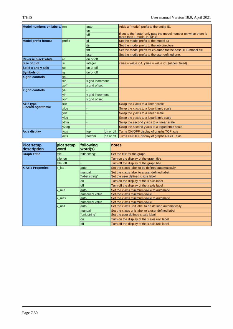
autoModel numbers on labels. mn Adds a "model" prefix to the entity IS.
If set to the "auto" only puts the model number on when there is more than 1 model in T/HIS
onoff
id Set the model prefix to the model IDModel prefix format prefix
dir Set the model prefix to the job directory
thf Set the model prefix tot eh amne fof the base THF/model file
user Set the modle prefix to the user defined one.
Reverse black white re on or offSize of plot si integer xsize = value x 4, ysize = value x 3 (aspect fixed)
Solid x and y axis so on or off
Symbols on sy on or off
xau -X grid controlsxin x grid increment
xoff x grid offset
yau -Y grid controlsyin y grid increment
yoff y grid offset
xlin - Swap the x axis to a linear scaleAxis type, Linear/Logarithmic xlog - Swap the x axis to a logarithmic scale
ylin - Swap the y axis to a linear scale
ylog - Swap the y axis to a logarithmic scale
y2lin - Swap the second y axis to a linear scale
y2log - Swap the second y axis to a logarithmic scale
axis top on or off Turns ON/OFF display of graphs TOP axisAxis display axis bottom on or off Turns ON/OFF display of graphs RIGHT axis
Plot setup description
plot setup word
following word(s)
notes
title "title string" Set the title for the graph. Graph Ttitletitle_on - Turn on the display of the graph title
title_off - Turn off the display of the graph title
auto Set the x axis label to be defined automaticallyX Axis Properties x_lab
manual Set the x axis label to a user defined label "label string" Set the user defined x axis label
on Turn on the display of the x axis label
off Turn off the display of the x axis label
auto Set the x axis minimum value to automaticx_minnumerical value Set the x axis minimum valueauto Set the x axis minimum value to automaticx_maxnumerical value Set the x axis minimum valueauto Set the x axis unit label to be defined automaticallyx_unit
manual Set the x axis unit label to a user defined label "unit string" Set the user defined x axis label
on Turn on the display of the x axis unit label
off Turn off the display of the x axis unit label
T/HIS User manual Version 18.0, April 2021
Page 7.50
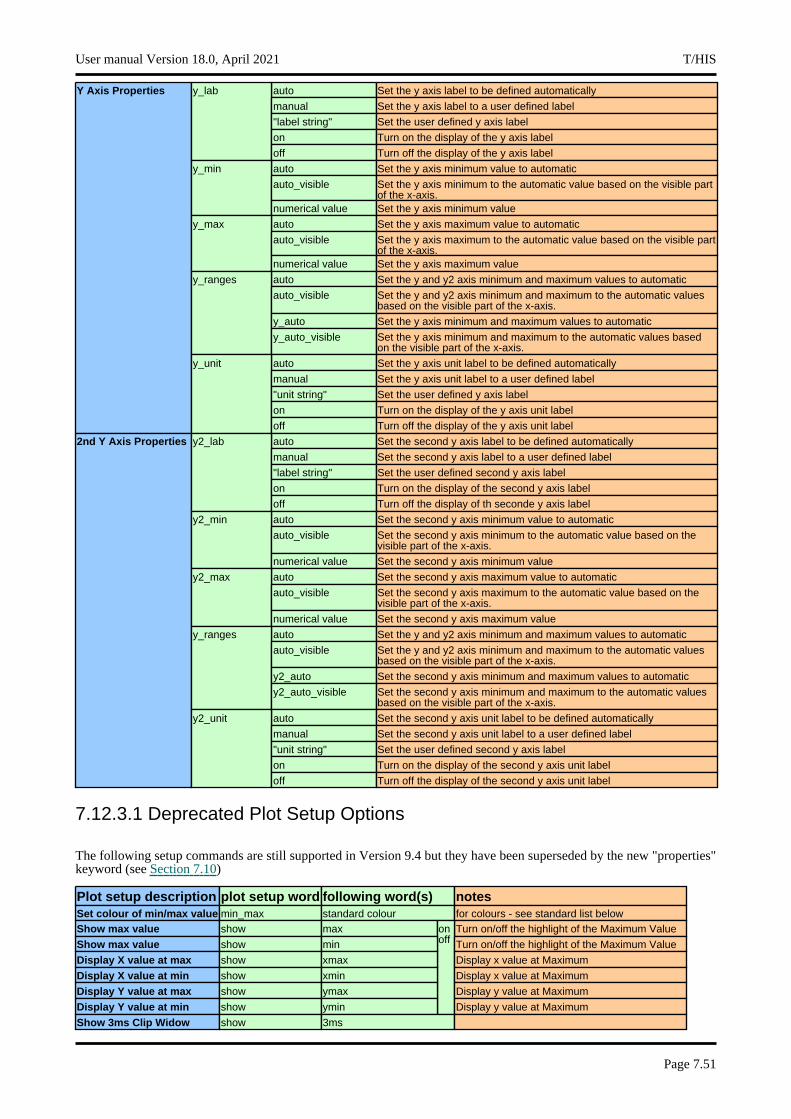
auto Set the y axis label to be defined automaticallyY Axis Properties y_lab
manual Set the y axis label to a user defined label
"label string" Set the user defined y axis label
on Turn on the display of the y axis label
off Turn off the display of the y axis label
auto Set the y axis minimum value to automaticy_min
auto_visible Set the y axis minimum to the automatic value based on the visible part of the x-axis.
numerical value Set the y axis minimum value
auto Set the y axis maximum value to automaticy_max
auto_visible Set the y axis maximum to the automatic value based on the visible part of the x-axis.
numerical value Set the y axis maximum value
auto Set the y and y2 axis minimum and maximum values to automaticy_ranges
auto_visible Set the y and y2 axis minimum and maximum to the automatic values based on the visible part of the x-axis.
y_auto Set the y axis minimum and maximum values to automatic
y_auto_visible Set the y axis minimum and maximum to the automatic values based on the visible part of the x-axis.
auto Set the y axis unit label to be defined automaticallyy_unit
manual Set the y axis unit label to a user defined label
"unit string" Set the user defined y axis label
on Turn on the display of the y axis unit label
off Turn off the display of the y axis unit label
auto Set the second y axis label to be defined automatically2nd Y Axis Properties y2_lab
manual Set the second y axis label to a user defined label
"label string" Set the user defined second y axis label
on Turn on the display of the second y axis label
off Turn off the display of th seconde y axis label
auto Set the second y axis minimum value to automaticy2_min
auto_visible Set the second y axis minimum to the automatic value based on the visible part of the x-axis.
numerical value Set the second y axis minimum value
auto Set the second y axis maximum value to automaticy2_max
auto_visible Set the second y axis maximum to the automatic value based on the visible part of the x-axis.
numerical value Set the second y axis maximum value
auto Set the y and y2 axis minimum and maximum values to automaticy_ranges
auto_visible Set the y and y2 axis minimum and maximum to the automatic values based on the visible part of the x-axis.
y2_auto Set the second y axis minimum and maximum values to automatic
y2_auto_visible Set the second y axis minimum and maximum to the automatic values based on the visible part of the x-axis.
auto Set the second y axis unit label to be defined automaticallyy2_unit
manual Set the second y axis unit label to a user defined label
"unit string" Set the user defined second y axis label
on Turn on the display of the second y axis unit label
off Turn off the display of the second y axis unit label
7.12.3.1 Deprecated Plot Setup Options
The following setup commands are still supported in Version 9.4 but they have been superseded by the new "properties" keyword (see Section 7.10)
Plot setup description plot setup word following word(s) notesSet colour of min/max value min_max standard colour for colours - see standard list belowShow max value show max Turn on/off the highlight of the Maximum Value on
off Show max value show min Turn on/off the highlight of the Maximum Value
Display X value at max show xmax Display x value at Maximum
Display X value at min show xmin Display x value at Maximum
Display Y value at max show ymax Display y value at Maximum
Display Y value at min show ymin Display y value at Maximum
Show 3ms Clip Widow show 3ms
User manual Version 18.0, April 2021 T/HIS
Page 7.51
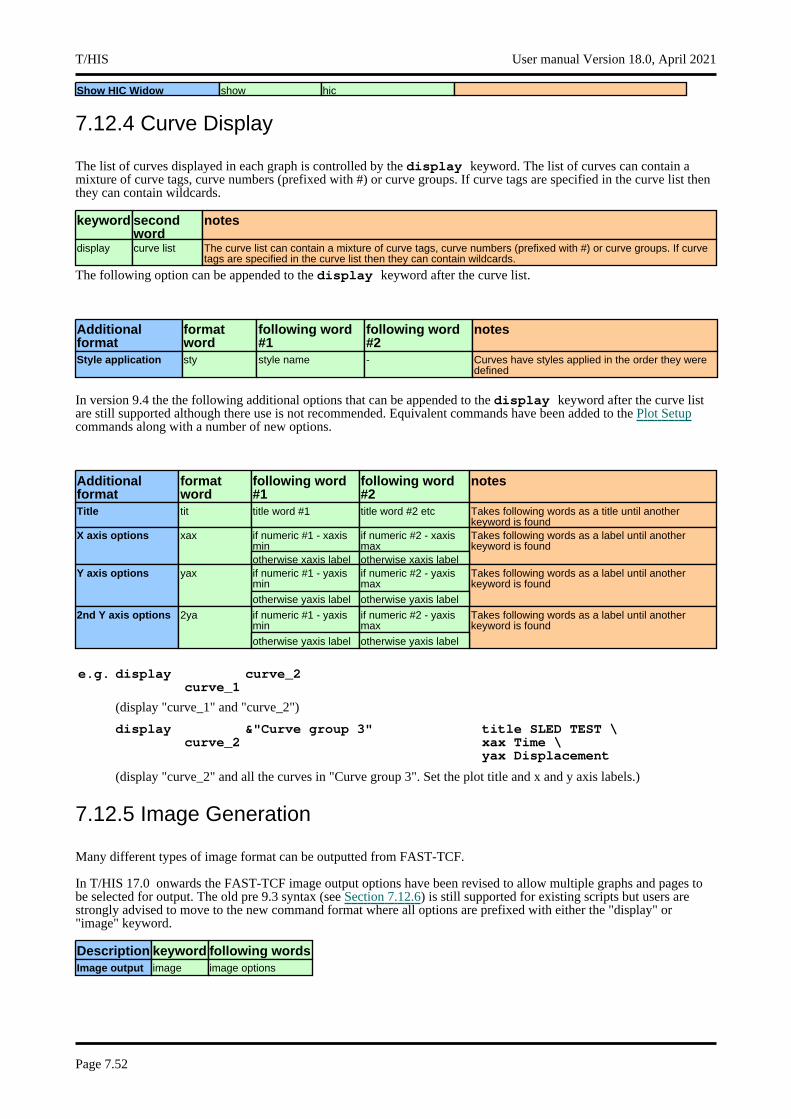
Show HIC Widow show hic
7.12.4 Curve Display
The list of curves displayed in each graph is controlled by the display keyword. The list of curves can contain a mixture of curve tags, curve numbers (prefixed with #) or curve groups. If curve tags are specified in the curve list then they can contain wildcards.
keyword second word
notes
display curve list The curve list can contain a mixture of curve tags, curve numbers (prefixed with #) or curve groups. If curve tags are specified in the curve list then they can contain wildcards.
The following option can be appended to the display keyword after the curve list.
Additional format
format word
following word #1
following word #2
notes
Style application sty style name - Curves have styles applied in the order they were defined
In version 9.4 the the following additional options that can be appended to the display keyword after the curve list are still supported although there use is not recommended. Equivalent commands have been added to the Plot Setupcommands along with a number of new options.
Additional format
format word
following word #1
following word #2
notes
Title tit title word #1 title word #2 etc Takes following words as a title until another keyword is found
if numeric #1 - xaxis min
if numeric #2 - xaxis max
X axis options xax Takes following words as a label until another keyword is found
otherwise xaxis label otherwise xaxis labelif numeric #1 - yaxis min
if numeric #2 - yaxis max
Y axis options yax Takes following words as a label until another keyword is found
otherwise yaxis label otherwise yaxis label
if numeric #1 - yaxis min
if numeric #2 - yaxis max
2nd Y axis options 2ya Takes following words as a label until another keyword is found
otherwise yaxis label otherwise yaxis label
e.g. display curve_1
curve_2
(display "curve_1" and "curve_2")
displaycurve_2
&"Curve group 3" title SLED TEST \xax Time \yax Displacement
(display "curve_2" and all the curves in "Curve group 3". Set the plot title and x and y axis labels.)
7.12.5 Image Generation
Many different types of image format can be outputted from FAST-TCF.
In T/HIS 17.0 onwards the FAST-TCF image output options have been revised to allow multiple graphs and pages to be selected for output. The old pre 9.3 syntax (see Section 7.12.6) is still supported for existing scripts but users are strongly advised to move to the new command format where all options are prefixed with either the "display" or "image" keyword.
Description keyword following wordsImage output image image options
T/HIS User manual Version 18.0, April 2021
Page 7.52
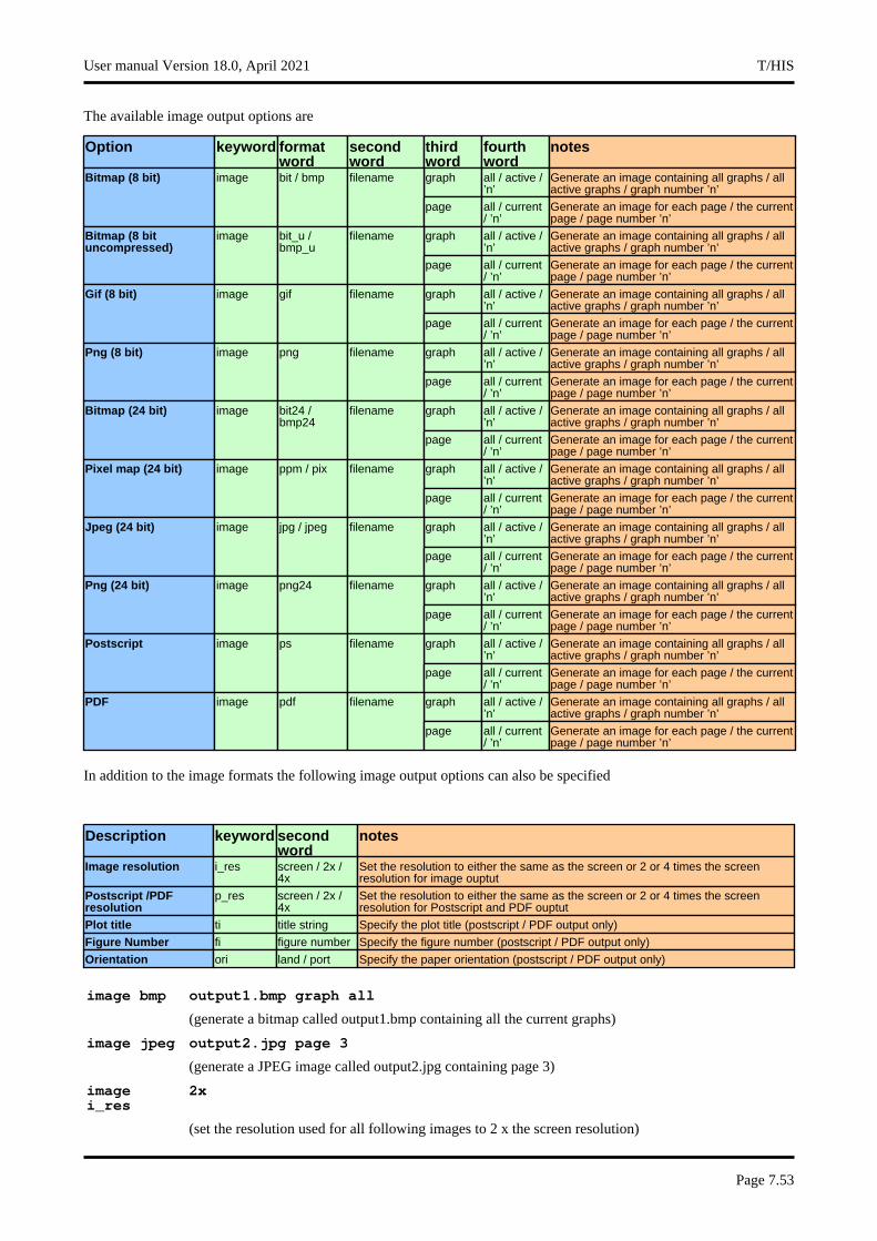
The available image output options are
Option keyword format word
second word
third word
fourth word
notes
graph all / active / ’n’
Generate an image containing all graphs / all active graphs / graph number ’n’
Bitmap (8 bit) image bit / bmp filename
page all / current / ’n’
Generate an image for each page / the current page / page number ’n’
graph all / active / ’n’
Generate an image containing all graphs / all active graphs / graph number ’n’
Bitmap (8 bit uncompressed)
image bit_u / bmp_u
filename
page all / current / ’n’
Generate an image for each page / the current page / page number ’n’
graph all / active / ’n’
Generate an image containing all graphs / all active graphs / graph number ’n’
Gif (8 bit) image gif filename
page all / current / ’n’
Generate an image for each page / the current page / page number ’n’
graph all / active / ’n’
Generate an image containing all graphs / all active graphs / graph number ’n’
Png (8 bit) image png filename
page all / current / ’n’
Generate an image for each page / the current page / page number ’n’
graph all / active / ’n’
Generate an image containing all graphs / all active graphs / graph number ’n’
Bitmap (24 bit) image bit24 / bmp24
filename
page all / current / ’n’
Generate an image for each page / the current page / page number ’n’
graph all / active / ’n’
Generate an image containing all graphs / all active graphs / graph number ’n’
Pixel map (24 bit) image ppm / pix filename
page all / current / ’n’
Generate an image for each page / the current page / page number ’n’
graph all / active / ’n’
Generate an image containing all graphs / all active graphs / graph number ’n’
Jpeg (24 bit) image jpg / jpeg filename
page all / current / ’n’
Generate an image for each page / the current page / page number ’n’
graph all / active / ’n’
Generate an image containing all graphs / all active graphs / graph number ’n’
Png (24 bit) image png24 filename
page all / current / ’n’
Generate an image for each page / the current page / page number ’n’
graph all / active / ’n’
Generate an image containing all graphs / all active graphs / graph number ’n’
Postscript image ps filename
page all / current / ’n’
Generate an image for each page / the current page / page number ’n’
graph all / active / ’n’
Generate an image containing all graphs / all active graphs / graph number ’n’
PDF image pdf filename
page all / current / ’n’
Generate an image for each page / the current page / page number ’n’
In addition to the image formats the following image output options can also be specified
Description keyword second word
notes
Image resolution i_res screen / 2x / 4x
Set the resolution to either the same as the screen or 2 or 4 times the screen resolution for image ouptut
Postscript /PDF resolution
p_res screen / 2x / 4x
Set the resolution to either the same as the screen or 2 or 4 times the screen resolution for Postscript and PDF ouptut
Plot title ti title string Specify the plot title (postscript / PDF output only)
Figure Number fi figure number Specify the figure number (postscript / PDF output only)
Orientation ori land / port Specify the paper orientation (postscript / PDF output only)
image bmp output1.bmp graph all
(generate a bitmap called output1.bmp containing all the current graphs)
image jpeg output2.jpg page 3
(generate a JPEG image called output2.jpg containing page 3)
image i_res
2x
(set the resolution used for all following images to 2 x the screen resolution)
User manual Version 18.0, April 2021 T/HIS
Page 7.53
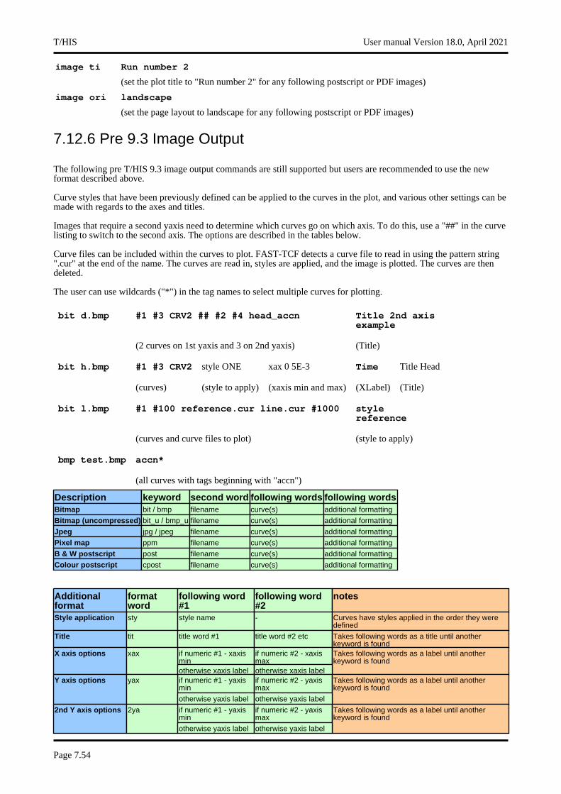
image ti Run number 2
(set the plot title to "Run number 2" for any following postscript or PDF images)
image ori landscape
(set the page layout to landscape for any following postscript or PDF images)
7.12.6 Pre 9.3 Image Output
The following pre T/HIS 9.3 image output commands are still supported but users are recommended to use the new format described above.
Curve styles that have been previously defined can be applied to the curves in the plot, and various other settings can be made with regards to the axes and titles.
Images that require a second yaxis need to determine which curves go on which axis. To do this, use a "##" in the curve listing to switch to the second axis. The options are described in the tables below.
Curve files can be included within the curves to plot. FAST-TCF detects a curve file to read in using the pattern string ".cur" at the end of the name. The curves are read in, styles are applied, and the image is plotted. The curves are then deleted.
The user can use wildcards ("*") in the tag names to select multiple curves for plotting.
bit d.bmp #1 #3 CRV2 ## #2 #4 head_accn Title 2nd axis example
(2 curves on 1st yaxis and 3 on 2nd yaxis) (Title)
bit h.bmp #1 #3 CRV2 style ONE xax 0 5E-3 Time Title Head
(curves) (style to apply) (xaxis min and max) (XLabel) (Title)
bit l.bmp #1 #100 reference.cur line.cur #1000 style reference
(curves and curve files to plot) (style to apply)
bmp test.bmp accn*
(all curves with tags beginning with "accn")
Description keyword second word following words following wordsBitmap bit / bmp filename curve(s) additional formatting
Bitmap (uncompressed) bit_u / bmp_u filename curve(s) additional formatting
Jpeg jpg / jpeg filename curve(s) additional formatting
Pixel map ppm filename curve(s) additional formatting
B & W postscript post filename curve(s) additional formatting
Colour postscript cpost filename curve(s) additional formatting
Additional format
format word
following word #1
following word #2
notes
Style application sty style name - Curves have styles applied in the order they were defined
Title tit title word #1 title word #2 etc Takes following words as a title until another keyword is found
if numeric #1 - xaxis min
if numeric #2 - xaxis max
X axis options xax Takes following words as a label until another keyword is found
otherwise xaxis label otherwise xaxis labelif numeric #1 - yaxis min
if numeric #2 - yaxis max
Y axis options yax Takes following words as a label until another keyword is found
otherwise yaxis label otherwise yaxis label
if numeric #1 - yaxis min
if numeric #2 - yaxis max
2nd Y axis options 2ya Takes following words as a label until another keyword is found
otherwise yaxis label otherwise yaxis label
T/HIS User manual Version 18.0, April 2021
Page 7.54
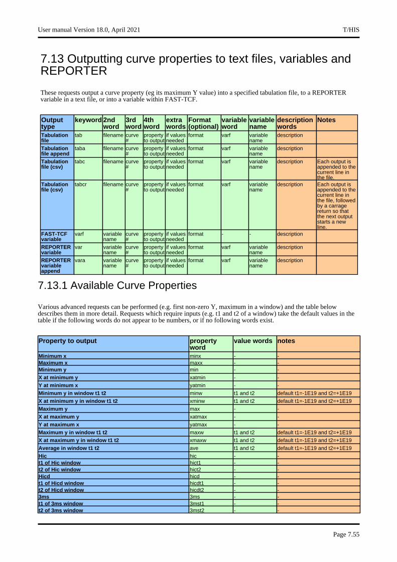
7.13 Outputting curve properties to text files, variables and REPORTER
These requests output a curve property (eg its maximum Y value) into a specified tabulation file, to a REPORTER variable in a text file, or into a variable within FAST-TCF.
Output type
keyword 2nd word
3rd word
4th word
extra words
Format (optional)
variable word
variable name
description words
Notes
Tabulation file
tab filename curve #
property to output
if values needed
format varf variable name
description
Tabulation file append
taba filename curve #
property to output
if values needed
format varf variable name
description
Tabulation file (csv)
tabc filename curve #
property to output
if values needed
format varf variable name
description Each output is appended to the current line in the file.
Tabulation file (csv)
tabcr filename curve #
property to output
if values needed
format varf variable name
description Each output is appended to the current line in the file, followed by a carrage return so that the next output starts a new line.
FAST-TCF variable
varf variable name
curve #
property to output
if values needed
format - - description
REPORTER variable
var variable name
curve #
property to output
if values needed
format varf variable name
description
REPORTER variable append
vara variable name
curve #
property to output
if values needed
format varf variable name
description
7.13.1 Available Curve Properties
Various advanced requests can be performed (e.g. first non-zero Y, maximum in a window) and the table below describes them in more detail. Requests which require inputs (e.g. t1 and t2 of a window) take the default values in the table if the following words do not appear to be numbers, or if no following words exist.
Property to output property word
value words notes
Minimum x minx - -Maximum x maxx - -Minimum y min - -
X at minimum y xatmin - -
Y at minimum x yatmin - -
Minimum y in window t1 t2 minw t1 and t2 default t1=-1E19 and t2=+1E19
X at minimum y in window t1 t2 xminw t1 and t2 default t1=-1E19 and t2=+1E19
Maximum y max - -
X at maximum y xatmax - -
Y at maximum x yatmax - -
Maximum y in window t1 t2 maxw t1 and t2 default t1=-1E19 and t2=+1E19
X at maximum y in window t1 t2 xmaxw t1 and t2 default t1=-1E19 and t2=+1E19
Average in window t1 t2 ave t1 and t2 default t1=-1E19 and t2=+1E19
Hic hic - -t1 of Hic window hict1 - -t2 of Hic window hict2 - -Hicd hicd - -t1 of Hicd window hicdt1 - -t2 of Hicd window hicdt2 - -3ms 3ms - -t1 of 3ms window 3mst1 - -t2 of 3ms window 3mst2 - -
User manual Version 18.0, April 2021 T/HIS
Page 7.55
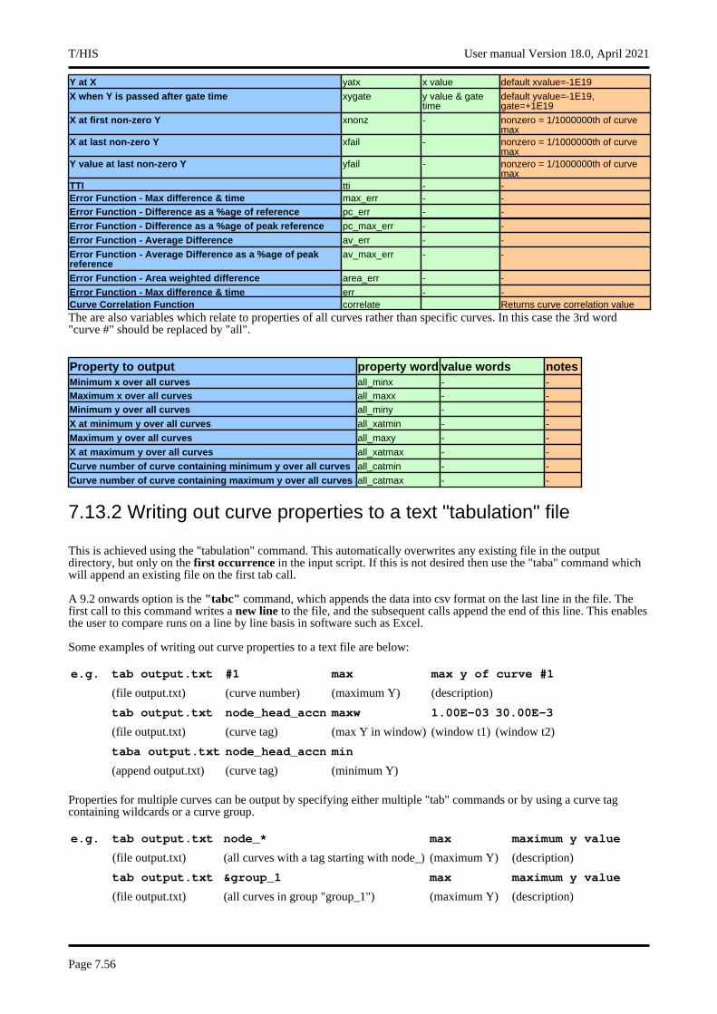
Y at X yatx x value default xvalue=-1E19
X when Y is passed after gate time xygate y value & gate time
default yvalue=-1E19, gate=+1E19
X at first non-zero Y xnonz - nonzero = 1/1000000th of curve max
X at last non-zero Y xfail - nonzero = 1/1000000th of curve max
Y value at last non-zero Y yfail - nonzero = 1/1000000th of curve max
TTI tti - -Error Function - Max difference & time max_err - -Error Function - Difference as a %age of reference pc_err - -
Error Function - Difference as a %age of peak reference pc_max_err - -
Error Function - Average Difference av_err - -
Error Function - Average Difference as a %age of peak reference
av_max_err - -
Error Function - Area weighted difference area_err - -
Error Function - Max difference & time err - -Curve Correlation Function correlate Returns curve correlation valueThe are also variables which relate to properties of all curves rather than specific curves. In this case the 3rd word "curve #" should be replaced by "all".
Property to output property word value words notesMinimum x over all curves all_minx - -Maximum x over all curves all_maxx - -Minimum y over all curves all_miny - -
X at minimum y over all curves all_xatmin - -
Maximum y over all curves all_maxy - -
X at maximum y over all curves all_xatmax - -
Curve number of curve containing minimum y over all curves all_catmin - -
Curve number of curve containing maximum y over all curves all_catmax - -
7.13.2 Writing out curve properties to a text "tabulation" file
This is achieved using the "tabulation" command. This automatically overwrites any existing file in the output directory, but only on the first occurrence in the input script. If this is not desired then use the "taba" command which will append an existing file on the first tab call.
A 9.2 onwards option is the "tabc" command, which appends the data into csv format on the last line in the file. The first call to this command writes a new line to the file, and the subsequent calls append the end of this line. This enables the user to compare runs on a line by line basis in software such as Excel.
Some examples of writing out curve properties to a text file are below:
e.g. tab output.txt #1 max max y of curve #1
(file output.txt) (curve number) (maximum Y) (description)
tab output.txt node_head_accn maxw 1.00E-03 30.00E-3
(file output.txt) (curve tag) (max Y in window) (window t1) (window t2)
taba output.txt node_head_accn min
(append output.txt) (curve tag) (minimum Y)
Properties for multiple curves can be output by specifying either multiple "tab" commands or by using a curve tag containing wildcards or a curve group.
e.g. tab output.txt node_* max maximum y value
(file output.txt) (all curves with a tag starting with node_) (maximum Y) (description)
tab output.txt &group_1 max maximum y value
(file output.txt) (all curves in group "group_1") (maximum Y) (description)
T/HIS User manual Version 18.0, April 2021
Page 7.56
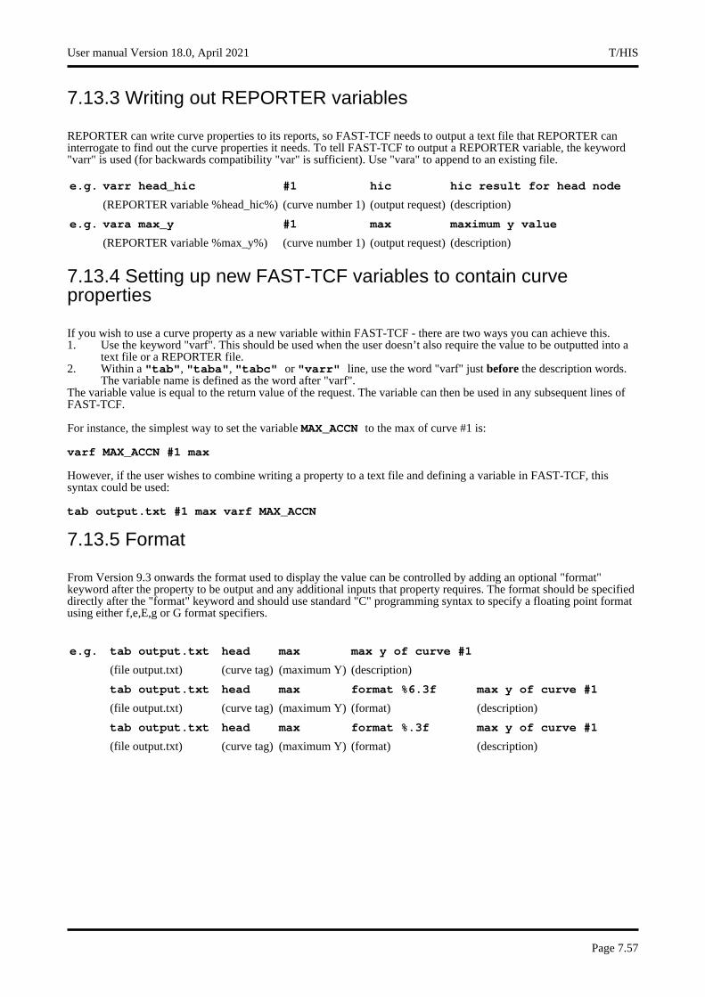
7.13.3 Writing out REPORTER variables
REPORTER can write curve properties to its reports, so FAST-TCF needs to output a text file that REPORTER can interrogate to find out the curve properties it needs. To tell FAST-TCF to output a REPORTER variable, the keyword "varr" is used (for backwards compatibility "var" is sufficient). Use "vara" to append to an existing file.
e.g. varr head_hic #1 hic hic result for head node
(REPORTER variable %head_hic%) (curve number 1) (output request) (description)
e.g. vara max_y #1 max maximum y value
(REPORTER variable %max_y%) (curve number 1) (output request) (description)
7.13.4 Setting up new FAST-TCF variables to contain curve properties
If you wish to use a curve property as a new variable within FAST-TCF - there are two ways you can achieve this. 1. Use the keyword "varf". This should be used when the user doesn’t also require the value to be outputted into a
text file or a REPORTER file.2. Within a "tab", "taba", "tabc" or "varr" line, use the word "varf" just before the description words.
The variable name is defined as the word after "varf".The variable value is equal to the return value of the request. The variable can then be used in any subsequent lines of FAST-TCF.
For instance, the simplest way to set the variable MAX_ACCN to the max of curve #1 is:
varf MAX_ACCN #1 max
However, if the user wishes to combine writing a property to a text file and defining a variable in FAST-TCF, this syntax could be used:
tab output.txt #1 max varf MAX_ACCN
7.13.5 Format
From Version 9.3 onwards the format used to display the value can be controlled by adding an optional "format" keyword after the property to be output and any additional inputs that property requires. The format should be specified directly after the "format" keyword and should use standard "C" programming syntax to specify a floating point format using either f,e,E,g or G format specifiers.
e.g. tab output.txt head max max y of curve #1
(file output.txt) (curve tag) (maximum Y) (description)
tab output.txt head max format %6.3f max y of curve #1
(file output.txt) (curve tag) (maximum Y) (format) (description)
tab output.txt head max format %.3f max y of curve #1
(file output.txt) (curve tag) (maximum Y) (format) (description)
User manual Version 18.0, April 2021 T/HIS
Page 7.57
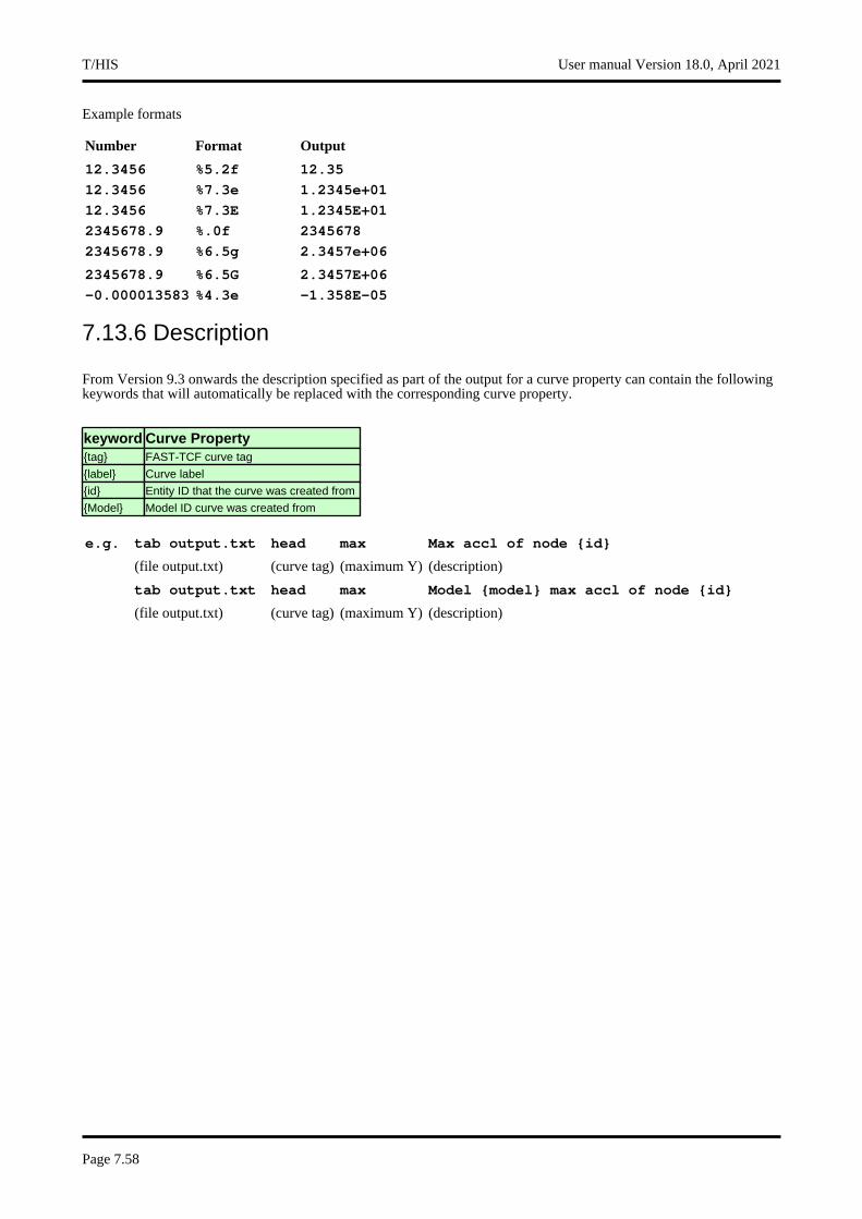
Example formats
Number Format Output
12.3456 %5.2f 12.35
12.3456 %7.3e 1.2345e+01
12.3456 %7.3E 1.2345E+01
2345678.9 %.0f 2345678
2345678.9 %6.5g 2.3457e+06
2345678.9 %6.5G 2.3457E+06
-0.000013583 %4.3e -1.358E-05
7.13.6 Description
From Version 9.3 onwards the description specified as part of the output for a curve property can contain the following keywords that will automatically be replaced with the corresponding curve property.
keyword Curve Property{tag} FAST-TCF curve tag
{label} Curve label
{id} Entity ID that the curve was created from
{Model} Model ID curve was created from
e.g. tab output.txt head max Max accl of node {id}
(file output.txt) (curve tag) (maximum Y) (description)
tab output.txt head max Model {model} max accl of node {id}
(file output.txt) (curve tag) (maximum Y) (description)
T/HIS User manual Version 18.0, April 2021
Page 7.58

7.14 FAST-TCF CURVE OUTPUT
Curves can be written out to either T/HIS curve files or CSV files from within a FAST-TCF script by using either the "app", "cop", "csv" or "csv2" keyword.
Description keyword second word
third word
notes
Copy into file cop filename curve list - will overwrite any previous file
Append into file
app filename curve list - will append any previous file
CSV file TYPE 1
csv filename curve list - will overwrite any previous csv file. CSV has the format X1,Y1,X2,Y2,X3,Y3
last word = auto will overwrite any previous csv file. CSV has the format X1,Y1,Y2,Y3x axis interval is taken from curve #1 if all curves are chosen
CSV file TYPE 2
csv2 filename curve list
2nd last word= x start timelast word = x axis interval
will overwrite any previous csv file. CSV has the format X1,Y1,Y2,Y3start time and interval are defined in the line
The curve list for all of these commands can contain either curve tags (with or without wildcards), curve numbers (prefixed with #), curve groups or ’*’ to select all curves.
e.g. copy output_file.cur curve_1 &"group 1"
(Write "curve_1" and all the curves in curve group "group 1" to a new file "output_file.cur")
append output_file.cur curve_1 &"group 1"
(Append "curve_1" and all the curves in curve group "group 1" to the file "output_file.cur")
csv output.csv curve_1* curve_2*
(Write all curves with tags that start with "curve_1" or "curve_2" to a CSV called "output.csv")
NOTE : There is no limit to the number of curves that can be output to a file but there is a limit to the number of items that can be specified in the curve list (currently 100). If more than 100 curves are to be output to a file then a curvegroup containing all of the curves should be created and used within the curve list. Alternatively if the curves are being written to a T/HIS curve file then the first 100 curves can be output using the "cop" keyword and then additional curves can be appended to the file using the "app" keyword.
7.14.1 Specifying curves using Curve Numbers
When outputting curves to a file a range of explicit curve numbers can be specified using the syntax #start:#end. This option only applies to curve numbers because curve tag can be defined in an arbitrary order.
7.14.2 CSV files
If a CSV/CSV2 file is written out from within a FAST-TCF script then by default it will contain rows containing UNIT information for the curves if UNITS have been defined. This additional information can be turned off if it isn’t required (see Section 7.5.5)
User manual Version 18.0, April 2021 T/HIS
Page 7.59
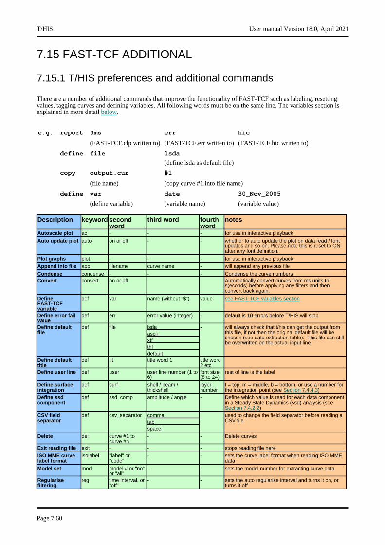
7.15 FAST-TCF ADDITIONAL
7.15.1 T/HIS preferences and additional commands
There are a number of additional commands that improve the functionality of FAST-TCF such as labeling, resetting values, tagging curves and defining variables. All following words must be on the same line. The variables section is explained in more detail below.
e.g. report 3ms err hic
(FAST-TCF.clp written to) (FAST-TCF.err written to) (FAST-TCF.hic written to)
define file lsda
(define lsda as default file)
copy output.cur #1
(file name) (copy curve #1 into file name)
define var date 30_Nov_2005
(define variable) (variable name) (variable value)
Description keyword second word
third word fourth word
notes
Autoscale plot ac - - - for use in interactive playback
Auto update plot auto on or off - - whether to auto update the plot on data read / font updates and so on. Please note this is reset to ON after any font definition.
Plot graphs plot - - - for use in interactive playback
Append into file app filename curve name - will append any previous file
Condense condense - - - Condense the curve numbersConvert convert on or off Automatically convert curves from ms units to
s(econds) before applying any filters and then convert back again.
Define FAST-TCF variable
def var name (without "$") value see FAST-TCF variables section
Define error fail value
def err error value (integer) - default is 10 errors before T/HIS will stop
lsdaDefine default file
def file - will always check that t/his can get the output from this file, if not then the original default file will be chosen (see data extraction table). This file can still be overwritten on the actual input line
asciixtfthfdefault
Define default title
def tit title word 1 title word 2 etc
Define user line def user user line number (1 to 6)
font size (8 to 24)
rest of line is the label
Define surface integration
def surf shell / beam / thickshell
layer number
t = top, m = middle, b = bottom, or use a number for the integration point (see Section 7.4.4.3)
Define ssd component
def ssd_comp amplitude / angle - Define which value is read for each data component in a Steady State Dynamics (ssd) analysis (see Section 7.4.2.2)
commaCSV field separator
def csv_separator used to change the field separator before reading a CSV file.tab
space
Delete del curve #1 to curve #n
- - Delete curves
Exit reading file exit - - - stops reading file here
ISO MME curve label format
isolabel "label" or "code"
- - sets the curve label format when reading ISO MME data
Model set mod model # or "no" or "all"
- - sets the model number for extracting curve data
Regularise filtering
reg time interval, or "off"
- - sets the auto regularise interval and turns it on, or turns it off
T/HIS User manual Version 18.0, April 2021
Page 7.60

3msReport files written
rep - - To turn off see the reset2 keywordasierrhicthivtti
reset1 - - - All curves and curve tags deletedResetreset2 - - - Plot setup defaulted and all style definitions
removed. Report files not written
reset3 - - - Variable names and default title removedcol colour number
(1-6)RRGGBB (6-digit hexadecimal)
- 6-digit hexadecimal format for rgb colour values.User-defined colours
col_rgb colour number (1-6)
r g b (3 integers in range 0-255, separated by spaces)
- Seperate integer format for rgb colour values.
7.15.2 Limits
Description limitword limit per line 80 words
include file name 150 characterstag length 60 characters
7.15.3 Variables
Variable names can only have "a-z", "0-9" and "_" in them. Variables can be inserted anywhere in the script, FAST-TCF will replace any variables with their corresponding values before processing the line, for example:
define var output displacementdefine var nod_id 12345678define var xscale 0.001
node $nod_id $output x xscale $xscale
converts into:
node 12345678 displacement x xscale 0.001
Variable definitions can contain several words or other varaibles, and these will be joined together to form the final variable value, for example:
define var day 31stdefine var month januarydefine var year 2099define var date $day _ $month _ $year
creates the variable date with value 31st_january_2099
Because variables cannot have anything other than "a-z", "0-9" and "_" in them, it is possible to use variables within strings:
define var analysis run01_vers2
read january_$analysis.cur
converts into
read january_run01_vers2.cur
However, sometimes the user may want to insert a variable within other alphanumeric words, in these circumstances use a "$$" terminator to designate the end of the variable name:
define var analysis xyz_run01read $analysis$$_x.cur
converts into
User manual Version 18.0, April 2021 T/HIS
Page 7.61
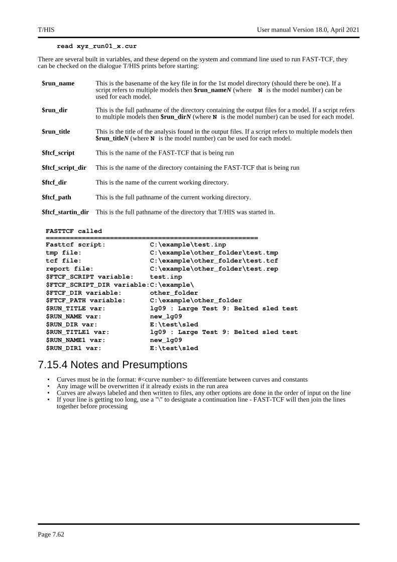
read xyz_run01_x.cur
There are several built in variables, and these depend on the system and command line used to run FAST-TCF, they can be checked on the dialogue T/HIS prints before starting:
$run_name This is the basename of the key file in for the 1st model directory (should there be one). If a script refers to multiple models then $run_nameN (where N is the model number) can be used for each model.
$run_dir This is the full pathname of the directory containing the output files for a model. If a script refers to multiple models then $run_dirN (where N is the model number) can be used for each model.
$run_title This is the title of the analysis found in the output files. If a script refers to multiple models then $run_titleN (where N is the model number) can be used for each model.
$ftcf_script This is the name of the FAST-TCF that is being run
$ftcf_script_dir This is the name of the directory containing the FAST-TCF that is being run
$ftcf_dir This is the name of the current working directory.
$ftcf_path This is the full pathname of the current working directory.
$ftcf_startin_dir This is the full pathname of the directory that T/HIS was started in.
FASTTCF called=====================================================Fasttcf script: C:\example\test.inptmp file: C:\example\other_folder\test.tmptcf file: C:\example\other_folder\test.tcfreport file: C:\example\other_folder\test.rep$FTCF_SCRIPT variable: test.inp$FTCF_SCRIPT_DIR variable:C:\example\$FTCF_DIR variable: other_folder$FTCF_PATH variable: C:\example\other_folder$RUN_TITLE var: lg09 : Large Test 9: Belted sled test$RUN_NAME var: new_lg09$RUN_DIR var: E:\test\sled$RUN_TITLE1 var: lg09 : Large Test 9: Belted sled test$RUN_NAME1 var: new_lg09$RUN_DIR1 var: E:\test\sled
7.15.4 Notes and Presumptions• Curves must be in the format: #<curve number> to differentiate between curves and constants• Any image will be overwritten if it already exists in the run area• Curves are always labeled and then written to files, any other options are done in the order of input on the line• If your line is getting too long, use a "\" to designate a continuation line - FAST-TCF will then join the lines
together before processing
T/HIS User manual Version 18.0, April 2021
Page 7.62
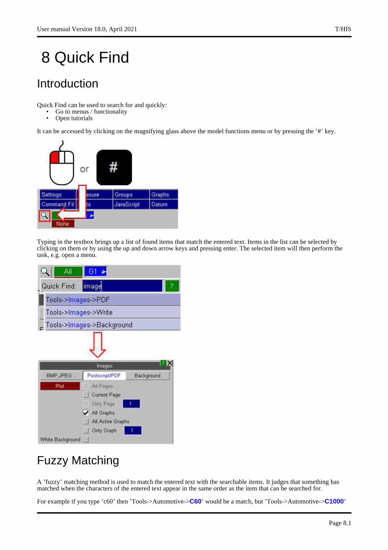
8 Quick Find
Introduction
Quick Find can be used to search for and quickly:• Go to menus / functionality• Open tutorials
It can be accessed by clicking on the magnifying glass above the model functions menu or by pressing the ’#’ key.
Typing in the textbox brings up a list of found items that match the entered text. Items in the list can be selected by clicking on them or by using the up and down arrow keys and pressing enter. The selected item will then perform the task, e.g. open a menu.
Fuzzy Matching
A ’fuzzy’ matching method is used to match the entered text with the searchable items. It judges that something has matched when the characters of the entered text appear in the same order as the item that can be searched for.
For example if you type ’c60’ then ’Tools->Automotive->C60’ would be a match, but ’Tools->Automotive->C1000’
User manual Version 18.0, April 2021 T/HIS
Page 8.1

wouldn’t because the ’6’ doesn’t match. (Note that the search is case insensitive).
Additionally, if the entered search pattern contains spaces and the characters do not all match in the same order then T/HIS will look to see if the words can be swapped to find a match.
For example ’back image’ would find ’Image->Background’ even though the words do not appear in that order.
This hopefully makes it easier to find items as you do not need to know the precise search term.
The found items are listed in order of how closely they match the entered text so items that more closely match appear nearer the top of the list. It determines this by assigning a score to each match, with higher scores given to items that contain consecutively matched characters and if the characters appear at the start of words.
Search Terms
The default search term associated with a menu item is the trail of menus/buttons you would need to manually open/press, e.g. to get to the C60 filter you would need to go to Tools, then Automotive then C60, hence the search term ’Tools->Automotive->C60’.
In addition, some menus have alternative search terms associated with them. For example C60 can also be found from the alternative text ’SAE class 60 filter’:
This can be useful for cases where you don’t know or can’t remember under which menu some functionality lives.
Note that the alternative text appears in brackets under the default search term so you can see how you would get to the menu manually.
If you can’t find menus that you know exist in T/HIS it is likely that you are using different terminology to what we expect. If so, please contact Oasys Ltd and we can add alternative text based on what you are entering as your search text.
Alternative text associated with a menu may also describe some of the features on a menu. For example the text colour is set in the Display menu, but if you didn’t know this it would be hard to find.
In this case the alternative text ’Text Colour’ is associated with this menu:
T/HIS User manual Version 18.0, April 2021
Page 8.2
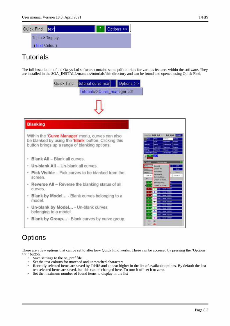
Tutorials
The full installation of the Oasys Ltd software contains some pdf tutorials for various features within the software. They are installed in the $OA_INSTALL/manuals/tutorials/this directory and can be found and opened using Quick Find.
Options
There are a few options that can be set to alter how Quick Find works. These can be accessed by pressing the ’Options >>’’ button.
• Save settings to the oa_pref file• Set the text colours for matched and unmatched characters• Recently selected items are saved by T/HIS and appear higher in the list of available options. By default the last
ten selected items are saved, but this can be changed here. To turn it off set it to zero.• Set the maximum number of found items to display in the list
User manual Version 18.0, April 2021 T/HIS
Page 8.3

T/HIS User manual Version 18.0, April 2021
Page 8.4
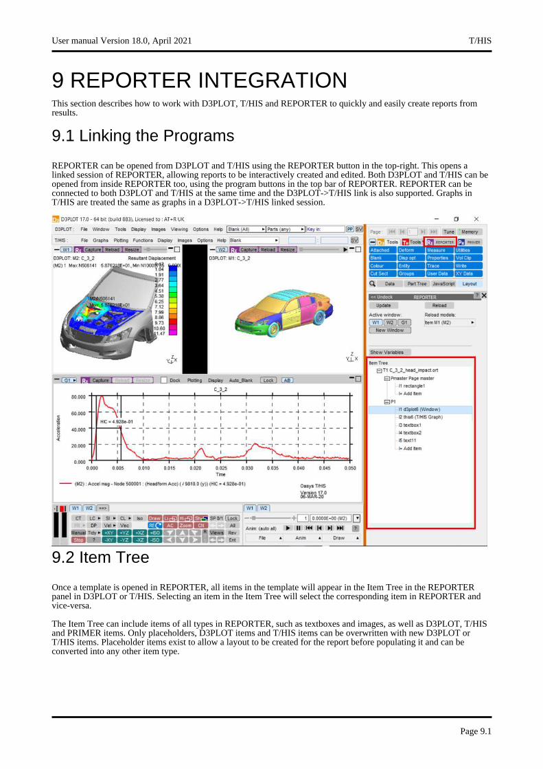
9 REPORTER INTEGRATION This section describes how to work with D3PLOT, T/HIS and REPORTER to quickly and easily create reports from results.
9.1 Linking the Programs
REPORTER can be opened from D3PLOT and T/HIS using the REPORTER button in the top-right. This opens a linked session of REPORTER, allowing reports to be interactively created and edited. Both D3PLOT and T/HIS can be opened from inside REPORTER too, using the program buttons in the top bar of REPORTER. REPORTER can be connected to both D3PLOT and T/HIS at the same time and the D3PLOT->T/HIS link is also supported. Graphs in T/HIS are treated the same as graphs in a D3PLOT->T/HIS linked session.
9.2 Item Tree
Once a template is opened in REPORTER, all items in the template will appear in the Item Tree in the REPORTER panel in D3PLOT or T/HIS. Selecting an item in the Item Tree will select the corresponding item in REPORTER and vice-versa.
The Item Tree can include items of all types in REPORTER, such as textboxes and images, as well as D3PLOT, T/HIS and PRIMER items. Only placeholders, D3PLOT items and T/HIS items can be overwritten with new D3PLOT or T/HIS items. Placeholder items exist to allow a layout to be created for the report before populating it and can be converted into any other item type.
User manual Version 18.0, April 2021 T/HIS
Page 9.1
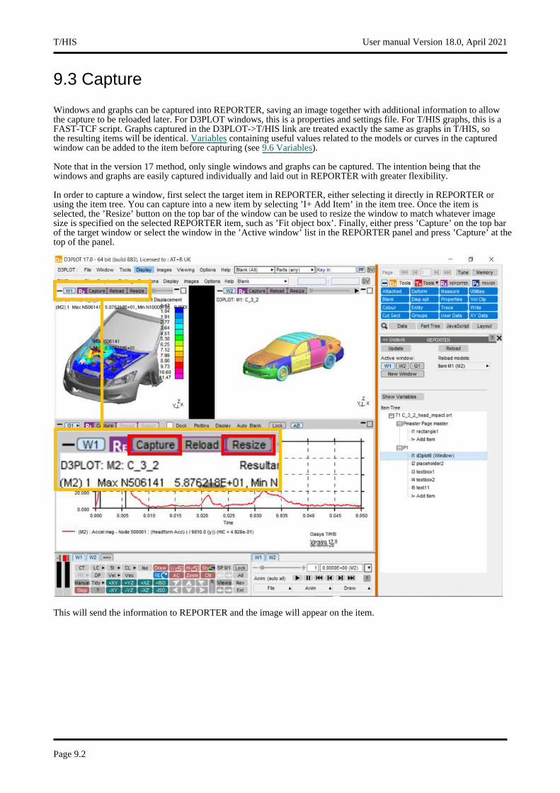
9.3 Capture
Windows and graphs can be captured into REPORTER, saving an image together with additional information to allow the capture to be reloaded later. For D3PLOT windows, this is a properties and settings file. For T/HIS graphs, this is a FAST-TCF script. Graphs captured in the D3PLOT->T/HIS link are treated exactly the same as graphs in T/HIS, so the resulting items will be identical. Variables containing useful values related to the models or curves in the captured window can be added to the item before capturing (see 9.6 Variables).
Note that in the version 17 method, only single windows and graphs can be captured. The intention being that the windows and graphs are easily captured individually and laid out in REPORTER with greater flexibility.
In order to capture a window, first select the target item in REPORTER, either selecting it directly in REPORTER or using the item tree. You can capture into a new item by selecting ’I+ Add Item’ in the item tree. Once the item is selected, the ’Resize’ button on the top bar of the window can be used to resize the window to match whatever image size is specified on the selected REPORTER item, such as ’Fit object box’. Finally, either press ’Capture’ on the top bar of the target window or select the window in the ’Active window’ list in the REPORTER panel and press ’Capture’ at the top of the panel.
This will send the information to REPORTER and the image will appear on the item.
T/HIS User manual Version 18.0, April 2021
Page 9.2
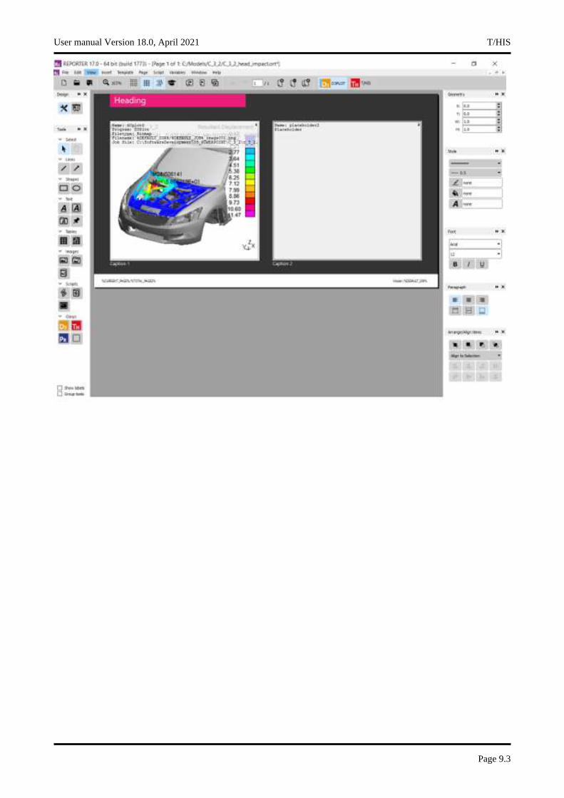
User manual Version 18.0, April 2021 T/HIS
Page 9.3
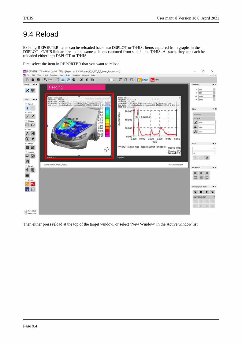
9.4 Reload
Existing REPORTER items can be reloaded back into D3PLOT or T/HIS. Items captured from graphs in the D3PLOT->T/HIS link are treated the same as items captured from standalone T/HIS. As such, they can each be reloaded either into D3PLOT or T/HIS.
First select the item in REPORTER that you want to reload.
Then either press reload at the top of the target window, or select ’New Window’ in the Active window list.
T/HIS User manual Version 18.0, April 2021
Page 9.4
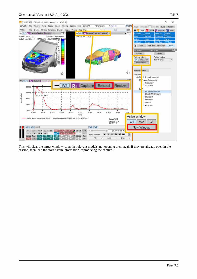
This will clear the target window, open the relevant models, not opening them again if they are already open in the session, then load the stored item information, reproducing the capture.
User manual Version 18.0, April 2021 T/HIS
Page 9.5

9.4.1 Reload Models
The models used in an existing item are listed in the ‘Reload models’ list. The models will be listed as ‘Item Mn’, where n is the index of the model in the item, not of the model in the session. If the model is also open in the current session, then the model ID in the current session will be displayed in brackets.
Each entry in the list has a popup attached, allowing the model to replaced either by a model in the current session or by browsing for a model. This will not change the models stored in the item, but instead when the item is reloaded into the current session the replacement models will be used. The resulting window will then need to be captured, either into a new item or to overwrite the original.
T/HIS User manual Version 18.0, April 2021
Page 9.6
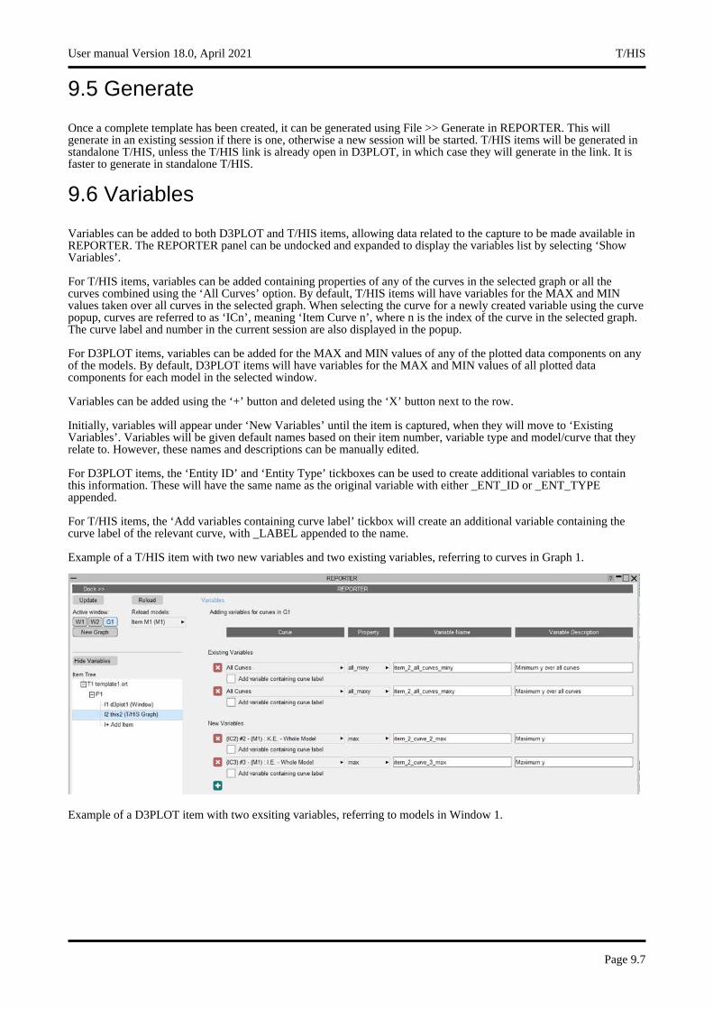
9.5 Generate
Once a complete template has been created, it can be generated using File >> Generate in REPORTER. This will generate in an existing session if there is one, otherwise a new session will be started. T/HIS items will be generated in standalone T/HIS, unless the T/HIS link is already open in D3PLOT, in which case they will generate in the link. It is faster to generate in standalone T/HIS.
9.6 Variables
Variables can be added to both D3PLOT and T/HIS items, allowing data related to the capture to be made available in REPORTER. The REPORTER panel can be undocked and expanded to display the variables list by selecting ‘Show Variables’.
For T/HIS items, variables can be added containing properties of any of the curves in the selected graph or all the curves combined using the ‘All Curves’ option. By default, T/HIS items will have variables for the MAX and MIN values taken over all curves in the selected graph. When selecting the curve for a newly created variable using the curve popup, curves are referred to as ‘ICn’, meaning ‘Item Curve n’, where n is the index of the curve in the selected graph. The curve label and number in the current session are also displayed in the popup.
For D3PLOT items, variables can be added for the MAX and MIN values of any of the plotted data components on any of the models. By default, D3PLOT items will have variables for the MAX and MIN values of all plotted data components for each model in the selected window.
Variables can be added using the ‘+’ button and deleted using the ‘X’ button next to the row.
Initially, variables will appear under ‘New Variables’ until the item is captured, when they will move to ‘Existing Variables’. Variables will be given default names based on their item number, variable type and model/curve that they relate to. However, these names and descriptions can be manually edited.
For D3PLOT items, the ‘Entity ID’ and ‘Entity Type’ tickboxes can be used to create additional variables to contain this information. These will have the same name as the original variable with either _ENT_ID or _ENT_TYPE appended.
For T/HIS items, the ‘Add variables containing curve label’ tickbox will create an additional variable containing the curve label of the relevant curve, with _LABEL appended to the name.
Example of a T/HIS item with two new variables and two existing variables, referring to curves in Graph 1.
Example of a D3PLOT item with two exsiting variables, referring to models in Window 1.
User manual Version 18.0, April 2021 T/HIS
Page 9.7
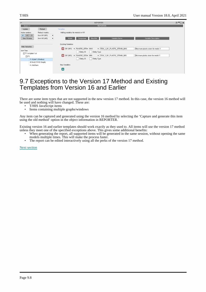
9.7 Exceptions to the Version 17 Method and Existing Templates from Version 16 and Earlier
There are some item types that are not supported in the new version 17 method. In this case, the version 16 method will be used and nothing will have changed. These are:
• T/HIS JavaScript items• Items containing multiple graphs/windows
Any item can be captured and generated using the version 16 method by selecting the ‘Capture and generate this item using the old method’ option in the object information in REPORTER.
Existing version 16 and earlier templates should work exactly as they used to. All items will use the version 17 method unless they meet one of the specified exceptions above. This gives some additional benefits:
• When generating the report, all supported items will be generated in the same session, without opening the same models multiple times. This will make the process faster.
• The report can be edited interactively using all the perks of the version 17 method.
Next section
T/HIS User manual Version 18.0, April 2021
Page 9.8
APPENDICESA - LS-DYNA Data Components
B - T/HIS Curve File Format
C - T/HIS Bulk Data File Format
D - Filtering
E - Injury Criteria
F - Curve Correlation
G - The ERROR Calculation
H - The "oa_pref" Preference File
I - Windows File Associations
J - T-HIS JavaScript API
K - Typed Commands
User manual Version 18.0, April 2021 T/HIS
Page A.1

APPENDIX A - LS-DYNA Data Components
A.1 Model Data Components
The following global data components are available.
Component THF (d3thdt) XTF (xtfile) LSDA (binout) ASCII
DT Time Step yes yes yes
KE Kinetic energy yes yes yes
IE Internal energy yes yes yes
SWE Stonewall energy yes yes
SPE Spring and damper energy yes yes
HG Hourglass energy yes yes
SDE System damping energy yes yes
JE Joint internal energy yes yes
SIE Sliding interface energy yes yes
EW External work yes yes yes
RBE Rigid Body stopper energy yes
TE Total energy yes yes yes
TER Total/initial energy ratio yes yes
VX Average X velocity yes yes yes
VY Average Y velocity yes yes yes
VZ Average Z velocity yes yes yes
TZC Time per zone cycle yes yes
AM Added mass yes yes
PM %age Mass increase yes yes
EKE Eroded Kinetic energy yes yes
EIE Eroded Internal energy yes yes
EHG Eroded Hourglass energy yes yes
ER Energy Ratio w/o Eroded yes yes
DRCE Current Distortional Kinetic Energy yes
DRMX Maximum Distortional Kinetic Energy yes
DRCO Convergence Factor yes
DRKE Total Kinetic Energy yes
A.2 Part Data Components
For Parts the following data components are available.
Component THF (d3thdt) XTF (xtfile) LSDA (binout) ASCII
KE Kinetic energy yes yes yes
IE Internal energy yes yes yes
HG Hourglass energy yes yes
TE Total energy yes yes yes
T/HIS User manual Version 18.0, April 2021
Page A.2
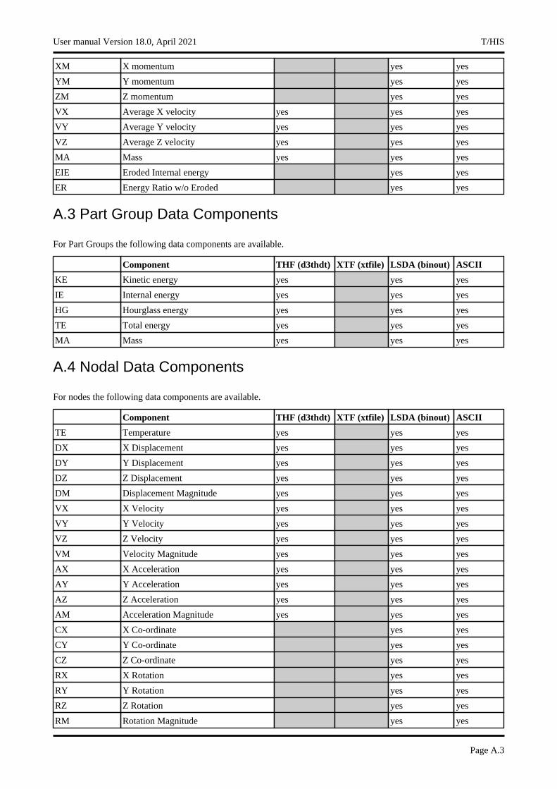
XM X momentum yes yes
YM Y momentum yes yes
ZM Z momentum yes yes
VX Average X velocity yes yes yes
VY Average Y velocity yes yes yes
VZ Average Z velocity yes yes yes
MA Mass yes yes yes
EIE Eroded Internal energy yes yes
ER Energy Ratio w/o Eroded yes yes
A.3 Part Group Data Components
For Part Groups the following data components are available.
Component THF (d3thdt) XTF (xtfile) LSDA (binout) ASCII
KE Kinetic energy yes yes yes
IE Internal energy yes yes yes
HG Hourglass energy yes yes yes
TE Total energy yes yes yes
MA Mass yes yes yes
A.4 Nodal Data Components
For nodes the following data components are available.
Component THF (d3thdt) XTF (xtfile) LSDA (binout) ASCII
TE Temperature yes yes yes
DX X Displacement yes yes yes
DY Y Displacement yes yes yes
DZ Z Displacement yes yes yes
DM Displacement Magnitude yes yes yes
VX X Velocity yes yes yes
VY Y Velocity yes yes yes
VZ Z Velocity yes yes yes
VM Velocity Magnitude yes yes yes
AX X Acceleration yes yes yes
AY Y Acceleration yes yes yes
AZ Z Acceleration yes yes yes
AM Acceleration Magnitude yes yes yes
CX X Co-ordinate yes yes
CY Y Co-ordinate yes yes
CZ Z Co-ordinate yes yes
RX X Rotation yes yes
RY Y Rotation yes yes
RZ Z Rotation yes yes
RM Rotation Magnitude yes yes
User manual Version 18.0, April 2021 T/HIS
Page A.3
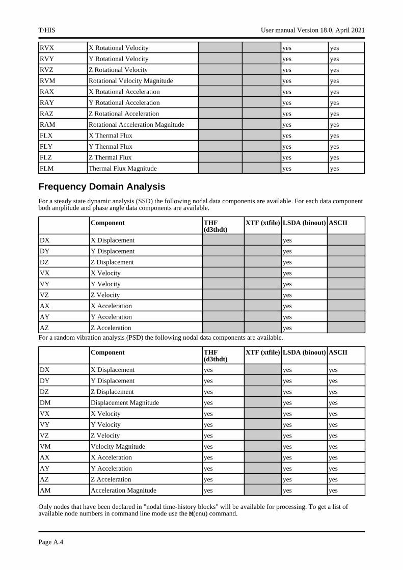
RVX X Rotational Velocity yes yes
RVY Y Rotational Velocity yes yes
RVZ Z Rotational Velocity yes yes
RVM Rotational Velocity Magnitude yes yes
RAX X Rotational Acceleration yes yes
RAY Y Rotational Acceleration yes yes
RAZ Z Rotational Acceleration yes yes
RAM Rotational Acceleration Magnitude yes yes
FLX X Thermal Flux yes yes
FLY Y Thermal Flux yes yes
FLZ Z Thermal Flux yes yes
FLM Thermal Flux Magnitude yes yes
Frequency Domain AnalysisFor a steady state dynamic analysis (SSD) the following nodal data components are available. For each data component both amplitude and phase angle data components are available.
Component THF (d3thdt)
XTF (xtfile) LSDA (binout) ASCII
DX X Displacement yes
DY Y Displacement yes
DZ Z Displacement yes
VX X Velocity yes
VY Y Velocity yes
VZ Z Velocity yes
AX X Acceleration yes
AY Y Acceleration yes
AZ Z Acceleration yes
For a random vibration analysis (PSD) the following nodal data components are available.
Component THF (d3thdt)
XTF (xtfile) LSDA (binout) ASCII
DX X Displacement yes yes yes
DY Y Displacement yes yes yes
DZ Z Displacement yes yes yes
DM Displacement Magnitude yes yes yes
VX X Velocity yes yes yes
VY Y Velocity yes yes yes
VZ Z Velocity yes yes yes
VM Velocity Magnitude yes yes yes
AX X Acceleration yes yes yes
AY Y Acceleration yes yes yes
AZ Z Acceleration yes yes yes
AM Acceleration Magnitude yes yes yes
Only nodes that have been declared in "nodal time-history blocks" will be available for processing. To get a list of available node numbers in command line mode use the M(enu) command.
T/HIS User manual Version 18.0, April 2021
Page A.4
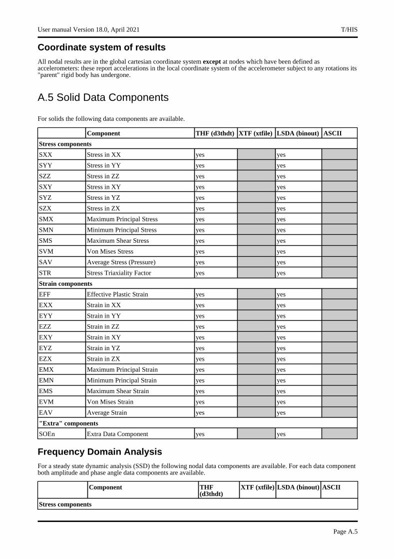
Coordinate system of resultsAll nodal results are in the global cartesian coordinate system except at nodes which have been defined as accelerometers: these report accelerations in the local coordinate system of the accelerometer subject to any rotations its "parent" rigid body has undergone.
A.5 Solid Data Components
For solids the following data components are available.
Component THF (d3thdt) XTF (xtfile) LSDA (binout) ASCII
Stress components
SXX Stress in XX yes yes
SYY Stress in YY yes yes
SZZ Stress in ZZ yes yes
SXY Stress in XY yes yes
SYZ Stress in YZ yes yes
SZX Stress in ZX yes yes
SMX Maximum Principal Stress yes yes
SMN Minimum Principal Stress yes yes
SMS Maximum Shear Stress yes yes
SVM Von Mises Stress yes yes
SAV Average Stress (Pressure) yes yes
STR Stress Triaxiality Factor yes yes
Strain components
EFF Effective Plastic Strain yes yes
EXX Strain in XX yes yes
EYY Strain in YY yes yes
EZZ Strain in ZZ yes yes
EXY Strain in XY yes yes
EYZ Strain in YZ yes yes
EZX Strain in ZX yes yes
EMX Maximum Principal Strain yes yes
EMN Minimum Principal Strain yes yes
EMS Maximum Shear Strain yes yes
EVM Von Mises Strain yes yes
EAV Average Strain yes yes
"Extra" components
SOEn Extra Data Component yes yes
Frequency Domain AnalysisFor a steady state dynamic analysis (SSD) the following nodal data components are available. For each data component both amplitude and phase angle data components are available.
Component THF (d3thdt)
XTF (xtfile) LSDA (binout) ASCII
Stress components
User manual Version 18.0, April 2021 T/HIS
Page A.5
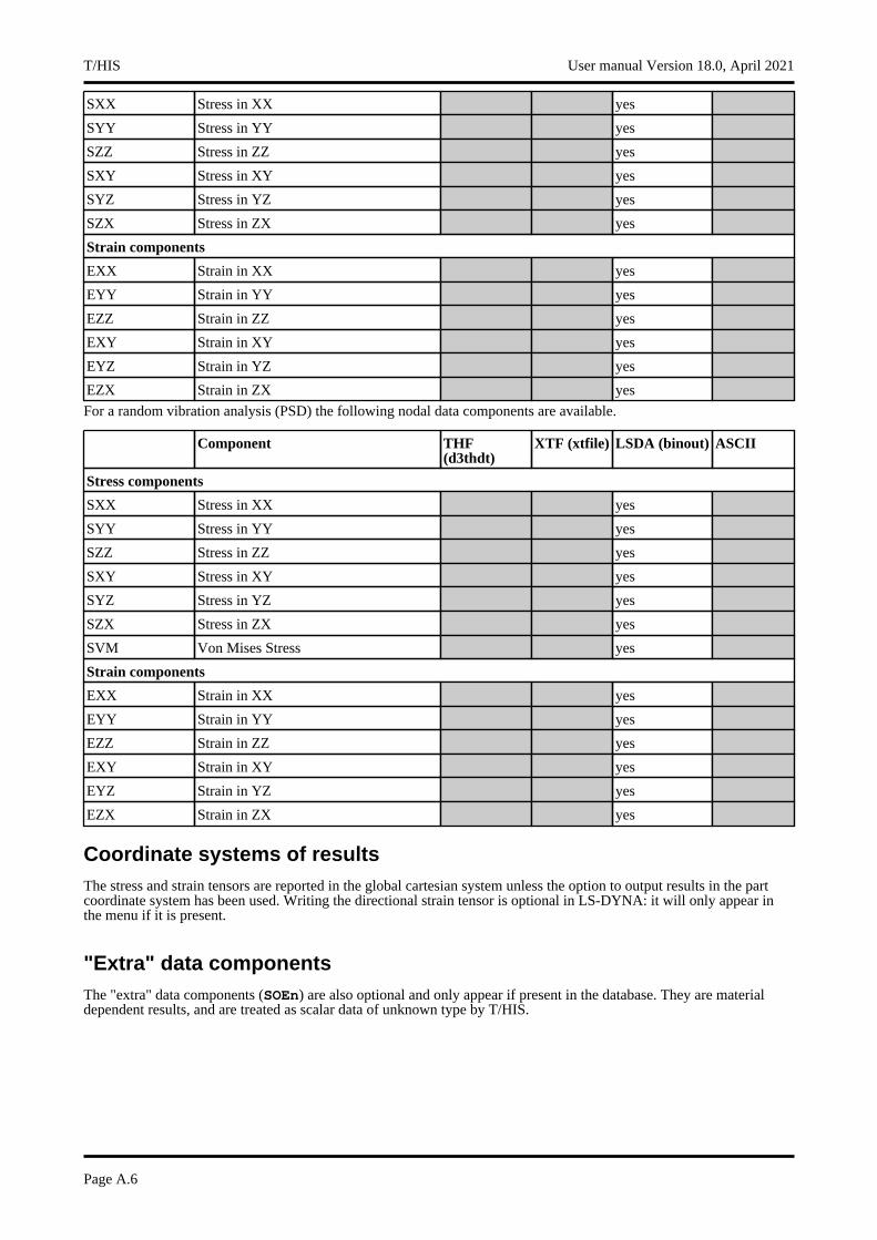
SXX Stress in XX yes
SYY Stress in YY yes
SZZ Stress in ZZ yes
SXY Stress in XY yes
SYZ Stress in YZ yes
SZX Stress in ZX yes
Strain components
EXX Strain in XX yes
EYY Strain in YY yes
EZZ Strain in ZZ yes
EXY Strain in XY yes
EYZ Strain in YZ yes
EZX Strain in ZX yes
For a random vibration analysis (PSD) the following nodal data components are available.
Component THF (d3thdt)
XTF (xtfile) LSDA (binout) ASCII
Stress components
SXX Stress in XX yes
SYY Stress in YY yes
SZZ Stress in ZZ yes
SXY Stress in XY yes
SYZ Stress in YZ yes
SZX Stress in ZX yes
SVM Von Mises Stress yes
Strain components
EXX Strain in XX yes
EYY Strain in YY yes
EZZ Strain in ZZ yes
EXY Strain in XY yes
EYZ Strain in YZ yes
EZX Strain in ZX yes
Coordinate systems of resultsThe stress and strain tensors are reported in the global cartesian system unless the option to output results in the part coordinate system has been used. Writing the directional strain tensor is optional in LS-DYNA: it will only appear in the menu if it is present.
"Extra" data componentsThe "extra" data components (SOEn) are also optional and only appear if present in the database. They are material dependent results, and are treated as scalar data of unknown type by T/HIS.
T/HIS User manual Version 18.0, April 2021
Page A.6
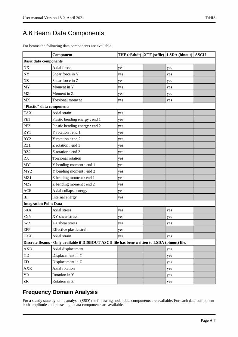
A.6 Beam Data Components
For beams the following data components are available.
Component THF (d3thdt) XTF (xtfile) LSDA (binout) ASCII
Basic data components
NX Axial force yes yes
NY Shear force in Y yes yes
NZ Shear force in Z yes yes
MY Moment in Y yes yes
MZ Moment in Z yes yes
MX Torsional moment yes yes
"Plastic" data components
EAX Axial strain yes
PE1 Plastic bending energy : end 1 yes
PE2 Plastic bending energy : end 2 yes
RY1 Y rotation : end 1 yes
RY2 Y rotation : end 2 yes
RZ1 Z rotation : end 1 yes
RZ2 Z rotation : end 2 yes
RX Torsional rotation yes
MY1 Y bending moment : end 1 yes
MY2 Y bending moment : end 2 yes
MZ1 Z bending moment : end 1 yes
MZ2 Z bending moment : end 2 yes
ACE Axial collapse energy yes
IE Internal energy yes
Integration Point Data
SXX Axial stress yes yes
SXY XY shear stress yes yes
SZX ZX shear stress yes yes
EFF Effective plastic strain yes
EXX Axial strain yes yes
Discrete Beams - Only available if DISBOUT ASCII file has bene written to LSDA (binout) file.
AXD Axial displacement yes
YD Displacement in Y yes
ZD Displacement in Z yes
AXR Axial rotation yes
YR Rotation in Y yes
ZR Rotation in Z yes
Frequency Domain AnalysisFor a steady state dynamic analysis (SSD) the following nodal data components are available. For each data component both amplitude and phase angle data components are available.
User manual Version 18.0, April 2021 T/HIS
Page A.7

Component THF (d3thdt)
XTF (xtfile) LSDA (binout) ASCII
Basic data components
NX Axial force yes
NY Shear force in Y yes
NZ Shear force in Z yes
MY Moment in Y yes
MZ Moment in Z yes
MX Torsional moment yes
Integration point data
SXX Axial stress yes
SXY XY shear stress yes
SZX ZX shear stress yes
EFF Effective plastic strain yes
EXX Axial strain yes
For a random vibration analysis (PSD) the following nodal data components are available.
Component THF (d3thdt)
XTF (xtfile) LSDA (binout) ASCII
Basic data components
NX Axial force yes
NY Shear force in Y yes
NZ Shear force in Z yes
MY Moment in Y yes
MZ Moment in Z yes
MX Torsional moment yes
Integration point data
SXX Axial stress yes
SXY XY shear stress yes
SZX ZX shear stress yes
EFF Effective plastic strain yes
EXX Axial strain yes
Additional Beam Results: written if requested from LS-DYNAIn addition to the basic data components additional beam results may be output to the .THF file for both Belytschko-Schwer and Hughes-Lui beam elements. As no indication of the element type is written to the .THF file it is impossible for T/HIS to work out whether a specific element is a Belytschko-Schwer or a Hughes-Liu beam. As the element type is unknown the user must know which element type a beam is in order to extract the correct results.
Belytschko-Schwer BeamsIf you have used Belytschko-Schwer beams with a resultant plastic material model the following "plastic" results will also be written out to .THF file: (Note that these data are written even if the *DATABASE_EXTENT_BINARY card field <beamip> is not set - the presence of a resultant beam material triggers their output automatically. This is not the case for Hughes-Liu data components, for which output must be requested explicitly, see below.)
T/HIS User manual Version 18.0, April 2021
Page A.8
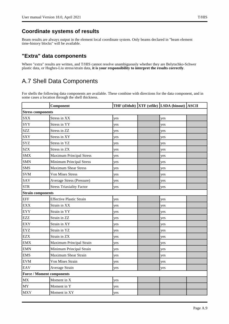
Coordinate systems of resultsBeam results are always output in the element local coordinate system. Only beams declared in "beam element time-history blocks" will be available.
"Extra" data componentsWhere "extra" results are written, and T/HIS cannot resolve unambiguously whether they are Belytschko-Schwer plastic data, or Hughes-Liu stress/strain data, it is your responsibility to interpret the results correctly.
A.7 Shell Data Components
For shells the following data components are available. These combine with directions for the data component, and in some cases a location through the shell thickness.
Component THF (d3thdt) XTF (xtfile) LSDA (binout) ASCII
Stress components
SXX Stress in XX yes yes
SYY Stress in YY yes yes
SZZ Stress in ZZ yes yes
SXY Stress in XY yes yes
SYZ Stress in YZ yes yes
SZX Stress in ZX yes yes
SMX Maximum Principal Stress yes yes
SMN Minimum Principal Stress yes yes
SMS Maximum Shear Stress yes yes
SVM Von Mises Stress yes yes
SAV Average Stress (Pressure) yes yes
STR Stress Triaxiality Factor yes yes
Strain components
EFF Effective Plastic Strain yes yes
EXX Strain in XX yes yes
EYY Strain in YY yes yes
EZZ Strain in ZZ yes yes
EXY Strain in XY yes yes
EYZ Strain in YZ yes yes
EZX Strain in ZX yes yes
EMX Maximum Principal Strain yes yes
EMN Minimum Principal Strain yes yes
EMS Maximum Shear Strain yes yes
EVM Von Mises Strain yes yes
EAV Average Strain yes yes
Force / Moment components
MX Moment in X yes
MY Moment in Y yes
MXY Moment in XY yes
User manual Version 18.0, April 2021 T/HIS
Page A.9
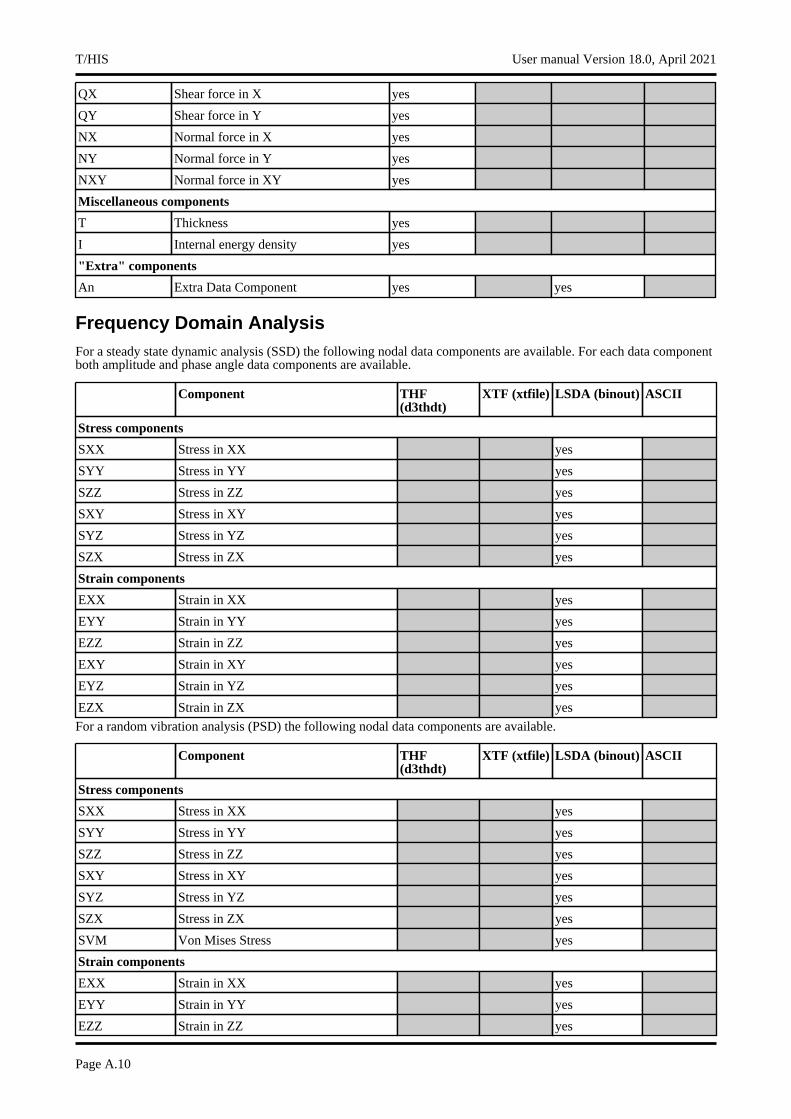
QX Shear force in X yes
QY Shear force in Y yes
NX Normal force in X yes
NY Normal force in Y yes
NXY Normal force in XY yes
Miscellaneous components
T Thickness yes
I Internal energy density yes
"Extra" components
An Extra Data Component yes yes
Frequency Domain AnalysisFor a steady state dynamic analysis (SSD) the following nodal data components are available. For each data component both amplitude and phase angle data components are available.
Component THF (d3thdt)
XTF (xtfile) LSDA (binout) ASCII
Stress components
SXX Stress in XX yes
SYY Stress in YY yes
SZZ Stress in ZZ yes
SXY Stress in XY yes
SYZ Stress in YZ yes
SZX Stress in ZX yes
Strain components
EXX Strain in XX yes
EYY Strain in YY yes
EZZ Strain in ZZ yes
EXY Strain in XY yes
EYZ Strain in YZ yes
EZX Strain in ZX yes
For a random vibration analysis (PSD) the following nodal data components are available.
Component THF (d3thdt)
XTF (xtfile) LSDA (binout) ASCII
Stress components
SXX Stress in XX yes
SYY Stress in YY yes
SZZ Stress in ZZ yes
SXY Stress in XY yes
SYZ Stress in YZ yes
SZX Stress in ZX yes
SVM Von Mises Stress yes
Strain components
EXX Strain in XX yes
EYY Strain in YY yes
EZZ Strain in ZZ yes
T/HIS User manual Version 18.0, April 2021
Page A.10
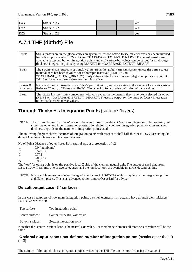
EXY Strain in XY yes
EYZ Strain in YZ yes
EZX Strain in ZX yes
A.7.1 THF (d3thdt) File
Stress Stress tensors are in the global cartesian system unless the option to use material axes has been invoked for orthotropic materials (CMPFLG on *DATABASE_EXTENT_BINARY). By default results are available at top and bottom integration points and mid-surface but values can be output for all through thickness integration points by using MAXINT on *DATABASE_EXTENT_BINARY
Strain The Strain tensors output is optional. Values are in the global cartesian system unless the option to use material axes has been invoked for orthotropic materials (CMPFLG on *DATABASE_EXTENT_BINARY). Only values at the top and bottom integration points are output. T/HIS will average these values for the mid surface.
Forces & Moments
Force and moment resultants are <data> per unit width, and are written in the element local axis system. Refer to "Theory of Plates and Shells", Timoshenko, for a precise definition of these values.
Extra The "Extra History" data components will only appear in the menu if they have been selected for output (NEIPS on *DATABASE_EXTENT_BINARY). These are output for the same surfaces / integration points as the stress tensor values.
Through Thickness Integration Points (surfaces/layers)
NOTE: The top and bottom "surfaces" are not the outer fibres if the default Gaussian integration rules are used, but rather the outer and inner integration points. The relationship between integration point location and shell thickness depends on the number of integration points used.
The following diagram shows locations of integration points with respect to shell half-thickness (t/2) assuming the default Gaussian integration rules have been used:
No of PointsDistance of outer fibres from neutral axis as a proportion of t/21 0.0 (membrane)2 0.577 t/23 0.7754 0.861 t/25 0.906The "top" (or outer) point is on the positive local Z side of the element neutral axis. The output of shell data from LS-DYNA will fall into one of two categories, and the "surface" options available in T/HIS depend on this.
NOTE: It is possible to use non-default integration schemes in LS-DYNA which may locate the integration points at different places. This is an advanced topic: contact Oasys Ltd for advice.
Default output case: 3 "surfaces"
In this case, regardless of how many integration points the shell elements may actually have through their thickness, LS-DYNA writes out:
Top surface : Top integration point
Centre surface : Computed neutral axis value
Bottom surface : Bottom integration point
Note that the "centre" surface here is the neutral axis value. For membrane elements all three sets of values will be the same.
Optional output case: user-defined number of integration points (maxint other than 0 or 3)
The number of through thickness integration points written to the THF file can be modified using the value of
User manual Version 18.0, April 2021 T/HIS
Page A.11
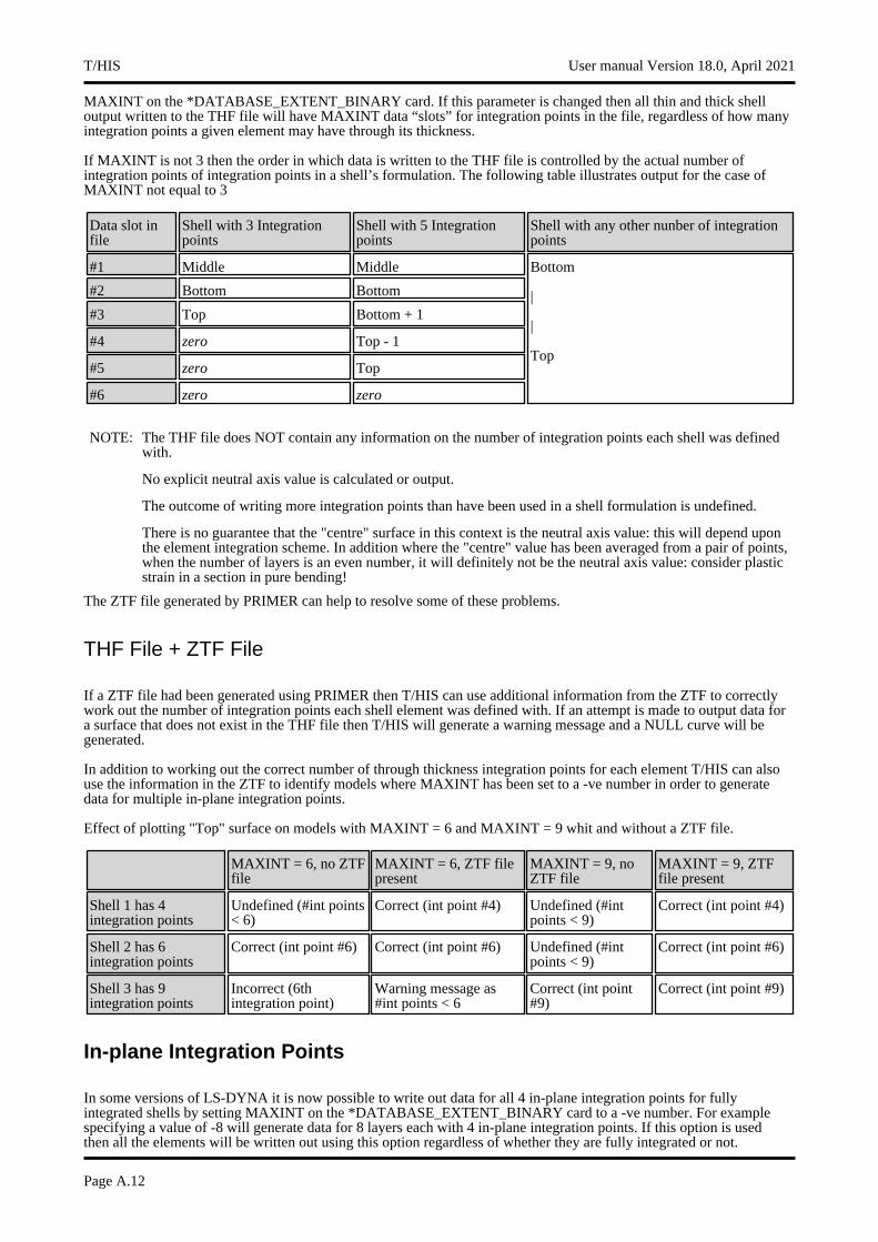
MAXINT on the *DATABASE_EXTENT_BINARY card. If this parameter is changed then all thin and thick shell output written to the THF file will have MAXINT data “slots” for integration points in the file, regardless of how many integration points a given element may have through its thickness.
If MAXINT is not 3 then the order in which data is written to the THF file is controlled by the actual number of integration points of integration points in a shell’s formulation. The following table illustrates output for the case of MAXINT not equal to 3
Data slot in file
Shell with 3 Integration points
Shell with 5 Integration points
Shell with any other nunber of integration points
#1 Middle Middle Bottom
|
|
Top
#2 Bottom Bottom
#3 Top Bottom + 1
#4 zero Top - 1
#5 zero Top
#6 zero zero
NOTE: The THF file does NOT contain any information on the number of integration points each shell was defined with.
No explicit neutral axis value is calculated or output.
The outcome of writing more integration points than have been used in a shell formulation is undefined.
There is no guarantee that the "centre" surface in this context is the neutral axis value: this will depend upon the element integration scheme. In addition where the "centre" value has been averaged from a pair of points, when the number of layers is an even number, it will definitely not be the neutral axis value: consider plastic strain in a section in pure bending!
The ZTF file generated by PRIMER can help to resolve some of these problems.
THF File + ZTF File
If a ZTF file had been generated using PRIMER then T/HIS can use additional information from the ZTF to correctly work out the number of integration points each shell element was defined with. If an attempt is made to output data for a surface that does not exist in the THF file then T/HIS will generate a warning message and a NULL curve will be generated.
In addition to working out the correct number of through thickness integration points for each element T/HIS can also use the information in the ZTF to identify models where MAXINT has been set to a -ve number in order to generate data for multiple in-plane integration points.
Effect of plotting "Top" surface on models with MAXINT = 6 and MAXINT = 9 whit and without a ZTF file.
MAXINT = 6, no ZTF file
MAXINT = 6, ZTF file present
MAXINT = 9, no ZTF file
MAXINT = 9, ZTF file present
Shell 1 has 4 integration points
Undefined (#int points < 6)
Correct (int point #4) Undefined (#int points < 9)
Correct (int point #4)
Shell 2 has 6 integration points
Correct (int point #6) Correct (int point #6) Undefined (#int points < 9)
Correct (int point #6)
Shell 3 has 9 integration points
Incorrect (6th integration point)
Warning message as #int points < 6
Correct (int point #9)
Correct (int point #9)
In-plane Integration Points
In some versions of LS-DYNA it is now possible to write out data for all 4 in-plane integration points for fully integrated shells by setting MAXINT on the *DATABASE_EXTENT_BINARY card to a -ve number. For example specifying a value of -8 will generate data for 8 layers each with 4 in-plane integration points. If this option is used then all the elements will be written out using this option regardless of whether they are fully integrated or not.
T/HIS User manual Version 18.0, April 2021
Page A.12
As there is no information in the THF to indicate that data for 4 in-plane integration points has been written to the file then the file format will be exactly the same as for an analysis with a +ve value of MAXINT 4 times larger. For example MAXINT = -8 and MAXINT = 32 will both produce THF files with 32 integration points worth of data and there is no way for T/HIS to know which value of MAXINT was used to generate the data. The ZTF file generated by PRIMER can help to resolve this problem.
If multiple in-plane integration points are written to the THF file then they are written in the following order.
Layer 1 - in-plane int point #1Layer 2 - in-plane int point #1....Layer n - in-plane int point #1Layer 1 - in-plane int point #2Layer 2 - in-plane int point #2....Layer n - in-plane int point #2Layer 1 - in-plane int point #3....
NOTE: If non fully integrated shells are included in the list of elements written to the THF file then in some versions of LS-DYNA the 2nd, 3rrd and 4th in-plane values will all be zero. Care should therefore be taken if the 4 in-plane values are averaged.
In some versions of LS-DYNA the 1st in-plane integration point is correctly written out using the global axis system while the 2nd, 3rd and 4th in-plane values are written using the elements local coordinate system. Care should therefore be taken if the 4 in-plane values are averaged.
A.7.2 LSDA (binout) File
Stress By default stress tensors are in the local element coordinate system. Values are written out for all the through thickness and in-plane integration points.
Strain The Strain tensors output is optional. By defaul the values are in the local element coordinate systems and only values at the top and bottom integration points are output. T/HIS will average these values for the mid surface.
Forces & Moments
These are not written to the LSDA file.
Extra By default "Extra" data components are not written to the LSDA file.
Some recent versions of LS-DYNA can now write the"Extra" data components to the LSDA file if the parameters OPTION1, OPTION2, OPTION3 and OPTION4 are set on the *DATABASE_ELOUT card.
Global v Local coordinate system results
The LSDA file can contain both ELOUT and ELOUTDET data components. By default T/HIS uses the data from ELOUTDET as ELOUT only contains a subset of the data in ELOUDET.
In some versions of LS-DYNA it is possible to change the Shell and ThickShell data components written to the ELOUT so that they are defined using the Global coordinate system (see EOCS on *CONTROL_OUTPUT) instead of the default local element coordinate system If this option is used then only the ELOUT file is modified, the ELOUDET file is still written using the local element coordinate system.
If T/HIS detects that the LSDA file contains both ELOUT and ELOUDET and that they are using different coordinate systems then T/HIS will display an additional option can be used to force T/HIS to use the ELOUT file data instead of the ELOUTDET data.
Through Thickness Integration Points (surfaces/layers)
Unlike the THF file the LSDA file can contain different numbers of integration points for each element. This means that if "Top" surface is selected T/HIS can correctly identify which integration point it needs to read data from.
User manual Version 18.0, April 2021 T/HIS
Page A.13
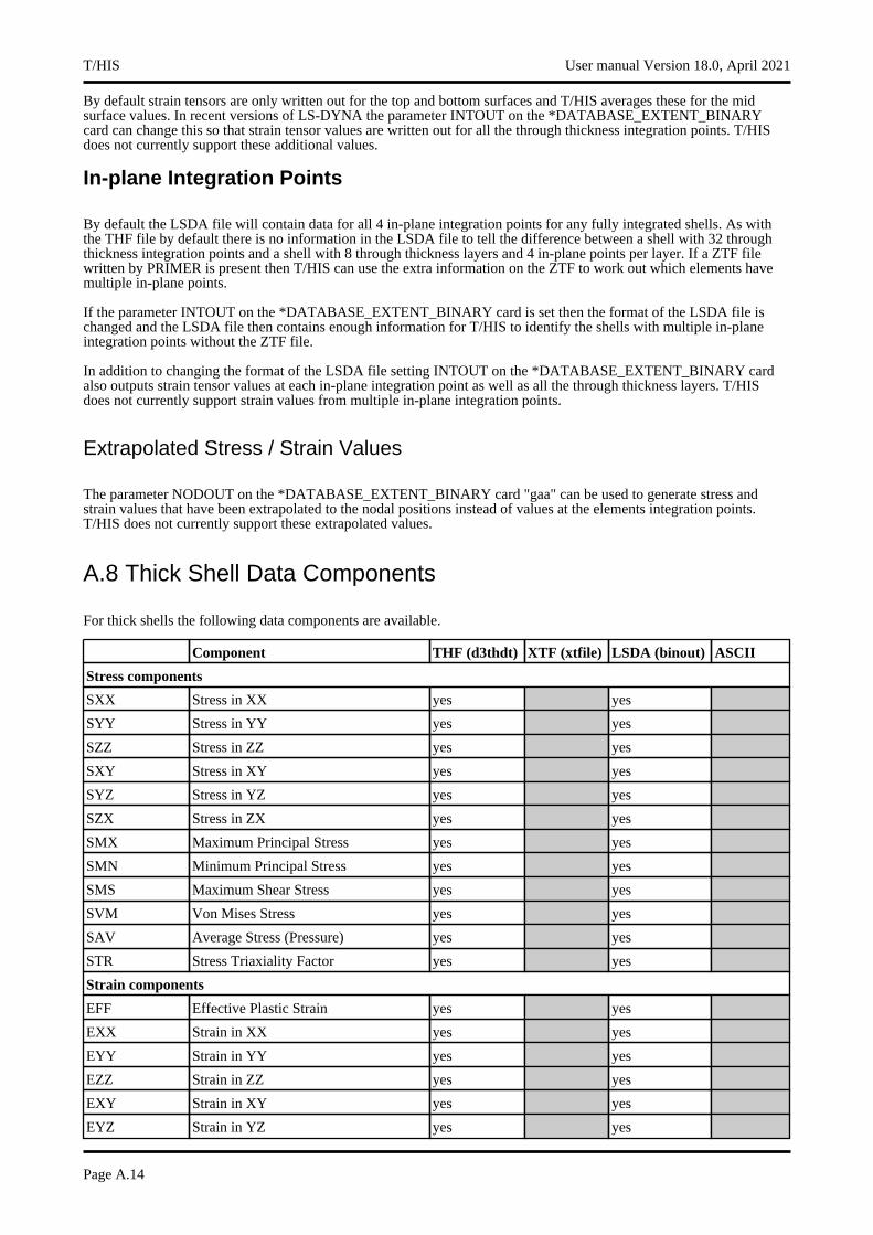
By default strain tensors are only written out for the top and bottom surfaces and T/HIS averages these for the mid surface values. In recent versions of LS-DYNA the parameter INTOUT on the *DATABASE_EXTENT_BINARY card can change this so that strain tensor values are written out for all the through thickness integration points. T/HIS does not currently support these additional values.
In-plane Integration Points
By default the LSDA file will contain data for all 4 in-plane integration points for any fully integrated shells. As with the THF file by default there is no information in the LSDA file to tell the difference between a shell with 32 through thickness integration points and a shell with 8 through thickness layers and 4 in-plane points per layer. If a ZTF file written by PRIMER is present then T/HIS can use the extra information on the ZTF to work out which elements have multiple in-plane points.
If the parameter INTOUT on the *DATABASE_EXTENT_BINARY card is set then the format of the LSDA file is changed and the LSDA file then contains enough information for T/HIS to identify the shells with multiple in-plane integration points without the ZTF file.
In addition to changing the format of the LSDA file setting INTOUT on the *DATABASE_EXTENT_BINARY card also outputs strain tensor values at each in-plane integration point as well as all the through thickness layers. T/HIS does not currently support strain values from multiple in-plane integration points.
Extrapolated Stress / Strain Values
The parameter NODOUT on the *DATABASE_EXTENT_BINARY card "gaa" can be used to generate stress and strain values that have been extrapolated to the nodal positions instead of values at the elements integration points. T/HIS does not currently support these extrapolated values.
A.8 Thick Shell Data Components
For thick shells the following data components are available.
Component THF (d3thdt) XTF (xtfile) LSDA (binout) ASCII
Stress components
SXX Stress in XX yes yes
SYY Stress in YY yes yes
SZZ Stress in ZZ yes yes
SXY Stress in XY yes yes
SYZ Stress in YZ yes yes
SZX Stress in ZX yes yes
SMX Maximum Principal Stress yes yes
SMN Minimum Principal Stress yes yes
SMS Maximum Shear Stress yes yes
SVM Von Mises Stress yes yes
SAV Average Stress (Pressure) yes yes
STR Stress Triaxiality Factor yes yes
Strain components
EFF Effective Plastic Strain yes yes
EXX Strain in XX yes yes
EYY Strain in YY yes yes
EZZ Strain in ZZ yes yes
EXY Strain in XY yes yes
EYZ Strain in YZ yes yes
T/HIS User manual Version 18.0, April 2021
Page A.14
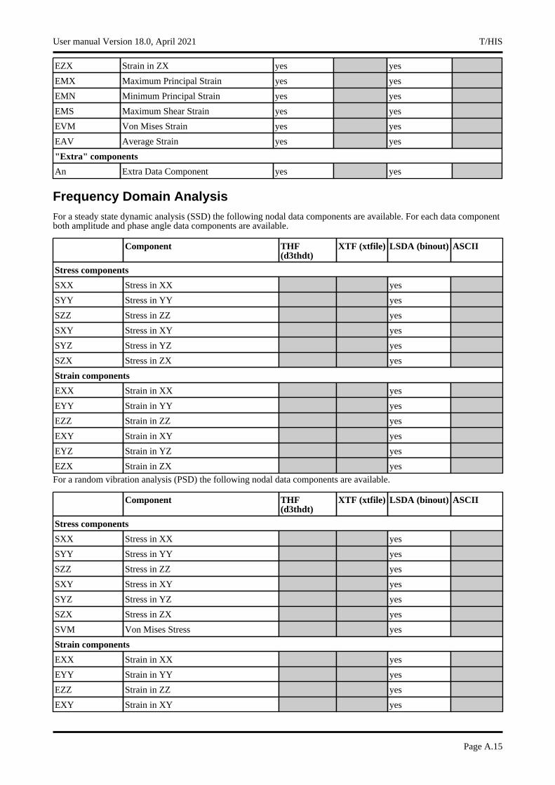
EZX Strain in ZX yes yes
EMX Maximum Principal Strain yes yes
EMN Minimum Principal Strain yes yes
EMS Maximum Shear Strain yes yes
EVM Von Mises Strain yes yes
EAV Average Strain yes yes
"Extra" components
An Extra Data Component yes yes
Frequency Domain AnalysisFor a steady state dynamic analysis (SSD) the following nodal data components are available. For each data component both amplitude and phase angle data components are available.
Component THF (d3thdt)
XTF (xtfile) LSDA (binout) ASCII
Stress components
SXX Stress in XX yes
SYY Stress in YY yes
SZZ Stress in ZZ yes
SXY Stress in XY yes
SYZ Stress in YZ yes
SZX Stress in ZX yes
Strain components
EXX Strain in XX yes
EYY Strain in YY yes
EZZ Strain in ZZ yes
EXY Strain in XY yes
EYZ Strain in YZ yes
EZX Strain in ZX yes
For a random vibration analysis (PSD) the following nodal data components are available.
Component THF (d3thdt)
XTF (xtfile) LSDA (binout) ASCII
Stress components
SXX Stress in XX yes
SYY Stress in YY yes
SZZ Stress in ZZ yes
SXY Stress in XY yes
SYZ Stress in YZ yes
SZX Stress in ZX yes
SVM Von Mises Stress yes
Strain components
EXX Strain in XX yes
EYY Strain in YY yes
EZZ Strain in ZZ yes
EXY Strain in XY yes
User manual Version 18.0, April 2021 T/HIS
Page A.15
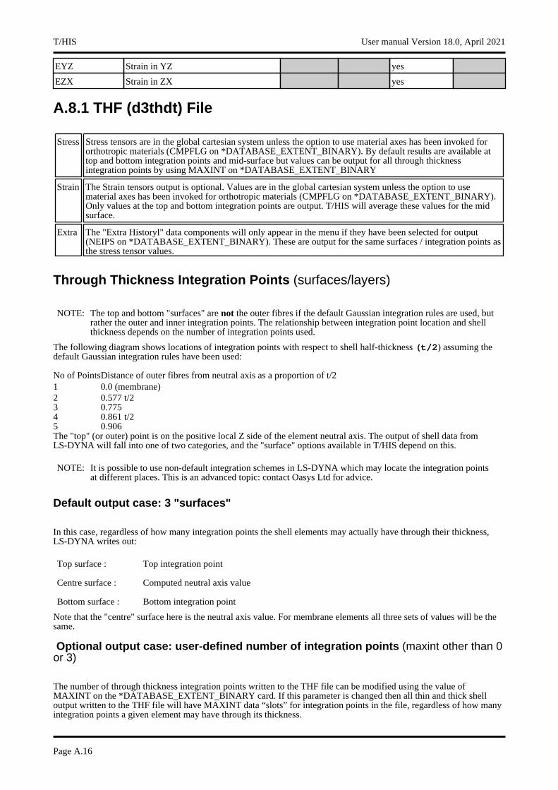
EYZ Strain in YZ yes
EZX Strain in ZX yes
A.8.1 THF (d3thdt) File
Stress Stress tensors are in the global cartesian system unless the option to use material axes has been invoked for orthotropic materials (CMPFLG on *DATABASE_EXTENT_BINARY). By default results are available at top and bottom integration points and mid-surface but values can be output for all through thickness integration points by using MAXINT on *DATABASE_EXTENT_BINARY
Strain The Strain tensors output is optional. Values are in the global cartesian system unless the option to use material axes has been invoked for orthotropic materials (CMPFLG on *DATABASE_EXTENT_BINARY). Only values at the top and bottom integration points are output. T/HIS will average these values for the mid surface.
Extra The "Extra Historyl" data components will only appear in the menu if they have been selected for output (NEIPS on *DATABASE_EXTENT_BINARY). These are output for the same surfaces / integration points as the stress tensor values.
Through Thickness Integration Points (surfaces/layers)
NOTE: The top and bottom "surfaces" are not the outer fibres if the default Gaussian integration rules are used, but rather the outer and inner integration points. The relationship between integration point location and shell thickness depends on the number of integration points used.
The following diagram shows locations of integration points with respect to shell half-thickness (t/2) assuming the default Gaussian integration rules have been used:
No of PointsDistance of outer fibres from neutral axis as a proportion of t/21 0.0 (membrane)2 0.577 t/23 0.7754 0.861 t/25 0.906The "top" (or outer) point is on the positive local Z side of the element neutral axis. The output of shell data from LS-DYNA will fall into one of two categories, and the "surface" options available in T/HIS depend on this.
NOTE: It is possible to use non-default integration schemes in LS-DYNA which may locate the integration points at different places. This is an advanced topic: contact Oasys Ltd for advice.
Default output case: 3 "surfaces"
In this case, regardless of how many integration points the shell elements may actually have through their thickness, LS-DYNA writes out:
Top surface : Top integration point
Centre surface : Computed neutral axis value
Bottom surface : Bottom integration point
Note that the "centre" surface here is the neutral axis value. For membrane elements all three sets of values will be the same.
Optional output case: user-defined number of integration points (maxint other than 0 or 3)
The number of through thickness integration points written to the THF file can be modified using the value of MAXINT on the *DATABASE_EXTENT_BINARY card. If this parameter is changed then all thin and thick shell output written to the THF file will have MAXINT data “slots” for integration points in the file, regardless of how many integration points a given element may have through its thickness.
T/HIS User manual Version 18.0, April 2021
Page A.16
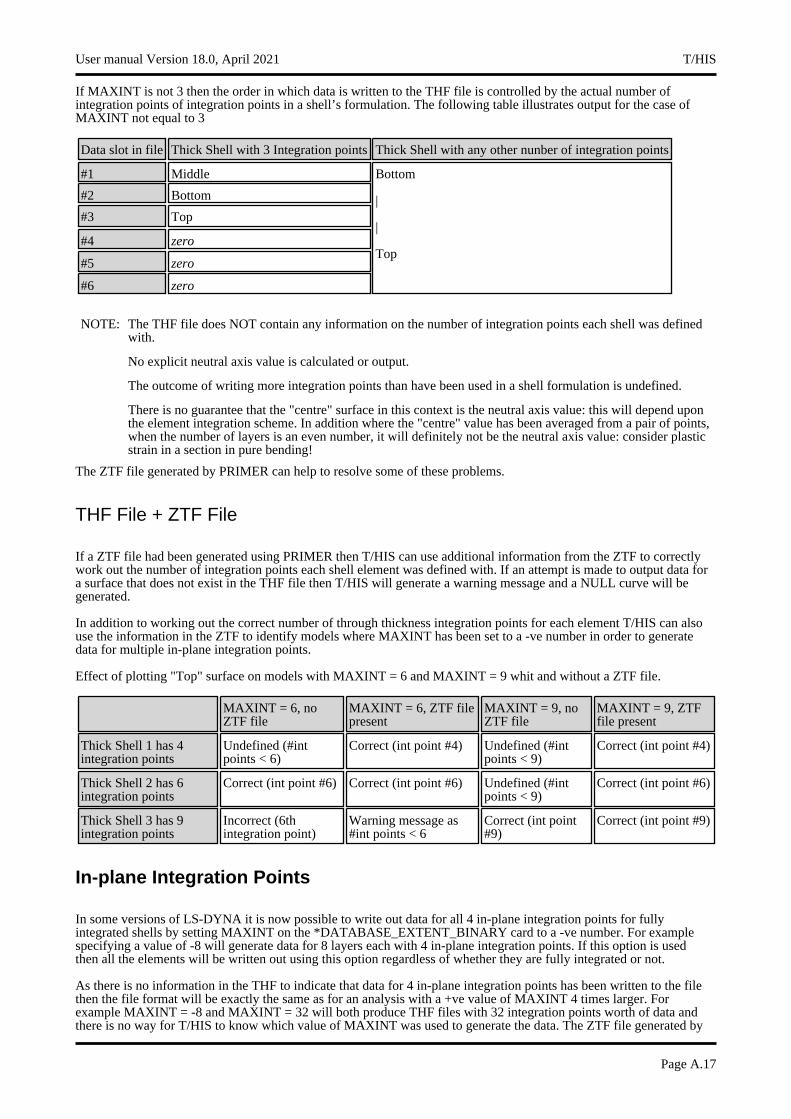
If MAXINT is not 3 then the order in which data is written to the THF file is controlled by the actual number of integration points of integration points in a shell’s formulation. The following table illustrates output for the case of MAXINT not equal to 3
Data slot in file Thick Shell with 3 Integration points Thick Shell with any other nunber of integration points
#1 Middle Bottom
|
|
Top
#2 Bottom
#3 Top
#4 zero
#5 zero
#6 zero
NOTE: The THF file does NOT contain any information on the number of integration points each shell was defined with.
No explicit neutral axis value is calculated or output.
The outcome of writing more integration points than have been used in a shell formulation is undefined.
There is no guarantee that the "centre" surface in this context is the neutral axis value: this will depend upon the element integration scheme. In addition where the "centre" value has been averaged from a pair of points, when the number of layers is an even number, it will definitely not be the neutral axis value: consider plastic strain in a section in pure bending!
The ZTF file generated by PRIMER can help to resolve some of these problems.
THF File + ZTF File
If a ZTF file had been generated using PRIMER then T/HIS can use additional information from the ZTF to correctly work out the number of integration points each shell element was defined with. If an attempt is made to output data for a surface that does not exist in the THF file then T/HIS will generate a warning message and a NULL curve will be generated.
In addition to working out the correct number of through thickness integration points for each element T/HIS can also use the information in the ZTF to identify models where MAXINT has been set to a -ve number in order to generate data for multiple in-plane integration points.
Effect of plotting "Top" surface on models with MAXINT = 6 and MAXINT = 9 whit and without a ZTF file.
MAXINT = 6, no ZTF file
MAXINT = 6, ZTF file present
MAXINT = 9, no ZTF file
MAXINT = 9, ZTF file present
Thick Shell 1 has 4 integration points
Undefined (#int points < 6)
Correct (int point #4) Undefined (#int points < 9)
Correct (int point #4)
Thick Shell 2 has 6 integration points
Correct (int point #6) Correct (int point #6) Undefined (#int points < 9)
Correct (int point #6)
Thick Shell 3 has 9 integration points
Incorrect (6th integration point)
Warning message as #int points < 6
Correct (int point #9)
Correct (int point #9)
In-plane Integration Points
In some versions of LS-DYNA it is now possible to write out data for all 4 in-plane integration points for fully integrated shells by setting MAXINT on the *DATABASE_EXTENT_BINARY card to a -ve number. For example specifying a value of -8 will generate data for 8 layers each with 4 in-plane integration points. If this option is used then all the elements will be written out using this option regardless of whether they are fully integrated or not.
As there is no information in the THF to indicate that data for 4 in-plane integration points has been written to the file then the file format will be exactly the same as for an analysis with a +ve value of MAXINT 4 times larger. For example MAXINT = -8 and MAXINT = 32 will both produce THF files with 32 integration points worth of data and there is no way for T/HIS to know which value of MAXINT was used to generate the data. The ZTF file generated by
User manual Version 18.0, April 2021 T/HIS
Page A.17

PRIMER can help to resolve this problem.
If multiple in-plane integration points are written to the THF file then they are written in the following order.
Layer 1 - in-plane int point #1Layer 2 - in-plane int point #1....Layer n - in-plane int point #1Layer 1 - in-plane int point #2Layer 2 - in-plane int point #2....Layer n - in-plane int point #2Layer 1 - in-plane int point #3....
NOTE: If non fully integrated shells are included in the list of elements written to the THF file then in some versions of LS-DYNA the 2nd, 3rrd and 4th in-plane values will all be zero. Care should therefore be taken if the 4 in-plane values are averaged.
In some versions of LS-DYNA the 1st in-plane integration point is correctly written out using the global axis system while the 2nd, 3rd and 4th in-plane values are written using the elements local coordinate system. Care should therefore be taken if the 4 in-plane values are averaged.
A.8.2 LSDA (binout) File
Stress By default stress tensors are in the local element coordinate system. Values are written out for all the through thickness and in-plane integration points.
Strain The Strain tensors output is optional. By default values are in the local element coordinate systems and only values at the top and bottom integration points are output. T/HIS will average these values for the mid surface.
Extra By default "Extra" data components are not written to the LSDA file.
Some recent versions of LS-DYNA can now write the"Extra" data components to the LSDA file if the parameters OPTION1, OPTION2, OPTION3 and OPTION4 are set on the *DATABASE_ELOUT card.
Global v Local coordinate system results
The LSDA file can contain both ELOUT and ELOUTDET data components. By default T/HIS uses the data from ELOUTDET as ELOUT only contains a subset of the data in ELOUDET.
In some versions of LS-DYNA it is possible to change the Shell and ThickShell data components written to the ELOUT so that they are defined using the Global coordinate system (see EOCS on *CONTROL_OUTPUT) instead of the default local element coordinate system If this option is used then only the ELOUT file is modified, the ELOUDET file is still written using the local element coordinate system.
If T/HIS detects that the LSDA file contains both ELOUT and ELOUDET and that they are using different coordinate systems then T/HIS will display an additional option can be used to force T/HIS to use the ELOUT file data instead of the ELOUTDET data.
Through Thickness Integration Points (surfaces/layers)
Unlike the THF file the LSDA file can contain different numbers of integration points for each element. This means that if "Top" surface is selected T/HIS can correctly identify which integration point it needs to read data from.
By default strain tensors are only written out for the top and bottom surfaces and T/HIS averages these for the mid surface values. In recent versions of LS-DYNA the parameter INTOUT on the *DATABASE_EXTENT_BINARY card can change this so that strain tensor values are written out for all the through thickness integration points. T/HIS does not currently support these additional values.
T/HIS User manual Version 18.0, April 2021
Page A.18
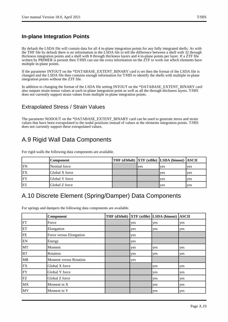
In-plane Integration Points
By default the LSDA file will contain data for all 4 in-plane integration points for any fully integrated shells. As with the THF file by default there is no information in the LSDA file to tell the difference between a shell with 32 through thickness integration points and a shell with 8 through thickness layers and 4 in-plane points per layer. If a ZTF file written by PRIMER is present then T/HIS can use the extra information on the ZTF to work out which elements have multiple in-plane points.
If the parameter INTOUT on the *DATABASE_EXTENT_BINARY card is set then the format of the LSDA file is changed and the LSDA file then contains enough information for T/HIS to identify the shells with multiple in-plane integration points without the ZTF file.
In addition to changing the format of the LSDA file setting INTOUT on the *DATABASE_EXTENT_BINARY card also outputs strain tensor values at each in-plane integration point as well as all the through thickness layers. T/HIS does not currently support strain values from multiple in-plane integration points.
Extrapolated Stress / Strain Values
The parameter NODOUT on the *DATABASE_EXTENT_BINARY card can be used to generate stress and strain values that have been extrapolated to the nodal positions instead of values at the elements integration points. T/HIS does not currently support these extrapolated values.
A.9 Rigid Wall Data Components
For rigid walls the following data components are available.
Component THF (d3thdt) XTF (xtfile) LSDA (binout) ASCII
FN Normal force yes yes yes
FX Global X force yes yes
FY Global Y force yes yes
FZ Global Z force yes yes
A.10 Discrete Element (Spring/Damper) Data Components
For springs and dampers the following data components are available.
Component THF (d3thdt) XTF (xtfile) LSDA (binout) ASCII
FT Force yes yes yes
ET Elongation yes yes yes
FE Force versus Elongation yes
EN Energy yes
MT Moment yes yes yes
RT Rotation yes yes yes
MR Moment versus Rotation yes
FX Global X force yes yes
FY Global Y force yes yes
FZ Global Z force yes yes
MX Moment in X yes yes
MY Moment in Y yes yes
User manual Version 18.0, April 2021 T/HIS
Page A.19
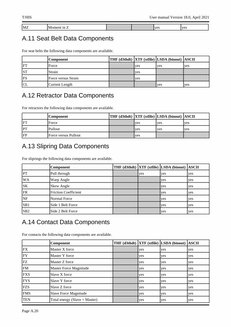
MZ Moment in Z yes yes
A.11 Seat Belt Data Components
For seat belts the following data components are available.
Component THF (d3thdt) XTF (xtfile) LSDA (binout) ASCII
FT Force yes yes yes
ST Strain yes
FS Force versus Strain yes
CL Current Length yes yes
A.12 Retractor Data Components
For retractors the following data components are available.
Component THF (d3thdt) XTF (xtfile) LSDA (binout) ASCII
FT Force yes yes yes
PT Pullout yes yes yes
FP Force versus Pullout yes
A.13 Slipring Data Components
For sliprings the following data components are available.
Component THF (d3thdt) XTF (xtfile) LSDA (binout) ASCII
PT Pull through yes yes yes
WA Warp Angle yes yes
SK Skew Angle yes yes
FR Friction Coefficient yes yes
NF Normal Force yes yes
SB1 Side 1 Belt Force yes yes
SB2 Side 2 Belt Force yes yes
A.14 Contact Data Components
For contacts the following data components are available.
Component THF (d3thdt) XTF (xtfile) LSDA (binout) ASCII
FX Master X force yes yes yes
FY Master Y force yes yes yes
FZ Master Z force yes yes yes
FM Master Force Magnitude yes yes yes
FXS Slave X force yes yes yes
FYS Slave Y force yes yes yes
FZS Slave Z force yes yes yes
FMS Slave Force Magnitude yes yes yes
TEN Total energy (Slave + Master) yes yes yes
T/HIS User manual Version 18.0, April 2021
Page A.20
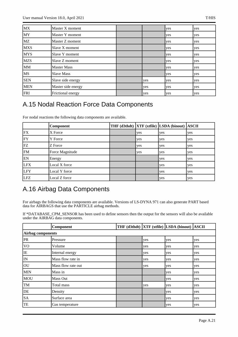
MX Master X moment yes yes
MY Master Y moment yes yes
MZ Master Z moment yes yes
MXS Slave X moment yes yes
MYS Slave Y moment yes yes
MZS Slave Z moment yes yes
MM Master Mass yes yes
MS Slave Mass yes yes
SEN Slave side energy yes yes yes
MEN Master side energy yes yes yes
FRI Frictional energy yes yes yes
A.15 Nodal Reaction Force Data Components
For nodal reactions the following data components are available.
Component THF (d3thdt) XTF (xtfile) LSDA (binout) ASCII
FX X Force yes yes yes
FY Y Force yes yes yes
FZ Z Force yes yes yes
FM Force Magnitude yes yes yes
EN Energy yes yes
LFX Local X force yes yes
LFY Local Y force yes yes
LFZ Local Z force yes yes
A.16 Airbag Data Components
For airbags the following data components are available. Versions of LS-DYNA 971 can also generate PART based data for AIRBAGS that use the PARTICLE airbag methods.
If *DATABASE_CPM_SENSOR has been used to define sensors then the output for the sensors will also be available under the AIRBAG data components.
Component THF (d3thdt) XTF (xtfile) LSDA (binout) ASCII
Airbag components
PR Pressure yes yes yes
VO Volume yes yes yes
IE Internal energy yes yes yes
IN Mass flow rate in yes yes yes
OU Mass flow rate out yes yes yes
MIN Mass in yes yes
MOU Mass Out yes yes
TM Total mass yes yes yes
DE Density yes yes
SA Surface area yes yes
TE Gas temperature yes yes
User manual Version 18.0, April 2021 T/HIS
Page A.21
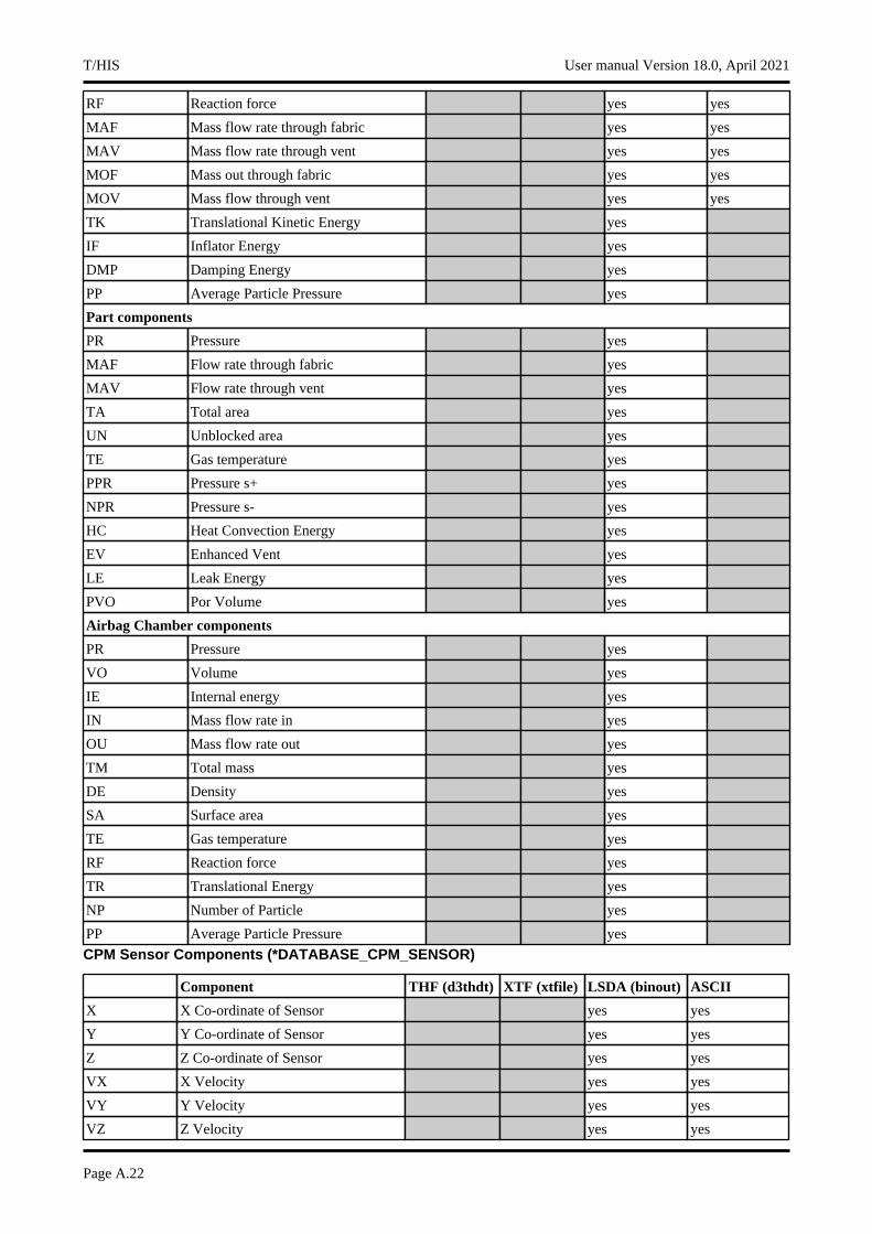
RF Reaction force yes yes
MAF Mass flow rate through fabric yes yes
MAV Mass flow rate through vent yes yes
MOF Mass out through fabric yes yes
MOV Mass flow through vent yes yes
TK Translational Kinetic Energy yes
IF Inflator Energy yes
DMP Damping Energy yes
PP Average Particle Pressure yes
Part components
PR Pressure yes
MAF Flow rate through fabric yes
MAV Flow rate through vent yes
TA Total area yes
UN Unblocked area yes
TE Gas temperature yes
PPR Pressure s+ yes
NPR Pressure s- yes
HC Heat Convection Energy yes
EV Enhanced Vent yes
LE Leak Energy yes
PVO Por Volume yes
Airbag Chamber components
PR Pressure yes
VO Volume yes
IE Internal energy yes
IN Mass flow rate in yes
OU Mass flow rate out yes
TM Total mass yes
DE Density yes
SA Surface area yes
TE Gas temperature yes
RF Reaction force yes
TR Translational Energy yes
NP Number of Particle yes
PP Average Particle Pressure yes
CPM Sensor Components (*DATABASE_CPM_SENSOR)
Component THF (d3thdt) XTF (xtfile) LSDA (binout) ASCII
X X Co-ordinate of Sensor yes yes
Y Y Co-ordinate of Sensor yes yes
Z Z Co-ordinate of Sensor yes yes
VX X Velocity yes yes
VY Y Velocity yes yes
VZ Z Velocity yes yes
T/HIS User manual Version 18.0, April 2021
Page A.22
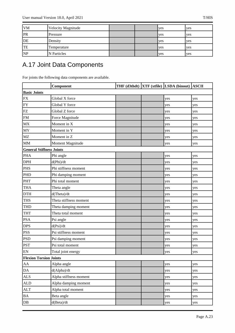
VM Velocity Magnitude yes yes
PR Pressure yes yes
DE Density yes yes
TE Temperature yes yes
NP N Particles yes yes
A.17 Joint Data Components
For joints the following data components are available.
Component THF (d3thdt) XTF (xtfile) LSDA (binout) ASCII
Basic Joints
FX Global X force yes yes
FY Global Y force yes yes
FZ Global Z force yes yes
FM Force Magnitude yes yes
MX Moment in X yes yes
MY Moment in Y yes yes
MZ Moment in Z yes yes
MM Moment Magnitude yes yes
General Stiffness Joints
PHA Phi angle yes yes
DPH d(Phi)/dt yes yes
PHS Phi stiffness moment yes yes
PHD Phi damping moment yes yes
PHT Phi total moment yes yes
THA Theta angle yes yes
DTH d(Theta)/dt yes yes
THS Theta stiffness moment yes yes
THD Theta damping moment yes yes
THT Theta total moment yes yes
PSA Psi angle yes yes
DPS d(Psi)/dt yes yes
PSS Psi stiffness moment yes yes
PSD Psi damping moment yes yes
PST Psi total moment yes yes
EN Total joint energy yes yes
Flexion Torsion Joints
AA Alpha angle yes yes
DA d(Alpha)/dt yes yes
ALS Alpha stiffness moment yes yes
ALD Alpha damping moment yes yes
ALT Alpha total moment yes yes
BA Beta angle yes yes
DB d(Beta)/dt yes yes
User manual Version 18.0, April 2021 T/HIS
Page A.23

BES Beta stiffness moment yes yes
BED Beta damping moment yes yes
BET Beta total moment yes yes
GA Gamma angle yes yes
DG d(Gamma)/dt yes yes
GSF Gamma scale factor yes yes
EN Total joint energy yes yes
Translational Joints
XD X displacement yes yes
DXD d(X)/dt yes yes
YD Y displacement yes yes
DYD d(Y)/dt yes yes
ZD Z displacement yes yes
DZD d(Z)/dt yes yes
XSF X stiffness yes yes
XDF X damping yes yes
XTF X total yes yes
YSF Y stiffness yes yes
YDF Y damping yes yes
YTF Y total yes yes
ZSF Z stiffness yes yes
ZDF Z damping yes yes
ZTF Z total yes yes
EN Total joint energy yes yes
A.18 Cross Section Data Components
For cross sections the following data components are available.
Component THF (d3thdt) XTF (xtfile) LSDA (binout) ASCII
FX X Force yes yes
FY Y Force yes yes
FZ Z Force yes yes
RM Force Magnitude yes yes
MX Moment in X yes yes
MY Moment in Y yes yes
MZ Moment in Z yes yes
MM Moment Magnitude yes yes
CX X centroid coordinate yes yes
CY Y centroid coordinate yes yes
CZ Z centroid coordinate yes yes
AR Area of Cross Section yes yes
A.19 Subsystem Data Components
T/HIS User manual Version 18.0, April 2021
Page A.24

For subsystems the following data components are available.
Component THF (d3thdt) XTF (xtfile) LSDA (binout) ASCII
KE Kinetic energy yes yes
IE Internal energy yes yes
HG Hourglass energy yes yes
KR Kinetic energy ratio yes yes
IM Internal energy ratio yes yes
XM X momentum yes yes
YM Y momentum yes yes
ZM Z momentum yes yes
User manual Version 18.0, April 2021 T/HIS
Page A.25

A.20 Geometric Contact Data Components
For geometric contact entities the following data components are available.
Component THF (d3thdt) XTF (xtfile) LSDA (binout) ASCII
FX X Force yes yes
FY Y Force yes yes
FZ Z Force yes yes
RM Force Magnitude yes yes
MX Moment in X yes yes
MY Moment in Y yes yes
MZ Moment in Z yes yes
MM Moment Magnitude yes yes
A.21 Nodal Rigid Body Data Components
For nodal rigid bodies the following data components are available.
Component THF (d3thdt) XTF (xtfile) LSDA (binout) ASCII
DX X Displacement yes yes
DY Y Displacement yes yes
DZ Z Displacement yes yes
DM Displacement Magnitude yes yes
VX X Velocity yes yes
VY Y Velocity yes yes
VZ Z Velocity yes yes
VM Velocity Magnitude yes yes
AX X Acceleration yes yes
AY Y Acceleration yes yes
AZ Z Acceleration yes yes
AM Acceleration Magnitude yes yes
CX X Co-ordinate yes yes
CY Y Co-ordinate yes yes
CZ Z Co-ordinate yes yes
RX X Rotation yes yes
RY Y Rotation yes yes
RZ Z Rotation yes yes
RM Rotation Magnitude yes yes
RVX X Rotational Velocity yes yes
RVY Y Rotational Velocity yes yes
RVZ Z Rotational Velocity yes yes
RVM Rotational Velocity Magnitude yes yes
RAX X Rotational Acceleration yes yes
RAY Y Rotational Acceleration yes yes
RAZ Z Rotational Acceleration yes yes
T/HIS User manual Version 18.0, April 2021
Page A.26
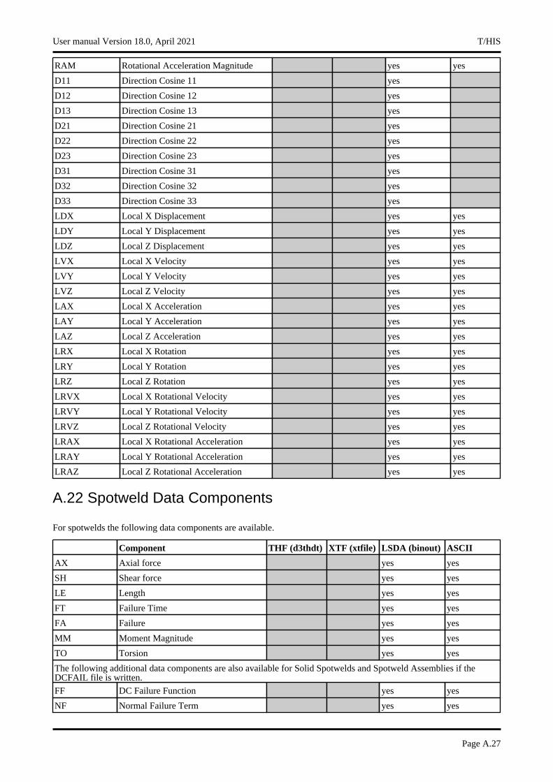
RAM Rotational Acceleration Magnitude yes yes
D11 Direction Cosine 11 yes
D12 Direction Cosine 12 yes
D13 Direction Cosine 13 yes
D21 Direction Cosine 21 yes
D22 Direction Cosine 22 yes
D23 Direction Cosine 23 yes
D31 Direction Cosine 31 yes
D32 Direction Cosine 32 yes
D33 Direction Cosine 33 yes
LDX Local X Displacement yes yes
LDY Local Y Displacement yes yes
LDZ Local Z Displacement yes yes
LVX Local X Velocity yes yes
LVY Local Y Velocity yes yes
LVZ Local Z Velocity yes yes
LAX Local X Acceleration yes yes
LAY Local Y Acceleration yes yes
LAZ Local Z Acceleration yes yes
LRX Local X Rotation yes yes
LRY Local Y Rotation yes yes
LRZ Local Z Rotation yes yes
LRVX Local X Rotational Velocity yes yes
LRVY Local Y Rotational Velocity yes yes
LRVZ Local Z Rotational Velocity yes yes
LRAX Local X Rotational Acceleration yes yes
LRAY Local Y Rotational Acceleration yes yes
LRAZ Local Z Rotational Acceleration yes yes
A.22 Spotweld Data Components
For spotwelds the following data components are available.
Component THF (d3thdt) XTF (xtfile) LSDA (binout) ASCII
AX Axial force yes yes
SH Shear force yes yes
LE Length yes yes
FT Failure Time yes yes
FA Failure yes yes
MM Moment Magnitude yes yes
TO Torsion yes yes
The following additional data components are also available for Solid Spotwelds and Spotweld Assemblies if the DCFAIL file is written.
FF DC Failure Function yes yes
NF Normal Failure Term yes yes
User manual Version 18.0, April 2021 T/HIS
Page A.27
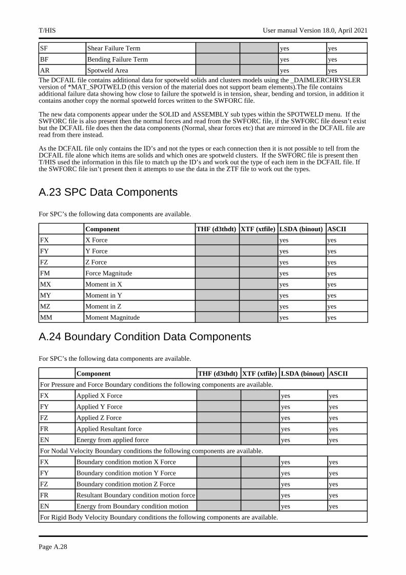
SF Shear Failure Term yes yes
BF Bending Failure Term yes yes
AR Spotweld Area yes yes
The DCFAIL file contains additional data for spotweld solids and clusters models using the _DAIMLERCHRYSLER version of *MAT_SPOTWELD (this version of the material does not support beam elements).The file contains additional failure data showing how close to failure the spotweld is in tension, shear, bending and torsion, in addition it contains another copy the normal spotweld forces written to the SWFORC file.
The new data components appear under the SOLID and ASSEMBLY sub types within the SPOTWELD menu. If the SWFORC file is also present then the normal forces and read from the SWFORC file, if the SWFORC file doesn’t exist but the DCFAIL file does then the data components (Normal, shear forces etc) that are mirrored in the DCFAIL file are read from there instead.
As the DCFAIL file only contains the ID’s and not the types or each connection then it is not possible to tell from the DCFAIL file alone which items are solids and which ones are spotweld clusters. If the SWFORC file is present then T/HIS used the information in this file to match up the ID’s and work out the type of each item in the DCFAIL file. If the SWFORC file isn’t present then it attempts to use the data in the ZTF file to work out the types.
A.23 SPC Data Components
For SPC’s the following data components are available.
Component THF (d3thdt) XTF (xtfile) LSDA (binout) ASCII
FX X Force yes yes
FY Y Force yes yes
FZ Z Force yes yes
FM Force Magnitude yes yes
MX Moment in X yes yes
MY Moment in Y yes yes
MZ Moment in Z yes yes
MM Moment Magnitude yes yes
A.24 Boundary Condition Data Components
For SPC’s the following data components are available.
Component THF (d3thdt) XTF (xtfile) LSDA (binout) ASCII
For Pressure and Force Boundary conditions the following components are available.
FX Applied X Force yes yes
FY Applied Y Force yes yes
FZ Applied Z Force yes yes
FR Applied Resultant force yes yes
EN Energy from applied force yes yes
For Nodal Velocity Boundary conditions the following components are available.
FX Boundary condition motion X Force yes yes
FY Boundary condition motion Y Force yes yes
FZ Boundary condition motion Z Force yes yes
FR Resultant Boundary condition motion force yes yes
EN Energy from Boundary condition motion yes yes
For Rigid Body Velocity Boundary conditions the following components are available.
T/HIS User manual Version 18.0, April 2021
Page A.28

FX Boundary condition motion X Force yes yes
FY Boundary condition motion Y Force yes yes
FZ Boundary condition motion Z Force yes yes
FR Resultant Boundary condition motion force yes yes
EN Energy from Boundary condition motion yes yes
MX Boundary condition motion X Moment yes yes
MY Boundary condition motion Y Moment yes yes
MZ Boundary condition motion Z Moment yes yes
MM Boundary condition moment Magnitude yes yes
A.25 FSI Data Components
For Fluid structural interactions the following data components are available.
Component THF (d3thdt) XTF (xtfile) LSDA (binout) ASCII
PR Pressure yes
FX X Force yes
FY Y Force yes
FZ Z Force yes
FM Force Magnitude yes
PL Porous Leakage yes
MF Mass Flux yes
LFX Leakage X Force yes
LFY Leakage X Force yes
LFZ Leakage X Force yes
LFM Leakage Force Magnitude yes
TE Part Temperature yes
X X Co-ordinate of Sensor yes
Y Y Co-ordinate of Sensor yes
Z Z Co-ordinate of Sensor yes
PR Pressure yes
SO Cpld Solid ID yes
TE Temperature at Sensor yes
A.26 SPH Data Components
For SPH’s the following data components are available.
Component THF (d3thdt) XTF (xtfile) LSDA (binout) ASCII
DE Density yes yes
EXX Strain in XX yes yes
EYY Strain in YY yes yes
EZZ Strain in ZZ yes yes
EXY Strain in XY yes yes
EYZ Strain in YZ yes yes
EZX Strain in ZX yes yes
User manual Version 18.0, April 2021 T/HIS
Page A.29
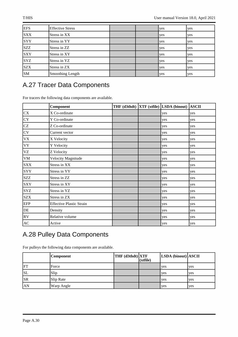
EFS Effective Stress yes yes
SXX Stress in XX yes yes
SYY Stress in YY yes yes
SZZ Stress in ZZ yes yes
SXY Stress in XY yes yes
SYZ Stress in YZ yes yes
SZX Stress in ZX yes yes
SM Smoothing Length yes yes
A.27 Tracer Data Components
For tracers the following data components are available.
Component THF (d3thdt) XTF (xtfile) LSDA (binout) ASCII
CX X Co-ordinate yes yes
CY Y Co-ordinate yes yes
CZ Z Co-ordinate yes yes
CV Current vector yes yes
VX X Velocity yes yes
VY Y Velocity yes yes
VZ Z Velocity yes yes
VM Velocity Magnitude yes yes
SXX Stress in XX yes yes
SYY Stress in YY yes yes
SZZ Stress in ZZ yes yes
SXY Stress in XY yes yes
SYZ Stress in YZ yes yes
SZX Stress in ZX yes yes
EFP Effective Plastic Strain yes yes
DE Density yes yes
RV Relative volume yes yes
AC Active yes yes
A.28 Pulley Data Components
For pulleys the following data components are available.
Component THF (d3thdt) XTF (xtfile)
LSDA (binout) ASCII
FT Force yes yes
SL Slip yes yes
SR Slip Rate yes yes
AN Warp Angle yes yes
T/HIS User manual Version 18.0, April 2021
Page A.30
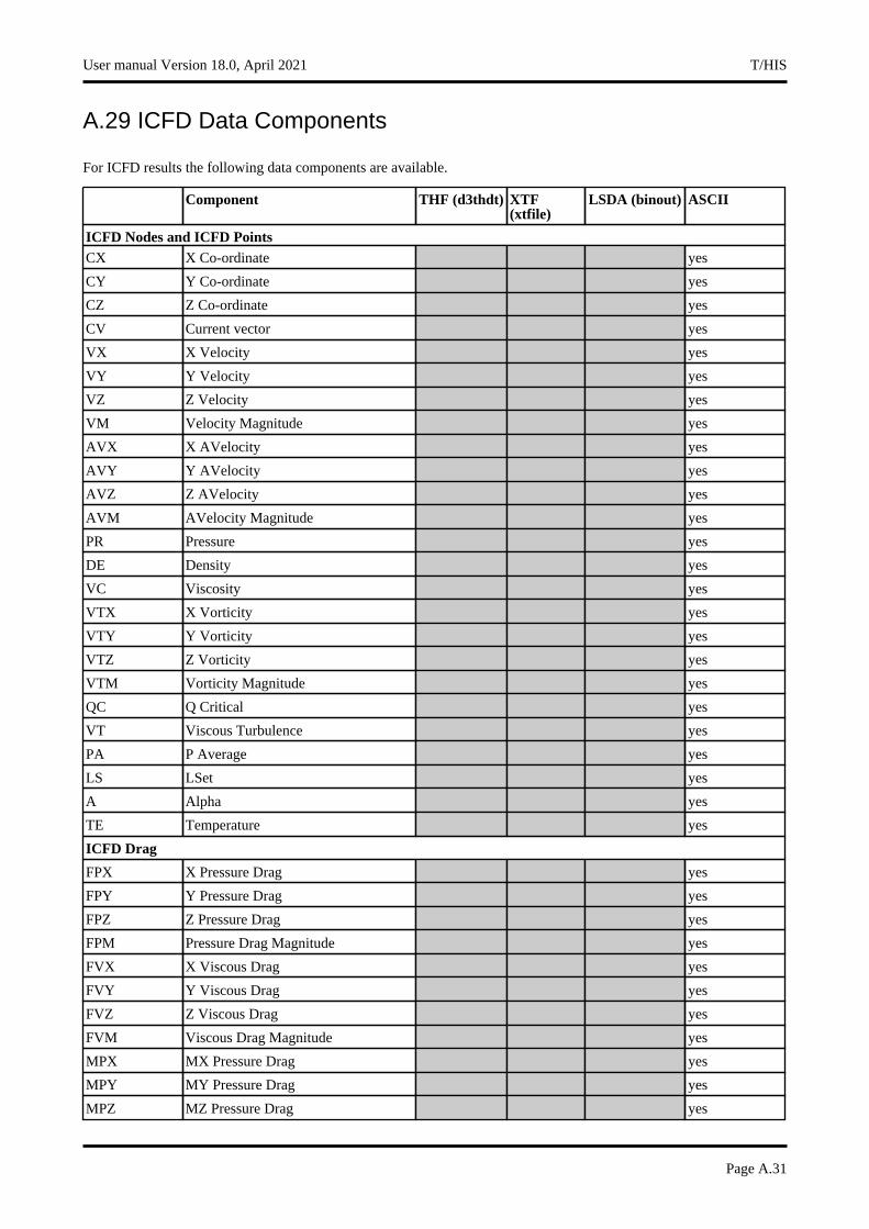
A.29 ICFD Data Components
For ICFD results the following data components are available.
Component THF (d3thdt) XTF (xtfile)
LSDA (binout) ASCII
ICFD Nodes and ICFD PointsCX X Co-ordinate yes
CY Y Co-ordinate yes
CZ Z Co-ordinate yes
CV Current vector yes
VX X Velocity yes
VY Y Velocity yes
VZ Z Velocity yes
VM Velocity Magnitude yes
AVX X AVelocity yes
AVY Y AVelocity yes
AVZ Z AVelocity yes
AVM AVelocity Magnitude yes
PR Pressure yes
DE Density yes
VC Viscosity yes
VTX X Vorticity yes
VTY Y Vorticity yes
VTZ Z Vorticity yes
VTM Vorticity Magnitude yes
QC Q Critical yes
VT Viscous Turbulence yes
PA P Average yes
LS LSet yes
A Alpha yes
TE Temperature yes
ICFD Drag
FPX X Pressure Drag yes
FPY Y Pressure Drag yes
FPZ Z Pressure Drag yes
FPM Pressure Drag Magnitude yes
FVX X Viscous Drag yes
FVY Y Viscous Drag yes
FVZ Z Viscous Drag yes
FVM Viscous Drag Magnitude yes
MPX MX Pressure Drag yes
MPY MY Pressure Drag yes
MPZ MZ Pressure Drag yes
User manual Version 18.0, April 2021 T/HIS
Page A.31
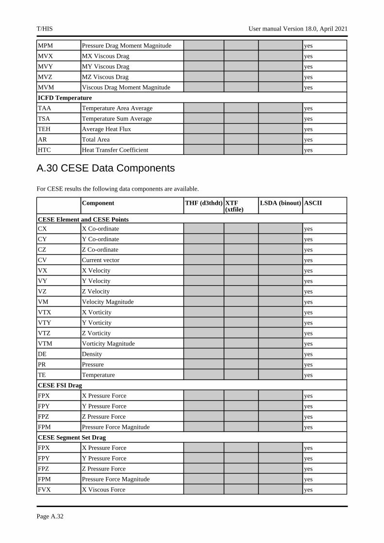
MPM Pressure Drag Moment Magnitude yes
MVX MX Viscous Drag yes
MVY MY Viscous Drag yes
MVZ MZ Viscous Drag yes
MVM Viscous Drag Moment Magnitude yes
ICFD Temperature
TAA Temperature Area Average yes
TSA Temperature Sum Average yes
TEH Average Heat Flux yes
AR Total Area yes
HTC Heat Transfer Coefficient yes
A.30 CESE Data Components
For CESE results the following data components are available.
Component THF (d3thdt) XTF (xtfile)
LSDA (binout) ASCII
CESE Element and CESE PointsCX X Co-ordinate yes
CY Y Co-ordinate yes
CZ Z Co-ordinate yes
CV Current vector yes
VX X Velocity yes
VY Y Velocity yes
VZ Z Velocity yes
VM Velocity Magnitude yes
VTX X Vorticity yes
VTY Y Vorticity yes
VTZ Z Vorticity yes
VTM Vorticity Magnitude yes
DE Density yes
PR Pressure yes
TE Temperature yes
CESE FSI Drag
FPX X Pressure Force yes
FPY Y Pressure Force yes
FPZ Z Pressure Force yes
FPM Pressure Force Magnitude yes
CESE Segment Set Drag
FPX X Pressure Force yes
FPY Y Pressure Force yes
FPZ Z Pressure Force yes
FPM Pressure Force Magnitude yes
FVX X Viscous Force yes
T/HIS User manual Version 18.0, April 2021
Page A.32
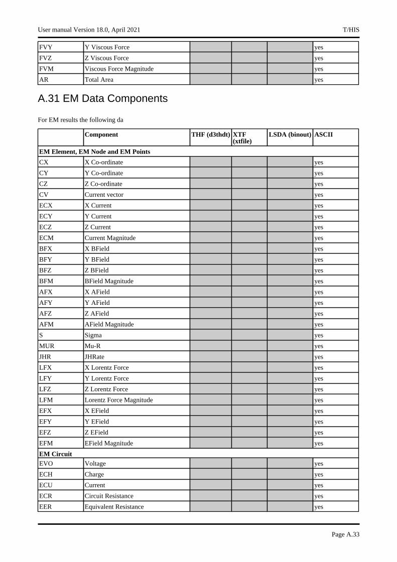
FVY Y Viscous Force yes
FVZ Z Viscous Force yes
FVM Viscous Force Magnitude yes
AR Total Area yes
A.31 EM Data Components
For EM results the following da
Component THF (d3thdt) XTF (xtfile)
LSDA (binout) ASCII
EM Element, EM Node and EM Points
CX X Co-ordinate yes
CY Y Co-ordinate yes
CZ Z Co-ordinate yes
CV Current vector yes
ECX X Current yes
ECY Y Current yes
ECZ Z Current yes
ECM Current Magnitude yes
BFX X BField yes
BFY Y BField yes
BFZ Z BField yes
BFM BField Magnitude yes
AFX X AField yes
AFY Y AField yes
AFZ Z AField yes
AFM AField Magnitude yes
S Sigma yes
MUR Mu-R yes
JHR JHRate yes
LFX X Lorentz Force yes
LFY Y Lorentz Force yes
LFZ Z Lorentz Force yes
LFM Lorentz Force Magnitude yes
EFX X EField yes
EFY Y EField yes
EFZ Z EField yes
EFM EField Magnitude yes
EM CircuitEVO Voltage yes
ECH Charge yes
ECU Current yes
ECR Circuit Resistance yes
EER Equivalent Resistance yes
User manual Version 18.0, April 2021 T/HIS
Page A.33

ECI Inductance yes
EM1 Mutual Inductance 1 yes
EM2 Mutual Inductance 2 yes
EM3 Mutual Inductance 3 yes
EM Circuit0DEVO Voltage yes
ECH Charge yes
ECU Current yes
ECE Total Energy yes
EM PartDataLFX X Lorentz Force yes
LFY Y Lorentz Force yes
LFZ Z Lorentz Force yes
LFM Lorentz Force Magnitude yes
JHE Joule Heating Energy yes
MAG Magnetic Energy yes
KIN Kinetic Energy yes
PLA Plastic Energy yes
EM IsoPotOutEVO Voltage yes
ECU Current yes
EM CircuitResECV Contact Current yes
ECR Contact Resistance yes
ECJ Contact Joule heat rate yes
ECA Contact Area yes
EM BoundaryOut
EBV Voltage yes
EBC Current yes
EBA Area yes
EM IsoPotConnOutEVO Voltage yes
ECH Charge yes
ECU Current yes
ECR Contact Resistance yes
POW Power yes
ENE Energy yes
EM RandlesCellTVO TotVoltage yes
OCV OCV yes
DVO DampVoltage yes
RCU Current yes
SOC SOC yes
SOF SOCFunc yes
SOS SOCShift yes
T/HIS User manual Version 18.0, April 2021
Page A.34
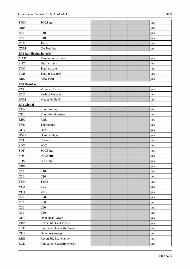
SOM SOCSum yes
RR0 R0 yes
R10 R10 yes
C10 C10 yes
TEM Temp yes
CNM Ckt Number yes
EM RandlesIntshortCellMXR Maximum resistance yes
SHC Short circuits yes
TOC Total circuits yes
TOR Total resistance yes
ARS Area short yes
EM RogoCoil
RVC Volume Current yes
RSC Surface Current yes
RVM Magnetic Field yes
EM GlobalRUN Run timestep yes
CFL Condition timestep yes
RBC Ratio yes
TVO TotVoltage yes
OCV OCV yes
DVO DampVoltage yes
RCU Current yes
SOC SOC yes
SOF SOCFunc yes
SOS SOCShift yes
SOM SOCSum yes
RR0 R0 yes
R10 R10 yes
C10 C10 yes
TEM Temp yes
VC2 VC2 yes
VC3 VC3 yes
R20 R20 yes
R30 R30 yes
C20 C20 yes
C30 C30 yes
OHP Ohm Heat Power yes
RHP Reversible Heat Power yes
ECP Equivalent Capacity Power yes
OHE Ohm heat energy yes
RHE Reversible heat energy yes
ECE Equivalent Capacity energy yes
User manual Version 18.0, April 2021 T/HIS
Page A.35
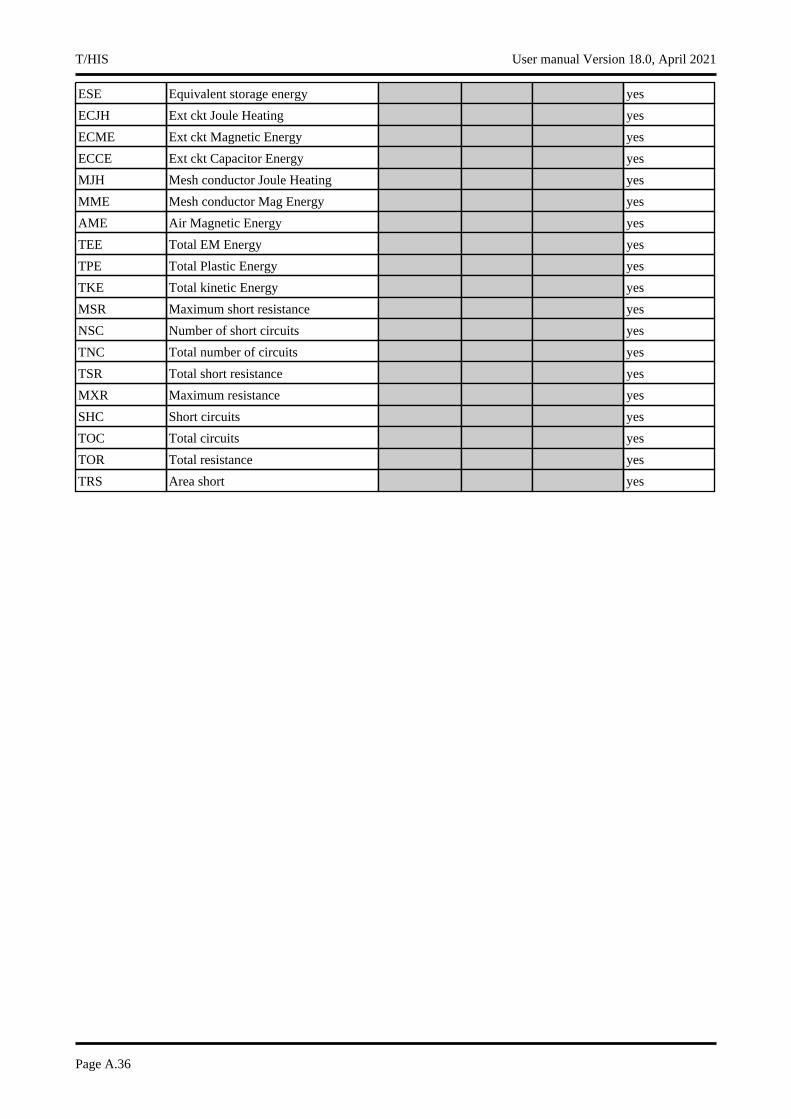
ESE Equivalent storage energy yes
ECJH Ext ckt Joule Heating yes
ECME Ext ckt Magnetic Energy yes
ECCE Ext ckt Capacitor Energy yes
MJH Mesh conductor Joule Heating yes
MME Mesh conductor Mag Energy yes
AME Air Magnetic Energy yes
TEE Total EM Energy yes
TPE Total Plastic Energy yes
TKE Total kinetic Energy yes
MSR Maximum short resistance yes
NSC Number of short circuits yes
TNC Total number of circuits yes
TSR Total short resistance yes
MXR Maximum resistance yes
SHC Short circuits yes
TOC Total circuits yes
TOR Total resistance yes
TRS Area short yes
T/HIS User manual Version 18.0, April 2021
Page A.36

A.32 Particle Blast Data Components
For PBLASTs the following data components are available.
Component THF (d3thdt) XTF (xtfile)
LSDA (binout)
ASCII
Particle blast components
AIE Air internal energy yes yes
DPIE Detonation product internal energy yes yes
OIE Outside domain internal energy yes yes
ATE Air translational energy yes yes
DPTE Detonation product translational energy
yes yes
OTE Outside domain translational energy yes yes
Part components
APR Air pressure yes yes
DPPR Detonation product pressure yes yes
RPR Resultant pressure yes yes
AR Surface Area yes yes
AFX Air X Force yes yes
AFY Air Y Force yes yes
AFZ Air Z Force yes yes
DPFX Detonation product X Force yes yes
DPFY Detonation product Y Force yes yes
DPFZ Detonation product Z Force yes yes
RFX Resultant X Force yes yes
RFY Resultant Y Force yes yes
RFZ Resultant Z Force yes yes
A.33 Pressure Tube Data Components
For pressure tubes the following data components are available.
Component THF (d3thdt) XTF (xtfile)
LSDA (binout) ASCII
AR Cross section area yes yes
DE Density yes yes
PR Pressure yes yes
VEL Velocity yes yes
User manual Version 18.0, April 2021 T/HIS
Page A.37
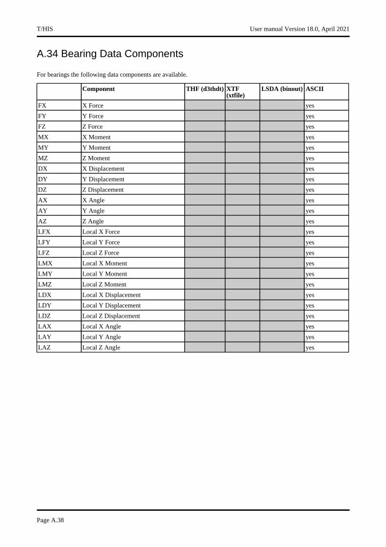
A.34 Bearing Data Components
For bearings the following data components are available.
Component THF (d3thdt) XTF (xtfile)
LSDA (binout) ASCII
FX X Force yes
FY Y Force yes
FZ Z Force yes
MX X Moment yes
MY Y Moment yes
MZ Z Moment yes
DX X Displacement yes
DY Y Displacement yes
DZ Z Displacement yes
AX X Angle yes
AY Y Angle yes
AZ Z Angle yes
LFX Local X Force yes
LFY Local Y Force yes
LFZ Local Z Force yes
LMX Local X Moment yes
LMY Local Y Moment yes
LMZ Local Z Moment yes
LDX Local X Displacement yes
LDY Local Y Displacement yes
LDZ Local Z Displacement yes
LAX Local X Angle yes
LAY Local Y Angle yes
LAZ Local Z Angle yes
T/HIS User manual Version 18.0, April 2021
Page A.38
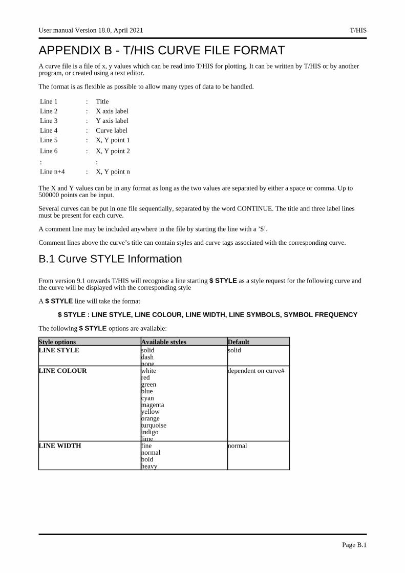
APPENDIX B - T/HIS CURVE FILE FORMATA curve file is a file of x, y values which can be read into T/HIS for plotting. It can be written by T/HIS or by another program, or created using a text editor.
The format is as flexible as possible to allow many types of data to be handled.
Line 1 : Title
Line 2 : X axis label
Line 3 : Y axis label
Line 4 : Curve label
Line 5 : X, Y point 1
Line 6 : X, Y point 2
: :
Line n+4 : X, Y point n
The X and Y values can be in any format as long as the two values are separated by either a space or comma. Up to 500000 points can be input.
Several curves can be put in one file sequentially, separated by the word CONTINUE. The title and three label lines must be present for each curve.
A comment line may be included anywhere in the file by starting the line with a ’$’.
Comment lines above the curve’s title can contain styles and curve tags associated with the corresponding curve.
B.1 Curve STYLE Information
From version 9.1 onwards T/HIS will recognise a line starting $ STYLE as a style request for the following curve and the curve will be displayed with the corresponding style
A $ STYLE line will take the format
$ STYLE : LINE STYLE, LINE COLOUR, LINE WIDTH, LINE SYMBOLS, SYMBOL FREQUENCY
The following $ STYLE options are available:
Style options Available styles DefaultLINE STYLE solid
dashnone
solid
LINE COLOUR whiteredgreenbluecyanmagentayelloworangeturquoiseindigolime
dependent on curve#
LINE WIDTH finenormalboldheavy
normal
User manual Version 18.0, April 2021 T/HIS
Page B.1
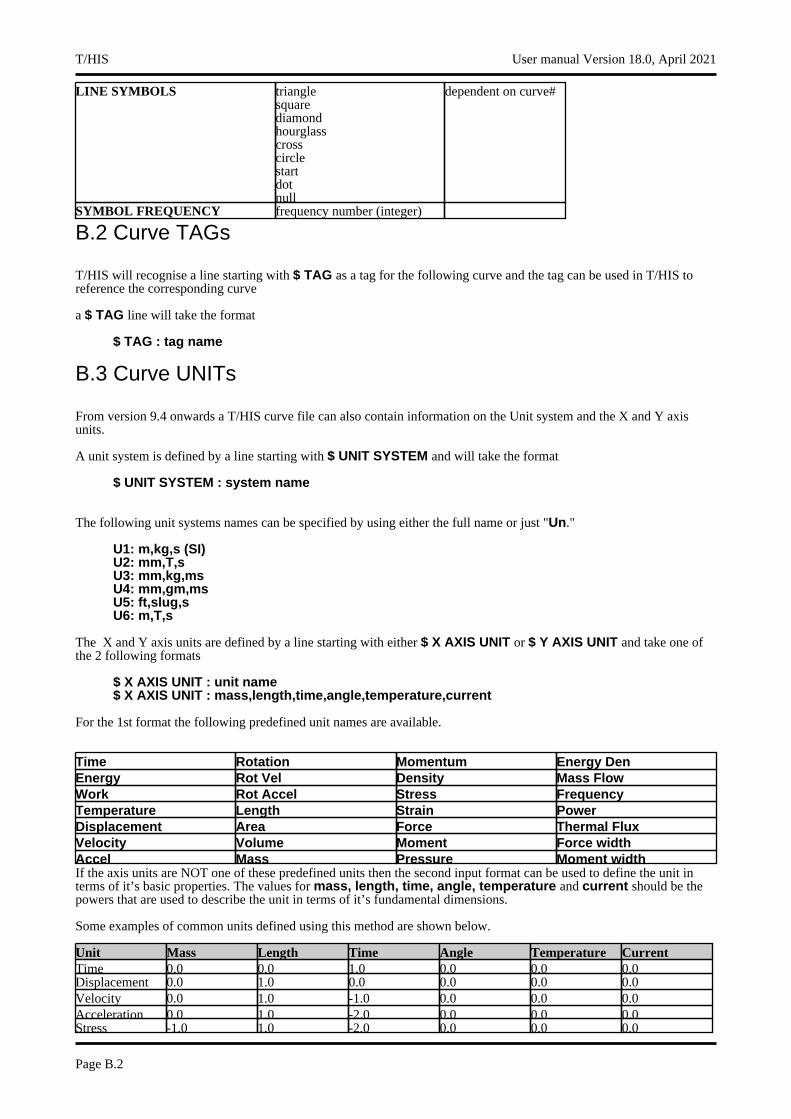
LINE SYMBOLS trianglesquarediamondhourglasscrosscirclestartdotnull
dependent on curve#
SYMBOL FREQUENCY frequency number (integer)
B.2 Curve TAGs
T/HIS will recognise a line starting with $ TAG as a tag for the following curve and the tag can be used in T/HIS to reference the corresponding curve
a $ TAG line will take the format
$ TAG : tag name
B.3 Curve UNITs
From version 9.4 onwards a T/HIS curve file can also contain information on the Unit system and the X and Y axis units.
A unit system is defined by a line starting with $ UNIT SYSTEM and will take the format
$ UNIT SYSTEM : system name
The following unit systems names can be specified by using either the full name or just "Un."
U1: m,kg,s (SI)U2: mm,T,sU3: mm,kg,msU4: mm,gm,msU5: ft,slug,sU6: m,T,s
The X and Y axis units are defined by a line starting with either $ X AXIS UNIT or $ Y AXIS UNIT and take one of the 2 following formats
$ X AXIS UNIT : unit name$ X AXIS UNIT : mass,length,time,angle,temperature,current
For the 1st format the following predefined unit names are available.
Time Rotation Momentum Energy Den Energy Rot Vel Density Mass Flow Work Rot Accel Stress Frequency Temperature Length Strain Power Displacement Area Force Thermal Flux Velocity Volume Moment Force width Accel Mass Pressure Moment width If the axis units are NOT one of these predefined units then the second input format can be used to define the unit in terms of it’s basic properties. The values for mass, length, time, angle, temperature and current should be the powers that are used to describe the unit in terms of it’s fundamental dimensions.
Some examples of common units defined using this method are shown below.
Unit Mass Length Time Angle Temperature Current Time 0.0 0.0 1.0 0.0 0.0 0.0 Displacement 0.0 1.0 0.0 0.0 0.0 0.0 Velocity 0.0 1.0 -1.0 0.0 0.0 0.0 Acceleration 0.0 1.0 -2.0 0.0 0.0 0.0 Stress -1.0 1.0 -2.0 0.0 0.0 0.0
T/HIS User manual Version 18.0, April 2021
Page B.2

B.4 Example
The following example shows a curve file containing 2 curves.
The first curve will be plotted with a bold, solid, green line with triangular symbols every other data point. The curve contains 5 data points and is given a reference tag CURVE_1
The second curve will be plotted with a dashed, white, normal line. No symbols will be displayed. The curve contains 2 data points and has no reference tag.
$ Comment line$ STYLE : solid,green,bold,triangle,2 Style line$ TAG : CURVE_1 Tag line$ Comment lineCURVE FILE EXAMPLE ;TitleTime ;X axis labelDisplacement ;Y axis labelCurve number 1 ;Curve label0 2.0 ;1st data pair1.0 4E-34.0, 4.75 410.0 8.9 ;End of 1st curveCONTINUE$ Comment line$ Comment line$ STYLE : dash,white,,, Style lineCURVE FILE EXAMPLE ;TitleTimeDisplacementCurve number 20.0 7E22.0 8.7E-9Notes:
The abscissa (x axis) values are assumed to be in the correct order.The free format allowed for the data points.The style line must contain 5 comma separated words in the order LINE STYLE, LINE COLOUR, LINE WIDTH, LINE SYMBOLS, SYMBOL FREQUENCY to be successfully understood by T/HIS.If any words are unspecified in the style line, as in curve 2, T/HIS will take the default option.
User manual Version 18.0, April 2021 T/HIS
Page B.3

T/HIS User manual Version 18.0, April 2021
Page B.4
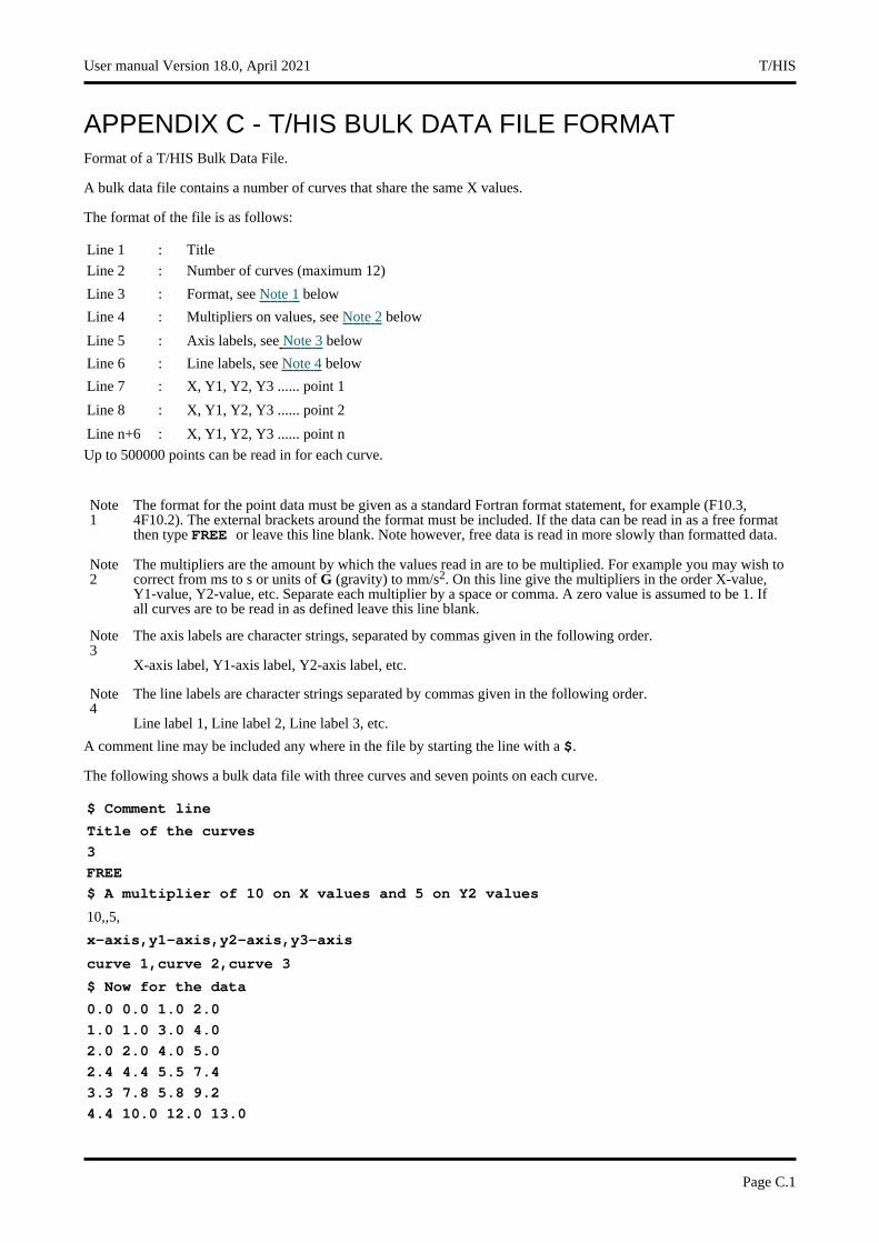
APPENDIX C - T/HIS BULK DATA FILE FORMATFormat of a T/HIS Bulk Data File.
A bulk data file contains a number of curves that share the same X values.
The format of the file is as follows:
Line 1 : Title
Line 2 : Number of curves (maximum 12)
Line 3 : Format, see Note 1 below
Line 4 : Multipliers on values, see Note 2 below
Line 5 : Axis labels, see Note 3 below
Line 6 : Line labels, see Note 4 below
Line 7 : X, Y1, Y2, Y3 ...... point 1
Line 8 : X, Y1, Y2, Y3 ...... point 2
Line n+6 : X, Y1, Y2, Y3 ...... point n
Up to 500000 points can be read in for each curve.
Note 1
The format for the point data must be given as a standard Fortran format statement, for example (F10.3, 4F10.2). The external brackets around the format must be included. If the data can be read in as a free format then type FREE or leave this line blank. Note however, free data is read in more slowly than formatted data.
Note 2
The multipliers are the amount by which the values read in are to be multiplied. For example you may wish to correct from ms to s or units of G (gravity) to mm/s2. On this line give the multipliers in the order X-value, Y1-value, Y2-value, etc. Separate each multiplier by a space or comma. A zero value is assumed to be 1. If all curves are to be read in as defined leave this line blank.
Note 3
The axis labels are character strings, separated by commas given in the following order.
X-axis label, Y1-axis label, Y2-axis label, etc.
Note 4
The line labels are character strings separated by commas given in the following order.
Line label 1, Line label 2, Line label 3, etc.
A comment line may be included any where in the file by starting the line with a $.
The following shows a bulk data file with three curves and seven points on each curve.
$ Comment line
Title of the curves
3
FREE
$ A multiplier of 10 on X values and 5 on Y2 values
10,,5,
x-axis,y1-axis,y2-axis,y3-axis
curve 1,curve 2,curve 3
$ Now for the data
0.0 0.0 1.0 2.0
1.0 1.0 3.0 4.0
2.0 2.0 4.0 5.0
2.4 4.4 5.5 7.4
3.3 7.8 5.8 9.2
4.4 10.0 12.0 13.0
User manual Version 18.0, April 2021 T/HIS
Page C.1

T/HIS User manual Version 18.0, April 2021
Page C.2
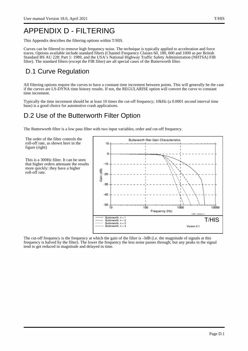
APPENDIX D - FILTERINGThis Appendix describes the filtering options within T/HIS.
Curves can be filtered to remove high frequency noise. The technique is typically applied to acceleration and force traces. Options available include standard filters (Channel Frequency Classes 60, 180, 600 and 1000 as per British Standard BS AU 228: Part 1: 1989, and the USA’s National Highway Traffic Safety Administration (NHTSA) FIR filter). The standard filters (except the FIR filter) are all special cases of the Butterworth filter.
D.1 Curve Regulation
All filtering options require the curves to have a constant time increment between points. This will generally be the case if the curves are LS-DYNA time history results. If not, the REGULARISE option will convert the curve to constant time increment.
Typically the time increment should be at least 10 times the cut-off frequency; 10kHz (a 0.0001 second interval time base) is a good choice for automotive crash applications.
D.2 Use of the Butterworth Filter Option
The Butterworth filter is a low pass filter with two input variables; order and cut-off frequency.
The order of the filter controls the roll-off rate, as shown here in the figure (right)
This is a 300Hz filter. It can be seen that higher orders attenuate the results more quickly: they have a higher roll-off rate.
The cut-off frequency is the frequency at which the gain of the filter is -3dB (i.e. the magnitude of signals at this frequency is halved by the filter). The lower the frequency the less noise passes through; but any peaks in the signal tend to get reduced in magnitude and delayed in time.
User manual Version 18.0, April 2021 T/HIS
Page D.1
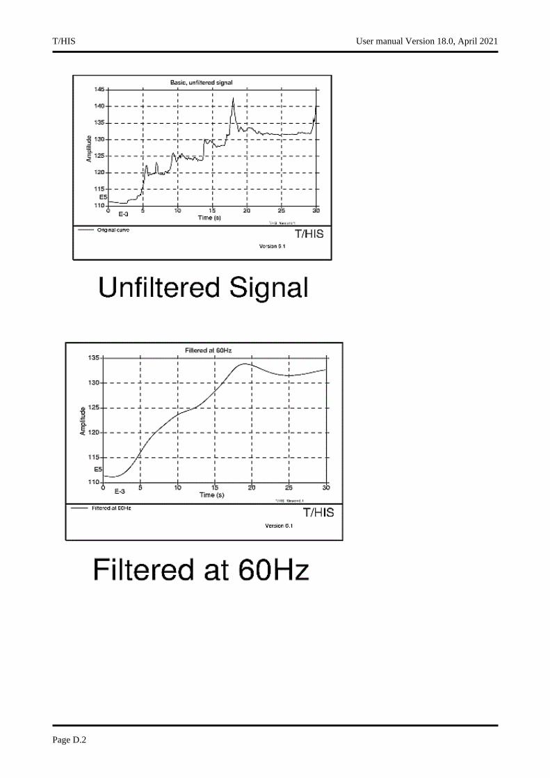
T/HIS User manual Version 18.0, April 2021
Page D.2
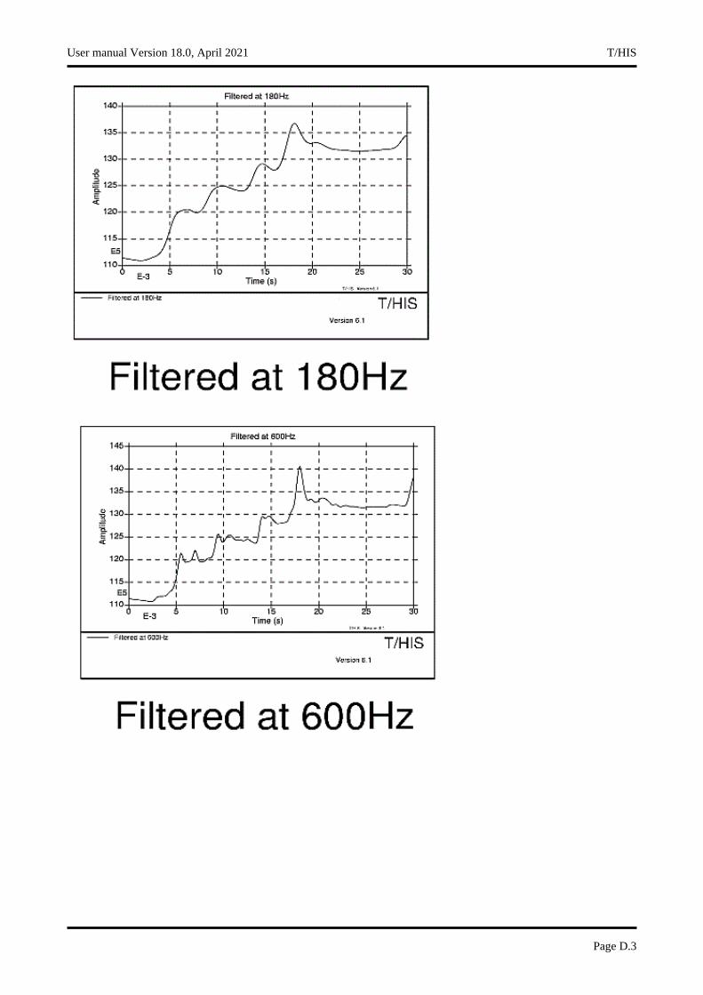
User manual Version 18.0, April 2021 T/HIS
Page D.3
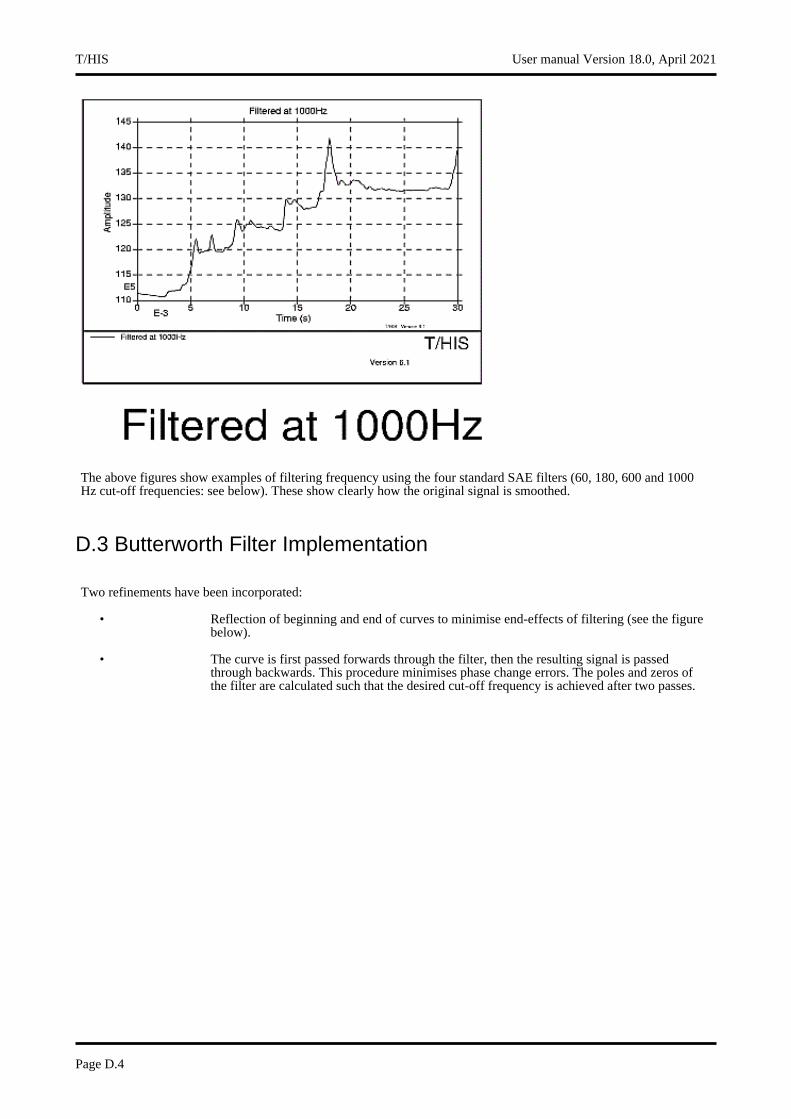
The above figures show examples of filtering frequency using the four standard SAE filters (60, 180, 600 and 1000 Hz cut-off frequencies: see below). These show clearly how the original signal is smoothed.
D.3 Butterworth Filter Implementation
Two refinements have been incorporated:
• Reflection of beginning and end of curves to minimise end-effects of filtering (see the figure below).
• The curve is first passed forwards through the filter, then the resulting signal is passed through backwards. This procedure minimises phase change errors. The poles and zeros of the filter are calculated such that the desired cut-off frequency is achieved after two passes.
T/HIS User manual Version 18.0, April 2021
Page D.4
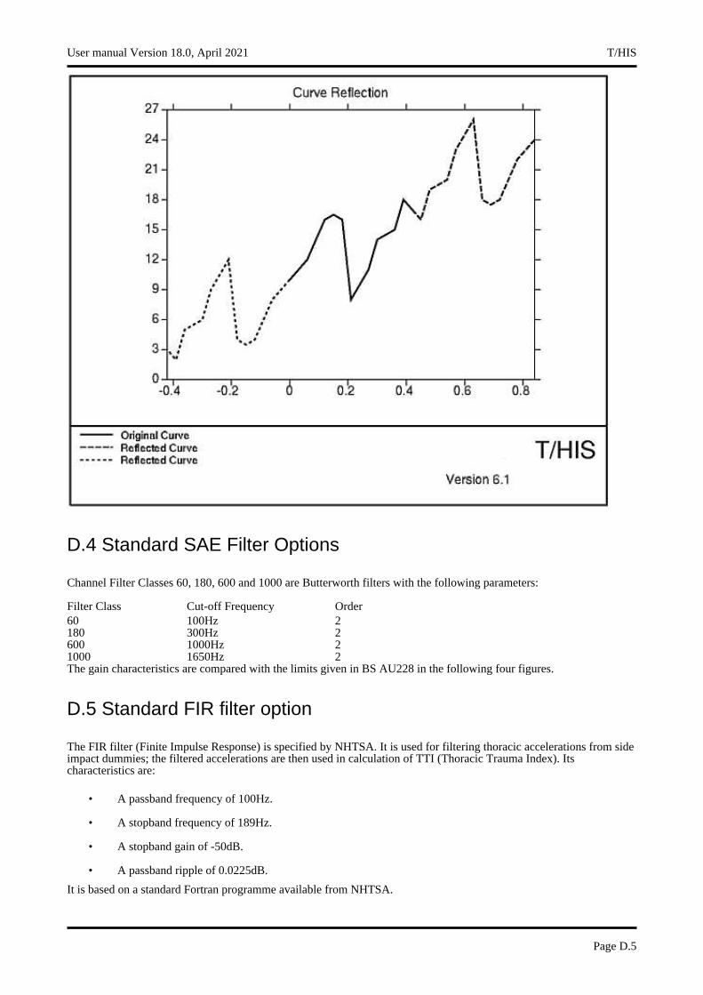
D.4 Standard SAE Filter Options
Channel Filter Classes 60, 180, 600 and 1000 are Butterworth filters with the following parameters:
Filter Class Cut-off Frequency Order 60 100Hz 2 180 300Hz 2 600 1000Hz 2 1000 1650Hz 2The gain characteristics are compared with the limits given in BS AU228 in the following four figures.
D.5 Standard FIR filter option
The FIR filter (Finite Impulse Response) is specified by NHTSA. It is used for filtering thoracic accelerations from side impact dummies; the filtered accelerations are then used in calculation of TTI (Thoracic Trauma Index). Its characteristics are:
• A passband frequency of 100Hz.
• A stopband frequency of 189Hz.
• A stopband gain of -50dB.
• A passband ripple of 0.0225dB.
It is based on a standard Fortran programme available from NHTSA.
User manual Version 18.0, April 2021 T/HIS
Page D.5
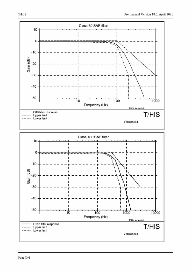
T/HIS User manual Version 18.0, April 2021
Page D.6
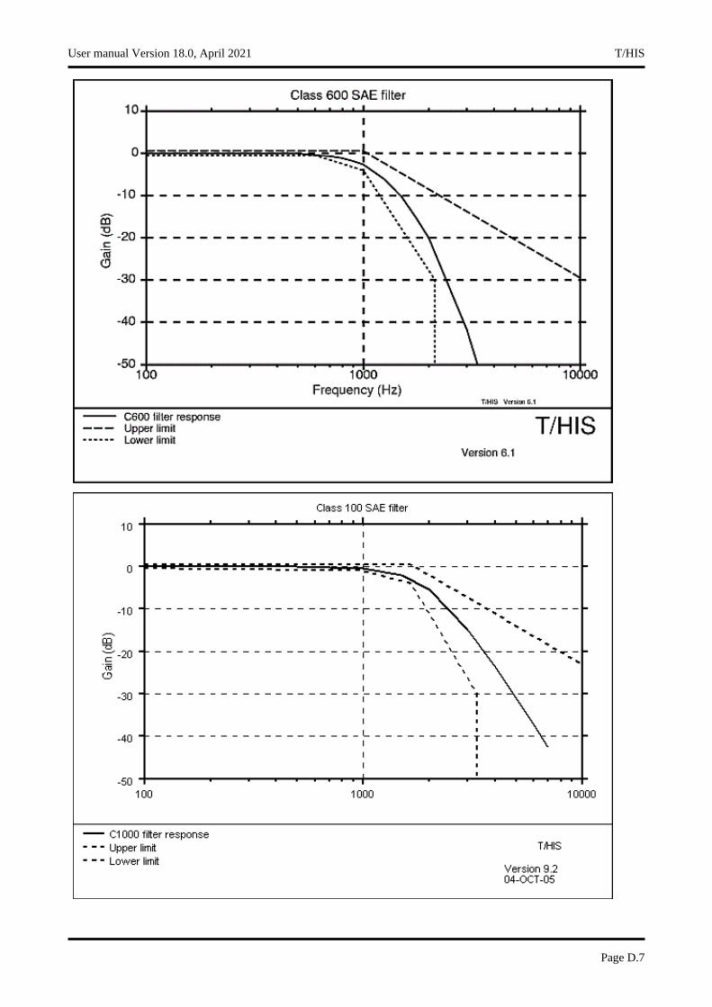
User manual Version 18.0, April 2021 T/HIS
Page D.7

T/HIS User manual Version 18.0, April 2021
Page D.8

APPENDIX E - INJURY CRITERIAT/HIS has the option to calculate two of the injury criteria that are used currently in occupant protection. These are the head impact criteria or HIC value and 3ms clip value. These criteria are defined as follows:
E.1 HIC Value
The HIC value is calculated from the resultant acceleration time history of the head centre of gravity filtered through a class 1000 filter. The HIC value is then calculated from;
Where a is the acceleration expressed in g, and t1 and t2 are any two points in time. It is now usual for an upper limit on the range t2-t1 of 36ms to be applied.
E.2 3ms Clip
The 3ms clip value is the maximum value of acceleration that is exceeded for a period of not less than 3 ms. This is not an easily comprehended definition: the following may be of more use:
(1) At each time point T, take the interval (T to T+3ms);
(2) In this interval find the lowest acceleration value;
(3) The "3ms Clip" value is the interval (T to T+3ms) which has the largest "lowest" value as calculated in (2) above.
So, perhaps, a better definition might be: "the 3ms interval with the highest lowest acceleration value".
E.3 Viscous Criteria
The VC value is calculated from a compression time history using the following formula (the values of the constants A and B assume the compression is in metres);
User manual Version 18.0, April 2021 T/HIS
Page E.1
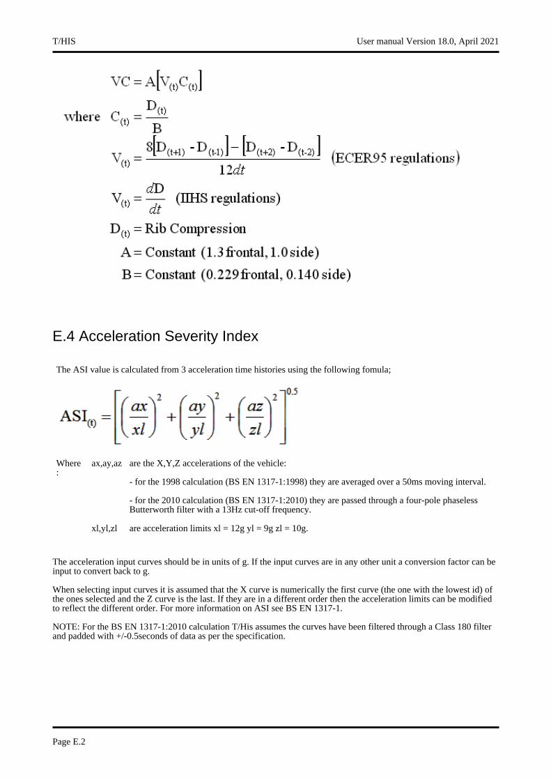
E.4 Acceleration Severity Index
The ASI value is calculated from 3 acceleration time histories using the following fomula;
Where :
ax,ay,az are the X,Y,Z accelerations of the vehicle:
- for the 1998 calculation (BS EN 1317-1:1998) they are averaged over a 50ms moving interval.
- for the 2010 calculation (BS EN 1317-1:2010) they are passed through a four-pole phaseless Butterworth filter with a 13Hz cut-off frequency.
xl,yl,zl are acceleration limits xl = 12g yl = 9g zl = 10g.
The acceleration input curves should be in units of g. If the input curves are in any other unit a conversion factor can be input to convert back to g.
When selecting input curves it is assumed that the X curve is numerically the first curve (the one with the lowest id) of the ones selected and the Z curve is the last. If they are in a different order then the acceleration limits can be modified to reflect the different order. For more information on ASI see BS EN 1317-1.
NOTE: For the BS EN 1317-1:2010 calculation T/His assumes the curves have been filtered through a Class 180 filter and padded with +/-0.5seconds of data as per the specification.
T/HIS User manual Version 18.0, April 2021
Page E.2
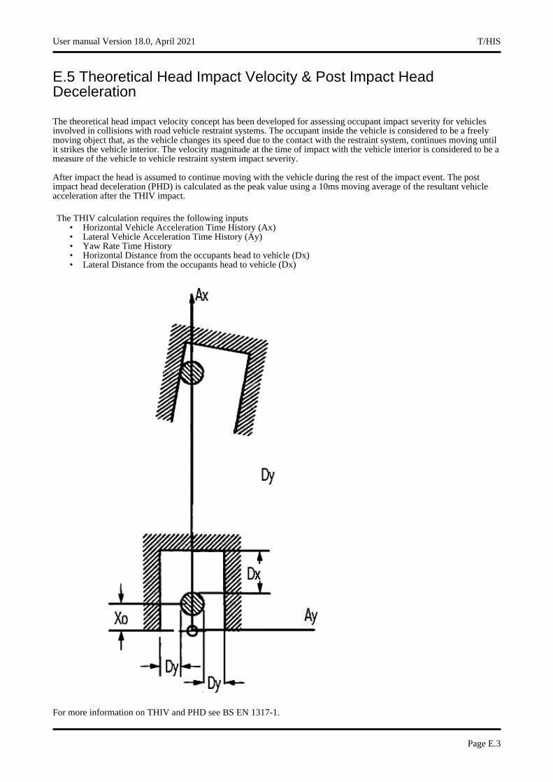
E.5 Theoretical Head Impact Velocity & Post Impact Head Deceleration
The theoretical head impact velocity concept has been developed for assessing occupant impact severity for vehicles involved in collisions with road vehicle restraint systems. The occupant inside the vehicle is considered to be a freely moving object that, as the vehicle changes its speed due to the contact with the restraint system, continues moving until it strikes the vehicle interior. The velocity magnitude at the time of impact with the vehicle interior is considered to be a measure of the vehicle to vehicle restraint system impact severity.
After impact the head is assumed to continue moving with the vehicle during the rest of the impact event. The post impact head deceleration (PHD) is calculated as the peak value using a 10ms moving average of the resultant vehicle acceleration after the THIV impact.
The THIV calculation requires the following inputs• Horizontal Vehicle Acceleration Time History (Ax)• Lateral Vehicle Acceleration Time History (Ay)• Yaw Rate Time History• Horizontal Distance from the occupants head to vehicle (Dx)• Lateral Distance from the occupants head to vehicle (Dx)
For more information on THIV and PHD see BS EN 1317-1.
User manual Version 18.0, April 2021 T/HIS
Page E.3

E.6 Biomechanical neck injury predictor (NIJ)
The biomechanical neck injury predictor is a measure of the injury due to the load transferred through the occipital condyles. Its calculation combines the neck axial force and the flexion/extension moment about the occipital condoyles.
It is used in association with the USSID dummy for standard American frontal impact tests.
The shear force (Fx), axial force (Fz) and bending moment (My) are measured by the dummy upper neck load cell for the duration of the crash, using force and moment definitions consistent with SAE J221/1. T/HIS will caculate the bending moment using the equation:
My = My’ - e • Fx
Where e is the e distance specified in the input window, Fx is the shear force.
Shear force, axial force and bending moment must be filtered using an SAE Channel Frequency Class 600 filter (C600) for the purposes of calculation.
During the collision, the Axial Force (Fz) can be in either tension or compression whilst the occipital condyle bending moment (Mocy) can be in either flexion or extension. This results in 4 possible loading conditions corresponding to the 4 curves output by T/HIS; tension-extension (Nte), tension-flexion (Ntf), compression-extension (Nce), and compression-flexion (Ncf). At each point in time only one of these 4 conditions can be met, hence the NIJ value is calculated for that condition and the value for the other 3 conditions is considered a value of zero..
The expression for calculating each NIJ loading condition is given by:
NIJ = (Fz/Fzc) + (Mocy/Myc)
where Fz and Mocy are as defined above, Fzc and Myc refer to the axial force and Bending moment critical values, given below:
The values of Fzc and Myc vary depending on the occupant, the occupants position and the sign of Fz and Mocy
For the dummy to pass the test, the following conditions must be met:
(i) None of the 4 NIJ values may exceed 1.0 at any time during the event
(ii) Peak Tension Force (Fz), measured at the upper neck load cell, may not exceed the specific dummy’s limit (e.g. 2070N for the Hybrid III small female) at any time
(iii) Peak Compression Force (Fz), measured at the upper neck load cell, may not exceed the specific dummy’s limit (e.g. 2520N for the Hybrid III small female) at any time
For more information on the use and calculation of NIJ, refer to the FMVSS 208 document
E.7 The Thoracic Trauma Index (TTI)
The Thoracic Trauma Index is used as a predictor of thoracic injury severity in the USSID dummy in standard American Side Impact tests.
The Index considers both rib and Thorax acceleration in an impast.
The expression for calculating TTI is given by:
TTI = (G(R) + G(LS))/2
Where G(R) is the greater of the peak accelerations of either the upper or lower rib, expressed in g, and G(LS) is the peak acceleration in the lower spine (T12), expressed in g.
For the dummy to pass the test, the following conditions must be met:
(i) The TTI value must not exceed;(a) 85g for a passenger car with 4 side doors, and for any multipurpose vehicle, truck or bus(b) 90g for a passenger car with 2 side doors
(ii) The peak lateral acceleration of the pelvis shall not exceed 130g
T/HIS User manual Version 18.0, April 2021
Page E.4

(iii) Any side door, struck by the moving deformable barrier, shall not seperate totally from the car.
(iv) Any door not struck by the moving deformable barrier must meet the following requirements;(a) The door chall not disengage from the latched position(b) The latch shall not seperate from the striker(c) The hinge components shall not seperate from each other or from their attachment to the vehicle(d) Neither the latch nor the hinge systems of the door shall pull out of their anchorage
For more information on the use and calculation of TTI, refer to the FMVSS 214 document
User manual Version 18.0, April 2021 T/HIS
Page E.5

T/HIS User manual Version 18.0, April 2021
Page E.6
APPENDIX F - Curve Correlation
COR1 and COR2
The Correlation functions COR1 and COR2 provide a measure of the degree to which two curves match. When comparing curves by eye, the quality of correlation may be judged on the basis of how well matched are the patterns of peaks, the overall shapes of the curves, etc, and can allow for differences of timing as well as magnitude. Thus a simple function based on the difference of Y-values (such as T/HIS ERR function) does not measure correlation in the same way as the human eye. The T/HIS correlation function attempts to include and quantify the more subtle ways in which the correlation of two curves may be judged.
The correlation function may be applied to any two curves whose x-values increase monotonically (e.g. responses versus time). The results are independent of the units used, e.g. milliseconds or seconds are both acceptable. The sign of the y-values is not important.
Only the overlap time period is considered (i.e. the range of x-values for which both curves have a y-value). The time period (range of X-values) and maximum absolute Y-value are used to non-dimensionalise the curves such that x-values run from 0 to 1, and the maximum absolute y-value is 1.
Five measures of correlation are calculated. Each is given equal weighting. The final correlation score is given as a percentage - two identical curves would score 100%.
The first two measures require identification of peaks in the curves. An unlimited number of peaks in each curve will be considered. A peak is defined as a local maximum (or in the case of negative y-values a minimum), satisfying the following criteria:
• Absolute y-value at least 0.5• Separated from any larger peak by a trough (local minimum) at least 0.2 deep.
Peaks of positive or negative signs are considered. Peaks are matched only against peaks of the same sign in the other curve.
Measure 1 - Peak values
For each identified peak in Curve A, find the maximum value in Curve B within the same time range for which the value in Curve A is within a tolerance of the peak value. Points are lost according to the error in y-values compared to a tolerance limit. Repeat for peaks in curve B against values in Curve A.
This measure allows for the situation where curves are similar but the peaks are more strongly delineated in one of the curves, such that the program does not recognise the other curve as having a peak in that location.
Measure 2 - Peak matching
For each identified peak in Curve A, find the closest identified peak in Curve B. Points are lost according to the largest error (timing or y-value) compared to tolerance limits; points are also lost if there is no corresponding peak in Curve B. Repeat for Curve A peaks matched against those of Curve B.
User manual Version 18.0, April 2021 T/HIS
Page F.1
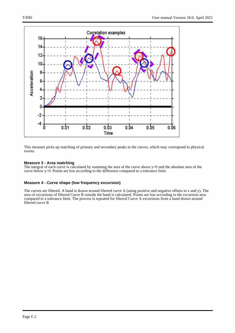
This measure picks up matching of primary and secondary peaks in the curves, which may correspond to physical events.
Measure 3 - Area matching The integral of each curve is calculated by summing the area of the curve above y=0 and the absolute area of the curve below y=0. Points are lost according to the difference compared to a tolerance limit.
Measure 4 - Curve shape (low frequency excursion)
The curves are filtered. A band is drawn around filtered curve A (using positive and negative offsets in x and y). The area of excursions of filtered Curve B outside the band is calculated. Points are lost according to the excursion area compared to a tolerance limit. The process is repeated for filtered Curve A excursions from a band drawn around filtered curve B
T/HIS User manual Version 18.0, April 2021
Page F.2
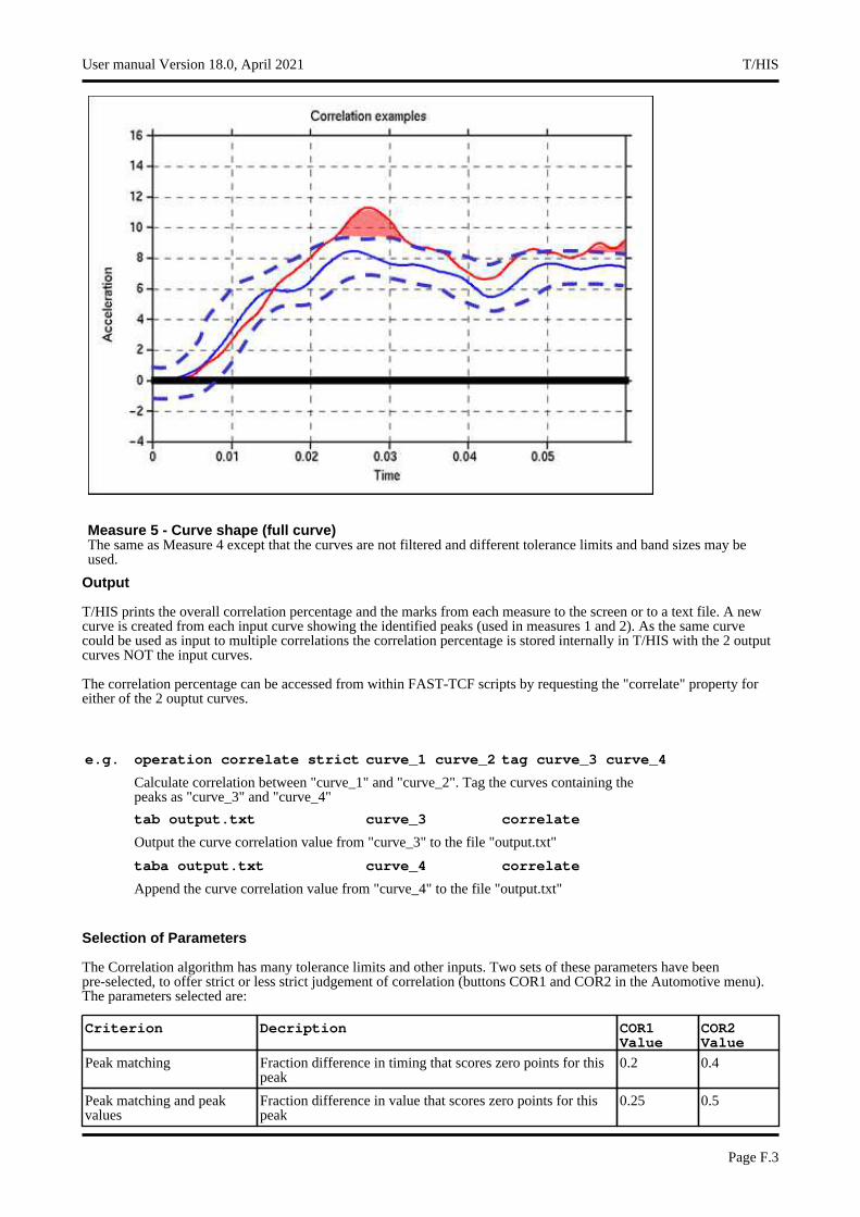
Measure 5 - Curve shape (full curve) The same as Measure 4 except that the curves are not filtered and different tolerance limits and band sizes may be used.
Output
T/HIS prints the overall correlation percentage and the marks from each measure to the screen or to a text file. A new curve is created from each input curve showing the identified peaks (used in measures 1 and 2). As the same curve could be used as input to multiple correlations the correlation percentage is stored internally in T/HIS with the 2 output curves NOT the input curves.
The correlation percentage can be accessed from within FAST-TCF scripts by requesting the "correlate" property for either of the 2 ouptut curves.
e.g. operation correlate strict curve_1 curve_2 tag curve_3 curve_4
Calculate correlation between "curve_1" and "curve_2". Tag the curves containing the peaks as "curve_3" and "curve_4"
tab output.txt curve_3 correlate
Output the curve correlation value from "curve_3" to the file "output.txt"
taba output.txt curve_4 correlate
Append the curve correlation value from "curve_4" to the file "output.txt"
Selection of Parameters
The Correlation algorithm has many tolerance limits and other inputs. Two sets of these parameters have been pre-selected, to offer strict or less strict judgement of correlation (buttons COR1 and COR2 in the Automotive menu). The parameters selected are:
Criterion Decription COR1 Value
COR2 Value
Peak matching Fraction difference in timing that scores zero points for this peak
0.2 0.4
Peak matching and peak values
Fraction difference in value that scores zero points for this peak
0.25 0.5
User manual Version 18.0, April 2021 T/HIS
Page F.3

Area matching Fraction difference in integral that scores zero points 0.3 0.5
Curve shape (low frequency trend)
Size of tolerance band in X and Y, as fractions of the curve extent in X and Y
0.025 0.05
Curve shape (low frequency trend)
Excursion area fraction scoring zero points 0.1 0.2
Curve shape (full curve) Size of tolerance band in X and Y, as fractions of the curve extent in X and Y
0.025 0.05
Curve shape (full curve) Excursion area fraction scoring zero points 0.2 0.4
It is expected that, if COR1 rates Curves A and B as better correlated than C and D, then COR2 would also rate the pairs of curves in the same order. The percentage correlation would be greater in each case from COR2 than from COR1. COR1 will provide a greater difference (discrimination) between well-correlated and very well-correlated pairs of curves; while COR2 will provide greater discrimination between averagely-correlated and poorly-correlated pairs of curves. The purpose of offering both versions of the correlation function is to allow the user to select a calibration of the function appropriate to the typical input curves used.
T/HIS User manual Version 18.0, April 2021
Page F.4

Examples COR1 COR2
17% 42%
27% 62%
User manual Version 18.0, April 2021 T/HIS
Page F.5
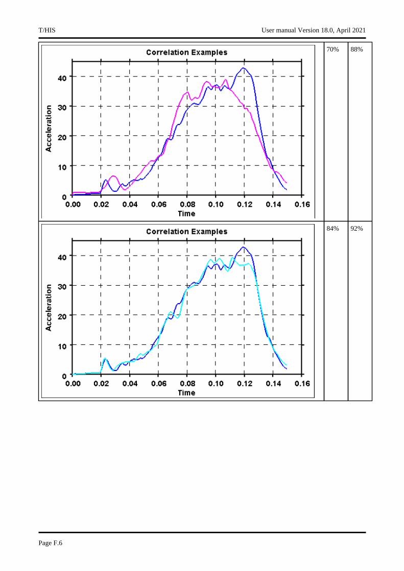
70% 88%
84% 92%
T/HIS User manual Version 18.0, April 2021
Page F.6
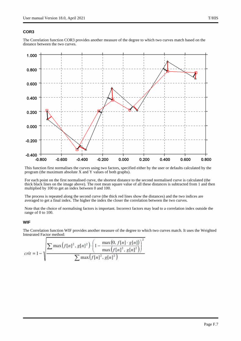
COR3
The Correlation function COR3 provides another measure of the degree to which two curves match based on the distance between the two curves.
This function first normalises the curves using two factors, specified either by the user or defaults calculated by the program (the maximum absolute X and Y values of both graphs).
For each point on the first normalised curve, the shortest distance to the second normalised curve is calculated (the thick black lines on the image above). The root mean square value of all these distances is subtracted from 1 and then multiplied by 100 to get an index between 0 and 100.
The process is repeated along the second curve (the thick red lines show the distances) and the two indices are averaged to get a final index. The higher the index the closer the correlation between the two curves.
Note that the choice of normalising factors is important. Incorrect factors may lead to a correlation index outside the range of 0 to 100.
WIF
The Correlation function WIF provides another measure of the degree to which two curves match. It uses the Weighted Integrated Factor method:
User manual Version 18.0, April 2021 T/HIS
Page F.7

T/HIS User manual Version 18.0, April 2021
Page F.8
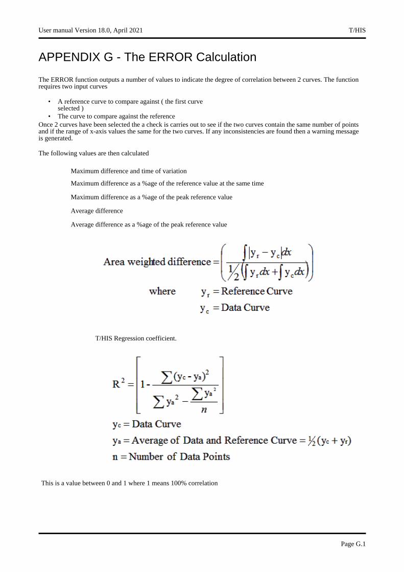
APPENDIX G - The ERROR Calculation
The ERROR function outputs a number of values to indicate the degree of correlation between 2 curves. The function requires two input curves
• A reference curve to compare against ( the first curve selected )
• The curve to compare against the referenceOnce 2 curves have been selected the a check is carries out to see if the two curves contain the same number of points and if the range of x-axis values the same for the two curves. If any inconsistencies are found then a warning message is generated.
The following values are then calculated
Maximum difference and time of variation
Maximum difference as a %age of the reference value at the same time
Maximum difference as a %age of the peak reference value
Average difference
Average difference as a %age of the peak reference value
T/HIS Regression coefficient.
This is a value between 0 and 1 where 1 means 100% correlation
User manual Version 18.0, April 2021 T/HIS
Page G.1

T/HIS User manual Version 18.0, April 2021
Page G.2
APPENDIX H - The "oa_pref" preference file This file contains code-specific preferences that can be used to modify the behaviour of T/HIS. It is optional and, where entries (or the whole file) are omitted T/HIS will revert to its default settings.
"oa_pref" naming convention and locations The file is called "oa_pref. It is looked for in the following places in the order given:
• The optional administration directory defined by the environmental variable ($OA_ADMIN or $OA_ADMIN_xx where xx is the release number).
• The site-wide installation directory defined by the environment variable ($OA_INSTALL) • The user’s home directory: $HOME (Unix/Linux) or %USERPROFILE% (Windows)• The current working directory
See Installation organisation for an explanation of the directory structure.
All four files are read (if they exist) and the last preference read will be the one used, so the file can be customised for a particular job or user at will.Files do not have to exist in any of these locations, and if none exists the programme defaults will be used.
On Unix and Linux: $HOME on Unix and Linux is usually the home directory specified for each user in the system password file.The shell command "printenv" (or on some systems "setenv") will show the value of this variable if set.If not set then it is defined as the "~" directory for the user. The command "cd; pwd" will show this.
On Windows: %USERPROFILE% on Windows is usually C:\Documents and Settings\<user id>\Issuing the "set" command from an MS-DOS prompt will show the value of this and other variables.
Generally speaking you should put • Organisation-wide options in the version in $OA_ADMIN_xx and/or $OA_INSTALL, • User-specific options in $HOME / %USERPROFILE%• Project-specific options in the current working directory.
The file contains preferences for the SHELL (lines commencing shell*), THIS (lines commencing this*), D3PLOT (lines commencing d3plot*), PRIMER (lines commencing primer*)and REPORTER (lines commencing reporter*). All lines take the format <preference name> <preference value>.
The general copy of the preference file should be present in the $OA_ADMIN_xx and/or $OA_INSTALL directory. This should contain the preferences most suitable for all software users on the system.
An individual’s specific preferences file can be stored in the individual’s home area. This can be used to personally customise the software to the individual’s needs.
Whenever one of the programs whose preferences can be stored in the oa_pref file is fired up, the program will take preferences first from the general preference file in the $OA_ADMIN_xx directory (if it exists) then the $OA_INSTALL directory, then from the file in the user’s home area, then from the current working directory.
Preferences defined in the general oa_pref file can be modified in the user’s personal file but they can’t be removed by it.
From version 9.4 onwards preferences can be locked. If a preference is locked it cannot be changed in an oa_pref file in a more junior directory. To lock a preference use the syntax ’this#’ rather than ’this*’.
The interactive Preferences Editor
You are free to edit oa_pref files by hand, but there is an interactive "Preferences Editor" that may be called from within T/HIS that makes the job much easier.
It is started by Options, Edit Preferences or through the Preferences Button in the Tool menu
The preferences editor reads an XML file that contains all possible preferences and their valid options, and allows you to change them at will. In this example the user is changing the background colour in D3PLOT.
Note that changes made in the Preferences editor will not affect the current session of D3PLOT, they will only take effect the next time it is run.
User manual Version 18.0, April 2021 T/HIS
Page H.1

If you have write permission on the oa_pref file in the $OASYS directory you will be asked if you want to update that file, otherwise you will only be given the option of updating your own file in your $HOME / $USERPROFILE directory.
In this example the user is changing the background colour.
The option is "active" (ie present in the oa_pref file) and currently is set to WHITE.
Usage is:• Select an option in the Tree on
the left hand side• Make it active / inactive• If active select a value from
the popup, or type in a value if necessary
The colour of the highlighting in the left hand side tree is significant:
Green Means that the option has been read from your $HOME/$USERPROFILE file.
Red Means that the option has been read from the $OA_INSTALL file.
Magenta Means that the option had been read from the $OA_ADMIN file.
In either event, regardless of the data source, the updated option will be written to the file chosen when you started the preferences editor.
Because of the order of file reading (see above), and option read from the master $OASYS file, amended, and written to your local $HOME file will take precedence when you next run T/HIS.
Locking Preferences
From version 9.4 onwards preferences can be locked. Beside each option in the preference editor is a padlock symbol. If the symbol is green then the option is unlocked, if it is red then it is locked. If a preference option has been locked in a file that the user can not modify then an error message will be generated if the user tries to edit that option.
If a user manually edits the "oa_pref" file to try and set an option that has been locked in another preference file then the option will be ignored in the users preference file.
T/HIS User manual Version 18.0, April 2021
Page H.2
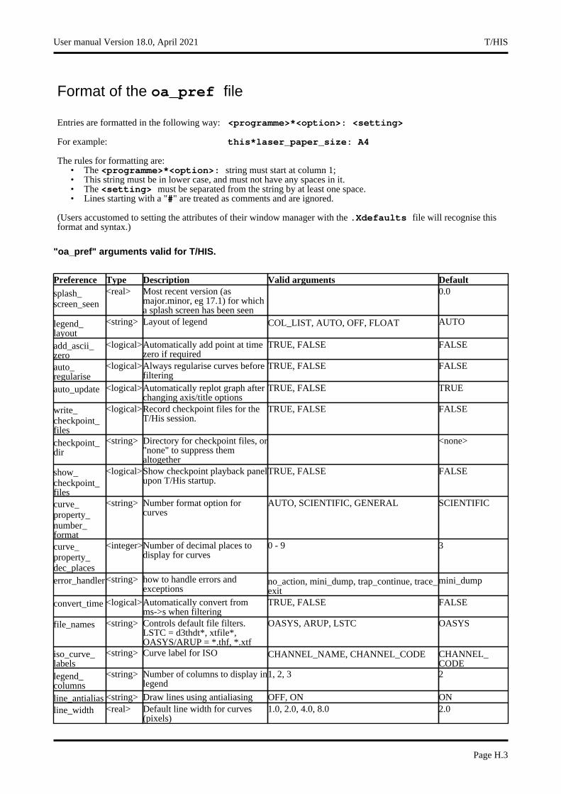
Format of the oa_pref file
Entries are formatted in the following way: <programme>*<option>: <setting>
For example: this*laser_paper_size: A4
The rules for formatting are:• The <programme>*<option>: string must start at column 1;• This string must be in lower case, and must not have any spaces in it.• The <setting> must be separated from the string by at least one space.• Lines starting with a "#" are treated as comments and are ignored.
(Users accustomed to setting the attributes of their window manager with the .Xdefaults file will recognise this format and syntax.)
"oa_pref" arguments valid for T/HIS.
Preference Type Description Valid arguments Defaultsplash_screen_seen
<real> Most recent version (as major.minor, eg 17.1) for which a splash screen has been seen
0.0
legend_layout
<string> Layout of legend COL_LIST, AUTO, OFF, FLOAT AUTO
add_ascii_zero
<logical>Automatically add point at time zero if required
TRUE, FALSE FALSE
auto_regularise
<logical>Always regularise curves before filtering
TRUE, FALSE FALSE
auto_update <logical>Automatically replot graph after changing axis/title options
TRUE, FALSE TRUE
write_checkpoint_files
<logical>Record checkpoint files for the T/His session.
TRUE, FALSE FALSE
checkpoint_dir
<string> Directory for checkpoint files, or "none" to suppress them altogether
<none>
show_checkpoint_files
<logical>Show checkpoint playback panel upon T/His startup.
TRUE, FALSE FALSE
curve_property_number_format
<string> Number format option for curves
AUTO, SCIENTIFIC, GENERAL SCIENTIFIC
curve_property_dec_places
<integer>Number of decimal places to display for curves
0 - 9 3
error_handler<string> how to handle errors and exceptions
no_action, mini_dump, trap_continue, trace_exit
mini_dump
convert_time <logical>Automatically convert from ms->s when filtering
TRUE, FALSE FALSE
file_names <string> Controls default file filters. LSTC = d3thdt*, xtfile*, OASYS/ARUP = *.thf, *.xtf
OASYS, ARUP, LSTC OASYS
iso_curve_labels
<string> Curve label for ISO CHANNEL_NAME, CHANNEL_CODE CHANNEL_CODE
legend_columns
<string> Number of columns to display in legend
1, 2, 3 2
line_antialias <string> Draw lines using antialiasing OFF, ON ONline_width <real> Default line width for curves
(pixels)1.0, 2.0, 4.0, 8.0 2.0
User manual Version 18.0, April 2021 T/HIS
Page H.3

datum_file <string> File containing DATUM line definitons
<none>
macro_directory
<string> Specify a directory for T/HIS to look in for MACRO definitions
$OA_INSTALL/this_library/macros
master_group_file
<string> Filename for default group information
<none>
read_group_files
<string> Default action when a group file is found in a model directory and T/HIS has already read a group file.
IGNORE, DELETE, OVERWRITE, INCREMENT
IGNORE
pemag_calculation_v12
<logical>Whether the PEMAG calculation uses the v12 logic.
TRUE, FALSE FALSE
plot_format <string> Default format of plot COLUMN, DEFAULT, AUTO, OFF, FULL, FLOATING
COLUMN
prefix_format<string> Select the prefix formatting for Legend curve labels.
MODEL, DIRECTORY, ROOTNAME, USER
MODEL
regularise_dt <real> Time interval for automatic curve regularisation
0.0001
second_y_axis
<logical>Display 2nd y axis TRUE, FALSE FALSE
show_hic_value
<string> Display HIC value ON, OFF OFF
show_3ms_value
<string> Display 3ms Clip value ON, OFF OFF
show_thiv_value
<string> Display THIV value ON, OFF OFF
show_phd_value
<string> Display PHD value ON, OFF OFF
injury_text_colour
<string> Colour used to display injury criteria values (hex code e.g. 0XA1B2C3 or core colour name e.g. OLIVE)
FOREGROUND, WHITE, BLACK, RED, GREEN, BLUE, CYAN, MAGENTA, YELLOW, ORANGE, TURQUOISE, INDIGO, LIME, SKY, PINK, PALE_YELLOW, GOLD, OLIVE, DARK_MAGENTA, MEDIUM_GREEN, MEDIUM_BLUE, HOT_PINK, LIGHT_PINK, SEA_GREEN, MAROON, DARK_GREEN, PURPLE, NAVY, DARK_GREY, MEDIUM_GREY, LIGHT_GREY
FOREGROUND
injury_line_colour
<string> Colour used to display injury criteria lines (hex code e.g. 0XA1B2C3 or core colour name e.g. OLIVE)
FOREGROUND, WHITE, BLACK, RED, GREEN, BLUE, CYAN, MAGENTA, YELLOW, ORANGE, TURQUOISE, INDIGO, LIME, SKY, PINK, PALE_YELLOW, GOLD, OLIVE, DARK_MAGENTA, MEDIUM_GREEN, MEDIUM_BLUE, HOT_PINK, LIGHT_PINK, SEA_GREEN, MAROON, DARK_GREEN, PURPLE, NAVY, DARK_GREY, MEDIUM_GREY, LIGHT_GREY
FOREGROUND
hic_time_window
<real> Length of time window for HIC automotive operation.
1e-10 - 1e37 0.036
hic_scale_factor
<real> Scale factor for acceleration used in HIC automotive operation.
1e-10 - 1e37 9.81
equation_x_start
<real> X axis start value for equation curves.
-1e37 - 1e37 0.0
equation_x_interval
<real> X interval between points for equation curves.
1e-10 - 1e37 0.001
equation_npoints
<real> Number of points for equation curves. Not used if equation_x_interval is defined.
1 - 1e7 0.001
T/HIS User manual Version 18.0, April 2021
Page H.4
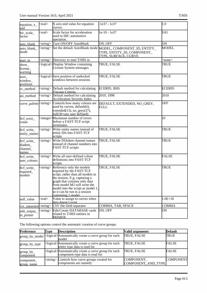
equation_x_end
<real> X axis end value for equation curves.
-1e37 - 1e37 1.0
hic_scale_factor
<real> Scale factor for acceleration used in HIC automotive operation.
1e-10 - 1e37 9.81
auto_blank <string> Turn ON/OFF AutoBlank ON, OFF ONauto_blank_mode
<string> Set the default AutoBlank mode MODEL, COMPONENT_ID, ENTITY_TYPE, ENTITY_ID, COMPONENT_TYPE, SURFACE, CURVE
MODEL
start_in <string> Directory to start T/HIS in <none>show_license_warning
<logical>Display Window containing License System messages
TRUE, FALSE TRUE
save_window_positions
<logical>Save position of undocked windows between sessions
TRUE, FALSE TRUE
vc_method <string> Default method for calculating Viscous Criteria
ECER95, IIHS ECER95
asi_method <string> Default method for calculating Acceleration Severity Index
2010, 1998 2010
curve_palette <string> Controls how many colours are used by curves, default(6), extended(13), no_grey(27), full(30+any user defined)
DEFAULT, EXTENDED, NO_GREY, FULL
OFF
ftcf_error_count
<integer>Maximum number of errors before a FAST-TCF script terminates
10
ftcf_write_entity_names
<string> Write entity names instead of entity IDs into FAST-TCF scripts
TRUE, FALSE TRUE
ftcf_write_diadem_channel_names
<string> Write DIAdem channel names instead of channel numbers into FAST-TCF scripts
TRUE, FALSE TRUE
ftcf_write_user_colours
<string> Write all user-defined colour definitions into FAST-TCF scripts
TRUE, FALSE FALSE
ftcf_write_required_models
<string> Reference only the models required by the FAST-TCF script, rather than all models in the session. E.g. capturing a graph that contains only data from model M2 will write the model into the script as model 1, so it can be run in a session containing 1 model.
TRUE, FALSE TRUE
null_value <real> Value to assign to curves when data doesn’t exist
1.0E+18
csv_separator<string> CSV file field separator COMMA, TAB, SPACE COMMA
edit_output_in_primer
<string> Edit/Create DATABASE cards related to T/HIS entities in PRIMER
ON, OFF ON
The following options control the automatic creation of curve groups.
Preference Type Description Valid arguments Defaultgroup_by_model <logical>Automatically create a curve group for each
modelTRUE, FALSE TRUE
group_by_type <logical>Automatically create a curve group for each entity type data is read for
TRUE, FALSE FALSE
group_by_component
<logical>Automatically create a curve group for each component type data is read for
TRUE, FALSE FALSE
component_group_name
<string> Controls how curve groups created for components are named)
COMPONENT, COMPONENT_AND_TYPE
COMPONENT
User manual Version 18.0, April 2021 T/HIS
Page H.5
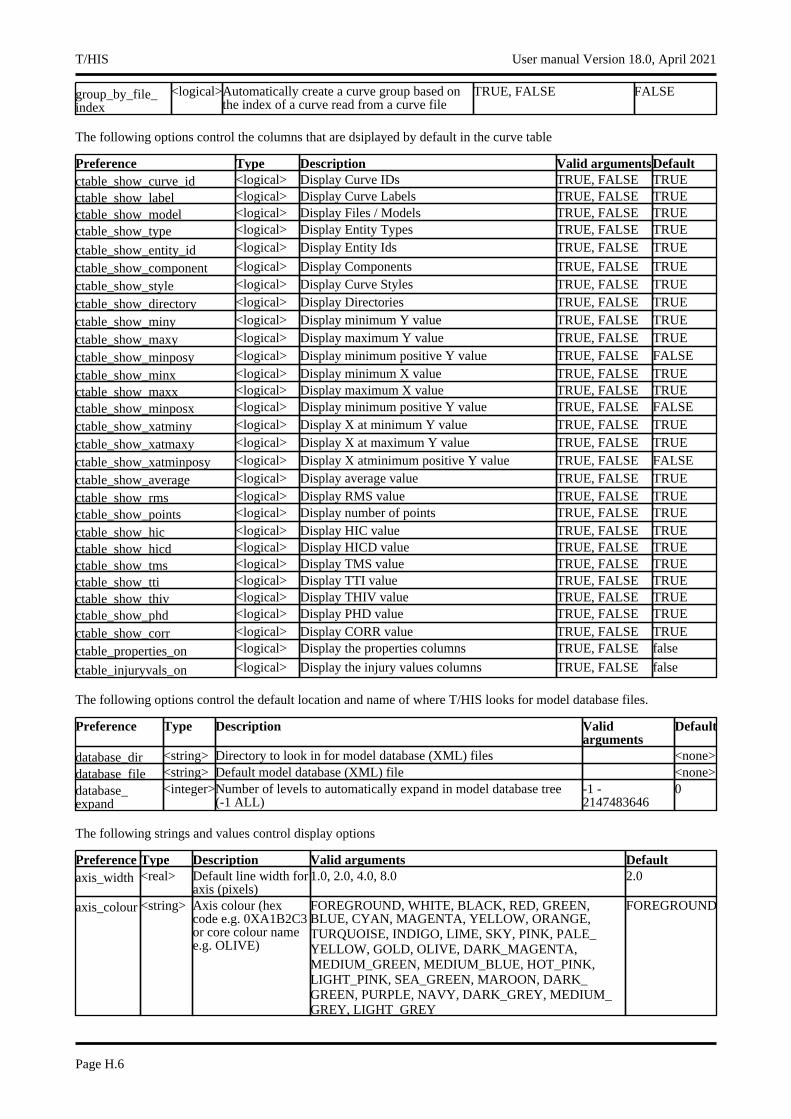
group_by_file_index
<logical>Automatically create a curve group based on the index of a curve read from a curve file
TRUE, FALSE FALSE
The following options control the columns that are dsiplayed by default in the curve table
Preference Type Description Valid argumentsDefaultctable_show_curve_id <logical> Display Curve IDs TRUE, FALSE TRUEctable_show_label <logical> Display Curve Labels TRUE, FALSE TRUEctable_show_model <logical> Display Files / Models TRUE, FALSE TRUEctable_show_type <logical> Display Entity Types TRUE, FALSE TRUE
ctable_show_entity_id <logical> Display Entity Ids TRUE, FALSE TRUE
ctable_show_component <logical> Display Components TRUE, FALSE TRUE
ctable_show_style <logical> Display Curve Styles TRUE, FALSE TRUE
ctable_show_directory <logical> Display Directories TRUE, FALSE TRUE
ctable_show_miny <logical> Display minimum Y value TRUE, FALSE TRUE
ctable_show_maxy <logical> Display maximum Y value TRUE, FALSE TRUE
ctable_show_minposy <logical> Display minimum positive Y value TRUE, FALSE FALSE
ctable_show_minx <logical> Display minimum X value TRUE, FALSE TRUEctable_show_maxx <logical> Display maximum X value TRUE, FALSE TRUEctable_show_minposx <logical> Display minimum positive Y value TRUE, FALSE FALSE
ctable_show_xatminy <logical> Display X at minimum Y value TRUE, FALSE TRUE
ctable_show_xatmaxy <logical> Display X at maximum Y value TRUE, FALSE TRUE
ctable_show_xatminposy <logical> Display X atminimum positive Y value TRUE, FALSE FALSE
ctable_show_average <logical> Display average value TRUE, FALSE TRUE
ctable_show_rms <logical> Display RMS value TRUE, FALSE TRUEctable_show_points <logical> Display number of points TRUE, FALSE TRUE
ctable_show_hic <logical> Display HIC value TRUE, FALSE TRUEctable_show_hicd <logical> Display HICD value TRUE, FALSE TRUEctable_show_tms <logical> Display TMS value TRUE, FALSE TRUEctable_show_tti <logical> Display TTI value TRUE, FALSE TRUEctable_show_thiv <logical> Display THIV value TRUE, FALSE TRUEctable_show_phd <logical> Display PHD value TRUE, FALSE TRUE
ctable_show_corr <logical> Display CORR value TRUE, FALSE TRUE
ctable_properties_on <logical> Display the properties columns TRUE, FALSE false
ctable_injuryvals_on <logical> Display the injury values columns TRUE, FALSE false
The following options control the default location and name of where T/HIS looks for model database files.
Preference Type Description Valid arguments
Default
database_dir <string> Directory to look in for model database (XML) files <none>database_file <string> Default model database (XML) file <none>database_expand
<integer>Number of levels to automatically expand in model database tree (-1 ALL)
-1 - 2147483646
0
The following strings and values control display options
Preference Type Description Valid arguments Defaultaxis_width <real> Default line width for
axis (pixels)1.0, 2.0, 4.0, 8.0 2.0
axis_colour <string> Axis colour (hex code e.g. 0XA1B2C3 or core colour name e.g. OLIVE)
FOREGROUND, WHITE, BLACK, RED, GREEN, BLUE, CYAN, MAGENTA, YELLOW, ORANGE, TURQUOISE, INDIGO, LIME, SKY, PINK, PALE_YELLOW, GOLD, OLIVE, DARK_MAGENTA, MEDIUM_GREEN, MEDIUM_BLUE, HOT_PINK, LIGHT_PINK, SEA_GREEN, MAROON, DARK_GREEN, PURPLE, NAVY, DARK_GREY, MEDIUM_GREY, LIGHT_GREY
FOREGROUND
T/HIS User manual Version 18.0, April 2021
Page H.6
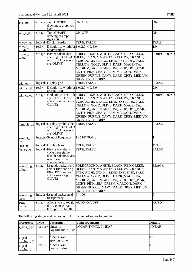
axis_top <string> Turn ON/OFF drawing of graph top axis
ON, OFF ON
axis_right <string> Turn ON/OFF drawing of graph right axis
ON, OFF ON
border_on <logical>Display border TRUE, FALSE TRUEborder_width
<real> Default line width for border (pixels)
1.0, 2.0, 4.0, 8.0 1.0
border_colour
<string> Border colour (hex code e.g. 0XA1B2C3 or core colour name e.g. OLIVE)
FOREGROUND, WHITE, BLACK, RED, GREEN, BLUE, CYAN, MAGENTA, YELLOW, ORANGE, TURQUOISE, INDIGO, LIME, SKY, PINK, PALE_YELLOW, GOLD, OLIVE, DARK_MAGENTA, MEDIUM_GREEN, MEDIUM_BLUE, HOT_PINK, LIGHT_PINK, SEA_GREEN, MAROON, DARK_GREEN, PURPLE, NAVY, DARK_GREY, MEDIUM_GREY, LIGHT_GREY
FOREGROUND
grid_on <logical>Display grid TRUE, FALSE FALSE
grid_width <real> Default line width for grid (pixels)
1.0, 2.0, 4.0, 8.0 2.0
grid_colour <string> Grid colour (hex code e.g. 0XA1B2C3 or core colour name e.g. OLIVE)
FOREGROUND, WHITE, BLACK, RED, GREEN, BLUE, CYAN, MAGENTA, YELLOW, ORANGE, TURQUOISE, INDIGO, LIME, SKY, PINK, PALE_YELLOW, GOLD, OLIVE, DARK_MAGENTA, MEDIUM_GREEN, MEDIUM_BLUE, HOT_PINK, LIGHT_PINK, SEA_GREEN, MAROON, DARK_GREEN, PURPLE, NAVY, DARK_GREY, MEDIUM_GREY, LIGHT_GREY
FOREGROUND
symbols_on<logical>Display symbols (hex code e.g. 0XA1B2C3 or core colour name e.g. OLIVE)
TRUE, FALSE FALSE
symbol_freq
<integer>Symbol Frequency 1 - 2147483646 1
lines_on <logical>Display lines TRUE, FALSE TRUEfix_styles <logical>Fix curve styles to
cycle through the default colours/styles regardless of the curve number
TRUE, FALSE FALSE
legend_bg_colour
<string> Legends background colour (hex code e.g. 0XA1B2C3 or core colour name e.g. OLIVE)
FOREGROUND, WHITE, BLACK, RED, GREEN, BLUE, CYAN, MAGENTA, YELLOW, ORANGE, TURQUOISE, INDIGO, LIME, SKY, PINK, PALE_YELLOW, GOLD, OLIVE, DARK_MAGENTA, MEDIUM_GREEN, MEDIUM_BLUE, HOT_PINK, LIGHT_PINK, SEA_GREEN, MAROON, DARK_GREEN, PURPLE, NAVY, DARK_GREY, MEDIUM_GREY, LIGHT_GREY
BLACK
legend_bg_trans
<integer>Legend background transparency
0 - 100 0
show_prefix
<string> Allows you to toggle the Legend curve label prefix On/Off
AUTO, ON, OFF AUTO
The following strings and values control formatting of values for graphs
Preference Type Description Valid arguments Defaultx_axis_type <string> Linear or
Logarithmic X Axis type
LOGARITHMIC, LINEAR LINEAR
x_grid_spacing_off
<real> X-Axis Grid Spacing value
0.0
x_grid_spacing_int
<real> X-Axis Grid Interval value
0.0
User manual Version 18.0, April 2021 T/HIS
Page H.7
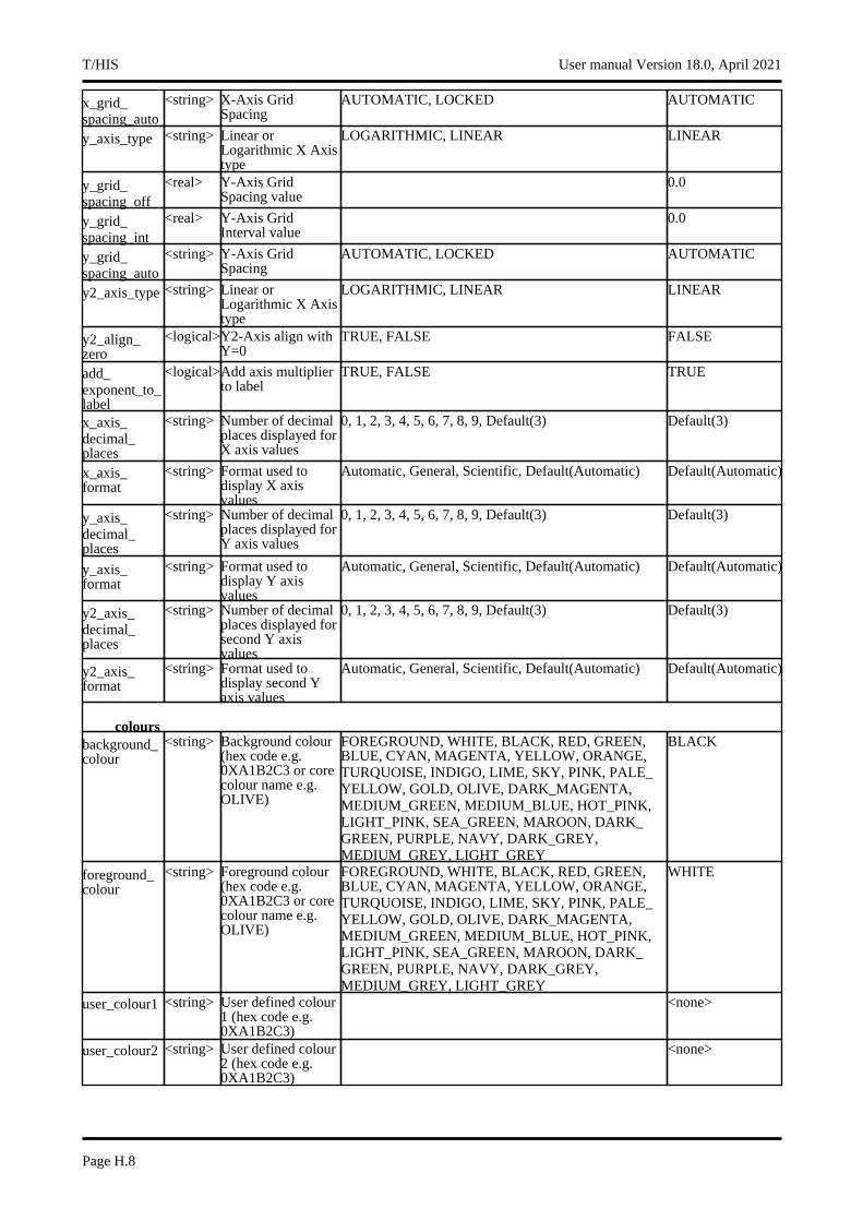
x_grid_spacing_auto
<string> X-Axis Grid Spacing
AUTOMATIC, LOCKED AUTOMATIC
y_axis_type <string> Linear or Logarithmic X Axis type
LOGARITHMIC, LINEAR LINEAR
y_grid_spacing_off
<real> Y-Axis Grid Spacing value
0.0
y_grid_spacing_int
<real> Y-Axis Grid Interval value
0.0
y_grid_spacing_auto
<string> Y-Axis Grid Spacing
AUTOMATIC, LOCKED AUTOMATIC
y2_axis_type <string> Linear or Logarithmic X Axis type
LOGARITHMIC, LINEAR LINEAR
y2_align_zero
<logical>Y2-Axis align with Y=0
TRUE, FALSE FALSE
add_exponent_to_label
<logical>Add axis multiplier to label
TRUE, FALSE TRUE
x_axis_decimal_places
<string> Number of decimal places displayed for X axis values
0, 1, 2, 3, 4, 5, 6, 7, 8, 9, Default(3) Default(3)
x_axis_format
<string> Format used to display X axis values
Automatic, General, Scientific, Default(Automatic) Default(Automatic)
y_axis_decimal_places
<string> Number of decimal places displayed for Y axis values
0, 1, 2, 3, 4, 5, 6, 7, 8, 9, Default(3) Default(3)
y_axis_format
<string> Format used to display Y axis values
Automatic, General, Scientific, Default(Automatic) Default(Automatic)
y2_axis_decimal_places
<string> Number of decimal places displayed for second Y axis values
0, 1, 2, 3, 4, 5, 6, 7, 8, 9, Default(3) Default(3)
y2_axis_format
<string> Format used to display second Y axis values
Automatic, General, Scientific, Default(Automatic) Default(Automatic)
coloursbackground_colour
<string> Background colour (hex code e.g. 0XA1B2C3 or core colour name e.g. OLIVE)
FOREGROUND, WHITE, BLACK, RED, GREEN, BLUE, CYAN, MAGENTA, YELLOW, ORANGE, TURQUOISE, INDIGO, LIME, SKY, PINK, PALE_YELLOW, GOLD, OLIVE, DARK_MAGENTA, MEDIUM_GREEN, MEDIUM_BLUE, HOT_PINK, LIGHT_PINK, SEA_GREEN, MAROON, DARK_GREEN, PURPLE, NAVY, DARK_GREY, MEDIUM_GREY, LIGHT_GREY
BLACK
foreground_colour
<string> Foreground colour (hex code e.g. 0XA1B2C3 or core colour name e.g. OLIVE)
FOREGROUND, WHITE, BLACK, RED, GREEN, BLUE, CYAN, MAGENTA, YELLOW, ORANGE, TURQUOISE, INDIGO, LIME, SKY, PINK, PALE_YELLOW, GOLD, OLIVE, DARK_MAGENTA, MEDIUM_GREEN, MEDIUM_BLUE, HOT_PINK, LIGHT_PINK, SEA_GREEN, MAROON, DARK_GREEN, PURPLE, NAVY, DARK_GREY, MEDIUM_GREY, LIGHT_GREY
WHITE
user_colour1 <string> User defined colour 1 (hex code e.g. 0XA1B2C3)
<none>
user_colour2 <string> User defined colour 2 (hex code e.g. 0XA1B2C3)
<none>
T/HIS User manual Version 18.0, April 2021
Page H.8
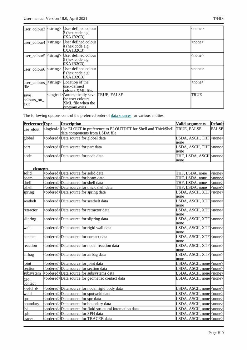
user_colour3 <string> User defined colour 3 (hex code e.g. 0XA1B2C3)
<none>
user_colour4 <string> User defined colour 4 (hex code e.g. 0XA1B2C3)
<none>
user_colour5 <string> User defined colour 5 (hex code e.g. 0XA1B2C3)
<none>
user_colour6 <string> User defined colour 6 (hex code e.g. 0XA1B2C3)
<none>
user_colours_file
<string> Location of the user-defined colours XML file.
<none>
save_colours_on_exit
<logical>Automatically save the user colours XML file when the program exits.
TRUE, FALSE TRUE
The following options control the preferred order of data sources for various entities
Preference Type Description Valid arguments Defaultuse_elout <logical> Use ELOUT in preference to ELOUTDET for Shell and ThickShell
data components from LSDA fileTRUE, FALSE FALSE
global <ordered>Data source for global data LSDA, ASCII, THF, none
<none>
part <ordered>Data source for part data LSDA, ASCII, THF, none
<none>
node <ordered>Data source for node data THF, LSDA, ASCII, none
<none>
elementssolid <ordered>Data source for solid data THF, LSDA, none <none>beam <ordered>Data source for beam data THF, LSDA, none <none>shell <ordered>Data source for shell data THF, LSDA, none <none>tshell <ordered>Data source for thick shell data THF, LSDA, none <none>spring <ordered>Data source for spring data LSDA, ASCII, XTF,
none<none>
seatbelt <ordered>Data source for seatbelt data LSDA, ASCII, XTF, none
<none>
retractor <ordered>Data source for retractor data LSDA, ASCII, XTF, none
<none>
slipring <ordered>Data source for slipring data LSDA, ASCII, XTF, none
<none>
wall <ordered>Data source for rigid wall data LSDA, ASCII, XTF, none
<none>
contact <ordered>Data source for contact data LSDA, ASCII, XTF, none
<none>
reaction <ordered>Data source for nodal reaction data LSDA, ASCII, XTF, none
<none>
airbag <ordered>Data source for airbag data LSDA, ASCII, XTF, none
<none>
joint <ordered>Data source for joint data LSDA, ASCII, none <none>section <ordered>Data source for section data LSDA, ASCII, none <none>subsystem <ordered>Data source for subsystems data LSDA, ASCII, none <none>
geo_contact
<ordered>Data source for geometric contact data LSDA, ASCII, none <none>
nodal_rb <ordered>Data source for nodal rigid body data LSDA, ASCII, none <none>weld <ordered>Data source for spotweld data LSDA, ASCII, none <none>spc <ordered>Data source for spc data LSDA, ASCII, none <none>boundary <ordered>Data source for boundary data LSDA, ASCII, none <none>fsi <ordered>Data source for fluid structural interaction data LSDA, ASCII, none <none>sph <ordered>Data source for SPH data LSDA, ASCII, none <none>tracer <ordered>Data source for TRACER data LSDA, ASCII, none <none>
User manual Version 18.0, April 2021 T/HIS
Page H.9
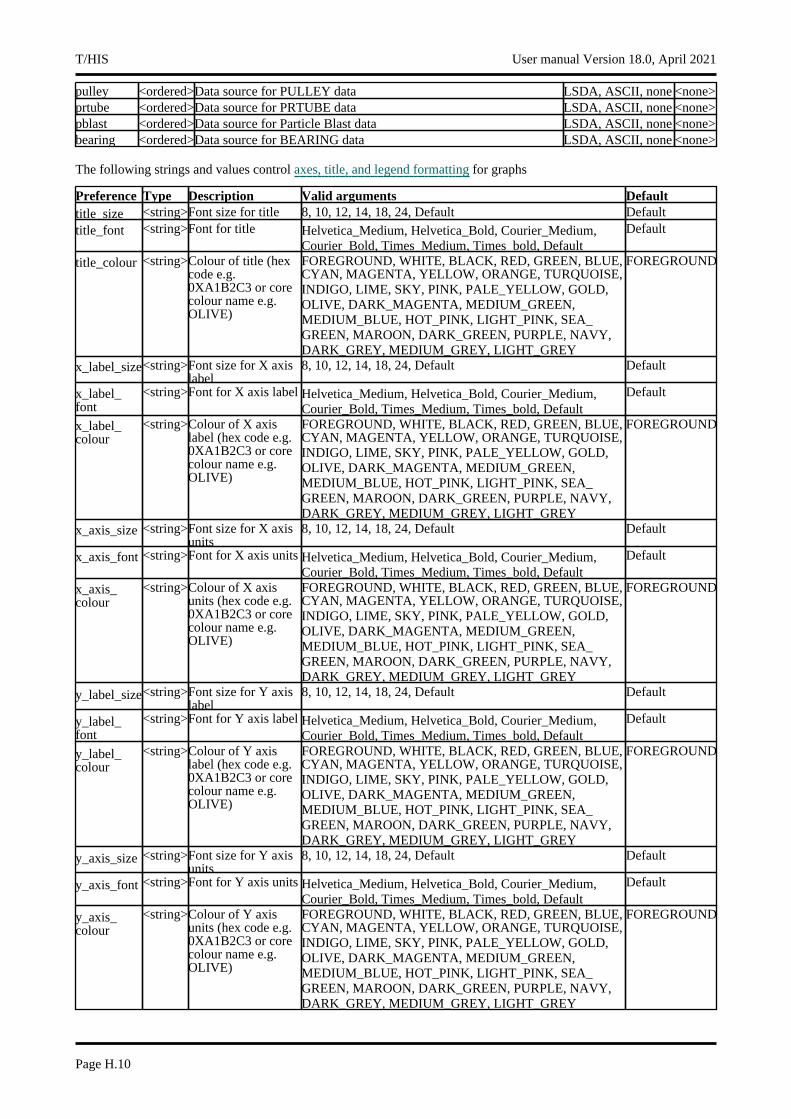
pulley <ordered>Data source for PULLEY data LSDA, ASCII, none <none>prtube <ordered>Data source for PRTUBE data LSDA, ASCII, none <none>pblast <ordered>Data source for Particle Blast data LSDA, ASCII, none <none>bearing <ordered>Data source for BEARING data LSDA, ASCII, none <none>
The following strings and values control axes, title, and legend formatting for graphs
Preference Type Description Valid arguments Defaulttitle_size <string>Font size for title 8, 10, 12, 14, 18, 24, Default Defaulttitle_font <string>Font for title Helvetica_Medium, Helvetica_Bold, Courier_Medium,
Courier_Bold, Times_Medium, Times_bold, DefaultDefault
title_colour <string>Colour of title (hex code e.g. 0XA1B2C3 or core colour name e.g. OLIVE)
FOREGROUND, WHITE, BLACK, RED, GREEN, BLUE, CYAN, MAGENTA, YELLOW, ORANGE, TURQUOISE, INDIGO, LIME, SKY, PINK, PALE_YELLOW, GOLD, OLIVE, DARK_MAGENTA, MEDIUM_GREEN, MEDIUM_BLUE, HOT_PINK, LIGHT_PINK, SEA_GREEN, MAROON, DARK_GREEN, PURPLE, NAVY, DARK_GREY, MEDIUM_GREY, LIGHT_GREY
FOREGROUND
x_label_size<string>Font size for X axis label
8, 10, 12, 14, 18, 24, Default Default
x_label_font
<string>Font for X axis label Helvetica_Medium, Helvetica_Bold, Courier_Medium, Courier_Bold, Times_Medium, Times_bold, Default
Default
x_label_colour
<string>Colour of X axis label (hex code e.g. 0XA1B2C3 or core colour name e.g. OLIVE)
FOREGROUND, WHITE, BLACK, RED, GREEN, BLUE, CYAN, MAGENTA, YELLOW, ORANGE, TURQUOISE, INDIGO, LIME, SKY, PINK, PALE_YELLOW, GOLD, OLIVE, DARK_MAGENTA, MEDIUM_GREEN, MEDIUM_BLUE, HOT_PINK, LIGHT_PINK, SEA_GREEN, MAROON, DARK_GREEN, PURPLE, NAVY, DARK_GREY, MEDIUM_GREY, LIGHT_GREY
FOREGROUND
x_axis_size <string>Font size for X axis units
8, 10, 12, 14, 18, 24, Default Default
x_axis_font <string>Font for X axis units Helvetica_Medium, Helvetica_Bold, Courier_Medium, Courier_Bold, Times_Medium, Times_bold, Default
Default
x_axis_colour
<string>Colour of X axis units (hex code e.g. 0XA1B2C3 or core colour name e.g. OLIVE)
FOREGROUND, WHITE, BLACK, RED, GREEN, BLUE, CYAN, MAGENTA, YELLOW, ORANGE, TURQUOISE, INDIGO, LIME, SKY, PINK, PALE_YELLOW, GOLD, OLIVE, DARK_MAGENTA, MEDIUM_GREEN, MEDIUM_BLUE, HOT_PINK, LIGHT_PINK, SEA_GREEN, MAROON, DARK_GREEN, PURPLE, NAVY, DARK_GREY, MEDIUM_GREY, LIGHT_GREY
FOREGROUND
y_label_size<string>Font size for Y axis label
8, 10, 12, 14, 18, 24, Default Default
y_label_font
<string>Font for Y axis label Helvetica_Medium, Helvetica_Bold, Courier_Medium, Courier_Bold, Times_Medium, Times_bold, Default
Default
y_label_colour
<string>Colour of Y axis label (hex code e.g. 0XA1B2C3 or core colour name e.g. OLIVE)
FOREGROUND, WHITE, BLACK, RED, GREEN, BLUE, CYAN, MAGENTA, YELLOW, ORANGE, TURQUOISE, INDIGO, LIME, SKY, PINK, PALE_YELLOW, GOLD, OLIVE, DARK_MAGENTA, MEDIUM_GREEN, MEDIUM_BLUE, HOT_PINK, LIGHT_PINK, SEA_GREEN, MAROON, DARK_GREEN, PURPLE, NAVY, DARK_GREY, MEDIUM_GREY, LIGHT_GREY
FOREGROUND
y_axis_size <string>Font size for Y axis units
8, 10, 12, 14, 18, 24, Default Default
y_axis_font <string>Font for Y axis units Helvetica_Medium, Helvetica_Bold, Courier_Medium, Courier_Bold, Times_Medium, Times_bold, Default
Default
y_axis_colour
<string>Colour of Y axis units (hex code e.g. 0XA1B2C3 or core colour name e.g. OLIVE)
FOREGROUND, WHITE, BLACK, RED, GREEN, BLUE, CYAN, MAGENTA, YELLOW, ORANGE, TURQUOISE, INDIGO, LIME, SKY, PINK, PALE_YELLOW, GOLD, OLIVE, DARK_MAGENTA, MEDIUM_GREEN, MEDIUM_BLUE, HOT_PINK, LIGHT_PINK, SEA_GREEN, MAROON, DARK_GREEN, PURPLE, NAVY, DARK_GREY, MEDIUM_GREY, LIGHT_GREY
FOREGROUND
T/HIS User manual Version 18.0, April 2021
Page H.10
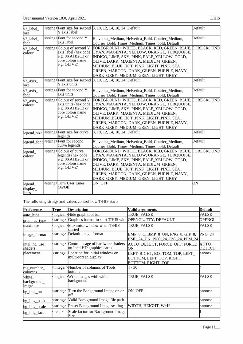
y2_label_size
<string>Font size for second Y axis label
8, 10, 12, 14, 18, 24, Default Default
y2_label_font
<string>Font for second Y axis label
Helvetica_Medium, Helvetica_Bold, Courier_Medium, Courier_Bold, Times_Medium, Times_bold, Default
Default
y2_label_colour
<string>Colour of second Y axis label (hex code e.g. 0XA1B2C3 or core colour name e.g. OLIVE)
FOREGROUND, WHITE, BLACK, RED, GREEN, BLUE, CYAN, MAGENTA, YELLOW, ORANGE, TURQUOISE, INDIGO, LIME, SKY, PINK, PALE_YELLOW, GOLD, OLIVE, DARK_MAGENTA, MEDIUM_GREEN, MEDIUM_BLUE, HOT_PINK, LIGHT_PINK, SEA_GREEN, MAROON, DARK_GREEN, PURPLE, NAVY, DARK_GREY, MEDIUM_GREY, LIGHT_GREY
FOREGROUND
y2_axis_size
<string>Font size for second Y axis units
8, 10, 12, 14, 18, 24, Default Default
y2_axis_font
<string>Font for second Y axis units
Helvetica_Medium, Helvetica_Bold, Courier_Medium, Courier_Bold, Times_Medium, Times_bold, Default
Default
y2_axis_colour
<string>Colour of second Y axis units (hex code e.g. 0XA1B2C3 or core colour name e.g. OLIVE)
FOREGROUND, WHITE, BLACK, RED, GREEN, BLUE, CYAN, MAGENTA, YELLOW, ORANGE, TURQUOISE, INDIGO, LIME, SKY, PINK, PALE_YELLOW, GOLD, OLIVE, DARK_MAGENTA, MEDIUM_GREEN, MEDIUM_BLUE, HOT_PINK, LIGHT_PINK, SEA_GREEN, MAROON, DARK_GREEN, PURPLE, NAVY, DARK_GREY, MEDIUM_GREY, LIGHT_GREY
FOREGROUND
legend_size <string>Font size for curve legends
8, 10, 12, 14, 18, 24, Default Default
legend_font <string>Font for second curve legends
Helvetica_Medium, Helvetica_Bold, Courier_Medium, Courier_Bold, Times_Medium, Times_bold, Default
Default
legend_colour
<string>Colour of curve legends (hex code e.g. 0XA1B2C3 or core colour name e.g. OLIVE)
FOREGROUND, WHITE, BLACK, RED, GREEN, BLUE, CYAN, MAGENTA, YELLOW, ORANGE, TURQUOISE, INDIGO, LIME, SKY, PINK, PALE_YELLOW, GOLD, OLIVE, DARK_MAGENTA, MEDIUM_GREEN, MEDIUM_BLUE, HOT_PINK, LIGHT_PINK, SEA_GREEN, MAROON, DARK_GREEN, PURPLE, NAVY, DARK_GREY, MEDIUM_GREY, LIGHT_GREY
FOREGROUND
legend_display_lines
<string>Turn User Lines On/Off
ON, OFF ON
The following strings and values control how T/HIS starts
Preference Type Description Valid arguments Defaultauto_hide <logical>Hide graph tool bar TRUE, FALSE FALSE
graphics_type <string> Graphics format to start T/HIS with OPENGL, TTY, DEFAULT OPENGL
maximise <logical>Maximise window when T/HIS started
TRUE, FALSE FALSE
image_format <string> Default image format BMP_8_C, BMP_8_UN, PNG_8, GIF_8, BMP_24_UN, PNG_24, JPG_24, PPM_24
PNG_24
intel_hd_use_shaders
<string> Control usage of hardware shaders on Intel HD graphics cards
AUTO_DETECT, FORCE_OFF, FORCE_ON
AUTO_DETECT
placement <string> Location for initial window on multi-screen display
LEFT, RIGHT, BOTTOM, TOP, LEFT_BOTTOM, LEFT_TOP, RIGHT_BOTTOM, RIGHT_TOP
<none>
rhs_number_columns
<integer>Number of columns of Tools buttons
4 - 50 4
white_background_image
<logical>Write images with white background
TRUE, FALSE FALSE
bg_img_on <string> Turn the Background Image on or off.
ON, OFF <none>
bg_img_path <string> Valid Background Image file path <none>
bg_img_scale <string> Preset Background Image scaling WIDTH, HEIGHT, W+H <none>
bg_img_fact <real> Scale factor for Background Image Size
1
User manual Version 18.0, April 2021 T/HIS
Page H.11
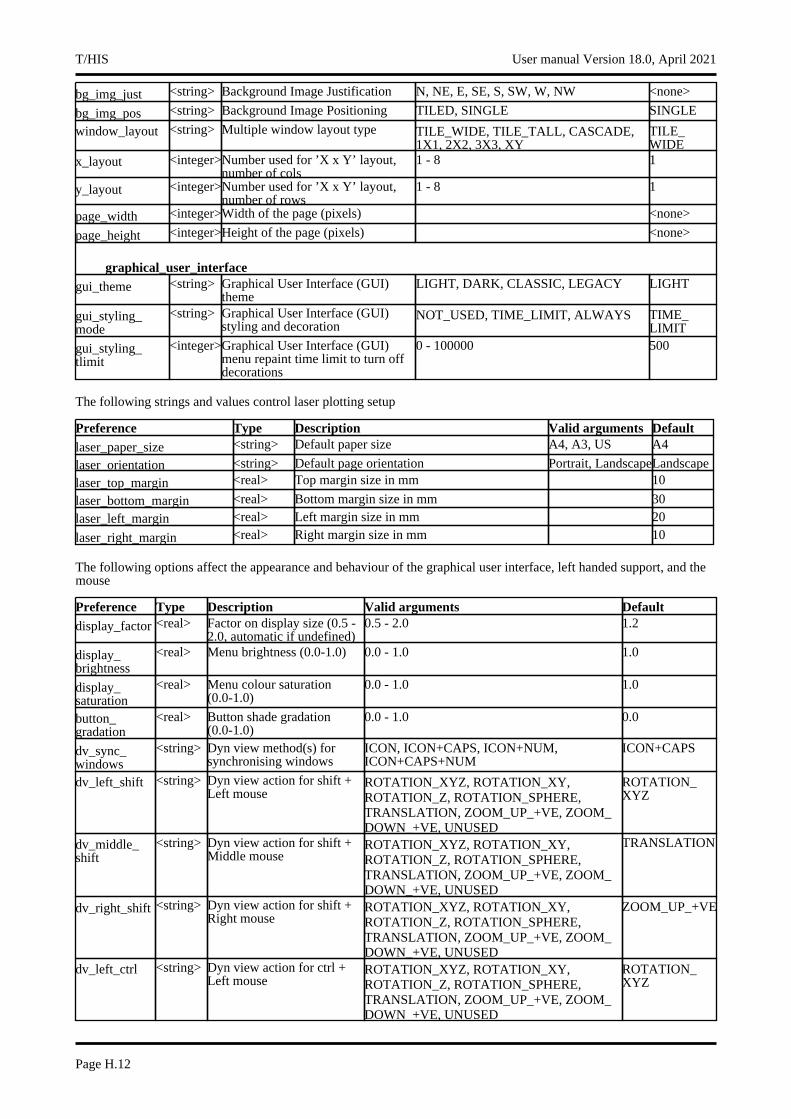
bg_img_just <string> Background Image Justification N, NE, E, SE, S, SW, W, NW <none>
bg_img_pos <string> Background Image Positioning TILED, SINGLE SINGLE
window_layout <string> Multiple window layout type TILE_WIDE, TILE_TALL, CASCADE, 1X1, 2X2, 3X3, XY
TILE_WIDE
x_layout <integer>Number used for ’X x Y’ layout, number of cols
1 - 8 1
y_layout <integer>Number used for ’X x Y’ layout, number of rows
1 - 8 1
page_width <integer>Width of the page (pixels) <none>
page_height <integer>Height of the page (pixels) <none>
graphical_user_interfacegui_theme <string> Graphical User Interface (GUI)
themeLIGHT, DARK, CLASSIC, LEGACY LIGHT
gui_styling_mode
<string> Graphical User Interface (GUI) styling and decoration
NOT_USED, TIME_LIMIT, ALWAYS TIME_LIMIT
gui_styling_tlimit
<integer>Graphical User Interface (GUI) menu repaint time limit to turn off decorations
0 - 100000 500
The following strings and values control laser plotting setup
Preference Type Description Valid arguments Defaultlaser_paper_size <string> Default paper size A4, A3, US A4
laser_orientation <string> Default page orientation Portrait, LandscapeLandscape
laser_top_margin <real> Top margin size in mm 10
laser_bottom_margin <real> Bottom margin size in mm 30
laser_left_margin <real> Left margin size in mm 20
laser_right_margin <real> Right margin size in mm 10
The following options affect the appearance and behaviour of the graphical user interface, left handed support, and the mouse
Preference Type Description Valid arguments Defaultdisplay_factor <real> Factor on display size (0.5 -
2.0, automatic if undefined)0.5 - 2.0 1.2
display_brightness
<real> Menu brightness (0.0-1.0) 0.0 - 1.0 1.0
display_saturation
<real> Menu colour saturation (0.0-1.0)
0.0 - 1.0 1.0
button_gradation
<real> Button shade gradation (0.0-1.0)
0.0 - 1.0 0.0
dv_sync_windows
<string> Dyn view method(s) for synchronising windows
ICON, ICON+CAPS, ICON+NUM, ICON+CAPS+NUM
ICON+CAPS
dv_left_shift <string> Dyn view action for shift + Left mouse
ROTATION_XYZ, ROTATION_XY, ROTATION_Z, ROTATION_SPHERE, TRANSLATION, ZOOM_UP_+VE, ZOOM_DOWN_+VE, UNUSED
ROTATION_XYZ
dv_middle_shift
<string> Dyn view action for shift + Middle mouse
ROTATION_XYZ, ROTATION_XY, ROTATION_Z, ROTATION_SPHERE, TRANSLATION, ZOOM_UP_+VE, ZOOM_DOWN_+VE, UNUSED
TRANSLATION
dv_right_shift <string> Dyn view action for shift + Right mouse
ROTATION_XYZ, ROTATION_XY, ROTATION_Z, ROTATION_SPHERE, TRANSLATION, ZOOM_UP_+VE, ZOOM_DOWN_+VE, UNUSED
ZOOM_UP_+VE
dv_left_ctrl <string> Dyn view action for ctrl + Left mouse
ROTATION_XYZ, ROTATION_XY, ROTATION_Z, ROTATION_SPHERE, TRANSLATION, ZOOM_UP_+VE, ZOOM_DOWN_+VE, UNUSED
ROTATION_XYZ
T/HIS User manual Version 18.0, April 2021
Page H.12
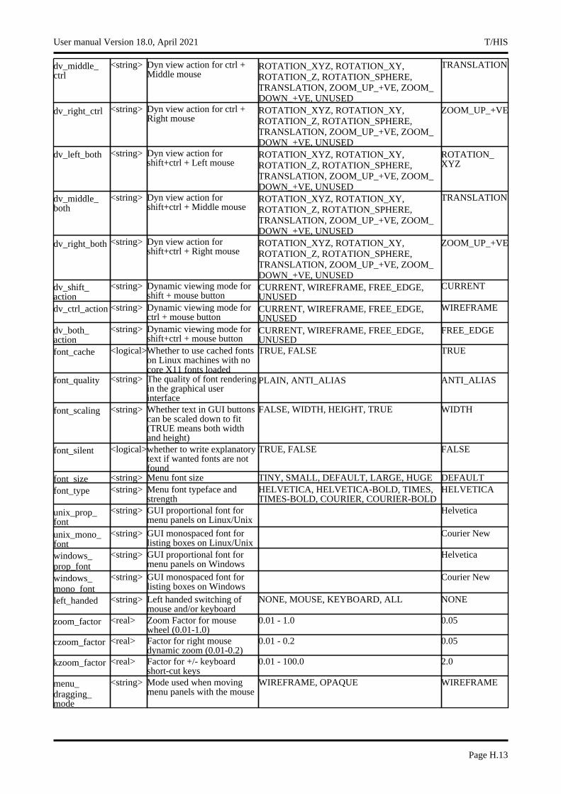
dv_middle_ctrl
<string> Dyn view action for ctrl + Middle mouse
ROTATION_XYZ, ROTATION_XY, ROTATION_Z, ROTATION_SPHERE, TRANSLATION, ZOOM_UP_+VE, ZOOM_DOWN_+VE, UNUSED
TRANSLATION
dv_right_ctrl <string> Dyn view action for ctrl + Right mouse
ROTATION_XYZ, ROTATION_XY, ROTATION_Z, ROTATION_SPHERE, TRANSLATION, ZOOM_UP_+VE, ZOOM_DOWN_+VE, UNUSED
ZOOM_UP_+VE
dv_left_both <string> Dyn view action for shift+ctrl + Left mouse
ROTATION_XYZ, ROTATION_XY, ROTATION_Z, ROTATION_SPHERE, TRANSLATION, ZOOM_UP_+VE, ZOOM_DOWN_+VE, UNUSED
ROTATION_XYZ
dv_middle_both
<string> Dyn view action for shift+ctrl + Middle mouse
ROTATION_XYZ, ROTATION_XY, ROTATION_Z, ROTATION_SPHERE, TRANSLATION, ZOOM_UP_+VE, ZOOM_DOWN_+VE, UNUSED
TRANSLATION
dv_right_both <string> Dyn view action for shift+ctrl + Right mouse
ROTATION_XYZ, ROTATION_XY, ROTATION_Z, ROTATION_SPHERE, TRANSLATION, ZOOM_UP_+VE, ZOOM_DOWN_+VE, UNUSED
ZOOM_UP_+VE
dv_shift_action
<string> Dynamic viewing mode for shift + mouse button
CURRENT, WIREFRAME, FREE_EDGE, UNUSED
CURRENT
dv_ctrl_action <string> Dynamic viewing mode for ctrl + mouse button
CURRENT, WIREFRAME, FREE_EDGE, UNUSED
WIREFRAME
dv_both_action
<string> Dynamic viewing mode for shift+ctrl + mouse button
CURRENT, WIREFRAME, FREE_EDGE, UNUSED
FREE_EDGE
font_cache <logical>Whether to use cached fonts on Linux machines with no core X11 fonts loaded
TRUE, FALSE TRUE
font_quality <string> The quality of font rendering in the graphical user interface
PLAIN, ANTI_ALIAS ANTI_ALIAS
font_scaling <string> Whether text in GUI buttons can be scaled down to fit (TRUE means both width and height)
FALSE, WIDTH, HEIGHT, TRUE WIDTH
font_silent <logical>whether to write explanatory text if wanted fonts are not found
TRUE, FALSE FALSE
font_size <string> Menu font size TINY, SMALL, DEFAULT, LARGE, HUGE DEFAULTfont_type <string> Menu font typeface and
strengthHELVETICA, HELVETICA-BOLD, TIMES, TIMES-BOLD, COURIER, COURIER-BOLD
HELVETICA
unix_prop_font
<string> GUI proportional font for menu panels on Linux/Unix
Helvetica
unix_mono_font
<string> GUI monospaced font for listing boxes on Linux/Unix
Courier New
windows_prop_font
<string> GUI proportional font for menu panels on Windows
Helvetica
windows_mono_font
<string> GUI monospaced font for listing boxes on Windows
Courier New
left_handed <string> Left handed switching of mouse and/or keyboard
NONE, MOUSE, KEYBOARD, ALL NONE
zoom_factor <real> Zoom Factor for mouse wheel (0.01-1.0)
0.01 - 1.0 0.05
czoom_factor <real> Factor for right mouse dynamic zoom (0.01-0.2)
0.01 - 0.2 0.05
kzoom_factor <real> Factor for +/- keyboard short-cut keys
0.01 - 100.0 2.0
menu_dragging_mode
<string> Mode used when moving menu panels with the mouse
WIREFRAME, OPAQUE WIREFRAME
User manual Version 18.0, April 2021 T/HIS
Page H.13
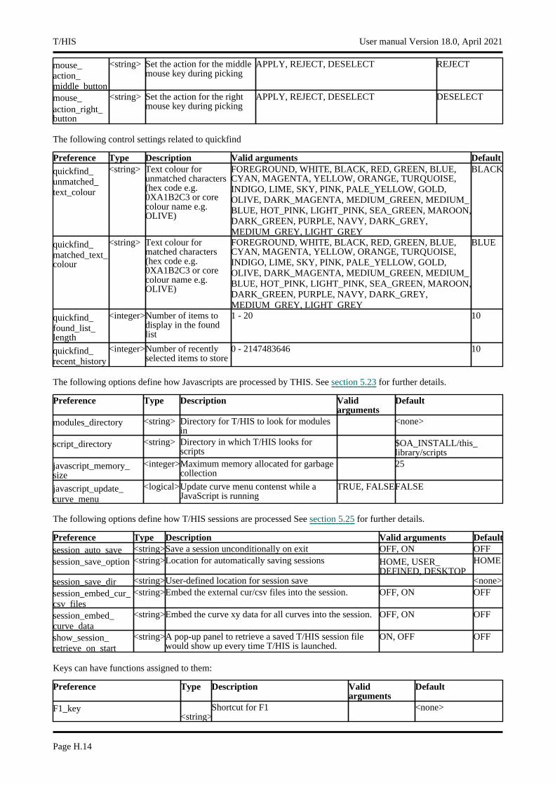
mouse_action_middle_button
<string> Set the action for the middle mouse key during picking
APPLY, REJECT, DESELECT REJECT
mouse_action_right_button
<string> Set the action for the right mouse key during picking
APPLY, REJECT, DESELECT DESELECT
The following control settings related to quickfind
Preference Type Description Valid arguments Defaultquickfind_unmatched_text_colour
<string> Text colour for unmatched characters (hex code e.g. 0XA1B2C3 or core colour name e.g. OLIVE)
FOREGROUND, WHITE, BLACK, RED, GREEN, BLUE, CYAN, MAGENTA, YELLOW, ORANGE, TURQUOISE, INDIGO, LIME, SKY, PINK, PALE_YELLOW, GOLD, OLIVE, DARK_MAGENTA, MEDIUM_GREEN, MEDIUM_BLUE, HOT_PINK, LIGHT_PINK, SEA_GREEN, MAROON, DARK_GREEN, PURPLE, NAVY, DARK_GREY, MEDIUM_GREY, LIGHT_GREY
BLACK
quickfind_matched_text_colour
<string> Text colour for matched characters (hex code e.g. 0XA1B2C3 or core colour name e.g. OLIVE)
FOREGROUND, WHITE, BLACK, RED, GREEN, BLUE, CYAN, MAGENTA, YELLOW, ORANGE, TURQUOISE, INDIGO, LIME, SKY, PINK, PALE_YELLOW, GOLD, OLIVE, DARK_MAGENTA, MEDIUM_GREEN, MEDIUM_BLUE, HOT_PINK, LIGHT_PINK, SEA_GREEN, MAROON, DARK_GREEN, PURPLE, NAVY, DARK_GREY, MEDIUM_GREY, LIGHT_GREY
BLUE
quickfind_found_list_length
<integer>Number of items to display in the found list
1 - 20 10
quickfind_recent_history
<integer>Number of recently selected items to store
0 - 2147483646 10
The following options define how Javascripts are processed by THIS. See section 5.23 for further details.
Preference Type Description Valid arguments
Default
modules_directory <string> Directory for T/HIS to look for modules in
<none>
script_directory <string> Directory in which T/HIS looks for scripts
$OA_INSTALL/this_library/scripts
javascript_memory_size
<integer>Maximum memory allocated for garbage collection
25
javascript_update_curve_menu
<logical>Update curve menu contenst while a JavaScript is running
TRUE, FALSEFALSE
The following options define how T/HIS sessions are processed See section 5.25 for further details.
Preference Type Description Valid arguments Defaultsession_auto_save <string>Save a session unconditionally on exit OFF, ON OFFsession_save_option <string>Location for automatically saving sessions HOME, USER_
DEFINED, DESKTOPHOME
session_save_dir <string>User-defined location for session save <none>session_embed_cur_csv_files
<string>Embed the external cur/csv files into the session. OFF, ON OFF
session_embed_curve_data
<string>Embed the curve xy data for all curves into the session. OFF, ON OFF
show_session_retrieve_on_start
<string>A pop-up panel to retrieve a saved T/HIS session file would show up every time T/HIS is launched.
ON, OFF OFF
Keys can have functions assigned to them:
Preference Type Description Valid arguments
Default
F1_key<string>
Shortcut for F1 <none>
T/HIS User manual Version 18.0, April 2021
Page H.14
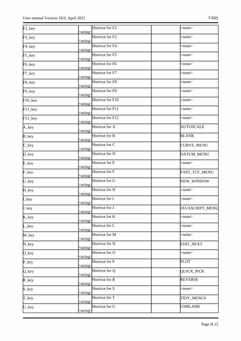
F2_key<string>
Shortcut for F2 <none>
F3_key<string>
Shortcut for F3 <none>
F4_key<string>
Shortcut for F4 <none>
F5_key<string>
Shortcut for F5 <none>
F6_key<string>
Shortcut for F6 <none>
F7_key<string>
Shortcut for F7 <none>
F8_key<string>
Shortcut for F8 <none>
F9_key<string>
Shortcut for F9 <none>
F10_key<string>
Shortcut for F10 <none>
F11_key<string>
Shortcut for F11 <none>
F12_key<string>
Shortcut for F12 <none>
A_key<string>
Shortcut for A AUTOSCALE
B_key<string>
Shortcut for B BLANK
C_key<string>
Shortcut for C CURVE_MENU
D_key<string>
Shortcut for D DATUM_MENU
E_key<string>
Shortcut for E <none>
F_key<string>
Shortcut for F FAST_TCF_MENU
G_key<string>
Shortcut for G NEW_WINDOW
H_key<string>
Shortcut for H <none>
I_key<string>
Shortcut for I <none>
J_key<string>
Shortcut for J JAVASCRIPT_MENU
K_key<string>
Shortcut for K <none>
L_key<string>
Shortcut for L <none>
M_key<string>
Shortcut for M <none>
N_key<string>
Shortcut for N EDIT_NEXT
O_key<string>
Shortcut for O <none>
P_key<string>
Shortcut for P PLOT
Q_key<string>
Shortcut for Q QUICK_PICK
R_key<string>
Shortcut for R REVERSE
S_key<string>
Shortcut for S <none>
T_key<string>
Shortcut for T TIDY_MENUS
U_key<string>
Shortcut for U UNBLANK
User manual Version 18.0, April 2021 T/HIS
Page H.15
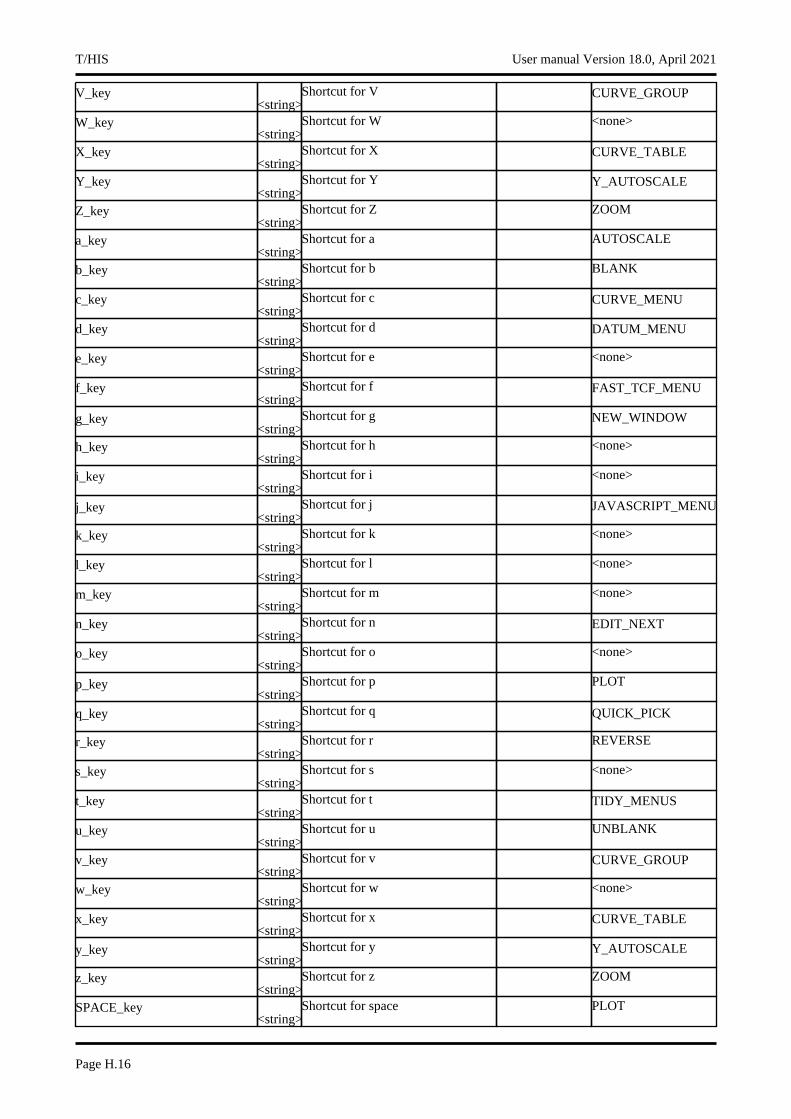
V_key<string>
Shortcut for V CURVE_GROUP
W_key<string>
Shortcut for W <none>
X_key<string>
Shortcut for X CURVE_TABLE
Y_key<string>
Shortcut for Y Y_AUTOSCALE
Z_key<string>
Shortcut for Z ZOOM
a_key<string>
Shortcut for a AUTOSCALE
b_key<string>
Shortcut for b BLANK
c_key<string>
Shortcut for c CURVE_MENU
d_key<string>
Shortcut for d DATUM_MENU
e_key<string>
Shortcut for e <none>
f_key<string>
Shortcut for f FAST_TCF_MENU
g_key<string>
Shortcut for g NEW_WINDOW
h_key<string>
Shortcut for h <none>
i_key<string>
Shortcut for i <none>
j_key<string>
Shortcut for j JAVASCRIPT_MENU
k_key<string>
Shortcut for k <none>
l_key<string>
Shortcut for l <none>
m_key<string>
Shortcut for m <none>
n_key<string>
Shortcut for n EDIT_NEXT
o_key<string>
Shortcut for o <none>
p_key<string>
Shortcut for p PLOT
q_key<string>
Shortcut for q QUICK_PICK
r_key<string>
Shortcut for r REVERSE
s_key<string>
Shortcut for s <none>
t_key<string>
Shortcut for t TIDY_MENUS
u_key<string>
Shortcut for u UNBLANK
v_key<string>
Shortcut for v CURVE_GROUP
w_key<string>
Shortcut for w <none>
x_key<string>
Shortcut for x CURVE_TABLE
y_key<string>
Shortcut for y Y_AUTOSCALE
z_key<string>
Shortcut for z ZOOM
SPACE_key<string>
Shortcut for space PLOT
T/HIS User manual Version 18.0, April 2021
Page H.16

ZERO_key<string>
Shortcut for 0 COPY_AXIS
ONE_key<string>
Shortcut for 1 TILE_TALL
TWO_key<string>
Shortcut for 2 TILE_WIDE
THREE_key<string>
Shortcut for 3 CASCADE
FOUR_key<string>
Shortcut for 4 LAYOUT_1X1
FIVE_key<string>
Shortcut for 5 LAYOUT_2X2
SIX_key<string>
Shortcut for 6 LAYOUT_3X3
SEVEN_key<string>
Shortcut for 7 <none>
EIGHT_key<string>
Shortcut for 8 <none>
NINE_key<string>
Shortcut for 9 <none>
EXCLAMATION_key<string>
Shortcut for ! <none>
DOUBLEQUOTE_key<string>
Shortcut for " <none>
HASH_key<string>
Shortcut for # <none>
DOLLAR_key<string>
Shortcut for $ <none>
PERCENT_key<string>
Shortcut for % <none>
AMPERSAND_key<string>
Shortcut for & <none>
SINGLEQUOTE_key<string>
Shortcut for ’ <none>
LEFTBRACKET_key<string>
Shortcut for ( <none>
RIGHTBRACKET_key<string>
Shortcut for ) <none>
ASTERISK_key<string>
Shortcut for * <none>
PLUS_key<string>
Shortcut for + ZOOM_IN
COMMA_key<string>
Shortcut for , <none>
MINUS_key<string>
Shortcut for - ZOOM_OUT
DOT_key<string>
Shortcut for . <none>
SLASH_key<string>
Shortcut for / SHORTCUT
COLON_key<string>
Shortcut for : <none>
SEMICOLON_key<string>
Shortcut for ; <none>
LESSTHAN_key<string>
Shortcut for < <none>
EQUALS_key<string>
Shortcut for = ZOOM_IN
GREATERTHAN_key<string>
Shortcut for > <none>
QUESTIONMARK_key<string>
Shortcut for ? SHORTCUT
AT_key<string>
Shortcut for @ <none>
User manual Version 18.0, April 2021 T/HIS
Page H.17
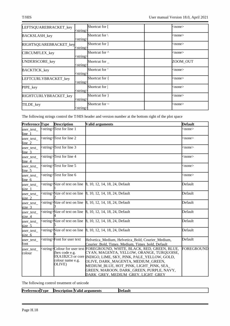
LEFTSQUAREBRACKET_key<string>
Shortcut for [ <none>
BACKSLASH_key<string>
Shortcut for \ <none>
RIGHTSQUAREBRACKET_key<string>
Shortcut for ] <none>
CIRCUMFLEX_key<string>
Shortcut for ^ <none>
UNDERSCORE_key<string>
Shortcut for _ ZOOM_OUT
BACKTICK_key<string>
Shortcut for ‘ <none>
LEFTCURLYBRACKET_key<string>
Shortcut for { <none>
PIPE_key<string>
Shortcut for | <none>
RIGHTCURLYBRACKET_key<string>
Shortcut for } <none>
TILDE_key<string>
Shortcut for ~ <none>
The following strings control the T/HIS header and version number at the bottom right of the plot space
Preference Type Description Valid arguments Defaultuser_text_line_1
<string>Text for line 1 <none>
user_text_line_2
<string>Text for line 2 <none>
user_text_line_3
<string>Text for line 3 <none>
user_text_line_4
<string>Text for line 4 <none>
user_text_line_5
<string>Text for line 5 <none>
user_text_line_6
<string>Text for line 6 <none>
user_text_size_1
<string>Size of text on line 1
8, 10, 12, 14, 18, 24, Default Default
user_text_size_2
<string>Size of text on line 2
8, 10, 12, 14, 18, 24, Default Default
user_text_size_3
<string>Size of text on line 3
8, 10, 12, 14, 18, 24, Default Default
user_text_size_4
<string>Size of text on line 4
8, 10, 12, 14, 18, 24, Default Default
user_text_size_5
<string>Size of text on line 5
8, 10, 12, 14, 18, 24, Default Default
user_text_size_6
<string>Size of text on line 6
8, 10, 12, 14, 18, 24, Default Default
user_text_font
<string>Font for user text Helvetica_Medium, Helvetica_Bold, Courier_Medium, Courier_Bold, Times_Medium, Times_bold, Default
Default
user_text_colour
<string>Colour for user text (hex code e.g. 0XA1B2C3 or core colour name e.g. OLIVE)
FOREGROUND, WHITE, BLACK, RED, GREEN, BLUE, CYAN, MAGENTA, YELLOW, ORANGE, TURQUOISE, INDIGO, LIME, SKY, PINK, PALE_YELLOW, GOLD, OLIVE, DARK_MAGENTA, MEDIUM_GREEN, MEDIUM_BLUE, HOT_PINK, LIGHT_PINK, SEA_GREEN, MAROON, DARK_GREEN, PURPLE, NAVY, DARK_GREY, MEDIUM_GREY, LIGHT_GREY
FOREGROUND
The following control treatment of unicode
PreferenceType Description Valid arguments Default
T/HIS User manual Version 18.0, April 2021
Page H.18
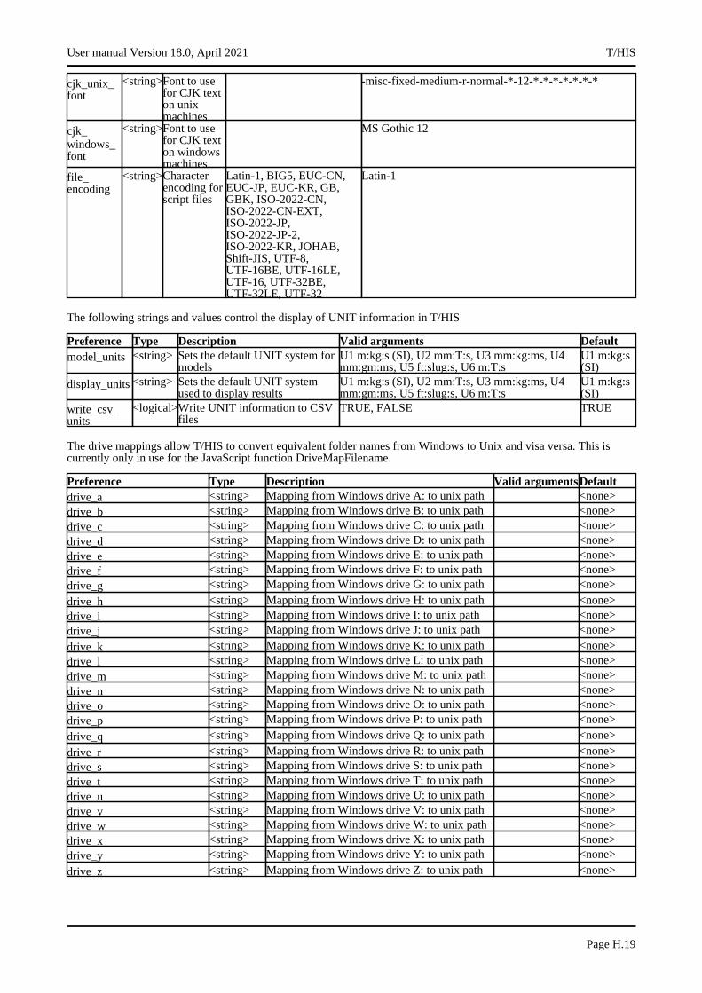
cjk_unix_font
<string>Font to use for CJK text on unix machines
-misc-fixed-medium-r-normal-*-12-*-*-*-*-*-*-*
cjk_windows_font
<string>Font to use for CJK text on windows machines
MS Gothic 12
file_encoding
<string>Character encoding for script files
Latin-1, BIG5, EUC-CN, EUC-JP, EUC-KR, GB, GBK, ISO-2022-CN, ISO-2022-CN-EXT, ISO-2022-JP, ISO-2022-JP-2, ISO-2022-KR, JOHAB, Shift-JIS, UTF-8, UTF-16BE, UTF-16LE, UTF-16, UTF-32BE, UTF-32LE, UTF-32
Latin-1
The following strings and values control the display of UNIT information in T/HIS
Preference Type Description Valid arguments Defaultmodel_units <string> Sets the default UNIT system for
modelsU1 m:kg:s (SI), U2 mm:T:s, U3 mm:kg:ms, U4 mm:gm:ms, U5 ft:slug:s, U6 m:T:s
U1 m:kg:s (SI)
display_units <string> Sets the default UNIT system used to display results
U1 m:kg:s (SI), U2 mm:T:s, U3 mm:kg:ms, U4 mm:gm:ms, U5 ft:slug:s, U6 m:T:s
U1 m:kg:s (SI)
write_csv_units
<logical>Write UNIT information to CSV files
TRUE, FALSE TRUE
The drive mappings allow T/HIS to convert equivalent folder names from Windows to Unix and visa versa. This is currently only in use for the JavaScript function DriveMapFilename.
Preference Type Description Valid argumentsDefaultdrive_a <string> Mapping from Windows drive A: to unix path <none>drive_b <string> Mapping from Windows drive B: to unix path <none>drive_c <string> Mapping from Windows drive C: to unix path <none>drive_d <string> Mapping from Windows drive D: to unix path <none>drive_e <string> Mapping from Windows drive E: to unix path <none>drive_f <string> Mapping from Windows drive F: to unix path <none>drive_g <string> Mapping from Windows drive G: to unix path <none>
drive_h <string> Mapping from Windows drive H: to unix path <none>drive_i <string> Mapping from Windows drive I: to unix path <none>drive_j <string> Mapping from Windows drive J: to unix path <none>
drive_k <string> Mapping from Windows drive K: to unix path <none>drive_l <string> Mapping from Windows drive L: to unix path <none>drive_m <string> Mapping from Windows drive M: to unix path <none>drive_n <string> Mapping from Windows drive N: to unix path <none>drive_o <string> Mapping from Windows drive O: to unix path <none>drive_p <string> Mapping from Windows drive P: to unix path <none>
drive_q <string> Mapping from Windows drive Q: to unix path <none>
drive_r <string> Mapping from Windows drive R: to unix path <none>drive_s <string> Mapping from Windows drive S: to unix path <none>drive_t <string> Mapping from Windows drive T: to unix path <none>drive_u <string> Mapping from Windows drive U: to unix path <none>drive_v <string> Mapping from Windows drive V: to unix path <none>drive_w <string> Mapping from Windows drive W: to unix path <none>drive_x <string> Mapping from Windows drive X: to unix path <none>drive_y <string> Mapping from Windows drive Y: to unix path <none>
drive_z <string> Mapping from Windows drive Z: to unix path <none>
User manual Version 18.0, April 2021 T/HIS
Page H.19

Global preferences.
From version 9.3 onwards global preferences that apply to all programs can be specified using "oasys" as the program name.
oasys*<keyword>: <argument
At present the following global preferences can be defined
If a preference is defined twice using both "oasys*" and "this*" then the "this*" setting will override the global setting.
Preference Type Description Valid arguments Defaultfile_names <string> Controls input filename syntax. LSTC =
d3*, OASYS = job.ptf*OASYS, LSTC OASYS
html_application
<string> Location of HTML browser <none>
html_application_linux
<string> Location of HTML browser for linux (use if the same oa_pref file is used for windows and linux)
<none>
html_application_windows
<string> Location of HTML browser for windows (use if the same oa_pref file is used for windows and linux)
<none>
image_format <string> Default image format BMP_8_C, BMP_8_UN, PNG_8, GIF_8, BMP_24_UN, PNG_24, JPG_24, PPM_24
PNG_24
intel_hd_use_shaders
<string> Control usage of hardware shaders on Intel HD graphics cards
AUTO_DETECT, FORCE_OFF, FORCE_ON
AUTO_DETECT
locale <string> Language and country locale to use (overrides system one)
<none>
maximise <logical>Maximise window when Program is started TRUE, FALSE FALSE
pdf_application <string> Location of PDF browser <none>
pdf_application_linux
<string> Location of PDF browser for linux (use if the same oa_pref file is used for windows and linux)
<none>
pdf_application_windows
<string> Location of PDF browser for windows (use if the same oa_pref file is used for windows and linux)
<none>
placement <string> Location for initial window on multi-screen display
LEFT, RIGHT, BOTTOM, TOP, LEFT_BOTTOM, LEFT_TOP, RIGHT_BOTTOM, RIGHT_TOP
<none>
start_in <string> Directory to start Program in <none>
temp_file_expiry
<integer>Age in days after which a temporary filename can be reused, 0 = never
0 - 10000 31
show_license_warning
<logical>Display Window containing License System messages
TRUE, FALSE TRUE
post_uses_primer
<logical>ADMIN/INSTALL pref which allows D3Plot, T/his to take an available Primer license
TRUE, FALSE TRUE
save_window_positions
<logical>Save position of undocked windows between sessions
TRUE, FALSE TRUE
The following control directories
Preference Type Description Valid arguments Defaulthome_dir <string> "home" directory for user <none>install_dir <string> Directory Oasys Ltd software is installed in <none>manuals_dir <string> Directory user manuals are installed in <none>
temp_dir <string> temporary directory for user <none>
write_checkpoint_files
<logical>Record checkpoint files for the PRIMER, D3PLOT or T/His sessions.
TRUE, FALSE FALSE
checkpoint_dir <string> Directory for checkpoint files. If omitted use cwd. <none>
T/HIS User manual Version 18.0, April 2021
Page H.20
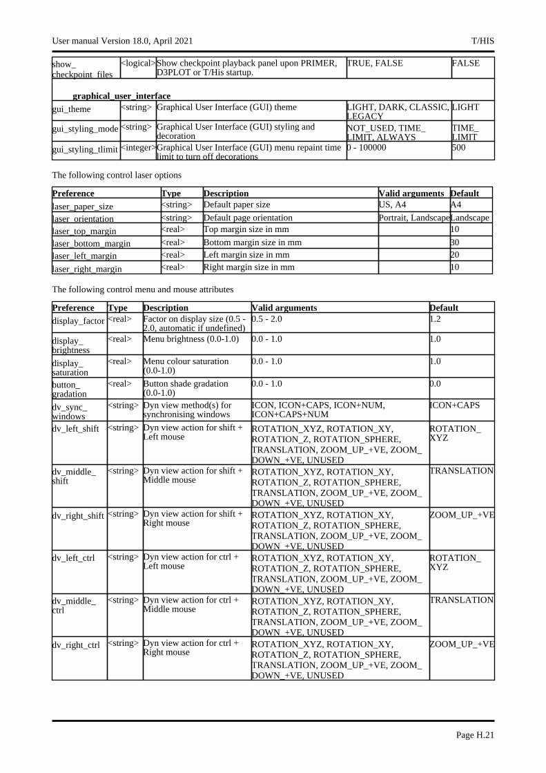
show_checkpoint_files
<logical>Show checkpoint playback panel upon PRIMER, D3PLOT or T/His startup.
TRUE, FALSE FALSE
graphical_user_interfacegui_theme <string> Graphical User Interface (GUI) theme LIGHT, DARK, CLASSIC,
LEGACYLIGHT
gui_styling_mode <string> Graphical User Interface (GUI) styling and decoration
NOT_USED, TIME_LIMIT, ALWAYS
TIME_LIMIT
gui_styling_tlimit <integer>Graphical User Interface (GUI) menu repaint time limit to turn off decorations
0 - 100000 500
The following control laser options
Preference Type Description Valid arguments Defaultlaser_paper_size <string> Default paper size US, A4 A4
laser_orientation <string> Default page orientation Portrait, LandscapeLandscape
laser_top_margin <real> Top margin size in mm 10
laser_bottom_margin <real> Bottom margin size in mm 30
laser_left_margin <real> Left margin size in mm 20
laser_right_margin <real> Right margin size in mm 10
The following control menu and mouse attributes
Preference Type Description Valid arguments Defaultdisplay_factor <real> Factor on display size (0.5 -
2.0, automatic if undefined)0.5 - 2.0 1.2
display_brightness
<real> Menu brightness (0.0-1.0) 0.0 - 1.0 1.0
display_saturation
<real> Menu colour saturation (0.0-1.0)
0.0 - 1.0 1.0
button_gradation
<real> Button shade gradation (0.0-1.0)
0.0 - 1.0 0.0
dv_sync_windows
<string> Dyn view method(s) for synchronising windows
ICON, ICON+CAPS, ICON+NUM, ICON+CAPS+NUM
ICON+CAPS
dv_left_shift <string> Dyn view action for shift + Left mouse
ROTATION_XYZ, ROTATION_XY, ROTATION_Z, ROTATION_SPHERE, TRANSLATION, ZOOM_UP_+VE, ZOOM_DOWN_+VE, UNUSED
ROTATION_XYZ
dv_middle_shift
<string> Dyn view action for shift + Middle mouse
ROTATION_XYZ, ROTATION_XY, ROTATION_Z, ROTATION_SPHERE, TRANSLATION, ZOOM_UP_+VE, ZOOM_DOWN_+VE, UNUSED
TRANSLATION
dv_right_shift <string> Dyn view action for shift + Right mouse
ROTATION_XYZ, ROTATION_XY, ROTATION_Z, ROTATION_SPHERE, TRANSLATION, ZOOM_UP_+VE, ZOOM_DOWN_+VE, UNUSED
ZOOM_UP_+VE
dv_left_ctrl <string> Dyn view action for ctrl + Left mouse
ROTATION_XYZ, ROTATION_XY, ROTATION_Z, ROTATION_SPHERE, TRANSLATION, ZOOM_UP_+VE, ZOOM_DOWN_+VE, UNUSED
ROTATION_XYZ
dv_middle_ctrl
<string> Dyn view action for ctrl + Middle mouse
ROTATION_XYZ, ROTATION_XY, ROTATION_Z, ROTATION_SPHERE, TRANSLATION, ZOOM_UP_+VE, ZOOM_DOWN_+VE, UNUSED
TRANSLATION
dv_right_ctrl <string> Dyn view action for ctrl + Right mouse
ROTATION_XYZ, ROTATION_XY, ROTATION_Z, ROTATION_SPHERE, TRANSLATION, ZOOM_UP_+VE, ZOOM_DOWN_+VE, UNUSED
ZOOM_UP_+VE
User manual Version 18.0, April 2021 T/HIS
Page H.21
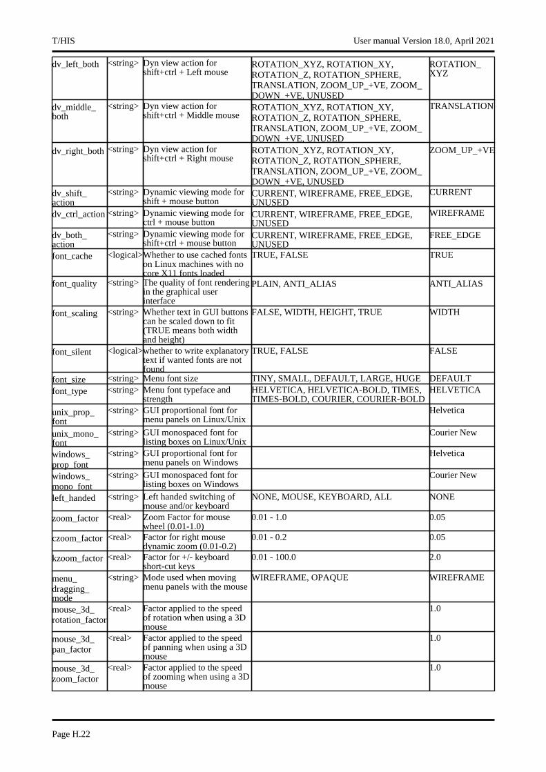
dv_left_both <string> Dyn view action for shift+ctrl + Left mouse
ROTATION_XYZ, ROTATION_XY, ROTATION_Z, ROTATION_SPHERE, TRANSLATION, ZOOM_UP_+VE, ZOOM_DOWN_+VE, UNUSED
ROTATION_XYZ
dv_middle_both
<string> Dyn view action for shift+ctrl + Middle mouse
ROTATION_XYZ, ROTATION_XY, ROTATION_Z, ROTATION_SPHERE, TRANSLATION, ZOOM_UP_+VE, ZOOM_DOWN_+VE, UNUSED
TRANSLATION
dv_right_both <string> Dyn view action for shift+ctrl + Right mouse
ROTATION_XYZ, ROTATION_XY, ROTATION_Z, ROTATION_SPHERE, TRANSLATION, ZOOM_UP_+VE, ZOOM_DOWN_+VE, UNUSED
ZOOM_UP_+VE
dv_shift_action
<string> Dynamic viewing mode for shift + mouse button
CURRENT, WIREFRAME, FREE_EDGE, UNUSED
CURRENT
dv_ctrl_action <string> Dynamic viewing mode for ctrl + mouse button
CURRENT, WIREFRAME, FREE_EDGE, UNUSED
WIREFRAME
dv_both_action
<string> Dynamic viewing mode for shift+ctrl + mouse button
CURRENT, WIREFRAME, FREE_EDGE, UNUSED
FREE_EDGE
font_cache <logical>Whether to use cached fonts on Linux machines with no core X11 fonts loaded
TRUE, FALSE TRUE
font_quality <string> The quality of font rendering in the graphical user interface
PLAIN, ANTI_ALIAS ANTI_ALIAS
font_scaling <string> Whether text in GUI buttons can be scaled down to fit (TRUE means both width and height)
FALSE, WIDTH, HEIGHT, TRUE WIDTH
font_silent <logical>whether to write explanatory text if wanted fonts are not found
TRUE, FALSE FALSE
font_size <string> Menu font size TINY, SMALL, DEFAULT, LARGE, HUGE DEFAULTfont_type <string> Menu font typeface and
strengthHELVETICA, HELVETICA-BOLD, TIMES, TIMES-BOLD, COURIER, COURIER-BOLD
HELVETICA
unix_prop_font
<string> GUI proportional font for menu panels on Linux/Unix
Helvetica
unix_mono_font
<string> GUI monospaced font for listing boxes on Linux/Unix
Courier New
windows_prop_font
<string> GUI proportional font for menu panels on Windows
Helvetica
windows_mono_font
<string> GUI monospaced font for listing boxes on Windows
Courier New
left_handed <string> Left handed switching of mouse and/or keyboard
NONE, MOUSE, KEYBOARD, ALL NONE
zoom_factor <real> Zoom Factor for mouse wheel (0.01-1.0)
0.01 - 1.0 0.05
czoom_factor <real> Factor for right mouse dynamic zoom (0.01-0.2)
0.01 - 0.2 0.05
kzoom_factor <real> Factor for +/- keyboard short-cut keys
0.01 - 100.0 2.0
menu_dragging_mode
<string> Mode used when moving menu panels with the mouse
WIREFRAME, OPAQUE WIREFRAME
mouse_3d_rotation_factor
<real> Factor applied to the speed of rotation when using a 3D mouse
1.0
mouse_3d_pan_factor
<real> Factor applied to the speed of panning when using a 3D mouse
1.0
mouse_3d_zoom_factor
<real> Factor applied to the speed of zooming when using a 3D mouse
1.0
T/HIS User manual Version 18.0, April 2021
Page H.22
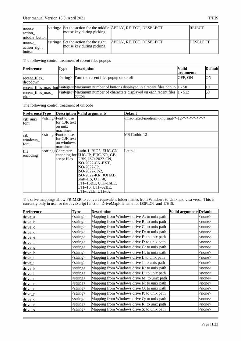
mouse_action_middle_button
<string> Set the action for the middle mouse key during picking
APPLY, REJECT, DESELECT REJECT
mouse_action_right_button
<string> Set the action for the right mouse key during picking
APPLY, REJECT, DESELECT DESELECT
The following control treatment of recent files popups
Preference Type Description Valid arguments
Default
recent_files_dropdown
<string> Turn the recent files popup on or off OFF, ON ON
recent_files_max_but<integer>Maximum number of buttons displayed in a recent files popup 1 - 50 10recent_files_max_char
<integer>Maximum number of characters displayed on each recent files button
1 - 512 50
The following control treatment of unicode
PreferenceType Description Valid arguments Defaultcjk_unix_font
<string>Font to use for CJK text on unix machines
-misc-fixed-medium-r-normal-*-12-*-*-*-*-*-*-*
cjk_windows_font
<string>Font to use for CJK text on windows machines
MS Gothic 12
file_encoding
<string>Character encoding for script files
Latin-1, BIG5, EUC-CN, EUC-JP, EUC-KR, GB, GBK, ISO-2022-CN, ISO-2022-CN-EXT, ISO-2022-JP, ISO-2022-JP-2, ISO-2022-KR, JOHAB, Shift-JIS, UTF-8, UTF-16BE, UTF-16LE, UTF-16, UTF-32BE, UTF-32LE, UTF-32
Latin-1
The drive mappings allow PRIMER to convert equivalent folder names from Windows to Unix and visa versa. This is currently only in use for the JavaScript function DriveMapFilename for D3PLOT and T/HIS.
Preference Type Description Valid argumentsDefaultdrive_a <string> Mapping from Windows drive A: to unix path <none>drive_b <string> Mapping from Windows drive B: to unix path <none>drive_c <string> Mapping from Windows drive C: to unix path <none>drive_d <string> Mapping from Windows drive D: to unix path <none>drive_e <string> Mapping from Windows drive E: to unix path <none>drive_f <string> Mapping from Windows drive F: to unix path <none>drive_g <string> Mapping from Windows drive G: to unix path <none>
drive_h <string> Mapping from Windows drive H: to unix path <none>drive_i <string> Mapping from Windows drive I: to unix path <none>drive_j <string> Mapping from Windows drive J: to unix path <none>
drive_k <string> Mapping from Windows drive K: to unix path <none>drive_l <string> Mapping from Windows drive L: to unix path <none>drive_m <string> Mapping from Windows drive M: to unix path <none>drive_n <string> Mapping from Windows drive N: to unix path <none>drive_o <string> Mapping from Windows drive O: to unix path <none>drive_p <string> Mapping from Windows drive P: to unix path <none>
drive_q <string> Mapping from Windows drive Q: to unix path <none>
drive_r <string> Mapping from Windows drive R: to unix path <none>drive_s <string> Mapping from Windows drive S: to unix path <none>
User manual Version 18.0, April 2021 T/HIS
Page H.23

drive_t <string> Mapping from Windows drive T: to unix path <none>drive_u <string> Mapping from Windows drive U: to unix path <none>drive_v <string> Mapping from Windows drive V: to unix path <none>drive_w <string> Mapping from Windows drive W: to unix path <none>drive_x <string> Mapping from Windows drive X: to unix path <none>drive_y <string> Mapping from Windows drive Y: to unix path <none>
drive_z <string> Mapping from Windows drive Z: to unix path <none>
T/HIS User manual Version 18.0, April 2021
Page H.24
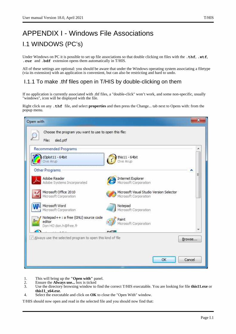
APPENDIX I - Windows File Associations
I.1 WINDOWS (PC’s)
Under Windows on PC it is possible to set up file associations so that double clicking on files with the .thf, .xtf, .cur and .bdf extension opens them automatically in T/HIS.
All of these settings are optional: you should be aware that under the Windows operating system associating a filetype (via its extension) with an application is convenient, but can also be restricting and hard to undo.
I.1.1 To make .thf files open in T/HIS by double-clicking on them
If no application is currently associated with .thf files, a "double-click" won’t work, and some non-specific, usually "windows", icon will be displayed with the file.
Right click on any .thf file, and select properties and then press the Change... tab next to Opens with: from the popup menu.
1. This will bring up the "Open with" panel.2. Ensure the Always use... box is ticked3. Use the directory browsing window to find the correct T/HIS executable. You are looking for file this11.exe or
this11_x64.exe.4. Select the executable and click on OK to close the "Open With" window.
T/HIS should now open and read in the selected file and you should now find that:
User manual Version 18.0, April 2021 T/HIS
Page I.1
• All .thf files on your system show the T/HIS icon.
• Double-clicking on any such file starts T/HIS and opens that file.
It is not possible to set up the filename "d3thdt" for double-clicking in this way since Windows requires filename extensions when assigning applications to files.)
I.1.2 To make .xtf, .cur and .bdf files open in T/HIS by double-clicking on them
The procedure is exactly the same as for .thf files, and must be carried out for each of the file types that you wish to process by double-clicking:
.xtf LS-DYNA Extra Time History file
.cur T/HIS Curve file
.bdf T/HIS Bulk Data file
Note that: File types .thf and .xtf are opened in this way, but no contents are read in.
File types .cur and .bdf are opened and their complete contents read in.
T/HIS User manual Version 18.0, April 2021
Page I.2
APPENDIX J - T-HIS JavaScript APIDescription of T/HIS API functions and methods.
The following pages describe the functions ("methods") available in the T/HIS Javascript interface. For information about how to run Javascript files see Section 5.23.
global classThe global class is the main JavaScript class. More...
The T/HIS JavaScript API provides many class constants, properties and methods. For Arup to be able to extend and enhance the API in the future any constant, property or method names beginning with a lowercase or uppercase letter are reserved.If you need to add your own properties or methods to one of the existing classes then to avoid any potential future conflict you should ensure that the name begins with either an underscore (_) or a dollar sign ($) or the name is prefixed with your own unique identifier.For example if company ’ABC’ need to add a property called ’example’ then to avoid any potential future conflict use one of:
• _example • $example • ABC_example
Class functions• AllocateFlag() • ClearFlag(flag[Flag]) • DialogueInput(string_1, (string_2 ... string_n)[One or more Javascript strings]) • DialogueInputNoEcho(string_1, (string_2 ... string_n)[One or more Javascript strings]) • DisableUpdate() • EnableUpdate() • ErrorMessage(string[Any valid javascript type]) • Execute(data[object]) • Exit() • GetCurrentDirectory() • GetFtcfVar(name[string]) • GetInstallDirectory() • GetPreferenceValue(program[string], name[string]) • GetStartInDirectory() • Getenv(name[string]) • Message(string[Any valid javascript type]) • MilliSleep(time[integer]) • NumberToString(number[integer/real], width[integer], pref_int (optional)[boolean]) • Plot() • Print(string[Any valid javascript type]) • Println(string[Any valid javascript type]) • ReturnFlag(flag[Flag]) • SetCurrentDirectory(directory path[string]) • SetFtcfVar(name[string]) • Sleep(time[integer]) • System(string[Any valid javascript type]) • Unix() • WarningMessage(string[Any valid javascript type]) • Windows()
Detailed DescriptionThe global class declares the global object in JavaScript that contains the global properties and methods. As well as the core JavaScript methods, T/HIS also defines other additional ones. e.g. Message(), Print() etc. See the documentation below for more details.
Details of functions
AllocateFlag() [static]
Description
Allocate a flag for use in the script. See also ReturnFlag() and Once allocated the flag is automatically cleared for all entity types and all the curves currently in T/HIS.
User manual Version 18.0, April 2021 T/HIS
Page J.1
Arguments
No arguments
Return type
Flag (integer)
Example
To allocate a flag
var flag = AllocateFlag();
ClearFlag(flag[Flag]) [static]
Description
Clears a flag on all curves and entity types.
Arguments
Name Type Description
flag Flag The flag to return.
Return type
No return value.
Example
To clear flag f:
ClearFlag(f);
DialogueInput(string_1, (string_2 ... string_n)[One or more Javascript strings]) [static]
Description
Execute one or more lines of command line dialogue input.
Arguments
Name Type Description
string_1, (string_2 ... string_n)
One or more Javascript strings
The command(s) that are to be executed as if they had been typed into the dialogue box
Return type
No return value
Example
To mulitple curves 1 and 2 by 10:
DialogueInputNoEcho("/op mul #1 10 #", "/op mul #2 10 #");
Note that each call to DialogueInput starts afresh at the top of the T/HIS command line "tree", so where multiple commands need to be given at sub-menu levels they need to be included in a single call.
DialogueInputNoEcho(string_1, (string_2 ... string_n)[One or more Javascript strings]) [static]
Description
Execute one or more lines of command line dialogue input with no echo of commands to dialogue box.
T/HIS User manual Version 18.0, April 2021
Page J.2
Arguments
Name Type Description
string_1, (string_2 ... string_n)
One or more Javascript strings
The command(s) that are to be executed as if they had been typed into the dialogue box
Return type
No return value
Example
To mulitple curves 1 and 2 by 10:
DialogueInputNoEcho("/op mul #1 10 #", "/op mul #2 10 #");
As with DialogueInput above each call starts at the top of the T/HIS command tree structure, so any commands destined for sub-menus must all be arguments to a single call.
DisableUpdate() [static]
Description
Temporarily disable the plotting of curves within graphs.
Arguments
No arguments
Return type
No return value
Example
Temporarily disable the plotting of curves within graphs
DisableUpdate();
EnableUpdate() [static]
Description
Re-enable the plotting of curves within graphs.
Arguments
No arguments
Return type
No return value
Example
Re-enable the plotting of curves within graphs
EnableUpdate();
ErrorMessage(string[Any valid javascript type]) [static]
Description
Print an error message to the dialogue box adding a carriage return.
User manual Version 18.0, April 2021 T/HIS
Page J.3
Arguments
Name Type Description
string Any valid javascript type The string/item that you want to print
Return type
No return value
Example
To print the title of model object m as an error to the dialogue box
ErrorMessage("The title is " + m.title);
Execute(data[object]) [static]
Description
Execute a program or script outside T/HIS and get the standard output and error streams.
Arguments
Name Type Description
data object Execute data Object has the following properties:
Name Type Description
arguments (optional) Array of strings The arguments to pass to program
program string The program you want to run
Return type
Object with the following properties:
Name Type Description
status integer The exit code from the program/script
stderr string The standard error output from the program/script
stdout string The standard output from the program/script
Example
To run script "example.bat" with arguments "foo" and "bar":
var output = Execute( { program: ’example.bat’, arguments: [ ’foo’, ’bar’ ]} );var text = output.stdout;var errors = output.stderr;var ecode = output.status;
Exit() [static]
Description
Exit script
Arguments
No arguments
Return type
No return value
T/HIS User manual Version 18.0, April 2021
Page J.4
Example
Exit with
Exit();
GetCurrentDirectory() [static]
Description
Get the current working directory
Arguments
No arguments
Return type
String containing current working directory
Example
To get the current directory:
var cwd = GetCurrentDirectory();
GetFtcfVar(name[string]) [static]
Description
Get the value of a FAST-TCF variable
Arguments
Name Type Description
name string The FAST-TCF variable name (case independent)
Return type
String containing variable value or null if variable does not exist
Example
To get the value for FAST-TCF variable Job
var job_name = GetFtcfVar("Job");
GetInstallDirectory() [static]
Description
Get the directory in which executables are installed. This is the OA_INSTALL environment variable, or if that is not set the directory in which the current executable is installed. Returns NULL if not found
Arguments
No arguments
Return type
string
Example
To get the install directory:
var install_dir = GetInstallDirectory();
User manual Version 18.0, April 2021 T/HIS
Page J.5

GetPreferenceValue(program[string], name[string]) [static]
Description
Get the Preference value with the given string in the any of admin ("OA_ADMIN") or install ("OA_INSTALL") or home ("OA_HOME") directory oa_pref
Arguments
Name Type Description
program string The program name string : Valid values are ’All’, ’D3Plot’, ’Primer’, ’Reporter’, ’Shell’, ’T/His’
name string The preference name string
Return type
: String containing preference value or null if preference string is not present in any oa_pref. Also if none of the above environment variables are not present, then API simply returns null. While returning preference value, locked preference value in admin and then install oa_pref takes precedence over home oa_pref. If preference is not locked in any of these oa_pref, preference in home directory oa_pref is returned.
Example
To get the preference value:
var pref_list = GetPreferenceValue(’All’, "font_size");
GetStartInDirectory() [static]
Description
Get the directory passed to T/HIS by the -start_in command line argument
Arguments
No arguments
Return type
String containing start_in directory or NULL if not set
Example
To get the start_in directory:
var start_in = GetStartInDirectory();
Getenv(name[string]) [static]
Description
Get the value of an environment variable
Arguments
Name Type Description
name string The environment variable name
Return type
String containing variable value or null if variable does not exist
T/HIS User manual Version 18.0, April 2021
Page J.6

Example
To get the value for environment variable HOME
var home = Getenv("HOME");
Message(string[Any valid javascript type]) [static]
Description
Print a message to the dialogue box adding a carriage return.
Arguments
Name Type Description
string Any valid javascript type
The string/item that you want to print. If ’\r’ is added to the end of the string then instead of automatically adding a carriage return in the dialogue box, the next message will overwrite the current one. This may be useful for giving feedback to the dialogue box when doing an operation.
Return type
No return value
Example
To print the title of model object m as a message to the dialogue box
Message("The title is " + m.title);
MilliSleep(time[integer]) [static]
Description
Pause execution of the script for time milliseconds. See also Sleep()
Arguments
Name Type Description
time integer Number of milliseconds to pause for
Return type
No return value
Example
To pause for 500 milliseconds
MilliSleep(500);
NumberToString(number[integer/real], width[integer], pref_int (optional)[boolean]) [static]
Description
Formats a number to a string with the specified width.
User manual Version 18.0, April 2021 T/HIS
Page J.7
Arguments
Name Type Description
number integer/real The number you want to format.
width integer The width of the string you want to format it to (must be less than 80).
pref_int (optional)
boolean By default only integer values inside the single precision 32 bit signed integer limit of approximately +/-2e9 are formatted as integers, all other numeric values are formatted as floats. With this argument set to TRUE then integer values up to the mantissa precision of a 64 bit float, approximately +/-9e15, will also be formatted as integers.
Return type
String containing the number
Example
To write the number 1.2345e+6 to a string 10 characters wide
var str = NumberToString(1.2345e+6, 10);
Plot() [static]
Description
Updates all the T/HIS graphs.
Arguments
No arguments
Return type
No return value
Example
Update all graphs
Plot();
Print(string[Any valid javascript type]) [static]
Description
Print a string to stdout. Note that a carriage return is not added.
Arguments
Name Type Description
string Any valid javascript type The string/item that you want to print
Return type
No return value
Example
To print string "Hello, world!"
Print("Hello, world!");
To print the title of model object m with a carriage return
print("The title is " + m.title + "\n");
T/HIS User manual Version 18.0, April 2021
Page J.8
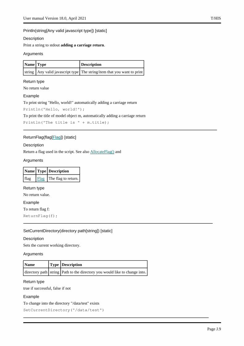
Println(string[Any valid javascript type]) [static]
Description
Print a string to stdout adding a carriage return.
Arguments
Name Type Description
string Any valid javascript type The string/item that you want to print
Return type
No return value
Example
To print string "Hello, world!" automatically adding a carriage return
Println("Hello, world!");
To print the title of model object m, automatically adding a carriage return
Println("The title is " + m.title);
ReturnFlag(flag[Flag]) [static]
Description
Return a flag used in the script. See also AllocateFlag() and
Arguments
Name Type Description
flag Flag The flag to return.
Return type
No return value.
Example
To return flag f:
ReturnFlag(f);
SetCurrentDirectory(directory path[string]) [static]
Description
Sets the current working directory.
Arguments
Name Type Description
directory path string Path to the directory you would like to change into.
Return type
true if successful, false if not
Example
To change into the directory "/data/test" exists
SetCurrentDirectory("/data/test")
User manual Version 18.0, April 2021 T/HIS
Page J.9
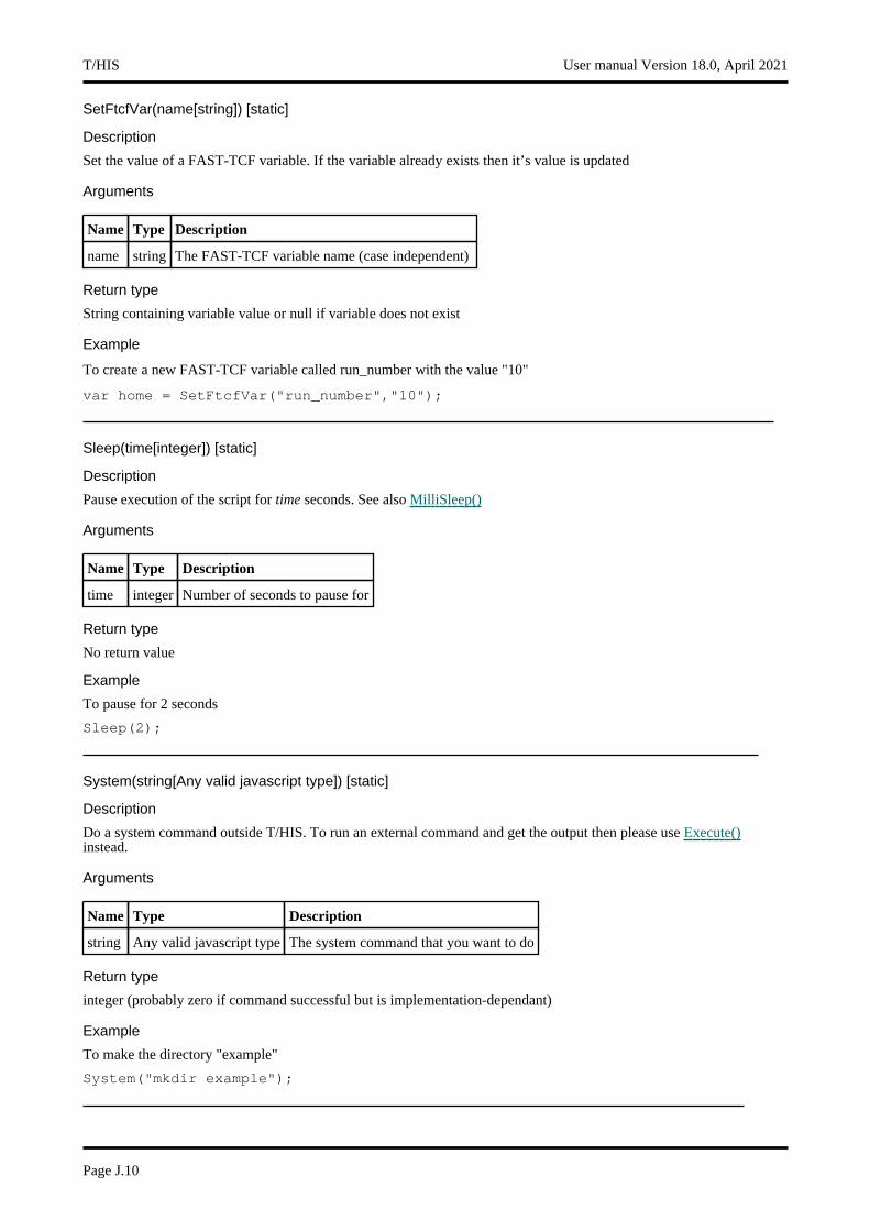
SetFtcfVar(name[string]) [static]
Description
Set the value of a FAST-TCF variable. If the variable already exists then it’s value is updated
Arguments
Name Type Description
name string The FAST-TCF variable name (case independent)
Return type
String containing variable value or null if variable does not exist
Example
To create a new FAST-TCF variable called run_number with the value "10"
var home = SetFtcfVar("run_number","10");
Sleep(time[integer]) [static]
Description
Pause execution of the script for time seconds. See also MilliSleep()
Arguments
Name Type Description
time integer Number of seconds to pause for
Return type
No return value
Example
To pause for 2 seconds
Sleep(2);
System(string[Any valid javascript type]) [static]
Description
Do a system command outside T/HIS. To run an external command and get the output then please use Execute()instead.
Arguments
Name Type Description
string Any valid javascript type The system command that you want to do
Return type
integer (probably zero if command successful but is implementation-dependant)
Example
To make the directory "example"
System("mkdir example");
T/HIS User manual Version 18.0, April 2021
Page J.10

Unix() [static]
Description
Test whether script is running on a Unix/Linux operating system. See also Windows()
Arguments
No arguments
Return type
true if Unix/Linux, false if not
Example
To test if the OS is Unix
if ( Unix() )
WarningMessage(string[Any valid javascript type]) [static]
Description
Print a warning message to the dialogue box adding a carriage return.
Arguments
Name Type Description
string Any valid javascript type The string/item that you want to print
Return type
No return value
Example
To print the title of model object m as a warning to the dialogue box
WarningMessage("The title is " + m.title);
Windows() [static]
Description
Test whether script is running on a Windows operating system. See also Unix()
Arguments
No arguments
Return type
true if Windows, false if not
Example
To test if the OS is Windows
if ( Windows() )
User manual Version 18.0, April 2021 T/HIS
Page J.11
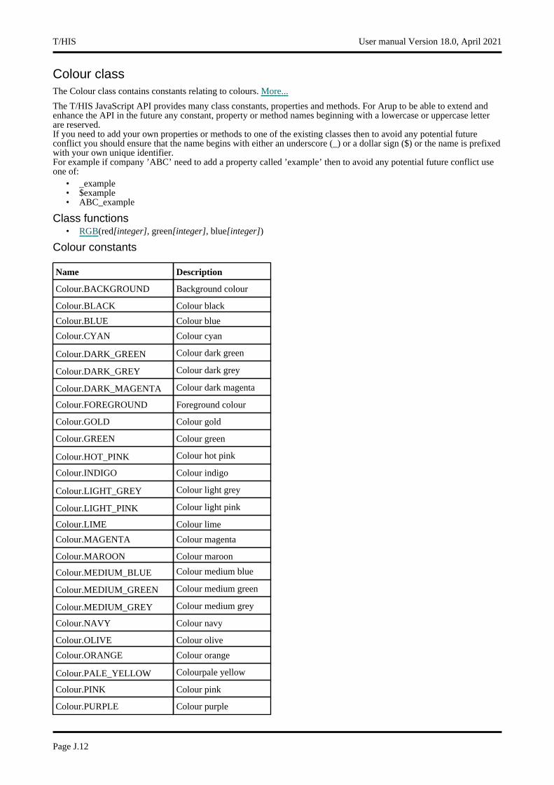
Colour classThe Colour class contains constants relating to colours. More...
The T/HIS JavaScript API provides many class constants, properties and methods. For Arup to be able to extend and enhance the API in the future any constant, property or method names beginning with a lowercase or uppercase letter are reserved.If you need to add your own properties or methods to one of the existing classes then to avoid any potential future conflict you should ensure that the name begins with either an underscore (_) or a dollar sign ($) or the name is prefixed with your own unique identifier.For example if company ’ABC’ need to add a property called ’example’ then to avoid any potential future conflict use one of:
• _example • $example • ABC_example
Class functions• RGB(red[integer], green[integer], blue[integer])
Colour constants
Name Description
Colour.BACKGROUND Background colour
Colour.BLACK Colour black
Colour.BLUE Colour blue
Colour.CYAN Colour cyan
Colour.DARK_GREEN Colour dark green
Colour.DARK_GREY Colour dark grey
Colour.DARK_MAGENTA Colour dark magenta
Colour.FOREGROUND Foreground colour
Colour.GOLD Colour gold
Colour.GREEN Colour green
Colour.HOT_PINK Colour hot pink
Colour.INDIGO Colour indigo
Colour.LIGHT_GREY Colour light grey
Colour.LIGHT_PINK Colour light pink
Colour.LIME Colour lime
Colour.MAGENTA Colour magenta
Colour.MAROON Colour maroon
Colour.MEDIUM_BLUE Colour medium blue
Colour.MEDIUM_GREEN Colour medium green
Colour.MEDIUM_GREY Colour medium grey
Colour.NAVY Colour navy
Colour.OLIVE Colour olive
Colour.ORANGE Colour orange
Colour.PALE_YELLOW Colourpale yellow
Colour.PINK Colour pink
Colour.PURPLE Colour purple
T/HIS User manual Version 18.0, April 2021
Page J.12
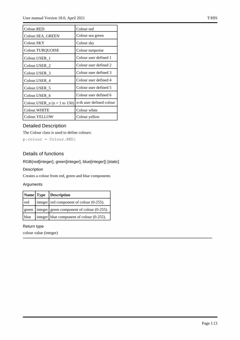
Colour.RED Colour red
Colour.SEA_GREEN Colour sea green
Colour.SKY Colour sky
Colour.TURQUOISE Colour turquoise
Colour.USER_1 Colour user defined 1
Colour.USER_2 Colour user defined 2
Colour.USER_3 Colour user defined 3
Colour.USER_4 Colour user defined 4
Colour.USER_5 Colour user defined 5
Colour.USER_6 Colour user defined 6
Colour.USER_n (n = 1 to 150) n-th user defined colour
Colour.WHITE Colour white
Colour.YELLOW Colour yellow
Detailed DescriptionThe Colour class is used to define colours:
p.colour = Colour.RED;
Details of functions
RGB(red[integer], green[integer], blue[integer]) [static]
Description
Creates a colour from red, green and blue components
Arguments
Name Type Description
red integer red component of colour (0-255).
green integer green component of colour (0-255).
blue integer blue component of colour (0-255).
Return type
colour value (integer)
User manual Version 18.0, April 2021 T/HIS
Page J.13

Component classThe following component constants can be used in GetDataFlagged() in T/HIS.
Component constants
Constants for MODEL
Name Description
Component.GSTP Time step
Component.GKE Kinetic energy
Component.GIE Internal energy
Component.GSWE Stonewall energy
Component.GSPE Spring and damper energy
Component.GHG Hourglass energy
Component.GSDE System damping energy
Component.GJE Joint internal energy
Component.GSIE Sliding interface energy
Component.GEW External work
Component.GRBE Rigid Body stopper energy
Component.GTE Total energy
Component.GTER Total/initial energy
Component.GVX Average X velocity
Component.GVY Average Y velocity
Component.GVZ Average Z velocity
Component.GTZC Time per zone cycle
Component.GMASS Total mass
Component.GMADD Added mass
Component.GPM %age Mass increase
Component.GEKE Eroded Kinetic energy
Component.GEIE Eroded Internal energy
Component.GEHG Eroded Hourglass energy
Component.GER Energy Ratio w/o Eroded
Component.DRCE Current Distortional KE
Component.DRMX Maximum Distortional KE
Component.DRCO Convergence Factor
Component.DRKE Total Kinetic energy
Component.LKE Lumped Kinetic energy
Constants for PART
Name Description
Component.GKE Kinetic energy
T/HIS User manual Version 18.0, April 2021
Page J.14
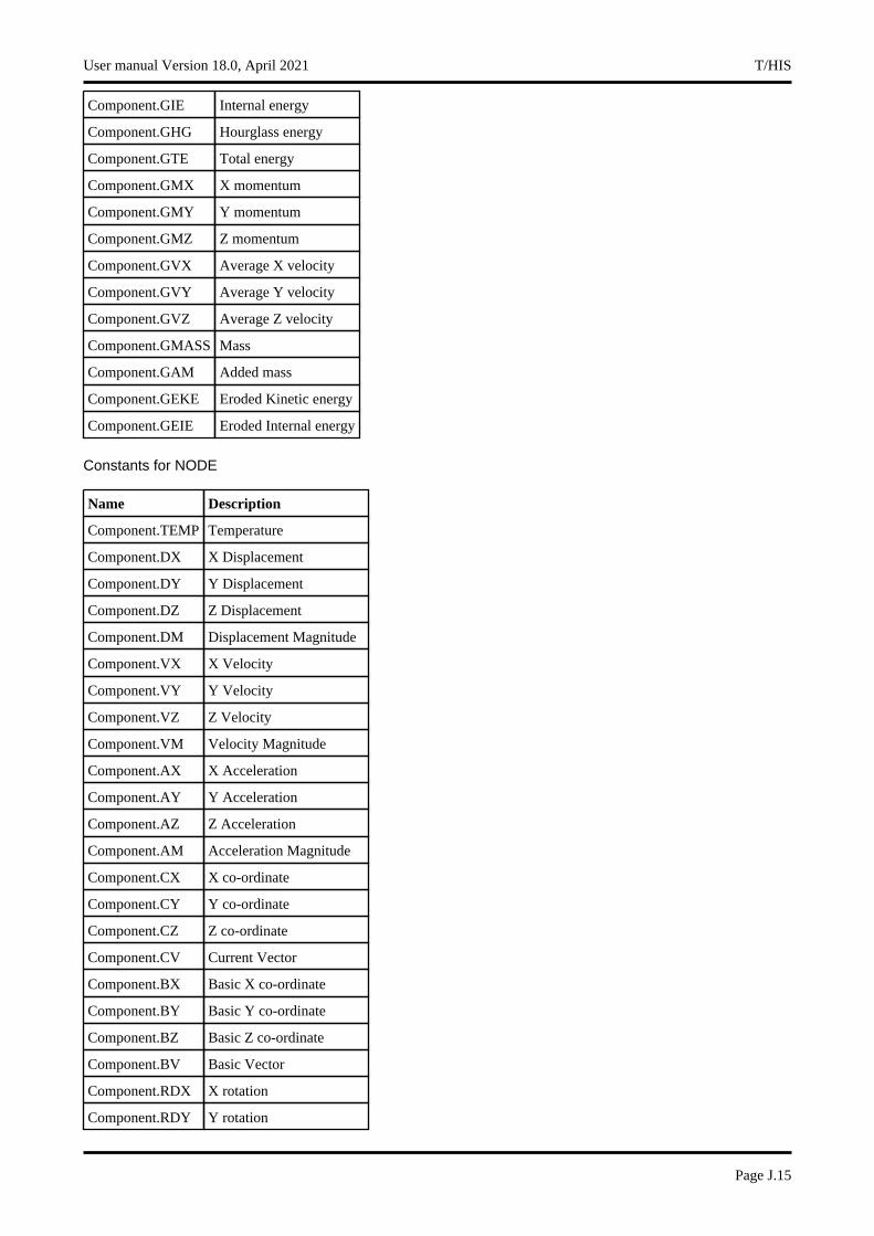
Component.GIE Internal energy
Component.GHG Hourglass energy
Component.GTE Total energy
Component.GMX X momentum
Component.GMY Y momentum
Component.GMZ Z momentum
Component.GVX Average X velocity
Component.GVY Average Y velocity
Component.GVZ Average Z velocity
Component.GMASS Mass
Component.GAM Added mass
Component.GEKE Eroded Kinetic energy
Component.GEIE Eroded Internal energy
Constants for NODE
Name Description
Component.TEMP Temperature
Component.DX X Displacement
Component.DY Y Displacement
Component.DZ Z Displacement
Component.DM Displacement Magnitude
Component.VX X Velocity
Component.VY Y Velocity
Component.VZ Z Velocity
Component.VM Velocity Magnitude
Component.AX X Acceleration
Component.AY Y Acceleration
Component.AZ Z Acceleration
Component.AM Acceleration Magnitude
Component.CX X co-ordinate
Component.CY Y co-ordinate
Component.CZ Z co-ordinate
Component.CV Current Vector
Component.BX Basic X co-ordinate
Component.BY Basic Y co-ordinate
Component.BZ Basic Z co-ordinate
Component.BV Basic Vector
Component.RDX X rotation
Component.RDY Y rotation
User manual Version 18.0, April 2021 T/HIS
Page J.15
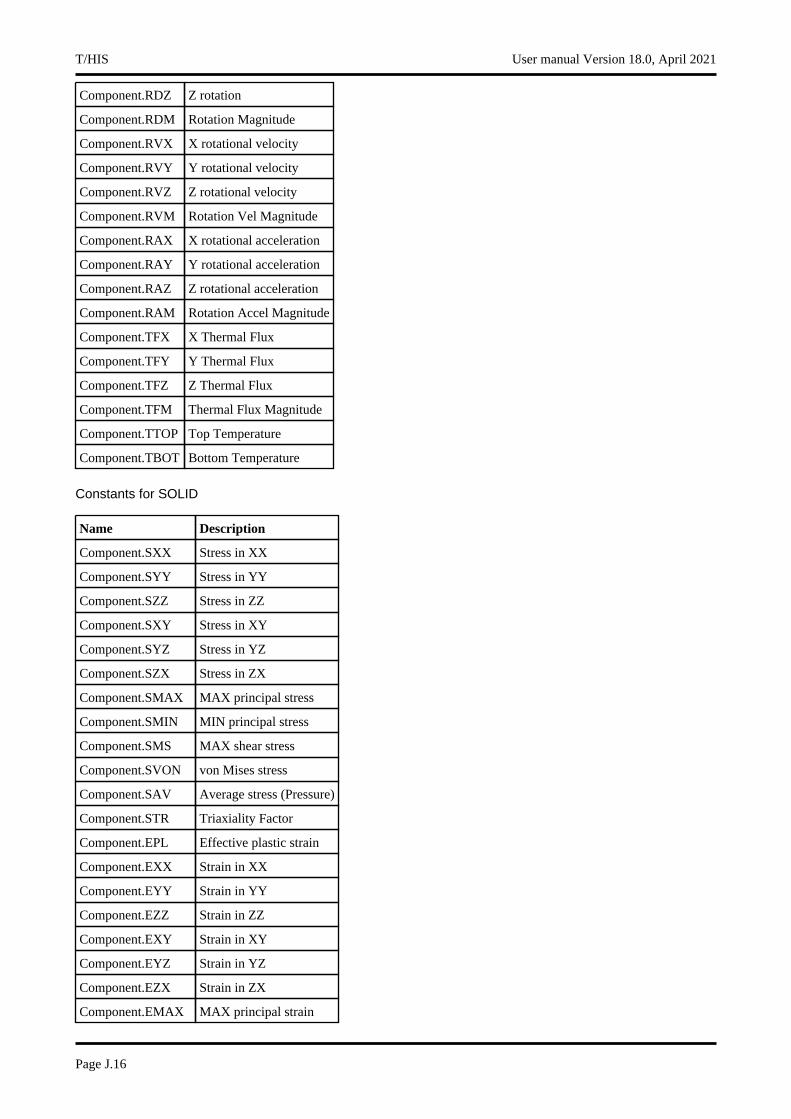
Component.RDZ Z rotation
Component.RDM Rotation Magnitude
Component.RVX X rotational velocity
Component.RVY Y rotational velocity
Component.RVZ Z rotational velocity
Component.RVM Rotation Vel Magnitude
Component.RAX X rotational acceleration
Component.RAY Y rotational acceleration
Component.RAZ Z rotational acceleration
Component.RAM Rotation Accel Magnitude
Component.TFX X Thermal Flux
Component.TFY Y Thermal Flux
Component.TFZ Z Thermal Flux
Component.TFM Thermal Flux Magnitude
Component.TTOP Top Temperature
Component.TBOT Bottom Temperature
Constants for SOLID
Name Description
Component.SXX Stress in XX
Component.SYY Stress in YY
Component.SZZ Stress in ZZ
Component.SXY Stress in XY
Component.SYZ Stress in YZ
Component.SZX Stress in ZX
Component.SMAX MAX principal stress
Component.SMIN MIN principal stress
Component.SMS MAX shear stress
Component.SVON von Mises stress
Component.SAV Average stress (Pressure)
Component.STR Triaxiality Factor
Component.EPL Effective plastic strain
Component.EXX Strain in XX
Component.EYY Strain in YY
Component.EZZ Strain in ZZ
Component.EXY Strain in XY
Component.EYZ Strain in YZ
Component.EZX Strain in ZX
Component.EMAX MAX principal strain
T/HIS User manual Version 18.0, April 2021
Page J.16
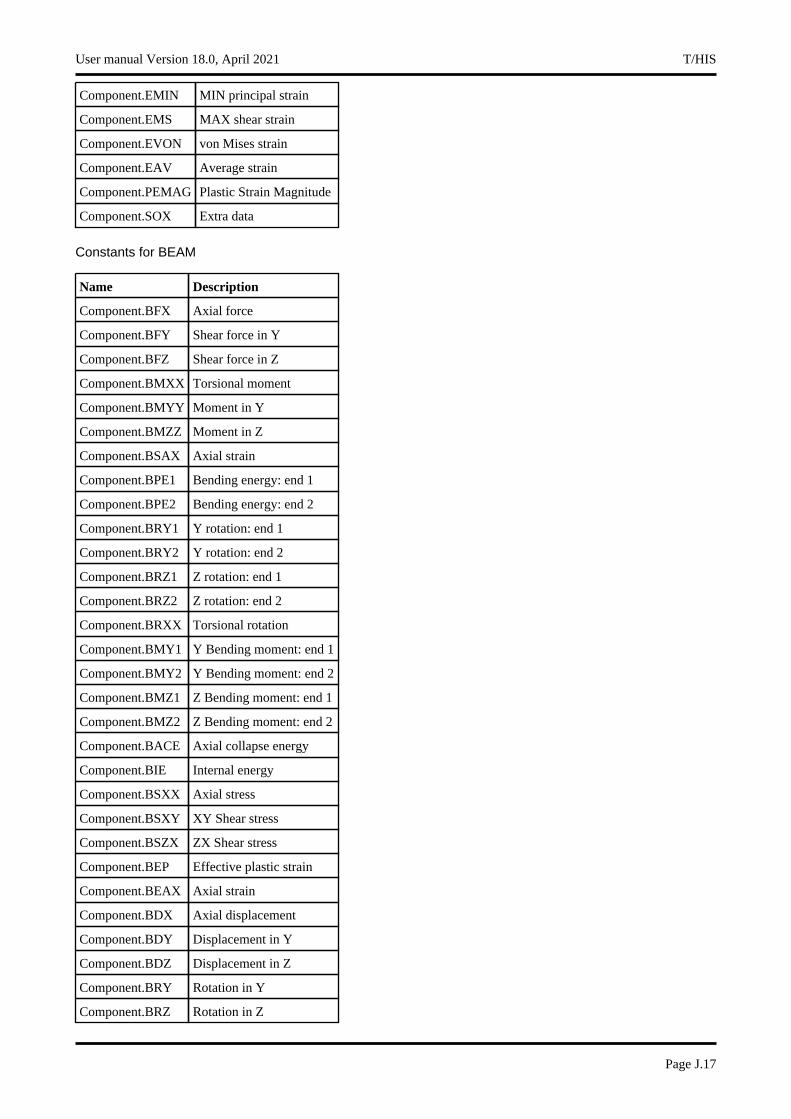
Component.EMIN MIN principal strain
Component.EMS MAX shear strain
Component.EVON von Mises strain
Component.EAV Average strain
Component.PEMAG Plastic Strain Magnitude
Component.SOX Extra data
Constants for BEAM
Name Description
Component.BFX Axial force
Component.BFY Shear force in Y
Component.BFZ Shear force in Z
Component.BMXX Torsional moment
Component.BMYY Moment in Y
Component.BMZZ Moment in Z
Component.BSAX Axial strain
Component.BPE1 Bending energy: end 1
Component.BPE2 Bending energy: end 2
Component.BRY1 Y rotation: end 1
Component.BRY2 Y rotation: end 2
Component.BRZ1 Z rotation: end 1
Component.BRZ2 Z rotation: end 2
Component.BRXX Torsional rotation
Component.BMY1 Y Bending moment: end 1
Component.BMY2 Y Bending moment: end 2
Component.BMZ1 Z Bending moment: end 1
Component.BMZ2 Z Bending moment: end 2
Component.BACE Axial collapse energy
Component.BIE Internal energy
Component.BSXX Axial stress
Component.BSXY XY Shear stress
Component.BSZX ZX Shear stress
Component.BEP Effective plastic strain
Component.BEAX Axial strain
Component.BDX Axial displacement
Component.BDY Displacement in Y
Component.BDZ Displacement in Z
Component.BRY Rotation in Y
Component.BRZ Rotation in Z
User manual Version 18.0, April 2021 T/HIS
Page J.17
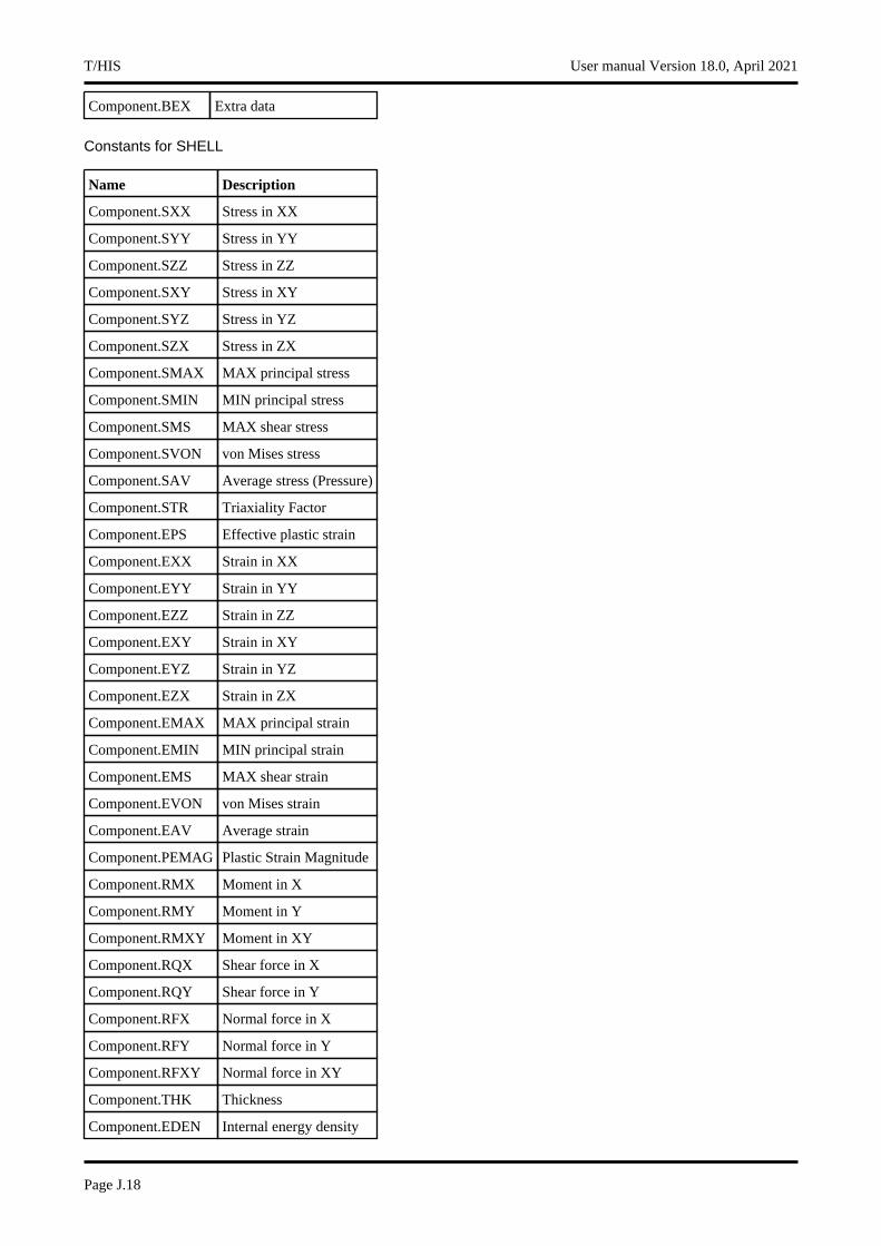
Component.BEX Extra data
Constants for SHELL
Name Description
Component.SXX Stress in XX
Component.SYY Stress in YY
Component.SZZ Stress in ZZ
Component.SXY Stress in XY
Component.SYZ Stress in YZ
Component.SZX Stress in ZX
Component.SMAX MAX principal stress
Component.SMIN MIN principal stress
Component.SMS MAX shear stress
Component.SVON von Mises stress
Component.SAV Average stress (Pressure)
Component.STR Triaxiality Factor
Component.EPS Effective plastic strain
Component.EXX Strain in XX
Component.EYY Strain in YY
Component.EZZ Strain in ZZ
Component.EXY Strain in XY
Component.EYZ Strain in YZ
Component.EZX Strain in ZX
Component.EMAX MAX principal strain
Component.EMIN MIN principal strain
Component.EMS MAX shear strain
Component.EVON von Mises strain
Component.EAV Average strain
Component.PEMAG Plastic Strain Magnitude
Component.RMX Moment in X
Component.RMY Moment in Y
Component.RMXY Moment in XY
Component.RQX Shear force in X
Component.RQY Shear force in Y
Component.RFX Normal force in X
Component.RFY Normal force in Y
Component.RFXY Normal force in XY
Component.THK Thickness
Component.EDEN Internal energy density
T/HIS User manual Version 18.0, April 2021
Page J.18
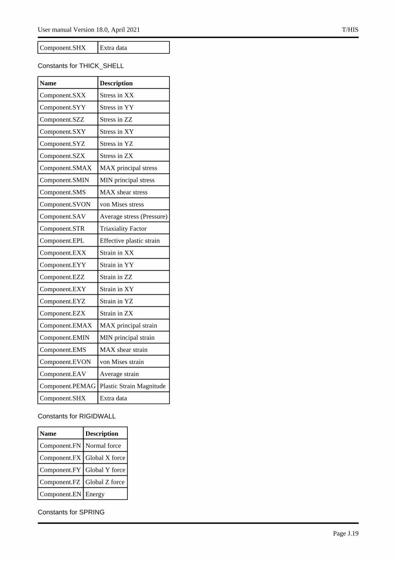
Component.SHX Extra data
Constants for THICK_SHELL
Name Description
Component.SXX Stress in XX
Component.SYY Stress in YY
Component.SZZ Stress in ZZ
Component.SXY Stress in XY
Component.SYZ Stress in YZ
Component.SZX Stress in ZX
Component.SMAX MAX principal stress
Component.SMIN MIN principal stress
Component.SMS MAX shear stress
Component.SVON von Mises stress
Component.SAV Average stress (Pressure)
Component.STR Triaxiality Factor
Component.EPL Effective plastic strain
Component.EXX Strain in XX
Component.EYY Strain in YY
Component.EZZ Strain in ZZ
Component.EXY Strain in XY
Component.EYZ Strain in YZ
Component.EZX Strain in ZX
Component.EMAX MAX principal strain
Component.EMIN MIN principal strain
Component.EMS MAX shear strain
Component.EVON von Mises strain
Component.EAV Average strain
Component.PEMAG Plastic Strain Magnitude
Component.SHX Extra data
Constants for RIGIDWALL
Name Description
Component.FN Normal force
Component.FX Global X force
Component.FY Global Y force
Component.FZ Global Z force
Component.EN Energy
Constants for SPRING
User manual Version 18.0, April 2021 T/HIS
Page J.19
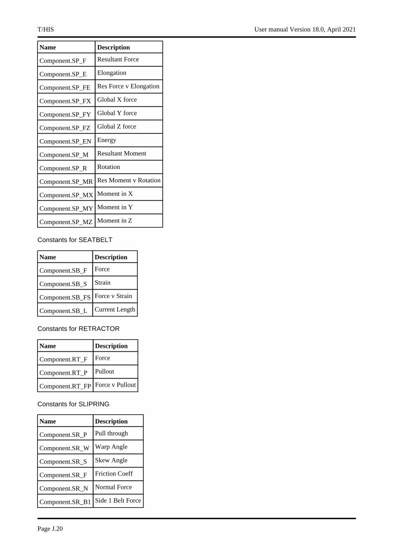
Name Description
Component.SP_F Resultant Force
Component.SP_E Elongation
Component.SP_FE Res Force v Elongation
Component.SP_FX Global X force
Component.SP_FY Global Y force
Component.SP_FZ Global Z force
Component.SP_EN Energy
Component.SP_M Resultant Moment
Component.SP_R Rotation
Component.SP_MR Res Moment v Rotation
Component.SP_MX Moment in X
Component.SP_MY Moment in Y
Component.SP_MZ Moment in Z
Constants for SEATBELT
Name Description
Component.SB_F Force
Component.SB_S Strain
Component.SB_FS Force v Strain
Component.SB_L Current Length
Constants for RETRACTOR
Name Description
Component.RT_F Force
Component.RT_P Pullout
Component.RT_FP Force v Pullout
Constants for SLIPRING
Name Description
Component.SR_P Pull through
Component.SR_W Warp Angle
Component.SR_S Skew Angle
Component.SR_F Friction Coeff
Component.SR_N Normal Force
Component.SR_B1 Side 1 Belt Force
T/HIS User manual Version 18.0, April 2021
Page J.20
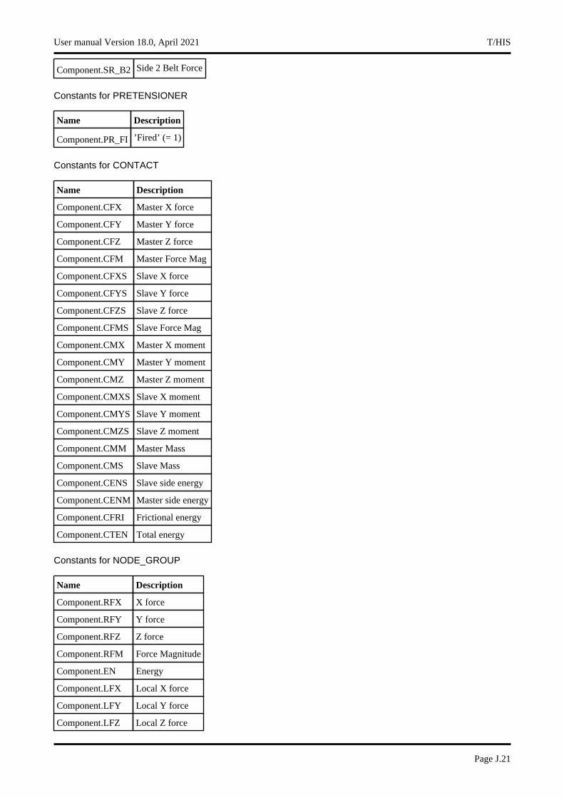
Component.SR_B2 Side 2 Belt Force
Constants for PRETENSIONER
Name Description
Component.PR_FI ’Fired’ (= 1)
Constants for CONTACT
Name Description
Component.CFX Master X force
Component.CFY Master Y force
Component.CFZ Master Z force
Component.CFM Master Force Mag
Component.CFXS Slave X force
Component.CFYS Slave Y force
Component.CFZS Slave Z force
Component.CFMS Slave Force Mag
Component.CMX Master X moment
Component.CMY Master Y moment
Component.CMZ Master Z moment
Component.CMXS Slave X moment
Component.CMYS Slave Y moment
Component.CMZS Slave Z moment
Component.CMM Master Mass
Component.CMS Slave Mass
Component.CENS Slave side energy
Component.CENM Master side energy
Component.CFRI Frictional energy
Component.CTEN Total energy
Constants for NODE_GROUP
Name Description
Component.RFX X force
Component.RFY Y force
Component.RFZ Z force
Component.RFM Force Magnitude
Component.EN Energy
Component.LFX Local X force
Component.LFY Local Y force
Component.LFZ Local Z force
User manual Version 18.0, April 2021 T/HIS
Page J.21
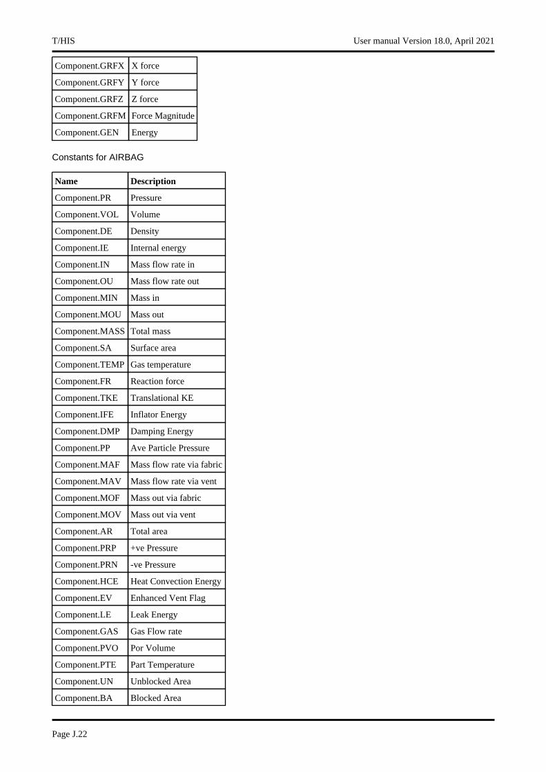
Component.GRFX X force
Component.GRFY Y force
Component.GRFZ Z force
Component.GRFM Force Magnitude
Component.GEN Energy
Constants for AIRBAG
Name Description
Component.PR Pressure
Component.VOL Volume
Component.DE Density
Component.IE Internal energy
Component.IN Mass flow rate in
Component.OU Mass flow rate out
Component.MIN Mass in
Component.MOU Mass out
Component.MASS Total mass
Component.SA Surface area
Component.TEMP Gas temperature
Component.FR Reaction force
Component.TKE Translational KE
Component.IFE Inflator Energy
Component.DMP Damping Energy
Component.PP Ave Particle Pressure
Component.MAF Mass flow rate via fabric
Component.MAV Mass flow rate via vent
Component.MOF Mass out via fabric
Component.MOV Mass out via vent
Component.AR Total area
Component.PRP +ve Pressure
Component.PRN -ve Pressure
Component.HCE Heat Convection Energy
Component.EV Enhanced Vent Flag
Component.LE Leak Energy
Component.GAS Gas Flow rate
Component.PVO Por Volume
Component.PTE Part Temperature
Component.UN Unblocked Area
Component.BA Blocked Area
T/HIS User manual Version 18.0, April 2021
Page J.22
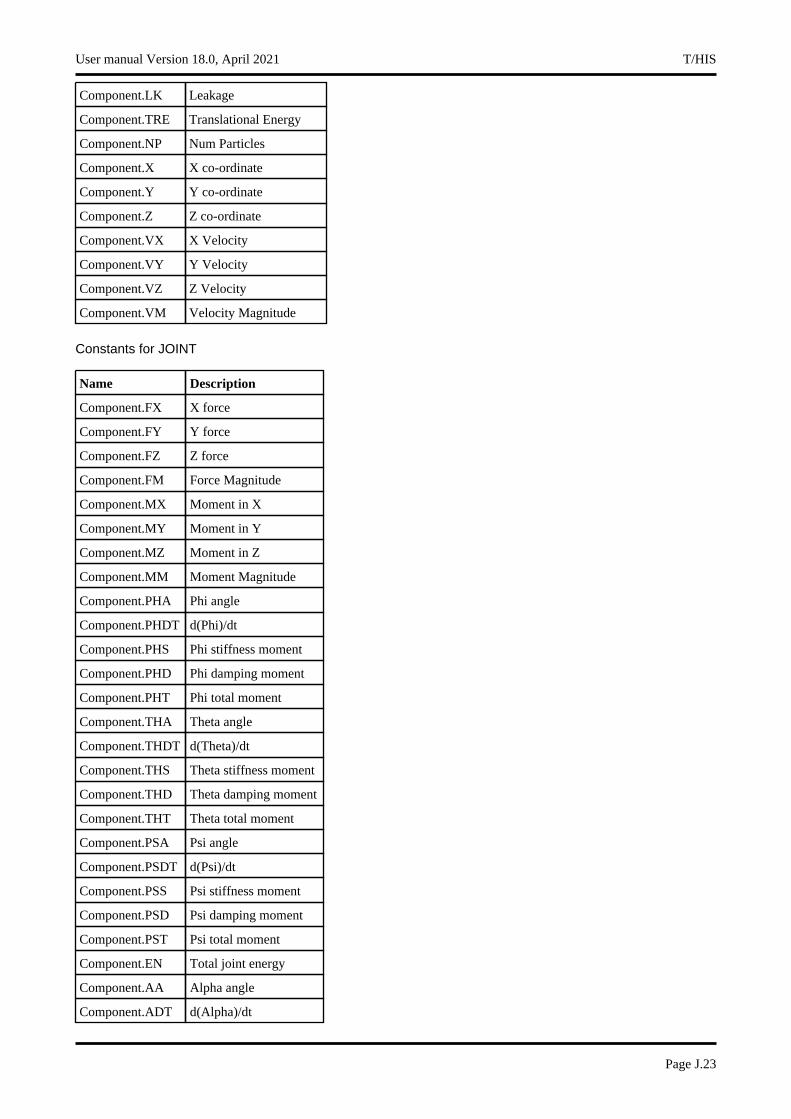
Component.LK Leakage
Component.TRE Translational Energy
Component.NP Num Particles
Component.X X co-ordinate
Component.Y Y co-ordinate
Component.Z Z co-ordinate
Component.VX X Velocity
Component.VY Y Velocity
Component.VZ Z Velocity
Component.VM Velocity Magnitude
Constants for JOINT
Name Description
Component.FX X force
Component.FY Y force
Component.FZ Z force
Component.FM Force Magnitude
Component.MX Moment in X
Component.MY Moment in Y
Component.MZ Moment in Z
Component.MM Moment Magnitude
Component.PHA Phi angle
Component.PHDT d(Phi)/dt
Component.PHS Phi stiffness moment
Component.PHD Phi damping moment
Component.PHT Phi total moment
Component.THA Theta angle
Component.THDT d(Theta)/dt
Component.THS Theta stiffness moment
Component.THD Theta damping moment
Component.THT Theta total moment
Component.PSA Psi angle
Component.PSDT d(Psi)/dt
Component.PSS Psi stiffness moment
Component.PSD Psi damping moment
Component.PST Psi total moment
Component.EN Total joint energy
Component.AA Alpha angle
Component.ADT d(Alpha)/dt
User manual Version 18.0, April 2021 T/HIS
Page J.23
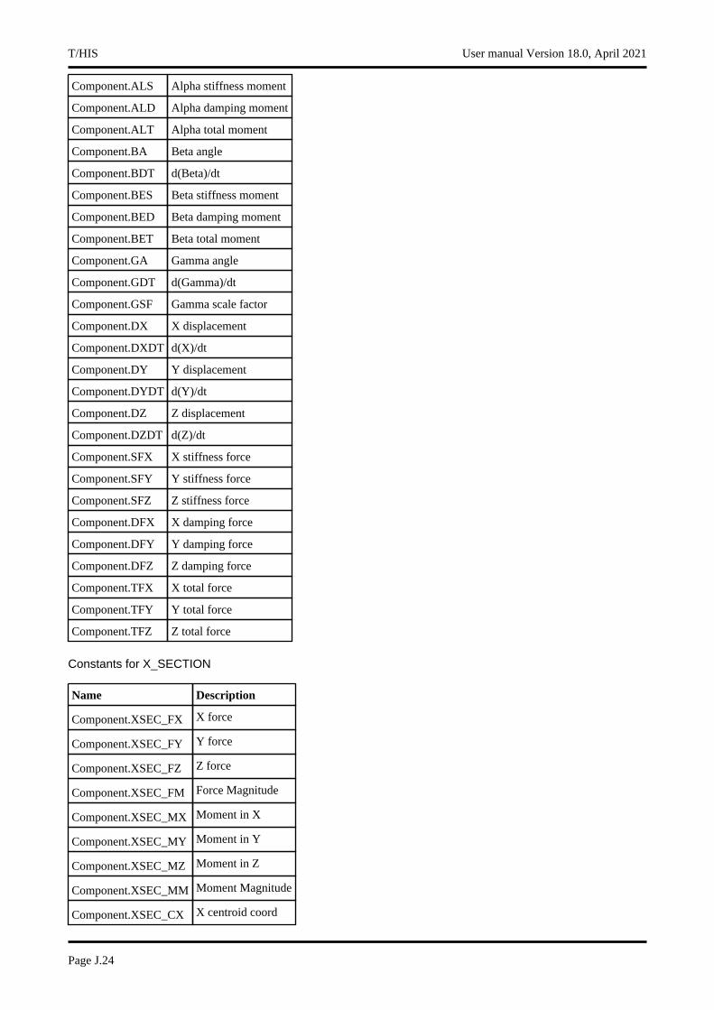
Component.ALS Alpha stiffness moment
Component.ALD Alpha damping moment
Component.ALT Alpha total moment
Component.BA Beta angle
Component.BDT d(Beta)/dt
Component.BES Beta stiffness moment
Component.BED Beta damping moment
Component.BET Beta total moment
Component.GA Gamma angle
Component.GDT d(Gamma)/dt
Component.GSF Gamma scale factor
Component.DX X displacement
Component.DXDT d(X)/dt
Component.DY Y displacement
Component.DYDT d(Y)/dt
Component.DZ Z displacement
Component.DZDT d(Z)/dt
Component.SFX X stiffness force
Component.SFY Y stiffness force
Component.SFZ Z stiffness force
Component.DFX X damping force
Component.DFY Y damping force
Component.DFZ Z damping force
Component.TFX X total force
Component.TFY Y total force
Component.TFZ Z total force
Constants for X_SECTION
Name Description
Component.XSEC_FX X force
Component.XSEC_FY Y force
Component.XSEC_FZ Z force
Component.XSEC_FM Force Magnitude
Component.XSEC_MX Moment in X
Component.XSEC_MY Moment in Y
Component.XSEC_MZ Moment in Z
Component.XSEC_MM Moment Magnitude
Component.XSEC_CX X centroid coord
T/HIS User manual Version 18.0, April 2021
Page J.24
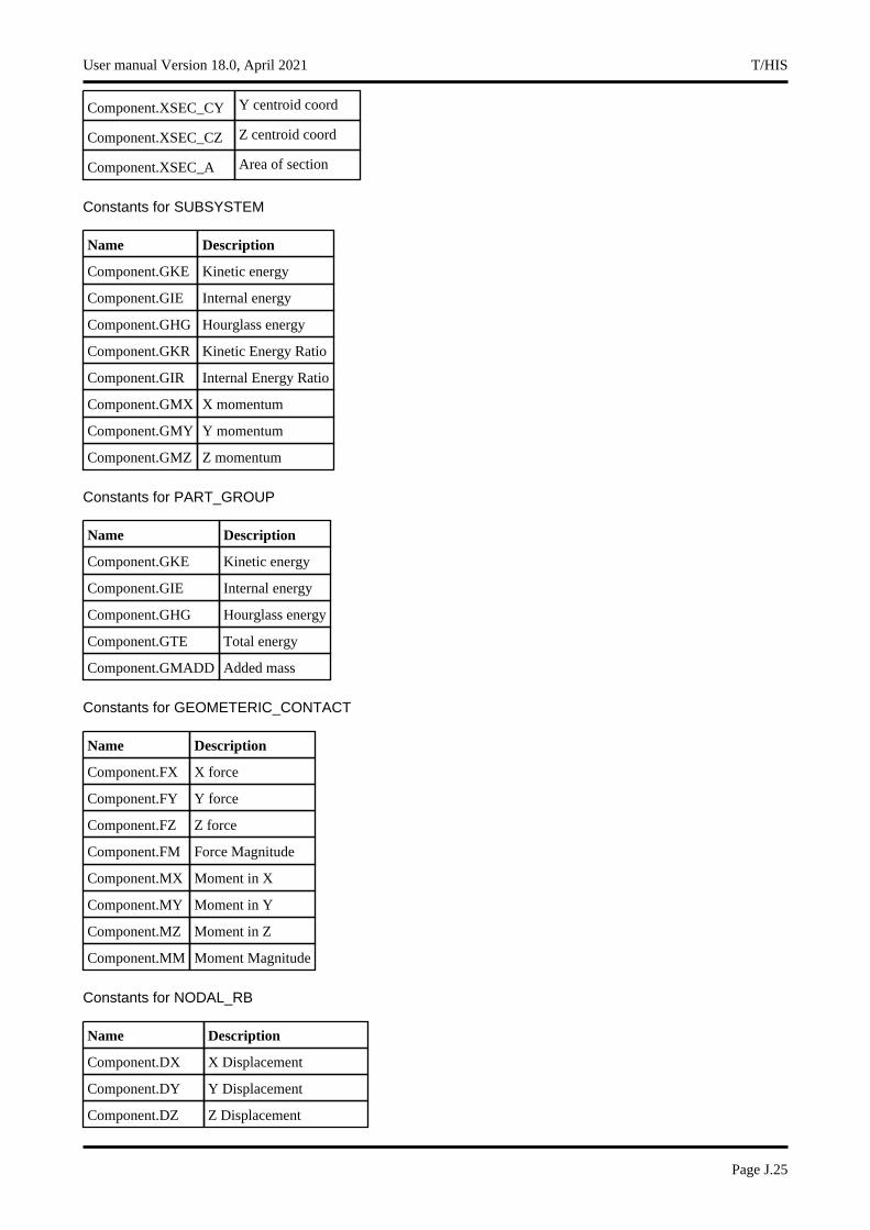
Component.XSEC_CY Y centroid coord
Component.XSEC_CZ Z centroid coord
Component.XSEC_A Area of section
Constants for SUBSYSTEM
Name Description
Component.GKE Kinetic energy
Component.GIE Internal energy
Component.GHG Hourglass energy
Component.GKR Kinetic Energy Ratio
Component.GIR Internal Energy Ratio
Component.GMX X momentum
Component.GMY Y momentum
Component.GMZ Z momentum
Constants for PART_GROUP
Name Description
Component.GKE Kinetic energy
Component.GIE Internal energy
Component.GHG Hourglass energy
Component.GTE Total energy
Component.GMADD Added mass
Constants for GEOMETERIC_CONTACT
Name Description
Component.FX X force
Component.FY Y force
Component.FZ Z force
Component.FM Force Magnitude
Component.MX Moment in X
Component.MY Moment in Y
Component.MZ Moment in Z
Component.MM Moment Magnitude
Constants for NODAL_RB
Name Description
Component.DX X Displacement
Component.DY Y Displacement
Component.DZ Z Displacement
User manual Version 18.0, April 2021 T/HIS
Page J.25
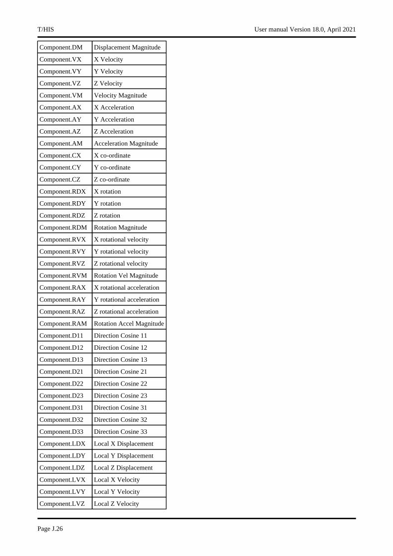
Component.DM Displacement Magnitude
Component.VX X Velocity
Component.VY Y Velocity
Component.VZ Z Velocity
Component.VM Velocity Magnitude
Component.AX X Acceleration
Component.AY Y Acceleration
Component.AZ Z Acceleration
Component.AM Acceleration Magnitude
Component.CX X co-ordinate
Component.CY Y co-ordinate
Component.CZ Z co-ordinate
Component.RDX X rotation
Component.RDY Y rotation
Component.RDZ Z rotation
Component.RDM Rotation Magnitude
Component.RVX X rotational velocity
Component.RVY Y rotational velocity
Component.RVZ Z rotational velocity
Component.RVM Rotation Vel Magnitude
Component.RAX X rotational acceleration
Component.RAY Y rotational acceleration
Component.RAZ Z rotational acceleration
Component.RAM Rotation Accel Magnitude
Component.D11 Direction Cosine 11
Component.D12 Direction Cosine 12
Component.D13 Direction Cosine 13
Component.D21 Direction Cosine 21
Component.D22 Direction Cosine 22
Component.D23 Direction Cosine 23
Component.D31 Direction Cosine 31
Component.D32 Direction Cosine 32
Component.D33 Direction Cosine 33
Component.LDX Local X Displacement
Component.LDY Local Y Displacement
Component.LDZ Local Z Displacement
Component.LVX Local X Velocity
Component.LVY Local Y Velocity
Component.LVZ Local Z Velocity
T/HIS User manual Version 18.0, April 2021
Page J.26
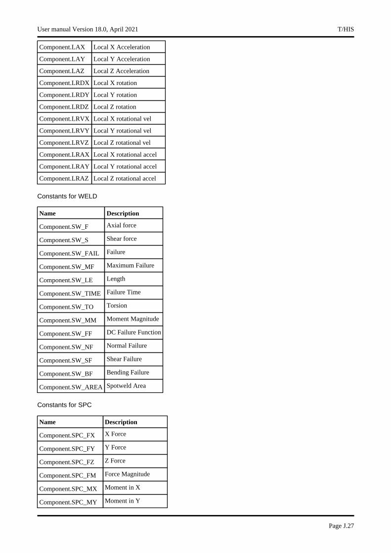
Component.LAX Local X Acceleration
Component.LAY Local Y Acceleration
Component.LAZ Local Z Acceleration
Component.LRDX Local X rotation
Component.LRDY Local Y rotation
Component.LRDZ Local Z rotation
Component.LRVX Local X rotational vel
Component.LRVY Local Y rotational vel
Component.LRVZ Local Z rotational vel
Component.LRAX Local X rotational accel
Component.LRAY Local Y rotational accel
Component.LRAZ Local Z rotational accel
Constants for WELD
Name Description
Component.SW_F Axial force
Component.SW_S Shear force
Component.SW_FAIL Failure
Component.SW_MF Maximum Failure
Component.SW_LE Length
Component.SW_TIME Failure Time
Component.SW_TO Torsion
Component.SW_MM Moment Magnitude
Component.SW_FF DC Failure Function
Component.SW_NF Normal Failure
Component.SW_SF Shear Failure
Component.SW_BF Bending Failure
Component.SW_AREA Spotweld Area
Constants for SPC
Name Description
Component.SPC_FX X Force
Component.SPC_FY Y Force
Component.SPC_FZ Z Force
Component.SPC_FM Force Magnitude
Component.SPC_MX Moment in X
Component.SPC_MY Moment in Y
User manual Version 18.0, April 2021 T/HIS
Page J.27

Component.SPC_MZ Moment in Z
Component.SPC_MM Moment Magnitude
Component.SPC_XTF X Total Set Force
Component.SPC_YTF Y Total Set Force
Component.SPC_ZTF Z Total Set Force
Component.SPC_RF Resultant Set Force
Component.SPC_XMF X Total Model Force
Component.SPC_YMF Y Total Model Force
Component.SPC_ZMF Z Total Model Force
Component.SPC_RMF Resultant Model Force
Constants for BOUNDARY
Name Description
Component.FX Applied X Force
Component.FY Applied Y Force
Component.FZ Applied Z Force
Component.FR Applied Resultant force
Component.MX Applied X Moment
Component.MY Applied Y Moment
Component.MZ Applied Z Moment
Component.MM Applied Moment Magnitude
Component.EN Energy from applied force
Constants for FSI
Name Description
Component.PR Pressure
Component.FX X force
Component.FY Y force
Component.FZ Z force
Component.FM Force Magnitude
Component.MP Mass (Porous+Vent)
Component.ML Mass (Leakage)
Component.LFX Leakage X Force
Component.LFY Leakage Y Force
Component.LFZ Leakage Z Force
Component.LFM Leakage Force Magnitude
Component.TEMP Temperature
Component.TC Temperature Change
T/HIS User manual Version 18.0, April 2021
Page J.28
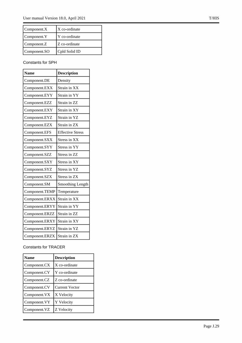
Component.X X co-ordinate
Component.Y Y co-ordinate
Component.Z Z co-ordinate
Component.SO Cpld Solid ID
Constants for SPH
Name Description
Component.DE Density
Component.EXX Strain in XX
Component.EYY Strain in YY
Component.EZZ Strain in ZZ
Component.EXY Strain in XY
Component.EYZ Strain in YZ
Component.EZX Strain in ZX
Component.EFS Effective Stress
Component.SXX Stress in XX
Component.SYY Stress in YY
Component.SZZ Stress in ZZ
Component.SXY Stress in XY
Component.SYZ Stress in YZ
Component.SZX Stress in ZX
Component.SM Smoothing Length
Component.TEMP Temperature
Component.ERXX Strain in XX
Component.ERYY Strain in YY
Component.ERZZ Strain in ZZ
Component.ERXY Strain in XY
Component.ERYZ Strain in YZ
Component.ERZX Strain in ZX
Constants for TRACER
Name Description
Component.CX X co-ordinate
Component.CY Y co-ordinate
Component.CZ Z co-ordinate
Component.CV Current Vector
Component.VX X Velocity
Component.VY Y Velocity
Component.VZ Z Velocity
User manual Version 18.0, April 2021 T/HIS
Page J.29
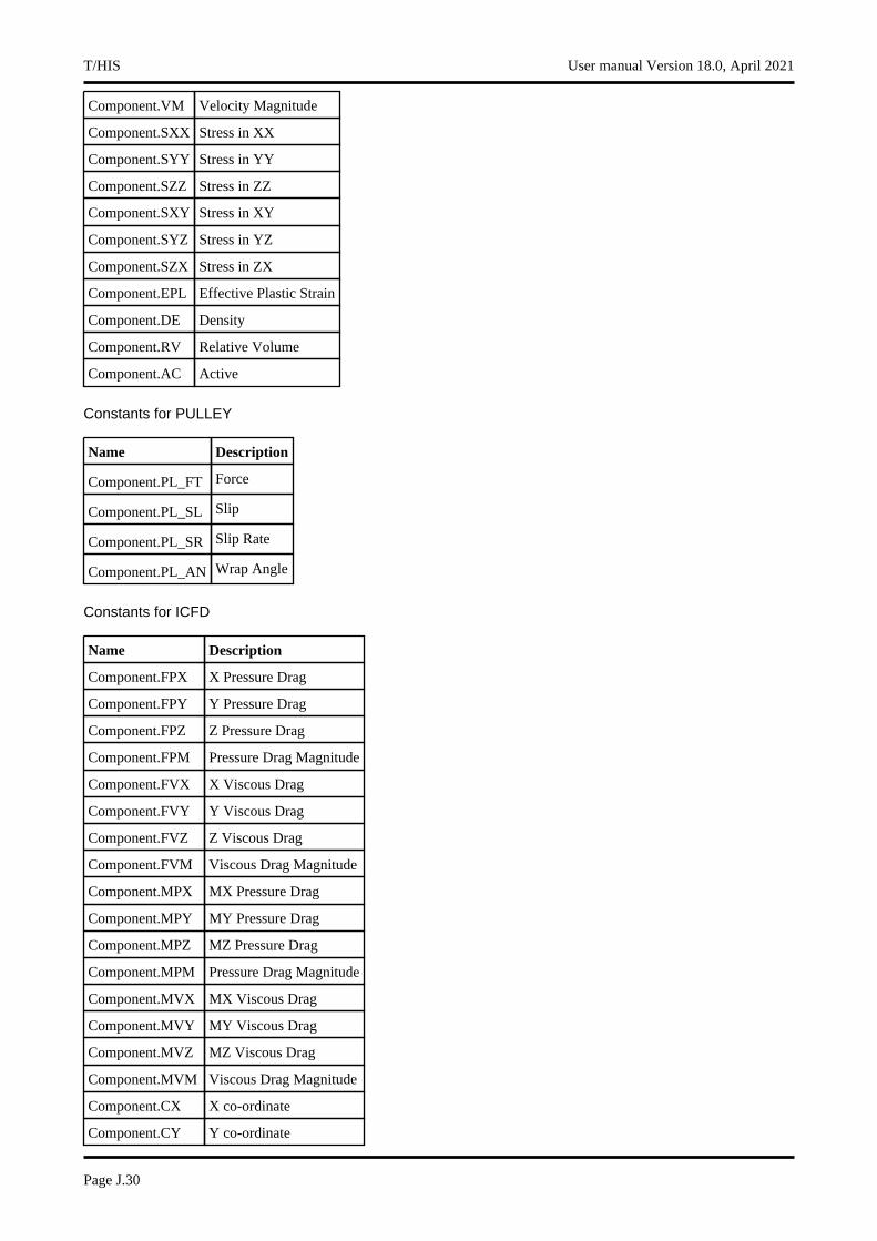
Component.VM Velocity Magnitude
Component.SXX Stress in XX
Component.SYY Stress in YY
Component.SZZ Stress in ZZ
Component.SXY Stress in XY
Component.SYZ Stress in YZ
Component.SZX Stress in ZX
Component.EPL Effective Plastic Strain
Component.DE Density
Component.RV Relative Volume
Component.AC Active
Constants for PULLEY
Name Description
Component.PL_FT Force
Component.PL_SL Slip
Component.PL_SR Slip Rate
Component.PL_AN Wrap Angle
Constants for ICFD
Name Description
Component.FPX X Pressure Drag
Component.FPY Y Pressure Drag
Component.FPZ Z Pressure Drag
Component.FPM Pressure Drag Magnitude
Component.FVX X Viscous Drag
Component.FVY Y Viscous Drag
Component.FVZ Z Viscous Drag
Component.FVM Viscous Drag Magnitude
Component.MPX MX Pressure Drag
Component.MPY MY Pressure Drag
Component.MPZ MZ Pressure Drag
Component.MPM Pressure Drag Magnitude
Component.MVX MX Viscous Drag
Component.MVY MY Viscous Drag
Component.MVZ MZ Viscous Drag
Component.MVM Viscous Drag Magnitude
Component.CX X co-ordinate
Component.CY Y co-ordinate
T/HIS User manual Version 18.0, April 2021
Page J.30
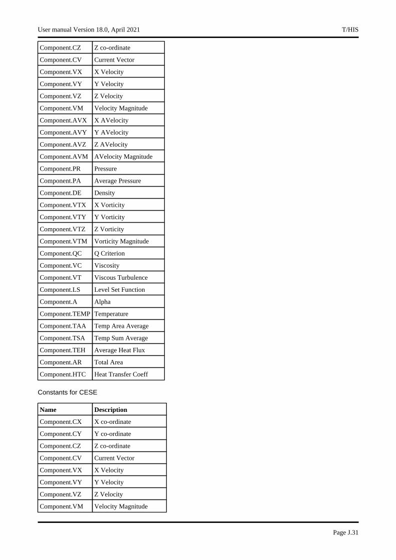
Component.CZ Z co-ordinate
Component.CV Current Vector
Component.VX X Velocity
Component.VY Y Velocity
Component.VZ Z Velocity
Component.VM Velocity Magnitude
Component.AVX X AVelocity
Component.AVY Y AVelocity
Component.AVZ Z AVelocity
Component.AVM AVelocity Magnitude
Component.PR Pressure
Component.PA Average Pressure
Component.DE Density
Component.VTX X Vorticity
Component.VTY Y Vorticity
Component.VTZ Z Vorticity
Component.VTM Vorticity Magnitude
Component.QC Q Criterion
Component.VC Viscosity
Component.VT Viscous Turbulence
Component.LS Level Set Function
Component.A Alpha
Component.TEMP Temperature
Component.TAA Temp Area Average
Component.TSA Temp Sum Average
Component.TEH Average Heat Flux
Component.AR Total Area
Component.HTC Heat Transfer Coeff
Constants for CESE
Name Description
Component.CX X co-ordinate
Component.CY Y co-ordinate
Component.CZ Z co-ordinate
Component.CV Current Vector
Component.VX X Velocity
Component.VY Y Velocity
Component.VZ Z Velocity
Component.VM Velocity Magnitude
User manual Version 18.0, April 2021 T/HIS
Page J.31
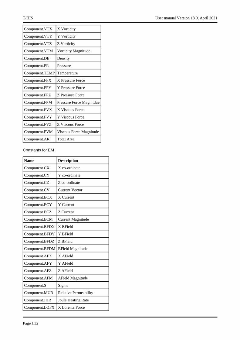
Component.VTX X Vorticity
Component.VTY Y Vorticity
Component.VTZ Z Vorticity
Component.VTM Vorticity Magnitude
Component.DE Density
Component.PR Pressure
Component.TEMP Temperature
Component.FPX X Pressure Force
Component.FPY Y Pressure Force
Component.FPZ Z Pressure Force
Component.FPM Pressure Force Magnitdue
Component.FVX X Viscous Force
Component.FVY Y Viscous Force
Component.FVZ Z Viscous Force
Component.FVM Viscous Force Magnitude
Component.AR Total Area
Constants for EM
Name Description
Component.CX X co-ordinate
Component.CY Y co-ordinate
Component.CZ Z co-ordinate
Component.CV Current Vector
Component.ECX X Current
Component.ECY Y Current
Component.ECZ Z Current
Component.ECM Current Magnitude
Component.BFDX X BField
Component.BFDY Y BField
Component.BFDZ Z BField
Component.BFDM BField Magnitude
Component.AFX X AField
Component.AFY Y AField
Component.AFZ Z AField
Component.AFM AField Magnitude
Component.S Sigma
Component.MUR Relative Permeability
Component.JHR Joule Heating Rate
Component.LOFX X Lorentz Force
T/HIS User manual Version 18.0, April 2021
Page J.32
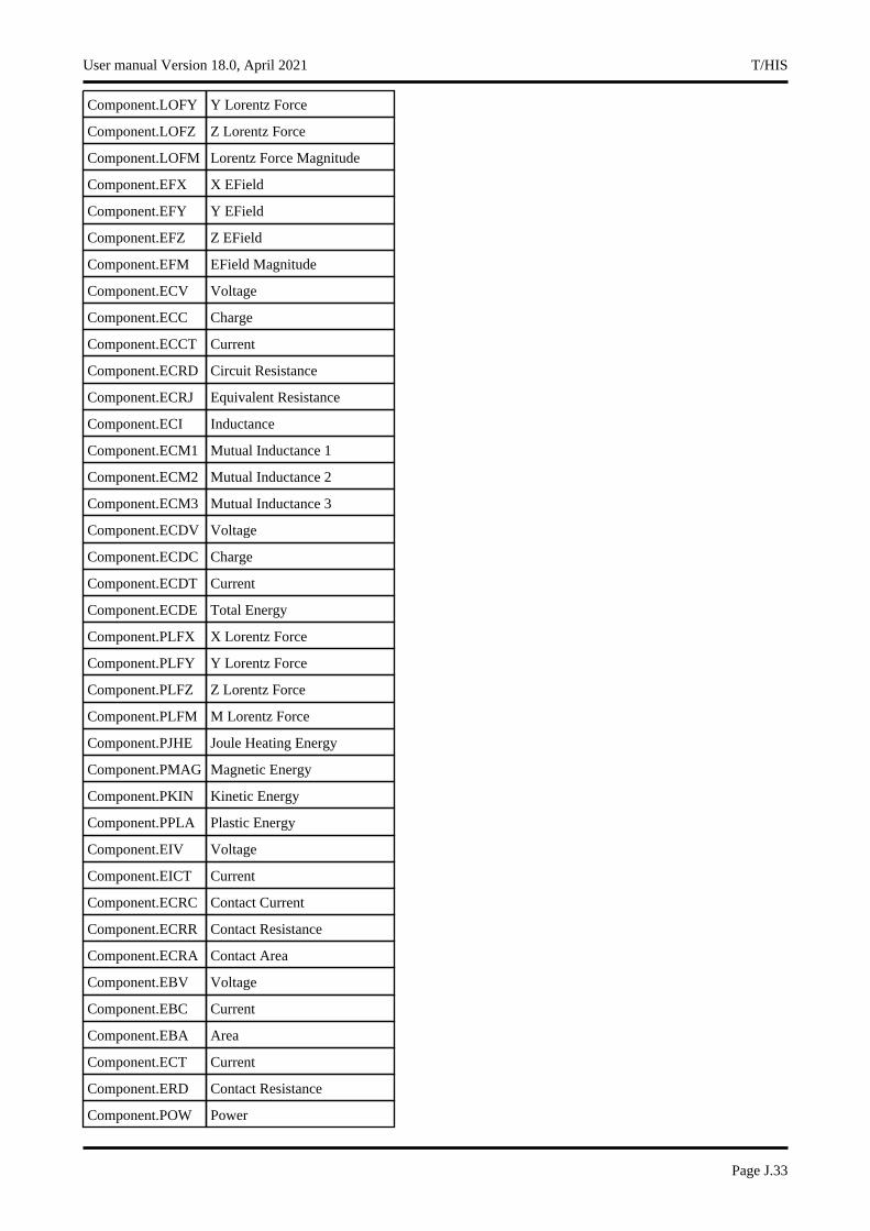
Component.LOFY Y Lorentz Force
Component.LOFZ Z Lorentz Force
Component.LOFM Lorentz Force Magnitude
Component.EFX X EField
Component.EFY Y EField
Component.EFZ Z EField
Component.EFM EField Magnitude
Component.ECV Voltage
Component.ECC Charge
Component.ECCT Current
Component.ECRD Circuit Resistance
Component.ECRJ Equivalent Resistance
Component.ECI Inductance
Component.ECM1 Mutual Inductance 1
Component.ECM2 Mutual Inductance 2
Component.ECM3 Mutual Inductance 3
Component.ECDV Voltage
Component.ECDC Charge
Component.ECDT Current
Component.ECDE Total Energy
Component.PLFX X Lorentz Force
Component.PLFY Y Lorentz Force
Component.PLFZ Z Lorentz Force
Component.PLFM M Lorentz Force
Component.PJHE Joule Heating Energy
Component.PMAG Magnetic Energy
Component.PKIN Kinetic Energy
Component.PPLA Plastic Energy
Component.EIV Voltage
Component.EICT Current
Component.ECRC Contact Current
Component.ECRR Contact Resistance
Component.ECRA Contact Area
Component.EBV Voltage
Component.EBC Current
Component.EBA Area
Component.ECT Current
Component.ERD Contact Resistance
Component.POW Power
User manual Version 18.0, April 2021 T/HIS
Page J.33
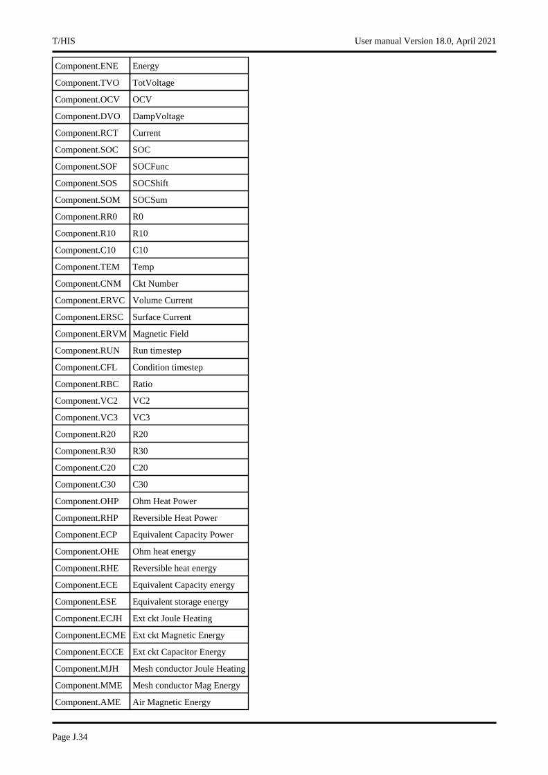
Component.ENE Energy
Component.TVO TotVoltage
Component.OCV OCV
Component.DVO DampVoltage
Component.RCT Current
Component.SOC SOC
Component.SOF SOCFunc
Component.SOS SOCShift
Component.SOM SOCSum
Component.RR0 R0
Component.R10 R10
Component.C10 C10
Component.TEM Temp
Component.CNM Ckt Number
Component.ERVC Volume Current
Component.ERSC Surface Current
Component.ERVM Magnetic Field
Component.RUN Run timestep
Component.CFL Condition timestep
Component.RBC Ratio
Component.VC2 VC2
Component.VC3 VC3
Component.R20 R20
Component.R30 R30
Component.C20 C20
Component.C30 C30
Component.OHP Ohm Heat Power
Component.RHP Reversible Heat Power
Component.ECP Equivalent Capacity Power
Component.OHE Ohm heat energy
Component.RHE Reversible heat energy
Component.ECE Equivalent Capacity energy
Component.ESE Equivalent storage energy
Component.ECJH Ext ckt Joule Heating
Component.ECME Ext ckt Magnetic Energy
Component.ECCE Ext ckt Capacitor Energy
Component.MJH Mesh conductor Joule Heating
Component.MME Mesh conductor Mag Energy
Component.AME Air Magnetic Energy
T/HIS User manual Version 18.0, April 2021
Page J.34
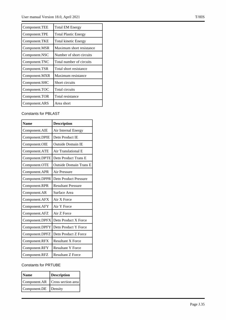
Component.TEE Total EM Energy
Component.TPE Total Plastic Energy
Component.TKE Total kinetic Energy
Component.MSR Maximum short resistance
Component.NSC Number of short circuits
Component.TNC Total number of circuits
Component.TSR Total short resistance
Component.MXR Maximum resistance
Component.SHC Short circuits
Component.TOC Total circuits
Component.TOR Total resistance
Component.ARS Area short
Constants for PBLAST
Name Description
Component.AIE Air Internal Energy
Component.DPIE Detn Product IE
Component.OIE Outside Domain IE
Component.ATE Air Translational E
Component.DPTE Detn Product Trans E
Component.OTE Outside Domain Trans E
Component.APR Air Pressure
Component.DPPR Detn Product Pressure
Component.RPR Resultant Pressure
Component.AR Surface Area
Component.AFX Air X Force
Component.AFY Air Y Force
Component.AFZ Air Z Force
Component.DPFX Detn Product X Force
Component.DPFY Detn Product Y Force
Component.DPFZ Detn Product Z Force
Component.RFX Resultant X Force
Component.RFY Resultant Y Force
Component.RFZ Resultant Z Force
Constants for PRTUBE
Name Description
Component.AR Cross section area
Component.DE Density
User manual Version 18.0, April 2021 T/HIS
Page J.35
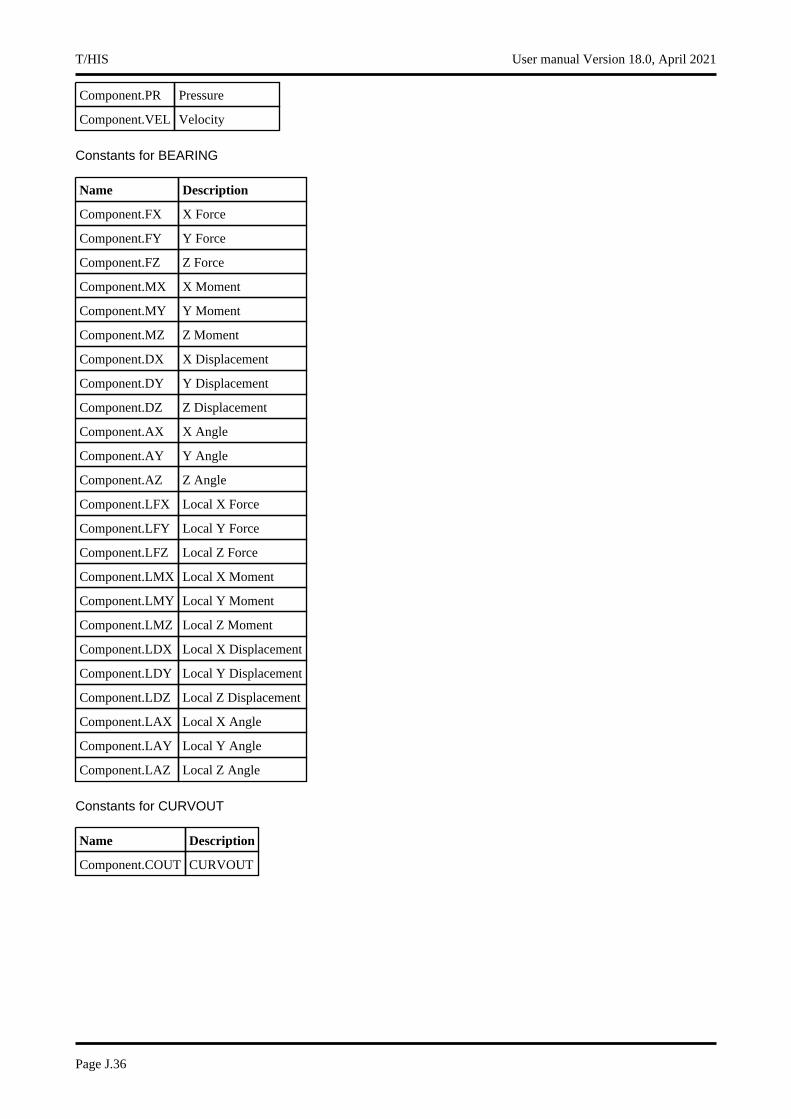
Component.PR Pressure
Component.VEL Velocity
Constants for BEARING
Name Description
Component.FX X Force
Component.FY Y Force
Component.FZ Z Force
Component.MX X Moment
Component.MY Y Moment
Component.MZ Z Moment
Component.DX X Displacement
Component.DY Y Displacement
Component.DZ Z Displacement
Component.AX X Angle
Component.AY Y Angle
Component.AZ Z Angle
Component.LFX Local X Force
Component.LFY Local Y Force
Component.LFZ Local Z Force
Component.LMX Local X Moment
Component.LMY Local Y Moment
Component.LMZ Local Z Moment
Component.LDX Local X Displacement
Component.LDY Local Y Displacement
Component.LDZ Local Z Displacement
Component.LAX Local X Angle
Component.LAY Local Y Angle
Component.LAZ Local Z Angle
Constants for CURVOUT
Name Description
Component.COUT CURVOUT
T/HIS User manual Version 18.0, April 2021
Page J.36
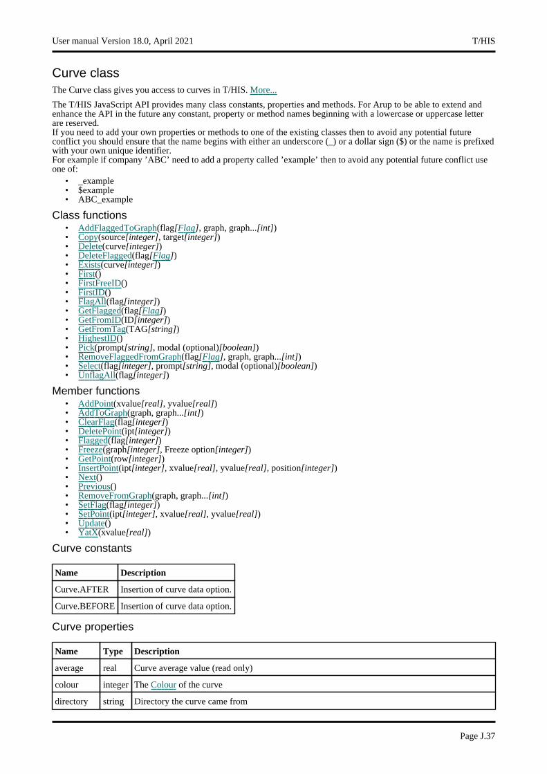
Curve classThe Curve class gives you access to curves in T/HIS. More...
The T/HIS JavaScript API provides many class constants, properties and methods. For Arup to be able to extend and enhance the API in the future any constant, property or method names beginning with a lowercase or uppercase letter are reserved.If you need to add your own properties or methods to one of the existing classes then to avoid any potential future conflict you should ensure that the name begins with either an underscore (_) or a dollar sign ($) or the name is prefixed with your own unique identifier.For example if company ’ABC’ need to add a property called ’example’ then to avoid any potential future conflict use one of:
• _example • $example • ABC_example
Class functions• AddFlaggedToGraph(flag[Flag], graph, graph...[int]) • Copy(source[integer], target[integer]) • Delete(curve[integer]) • DeleteFlagged(flag[Flag]) • Exists(curve[integer]) • First() • FirstFreeID() • FirstID() • FlagAll(flag[integer]) • GetFlagged(flag[Flag]) • GetFromID(ID[integer]) • GetFromTag(TAG[string]) • HighestID() • Pick(prompt[string], modal (optional)[boolean]) • RemoveFlaggedFromGraph(flag[Flag], graph, graph...[int]) • Select(flag[integer], prompt[string], modal (optional)[boolean]) • UnflagAll(flag[integer])
Member functions• AddPoint(xvalue[real], yvalue[real]) • AddToGraph(graph, graph...[int]) • ClearFlag(flag[integer]) • DeletePoint(ipt[integer]) • Flagged(flag[integer]) • Freeze(graph[integer], Freeze option[integer]) • GetPoint(row[integer]) • InsertPoint(ipt[integer], xvalue[real], yvalue[real], position[integer]) • Next() • Previous() • RemoveFromGraph(graph, graph...[int]) • SetFlag(flag[integer]) • SetPoint(ipt[integer], xvalue[real], yvalue[real]) • Update() • YatX(xvalue[real])
Curve constants
Name Description
Curve.AFTER Insertion of curve data option.
Curve.BEFORE Insertion of curve data option.
Curve properties
Name Type Description
average real Curve average value (read only)
colour integer The Colour of the curve
directory string Directory the curve came from
User manual Version 18.0, April 2021 T/HIS
Page J.37
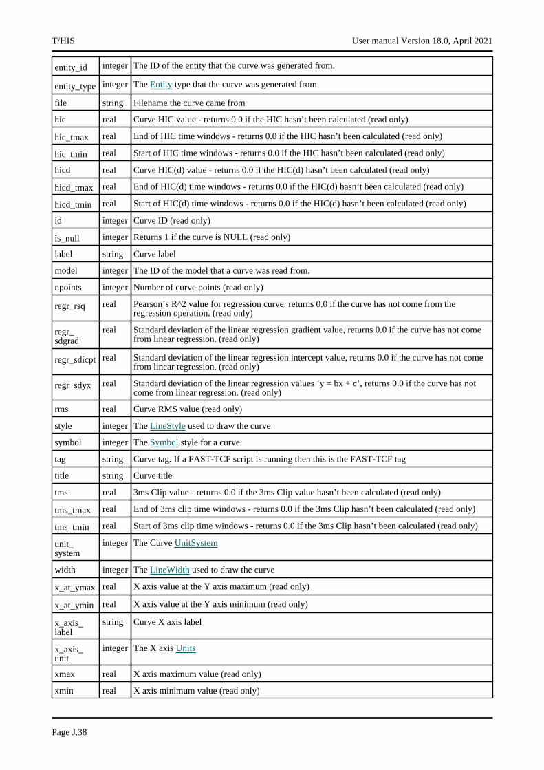
entity_id integer The ID of the entity that the curve was generated from.
entity_type integer The Entity type that the curve was generated from
file string Filename the curve came from
hic real Curve HIC value - returns 0.0 if the HIC hasn’t been calculated (read only)
hic_tmax real End of HIC time windows - returns 0.0 if the HIC hasn’t been calculated (read only)
hic_tmin real Start of HIC time windows - returns 0.0 if the HIC hasn’t been calculated (read only)
hicd real Curve HIC(d) value - returns 0.0 if the HIC(d) hasn’t been calculated (read only)
hicd_tmax real End of HIC(d) time windows - returns 0.0 if the HIC(d) hasn’t been calculated (read only)
hicd_tmin real Start of HIC(d) time windows - returns 0.0 if the HIC(d) hasn’t been calculated (read only)
id integer Curve ID (read only)
is_null integer Returns 1 if the curve is NULL (read only)
label string Curve label
model integer The ID of the model that a curve was read from.
npoints integer Number of curve points (read only)
regr_rsq real Pearson’s R^2 value for regression curve, returns 0.0 if the curve has not come from the regression operation. (read only)
regr_sdgrad
real Standard deviation of the linear regression gradient value, returns 0.0 if the curve has not come from linear regression. (read only)
regr_sdicpt real Standard deviation of the linear regression intercept value, returns 0.0 if the curve has not come from linear regression. (read only)
regr_sdyx real Standard deviation of the linear regression values ’y = bx + c’, returns 0.0 if the curve has not come from linear regression. (read only)
rms real Curve RMS value (read only)
style integer The LineStyle used to draw the curve
symbol integer The Symbol style for a curve
tag string Curve tag. If a FAST-TCF script is running then this is the FAST-TCF tag
title string Curve title
tms real 3ms Clip value - returns 0.0 if the 3ms Clip value hasn’t been calculated (read only)
tms_tmax real End of 3ms clip time windows - returns 0.0 if the 3ms Clip hasn’t been calculated (read only)
tms_tmin real Start of 3ms clip time windows - returns 0.0 if the 3ms Clip hasn’t been calculated (read only)
unit_system
integer The Curve UnitSystem
width integer The LineWidth used to draw the curve
x_at_ymax real X axis value at the Y axis maximum (read only)
x_at_ymin real X axis value at the Y axis minimum (read only)
x_axis_label
string Curve X axis label
x_axis_unit
integer The X axis Units
xmax real X axis maximum value (read only)
xmin real X axis minimum value (read only)
T/HIS User manual Version 18.0, April 2021
Page J.38
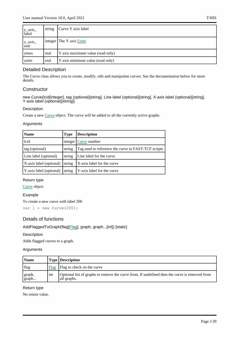
y_axis_label
string Curve Y axis label
y_axis_unit
integer The Y axis Units
ymax real Y axis maximum value (read only)
ymin real Y axis minimum value (read only)
Detailed DescriptionThe Curve class allows you to create, modify, edit and manipulate curves. See the documentation below for more details.
Constructor
new Curve(lcid[integer], tag (optional)[string], Line label (optional)[string], X-axis label (optional)[string], Y-axis label (optional)[string])
Description
Create a new Curve object. The curve will be added to all the currently active graphs.
Arguments
Name Type Description
lcid integer Curve number
tag (optional) string Tag used to reference the curve in FAST-TCF scripts
Line label (optional) string Line label for the curve
X-axis label (optional) string X-axis label for the curve
Y-axis label (optional) string Y-axis label for the curve
Return type
Curve object
Example
To create a new curve with label 200
var l = new Curve(200);
Details of functions
AddFlaggedToGraph(flag[Flag], graph, graph...[int]) [static]
Description
Adds flagged curves to a graph.
Arguments
Name Type Description
flag Flag Flag to check on the curve
graph, graph...
int Optional list of graphs to remove the curve from, If undefined then the curve is removed from all graphs.
Return type
No return value.
User manual Version 18.0, April 2021 T/HIS
Page J.39
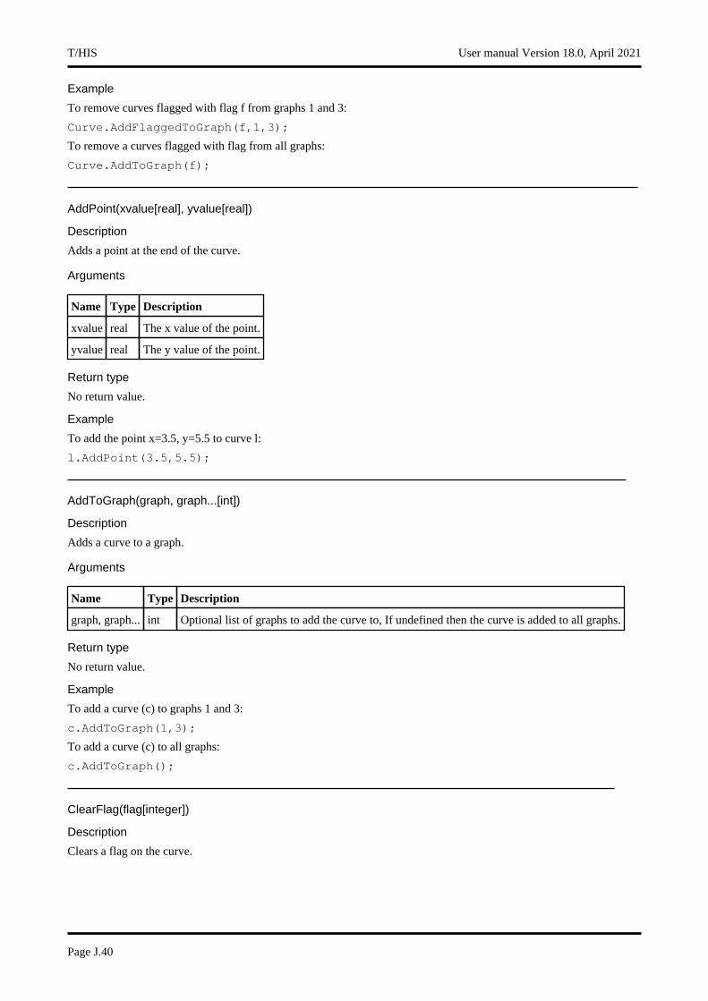
Example
To remove curves flagged with flag f from graphs 1 and 3:
Curve.AddFlaggedToGraph(f,1,3);
To remove a curves flagged with flag from all graphs:
Curve.AddToGraph(f);
AddPoint(xvalue[real], yvalue[real])
Description
Adds a point at the end of the curve.
Arguments
Name Type Description
xvalue real The x value of the point.
yvalue real The y value of the point.
Return type
No return value.
Example
To add the point x=3.5, y=5.5 to curve l:
l.AddPoint(3.5,5.5);
AddToGraph(graph, graph...[int])
Description
Adds a curve to a graph.
Arguments
Name Type Description
graph, graph... int Optional list of graphs to add the curve to, If undefined then the curve is added to all graphs.
Return type
No return value.
Example
To add a curve (c) to graphs 1 and 3:
c.AddToGraph(1,3);
To add a curve (c) to all graphs:
c.AddToGraph();
ClearFlag(flag[integer])
Description
Clears a flag on the curve.
T/HIS User manual Version 18.0, April 2021
Page J.40

Arguments
Name Type Description
flag integer Flag to clear on the curve
Return type
No return value
Example
To clear flag f for curve l:
l.ClearFlag(f);
Copy(source[integer], target[integer]) [static]
Description
Copies a curve.
Arguments
Name Type Description
source integer ID of curve to copy from
target integer ID of curve to copy to
Return type
No return value
Example
To copy curve 1 to curve 4:
Curve.Copy(1,4);
To copy curve a to curve b,
Curve.Copy(a.id,b.id);
Delete(curve[integer]) [static]
Description
Deletes a curve
Arguments
Name Type Description
curve integer ID of curve to delete
Return type
No return value
Example
To delete curve n
Curve.Delete(n);
User manual Version 18.0, April 2021 T/HIS
Page J.41
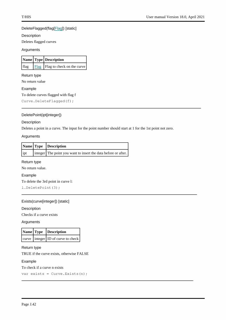
DeleteFlagged(flag[Flag]) [static]
Description
Deletes flagged curves
Arguments
Name Type Description
flag Flag Flag to check on the curve
Return type
No return value
Example
To delete curves flagged with flag f
Curve.DeleteFlagged(f);
DeletePoint(ipt[integer])
Description
Deletes a point in a curve. The input for the point number should start at 1 for the 1st point not zero.
Arguments
Name Type Description
ipt integer The point you want to insert the data before or after.
Return type
No return value.
Example
To delete the 3rd point in curve l:
l.DeletePoint(3);
Exists(curve[integer]) [static]
Description
Checks if a curve exists
Arguments
Name Type Description
curve integer ID of curve to check
Return type
TRUE if the curve exists, otherwise FALSE
Example
To check if a curve n exists
var exists = Curve.Exists(n);
T/HIS User manual Version 18.0, April 2021
Page J.42
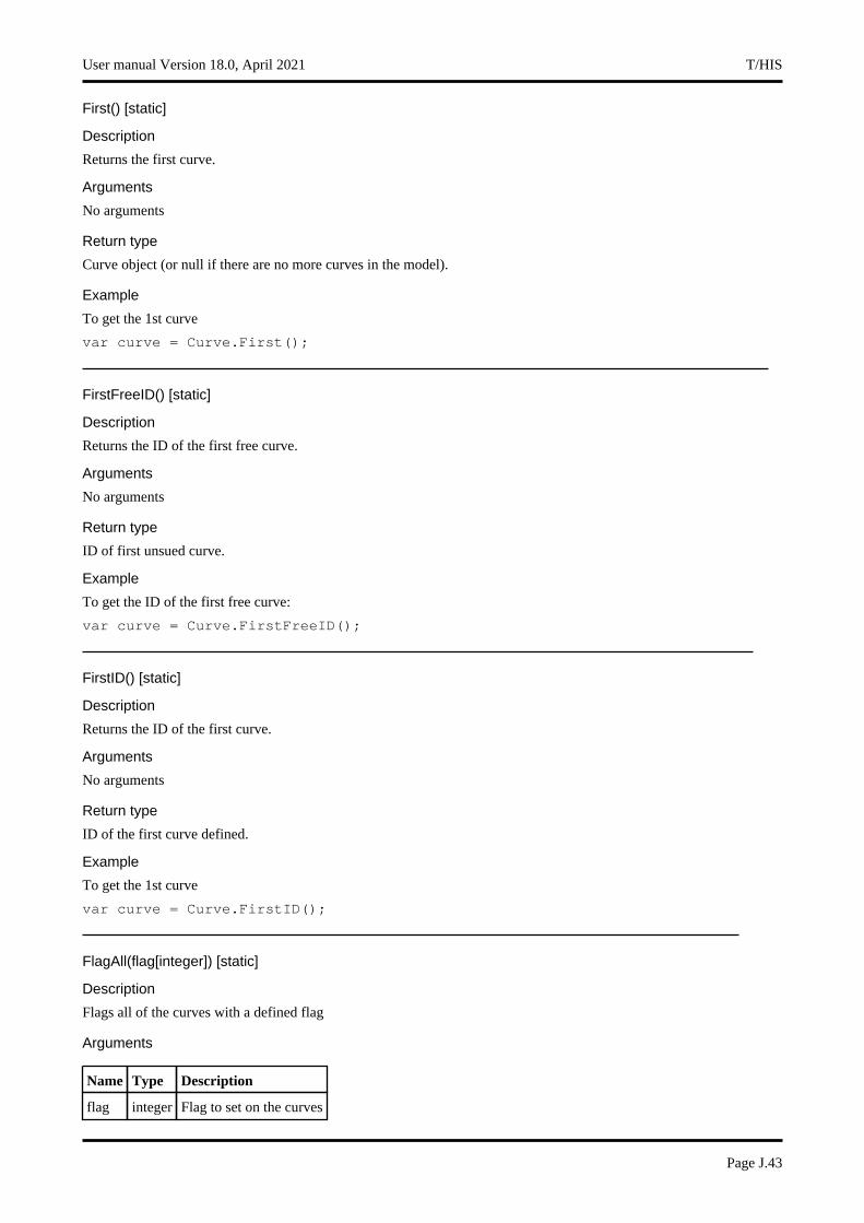
First() [static]
Description
Returns the first curve.
Arguments
No arguments
Return type
Curve object (or null if there are no more curves in the model).
Example
To get the 1st curve
var curve = Curve.First();
FirstFreeID() [static]
Description
Returns the ID of the first free curve.
Arguments
No arguments
Return type
ID of first unsued curve.
Example
To get the ID of the first free curve:
var curve = Curve.FirstFreeID();
FirstID() [static]
Description
Returns the ID of the first curve.
Arguments
No arguments
Return type
ID of the first curve defined.
Example
To get the 1st curve
var curve = Curve.FirstID();
FlagAll(flag[integer]) [static]
Description
Flags all of the curves with a defined flag
Arguments
Name Type Description
flag integer Flag to set on the curves
User manual Version 18.0, April 2021 T/HIS
Page J.43
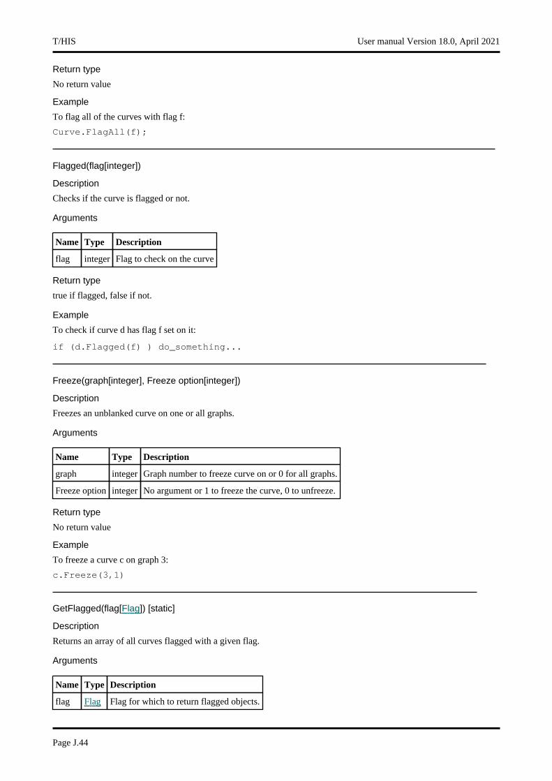
Return type
No return value
Example
To flag all of the curves with flag f:
Curve.FlagAll(f);
Flagged(flag[integer])
Description
Checks if the curve is flagged or not.
Arguments
Name Type Description
flag integer Flag to check on the curve
Return type
true if flagged, false if not.
Example
To check if curve d has flag f set on it:
if (d.Flagged(f) ) do_something...
Freeze(graph[integer], Freeze option[integer])
Description
Freezes an unblanked curve on one or all graphs.
Arguments
Name Type Description
graph integer Graph number to freeze curve on or 0 for all graphs.
Freeze option integer No argument or 1 to freeze the curve, 0 to unfreeze.
Return type
No return value
Example
To freeze a curve c on graph 3:
c.Freeze(3,1)
GetFlagged(flag[Flag]) [static]
Description
Returns an array of all curves flagged with a given flag.
Arguments
Name Type Description
flag Flag Flag for which to return flagged objects.
T/HIS User manual Version 18.0, April 2021
Page J.44
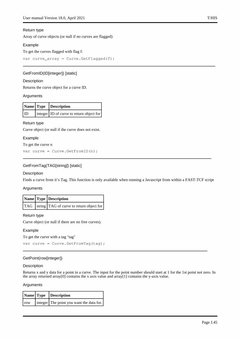
Return type
Array of curve objects (or null if no curves are flagged)
Example
To get the curves flagged with flag f:
var curve_array = Curve.GetFlagged(f);
GetFromID(ID[integer]) [static]
Description
Returns the curve object for a curve ID.
Arguments
Name Type Description
ID integer ID of curve to return object for
Return type
Curve object (or null if the curve does not exist.
Example
To get the curve n
var curve = Curve.GetFromID(n);
GetFromTag(TAG[string]) [static]
Description
Finds a curve from it’s Tag. This function is only available when running a Javascript from within a FAST-TCF script
Arguments
Name Type Description
TAG string TAG of curve to return object for
Return type
Curve object (or null if there are no free curves).
Example
To get the curve with a tag "tag"
var curve = Curve.GetFromTag(tag);
GetPoint(row[integer])
Description
Returns x and y data for a point in a curve. The input for the point number should start at 1 for the 1st point not zero. In the array returned array[0] contains the x axis value and array[1] contains the y-axis value.
Arguments
Name Type Description
row integer The point you want the data for.
User manual Version 18.0, April 2021 T/HIS
Page J.45

Return type
Array of reals
Example
To get the curve data for the 3rd point for curve l:
if (l.npoints >= 3){
var point_data = l.GetPoint(3);}
HighestID() [static]
Description
Returns the ID of the highest curve currently being used
Arguments
No arguments
Return type
ID of highest curve currently being used.
Example
To get the highest curve ID
var id= Curve.HighestID();
InsertPoint(ipt[integer], xvalue[real], yvalue[real], position[integer])
Description
Inserts a new point before or after the specified point.
Arguments
Name Type Description
ipt integer The point you want to insert the data before or after.
xvalue real The x value of the point.
yvalue real The y value of the point.
position integer Specify either before or after the selected pioint. Use ’Curve.BEFORE’ for before, and ’Curve.AFTER’ for after.
Return type
No return value.
Example
To insert the values after the 3rd row to x=3, y=5 for curve l:
l.InsertPoint(3, 3, 5, Curve.AFTER);
Next()
Description
Returns the next curve in the model.
T/HIS User manual Version 18.0, April 2021
Page J.46
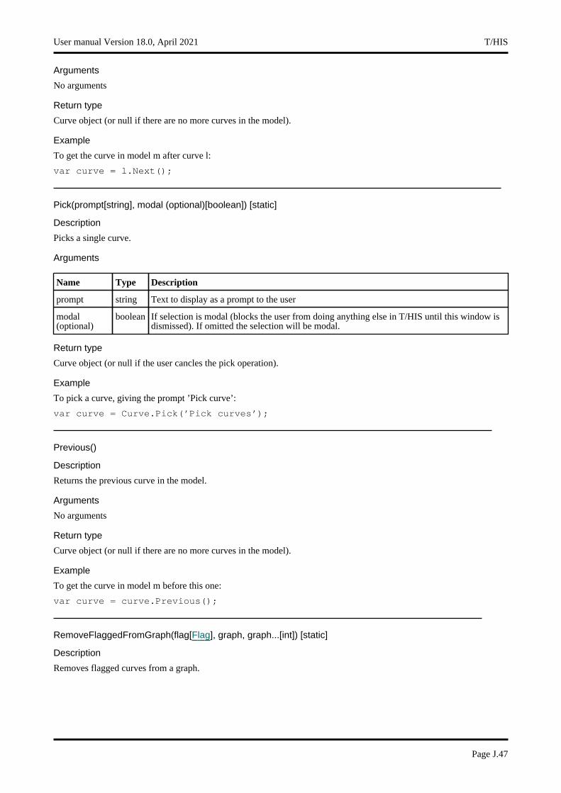
Arguments
No arguments
Return type
Curve object (or null if there are no more curves in the model).
Example
To get the curve in model m after curve l:
var curve = l.Next();
Pick(prompt[string], modal (optional)[boolean]) [static]
Description
Picks a single curve.
Arguments
Name Type Description
prompt string Text to display as a prompt to the user
modal (optional)
boolean If selection is modal (blocks the user from doing anything else in T/HIS until this window is dismissed). If omitted the selection will be modal.
Return type
Curve object (or null if the user cancles the pick operation).
Example
To pick a curve, giving the prompt ’Pick curve’:
var curve = Curve.Pick(’Pick curves’);
Previous()
Description
Returns the previous curve in the model.
Arguments
No arguments
Return type
Curve object (or null if there are no more curves in the model).
Example
To get the curve in model m before this one:
var curve = curve.Previous();
RemoveFlaggedFromGraph(flag[Flag], graph, graph...[int]) [static]
Description
Removes flagged curves from a graph.
User manual Version 18.0, April 2021 T/HIS
Page J.47
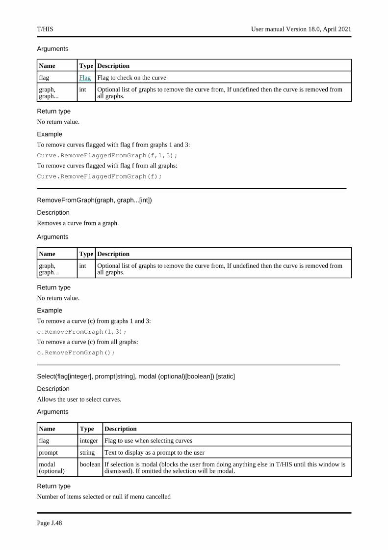
Arguments
Name Type Description
flag Flag Flag to check on the curve
graph, graph...
int Optional list of graphs to remove the curve from, If undefined then the curve is removed from all graphs.
Return type
No return value.
Example
To remove curves flagged with flag f from graphs 1 and 3:
Curve.RemoveFlaggedFromGraph(f,1,3);
To remove curves flagged with flag f from all graphs:
Curve.RemoveFlaggedFromGraph(f);
RemoveFromGraph(graph, graph...[int])
Description
Removes a curve from a graph.
Arguments
Name Type Description
graph, graph...
int Optional list of graphs to remove the curve from, If undefined then the curve is removed from all graphs.
Return type
No return value.
Example
To remove a curve (c) from graphs 1 and 3:
c.RemoveFromGraph(1,3);
To remove a curve (c) from all graphs:
c.RemoveFromGraph();
Select(flag[integer], prompt[string], modal (optional)[boolean]) [static]
Description
Allows the user to select curves.
Arguments
Name Type Description
flag integer Flag to use when selecting curves
prompt string Text to display as a prompt to the user
modal (optional)
boolean If selection is modal (blocks the user from doing anything else in T/HIS until this window is dismissed). If omitted the selection will be modal.
Return type
Number of items selected or null if menu cancelled
T/HIS User manual Version 18.0, April 2021
Page J.48
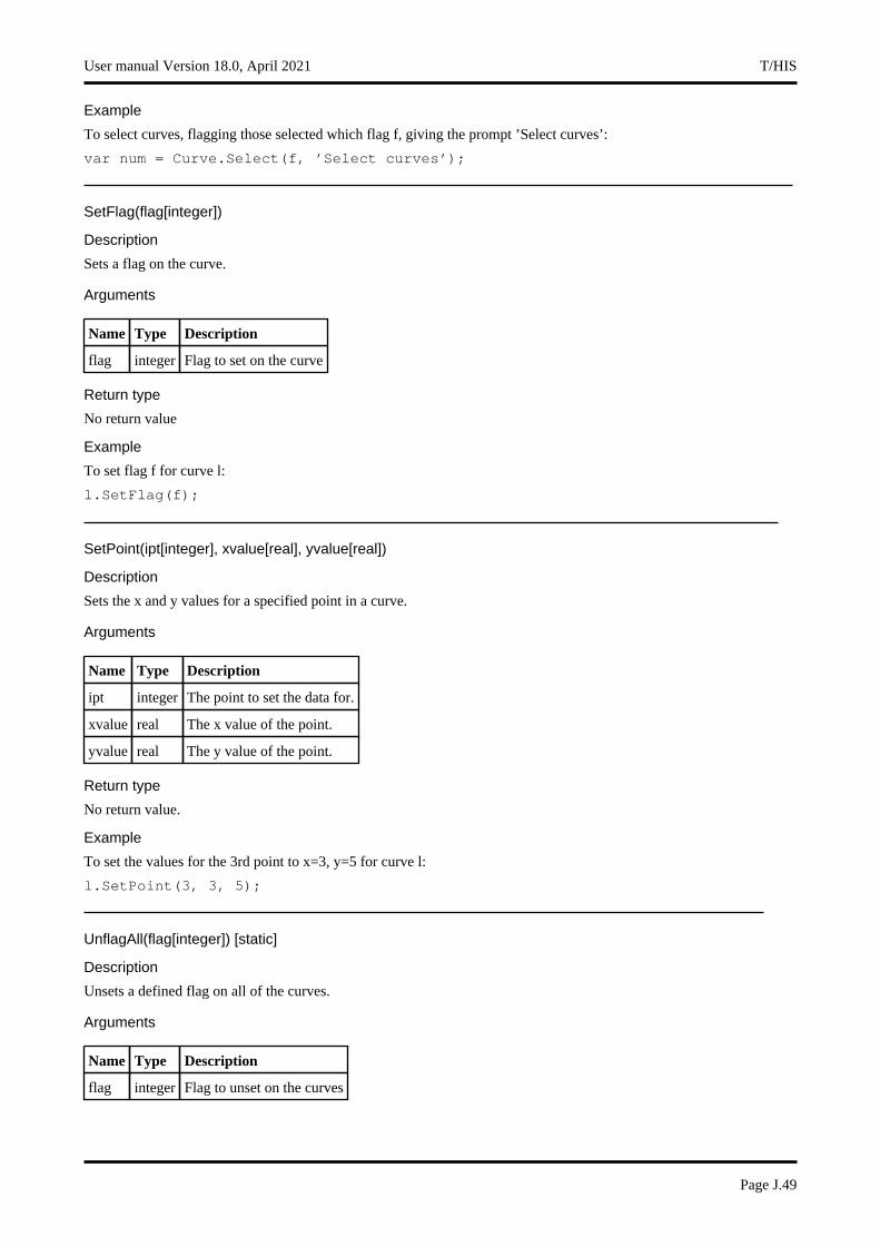
Example
To select curves, flagging those selected which flag f, giving the prompt ’Select curves’:
var num = Curve.Select(f, ’Select curves’);
SetFlag(flag[integer])
Description
Sets a flag on the curve.
Arguments
Name Type Description
flag integer Flag to set on the curve
Return type
No return value
Example
To set flag f for curve l:
l.SetFlag(f);
SetPoint(ipt[integer], xvalue[real], yvalue[real])
Description
Sets the x and y values for a specified point in a curve.
Arguments
Name Type Description
ipt integer The point to set the data for.
xvalue real The x value of the point.
yvalue real The y value of the point.
Return type
No return value.
Example
To set the values for the 3rd point to x=3, y=5 for curve l:
l.SetPoint(3, 3, 5);
UnflagAll(flag[integer]) [static]
Description
Unsets a defined flag on all of the curves.
Arguments
Name Type Description
flag integer Flag to unset on the curves
User manual Version 18.0, April 2021 T/HIS
Page J.49
Return type
No return value
Example
To unset the flag f on all of the curves:
Curve.UnflagAll(f);
Update()
Description
Updates a curve properties (min,max, average values etc).
Arguments
No arguments
Return type
No return value.
Example
To update the properties of curve l:
l.Update();
YatX(xvalue[real])
Description
Returns the y value of the curve at a given x value, interpolating if requested x value lies between data points.
Arguments
Name Type Description
xvalue real The x value.
Return type
real
Example
To get the y value of curve c when x=1.4:
var y = c.YatX(1.4);
T/HIS User manual Version 18.0, April 2021
Page J.50

Datum classThe Datum class gives you access to datums in T/HIS. More...
The T/HIS JavaScript API provides many class constants, properties and methods. For Arup to be able to extend and enhance the API in the future any constant, property or method names beginning with a lowercase or uppercase letter are reserved.If you need to add your own properties or methods to one of the existing classes then to avoid any potential future conflict you should ensure that the name begins with either an underscore (_) or a dollar sign ($) or the name is prefixed with your own unique identifier.For example if company ’ABC’ need to add a property called ’example’ then to avoid any potential future conflict use one of:
• _example • $example • ABC_example
Class functions• Delete(datum[string]) • Exists(datum[string]) • First() • GetFromAcronym(datum[string])
Member functions• AddToGraph(graph, graph...[int]) • Next() • RemoveFromGraph(graph, graph...[int])
Datum constants
Name Description
Datum.CONSTANT_X Constant X type datum.
Datum.CONSTANT_Y Constant Y type datum.
Datum.CONSTANT_Y2 Constant Y2 type datum.
Datum.FILL_ABOVE_BELOW Fill datum above and below.
Datum.FILL_RIGHT_LEFT Fill datum right and left.
Datum.LABEL_10_POINT Label font size 10.
Datum.LABEL_12_POINT Label font size 12.
Datum.LABEL_14_POINT Label font size 14.
Datum.LABEL_18_POINT Label font size 16.
Datum.LABEL_24_POINT Label font size 24.
Datum.LABEL_8_POINT Label font size 8.
Datum.LABEL_ABOVE_CENTRE Label position above centre.
Datum.LABEL_ABOVE_LEFT Label position above left.
Datum.LABEL_ABOVE_RIGHT Label position above right.
Datum.LABEL_AUTOMATIC Label automatic font size.
Datum.LABEL_BELOW_CENTRE Label position below centre.
Datum.LABEL_BELOW_LEFT Label position below left.
Datum.LABEL_BELOW_RIGHT Label position below right.
Datum.LABEL_BOTTOM_LEFT Label position bottom left.
Datum.LABEL_BOTTOM_RIGHT Label position bottom right.
Datum.LABEL_COURIER_BOLD Label Courier bold font.
User manual Version 18.0, April 2021 T/HIS
Page J.51

Datum.LABEL_COURIER_MEDIUM Label Courier medium font.
Datum.LABEL_DEFAULT Label default font.
Datum.LABEL_HELVETICA_BOLD Label Helvetica bold font.
Datum.LABEL_HELVETICA_MEDIUM Label Helvetica medium font.
Datum.LABEL_HORIZONTAL Label horizonal orientation.
Datum.LABEL_MIDDLE_LEFT Label position middle left.
Datum.LABEL_MIDDLE_RIGHT Label position middle right.
Datum.LABEL_NONE No label.
Datum.LABEL_TIMES_BOLD Label Times bold font.
Datum.LABEL_TIMES_MEDIUM Label Times medium font.
Datum.LABEL_TOP_LEFT Label position top left.
Datum.LABEL_TOP_RIGHT Label position top right.
Datum.LABEL_VERTICAL Label vertical orientation.
Datum.POINTS Points type datum.
Datum properties
Name Type Description
acronym string Datum acronym
fill_colour_above
Colour The colour above the datum line
fill_colour_below
Colour The colour below the datum line
fill_colour_between
Colour The colour in between the datum line and the optional second datum line
fill_colour_left
Colour The colour left of the datum line
fill_colour_right
Colour The colour right of the datum line
fill_type integer The fill type. Can be Datum.FILL_ABOVE_BELOW, Datum.FILL_RIGHT_LEFT. Note that this can only be changed if the datum is of the type Datum.POINTS.
label string Datum label
label2 string Label for optional 2nd datum line
label_colour
Colour The colour of the datum label
label_font integer The label font. Can be Datum.LABEL_DEFAULT, Datum.LABEL_HELVETICA_BOLD, Datum.LABEL_HELVETICA_MEDIUM, Datum.LABEL_TIMES_BOLD, Datum.LABEL_TIMES_MEDIUM, Datum.LABEL_COURIER_BOLD, Datum.LABEL_COURIER_MEDIUM
label_orientation
integer The orientation of the label. Can be Datum.LABEL_HORIZONTAL, Datum.LABEL_VERTICAL
T/HIS User manual Version 18.0, April 2021
Page J.52
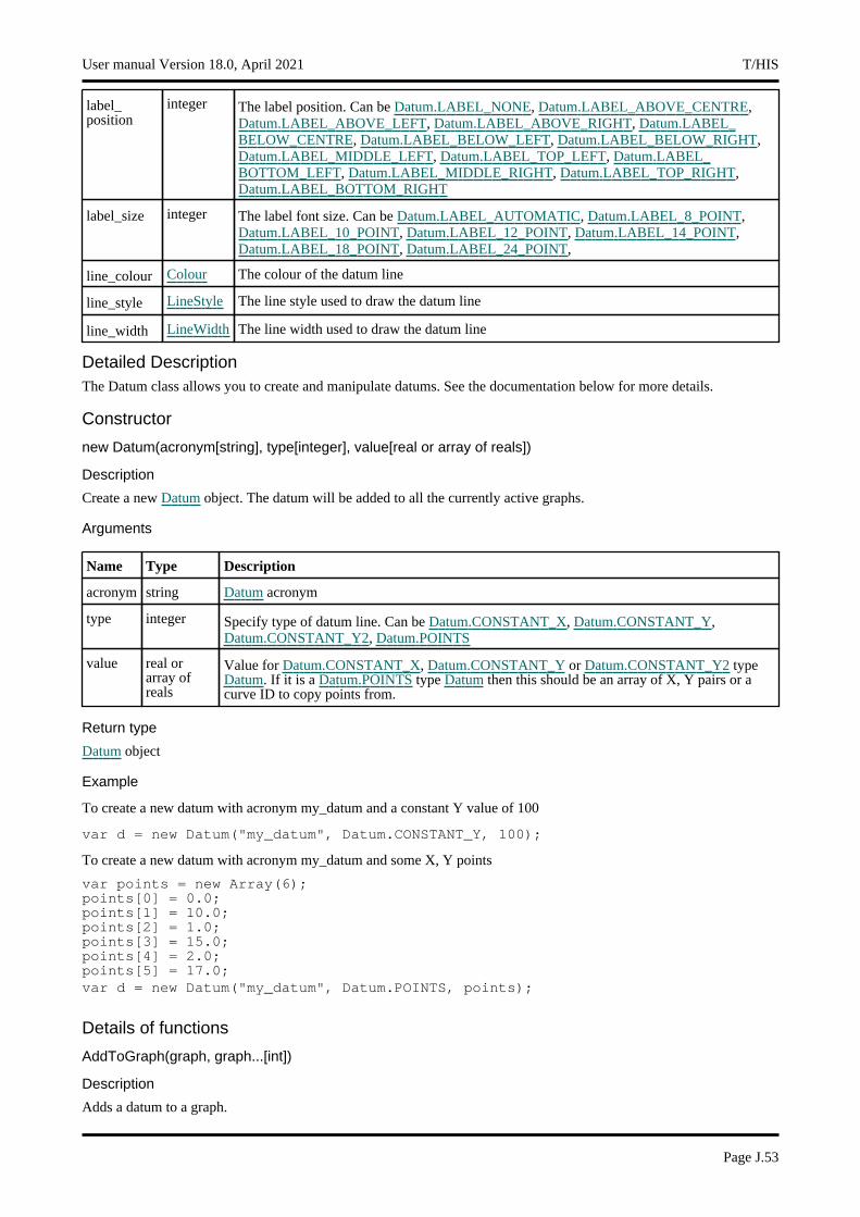
label_position
integer The label position. Can be Datum.LABEL_NONE, Datum.LABEL_ABOVE_CENTRE, Datum.LABEL_ABOVE_LEFT, Datum.LABEL_ABOVE_RIGHT, Datum.LABEL_BELOW_CENTRE, Datum.LABEL_BELOW_LEFT, Datum.LABEL_BELOW_RIGHT, Datum.LABEL_MIDDLE_LEFT, Datum.LABEL_TOP_LEFT, Datum.LABEL_BOTTOM_LEFT, Datum.LABEL_MIDDLE_RIGHT, Datum.LABEL_TOP_RIGHT, Datum.LABEL_BOTTOM_RIGHT
label_size integer The label font size. Can be Datum.LABEL_AUTOMATIC, Datum.LABEL_8_POINT, Datum.LABEL_10_POINT, Datum.LABEL_12_POINT, Datum.LABEL_14_POINT, Datum.LABEL_18_POINT, Datum.LABEL_24_POINT,
line_colour Colour The colour of the datum line
line_style LineStyle The line style used to draw the datum line
line_width LineWidth The line width used to draw the datum line
Detailed DescriptionThe Datum class allows you to create and manipulate datums. See the documentation below for more details.
Constructor
new Datum(acronym[string], type[integer], value[real or array of reals])
Description
Create a new Datum object. The datum will be added to all the currently active graphs.
Arguments
Name Type Description
acronym string Datum acronym
type integer Specify type of datum line. Can be Datum.CONSTANT_X, Datum.CONSTANT_Y, Datum.CONSTANT_Y2, Datum.POINTS
value real or array of reals
Value for Datum.CONSTANT_X, Datum.CONSTANT_Y or Datum.CONSTANT_Y2 type Datum. If it is a Datum.POINTS type Datum then this should be an array of X, Y pairs or a curve ID to copy points from.
Return type
Datum object
Example
To create a new datum with acronym my_datum and a constant Y value of 100
var d = new Datum("my_datum", Datum.CONSTANT_Y, 100);
To create a new datum with acronym my_datum and some X, Y points
var points = new Array(6);points[0] = 0.0;points[1] = 10.0;points[2] = 1.0;points[3] = 15.0;points[4] = 2.0;points[5] = 17.0;var d = new Datum("my_datum", Datum.POINTS, points);
Details of functions
AddToGraph(graph, graph...[int])
Description
Adds a datum to a graph.
User manual Version 18.0, April 2021 T/HIS
Page J.53
Arguments
Name Type Description
graph, graph... int Optional list of graphs to add the datum to, If undefined then the datum is added to all graphs.
Return type
No return value.
Example
To add a datum (d) to graphs 1 and 3:
d.AddToGraph(1,3);
To add a datum (d) to all graphs:
d.AddToGraph();
Delete(datum[string]) [static]
Description
Deletes a datum
Arguments
Name Type Description
datum string Acronym of datum to delete
Return type
No return value
Example
To delete datum "my_datum"
Datum.Delete("my_datum");
Exists(datum[string]) [static]
Description
Checks if a datum exists
Arguments
Name Type Description
datum string Acronym of datum to check
Return type
TRUE if the datum exists, otherwise FALSE
Example
To check if a datum "my_datum" exists
var exists = Datum.Exists("my_datum");
T/HIS User manual Version 18.0, April 2021
Page J.54
First() [static]
Description
Returns the first datum.
Arguments
No arguments
Return type
Datum object (or null if there are no datum in the model).
Example
To get the 1st datum
var d = Datum.First();
GetFromAcronym(datum[string]) [static]
Description
Returns the datum object for a datum acronym.
Arguments
Name Type Description
datum string Acronym of datum to return object for
Return type
Datum object (or null if the datum does not exist).
Example
To get the datum "my_datum"
var d = Datum.GetFromAcronym("my_datum");
Next()
Description
Returns the next datum in the model.
Arguments
No arguments
Return type
Datum object (or null if there are no more datums in the model).
Example
To get the next datum after datum d:
var datum = d.Next();
RemoveFromGraph(graph, graph...[int])
Description
Removes a datum from a graph.
User manual Version 18.0, April 2021 T/HIS
Page J.55
Arguments
Name Type Description
graph, graph...
int Optional list of graphs to remove the datum from, If undefined then the datum is removed from all graphs.
Return type
No return value.
Example
To remove a datum (d) from graphs 1 and 3:
d.RemoveFromGraph(1,3);
To remove a datum (d) from all graphs:
d.RemoveFromGraph();
T/HIS User manual Version 18.0, April 2021
Page J.56
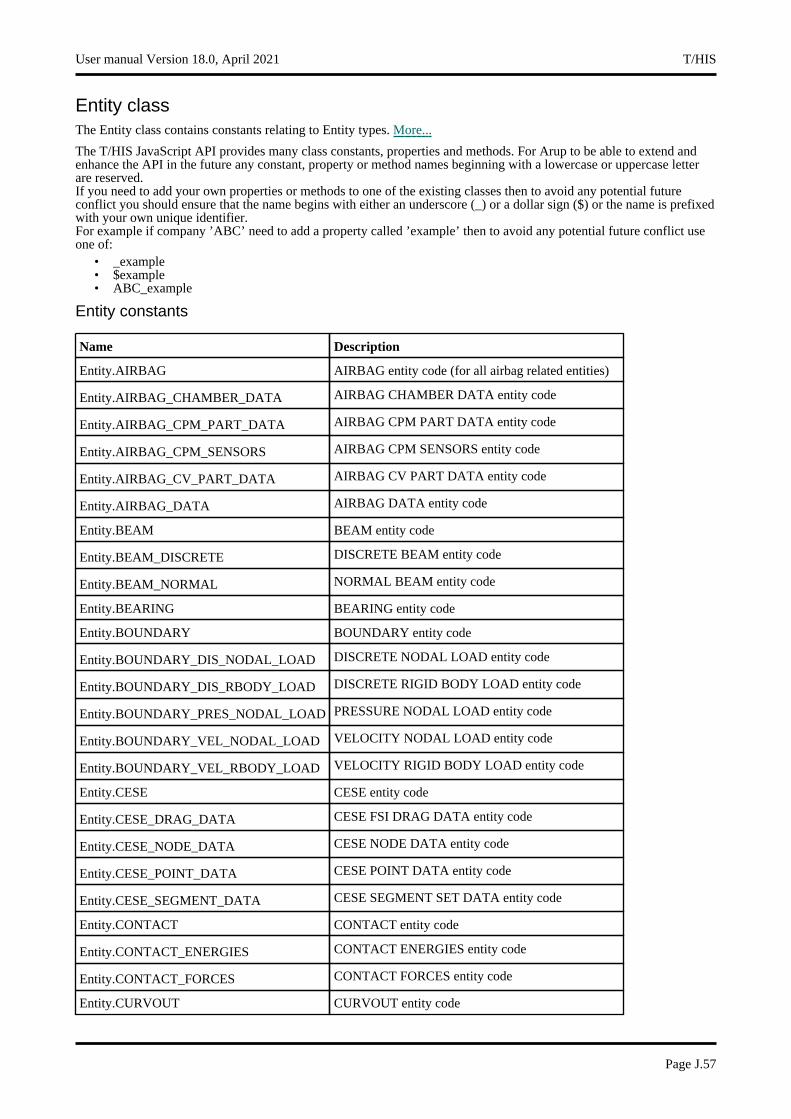
Entity classThe Entity class contains constants relating to Entity types. More...
The T/HIS JavaScript API provides many class constants, properties and methods. For Arup to be able to extend and enhance the API in the future any constant, property or method names beginning with a lowercase or uppercase letter are reserved.If you need to add your own properties or methods to one of the existing classes then to avoid any potential future conflict you should ensure that the name begins with either an underscore (_) or a dollar sign ($) or the name is prefixed with your own unique identifier.For example if company ’ABC’ need to add a property called ’example’ then to avoid any potential future conflict use one of:
• _example • $example • ABC_example
Entity constants
Name Description
Entity.AIRBAG AIRBAG entity code (for all airbag related entities)
Entity.AIRBAG_CHAMBER_DATA AIRBAG CHAMBER DATA entity code
Entity.AIRBAG_CPM_PART_DATA AIRBAG CPM PART DATA entity code
Entity.AIRBAG_CPM_SENSORS AIRBAG CPM SENSORS entity code
Entity.AIRBAG_CV_PART_DATA AIRBAG CV PART DATA entity code
Entity.AIRBAG_DATA AIRBAG DATA entity code
Entity.BEAM BEAM entity code
Entity.BEAM_DISCRETE DISCRETE BEAM entity code
Entity.BEAM_NORMAL NORMAL BEAM entity code
Entity.BEARING BEARING entity code
Entity.BOUNDARY BOUNDARY entity code
Entity.BOUNDARY_DIS_NODAL_LOAD DISCRETE NODAL LOAD entity code
Entity.BOUNDARY_DIS_RBODY_LOAD DISCRETE RIGID BODY LOAD entity code
Entity.BOUNDARY_PRES_NODAL_LOAD PRESSURE NODAL LOAD entity code
Entity.BOUNDARY_VEL_NODAL_LOAD VELOCITY NODAL LOAD entity code
Entity.BOUNDARY_VEL_RBODY_LOAD VELOCITY RIGID BODY LOAD entity code
Entity.CESE CESE entity code
Entity.CESE_DRAG_DATA CESE FSI DRAG DATA entity code
Entity.CESE_NODE_DATA CESE NODE DATA entity code
Entity.CESE_POINT_DATA CESE POINT DATA entity code
Entity.CESE_SEGMENT_DATA CESE SEGMENT SET DATA entity code
Entity.CONTACT CONTACT entity code
Entity.CONTACT_ENERGIES CONTACT ENERGIES entity code
Entity.CONTACT_FORCES CONTACT FORCES entity code
Entity.CURVOUT CURVOUT entity code
User manual Version 18.0, April 2021 T/HIS
Page J.57
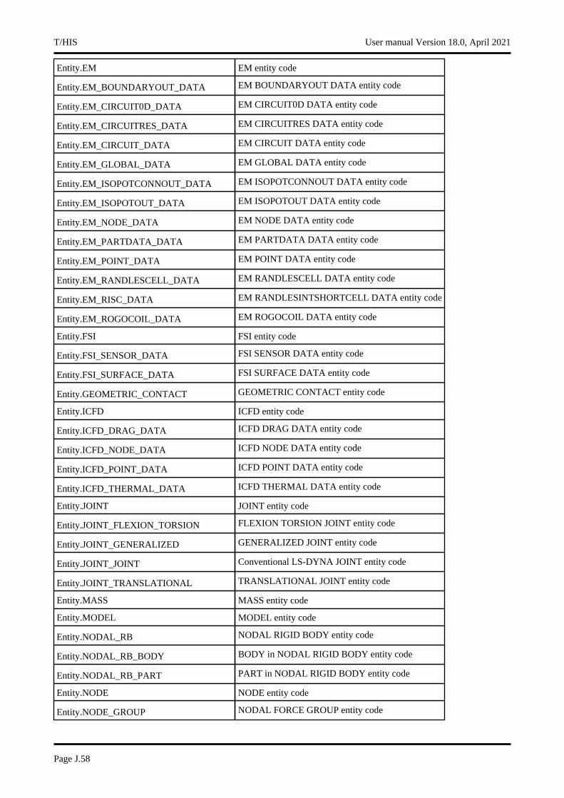
Entity.EM EM entity code
Entity.EM_BOUNDARYOUT_DATA EM BOUNDARYOUT DATA entity code
Entity.EM_CIRCUIT0D_DATA EM CIRCUIT0D DATA entity code
Entity.EM_CIRCUITRES_DATA EM CIRCUITRES DATA entity code
Entity.EM_CIRCUIT_DATA EM CIRCUIT DATA entity code
Entity.EM_GLOBAL_DATA EM GLOBAL DATA entity code
Entity.EM_ISOPOTCONNOUT_DATA EM ISOPOTCONNOUT DATA entity code
Entity.EM_ISOPOTOUT_DATA EM ISOPOTOUT DATA entity code
Entity.EM_NODE_DATA EM NODE DATA entity code
Entity.EM_PARTDATA_DATA EM PARTDATA DATA entity code
Entity.EM_POINT_DATA EM POINT DATA entity code
Entity.EM_RANDLESCELL_DATA EM RANDLESCELL DATA entity code
Entity.EM_RISC_DATA EM RANDLESINTSHORTCELL DATA entity code
Entity.EM_ROGOCOIL_DATA EM ROGOCOIL DATA entity code
Entity.FSI FSI entity code
Entity.FSI_SENSOR_DATA FSI SENSOR DATA entity code
Entity.FSI_SURFACE_DATA FSI SURFACE DATA entity code
Entity.GEOMETRIC_CONTACT GEOMETRIC CONTACT entity code
Entity.ICFD ICFD entity code
Entity.ICFD_DRAG_DATA ICFD DRAG DATA entity code
Entity.ICFD_NODE_DATA ICFD NODE DATA entity code
Entity.ICFD_POINT_DATA ICFD POINT DATA entity code
Entity.ICFD_THERMAL_DATA ICFD THERMAL DATA entity code
Entity.JOINT JOINT entity code
Entity.JOINT_FLEXION_TORSION FLEXION TORSION JOINT entity code
Entity.JOINT_GENERALIZED GENERALIZED JOINT entity code
Entity.JOINT_JOINT Conventional LS-DYNA JOINT entity code
Entity.JOINT_TRANSLATIONAL TRANSLATIONAL JOINT entity code
Entity.MASS MASS entity code
Entity.MODEL MODEL entity code
Entity.NODAL_RB NODAL RIGID BODY entity code
Entity.NODAL_RB_BODY BODY in NODAL RIGID BODY entity code
Entity.NODAL_RB_PART PART in NODAL RIGID BODY entity code
Entity.NODE NODE entity code
Entity.NODE_GROUP NODAL FORCE GROUP entity code
T/HIS User manual Version 18.0, April 2021
Page J.58
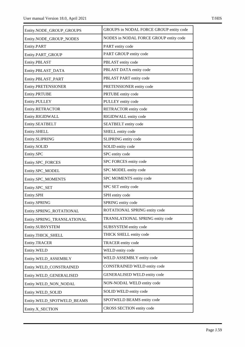
Entity.NODE_GROUP_GROUPS GROUPS in NODAL FORCE GROUP entity code
Entity.NODE_GROUP_NODES NODES in NODAL FORCE GROUP entity code
Entity.PART PART entity code
Entity.PART_GROUP PART GROUP entity code
Entity.PBLAST PBLAST entity code
Entity.PBLAST_DATA PBLAST DATA entity code
Entity.PBLAST_PART PBLAST PART entity code
Entity.PRETENSIONER PRETENSIONER entity code
Entity.PRTUBE PRTUBE entity code
Entity.PULLEY PULLEY entity code
Entity.RETRACTOR RETRACTOR entity code
Entity.RIGIDWALL RIGIDWALL entity code
Entity.SEATBELT SEATBELT entity code
Entity.SHELL SHELL entity code
Entity.SLIPRING SLIPRING entity code
Entity.SOLID SOLID entity code
Entity.SPC SPC entity code
Entity.SPC_FORCES SPC FORCES entity code
Entity.SPC_MODEL SPC MODEL entity code
Entity.SPC_MOMENTS SPC MOMENTS entity code
Entity.SPC_SET SPC SET entity code
Entity.SPH SPH entity code
Entity.SPRING SPRING entity code
Entity.SPRING_ROTATIONAL ROTATIONAL SPRING entity code
Entity.SPRING_TRANSLATIONAL TRANSLATIONAL SPRING entity code
Entity.SUBSYSTEM SUBSYSTEM entity code
Entity.THICK_SHELL THICK SHELL entity code
Entity.TRACER TRACER entity code
Entity.WELD WELD entity code
Entity.WELD_ASSEMBLY WELD ASSEMBLY entity code
Entity.WELD_CONSTRAINED CONSTRAINED WELD entity code
Entity.WELD_GENERALISED GENERALISED WELD entity code
Entity.WELD_NON_NODAL NON-NODAL WELD entity code
Entity.WELD_SOLID SOLID WELD entity code
Entity.WELD_SPOTWELD_BEAMS SPOTWELD BEAMS entity code
Entity.X_SECTION CROSS SECTION entity code
User manual Version 18.0, April 2021 T/HIS
Page J.59

Detailed DescriptionThe Entity class is used to define entity type codes that can then be compared with the entity Curve property and input for functions in the Model class.
Node = Entity.NODE;
T/HIS User manual Version 18.0, April 2021
Page J.60
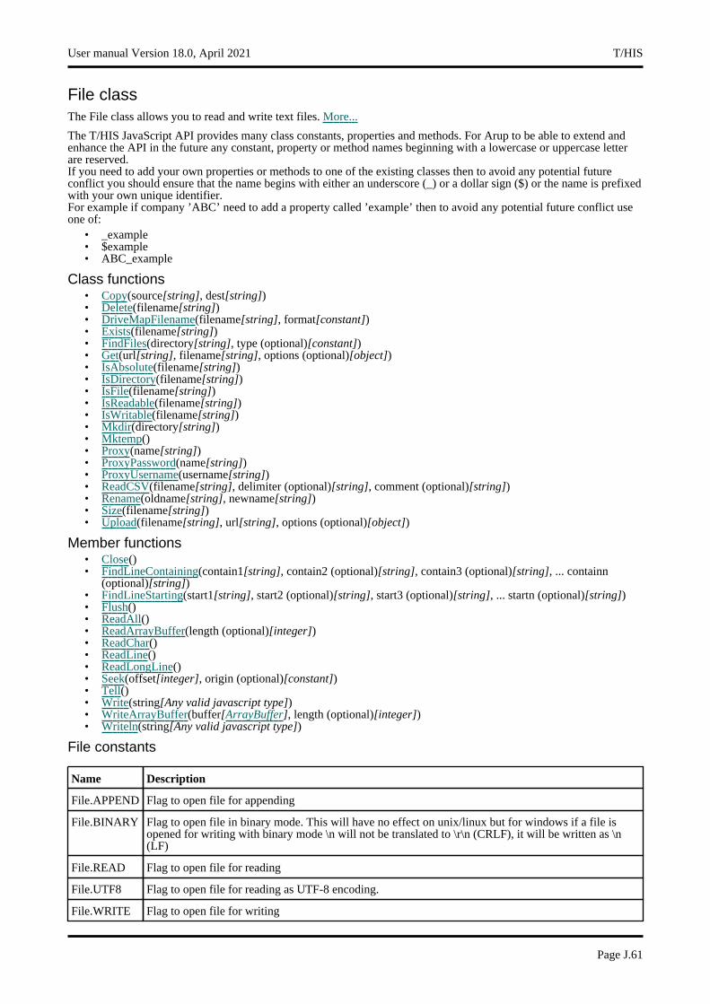
File classThe File class allows you to read and write text files. More...
The T/HIS JavaScript API provides many class constants, properties and methods. For Arup to be able to extend and enhance the API in the future any constant, property or method names beginning with a lowercase or uppercase letter are reserved.If you need to add your own properties or methods to one of the existing classes then to avoid any potential future conflict you should ensure that the name begins with either an underscore (_) or a dollar sign ($) or the name is prefixed with your own unique identifier.For example if company ’ABC’ need to add a property called ’example’ then to avoid any potential future conflict use one of:
• _example • $example • ABC_example
Class functions• Copy(source[string], dest[string]) • Delete(filename[string]) • DriveMapFilename(filename[string], format[constant]) • Exists(filename[string]) • FindFiles(directory[string], type (optional)[constant]) • Get(url[string], filename[string], options (optional)[object]) • IsAbsolute(filename[string]) • IsDirectory(filename[string]) • IsFile(filename[string]) • IsReadable(filename[string]) • IsWritable(filename[string]) • Mkdir(directory[string]) • Mktemp() • Proxy(name[string]) • ProxyPassword(name[string]) • ProxyUsername(username[string]) • ReadCSV(filename[string], delimiter (optional)[string], comment (optional)[string]) • Rename(oldname[string], newname[string]) • Size(filename[string]) • Upload(filename[string], url[string], options (optional)[object])
Member functions• Close() • FindLineContaining(contain1[string], contain2 (optional)[string], contain3 (optional)[string], ... containn
(optional)[string]) • FindLineStarting(start1[string], start2 (optional)[string], start3 (optional)[string], ... startn (optional)[string]) • Flush() • ReadAll() • ReadArrayBuffer(length (optional)[integer]) • ReadChar() • ReadLine() • ReadLongLine() • Seek(offset[integer], origin (optional)[constant]) • Tell() • Write(string[Any valid javascript type]) • WriteArrayBuffer(buffer[ArrayBuffer], length (optional)[integer]) • Writeln(string[Any valid javascript type])
File constants
Name Description
File.APPEND Flag to open file for appending
File.BINARY Flag to open file in binary mode. This will have no effect on unix/linux but for windows if a file is opened for writing with binary mode \n will not be translated to \r\n (CRLF), it will be written as \n (LF)
File.READ Flag to open file for reading
File.UTF8 Flag to open file for reading as UTF-8 encoding.
File.WRITE Flag to open file for writing
User manual Version 18.0, April 2021 T/HIS
Page J.61
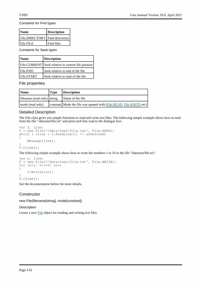
Constants for Find types
Name Description
File.DIRECTORY Find directories
File.FILE Find files
Constants for Seek types
Name Description
File.CURRENT Seek relative to current file position
File.END Seek relative to end of the file
File.START Seek relative to start of the file
File properties
Name Type Description
filename (read only) string Name of the file
mode (read only) constant Mode the file was opened with (File.READ, File.WRITE etc)
Detailed DescriptionThe File class gives you simple functions to read and write text files. The following simple example shows how to read from the file "/data/test/file.txt" and print each line read to the dialogue box:
var f, line;f = new File("/data/test/file.txt", File.READ);while ( (line = f.ReadLine()) != undefined){
Message(line);}f.Close();
The following simple example shows how to write the numbers 1 to 10 to the file "/data/test/file.txt":
var n, line;f = new File("/data/test/file.txt", File.WRITE);for (n=1; n<=10; n++){
f.Writeln(n);}f.Close();
See the documentation below for more details.
Constructor
new File(filename[string], mode[constant])
Description
Create a new File object for reading and writing text files.
T/HIS User manual Version 18.0, April 2021
Page J.62
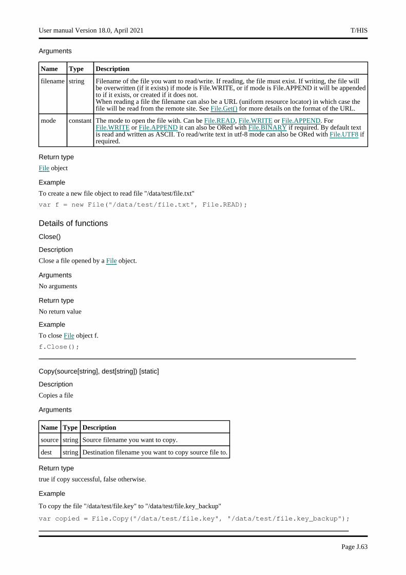
Arguments
Name Type Description
filename string Filename of the file you want to read/write. If reading, the file must exist. If writing, the file will be overwritten (if it exists) if mode is File.WRITE, or if mode is File.APPEND it will be appended to if it exists, or created if it does not.When reading a file the filename can also be a URL (uniform resource locator) in which case the file will be read from the remote site. See File.Get() for more details on the format of the URL.
mode constant The mode to open the file with. Can be File.READ, File.WRITE or File.APPEND. For File.WRITE or File.APPEND it can also be ORed with File.BINARY if required. By default text is read and written as ASCII. To read/write text in utf-8 mode can also be ORed with File.UTF8 if required.
Return type
File object
Example
To create a new file object to read file "/data/test/file.txt"
var f = new File("/data/test/file.txt", File.READ);
Details of functions
Close()
Description
Close a file opened by a File object.
Arguments
No arguments
Return type
No return value
Example
To close File object f.
f.Close();
Copy(source[string], dest[string]) [static]
Description
Copies a file
Arguments
Name Type Description
source string Source filename you want to copy.
dest string Destination filename you want to copy source file to.
Return type
true if copy successful, false otherwise.
Example
To copy the file "/data/test/file.key" to "/data/test/file.key_backup"
var copied = File.Copy("/data/test/file.key", "/data/test/file.key_backup");
User manual Version 18.0, April 2021 T/HIS
Page J.63
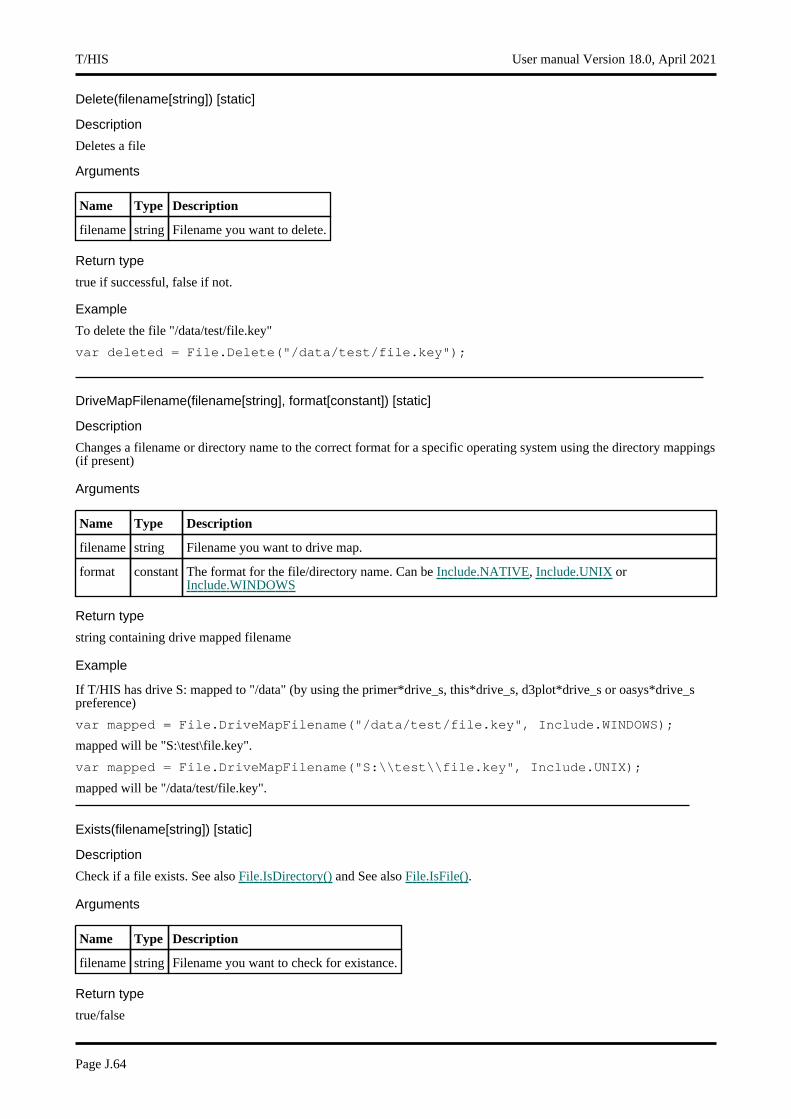
Delete(filename[string]) [static]
Description
Deletes a file
Arguments
Name Type Description
filename string Filename you want to delete.
Return type
true if successful, false if not.
Example
To delete the file "/data/test/file.key"
var deleted = File.Delete("/data/test/file.key");
DriveMapFilename(filename[string], format[constant]) [static]
Description
Changes a filename or directory name to the correct format for a specific operating system using the directory mappings (if present)
Arguments
Name Type Description
filename string Filename you want to drive map.
format constant The format for the file/directory name. Can be Include.NATIVE, Include.UNIX or Include.WINDOWS
Return type
string containing drive mapped filename
Example
If T/HIS has drive S: mapped to "/data" (by using the primer*drive_s, this*drive_s, d3plot*drive_s or oasys*drive_s preference)
var mapped = File.DriveMapFilename("/data/test/file.key", Include.WINDOWS);
mapped will be "S:\test\file.key".
var mapped = File.DriveMapFilename("S:\\test\\file.key", Include.UNIX);
mapped will be "/data/test/file.key".
Exists(filename[string]) [static]
Description
Check if a file exists. See also File.IsDirectory() and See also File.IsFile().
Arguments
Name Type Description
filename string Filename you want to check for existance.
Return type
true/false
T/HIS User manual Version 18.0, April 2021
Page J.64
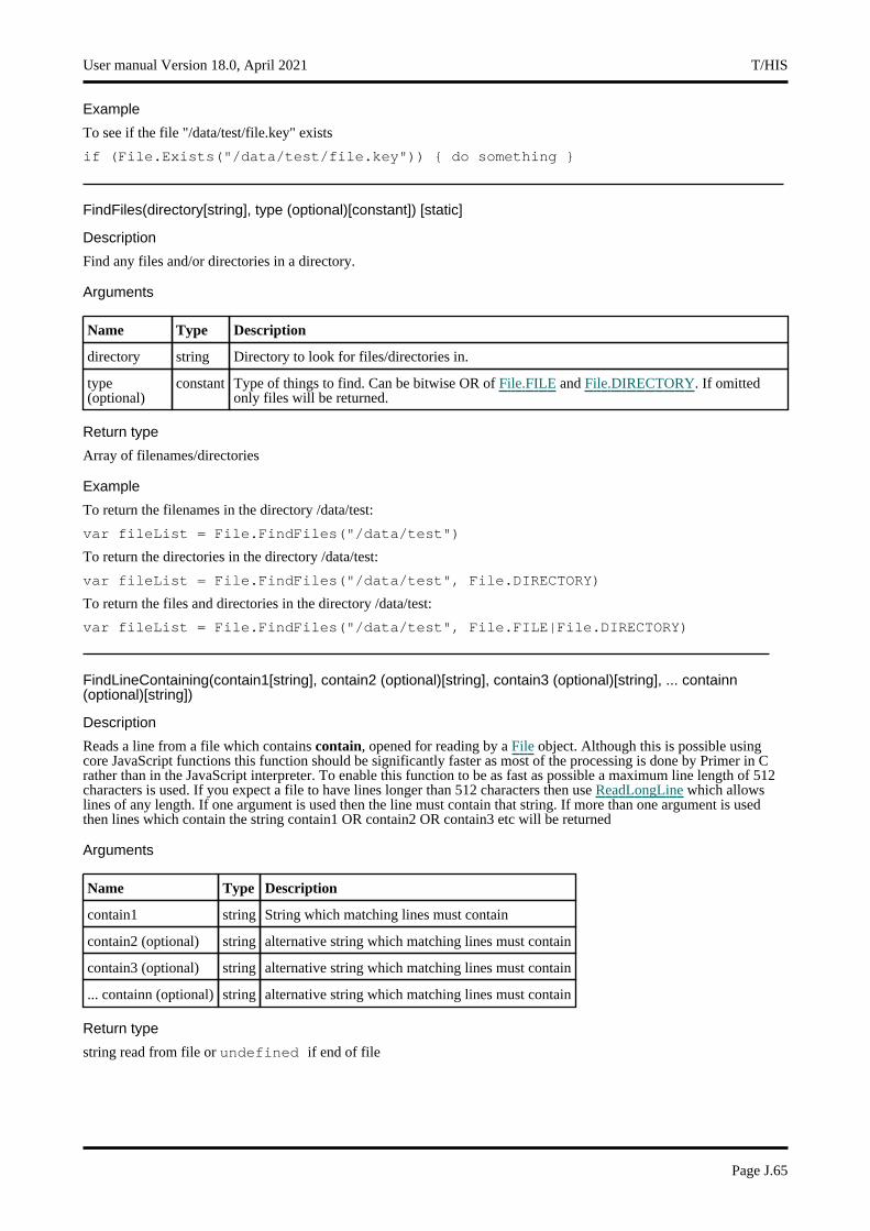
Example
To see if the file "/data/test/file.key" exists
if (File.Exists("/data/test/file.key")) { do something }
FindFiles(directory[string], type (optional)[constant]) [static]
Description
Find any files and/or directories in a directory.
Arguments
Name Type Description
directory string Directory to look for files/directories in.
type (optional)
constant Type of things to find. Can be bitwise OR of File.FILE and File.DIRECTORY. If omitted only files will be returned.
Return type
Array of filenames/directories
Example
To return the filenames in the directory /data/test:
var fileList = File.FindFiles("/data/test")
To return the directories in the directory /data/test:
var fileList = File.FindFiles("/data/test", File.DIRECTORY)
To return the files and directories in the directory /data/test:
var fileList = File.FindFiles("/data/test", File.FILE|File.DIRECTORY)
FindLineContaining(contain1[string], contain2 (optional)[string], contain3 (optional)[string], ... containn (optional)[string])
Description
Reads a line from a file which contains contain, opened for reading by a File object. Although this is possible using core JavaScript functions this function should be significantly faster as most of the processing is done by Primer in C rather than in the JavaScript interpreter. To enable this function to be as fast as possible a maximum line length of 512 characters is used. If you expect a file to have lines longer than 512 characters then use ReadLongLine which allows lines of any length. If one argument is used then the line must contain that string. If more than one argument is used then lines which contain the string contain1 OR contain2 OR contain3 etc will be returned
Arguments
Name Type Description
contain1 string String which matching lines must contain
contain2 (optional) string alternative string which matching lines must contain
contain3 (optional) string alternative string which matching lines must contain
... containn (optional) string alternative string which matching lines must contain
Return type
string read from file or undefined if end of file
User manual Version 18.0, April 2021 T/HIS
Page J.65
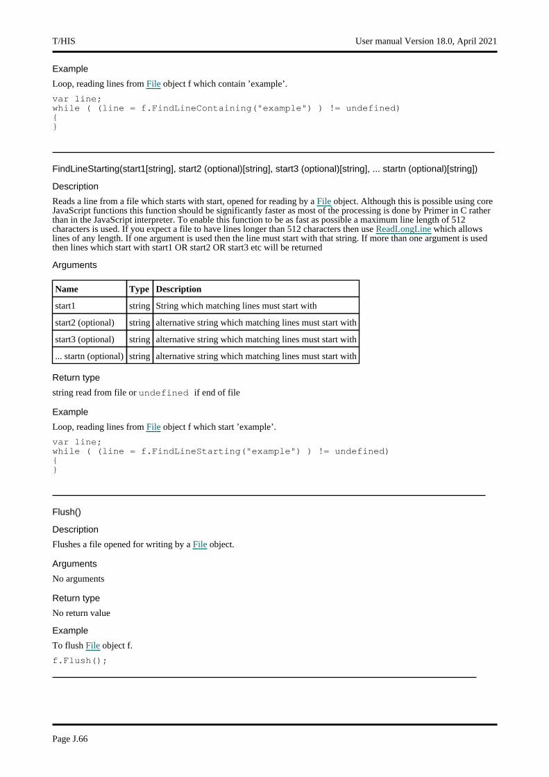
Example
Loop, reading lines from File object f which contain ’example’.
var line;while ( (line = f.FindLineContaining("example") ) != undefined){}
FindLineStarting(start1[string], start2 (optional)[string], start3 (optional)[string], ... startn (optional)[string])
Description
Reads a line from a file which starts with start, opened for reading by a File object. Although this is possible using core JavaScript functions this function should be significantly faster as most of the processing is done by Primer in C rather than in the JavaScript interpreter. To enable this function to be as fast as possible a maximum line length of 512 characters is used. If you expect a file to have lines longer than 512 characters then use ReadLongLine which allows lines of any length. If one argument is used then the line must start with that string. If more than one argument is used then lines which start with start1 OR start2 OR start3 etc will be returned
Arguments
Name Type Description
start1 string String which matching lines must start with
start2 (optional) string alternative string which matching lines must start with
start3 (optional) string alternative string which matching lines must start with
... startn (optional) string alternative string which matching lines must start with
Return type
string read from file or undefined if end of file
Example
Loop, reading lines from File object f which start ’example’.
var line;while ( (line = f.FindLineStarting("example") ) != undefined){}
Flush()
Description
Flushes a file opened for writing by a File object.
Arguments
No arguments
Return type
No return value
Example
To flush File object f.
f.Flush();
T/HIS User manual Version 18.0, April 2021
Page J.66
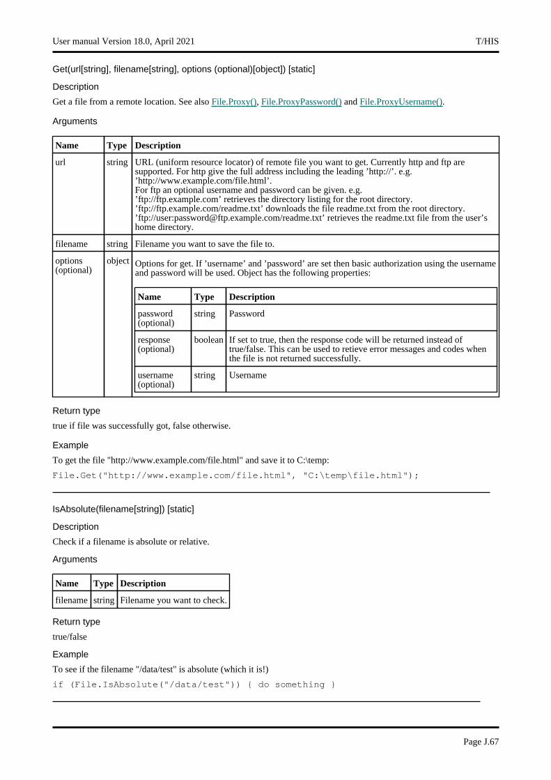
Get(url[string], filename[string], options (optional)[object]) [static]
Description
Get a file from a remote location. See also File.Proxy(), File.ProxyPassword() and File.ProxyUsername().
Arguments
Name Type Description
url string URL (uniform resource locator) of remote file you want to get. Currently http and ftp are supported. For http give the full address including the leading ’http://’. e.g. ’http://www.example.com/file.html’.For ftp an optional username and password can be given. e.g.’ftp://ftp.example.com’ retrieves the directory listing for the root directory.’ftp://ftp.example.com/readme.txt’ downloads the file readme.txt from the root directory.’ftp://user:[email protected]/readme.txt’ retrieves the readme.txt file from the user’s home directory.
filename string Filename you want to save the file to.
options (optional)
object Options for get. If ’username’ and ’password’ are set then basic authorization using the username and password will be used. Object has the following properties:
Name Type Description
password (optional)
string Password
response (optional)
boolean If set to true, then the response code will be returned instead of true/false. This can be used to retieve error messages and codes when the file is not returned successfully.
username (optional)
string Username
Return type
true if file was successfully got, false otherwise.
Example
To get the file "http://www.example.com/file.html" and save it to C:\temp:
File.Get("http://www.example.com/file.html", "C:\temp\file.html");
IsAbsolute(filename[string]) [static]
Description
Check if a filename is absolute or relative.
Arguments
Name Type Description
filename string Filename you want to check.
Return type
true/false
Example
To see if the filename "/data/test" is absolute (which it is!)
if (File.IsAbsolute("/data/test")) { do something }
User manual Version 18.0, April 2021 T/HIS
Page J.67
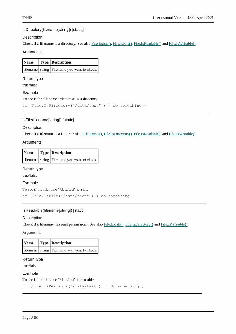
IsDirectory(filename[string]) [static]
Description
Check if a filename is a directory. See also File.Exists(), File.IsFile(), File.IsReadable() and File.IsWritable().
Arguments
Name Type Description
filename string Filename you want to check.
Return type
true/false
Example
To see if the filename "/data/test" is a directory
if (File.IsDirectory("/data/test")) { do something }
IsFile(filename[string]) [static]
Description
Check if a filename is a file. See also File.Exists(), File.IsDirectory(), File.IsReadable() and File.IsWritable().
Arguments
Name Type Description
filename string Filename you want to check.
Return type
true/false
Example
To see if the filename "/data/test" is a file
if (File.IsFile("/data/test")) { do something }
IsReadable(filename[string]) [static]
Description
Check if a filename has read permissions. See also File.Exists(), File.IsDirectory() and File.IsWritable().
Arguments
Name Type Description
filename string Filename you want to check.
Return type
true/false
Example
To see if the filename "/data/test" is readable
if (File.IsReadable("/data/test")) { do something }
T/HIS User manual Version 18.0, April 2021
Page J.68
IsWritable(filename[string]) [static]
Description
Check if a filename has write permissions. If filename exists and it is a file then it is checked to see if it can be opened with write (File.APPEND permissions). If filename exists and it is a directory then the directory is checked for write permission (can files be created in the directory). If filename does not exist then it is assumed to be a file and is checked to see if it can be opened for writing (File.WRITE permissions). See also File.Exists(), File.IsDirectory() and File.IsReadable().
Arguments
Name Type Description
filename string Filename you want to check.
Return type
true/false
Example
To see if the filename "/data/test" is writable
if (File.IsWritable("/data/test")) { do something }
Mkdir(directory[string]) [static]
Description
Make a directory. If Primer preference ’directory_permission’ is set e.g.755 then this will apply (same as if set by chmod 755) ignoring any setting of umask. If there is no preference then the users current setting of umask will control permissions (same as system mkdir)
Arguments
Name Type Description
directory string The name of the directory you want to create.
Return type
true if successfully created, false if not.
Example
To make the directory "/data/test"
var success = File.Mkdir("/data/test");
Mktemp() [static]
Description
Make a temporary filename for writing a temporary file.
Arguments
No arguments
Return type
String name of temporary filename that can be used.
Example
To get a temp filename"
var filename = File.Mktemp();
User manual Version 18.0, April 2021 T/HIS
Page J.69

Proxy(name[string]) [static]
Description
Set a proxy for files opened by http, ftp etc. See also File.Get(), File.ProxyPassword() and File.ProxyUsername().
Arguments
Name Type Description
name string The name of the proxy.
Return type
No return value
Example
To set the proxy to "http://example.proxy.com" using port 80:
File.Proxy("http://example.proxy.com:80");
ProxyPassword(name[string]) [static]
Description
Set a proxy password for files opened by http, ftp etc. See also File.Get(), File.Proxy() and File.ProxyUsername().
Arguments
Name Type Description
name string Password for the proxy server.
Return type
No return value
Example
To set the proxy password to "password":
File.ProxyPassword("password");
ProxyUsername(username[string]) [static]
Description
Set a proxy username for files opened by http, ftp etc. See also File.Get(), File.Proxy() and File.ProxyPassword().
Arguments
Name Type Description
username string The username for the proxy.
Return type
No return value
Example
To set the proxy username to "username":
File.ProxyUsername("username");
T/HIS User manual Version 18.0, April 2021
Page J.70
ReadAll()
Description
Reads all the remaining characters from a file opened for reading by a File object. As this function can read the entire file as a string be careful when reading large files as it will consume large amounts of memory.
Arguments
No arguments
Return type
String. Characters read from file or undefined if end of file
Example
Read all characters from File object f.
var c = f.ReadAll();
ReadArrayBuffer(length (optional)[integer])
Description
Reads binary data from a file opened for reading by a File object. The data is returned as an ArrayBuffer object. For more details on how to use an ArrayBuffer see the following links:https://developer.mozilla.org/en/JavaScript_typed_arrayshttps://developer.mozilla.org/en/JavaScript_typed_arrays/ArrayBufferhttps://developer.mozilla.org/en/JavaScript_typed_arrays/ArrayBufferViewhttps://developer.mozilla.org/en/JavaScript_typed_arrays/DataView.
Arguments
Name Type Description
length (optional)
integer Number of bytes to try to read from the file. If omitted all the remaining data from the file will be read.
Return type
ArrayBuffer object or undefined if end of file
Example
To read data as 32bit unsigned integers from File object f.
var ab = f.ReadArrayBuffer();var u32 = new Uint32Array(ab);for (var i=0; i<u32.length; i++{
var value = u32[i];}
ReadCSV(filename[string], delimiter (optional)[string], comment (optional)[string]) [static]
Description
Reads the input CSV file and returns an array of string arrays. If the CSV file has legitimate records the function returns an Array object containing sub-arrays of strings otherwise the function returns NULL. The lengths of all the sub-arrays are the same and equal to maximum number of fields in any of the records. For records in a CSV file having fewer fields, the respective sub-arrays are padded with NULL elements to the maximum array length.
User manual Version 18.0, April 2021 T/HIS
Page J.71
Arguments
Name Type Description
filename string Filename you want to read CSV options from.
delimiter (optional) string Delimiter string to be used. Default is a comma (",").
comment (optional) string Comment string to be used. Default is a dollar sign ("$").
Return type
Array object containing string arrays.
Example
To Read CSV file "sample.csv" and print all records to a Window.
var csv_file_path = "C:\\sample.csv";var records = "";if(!File.Exists(csv_file_path)){
Window.Information("CSV file %s not present", csv_file_path);Exit();
}var csv_array = File.ReadCSV(csv_file_path);if(csv_array != null){
for(var i = 0; i < csv_array.length; i++){
var record_array = csv_array[i];for(var j = 0; j < record_array.length; j++){
if(record_array[j] != null)records = records + record_array[j] + " , ";
}records = records + "\n";
}}Options.max_window_lines = csv_array.length;Window.Information("File.ReadCSV Ouptut", records);
To Read CSV file "sample.csv" with delimiter string "::" and comment string "##".
var csv_array = File.ReadCSV(csv_file_path, "::", "##");
ReadChar()
Description
Reads a single character from a file opened for reading by a File object.
Arguments
No arguments
Return type
character read from file or
undefined
if end of file
T/HIS User manual Version 18.0, April 2021
Page J.72
Example
Loop, reading characters from File object f.
var c;while ( (c = f.ReadChar()) != undefined) { ... }
ReadLine()
Description
Reads a line from a file opened for reading by a File object. To enable this function to be as fast as possible a maximum line length of 512 characters is used. If you expect a file to have lines longer than 512 characters then use ReadLongLine which allows lines of any length.
Arguments
No arguments
Return type
string read from file or
undefined
if end of file
Example
Loop, reading lines from File object f.
var line;while ( (line = f.ReadLine()) != undefined) { ... }
ReadLongLine()
Description
Reads a line from a file opened for reading by a File object. The line can be any length. If your file has lines shorter than 512 characters then you may want to use ReadLine instead which is faster.
Arguments
No arguments
Return type
string read from file or
undefined
if end of file
Example
Loop, reading lines from File object f.
var line;while ( (line = f.ReadLongLine()) != undefined) { ... }
Rename(oldname[string], newname[string]) [static]
Description
Rename an existing file to have a different name.
User manual Version 18.0, April 2021 T/HIS
Page J.73
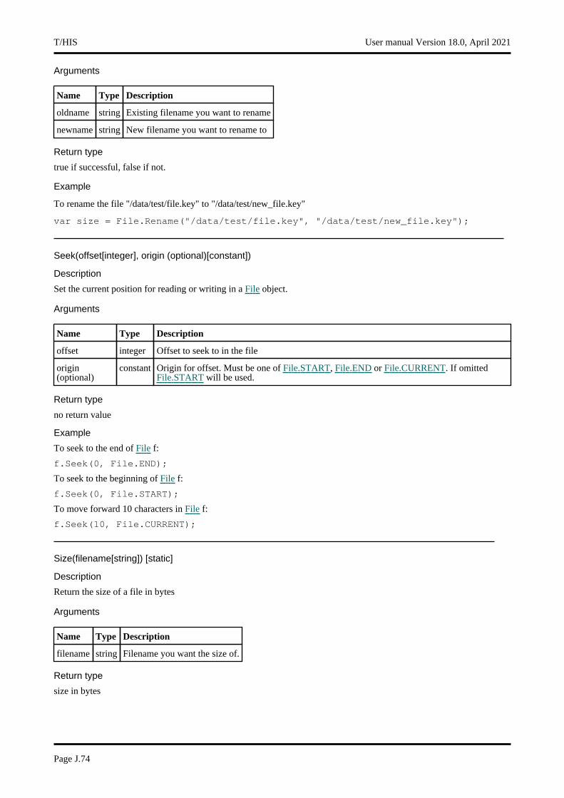
Arguments
Name Type Description
oldname string Existing filename you want to rename
newname string New filename you want to rename to
Return type
true if successful, false if not.
Example
To rename the file "/data/test/file.key" to "/data/test/new_file.key"
var size = File.Rename("/data/test/file.key", "/data/test/new_file.key");
Seek(offset[integer], origin (optional)[constant])
Description
Set the current position for reading or writing in a File object.
Arguments
Name Type Description
offset integer Offset to seek to in the file
origin (optional)
constant Origin for offset. Must be one of File.START, File.END or File.CURRENT. If omitted File.START will be used.
Return type
no return value
Example
To seek to the end of File f:
f.Seek(0, File.END);
To seek to the beginning of File f:
f.Seek(0, File.START);
To move forward 10 characters in File f:
f.Seek(10, File.CURRENT);
Size(filename[string]) [static]
Description
Return the size of a file in bytes
Arguments
Name Type Description
filename string Filename you want the size of.
Return type
size in bytes
T/HIS User manual Version 18.0, April 2021
Page J.74
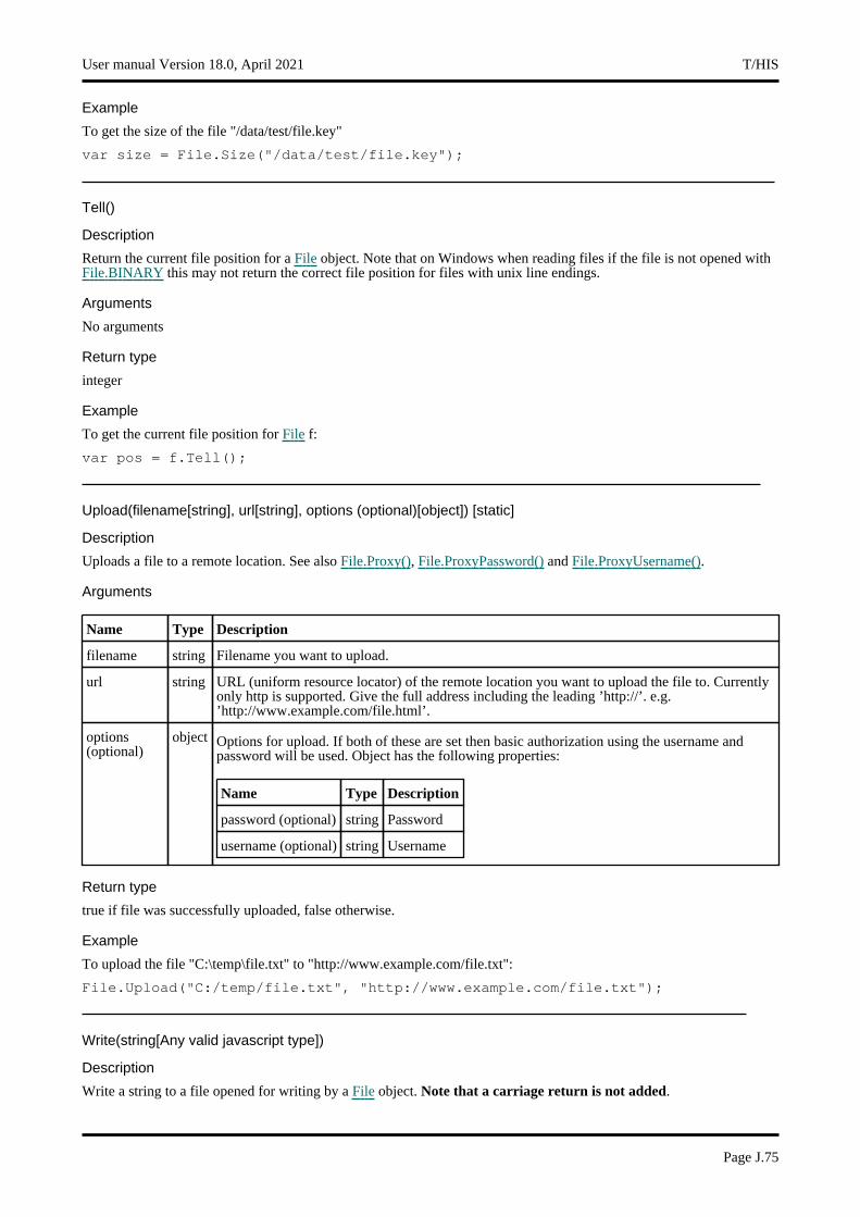
Example
To get the size of the file "/data/test/file.key"
var size = File.Size("/data/test/file.key");
Tell()
Description
Return the current file position for a File object. Note that on Windows when reading files if the file is not opened with File.BINARY this may not return the correct file position for files with unix line endings.
Arguments
No arguments
Return type
integer
Example
To get the current file position for File f:
var pos = f.Tell();
Upload(filename[string], url[string], options (optional)[object]) [static]
Description
Uploads a file to a remote location. See also File.Proxy(), File.ProxyPassword() and File.ProxyUsername().
Arguments
Name Type Description
filename string Filename you want to upload.
url string URL (uniform resource locator) of the remote location you want to upload the file to. Currently only http is supported. Give the full address including the leading ’http://’. e.g. ’http://www.example.com/file.html’.
options (optional)
object Options for upload. If both of these are set then basic authorization using the username and password will be used. Object has the following properties:
Name Type Description
password (optional) string Password
username (optional) string Username
Return type
true if file was successfully uploaded, false otherwise.
Example
To upload the file "C:\temp\file.txt" to "http://www.example.com/file.txt":
File.Upload("C:/temp/file.txt", "http://www.example.com/file.txt");
Write(string[Any valid javascript type])
Description
Write a string to a file opened for writing by a File object. Note that a carriage return is not added.
User manual Version 18.0, April 2021 T/HIS
Page J.75
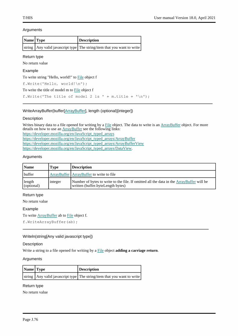
Arguments
Name Type Description
string Any valid javascript type The string/item that you want to write
Return type
No return value
Example
To write string "Hello, world!" to File object f
f.Write("Hello, world!\n");
To write the title of model m to File object f
f.Write("The title of model 2 is " + m.title + "\n");
WriteArrayBuffer(buffer[ArrayBuffer], length (optional)[integer])
Description
Writes binary data to a file opened for writing by a File object. The data to write is an ArrayBuffer object. For more details on how to use an ArrayBuffer see the following links:https://developer.mozilla.org/en/JavaScript_typed_arrayshttps://developer.mozilla.org/en/JavaScript_typed_arrays/ArrayBufferhttps://developer.mozilla.org/en/JavaScript_typed_arrays/ArrayBufferViewhttps://developer.mozilla.org/en/JavaScript_typed_arrays/DataView.
Arguments
Name Type Description
buffer ArrayBuffer ArrayBuffer to write to file
length (optional)
integer Number of bytes to write to the file. If omitted all the data in the ArrayBuffer will be written (buffer.byteLength bytes)
Return type
No return value
Example
To write ArrayBuffer ab to File object f.
f.WriteArrayBuffer(ab);
Writeln(string[Any valid javascript type])
Description
Write a string to a file opened for writing by a File object adding a carriage return.
Arguments
Name Type Description
string Any valid javascript type The string/item that you want to write
Return type
No return value
T/HIS User manual Version 18.0, April 2021
Page J.76

Example
To write string "Hello, world!" to File object f automatically adding a carriage return
f.Writeln("Hello, world!");
To write the title of model m to File object f automatically adding a carriage return
f.Writeln("The title of model 2 is " + m.title);
User manual Version 18.0, April 2021 T/HIS
Page J.77
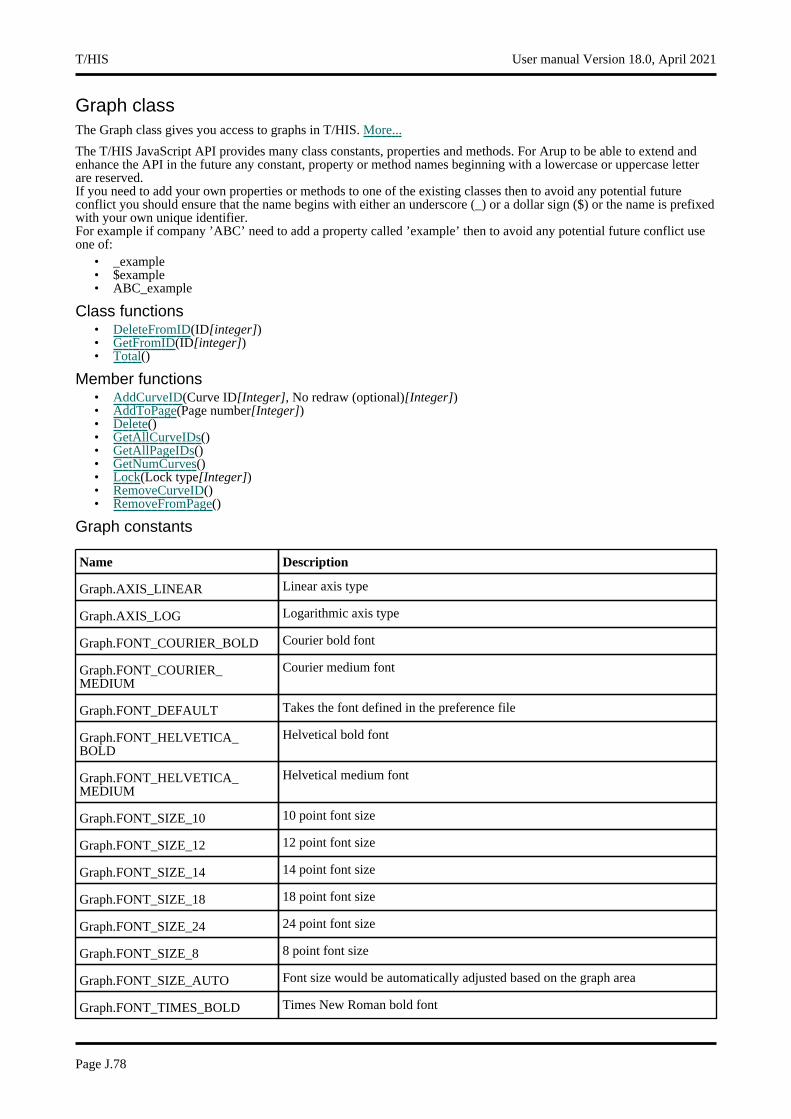
Graph classThe Graph class gives you access to graphs in T/HIS. More...
The T/HIS JavaScript API provides many class constants, properties and methods. For Arup to be able to extend and enhance the API in the future any constant, property or method names beginning with a lowercase or uppercase letter are reserved.If you need to add your own properties or methods to one of the existing classes then to avoid any potential future conflict you should ensure that the name begins with either an underscore (_) or a dollar sign ($) or the name is prefixed with your own unique identifier.For example if company ’ABC’ need to add a property called ’example’ then to avoid any potential future conflict use one of:
• _example • $example • ABC_example
Class functions• DeleteFromID(ID[integer]) • GetFromID(ID[integer]) • Total()
Member functions• AddCurveID(Curve ID[Integer], No redraw (optional)[Integer]) • AddToPage(Page number[Integer]) • Delete() • GetAllCurveIDs() • GetAllPageIDs() • GetNumCurves() • Lock(Lock type[Integer]) • RemoveCurveID() • RemoveFromPage()
Graph constants
Name Description
Graph.AXIS_LINEAR Linear axis type
Graph.AXIS_LOG Logarithmic axis type
Graph.FONT_COURIER_BOLD Courier bold font
Graph.FONT_COURIER_MEDIUM
Courier medium font
Graph.FONT_DEFAULT Takes the font defined in the preference file
Graph.FONT_HELVETICA_BOLD
Helvetical bold font
Graph.FONT_HELVETICA_MEDIUM
Helvetical medium font
Graph.FONT_SIZE_10 10 point font size
Graph.FONT_SIZE_12 12 point font size
Graph.FONT_SIZE_14 14 point font size
Graph.FONT_SIZE_18 18 point font size
Graph.FONT_SIZE_24 24 point font size
Graph.FONT_SIZE_8 8 point font size
Graph.FONT_SIZE_AUTO Font size would be automatically adjusted based on the graph area
Graph.FONT_TIMES_BOLD Times New Roman bold font
T/HIS User manual Version 18.0, April 2021
Page J.78

Graph.FONT_TIMES_MEDIUM Times New Roman medium font
Graph.GRID_OFF Turn off the grid.
Graph.GRID_ON Turn on the grid.
Graph.LEGEND_1_COLUMN Curve labels will be displayed in a single column in the legend
Graph.LEGEND_2_COLUMN Curve labels will be displayed in two columns in the legend
Graph.LEGEND_AUTO Automatic legend layout (see Legend)
Graph.LEGEND_COLUMN_LIST Column list legend layout (see Legend)
Graph.LEGEND_FLOATING Floating legend layout (see Legend)
Graph.LEGEND_OFF Off legend layout (see Legend)
Graph.NO Flag for no.
Graph.OFF Flag to turn off.
Graph.ON Flag to turn on.
Graph.PREFIX_AUTO Automatically add prefix to the curve label in the legend (see Legend)
Graph.PREFIX_DIR Directory name of the model will be used as the curve label prefix in the legend (see Legend)
Graph.PREFIX_MODEL_NUMBER
Model number will be used as the curve label prefix in the legend (see Legend)
Graph.PREFIX_OFF Turn off the curve label prefix in the legend (see Legend)
Graph.PREFIX_ON Add prefix to the curve label in the legend (see Legend)
Graph.PREFIX_THF Root name of the THF file will be used as the curve label prefix in the legend (see Legend)
Graph.PREFIX_USER_DEFINED A user defined prefix will be used as the curve label prefix in the legend (see Legend)
Graph.YES Flag for yes.
Graph properties
Name Type Description
active constant If the graph is active or inactive. Can take Graph.YES or Graph.NO
add_x_units constant shows x-axis units. It can take either Graph.ON or Graph.OFF
add_y2_units constant shows second y-axis units. It can take either Graph.ON or Graph.OFF
add_y_units constant shows y-axis units. It can take either Graph.ON or Graph.OFF
auto_title string Turn on to set graph title automatically and turn off to define the graph title manually using the property Graph.title. Can take either Graph.ON or Graph.OFF
auto_xlabel constant Turn on to set label for the x-axis automatically and turn off to define the label for the x-axis manually using the property xlabel. Can take either Graph.ON or Graph.OFF
auto_xmax constant Can take either Graph.ON or Graph.OFF. Graph.ON will set the maximum value for the y-axis range automatically and Graph.OFF will use the property xmax value as the maximum value for the x-axis range
auto_xmin constant Can take either Graph.ON or Graph.OFF. Graph.ON will set the minimum value for the x-axis range automatically and Graph.OFF will use the property xmin value as the minimum value for the x-axis range
User manual Version 18.0, April 2021 T/HIS
Page J.79
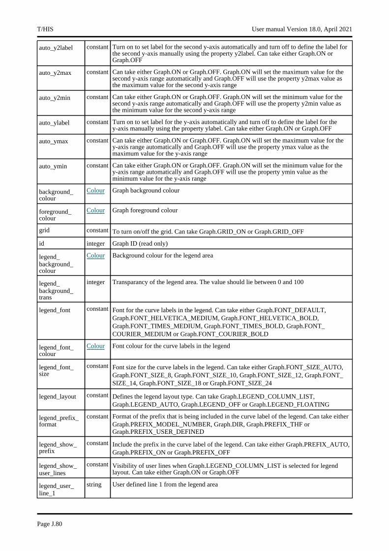
auto_y2label constant Turn on to set label for the second y-axis automatically and turn off to define the label for the second y-axis manually using the property y2label. Can take either Graph.ON or Graph.OFF
auto_y2max constant Can take either Graph.ON or Graph.OFF. Graph.ON will set the maximum value for the second y-axis range automatically and Graph.OFF will use the property y2max value as the maximum value for the second y-axis range
auto_y2min constant Can take either Graph.ON or Graph.OFF. Graph.ON will set the minimum value for the second y-axis range automatically and Graph.OFF will use the property y2min value as the minimum value for the second y-axis range
auto_ylabel constant Turn on to set label for the y-axis automatically and turn off to define the label for the y-axis manually using the property ylabel. Can take either Graph.ON or Graph.OFF
auto_ymax constant Can take either Graph.ON or Graph.OFF. Graph.ON will set the maximum value for the y-axis range automatically and Graph.OFF will use the property ymax value as the maximum value for the y-axis range
auto_ymin constant Can take either Graph.ON or Graph.OFF. Graph.ON will set the minimum value for the y-axis range automatically and Graph.OFF will use the property ymin value as the minimum value for the y-axis range
background_colour
Colour Graph background colour
foreground_colour
Colour Graph foreground colour
grid constant To turn on/off the grid. Can take Graph.GRID_ON or Graph.GRID_OFF
id integer Graph ID (read only)
legend_background_colour
Colour Background colour for the legend area
legend_background_trans
integer Transparancy of the legend area. The value should lie between 0 and 100
legend_font constant Font for the curve labels in the legend. Can take either Graph.FONT_DEFAULT, Graph.FONT_HELVETICA_MEDIUM, Graph.FONT_HELVETICA_BOLD, Graph.FONT_TIMES_MEDIUM, Graph.FONT_TIMES_BOLD, Graph.FONT_COURIER_MEDIUM or Graph.FONT_COURIER_BOLD
legend_font_colour
Colour Font colour for the curve labels in the legend
legend_font_size
constant Font size for the curve labels in the legend. Can take either Graph.FONT_SIZE_AUTO, Graph.FONT_SIZE_8, Graph.FONT_SIZE_10, Graph.FONT_SIZE_12, Graph.FONT_SIZE_14, Graph.FONT_SIZE_18 or Graph.FONT_SIZE_24
legend_layout constant Defines the legend layout type. Can take Graph.LEGEND_COLUMN_LIST, Graph.LEGEND_AUTO, Graph.LEGEND_OFF or Graph.LEGEND_FLOATING
legend_prefix_format
constant Format of the prefix that is being included in the curve label of the legend. Can take either Graph.PREFIX_MODEL_NUMBER, Graph.DIR, Graph.PREFIX_THF or Graph.PREFIX_USER_DEFINED
legend_show_prefix
constant Include the prefix in the curve label of the legend. Can take either Graph.PREFIX_AUTO, Graph.PREFIX_ON or Graph.PREFIX_OFF
legend_show_user_lines
constant Visibility of user lines when Graph.LEGEND_COLUMN_LIST is selected for legend layout. Can take either Graph.ON or Graph.OFF
legend_user_line_1
string User defined line 1 from the legend area
T/HIS User manual Version 18.0, April 2021
Page J.80
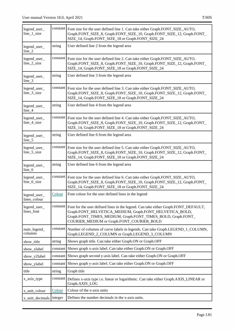
legend_user_line_1_size
constant Font size for the user defined line 1. Can take either Graph.FONT_SIZE_AUTO, Graph.FONT_SIZE_8, Graph.FONT_SIZE_10, Graph.FONT_SIZE_12, Graph.FONT_SIZE_14, Graph.FONT_SIZE_18 or Graph.FONT_SIZE_24
legend_user_line_2
string User defined line 2 from the legend area
legend_user_line_2_size
constant Font size for the user defined line 2. Can take either Graph.FONT_SIZE_AUTO, Graph.FONT_SIZE_8, Graph.FONT_SIZE_10, Graph.FONT_SIZE_12, Graph.FONT_SIZE_14, Graph.FONT_SIZE_18 or Graph.FONT_SIZE_24
legend_user_line_3
string User defined line 3 from the legend area
legend_user_line_3_size
constant Font size for the user defined line 3. Can take either Graph.FONT_SIZE_AUTO, Graph.FONT_SIZE_8, Graph.FONT_SIZE_10, Graph.FONT_SIZE_12, Graph.FONT_SIZE_14, Graph.FONT_SIZE_18 or Graph.FONT_SIZE_24
legend_user_line_4
string User defined line 4 from the legend area
legend_user_line_4_size
constant Font size for the user defined line 4. Can take either Graph.FONT_SIZE_AUTO, Graph.FONT_SIZE_8, Graph.FONT_SIZE_10, Graph.FONT_SIZE_12, Graph.FONT_SIZE_14, Graph.FONT_SIZE_18 or Graph.FONT_SIZE_24
legend_user_line_5
string User defined line 6 from the legend area
legend_user_line_5_size
constant Font size for the user defined line 5. Can take either Graph.FONT_SIZE_AUTO, Graph.FONT_SIZE_8, Graph.FONT_SIZE_10, Graph.FONT_SIZE_12, Graph.FONT_SIZE_14, Graph.FONT_SIZE_18 or Graph.FONT_SIZE_24
legend_user_line_6
string User defined line 6 from the legend area
legend_user_line_6_size
constant Font size for the user defined line 6. Can take either Graph.FONT_SIZE_AUTO, Graph.FONT_SIZE_8, Graph.FONT_SIZE_10, Graph.FONT_SIZE_12, Graph.FONT_SIZE_14, Graph.FONT_SIZE_18 or Graph.FONT_SIZE_24
legend_user_lines_colour
Colour Font colour for the user defined lines in the legend
legend_user_lines_font
constant Font for the user defined lines in the legend. Can take either Graph.FONT_DEFAULT, Graph.FONT_HELVETICA_MEDIUM, Graph.FONT_HELVETICA_BOLD, Graph.FONT_TIMES_MEDIUM, Graph.FONT_TIMES_BOLD, Graph.FONT_COURIER_MEDIUM or Graph.FONT_COURIER_BOLD
num_legend_columns
constant Number of columns of curve labels in legends. Can take Graph.LEGEND_1_COLUMN, Graph.LEGEND_2_COLUMN or Graph.LEGEND_3_COLUMN
show_title string Shows graph title. Can take either Graph.ON or Graph.OFF
show_xlabel constant Shows graph x-axis label. Can take either Graph.ON or Graph.OFF
show_y2label constant Shows graph second y-axis label. Can take either Graph.ON or Graph.OFF
show_ylabel constant Shows graph y-axis label. Can take either Graph.ON or Graph.OFF
title string Graph title
x_axis_type constant Defines x-axis type i.e. linear or logarithmic. Can take either Graph.AXIS_LINEAR or Graph.AXIS_LOG
x_unit_colour Colour Colour of the x-axis units
x_unit_decimals integer Defines the number decimals in the x-axis units.
User manual Version 18.0, April 2021 T/HIS
Page J.81
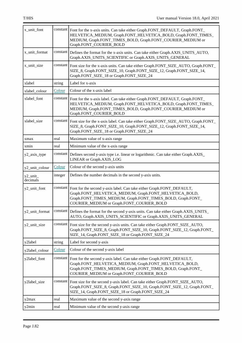
x_unit_font constant Font for the x-axis units. Can take either Graph.FONT_DEFAULT, Graph.FONT_HELVETICA_MEDIUM, Graph.FONT_HELVETICA_BOLD, Graph.FONT_TIMES_MEDIUM, Graph.FONT_TIMES_BOLD, Graph.FONT_COURIER_MEDIUM or Graph.FONT_COURIER_BOLD
x_unit_format constant Defines the format for the x-axis units. Can take either Graph.AXIS_UNITS_AUTO, Graph.AXIS_UNITS_SCIENTIFIC or Graph.AXIS_UNITS_GENERAL
x_unit_size constant Font size for the x-axis units. Can take either Graph.FONT_SIZE_AUTO, Graph.FONT_SIZE_8, Graph.FONT_SIZE_10, Graph.FONT_SIZE_12, Graph.FONT_SIZE_14, Graph.FONT_SIZE_18 or Graph.FONT_SIZE_24
xlabel string Label for x-axis
xlabel_colour Colour Colour of the x-axis label
xlabel_font constant Font for the x-axis label. Can take either Graph.FONT_DEFAULT, Graph.FONT_HELVETICA_MEDIUM, Graph.FONT_HELVETICA_BOLD, Graph.FONT_TIMES_MEDIUM, Graph.FONT_TIMES_BOLD, Graph.FONT_COURIER_MEDIUM or Graph.FONT_COURIER_BOLD
xlabel_size constant Font size for the x-axis label. Can take either Graph.FONT_SIZE_AUTO, Graph.FONT_SIZE_8, Graph.FONT_SIZE_10, Graph.FONT_SIZE_12, Graph.FONT_SIZE_14, Graph.FONT_SIZE_18 or Graph.FONT_SIZE_24
xmax real Maximum value of x-axis range
xmin real Minimum value of the x-axis range
y2_axis_type constant Defines second y-axis type i.e. linear or logarithmic. Can take either Graph.AXIS_LINEAR or Graph.AXIS_LOG
y2_unit_colour Colour Colour of the second y-axis units
y2_unit_decimals
integer Defines the number decimals in the second y-axis units.
y2_unit_font constant Font for the second y-axis label. Can take either Graph.FONT_DEFAULT, Graph.FONT_HELVETICA_MEDIUM, Graph.FONT_HELVETICA_BOLD, Graph.FONT_TIMES_MEDIUM, Graph.FONT_TIMES_BOLD, Graph.FONT_COURIER_MEDIUM or Graph.FONT_COURIER_BOLD
y2_unit_format constant Defines the format for the second y-axis units. Can take either Graph.AXIS_UNITS_AUTO, Graph.AXIS_UNITS_SCIENTIFIC or Graph.AXIS_UNITS_GENERAL
y2_unit_size constant Font size for the second y-axis units. Can take either Graph.FONT_SIZE_AUTO, Graph.FONT_SIZE_8, Graph.FONT_SIZE_10, Graph.FONT_SIZE_12, Graph.FONT_SIZE_14, Graph.FONT_SIZE_18 or Graph.FONT_SIZE_24
y2label string Label for second y-axis
y2label_colour Colour Colour of the second y-axis label
y2label_font constant Font for the second y-axis label. Can take either Graph.FONT_DEFAULT, Graph.FONT_HELVETICA_MEDIUM, Graph.FONT_HELVETICA_BOLD, Graph.FONT_TIMES_MEDIUM, Graph.FONT_TIMES_BOLD, Graph.FONT_COURIER_MEDIUM or Graph.FONT_COURIER_BOLD
y2label_size constant Font size for the second y-axis label. Can take either Graph.FONT_SIZE_AUTO, Graph.FONT_SIZE_8, Graph.FONT_SIZE_10, Graph.FONT_SIZE_12, Graph.FONT_SIZE_14, Graph.FONT_SIZE_18 or Graph.FONT_SIZE_24
y2max real Maximum value of the second y-axis range
y2min real Minimum value of the second y-axis range
T/HIS User manual Version 18.0, April 2021
Page J.82
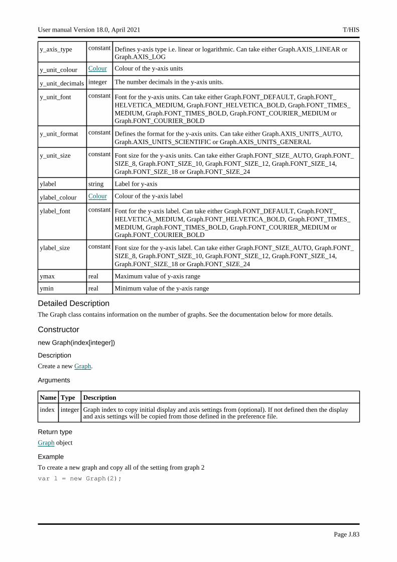
y_axis_type constant Defines y-axis type i.e. linear or logarithmic. Can take either Graph.AXIS_LINEAR or Graph.AXIS_LOG
y_unit_colour Colour Colour of the y-axis units
y_unit_decimals integer The number decimals in the y-axis units.
y_unit_font constant Font for the y-axis units. Can take either Graph.FONT_DEFAULT, Graph.FONT_HELVETICA_MEDIUM, Graph.FONT_HELVETICA_BOLD, Graph.FONT_TIMES_MEDIUM, Graph.FONT_TIMES_BOLD, Graph.FONT_COURIER_MEDIUM or Graph.FONT_COURIER_BOLD
y_unit_format constant Defines the format for the y-axis units. Can take either Graph.AXIS_UNITS_AUTO, Graph.AXIS_UNITS_SCIENTIFIC or Graph.AXIS_UNITS_GENERAL
y_unit_size constant Font size for the y-axis units. Can take either Graph.FONT_SIZE_AUTO, Graph.FONT_SIZE_8, Graph.FONT_SIZE_10, Graph.FONT_SIZE_12, Graph.FONT_SIZE_14, Graph.FONT_SIZE_18 or Graph.FONT_SIZE_24
ylabel string Label for y-axis
ylabel_colour Colour Colour of the y-axis label
ylabel_font constant Font for the y-axis label. Can take either Graph.FONT_DEFAULT, Graph.FONT_HELVETICA_MEDIUM, Graph.FONT_HELVETICA_BOLD, Graph.FONT_TIMES_MEDIUM, Graph.FONT_TIMES_BOLD, Graph.FONT_COURIER_MEDIUM or Graph.FONT_COURIER_BOLD
ylabel_size constant Font size for the y-axis label. Can take either Graph.FONT_SIZE_AUTO, Graph.FONT_SIZE_8, Graph.FONT_SIZE_10, Graph.FONT_SIZE_12, Graph.FONT_SIZE_14, Graph.FONT_SIZE_18 or Graph.FONT_SIZE_24
ymax real Maximum value of y-axis range
ymin real Minimum value of the y-axis range
Detailed DescriptionThe Graph class contains information on the number of graphs. See the documentation below for more details.
Constructor
new Graph(index[integer])
Description
Create a new Graph.
Arguments
Name Type Description
index integer Graph index to copy initial display and axis settings from (optional). If not defined then the display and axis settings will be copied from those defined in the preference file.
Return type
Graph object
Example
To create a new graph and copy all of the setting from graph 2
var l = new Graph(2);
User manual Version 18.0, April 2021 T/HIS
Page J.83
Details of functions
AddCurveID(Curve ID[Integer], No redraw (optional)[Integer])
Description
Adds a curve to the graph.
Arguments
Name Type Description
Curve ID Integer ID of the curve to add.
No redraw (optional)
Integer If this argument is 1 then the graph will not be redrawn after the curve is added. This is to be used if a large number of curves are to be added to a graph, so as to avoid the same curves being drawn multiple times. No argument or 0 will trigger a redraw after the curve is added.
Return type
Returns true if the curve is successfully added to the graph else it would return false
Example
To add a curve with id (n) to the graph (g):
g.AddCurveID(n);
AddToPage(Page number[Integer])
Description
Adds the graph to the page.
Arguments
Name Type Description
Page number Integer Page number for which to add the graph to.
Return type
Returns true if the graph is successfully added to the page else it would return false
Example
To add a graph (g) to page id (n):
g.AddToPage(n);
Delete()
Description
Deletes the graph
Arguments
No arguments
Return type
No return value
Example
Deletes the graph (g)
g.Delete();
T/HIS User manual Version 18.0, April 2021
Page J.84
DeleteFromID(ID[integer]) [static]
Description
Deletes a graph
Arguments
Name Type Description
ID integer ID of graph to delete
Return type
No return value
Example
To delete the graph n
Graph.DeleteFromID(n);
Maximum number of graphs in T/HIS is 32
GetAllCurveIDs()
Description
Returns the IDs of the curves present in the graph in an array.
Arguments
No arguments
Return type
Array integers
Example
To get the array of all the curve ids present in a graph (g):
var num = g.GetAllCurveIDs();
GetAllPageIDs()
Description
Returns all the pages containing the graph.
Arguments
No arguments
Return type
Array of integers
Example
To get the list of all page ids containing the graph (g):
var pages_ids = g.GetAllPageIDs();
GetFromID(ID[integer]) [static]
Description
Returns the graph object for a given graph id.
User manual Version 18.0, April 2021 T/HIS
Page J.85
Arguments
Name Type Description
ID integer ID of graph to return the graph for
Return type
Graph object or NULL if graph does not exists
Example
To get the graph n
var num = Graph.GetFromID(n);
Maximum number of graphs in T/HIS is 32
GetNumCurves()
Description
Returns number curves present in the graph.
Arguments
No arguments
Return type
Number of curves present in the graph.
Example
To find number of curves in a graph (g):
var num = g.GetNumCurves();
Lock(Lock type[Integer])
Description
Locks the blanking status of either blanked curves, unblanked curves or all curves on the graph.
Arguments
Name Type Description
Lock type
Integer No argument or 0 to lock blanked curves, -1 to unlock blanked curves, -2 to unfreeze all visible curves
Return type
No return value
Example
To lock all blanked curves on graph g:
g.Lock();
RemoveCurveID()
Description
Removs a curve from the graph.
Arguments
No arguments
T/HIS User manual Version 18.0, April 2021
Page J.86
Return type
Returns true if the curve is successfully removed from the graph else it would return false
Example
To remove a curve with id (n) from the graph (g):
g.RemoveCurveID(n);
RemoveFromPage()
Description
Removs the graph from a page.
Arguments
No arguments
Return type
Returns true if the graph is successfully removed from the page else it would return false
Example
To remove the graph (g) from page with id (n):
g.RemoveFromPage(n);
Total() [static]
Description
Returns the total number of graphs.
Arguments
No arguments
Return type
integer
Example
To find how many graphs there are in T/HIS:
var num = Graph.Total();
User manual Version 18.0, April 2021 T/HIS
Page J.87

Group classThe Group class gives you access to groups in T/HIS. More...
The T/HIS JavaScript API provides many class constants, properties and methods. For Arup to be able to extend and enhance the API in the future any constant, property or method names beginning with a lowercase or uppercase letter are reserved.If you need to add your own properties or methods to one of the existing classes then to avoid any potential future conflict you should ensure that the name begins with either an underscore (_) or a dollar sign ($) or the name is prefixed with your own unique identifier.For example if company ’ABC’ need to add a property called ’example’ then to avoid any potential future conflict use one of:
• _example • $example • ABC_example
Class functions• DeleteGroup(group ID or name[integer or string], delete automatic groups (optional)[integer]) • Get(Name[string]) • GetFromID(ID[integer]) • Total()
Member functions• Add(Curve[Curve]) • AddAll() • AddID(ID[integer]) • Contains(Curve[Curve]) • ContainsID(ID[integer]) • GetCurveIDs() • GetCurves() • Remove(Curve[Curve]) • RemoveAll() • RemoveID(ID[integer]) • Spool() • SpoolID() • StartSpool()
Group properties
Name Type Description
crv_at_ymax integer Curve number of the curve with the maximum Y value in the group.
crv_at_ymin integer Curve number of the curve with the minimum Y value in the group.
curves integer Number of curves in the group (read only)
name string Group name (read only)
x_at_ymax real X value at the maximum Y value over all curves in the group.
x_at_ymin real X value at the minimum Y value over all curves in the group.
x_at_yminpos real X value at the minimum positive Y value over all curves in the group.
xmax real Maximum X value over all curves in the group.
xmin real Minimum X value over all curves in the group.
xminpos real Minimum positive X value over all curves in the group.
ymax real Maximum Y value over all curves in the group.
ymin real Minimum Y value over all curves in the group.
yminpos real Minimum positive Y value over all curves in the group.
Detailed DescriptionThe Group class allows you to create, and modify groups. See the documentation below for more details.
T/HIS User manual Version 18.0, April 2021
Page J.88
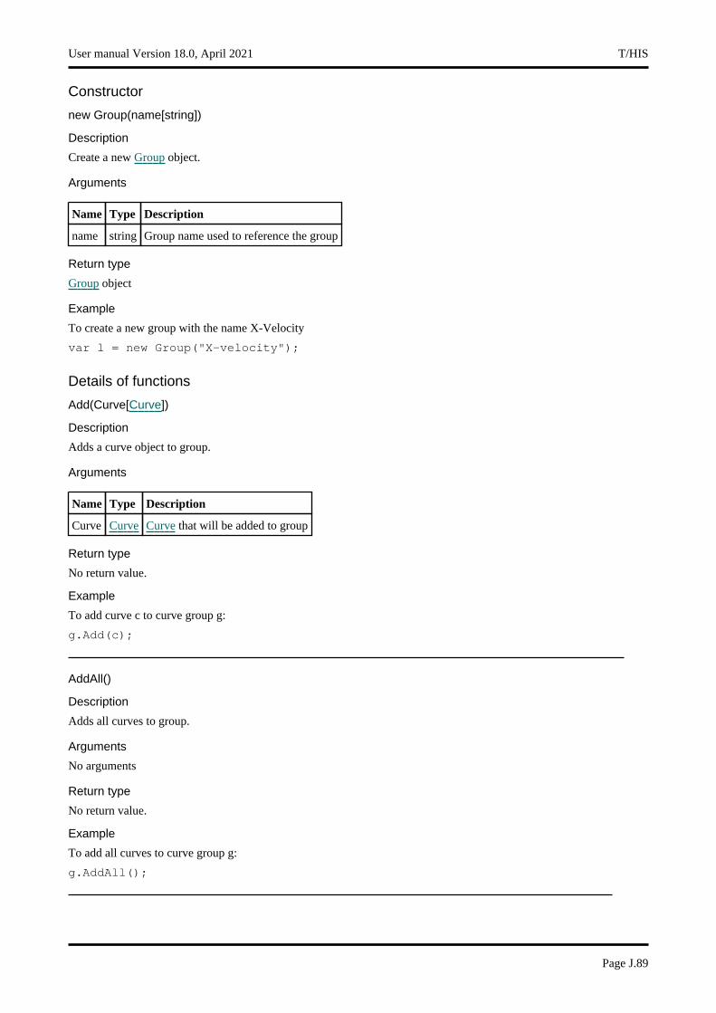
Constructor
new Group(name[string])
Description
Create a new Group object.
Arguments
Name Type Description
name string Group name used to reference the group
Return type
Group object
Example
To create a new group with the name X-Velocity
var l = new Group("X-velocity");
Details of functions
Add(Curve[Curve])
Description
Adds a curve object to group.
Arguments
Name Type Description
Curve Curve Curve that will be added to group
Return type
No return value.
Example
To add curve c to curve group g:
g.Add(c);
AddAll()
Description
Adds all curves to group.
Arguments
No arguments
Return type
No return value.
Example
To add all curves to curve group g:
g.AddAll();
User manual Version 18.0, April 2021 T/HIS
Page J.89
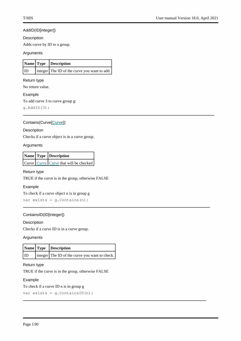
AddID(ID[integer])
Description
Adds curve by ID to a group.
Arguments
Name Type Description
ID integer The ID of the curve you want to add.
Return type
No return value.
Example
To add curve 3 to curve group g:
g.AddID(3);
Contains(Curve[Curve])
Description
Checks if a curve object is in a curve group.
Arguments
Name Type Description
Curve Curve Curve that will be checked
Return type
TRUE if the curve is in the group, otherwise FALSE
Example
To check if a curve object n is in group g
var exists = g.Contains(n);
ContainsID(ID[integer])
Description
Checks if a curve ID is in a curve group.
Arguments
Name Type Description
ID integer The ID of the curve you want to check.
Return type
TRUE if the curve is in the group, otherwise FALSE
Example
To check if a curve ID n is in group g
var exists = g.ContainsID(n);
T/HIS User manual Version 18.0, April 2021
Page J.90
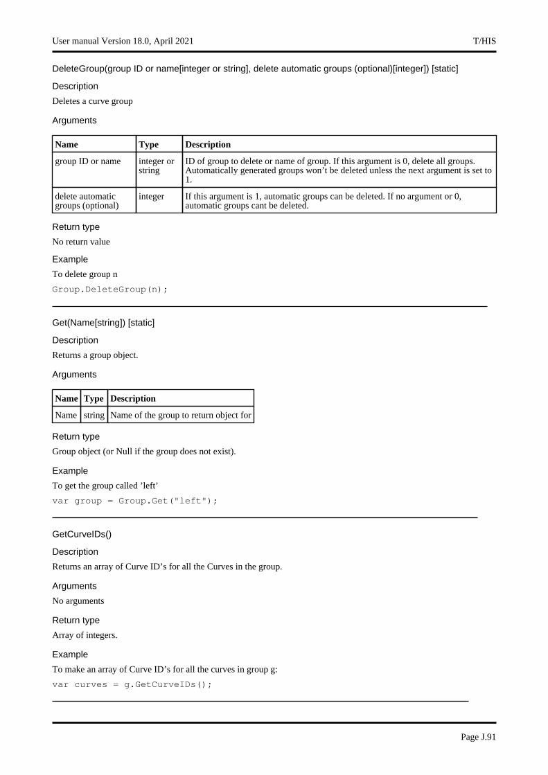
DeleteGroup(group ID or name[integer or string], delete automatic groups (optional)[integer]) [static]
Description
Deletes a curve group
Arguments
Name Type Description
group ID or name integer or string
ID of group to delete or name of group. If this argument is 0, delete all groups. Automatically generated groups won’t be deleted unless the next argument is set to 1.
delete automatic groups (optional)
integer If this argument is 1, automatic groups can be deleted. If no argument or 0, automatic groups cant be deleted.
Return type
No return value
Example
To delete group n
Group.DeleteGroup(n);
Get(Name[string]) [static]
Description
Returns a group object.
Arguments
Name Type Description
Name string Name of the group to return object for
Return type
Group object (or Null if the group does not exist).
Example
To get the group called ’left’
var group = Group.Get("left");
GetCurveIDs()
Description
Returns an array of Curve ID’s for all the Curves in the group.
Arguments
No arguments
Return type
Array of integers.
Example
To make an array of Curve ID’s for all the curves in group g:
var curves = g.GetCurveIDs();
User manual Version 18.0, April 2021 T/HIS
Page J.91
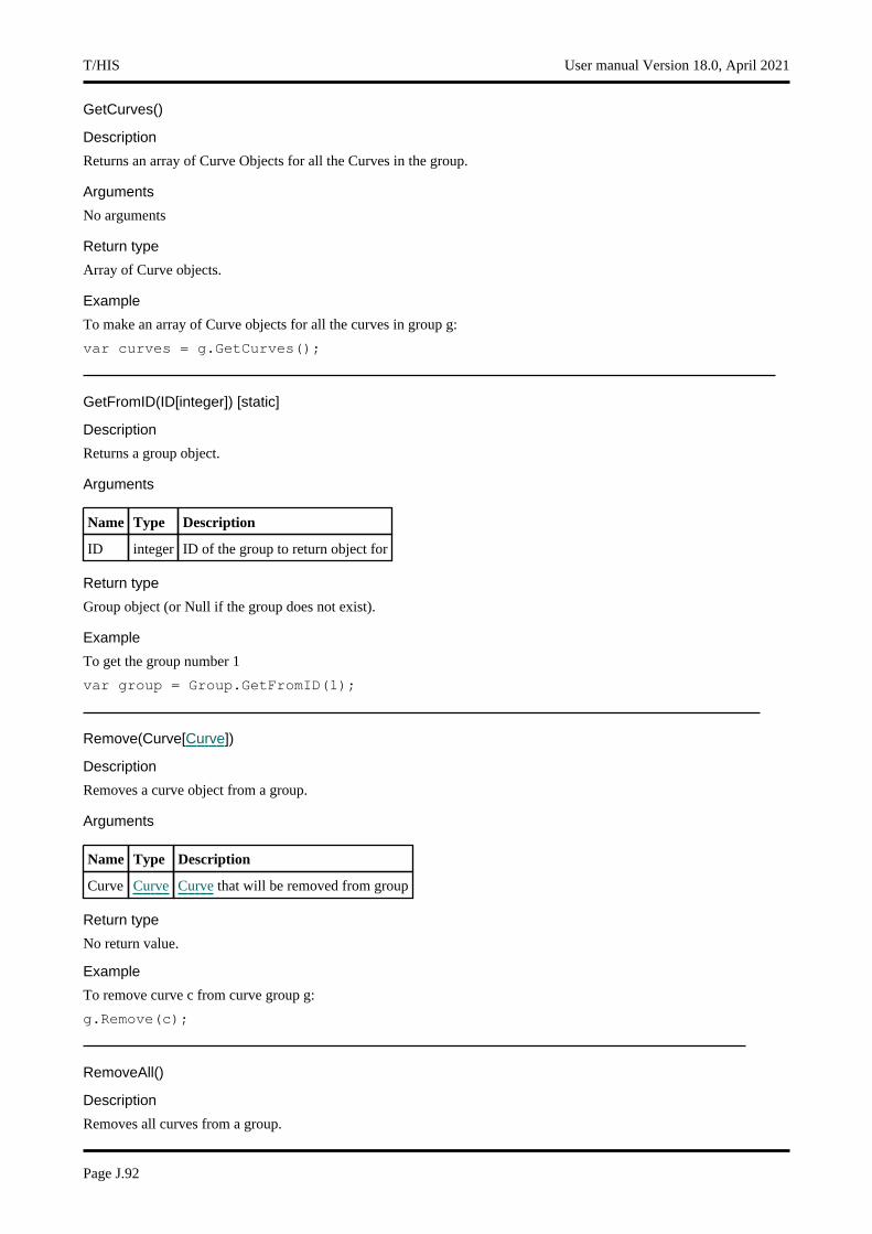
GetCurves()
Description
Returns an array of Curve Objects for all the Curves in the group.
Arguments
No arguments
Return type
Array of Curve objects.
Example
To make an array of Curve objects for all the curves in group g:
var curves = g.GetCurves();
GetFromID(ID[integer]) [static]
Description
Returns a group object.
Arguments
Name Type Description
ID integer ID of the group to return object for
Return type
Group object (or Null if the group does not exist).
Example
To get the group number 1
var group = Group.GetFromID(1);
Remove(Curve[Curve])
Description
Removes a curve object from a group.
Arguments
Name Type Description
Curve Curve Curve that will be removed from group
Return type
No return value.
Example
To remove curve c from curve group g:
g.Remove(c);
RemoveAll()
Description
Removes all curves from a group.
T/HIS User manual Version 18.0, April 2021
Page J.92
Arguments
No arguments
Return type
No return value.
Example
To remove all curves from curve group g:
g.RemoveAll();
RemoveID(ID[integer])
Description
Remove a curve by ID from a group.
Arguments
Name Type Description
ID integer The ID of the curve you want to remove.
Return type
No return value.
Example
To remove curve 3 from curve group g:
g.RemoveID(3);
Spool()
Description
Spools a group, entry by entry and returns the curve objects. See also Group.StartSpool
Arguments
No arguments
Return type
Curve Object of item, or NULL if no more curves in group
Example
To spool group g:
var id;g.StartSpool();while (id = g.Spool() ){
do something...}
SpoolID()
Description
Spools a group, entry by entry and returns the curve ID’s or 0 when no more curves in group. See also Group.StartSpool
Arguments
No arguments
User manual Version 18.0, April 2021 T/HIS
Page J.93
Return type
integer
Example
To spool group g :
var id;g.StartSpool();while (id = g.SpoolID() ){
do something...}
StartSpool()
Description
Starts a group spooling operation. See also Group.Spool
Arguments
No arguments
Return type
No return value
Example
To start spooling group g:
g.StartSpool();
Total() [static]
Description
Returns the total number of curve group currently defined
Arguments
No arguments
Return type
Number of curve groups currently defined.
Example
To get the number of curve groups
var total = Group.Total();
T/HIS User manual Version 18.0, April 2021
Page J.94

Include classThe Include class allows you to access the include files in a model. More...
The T/HIS JavaScript API provides many class constants, properties and methods. For Arup to be able to extend and enhance the API in the future any constant, property or method names beginning with a lowercase or uppercase letter are reserved.If you need to add your own properties or methods to one of the existing classes then to avoid any potential future conflict you should ensure that the name begins with either an underscore (_) or a dollar sign ($) or the name is prefixed with your own unique identifier.For example if company ’ABC’ need to add a property called ’example’ then to avoid any potential future conflict use one of:
• _example • $example • ABC_example
Include constants
Constants for Directory separators
Name Description
Include.NATIVE Use directory separators native to this machine when writing directory names.
Include.UNIX Use unix directory separators when writing directory names.
Include.WINDOWS Use windows directory separators when writing directory names.
Detailed DescriptionThe Include class allows to create and query include files in a model. This class was originally in PRIMER but has now been transferred to T/HIS and D3PLOT to allow consistency between the programs. See File.DriveMapFilename for the current use of this class.
User manual Version 18.0, April 2021 T/HIS
Page J.95
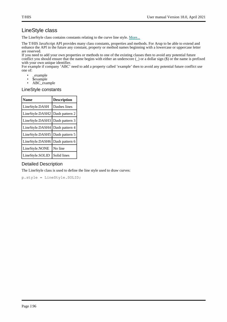
LineStyle classThe LineStyle class contains constants relating to the curve line style. More...
The T/HIS JavaScript API provides many class constants, properties and methods. For Arup to be able to extend and enhance the API in the future any constant, property or method names beginning with a lowercase or uppercase letter are reserved.If you need to add your own properties or methods to one of the existing classes then to avoid any potential future conflict you should ensure that the name begins with either an underscore (_) or a dollar sign ($) or the name is prefixed with your own unique identifier.For example if company ’ABC’ need to add a property called ’example’ then to avoid any potential future conflict use one of:
• _example • $example • ABC_example
LineStyle constants
Name Description
LineStyle.DASH Dashes lines
LineStyle.DASH2 Dash pattern 2
LineStyle.DASH3 Dash pattern 3
LineStyle.DASH4 Dash pattern 4
LineStyle.DASH5 Dash pattern 5
LineStyle.DASH6 Dash pattern 6
LineStyle.NONE No line
LineStyle.SOLID Solid lines
Detailed DescriptionThe LineStyle class is used to define the line style used to draw curves:
p.style = LineStyle.SOLID;
T/HIS User manual Version 18.0, April 2021
Page J.96
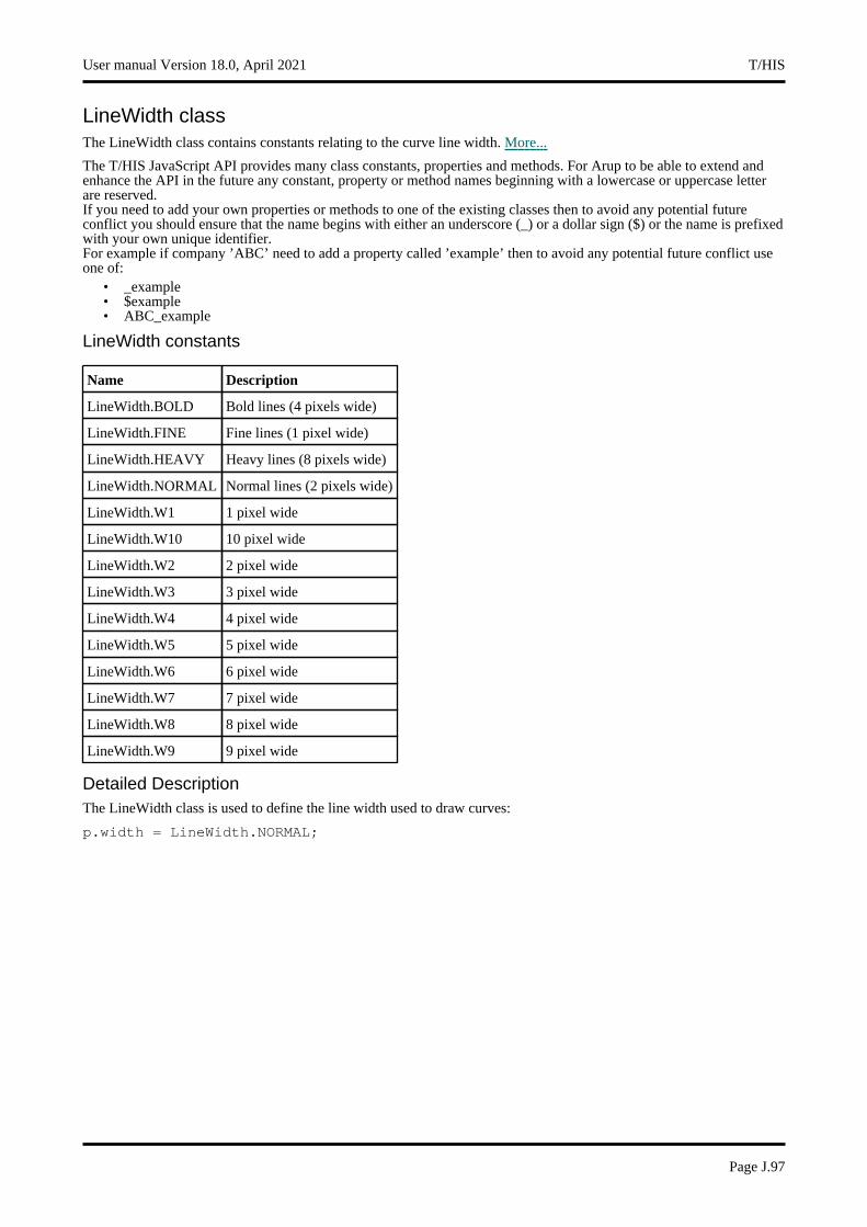
LineWidth classThe LineWidth class contains constants relating to the curve line width. More...
The T/HIS JavaScript API provides many class constants, properties and methods. For Arup to be able to extend and enhance the API in the future any constant, property or method names beginning with a lowercase or uppercase letter are reserved.If you need to add your own properties or methods to one of the existing classes then to avoid any potential future conflict you should ensure that the name begins with either an underscore (_) or a dollar sign ($) or the name is prefixed with your own unique identifier.For example if company ’ABC’ need to add a property called ’example’ then to avoid any potential future conflict use one of:
• _example • $example • ABC_example
LineWidth constants
Name Description
LineWidth.BOLD Bold lines (4 pixels wide)
LineWidth.FINE Fine lines (1 pixel wide)
LineWidth.HEAVY Heavy lines (8 pixels wide)
LineWidth.NORMAL Normal lines (2 pixels wide)
LineWidth.W1 1 pixel wide
LineWidth.W10 10 pixel wide
LineWidth.W2 2 pixel wide
LineWidth.W3 3 pixel wide
LineWidth.W4 4 pixel wide
LineWidth.W5 5 pixel wide
LineWidth.W6 6 pixel wide
LineWidth.W7 7 pixel wide
LineWidth.W8 8 pixel wide
LineWidth.W9 9 pixel wide
Detailed DescriptionThe LineWidth class is used to define the line width used to draw curves:
p.width = LineWidth.NORMAL;
User manual Version 18.0, April 2021 T/HIS
Page J.97
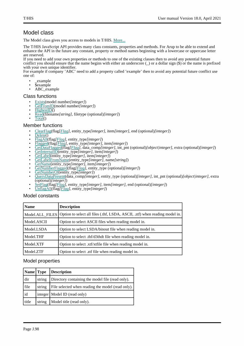
Model classThe Model class gives you access to models in T/HIS. More...
The T/HIS JavaScript API provides many class constants, properties and methods. For Arup to be able to extend and enhance the API in the future any constant, property or method names beginning with a lowercase or uppercase letter are reserved.If you need to add your own properties or methods to one of the existing classes then to avoid any potential future conflict you should ensure that the name begins with either an underscore (_) or a dollar sign ($) or the name is prefixed with your own unique identifier.For example if company ’ABC’ need to add a property called ’example’ then to avoid any potential future conflict use one of:
• _example • $example • ABC_example
Class functions• Exists(model number[integer]) • GetFromID(model number[integer]) • HighestID() • Read(filename[string], filetype (optional)[integer]) • Total()
Member functions• ClearFlag(flag[Flag], entity_type[integer], item[integer], end (optional)[integer]) • Delete() • FlagAll(flag[Flag], entity_type[integer]) • Flagged(flag[Flag], entity_type[integer], item[integer]) • GetDataFlagged(flag[Flag], data_comp[integer], int_pnt (optional)[object|integer], extra (optional)[integer]) • GetInternalID(entity_type[integer], item[integer]) • GetLabel(entity_type[integer], item[integer]) • GetLabelFromName(entity_type[integer], name[string]) • GetName(entity_type[integer], item[integer]) • GetNumberFlagged(flag[Flag], entity_type (optional)[integer]) • GetNumberOf(entity_type[integer]) • QueryDataPresent(data_comp[integer], entity_type (optional)[integer], int_pnt (optional)[object|integer], extra
(optional)[integer]) • SetFlag(flag[Flag], entity_type[integer], item[integer], end (optional)[integer]) • UnflagAll(flag[Flag], entity_type[integer])
Model constants
Name Description
Model.ALL_FILES Option to select all files (.thf, LSDA, ASCII, .ztf) when reading model in.
Model.ASCII Option to select ASCII files when reading model in.
Model.LSDA Option to select LSDA/binout file when reading model in.
Model.THF Option to select .thf/d3thdt file when reading model in.
Model.XTF Option to select .xtf/xtfile file when reading model in.
Model.ZTF Option to select .ztf file when reading model in.
Model properties
Name Type Description
dir string Directory containing the model file (read only).
file string File selected when reading the model (read only).
id integer Model ID (read only)
title string Model title (read only).
T/HIS User manual Version 18.0, April 2021
Page J.98

Detailed DescriptionThe Model class contains information on filenames and directories belonging to a model. See the documentation below for more details.
Details of functions
ClearFlag(flag[Flag], entity_type[integer], item[integer], end (optional)[integer])
Description
Clears a defined flag on an internal (or external) item(s) of type of entity_type in the model.
Arguments
Name Type Description
flag Flag The flag you want to clear.
entity_type integer The Entity type that the defined flag will be cleared on.
item integer If +ive: The internal item number starting from 1. If -ive: The external item label.
end (optional) integer To unflag range of items, specify an optional end of range. Unflags items from item to range.
Return type
TRUE if the flag is successfully cleared on the item, otherwise FALSE
Example
To clear the flag f on the 6th node in model m:
m.ClearFlag(f, Entity.NODE, 6);
To clear the flag f on the Node 13456 in model m:
m.ClearFlag(f, Entity.NODE, -13456);
To clear the flag f on the first 10 nodes in model m:
m.ClearFlag(f, Entity.NODE, 1, 10);
To clear the flag f on nodes with labels 1000, 1001, 1002, ..., 1009 in model m:
m.ClearFlag(f, Entity.NODE, -1000, -1009);
Delete()
Description
Deletes a modelDo not use the Model object after calling this method.
Arguments
No arguments
Return type
TRUE if the model sucessfully deleted, otherwise FALSE
Example
To delete model m:
var deleted = m.Delete();
User manual Version 18.0, April 2021 T/HIS
Page J.99
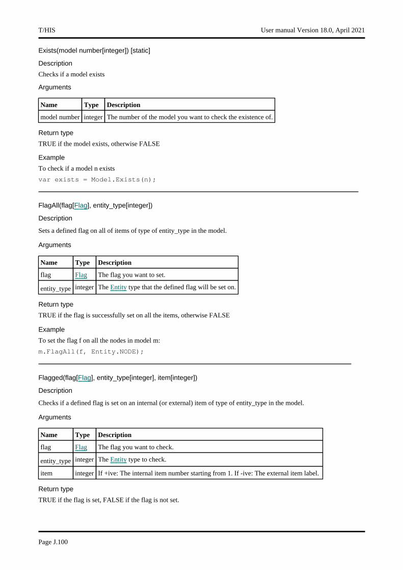
Exists(model number[integer]) [static]
Description
Checks if a model exists
Arguments
Name Type Description
model number integer The number of the model you want to check the existence of.
Return type
TRUE if the model exists, otherwise FALSE
Example
To check if a model n exists
var exists = Model.Exists(n);
FlagAll(flag[Flag], entity_type[integer])
Description
Sets a defined flag on all of items of type of entity_type in the model.
Arguments
Name Type Description
flag Flag The flag you want to set.
entity_type integer The Entity type that the defined flag will be set on.
Return type
TRUE if the flag is successfully set on all the items, otherwise FALSE
Example
To set the flag f on all the nodes in model m:
m.FlagAll(f, Entity.NODE);
Flagged(flag[Flag], entity_type[integer], item[integer])
Description
Checks if a defined flag is set on an internal (or external) item of type of entity_type in the model.
Arguments
Name Type Description
flag Flag The flag you want to check.
entity_type integer The Entity type to check.
item integer If +ive: The internal item number starting from 1. If -ive: The external item label.
Return type
TRUE if the flag is set, FALSE if the flag is not set.
T/HIS User manual Version 18.0, April 2021
Page J.100
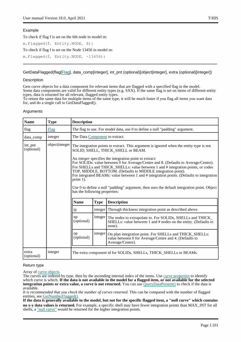
Example
To check if flag f is set on the 6th node in model m:
m.Flagged(f, Entity.NODE, 6);
To check if flag f is set on the Node 13456 in model m:
m.Flagged(f, Entity.NODE, -13456);
GetDataFlagged(flag[Flag], data_comp[integer], int_pnt (optional)[object|integer], extra (optional)[integer])
Description
Gets curve objects for a data component for relevant items that are flagged with a specified flag in the model. Some data components are valid for different entity types (e.g. SXX). If the same flag is set on items of different entity types, data is returned for all relevant, flagged entity types. To return the same data for multiple items of the same type, it will be much faster if you flag all items you want data for, and do a single call to GetDataFlagged().
Arguments
Name Type Description
flag Flag The flag to use. For model data, use 0 to define a null "padding" argument.
data_comp integer The Data Component to extract.
int_pnt (optional)
object|integer The integration points to extract. This argument is ignored when the entity type is not SOLID, SHELL, THICK_SHELL or BEAM.
An integer specifies the integration point to extract:For SOLIDs: value between 0 for Average/Centre and 8. (Defaults to Average/Centre).For SHELLs and THICK_SHELLs: value between 1 and # integration points, or codes TOP, MIDDLE, BOTTOM. (Defaults to MIDDLE integration point). For integrated BEAMs: value between 1 and # integration points. (Defaults to integration point 1).
Use 0 to define a null "padding" argument, then uses the default integration point. Object has the following properties:
Name Type Description
ip integer Through thickness integration point as described above.
np (optional)
integer The nodes to extrapolate to. For SOLIDs, SHELLs and THICK_SHELLs: value between 1 and # nodes on the entity. (Defaults to none).
op (optional)
integer On plan integration point. For SHELLs and THICK_SHELLs: value between 0 for Average/Centre and 4. (Defaults to Average/Centre).
extra (optional)
integer The extra component id for SOLIDs, SHELLs, THICK_SHELLs or BEAMs.
Return type
Array of curve objects. The curves are ordered by type, then by the ascending internal index of the items. Use curve properties to identify which curve is which. If the data is not available in the model for a flagged item, or not available for the selected integration points or extra value, a curve is not returned. You can use QueryDataPresent() to check if the data is available.It is recommended that you check the number of curves returned. This can be compared with the number of flagged entities, see GetNumberFlagged().If the data is generally available in the model, but not for the specific flagged item, a "null curve" which contains no x-y data values is returned. For example, a specific shell may have fewer integration points than MAX_INT for all shells, a "null curve" would be returned for the higher integration points.
User manual Version 18.0, April 2021 T/HIS
Page J.101

Example
To get X direct stress for flagged SOLIDs, SHELLs and THICK_SHELLs with flag f in model m:
var cur_array = m.GetDataFlagged(f, Component.SXX);
To get X direct stress at top integration point for flagged SHELLs and THICK_SHELLs with flag f in model m:
var cur_array = m.GetDataFlagged(f, Component.SXX, TOP);
To get X direct stress at top integration point, and on-plan integration point 3 for flagged SHELLs and THICK_SHELLs with flag f in model m:
var cur_array = m.GetDataFlagged(f, Component.SXX, {ip:TOP, op:3});
To get extra beam data 3 for flagged BEAMs with flag f in model m:
var cur_array = m.GetDataFlagged(f, Component.BEX, 0, 3);
To get the total mass in model m:
var cur_array = m.GetDataFlagged(0, Component.GMASS);
GetFromID(model number[integer]) [static]
Description
Returns the Model object for a model ID or null if model does not exist.
Arguments
Name Type Description
model number integer number of the model you want the Model object for
Return type
Model object (or null if model does not exist).
Example
To get the model n
var model = Model.GetFromID(n);
GetInternalID(entity_type[integer], item[integer])
Description
Gets the internal ID of external item of type entity_type in the model.
Arguments
Name Type Description
entity_type integer The Entity type of the item.
item integer The external item number.
Return type
Integer internal ID (starting from 1) with reference to the entity_type code.
Example
To get the internal ID of Airbag 300 in model m:
var x = m.GetInternalID(Entity.AIRBAG, 300);
T/HIS User manual Version 18.0, April 2021
Page J.102
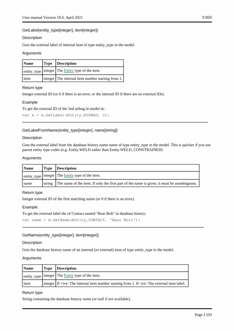
GetLabel(entity_type[integer], item[integer])
Description
Gets the external label of internal item of type entity_type in the model.
Arguments
Name Type Description
entity_type integer The Entity type of the item.
item integer The internal item number starting from 1.
Return type
Integer external ID (or 0 if there is an error, or the internal ID if there are no external IDs).
Example
To get the external ID of the 2nd airbag in model m:
var x = m.GetLabel(Entity.AIRBAG, 2);
GetLabelFromName(entity_type[integer], name[string])
Description
Gets the external label from the database history name name of type entity_type in the model. This is quicker if you use parent entity type codes (e.g. Entity.WELD rather than Entity.WELD_CONSTRAINED)
Arguments
Name Type Description
entity_type integer The Entity type of the item.
name string The name of the item. If only the first part of the name is given, it must be unambiguous.
Return type
Integer external ID of the first matching name (or 0 if there is an error).
Example
To get the external label the of Contact named "Rear Bolt" in database history:
var name = m.GetName(Entity.CONTACT, "Rear Bolt");
GetName(entity_type[integer], item[integer])
Description
Gets the database history name of an internal (or external) item of type entity_type in the model.
Arguments
Name Type Description
entity_type integer The Entity type of the item.
item integer If +ive: The internal item number starting from 1. If -ive: The external item label.
Return type
String containing the database history name (or null if not available).
User manual Version 18.0, April 2021 T/HIS
Page J.103
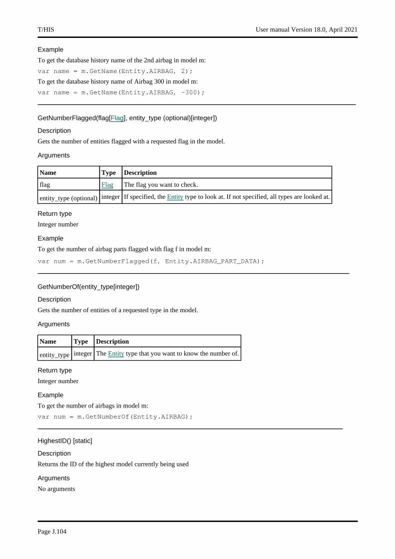
Example
To get the database history name of the 2nd airbag in model m:
var name = m.GetName(Entity.AIRBAG, 2);
To get the database history name of Airbag 300 in model m:
var name = m.GetName(Entity.AIRBAG, -300);
GetNumberFlagged(flag[Flag], entity_type (optional)[integer])
Description
Gets the number of entities flagged with a requested flag in the model.
Arguments
Name Type Description
flag Flag The flag you want to check.
entity_type (optional) integer If specified, the Entity type to look at. If not specified, all types are looked at.
Return type
Integer number
Example
To get the number of airbag parts flagged with flag f in model m:
var num = m.GetNumberFlagged(f, Entity.AIRBAG_PART_DATA);
GetNumberOf(entity_type[integer])
Description
Gets the number of entities of a requested type in the model.
Arguments
Name Type Description
entity_type integer The Entity type that you want to know the number of.
Return type
Integer number
Example
To get the number of airbags in model m:
var num = m.GetNumberOf(Entity.AIRBAG);
HighestID() [static]
Description
Returns the ID of the highest model currently being used
Arguments
No arguments
T/HIS User manual Version 18.0, April 2021
Page J.104

Return type
ID of highest model currently being used.
Example
To get the highest model ID
var id= Model.HighestID();
QueryDataPresent(data_comp[integer], entity_type (optional)[integer], int_pnt (optional)[object|integer], extra (optional)[integer])
Description
Checks if a data component data_comp for a given entity is present in a model’s database. For SOLIDs, SHELLs, THICK_SHELLs and BEAMs the integration point and extra component ID can also be checked. This will show if curves for any flagged items of this type will be returned for GetDataFlagged(). Note, it does not check if the data component is valid, for example a specific shell may have fewer integration points than MAX_INT for all shells, so curves returned for GetDataFlagged() may still be "null" with no x-y data.
Arguments
Name Type Description
data_comp integer The Data Component to check.
entity_type (optional)
integer The Entity type to check. This argument can only be omitted when checking for global model data.
int_pnt (optional)
object|integer The integration points to check. This argument is ignored if the entity type is not SOLID, SHELL, THICK_SHELL or BEAM.
An integer specifies the integration point to check:For SOLIDs: value between 0 for Average/Centre and 8. (Defaults to Average/Centre).For SHELLs and THICK_SHELLs: value between 1 and # integration points, or codes TOP, MIDDLE, BOTTOM. (Defaults to MIDDLE integration point). For integrated BEAMs: value between 1 and # integration points. (Defaults to integration point 1).
Use 0 to define a null "padding" argument, then checks the default integration point. Object has the following properties:
Name Type Description
ip integer Through thickness integration point as described above.
np (optional)
integer The nodes to extrapolate to. For SOLIDs, SHELLs and THICK_SHELLs: value between 1 and # nodes on the entity. (Defaults to none).
op (optional)
integer On plan integration point. For SHELLs and THICK_SHELLs: value between 0 for Average/Centre and 4. (Defaults to Average/Centre).
extra (optional)
integer The extra component id for SOLIDs, SHELLs, THICK_SHELLs or BEAMs.
Return type
JS_TRUE if data is present, otherwise JS_FALSE.
User manual Version 18.0, April 2021 T/HIS
Page J.105
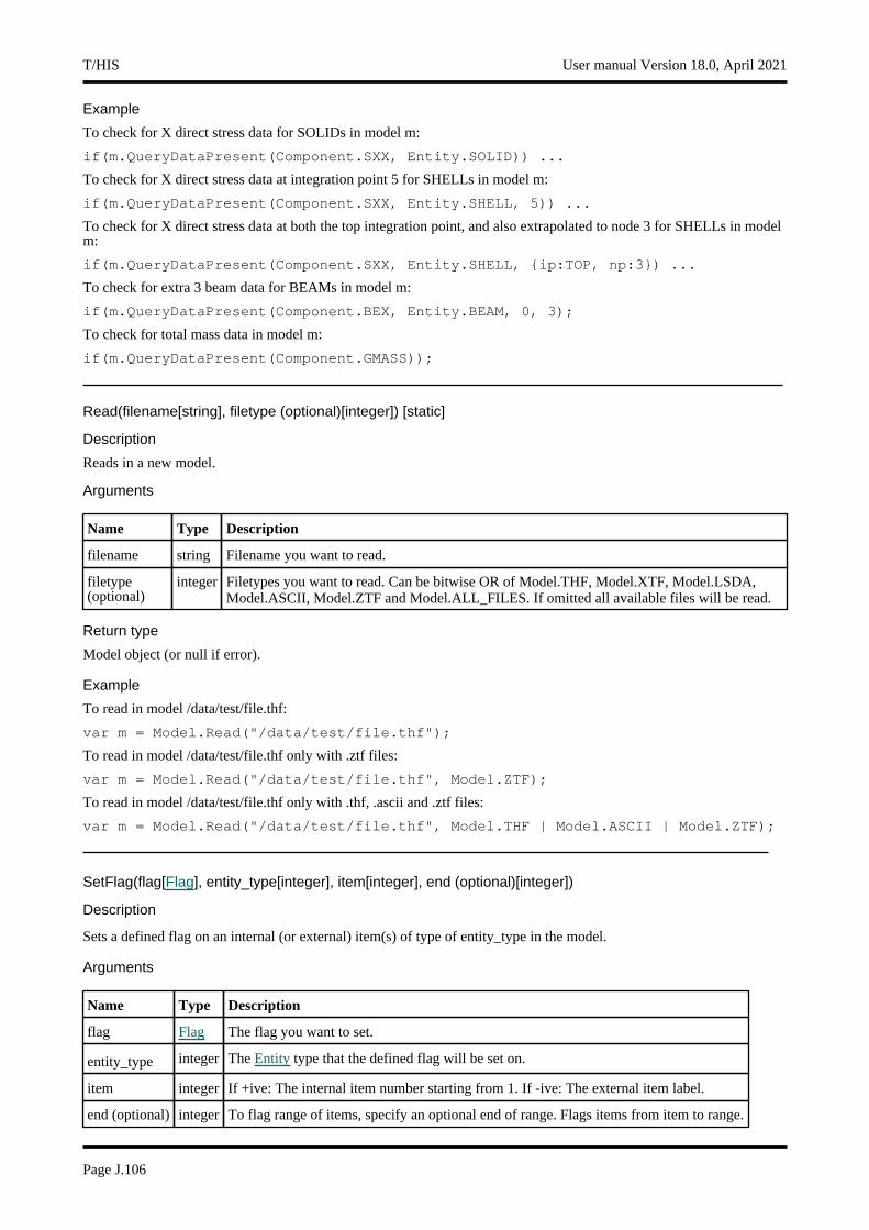
Example
To check for X direct stress data for SOLIDs in model m:
if(m.QueryDataPresent(Component.SXX, Entity.SOLID)) ...
To check for X direct stress data at integration point 5 for SHELLs in model m:
if(m.QueryDataPresent(Component.SXX, Entity.SHELL, 5)) ...
To check for X direct stress data at both the top integration point, and also extrapolated to node 3 for SHELLs in model m:
if(m.QueryDataPresent(Component.SXX, Entity.SHELL, {ip:TOP, np:3}) ...
To check for extra 3 beam data for BEAMs in model m:
if(m.QueryDataPresent(Component.BEX, Entity.BEAM, 0, 3);
To check for total mass data in model m:
if(m.QueryDataPresent(Component.GMASS));
Read(filename[string], filetype (optional)[integer]) [static]
Description
Reads in a new model.
Arguments
Name Type Description
filename string Filename you want to read.
filetype (optional)
integer Filetypes you want to read. Can be bitwise OR of Model.THF, Model.XTF, Model.LSDA, Model.ASCII, Model.ZTF and Model.ALL_FILES. If omitted all available files will be read.
Return type
Model object (or null if error).
Example
To read in model /data/test/file.thf:
var m = Model.Read("/data/test/file.thf");
To read in model /data/test/file.thf only with .ztf files:
var m = Model.Read("/data/test/file.thf", Model.ZTF);
To read in model /data/test/file.thf only with .thf, .ascii and .ztf files:
var m = Model.Read("/data/test/file.thf", Model.THF | Model.ASCII | Model.ZTF);
SetFlag(flag[Flag], entity_type[integer], item[integer], end (optional)[integer])
Description
Sets a defined flag on an internal (or external) item(s) of type of entity_type in the model.
Arguments
Name Type Description
flag Flag The flag you want to set.
entity_type integer The Entity type that the defined flag will be set on.
item integer If +ive: The internal item number starting from 1. If -ive: The external item label.
end (optional) integer To flag range of items, specify an optional end of range. Flags items from item to range.
T/HIS User manual Version 18.0, April 2021
Page J.106
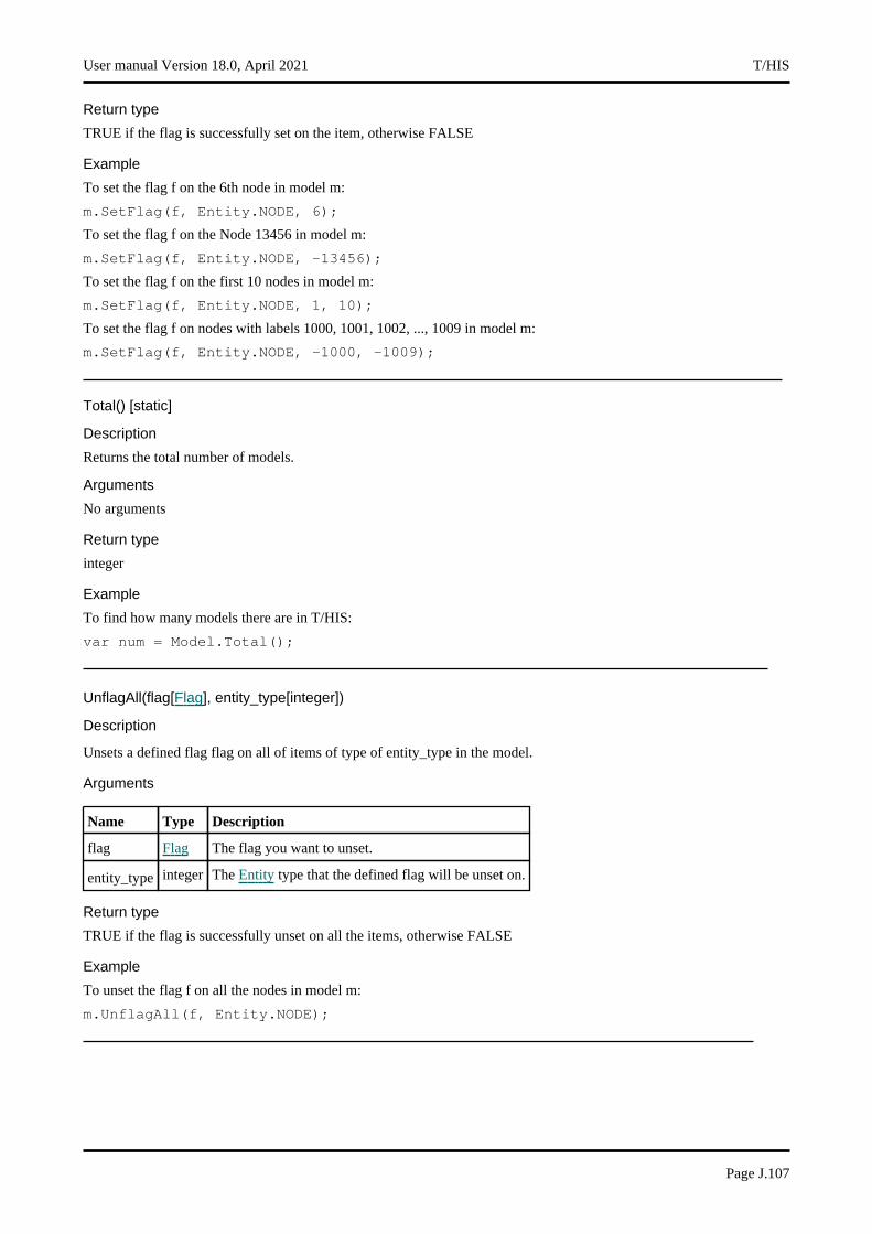
Return type
TRUE if the flag is successfully set on the item, otherwise FALSE
Example
To set the flag f on the 6th node in model m:
m.SetFlag(f, Entity.NODE, 6);
To set the flag f on the Node 13456 in model m:
m.SetFlag(f, Entity.NODE, -13456);
To set the flag f on the first 10 nodes in model m:
m.SetFlag(f, Entity.NODE, 1, 10);
To set the flag f on nodes with labels 1000, 1001, 1002, ..., 1009 in model m:
m.SetFlag(f, Entity.NODE, -1000, -1009);
Total() [static]
Description
Returns the total number of models.
Arguments
No arguments
Return type
integer
Example
To find how many models there are in T/HIS:
var num = Model.Total();
UnflagAll(flag[Flag], entity_type[integer])
Description
Unsets a defined flag flag on all of items of type of entity_type in the model.
Arguments
Name Type Description
flag Flag The flag you want to unset.
entity_type integer The Entity type that the defined flag will be unset on.
Return type
TRUE if the flag is successfully unset on all the items, otherwise FALSE
Example
To unset the flag f on all the nodes in model m:
m.UnflagAll(f, Entity.NODE);
User manual Version 18.0, April 2021 T/HIS
Page J.107
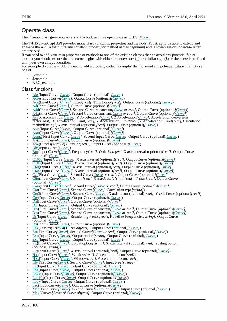
Operate classThe Operate class gives you access to the built in curve operations in T/HIS. More...
The T/HIS JavaScript API provides many class constants, properties and methods. For Arup to be able to extend and enhance the API in the future any constant, property or method names beginning with a lowercase or uppercase letter are reserved.If you need to add your own properties or methods to one of the existing classes then to avoid any potential future conflict you should ensure that the name begins with either an underscore (_) or a dollar sign ($) or the name is prefixed with your own unique identifier.For example if company ’ABC’ need to add a property called ’example’ then to avoid any potential future conflict use one of:
• _example • $example • ABC_example
Class functions• Abs(Input Curve[Curve], Output Curve (optional)[Curve]) • Acos(Input Curve[Curve], Output Curve (optional)[Curve]) • Acu(Input Curve[Curve], Offset[real], Time Period[real], Output Curve (optional)[Curve]) • Ad(Input Curve[Curve], Output Curve (optional)[Curve]) • Add(Input Curve[Curve], Second Curve or constant[Curve or real], Output Curve (optional)[Curve]) • Adx(First Curve[Curve], Second Curve or constant[Curve or real], Output Curve (optional)[Curve]) • Asi(X Acceleration[Curve], Y Acceleration[Curve], Z Acceleration[Curve], Acceleration conversion
factor[real], X Acceleration Limit[real], Y Acceleration Limit[real], Z Acceleration Limit[real], Calculation method[string], X axis interval (optional)[real], Output Curve (optional)[Curve])
• Asin(Input Curve[Curve], Output Curve (optional)[Curve]) • Atan(Input Curve[Curve], Output Curve (optional)[Curve]) • Atan2(First Input Curve[Curve], Second Input Curve[Curve], Output Curve (optional)[Curve]) • Av(Input Curve[Curve], Output Curve (optional)[Curve]) • Ave(Curves[Array of Curve objects], Output Curve (optional)[Curve]) • Blc(Input Curve[Curve]) • But(Input Curve[Curve], Frequency[real], Order[integer], X axis interval (optional)[real], Output Curve
(optional)[Curve]) • C1000(Input Curve[Curve], X axis interval (optional)[real], Output Curve (optional)[Curve]) • C180(Input Curve[Curve], X axis interval (optional)[real], Output Curve (optional)[Curve]) • C60(Input Curve[Curve], X axis interval (optional)[real], Output Curve (optional)[Curve]) • C600(Input Curve[Curve], X axis interval (optional)[real], Output Curve (optional)[Curve]) • Cat(First Curve[Curve], Second Curve[Curve or real], Output Curve (optional)[Curve]) • Clip(Input Curve[Curve], X min[real], X max[real], Y min[real], Y max[real], Output Curve
(optional)[Curve]) • Com(First Curve[Curve], Second Curve[Curve or real], Output Curve (optional)[Curve]) • Cor(First Curve[Curve], Second Curve[Curve], Correlation type[string]) • Cor3(First Curve[Curve], Second Curve[Curve], X axis factor (optional)[real], Y axis factor (optional)[real]) • Cos(Input Curve[Curve], Output Curve (optional)[Curve]) • Da(Input Curve[Curve], Output Curve (optional)[Curve]) • Dif(Input Curve[Curve], Output Curve (optional)[Curve]) • Div(First Curve[Curve], Second Curve or constant[Curve or real], Output Curve (optional)[Curve]) • Dix(First Curve[Curve], Second Curve or constant[Curve or real], Output Curve (optional)[Curve]) • Ds(Input Curve[Curve], Broadening Factor[real], Redefine Frequencies[string], Output Curve
(optional)[Curve]) • Dv(Input Curve[Curve], Output Curve (optional)[Curve]) • Env(Curves[Array of Curve objects], Output Curve (optional)[Curve]) • Err(First Curve[Curve], Second Curve[Curve or real], Output Curve (optional)[Curve]) • Exc(Input Curve[Curve], Output option[string], Output Curve (optional)[Curve]) • Exp(Input Curve[Curve], Output Curve (optional)[Curve]) • Fft(Input Curve[Curve], Output option[string], X axis interval (optional)[real], Scaling option
(optional)[string]) • Fir(Input Curve[Curve], X axis interval (optional)[real], Output Curve (optional)[Curve]) • Hic(Input Curve[Curve], Window[real], Acceleration factor[real]) • Hicd(Input Curve[Curve], Window[real], Acceleration factor[real]) • Ifft(First Curve[Curve], Second Curve[Curve], Input type[string]) • Int(Input Curve[Curve], Output Curve (optional)[Curve]) • Log(Input Curve[Curve], Output Curve (optional)[Curve]) • Log10(Input Curve[Curve], Output Curve (optional)[Curve]) • Log10x(Input Curve[Curve], Output Curve (optional)[Curve]) • Logx(Input Curve[Curve], Output Curve (optional)[Curve]) • Lsq(Input Curve[Curve], Output Curve (optional)[Curve]) • Map(First Curve[Curve], Second Curve[Curve or real], Output Curve (optional)[Curve]) • Max(Curves[Array of Curve objects], Output Curve (optional)[Curve])
T/HIS User manual Version 18.0, April 2021
Page J.108
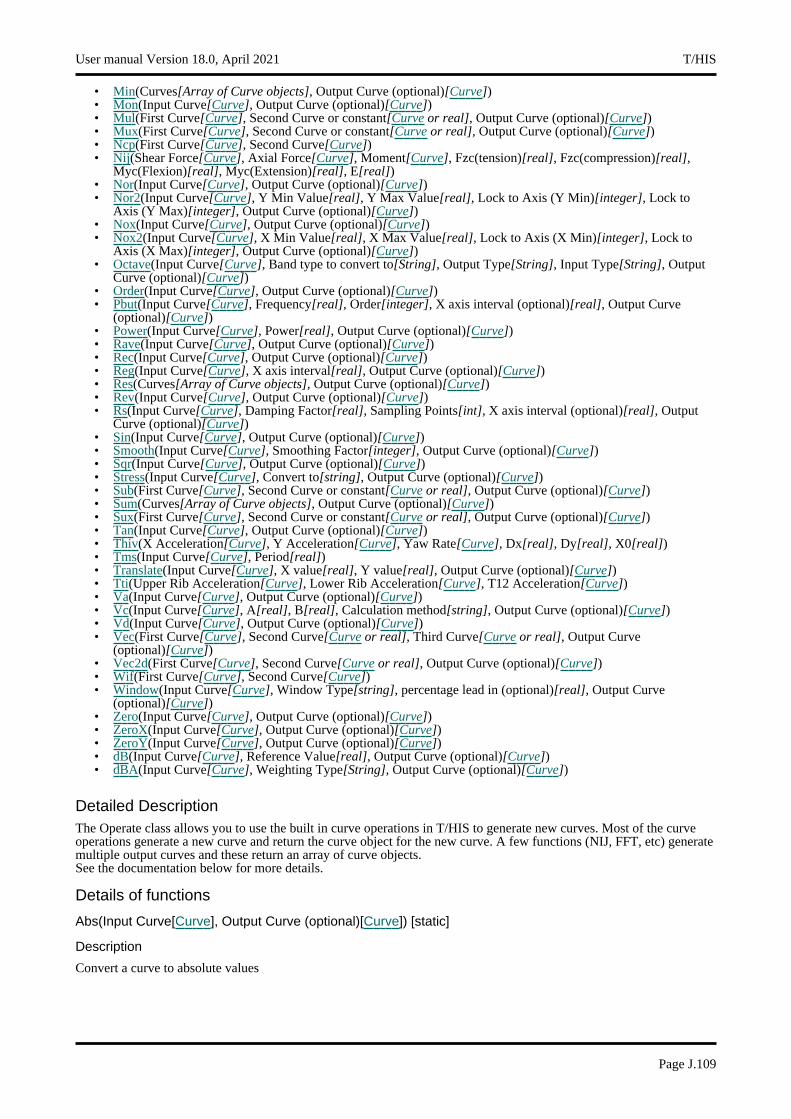
• Min(Curves[Array of Curve objects], Output Curve (optional)[Curve]) • Mon(Input Curve[Curve], Output Curve (optional)[Curve]) • Mul(First Curve[Curve], Second Curve or constant[Curve or real], Output Curve (optional)[Curve]) • Mux(First Curve[Curve], Second Curve or constant[Curve or real], Output Curve (optional)[Curve]) • Ncp(First Curve[Curve], Second Curve[Curve]) • Nij(Shear Force[Curve], Axial Force[Curve], Moment[Curve], Fzc(tension)[real], Fzc(compression)[real],
Myc(Flexion)[real], Myc(Extension)[real], E[real]) • Nor(Input Curve[Curve], Output Curve (optional)[Curve]) • Nor2(Input Curve[Curve], Y Min Value[real], Y Max Value[real], Lock to Axis (Y Min)[integer], Lock to
Axis (Y Max)[integer], Output Curve (optional)[Curve]) • Nox(Input Curve[Curve], Output Curve (optional)[Curve]) • Nox2(Input Curve[Curve], X Min Value[real], X Max Value[real], Lock to Axis (X Min)[integer], Lock to
Axis (X Max)[integer], Output Curve (optional)[Curve]) • Octave(Input Curve[Curve], Band type to convert to[String], Output Type[String], Input Type[String], Output
Curve (optional)[Curve]) • Order(Input Curve[Curve], Output Curve (optional)[Curve]) • Pbut(Input Curve[Curve], Frequency[real], Order[integer], X axis interval (optional)[real], Output Curve
(optional)[Curve]) • Power(Input Curve[Curve], Power[real], Output Curve (optional)[Curve]) • Rave(Input Curve[Curve], Output Curve (optional)[Curve]) • Rec(Input Curve[Curve], Output Curve (optional)[Curve]) • Reg(Input Curve[Curve], X axis interval[real], Output Curve (optional)[Curve]) • Res(Curves[Array of Curve objects], Output Curve (optional)[Curve]) • Rev(Input Curve[Curve], Output Curve (optional)[Curve]) • Rs(Input Curve[Curve], Damping Factor[real], Sampling Points[int], X axis interval (optional)[real], Output
Curve (optional)[Curve]) • Sin(Input Curve[Curve], Output Curve (optional)[Curve]) • Smooth(Input Curve[Curve], Smoothing Factor[integer], Output Curve (optional)[Curve]) • Sqr(Input Curve[Curve], Output Curve (optional)[Curve]) • Stress(Input Curve[Curve], Convert to[string], Output Curve (optional)[Curve]) • Sub(First Curve[Curve], Second Curve or constant[Curve or real], Output Curve (optional)[Curve]) • Sum(Curves[Array of Curve objects], Output Curve (optional)[Curve]) • Sux(First Curve[Curve], Second Curve or constant[Curve or real], Output Curve (optional)[Curve]) • Tan(Input Curve[Curve], Output Curve (optional)[Curve]) • Thiv(X Acceleration[Curve], Y Acceleration[Curve], Yaw Rate[Curve], Dx[real], Dy[real], X0[real]) • Tms(Input Curve[Curve], Period[real]) • Translate(Input Curve[Curve], X value[real], Y value[real], Output Curve (optional)[Curve]) • Tti(Upper Rib Acceleration[Curve], Lower Rib Acceleration[Curve], T12 Acceleration[Curve]) • Va(Input Curve[Curve], Output Curve (optional)[Curve]) • Vc(Input Curve[Curve], A[real], B[real], Calculation method[string], Output Curve (optional)[Curve]) • Vd(Input Curve[Curve], Output Curve (optional)[Curve]) • Vec(First Curve[Curve], Second Curve[Curve or real], Third Curve[Curve or real], Output Curve
(optional)[Curve]) • Vec2d(First Curve[Curve], Second Curve[Curve or real], Output Curve (optional)[Curve]) • Wif(First Curve[Curve], Second Curve[Curve]) • Window(Input Curve[Curve], Window Type[string], percentage lead in (optional)[real], Output Curve
(optional)[Curve]) • Zero(Input Curve[Curve], Output Curve (optional)[Curve]) • ZeroX(Input Curve[Curve], Output Curve (optional)[Curve]) • ZeroY(Input Curve[Curve], Output Curve (optional)[Curve]) • dB(Input Curve[Curve], Reference Value[real], Output Curve (optional)[Curve]) • dBA(Input Curve[Curve], Weighting Type[String], Output Curve (optional)[Curve])
Detailed DescriptionThe Operate class allows you to use the built in curve operations in T/HIS to generate new curves. Most of the curve operations generate a new curve and return the curve object for the new curve. A few functions (NIJ, FFT, etc) generate multiple output curves and these return an array of curve objects. See the documentation below for more details.
Details of functions
Abs(Input Curve[Curve], Output Curve (optional)[Curve]) [static]
Description
Convert a curve to absolute values
User manual Version 18.0, April 2021 T/HIS
Page J.109
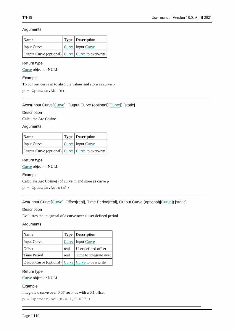
Arguments
Name Type Description
Input Curve Curve Input Curve
Output Curve (optional) Curve Curve to overwrite
Return type
Curve object or NULL
Example
To convert curve m to absolute values and store as curve p
p = Operate.Abs(m);
Acos(Input Curve[Curve], Output Curve (optional)[Curve]) [static]
Description
Calculate Arc Cosine
Arguments
Name Type Description
Input Curve Curve Input Curve
Output Curve (optional) Curve Curve to overwrite
Return type
Curve object or NULL
Example
Calculate Arc Cosine() of curve m and store as curve p
p = Operate.Acos(m);
Acu(Input Curve[Curve], Offset[real], Time Period[real], Output Curve (optional)[Curve]) [static]
Description
Evaluates the integratal of a curve over a user defined period
Arguments
Name Type Description
Input Curve Curve Input Curve
Offset real User defined offset
Time Period real Time to integrate over
Output Curve (optional) Curve Curve to overwrite
Return type
Curve object or NULL
Example
Integrate c curve over 0.07 seconds with a 0.1 offset.
p = Operate.Acu(m,0.1,0.007);
T/HIS User manual Version 18.0, April 2021
Page J.110

Ad(Input Curve[Curve], Output Curve (optional)[Curve]) [static]
Description
Convert acceleration spectrum to a displacment spectrum
Arguments
Name Type Description
Input Curve Curve Input Curve
Output Curve (optional) Curve Curve to overwrite
Return type
Curve object or NULL
Example
Convert curve m and store as curve p
p = Operate.Ad(m);
Add(Input Curve[Curve], Second Curve or constant[Curve or real], Output Curve (optional)[Curve]) [static]
Description
Add Y axis values
Arguments
Name Type Description
Input Curve Curve Input Curve
Second Curve or constant Curve or real Second Curve or constant
Output Curve (optional) Curve Curve to overwrite
Return type
Curve object or NULL
Example
To add curves m and n together and store as curve p
p = Operate.Add(m,n);
To add 20.0 to the values in curve m and store as curve p
p = Operate.Add(m,20.0);
Adx(First Curve[Curve], Second Curve or constant[Curve or real], Output Curve (optional)[Curve]) [static]
Description
Add X axis values
Arguments
Name Type Description
First Curve Curve First Curve
Second Curve or constant Curve or real Second Curve or constant
Output Curve (optional) Curve Curve to overwrite
User manual Version 18.0, April 2021 T/HIS
Page J.111
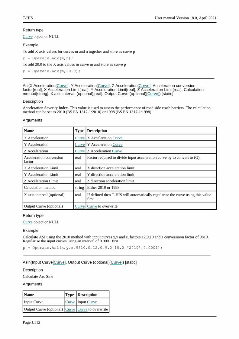
Return type
Curve object or NULL
Example
To add X axis values for curves m and n together and store as curve p
p = Operate.Adx(m,n);
To add 20.0 to the X axis values in curve m and store as curve p
p = Operate.Adx(m,20.0);
Asi(X Acceleration[Curve], Y Acceleration[Curve], Z Acceleration[Curve], Acceleration conversion factor[real], X Acceleration Limit[real], Y Acceleration Limit[real], Z Acceleration Limit[real], Calculation method[string], X axis interval (optional)[real], Output Curve (optional)[Curve]) [static]
Description
Acceleration Severity Index. This value is used to assess the performance of road side crash barriers. The calculation method can be set to 2010 (BS EN 1317-1:2010) or 1998 (BS EN 1317-1:1998).
Arguments
Name Type Description
X Acceleration Curve X Acceleration Curve
Y Acceleration Curve Y Acceleration Curve
Z Acceleration Curve Z Acceleration Curve
Acceleration conversion factor
real Factor required to divide input acceleration curve by to convert to (G)
X Acceleration Limit real X direction acceleration limit
Y Acceleration Limit real Y direction acceleration limit
Z Acceleration Limit real Z direction acceleration limit
Calculation method string Either 2010 or 1998.
X axis interval (optional) real If defined then T-HIS will automatically regularise the curve using this value first
Output Curve (optional) Curve Curve to overwrite
Return type
Curve object or NULL
Example
Calculate ASI using the 2010 method with input curves x,y and z, factors 12,9,10 and a conversioon factor of 9810. Regularise the input curves using an interval of 0.0001 first.
p = Operate.Asi(x,y,z,9810.0,12.0,9.0,10.0,"2010",0.0001);
Asin(Input Curve[Curve], Output Curve (optional)[Curve]) [static]
Description
Calculate Arc Sine
Arguments
Name Type Description
Input Curve Curve Input Curve
Output Curve (optional) Curve Curve to overwrite
T/HIS User manual Version 18.0, April 2021
Page J.112
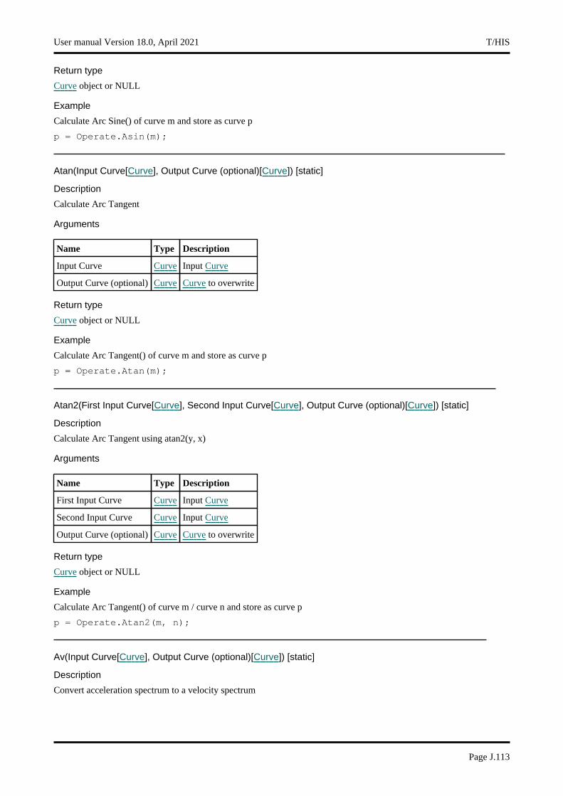
Return type
Curve object or NULL
Example
Calculate Arc Sine() of curve m and store as curve p
p = Operate.Asin(m);
Atan(Input Curve[Curve], Output Curve (optional)[Curve]) [static]
Description
Calculate Arc Tangent
Arguments
Name Type Description
Input Curve Curve Input Curve
Output Curve (optional) Curve Curve to overwrite
Return type
Curve object or NULL
Example
Calculate Arc Tangent() of curve m and store as curve p
p = Operate.Atan(m);
Atan2(First Input Curve[Curve], Second Input Curve[Curve], Output Curve (optional)[Curve]) [static]
Description
Calculate Arc Tangent using atan2(y, x)
Arguments
Name Type Description
First Input Curve Curve Input Curve
Second Input Curve Curve Input Curve
Output Curve (optional) Curve Curve to overwrite
Return type
Curve object or NULL
Example
Calculate Arc Tangent() of curve m / curve n and store as curve p
p = Operate.Atan2(m, n);
Av(Input Curve[Curve], Output Curve (optional)[Curve]) [static]
Description
Convert acceleration spectrum to a velocity spectrum
User manual Version 18.0, April 2021 T/HIS
Page J.113
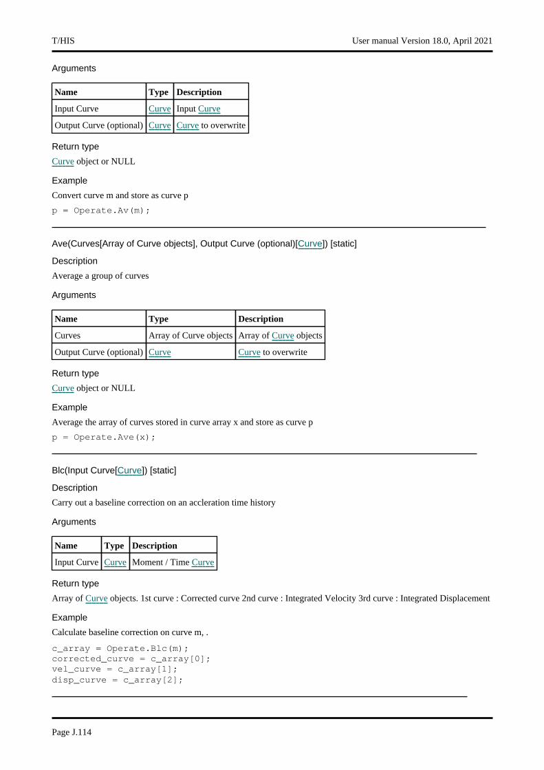
Arguments
Name Type Description
Input Curve Curve Input Curve
Output Curve (optional) Curve Curve to overwrite
Return type
Curve object or NULL
Example
Convert curve m and store as curve p
p = Operate.Av(m);
Ave(Curves[Array of Curve objects], Output Curve (optional)[Curve]) [static]
Description
Average a group of curves
Arguments
Name Type Description
Curves Array of Curve objects Array of Curve objects
Output Curve (optional) Curve Curve to overwrite
Return type
Curve object or NULL
Example
Average the array of curves stored in curve array x and store as curve p
p = Operate.Ave(x);
Blc(Input Curve[Curve]) [static]
Description
Carry out a baseline correction on an accleration time history
Arguments
Name Type Description
Input Curve Curve Moment / Time Curve
Return type
Array of Curve objects. 1st curve : Corrected curve 2nd curve : Integrated Velocity 3rd curve : Integrated Displacement
Example
Calculate baseline correction on curve m, .
c_array = Operate.Blc(m);corrected_curve = c_array[0];vel_curve = c_array[1];disp_curve = c_array[2];
T/HIS User manual Version 18.0, April 2021
Page J.114
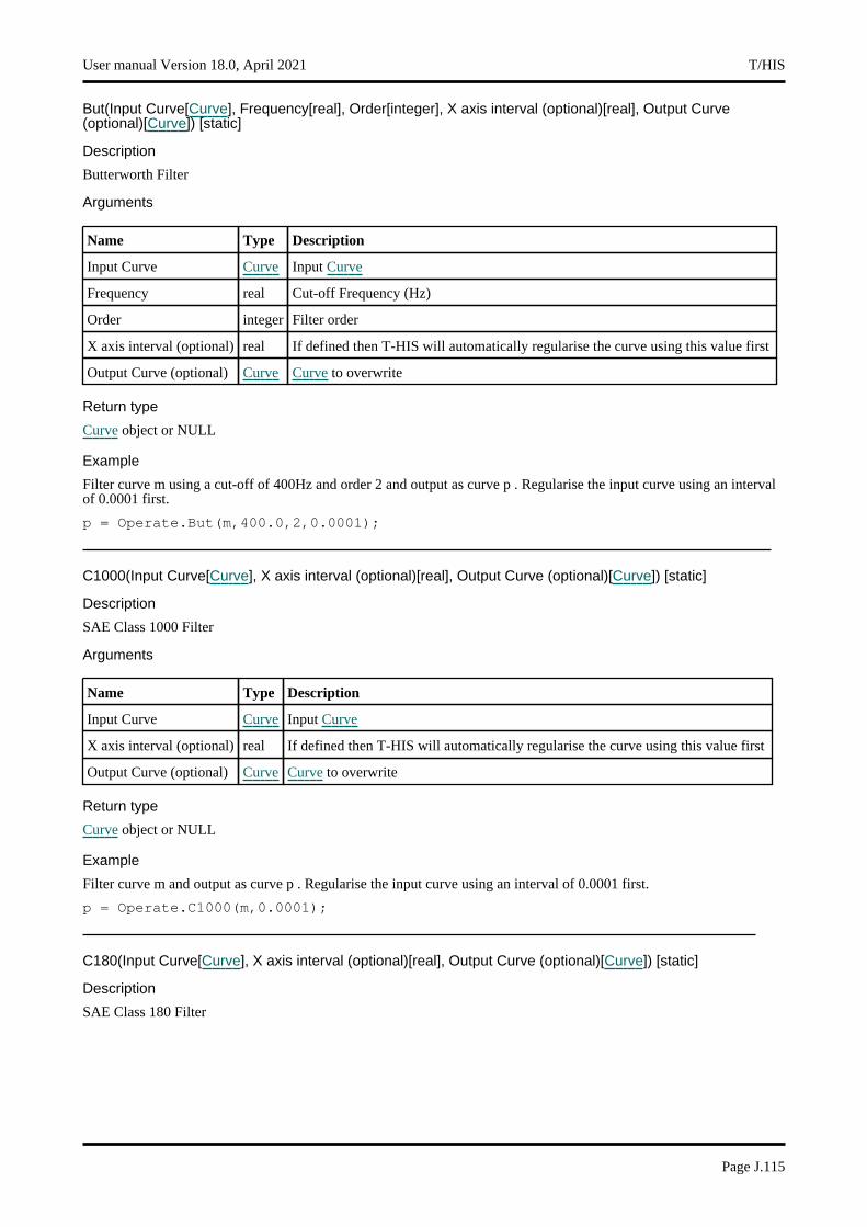
But(Input Curve[Curve], Frequency[real], Order[integer], X axis interval (optional)[real], Output Curve (optional)[Curve]) [static]
Description
Butterworth Filter
Arguments
Name Type Description
Input Curve Curve Input Curve
Frequency real Cut-off Frequency (Hz)
Order integer Filter order
X axis interval (optional) real If defined then T-HIS will automatically regularise the curve using this value first
Output Curve (optional) Curve Curve to overwrite
Return type
Curve object or NULL
Example
Filter curve m using a cut-off of 400Hz and order 2 and output as curve p . Regularise the input curve using an interval of 0.0001 first.
p = Operate.But(m,400.0,2,0.0001);
C1000(Input Curve[Curve], X axis interval (optional)[real], Output Curve (optional)[Curve]) [static]
Description
SAE Class 1000 Filter
Arguments
Name Type Description
Input Curve Curve Input Curve
X axis interval (optional) real If defined then T-HIS will automatically regularise the curve using this value first
Output Curve (optional) Curve Curve to overwrite
Return type
Curve object or NULL
Example
Filter curve m and output as curve p . Regularise the input curve using an interval of 0.0001 first.
p = Operate.C1000(m,0.0001);
C180(Input Curve[Curve], X axis interval (optional)[real], Output Curve (optional)[Curve]) [static]
Description
SAE Class 180 Filter
User manual Version 18.0, April 2021 T/HIS
Page J.115

Arguments
Name Type Description
Input Curve Curve Input Curve
X axis interval (optional) real If defined then T-HIS will automatically regularise the curve using this value first
Output Curve (optional) Curve Curve to overwrite
Return type
Curve object or NULL
Example
Filter curve m and output as curve p . Regularise the input curve using an interval of 0.0001 first.
p = Operate.C180(m,0.0001);
C60(Input Curve[Curve], X axis interval (optional)[real], Output Curve (optional)[Curve]) [static]
Description
SAE Class 60 Filter
Arguments
Name Type Description
Input Curve Curve Input Curve
X axis interval (optional) real If defined then T-HIS will automatically regularise the curve using this value first
Output Curve (optional) Curve Curve to overwrite
Return type
Curve object or NULL
Example
Filter curve m and output as curve p . Regularise the input curve using an interval of 0.0001 first.
p = Operate.C60(m,0.0001);
C600(Input Curve[Curve], X axis interval (optional)[real], Output Curve (optional)[Curve]) [static]
Description
SAE Class 600 Filter
Arguments
Name Type Description
Input Curve Curve Input Curve
X axis interval (optional) real If defined then T-HIS will automatically regularise the curve using this value first
Output Curve (optional) Curve Curve to overwrite
Return type
Curve object or NULL
T/HIS User manual Version 18.0, April 2021
Page J.116

Example
Filter curve m and output as curve p . Regularise the input curve using an interval of 0.0001 first.
p = Operate.C600(m,0.0001);
Cat(First Curve[Curve], Second Curve[Curve or real], Output Curve (optional)[Curve]) [static]
Description
Concatenate 2 curves together
Arguments
Name Type Description
First Curve Curve First Curve
Second Curve Curve or real Second Curve
Output Curve (optional) Curve Curve to overwrite
Return type
Curve object or NULL
Example
To concatenate the values for curve n to those in curve m and store as curve p
p = Operate.Cat(m,n);
Clip(Input Curve[Curve], X min[real], X max[real], Y min[real], Y max[real], Output Curve (optional)[Curve]) [static]
Description
Clip a curve
Arguments
Name Type Description
Input Curve Curve Input Curve
X min real X minimum value
X max real X maximum value
Y min real Y minimum value
Y max real Y maximum value
Output Curve (optional) Curve Curve to overwrite
Return type
Curve object or NULL
Example
Clip a curve m to within 0.1<x<0.3, 0.0<y<100.0 and store as curve p
p = Operate.Clip(m,0.1,0.3,0.0,100.0);
Com(First Curve[Curve], Second Curve[Curve or real], Output Curve (optional)[Curve]) [static]
Description
Combine Y axis values from 2 curves together
User manual Version 18.0, April 2021 T/HIS
Page J.117

Arguments
Name Type Description
First Curve Curve First Curve
Second Curve Curve or real Second Curve
Output Curve (optional) Curve Curve to overwrite
Return type
Curve object or NULL
Example
To combine the Y axis values for curve n to those in curve m and store as curve p
p = Operate.Com(m,n);
Cor(First Curve[Curve], Second Curve[Curve], Correlation type[string]) [static]
Description
Curve Correlation function. This Correlation function provides a measure of the degree to which two curves match. When comparing curves by eye, the quality of correlation may be judged on the basis of how well matched are the patterns of peaks, the overall shapes of the curves, etc, and can allow for differences of timing as well as magnitude. Thus a simple function based on the difference of Y-values (such as T/HIS ERR function) does not measure correlation in the same way as the human eye. The T/HIS correlation function attempts to include and quantify the more subtle ways in which the correlation of two curves may be judged. The correlation can be calculated using either a strict or loose set of input parameters. The degree of correlation is rated between 0 and 100.
Arguments
Name Type Description
First Curve Curve First Curve
Second Curve Curve Second Curve
Correlation type string Correlation type, strict or loose
Return type
real
Example
Calculate the correlation between curves m and n using the strict input parameters.
val = Operate.Cor(m,n,"strict");
Cor3(First Curve[Curve], Second Curve[Curve], X axis factor (optional)[real], Y axis factor (optional)[real]) [static]
Description
Curve Correlation function. This function first normalises the curves using two factors either specified by the user or defaults calculated by the program (the maximum absolute X and Y values of both graphs). For each point on the first normalised curve, the shortest distance to the second normalised curve is calculated. The root mean square value of all these distances is subtracted from 1 and then multiplied by 100 to get an index between 0 and 100. The process is repeated along the second curve and the two indices are averaged to get a final index. The higher the index the closer the correlation between the two curves. Note that the choice of normalising factors is important. Incorrect factors may lead to a correlation index outside the range of 0 to 100
T/HIS User manual Version 18.0, April 2021
Page J.118
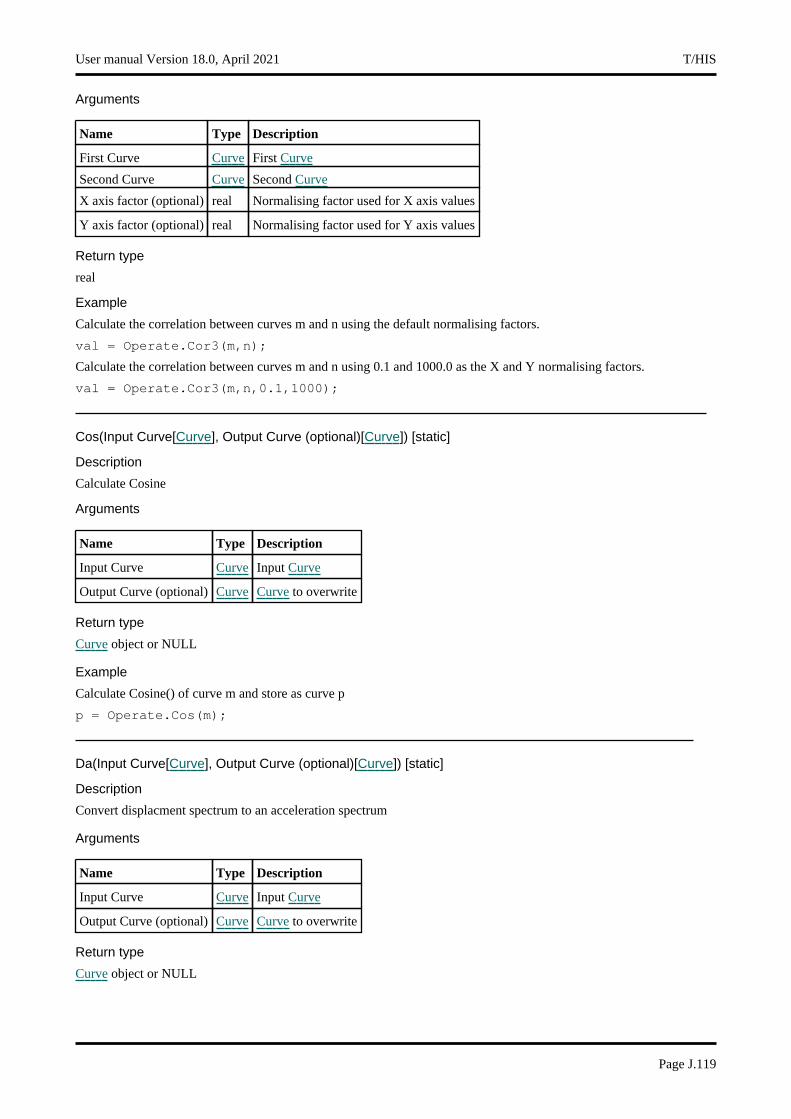
Arguments
Name Type Description
First Curve Curve First Curve
Second Curve Curve Second Curve
X axis factor (optional) real Normalising factor used for X axis values
Y axis factor (optional) real Normalising factor used for Y axis values
Return type
real
Example
Calculate the correlation between curves m and n using the default normalising factors.
val = Operate.Cor3(m,n);
Calculate the correlation between curves m and n using 0.1 and 1000.0 as the X and Y normalising factors.
val = Operate.Cor3(m,n,0.1,1000);
Cos(Input Curve[Curve], Output Curve (optional)[Curve]) [static]
Description
Calculate Cosine
Arguments
Name Type Description
Input Curve Curve Input Curve
Output Curve (optional) Curve Curve to overwrite
Return type
Curve object or NULL
Example
Calculate Cosine() of curve m and store as curve p
p = Operate.Cos(m);
Da(Input Curve[Curve], Output Curve (optional)[Curve]) [static]
Description
Convert displacment spectrum to an acceleration spectrum
Arguments
Name Type Description
Input Curve Curve Input Curve
Output Curve (optional) Curve Curve to overwrite
Return type
Curve object or NULL
User manual Version 18.0, April 2021 T/HIS
Page J.119

Example
Convert curve m and store as curve p
p = Operate.Da(m);
Dif(Input Curve[Curve], Output Curve (optional)[Curve]) [static]
Description
Differentiate a curve
Arguments
Name Type Description
Input Curve Curve Input Curve
Output Curve (optional) Curve Curve to overwrite
Return type
Curve object or NULL
Example
To differentiate curve m and store as curve p
p = Operate.Dif(m);
Div(First Curve[Curve], Second Curve or constant[Curve or real], Output Curve (optional)[Curve]) [static]
Description
Divide Y axis values
Arguments
Name Type Description
First Curve Curve First Curve
Second Curve or constant Curve or real Second Curve or constant
Output Curve (optional) Curve Curve to overwrite
Return type
Curve object or NULL
Example
To divide the Y axis values for curve n by curve m and store as curve p
p = Operate.Div(m,n);
To devide the Y axis values in curve m by 20.0 and store as curve p
p = Operate.Div(m,20.0);
Dix(First Curve[Curve], Second Curve or constant[Curve or real], Output Curve (optional)[Curve]) [static]
Description
Divide X axis values
T/HIS User manual Version 18.0, April 2021
Page J.120

Arguments
Name Type Description
First Curve Curve First Curve
Second Curve or constant Curve or real Second Curve or constant
Output Curve (optional) Curve Curve to overwrite
Return type
Curve object or NULL
Example
To divide the X axis values for curve n by curve m and store as curve p
p = Operate.Dix(m,n);
To devide the X axis values in curve m by 20.0 and store as curve p
p = Operate.Dix(m,20.0);
Ds(Input Curve[Curve], Broadening Factor[real], Redefine Frequencies[string], Output Curve (optional)[Curve]) [static]
Description
Generate a design spectrum from a reponse spectrum
Arguments
Name Type Description
Input Curve Curve Input Curve
Broadening Factor real Spectrum broadening factor
Redefine Frequencies string T-HIS selects a new set of frequencies for the output (yes or no)
Output Curve (optional) Curve Curve to overwrite
Return type
Curve object or NULL
Example
Convert curve m and let T-HIS determine the new frequencies, store as curve p
p = Operate.Ds(m,"yes");
Dv(Input Curve[Curve], Output Curve (optional)[Curve]) [static]
Description
Convert displacment spectrum to a velocity spectrum
Arguments
Name Type Description
Input Curve Curve Input Curve
Output Curve (optional) Curve Curve to overwrite
Return type
Curve object or NULL
User manual Version 18.0, April 2021 T/HIS
Page J.121

Example
Convert curve m and store as curve p
p = Operate.Dv(m);
Env(Curves[Array of Curve objects], Output Curve (optional)[Curve]) [static]
Description
Generate an Envelope that bounds the min and max values of a group of curves
Arguments
Name Type Description
Curves Array of Curve objects Array of Curve objects
Output Curve (optional) Curve Curve to overwrite
Return type
Curve object or NULL
Example
Envelope of curves stored in curve array x and store as curve p
p = Operate.Env(x);
Err(First Curve[Curve], Second Curve[Curve or real], Output Curve (optional)[Curve]) [static]
Description
Calculate the degree of correlation between 2 curves
Arguments
Name Type Description
First Curve Curve First Curve
Second Curve Curve or real Second Curve
Output Curve (optional) Curve Curve to overwrite
Return type
Curve object or NULL
Example
To calculate the correlation between curves n and m and store as curve p
p = Operate.Err(m,n);
Exc(Input Curve[Curve], Output option[string], Output Curve (optional)[Curve]) [static]
Description
Calculate and displays an EXCeedence plot. This is a plot of force (Y axis) versus cumulative time (X axis) for which the force level has been exceeded. By default the Automatic option will create an exceedence plot using either the +ve OR the -ve values depending on which the input curve contains most of. The Positive option will calculate the exceedence plot using only the points with +ve y values. The Negative option will calculate the exceedence plot using only the points with -ve y values.
T/HIS User manual Version 18.0, April 2021
Page J.122

Arguments
Name Type Description
Input Curve Curve Input Curve
Output option string Select between automatic, positive or negative.
Output Curve (optional) Curve Curve to overwrite
Return type
Curve object or NULL
Example
Calculate Exceedence plot for curve m, using the positive option and store as curve p
p = Operate.Exc(m,"positive");
Exp(Input Curve[Curve], Output Curve (optional)[Curve]) [static]
Description
Calculate E to the power of Y axis values
Arguments
Name Type Description
Input Curve Curve Input Curve
Output Curve (optional) Curve Curve to overwrite
Return type
Curve object or NULL
Example
Calculate E to the power of Y axis values for curve m and store as curve p
p = Operate.Exp(m);
Fft(Input Curve[Curve], Output option[string], X axis interval (optional)[real], Scaling option (optional)[string]) [static]
Description
Fast Fourier Transform
Arguments
Name Type Description
Input Curve Curve Input Curve
Output option string Generate magnitude, magnitude+phase or real+imaginary, (one of magnitude,phase,real)
X axis interval (optional)
real If defined then T-HIS will automatically regularise the curve using this value first
Scaling option (optional)
string Scaling option, (either one or two)
Return type
Curve object/array or NULL
User manual Version 18.0, April 2021 T/HIS
Page J.123

Example
Generate magnitude and phase curves and return a curve array. Regularise the input curve using an interval of 0.0001 first and scale using option two.
c_array = Operate.Fft(m,"phase",0.0001,"one");mag_curve = c_array[0];phase_curve = c_array[1];
Fir(Input Curve[Curve], X axis interval (optional)[real], Output Curve (optional)[Curve]) [static]
Description
FIR Filter
Arguments
Name Type Description
Input Curve Curve Input Curve
X axis interval (optional) real If defined then T-HIS will automatically regularise the curve using this value first
Output Curve (optional) Curve Curve to overwrite
Return type
Curve object or NULL
Example
Filter curve m and output as curve p . Regularise the input curve using an interval of 0.0001 first.
p = Operate.Fir(m,0.0001);
Hic(Input Curve[Curve], Window[real], Acceleration factor[real]) [static]
Description
HIC Calculation. After calculating the HIC value for a curve the value can also be obtained from the curve using the Curve.hic property. In addition to the HIC value the start and end time for the time window can also be obtained using the Curve.hic_tmin and Curve.hic_tmax properties.
Arguments
Name Type Description
Input Curve Curve Input Curve
Window real Maximum time window
Acceleration factor real Factor required to divide input acceleration curve by to convert to (G)
Return type
real
Example
Calculate HIC for curve m, using a window of 0.036s and a factor of 9810.
val = Operate.Hic(m,0.036,9810.0);
T/HIS User manual Version 18.0, April 2021
Page J.124
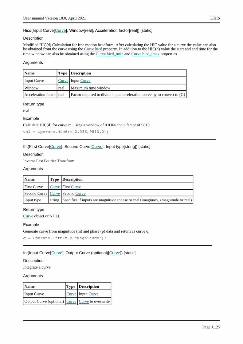
Hicd(Input Curve[Curve], Window[real], Acceleration factor[real]) [static]
Description
Modified HIC(d) Calculation for free motion headform. After calculating the HIC value for a curve the value can also be obtained from the curve using the Curve.hicd property. In addition to the HIC(d) value the start and end time for the time window can also be obtained using the Curve.hicd_tmin and Curve.hicd_tmax properties.
Arguments
Name Type Description
Input Curve Curve Input Curve
Window real Maximum time window
Acceleration factor real Factor required to divide input acceleration curve by to convert to (G)
Return type
real
Example
Calculate HIC(d) for curve m, using a window of 0.036s and a factor of 9810.
val = Operate.Hicd(m,0.036,9810.0);
Ifft(First Curve[Curve], Second Curve[Curve], Input type[string]) [static]
Description
Inverse Fast Fourier Transform
Arguments
Name Type Description
First Curve Curve First Curve
Second Curve Curve Second Curve
Input type string Specifies if inputs are magnitude+phase or real+imaginary, (magnitude or real)
Return type
Curve object or NULL
Example
Generate curve from magnitude (m) and phase (p) data and return as curve q.
q = Operate.Ifft(m,p,"magnitude");
Int(Input Curve[Curve], Output Curve (optional)[Curve]) [static]
Description
Integrate a curve
Arguments
Name Type Description
Input Curve Curve Input Curve
Output Curve (optional) Curve Curve to overwrite
User manual Version 18.0, April 2021 T/HIS
Page J.125
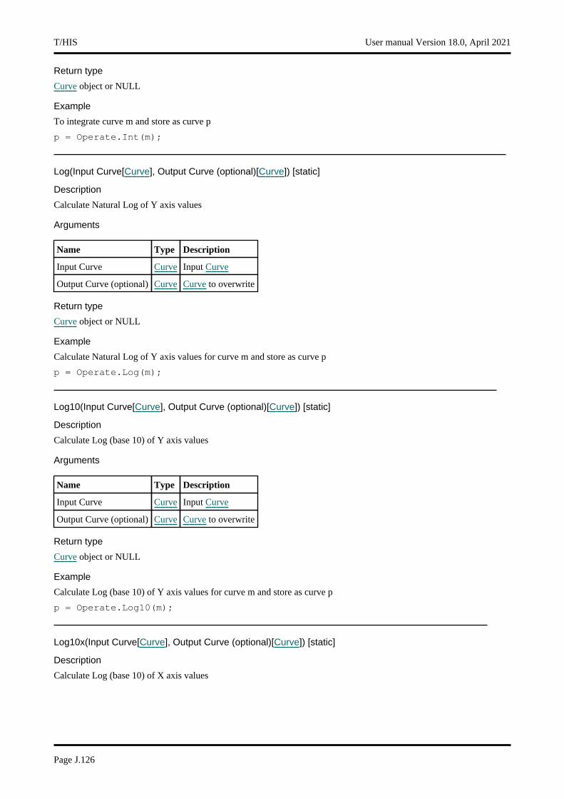
Return type
Curve object or NULL
Example
To integrate curve m and store as curve p
p = Operate.Int(m);
Log(Input Curve[Curve], Output Curve (optional)[Curve]) [static]
Description
Calculate Natural Log of Y axis values
Arguments
Name Type Description
Input Curve Curve Input Curve
Output Curve (optional) Curve Curve to overwrite
Return type
Curve object or NULL
Example
Calculate Natural Log of Y axis values for curve m and store as curve p
p = Operate.Log(m);
Log10(Input Curve[Curve], Output Curve (optional)[Curve]) [static]
Description
Calculate Log (base 10) of Y axis values
Arguments
Name Type Description
Input Curve Curve Input Curve
Output Curve (optional) Curve Curve to overwrite
Return type
Curve object or NULL
Example
Calculate Log (base 10) of Y axis values for curve m and store as curve p
p = Operate.Log10(m);
Log10x(Input Curve[Curve], Output Curve (optional)[Curve]) [static]
Description
Calculate Log (base 10) of X axis values
T/HIS User manual Version 18.0, April 2021
Page J.126
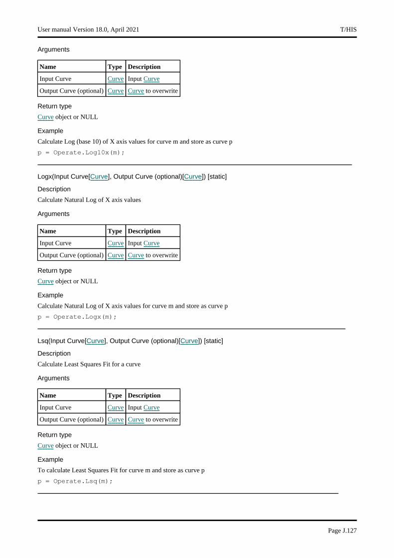
Arguments
Name Type Description
Input Curve Curve Input Curve
Output Curve (optional) Curve Curve to overwrite
Return type
Curve object or NULL
Example
Calculate Log (base 10) of X axis values for curve m and store as curve p
p = Operate.Log10x(m);
Logx(Input Curve[Curve], Output Curve (optional)[Curve]) [static]
Description
Calculate Natural Log of X axis values
Arguments
Name Type Description
Input Curve Curve Input Curve
Output Curve (optional) Curve Curve to overwrite
Return type
Curve object or NULL
Example
Calculate Natural Log of X axis values for curve m and store as curve p
p = Operate.Logx(m);
Lsq(Input Curve[Curve], Output Curve (optional)[Curve]) [static]
Description
Calculate Least Squares Fit for a curve
Arguments
Name Type Description
Input Curve Curve Input Curve
Output Curve (optional) Curve Curve to overwrite
Return type
Curve object or NULL
Example
To calculate Least Squares Fit for curve m and store as curve p
p = Operate.Lsq(m);
User manual Version 18.0, April 2021 T/HIS
Page J.127
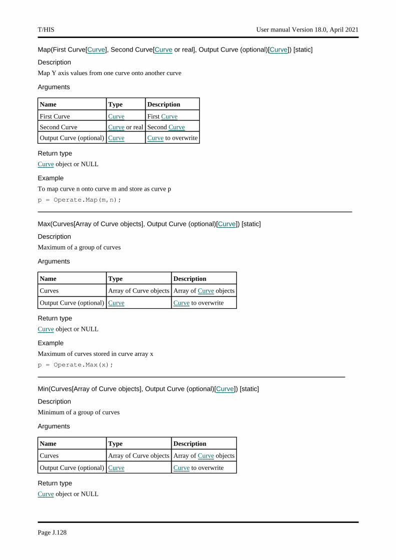
Map(First Curve[Curve], Second Curve[Curve or real], Output Curve (optional)[Curve]) [static]
Description
Map Y axis values from one curve onto another curve
Arguments
Name Type Description
First Curve Curve First Curve
Second Curve Curve or real Second Curve
Output Curve (optional) Curve Curve to overwrite
Return type
Curve object or NULL
Example
To map curve n onto curve m and store as curve p
p = Operate.Map(m,n);
Max(Curves[Array of Curve objects], Output Curve (optional)[Curve]) [static]
Description
Maximum of a group of curves
Arguments
Name Type Description
Curves Array of Curve objects Array of Curve objects
Output Curve (optional) Curve Curve to overwrite
Return type
Curve object or NULL
Example
Maximum of curves stored in curve array x
p = Operate.Max(x);
Min(Curves[Array of Curve objects], Output Curve (optional)[Curve]) [static]
Description
Minimum of a group of curves
Arguments
Name Type Description
Curves Array of Curve objects Array of Curve objects
Output Curve (optional) Curve Curve to overwrite
Return type
Curve object or NULL
T/HIS User manual Version 18.0, April 2021
Page J.128
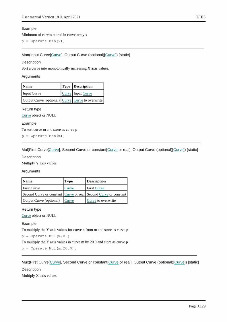
Example
Minimum of curves stored in curve array x
p = Operate.Min(x);
Mon(Input Curve[Curve], Output Curve (optional)[Curve]) [static]
Description
Sort a curve into monotonically increasing X axis values.
Arguments
Name Type Description
Input Curve Curve Input Curve
Output Curve (optional) Curve Curve to overwrite
Return type
Curve object or NULL
Example
To sort curve m and store as curve p
p = Operate.Mon(m);
Mul(First Curve[Curve], Second Curve or constant[Curve or real], Output Curve (optional)[Curve]) [static]
Description
Multiply Y axis values
Arguments
Name Type Description
First Curve Curve First Curve
Second Curve or constant Curve or real Second Curve or constant
Output Curve (optional) Curve Curve to overwrite
Return type
Curve object or NULL
Example
To multiply the Y axis values for curve n from m and store as curve p
p = Operate.Mul(m,n);
To multiply the Y axis values in curve m by 20.0 and store as curve p
p = Operate.Mul(m,20.0);
Mux(First Curve[Curve], Second Curve or constant[Curve or real], Output Curve (optional)[Curve]) [static]
Description
Multiply X axis values
User manual Version 18.0, April 2021 T/HIS
Page J.129
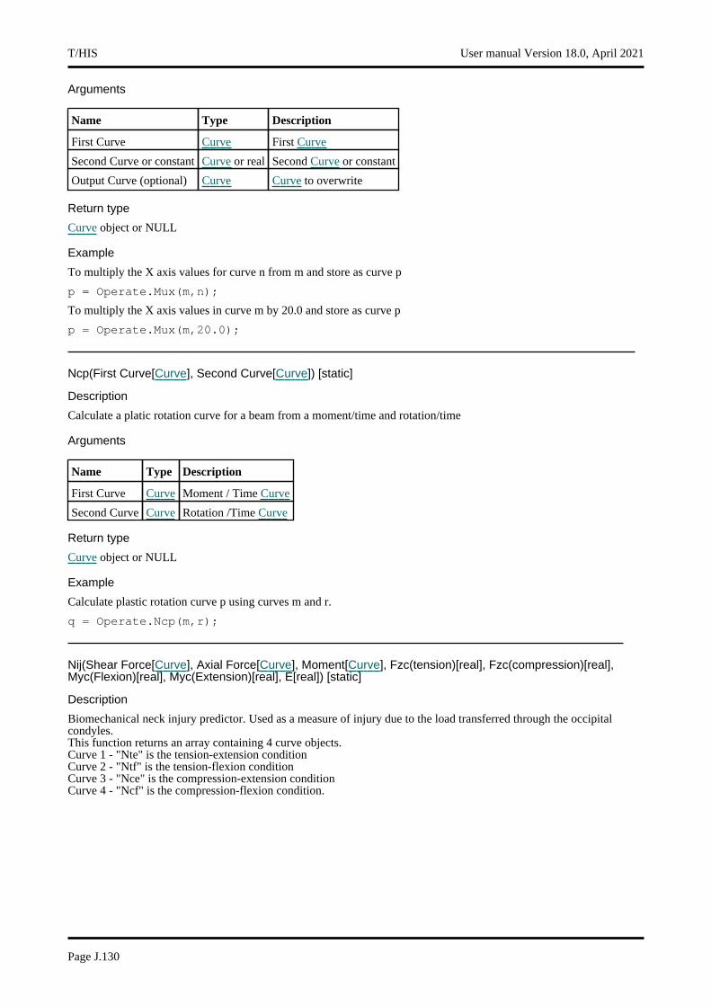
Arguments
Name Type Description
First Curve Curve First Curve
Second Curve or constant Curve or real Second Curve or constant
Output Curve (optional) Curve Curve to overwrite
Return type
Curve object or NULL
Example
To multiply the X axis values for curve n from m and store as curve p
p = Operate.Mux(m,n);
To multiply the X axis values in curve m by 20.0 and store as curve p
p = Operate.Mux(m,20.0);
Ncp(First Curve[Curve], Second Curve[Curve]) [static]
Description
Calculate a platic rotation curve for a beam from a moment/time and rotation/time
Arguments
Name Type Description
First Curve Curve Moment / Time Curve
Second Curve Curve Rotation /Time Curve
Return type
Curve object or NULL
Example
Calculate plastic rotation curve p using curves m and r.
q = Operate.Ncp(m,r);
Nij(Shear Force[Curve], Axial Force[Curve], Moment[Curve], Fzc(tension)[real], Fzc(compression)[real], Myc(Flexion)[real], Myc(Extension)[real], E[real]) [static]
Description
Biomechanical neck injury predictor. Used as a measure of injury due to the load transferred through the occipital condyles. This function returns an array containing 4 curve objects. Curve 1 - "Nte" is the tension-extension condition Curve 2 - "Ntf" is the tension-flexion condition Curve 3 - "Nce" is the compression-extension condition Curve 4 - "Ncf" is the compression-flexion condition.
T/HIS User manual Version 18.0, April 2021
Page J.130
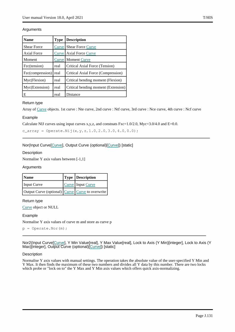
Arguments
Name Type Description
Shear Force Curve Shear Force Curve
Axial Force Curve Axial Force Curve
Moment Curve Moment Curve
Fzc(tension) real Critical Axial Force (Tension)
Fzc(compression) real Critical Axial Force (Compression)
Myc(Flexion) real Critical bending moment (Flexion)
Myc(Extension) real Critical bending moment (Extension)
E real Distance
Return type
Array of Curve objects. 1st curve : Nte curve, 2nd curve : Ntf curve, 3rd curve : Nce curve, 4th curve : Ncf curve
Example
Calculate NIJ curves using input curves x,y,z, and constnats Fxc=1.0/2.0, Myc=3.0/4.0 and E=0.0.
c_array = Operate.Nij(x,y,z,1.0,2.0,3.0,4.0,0.0);
Nor(Input Curve[Curve], Output Curve (optional)[Curve]) [static]
Description
Normalise Y axis values between [-1,1]
Arguments
Name Type Description
Input Curve Curve Input Curve
Output Curve (optional) Curve Curve to overwrite
Return type
Curve object or NULL
Example
Normalise Y axis values of curve m and store as curve p
p = Operate.Nor(m);
Nor2(Input Curve[Curve], Y Min Value[real], Y Max Value[real], Lock to Axis (Y Min)[integer], Lock to Axis (Y Max)[integer], Output Curve (optional)[Curve]) [static]
Description
Normalise Y axis values with manual settings. The operation takes the absolute value of the user-specified Y Min and Y Max. It then finds the maximum of these two numbers and divides all Y data by this number. There are two locks which probe or "lock on to" the Y Max and Y Min axis values which offers quick axis-normalizing.
User manual Version 18.0, April 2021 T/HIS
Page J.131

Arguments
Name Type Description
Input Curve Curve First Curve
Y Min Value real The Minimum Y value
Y Max Value real The Maximum Y value
Lock to Axis (Y Min) integer Set the Lock button for the Y Minimum textbox
Lock to Axis (Y Max) integer Set the Lock button for the Y Maximum textbox
Output Curve (optional) Curve Curve to overwrite
Return type
Curve object or NULL
Example
Normalise the Y axis values of curve m taking the absolute maximum between the two values -200 and 100 (which for this example will equate to 200) with the Y Min Lock active and the Y Max Lock Inactive. This is then stored as curve p.
p = Operate.Nor2(m, -200, 100, 1, 0);
Nox(Input Curve[Curve], Output Curve (optional)[Curve]) [static]
Description
Normalise X axis values between [-1,1]
Arguments
Name Type Description
Input Curve Curve Input Curve
Output Curve (optional) Curve Curve to overwrite
Return type
Curve object or NULL
Example
Normalise X axis values of curve m and store as curve p
p = Operate.Nox(m);
Nox2(Input Curve[Curve], X Min Value[real], X Max Value[real], Lock to Axis (X Min)[integer], Lock to Axis (X Max)[integer], Output Curve (optional)[Curve]) [static]
Description
Normalise X axis values with manual settings. The operation takes the absolute value of the user-specified X Min and X Max. It then finds the maximum of these two numbers and divides all X data by this number. There are two locks which probe or "lock on to" the X Max and X Min axis values which offers quick axis-normalizing.
T/HIS User manual Version 18.0, April 2021
Page J.132
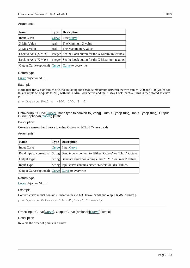
Arguments
Name Type Description
Input Curve Curve First Curve
X Min Value real The Minimum X value
X Max Value real The Maximum X value
Lock to Axis (X Min) integer Set the Lock button for the X Minimum textbox
Lock to Axis (X Max) integer Set the Lock button for the X Maximum textbox
Output Curve (optional) Curve Curve to overwrite
Return type
Curve object or NULL
Example
Normalise the X axis values of curve m taking the absolute maximum between the two values -200 and 100 (which for this example will equate to 200) with the X Min Lock active and the X Max Lock Inactive. This is then stored as curve p.
p = Operate.Nox2(m, -200, 100, 1, 0);
Octave(Input Curve[Curve], Band type to convert to[String], Output Type[String], Input Type[String], Output Curve (optional)[Curve]) [static]
Description
Coverts a narrow band curve to either Octave or 1/Third Octave bands
Arguments
Name Type Description
Input Curve Curve Input Curve
Band type to convert to String Band type to convert to. Either "Octave" or "Third" Octave.
Output Type String Generate curve containing either "RMS" or "mean" values.
Input Type String Input curve contains either "Linear" or "dB" values.
Output Curve (optional) Curve Curve to overwrite
Return type
Curve object or NULL
Example
Convert curve m that contains Linear values to 1/3 Octave bands and output RMS in curve p
p = Operate.Octave(m,"third","rms","linear");
Order(Input Curve[Curve], Output Curve (optional)[Curve]) [static]
Description
Reverse the order of points in a curve
User manual Version 18.0, April 2021 T/HIS
Page J.133

Arguments
Name Type Description
Input Curve Curve Input Curve
Output Curve (optional) Curve Curve to overwrite
Return type
Curve object or NULL
Example
Reverse the order of points in curve m and store as curve p
p = Operate.Order(m);
Pbut(Input Curve[Curve], Frequency[real], Order[integer], X axis interval (optional)[real], Output Curve (optional)[Curve]) [static]
Description
Pure Butterworth Filter
Arguments
Name Type Description
Input Curve Curve Input Curve
Frequency real Cut-off Frequency (Hz)
Order integer Filter order
X axis interval (optional) real If defined then T-HIS will automatically regularise the curve using this value first
Output Curve (optional) Curve Curve to overwrite
Return type
Curve object or NULL
Example
Filter curve m using a cut-off of 400Hz and order 2 and output as curve p. Regularise the input curve using an interval of 0.0001 first.
p = Operate.Pbut(m,400.0,2,0.0001);
Power(Input Curve[Curve], Power[real], Output Curve (optional)[Curve]) [static]
Description
Raise to the power
Arguments
Name Type Description
Input Curve Curve Input Curve
Power real Power to raise Y axis values by
Output Curve (optional) Curve Curve to overwrite
Return type
Curve object or NULL
T/HIS User manual Version 18.0, April 2021
Page J.134
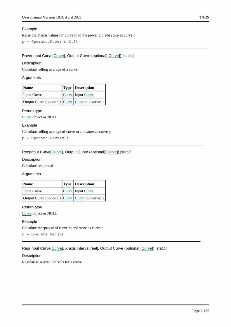
Example
Raise the Y axis values for curve m to the power 2.5 and store as curve p
p = Operate.Power(m,2.5);
Rave(Input Curve[Curve], Output Curve (optional)[Curve]) [static]
Description
Calculate rolling average of a curve
Arguments
Name Type Description
Input Curve Curve Input Curve
Output Curve (optional) Curve Curve to overwrite
Return type
Curve object or NULL
Example
Calculate rolling average of curve m and store as curve p
p = Operate.Rave(m);
Rec(Input Curve[Curve], Output Curve (optional)[Curve]) [static]
Description
Calculate reciprocal
Arguments
Name Type Description
Input Curve Curve Input Curve
Output Curve (optional) Curve Curve to overwrite
Return type
Curve object or NULL
Example
Calculate receprocal of curve m and store as curve p
p = Operate.Rec(m);
Reg(Input Curve[Curve], X axis interval[real], Output Curve (optional)[Curve]) [static]
Description
Regularise X axis intervals for a curve.
User manual Version 18.0, April 2021 T/HIS
Page J.135

Arguments
Name Type Description
Input Curve Curve Input Curve
X axis interval real New X axis interval
Output Curve (optional) Curve Curve to overwrite
Return type
Curve object or NULL
Example
Regularise curve m using a new X axis intreval of 0.0001.
p = Operate.Reg(m,0.0001);
Res(Curves[Array of Curve objects], Output Curve (optional)[Curve]) [static]
Description
Resultant of a group of curves
Arguments
Name Type Description
Curves Array of Curve objects Array of Curve objects
Output Curve (optional) Curve Curve to overwrite
Return type
Curve object or NULL
Example
Resultant of curves stored in curve array x
p = Operate.Res(x);
Rev(Input Curve[Curve], Output Curve (optional)[Curve]) [static]
Description
Reverse X and Y axis values
Arguments
Name Type Description
Input Curve Curve Input Curve
Output Curve (optional) Curve Curve to overwrite
Return type
Curve object or NULL
Example
Reverse X and Y axis values of curve m and store as curve p
p = Operate.Rev(m);
T/HIS User manual Version 18.0, April 2021
Page J.136
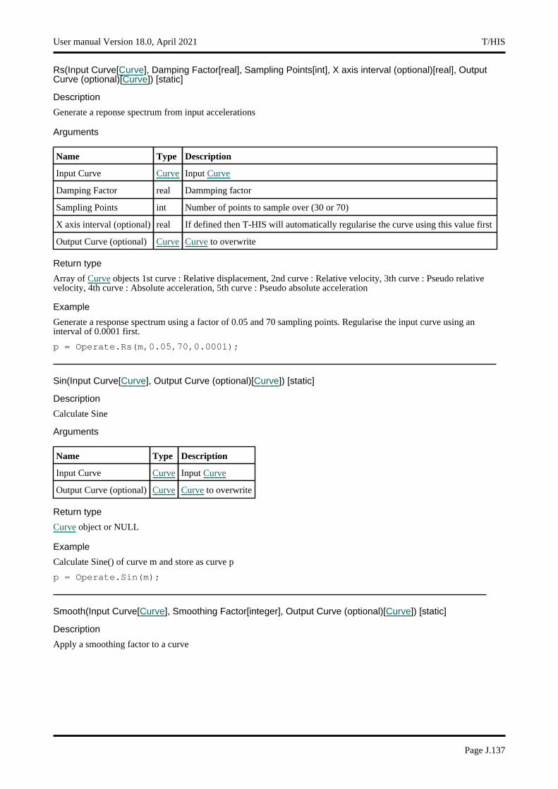
Rs(Input Curve[Curve], Damping Factor[real], Sampling Points[int], X axis interval (optional)[real], Output Curve (optional)[Curve]) [static]
Description
Generate a reponse spectrum from input accelerations
Arguments
Name Type Description
Input Curve Curve Input Curve
Damping Factor real Dammping factor
Sampling Points int Number of points to sample over (30 or 70)
X axis interval (optional) real If defined then T-HIS will automatically regularise the curve using this value first
Output Curve (optional) Curve Curve to overwrite
Return type
Array of Curve objects 1st curve : Relative displacement, 2nd curve : Relative velocity, 3th curve : Pseudo relative velocity, 4th curve : Absolute acceleration, 5th curve : Pseudo absolute acceleration
Example
Generate a response spectrum using a factor of 0.05 and 70 sampling points. Regularise the input curve using an interval of 0.0001 first.
p = Operate.Rs(m,0.05,70,0.0001);
Sin(Input Curve[Curve], Output Curve (optional)[Curve]) [static]
Description
Calculate Sine
Arguments
Name Type Description
Input Curve Curve Input Curve
Output Curve (optional) Curve Curve to overwrite
Return type
Curve object or NULL
Example
Calculate Sine() of curve m and store as curve p
p = Operate.Sin(m);
Smooth(Input Curve[Curve], Smoothing Factor[integer], Output Curve (optional)[Curve]) [static]
Description
Apply a smoothing factor to a curve
User manual Version 18.0, April 2021 T/HIS
Page J.137

Arguments
Name Type Description
Input Curve Curve Input Curve
Smoothing Factor integer Number of points to average over
Output Curve (optional) Curve Curve to overwrite
Return type
Curve object or NULL
Example
Smooth curve m using 7 points and store as curve p
p = Operate.Smooth(m,7);
Sqr(Input Curve[Curve], Output Curve (optional)[Curve]) [static]
Description
Square root of a curve
Arguments
Name Type Description
Input Curve Curve Input Curve
Output Curve (optional) Curve Curve to overwrite
Return type
Curve object or NULL
Example
Square root curve m and store as curve p
p = Operate.Sqr(m);
Stress(Input Curve[Curve], Convert to[string], Output Curve (optional)[Curve]) [static]
Description
Convert between true and engineering stress
Arguments
Name Type Description
Input Curve Curve Input Curve
Convert to string Type to convert to (True or Engineering)
Output Curve (optional) Curve Curve to overwrite
Return type
Curve object or NULL
Example
Convert curve m from engineering to true strees and store as curve p
p = Operate.Stress(m,"True");
T/HIS User manual Version 18.0, April 2021
Page J.138
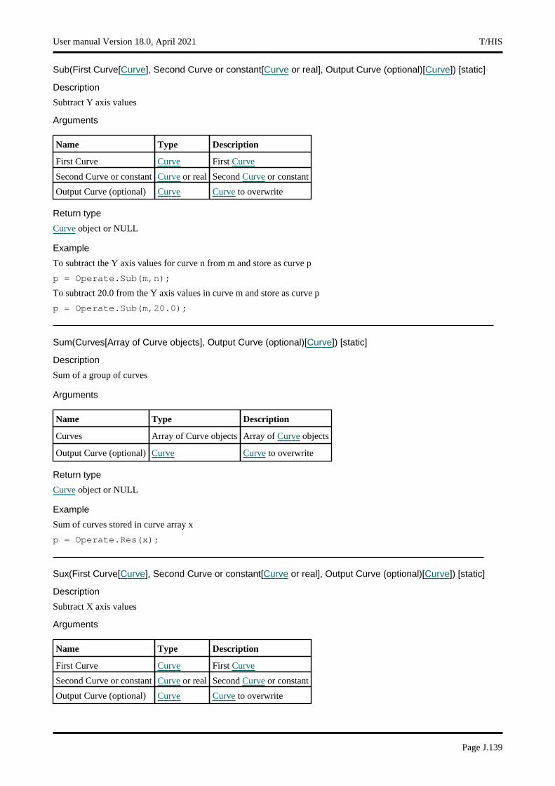
Sub(First Curve[Curve], Second Curve or constant[Curve or real], Output Curve (optional)[Curve]) [static]
Description
Subtract Y axis values
Arguments
Name Type Description
First Curve Curve First Curve
Second Curve or constant Curve or real Second Curve or constant
Output Curve (optional) Curve Curve to overwrite
Return type
Curve object or NULL
Example
To subtract the Y axis values for curve n from m and store as curve p
p = Operate.Sub(m,n);
To subtract 20.0 from the Y axis values in curve m and store as curve p
p = Operate.Sub(m,20.0);
Sum(Curves[Array of Curve objects], Output Curve (optional)[Curve]) [static]
Description
Sum of a group of curves
Arguments
Name Type Description
Curves Array of Curve objects Array of Curve objects
Output Curve (optional) Curve Curve to overwrite
Return type
Curve object or NULL
Example
Sum of curves stored in curve array x
p = Operate.Res(x);
Sux(First Curve[Curve], Second Curve or constant[Curve or real], Output Curve (optional)[Curve]) [static]
Description
Subtract X axis values
Arguments
Name Type Description
First Curve Curve First Curve
Second Curve or constant Curve or real Second Curve or constant
Output Curve (optional) Curve Curve to overwrite
User manual Version 18.0, April 2021 T/HIS
Page J.139
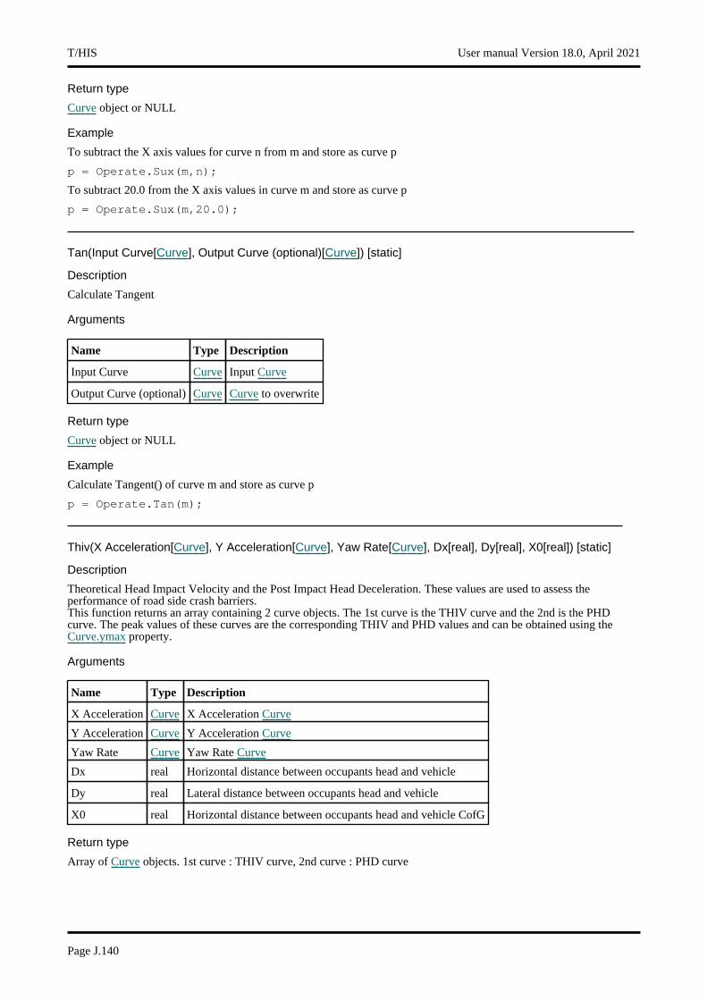
Return type
Curve object or NULL
Example
To subtract the X axis values for curve n from m and store as curve p
p = Operate.Sux(m,n);
To subtract 20.0 from the X axis values in curve m and store as curve p
p = Operate.Sux(m,20.0);
Tan(Input Curve[Curve], Output Curve (optional)[Curve]) [static]
Description
Calculate Tangent
Arguments
Name Type Description
Input Curve Curve Input Curve
Output Curve (optional) Curve Curve to overwrite
Return type
Curve object or NULL
Example
Calculate Tangent() of curve m and store as curve p
p = Operate.Tan(m);
Thiv(X Acceleration[Curve], Y Acceleration[Curve], Yaw Rate[Curve], Dx[real], Dy[real], X0[real]) [static]
Description
Theoretical Head Impact Velocity and the Post Impact Head Deceleration. These values are used to assess the performance of road side crash barriers. This function returns an array containing 2 curve objects. The 1st curve is the THIV curve and the 2nd is the PHD curve. The peak values of these curves are the corresponding THIV and PHD values and can be obtained using the Curve.ymax property.
Arguments
Name Type Description
X Acceleration Curve X Acceleration Curve
Y Acceleration Curve Y Acceleration Curve
Yaw Rate Curve Yaw Rate Curve
Dx real Horizontal distance between occupants head and vehicle
Dy real Lateral distance between occupants head and vehicle
X0 real Horizontal distance between occupants head and vehicle CofG
Return type
Array of Curve objects. 1st curve : THIV curve, 2nd curve : PHD curve
T/HIS User manual Version 18.0, April 2021
Page J.140
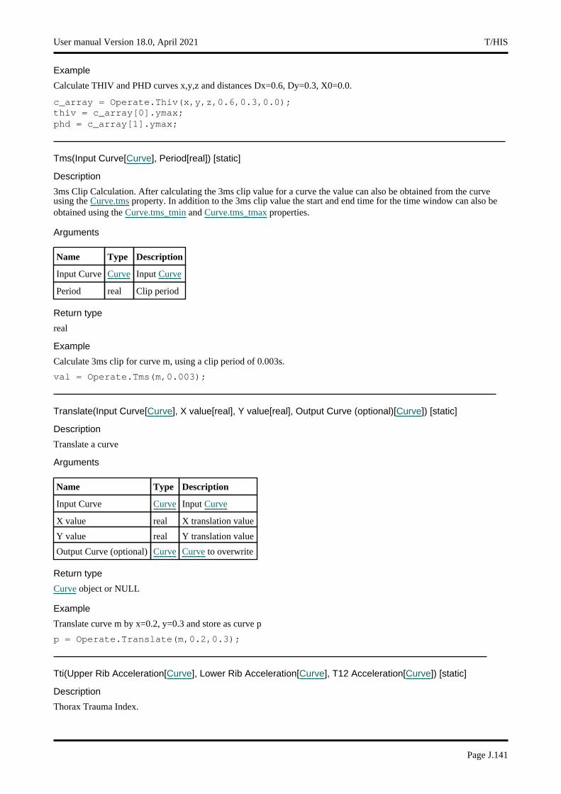
Example
Calculate THIV and PHD curves x,y,z and distances Dx=0.6, Dy=0.3, X0=0.0.
c_array = Operate.Thiv(x,y,z,0.6,0.3,0.0);thiv = c_array[0].ymax;phd = c_array[1].ymax;
Tms(Input Curve[Curve], Period[real]) [static]
Description
3ms Clip Calculation. After calculating the 3ms clip value for a curve the value can also be obtained from the curve using the Curve.tms property. In addition to the 3ms clip value the start and end time for the time window can also be obtained using the Curve.tms_tmin and Curve.tms_tmax properties.
Arguments
Name Type Description
Input Curve Curve Input Curve
Period real Clip period
Return type
real
Example
Calculate 3ms clip for curve m, using a clip period of 0.003s.
val = Operate.Tms(m,0.003);
Translate(Input Curve[Curve], X value[real], Y value[real], Output Curve (optional)[Curve]) [static]
Description
Translate a curve
Arguments
Name Type Description
Input Curve Curve Input Curve
X value real X translation value
Y value real Y translation value
Output Curve (optional) Curve Curve to overwrite
Return type
Curve object or NULL
Example
Translate curve m by x=0.2, y=0.3 and store as curve p
p = Operate.Translate(m,0.2,0.3);
Tti(Upper Rib Acceleration[Curve], Lower Rib Acceleration[Curve], T12 Acceleration[Curve]) [static]
Description
Thorax Trauma Index.
User manual Version 18.0, April 2021 T/HIS
Page J.141

Arguments
Name Type Description
Upper Rib Acceleration Curve Upper Rib Acceleration Curve
Lower Rib Acceleration Curve Lower Rib Acceleration Curve
T12 Acceleration Curve T12 Acceleration Curve
Return type
real
Example
Calculate TTI using curves x,y and z as inputs.
val = Operate.TTi(x,y,z);
Va(Input Curve[Curve], Output Curve (optional)[Curve]) [static]
Description
Convert velocity spectrum to an acceleration spectrum
Arguments
Name Type Description
Input Curve Curve Input Curve
Output Curve (optional) Curve Curve to overwrite
Return type
Curve object or NULL
Example
Convert curve m and store as curve p
p = Operate.Va(m);
Vc(Input Curve[Curve], A[real], B[real], Calculation method[string], Output Curve (optional)[Curve]) [static]
Description
Viscous Criteria calculate. The VC calculation can be done using 2 different calculation methods ECER95 and IIHS.
Arguments
Name Type Description
Input Curve Curve Input Curve
A real Constant A
B real Constant B
Calculation method string Either ECER95 or IIHS.
Output Curve (optional) Curve Curve to overwrite
Return type
Curve object or NULL
T/HIS User manual Version 18.0, April 2021
Page J.142
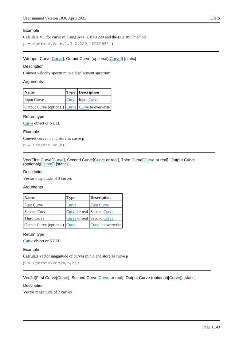
Example
Calculate VC for curve m, using A=1.3, B=0.229 and the ECER95 method
p = Operate.Vc(m,1.3,0.229,"ECER95");
Vd(Input Curve[Curve], Output Curve (optional)[Curve]) [static]
Description
Convert velocity spectrum to a displacment spectrum
Arguments
Name Type Description
Input Curve Curve Input Curve
Output Curve (optional) Curve Curve to overwrite
Return type
Curve object or NULL
Example
Convert curve m and store as curve p
p = Operate.Vd(m);
Vec(First Curve[Curve], Second Curve[Curve or real], Third Curve[Curve or real], Output Curve (optional)[Curve]) [static]
Description
Vector magnitude of 3 curves
Arguments
Name Type Description
First Curve Curve First Curve
Second Curve Curve or real Second Curve
Third Curve Curve or real Second Curve
Output Curve (optional) Curve Curve to overwrite
Return type
Curve object or NULL
Example
Calculate vector magnitude of curves m,n,o and store as curve p
p = Operate.Vec(m,n,o);
Vec2d(First Curve[Curve], Second Curve[Curve or real], Output Curve (optional)[Curve]) [static]
Description
Vector magnitude of 2 curves
User manual Version 18.0, April 2021 T/HIS
Page J.143
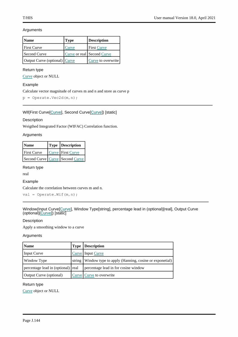
Arguments
Name Type Description
First Curve Curve First Curve
Second Curve Curve or real Second Curve
Output Curve (optional) Curve Curve to overwrite
Return type
Curve object or NULL
Example
Calculate vector magnitude of curves m and n and store as curve p
p = Operate.Vec2d(m,n);
Wif(First Curve[Curve], Second Curve[Curve]) [static]
Description
Weigthed Integrated Factor (WIFAC) Correlation function.
Arguments
Name Type Description
First Curve Curve First Curve
Second Curve Curve Second Curve
Return type
real
Example
Calculate the correlation between curves m and n.
val = Operate.Wif(m,n);
Window(Input Curve[Curve], Window Type[string], percentage lead in (optional)[real], Output Curve (optional)[Curve]) [static]
Description
Apply a smoothing window to a curve
Arguments
Name Type Description
Input Curve Curve Input Curve
Window Type string Window type to apply (Hanning, cosine or exponetial)
percentage lead in (optional) real percentage lead in for cosine window
Output Curve (optional) Curve Curve to overwrite
Return type
Curve object or NULL
T/HIS User manual Version 18.0, April 2021
Page J.144
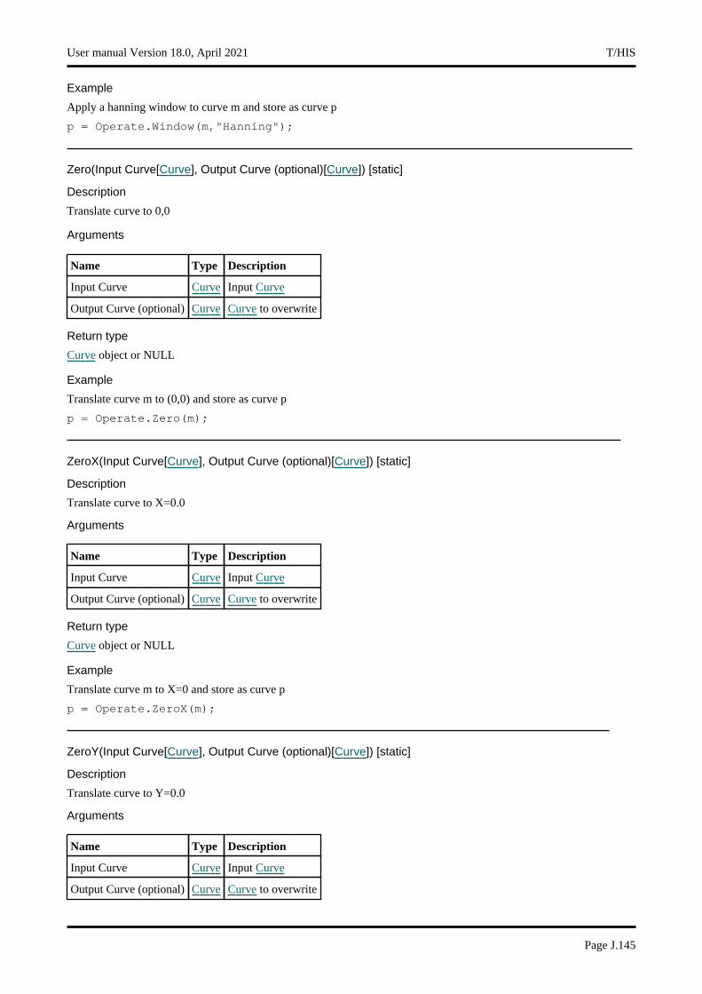
Example
Apply a hanning window to curve m and store as curve p
p = Operate.Window(m,"Hanning");
Zero(Input Curve[Curve], Output Curve (optional)[Curve]) [static]
Description
Translate curve to 0,0
Arguments
Name Type Description
Input Curve Curve Input Curve
Output Curve (optional) Curve Curve to overwrite
Return type
Curve object or NULL
Example
Translate curve m to (0,0) and store as curve p
p = Operate.Zero(m);
ZeroX(Input Curve[Curve], Output Curve (optional)[Curve]) [static]
Description
Translate curve to X=0.0
Arguments
Name Type Description
Input Curve Curve Input Curve
Output Curve (optional) Curve Curve to overwrite
Return type
Curve object or NULL
Example
Translate curve m to X=0 and store as curve p
p = Operate.ZeroX(m);
ZeroY(Input Curve[Curve], Output Curve (optional)[Curve]) [static]
Description
Translate curve to Y=0.0
Arguments
Name Type Description
Input Curve Curve Input Curve
Output Curve (optional) Curve Curve to overwrite
User manual Version 18.0, April 2021 T/HIS
Page J.145
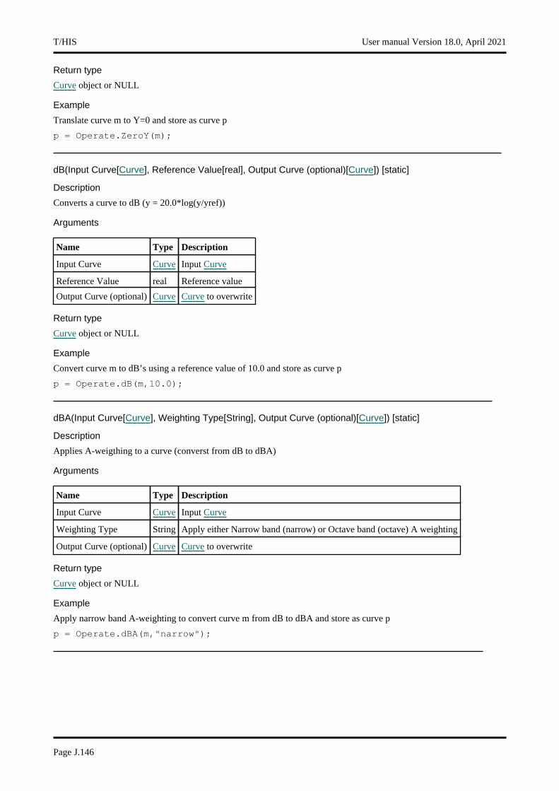
Return type
Curve object or NULL
Example
Translate curve m to Y=0 and store as curve p
p = Operate.ZeroY(m);
dB(Input Curve[Curve], Reference Value[real], Output Curve (optional)[Curve]) [static]
Description
Converts a curve to dB (y = 20.0*log(y/yref))
Arguments
Name Type Description
Input Curve Curve Input Curve
Reference Value real Reference value
Output Curve (optional) Curve Curve to overwrite
Return type
Curve object or NULL
Example
Convert curve m to dB’s using a reference value of 10.0 and store as curve p
p = Operate.dB(m,10.0);
dBA(Input Curve[Curve], Weighting Type[String], Output Curve (optional)[Curve]) [static]
Description
Applies A-weigthing to a curve (converst from dB to dBA)
Arguments
Name Type Description
Input Curve Curve Input Curve
Weighting Type String Apply either Narrow band (narrow) or Octave band (octave) A weighting
Output Curve (optional) Curve Curve to overwrite
Return type
Curve object or NULL
Example
Apply narrow band A-weighting to convert curve m from dB to dBA and store as curve p
p = Operate.dBA(m,"narrow");
T/HIS User manual Version 18.0, April 2021
Page J.146
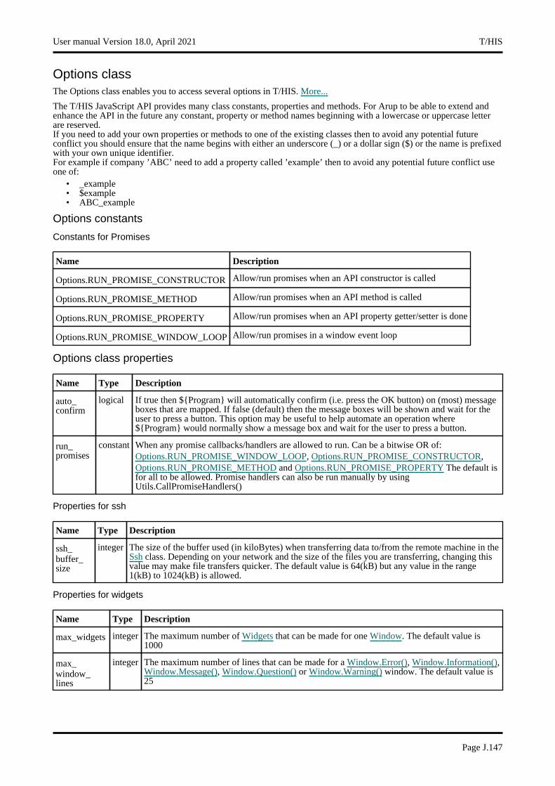
Options classThe Options class enables you to access several options in T/HIS. More...
The T/HIS JavaScript API provides many class constants, properties and methods. For Arup to be able to extend and enhance the API in the future any constant, property or method names beginning with a lowercase or uppercase letter are reserved.If you need to add your own properties or methods to one of the existing classes then to avoid any potential future conflict you should ensure that the name begins with either an underscore (_) or a dollar sign ($) or the name is prefixed with your own unique identifier.For example if company ’ABC’ need to add a property called ’example’ then to avoid any potential future conflict use one of:
• _example • $example • ABC_example
Options constants
Constants for Promises
Name Description
Options.RUN_PROMISE_CONSTRUCTOR Allow/run promises when an API constructor is called
Options.RUN_PROMISE_METHOD Allow/run promises when an API method is called
Options.RUN_PROMISE_PROPERTY Allow/run promises when an API property getter/setter is done
Options.RUN_PROMISE_WINDOW_LOOP Allow/run promises in a window event loop
Options class properties
Name Type Description
auto_confirm
logical If true then ${Program} will automatically confirm (i.e. press the OK button) on (most) message boxes that are mapped. If false (default) then the message boxes will be shown and wait for the user to press a button. This option may be useful to help automate an operation where ${Program} would normally show a message box and wait for the user to press a button.
run_promises
constant When any promise callbacks/handlers are allowed to run. Can be a bitwise OR of: Options.RUN_PROMISE_WINDOW_LOOP, Options.RUN_PROMISE_CONSTRUCTOR, Options.RUN_PROMISE_METHOD and Options.RUN_PROMISE_PROPERTY The default is for all to be allowed. Promise handlers can also be run manually by using Utils.CallPromiseHandlers()
Properties for ssh
Name Type Description
ssh_buffer_size
integer The size of the buffer used (in kiloBytes) when transferring data to/from the remote machine in the Ssh class. Depending on your network and the size of the files you are transferring, changing this value may make file transfers quicker. The default value is 64(kB) but any value in the range 1(kB) to 1024(kB) is allowed.
Properties for widgets
Name Type Description
max_widgets integer The maximum number of Widgets that can be made for one Window. The default value is 1000
max_window_lines
integer The maximum number of lines that can be made for a Window.Error(), Window.Information(), Window.Message(), Window.Question() or Window.Warning() window. The default value is 25
User manual Version 18.0, April 2021 T/HIS
Page J.147

Detailed DescriptionThe Options class is used to get/set options that T/HIS uses for certain functions. The options are available as class properties. See the documentation for more details. An example: Options.mass_properties_include_attached_mass_deformable_elems=true
T/HIS User manual Version 18.0, April 2021
Page J.148
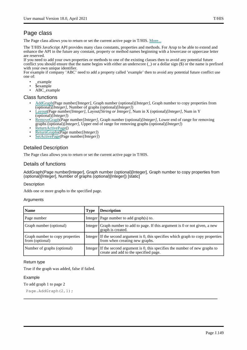
Page classThe Page class allows you to return or set the current active page in T/HIS. More...
The T/HIS JavaScript API provides many class constants, properties and methods. For Arup to be able to extend and enhance the API in the future any constant, property or method names beginning with a lowercase or uppercase letter are reserved.If you need to add your own properties or methods to one of the existing classes then to avoid any potential future conflict you should ensure that the name begins with either an underscore (_) or a dollar sign ($) or the name is prefixed with your own unique identifier.For example if company ’ABC’ need to add a property called ’example’ then to avoid any potential future conflict use one of:
• _example • $example • ABC_example
Class functions• AddGraph(Page number[Integer], Graph number (optional)[Integer], Graph number to copy properties from
(optional)[Integer], Number of graphs (optional)[Integer]) • Layout(Page number[Integer], Layout[String or Integer], Num in X (optional)[Integer], Num in Y
(optional)[Integer]) • RemoveGraph(Page number[Integer], Graph number (optional)[Integer], Lower end of range for removing
graphs (optional)[Integer], Upper end of range for removing graphs (optional)[Integer]) • ReturnActivePage() • ReturnGraphs(Page number[Integer]) • SetActivePage(Page number[Integer])
Detailed DescriptionThe Page class allows you to return or set the current active page in T/HIS.
Details of functions
AddGraph(Page number[Integer], Graph number (optional)[Integer], Graph number to copy properties from (optional)[Integer], Number of graphs (optional)[Integer]) [static]
Description
Adds one or more graphs to the specified page.
Arguments
Name Type Description
Page number Integer Page number to add graph(s) to.
Graph number (optional) Integer Graph number to add to page. If this argument is 0 or not given, a new graph is created.
Graph number to copy properties from (optional)
Integer If the second argument is 0, this specifies which graph to copy properties from when creating new graphs.
Number of graphs (optional) Integer If the second argument is 0, this specifies the number of new graphs to create and add to the specified page.
Return type
True if the graph was added, false if failed.
Example
To add graph 1 to page 2
Page.AddGraph(2,1);
User manual Version 18.0, April 2021 T/HIS
Page J.149
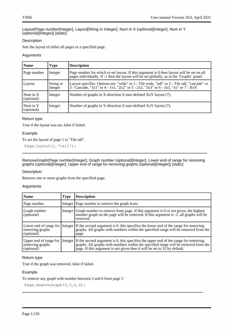
Layout(Page number[Integer], Layout[String or Integer], Num in X (optional)[Integer], Num in Y (optional)[Integer]) [static]
Description
Sets the layout of either all pages or a specified page.
Arguments
Name Type Description
Page number Integer Page number for which to set layout. If this argument is 0 then layout will be set on all pages individually. If -1 then the layout will be set globally, as in the ’Graphs’ panel.
Layout String or Integer
Layout specifier. Options are: "wide" or 1 - Tile wide, "tall" or 2 - Tile tall, "cascade" or 3 - Cascade, "1x1" or 4 - 1x1, "2x2" or 5 - 2x2, "3x3" or 6 - 3x3, "xy" or 7 - XxY.
Num in X (optional)
Integer Number of graphs in X-direction if user-defined XxY layout (7).
Num in Y (optional)
Integer Number of graphs in Y-direction if user-defined XxY layout (7).
Return type
True if the layout was set, false if failed.
Example
To set the layout of page 1 to ’Tile tall’.
Page.Layout(1,"tall");
RemoveGraph(Page number[Integer], Graph number (optional)[Integer], Lower end of range for removing graphs (optional)[Integer], Upper end of range for removing graphs (optional)[Integer]) [static]
Description
Remove one or more graphs from the specified page.
Arguments
Name Type Description
Page number Integer Page number to remove the graph from.
Graph number (optional)
Integer Graph number to remove from page. If this argument is 0 or not given, the highest number graph on the page will be removed. If this argument is -1, all graphs will be removed.
Lower end of range for removing graphs (optional)
Integer If the second argument is 0, this specifies the lower end of the range for removing graphs. All graphs with numbers within the specified range will be removed from the page.
Upper end of range for removing graphs (optional)
Integer If the second argument is 0, this specifies the upper end of the range for removing graphs. All graphs with numbers within the specified range will be removed from the page. If this argument is not given then it will be set to 32 by default.
Return type
True if the graph was removed, false if failed.
Example
To remove any graph with number between 2 and 6 from page 3
Page.RemoveGraph(3,0,2,6);
T/HIS User manual Version 18.0, April 2021
Page J.150
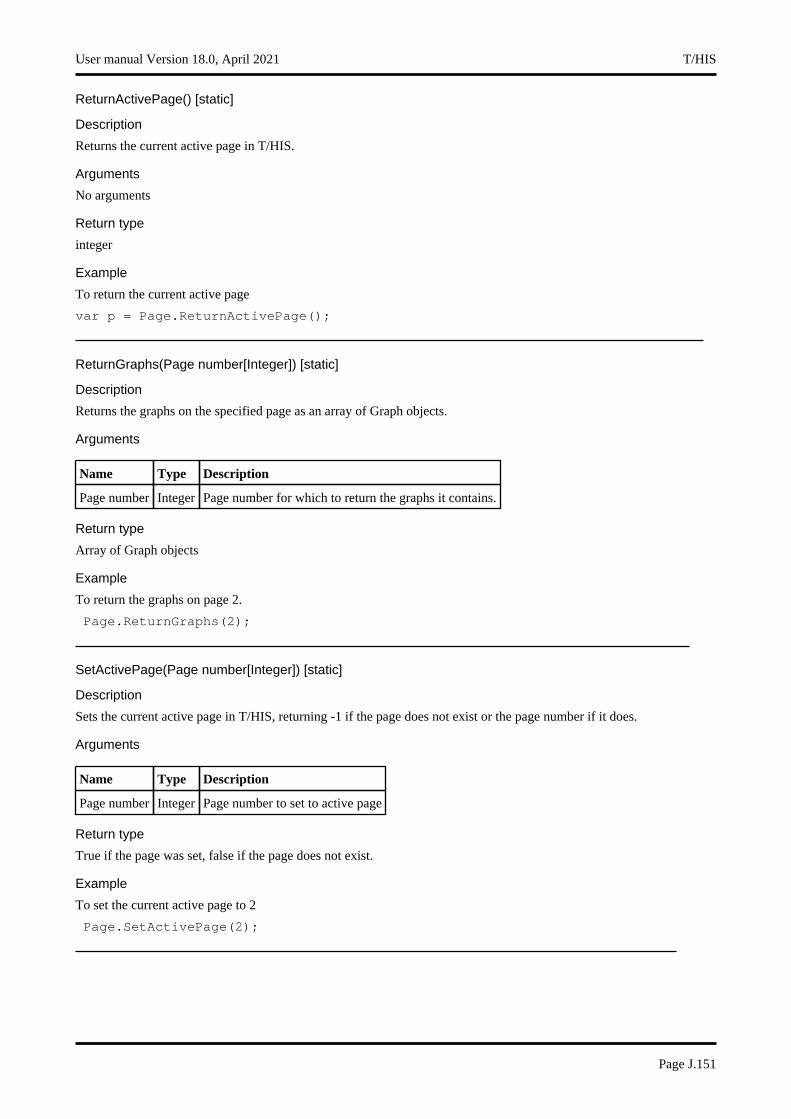
ReturnActivePage() [static]
Description
Returns the current active page in T/HIS.
Arguments
No arguments
Return type
integer
Example
To return the current active page
var p = Page.ReturnActivePage();
ReturnGraphs(Page number[Integer]) [static]
Description
Returns the graphs on the specified page as an array of Graph objects.
Arguments
Name Type Description
Page number Integer Page number for which to return the graphs it contains.
Return type
Array of Graph objects
Example
To return the graphs on page 2.
Page.ReturnGraphs(2);
SetActivePage(Page number[Integer]) [static]
Description
Sets the current active page in T/HIS, returning -1 if the page does not exist or the page number if it does.
Arguments
Name Type Description
Page number Integer Page number to set to active page
Return type
True if the page was set, false if the page does not exist.
Example
To set the current active page to 2
Page.SetActivePage(2);
User manual Version 18.0, April 2021 T/HIS
Page J.151
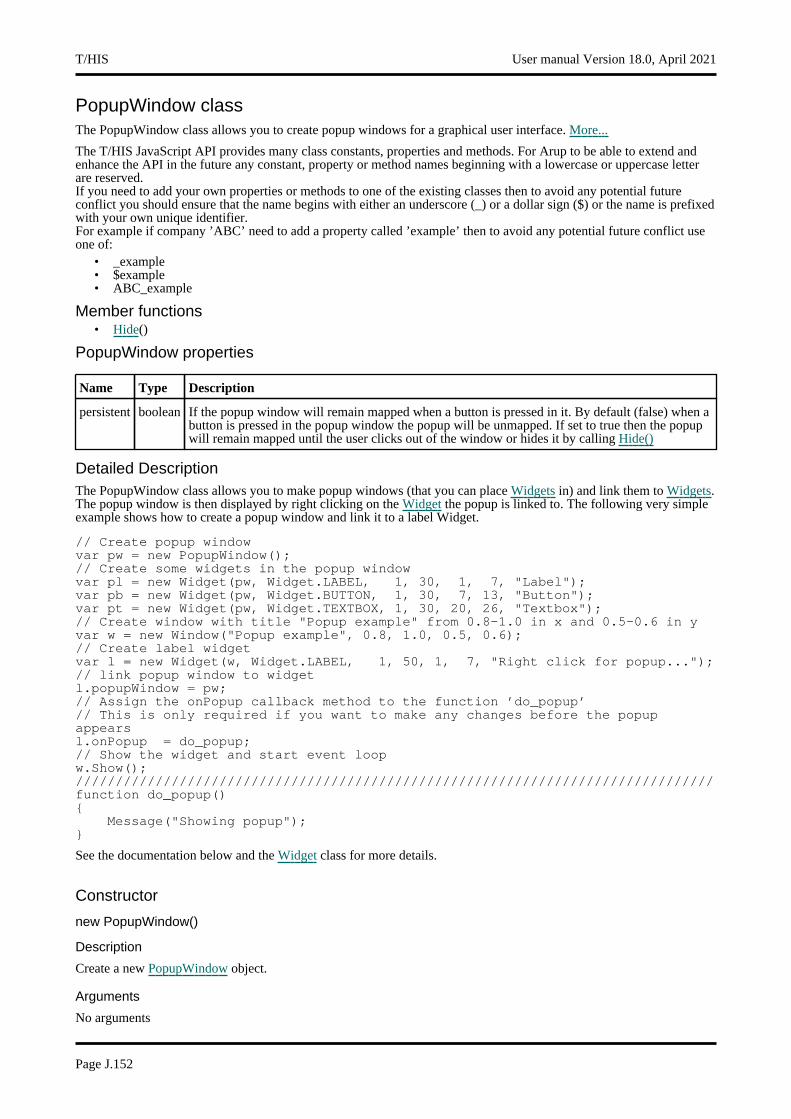
PopupWindow classThe PopupWindow class allows you to create popup windows for a graphical user interface. More...
The T/HIS JavaScript API provides many class constants, properties and methods. For Arup to be able to extend and enhance the API in the future any constant, property or method names beginning with a lowercase or uppercase letter are reserved.If you need to add your own properties or methods to one of the existing classes then to avoid any potential future conflict you should ensure that the name begins with either an underscore (_) or a dollar sign ($) or the name is prefixed with your own unique identifier.For example if company ’ABC’ need to add a property called ’example’ then to avoid any potential future conflict use one of:
• _example • $example • ABC_example
Member functions• Hide()
PopupWindow properties
Name Type Description
persistent boolean If the popup window will remain mapped when a button is pressed in it. By default (false) when a button is pressed in the popup window the popup will be unmapped. If set to true then the popup will remain mapped until the user clicks out of the window or hides it by calling Hide()
Detailed DescriptionThe PopupWindow class allows you to make popup windows (that you can place Widgets in) and link them to Widgets. The popup window is then displayed by right clicking on the Widget the popup is linked to. The following very simple example shows how to create a popup window and link it to a label Widget.
// Create popup windowvar pw = new PopupWindow();// Create some widgets in the popup windowvar pl = new Widget(pw, Widget.LABEL, 1, 30, 1, 7, "Label");var pb = new Widget(pw, Widget.BUTTON, 1, 30, 7, 13, "Button");var pt = new Widget(pw, Widget.TEXTBOX, 1, 30, 20, 26, "Textbox");// Create window with title "Popup example" from 0.8-1.0 in x and 0.5-0.6 in yvar w = new Window("Popup example", 0.8, 1.0, 0.5, 0.6);// Create label widgetvar l = new Widget(w, Widget.LABEL, 1, 50, 1, 7, "Right click for popup...");// link popup window to widgetl.popupWindow = pw;// Assign the onPopup callback method to the function ’do_popup’// This is only required if you want to make any changes before the popup appearsl.onPopup = do_popup;// Show the widget and start event loopw.Show();////////////////////////////////////////////////////////////////////////////////function do_popup(){
Message("Showing popup");}
See the documentation below and the Widget class for more details.
Constructor
new PopupWindow()
Description
Create a new PopupWindow object.
Arguments
No arguments
T/HIS User manual Version 18.0, April 2021
Page J.152
Return type
PopupWindow object
Example
To create a PopupWindow containing the buttons "Create" and "Edit" and link it to button b:
var pw = new PopupWindow();var c = new Widget(pw, Widget.BUTTON, 1, 30, 1, 7, "Create");var e = new Widget(pw, Widget.BUTTON, 1, 30, 7, 13, "Edit");b.popupWindow = pw;
Details of functions
Hide()
Description
Hides (unmaps) the popup window.
Arguments
No arguments
Return type
No return value
Example
To hide popup window w:
w.Hide();
User manual Version 18.0, April 2021 T/HIS
Page J.153
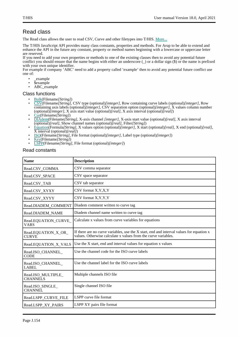
Read classThe Read class allows the user to read CSV, Curve and other filetypes into T/HIS. More...
The T/HIS JavaScript API provides many class constants, properties and methods. For Arup to be able to extend and enhance the API in the future any constant, property or method names beginning with a lowercase or uppercase letter are reserved.If you need to add your own properties or methods to one of the existing classes then to avoid any potential future conflict you should ensure that the name begins with either an underscore (_) or a dollar sign ($) or the name is prefixed with your own unique identifier.For example if company ’ABC’ need to add a property called ’example’ then to avoid any potential future conflict use one of:
• _example • $example • ABC_example
Class functions• Bulk(Filename[String]) • CSV(Filename[String], CSV type (optional)[integer], Row containing curve labels (optional)[integer], Row
containing axis labels (optional)[integer], CSV separation option (optional)[integer], X values column number (optional)[integer], X axis start value (optional)[real], X axis interval (optional)[real])
• Cur(Filename[String]) • DIAdem(Filename[String], X-axis channel [integer], X-axis start value (optional)[real], X axis interval
(optional)[real], Show channel names (optional)[real], Filter[String]) • Equation(Formula[String], X values option (optional)[integer], X start (optional)[real], X end (optional)[real],
X interval (optional)[real]) • ISO(Filename[String], File format (optional)[integer], Label type (optional)[integer]) • Key(Filename[String]) • LSPP(Filename[String], File format (optional)[integer])
Read constants
Name Description
Read.CSV_COMMA CSV comma separator
Read.CSV_SPACE CSV space separator
Read.CSV_TAB CSV tab separator
Read.CSV_XYXY CSV format X,Y,X,Y
Read.CSV_XYYY CSV format X,Y,Y,Y
Read.DIADEM_COMMENT Diadem comment written to curve tag
Read.DIADEM_NAME Diadem channel name written to curve tag
Read.EQUATION_CURVE_VARS
Calculate x values from curve variables for equations
Read.EQUATION_X_OR_CURVE
If there are no curve variables, use the X start, end and interval values for equation x values. Otherwise calculate x values from the curve variables.
Read.EQUATION_X_VALS Use the X start, end and interval values for equation x values
Read.ISO_CHANNEL_CODE
Use the channel code for the ISO curve labels
Read.ISO_CHANNEL_LABEL
Use the channel label for the ISO curve labels
Read.ISO_MULTIPLE_CHANNELS
Multiple channels ISO file
Read.ISO_SINGLE_CHANNEL
Single channel ISO file
Read.LSPP_CURVE_FILE LSPP curve file format
Read.LSPP_XY_PAIRS LSPP XY pairs file format
T/HIS User manual Version 18.0, April 2021
Page J.154
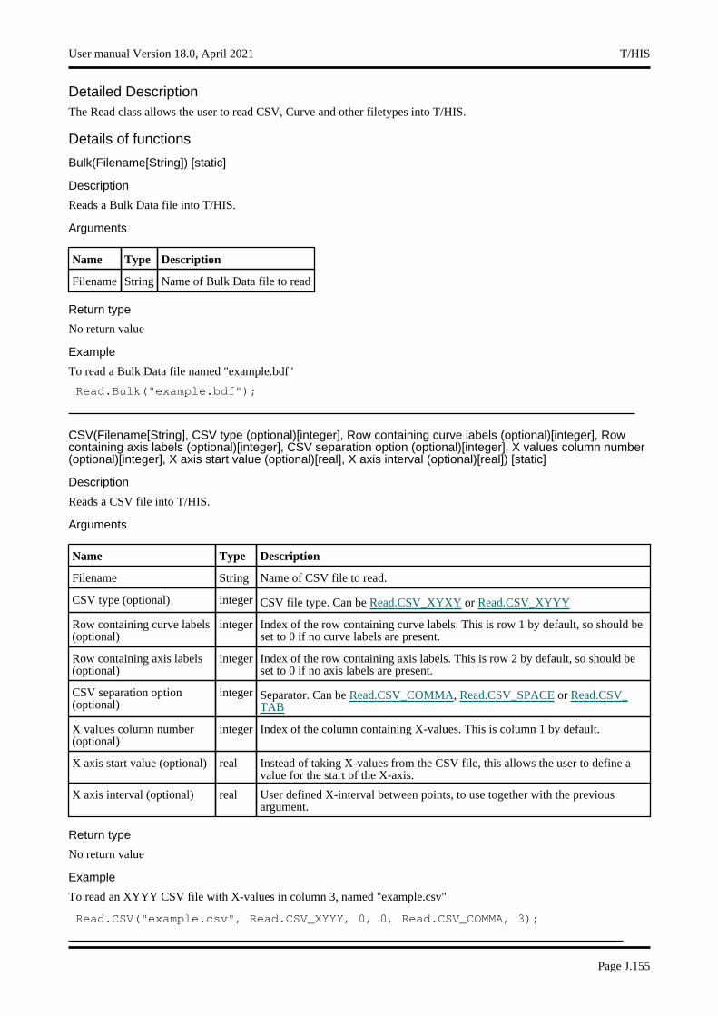
Detailed DescriptionThe Read class allows the user to read CSV, Curve and other filetypes into T/HIS.
Details of functions
Bulk(Filename[String]) [static]
Description
Reads a Bulk Data file into T/HIS.
Arguments
Name Type Description
Filename String Name of Bulk Data file to read
Return type
No return value
Example
To read a Bulk Data file named "example.bdf"
Read.Bulk("example.bdf");
CSV(Filename[String], CSV type (optional)[integer], Row containing curve labels (optional)[integer], Row containing axis labels (optional)[integer], CSV separation option (optional)[integer], X values column number (optional)[integer], X axis start value (optional)[real], X axis interval (optional)[real]) [static]
Description
Reads a CSV file into T/HIS.
Arguments
Name Type Description
Filename String Name of CSV file to read.
CSV type (optional) integer CSV file type. Can be Read.CSV_XYXY or Read.CSV_XYYY
Row containing curve labels (optional)
integer Index of the row containing curve labels. This is row 1 by default, so should be set to 0 if no curve labels are present.
Row containing axis labels (optional)
integer Index of the row containing axis labels. This is row 2 by default, so should be set to 0 if no axis labels are present.
CSV separation option (optional)
integer Separator. Can be Read.CSV_COMMA, Read.CSV_SPACE or Read.CSV_TAB
X values column number (optional)
integer Index of the column containing X-values. This is column 1 by default.
X axis start value (optional) real Instead of taking X-values from the CSV file, this allows the user to define a value for the start of the X-axis.
X axis interval (optional) real User defined X-interval between points, to use together with the previous argument.
Return type
No return value
Example
To read an XYYY CSV file with X-values in column 3, named "example.csv"
Read.CSV("example.csv", Read.CSV_XYYY, 0, 0, Read.CSV_COMMA, 3);
User manual Version 18.0, April 2021 T/HIS
Page J.155
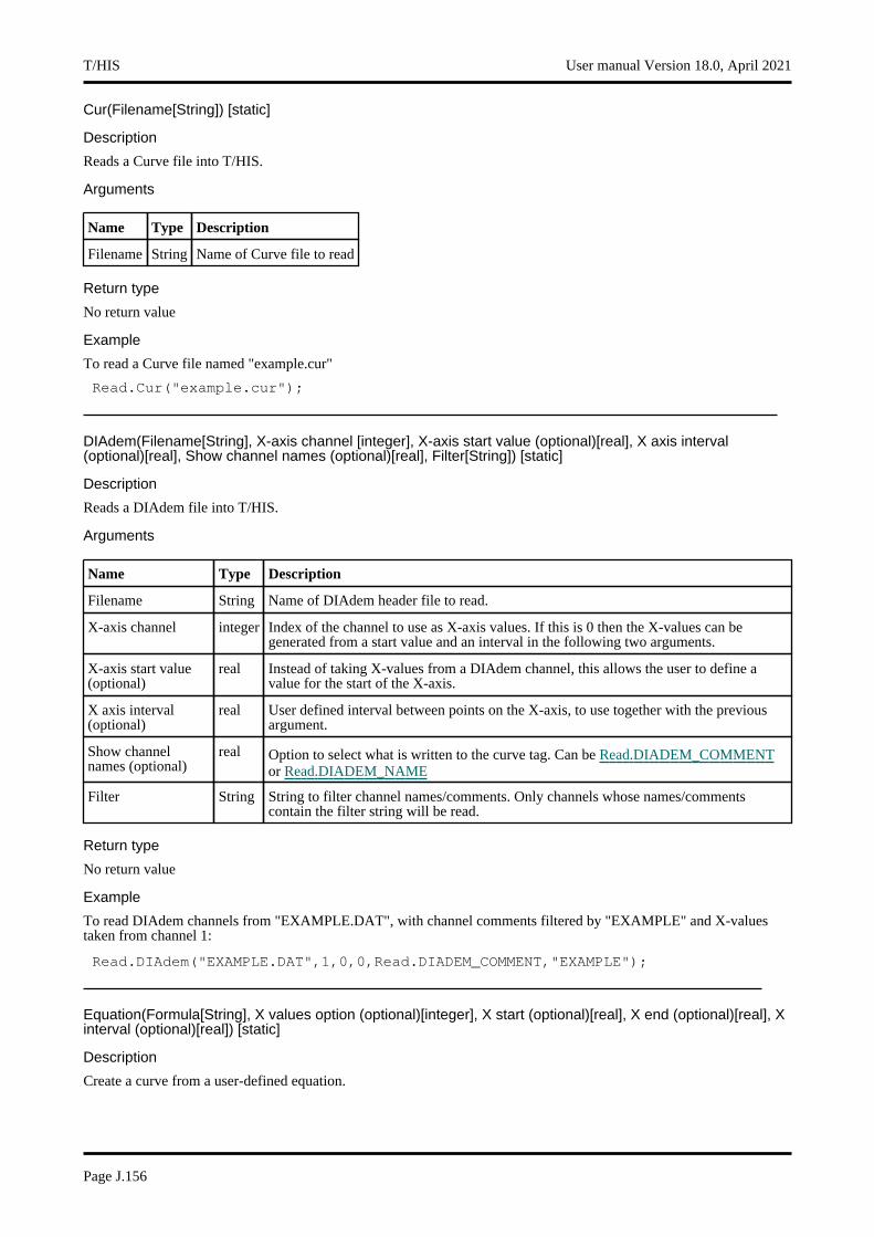
Cur(Filename[String]) [static]
Description
Reads a Curve file into T/HIS.
Arguments
Name Type Description
Filename String Name of Curve file to read
Return type
No return value
Example
To read a Curve file named "example.cur"
Read.Cur("example.cur");
DIAdem(Filename[String], X-axis channel [integer], X-axis start value (optional)[real], X axis interval (optional)[real], Show channel names (optional)[real], Filter[String]) [static]
Description
Reads a DIAdem file into T/HIS.
Arguments
Name Type Description
Filename String Name of DIAdem header file to read.
X-axis channel integer Index of the channel to use as X-axis values. If this is 0 then the X-values can be generated from a start value and an interval in the following two arguments.
X-axis start value (optional)
real Instead of taking X-values from a DIAdem channel, this allows the user to define a value for the start of the X-axis.
X axis interval (optional)
real User defined interval between points on the X-axis, to use together with the previous argument.
Show channel names (optional)
real Option to select what is written to the curve tag. Can be Read.DIADEM_COMMENTor Read.DIADEM_NAME
Filter String String to filter channel names/comments. Only channels whose names/comments contain the filter string will be read.
Return type
No return value
Example
To read DIAdem channels from "EXAMPLE.DAT", with channel comments filtered by "EXAMPLE" and X-values taken from channel 1:
Read.DIAdem("EXAMPLE.DAT",1,0,0,Read.DIADEM_COMMENT,"EXAMPLE");
Equation(Formula[String], X values option (optional)[integer], X start (optional)[real], X end (optional)[real], X interval (optional)[real]) [static]
Description
Create a curve from a user-defined equation.
T/HIS User manual Version 18.0, April 2021
Page J.156
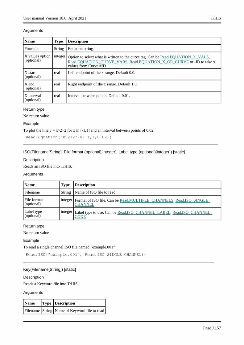
Arguments
Name Type Description
Formula String Equation string.
X values option (optional)
integer Option to select what is written to the curve tag. Can be Read.EQUATION_X_VALS, Read.EQUATION_CURVE_VARS, Read.EQUATION_X_OR_CURVE or -ID to take x values from Curve #ID
X start (optional)
real Left endpoint of the x range. Default 0.0.
X end (optional)
real Right endpoint of the x range. Default 1.0.
X interval (optional)
real Interval between points. Default 0.01.
Return type
No return value
Example
To plot the line y = x^2+2 for x in [-1,1] and an interval between points of 0.02:
Read.Equation("x^2+2",0,-1,1,0.02);
ISO(Filename[String], File format (optional)[integer], Label type (optional)[integer]) [static]
Description
Reads an ISO file into T/HIS.
Arguments
Name Type Description
Filename String Name of ISO file to read
File format (optional)
integer Format of ISO file. Can be Read.MULTIPLE_CHANNELS, Read.ISO_SINGLE_CHANNEL
Label type (optional)
integer Label type to use. Can be Read.ISO_CHANNEL_LABEL, Read.ISO_CHANNEL_CODE
Return type
No return value
Example
To read a single channel ISO file named "example.001"
Read.ISO("example.001", Read.ISO_SINGLE_CHANNEL);
Key(Filename[String]) [static]
Description
Reads a Keyword file into T/HIS.
Arguments
Name Type Description
Filename String Name of Keyword file to read
User manual Version 18.0, April 2021 T/HIS
Page J.157
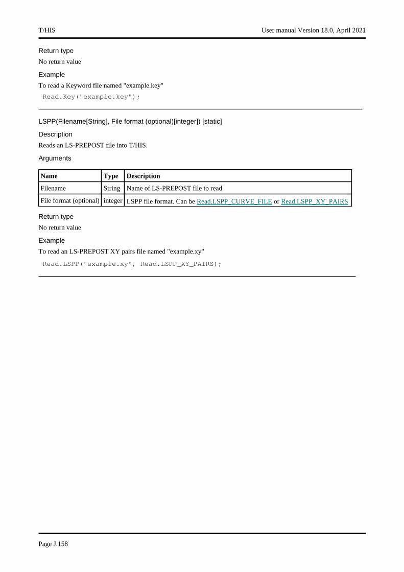
Return type
No return value
Example
To read a Keyword file named "example.key"
Read.Key("example.key");
LSPP(Filename[String], File format (optional)[integer]) [static]
Description
Reads an LS-PREPOST file into T/HIS.
Arguments
Name Type Description
Filename String Name of LS-PREPOST file to read
File format (optional) integer LSPP file format. Can be Read.LSPP_CURVE_FILE or Read.LSPP_XY_PAIRS
Return type
No return value
Example
To read an LS-PREPOST XY pairs file named "example.xy"
Read.LSPP("example.xy", Read.LSPP_XY_PAIRS);
T/HIS User manual Version 18.0, April 2021
Page J.158
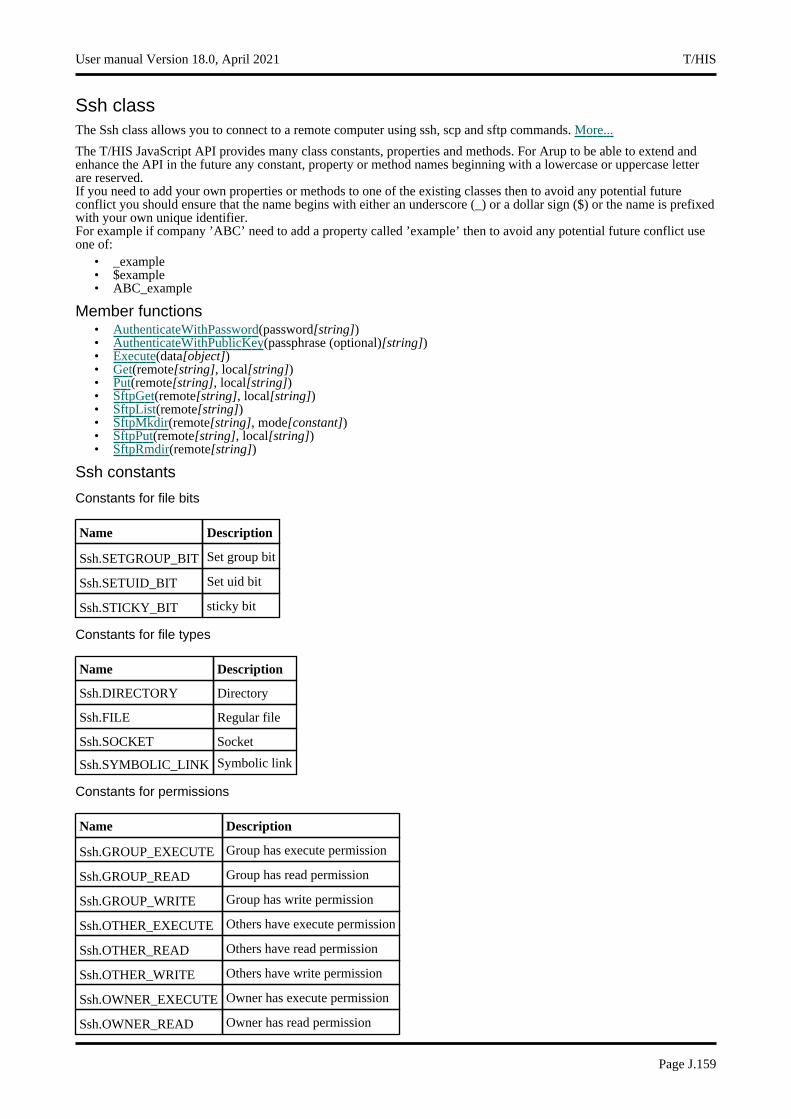
Ssh classThe Ssh class allows you to connect to a remote computer using ssh, scp and sftp commands. More...
The T/HIS JavaScript API provides many class constants, properties and methods. For Arup to be able to extend and enhance the API in the future any constant, property or method names beginning with a lowercase or uppercase letter are reserved.If you need to add your own properties or methods to one of the existing classes then to avoid any potential future conflict you should ensure that the name begins with either an underscore (_) or a dollar sign ($) or the name is prefixed with your own unique identifier.For example if company ’ABC’ need to add a property called ’example’ then to avoid any potential future conflict use one of:
• _example • $example • ABC_example
Member functions• AuthenticateWithPassword(password[string]) • AuthenticateWithPublicKey(passphrase (optional)[string]) • Execute(data[object]) • Get(remote[string], local[string]) • Put(remote[string], local[string]) • SftpGet(remote[string], local[string]) • SftpList(remote[string]) • SftpMkdir(remote[string], mode[constant]) • SftpPut(remote[string], local[string]) • SftpRmdir(remote[string])
Ssh constants
Constants for file bits
Name Description
Ssh.SETGROUP_BIT Set group bit
Ssh.SETUID_BIT Set uid bit
Ssh.STICKY_BIT sticky bit
Constants for file types
Name Description
Ssh.DIRECTORY Directory
Ssh.FILE Regular file
Ssh.SOCKET Socket
Ssh.SYMBOLIC_LINK Symbolic link
Constants for permissions
Name Description
Ssh.GROUP_EXECUTE Group has execute permission
Ssh.GROUP_READ Group has read permission
Ssh.GROUP_WRITE Group has write permission
Ssh.OTHER_EXECUTE Others have execute permission
Ssh.OTHER_READ Others have read permission
Ssh.OTHER_WRITE Others have write permission
Ssh.OWNER_EXECUTE Owner has execute permission
Ssh.OWNER_READ Owner has read permission
User manual Version 18.0, April 2021 T/HIS
Page J.159

Ssh.OWNER_WRITE Owner has write permission
Detailed DescriptionThe Ssh class gives you simple functions to do secure connections to a remote computer using ssh. The Oasys Ltd LS-DYNA environment software is built with the OpenSSH library to support the ssh, scp and sftp protocols. The basic workflow is to create a connection using the Ssh constructor, authenticate the connection either by using a password and AuthenticateWithPassword or with a public key and AuthenticateWithPublicKey then the method Execute can be used to execute commands on the remote machine, the methods Get and Put can be used to copy files to and from the remote machine using scp, and the commands SftpGet, SftpList, SftpMkdir, SftpPut and SftpRmdir can be used to perform secure file transfer commands.ssh uses a public and private key pair to do communication. The software uses RSA for the private and public keys and stores them in the files id_rsa and id_rsa.pub in the .oasys_ssh directory of your home directory (C:\Users\your.name\.oasys_ssh on Windows by default). A key length of 2048 bits is recommended. You keep your private key secure in your .oasys_ssh directory but the public key can be copied to the authorized_keys file on remote machines so that authentication can be done etc. The software also maintains fingerprints for the machines you connect to to ensure that you are connecting to the machine that you think you are. The first time you connect to a machine you are asked to confirm the remote machine is correct and the software stores the fingerprint for it in the known_hosts file in your .oasys_ssh directory. For second and subsequent connections the software checks the fingerprint of the remote machine against the one it has stored and will only connect if it matches. When creating a new ssh connection to a remote machine and transferring files a small ’buffer’ is required to transfer the data. The size of this buffer can be controlled using the Options.ssh_buffer_size property before the Ssh object is created.
Constructor
new Ssh(hostname[string], username[string])
Description
Create a new Ssh object for secure communication to a remote computer.
Arguments
Name Type Description
hostname string The hostname of the machine that you want to connect to
username string The username on the machine that you want to connect to
Return type
Ssh object
Example
To create a connection to machine "example" as user "username"
var s = new Ssh("example", "username");
Details of functions
AuthenticateWithPassword(password[string])
Description
Authenticate the connection using password.
Arguments
Name Type Description
password string The password for the username on the remote machine
Return type
no return value
T/HIS User manual Version 18.0, April 2021
Page J.160
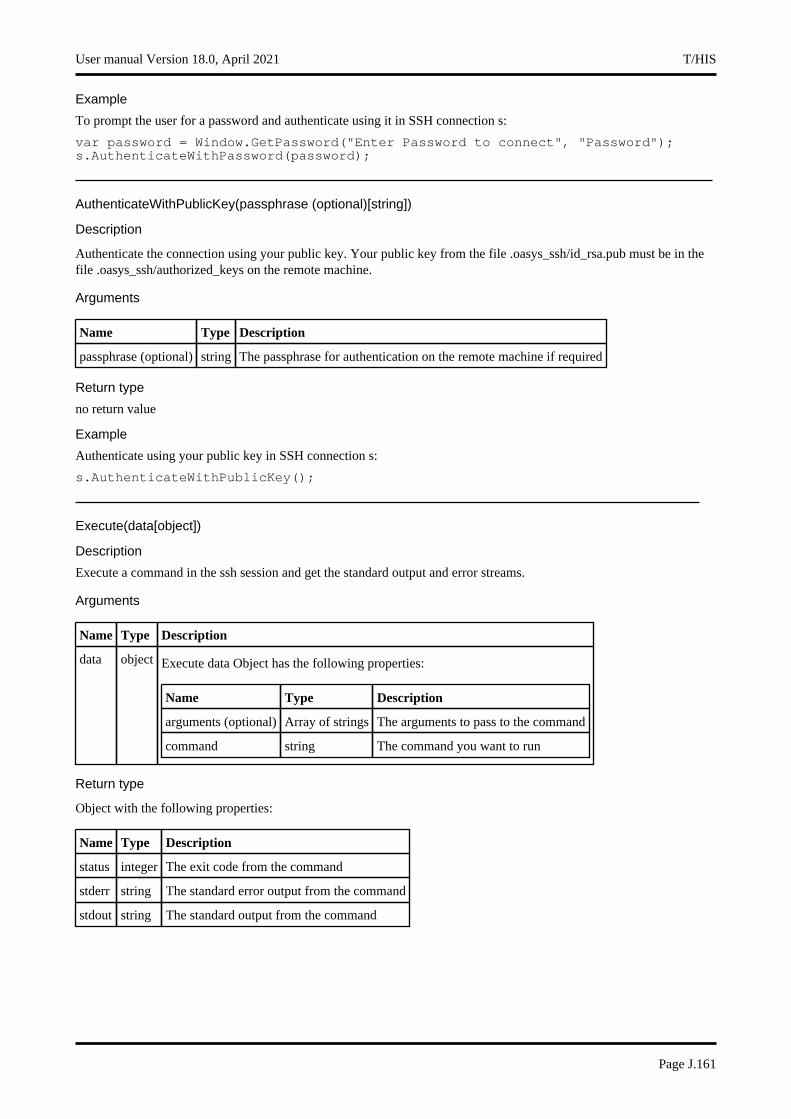
Example
To prompt the user for a password and authenticate using it in SSH connection s:
var password = Window.GetPassword("Enter Password to connect", "Password");s.AuthenticateWithPassword(password);
AuthenticateWithPublicKey(passphrase (optional)[string])
Description
Authenticate the connection using your public key. Your public key from the file .oasys_ssh/id_rsa.pub must be in the file .oasys_ssh/authorized_keys on the remote machine.
Arguments
Name Type Description
passphrase (optional) string The passphrase for authentication on the remote machine if required
Return type
no return value
Example
Authenticate using your public key in SSH connection s:
s.AuthenticateWithPublicKey();
Execute(data[object])
Description
Execute a command in the ssh session and get the standard output and error streams.
Arguments
Name Type Description
data object Execute data Object has the following properties:
Name Type Description
arguments (optional) Array of strings The arguments to pass to the command
command string The command you want to run
Return type
Object with the following properties:
Name Type Description
status integer The exit code from the command
stderr string The standard error output from the command
stdout string The standard output from the command
User manual Version 18.0, April 2021 T/HIS
Page J.161

Example
To run command "example.bat" with arguments "foo" and "bar" in SSH connection s:
var output = s.Execute( { command: ’example.bat’, arguments: [ ’foo’, ’bar’ ]} );var text = output.stdout;var errors = output.stderr;var ecode = output.status;
Get(remote[string], local[string])
Description
Gets a file from the ssh connection using scp.
Arguments
Name Type Description
remote string The path of the remote file to get
local string The path of the local file to write
Return type
no return value
Example
To get the remote file "/path/to/file.txt", creating local file "C:\path\to\file.txt" in SSH connection s:
s.Get("/path/to/file.txt", "C:\\path\\to\\file.txt");
Put(remote[string], local[string])
Description
Puts a file on the remote ssh connection using scp.
Arguments
Name Type Description
remote string The path of the remote file to put
local string The path of the local file to read
Return type
no return value
Example
To put the local file "C:\path\to\file.txt" to remote file "/path/to/file.txt" in SSH connection s:
s.Put("/path/to/file.txt", "C:\\path\\to\\file.txt");
SftpGet(remote[string], local[string])
Description
Gets a file from the ssh connection using sftp.
T/HIS User manual Version 18.0, April 2021
Page J.162

Arguments
Name Type Description
remote string The path of the remote file to get
local string The path of the local file to write
Return type
no return value
Example
To get the remote file "file.txt", creating local file "C:\path\to\file.txt" in SSH connection s using sftp:
s.SftpGet("file.txt", "C:\\path\\to\\file.txt");
SftpList(remote[string])
Description
Gets a listing from the ssh connection using sftp.
Arguments
Name Type Description
remote string The remote path to get the listing from
Return type
Object with the following properties:
Name Type Description
atime integer Access time for the file (seconds since epoch)
gid integer The group ID
info constant Bitwise information for the file/directory. See the permissions, file types and file bits constants
mtime integer Modification time for the file (seconds since epoch)
name string The name of the file/directory
size integer The size of the file
uid integer The user ID
Example
To get listing from the the remote path "temp" in SSH connection s using sftp:
var listing = s.SftpList("temp");for (l=0; l<listing.length; l++){
Message(listing[l].name + ":" + listing[l].size;}
SftpMkdir(remote[string], mode[constant])
Description
Creates a directory in the remote ssh connection using sftp.
User manual Version 18.0, April 2021 T/HIS
Page J.163

Arguments
Name Type Description
remote string The remote directory to create
mode constant The mode/permissions for the directory. See the permissions constants for details. Note that the user’s file-creation mask (umask) value will also be taken into account when creating the directory.
Return type
true if successful, false if not
Example
To create the remote path "temp" with, create, write and execute permissions for only the owner, in SSH connection s using sftp:
var success = s.SftpMkdir("temp", Ssh.OWNER_READ|Ssh.OWNER_WRITE|Ssh.OWNER_EXECUTE);
SftpPut(remote[string], local[string])
Description
Puts a file on the remote ssh connection using sftp.
Arguments
Name Type Description
remote string The path of the remote file to put
local string The path of the local file to read
Return type
no return value
Example
To put the local file "C:\path\to\file.txt" to remote file "file.txt" in SSH connection s:
s.SftpPut("file.txt", "C:\\path\\to\\file.txt");
SftpRmdir(remote[string])
Description
Deletes a directory in the remote ssh connection using sftp. If this fails it is probably because the directory is not empty.
Arguments
Name Type Description
remote string The remote directory to delete
Return type
true if successful, false if not
Example
To delete the remote path "temp" in SSH connection s using sftp:
var success = s.SftpRmdir("temp");
T/HIS User manual Version 18.0, April 2021
Page J.164
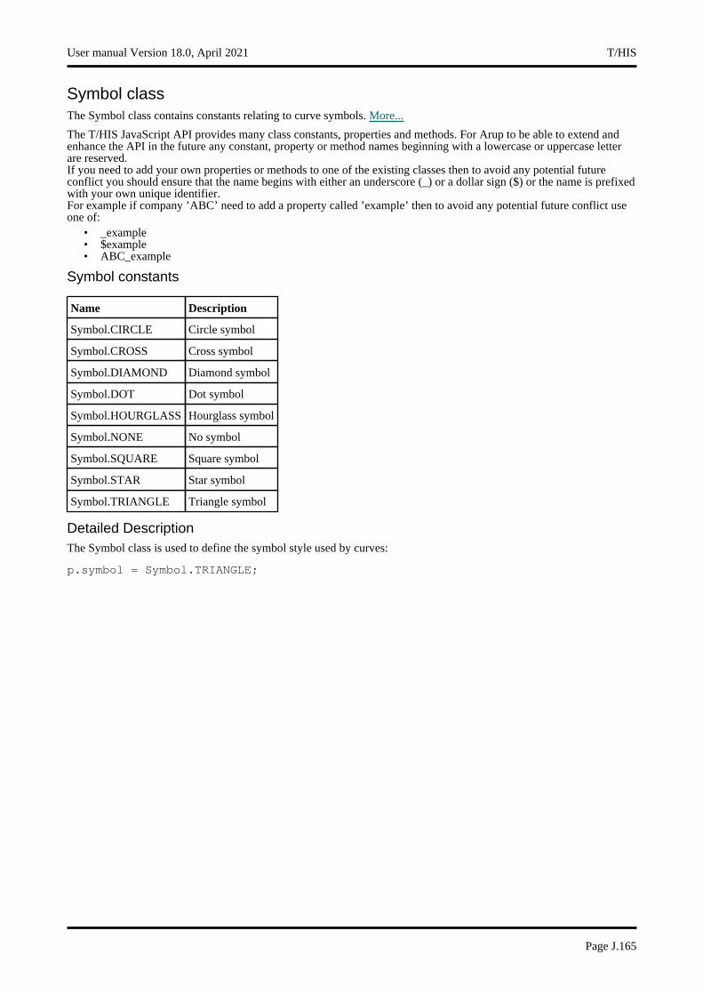
Symbol classThe Symbol class contains constants relating to curve symbols. More...
The T/HIS JavaScript API provides many class constants, properties and methods. For Arup to be able to extend and enhance the API in the future any constant, property or method names beginning with a lowercase or uppercase letter are reserved.If you need to add your own properties or methods to one of the existing classes then to avoid any potential future conflict you should ensure that the name begins with either an underscore (_) or a dollar sign ($) or the name is prefixed with your own unique identifier.For example if company ’ABC’ need to add a property called ’example’ then to avoid any potential future conflict use one of:
• _example • $example • ABC_example
Symbol constants
Name Description
Symbol.CIRCLE Circle symbol
Symbol.CROSS Cross symbol
Symbol.DIAMOND Diamond symbol
Symbol.DOT Dot symbol
Symbol.HOURGLASS Hourglass symbol
Symbol.NONE No symbol
Symbol.SQUARE Square symbol
Symbol.STAR Star symbol
Symbol.TRIANGLE Triangle symbol
Detailed DescriptionThe Symbol class is used to define the symbol style used by curves:
p.symbol = Symbol.TRIANGLE;
User manual Version 18.0, April 2021 T/HIS
Page J.165
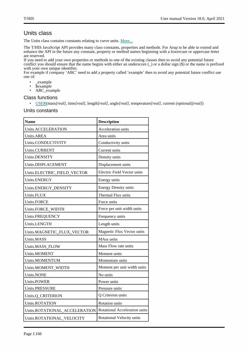
Units classThe Units class contains constants relating to curve units. More...
The T/HIS JavaScript API provides many class constants, properties and methods. For Arup to be able to extend and enhance the API in the future any constant, property or method names beginning with a lowercase or uppercase letter are reserved.If you need to add your own properties or methods to one of the existing classes then to avoid any potential future conflict you should ensure that the name begins with either an underscore (_) or a dollar sign ($) or the name is prefixed with your own unique identifier.For example if company ’ABC’ need to add a property called ’example’ then to avoid any potential future conflict use one of:
• _example • $example • ABC_example
Class functions• USER(mass[real], time[real], length[real], angle[real], temperature[real], current (optional)[real])
Units constants
Name Description
Units.ACCELERATION Acceleration units
Units.AREA Area units
Units.CONDUCTIVITY Conductivity units
Units.CURRENT Current units
Units.DENSITY Density units
Units.DISPLACEMENT Displacement units
Units.ELECTRIC_FIELD_VECTOR Electric Field Vector units
Units.ENERGY Energy units
Units.ENERGY_DENSITY Energy Density units
Units.FLUX Thermal Flux units
Units.FORCE Force units
Units.FORCE_WIDTH Force per unit width units
Units.FREQUENCY Frequency units
Units.LENGTH Length units
Units.MAGNETIC_FLUX_VECTOR Magnetic Flux Vector units
Units.MASS MAss units
Units.MASS_FLOW Mass Flow rate units
Units.MOMENT Moment units
Units.MOMENTUM Momentum units
Units.MOMENT_WIDTH Moment per unit width units
Units.NONE No units
Units.POWER Power units
Units.PRESSURE Pressure units
Units.Q_CRITERION Q Criterion units
Units.ROTATION Rotation units
Units.ROTATIONAL_ACCELERATION Rotational Acceleration units
Units.ROTATIONAL_VELOCITY Rotational Velocity units
T/HIS User manual Version 18.0, April 2021
Page J.166

Units.STRAIN Strain units
Units.STRESS Stress units
Units.TEMPERATURE Temperature units
Units.THERMAL_DIFFUSIVITY Thermal Diffusivity units
Units.TIME Time units
Units.UNKNOWN Unknown units
Units.VECTOR_POTENTIAL Vector Potential units
Units.VELOCITY Velocity units
Units.VISCOSITY Viscosity units
Units.VOLUME Volume units
Units.VORTICITY Vorticity units
Units.WORK Work units
Detailed DescriptionThe Units class is used to define the units for each axis of a curve:
p.x_axis_units = Units.LENGTH
Details of functions
USER(mass[real], time[real], length[real], angle[real], temperature[real], current (optional)[real]) [static]
Description
Setup a user defined UNIT
Arguments
Name Type Description
mass real Power for mass dimensions.
time real Power for time dimensions.
length real Power for length dimensions.
angle real Power for angle dimensions.
temperature real Power for temperature dimensions.
current (optional) real Power for current dimensions.
Return type
integer
Example
To set the y-axis unit of curve l to (m/s)^2:
l.y_unit = Units.USER(0.0,2.0,-2.0,0.0,0.0,0.0);
User manual Version 18.0, April 2021 T/HIS
Page J.167
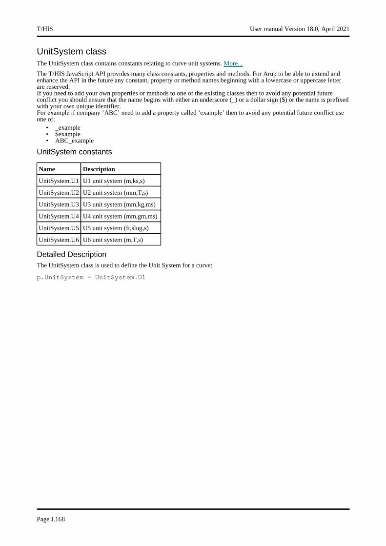
UnitSystem classThe UnitSystem class contains constants relating to curve unit systems. More...
The T/HIS JavaScript API provides many class constants, properties and methods. For Arup to be able to extend and enhance the API in the future any constant, property or method names beginning with a lowercase or uppercase letter are reserved.If you need to add your own properties or methods to one of the existing classes then to avoid any potential future conflict you should ensure that the name begins with either an underscore (_) or a dollar sign ($) or the name is prefixed with your own unique identifier.For example if company ’ABC’ need to add a property called ’example’ then to avoid any potential future conflict use one of:
• _example • $example • ABC_example
UnitSystem constants
Name Description
UnitSystem.U1 U1 unit system (m,ks,s)
UnitSystem.U2 U2 unit system (mm,T,s)
UnitSystem.U3 U3 unit system (mm,kg,ms)
UnitSystem.U4 U4 unit system (mm,gm,ms)
UnitSystem.U5 U5 unit system (ft,slug,s)
UnitSystem.U6 U6 unit system (m,T,s)
Detailed DescriptionThe UnitSystem class is used to define the Unit System for a curve:
p.UnitSystem = UnitSystem.U1
T/HIS User manual Version 18.0, April 2021
Page J.168
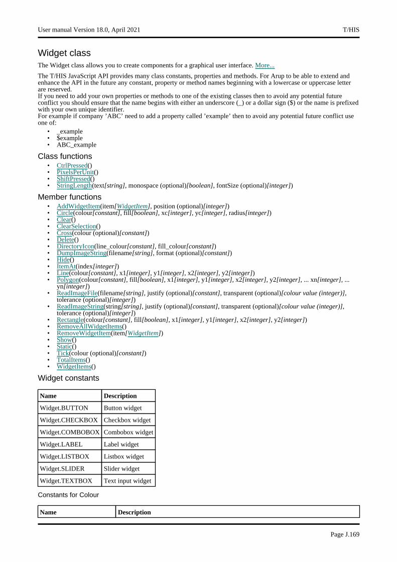
Widget classThe Widget class allows you to create components for a graphical user interface. More...
The T/HIS JavaScript API provides many class constants, properties and methods. For Arup to be able to extend and enhance the API in the future any constant, property or method names beginning with a lowercase or uppercase letter are reserved.If you need to add your own properties or methods to one of the existing classes then to avoid any potential future conflict you should ensure that the name begins with either an underscore (_) or a dollar sign ($) or the name is prefixed with your own unique identifier.For example if company ’ABC’ need to add a property called ’example’ then to avoid any potential future conflict use one of:
• _example • $example • ABC_example
Class functions• CtrlPressed() • PixelsPerUnit() • ShiftPressed() • StringLength(text[string], monospace (optional)[boolean], fontSize (optional)[integer])
Member functions• AddWidgetItem(item[WidgetItem], position (optional)[integer]) • Circle(colour[constant], fill[boolean], xc[integer], yc[integer], radius[integer]) • Clear() • ClearSelection() • Cross(colour (optional)[constant]) • Delete() • DirectoryIcon(line_colour[constant], fill_colour[constant]) • DumpImageString(filename[string], format (optional)[constant]) • Hide() • ItemAt(index[integer]) • Line(colour[constant], x1[integer], y1[integer], x2[integer], y2[integer]) • Polygon(colour[constant], fill[boolean], x1[integer], y1[integer], x2[integer], y2[integer], ... xn[integer], ...
yn[integer]) • ReadImageFile(filename[string], justify (optional)[constant], transparent (optional)[colour value (integer)],
tolerance (optional)[integer]) • ReadImageString(string[string], justify (optional)[constant], transparent (optional)[colour value (integer)],
tolerance (optional)[integer]) • Rectangle(colour[constant], fill[boolean], x1[integer], y1[integer], x2[integer], y2[integer]) • RemoveAllWidgetItems() • RemoveWidgetItem(item[WidgetItem]) • Show() • Static() • Tick(colour (optional)[constant]) • TotalItems() • WidgetItems()
Widget constants
Name Description
Widget.BUTTON Button widget
Widget.CHECKBOX Checkbox widget
Widget.COMBOBOX Combobox widget
Widget.LABEL Label widget
Widget.LISTBOX Listbox widget
Widget.SLIDER Slider widget
Widget.TEXTBOX Text input widget
Constants for Colour
Name Description
User manual Version 18.0, April 2021 T/HIS
Page J.169
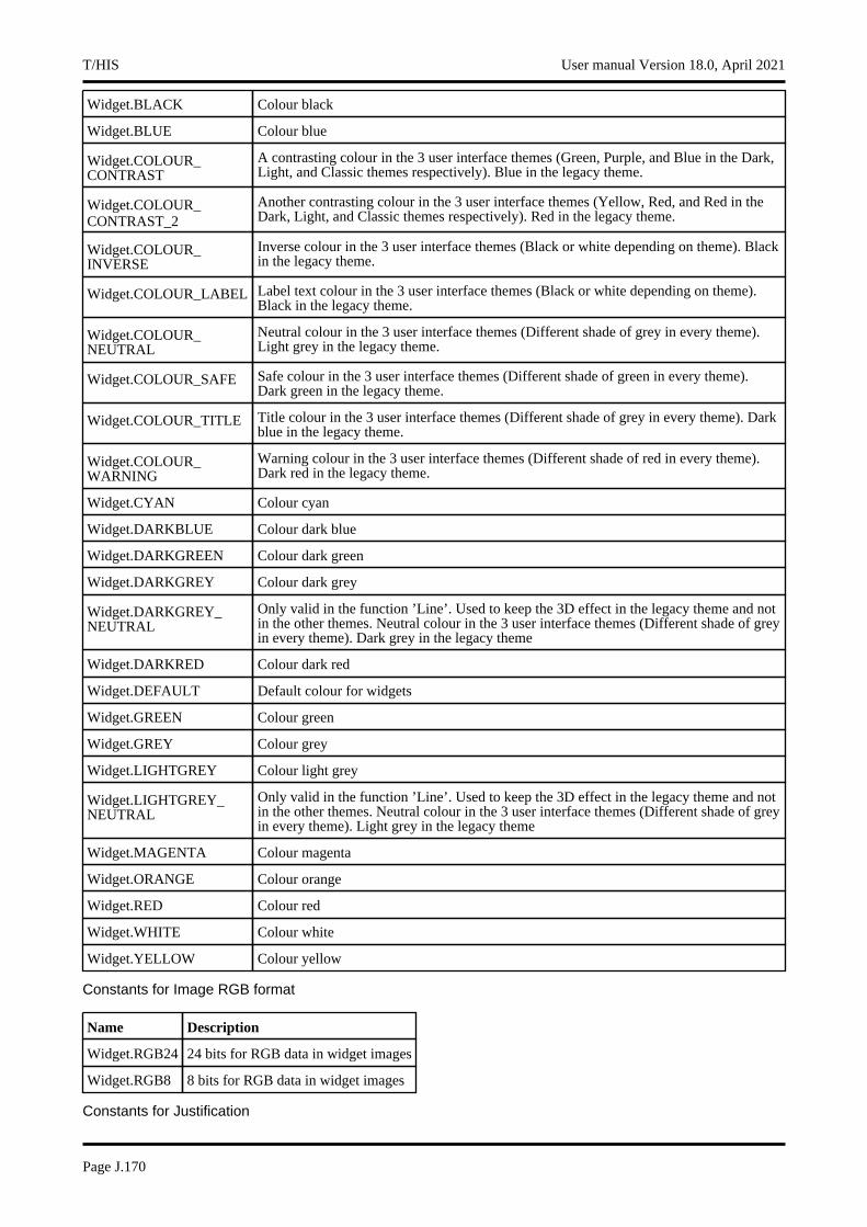
Widget.BLACK Colour black
Widget.BLUE Colour blue
Widget.COLOUR_CONTRAST
A contrasting colour in the 3 user interface themes (Green, Purple, and Blue in the Dark, Light, and Classic themes respectively). Blue in the legacy theme.
Widget.COLOUR_CONTRAST_2
Another contrasting colour in the 3 user interface themes (Yellow, Red, and Red in the Dark, Light, and Classic themes respectively). Red in the legacy theme.
Widget.COLOUR_INVERSE
Inverse colour in the 3 user interface themes (Black or white depending on theme). Black in the legacy theme.
Widget.COLOUR_LABEL Label text colour in the 3 user interface themes (Black or white depending on theme). Black in the legacy theme.
Widget.COLOUR_NEUTRAL
Neutral colour in the 3 user interface themes (Different shade of grey in every theme). Light grey in the legacy theme.
Widget.COLOUR_SAFE Safe colour in the 3 user interface themes (Different shade of green in every theme). Dark green in the legacy theme.
Widget.COLOUR_TITLE Title colour in the 3 user interface themes (Different shade of grey in every theme). Dark blue in the legacy theme.
Widget.COLOUR_WARNING
Warning colour in the 3 user interface themes (Different shade of red in every theme). Dark red in the legacy theme.
Widget.CYAN Colour cyan
Widget.DARKBLUE Colour dark blue
Widget.DARKGREEN Colour dark green
Widget.DARKGREY Colour dark grey
Widget.DARKGREY_NEUTRAL
Only valid in the function ’Line’. Used to keep the 3D effect in the legacy theme and not in the other themes. Neutral colour in the 3 user interface themes (Different shade of grey in every theme). Dark grey in the legacy theme
Widget.DARKRED Colour dark red
Widget.DEFAULT Default colour for widgets
Widget.GREEN Colour green
Widget.GREY Colour grey
Widget.LIGHTGREY Colour light grey
Widget.LIGHTGREY_NEUTRAL
Only valid in the function ’Line’. Used to keep the 3D effect in the legacy theme and not in the other themes. Neutral colour in the 3 user interface themes (Different shade of grey in every theme). Light grey in the legacy theme
Widget.MAGENTA Colour magenta
Widget.ORANGE Colour orange
Widget.RED Colour red
Widget.WHITE Colour white
Widget.YELLOW Colour yellow
Constants for Image RGB format
Name Description
Widget.RGB24 24 bits for RGB data in widget images
Widget.RGB8 8 bits for RGB data in widget images
Constants for Justification
T/HIS User manual Version 18.0, April 2021
Page J.170
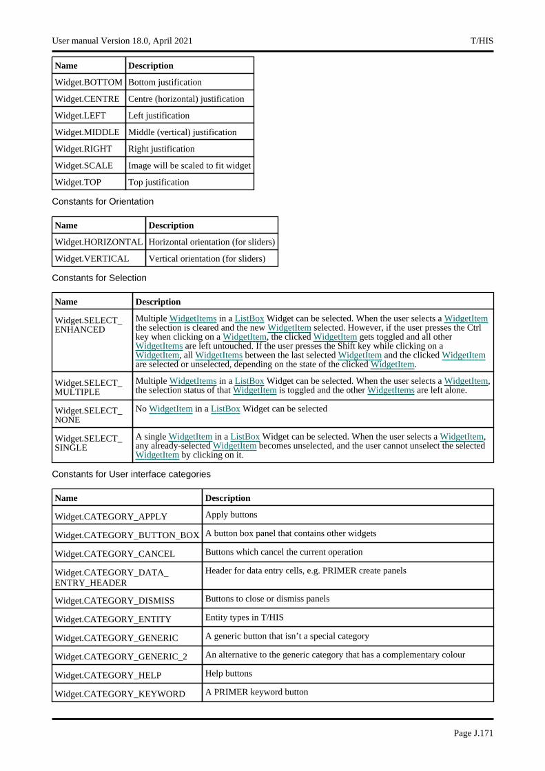
Name Description
Widget.BOTTOM Bottom justification
Widget.CENTRE Centre (horizontal) justification
Widget.LEFT Left justification
Widget.MIDDLE Middle (vertical) justification
Widget.RIGHT Right justification
Widget.SCALE Image will be scaled to fit widget
Widget.TOP Top justification
Constants for Orientation
Name Description
Widget.HORIZONTAL Horizontal orientation (for sliders)
Widget.VERTICAL Vertical orientation (for sliders)
Constants for Selection
Name Description
Widget.SELECT_ENHANCED
Multiple WidgetItems in a ListBox Widget can be selected. When the user selects a WidgetItemthe selection is cleared and the new WidgetItem selected. However, if the user presses the Ctrl key when clicking on a WidgetItem, the clicked WidgetItem gets toggled and all other WidgetItems are left untouched. If the user presses the Shift key while clicking on a WidgetItem, all WidgetItems between the last selected WidgetItem and the clicked WidgetItemare selected or unselected, depending on the state of the clicked WidgetItem.
Widget.SELECT_MULTIPLE
Multiple WidgetItems in a ListBox Widget can be selected. When the user selects a WidgetItem, the selection status of that WidgetItem is toggled and the other WidgetItems are left alone.
Widget.SELECT_NONE
No WidgetItem in a ListBox Widget can be selected
Widget.SELECT_SINGLE
A single WidgetItem in a ListBox Widget can be selected. When the user selects a WidgetItem, any already-selected WidgetItem becomes unselected, and the user cannot unselect the selected WidgetItem by clicking on it.
Constants for User interface categories
Name Description
Widget.CATEGORY_APPLY Apply buttons
Widget.CATEGORY_BUTTON_BOX A button box panel that contains other widgets
Widget.CATEGORY_CANCEL Buttons which cancel the current operation
Widget.CATEGORY_DATA_ENTRY_HEADER
Header for data entry cells, e.g. PRIMER create panels
Widget.CATEGORY_DISMISS Buttons to close or dismiss panels
Widget.CATEGORY_ENTITY Entity types in T/HIS
Widget.CATEGORY_GENERIC A generic button that isn’t a special category
Widget.CATEGORY_GENERIC_2 An alternative to the generic category that has a complementary colour
Widget.CATEGORY_HELP Help buttons
Widget.CATEGORY_KEYWORD A PRIMER keyword button
User manual Version 18.0, April 2021 T/HIS
Page J.171
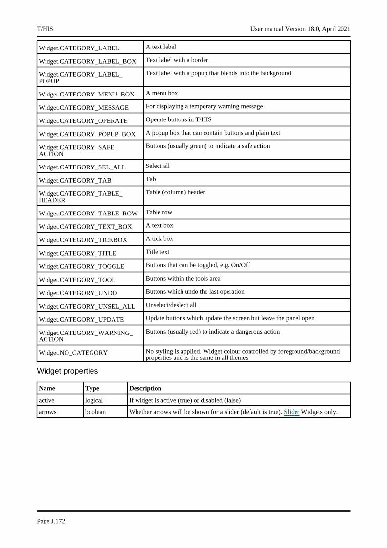
Widget.CATEGORY_LABEL A text label
Widget.CATEGORY_LABEL_BOX Text label with a border
Widget.CATEGORY_LABEL_POPUP
Text label with a popup that blends into the background
Widget.CATEGORY_MENU_BOX A menu box
Widget.CATEGORY_MESSAGE For displaying a temporary warning message
Widget.CATEGORY_OPERATE Operate buttons in T/HIS
Widget.CATEGORY_POPUP_BOX A popup box that can contain buttons and plain text
Widget.CATEGORY_SAFE_ACTION
Buttons (usually green) to indicate a safe action
Widget.CATEGORY_SEL_ALL Select all
Widget.CATEGORY_TAB Tab
Widget.CATEGORY_TABLE_HEADER
Table (column) header
Widget.CATEGORY_TABLE_ROW Table row
Widget.CATEGORY_TEXT_BOX A text box
Widget.CATEGORY_TICKBOX A tick box
Widget.CATEGORY_TITLE Title text
Widget.CATEGORY_TOGGLE Buttons that can be toggled, e.g. On/Off
Widget.CATEGORY_TOOL Buttons within the tools area
Widget.CATEGORY_UNDO Buttons which undo the last operation
Widget.CATEGORY_UNSEL_ALL Unselect/deslect all
Widget.CATEGORY_UPDATE Update buttons which update the screen but leave the panel open
Widget.CATEGORY_WARNING_ACTION
Buttons (usually red) to indicate a dangerous action
Widget.NO_CATEGORY No styling is applied. Widget colour controlled by foreground/background properties and is the same in all themes
Widget properties
Name Type Description
active logical If widget is active (true) or disabled (false)
arrows boolean Whether arrows will be shown for a slider (default is true). Slider Widgets only.
T/HIS User manual Version 18.0, April 2021
Page J.172

background constant Widget background colour. Can be: Widget.BLACK, Widget.WHITE, Widget.RED, Widget.GREEN, Widget.BLUE, Widget.CYAN, Widget.MAGENTA, Widget.YELLOW, Widget.DARKRED, Widget.DARKGREEN, Widget.DARKBLUE, Widget.GREY, Widget.DARKGREY, Widget.LIGHTGREY, Widget.ORANGE, Widget.DEFAULT, Widget.COLOUR_NEUTRAL, Widget.COLOUR_CONTRAST, Widget.COLOUR_CONTRAST_2, Widget.COLOUR_WARNING, Widget.COLOUR_SAFE, Widget.COLOUR_TITLE, Widget.COLOUR_INVERSE, Widget.DARKGREY_NEUTRAL, Widget.LIGHTGREY_NEUTRALNote, background colours in the Window.THEME_DARK, Window.THEME_LIGHT, and Window.THEME_CLASSIC themes will be determined by the category of the widget not the background colour. To override this behaviour and use this background colour first set the widget category to Widget.NO_CATEGORY.
bottom integer Widget bottom coordinate
category constant The button category which determines the button’s appearance when using the new user interface, see Window.Theme()
fontSize integer Widget font size in points. Currently only supports the following sizes: 6, 7, 8, 10, 12, 14, 18, 24. Can be used only with Widget.LABEL and Widget.BUTTON. Both LATIN1 and UTF-8 encoding is supported on Windows but Linux only supports LATIN1 encoding at the moment.
foreground constant Widget foreground colour. Can be: Widget.BLACK, Widget.WHITE, Widget.RED, Widget.GREEN, Widget.BLUE, Widget.CYAN, Widget.MAGENTA, Widget.YELLOW, Widget.DARKRED, Widget.DARKGREEN, Widget.DARKBLUE, Widget.GREY, Widget.DARKGREY, Widget.LIGHTGREY, Widget.ORANGE, Widget.DEFAULT, Widget.COLOUR_NEUTRAL, Widget.COLOUR_CONTRAST, Widget.COLOUR_CONTRAST_2, Widget.COLOUR_WARNING, Widget.COLOUR_SAFE, Widget.COLOUR_TITLE, Widget.COLOUR_LABEL, Widget.COLOUR_INVERSE, Widget.DARKGREY_NEUTRAL, Widget.LIGHTGREY_NEUTRAL
hover string Widget hover text
imageHeight (read only)
integer Height of widget image (pixels)
imageWidth (read only)
integer Width of widget image (pixels)
justify constant Widget justification. Can be: Widget.LEFT, Widget.RIGHT or Widget.CENTRE(default).
left integer Widget left coordinate
lineWidth integer Width of lines when drawing graphics (initially 1; values 1-100 allowed).
macroTag string Tag to use for this widget when recording a macro. If empty then the text property value will be used.
maximum integer The maximum value allowed for a slider (default is 100). Slider Widgets only.
minimum integer The minimum value allowed for a slider (default is 0). Slider Widgets only.
monospace boolean true if the widget uses a monospace font instead of a proportional width font (default). Label and button Widgets only.
onChange function Function to call when the text in a TEXTBOX widget, the selection in a COMBOBOX widget or the value of a SLIDER is changed. The Widget object is accessible in the function using the ’this’ keyword (see the example below for more details of how to define the function and how to use the ’this’ keyword). To unset the function set the property to null. Note that this function is called when the user actually types something into the textbox, selects an item in the combobox or moves the slider, NOT when the Widget.text or Widget.value property changes.
User manual Version 18.0, April 2021 T/HIS
Page J.173
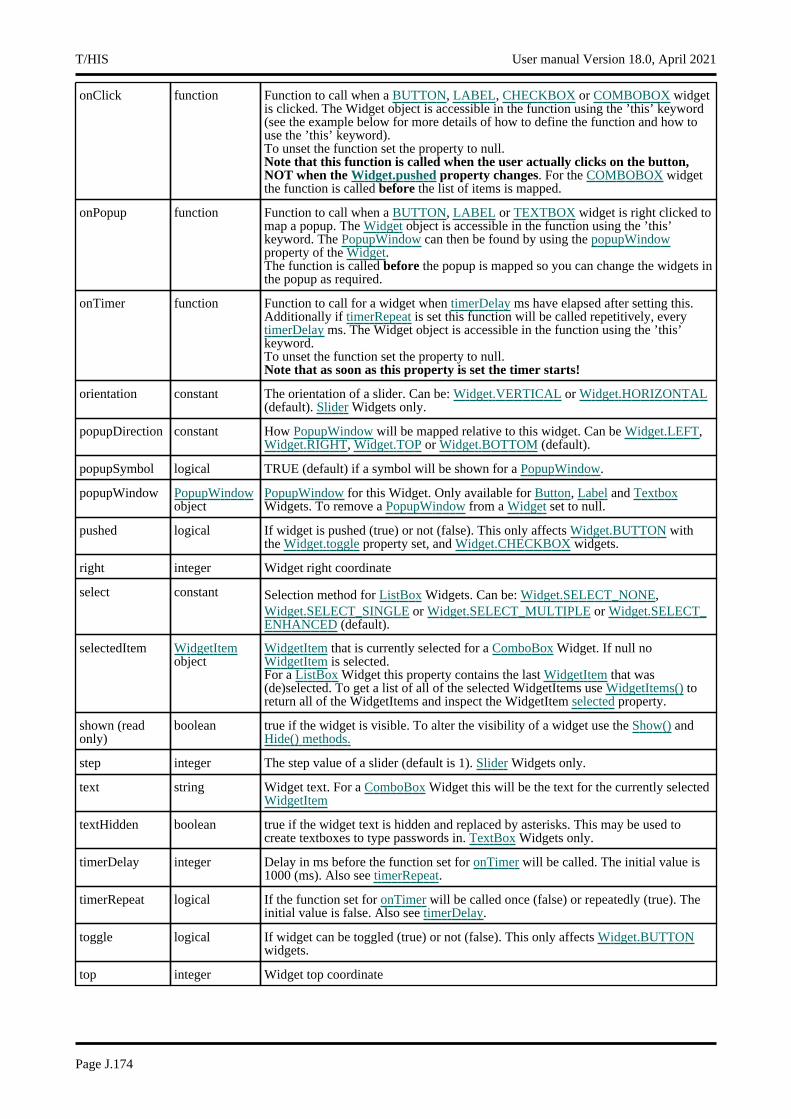
onClick function Function to call when a BUTTON, LABEL, CHECKBOX or COMBOBOX widget is clicked. The Widget object is accessible in the function using the ’this’ keyword (see the example below for more details of how to define the function and how to use the ’this’ keyword). To unset the function set the property to null. Note that this function is called when the user actually clicks on the button, NOT when the Widget.pushed property changes. For the COMBOBOX widget the function is called before the list of items is mapped.
onPopup function Function to call when a BUTTON, LABEL or TEXTBOX widget is right clicked to map a popup. The Widget object is accessible in the function using the ’this’ keyword. The PopupWindow can then be found by using the popupWindowproperty of the Widget. The function is called before the popup is mapped so you can change the widgets in the popup as required.
onTimer function Function to call for a widget when timerDelay ms have elapsed after setting this. Additionally if timerRepeat is set this function will be called repetitively, every timerDelay ms. The Widget object is accessible in the function using the ’this’ keyword. To unset the function set the property to null. Note that as soon as this property is set the timer starts!
orientation constant The orientation of a slider. Can be: Widget.VERTICAL or Widget.HORIZONTAL(default). Slider Widgets only.
popupDirection constant How PopupWindow will be mapped relative to this widget. Can be Widget.LEFT, Widget.RIGHT, Widget.TOP or Widget.BOTTOM (default).
popupSymbol logical TRUE (default) if a symbol will be shown for a PopupWindow.
popupWindow PopupWindowobject
PopupWindow for this Widget. Only available for Button, Label and TextboxWidgets. To remove a PopupWindow from a Widget set to null.
pushed logical If widget is pushed (true) or not (false). This only affects Widget.BUTTON with the Widget.toggle property set, and Widget.CHECKBOX widgets.
right integer Widget right coordinate
select constant Selection method for ListBox Widgets. Can be: Widget.SELECT_NONE, Widget.SELECT_SINGLE or Widget.SELECT_MULTIPLE or Widget.SELECT_ENHANCED (default).
selectedItem WidgetItemobject
WidgetItem that is currently selected for a ComboBox Widget. If null no WidgetItem is selected.For a ListBox Widget this property contains the last WidgetItem that was (de)selected. To get a list of all of the selected WidgetItems use WidgetItems() to return all of the WidgetItems and inspect the WidgetItem selected property.
shown (read only)
boolean true if the widget is visible. To alter the visibility of a widget use the Show() and Hide() methods.
step integer The step value of a slider (default is 1). Slider Widgets only.
text string Widget text. For a ComboBox Widget this will be the text for the currently selected WidgetItem
textHidden boolean true if the widget text is hidden and replaced by asterisks. This may be used to create textboxes to type passwords in. TextBox Widgets only.
timerDelay integer Delay in ms before the function set for onTimer will be called. The initial value is 1000 (ms). Also see timerRepeat.
timerRepeat logical If the function set for onTimer will be called once (false) or repeatedly (true). The initial value is false. Also see timerDelay.
toggle logical If widget can be toggled (true) or not (false). This only affects Widget.BUTTONwidgets.
top integer Widget top coordinate
T/HIS User manual Version 18.0, April 2021
Page J.174
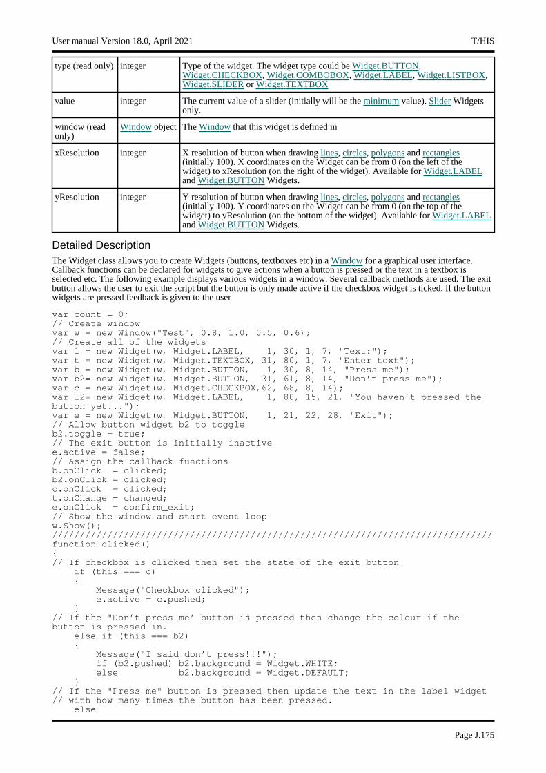
type (read only) integer Type of the widget. The widget type could be Widget.BUTTON, Widget.CHECKBOX, Widget.COMBOBOX, Widget.LABEL, Widget.LISTBOX, Widget.SLIDER or Widget.TEXTBOX
value integer The current value of a slider (initially will be the minimum value). Slider Widgets only.
window (read only)
Window object The Window that this widget is defined in
xResolution integer X resolution of button when drawing lines, circles, polygons and rectangles(initially 100). X coordinates on the Widget can be from 0 (on the left of the widget) to xResolution (on the right of the widget). Available for Widget.LABELand Widget.BUTTON Widgets.
yResolution integer Y resolution of button when drawing lines, circles, polygons and rectangles(initially 100). Y coordinates on the Widget can be from 0 (on the top of the widget) to yResolution (on the bottom of the widget). Available for Widget.LABELand Widget.BUTTON Widgets.
Detailed DescriptionThe Widget class allows you to create Widgets (buttons, textboxes etc) in a Window for a graphical user interface. Callback functions can be declared for widgets to give actions when a button is pressed or the text in a textbox is selected etc. The following example displays various widgets in a window. Several callback methods are used. The exit button allows the user to exit the script but the button is only made active if the checkbox widget is ticked. If the button widgets are pressed feedback is given to the user
var count = 0;// Create windowvar w = new Window("Test", 0.8, 1.0, 0.5, 0.6);// Create all of the widgetsvar l = new Widget(w, Widget.LABEL, 1, 30, 1, 7, "Text:");var t = new Widget(w, Widget.TEXTBOX, 31, 80, 1, 7, "Enter text");var b = new Widget(w, Widget.BUTTON, 1, 30, 8, 14, "Press me");var b2= new Widget(w, Widget.BUTTON, 31, 61, 8, 14, "Don’t press me");var c = new Widget(w, Widget.CHECKBOX,62, 68, 8, 14);var l2= new Widget(w, Widget.LABEL, 1, 80, 15, 21, "You haven’t pressed the button yet...");var e = new Widget(w, Widget.BUTTON, 1, 21, 22, 28, "Exit");// Allow button widget b2 to toggleb2.toggle = true;// The exit button is initially inactivee.active = false;// Assign the callback functionsb.onClick = clicked;b2.onClick = clicked;c.onClick = clicked;t.onChange = changed;e.onClick = confirm_exit;// Show the window and start event loopw.Show();////////////////////////////////////////////////////////////////////////////////function clicked(){// If checkbox is clicked then set the state of the exit button
if (this === c){
Message("Checkbox clicked");e.active = c.pushed;
}// If the "Don’t press me’ button is pressed then change the colour if the button is pressed in.
else if (this === b2){
Message("I said don’t press!!!");if (b2.pushed) b2.background = Widget.WHITE;else b2.background = Widget.DEFAULT;
}// If the "Press me" button is pressed then update the text in the label widget// with how many times the button has been pressed.
else
User manual Version 18.0, April 2021 T/HIS
Page J.175
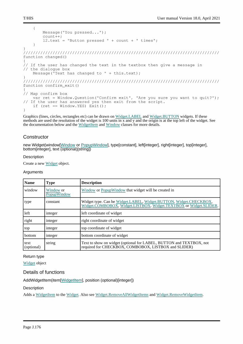
{Message("You pressed...");count++;l2.text = "Button pressed " + count + " times";
}}////////////////////////////////////////////////////////////////////////////////function changed(){// If the user has changed the text in the textbox then give a message in// the dialogue box
Message("Text has changed to " + this.text);}////////////////////////////////////////////////////////////////////////////////function confirm_exit(){// Map confirm box
var ret = Window.Question("Confirm exit", "Are you sure you want to quit?");// If the user has answered yes then exit from the script.
if (ret == Window.YES) Exit();}
Graphics (lines, circles, rectangles etc) can be drawn on Widget.LABEL and Widget.BUTTON widgets. If these methods are used the resolution of the widget is 100 units in x and y and the origin is at the top left of the widget. See the documentation below and the WidgetItem and Window classes for more details.
Constructor
new Widget(window[Window or PopupWindow], type[constant], left[integer], right[integer], top[integer], bottom[integer], text (optional)[string])
Description
Create a new Widget object.
Arguments
Name Type Description
window Window or PopupWindow
Window or PopupWindow that widget will be created in
type constant Widget type. Can be Widget.LABEL, Widget.BUTTON, Widget.CHECKBOX, Widget.COMBOBOX, Widget.LISTBOX, Widget.TEXTBOX or Widget.SLIDER.
left integer left coordinate of widget
right integer right coordinate of widget
top integer top coordinate of widget
bottom integer bottom coordinate of widget
text (optional)
string Text to show on widget (optional for LABEL, BUTTON and TEXTBOX, not required for CHECKBOX, COMBOBOX, LISTBOX and SLIDER)
Return type
Widget object
Details of functions
AddWidgetItem(item[WidgetItem], position (optional)[integer])
Description
Adds a WidgetItem to the Widget. Also see Widget.RemoveAllWidgetItems and Widget.RemoveWidgetItem.
T/HIS User manual Version 18.0, April 2021
Page J.176
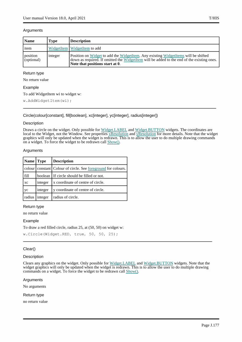
Arguments
Name Type Description
item WidgetItem WidgetItem to add
position (optional)
integer Position on Widget to add the WidgetItem. Any existing WidgetItems will be shifted down as required. If omitted the WidgetItem will be added to the end of the existing ones. Note that positions start at 0.
Return type
No return value
Example
To add WidgetItem wi to widget w:
w.AddWidgetItem(wi);
Circle(colour[constant], fill[boolean], xc[integer], yc[integer], radius[integer])
Description
Draws a circle on the widget. Only possible for Widget.LABEL and Widget.BUTTON widgets. The coordinates are local to the Widget, not the Window. See properties xResolution and yResolution for more details. Note that the widget graphics will only be updated when the widget is redrawn. This is to allow the user to do multiple drawing commands on a widget. To force the widget to be redrawn call Show().
Arguments
Name Type Description
colour constant Colour of circle. See foreground for colours.
fill boolean If circle should be filled or not.
xc integer x coordinate of centre of circle.
yc integer y coordinate of centre of circle.
radius integer radius of circle.
Return type
no return value
Example
To draw a red filled circle, radius 25, at (50, 50) on widget w:
w.Circle(Widget.RED, true, 50, 50, 25);
Clear()
Description
Clears any graphics on the widget. Only possible for Widget.LABEL and Widget.BUTTON widgets. Note that the widget graphics will only be updated when the widget is redrawn. This is to allow the user to do multiple drawing commands on a widget. To force the widget to be redrawn call Show().
Arguments
No arguments
Return type
no return value
User manual Version 18.0, April 2021 T/HIS
Page J.177
Example
To clear any graphics for widget w:
w.Clear();
ClearSelection()
Description
Clears selection of any WidgetItems on the widget. Only possible for Widget.COMBOBOX and Widget.LISTBOXwidgets.
Arguments
No arguments
Return type
no return value
Example
To clear selection of any WidgetItems for widget w:
w.ClearSelection();
Cross(colour (optional)[constant])
Description
Draws a cross symbol on the widget. Only possible for Widget.LABEL and Widget.BUTTON widgets.
Arguments
Name Type Description
colour (optional)
constant Colour of cross symbol. See foreground for colours. If omitted, current foreground colour is used.
Return type
no return value
Example
To draw a red cross symbol on widget w:
w.Cross(Widget.RED);
CtrlPressed() [static]
Description
Check to see if the Ctrl key is pressed
Arguments
No arguments
Return type
true/false
Example
To test if someone has the Ctrl key pressed:
if (Widget.CtrlPressed()) { ... }
T/HIS User manual Version 18.0, April 2021
Page J.178
Delete()
Description
Deletes the widget from T/HIS (removing it from the window it is defined in) and returns any memory/resources used for the widget. This function should not normally need to be called. However, sometimes a script may want to recreate widgets in a window many times and unless the old widgets are deleted T/HIS will reach the maximum number of widgets for a window (Options.max_widgets). To avoid this problem this method can be used to force T/HIS to delete and return the resources for a widget. Do not use the Widget object after calling this method.
Arguments
No arguments
Return type
no return value
Example
To delete widget w:
w.Delete();
DirectoryIcon(line_colour[constant], fill_colour[constant])
Description
Draws a directory icon on the widget. Only possible for Widget.BUTTON widgets.
Arguments
Name Type Description
line_colour
constant Colour of lines of folder (only used in the old UI - in the new UI it will be ignored, a standard icon is always used). See foreground for colours.
fill_colour
constant Colour of fill of folder (only used in the old UI - in the new UI it will be ignored, a standard icon is always used). See foreground for colours.
Return type
no return value
Example
To draw a directory icon on widget btn:
btn.DirectoryIcon(Widget.BLACK, Widget.YELLOW);
DumpImageString(filename[string], format (optional)[constant])
Description
Dumps a string representation of an image for a widget to a file in a form that can be used by Widget.ReadImageString(). Only possible for Widget.LABEL and Widget.BUTTON widgets.
Arguments
Name Type Description
filename string Filename to dump string representation to
format (optional)
constant Can be Widget.RGB8 or Widget.RGB24. Before version 15 T/HIS only used 8 bits to store RGB (red, green and blue) colour information for widget images. In version 15 widget images have been changed to use 24 bits to store RGB information (8 bits for red, 8 bits for green and 8 bits for blue). Both formats are supported. If omitted the new Widget.RGB24 format will be used. See Widget.ReadImageString() for more details.
User manual Version 18.0, April 2021 T/HIS
Page J.179

Return type
no return value
Example
To dump the image data to file ’image_data’ for widget w with the old 8 bit RGB representation:
w.DumpImageString(’image_data’, Widget.RGB8);
To dump the image data to file ’image_data’ for widget w with 24 bit RGB representation:
w.DumpImageString(’image_data’, Widget.RGB24);
Hide()
Description
Hides the widget on the screen
Arguments
No arguments
Return type
No return value
Example
To hide widget w
w.Hide();
ItemAt(index[integer])
Description
Returns the WidgetItem object used at index in this Widget. See also Widget.TotalItems() and Widget.WidgetItems().
Arguments
Name Type Description
index integer index to return WidgetItem for. Note that indices start at 0.
Return type
WidgetItem object.
Example
To loop over the WidgetItems used in Widget w
for (i=0; i<w.TotalItems(); i++){
wi = w.ItemAt(i);}
Line(colour[constant], x1[integer], y1[integer], x2[integer], y2[integer])
Description
Draws a line on the widget. Only possible for Widget.LABEL and Widget.BUTTON widgets. The coordinates are local to the Widget, not the Window. See properties xResolution and yResolution for more details. Note that the widget graphics will only be updated when the widget is redrawn. This is to allow the user to do multiple drawing commands on a widget. To force the widget to be redrawn call Show().
T/HIS User manual Version 18.0, April 2021
Page J.180
Arguments
Name Type Description
colour constant Colour of line. See foreground for colours.
x1 integer x coordinate of start of line.
y1 integer y coordinate of start of line.
x2 integer x coordinate of end of line.
y2 integer y coordinate of end of line.
Return type
no return value
Example
To draw a red line from (10, 90) to (90, 10) on widget w:
w.Line(Widget.RED, 10, 90, 90, 10);
PixelsPerUnit() [static]
Description
Returns the number of pixels per unit coordinate. This will vary depending on the monitor T/HIS is running on.
Arguments
No arguments
Return type
pixels/unit (real)
Example
To return how many pixels there are per unit coordinate:
var ppu = Widget.PixelsPerUnit();
Polygon(colour[constant], fill[boolean], x1[integer], y1[integer], x2[integer], y2[integer], ... xn[integer], ... yn[integer])
Description
Draws a polygon on the widget. Only possible for Widget.LABEL and Widget.BUTTON widgets. The coordinates are local to the Widget, not the Window. See properties xResolution and yResolution for more details. Note that the widget graphics will only be updated when the widget is redrawn. This is to allow the user to do multiple drawing commands on a widget. To force the widget to be redrawn call Show().
User manual Version 18.0, April 2021 T/HIS
Page J.181

Arguments
Name Type Description
colour constant Colour of polygon. See foreground for colours.
fill boolean If polygon should be filled or not.
x1 integer x coordinate of point 1.
y1 integer y coordinate of point 1.
x2 integer x coordinate of point 2.
y2 integer y coordinate of point 2.
... xn integer x coordinate of point n.
... yn integer y coordinate of point n.
Alternatively instead of x1, y1 etc you can specify a single argument which is an array of coordinates to use. In either case the number of points (x, y pairs) is limited to 500. Any extra points will be ignored.
Return type
no return value
Example
To draw a red filled triangle with corners (20, 20) and (50, 80) and (80, 20) on widget w:
w.Polygon(Widget.RED, true, 20, 20, 50, 80, 80, 20);
ReadImageFile(filename[string], justify (optional)[constant], transparent (optional)[colour value (integer)], tolerance (optional)[integer])
Description
Reads an image from a file to show on the widget. Only possible for Widget.LABEL and Widget.BUTTON widgets. The image will be shown on the widget underneath any text. Note that due to the way that colours are used for menus in T/HIS only a small number of colours are available for Widget images. Black and white images will display without any issues but colour images will be displayed with a reduced set of colours.
Arguments
Name Type Description
filename string Image file (BMP, GIF, JPEG or PNG) to read. To remove an image use null.
justify (optional)
constant Widget justification. Can be a bitwise or of Widget.LEFT, Widget.RIGHT or Widget.CENTRE and Widget.TOP, Widget.MIDDLE or Widget.BOTTOM. Additionally Widget.SCALE can be used to scale the image (either reducing or enlarging it) so that it fills the widget. If omitted the default is Widget.CENTRE|Widget.MIDDLE without scaling.
transparent (optional)
colour value (integer)
Transparent colour. Must be a colour returned by Colour.RGB() in T/HIS. If given then this colour will be replaced by a transparent colour. i.e. the widget background colour will be shown. If omitted or null no transparency will be used.
tolerance (optional)
integer Tolerance for transparent colour (0-255).Any pixels in the image that have a red, green and blue colour value within tolerance of the transparent colour will be transparent.For example if the transparent colour was given as Colour.RGB(255, 0, 0) and tolerance is 0 only pixels which have red value 255 and green value 0 and blue value 0 will be made transparent.If tolerance is 4, pixels which have red values between 251 and 255 and green values between 0 and 4 and blue values between 0 and 4 will be made transparent.If omitted a value of 8 will be used.
Return type
no return value
T/HIS User manual Version 18.0, April 2021
Page J.182

Example
To read image example.png for widget w and place it at the top left:
w.ReadImageFile("example.png", Widget.TOP|Widget.LEFT);
To read image example.png for widget w and place it at the top left, scaling it to fit the widget:
w.ReadImageFile("example.png", Widget.TOP|Widget.LEFT|Widget.SCALE);
To read image example.png for widget w and place it at the top left, replacing red with a transparent colour:
w.ReadImageFile("example.png", Widget.TOP|Widget.LEFT, Colour.RGB(255, 0, 0));
To remove an image from widget w:
w.ReadImageFile(null);
ReadImageString(string[string], justify (optional)[constant], transparent (optional)[colour value (integer)], tolerance (optional)[integer])
Description
Reads an image from a JavaScript string previously created by Widget.DumpImageString() to show on the widget. Only possible for Widget.LABEL and Widget.BUTTON widgets. The image will be shown on the widget underneath any text.Note, prior to version 15 of T/HIS only a small number of colours were available for Widget images. In version 14 and earlier the RGB (red, green and blue) information for each pixel in the image was packed into a single byte (8 bits) with 3 bits for red, 3 for green and 2 for blue. Widget.DumpImageString() always returned the string beginning with "RRRGGGBB_RLE" which is this 8 bit format with run length encoding. This is format Widget.RGB8.In version 15 support for Widget images was enhanced to give 24bit support for colours. The RGB information for each pixel has 8 bits for red, 8 bits for green and 8 bits for blue. This is format Widget.RGB24.From version 15 Widget.DumpImageString() can either return the the old 8 bit format Widget.RGB8 (string beginning with "RRRGGGBB_RLE") or return the the new 24bit format Widget.RGB24 (string beginning with "RGB24_Z").ReadImageString supports both formats.
Arguments
Name Type Description
string string String containing the image data previously created by Widget.DumpImageString(). To remove an image use null.
justify (optional)
constant Widget justification. Can be a bitwise or of Widget.LEFT, Widget.RIGHT or Widget.CENTRE and Widget.TOP, Widget.MIDDLE or Widget.BOTTOM. Additionally Widget.SCALE can be used to scale the image (either reducing or enlarging it) so that it fills the widget. If omitted the default is Widget.CENTRE|Widget.MIDDLE without scaling.
transparent (optional)
colour value (integer)
Transparent colour. Must be a colour returned by Colour.RGB() in T/HIS. If given then this colour will be replaced by a transparent colour. i.e. the widget background colour will be shown. If omitted or null no transparency will be used.
tolerance (optional)
integer Tolerance for transparent colour (0-255). Only used for the new 24bit format Widget.RGB24 (strings beginning with "RGB24_Z"). Ignored for the old 8 bit format Widget.RGB8 (strings beginning with "RRRGGGBB_RLE").Any pixels in the image that have a red, green and blue colour value within tolerance of the transparent colour will be transparent.For example if the transparent colour was given as Colour.RGB(255, 0, 0) and tolerance is 0 only pixels which have red value 255 and green value 0 and blue value 0 will be made transparent.If tolerance is 4, pixels which have red values between 251 and 255 and green values between 0 and 4 and blue values between 0 and 4 will be made transparent.If omitted a value of 8 will be used.
Return type
no return value
User manual Version 18.0, April 2021 T/HIS
Page J.183
Example
To read image data from string s for widget w and place it at the top left:
w.ReadImageString(s, Widget.TOP|Widget.LEFT);
To read image data from string s for widget w and place it at the top left, scaling it to fit the widget:
w.ReadImageString(s, Widget.TOP|Widget.LEFT|Widget.SCALE);
To read image data from string s for widget w and place it at the top left, replacing red with a transparent colour:
w.ReadImageString(s, Widget.TOP|Widget.LEFT, Colour.RGB(255, 0, 0));
To remove an image from widget w:
w.ReadImageString(null);
Rectangle(colour[constant], fill[boolean], x1[integer], y1[integer], x2[integer], y2[integer])
Description
Draws a rectangle on the widget. Only possible for Widget.LABEL and Widget.BUTTON widgets. The coordinates are local to the Widget, not the Window. See properties xResolution and yResolution for more details. Note that the widget graphics will only be updated when the widget is redrawn. This is to allow the user to do multiple drawing commands on a widget. To force the widget to be redrawn call Show().
Arguments
Name Type Description
colour constant Colour of rectangle. See foreground for colours.
fill boolean If rectangle should be filled or not.
x1 integer x coordinate of first corner of rectangle.
y1 integer y coordinate of first corner of rectangle.
x2 integer x coordinate of second (opposite) corner of rectangle.
y2 integer y coordinate of second (opposite) corner of rectangle.
Return type
no return value
Example
To draw a red filled rectangle with corners (20, 20) and (80, 80) on widget w:
w.Rectangle(Widget.RED, true, 20, 20, 80, 80);
RemoveAllWidgetItems()
Description
Removes any WidgetItems from the Widget. Also see Widget.AddWidgetItem and Widget.RemoveWidgetItem.
Arguments
No arguments
Return type
No return value
Example
To remove all WidgetItems from widget w:
w.RemoveAllWidgetItems();
T/HIS User manual Version 18.0, April 2021
Page J.184
RemoveWidgetItem(item[WidgetItem])
Description
Removes a WidgetItem from the Widget. Also see Widget.AddWidgetItem and Widget.RemoveAllWidgetItems.
Arguments
Name Type Description
item WidgetItem WidgetItem to remove
Return type
No return value
Example
To remove WidgetItem wi from widget w:
w.RemoveWidgetItem(wi);
ShiftPressed() [static]
Description
Check to see if the Shift key is pressed
Arguments
No arguments
Return type
true/false
Example
To test if someone has the Shift key pressed:
if (Widget.ShiftPressed()) { ... }
Show()
Description
Shows the widget on the screen
Arguments
No arguments
Return type
No return value
Example
To show widget w:
w.Show();
User manual Version 18.0, April 2021 T/HIS
Page J.185
Static()
Description
Windows have two different regions for Widgets. A ’normal’ region which can be scrolled if required (if the window is made smaller scrollbars will be shown which can be used to scroll the contents) and a ’static’ region at the top of the Window which is fixed and does not scroll. For an example of a static region in a Window see any of the keyword editing panels. The ’Dismiss’, ’Create’, ’Reset’ etc buttons are in the static region. By default Widgets are put into the normal region of the Window. This method puts the Widget to the static region of the Window.
Arguments
No arguments
Return type
No return value
Example
To put widget w in the static part of the window:
w.Static();
StringLength(text[string], monospace (optional)[boolean], fontSize (optional)[integer]) [static]
Description
Returns the length of a string in Widget units. This can be used to find what size a Widget must be to be able to display the string.
Arguments
Name Type Description
text string Text to find the width of
monospace (optional)
boolean If true then width will be calculated using a monospace font. If false (default) then the normal proportional width font will be used
fontSize (optional)
integer Calculation can be based on a defined font size, at the moment support is added only for font sizes of 6, 7, 8, 10, 12, 14, 18 and 24.
Return type
integer
Example
To get the width of string ’Example’:
var len = Widget.StringLength(’Example’);
Tick(colour (optional)[constant])
Description
Draws a tick symbol on the widget. Only possible for Widget.LABEL and Widget.BUTTON widgets.
Arguments
Name Type Description
colour (optional)
constant Colour of tick symbol. See foreground for colours. If omitted, current foreground colour is used.
Return type
no return value
T/HIS User manual Version 18.0, April 2021
Page J.186
Example
To draw a red tick symbol on widget w:
w.Tick(Widget.RED);
TotalItems()
Description
Returns the number of the WidgetItem objects used in this Widget (or 0 if none used). See also Widget.ItemAt() and Widget.WidgetItems().
Arguments
No arguments
Return type
integer
Example
To return the total number of WidgetItems used for Widget w
var total = w.TotalItems();
WidgetItems()
Description
Returns an array of the WidgetItem objects used in this Widget (or null if none used). See also Widget.ItemAt() and Widget.TotalItems().
Arguments
No arguments
Return type
Array of WidgetItem objects
Example
To return WidgetItems used for Widget w
var wi = w.WidgetItems();
User manual Version 18.0, April 2021 T/HIS
Page J.187

WidgetItem classThe WidgetItem class allows you to create items for combobox and listbox Widgets. More...
The T/HIS JavaScript API provides many class constants, properties and methods. For Arup to be able to extend and enhance the API in the future any constant, property or method names beginning with a lowercase or uppercase letter are reserved.If you need to add your own properties or methods to one of the existing classes then to avoid any potential future conflict you should ensure that the name begins with either an underscore (_) or a dollar sign ($) or the name is prefixed with your own unique identifier.For example if company ’ABC’ need to add a property called ’example’ then to avoid any potential future conflict use one of:
• _example • $example • ABC_example
WidgetItem properties
Name Type Description
background constant Widget background colour. Can be: Widget.BLACK, Widget.WHITE, Widget.RED, Widget.GREEN, Widget.BLUE, Widget.CYAN, Widget.MAGENTA, Widget.YELLOW, Widget.DARKRED, Widget.DARKGREEN, Widget.DARKBLUE, Widget.GREY, Widget.DARKGREY, Widget.LIGHTGREY or Widget.DEFAULT
foreground constant Widget foreground colour. Can be: Widget.BLACK, Widget.WHITE, Widget.RED, Widget.GREEN, Widget.BLUE, Widget.CYAN, Widget.MAGENTA, Widget.YELLOW, Widget.DARKRED, Widget.DARKGREEN, Widget.DARKBLUE, Widget.GREY, Widget.DARKGREY, Widget.LIGHTGREY or Widget.DEFAULT
hover string WidgetItem’s hover text
index (read only)
integer The index of this widgetitem in the parent widget (undefined if widgetitem is not assigned to a widget).
monospace boolean true if the widgetitem uses a monospace font instead of a proportional width font (default).
onClick function Function to call when a widget item in a COMBOBOX or LISTBOX widget is clicked. The Widgetitem object is accessible in the function using the ’this’ keyword.
onMouseOver function Function to call when the mouse moves over a widget item in a COMBOBOX or LISTBOXwidget. The Widgetitem object is accessible in the function using the ’this’ keyword.
selectable logical If the widget item can be selected (true) or not (false).
selected logical If the widget item is selected (true) or not (false).
text string Widget text
widget (read only)
object The widget that this item is defined for (null if not set)
Detailed DescriptionThe WidgetItem class allows you to create items for combobox and listbox Widgets in a Window for a graphical user interface. The following example shows how WidgetItems are used to create a Combobox Widget and how to assign callbacks to determine when the selection has been changed.
var items = ["D3PLOT", "PRIMER", "SHELL", "REPORTER", "T/HIS"]// Create windowvar w = new Window("Combobox example", 0.8, 1.0, 0.5, 0.6);// A simple combobox with a few itemsvar cl= new Widget(w, Widget.LABEL, 1, 30, 1, 7, "Programs:");var cb= new Widget(w, Widget.COMBOBOX, 31, 61, 1, 7);// Add WidgetItems to Comboboxfor (i=0; i<items.length; i++)
var wi = new WidgetItem(cb, items[i]);// A combobox with many items showing a slider.var li= new Widget(w, Widget.LABEL, 1, 30, 8, 14, "Long list:");var ci= new Widget(w, Widget.COMBOBOX, 31, 61, 8, 14);// Add WidgetItems to Combobox// As an example we also make some of the WidgetItems unselectable and
T/HIS User manual Version 18.0, April 2021
Page J.188
// change the background colourfor (i=1; i<=100; i++){
var wi = new WidgetItem(ci, "Item "+i);if ( (i % 10) == 5){
wi.selectable = false;wi.background = Widget.WHITE;
}}var e = new Widget(w, Widget.BUTTON, 1, 21, 15, 21, "Exit");// Assign callbackscb.onClick = clicked;cb.onChange = changed;ci.onClick = clicked;ci.onChange = changed;e.onClick = confirm_exit// Show the window and start event loopw.Show();////////////////////////////////////////////////////////////////////////////////function clicked(){// If combobox is clicked then print the current selection
if (this.selectedItem)Message("selection is currently ’"+this.selectedItem.text+"’");
}////////////////////////////////////////////////////////////////////////////////function changed(){// If combobox selection is changed then print the new selection
if (this.selectedItem)Message("selection is now ’"+this.selectedItem.text+"’");
}////////////////////////////////////////////////////////////////////////////////function confirm_exit(){// Map confirm box
var ret = Window.Question("Confirm exit", "Are you sure you want to quit?");// If the user has answered yes then exit from the script.
if (ret == Window.YES) Exit();}
See the documentation below and the Window and Widget classes for more details.
Constructor
new WidgetItem(widget[Widget], text[string], selectable (optional)[boolean])
Description
Create a new WidgetItem object.
Arguments
Name Type Description
widget Widget Widget that widget item will be created in. This can be null in which case the WidgetItemwill be created but not assigned to a Widget. It can be assigned later by using Widget.AddWidgetItem().
text string Text to show on widget item
selectable (optional)
boolean If the widget item can be selected. If omitted the widget item will be selectable.
Return type
WidgetItem object
User manual Version 18.0, April 2021 T/HIS
Page J.189
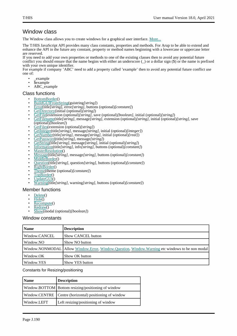
Window classThe Window class allows you to create windows for a graphical user interface. More...
The T/HIS JavaScript API provides many class constants, properties and methods. For Arup to be able to extend and enhance the API in the future any constant, property or method names beginning with a lowercase or uppercase letter are reserved.If you need to add your own properties or methods to one of the existing classes then to avoid any potential future conflict you should ensure that the name begins with either an underscore (_) or a dollar sign ($) or the name is prefixed with your own unique identifier.For example if company ’ABC’ need to add a property called ’example’ then to avoid any potential future conflict use one of:
• _example • $example • ABC_example
Class functions• BottomBorder() • BuildGUIFromString(guistring[string]) • Error(title[string], error[string], buttons (optional)[constant]) • GetDirectory(initial (optional)[string]) • GetFile(extension (optional)[string], save (optional)[boolean], initial (optional)[string]) • GetFilename(title[string], message[string], extension (optional)[string], initial (optional)[string], save
(optional)[boolean]) • GetFiles(extension (optional)[string]) • GetInteger(title[string], message[string], initial (optional)[integer]) • GetNumber(title[string], message[string], initial (optional)[real]) • GetPassword(title[string], message[string]) • GetString(title[string], message[string], initial (optional)[string]) • Information(title[string], info[string], buttons (optional)[constant]) • MasterResolution() • Message(title[string], message[string], buttons (optional)[constant]) • MiddleBorder() • Question(title[string], question[string], buttons (optional)[constant]) • RightBorder() • Theme(theme (optional)[constant]) • TopBorder() • UpdateGUI() • Warning(title[string], warning[string], buttons (optional)[constant])
Member functions• Delete() • Hide() • Recompute() • Redraw() • Show(modal (optional)[boolean])
Window constants
Name Description
Window.CANCEL Show CANCEL button
Window.NO Show NO button
Window.NONMODAL Allow Window.Error, Window.Question, Window.Warning etc windows to be non modal
Window.OK Show OK button
Window.YES Show YES button
Constants for Resizing/positioning
Name Description
Window.BOTTOM Bottom resizing/positioning of window
Window.CENTRE Centre (horizontal) positioning of window
Window.LEFT Left resizing/positioning of window
T/HIS User manual Version 18.0, April 2021
Page J.190
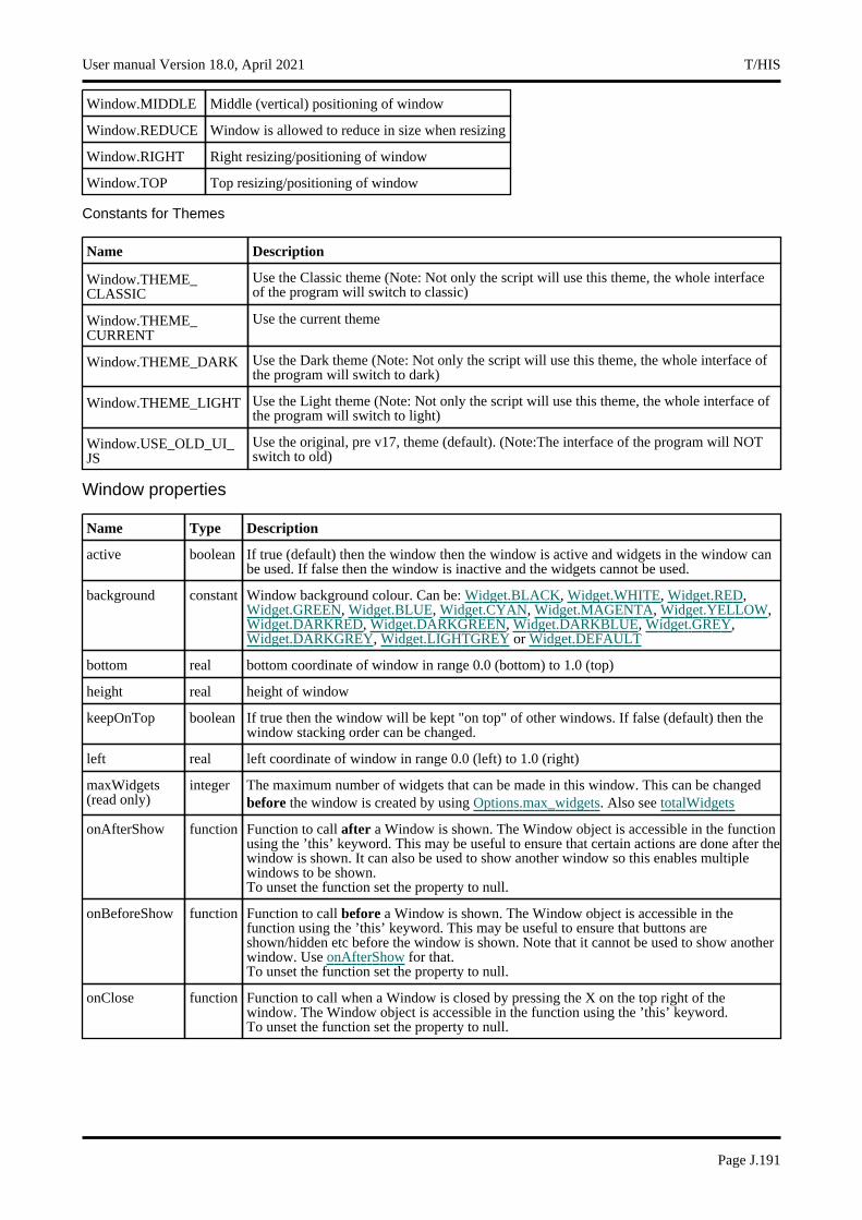
Window.MIDDLE Middle (vertical) positioning of window
Window.REDUCE Window is allowed to reduce in size when resizing
Window.RIGHT Right resizing/positioning of window
Window.TOP Top resizing/positioning of window
Constants for Themes
Name Description
Window.THEME_CLASSIC
Use the Classic theme (Note: Not only the script will use this theme, the whole interface of the program will switch to classic)
Window.THEME_CURRENT
Use the current theme
Window.THEME_DARK Use the Dark theme (Note: Not only the script will use this theme, the whole interface of the program will switch to dark)
Window.THEME_LIGHT Use the Light theme (Note: Not only the script will use this theme, the whole interface of the program will switch to light)
Window.USE_OLD_UI_JS
Use the original, pre v17, theme (default). (Note:The interface of the program will NOT switch to old)
Window properties
Name Type Description
active boolean If true (default) then the window then the window is active and widgets in the window can be used. If false then the window is inactive and the widgets cannot be used.
background constant Window background colour. Can be: Widget.BLACK, Widget.WHITE, Widget.RED, Widget.GREEN, Widget.BLUE, Widget.CYAN, Widget.MAGENTA, Widget.YELLOW, Widget.DARKRED, Widget.DARKGREEN, Widget.DARKBLUE, Widget.GREY, Widget.DARKGREY, Widget.LIGHTGREY or Widget.DEFAULT
bottom real bottom coordinate of window in range 0.0 (bottom) to 1.0 (top)
height real height of window
keepOnTop boolean If true then the window will be kept "on top" of other windows. If false (default) then the window stacking order can be changed.
left real left coordinate of window in range 0.0 (left) to 1.0 (right)
maxWidgets (read only)
integer The maximum number of widgets that can be made in this window. This can be changed before the window is created by using Options.max_widgets. Also see totalWidgets
onAfterShow function Function to call after a Window is shown. The Window object is accessible in the function using the ’this’ keyword. This may be useful to ensure that certain actions are done after the window is shown. It can also be used to show another window so this enables multiple windows to be shown. To unset the function set the property to null.
onBeforeShow function Function to call before a Window is shown. The Window object is accessible in the function using the ’this’ keyword. This may be useful to ensure that buttons are shown/hidden etc before the window is shown. Note that it cannot be used to show another window. Use onAfterShow for that. To unset the function set the property to null.
onClose function Function to call when a Window is closed by pressing the X on the top right of the window. The Window object is accessible in the function using the ’this’ keyword. To unset the function set the property to null.
User manual Version 18.0, April 2021 T/HIS
Page J.191
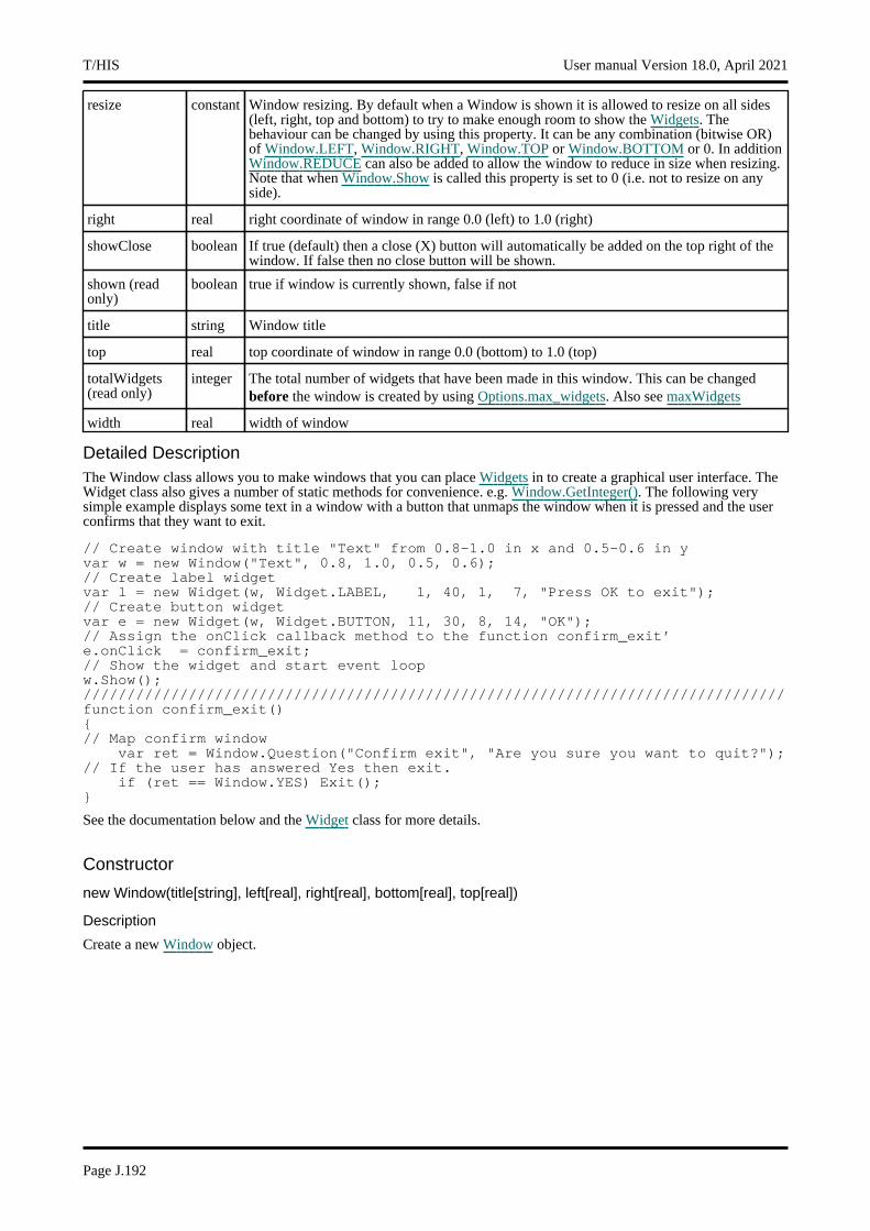
resize constant Window resizing. By default when a Window is shown it is allowed to resize on all sides (left, right, top and bottom) to try to make enough room to show the Widgets. The behaviour can be changed by using this property. It can be any combination (bitwise OR) of Window.LEFT, Window.RIGHT, Window.TOP or Window.BOTTOM or 0. In addition Window.REDUCE can also be added to allow the window to reduce in size when resizing. Note that when Window.Show is called this property is set to 0 (i.e. not to resize on any side).
right real right coordinate of window in range 0.0 (left) to 1.0 (right)
showClose boolean If true (default) then a close (X) button will automatically be added on the top right of the window. If false then no close button will be shown.
shown (read only)
boolean true if window is currently shown, false if not
title string Window title
top real top coordinate of window in range 0.0 (bottom) to 1.0 (top)
totalWidgets (read only)
integer The total number of widgets that have been made in this window. This can be changed before the window is created by using Options.max_widgets. Also see maxWidgets
width real width of window
Detailed DescriptionThe Window class allows you to make windows that you can place Widgets in to create a graphical user interface. The Widget class also gives a number of static methods for convenience. e.g. Window.GetInteger(). The following very simple example displays some text in a window with a button that unmaps the window when it is pressed and the user confirms that they want to exit.
// Create window with title "Text" from 0.8-1.0 in x and 0.5-0.6 in yvar w = new Window("Text", 0.8, 1.0, 0.5, 0.6);// Create label widgetvar l = new Widget(w, Widget.LABEL, 1, 40, 1, 7, "Press OK to exit");// Create button widgetvar e = new Widget(w, Widget.BUTTON, 11, 30, 8, 14, "OK");// Assign the onClick callback method to the function confirm_exit’e.onClick = confirm_exit;// Show the widget and start event loopw.Show();////////////////////////////////////////////////////////////////////////////////function confirm_exit(){// Map confirm window
var ret = Window.Question("Confirm exit", "Are you sure you want to quit?");// If the user has answered Yes then exit.
if (ret == Window.YES) Exit();}
See the documentation below and the Widget class for more details.
Constructor
new Window(title[string], left[real], right[real], bottom[real], top[real])
Description
Create a new Window object.
T/HIS User manual Version 18.0, April 2021
Page J.192
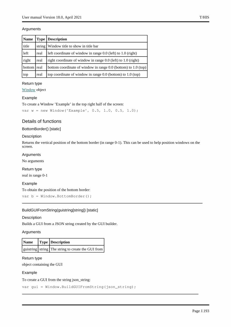
Arguments
Name Type Description
title string Window title to show in title bar
left real left coordinate of window in range 0.0 (left) to 1.0 (right)
right real right coordinate of window in range 0.0 (left) to 1.0 (right)
bottom real bottom coordinate of window in range 0.0 (bottom) to 1.0 (top)
top real top coordinate of window in range 0.0 (bottom) to 1.0 (top)
Return type
Window object
Example
To create a Window ’Example’ in the top right half of the screen:
var w = new Window(’Example’, 0.5, 1.0, 0.5, 1.0);
Details of functions
BottomBorder() [static]
Description
Returns the vertical position of the bottom border (in range 0-1). This can be used to help position windows on the screen.
Arguments
No arguments
Return type
real in range 0-1
Example
To obtain the position of the bottom border:
var b = Window.BottomBorder();
BuildGUIFromString(guistring[string]) [static]
Description
Builds a GUI from a JSON string created by the GUI builder.
Arguments
Name Type Description
guistring string The string to create the GUI from
Return type
object containing the GUI
Example
To create a GUI from the string json_string:
var gui = Window.BuildGUIFromString(json_string);
User manual Version 18.0, April 2021 T/HIS
Page J.193
Delete()
Description
Deletes the window from T/HIS and returns any memory/resources used for the window. This function should not normally need to be called. However, in exceptional circumstances if a script recreates windows many times T/HIS may run out of USER objects on Microsoft Windows because of the way T/HIS creates and shows windows. To avoid this problem this method can be used to force T/HIS to return the resources for a window. Do not use the Window object after calling this method.
Arguments
No arguments
Return type
No return value
Example
To delete window w:
w.Delete();
Error(title[string], error[string], buttons (optional)[constant]) [static]
Description
Show an error message in a window.
Arguments
Name Type Description
title string Title for window.
error string Error message to show in window. The maximum number of lines that can be shown is controlled by the Options.max_window_lines option.
buttons (optional)
constant The buttons to use. Can be bitwise OR of Window.OK, Window.CANCEL, Window.YES or Window.NO. If this is omitted an OK button will be used. By default the window will be modal. If Window.NONMODAL is also given the window will be non-modal instead.
Return type
Button pressed
Example
To show error Critical error!\nAbort? in window with title Error with Yes and No buttons:
var answer = Window.Error("Error", "Critical error!\nAbort?", Window.YES | Window.NO);if (answer == Window.YES) Exit();
GetDirectory(initial (optional)[string]) [static]
Description
Map the directory selector box native to your machine, allowing you to choose a directory. On Unix this will be a Motif selector. Windows will use the standard windows directory selector.
Arguments
Name Type Description
initial (optional) string Initial directory to start from.
T/HIS User manual Version 18.0, April 2021
Page J.194
Return type
directory (string), (or null if cancel pressed).
Example
To select a directory:
var dir = Window.GetDirectory();
GetFile(extension (optional)[string], save (optional)[boolean], initial (optional)[string]) [static]
Description
Map a file selector box allowing you to choose a file. See also Window.GetFiles() and Window.GetFilename().
Arguments
Name Type Description
extension (optional)
string Extension to filter by.
save (optional)
boolean If true the file selector is to be used for saving a file. If false (default) the file selector is for opening a file. Due to native operating system file selector differences, on linux new filenames can only be given when saving a file. On windows it is possible to give new filenames when opening or saving a file.
initial (optional)
string Initial directory to start from.
Return type
filename (string), (or null if cancel pressed).
Example
To select a file using extension ’.key’:
var file = Window.GetFile(".key");
GetFilename(title[string], message[string], extension (optional)[string], initial (optional)[string], save (optional)[boolean]) [static]
Description
Map a window allowing you to input a filename (or select it using a file selector). OK and Cancel buttons are shown. See also Window.GetFile().
Arguments
Name Type Description
title string Title for window.
message string Message to show in window.
extension (optional)
string Extension to filter by.
initial (optional)
string Initial value.
save (optional)
boolean If true the file selector is to be used for saving a file. If false (default) the file selector is for opening a file. Due to native operating system file selector differences, on linux new filenames can only be given when saving a file. On windows it is possible to give new filenames when opening or saving a file.
User manual Version 18.0, April 2021 T/HIS
Page J.195

Return type
filename (string), (or null if cancel pressed).
Example
To create an file input window with title Choose file and message Choose the file to open and return the filename input:
var filename = Window.GetFilename("Choose file", "Choose the file to open");
GetFiles(extension (optional)[string]) [static]
Description
Map a file selector box allowing you to choose multiple files. See also Window.GetFile() and Window.GetFilename().
Arguments
Name Type Description
extension (optional) string Extension to filter by.
Return type
Array of filenames (strings), or null if cancel pressed.
Example
To select multiple files using extension ’.key’:
var files = Window.GetFiles(".key");
GetInteger(title[string], message[string], initial (optional)[integer]) [static]
Description
Map a window allowing you to input an integer. OK and Cancel buttons are shown.
Arguments
Name Type Description
title string Title for window.
message string Message to show in window.
initial (optional) integer Initial value.
Return type
value input (integer), or null if cancel pressed.
Example
To create an input window with title Input and message Input integer and return the value input:
var value = Window.GetInteger("Input", "Input integer");
GetNumber(title[string], message[string], initial (optional)[real]) [static]
Description
Map a window allowing you to input a number. OK and Cancel buttons are shown.
T/HIS User manual Version 18.0, April 2021
Page J.196
Arguments
Name Type Description
title string Title for window.
message string Message to show in window.
initial (optional) real Initial value.
Return type
value input (real), or null if cancel pressed.
Example
To create an input window with title Input and message Input number and return the value input:
var value = Window.GetNumber("Input", "Input number");
GetPassword(title[string], message[string]) [static]
Description
Map a window allowing you to input a password. OK and Cancel buttons are shown.This is identical to Window.GetString except the string is hidden and no initial value can be given.
Arguments
Name Type Description
title string Title for window.
message string Message to show in window.
Return type
value input (string), or null if cancel pressed.
Example
To create an input window with title Input and message Input password and return the value input:
var value = Window.GetPassword("Input", "Input password");
GetString(title[string], message[string], initial (optional)[string]) [static]
Description
Map a window allowing you to input a string. OK and Cancel buttons are shown.
Arguments
Name Type Description
title string Title for window.
message string Message to show in window.
initial (optional) string Initial value.
Return type
value input (string), or null if cancel pressed.
User manual Version 18.0, April 2021 T/HIS
Page J.197
Example
To create an input window with title Input and message Input string and return the value input:
var value = Window.GetString("Input", "Input string");
Hide()
Description
Hides (unmaps) the window.
Arguments
No arguments
Return type
No return value
Example
To hide window w:
w.Hide();
Information(title[string], info[string], buttons (optional)[constant]) [static]
Description
Show information in a window.
Arguments
Name Type Description
title string Title for window.
info string Information to show in window. The maximum number of lines that can be shown is controlled by the Options.max_window_lines option.
buttons (optional)
constant The buttons to use. Can be bitwise OR of Window.OK, Window.CANCEL, Window.YES or Window.NO. If this is omitted an OK button will be used. By default the window will be modal. If Window.NONMODAL is also given the window will be non-modal instead.
Return type
Button pressed
Example
To show information Information in window with title Example with OK and Cancel buttons:
var answer = Window.Information("Example", "Information", Window.OK | Window.CANCEL);if (answer == Window.CANCEL) Message("You pressed the Cancel button");
MasterResolution() [static]
Description
Returns the resolution of the master programme window in pixels
Arguments
No arguments
Return type
Array of numbers containing x and y resolution in pixels
T/HIS User manual Version 18.0, April 2021
Page J.198
Example
To get the resolution of the main window:
var res = Window.MasterResolution();
Message(title[string], message[string], buttons (optional)[constant]) [static]
Description
Show a message in a window.
Arguments
Name Type Description
title string Title for window.
message string Message to show in window. The maximum number of lines that can be shown is controlled by the Options.max_window_lines option.
buttons (optional)
constant The buttons to use. Can be bitwise OR of Window.OK, Window.CANCEL, Window.YES or Window.NO. If this is omitted an OK button will be used By default the window will be modal. If Window.NONMODAL is also given the window will be non-modal instead.
Return type
Button pressed
Example
To show message Press YES or NO in window with title Example with YES and NO buttons:
var answer = Window.Message("Example", "Press YES or NO", Window.YES | Window.NO);if (answer == Window.NO) Message("You pressed No");
MiddleBorder() [static]
Description
Returns the vertical position of the middle border (in range 0-1). The middle border is the border between the tools/keywords window and the docked windows. This can be used to help position windows on the screen.
Arguments
No arguments
Return type
real in range 0-1
Example
To obtain the position of the middle border:
var b = Window.MiddleBorder();
Question(title[string], question[string], buttons (optional)[constant]) [static]
Description
Show a question in a window.
User manual Version 18.0, April 2021 T/HIS
Page J.199

Arguments
Name Type Description
title string Title for window.
question string Question to show in window. The maximum number of lines that can be shown is controlled by the Options.max_window_lines option.
buttons (optional)
constant The buttons to use. Can be bitwise OR of Window.OK, Window.CANCEL, Window.YES or Window.NO. If this is omitted Yes and No button will be used. By default the window will be modal. If Window.NONMODAL is also given the window will be non-modal instead.
Return type
Button pressed
Example
To show question Do you want to continue? in window with title Question:
var answer = Window.Question("Question", "Do you want to continue?");if (answer == Window.NO) Message("You pressed No");
Recompute()
Description
Recomputes the positions of widgets in the window. If you have static widgets and ’normal’ widgets in a window and you show and/or hide widgets the window needs to be recomputed to refresh the graphics, scroll bars etc. Calling this method will recompute and redraw the window.
Arguments
No arguments
Return type
No return value
Example
To recompute window w:
w.Recompute();
Redraw()
Description
Redraws the window. Sometimes if you show, hide or draw graphics on widgets the window needs to be redrawn to refresh the graphics. Calling this method will redraw the window refreshing the graphics.
Arguments
No arguments
Return type
No return value
Example
To redraw window w:
w.Redraw();
T/HIS User manual Version 18.0, April 2021
Page J.200
RightBorder() [static]
Description
Returns the horizontal position of the right border (in range 0-1). This can be used to help position windows on the screen.
Arguments
No arguments
Return type
real in range 0-1
Example
To obtain the position of the right border:
var b = Window.RightBorder();
Show(modal (optional)[boolean])
Description
Shows (maps) the window and waits for user input.
Arguments
Name Type Description
modal (optional)
boolean If this window is modal (true) then the user is blocked from doing anything else in T/HIS until this window is dismissed). If non-modal (false) then the user can still use other functions in T/HIS.If omitted the window will be modal.Note that making a window modal will stop interaction in all other windows and may prevent operations such as picking from working in any macros that are run from scripts.
Return type
No return value
Example
To show window w:
w.Show();
To show window w allowing the user to use other functions in T/HIS:
w.Show(false);
Theme(theme (optional)[constant]) [static]
Description
Set or get a user interface theme.
Arguments
Name Type Description
theme (optional)
constant If it is provided it is used to set the current theme. Can be either Window.USE_OLD_UI_JS, Window.THEME_CURRENT, Window.THEME_DARK, Window.THEME_LIGHT, Window.THEME_CLASSIC.
Return type
Integer. When getting the theme one of: Window.USE_OLD_UI_JS, Window.THEME_DARK, Window.THEME_LIGHT, Window.THEME_CLASSIC
User manual Version 18.0, April 2021 T/HIS
Page J.201
Example
To determine the current theme:
var ui = Window.Theme();if(ui == Window.THEME_DARK){
print("Theme is dark\n");}else if(ui == Window.THEME_LIGHT){
print("Theme is light\n");}else if(ui == Window.THEME_CLASSIC){
print("Theme is classic\n");}else{
print("Theme is not set\n");}
To keep the original (pre v17) appearance of your JavaScript (default):
Window.Theme(Window.USE_OLD_UI_JS);
To use the current user interface theme:
Window.Theme(Window.THEME_CURRENT);
To use the dark user interface theme:
Window.Theme(Window.THEME_DARK);
TopBorder() [static]
Description
Returns the vertical position of the top border (in range 0-1). This can be used to help position windows on the screen. This is no longer used in T/HIS and will always be 1 but is left for backwards compatibility.
Arguments
No arguments
Return type
real in range 0-1
Example
To obtain the position of the top border:
var b = Window.TopBorder();
UpdateGUI() [static]
Description
Force GUI to be updated. This function is not normally needed but if you are doing a computationally expensive operation and want to update the GUI it may be necessary as the GUI update requests are cached until there is spare time to update them. Calling this function forces any outstanding requests to be flushed.
Arguments
No arguments
Return type
No return value
T/HIS User manual Version 18.0, April 2021
Page J.202
Example
To force update of GUI:
Window.UpdateGUI();
Warning(title[string], warning[string], buttons (optional)[constant]) [static]
Description
Show a warning message in a window.
Arguments
Name Type Description
title string Title for window.
warning string Warning message to show in window. The maximum number of lines that can be shown is controlled by the Options.max_window_lines option.
buttons (optional)
constant The buttons to use. Can be bitwise OR of Window.OK, Window.CANCEL, Window.YES or Window.NO. If this is omitted an OK button will be used. By default the window will be modal. If Window.NONMODAL is also given the window will be non-modal instead.
Return type
Button pressed
Example
To show warning Title is blank\nSet to ID? in window with title Warning with Yes and No buttons:
var answer = Window.Warning("Warning", "Title is blank\nSet to ID?", Window.YES | Window.NO);if (answer == Window.NO) Message("You pressed No");
User manual Version 18.0, April 2021 T/HIS
Page J.203

XMLParser classThe XMLParser class enables reading data from XML files. More...
The T/HIS JavaScript API provides many class constants, properties and methods. For Arup to be able to extend and enhance the API in the future any constant, property or method names beginning with a lowercase or uppercase letter are reserved.If you need to add your own properties or methods to one of the existing classes then to avoid any potential future conflict you should ensure that the name begins with either an underscore (_) or a dollar sign ($) or the name is prefixed with your own unique identifier.For example if company ’ABC’ need to add a property called ’example’ then to avoid any potential future conflict use one of:
• _example • $example • ABC_example
Member functions• Parse(filename[string])
XMLParser properties
Name Type Description
characterDataHandler function Function to call when character data is found. The function will be called with 1 argument which is a string containing the character data
commentHandler function Function to call when a comment is found. The function will be called with 1 argument which is a string containing the text inside the comment
endCDATAHandler function Function to call at the end of a CDATA section. The function does not have any arguments.
endElementHandler function Function to call when an element end tag is found. The function will be called with 1 argument which is a string containing the name of the element
startCDATAHandler function Function to call at the start of a CDATA section. The function does not have any arguments.
startElementHandler function Function to call when an element start tag is found. The function will be called with 2 arguments. Argument 1 is a string containing the name of the element. Argument 2 is an object containing the element attributes
Detailed DescriptionThe XMLParser class provides a stream-oriented parser to enable you to read XML files. You register callback (or handler) functions with the parser and then parse the document. As the parser recognizes parts of the document, it will call the appropriate handler for that part (if you’ve registered one.) The document is fed to the parser in pieces. This allows you to parse really huge documents that won’t fit into memory.There are currently 6 handlers which can be set: XMLParser.startElementHandler, XMLParser.endElementHandler, XMLParser.characterDataHandler, XMLParser.commentHandler, XMLParser.startCDATAHandler and XMLParser.endCDATAHandler. The following simple example shows how the parser could be used.
// Create a new parser objectvar p = new XMLParser();// assign handlersp.startElementHandler = startElem;p.endElementHandler = endElem;p.characterDataHandler = text;p.commentHandler = comment;// parse the filep.Parse("/data/test.xml");////////////////////////////////////////////////////////////////////////////////function startElem(name, attr){// handler to be called when a start element is found// Print element name
Println("START: " + name);// Print attributes
for (n in attr){
T/HIS User manual Version 18.0, April 2021
Page J.204

Println(" attr: " + n + "=" + attr[n]);}
}function endElem(name){// handler to be called when an end element is found// Print element name
Println("END: " + name);}function text(str){// handler to be called when text is found// Print text
Println("TEXT: ’" + str + "’");}function comment(str){// handler to be called when a comment is found// Print comment
Println("COMMENT: ’" + str + "’");}
See the documentation below for more details.
Constructor
new XMLParser()
Description
Create a new XMLParser object for reading XML files.
Arguments
No arguments
Return type
XMLParser object
Example
To create a new XMLParser object
var p = new XMLParser();
Details of functions
Parse(filename[string])
Description
starts parsing an XML file
Arguments
Name Type Description
filename string XML file to parse
Return type
No return value
Example
To parse XML file "/data/test.xml"
var p = new XMLParser();p.Parse("/data/test.xml");
User manual Version 18.0, April 2021 T/HIS
Page J.205

T/HIS User manual Version 18.0, April 2021
Page J.206
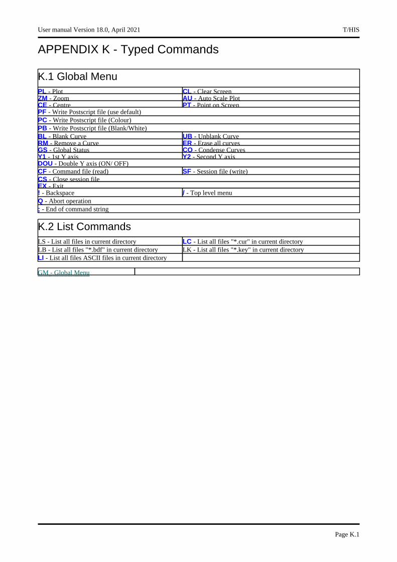
APPENDIX K - Typed Commands
K.1 Global MenuPL - Plot CL - Clear ScreenZM - Zoom AU - Auto Scale PlotCE - Centre PT - Point on ScreenPF - Write Postscript file (use default)PC - Write Postscript file (Colour)PB - Write Postscript file (Blank/White)BL - Blank Curve UB - Unblank CurveRM - Remove a Curve ER - Erase all curvesGS - Global Status CO - Condense CurvesY1 - 1st Y axis Y2 - Second Y axisDOU - Double Y axis (ON/ OFF)CF - Command file (read) SF - Session file (write)CS - Close session fileEX - Exit! - Backspace / - Top level menuQ - Abort operation; - End of command string
K.2 List CommandsLS - List all files in current directory LC - List all files "*.cur" in current directoryLB - List all files "*.bdf" in current directory LK - List all files "*.key" in current directoryLI - List all files ASCII files in current directory
GM - Global Menu
User manual Version 18.0, April 2021 T/HIS
Page K.1
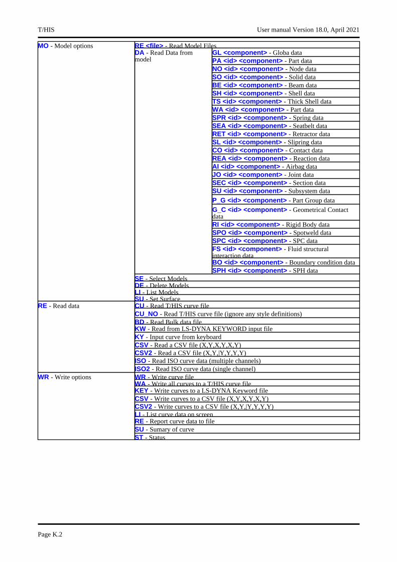
RE <file> - Read Model FilesMO - Model optionsGL <component> - Globa dataDA - Read Data from
model PA <id> <component> - Part dataNO <id> <component> - Node dataSO <id> <component> - Solid dataBE <id> <component> - Beam dataSH <id> <component> - Shell dataTS <id> <component> - Thick Shell dataWA <id> <component> - Part dataSPR <id> <component> - Spring dataSEA <id> <component> - Seatbelt dataRET <id> <component> - Retractor dataSL <id> <component> - Slipring dataCO <id> <component> - Contact dataREA <id> <component> - Reaction dataAI <id> <component> - Airbag dataJO <id> <component> - Joint dataSEC <id> <component> - Section dataSU <id> <component> - Subsystem data
P_G <id> <component> - Part Group data
G_C <id> <component> - Geometrical Contact dataRI <id> <component> - Rigid Body dataSPO <id> <component> - Spotweld dataSPC <id> <component> - SPC dataFS <id> <component> - Fluid structural interaction dataBO <id> <component> - Boundary condition dataSPH <id> <component> - SPH data
SE - Select ModelsDE - Delete ModelsLI - List ModelsSU - Set SurfaceCU - Read T/HIS curve fileRE - Read dataCU_NO - Read T/HIS curve file (ignore any style definitions)BD - Read Bulk data fileKW - Read from LS-DYNA KEYWORD input fileKY - Input curve from keyboardCSV - Read a CSV file (X,Y,X,Y,X,Y)CSV2 - Read a CSV file (X,Y,|Y,Y,Y,Y)ISO - Read ISO curve data (multiple channels)ISO2 - Read ISO curve data (single channel)WR - Write curve fileWR - Write optionsWA - Write all curves to a T/HIS curve fileKEY - Write curves to a LS-DYNA Keyword fileCSV - Write curves to a CSV file (X,Y,X,Y,X,Y)CSV2 - Write curves to a CSV file (X,Y,|Y,Y,Y,Y)LI - List curve data on screenRE - Report curve data to fileSU - Sumary of curveST - Status
T/HIS User manual Version 18.0, April 2021
Page K.2
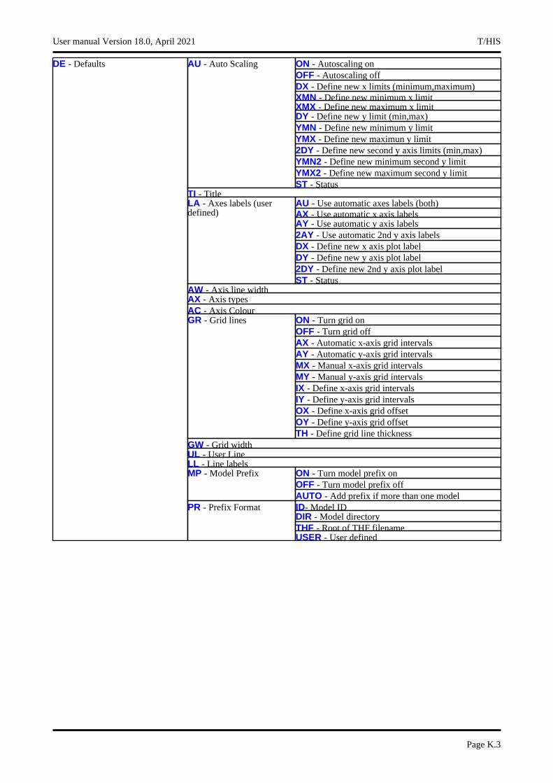
DE - Defaults ON - Autoscaling onAU - Auto ScalingOFF - Autoscaling offDX - Define new x limits (minimum,maximum)XMN - Define new minimum x limitXMX - Define new maximum x limitDY - Define new y limit (min,max)YMN - Define new minimum y limitYMX - Define new maximun y limit2DY - Define new second y axis limits (min,max)YMN2 - Define new minimum second y limitYMX2 - Define new maximum second y limitST - Status
TI - Title AU - Use automatic axes labels (both)LA - Axes labels (user
defined) AX - Use automatic x axis labelsAY - Use automatic y axis labels2AY - Use automatic 2nd y axis labelsDX - Define new x axis plot labelDY - Define new y axis plot label2DY - Define new 2nd y axis plot labelST - Status
AW - Axis line widthAX - Axis typesAC - Axis Colour
ON - Turn grid onGR - Grid linesOFF - Turn grid offAX - Automatic x-axis grid intervalsAY - Automatic y-axis grid intervalsMX - Manual x-axis grid intervalsMY - Manual y-axis grid intervalsIX - Define x-axis grid intervalsIY - Define y-axis grid intervalsOX - Define x-axis grid offsetOY - Define y-axis grid offsetTH - Define grid line thickness
GW - Grid widthUL - User LineLL - Line labels
ON - Turn model prefix onMP - Model PrefixOFF - Turn model prefix offAUTO - Add prefix if more than one modelID- Model IDPR - Prefix Format DIR - Model directoryTHF - Root of THF filenameUSER - User defined
User manual Version 18.0, April 2021 T/HIS
Page K.3
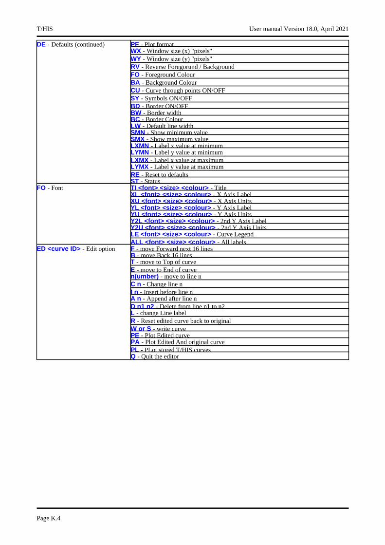
PF - Plot formatDE - Defaults (continued)WX - Window size (x) "pixels"WY - Window size (y) "pixels"RV - Reverse Foregorund / BackgroundFO - Foreground ColourBA - Background ColourCU - Curve through points ON/OFFSY - Symbols ON/OFFBD - Border ON/OFFBW - Border widthBC - Border ColourLW - Default line widthSMN - Show minimum valueSMX - Show maximum valueLXMN - Label x value at minimumLYMN - Label y value at minimumLXMX - Label x value at maximumLYMX - Label y value at maximumRE - Reset to defaultsST - StatusTI <font> <size> <colour> - Title FO - FontXL <font> <size> <colour> - X Axis LabelXU <font> <size> <colour> - X Axis UnitsYL <font> <size> <colour> - Y Axis LabelYU <font> <size> <colour> - Y Axis UnitsY2L <font> <size> <colour> - 2nd Y Axis LabelY2U <font> <size> <colour> - 2nd Y Axis UnitsLE <font> <size> <colour> - Curve LegendALL <font> <size> <colour> - All labelsF - move Forward next 16 linesED <curve ID> - Edit optionB - move Back 16 linesT - move to Top of curveE - move to End of curven(umber) - move to line nC n - Change line nI n - Insert before line nA n - Append after line nD n1 n2 - Delete from line n1 to n2L - change Line label R - Reset edited curve back to originalW or S - write curve PE - Plot Edited curvePA - Plot Edited And original curvePL - PLot stored T/HIS curvesQ - Quit the editor
T/HIS User manual Version 18.0, April 2021
Page K.4
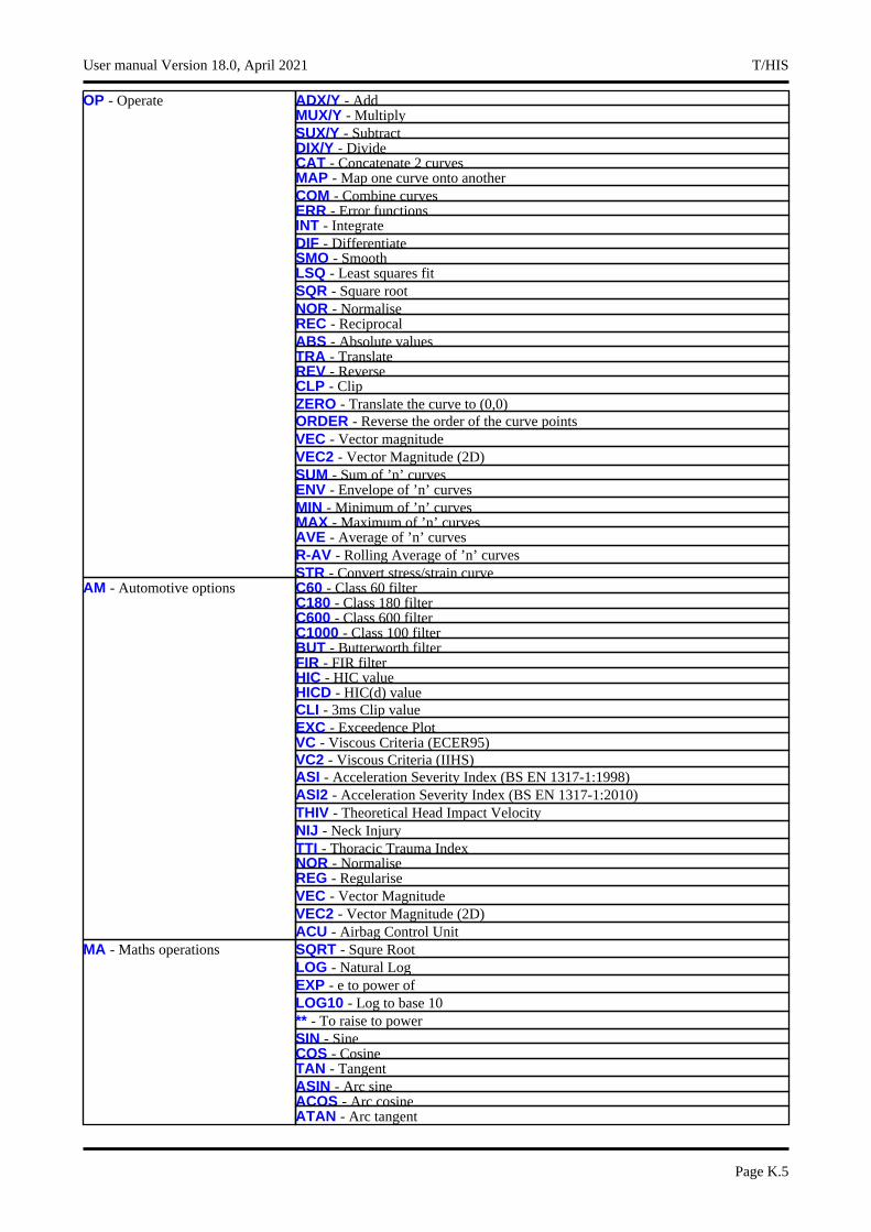
ADX/Y - AddOP - OperateMUX/Y - MultiplySUX/Y - SubtractDIX/Y - DivideCAT - Concatenate 2 curvesMAP - Map one curve onto anotherCOM - Combine curvesERR - Error functionsINT - IntegrateDIF - DifferentiateSMO - SmoothLSQ - Least squares fitSQR - Square rootNOR - NormaliseREC - ReciprocalABS - Absolute valuesTRA - TranslateREV - ReverseCLP - Clip ZERO - Translate the curve to (0,0)ORDER - Reverse the order of the curve points VEC - Vector magnitudeVEC2 - Vector Magnitude (2D)SUM - Sum of ’n’ curvesENV - Envelope of ’n’ curvesMIN - Minimum of ’n’ curvesMAX - Maximum of ’n’ curvesAVE - Average of ’n’ curvesR-AV - Rolling Average of ’n’ curvesSTR - Convert stress/strain curveC60 - Class 60 filterAM - Automotive optionsC180 - Class 180 filterC600 - Class 600 filterC1000 - Class 100 filterBUT - Butterworth filterFIR - FIR filterHIC - HIC valueHICD - HIC(d) valueCLI - 3ms Clip valueEXC - Exceedence PlotVC - Viscous Criteria (ECER95)VC2 - Viscous Criteria (IIHS)ASI - Acceleration Severity Index (BS EN 1317-1:1998)ASI2 - Acceleration Severity Index (BS EN 1317-1:2010)THIV - Theoretical Head Impact VelocityNIJ - Neck InjuryTTI - Thoracic Trauma IndexNOR - NormaliseREG - RegulariseVEC - Vector MagnitudeVEC2 - Vector Magnitude (2D)ACU - Airbag Control UnitSQRT - Squre RootMA - Maths operationsLOG - Natural LogEXP - e to power ofLOG10 - Log to base 10** - To raise to powerSIN - SineCOS - CosineTAN - TangentASIN - Arc sineACOS - Arc cosineATAN - Arc tangent
User manual Version 18.0, April 2021 T/HIS
Page K.5
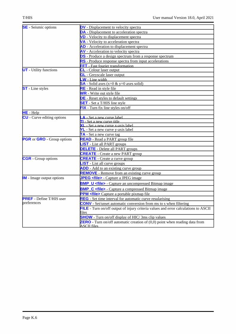
DV - Displacement to velocity spectraSE - Seismic optionsDA - Displacement to acceleration spectraVD - Velocity to displacement spectraVA - Velocity to acceleration spectraAD - Acceleration to displacement spectraAV - Acceleration to velocity spectraDS - Produce a design spectrum from a response spectrumRS - Produce response spectra from input accelerationsFFT - Fast fourier transformationCL - Colour laser outputUT - Utility functionsGL - Greyscale laser outputLW - Line widthSA - Solid axes (x=0 & y=0 axes solid)RE - Read in style fileST - Line stylesWR - Write out style fileDE - Reset styles to default settingsSET - Set a T/HIS line styleFIX - Turn fix line styles on/off
HE - HelpLA - Set a new curve labelCU - Curve editing optionsTI - Set a new curve titleXL - Set a new curve x-axis labelYL - Set a new curve y-axis labelTA - Set a new curve tagREAD - Read a PART group filePGR or GRO - Group optionsLIST - List all PART groupsDELETE - Delete all PART groupsCREATE - Create a new PART groupCREATE - Create a curve groupCGR - Group optionsLIST - List all curve groupsADD - Add to an existing curve groupREMOVE - Remove from an existing curve groupJPEG <file> - Capture a JPEG imageIM - Image output options
BMP_U <file> - Capture an uncompressed Bitmap image
BMP_C <file> - Capture a compressed Bitmap imagePPM <file> Capture a portable pixmap fileREG - Set time interval for automatic curve resularisingPREF - Define T/HIS user
preferences CONV - Set/unset automatic conversion from ms to s when filteringFILE - Turn on/off output of injury criteria values and error calculations to ASCII filesSHOW - Turn on/off display of HIC/ 3ms clip valuesZERO - Turn on/off automatic creation of (0,0) point when reading data from ASCII files
T/HIS User manual Version 18.0, April 2021
Page K.6
Installation organisationThe version18installation can be customised to try and avoid a number of issues that often occur in large organisations with many users.
• Large organisations generally imply large networks, and it is often the case that the performance of these networks can be intermittent or poor, therefore it is common practice to perform an installation of the software on the local disk of each machine, rather then having a single installation on a remote disk.
This avoids the pauses and glitches that can occur when running executable files over a network, but it also means that all the configuration files in, or depending upon, the top level "Admin" directory have to be copied to all machines and, more to the point, any changes or additions to such files also have to be copied to all machines.
• In larger organisations the "one person per computer" philosophy may not apply, with the consequence that users will tend to have a floating home area on a network drive and may not use the same machine every day.
This is not usually a problem on Linux where the "home" directory is tied to the login name not the machine. However on Windows platforms it means that %USERPROFILE%, which is typically on the local C drive of a machine, is not a good place to consider as "home" since it will be tied to a given computer, therefore a user who saves a file in their home directory on machine A may not be able to access it from machine B.
• In a similar vein placing large temporary files on the /tmp partition (Linux) or the C: drive (Windows) may result in local disks becoming too full, or quotas exceeded.
This section gives only a brief summary of the installation organisation, and you should refer to the separate Installation Guide if you want to find out more about the details of installation, licensing, and other related issues.
Version18.0 Installation structure
In version18.0 the option is provided to separate a top-level ’administration’ directory from the ’installation’ one where the executables are located.
For large installations on many machines this allows central configuration and administration files to exist in one place only, but executables to be installed locally on users’ machines to give better performance. Version18.0 also allows the following items to be configured
• The location for user manuals and other documentation.• The definition of a user’s home directory.• The definition of the temporary directory for scratch files.
In addition parsing of the ’oa_pref’ (preferences) file will now handle environment variables, so that a generic preference can be configured to give a user-specific result, and preferences may be ’locked’ so that those set at the administration level cannot be changed by users.
These changes are entirely optional, and users performing a simple installation on a single machine do not need to make any changes to their existing installation practice.
Directory Status Directory Content and purpose oa_pref file option
OA_ADMIN_xx
Optional Top level configuration files.(xx =18for release18.0, thus OA_ADMIN_18)
Admin level oa_pref fileOther configuration filesTimeout configuration file
User manual Version 18.0, April 2021 T/HIS
Page L.1
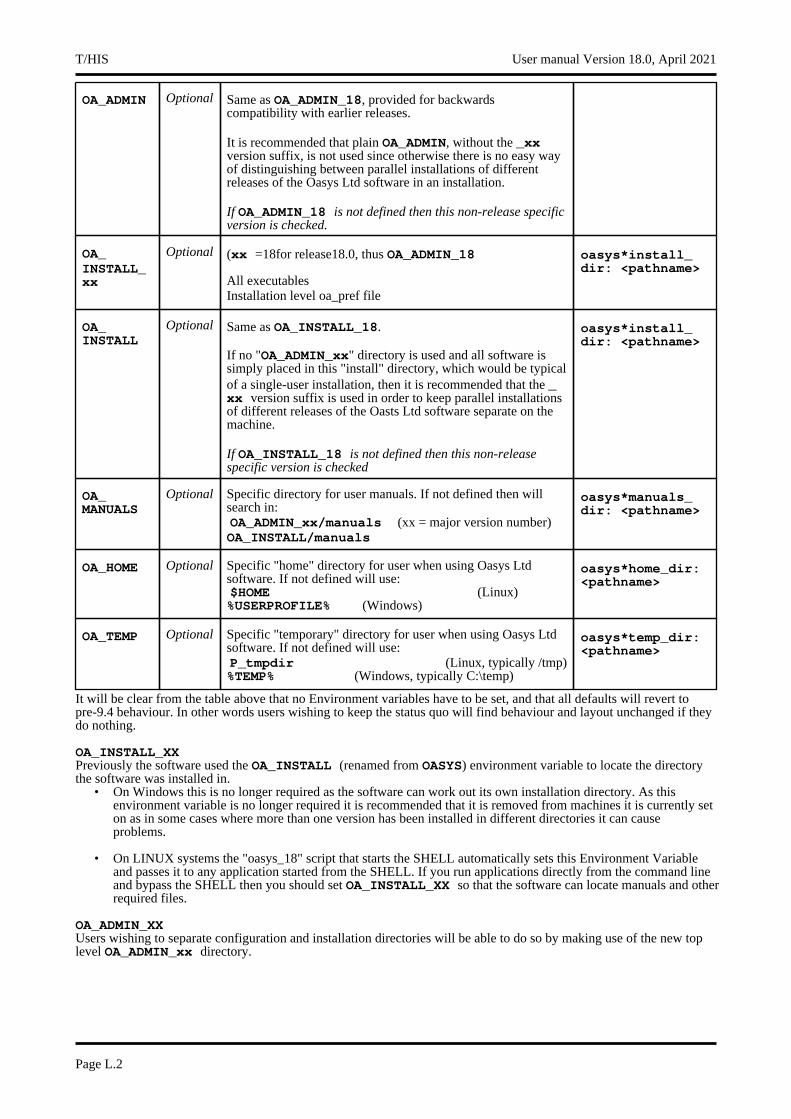
OA_ADMIN Optional Same as OA_ADMIN_18, provided for backwards compatibility with earlier releases.
It is recommended that plain OA_ADMIN, without the _xx version suffix, is not used since otherwise there is no easy way of distinguishing between parallel installations of different releases of the Oasys Ltd software in an installation.
If OA_ADMIN_18 is not defined then this non-release specific version is checked.
OA_INSTALL_xx
Optional (xx =18for release18.0, thus OA_ADMIN_18
All executablesInstallation level oa_pref file
oasys*install_dir: <pathname>
OA_INSTALL
Optional Same as OA_INSTALL_18.
If no "OA_ADMIN_xx" directory is used and all software is simply placed in this "install" directory, which would be typical of a single-user installation, then it is recommended that the _xx version suffix is used in order to keep parallel installations of different releases of the Oasts Ltd software separate on the machine.
If OA_INSTALL_18 is not defined then this non-release specific version is checked
oasys*install_dir: <pathname>
OA_MANUALS
Optional Specific directory for user manuals. If not defined then will search in:OA_ADMIN_xx/manuals (xx = major version number) OA_INSTALL/manuals
oasys*manuals_dir: <pathname>
OA_HOME Optional Specific "home" directory for user when using Oasys Ltd software. If not defined will use:$HOME (Linux)%USERPROFILE% (Windows)
oasys*home_dir: <pathname>
OA_TEMP Optional Specific "temporary" directory for user when using Oasys Ltd software. If not defined will use:P_tmpdir (Linux, typically /tmp)%TEMP% (Windows, typically C:\temp)
oasys*temp_dir: <pathname>
It will be clear from the table above that no Environment variables have to be set, and that all defaults will revert to pre-9.4 behaviour. In other words users wishing to keep the status quo will find behaviour and layout unchanged if they do nothing.
OA_INSTALL_XXPreviously the software used the OA_INSTALL (renamed from OASYS) environment variable to locate the directory the software was installed in.
• On Windows this is no longer required as the software can work out its own installation directory. As this environment variable is no longer required it is recommended that it is removed from machines it is currently set on as in some cases where more than one version has been installed in different directories it can cause problems.
• On LINUX systems the "oasys_18" script that starts the SHELL automatically sets this Environment Variable and passes it to any application started from the SHELL. If you run applications directly from the command line and bypass the SHELL then you should set OA_INSTALL_XX so that the software can locate manuals and other required files.
OA_ADMIN_XXUsers wishing to separate configuration and installation directories will be able to do so by making use of the new top level OA_ADMIN_xx directory.
T/HIS User manual Version 18.0, April 2021
Page L.2
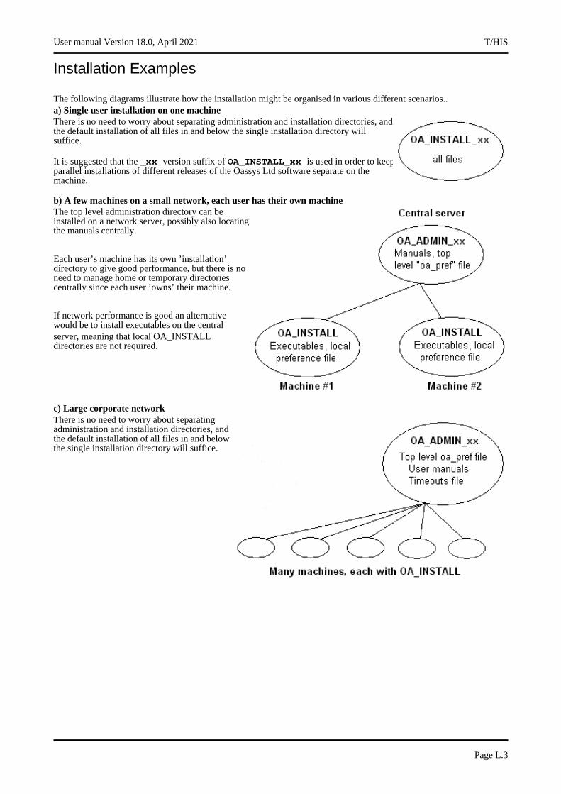
Installation Examples
The following diagrams illustrate how the installation might be organised in various different scenarios..a) Single user installation on one machine There is no need to worry about separating administration and installation directories, and the default installation of all files in and below the single installation directory will suffice.
It is suggested that the _xx version suffix of OA_INSTALL_xx is used in order to keep parallel installations of different releases of the Oassys Ltd software separate on the machine.
b) A few machines on a small network, each user has their own machine The top level administration directory can be installed on a network server, possibly also locating the manuals centrally.
Each user’s machine has its own ’installation’ directory to give good performance, but there is no need to manage home or temporary directories centrally since each user ’owns’ their machine.
If network performance is good an alternative would be to install executables on the central server, meaning that local OA_INSTALL directories are not required.
c) Large corporate network There is no need to worry about separating administration and installation directories, and the default installation of all files in and below the single installation directory will suffice.
User manual Version 18.0, April 2021 T/HIS
Page L.3

Dynamic configuration using the top level oa_pref file.
A further improvement is that all environment variables below OA_ADMIN_xx may either be set explicitly, or dynamically using the options in the oa_pref file at the top OA_ADMIN_xx level. This permits parallel installations of different versions of the software to co-exist, with only the top level administration directory names being distinct. For example:
Release18.0 Release18.1
Top level directory OA_ADMIN_18 Top level directory OA_ADMIN_181
oa_pref file in OA_ADMIN_18 contains:
oasys*install_dir: <pathname for 18.0 installation>oasys*manuals_dir: <pathname for 18.0 manuals>
oasys*home_dir: <pathname for home directory>oasys*temp_dir: <pathname for temporary files>
oa_pref file in OA_ADMIN_181 contains:
oasys*install_dir: <pathname for 18.1 installation>oasys*manuals_dir: <pathname for18.1 manuals>
} would almost certainly be unchanged between major} versions, although they could be different if desired
Pathnames in the oa_pref file may contain environment variables which will be resolved before being applied.
The hierarchy of oa_pref file reading
It will be clear from the above that in a large installation the "oa_pref" files have a significant role. Each piece of software reads them in the following order:
OA_ADMIN_xx Top level configuration
OA_INSTALL_xx Installation level
OA_HOME User’s personal "home" file
Current working directory File specific to the current directory (rarely used)
The rules for reading these files are:• If a given directory does not exist, or no file is found in that directory, then no action is taken. This is not an
error.• A more recently read definition supersedes one read earlier, therefore "local" definitions can supersede "global"
ones (unless it was locked ).• If two of more of the directories in the table above are the same then that file is only read once from the first
instance.
Locking Preference Options
From version 9.4 onwards preference options can be locked. If a preference option is locked in a file then that preference option will be ignored in any of the subsequent preference files that are read.
Therefore by locking a preference in a top-level file in the hierarchy above, eg in OA_ADMIN_xx, and then protecting that file to be read-only, an administrator can set preferences that cannot be altered by users since any definitions of that preference in their private oa_pref files will be ignored.
Preferences are locked by using a hash (#) rather than an asterisk (*) between the code name and the preference string. For example:
T/HIS User manual Version 18.0, April 2021
Page L.4

primer*maximise: true Normal case using "*", means an unlocked preference
primer#maximise: true Locked case using "#"
These changes may be made either by editing the file manually, or by using the preferences editor.
User manual Version 18.0, April 2021 T/HIS
Page L.5

T/HIS User manual Version 18.0, April 2021
Page L.6
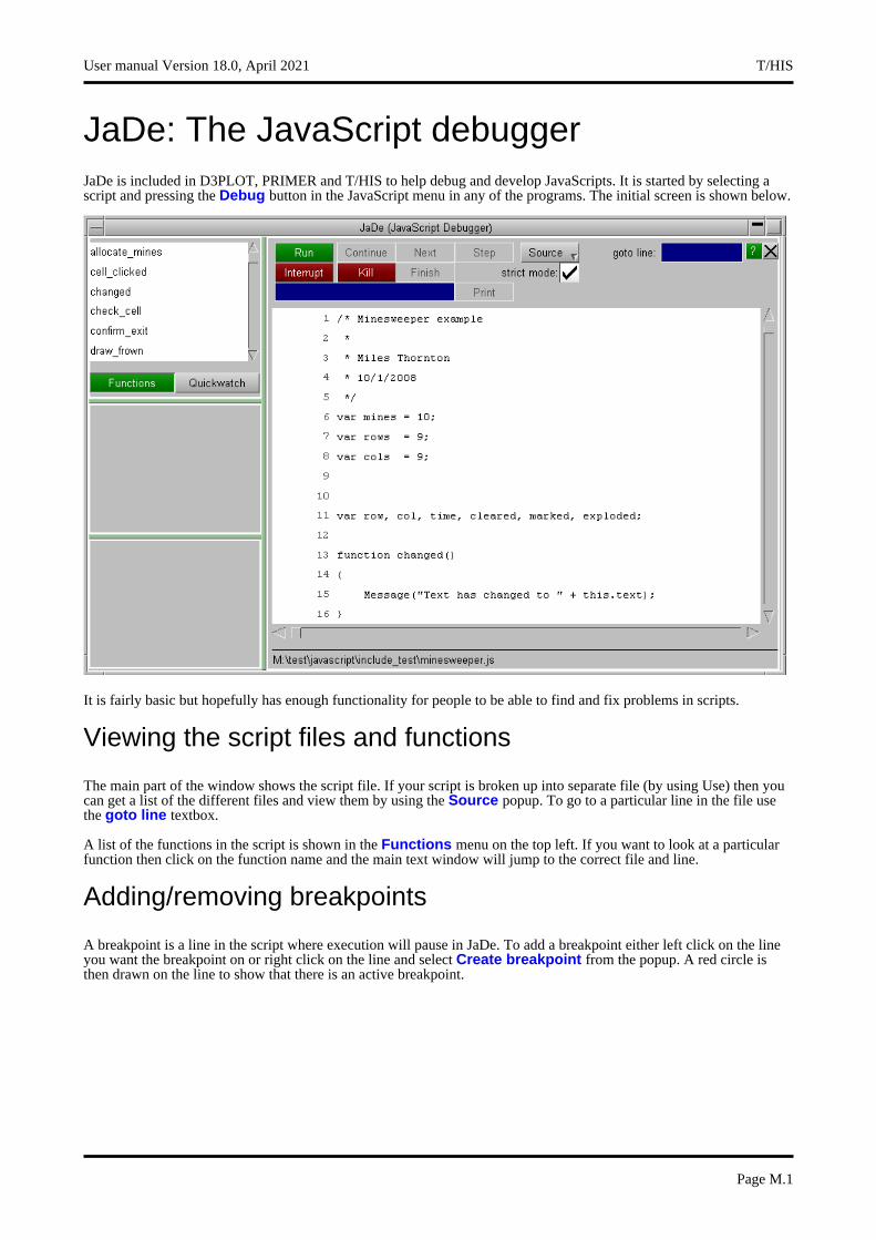
JaDe: The JavaScript debuggerJaDe is included in D3PLOT, PRIMER and T/HIS to help debug and develop JavaScripts. It is started by selecting a script and pressing the Debug button in the JavaScript menu in any of the programs. The initial screen is shown below.
It is fairly basic but hopefully has enough functionality for people to be able to find and fix problems in scripts.
Viewing the script files and functions
The main part of the window shows the script file. If your script is broken up into separate file (by using Use) then you can get a list of the different files and view them by using the Source popup. To go to a particular line in the file use the goto line textbox.
A list of the functions in the script is shown in the Functions menu on the top left. If you want to look at a particular function then click on the function name and the main text window will jump to the correct file and line.
Adding/removing breakpoints
A breakpoint is a line in the script where execution will pause in JaDe. To add a breakpoint either left click on the line you want the breakpoint on or right click on the line and select Create breakpoint from the popup. A red circle is then drawn on the line to show that there is an active breakpoint.
User manual Version 18.0, April 2021 T/HIS
Page M.1
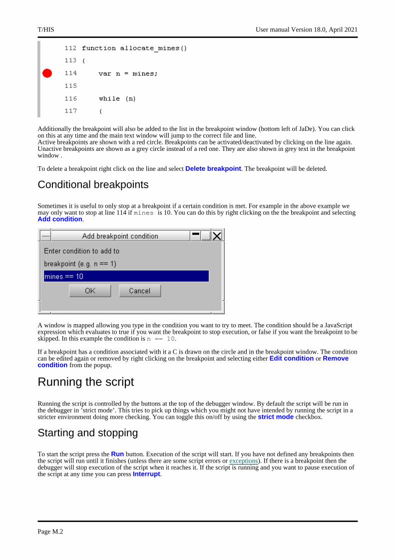
Additionally the breakpoint will also be added to the list in the breakpoint window (bottom left of JaDe). You can click on this at any time and the main text window will jump to the correct file and line.Active breakpoints are shown with a red circle. Breakpoints can be activated/deactivated by clicking on the line again. Unactive breakpoints are shown as a grey circle instead of a red one. They are also shown in grey text in the breakpoint window .
To delete a breakpoint right click on the line and select Delete breakpoint. The breakpoint will be deleted.
Conditional breakpoints
Sometimes it is useful to only stop at a breakpoint if a certain condition is met. For example in the above example we may only want to stop at line 114 if mines is 10. You can do this by right clicking on the the breakpoint and selecting Add condition.
A window is mapped allowing you type in the condition you want to try to meet. The condition should be a JavaScript expression which evaluates to true if you want the breakpoint to stop execution, or false if you want the breakpoint to be skipped. In this example the condition is n == 10.
If a breakpoint has a condition associated with it a C is drawn on the circle and in the breakpoint window. The condition can be edited again or removed by right clicking on the breakpoint and selecting either Edit condition or Remove condition from the popup.
Running the script
Running the script is controlled by the buttons at the top of the debugger window. By default the script will be run in the debugger in ’strict mode’. This tries to pick up things which you might not have intended by running the script in a stricter environment doing more checking. You can toggle this on/off by using the strict mode checkbox.
Starting and stopping
To start the script press the Run button. Execution of the script will start. If you have not defined any breakpoints then the script will run until it finishes (unless there are some script errors or exceptions). If there is a breakpoint then the debugger will stop execution of the script when it reaches it. If the script is running and you want to pause execution of the script at any time you can press Interrupt.
T/HIS User manual Version 18.0, April 2021
Page M.2

The line that the debugger has paused the script on is shown by a green triangle. In the above example it is paused at line 114. The middle panel on the left shows the call stack. See the call stack section below for more details.
Stepping and continuing
Once the script is paused in the debugger you can step through the source code by using the Continue, Next, Step and Finish buttons.
Continue will resume execution of the script again.Next continues to the next line in the current function. i.e. it will step over a function call.Step continues execution to the next source line (which may be in a different function. i.e. it will step into a function call).Finish will finish executing the current function and stop at the next line in the calling function (the function above this in the call stack).
Alternatively, if you want to continue until a particular line you can right click on the line you want to continue until and select Continue to here from the popup.
Printing the value of a variable
If you want to see the value of a variable you can type the name of the variable you want to see in the textbox at the top of the debugger and press Print. JaDe will evaluate the variable and output the result in the statusbar at the bottom of the debugger.
Using Quickwatch
If you want to look at the values for lots of variables it is annoying to have to type the variable name in and press Print for each one. A better way is to use Quickwatch at the top left of JaDe
User manual Version 18.0, April 2021 T/HIS
Page M.3
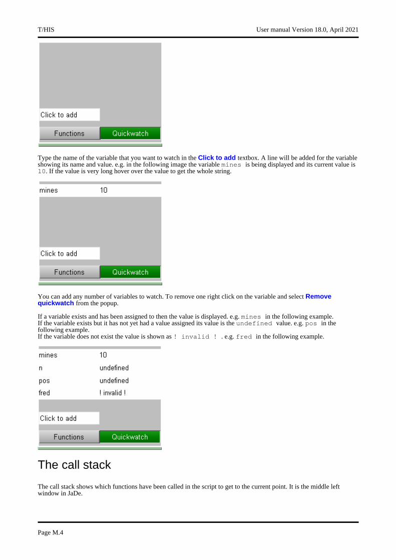
Type the name of the variable that you want to watch in the Click to add textbox. A line will be added for the variable showing its name and value. e.g. in the following image the variable mines is being displayed and its current value is 10. If the value is very long hover over the value to get the whole string.
You can add any number of variables to watch. To remove one right click on the variable and select Remove quickwatch from the popup.
If a variable exists and has been assigned to then the value is displayed. e.g. mines in the following example.If the variable exists but it has not yet had a value assigned its value is the undefined value. e.g. pos in the following example.If the variable does not exist the value is shown as ! invalid ! . e.g. fred in the following example.
The call stack
The call stack shows which functions have been called in the script to get to the current point. It is the middle left window in JaDe.
T/HIS User manual Version 18.0, April 2021
Page M.4
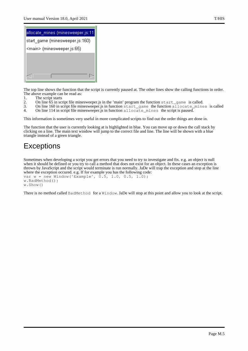
The top line shows the function that the script is currently paused at. The other lines show the calling functions in order. The above example can be read as:1. The script starts2. On line 65 in script file minesweeper.js in the ’main’ program the function start_game is called.3. On line 160 in script file minesweeper.js in function start_game the function allocate_mines is called4. On line 114 in script file minesweeper.js in function allocate_mines the script is paused.
This information is sometimes very useful in more complicated scripts to find out the order things are done in.
The function that the user is currently looking at is highlighted in blue. You can move up or down the call stack by clicking on a line. The main text window will jump to the correct file and line. The line will be shown with a blue triangle instead of a green triangle.
Exceptions
Sometimes when developing a script you get errors that you need to try to investigate and fix. e.g. an object is null when it should be defined or you try to call a method that does not exist for an object. In these cases an exception is thrown by JavaScript and the script would terminate is run normally. JaDe will trap the exception and stop at the line where the exception occured. e.g. If for example you has the following code:var w = new Window(’Example’, 0.5, 1.0, 0.5, 1.0);w.BadMethod();w.Show()
There is no method called BadMethod for a Window. JaDe will stop at this point and allow you to look at the script.
User manual Version 18.0, April 2021 T/HIS
Page M.5

T/HIS User manual Version 18.0, April 2021
Page M.6
Licences used in softwareThe Oasys LS-DYNA environment Ltd software uses several third party libraries and executables. The licences for them are given below
Apple Public SourceCopyright (c) 1999 Apple Computer, Inc. All rights reserved.The contents of this file constitute Original Code as defined in andare subject to the Apple Public Source License Version 1.1 (the"License"). You may not use this file except in compliance with theLicense. Please obtain a copy of the License athttp://www.apple.com/publicsource and read it before using this file.
This Original Code and all software distributed under the License aredistributed on an "AS IS" basis, WITHOUT WARRANTY OF ANY KIND, EITHEREXPRESS OR IMPLIED, AND APPLE HEREBY DISCLAIMS ALL SUCH WARRANTIES,INCLUDING WITHOUT LIMITATION, ANY WARRANTIES OF MERCHANTABILITY,FITNESS FOR A PARTICULAR PURPOSE OR NON-INFRINGEMENT. Please see theLicense for the specific language governing rights and limitationsunder the License.Copyright (c) 1992 NeXT Computer, Inc. All rights reserved.
Note: the URL http://www.apple.com/publicsource cited above no longer exists, see instead https://spdx.org/licenses/APSL-1.1.html
Draco
google/draco is licensed under the Apache License:Licensed under the Apache License, Version 2.0 (the "License");you may not use this file except in compliance with the License.You may obtain a copy of the License at
http://www.apache.org/licenses/LICENSE-2.0Unless required by applicable law or agreed to in writing, softwaredistributed under the License is distributed on an "AS IS" BASIS,WITHOUT WARRANTIES OR CONDITIONS OF ANY KIND, either express or implied.See the License for the specific language governing permissions andlimitations under the License.
ExpatCopyright (c) 1998, 1999, 2000 Thai Open Source Software Center Ltd
and Clark CooperCopyright (c) 2001, 2002, 2003, 2004, 2005, 2006 Expat maintainers.Permission is hereby granted, free of charge, to any person obtaininga copy of this software and associated documentation files (the"Software"), to deal in the Software without restriction, includingwithout limitation the rights to use, copy, modify, merge, publish,distribute, sublicense, and/or sell copies of the Software, and topermit persons to whom the Software is furnished to do so, subject tothe following conditions:The above copyright notice and this permission notice shall be includedin all copies or substantial portions of the Software.THE SOFTWARE IS PROVIDED "AS IS", WITHOUT WARRANTY OF ANY KIND,EXPRESS OR IMPLIED, INCLUDING BUT NOT LIMITED TO THE WARRANTIES OFMERCHANTABILITY, FITNESS FOR A PARTICULAR PURPOSE AND NONINFRINGEMENT.IN NO EVENT SHALL THE AUTHORS OR COPYRIGHT HOLDERS BE LIABLE FOR ANYCLAIM, DAMAGES OR OTHER LIABILITY, WHETHER IN AN ACTION OF CONTRACT,TORT OR OTHERWISE, ARISING FROM, OUT OF OR IN CONNECTION WITH THESOFTWARE OR THE USE OR OTHER DEALINGS IN THE SOFTWARE
FreeType
User manual Version 18.0, April 2021 T/HIS
Page N.1
Portions of this software are copyright The FreeType Project (www.freetype.org). All rights reserved.The FreeType Project LICENSE----------------------------
2006-Jan-27Copyright 1996-2002, 2006 by
David Turner, Robert Wilhelm, and Werner LembergIntroduction============The FreeType Project is distributed in several archive packages;some of them may contain, in addition to the FreeType font engine,various tools and contributions which rely on, or relate to, theFreeType Project.This license applies to all files found in such packages, andwhich do not fall under their own explicit license. The licenseaffects thus the FreeType font engine, the test programs,documentation and makefiles, at the very least.This license was inspired by the BSD, Artistic, and IJG(Independent JPEG Group) licenses, which all encourage inclusionand use of free software in commercial and freeware productsalike. As a consequence, its main points are that:o We don’t promise that this software works. However, we will beinterested in any kind of bug reports. (‘as is’ distribution)
o You can use this software for whatever you want, in parts orfull form, without having to pay us. (‘royalty-free’ usage)
o You may not pretend that you wrote this software. If you useit, or only parts of it, in a program, you must acknowledgesomewhere in your documentation that you have used theFreeType code. (‘credits’)
We specifically permit and encourage the inclusion of thissoftware, with or without modifications, in commercial products.We disclaim all warranties covering The FreeType Project andassume no liability related to The FreeType Project.Finally, many people asked us for a preferred form for acredit/disclaimer to use in compliance with this license. We thusencourage you to use the following text:""" Portions of this software are copyright <year> The FreeTypeProject (www.freetype.org). All rights reserved."""Please replace <year> with the value from the FreeType version youactually use.
Legal Terms===========0. Definitions--------------Throughout this license, the terms ‘package’, ‘FreeType Project’,and ‘FreeType archive’ refer to the set of files originallydistributed by the authors (David Turner, Robert Wilhelm, andWerner Lemberg) as the ‘FreeType Project’, be they named as alpha,beta or final release.‘You’ refers to the licensee, or person using the project, where‘using’ is a generic term including compiling the project’s sourcecode as well as linking it to form a ‘program’ or ‘executable’.This program is referred to as ‘a program using the FreeTypeengine’.This license applies to all files distributed in the originalFreeType Project, including all source code, binaries anddocumentation, unless otherwise stated in the file in itsoriginal, unmodified form as distributed in the original archive.If you are unsure whether or not a particular file is covered bythis license, you must contact us to verify this.The FreeType Project is copyright (C) 1996-2000 by David Turner,Robert Wilhelm, and Werner Lemberg. All rights reserved except asspecified below.
1. No Warranty--------------THE FREETYPE PROJECT IS PROVIDED ‘AS IS’ WITHOUT WARRANTY OF ANYKIND, EITHER EXPRESS OR IMPLIED, INCLUDING, BUT NOT LIMITED TO,WARRANTIES OF MERCHANTABILITY AND FITNESS FOR A PARTICULARPURPOSE. IN NO EVENT WILL ANY OF THE AUTHORS OR COPYRIGHT HOLDERSBE LIABLE FOR ANY DAMAGES CAUSED BY THE USE OR THE INABILITY TO
T/HIS User manual Version 18.0, April 2021
Page N.2
USE, OF THE FREETYPE PROJECT.2. Redistribution-----------------This license grants a worldwide, royalty-free, perpetual andirrevocable right and license to use, execute, perform, compile,display, copy, create derivative works of, distribute andsublicense the FreeType Project (in both source and object codeforms) and derivative works thereof for any purpose; and toauthorize others to exercise some or all of the rights grantedherein, subject to the following conditions:o Redistribution of source code must retain this license file(‘FTL.TXT’) unaltered; any additions, deletions or changes tothe original files must be clearly indicated in accompanyingdocumentation. The copyright notices of the unaltered,original files must be preserved in all copies of sourcefiles.
o Redistribution in binary form must provide a disclaimer thatstates that the software is based in part of the work of theFreeType Team, in the distribution documentation. We alsoencourage you to put an URL to the FreeType web page in yourdocumentation, though this isn’t mandatory.
These conditions apply to any software derived from or based onthe FreeType Project, not just the unmodified files. If you useour work, you must acknowledge us. However, no fee need be paidto us.
3. Advertising--------------Neither the FreeType authors and contributors nor you shall usethe name of the other for commercial, advertising, or promotionalpurposes without specific prior written permission.We suggest, but do not require, that you use one or more of thefollowing phrases to refer to this software in your documentationor advertising materials: ‘FreeType Project’, ‘FreeType Engine’,‘FreeType library’, or ‘FreeType Distribution’.As you have not signed this license, you are not required toaccept it. However, as the FreeType Project is copyrightedmaterial, only this license, or another one contracted with theauthors, grants you the right to use, distribute, and modify it.Therefore, by using, distributing, or modifying the FreeTypeProject, you indicate that you understand and accept all the termsof this license.
4. Contacts-----------There are two mailing lists related to FreeType:o [email protected] general use and applications of FreeType, as well asfuture and wanted additions to the library and distribution.If you are looking for support, start in this list if youhaven’t found anything to help you in the documentation.
o [email protected] bugs, as well as engine internals, design issues,specific licenses, porting, etc.
Our home page can be found athttp://www.freetype.org
--- end of FTL.TXT ---
FFmpegFFmpeg is free software; you can redistribute it and/ormodify it under the terms of the GNU Lesser General PublicLicense as published by the Free Software Foundation; eitherversion 2.1 of the License, or (at your option) any later version.
FFmpeg is distributed in the hope that it will be useful,but WITHOUT ANY WARRANTY; without even the implied warranty ofMERCHANTABILITY or FITNESS FOR A PARTICULAR PURPOSE. See the GNULesser General Public License for more details.
You should have received a copy of the GNU Lesser General PublicLicense along with FFmpeg; if not, write to the Free Software
User manual Version 18.0, April 2021 T/HIS
Page N.3
Foundation, Inc., 51 Franklin Street, Fifth Floor, Boston, MA 02110-1301 USA
JpegThe authors make NO WARRANTY or representation, either express or implied,with respect to this software, its quality, accuracy, merchantability, orfitness for a particular purpose. This software is provided "AS IS", and you,its user, assume the entire risk as to its quality and accuracy.This software is copyright (C) 1991-2012, Thomas G. Lane, Guido Vollbeding.All Rights Reserved except as specified below.Permission is hereby granted to use, copy, modify, and distribute thissoftware (or portions thereof) for any purpose, without fee, subject to theseconditions:(1) If any part of the source code for this software is distributed, then thisREADME file must be included, with this copyright and no-warranty noticeunaltered; and any additions, deletions, or changes to the original filesmust be clearly indicated in accompanying documentation.(2) If only executable code is distributed, then the accompanyingdocumentation must state that "this software is based in part on the work ofthe Independent JPEG Group".(3) Permission for use of this software is granted only if the user acceptsfull responsibility for any undesirable consequences; the authors acceptNO LIABILITY for damages of any kind.These conditions apply to any software derived from or based on the IJG code,not just to the unmodified library. If you use our work, you ought toacknowledge us.Permission is NOT granted for the use of any IJG author’s name or company namein advertising or publicity relating to this software or products derived fromit. This software may be referred to only as "the Independent JPEG Group’ssoftware".We specifically permit and encourage the use of this software as the basis ofcommercial products, provided that all warranty or liability claims areassumed by the product vendor.
LibcurlCOPYRIGHT AND PERMISSION NOTICECopyright (c) 1996 - 2012, Daniel Stenberg, <[email protected]>.All rights reserved.Permission to use, copy, modify, and distribute this software for any purposewith or without fee is hereby granted, provided that the above copyrightnotice and this permission notice appear in all copies.THE SOFTWARE IS PROVIDED "AS IS", WITHOUT WARRANTY OF ANY KIND, EXPRESS ORIMPLIED, INCLUDING BUT NOT LIMITED TO THE WARRANTIES OF MERCHANTABILITY,FITNESS FOR A PARTICULAR PURPOSE AND NONINFRINGEMENT OF THIRD PARTY RIGHTS. INNO EVENT SHALL THE AUTHORS OR COPYRIGHT HOLDERS BE LIABLE FOR ANY CLAIM,DAMAGES OR OTHER LIABILITY, WHETHER IN AN ACTION OF CONTRACT, TORT OROTHERWISE, ARISING FROM, OUT OF OR IN CONNECTION WITH THE SOFTWARE OR THE USEOR OTHER DEALINGS IN THE SOFTWARE.Except as contained in this notice, the name of a copyright holder shall notbe used in advertising or otherwise to promote the sale, use or other dealingsin this Software without prior written authorization of the copyright holder.
Libfamelibfame - Fast Assembly MPEG Encoder LibraryCopyright (C) 2000-2001 Vivien ChappelierThis library is free software; you can redistribute it and/ormodify it under the terms of the GNU Library General PublicLicense as published by the Free Software Foundation; eitherversion 2 of the License, or (at your option) any later version.This library is distributed in the hope that it will be useful,but WITHOUT ANY WARRANTY; without even the implied warranty ofMERCHANTABILITY or FITNESS FOR A PARTICULAR PURPOSE. See the GNULibrary General Public License for more details.You should have received a copy of the GNU Library General PublicLicense along with this library; if not, write to the FreeSoftware Foundation, Inc., 675 Mass Ave, Cambridge, MA 02139, USA.
T/HIS User manual Version 18.0, April 2021
Page N.4

LibgifThe GIFLIB distribution is Copyright (c) 1997 Eric S. RaymondPermission is hereby granted, free of charge, to any person obtaining a copyof this software and associated documentation files (the "Software"), to dealin the Software without restriction, including without limitation the rightsto use, copy, modify, merge, publish, distribute, sublicense, and/or sellcopies of the Software, and to permit persons to whom the Software isfurnished to do so, subject to the following conditions:The above copyright notice and this permission notice shall be included inall copies or substantial portions of the Software.THE SOFTWARE IS PROVIDED "AS IS", WITHOUT WARRANTY OF ANY KIND, EXPRESS ORIMPLIED, INCLUDING BUT NOT LIMITED TO THE WARRANTIES OF MERCHANTABILITY,FITNESS FOR A PARTICULAR PURPOSE AND NONINFRINGEMENT. IN NO EVENT SHALL THEAUTHORS OR COPYRIGHT HOLDERS BE LIABLE FOR ANY CLAIM, DAMAGES OR OTHERLIABILITY, WHETHER IN AN ACTION OF CONTRACT, TORT OR OTHERWISE, ARISING FROM,OUT OF OR IN CONNECTION WITH THE SOFTWARE OR THE USE OR OTHER DEALINGS INTHE SOFTWARE.
LibpngThis copy of the libpng notices is provided for your convenience. In case ofany discrepancy between this copy and the notices in the file png.h that isincluded in the libpng distribution, the latter shall prevail.COPYRIGHT NOTICE, DISCLAIMER, and LICENSE:If you modify libpng you may insert additional notices immediately followingthis sentence.This code is released under the libpng license.libpng versions 1.2.6, August 15, 2004, through 1.5.11, June 14, 2012, areCopyright (c) 2004, 2006-2012 Glenn Randers-Pehrson, and aredistributed according to the same disclaimer and license as libpng-1.2.5with the following individual added to the list of Contributing Authors
Cosmin Trutalibpng versions 1.0.7, July 1, 2000, through 1.2.5 - October 3, 2002, areCopyright (c) 2000-2002 Glenn Randers-Pehrson, and aredistributed according to the same disclaimer and license as libpng-1.0.6with the following individuals added to the list of Contributing Authors
Simon-Pierre CadieuxEric S. RaymondGilles Vollant
and with the following additions to the disclaimer:There is no warranty against interference with your enjoyment of thelibrary or against infringement. There is no warranty that ourefforts or the library will fulfill any of your particular purposesor needs. This library is provided with all faults, and the entirerisk of satisfactory quality, performance, accuracy, and effort is withthe user.
libpng versions 0.97, January 1998, through 1.0.6, March 20, 2000, areCopyright (c) 1998, 1999 Glenn Randers-Pehrson, and aredistributed according to the same disclaimer and license as libpng-0.96,with the following individuals added to the list of Contributing Authors:
Tom LaneGlenn Randers-PehrsonWillem van Schaik
libpng versions 0.89, June 1996, through 0.96, May 1997, areCopyright (c) 1996, 1997 Andreas DilgerDistributed according to the same disclaimer and license as libpng-0.88,with the following individuals added to the list of Contributing Authors:
John BowlerKevin BraceySam BushellMagnus HolmgrenGreg RoelofsTom Tanner
libpng versions 0.5, May 1995, through 0.88, January 1996, areCopyright (c) 1995, 1996 Guy Eric Schalnat, Group 42, Inc.For the purposes of this copyright and license, "Contributing Authors"is defined as the following set of individuals:
Andreas DilgerDave Martindale
User manual Version 18.0, April 2021 T/HIS
Page N.5
Guy Eric SchalnatPaul SchmidtTim Wegner
The PNG Reference Library is supplied "AS IS". The Contributing Authorsand Group 42, Inc. disclaim all warranties, expressed or implied,including, without limitation, the warranties of merchantability and offitness for any purpose. The Contributing Authors and Group 42, Inc.assume no liability for direct, indirect, incidental, special, exemplary,or consequential damages, which may result from the use of the PNGReference Library, even if advised of the possibility of such damage.Permission is hereby granted to use, copy, modify, and distribute thissource code, or portions hereof, for any purpose, without fee, subjectto the following restrictions:1. The origin of this source code must not be misrepresented.2. Altered versions must be plainly marked as such and must not
be misrepresented as being the original source.3. This Copyright notice may not be removed or altered from any
source or altered source distribution.The Contributing Authors and Group 42, Inc. specifically permit, withoutfee, and encourage the use of this source code as a component tosupporting the PNG file format in commercial products. If you use thissource code in a product, acknowledgment is not required but would beappreciated.A "png_get_copyright" function is available, for convenient use in "about"boxes and the like:
printf("%s",png_get_copyright(NULL));Also, the PNG logo (in PNG format, of course) is supplied in thefiles "pngbar.png" and "pngbar.jpg (88x31) and "pngnow.png" (98x31).Libpng is OSI Certified Open Source Software. OSI Certified Open Source is acertification mark of the Open Source Initiative.Glenn Randers-Pehrsonglennrp at users.sourceforge.netJune 14, 2012
LibxlsxwriterLibxlsxwriter is released under a FreeBSD license:
Copyright 2014-2016, John McNamara All rights reserved.Redistribution and use in source and binary forms, with or withoutmodification, are permitted provided that the following conditions aremet:1. Redistributions of source code must retain the above copyright notice,
this list of conditions and the following disclaimer.2. Redistributions in binary form must reproduce the above copyright
notice, this list of conditions and the following disclaimer in thedocumentation and/or other materials provided with the distribution.
THIS SOFTWARE IS PROVIDED BY THE COPYRIGHT HOLDERS AND CONTRIBUTORS "ASIS" AND ANY EXPRESS OR IMPLIED WARRANTIES, INCLUDING, BUT NOT LIMITED TO,THE IMPLIED WARRANTIES OF MERCHANTABILITY AND FITNESS FOR A PARTICULARPURPOSE ARE DISCLAIMED. IN NO EVENT SHALL THE COPYRIGHT OWNER ORCONTRIBUTORS BE LIABLE FOR ANY DIRECT, INDIRECT, INCIDENTAL, SPECIAL,EXEMPLARY, OR CONSEQUENTIAL DAMAGES (INCLUDING, BUT NOT LIMITED TO,PROCUREMENT OF SUBSTITUTE GOODS OR SERVICES; LOSS OF USE, DATA, ORPROFITS; OR BUSINESS INTERRUPTION) HOWEVER CAUSED AND ON ANY THEORY OFLIABILITY, WHETHER IN CONTRACT, STRICT LIABILITY, OR TORT (INCLUDINGNEGLIGENCE OR OTHERWISE) ARISING IN ANY WAY OUT OF THE USE OF THISSOFTWARE, EVEN IF ADVISED OF THE POSSIBILITY OF SUCH DAMAGE.The views and conclusions contained in the software and documentation arethose of the authors and should not be interpreted as representingofficial policies, either expressed or implied, of the FreeBSD Project.
Libxlsxwriter includes ‘queue.h‘ from FreeBSD and the ‘minizip‘ component of‘zlib‘ which have the following licenses:Queue.h from FreeBSD:
Copyright (c) 1991, 1993The Regents of the University of California. All rights reserved.Redistribution and use in source and binary forms, with or withoutmodification, are permitted provided that the following conditionsare met:1. Redistributions of source code must retain the above copyright
T/HIS User manual Version 18.0, April 2021
Page N.6
notice, this list of conditions and the following disclaimer.2. Redistributions in binary form must reproduce the above copyright
notice, this list of conditions and the following disclaimer in thedocumentation and/or other materials provided with the distribution.
4. Neither the name of the University nor the names of its contributorsmay be used to endorse or promote products derived from this softwarewithout specific prior written permission.
THIS SOFTWARE IS PROVIDED BY THE REGENTS AND CONTRIBUTORS ‘‘AS IS’’ ANDANY EXPRESS OR IMPLIED WARRANTIES, INCLUDING, BUT NOT LIMITED TO, THEIMPLIED WARRANTIES OF MERCHANTABILITY AND FITNESS FOR A PARTICULAR PURPOSEARE DISCLAIMED. IN NO EVENT SHALL THE REGENTS OR CONTRIBUTORS BE LIABLEFOR ANY DIRECT, INDIRECT, INCIDENTAL, SPECIAL, EXEMPLARY, OR CONSEQUENTIALDAMAGES (INCLUDING, BUT NOT LIMITED TO, PROCUREMENT OF SUBSTITUTE GOODSOR SERVICES; LOSS OF USE, DATA, OR PROFITS; OR BUSINESS INTERRUPTION)HOWEVER CAUSED AND ON ANY THEORY OF LIABILITY, WHETHER IN CONTRACT, STRICTLIABILITY, OR TORT (INCLUDING NEGLIGENCE OR OTHERWISE) ARISING IN ANY WAYOUT OF THE USE OF THIS SOFTWARE, EVEN IF ADVISED OF THE POSSIBILITY OFSUCH DAMAGE.
Zlib has the following License/Copyright:(C) 1995-2013 Jean-loup Gailly and Mark AdlerThis software is provided ’as-is’, without any express or impliedwarranty. In no event will the authors be held liable for any damagesarising from the use of this software.Permission is granted to anyone to use this software for any purpose,including commercial applications, and to alter it and redistribute itfreely, subject to the following restrictions:1. The origin of this software must not be misrepresented; you must not
claim that you wrote the original software. If you use this softwarein a product, an acknowledgment in the product documentation would beappreciated but is not required.
2. Altered source versions must be plainly marked as such, and must not bemisrepresented as being the original software.
3. This notice may not be removed or altered from any source distribution.Jean-loup Gailly Mark [email protected] [email protected]
MPEG-LATHIS PRODUCT IS LICENSED UNDER THEAVC PATENT PORTFOLIO LICENSE FOR THE PERSONAL USE OF ACONSUMER OR OTHER USES IN WHICH IT DOES NOT RECEIVEREMUNERATION TO (i) ENCODE VIDEO IN COMPLIANCE WITH THEAVC STANDARD ("AVC VIDEO") AND/OR (ii) DECODE AVC VIDEOTHAT WAS ENCODED BY A CONSUMER ENGAGED IN A PERSONALACTIVITY AND/OR WAS OBTAINED FROM A VIDEO PROVIDERLICENSED TO PROVIDE AVC VIDEO. NO LICENSE IS GRANTED ORSHALL BE IMPLIED FOR ANY OTHER USE. ADDITIONALINFORMATION MAY BE OBTAINED FROM MPEG LA, L.L.C. SEEHTTP://WWW.MPEGLA.COM
OpensslLICENSE ISSUES==============The OpenSSL toolkit stays under a double license, i.e. both the conditions ofthe OpenSSL License and the original SSLeay license apply to the toolkit.See below for the actual license texts.OpenSSL License---------------
/* ====================================================================* Copyright (c) 1998-2017 The OpenSSL Project. All rights reserved.** Redistribution and use in source and binary forms, with or without* modification, are permitted provided that the following conditions* are met:** 1. Redistributions of source code must retain the above copyright* notice, this list of conditions and the following disclaimer. ** 2. Redistributions in binary form must reproduce the above copyright
User manual Version 18.0, April 2021 T/HIS
Page N.7
* notice, this list of conditions and the following disclaimer in* the documentation and/or other materials provided with the* distribution.** 3. All advertising materials mentioning features or use of this* software must display the following acknowledgment:* "This product includes software developed by the OpenSSL Project* for use in the OpenSSL Toolkit. (http://www.openssl.org/)"** 4. The names "OpenSSL Toolkit" and "OpenSSL Project" must not be used to* endorse or promote products derived from this software without* prior written permission. For written permission, please contact* [email protected].** 5. Products derived from this software may not be called "OpenSSL"* nor may "OpenSSL" appear in their names without prior written* permission of the OpenSSL Project.** 6. Redistributions of any form whatsoever must retain the following* acknowledgment:* "This product includes software developed by the OpenSSL Project* for use in the OpenSSL Toolkit (http://www.openssl.org/)"** THIS SOFTWARE IS PROVIDED BY THE OpenSSL PROJECT ‘‘AS IS’’ AND ANY* EXPRESSED OR IMPLIED WARRANTIES, INCLUDING, BUT NOT LIMITED TO, THE* IMPLIED WARRANTIES OF MERCHANTABILITY AND FITNESS FOR A PARTICULAR* PURPOSE ARE DISCLAIMED. IN NO EVENT SHALL THE OpenSSL PROJECT OR* ITS CONTRIBUTORS BE LIABLE FOR ANY DIRECT, INDIRECT, INCIDENTAL,* SPECIAL, EXEMPLARY, OR CONSEQUENTIAL DAMAGES (INCLUDING, BUT* NOT LIMITED TO, PROCUREMENT OF SUBSTITUTE GOODS OR SERVICES;* LOSS OF USE, DATA, OR PROFITS; OR BUSINESS INTERRUPTION)* HOWEVER CAUSED AND ON ANY THEORY OF LIABILITY, WHETHER IN CONTRACT,* STRICT LIABILITY, OR TORT (INCLUDING NEGLIGENCE OR OTHERWISE)* ARISING IN ANY WAY OUT OF THE USE OF THIS SOFTWARE, EVEN IF ADVISED* OF THE POSSIBILITY OF SUCH DAMAGE.* ====================================================================** This product includes cryptographic software written by Eric Young* ([email protected]). This product includes software written by Tim* Hudson ([email protected]).**/Original SSLeay License-----------------------/* Copyright (C) 1995-1998 Eric Young ([email protected])* All rights reserved.** This package is an SSL implementation written* by Eric Young ([email protected]).* The implementation was written so as to conform with Netscapes SSL.* * This library is free for commercial and non-commercial use as long as* the following conditions are aheared to. The following conditions* apply to all code found in this distribution, be it the RC4, RSA,* lhash, DES, etc., code; not just the SSL code. The SSL documentation* included with this distribution is covered by the same copyright terms* except that the holder is Tim Hudson ([email protected]).* * Copyright remains Eric Young’s, and as such any Copyright notices in* the code are not to be removed.* If this package is used in a product, Eric Young should be given attribution* as the author of the parts of the library used.* This can be in the form of a textual message at program startup or* in documentation (online or textual) provided with the package.* * Redistribution and use in source and binary forms, with or without* modification, are permitted provided that the following conditions* are met:* 1. Redistributions of source code must retain the copyright* notice, this list of conditions and the following disclaimer.* 2. Redistributions in binary form must reproduce the above copyright
T/HIS User manual Version 18.0, April 2021
Page N.8
* notice, this list of conditions and the following disclaimer in the* documentation and/or other materials provided with the distribution.* 3. All advertising materials mentioning features or use of this software* must display the following acknowledgement:* "This product includes cryptographic software written by* Eric Young ([email protected])"* The word ’cryptographic’ can be left out if the rouines from the library* being used are not cryptographic related :-).* 4. If you include any Windows specific code (or a derivative thereof) from * the apps directory (application code) you must include an acknowledgement:* "This product includes software written by Tim Hudson ([email protected])"* * THIS SOFTWARE IS PROVIDED BY ERIC YOUNG ‘‘AS IS’’ AND* ANY EXPRESS OR IMPLIED WARRANTIES, INCLUDING, BUT NOT LIMITED TO, THE* IMPLIED WARRANTIES OF MERCHANTABILITY AND FITNESS FOR A PARTICULAR PURPOSE* ARE DISCLAIMED. IN NO EVENT SHALL THE AUTHOR OR CONTRIBUTORS BE LIABLE* FOR ANY DIRECT, INDIRECT, INCIDENTAL, SPECIAL, EXEMPLARY, OR CONSEQUENTIAL* DAMAGES (INCLUDING, BUT NOT LIMITED TO, PROCUREMENT OF SUBSTITUTE GOODS* OR SERVICES; LOSS OF USE, DATA, OR PROFITS; OR BUSINESS INTERRUPTION)* HOWEVER CAUSED AND ON ANY THEORY OF LIABILITY, WHETHER IN CONTRACT, STRICT* LIABILITY, OR TORT (INCLUDING NEGLIGENCE OR OTHERWISE) ARISING IN ANY WAY* OUT OF THE USE OF THIS SOFTWARE, EVEN IF ADVISED OF THE POSSIBILITY OF* SUCH DAMAGE.* * The licence and distribution terms for any publically available version or* derivative of this code cannot be changed. i.e. this code cannot simply be* copied and put under another distribution licence* [including the GNU Public Licence.]*/
PCREPCRE LICENCE------------PCRE is a library of functions to support regular expressions whose syntaxand semantics are as close as possible to those of the Perl 5 language.Release 7 of PCRE is distributed under the terms of the "BSD" licence, asspecified below. The documentation for PCRE, supplied in the "doc"directory, is distributed under the same terms as the software itself.The basic library functions are written in C and are freestanding. Alsoincluded in the distribution is a set of C++ wrapper functions.THE BASIC LIBRARY FUNCTIONS---------------------------Written by: Philip HazelEmail local part: ph10Email domain: cam.ac.ukUniversity of Cambridge Computing Service,Cambridge, England.Copyright (c) 1997-2008 University of CambridgeAll rights reserved.THE C++ WRAPPER FUNCTIONS-------------------------Contributed by: Google Inc.Copyright (c) 2007-2008, Google Inc.All rights reserved.THE "BSD" LICENCE-----------------Redistribution and use in source and binary forms, with or withoutmodification, are permitted provided that the following conditions are met:
* Redistributions of source code must retain the above copyright notice,this list of conditions and the following disclaimer.
* Redistributions in binary form must reproduce the above copyrightnotice, this list of conditions and the following disclaimer in thedocumentation and/or other materials provided with the distribution.
* Neither the name of the University of Cambridge nor the name of GoogleInc. nor the names of their contributors may be used to endorse orpromote products derived from this software without specific priorwritten permission.
THIS SOFTWARE IS PROVIDED BY THE COPYRIGHT HOLDERS AND CONTRIBUTORS "AS IS"AND ANY EXPRESS OR IMPLIED WARRANTIES, INCLUDING, BUT NOT LIMITED TO, THE
User manual Version 18.0, April 2021 T/HIS
Page N.9
IMPLIED WARRANTIES OF MERCHANTABILITY AND FITNESS FOR A PARTICULAR PURPOSEARE DISCLAIMED. IN NO EVENT SHALL THE COPYRIGHT OWNER OR CONTRIBUTORS BELIABLE FOR ANY DIRECT, INDIRECT, INCIDENTAL, SPECIAL, EXEMPLARY, ORCONSEQUENTIAL DAMAGES (INCLUDING, BUT NOT LIMITED TO, PROCUREMENT OFSUBSTITUTE GOODS OR SERVICES; LOSS OF USE, DATA, OR PROFITS; OR BUSINESSINTERRUPTION) HOWEVER CAUSED AND ON ANY THEORY OF LIABILITY, WHETHER INCONTRACT, STRICT LIABILITY, OR TORT (INCLUDING NEGLIGENCE OR OTHERWISE)ARISING IN ANY WAY OUT OF THE USE OF THIS SOFTWARE, EVEN IF ADVISED OF THEPOSSIBILITY OF SUCH DAMAGE.End
PDFHummus
Is licensed under the Apache License:Copyright 2011 Gal Kahana PDFWriterLicensed under the Apache License, Version 2.0 (the "License");you may not use this file except in compliance with the License.You may obtain a copy of the License at
http://www.apache.org/licenses/LICENSE-2.0Unless required by applicable law or agreed to in writing, softwaredistributed under the License is distributed on an "AS IS" BASIS,WITHOUT WARRANTIES OR CONDITIONS OF ANY KIND, either express or implied.See the License for the specific language governing permissions andlimitations under the License.
POV-Ray
Is licensed under the GNU AFFERO GENERAL PUBLIC LICENSE Version 3, 19 November 2007 which may be found here http://www.povray.org/povlegal.html
Oasys Ltd use the POV-Ray executable in unmodified form as a separate, stand-alone entity. We have not modified the source code or the executable in any way.
We convey the executable as part of our installation package, and in accordance with the licence:• Users who install POV-Ray must accept the licence terms cited above.• We provide a download of the POV-Ray executable and source code on our website
http://www.oasys-software.com/dyna/en/
SmoothSort
Is licensed under the Creative Commons Attribution-ShareAlike 3.0 license which may be found here:https://creativecommons.org/licenses/by-sa/3.0/legalcode
Oasys Ltd acknowledge Wikibooks as the source of this algorithm, which is used in unmodified form.
SpidermonkeyMozilla Public License Version 2.0==================================1. Definitions--------------1.1. "Contributor"
means each individual or legal entity that creates, contributes tothe creation of, or owns Covered Software.
1.2. "Contributor Version"means the combination of the Contributions of others (if any) usedby a Contributor and that particular Contributor’s Contribution.
1.3. "Contribution"means Covered Software of a particular Contributor.
1.4. "Covered Software"means Source Code Form to which the initial Contributor has attachedthe notice in Exhibit A, the Executable Form of such Source CodeForm, and Modifications of such Source Code Form, in each case
T/HIS User manual Version 18.0, April 2021
Page N.10
including portions thereof.1.5. "Incompatible With Secondary Licenses"
means(a) that the initial Contributor has attached the notice described
in Exhibit B to the Covered Software; or(b) that the Covered Software was made available under the terms of
version 1.1 or earlier of the License, but not also under theterms of a Secondary License.
1.6. "Executable Form"means any form of the work other than Source Code Form.
1.7. "Larger Work"means a work that combines Covered Software with other material, in a separate file or files, that is not Covered Software.
1.8. "License"means this document.
1.9. "Licensable"means having the right to grant, to the maximum extent possible,whether at the time of the initial grant or subsequently, any andall of the rights conveyed by this License.
1.10. "Modifications"means any of the following:(a) any file in Source Code Form that results from an addition to,
deletion from, or modification of the contents of CoveredSoftware; or
(b) any new file in Source Code Form that contains any CoveredSoftware.
1.11. "Patent Claims" of a Contributormeans any patent claim(s), including without limitation, method,process, and apparatus claims, in any patent Licensable by suchContributor that would be infringed, but for the grant of theLicense, by the making, using, selling, offering for sale, havingmade, import, or transfer of either its Contributions or itsContributor Version.
1.12. "Secondary License"means either the GNU General Public License, Version 2.0, the GNULesser General Public License, Version 2.1, the GNU Affero GeneralPublic License, Version 3.0, or any later versions of thoselicenses.
1.13. "Source Code Form"means the form of the work preferred for making modifications.
1.14. "You" (or "Your")means an individual or a legal entity exercising rights under thisLicense. For legal entities, "You" includes any entity thatcontrols, is controlled by, or is under common control with You. Forpurposes of this definition, "control" means (a) the power, director indirect, to cause the direction or management of such entity,whether by contract or otherwise, or (b) ownership of more thanfifty percent (50%) of the outstanding shares or beneficialownership of such entity.
2. License Grants and Conditions--------------------------------2.1. GrantsEach Contributor hereby grants You a world-wide, royalty-free,non-exclusive license:(a) under intellectual property rights (other than patent or trademark)
Licensable by such Contributor to use, reproduce, make available,modify, display, perform, distribute, and otherwise exploit itsContributions, either on an unmodified basis, with Modifications, oras part of a Larger Work; and
(b) under Patent Claims of such Contributor to make, use, sell, offerfor sale, have made, import, and otherwise transfer either itsContributions or its Contributor Version.
2.2. Effective DateThe licenses granted in Section 2.1 with respect to any Contributionbecome effective for each Contribution on the date the Contributor firstdistributes such Contribution.2.3. Limitations on Grant ScopeThe licenses granted in this Section 2 are the only rights granted underthis License. No additional rights or licenses will be implied from thedistribution or licensing of Covered Software under this License.Notwithstanding Section 2.1(b) above, no patent license is granted by a
User manual Version 18.0, April 2021 T/HIS
Page N.11
Contributor:(a) for any code that a Contributor has removed from Covered Software;
or(b) for infringements caused by: (i) Your and any other third party’s
modifications of Covered Software, or (ii) the combination of itsContributions with other software (except as part of its ContributorVersion); or
(c) under Patent Claims infringed by Covered Software in the absence ofits Contributions.
This License does not grant any rights in the trademarks, service marks,or logos of any Contributor (except as may be necessary to comply withthe notice requirements in Section 3.4).2.4. Subsequent LicensesNo Contributor makes additional grants as a result of Your choice todistribute the Covered Software under a subsequent version of thisLicense (see Section 10.2) or under the terms of a Secondary License (ifpermitted under the terms of Section 3.3).2.5. RepresentationEach Contributor represents that the Contributor believes itsContributions are its original creation(s) or it has sufficient rightsto grant the rights to its Contributions conveyed by this License.2.6. Fair UseThis License is not intended to limit any rights You have underapplicable copyright doctrines of fair use, fair dealing, or otherequivalents.2.7. ConditionsSections 3.1, 3.2, 3.3, and 3.4 are conditions of the licenses grantedin Section 2.1.3. Responsibilities-------------------3.1. Distribution of Source FormAll distribution of Covered Software in Source Code Form, including anyModifications that You create or to which You contribute, must be underthe terms of this License. You must inform recipients that the SourceCode Form of the Covered Software is governed by the terms of thisLicense, and how they can obtain a copy of this License. You may notattempt to alter or restrict the recipients’ rights in the Source CodeForm.3.2. Distribution of Executable FormIf You distribute Covered Software in Executable Form then:(a) such Covered Software must also be made available in Source Code
Form, as described in Section 3.1, and You must inform recipients ofthe Executable Form how they can obtain a copy of such Source CodeForm by reasonable means in a timely manner, at a charge no morethan the cost of distribution to the recipient; and
(b) You may distribute such Executable Form under the terms of thisLicense, or sublicense it under different terms, provided that thelicense for the Executable Form does not attempt to limit or alterthe recipients’ rights in the Source Code Form under this License.
3.3. Distribution of a Larger WorkYou may create and distribute a Larger Work under terms of Your choice,provided that You also comply with the requirements of this License forthe Covered Software. If the Larger Work is a combination of CoveredSoftware with a work governed by one or more Secondary Licenses, and theCovered Software is not Incompatible With Secondary Licenses, thisLicense permits You to additionally distribute such Covered Softwareunder the terms of such Secondary License(s), so that the recipient ofthe Larger Work may, at their option, further distribute the CoveredSoftware under the terms of either this License or such SecondaryLicense(s).3.4. NoticesYou may not remove or alter the substance of any license notices(including copyright notices, patent notices, disclaimers of warranty,or limitations of liability) contained within the Source Code Form ofthe Covered Software, except that You may alter any license notices tothe extent required to remedy known factual inaccuracies.3.5. Application of Additional TermsYou may choose to offer, and to charge a fee for, warranty, support,indemnity or liability obligations to one or more recipients of CoveredSoftware. However, You may do so only on Your own behalf, and not onbehalf of any Contributor. You must make it absolutely clear that any
T/HIS User manual Version 18.0, April 2021
Page N.12
such warranty, support, indemnity, or liability obligation is offered byYou alone, and You hereby agree to indemnify every Contributor for anyliability incurred by such Contributor as a result of warranty, support,indemnity or liability terms You offer. You may include additionaldisclaimers of warranty and limitations of liability specific to anyjurisdiction.4. Inability to Comply Due to Statute or Regulation---------------------------------------------------If it is impossible for You to comply with any of the terms of thisLicense with respect to some or all of the Covered Software due tostatute, judicial order, or regulation then You must: (a) comply withthe terms of this License to the maximum extent possible; and (b)describe the limitations and the code they affect. Such description mustbe placed in a text file included with all distributions of the CoveredSoftware under this License. Except to the extent prohibited by statuteor regulation, such description must be sufficiently detailed for arecipient of ordinary skill to be able to understand it.5. Termination--------------5.1. The rights granted under this License will terminate automaticallyif You fail to comply with any of its terms. However, if You becomecompliant, then the rights granted under this License from a particularContributor are reinstated (a) provisionally, unless and until suchContributor explicitly and finally terminates Your grants, and (b) on anongoing basis, if such Contributor fails to notify You of thenon-compliance by some reasonable means prior to 60 days after You havecome back into compliance. Moreover, Your grants from a particularContributor are reinstated on an ongoing basis if such Contributornotifies You of the non-compliance by some reasonable means, this is thefirst time You have received notice of non-compliance with this Licensefrom such Contributor, and You become compliant prior to 30 days afterYour receipt of the notice.5.2. If You initiate litigation against any entity by asserting a patentinfringement claim (excluding declaratory judgment actions,counter-claims, and cross-claims) alleging that a Contributor Versiondirectly or indirectly infringes any patent, then the rights granted toYou by any and all Contributors for the Covered Software under Section2.1 of this License shall terminate.5.3. In the event of termination under Sections 5.1 or 5.2 above, allend user license agreements (excluding distributors and resellers) whichhave been validly granted by You or Your distributors under this Licenseprior to termination shall survive termination.************************************************************************* ** 6. Disclaimer of Warranty ** ------------------------- ** ** Covered Software is provided under this License on an "as is" ** basis, without warranty of any kind, either expressed, implied, or ** statutory, including, without limitation, warranties that the ** Covered Software is free of defects, merchantable, fit for a ** particular purpose or non-infringing. The entire risk as to the ** quality and performance of the Covered Software is with You. ** Should any Covered Software prove defective in any respect, You ** (not any Contributor) assume the cost of any necessary servicing, ** repair, or correction. This disclaimer of warranty constitutes an ** essential part of this License. No use of any Covered Software is ** authorized under this License except under this disclaimer. ** ************************************************************************************************************************************************** ** 7. Limitation of Liability ** -------------------------- ** ** Under no circumstances and under no legal theory, whether tort ** (including negligence), contract, or otherwise, shall any ** Contributor, or anyone who distributes Covered Software as ** permitted above, be liable to You for any direct, indirect, ** special, incidental, or consequential damages of any character ** including, without limitation, damages for lost profits, loss of *
User manual Version 18.0, April 2021 T/HIS
Page N.13
* goodwill, work stoppage, computer failure or malfunction, or any ** and all other commercial damages or losses, even if such party ** shall have been informed of the possibility of such damages. This ** limitation of liability shall not apply to liability for death or ** personal injury resulting from such party’s negligence to the ** extent applicable law prohibits such limitation. Some ** jurisdictions do not allow the exclusion or limitation of ** incidental or consequential damages, so this exclusion and ** limitation may not apply to You. ** *************************************************************************8. Litigation-------------Any litigation relating to this License may be brought only in thecourts of a jurisdiction where the defendant maintains its principalplace of business and such litigation shall be governed by laws of thatjurisdiction, without reference to its conflict-of-law provisions.Nothing in this Section shall prevent a party’s ability to bringcross-claims or counter-claims.9. Miscellaneous----------------This License represents the complete agreement concerning the subjectmatter hereof. If any provision of this License is held to beunenforceable, such provision shall be reformed only to the extentnecessary to make it enforceable. Any law or regulation which providesthat the language of a contract shall be construed against the draftershall not be used to construe this License against a Contributor.10. Versions of the License---------------------------10.1. New VersionsMozilla Foundation is the license steward. Except as provided in Section10.3, no one other than the license steward has the right to modify orpublish new versions of this License. Each version will be given adistinguishing version number.10.2. Effect of New VersionsYou may distribute the Covered Software under the terms of the versionof the License under which You originally received the Covered Software,or under the terms of any subsequent version published by the licensesteward.10.3. Modified VersionsIf you create software not governed by this License, and you want tocreate a new license for such software, you may create and use amodified version of this License if you rename the license and removeany references to the name of the license steward (except to note thatsuch modified license differs from this License).10.4. Distributing Source Code Form that is Incompatible With SecondaryLicensesIf You choose to distribute Source Code Form that is Incompatible WithSecondary Licenses under the terms of this version of the License, thenotice described in Exhibit B of this License must be attached.Exhibit A - Source Code Form License Notice-------------------------------------------
This Source Code Form is subject to the terms of the Mozilla PublicLicense, v. 2.0. If a copy of the MPL was not distributed with thisfile, You can obtain one at http://mozilla.org/MPL/2.0/.
If it is not possible or desirable to put the notice in a particularfile, then You may include the notice in a location (such as a LICENSEfile in a relevant directory) where a recipient would be likely to lookfor such a notice.You may add additional accurate notices of copyright ownership.Exhibit B - "Incompatible With Secondary Licenses" Notice---------------------------------------------------------This Source Code Form is "Incompatible With Secondary Licenses", asdefined by the Mozilla Public License, v. 2.0.
TreeviewCopyright (C) 2006 Conor O’Mahony ([email protected])All rights reserved.This application includes the TreeView script.
T/HIS User manual Version 18.0, April 2021
Page N.14

You are not authorized to download and/or use the TreeView source code from thisapplication for your own purposes. For your own FREE copy of the TreeView script,please visit the http://www.treeview.net Web site.THIS SOFTWARE IS PROVIDED "AS IS" AND WITHOUT ANY EXPRESS OR IMPLIED WARRANTIES,INCLUDING, WITHOUT LIMITATION, THE IMPLIED WARRANTIES OF MERCHANTABILITY AND FITNESSFOR A PARTICULAR PURPOSE.If Customer is using the free version of SOFTWARE, Customer must ensure that the"JavaScript Tree Menu" link at the top of the TreeView is visible and readable in theirWeb page or application.Customer may not harm the GUBUSOFT intellectual property rights using any media or viaany electronic or other method now known or later discovered.Customer may not use the GubuSoft name, the name of the TreeView author, or the namesof any source code contributors to endorse or promote products derived from thisSOFTWARE without specific prior written permission.Customer may not utilize the SOFTWARE in a manner which is disparaging to GUBUSOFT.
Win-iconvwin_iconv is a iconv implementation using Win32 API to convert.win_iconv is placed in the public domain.Yukihiro Nakadaira <[email protected]>
x264
The x264 software library is used under commercial license from x264, LLC
Zlib(C) 1995-2013 Jean-loup Gailly and Mark AdlerThis software is provided ’as-is’, without any express or impliedwarranty. In no event will the authors be held liable for any damagesarising from the use of this software.Permission is granted to anyone to use this software for any purpose,including commercial applications, and to alter it and redistribute itfreely, subject to the following restrictions:1. The origin of this software must not be misrepresented; you must not
claim that you wrote the original software. If you use this softwarein a product, an acknowledgment in the product documentation would beappreciated but is not required.
2. Altered source versions must be plainly marked as such, and must not bemisrepresented as being the original software.
3. This notice may not be removed or altered from any source distribution.Jean-loup Gailly Mark [email protected] [email protected]
User manual Version 18.0, April 2021 T/HIS
Page N.15

T/HIS User manual Version 18.0, April 2021
Page N.16
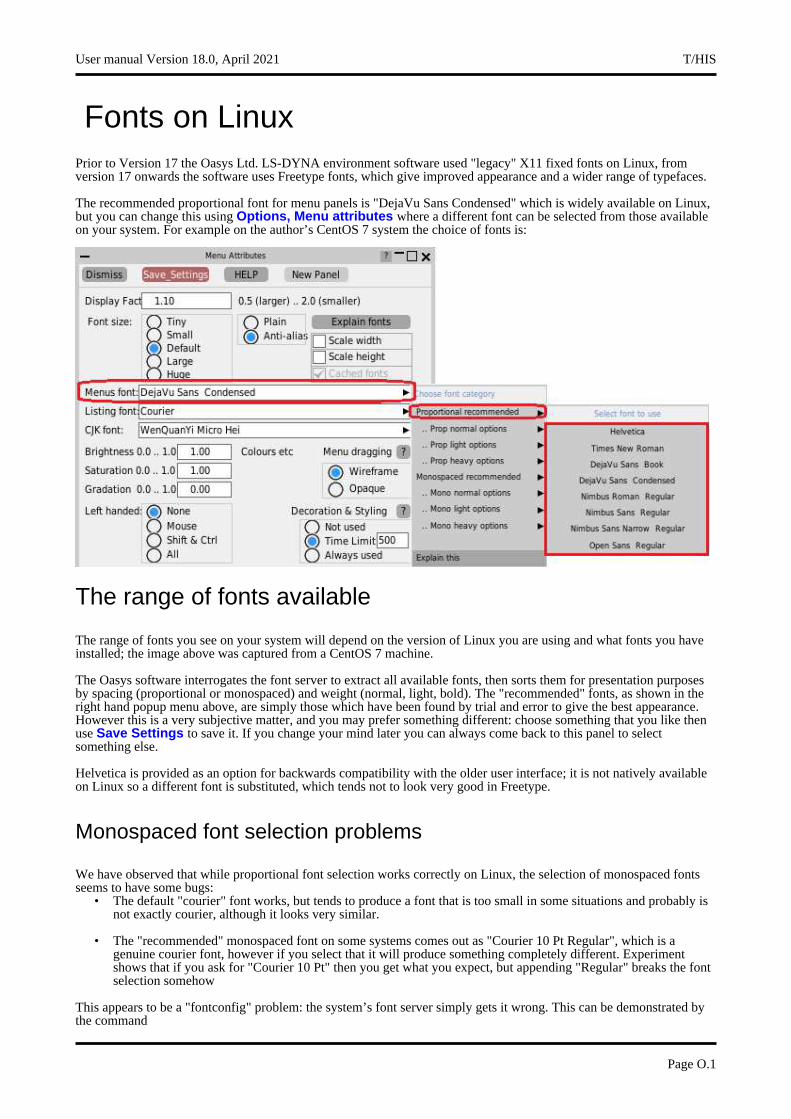
Fonts on LinuxPrior to Version 17 the Oasys Ltd. LS-DYNA environment software used "legacy" X11 fixed fonts on Linux, from version 17 onwards the software uses Freetype fonts, which give improved appearance and a wider range of typefaces.
The recommended proportional font for menu panels is "DejaVu Sans Condensed" which is widely available on Linux, but you can change this using Options, Menu attributes where a different font can be selected from those available on your system. For example on the author’s CentOS 7 system the choice of fonts is:
The range of fonts available
The range of fonts you see on your system will depend on the version of Linux you are using and what fonts you have installed; the image above was captured from a CentOS 7 machine.
The Oasys software interrogates the font server to extract all available fonts, then sorts them for presentation purposes by spacing (proportional or monospaced) and weight (normal, light, bold). The "recommended" fonts, as shown in the right hand popup menu above, are simply those which have been found by trial and error to give the best appearance. However this is a very subjective matter, and you may prefer something different: choose something that you like then use Save Settings to save it. If you change your mind later you can always come back to this panel to select something else.
Helvetica is provided as an option for backwards compatibility with the older user interface; it is not natively available on Linux so a different font is substituted, which tends not to look very good in Freetype.
Monospaced font selection problems
We have observed that while proportional font selection works correctly on Linux, the selection of monospaced fonts seems to have some bugs:
• The default "courier" font works, but tends to produce a font that is too small in some situations and probably is not exactly courier, although it looks very similar.
• The "recommended" monospaced font on some systems comes out as "Courier 10 Pt Regular", which is a genuine courier font, however if you select that it will produce something completely different. Experiment shows that if you ask for "Courier 10 Pt" then you get what you expect, but appending "Regular" breaks the font selection somehow
This appears to be a "fontconfig" problem: the system’s font server simply gets it wrong. This can be demonstrated by the command
User manual Version 18.0, April 2021 T/HIS
Page O.1
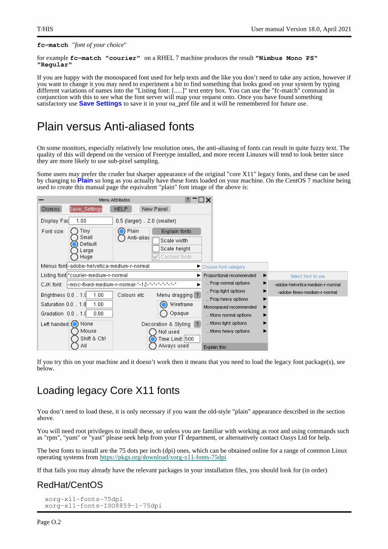
fc-match "font of your choice"
for example fc-match "courier" on a RHEL 7 machine produces the result "Nimbus Mono PS" "Regular"
If you are happy with the monospaced font used for help texts and the like you don’t need to take any action, however if you want to change it you may need to experiment a bit to find something that looks good on your system by typing different variations of names into the "Listing font: [.....]" text entry box. You can use the "fc-match" command in conjunction with this to see what the font server will map your request onto. Once you have found something satisfactory use Save Settings to save it in your oa_pref file and it will be remembered for future use.
Plain versus Anti-aliased fonts
On some monitors, especially relatively low resolution ones, the anti-aliasing of fonts can result in quite fuzzy text. The quality of this will depend on the version of Freetype installed, and more recent Linuxes will tend to look better since they are more likely to use sub-pixel sampling.
Some users may prefer the cruder but sharper appearance of the original "core X11" legacy fonts, and these can be used by changing to Plain so long as you actually have these fonts loaded on your machine. On the CentOS 7 machine being used to create this manual page the equivalent "plain" font image of the above is:
If you try this on your machine and it doesn’t work then it means that you need to load the legacy font package(s), see below.
Loading legacy Core X11 fonts
You don’t need to load these, it is only necessary if you want the old-style "plain" appearance described in the section above.
You will need root privileges to install these, so unless you are familiar with working as root and using commands such as "rpm", "yum" or "yast" please seek help from your IT department, or alternatively contact Oasys Ltd for help.
The best fonts to install are the 75 dots per inch (dpi) ones, which can be obtained online for a range of common Linux operating systems from https://pkgs.org/download/xorg-x11-fonts-75dpi
If that fails you may already have the relevant packages in your installation files, you should look for (in order)
RedHat/CentOSxorg-x11-fonts-75dpixorg-x11-fonts-ISO8859-1-75dpi
T/HIS User manual Version 18.0, April 2021
Page O.2
xorg-x11-fonts-Type1xorg-x11-fonts-miscxorg-x11-fonts-100dpixorg-x11-fonts-ISO8859-1-100dpi
You don’t have to install all of these.
The 75dpi and 100dpi font packages are the same typefaces at different resolutions. You should choose the one which gives the best looking results on your display, but in the author’s experience the 75dpi one looks fine but the 100dpi one looks as if a spider was let loose with a leaky pen! Always try the 75dpi one first.
To manage fonts on RHEL/CentOS do the following:• Log in as root
• To see the X11 fonts currently installed type "yum list installed | grep xorg | grep font"
• To see X11 fonts available but not installed "yum list available | grep xorg | grep font"
• To install something "yum install package", for example "yum install xorg-x11-fonts-75dpi"
You can list the range of "yum" commands available with "man yum".
SUSExorg-x11-fonts-corexorg-x11-fonts
User manual Version 18.0, April 2021 T/HIS
Page O.3

T/HIS User manual Version 18.0, April 2021
Page O.4

The JavaScript GUI BuilderThe JavaScript GUI Builder is an interactive GUI Builder, available in D3PLOT, PRIMER and T/HIS, making it easier to create JavaScript GUIs, removing the need to write code to create windows and widgets.
It can be started by pressing the GUI Builder button in the JavaScript menu in any of the programs.
You can then design and save your GUI to a file:
Then read the file in your script to automatically generate the window and widgets:
User manual Version 18.0, April 2021 T/HIS
Page P.1
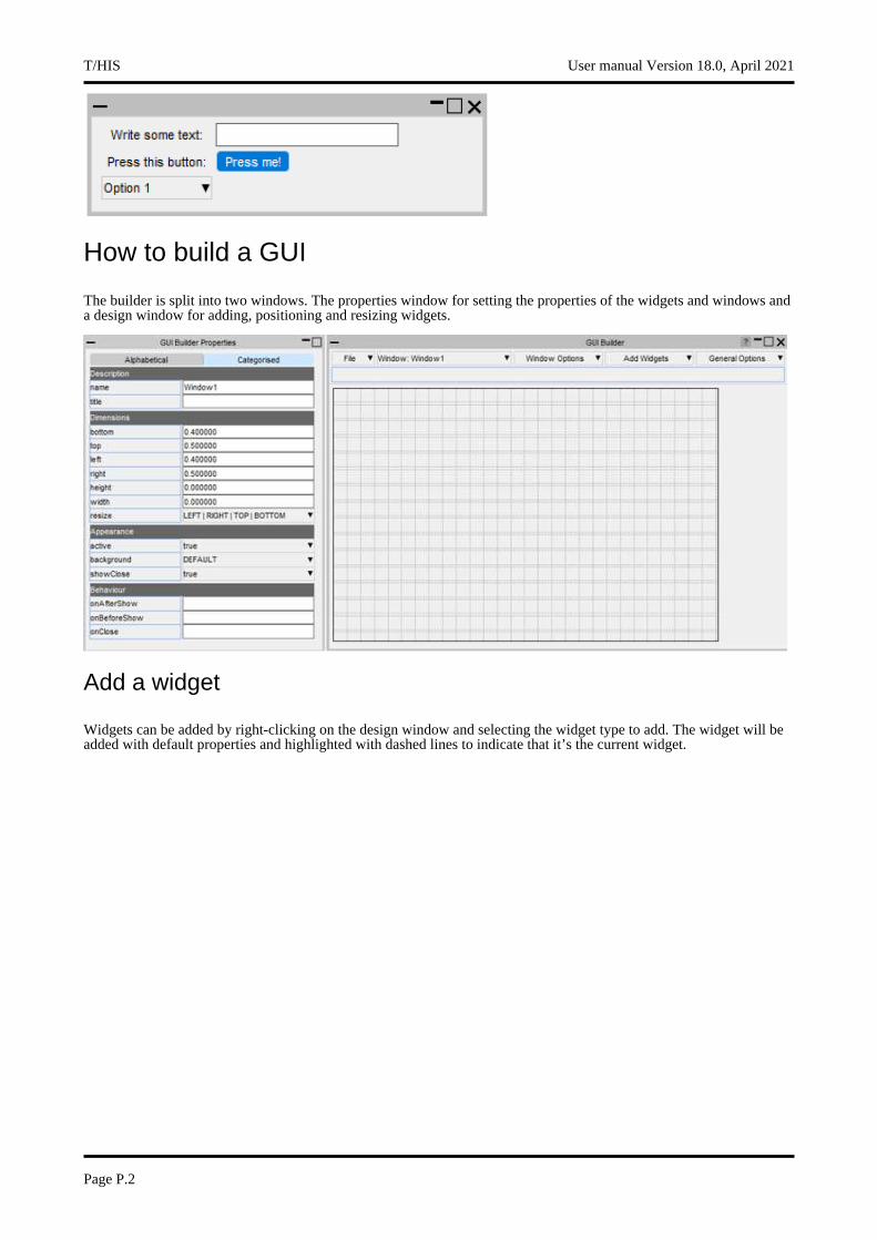
How to build a GUI
The builder is split into two windows. The properties window for setting the properties of the widgets and windows and a design window for adding, positioning and resizing widgets.
Add a widget
Widgets can be added by right-clicking on the design window and selecting the widget type to add. The widget will be added with default properties and highlighted with dashed lines to indicate that it’s the current widget.
T/HIS User manual Version 18.0, April 2021
Page P.2
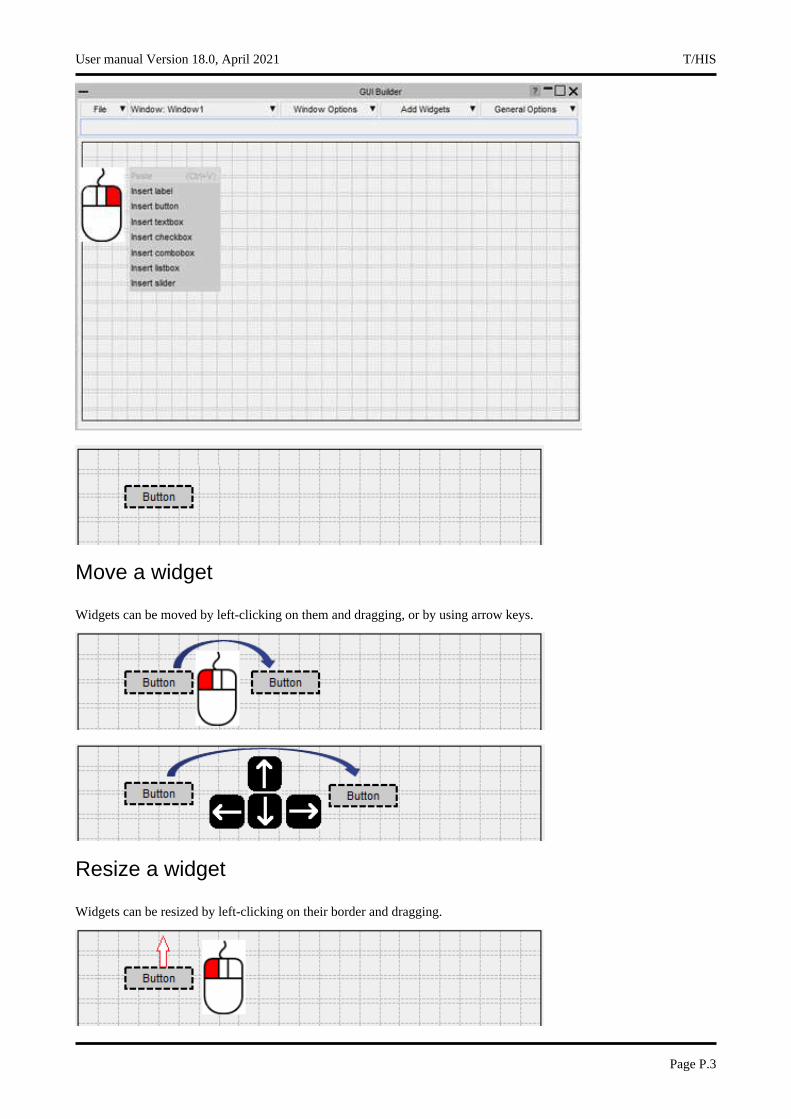
Move a widget
Widgets can be moved by left-clicking on them and dragging, or by using arrow keys.
Resize a widget
Widgets can be resized by left-clicking on their border and dragging.
User manual Version 18.0, April 2021 T/HIS
Page P.3

Selecting widgets
Multiple widgets can be selected by holding the Ctrl or Shift keys and left-clicking.
Alternatively a box can be dragged around the widgets you want to select.
Aligning widgets
When multiple widgets are selected the borders can be aligned by right-clicking on the widget you want to align the other widgets to, and then selecting how you want them to be aligned.
Setting the properties of widgets
T/HIS User manual Version 18.0, April 2021
Page P.4

The properties of a widget can be modified in the properties window, e.g. change the category to CATEGORY_APPLY.
The appearance of the widget will update in the design window. If multiple widgets are selected the property will be applied to all the selected widgets.
Copying and pasting widgets
You can copy and paste widgets by right-clicking on them and selecting Copy and then right-clicking on the window and selecting Paste. The new widget will have all the same properties as the copied widget.
Alternatively you can use the shortcuts Ctrl-C and Ctrl-V.
User manual Version 18.0, April 2021 T/HIS
Page P.5
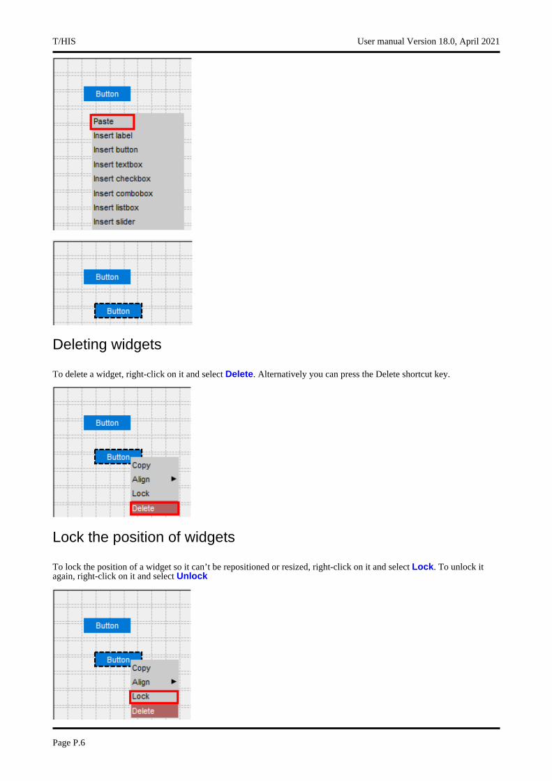
Deleting widgets
To delete a widget, right-click on it and select Delete. Alternatively you can press the Delete shortcut key.
Lock the position of widgets
To lock the position of a widget so it can’t be repositioned or resized, right-click on it and select Lock. To unlock it again, right-click on it and select Unlock
T/HIS User manual Version 18.0, April 2021
Page P.6

Adding widgetitems to comboboxes and listboxes
To add WidgetItems to a Combobox or Listbox, right-click on it and select Edit WidgetItems. This will update the design window where you can add WidgetItems by pressing the Add New WidgetItem button.
The appearance of the current WidgetItem can be modified in the same way as Widgets by clicking on the WidgetItem and updating its properties. To delete a WidgetItem, click on the - on the right hand side. Once you have finished, press Apply to return to the normal design window.
Adding windows
Additional windows can be created by clicking on the Window Options dropdown menu. You can add either a Main Window or PopupWindow.
User manual Version 18.0, April 2021 T/HIS
Page P.7
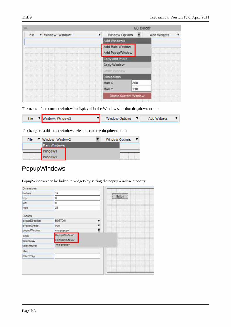
The name of the current window is displayed in the Window selection dropdown menu.
To change to a different window, select it from the dropdown menu.
PopupWindows
PopupWindows can be linked to widgets by setting the popupWindow property.
T/HIS User manual Version 18.0, April 2021
Page P.8
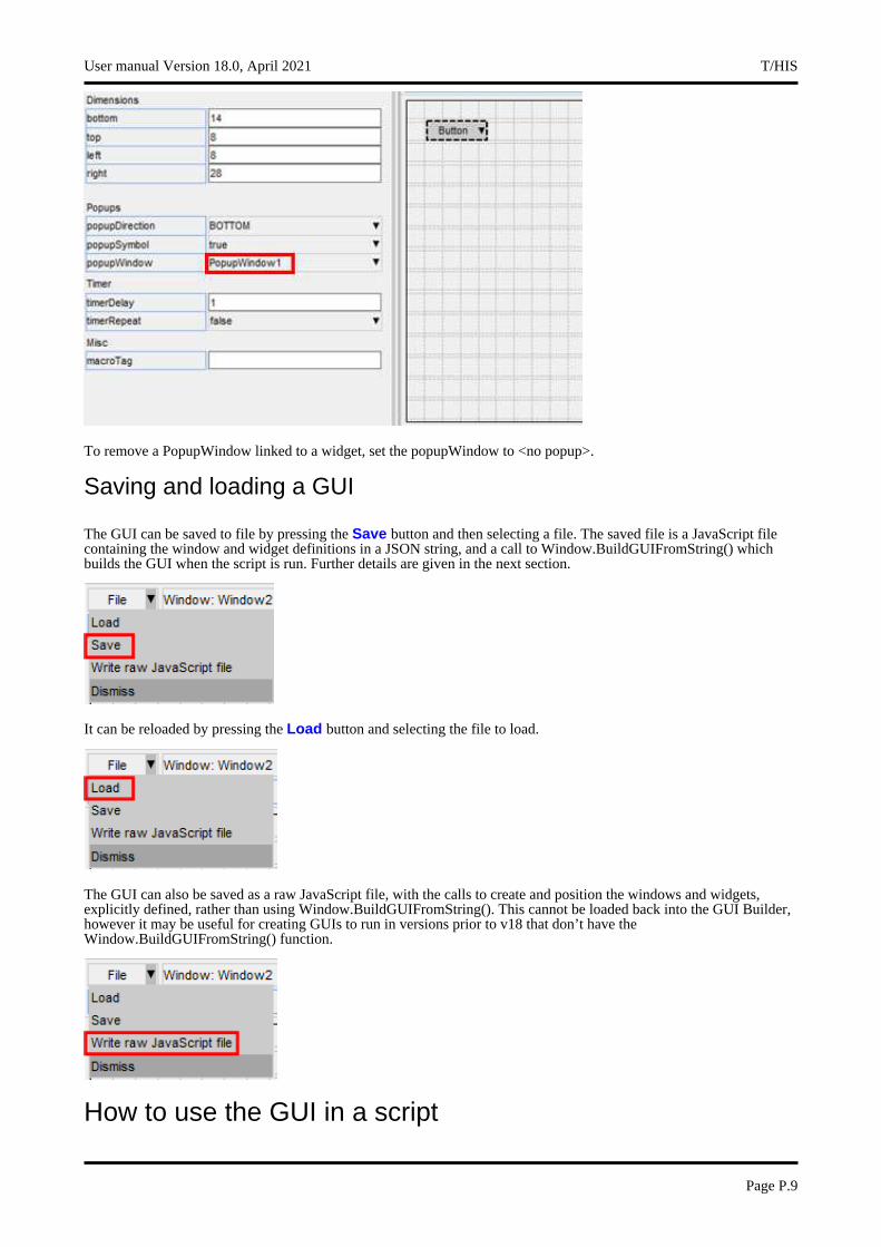
To remove a PopupWindow linked to a widget, set the popupWindow to <no popup>.
Saving and loading a GUI
The GUI can be saved to file by pressing the Save button and then selecting a file. The saved file is a JavaScript file containing the window and widget definitions in a JSON string, and a call to Window.BuildGUIFromString() which builds the GUI when the script is run. Further details are given in the next section.
It can be reloaded by pressing the Load button and selecting the file to load.
The GUI can also be saved as a raw JavaScript file, with the calls to create and position the windows and widgets, explicitly defined, rather than using Window.BuildGUIFromString(). This cannot be loaded back into the GUI Builder, however it may be useful for creating GUIs to run in versions prior to v18 that don’t have the Window.BuildGUIFromString() function.
How to use the GUI in a script
User manual Version 18.0, April 2021 T/HIS
Page P.9

The GUI is saved to a JavaScript file, containing the GUI definition in a JSON string and a call to Window.BuildGUIFromString(). It is saved with the extension .jsi to indicate that it should be included from another file. You should not need to edit this file.
When saving the GUI a *.js file is also written to demonstrate how to include the *.jsi file and display the GUI. This can be used as a template to follow and modify.
It is written to the same folder as the *.jsi file and named <jsi_filename>_TEMPLATE.js, e.g. if the *.jsi file is called demo.jsi, the *.js file will be saved as demo_TEMPLATE.js
The following sections explain how you can reference the Windows, Widgets and WidgetItem objects within your script.
Read the GUI into a script
To read the GUI in a script you need to include the *.jsi file with the Use() function.
This will create a global variable (gui by default) containing all the GUI objects. The name of the variable can be changed in the GUI builder menu under General Options.
For example, to include the GUI saved in C:\my_gui.jsi:
Use("C:\\my_gui.jsi");
Accessing the Window objects
The GUI Window objects are stored as properties on the global GUI object. The name of the property is whatever was defined in the properties window in the GUI builder.
To display the Window called my_window use the Show() method:
if (gui) gui.my_window.Show();
Accessing the Widget objects
Similarly, each Widget object is a property of the Window object. The name of the Widget property is whatever was defined in the properties window in the GUI builder.
T/HIS User manual Version 18.0, April 2021
Page P.10
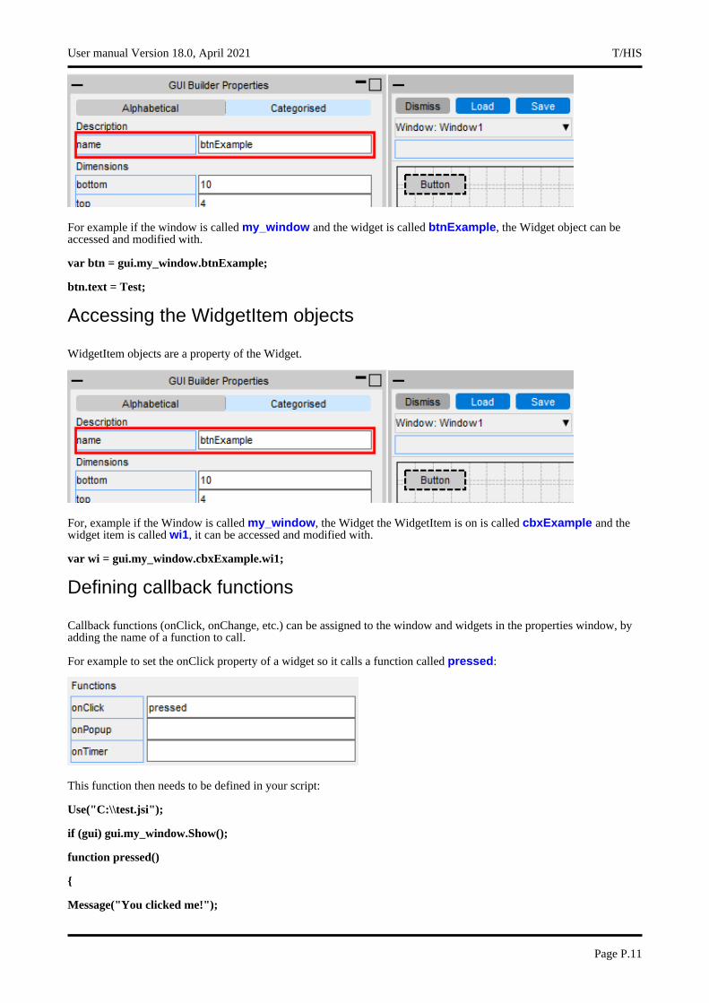
For example if the window is called my_window and the widget is called btnExample, the Widget object can be accessed and modified with.
var btn = gui.my_window.btnExample;
btn.text = Test;
Accessing the WidgetItem objects
WidgetItem objects are a property of the Widget.
For, example if the Window is called my_window, the Widget the WidgetItem is on is called cbxExample and the widget item is called wi1, it can be accessed and modified with.
var wi = gui.my_window.cbxExample.wi1;
Defining callback functions
Callback functions (onClick, onChange, etc.) can be assigned to the window and widgets in the properties window, by adding the name of a function to call.
For example to set the onClick property of a widget so it calls a function called pressed:
This function then needs to be defined in your script:
Use("C:\\test.jsi");
if (gui) gui.my_window.Show();
function pressed()
{
Message("You clicked me!");
User manual Version 18.0, April 2021 T/HIS
Page P.11

}
T/HIS User manual Version 18.0, April 2021
Page P.12
Related Documents