Thin water films driven by air through surface roughness

Retrospective Theses and Dissertations Iowa State University Capstones, Theses andDissertations

2008

Thin water films driven by air through surfaceroughnessGuoqing WangIowa State University

Follow this and additional works at: https://lib.dr.iastate.edu/rtd

Part of the Aerospace Engineering Commons

This Dissertation is brought to you for free and open access by the Iowa State University Capstones, Theses and Dissertations at Iowa State UniversityDigital Repository. It has been accepted for inclusion in Retrospective Theses and Dissertations by an authorized administrator of Iowa State UniversityDigital Repository. For more information, please contact [email protected].

Recommended CitationWang, Guoqing, "Thin water films driven by air through surface roughness" (2008). Retrospective Theses and Dissertations. 15864.https://lib.dr.iastate.edu/rtd/15864

Thin water films driven by air through surface roughness

by

Guoqing Wang

A dissertation submitted to the graduate faculty

in partial fulfillment of the requirements for the degree of

DOCTOR OF PHILOSOPHY

Major: Aerospace Engineering

Program of Study Committee:Alric Rothmayer, Major Professor

Richard H. PletcherTom I-Ping ShihAmbar K. Mitra

Fred L. Haan

Iowa State University

Ames, Iowa

2008

Copyright c© Guoqing Wang, 2008. All rights reserved.

UMI Number: 3296799

32967992008

UMI MicroformCopyright

All rights reserved. This microform edition is protected against unauthorized copying under Title 17, United States Code.

ProQuest Information and Learning Company 300 North Zeeb Road

P.O. Box 1346 Ann Arbor, MI 48106-1346

by ProQuest Information and Learning Company.

ii

DEDICATION

I would like to dedicate this dissertation to my wife Xi Chen and my daughter Cindy. Their

support is the power for me to complete this work.

iii

TABLE OF CONTENTS

LIST OF TABLES . . . . . . . . . . . . . . . . . . . . . . . . . . . . . . . . . . . v

LIST OF FIGURES . . . . . . . . . . . . . . . . . . . . . . . . . . . . . . . . . . vi

ACKNOWLEDGEMENTS . . . . . . . . . . . . . . . . . . . . . . . . . . . . . . xv

ABSTRACT . . . . . . . . . . . . . . . . . . . . . . . . . . . . . . . . . . . . . . . xvi

CHAPTER 1. Introduction . . . . . . . . . . . . . . . . . . . . . . . . . . . . . 1

CHAPTER 2. Thin water films . . . . . . . . . . . . . . . . . . . . . . . . . . . 3

2.1 Films driven by nonlinear condensed layers . . . . . . . . . . . . . . . . . . . . 3

2.2 Films on scales shorter than the condensed layer . . . . . . . . . . . . . . . . . 4

2.3 Numerical methods and solutions . . . . . . . . . . . . . . . . . . . . . . . . . . 9

2.3.1 Films and beads flowing through roughness fields . . . . . . . . . . . . . 9

2.3.2 Heat transfer of water films and beads flowing through roughness fields 17

2.4 Limit solutions . . . . . . . . . . . . . . . . . . . . . . . . . . . . . . . . . . . . 18

2.4.1 Limit of small heights . . . . . . . . . . . . . . . . . . . . . . . . . . . . 21

2.4.2 Limit of large shear stress . . . . . . . . . . . . . . . . . . . . . . . . . . 25

2.5 Some additional details for the solutions of the limit equations . . . . . . . . . 25

2.5.1 An analytical solution of perturbed film equations as Λ → ∞ . . . . . . 25

2.5.2 A solution with Fourier series as H → 0 . . . . . . . . . . . . . . . . . . 27

CHAPTER 3. Stability of film fronts . . . . . . . . . . . . . . . . . . . . . . . 30

3.1 Problem formulation . . . . . . . . . . . . . . . . . . . . . . . . . . . . . . . . . 30

3.2 Solitons . . . . . . . . . . . . . . . . . . . . . . . . . . . . . . . . . . . . . . . . 31

3.3 Stability analysis . . . . . . . . . . . . . . . . . . . . . . . . . . . . . . . . . . . 32

iv

3.4 Comparison with experimental data . . . . . . . . . . . . . . . . . . . . . . . . 40

3.5 Instability of film fronts moving through surface roughness . . . . . . . . . . . . 43

CHAPTER 4. Surfactant transport within thin films . . . . . . . . . . . . . . 53

4.1 Problem formulation . . . . . . . . . . . . . . . . . . . . . . . . . . . . . . . . . 53

4.2 Numerical methods and solutions . . . . . . . . . . . . . . . . . . . . . . . . . . 57

CHAPTER 5. Water films and droplets motion near a stagnation line . . . 62

5.1 Multiple scales near a stagnation line . . . . . . . . . . . . . . . . . . . . . . . . 62

5.1.1 Scale derivation . . . . . . . . . . . . . . . . . . . . . . . . . . . . . . . . 62

5.1.2 Numerical results . . . . . . . . . . . . . . . . . . . . . . . . . . . . . . . 65

5.2 Thin films with a disjoining pressure model . . . . . . . . . . . . . . . . . . . . 71

5.2.1 Disjoining pressure models . . . . . . . . . . . . . . . . . . . . . . . . . 71

5.2.2 Numerical results . . . . . . . . . . . . . . . . . . . . . . . . . . . . . . . 73

5.3 A new disjoining pressure model . . . . . . . . . . . . . . . . . . . . . . . . . . 80

5.3.1 Surface thermodynamics of droplets on precursor films . . . . . . . . . . 80

5.3.2 Inhomogeneous disjoining pressure empirical model . . . . . . . . . . . . 87

5.4 Numerical solutions and comparisons . . . . . . . . . . . . . . . . . . . . . . . . 88

CHAPTER 6. Conclusions . . . . . . . . . . . . . . . . . . . . . . . . . . . . . . 103

APPENDIX A. ADI-Iterative method and its algorithm . . . . . . . . . . . . 104

A.1 Linearization and ADI-Iterative method . . . . . . . . . . . . . . . . . . . . . . 104

A.2 Finite difference equations . . . . . . . . . . . . . . . . . . . . . . . . . . . . . . 106

APPENDIX B. The disjoining pressure term and its functional derivative . 113

B.1 Derivatives of the functions T , U and W . . . . . . . . . . . . . . . . . . . . . 114

B.2 Finite difference equation of the terms with B . . . . . . . . . . . . . . . . . . . 116

B.3 Finite difference equation of the terms with U . . . . . . . . . . . . . . . . . . . 120

B.4 Finite difference equation of the terms with W . . . . . . . . . . . . . . . . . . 124

BIBLIOGRAPHY . . . . . . . . . . . . . . . . . . . . . . . . . . . . . . . . . . . 129

v

LIST OF TABLES

Table 3.1 Coefficients in equations (3.13) and (3.14). . . . . . . . . . . . . . . . . 41

Table 3.2 Comparisons of the experimental wavelength l∗exp and the computed

wavelength at largest temporal growth rate, l∗max, in equation (3.15) . 42

Table 4.1 Coefficients in equation (4.2) . . . . . . . . . . . . . . . . . . . . . . . 54

Table 4.2 Coefficients in equation (4.3) . . . . . . . . . . . . . . . . . . . . . . . 54

vi

LIST OF FIGURES

Figure 2.1 The roughness diameters, △, and the roughness/water heights, h∗/L,

showing the relationship of the short scale roughness considered in

this study to the condensed layer (CL), triple-deck (TD) and near-wall

Navier-Stokes (NS) structures. . . . . . . . . . . . . . . . . . . . . . . 5

Figure 2.2 Typical two-dimensional flow of an initially uniform film driven by air

shear stress past a single roughness element at T = 18.31. (a) Steady

film around the roughness element, (b) traveling wave far downstream

of the roughness, generated by the unsteady flow past the roughness at

early time. The spatial computational domain is X ∈ (−12, 28), and

nx is the number of spatial grid points. . . . . . . . . . . . . . . . . . . 11

Figure 2.3 Typical steady state water film driven by air shear stress through a

three dimensional roughness field: (a) 3D view and (b) top view of

aligned roughness, (c) 3D view and (d) top view of offset roughness.

Water flow and air shear is in direction of the arrows. The undisturbed

film thickness is 0.1. . . . . . . . . . . . . . . . . . . . . . . . . . . . . 12

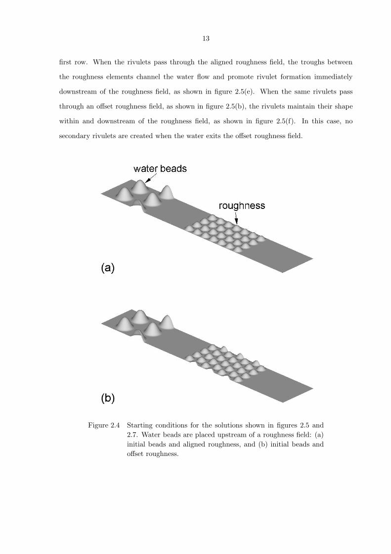
Figure 2.4 Starting conditions for the solutions shown in figures 2.5 and 2.7. Water

beads are placed upstream of a roughness field: (a) initial beads and

aligned roughness, and (b) initial beads and offset roughness. . . . . . 13

vii

Figure 2.5 Water beads driven by air shear stress through wetted roughness fields.

The water flows through an aligned roughness field at (a) T = 10, (c)

T = 24, and (e) T = 50, and through an offset roughness field at (b)

T = 10, (d) T = 24, and (f) T = 50. The direction of water flow and

air shear is from upper left to lower right. Note that the dimension of

these figures in the Z-direction is (−4, 4), and in the X-direction it is

(5, 21) for (a) and (b), (14, 30) for (c) and (d), and (23, 39) for (e) and

(f). . . . . . . . . . . . . . . . . . . . . . . . . . . . . . . . . . . . . . . 14

Figure 2.6 Initial conditions for a film front with spanwise perturbations driven

by the air shear stress through an irregular roughness field. Note that

the dimension of these figures in the Z-direction is (−4, 4), and in the

X-direction it is (−2, 25). . . . . . . . . . . . . . . . . . . . . . . . . . . 15

Figure 2.7 Typical solution of the perturbed film fronts driven by the air shear

stress through wetted irregular roughness fields. The film thickness

contours are at (a) T = 5, (b) T = 12.5, and (c) T = 20. Note that

the dimension of these figures in the Z-direction is (−4, 4), and in the

X-direction it is (−2, 25) for (a) and (b), (6, 33) for (c). . . . . . . . . . 16

Figure 2.8 Typical perturbed heat flux qair when the large beads of figure 2.4 are

driven by air shear stress through wetted roughness fields. The water

flows through an aligned roughness field with q = −1 at (a) T = 10,

(c) T = 24, and (e) T = 50, and through an offset roughness field with

q = +1 at (b) T = 10, (d) T = 24, and (f) T = 50. Note that the

coordinates and dimensions of these figures are the same as those in

figure 2.5. . . . . . . . . . . . . . . . . . . . . . . . . . . . . . . . . . . 19

viii

Figure 2.9 Typical contours of the perturbed heat flux qair when the perturbed film

fronts are driven by air shear stress through wetted irregular roughness

fields when the ambient heat flux is q = −1 in the air. The contours of

the perturbed heat flux are at (a) T = 5, (b) T = 12.5, and (c) T = 20.

Note that the coordinates and dimensions of these figures are the same

as those in figure 2.7. . . . . . . . . . . . . . . . . . . . . . . . . . . . . 20

Figure 2.10 Comparison between computed solutions of (2.35) and (2.36) and the

limit solution of (2.39) and (2.40) at τ ≃ 14.4. (a) Solutions for the

film near a roughness element which has N = 2 in (2.33). The values of

H approaching the limit solutions are: H = 1, 0.5, 0.1. (b) Solutions

for the traveling wave far downstream of the roughness for the same

conditions as figure 2.10(a). . . . . . . . . . . . . . . . . . . . . . . . . 22

Figure 2.11 Comparison between computed solutions of (2.35) and (2.36) and the

limit solution of (2.39) and (2.41) for a moving water bead at τ ≃ 14.4.

(a) Solutions when the initial bead shape has N = 1 in (2.33). The val-

ues ofHb approaching the limit solution are: Hb = 1, 0.5, 0.2, 0.1, 0.05.

(b) Solutions when the initial bead shape has N = 4 in (2.33). The val-

ues of Hb approaching the limit solutions are: Hb = 0.2, 0.1, 0.05. . . . 23

Figure 2.12 Comparison between computed solutions of (2.35) and (2.36) and the

limit solution of (2.43) and (2.44) as Λ → ∞ at t = 20. (a) The film near

the roughness with N = 1 in (2.33). The values of Λ approaching the

limit solutions are: Λ = 1, 2, 5, 10, 102, 103, 104. (b) The traveling

wave far downstream of the roughness for the same conditions as figure

2.12(a). . . . . . . . . . . . . . . . . . . . . . . . . . . . . . . . . . . . . 24

ix

Figure 3.1 Comparisons of solutions of the nonlinear film equations (2.35) and

(2.36) and solutions of the soliton equation (3.4). (a) Initial conditions

near X = 0 and ξ = 0, (b) Solutions of equations (3.4), (2.35) and (2.36)

using the initial conditions given in (a), where the solid and dashed lines

plotted over each other in (b) are solutions of (3.4); the symbols (O)

and (�) are solutions of (2.35) and (2.36) but shifted in X . . . . . . . 33

Figure 3.2 Typical solitons for different shear stress parameter Λ and different

downstream film thickness parameters δ. In figures (a) and (b), (——,

– – – –, – · – · – · –) are solutions of (3.4), while the symbols (O), (�)

and (♦) are solutions of (2.35) and (2.36) . . . . . . . . . . . . . . . . . 34

Figure 3.3 Typical solutions of the film front with spanwise perturbations. (a) Ini-

tial perturbations of the film front with wavenumber β = π/2, (b) un-

stable film front resulting from (a) showing the formulation of rivulets,

(c) initial perturbations of the film front with wavenumber β = π,

(d) stable film front resulting from (c) showing the return to a two-

dimensional soliton. Note that the dimension of these figures in the

Z-direction is (−4, 4), and in the X-direction it is (3, 7) for (a) and (c),

(3,15) for (b) and (d). . . . . . . . . . . . . . . . . . . . . . . . . . . . 36

Figure 3.4 Typical time evolution of the perturbation film thickness for unstable

disturbances with different initial conditions. (a) Four initial conditions

used for equation (3.9), (b) transient solutions resulting from the initial

condition of (a). The temporal growth rates, σr, are extracted from the

slopes of the curves at large time. . . . . . . . . . . . . . . . . . . . . . 37

x

Figure 3.5 Typical temporal growth rate, σr, of the linear perturbation plotted

against spanwise wavenumber, β. The line with symbols (O) is the

solution with Λ = 25.119 and δ = 0.4, and the line with symbols (♦)

is the solution with Λ = 10 and δ = 0.4. The subfigure shows the

definitions of the largest temporal growth rate, σr,max, and the most

unstable wavenumber, βmax. . . . . . . . . . . . . . . . . . . . . . . . . 38

Figure 3.6 (a) The most unstable spanwise wavelength lmax and (b) the largest

temporal growth rate σr,max, and (c) the neutral spanwise wavelength

ln, where the downstream film thickness parameter δ ranges from 0.1

to 0.9. The symbols are the numerically computed data points. The

lines are least squares curve fits of the computed solutions. . . . . . . . 39

Figure 3.7 Illustration of wavelengths as a function of the nondimensional down-

stream film thickness δ. . . . . . . . . . . . . . . . . . . . . . . . . . . . 42

Figure 3.8 Typical results of film fronts interacting with sinusoidal surface rough-

ness elements in the spanwise direction. (a) An initial film front and si-

nusoidal surface roughness elements with H = 3.226, (b) the computed

rivulet lengths at selected times (O) and the rivulet lengths predicted

by the stability analysis, (c) unstable film fronts at τ ≈ 0.369 resulting

from the initial condition shown in figure 3.8(a) and the definition of

a rivulet length L (τ), (d) unstable film fronts at τ ≈ 0.369 resulting

from same surface roughness elements shown in figure 3.8(a) except that

H = 0.3226. Note that the dimension of these figures in the Z-direction

is (−4, 4), and in the X-direction it is (−5, 15) for (a), and (22.67, 33)

for (c) and (d). . . . . . . . . . . . . . . . . . . . . . . . . . . . . . . . 44

Figure 3.9 Typical solutions of the water film fronts driven by air through an

array of isolated roughness elements and the evolution of disturbance

interactions. Solid circles are the roughness elements, lines are the file

fronts (moving in the x-direction). . . . . . . . . . . . . . . . . . . . . . 47

xi

Figure 3.10 Typical solutions of water film fronts driven by air through a random

roughness field shown at different time. The direction of water flow and

air shear is from left to right. Note that the dimension of these figures

in the X-direction is (−6, 40), and in the Z-direction it is (−8, 8). . . . 48

Figure 3.11 Typical snapshots of the moving contact line as film fronts driven by

air move through a random roughness field, and the evolution of the

wavenumber n of the disturbed moving contact line and its correspond-

ing magnitude. . . . . . . . . . . . . . . . . . . . . . . . . . . . . . . . 49

Figure 3.12 Typical solutions of water film fronts driven by air through a random

roughness. The direction of water flow and air shear is from upper left to

lower right. Note that the dimension of these figures in the Z-direction

is (−12, 12), and in the X-direction it is (−6, 30). . . . . . . . . . . . . 51

Figure 3.13 Typical snapshots of the moving contact line as film fronts driven by air

move through a random roughness field, and the evolution of the wave

number n of the disturbed moving contact line and its corresponding

magnitude. . . . . . . . . . . . . . . . . . . . . . . . . . . . . . . . . . . 52

Figure 4.1 (a) Comparison of viscosity of ethylene glycol using equations (4.1),

(4.2), and (4.3). Note that the result of equation (4.2) at θ∗ = 273.15

is out of the range of the experiment (see Sun & Teja (2003)). (b) The

viscosity of propylene glycol. The symbol (O) is the result of equation

(4.1), the solid lines are the results of equation (4.3), the dashed lines

are the results of equation (4.2). . . . . . . . . . . . . . . . . . . . . . . 55

Figure 4.2 Typical solutions of surfactant together with water injected into an

aligned roughness field. (a) Film thickness and (b) surfactant concen-

tration. . . . . . . . . . . . . . . . . . . . . . . . . . . . . . . . . . . . . 59

Figure 4.3 Typical solutions of surfactant together with water injected into an

offset roughness field. (a) Film thickness and (b) surfactant concentration. 60

xii

Figure 4.4 Evolution of pure water beads deposited onto a thin water film which

has a uniform concentration of ethylene glycol, C = 0.2. The film is

driven by the air shear stress λ = 1. . . . . . . . . . . . . . . . . . . . . 61

Figure 5.1 Comparisons between exact solutions and numerical solutions for a flat

film driven by air near the stagnation line. (a) Solutions with different

initial film thickness δ, (b) solutions with different slopes, k, of the

shear stress λ = kX when δ = 0.1. Note that δ is δ = F0, initial, and

the coefficient k is in the sequence, i.e. k = 0.2, 1, 2, 10, 20. . . . . . . 67

Figure 5.2 Comparisons of numerical solutions when the air shear stress is chosen

to be a linear and a nonlinear function of X. X is the distance from

the stagnation line. . . . . . . . . . . . . . . . . . . . . . . . . . . . . . 68

Figure 5.3 Typical solutions of droplets deposited on a flat plate near a stagnation

line and driven by air to both sides. The precursor film thickness is

δ = 0.001 (top three figures) and δ = 0.0001 (bottom three figures). . . 69

Figure 5.4 Typical solutions of droplets deposited on a flat plate near a stagnation

line and driven by air to both sides. The shear stress rate is k = 0.1

(top three figures) and k = 0.01 (bottom three figures). . . . . . . . . . 70

Figure 5.5 A typical solution of droplets randomly deposited on a roughness field

near the stagnation line and driven by air towards both directions. The

roughness elements are randomly placed near the stagnation line. Note

that the shear stress is λ = 2X and the initial uniform film thickness is

δ = 0.05. . . . . . . . . . . . . . . . . . . . . . . . . . . . . . . . . . . . 72

Figure 5.6 Typical solutions using a disjoining pressure model, with rivulets driven

by air which are broken into droplets. Note that the dimension of these

figures in Z-direction is (−2, 2), and in X-direction it is (−2, 2) for figure

5.6(a), (0, 9) for figure 5.6(b), and (1, 18) for figure 5.6(c). . . . . . . . 74

xiii

Figure 5.7 Typical solution of a single droplet interacting with roughness elements,

moving around the roughness elements and leaving the roughness field

when driven by air and with a large disjoining pressure. . . . . . . . . 76

Figure 5.7 cont. Typical solution of a single droplet interacting with roughness el-

ements, moving around the roughness elements and leaving the rough-

ness field when driven by air and with a large disjoining pressure. . . 77

Figure 5.8 Typical solutions of droplets driven by air through an offset roughness

field with a large disjoining pressure, where two droplets are stopped

by roughness elements and later merge. . . . . . . . . . . . . . . . . . . 78

Figure 5.9 Typical solution of droplets driven by air through an offset roughness

field with a large disjoining pressure, where the droplets interact with

roughness elements, merge together and separate into two droplets. . . 79

Figure 5.10 Comparison of the film, droplet and rivulet patterns as water is driven

by air near a stagnation line with/without the disjoining pressure model

with (m,n) = (3, 2), δ = 0.01 and λ = 2X. . . . . . . . . . . . . . . . . 80

Figure 5.11 A virtual variation of a droplet on dry surface from an equilibrium state. 81

Figure 5.12 Schematic diagrams of droplets on a wet surface when the precursor

layer thickness is δ . . . . . . . . . . . . . . . . . . . . . . . . . . . . . 83

Figure 5.13 The comparisons between the classical disjoining pressure model (5.32)

and the new model (5.38). The coefficients are B = 1 in both models.

Note that the parameters m, n and k in these two models are arbitrarily

selected simply to illustrate the qualitative difference between the models. 84

Figure 5.14 A comparison of the difference between y = 1F and y = tanh

(1F

). . . 85

Figure 5.15 The typical solutions of a droplet on a precursor layer without any

driving force when the new disjoining pressure model and the classical

disjoining pressure model are used. Note that the initial droplet profile

is shown in figure 5.15(a). . . . . . . . . . . . . . . . . . . . . . . . . . 86

xiv

Figure 5.16 Example of the contact angle, height and diameter computed in this

study. . . . . . . . . . . . . . . . . . . . . . . . . . . . . . . . . . . . . 91

Figure 5.17 Diagram of the contact angle calculation in this study. . . . . . . . . . 92

Figure 5.18 The advancing and receding contact angles when the empirical formulae

(5.40), (5.43) and (5.44) are used to simulate droplets on an inclined sur-

face. Note that the least squares linear fit (A) is from equation (5.53),

while the least squares linear fit (B) is from equation (5.54). . . . . . . 93

Figure 5.19 Droplets calculated with the new disjoining pressure model, i.e. (5.45),

(5.46) and (5.47) . . . . . . . . . . . . . . . . . . . . . . . . . . . . . . 94

Figure 5.20 The least squre linear fit to show the relation between the droplet

heights and the temperature in the experiment by Hansman & Turnock

(1988) . . . . . . . . . . . . . . . . . . . . . . . . . . . . . . . . . . . . 94

Figure 5.21 Typical deformation number ζ of a single droplet driven by a shear

stress λ = 1.793. Note that ∆B = 326 is used in the empirical formula.

τd is the deformation time, i.e. ζ(t=τd)ζ(t→∞) ≥ 0.95. ζ is defined in equation

(5.60). . . . . . . . . . . . . . . . . . . . . . . . . . . . . . . . . . . . . 98

Figure 5.22 Diagram of a solution which would produce a deformation number ζ ≈

2, as a droplet moves away from its initial location. . . . . . . . . . . . 99

Figure 5.23 A schematic diagram of the parameter window used to define a pseudo-

stationary droplet. For example, a droplet is marked as a stationary

droplet if the deformation time is within the interval, (τd − ∆τ) ≤ t ≤

(τd + ∆τ), and the deforming number is within the interval, (ζs − ∆ζ) ≤

ζ ≤ (ζs + ∆ζ) at the same time. . . . . . . . . . . . . . . . . . . . . . . 100

Figure 5.24 Comparison between Olsen & Walker’ experimental data and the nu-

merical solutions when the empirical formulae (5.40), (5.43) and (5.44)

are applied. . . . . . . . . . . . . . . . . . . . . . . . . . . . . . . . . . 102

xv

ACKNOWLEDGEMENTS

I would like to take this opportunity to express my thanks to those who helped me with

various aspects of conducting research and the writing of this dissertation. First and foremost,

Dr. Alric Rothmayer for his guidance, patience and support throughout this research and the

writing of this dissertation. I would also like to thank my committee for their efforts and

contributions to this work: Dr. Richard H. Pletcher, Dr. Tom I-Ping Shih, Dr. Ambar K.

Mitra, and Dr. Fred L. Haan. I would also like to thank Dr. Mark G. Potapczuk, Dr. Jen

Ching Tsao, Mr. Brian D. Matheis, Mr. Otta P. Shourya, Mr. Joshua A. Krakos, Mr. Ben

Rider for their help during these years.

This research was partially supported by NASA contract NAG3-2863, through the Ic-

ing Branch at the NASA Glenn Research Center. The author would like to thank Dr. M.

Potapczuk and T. Bond for their helpful guidance and support.

My wife, Xi Chen, my parents, Mr. Gaobo Xiao and Mrs. Yihua Wang, and my parents-in-

law, Mr. Youshi Chen and Mrs. Sufen Fu, deserve special thanks for their undivided attention

and moral support.

xvi

ABSTRACT

The interaction between thin films and roughness surfaces has been studied when the

thin viscosity-dominated films are driven by the air shear stress in the context of a high

Reynolds number boundary layer theory. A number of properties of this model are examined,

such as transport and pooling of water in a roughness field, heat transfer of film/roughness

combinations, and rivulet formation. For rivulet formation due to the instability of two-

dimensional film fronts, a general formula for the largest unstable wavelength, the fastest

temporal growth rate, and the neutral wavelength has been developed from the linear instability

analysis. This formula is validated using experimental data for film fronts on flat surfaces which

are driven by constant surface tension gradients. This formula is also validated using numerical

simulations of film fronts moving through various roughened surfaces.

To describe a water bead on a precursor film, a new disjoining pressure model is developed

from a modified classical long-distance disjoining pressure model. This model satisfies the

requirement that the disjoining pressure on the precursor film is larger than zero. Another

advantage of this modified model is that an effective distance used in classical long-distance

disjoining pressure models is avoided even when a water bead is on a dry surface. This model

is validated using experimental data from aircraft icing tests.

1

CHAPTER 1. Introduction

When an aircraft flies through a cloud of supercooled water droplets, and the temperature

is sufficiently low, the droplets can impact the aircraft and ice can accrete on wing surfaces. At

temperature sufficiently close to freezing, impacting droplets partially freeze and a residue of

water can remain on a roughened ice surface, often in the form of a thin water film. A number

of studies have shown that air-driven films are a common feature of water transport along

accreted ice surfaces. For example, Thomas, Cassoni & MacArthur (1996) have shown that

supercooled droplets on ice run back as a liquid film, and experiments by Vargas (2005) have

shown that the ice surface can be wet everywhere in glaze icing conditions near the stagnation

line. Thin water films are also a commonly used model for water transport in engineering

simulations of aircraft icing (see Bourgault, Beaugendre & Habashi 2000; Myers, Charpin &

Chapman 2002, for example).

Thin films which are driven by body and external forces have been studied both experimen-

tally and theoretically in a variety of situations, with the majority of cases involving gravity

and Marangoni forces. For gravity driven films, Huppert (1982) experimentally showed that

a film front moving along an inclined plate became unstable to disturbances along the front,

forming rivulets. Huppert also found that the wavelength of the unstable film front was a func-

tion of both the surface tension and the gravity force component directed along the surface

(also see Silvi & Dussan 1985; Jerrett & de Bruyn 1992). Stability of gravity-driven film fronts

on an inclined surface were studied numerically by Troian, Herbolzheimer, Safran & Joanny

(1989) (also see Schwartz 1989; Bertozzi & Brenner 1997). A number of authors have consid-

ered similar effects when the film is driven by Marangoni forces, which are stresses generated

by temperature gradients (see Levich 1962; Levich & Krylov 1969; Cazabat, Heslot, Troian

2

& Carles 1990; Cazabat, Heslot, Carles & Troian 1992; Oron, Davis, & Bankoff 1997; Eres,

Schwartz & Roy 2000; Luo & Pozrikdis 2006).

For wind-driven shallow water, the formation of interfacial waves and hydrodynamic sta-

bilities have been studied with linear theories (see Lin 1955; Stoker 1957; Lighthill 1978) as

well as with nonlinear theories (see Eckhaus 1965; Whitham 1974; Joseph 1976; Leibovich &

Seebass 1974). The generation of wind-driven waves on thin films has been examined by Lock

(1954), Craik (1966) and Akylas (1982), while equivalent studies of waves driven by turbulent

air streams may be found in Miles (1959, 1962) (also see Valenzuela 1976; van Gastel, Janssen

& Komen 1985; Belcher, Harris & Street 1994). A long-wave instability mechanism of water-

wave formation induced by viscosity differences at interfaces has been studied by Yih (1967,

1990), while short-wave viscous instabilities have been studied by Hooper & Boyd (1987) (also

see Blennerhassett & Smith 1987). Of more relevance to this study, high Reynolds number

asymptotic methods have been used by Feldman (1957) (also see Timoshin 1997; Tsao, Roth-

mayer & Ruban 1997; Rothmayer & Tsao 2000) to study the instability of thin shear-driven

films. Recent experiments by Marshall & Ettema (2004) have also examined the formation of

wind-driven rivulets, but starting from very large droplets.

This study primarily focuses on thin water films driven by air shear stress through rough-

ness, where thin viscosity-dominated films are described in the context of a high Reynolds

number boundary layer theory on scales which are small enough that air driven instabilities do

not effect the flow. A number of properties of this model are examined, including transport and

pooling of water in a roughness field, heat transfer of film/roughness combinations, run-back

of water beads, and rivulet formation due to the instability of two-dimensional film fronts.

3

CHAPTER 2. Thin water films

In the current study, water is driven by air through a roughness field which lies underneath

an attached laminar Prandtl boundary layer. The air is assumed to be an ideal gas and the

water is incompressible. In following sections, the superscript ”∗” denotes variables which are

dimensional, while the subscript ”∞” denotes free-stream variables. For example, the density

ρ∞, velocity V∞, temperature θ∞, and pressure P∞ are reference variables measured in the air

free stream. The characteristic length L is typically taken to be the radius of curvature of the

leading edge of an airfoil or an airfoil chord length.

A non-dimensional Cartesian coordinates system (x, y, z) is located at a point within a

laminar Prandtl boundary layer, where the local non-dimensional streamwise shear stress is

Re−1/2λ, where Re = ρ∞V∞L/µ∞ is the free-stream Reynolds number. The coordinate x

is the streamwise direction, y is the normal direction to the surface, and z is the spanwise

direction.

2.1 Films driven by nonlinear condensed layers

When a thin liquid film is driven by air over roughness with diameter Re−3/4 ≪ ∆ ≪

Re−3/8 and height Re−1/2∆1/3, the condensed layer or wall layer (see Bogolepov & Neiland

1971, 1976; Smith, Brighton, Jackson & Hunt 1981; Rothmayer & Smith 1998) allows a pressure

and shear stress feedback between the viscous sublayer airflow and the liquid film when the

length scale of the interaction is ∆ = Re−9/14σ3/7 (see Rothmayer & Tsao 2000; Rothmayer,

Matheis & Timoshin 2002), where σ = σ∗/ (V∞µ∞) is a dimensionless surface tension. The

air pressure and shear at the liquid/air interface tend to destabilize the liquid surface, while

surface tension acts to stabilize the interface. The condensed layer streamwise, spanwise and

4

wall normal length scales of Rothmayer & Tsao (2000) are given in terms of the Reynolds

number Re and dimensionless surface tension σ, with

(x, y, z) =(Re−9/14σ3/7X, Re−5/7σ1/7Y, Re−9/14σ3/7Z

). (2.1)

When the surface tension is large (i.e. σ ∼ O(Re5/8

)) this interaction is controlled by a triple-

deck (see Neiland 1969; Stewartson & Williams 1969; Messiter 1970; Timoshin 1997; Tsao et

al. 1997; Timoshin & Hooper 2000; Pelekasis & Tsamopoulos 2001).

In the condensed layer, both the air sublayer and water film are controlled by unsteady

boundary layer equations, providing that the viscosity ratio M = µ∗water(θ∞)/µ∞ between the

air and water is related to the density ratio, Daw = ρ∞/ρ∗

water, as follows

M = MD−1/2aw , (2.2)

where M typically ranges from 3 to 5 (see Rothmayer 2003). The air and water are coupled

through a combination of pressure and shear stress in the sense that changes to the water

interface shape create a pressure and shear stress response in the air, and the pressure and shear

stress combination drives the water into motion. Solutions of the triple-deck and condensed

layer problems may be found in Timoshin (1997), Tsao et al. (1997), Rothmayer & Tsao

(2000), Pelekasis & Tsamopoulos (2001), Rothmayer et al. (2002) and Matheis & Rothmayer

(2003).

2.2 Films on scales shorter than the condensed layer

An asymptotic solution on scales shorter than those of the condensed layer is used here

to examine properties of the Rothmayer & Tsao (2000) structure in a simplified setting. The

main new perturbation parameter is the streamwise length scale, ∆, which is assumed to be

less than the condensed layer value of Rothmayer & Tsao (2000) but larger than the near wall

Navier-Stokes scale, i.e.

Re−3/4 ≪ ∆ ≪ Re−9/14σ−3/7. (2.3)

5

h∗/L

Re−1/2

Re−5/8

Re−5/7σ1/7

Re−3/4

Re−3/4 Re−9/14σ3/7 Re−3/8 ∆

Re−1/2∆1/3 TD

CLNS

Re1/4σ−1/2∆3/2

Film thickness at air boundary layer thickness

Figure 2.1 The roughness diameters, △, and the roughness/water heights,

h∗/L, showing the relationship of the short scale roughness con-

sidered in this study to the condensed layer (CL), triple-deck

(TD) and near-wall Navier-Stokes (NS) structures.

Wang & Rothmayer (2005) found that surface roughness on this scale, as shown in figure 2.1,

can first interact with a thin film when the film thickness and roughness heights are both

h∗/L = Re1/4σ−1/2∆3/2h, (2.4)

where h∗ is a dimensional undisturbed film thickness. This relation effectively sets the stream-

wise length scale for the interaction, given a known ambient film thickness h∗/L. When the

surface roughness is the perturbation source for the air and water system, the time scale for a

laminar unsteady response of the water interface is

t = Re−3/4σ1/2D−1/2aw ∆−1/2T , (2.5)

and the air is quasi-steady and laminar. Some trial and error reveals that the expansions of

lengths, velocities, temperature and pressure in the water film take the form

(x, y, z) =(∆X, Re1/4σ−1/2∆3/2Y, ∆Z

), (2.6)

6

(u, v, w) ∼(Re3/4σ−1/2D1/2

aw ∆3/2U, Reσ−1D1/2aw ∆2V, Re3/4σ−1/2D1/2

aw ∆3/2W)

+ · · · , (2.7)

θ ∼ 1 ∓ Θ +Re3/4σ−1/2D1/2aw ∆3/2Θϑ+ · · · , (2.8)

where the upper sign ”−” is used for above freezing freestream and the lower sign ”+” is used

for below freezing freestream. The water pressure is

p ∼ PB +Re−3/4σ1/2∆−1/2P + · · · , (2.9)

where PB is the local air boundary layer pressure. The air, on the other hand, is a linearized

condensed layer with

(x, y, z) =(∆X,Re−1/2∆1/3Y ,∆Z

), (2.10)

u ∼ ∆1/3λY +Re3/4σ−1/2∆3/2U + · · · ,

v ∼ Re1/4σ−1/2∆5/6V + · · · ,

w ∼ Re3/4σ−1/2∆3/2W + · · · ,

(2.11)

θ ∼ 1 ∓ Θ + q∆1/3ΘY +Re3/4σ−1/2∆3/2Θϑ+ · · · , (2.12)

and

p ∼ PB +Re3/4σ−1/2∆11/6P + · · · , (2.13)

where λ is the air boundary layer shear stress and q is the boundary layer heat flux in the

air, i.e. q = Re−1/2Θ−1∂θ/∂y, both measured at the wall. Note that Θ is a dimensionless

perturbation of the free-stream temperature θ∞ from a constant prescribed wall temperature,

which is taken to be the freezing temperature θ∗freezing for aircraft icing applications, i.e.

Θ =∣∣∣(θ∗freezing − θ∞

)/θ∗freezing

∣∣∣. The water surface and the underlying surface roughness

have the same height scale as that of the undisturbed water film, i.e.

(fwater, fice) ∼ Re1/4σ−1/2∆3/2 (Fwater, Fice) + · · · , (2.14)

where fwater and fice are the functions for water film height and underlying ice roughness,

respectively.

7

The following equations are obtained by substituting the above expansions into the non-

dimensionalized mass conservation equation, the Navier-Stokes equations, and the energy con-

servation equation in both the air and water. In these equations, gravity is assumed to be

sufficiently small, i.e.

G =Lg

V 2∞

≪ Re−3/4σ1/2Daw∆−3/2, (2.15)

where g = 9.8m/s2. In the air, the mass conservation equation is

∂U

∂X+∂V

∂Y+∂W

∂Z= 0. (2.16)

The momentum conservation equations are

λY∂U

∂X+ λV = −

∂P

∂X+∂2U

∂Y 2, (2.17)

∂P

∂Y= 0, (2.18)

and

λY∂W

∂X= −

∂P

∂Z+∂2W

∂Y 2. (2.19)

The energy conservation equation is

λY∂ϑ

∂X+ qV = Pr−1 ∂

2ϑ

∂Y 2. (2.20)

The boundary conditions in the air are

U → λ (Fwater − h) and ϑ→ q (Fwater − h) as Y → ∞, (2.21)

and

U = V = W = 0 and ϑ = 0 on Y = Fwater, (2.22)

where h is the undisturbed dimensionless water film thickness. In the water, the mass, mo-

mentum, and energy equations are

∂U

∂X+∂V

∂Y+∂W

∂Z= 0, (2.23)

0 = −∂P

∂X+ M

∂2U

∂Y 2, (2.24)

8

∂P

∂Y= 0, (2.25)

0 = −∂P

∂Z+ M

∂2W

∂Y 2, (2.26)

and

Pr−1 ∂2ϑ

∂Y 2= 0. (2.27)

At the interface between water and the solid ice surface, the conditions of no-slip and constant

wall temperature are

Uwater = Vwater = Wwater = 0 and ϑ = 0 on Y = Fice. (2.28)

At the interface between water and air, the shear stress in air is balanced by that in the water,

i.e.

M

(∂U

∂Y

)

water

= λ and M

(∂W

∂Y

)

water

= 0 on Y = Fwater, (2.29a,b)

and the pressure is balanced by surface tension due to the curvature of the water surface

P = −

(∂2Fwater

∂X2+∂2Fwater

∂Z2

)on Y = Fwater. (2.30)

The kinematic condition on the water/air interface Y = Fwater is

Vwater =∂Fwater

∂T+ Uwater

∂Fwater

∂X+Wwater

∂Fwater

∂Z. (2.31)

Combining equations (2.23-2.31), a lubrication equation is found for the water interface

∂Fwater

∂T+

∂

∂X

(λF 2

2

)+

∂

∂X

(−F 3

3

∂P

∂X

)+

∂

∂Z

(−F 3

3

∂P

∂Z

)= 0, (2.32)

where T = T /M, F = Fwater − Fice and P is given by equation (2.30). Note that in contrast

to the condensed layer and triple-deck, the air is now decoupled from the water film. The

water film is solved first, given an applied air shear stress, and the air has a linear response to

changes in the water film interface shape.

9

2.3 Numerical methods and solutions

When numerically simulating the motion of a thin film, one challenging problem is the

development of a model which captures fluid spreading on any surface where three media can

co-exist, namely liquid, gas, and solid. The interface between these three media is called the

contact line. The central problem (see Dussan 1979; de Gennes 1985) is that the boundaries

for both liquid and gas on the solid surface are no-slip, i.e. zero velocity, whereas the liquid

must be able to move forward or backward along the solid surface in order to move the contact

line. This situation leads to a stress singularity at the contact line. Current understanding

of general contact line behavior is poor and often requires complex and detailed simulations

near the contact line, which is beyond the scope of this study. However, there are a number

of well-known ways to avoid the contact line singularity in numerical simulations, for example

by using a slip boundary condition (see Dussan & Davis 1974) or a precursor film (see Diez,

Kondic & Bertozzi 2000). In this study, the precursor film method is used. In other words, it

is assumed that the whole roughness field is covered by a very thin water film. A fourth order

Runge-Kutta method is used for the time integration of the lubrication equation (2.32) (see

Abramowitz & Stegun 1972). For the spatial differencing, a combination of central differencing

and the positivity preserving scheme of Diez et al. (2000) is used. In the air, the Smith (1983)

transformation is used for equations (2.16-2.20). The resulting air equations are solved using

a finite difference method.

2.3.1 Films and beads flowing through roughness fields

Figure 2.2 shows a grid size study for a single, smooth, two-dimensional roughness element

which is initially covered by a water film with uniform thickness, where the initial film thickness

is h = 0.2 and the air shear stress is λ = 4. The roughness shape is given by

Fice (X,Z) = c · exp

[−

N∑

n=0

tn

2n

], (2.33)

where, in three-dimensions, t = (X −X0)2/a2 + (Z − Z0)

2/b2. In figure 2.2, c = 1, b = ∞ and

N = 5. Note that if a = b = c then equation (2.33) approaches a hemisphere as N → ∞.

10

Due to the interaction between the roughness and water film, the water mass is redistributed

about the roughness element. The film surface becomes steady at long time in the immediate

vicinity of the roughness element, which is the result shown in figure 2.2(a). At the same time,

a decaying traveling wave is observed far downstream of the roughness, as shown in figure

2.2(b). It should be noted that the numerical simulations with different grid sizes shown in

figure 2.2 agree well with each other.

Equivalent steady solutions about three-dimensional roughness fields are shown in figure

2.3. The roughness elements are distributed using two patterns: an aligned pattern is shown

in figures 2.3(a) and 2.3(b), and an offset pattern is shown in figures 2.3(c) and 2.3(d). The

hump geometry in figure 2.3 is given by equation (2.33) with N = 4. Initially, a uniform thin

water film covers the entire domain, where the upstream film thickness is h = 0.1 and the air

shear stress is λ = 4. In these figures, the green areas correspond to films having a thickness

which is the same as that of the undisturbed upstream film. The red regions have smaller

film thickness (down to 50% of the initial film thickness), and the blue regions have larger

film thickness (up to 150% of the initial film thickness). Figures 2.3(a) and 2.3(b) show that

the film pools near the first row of roughness elements, is directed into the trough between

the downstream roughness, and thins out in the region immediately behind each roughness

element. Similar solutions are seen in the first row of offset roughness elements, i.e. figures

2.3(c) and 2.3(d). However, in the offset case, the water from the gap between the first row

directly impacts the roughness elements in the second row, pooling in front of the second row

of roughness elements and subsequently flowing into the gaps between the roughness. This

pattern is repeated further downstream.

When large beads are placed on the surface, they run back and eventually tend to form

rivulets, as shown in figures 2.4 and 2.5. The roughness geometry in these figures is a smoothed

parabola of revolution with N = 6 in equation (2.34), and the initial bead geometry is a

parabola of revolution with N = 4 in (2.34). The formula used to generate the smoothed

elliptic paraboloid is

Fice (X,Z) = c · exp

(−

N∑

n=0

tn

n

), (2.34)

11

X-2 -1 0 1 2

0

0.4

0.8

1.2

1.6

2

Water surface: nx=1023Initial water surface

Water surface: nx=2047

Roughness

F

(a)

X7 14 21

0.18

0.19

0.2

0.21Water surface: nx=2047Water surface: nx=1023Initial water surface

F

(b)

Figure 2.2 Typical two-dimensional flow of an initially uniform film driven

by air shear stress past a single roughness element at T = 18.31.

(a) Steady film around the roughness element, (b) traveling

wave far downstream of the roughness, generated by the un-

steady flow past the roughness at early time. The spatial com-

putational domain is X ∈ (−12, 28), and nx is the number of

spatial grid points.

12

Figure 2.3 Typical steady state water film driven by air shear stress

through a three dimensional roughness field: (a) 3D view and

(b) top view of aligned roughness, (c) 3D view and (d) top view

of offset roughness. Water flow and air shear is in direction of

the arrows. The undisturbed film thickness is 0.1.

with t =[a (X −X0)

2 + b (Z − Z0)2]/c. In figures 2.4(a) and 2.4(b), the same large water

beads are placed far upstream of an aligned and offset roughness field, respectively, and the

entire downstream surface is covered by a very thin film. These beads are about three times

the height of the downstream roughness elements. In figures 2.5(a-f), the blue regions are the

regions which are covered by an extremely thin film (about 1.4% of the roughness height).

The film thickness increases progressively as the color changes from blue to red. As shown

in figures 2.5(a) and 2.5(b), the leading row of beads form rivulets as they run back along

the smooth surface, while the beads in the second row flow into the rivulets created by the

13

first row. When the rivulets pass through the aligned roughness field, the troughs between

the roughness elements channel the water flow and promote rivulet formation immediately

downstream of the roughness field, as shown in figure 2.5(e). When the same rivulets pass

through an offset roughness field, as shown in figure 2.5(b), the rivulets maintain their shape

within and downstream of the roughness field, as shown in figure 2.5(f). In this case, no

secondary rivulets are created when the water exits the offset roughness field.

Figure 2.4 Starting conditions for the solutions shown in figures 2.5 and

2.7. Water beads are placed upstream of a roughness field: (a)

initial beads and aligned roughness, and (b) initial beads and

offset roughness.

14

Figure 2.5 Water beads driven by air shear stress through wetted rough-

ness fields. The water flows through an aligned roughness field

at (a) T = 10, (c) T = 24, and (e) T = 50, and through an offset

roughness field at (b) T = 10, (d) T = 24, and (f) T = 50. The

direction of water flow and air shear is from upper left to lower

right. Note that the dimension of these figures in the Z-direc-

tion is (−4, 4), and in the X-direction it is (5, 21) for (a) and

(b), (14, 30) for (c) and (d), and (23, 39) for (e) and (f).

15

(a) 3D view

(b) Top view

Figure 2.6 Initial conditions for a film front with spanwise perturbations

driven by the air shear stress through an irregular roughness

field. Note that the dimension of these figures in the Z-direction

is (−4, 4), and in the X-direction it is (−2, 25).

16

(a) T = 5

(b) T = 12.5

(c) T = 20

Figure 2.7 Typical solution of the perturbed film fronts driven by the air

shear stress through wetted irregular roughness fields. The film

thickness contours are at (a) T = 5, (b) T = 12.5, and (c)

T = 20. Note that the dimension of these figures in the Z-di-

rection is (−4, 4), and in the X-direction it is (−2, 25) for (a)

and (b), (6, 33) for (c).

17

As shown in the above cases, beads driven by the air shear stress through a roughness

field have formed rivulets. When film fronts are driven by air over a flat surface, the film

fronts will be stable if the wavelength of a spanwise perturbation is smaller than a critical

value, otherwise the film fronts will be unstable (see chapter 3 and Wang & Rothmayer (2005,

2007)). A more complex example of rivulet formation occurs when a perturbed film front moves

through an irregular roughness field. As shown in figure 2.6, a film front with small wavelength

perturbation is driven by the air shear stress λ = 2 with the upstream film thickness h = 0.61

and the downstream film thickness δ = 0.01. The color corresponds to the film thickness.

At T = 5, the initial perturbation to the film front dies out and the film front becomes a

two-dimensional soliton, as shown in figure 2.7(a). The soliton moves forward at a constant

speed and has a fixed shape (see chapter 3 and Wang & Rothmayer (2005, 2007)). When the

film front arrives at the irregular roughness field, as shown in figure 2.7(b), the film front is

disturbed due to the interaction with the roughness elements. As shown in figure 2.7(c), a

rivulet is formed when the film front passes through the roughness field.

2.3.2 Heat transfer of water films and beads flowing through roughness fields

As water films and large beads flow through the roughness fields shown in figures 2.4(a)

and 2.4(b), the ambient leading order boundary layer scaled heat flux q in the air is O (1). The

height scale of (2.6) and (2.14) is less than that of the air condensed layer (i.e. Re1/4σ−1/2∆3/2 ≪

Re−1/2∆1/3 when ∆ ≪ Re−9/14σ−3/7). This means that the heat flux and temperature are

small perturbations on local boundary layer values, as given by (2.8), (2.12), (2.20) and (2.27).

In air, the governing equations (2.16-2.20) are quasi-steady, and they are solved at each time

step after the water film surface has been updated. A finite difference scheme and block tri-

diagonal method are used to solve these equations after they are simplified using the Smith

(1983) transformation.

Figure 2.8 is the top view of the perturbed heat flux qair = ∂ϑ/∂Y on the water surface

shown in figure 2.5 (Note that the perturbed water heat flux is proportional to the perturbed

air heat flux). Figures 2.8(a,c,e) show the perturbed heat flux qair when the ambient leading

18

order heat flux is q = −1, where the air/water interfaces are those shown in figures 2.5(a,c,e)

respectively. Figures 2.8(b,d,f) show qair when q = 1, where the air/water interfaces are

those shown in figures 2.5(b,d,f) respectively. In figure 2.8, the red regions are the positively

perturbed heat flux, i.e. qair > 0. In other words, the red regions are heated. The blue regions

are the negatively perturbed heat flux, i.e. qair < 0, and these regions are cooled. The green

regions are where the perturbed heat flux is almost zero, in other words the heat flux in these

regions is the same as the surface without roughness. These figures show that the ambient

heat flux is enhanced at the top of the water and roughness protuberances, and the ambient

heat flux is suppressed around the edges of roughness and water features.

Figures 2.9(a, b, c) show the top view of the perturbed heat flux qair on the water on water

surface shown in figure 2.7 with q = −1. The perturbed heat flux qair is zero at the green

regions, while it is lower to −0.5 at the water protuberances and roughness peaks and it is up

to 0.7 at their feet.

2.4 Limit solutions

Two limit solutions are considered in order to verify the accuracy of the numerical scheme

used to solve the lubrication equation. Both limit solutions are given in terms of the rescaled

variables, F = hf , Fice = hicefice, τ = h3/3T , Λ = 3λ/(2h2), and H = hice/h, where h is the

initial uniform film thickness and hice is the maximum height of roughness elements on the

wall. Using these variables, the film equation (2.32) becomes

∂f

∂τ+

∂

∂X

(Λf2 −

∂p

∂Xf3

)+

∂

∂Z

(−∂p

∂Zf3

)= 0, (2.35)

where

p = −

[∂2f

∂Z2+∂2f

∂Z2+H

(∂2fice

∂Z2+∂2fice

∂Z2

)]. (2.36)

The spanwise boundary condition is periodic and the streamwise boundary condition is

f = 1 and ∂f/∂X = 0 as X → ±∞ . (2.37)

19

Figure 2.8 Typical perturbed heat flux qair when the large beads of fig-

ure 2.4 are driven by air shear stress through wetted roughness

fields. The water flows through an aligned roughness field with

q = −1 at (a) T = 10, (c) T = 24, and (e) T = 50, and through

an offset roughness field with q = +1 at (b) T = 10, (d) T = 24,

and (f) T = 50. Note that the coordinates and dimensions of

these figures are the same as those in figure 2.5.

20

(a) T = 5

(b) T = 12.5

(c) T = 20

Figure 2.9 Typical contours of the perturbed heat flux qair when the per-

turbed film fronts are driven by air shear stress through wetted

irregular roughness fields when the ambient heat flux is q = −1

in the air. The contours of the perturbed heat flux are at (a)

T = 5, (b) T = 12.5, and (c) T = 20. Note that the coordinates

and dimensions of these figures are the same as those in figure

2.7.

21

2.4.1 Limit of small heights

In this limit, the roughness height hice and uniform film thickness h both become much

smaller than the roughness diameter (i.e. h→ 0 and hice → 0), and the roughness height ratio

also becomes small, i.e. H = hice/h → 0. The expansions for film thickness and pressure are

given by

f ∼ 1 +Hf + · · · , p ∼ Hp+ · · · , (2.38a,b)

and the perturbations f and p satisfy the following equations

∂f

∂τ+

∂

∂X

(2Λf −

∂p

∂X

)+

∂

∂Z

(−∂p

∂Z

)= 0 (2.39)

and

p = −

(∂2f

∂X2+∂2f

∂Z2+∂2fice

∂X2+∂2fice

∂Z2

). (2.40)

Comparisons between this limit solution and solutions of equations (2.35) and (2.36) with

Λ = 1.5 for different small values of H are shown in figure 2.10, where the three dashed lines

are the solutions of (2.35) and (2.36), while the symbols (o) and solid lines are calculated from

the equations (2.39) and (2.40) using both a finite difference and spectral method (see Canuto,

Hussaini, Quarteroni & Zang 1988). It is clear that the solutions of (2.35) and (2.36) approach

the limit solutions of (2.39) and (2.40).

When small beads are placed on a wetted flat plate, i.e. fice = 0, a similar solution may

be found. In this situation the controlling parameter is the ratio of bead height hbead and

film thickness h, i.e. Hb = hbead/h → 0. Using the same expansions as (2.38a,b), but with H

replaced by Hb, the limit equation is (2.39) but with the pressure term (2.40) replaced by

p = −

(∂2f

∂X2+∂2f

∂Z2

). (2.41)

Comparisons between this limit solution and solutions of (2.35) and (2.36) for different small

Hb with shear stress parameter Λ = 1.5 are shown in figure 2.11, where the dashed lines are

calculated from (2.35) and (2.36) while the symbols (o) and solid line are calculated from

equations (2.39) and (2.41). Again, figure 2.11 shows that the solutions of (2.35) and (2.36)

approach the limit solution of (2.39) and (2.41).

22

-8 -6 -4 -2 0 2 4 6-0.4

0

0.4

0.8limit soln. (spectral)

H=1

limit soln. (f.d.)

H=0.5H=0.1

(a)

f

X

20 30 40 50 60-0.1

-0.05

0

0.05limit soln. (spectral)

H=1

limit soln. (f.d.)

H=0.5H=0.1

(b)

f

X

Figure 2.10 Comparison between computed solutions of (2.35) and (2.36)

and the limit solution of (2.39) and (2.40) at τ ≃ 14.4. (a) So-

lutions for the film near a roughness element which has N = 2

in (2.33). The values of H approaching the limit solutions

are: H = 1, 0.5, 0.1. (b) Solutions for the traveling wave far

downstream of the roughness for the same conditions as figure

2.10(a).

23

30 40 50 60-0.1

0

0.1

0.2

0.3

0.4

0.5limit soln. (spectral)limit soln. (f.d.)

H =1

(a)

b

bH =0.05

f

X

30 40 50 60-0.1

0

0.1

0.2

0.3

0.4

0.5

limit soln. (spectral)limit soln. (f.d.)

H =0.2

(b)

b

bH =0.05bH =0.1

f

X

Figure 2.11 Comparison between computed solutions of (2.35) and (2.36)

and the limit solution of (2.39) and (2.41) for a moving water

bead at τ ≃ 14.4. (a) Solutions when the initial bead shape

has N = 1 in (2.33). The values of Hb approaching the limit

solution are: Hb = 1, 0.5, 0.2, 0.1, 0.05. (b) Solutions when

the initial bead shape has N = 4 in (2.33). The values of Hb

approaching the limit solutions are: Hb = 0.2, 0.1, 0.05.

24

-10 -5 0 5 10-0.25

-0.125

0

0.125

0.25

increasing

limit soln. (f.d.)

(a)

Λ

f

X

30 35 40 45 50-0.25

-0.125

0

0.125

0.25

increasing

limit soln. (f.d.)

(b)

Λ

f

X

Figure 2.12 Comparison between computed solutions of (2.35) and (2.36)

and the limit solution of (2.43) and (2.44) as Λ → ∞ at

t = 20. (a) The film near the roughness with N = 1 in

(2.33). The values of Λ approaching the limit solutions are:

Λ = 1, 2, 5, 10, 102, 103, 104. (b) The traveling wave far

downstream of the roughness for the same conditions as figure

2.12(a).

25

2.4.2 Limit of large shear stress

The second limit solution is when the normalized air shear stress Λ becomes large, i.e.

Λ = 3λ/(2h2)→ ∞. The film thickness and pressure are given by

f ∼ 1 + Λ−1f + · · · , p ∼ p0 + Λ−1p1 + · · · , (2.42a,b)

where f and p0 satisfy the following equations

∂f

∂t+ 2

∂f

∂X=

(∂2p0

∂X2+∂2p0

∂Z2

)(2.43)

and

p0 = −H

(∂2fice

∂X2+∂2fice

∂Z2

), (2.44)

with the scaled time τ = Λ−1t. A comparison between the solution of equations (2.43) and

(2.44) and solutions of (2.35) and (2.36) is shown in figures 2.12(a) and 2.12(b). The symbols

(o) are the solution of (2.43) and (2.44), while the dashed or solid lines are calculated from

(2.35) and (2.36). Figure 2.12(a) shows that the solutions around the roughness for different

large shear stress Λ and H = 0.5 are similar to those shown previously. In both figures 2.12(a)

and 2.12(b), the solutions of (2.35) and (2.36) approach the limit solution of (2.43) and (2.44)

as the parameter Λ → ∞.

2.5 Some additional details for the solutions of the limit equations

2.5.1 An analytical solution of perturbed film equations as Λ → ∞

As the air shear stress goes to infinity, i.e. Λ → ∞, the limit solution of the film equation

is discussed in section 2.4. A brief discussion of this analytical solution is given below. For

simplicity, equations (2.43) and (2.44) in two-dimensional situations is considered here, i.e.

∂f

∂t+ 2

∂f

∂x= B −

∂4fr

∂x4, (2.45)

where the boundary condition is f (+∞, t) = f (−∞, t) = 1, fr is the roughness surface which

is a function of x, and B is an additional constant added to model the nondimensional mass

deposition rate.

26

According to the properties of equation (2.45) and numerical solutions shown in figure 2.10,

the exact solution is assumed to consist of a steady component and a unsteady component, i.e.

f (x, t) = 1 + s (x) + u (x, t) , (2.46)

where s (x) is the steady solution of thin films around the surface roughness, and u (x, t) is

composed of the traveling waves on the film surface, which are generated by the interaction

between the surface roughness and the free water surface. From the boundary conditions of

equation (2.45), it is easy to show that

u (+∞, t) = u (−∞, t) = 0 and s (+∞) = s (−∞) = 0. (2.47a,b)

Equation (2.46) is substituted into equation (2.45), and the governing equation of the

traveling wave becomes

∂u

∂t+ 2

∂u

∂x= B, (2.48)

with the boundary conditions u (+∞, t) = u (−∞, t) = 0 and the initial conditions u (x, 0) =

f (x, 0) − s (x) − 1, while for the steady solution the equation is

2∂s

∂x= −

∂4fr

∂x4, (2.49)

with the boundary conditions s (+∞) = s (−∞) = 0.

With the relation U = u − Bt, the wave equation (2.48) becomes a homogeneous wave

equation, i.e.

∂U

∂t+ 2

∂U

∂x= 0, (2.50)

and the classical solution of the wave equation (2.50) is

U (x, t) = G (x− 2t) , (2.51)

where G (·) is a function determined by the initial condition u (x, 0). Therefore, it is found

that

u (x, t) = G (x− 2t) +Bt. (2.52)

Furthermore, the steady solution of equation (2.49) is

s = −1

2

∂3fr

∂x3+ C, (2.53)

27

where C = 0 from the boundary conditions. From the equations of the traveling wave and

the steady solution, i.e. equations (2.52), (2.53) and the expansion (2.46), the solution of the

equation (2.45) is

f (x, t) = 1 −1

2

∂3fr

∂x3+G (x− 2t) +Bt. (2.54)

If the initial condition of equation (2.45) is set to be f (x, 0) = g (x), the function G (·)

becomes

G (·) = g (·) +1

2

∂3

∂x3[fr (·)] − 1 (2.55)

Finally the solution of equation (2.45) is

f (x, t) =1

2

{∂3

∂x3[fr (x− 2t)] −

∂3

∂x3[fr (x)]

}+ g (x− 2t) +Bt, (2.56)

where g (x) = f (x, 0).

2.5.2 A solution with Fourier series as H → 0

The numerical solutions as H → 0 have been discussed in section 2.4. A discussion of

one solution using Fourier series is given below. For simplicity, equations (2.39) and (2.40) in

two-dimensions is considered here, i.e.

∂f

∂t+ 2Λ

∂f

∂x+∂4f

∂x4= B −

∂4fr

∂x4, (2.57)

where the boundary condition is f (+∞, t) = f (−∞, t) = 1, fr is again the roughness surface

which is a function of x, and B is again a constant parameter used to model the nondimensional

mass deposition rate.

Similarly, the perturbed film thickness f is written as

f (x, t) = 1 + s (x) + u (x, t) , (2.58)

where the boundary conditions of the unsteady component u (x, t) and the steady component

s (x) are

u (+∞, t) = u (−∞, t) = 0 and s (+∞) = s (−∞) = 0. (2.59a,b)

28

With the substitution of equation (2.58) into equation (2.57), the governing equation of

the unsteady component u (x, t) becomes

∂u

∂t+ 2Λ

∂u

∂x+∂4u

∂x4= B, (2.60)

with the boundary conditions u (+∞, t) = u (−∞, t) = 0 and the initial condition u (x, 0) =

f (x, 0) − s (x) − 1. For the steady component s (x), the equation is

2Λ∂s

∂x+∂4s

∂x4= −

∂4fr

∂x4, (2.61)

with the boundary conditions s (+∞) = s (−∞) = 0.

Similarly, with the relation U = u−Bt, the wave equation (2.60) is rewritten as

∂U

∂t+ 2Λ

∂U

∂x+∂4U

∂x4= 0. (2.62)

With the Fourier expansion of the variable U , i.e.

U (x, t) =

+∞∑

n=−∞

an (t) · exp (iαnx) , (2.63)

equation (2.62) becomes

dan (t)

dt+(iαn2Λ + α4

n

)· an (t) = 0. (2.64)

Finally, the solution of equation (2.62) is

U (x, t) =

+∞∑

n=−∞

Cn · exp(−α4

nt)· exp [iαn (x− 2Λt)] , (2.65)

where the Fourier coefficients Cn are calculated from the initial boundary conditions u (x, 0) =

g (x), i.e.

Cn =

+∞∑

n=−∞

g (x) · exp (−iαnx) . (2.66)

Using Fourier series for the steady solution s (x) and the roughness surface fr, i.e.

s (x) =+∞∑

n=−∞

bn · exp (iαnx) (2.67)

and

fr (x) =

+∞∑

n=−∞

frn · exp (iαnx) , (2.68)

29

the steady equation (2.60) becomes

iαn2Λbn + (iαn)4 bn = − (iαn)4 frn. (2.69)

Finally, Fourier coefficients bn in the steady solution s (x) are

bn = −α3

nfrn

i2Λ + α3n

. (2.70)

Therefore, the solution of the equation (2.57) with Fourier transformation is

f (x, t) = 1 + s (x) + u (x, t) , (2.71)

with

s (x) =

+∞∑

n=−∞

{−

α3nfrn

i2Λ + α3n

· exp (iαnx)

}(2.72)

and

u (x, t) = Bt++∞∑

n=−∞

{Cn · exp

(−α4

nt)· exp [iαn (x− 2Λt)]

}, (2.73)

where Cn and frn are given by equations (2.66) and (2.68), respectively.

The same method can be applied to the limit solution of a bead as Hb → 0. The difference

is that the steady solution is zero and the unsteady solution is completely determined by the

initial conditions.

30

CHAPTER 3. Stability of film fronts

3.1 Problem formulation

A number of studies of have considered the stability of two-dimensional film fronts to three-

dimensional disturbances. The experiments by Huppert (1982) and Cazabat et al. (1990)

examined the instability of film fronts on inclined or vertical plates when the film was driven

by gravity and Marangoni forces respectively. Brzoska, Brochard-Wyart & Rondelez (1992)

considered a film driven by Marangoni forces on a horizontal plate, and concluded from exper-

imental data that the width of the rim near the contact line plays a crucial role in the onset of

the film front instability. Cazabat et al. (1992) and Kataoka & Troian (1997) also performed

a linear stability analysis of a film front driven by Marangoni forces and gravity. For the films

simply driven by the gravity, de Bruyn (1992) experimentally measured the unsteady film

rivulet lengths and calculated the temporal growth when the films formed on inclined glass

surface with small inclination angles, i.e. between 2o and 21o. Brenner (1993) estimated the

temporal growth rate and the largest wavelength when the unstable film fronts were driven by

gravity over an inclined surface. Experiments by Johnson et al. (1999) showed the instabilities

of film fronts on inclined surfaces with a rang of inclination angles, i.e. between 7.2o and 90o.

Diez & Kondic (2001) presented the numerical results of unstable film fronts.

In order to perform a stability analysis for shear driven films, the film equation (2.32) is

first renormalized so that the upstream film thickness is 1 and the downstream film thickness is

δ, which results in the equations (2.35) and (2.36). That is, a smooth jump exists in the initial

film thickness along the flow direction. The region over which this height change occurs is the

film front. The flow is assumed to be periodic in the spanwise direction, and the streamwise

31

boundary conditions are taken to be

X = −∞ : f = 1 and ∂f/∂X = 0

X = ∞ : f = δ and ∂f/∂X = 0

. (3.1)

The following section considers the three-dimensional stability of two-dimensional solitons of

(2.35) and (2.36).

3.2 Solitons

In two-dimensions, the governing equations (2.35) and (2.36) can be simplified to give

∂f

∂τ+

∂

∂X

(Λf2 +

∂3f

∂X3f3

)= 0. (3.2)

The streamwise boundary conditions are given by the equation (3.1). If this two-dimensional

film front is observed in a moving coordinate frame which has speed c, i.e.

ξ = x− cτ, (3.3)

and using f (X, τ) = g0 (ξ), then the two-dimensional film equation (3.2) becomes

∂

∂ξ

[−cg0 + Λg2

0 + g30

∂3g0∂ξ3

]= 0, (3.4)

and the boundary conditions (3.1) become

ξ = −∞ : g0 = 1 and ∂g0/∂ξ = 0

ξ = ∞ : g0 = δ and ∂g0/∂ξ = 0

. (3.5)

Again, δ is an imposed jump discontinuity in the film thickness which is smoothed out within

the soliton. Applying the boundary condition (3.5) to equation (3.4) after integration yields

the wavespeed

c = Λ(1 + δ) . (3.6)

The wavespeed (3.6) is similar to the one found by Kataoka & Troian (1997). A fourth order

Runge-Kutta method is used to solve soliton equation (3.4), where a fictitious time derivative

of g0 is added in order to stabilize the numerical solution, i.e.

∂g0∂τ

+∂

∂ξ

[−cg0 + Λg2

0 + g30

∂3g0∂ξ3

]= 0, (3.7)

32

where τ is the fictitious time. The boundary conditions are the same as equation (3.5). When

the fictitious time τ goes to infinity, i.e. τ → ∞, the solutions of (3.7) will converge to the exact

solutions of (3.4). Typical τ → ∞ solutions are shown in figure 3.1(b) for the two different

initial conditions g0(ξ, τ = 0) given in figure 3.1(a). The wavespeed is c = 1.5, the shear stress

parameter is Λ = 1, the downstream film thickness is δ = 0.5. The solutions of (3.4) stay near

ξ = 0, while solutions of (2.35) and (2.36) move downstream. In figure 3.1(b) the solutions of

(2.35) and (2.36) are shifted by a distance τc in order to make the comparison. Note that the

final solutions of (3.4) shown in figure 3.1(b) are independent of the initial conditions shown

in figure 3.1(a).

Figure 3.2(a) shows typical solutions of (3.4) with Λ = 1, when the downstream film

thickness varies over the range δ = 0.1, 0.5, 0.9. Solutions of (3.4) when the shear stress

parameter Λ varies over the range Λ = 1, 10, 100 are shown in figure 3.2(b), with δ = 0.5.

Figures 3.2(a) and 3.2(b) also show comparisons between solutions of (3.4) and numerical

solutions of (2.35) and (2.36). Again, the solutions of (2.35) and (2.36) are shifted by a distance

τc in order to compare with the soliton solutions. For the different shear stress parameters

Λ and downstream thickness parameters δ, there is good agreement between the solutions of

(3.4) and the solutions of (2.35) and (2.36).

3.3 Stability analysis

The solitons of (3.4) shown in figure 3.2 are perturbed in the spanwise direction as follows

[f, p, fice] = [g0 (ξ) , p0 (ξ) , 0] + ǫ [g1 (ξ, τ) , p1 (ξ, τ) , Sice (ξ, τ)] exp (iβz) + c.c., (3.8)

where ǫ≪ 1, g0 is a solution of (3.4) and the pressure is p0 = −∂2g0/∂ξ2. β is the wavenumber

in the z-direction (i.e. the direction across the two-dimensional wave front). The spanwise

wavelength of the perturbation is l = 2π/β. When equation (3.8) is substituted into (2.35)

and (2.36) the perturbations are found to satisfy

∂g1∂τ

+∂

∂ξ

[(−c+ 2Λg0 − 3g2

0

∂p0

∂ξ

)g1 − g3

0

∂p1

∂ξ

]+ β2g3

0p1 = 0, (3.9)

33

-2 -1 0 1 20.4

0.6

0.8

1

1.2Initial condition 1Initial condition 2

(a)

g0

X, ξ

-15 -12 -9 -6 -3 0 3 6 90.4

0.6

0.8

1

1.29 12 15 18 21 24 27 30

Initial condition 1Initial condition 2

Film Eq. (4.1)Initial condition 1Initial condition 2

Soliton Eq. (5.4)

(b)

X (Film equation)

g0

ξ

Figure 3.1 Comparisons of solutions of the nonlinear film equations (2.35)

and (2.36) and solutions of the soliton equation (3.4). (a) Initial

conditions near X = 0 and ξ = 0, (b) Solutions of equations

(3.4), (2.35) and (2.36) using the initial conditions given in (a),

where the solid and dashed lines plotted over each other in (b)

are solutions of (3.4); the symbols (O) and (�) are solutions of

(2.35) and (2.36) but shifted in X .

34

-18 -12 -6 0 6 120

0.4

0.8

1.2

1.6

(a)

δ=0.9

δ=0.1δ=0.5

δ=0.1δ=0.5δ=0.9

Film Eq. (4.1)

Soliton Eq. (5.4)

Λ=1

g0

ξ

-12 -9 -6 -3 0 3 60.4

0.6

0.8

1

1.2

Λ=100

Λ=1Λ=10

Λ=1Λ=10Λ=100

Soliton Eq. (5.4)

Film Eq. (4.1)δ=0.5

(b)

g0

ξ

Figure 3.2 Typical solitons for different shear stress parameter Λ and dif-

ferent downstream film thickness parameters δ. In figures (a)

and (b), (——, – – – –, – · – · – · –) are solutions of (3.4), while

the symbols (O), (�) and (♦) are solutions of (2.35) and (2.36)

.

35

with

p1 = −

[∂2

∂ξ2(g1 +HSice) − β2 (g1 +HSice)

]. (3.10)

The ice surface roughness can be assumed to be periodic in the spanwise direction with Fice =

Sice (ξ) exp (iβz) + c.c.. However, solutions presented here assume that there is no underlying

roughness, i.e. Sice = 0.

In order to provide an example of the typical behavior encountered in this problem, smooth

”perturbations” with different spanwise wavelengths are added to a two-dimensional soliton in

figures 3.3(a) and 3.3(c). In the numerical solutions, a periodic boundary condition is applied in

the spanwise direction at the same wavelength as the initial spanwise wave front perturbation.

The spanwise perturbations are cosine functions, and their streamwise form is given by equation

(2.33) or (2.34). Typical solutions of (2.35) and (2.36) with Λ = 78.044 and δ = 0.0323 are

shown in figures 3.3(b) and 3.3(d) (the two solutions arise from the initial conditions shown

in figures 3.3(a) and 3.3(c) respectively). The contour variable shown in figures 3.3(b) and

3.3(d) is a film thickness difference, i.e. f (X,Z, τ)− f (X,Z, 0), where f (X,Z, 0) is the initial

condition shown in figures 3.3(a) and 3.3(c) and f (X,Z, τ) is the solution of (2.35) and (2.36).

When the spanwise wavelength of the perturbation is sufficiently small the disturbance decays,

as shown in figure 3.3(d). However, for sufficiently large spanwise disturbance wavelength the

film front grows into rivulets, as shown in figure 3.3(b).

To establish the critical wavelengths at which rivulets can form, the stability equation

(3.9) is solved using a fourth order Runge-Kutta method over a range of shear stress param-

eters, Λ, and downstream film thickness parameters, δ. Figure 3.4(a) shows four different

initial conditions used to calculate the unstable disturbances of (3.9) which are shown in figure

3.4(b). Figure 3.4(b) shows the typical transient evolution of the largest linear perturbation

|∆g1|max (τ), i.e. at a given time τ

|∆g1|max = maxξ

|g1 (ξ, τ) − g1 (ξ, 0)| , (3.11)

for unstable disturbances with wavenumber β = 1, shear stress parameter Λ = 10 and down-

stream film thickness parameter δ = 0.1. The temporal growth rates, σr, are extracted from

36

Figure 3.3 Typical solutions of the film front with spanwise perturbations.

(a) Initial perturbations of the film front with wavenumber

β = π/2, (b) unstable film front resulting from (a) showing

the formulation of rivulets, (c) initial perturbations of the film

front with wavenumber β = π, (d) stable film front resulting

from (c) showing the return to a two-dimensional soliton. Note

that the dimension of these figures in the Z-direction is (−4, 4),

and in the X-direction it is (3, 7) for (a) and (c), (3,15) for (b)

and (d).

37

-2 -1 0 1 20

0.5

1

1.5

(a)

g1

ξ

0 0.5 1 1.5

2

4

6

81012

(b)

|∆g 1| m

ax

τ

Figure 3.4 Typical time evolution of the perturbation film thickness for

unstable disturbances with different initial conditions. (a) Four

initial conditions used for equation (3.9), (b) transient solutions

resulting from the initial condition of (a). The temporal growth

rates, σr, are extracted from the slopes of the curves at large

time.

38

the slopes of these curves at large time, i.e.

σr = limτ→∞

d

dτ(log10 |∆g1|max) . (3.12)

The temporal growth rate σr of the four curves shown in figure 3.4(b) are found to be almost

the same. For the remaining computations, the initial condition, g1 (ξ, τ = 0), is taken to be

the long dashed line shown in figure 3.4(a).

0.6 0.90.18

0.24

10-2 10-1 100-0.05

0

0.05

0.1

0.15

0.2

0.25

βmax

σr,

max

βn

β

σr

Figure 3.5 Typical temporal growth rate, σr, of the linear perturbation

plotted against spanwise wavenumber, β. The line with symbols

(O) is the solution with Λ = 25.119 and δ = 0.4, and the line

with symbols (♦) is the solution with Λ = 10 and δ = 0.4. The

subfigure shows the definitions of the largest temporal growth

rate, σr,max, and the most unstable wavenumber, βmax.

In figure 3.5, the typical temporal growth rate σr of the linear perturbation is calculated for

different wavenumbers β when the shear stress parameter Λ is 10 and 25.119 with a downstream

film thickness parameter δ = 0.4. As the wavenumber β increases, the temporal growth rate σr

reaches its peak value at the most unstable wavenumber βmax shown in figure 3.5. Disturbances

at much shorter spanwise wavelength are found to be stable. In subsequent figures, the most

unstable wavelength is lmax = 2π/βmax and the neutral wavelength is ln = 2π/βn, where βn is

the neutral wavenumber shown in figure 3.5.

39

10-1 100 101 102 103 104100

101

102

103

(a)

δ=0.9

δ=0.1

l max

Λ

10-1 100 101 102 103 10410-8

10-6

10-4

10-2

100

102

104

δ=0.9

δ=0.1

(b)

σr,

max

Λ

10-1 100 101 102 103 104

100

101

102

δ=0.1

δ=0.9

(c)

l n

Λ

Figure 3.6 (a) The most unstable spanwise wavelength lmax and (b) the

largest temporal growth rate σr,max, and (c) the neutral span-

wise wavelength ln, where the downstream film thickness pa-

rameter δ ranges from 0.1 to 0.9. The symbols are the numer-

ically computed data points. The lines are least squares curve

fits of the computed solutions.

40

The most unstable wavelength lmax, and the largest temporal growth rate σr,max are plotted

against the shear stress parameter Λ in figures 3.6(a,b) with δ ranging from 0.1 to 0.9. In these

two figures, the numerically computed data points lie approximately along a straight line for

a fixed value of δ, and the slopes of these lines are extracted using a linear least squares curve

fit. A general formula which is found to fit the data points is

Φ (δ, Λ) = ψ (δ) · Λa, (3.13)

where Φ is the variable being fitted, i.e. the most unstable wavelength lmax, the neutral

wavelength ln, or the largest temporal growth rate σr,max. It is plausible to guess that ψ (δ)

is a function of the downstream film thickness δ only. A polynomial function of δ is used to

complete the curve fit, i.e.

log10 ψ (δ) = α0 + α1δ + α2δ2 + α3δ

3 + α4δ4 + α5δ

5, (3.14)

where the coefficients αi and the parameter a of equation (3.13) are given in Table 3.1, and are

all calculated using a least squares method. It should be noted that a variety of polynomials

were tested for the curve fit (both lower and higher order than equation (3.14)). Comparisons

of the final curve fits with the numerically computed data points are shown in figures 3.6(a,

b). From equations (3.13) and (3.14) together with the scales given in section 2.2, it is found

that the dimensional spanwise wavelength at largest temporal growth rate is given by

l∗max = ψ (δ) ·

[3

2

λ∗

(h∗)2 σ∗

]−1/3

, (3.15)

where λ∗ is the air shear stress, i.e. λ∗ = µ∗∂u∗/∂y∗. In addition, l∗max, σ∗, and h∗ are the

most unstable spanwise wavelength, the surface tension, and the undisturbed film thickness,

respectively. The parameter δ is the ratio of downstream to upstream film thickness.

3.4 Comparison with experimental data

The experiment by Cazabat et al. (1990) demonstrated the instability of a film front driven

by a constant surface tension gradient, τ = dγdx , which is induced by temperature gradients along

the film surface on a vertical differentially heated flat wall (also see Ludviksson & Lightfoot

41

Table 3.1 Coefficients in equations (3.13) and (3.14).

a α0 α1 α2 α3 α4 α5

lmax −1/3 1.19421 0.77073 -4.47281 15.44012 -20.11550 10.35426

σr,max 4/3 -1.16833 -6.80194 27.63429 -80.05700 98.82053 -48.29411

ln −1/3 0.98733 0.81263 -3.50422 12.45144 -16.83387 9.10138

(1971)). Though such flows are also termed Marangoni flows (see Levich (1962); Levich &

Krylov (1969)), the driving force is equivalent to a surface shear stress driven film (see Eres et

al. (2000)). Eres et al. (2000) derived a film equation where the film is driven by a constant

surface tension gradient τ . If the gravity and the substrate velocity is zero, the film equation

found by Eres et al. (2000) becomes

∂h

∂t= −

σ

3µ▽ ·(h3 ▽▽2h

)−

τ

2µ

∂h2

∂x, (3.16)

where h is the film thickness, σ is the surface tension, µ is the viscosity, and τ is the constant

surface tension gradient τ = dγdx . Equation (3.16) is similar to the film equation (2.32) and

(2.30), though the types of driving forces are different. When the way shown by Eres et al.

(2000) is used to derive the shear-driven or Marangoni-force-driven dimensional film equations,

such dimensional equations will be in the same form without any differences. The mathematic

properties of these two equations are close to each other due to their similarity. Without

available experimental data on the instability of air-shear-stress driven films, a comparison with

the surface-tension-gradient driven films is shown in Table 3.2, where µ∗ is the dimensional

viscosity, λ∗ = τ is the dimensional surface tension gradient, h∗ is the dimensional upstream

film thickness, and l∗exp is the dimensional wavelength measured in the experiments (see Cazabat

et al. (1990); Cazabat et al. (1992)).

Figure 3.7 is the illustration of wavelengths l∗ and the nondimensional downstream film

thickness δ in the experiment (see Cazabat et al. (1990, 1992)). The symbols (—�—) are the

experimental wavelengths, the symbols (– –O– –) are the most unstable wavelengths calcu-

lated from equation (3.15), and the symbols (—♦—) are the dimensional neutral wavelengths.

This figure shows the differences between the experimental wavelength l∗exp and the computed

42

Table 3.2 Comparisons of the experimental wavelength l∗exp and the com-

puted wavelength at largest temporal growth rate, l∗max, in equa-

tion (3.15)

µ∗ λ∗ h∗ δ · h∗a l∗exp l∗maxb Errorc

(mPa · s) (Pa) (µm) (µm) (µm) (µm) ×100%

20 0.5 0.86 0.02 600d 438.09 26.99

20 0.27 0.65 0.02 610d 450.74 26.11

20 0.21 0.54 0.025 480 440.81 8.16

20 0.10 0.27 0.033 370 375.66 −1.53

20 0.054 0.17 0.05 340 383.32 −12.74

100 0.21 0.65 0.025e 580 494.60 14.72

500 0.21 0.33 0.025e 340 325.78 4.18

aδ · h∗ is the dimensional downstream film thickness, and the values of this parameter are the same as thoseof e0 shown in Table 1 (see Cazabat et al. (1992)).

bThe dimensional surface tension is σ∗ = 0.20N · m−1 shown in Table 1 (see Cazabat et al. (1992)).cError =

l∗exp

−l∗max

l∗exp

× 100%.dThe authors stated that the ”Linear regime too short to give a precise reading” (see Cazabat et al. (1990)).eThere is no corresponding data in the paper by Cazabat et al. (1992).

0.1 0.2 0.3 0.4200

400

600

800Experimental data

Wavelength at σr,max

Wav

elen

gth

l∗(µ

m)

Nondimensional downstream film thickness δ

Neutral wavelength

Figure 3.7 Illustration of wavelengths as a function of the nondimensional

downstream film thickness δ.

43

wavelength at largest temporal growth rate, l∗max, when they are plotted against the nondi-

mensional downstream film thickness δ. The computed wavelengths quantitatively agree with

the experimental values, even when δ is somewhat smaller than 0.1 which is the smallest δ as

shown in figure 3.6.

3.5 Instability of film fronts moving through surface roughness

When a thin film flows over three-dimensional roughness, the film will be disturbed and

spanwise perturbations of the film front will be generated by the roughness. For example,

Kalliadasis & Homsy (2001) studied the stability of a thin film flowing over a trench which had

a change in topography only in the streamwise direction. Using an energy analysis Kalliadasis

& Homsy (2001) showed that the stability of a capillary ridge depended on the topography

at small wavenumbers and the surface tension at high wavenumbers. In this study, spanwise

perturbations of film fronts similar to those shown in figures 3.3(a) and 3.3(c) may be induced

by three-dimensional roughness elements as shown in figure 3.8(a).

In figure 3.8(a), a film front is placed far upstream of a row of sinusoidal surface roughness

elements with H = hice/h = 3.226, which is the ratio of roughness height hice and undisturbed

upstream film thickness h. This film front is driven by the scaled air shear stress Λ = 78.044

and has a downstream film thickness δ = 0.0323. Note that the spanwise wavelength of the

sinusoidal roughness elements is l = 4, which is the same as that of spanwise perturbations

of the film front shown in figure 3.3(a). Figure 3.8(b) shows the transient rivulet lengths

which grow from the roughness induced perturbations of the two-dimensional film front. In

this figure, the dashed lines with symbols (O) are the computed rivulet lengths L (τ) with

H = 0.161 and 0.00323. The solid lines have the same slope as the solution of the stability

analysis, i.e. the largest temporal growth rate σr as defined by equation (3.12). These two

solid lines are shifted to lie along the computed nonlinear solutions L (τ) during the intervals

when L (τ) obeys a power law (i.e. the relevant comparisons are the slopes of the lines). Figure

3.8(b) shows that the temporal growth rates of computed rivulets are correctly predicted by

the stability analysis when the roughness height ratio H is sufficiently small. Figures 3.8(c)

44

Figure 3.8 Typical results of film fronts interacting with sinusoidal surface

roughness elements in the spanwise direction. (a) An initial film

front and sinusoidal surface roughness elements withH = 3.226,

(b) the computed rivulet lengths at selected times (O) and the

rivulet lengths predicted by the stability analysis, (c) unstable

film fronts at τ ≈ 0.369 resulting from the initial condition

shown in figure 3.8(a) and the definition of a rivulet length

L (τ), (d) unstable film fronts at τ ≈ 0.369 resulting from same

surface roughness elements shown in figure 3.8(a) except that

H = 0.3226. Note that the dimension of these figures in the

Z-direction is (−4, 4), and in the X-direction it is (−5, 15) for

(a), and (22.67, 33) for (c) and (d).

45

and 3.8(d) show the rivulets which are generated as the film front moves over the roughness.

The rivulets are similar to the ones shown in figure 3.3(b). The larger the roughness height

ratio H, the faster the rivulets develop, as shown in figures 3.8(c) and 3.8(d).

The numerical results for the film fronts disturbed by smooth roughness elements have

shown that the initial stages of spanwise perturbations on the film fronts are well predicted

by the linear instability analysis if the the perturbations are small enough. These results also

show that the higher the roughness elements, the stronger the nonlinear effects on the rivulets

development. For example, the rivulet length in figures 3.8(c) develops faster than in figure

3.8(d). Some additional results for the evolution of disturbed film fronts are shown in the

following figures. Figure 3.9 shows an array of isolated roughness elements locate downstream

of a two-dimensional film front. Figure 3.9(a) shows the snapshots of the moving contact

line, as the contact line is disturbed by the isolated roughness elements. The black dots are

the top view of the roughness elements, and the solid lines are the contact lines. This figure

shows that two rivulets are created as the spanwise disturbances on the contact lines grow.

When the number of isolated roughness elements is 4, the number of rivulets is still 2 as

shown in figure 3.9(d), though more disturbances are found on the moving contact lines. From

the comparisons between figures 3.9(a) and 3.9(d), it is found that the disturbances at the

largest temporal growth rate σr, max will quickly grow into rivulets, while other disturbances

at other temporal growth rates will eventually die out. It is obvious that the largest unstable

wavelengths in figures 3.9(a) and 3.9(d) are both l = 4. From the linear instability analysis,

i.e. equations (3.13) and (3.14), the largest unstable wavelength is lmax = 3.838, which is

very close to the wavelengths measured from figures 3.9(a) and 3.9(d). The largest unstable

wavelength explains why there are only two rivulets created in figure 3.9(d) even if there are

more isolated roughness elements. Figures 3.9(b) and 3.9(c) show another row of isolated

roughness elements placed downstream of the original roughness. The disturbances generated

by the first row of roughness elements are driven by air through a second row of roughness

elements, where new disturbances are created and interact with the oncoming disturbances.

Due to the strong nonlinearity, the spanwise disturbances with the largest wavelength grow

46

into rivulets, while others die out.

Figure 3.10 shows the evolution of thin film fronts driven by air through a random roughness

field, where the roughness elements are isolated and have different sizes. The scaled air shear

stress is Λ = 78.044 and the downstream film thickness is δ = 0.0323. As the film fronts

arrive at the roughness field as shown in figure 3.10(a), the fronts are disturbed and spanwise

disturbances are created. When the disturbed film fronts move through the roughness field,

the magnitude of the disturbances are small and the rivulet doesn’t develop much as shown

in figures 3.10(b) and 3.10(b). The rivulet lengths are measurable when the film fronts leave

the roughness field as shown in figure 3.10(d). This figure also shows that a rivulet with a

small wavelength located between X = 4 and X = −2 grows for a while, but soon merges with

its neighbouring rivulets. Again, a disturbance will grow sooner than other disturbances if its

spanwise wavelength is nearer the most unstable wavelength. Due to the different temporal

growth rates, the rivulets have different lengths and the wavelengths vary a lot. The smallest

wavelength in figures 3.10(e) and 3.10(f) is about l = 2.9. However, it is important to note

that this smallest value is not smaller than the neutral wavelength ln = 2.396 predicted with

equations (3.13) and (3.14). The snapshots of the moving contact line are usually used to

describe the moving film fronts, as shown in figure 3.11(a). The black dots are the top view of

the roughness elements, and the solid lines are the top view of moving contact lines. Because of

the random locations of the isolated roughness elements, the disturbances interact differently

with the roughness elements and the disturbances moving downstream. The strong nonlinearity

changes everything and fewer rivulets are created. Figures 3.11(b) and 3.11(c) are a spectrum

analysis of the disturbed moving contact lines. These two figures are the three-dimensional

view and the top view of the spectrum, where the magnitude of each wavenumber n is plotted

against the time τ . As time progresses, the wavenumber of the largest magnitude becomes

n = 4. In another word, the rivulet number is finally 4. With the spectrum analysis, it is much

helpful to predicate the film fronts instability and measure the rivulet number.

Figure 3.12 is another example of the film fronts driven by air through a random roughness

field, where more isolated roughness elements are placed downstream. The dimensions of the

47

(a) (b)

(c) (d)

Figure 3.9 Typical solutions of the water film fronts driven by air through

an array of isolated roughness elements and the evolution of dis-

turbance interactions. Solid circles are the roughness elements,

lines are the file fronts (moving in the x-direction).

48

(a) τ = 4.7666 × 10−2 (b) τ = 6.7526 × 10−2

(c) τ = 7.9443 × 10−2 (d) τ = 1.1916 × 10−1

(e) τ = 1.5889 × 10−1 (f) τ = 1.9861 × 10−1

Figure 3.10 Typical solutions of water film fronts driven by air through a

random roughness field shown at different time. The direction

of water flow and air shear is from left to right. Note that the

dimension of these figures in the X-direction is (−6, 40), and

in the Z-direction it is (−8, 8).

49

(a) Snapshots of the moving contact line

(b) 3D view of the wavenumber n (c) Top view of the wavenumber n

Figure 3.11 Typical snapshots of the moving contact line as film fronts

driven by air move through a random roughness field, and

the evolution of the wavenumber n of the disturbed moving

contact line and its corresponding magnitude.

50

computation domain in the Z-direction is (−12, 12), and in the X-direction it is (−6, 30), which

is wider than that in figures 3.10 and 3.11. The scaled air shear stress is also Λ = 78.044 and

the downstream film thickness is also δ = 0.0323. Measured from figure 3.13(a), the average

wavelength is still 4, though more rivulets are created than in figure 3.11(a). It is interesting to

note that rivulet merging happens clearly between X = −4 and X = −10.5 in figures 3.12 and

3.13(a), where two neighbouring rivulets combine to form a larger rivulet. Figures 3.13(b) and

3.13(c) again are the spectrum analysis of the moving contact lines. The wavenumber of the

largest magnitude at time τ is finally the same as that of the rivulet number, i.e. 6. This also

indicates that not any disturbances can grow to form rivulets, only the ones whose wavelength

is closest to the most unstable wavelength. The spectrum analysis helps reveal the evolution

of the disturbances, especially when the roughness field is irregular.

51

(a) τ = 0.1192 (b) τ = 0.1589

(c) τ = 0.1986 (d) τ = 0.2383

(e) τ = 0.2780 (f) τ = 0.3297

Figure 3.12 Typical solutions of water film fronts driven by air through a

random roughness. The direction of water flow and air shear is

from upper left to lower right. Note that the dimension of these

figures in the Z-direction is (−12, 12), and in the X-direction

it is (−6, 30).

52

(a) Snapshots of the moving contact line

(b) 3D view of the wave number n (c) Top view of the wave number n

Figure 3.13 Typical snapshots of the moving contact line as film fronts

driven by air move through a random roughness field, and

the evolution of the wave number n of the disturbed moving

contact line and its corresponding magnitude.

53

CHAPTER 4. Surfactant transport within thin films

4.1 Problem formulation

A soluble and insoluble surfactant moving together with a film has been studied by Grotberg

(1988, 1992, 1993) (also see Troian et al. (1989), Matar & Troian (1999), Warner et al. (2002),

Edmonstone et al. (2005)). In these studies the viscosity is constant everywhere even when

the surfactant concentration varies. However, surfactant diffusion and convection within a

thin film will change the viscosity of the liquid mixture, especially when the liquid viscosity

is strongly dependent on its concentration, as is the case with ethylene glycol and propylene

glycol.

The surfactant glycol is usually used to de-ice/anti-ice wings. Bilanin & Anderson (1995)

have also shown that surfactants which are contained in impinging water can have a significant

effect on ice shapes. When considering de-icing and anti-icing applications, the surfactant

will combine with the thin water film near the leading edge of an airfoil. For example, when

ethylene glycol or propylene glycol is injected from holes at the leading edge of an airfoil it

will mix with water and the viscosity of the mixture will vary everywhere within the film. The

viscosity of ethylene glycol and water mixtures varies as a known function of percentage weight

at T = 293.15K (see Weast et al. (1986)). When the data points of Weast et al. (1986) are

curve fit using a least squares method, the dynamic viscosity is found to be a simple function

of the percentage weight of ethylene glycol, w × 100%, i.e.

log10 µm = kw + b, (4.1)

where k = 1.155, b = −7.70 × 10−3, and µm is the mixture viscosity with units of kg/ (m · s).

54

Table 4.1 Coefficients in equation (4.2)

A1 A2 A3 A4 A5 A6

-3.61359 986.519 127.861 -0.165301 -0.287325 1.10978

Table 4.2 Coefficients in equation (4.3)

Surfactant A1 A2 A3 A4 A5

Ethylene glycol 0.83818 -1.37620 -0.076729 1.07720 -0.20174

Propylene glycol 1.18886 -1.49110 -0.69682 1.13633 0.06735

Another viscosity formula for ethylene glycol and water mixtures is (see Sun & Teja (2003))

lnµm = wy1 + (1 − w) y2 + (y1 − y2)w (1 − w) (A4 +A5w +A6ϑ) , (4.2)

where the dimensionless temperature difference is ϑ = (θ∗ − 273.15) / (1K), w is the percentage

weight of ethylene glycol, y1 = A1+A2/ (ϑ+A3), and y2 = −3.750990−590.9808/ (ϑ+ 137.2645).

The coefficients in equation (4.2), i.e. A1 ↔ A6, are shown in Table 4.1. Equation (4.2) is

taken from the experiment in the temperature range θ∗ = 290K ↔ 450K. A third viscosity

formula for both ethylene glycol and propylene glycol (see ASHRAE (2001)) is

lnµm = A1 +A2w +A3273.15/θ∗ +A4w273.15/θ∗ +A5 (273.15/θ∗)2 , (4.3)

where θ∗ is the dimensional temperature. The coefficients in equation (4.3), i.e. A1 ↔ A5, are

shown in Table 4.2. Equations (4.1) and (4.2) are valid when the temperature is θ∗ ≥ 290K,

while equation (4.3) is valid when the temperature is θ∗ ≥ 223.15K. Figure 4.1(a) shows a

comparison of the viscosity of ethylene glycol calculated using the above three formulae, where

the extended results of equation (4.2) are compared with the results of equation (4.3). Figure

4.1(b) shows the viscosity of propylene glycol calculated using equation (4.3).

In the first example, ethylene glycol and propylene glycol are injected into the film through

small holes on the airfoil surface. The injection velocity is assumed to be small, and the local

film thickness changes smoothly. The injection is applied as a boundary condition under the

thin film. Using the scales of section 2.2, the lubrication equation with the surfactant injected

55

Weight percent

Vis

cosi

ty(E

thyl

ene

glyc

ol+

wat

er)

0 0.2 0.4 0.6 0.8 1

100

101

102

θ∗ = 273.15K

θ∗ = 293.15K

θ∗ = 313.15K

(a) Viscosity of ethylene glycol

Weight percent

Vis

cosi

ty(P

ropy

lene

glyc

ol+

wat

er)

0 0.2 0.4 0.6 0.8 1

100

101

102

θ∗ = 273.15K

θ∗ = 293.15K

θ∗ = 313.15K

(b) Viscosity of propylene glycol

Figure 4.1 (a) Comparison of viscosity of ethylene glycol using equations

(4.1), (4.2), and (4.3). Note that the result of equation (4.2) at

θ∗ = 273.15 is out of the range of the experiment (see Sun &

Teja (2003)). (b) The viscosity of propylene glycol. The symbol

(O) is the result of equation (4.1), the solid lines are the results

of equation (4.3), the dashed lines are the results of equation

(4.2).

56

into the film is

µm∂Fwater

∂T+

∂

∂X

(µmU0F +D1

F 2

2−∂P

∂X

F 3

3

)+

∂

∂Z

(µmW0F +D3

F 2

2−∂P

∂Z

F 3

3

)

=∂ lnµm

∂X

(D1

F 2

2−∂P

∂X

F 3

3

)+∂ lnµm

∂Z

(D3

F 2

2−∂P

∂Z

F 3

3

)

+ µm

(V0 − U0

∂Fice

∂X−W0

∂Fice

∂Z

), (4.4)

where F = Fwater − Fice. Fwater is now the height of the water glycol mixture and

P = −

(∂2F

∂X2+∂2F

∂Z2+∂2Fice

∂X2+∂2Fice

∂Z2

). (4.5)

The shear stresses including Marangoni forces due to the surfactant gradient are

D1 = −A

B

∂ ln (A−BΓ)

∂X+ λ, (4.6)

and

D3 = −A

B

∂ ln (A−BΓ)

∂Z, (4.7)

where A and B are dimensionless variables obtained from a and b in the Langmuir equation

(see Vold & Vold (1983)), i.e.

Γ∗ =aC∗

1 + bC∗. (4.8)

Γ is the dimensionless surface excess concentration from the Gibbs adsorption isotherm law

(see Rosen (1989)), i.e.

Γ∗ = −1

Rθ∗∂σ∗

∂ lnC∗, (4.9)

where R is the gas constant, θ∗ is the absolute temperature, σ∗ is the surface tension, C∗ is the

bulk concentration, and Γ∗ is the surface excess concentration. Note that the surface tension

σ∗ will be constant when the surfactant concentration is bigger than the critical micelle con-

centration (CMC) (see Islam & Kato (2003)). The dimensional surfactant transport equation

is (see Stone (1990), Wong et al. (1996))

∂Γ∗

∂T ∗

)

n

+ Γ∗W ∗ ▽s ·−→n = −▽s ·

(Γ∗

−→u∗s

)+D∗

s ▽2s Γ∗. (4.10)

Using the scales of section 2.2, equation (4.10) becomes

∂Γ

∂T+∂ (ΓU)

∂X+∂ (ΓU)

∂Z= Ds

(∂2Γ

∂X2+∂2Γ

∂Z2

), (4.11)

57

where the velocities U and W from the film equation (4.4) are

µmU = −∂P

∂X

F 2

2+ µmU0 +

(−A

B

∂ ln (A−BΓ)

∂X+ µairλ

)F, (4.12)

and

µmW = −∂P

∂Z

F 2

2+ µmW0 +

(−A

B

∂ ln (A−BΓ)

∂Z

)F. (4.13)

Note that the Peclet number, Pe = V∞L/D∗

s , must satisfy Pe−1Ds ∼ △5/2σ−3/2Re3/4.

4.2 Numerical methods and solutions

The lubrication equation (4.4) is solved together the surfactant transport equation (4.11)

using a 4th order Runge-Kutta method. A MUSCL difference scheme (see Van Leer (1979))

has been used to discretize the convection terms in equation (4.11), and the method of artificial

compressibility (see Shapiro & Drikakis (2005)) is also used. The diffusion terms are central

differenced. When the film mixes with the injected surfactant, a quick mixing model with a

volume averaged method is used. In other words, it is assumed that the injected liquid mixes

with the film quickly in the direction normal to the surface and the local concentration of

surfactant comes quickly to its equilibrium value. The molarity of the ethylene glycol and

water mixture, C(inj), is

C(inj) = x(inj)/[67.02 · x(inj)/1100 + 18.02 ·

(1 − x(inj)

)/1000

], (4.14)

where x(inj) is a mole function of the ethylene glycol injected into the film. Using a volume

averaged method, the molarity of the ethylene glycol after quick mixing during the time interval

∆T is

C(new) =[C(n) · F + C(inj) ·

∣∣∣u(inj)∣∣∣ · ∆T

]/[F +

∣∣∣u(inj)∣∣∣ · ∆T

], (4.15)

where C(new) is the molarity of the ethylene glycol and water mixtures, C(n) is the molarity

of the ethylene glycol at T = n∆T , and water mixtures F is the film thickness, and∣∣u(inj)

∣∣

is the given speed of the liquid injected into the thin film through the holes on the solid wall.

The mass of water, mwater with units of kg, is

mwater =∣∣∣u(inj)

∣∣∣ · ∆T ·(1 − x(inj)

)y · 18.02 + F ·

(1 − C(n) · 67.02/1100

)· 1000, (4.16)

58

and the mass of ethylene glycol, mEG with units of kg, is

mEG =∣∣∣u(inj)

∣∣∣ · ∆T · x(inj)y · 18.02 + F · C(n) · 67.02, (4.17)

where y = x(inj) ·67.02/1100+(1 − x(inj)

)·18.02/1000. The viscosity µm of the ethylene glycol

and water mixtures is calculated by equation (4.2) using the mass of ethylene glycol mEG and

water mwater in equations (4.1) and (4.2), respectively.

As shown in figure 4.3, a surfactant is injected into a thin water film with δ = 0.08 through

small holes on the wall. The surfactant mixes with the water quickly, convects and diffuses

together with the thin film, which is driven by air shear stress through the aligned and offset

roughness fields. The diffusion coefficient is Ds = 0.1 and the initial dimensionless molarity

of the injected surfactant is C(inj) = 0.6. Figures 4.2(a) and 4.3(a) show the film thickness at

T = 9.677, and figures 4.2(b) and 4.3(b) show the surfactant concentration on the film surface

at T = 9.677. The surfactant is transported with the water and changes the viscosity of the

water/glycol mixture. It is found that the heads of rivulets in figure 4.3 are thinner than those

in figure 2.5. Because the viscosity is larger within the injected streams that form the rivulets,

the surfactant suppresses the formation of larger rivulet heads.

In figure 4.4, pure water droplets are statically and randomly placed onto a uniform thin

film with thickness δ = 0.1, where the concentration of ethylene glycol is initially C = 0.2. The

sizes of beads are randomly given, but their geometry is controlled by an approximate ellipsoid

formula (see Wang & Rothmayer (2005)) and their height, short-axis and long-axis vary from

0.2 to 0.4. When the beads are placed on the film of ethylene glycol, the surfactant will mix

with the water beads due to the concentration gradients and convection. At the same time,

the concentration of glycol in the film becomes non-uniform, as shown in figure 4.4(a). The

blue is low concentration of ethylene glycol, while the red is high concentration. As shown in

figure 4.4(b), when more pure water beads are placed into this region they are driven together

by air shear stress. At the front of beads, the glycol concentration is found to be high, which

leads to a high viscosity according to equations (4.1) and (4.2) and a thickening of the film.

As shown in figure 4.4(b), a thinner film front is formed when the pure water beads are mixing

and driven by air shear stress.

59

(a) Film thickness, aligned roughness

(b) Surfactant concentration, aligned roughness

Figure 4.2 Typical solutions of surfactant together with water injected into

an aligned roughness field. (a) Film thickness and (b) surfactant

concentration.

60

(a) Film thickness, offset roughness

(b) Surfactant concentration, offset roughness

Figure 4.3 Typical solutions of surfactant together with water injected into

an offset roughness field. (a) Film thickness and (b) surfactant

concentration.

61

(a) T = 0.20

(b) T = 1.47

Figure 4.4 Evolution of pure water beads deposited onto a thin water film

which has a uniform concentration of ethylene glycol, C = 0.2.

The film is driven by the air shear stress λ = 1.

62

CHAPTER 5. Water films and droplets motion near a stagnation line

5.1 Multiple scales near a stagnation line

5.1.1 Scale derivation

Rothmayer (2006) developed a multiscale and multiphase method for handling air, water

and ice surface interactions on different time scales near a stagnation line. Starting from

Rothmayer’s (2006) theory, a thin water film driven by air past surface roughness near a

stagnation line is studied here. For the icing application, the density is assumed to be ρ ∼

1+ΘR+ · · · at the leading edge of an airfoil. The length, velocities, temperature and pressure

expansions in the air near a stagnation line (see Rothmayer (2006)) are

xi = Re−1/2Xi, (5.1)

vi ∼ Re−1/2Vi + · · · , (5.2)

θ ∼ 1 ∓ Θ +M2∞ϑ+ · · · , (5.3)

and

p ∼ PB +Re−1P + · · · , (5.4)

where PB is the pressure at the stagnation point. The time scale in the air is

t ∼ τ . (5.5)

Water films flowing over solid ice surfaces near the stagnation line are assumed to be formed

by uniformly impacting droplets, and the magnitude of the film thickness at equilibrium is (see

Rothmayer (2003))

fwater ∼ LWC1/2Re−1/4D−1/4aw Fwater + · · · , (5.6)

63

where LWC is the dimensionless liquid water content, i.e. LWC = LWC∗/ρ∗water. If LWC ∼

O(Re−1/2Daw

)(see Rothmayer (2003)), then the length scales in the water become

(x, y, z) =(Re−1/2X, Re−1/2D1/4

aw Y, Re−1/2Z

), (5.7)

and the expansions of velocities, temperature and pressure at leading order are

(u, v,w) ∼(Re−1/2D3/4

aw U,Re−1/2DawV,Re

−1/2D3/4aw W

)+ · · · , (5.8)

θ ∼ 1 ∓ Θ +D3/4aw M

2∞ϑ+ · · · , (5.9)

p ∼ PB +Re−1D−1/4aw P + · · · . (5.10)

Note that the dimensionless surface tension σ is σ = Re−1/2D−1/2aw Σ. The time scale in water

is

t ∼ D−3/4aw τ, (5.11)

which is much larger than that in the air, i.e. equation (5.5). As shown in equations (5.5) and

(5.11), the time scale in the water is about 178 times larger than that in the air if the density

ratio is Daw ≃ 10−3. To take the different time scales into account, the method developed by

Rothmayer (2006) is used here. The multiple time scales are

t0 = t and D−3/4aw t1 = t, (5.12)

i.e.

∂t ∼ ∂t0 +D3/4aw ∂t1 + · · · . (5.13)

Expansions of water film thickness, velocities, pressure and temperature in air/water system

are

fwater ∼ Re−1/2D1/4aw F0 (t0, t1, xi) +Re−1/2DawF1 (t0, t1, xi) + · · · , (5.14)

v ∼ Re−1/2DawV0 +Re−1/2D5/4aw V1 + · · · , (5.15)

(u,w) ∼ Re−1/2D3/4aw (U0,W0) +Re−1/2Daw (U1,W1) + · · · , (5.16)

p ∼ PB +Re−1D−1/4aw P0 +Re−1D1/2

aw P1 + · · · (5.17)

64

and

θ ∼ 1 ∓ Θ +D3/4aw Θϑ0 +DawΘϑ1 + · · · . (5.18)

After above expansions are substituted into the dimensionless kinematic boundary condition

v =∂fwater

∂t+ u

∂fwater

∂x+ w

∂fwater

∂z, (5.19)

At the leading order, i.e. O(Re−1/2D

1/4aw

), the equation is

∂F0

∂t0= 0. (5.20)

Note that equation (5.20) shows that F0 is independent of the short time scale t0. From

the definition of pressure P0, it is easy to determine that P0 = P0 (t1, · · · ), while at order

O(Re−1/2Daw

)the kinematic boundary condition becomes

V0 =∂F1

∂t0+∂F0

∂t1+ U0

∂F0

∂X+W0

∂F0

∂Z. (5.21)

The mass conservation, momentum conservation and energy conservation equations at leading

order in the water become

∂U0

∂X+∂V0

∂Y+∂W0

∂Z= 0, (5.22)

∂U0

∂t0= −

∂P0

∂X+∂2U0

∂Y 2, (5.23)

0 =∂P0

∂Y, (5.24)

∂W0

∂t0= −

∂P0

∂Z+∂2W0

∂Y 2, (5.25)

∂ϑ0

∂t0=

1

Pr

∂2ϑ0

∂Y 2. (5.26)

Note that the entire film is now an interface layer, as defined in Rothmayer (2006). The

time-averaged lubrication equation near a stagnation line is then found to be

∂F0

∂t1+

∂

∂X

(λX

F 2

2−∂P0

∂X

F 3

3

)+

∂

∂X

(λZ

F 2

2−∂P0

∂Z

F 3

3

)= 0, (5.27)

where λX and λZ are the time averaged air shear stresses in the streamwise and spanwise

directions respectively, i.e.

(λX , λZ

)= lim

T0→∞

1

T0

∫ t0=T0+ta

t0=ta

(λX , λZ) dt0, (5.28)

65

where ta is the initial time value and the time interval T0 is assumed to be sufficiently large.

The air streamwise and spanwise shear stresses, i.e. λX and λZ , can be nonlinear functions of

t0 and t1. The film thickness F is F = F0 − Fice, and the pressure is

P0 = −ΣK = −Σ

(∂2F0

∂X2+∂2F0

∂Z2

). (5.29)

For simplicity, Σ = 1 is used in the following calculations. The above analysis says that the

stagnation line film responds as a lubrication equation to an average applied air shear stress.

This final result may be readily seen by noting that the film shape F0 does not respond to the

faster air time scale. A time average of the Stokes layer equations within the film, i.e. equations

(5.22-5.26), over the fast air time scale yields the same steady Stokes equations which produce

the standard lubrication equation used in previous sections, but now on the slower water time

scale. In the following sections, the numerical boundary conditions of equation (5.27) are taken

to be

∂F0/∂X = 0 as X → ±∞ . (5.30)

Equation (5.27) shows that the effects of high frequency nonlinear air disturbances can be

neglected within the context of the multiscale problem. Furthermore, the air shear stress near

the stagnation line for a self-similar solution (see Schlichting & Gersten (1999), Rothmayer

(2003)) is a well-known power function of the distance from the stagnation point. For simplicity,

the air shear stress is taken to be a linear function, i.e. the pressure gradient parameter is

β = 1 in the self-similar solution near a stagnation line.

5.1.2 Numerical results

When a film with a uniform thickness on a flat surface is driven by air near a stagnation

line, the air shear stress is assumed to be λ = kX and the exact solution of equation (5.27) for

the decrease of the stagnation film height when no additional water mass is deposited on the

surface is

[F0 (t1)]−1 = kt1/2 + [F0, initial]

−1 , (5.31)

where F0, initial = F0 (t1 = 0). Figures. 5.1 and 5.2 show comparisons of exact solutions of

equation (5.31) and numerical solutions of equation (5.27). As shown in figure 5.1(a), initial

66

film thicknesses are different, i.e. δ = 0.04, 0.1, 0.4, and the air shear stress is a linear function

of location X, i.e. λ = 2X. In this figure the solid lines are solutions of equation (5.31), while

the symbols are the numerical solutions of equation (5.27), which agree well with the exact

solutions. In figure 5.1(b), the slopes of air shear stress are different, i.e. k = 0.2, 1, 2, 10, 20,

where exact solutions of equation (5.31) are shown as the solid lines and these agree well with

numerical solutions of equation (5.27) which are shown as the symbols. If the shear stress is

a more complicated nonlinear function of X, for example λ = 100 tanh (0.02X), it approaches

the shear stress λ = 2X in the region of 10 ≤ X ≤ 10 as shown in figure 5.2(a). However,

this nonlinear shear stress λ = 100 tanh (0.02X) will approach the constant values λ = ±100

when X → ±∞, i.e. this shear stress will be constant and its derivatives will be zero when

X → ±∞, which means that the boundary condition (5.30) can be used for this applied shear

profile. Thicknesses with λ = 2X and λ = 100 tanh (0.02X) are compared at X = 0 and

X = ±25 as shown in figure 5.2(b).

Figures 5.3 and 5.4 show three-dimensional droplets which are driven by air with λ = 0.1X

to both sides of stagnation line, i.e. the red lines. In figure 5.3(a), smaller sized droplets

are deposited on the left side of the stagnation line, and bigger droplets are placed at the

stagnation line and to the right of the stagnation line. As shown in figures 5.3(b) and 5.3(c)

at t1 = 3.13 and 6.25 respectively, the droplets’ shapes and locations are almost the same if

the precursor film thicknesses are δ = 0.001 and 0.0001. It is clear that the droplets at the

stagnation line do not change much. However, the further the droplets are from stagnation

line the faster they will run back. In figure 5.4, droplets are driven by different shear stresses,

i.e. λ = 0.1X and λ = 0.01X. As shown in figures 5.4(b) and 5.4(c), the larger the slope of

shear stress, the faster the droplets will run back at the same location. However, the droplets

maintain almost constant shape at the stagnation line, i.e. when λ = 0.

Randomly deposited three-dimensions droplets driven by air near a stagnation line are

shown in figure 5.5. figure 5.5(a) shows the different roughness elements which are randomly

placed near the stagnation line. The water droplets are randomly and continuously deposited

onto this region, and driven by air toward both sides of the stagnation line, as shown in

67

0 10 20 30 40 500

0.2

0.4

0.6

0.8

1

1.2X = ±25 (numerical)

X = 0 (numerical)

ExactF

0/δ

t1

δ = 0.04

δ = 0.1

δ = 0.4

(a) Different δ

0 10 20 30 40 500

0.4

0.8

1.2

1.6

k = 0.2

k = 10

F0/δ

t1

X = ±25 (numerical)

X = 0 (numerical)

Exact

(b) Different k

Figure 5.1 Comparisons between exact solutions and numerical solutions

for a flat film driven by air near the stagnation line. (a) Solu-

tions with different initial film thickness δ, (b) solutions with

different slopes, k, of the shear stress λ = kX when δ = 0.1.

Note that δ is δ = F0, initial, and the coefficient k is in the

sequence, i.e. k = 0.2, 1, 2, 10, 20.

68

-10 -5 0 5 10-20

-10

0

10

20

λ = 100 tanh (0.02X)

λ = 2X

X

F0

(a) Linear/nonlinear air shear stresses

0 10 20 30 40 500.2

0.4

0.6

0.8

1

X = ±25 (λ = 2X)

X = ±25 (λ = 100 tanh (0.02X))

X = 0 (λ = 2X)

X = 0 (λ = 100 tanh (0.02X))

F0

t1

(b) Film thickness

Figure 5.2 Comparisons of numerical solutions when the air shear stress is

chosen to be a linear and a nonlinear function of X. X is the

distance from the stagnation line.

69

(a) t1 = 0

(b) t1 = 3.13

(c) t1 = 6.25

Figure 5.3 Typical solutions of droplets deposited on a flat plate near a

stagnation line and driven by air to both sides. The precursor

film thickness is δ = 0.001 (top three figures) and δ = 0.0001

(bottom three figures).

70

(a) t1 = 0

(b) t1 = 3.13

(c) t1 = 6.25

Figure 5.4 Typical solutions of droplets deposited on a flat plate near a

stagnation line and driven by air to both sides. The shear stress

rate is k = 0.1 (top three figures) and k = 0.01 (bottom three

figures).

71

figures 5.5(b) and 5.5(c). Due to the interaction between roughness elements and droplets, the

patterns of rivulets look quite different on either side of the stagnation line. Because the shear

stress is small at the stagnation line, the droplets merge together there and the water thickness

increases when droplets are continuously deposited.

5.2 Thin films with a disjoining pressure model

5.2.1 Disjoining pressure models

When the thickness of a thin film is about 0.1 ∼ 1µm, it can be still treated as a continuous

media (see de Gennes (1985)). However, van der Waals forces can come into play and their

effect is called a disjoining pressure, Π (see Deryagin & Churaev (1976), Frumkin (1938)).

When the film thickness is small enough, a disjoining pressure dominates, and the stability

and wettability are also controlled by this effect (see Wu & Wong (2004)). Williams & Davis

(1982) studied thin liquid films effected by molecular forces using long wave theory, and showed

that film rupture is accelerated due to the nonlinear effects. Burelbach, Bankoff & Davis

(1988) studied the long wave evolution equation effected by the van der Waals attractions

and the Marangoni force. Usually, the disjoining pressure Π contains total intermolecular pair

potentials per unit area, which consists of intermolecular attractive and repulsive potentials.

Similar intermolecular pair potentials can be derived with a microscopic density functional

theory (see Bauer & Dietrich (1999), Dietrich & Napiorkowski (1991)). For a more general

power-law potential, a dimensionless formula of a disjoining pressure Π in a thin film, i.e.

P0 = −ΣK − Π (see equation (5.29)), is often written as

Π = Bm

(δ

F

)m

−Bn

(δ

F

)n

, (5.32)

where m and n are integers, and m > n > 1. Bm and Bn are dimensionless coefficients of

repulsive and attractive terms, which are related to the droplet dynamic contact angle (see

Schwartz & Eley (1998)). F is the thickness of the film at a given position X, and δ is

the precursor film thickness used in this paper. The integer pair (m,n) is often set to be

(m,n) = (3, 2) (see Schwartz & Eley (1998), Eres, Schwartz & Roy (2000)), (m,n) = (4, 3)

72

(a) t1 = 0

(b) t1 = 0.64

(c) t1 = 3.2

Figure 5.5 A typical solution of droplets randomly deposited on a rough-

ness field near the stagnation line and driven by air towards

both directions. The roughness elements are randomly placed

near the stagnation line. Note that the shear stress is λ = 2X

and the initial uniform film thickness is δ = 0.05.

73

(see de Gennes (1985), Oron & Bankoff (1999), Schwartz & Eley (1998), Glasner (2003)),

(m,n) = (6, 3) (see Pismen & Thiele (2006)), and (m,n) = (9, 3) (see Khanna & Sharma

(1997)).

Hocking (1993) derived a disjoining pressure which is dependent on the contact angle α at

equilibrium, but allowed the slope of the value ∂F/∂X to be different from the equilibrium

value, i.e.

Π =B

F 3

(α4 −

∂4F

∂X4

). (5.33)

Starting from the minimum total energy in a droplet, Wu & Wong (2004) derived a slope-

dependent disjoining pressure, i.e.

Π =B

F 3

(α4 −

∂4F

∂X4+ 2F

(∂F

∂X

)2 ∂2F

∂X2

), (5.34)

where α is a contact angle and B is a material constant. Wu & Wong (2004) argued that the

higher-order term in the disjoining pressure (5.34), i.e. 2B/F 2 (∂F/∂X)2 ∂2F/∂X2, prevents

a contact line from moving without slip. To evaluate the effects of a disjoining pressure model

on droplet motion, the disjoining pressure (5.32) is used in this study.

In the icing problem, the water film thickness is on the order of 20 ∼ 40µm, and sometimes

it is a lot thinner due to the phase change. Droplets and beads are found to remain near the

stagnation line or move along the water film when they are far from the stagnation line (see

Olsen & Walker (1987)).

5.2.2 Numerical results

A typical example of the effect of the disjoining pressure is shown in figure 5.6(a), where a

short rivulet at a film front is driven by air shear stress. The upstream film thickness is h = 0.3

and downstream film thickness is δ = 0.1, and the air shear stress is λ = 2. The parameters

in the disjoining pressure model (5.32) are (m,n) = (3, 2) and Bm = Bn = 30. Figure

5.6(b) shows that when the short rivulet is broken into droplets by the disjoining pressure,

the corresponding perturbation at the film front propagates back into the deeper film. At the

same time ”holes” form in the film near the film front, and more isolated droplets are formed

from the film breakup.

74

(a) t1 = 0

(b) t1 = 20

(c) t1 = 40

Figure 5.6 Typical solutions using a disjoining pressure model, with

rivulets driven by air which are broken into droplets. Note that

the dimension of these figures in Z-direction is (−2, 2), and in

X-direction it is (−2, 2) for figure 5.6(a), (0, 9) for figure 5.6(b),

and (1, 18) for figure 5.6(c).

75

When droplets move near the stagnation line at the leading edge of wing, the solid ice

surface is usually not flat due to the growth of ice roughness elements. The droplets move

through these roughness fields, and their behavior will be examined when the disjoining pres-

sure is large. Figure 5.7(a) shows a droplet which is deposited in front of three roughness

elements which are labeled 1, 2, 3, and the direction of droplet movement is shown in 5.7(b).

Figures 5.7(c-h) show the interaction between the droplet and the three roughness elements.

At t1 = 0.096, the droplet touches the roughness 1, and begins to deform under the air shear

force, disjoining pressure and capillary force. At t1 = 0.256, the droplet moves into the gap

between the roughness elements 1 and 2, and at t1 = 0.448, it has been stopped for a while in

the gap between the three roughness elements. The droplet continues to deform, as shown in

figure 5.7(f), but it also slides around the roughness 3 and eventually leaves the roughness field

as shown in figure 5.7(h). At this point, the droplet shape returns to a circle (as seen from the

top view). Note that the parameters in the disjoining pressure model (5.32) are (m,n) = (3, 2)

and Bm = Bn = 400, and the shear stress is λ = 2, all of which are the same for results shown

in figures 5.7-5.9.

Two droplets of the same size are placed upstream of a roughness field and are driven by

air in figure 5.8. The droplets are trapped between the gap of roughness elements in figure

5.8(b) at t1 = 0.5, and they do not move for a while. At t1 = 2 as shown in figure 5.8(c), the

stable status is broken and two droplets begin to move around the roughness. At t1 = 3.4,

they merge and are stopped by the roughness elements again.

In figure 5.9, three droplets with the same size as those droplets shown in figures 5.8 are

placed upstream of an offset roughness field. The droplets are stopped by the roughness at

t1 = 0.768, and they merge together into a larger droplet at t1 = 0.896. Due to the disjoining

pressure and the effect of roughness the bigger water droplet is split into two droplets as shown

in figure 5.9(d). These two droplets will move forward as they are driven by air.

Finally, figure 5.10 shows a comparison of droplet motion near a stagnation line with and

without a disjoining pressure model. As shown in figure 5.10(a), the water droplets merge

together and more thin films are observed than when a disjoining pressure model is used in

76

(a) 3D view (b) Top view as t1 = 0

(c) t1 = 0.096 (d) t1 = 0.256

Figure 5.7 Typical solution of a single droplet interacting with roughness

elements, moving around the roughness elements and leaving

the roughness field when driven by air and with a large disjoin-

ing pressure.

77

(e) t1 = 0.448 (f) t1 = 1.92

(g) t1 = 2.688 (h) t1 = 2.848

Figure 5.7 cont. Typical solution of a single droplet interacting with rough-

ness elements, moving around the roughness elements and leav-

ing the roughness field when driven by air and with a large

disjoining pressure.

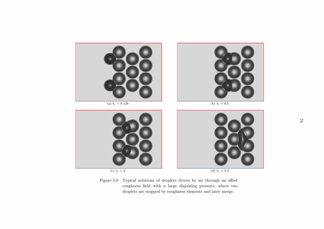
78

(a) t1 = 0.128 (b) t1 = 0.5

(c) t1 = 2 (d) t1 = 3.4

Figure 5.8 Typical solutions of droplets driven by air through an offset

roughness field with a large disjoining pressure, where two

droplets are stopped by roughness elements and later merge.

79

(a) t1 = 0.128 (b) t1 = 0.768

(c) t1 = 0.896 (d) t1 = 0.96

Figure 5.9 Typical solution of droplets driven by air through an offset

roughness field with a large disjoining pressure, where the

droplets interact with roughness elements, merge together and

separate into two droplets.

80

(a) Coefficient Bm = Bn = 0

(b) Coefficient Bm = Bn = 20

Figure 5.10 Comparison of the film, droplet and rivulet patterns as water is

driven by air near a stagnation line with/without the disjoining

pressure model with (m,n) = (3, 2), δ = 0.01 and λ = 2X.

figure 5.10(b). With a disjoining pressure model, more isolated droplets are observed, and the

droplets tend to remain near the stagnation line, pile together, and interact with each other

to form well-defined meandering rivulets.

5.3 A new disjoining pressure model

5.3.1 Surface thermodynamics of droplets on precursor films

A droplet on a dry surface is shown in figure 5.11, where the contact lines (in two-

dimensional situations) are the red points in this two-dimensional schematic diagram. The

81

Vapor

Liquid

Solid surface

δTContact line

θ

Figure 5.11 A virtual variation of a droplet on dry surface from an equi-

librium state.

contact angle is θ and the geometry is symmetric when the driving force is zero in the stream-

wise direction and gravity is neglected. The symbol δT is the virtual displacement of the

contact lines. These models (see Laplace (1806) and Young (1805)) can be derived from the

Helmholtz free energy using a virtual displacement method (see Johnson (1950); Roura (2004,

2005); Lanczos, (1966)). The Laplace equation (see Laplace (1806)) is

PL − PV = γLV

(1

r1+

1

r2

), (5.35)

where PL and PV are the pressure in the liquid and vapor phases, respectively. γLV is the

surface tension between the liquid and vapor phase, i.e. on the liquid droplet surface. r1 and

r2 are the principal radii of the droplet shape. The Young equation (see Young (1805)) is,

γLV cos θ = γSV − γSL, (5.36)

where γij is the surface tension between the ith phase and the jth phase, and the indices i, j

are those of the liquid, vapor and solid phases. Johnson (1950) pointed out that the energy of

a droplet is a minimum value when both the Laplace and Young equations are satisfied, when

the droplet is on a dry solid surface.

82

However, Hardy (1919) found that a precursor liquid layer is created during the droplet

deformation before the droplet moves (also see Beaglehole (1989); Cazabat (1987); de Gennes

(1985)). Such a precursor layer clearly exists in the experimental photos taken by Albrecht,

Otto & Leiderer (1992). The model of a droplet on a precursor film shown in figure 5.12 is

used in this study, where the solid surface is covered by a precursor film with a thickness δ.

The assumptions of this model are:

1. the rigid solid surface is smooth, isotropic, homogeneous, and insoluble in the liquid;

2. the film, vapor and solid surface are simple thermodynamic phases, respectively;

3. these three phases are homogeneous and not subject to any chemical or interactions with

external fields.

When the solid surface is covered by a thin precursor layer, the contact line/point shown in

figure 5.11 becomes the nominal contact line/point shown in figure 5.12. The contact angle is

defined as the angle between the tangent line of the macroscopic droplet shape and the flat

precursor film surface. The same model was used by Li & Neumann (1991) to present the

surface thermodynamics of a droplet on a precursor film (also see Neumann & Spelt (1996)).

One mechanical equilibrium condition derived by Li & Neumann (1991) is

Π = pv, (5.37)

where pv is the pressure of the bulk vapor phase, and Π is the disjoining pressure named by

Derjaguin & Churaev (1976) (also see Frumkin (1938)). The vapor pressure pv in the air is

bigger than zero. However, the classical disjoining pressure, i.e. the long-range van der Waals

force shown in equation (5.32), is less than zero when the dimensionless coefficients Bm and

Bn of repulsive and attractive terms in (5.32) are the same. The second disadvantage of the

classical disjoining pressure model (5.32) is that an effective length of the precursor layer should

be introduced into the analysis and simulation if the film thickness goes to zero (see Owens

et al. (1978); Mitchell & Richmond (1974); Glasner (2003); Butt & Stark (2005)). To avoid

these problems in the classical disjoining pressure models, e.g. equation (5.32), a new model

83

is presented here,

Π = B [T (F )m − T (F )n] , (5.38)

where the function T (F ) is a hyperbolic tangent function of the droplet thickness, i.e.

T (F ) = tanh

[(δ

F

)k], (5.39)

where k is usually defined as an integer, though it might be a real number. Note that k = 2 is

used in this study. The profiles of the new and classical models are plotted in the figure 5.13,

where the green line is the profile of the new disjoining pressure model, and the red line is the

profile of the classical disjoining pressure model. The classical disjoining pressure Π goes to

negative infinity as the the thickness F goes to zero, whereas the new disjoining pressure Π

goes to zero. This means that (5.38) can be applied to a droplet on a dry solid surface without

any extra assumptions, such as the effective film thickness. The values of both models become

the same, and will approach zero, when the film thickness F goes to infinity. Figure 5.14 shows

the difference between the functions y = 1F and y = tanh

(1F

), which also shows the tendency

of the new and classical pressure models to approach each other as F → ∞.

Vapor

Liquid

Solid surface

Precursorfilm

δ

Nominalcontact line

Θ

Figure 5.12 Schematic diagrams of droplets on a wet surface when the

precursor layer thickness is δ

84

0.01 0.02 0.03 0.04 0.05-0.05

0

0.05

0.1

0.15

0.2

F

Π = −B

{tanh

[(δF

)2]3− tanh

[(δF

)2]2}

Π = −B{(

δF

)6−(

δF

)4}

Π = 0

Figure 5.13 The comparisons between the classical disjoining pressure

model (5.32) and the new model (5.38). The coefficients are

B = 1 in both models. Note that the parameters m, n and k

in these two models are arbitrarily selected simply to illustrate

the qualitative difference between the models.

85

0 0.2 0.4 0.6 0.8 10

0.2

0.4

0.6

0.8

1

y = 1F

y = tanh(

1F

)

1F

Figure 5.14 A comparison of the difference between y = 1F and

y = tanh(

1F

)

86

-0.1 -0.05 0 0.05 0.10

0.05

0.1

0.15

X

(a) Initial droplet shape

-0.4 -0.2 0 0.2 0.40

0.01

0.02

0.03

0.04

0.05

0.06

X

Π = −B

{tanh

[(δF

)2]3− tanh

[(δF

)2]2}

Π = −B{(

δF

)6−(

δF

)4}

(b) Steady droplet shape as T → ∞

Figure 5.15 The typical solutions of a droplet on a precursor layer without

any driving force when the new disjoining pressure model and

the classical disjoining pressure model are used. Note that the

initial droplet profile is shown in figure 5.15(a).

87

Consider an example of a droplet lying on a precursor layer, with the driving forces zero

everywhere. Both the classical disjoining pressure model and the new disjoining pressure

model are used in the simulation. The initial droplet shape is shown in figure 5.15(a), which

is approximately a parabola. The steady solutions using the two disjoining pressure models

are shown in figure 5.15(b). The droplet profile with higher maximum height is the solution

using the new disjoining pressure (5.38). The lower one is the solution using the classical

disjoining pressure model (5.32). Figure 5.15(b) shows that the classical disjoining pressure

model increases the precursor film thickness when the droplet reaches its steady state, while

the new disjoining pressure model decreases the precursor film thickness. Moreover, the final

droplet geometries are slightly different when the classical and new disjoining pressure models

are used.

5.3.2 Inhomogeneous disjoining pressure empirical model

Often droplets or beads don’t move when they are statically deposited on a real solid surface,

such as glass windows and metal surfaces. However, the droplet will move if a sufficiently large

driving force is applied. A formula is constructed here to simulate a stationary droplet sticking

to a solid surface if the droplet is driven by air or gravity using the new disjoining pressure

model (5.38). The coefficient of the disjoining pressure is a function of the film thickness and

its derivatives, i.e. the coefficients of inhomogeneous disjoining pressure model (5.45) are taken

to be

B = B0 + △B · [U (F ) +W (F )] , (5.40)

where

U (F ) = tanh

[−βFx

(δ

F

)k]

(5.41)

and

W (F ) = tanh

[β (Fx)2

(δ

F

)k]. (5.42)

With this formula, the edge of the droplet on the precursor film will be detected automatically.

If a proper value of the parameter △B is chosen then the droplet will become stationary.

88

Another possible pair of formulae for W and U are

U (F ) = tanh

[−βFFx

(δ

F

)k]

(5.43)

and

W (F ) = tanh

[β (Fx)2

(δ

F

)k]. (5.44)

Note that both of these two pairs of coefficients were tested in the numerical simulation, and

both could simulate stationary droplets on a solid surface. However, the grid independence

study shows that the grid size must not be too large. To limit the discussion, one pair of

inhomogeneous coefficients W and U , i.e. (5.41) and (5.42), is applied to the film equation,

e.g. equation (5.27) and (5.29). In the following simulations, the disjoining pressure is added

to the film equation in the form

∂F

∂t+

∂

∂X

(λX

F 2

2−∂P

∂X

F 3

3

)+

∂

∂X

(λZ

F 2

2−∂P

∂Z

F 3

3

)= 0, (5.45)

where

P = −ΣK − Π = −Σ

(∂2F

∂X2+∂2F

∂Z2

)− Π, (5.46)

Π = [B + ∆B (U +W )] · [T (F )m − T (F )n] , (5.47)

T (F ) = tanh

[(δ

F

)k], (5.48)

and m, n and k are defined previously.

5.4 Numerical solutions and comparisons

An empirical model, i.e. film equation (5.45) and (5.46) together with the inhomogeneous

coefficient (5.47), is presented in the above sections. To validate this model, droplets on an

inclined surface and droplets near a stagnation line at the leading edge of an airfoil are simulated

using an ADI-Iteration method and pseudo-linear method discussed in appendices A and B.

Appendix A gives the numerical algorithm for the two dimensional film equation, which is

solved as a system of pentadiagonal difference equations. The boundary conditions in both the

streamwise and spanwise directions are periodic, while the non-periodic boundary conditions

89

are used in the film front direction of motion. The difference equations of the inhomogeneous

coefficients (5.47) are given in Appendix B, which are linearized using the functional derivative

(see Oron & Bankoff (1999)).

A. Comparison with Hansman & Turnock’s experiment

The experiment of Hansman & Turnock (1988) shows that the average of the advancing

and receding contact angle depends on temperature. In their experiment, the inclination angle

is 30o, and the droplet’s volume is increased by continuously injecting water into the droplet

until the droplet moves. Rothmayer & Tsao (2001) applied the above experiment to a model

that simulates droplet motion near a stagnation line. In this section, a droplet on an inclined

surface is simulated using the empirical formulae (5.40), (5.43) and (5.44), when the advancing

and receding contact angles are different.

In the experiment of Hansman & Turnock (1988), the contact angle of a droplet on an

inclined surface was not presented as a function of the droplet geometrical parameters, such as

the droplet volume, height or diameter. Instead, Hansman & Turnock (1988) found a relation

between the temperature and contact angles when the droplet was driven by gravity. This

process is simulated in figures 5.16 to 5.20. The solutions are parametrized by a variable, i.e.

∆B, in the empirical formulae 5.40, 5.43 and 5.44, because ∆B is analogous to temperature

in the Hansman & Turnock’s experiment (1988).

Figure 5.16(a) shows the definition of the contact angle used in this study. When a droplet

is on an inclined surface, it is driven by the gravity force. The arrow with the acceleration

g shows the direction of the driving force. The droplet deforms but does not move away

from the original position, providing that it is sufficiently small. When the droplet is almost

stationary, the receding/advancing contact angles, i.e. ΘR and ΘA can be measured in the

macroscopic view, which is indicated with the tangent lines near the contact points. Figure

5.16(b) shows the definition of droplet height and diameter. Initially, a symmetric parabolic

shape is placed on a surface which is inclined to an angle of 30o. The volume of the droplet is

calculated using the initial droplet height and diameter. Therefore, the initial droplet height

is the only parameter needed to determine the droplet volume. The effect from the precursor

90

film thickness, δ, is negligible in the volume calculation, because δ is much smaller than H.

Note that the approximate parabolic shape in this study is given by equation (2.34).

Figure 5.17 shows the calculation of the contact angle, where the angle is defined as the

angle between the tangent line at any point on the droplet surface and the x-axis, i.e.

Θ = arctan

(∂F

∂X

). (5.49)

The receding contact angle, ΘR, and the advancing contact angle, ΘA, in figure 5.18, at initial

Height = 1 in this case, are defined as the absolute values of the maximum and minimum

values shown in figure 5.17, respectively.

Figure 5.18(a) shows the difference between ΘA and ΘR, which is transformed into a

function of temperature T . As defined in figure 5.17(a), ΘA is the advancing contact angle,

and ΘR is the receding contact angle. The solid squares are the experimental results, which

are obtained from the Hansman & Turnock’s experimental data (1988). The line is the least

squares linear fit of the experimental results as well as the numerical results (see discussion

below), where the parameter ∆B used in the disjoining pressure model is transformed to the

temperature T through the equation (5.50)

∆B = −12.27866 · T − 13.64195. (5.50)

Note that the least squares linear fit of the contact angle difference for the numerical data is

ΘA − ΘR = 0.10076 · ∆B + 2.69979, (5.51)

while for the experimental data, it is

ΘA − ΘR = −1.23724 · T + 1.32519. (5.52)

Equation (5.50) is the solution of equations (5.51) and (5.52). Note that equation (5.50) is

selected to give exact agreement with the experimental data. The ”numerical data” in figure

5.18 are the actual results obtained when using (5.50) in the simulations. Figure 5.18(b) shows

the average advancing and receding contact angles of the water droplet, i.e. (ΘA + ΘR) /2.

91

-1

-0.5

0

0.5

1

0

0.2

0.4

0.6

0.8

1

g

X

Y

ΘR

ΘA

(a) Contact angle

-1

-0.5

0

0.5

1

0

0.2

0.4

0.6

0.8

1

X

Y

Hei

ght

Diameter

(b) Diameter and height

Figure 5.16 Example of the contact angle, height and diameter computed

in this study.

92

-2

-1

0

1

2

-60

-40

-20

0

20

40

Angl

e

X

ΘR

ΘA

Figure 5.17 Diagram of the contact angle calculation in this study.

When the relation 5.50 is applied into the linear fit of the numerical results, the average of the

advancing and receding contact angles becomes a function of the temperature, i.e.

(ΘA + ΘR) /2 = −1.40950 · T + 21.93939, (5.53)

while the least square linear fit of the experimental results is

(ΘA + ΘR) /2 = −1.60041 · T + 9.89117. (5.54)

Note that two formulae similar to equations (5.52) and (5.54) are used by Rothmayer & Tsao

(2001), though the coefficients are slightly different.

Figure 5.19 shows the droplet shapes in the simulation when they are placed on an inclined

surface and driven by gravity. All numerical data shown in this comparison are found from

these droplet shapes, and the least squares linear fit all depends on this data. As the droplet

size changes the parameter ∆B changes, which is analogous to the temperature T , as shown

in figure 5.20.

Algorithm for computing bead runback:

93

-25 -20 -15 -10 -5 00

10

20

30

40

Least squares linear fit

Experimental data

Numerical data

ΘA−

ΘR

Temperature T (oC)

(a) Advancing and receding contact angle hysteresis

-25 -20 -15 -10 -5 010

20

30

40

50

60

-25 -20 -15 -10 -5 010

20

30

40

50

60

Least squares linear fit (A)

Experimental data

Numerical data

(ΘA

+Θ

R)/2

Temperature T (oC)

Least squares linear fit (B)

(b) Average of advancing and receding contact angles

Figure 5.18 The advancing and receding contact angles when the em-

pirical formulae (5.40), (5.43) and (5.44) are used to sim-

ulate droplets on an inclined surface. Note that the

least squares linear fit (A) is from equation (5.53), while the

least squares linear fit (B) is from equation (5.54).

94

-3

-2

-1

0

1

2

3

0

0.5

1

1.5

2

X

Y

Figure 5.19 Droplets calculated with the new disjoining pressure model,

i.e. (5.45), (5.46) and (5.47)

-25 -20 -15 -10 -5 00

1

2

3

Temperature T (oC)

Init

ialdro

ple

thei

ghts Least squares linear fit

Numerical data

Figure 5.20 The least squre linear fit to show the relation between the

droplet heights and the temperature in the experiment by

Hansman & Turnock (1988)

95

1. Initialize a droplet on an inclined surface.

A finite volume droplet is created on an inclined surface, where the inclination angle is 30

degrees. The initial droplet shape is approximately parabolic. The figure 5.16(a) shows

the definition of the advancing and receding contact angles. The definition of the droplet

height and diameter is shown in figure 5.16(b).

2. Search for an appropriate value of ∆B.

For a given droplet volume, ∆B is found so that the droplet remains stationary on the

inclined surface for a long time. Because the droplet continues deforming, the stationary

status is only reached after a long time if a correct ∆B can be found.

3. Calculating the contact angles

The advancing and receding contact angles are calculated through the definition in equa-

tion (5.49). These are also shown in figure 5.17(a).

4. Changing the droplet volume

The droplet volume is gradually increased, and steps 3 and 4 are repeated for each

droplet. The contact angles and droplet volume are determined from the last solution

which remaining steady.

5. Data fitting and comparison

A least squares linear fit is used for the data fitting. The contact angle is a function of

∆B, which is analogous to temperature in the Hansman & Turnock’s experiment. As

shown in figures 5.18, two equations are found from the least squares fit. One is used for

the transformation between the temperature T and the variable ∆B. The comparison

between the experimental data and numerical data is also shown in figures 5.18.

B. Comparison with Olsen & Walker’s experiment

To validate the empirical formulae, a comparison is made with the experimental data of

Olsen & Walker (1987), which are above freezing experiments of droplet runback on a smooth

96

surface. The sizes of the water droplets in the experiment are given at the different distance

from the stagnation line, which are used as the initial input in the simulations. A fixed ∆B

is used in this comparison, which amounts to fixing the contact angle of the droplets (note

that in Olsen & Walker’s (1987) experiment the contact angles were approximately constant).

The steps used in the comparison are given below. The precursor film thickness is 0.01 in all

simulations, which is negligible in the volume calculation. The parameters m = 3 and n = 2

in equation (5.38) are used in this study, though others could be used.

To translate the diameters from a dimensionless variable D to a dimensional variable D∗,

the scales in section 2.2 are used. For the thin water film, the scale ∆ is less than the condensed

layer value of Rothmayer & Tsao (2000) but larger than the near wall Navier-Stokes scale, i.e.

Re−3/4 ≪ ∆ ≪ Re−9/14σ−3/7. (5.55)

With σ = ΣD−1/2aw , Re = 104 and Daw = 10−3, the inequality (5.55) becomes

10−3 ≪ ∆ ≪ 1.1788 × 10−2. (5.56)

The arithmetic average of the scale ∆ is used to estimate the droplets diameter transformation,

i.e.

∆ =1

2

(1.1788 × 10−2 + 10−3

)≈ 6.4 × 10−3. (5.57)

The characteristic length L∗ is the diameter of the nose at the leading edge of an airfoil, i.e.

L∗ = 3.8 cm (see Olsen & Walker (1988)). The final diameter transformation becomes

D∗ = L∗∆D ≈ 3.8 × 10−2 × 6.4 × 10−3 ×D = 243.2 ·D µm. (5.58)

The algorithm used in the comparison with Olsen & Walker’s experiment is

1. Initialize a droplet at the leading edge of an airfoil

A finite volume droplet is created on a flat surface, and the droplet shape is approximately

parabolic. The droplet volume is calculated from the experimental value. For example,

at s∗ = 9mm, the droplet diameter is about 160µm, and the ratio of its height and

diameter is 0.26 (see Olsen & Walker (1988)). A dimensionless droplet is placed on flat

surface using the non-dimensionalization and the scale transformation.

97

2. The shear stress λ

An empirical formula based on the laminar flow is used for the shear stress calculation

(see Rothmayer & Tsao (2001)), i.e.

λ = 3.19

{1.66

(s∗

19mm

)−

(s∗

19mm

)2}

(5.59)

At s∗ = 9mm, the shear stress is λ = 1.793. A shear driven thin film equation is solved

together the empirical formula.

3. Set parameters in the empirical formula

B0 = 100 is fixed for all simulations. ∆B is an unknown constant. A droplet at s∗ = 9mm

is first simulated using a series of ∆B. For example, an initial droplet shape (rescaled

dimensionless H = 1.404) is shown as a solid red line in figure 5.21(a). ∆B = 326 in the

empirical formula is used in this simulation. Due to the shear stress and the capillary

force, the droplet starts to deform as t > 0, and it eventually becomes stationary as t

goes to ∞. The stationary solution is the green line shown in figure 5.21(a). Figure

5.21(b) shows that the deformation number ζ of a typical solution is a function of time.

The definition of ζ is shown in equation (5.60). When t < 1 the droplet deformes a lot.

When t > 1 it becomes almost stationary. The same ∆B, i.e. ∆B = 326, is fixed for all

other simulations in this comparison. The deforming time, i.e. τd = 1, in this simulation

is used as a reference time to evaluate the deformation time of the other simulations in

this comparison.

4. The droplet deformation and displacement

It is known that the droplet deforms anytime and anywhere, but it is hard to observe

such a micro deformation in short time. In this study, an equation (5.60) is used to

measure the amount of the droplet deformation and displacement:

ζ =

∫ +∞

−∞|F (X,T ) − F (X, t = 0)| dX∫ +∞

−∞F (X, t = 0)dX

(5.60)

Note that ζ = 0 is the initial state. One limit solution as ζ = 1 is the droplet becomes

completely flat and the thickness approaches zero, but that will not happen in this

98

-1 -0.5 0 0.5 10

0.2

0.4

0.6

0.8

1

1.2

1.4

1.6

X

FF (X, t = 0)

F (X, t → ∞)

(a) Typical stationary droplet

0 0.5 1 1.5 2 2.5 30

0.2

0.4

0.6

0.8

1

Time t

Difor

mat

ion

num

ber

ζ

ζ (t)

Deforming Stationary

τd

(b) Typical ζ (t) profile

Figure 5.21 Typical deformation number ζ of a single droplet driven by a

shear stress λ = 1.793. Note that ∆B = 326 is used in the em-

pirical formula. τd is the deformation time, i.e. ζ(t=τd)ζ(t→∞) ≥ 0.95.

ζ is defined in equation (5.60).

99

comparison. ζ = 2 occurs when the droplet completely moves away from its initial

location, which is schematically shown in the diagram 5.22. In this study, the droplet is

assumed to be stationary if the deformation number ζ is in the following range while the

deformation time is within a time interval (τd − ∆τ) ≤ t ≤ (τd + ∆τ), i.e.

(ζs − ∆ζ) ≤ ζ ≤ (ζs + ∆ζ) , (5.61)

where the time τd is determined by the step 3, at which time the deforming number ζs

is ζs = ζ (t = τd). ∆τ is a fixed time interval, which is kept constant in this comparison.

Similarly, ∆ζ is a fixed value for all other simulations.

-2 0 2 4 60.5

1

1.5

2

F

X

F (X, t = 0) F (X, t > 0)

Figure 5.22 Diagram of a solution which would produce a deformation

number ζ ≈ 2, as a droplet moves away from its initial lo-

cation.

5. Droplets at the same location s∗

Different size droplets are simulated at the same location, and they are driven by the

same shear stress λ. If the droplets deformation number ζ is within the range defined in

step 4, the droplets are stationary. Otherwise, they will be marked as moving droplets.

6. Droplets at the different locations s∗

At different locations, the shear stress λ is different. Several different size droplets are

again simulated using the same parameters in the empirical formula but using the differ-

ent shear stress.

100

0 0.5 1 1.5 20

0.2

0.4

0.6

0.8

1

Time t

Difor

mat

ion

num

ber

ζ

(τd, ζs)

2∆ζ

2∆τ

Figure 5.23 A schematic diagram of the parameter window used to define

a pseudo-stationary droplet. For example, a droplet is marked

as a stationary droplet if the deformation time is within the

interval, (τd − ∆τ) ≤ t ≤ (τd + ∆τ), and the deforming num-

ber is within the interval, (ζs − ∆ζ) ≤ ζ ≤ (ζs + ∆ζ) at the

same time.

101

7. Comparison with the experiment

After steps 1 to 6 are finished, the numerical diameters are compared with the experimen-

tal results, which are shown in figures 5.24. Figure 5.24(a) shows the droplet diameters

at different locations when those droplets are driven by the shear stress near the lead-

ing edge of the airfoil. The discrete diameters at the different locations show that the

droplets can be stationary when the criteria (5.61) is used. ∆τ is about 50% of τd, and

∆ζ is about 10% of ζs shown in step ”The droplet deformation and displacement”. As

the droplet size increases, the probability of moving away from its initial location be-

comes large. The large diameter drops will move first, though sometime the deforming

number ζ is still small. Hence, the droplet profile, i.e. figure 5.24(b), is used to show

the droplet motion. The reasonable trend of the droplet diameters at different locations

is found when a series of different size droplets are simulated with one fixed parameter

∆B = 326.

In summary, it is convenient to use this empirical formula to simulate the droplets driven

by the air shear stress when the parameter ∆B is a fixed number, provided that it is

selected correctly. The computational cost of this simulation is quite high.

102

0 5 10 15 20 250

400

800

1200

1600

Bea

dD

iam

eter

(µm

)

s∗ (mm)

Experimental data

Computed moving droplets

Computed stationary droplets

(a) Diameters of droplets along the Olsen & Walker airfoil

-1 -0.5 0 0.5 10

1

2

3D*=170.24D*=206.72D*=243.20

-1 -0.5 0 0.5 10

1

2

3D*=279.68D*=333.18D*=381.18

X

F

(b) Droplet profiles at a distance s∗ = 9 (mm)

Figure 5.24 Comparison between Olsen & Walker’ experimental data and

the numerical solutions when the empirical formulae (5.40),

(5.43) and (5.44) are applied.

103

CHAPTER 6. Conclusions

An asymptotic theory is applied to thin water films flowing past small roughness when

the thin viscosity-dominated films are driven by the air shear stress in the context of a high

Reynolds number boundary layer theory. Some properties of this model are explored in different

settings, such as transport and interaction of water in a roughness field, perturbed heat transfer

of film/roughness combinations and films with surfactant. For the water transport around the

surface roughness, different roughness patterns induce the different water pooling as the water

mass is redistributed through the interactions. When the ambient leading order heat flux is

fixed, the analysis shows the amount of change of the perturbed heat flux due to the non-

uniform water surface though perturbed heat flux is not significantly effected. Based on a

linear instability analysis, a general formula has been developed for the instability of film

fronts and rivulet creation by film front perturbations and surface roughness. It also shows

that rivulets can be formed from instabilities of very thin films. After analysis of bead runback

near stagnation lines, it is found that the disjoining pressure model is required for the accurate

simulation of water beads and rivulets. a new modified disjoining pressure model is developed

together with an empirical formula, which is validated through comparisons with experimental

data from aircraft icing tests.

104

APPENDIX A. ADI-Iterative method and its algorithm

This method is used in section 3.5, Instability of film fronts moving through surface rough-

ness, and chapter 5 as well as water films and beads motion near a stagnation line.

A.1 Linearization and ADI-Iterative method

The thin film equation with a precursor layer is:

Ft + ▽ ·(−→λ F 2

)+ ▽ · (H (F ) ▽ P ) = 0, (A.1)

where the coefficient H (F ) is H (F ) = 13F

3 and P = − ▽2 (F + r) − Π. r is the surface

roughness function, and Π is the disjoining pressure. The classical disjoining pressure Π =

−B[(

δF

)m−(

δF

)n]is used as the example here. Equation (A.1) is rewritten as

Ft = −g (F ) , (A.2)

where the function g (F ) is g (F ) = ▽ ·(−→λ F 2

)+ ▽ · (H (F ) ▽ P ).

A general algorithm of the Crank-Nicolson method (see Crank J. & Nicolson P. (1947);

Tannehill, Dale & Pletcher (1997)) is used in this study, i.e.

Fn+1 − Fn = −∆t ·[θ · g

(Fn+1

)+ (1 − θ) · g (Fn)

], (A.3)

where θ is a constant and 0 ≤ θ ≤ 1. The above equation becomes

Fn+1 + ∆t · θ · g(Fn+1

)= Fn − ∆t · (1 − θ) · g (Fn) , (A.4)

where g (F ) = ▽ ·(−→λ · F 2

)+ ▽ ·

(H (F ) ▽▽2 (F + r)

)−▽2 (H (F ) Π). Its linearization is

g (F ) = g(F)

+ gF

(F)v + · · · · · · , (A.5)

105

where gF

(F)v is the functional derivative (see Oron & Bankoff (1999)), or the Jacobian of

the function g (F ), i.e.

gF (F ) v = ▽ ·(2−→λ Fv

)+ ▽ ·

(HF v▽▽2 (F + r) +H ▽▽2v

)−▽2 (PDisjP,v) , (A.6)

where PDisjP,v =(H(Fn+1

)Π)Fv and v = F − F . F is the guess value in the linearization,

which is updated in inner iterations till it is convergent to a criteria. The equation (A.4) finally

becomes

v + θ · ∆t · gF

(Fn+1

)v = −

(Fn+1 − Fn

)− (1 − θ) · ∆t · g (Fn) − θ · ∆t · g

(Fn+1

), (A.7)

where

g (F ) = ▽ ·(−→λ · F 2

)+ ▽ ·

(H (F ) ▽▽2 (F + r)

)−▽2 (H (F ) Π) , (A.8)

and

gF (F ) v = ▽ ·(2−→λ Fv

)+ ▽ ·

(HF v▽▽2 (F + r) +H ▽▽2v

)−▽2 (PDisjP,Fv) . (A.9)

To accelerate the calculation of the thin film equation, the pseudo-linear factorization

method (see Witelski & Bowen (2003)) is applied in this study. Finally, the above difference

equation (A.7) becomes

Lxw = −(Fn+1 − Fn

)− (1 − θ) · ∆t · g (Fn) − θ · ∆t · g

(Fn+1

), (A.10)

Lzv = w, (A.11)

Fn+1(k+1) = Fn+1

(k) + v, (A.12)

where

Lx = I + θ · ∆t(Bx + Dx + Ex + Gx

), (A.13)

Lz = I + θ · ∆t(Bz + Dz + Ez + Gz

), (A.14)

Bx = ∂x

[2λxF

n+1], (A.15)

Bz = ∂z

[2λzF

n+1], (A.16)

Dx = ∂x

[H(Fn+1

)∂xxx

], (A.17)

106

Dz = ∂z

[H(Fn+1

)∂zzz

], (A.18)

Ex = ∂x

[HF∂xxx

(Fn+1 + r

)], (A.19)

Ez = ∂z

[HF∂zzz

(Fn+1 + r

)], (A.20)

Gx = ∂xx, (A.21)

and

Gz = ∂zz. (A.22)

A.2 Finite difference equations

1. x-direction

Here is the summary of the finite difference equations in x-direction used in the simula-

tions.

Lxw =[I + θ · ∆t

(Bx + Dx + Ex + Gx

)]w

= −(Fn+1 − Fn

)− (1 − θ) · ∆t · g (Fn) − θ · ∆t · g

(Fn+1

),

(A.23)

Lxw =[I + θ · ∆t

(Bx + Dx + Ex + Gx

)]w

= −(Fn+1 − Fn

)− (1 − θ) · ∆t · g (Fn) − θ · ∆t · g

(Fn+1

),

(A.24)

where

Bx = ∂x

[2λxF

n+1], (A.25)

Dx = ∂x

[H(Fn+1

)∂xxx

], (A.26)

Ex = ∂x

[HF∂xxx

(Fn+1 + r

)], (A.27)

and

Gx = ∂xx. (A.28)

• Shear stress terms

term1 = Bwi−1,k +Dwi+1,k (A.29)

107

where

B = −2λxi−1,kFi−1,k

2 △ x, (A.30)

D = −2λxi+1,kFi+1,k

2 △ x. (A.31)

• The highest order nonlinear terms with Fw = F + r

term2 = Awi−2,k +Bwi−1,k +Cwi,k +Dwi+1,k + Ewi+2,k, (A.32)

where

A =1

(△x)4am, (A.33)

B =1

(△x)4(−3am − ap) , (A.34)

C =1

(△x)4(3am + 3ap) , (A.35)

D =1

(△x)4(−am − 3ap) , (A.36)

E =1

(△x)4ap, (A.37)

with

ap =

(Fn+1

i,k

)3, if Fn+1

i,k = Fn+1i+1,k;

2( eF n+1

i,keF n+1

i+1,k)2eF n+1

i,k+ eF n+1

i+1,k

, otherwise,

(A.38)

and

am =

(Fn+1

i,k

)3, if Fn+1

i,k = Fn+1i−1,k;

2( eF n+1

i,keF n+1

i−1,k)2eF n+1

i,k+ eF n+1

i−1,k

, otherwise.

(A.39)

• Mixed derivatives

term31 =1

(△x)4ap (Fw,i+2,k − 3Fw,i+1,k + 3Fw,i,k − Fw,i−1,k) , (A.40)

and

term32 =1

(△x)4am (Fw,i−2,k − 3Fw,i−1,k + 3Fw,i,k − Fw,i+1,k) . (A.41)

108

Then

term31 = Cwi,k +Dwi+1,k, (A.42)

where

C =

(Fn+1

i,k

)3C4p, if Fn+1

i,k = Fn+1i+1,k;

C3pC4p, otherwise,

(A.43)

D =

0, if Fn+1i,k = Fn+1

i+1,k;

C2pC4p, otherwise,

(A.44)

and

C4p = (Fw,i+2,k − 3Fw,i+1,k + 3Fw,i,k − Fw,i−1,k) . (A.45)

term32 = Bwi−1,k + Cwi,k, (A.46)

with

B =

0, if Fn+1i,k = Fn+1

i−1,k;

C3mC4m, otherwise,

(A.47)

C =

(Fn+1

i,k

)3C4m, if Fn+1

i,k = Fn+1i−1,k;

C2mC4m, otherwise,

(A.48)

and

C4m = (Fw,i−2,k − 3Fw,i−1,k + 3Fw,i,k − Fw,i+1,k) . (A.49)

In above equations, the functions C2 (x, y)and C3 (x, y) are

C2 (x, y) = 2xy2

x+ y

(2 −

x

x+ y

)= C3 (y, x) . (A.50)

• Disjoining pressure terms

Here is an example as m = 4 and n = 3 for the classical disjoining pressure, i.e.

Π = Bm

(δ

F

)m

−Bn

(δ

F

)n

. (A.51)

109

One difference equation of the disjoining pressure terms is

term4 = Bwi−1,k + Cwi,k +Dwi+1,k, (A.52)

where

B =Bcoeff,DisJP

(△x)2

(−4δ4

F 2i−1, k

+3δ3

Fi−1, k

), (A.53)

C =Bcoeff,DisJP

(△x)2

(−4δ4

F 2i, k

+3δ3

Fi, k

), (A.54)

D =Bcoeff,DisJP

(△x)2

(−4δ4

F 2i+1, k

+3δ3

Fi+1, k

). (A.55)

For the new disjoining pressure model with the inhomogeneous coefficients, there

will be details later.

2. z-direction

Lzv =[I + θ · ∆t

(Bz + Dz + Ez + Gz

)]v = w, (A.56)

where

Bz = ∂z

[2λzF

n+1], (A.57)

Dz = ∂z

[H(Fn+1

)∂zzz

], (A.58)

Ez = ∂z

[HF∂zzz

(Fn+1 + r

)], (A.59)

Gz = ∂zz. (A.60)

• Shear stress terms

The difference equation of the shear term is

term1 = Bwi,k−1 +Dwi,k+1, (A.61)

where

B = −2λz,i,k−1Fi,k−1

2 △ z, (A.62)

D = −2λz,i,k+1Fi,k+1

2 △ z. (A.63)

110

• The highest order nonlinear terms with Fw = F + r

The difference equation of the highest order nonlinear term is

term2 = Awi,k−2 +Bwi,k−1 +Cwi,k +Dwi,k+1 + Ewi,k+2, (A.64)

where

A =1

(△z)4am, (A.65)

B =1

(△z)4(−3am − ap) , (A.66)

C =1

(△z)4(3am + 3ap) , (A.67)

D =1

(△z)4(−am − 3ap) , (A.68)

E =1

(△z)4ap. (A.69)

with

ap =

(Fn+1

i,k

)3, if Fn+1

i,k = Fn+1i,k+1;

2( eF n+1

i,keF n+1

i,k+1)2eF n+1

i,k+ eF n+1

i,k+1

, otherwise,

(A.70)

am =

(Fn+1

i,k

)3, if Fn+1

i,k = Fn+1i,k−1;

2( eF n+1

i,keF n+1

i,k−1)2eF n+1

i,k+ eF n+1

i,k−1

, otherwise.

(A.71)

• Mixed derivatives The difference equation of the mixed derivatives is

term31 =1

(△z)4ap (Fw,i,k+2 − 3Fw,i,k+1 + 3Fw,i,k − Fw,i,k−1) , (A.72)

and

term32 =1

(△z)4am (Fw,i,k−2 − 3Fw,i,k−1 + 3Fw,i,k − Fw,i,k+1) . (A.73)

After the simplification, they become

term31 = Cwi,k +Dwi,k+1, (A.74)

111

where

C =

(Fn+1

i,k

)3C4p, if Fn+1

i,k = Fn+1i,k+1;

C3pC4p, otherwise,

(A.75)

D =

0, if Fn+1i,k = Fn+1

i,k+1;

C2pC4p, otherwise.

(A.76)

and

C4p = (Fw,i,k+2 − 3Fw,i,k+1 + 3Fw,i,k − Fw,i,k−1) . (A.77)

term32 = Bwi,k−1 + Cwi,k, (A.78)

where

B =

0, if Fn+1i,k = Fn+1

i,k−1;

C3mC4m, otherwise,

(A.79)

C =

(Fn+1

i,k

)3C4m, if Fn+1

i,k = Fn+1i,k−1;

C2mC4m, otherwise.

(A.80)

and

C4m = (Fw,i,k−2 − 3Fw,i,k−1 + 3Fw,i,k − Fw,i,k+1) . (A.81)

In above equations, the functions C2 (x, y)and C3 (x, y) are

C2 (x, y) = 2xy2

x+ y

(2 −

x

x+ y

)= C3 (y, x) , (A.82)

• Disjoining pressure terms

Here is an example as m = 4 and n = 3 for the classical disjoining pressure.

term4 = Bwi−1,k + Cwi,k +Dwi+1,k, (A.83)

112

where

B =Bcoeff,DisJP

(△z)2

(−4δ4

F 2i, k−1

+3δ3

Fi, k−1

), (A.84)

C =Bcoeff,DisJP

(△z)2

(−4δ4

F 2i, k

+3δ3

Fi, k

), (A.85)

D =Bcoeff,DisJP

(△z)2

(−4δ4

F 2i, k+1

+3δ3

Fi, k+1

). (A.86)

For the new disjoining pressure model with the inhomogeneous coefficients, there

will be details later.

113

APPENDIX B. The disjoining pressure term and its functional derivative

This method is used in the chapter 5, as well as for water films and beads motion near a

stagnation line.

The new disjoining pressure model and the inhomogeneous coefficients are applied in the

bead simulation. This is also the finite difference equations to solve the disjoining pressure

terms in the one-dimensional thin film equation. The discussion below is the finite difference

equation of one disjoining pressure term.

When the disjoining pressure model is applied to the thin film equation, the term with the

disjoining pressure is

∂

∂x

(F 3 ∂Π

∂x

)=

∂

∂x

(F 3 ∂

∂x[BT (F )m]

)−

∂

∂x

(F 3 ∂

∂x[BT (F )n]

), (B.1)

where (m,n) = (3, 2) and k = 2 are used as an example, the new disjoining pressure model,

i.e.

Π = B [T (F )m − T (F )n] , (B.2)

is used. The hyperbolic tangent function T (F ) is

T (F ) = tanh

[(δ

F

)k], (B.3)

the inhomogeneous coefficient is

B = B0 + △B (U +W ) , (B.4)

where

U (F ) = tanh

[−FFx

(δ

F

)k], (B.5)

and

W (F ) = tanh

[(Fx)2

(δ

F

)k]. (B.6)

114

B.1 Derivatives of the functions T , U and W

In the new disjoining pressure model with inhomogeneous coefficients, the derivatives of

some terms are

1. The hyperbolic tangent function T

∂

∂x[T (F )m] = m

{T (F )m−1 − T (F )m+1

} ∂

∂x

[(δ

F

)k]

(B.7)

2. The first derivative of the inhomogeneous function U

∂

∂x[U (F )] = A1 (A2 +A3 +A4) , (B.8)

where

A1 = −(1 − U2

), (B.9a)

A2 = F

[(δ

F

)k]∂2F

∂x2, (B.9b)

A3 = F∂

∂x

[(δ

F

)k]∂F

∂x, (B.9c)

A4 =

(∂F

∂x

)2[(

δ

F

)k]. (B.9d)

3. The second derivative of the inhomogeneous function U

∂2

∂x2[U (F )] =

∂A1

∂x(A2 +A3 +A4) +A1

(∂A2

∂x+∂A3

∂x+∂A4

∂x

), (B.10)

where

A1 = −(1 − U2

), (B.11a)

A2 = F

[(δ

F

)k]∂2F

∂x2, (B.11b)

A3 = F∂

∂x

[(δ

F

)k]∂F

∂x, (B.11c)

A4 =

(∂F

∂x

)2[(

δ

F

)k], (B.11d)

115

and

∂A1

∂x= 2U

∂U

∂x, (B.12a)

∂A2

∂x= F

∂

∂x

[(δ

F

)k]∂2F

∂x2+ F

[(δ

F

)k]∂3F

∂x3+∂F

∂x

[(δ

F

)k]∂2F

∂x2, (B.12b)

∂A3

∂x= F

∂2

∂x2

[(δ

F

)k]∂F

∂x+ F

∂

∂x

[(δ

F

)k]∂2F

∂x2+

∂

∂x

[(δ

F

)k](

∂F

∂x

)2

, (B.12c)

∂A4

∂x= 2

∂F

∂x

∂2F

∂x2

[(δ

F

)k]

+

(∂F

∂x

)2 ∂

∂x

[(δ

F

)k]. (B.12d)

4. The first derivative of the inhomogeneous function W

∂

∂x[W (F )] = βA1 (A2 +A3) , (B.13)

where

A1 =(1 −W 2

), (B.14a)

A2 = 2

(δ

F

)k ∂F

∂x

∂2F

∂x2, (B.14b)

A3 =

(∂F

∂x

)2 ∂

∂x

[(δ

F

)k]. (B.14c)

5. The second derivative of the inhomogeneous function W

∂2

∂x2[W (F )] = β

{∂A1

∂x(A2 +A3) +A1

(∂A2

∂x+∂A3

∂x

)}, (B.15)

where

A1 =(1 −W 2

), (B.16a)

A2 = 2

(δ

F

)k ∂F

∂x

∂2F

∂x2, (B.16b)

A3 =

(∂F

∂x

)2 ∂

∂x

[(δ

F

)k], (B.16c)

and

∂A1

∂x=

∂

∂x

(1 −W 2

)= −2W

∂W

∂x, (B.17)

116

∂A2

∂x=

∂

∂x

[2

(δ

F

)k ∂F

∂x

∂2F

∂x2

]

= 2∂

∂x

[(δ

F

)k]∂F

∂x

∂2F

∂x2+ 2

(δ

F

)k ∂2F

∂x2

∂2F

∂x2+ 2

(δ

F

)k ∂F

∂x

∂3F

∂x3,

(B.18)

∂A3

∂x=

∂

∂x

{(∂F

∂x

)2 ∂

∂x

[(δ

F

)k]}

= 2∂F

∂x

∂2F

∂x2

∂

∂x

[(δ

F

)k]

+

(∂F

∂x

)2 ∂2

∂x2

[(δ

F

)k].

(B.19)

B.2 Finite difference equation of the terms with B

For simplicity, one component in equation (B.1), i.e. ∂∂x

(F 3 ∂

∂x [BT (F )m])

is used to illus-

trate the numerical scheme:

∂

∂x

(F 3 ∂

∂x[BT (F )m]

)= (term11 + term11) +

(−2mδ2

)· (term21 + term22) , (B.20)

where

term11 =∂

∂x

(T (F )m F 3

) ∂B∂x

, (B.21a)

term12 = T (F )m F 3 ∂2B

∂x2, (B.21b)

term21 =[T (F )m−1 − T (F )m+1

] ∂B∂x

∂F

∂x, (B.21c)

term22 = B[T (F )m−1 − T (F )m+1

] ∂2F

∂x2. (B.21d)

1. Functional derivatives of term 1 The functional derivative of the term 1 is

〈term1〉F v =∂

∂x

⟨(T (F )m F 3∂B

∂x

)⟩

F

v. (B.22)

It is written as

〈term1〉F v = part1 + part2 + part3, (B.23)

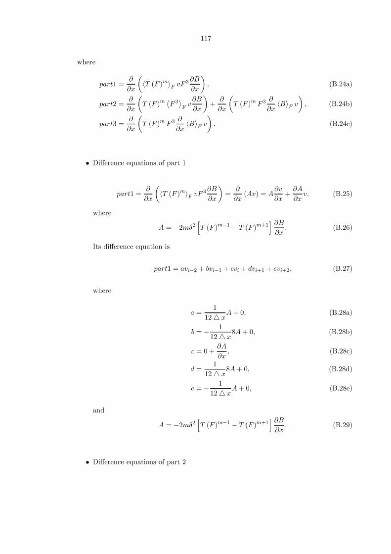
117

where

part1 =∂

∂x

(〈T (F )m〉F vF

3∂B

∂x

), (B.24a)

part2 =∂

∂x

(T (F )m ⟨F 3

⟩Fv∂B

∂x

)+

∂

∂x

(T (F )m F 3 ∂

∂x〈B〉F v

), (B.24b)

part3 =∂

∂x

(T (F )m F 3 ∂

∂x〈B〉F v

). (B.24c)

• Difference equations of part 1

part1 =∂

∂x

(〈T (F )m〉F vF

3 ∂B

∂x

)=

∂

∂x(Av) = A

∂v

∂x+∂A

∂xv, (B.25)

where

A = −2mδ2[T (F )m−1 − T (F )m+1

] ∂B∂x

. (B.26)

Its difference equation is

part1 = avi−2 + bvi−1 + cvi + dvi+1 + evi+2, (B.27)

where

a =1

12 △ xA+ 0, (B.28a)

b = −1

12 △ x8A+ 0, (B.28b)

c = 0 +∂A

∂x, (B.28c)

d =1

12 △ x8A+ 0, (B.28d)

e = −1

12 △ xA+ 0, (B.28e)

and

A = −2mδ2[T (F )m−1 − T (F )m+1

] ∂B∂x

. (B.29)

• Difference equations of part 2

118

part2 =∂

∂x

(T (F )m ⟨F 3

⟩Fv∂B

∂x

)= A

∂v

∂x+∂A

∂xv, (B.30)

where

A = T (F )m 3F 2∂B

∂x. (B.31)

The difference equation is

part2 = avi−2 + bvi−1 + cvi + dvi+1 + evi+2, (B.32)

where

a =1

12 △ xA+ 0, (B.33a)

b = −1

12 △ x8A+ 0, (B.33b)

c = 0 +∂A

∂x, (B.33c)

d =1

12 △ x8A+ 0, (B.33d)

e = −1

12 △ xA+ 0, (B.33e)

and

A = 3T (F )m F 2∂B

∂x. (B.34)

2. Functional derivatives of term 2

The term2 is

term2 =∂

∂x

{B[T (F )m−1 − T (F )m+1

] ∂F∂x

}. (B.35)

The differential equation is

〈term2〉F v =

⟨∂

∂x

{B[T (F )m−1 − T (F )m+1

] ∂F∂x

}⟩

F

v

= part1 + part2 + part3,

(B.36)

119

where

part1 =∂

∂x

{B[T (F )m−1 − T (F )m+1

]⟨∂F∂x

⟩

F

v

}, (B.37a)

part2 =∂

∂x

{B⟨[T (F )m−1 − T (F )m+1

]⟩Fv∂F

∂x

}, (B.37b)

part3 =∂

∂x

{〈B〉F v

[T (F )m−1 − T (F )m+1

] ∂F∂x

}. (B.37c)

The difference equation of each component in the term2, i.e. part1, part2 and part3 is

written as following text.

• part 1

part1 = avi−2 + bvi−1 + cvi + dvi+1 + evi+2, (B.38)

where

a = −1

12 (△x)2A+

1

12 △ x

∂A

∂x, (B.39a)

b =1

12 (△x)216A−

1

12 △ x8∂A

∂x, (B.39b)

c = −1

12 (△x)230A + 0, (B.39c)

d =1

12 (△x)216A+

1

12 △ x8∂A

∂x, (B.39d)

e = −1

12 (△x)2A−

1

12 △ x

∂A

∂x, (B.39e)

and

A = B[T (F )m−1 − T (F )m+1

]. (B.40)

• part 2

part2 =∂

∂x

{B⟨[T (F )m−1 − T (F )m+1

]⟩Fv∂F

∂x

}

= A∂v

∂x+∂A

∂xv,

(B.41)

120

where

A = B · C · D, (B.42)

C =∂

∂x

[(δ

F

)k], (B.43)

D ={

(m− 1)[T (F )m−2 − T (F )m

]− (m+ 1)

[T (F )m − T (F )m+2

]}. (B.44)

Its difference equation is

part2 = avi−2 + bvi−1 + cvi + dvi+1 + evi+2, (B.45)

where

a =1

12 △ xA+ 0, (B.46a)

b = −1

12 △ x8A+ 0, (B.46b)

c = 0 +∂A

∂x, (B.46c)

d =1

12 △ x8A+ 0, (B.46d)

e = −1

12 △ xA+ 0, (B.46e)

and

A = B · C · D, (B.47)

C =∂

∂x

[(δ

F

)k], (B.48)

D ={

(m− 1)[T (F )m−2 − T (F )m

]− (m+ 1)

[T (F )m − T (F )m+2

]}. (B.49)

B.3 Finite difference equation of the terms with U

1. Term 1

term1 =∂

∂x

(T (F )m F 3 ∂

∂x〈B0〉F v

)

= △B ·∂

∂x

{T (F )m F 3

[∂

∂x〈U (F )〉F v +

∂

∂x〈W (F )〉F v

]} (B.50)

121

The term of U is

part1 = △B ·∂

∂x

{T (F )m F 3

[∂

∂x〈U (F )〉F v

]}

= β (part11 + part12) ,

(B.51)

where

part11 =∂

∂x

{T (F )m F 3 ∂

∂x

⟨−(1 − U2

)F∂

∂x

[(δ

F

)k

v

]⟩}, (B.52)

part12 =∂

∂x

{T (F )m F 3 ∂

∂x

⟨−(1 − U2

) ∂F∂x

[(δ

F

)k

v

]⟩}. (B.53)

• part11

part11 = avi−2 + bvi−1 + cvi + dvi+1 + evi+2, (B.54)

where

a =1

12 △ xCi−2A1 −

1

12 (△x)2Ci−2A2 −

1

2 (△x)3Ci−2A3, (B.55a)

b = −1

12 △ x8Ci−1A1 +

1

12 (△x)216Ci−1A2 +

1

2 (△x)32Ci−1A3, (B.55b)

c = −1

12 (△x)230CiA2, (B.55c)

d =1

12 △ x8Ci+1A1 +

1

12 (△x)216Ci+1A2 −

1

2 (△x)32Ci+1A3, (B.55d)

e = −1

12 △ xCi+2A1 −

1

12 (△x)2Ci+2A2 +

1

2 (△x)3Ci+2A3, (B.55e)

and

A1 =∂

∂x

(A∂D

∂x

), (B.56a)

A2 = A∂D

∂x+

∂

∂x(AD) , (B.56b)

A3 = AD, (B.56c)

A = T (F )m F 3, (B.56d)

D = −(1 − U2

)F, (B.56e)

C =

(δ

F

)k

. (B.56f)

122

• part12

part12 = avi−2 + bvi−1 + cvi + dvi+1 + evi+2, (B.57)

where

a = −1

12 (△x)2Ci−2A1 +

1

12 △ xCi−2A2 + 0, (B.58a)

b =1

12 (△x)216Ci−1A1 −

1

12 △ x8Ci−1A2 + 0, (B.58b)

c = −1

12 (△x)230CiA1 + 0 + CiA3, (B.58c)

d =1

12 (△x)216Ci+1A1 +

1

12 △ x8Ci+1A2 + 0, (B.58d)

e = −1

12 (△x)2Ci+2A1 −

1

12 △ xCi+2A2 + 0, (B.58e)

and

A1 = AD, (B.59a)

A2 =∂

∂x(AD) +A

∂D

∂x, (B.59b)

A3 =∂

∂x

{A∂D

∂x

}, (B.59c)

with

A = T (F )m F 3, (B.60a)

D = −(1 − U2

) ∂F∂x

, (B.60b)

C =

(δ

F

)k

. (B.60c)

2. term 2

The term2 is

term2 =∂

∂x

{B[T (F )m−1 − T (F )m+1

] ∂F∂x

}, (B.61)

123

Its functional derivative is

〈term2〉F v =∂

∂x

{〈B〉F v

[T (F )m−1 − T (F )m+1

] ∂F∂x

}

+∂

∂x

{B⟨[T (F )m−1 − T (F )m+1

]⟩

Fv∂F

∂x

}

+∂

∂x

{B[T (F )m−1 − T (F )m+1

]⟨∂F∂x

⟩

F

v

}.

(B.62)

The terms having U are

part1 =∂

∂x

{〈U (F )〉F v

[T (F )m−1 − T (F )m+1

] ∂F∂x

}

= β (part11 + part12) ,

(B.63)

where

part11 =∂

∂x

{−(1 − U2

) [T (F )m−1 − T (F )m+1

]F∂F

∂x

∂

∂x

[(δ

F

)k

v

]}, (B.64)

part12 =∂

∂x

{−(1 − U2

) [T (F )m−1 − T (F )m+1

] ∂F∂x

∂F

∂x

[(δ

F

)k

v

]}. (B.65)

• part11

The finite difference equation of the term part11 is

part11 = avi−2 + bvi−1 + cvi + dvi+1 + evi+2, (B.66)

where

a =1

12 △ xCi−2

∂D

∂x−

1

12 (△x)2Ci−2D, (B.67a)

b = −1

12 △ x8Ci−1

∂D

∂x+

1

12 (△x)216Ci−1D, (B.67b)

c = 0 −1

12 (△x)230CiD, (B.67c)

d =1

12 △ x8Ci+1

∂D

∂x+

1

12 (△x)216Ci+1D, (B.67d)

e = −1

12 △ xCi+2

∂D

∂x−

1

12 (△x)2Ci+2D, (B.67e)

124

and

D = −(1 − U2

) [T (F )m−1 − T (F )m+1

] ∂F∂x

F, (B.68a)

C =

(δ

F

)k

. (B.68b)

• part12

The finite difference equation of the term part12 is

part12 = avi−2 + bvi−1 + cvi + dvi+1 + evi+2, (B.69)

where

a =1

12 △ xCi−2D + 0, (B.70a)

b = −1

12 △ x8Ci−1D + 0, (B.70b)

c = 0 + Ci∂D

∂x, (B.70c)

d =1

12 △ x8Ci+1D + 0, (B.70d)

e = −1

12 △ xCi+2D + 0, (B.70e)

with

D = −(1 − U2

) [T (F )m−1 − T (F )m+1

](∂F∂x

)2

, (B.71a)

C =

(δ

F

)k

. (B.71b)

B.4 Finite difference equation of the terms with W

1. Term 1

term1 = △B ·∂

∂x

{T (F )m F 3

[∂

∂x〈W (F )〉F v

]}, (B.72)

where

〈W (F )〉F v = β(1 −W 2

) ∂F∂x

{2∂

∂x

[(δ

F

)k

v

]−

∂

∂x

[(δ

F

)k]v

}. (B.73)

125

The above equation can be written as

part2 = △B ·∂

∂x

{T (F )m F 3

[∂

∂x〈W (F )〉F v

]}

= β (part21 + part22) ,

(B.74)

where

part21 =∂

∂x

⟨T (F )m F 3 ∂

∂x

{2(1 −W 2

) ∂F∂x

∂

∂x

[(δ

F

)k

v

]}⟩, (B.75a)

part22 =∂

∂x

{T (F )m F 3 ∂

∂x

{−(1 −W 2

) ∂F∂x

∂

∂x

[(δ

F

)k]v

}}. (B.75b)

• part21

The finite difference equation of the part21 is

part21 = avi−2 + bvi−1 + cvi + dvi+1 + evi+2, (B.76)

where

a = −1

2 (△x)3Ci−2A1 −

1

12 (△x)2Ci−2A2 +

1

12 △ xCi−2A3, (B.77a)

b =1

2 (△x)32Ci−1A1 +

1

12 (△x)216Ci−1A2 −

1

12 △ x8Ci−1A3, (B.77b)

c = 0 −1

12 (△x)230CiA2 + 0, (B.77c)

d = −1

2 (△x)32Ci+1A1 +

1

12 (△x)216Ci+1A2 +

1

12 △ x8Ci+1A3, (B.77d)

e =1

2 (△x)3Ci+2A1 −

1

12 (△x)2Ci+2A2 −

1

12 △ xCi+2A3, (B.77e)

and

A1 = AD, (B.78a)

A2 = A∂D

∂x+

∂

∂x(AD) , (B.78b)

A3 =∂

∂x

{A∂D

∂x

}, (B.78c)

126

and

A = T (F )m F 3, (B.79a)

D = 2(1 −W 2

) ∂F∂x

, (B.79b)

C =

(δ

F

)k

. (B.79c)

• part22

For the part22, the finite difference equation is

part22 = avi−2 + bvi−1 + cvi + dvi+1 + evi+2, (B.80)

where

a = −1

12 (△x)2AD +

1

12 △ x

{A∂D

∂x+

∂

∂x(AD)

}+ 0, (B.81a)

b =1

12 (△x)216AD −

1

12 △ x8

{A∂D

∂x+

∂

∂x(AD)

}+ 0, (B.81b)

c = −1

12 (△x)230AD + 0 +

∂

∂x

{A∂D

∂x

}, (B.81c)

d =1

12 (△x)216AD +

1

12 △ x8

{A∂D

∂x+

∂

∂x(AD)

}+ 0, (B.81d)

e = −1

12 (△x)2AD −

1

12 △ x

{A∂D

∂x+

∂

∂x(AD)

}+ 0, (B.81e)

and

A = T (F )m F 3, (B.82a)

D = −(1 −W 2

) ∂F∂x

∂

∂x

[(δ

F

)k]. (B.82b)

2. Term 2

In the term 2, the part 2 is

part2 =∂

∂x

{〈W (F )〉F v

[T (F )m−1 − T (F )m+1

] ∂F∂x

}, (B.83)

127

with

〈W (F )〉F v = β(1 −W 2

) ∂F∂x

{2∂

∂x

[(δ

F

)k

v

]−

∂

∂x

[(δ

F

)k]v

}. (B.84)

Then part2 becomes

part2 = β (part21 + part22) , (B.85)

where

part21 =∂

∂x

{2(1 −W 2

) [T (F )m−1 − T (F )m+1

](∂F∂x

)2 ∂

∂x

[(δ

F

)k

v

]}, (B.86a)

part22 =∂

∂x

{−(1 −W 2

) [T (F )m−1 − T (F )m+1

](∂F∂x

)2 ∂

∂x

[(δ

F

)k]v

}. (B.86b)

• part21 Finally, the finite difference equations are

part21 = avi−2 + bvi−1 + cvi + dvi+1 + evi+2, (B.87)

where

a = −1

12 (△x)2Ci−2D +

1

12 △ xCi−2

∂D

∂x, (B.88a)

b =1

12 (△x)216Ci−1D −

1

12 △ x8Ci−1

∂D

∂x, (B.88b)

c = −1

12 (△x)230CiD + 0, (B.88c)

d =1

12 (△x)216Ci+1D +

1

12 △ x8Ci+1

∂D

∂x, (B.88d)

e = −1

12 (△x)2Ci+2D −

1

12 △ xCi+2

∂D

∂x, (B.88e)

and

C =

(δ

F

)k

, (B.89a)

D = 2(1 −W 2

) [T (F )m−1 − T (F )m+1

](∂F∂x

)2

. (B.89b)

128

• part22

part22 = avi−2 + bvi−1 + cvi + dvi+1 + evi+2, (B.90)

where

a =1

12 △ xD + 0, (B.91a)

b = −1

12 △ x8D + 0, (B.91b)

c = 0 +∂D

∂x, (B.91c)

d =1

12 △ x8D + 0, (B.91d)

e = −1

12 △ xD + 0, (B.91e)

and

D = −(1 −W 2

) [T (F )m−1 − T (F )m+1

](∂F∂x

)2 ∂

∂x

[(δ

F

)k]. (B.92)

129

BIBLIOGRAPHY

[1] Achenbach, E. (1977). The effect of surface roughness on the heat transfer from a circular

cylinder to the cross flow of air. International Journal of Heat and Mass Transfer, 20,

359–369.

[2] Abramowitz, M. & Stegun, I. A. (Eds.) (1972). Handbook of Mathematical Functions with

Formulas, Graphs, and Mathematical Tables. 9th printing, New York: Dover.

[3] Akylas, T. R. (1982). A nonlinear theory for the generation of water waves by wind.

Studies in Applied Mathematics, 67, 1–24.

[4] Atlanta: ASHRAE (2001). Handbook of fundamentals. American Society of Heating, Re-

frigeration, and Air-Conditioning Engineers, Inc.

[5] Babak, V. G. (1992). Line tension in the thermodynamics of thin liquid films. Russian

Chemical Review translated from Uspekhi Khimii, 61 (10), 975–989.

[7] Babak, V. G. (1998). Thermodynamics of plane-parallel liquid films, Colloids and Surfaces

A, 142, 135–153.

[7] Babak, V. G. (1999). Generalised line tension theory revisited, Colloids and Surfaces A,

156, 423–448.

[8] Bauer, S. & Dietrich, S. (1999). Wetting films on chemically heterogeneous substrates.

Physical Review E, 60, 6919–6941.

130

[9] Belcher, S. E., Harris, J. A. & Street, R. L. (1994). Linear dynamics of wind waves in

coupled turbulent air-water flow. Part 1. Theory. Journal of Fluid Mechanics, 271, 119–

151.

[10] Bernis, F. & Friedman, A. (1974). Higher order nonlinear degenerate parabolic equations.

Journal of differential equations, 83, 71–95.

[11] Bertozzi, A. L. & Pugh, M. (1996). The lubrication approximation for the viscous films:

regularity and long time behavior of weak solution. Communications on pure and applied

mathematics, 29, 321–342.

[12] Bilanin, A. J. & Anderson, D. N. (1995). Ice accretion with varying surface tension. AIAA

paper 95-0538, presented at the 33rd Aerospace Sciences Meeting, Reno NV.

[13] Bertozzi A. L. & Brenner, M. P. (1997). Linear stability and transient growth in driven

contact lines. Physics of Fluids, 9 (3), 530–539.

[14] Blennerhassett, P. J. & Smith, F. T. (1987). Short-scale waves on wind-driven water (‘cat’s

paws’). Proceedings of the Royal Society of London, A410, 1–17.

[15] Bogolepov V. V. & Neiland, V. Ya. (1971). Viscous gas motion near small irregularities

on a rigid body surface in supersonic flow. Trudy TsAGI, 1363.

[16] Bogolepov V. V. & Neiland, V. Ya. (1976). Investigation of local perturbations in viscous

supersonic flows. Aeromechanics, Collected articles, Moscow Science 104–118. (in Rus-

sian Aeromekhanika. Sb. statej. Moskva. Nauka. 1976. ss. 104–118). translated in Soviet

Research-Fluid Mechanics Soviet Research/Scripta Technica, USA, 1980 2, 84–95.

[17] Borgas, M. S. & Grotberg, J. B. (1988). Monolayer flow on a thin film. Journal of Fluid

Mechanics, 193, 151–170.

[18] Bourgault, Y., Beaugendre, H. & Habashi, W.G. (2000). Development of a shallow water

icing model in FENSAP-ICE. Journal of Aircraft, 37 (4), 640–646.

131

[19] Bourgault, Y., Habashi, W. G. & Beaugendre, H. (1999). Development of a shallow water

icing model in FENSAP-ICE. AIAA paper 99-0246, presented at the 37th Aerospace

Sciences Meeting, Reno NV.

[20] Boruvka, L. & Neumann, A. W. (1977). Generalization of the classical theory of capillarity.

The Journal of Chemical Physics, 66 (12), 5464–5476.

[21] Brenner, M. P. (1993). Instability mechanism at driven contact lines. Physiccal Review E,

47 (6), 4597–4599.

[22] Brzoska, J. B., Brochard-Wyart, F. & Rondelez, F. (1992). Exponential growth of fingering

instabilities of spreading films under horizontal thermal gradients. Europhysics Letters,

19 (2), 97–102.

[23] Burelbach, J. P., Bankoff, S. G. & Davis, S. H. (1988). Nonlinear stability of evaporat-

ing/condensing liquid films. Journal of Fluid Mechanics, 195, 463–494.

[24] Canuto, C., Hussaini, M. Y., Quarteroni, A. & Zang T. A. (1988). Spectral methods in

fluid dynamics. Berlin: Springer Series in Computational Physics.

[25] Cazabat, A. M., Heslot, F., Carles P. & Troian, S. M. (1992). Hydrodynamic fingering

instability of driven wetting films. Advances in Colloid and Interface Science, 39, 61–75.

[26] Cazabat, A. M., Heslot, F., Troian, S. M. & Carles P. (1990). Fingering instability of thin

spreading films driven by temperature gradients. Nature, 346, 824–826.

[27] Churaev, N. V., Starov, V. M. & Derjaguin, B. V. (1982). The shape of the transition zone

between a thin film and bulk liquid and the line tension. Journal of Colloid and Interface

Science, 89, 16–24.

132

[28] Craik, A. D. D. (1966). Wind-generated waves in thin liquid films. Journal of Fluid Me-

chanics, 26, 369–392.

[29] Crank J. & Nicolson P. (1947). A practical method for numerical evaluation of solutions

of partial differential equations of the heat conduction type. Proceedings of the Cambridge

Philosophical Society, 43, 50–67.

[30] Davis, S. H. (1987). Thermocapillary instabilities. Annual Review of Fluid Mechanics, 19,

403–435.

[31] de Bruyn, J. R. (1992). Growth of fingers at a driven three-phase contact line. Physical

Review A, 46 (8), R4500.

[32] de Gennes, P. G. (1985). Wetting: statics and dynamics. Reviews of Modern Physics, 57,

827–863.

[34] Derjaguin, B. V. & Churaev, N. V. (1976). Polymolecular adsorption and capillary con-

densation in narrow slit pores. Journal of Colloid and Interface Science, 54 (2), 157–175.

[34] Derjaguin, B. V. & Churaev, N. V. (1986). Properties of water layers adjacent to interfaces.

In Fluid interfacial phenomena edited by C. A. Croxton. New York: Wiley.

[35] Dietrich, S. & Napiorkowski, M. (1991). Analytic results for wetting transitions in the

presence of van der Waals tails. Physical Review A, 43, 1861–1885.

[36] Diez, J. & Kondic, L. (2001). Contact line instabilities of thin liquid films. Physical Review

Letters, 86 (4), 632–635.

[37] Diez, J., Kondic, L. & Bertozzi, A. L. (2000). Global models for moving contact lines.

Physical Review E, 63, 011208.

[38] Dobbs, H. T. & Indekeu, J. O. (1993). Line tension at wetting: interface displacement

model beyond the gradient-squared approximation. Physica A, 201, 457–481.

133

[39] Dussan V E. B. & Davis, S. H. (1974). On the motion of a fluid-fluid interface along a

solid surface. Journal of Fluid Mechanics, 65, 71–95.

[40] Dussan V E. B. (1979). On the spreading of liquids on solid surface: Static and dynamic

contact lines. Journal of Fluid Mechanics, 11, 371–400.

[41] Edmonstone, B. D., Matar, O. K. & Craster, R. V. (2002). Surfactant-induced fingering

phenomena in thin film flow down an inclined plane. Physica D, 209, 62–79.

[42] Eckhaus, W. (1965). Studies in nonlinear stability theory. Berlin: Springer.

[43] Eres, M. H., Schwartz, L. W. & Roy, R. V. (2000). Fingering phenomena for driven coating

films. Physics of Fluids, 12, 1278–1295.

[44] Fan, H., Gao, Y. X. & Huang, X. Y. (2001). Thermodynamics modeling for moving contact

line in gas/liquid/solid system: Capillary rise problem revisited. Physics of Fluids, 13 (6),

1615–1623.

[45] Fan, H. (2006). Liquid droplet spreading with line tension effect. Journal of Physics:

Condensed Matter, 18, 4481–4488.

[46] Feldman, S. (1957). On the hydrodynamic stability of two viscous incompressible fluids

in parallel uniform shearing motion. Journal of Fluid Mechanics, 2, 343–370.

[47] Finn, R. (1986). Equilibrium capillary system. New York: Springer-Verlag.

[48] Frumkin, A. N. (1938). On the phenomena of wetting and sticking of bubbles. Zhurnal

Fizicheskoi Khimii, 12, 337–345, (in Russian).

[49] Gaver, D. P., III & Grotberg, J. B. (1990). The dynamics of a localized surfactant on a

thin film. Journal of Fluid Mechanics, 213, 127–148.

[50] Glasner, K. B. (2003). Spreading of droplets under the influence of intermolecular forces.

Physics of Fluids, 15 (7), 1837–1842.

134

[51] Halpern, D. & Grotberg, J. B. (1992). Dynamics and transport of a localized soluble

surfactant on a thin film. Journal of Fluid Mechanics, 237, 1–11.

[52] Hansman, R. J. & Turnock, S. R. (1989). Investigation of surface water behavior during

glaze ice accretion. Journal of Aircraft, 26 (2), 140–147.

[53] Hocking, L. M. (1993). The influence of intermolecular forces on thin fluid layers. Physics

of Fluids, 5, 793–799.

[54] Hooper, A. P. & Boyd, W. G. (1987). Shear-flow instability due to a wall and a viscosity

discontinuity at the interface. Journal of Fluid Mechanics, 179, 201–225.

[55] Huppert, H. E. (1982). Flow and instability of a viscous current down a slope. Nature,

300, 427–429.

[56] Indekeu, J. O. (1992). Line tension near the wetting transition: results from an interface

displacement model. Physica A, 183, 439–461.

[57] Indekeu, J. O. (1994). Line tension at wetting. International Journal of Modern Physics

B, 8 (3), 309–345.

[58] Islam, Md. N. & Kato, T. (2003). Thermodynamic study on surface adsorption and micelle

formation of poly(ethylene glycol) mono-n-tetradecyl ethers. Langmuir, 19, 7201–7205.

[59] Jerrett, J. M. & de Bruyn, J. R. (1992). Fingering instability of a gravitationally driven

contact line. Physics of Fluids A, 4 (2), 234–242.

[60] Joesph, D. D. (1976). Stability of fluid motions. 2 vols. Springer Tracts in natural philos-

ophy, vols 27 and 28. Berlin: Springer.

[61] Johnson, M. F. G., Schluter, R. A., Miksis, M. J., & Bankoff, S. G. (1992). Experimental

study of rivulet formation on an inclined plate by fluorescent imaging. Journal of Fluid

Mechanics, 394, 339–354.

135

[62] Johnson, R. E. (1959). Conflicts between gibbsian thermodynamics and recent treatments

of interfacial energies in solid-liquid-vapor system. Journal of Physical Chemistry, 63,

1655–1658.

[63] Kalliadasis, S., Bielarz, C. & Homsy, G. M. (2000). Steady free-surface thin film flows

over topography. Physics of Fluids, 12 (8), 1889–1998.

[64] Kalliadasis, S. & Homsy, G. M. (2001). Stability of free-surface thin film flows over to-

pography. Journal of Fluid Mechanics, 448, 387–410

[65] Kataoka, D. E. & Troian, S. M. (1997). A theoretical study of instabilities at the advancing

front of thermally driven coating films. Journal of Colloid and Interface Science, 192, 350–

362.

[66] Khanna, R. & Sharma, A. (1997). Pattern formation in spontaneous dewetting of thin

apolar films. Journal of Colloid and Interface Science, 195 (1), 42–50.

[68] Kralchevsky, P. A. & Ivanov, I. B. (1985). On the Mechanical Equilibrium between a Film

of Finite Thickness and the External Meniscus. Chemical Physics Letters, 121, 111–116.

[68] Kralchevsky, P. A. & Ivanov, I. B. (1985). The Transition Region between a Thin Film

and the Capillary Meniscus. Chemical Physics Letters, 121, 116–121.

[69] Krotov, V. V. & Rusanov, A. I. (1999). Physicochemical hydrodynamics of capillary sys-

tem. London: Imperial College Press.

[70] Lanczos, C. (1966) The variational principles of mechanics. Third Edition. Toronto: Uni-

versity of Toronto Press.

[71] Leibovich, S. & Seebass, A. R. (1974). Nonlinear waves. Ithaca [N.Y.]: Cornell University

Press.

[72] Levich, V. G. (1962). Physicochemical hydrodynamics. U.S.S.R Translated by Scripta Tech-

nica, Inc, 1962.

136

[73] Levich, V. G. & Krylov, V. S. (1969). Surface-tension-driven phenomena. Annual Review

of Fluid Mechanics, 1, 293–316.

[74] Li, D. & Neumann, A. W. (1991). Thermodynamics of contact angle phenomena in the

presence of a thin liquid film. Advances in Colloid and Interface Science, 36, 125–151.

[75] Lighthill, M. J. (1978). Waves in fluids. Cambridge: Cambridge University Press.

[76] Lin, C. C. (1955). The theory of hydrodynamic stability. Cambridge: Cambridge University

Press.

[77] Lock, R. C. (1954). Hydrodynamic stability of the flow in the laminar boundary layer be-

tween parallel streams. Proceedings of the Cambridge Philosophical Society. Mathematical

and Physical Sciences, 50, 105–124.

[78] Ludviksson, V. & Lightfoot, E. N. (1971). The dynamics of thin liquid films in the presence

of surface-tension gradients. AIChE Journal, 17 (5), 1166–1173.

[79] Luo, H. & Pozrikdis C. (2006). Shear-driven and channel flow of a liquid film over a

corrugated or indented wall. Journal of Fluid Mechanics, 556, 167–188.

[80] Matar, O. K. & Troian, S. M. (1999). The development of transient fingering patterns

during the spreading of surfactant coated films. Physics of Fluids, 11 (11), 3232–3246.

[81] Matheis, B. D. & Rothmayer, A. P. (2003). Impact of underlying surface roughness on

water mass transport. AIAA paper 2003-1220, presented at the 41st Aerospace Sciences

Meeting, Reno NV.

[82] Marshall, J. S. & Ettema, R. (2004). Contact-line instabilities of driven liquid films. In:

Rahman M. (ed.), Instability of Flows. Southampton, UK; Boston: WIT Press.

[83] Messiter, A. F. (1970). Boundary-layer flow near the trailing edge of a flat plate. SIAM

Journal on Applied Mathematics, 18 (1), 241–257.

137

[84] Messinger, B. L. (1953). Equilibrium temperature of unheated icing surface as a function

of airspeed. Journal of Aeronautical Science, 20 (1), 29–42.

[85] Miles, J. W. (1959). On the generation of surface waves by shear flows. Part 2. Journal of

Fluid Mechanics, 6, 568–582.

[86] Miles, J. W. (1962). On the generation of surface waves by shear flows. Part 4. Journal of

Fluid Mechanics, 13, 433–448.

[87] Minkov, E. & Novick-Cohen, A. (2001). Droplet profiles under the influence of van der

Waals forces. European Journal of Applied Mathematics, 12, 367–393.

[88] Witelski, T.P. & Bowen, M. (2003). ADI schemes for higher-order nonlinear diffusion

equations. Applied Numerical Mathematics, 45, 331–351.

[89] Myers, T. G., Charpin, J. P. E. & Chapman, S. J. (2002). The flow and solidification of a

thin film on an arbitrary three dimensional surface. Physics of Fluids, 14(8), 2788–2803.

[90] Neiland, V. Ya. (1969). Theory of laminar boundary layer separation in supersonic flow.

Fluid Dynamics, 4 (4), 33–35.

[91] Neumann, A. W. & Spelt, J. K. (1996). Applied surface thermodynamics. New York:

Marcel Dekker.

[92] Olsen, W., Shaw, R. & Newton, J. (1984). Ice shapes and the resulting drag increase for

a NACA 0012 airfoil. AIAA paper 1984-0109, presented at the 22nd Aerospace Sciences

Meeting, Reno NV.

[93] Olsen, W. & Walker, E. (1987). Experimental evidence for modifying the current physical

model for ice accretion on aircraft structures. NASA Technical Memorandum 87184, 1–45.

[94] Oron, A. & Bankoff, S. G. (1999). Dewetting of a heated surface by an evaporating

liquid film under conjoining/disjoining pressures. Journal of Colloid and Interface Science,

218 (1), 152–166.

138

[95] Oron, A., Davis, S. H. & Bankoff, S. G. (1997). Long-scale evolution of thin liquid films.

Reviews of Modern Physics, 69 (3), 931–980.

[96] Poinsatte, P. E., Van Fossen, G. J., Newton, J. E. & De Witt, K. J. (1991). Heat transfer

measurements from a smooth NACA 0012 airfoil. Journal of Aircraft, 28 (12), 892–898.

[97] Poinsatte, P. E., Van Fossen, G. J. & De Witt, K. J. (1991). Roughness effects on heat

transfer from a NACA 0012 airfoil. Journal of Aircraft, 28 (12), 908–911.

[98] Pelekasis, N. A. & Tsamopoulos, J. A. (2001). Linear stability of a gas boundary layer

flowing past a thin liquid film over a flat plate. Journal of Fluid Mechanics, 436, 321–352.

[99] Pismen, L. M. & Thiele, U. (2006). Asymptotic theory for a moving droplet driven by a

wettability gradient. Physics of Fluids, 18 (041204).

[100] R Rosen, M. J. (1989). Surfactants and interfacial phenomena. 2nd ed., New York: Wiley.

[101] Rothmayer, A. P. (2003). Scaling laws for water and ice layers on airfoils. AIAA paper

2003-1217, presented at the 41st Aerospace Sciences Meeting, Reno NV.

[102] Rothmayer, A. P. (2003). On the creation of ice surface roughness by interfacial insta-

bilities. AIAA paper 2003-0972, presented at the 41st Aerospace Sciences Meeting, Reno

NV.

[103] Rothmayer, A. P. & Krakos, J.A. (2004). Residual droplet impacts and thin film dy-

namics. AIAA paper 2004-0057, presented at the 42nd Aerospace Sciences Meeting, Reno

NV.

[104] Rothmayer, A. P. (2006). Stagnation point icing. AIAA paper 2006-1081, presented at

the 44th Aerospace Sciences Meeting, Reno NV.

[105] Rothmayer, A. P., Matheis, B. D. & Timoshin, S. N. (2002). Thin liquid film flowing

over external aerodynamic surfaces. Journal of Engineering Mathematics, 42, 341–357.

139

[106] Rothmayer, A. P. & Smith, F. T. (1998). Incompressible triple-deck theory. Part III

Chapter 23 In: R.W. Johnson (ed.), The Handbook of Fluid Dynamics, Boca Raton: CRC

Press, 23/1–23/24.

[107] Rothmayer, A. P. & Tsao, J. C. (2000). Water film runback on an airfoil surface. AIAA

paper 2000-0237, presented at the 38th Aerospace Sciences Meeting, Reno NV.

[109] Roura, P. & Fort, J. (2004). Local thermodynamic derivation of Youngs equation. Journal

of Colloid and Interface Science, 272, 420–429

[109] Roura, P. (2005). Thermodynamic derivations of the mechanical equilibrium conditions

for fluid surfaces: Youngs and Laplaces equations. American Journal of Physics, 73 (12),

1139–1147

[110] Rusanov, A. I. (1992). Problems of surface thermodynamics. Pure and Applied Chemistry,

64 (1), 111–124.

[111] Schlichting, H. & Gersten, K. (1999). Boundary layer theory. New York: Springer-Verlag.

[112] Schwartz, L. W. & Eley, R. R. (1998). Simulation of droplet motion on low-energy and

heterogeneous surfaces. Journal of Colloid and Interface Science, 202 (1), 173–188.

[113] Schwartz, L. W. (1989). Viscous flows down an inclined plane: instability and finger

formation. Physics of Fluids A, 1 (3), 443–445.

[114] Schwartz, L. W. & Weidner, D. E. (1995). Modeling of coating flows on curved surfaces.

Journal of Engineering Mathematics, 29, 91–103.

[115] Shapiro, E. & Drikakis, D. (2005). Artificial compressibility, characteristics-based

schemes for variable density, incompressible, multi-species flows. Part I. Derivation of dif-

ferent formulations and constant density limit. Journal of Computational Physics, 210 (2),

584–607.

140

[116] Shuaib, N. H., Powera, H. & Hibberd, S. (2006). Multiple solutions of gravity and surface

shear driven thin film flows over a rectangular cavity. Physics of Fluids, 12, No.057102.

[117] Silvi, N. & Dussan, V E. B. (1985). On the rewetting of an inclined solid surface by a

liquid. Physics of Fluids, 28 (1), 5–7.

[118] Smith, F. T., Brighton, P. W. M., Jackson, P. S. & Hunt, J. C. R. (1981). On boundary-

layer flow past two-dimensional obstacles. Journal of Fluid Mechanics, 113, 123–152.

[119] Smith, F. T. (1983). Properties and a finite-difference approach for interactive three-

dimensional boundary layers. United Technologies Research Center Rept., 83 (46).

[120] Solomentsev, Y. & White, L. R. (1999). Microscopic drop profiles and the origins of line

tension. Journal of Colloid and Interface Science, 218, 122–136

[121] Stewartson, K. & Williams, P. G. (1969). Self induced separation. Proceedings of the

Royal Society of London, A312, 181–206.

[122] Stillwagon, L. E. & Larson, R. G. (1990). Levelling of thin films over uneven substrates

during spin coating. Physics of Fluids A, 2 (11), 1937–1944.

[123] Stoker, J. J. (1957). Water waves. New York: Interscience.

[124] Stone, H. A. (1990). A simple derivation of the time-dependent convective-diffusion equa-

tion for surfactant transport along a deforming interface. Physics of Fluids A, 2, 111–112.

[125] Sun, T. F. & Teja, A. S. (2003). Density, viscosity, and thermal conductivity of aqueous

ethylene, diethylene, and triethylene glycol mixtures between 290 K and 450 K. Journal

of Chemical & Engineering Data, 48, 198–202.

[126] Thomas, S. K., Cassoni, R. P. & MacArthur, C. D. (1996). Aircraft anti-icing and de-icing

techniques and modeling. Journal of Aircraft, 33 (5), 841–854.

[127] Tannehill, J. C., Dale, A. A. & Pletcher, R. H. (1997). Computational Fluid Mechanics

and Heat Transfer(2nd edition). Taylor & Francis.

141

[128] Timoshin, S. N. (1997). Instability in a high Reynolds number boundary layer on a

film-coated surface. Journal of Fluid Mechanics, 353, 163–195.

[129] Timoshin, S. N. & Hooper, A. P. (2000). Mode coalescence in a two-fluid boundary-layer

stability problem. Physics of Fluids, 12, 1969–1978.

[130] Troian, S. M., Wu, X. L. & Safran S. A. (1989). Fingering instability in thin wetting

films. Physical Review Letters, 62, 1496–1500.

[131] Troian, S. M., Herbolzheimer, E., Safran, S. A. & Joanny J. F. (1989). Fingering insta-

bilities of driven spreading films. Europhysics Letters, 10 (1), 25–30.

[132] Tsao, J. C., Rothmayer, A. P. & Ruban, A. I. (1997). Stability of air flow past thin liquid

films on airfoils. Computers & Fluids, 26 (5), 427–452.

[133] Yih, C. S. (1967). Instability due to viscosity stratification. Journal of Fluid Mechanics,

27, 337–352.

[134] Yih, C. S. (1990). Wave formation on a liquid layer for de-icing airplane wings. Journal

of Fluid Mechanics, 212, 41–53.

[135] van Leer, B. (1979). Towards the ultimate conservative difference scheme. V. A second-

order sequel to Godunov’s method. Journal of Computational Physics, 32, 101–136.

[136] Valenzuela, G. R. (1976). The growth of gravity-capillary waves in a coupled shear flow.

Journal of Fluid Mechanics, 76, 229–250.

[137] van Gastel, K., Janssen, P. A. E. M. & Komen, G. J. (1985). On phase velocity and

growth rate of wind-induced gravity-capillary waves. Journal of Fluid Mechanics, 161,

199–216.

[138] Vargas, M. (2005). Current experimental basis for modeling ice accretions on swept wings.

AIAA paper 2005-5188, presented at the 4th AIAA Theoretical Fluid Mechanics Meeting,

Toronto, Ontario Canada.

142

[139] Vold, R. D. & Vold, M. J. (1983). Colloid and interface chemistry. London: Addison-

Wesley.

[140] Wang, G. & Rothmayer, A. P. (2005). Air driven water flow past small scale surface

roughness. AIAA paper 2005-0653, presented at the 43rd Aerospace Sciences Meeting,

Reno NV.

[141] Wang, G. & Rothmayer, A. P. (2007a). Properties of thin water films driven by air

through surface roughness. AIAA paper 2007-0901, presented at the 45th Aerospace Sci-

ences Meeting, Reno NV.

[142] Wang, G. & Rothmayer, A. P. (2007b). Thin water films driven by air shear stress

through roughness. Computers & Fluids, accepted.

[143] Warner, M. R. E., Craster R. V. & Matar, O. K. (2002). Unstable van der Waals driven

line rupture in Marangoni driven thin viscous films. Physics of Fluids, 14 (5), 1642–1654.

[145] Weast, R. C., Astle, M. J. & Beyer, W. H. (1986). CRC Handbook of Chemistry and

Physics. Boca Raton, FL: CRC Press.

[145] White, L. R. (1977). On deviations from Young’s equation. Journal of the Chemical

Society, Faraday Transactions, 73, 390–398.

[146] Whitham, G. B. (1974). Linear and nonlinear waves. New York: Wiley.

[147] Williams, M. B. & Davis, S. H. (1982). Nonlinear theory of film rupture. Journal of

Colloid and Interface Science, 90 (1), 220–228.

[148] Wong, H., Rumschitzki, D. & Maldarelli, C. (1996). On the surfactant mass balance at

a deforming fluid interface. Physics of Fluids, 8 (11), 3203–3204.

[149] Wu, Q. F. & Wong, H. (2004). A slope-dependent disjoining pressure for non-zero contact

angles. Journal of Fluid Mechanics, 506, 157–185.