Thin-Wall Calculation for Layered Manufacturing Sara McMains Jordan Smith Carlo S´ equin University of California, Berkeley Abstract We describe a new algorithm for making partially hollow layered parts with thin, dense walls of approximately uniform thickness, for faster build times and reduced material usage. We have im- plemented our algorithm and tested its output on a fused deposi- tion modeling (FDM) machine, using separate build volumes for a loosely filled interior and a thin, solid, exterior wall. The build volumes are derived as Boolean combinations of slice contours and their offsets. The Booleans are efficiently calculated via OpenGL winding number rules and the offset contours are generated from robustly generated Voronoi diagrams of the slices. Our algorithm guarantees that the exterior surface of the final part will be of high quality with no gaps while still allowing an efficient build. Introduction Designers who want to make prototypes of solid three-dimensional parts directly from CAD descriptions are increasingly turning to a class of technologies collectively referred to as layered manufactur- ing or solid freeform fabrication (SFF). These technologies include stereolithography (SLA), 3-D printing, fused deposition modeling (FDM), selective laser sintering (SLS), and laminated object manu- facturing (LOM)[4]. In all these processes, a triangulated boundary representation (b-rep) of the CAD model of the part in STL format [1] is sliced into horizontal, 2.5-D layers of uniform thickness. Each cross sectional layer is successively deposited, hardened, fused, or cut, depending on the particular process, and attached to the layer beneath it. (For technologies such as SLA and FDM, a sacrificial support structure must also be built to support overhanging geome- try.) The stacked layers form the final part. With most additive layered SFF processes, build time is roughly proportional to the solid volume of the final part. With FDM, it is proportional to the amount of material deposited (for the part and for supports). With SLS or SLA, it is proportional to the scan and dwell time of the laser solidifying the build material. When making a model of a solid part with a low surface area to volume ratio, using a process such as FDM, we can complete the build considerably faster if we don’t fill the interior of the part densely. For a fairly sturdy final part, we can fill the interior with a loose cross-hatched pattern for support, with a solid wall several layers thick at the surface. The QuickSlice software [22] provided with the Stratasys FDM machine includes a fast build option. The software identifies slices that are “hidden” by slices above and below, and for these it builds a dense shell consisting of three concentric “roads” inside the perime- ter, and fills the interior (the hidden part) with a looser fill pattern of parallel roads, as shown in Figure 1. The drawback of this straight-forward approach is that if the slice intersects any part surfaces that approach horizontal, the software will do a solid fill on the entire slice because near the intersection with the near-horizontal faces the loose fill pattern would be visible. For large layers whose interiors would be almost entirely hidden, this is a waste of time and material for the hidden portion of the interior. Experienced users of FDM machines may manually re- assign such layers to be built with the fast build option and change Figure 1: For a simple rectangular block, all of the interior slices are “hidden” and thus can be built using the fast build style pic- tured on the left. For contrast, the regular solid-fill build style used on the top and bottom slices is pictured on the right, with densely spaced parallel roads in the interior. In areas where a part surface shows a shallow slope with respect to the build plane, the build style on the left cannot be used. the number of concentric roads, but if they are too aggressive the result is a part such as the one pictured in Figure 2, where gaps in the surface are visible at the near-horizontal faces. Figure 2: Gaps result in a part built with an over-aggressive manual extension of the QuickSlice software’s fast build region. Ideally, we would like to divide the part into a thin outer wall region (for the solid fill) and an interior region (for the loose fill). This division could be accomplished by finding the exact interior offset surface in 3D and then slicing this offset surface along with the original part; unfortunately, calculating a 3D offset is slow, dif- ficult to program, and subject to failures caused by numerical accu- racy limitations in floating point calculations. Since the wall need not be of perfectly uniform thickness, we can use a robust, easier- to-compute approximation while still obtaining full coverage at the part’s surface.

Welcome message from author
This document is posted to help you gain knowledge. Please leave a comment to let me know what you think about it! Share it to your friends and learn new things together.
Transcript
Thin-Wall Calculation for Layered Manufacturing
Sara McMains Jordan Smith Carlo Sequin
University of California, Berkeley
Abstract
We describe a new algorithm for making partially hollow layeredparts with thin, dense walls of approximately uniform thickness,for faster build times and reduced material usage. We have im-plemented our algorithm and tested its output on a fused deposi-tion modeling (FDM) machine, using separate build volumes fora loosely filled interior and a thin, solid, exterior wall. The buildvolumes are derived as Boolean combinations of slice contours andtheir offsets. The Booleans are efficiently calculated via OpenGLwinding number rules and the offset contours are generated fromrobustly generated Voronoi diagrams of the slices. Our algorithmguarantees that the exterior surface of the final part will be of highquality with no gaps while still allowing an efficient build.
Introduction
Designers who want to make prototypes of solid three-dimensionalparts directly from CAD descriptions are increasingly turning to aclass of technologies collectively referred to as layered manufactur-ing or solid freeform fabrication (SFF). These technologies includestereolithography (SLA), 3-D printing, fused deposition modeling(FDM), selective laser sintering (SLS), and laminated object manu-facturing (LOM)[4]. In all these processes, a triangulated boundaryrepresentation (b-rep) of the CAD model of the part in STL format[1] is sliced into horizontal, 2.5-D layers of uniform thickness. Eachcross sectional layer is successively deposited, hardened, fused, orcut, depending on the particular process, and attached to the layerbeneath it. (For technologies such as SLA and FDM, a sacrificialsupport structure must also be built to support overhanging geome-try.) The stacked layers form the final part.
With most additive layered SFF processes, build time is roughlyproportional to the solid volume of the final part. With FDM, it isproportional to the amount of material deposited (for the part andfor supports). With SLS or SLA, it is proportional to the scan anddwell time of the laser solidifying the build material.
When making a model of a solid part with a low surface areato volume ratio, using a process such as FDM, we can completethe build considerably faster if we don’t fill the interior of the partdensely. For a fairly sturdy final part, we can fill the interior witha loose cross-hatched pattern for support, with a solid wall severallayers thick at the surface.
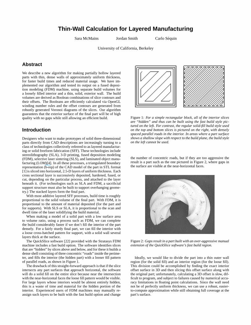
The QuickSlice software [22] provided with the Stratasys FDMmachine includes a fast build option. The software identifies slicesthat are “hidden” by slices above and below, and for these it builds adense shell consisting of three concentric “roads” inside the perime-ter, and fills the interior (the hidden part) with a looser fill patternof parallel roads, as shown in Figure 1.
The drawback of this straight-forward approach is that if the sliceintersects any part surfaces that approach horizontal, the softwarewill do a solid fill on the entire slice because near the intersectionwith the near-horizontal faces the loose fill pattern would be visible.For large layers whose interiors would be almost entirely hidden,this is a waste of time and material for the hidden portion of theinterior. Experienced users of FDM machines may manually re-assign such layers to be built with the fast build option and change
Figure 1: For a simple rectangular block, all of the interior slicesare “hidden” and thus can be built using the fast build style pic-tured on the left. For contrast, the regular solid-fill build style usedon the top and bottom slices is pictured on the right, with denselyspaced parallel roads in the interior. In areas where a part surfaceshows a shallow slope with respect to the build plane, the build styleon the left cannot be used.
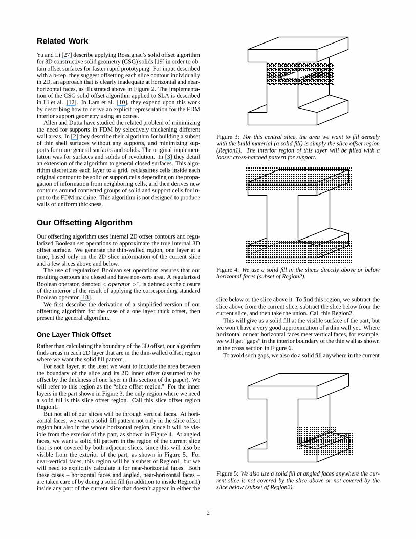
the number of concentric roads, but if they are too aggressive theresult is a part such as the one pictured in Figure 2, where gaps inthe surface are visible at the near-horizontal faces.
��������������������������������������������������������������������������������������������������������������������������������������������������������������������������������������������������������������������������������������������������������������������������������������������������������������������������������������������������������������������������������������������������������������������������������������������������������������������������������������������������������������������
Figure 2: Gaps result in a part built with an over-aggressive manualextension of the QuickSlice software’s fast build region.
Ideally, we would like to divide the part into a thin outer wallregion (for the solid fill) and an interior region (for the loose fill).This division could be accomplished by finding the exact interioroffset surface in 3D and then slicing this offset surface along withthe original part; unfortunately, calculating a 3D offset is slow, dif-ficult to program, and subject to failures caused by numerical accu-racy limitations in floating point calculations. Since the wall neednot be of perfectly uniform thickness, we can use a robust, easier-to-compute approximation while still obtaining full coverage at thepart’s surface.
Related Work
Yu and Li [27] describe applying Rossignac’s solid offset algorithmfor 3D constructive solid geometry (CSG) solids [19] in order to ob-tain offset surfaces for faster rapid prototyping. For input describedwith a b-rep, they suggest offsetting each slice contour individuallyin 2D, an approach that is clearly inadequate at horizontal and near-horizontal faces, as illustrated above in Figure 2. The implementa-tion of the CSG solid offset algorithm applied to SLA is describedin Li et al. [12]. In Lam et al. [10], they expand upon this workby describing how to derive an explicit representation for the FDMinterior support geometry using an octree.
Allen and Dutta have studied the related problem of minimizingthe need for supports in FDM by selectively thickening differentwall areas. In [2] they describe their algorithm for building a subsetof thin shell surfaces without any supports, and minimizing sup-ports for more general surfaces and solids. The original implemen-tation was for surfaces and solids of revolution. In [3] they detailan extension of the algorithm to general closed surfaces. This algo-rithm discretizes each layer to a grid, reclassifies cells inside eachoriginal contour to be solid or support cells depending on the propa-gation of information from neighboring cells, and then derives newcontours around connected groups of solid and support cells for in-put to the FDM machine. This algorithm is not designed to producewalls of uniform thickness.
Our Offsetting Algorithm
Our offsetting algorithm uses internal 2D offset contours and regu-larized Boolean set operations to approximate the true internal 3Doffset surface. We generate the thin-walled region, one layer at atime, based only on the 2D slice information of the current sliceand a few slices above and below.
The use of regularized Boolean set operations ensures that ourresulting contours are closed and have non-zero area. A regularizedBoolean operator, denoted < operator >∗, is defined as the closureof the interior of the result of applying the corresponding standardBoolean operator [18].
We first describe the derivation of a simplified version of ouroffsetting algorithm for the case of a one layer thick offset, thenpresent the general algorithm.
One Layer Thick Offset
Rather than calculating the boundary of the 3D offset, our algorithmfinds areas in each 2D layer that are in the thin-walled offset regionwhere we want the solid fill pattern.
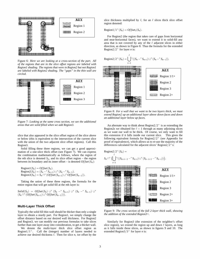
For each layer, at the least we want to include the area betweenthe boundary of the slice and its 2D inner offset (assumed to beoffset by the thickness of one layer in this section of the paper). Wewill refer to this region as the “slice offset region.” For the innerlayers in the part shown in Figure 3, the only region where we needa solid fill is this slice offset region. Call this slice offset regionRegion1.
But not all of our slices will be through vertical faces. At hori-zontal faces, we want a solid fill pattern not only in the slice offsetregion but also in the whole horizontal region, since it will be vis-ible from the exterior of the part, as shown in Figure 4. At angledfaces, we want a solid fill pattern in the region of the current slicethat is not covered by both adjacent slices, since this will also bevisible from the exterior of the part, as shown in Figure 5. Fornear-vertical faces, this region will be a subset of Region1, but wewill need to explicitly calculate it for near-horizontal faces. Boththese cases – horizontal faces and angled, near-horizontal faces –are taken care of by doing a solid fill (in addition to inside Region1)inside any part of the current slice that doesn’t appear in either the
��������������������������������������������������������������������������������������������
��������������������������������������������������������������������������������������������
��������������������������������������������������������������������������������������������
Figure 3: For this central slice, the area we want to fill denselywith the build material (a solid fill) is simply the slice offset region(Region1). The interior region of this layer will be filled with alooser cross-hatched pattern for support.
����������������������������������������������������������������������������������������������������������������������������������������������������
����������������������������������������������������������������������������������������������������������������������������������������������������
����������������������������������������������������������������������������������������������������������������������������������������������������
Figure 4: We use a solid fill in the slices directly above or belowhorizontal faces (subset of Region2).
slice below or the slice above it. To find this region, we subtract theslice above from the current slice, subtract the slice below from thecurrent slice, and then take the union. Call this Region2.
This will give us a solid fill at the visible surface of the part, butwe won’t have a very good approximation of a thin wall yet. Wherehorizontal or near horizontal faces meet vertical faces, for example,we will get “gaps” in the interior boundary of the thin wall as shownin the cross section in Figure 6.
To avoid such gaps, we also do a solid fill anywhere in the current
���������������������������������������
����������������������������������������������������
���������������������������������������������������
��������������������������������������������������������������������
Figure 5: We also use a solid fill at angled faces anywhere the cur-rent slice is not covered by the slice above or not covered by theslice below (subset of Region2).
2
��� ��������
��
���� ��
�����������
���������
��������
���������������������������������������
������������������������������������������������������
������������������������������������������������������ ��
���
������������ ��������������������������������
KEY
Region 1
Region 2���������������
Figure 6: Here we are looking at a cross-section of the part. Allof the regions that are in the slice offset regions are labeled withRegion1 shading. The regions that were in Region2 but not Region1are labeled with Region2 shading. The “gaps” in the thin wall arecircled.
��
������������
��� ��������������� ������
��������� �
����
�� �
������������������������������
�����������������
����������������� ���
���������������
��������������������������������
����������
�����������������������
��������
��
�� KEY
Region 1
Region 2
Region 3
����������
�����
����������
Figure 7: Looking at the same cross section, we see the additionalareas that are solid filled when we add Region3.
slice that also appeared in the slice offset region of the slice aboveor below (this is equivalent to the intersection of the current slicewith the union of the two adjacent slice offset regions). Call thisRegion3.
Solid filling these three regions, we can get a good approxi-mation of a one-slice thick offset (see Figure 7). We can expressthe combination mathematically as follows, where the region ofthe nth slice is denoted Sn, and its slice offset region – the regionbetween its boundary and its inner offset – is denoted Of fset(Sn):
Region1(Sn) = Of fset(Sn).Region2(Sn) = (Sn−
∗ Sn+1)∪∗ (Sn−
∗ Sn−1).Region3(Sn) = Sn ∩
∗ (Of fset(Sn+1)∪∗ Of fset(Sn−1)).
Taking the union of these three regions, the formula for theentire region that will get solid fill at the nth layer is:
Solid(Sn) = Of fset(Sn) ∪∗ (Sn −
∗ Sn+1) ∪∗ (Sn −
∗ Sn−1) ∪∗
(Sn ∩∗ (Of fset(Sn+1)∪
∗ Of fset(Sn−1))).
Multi-Layer Thick Offset
Typically the solid fill thin wall should be thicker than only a singlelayer to obtain a sturdy part. For Region1, we simply change theoffset distance based on our desired wall thickness. For Region2and Region3, we can modify our previous formulas to take slicesfurther than one layer away into consideration, to get a thicker wall.
We denote the multi-layer thick slice offset region asRegion1/1+ . Call the (integer) number of layers needed toachieve our desired thickness `. Then for slice n, we offset by the
slice thickness multiplied by `, for an ` slices thick slice offsetregion denoted:
Region1/1+(Sn) = Of fset`(Sn).
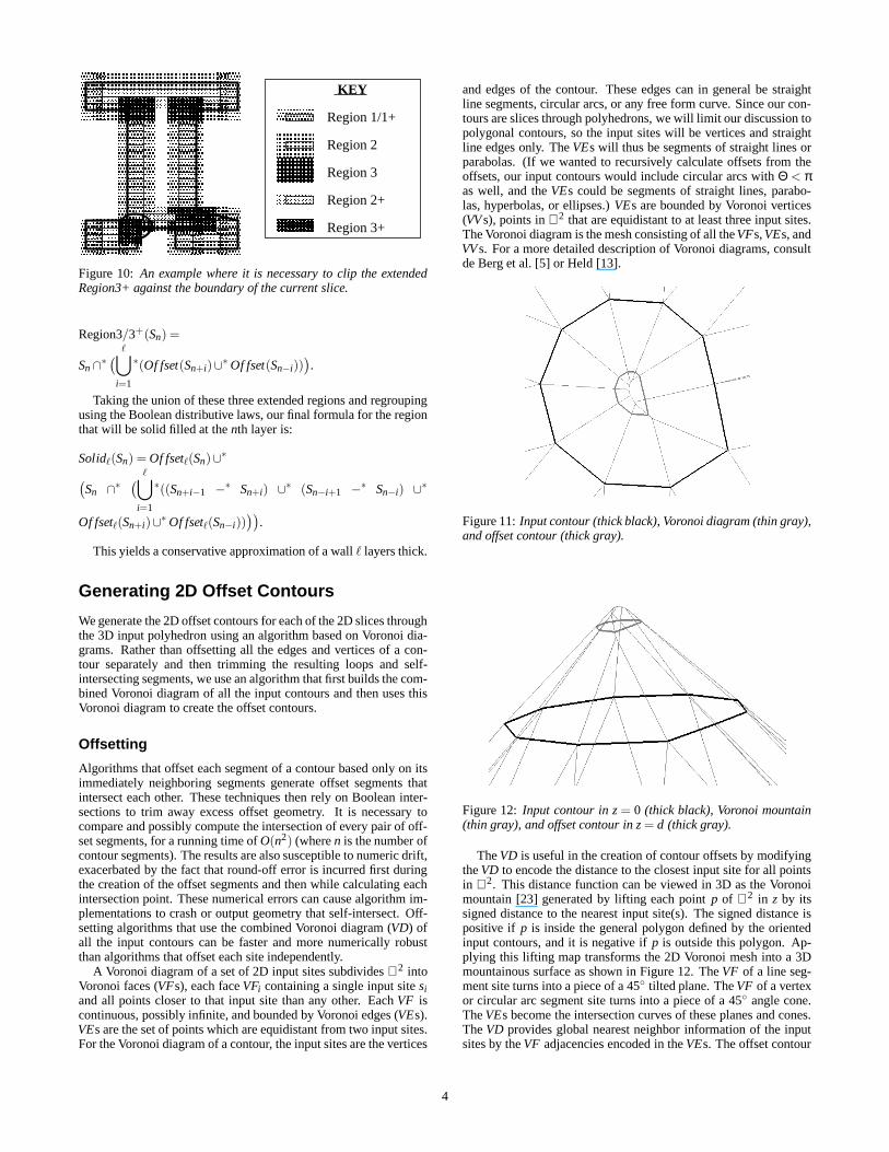
For Region2 (the region that takes care of gaps from horizontaland near-horizontal faces), we want to extend it to solid-fill anyarea that is not covered by any of the ` adjacent slices in eitherdirection, as shown in Figure 8. Thus the formula for the extendedRegion2/2+ for layer n is:
Region2/2+(Sn) =⋃
i=1
∗((Sn−∗ Sn+i)∪
∗ (Sn−∗ Sn−i)).
�������������������
�����������������������������
������������������������������
������������������
������������������
���������������������������������������������������
������������������������������
������������������������������
������������������������������������������
����������
��������������������
����
��
�����
����
�� �
����������
������������������
������
������
��� ���������
KEY
Region 1/1+
Region 2
Region 3
Region 2+
����
����������
�����
��
Figure 8: For a wall that we want to be two layers thick, we mustextend Region2 up an additional layer above down faces and downan additional layer below up faces.
An alternate way to think about Region2/2+ is as extending theRegion2s we obtained for ` = 1 through as many adjoining slicesas we want our wall to be thick. Of course, we only want to fillthis extension if it falls inside our current slice. This gives thefollowing equivalent formula for Region2/2+ (see Appendix forproof of equivalence), which allows us to re-use the majority of thedifferences calculated for the adjacent slices’ Region2/2+s:
Region2/2+(Sn) =
Sn ∩∗(
⋃
i=1
∗((Sn+i−1−∗ Sn+i)∪
∗ (Sn−i+1 −∗ Sn−i))
)
.
������ � � � � � � � � � � � � � � � � � � � � ������������
������������������
������������������������������
������������������������������
�������������������������������������������������������������������������������������
������������������
������������������
����������������������������������������������������������������������
������
� � � � � � � � � � � � � � � � � � � � � �
� � � �
� � � �
� �
���������������
����� �����
������������������������
������������������������������������������
����������
����������
����� �������������
����� �����
���������� ��������
���
KEY
Region 1/1+
Region 2
Region 3
Region 2+
Region 3+
� � � �
����������
�����
����������
Figure 9: The cross section of the full 2-layer thick wall, showingthe addition of the extended Region3+.
Similarly for Region3 (the extension of the neighbor’s offsetslice region), we extend the region up and down ` layers, as longas it falls inside these slices, as shown in figures 9 and 10. Theextended Region3/3+ for layer n is:
3
������������������������������������������������������������
������������������
������������������������������
������������������������������
�������������������������������������������������������������������������������������
������������������
���������
���������
����������������������������������������������������������������������
������
���������������
����������
����������
�����������
����������
����� �����
��������
������������������������������������������
����������
����������
�������������
����� �����
�����������
KEY
Region 1/1+
Region 2
Region 3
Region 2+
Region 3+
����������
����������
�����
�����
�����
���������
���������������
�����������������������������������������������
����������������� �����
�����
Figure 10: An example where it is necessary to clip the extendedRegion3+ against the boundary of the current slice.
Region3/3+(Sn) =
Sn ∩∗(
⋃
i=1
∗(Of fset(Sn+i)∪∗ Of fset(Sn−i))
)
.
Taking the union of these three extended regions and regroupingusing the Boolean distributive laws, our final formula for the regionthat will be solid filled at the nth layer is:
Solid`(Sn) = Of fset`(Sn)∪∗
(
Sn ∩∗
(
⋃
i=1
∗((Sn+i−1 −∗ Sn+i) ∪
∗ (Sn−i+1 −∗ Sn−i) ∪
∗
Of fset`(Sn+i)∪∗ Of fset`(Sn−i))
))
.
This yields a conservative approximation of a wall ` layers thick.
Generating 2D Offset Contours
We generate the 2D offset contours for each of the 2D slices throughthe 3D input polyhedron using an algorithm based on Voronoi dia-grams. Rather than offsetting all the edges and vertices of a con-tour separately and then trimming the resulting loops and self-intersecting segments, we use an algorithm that first builds the com-bined Voronoi diagram of all the input contours and then uses thisVoronoi diagram to create the offset contours.
Offsetting
Algorithms that offset each segment of a contour based only on itsimmediately neighboring segments generate offset segments thatintersect each other. These techniques then rely on Boolean inter-sections to trim away excess offset geometry. It is necessary tocompare and possibly compute the intersection of every pair of off-set segments, for a running time of O(n2) (where n is the number ofcontour segments). The results are also susceptible to numeric drift,exacerbated by the fact that round-off error is incurred first duringthe creation of the offset segments and then while calculating eachintersection point. These numerical errors can cause algorithm im-plementations to crash or output geometry that self-intersect. Off-setting algorithms that use the combined Voronoi diagram (VD) ofall the input contours can be faster and more numerically robustthan algorithms that offset each site independently.
A Voronoi diagram of a set of 2D input sites subdivides ℜ2 intoVoronoi faces (VFs), each face VFi containing a single input site siand all points closer to that input site than any other. Each VF iscontinuous, possibly infinite, and bounded by Voronoi edges (VEs).VEs are the set of points which are equidistant from two input sites.For the Voronoi diagram of a contour, the input sites are the vertices
and edges of the contour. These edges can in general be straightline segments, circular arcs, or any free form curve. Since our con-tours are slices through polyhedrons, we will limit our discussion topolygonal contours, so the input sites will be vertices and straightline edges only. The VEs will thus be segments of straight lines orparabolas. (If we wanted to recursively calculate offsets from theoffsets, our input contours would include circular arcs with Θ < πas well, and the VEs could be segments of straight lines, parabo-las, hyperbolas, or ellipses.) VEs are bounded by Voronoi vertices(VV s), points in ℜ2 that are equidistant to at least three input sites.The Voronoi diagram is the mesh consisting of all the VFs, VEs, andVV s. For a more detailed description of Voronoi diagrams, consultde Berg et al. [5] or Held [13].
��������������������������������������������������������������������������������������������������������������������������������������������������������������������������������������������������������������������������������������������������������������������������������������������������������������������������������������������������������������������������������������������������������������������������������������������������������������������������������������������������������������������
Figure 11: Input contour (thick black), Voronoi diagram (thin gray),and offset contour (thick gray).
��������������������������������������������������������������������������������������������������������������������������������������������������������������������������������������������������������������������������������������������������������������������������������������������������������������������������������������������������������������������������������������������������������������������������������������������������������������������������������������������������������������������
Figure 12: Input contour in z = 0 (thick black), Voronoi mountain(thin gray), and offset contour in z = d (thick gray).
The VD is useful in the creation of contour offsets by modifyingthe VD to encode the distance to the closest input site for all pointsin ℜ2. This distance function can be viewed in 3D as the Voronoimountain [23] generated by lifting each point p of ℜ2 in z by itssigned distance to the nearest input site(s). The signed distance ispositive if p is inside the general polygon defined by the orientedinput contours, and it is negative if p is outside this polygon. Ap-plying this lifting map transforms the 2D Voronoi mesh into a 3Dmountainous surface as shown in Figure 12. The VF of a line seg-ment site turns into a piece of a 45◦ tilted plane. The VF of a vertexor circular arc segment site turns into a piece of a 45◦ angle cone.The VEs become the intersection curves of these planes and cones.The VD provides global nearest neighbor information of the inputsites by the VF adjacencies encoded in the VEs. The offset contour
4
may step directly between VFs of input sites that were not consecu-tive sites in the input contour. An example is illustrated in the lowerright corner of the offset contour in Figure 11. This nearest neigh-bor information eliminates the extraneous pairwise comparisons ofsites found in the brute force Boolean approach to offsetting. Cre-ating the Voronoi diagram of the input contours takes only timeO(n logn), because the creation of the VD can be reduced to sort-ing. Generating offset contours once the Voronoi diagram is createdtakes O(n) time, so total running time including the creation of theVoronoi diagram is O(n log n).
Kim [8] describes an O(n) algorithm for constructing an offsetcontour of a simple input polygon using the Voronoi diagram ofthe polygon and two stacks to manage the creation of disjoint con-tour loops in the offset contour. The algorithm proceeds by walkingaround the input contour, creating offset segments when they ex-ist, and jumps to create new contour loops when discontinuities areencountered. This only works for a single simple input contour.
A more general approach to creating the offset contours is toslice the Voronoi mountain by a plane z = d where d is the signedoffset distance: d > 0 offsets the polygon inward, d = 0 is the set ofinput contours, and d < 0 offsets the polygon outward. The offsetcontours at a distance d are equivalent to the slice contours createdby slicing the Voronoi mountain with the plane z = d and then pro-jecting back into the z = 0 plane.
Voronoi Diagrams
Several algorithms have been developed for calculating the Voronoidiagram of a contour, many based on a divide and conquer ap-proach. These algorithms are based on Shamos and Hoey’s divideand conquer algorithm for creating the Voronoi diagram of a set ofvertices in ℜ2 [20]. Their algorithm divides the input vertices intotwo half sets VL and VR based on their geometric position, recur-sively creates the VDL and VDR of those two sets respectively, andthen merges VDL and VDR to create the VD of the whole set. Thekey operation in the algorithm is the O(n) merge step. The mergebuilds the bisector polyline that separates the sites of VL and VR,and it prunes away the defunct geometry from the VDL and VDR.The key insight in the merge step is that all portions of VDL thatlie to the right of the bisector polyline will not be in the final VD,and vice versa. Others ([11] and [6]) describe algorithms that dothe same work in creating the Delaunay triangulation of a set ofvertices, the planar dual of the Voronoi diagram of a set of vertices.
Held [13] and Kim et al. [9] describe algorithms that createthe VD of an input polygon with straight lines and circular arcsas edges. These algorithms are both generalizations of the Voronoidiagram for point sets. Instead of dividing the input sites by geo-metric position, these algorithms divide the contour into two halvesbased on the topological counterclockwise ordering around the in-put contour. Both algorithms limit themselves to creating the VDof the inside of the contour only. Both algorithms create the bi-sector polyline during the merge step by creating representations ofthe VEs between the VFs and then intersecting the VEs. The majordifference between the two approaches is the representation of thefunctions for the VEs. Held uses an implicit form parameterized bythe distance to the input contour. Kim et al. use rational quadraticBezier segments to represent the conic curves for the VEs. Held’sapproach gives a parameterization that is very intuitive, but it doesnot always have unique points for a parameter value. Kim et al.create VEs with monotonic parameterizations, so when offsettingthe parameterization yields at most one unique point. Kim et al.are able to simplify coding to a single operation, the intersection ofa rational Bezier with a rational Bezier, but this may come at theexpense of some numerical accuracy. Held’s algorithm has manymore intersection cases, but it is possible for it to generate highernumeric accuracy. Held specifically mentions the handling of a sin-
gle general outer contour with convex inner contours. It is not clearwhether the algorithm can be extended to handle island contoursof arbitrary shapes. These divide and conquer algorithms are worstcase optimal with O(n log n).
Our Offset Implementation
When creating polygon offsets for SFF, it is necessary to handlecontours made up of arbitrary straight line segments with arbitraryisland contours. The 2D contours are created by slicing 3D polyhe-dral approximations of free form shapes. The primitives are alwayslinear, but the configurations can be very general and may be higherin complexity than examples normally experienced in NC pocketmachining. Our approach is to create the Voronoi diagram of thesecontours, and then create the offset contours by conceptually slicingthe Voronoi mountain.
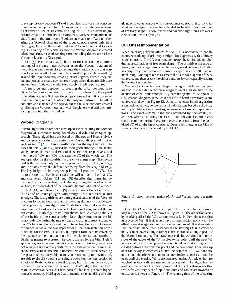
We construct the Voronoi diagram using a divide and conquermethod that builds the Voronoi diagram on the inside and on theoutside of each input contour. By computing the inside and out-side Voronoi diagram, it makes it possible to handle arbitrary islandcontours as shown in Figure 13. A major concern in this algorithmis numeric accuracy, so we make all calculations based on the orig-inal input data without creating intermediate bisector representa-tions. The exact arithmetic methods presented by Shewchuk [21]are used when calculating the VV s. The individual contour VDscan be combined using the same merge operation to form the com-bined VD of all the input contours. Details for merging the VDs ofisland contours are discussed by Held [13].
��������������������������������������������������������������������������������������������������������������������������������������������������������������������������������������������������������������������������������������������������������������������������������������������������������������������������������������������������������������������������������������������������������������������������������������������������������������������������������������������������������������������
Figure 13: Input contour (thick black) and Voronoi diagram (thingray).
Once the VD is created, we compute the offset contours by walk-ing the edges of the VD as shown in Figure 14. The algorithm startsby marking all of the VEs as unprocessed. It then picks the firstunprocessed VE. If it does not have an intersection point with theoffset plane it is ignored and marked as processed. If it does inter-sect the offset plane, then it becomes the starting VE in a crawl ofthe VD to recover a single offset contour around a single peak ofthe Voronoi mountain. The crawl proceeds by walking the interiorsides of the edges of the VF in clockwise order until the next VEintersected by the offset plane is encountered. A contour segment iscreated between the previous point and the new point. Then we stepover the newly intersected VE into the adjacent VF . We continueto trace out the offset contour in counterclockwise order around thepeak until the starting VE is encountered again. All edges that aretouched in this walk are marked as processed. The algorithm re-peats until all edges have been processed. This offsetting algorithmworks for arbitrary sets of input contours and can offset inwards oroutwards as shown in Figure 14. The running time of the offsetting
5
algorithm only is O(n) because it touches each of the O(n) edgesof the Voronoi diagram a constant number of times.
��������������������������������������������������������������������������������������������������������������������������������������������������������������������������������������������������������������������������������������������������������������������������������������������������������������������������������������������������������������������������������������������������������������������������������������������������������������������������������������������������������������������
Figure 14: Input contour (thick black), Voronoi diagram (thin gray),and one inner and two outer offset contours (thick gray).
Thin Wall Implementation
Our algorithm takes a tessellated b-rep as input, either in STL [1]or in SIF, our Solid Interchange Format [16, 14]. We use our slicingsoftware described in [15] to slice the input, exploiting geometricand topological inter-slice coherence to efficiently calculate sliceswith explicit nesting of their oriented contours. We output the slicesin our neutral layer format, L-SIF (Layered Solid Interchange For-mat) [24]. For SIF input files that contained Booleans, the L-SIFformat describes each layer as a Boolean combination of closed,oriented contours. In the latter case, we use OpenGL to evaluate any2D Booleans (for details on using OpenGL for efficient Booleanevaluation, see [26]; see [25] for a description of our implementa-tion). Even if the input didn’t contain any explicit Booleans, wealso process the output with OpenGL to perform “unary” unions[7] of each slice with itself, in order to remove any artifacts fromself-intersections in the original files [17]. Next each slice is offsetin 2D, using the algorithm described above.
The slices and their offsets are taken as input to the thin-wallgeneration program. For evaluating the Boolean expressions in theformula for the solid-filled region, it also uses OpenGL. For moreefficient calculations, we store the intermediate results (the differ-ences between adjacent slices, and subsets of the summations ofunions) for reuse in neighboring slice calculations. The loose-filledregion is found by subtracting this result from the original slice.We output the resulting oriented, nested contours for each slice,specifying whether each contour is to be loose-filled or solid-filled,in the SSL slice format used by QuickSlice[22]. We then rely onQuickSlice to calculate where external supports for overhangs areneeded and to compute the actual roads, using the fill styles as spec-ified in our SSL file.
Results
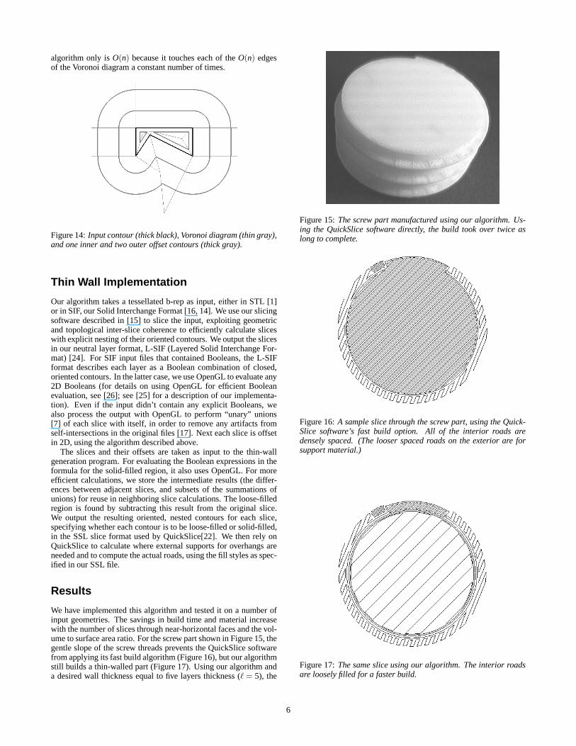
We have implemented this algorithm and tested it on a number ofinput geometries. The savings in build time and material increasewith the number of slices through near-horizontal faces and the vol-ume to surface area ratio. For the screw part shown in Figure 15, thegentle slope of the screw threads prevents the QuickSlice softwarefrom applying its fast build algorithm (Figure 16), but our algorithmstill builds a thin-walled part (Figure 17). Using our algorithm anda desired wall thickness equal to five layers thickness (` = 5), the
��������������������������������������������������������������������������������������������������������������������������������������������������������������������������������������������������������������������������������������������������������������������������������������������������������������������������������������������������������������������������������������������������������������������������������������������������������������������������������������������������������������������
Figure 15: The screw part manufactured using our algorithm. Us-ing the QuickSlice software directly, the build took over twice aslong to complete.
Figure 16: A sample slice through the screw part, using the Quick-Slice software’s fast build option. All of the interior roads aredensely spaced. (The looser spaced roads on the exterior are forsupport material.)
Figure 17: The same slice using our algorithm. The interior roadsare loosely filled for a faster build.
6
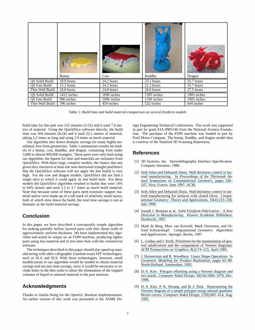
Bunny Cow Buddha DragonQS Solid Build 18.8 hours 24.2 hours 23.1 hours 35.7 hoursQS Fast Build 15.2 hours 24.2 hours 21.2 hours 35.7 hoursThin Wall Build 10.8 hours 14.8 hours 18.6 hours 27.5 hoursQS Solid Build 1412 inches 1696 inches 1395 inches 1905 inchesQS Fast Build 996 inches 1696 inches 1190 inches 1905 inchesThin Wall Build 396 inches 459 inches 532 inches 644 inches
Table 1: Build time and build material comparison on several freeform models
build time for this part was 232 minutes (3:52) and it used 7.6 me-ters of material. Using the QuickSlice software directly, the buildtime was 504 minutes (8:24) and it used 22.1 meters of material,taking 2.2 times as long and using 2.9 times as much material.
Our algorithm also shows dramatic savings for many highly tes-sellated, free-form geometries. Table 1 summarizes results for mod-els of a bunny, cow, Buddha, and dragon, containing from under3,000 to almost 900,000 triangles. These parts were only built usingour algorithm; the figures for time and materials are estimates fromQuickSlice. With these large, complex models, the chance that anygiven slice intersects at least one near-horizontal triangle (and hencethat the QuickSlice software will not apply the fast build) is veryhigh. For the cow and dragon models, QuickSlice did not find asingle slice to which it could apply its fast build style. For thesemodels the QuickSlice algorithm resulted in builds that were 14%to 64% slower and used 2.2 to 3.7 times as much build material.Note that because some of these parts need extensive support ma-terial and/or were made up of a tall stack of relatively small layers,both of which slow down the build, the total time savings is not asdramatic as the build material savings.
Conclusion
In this paper, we have described a conceptually simple algorithmfor making partially hollow layered parts with thin, dense walls ofapproximately uniform thickness. We have implemented this algo-rithm and tested its output on an FDM machine, producing lighterparts using less material and in less time than with the commercialsoftware.
The techniques described in this paper should also speed up man-ufacturing with other calligraphic (random-scan) SFF technologies,such as SLA and SLS. With those technologies, however, smallmodifications to our algorithm would be needed to obtain materialsavings and not just time savings, since it would be necessary to in-clude holes in the thin walls to allow the elimination of the trappedvolumes of liquid or unfused material in the part interiors.
Acknowledgments
Thanks to Jianlin Wang for the OpenGL Boolean implementation.An earlier version of this work was presented at the ASME De-
sign Engineering Technical Conferences. This work was supportedin part by grant EIA-9905140 from the National Science Founda-tion. The purchase of the FDM machine was funded in part byFord Motor Company. The bunny, Buddha, and dragon model datais courtesy of the Stanford 3D Scanning Repository.
References
[1] 3D Systems, Inc. Stereolithography Interface Specification.Company literature, 1988.
[2] Seth Allen and Debasish Dutta. Wall thickness control in lay-ered manufacturing. In Proceedings of the Thirteenth An-nual Symposium on Computational Geometry, pages 240–247, Nice, France, June 1997. ACM.
[3] Seth Allen and Debasish Dutta. Wall thickness control in lay-ered manufacturing for surfaces with closed slices. Compu-tational Geometry: Theory and Applications, 10(4):223–238,July 1998.
[4] Joseph J. Beaman et al. Solid Freeform Fabrication : A NewDirection in Manufacturing. Kluwer Academic Publishers,Dordrecht, 1997.
[5] Mark de Berg, Marc van Kreveld, Mark Overmars, and Ot-fried Schwarzkopf. Computational Geometry: Algorithmsand Applications. Springer, Berlin, 1997.
[6] L. Guibas and J. Stolfi. Primitives for the manipulation of gen-eral subdivisions and the computation of Voronoi diagrams.ACM Transactions on Graphics, 4(2):74–123, April 1985.
[7] J. Heisserman and R. Woodbury. Unary Shape Operations. InGeometric Modeling for Product Realization, pages 63–80.North-Holland, Amsterdam, 1992.
[8] D.-S. Kim. Polygon offsetting using a Voronoi diagram andtwo stacks. Computer Aided Design, 30(14):1069–1076, Dec.1998.
[9] D.-S. Kim, P. K. Hwang, and B.-J. Park. Representing theVoronoi diagram of a simple polygon using rational quadraticBezier curves. Computer Aided Design, 27(8):605–614, Aug.1995.
7
[10] T. W. Lam, K. M. Yu, K. M. Cheung, and C. L. Li. Octreereinforced thin shell object rapid prototyping by fused depo-sition modelling. International Journal of Advanced Manu-facturing Technology, 14(9):631–636, 1998.
[11] D. T. Lee and B. J. Schachter. Two algorithms for constructinga Delaunay triangulation. International Journal of Computer& Information Sciences, 9(3):219–242, June 1980.
[12] C. L. Li, K. M. Yu, and T. W. Lam. Implementation and eval-uation of thin-shell rapid prototype. Computers in Industry,35(2):185–193, March 1998.
[13] M. Held. On the Computational Geometry of Pocket Milling.Springer, Berlin, lncs edition, 1991.
[14] Sara McMains. The SIF SFF Page.http://www.cs.berkeley.edu/˜ug/sif 2 0/SIF SFF.shtml,1999.
[15] Sara McMains and Carlo Sequin. A Coherent Sweep PlaneSlicer for Layered Manufacturing. In Fifth Symposium onSolid Modeling and Applications, pages 285–295, Ann Arbor,MI, June 1999. ACM.
[16] Sara McMains, Carlo Sequin, and Jordan Smith. SIF: A SolidInterchange Format for Rapid Prototyping. In Proceedings ofthe 31st CIRP International Seminar on Manufacturing Sys-tems, pages 40–45. CIRP, May 1998.
[17] Sara McMains, Jordan Smith, and Carlo Sequin. The Evo-lution of a Layered Manufacturing Interchange Format. InASME Design Engineering Technical Conferences 2002, 28thDesign Automation Conference, pages DETC2002/DAC–34136, Montreal, September 2002. ASME.
[18] A. A. G. Requicha. Representations for Rigid Solids: Theory,Methods, and Systems. ACM Computing Surveys, pages 437–464, December 1980.
[19] J. R. Rossignac. Blending and Offsetting Solid Models. PhDthesis, University of Rochester, 1985.
[20] M. I. Shamos and D. Hoey. Closest Point Problems. Proceed-ings 16th Annual IEEE Symposium on Foundation of Com-puter Science, Oct. 1975.
[21] J. R. Shewchuk. Adaptive Precision Floating-Point Arith-metic and Fast Robust Geometric Predicates. Discrete &Computational Geometry, 18(3):305–363, Oct. 1997.
[22] Stratasys, Inc., Eden Prairie, MN. QuickSlice 6.2, 1999.
[23] D. Veeramani and Y.-S. Gau. Selection of an optimal set ofcutting-tool sizes for 2 1/2 D pocket machining. ComputerAided Design, 29(12):869–877, Dec. 1997.
[24] Jianlin Wang. L-SIF Version 1.0.http://www.cs.berkeley.edu/˜ug/LSIF/LSIF.html, 1999.
[25] Jianlin Wang. Layer-based boolean operation for solid free-form fabrication. Master’s thesis, University of California,Berkeley, 2001.
[26] Mason Woo, Jackie Neider, Tom Davis, and Dave Shreiner.OpenGL(R) Programming Guide: The Official Guide toLearning OpenGL, Version 1.2. Addison-Wesley, Reading,Massachusetts, third edition, 1999.
[27] K. M. Yu and C. L. Li. Speeding up rapid prototyping by off-set. Proceedings of the Institution of Mechanical Engineers,Part B, 209(B1):1–8, 1995.
8
Related Documents