Thickness distribution of a cooling pyroclastic flow deposit on

www.elsevier.com/locate/jvolgeores

Journal of Volcanology and Geotherm

Thickness distribution of a cooling pyroclastic flow deposit on

Augustine Volcano, Alaska: Optimization using InSAR,

FEMs, and an adaptive mesh algorithm

Timothy Masterlark a,*, Zhong Lu b, Russell Rykhus b

a Department of Geological Sciences, University of Alabama, Tuscaloosa, AL 35487, United Statesb USGS National Center for EROS, SAIC, Sioux Falls, SD 57198, United States

Received 20 May 2004; received in revised form 9 September 2004

Available online 21 September 2005

Abstract

Interferometric synthetic aperture radar (InSAR) imagery documents the consistent subsidence, during the interval 1992–

1999, of a pyroclastic flow deposit (PFD) emplaced during the 1986 eruption of Augustine Volcano, Alaska. We construct finite

element models (FEMs) that simulate thermoelastic contraction of the PFD to account for the observed subsidence. Three-

dimensional problem domains of the FEMs include a thermoelastic PFD embedded in an elastic substrate. The thickness of the

PFD is initially determined from the difference between post- and pre-eruption digital elevation models (DEMs). The initial

excess temperature of the PFD at the time of deposition, 640 8C, is estimated from FEM predictions and an InSAR image via

standard least-squares inverse methods. Although the FEM predicts the major features of the observed transient deformation,

systematic prediction errors (RMSE=2.2 cm) are most likely associated with errors in the a priori PFD thickness distribution

estimated from the DEM differences. We combine an InSAR image, FEMs, and an adaptive mesh algorithm to iteratively

optimize the geometry of the PFD with respect to a minimized misfit between the predicted thermoelastic deformation and

observed deformation. Prediction errors from an FEM, which includes an optimized PFD geometry and the initial excess PFD

temperature estimated from the least-squares analysis, are sub-millimeter (RMSE=0.3 mm). The average thickness (9.3 m),

maximum thickness (126 m), and volume (2.1�107 m3) of the PFD, estimated using the adaptive mesh algorithm, are about

twice as large as the respective estimations for the a priori PFD geometry. Sensitivity analyses suggest unrealistic PFD thickness

distributions are required for initial excess PFD temperatures outside of the range 500–800 8C.D 2005 Elsevier B.V. All rights reserved.

Keywords: finite element analysis; interferometry; deformation; thermoelastic properties; volcano

1. Introduction

0377-0273/$ - see front matter D 2005 Elsevier B.V. All rights reserved.

doi:10.1016/j.jvolgeores.2005.07.004

* Corresponding author. Tel.: +1 205 348 5095.

E-mail address: [email protected] (T. Masterlark).

Interferometric synthetic aperture radar (InSAR)

imagery can map incremental deformation that

occurs during a time interval. Analyses of InSAR

al Research 150 (2006) 186–201

b

distance, km

0 5

N

-160o

-152 o

Anchorage

A l a s k a

56o

58o

Cook Inlet

Augustinevolcano

Bering Sea

Gulf ofAlaska

a

200

400

600

1986 PFD

extent of

Aleutia

n Arc

West Island

Augustinevolcano

N

Fig. 1. Study site. (a) Location. Augustine Volcano is an island

located in the southwest part of Cook Inlet, Alaska. (b) Shaded

relief image of Augustine Volcano. The shaded relief image is

constructed from a post-1986 eruption digital elevation model

The terrestrial area of the volcano, including West Island, is 92

km2. The 200 m contour intervals reveal the overall symmetry of the

volcano. The asymmetric regions along the coastal margin are due

to episodic debris avalanches (Beget and Kienle, 1992). The white

dots outline the assumed spatial extent of the 1986 PFD. The sta

near the upper left corner of the PFD marks the location of wave cu

exposures and the embedded aluminum float used for in situ tem

perature and density experiments (Beget and Limke, 1989).

T. Masterlark et al. / Journal of Volcanology and Geothermal Research 150 (2006) 186–201 187

imagery have documented deformation associated

with a wide variety of geomechanical phenomena,

such as glacier movements (Stenoien and Bentley,

2000), coseismic slip (Massonnet et al., 1993), post-

seismic relaxation (Pollitz et al., 2001), poroelastic

rebound (Peltzer et al., 1996), cooling lava (Stevens

et al., 2001), and magma intrusion (Masterlark and

Lu, 2004). InSAR imagery has been especially use-

ful for studying volcanoes that are restless but

poorly instrumented because of their remote loca-

tions (Lu et al., 2003b). Volcano deformation attrib-

uted to magmatic unrest is often a precursor for

eruptive activity (Lipman et al., 1981; Lu et al.,

2003a). Combinations of InSAR imagery and nu-

merical modeling can differentiate between mag-

matic activity and other deformation mechanisms

(Lu et al., 2002; Masterlark and Lu, 2004) and

are therefore powerful volcano hazards assessment

tools.

InSAR imagery indicates that the north flank of

Augustine Volcano, Alaska, was actively deforming

during 1992–1999 (Lu et al., 2003b). This region of

deformation corresponds to the spatial extent of the

pyroclastic flow deposit (PFD) emplaced during the

1986 eruption of Augustine Volcano. We attribute

this deformation to post-emplacement behavior of

the PFD. Consistent with other geodetic observa-

tions of the volcano (Pauk et al., 2001), volcano-

wide deformation attributed to possible magmatic

activity is not observed with InSAR images span-

ning 1992–1999.

This study is concerned with quantifying the

post-eruption deformation of the PFD emplaced

during the 1986 eruption of Augustine Volcano.

We construct finite element models (FEMs) that

simulate the post-eruptive thermoelastic contraction

of the initially hot and geometrically complex PFD.

Results of this study indicate that (1) InSAR ima-

gery documents the systematic post-emplacement

subsidence of the PFD; (2) linear thermoelastic

behavior, which simulates the cooling PFD, can

account for the observed deformation; and (3) a

technique combining InSAR imagery, FEMs, and

an adaptive mesh algorithm can optimize the poorly

constrained geometry of the PFD. This optimization

generates a PFD thickness distribution map derived

from remote sensing data and linear thermoelastic

deformation mechanics.

2. Augustine Volcano

Augustine Volcano forms a 92 km2 island in the

southwest end of Cook Inlet, Alaska (Fig. 1). Augus-

tine’s volcanism began in the late Pleistocene and the

volcano is the youngest (Miller et al., 1998) and

most active of the four volcanoes (Spurr, Redoubt,

Iliamna, and Augustine) that form a line roughly

parallel to Cook Inlet. The maximum elevation is

currently about 1250 m above sea level. However,

.

r

t

-

T. Masterlark et al. / Journal of Volcanology and Geothermal Research 150 (2006) 186–201188

the summit elevation and morphology fluctuate sig-

nificantly during eruptions due to a combination of

lava dome growth and explosive removal (Swanson

and Kienle, 1988). The volcano’s structure consists

of a dome and lava flow complex surrounded by an

assembly of ash, lahar, avalanche, and PFD deposits

(Beget and Kienle, 1992; Miller et al., 1998;

Waythomas and Waitt, 1998). The primarily andesitic

composition of Augustine Volcano accounts for the

historically explosive eruption behavior and is com-

parable to rocks of the other Cook Inlet volcanoes

(Miller et al., 1998).

Six documented eruptions occurred in the twen-

tieth century and a similar number of earlier erup-

tions with ages up to two thousand years have been

identified based on carbon dating techniques (Sim-

kin and Siebert, 1994). Hummocky offshore topo-

graphy, revealed by bathymetry data, reveals the

extent of episodic debris flows from the peak of

Augustine Volcano (Beget and Kienle, 1992). Water

depths surrounding Augustine Volcano are limited

to a few tens of meters for offshore distances up to

several kilometers. West Island (Fig. 1) is a terres-

trial expression of a debris avalanche that extends

several kilometers to the northwest of Augustine

Volcano.

Others describe the most recent (1986) eruption

of Augustine Volcano in detail (e.g., Swanson and

Kienle, 1988; Miller et al., 1998; Waythomas and

Waitt, 1998) and a summary of the eruption is

given here. The 1986 eruption had three major

episodes: March 27–April 2, April 23–28, and

August 22–September 1. A seismic swarm began

five weeks prior to the initial eruption episode. An

ash cloud created during the initial eruption epi-

sode (March 27–April 2, 1986) reached an altitude

of 12,000 m. This episode produced substantial

lahar and pyroclastic flows that cover the northern

flank of the volcano. The second eruption episode

(April 23–28, 1986) produced a small lava flow,

pyroclastic flows, and an ash plume that reached

an altitude of 3700 m. The third eruption episode

(August 22–September 1, 1986) produced a small

lava flow, more pyroclastic flows, and a small ash

cloud. This final episode culminated with dome

building.

PFDs generated from the 1986 eruption blanket a

fan-shaped region of the northern flank of Augustine

Volcano (Beget and Limke, 1989). Coverage by the

lithic block and ash flow deposits of the PFD is

narrow near the peak and widens in the down slope

direction. These deposits extend all the way to the

coast to the north–northeast of the Peak. Directly to

the north of the peak, the lithic block and ash deposits

give way to lithic-rich pumice deposits of the PFD,

which extend to the coast. Beget and Limke (1989)

provide constraints on the emplacement density, tem-

perature, and thickness for a region of the PFD near

the coast (Fig. 1b). Based on the submergence of a

spherical aluminum fishing float transported on the

PFD, they estimate the upper limit for the emplace-

ment density of the PFD is 1360 kg m�3. The sub-

merged region of the float is oxidized and discolored.

An in situ field experiment on a portion of the sphe-

rical float above the discolored region suggests the

initial temperature of the PFD from the 1986 eruption

of Augustine Volcano is at least 425 8C. Beget andLimke (1989) also report wave-cut exposures that

suggest the PFD thickness near the northern coast is

1 to 2 m.

3. Data

3.1. InSAR images

We construct eighteen InSAR images from syn-

thetic aperture radar image pairs acquired by ERS-1

and ERS-2 C-band (wavelength=5.66 cm) radar

satellites using the two-pass InSAR method described

by Massonnet and Feigl (1998). These InSAR images

document the surface deformation of Augustine Vol-

cano during 1992–1999 (Fig. 2). Individual images

span a variety of roughly annual intervals during this

seven-year period (Fig. 3). The InSAR data include

five different line-of-sight (LOS) vectors (Table 1)

from both ascending and descending passes and

reveal systematic changes in range, between the

satellites and the land surface, along the north flank

of the volcano. This region corresponds to the spatial

extent of the PFD emplaced during the 1986 eruption

(Fig. 4).

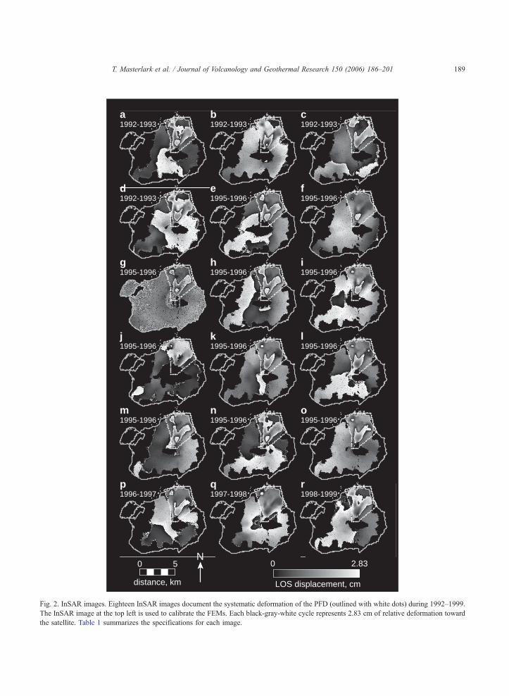
Each InSAR image maps a single, mostly vertical,

component of deformation parallel to the correspond-

ing LOS vector. The systematic and positive changes

in range shown in all images suggest the PFD is

LOS displacement, cm

0 2.83N

distance, km

0 5

a1992-1993

d1992-1993

m1995-1996

p1996-1997

g1995-1996

j1995-1996

b1992-1993

e1995-1996

n1995-1996

q1997-1998

h1995-1996

k1995-1996

c1992-1993

f1995-1996

o1995-1996

r1998-1999

i1995-1996

l1995-1996

Fig. 2. InSAR images. Eighteen InSAR images document the systematic deformation of the PFD (outlined with white dots) during 1992–1999.

The InSAR image at the top left is used to calibrate the FEMs. Each black-gray-white cycle represents 2.83 cm of relative deformation toward

the satellite. Table 1 summarizes the specifications for each image.


1994 1996 199819931992 1995 1997 1999

ab

cd

efghijkl

mno

pq

r

year

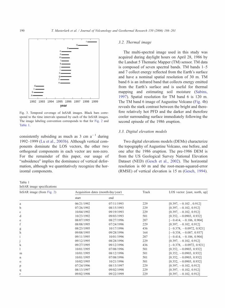
Fig. 3. Temporal coverage of InSAR images. Black bars corre-

spond to the time intervals spanned by each of the InSAR images.

The image labeling convention corresponds to that for Fig. 2 and

Table 1.


consistently subsiding as much as 3 cm a�1 during

1992–1999 (Lu et al., 2003b). Although vertical com-

ponents dominate the LOS vectors, the other two

orthogonal components in each vector are non-zero.

For the remainder of this paper, our usage of

bsubsidenceQ implies the dominance of vertical defor-

mation, although we quantitatively recognize the hor-

izontal components.

Table 1

InSAR image specifications

InSAR image (from Fig. 2) Acquisition dates (month/day/ye

start end

a 06/21/1992 07/11/1

b 07/26/1992 08/15/

c 10/04/1992 09/19/

d 10/23/1992 09/03/

e 08/07/1995 08/27/

f 08/08/1995 07/24/

g 08/23/1995 10/17/

h 09/08/1995 09/28/

i 09/11/1995 10/01/

j 09/12/1995 08/28/

k 09/27/1995 09/12/

l 10/01/1995 07/08/

m 10/01/1995 08/12/

n 10/01/1995 07/08/

o 10/02/1995 10/21/

p 07/24/1996 08/13/

q 08/13/1997 09/02/

r 09/02/1998 09/22/

3.2. Thermal image

The multi-spectral image used in this study was

acquired during daylight hours on April 28, 1986 by

the Landsat 5 Thematic Mapper (TM) sensor. TM data

is composed of seven spectral bands. TM bands 1–5

and 7 collect energy reflected from the Earth’s surface

and have a nominal spatial resolution of 30 m. TM

band 6 is an infrared band that collects energy emitted

from the Earth’s surface and is useful for thermal

mapping and estimating soil moisture (Sabins,

1997). Spatial resolution for TM band 6 is 120 m.

The TM band 6 image of Augustine Volcano (Fig. 4b)

reveals the stark contrast between the bright and there-

fore relatively hot PFD and the darker and therefore

cooler surrounding surface immediately following the

second episode of the 1986 eruption.

3.3. Digital elevation models

Two digital elevations models (DEMs) characterize

the topography of Augustine Volcano, one before, and

one after the 1986 eruption. The pre-1986 DEM is

from the US Geological Survey National Elevation

Dataset (NED) (Gesch et al., 2002). The horizontal

resolution is 60 m and the root-mean-squared-error

(RMSE) of vertical elevation is 15 m (Gesch, 1994).

ar) Track LOS vector: [east, north, up]

993 229 [0.397, �0.102 , 0.912]

1993 229 [0.397, �0.102, 0.912]

1993 229 [0.397, �0.102, 0.912]

1993 501 [0.352, �0.0903, 0.932]

1996 207 [�0.414, �0.106, 0.904]

1996 229 [0.397, �0.102, 0.912]

1996 436 [�0.378, �0.0972, 0.921]

1996 164 [�0.338, �0.087, 0.937]

1996 207 [�0.414, �0.106, 0.904]

1996 229 [0.397, �0.102, 0.912]

1996 436 [�0.378, �0.0972, 0.921]

1996 501 [0.352, �0.0903, 0.932]

1996 501 [0.352, �0.0903, 0.932]

1996 501 [0.352, �0.0903, 0.932]

1996 501 [0.352, �0.0903, 0.932]

1997 229 [0.397, �0.102, 0.912]

1998 229 [0.397, �0.102, 0.912]

1999 229 [0.397, �0.102, 0.912]

PFD

lava

b

c

disp

lace

men

t, cm

0

2.83

a

distance, km

N

0 1 2 3 4 5

+20 m

-20 m

contour intervals

Fig. 4. PFD observations. The white dots outline the assumed limits

for the spatial extent of the 1986 PFD. The coastline is derived from

the post-1986 DEM. (a) InSAR image spanning the post-emplace-

ment interval 1992–1993 (also shown in Fig. 2a). The grayscale bar

on the right identifies the relative displacement toward the satellite,

projected onto the LOS vector. Each black-gray-white cycle repre-

sents 2.83 cm of relative deformation toward the satellite. (b) Land-

sat 5 image, TM band 6 (thermal data). The image reveals the lateral

extent of the relatively hot (white) PFD and newly emplaced lava

with respect to the relatively cold (gray) island. The image acquisi-

tion date is April 28, 1986. (c) DEM difference map. The 20 m

contour intervals represent differences between the post-1986 DEM

and the pre-1986 DEM. Positive and negative thickness contours are

white and gray, respectively.


The maximum elevation of the pre-1986 DEM is 1229

m. The 1 :63,000 Iliamna quadrangle, for which con-

tours were derived from air photos taken in 1957 and

was field annotated in 1958, is the source data of the

NED pre-1986 eruption DEM for Augustine Volcano.

The NED metadata indicate that the contours for the

Iliamna quadrangle were most recently updated in

1977. It is unknown whether the contours were

updated in part, or as a whole. Therefore, the DEM

may portray the topography for multiple dates.

Because of this temporal ambiguity, the pre-1986

eruption DEM may also predate the 1976 eruption.

For the purposes of this study, we assume this DEM

represents the post-1976 topography as suggested by

the NED metadata. The post-1986 DEM is con-

structed entirely from photogrammetric data acquired

after the 1986 eruption. The horizontal posting is 10 m

with a resolution of 15 m and the RMSE of vertical

elevation is less than 15 m (D. Dzurisin, personal

comm., 2002). The maximum elevation of this post-

1986 DEM is 1250 m.

Both DEMs are resampled to 20 m resolution to

match that of the InSAR imagery. The difference

between the two DEMs represents the changes in

elevation associated with the eruption (Fig. 4c).

These changes can be caused by a variety of phenom-

ena, such as volcano-wide deformation due to subsur-

face processes (e.g., Masterlark and Lu, 2004) and

deposition of erupted materials (e.g., Stevens et al.,

2001; Lu et al., 2003c). Based on the differences

between post- and pre-eruption DEMs, the estimated

volume of the PFD is 9.9�106 m3. This estimation

assumes the negative thickness (Fig. 4c) is zero. The

DEM difference image, with its non-physical negative

PFD thickness, presumably indicates the poor quality

of the pre-eruptive DEM and justifies the need for a

relatively accurate estimate of thickness distribution

for the 1986 PDF using the innovative approach

proposed in this paper.

4. Method

4.1. Finite element models

FEMs in this study are constructed with the finite

element code ABAQUS (Hibbet et al., 2003). The

code allows for heterogeneous distributions of mate-

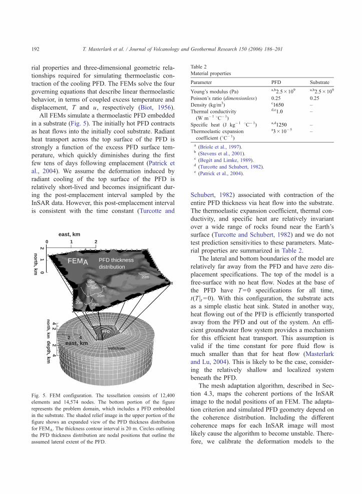
Table 2

Material properties

Parameter PFD Substrate

Young’s modulus (Pa) a,b2.5�109 a,b2.5�109

Poisson’s ratio (dimensionless) 0.25 0.25

Density (kg/m3) c1650 –

Thermal conductivity

(W m�1 8C�1)

d,e1.0 –

Specific heat (J kg�1 8C�1) a,d1250 –

Thermoelastic expansion

coefficient (8C�1)

a3�10�5 –

a (Briole et al., 1997).b (Stevens et al., 2001).c (Beget and Limke, 1989).d (Turcotte and Schubert, 1982).e (Patrick et al., 2004).


rial properties and three-dimensional geometric rela-

tionships required for simulating thermoelastic con-

traction of the cooling PFD. The FEMs solve the four

governing equations that describe linear thermoelastic

behavior, in terms of coupled excess temperature and

displacement, T and u, respectively (Biot, 1956).

All FEMs simulate a thermoelastic PFD embedded

in a substrate (Fig. 5). The initially hot PFD contracts

as heat flows into the initially cool substrate. Radiant

heat transport across the top surface of the PFD is

strongly a function of the excess PFD surface tem-

perature, which quickly diminishes during the first

few tens of days following emplacement (Patrick et

al., 2004). We assume the deformation induced by

radiant cooling of the top surface of the PFD is

relatively short-lived and becomes insignificant dur-

ing the post-emplacement interval sampled by the

InSAR data. However, this post-emplacement interval

is consistent with the time constant (Turcotte and

substrate

PFD

20m

20m

20m

20m

40m

PFD thicknessdistribution

FEMA

60m

4 2n

orth

, km4

2d

epth

, km

42east, km

21

east, km0

12

no

rth, km 0

Fig. 5. FEM configuration. The tessellation consists of 12,400

elements and 14,574 nodes. The bottom portion of the figure

represents the problem domain, which includes a PFD embedded

in the substrate. The shaded relief image in the upper portion of the

figure shows an expanded view of the PFD thickness distribution

for FEMA. The thickness contour interval is 20 m. Circles outlining

the PFD thickness distribution are nodal positions that outline the

assumed lateral extent of the PFD.

Schubert, 1982) associated with contraction of the

entire PFD thickness via heat flow into the substrate.

The thermoelastic expansion coefficient, thermal con-

ductivity, and specific heat are relatively invariant

over a wide range of rocks found near the Earth’s

surface (Turcotte and Schubert, 1982) and we do not

test prediction sensitivities to these parameters. Mate-

rial properties are summarized in Table 2.

The lateral and bottom boundaries of the model are

relatively far away from the PFD and have zero dis-

placement specifications. The top of the model is a

free-surface with no heat flow. Nodes at the base of

the PFD have T=0 specifications for all time,

t(Tjt =0). With this configuration, the substrate acts

as a simple elastic heat sink. Stated in another way,

heat flowing out of the PFD is efficiently transported

away from the PFD and out of the system. An effi-

cient groundwater flow system provides a mechanism

for this efficient heat transport. This assumption is

valid if the time constant for pore fluid flow is

much smaller than that for heat flow (Masterlark

and Lu, 2004). This is likely to be the case, consider-

ing the relatively shallow and localized system

beneath the PFD.

The mesh adaptation algorithm, described in Sec-

tion 4.3, maps the coherent portions of the InSAR

image to the nodal positions of an FEM. The adapta-

tion criterion and simulated PFD geometry depend on

the coherence distribution. Including the different

coherence maps for each InSAR image will most

likely cause the algorithm to become unstable. There-

fore, we calibrate the deformation models to the

2

east, km

nort

h, k

m

1

12

0

hihchb

Fig. 6. PFD nodal positions: the free-surface. The open circles, hb

outline the lateral extent of the PFD (e.g., shown in Fig. 1b). The

black and gray circles correspond to nodal positions that lie within

the respective coherent and incoherent portions of the InSAR image

Locations for impulse response functions (G), displacements (dobs

and predictions (dpre) correspond to hc.


representative InSAR image shown in Figs. 2a and 4a.

This image spans the time interval June 21, 1992

through July 11, 1993. We chose the InSAR image

shown in Figs. 2a and 4a for two reasons. First,

among the available InSAR images, the chosen

image spans a time interval nearest to the 1986 PFD

emplacement event (Fig. 3). Thermoelastic deforma-

tion decays temporally and an InSAR image spanning

a relatively earlier time interval should have a greater

deformation signal-to-noise ratio with respect to an

image constructed from scenes acquired later on,

assuming all InSAR images have constant noise char-

acteristics. Second, implementing phase ramping cor-

rections to the InSAR images will confound the

algorithm in its current form. The chosen InSAR

image suggests negligible deformation near the mar-

gins of the PFD. In this case, we need not correct the

deformation for phase ramping (e.g., Masterlark and

Lu, 2004). Alternatively, phase ramping corrections

would be required, for example, to account for the

non-zero deformation along the PFD margins in the

InSAR image shown in Fig. 2b. The inability to

allow for phase ramping corrections is a limitation

of the algorithm presented in this paper. However,

the concepts presented in this paper lay the founda-

tions for more complex approaches that may expli-

citly include multiple InSAR images and phase

ramping corrections.

We test the sensitivity to the heat sink configura-

tion by simulating a problem domain having adia-

batic conditions. For this FEM, the substrate and

PFD are given the same material property specifica-

tions. All problem domain boundaries have no heat

flow specifications. This model does not include

Tjt=0 specifications associated with the heat sink

configuration discussed above. Predictions from this

model poorly characterize the systematic subsidence

of the PFD because the predicted expansion of the

heating substrate counteracts the predicted subsi-

dence of the cooling PFD. We therefore reject the

adiabatic configuration and assume the substrate acts

as a heat sink.

4.2. DEM difference configuration

The first model, FEMA, simulates a PFD having a

thickness distribution, h, corresponding to the differ-

ence between post- and pre-eruption digital elevation

models (Figs. 4 and 5). For this configuration, the

predicted displacement at time t is a linear function of

the initial excess temperature of the PFD, T0PFD, which

we estimate using the linear least-squares inverse

solution (Menke, 1989):

TPFD0 ¼ GTG

� ��1GTdobs: ð1Þ

The data kernel, G, is a column vector of unit

impulse response functions. Each element Gj is the

predicted thermoelastic displacement, due to a unit of

initial excess temperature within the PFD, projected

onto the LOS vector for nodal position j. The data

vector, dobs, is assembled from the observed LOS

displacements. Each element djobs represents the

local LOS displacements interpolated to nodal posi-

tion j. All nodal positions in G and dobs correspond to

the coherent portions of the InSAR image, excluding

the lateral boundaries of the PFD. Positions used to

construct G and dobs are denoted hc in Fig. 6. Inco-

herent nodal positions, hi, are not populated.

Solving Eq. (1) gives the least-squares estimate for

the initial excess temperature, T0PFD=640F10 8C.

The root-mean-squared-error (RMSE) between the

observed and predicted displacements, dobs and dpre,

respectively, is 2.2 cm. Predictions from this model

,

.

)


are a significant improvement over the null hypothesis

at the 95% confidence level. However, the residual

from this model contains systematic errors. A visual

inspection of the predictions and residual suggests this

model roughly accounts for the observed deformation

in the southern and eastern regions of the PFD, where

the DEM differences are relatively large (Fig. 7).

Conversely, predictions are poor for regions of the

PFD where DEM differences are relatively small or

zero. This relationship suggests either that (1) the

thermoelastic deformation mechanism, which is a

strong function of the PFD thickness, is inappropriate;

(2) the thermoelastic model specifications, such as the

boundary conditions and material property distribu-

tions, poorly approximate the natural system; or (3)

the thickness distribution of the PFD estimated from

the DEM differences contains systematic errors. Field

observations (Beget and Limke, 1989) and remote

sensing data (Fig. 4b) indicate the PFD was initially

hot. Cooling of this initially hot material will induce

thermoelastic deformation. The proposed model con-

figurations honor the horizontal geometry of the PFD

and the thermoelastic material properties are relatively

invariant. The requirement for thermoelastic deforma-

tion and the relatively invariant thermoelastic material

properties, combined with the prediction misfit versus

PFD thickness correlation (Fig. 7), suggest the sys-

tematic prediction errors are due to the DEM differ-

ences poorly approximating the PFD thickness

distribution. Furthermore, the unknown acquisition

dates of the pre-1986 eruption DEM introduce uncer-

tainty as to whether or not the DEM elevations are

contaminated by materials deposited during the 1976

eruption. This ambiguity suggests the thickness dis-

tribution of the PFD estimated with the DEM differ-

ences is unreliable and a cause of the misfit.

4.3. PFD thickness: adaptive mesh algorithm

We design three additional models to reduce the

systematic prediction errors associated with the a

priori PFD thickness distribution and test deformation

prediction sensitivities to the initial excess tempera-

ture specifications of the PFD. These three models are

part of adaptive mesh algorithms that calibrate the

predicted thermoelastic deformation, for specified

initial excess temperatures, with respect to the

observed InSAR image, while iteratively optimizing

the PFD thickness distributions. The underlying pre-

mise of the algorithm is that the thermoelastic sub-

sidence predicted for a point j at the surface of the

PFD is solely a function of the local PFD thickness

near point j. The a priori initial excess temperature of

the PFD for FEMB, our preferred model, is 640 8C.This is the initial excess temperature estimation

obtained from the least-squares inverse analysis.

Computational requirements for each iteration of the

adaptive mesh algorithm include model runs for a

two-dimensional FEM that solves Laplace’s equation

and the three-dimensional FEMB that solves for ther-

moelastic deformation.

The adaptive mesh algorithm is illustrated in Fig. 8

and described here. The algorithm starts with initial

conditions of 1.0 m thickness throughout the PFD

(h=1.0); all elements of the incremental thickness

vector, D, are 1.0 m; and the iteration counter, k, is

one. The initial thickness of the PFD is set to 1.0 m,

rather than zero, because the three-dimensional finite

element model requires a finite initial thickness. Ther-

moelastic deformation of this 1.0 m thick PFD is

negligible during 1992–1999. The optimized PFD

thickness distributions and volume estimates reported

hereafter do not include this initial thickness.

The iterative procedure begins with a Laplacian

operator and Dirichlet boundary conditions to esti-

mate the vertical coordinates for nodal positions cor-

responding to incoherent regions, hi, for the specified

distribution hc. The finite element approximation of

Laplace’s equation (Wang and Anderson, 1982) is

automatically implemented by constructing a two-

dimensional mesh from the horizontal nodal coordi-

nates extracted from the top surface of the PFD por-

tion of FEMB and imposing the above specifications.

Fig. 6 illustrates the nomenclature for h. The three

dimensional PFD is constructed by an automated

tessellation of the space contained by the flat base

and the upper surface, h, of the PFD. The PFD is then

automatically embedded into the three-dimensional

substrate to update the mesh of FEMB (Fig. 5).

Thermoelastic displacements are calculated using

FEMB and projected onto the LOS vector to obtain

dpre. The thickness hj, for which predicted subsidence

djpre underestimates observed subsidence dj

obs, is

increased by Dj. The thickness hj corresponding to a

PFD surface node, for which predicted subsidence djpre

overestimates observed subsidence djobs, is decreased


by bDj, where b is a damping parameter with a value

of 0.9 and Dj is updated to bDj. This damping stabi-

lizes the iterative procedure. Each iteration increases

the maximum thickness by 1.0 m until all subsidence

predictions have met or exceeded the observed sub-

sidence values, at which point all elements of D are

less than 1.0 m and kstop is set equal to the number of

completed iterations. This produces a PFD thickness

distribution that is precise to within 1 m. However, the

accuracy of the estimated distribution is somewhat

elusive because it depends on the validity of the

model and associated assumptions.

5. Results

5.1. Preferred model

For FEMB and the assumed initial excess tempera-

ture, T0PFD=640 8C, the adaptive mesh algorithm

converges after 126 iterations (Fig. 9). The residual

for this model is sub-millimeter (RMSE=0.3 mm) and

the predictions, dpre, are virtually indistinguishable

from the data, dobs (Fig. 10). The optimized average

thickness, maximum thickness, and volume of the

PFD are 9.3 m, 126 m, and 2.1�107 m3, respectively

(Fig. 11). The misfit and estimated PFD volume

rapidly decrease and increase, respectively, during

the first ~50 iterations. The thickness distributions

for 50 and 126 iterations are essentially the same.

However, the thickness peak near the southwest part

of the PFD (Fig. 10c) appears truncated for solutions

of 50 versus 126 iterations. With the exception of this

thickness peak, the thickness distribution estimated

using the adaptive mesh algorithm is within the uncer-

Fig. 7. FEMA results. (a) Observed displacements. Circles represen

the observed displacements interpolated to nodal positions. Relative

displacements are shaded according to the grayscale at the bottom

Each black-gray-white cycle represents 2.83 cm of relative defor

mation toward the satellite. (b) Predicted displacements. Circles

represent the predicted nodal displacements due to thermoelastic

contraction. Relative displacements are shaded according to the

grayscale at the bottom. (c) Absolute residual. The absolute residua

distribution inversely correlates to the DEM difference distribution

for which positive values (thickness) are shown with white 20 m

contour intervals. Misfit is minimal near regions where the DEM

difference distribution suggests significant PFD thickness. How

ever, deformation predictions are poor elsewhere in the problem

domain.

t

.

-

l

,

-

5.0

2.0

4.0

1.0

6.0

0.0PF

D v

olum

e,X

107

m3

3.0

0.000

0.001

0.002

0.003

0.004

0.005

0.006

0.020

0.022

0.032

0.034

RM

SE

mis

fit, m

FEMA

FEMA

null

iterations0 100 200 300

iterations0 100 200 300

FEMB: kstop = 126 T0

PFD = 641 oC

FEMC: kstop = 336 T0

PFD = 500 oC

FEMD: kstop = 27 T0

PFD = 800 oC

a

b

Fig. 9. Iterative evolution of the PFD thickness distribution. (a)

Iterative misfit improvement. The misfit decreases rapidly over the

first several tens of iterations. The misfits for the null hypothesis and

FEMA are substantially greater than those for FEMB, FEMC, and

FEMD. (b) Iterative PFD volume development. The estimated PFD

volumes undergo rapid increases over the first several tens of

iterations. The PFD volumes estimated using the adaptive mesh

algorithm are all greater than that estimated from the DEM differ-

ence distribution. The explanation from (a) also applies to (b).

djpre < dj

obs :

hjc = hj

c - β∗δδ

β∗δδ

j

δj = j

calculate thermoelastic deformation

Import PFD thickness distribution into FEMB

or

PFD mesh adaptation

all < 1.0 ?

Convergence criterion

no

djpre > dj

obs :

hjc = hj

c + j

yes Done

hb = 1.0hc (specified)hi

FEM: 2 h = 0 ∇

fill thicknessdistribution gaps

(see Figure 6 for spatial distribution of h)

k =

k +

1

Initializeh = 1.0 , δ = 1.0 m , and k = 1

δ

δ

Fig. 8. Adaptive mesh algorithm.


tainty of the DEM difference estimation. This sug-

gests DEMs having much more precise uncertainties,

with respect to the two DEMs used in this study, are

required to constrain the geometry of the PFD.

Forward modeling predictions indicate the subsi-

dence rate decreases slightly during the temporal

window covered by the InSAR images (Fig. 12).

These predictions of the transient thermoelastic defor-

mation are qualitatively consistent with the persistent

maximum subsidence rate of ~3 cm yr�1 suggested

by the 18 InSAR images. The predicted displacement

for the point overlying the thickest portion of the PFD

is almost purely vertical (Fig. 12a). However, the

predicted horizontal displacement components are

more significant, with respect to the predicted vertical

components, along the lateral margins of the PFD.

5.2. Sensitivity to initial excess temperature

The amplitude of the predicted thickness distribu-

tion is inversely related to the initial excess tempera-

ture of the PFD (Fig. 9). For a given amount of

subsidence, a low initial excess temperature requires

a relatively thick PFD, whereas a thin PFD is required

for a high initial excess temperature. Others suggest

PFD emplacement temperatures can range from 400

to 1000 8C (Banks and Hoblitt, 1981) or similarly

from 300 to 800 8C (Waythomas and Waitt, 1998).

The initial temperature of the PFD is the sum of the

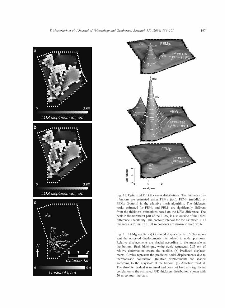
Fig. 10. FEMB results. (a) Observed displacements. Circles repre

sent the observed displacements interpolated to nodal positions

Relative displacements are shaded according to the grayscale a

the bottom. Each black-gray-white cycle represents 2.83 cm o

relative deformation toward the satellite. (b) Predicted displace

ments. Circles represent the predicted nodal displacements due to

thermoelastic contraction. Relative displacements are shaded

according to the grayscale at the bottom. (c) Absolute residual

The absolute residual is minimal and does not have any significan

correlation to the estimated PFD thickness distribution, shown with

20 m contour intervals.

20m

20m

20m FEMB:

k stop = 126T0

PFD = 641 oC

20m

FEMD:

kstop = 27T0

PFD =800 oC

20m

100m

200m

300m

FEMC:

kstop = 336T0

PFD = 500 oC

20m

21

east, km

12n

orth

, km

0

0

100m

Fig. 11. Optimized PFD thickness distributions. The thickness dis

tributions are estimated using FEMB (top), FEMC (middle), o

FEMD (bottom) in the adaptive mesh algorithm. The thickness

peaks estimated for FEMB and FEMC are significantly differen

from the thickness estimations based on the DEM difference. The

peak in the northwest part of the FEMC is also outside of the DEM

difference uncertainty. The contour interval for the estimated PFD

thickness is 20 m. The 100 m contours are shown in bold white.


-

.

t

f

-

.

t

-

r

t

Table 3

Sensitivity to initial excess temperature

FEMA FEMB FEMC FEMD

T0PFD (8C) a640F10 640 500 800

kstop – 126 336 27

RMSE (cm) 2.2 0.03 0.09 0.18

h, average (m) 4.3 9.3 25.2 6.2

h, maximum (m) 61 126 336 27

PFD volume (m3) 9.9�106 2.1�107 5.7�107 1.4�107

a Least-squares estimation.


ambient and initial excess temperatures. Assuming an

ambient temperature of ~0 8C (NOAA, 2002), the

initial excess temperature determined using FEMA

(T0PFD=640 8C) is equivalent to the initial emplace-

ment temperature of the PFD and within the expected

range of initial emplacement temperatures.

Our estimated initial excess temperature (T0PFD=

640 8C) is in agreement with an in situ field experi-

ment that suggests the initial temperature of the PFD

from the 1986 eruption of Augustine Volcano is at

least 425 8C (Beget and Limke, 1989). If the initial

excess temperature is much less than 640 8C, the

thickness of the PFD would have to be much greater

than that estimated for both FEMA and FEMB. Results

from the adaptive mesh algorithm using FEMC

(T0PFD=500 8C) predict the average thickness of the

PFD is 25 m, the maximum thickness is 336 m, and

the volume is 5.7�107 m3. These results are unlikely

based on the DEM data, particularly for the thickness

peak (Fig. 11), and field observations of wave cuts

year

-1.0

-0.8

-0.6

-0.4

-0.2

0.0

1985 1990 1995 2000

-1.0

-0.8

-0.6

-0.4

-0.2

0.0

ux

uy

uz

164

207

229

436

501

track

dis

pla

cem

ent,

md

isp

lace

men

t, m

a

b

Fig. 12. Transient thermoelastic deformation. We present displace-

ment predictions for the point overlying the thickest portion of the

PFD, which is estimated using FEMB. The gray rectangle shows the

interval 1992–1999, during which all curves are relatively linear. (a)

Thermoelastic displacement as a function of time for each displace-

ment component. (b) LOS displacement. The three displacement

components are projected onto the five different LOS vectors of the

InSAR images. Individual curves are labeled in the expanded view.

that constrain the thickness of the PFD near the north-

ern coast to 1 or 2 m (Beget and Limke, 1989) (Fig.

1b). The PFD thickness predicted using FEMC is more

than 10 m for this coastal location.

Alternatively, FEMD has a much higher initial

excess temperature specification (T0PFD=800 8C).

Results from the adaptive mesh algorithm using this

model predict the average thickness of the PFD is 6.2

m, the maximum thickness is 27 m, and the volume

is 1.4�107 m3 (Fig. 11). This model estimates the

thickness peak in the southwest part of the PFD is

much less than the thickness estimated from DEM

difference, 61 m. Previous estimations suggest the

PFD volume is about 5�107 m3 (Swanson and

Kienle, 1988), a value that favors lower initial excess

temperatures and a relatively thick PFD. Table 3

summarizes results of FEMA, FEMB, FEMC,

FEMD, and the sensitivity analysis for initial excess

temperature. Fig. 11 illustrates the optimal PFD

thickness distributions as a function of initial excess

temperature.

6. Discussion

6.1. Model limitations

The relatively simple three-dimensional models of

thermoelastic deformation reasonably approximate

the observed deformation. In order to isolate the

effects of the initial excess temperature of the PFD

on the thickness distribution estimations, we impose

numerous simplifications and assumptions. We

assume the substrate is a relatively weak homoge-

neous material (Table 2) (Briole et al., 1997; Stevens

et al., 2001; Lu et al., 2005). This may be an over-

simplification of the volcano’s structure, which


includes a layered assembly of lava, ash, lahar, ava-

lanche, and PFD materials (Beget and Kienle, 1992;

Miller et al., 1998; Waythomas and Waitt, 1998).

Although a system of layered materials may be a

better approximation for the substrate, this additional

structural complexity requires constraining data that is

currently unavailable.

We assume the PFD is a homogeneous material,

having a uniform initial excess temperature. Field

observations suggest the region representing the

PFD actually consists of lithic block and ash flow

deposits, lithic-rich pumice flow deposits, and lahar

deposits (Beget and Limke, 1989). Furthermore, there

may be additional depositional gradations within each

region. This heterogeneous distribution of material

properties suggests a non-uniform initial excess tem-

perature distribution within the PFD. On the other

hand, the relatively fast emplacement process of the

PFD suggests a homogeneous initial temperature may

be appropriate. The lack of sufficient constraining

data does not allow us to resolve this issue.

6.2. Other deformation mechanisms

We assume linear thermoelastic behavior is the sole

deformation mechanism. Other mechanisms related to

the thickness of the PFD, but unrelated to the thermal

loading, may also contribute to the observed subsi-

dence. PFDs undergo significant porosity reduction

(compaction) following emplacement. The time con-

stant for this process is on the order of hour to days

(Rowley et al., 1981), whereas the time constant for

thermoelastic contraction is on the order of years

(Turcotte and Schubert, 1982). For the purposes of

this analysis, we neglect compaction as a deformation

mechanism because most of the compaction-related

deformation occurs within a short interval following

the emplacement. Relatively little thermoelastic defor-

mation occurs during the corresponding interval.

Furthermore, the InSAR images document deforma-

tion during intervals that begin six years after PFD

emplacement and long after the bulk of the PFD

compaction.

Transient poroelastic deformation of the substrate

is caused by the decay of excess pore fluid pressures

initiated by the overlying gravity load of the newly

emplaced PFD. The initial response to this loading is

undrained and relatively stiff, with respect to the

drained conditions, because the pore fluids bear a

portion of the load as excess pore fluid pressure

(Wang, 2000). As the excess pore fluid pressure

decays, the substrate conditions migrate from

undrained (stiff) to drained (compliant) conditions

and the land surface undergoes subsidence. However,

because of the relatively shallow and local flow sys-

tem associated with this loading, the time constant for

the poroelastic response is most likely too small to

account for the systematic decadal deformation (Lu et

al., 2004).

Transient viscoelastic deformation is caused by

the viscous flow of the substrate in response to the

gravity load initiated by the emplacement of the

PFD. Initially, the substrate behaves as a simple

elastic material in response to the gravity load.

Viscous flow, which is driven by deviatoric stresses

in the substrate, ensues following the initial loading

event. The expected time constant for this deforma-

tion (Briole et al., 1997; Stevens et al., 2001; Lu et

al., 2004) is of the same order as that for thermo-

elastic deformation and suggests the observed sub-

sidence may be caused, in part, by viscoelastic

relaxation. It is difficult to conclusively predict the

effects of viscoelastic relaxation based on the avail-

able constraining data. This deformation mechanism

is also a function of the PFD thickness distribution.

Investigations of deforming lava flows (Lu et al.,

2004) suggest the magnitude of viscoelastic defor-

mation is a few tens-of-percent of that for thermo-

elastic relaxation.

Thermoelastic deformation alone can account for

the observed deformation and is consistent with the

thermal information derived from field observations

(Beget and Limke, 1989) and remote sensing data (Fig.

4b). Viscoelastic deformation may account for the

observed subsidence, but it cannot account for the

thermal observations (Beget and Limke, 1989) and

the thermal anomaly shown in Fig. 4b. It is likely

that the observed deformation is the result of some

combination of thermoelastic and viscoelastic mechan-

isms, but we cannot resolve the relative contributions

from each without further constraining data. Interest-

ingly, all of the alternative deformation mechanisms

suggested above will increase the deformation rate.

Therefore, thickness distributions and initial tempera-

ture estimations represent upper bounds, rather than

actual estimations.


6.3. Mesh adaptation

Mesh construction has historically been a labor-

intensive component of constructing three-dimensional

FEMs of geomechanical systems. Computational sim-

plicity is often cited to justify oversimplified models of

deformational systems, particularly for inverse ana-

lyses (Masterlark, 2003). The validity of many assump-

tions associated with the FEMs and mesh adaptation

algorithm used in this study is arguable. However, the

excellent agreement of displacement observations and

predictions demonstrates the success of the mesh adap-

tation algorithm introduced in this study, which can

automatically optimize the geometric configuration of

an FEM. If available, high quality pre- and post-event

digital elevation models can precisely constrain the

vertical geometric components of a newly emplaced

material (Stevens et al., 2001; Lu et al., 2003c). In that

case, an adaptive mesh algorithm is unnecessary. The

value of the adaptive mesh algorithm lies in applica-

tions for which geometric constraining data are lacking,

as is the case for the PFD emplaced during the 1986

eruption of Augustine Volcano.

7. Conclusions

Thermoelastic deformation predictions, subject to

an assumed a priori PFD thickness distribution, con-

tain systematic errors and poorly approximate the

observed deformation. Accurate simulation of post-

emplacement deformation of the PFD due to thermo-

elastic contraction requires an accurate estimation of

the PFD thickness distribution. The proposed method

combines InSAR data, FEMs, and an adaptive mesh

algorithm to generate optimized thickness distribution

maps of the PFD emplaced during the 1986 eruption

of Augustine Volcano. The preferred model (FEMB),

which is used in the proposed method, suggests

thermoelastic contraction is a plausible mechanism

to account for the observed subsidence of the PFD.

Displacement predictions from this model are

remarkably consistent with observations.

FEMs are powerful tools that allow us to simu-

late a wide variety of complex geomechanical sys-

tems having a priori geometric specifications.

Reconfiguring the mesh of an FEM can be labor-

intensive and is a significant drawback to geome-

chanical applications of FEMs. This study demon-

strates a method that automatically performs iterative

mesh reconfigurations, which can greatly reduce

misfit attributed to an a priori geometric configura-

tion. Further development of these methods may

allow investigators to do away with many of the

restrictive model assumptions and oversimplified

configurations typically invoked for operational

and computational simplicity.

Acknowledgements

This research was performed by SAIC under US

Geological Survey contract number 03CRCN0001.

Funding was provided in part from NASA (NRA-

99-OES-10 RADARSAT-0025-0056). ERS-1 and

ERS-2 SAR images are copyright n 1992–1999 Eur-

opean Space Agency and provided by the Alaska

Satellite Facility. We thank T. Miller and D. Dzurisin

for useful discussions on the 1986 pyroclastic flows.

D.B. Gesch and B.K. Wylie provided technical

reviews. Insightful comments by guest editor M.

Poland and the reviews provided by G. Wadge and

an anonymous reviewer greatly improved this paper.

Appendix A. Symbols

d vector, LOS displacements

G vector, unit impulse response functions

h vector, thickness distribution

j nodal position index

k iteration index

T time

T excess temperature

T0PFD initial excess temperature of PFD

u displacement

D vector, incremental thickness distribution

References

Banks, N.G., Hoblitt, R.P., 1981. Summary of temperature studies

of 1980 deposits. In: Lipman, P.W., Mullineaux, D.R. (Eds.),

The 1980 Eruptions of Mount St. Helens, Washington, U.S.

Geological Survey Professional Paper, vol. 1250, pp. 295–313.

Beget, J.E., Kienle, J., 1992. Cyclic formation of debris avalanches

at Mount St Augustine volcano. Nature 356, 701–704.


Beget, J.E., Limke, A.J., 1989. Density and void ratio on emplace-

ment of a small pyroclastic flow, Mount St. Augustine, Alaska.

Journal of Volcanology and Geothermal Research 39, 349–353.

Biot, M.A., 1956. Thermoelasticity and irreversible thermody-

namics. Journal of Applied Physics 27, 240–253.

Briole, P., Massonnet, D., Delacourt, C., 1997. Post-eruptive defor-

mation associated with the 1986–87 and 1989 lava flows of Etna

detected by radar interferometry. Geophysical Research Letters

24, 37–40.

Gesch, D., 1994. Topographic data requirement for EOS global

change research. USGS Open-File Report, 94–62.

Gesch, D., Oimoen, M., Greenlee, S., Nelson, C., Steuck, M., Tyler,

D., 2002. The national elevation dataset. Photogrammetric Engi-

neering and Remote Sensing 68, 5–11.

Hibbet, Karlsson, and Sorensen, Inc., 2003. ABAQUS, version 6.4,

http://www.hks.com.

Lipman, P., Moore, J.G., Swanson, D.A., 1981. Bulging of the north

flank before the May 18 eruption—geodetic data. In: Lipman,

P.W., Mullineaux, D.R. (Eds.), The 1980 Eruptions of Mount St.

Helens, Washington, U.S. Geological Survey Professional

Paper, vol. 1250, pp. 143–155.

Lu, Z., Masterlark, T., Power, J., Dzurisin, D., Wicks Jr., C.,

Thatcher, W., 2002. Subsidence at Kiska volcano, western

Aleutians, detected by satellite radar interferometry. Geophysi-

cal Research Letters 29, 1855. doi: 10.1029/2002GL014948.

Lu, Z., Masterlark, T., Dzurisin, D., Rykhus, R., Wicks Jr., C.,

2003a. Transient inflation rate detected with satellite interfero-

metry and its implication to the plumbing system at Westdahl

volcano, Alaska. Journal of Geophysical Research 108, 2354.

doi: 10.1029/2002JB002311.

Lu, Z., Wicks Jr., C., Dzurisin, D., Power, J., Thatcher, W., Master-

lark, T., 2003b. Interferometric synthetic aperture radar studies of

Alaska volcanoes. Earth Observation Magazine 12, 8–18.

Lu, Z., Fielding, E., Patrick, M., Trautwein, C., 2003c. Estimating

lava volume by precision combination of multiple baseline space-

borne and airborne interferometric synthetic aperture radar: the

1997 eruption of Okmok volcano, Alaska. IEEE Transactions on

Geoscience and Remote Sensing 41, 1428–1436.

Lu, Z., Masterlark, T., Dzurisin, D., 2005. Interferometric synthetic

aperture radar study of Okmok volcano, Alaska, 1992-2003:

magma supply dynamics and postemplacement lava flow defor-

mation. Journal of Geophysical Research 110, B02403. doi:

10.1029/2004JB003148.

Massonnet, D., Feigl, K., 1998. Radar interferometry and its appli-

cation to changes in the Earth’s surface. Reviews of Geophysics,

441–500.

Massonnet, D., Rossi, M., Carmona, C., Adragna, F., Peltzer, G.,

Feigl, K., Rabaute, T., 1993. The displacement field of the

Landers earthquake mapped by radar interferometry. Nature

364, 138–142.

Masterlark, T., 2003. Finite element model predictions of static

deformation from dislocation sources in a subduction zone:

Sensitivities to homogeneous, isotropic, Poisson-solid, and

half-space assumptions. Journal of Geophysical Research 108,

2540. doi: 10.1029/2002JB002296.

Masterlark, T., Lu, Z., 2004. Transient volcano deformation sources

imaged with interferometric synthetic aperture radar: application

to Seguam Island, Alaska. Journal of Geophysical Research

109, B01401. doi: 10.1029/2003JB002568.

Menke, W., 1989. Geophysical Data Analysis: Discrete Inverse

Theory. International Geophysical Series, vol. 45. Academic

Press, Inc., San Diego.

Miller, T.P., McGimsey, R.G., Richter, D.H., Riehle, J.R., Nye, C.J.,

Yount, M.E., Dumoulin, J.A., 1998. Catalog of the historically

active volcanoes of Alaska. US Geological Survey Open-File

Report 98-0582.

NOAA, 2002. Climatography of theUnited States No. 85, http://www.

ncdc.noaa.gov/climatenormals/clim85/CLIM85_TEMP01.pdf,

Ashville, NC.

Patrick, M.R., Dehn, J., Dean, K., 2004. Numerical modeling of

lava cooling applied to the 1997 Okmok eruption: approach

and analysis. Journal of Geophysical Research 109, B03202.

doi: 10.1029/2003JB002537.

Pauk, B.A., Power, J.A., Lisowski, M., Dzurisin, D., Iwatsubo, E.Y.,

Melbourne, T., 2001. Global positioning system (GPS) survey

of Augustine volcano, Alaska, August 3–8, 2000: Data proces-

sing, geodetic coordinates and comparison with prior geodetic

surveys. US Geological Survey Open-File Report 01-0099.

Peltzer, G., Rosen, P., Rogez, F., Hudnut, K., 1996. Postseismic

rebound in fault step-overs caused by pore-fluid flow. Science

273, 1202–1204.

Pollitz, F.F., Wicks, C., Thatcher, W., 2001. Mantle flow beneath a

continental strike-slip fault: postseismic deformation after the

1999 Hector Mine earthquake. Science 293, 1814–1818.

Rowley, P.D., Kuntz, M.A., Macleod, N.S., 1981. Pyroclastic-flow

deposits. In: Lipman, P.W., Mullineaux, D.R. (Eds.), The 1980

Eruptions of Mount St. Helens, Washington, U.S. Geological

Survey Professional Paper, vol. 1250, pp. 489–512.

Sabins, F.F., 1997. Remote Sensing Principles and Interpretation,

3rd edition. W.H. Freeman and Company, New York.

Simkin, T., Siebert, L., 1994. Volcanoes of the World. Geoscience

Press, Tucson. 349 pp.

Stenoien, M.D., Bentley, C.R., 2000. Pine island glacier, Antarctica:

a study of the catchment using interferometric synthetic aperture

radar measurements and radar altimetry. Journal of Geophysical

Research 105, 21761–21780.

Stevens, N.F., Wadge, G., Williams, C.A., Morely, J.G., Muller, J.-

P., Murray, J.B., Upton, U., 2001. Surface movements of

emplaced lava flows measured by synthetic aperture radar inter-

ferometry. Journal of Geophysical Research 106, 11293–11313.

Swanson, S.E., Kienle, J., 1988. The 1986 eruption of Mount St.

Augustine: field test of a hazard evaluation. Journal of Geophy-

sical Research 93, 4500–4520.

Turcotte, D.L., Schubert, G.J., 1982. Geodynamics: Applications of

Continuum Physics to Geological Problems. John Wiley &

Sons, New York.

Wang, H.F., 2000. Theory of Linear Poroelasticity: with Applica-

tions to Geomechanics. Princeton University Press, Princeton.

Wang, H.F., Anderson, M.P., 1982. Introduction to Groundwater

Modeling: Finite Difference and Finite Element Methods. Aca-

demic Press, San Diego.

Waythomas, C.F., Waitt, R.B., 1998. Preliminary volcano-hazard

assessment for Augustine volcano, Alaska. USGS Open-File

Report 98–106.

http://www.hks.com

http://dx.doi.org/doi: 10.1029/2002GL014948

http://dx.doi.org/doi: 10.1029/2002JB002311


http://www.ncdc.noaa.gov/climatenormals/clim85/CLIM85 _ TEMP01.pdf,


http://dx.doi.org/10.1029/2004JB003148


Thickness distribution of a cooling pyroclastic flow deposit on

Documents