THESIS WITH CORRECTIONS - CORE

van Huellen, Sophie (2015) Excess volatility or volatile fundamentals? : the impact of financial speculation on commodity markets and implications for cocoa farmers in Ghana. PhD Thesis. SOAS, University of London

http://eprints.soas.ac.uk/23691

Copyright © and Moral Rights for this thesis are retained by the author and/or other

copyright owners.

A copy can be downloaded for personal non‐commercial research or study, without prior

permission or charge.

This thesis cannot be reproduced or quoted extensively from without first obtaining

permission in writing from the copyright holder/s.

The content must not be changed in any way or sold commercially in any format or

medium without the formal permission of the copyright holders.

When referring to this thesis, full bibliographic details including the author, title, awarding

institution and date of the thesis must be given e.g. AUTHOR (year of submission) "Full

thesis title", name of the School or Department, PhD Thesis, pagination.

EXCESS VOLATILITY OR VOLATILE FUNDAMENTALS?

THE IMPACT OF FINANCIAL SPECULATION ON

COMMODITY MARKETS AND IMPLICATIONS FOR COCOA

FARMERS IN GHANA

Sophie van Huellen

Thesis submitted for the degree of PhD

2015

Department of Economics SOAS, University of London

2

Declaration for SOAS PhD thesis

I have read and understood regulation 17.9 of the Regulations for students of the SOAS,

University of London concerning plagiarism. I undertake that all the material presented for

examination is my own work and has not been written for me, in whole or in part, by any

other person. I also undertake that any quotation or paraphrase from the published or

unpublished work of another person has been duly acknowledged in the work which I

present for examination.

Signed: ____________________________ Date: _________________

3

Abstract

The rising prices and high volatility in commodity markets, observed since 2002, have

triggered a debate about whether these dynamics are in excess of what could be explained

by market fundamentals alone. It has been argued by many that the price dynamics

generated are linked to the behaviour of financial investors, in particular to that of a new

class of investors known as index traders. This has given rise to two questions: firstly, what

explains this high price volatility and, secondly, what are the implications of such price

volatility for commodity producers?

To answer the first question, this thesis investigates the relationships between dynamics in

cash and futures prices, and between dynamics of futures with different maturities for

selected grain and soft commodities using time series econometrics. By analysing the

relationships between price series that follow common market fundamentals, price

dynamics generated by non-market fundamental factors can be identified. To answer the

second question, cocoa producers in Ghana were chosen for a case study, and semi-

structured interviews with stakeholders in the cocoa–chocolate chain were conducted.

These interviews revealed the institutional structure of the cocoa chain and the nature of

transactions across the different chain nodes.

Chapter 1 contextualises the research and develops research questions. Chapter 2 presents

a review of theoretical and empirical literature relevant to the first research question.

Chapter 3 empirically tests assumptions about traders’ behaviour underlying the relevant

theories. Chapters 4 and 5 provide investigations into the influence of different investor

groups on price dynamics in commodity futures markets. Chapter 6 presents an

institutional theory for price relevant to the second research question. With reference to

this theory, Chapter 7 discusses the case of the Ghanaian cocoa sector. Chapter 8

summarises key findings and discusses implications for theories and policies, as well as for

future research.

4

Acknowledgement

Foremost, I want to thank my PhD supervisor, Professor Machiko Nissanke, who is not

only the best supervisor I could have wished for, but also a great mentor and friend. I owe

many of my achievements over the past years, including finishing this thesis, to her.

My thanks need to be extended to my second supervisors, Professor Duo Qin, for her

tireless intellectual support, her mentoring and friendship. I also want to thank my third

supervisor, Dr. Graham Smith, for his guidance throughout the PhD process.

A very special thanks goes to my mother, my brother and my partner for their

unconditional moral support, their patience, love and unbreakable belief in my ability to

finish this thesis.

My PhD experience would not have been the same without my close friends and colleagues

at SOAS, especially my ‘sisters in crime’, Ilara and Nana. We went through a lot together

including the birth of our little baby boy, Kwaku. Special thanks go to Tony, Aftab and

Gilad for their proofreading and constructive feedback on chapter drafts.

I also wish to thank my two external examiners, Professor Raphael Kaplinsky and Dr. Jörg

Mayer, for carefully reading through this lengthy piece of work and providing the most

constructive and insightful feedback.

My thanks also go to the numerous cocoa stakeholders I interviewed during my fieldwork

and to whom I am grateful for the invaluable insights shared with me.

Last but not least, I wish to thank Andrey Kuleshov and Elena Ivashentseva, as well as the

German National Academic Foundation for their generous financial support, without

which this research would not have been possible.

5

Table of Contents

Declaration for SOAS PhD thesis .................................................................................................. 2

Abstract ............................................................................................................................................... 3

Acknowledgement ............................................................................................................................. 4

List of Figures .................................................................................................................................... 9

List of Tables ................................................................................................................................... 11

List of Abbreviations ...................................................................................................................... 12

Chapter 1 Introduction ............................................................................................................ 14

1.1 Introduction and Motivation ............................................................................. 14

1.2 Research Questions and Hypotheses ................................................................. 21

1.3 Contribution and Originality .............................................................................. 24

1.4 Thesis Outline ................................................................................................... 26

Chapter 2 Fundamentals versus Financialisation ................................................................. 29

2.1 Introduction ...................................................................................................... 29

2.2 Theories on Price Formation in Commodity Markets ........................................ 30

2.2.1 Theory of Storage ....................................................................................... 31

2.2.2 Theory of Risk Premium ............................................................................ 34

2.3 Theories on Price Formation in Asset Markets .................................................. 41

2.3.1 Efficient Market Hypothesis ....................................................................... 41

2.3.2 Bounded Rationality and Rational Herding ................................................. 45

2.3.3 Fundamental Uncertainty and the Keynesian Tradition .............................. 52

2.4 A Synthesis: Uncertainty and Heterogeneous Traders ........................................ 55

2.5 Empirical Evidence ........................................................................................... 66

2.5.1 Trader Composition and Price Level and Volatility .................................... 68

2.5.2 Trader Composition and Co-movement ..................................................... 75

2.6 Concluding Remarks .......................................................................................... 77

6

Chapter 3 Traders’ Behaviour under Uncertainty ................................................................ 79

3.1 Introduction ...................................................................................................... 79

3.2 Heterogeneity and the Financialisation Hypothesis ............................................ 79

3.3 How to Quantify Speculative Demand? ............................................................. 82

3.3.1 Data Availability and Limitations ................................................................ 83

3.3.2 Trader Heterogeneity in Commodity Markets............................................. 87

3.4 Empirical Analysis of Traders’ Behaviour .......................................................... 92

3.4.1 Data and Methodology ............................................................................... 97

3.4.2 Extrapolation, Herding and Heterogeneity ............................................... 103

3.5 Conclusion ...................................................................................................... 116

Chapter 4 Futures and Cash Market Linkages ................................................................... 118

4.1 Introduction .................................................................................................... 118

4.2 The Fragile Relationship between Futures and Cash Markets........................... 119

4.3 Basis Risk and Market Failure .......................................................................... 122

4.3.1 Data and Methodology ............................................................................. 126

4.3.2 Lead–Lag and Co-integrating Relationship ............................................... 130

4.3.3 Conventional Theories and the Long-Run Equilibrium ............................ 133

4.3.4 Structural Breaks in the Long-run Equilibrium ......................................... 138

4.4 The Conundrum of Non-Convergence ............................................................ 142

4.4.1 An Alternative Explanation for the Extent of Non-Convergence ............. 152


4.4.3 Empirical Results ..................................................................................... 157

4.5 Conclusion ...................................................................................................... 168

Chapter 5 The Commodity Term Structure ....................................................................... 170

5.1 Introduction .................................................................................................... 170

5.2 A Theory on Intertemporal Pricing .................................................................. 170

5.3 The Term Structure of Cocoa and Coffee ........................................................ 176

7

5.4 Term Structure Anomalies ............................................................................... 181


5.4.2 Calendar Spread Analysis .......................................................................... 186

5.4.3 Two-Step Futures Curve Analysis ............................................................. 189

5.5 Conclusion ...................................................................................................... 203

Chapter 6 Price Formation in Commodity Sectors ........................................................... 204

6.1 Introduction .................................................................................................... 204

6.2 Commodity Chains and Governance ............................................................... 205

6.2.1 Driveness and Lead Firms ........................................................................ 207

6.2.2 Coordination and Standards ..................................................................... 208

6.2.3 Conventions and Systems of Justification ................................................. 211

6.3 Institutional Theory for Price .......................................................................... 213

6.4 Governance, Transactions and Institutions ...................................................... 217

6.5 Concluding Remarks ........................................................................................ 222

Chapter 7 The Case of Ghanaian Cocoa ............................................................................. 223

7.1 Introduction .................................................................................................... 223

7.2 The History of Cocoa in Ghana ....................................................................... 224

7.2.1 Cocoa under Colonial Power .................................................................... 224

7.2.2 Cocoa under Independence ...................................................................... 229

7.2.3 Cocoa under Structural Adjustment and Beyond ...................................... 233

7.3 Structure of the Ghanaian Cocoa Sector .......................................................... 241

7.4 Price Formation and Risk Allocation ............................................................... 247

7.4.1 Global Marketing: Traders, Grinders and Manufacturers .......................... 247

7.4.2 External Marketing: The Cocoa Marketing Company ............................... 257

7.4.3 Internal Marketing: The Producer Price Research Committee .................. 265

7.5 Conclusion ...................................................................................................... 281

Chapter 8 Summary, Conclusion and Implications ........................................................... 284

8.1 Introduction .................................................................................................... 284

8.2 Key Findings ................................................................................................... 285

8

8.3 Implications ..................................................................................................... 288

8.3.1 Implications for Theory ............................................................................ 288

8.3.2 Implications for Policy ............................................................................. 290

8.4 Directions for Future Research ........................................................................ 291

Bibliography ................................................................................................................................... 293

Appendix ........................................................................................................................................ 319

Appendix Chapter 2 ................................................................................................... 319





9

List of Figures

Figure 1.1: Commodity Market Prices ......................................................................................... 14

Figure 1.2: Commodity Market Volatility .................................................................................... 14

Figure 1.3: Amount of Outstanding Commodity-linked Derivatives ...................................... 17

Figure 1.4: Number of Outstanding Commodity Exchange Contracts .................................. 17

Figure 1.5: Ghana’s Export Earnings ........................................................................................... 24

Figure 2.1: Market Dynamics under Fundamental Arbitrage ................................................... 55

Figure 2.2: Market Dynamics under Speculative Bubbles ......................................................... 59

Figure 2.3: Book Effect of Index Traders ................................................................................... 60

Figure 2.4: Index Rollover Effect in a Normal Market ............................................................. 62

Figure 2.5: The Different Theories on Commodity Price Formation ..................................... 64

Figure 3.1: Traders Typology after CFTC Reports .................................................................... 86

Figure 3.2: Commodity Price Indices ........................................................................................... 87

Figure 3.3: Covariance Between Commodity Index and Single Commodity ......................... 87

Figure 3.4: Annual Average Open Interest.................................................................................. 88

Figure 3.5: Trader-composition in Total Open Interest ............................................................ 89

Figure 3.6: Working’s T-Index with COT and CIT Data ......................................................... 90

Figure 3.7: Open Interest and Volume Across Contracts ......................................................... 90

Figure 3.8: Market Concentration ................................................................................................. 91

Figure 3.9: Index Traders’ Positions by CIT, DCOT and IID............................................... 113

Figure 4.1: Speculative Investment and Limits to Arbitrage................................................... 121

Figure 4.2: Hedging Effectiveness .............................................................................................. 122

Figure 4.3: Market Basis for Various Cash Markets ................................................................. 123

Figure 4.4: Continuous Daily May-March Spread .................................................................... 124

Figure 4.5: Cocoa Stock-to-Grinding Ratio and Changes in End-of-Season Stock ............ 125

Figure 4.6: Wheat Stock-to-Use Ratio and Changes in End-of-Year Stock ......................... 126

Figure 4.7: Annual Difference of Logged Futures and Cash Prices ...................................... 131

Figure 4.8: Wrongly Categorised Traders in the COT Commercial Category ..................... 137

Figure 4.9: Basis at Each Futures Contract’s Maturity Day .................................................... 143

Figure 4.10: March Cocoa Contracts Relative to Cash Prices ................................................ 144

Figure 4.11: December Wheat Contracts Relative to Cash Prices ......................................... 144

Figure 4.12: Wheat Basis and Storage at Exchange Registered Warehouses ....................... 145

Figure 4.13: Wheat Price Volatility ............................................................................................. 147

Figure 4.14: Wheat Basis and Average Percentage of Full Carry ........................................... 148

Figure 4.15: Cocoa Basis and Storage Level at Exchange Registered Warehouses ............. 150

Figure 4.16: Hedging and Index Pressure .................................................................................. 153

Figure 4.17: Model 1–3 Observed and Fitted Basis at CBOT Wheat ................................... 159

Figure 4.18: Model 4–6 Observed and Fitted Basis at CBOT Wheat ................................... 162

Figure 4.19: Model 1–3 Observed and Fitted Basis at ICE Cocoa ........................................ 164

Figure 4.20: Model 4–6 Observed and Fitted Basis at ICE Cocoa ........................................ 165

Figure 4.21: Wheat Market Trader Positions ............................................................................ 166

Figure 4.22: Cocoa Market Trader Positions ............................................................................ 167

Figure 4.23: US Wheat Cash Prices minus Prices in Canada, Argentina, Australia ............. 168

Figure 5.1: Stylized Futures Curve Patterns .............................................................................. 171

Figure 5.2: Continuous Calendar Spread ................................................................................... 176

10

Figure 5.3: Term Structure and Change in Inventory .............................................................. 177

Figure 5.4: Monthly Price Level, Futures Curve, and Intertemporal Spread ....................... 178

Figure 5.5: Difference in Volatility of Next-to-maturity and Deferred Contracts .............. 179

Figure 5.6: Percentage Share Trader Type and Total OI ........................................................ 180

Figure 5.7: Four Factor Nelson-Siegel Properties .................................................................... 197

Figure 6.1: Transactions, Governance and Economic Rents ................................................. 221

Figure 7.1: Export Prices and Producer Price Share in Export Prices .................................. 229

Figure 7.2: Ghana Cocoa Production Per Region and Crop Year ......................................... 232

Figure 7.3: Share in Total Volume of Purchases by Company ............................................... 238

Figure 7.4: Grinders’ and Chocolate Manufacturers’ Market Share ...................................... 239

Figure 7.5: Map of Ghana’s Main Cocoa Growing Areas and Interview Sites .................... 241

Figure 7.6: Ghana’s Cocoa Chain Structure .............................................................................. 243

Figure 7.7: Beans and Scale in a Shed in a Cocoa Village near Kumasi ................................ 244

Figure 7.8: Cocoa Bean Sacks to be Offloaded Into a Bulk Warehouse at Takoradi Port 245

Figure 7.9: Export Destinations of Raw Ghanaian Beans ...................................................... 246

Figure 7.10: Cocoa Bean Content in Intermediate Products .................................................. 248

Figure 7.11: Cocoa Powder and Butter Ratios at US Markets ................................................ 250

Figure 7.12: Japanese Lotte Ghana Chocolate Bar................................................................... 261

Figure 7.13: Predicted and Realised Cocoa Income and Sources of Loss ............................ 264

Figure 7.14: CMC Performance of Forward Sales Compared to ICCO World Prices ....... 265

Figure 7.15: Price Formation in the Ghanaian Cocoa Industry ............................................. 266

Figure 7.16: Percentage Share of Government in Total Cocoa Income ............................... 268

Figure 7.17: Different Stakeholders’ Share in Net-FOB ......................................................... 268

Figure 7.18: Nominal and Real Net-FOB Rate per Cocoa Tonne ........................................ 271

Figure 7.19: Cocoa Passbooks of Certified and Non-Certified Farmers .............................. 277

Figure 7.20: Establishing and Negotiating Premium, Factors to consider ........................... 278

Figure 7.21: Cocoa Jute Sack with Chip Number and Shed with Number .......................... 279

Figure 7.22: Producer Prices in Ghana and Ivory Coast ......................................................... 283

11

List of Tables

Table 3.1: Trader Behaviour and Potential Market Information Variables .......................... 102

Table 3.2: Market Information Variables, Definitions and Sources ...................................... 103

Table 3.3: Estimation Results Extrapolative Trading .............................................................. 104

Table 3.4: Estimation Results Extrapolative Trading Asymmetries ...................................... 105

Table 3.5: Hansen Parameter Instability Tests .......................................................................... 106

Table 3.6: Estimation Results Herding for the Wheat Market ............................................... 108

Table 3.7: Estimation Results Herding for the Cocoa Market ............................................... 108

Table 3.8: Estimation Results Herding for the Coffee Market .............................................. 109

Table 3.9: Expected Signs for Index Traders ............................................................................ 109

Table 3.10: Estimation Results Heterogeneity Index Traders in Wheat ............................... 111

Table 3.11: Estimation Results Heterogeneity Index Traders in Cocoa ............................... 112

Table 3.12: Estimation Results Heterogeneity Index Traders in Coffee .............................. 112

Table 3.13: Estimation Results Non-Commercial Traders’ Strategies .................................. 114

Table 3.14: Estimation Results Commercial Traders’ Strategies ............................................ 115

Table 4.1: Summary Evidence on the Presence of a Co-integrating Relationship .............. 133

Table 4.2: Expected Signs of Explanatory Variables in Backward ECM ............................. 134

Table 4.3: Cocoa Summary Results Forward ECM ................................................................. 135

Table 4.4: Cocoa Summary Results Backward ECM ............................................................... 136

Table 4.5: Wheat Summary Results Forward ECM ................................................................. 137

Table 4.6: Wheat Summary Results Backward ECM ............................................................... 138

Table 4.7: Hansen Test for the Restricted Model .................................................................... 139

Table 4.8: List of Wheat Market Variables ................................................................................ 156

Table 4.9: List of Cocoa Market Variables ................................................................................ 157

Table 4.10: Wheat Regression Results and Residual Diagnostics for Model 1–3 ................ 158

Table 4.11: Wheat Regression Results and Residual Diagnostics for Model 4–6 ................ 161

Table 4.12: Cocoa Regression Results and Residual Diagnostics for Model 1–3 ................ 163

Table 4.13: Cocoa Regression Results and Residual Diagnostics for Model 4–6 ................ 164

Table 5.1: Variable Overview and Expected Signs .................................................................. 187

Table 5.2: Results Cocoa Calendar Spread Model .................................................................... 188

Table 5.3: Results Coffee Calendar Spread Model ................................................................... 189

Table 5.4: Johansen Co-integration Test for Continuous Futures Prices ............................. 191

Table 5.5: Component Eigenvalues and Percentage of Variation Explained ....................... 192

Table 5.6: Component Eigenvectors and Loadings ................................................................. 193

Table 5.7: Correlation Matrix for Cocoa Component and Factor Scores ............................ 199

Table 5.8: Correlation Matrix for Cocoa Component and Factor Scores ............................ 199

Table 5.9: Futures Curve Factor Regression Results Cocoa ................................................... 201

Table 5.10: Futures Curve Factor Regression Results Coffee ................................................ 203

Table 6.1: Transaction Typology under Commons ................................................................. 215

Table 7.1: Cocoa Bean Production and Grinding per Country and Region ......................... 240

Table 7.2: Local Processing Companies in Ghana ................................................................... 251

Table 7.3: Statistics of Projected Net-FOB Sharing ................................................................ 267

12

List of Abbreviations

ADF Augmented Dickey-Fuller

ADM Archer Daniel Midland

AFCC Association Francais du Commerce des Cacaos

AR Auto Regressive

ARDL Autoregressive Distributed Lag

ARIMA Autoregressive Integrated Moving Average

BC Barclays Capital

BIS Bank of International Settlements

CAL Cocoa Association London

CAPM Capital Asset-pricing Model

CBOT Chicago Board of Trade

CFTC US Commodity Futures Trading Commission

CIT Commodity Index Trader Supplement

CMAA Cocoa Merchants’ Association of America

CMB Cocoa Marketing Board

CMC Cocoa Marketing Company

CMWAC Commission on the Marketing of West African Cocoa

COT Commitment of Traders Report

CPC Cocoa Purchasing Company

CPP Convention People’s Party

CRADF Co-integrating Regression ADF

CRIG Cocoa Research Institute Ghana

CSSVSC Cocoa Swollen Shoot and Virus Disease Control Unit

DCOT Disaggregated Commitment of Traders Report

ECM Error Correction Model

ECX Ethiopian Commodity Exchange

FAO United Nations Food and Agricultural Organisation

FAVAR Factor-augmented VAR

FCC Federation of Cocoa Commerce

FED Federal Reserve

FOB Free on Board

GARCH Generalized Autoregressive Conditional Heteroskedasticity

GATT General Agreement on Tariffs and Trade

IATP Institute for Agriculture and Trade Policy

ICA International Cocoa Agreement

ICCO International Cocoa Organisation

ICO International Coffee Organsiation

IFS International Financial Statistics

IMF International Monetary Fund

ITC International Trade Centre

KPSS Kwiatkowski-Phillips-Schmidt-Shin

LBA Licenced Buying Agent

LBC Licenced Buying Company

NGO Non-governmental Organisation

13

OECD Organisation for Economic Co-operation and Development

OTC Over the Counter

PBA Producer Buying Agency

PNP People’s National Party

PP Phillips-Perron

PPRC Producer Price Review Committee

QCD Quality Control Division

TCC Tropical Commodity Coalition

UCA United African Company

UGFCC United Ghana Farmers’ Council Co-operative

UK United Kingdom

US United States

USDA United States Department of Agriculture

VAR Vector Autoregressive

WAPD Western Africa Programmes Department

WTI West Texas Intermediate

14

Chapter 1 Introduction

1.1 Introduction and Motivation

Two decades of low prices of primary commodities came to an end in 2002 when prices

across commodity markets experienced a steep and synchronised upward trend, peaking in

2008. The subsequent global financial crisis unleashed a ‘free fall’ of prices, which was

followed by a short period of stabilisation and a bounce back of some prices to almost pre-

crisis levels in 2011 (Figure 1.1). Although debates have started as to whether or not the

increase in terms of real prices was unprecedented, volatility surely was extraordinary

(Figure 1.2).

Figure 1.1: Commodity Market Prices (monthly indices of nominal prices 2005=100, Jan. 2005–Apr. 2014)

Figure 1.2: Commodity Market Volatility

(12 months centred moving variance of price indices, Jan. 1992–Apr. 2014)

Source: International Monetary Fund (IMF), International Financial Statistics (IFS): Commodity Indices (author’s calculation).

General equilibrium theory explains co-movements of seemingly unrelated commodities

and extreme price volatility, as observed in Figures 1.1–2, by strong systematic factors in

commodity market fundamentals and intrinsically low short-run supply or demand

elasticities. Low elasticities can lead to substantial price hikes or falls from small supply and

demand disruptions (Labys, et al. 1991, 4-5). Within this theoretical framework, market

fundamentals are factors that drive supply and demand of fully rational, utility-maximising

70

90

110

130

150

170

190

210

230

250

270

2005 2006 2007 2008 2009 2010 2011 2012 2013 2014

All Commodities (fuel and

non-fuel)

Food

Beverages

Agricultural Raw Materials

Metals

Crude Oil (petroleum)

0

500

1000

1500

2000

2500

3000

3500

4000

4500

5000

19

92

19

93

19

94

19

95

19

96

19

97

19

98

19

99

20

00

20

01

20

02

20

03

20

04

20

05

20

06

20

07

20

08

20

09

20

10

20

11

20

12

20

13

All Commodities (fuel and

non-fuel)

Food

Beverages

Agricultural Raw Materials

Metals

Crude Oil (petroleum)

15

agents. A commodity’s fundamental value, then, refers to the hypothetical price at which the

physical commodity would trade in the general market equilibrium of a perfectly efficient

market.

Regarding the price trends in the past decade, it is argued that commodities have entered a

‘super price cycle’, spurred by increasing demand from emerging market economies, which

has reversed previously decreasing terms of trade (Kaplinsky 2006). On the supply side, (1)

low investment in the preceding decades of the 1980s and 1990s, (2) low world stock

inventories during 2007–08, (3) increasing costs of transportation and production due to

rising fuel prices (Baffes 2007), and (4) a depreciation of the dollar against other major

currencies have further accelerated the price increase (Jumah and Kunst 2001). For

agricultural commodities, (1) the shift of arable land from food production to production

of biofuel, (2) the effects of climate change, and (3) the repercussions from two decades of

market liberalisation that has left an ‘institutional vacuum’ in many producer countries are

additional factors contributing to high prices (Nissanke 2012a).

Although these factors are widely accepted as influential, doubts have been raised about

whether they are sufficient to explain anomalies like the synchronised price movements and

unprecedented volatility in commodity markets over the last decade—see Basu and Gavin

(2011) and Frenk (2011). Due to the difficulty of fully attributing price dynamics to

developments in market fundamental factors, various researchers have suggested that the

applications of novel investment instruments and strategies have caused a structural break

in market behaviour. The arrival of formerly excluded trader types in commodity

derivatives markets, such as index traders, precipitated these instruments and strategies.

Structural breaks are reflected in ‘excess’ volatility and ‘excess’ co-movement of commodity

prices—that is, price dynamics that are in excess of what can be explained by market

fundamental factors (Institute for Agriculture and Trade Policy (IATP) 2011; Nissanke

2011; 2012a).

As hypothesised by Mayer (2009), the renewed interest1 of financial market investors in

commodity markets can be attributed to: (1) a general shift in portfolio strategies since the

early 2000s; (2) the fact that commodity futures, due to their low correlation with stock

markets, were found to have favourable diversification properties if added to a portfolio;

and (3) possibilities of gaining higher returns on price trends and volatility in commodity

1 In the 1970s primary commodity futures markets had already seen a substantial increase in investment interest, and this phenomenon, similar to today, triggered a debate about a causal link between price volatility and investment activity (Labys and Thomas 1975, Maizels 1992). However, the situations differ in the scale of investment inflow and the nature of investment instruments used.

16

futures markets against the background of a low-interest-rate environment. Different from

previous episodes of financial liquidity inflow into commodity futures markets, desired

exposure to commodities is achieved mainly through investing in commodity index funds.

For US commodity futures markets, the Commodity Futures Modernization Act in

December 2000 made possible the availability and spread of index-based and other more

complex instruments (US Commodity Futures Trading Commission (CFTC) 2008; Frenk

2011).

The phenomenon of an unprecedented inflow of financial investments into commodity

derivatives markets and, in particular, futures exchanges associated with the entry of

speculative traders applying new investment instruments and strategies shall be referred to

as the financialisation of commodity derivatives markets in this thesis. This interpretation of

the term ‘financialisation’ follows the United Nations Conference on Trade and

Development (UNCTAD 2009; 2011) and should not be confused with a wider literature

on financialisation, which refers to the ‘growing importance of financial motives, financial

markets, financial actors and financial institutions’ (Epstein 2005, 3). Although these

developments are linked (Newman 2009), the thesis focuses on the investment aspect.

Speculation, in this context, is defined as any buying or selling in the futures or the physical

markets that is motivated by an expected gain through a future change in the price relative

to the going price and not by an expected gain through the use of the commodity or any

kind of transformation or transfer between different markets (Kaldor 1939). A speculator is

someone whose main business does not involve the sale, acquisition, use, or transformation

of the physical commodity. Following these definitions, commercial hedgers, active in

commodity futures markets, are not speculators, but can engage in speculation in both the

physical and the futures market. Non-commercial traders, active in commodity futures

markets, whose main line of business does not involve the sale or acquisition of the

physical commodity, are always speculators and engage in speculation. Hence, speculators

always trade speculatively, while not every trader who speculates is a speculator per se.

At the heart of the financialisation hypothesis is not necessarily the novelty of the instruments

but rather the general detachment of investment strategies from market fundamental

factors. In this context, proponents of this hypothesis argue that such speculative

investments cause commodity futures prices to divert from their fundamental value and

commodity markets to progressively behave like asset markets (Domanski and Heath

2007). This thesis presents empirical evidence in support of this hypothesis; however, it

substantiates and amends it in important ways.

17

The growth in the activity of commodity derivatives markets since the early 2000s is indeed

impressive. As estimated by the Bank for International Settlements (BIS)2, the volume, in

US dollars, of commodities traded over-the-counter (OTC)3 increased more than 12-fold

(Figure 1.3). Over the same time period, the number of contracts outstanding on

commodity exchanges almost quadrupled between 2002 and 2008 (Figure 1.4). In the

aftermath of the 2008 crisis, the appetite for OTC products decreased, but the number of

exchange-traded contracts grew continuously. However, the jump in exchange-traded

contracts in 2013 does not solely reflect new liquidity, but is partly attributable to a change

in regulations for US commodity markets, which dictated clearing for swaps previously

traded OTC. Contracts hence existed already, but only became visible in 2013 (Heidorn, et

al. 2014).

Figure 1.3: Amount of Outstanding Commodity-linked Derivatives (in trillions of US$, 1998–2014)

Figure 1.4: Number of Outstanding Commodity Exchange Contracts

(in millions of contracts, 1998–2014)

Source: BIS, 2014, BIS Quarterly Review: OTC Commodity Derivatives & Exchange Derivatives.

Given the almost explosive liquidity inflow, the narrative of the latest commodity crisis

opens parallels to well-known, self-fulfilling crisis models, drawn from experiences in

currency markets (Nissanke 2012a; 2012b). The global savings glut provided money at a

low cost, which, spurred by a low-interest environment, led to increasing investments in

derivative instruments by traders in search of higher returns. The liquidity poured into

commodity derivatives could not be fully absorbed, causing prices to increase excessively.

Conversely, the anticipated recession and the resulting tightened credit conditions led to

massive liquidations and triggered a synchronised price fall across commodities.

2 Data is based on semi-annual reports of 13 countries and triennial data of another 34 countries (BIS 2013). 3 OTC refers to contracts that are not cleared via registered exchanges, but traded privately.

0

2000

4000

6000

8000

10000

12000

14000

19

98

19

99

20

00

20

01

20

02

20

03

20

04

20

05

20

06

20

07

20

08

20

09

20

10

20

11

20

12

20

13

Gold Precious metals Other commodities

0

20

40

60

80

100

120

19

98

19

99

20

00

20

01

20

02

20

03

20

04

20

05

20

06

20

07

20

08

20

09

20

10

20

11

20

12

20

13

commodity futures contractscommodity option contracts

18

However, this conjecture remains contested. The five points, outlined below in italics,

condense the main arguments put forward against a causal relationship between the latest

liquidity inflow and price dynamics in commodity futures markets (Hailu and Weersink

2011). The arguments are contrasted with counter arguments in non-italicised text:

(1) A speculative bubble must be accompanied by a rise in inventory holdings (Hamilton 2009). This is

because, although the cash price could be forced to increase by futures price movements through arbitrage, a

price level above the market fundamental value can only be sustained by artificial scarcity4. However, for

some commodities inventories were depleted during the price rise (Irwin and Sanders 2011).

Inventory depletion only occurred in metal and energy markets (Korniotis 2009; Pirrong

2008). For other commodity markets, inventory holdings increased during the pre-2008

price rise (Lagi, et al. 2011). As metals and oil, unlike non-extractive resources, can be

stored below ground, non-extraction has the same effect as inventory build-up. Hence,

these cases do not serve as a convincing argument against the financialisation hypothesis

(Caballero, Farhi and Gourinchas 2008).

(2) For the reason that futures traders take the counter position of any contract opened, there is no limit to

the number of futures contracts possibly bought and sold at any given price level. Therefore, there is no excess

in demand or supply that could cause price changes (Krugman 2011).

While there is no limit to the number of contracts that can potentially be cleared at any

commodity exchange, demand for long over short positions will lead to higher prices in

order to attract new shorts for the market to clear, and vice versa (Petzel 2009). As in any

other marketplace, prices will move in order to attract the more scarce counterparty

(Daigler 1994). If counterparty positions are less than perfectly elastic, prices can change

substantially (Mayer 2009).

(3) Index investments are predictable and, as such, cannot have any (prolonged) price impact. Other market

participants always know that the liquidity added by index traders is unrelated to market fundamentals.

Since prices are ultimately driven by traders’ expectations, prices do not change in response to a change in

index traders’ positions (Irwin and Sanders 2010).

Although market participants are possibly aware of the presence of index investors, as well

as the timing of their repositioning, the market entry and exit decisions of index traders are

unpredictable (Irwin and Sanders 2012).

4 An alternative possibility is a perfectly inelastic demand, which might be the case in the short-run but probably not in the long-run.

19

(4) If index trading caused the 2002–08 price rise and price volatility, these effects should be more

pronounced in commodity markets with larger index trader participation than in markets with few index

investments. However, commodities that lack futures markets completely, or have only thinly traded futures

markets, saw similar price dynamics over the same period (Redrado, et al. 2009; Stoll and Whaley

2011).

There is a substantial selection bias when comparing price behaviour in commodity

markets with large index investments against price behaviour in commodity markets with

low index trader participation. Commodity markets with low or no index participation

either lack futures exchanges or have only thinly traded futures markets. Thinly traded

markets have always been more volatile than liquid markets. Furthermore, physical markets

are prone to political interventions, as evidenced by the example of rice, for which export

bans in several countries were imposed in 2008 in the wake of rising food prices (Timmer

2009). Last, but not least, if one commodity is a close substitute to another commodity

with a liquid futures market, cross-price elasticity is likely to result in higher prices for the

substitute as well.

(5) With reference to Working’s T-index, which is commonly used to measure the excess of speculators

relative to hedgers (Working 1960), it is argued that the presence of speculators is not excessive when

compared to historical data (Buyuksahin and Robe 2014; Sanders, Irwin and Merrin 2010).

However, the trader-position data used for the T-index’s calculation is not equivalent to

trading behaviour, and the index does not distinguish between index and other speculative

traders. Although historically, speculators’ market weight might have been non-excessive,

speculative trading may have shifted towards strategies which are more unrelated to market

fundamentals. Moreover, speculators (except index traders) often follow short-term trading

strategies, which implies that they frequently close out their positions at the end of the

trading day. Therefore, although open interest data by speculators at the end of the trading

day, on which the T-index is based, is small, speculators’ trading volume during the day

might be large.

For each argument against the financialisation hypothesis, counterarguments can be

presented. Therefore, objections against the hypothesis are fragile. Yet, the exact

mechanisms by which the financialisation of commodity derivatives markets affects price

dynamics in commodity markets—derivatives and physical—is not well understood. One

reason for this lack of comprehension, as argued in this thesis, concerns confusion between

two different strands of literatures. Proponents of the financialisation hypothesis explain

price dynamics in commodity futures markets with reference to asset-pricing theories.

20

Opponents of the financialisation hypothesis explain price dynamics in commodity markets

with reference to general equilibrium and rational expectation models. Both strands of

literature, however, lack a framework that takes into account the commodity market’s

specific interplay between futures, cash and inventory markets and the implications for

price formation. When this interplay is considered in the literature, deliberations are

tangential, without a deeper understanding of how speculative mechanisms in both markets

can feed on each other.

This gap in the literature is particularly surprising, since the link between financial and

commodity markets is thought to have served as the main transmission channel of the

financial meltdown in 2008 to world trade and the real economy, with severe consequences

for food security and income for some of the world’s poorest (Nissanke 2012a). Rising fuel

and food prices sparked social and political unrest globally, and the livelihoods of the poor

were particularly hard hit (Harrigan 2011). The sharp decline in prices in mid-2008

threatened the income of smallholder commodity producers and the stability of those

developing countries, which are heavily reliant on primary commodities for exports.

Commodity futures markets fulfil two main welfare-enhancing functions, which are price

discovery and risk management. If the claim of the financialisation hypothesis proves to be

true, these critical functions are compromised. A failure of futures markets in performing

these functions does not only have ramifications for the stakeholders of the particular

commodity sector, relying directly or indirectly on these functions for their businesses and

livelihoods, but the failure further undermines the very legitimacy of commodity futures

markets. Further, in this scenario, the reliance of market practitioners on futures market

prices as a yardstick is misguided. While the preservation of these core functions is crucial,

malfunctioning—often not considered in the existing debates—can have detrimental

effects on the commodity sector as a whole, as well as on those countries depending

heavily on primary commodities for imports and exports.

The remainder of this chapter is divided into three sections. Section 2 presents the research

questions, and the hypotheses and methodology, which aim to answer these questions.

Section 3 discusses the main contributions of this thesis in the context of the broader

debate in the literature. Finally, Section 4 presents the structure of the thesis and provides a

short description of each chapter of this thesis.

21

1.2 Research Questions and Hypotheses

Against the background of the discussion in Section 1, this thesis is guided by one

overarching research question and two hypotheses:

Question—How, and in what way, are commodity prices affected by the latest episode of

financialisation?

Hypothesis 1 (H1)—Commodity futures markets are increasingly driven by

speculative liquidity, leading to these markets behaving like asset markets and price

dynamics becoming unrelated to commodity markets’ specific fundamentals.

Hypothesis 2 (H2)—These price dynamics in futures markets both directly and

indirectly affect price dynamics in the physical market, and speculation in both

markets feeds on each other.

Two sub-questions (Q1 and Q2), which decisively guide the structure of this thesis, are

derived from the main question.

Q1—How, and in what way, is price formation in commodity futures markets affected by

financialisation?

H1.1—Price formation in commodity futures markets is driven by traders’

expectations that, in turn, inform investment strategies.

H1.2—Investment strategies based on expectations unrelated to market

fundamentals materialise empirically in excessive volatility, and other anomalies in

market basis5 and market term structure6 occur.

Q2—How, and in what way, do price dynamics in commodity futures markets affect

commodity sectors and, in particular, commodity producers and producing countries?

H2.1—Price dynamics in the financial market spill over to the physical markets not

only through arbitrage and traders’ expectations, but also through the institutional

framework, which guides price formation and risk allocation processes in a

commodity sector.

5 The basis is the difference between the underlying cash price of a commodity and the price of the respective futures contract at any given point in time [ = − ,]. 6 The term structure refers to the price structure of simultaneously traded futures contracts with different maturity dates.

22

H2.2—If there are asymmetric power relationships within a commodity sector,

market risk and price pressure are passed on to the weaker end of the commodity

chain.

H2.3—In the case of cash crops and agricultural commodities, this weaker end is

comprised of farmers.

The overarching research question and two sub-questions are assessed empirically on the

example of soft and agricultural commodities, which differ in their exposure to financial

investments, nature of the commodity and structure of the commodity sector.

Regarding Q1, the International Commodity Exchange (ICE) cocoa (‘cocoa’, hereafter) is

analysed in comparison with ICE Arabica coffee ‘C’ (‘coffee’, hereafter) and the Chicago

Board of Trade (CBOT) soft red winter wheat (‘wheat’, hereafter). Time series econometric

techniques and other non-parametric techniques are chosen in order to investigate trader

behaviour and the relationship between financial investments and price dynamics.

Regarding Q2, Ghana’s cocoa sector, the second largest globally in terms of production,

serves as a case study. Semi-structured interviews were conducted with stakeholders in the

Ghanaian and global cocoa sector. On the basis of these interviews the institutional

structure of the global and Ghanaian cocoa sector is identified.

Cocoa and coffee production is confined to a small area around the equatorial belt.

Production cycles are highly sensitive to climate conditions and the political stability of the

few producing countries. Therefore, these markets have always been highly volatile. While

cocoa and coffee supply patterns are similar due to the physical resemblance of the crops,

coffee futures markets saw a greater inflow of financial investments than cocoa futures

markets. These commodities hence make a good comparative case study on anomalies in

the market term structure, which is driven by supply cycles as well as financial investments.

The CBOT soft red winter wheat market is one of the most liquid commodity futures and

saw the second highest inflow of index-based investments between 1992 and 2008, only

after crude oil (CFTC 2008). The wheat market is therefore a prime choice for an

investigation into the impact of index investments on price dynamics.

As the availability of trader-position data—an essential ingredient for the empirical

analysis—is confined to US markets, only US-based commodity futures markets are

analysed in the context of Q1. Data availability further confines the analysis to particular

23

categories of trader-position data. Publicly available7 trader-position data is highly

aggregated into predefined categories. These categories can only serve as an approximation

of trading strategies, which are subject to the following analyses.

The approximation to trading strategies by aggregated position data, as shall be shown later

in this thesis, is relatively precise for index traders, but not for other traders. While index

traders have played an important role in the latest commodity price cycle due to their large

market weight and deserve particular attention due to their relatively recent arrival in

commodity futures markets, other speculative traders are equally important. However, due

to the heterogeneity of trading strategies employed by traders in the remaining predefined

categories, statistical inference about the impact of these traders on price dynamics is

impeded. The focus of the empirical analyses is hence on the role of index traders with

some imploratory insights into the role of other speculative traders.

Cocoa is chosen as a case study with respect to Q2. In the case of cash crops like cocoa,

the implications of price volatility and malfunctioning of futures markets are highly

developmental. Major cocoa growing regions are located in West Africa, South America

and Southeast Asia. Price fluctuations, therefore, affect the economies of some of the

world’s poorest countries. Secondly, cocoa, especially in West Africa, is a smallholder crop,

providing livelihoods for 40 to 50 million people, and producer prices directly affect rural

family income (UNCTAD 2008). Thirdly, the cocoa–chocolate chain is highly centralised in

the hands of few multinational grinders8 and brand-name companies. In 2010 five

companies controlled more than 50 per cent of the market for export and processing, while

another five companies controlled almost half of the world’s total confectionary sales

(Tropical Commodity Coalition (TCC) 2010). Since then, market concentration, especially

in the grinding segment, has grown even further with three more mergers among the ten

biggest companies in the trading, grinding, and processing segment. Cocoa trade is hence a

prime example of asymmetric bargaining power.

Ghana, as the second largest cocoa producer globally, depends heavily on the sector for

foreign exchange earnings and trade income (Figure 1.5). Further, the Ghanaian cocoa

sector is a particularly interesting case study because of its unique institutional structure. As

the only cocoa-producing nation that has withstood the pressure from international donors

to fully liberalise its cocoa sector, Ghana, through its cocoa marketing board (‘Cocobod’,

hereafter), maintains a monopoly on Ghanaian cocoa beans in the world market. This

7 Non-aggregated trader-position data exists, but is not publicly available and the researcher was denied access upon request, due to the sensitivity of the data. 8 Companies who process raw beans into cocoa powder, liquor, butter and even finished chocolate.

24

arguably has implications for market power and price formation, as well as risk allocation

processes within the Ghanaian cocoa sector and the global cocoa market.

Figure 1.5: Ghana’s Export Earnings (annual composition % share, based on US$ values, 1996–2013)

Source: Comtrade Database (author’s calculation).

Moreover, taking Ghana’s cocoa sector as a case study is especially timely, as the recent

commodity crisis has revived a debate about market-based price risk management for cash

crop farmers (World Bank (WB) 2011). A series of projects, which have been implemented

in order to empower farmers in this regard, have shown only limited success—e.g.,

Ethiopia Commodity Exchange (ECX) (Jayne, et al. 2014). The case of Ghana could pose

an alternative to the widely promoted market-based risk management strategies (Williams

2009).

1.3 Contribution and Originality

The dissertation attempts to contribute to the literature with respect to Q1 and Q2,

empirically and theoretically.

In an attempt to answer Q1, the thesis provides a synthesis of two strands of theoretical

literatures: asset-pricing theories and commodity market-specific no-arbitrage models. It is

argued that with the increasing inflow of financial investments into commodity futures

markets, commodity futures increasingly behave like asset markets, and asset-pricing

theories are needed in order to understand price dynamics observed in commodity futures

markets. However, while these theories have informed the debate about the financialisation

of commodity derivatives markets, they ignore the commodity-specific interplay between

physical, storage and futures markets. In order to understand the complex feedback

mechanisms between markets, no-arbitrage theories are taken into consideration. The

0%

10%

20%

30%

40%

50%

60%

70%

80%

90%

100%

19

96

19

97

19

98

19

99

20

00

20

01

20

03

20

04

20

05

20

06

20

07

20

08

20

09

20

10

20

11

20

12

20

13

Wood

Gold

Oil

Cocoa

25

synthesis of both strands of literatures allows me to incorporate the interdependence

between derivatives and physical markets to show how speculation in both markets can

feed on each other. Further, the synthesis facilitates a better understanding of implications

of financialisation for the commodity sector as a whole in anticipation of Q2.

The empirical literature, which investigates the impact of financialisation on dynamics in

commodity futures markets, predominantly focuses on price dynamics in single futures

markets. Such investigations seek to identify the excess in price level and price volatility.

This is an almost impossible task, since fundamental factors are either not well defined or

not easily quantifiable. Hence, the extent to which a price series moves against its

fundamental value is difficult to identify.

This thesis proposes an alternative approach that is based on the difference between two

commodity price series, as, for instance, the futures price and its underlying physical price,

or price series of futures contracts with different maturity dates. Since these pairs of price

series are driven by almost the same commodity-specific fundamentals, the difference in

level and variability can be attributed to factors that are specific to the particular price

series, including the different composition of traders in the particular market or contract.

The composition of trading positions in the physical market differs from the futures

market due to the presence of financial speculators in the latter. Further, the composition

of traders differs across contracts with different maturity dates, since traders are

heterogeneous in their investment interests and strategies. While some trading strategies

involve taking positions in longer-dated contracts, other speculators might take positions in

shorter-dated contracts. Since different traders are active in physical and futures markets

and futures contracts with different maturity dates, differences in price dynamics can be

linked to differences in trader composition.

This novel approach does not only enable the researcher to sidestep the difficulties

associated with determining the fundamental value of a commodity, it also provides

insights into the impact of speculative trading on the relationship between futures and

physical markets, as well as the market term structure. Both relationships are relevant for

and closely watched by market practitioners. Despite the practical relevance, these

relationships have been almost neglected in the empirical literature.

The analytical framework proposed by the thesis in order to answer Q2 draws on the

global commodity chain literature, which is combined with institutional economics. It is

argued that although the global commodity chain framework is useful for an analysis of the

26

institutional structure and embedded power relationships within a particular commodity

sector, existing literature in commodity chain analysis at present neglects price formation,

as well as risk allocation processes (Gilbert 2008b). An institutional theory on price and, in

particular, the transaction theory advanced by John R. Commons (1934) is used together

with global commodity chain frameworks in order to shed light on these processes.

The analytical framework is empirically backed by semi-structured interviews with key

stakeholders in the Ghanaian and global cocoa sector. The interviews were conducted

during three months of fieldwork in Ghana, as well as in-person contacts and telephone

interviews with stakeholders in the US, Germany and the UK. These interviews provide a

systematic analysis of the Ghanaian cocoa sector, which enables the researcher to link price

formation and risk allocation to the evolution of the institutional structure of global,

regional and national cocoa trade.

1.4 Thesis Outline

The rest of the thesis is divided into seven chapters:

Chapter 2 presents a critical review of existing theories on price formation in commodity

markets in the context of the overarching research question and sub-question Q1. The

theoretical literature is divided into two strands, which are arbitrage and rational

expectation theories. Underlying assumptions of both theoretical traditions are outlined

and critically assessed before the two strands are synthesised towards a theoretical

foundation for the financialisation hypothesis, as outlined in H1 and H2. The theoretical

discussion is followed by a literature review of empirical studies, which aim to test different

components of the financialisation hypothesis. Shortcomings in method and methodology

of the empirical literature are identified, and an outlook towards a more fruitful empirical

approach is presented.

Chapter 3 provides an empirical analysis of hypothesis H1.1. Assumptions about trader

behaviour are formalised, before traders’ position data are analysed descriptively for the

three markets serving as case studies: cocoa, coffee and wheat. A detailed discussion about

the quality of the data available on traders’ positions and the ability of the data to capture

traders’ behaviour precedes a time series econometric analysis, which tests whether traders

engage in extrapolation, herding and other investment strategies unrelated to market

fundamentals. The empirical analysis, together with the discussion on limitations in the

available data, lay the foundation for the empirical investigations in Chapters 4 and 5.

27

Chapter 4 provides an analysis of the relationship between cash and futures markets with

respect to hypothesis H1.2. The cocoa and wheat markets serve as case studies. Firstly, the

continuous relationship between physical and futures market prices is analysed using time

series econometric techniques, including Granger non-causality and co-integration analysis.

It is further tested for structural breaks in the co-integrating relationship, which could

indicate differences in price dynamics in both markets. Secondly, the convergence between

cash and futures markets at each futures contract’s maturity date is analysed using simple

regression analysis. Although, no-arbitrage theories dictate convergence, non-convergence

has emerged in both the wheat and the cocoa market over the last decades.

Chapter 5 further contributes to the empirical investigation into hypothesis H1.2 and

presents an analysis of intertemporal pricing between futures contracts with different

maturity dates. The cocoa and coffee markets serve as case studies. Firstly, the relationships

between pairs of consecutive futures contracts is analysed using dynamic econometric

models. Secondly, a two-step econometric method is applied, which links traders’ positions

and other explanatory variables to the particular shape of the futures curve. In a first step,

the shape of the futures curve is extracted in a parsimonious way, using non-parametric

methods. In a second step, the relationship between the shape of the futures curve and

explanatory variables is estimated.

After investigating the financial markets of cocoa, coffee and wheat, Chapter 6 and 7

present, with reference to Q2, an analysis of the relevance of price dynamics in the futures

market for the commodity sector as a whole, taking the Ghanaian and global cocoa sector

as a case study.

Chapter 6 develops an analytical framework that enables the researcher to reveal the

institutional structure governing price formation and risk allocation mechanisms at all

stages of a commodity sector in the context of hypothesis H2.1. Towards this aim, the

global commodity chain and value chain literature is critically reviewed and combined with

institutional theories of price formation and, in particular, with the work of John R.

Commons (1934).

Chapter 7 presents a case study of the Ghanaian cocoa sector in the context of hypotheses

H2.2 and H2.3, and with reference to the analytical framework outlined in Chapter 6. The

analysis commences with an assessment of the historical evolution of the institutional

structures of the cocoa sector. In a second step, the structure of the Ghanaian cocoa sector

is outlined, followed by an in-depth analysis of price formation and risk allocation

processes at different nodes of the cocoa chain. The analysis is based on material collected

28

through semi-structured interviews with stakeholders in the global and Ghanaian cocoa

sector.

Chapter 8 concludes with a summary of the findings and discussions on implications for

theory and policy, and suggests directions and issues for future research.

29

Chapter 2 Fundamentals versus Financialisation

2.1 Introduction

Chapter 1 hypothesised that the financialisation of commodity derivatives markets,

understood as the increasing inflow of financial investments into commodity derivatives

markets for portfolio diversification or speculation, has caused commodity markets to

behave like asset markets. This behaviour materialises empirically in the synchronised price

rise across commodity and asset markets and in the unprecedented volatility in commodity

markets since 2002. These price dynamics are considered excessive, that is, in excess of

what existing theories on price formation in commodity markets could explain with market

fundamentals.

Existing neoclassical theories on price formation in commodity markets are based on

general equilibrium and rational expectation frameworks applied to the physical commodity

market. The possibility of arbitrage ensures a close relationship between physical and

derivatives markets. However, these theories fail to account for price formation

mechanisms in commodity futures markets beyond mechanical arbitrage relationships. For

an understanding of such price formation mechanisms, asset-pricing theories are more

appropriate. These two theoretical approaches are consistent in their prediction of price

dynamics, as long as asset-pricing theories assume that traders’ expectations in commodity

futures markets are driven by fundamental factors of the underlying physical market. In

that way, the consensus of futures traders’ expectations coincides with general equilibrium

conditions in the physical commodity market.

However, as argued further in this chapter, the validity of asset-pricing theories that link

price dynamics in commodity futures markets exclusively to market fundamental factors

depends on stringent and unrealistic assumptions about traders’ behaviour and uncertainty.

Relaxing these assumptions, in the tradition of bounded rationality, rational herding and

Post-Keynesian literatures, opens the way towards a more fruitful discussion about price

formation in commodity futures markets. However, these asset-pricing theories fail to

incorporate the interplay between futures, cash and inventory markets. This interplay is

peculiar to commodity markets and can lead to complex speculative feedback mechanisms.

Therefore, Chapter 2 aims to synthesise existing theories on price formation in commodity

and asset markets in order to lay the ground for a theoretical framework for the

financialisation hypothesis. It will be shown that the synthesis provides a more appropriate

framework for explaining price dynamics in commodity markets, which accounts for the

30

mechanisms through which speculative influences in physical and derivatives markets feed

on each other. A thorough investigation of these mechanisms is essential to understand the

impact of financialisation on price formation and risk management in commodity markets.

The remainder of this chapter is structured as follows: Section 2 reviews theories on price

formation in commodity markets. While those theories capture the interrelationship

between cash, inventory and futures markets, they locate the price formation process in the

physical market. Speculative influences on price formation enter through inventory

hoarding in the storage market. Section 3 reviews theories on price formation in asset

markets. It is shown that by easing some of the stringent assumptions of the neoclassical

rational expectations framework, price dynamics such as excessive volatility and speculative

bubbles can be explained by financial traders’ heterogeneous investment strategies.

Speculative influences on price formation processes enter through financial traders’

behaviour. Section 4 provides a synthesis of the two theoretical approaches on price

formation. Synthesising both literatures allows me to construct a theoretical foundation for

the financialisation hypothesis of commodity markets, which accounts for the dynamic

interplay between physical and futures markets and for the speculative influences in both

markets. Section 5 provides a critical overview of methodologies used in empirical studies

on the influence of financial investments on price dynamics. The chapter concludes in

Section 6 by identifying gaps in the existing empirical literature and suggesting ways

forward.

2.2 Theories on Price Formation in Commodity Markets

Historically, two strands of theories describe the dynamics of price formation in

commodity markets: the theory of storage ascribed to Kaldor (1939), Working (1949) and later,

to Brennan (1958), and the theory of normal backwardation advanced by Keynes (1930) and

Hicks (1939). In both theories, prices are understood to be discovered in the physical

markets in a general equilibrium framework, while the possibility of arbitrage ensures

alignment of the futures price9 to its underlying physical market.

A simple no-arbitrage condition between the futures and the cash price, which is the price

in the physical market for immediate delivery10, therefore builds the foundation of both

9 Originally, these concepts were developed on the relationship between the physical and the forward price, not the futures price. However, subsequent literatures have adopted the formal representation to describe the relationship between cash and futures markets—e.g., Hull (2011), Geman (2005), and Fabozzi, Fuss and Kaiser (2008). 10 The ‘cash price’ is often denoted as ‘spot price’. In the literature, the spot price is commonly approximated with the closest-to-maturity futures price. Since the following debate emphasises the distinct dynamics in the physical and derivatives market, we will retain the term ‘cash price’.

31

theoretical strands. If no riskless arbitrage opportunity exists, the futures price must equal

the cash price plus a compensation for the ‘carry cost proper’ (Kaldor 1939). The ‘carry

cost proper’ consists of the opportunity costs incurred by buying the physical commodity

now, i.e., the forgone risk-free interest rate11 [,] and the storage costs [,] for carrying

it until the futures contract’s maturity date. Let t be the current point in time and T the

futures contract maturity date, then the no-arbitrage condition between the futures price

[,] and cash price [] can be written as12:

, = 1 , , (2.1)

As the carry cost proper approaches zero with t → T, the futures price at maturity equals

the cash price at time T. If this were not the case, risk-free arbitrage opportunities would

arise. Hence, Equation 2.1 must always hold under the law of one price (see Appendix 2.1

for a discussion). However, empirical data have shown that futures and cash prices do not

necessarily comply with this law. In particular, the situation in which the futures contract

trades below the cash price (backwardation) has received some attention, since according to

Equation 2.1, futures contracts are bound to trade above the cash price (contango) at all

times (as , , 0). The theory of storage and the theory of risk premium offer two

distinct, although complementary, explanations for deviations from Equation 2.1. Those

two theories shall be discussed in turn.

2.2.1 Theory of Storage

The theory of storage explains backwardation with the distinct economic properties of the

physical good compared to its derivative. Kaldor (1939) was first to argue that ‘net carrying

costs’ are also determined by a utility-based reward (‘yield of goods’) from owning a

commodity, which must be subtracted from the carry cost proper. Hence, the

compensation for holding the commodity consists of the carry cost proper [, ,]

less the yield of goods or ‘convenience yield’ [,], which is received because of the

flexibility gained from holding inventories (Brennan 1958). Kaldor (1939) argues that if

speculative stocks – that is, stocks that exist in excess of what is required for normal business

– are positive, net carrying cost (carry cost proper minus convenience yield) is likely to be

11 While the theory refers to the risk-free rate, empirical research usually considers the LIBOR rate instead. The LIBOR rate is more appropriate in applied studies, since for the execution of an arbitrage trade, one has to borrow money in order to buy the physical commodity. 12 The equation is a simplification valid for linear rates—see Pindyck (2001), Hernandez and Torero (2010). In more general terms, the futures price can be rewritten as the continuously compounded cash price,

following Hull (2011, 123-5): , = ∗, with = − !. As the carry cost proper approaches zero with ! → and hence → 0, the futures price at maturity must equal the current cash price.

32

positive, and if the stocks are zero, net carrying cost is likely to be negative. Therefore, the

market would ‘normally’ be in contango, accounting for the cost of carry, and in

backwardation only if the convenience yield strongly exceeded the costs associated with

storing the commodity. That is the case when speculative stocks are depleted (Working

1949). Extending Equation 2.1, accordingly, yields:13

, = 1 , , − , (2.2)

The futures price is thus determined by the cash price, the foregone interest rate over the

period t to T, physical storage cost over the same period and utility gained from

inventories. Equation 2.2 implies that if the convenience yield is high, the market basis is

strongly positive. The net storage cost determines if cash prices exceed futures prices

(, − , ≪ 0, strong backwardation and positive market basis) or futures exceed cash

prices (, − , > 0, contango and negative market basis)14. While the extent of

backwardation has not a limit, a contango has its maximum in the carry cost proper

(Lautier 2005). A negative basis, in theory, cannot exceed, (with, = 0; physical full

carry15), while a positive basis depends on the ‘size’ of the convenience yield.

The convenience yield found multiple interpretations in the literature. Kaldor (1939)

originally introduced the yield as the inverse of Keynes ‘own rate of interest’. Keynes (1936,

142-54) argues that every durable commodity has a “rate of interest in terms of itself”. The

nature of the commodity rate of interest is, according to Keynes, commodity-specific and is

constituted by the yield or output that a commodity produces by assisting some production

or supply service and by its power of disposal, that is, its liquidity premium. Since

commodity futures are denominated in money terms and not commodity terms, the

difference between two futures contracts in money terms reflects both the own rate of

interest of money and the own rate of interest of the commodity. Although not explicit in

Keynes’s writings, this leads to the functional form as specified by Kaldor (1939)—see

Appendix 2.2 for a discussion. Hence, in Keynes’s terms, the convenience yield is

determined by the demand for the physical commodity relative to money.

13 For non-linear rates, (Hull 2011, 120-1): , = $%∗. 14 If the net convenience yield is zero, the cash price equals the discounted futures price: = , 1 ,⁄ . If the cash price is less than the futures price but greater than the discounted futures price, the market is said to be in weak backwardation. 15 Physical full carry is the situation in which the price difference between physical and futures price, or between futures prices of contracts with different maturity dates, fully compensates for the storage costs incurred.

33

Later authors moved away from Keynes’s concept towards a utility-based explanation of

the convenience yield. Brennan (1958) assigns the convenience yield to the utility received

by an owner of a commodity due to the opportunity gained by taking advantage of an

unexpected increase in demand. Bozic and Fortenbery (2011) and Pirrong (2011)

understand the convenience yield as an insurance-like reward, which accrues to the

inventory owner in times of market uncertainty. Despite the different opinions on what

constitutes the convenience yield, authors agree on a close link between the yield and the

storage market through an inverse relationship between the yield and the commodity’s

availability. Since the convenience yield converges to zero when a futures contract

approaches maturity, the no-arbitrage condition implies convergence of cash and futures

prices at the end of each contract’s maturity.

Thus, the convenience yield links the futures market not only to the cash market but also to

the inventory market. Pindyck (2001), in his structural model, formally illustrates the

relationships between all three markets and shows that if a commodity is storable, the

equilibrium in the physical market is not only governed by production and consumption

over one period, but also by changes in inventories. Thus, for the physical market to be in

equilibrium, net demand has to equal net supply. Therefore, the inverse demand function is

a function of supply-and-demand-shifting variables (market fundamentals) and inventory.

In reference to the convenience yield concept, Pindyck (2001) argues that consumers and

producers hold inventories for precautionary reasons—to reduce costs of adjustment, to

avoid running out of stock and to manage price variation. Hence, the utility gained from

the insurance properties of inventory drives the demand for storage. The futures market

price, in the tradition of theories of storage, is derived from the no-arbitrage condition

outlined previously. It is interesting to note that in Pindyck’s (2001) model the futures

market does not serve a price discovery function but an information function as it reveals

the size of the convenience yield and hence, storage availability, as well as agents’

preferences (under the assumption that the structural model holds).

Four important insights can be derived from these deliberations. Firstly, the impact of any

shift in demand for, or supply of, the physical commodity on the cash price depends on

what happens to inventories, which serve as a buffer. Secondly, the convenience yield is a

negative function of inventories. Thirdly, greater cash price volatility and market

uncertainty will result in an upward shift in the demand for storage, as the insurance

property of inventories becomes more desirable. Fourthly, greater cash price volatility also

34

results in an upward shift of the net demand in the cash market, as greater volatility causes

an increase in the value of the producers’ ‘operating options’16.

These theoretical considerations are empirically endorsed by Bozic and Fortenbery (2011),

who find that inventories are moving not only with levels, but also with second and third

moments of prices. Their explanation is similar to Pindyck’s (2001). However, they stress

that the relationship between inventory and price is non-linear, since inventories can only

reduce upward pressure until stock runs out. Pirrong (2011) suggests that with increasing

price volatility, actors in the physical market accumulate precautionary inventories.

Consequently, higher orders of commodity futures prices affect inventory management,

and hence, cash prices. Deaton and Laroque (1992) develop a ‘competitive storage’ model,

based on the consideration that traders might hold back inventories if expecting higher

returns. This behaviour drives up cash prices, as conditions in the physical market tighten.

Such a scenario was empirically confirmed by Singleton (2014) for the crude oil market.

In essence, the availability of inventories affects both the level and variance of the cash

market price and the relationship between the cash and the futures market through the

convenience yield. This triangular relationship unfolds complex feedback mechanisms.

Positive price trends in volatile markets can be intensified through inventory hoarding,

either because inventories serve as physical options or because they are accumulated for

precautionary reasons. Further, owners of the physical commodity might hold back

inventories in the expectation of a future price rise, and hence, amplify positive price

trends.

2.2.2 Theory of Risk Premium

A second, arbitrage-based approach to commodity futures pricing assumes that prices

should be subject to a risk premium. This idea is informed by the theory of ‘normal

backwardation’ advanced by Keynes (1930) and based on the conjecture that non-

commercial speculators demand a premium for taking on commercial hedgers’ risk.

Commercial traders, who hold the physical commodity over a particular time period for

their regular business, can insure themselves against declining prices, i.e. a depreciation of

their storage value, by entering into a short futures position. If prices decline, the gain from

the short futures position, in theory, offsets the loss in the long physical position. Market

actors with a future buying obligation adopt a similar hedging strategy when they take a

long futures position.

16 In a similar way to financial options, volatility imposes opportunity costs to exercising the option rather than preserving it, i.e., to selling the commodity rather than storing it.

35

If there were as many long hedgers as short hedgers were in the market, only commercial

hedgers would be needed for the futures market to function. Since this is an unlikely

scenario, non-commercial speculators are invaluable in providing liquidity. Commercial

traders are not exposed to any price risk after entering into the hedging position, while

non-commercial traders take on risk exposure. Keynes (1930) and later, Hicks (1939, 147-

8) argued that the speculators would demand a premium for their insurance service to

hedgers. Depending on the relative weight of short and long hedgers in the market, futures

markets would be in contango if consumers’ hedging demand exceed that of producers

(more long than short hedgers are in the market), or in backwardation if producers’

hedging demand exceed that of consumers (more short than long hedgers are in the

market). Since Keynes assumes commercial hedgers to be short, he referred to such a

situation as ‘normal backwardation’ (Keynes 1930). However, as noted by Kaldor (1939),

the premium does not necessarily relate to backwardation, as both producers and

consumers can be hedgers. Although Hicks (1939, 146) raises the same point as Kaldor, he

argues in favour of the assumption of predominantly short hedging, and indeed Keynes’s

theory remains unchallenged for most commodity futures markets (see Chapter 3).

Working (1949) adds the profile of an arbitrageur to hedgers. He stresses that commercial

traders are likely to actively position themselves in line with their market expectations,

rather than passively hedge their risk exposure. He argues that hedging is both a form of

arbitrage and, following the definition given in Chapter 1, speculation. While the hedger

enters into the hedge if she believes that the price will move to her disadvantage, the non-

commercial arbitrage trader only enters into a trade if there are significant price deviations

already. Therefore, according to Working (1949), hedgers trade even more speculatively

than speculators. Kaldor (1939) makes a similar argument, noting that a market with more

short than long hedgers can either be a result of expectations or of physical exposure.

Although the theory of storage is not controversial, the theory of normal backwardation is

frequently contested (Fama and French 1987). The convenience yield relates back to the

concept of utility, which has a well-elaborated theoretical foundation in neoclassical

economic theory, but the argument of Keynes’s risk premium is based on the assumption

of excess demand, which is not easily compatible with neoclassical theorising (Cootner

1960). Two strands of theories, which seek to make Keynes’s risk premium coherent with

neoclassical theories, have been derived from his original ideas: (1) theories of asset-pricing,

which assign a risk premium to (systematic) risk; and (2) theories of hedging pressure,

which incorporate market imperfections, like transaction costs, into multiple-period pricing

models.

36

With reference to Keynes (1930), Kaldor (1939) synthesises the convenience yield and risk

premium approach. He links the premium to the uncertain expectations on future prices

and thereby builds the foundation for asset-pricing models. If expectations are uncertain,

the difference between the current price and the expected price covers not only carrying

costs, but also a risk premium. According to Kaldor (1939), the premium varies with the

degree of uncertainty, i.e., the dispersion of expectations around the mean or the own price

variance, and increases proportionally to the original cash outlay. Since commodity owners

free themselves from price uncertainty by selling forward, the forward price falls short of

the expected price by the risk premium. Hence, the forward price becomes a biased

estimator of the expected future cash price. Under the assumption of uncertainty, as

defined by Kaldor, the difference between the expected cash price and the current cash

price is determined by the risk-free interest rate, net carrying costs, and the risk premium

(Hernandez and Torero 2010).

'() − = , , − , *, (2.3)

with *, being the risk premium, which is a function of the variation of expectations on

the future cash price. When substituting for the net storage costs17, from Equation 2.2 and

2.3 it follows:

, = '() − *, (2.4)

Kaldor (1939) argues that if speculative stocks are zero, the convenience yield compensates

for the carry costs proper, the interest rate and the risk premium18, and the expected future

cash price equals the current cash price, which follows from Equation 2.3. Hence, in this

particular case, the forward price falls short of the cash price by the risk premium: , =1 − *,. This is a situation of backwardation. If the convenience yield outweighs the

carry cost proper, interest rate and risk premium, the cash price exceeds the expected cash

price by more than the risk premium19. If speculative stocks are abundant, the convenience

yield approaches zero, and the current cash price is the expected cash price minus storage

costs proper and interest rate. The cash price is thus lower than the forward price, and the

17 , −, = , − , 1. 18 So that: , *, , = , and thus, , *, , − , = 0. 19 If , *, , − , < 0, then > '() > ,.

37

forward price falls short of the expected price by the risk premium20. This is a situation of

contango.

Departing from Kaldor (1939), Dusak (1973) links the risk premium not to the own price

risk (idiosyncratic risk), but to the joint price risk of the asset with a wider market portfolio

(systematic risk). She is the first to apply a capital asset-pricing model (CAPM) to the

commodity futures market and to show that the expected excess return which accrues to

the holder of a commodity futures contract21 is equal to the excess market return22

multiplied by the market beta23, as a measure for systematic risk. Hence, in contrast to

Kaldor’s approach, the size of the risk premium depends on the covariance with a perfectly

diversified market portfolio instead of the own price variance. This reasoning is grounded

in the conviction that idiosyncratic risk can be diversified away, and thus, should not be

priced. Only variance that is correlated with the overall market variation, and hence,

systematic, should be reflected in the risk premium. According to Dusak (1973),

commodity excess returns can be written as:

',-.,/ − ,, = ,',-0,/ − ,,/1. (2.5)

with ',-.,/ being the expected return on a long commodity futures position, ',-0,/ the expected return on a diversified portfolio or an investor’s total wealth and 1. the

market beta. The expected risk premium is hence proportional to the market beta. After

rearranging, Equation 2.5 can be rewritten as24:

, = '() − *, (2.6)

with *, = 1. ',-0,/ − ,, being the risk premium according to Dusak’s (1973)

model. Hence, the current futures price is defined as the expected cash price minus the risk

premium multiplied by the original cash outlay.

This expression looks identical to Kaldor’s (1939) derivation of the risk premium in

Equation 2.4. Again, the futures price becomes a (downward) biased estimate of the future

20 < , < '(). 21 The return to a commodity futures long position minus the risk-free rate of return. 22 Excess return on a fully diversified portfolio. 23 Defined in Equation 2.5 as 1. = .2345,467845 .

24 After substituting and rearranging, 1 ,, = '() − 1.',-0,/ − ,,. If returns are expressed

in terms of prices, so that',-.,/ = 9(:;)$:: , the current cash price can be written as:<1 ,, = '(<) −<1. ',-0,/ − ,,. Following Dusak (1973), one can interpret < 1 ,, as the current futures price for delivery and payment in period T and '(<) as the cash price expected to prevail at time T, which leads to Equation 2.6.

38

cash price. Dusak (1973) is criticised by Carter, Rausser, and Schmitz (1983) firstly, for only

considering the case of long traders, and secondly, for arguing against Keynes’s risk

premium by assuming it away25. They correct for these shortcomings and find evidence for

both systematic and idiosyncratic risk for three agricultural commodity markets.

Although all risk premium models reviewed reach a similar conclusion in that the futures

price is a biased estimator of the future cash price, the bias is derived differently among the

models. Keynes links the premium to hedgers’ demand, relative to speculators’ willingness

to enter into futures contracts. Kaldor understands the risk premium in terms of the own

price variation, and Dusak and later authors derive the premium from the systematic risk

component. Alongside theories which link the risk premium to own and cross-price

variation, another theoretical strand developed, the so-called hedging pressure theories,

which are, arguably, closer to Keynes’s original idea.

Hedging pressure models are commonly derived from a general equilibrium framework in

which rational agents maximise their utility over future consumption with respect to their

optimal investment choices, regarding their positions on futures and other (commonly,

stock) markets. The risk premium is derived as a function of commercial traders’ demand

for hedging positions. Due to the problems associated with incorporating an excess

demand framework into neoclassical theories, market frictions are introduced to make such

a framework consistent (Hirshleifer 1988; 1990; Bessembinder 1992; Chang 1985). Without

market friction, hedging demand would always meet liquidity supplied by speculators, and

no price effect would arise. Under the assumption of market frictions – that is, under the

assumption that the supply of contrarians to hedging positions is not perfectly elastic –

hedging pressure models link the size of the basis over a contract’s life cycle to the hedgers’

demand as compared to speculators’ willingness to enter the market.

Hirshleifer (1988), in his model, distinguishes between two trader types—producers

(hedgers) and outside investors (speculators)—and assumes that the latter type faces

transaction costs, due to fixed set-up costs or effective informational barriers. As a result,

future consumption functions of speculators who chose to participate in futures markets

differ from those who decide against futures market participation. A trader’s optimal

choice of positions regarding future consumption depends on the size of the transaction

cost that governs speculators’ participatory choices. The number of traders in the exchange

is thus endogenously defined by the size of the transaction cost. Hirshleifer (1988) shows

that in such a setting the risk premium entails a systematic risk component, which depends 25 They also criticise her for including only common stocks, which leads to downward-biased market betas.

39

on the market beta, and a residual risk component, which rises with transaction costs and

hence, the number of non-commercial speculators participating in the market. In the

tradition of Keynes’s risk premium, Hirschleifer (1988) argues that the residual risk

premium exists to compensate speculators for their costs. In a later model, he corrects for

only considering short hedgers by assuming fixed set-up costs for long hedgers and risk-

averse speculators (Hirshleifer 1990). If both long and short hedgers are free of transaction

costs, every short hedger would meet a long hedger, and no hedging pressure would build

up. The non-participation choice of some consumers, driven by a fixed set-up cost, thus

restores the claim of hedging pressure made in his earlier model. When short hedgers are in

excess of long hedgers, the futures price exhibits a downward bias, which means the

market is in backwardation.

Hirschleifer (1988; 1990) justifies his assumption of transaction costs incurred by

speculators and/or consumers, but not producers, by the size of their businesses. He links

set-up costs to scale economies and argues that consumers and speculators often run

smaller businesses than commodity producers. However, this might not necessarily be the

case, considering that the commodity processing and manufacturing sector is often as

concentrated as the commodity production/extraction sector (see Chapter 7). The

commodity industries’ structures might reveal an alternative explanation. Consumers,

especially in the agricultural and soft commodity sectors often manage their risk outside the

financial futures exchange via forward transactions. Further, the supply of speculative

liquidity could be restrained, since speculators are disadvantaged against hedgers. The

disadvantage arises because speculators lack the infrastructure for handling physical

commodities, which means that they are constrained in their trading strategies and cannot

exit the market by taking delivery.

Acharya, Lochstoer, and Ramadorai (2013) suggest an interesting variation of Hirshleifer’s

(1988; 1990) hedging pressure model by synthesising it with Deaton and Laroque’s (1992)

optimal inventory management model. They show that with the assumption of market

friction, hedging pressure not only impacts futures prices, but also cash market prices

through inventory adjustments. According to their model, which assumes that short

hedgers dominate in the market, the premium paid to speculators suppresses prices of

longer-dated futures contracts relative to shorter-dated ones. Consequently, the costs for

40

short hedgers increase due to the supressed carry26. Producers might seek to avoid cost

through the release of inventories, which then results in suppressed cash prices27.

Bessembinder (1992), similar to Hirshleifer (1988), combines the CAPM framework with

the hedging pressure hypothesis and links the market basis to systematic risk and hedgers’

demand. He finds evidence that after controlling for systematic risk, hedging pressure is

significant for foreign currency and agricultural futures. De Roon, Nijman, and Veld (2000)

further show that the risk premium also depends on hedging pressure from other markets,

due to what they call ‘cross-hedging pressure’. Further, Basu and Miffre (2013) find

evidence that hedging pressure is a systematic factor in determining commodity futures risk

premiums.

In contrast to previously reviewed theories of convenience yield and risk premium, the

theory of hedging pressure accounts firstly, for the difference in traders active in the

physical and derivatives markets in the form of non-commercial speculators, and secondly,

for the possibility of traders executing price pressure in the futures market, which causes a

deviation of the futures price from the underlying physical market price.

However, despite these important insights, the theory of hedging pressure—like related

theories which are based on the no-arbitrage condition between cash and futures

markets—seems to suggest that price discovery takes place in the physical market (Stein

1981; Chang 1985). Deviations from the no-arbitrage condition are explained by competing

theories, which account for the ‘residual’ price variation, i.e., the variation that is not

explained by the cash price and carry variables (Hayes 2006). However, the direction of

causation of price formation between cash and futures markets does not logically follow

from the no-arbitrage condition.

Therefore, it is sensible to assume price formation mechanisms to be present in both the

physical and the futures markets. This insight opens possibilities for bi-directional feedback

mechanisms between those two markets, as shall be elaborated further in Section 2.4.

Before considering dynamics in both markets jointly, another strand of literature is

reviewed, which provides theories on price formation in asset markets.

26 The market carry refers to the level difference between the nearest-to-expiration and the next-nearest-to-expiration contract price, i.e., the return one can earn carrying the physical commodity until the end of the next-nearest-to-expiration contract maturity. 27 The same rationale applies to long hedgers dominating the market and is analogous to the argument that index traders caused excess demand for long positions, and as such, pushed futures and physical prices upward.

41

2.3 Theories on Price Formation in Asset Markets

Neither the theory of storage, nor the theory of risk premium, leaves scope for an analysis

of price formation in commodity futures markets. These theories are predominantly

concerned with an arbitrage relationship between the cash and the futures markets, and the

interplay between those two markets and the inventory market. A theory that is concerned

with price formation processes in derivatives markets is the efficient market hypothesis,

first formulated by Fama (1965).

Although the efficient market hypothesis can be applied to commodity futures markets, its

stringent assumptions linked to the neoclassical rational expectations framework have been

doomed as unrealistic. Alternative theories emerged from this debate, including bounded

rationality, rational herding and the Post-Keynesian theory of fundamental uncertainty.

Those theoretical strands are discussed in the following sub-sections.

It is argued that if the stringent assumptions of the efficient market hypothesis are eased,

an analytical framework can be derived that is more appropriate for explaining price

dynamics observed in asset markets and, by implication, price dynamics in commodity

futures markets.

2.3.1 Efficient Market Hypothesis

In contrast to theories discussed previously, the efficient market hypothesis concerns itself

with the translation of information into prices. It thus provides a theoretical framework for

price formation in futures markets beyond no-arbitrage relationships with the physical

market. According to this hypothesis, commodity futures prices reflect nothing but

information on market fundamentals. This conjecture is based on the rationale that the

value of a futures contract is determined by the consensus expectations on the market’s future

fundamental value. Each rational trader is assumed to base her trading decision on a subset (=>,) of the total information set of market fundamentals [=?]. Consequently, each position

taken by a trader will add to the market information density. With perfect foresight, the

probability of the future price of the commodity would be certain, so that: <(@|=?) = 1,

and hence: , = '(|=?) = . Since traders’ expectations directly translate into prices

via their positions taken, the more market participants, the closer the futures price

approaches its ‘true’ fundamental value.

Under this premise, price deviations away from market fundamentals would introduce

riskless arbitrage opportunities, which are instantaneously exploited by arbitrage traders,

42

who know the market fundamental value and bring the price back into equilibrium.

Financial derivative instruments are assumed crucial for ‘market completeness’, in the sense

that they provide arbitrageurs with the necessary flexibility to fully exploit arbitrage

opportunities (C. P. Jones 2007; Deville, Gresse and Séverac 2014).

The logic of the efficient market hypothesis critically depends on the assumption that key

market participants evaluate assets on the basis of market fundamentals only, act fully

rationally, base their actions on publicly available information or their own private sources

and do so independently of each other. From this assumption, it follows that traders’ price

expectations are identically and independently distributed around the fundamental value of

the commodity (M. Carter 1991). Even if irrational ‘noise’ traders, who are defined as

traders that do not base their information on market fundamentals, existed in the market,

their behaviour is assumed to be uncorrelated, which implies that their positions cancel out.

However, Fama (1965) argues that the efficient market hypothesis does not hinge on the

absence of correlation between noise traders as long as arbitrage is possible. As long as

enough sophisticated traders are active in the market, they would take advantage of the

price deviation if unconstrained in their resources.

It is important to note that Fama’s (1965) arbitrage mechanism differs from what is implied

by the no-arbitrage condition suggested by the theories of storage and risk premium. Fama

(1965) considers arbitrage possibilities for the price level and not the relative prices (e.g., of

cash and futures) as done by the theories reviewed earlier. These two forms of arbitrage,

often used interchangeably, have to be distinguished since their implications for market

dynamics differ, a fact that is overlooked in the literature. In the following, I will

differentiate between fundamental arbitrage and spatial arbitrage. In the case of fundamental

arbitrage, to which Fama (1965) refers, arbitrage is exploited if prices deviate from their

fundamental value (the price level is misspecified). In the case of spatial arbitrage, arbitrage

is exploited if cash or any other close substitute and futures prices deviate (relative prices

are misspecified).

Regarding fundamental arbitrage, informed traders, based on their expectations of a

commodity’s latent fundamental value, are assumed to go short if they think the

commodity is overvalued or to go long if the commodity is undervalued, thus arbitraging

away the misalignment. In contrast, if arbitrage opportunities of the spatial kind arise,

traders are predicted to profit from buying in one market and selling in the other, thereby

forcing the two markets to realign.

43

By implication, spatial arbitrage only enforces a close relationship between two related

markets, but it does not necessarily link an asset to its fundamental value. An adjustment of

an asset towards its fundamental value through spatial arbitrage only occurs if, firstly, the

close substitute, with which the arbitrage trade is made, is priced according to its

fundamental value and, secondly, if the asset price adjusts towards the price of its close

substitute and not the reverse. Fundamental arbitrage, in contrast, only corrects for an

over- or under-valuation of an asset, but not for relative prices. As shall be elaborated more

in Section 2.4, the differentiation between fundamental and spatial arbitrage and their

different implications for price formation processes are cornerstones of the financialisation

hypothesis outlined in this thesis (see Figure 2.5).

Not only do implications for price dynamics differ for the two types of arbitrage, but also

underlying assumptions. Regarding fundamental arbitrage, two assumptions are made.

Firstly, informed traders believe in the efficient market hypothesis—that is, they believe

that the market will revert to its fundamental value28. Secondly, a probabilistic guess can be

made about the fundamental value of the commodity on the basis of available information.

As shall be elaborated in Section 2.3.2, the first assumption is questionable if trading

decisions by noise traders are correlated. If this is the case, prices can systematically deviate

from the fundamental value, which implies arbitrage traders lose on their positions, at least

in the short-run. The profitability of an arbitrage position, then, depends on the relative

market weight and resources of fundamental arbitrage traders relative to other uninformed

speculators.

The second assumption is based on the ability of rational individuals to quantify

uncertainty, i.e., the assumption of ergodic systems. The literature, which questions the

existence of such systems, shall be reviewed in Section 2.3.3. However, even if ergodicity is

retained and only uncertainty—in the sense that traders face cognitive limitations in

predicting the future with certainty—is assumed, fundamental arbitrage is not riskless even

for sophisticated traders.

The possibility of spatial arbitrage critically depends on the availability of an ‘essentially

similar’ asset (Shleifer 2000, 3-5). If two assets are not close substitutes, the arbitrage is not

riskless (Harris and Gurel 1986). For commodity futures, the close substitute for one

28 This assumption is logically inconsistent. Traders who believe in the efficient market hypothesis would have no motivation to trade, since they cannot expect any excess returns from a fully efficient market. A variation of this argument is made by Grossman (1976) and Grossman and Stiglitz (1980), who stress that it is nonsensical in such an environment to entertain costly information gathering if no return can be expected, and hence, the optimal choice of each trader would be to trade uninformed, if at all.

44

futures contract could be (1) a longer or shorter-dated futures contract of the same

commodity at the same futures exchange; (2) a futures contract of the same commodity at

different futures exchanges (e.g., cocoa is traded on the London and New York exchanges);

or (3) a futures contract and the underlying physical good. Any difficulties in trading one

asset against the other, like transaction costs, exchange rate risk and timing mismatch,

impose limits to spatial arbitrage.

The validity of the efficient market hypothesis, and also Fama’s (1965) argument, ultimately

depends on the effectiveness of fundamental arbitrage (Shleifer 2000, 13). If arbitrage is

not riskless, traders may refrain from arbitraging and market inefficiencies could arise. The

assumptions necessary for effective fundamental arbitrage have been questioned on various

grounds. One is the observation that traders are heterogeneous in trading motives and

strategies beyond the informed–uninformed or arbitrageur–noise trader dichotomy. The

financialisation hypothesis is essentially based on literature, which suggests a wide variety of

trader behaviour.

The assumption of different trading motives and strategies applied by heterogeneous

traders provides a more realistic account of asset markets, in general, and commodity

futures markets, in particular, and builds a strong argument against the view of market

dynamics drawn from the efficient market hypothesis (Nissanke 2012a). If market

participants are heterogeneous in their investment motives and trading strategies, not every

investor’s position necessarily adds to the overall information set regarding market

fundamentals (Hayes 2006; Adam and Marcet 2010b). Since market fundamentals might be

less reflected in futures prices with the entry of new speculators, liquidity can be

destabilizing (Stein 1981).

This consideration sharply contradicts the conventional wisdom that the more liquid the

market is, the more efficient and the more tranquil it is. This is because liquidity is often

mistakenly equated with information content. This assertion is problematic, even if one

ignores the possibility that traders might base their investment decisions on information

about non-fundamental factors. An increase in liquidity does not necessarily imply a larger

sample of opinions on the future fundamental value, i.e., there is not necessarily higher

information content (Davidson 1998). The size of the sample of opinions on the market’s

future fundamental value, and hence, the precision of the estimate—i.e., the futures

price—depend on the number of traders and the diversity of independent information on

market fundamentals they hold (Jones and Seguin 1997). This is not guaranteed by liquidity.

If market efficiency is defined as the speed with which new, not exclusively fundamental-

45

based information is incorporated into prices, liquidity might foster market efficiency, but

not necessarily price stability and price discovery (Hirshleifer 2001). By allowing for the

heterogeneity in traders’ investment strategies and investment motives, liquidity does not

necessarily increase the precision with which prices mirror market fundamentals, liquidity

also does not necessarily lower the amplitude of price movements (O'Hara 1997, 216-7).

Furthermore, liquidity is understood as an indicator for the magnitude of the price impact

of a single trader. Since the relative weight of an investor is smaller when the market is

more liquid, liquidity is assumed to guarantee only a marginal price impact from each

investor. The validity of this assertion depends on the assumption that traders act

independently. If this assumption is violated, positions taken by only few traders might

trigger a systematic response by others. Hence, a few traders can exert a significant ‘weight-

of-market’ impact (Nissanke 2012a).

The assumption of heterogeneous market participants is not peculiar to the commodity

market. It was introduced as a hypothesis to explain certain anomalies—especially in the

stock and foreign exchange markets—which essentially contradict the efficient market

hypothesis. Approaches seeking more consistency with neoclassical theories introduce

either market frictions or bounded rationality in order to ease the assumption of fully

rational agents and perfect foresight. This allows for the introduction of limits to arbitrage

and hence, limits to market efficiency. From these approaches, behavioural finance and

market microstructure theories evolved. Behavioural finance derives implications for price

formation from behavioural traits of market actors, while microstructure theories

additionally consider the institutional environment in which prices form (O'Hara 1997, 6).

Both strands of literature show that speculative bubbles are possible, with the

acknowledgement of heterogeneity of traders in their motives and strategies.

Another approach acknowledging the possibility of speculative bubbles, but less

compatible with neoclassical theorising, is followed by Post-Keynesians. These authors

argue that market actors are confronted with fundamental uncertainty. In such an uncertain

environment, economic agents interact diversely and strategically.

These different schools of thoughts shall be revisited next, before an alternative view on

price formation in commodity markets is composed and presented in Section 2.4.

2.3.2 Bounded Rationality and Rational Herding

The bounded rationality and the rational herding literatures are motivated by the need to

explain anomalies like frequent deviations of asset prices from their hypothetical

46

fundamental value, fat tails of return distributions, and volatility in excess of market

fundamentals in stock and in foreign exchange markets. The bounded rationality perspective is

closely linked to behavioural finance, which moves away from the assumption of fully

rational agents and takes a more eclectic approach to understanding agents’ behaviour.

Theories are informed by cognitive science, human psychology, evolutionary biology and

sociology (Baddeley 2010). The rational herding perspective introduces market frictions and is

closely associated with market microstructure theories, which take the institutional

environment and its links to the price formation process into consideration. Both strands

of literature tend to divide financial market participants into two categories: informed

fundamental arbitrage traders and uninformed systematic noise traders29. Noise traders are

assumed to be systematic so that their trades correlate and introduce noisy price signals

(Black 1986).

The assumption of correlated noise traders is in contrast to the efficient market hypothesis

reviewed previously. Hence, if one takes the efficient market hypothesis at face value, two

questions arise (O'Hara 1997, 96-8). Firstly, noise traders supposedly lose money because

they trade on the ‘wrong side’ of the market and, therefore, are eventually driven out of the

market. The assumption of a continual flow of loss-making traders into and out of the

market, despite the persistent evidence that they have the wrong strategy, demands an

explanation. Secondly, if noise traders do not follow market fundamentals, then what

constitutes the common factor driving their positions? Both bounded rationality and

rational herding theories provide answers to these questions.

Regarding the latter question, noise traders’ apply extrapolative strategies, which build upon

technical indicators generated by models without an anchor in market fundamentals.

Although, the models are highly sophisticated, they are based on the same trading signals

derived from common data and indicators, and hence, noise traders’ positions can be

correlated—see De Long, et al. (1990). Further, noise traders apply herding strategies by

which they deliberately follow other seemingly informed traders—see Banerjee (1992).

Although McAleer and Radalj (2013) insist that herding necessitates the deliberate

mimicking of other agents, Devenow and Welch (1996) understand herding more broadly

as a phenomenon that is driven by some coordination mechanism, such as a widely spread

trading rule (extrapolative strategy) or the ability to observe other agents (herding strategy).

Strategies of herding and extrapolation clearly overlap. Nevertheless, the distinction is

29 The Post-Keynesian approach does not rely on such a distinction, because with fundamental uncertainty, the future is unpredictable. Hence, rational behaviour, as defined by neoclassical economists, is a logical impossibility, which makes the distinction between rational and irrational behaviour obsolete (Davidson 2002, 56).

47

important, as it is useful to differentiate between the motives underlying those strategies,

which are association with either the bounded rationality or rational herding literature.

The bounded rationality school, in its endeavour to explain price volatility and movements

of asset prices away from their fundamental value, introduces noise traders that do not act

rationally in the neoclassical sense of fully informed, utility-maximising agents. However,

the conceptualisation of non-rational behaviour has changed as the literature developed.

While earlier studies understand noise traders as non-rational insofar as their demand for

risky assets is affected by beliefs and sentiments (Shleifer and Summers 1990), later studies

focus on the cognitive limitations of optimising agents, which apply trial-and-error

strategies in an evolutionary manner (De Grauwe and Grimaldi 2006; Hirshleifer 2001; Lo

2004).

Despite the differences, both manifestations of the bounded rationality literature come to

the same conclusion that information on past prices and traders’ positions is not

redundant, but contains valuable indications regarding how other traders behave under

uncertainty (Adam and Marcet 2010a). Historical price and position data hence reveal

important information about latent behavioural tendencies of other traders, which induce

certain stochastic price processes.

The early bounded rationality literature is strongly intertwined with empirical psychology.

The term bounded rationality was originally coined by Simon (1957; 1959; 1955), who

argues that individuals are unable to act as assumed in the neoclassical optimisation

process. For example, Tversky and Kahneman (1974) show in experimental settings that

people rely on simple heuristics when assessing probabilities and that cognitive biases are

systematic30. In this tradition, Shleifer and Summers (1990) and Shleifer (2000, 113-6) base

their models on two phenomena documented by the cognitive science literature—

‘conservatism’ and ‘representativeness’. Investors, showing these behavioural traits, do not

incorporate information immediately, but over time, and tend to become overly optimistic

after receiving a series of ‘good news’. Similarly, De Long, et al. (1990) argue that for the

estimation of probabilities, individuals employ heuristics that can lead to non-random

biases that are correlated across subjects. As a result, markets overreact or underreact to

information, showing empirical patterns such as fat-tailed return distributions, excessive

volatility and bubbles.

30 Almost a decade later, the authors co-edited a book under the same title with a collection of papers that summarised similar experiments (Kahneman, Slovic and Tversky 1982).

48

More recent bounded rationality models suggest successively adjusted strategies as a

foundation for explaining traders’ behaviours. De Grauwe and Grimaldi (2006) introduce

transactions costs, which leads the researchers to assume that rationally informed traders

only trade if the asset, in this case the exchange rate, is outside the ‘transaction cost

band’—that they only trade if the arbitrage position compensates for the transaction costs.

Noise traders, or ‘chartists’, are assumed to compute the moving average of past exchange

rates and extrapolate these into the future31. As the future becomes more uncertain, rational

traders switch to trial-and-error strategies, including technical indicators. Such behaviour of

market participants results in multiple equilibria. Hirshleifer (2001) also proposes a trial-

and-error approach to trader behaviour and explicitly links such behaviour to evolutionary

processes. He argues that rule-of-thumb trading strategies are correlated across traders,

since people share similar heuristics, ones that have worked well in humanity’s evolutionary

past. He envisions the subordination of the purely rational paradigm as a special case under

a broader psychological paradigm.

Lo (2004) claims to have developed such a new paradigm, which he terms the ‘adaptive

market hypothesis’. In a similar manner to Hirshleifer (2001) and other bounded rationality

scholars, he links traders’ behaviour to psychological processes. His approach builds on

evolutionary psychology by applying the principles of evolution to financial interaction (Lo

2005). Optimisation of behaviour is understood as a trial-and-error process of applying

different heuristics, including technical indicators, which, if challenges remain stable, adapt

to deliver the optimal result. Suboptimal outcomes are not unlikely in the interim, although

behaviour is never considered to be irrational, rather ‘maladaptive’ (Lo 2004). Distinct

groups of market participants are understood as species that compete for scarce resources

that are profit opportunities. Investment strategies undergo cycles of profit and loss, with

Schumpeterian rents accruing to innovative strategies. With these cycles of profitability, Lo

(2012) is able to address the puzzle posed by Grossman and Stiglitz (1980) and explain

various financial anomalies.

In contrast to the bounded rationality school, the rational herding literature shows that

herding strategies can be rational in the presence of market frictions. Devenow and Welch

(1996) distinguish between three different causes for the occurrence of rational herding

which are (1) payoff externalities, (2) principal-agent problems, and (3) informational

learning. The first friction includes, for instance, bank runs where the payoff to one agent

31 Certainly, chartists use far more sophisticated statistical models than simple moving averages, which can, at best, be only an approximation. However, these extrapolative models could similarly result in positive feedback trading, since even sophisticated algorithms are based on the same data and indicators available.

49

adopting a certain strategy increases as other agents adopt the same strategy. The second

friction arises from strategic human interaction. Asset managers might prefer to ‘hide in the

herd’, since a mistake is less damaging to a manager’s reputation if the same mistake is

made by many (ibid.). This is a realistic assumption, because asset managers’ performances

are usually measured against each other and not in absolute return terms. The third friction

arises when partially informed agents discard their own information in the light of

information inferred from the observed actions of other agents.

Regarding the third cause for rational herding, Welch (1992) coined the term ‘information

cascades’ and introduced an informational learning model in which, under uncertainty,

herding becomes the rational strategy. In his model, agents make decisions sequentially and

update their beliefs in a Bayesian probability model, given the information about previous

agents’ decisions. Similarly, Banerjee (1992) builds a sequential decision model in which

agents can observe previous decisions made by other agents without knowing whether the

persons making the prior decisions were knowledgeable. He shows that even if an agent

knows with a certain probability that her information is wrong, she does what she observes

others are doing, even if this means discarding her own information. The model is built

upon the assumption that all agents are rational in the Bayesian sense, i.e., they base their

decisions on estimated probabilities using Bayes’ law.

Bikhchandani, Hirshleifer and Welch (1992) stress the fragility of such systems in the

presence of external disturbances. They distinguish between ‘previous-action-observable’

regimes and ‘previous-signal-observable’ regimes. In the former case the information

cascade continues, while in the latter case the information cascade breaks if a long enough

series of opposing signals occurs. Under the latter regime, it is assumed that the decision-

maker’s signal or knowledge is made available to everyone after the decision is made,

regardless of whether the trader followed or ignored her own signal. The former case is

arguably a better reflection of reality, as position data on futures exchanges are publicly

available, although with a delay, while traders’ information is undisclosed.

Adam and Marcet (2010a) also assume Bayesian optimisation under imperfect knowledge.

They provide a micro foundation for models of adaptive learning where agents are

‘internally rational’, which means that they maximise discounted expected utility under

uncertainty, however, with consistent subjective beliefs about the future. Agents might not

be ‘externally rational’, which means that they might not know the true stochastic process

for variables beyond their control, like market outcomes and fundamentals. By relaxing the

external rationality assumption, Adam and Marcet (2010a) formally show that the

50

equilibrium market price is equal to the marginal investor’s expected sum of total payoff in

the next period, rather than the sum of all future payoffs. In a later paper, they show how

their learning model could give rise to low-frequency boom and bust cycles in asset prices

(Adam and Marcet 2010b).

Another strand of literature focuses on principal–agent problems, arguing that it is rational

for agents to follow the pack in order to protect their reputation, client base, or ‘to be on

the safe side’ (Devenow and Welch 1996). Scharfenstein and Stein (1990) suggest that

agents tend to imitate others, because they perceive a mistake to be more reputationally

damaging if it is made by one person alone, whereas it becomes excusable if it is made by

many. De Brouwer (2001, 156-7) adapts this argument to explain the performance of

traders in the Asian financial crisis of 1997–98. Since macro hedge funds were commonly

perceived as having the best market knowledge, smaller traders were strongly incentivised

to mimic those funds. These behavioural assumptions are also demonstrated by Lütje and

Menkhoff (2000), through a survey conducted among German fund managers.

Another field of theories is based on externalities and game theoretical considerations in

which presumably irrational behaviour, like herding, becomes rational in the presence of

negative externalities. This literature mostly focuses on second- and third-generation

currency crisis models. In such models, it has been shown that it is rational for an

individual trader to pull out of a market if she believes that others might do so as well (e.g.,

bank runs, or the risk of a currency devaluation). In order not to be caught at the bottom, a

trader tries to be among the first ones pulling out (Obstfeld 1986; 1996). Although in the

first-generation currency crisis models—e.g., Krugman (1979)—changes in fundamentals

are believed to precede the crisis, it is acknowledged in later models that fundamentals can

fulfil expectations ex-post and that a crisis can evolve in a self-fulfilling manner. Jeanne

(2000) distinguishes between ‘speculative attack’ and ‘escape-close’ models. The latter type,

associated with second- and third-generation models, emphasises the self-fulfilling element

of speculation, as market fundamentals are endogenised with mutual feedback mechanisms

between speculative expectations and market fundamentals.

Both bounded rationality and rational herding theories come to the conclusion that

positions taken by noise traders can be strongly correlated and lead to aggregate demand

shifts, which impact prices if the noise traders’ momentum in the market is large enough.

These theories clearly break with the efficient market hypothesis, which assumes that noise

traders’ positions are independently distributed, so that the aggregated impact is zero.

Although, as pointed out before, the efficient market hypothesis does not hinge on the

51

assumption of uncorrelated noise traders as long as fundamental arbitrage is efficient,

various reasons have been put forward in the literature for why arbitrage is generally risky,

and hence, systematic limits to fundamental arbitrage exist.

The conjecture that arbitrage is generally risky departs from four properties of financial

markets: (1) the presence of ‘noise trader risk’, (2) market imperfections and transaction

costs, (3) agency problems, and (4) information asymmetry.

In the presence of noise traders, rational arbitrage traders face two types of risk,

fundamental risk and the risk that the mispricing worsens. The second type of risk is

aggravated by the presence of noise traders and coined ‘noise trader risk’ by De Long, et al.

(1990). If mispricing worsens, fundamental arbitrage traders are required to put more

money on the trade. If capital is constrained or costly, the trader might be forced out of the

market before her arbitrage trade pays off due to margin calls and interest rates on

borrowed capital. Even without the presence of noise traders, fundamental arbitrage is not

riskless, since traders do not have perfect knowledge about the fundamental value. If

arbitrage traders are risk-averse and trade with a finite horizon, their willingness to trade

against mispricing is limited (Shleifer and Summers 1990).

Further, the fact that arbitrage involves capital introduces various agency problems. If an

arbitrage trader is trading on behalf of a client while losing money, it might be difficult and

costly for her to acquire further capital to continue the trade.

Shleifer and Vishny (1997) argue that since arbitrage requires deep and specialised

knowledge about the market, only a tiny group of traders has this knowledge. Hence, their

market weight might be too small, and prices might move against them in the short-run,

forcing them to liquidate their positions and act unwillingly as positive feedback traders,

i.e., they would act as trend-following traders, thus aggravating the existing price trend.

Last but not least, informed arbitrage traders might even purposely turn into positive

feedback traders as argued by Shleifer (2000, 156). If arbitrage traders are aware of noise

traders employing extrapolative strategies, arbitrageurs are tempted to bid up the price

higher than warranted by fundamentals in order to stimulate noise traders into acting as

positive feedback traders to, in turn, bid up the price even further.

Shleifer (2000, 156) concludes that in the presence of extrapolative traders, ‘arbitrage can

be destabilizing’ and extrapolative traders, although losing in the long-run, might gain

significantly in the short-run. In the same spirit, Shleifer and Summers (1990) explain the

continuing entrance of noise traders into the market by arguing that less risk-averse noise

52

traders are more aggressive in their trading than arbitrageurs. If risk is rewarded, those

traders earn higher average returns than arbitrage traders. Such trading strategies come at a

greater volatility, so that most traders become poor and only a few, very rich. De Long, et

al. (1990) show that most noise traders fail, but noise traders as a group come to dominate

the market. Although most noise traders are eventually driven out of the market, the high

reward, which accrues to some, motivates others to follow. Hence, noise traders, if their

weight in the market is large enough, create their own space in which their price bets are

rewarded in a self-fulfilling manner (Shleifer, 2000, 52).

Although both areas of literatures differ in their underlying assumptions—bounded

rationality assumes partially rational agents, while rational herding assumes market

frictions—they similarly conclude that trend-following and herding tendencies arise, which

result in limits to fundamental arbitrage. In such scenarios, bubbles and price movements

away from a market’s fundamental value are likely to arise.

2.3.3 Fundamental Uncertainty and the Keynesian Tradition

The Post-Keynesian literature, although coming to a similar conclusion on traders’

behaviour and the possibility of speculative bubbles, as the previously reviewed literature,

starts from a different understanding of uncertainty. In neoclassical models, uncertainty is

equated with ‘probabilistic risk’, but the Post-Keynesian authors argue that ‘true’

uncertainty is not quantifiable (Davidson 2002, 39-40). It is argued that if the future is risky,

these risks are measurable, and by applying probability theory, the future is knowable.

In contrast, if the future is uncertain, it cannot be reliably forecasted. Thus, an uncertain

future is unknowable and must consequently be restricted to non-quantitative terms. This

leads to the postulate of a non-ergodic system in which the future cannot be calculated on

the basis of past and present data. This entails an important distinction from the bounded

rationality literature, which has as its underlying assumption that while the future is

knowable, it is unknown by traders due to cognitive limitations (Lawson 1985). For the

bounded rationality school, uncertainty is an epistemological problem, whereas it is an

ontological one for Post-Keynesians (Dunn 2001).

Ergodicity, the necessary assumption for the existence of a predictable future, is rejected on

the basis of the transmutable nature of the future resulting in ‘fundamental uncertainty

(Dunn 2001; 2008, 96-8). If the system is permanently changed, the past is not

representative of the future (Davidson 2002, 47). Elapsing time does not change the sample

size, but the sample itself. To put it differently, by looking into the past for a prediction of

53

the future, a greater sample—which would make a more representative data set from the

same population—is not drawn, but a sample that provides a systematically different data

set from a different population is drawn. Expectations based on statistical estimators are

therefore misleading. In contrast, rational expectation models require the existence of an

ergodic system where today’s knowledge is projectable onto the future (Davidson 2002,

51). Not only is ergodicity rejected, but it is also assumed that people are aware that they

cannot foresee future events, that is, they are aware of true uncertainty (Hicks 1977, vii;

Davidson 1991).

If the future is unknown, a commodity’s fundamental value cannot be known by market

practitioners, and no such thing as the efficient equilibrium price exists (Bernstein 1999).

Further, if market practitioners are aware of the unknowability of the future, portfolio

protection through diversification against changes in financial markets is an important

activity (Davidson 2002, 188). So, too, is speculation over the psychological state of other

market practitioners (Carabelli 2002). The insight that expectations translate into prices,

then, produces behaviour, as in Keynes’s famous example of people betting on the winner

of a beauty contest based on how they think other people will evaluate beauty and not on

their own judgements.

Keynes’s own writing about uncertainty and the ability to know the future is not as explicit

as suggested, and slightly different interpretations are proposed by Post-Keynesian scholars

(Rosser Jr. 2001). For instance, Lawson (1985) stresses that Keynes does not reject the

existence of knowledge per se. Lawson (1985) distinguishes between three cases, which are

knowledge of, knowledge about, and the unknowable. ‘Knowledge about’ is knowledge

about the probability proposition of something (secondary proposition), but not the

‘knowledge of’ something (primary proposition). Knowledge of a secondary proposition

then leads to a ‘rational belief of the appropriate degree’ in the primary proposition. He

distinguishes between cases where the probability is unknown due to lack of skills—close

to the bounded rationality literature—and cases where the probability is immeasurable or

indeterminate. Only in the latter case does true uncertainty exist, under which people fall

back on conventions. For Lawson (1985), conventions fulfil an important role of making

behaviour predictable, at least in the short-run. Interestingly, what he seems to argue is that

conventions make knowledge about the future possible to some degree, but not of the

future.

For Lawson (1985), trader heterogeneity exists, since trading motives are conditioned on

knowledge and the interpretation of knowledge that is obtained by each individual trader

54

through practice. Different societies or forms of societies will bring about different trading

motives, and hence, behaviour. Similarly, Bibow, Lewis, and Runde (2005) refer to Beckert

(1996) and argue that reliance on peoples’ ‘social devices’ makes action more predictable.

Mimicking then arises from the attempt to conform to the majority. Shiller (2014)

combines economic sociology with human psychology and Keynes’s remarks on

conventions. He borrows from Durkheim’s notion of ‘collective consciousness’ in arguing

that price formation is a convention, but maintains the ergodicity assumption, and thus, is

closer to the bounded rationality school.

Comparing the bounded rationality literature reviewed earlier with Post-Keynesian

approaches, the distinction comes down to the question of whether the world is

predetermined or open to choice – that is, whether we live in an ergodic or non-ergodic

system, or what Lawson (1977) terms a closed (immutable) or an open (transmutable)

system. The break with the efficient market hypothesis is necessarily stronger for Post-

Keynesians, since future market fundamentals are indeterminate (i.e., no stable market

fundamentals can exist), while for the bounded rationality school, the fundamentals are

determinate, (i.e., stable market fundamentals exist), but only the agents’ abilities to fully

grasp market fundamentals are questioned.

While the distinction is vital, it is useful to conclude that the consequences for the

behaviour of agents derived from both theories are similar. For both schools of thought,

the past only offers limited guidance for predicting future events, either because it cannot

be fully comprehended or because it is substantially different from the future. In such a

setting, maximisation, or optimisation, is not possible, and agents return to rules of thumb

and conventions (Dunn 2001).

Hedging pressure theories, reviewed in Section 2.2.2, describe how the interplay between

hedgers and speculators in commodity futures markets affects the relationship between the

physical and the derivatives market price. Theories on price formation in asset markets,

reviewed in this section, further differentiate between informed and uninformed

speculators and show that uninformed speculators, or noise traders, can systematically

impact asset prices, which results in speculative bubbles and excessive volatility. The

combination of both theories, amended by another trader category of index traders,

provides the theoretical foundation for the financialisation hypothesis proposed in this

thesis. Further, theories of convenience yield and risk premium enable the identification of

implications of the financialisation hypothesis for the complex interplay between futures,

cash and storage markets. These considerations are set forth in Section 2.4.

55

2.4 A Synthesis: Uncertainty and Heterogeneous Traders

The combination of the efficient market hypothesis with no-arbitrage theories provides the

neoclassical foundation for a theory on price formation in commodity futures markets.

Two types of players are assumed to be active in commodity futures markets: hedgers, who

are consumers and producers, and speculators, who act as rational fundamental arbitrage

traders (Masters and White 2008). Hedgers aim to reduce their price risk exposure in the

physical market, while rational arbitrage traders aim to maximise profits by exploiting

arbitrage opportunities. Arbitrage traders base their investment decision on information—

private or public—about market fundamentals and thereby add to market information

density. Although it is acknowledged that traders might err in their expectations on future

market fundamentals, their errors are assumed to be random, and hence, likely to cancel

out.

Figure 2.1: Market Dynamics under Fundamental Arbitrage

Source: Adapted from Tokic (2011).

Under such conditions, consumers and producers in the market go long or short according

to their hedging needs, the inventory level and expectations on market fundamentals. If

prices temporally rise beyond the upper bound of a range within which informed

commercial traders locate the fundamental value32, producers, expecting prices to decline in

the future, take advantage of the favourable price level by selling speculative inventories. In

32 It appears realistic to assume that even informed traders disagree about the fundamental value, since economic data never fully corresponds to theoretical concepts and economic theory disagrees on the exact model formalisation.

56

addition, consumers, as well as rational arbitrage traders, go short in the futures market to

lock in temporarily high prices. Meanwhile, consumers, likewise expecting a future decline

in prices, deplete their inventories with the intention of postponing buying. As a result, the

demand for short contracts increases along with the supply on the physical market, which

puts downward pressure on both futures and cash prices, and prices are realigned with the

expected fundamental value. With greater availability of storage, the convenient yield

declines and the carry strengthens, compensating for inventory holding. The increasing

carry eventually curbs inventory sales. The inverse case applies if prices are temporarily

below the expected fundamental value (Figure 2.1).

Hedgers, in this framework, fulfil a dual arbitrage role. While informed, non-commercial

speculators align prices with the fundamental value, commercial hedgers fulfil the task of

aligning not only prices with market fundamentals but also the physical and the futures

markets through spatial arbitrage. Noise traders, as discussed previously, are arguably left

without any price impact, since informed traders arbitrage away any price inconsistencies.

Uninformed noise traders are, then, valuable liquidity providers who serve as

counterparties for hedgers (Tokic 2011).

One of the most striking developments over the last decade, which has attracted wide

attention among academics and policymakers alike, is the relatively sudden influx of

liquidity associated with index investment into commodity derivatives markets. Index

traders invest in a basket of commodity futures and allocate investments into the respective

markets, in accordance with the composition of the index they are seeking to replicate

(Heidorn, et al. 2014). Such investment instruments are novel for commodities, but have a

long history in other financial markets33.

In this context, the binary division between informed and uninformed34 traders is amended

by a third category to capture index traders. Index traders are categorised as ‘passive’ noise

traders, in the sense that their investments are unrelated to market-specific traits, whilst

‘active’ informed and uninformed traders base their investment decisions actively on

market-specific dynamics (Nissanke 2012a). Further, for commodity markets, the active,

informed trader category is subdivided into commercial hedgers and non-commercial

arbitrageurs. It is important to note that the active uninformed trader category here

corresponds to the uninformed noise trader category, as defined in the previously reviewed

33 The impact of portfolio insurance strategies, such as index trading, on market performance was already acknowledged in the late 1980s for security markets (Black 1986). 34 Accepting the notion of uncertainty as either an epistemological or ontological reality suggests using ‘informed’ instead of ‘rational’ and ‘uninformed’ rather than ‘irrational’.

57

bounded rationality literature. Hence, in this section the noise trader category is defined

differently than before, or to be more precise, the noise trader category is split into the

passive (index trader) and the active (uninformed speculator) noise traders.

Index traders, subsumed under the passive noise trader category, commonly invest with the

aim of portfolio diversification (Masters and White 2008). Since index investors do not

attempt to time or arbitrage the market, their trading behaviour is largely detached from the

respective market’s fundamental information set. Instead, positions taken are arguably

correlated with overall market sentiments and global liquidity cycles, as index traders’

investment decisions are based on portfolio considerations. Further, unlike uninformed

speculators, who take positions on both sides of the market (going long and short), traders

who seek passive exposure to commodity prices are overwhelmingly long. As a result of

their particular trading strategies, index traders’ positions are correlated as to the timing of

their entry in the market, driven by global liquidity cycles, as well as their repositioning by

rolling over long positions.

Following the bounded rationality and rational herding literature, index traders are likely to

have a systematic impact on prices, and index traders’ effects can be amplified by other

traders, who employ extrapolative and herding strategies. Either under the assumption of

market frictions (non-perfect elasticity of supply), or by acknowledging demand-driven

price dynamics in the Keynesian tradition, long-only positions by index traders induce

upward pressure on futures prices. These conjectured price dynamics are reminiscent of the

hedging pressure hypothesis by which various authors have shown that short hedgers

induce a bias to futures prices as an insurance premium to speculators (see Section 2.2.2).

Therefore, index traders’ demand for long positions, like hedgers’ demand for short

positions, is expected to have a decisive impact on futures prices. Since index traders take

long-only positions, this price impact results in a positive premium on the futures price

over the cash market price. In the following, I will refer to this price pressure effect

induced by index traders as index pressure35.

Since the presence of index traders in commodity futures markets is a relatively recent

phenomenon, only a few studies provide a microstructure model for commodity futures

markets that explicitly accounts for the presence of index traders. Among those studies,

Brunetti and Reiffen (2014) suggest an equilibrium model, which includes index traders,

speculators and hedgers. Their model predicts that the spread between two contracts is

35A more general version of this hypothesis is brought forward by Harris and Gurel (1986) as the ‘price pressure hypothesis’. They argue that with a shift in demand, investors who accommodate the demand shifts need to be compensated for their services.

58

enlarged by index traders rolling over contracts, and that the spread is correlated across

commodities listed in the same index. A larger spread implies a decrease in the hedging

costs. Their insights are based on the hedging pressure and risk premium approach in that

they argue that index traders provide the liquidity to hedgers, so that the risk premium and,

hence, hedging costs decline. However, their model is incomplete, as it only assumes short

hedgers—hedging costs for long hedgers would increase with the presence of index

traders—and it does not consider the relationship between the futures and the cash

markets.

Basak and Pavlova (2013) propose another structural model, which faces similar problems

as the Brunetti and Reiffen (2014) model. They suggest a dual trader division in which they

contrast hedgers and index traders. Different from Brunetti and Reiffen (2014), Basak and

Pavlova (2013) do not make reference to the hedging pressure literature, but locate their

model within a wider empirical and theoretical literature dealing with the effect of index

traders on stock markets and price pressure hypotheses. Although they are able to derive

many of the empirically observed anomalies and claims made by the financialisation

hypothesis, like speculative bubbles, excessive co-movement, excessive volatility and

various spillover effects across indexed and non-indexed commodity markets, they are also

unable to extend the model to the physical market beyond a mechanical no-arbitrage

condition. This shortcoming is explicitly acknowledged by the authors. By using the no-

arbitrage condition for an extension to the cash market, they simply substitute the futures

price with the cash price plus carry.

This crude way of dealing with the problem reveals a key difficulty with price discovery

models for commodity markets. While the early models locate price discovery in the

physical market in a general equilibrium framework, the later market microstructure models

locate price discovery in the futures market. The former models derive the futures price as

a mirror of the cash price, while the latter models derive the cash prices as a mirror of the

futures price. Either way, price discovery on one of the two markets is removed from

consideration with assumptions of the no-arbitrage conditions that equate one market price

with the other. As a result, these theories are unable to fully reflect the dynamic interplay between

both markets.

Furthermore, the role of speculation in commodity markets is conceptualised differently in

no-arbitrage and asset-pricing theories. For the former theories, speculation enters as a

determining factor only through hoarding in the inventory market. For the latter theories,

speculation is included only through bounded rationality and rational herding in the futures

59

market. The problems with these conflicting theories are addressed further here, after first

reviewing the effect of index and speculative traders on dynamics in the futures market.

Possible scenarios for the emergence of speculative bubbles in the presence of index

traders can be derived based on the bounded rationality and rational herding theories. If

the weight of passive index positions magnified by extrapolative traders outweighs the

weight of positions of informed arbitrageurs and hedgers, the efficient market hypothesis is

likely to fail, even in liquid markets (Hull 2011, 531-3). With increasing uncertainty, traders

employing extrapolative strategies are rewarded for the risk they take on, and these

strategies could eventually become more profitable than arbitrage trading (Gromb and

Vayanos 2010). If uncertainty is high, extrapolative traders engaging in positive feedback

trading are likely to prevail. This may prompt arbitrageurs to close their short positions by

going long, as margin calls pose increasing costs36 and trend-following behaviour becomes

profitable (Kilian and Taylor 2001; De Long, et al. 1990). Further, with increasing

uncertainty, the bounds within which informed traders locate the fundamental value move

apart. This delays price reversion further (Figure 2.2)37.

Figure 2.2: Market Dynamics under Speculative Bubbles

Source: Adapted from Tokic (2011).

36 The same argument was made by Tokic (2011) for commercial hedgers in the oil market and reported by the CFTC (2010) for the case of cotton in March 2008. 37 This contradicts De Grauwe and Grimaldi (2006). The reason for this is that they relate the fundamental price band to transaction costs while we argue for uncertainty, in line with Kilian and Taylor’s (2001) argument.

60

If the scenario as outlined above proves well founded, price deviations from market

fundamentals can be explained by the changing composition and strategic interaction of

different trader types exerting weight-of-market power. The market then oscillates between

‘fundamental equilibrium’ and ‘bubble equilibrium’ states. At a certain ‘tipping point’, the

market becomes excessively speculative, and arbitrage traders switch to simple trading

heuristics rather than providing balanced liquidity (Nissanke 2012a).

Upward price dynamics can be exaggerated similarly to downward price dynamics. If

traders in times of financial distress face borrowing constraints or other pressures to

liquidate their assets, the upward price trend will be reversed (M. Carter 1991). With index

investors seeking diversification of their portfolios and increasingly contributing to the

liquidity in commodity futures markets, a shock in the ‘central’ market, such as stock

markets, could lead to the massive exit of traders from ‘satellite’ markets, such as

commodity markets, causing cross-market contagion (Gromb and Vayanos 2010).

Importantly, this development suggests a close relationship between financial and

commodity markets and explains the double crisis in 2008–09 (Lagi, et al. 2011).

Speculative bubbles in commodity markets are not new phenomena (Maizels 1987; 1994;

Amin 1995), and bubble scenarios for stock and foreign exchange markets have been

examined within the informed–uninformed trader dichotomy, as discussed in Section 2.3.

The 2002–08 price surge in commodity markets, therefore, cannot be ascribed solely to the

presence of index traders.

Figure 2.3: Book Effect of Index Traders

Source: Author.

However, this thesis argues that index traders’ characteristic investment patterns have

decisively contributed to the persistence of such phenomena. Considering the trading book

61

at a particular point in time, as depicted in Figure 2.3, a sudden influx of index traders

shifts the settlement price upwards. Index traders push prices upwards, since their demand

for long positions is price inelastic. Since index traders allocate a certain investment amount

across commodity markets, index traders are insensitive to price changes in any particular

commodity market and only change positions if changing total index exposure or if

reweighting the index.

This conjectured price impact of index traders is strengthened by earlier findings on stock

price behaviour and index inclusion, which show that an inclusion of a company in one of

the major indices is accompanied by a substantial and relatively permanent rise in returns

(Harris und Gurel 1986; Shleifer 1986). Grossman (1988), as well as Brennan and Schwartz

(1989), point out that with the presence of portfolio insurance traders (that is, index

traders), the information content of the market is reduced and price volatility increases

significantly.

Such studies are also related to the literature on excess co-movements of indexed stocks

due to common demand shifts, as suggested by Pindyck and Rotemberg (1990). Shleifer

(2000, 37–39) shows in a structural dynamic model that co-movement of securities might

not be caused by common fundamentals but by speculative investments. This conjecture is

further empirically supported by studies undertaken by, inter alia, Greenwood (2005) and

Barberis, Wurgler and Shleifer (2005), who confirm that the degree of co-movement

between stocks included in the Nikkei 225 and S&P 500, respectively, are related to price-

pressures exerted by correlated investors’ demand.

What follows from the stock market literature is that passive index traders, who trade in a

unidirectional manner, have a significant impact on the prevailing price level and price

dynamics in commodity futures markets. Such a price impact is a potential candidate for

shifting the price beyond the upper bound of the fundamental value, as depicted in

Figure 2.2. If information density is low, the price impact might conflict with an

information signal, and extrapolative traders are likely to amplify the more newly

introduced trend.

This situation is even more likely in commodity markets, where information asymmetry is

an inherent feature. Commercial traders have a known information advantage on inventory

levels, as well as future production and consumption. Therefore, since the identity of a

trader is not disclosed, the activity of a large inflow of index traders could easily be

confused with a trade placed by an informed hedger. Further, following the price-pressure

and hedging-pressure hypotheses, it has been shown that in the presence of market

62

frictions and transaction costs, the supply of contrarian traders is not perfectly elastic.

Considering margin calls, trading fees and various capital constraints, a large inflow of

long-only index traders is likely to have a substantial price impact.

On the basis of no-arbitrage theories reviewed in Section 2.2, the analysis can be extended

to the relationship between cash and futures markets and futures contracts with different

maturity dates. This allows me to draw implications of the financialisation of commodity

derivatives markets on the physical market and the commodity markets’ specific interplay

between storage, cash and futures markets.

Index trading might not only impact the price level, but also the term structure, which is

the price difference between futures contracts with different maturities. Since the term

structure entails important information for actors in the physical market, commercial

traders’ decisions could be affected, which would then result in potential spillover effects to

physical commodity markets.

As illustrated in Figure 2.4, if the entry of passive index traders puts price pressure on the

contract they are in, denoted as [F1], the contract’s price increases as long as index traders

enter the market between t1 and t2. This trend is further magnified by the presence of

extrapolative traders. When index traders rollover their contracts at maturity between t2 and

T1, they execute upward price pressure on the deferred contract [F2] and downward price

pressure on the maturing contract [F1]. This implies that, firstly, due to the presence of

extrapolative traders, contracts are inflated more over their life cycle than they are deflated

by the exit of index traders, and that, secondly, the carry of the market is increased.

Figure 2.4: Index Rollover Effect in a Normal Market

Source: Author.

63

This effect of index traders on the futures market’s term structure has been theoretically

and empirically confirmed by Brunetti and Reiffen (2014), who find that the spread

between contracts with different maturity dates increases with the rollover of index traders.

The suggestion that index investment either turns the market into a strong carry or

strengthens an existing carry is consistent with the index pressure hypothesis outlined

previously.

For markets of storable commodities, a carry is considered ‘normal’ in order to compensate

for the storage costs. The market would only become ‘inverted’, that is, deferred contracts

would trade at a lower price than closer-to-maturity contracts, if the convenience yield rises

to the extent where it completely offsets the storage costs—which might occur when

inventories are low. However, if index investment strengthens, so does the carry and hence,

the costs to carry inventories over into the next period declines. If a high percentage of full

carry38 coincides with price volatility, owners of the physical commodity might be reluctant

to sell due to (1) the implicit option value of stock holdings (Pindyck 2001; Irwin and

Sanders 2012); or (2) the utility gained from precautionary holdings in times of high market

uncertainty (Bozic and Fortenbery 2011; Pirrong 2011); or (3) the expectation of higher

prices in the future, given a positive underlying price trend (Deaton and Laroque 1992;

Singleton 2014).

Because of the limits to spatial arbitrage imposed by physical traders’ reluctance to sell into

the storage market, futures and cash market prices might fail to converge at the end of a

futures contract’s maturity. Moreover, high price volatility alone might impose limits to

both spatial and fundamental arbitrage, as arbitrage trading becomes risky. As argued by

Lyons (2001), arbitrage is only profitable if the returns to the arbitrage trade reach a certain

threshold conventionally measured by the ‘Sharpe ratio’. This is a relative measure of the

returns on an arbitrage strategy with respect to the variance of the returns on such strategy.

Thus, high price volatility and larger carry situations might impose limits to spatial

arbitrage, and hence, cause non-convergence between the cash and futures market. The

extent of non-convergence could be further increased by the index traders’ roll effect.

The efficient market hypothesis assumes that the full-information value, i.e., the market-

clearing price in the futures market under perfect foresight, equals the fundamental value,

i.e., the market-clearing price in general equilibrium in the physical market, as depicted in

38 The percent of full carry is estimated as the percentage of the storage plus interest compensated for by the

carry [email protected] G ∗ 100, with HI being the cost of storage, J the foregone interest rate and 1 and 2 , the

prices of the nearest and next-nearest contract to maturity, respectively (Irwin, et al. 2011).

64

Figure 2.5. However, considering the differences in trader composition and market

structure between physical and derivatives markets, clearing prices on both markets may

diverge (O'Hara 1997, 227). If traders’ expectations do not coincide with fundamentals of

the physical market, or if traders do not base their investment choices (only) on these

fundamental factors, the market-clearing price of the commodity futures market does not

necessarily equate the fundamental value of the commodity underlying the futures.

Figure 2.5: The Different Theories on Commodity Price Formation

Source: Author.

This argument is not new and was already considered by Working (1948), who notes that

“the question whether cash and future markets are equivalent apart from the time element

includes the question whether cash and futures prices may differ because they reflect the

opinion of substantially different groups of traders”. He also notes that a deviation

between the two markets “requires the supposition that arbitrage between the cash and

future price may be inefficient”, which is when limits to spatial arbitrage exist. Although

Working (1948) discards the idea to treat the two markets separately, he acknowledges that

if hedgers are scarce—he appears to assume that only hedgers are true arbitrageurs—the

relationship between cash and futures markets may break down. Considering that spatial

arbitrage is only riskless at a futures contract’s maturity (Yang, Bessler and Leatham 2001),

prices might deviate substantially over a contract’s life cycle.

Furthermore, mispricing in one market might spill over to the other market. As outlined

before, there is no logical reason for the ex-ante belief that the direction of causation would

only go from the cash to the futures market. Distortions in the futures market might not

only have a direct impact on physical prices via spatial arbitrage trades, but also due to the

fact that cash prices often consist of the futures prices and an agreed premium accounting

65

for quality considerations (see Chapter 7). If the responsiveness of demand with respect to

prices is low, i.e., if the price elasticity of demand is close to zero in the short-run, the cash

market price might follow the futures price for some time. This is particularly true if there

is uncertainty about market fundamentals and the overall amount of supply available. The

reversal of such a speculative price trend might also be delayed, as producers’ and

consumers’ financial planning timeframes allow demand and supply in the cash market to

react to price changes only after a significant lag. Lagi et al. (2011), with reference to

interviews they conducted, point out that the delay with which prices enter planning

decisions might be up to 12 months. And further, even if inventories start to adjust,

information on such changes will enter the futures markets with an additional time lag.

Recalling the work of Acharya, Lochstoer and Ramadorai’s (2013) on the impact of

hedging pressure on cash market prices, the dominance of long index positions in the

market would lead to a large carry, which, in turn, motivates inventory accumulation, and

so would lead to an increase in the cash market price.

If a market’s fundamental value is understood as a latent price, which is determined by

structural factors behind market-clearing conditions in equilibrium, then the hypothetical

framework outlined implies that if cash and futures markets differ systematically in the

factors driving demand and supply (and price) in these markets, their market fundamental

values differ as well. This occurs because demand and supply by speculative investors and

index traders in the futures market and the factors driving such demand and supply enter

the underlying price trend, and thus, become a market fundamental for the respective

market (Gilbert 2008a).

The potential inconsistency between equilibrium conditions in the physical and the futures

market causes contrary price signals spilling over from one market to the other, creating

uncertainty and price volatility and abrupt market adjustments at maturity dates. With high

volatility and a strengthened carry, it has been shown that spatial arbitrage is limited, which

further disconnects the two markets. Furthermore, misleading information signals about

storage levels can be transmitted through a term structure, which is not solely driven by

physical market fundamentals. This can lead to various spillover effects from futures to

cash markets.

The presence of uncertainty, whether in an epistemological or ontological sense,

contradicts the rationality assumptions of the efficient market hypothesis, and trader

behaviour—as suggested by bounded rationality, rational herding and Post-Keynesian

scholars—provides a more accurate description of market realities. Against this

66

background, fundamental arbitrage is limited, and futures prices can be in excess—

regarding level, volatility and co-movement—of demand and supply conditions prevalent

in physical commodity markets. Although physical and futures markets might not be linked

through fundamental arbitrage, they are linked though spatial arbitrage, which results in

spillover effects of price dynamics from futures to cash markets and high market volatility

caused by inconsistent price signals in both markets.

If, however, limits to spatial arbitrage exist, these differences in driving factors underlying

price dynamics in the physical and the futures markets, including demand by index traders

and uninformed speculators, are revealed in non-convergence between cash and futures

markets and the extent of the market basis at maturity. Similarly, variations in index and

uninformed speculative investments across futures contracts with different maturities are

revealed in the shape of the market’s term structure.

Long-established theories considering heterogeneity among traders are applicable, with few

amendments, to commodity markets and build the foundation of what could be termed

financialisation with respect to commodity futures markets. These theories build on the

assumption of uncertainty as an epistemological or ontological reality, which results in

certain behavioural tendencies of financial traders and heterogeneity regarding their

investment motives and strategies. Under these assumptions, index and uninformed

speculative traders’ investments can affect price formation mechanisms in commodity

futures markets. Implications of the financialisation hypothesis for the relationship between

physical and futures markets and futures contracts with different maturity dates can be

derived on the basis of no-arbitrage theories.

However, the strength of the financialisation effect, which is linked to the relative market

weight of traders and the degree of uncertainty, has to be determined empirically. This

leads to the Section 2.5, which provides a review of the empirical literature on the

financialisation of commodity markets.

2.5 Empirical Evidence

Empirical investigations into the financialisation of commodity markets fall into two

different, although linked, fields. By far the most popular field of research investigates the

impact of traders’ investment positions on price level and price volatility. The second field

focuses on the synchronisation of price dynamics across commodity futures markets and

between commodity and equity markets.

67

Various papers provide reviews and assessments of evidence presented by the empirical

literature—e.g., Irwin and Sanders (2010), Tollens (2011), Hailu and Weersink (2011). The

aim of the following literature review is to provide an overview of methodologies used in

existing empirical studies and to reveal potential flaws. Appendix 2.3 summarises studies

published on the latest commodity price developments. It can safely be said that the

evidence regarding the effect of speculative and index investments on price formation in

commodity futures markets is, so far, inconclusive.

Methodologies employed by studies focusing on price level, change and volatility include:

• Simulations run with structural models that are derived from market microstructure

theory and the literature on heterogeneous agents, the results of which are then

compared to observed prices;

• Simple regression analysis between returns (and/or price volatility) and changes in

traders’ positions (and in some studies, fundamental factors are included);

• Granger or rolling Granger non-causality tests between traders’ positions and

commodity returns (and/or price volatility);

• Vector autoregressive (VAR) models combined with impulse response analyses;

• Rolling unit root tests that identify explosive growth in prices as evidence for

extrapolative trading strategies;

• Error correction models (ECM), which investigate the speed of adjustment towards

market fundamentals;

• Smooth transition functions, Markov-switching models and other non-linear and non-

parametric models.

Methodologies employed by studies focusing on co-movement include:

• Simple correlation, rolling correlation, dynamic conditional correlation and other

variations;

• Panel regression analysis;

• Non-parametric methods like common factor analysis;

• Network analysis and clustering.

In the following sub-section, these two fields of empirical studies are reviewed critically.

68

2.5.1 Trader Composition and Price Level and Volatility

By far, the most influential papers discussed in the early debate are a study published by

Masters and White (2008) and an Organisation for Economic Co-operation and

Development (OECD) study that was authored by Irwin and Sanders (2010). The former

study presents descriptive evidence for index traders’ investment inflow coinciding with

rising commodity prices. By contrast, Irwin and Sanders (2010) argue with econometric

tests that little evidence for a causal relationship between index trading activities and

commodity futures price dynamics exists. Irwin and Sanders (2010) run several Granger

non-causality tests to investigate the impact of index traders’ net-long positions (long

minus short positions) on commodity futures returns, as well as swap dealers39 net-long

positions on price volatility for 12 agricultural commodities. Most coefficients are

insignificant.

Irwin and Sanders’ (2010) approach was subject to criticism for several reasons. One of the

most substantial, because it also applies to many other empirical papers—e.g., Stoll and

Whaley (2011), Lehecka (2013)—is that Granger non-causality tests have low power in

identifying lead–lag relationships between commodity prices and trading positions, because

published position data are only available in weekly frequency. As it is assumed that

expectations are translated into prices almost instantaneously, data in weekly frequency are

inappropriate for analysing a timewise causal relationship. Further, financial market data,

like commodity futures prices, are known for their large noise component, which obscures

underlying signals and hampers inference in a Granger non-causality framework (Frenk

2011).

In addition to limitations in the data, Irwin and Sanders (2010), ex ante, preclude any

amplifying collinear effects between index traders and other speculators, since they omit

the latter trader type. The same criticism applies to their later paper, Irwin and Sanders

(2012). Moreover, due to the difficulties associated with non-stationary time series, they

chose commodity returns as the response variable. This choice limits the scope of

investigations to weekly changes in commodity prices. Any potential long-run or

cumulative impact of index investors’ positions on commodity prices cannot be revealed in

such test40.

39 Swap dealers are a particular trader category that is heavily involved in index trading, and hence, was used as a proxy for index traders in several studies (see Chapter 3 for more detail). 40 Unless a great amount of lags is included, which is not the case.

69

Gilbert (2008a; 2010a; 2010b) also runs Granger non-causality tests, taking commodity

returns as the regressant. In contrast to Irwin and Sanders (2010), he firstly allows for

amplifying effects between index investors and other non-commercial traders by including

both trader types (Gilbert 2008a; 2010a) and, secondly, he controls for market

fundamentals and endogeneity problems between prices, open interest and market

fundamentals in a three-stage least squares regression (Gilbert 2010b). He finds that index

investments have a persistent impact on oil, metal and soybean prices. Findings for other

agricultural commodities are insignificant. These results are confirmed by Mayer (2009),

who conducts Granger non-causality tests, investigating the lagged correlation between the

share of index traders and other non-commercial traders with commodity returns. He finds

evidence for changes in index investments Granger-causing changes in price for five out of

eight commodity markets. Robles, Torero and von Braun (2009) use rolling Granger non-

causality tests to control for parameter instability. They assess the impact of past values of

various speculation indicators (similar to Working’s T-index) on price changes for wheat,

maize, soybeans and rice. Their results show that past values of the chosen indicators are

significantly and positively associated with price changes over several time periods.

VAR models, combined with impulse response analyses, are suggested by Timmer (2009)

and, in a more sophisticated way, by Juvenal and Petrella (2011). Timmer (2009) assess the

impact of various factors including oil prices, exchange rate movements and dynamics in

other commodity markets on rice, wheat and corn returns. He concludes that speculative

demand in the futures market had a short-run impact on wheat and corn prices. Juvenal

and Petrella (2011) follow a suggestion by Bernanke, Boivin and Eliasz (2004) and augment

their structural VAR by a small set of principal components. Their factor-augmented VAR

(FAVAR) has the advantage of capturing unobservable factors inferred from a large

amount of information from observable economic variables. Juvenal and Petrella (2011)

analyse the impact of shocks from oil supply, global demand, speculative oil inventory

demand and financial speculative demand. Informed by Hamilton’s (2009) structural model

for speculation in oil markets, they derive restrictions on the signs of the parameters

estimated. Global demand shocks are found to be the strongest driver behind price

fluctuations and co-movement across commodities. The second strongest driver is found

to be financial investments. Financial investment is especially significant between 2004 and

2008. Since VAR models are basically systems of Granger non-causality tests (Qin 2013,

43), the same criticism concerning the data frequency, noisiness of the data and exclusion

of the long-run component applies.

70

Gilbert (2010b), Amanor-Boadu and Zereyesus (2009), Irwin and Sanders (2012), Stoll and

Whaley (2011), and Singleton (2014) conduct contemporaneous regression analyses in

addition to or instead of Granger non-causality tests. Amanor-Boudu and Zereyesus (2009)

regress contemporaneous changes in non-commercial traders’ positions on returns in an

autoregressive integrated moving average (ARIMA) framework for corn, wheat and

soybeans. They find that the relationship is insignificant.

Irwin and Sanders (2012) conduct a cross-sectional data analysis and employ a new data set,

which supposedly captures the positions of index traders more precisely. The inclusion of

contemporaneous and lagged values of these data provides no evidence for index traders’

impact on prices over the sample period late-2007 to 2011. However, the index position

data taken from the larger trader reporting system of the CFTC used by Irwin and Sanders

(2012) are reported quarterly and hence, come at even lower frequency than the alternative

CFTC weekly reports used by other studies. Because of the low data frequency and the

limited time period for which the data are available—a time period that is known to have

experienced a decrease in index positions across commodity markets—results have to be

viewed with caution.

Stoll and Whaley (2011) include contemporaneous values of index and other speculative

investment flows in dollar terms in their regression. They find that investments by other

speculators are significantly and positively related to commodity returns. The coefficient on

index investment is insignificant. The use of investment data in US dollar units rather than

the number of open contracts, as used in most studies, is questionable, given the way

position data increase with both additional open interest and the dollar price level. Further,

only contemporaneous positions and no lagged values for index and other speculative

demand are considered, which restricts the model to static correlation between traders’

positions and commodity returns.

In a more comprehensive analysis, Singleton (2014) includes index traders’ positions,

managed-money spread positions41 and aggregated open interest, as well as various

indicators to control for traders’ expectations on market fundamentals and overall market

sentiments, in a linear regression model on crude oil futures returns. In contrast to

previous studies, he finds that changes in index and managed-money spread positions have

the largest impact on crude oil futures returns during the price peak in 2008. This evidence

is significant for contracts with different maturities. Interestingly, Singleton (2014) uses 13

41 A particular group of speculative traders that does not engage in index trading (see Chapter 3 for more detail).

71

weeks of changes42 in index and managed-money spread positions instead of weekly

changes.

Bos and van der Molen (2012) use a similarly comprehensive data set to account for

fundamental factors, as well as index positions. In their study of global coffee markets, they

employ nonparametric estimation methods that do not presuppose any underlying

distribution of the data. They argue that the impact of index investors on price formation

might be negligible, on average, but substantial and significant in short time periods. This

‘spiky’ impact cannot be captured by models relying on mean-variance estimation methods.

By using nonparametric models, they find significant evidence that in times of market

inefficiencies, index investments have a significant and positive impact on coffee prices.

Many of the studies investigating the impact of financial investments on commodity futures

returns also conduct analyses on the impact of such investments on price volatility. One of

the earliest studies in this regard is published by Holt and Irwin (2000), who find that the

positions of large hedge funds are positively correlated with price volatility. They argue that

such volatility is not caused by hedge funds acting as noise traders, because this would have

presupposed that these had to make losses, which they cannot find in the data. This

argument can be refuted, since, according to the bounded rationality and rational herding

hypotheses, noise trading can be highly profitable. Irwin and Sander (2010; 2012) assess the

impact of index traders on implied and realised volatility in a Granger non-causality

framework. They find either no significant relationship between volatility and index

investment or a significant negative relationship for a few markets.

Further, Brunetti, Buyuksahin and Harris (2010) find that the activities of hedge funds and

swap dealers reduce volatility. Although they employ Granger non-causality tests, their

methodology might not be subject to the same criticism as previously applied, as non-

public daily position data are used. The higher frequency of the data partly rebuts the

criticism of Granger non-causality tests. However, such tests remain problematic due to the

large noise component. Moreover, the authors take swap traders’ positions as a proxy for

index investments, which is found to be imprecise (Irwin and Sanders 2012).

Power and Turvey (2011) overcome the noisiness of the data by filtering aggregate volume

data from January 1998 to December 2006 by wavelet transformations. Herein, they extract

variation in trade volume with a time horizon beyond one month. Their method is

42 Herein he aims to assess the intermediate impact of traders’ positions on price formation. Short-run (over a few days) lead–lag relationships are, according to Singleton (2014), of limited use for assessing the long-run price pressure effect of investment flows.

72

motivated by the observation that index traders invest on a long-term horizon only. Low

frequency variation in volume can thus be attributed to index traders. After applying the

filter, they employ two-stage least squares models, regressing price volatility on index

positions. Their approach is problematic firstly, because commercial hedgers also tend to

follow a long-term investment approach and, secondly, because they exclude the time

period after 2006 by arguing that important structural changes, which drove prices

independently from index positions, had occurred. However, the validity of this assertion is

at the core of the financialisation debate.

Position data disaggregated by trader type are made publicly available by the CFTC for US

futures markets and used by the majority of studies investigating the effect of

financialisation on commodity markets, including the studies reviewed so far. However,

several limitations have been identified with this data (see also Chapter 3). Firstly, positions

data are published weekly. Secondly, positions in a particular commodity exchange are

aggregated across all traded futures contracts. Thirdly, disaggregation is done according to

the commercial background of each trader. While this poses difficulties in itself, since

distinctions between commercial backgrounds are often not clearcut, the commercial

affiliation does not necessarily imply a certain trading behaviour. Given these limitations in

the data, some researchers suggest identifying price patterns, which are associated with a

certain trading behaviour, instead.

For instance, Gilbert’s (2008a; 2010a; 2010b) test for extrapolative trading is based on the

argument that a root of a price series slightly greater than 1 indicates that past price trends

are exaggerated in the preceding time periods, which is evidence for extrapolation. He finds

many time periods in which explosive growth of metal prices is significant (Gilbert 2008a).

These results are supported by a later study on agricultural commodities (Gilbert 2010a). In

order to solve the somewhat arbitrary choice of the sample periods tested, he proposes a

recursive unit-root test in his later paper (Gilbert 2010b). Results confirm his previous

findings.

Liao-Etienne, Irwin and Garcia (2012) combine the search for explosive bubble behaviour

with Granger non-causality tests. They employ a forward and backward recursive

procedure developed by Phillips, Shi and Yu (2012) 43 to test for unit roots in price series

based on the standard Augmented Dickey-Fuller (ADF) test. For corn, soybean and wheat

futures, they identify explosive periods between late-2007 and mid-2008, as well as in the

second half of 2010. In a second step, they develop dummy variables for the explosive

43 Gilbert employs a similar method developed by Phillips, Wu and Yu (2011).

73

growth periods and apply a Granger non-causality test to investigate the relationship

between commodity index positions and changes in futures prices. Granger non-causality

test results are insignificant for all but the CBOT wheat market, where changes in index

net-long positions are significantly related to returns in bubble and non-bubble periods. In

a later study, Liao-Etienne, Irwin and Garcia (2014) apply the same unit root test to single

futures contracts to avoid the noise that is introduced when rolling over futures contracts

at maturity dates44. For all 12 agricultural markets included in their analysis, various bubble

periods are identified between 1970 and 2011. However, bubble episodes are of short

duration, with 80–90 per cent lasting fewer than 10 days, and representing a maximum of 2

per cent of price behaviour.

The same test for explosive price behaviour is used by Coakley, Kellard and Tsvetanov

(2015) for the crude oil market. They use continuous futures price series of all

simultaneously traded contracts, that is, the continuous time series of the closest, the

second-closest, and the third-closest, etc., contract to maturity45. Their analysis spans the

time period 1995–2012. Results indicate that all series exhibit periods of bubble behaviour

that ends in late 2008. Moreover, they find that bubbles in longer-dated contracts start

much earlier and are longer lasting than bubbles in the shorter-dated contracts.

Also, Cifarelli and Paladino (2010), Lagi, et al. (2011), and Vansteenkiste (2011) seek

evidence for extrapolative feedback trading in the price data itself. They develop structural

models, which explicitly allow for heterogeneous agents, as suggested by market

microstructure theory.

For instance, Cifarelli and Paladino (2010) incorporate positive feedback trading into a

multivariate CAPM on crude oil prices. They find evidence for the conjecture that, in

recent time periods, extrapolative trading strategies have caused considerable departure of

the crude oil futures price from its fundamental value. Lagi, et al. (2011) construct a

dynamic structural model derived from the theory of storage and heterogeneous agent

models. They find that most of the food price dynamics observed from 2004 onwards can

be ascribed to ethanol convergence and speculation. Vansteenkiste (2011) assumes two

market regimes, a ‘fundamental-based’ and a ‘chartist-based’ regime. While the former is

described by the theory of storage, the latter is described by a model derived from the

market microstructure theory that accounts for heterogeneous agents and positive-

44 The noise is particularly strong if first differences are used, since then positive/negative changes can be due to price changes as well as backwardation/contango in the market (Liao-Etienne, Irwin and Garcia 2014). 45 They avoid the calendar effect by rolling over at maturity with the closing price of the last business day of each month.

74

feedback trading. A Markov regime switching function, conditioned on Working’s T-index,

determines the market’s dynamic switching between these two regimes. She finds

significant evidence that an increase in speculative activity increases the probability of the

market remaining in the ‘chartist regime’. And, further, that the probability of being in the

‘chartist regime’ has significantly increased from 2004 onwards.

However, no direct inference from traders’ behaviour on price dynamics can be drawn

from models focusing on price patterns, which is a major shortcoming. Hence, other

explanations for explosive price behaviour might be equally valid. An exception might be

made for Liao-Etienne, Irwin and Garcia (2012), however, they are confronted with the

problems identified with Ganger non-causality tests.

Further interesting approaches to the question of how to assess the impact of

financialisation on commodity futures prices are suggested by Schulmeister (2009), Basu,

Oomen and Stremme (2010), Mou (2011), and Brunetti and Reiffen (2014). These authors

model the profitability of investment strategies, which explicitly accounts for noise trading.

Schulmeister (2009) investigates the profitability of over 1,000 popular technical trading

strategies and finds that strategies are profitable and that exit and entry points are largely

synchronized. Mou (2011) shows that a strategy of front-running the roll of large

commodity indices offers prolonged arbitrage opportunities. This finding implies that

index traders have a significant price impact and that limits to spatial arbitrage exist. Basu,

Oomen and Stremme (2010) compare the performance of trading algorithms, including

information on positions of different trader types with those who exclude such

information. They find that, in retrospect, algorithms including position information yield

returns 12 times higher than their restricted alternatives. Hence, information on positions

by different trader types entails predictive power on future price developments. Brunetti

and Reiffen (2014) investigate the impact of index traders on the cost of hedging. They find

that the roll of index traders increases the spread between the maturing and next-to-

maturity contracts. However, since they approximate index traders’ position with swap

traders' open interest, their results are problematic.

ECMs, which incorporate long-run and short-run effects, were suggested by Maurice and

Davis (2011), Kaufmann (2011), Redrado, et al. (2009), and Beckmann, Belke and Czudaj

(2014).

Maurice and Davis (2011) use an ECM to test for the efficiency of the futures market, by

analysing the speed of adjustment between futures and cash prices for cocoa and coffee

75

markets. Since they find an adjustment parameter above 0.5 and co-integration between

cash and futures prices for all markets over the time period 1990 to 2011, they conclude

that futures markets of those commodities are efficient despite financial investments. The

validity of this argument is questionable both because it is not investigated whether or not

the co-integrating relationship breaks and because the cash price might be influenced by

financial investments if spatial arbitrage is effective.

Kaufmann (2011) takes a more reliable approach. He suggests an ECM to assess the

adjustment process of the West Texas Intermediate (WTI) crude oil futures prices towards

its physical market fundamentals. He defines factors considered to be market fundamentals

and formulates an ECM based on the co-integrating relationship between these variables.

He finds that the co-integrating relationship between crude oil futures and their

fundamental variables breaks down between 2007 and 2008.

Redrado, et al. (2009) account for market fundamentals and, in addition, non-linearity in

the market adjustment process and regime switching via transition functions conditioned

on the price misalignment between the current and the fundamental value. Instead of single

commodities, aggregates for metal and food commodities are used. Given the

heterogeneity of commodities within, as well as between, the aggregates, the fundamental

value is almost certainly erroneous. Moreover, the transition function, which drives changes

in the speed of adjustment, is conditioned only on the size of the misalignment. No

information on the presence of speculative investments is included. Although the authors

suggest that the existence of small misalignments over a prolonged time period might be

caused by market sentiment, their model does not provide support for this conjecture.

Beckmann, Belke and Czudaj (2014) analyse the short-run and long-run effect of global

liquidity on commodity prices in a Markov switching vector ECM. They approximate

global liquidity with the first principal component of money supply time series of the US

and various other European countries. They find a significant long-run relationship

between global liquidity and commodity prices.

2.5.2 Trader Composition and Co-movement

In addition to explosive bubbles and excessive volatility, empirical studies focus on

excessive co-movement in the price dynamics between different commodities, as well as

between commodities and equities.

Tang and Xiong (2012) were first to test for excessive co-movement in the context of the

latest commodity crisis. They employ simple linear regressions to assess the correlation of

76

different non-energy commodities included and excluded in the major commodity indices,

before and after 2004 with oil prices. They regress commodity futures returns on oil

returns, as well as on control variables, capturing market fundamentals. In that way, they

seek to test if, firstly, the correlation between oil prices and prices of other commodities

has increased after 2004 and, secondly, whether this effect is significantly stronger for

commodities included in the major commodity indices as would be expected if index

investment drove price dynamics. They find that correlation between non-energy

commodities and oil increased significantly, and that this development is more pronounced

for indexed commodities than for off-index commodities.

However, their methodology has to be criticised on several grounds. Firstly, oil prices have

to be considered as a fundamental factor for some commodities. Secondly, no control

variable for ethanol conversion—one of the major forces repeatedly suggested as being

behind a strengthened correlation between oil prices and agricultural commodity prices—is

added. Thirdly, a comparison between off-index and indexed commodities is biased

because of the potential differences in market characteristics other than index inclusion or

exclusion such as, liquidity and market completeness. Last but not least, simple changes in

the correlation between oil and other commodity returns do not allow a direct inference to

be made on the factors causing these changes. Nevertheless, Tang and Xiong (2012)

attribute the causes to index investment.

Buyuksahin and Robe (2011; 2014) provide tests on the impact of financial investors on the

co-movement between commodity and equity prices by employing non-public daily

position data in an autoregressive distributed lag (ARDL) model. In their analysis on

changes in cross-market linkages between energy commodity and equity markets between

2000 and 2010, they find that it is not index traders, but hedge funds, which are active in

both equity and commodity markets, have contributed to an increase in correlation.

Silvennoinen and Thorp (2013) choose a non-linear modelling strategy by using double

smooth transition conditional correlation functions. They condition the transition function

on expected stock volatility and the participation of speculators. The model thus allows for

shifts between different market states, conditioned on speculators’ weight-of-market and

expected volatility. They find that transition indicators are significant and that commodities

listed in the major commodity indices show a higher degree of co-movement than

commodities excluded from major indices.

Bicchetti and Mayestre (2013) analyse the potential impact of high frequency traders on co-

movement between commodity futures and the US stock market. Such analysis is made

77

possible by using the recently available Thomson Reuters Tick History database. They

compute rolling correlations at three different frequencies—1 hour, 5 minutes, 10

seconds—between returns in the most liquid US commodity markets and the S&P 500

futures contracts over the time period, 1997 to 2011. They find a synchronized structural

break, which starts during 2008 and continues afterwards, and conclude that this is

consistent with the conjecture that recent financial innovations in commodity futures

exchanges have a positive impact on commodity–equity co-movement.

Ncube, Tessa and Gurara (2014) account for market fundamentals before analysing the

monthly time-varying, pairwise co-movement between two groups of soft and grain

commodities with crude oil during the time period, 1980 to 2014. They use a multivariate

Generalized Autoregressive Conditional Heteroskedasticity (GARCH) model and find no

particular evidence for excessive co-movement, but note that during an economic

downturn co-movement increases. They explain this by precautionary inventory hoarding

during these time periods, synchronised across markets.

Gomez, et al. (2014) analyse co-movement across a wide range of different commodities by

network analysis between 1992 and 2010. They use a correlation matrix ordered according

to the vicinity of its elements and construct a hierarchical network from it. In this way they

are able to depict an accurate typology and hierarchy of the overall co-movement involved

in commodity price dynamics. Their network analysis reveals that while there is no

persistent increase in co-movement from mid-2008 to late 2009, co-movement almost

doubled when compared to the average correlation. The authors link this phenomenon to

speculation and uncertainty in the market. However, as with Tang and Xiong (2012) and

Ncube, Tessa and Gurara (2014), no testable link is established between trader behaviour

and variations in co-movement.

2.6 Concluding Remarks

In the previous discussion this thesis has shown that, under the assumption of uncertainty

and information asymmetry, traders are likely to engage in extrapolation, herding and

portfolio insurance strategies. These trading strategies have been demonstrated to lead

potentially to price developments away from what is considered to be market

fundamentals. Under the uncertainty assumption, either in the epistemological or

ontological sense, fundamental arbitrage is limited. The relationship between markets

supposedly driven by the same market fundamentals, then, hinges on the possibility of

spatial arbitrage. However, price formation theories based on spatial arbitrage neither

78

suggest a direction of the effect of arbitrage trade, nor do they suggest arbitrage to be

linked to market fundamentals. Hence, price dynamics introduced by index traders and

other uninformed speculators can spill over to physical commodity markets through spatial

arbitrage, changes in traders’ expectations and commercial traders’ reaction to changes in

the market term structure.

Most of the empirical studies reviewed face the difficulty that the methodology employed

does not fully correspond to the dynamic processes outlined as the financialisation of

commodity markets hypothesis in this thesis. Either market fundamentals or positions by

traders other than index traders are omitted. Since these factors are suggested as correlated

with index positions, the coefficients estimated are likely to be subject to omitted variable

bias. Further, given concerns over non-stationarity, most models are estimated in first

differences. This confines the analysis to weekly changes, which are not expected to reveal

any effect.

While the majority of the empirical literature focuses on testing price levels and volatility,

the relative price between cash and futures market and simultaneously traded futures might

be more revealing. This is because fundamental factors are notoriously difficult to quantify

(Black 1986). It is close to impossible to make a full assessment of the extent to which

price dynamics are related to market fundamentals or to uninformed speculators’ and index

traders’ demand, since either data on identified market fundamentals are missing or

conflicting theories on what constitutes market fundamentals exist.

A way around the question of market fundamentals is to look at market basis and term

structure effects. If two price series are supposedly driven by the same market

fundamentals, their difference can only be explained, apart from the time factor (carry

variables), by the difference in traders active in the different markets or contracts under

investigation. For this reason, price differentials between cash and futures markets, as well

as between contracts with distinct maturity dates, might serve as a more fertile ground for

analysing the effect of different trader types on price formation processes. Further, such an

analysis has arguably higher relevance for market practitioners, since potential spillover

effects between derivatives markets and physical markets are taken into consideration.

However, before such analyses can be conducted, assumptions made by the financialisation

hypothesis on the behavioural traits of traders should be carefully tested. This will be done

in the following Chapter 3.

79

Chapter 3 Traders’ Behaviour under Uncertainty

3.1 Introduction

Chapter 2 outlined how the interplay of different trader types could affect commodity

markets’ price level, volatility, markets’ term structures and market basis. Various

assumptions about traders’ behaviour under uncertainty underlie these considerations.

These assumptions, as shall be elaborated more in the following, can be summarised in

three hypotheses: (1) uninformed speculators employ extrapolative trading strategies, (2)

uninformed speculators engage in herding strategies, and (3) traders are heterogeneous in

their trading strategies and motives.

However, the empirical literature, which investigates these assumptions with respect to

commodity futures markets, is thin. The great majority of empirical studies on the

financialisation of commodity markets directly jumps to test the impact of traders’

positions on price dynamics (see Chapter 2: Section 2.5), without an assessment of whether

assumptions about traders’ behaviour hold or the data used adequately reflect traders’

behaviour.

Therefore, this Chapter 3 is dedicated to systematically test assumptions about traders’

behaviour under uncertainty as outlined in Chapter 2: Section 2.4, and to carefully assess

the adequacy of the data available.

The introduction aside, this chapter is divided into four sections. Section 2 builds on the

trader categorisation which has been introduced in Chapter 2: Section 2.4 and suggests a

formalisation of the behavioural assumptions made. Against the background of the abstract

trader categorisation proposed in the previous section, Section 3 discusses data availability

and limitations. The discussion is followed by a descriptive analysis of trader-position data

for the cocoa, coffee and wheat markets, which serve as case studies in this and the

following empirical chapters. Section 4 presents an econometric analysis of trading motives

and strategies. The analysis commences with a review of methodologies used for similar

empirical investigations. Several shortcomings in the existing literature are identified. On

the basis of this critique, I develop alternative empirical frameworks for testing the three

hypotheses outlined above. The last Section 5 discusses the insights gained.

3.2 Heterogeneity and the Financialisation Hypothesis

Four stylised trader categories have been identified: informed hedgers, informed

speculators, uninformed speculators, and noise traders. The first three categories are

80

considered to be active traders, in so far as their investment decisions are made on the basis

of market-specific considerations. The index trader category is considered to be passive,

since index traders’ investment decisions are thought to be unrelated to developments in

the market they are investing in. Further, the first two trader categories are informed, that

is, they are knowledgeable about market fundamentals and take those into consideration

when investing. The latter two categories belong to the uninformed trader group. Their

investment decisions are not based on a thorough assessment of market fundamentals.

Instead these traders base their investment decisions on past price and volume patterns or

considerations about market developments outside the particular market they are investing

in, like portfolio diversification.

The hedger or commercial trader category comprises all traders, whose core business is

related to activities in the physical market. It is commonly assumed that their main trading

motive is hedging their physical exposure. For this purpose, they offset their long (storage,

production) or short (future purchasing) physical position by a short or long position in

futures. However, they are known to engage in strategic hedging in order to minimise their

risk by simultaneously maximising their revenue (CFTC 2008). This means that they

potentially over- or under-hedge depending on their view of future market developments.

Due to their engagement in the physical market, they are thought to be informed and base

their trading decisions on their expectations regarding future market fundamentals. Since

they are active in both the financial and physical side, they are able to execute not only

fundamental but also spatial arbitrage where it arises, and thus enforce a close relationship

between cash and futures markets.

The demand function of the ith commercial hedger in the futures exchange can be

described as46:

L>,.: = M>,' <>,CNΩ>,C − </ (3.1)

M> is a factor for risk aversion.' <>,CNΩ>,C is the expected fundamental value of the

commodity futures (that is the expected cash price at time F) conditioned on Ω>,C, which is

the ith commercial hedger’s information set on market fundamentals. < is the current price

of the commodity. Under perfect foresight:Ω>,C = ΩPC and L.: = (<C − <) for all

commercial traders.

46 The notation used is partly adapted from Tokic (2011).

81

Non-commercial informed arbitrage traders are assumed to base their decisions on

expected futures prices, given hedging demand that drives the risk premium, and their

knowledge about market fundamentals.

LQ,FR = MQ,' <Q,@N∑L>,.: , ΩQ,C − </ (3.2)

' <Q,@N ∑L>,.: , ΩQ,C is the expected price for one period ahead given hedgers demand

and information about market fundamentals. If assuming perfect foresight and frictionless

markets and that only rational arbitrage traders and hedgers are in the market, Equation 3.2

becomes LFR = (<C − <) for all arbitrage traders.

Under the efficient market hypothesis, the presence of uninformed traders is not

precluded, but these are assumed to be white noise, with equally positive and negative

feedback traders in the market.

LT,UC = ∓1T(<$@ − <$D) (3.3)

with 1T being the sensitivity of the kth feedback trader’s demand to price changes over the

previous time period. Trading dynamics as depicted in Figure 2.1 would prevail if the

behavioural assumptions of Equations 3.1–3 held.

As discussed previously, index traders have become increasingly active in commodity

futures markets. Because of their distinctive investment behaviour, they have to be

modelled as a separate trader category:

LW,FX = MW,' <W,:NΩW,0 − PZ/ (3.4)

' <W,:NΩW,0 is the expectation on price dynamics with respect to information about

overall market conditions affecting index traders’ investment portfolio. Their position-

taking is hence linked to systemic market factors rather than idiosyncratic market

fundamentals. The presence of index traders changes the overall demand taken into

account by informed arbitrage traders. Equation 3.2 has to be amended accordingly:

LQ,FR = MQ,' <Q,@N∑L>,.: ∑LW,FX , ΩQ,C − </ (3.5)

Under perfect foresight, informed arbitrage traders are able to differentiate between L>,.:

and LW,FX, and consequently discard index traders’ demand as noise, which would yield

82

Equation 3.2. However, if relaxing the assumptions of the efficient market hypothesis, so

that:

(1) There is uncertainty about market fundamentals among traders;

(2) There is known informational asymmetry among traders;

(3) Traders interact strategically and hence not independently of each other.

The third assumption follows from the first and the second. If there is uncertainty about

future market fundamentals and awareness about information asymmetry, additional

demand from index traders is likely to enter arbitrage traders’ expectations.

Since large commercial traders have a known information advantage, it is rational,

especially for smaller traders, to follow large orders. This information advantage arises

from an opaque storage market, a high market concentration and high costs associated with

information gathering. Against this background, herding and extrapolative strategies are

rational, especially for smaller traders. The systematic exploitation of data on past prices

and other traders’ investment choices is likely to result in a prevalence of positive feedback

traders in Equation 3.3. The presence of index traders is not a necessary condition for such

situation to evolve, but given trader anonymity and the conformity of index traders’

positions, these are likely candidates for inducing price pressure.

3.3 How to Quantify Speculative Demand?

In reality, it is difficult to maintain the stylised trader categories as presented, and the

distinction between trader types according to their investment behaviour is not as explicit

as suggested (Heumesser and Starlitz 2013). Further, the categories, although useful, are

too narrow to reflect the full behavioural spectrum. For instance, it is suggested that traders

can be distinguished according to how knowledgeable they are about market fundamentals

and how sensitive they are regarding idiosyncratic market factors. Other traits, like

investment horizon, are neglected. High frequency traders employ different trading

strategies and have a different price effect than lower frequency traders, although they

might be equally well informed or sensitive to idiosyncratic market factors.

Another neglected strategy is market manipulation. Since most strategies categorised as

market manipulation require the manipulator to hold a high market weight and the ability

to store the physical product, large commercial traders, as well as large non-commercial

traders, who acquired storage space, are likely candidates (Heidorn, et al. 2014)47. Market

47 This insight motivated Gilbert (2010b) to regard traders’ positions as endogenous.

83

manipulation can be regarded as the purposeful exploitation of power in order to create

price pressure48. Commodity futures markets are particularly prone to such incidences for

several reasons. Firstly, markets are often extremely centralised. Secondly, information

asymmetry between hedgers and non-commercial traders is structural. Trading on private

information is an important aspect of a hedger’s usual business. Cases of market abuse or

manipulation are, however, incidental and not continuous. They can hence only be studied

on a case-by-case basis.

Further, there are some practical difficulties with categorising traders. Categorisation is only

feasible on the basis of observable and time invariant properties. However, trading

strategies are neither observable nor static. There is arguably a circular relationship between

investment strategies and their price impact, as the performance of investment strategies is

reviewed regularly and adapted constantly (Lo 2004). Trading strategies are per se

unobservable. Therefore, trader-position data, distinguished by the particular industry in

which the respective trader is predominantly engaged in, are used as an approximation for

behaviour. This again poses serious empirical challenges. Traders’ strategies within a

particular industry are not necessarily homogeneous. Not only are industry groups

heterogeneous, but trading strategies are often not linked to just one particular industry

group, and there is a known overlap of strategies that are used across industries.

While the categorisation suggested in the literature is useful, it is neither complete nor easily

linkable to observable traits. In order to quantitatively assess the impact of various trading

strategies on the price formation mechanism in commodity futures markets, available data

used to quantify such strategies has to be carefully assessed before employing it in a

regression-type analysis.

3.3.1 Data Availability and Limitations

Most commodity exchanges provide daily volume and open interest data for each traded

futures contract. Volume counts the number of contracts traded over each trading day.

Open interest counts the number of outstanding contracts at the end of each trading day

(Lucia and Pardo 2010). Conventionally, daily volume is regarded as short-term investment

and taken as a proxy for speculative activity, while open interest is regarded as long-term

investment and ascribed to hedgers. Although the empirical literature confirms that volume

48 A definition of market manipulation is difficult, since the term is juristically defined and hence changes under the respective jurisdiction. Further, the abuse of a position of power can be regarded unfair but not necessarily unlawful. For the following the above definition should suffice.

84

is largely speculative while positions measured by open interest tend to be dominated by

hedgers (ibid.), no further disaggregation of volume by trader type is possible.

Open interest data disaggregated by different trader types is available for US-based futures

markets through the CFTC Commitments of Traders (COT) reports. These data sources

have been widely used in the empirical literature on commodity markets. The CFTC

provides a breakdown of each Tuesday’s open interest by different trader types for US

futures exchanges in three major flagship reports, which suggest different categorisations

regarding the traders’ commercial backgrounds. The COT report is the earliest data

publication, which dates back to the 1980s for some commodity markets, and distinguishes

between commercial (hedgers) and non-commercial (speculators) traders. In 2008, the

CFTC commenced the publication of the Commodity Index Trader Supplement (CIT),

which adds index traders as a separate category and is available from the beginning of 2006.

The third major report is the Disaggregated Commitment of Traders Report (DCOT),

which distinguishes between producers and consumers, money managers, other non-

commercial traders and swap dealers, and provides data starting from mid-2006.

Additionally to the three main reports, the Index Investment Data Report (IID) is

published on a monthly frequency.

The IID report captures index traders’ positions more precisely than the weekly CIT

report. Data collection is based on a special call for traders classified as index traders. In

the CIT report, all positions by an index trader are enumerated as index positions, but the

special call allows for a differentiation between the index-based and non-index-based

positions of a trader who is predominantly engaged in index trading. The IID data are

often used as a benchmark to assess the extent to which other categories reflect index

investment. Among the weekly reports, the CIT index trader category is found to reflect

index positions most accurately (Irwin and Sanders 2012).

The CIT supplement was produced on recommendation of a CFTC staff report in 2008

which identified various shortcomings with the earlier COT data (CFTC 2008). One

shortcoming arises from a controversy over the definition of commercial hedgers. Firstly,

the institutional structure of US commodity exchanges provides strong incentives for

traders to register under the commercial category, since position limits are less stringent for

traders in this category. This incentive leads to overestimation of traders in the commercial

category (Sanders, Boris and Manfredo 2004). This conjecture is supported by Ederington

and Lee (2002), who analyse non-public position data for the heating oil market. The data

enable them to identify the line of business of each individual trader. They conclude that

85

commercial traders cannot easily be regarded as hedgers, because many firms with no

obvious physical business are also contained in this group. Secondly, the classification of

swap traders poses various challenges. Swap dealers provide tailored derivative products to

a wide customer base on an OTC-basis. They usually net their exposure internally and

hedge their residual price risk at the more standardised exchange. Since they engage in

futures trading for hedging of risk that results from their commercial business, swap traders

were categorised as commercial traders (CFTC 2008). The report recommends redefining

the commercial trader category and creating a separate category for swap traders. These

recommendations resulted in the publication of the CIT and DCOT reports.

The DCOT report started publication shortly after the CIT report in September 2009. The

report provides more detailed classifications of non-commercial traders into swap dealers,

managed money and other non-commercial traders than the CIT report. Money managers

are either commodity trading advisors or commodity pool operators49 or any other fund

(CFTC 2009). Other non-commercial traders are all reportable traders, who are neither

swap dealers nor funds. These are mainly institutional investors and investment banks.

Clients, who seek exposure to commodity indices, operate through swap dealers. Hence,

there is some similarity between the CIT index trader category and the DCOT swap trader

category. However, there are also important differences, since swap dealers also include

non-index based swap traders’ positions, while the index trader category—in addition to

swap dealers—includes large investment funds which engage in index trading directly at the

exchange (CFTC 2009). The CIT category captures index investment more precisely, but

the DCOT money manager category is an interesting addition as it captures funds known

to engage particularly often in extrapolative trading strategies. Further, the producer

merchant category in the DCOT report reflects hedging demand more accurately than the

commercial trader category of the CIT supplement report, due to the remaining non-index

swap traders in the latter.

Despite the carefully defined trader categories, it is often not clear into which category a

particular market participant might fall. Brokers, in particular, operate for a variety of

clients with diverse investment interests and industry backgrounds, so brokers’ positions

should ideally be disaggregated by client. Further, traders often engage in multiple

commercial businesses—for instance, commercial traders use hedge funds (see Chapter 7),

49 A commodity pool acts similar to an investment trust or a syndicate and solicits or accepts funds, securities, or property for the purpose of trading commodity futures contracts or options. The commodity pool operator makes trading decisions on behalf of the pool or engages a commodity trading advisor to do so. Managers at hedge funds or their advisors are often registered with the CFTC as commodity pool operators (CFTC 2015).

86

index traders invest for non-index purposes, etc. The disaggregation of such positions is

tedious and the categorisation often relies, to a certain extent, on the judgment of the

person doing the categorising.

Most importantly, one has to keep in mind that the CFTC can only observe the trader but

not the trading activity executed. If trading activities are diverse in one particular trader

category, the category is inadequate for capturing investment strategies. Given that the

classification of traders is based on commercial categories and not trading strategies, the

categorisation suggested by the CFTC is not one-to-one translatable into the stylised

theoretical categories proposed. The typology in Figure 3.1 is an attempt, nevertheless, to

link the theoretical classifications to the industry groups as suggested by the CFTC reports.

Appendix 3.1 provides a more detailed account.

Figure 3.1: Traders Typology after CFTC Reports

Source: Author.

The active and uninformed category corresponds to extrapolative and herding strategies

associated with uninformed speculators. The active and informed category corresponds to

arbitrage strategies associated with informed hedgers or informed speculators, who engage

in fundamental and spatial arbitrage trades. The passive noise trader category corresponds

to portfolio diversification strategies and is associated with index traders.

Besides concerns over the degree of precision with which commercial categories reflect

trading strategies, the data frequency is problematic, since CFTC reports are published

weekly. Further, intra-day traders are excluded from the open interest data. This leads to an

underestimation of the impact of traders engaging in short-term investment strategies,

especially found among the money managers and other non-commercial trader categories.

informed

uninformed

noise

Theory COT

index

trader

COT-CIT DCOT

com

.

trader

87

In the following section, observed trader-position data are carefully analysed for three

commodity markets—wheat, coffee and cocoa—before conducting econometric tests.

3.3.2 Trader Heterogeneity in Commodity Markets

Wheat, cocoa and coffee experienced similar price surges and high levels of volatility from

the early 2000s onwards. Prices peaked in mid-2008 and experienced a sharp decline until

the beginning of 2009 (Figure 3.2). While wheat, concurrently with the overall commodity

price index, reached another slightly lower price peak in early 2011, cocoa prices already

surpassed the 2008 peak in early 2010. Coffee prices reached a level almost twice the

previous peak in early 2011.

Figure 3.2: Commodity Price Indices (index 2010=100, monthly, Jan. 2004–Jul. 2014)

Figure 3.3: Covariance Between Commodity Index and Single Commodity (three-year monthly centred moving covariance, Jun. 2011–Apr. 2013)

Source: IMF, IFS: Commodity Prices (author’s calculation).

Coffee and wheat show a high degree of co-movement with the overall commodity price

index since 2002 and 2004 respectively, while cocoa is the least strongly correlated

(Figure 3.3). However, since mid-2011 the degree of co-movement with the overall

0

20

40

60

80

100

120

140

160

180

200

2004 2005 2006 2007 2008 2009 2010 2011 2012 2013 2014

All Commodities

Food

Beverages

Cocoa

Coffee

Wheat

-1

-0.8

-0.6

-0.4

-0.2

0

0.2

0.4

0.6

0.8

1

2001 2002 2003 2004 2005 2006 2007 2008 2009 2010 2011 2012

Cocoa

Coffee

Wheat

88

commodity index for both, wheat and coffee, declined. This coincides with a decline in oil

prices and index investment in these markets.

All three commodities—again cocoa to the least extent—experienced an unprecedented

inflow of liquidity, revealed in rising open interest over the last decade (Figure 3.4). In

2006, open interest in the wheat market had jumped to a level 2.5 times as high as in 2004.

For cocoa and coffee, the rise was more steady, but clearly visible as well. The extent of

liquidity inflow can at least partly be linked to index investment. Wheat is included in all

major basket commodity indices and is cited as the second most affected US market by

index investment between 1992 and 2008, only after crude oil (CFTC 2008). Although

coffee and cocoa are included in commodity indices as well, these are given smaller weights

than wheat, which results in less index investment.

Figure 3.4: Annual Average Open Interest (contracts in millions, 1996 - 2014)

Wheat Coffee Cocoa

Source: CFTC, COT.

The difference in trader composition in these three markets is revealed by the shares of

trader types in total open interest (Figure 3.5). While money managers and swap traders

dominate the wheat market, cocoa and coffee are still dominated by commercial traders.

The disaggregation into short and long positions provides evidence for the predominant

strategy employed by different trader types. Commercial traders are overwhelmingly short,

in support of Keynes’s normal backwardation theory. Index traders, here approximated by

swap traders, are predominantly long, as suggested by the financialisation hypothesis.

Although index traders provide liquidity to commercial hedgers, their positions, especially

in the wheat market, seem to exceed commercial hedgers’ demand for trading

counterparties, so that money managers and other non-commercial traders step in to fulfil

the counterparty role for index traders (see Chapter 4).

0

0.1

0.2

0.3

0.4

0.5

0.6

19

98

20

00

20

02

20

04

20

06

20

08

20

10

20

12

Wheat Options Wheat Futures

0

0.05

0.1

0.15

0.2

0.25

19

98

20

00

20

02

20

04

20

06

20

08

20

10

20

12

Coffee Options Coffee Futures

0

0.05

0.1

0.15

0.2

0.25

19

98

20

00

20

02

20

04

20

06

20

08

20

10

20

12

Cocoa Options Cocoa Futures

89

Figure 3.5: Trader-composition in Total Open Interest (end of month % share, Jun. 2006–Dec. 2014)

Wheat Percentage Open Interest Percentage Long Positions Percentage Short Positions

Cocoa

Percentage Open Interest Percentage Long Positions Percentage Short Positions

Coffee

Percentage Open Interest Percentage Long Positions Percentage Short Positions

Notes: pm stands for Producer and Merchant, swap for Swap Dealers, mm for Money Managers, and other for Other Reportables. Source: CFTC, DCOT (author’s calculation).

Early researchers into commodity markets attempted to measure this ‘excess’ of speculative

liquidity. The most prominent indicator to evaluate the degree of speculation is Woking’s

T-index, which estimates the ratio between hedgers’ demand and the supply of speculative

positions (Working 1960). However, since estimation is commonly based on the COT

commercial and non-commercial categories, the T-index tends to underestimate the degree

0

10

20

30

40

50

60

2006 2008 2010 2012 2014

0

10

20

30

40

50

60

2006 2008 2010 2012 2014

0

10

20

30

40

50

60

2006 2008 2010 2012 2014

0

10

20

30

40

50

60

70

80

2006 2008 2010 2012 2014

0

10

20

30

40

50

60

70

80

2006 2008 2010 2012 2014

0

10

20

30

40

50

60

70

80

2006 2008 2010 2012 2014

0

10

20

30

40

50

60

70

80

2006 2008 2010 2012 2014

0

10

20

30

40

50

60

70

80

2006 2008 2010 2012 2014

0

10

20

30

40

50

60

70

80

2006 2008 2010 2012 2014

90

of speculation, due to the misclassification of swap traders. This bias is clearly visible in

Figure 3.6. For the wheat market, Working’s T-index, estimated by COT data, does not

exceed 1.4 until 2013, but, estimated by CIT data, the index reaches values up to 1.7 over

the same time period. The difference reveals the extent of index trading, that is categorised

as commercial positions in the COT data set. Moreover, intra-day positions are excluded,

which adds to the bias.

Figure 3.6: Working’s T-Index with COT and CIT Data (end of month, Jan. 1998–Dec. 2013)

Source: CFTC, COT and CIT (author’s calculation).

Although no disaggregation of open interest or volume by different trader types is available

for individual commodity contracts, changes in the allocation of open interest and volume

across simultaneously traded contracts still provide insights into changes in trading

strategies associated with particular trader types (see Chapter 5). For the wheat market, that

has been most affected by index investment, a clear shift towards longer-dated contracts in

both open interest and volume is visible (Figure 3.7). Both hedgers and index traders use

longer-dated contracts. However, the increase coincides with an increase in index

investment, but not hedging positions, and can hence be linked to the former.

Figure 3.7: Open Interest and Volume Across Contracts Open Interest (in %, 2003–2015)

Wheat Coffee Cocoa

1

1.1

1.2

1.3

1.4

1.5

1.6

1.7

1.8

1.9

2

2.1

Wheat (COT)

Cocoa (COT)

Coffee (COT)

Wheat (CIT)

Cocoa (CIT)

Coffee (CIT)

0%

20%

40%

60%

80%

100%

20

03

20

04

20

05

20

06

20

07

20

08

20

09

20

10

20

11

20

12

20

13

20

14

0%

20%

40%

60%

80%

100%

20

03

20

04

20

05

20

06

20

07

20

08

20

09

20

10

20

11

20

12

20

13

20

14

20

15

0%

20%

40%

60%

80%

100%

20

03

20

04

20

05

20

06

20

07

20

08

20

09

20

10

20

11

20

12

20

13

20

14

91

Volume (in %, 2003–2015)

Wheat Coffee Cocoa

Note: “1-2” indicates aggregated volume of the next-to-maturity and second next-to-maturity contract, etc. Source: Datastream (author’s calculation).

For the cocoa market, that has seen the least index investment, open interest shifted

towards the short-dated contracts, at least until 2008 and again from 2012 onward. These

dynamics roughly coincide with the cocoa price cycle (Figure 3.2) and are probably linked

to speculators, who seek short-term exposure in order to benefit from a price rise.

Interestingly, for both wheat and coffee, there is an increase of volume in deferred

contracts during the 2008 price peak. This effect might be due to hedgers and index traders

being forced to close out their positions during those volatile times.

Wheat, coffee and cocoa do not only differ in the composition of open interest and

volume, but also in the degree of market concentration. One measure of concentration in

the futures market is the average number of contracts held per trader. This can be

calculated from the CFTC reports. As shown in Figure 3.8, market concentration is high

for the cocoa market and has been high historically compared to the coffee and wheat

markets.

Figure 3.8: Market Concentration (long and short reporting traders, end of month, Jan. 1998–Dec. 2013)

Source: CFTC, COT (author’s calculation).

0%

20%

40%

60%

80%

100%

20

03

20

04

20

05

20

06

20

07

20

08

20

09

20

10

20

11

20

12

20

13

20

14

0%

20%

40%

60%

80%

100%

20

03

20

04

20

05

20

06

20

07

20

08

20

09

20

10

20

11

20

12

20

13

20

14

20

15

0%

20%

40%

60%

80%

100%

20

03

20

04

20

05

20

06

20

07

20

08

20

09

20

10

20

11

20

12

20

13

20

14

0

500

1000

1500

2000

2500

3000

3500

4000

1998 1999 2000 2001 2002 2003 2004 2005 2006 2007 2008 2009 2010 2011 2012 2013

Cocoa

Coffee

Wheat

92

For the wheat market, concentration increased between 2004 and 2005 to a level as high as

for cocoa. This might be linked to the entry of swap traders with a large client base or large

institutional investors and investment banks.

Due to its small size and few players on the physical side, the cocoa market has always been

prone to market manipulation. The latest incident occurred in mid-2010 at the London

cocoa exchange. Oversight is less stringent in London than in New York and the market is

more opaque—no position data disaggregated by trader type is made public—so that

London is more exposed to manipulation. A single hedge fund, associated with one of the

largest cocoa trading houses, squeezed the market by taking large-scale long positions in

the July 2010 contract and eventually forced short traders into delivery according to a

report by the International Cocoa Organization (ICCO 2010). Those unable to deliver had

to settle in cash with the long trader, who could then bid up the settlement price. The

physical position, which gained value through the forced delivery, was subsequently hedged

at the exchange in order to lock in temporarily high prices. Thereby, the trader is believed

to have profited twice from the squeeze. Market manipulation of this kind is only possible

by large traders that are strong both in the physical and in the derivatives market. The

structure of the industry hence plays a key part in determining whether these manipulations

are likely to occur (see Chapter 7).

While cases of market manipulation are incidental, behavioural traits like herding,

extrapolating and passivity regarding market fundamentals are systematic. The following

empirical investigation tests whether there is evidence for those systematic behavioural

tendencies in wheat, coffee and cocoa.

3.4 Empirical Analysis of Traders’ Behaviour

The key elements of the financialisation hypothesis outlined in Chapter 2 are assumptions

about traders’ behaviour under uncertainty. Various suggestions have been made for the

behavioural traits of different traders in commodity futures markets that could potentially

lead to speculative bubbles, excessive volatility and other market inefficiencies. These can

be summarised in three testable hypotheses:

(1) Traders engage in extrapolation;

(2) Traders engage in herding;

(3) Traders are heterogeneous in their trading motives.

93

The first two hypotheses are linked to the bounded rationality, rational herding and

fundamental uncertainty literature. The last hypothesis reflects the heterogeneity

assumptions made and the particular traits attributed to different trader types. These

hypotheses will be tested consecutively.

Despite the fact that many theories on speculative bubbles build on behavioural

assumptions, empirical investigation of trader behaviour is generally thin for commodity

futures markets (Devenow and Welch 1996). Studies can be divided into three broad areas.

One area is concerned with price patterns, which arise as a consequence of certain

behaviour—e.g., Gleason, Lee and Mathur (2003), Christie and Huang (1995). These

studies provide indirect tests for trader behaviour, which, however, only hold if there is a

single path of causality between latent behaviour and observed price patterns (price pattern

literature). Another strand analyses data on traders’ positions and investigates traders’

investment motives and strategies (position taking literature). The most prominent strand of

literature looks into the question of whether traders’ positions or traders’ sentiments

predict future returns (forecastability literature)—e.g., Tornell and Yuan (2009), Rouwenhorst

and Tang (2012); and Wang (2001), Sanders, Boris and Manfredo (2004) for an overview.

The most interesting area for market practitioners is the latter one, which explains the

many publications in this area.

Although more prominent, the forecastability literature is less useful in testing behavioural

assumptions. Since this is the intention of this Chapter 3, the focus is on the position taking

literature. The few empirical papers that have taken this route will be discussed next.

Appendix 3.2 provides a technical summary, complementing this review. Some of the

studies will be familiar already, since they have previously been mentioned in Chapter 2:

Section 2.5. However, the previous review focused on the link between trader behaviour

and price dynamics50. The elements of the literature that were dedicated to testing

behavioural assumptions were hence ignored.

One way of analysing traders’ behavioural traits is by psychological profiling, as for instance

done by Canoles, et al. (1998). The authors survey 25 commodity brokers and their 114

clients in Alabama and find that commodity speculators have the ‘psychological profile of

habitual gamblers’. Similar insights are given by Schwager (1992; 1989). He conducted

numerous interviews with commodity traders, which reveal insights into trading strategies

that are not based on market fundamentals. A more recent study by Barclays Capital (BC

2012), based on interviews with traders, similarly finds that most traders do not cite market

50 Here the focus is on the reverse impact of price dynamics on traders’ positions.

94

fundamentals as the main motive for position changes. No less than 45 per cent of the

traders interviewed reduced their commodity exposure in 2011 due to the general desire to

reduce risky assets, rather than due to commodity-specific concerns. An additional 25 per

cent cited other non-commodity related factors, such as the need to reduce the dollar

exposure of their portfolios.

Ederington and Lee (2002) provide valuable insights into the diversity of traders. They use

non-public CFTC data with information about each trader’s line of business. They find that

especially traders in the speculator category differ in their holding strategies. Commodity

pool operators and hedge funds speculate on price fluctuations in the short-term with most

of their positions being taken in the nearby contracts, while floor traders51 are more

involved in trading longer-dated contracts. Commercial traders tend to hold their short

positions significantly longer than their long positions. This indicates that those hedge with

a long-term focus and speculate with a short-term horizon52. Producers and intermediaries

use the futures market as temporary hedge until their forward/OTC contract can be

matched. Commodity pool operators take only long or only short positions, and rarely the

spread positions53 that are characteristic for other speculative traders like investment banks.

Commodity trading advisors hold more spread positions and position themselves in the

medium-term. These findings do not only reveal the extent of trader heterogeneity but also

expose the inherent difficulties with the publicly available CFTC data sets, which are unable

to reflect this diversity.

An attempt to formally test for extrapolative strategies employed by traders is made by

Sanders, Boris and Manfredo (2004). The authors suggest two variables for capturing

traders’ behaviour based on the COT report. Firstly, weekly percentage of total open

interest held by each trader category and secondly, with reference to De Roon, Nijman and

Veld’s (2000) measure for hedging pressure, the weekly percentage net-long position. The

first variable captures the relative market weight of each trader category and the second

provides the normalised size of the net-positions by trader type. The authors employ

Granger non-causality tests to examine the lead–lag relationship between net-long positions

and commodity futures returns for several energy commodity markets between October

1992 and December 1999. For non-commercial traders they find that net-long positions are

51 Floor traders are brokers which either execute trades on behalf of others or execute their own trades (CFTC 2015). 52 If accepting the assumption that most commercial traders are short hedgers, that is, producers rather than consumers. 53 Spread trading is the simultaneous sale and purchase of different futures contracts with different delivery months or futures contracts of different commodities. A spread position takes advantage of changes in relative prices.

95

significant positively related to returns, while this effect is significantly negative for

commercial traders. They argue that their results suggest positive feedback trading by non-

commercial traders.

However, these findings are problematic for two main reasons. Firstly, the adding up

constraint—if non-reporting traders’ positions are minimal—implies that the commercial

and non-commercial trader categories are counter images: commercial traders being net-

short implies that non-commercial traders must be net-long. Results for one category have

to be the inverse of the other (Wang 2003). Secondly, the COT categories are misleading.

Similar pitfalls are found in a study by Wang (2003), although he explicitly acknowledges

these limitations. He analyses trader behaviour for eight different commodity markets using

COT commercial and non-commercial categories and additionally controls for various

other trading motives by a trading sentiment index. This index is significantly positively

related to changes in non-commercial traders’ positions. In contrast to Sanders, Boris and

Manfredo (2004), he finds that commercial traders engage in positive feedback trading,

which he explains by hedging practices involving synthetic options.

Rouwenhorst and Tang (2012) apply data by all three major CFTC reports and analyse

both the contemporaneous and lagged-Granger relationship between changes in net-long

positions normalised by total open interest, excess returns and market basis for 28

individual commodity markets. In line with Sanders, Boris and Manfredo (2004), they find

that commercial positions are strongly negatively related while non-commercial positions

are strongly positively related to returns. In contrast, swap dealer positions and, even more

so, index traders’ positions are found to only marginally co-vary with returns. These

findings support the hypothesis that swap dealers and index traders are passive in the

market. Further, the authors find that positive feedback strategies employed by non-

commercial traders are largely driven by managed money positions.

A test for herding is proposed by McAleer and Radalj (2013), who utilise the COT data in

order to analyse the extent of herding activity in gold, oil—for which they find no evidence

for herding—and other, non-commodity, futures. They assume that small traders employ

herding strategies to mimic larger traders’ position taking. In order to test for this

conjecture, they approximate small traders with non-reporting traders and large traders

with non-commercial reporting traders. Two assumptions underlie this choice of variables.

Firstly, reporting non-commercial traders are assumed to be informed traders. Secondly,

non-reporting traders are assumed to be uninformed traders. This is problematic as both

the motives and commercial background of non-reporting trades is unknown. Further,

96

other studies suggest that the non-commercial trader category is heterogeneous and does

comprise of informed and uninformed traders (Ederington and Lee 2002). Finally, while

the argument that non-reporting traders are less informed is reasonable, since information

gathering is costly and large traders are more likely to have the financial resources to engage

in such activity, earlier deliberations suggest that small traders would rather follow

commercial than non-commercial traders. This is because commercial traders, due to their

engagement in the physical market, have a known information advantage over inventory

data and future supply and demand.

Domanski and Heath (2007) explicitly tested for the heterogeneity assumptions regarding

trader behaviour underlying the financialisation literature. They base their analysis on the

COT report for the crude oil, natural gas, gold and copper markets. The dependent

variable is the share of non-commercial traders’ net-long open interest in total open

interest. Explanatory variables are informed by considerations about speculators’ trading

motives and include returns, roll returns, volatility, opportunity costs (short-term interest

rate) and diversification benefits, like correlation with equity price indices and expected

inflation. The model is estimated for 1998-2001 and 2002-2006, and it is tested whether

coefficients change significantly between the two time periods. Results suggest that short-

term factors, such as returns and the short-run interest rate, have become more important

in recent years, while diversification benefits have declined in importance.

Mayer (2009) extends the analysis by Domanski and Heath (2007) to other commodity

market. He employs similar explanatory variables linked to return and diversification

considerations as in Domanski and Heath (2007). However, instead of only looking at non-

commercial traders’ motivations, he analyses the behavioural tendencies of both index and

other non-commercial speculators by using CIT index traders’ position data. This

unfortunately restricts the data set that includes index traders to 29 oberservations in the

period from January 2006 to June 2008. However, estimations based on COT non-

commercial traders’ positions are estimated for a larger sample including the three

consecutive time periods 1999-2001, 2002-2004 and 2005-2008.

Mayer (2009) finds that index traders, as well as non-commercial traders’ positions are

strongly driven by return considerations. For index traders, roll returns have a significant

influence on position-taking, but for non-commercial traders the main drivers are spot

returns. These findings reveal the different trading strategies employed. For index traders,

who pursue long-only investments, rolling over the position from one contract to another

is an essential characteristic of their strategy. Coefficients for variables that capture

97

diversification benefits are less significant for the later time periods for non-commercial

traders. Mayer (2009) suggests that speculative motives have gained importance over

diversification benefits. However, results can also be explained by the fact that only post-

2005 index traders are accounted for in a separate category. In prior years, some of the

index traders are categorised as non-commercial traders54. In a later paper, Mayer (2012)

adjusts the definition of the explanatory variables slightly, but results remain largely similar.

There are several shortcomings in the existing empirical literature, besides those stemming

from limitations in the data available.

Regarding the estimation of extrapolative strategies, studies consider return data only.

However, most traders base their investment decisions on more complex technical

indicators. Further, technical traders are known to often trade intra-day. Considering only

open interest data results in an underestimation of the extent of extrapolation present in

the market.

Regarding tests for herding, while non-reporting traders are the best proxy for small

uninformed traders available, large non-commercial traders are not the optimal choice as a

proxy for informed traders. Moreover, reportable commercial and non-commercial traders’

positions are not necessarily large enough to trigger herding behaviour by smaller traders.

Theoretical considerations also suggest that traders are more likely to engage in herding in

the presence of uncertainty, which is not accounted for in existing studies.

Finally, regarding tests for heterogeneity in trader behaviour, parameter variance is not

analysed beyond periodisation of the available time span. Further, existing studies exclude

the behaviour of non-index non-commercial and commercial traders from their analysis.

Therefore, the following section addresses these shortcomings and proposes alternative

methods to empirically test for trader behaviour, which circumvent the shortcomings

identified in the reviewed literature. In the succeeding Section 3.4.2 I will conduct my own

empirical analysis and discuss results in the context of the hypotheses outlined in Chapters

1 and 2.

3.4.1 Data and Methodology

Three hypotheses on traders’ behaviour were proposed: (1) traders engage in extrapolative

strategies, (2) traders engage in herding, especially under uncertainty, and (3) traders are

54 Mayer (2009; 2012) refutes this as unlikely as the share of index traders is small and between 10 to 15 per cent. However, for some markets, like wheat, the share of index traders’ position in the COT commercial category greatly exceeds 15 per cent.

98

heterogeneous and follow different investment strategies that may or may not be linked to

market-specific considerations.

Various shortcomings in the empirical literature, which seeks to test these hypotheses, have

been identified. The next sub-section develops alternative methodologies, which overcome

these shortcomings, before empirical results for extrapolation, herding and heterogeneity

are presented in the last sub-section.

3.4.1.1 Extrapolation

Chartism, stop-loss trading, momentum trading and more sophisticated trading algorithms

are common extrapolative strategies, well-known and discussed in the empirical finance

literature (Shleifer and Summers 1990). These strategies are used for detecting patterns in

price and position data that could give an indication of future price developments. Some of

the most prominent extrapolative indicators are used in order to test the extent to which

such strategies have been employed in commodity futures markets.

Two models are estimated in order to test for the significance of extrapolative trading

strategies employed by short-term intra-day traders. Using intra-day positions has the

advantage that long-term traders, like hedgers, are filtered out. Hence intra-day positions

closely represent short-term speculative trading motives. Intra-day volume [ is estimated

as the daily volume less the change in open interest. For estimation, all days without any

trading activity, i.e., zero volume, are excluded. Since [ has, par definition, to be strictly

positive at all times, the data are filtered for non-positive values and where these occur due

to data anomalies55, intra-day volume is replaced by total volume at the particular trading

day. The first model, specified in Equation 3.6, tests whether traders respond to technical

trading indicators in an autoregressive regression equation of order k, AR(k):

∆[ = M] ^ M>∆[$>T>_@ 1@' 1D- ` (3.6)

The lag length is determined by downwards testing from a maximum lag length of 20

trading days and Akaike Information Criteria (AIC). ' is the extrapolative trading signal

and - is market returns estimated as the difference between current and last period’s

commodity price of the next-to-maturity contract in logarithms. ' is estimated as the sum

of buy-signals, sell-signals and support signals by different prominent technical trading

indicators: relative strength index, moving average convergence divergence, open interest

55 A maximum of five cases have been detected per market.

99

momentum, and volume oscillator. Those indicators are described in greater detail in

Appendix 3.3. Since ' comprises two extrapolative indicators and two support

indicators:' ∈ (0; 4). The null hypothesis that traders do not engage in extrapolative

trading is tested using t-tests. The alternative hypothesis is that traders follow extrapolative

trading signals:

d]:1@ = 0

df:1@ ≠ 0 In order to identify potential asymmetries in traders’ reaction to buy- and sell-signals,

another model differentiates between bullish and bearish signals as specified in Equation

3.7. If traders are risk-averse, the reaction to a sell-signal should be greater than to a buy-

signal.

∆[ = M] ^ M>∆[$>T>_@ 1@'h 1D'I 1i- ` (3.7)

The null hypothesis is that traders are risk neutral, which means they react equally to buy

and sell-signals. The alternative hypothesis is that traders are risk-averse56, which means

that they react more strongly to sell-signals than to buy-signals.

d]:1@ = 1D

df:1@ ≠1D

The hypotheses are tested using Wald test for general restrictions based on Chi-squared.

Since the test is not invariant to how the null hypothesis is formulated, both formulations 1@ = 1D and 1D = 1@ are tested.

Daily closing price data are used together with daily volume and open interest obtained

from Thomson Reuters Datastream. Continuous time series are created by taking the next-

to-maturity contract and rolling over into the second next-to-maturity contract at the day

the next-to-maturity contract ceases trading.

3.4.1.2 Herding

In order to test for herding behaviour, I take the model proposed by McAleer and Radalji

(2013) as a baseline and amend it by three variations towards a more appropriate definition

56 Two alternative hypotheses exist: risk-averse (1@ <1D) and risk-loving (1@ >1D).

100

of large traders’ positions. Firstly, the net-positions of the four largest traders active in the

market are taken as an explanatory variable. Secondly, as an alternative explanatory variable,

commercial traders’ net-positions are used as a proxy for large informed traders. Thirdly,

index traders, approximated by swap traders57, are used in order to test whether small

traders mistake large index traders’ positions for informed hedgers’ positions.

The test is repeated for long and short positions separately. A difference in coefficients for

long and short positions can arise due to risk aversion. Small traders might be more

inclined to follow large sell positions than buy positions. Last but not least, uncertainty is

controlled for by including market volatility. These considerations regarding risk aversion

and uncertainty have been omitted from McAller and Radalji’s (2013) study.

Only the COT and DCOT reports provide information on the share held by the largest

four traders in total long and total short positions. With this information and knowledge

about the total number of open contracts in the market, the total amount of contracts held

short and long by the four largest traders is recovered. This information is used to build a

proxy for large traders’ positions. Further, the correlation coefficients between the large

traders’ positions and the positions of different trader classifications are estimated in order

to identify the trader category within which these large traders predominantly fall. Given

hedging exemptions for hedgers and swap traders, it is expected that large traders fall into

these two categories.

In line with the analysis by McAller and Radalji (2013), I include contemporaneous and

lagged returns to control for herding-like behaviour, which is caused by trend-following

(see Chapter 2: Section 2.3.2). Thereby, the extent of unidirectional trading can be clearly

assigned to either extrapolative trading or herding. The regression equation is specified as

∆ ,> = M] M@∆j >,$@ MD- Mi-$@ Mk∆lmj^ 1Q∆ $Q,>T

Q_@ n (3.8)

with i = net-long, long, short, lmj is the past week’s daily volatility (Tuesday to

Tuesday variance) as a proxy for market distress, ∆ ,> is the change of small traders’ i

position over time period t-1 to t, and ∆j ,> is the change of large traders’ i position over

57 DCOT swap traders’ positions have to be used since the CIT report does not provide position data for the four largest traders.

101

the same time period. The null hypothesis is that small traders do not herd and the

alternative is that they herd.

d2:M@ ≤ 0

df:M@ > 0.

If Mp@ is significantly smaller than zero, small traders act as counterparties for large traders.

If the coefficient is significantly greater than zero, evidence for small traders engaging in

herding is found. Further, a significantly positive return coefficient indicates extrapolative

behaviour. Lastly, the larger the lag length, decided by downward testing and AIC, the

greater is the persistence, or the more long-term the small traders’ investment horizon.

Data on market returns and volatility are estimated based on the continuous next-to-

maturity contract, which is obtained from Thomson Reuters Datastream. Returns are

estimated Tuesday to Tuesday. This is weekly data, taking every Tuesday’s entry point,

determined by the availability of the COT reports.

3.4.1.3 Heterogeneity

Finally, the heterogeneity assumptions underlying the financialisation hypothesis are tested.

A lagged regression equation in monthly frequency is chosen.

qj>, = M] ^ MQΩQ,$@TQ_@ 1@-$@ 1Dqj>,$@ ` (3.9)

For the ith trader type, with i = com, ncom, index, pm, mm, swap, other58. qj>, are net-

long positions divided by total open interest, ∑ΩQ,$@ is the sum of relevant market

information for the particular trader, and -$@ are returns lagged one period. The

regression analysis is conducted in several steps focusing in turn on index traders i =

index, swap, other non-commercial traders i = ncom, mm, other, and hedgers i =

com, pm.

Firstly, regression results obtained by Mayer (2009, 2012) are replicated for comparative

reasons and amended in several ways. A longer time period is chosen, data from additional

trader-position reports are considered, and the information set ∑ΩQ,$@ is altered by

redefining some of the explanatory variables as listed in Table 3.2. Secondly, the analysis is

58 These categories refer to those in Figure 3.1 in the following way: com – commercial trader, ncom – non-commercial trader, index – index trader, pm – producer, mm – money managed money, swap – swap trader, other – other non-commercial trader.

102

extended to non-index non-commercial traders. Thirdly, positions taken by commercial

hedgers are analysed by adding variables that capture hedging effectiveness and hedging

costs. This way, the analysis is extended to other non-commercial speculators and hedgers

following previous theoretical deliberations summarised in Table 3.1. Moreover, recursive

estimation methods are used throughout, in order to overcome the arbitrariness in the

periodization of earlier studies.

Table 3.1: Trader Behaviour and Potential Market Information Variables

Trader Behaviour Variables

Commercial hedgers ∑,' <>,CNΩ>,C/ Fundamentals:

• Calendar spread (carry), exchange rate. Hedging costs:

• Basis size, hedging effectiveness, volatility.

Non-commercial traders (informed) ∑,' <Q,@N ∑L>,.: ∑LW,FX , ΩQ,C/

Returns:

• Returns, roll returns, volatility, interest rate. Hedging demand:

• Hedging positions.

Non-commercial traders (uninformed) ∑(<$@ − <$D) Trading indicators:

• Returns, technical indicators.

Passive index traders ∑,' <W,:NΩW,0/ Returns:

• Returns, roll returns, volatility, interest rate. Diversification:

• Market beta, expected inflation, exchange rate.

Table 3.1 lists the behavioural assumptions made regarding the information sets used in the

regression analysis. The empirical literature has so far focused on ΩW,0, that is on market

information thought to be relevant for index traders. In the following analysis, hypotheses

made on other trader categories are tested as well.

Table 3.2 provides a list of all explanatory variables, definitions and data sources. Two

variations from Mayer (2009; 2012) regarding variable definitions are suggested. Most index

investment—at least in the early years—is motivated by the aim to replicate the main

basket commodity indices. One of the most prominent indices is the S&P GSCI. All three

commodities investigated here are included. However, the weight of these commodities in

the index is relatively small. In 2014 cocoa had a weight of 0.23 per cent, coffee 0.58 per

cent and Chicago wheat 3.45 per cent (Heidorn, et al. 2014). Since the highest weight in the

S&P GSCI is put on energy commodities, the performance of those commodities is

decisive for the overall performance of the index. Due to the small weight of the

commodities analysed, the returns to the index will not be linked to the returns of the

particular markets analysed.

103

Table 3.2: Market Information Variables, Definitions and Sources Variable Definition Source

Fu

nd

am

enta

ls

Calendar Spread The difference between the third-to-maturity and next-to-maturity futures settlement price as the last Tuesday of each month.

Thomson Reuters Datastream

Basis Size The difference between the underlying cash price and next-to-maturity futures’ settlement price at the last Tuesday of each month.


Hedging effectiveness

One minus the twelve months backward looking variance of the market basis divided by the one month backward looking variance of the cash market prices.


Retu

rns

Returns Percentage change of the logarithmic futures price taking the last Tuesday’s settlement price of the current and previous month of the next to delivery contract.


Roll returns

The twelve month backward looking moving average of roll return defined as the difference between the last Tuesday’s of the month closing price of the next-to-maturity and third next-to-maturity contract. Prices are in logarithms.


Volatility Twelve month standard deviation (backward looking) of the returns on the third next-to-maturity contract.


Interest rate Average of the three month deposit interest rates in US, UK, Japan, Canada, France, Germany, Netherlands, and Switzerland. The averages over the last Tuesday of each month are taken.


Technical indicators

See Appendix 3.2. Series are constructed from daily next-to-maturity contract settlement prices, open interest and volume data.


Diversifica

tion

Market beta Twelve month backward looking correlation of commodity returns (next-to-maturity) with Standard and Poor 500 equity index returns.


Expected inflation

Difference between inflation indexed and nominal market yield on Treasury security at 10-year constant maturity.

Federal Reserve, United States

Exchange Rate US-trade weighted value of US dollar against major currencies, index March 1973=100.

Federal Reserve, United States1

Note: 1 For details on the weights and estimation see Federal Reserve (FED) (2014)

Looking at Mayer’s (2012) results, index traders’ behaviour for those commodities strongly

represented in the basket indices, like crude oil, is found to be close to the predictions

made, while this does not necessarily apply to index positions in other markets, which have

a lower index share. A potential explanation is that the demand for index exposure is linked

to the diversification benefits of the commodity index as a whole and not the particular

commodity. Hence, I redefine returns and market beta variables as total returns of the S&P

GSCI index and the twelve months backward-looking correlation between S&P GSCI total

returns and S&P 500 equity returns as an alternative market beta. The passivity assumption

for index traders is even stronger for these alternative variable definitions.

In order to capture the roll yield variable accurately, the data selection is informed by index

traders’ rolling date. Since for wheat, coffee and cocoa there are only five maturity months,

the usual maturity day—about two to three weeks into the months—is taken and the data

point eight calendar days before this day (the time of the roll) is chosen for every month.

The same date is chosen in the construction of all other variables.

3.4.2 Extrapolation, Herding and Heterogeneity

Section 3.4 commenced with a critical review of methodologies employed in empirical

studies on traders’ behaviour. On the basis of the review, the previous sub-section

104

presented alternative methodologies which overcome shortcomings identified in the

existing literature. The following sub-section presents empirical results for the econometric

tests conducted on extrapolative, herding and heterogeneous trading motives.

Several difficulties with the available data have been identified in Section 3.3. The most

critical of which is the continuous alteration of trading strategies. For the tests conducted,

an alteration in the trading strategy is revealed in the time variance of the coefficients

estimates. In order to account for parameter instability, recursive and rolling window least-

square estimations are conducted for most tests (Pollock 2003).

3.4.2.1 Results for Extrapolation

Regression Equation 3.6 is estimated for all three markets using contemporaneous and

lagged explanatory variables over the time period January 1990 to December 2014 in daily

frequency. For all three markets,1r@, the coefficient on the trading signal indicator, is

strongly significant and positive in both the contemporaneous and the lagged regression.

The null hypothesis of no extrapolative trading can hence be rejected at the one per cent

level in all cases. Further,1rD, the coefficient on returns, is significantly negative in the

contemporaneous regressions, except for the wheat market. This indicates that negative

returns are associated with a higher trading activity than positive return, which is evidence

for risk aversion. Throughout, a great amount of persistence is found in the volume data

and autocorrelation is significant for a long lag length (Table 3.3).

Table 3.3: Estimation Results Extrapolative Trading (1st Jan. 1990 – 9th Dec. 2014)

Cocoa Wheat Coffee AR(i) AR(18) AR(19) AR(18)

Coef s.e.1 Partial r2 Coef s.e.1 Partial r2 Coef s.e.1 Partial r2 Contemporaneous 1r@ 544.184** 83.27 0.0069 1247.79** 258.9 0.0037 693.20** 94.79 0.0085 1rD -8470.41** 2524. 0.0018 -10883.7 10670 0.0002 -9962.2** 2449. 0.0026

Diagnos.

AR 1-2: Normality:

Hetero: RESET:

17.285 [0.0000]** 1993.9 [0.0000]** 16.272 [0.0000]** 2.4778 [0.1155]

AR 1-2: Normality:

Hetero: RESET:

17.152 [0.0000]** 2343.4 [0.0000]** 30.654 [0.0000]** 2.8438 [0.0918]

AR 1-2: Normality:

Hetero: RESET:

22.442 [0.0000]** 3821.8 [0.0000]** 21.883 [0.0000]** 98.458 [0.0000]**

Lagged 1r@ 362.158** 75.36 0.0037 1326.26** 238.4 0.0049 651.55** 106.1 0.0060 1rD -2679.96 2910. 0.0001 1106.41 11390 0.0000 -2058.60 2962. 0.0001

Diagnos.

AR 1-2: Normality:

Hetero: RESET:

2.7291 [0.0654] 2076.2 [0.0000]** 16.605 [0.0000]** 4.5475 [0.0330]*

AR 1-2: Normality:

Hetero: RESET:

9.3868 [0.0001]** 2401.2 [0.0000]** 28.981 [0.0000]** 2.2443 [0.1342]

AR 1-2: Normality:

Hetero: RESET:

9.8781 [0.0001]** 3750.5 [0.0000]** 18.080 [0.0000]** 104.64 [0.0000]**

Note: 1 Newey West standard errors. * indicates significance at 5% and ** indicates significance at 1% level. All variables are in first differences (returns and indices) and found stationary at the 1 % significance level using ADF tests.

From the recursively estimated coefficients, one can see that the coefficient on returns in

the cocoa market turned significantly negative in 2007, indicating a greater degree of risk

105

aversion since then. For all three markets, the coefficient on the trading-signal index

appears to have increased over recent years, in particular since 2004 and more visibly from

2008 onwards. This is probably due to a change in trader composition around this time that

caused extrapolative trading strategies to gain in importance (Appendix 3.4, Figures 3.4.1–

3).

Table 3.4 presents results from regression Equation 3.7 together with the Wald test

statistics for asymmetry. For all three markets, the coefficient on sell-signals, 1r@I, is larger

than the coefficient on buy-signals, 1r@h, as hypothesised. Sell-signals have a significantly

positive effect on intra-day volume, both contemporaneously and lagged. In contrast, only

contemporaneous buy-signals are significant at the five per cent level for all markets.

Although the coefficient for sell-signals is larger than for buy-signals in all cases, the

difference is only statistically significant for the coffee market.

Table 3.4: Estimation Results Extrapolative Trading Asymmetries (1st Jan. 1990 – 9th Dec. 2014)

Cocoa Wheat Coffee AR(i) AR(18) AR(19) AR(18)

Coef s.e.1 Part. r2 Coef s.e.1 Part. r2 Coef s.e.1 Part. r2 Contemporaneous 1r@h 459.374** 126.4 0.0021 1015.71* 396.1 0.0011 462.430** 168.5 0.0012 1r@I 602.353** 98.74 0.0060 1360.36** 301.2 0.0033 781.407** 116.1 0.0072 d]:1@h = 1@I(3) d]:1@I = 1@h(3)

Chi^2(1) = 1.3184 [0.2509] Chi^2(1) = 1.0065 [0.3157]

Chi^2(1) = 0.81948 [0.3653] Chi^2(1) = 0.54689 [0.4596]

Chi^2(1) = 5.1978 [0.0226]* Chi^2(1) = 2.3109 [0.1285] 1rD -8455.5** 2521. 0.0018 -10358.4 10810 0.0001 -9799.84** 2370. 0.0027

Diagnostics

AR 1-2: Normality:

Hetero: RESET:

11.509 [0.0000]** 1986.5 [0.0000]** 16.226 [0.0000]** 2.4571 [0.1170]

AR 1-2: Normality:

Hetero: RESET:

18.140 [0.0000]** 2347.1 [0.0000]** 29.292 [0.0000]** 2.5021 [0.1137]

AR 1-2: Normality:

Hetero: RESET:

27.316 [0.0000]** 3188.2 [0.0000]** 15.897 [0.0000]** 52.305 [0.0000]**

Lagged 1r@h 370.668** 127.7 0.0014 904.770* 400.8 0.0008 354.512 184.1 0.0006 1r@I 367.220** 89.94 0.0027 1542.75** 290.3 0.0045 739.98** 109.4 0.0073 d]:1@h = 1@I(3) d]:1@I = 1@h(3)

Chi^2(1) =0.00060032 [0.9805] Chi^2(1) =0.00053210 [0.9816]

Chi^2(1) = 2.2232 [0.1359] Chi^2(1) = 1.6684 [0.1965]

Chi^2(1) = 5.9221 [0.0150]* Chi^2(1) = 3.8284 [0.0504] 1rD -2711.81 2916. 0.0001 2136.55 11520 0.0000 -1658.68 2908. 0.001

Diagnostics

AR 1-2: Normality:

Hetero: RESET:

2.6199 [0.0729] 2076.2 [0.0000]** 15.925 [0.0000]** 4.5442 [0.0331]*

AR 1-2: Normality:

Hetero: RESET:

9.8818 [0.0001]** 2405.5 [0.0000]** 26.829 [0.0000]** 2.0132 [0.1560]

AR 1-2: Normality:

Hetero: RESET:

12.175 [0.0000]** 3159.1 [0.0000]** 14.380 [0.0000]** 55.828 [0.0000]**

Note: (1) Newey West standard errors. (3) Testing for general restrictions using Newey West standard errors. * indicates significance at 5% and ** indicates significance at 1% level. All variables in first differences (returns and indices) and found stationary at the 1 % level using ADF tests.

Recursive coefficient estimates reveal that both buy- and sell-indicators gained prominence

over the years. This is particularly visible for buy-signals in the coffee market since 2008

(Appendix 3.4, Figures 3.4.4–6). With the estimation of rolling windows over 500 days,

sudden changes in the size of the coefficients are identified more clearly (Appendix 3.5,

Figures 3.5.1–3). For the wheat market a significantly positive relationship between sell-

signals and trading volume is found since the late 1990s. This relationship strengthens,

however not continuously, from 2002 onwards. For cocoa and coffee, the sell-signal is

106

found to be significant from the early 1990s and increases over recent years with a small

kink during the price peak period in late 2008 for coffee. Interestingly, buy-signals are

strongly significant and positively linked to trading volume from 2007 onwards with a

visible drop in late 2008 coinciding with the commodity and financial crisis. While changes

in returns do not appear to have been significantly related to trading volume for wheat and

coffee, for the cocoa market the relationship is strongly negative between 2005 and 2010,

which indicates risk aversion during these years.

Tests for changes in trading patterns, using Hansen’s (1992a) parameter instability test,

reveal that most of the parameter instability observed in recursive graphs is not statistically

significant (Table 3.5). However, instability is confirmed for the contemporaneous

relationship between trading signals and intra-day volume. By differentiating between buy-

and sell-signals, this effect can be attributed to non-constancy in traders’ reaction to sell-

signals.

Table 3.5: Hansen Parameter Instability Tests Cocoa Wheat Coffee

Combined Indicator

Contemporaneous 1r@ 0.55080* 0.92540** 0.72205* 1rD 0.53412* 0.04006 0.12679

Lagged 1r@ 0.14414 0.27370 0.18632 1rD 0.03882 0.27365 0.11667

Sell and Buy Indicators

Contemporaneous

1r@h 0.34231 0.34136 0.04534 1r@I 0.28806 0.59619* 0.81335** 1rD 0.54051* 0.04025 0.11958

Lagged

1r@h 0.21764 0.06575 0.06239 1r@I 0.34564 0.40713 0.22130 1rD 0.03936 0.27550 0.12165

Notes: * indicates significance at the 5 per cent level and ** indicates significance at the 1 per cent level.

One reason for this is probably the reaction to sell-signals during the 2008 price slump.

Traders reacted more strongly to those signals than before, since risk aversion increased

amidst fears for the stability of the financial system as a whole. Another reason is the

growth in computerised trading (Baffes 2011). In 2006, CBOT launched electronic futures

trading, while ICE did so a year later. Computerised trading promoted technical strategies

based on complex algorithms at high frequency. The introduction of these new trading

platforms coincides with an increase in the trading-signal coefficients for all three markets.

However, low R-squares, parameter instability, as well as unfavourable residual diagnostics

of estimated models suggest the omission of important variables, like changes in

technology, as well as global market sentiments. This observation reveals the difficulty to

approximate latent investment strategies with observed position data.

107

3.4.2.2 Results for Herding

Before estimating regression Equation 3.8, the correlation coefficients between net-long,

long, and short positions of different COT and DCOT trader categories and the largest

four and eight traders are estimated. Results are reported in Appendix 3.6, Tables 3.6.1–6.

Correlation coefficients for the wheat market clearly support the previous conjecture that

the four largest traders’ short positions can be attributed to commercial hedgers, while their

long positions can be attributed to index traders. Table 3.6.1b shows an almost perfect

correlation between the largest traders’ and hedgers’ short positions and the largest traders’

and swap traders’ long positions. Interestingly, using the COT data set, as shown in Table

3.6.4b, both the largest traders’ short and long positions have a high correlation with the

commercial hedger category. This, once again, shows the extent to which the COT

commercial category captures index traders.

Results are not as distinct for the cocoa and coffee markets. For the cocoa market, the

COT commercial trader-position data correlate with the four largest traders’ positions

(Table 3.6.5a-b). Further, the largest traders’ long positions correlate with both swap

traders’ and hedgers’ positions (Table 3.6.2b). This can be explained by the finding that

index traders only make up a small percentage share of total open interest in the cocoa

market so that commercial traders at least partly constitute both the four largest traders’

long and short positions.

For the coffee market, the largest traders’ long positions correlate with both long positions

by commercial and long positions by non-commercial traders in the COT data set (Table

3.6.6b). The correlation table for the DCOT data reveals that the reason for this anomaly is

that the largest traders’ long positions are correlated with both swap traders’ and money

managers’ positions (Table 3.6.3b). This is unexpected.

Results from regression Equation 3.8 for the wheat market provide little evidence for small

traders mimicking the largest traders’ positions. There is evidence, however, for small

traders imitating hedgers’ long and short positions. Further, there is strong evidence for

small traders engaging in trend-following behaviour. All coefficients, but those for sell-

positions on returns, are significant at the five per cent level and show the expected sign

(Table 3.6).

108

Table 3.6: Estimation Results Herding for the Wheat Market COT (Jan. 1993 – Dec. 2013) DCOT (Jun. 2006 – Dec. 2014) Net-long Short Long Net-long Short Long

AR(i) AR(5) AR(0) AR(0) AR(2) AR(2) AR(2) Coef. s.e.1 Coef. s.e. Coef. s.e. Coef. s.e.1 Coef. s.e.1 Coef. s.e.1 Mp@ -0.109** 0.032 0.003 0.025 -0.081* 0.040 -0.048* 0.024 -0.006 0.0291 0.014 0.053 MpD 10296.* 4277. -1252.6 3732. 10246.* 4405. 8263.** 3017. -2581.7 2737.0 5923.1* 2684. Mpi 14135.** 3159. -6143.5 3780. 9732.1* 4464. 7960.** 2668. -2564.1 3479.0 5367.3 3221. Mpk -0.459 0.402 0.393 0.516 -0.234 0.608 -0.126 0.287 -0.172 0.207 -0.371 0.293

AR17 Norm Heter Reset

1.8575 [0.0732] 850.32 [0.0000] 5.3393 [0.0000] 0.0320 [0.9686]

1.5883 [0.1349] 1303.8 [0.0000] 0.2577 [0.9789] 0.4963 [0.6089]

1.3427 [0.2265] 995.79 [0.0000] 0.2334 [0.9847] 0.5172 [0.5963]

1.3188 [0.2396] 102.64 [0.0000] 2.8274 [0.0010] 1.7406 [0.1767]

1.6489 [0.1200] 52.738 [0.0000] 5.2725 [0.0000] 3.3324 [0.0366]

1.9517 [0.0603] 45.454 [0.0000] 2.0827 [0.0118] 4.1821 [0.0159] Mp@s2t -0.039 0.021 0.029* 0.015 -0.008 0.020 0.016 0.017 0.038* 0.016 0.072** 0.024 Mp@u/ws2t 0.039 0.021 -0.029* 0.015 0.008 0.020 -0.050 0.028 0.048 0.071 0.009 0.032

Notes: (1) White standard errors. For the last two rows the same model as above is

estimated but alternative variable definitions are used to estimate Mp@. Diagnostics and remaining coefficients are not reported here to save space and because those differ only marginally.

Results for the cocoa market show significant mimicking of the largest traders’ buy- and

sell-positions by small traders. Evidence is also found for small traders following hedgers

but not non-commercial traders. This finding supports the previous conjecture that small,

uninformed traders are aware of the information advantage by large hedgers and hence

inclined to follow those traders’ positions. Again, small traders are found to engage in

trend-following behaviour with all coefficients on returns being significant at the five per

cent level and showing the expected sign (Table 3.7).

Table 3.7: Estimation Results Herding for the Cocoa Market COT (Jan. 1993 – Dec. 2013) DCOT (Jun. 2006 – Dec. 2014) Net-long Short Long Net-long Short Long

AR(i) AR(5) AR(7) AR(1) AR(3) AR(2) AR(2) Coef. s.e.1 Coef. s.e.1 Coef. s.e.2 Coef. s.e.2 Coef. s.e.2 Coef. s.e. Mp@ -0.01109 0.019 0.047** 0.017 0.0077 0.024 -0.0164 0.027 0.0362 0.024 0.0512* 0.025 MpD 4920.4** 983.7 -2125.* 880.6 3773.** 1122. 15069** 2051. -5507** 1594. 9374.** 1350. Mpi 886.76 888.1 -1220.3 871.0 1310.5 1168. 3958.0* 1648. -571.7 1774. 6668.** 1408. Mpk -0.0029 0.015 0.0015 0.013 -0.0048 0.011 0.0053 0.020 -0.003 0.016 -0.004 0.013


1.0287 [0.4090] 25.681 [0.0000] 4.2224 [0.0000] 2.6698 [0.1026]

1.4967 [0.1645] 116.57 [0.0000] 3.8315 [0.0000] 2.0424 [0.1533]

2.5282 [0.0139] 105.74 [0.0000] 3.0235 [0.0009] 4.7908 [0.0288]

3.1954 [0.0026] 37.045 [0.0000] 5.4120 [0.0000] 0.7749 [0.3792]

2.5746 [0.0131] 87.730 [0.0000] 4.6432 [0.0000] 1.1289 [0.2886]

1.8792 [0.0714] 78.535 [0.0000] 0.8351 [0.6307] 0.0003 [0.9852] Mp@s2t -0.0189 0.012 0.024* 0.011 0.0122 0.014 -0.042* 0.018 0.0113 0.014 0.0393* 0.020 Mp@u/ws2t 0.0189 0.012 -0.024* 0.011 -0.0122 0.014 0.0436 0.040 0.0930 0.072 0.0529 0.055

Notes: (1) White standard errors. For the last two rows the same model as above is

estimated but alternative variable definitions are used to estimate Mp@. Diagnostics and remaining coefficients are not reported here to save space and because those differ only marginally.

For the coffee market, evidence for herding is inconclusive. While herding in net-long

positions is significant, the coefficient is negative, which indicates that small traders act as

contrarians. However, the coefficient is significantly positive for the largest traders’ and

commercial hedgers’ long positions in the COT data set, which indicates that small traders

mimic the largest traders’ and commercial hedgers’ long positions. Evidence for trend-

following behaviour by smaller traders is also weaker compared to the other two markets.

109

Significant coefficients on returns are only found for the later sub-period covered by the

DCOT data set (Table 3.8).

Table 3.8: Estimation Results Herding for the Coffee Market

COT (Jan. 1993 – Dec. 2013) DCOT (Jun. 2006 – Dec. 2014) Net-long Short Long Net-long Short Long2

AR(i) AR(7) AR(12) AR(5) AR(2) AR(5) AR(5) Coef. s.e.1 Coef. s.e. Coef. s.e.1 Coef. s.e.3 Coef. s.e.1 Coef. s.e. Mp@ -0.056** 0.019 0.0089 0.018 0.069** 0.026 -0.0417 0.023 -0.0043 0.027 0.0644 0.036 MpD 587.54 623.8 -342.53 741.5 21.670 719.7 6360.8** 1308. -3194.* 1612. 2320.8 1659. Mpi 661.88 620.3 -1727.* 739.1 -514.82 711.5 1312.8 1009. 475.58 1187. 1859.1 1158. Mpk 0.0073 0.013 -0.0041 0.010 -0.0011 0.012 -0.0129 0.016 0.0222 0.013 0.0089 0.015


1.8780 [0.0698] 162.64 [0.0000] 3.5253 [0.0000] 12.664 [0.0004]

1.7813 [0.0874] 147.46 [0.0000] 1.4386 [0.0508] 20.734 [0.0000]

1.5926 [0.1336] 110.06 [0.0000] 3.7254 [0.0000] 8.0689 [0.0046]

5.8095 [0.0000] 116.14 [0.0000] 8.4041 [0.0000] 4.4662 [0.0351]

1.3415 [0.2290] 49.260 [0.0000] 2.7791 [0.0003] 4.4017 [0.0365]

1.6297 [0.1252] 27.561 [0.0000] 3.5595 [0.0000] 2.6690 [0.1031] Mp@s2t -0.03** 0.009 -0.0005 0.009 0.0314* 0.015 -0.042** 0.012 -0.0158 0.015 -0.0077 0.022 Mp@u/ws2t 0.03** 0.009 0.0005 0.009 -0.031* 0.015 0.0278 0.039 0.0498 0.081 0.0436 0.056

Notes: (1) White standard errors. (2) One more lag for returns added in order to account for remaining auto correlation. (3) Newey-West standard errors. For the last two rows the same model as above is estimated but alternative variable definitions are used to estimate Mp@. Diagnostics and remaining coefficients are not reported here to save space and because those differ only marginally.

Moreover, small traders’ positions are found to be more persistent in coffee than in the

other two markets with autoregressive lags being significant up to a lag length of 12 weeks.

This indicates a longer trading horizon for small traders in the coffee market. One reason

might be that for the coffee market some hedgers are small enough to be non-reporting

traders so that some small coffee traders behave like hedgers instead of uninformed

speculators.

3.4.2.3 Results for Heterogeneity

Mayer (2012) in reference to Domanski and Heath (2007) suggests that index traders’ net-

positions are positively related to return variables and negatively related to opportunity

costs. Index positions are expected to correspond positively to diversification benefits, like

expected inflation, depreciation of the dollar and low market beta. The coefficient for

market volatility could be positive or negative, given that higher volatility is associated with

higher returns as well as higher risk. Table 3.9 summarises the expected signs for the

coefficients in reference to the definitions of the variables described in Table 3.2 and

regression Equation 3.9.

Table 3.9: Expected Signs for Index Traders Return Roll Volatility Interest Correlation Inflation Ex.-rate Index + + +/– – – + –

Note: Expected signs as proposed by Mayer (2012).

Although previous authors have refrained from testing for non-stationarity, probably due

to the small sample size available, which makes unit-root tests unreliable, an ADF test is

110

conducted on trader-position variables, before proceeding with the regression analysis.

Results are reported in Appendix 3.7, Table 3.7.1–3. The null hypothesis of non-

stationarity in traders’ position data can be rejected at the five per cent level for the wheat

market, with the exception of DCOT swap trader position data. In contrast, for coffee the

test fails to reject non-stationarity for all, but index and other non-commercial traders’

positions. For the cocoa market, all, but positions by non-commercial trader in the CIT

report and hedgers in the DCOT report, are found stationary. Against this background,

regression results have to be interpreted with great care. Because of the overlapping

structure of the data due to the moving averages, I follow Mayer (2012) in choosing

Newey-West robust standard errors. Only DCOT and CIT data are used because of the

difficulties identified previously with the COT data.

The following analysis contributes to the existing empirical literature in several important

ways. Firstly, the sample size is enlarged considerably, which corrects for the small sample

used in Mayer (2012). Secondly, the trader types under analysis are extended to commercial

hedgers as well as further disaggregated into non-commercial trader types, like money

managers, swap traders and other non-commercial traders, as specified in the DCOT data

set. Thirdly, the IID index trader data are used in addition. Although the data reflect index

investment more precisely, it is only available since June 2010 in a monthly frequency,

which limits the sample size used in regressions including IID data to 53 observations.

Fourthly, results are tested for parameter instability by recursive and rolling window

estimation techniques (Pollock 2003). In this way, the timing of parameter changes can be

determined more precisely in comparison to the ad hoc periodization of the sample. Finally,

alternative definitions for return and correlation variables are suggested which are linked to

a commodity basket index rather than to a particular commodity market. If significant, the

passivity assumption for index traders is strengthened.

Table 3.10 provides summary results for index and swap trader categories in the wheat

market. Results for the same estimation with the remaining trader categories used as

dependent variable are reported in Appendix 3.8, Table 3.8.1. In line with previous studies,

index traders’ positions are not significantly linked to spot returns, but instead to roll

returns and opportunity costs. Further, variables, which capture diversification benefits, are

found to be significant more often for index and swap trader categories than for any other

trader category. Surprisingly, the signs for return variables, in particular roll yield and

opportunity cost, are unexpected, while coefficients on diversification variables show the

expected signs.

111

Table 3.10: Estimation Results Heterogeneity Index Traders in Wheat

Results Passive Trader

Return Roll Vola. Interest Correl. Inflation Ex.-rate Adj. R2 AR(1) r2

CIT Index

Jan.2006 - Oct.2014

-0.396* [0.192]

-2.706** [0.823]

-1.138 [0.781]

0.020** [0.005]

0.030* [0.012]

0.012* [0.005]

-0.000 [0.001]

0.663 0.2743

DCOT Swap

Jun.2006 - Oct.2014

-0.262 [0.169]

-4.086** [1.127]

-0.698 [0.869]

0.030** [0.008]

0.017 [0.015]

0.018* [0.007]

-0.002* [0.001]

0.801 0.2225

IID Index

Jun.2010 - Oct.2014

-0.110 [0.300]

-10.89* [4.241]

-4.068 [3.195]

0.003 [0.056]

-0.048* [0.023]

-0.051 [0.033]

-0.002 [0.004]

0.643 AR(0)

Results Passive Trader Stronger Assumptions

Return Roll Vola. Interest Correl. Inflation Ex.-rate Adj. R2 AR(1) r2 CIT Index

Jan.2006 - Oct.2014

0.130 [0.434]

-3.248** [0.835]

-0.620 [0.890]

0.020** [0.005]

0.007 [0.009]

0.012* [0.005]

-0.001 [0.001]

0.609 0.3427

DCOT Swap

Jun.2006 - Oct.2014

0.074 [0.304]

-4.795** [1.133]

-0.199 [1.026]

0.028** [0.009]

-0.006 [0.011]

0.017* [0.007]

-0.002* [0.001]

0.776 0.2164

IID Index

Jun.2010 - Oct.2014

-0.705 [1.048]

-12.34** [4.485]

-4.925 [3.555]

-0.029 [0.062]

0.019 [0.022]

-0.050 [0.036]

-0.003 [0.004]

0.630 AR(0)

Notes: Newey-West robust standard error, lag truncation 12. All independent variables are lagged once and the regression is estimated as an AR(1) process (the lag is excluded if found insignificant). Residuals are tested for normality, autocorrelation and heteroscedasticity. The null hypothesis of spherical residuals cannot be rejected at the 5 % level in all cases. * indicates significance at the 1 % level, and ** at the 5% level respectively.

Rolling window estimations reveal that the coefficient on roll returns is significantly

positive prior to 2009, as expected, and turns significantly negative at the beginning of 2013

(Appendix 3.9, Table 3.9.1). The coefficient on market beta or correlation—including both

the wheat market-specific correlation as well as S&P GSCI commodity index market

correlation—has been negative or insignificant previously and turned positive from early

2013 onwards. This switch of coefficients’ signs indicates a change in index investment

strategies in 2009 and again in early 2013. An explanation is the emergence of roll adjusted

and dynamic roll indices which take advantage of both normal and inverted markets, i.e.,

positive and negative roll yield (Heidorn, et al. 2014). Further, exchange traded notes on

specific commodities as well as indices on particular commodity groups became available,

so that the mass of index investment might not be linked to large basked commodity

indices like the S&P GSCI any longer. This conjecture is supported by the rolling window

coefficient for index traders’ reaction to S&P GSCI total returns (Appendix 3.10, Figure

3.10.1). The coefficient is significantly positive until 2008, but turns insignificant thereafter.

For the cocoa market, results are similar to wheat; however, less pronounced (Table 3.11).

The coefficient on roll yield is negative in all cases but only significant at the five per cent

level for the IID data set. Again, index traders show a positive response to higher market

correlation and interest rates. The rolling window estimated coefficients reveal that the

relationship between net index investment and roll yield had been positive until 2008 and

only turned negative in later years (Appendix 3.9, Table 3.9.2). The coefficient on market

correlation was negative between 2009 and 2012, but turned positive thereafter. This is

even more visible for the S&P GSCI market correlation (Appendix 3.10, Figure 3.10.2).

112

Interestingly, coefficients for the swap trader category yield insignificant coefficients

throughout, which might be due to a low percentage of index based investment in the swap

trader category for the cocoa market (Figure 3.9).

Table 3.11: Estimation Results Heterogeneity Index Traders in Cocoa



CIT Index

Jan.2006 - Oct.2014

-0.055 [0.117]

-5.266 [4.100]

1.269 [1.498]

-0.003 [0.003]

0.008 [0.011]

0.003 [0.003]

-0.003** [0.001]

0.822 0.2458

DCOT Swap

Jun.2006 - Oct.2014

-0.156 [0.143]

-3.211 [3.477]

1.835 [1.199]

0.000 [0.002]

-0.008 [0.009]

0.004 [0.003]

-0.001 [0.001]

0.663 0.5182

IID Index

Jun.2010 - Oct.2014

-0.024 [0.337]

-14.15* [6.976]

-2.039 [1.924]

0.038* [0.019]

0.049** [0.011]

0.038 [0.025]

0.003 [0.002]

0.633 AR(0)



Jan.2006 - Oct.2014

0.091 [0.157]

-4.585 [3.421]

1.153 [1.171]

-0.001 [0.004]

0.014* [0.007]

0.004 [0.002]

-0.004** [0.001]

0.843 0.2571

DCOT Swap

Jun.2006 - Oct.2014

-0.063 [0.206]

-0.973 [3.380]

0.955 [0.862]

0.002 [0.003]

0.004 [0.003]

-0.001 [0.001]

0.001 [0.001]

0.658 0.4780

IID Index

Jun.2010 - Oct.2014

0.096 [0.500]

-19.26* [9.720]

-1.850 [2.619]

0.0004 [0.019]

0.032** [0.006]

0.015** [0.005]

-0.002 [0.001]

0.713 AR(0)

Notes: Newey-West robust standard error, lag truncation 12. All independent variables are lagged once and the regression is estimated as an AR(1) process (the lag is excluded if found insignificant). Residuals are tested for normality, autocorrelation and heteroscedasticity. The null hypothesis of spherical residuals cannot be rejected at the 5 % level in all cases. AR(1) r2 is the partial r-square of the autoregressive component. * indicates significance at the 1 % level, and ** at the 5% level respectively.

As for the previous two markets, index traders’ net positions in the coffee market are

significantly negatively related to roll yield, in recent years while previously, the relationship

has been significantly positive (Appendix 3.9, Table 3.9.3). Exchange rate diversification

benefits are time invariant and significant with the predicted sign for all index categories,

but the IID data (Table 3.12). Surprisingly, results for the IID index positions deviate

substantially from results for the CIT index and DCOT swap positions.

Table 3.12: Estimation Results Heterogeneity Index Traders in Coffee



CIT Index

Jan.2006 - Oct.2014

-0.102 [0.190]

-8.698** [1.959]

0.259 [0.914]

-0.005 [0.003]

0.007 [0.008]

0.006 [0.004]

-0.004** [0.001]

0.682 0.4721

DCOT Swap

Jun.2006 - Oct.2014

-0.101 [0.155]

-5.794** [1.989]

-1.515 [0.947]

-0.003 [0.003]

-0.002 [0.008]

0.001 [0.004]

-0.003** [0.001]

0.807 0.5816

IID Index

Jun.2010 - Oct.2014

-0.404* [0.154]

-7.670 [5.000]

0.992* [0.369]

-0.015 [0.041]

-0.037* [0.018]

-0.022 [0.027]

-0.006 [0.004]

0.553 0.4233



Jan.2006 - Oct.2014

0.153 [0.296]

-11.27** [1.648]

1.448 [0.799]

-0.000 [0.003]

0.009** [0.003]

0.030* [0.008]

-0.005** [0.001]

0.714 0.5273

DCOT Swap

Jun.2006 - Oct.2014

0.248 [0.304]

-7.985** [1.940]

-0.705 [0.760]

0.001 [0.003]

0.021* [0.009]

0.003 [0.003]

-0.004** [0.001]

0.820 0.5890

IID Index

Jun.2010 - Oct.2014

0.405 [0.596]

-0.670 [5.713]

0.609 [0.476]

-0.035 [0.044]

-0.013 [0.025]

-0.034 [0.031]

-0.005 [0.004]

0.402 0.5165

Notes: Newey-West robust standard error, lag truncation 12. All independent variables are lagged once and the regression is estimated as an AR(1) process (the lag is excluded if found insignificant). Residuals are tested for normality, autocorrelation and heteroscedasticity. The null hypothesis of spherical residuals cannot be rejected at the 5 % level in all cases. AR(1) r2 is the partial r-square of the autoregressive component. * indicates significance at the 1 % level, and ** at the 5% level respectively.

113

Differences in results obtained from different proxies for index investment are explained

by the extent to which these positions resemble another for a particular market. For wheat,

all three position series move in parallel, with a slight underestimation of CIT and IID

index net-positions by the swap category (Figure 3.9).

Figure 3.9: Index Traders’ Positions by CIT, DCOT and IID (net-long in thousands, Jun. 2010–Oct. 2014)

Wheat Cocoa Coffee

Source: CFTC, Various Reports.

In contrast, for the cocoa market, swap positions are detached from index positions

provided by the two other reports. Hence, many of the swap positions in the cocoa market

are unrelated to index investment. For the coffee market, positions are more closely related

to one another than for cocoa until mid-2013. Thereafter net-long swap and CIT index

positions declined while IID index data show an increase. This means that swap traders

and other traders acting as index investors went short in their non-index related businesses

over this period. A potential reason might be the prolonged price decline in coffee between

2011 and 2014, which could have forced traders into short positions. A similar, but weaker,

dynamic is observed for the cocoa and wheat market. Another explanation is the decline in

oil prices, which caused investors to bet on falling prices across markets.

Against the evidence provided, it can be concluded that diversification considerations, like

changes in exchange rates and expected inflation, have regained importance since 2008.

Opportunity costs had a continuous negative impact on index investment, at least in cocoa

and coffee markets. Commodity market-specific returns continue to be unimportant for

index traders’ investment decisions. While previously, index total returns had a decisive

impact on index traders’ investment decisions, the importance of large basket indices seems

to have declined since 2008, probably in favour of more market-specific sub-indices. Most

interesting is the fact that the relationship between roll yield and index investment has

changed from strongly positive to strongly negative for all three markets under analysis.

0

50

100

150

200

250

2010 2011 2012 2013 2014

-5

5

15

25

35

45

2010 2011 2012 2013 2014

0

10

20

30

40

50

60

70

2010 2011 2012 2013 2014

114

One possible explanation is innovations in the structure of indices towards roll optimised

indices. Another explanation might be that index traders have caused a larger carry and

hence the negative relationship. The reverse relationship, with roll yield as the dependent

variable, has been estimated and found significant and negative as well. Furthermore, the

coefficient on index net positions is found time invariant in this reverse regression59, which

supports this conjecture.

Table 3.13: Estimation Results Non-Commercial Traders’ Strategies Results Wheat

Return Roll Volatility Interest Hedging Buy Sell Adj. R2 AR(1) r2

CIT (Jan. 2006 – Oct. 2014) Ncom 0.334

[0.249] -0.967 [1.089]

-0.410 [0.884]

0.007* [0.003]

0.019 [0.089]

-0.002 [0.002]

0.001 [0.001]

0.641 0.3359

DCOT (Jun. 2006 – Oct. 2014) Mm 0.556

[0.403] -0.641 [1.529]

0.249 [1.532]

0.010* [0.005]

0.075 [0.174]

-0.003 [0.003]

0.001 [0.002]

0.609 0.1941

Other -0.033 [0.145]

0.472 [0.531]

-0.881* [0.448]

-0.004* [0.002]

-0.042 [0.034]

0.000 [0.001]

0.000 [0.000]

0.590 0.4128

Swap -0.144 [0.302]

-2.322* [0.993]

1.175 [0.729]

0.008** [0.003]

0.021 [0.062]

0.001 [0.001]

-0.001 [0.001]

0.748 0.6024

Results Cocoa


CIT (Jan. 2006 – Oct. 2014) Ncom -0.354

[0.690] -2.217 [5.989]

0.948 [1.939]

-0.003 [0.005]

0.276* [0.134]

0.002 [0.003]

0.003** [0.001]

0.759 0.4573

DCOT (Jun. 2006 – Oct. 2014) Mm -0.143

[0.850] -9.763 [7.049]

1.195 [2.470]

-0.005 [0.005]

0.226 [0.232]

0.003 [0.004]

0.003** [0.001]

0.736 0.2043

Other 0.272* [0.128]

0.180 [1.433]

-0.066 [0.412]

-0.003* [0.001]

-0.007 [0.010]

-0.0004 [0.001]

-0.0005* [0.000]

0.627 0.2816

Swap -0.466* [0.209]

1.012 [2.037]

0.791 [0.715]

-0.004 [0.002]

0.001 [0.016]

-0.002 [0.002]

0.001** [0.000]

0.691 0.6946

Results Coffee


CIT (Jan. 2006 – Oct. 2014) Ncom -0.351

[0.413] -2.301 [2.490]

0.074 [1.653]

-0.002 [0.006]

0.073 [0.122]

0.001 [0.003]

0.003** [0.001]

0.716 0.2539

DCOT (Jun. 2006 – Oct. 2014) Mm -0.150

[0.544] 1.780 [3.748]

2.903 [2.032]

0.003 [0.007]

-0.127 [0.122]

0.0001 [0.003]

0.004** [0.002]

0.719 0.2605

Other -0.137 [0.157]

-1.771 [0.975]

-0.020 [0.610]

-0.003 [0.002]

-0.021 [0.017]

-0.0001 [0.001]

-0.0004 [0.000]

0.519 0.5257

Swap -0.136 [0.142]

-2.766* [1.198]

-2.212* [0.925]

-0.003 [0.003]

-0.036 [0.024]

-0.001 [0.001]

-0.001 [0.001]

0.799 0.6207

Notes: Newly-West robust standard errors are used. All independent variables are lagged once and the regression is estimated as an AR(1) process. Residuals are tested for normality, autocorrelation and heteroscedasticity. The null hypothesis of spherical residuals cannot be rejected at the 5 % level in all cases. AR(1) r2 is the partial r-square of the autoregressive component. * indicates significance at the 1 % level, and ** at the 5% level respectively.

In addition to index investment, other non-commercial traders’ strategies are analysed. As

hypothesised previously, non-commercial traders can either be informed or uninformed.

Uninformed traders are thought to rely on technical indicators like buy and sell-signals as

well as past returns, while informed traders take market fundamentals and hedgers’ demand

into consideration. Results for all three markets are summarised in Table 3.13. For the

wheat and cocoa market, the relationship between interest rates and net-long positions is

59 Results are not reported here, but similar evidence and a discussion is presented in Chapter 4.

115

significantly positive, with the notable exception of the other non-commercial trader

category (institutional investors and investment banks). Regarding the two smaller markets,

cocoa and coffee, sell-indicators are significant among especially those trader groups

associated with short-term trading strategies like money managers (hedge funds and other

commodity funds). Volatility is found to affect institutional investors’ positions as well as

swap traders’ positions negatively, while the effect is positive for money managers’

positions. This is expected since money managers are known to have a shorter trading

horizon and lower risk aversion.

Table 3.14: Estimation Results Commercial Traders’ Strategies Results Wheat

Return Volatility Interest Hedg. Eff. Basis ExRate Carry Adj. R2 AR(1) r2

CIT (Jan. 2006 – Oct. 2014) Com -0.470**

[0.174] 0.056 [1.235]

-0.005 [0.005]

0.015 [0.019]

-0.0002 [0.000]

0.0002 [0.001]

-0.0001 [0.000]

0.697 0.5357

DCOT (Jun. 2006 – Oct. 2014) Pm -0.785**

[0.207] 0.757 [1.625]

-0.012* [0.005]

-0.006 [0.021]

-0.0001 [0.000]

0.001 [0.001]

-0.0003 [0.000]

0.666 0.4536

Results Cocoa


CIT (Jan. 2006 – Oct. 2014) Com 0.434

[0.838] -1.711 [2.037]

0.002 [0.006]

0.018 [0.112]

0.0002* [0.000]

-0.001 [0.002]

0.0004 [0.000]

0.686 0.5791

DCOT (Jun. 2006 – Oct. 2014) Pm 0.160

[0.884] -0.396 [2.831]

0.003 [0.005]

0.033 [0.112]

0.0002* [0.000]

-0.003 [0.002]

0.0004 [0.000]

0.719 0.5677

Results Coffee


CIT (Jan. 2006 – Oct. 2014) Com 0.313

[0.372] -1.082 [1.413]

-0.004 [0.007]

-0.090 [0.191]

0.002 [0.002]

-0.001 [0.002]

0.003 [0.005]

0.704 0.6564

DCOT (Jun. 2006 – Oct. 2014) Pm 0.433

[0.503] -1.33 [1.924]

-0.008 [0.008]

-0.107 [0.197]

0.003 [0.002]

-0.001 [0.002]

0.005 [0.005]

0.749 0.6754

Notes: Newly-West robust standard errors are used. All independent variables are lagged once and the regression is estimated as an AR(1) process. Residuals are tested for normality, autocorrelation and heteroscedasticity. The null hypothesis of spherical residuals cannot be rejected at the 5 % level in all cases. AR(1) r2 is the partial r-square of the autoregressive component. * indicates significance at the 1 % level, and ** at the 5% level respectively.

In a third step, trading motives by commercial traders, that are believed to be

predominantly hedgers, are analysed (Table 3.14). For the wheat market, only returns are

significant and negative in line with the hedging pressure hypothesis. Hedgers’ positions

tend to be negatively related to interest rates, which is linked to inventory choices, since

inventory holdings are more costly in a high interest rate environment. For the cocoa

market, a positive relationship between market basis and net-long hedging positions is

found. If the basis rises, that is if the cash price is greater than the expiring futures contract

price, future owners of the physical product have to over-hedge in order to gain protection.

For instance, if the cash price declines less than the futures price a hedger would gain less

in her short physical position than she would lose in her long futures positions. In order to

116

compensate this effect, she would have to over-hedge, which explains the positive

relationship.

3.5 Conclusion

Assumptions made about extrapolative and herding strategies employed by speculative

traders under uncertainty are supported by the findings presented in this chapter. An

increase in traders’ reliance on technical indicators is observed since the early 2000s,

concurrently with the liquidity inflow over this period. The use of technical indicators was

boosted further around 2007 with the introduction of electronic trading platforms. Short-

term traders are found to be risk-averse on average, however in varying degrees. During

price slumps, an increase in risk aversion is detected, and during price highs, a decrease in

risk aversion. These findings support the cognitive phenomena referred to in the bounded

rationality literature. Moreover, small traders are found to engage in herding strategies,

particularly regarding commercial hedgers’ positions.

Results further confirm the heterogeneity assumption regarding behavioural traits of

different trader groups. Index traders do not react to market-specific returns, but to

diversification benefits and return considerations relevant to their passive investment

strategy. However, index strategies have changed significantly, not only regarding

diversification benefits, but also in relation to returns. Changes in coefficient estimates

suggest that index traders have moved away from large basket commodity indices towards

roll adjusted and more commodity-specific indices. Moreover, managed money funds are

found to be less risk-averse and more short-term oriented in their trading strategies than

institutional investors and investment banks. Funds are found to base their trading

strategies, at least to some extent, on technical trading indicators, as suggested by the

literature. The findings also support the hedging pressure theory and suggest that

commercial hedgers take hedging effectiveness and storage costs into consideration when

taking positions.

It can be conclude that, despite various shortcomings in the data available, convincing

evidence in favour of the assumptions made by the financialisation hypothesis has been

found. Uninformed speculative traders engage in extrapolative trading and herding, and

traders active in the market are heterogeneous in their investment motives and trading

strategies. However, parameter instability unveils the difficulty to attribute trader-position

data to investment strategies. Results suggest that strategies change dynamically and not

independently of market developments.

117

Identified shortcomings in trader-position data have important repercussions for the

analyses of the following two empirical chapters. Firstly, while herding and trend following

behaviour was identified via volume and open interest data, this behaviour could not be

assigned to a defined trader category. Traders in other categories than the index trader

category appear to be too heterogeneous in their trading strategies to make meaningful

inference about their behaviour on the basis of the predefined categories. Given the data

constraints, the following analyses will predominantly focus on the role of index traders.

118

Chapter 4 Futures and Cash Market Linkages

4.1 Introduction

Commodity futures markets fulfil two key functions: price discovery and risk management.

The orderly performance of these functions critically depends on the close relationship

between the physical and derivative markets. These are tied together by common

fundamentals (fundamental arbitrage), as well as the possibility of arbitrage between these

markets (spatial arbitrage). In the context of the discussion in Chapter 2: Section 2.4, it is

argued that if spatial arbitrage is limited and if factors driving price dynamics in the futures

market systematically differ from factors driving prices in the physical market, these

divergences show in a large basis which is carried from one contract to the next. If

fundamental arbitrage does not happen and spatial arbitrage is limited, non-convergence

between cash and futures prices at a futures contract’s maturity date can emerge (see

Figure 2.5).

In recent years, the market basis for many commodities reached unprecedented levels and

non-convergence became a frequent phenomenon. On the basis of hypotheses

substantiated in Chapter 2 and evidence presented in Chapter 3, this Chapter 4 links

traders’ behaviour to the increasing basis risk and the non-convergence of prices.

Hypotheses are empirically tested for the wheat and cocoa market. Both markets exhibited

large market basis and limits to spatial arbitrage in recent years which makes them good

case studies60.

The remainder of this chapter is structured as follows. Section 2 elaborates on arguments

made by the financialisation hypothesis and sets out implications for the relationship

between the futures and the underlying physical market. Section 3 analyses the continuous

relationship between cash and futures markets. The co-integrating relationship between

price series is modelled and amended by cost of carry and risk premium variables. Further,

tests for structural breaks are conducted and regime changes identified. Section 4

investigates potential reasons for the occurrence and extent of consecutive non-

convergence by testing various hypotheses raised in the literature as well as alternative

interpretations derived from the financialisation hypothesis in this thesis. Section 5

summarises the key findings.

60 Space constraints do not permit to extent the analysis to the coffee market. The coffee market serves as a cases study in the next Chapter 5.

119

4.2 The Fragile Relationship between Futures and Cash Markets

A close relationship between price dynamics in physical and futures markets is ensured by

two underlying mechanisms: (1) common market fundamentals, which equally drive price

formation in both markets, and (2) spatial arbitrage opportunities, which arise if prices in

these two markets deviate. Various studies have investigated the relationship between

futures and their underlying physical markets. The objective of these studies is twofold.

Firstly, they seek to test whether markets are efficient and well behaved, that is, whether

there exists a clearly defined and stable long-run relationship between the cash and the

futures market. If such a relationship breaks down or varies over time, those events are

ascribed to inefficiencies and market failure. Secondly, they seek to establish a lead–lag

relationship between the two markets with the aim of testing which market incorporates

any new information first.

Although theories, as reviewed in Chapter 2: Section 2.2–3, agree on a close relationship

between cash and futures markets, they disagree on the channels through which the link is

enforced, as well as the direction of price signals from one market to the other.

Conceptually, futures prices are derived from cash market prices by accounting for carry

costs in a no-arbitrage equation. Cash market prices, in turn, are governed by supply and

demand in a general equilibrium framework. Pindyck’s (2001) structural model is

symptomatic of such an approach. In his model, the futures market is thought to mirror

developments in the physical market and as such reveals useful information about the more

opaque cash and storage markets. However, he fails to discuss the mechanisms through

which information enters the futures market and hence how prices are formed. While he

asserts that the futures market follows the cash market, his model does not suggest or

explain a direction of causation.

The efficient market hypothesis, in contrast, allows price formation to take place in the

futures market since the driving force of price discovery is thought to be traders’

expectations. Demand and supply in the physical commodity market only indirectly enter

the futures market through traders’ expectation formation. In such a framework,

information efficiency dictates that both futures and cash markets should be perfectly and

contemporaneously correlated at all times and one should not lead the other (Brooks, Rew

and Ritson 2001). Only if one market incorporates information more slowly than the other,

i.e., one market is informationally inefficient, does a lead–lag relationship arise61. Attempts

61 The reason for lead–lag relationships between markets is not necessary inefficiency as shall be argued in Chapters 6 and 7 of the thesis.

120

to expose lead–lag relationships between markets are motivated by the assumption that

both markets are driven by the same fundamentals and hence move towards the same

fundamental value. If this assumption holds, the market that resembles the fundamental

value first, i.e., incorporates new information faster and more accurately, firstly indicates

potential arbitrage opportunities and secondly serves an important price discovery function

for the other market.

The question of which market is leading is important also from the financialisation point of

view. If the futures market is serving a price discovery function for the physical market,

deviations from the fundamental value in the financial market due to speculative

investments could easily spill over to the physical market. Although a lead–lag relationship

does not prove causality, it could add evidence to a more thorough analysis as presented in

Chapters 6 and 7. For example, it is known that the commodity futures market is often

considered as a benchmark by practitioners for physical transactions. This is because

financial markets are perceived as more transparent and more liquid, and because trading

involves almost no transaction costs and is close to frictionless (Brooks, Rew and Ritson

2001). The physical market, by contrast is considered to be opaque and prone to

externalities.

Another subject of empirical investigations is the question of whether the equilibrium

relationship suggested by theory holds. The theory of storage and the theory of risk

premium provide explanations for the deviation—despite common fundamentals—

between cash and futures prices over a contract’s life cycle. These are based on features,

which distinguish the derivative from the underlying physical product. Since these features

vanish with a futures contract’s maturity, futures and cash markets are notionally forced to

converge over time—if physical delivery is possible. Similarly, the efficient market

hypothesis explains price deviations by differences in the product itself, such as quality,

origin, etc. Theoretical approaches alike argue for a stable long-run equilibrium relationship

between cash and futures markets. Systematic and prolonged deviations from the

equilibrium are ascribed to externalities, like transaction costs and market failure.

This thesis argues otherwise. In Chapter 2: Section 2.4 it is questioned whether

fundamental arbitrage is always riskless. It is argued that if the market weight of

uninformed speculators, who obscure the information content of commodity futures

markets, grows, fundamental arbitrage becomes impossible and markets can move away

from their fundamental value for a prolonged period of time. In such a market regime,

factors driving price discovery in physical and financial markets differ. With inconsistent

121

demand signals, prices and market basis might become highly volatile and hedging

effectiveness declines. This thesis hypothesises that if limits to spatial arbitrage exist, the

price differential, which is caused by distinct factors driving price formation in both

markets, can build up over a contract’s life cycle and can be carried over from one contract

to the next. This results in convergence failure and a large market basis. While a volatile

basis and the declining hedging effectiveness show the failure of fundamental arbitrage,

non-convergence only occurs in the additional presence of limits to spatial arbitrage. Such

cases of limits to spatial arbitrage are of special interest, not only because these became

more frequent over the last decade (Irwin and Sanders 2010), but also because the extent of

the basis at a contract's maturity date gives some indication of the extent to which factors

driving prices in the futures diverge from factors driving prices in the physical market.

Figure 4.1 summarises how speculation in commodity futures markets is revealed in

dynamics in the cash–futures relationship if limits to both fundamental and spatial arbitrage

exist. These effects, large volatile basis and convergence failure, will be analysed in the

following two sub-sections in turn.

Figure 4.1: Speculative Investment and Limits to Arbitrage

Source: Author.

For the following empirical analyses, the cocoa and wheat markets are chosen as case

studies. Both markets recently exhibited a large basis and incidences of non-convergence.

They make an interesting comparative case, since the relative market weight of passive

traders is different (see Chapter 3) and the sign of the basis is reversed. While in the wheat

market physical wheat was trading significantly below the futures market price, in the cocoa

market the case was the reverse.

Speculative

investment

Long-only

investment

Non-fundamental

signals

Large and

volatile basis

Large carry

Limited

fundamental

arbitrage

Limited

spatial

arbitrage

Convergence

failure

122

4.3 Basis Risk and Market Failure

The close relationship between physical and futures markets is of immediate importance

for market practitioners, who seek to hedge their physical exposure via futures positions. If

price dynamics and price levels in both markets diverge, the effectiveness of hedging

strategies diminishes. The market basis measures the difference in price levels, while a

measure for hedging effectiveness regarding dynamics is one minus the ratio between the

variance of the hedge (basis) and the physical position (cash price).

If the variance of the hedge, relative to the variance in the outright physical position is

relatively small, the measure is close to one and the hedge is considered effective.

Figure 4.2 depicts the hedging effectiveness measure for the cocoa and wheat markets over

the time period from January 2000 to December 2013. For the cocoa market, the measure

is close to one until 2008 when it starts decreasing. Especially from 2010 onwards, hedging

effectiveness rapidly deteriorates and the volatility of the hedge outperforms the volatility

of the outright physical position on several occasions. For the wheat market, the volatility

of hedging positions frequently exceeded the volatility of the physical position since 2000,

and in earlier times not depicted.

Figure 4.2: Hedging Effectiveness (daily monthly, Jan. 2000–Dec. 2013)

Cocoa

Wheat

Notes: The underlying cash positions are Cocoa Ivory Coast beans and Wheat No.2 Hard (Kansas). Source: Datastream (author’s calculation).

-0.6

-0.4

-0.2

0

0.2

0.4

0.6

0.8

1

1.2

2000 2001 2002 2003 2004 2005 2006 2007 2008 2009 2010 2011 2012

-4

-3

-2

-1

0

1

2

2000 2001 2002 2003 2004 2005 2006 2007 2008 2009 2010 2011 2012

123

An exceptionally high basis occurred over the last decade in the cocoa and wheat market

(Figure 4.3). Although low hedging effectiveness in the wheat market does not necessarily

coincide with a large basis, when the wheat market basis exceeded $2 per bushel of wheat

(in absolute terms) in mid-2008, the hedging effectiveness measure was relatively low and

large spikes in the basis are accompanied by a negative hedging effectiveness measure. For

the cocoa market the increase in the size of the market basis clearly coincides with a

decrease in hedging effectiveness. The basis of cocoa from four different origins increased

from about 2006 onwards and peaked in late 2008 and again in mid-2010. There is a small

lag with which hedging effectiveness is restored after the basis shrinks. This is probably due

to the fact that the hedging effectiveness measure is calculated with backward looking

variances. Hence the value on a particular day does capture the last month’s market

adjustment mechanisms, which might have brought down the market basis already.

Figure 4.3: Market Basis for Various Cash Markets (daily monthly average)

Cocoa

(in USD per ton, Jan. 2000–Dec.2013)

Wheat

(in USD per bushel, Jan. 2000–Dec.2012)

Source: Datastream; US Merchant; USDA (author’s calculation).

A particularly low hedging effectiveness measure indicates market adjustments that result in

a volatile basis. Figure 4.4 provides a different angle regarding adjustments in the futures

price on the example of the spread between the May and March futures contracts (also

0

100

200

300

400

500

600

700

800

2000 2001 2002 2003 2004 2005 2006 2007 2008 2009 2010 2011 2012

Ghana

Nigeria

Cote d'Ivoire

Dominican

Republic

-2.5

-2

-1.5

-1

-0.5

0

0.5

1

1.5

2000 2001 2002 2003 2004 2005 2006 2007 2008 2009 2010 2011 2012

St. Louis

Kansas City

Memphis

Texas

124

referred to as the two-to-one calendar spread). The spread is calculated taking the

difference of the two next-to-maturity March and May futures contracts until the maturity

date of the March contract. At this date both contracts are rolled over into the

consecutively maturing March and May contracts. Large spikes at the maturity of the

March contract imply that either the price for the May contract suddenly drops (shoots up)

or the price of the March contract shoots up (drops). The latter is likely the case in the

presence of a large basis. At the contract’s maturity, arbitrage traders try to exploit the basis

and hence drive the futures price of the maturing contract upward if the market is in

backwardation and downward if the market is in contango. The extent of the spike then

reveals the degree of previous detachment between futures and cash markets.

Figure 4.4: Continuous Daily May-March Spread (Jan. 2000–Nov. 2012)

Cocoa

Wheat

Source: Datastream (author’s calculation).

Particularly large spikes are observed between 2009 and 2012 for the cocoa market and

volatility in the spread increases from 2008 onwards. These patterns probably arise due to

large price adjustments at the end of the March contracts, since the spikes coincide with a

large market basis and low hedging effectiveness. Further, the spread between the March

and May contracts appears to increase over the March contract’s life cycle. This is expected

since the March contract approaches the cash price towards its maturity date while the

deferred May contract reflects the market carry. This pattern only breaks in 2002–03 and

-120

-100

-80

-60

-40

-20

0

20

40

60

80

2000 2001 2002 2003 2004 2005 2006 2007 2008 2009 2010 2011 2012

US

D p

er

ton

ne

-140

-120

-100

-80

-60

-40

-20

0

20

40

60

2000 2001 2002 2003 2004 2005 2006 2007 2008 2009 2010 2011 2012 2013 2014

US

C p

er

bu

she

l

125

2008–09 in the presence of physical shortages that result in an inverted market (Figure 4.5).

The wheat market shows similar patterns, which are interrupted between 2007 and 2008

when the spread turns negative and exceptionally large, reaching more than $1.20 per

bushel of wheat. This spike coincides with a large market basis. Further, after 2008 the

spread flattens out, not showing any market adjustment at the March contract's maturity

dates, although the market basis remains high until mid-2010. This anomaly is addressed in

greater detail in Section 4.4.

Following general equilibrium theories, a volatile market basis and large market adjustments

are linked to changes in market fundamentals, especially changes in inventories. For cocoa,

a large positive market basis (backwardation) was partly accompanied by a relatively low

stock-to-grinding ratio indicating shortages in physical supply (Figure 4.5). In the presence

of shortages, the futures price is expected to be downward-biased through the convenience

yield, resulting in a positive basis. However, the extent of the basis remains puzzling.

Although the large adjustment in the two-to-one spread and a large basis occurred in a

year where supply fell short of demand, this event is unlikely to solely account for the spike

in the spread and the basis size, since an even larger decline in end-of-season stocks was

observable in 2006, while the calendar spread did not show any striking features

(Figure 4.4) and the basis remained relatively small (Figure 4.3).

Figure 4.5: Cocoa Stock-to-Grinding Ratio and Changes in End-of-Season Stock (annual, 1999–2013)

Source: ICCO, Quarterly Bulleting of Cocoa Statistics (author’s calculation).

For wheat, the market basis turned negative during a time of abundance, which occurred

due to an exceptionally good harvest in the 2008/09 crop season (Figure 4.6). Again, this is

expected since in times of abundance the convenience yield is small and storage costs high,

resulting in a large carry, i.e., upward bias of the futures price relative to the cash price (a

move into contango). The previously low stock-to-use ratio in 2007 coincides with large

-400

-300

-200

-100

0

100

200

300

400

0%

10%

20%

30%

40%

50%

60%

19

99

20

00

20

01

20

02

20

03

20

04

20

05

20

06

20

07

20

08

20

09

20

10

20

11

20

12

20

13

Ch

an

ge

in s

tock

s (i

n t

ho

usa

nd

to

nn

es)

Sto

ck-t

o-g

rin

din

g r

ati

o

Change in Ending Stocks

Stock-to-Grinding

126

price adjustments at the future contracts’ maturity dates and a backwardation, which is

reflected in a negative two-to-one spread (Figure 4.4).

Figure 4.6: Wheat Stock-to-Use Ratio and Changes in End-of-Year Stock (annual, 1999–2014)

Source: USDA Wheat Yearbook, Table 5 (author’s calculation).

Cocoa and wheat markets differ not only in the sign of the market basis, but also in the

composition of traders active in the market. While the cocoa market is generally dominated

by commercial traders with little index investment, the wheat market is dominated by non-

commercial traders with a significant share of index traders (see Figure 3.5).

Both markets recently experienced periods of exceptionally high market basis, although

with opposing signs, and consequently abrupt price adjustments at the contracts’

maturities. These events can partly be related to changes in supply and demand patterns.

However, especially for the wheat market, dynamics in the market basis and volatility

remain puzzling. In the following, the relationship between cash and futures prices over the

last decade will be analysed and linked to trader composition.


No-arbitrage conditions suggest that there is a stable long-run equilibrium relationship

between futures and cash market prices and that price series do not drift apart over time.

This means deviations are stationary (Brooks 2008, 344). This condition is exploited by co-

integration analysis. Two time series are co-integrated if the residual series of the co-

integrating regression is stationary. If co-integration is confirmed arbitrage is effective

(Gregory and Hansen 1996).

The conjecture that futures markets tend to incorporate new information on market

fundamentals faster than physical markets is supported by many empirical studies—e.g.,

Asche and Guttormsen (2002), Garbade and Silber (1938), Kuiper, Pennings and

-400

-300

-200

-100

100

200

300

400

-50

-40

-30

-20

-10

0

10

20

30

40

50

19

99

20

00

20

01

20

02

20

03

20

04

20

05

20

06

20

07

20

08

20

09

20

10

20

11

20

12

20

13

20

14

Ch

na

ge

in s

tock

s (i

n m

illio

n b

ush

els

of

wh

ea

t)

Sto

ck-t

o-u

se r

ati

o (

in %

)

Change in Ending Stocks

Stock-to-Use

127

Meulenberg (2002). Nevertheless, some studies find that lead–lag relationships are bi-

directional—e.g., Mahalik, Acharya and Babum (2009), Lagi, et al. (2011); that lead–lag

relationships are time variant—e.g., Silvapulle and Moosa (1999), Crain and Lee (1996),

Baldi, Peri and Vandone (2011); and that the cash market is leading the futures market—

e.g., Mohan and Love (2004), Quan (1992). However, empirical studies univocally detect a

long-run relationship between cash and futures markets, but the answer to the question of

which market is the leading one appears to differ with markets and observation periods

(see Appendix 4.1). In the following, I will adopt methodologies used in previous studies

including Granger non-causality tests, co-integrating residual ADF (CRADF) tests and

ECMs for an analysis of the wheat and cocoa markets.

The concept of co-integration reaches back to Engel and Granger (1987), according to

whom the co-integrating relationship between commodity futures and cash prices at time t

can be specified as in Equation 4.1. is the futures price, is the cash price, xD is the co-

integrating vector, and n is the equilibrium error that is the deviation from the equilibrium

relationship at time t.

= x@ xD n (4.1)

Equation 4.1 captures the long-run relationship between futures and cash prices. The co-

integrating vector is considered to be time invariant. For a co-integrating vector to exist,

both time series have to be integrated to the same order—commonly I(1)—and the

equilibrium error has to be stationary, that is integrated to the order zero, I(0).

The theories of storage and risk premium amend this long-run equilibrium relationship by

adding interest rates [y], storage costs [], convenience yield [z] and risk premium []. Following the hedging pressure and financialisation hypotheses, additional factors are

suggested, which are index pressure and speculative investments []. If and only if these

factors are stationary, the equilibrium error in Equation 4.1 can be assumed to be stationary

as well. The fully amended regression equation specifying the long-run equilibrium reads as

follows:

= M 1 x@y xD xiz xk x| n (4.2)

In order to conduct a co-integration analysis, the time series under consideration need to

be continuous. For both cocoa and wheat up to nine futures contracts with different

maturity dates are traded simultaneously. A continuous time series for futures prices is

128

constructed by taking the next-to-maturity contract and rolling it over into the second next-

to-maturity contract once the maturity date of the first contract is reached. Therein, the

effect of carry costs is smallest. Complications arising from non-stationary carry variables

are hence limited and Equation 4.1 is expected to hold. However, the results might give a

misleading picture of hedging effectiveness, since hedgers often take positions in deferred

contracts. Hence, an additional specification for the continuous futures price is proposed,

which is the weighted average of all simultaneously traded futures contracts. The weights

are estimated by the share of each contract’s open interest in total market open interest.

Hence, contracts which have a stronger trader interest receive a higher weight. Price and

open interest data are obtained from Thomson Reuters Datastream. The no. 2 soft red

winter wheat spot price at St. Louis, provided by the United States Department of

Agriculture (USDA), is chosen as the wheat cash price. For cocoa, the Ivory Coast good

fermented cocoa cash price, provided by the Cocoa Merchants Association of America62

(CMAA) is chosen.

Carry and risk variables are also considered. These include interest rate, storage costs,

convenience yield, systematic risk, hedging pressure and speculative demand. The interest

rate is approximated by the US dollar based LIBOR rate plus 200 basis points, which is

obtained from Thomson Reuters Datastream. Storage costs are unfortunately not publicly

available, but since they are known to vary little over time the bias introduced by omitting

those should be minimal. The convenience yield is latent and conceptually thought to vary

with the level and change of inventory. For the cocoa market, inventory data are provided

by the ‘Cocoa Warehouse Stock Report’, published monthly by the ICE Report Center. For

the wheat market, data on inventory levels are not available in monthly frequency. USDA

Wheat Yearbook Table 5 is used instead, which provides end-of-quarter data. In order to

derive a time series at monthly frequency, the quarterly entries are matched with the last

month of the respective quarter. The remaining months are interpolated. Systematic risk is

approximated by Pearson’s correlation coefficient between the S&P 500 index and

commodity prices over the past three years.

Hedging pressure is calculated based on the COT report and the CIT supplement. Every

last Thursday of a month’s observation is used. For the COT data set, hedging pressure is

calculated, following De Roon, Nijman and Veld (2000) and Acharya, Lochstoer and

62 The price is based on differentials collected by a weekly survey conducted by the association among its regular members.

129

Ramadorai (2013)63, by taking the net-long commercial positions normalised by total open

interest:

Ls2t = ~wWmJ2fW (4.3)

For the CIT data set, it is possible to differentiate between index pressure and hedging

pressure. Two variables are calculated on the basis of the sum of the net-long index and

commercial traders’ positions normalised by total open interest:

Ls2t = ~wW ywWmJ2fW ,y|~wW| > ywW 0,y|~wW| < ywW

L> = ~wW ywWmJ2fW ,y|~wW| < ywW 0,y|~wW| > ywW

(4.4)

Unfortunately, the CIT data only cover the time period January 2006 to December 2013,

while the COT data reach back to April 1995. Hypotheses made regarding the impact of

passive traders on futures prices can hence only be tested for a smaller data set. Because of

the small sample constraint, both the COT and CIT data sets are used, despite the

limitations identified with the former. In addition to the hedging and index pressure

variables, index traders’ market weight is included, defined as the average percentage share

of index traders’ open interest (long plus short) in total open interest. Seasonality in the

data is controlled for by taking annual differences. The logarithm of prices is taken. The

full data set ranges from April 1996 to December 2013.

ADF tests are conducted with a constant, and with a constant and a trend on variables in

annual differences to identify the order of integration. Results are reported in Appendix

4.2, Tables 4.2.1–3 for coca and Tables 4.2.4–6 for wheat. All time series are found to be

first difference stationary. In addition, all price series are found to be integrated to the

order one.

63 These studies use a slightly different indicator, withds2t = s2tF . In order to make the indicator

comparable to the index pressure variable, both hedging pressure and index pressure are net-long positions and standardized by total open interest.

130

4.3.2 Lead–Lag and Co-integrating Relationship

In a first step, the lead–lag relationship between futures and the underlying cash market is

identified by Granger non-causality tests. According to Granger (1969) a random variable

Yt is said to ‘cause’ another random variable Xt if it is “better able to predict Xt using all

available information than if the information apart from Yt has been used”.

Since the price series under consideration are non-stationary, a procedure proposed by

Toda and Yamamoto (1995) is used. A VAR model is estimated including the cash and the

futures price in logarithms as endogenous variables. The order of the VAR is determined

using the Schwarz information criterion (SIC) with a maximum lag length of 12. An

additional m lags are added to the optimal lag length found, with m being the maximum

order of integration of the included variables. In the present case m=1.

In order to prepare for a later analysis which, due to data restrictions, demands separating

the full sample into sub-samples, additional Granger non-causality tests are run for the sub-

samples April 1996 to December 2005 and January 2006 to December 2013. Both the

relationship between cash prices (spot) and the continuous time series of close to delivery

futures prices (fcont) and the relationship between cash prices (spot) and the weighted

average of simultaneously traded active contracts (fwa) are analysed. Full results are

reported in Appendix 4.3.

For the cocoa market, the null hypothesis of fcont not leading spot can be rejected at the five

per cent level for the full sample and both sub-samples. No evidence is found for the

reverse case of spot leading fcont. Further, no significant Granger causal relationship is found

between fwa and spot. This is not surprising since, for deferred contracts, omitted carry and

risk variables gain importance when considering the relationship between cash and futures

prices. For the wheat market, only for the later sub-period the null hypothesis of no

Granger causality, that is spot leading fcont, can be rejected at the five per cent level. Weak

evidence for the same relationship is found for the entire sample. Results do not change if

taking fwa instead of fcont. The similarity between results for fcont and fwa in the case of

wheat is probably caused by the high weight given to near-to-maturity contracts in the

creation of fwa, especially before 2006 (see Figure 3.7).

In a second step, the long-run equilibrium relationship as specified in Equation 4.1 is

estimated. An ADF test is conducted on the residuals n with no constant (Dickey and

Fuller 1979; Said and Dickey 1984). The lag length for the test regression is chosen by SIC.

Residual diagnostics have been applied in order to test for remaining autocorrelation up to

131

the 12th lag, and additional lags are considered if residuals show remaining autocorrelation.

Further, if heteroscedasticity is detected in the residuals, the Phillips-Perron test (PP) is

used instead of the ADF test (Phillips and Perron 1988). In addition, the Kwiatkowski-

Phillips-Schmidt-Shin (KPSS) test is used in order to check for robustness of previous

findings (Kwiatkowski, et al. 1992). As before, the observation period is split into two sub-

periods and estimated for forward (futures market is leading) and backward (cash market is

leading) co-integration using fcont and fwa.

Figure 4.7: Annual Difference of Logged Futures and Cash Prices (Apr. 1996–Dec. 2013)

Cocoa Wheat

-.8

-.6

-.4

-.2

.0

.2

.4

.6

.8

1996 1998 2000 2002 2004 2006 2008 2010 2012

D12LFCONT D12LSPOT

-1.2

-0.8

-0.4

0.0

0.4

0.8

1.2

1996 1998 2000 2002 2004 2006 2008 2010 2012

D12LSPOT D12LFCONT


Graphically, cash and futures markets appear to have common dynamics (Figure 4.7).

However, deviations are observable, especially for the wheat market in June 2005 and

December 2011. Results for the co-integration analysis are reported in Appendix 4.4, Table

4.4.1 for cocoa and Table 4.4.2 for wheat. Strong evidence for both forward and backward

co-integration is found for the cocoa market. This is even true for the relationship between

fwa and spot for which previously no Granger causality was found. The exception is the later

sub-period for fcont where forward co-integration is rejected by KPSS at the five per cent

level. Results for the wheat market resemble the cocoa market case and forward and

backward co-integration is significant at the five per cent level for the full sample and both

sub-samples. An exception is again the later sub-sample where in all cases co-integration is

rejected at the five per cent level by KPSS.

According to the Granger Representation Theorem, the relationship between two time

series can be expressed as an ECM if these two series are co-integrated (Engle and Granger

1987). By exploiting this theorem one can test for co-integration by testing whether the

relationship between the variables can be expressed in an ECM. An ECM has the

advantage that it incorporates the previous period’s disequilibrium error in the long-run

132

relationship. Both long-run and short-run dynamics can be modelled simultaneously with a

test for co-integration (Banerjee, Dolado and Mestre 1998). Starting from a simple ARDL

model for the cash–futures relationship, one can derive an ECM that incorporates the

long-run equilibrium Equation 4.1, so that (the derivation is provided in Appendix 4.5):

∆ = 1D∆ *($@ − x@ − xD$@) ` (4.5)

The [.] brackets above enclose the last period’s long-run equilibrium error. Hence, the long-

run coefficients are nested in the error correction term. The coefficient * indicates the

speed with which the market adjusts to its long-run equilibrium, i.e., the extent to which

the last period’s error is corrected. For the two time series to be co-integrated:ρ < 0, that

is, the speed of adjustment coefficient has to be significantly different from zero and

negative. Since in the case of co-integration the t-statistics calculated do not follow the

student t-distribution, Banerjee, Dolado and Mestre (1998), five per cent critical values are

used. Regression Equation 4.6 is estimated:

∆ = 1] 1@∗$@ 1D∆ 1i∗$@ ` (4.6)

with 1] = −*x@, 1@∗ = *, and −*xD = 1i∗. Residual diagnostics are estimated and the

optimal lag length is identified by testing downwards from a lag length of 12. Further, the

model is re-estimated on the split sample. Results are reported in Appendix 4.6, Table 4.6.1

for cocoa and Table 4.6.2 for wheat.

ECM t-tests for the cocoa market confirm the existence of a co-integrating relationship

between fcont and spot in all cases, but backward co-integration in the later sub-sample. For

the relationship between fwa and spot a significant co-integrating relationship is found only

for the full sample but not the sub-samples. In the case of the wheat market, results

confirm findings by the KPSS test and reject a forward co-integrating relationship for the

later sub-sample.

Table 4.1 summarises the evidence gained regarding co-integration and direction of

causation between futures and cash market prices. The cocoa market forward co-

integrating relationship between fcont and spot is found to be significant by all tests and only

the KPSS test rejects the null of a co-integrating relationship for the later sub-sample. Less

evidence is found for backward co-integration, given results from Granger non-causality

tests. Regarding fwa, results are inconclusive regarding the question which market is leading.

For the wheat market, in contrast to the cocoa market, most evidence is found for the

133

existence of a significant backward co-integrating relationship over the entire sample

period, while forward co-integration is mostly rejected for the latter sub-period. Results are

almost identical for fcont and fwa.

Table 4.1: Summary Evidence on the Presence of a Co-integrating Relationship (at 5 % significance level)

Cocoa fcon-spot Cocoa fwa-spot Wheat fcon-spot Wheat fwa-spot Forward

(Y=S) Backward (Y=F)

Forward (Y=S)

Backward (Y=F)

Forward (Y=S)

Backward (Y=F)

Forward (Y=S)

Backward (Y=F)

F E L F E L F E L F E L F E L F E L F E L F E L Granger O O O X X X X X X X X X X X X O X O X X X O X O CRADF O O O O O O O O O O O O O O O O O O O O O O O O KPSS O O X O O O O O O O O O O O X O O X O O X O O X ECM O O O O O X O X X O X X O O X O O O O X X O O O Σ “O” 11 8 7 7 7 10 6 10

Notes: “O” indicates significance at the 5 % level of a co-integrating relationship and “X” indicates no significance respectively. “F” indicates estimation over the full sample, “E” the early sup-sample, and “L” the late sub-sample.

In the following, explanatory variables, which capture variations in market fundamentals,

risk components and speculation, are added to the co-integrating relationship. Assumptions

made on the significance and impacts of these variables are assessed, and it is tested

whether those additional variables control for potential structural breaks in the co-

integrating relationship between cash and futures markets.

4.3.3 Conventional Theories and the Long-Run Equilibrium

Following theories of storage and risk premium, deviations between cash and futures prices

over a futures contract’s life cycle can be attributed to interest rates, costs of storage, and

level of inventory relative to demand. The theory of the risk premium is more controversial

and there are competing suggestions of what drives the premium. Among these are

hedging pressure, idiosyncratic risk, and systematic risk. Linked to hedging pressure

theories, an alternative driver of the premium has been identified by this thesis, which is

index pressure (see Chapter 2: Section 2.4). With reference to Equation 4.2, the ECM

regression Equation 4.6 is extended by these additional explanatory variables so that:

∆ = 1] 1@$@ 1D∆ 1i$@ ^M>∆>,T>_@ ^M>∗>,$@T

>_@ ` (4.7)

with explanatory variables , including the interest rate times the original cash outlay,

storage costs, convenience yield, risk premium, and hedging and index pressure. The co-

integrating relationship is modelled as before. Table 4.2 summarises expected signs of

estimated coefficients.

134

Table 4.2: Expected Signs of Explanatory Variables in Backward ECM = M y J zJ, ∆J L Theory 0 + + + – – +/– = M jJm- J ∆J <~ L~ Ly

Expected 0 + + + + – – +

If the regression is specified with the futures price as the dependent variable, the

coefficients for is expected to be strictly positive. Opportunity costs, that is, interest rate,

are expected to be positively related as well. The storage rate should be a function of

storage and is hence thought to increase with the level of storage and hence the coefficient

for level of storage should be positive. The convenience yield is approximated by level and

level change in inventories. Since the convenience yield should decrease with an increase in

inventories and a higher level of inventories, the coefficient for level and for level change

of inventories should be positive64. Following the theory of a risk premium, the coefficient

on the risk variable is expected to be negative. The coefficient for hedging pressure is

expected to be negative while it is expected to be positive for index pressure. If the

regression is calculated with the cash market price being the dependent variable,

coefficients are expected to switch signs.

Equation 4.7 is run for both forward and backward co-integration taking fcont and fwa price

series into consideration. By estimating both forward and backward co-integration, it is

tested whether previously rejected cases of co-integration might turn out to be significant

when controlling for carry, risk and speculative variables. Further, as before, the regression

is estimated over the full sample and two smaller sub-samples, which split in January 2006.

For the later sub-sample, index pressure and hedging pressure variables are jointly included

in an alternative model specification. Full estimation results are reported in Appendix 4.7

for cocoa and Appendix 4.8 for wheat.

4.3.3.1 Results Cocoa

Previously gained evidence suggests that the cocoa futures price is leading the cash prices,

that is, that the two price series are forward co-integrated. Multivariate forward ECMs only

reject the significance of a co-integrating relationship between fwa and spot for the early sub-

sample. Interestingly, a significant co-integrating relationship is found for all later sub-

sample cases where bivariate ECMs reject such a relationship. Hence, the previous

rejection of a co-integrating relationship appears to be caused by omitting carry, risk and

trader-position variables.

64 The coefficient for convenience yield should be negative but since there is an inverse relationship between storage and convenience yield the expected sign is the reverse.

135

Results of the multivariate forward ECMs are summarised in Table 4.3. Regression

specifications for which no significant co-integrating relationship is found are left blank.

The lagged level change short-run inventory variable is excluded due to multicollinearity

and hence left blank in all cases. If a variable is significant at the five per cent level, the sign

of the coefficient is provided. The insignificance of a variable is denoted by a ‘0’ in the

respective field.

Table 4.3: Cocoa Summary Results Forward ECM = ∆ _ %Exp. + – – – + + – –

Short-run

F E L A F E L A F E L A F E L A F E L A F E L A A A

fcon + + 0 0 0 + 0 0 0 0 0 0 – – – – 0 0 0 0 0 0 0 0 0 0

fwa + + + 0 0 0 – – – – – – + 0 + 0 0 0 0 – 0

Long-term

fcon + + + + 0 0 0 0 + + + 0 – 0 – – 0 + 0 – + 0

fwa + + + 0 0 – 0 – – 0 – 0 0 – 0 – +

Note: F is full sample, E is early sub-sample, L is later sub-sample, and A is alternative model specification later sub-sample.

Generally, carry, risk and trader-position variables show the predicted signs and are

significant in more instances for the ECM based on fwa than for the ECM based on fcont, as

expected. Carry and risk variables are assumed negligible for the latter case since they

approach zero with a contract’s maturity. Coefficients for level and level change in

inventory are significant in the short-run and long-run throughout all time periods.

However, for fcont the level of inventory is only significant in the long-run and with a

positive sign which is puzzling.

Coefficients for the systematic risk premium are insignificant for the early sub-sample but

significant for the later sub-sample. This is in line with the observation made by Domanski

und Heath (2007), who claim that commodity futures markets increasingly behave like asset

markets and Tang and Xiong’s (2012) observation that the correlation between stock and

commodity markets increased over the last decade. However, the sign switches for the

long-run to a negative which is puzzling. Also, the sign for the hedging pressure coefficient

appears to contradict theory for the later sub-sample, while it is significant with the

predicted sign for the earlier sub-sample.

Data restrictions make it impossible to test for index pressure effects in the earlier sub-

sample. Hence regression equations over the full sample and the earlier sub-sample only

consider hedging pressure, while for the later sub-sample both hedging and index pressure

effects are accounted for in an alternative model specification. Index pressure is significant

with the predicted sign in the short- and long-run. The sign only contradicts theory for

136

fcont. This could be due to the fact that index traders execute a positive price pressure in

general but a negative price pressure when exiting a maturing contract for their roll. Since

fcont comprises maturing contracts only, index positions induce a negative price pressure.

The same regression analysis is conducted for backward ECMs, taking the futures price as

the dependent variable. Results are summarised in Table 4.4. No significant backward co-

integrating relationship is found between fcont and spot. However, when using fwa, co-

integration is found significant for all sample periods except for the early sub-sample.

While a co-integrating relationship has previously been rejected for the later sub-sample it

is found significant if accounting for carry, risk and trader-position variables.

Table 4.4: Cocoa Summary Results Backward ECM = ∆ %Exp. + + + + – – +

Short-term


fwa + + + 0 0 0 + + + + + + 0 – – 0 0 – + 0

Long-term

fwa + + + 0 0 0 0 + + 0 + 0 0 0 0 + 0


With the exception of the systematic risk premium in the later sub-sample, all coefficients

show the predicted sign. While interest rates are insignificant throughout all sample

periods, inventory level and level change are highly significant across all observation

periods. Again, coefficients for systematic risk are only significant in the later sub-sample.

Distinct to the forward EMCs, hedging pressure is only significant jointly with index

pressure. As before, index pressure is significant in both the long- and short-run with the

expected sign.

4.3.3.2 Results Wheat

Table 4.5 summarises the results for forward ECMs on the wheat market. The existence of

a co-integrating relationship has previously been rejected for the later sub-sample by

bivariate ECMs. Even when accounting for carry, risk and trader-position variables, this

finding is not contradicted. However, co-integration is significant for the earlier sub-sample

period in the case of fwa, while it was formerly rejected by the bivariate ECM. Evidence

hints towards a general break in the co-integrating relationship in the latter half of the

sample, which cannot be captured by the added explanatory variables. Coefficients in the

multivariate forward ECMs are either insignificant or come with a reverse sign. An

exception is the coefficient for the futures price, which is significant and positive. The

insignificance of inventory variables is probably due to both the insufficient data frequency

137

and the heavy weight put on the near-to-maturity contracts for which carry variables are

less significant.

Table 4.5: Wheat Summary Results Forward ECM = ∆ %Exp. + – – – + + –

Short-term


fcon + + 0 + 0 0 0 0 0 0 0 0

fwa + + 0 0 0 0 0 0 0 0 – –

Long-term

fcon + + 0 0 0 0 + 0 0 0

fwa + + 0 0 0 0 0 0 – –


Hedging pressure is significant in the short- and long-run for fwa, however, with a sign that

is contrary to the hedging pressure hypothesis. An explanation is that the hedging pressure

variable, which is constructed with the commercial category of the COT report, does

capture index instead of hedging positions (see Chapter 3). If index traders outweigh

commercial traders—a likely scenario for the wheat market where up to 80 per cent of

COT commercial long positions are CIT index long positions (Figure 4.8)—the hedging

pressure variable might indeed capture index pressure instead.

Figure 4.8: Wrongly Categorised Traders in the COT Commercial Category (in %, weekly, Jan. 2006–Aug. 2014)

Wheat Cocoa

Source: CFTC, COT and CIT (author’s calculation).

In contrast to the cocoa market, the inclusion of carry and risk variables for the wheat

market results in a rejection of formerly significant backward co-integrating relationships

for the case of fcont. The hedging pressure coefficient shows the correct sign for the case of

the backward ECMs throughout all sample periods and index traders’ market weight has a

significantly positive effect on the price level (Table 4.6).

0%

10%

20%

30%

40%

50%

60%

70%

80%

90%

0%

5%

10%

15%

20%

25%

30%

35%

40%

45%

138

Table 4.6: Wheat Summary Results Backward ECM = ∆ %Exp. + + + + – – +

Short-term


fcon + + 0 0 0 0 0 0 0 0 – – 0 0

fwa + + + + 0 + 0 0 0 0 0 + 0 0 0 0 0 0 0 – 0 0 0 – 0 +

Long-term

fcon + + 0 0 0 0 0 0 – –

fwa + + 0 + 0 0 + 0 0 0 + – + 0 0 + 0 0 0 0 – +


Results for the cocoa and wheat market generally seem to confirm the theory of storage,

risk premium, hedging pressure and index pressure hypotheses. However, results for the

wheat market are weaker, which is probably partly linked to data insufficiency regarding

inventory and partly due to structural breaks and omitted variables dominating in the later

sub-sample.

4.3.4 Structural Breaks in the Long-run Equilibrium

Parameter instability can arise due to omitted variables or structural breaks (Hansen 1992a;

1992b). In the application at hand, this could mean that instability in the co-integrating

relationship between cash and futures prices arises because of omitted carry variables or

structural breaks in the co-integrating relationship. In the following, formal statistical tests

for parameter instability on the long-run co-integrating vector between cash and futures

prices are conducted. In addition, the time invariance of the speed of adjustment parameter

of restricted and unrestricted ECMs is assessed graphically by recursive estimation

techniques and rolling window estimation with reference to Pollock (2003). Since the co-

integrating vector, as well as the speed of adjustment parameter is estimated on a non-

stationary variable, the previously used Hansen parameter instability test is invalid (Hansen

1992a) and alternative tests are used (Hansen 1992b).

Hansen (1992b) suggests three different tests for parameter instability of coefficients

estimated on non-stationary variables. These are distinct in their test statistics as well as

alternative hypotheses. The null hypothesis for all three tests is constancy of the coefficient

under consideration. In the first test, denoted ‘SubF’, the timing of the break is treated as

unknown, but is otherwise conceptually similar to the break point Chow test in that it takes

as an alternative a significant difference between the parameter estimates before and after

the break point. This test is particularly useful to discover sudden regime shifts. For the

second and third test, denoted ‘MeanF’ and ‘Lc’, the alternative hypothesis is that the

parameter follows a Martingale process. Due to the nature of the alternative hypotheses,

139

the latter two tests are better in detecting a gradual shift over time rather than a sudden

regime shift. Results for all three tests are reported in Table 4.7.

Table 4.7: Hansen Test for the Restricted Model (monthly, Jan. 1996–Dec. 2013)

Forward Backward Spot - Fcont Spot – Fwa Fcont – Spot Fwa - Spot test stat.2 p-value1 test stat.2 p-value1 test stat.2 p-value1 test stat.2 p-value1

Wheat

SupF 6.494562 0.20 7.217602 0.20 6.714887 0.20 7.558482 0.20 MeanF 3.42081 0.20 3.443334 0.20 3.100561 0.20 3.343982 0.20 Lc 0.3019767 0.20 0.3062145 0.20 0.3012116 0.20 0.3204551 0.20

Cocoa SupF 11.85312 0.17 8.342783 0.20 61.78043 0.01** 16.35072 0.03* MeanF 2.86531 0.20 2.179609 0.20 14.49844 0.01** 6.454183 0.04* Lc 0.3178899 0.20 0.2109136 0.20 1.587633 0.01** 0.6816465 0.04* 1 p-value 0.20 means greater or equal to 0.20. 2 Estimated using R program file by Hansen (1992c). Method of estimation of covariance parameters: pre whitened, quadratic spectral kernel, automatic bandwidth selection. ** indicates significance at the 1% level and * indicates significance at the 5% level.

The long-run co-integrating relationship for the wheat market is found stable for all model

specifications. For the cocoa market, parameter stability is rejected at the one and five per

cent level for the backward co-integrating relationship using fcont and fwa respectively. This

adds to previous evidence which favours forward over backward co-integration. The

graphs in Appendix 4.9 depict the sequence of F statistics for structural change along with

the five per cent critical values (straight lines) of the ‘MeanF’ and ‘SubF’ as well as for a test

close to the break point Chow test. For the wheat market, the sequential F statistic

increases from about 2002 onwards and crosses the ‘MeanF’ five per cent critical value in

2005 for all four model specifications. Another break emerges in 2009, where the test

statistic approaches the five per cent critical value once more. This is evidence of an

increasing instability of the cash–futures relationship. A more swift structural change is

observed for the forward co-integrating relationship of the cocoa market in recent years. In

2011, the sequential F statistic crosses the five per cent critical value of both the ‘MeanF’

and the known break point test.

In addition to the instability tests on the co-integration regression, recursive coefficients are

estimated for the speed of adjustment term65 obtained by the ECMs reported previously.

The recursive estimation is done over an initial sample of 36 months for the COT data and

12 months for the CIT data. Then the model is re-estimated, adding one observation at a

time until the full sample is included. Estimations are conducted for both forward and

65 A separate statistical test for parameter instability is not needed for the long-run coefficients in the ECM since the long-run has been estimated and tested previously already (Gabriel, Lopes und Nunes 2003).

140

backward ECMs taking fcont and fwa as the regressant. Graphical results are reported in

Appendix 4.10 for wheat and Appendix 4.11 for cocoa.

Regarding recursively estimated coefficients for the wheat market, three patterns emerge.

Firstly, the speed of adjustment coefficient is generally larger, in absolute terms, for the

unrestricted model than for the restricted. Secondly, recursive residuals only exceed the two

standard deviation band after 2007 for the unrestricted model, while this is observed

throughout the sample for the restricted model. Thirdly, recursive residuals increase and

turn more volatile from 2007 onwards. This is more visible for the unrestricted model than

for the restricted model. These observations suggest that the addition of carry variables

helps to recover the co-integrating relationship between cash and futures markets.

However, this relationship, while stable before, weakens in more recent years. This is

exhibited by a stepwise reduction, in absolute terms, of the speed of adjustment coefficient

in 2003 and again in 2007 when taking the futures price as the dependent variable and in

2006 and 2011 if taking the cash price as the dependent variable. In recent years, the speed

of adjustment coefficient converges towards the level of the unrestricted models, which

suggests that carry variables have lost power in explaining the relationship between cash

and futures prices since then. Regarding the post-2006 sub-sample estimation, the decline

in the speed of adjustment coefficient is visible from late 2010 onwards for the unrestricted

model. However, the coefficient remains significant for the unrestricted model, while it

turns insignificant for the restricted model, suggesting no co-integration between cash and

futures prices for the latter time period.

Results for the recursive estimation of the speed of adjustment term in the ECMs

estimated on the cocoa market can be condensed in three main observations. Similar to the

case of wheat, the speed of adjustment coefficient is found larger, in absolute terms, for the

unrestricted than for the restricted models. Further, coefficient estimates for the

unrestricted models also tend to be more stable. This is particularly visible for the post-

2006 sub-sample estimation using fwa, where the restricted model shows a successive

deterioration in the speed of adjustment coefficient from 2010 onwards while the same

coefficient remains relatively stable for the unrestricted models. This is evidence for carry

and speculative variables accounting at least partly for the parameter instability.

Secondly, recursive residuals appear to increase over time and frequently move outside the

two standard deviations interval in more recent years. This is particularly pronounced for

ECMs based on the full sample estimation using fwa. For these models, residuals increase

for both the restricted and unrestricted models from late 2008 onwards, which surprisingly

141

coincide with an increase, in absolute terms, of the speed of adjustment coefficient as well

as more varying coefficient estimates.

Thirdly, the situation regarding the full sample estimation using fcont appears to be almost

the opposite, with the speed of adjustment coefficient deteriorating from 2009 onwards.

These seemingly contradictory results can be interpreted as a deteriorating relationship

between cash and futures market as well as an assimilation between the fwa and fcont

variable. This is either caused by a greater consonance of price variation in simultaneously

traded contracts or a greater weight given to the near-to-maturity contract in the fwa

variable due to an increase in open interest in this contract (see Figure 3.7). Since the speed

of adjustment coefficient is generally larger for the fcont-spot relationship than for the fwa-spot

relationship, the speed of adjustment coefficient for fwa improves.

Further, rolling window estimation is used for the speed of adjustment coefficient of the

full sample between fcont and spot forward and backward ECMs over a five year window.

Results are reported in Appendix 4.10. There is some evidence for an increasing gap

between the cash and the futures market from about 2004 onwards. For cocoa, there are

two interesting observations to make. The first is that the assumption that the cash market

is leading can be discarded. The second is that the relationship between cash and futures

prices is close until 2008, after which it deteriorates until a new, lower level of integration is

reached in 2012.

Overall, the long-run equilibrium relationship between cash and futures prices is

maintained throughout the sample January 1996 to December 2013. However, a weakening

of the relationship is observed over recent years for both markets. While the co-integrating

vector for the wheat market turns gradually more unstable and shows greater variation,

revealed in both the sequence of the F-statistic and the rolling window estimation, the

cocoa market has experienced a more sudden structural change in 2011. This is revealed in

the transition of the speed of adjustment term from -0.9 to -0.7 between 2009 and 2011 in

the rolling window estimation as well as in the detected structural break by the “MeanF”

and “SubF” test. Carry and trader-position variables appear to account for at least some of

the variation in coefficient estimates, but, especially, in recent years, they fail doing so.

The weakening and increasingly volatile link between cash and futures markets, reflected in

a reduced and unstable speed of adjustment coefficient, is strikingly obvious for both the

wheat and the cocoa market. Carry variables have lost explanatory power over recent years

and fail to explain the growing volatility in market basis. Concurrently, systematic risk and

index pressure have become significant drivers of market basis—an observation which

142

strongly supports the hypothesis that commodity markets increasingly behave like asset

market as a result of speculative trading. However, no conclusion can be drawn regarding

implications of changing price dynamics in the futures market for the cash market. For the

cocoa market, there is strong evidence for the futures leading the cash market, while the

evidence for wheat is weaker and the lead-lag relationship between futures and cash

markets shifts over time. A more thorough analysis of the relationship between cash and

futures markets, as will be presented in Chapter 7, is needed.

4.4 The Conundrum of Non-Convergence

The previous sub-section analysed the continuous relationship between the cash and

futures market. A related, but slightly different, question is whether both markets do not

only closely relate to each other but also converge at a futures contract’s maturity date. This

is an important question as non-convergence, similar to breaks in the co-integrating

relationship, points to market and hedging inefficiencies. In practice, convergence between

futures and spot prices is rarely exact as arbitrage is not costless. However, historically,

large differences between cash and futures prices during a contract’s delivery period have

been rare. If they occur, they are one-off events often associated with market manipulation

by single actors (Garcia, Irwin and Smith 2011). Against this background, the occurrence of

consecutive convergence failure in both the cocoa and the wheat market is puzzling.

Since March 2008, wheat contracts failed to converge for 11 consecutive months and the

futures contracts repeatedly matured with a price far66 above the cash market price. In the

cocoa futures market, convergence started to fail since the end of 2008 and was only re-

established in late 2011 (Figure 4.9). Differently from the wheat market, cocoa futures

consecutively matured below the cash market price. The large deviations between cash and

futures prices at maturity in March and May 2011 might partially be linked to the outbreak

of the second civil war in Ivory Coast, which resulted in a larger premium for cocoa from

this region. However, during the first civil war in 2002-04, non-convergence did not occur.

Further, the large basis was not specific to Ivorian cocoa (Figure 4.3).

66 The difference amounted to 25 per cent of the futures price.

143

Figure 4.9: Basis at Each Futures Contract’s Maturity Day (in USD, Mar. 2006–Sep. 2012)

Wheat

Cocoa


Figures 4.10-11 illustrate how non-converging futures contracts varied relative to the cash

price throughout their life cycles. Contracts are normalised by the cash market price and

the x-axis shows the remaining months to maturity. Before convergence failed, the cocoa

market turned from a contango in 2002 into a backwardation in 2003 (Figure 4.10).

Backwardation is commonly interpreted as a sign of a shortage in the physical market. This

is puzzling, since during 2003 stocks were increasing and the stock-to-grinding ratio

improved (Figure 4.5). However, the outbreak of the first civil war in Ivory Coast, the

largest cocoa producing country globally, gave rise to an expected shortage which explains

the backwardation. During the contract months when non-convergence was prevalent in

2009-11, contracts were surprisingly close to the cash market price before they moved into

a backwardation and further away from the underlying cash price.

-2.5

-2

-1.5

-1

-0.5

0

0.5

Ma

rch

Ma

y

July

Se

pte

mb

er

De

cem

be

r

Ma

rch

Ma

y

July

Se

pte

mb

er

De

cem

be

r

Ma

rch

Ma

y

July

Se

pte

mb

er

De

cem

be

r

Ma

rch

Ma

y

July

Se

pte

mb

er

De

cem

be

r

Ma

rch

Ma

y

July

Se

pte

mb

er

De

cem

be

r

Ma

rch

Ma

y

July

Se

pte

mb

er

De

cem

be

r

Ma

rch

Ma

y

July

Se

pte

mb

er

2006 2007 2008 2009 2010 2011 2012

-100

0

100

200

300

400

500

600

700

Ma

rM

ay

Jul

Se

pD

ec

Ma

rM

ay

Jul

Se

pD

ec

Ma

rM

ay

Jul

Se

pD

ec

Ma

rM

ay

Jul

Se

pD

ec

Ma

rM

ay

Jul

Se

pD

ec

Ma

rM

ay

Jul

Se

pD

ec

Ma

rM

ay

Jul

Se

pD

ec

Ma

rM

ay

Jul

Se

pD

ec

Ma

rM

ay

Jul

Se

pD

ec

2004 2005 2006 2007 2008 2009 2010 2011 2012

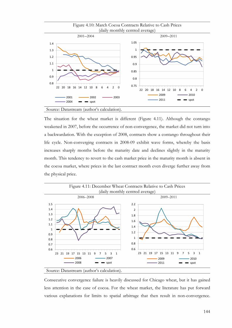
144

Figure 4.10: March Cocoa Contracts Relative to Cash Prices (daily monthly centred average)

2001–2004 2009–2011


The situation for the wheat market is different (Figure 4.11). Although the contango

weakened in 2007, before the occurrence of non-convergence, the market did not turn into

a backwardation. With the exception of 2008, contracts show a contango throughout their

life cycle. Non-converging contracts in 2008-09 exhibit wave forms, whereby the basis

increases sharply months before the maturity date and declines slightly in the maturity

month. This tendency to revert to the cash market price in the maturity month is absent in

the cocoa market, where prices in the last contract month even diverge further away from

the physical price.

Figure 4.11: December Wheat Contracts Relative to Cash Prices (daily monthly centred average)

2006–2008 2009–2011


Consecutive convergence failure is heavily discussed for Chicago wheat, but it has gained

less attention in the case of cocoa. For the wheat market, the literature has put forward

various explanations for limits to spatial arbitrage that then result in non-convergence.

0.8

0.9

1

1.1

1.2

1.3

1.4

22 20 18 16 14 12 10 8 6 4 2 0

2001 2002 2003

2004 spot

0.75

0.8

0.85

0.9

0.95

1

1.05

22 20 18 16 14 12 10 8 6 4 2 0

2009 2010

2011 spot

0.6

0.7

0.8

0.9

1

1.1

1.2

1.3

1.4

1.5

23 21 19 17 15 13 11 9 7 5 3 1

2006 2007

2008 spot

0.6

0.8

1

1.2

1.4

1.6

1.8

2

2.2

23 21 19 17 15 13 11 9 7 5 3 1

2009 2010

2011 spot

145

However, while studies suggest plausible theories about the occurrence of non-

convergence, it is argued here that those fail to explain the extent of the basis at the

contracts’ maturity date. The reasons for limits to arbitrage put forward in the literature

include insufficient storage space, specifications of the delivery certificates, and factors like

a large carry and price volatility which cause practitioners to refrain from selling

inventories.

Seamon (2010), for example, blames non-convergence on a shortage in delivery space. He

argues that, after a decade of a declining stock-to-use ratio, the good harvest in 2008/09

quickly exhausted existing storage capacities. Storage costs in turn increased, which

suppressed cash prices relative to futures prices. Indeed, wheat stocks in exchange

registered warehouses were high during the second jump in the basis from mid-2009 to

mid-2010 (Figure 4.12). This, however, was not the case when non-convergence started to

occur. In fact, stocks were low when the basis reached its first maximum in mid-2008 and

warehouses were only about 30 per cent full.

Figure 4.12: Wheat Basis and Storage at Exchange Registered Warehouses (monthly, Jan. 2008–Dec. 2012)

Basis and Storage Level Basis and Percentage of Storage Filled

Source: Datastream; USDA.

However, this observation on storage space can be explained by the time lag with which

stocks at the exchange-registered warehouses reflect new supply, especially in times of

previously low inventories. The harvest period for US winter wheat starts in mid-May,

which is about the time when the non-convergence problem started. Since commercial

storage space is filled before stocks in exchange-registered warehouses pile up, the excess

supply only becomes visible in exchange-registered storage facilities in later months. This is

a reasonable assumption as exchange inventories commonly reflect the quantity of residual

wheat, i.e., wheat that is not currently needed for commercial business, and hence it can be

-1.5

-1

-0.5

0

0.5

1

1.5

2

2.5

3

0

0.05

0.1

0.15

0.2

0.25

0.3

2008 2009 2010 2011 2012

Ba

sis

in U

SD

pe

r b

ush

el

Mill

ion

s o

f b

ush

els

of

wh

ea

t

Basis (F-S)

Stock

-1

-0.5

0

0.5

1

1.5

2

2.5

3

0

10

20

30

40

50

60

70

80

90

2008 2009 2010 2011 2012

Ba

sis

in U

SD

pe

r b

ush

el

% o

f st

ora

ge

ca

pa

city

fill

ed

Basis (F-S)

% Capacity Filled

146

freed for speculative purposes. With commercial storage facilities filling up, storage rates

were rising in May 2008 already, which then brought about the non-convergence.

Another explanation is based on the availability of delivery instruments. It is argued that

issuers of shipping certificates were reluctant to sell those certificates to potential arbitrage

traders, as the selling would have interfered with their normal merchanting activities

(O'Brien 2010). Every short trader in the futures market who seeks to make delivery has to

buy a shipping certificate from a regular firm—commonly a large commercial grain

merchant—that is eligible to issue such certificates. Hence, unless the short position holder

at the exchange is a regular firm, she is reliant on the availability of such certificates.

Regular firms, however, are not obliged to issue certificates. Although, according to the

CBOT rulebook, shipping certificates allow such firms to issue certificates over more

wheat than they store, the factor by which the certificates can exceed the amount stored in

registered warehouse is fixed (CBOT 2014). If they want to issue more certificates, they

eventually have to transfer wheat from their own warehouses to the exchange. Further, it

has been argued that since storage space at the exchange was already filled with wheat,

issuers of shipping certificates were reluctant to take on new wheat arriving due to high

opportunity costs incurred by a loss of space that could be used for storing other

commodities like soybeans and corn (Garcia, Irwin and Smith 2011).

The first argument fits the early period of non-convergence, when commercial grain traders

were still stocking up their previously depleted inventories for regular business. Hence, they

might have been reluctant to fill exchange-registered warehouses in order to sell shipping

certificates to potential arbitrage traders. The latter hypothesis applies to the second period

of non-convergence. During the time when the extent of non-convergence peaked first in

mid-2008, only 30 per cent of storage capacity at exchange registered warehouses was

filled. At the second peak, 70 per cent of storage capacity was taken (Figure 4.12).

Aulerich, Fishe and Harris (2011) ascribe the failure of convergence to a change in delivery

instruments. Instead of ‘warehouse receipts’, ‘shipping certificates’ were introduced.

Shipping certificates provide the owner with the option to choose if and when to take

control of the underlying physical commodity. The owner of the certificates can, instead of

executing his right to take physical delivery, sell the certificate into the next futures

contract. Since a shipping certificate can be conceptualised as an ‘embedded real option’,

which gains value with an increase in the price volatility of the underlying physical product,

owners of the certificate are incentivised to delay load-out when price volatility is high. This

147

might result in convergence failure. Indeed, price volatility was, by historical comparison,

high over the entire non-convergence period (Figure 4.13).

Figure 4.13: Wheat Price Volatility (3 months daily centred moving variance, in hundred USD per bushel,

Jan. 1990–Dec. 2012)


However, the CBOT wheat market was no exception and various other commodity futures

markets suffered from consecutive non-convergence, ones that had not introduced a

shipping certificate. In addition to wheat, Baldi, Peri and Vandone (2011) analyse the

CBOT corn and soybean markets, and Kaufman (2011) examines non-convergence in the

WTI crude oil market. Not all of these markets share the same delivery instruments.

Irwin, et al. (2011) argue that if the spread between the price of the expiring and the next-

to-expire contract is large enough to compensate for the costs of owning the delivery

instrument, i.e., the shipping certificate, the owner faces an incentive to postpone load-out.

This, in turn, postpones the purchase of the cash commodity, which holds back

convergence mechanisms. Hence, they investigate whether high two-to-one calendar

spreads, which is synonymous with a large financial carry67, occurred concurrently with

non-convergence in recent years. The financial carry was high before mid-2007 and after

mid-2009, but in-between the average percentage of full carry was at 50 per cent or below,

while non-convergence occurred (Figure 4.14).

67 The carry usually refers to the “percent of full carry” which is estimated as the percentage of the storage plus interest opportunity costs compensated for by the spread between the nearest to expiration and next

nearest to expiration contract price. This is represented by Hz = [email protected] G ∗ 100, with HI being the cost

of storage, J the foregone interest rate, and 1 and 2 the price of the nearest and next-nearest contract to maturity (Irwin, et al. 2011).

0

5

10

15

20

25

19

90

19

91

19

92

19

93

19

94

19

95

19

96

19

97

19

98

19

99

20

00

20

01

20

02

20

03

20

04

20

05

20

06

20

07

20

08

20

09

20

10

20

11

20

12

148

Figure 4.14: Wheat Basis and Average Percentage of Full Carry (at each contract’s maturity, Jan. 2006–Dec. 2012)


Irwin, et al. (2011) further investigate a hypothesis proposed by a staff report of the

Permanent Subcommittee on Investigations of the United States (US Senate 2009). The

staff report argues that index traders’ passive long positions have successively increased

futures prices, while physical prices remain unaffected by their demand and as a result led

to a large basis. Irwin, et al. (2011) test this hypothesis by event studies and Granger non-

causality tests. The event analysis shows a coinciding increase in carry with the roll of index

investors. In order to assess the continuity of the effect, Granger non-causality tests are

employed. Their results reject a significant impact of index traders’ positions on the market

carry, which leads the authors to argue that an increase in the precautionary demand for

commodity stocks driven by an increase in uncertainty about market fundamentals might

be at the root of the non-convergence. However, the observation that poor convergence

occurs whenever the carry is high is interesting and provokes the question: what caused the

large carry in the first place?

The previously discussed literature suggests cogent arguments for limits to arbitrage in the

wheat market. However, it fails to explain the extent of non-convergence. While non-

convergence can emerge if spatial arbitrage is limited, the extent of non-convergence

should still be confined by the possibility of fundamental arbitrage. Only a few researchers

attempt to explain this anomaly.

Garcia, Irwin and Smith (2011) argue that since storage costs at exchange-registered

warehouse are fixed by the exchange, physical storage charges eventually exceeded the

storage premium fixed by the exchange so that the calendar spread, which is bound to not

exceed financial full carry, could not fully reflect the costs incurred by storage in the

physical market. As a result costs were reflected in the non-convergence of futures and

-0.50

0.00

0.50

1.00

1.50

2.00

2.50

0

50

100

150

200

250

2006 2007 2008 2009 2010 2011 2012

Ba

sis

US

D p

er

bu

she

l

Ave

rag

e P

erc

en

tag

e o

f F

ull

Ca

rry

Basis[F-S]

AvPerFulCar

149

cash markets. They propose a ‘dynamic rational expectations commodity storage model’ in

which non-convergence could arise in equilibrium when the market price of physical

storage is greater than the cost of holding the delivery instrument, i.e., the premium charge

set by the exchange. They show that the ‘wedge’, which they define as the difference

between market storage costs plus convenience yield and the cost of holding the delivery

instrument, drives the basis at maturity.

Two independent equations for the cash and the futures market are assumed in their

model. The current cash price is defined as the continuously discounted expected future

cash price minus storage costs plus convenience yield, while the futures price is defined as

the continuously discounted expected futures price minus the exchange premium. The

difference between the current cash and futures price (basis) is hence the continuously

discounted expected basis plus the ‘wedge’ defined as: = ¡ − zJ − x, with ¡

being physical storage costs, zJ being the convenience yield which changes with

inventories, and x being the storage premium at the exchange68. The wedge is assumed to

vary with the level of inventories through the convenience yield and the physical storage

costs as long as the exchange premium remains constant. The authors argue that “a

relatively small wedge term in period t can have a large effect on the basis if it is expected

to persist for an extended period”, that is if it enters the expectation on the future basis.

However, for Garcia, Irwin and Smith’s (2011) model to be coherent, one has to accept

assumptions that violate the no-arbitrage conditions. Their model, and hence their

conclusion, is based on the crucial, however, implicit assumption that the cash price is

determined independently of the futures price. This assumption enables them to explain

the increasing basis in terms of the continuously discounted expected basis. This

assumption is necessary for their model to hold as otherwise the size of the basis could

only be related to the difference between physical storage costs and the storage premium at

the exchange (the wedge) and not to the expected basis. However, the size of the basis at

non-convergence is shown to be about 50 times the size of the wedge (van Huellen 2013).

Such a violation of no-arbitrage conditions demands justification. This can be found in the

financialisation hypothesis as outlined in Chapter 2. It has been argued that traders in the

physical and the futures market differ systematically in their investment motives and

strategies. As a result, expectations, investment decisions and hence prices are formed in a

fundamentally differently way in those markets. Depending on the relative weight of

68 The basis at maturity date T: − , = ¢9(I£¤)@ − ¡ zJ¥ − ¢9(C;£¤,;£¤)@; − x¥ ⇔ = ¢9(h;£¤)@; ¥.

150

traders, which are solely represented at the futures exchange, price differences can be

substantial. If limits to spatial arbitrage exist, those differences are carried over from one

contract into the next and the basis becomes excessive even at a contract's maturity.

What distinguished the Chicago wheat market case from other incidences of non-

convergence, and hence attracted attention, is that futures contracts traded far above

physical wheat prices. The rule that a contango has its maximum in the ‘carry cost proper’

(Lautier 2005) is hence consecutively violated. This is because a negative basis, as observed

in the case of wheat, in theory cannot exceed storage costs (, in Equation 2.2,

with, = 0; physical full carry). However, if limits to spatial arbitrage exist, this equation

cannot be enforced and the basis might exceed full carry.

For the cocoa market, in contrast to wheat, the sign of the basis was less puzzling, since a

positive basis depends on the ‘size’ of the convenience yield and hence has no limit

according to conventional theories. The case of the cocoa market consequently attracted

almost no attention. Commonly, a high marginal convenience yield, and hence a situation

of strong backwardation, is explained by a shortage of inventories. Cocoa storage levels

appeared relatively low during the months before non-convergence. This would explain the

market turning into backwardation. However, storage levels were rising again in late 2009

when non-convergence was prevalent (Figure 4.15).

Figure 4.15: Cocoa Basis and Storage Level at Exchange Registered Warehouses (monthly, Jan. 2006–Dec. 2012)

Source: Datastream; ICE Reporting Centre.

Arguably, in the wake of the crisis in Ivory Coast, market uncertainty was high and so was

the demand for precautionary inventories. Nevertheless, the convenience yield should

decline with a contract approaching its maturity date and eventually reach zero. Again, the

assumption of limits to spatial arbitrage is crucial. If these were not present, arbitrage

traders would take delivery in the futures market and sell in the physical market at a higher

0

50

100

150

200

250

300

350

400

450

500

0

1

2

3

4

5

6

2006 2007 2008 2009 2010 2011 2012

Mill

ion

s o

f co

coa

ba

gs

Basis [S-F]

Cocoa Stock

151

price. However, as argued for wheat before, if limits to arbitrage exist, convergence might

not be enforceable and the basis is carried over from one contract to the next.

For the cocoa market, reluctance or inability of physical traders to free their inventories for

speculative purposes could have contributed to limits to arbitrage. One likely reason is an

attempted squeeze, timed well with the arising shortage in the physical market, in the

London cocoa exchange, by one single hedge fund. Since October 2009, a single trader

built up a large long position in the July 2010 contract and eventually forced delivery of

over 240 thousand tonnes of cocoa—the entire European speculative stock (ICCO 2010).

As a result, cocoa prices at the London exchange reached a 33-year high, the basis spread

was inflated and the price differential between the American and the British exchange

reached more than $1,000 USD per tonne.

Hedgers assume that they are able to close out their futures position at a contract’s maturity

date. However, if a long trader is reluctant to close out her position, a short trader has to

deliver. When the hedge fund forced delivery for almost the entire long positions in the

July 2010 contract, short traders were forced to sell their inventory or acquire physical

cocoa to subsequently sell. If a short trader fails to deliver, the position is settled in cash,

which implies huge gains for the hedge fund and losses for the short trader (ICCO 2010).

As a result, inventories became scarce which, although the squeeze occurred on the

London exchange, had arguably direct implications also for the availability of speculative

stocks in the American futures market69.

While various cogent reasons for limits to spatial arbitrage have been presented for both

wheat and cocoa, research papers fail to explain the extent of non-convergence. I have

shown that Garchia, Irwin and Sanders’ (2011) structural model, which claims to explain

the extent of non-convergence, is based on the implicit assumption that price formation

mechanisms on the physical and the futures market differ systematically, which is a sharp

break with conventional rational expectation theories. In Chapter 2: Section 2.4 of this

thesis, a similar argument has been developed in the context of the financialisation

hypothesis, which suggests that physical and futures markets are driven by different market

fundamentals due to the different nature of traders active in the two markets. In the

following section I show that, by taking the assumption of trader heterogeneity serious, not

traders’ expectations of a continuously discounted market basis, as suggested by Garchia,

69 Such shortage would not show in the storage level since it is not caused by usage but by a change in ownership.

152

Irwin and Sanders’ (2011), explain the extent of non-convergence, but the different, though

linked, nature of investments and hence price formation at futures and cash market.

4.4.1 An Alternative Explanation for the Extent of Non-Convergence

Under normal market conditions, spatial arbitrage ensures that the equilibrium relationship

between cash and futures market prices holds at maturity regardless of the enforceability of

fundamental arbitrage. However, if there are limits to spatial arbitrage, deviations from the

efficient market hypothesis, that is limits to fundamental arbitrage, are revealed in the

market basis. In the presence of limits to spatial arbitrage, three market regimes can be

distinguished: (i) failure of fundamental arbitrage and storage cost differential, (ii) failure of

fundamental arbitrage, (iii) fundamental arbitrage.

¤,8 − ¤ = §©ª'¤,8/ − '¤,8/1 ¤ − x¤,8 ¡¤,8 − z¤,8 y'¤,8/ − '¤,8/ 1 ¤ yy0yyy

(4.8)

The efficient market hypothesis postulates that: '¤,8/ = ¤,8 = '¤,8/ = 8 so

that the futures price at T1 maturing at T2 is an unbiased estimator of the futures price at T2

maturing at T2, and the futures price maturing at T2 is an unbiased estimator of the

expected and realised cash price at T2. If these conditions hold, case (iii) prevails and

convergence is established despite limits to spatial arbitrage. However, if fundamental

arbitrage is rejected, expectations on futures and cash markets might not be congruent and

this gives rise to case (ii). In this case, expectations regarding future cash prices and future

futures prices are formed independently. Case (i) corresponds to Garchia, Irwin and

Sanders’ (2011) model in which price expectations are independent and storage cost

differentials occur.

If fundamental arbitrage is rejected, Keynes’s normal backwardation, which was later

transformed into hedging pressure, provides a strong argument for why expected cash

prices do not need to equal expected futures price. Hedging pressure models build on the

crucial dichotomy between ‘hedgers’ and ‘speculators’ as two distinct types of market

actors. With the entrance of new types of traders, this assumption has to be amended by

another category: index traders. Following the rationale of the hedging pressure hypothesis,

if a counterparty is scarce, due to market frictions like transaction costs, capital constraints

or fundamental uncertainty, the price has to move in order to attract traders to enter into

153

the market as a counterparty. Index traders, similarly to commercial hedgers, have to

compensate other non-commercial traders for entering into a contract. This consequently

causes the futures price to be a biased estimator for the expected future cash price. In other

words, the futures price will diverge from its fundamental value by the price pressure

exerted by either hedgers or index traders.

Since hedgers are predominantly net-short, index traders essentially supply liquidity to

commercial traders. This decreases the costs of hedging and as a result eases the

(downward) hedging pressure on prices. Hence, the presence of index traders could even

increase market efficiency in that they decrease the bias arising from hedging pressure. This

is only the case as long as index demand is not in excess of hedging positions. Index traders

indeed appear to have taken over the counterparty role for commercial hedgers from other

non-commercial traders for the cocoa and wheat market. However, in some cases, index

traders are far in excess of commercial traders' hedging demand, so other non-commercial

traders have to step in to cover the index traders’ long positions. I refer to such situation as

index pressure.

In Figure 4.16, the area for jointly commercial and non-commercial net-long positions

turns into a light purple (labelled excess com) when index traders’ net-long positions are fully

covered by commercial traders’ net-short positions. That is when non-commercial traders

are needed to take the counter position to commercial hedgers as in the hedging pressure

hypothesis. In the case where the area is in a light orange (labelled excess ncom), non-

commercial traders are needed to take the counter position of index traders because these

are not fully taken up by commercial traders. This is a case of index pressure.

Figure 4.16: Hedging and Index Pressure (monthly open interest, Jan. 2006–Dec. 2013)

Wheat

-0.25

-0.2

-0.15

-0.1

-0.05

0

0.05

0.1

0.15

0.2

0.25

0.3

20

06

20

07

20

08

20

09

20

10

20

11

20

12

20

13

Mill

ion

s

154

Cocoa

Source: CFTC (author’s own calculation).

For the wheat market, the case where index traders’ net-long positions are in excess of

hedgers' net-short positions prevails. As a result, the hedging pressure hypothesis is

reversed: speculators are needed to fill the long positions of index traders. In this case, the

futures price is expected to be upward-biased, since short traders need to be attracted. For

the cocoa market, the graph looks quite different. Only in late 2010 and between mid-2011

to mid-2012 did index traders’ positions exceed hedgers’ demand.

The predictions made by the index pressure hypothesis appear to be validated by the

examples of the cocoa and the wheat market. If index traders’ net-positions exactly cover

commercial traders’ net-hedging positions, the premium is expected to be zero. If passive

long traders exceed net-short hedging positions, the bias is expected to be positive, which

means a negative basis (index pressure: futures exceeds cash price). The reverse is predicted

when commercial net-short positions exceed index traders' net-long positions, which

means a positive basis (hedging pressure: cash exceeds futures price), as summarised by

Equation 4.9.

«y¬ = 0, y~wW ywW = 0> 0, y~wW ywW > 0< 0, y~wW ywW < 0 (4.9)

Since index trader participation in the cocoa market is relatively low so that the excess com

situation dominates in Figure 4.16, a positive market basis is expected. For the wheat

market, where index participation is relatively high and non-commercial traders have to

cover the excess long positions by index traders, the reverse is the case. As net-long index

-0.14

-0.12

-0.1

-0.08

-0.06

-0.04

-0.02

0

0.02

0.04

0.06

0.08

0.1

2006 2007 2008 2009 2010 2011 2012 2013 2014

Mill

ion

s

155

positions are larger than net-short commercial positions, the market basis is expected to be

negative. Both predictions are reflected in the actual market regimes.

Various causes for the occurrence, inspired by existing literature, of non-convergence were

noted in the previous section, while the present section has put forward a hypothesis on

the factors that explain the extent of non-convergence, which especially in the case of

wheat, was puzzling and remains so far unexplained. Garcia, Irwin and Sanders (2011)

attempt a formal model which they argue explains the extent of non-convergence.

However, their model was built on the implicit assumption that the formation of

expectations in the physical and the futures markets takes place independently. It is argued

here that such a deviation from conventional theories demands justification. This

justification is found in the financialisation theory. The reference of the financialisation

hypothesis does not only justify the implicit assumption made by the Garcia, Irwin and

Sanders (2011) model, but also suggests a radically different explanation for the extent of

non-convergence, which is index and hedging pressure. In the following sub-section, the

hypotheses about the extent of non-convergence discussed in the literature and the

alternative explanations promoted by this thesis are tested.


In an attempt to explain the extent of non-convergence, i.e., the size of the basis at

maturity, a simple regression analysis is conducted which relates the basis to various factors

which have been advanced in the literature cited above as well as to hedging and

speculative demand as hypothesised in this thesis.

The basis is defined as the difference between cash and futures prices − >, = >, at

each contract’s maturity, with y indicating the yth contract (e.g., May 2008 contract) at its

maturity date (e.g., 14th of May 2008). For the wheat market, price data for the cash and

the futures price have been obtained from Thomson Reuters Datastream. The futures price

is the CBOT no. 2 soft red winter wheat settlement price at the last day of trading of each

contract. The cash price is the no. 2 soft red winter wheat spot price at St. Louis provided

by the USDA.

Open interest differentiated by trader type, with commercial, non-commercial, index, and

non-reporting traders who hold positions below the reporting level, is obtained from the

CIT report. The relative market weight of each trader type is calculated as the average

percentage share of traders’ open interest (long plus short) in total open interest in the last

156

trading days of the contract, starting with the first trading day of the expiration month and

ending with the contract’s expiry day, which is usually two weeks into the maturity month.

The storage premium at the exchange is obtained from the CBOT. Data on storage costs

outside the exchange are not available, and hence the exchange premium can only serve as

an approximation for the variation in the storage costs difference. In order to capture limits

to arbitrage, which were related to storage capacity, the wheat stock-to-use ratio is used.

The estimate for the stock-to-use ratio is based on the USDA Wheat Yearbook Table 5 and

calculated as the ratio between ending stocks and total disappearance (depletion of

inventory) over the same period. As the data are available only quarterly, the ratios are

matched with different contracts in the following way: March with Q370 (December to

February), May with Q4 (March to May), July with the average of Q4 and Q1 the following

year, September with Q1 (June to August), December with Q2 (September to November).

The stock-to-use ratio is not ideal, as it does not capture the opportunity costs that might

have arisen due to a shortage of storage space. An alternative variable, the percentage of

storage capacity filled in CBOT exchange-registered warehouses is obtained from the

USDA Grain Stock Report, published every Friday. The observation on the last Friday

before each contract’s final trading day is used.

Lastly, the average percentage of full carry is estimated as the ratio between the total costs

of holding the delivery instrument until a contract’s maturity and the two-to-one calendar

spread over the life cycle of each contract from the point where it became the next-to-

maturity contract till its maturity (CME Group 2009). The interest rate used is the three-

month USD LIBOR plus 200 basis points, which is obtained from Thomson Reuters

Datastream. The variables used are summarised in Table 4.8.

Table 4.8: List of Wheat Market Variables

Variable Description

basis CBOT Soft Red Winter Wheat basis in USD cents per bushel of wheat.

index Average percentage share of index traders open interest (long plus short).

ncom_sp Average percentage share of non-commercial spread trader’s open interest.

ncom-sp Average percentage share of non-commercial traders’ open interest (long plus short excluding spread traders).

com Average percentage share of commercial traders’ open interest (long plus short).

nrep Average percentage share of non-reporting traders’ open interest (long plus short).

StCost Exchange premium for the currently trading contract in USD cents per bushel per day.

StToUs Stock-to-use ratio.

AvFlCar Average of the percentage of financial full carry over the contract’s life cycle.

CapFil Percentage of capacity filled in exchange registered warehouses at the contract’s maturity.

70 The quarters do not follow the calendar year, but the crop year.

157

The time period covered starts with the March 2006 contract and ends with the maturity of

the September 2012 contract. There are 35 observations in total. Unfortunately, data for

the percentage of storage filled in exchange-registered warehouses are only available from

January 2008 onwards, which constrains the sample of the model in which the variable is

included to 22 observations.

For cocoa, the traders’ position data are chosen in the same way as for wheat. For the cash

price, the Ivorian cash market price provided by Thomson Reuters Datastream is chosen.

The stock-to-grinding ratio is taken from the ICCO Quarterly Bulletin of Cocoa Statistics.

The data entries are available for March, June, October, and December. March is paired

with the March contracts’ maturity dates. For the May contracts’ maturity dates the average

between the March and June stock-to-grinding values is taken. July is paired with June.

Stock-to-grinding values for October are paired with the September maturity contracts and

the values for December with the basis values for contracts maturing in December.

Table 4.9: List of Cocoa Market Variables

Variable Description

basis ICE Cocoa basis in USD per tonne of cocoa.

index Average percentage share of index traders open interest (long plus short).

ncom_sp Average percentage share of non-commercial spread trader’s open interest.

ncom-sp Average percentage share of non-commercial traders’ open interest (long plus short excluding spread traders).

com Average percentage share of commercial traders’ open interest (long plus short).

nrep Average percentage share of non-reporting traders’ open interest (long plus short).

stCost The weighted average of storage costs in ICE registered warehouses.

stToGr Stock-to-grinding ratio.

iceMilSt Level of stocks at the ICE exchange registered warehouses.

exRate The end of month exchange rate CFA Franc per USD for the contract month.

The storage rate is calculated based on the actual storage rates as of date May 2001. The

weighted average was calculated from the storage rates at Port of New York, Port of

Delaware River, Port of Baltimore, and Port of Hampton Roads. The weights are derived

from the percentage share of cocoa stored at the respective ports. Regarding the interest

rate, the end of month value for the month in which the contract matures is taken. The

data are provided by the IMF, IFS data service. Variables used are summarised in Table 4.9:

4.4.3 Empirical Results

Different model specifications are run with the basis [] as the dependent variable and

varying explanatory variables in order to assess the contribution of each factor to the size

of the basis at maturity. The models are specified as:

158

= 1] ^1>>, n , y!n~JJL (4.10)

>, is the ith explanatory variable at the Tth maturity. 1]is the intercept coefficient and 1> is the slope coefficient of the ith explanatory variable, and n is the error term. The tables

below provide an overview of estimated coefficients, their standard errors, partial r-squares,

and residual diagnostics for each model (Tables 4.10-13).

4.4.3.1 Results for Wheat

Table 4.10 shows the regression results for the first three model specifications for the

wheat market. The first model specification includes the weight of speculative demand as

the percentage share of each trader group in total market open interest. Commercial

traders’ share is excluded in the first model specification to avoid perfect collinearity

between explanatory variables. The coefficient for the market weight of non-commercial

non-spread traders and index traders is negative and highly significant. The remaining

coefficients are insignificant. The overall fit of the model appears relatively good, with an

R-squared of about 0.6. However, residual diagnostics reveal a significant degree of

autocorrelation that indicates omitted variables.

Table 4.10: Wheat Regression Results and Residual Diagnostics for Model 1–3 Model 1 Model 2 Model 3

basis coeff. s.d. part. r^2 coeff. s.d. part. r^2 coeff. s.d. part. r^2

constant 1113.20*** 200.1 0.5178 947.81*** 164.0 0.5439 917.243*** 180.4 0.5084

index -25.273*** 4.490 0.5221 -24.882*** 3.574 0.6339 -24.9211*** 3.392 0.6834

ncom_sp -1.36663 2.602 0.0094 -2.77120 2.097 0.0587 -3.85766* 2.096 0.1284

ncom-sp -16.823*** 4.566 0.3189 -14.257*** 3.684 0.3485 -14.010*** 4.239 0.3040

nrep -18.4642 8.471 0.1408 -10.3022 7.013 0.0716 -7.60530 6.867 0.0468

stCost - - - 17966.*** 4259. 0.3886 16188.3*** 4132. 0.3804

stToUs - - - - - - 0.167315* 0.09663 0.1071

avFlCar - - - - - - -0.394175* 0.2141 0.1194

Diagnost.

sigma RSS R^2 Adj.R^2 log-likelihood Joint test: F(4,29) AR1-2.: F(2,27) Normal: Chi^2(2) Hetero.: F(8,25)

47.3613 65049.7463 0.596734 0.541111 -176.705 10.73 [0.000] 3.756 [0.036] 0.300 [0.861] 0.588 [0.779]


37.6883 39771.3305 0.753443 0.709416 -168.341 17.10 [0.000] 0.468 [0.631] 1.653 [0.438] 1.130 [0.383]

sigma RSS R^2 Adj.R^2 log-likelihood Joint test: F(7,26) AR1-2.: F(2,24) Normal.: Chi^2(2) Hetero.: F(14,19)

35.6689 31806.6893 0.80045 0.744576 -160.195 14.30 [0.000] 0.214 [0.809] 2.684 [0.261] 0.845 [0.620]

Note: * indicating significance at 10% level, ** indicating significance at 5% level, and *** indicating significance at 1% level respectively.

Since the market weight of different trader groups in the derivative market is unlikely to

directly affect the cash market, the negative coefficients indicate that non-commercial

traders’ relative demand results in a significant increase in the futures prices relative to the

cash prices. Estimated coefficients suggest that, ceteris paribus, if the market weight of

159

index traders increases by one per cent (either due to decreasing positions of non-index

traders or increasing open interest by index traders), the futures price increases by about

$0.25 USD per bushel of wheat on average relative to the cash price. For non-commercial

non-spread traders’ this would ceteris paribus result in a $0.17 USD per bushel of wheat

increase on average in the futures relative to the cash price.

In order to solve the non-convergence problem, the CBOT introduced a variable storage

rate (VSR) that was designed to successively narrow the gap between the storage premium

at the exchange and the storage rate in the physical market—the wedge. The VSR, effective

since the July 2010 contract’s maturity, increases at each contract’s maturity as long as

financial full carry prevails (CME Group 2009). Since the model seems to systematically

under-predict the size of the basis after mid-2010, when the VSR was introduced

(Figure 4.17), the second model specification includes the exchange storage premium

(stCost) as an additional explanatory variable.

Figure 4.17: Model 1–3 Observed and Fitted Basis at CBOT Wheat (in USD per bushel)

Source: Author’s calculation.

The additional coefficient is significant and the model has a better fit compared to the

previous one. Residual diagnostics also suggest spherical residuals. The size of the

coefficient indicates that for a 10/100 cent per bushel per day increase in the storage

premium, the futures price would ceteris paribus decrease by almost $1.80 USD on average

relative to the cash price.71 This effect counterbalances the otherwise upward price pressure

on the futures prices by non-commercial traders’ market weight, and hence adjusts for the

under prediction of the basis in the latter half of the sample period. This confirms Garcia,

71 Note that the storage rate is expressed in USD cents and is increased by 10/100 USD cents each time the average percentage of full carry over the maturing contract exceeded 80 per cent. Hence, it increases stepwise by 0.001 USD cents and not 1 USD cents, which means that the coefficient has to be divided by 100 for a meaningful interpretation.

-2.5

-2

-1.5

-1

-0.5

0

0.5

1

3 5 7 9 12 3 5 7 9 12 3 5 7 9 12 3 5 7 9 12 3 5 7 9 12 3 5 7 9 12 3 5 7 9

2006 2007 2008 2009 2010 2011 2012

basis

fitted01

fitted02

fitted03

160

Irwin, and Sanders’ (2011) hypothesis that a mismatch in the storage premium causes non-

convergence. According to their model, a higher exchange premium results in a smaller

wedge and consequently in a reduction of the difference between cash and futures prices

(decrease of the basis in absolute terms), as predicted in Equation 4.8.

Besides the storage premium mismatch, two further explanations for successive non-

convergence in the wheat market were put forward in the literature: firstly a high market

carry which resulted in a reluctance to load out, and secondly, insufficiencies in the delivery

system. In order to account for these two effects, the average percentage of full carry

(avFlCr) and the stock-to-use ratio (stToUs) are included. Both coefficients are weakly

significant. The coefficient on the average full carry is negative, supporting the theory that

the compensation for storage costs is related to non-convergence. However, the carry can

only explain the existence of limits to arbitrage but not the extent of non-convergence,

which probably accounts for its low significance. The coefficient on the stock-to-use ratio

is positive, indicating that as stocks increase relative to use, that is as supply becomes

relatively abundant, the premium of the futures price relative to the spot price decreases.

This is consistent with the theory of storage, which predicts that the marginal convenience

yield is a negative function of inventories (Pindyck 2001).

One might argue that the significance of the market weight of non-commercial traders is

due to a decreasing market weight of commercial traders resulting from a loss in hedging

effectiveness. Hence, the causality would be the reverse, where commercial traders exit the

market because of an increasing basis. The counter image of this effect is an increase in the

market share of non-commercial traders, which then shows a significant effect falsely

suggesting causality. In order to test for this alternative hypothesis, a fourth model is run

with the percentage share of commercial traders included (Table 4.11).

Indeed, by only including the share of commercial traders, the coefficient is significantly

positively related to the basis, supporting the above argument. However, the size of the

coefficient is smaller than the estimated effect of the market share of non-commercial

traders on the market basis. Further, comparing adjusted R-squares of model one with

model four, as a rough indicator of the relative goodness of fit, the first model specification

appears preferable. However, in order to test whether index trader or commercial traders’

market weight has the greater explanatory power, a direct comparison of models with only

one of the respective variables included is needed. This is done in model five. Both partial

r-square and adjusted R-square are significantly larger for the fifth model specification

where index traders’ market weight is included compared to the fourth model where only

161

the average share of commercial traders is included. This indicates that, while some of the

effect of index traders found in model three might be due to a decrease in commercial

traders' share, a great part is solely due to index traders’ price pressure effect.

Table 4.11: Wheat Regression Results and Residual Diagnostics for Model 4–6 Model 4 Model 5 Model 6

basis coeff. s.d. part. R^2 coeff. s.d. part. R^2 coeff. s.d. part. R^2

constant -385.16*** 68.40 0.5311 399.44*** 91.48 0.4051 976.228*** 297.3 0.4182

com 8.74365*** 2.184 0.3640 - - - - - -

index - - - -22.375*** 3.562 0.5850 -29.2057*** 5.822 0.6265

ncom-sp - - - - - - -13.9427** 5.845 0.2751

ncom_sp - - - - - - -2.68197 2.725 0.0606

nrep - - - - - - -7.37043 9.342 0.0398

stCost 20030.1*** 5424.0 0.3275 20168.*** 4360.0 0.4332 13886.5** 4720. 0.3659

stToUs 0.225253* 0.1248 0.1043 0.3004*** 0.1012 0.2392 - - -

avFlCar -0.267085 0.2826 0.0309 -0.15931 0.2260 0.0174 -0.419307* 0.2358 0.1741

capFil - - - - - - 1.81619* 0.9738 0.1882

Diagnost.


50.72 72030.6072 0.548092 0.483534 -173.683 8.49 [0.000] 1.14 [0.336] 10.6 [0.005] 1.05 [0.428]


40.9724 47004.5593 0.705102 0.662973 -166.64 16.74 [0.000] 0.091 [0.913] 0.341 [0.843] 2.471 [0.041]


36.0535 19497.8237 0.84928 0.778944 -110.175 12.07 [0.000] 0.090 [0.915] 3.414 [0.181] 5.133 [0.013]


This conjecture is further confirmed by an additional model (not reported here), which

jointly includes commercial and index traders’ market share and excludes non-commercial

spread traders instead. The coefficient on the market weight of commercial traders turns

insignificant while still positive. Although non-significant, the inclusion of commercial

traders’ market weight seems to result in a decrease of the effect of index traders, which

suggests that these trader groups are not independent. However, the effect of index traders’

market weight, as well as that of non-commercial non-spread traders’ market weight,

remains significant. This refutes the pervious hypothesis that non-commercial traders’

market weight is only significant on the basis of it being the counter-image of commercial

traders’ market weight.

Further, the variable for the stock-to-use ratio does not fully capture the argument of the

insufficiencies in the delivery system, which is related to high opportunity costs of storing

additional wheat as storage space becomes scarce. Hence, the stock-to-use variable (stToUs)

is replaced by the percentage of storage space filled at exchange-registered warehouses

(capFil) in a sixth model. Unfortunately, data for this new variable are only available from

January 2008 onwards, which reduces the sample size of this particular model to 22

observations. The coefficient for the additional variable is significant at the ten per cent

162

level and positively related to the market basis. This confirms the theory that a shortage in

storage capacity has contributed to limits to spatial arbitrage. However, the variable is

unable to explain the extent for non-convergence. Fitted and observed values for the basis

for model four to six are presented in Figure 4.18.

Figure 4.18: Model 4–6 Observed and Fitted Basis at CBOT Wheat (in USD per bushel)


4.4.3.2 Results for Cocoa

For the cocoa market, similar regression results are conducted, however, explanatory

variables differ slightly. The first model, as previously, includes the relative market weight

of different groups of non-commercial traders (Table 4.12). As for wheat, index traders’

market share is highly significant. A weakly significant coefficient is found for non-

commercial excluding spread traders’ and non-reporting traders’ market share. However,

while the coefficient for non-commercial traders has the same negative sign as in the case

of the wheat market, index traders’ market weight is positively related to the size of the

cocoa basis in contrast to findings for the wheat market.

This means that the larger the percentage share of index traders, the larger the market basis.

Since index traders are unlikely to directly impact the cash market price, index traders’

market weight appears to be negatively related to the futures prices. This is in stark contrast

to the index pressure hypothesis, which predicts the reverse. However, it partly supports

the information content hypothesis, since the greater the share of uninformed traders, the

further the futures prices is assumed to disengage with its underlying physical price. It

follows that the greater the share of index traders, the greater the share of uninformed

traders, the lower the information density and thus the greater the market basis in absolute

terms due to uncertainty and limits to arbitrage arising.

-2.5

-2

-1.5

-1

-0.5

0

0.5

1

3 5 7 9 12 3 5 7 9 12 3 5 7 9 12 3 5 7 9 12 3 5 7 9 12 3 5 7 9 12 3 5 7 9

2006 2007 2008 2009 2010 2011 2012

basis

fitted04

fitted05

fitted06

163

Table 4.12: Cocoa Regression Results and Residual Diagnostics for Model 1–3 Model 1 Model 2 Model 3


constant 39.6368 238.9 0.0009 224.213 481.5 0.0080 3257.87*** 758.2 0.4152

index 24.8985*** 8.169 0.2365 25.7324*** 7.172 0.3229 35.973*** 7.524 0.4679

ncom_sp 1.57133 6.273 0.0021 6.98208 5.691 0.0528 7.99079 5.151 0.0847

ncom-sp -10.8339* 5.593 0.1112 -3.64360 6.103 0.0130 3.49614 6.123 0.0124

nrep 52.7369* 27.11 0.1120 24.2769 26.11 0.0310 14.0208 23.88 0.0131

stCost - - - -1403.20** -2.21 0.1538 -1910.22*** 602.6 0.2788

stToGr - - - 16.3691** 6.033 0.2143 15.349*** 5.459 0.2332

iceMilSt - - - -26.2380 21.92 0.0504 -22.4902 19.83 0.0471

exRate - - - - - - 1.51411** 0.5668 0.2153

Diagnost.

sigma RSS R^2 Adj.R^2 log-likelihood Joint test: F(4,30) AR 1-3: F(3,27) Normal: Chi^2(2) Hetero.: F(8,26)

107.169 321588.368 0.439111 0.360885 -198.37 5.80 [0.001] 4.82 [0.008] 0.60 [0.740] 2.37 [0.046]


90.849 222845.667 0.620563 0.52219 -202.943 6.308 [0.000] 1.278 [0.304] 0.304 [0.859] 0.682 [0.766]


82.0087 174861.008 0.702266 0.610655 -198.7 7.666 [0.000] 0.542 [0.658] 0.372 [0.830] 1.024 [0.477]


In a second model, carry variables are included in addition to speculators’ market weight.

Storage costs (stCost) are highly significant and show an inverse relationship to the size of

the basis. The finding confirms the theory of storage, which predicts that ceteris paribus the

higher the storage cost, the larger the futures price relative to the cash price (stronger

contango). The stock-to-grinding ratio (stToGr) shows a significant positive relationship to

the market basis. This is puzzling, because, conventionally, the convenience yield should be

negatively related to the ratio. However, the reverse sign in the context of non-convergence

could be an indication of storage hoarding as outlined in Deaton and Laroque’s (1992)

model. If actors refuse to free speculative inventory for arbitrage trades, non-convergence

can arise, resulting in a positive link between basis and stock-to-grinding ratio. This effect

has been present in the cocoa market during the previously discussed market squeeze.

In a third model, the CFA Franc-USD exchange rate (exRate) is added in order to account

for idiosyncratic factors of the particular cash market price. The exchange rate is significant

and positively related to the market basis, which can either be due to a positive effect on

the cash price or a negative effect on the futures price. This is because the higher the

exchange rate the more expensive the domestic currency and the cheaper the product for

imports. Both the exchange rate and the commodity futures price are forward looking

(Chen, Rogoff and Rossi 2010). Hence, an explanation for the observed sign is that the

futures price incorporates the information signalled by the exchange rate sooner than the

cash price and hence decreases while the cash price remains unaffected in the short-run.

The adjusted r-square is highest for the third model and residuals for the second and third

164

model are spherical. Looking at the fitted values against the observed, the superior fit of

the third model is evident (Figure 4.19).

Figure 4.19: Model 1–3 Observed and Fitted Basis at ICE Cocoa (in USD per tonne)


As previously for the wheat market, it is tested whether the significant effect of index

traders is a result of a relative change in other trader’s market weight. Models four and five

include index traders’ and commercial traders’ market weight, respectively. The results for

cocoa are concur with findings for the wheat market in that coefficients for both trader

types are significant, however the model fit is better and partial r-square is higher for the

model with index traders’ market weight included (Table 4.13).

Table 4.13: Cocoa Regression Results and Residual Diagnostics for Model 4–6 Model 4 Model 5 Model 6


constant -196.765 357.3 0.0103 861.605* 492.0 0.0956 119.964 418.5 0.0029

com - - - -17.799*** 4.544 0.3461 -6.15367 4.409 0.0650

index 39.2616*** 6.086 0.5893 - - - 33.0704*** 7.453 0.4129

stCost -1655.7*** 528.9 0.2526 -1782.38** 696.3 0.1843 -1873.58*** 543.4 0.2980

stToGr 14.4763*** 4.749 0.2427 21.413*** 6.038 0.3025 16.2795*** 4.848 0.2871

iceMilSt -22.5945 18.99 0.0465 -13.1589 24.07 0.0102 -19.4593 18.83 0.0368

exRate 1.45531*** 0.4977 0.2277 1.35223** 0.6516 0.1293 1.66897*** 0.5131 0.2742

Diagnost.


81.172 191077.791 0.674654 0.61856 -200.252 12.03 [0.000] 1.021 [0.399] 0.389 [0.823] 2.353 [0.042]


102.432 304277.309 0.48191 0.392584 -208.394 5.395 [0.001] 1.759 [0.180] 1.019 [0.601] 1.399 [0.240]


79.8771 178649.732 0.695815 0.630632 -199.075 10.67 [0.000] 0.638 [0.598] 0.128 [0.938] 1.538 [0.184]


In a sixth model, both the relative market weight of index and commercial traders’ is

included. As for the wheat market, the commercial trader variable turns insignificant and

the partial r-square for both, index and commercial traders’ market weight decline, which

0

100

200

300

400

500

600

700

800

3 5 7 9 12 3 5 7 9 12 3 5 7 9 12 3 5 7 9 12 3 5 7 9 12 3 5 7 9 12 3 5 7 9 12

2006 2007 2008 2009 2010 2011 2012

basis

fitted01

fitted02

fitted03

165

indicates that these are not independent. The model fit of the sixth model specification is

found best and fitted values are able to replicate most of the basis size at maturity for the

observation period. While the first model under-predicts the extent of the basis between

2009 and 2011, model three with carry variables included yields a better fit. When

accounting for idiosyncratic factors, by the addition of the exchange rate, the basis size at

non-convergence is almost fully replicated (Figure 4.20).

Figure 4.20: Model 4–6 Observed and Fitted Basis at ICE Cocoa (in USD per tonne)


4.4.3.3 Comparison Wheat and Cocoa

Results for the cocoa market regarding the market weight of commercial and index traders

are puzzling. While coefficients for wheat regarding traders’ market weight yield signs in

line with the hedging and index pressure hypotheses, signs are reversed for the cocoa

market. The reason for this might be found by taking a closer look at traders’ position

taking in the two markets.

It is assumed that hedgers are not sensitive to the price level but to hedging effectiveness,

while index traders are not sensitive to idiosyncratic market factor. With declining hedging

effectiveness, the share of commercial traders is expected to decline, which means that the

share of index traders would increase as a result of commercial hedgers reacting to

convergence failure. This would mean that the higher the degree of non-convergence, the

higher the share of index traders as they react to idiosyncratic anomalies with a lag (or not

at all). Consequently, with the increasing share of index traders in the market, index

pressure increases. If index traders’ net positions exceed commercial hedgers net hedging

demand, a positive price bias is introduced, which strengthens the market’s contango and

causes the basis to turn negative (or become even more negative). The coefficient for the

wheat market suggests this relationship.

0

100

200

300

400

500

600

700

800

3 5 7 9 12 3 5 7 9 12 3 5 7 9 12 3 5 7 9 12 3 5 7 9 12 3 5 7 9 12 3 5 7 9 12

2006 2007 2008 2009 2010 2011 2012

basis

fitted04

fitted05

fitted06

166

Looking at total and net positions by different trader types, these behavioural assumptions

are confirmed for the wheat market. While net positions remain relatively stable, large

swings are observable in total positions. All trader types significantly reduced their total

positions over the time period of non-convergence. This is more pronounced for

commercial and non-commercial traders than for index traders. As a result, the market

weight of index traders increased (Figure 4.21).

Figure 4.21: Wheat Market Trader Positions (basis in USD (right), positions in thousands(left), Jan. 2006–Dec. 2012)

Total Positions Net Positions

Source: Datastream, CFTC CIT.

For the cocoa market the case is different, since commercial traders did not close out their

hedging position when non-convergence occurred. This is because commercial traders,

who are mostly short in the futures market, gain from the mispricing between cash and

futures prices in the particular case of the cocoa market. In the case of an overall price

increase, a positive basis indicates that the futures price does not rise as much as the

physical. Short hedgers hence gain on their futures position since the hedge does not fully

offset the price rise. Further, if the price level drops, the futures price drops more than the

cash market price and hence short hedgers again make a net gain. Therefore, short hedgers

are incentivised to stay in the market and even over-hedge. This explains why commercial

trader total positions were increasing during the period of non-convergence (Figure 4.22).

However, commercial net positions are not net-short the entire time period. The crisis in

Cote d’Ivoire is probably one cause of this development. With traders predicting coming

shortages, owners of the commodity are incentivised to under hedge, while consumers are

motivated to over hedge. With commercial traders betting on increasing prices, they turn

net-long just before the peak of non-convergence in early 2011. With hedgers being net-

-100

-50

0

50

100

150

200

250

300

0

100

200

300

400

500

600

2006 2007 2008 2009 2010 2011 2012

Basis [F-S] ncom_tot

com_tot index_tot

-250

-200

-150

-100

-50

0

50

100

150

200

250

-250

-200

-150

-100

-50

0

50

100

150

200

250

2006 2007 2008 2009 2010 2011 2012

Basis [F-S] com_nl

ncom_nl index_nl

167

long, the hedging pressure hypothesis is inverted, which explains the negative sign for

commercial traders in the cocoa market in contrast to the wheat market.

Figure 4.22: Cocoa Market Trader Positions (basis in USD (right), positions in thousands(left), Jan. 2006–Dec. 2012)

Total Positions Net Positions

Source: Datastream, DFTC CIT.

The second puzzle for the cocoa maker is the significant positive sign of the coefficient on

index trading. A possible explanation is the roll effect executed by index traders. Since the

market shows a strong backwardation (and the whole futures curve is inverted) index

traders earn roll yields when rolling over their positions. The prospect of a roll yield

motivates index traders to roll their positions more frequently (possibly each maturity

month). Index traders who close out their positions when a contract matures execute

downward pressure on the contract they are in and hence increase the market basis even

further (see Figure 2.4).

This explains why the futures price moved even further away from the cash price short

before maturity (Figure 4.10). While index traders over the contract’s life cycle execute no

significant price pressure, since commercial traders fully cover index positions most of the

time, they execute price pressure close to a contracts’ maturity date, when the market gets

thin.

Index traders in the wheat market execute significant price pressure over a contract's life

cycle. They hence strengthen the market’s contango and contribute to a continuously

decreasing market basis. If limits to spatial arbitrage exist, as suggested by the literature and

confirmed empirically, this results in a large negative basis which is carried over from one

contract into the next. In contrast, the market weight of index traders in the cocoa market

is marginal throughout a contract’s life cycle but potentially significant at maturity. With

-200

0

200

400

600

800

1000

0

50

100

150

200

250

300

Basis [S-F] ncom_tot

com_tot index_tot

-1000

-800

-600

-400

-200

0

200

400

600

800

1000

-100

-80

-60

-40

-20

0

20

40

60

80

2006 2007 2008 2009 2010 2011 2012

Basis [S-F] com_nl

ncom_nl index_nl

168

those traders having an additional incentive to rollover their contracts frequently due to an

inverted market regime, index traders execute downward price pressure on maturing

contracts, further increasing a positive market basis shortly before maturity. In both cases,

index traders contribute significantly to the absolute size of the market basis at maturity.

Figure 4.23: US Wheat Cash Prices minus Prices in Canada, Argentina, Australia (monthly, in USD per metric ton, May 1989–Apr. 2013)

Source: USDA.

For both markets, convergence was eventually restored. In the cocoa market, the market

basis declined again in mid-2011, when expectations about future shortages due to the civil

war in Cote d’Ivoire were revised as the harvest and exports remained almost stable and the

situation slowly deescalated in late 2011. For the wheat market, convergence was reinforced

with the introduction of the VSR. However, although convergence was restored, various

complaints by market participants about inflated storage costs, which resulted in

excessively high wheat cash prices, indicate that market order was still not fully achieved

(Stebbins 2011). Indeed, after the introduction of the VSR, US soft red winter wheat prices

increased rapidly relative to Canadian, Argentinean, and Australian prices (Figure 4.23). The

extent to which the futures price was previously detached from the underlying cash price is

revealed in suppressed cash prices after forced convergence.

4.5 Conclusion

Both wheat and cocoa markets were recently characterised by the excessive level and

volatility of the market basis and prolonged periods of convergence failure. These

phenomena have been theoretically linked to speculative investments, in particular

investments by index traders. Empirical results suggest that index pressure has significantly

altered the short- and long-run relationship between futures and cash markets. Further, the

continuous relationship between futures and the underlying cash market price is found to

have become increasingly volatile in recent years and several structural breaks have been

-600

-500

-400

-300

-200

-100

0

100

200

300

400

1989 1991 1993 1995 1997 1999 2001 2003 2005 2007 2009 2011

US

D p

er

me

tric

to

n

Canada

Argentina

Australia

169

identified. Concurrently, carry variables have lost explanatory power regarding the market

basis and adjustment between cash and futures prices takes longer than in previous

decades. These developments coincide with an increasing inflow of speculative liquidity

into these markets.

While cogent arguments have been proposed by the literature about reasons for limits to

arbitrage causing non-convergence, the extent of the basis at a contracts’ maturity date has

remained unexplained so far. This thesis builds on insights gained from the hedging

pressure hypothesis, which inspires the development of the index pressure hypothesis. This

way, the thesis is able to theoretically and empirically link the extent of non-convergence to

the composition of hedgers and speculators in the respective markets. Presented evidence

indicates that index traders have a positive price impact on futures prices over a contract’s

life cycle, while they execute negative price pressure on the maturing contracts when rolling

over their positions. Since index traders are only active on the derivative but not the

physical market, they significantly contribute to the extent of the market basis.

Findings suggest that speculative demand, and in particular index pressure, has not only

altered the price level in futures markets, but also severely undermined hedging

effectiveness in terms of basis size and basis volatility. This conclusion is supported by

results presented in earlier studies regarding increasing hedging costs over recent years—

e.g., Mallory, Liao-Etienne und Irwin (2011), Brunetti and Reiffen (2014). Consequently,

these findings put into question both the price discovery and risk management function of

futures markets. Last, but not least, the reaction of physical prices to the enforcement of

arbitrage in the case of wheat suggests that the direction of causation at least partially runs

from the futures to the cash market. This implies that speculative demand does potentially

affect both futures and physical market prices.

170

Chapter 5 The Commodity Term Structure

5.1 Introduction

Intertemporal price relations in commodity futures markets are of immediate importance

for price hedging, efficient inventory management and timing of production decisions. The

term structure influences storage, production and other decisions made by consumers,

producers and intermediaries in the commodity industry (Borovkova and Geman 2008).

An understanding of the term structure is hence imperative for any actor in the physical

commodity market.

In Chapter 2 existing theories of price formation on commodity futures markets have been

critically reviewed in the light of bounded rationality, rational herding and Post-Keynesian

theories. This Chapter 5 revisits the previous theoretical discussion in the context of

intertemporal pricing in commodity futures markets. In accordance with the

financialisation hypothesis it is argued that not only market fundamental factors, but also

factors specific to the derivative market influence the term structure of commodity futures.

The ICE coffee and ICE cocoa markets serve as case studies, which provide an interesting

comparison. Both crops have similarities in the production process with seasonality, which

would be reflected in their term structure, while, as discussed in Chapter 3, trader

composition in the two markets differs.

The introduction apart, Section 2 applies previously developed theories to intertemporal

pricing in commodity futures markets and identifies factors which drive prices across

different contracts. Section 3 provides graphical analyses of term structure behaviour in the

cocoa and coffee markets over the last decade. Potential anomalies are identified and

discussed in the context of preceding theoretical considerations. In Section 3 econometric

analyses are presented. Firstly, individual calendar spreads are related to various factors

identified as influential in the literature. Secondly, a two-step method is applied which links

explanatory variables to the particular shape of the futures curve. Section 4 concludes by

assessing the evidences and discussing implications for hedgers and speculators.

5.2 A Theory on Intertemporal Pricing

Two strands of theories are commonly referred to when explaining intertemporal price

relations on commodity markets: (1) theories based on no-arbitrage conditions, and (2)

theories based on informational efficiency. The theories of storage and risk premium

belong to the first category and present two complementary approaches to explaining

171

differences in commodity prices for a good acquired/sold at some future date at the

exchange (futures price) and a good acquired/sold immediately in the physical market (cash

price). Although these theories fall short of explicitly explaining price differences between

different futures contracts with distinct maturity dates, the no-arbitrage conditions, on

which those theories and progressions rest, are applicable to intertemporal pricing of

derivatives as well (Lautier 2005)72. The second category of theories related to

intertemporal pricing encompasses the efficient market hypothesis, which explains price

differentials by differences in expectations regarding future market regimes. Futures prices

are thought to be a reflection of what is expected to be the physical price at the expiration

date of the respective futures (Geman and Sarfo 2012).

Intertemporal price relations at futures markets are commonly described by the term

structure of the market. The term structure refers to a set of prices of futures contracts

with different maturity dates. By plotting the set of prices at a particular point in time the

futures curve is revealed, which can be understood as an instantaneous ‘snap-shot’ of

contracts with different maturity dates (Borovkova 2010). If the price of the futures

contract with longer time to maturity is higher than the price of a contract closer to

maturity, the market is said to be normal. In the reverse case the market is said to be

inverted73. Since at a single point in time several ‘live’ contracts are traded simultaneously,

the futures curve is not one straight line and indeed the slope coefficient of the curve in

different segments does not necessarily show the same sign.

Figure 5.1: Stylized Futures Curve Patterns

Figure 5.1 distinguishes between four stylized patterns that are frequently observed:

normal, inverted, inverted U and U-shaped. The X-axis provides the different maturity

72 Many empirical approaches to testing the validity of these two hypotheses approximated the spot price with the closest to delivery futures price due to liquidity concerns regarding the underlying physical market. Hence, they implicitly analyse the price relationship between futures of different maturities. 73 Note the crucial difference to contango and backwardation, which refer to intertemporal pricing between cash and futures prices.

T1 T2 T3 T4 T5 T6 T7 T8 T9 T10 T11 T12

Pri

ce

Contract Time to Maturity

Normal

Inverted

Interted U

U-Shaped

172

months, while the Y-axis indicates the price. Each node refers to one single contract with a

particular maturity date T1, T2 …, T12 and a price.

The simple arbitrage relationship between cash and futures markets, as discussed in

Chapters 2 and 4, links the price differential between the two markets to certain properties

which distinguish the physical commodity from the futures contract prior to its maturity. If

considering the intertemporal price relation between different futures contracts instead of

futures and cash prices, the influences of properties like storage costs and interest rate do

not decay when a contract approaches maturity. This is an important difference between

futures-cash and futures–futures relations. Since the delivery date for the cash price is

always the current date, the distance between the future’s delivery and the cash position

declines continuously with time. The relative time factor, which drives the decline in

storage and interest rate in the futures–cash relation, is static in the futures–futures relation,

because the distance between the contracts’ delivery dates does not decay as time elapses.

This is not to say that those factors are invariant through time, but that they do not

necessarily decrease proportionally with time.

A more formal way of looking at this is by considering Equation 2.1 for two futures

contracts with distinct maturity dates T1 and T2 (with T2 > T1). If solving for the cash

market price, the two equations can be set equal which, after rearrangement, yields:

,8 = ,¤ y, , (5.1)

with being the time difference between the two maturity dates74, , being equal to the

storage costs incurred by holding the physical product over the duration of , and y,

being the interest paid over the same time period. This simple no-arbitrage condition has

been amended in the theory of storage and the theory of normal backwardation by a

convenience yield and risk premium discussed in Chapter 2.

Since the convenience yield is derived from considerations about the relationship between

the physical product and the derivative, it becomes questionable whether this concept is

applicable to pricing of derivatives. In theory, a convenience yield accrues to the owner of

the physical commodity due to the commodity’s use value, which a derivative instrument

clearly lacks. Nevertheless, the concept is still applicable if physical delivery is possible.

While the futures positions can be liquidated against money any time, it can only be

exchanged against the physical goods at a certain point in time which is the contract’s

74 This is = D − @ = D − ! − @ − ! = D − @.

173

maturity date. This means, the contract that matures at an earlier date has a convenience

yield earlier than a contract with a later maturity date. Hence, the convenience yield in the

intertemporal price relation between derivatives should depend on the distance between

those two maturity dates (and as usual the demand for, and supply of, inventory).

In contrast to the convenience yield, the concepts of risk premium are not linked to the

physical properties of the commodity and hence directly transferable to intertemporal

derivative-pricing. However, various competing interpretations have been identified in the

literature, which yield different implications for term structure dynamics. If the risk

premium is linked to the own price variance (idiosyncratic risk) or market covariance

(systematic risk), the risk premium should vary with the variance and market covariance

across contracts. The own price variance, following Samuelson (1965), should be higher for

contracts closer to maturity compared to deferred contracts. The market covariance should

depend on the correlation of each contract with wider market dynamics. If the conjecture

that index traders and other non-commercial traders increase co-movements between

commodities and stock markets is true—see Tang und Xiong (2012), Juvenal und Petrella

(2011)—the risk premium should be higher for those contracts where a larger number of

these traders are active. If, however, the risk premium is understood as suggested by the

hedging and index pressure theories, the premium should vary with the relative market

weight of hedgers and index traders across the futures curve. Again, implications differ

from the cash–futures relationships, where hedging and index pressure can only affect

futures prices. For the futures curve each element of the intertemporal price equation is

affected and the effect depends on the different traders’ relative market weight in each

particular contract.

Recalling the simple no-arbitrage condition in Equation 5.1, the concepts of convenience

yield and risk premium can be incorporated.

,8 = ,¤ y, , − z, − , (5.2)

with z, being the convenience yield gained over the time period. The variable ,

resembles the risk premium which can take on different manifestations. More generally, let ! be the current point in time, > the point in time at which the ith contract matures, Q the

point in time at which the jth contract matures with j<i, and > the time span between the

maturities of the two contracts > − Q, then:

174

,® = ,¯ y,® ,® − z,® − ,® (5.3)

From this one can derive the slope coefficients for any two consecutive contracts:

,> = ,® − ,¯ > − Q = 1> y,® ,® − z,® − ,® (5.4)

Equation 5.4 describes the slope coefficient of a straight line connecting two adjunct nodes

(as in Figure 5.1)—this is, the relationship between two contracts with consecutive maturity

dates at time t. If storage costs, risk-free rate, convenience yield, and risk premium are

assumed constant through time75, one can rewrite so that:

= y − z − (5.5)

With the above representation, the slope coefficient is steeper, the smaller the convenience

yield and the risk premium and the larger are the storage cost and risk-free interest rate.

With a relatively high convenience yield and/or high risk premium the slope is flatter or

negative. Extending this exercise over all pairs of consecutive futures contracts would then

yield the observed shape of the futures curve at any particular point in time:

> = > (5.6)

However, if, and only if, storage cost, interest rate, convenience yield, and risk premium are

assumed constant through time—that is, for example, at time t convenience yield for T2 is

expected to be the same as for T1—the above Equation 5.6 holds. If this is not the case,

which is a more realistic scenario, the slope coefficient does not only vary with time, but

also with the segment of the futures curve, i.e., with i, so that:

> = y > (5.7)

The futures curve is hence not restricted to be linear, but can take on various functional

forms and shapes. Recalling Equation 5.4, we can identify different factors behind the

particular shape of the futures curve, i.e., the slope coefficient in particular segments.

Those factors vary with time t and segment i. A change not in the slope but the intersect

coefficient in Equation 5.7 occurs only if the price at zero time-to-maturity, i.e., the spot

75 So that: ,® = >,y,® = >y, z,® = >,z, and ,® = >.

175

price76 [], changes. A change in the overall slope of the futures curve occurs if there are

even changes in expected interest rate, storage costs, convenience yield, or risk premium

across all contracts. That is the slope coefficient for each pair of contract is transformed

linearly. A change in the curvature of the futures curve occurs if factors determining the

slope coefficient change unevenly across contracts, that is, differ with i.

While interest rate, storage cost and convenience yield are subject to traders’ expectations,

the risk premium is linked to contract-specific variation, correlation and relative trader-

positions. Hence on the one hand, the shape of the futures curve reflects participants’

perceptions of market fundamentals and anticipated price trends (Borovkova 2010). On the

other hand, it reflects trader-positions and contract-specific idiosyncratic and systemic risk.

Factors that are hypothesised to drive the risk premium, although derived from competing

theories, are not necessarily independent. Following the excessive co-movement

hypothesis, index traders are identified as one of the potential drivers of systemic risk,

while speculation in general is theoretically linked to excessive volatility and hence

idiosyncratic risk.

Along similar lines, Gabillon (1995) combines information efficiency with heterogeneous

agents and market microstructure theories in his commodity futures curve analysis. He

assumes that the first segment of the crude oil futures curve is populated by hedgers, while

the second segment is populated by financial investors. Since the two trader types are

driven by different investment motives, he argues that the first part of the futures curve is

driven by changes in inventories and supply and demand shocks in the physical market

(fundamentals), while the latter part is driven by changes in the interest rate, anticipated

inflation and prices for substitutes among the energy commodities (speculative demand).

Lautier (2005) seems to support Gabillon’s (1995) idea and argues that in order to extend

the logic of intertemporal pricing beyond the bivariate relationship between consecutive

futures contracts, one has to treat each individual contract as a single market. She

consequently links the price differential between contracts to the relative supply and

demand for each individual contract. According to her, the presence of wave forms—the

simultaneous presence of a normal and inverted market along the curve—can then be

explained by a surplus in the supply or demand of particular futures contracts (Lautier

2005)77.

76 The spot price is here understood as the commodity price at the futures market for immediate delivery which is only observable at the contracts’ maturity dates. 77 Working (1934) was probably the first to discuss this possibility, although arguing vehemently against it.

176

In the following analysis the hypothesised drivers of commodity futures curves shall be

tested by taking the two commodities, coffee and cocoa, with maturities in March, May,

July, September and December as case studies.

5.3 The Term Structure of Cocoa and Coffee

Over the last decade, the term structures of cocoa and coffee markets have shown some

salient features, which are difficult to explain by conventional theories. Figure 5.2 depicts

the continuous spread between the maturing and next-to-maturity contract. According to

the theory of storage, the spread is expected to exhibit cyclical behaviour reflecting market

adjustment processes over seasonal fluctuations in inventories.

Figure 5.2: Continuous Calendar Spread (continuous daily 2-to-1 spread and centred moving average, Jan. 2000–Dec. 2013)

Cocoa

Coffee


For both crops seasonal patterns are clearly visible. While coffee shows annual seasonality,

the cocoa spread additionally reflects larger growing cycles over five to six years. These

adjustment cycles cause the cocoa market to oscillate between normal and inverted market

regimes. In the coffee futures exchange a normal market regime prevails, hinting towards

more stable production cycles. However, the calendar spreads in both markets severely

misbehave, since 2007 for cocoa and 2009 for coffee. Seasonal cycles are interrupted and

-2

-1.5

-1

-0.5

0

0.5

1

1.5

2

2.5

3

2000 2001 2002 2003 2004 2005 2006 2007 2008 2009 2010 2011 2012 2013

ICE

co

coa

pri

ce d

iffe

ren

ce

(hu

nd

rets

US

D p

er

to

nn

e)

-0.04

-0.02

0

0.02

0.04

0.06

0.08

0.1

0.12

0.14

2000 2001 2002 2003 2004 2005 2006 2007 2008 2009 2010 2011 2012 2013

ICE

co

ffe

e '

c' p

rice

dif

fere

nce

(US

D p

er

lb)

177

flattened out while the size and volatility of the spread reaches exceptional levels, especially

for the more tranquil coffee market.

Despite these anomalies, the term structures of both markets appear to retain their links to

market fundamentals (inventories) throughout the time period. The bars in Figure 5.3

reflect net-inventory, whereby the lines indicate the price level of simultaneously traded

contracts, ordered by their maturity dates—with 1 being the maturing and 10 the most

deferred contract. Observations are shown as of each May contract’s maturity date. All

simultaneously traded contracts are normalised by the maturing May contract.

Figure 5.3: Term Structure and Change in Inventory (at each May contract’s maturity, May=100, normalised prices on left scale, 2000–2015)

Cocoa

Coffee

Source: Cocoa inventory obtained from ICCO, Quarterly Bulletin of Cocoa Statistics, World Cocoa Bean Production, Net-inventory: current net world crop (gross crop adjusted for loss in weight) minus grinding, several volumes (2015 crop is ICCO forecast in Vol. XLI No.1); coffee inventory obtained from ICO, 2012, Net-inventory: Annual change of inventories at the end of December: Importing country in 60-kg bags; cocoa and coffee futures prices obtained from Datastream (author’s calculation).

The graphics indicate that an inverted market occurs with tightening conditions in the

physical market. This is expected since the convenience yield is negatively related to

changes in inventories. For the cocoa market this effect is visible in 2002, 2007–08 and

-400

-200

0

200

400

600

800

80

90

100

110

120

130

140

20

00

20

01

20

02

20

03

20

04

20

05

20

06

20

07

20

08

20

09

20

10

20

11

20

12

20

13

20

14

20

15

Ne

t-in

ven

tory

in

th

ou

san

d t

on

ne

s Net-Inventory

10

9

8

7

6

5

4

3

2

1

-6

-4

-2

0

2

4

6

8

10

12

80

90

100

110

120

130

140

20

00

20

01

20

02

20

03

20

04

20

05

20

06

20

07

20

08

20

09

20

10

20

11

20

12

20

13

20

14

20

15

an

nu

al c

ha

ng

es

in i

nve

nto

rie

s

(mill

ion

s o

f 6

0-k

g b

ag

s)

Net-Inventory151413121110987654321

178

2015 when inventories depleted. The coffee market is predominantly normal with the

exception of 2010 when net-inventory decreased and the market became inverted.

Recalling Figure 5.2, the depletion of inventories coincides with volatile calendar spreads.

Another way of graphically analysing the term structure of commodity markets is borrowed

from Parsons (2010). Figure 5.4 depicts the price level, calendar spread between the

deferred (F8) and maturing (F1) contract and futures curves in a single graphic. Each

observation of the futures curve Ti at t0 is paired with the respective future point in time ti.

For the cocoa market the futures curve appears to rightly predict the direction of price

changes, however, underestimates its extent. Adjustments take place over the entire futures

curve and the shape of the curve is flexibly shifting between normal and inverted market

regimes. For the coffee market not much variation in the futures curve is observed until

2010 when a shortage arises. Although the market switches to inverted, as predicted by

theory, the futures curve loses its predictive power as it wrongly indicates falling prices in

early 2010 and rising prices in mid-2011.

Figure 5.4: Monthly Price Level, Futures Curve, and Intertemporal Spread (price level in USD left scale, Jan. 2000–Apr. 2014)

Cocoa

Coffee

Source: Datastream (author’s calculation)

Not only the shape of the futures curve but also the variance is of interest. According to

Samuelson (1965), the closer a contract is to its maturity date, the more volatile it should be

-250

-50

150

350

550

750

950

1150

1350

1550

1750

0

500

1000

1500

2000

2500

3000

3500

4000

F8-F1 (right scale)

Price Level

Backwardation

Contango

-50

0

50

100

150

200

250

300

0

50

100

150

200

250

300

350

F8-F1 (rigth scale)

Price Level

Contango

Backwardation

179

due to market adjustment effects. This is relevant with regards to Kaldor’s (1939) risk

premium hypothesis. If there are differences in the variance of simultaneously traded

contracts these should result in differences in the risk premium and hence contribute to

dynamics in the futures curve.

For the cocoa market, as visualised in Figure 5.5, the closest to maturity contract (Var(1))

shows a higher or similarly high volatility compared to the deferred contract (Var(8)) in

most times. However, inventory depletion appears to trigger high volatility in the maturing

contracts first and in the deferred contracts with a lag, leading to a wave-shape of the

volatility difference series in 2002, 2009, and 2012. Further, during the time period 2010 to

mid-2011 the volatility in the maturing contract by far exceeds volatility in the deferred

contract. This can be linked to convergence failure and potentially abrupt adjustment

mechanisms at maturity as discussed in Chapter 4.

Figure 5.5: Difference in Volatility of Next-to-maturity and Deferred Contracts (Var(1)-Var(7/8), 12-month daily centered moving variance, Jan. 2000–Apr. 2014)

Cocoa

Coffee


For the coffee market the difference in variance in mid-2000 is puzzling since it is only

associated with a decline in the growth rate of inventories but not a decline in net-

inventories. Only in 2004–06 inventories shrank, which is associated with volatility in both,

the longer- and shorter-dated contract. An even greater decline in inventories took place in

-100

-50

0

50

100

150

200

250

2000 2001 2002 2003 2004 2005 2006 2007 2008 2009 2010 2011 2012 2013

Th

ou

san

ds

Var(1)-Var(8) Var(1) Var(8)

-1

-0.5

0

0.5

1

1.5

2

2.5

2000 2001 2002 2003 2004 2005 2006 2007 2008 2009 2010 2011 2012 2013

Th

ou

san

ds

Var(1)-Var(7) Var(1) Var(7)

180

2010. As for cocoa, price adjustments go through the maturing contracts first and affect

the deferred contracts with a time lag, which results in a wave shape.

Lautier (2005) suggests that the price of individual futures contracts contributing to the

futures curve is determined by the relative demand and supply of traders. Since this

demand and supply is motivated by traders’ expectations, those expectations should be

reflected in the relative price of each contract. According to the financialisation hypothesis,

different traders follow different expectations/trading strategies, which are linked to

market-specific fundamentals or, alternatively, factors unrelated to the particular market.

The effect of different traders on the market term structure is however difficult to

determine since disaggregated open interest by trader type is only available as aggregate

positions across contracts, but not for individual contracts (see Chapter 3).

Figure 5.6: Percentage Share Trader Type and Total OI (total OI right scale in million contracts, Jan. 2000–Jun. 2014)

Cocoa

Coffee

Source: CFTC COT and CIT supplement.

In Figure 5.6 the COT data set is used until December 2005 and the CIT supplement since

January 2006. Especially for the coffee market the combination of the two data sets

becomes visible in the abrupt drop of the commercial traders’ market share in January

2006. While open interest in both markets is similar, index traders’ and non-commercial

traders’ market share is higher for the coffee market than for the cocoa market. Further,

0

0.1

0.2

0.3

0.4

0.5

0.6

0%

10%

20%

30%

40%

50%

60%

70%

80%

90%total OI (right scale)

com_pct

ncom_pct

index_pct

nrep_pct

0

0.1

0.2

0.3

0.4

0.5

0.6

0%

10%

20%

30%

40%

50%

60%

70%

total OI (right scale)

com_pct

ncom_pct

index_pct

nrep_pct

181

while for coffee most open interest is located in the near to maturity contracts, for cocoa a

considerable amount of open interest is in deferred contracts, which is probably due to the

higher share of commercial hedgers in the market (see Figure 3.7).

5.4 Term Structure Anomalies

Although most term structure models have been developed with reference to the interest

rate yield curve (Nelson and Siegel 1987; Litterman and Scheinkman 1991; Diebold and Li

2006), some of these approaches have been adapted to commodity markets. Especially for

energy commodity markets a rich literature on term structure forecasts and modelling has

evolved (Blanco and Stefiszyn 2002; Borovkova 2010). In particular the oil market enjoys

great popularity due to its economic significance, but also because oil futures contracts

trade with long maturities so that an extended futures curve and its shape can be observed

(Gabillon 1991; Parsons 2010).

Two approaches are commonly taken when analysing a market’s terms structure. The first

type, which is often referred to as ‘state variable approach’, is derived from structural no-

arbitrage models, which impose equilibrium conditions between futures contracts of

different maturities (Lin and Roberts 2006). Factors driving the evolution of the futures

curve derived from the equilibrium equation, are then modelled by certain stochastic

processes. Such models are deductive as they are based on assumptions about the

stochastic properties and functional form of the state variables (or factors) which constitute

the commodity futures curve. Various model specifications which differ in their choice of

factors and stochastic properties have been proposed, including one factor models

(Brennan and Schwartz 1985; Cortazar and Schwartz 1994), two factor models (Gabillon

1991; 1995), and three factor models (Schwartz 1997; Escobar, Hernández and Seco 2003;

Geman and Sarfo 2012). Spot price, convenience yield, interest rate, long-term price, and in

few cases seasonality (Frackler and Roberts 1999; Borovkova and Geman 2008; Borovkova

2010) are included as stochastic state variables and are modelled as geometric Brownian

motions, Wiener processes, Monte-Carlo processes, mean reversion processes and alike

(see Lautier (2005) for a more detailed review). Such models are predominantly concerned

with pricing of complex derivative instruments and value-at-risk modelling. Applications

for agricultural and soft commodity markets include Power and Turvey (2008), Richter and

Sorensen (2002) and Geman and Sarfo (2012).

The second type of term structure models is based on some variation of factor or

component analysis. Those models capture stylised features of the futures curve in a

182

parsimonious way. Two prominent types can be distinguished which are non-parametric

models like principal component analysis (PCA) and parametric models, as for example the

factor model suggested by Nelson and Siegel (1987). Compared to state variable

approaches, such models are more inductive since they seek to describe the futures curve,

rather than impose stochastic properties on structural factors. In PCA common properties

of historical price data resembling dominant shapes of the futures curve are extracted,

while the Nelson-Siegel factor model pre-imposes stylised shapes and estimates the factor

scores on a set of factor loadings.

PCA transforms a bunch of correlated time series into fewer uncorrelated components.

Each component captures common variation patterns underlying the time series. As the

components are produced by transformation, the original information is fully retained. In

addition, the analysis provides information on the degree of communality in variation

across the price series (Blanco and Stefiszyn 2002). In contrast to PCA, the model

suggested by Nelson and Siegel (1987) presupposes a structure of the components and

makes a-priori assumptions about the factor loadings. Factors are hence designed so that

they satisfy certain structural properties which are regarded desirable (Dunteman 1984,

171).

Due to their more inductive nature, factors and components lack a priori economic

meaning. Litterman and Scheinman (1991) were the first to assign different interpretations

to the first three components extracted from the yield curve of fixed-income securities by

PCA. They coined the terms ‘level’, ‘steepness’ and ‘curvature’ component for the three

stylised shapes of the loadings commonly found for yield curves. These interpretations

were widely adopted in the analytical literature and given different economic

interpretations. Blanco and Stefiszyn (2002) assign changes in the level to changes in the

overall price, and changes in the slope to changes in the convenience yield. Chantziara and

Skiadopoulos (2008) link the slope component to changes in the term structure from

normal to inverted markets and vice versa. They explicitly discard the fourth component as

noise. Borovkova (2010) argues that for energy markets the level component is linked to

changes in the global economy, the political situation and exploration techniques, while the

slope component captures the expected long-term price or a change in the convenience

yield. The third factor, according to her, is linked to volatilities of futures prices. Diebold

and Li (2006) slightly reformulate the Nelson and Siegel (1987) model specification and

show that the factor loadings can then be interpreted as level, slope and curvature in the

tradition of Litterman and Scheinman (1991).

183

Since the purpose of the analysis at hand is to study the relationship between the shape of

the futures curve and proposed factors that drive the futures curve, a method is needed,

which captures the joint evolution of futures contracts. Both, PCA and the Nelson-Siegel

factor model, provide methods to capture the latent factors of the futures curve in a

parsimonious way that maximises the amount of information contained in the original data

and reduces dimensionality. No-arbitrage models are less suitable since these impose

restrictions, which might not hold in reality. If restrictions do not hold, i.e., the model is

misspecified, the factors do not resemble the true dynamics of the futures curve (Afonso

and Martins 2012), which renders any preceding empirical analysis meaningless.

Although there has emerged a vast empirical literature that investigates the relationship

between commodity price levels and speculative investment (see Chapter2: Section 2.5),

only a few consider the impact of speculative investment on a commodity market’s term

structure. For example, Coakley, Kellard and Tsvetanov (2013) take continuous time series

of all simultaneously traded contracts into consideration when searching for bubble

behaviour in oil futures. Karstanje, Wel and Dijk (2013) employ an extension of the

Nelson-Siegel model in order to analyse the excessive co-movement hypothesis for level,

slope and curvature factors in futures curves of different commodities. They find a

significant increase in co-movement. Brunetti and Reiffen (2014) conduct a two-step

regression analysis for soybeans, wheat and corn futures in order to test the impact of

index traders’ positions on the costs of hedging. Since they approximate the cost of

hedging with calendar spreads, they implicitly test for the impact of index traders on the

futures curve. Irwin, et al. (2011) also test for the impact of index traders on the calendar

spread by event studies as well as Granger non-causality tests.

However, these existing empirical studies have several shortcomings. Irwin, et al. (2011)

and Brunetti and Reiffen (2014) only take the first two contracts into consideration but not

the futures curve as a whole. Coakley, Kellard and Tsvetanov (2015) analyse all traded

contracts, however, not their relationship and hence not the futures curve. Karstanje, et al.

(2013) takes the whole futures curve into consideration. However, they do not link the

observed co-movement to speculative variables like traders’ positions.


Previously, the slope coefficients between different nodes of the futures curve have been

linked to various explanatory variables. However, some of these hypothesised driving

factors, like risk premium and convenience yield, are latent while for others, like storage

costs, data are unavailable. These factors have to be approximated. Following earlier

184

deliberations, the convenience yield can be expressed as a function of current and expected

inventory changes [z,>∆J, E(∆I¤)]. Current inventory changes should affect the

convenience yield evenly across the term structure, while expected inventories, especially

for seasonal commodities, explain deviations in slope coefficients across the commodity

term structure resulting in bump and wave shapes. Storage cost should be a function of the

level of inventories, i.e., the demand for storage space [IZ]. The risk premium can

either be linked to the own price variation [,>σ,>D ], the market beta [,>β,>], or

hedging and index pressure [,>∑L,>). Recalling Equations 5.4–5, a functional form of

the slope of the futures curve for each pair of consecutive contracts can be derived.

, = y, J − z,∆J, ',(∆J,) − ,^L, , 1,, ,D (5.8)

A regression analysis following the above specification could be run for every observable

part of the futures curve, that is, the calendar spread between every two consecutive

contracts. Although results give a good indication of the relevance of hypothesised driving

factors for the different segments of the futures curve, such analysis misses taking the

futures curve as a whole into consideration and hence its particular shape. In order to

conduct a time series analysis on the term structure, methods have to be applied which

capture a three-dimensional dynamic process—the term structure evolves through time-

maturity-value space—into a two-dimensional time-value space only. Both PCA and the

parametric factor model developed by Nelson and Siegel (1987) can be used for this

purpose.

The advantage of the Nelson-Siegel model is that factors are easier to interpret. The

disadvantage is that they are restrictive as they impose properties on the futures curve a-

priori. Whether the pre-imposed factor loadings match observed dynamics has hence to be

assessed before estimation. Further, extracted factors might be correlated and hence

capture related dynamics. While components extracted by PCA are not subject to these

shortcomings, component loadings are non-robust in the sense that those are sensitive to

the particular sample under consideration. In the following, PCA will be used in order to

assess the fit of the factor loadings imposed by the Nelson-Siegel model. After assessing

the appropriateness of the Nelson-Sigel model for dynamics in the coffee and cocoa

market, factors extracted will be used in an autoregressive model (AR) in a second step,

which links suggested explanatory variables to the dynamics in the futures curve. A simpler

185

regression analysis, which tests the significance of identified explanatory variables on

individual calendar spreads, is conducted prior to the more complex factor model.

Although this has not been attempted for commodity markets in this precise form before,

empirical papers analysing non-commodity futures markets have used a similar

methodology. For example Diebold and Li (2006) employ a VAR model for their ‘out of

sample’ forecast of future term structure dynamics. However, no exogenous variables are

added. Alfonso and Martins (2012) use the Nelson-Siegel model to decompose the interest

rate yield curve into latent factors and then link those to macroeconomic and fiscal policy

variables in a VAR model.

In the cocoa and the coffee market, eight contracts are traded simultaneously—in later

years more than eight. Price data for each contract are obtained from Thomson Reuters

Datastream. Eight continuous time series are generated of the first- to eighth-closest

contract to maturity. In order to generate continuous time series, contracts are rolled over

into the contract with the next nearest maturity at the last trading day of the maturing

contract. Thereby the term structure can be represented in matrix form. For a commodity

with at minimum m simultaneously traded contracts [F] and a sample period which ranges

from time period t1 to tn we would have the following (m x n) matrix representation of the

commodity term structure over the sample period:

= µ@,@ ⋯ @,w⋮ ⋱ ⋮t,@ … t,wº (5.9)

Once the factors, resembling characteristic dynamics of the shape of the futures curve, are

extracted, these are linked to explanatory variables as identified in Equation 5.8. We follow

German and Sarfo (2012) and approximate the latent spot price with an average value of all

futures contracts. The advantage of taking all contracts into consideration, rather than

using the maturing contract, is that this quantity is void of seasonality and a robust

estimator of the overall price level, i.e., the level of the futures curve. The interest rate is

approximated with the US dollar LIBOR rate plus 200 basis points obtained from

Thomson Reuters Datastream. The ICE Report Centre publishes end of month warehouse

stocks available for coffee and cocoa, which serve as inventory data. An obvious shortcoming

in taking only exchange-registered stocks into considerations is that these are residual

stocks and hence might not be a reflection of actual supply and demand in the physical

market. However, since speculative stocks serve as a buffer, which is depleted in times of

186

shortages and is built up in times of abundance, changes in those should still be a reflection

of productive inventories. Speculative stocks can reveal future shortages earlier since they

are depleted for precautionary reasons in the wake of an expected squeeze. Idiosyncratic risk

is measured by the three-year backward moving variance of the weighted average futures

price. Weights are determined by the respective contract’s share in total open interest. In

order to capture differences in idiosyncratic risk across contracts, the difference in variance

between the continuous series of the closest and the deferred contract is considered.

Systematic risk is measured by the three-year backward moving covariance between the

weighted average future price and the S&P500 index. Variations across contracts are again

captured by the difference in covariance between the closer and the deferred contract.

In addition, explanatory variables capturing speculative positions are considered. Hedging

pressure (Dcom) and index pressure (Dix) are specified as in Equation 4.4. An additional

variable is designed to capture excessive speculation (Ncomex). Similar to Working’s (1960)

T-index, it measures the demand of non-commercial traders (non-commercial plus index

CIT category), which is in excess of commercial traders’ hedging demand. The measure is

constructed as following with subscripts s, l, and nl indicating short, long, and net-long

positions:

q~» =§©ª ~u~wW , y~wW > 0~W|~wW| , y~wW < 00,y~wW = 0

(5.10)

Since inventory data are only available as end of month data, the regression analyses are

conducted in monthly frequency. For this, the observations of the last Thursday of each

month are taken. If the date falls on a holiday, the previous weekday nearest to the

Thursday’s value is taken. Trader-position data, which includes index traders, are only

available from January 2006 onwards. For this reason the analysis is restricted to the time

period from January 2006 to May 2014.

5.4.2 Calendar Spread Analysis

The slope coefficient between each consecutive observable segment of the futures curve

was linked to various explanatory variables specified in Equation 5.8. Although a

relationship between single contracts does not permit capturing the dynamics of the futures

curve as a whole, it provides insights into how factors correlate with particular segments of

the curve. In the following, the continuous calendar spreads of the cocoa and coffee

187

markets are regressed in an AR model on explanatory variables which are designed to

capture cost of carry, convenience yield, risk premium and trader-positions.

The calendar spreads are defined as the difference between the logarithm of the price of

the deferred contract and the logarithm of the price of the near contract. In order to reduce

seasonality in the data, all variables are differenced annually. For both, cocoa and coffee

markets, calendar spreads have been tested for unit-roots. For the cocoa market all spreads

in levels are found stationary at the five per cent significance level. This is in contrast to the

coffee market, for which most spreads are found non-stationary and integrated to the order

one. This is probably caused by non-stationary carry and convenience yield variables

(Appendix 5.1). Since including these carry and convenience yield variables in the

regression could still yield stationary residuals, AR models for coffee are run in levels and

residuals are tested for non-stationarity. Equation 5.8 is transformed into an AR regression

specification so that:

, = M] ^,$>W

>_@ ^MQQ,TQ_@ ` (5.11)

with , being the calendar spread and = ¼y; J; ∆J; ∆J$@; 1; D; L½. The

appropriate lag length l is determined by testing downwards from a maximum lag length of

12. Lags found insignificant are excluded until the optimal lag length is reached.

Table 5.1: Variable Overview and Expected Signs Variable Name Description Sign

I J Level of inventory (then-thousand bags of cocoa, million bags of coffee). +

DI ∆J Changes in level of inventory. +

DI_1 ∆J$@ Last period’s changes in level of inventory. +/–

SLIBOR y Spot price times USD LIBOR rate plus 200 basis points. +

VAR D Past three year variance of near contract divided by variance of the deferred. –

COR 1 Past three year correlation S&P500 with near divided by correlation of deferred. –

OI_WEIGHT L Past three year average OI of near contract divided by OI of deferred contract. +/–

D_HEDGE L See specification Chapter 4. +/–

D_INDEX L See specification Chapter 4. +/–

NCOM_EX L See above. +/–

Table 5.1 provides a summary of the variables included in the regression analysis, the

respective definitions and expected signs. The trader-position variable is approximated by

hedging pressure, index pressure and excess speculation. As an additional control variable

the ratio between open interest figures in the two respective contracts is taken. The

inclusion is useful since position data do not provide information on the particular contract

in which the respective traders are active. For this reason the sign for the position data

variable remains undetermined. Note that this is not the case for the two risk variables,

188

since these are estimated for individual contracts and the ratio of the values for the two

contracts is taken.

Results for the cocoa market are summarised in Table 5.2. While the level of inventory

shows a positive and significant relationship for near and medium term calendar spreads,

changes in inventory are significant and negative for deferred spreads. This effect is

probably linked to expected seasonality. The interest rate shows a negative relationship

with the spread throughout, which is puzzling since higher opportunity costs should be

associated with a larger spread. Risk variables are found to be significant with the predicted

signs. While idiosyncratic risk is significant across spreads, systematic risk is only found

significant for deferred spreads. This is similar to the impact of hedging pressure and

excess speculative demand, which is significant for the same segments of the term structure

than systematic risk. This finding supports the previous conjecture that risk variables and

speculative positions are not independent. While index pressure is significant in the near

and deferred ends of the futures curve, hedging pressure is found to be significant in the

medium term, when also inventory variables are found significant. Hence, findings for the

cocoa market suggest that medium term contracts are driven and dominated by hedgers,

while near-to-maturity and deferred contracts are driven and dominated by speculators.

This coincides with a greater dominance of market fundamentals in the medium term

contracts and a greater dominance of financial risk variables in the maturing and deferred

contracts.

Table 5.2: Results Cocoa Calendar Spread Model 2-1 3-2 4-3 5-4 6-5 7-6^ 8-7

Carry Variables

I 2.093*** 1.920*** 9.738*** 1.389*** 7.788*** 0.270 0.587** DI 2.934 -0.917 7.054 -0.606 -4.276 -1.075** -1.064* DI_1 0.190 -1.107 -7.328 -1.509** -1.113** -0.004 -1.654*** SLIBOR -0.005* -0.006*** -0.003** -0.002 -0.001 -0.001 -0.002**

Risk VAR -196.5* -291.3*** -379.3*** -332.7*** -195.2*** -168.0** -268.6*** COR 4.885 -4.453 -4.990 -0.003 -2.191 -3.296*** 5.896

Trader Positions

OI_W 69.20 -41.66** -28.54 18.64 -0.285 -26.39** -4.115 COM_H -0.034 -0.008 0.013 0.020** 0.014* 0.001 -0.009 IND_H 0.150** 0.074*** 0.039 0.001 -0.015 0.061** 0.058*** NCOM_EX -1.084 -0.087 -0.390 -0.076 -0.422 -0.956*** -0.576

Note: *** indicates significance at the 1 per cent level, ** indicates significance at the 5 per cent level and * indicates significance at the 10 per cent level. ^ White standard errors are used due to presence of heteroscedasticity.

The same regression specifications are run for the coffee market and reported in Table 5.3.

Residuals are tested for unit roots and found stationary. Similar to cocoa, inventory

variables are significant in the near and medium term coincidental with hedging pressure.

Again, risk variables show the predicted sign and are significant for medium and deferred

contracts. Speculative demand and index pressure is significant for deferred contracts for

which market fundamental variables turn insignificant. Results, as before for cocoa,

189

confirm the conjecture that hedging pressure is associated with the dominance of market

fundamental variables, while index pressure and speculative demand is associated with the

dominance of risk variables.

Table 5.3: Results Coffee Calendar Spread Model 2-1 3-2 4-3 5-4^ 6-5 7-6 8-7 9-8^

Carry Variables

I 6.80*** 3.60*** 1.40* 1.80** 2.85** 0.42 2.33 6.03 DI -0.20 -1.49 5.44 3.36 8.75 4.61 -1.98 -21.5 DI_1 0.36*** 4.58 -2.36 0.63 3.83 8.47 8.40 -1.62 SLIBOR 3.12 12.2** -2.246 -11.7 -11.6** 2.62 0.28 30.4

Risk VAR -0.17* -0.00 -0.09*** -0.13*** -0.14*** -0.05 -0.04* -0.18*** COR 0.02 -0.00 0.00 -0.01 -0.01*** -0.00 0.00 -0.003*

Trader Positions

OI_W -0.01 -0.01** 0.01 0.01 0.00 -0.01 0.00 0.01 COM_H -0.02 0.09** 0.06* 0.15*** 0.14*** 0.14*** 0.08* -0.05 IND_H 0.19 0.04 0.10 0.02 0.11 0.19 0.22 1.00** NCOM_EX 0.00 -0.00 0.00 0.00 0.00 0.00 -0.00 -0.02**

Note: *** indicates significance at the 1 per cent level, ** indicates significance at the 5 per cent level and * indicates significance at the 10 per cent level. ^ White standard errors are reported due to presence of heteroscedasticity.

An obvious shortcoming of the presented analysis is that it only provides insight into

contemporaneous correlation. Dynamics beyond autoregressive elements remain

unconsidered. This is because of the low data frequency enforced by the availability of

inventory data. Another shortcoming is that the particular signs of the trader-position

variables are not interpretable. Despite these shortcomings, the significance of these

variables provides evidence for the distribution of different trader types across contracts

and their potential impact on particular segments of the futures curve.

5.4.3 Two-Step Futures Curve Analysis

The following analysis will adjust for some of the shortcoming of analysing individual

spreads—although not for the low data frequency—and take the shape of the futures curve

as a whole into consideration. In a first step, factors resembling the particular shape of the

futures curve are extracted using the method developed by Nelson and Siegel (1987) and

extended by Diebold and Li (2006). The underlying assumption is that the futures curve

can be summarised by three particular shapes commonly found with PCA in yield curves,

which are level, slope, and curvature. In order to test whether this assumption holds for

cocoa and coffee futures markets, PCA is conducted first. In a second step, the factor

scores are used in a regression model. Explanatory variables put forward previously are

tested for their significance in explaining the scores and hence the evolution of particular

shapes of the futures curves through time.

190

5.4.3.1 Principal Component Analysis

PCA is a nonparametric method to reduce the dimensionality of the data by linear

transformation (Dunteman 1984, 156). Its purpose is to transform a set of correlated

variables to an orthogonal set which reproduces the original variance-covariance structure

or correlation matrix (Chantziara and Skiadopoulos 2008). For this to be achieved, the

weights for the transformation are chosen such that the variance of the linear composite is

at maximum, i.e., has the highest possible correlation with the original data. This process of

maximising the variance is repeated until it is accounted for a chosen percentage of the

original variation. Hence, after the first composite with maximum variance—i.e., the first

principal component—is calculated, the second composite with maximum variance is

calculated from the residual correlation matrix under the additional restriction that it is

uncorrelated with the first principal component. This way, the different independent

dimensions of the common variance in the data series are iteratively captured in the

components (Dunteman 1984, 157-67). If the covariance matrix of the original variables is

non-singular, this process can be iterated as many times as there are variables.

This way, components can be extracted out of the different simultaneously traded

contracts. If the first component explains 100 per cent of the variation, the contracts are

moving in lockstep. With perfect contemporaneous correlation across futures contracts the

vector representing the time t change in the futures curve as defined in Equation 5.9 can

be expressed in terms of a single component (Barber and Copper 2012):

= «¾ (5.12)

With ¾ being an (mx1) vector independent of time (direction of the shift) and « being a

scalar changing over time (component of the shift in the direction U). This would

correspond to the case outlined in Equation 5.6. If not all of the variation can be explained

by one component, one could either add an error term as in Equation 5.13 or extent the

number of extracted components as in Equation 5.14. With m maturities a maximum of m

components would be required in order to capture the total variation.

= «¾ ` (5.13)

=^ «>¾>t>_@ (5.14)

191

Commonly the number of components is chosen so that k << m, but still a satisfactory

degree of variation is explained, as in Equation 5.15 (Barber and Copper 2012).

=^ «>¾>T>_@ ` (5.15)

Various authors stress the importance to de-season the data before conducting PCA.

Blanco and Stefiszyn (2002) suggest estimating components for each month individually so

that 12 PCAs are conducted over the entire sample period. Borovkova (2010) suggests

estimating the seasonal component and then subtracting it from the historical futures curve

before conducting PCA. She defines the seasonal component as the long-term (over the

entire sample) average price deviation from the daily level. However, Sclavounos and

Ellefsen (2009) show on the example of oil and energy commodity markets that only the

third principal component is affected by seasonality, while the first and second components

are unaffected by seasonal patterns and are unchanged after de-seasoning the data.

Further, the applicability of PCA on non-stationary data is questioned, since components

extracted could be spurious (Chantziara and Skiadopoulos 2008). This, however, is not the

case if time series are co-integrated. Yang and Shahabi (2005) show that in the presence of

a co-integrating vector, PCA analysis with variables in levels resembles the common

variation in the underlying data better than PCA analysis based on variables in first

differences. Hence, in order to proceed, a Johansen (1992) co-integration test is run on the

simultaneously traded contracts for cocoa and coffee. Due to the sensitivity of the test to

the choice of deterministic components (Ahking 2002), the test is run with and without a

linear trend. The lag length is chosen by testing downward for single time series in an AR

process starting from a lag length of 12. Continuous futures series are in logarithms.

Results are reported in Table 5.4.

Table 5.4: Johansen Co-integration Test for Continuous Futures Prices Cocoa (number of co-integration equations)

Data Trend: None None Linear Linear

Test Type No Intercept Intercept Intercept Intercept

No Trend No Trend No Trend Trend

Trace 5 4 5 4

Max-Eig 5 4 4 3

Coffee (number of co-integration equations)

Data Trend: None None Linear Linear

Test Type No Intercept Intercept Intercept Intercept

No Trend No Trend No Trend Trend

Trace 5 5 8 4

Max-Eig 4 4 4 3

Note: Critical values are based on MacKinnon, Haug, and Michelis (1999) at 5 per cent significance.

192

For both, cocoa and coffee, the Johansen tests identify several co-integrating relations.

However, the number varies with the choice of the deterministic components and test-

statistics used. With eight simultaneously trading contracts at most three to five co-

integrating equations are found. The exception is the trace test with linear trend included,

which detects at most eight co-integrating equations for coffee suggesting stationarity.

Given the co-integration results we can conclude that there is at least one co-integrating

relationship for the cocoa and coffee futures prices series. As discussed previously the co-

integrating relationship is expected to break if the carry variables driving the calendar

spread are non-stationary which explains the number of co-integrating vectors found.

Against the background of the previous discussion, PCA is conducted on the continuous

price series of simultaneously traded contracts in logarithms and annual differences. By

using annual differences, the price series are adjusted for seasonality in a less rigorous way

than suggested by Borovkova (2010), using the last year’s prices rather than the sample

average. Since PCA is not used in the preceding regression analysis but only as a yardstick

against which results from the factor model can be compared, this more simple way of de-

seasoning should suffice.

For both, cocoa and coffee, the PCA shows that over 99.99 per cent of the common

variation in the futures contracts is captured by the first four principal components. This

corresponds to findings for other future markets (Lautier 2005). Table 5.5 shows the

eigenvalues, percentage of variation and cumulative percentage of variance explained by all

principal components. The high percentage captured by the first component is due to the

non-stationarity of the data.

Table 5.5: Component Eigenvalues and Percentage of Variation Explained Cocoa Coffee

Eigenvalues % variation % cumulative Eigenvalues %variation %cumulative

PC1 7.982000 99.77 99.77 7.974000 99.68 99.68

PC2 0.015060 0.19 99.96 0.023490 0.29 99.97

PC3 0.002001 0.03 99.99 0.001036 0.01 99.99

PC4 0.000533 0.01 99.99 0.000603 0.01 99.99

PC5 0.000240 0.00 100.00 0.000262 0.00 100.00

PC6 0.000136 0.00 100.00 0.000072 0.00 100.00

PC7 0.000059 0.00 100.00 0.000051 0.00 100.00

PC8 0.000033 0.00 100.00 0.000032 0.00 100.00

The interpretation of the PCs is revealed by the correlation loadings that show how each

component affects or ‘loads on’ each variable (Chantziara and Skiadopoulos 2008). This is

made visible by the eigenvectors which reveal the dominant shapes of the term structure

(see Appendix 5.4). For cocoa and coffee the most common variation is a straight line,

which means contracts are shifting in parallel, in other words, the overall price level

193

changes. Component loadings have the same sign and are of similar magnitude. This

component is commonly interpreted as the level factor. The second component’s

eigenvector is monotonically increasing and can hence be interpreted as the slope

component. The slope component resembles the steepness of the curve, that is, the relative

distance between different contracts in terms of price. Component loading for the front

months might be of different sign and magnitude than for the back of the curve. The third

component’s eigenvector reveals a U-shape which can be understood as the curvature of

the futures curve. The last and barely significant eigenvector has a wave shape and shall in

the following be referred to as the wave component. In the interpretation of the last

component we differ from the literature which commonly discards the fourth component

as noise. However, the fourth component is retained for comparability with the Nelson-

Siegel procedure employed in the next sub-section.

Another way of understanding the loadings of the eigenvectors is in terms of the

contribution of each component to the variation in each of the continuous futures

contracts (Table 5.6). The first principal component for the cocoa and coffee market loads

equally heavy on all contracts (absolute values are considered). The second component

loads heavily on the contracts far up and far down the futures curve with reverse signs. The

third factor loads positively on both early contracts and contracts further up the futures

curve. The fourth factor shifts with relatively heavy loadings on the second, fifth, and

eighth contract for cocoa and second and third, sixth and eighth contracts for coffee.

Table 5.6: Component Eigenvectors and Loadings Eigenvectors and Loadings for Cocoa Eigenvectors and Loadings for Coffee

PC1 PC2 PC3 PC4 PC1 PC2 PC3 PC4

F1 -0.35 -0.67 0.62 -0.19 -0.35 -0.46 0.68 -0.37

F2 -0.35 -0.33 -0.30 0.54 -0.35 -0.38 0.03 0.41

F3 -0.35 -0.18 -0.38 0.22 -0.35 -0.27 -0.24 0.42

F4 -0.35 -0.03 -0.37 -0.23 -0.35 -0.13 -0.42 0.02

F5 -0.35 0.12 -0.22 -0.52 -0.35 0.04 -0.36 -0.38

F6 -0.35 0.25 0.04 -0.32 -0.35 0.21 -0.15 -0.47

F7 -0.35 0.37 0.24 0.07 -0.35 0.41 0.11 -0.01

F8 -0.35 0.45 0.37 0.44 -0.35 0.58 0.36 0.39

Althouth both markets reveal the characteristic futures curve shapes, as identified in the

empirical literature, one difference between the two markets is that the slope component

shows a convex form for the coffee market while it is concave for the cocoa market.

Further, the wave component loads differently for the coffee market, and the curvature

component loadings decay sooner and increase slower for cocoa than for coffee.

194

Once the eigenvectors are extracted, the matrix of the original data is multiplied with the

transpose of the eigenvectors—i.e., components—that are of interest for the following

analysis.

H = ¾′ × Á (5.16)

The transformation yields the features of the original data solely in terms of the vectors

chosen (eigenvector one to four). Hence, four continuous time series (component scores)

are generated which express the common variation in the originally eight continuous

futures contracts in terms of level, slope, curvature, and wave component. The evolution of

the scores over time is depicted in Appendix 5.5.

The first component scores reveal the common price level, i.e., the parallel shift of prices

across all contracts. The second component scores reveal the slope across contracts, i.e.,

whether the term structure is normal or inverted. A positive value indicates an upward

sloping term structure—that is, the contracts with longer maturities trade at a premium

(normal). A negative value indicates a downward sloping term structure—that is, contracts

with a shorter maturity trade at a premium (inverted). The third component scores, i.e., the

curvature, reveal if there is a maximum or minimum in the futures curve. A positive value

indicates a hump-shaped (concave) curve, while a negative value indicates a U-shaped

(convex) curve. The values of the fourth component scores indicate the form of the wave.

A positive value means the wave form is N-shaped (sinusoidal) and a negative value means

the wave form is inverted N-shaped (cosinusoidal).

For the cocoa market, the level closely resembles the inverse of the overall price level

(Figure 5.5.1). The component scores are negative as the axis is not the term structure but

the eigenvector. The slope indicates an inverted market from mid-2007 to mid-2009, in

early 2011 and again from early 2012 onwards. These periods are characterised by depleting

or low inventories (Figure 5.3). The curvature shows a positive spike in mid-2008 which is

probably due to price corrections after the price peak around that time. The time period

from mid-2010 to early 2011 sows a continuously concave term structure. This period is

associated with low inventory levels and incidences of convergence failure (cf. Chapter 4).

In 2007 and late 2010 the futures curve sowed N-shaped wave forms which in early 2011

switched to in inverted N-shape. This incidence coincides with high volatility in front

months (Figure 5.5).

195

The interpretation for the coffee market is similar to the cocoa market (Figure 5.5.2). The

level closely resembles the inverse of the coffee price. With reference to the slope we can

see that the coffee market became inverted in 2010 and returned to a normal market in

2011, which is closely linked to developments in inventories (Figure 5.3). The component

scores for the slope are generally less volatile than for the cocoa market indicating more

stable supply cycles as suggested earlier. Also the curvature scores are less volatile for

coffee. Convex futures curves are identified in 2007-08, 2011, and 2014, coinciding with

supply shortages (Figure 5.3). Further, the fourth wave component appears to capture

seasonal patterns in the term structure, which appear regularly before 2010, but irregularly

thereafter. This is also visible in Figure 5.2.

5.4.3.2 Nelson-Siegel Factor Method

An alternative method of reducing the dimensionality of the term structure is proposed by

Nelson and Siegel (1987). On the basis of empirical descriptions of yield curves as

monotonic, humped or S-shaped, they propose a function based on differential equations

of yield curves, which are able to generate these typical shapes:

= 1] 1@1 − $t%t/ 1D$t% (5.17)

is the maturity date and is a time constant that determines the rate at which the

regressors decay to zero (Nelson and Siegel 1987). The beta coefficients are estimated date-

by-date based on the forward rates of the contracts with different maturities and the

respective exponential components. The particular shape of the yield curve at each point in

time depends on the beta coefficients, which can be interpreted as measuring the strength

of the short- [1@], medium- [1D], and long-term [1]] components of the futures curve.

With this parsimonious representation, Nelson and Siegel (1987) are able to reconstruct

most of the historically observed shapes of the US T-bill with three time-varying

parameters.

While the shape of the loading in the Nelson and Siegel (1987) model is determined ex-

ante, the rate of decay of the loadings is decided by grid search so that the best fit is

reached. Bliss (1997) adds flexibility to the model by introducing a second decay factor for

the loading of the curvature component. Svensson (1994) adds a fourth curvature

component to the original model which is given a different decay factor than the first

curvature component loading. De Rezende and Ferreira (2013) analogue to Svensson’s

(1994) extension of the curvature component add a fifth factor which functions as an

196

additional slope component with a distinct decay factor from the first slope component.

Diebold and Li (2006) present an alternative specification of the Nelson and Siegel (1987)

model, given in Equation 5.18, for which the three parameters can be interpreted as the

latent level, slope and curvature factors in a similar manner as it has been done in PCA.

This is particularly useful for comparability reasons and ease of interpretation.

- = 1Â 1I Ã1 − $ÄÅ Æ 1. Ã1 − $ÄÅ − $ÄÆ (5.18)

Diebold and Li (2006) show that the first beta coefficient corresponds to the level

component [1Â], the second to the slope component [1I], and the third to the curvature

component [1.]. The Å value, similar to in Equation 5.17 governs the exponential decay

rate. The factor loading for the level is assumed to be one. The factor loadings of slope and

curvature vary with the number of month remaining until maturity [] and the decay rate

[Å]. The loading for the slope factor is a function of that starts at one and decays

monotonically to zero, while the loading for the curvature factor is a function of that

starts at one, increases and then decays to zero. The value of Å determines at which month the curvature has its maximum.

The factor scores can be extracted from the term structure by firstly estimating the factor

loadings for the slope Ç@$»ÈÉÊÄ Ë and the curvature Ç@$»ÈÉÊÄ∗ − $ÄË for each contracts’

maturity at each point in time (for the level component this is always one) and secondly

using OLS78 estimation method in order to find values for1Â,1I and 1. for each point in

time. The OLS regression equation is specified as79:

- = 1,Â 1,I 1,.H ` (5.19)

As there are as many regression equations as observations per continuous time series, i.e.,

one regression result for each month for a monthly data set, the exercise yields a

continuous monthly time series for1Â,1I, and 1..

Considering the strong seasonality in coffee and cocoa markets, level, slope and curvature

factors might be insufficient for capturing seasonal patterns in the futures curve. For

78 Fixing Å allows estimation by OLS. Diebold and Li (2006) have shown that the loss of precision is marginal if Å is fixed and is hence determined by grid search, which eases estimation. 79 In contrast to conventional notations, the 1 coefficients vary with time t while level, slope and factor loadings only vary with ,

197

example, employing the Nelson-Siegel model on the cocoa market, the Å coefficient is

fixed at 0.22416, which maximises the curvature factor loadings at the 8th month (see

Appendix 5.6). This value is identified by grid search over the entire data set and found to

yield the best fit on average. However, despite a good average fit, for some months the

model is unable to capture the particular shape of the futures curve (Figure 5.6.1). When

analysing the outlier dates, these mostly exhibit wave shapes, which cannot be captured by

the three defined factors. Inspired by Power and Turvey (2008) a fourth sinusoidal wave

component is added, which should increase the fit of the model:

- = 1Â 1I Ã 1 − $Ä∗Å ∗ Æ 1. Ã 1 − $Ä∗Å ∗ − $Ä∗Æ 1Ì− sinÐ−Å (5.20)

While the other factors have the same properties as before, the sinusoidal element loads

heavily on early and late months but less on medium-term months as it is shown in

Figure 5.7.

Figure 5.7: Four Factor Nelson-Siegel Properties

Note: For this example λ is fixed at 0.163026, so that the curvature factor has its maximum at the 11th month. Source: Author.

The regression equation for each time period t then reads as following:

- = 1,Â 1,I 1,.H 1,Ì ` (5.21)

For the cocoa market, as before, the grid search finds that Å = 0.22416 reveals the best fit.

In comparison to the earlier specification, the fit of the model increases substantially at

occasions where the futures curve takes on wave shapes. In Appendix 5.6 the improvement

is demonstrated on the example of the March 2008 futures curve (Figure 5.6.2).

-1.5

-1

-0.5

0

0.5

1

1.5

0

0.2

0.4

0.6

0.8

1

1.2

1 2 3 4 5 6 7 8 9 10 11 12 13 14 15 16 17 18 19 20 21 22 23 24

1

Level Slope Curvature Wave

198

The beta coefficients (factor scores) evolve similarly to the principal components scores

estimated previously, however, with reversed signs (Appendix 5.7, Figure 5.7.2). The level

reflects the overall price trend, while the slope indicates whether the market is normal or

inverted. A positive value indicates a downward sloping futures curve, i.e., the contracts

with longer maturities trade at a discount (inverted), and a negative value indicates an

upward sloping futures curve, i.e., contracts with shorter maturity trade at a discount

(normal). A positive value for the curvature coefficient indicates a convex and a negative a

concave curve. The wave component follows the same sign as the PCA wave component.

A positive value signals an N-shaped futures curve and a negative value signals an inverted

N-shaped curve.

As suggested, the level factor resembles the overall price level in the cocoa market. The

market is inverted only in 2008–09 and briefly in 2010. These time periods are associated

with declining inventory levels, and hence shortages in the physical market in line with the

theory of storage. These findings roughly coincide with what was revealed by PCA, with

the exception of early 2011, where PCA suggests an inverted market. The time periods

2008–10 and 2012 show a convex futures curve while in remaining time periods the futures

curve appears to have been concave. The wave component oscillates with increasing

amplitudes around zero from 2008 onward, while an increase in the volatility of the wave

component extracted by PCA is only visible from 2010 onwards.

For the coffee market, grid search analysis finds that Å = 0.199254 yields the best fit,

which means that the curvature has its maximum at the 9th month. Considering the

coefficient of contingency, the fit of the four factor model appears even better for the

coffee market than for the cocoa market (Appendix 5.7, Figure 5.7.3). However, between

the years 2010 and 2012 the fit of the model—although excellent during the remaining time

period—deteriorates slightly.

As for cocoa, the level factor closely resembles the overall price level. Further, according to

the slope factor, the coffee market is only inverted over the time period mid-2010, which is

slightly later than what PCA indicates. The inverted market coincides with a convex futures

curve. These years are associated with a shortage in the physical market (Figure 5.3).

However, an abrupt change of the curvature scores in mid-2008 and early 2011 is visible

which is striking. This change is found again in both the slope and the wave factor,

however, remains undetected by PCA.

199

5.4.3.3 Comparison between Nelson-Siegel and Principal Components

Despite the different methods, the factors and components extracted by the Nelson-Siegel

model and PCA correspond closely for the cocoa market. Reviewing the correlation matrix

of all scores, the close relationship between the level, slope, curvature and wave factors and

the respective component scores is clearly visible (Figure 5.7).

Table 5.7: Correlation Matrix for Cocoa Component and Factor Scores L S C W PC1 PC2 PC3 PC4

L 1.00

S 0.04 1.00

C -0.27 0.66 1.00

W 0.35 -0.49 -0.84 1.00

PC1 -0.92 -0.39 -0.06 -0.10 1.00

PC2 0.16 -0.60 0.06 -0.09 0.00 1.00

PC3 0.17 -0.28 -0.45 0.03 0.00 0.00 1.00

PC4 -0.15 0.36 0.49 -0.71 0.00 0.00 0.00 1.00

The correlation matrix for the coffee market differs for the wave component from what is

found for the cocoa market. The remaining three components correspond similarly well to

the respective factors. Instead of correlating with the wave factor, the fourth component is

strongly correlated with the level factor (Figure 5.8).

Table 5.8: Correlation Matrix for Cocoa Component and Factor Scores

L S C W PC1 PC2 PC3 PC4

L 1.00

S -0.02 1.00

C -0.46 0.68 1.00

W 0.74 0.10 -0.61 1.00

PC1 -0.89 -0.41 0.05 -0.61 1.00

PC2 0.26 -0.69 -0.24 -0.21 0.00 1.00

PC3 0.16 -0.31 -0.46 0.09 0.00 0.00 1.00

PC4 -0.07 0.06 0.20 -0.25 0.00 0.00 0.00 1.00

The missing correspondence between factors and components in the coffee market is also

visible from autocorrelation functions (Appendix 5.8). For the cocoa market these behave

similarly. The levels exhibit strong autocorrelation which only slowly decays.

Autocorrelation for the slope component scores is slightly stronger than for the slope

factor scores, but in both cases autocorrelation decays quicker than for the level. For the

curvature, no autocorrelation is present, while for the wave, both component and factor

scores show seasonality over four to six months periods (Figures 5.8.1–2).

For coffee this is where the strongest difference appears. While for the wave factor scores

no seasonality is visible and the scores show great persistence, the wave component scores

show no persistence. This means that wave forms, as picked up by the Nelson-Siegel factor

scores, in the coffee futures curve might stem from factors other than seasonal patterns

(Figures 5.8.3–4). These differences might be linked to abrupt changes in the coffee futures

200

curve in mid-2008 and 2011, which are picked up by the factors but not by PCA. These

shocks are puzzling and demand further investigation.

5.4.3.4 Empirical Results

Components and factors do not resemble the slope between consecutive contracts but

common variation in simultaneously traded contracts. However, the previously derived

relationship (Equations 5.8) still provides indication of which explanatory variables are

expected to drive which components. The level captures the common underlying price

trend. Dynamics in level scores should hence be linked to physical demand and supply and,

following the financialisation hypothesis, traders’ positions. Of greater interest regarding

previously reviewed theoretical considerations are the slope and the curvature scores. Both

capture dynamics, which affect the price level of simultaneously traded contracts

differently, that is, they capture the different shapes of the futures curve. Firstly, differences

can arise due to expectations about future developments in market fundamentals. These

include differences in storage costs, interest rate and convenience yield. Secondly,

differences can be caused by distinct trader-positions in certain contracts. If the differences

in traders’ positions arise due to expectations about market fundamentals, this would be

equivalent to the first reasoning. If traders’ positions are however motivated by factors

unrelated to market fundamentals, as hypothesised, these become driving factors in their

own right. Thirdly, risk premium, which is linked to idiosyncratic risk, systematic risk or

hedging pressure, can affect individual futures contracts differently.

Before conducting regression analyses, all factor series are tested for unit-roots. Test results

are reported in Appendix 5.9. For cocoa, all but the level factor scores, are found to be

stationary. For the coffee market results differ in that all, but the slope factor scores, are

found to be non-stationary and integrated to the order one. Given the presence of a unit

root in one cocoa and all, but one, coffee factor, AR(i) models with the first difference of

the factor scores as the dependent variable are run. The order i is determined by downward

testing from a maximum lag length of 12. In the presence of heteroscedasticity in the

residuals, White robust standard errors are used. In a second step, the same models are run

in levels. Residuals for those regressions involving non-stationary factor scores are tested

for a unit root using the ADF test procedure. For residuals of all regressions the null

hypothesis of a unit root can be rejected at the one per cent significance level. Estimated

values for cocoa are summarised in Table 5.9 and for coffee in Table 5.10. Full regression

results and residual diagnostics are reported in Appendix 5.10 for cocoa and Appendix 5.11

for coffee.

201

A positive coefficient in the level regression means a higher value of the explanatory

variable is associated with a higher price. A positive coefficient for the slope regression

indicates that a higher value for the explanatory variable is associated with a (more)

inverted market, and a lower value is associated with a (more) normal market. A positive

coefficient in the curvature regression indicates an association with a more convex (higher

at the tails and lower in the middle) futures curve while a negative coefficient indicates an

association with a more concave (higher at the middle and lower at the tails) futures curve.

For the wave regressions, a positive sign of a coefficient means that a higher value for the

independent variable is associated with an N-shaped futures curve. A negative value

indicates an association with an inverted N-shaped futures curve.

5.4.3.4.1 Results for Cocoa

Regression results for the cocoa market are reported in Table 5.9. As predicted by hedging

pressure theories, the hedging pressure variable is found to be significantly negatively

related to the price level.

Table 5.9: Futures Curve Factor Regression Results Cocoa First Difference Levels

Level Slope^ Curvature^ Wave^ Level Slope^ Curvature^ Wave^

I 64.51 26.99 -32.92 -3.00 -13.50 -4.69 -36.85 -1.69 DI -22.40 35.01 111.66 2.40 6.91 **71.44 96.48 -1.17 DI_1 7.57 0.86 20.34 0.46 41.51 8.27 -21.24 -0.49 SLIBOR -0.47 -0.42 -0.12 -0.02 **-2.16 0.55 ***-3.84 -0.06 VAR -0.38 ***6.37 5.15 0.25 -0.14 ***1.70 ***2.70 -0.01 COR 688.04 217.20 **-2013.9 -81.94 -249.945 ***417.89 **-526.48 *-19.06 WEIGHT 0.10 -0.19 *9.46 0.40 **11.26 1.00 **11.67 *0.50 COM_H ***-4.90 **-2.34 -1.50 -0.08 ***-3.54 -0.67 ***-4.54 *-0.14 IND_H -4.33 -3.32 2.14 0.33 -1.78 -1.61 *5.13 **0.36 NCOM_EX 2.40 ***7.20 ***-18.14 *-0.50 -7.60 2.57 -4.05 -0.17

Note: * indicates significance at the 10 per cent level, ** indicates significance at the 5 per cent level, *** indicates significance at the 1 per cent level. ^ White robust standard errors used.

Both, idiosyncratic and systematic, risk variables are significantly and positively related to

the slope of the futures curve. This indicates that higher risk is associated with an inverted

market, which is predicted by the theory of normal backwardation or risk premium.

Current changes in inventories are also found to be significantly positively related to the

slope factor. This is in contrast to the theory of storage, but, as for the calendar spread

regression results, might be explained by seasonal cycles, which cause the cocoa market to

oscillate between inverted and normal market regimes. Further, for the first difference

equation, a significantly positive relationship is found between the slope of the futures

curve and excess speculation. This means that speculative positions are associated with a

more inverted market regime in the cocoa market. The negative association between the

hedging pressure variable and the slope is puzzling, since hedging pressure should be

associated with an inverted market or a weaker carry. The negative sign, although

202

insignificant, for the index pressure variable indicates, as predicted, that index positions are

associated with a larger carry or normal futures curve.

Importantly, results for the curvature give an indication of the allocation of index traders

and hedgers across contracts. Hedging pressure is associated with a more concave futures

curve—that is, loads more heavily on the medium term—and index pressure is associated

with a more convex futures curve—that is, loads more heavily on the short- and long-term.

This supports findings obtained in the previous section and supports assumptions made in

Chapter 4 that while commercial traders dominate in the medium term (throughout a

contract’s life cycle), index traders have a particular price impact when they rollover (at the

tails of the futures curve).

This is further confirmed by a significant and positive coefficient for index pressure in the

wave factor regression, which suggests that index pressure is associated with an N-shaped

futures curve. In other words index pressure is associated with a suppressed price level of

maturing contracts and boosted price level of deferred contracts in line with Figure 2.4.

Another interesting observation is that idiosyncratic risk is stronger for the medium-term

contracts (positive coefficient in the curvature regression), while systematic risk is stronger

for the near to maturity and deferred contracts (negative coefficient in the curvature

regression), coinciding with what is found for hedging and index pressure respectively. The

finding that index pressure coincides with increased market covariance supports the

excessive co-movement hypothesis.

5.4.3.4.2 Results for Coffee

The same regression equations have been estimated for the coffee market and results are

reported in Table 5.10. As for cocoa, hedging pressure is found to be significantly

negatively related to the level, which is in line with the hedging pressure theory.

Surprisingly the slope factor is negatively associated with systematic risk which means

higher risk is associated with a normal market. This is in contrast to the theory of risk

premium and findings for the cocoa market. Findings regarding traders’ positions,

however, conform more closely to findings for the cocoa market. Hedging pressure is

negatively related to the slope factor and is significantly and negatively related to the

curvature, which means it is associated with a stronger weight on medium-term contracts.

In contrast to the cocoa market case, index pressure and speculative demand variables

remain insignificant throughout.

203

Table 5.10: Futures Curve Factor Regression Results Coffee First Difference Levels Level^ Slope^ Curvature^ Wave^ Level^ Slope^ Curvature^ Wave^

I -0.0101 *-0.0120 -0.0058 0.0079 *-0.0057 -0.0020 0.0026 -0.0001 DI *0.0405 -0.0073 -0.0462 0.0667 0.0181 *-0.0259 -0.0345 0.0063 DI_1 -0.0077 0.0111 0.0741 *-0.0900 0.0007 0.0012 0.0539 -0.0087 SLIBOR ***14.6545 -2.7225 **-10.2570 0.8698 -1.0358 0.7701 1.6549 -0.1639 VAR 0.0623 0.0392 -0.0269 0.0285 *0.0385 -0.0010 -0.0167 0.0029 COR 99.5802 -120.8280 -45.1602 -19.3944 68.9598 **-59.5308 -75.7106 -2.8467 WEIGHT **-0.3869 -0.0084 ***1.4824 ***-0.1307 -0.1619 0.0130 0.5382 -0.0296 COM_H 0.0495 ***-0.3455 ***-0.7940 0.0196 **-0.4867 -0.1348 -0.3608 -0.0215 IND_H -0.3650 -0.2919 -0.2389 -0.0094 -0.5040 -0.1330 -0.2803 -0.0583 NCOM_EX 1.3817 2.4652 4.1653 0.1714 0.9043 -1.5898 1.9655 0.8270

Note: * indicates significance at the 10 per cent level, ** indicates significance at the 5 per cent level, *** indicates significance at the 1 per cent level. ^ White robust standard errors used.

At large, result for the coffee market remain less clear than for cocoa, while results for the

cocoa market seem to support previous hypotheses on the positions of index and other

speculative traders and their impact on the shape of the futures curve.

5.5 Conclusion

Against the evidence presented, it can be concluded that over recent years in both cocoa

and coffee markets, the influence of fundamental factors has weakened. Further, futures

contracts which are dominated by hedgers—mostly the medium-term contracts—tend to

be driven by market fundamentals and those dominated by index traders—mostly the

short- and long-term contracts—tend to be driven by risk variables. This is particularly

pronounced for the cocoa market. However, not much can be said about the direction of

causation since the data frequency is too low to determine a lag structure. This is caused by

limitations stemming from the availability of inventory data. Reverse causality would mean

that contracts, which are driven by fundamentals might attract hedgers, while those

associated with risk are attractive to speculators. However, results presented in Chapter 3

reject this conjecture for index traders. Index traders are found to not react to market

specific factors including idiosyncratic risk.

At the same time, the significance of index pressure at the tails of the futures curve strongly

supports the conjecture that index traders’ passive rollover of contracts has a significant

price impact. It is likely that index pressure and other speculative positions have entered

the term structure of futures markets especially through the tails. Short-dated contracts are

known to serve a price discovery function for the physical market, while long-dated

contracts provide guidance over storage level to market practitioners. Identified speculative

influences are likely to undermine these core functions.

204

Chapter 6 Price Formation in Commodity Sectors

6.1 Introduction

Two major welfare enhancing functions are attributed to commodity futures markets: price

discovery and risk management (Chang 1985). Evidence presented in the preceding two

chapters suggests that these two critical functions have been undermined by structural

changes in global commodity futures markets. These changes have ramifications not only

for price discovery, but also for price risk exposure of commercial traders and, depending

on the organisational structure of commodity trade, other stakeholders in the sector

including commodity producers.

Considering asymmetric power relations, especially in agricultural commodity sectors, it is

reasonable to assume that risks, and associated costs, are passed on to the weaker end of

the sector (Kaplinsky 2004). This is presumably constituted by farmers in the case of

smallholder crops like cocoa, which will serve as a case study in the following Chapter 7. In

order to fully assess the impact of changes in commodity price dynamics at the futures

market on smallholder producers and cocoa producing countries, it is essential to gain a

better understanding (1) about the role of the futures market in the price formation

mechanisms across the sector, and (2) about the nature of risk allocation and management

within the sector

As previously discussed in Chapter 2, price impulses, whether speculative or based on

fundamentals, potentially spill-over from commodity futures markets to the respective

physical markets. While economic theory does not provide guidance on the direction of

causation between futures and physical markets, empirical studies present some case

sensitive evidence. For instance, the analysis in Chapter 4 reveals a bidirectional effect for

the wheat market, whereas, for the cocoa market, the futures price is found to lead the

physical price. However, such econometric exercise is limited as it does not allow inference

on what causes a particular lead–lag relationship.

In this Chapter 6, it is argued that the interrelationship between futures and physical

markets and its implications can only be understood by examining the underlying

institutional structure, which governs price formation mechanisms at all stages of the cocoa

sector. The focus on institutional structure instead of general equilibrium theory is

encouraged by the observation that cocoa beans are mostly traded outside a competitive

market environment.

205

For an analysis of the institutional structure of the cocoa sector and its implications for

price formation and risk allocation, two strands of literature are consulted. Firstly, the

global commodity and value chain literature (jointly referred to as chain literature hereafter)

provides a method to reveal the different segments of the commodity sector, and that way

to identify main stakeholders and their linkages. Despite the chain literature’s focus on

institutional structures and associated power relationships, the literature falls short of

providing a discussion on implications for price formation and risk allocation (Gilbert

2008b). A second strand of literature fills this gap, which is, institutional theories of price,

which in particular draw on the transaction framework by John R. Commons (1934). The

latter strand of literature provides a framework within which price formation and risk

allocation can be jointly understood.

The remainder of this chapter proceeds as follows. Section 2 reviews the chain literature

and the role of institutions within different approaches of the literature. Contributions

from empirical studies on cash crops like cocoa are reviewed alongside the theoretical

literature. Section 3 discusses institutional theories on price with reference to Commons’

transaction theory. Section 4 combines the two approaches towards an institutional theory

of price and risk following Palpacuer’s (2009) call for an institutional view on chain

analysis. Section 5 discusses the empirical applicability of this approach.

6.2 Commodity Chains and Governance

Cocoa beans are bought, sold, and transformed multiple times before being consumed as

ingredient in a chocolate bar, other confectionary products, foods or beverages. Along this

process the bean, raw or processed, is transferred between different actors in different

settings. These modes of transfer are institutional. According to Gibbon and Ponte (2005,

93) chain analysis “sees trade not only as being embedded in, but to a considerable extent

determined by, specific (but changing) institutional structures”. However, with the

literature evolving, the concept and role of institutions saw substantial transformations,

which can be summarised in the three conceptualisations of governance as ‘driveness’,

‘coordination’, and ‘convention’ (Gibbon, Bair and Ponte 2008).

Since this has been done in great detail elsewhere (Bair 2005; 2009; Kaplinsky 2013), I

eschew a full review of the chain literature and only summarise core ideas on institutions.

Further, I follow Gibbon, Bari and Ponte’s (2008) selection of the main strands of the

literature. This selection is necessarily narrow and excludes other traditions, as for instance

Marxist inspired system of provision (Fine 1994; 1996) and commodity system analysis

206

(Friedmann 1982). However, since the chosen chain tradition draws heavily on concepts in

institutional economics, it is critical to evaluate the chain literature in relations to

institutional theory and amend it by institutional theories of price formation and risk

allocation envisaged later in this chapter.

Despite its popularity, the chain framework has been criticised for being a method rather

than a methodology (Gilbert 2008b; Sturgeon 2009). The nature of the criticism is closely

linked to the evolution of the literature. The commodity chain concept has originally been

developed explicitly as an analytical tool, and not a methodology, within the tradition of the

world system theory of the 1980s (Hopkins and Wallerstein 1986; 1977; 1994). Later

authors picked up the chain analogy, but dropped the theoretical underpinning of the

world system theory. The first adaption of the chain analogy is based on the empirical

observation of new modes of production, which emerged in the East Asian Newly

Industrialised Countries (NICs) (Gereffi 1999). The evolving literature hence started off

inductively and the focus shifted from the world as a conceptual whole towards power

asymmetries embedded within single industries (Bair 2005).

The second transition into what is referred to as global value chain (GVC) analysis is born

out of a merger between different theories from management, business and the political

economy literatures (Bair 2005). Due to the interdisciplinary nature, some key terms

remained undefined and confused. The notion of ‘value chain’ was favoured over other

suggestions as it was perceived as most inclusive of possible chain activities80. The

terminology was foremost inspired by international business scholars and in particular

Porter’s (1985) work on competitive advantages (Gereffi, Humphrey and Sturgeon 2005).

Thereafter, the concept of ‘value-added’ entered the research agenda together with the

notion of chain upgrading, which describes the process of moving into more profitable

industry sections (Humphrey and Schmitz 2004b).

However, as argued by Kaplinsky (2013), although the plot of the value chain is a

descriptive construct, later contributions to the literature started providing an analytical

structure. One element of analytical structure can be linked to the notion of ‘governance’

and is, as shall be argued in the following, closely linked to institutional economic theories.

80 Also because of the confusion caused by the term commodity, since the chain literature encompassed primary commodities, indifferentiated factors, products and services (Kaplinsky 2013).

207

6.2.1 Driveness and Lead Firms

Gereffi (1994, 96-7) adds the concept of ‘governance structure’ to the commodity chain

framework of the world system approach, which became a core theme in the evolving

literature. He defines governance as ‘authority and power relations that determine how

financial, material, and human resources are allocated and flow within the chain’ (ibid.).

Power is exercised by what Gereffi (1999) calls the ‘lead firm’ in the chain, which controls

access to major resources that generate the most profitable returns. These lead firms

further have the ability to decide over the inclusion (or exclusion) of less powerful actors to

perform lower value added activities (Raikes, Jensen and Ponte 2000). Against this

background, Gereffi (1994, 97) distinguishes between ‘buyer-driven’ and ‘producer-driven’

commodity chains, representing different governance structures and modes of

organisation81. Buyer-driven commodity chains are defined as those where brand-named

merchandisers and large retailers play the central role in organising decentralised

production networks. Producer-driven commodity chains, are those where transnational

corporations control the production system with a high degree of vertical integration.

Especially in the context of agricultural and soft commodity chains, Gereffi’s framework

was repeatedly criticised for being too narrow. Cramer (1999) is first to point out the

necessity of broadening the focus from labour-intensive manufacturing only to include also

primary commodities. Gibbon (2001a), with reference to Cramer (1999), aims to fill this

gap by developing the concept of international ‘trader-driven’ commodity chains. In such

chains, international trading companies play a ‘coordinative role’. A position of economic

power is achieved and maintained by those firms through high entry barriers due to high

levels of working capital needed. Working capital is not only needed to exploit scale

economies through large trade volume, but also to hedge effectively via financial futures

markets and, at the same time, be able to benefit from market knowledge by outright

speculation. Market knowledge is acquired though vertical integration and close linkages

with the producer side, which is, particularly in developing countries, not easily established

(Gibbon 2001a; 2001b).

Talbot (2002) criticises Gibbon’s trader-driven chain for ignoring the part of the chain

beyond the traders. Talbot (2009) further stresses path dependency of the chain evolution

and, with reference to tropical chains, their colonial history. Fold (2002) suggests a bipolar

governance structure for cash crops like cocoa, where both grinders and branders are main

81 In his later work he adds ‘informedary-driven’ commodity chains, in which he accounts for the emergence of the internet (Gereffi 2001a; 2001b).

208

drivers. While grinders are working in the processing sector of raw cocoa beans, branders

engage in the manufacturing of consumer chocolate and marketing of the final product.

The interplay between both chain drivers then shapes complex power relationships

between lead firms, which remain unacknowledged in Gereffi’s framework. Fold and

Larsen (2011) later complement the dual structure by acknowledging the importance of

multinational retailers. The power struggle then involves three groups of lead firms—

buyers, branders and retailers—which compete at the vertical and horizontal chain level.

Besides particularities arising from agro-commodity chains, Gereffi’s concept was criticised

on more general terms for several reasons. Firstly, it cannot account for different forms of

transactions at different nodes of the chain (Raikes, Jensen and Ponte 2000). Secondly,

despite the institutional focus, which presents the chain as socially constructed and

historically determined, the core concept of ‘driveness’ is used in a rigid manner and it is

unclear whether the chain can switch between the governance structures (Gibbon, Bair and

Ponte 2008). Thirdly, the concept does not provide an analysis of the horizontal power

structure and leaves open the question whether different players at a lead firm segment

have the same influence than their neighbours (Kaplinsky and Morris 2000, 24).

6.2.2 Coordination and Standards

The observation of an increasing level of specialisation and product differentiation

necessitated a framework for more complex arrangements of chain governance, as has

empirically been shown by Sturgeon’s (2002) work on turn key suppliers, as well as studies

on the changing role of standards from product to process standards. Further, with a shift

from tangible to non-tangible factors of value addition, the buyer driven chain structure

became dominant, accompanied by an increasing importance of branding, marketing,

product development and coordination of inter-firm relations (Palpacuer 2000; Kaplinsky

and Morris 2000). In this context, the discussion transitioned from the overall governance

structures of the chain, to chain coordination at a more disaggregated level. Authors

implicitly and explicitly turned to transaction costs economics in order to explain the

growing importance of process standards and the resulting complexity of intra-chain power

relationships embedded in different modes of chain coordination.

Messner (2004, 23) identifies three different layers of governance regarding standards,

which is local and regional governance, private and public-private governance, and

international global governance. He argues that international lead firms adopt global

standards set by international organisation in order to reduce chain governance costs, while

the adoption of such standards at the local and regional level functions as a ‘ticket’ into the

209

chain. He puts forward three reasons for the growing importance of standards: (1) lowering

transaction costs in a world with limited information, (2) creating and safeguarding stable

expectations, and (3) providing an orientational and sense-giving-dimension (ibid, 36-7).

Nadvi and Wältring (2004, 54-6) add the use of standards as a marketing tool. The

challenge for newcomers in such system is not how to compete in a global competitive

world market but how to engage with private ‘rule systems’ and exploit or transform those

to their own advantage (Messner 2004, 32).

Humphrey and Schmitz (2004a, 97) define governance as inter-firm relationships and

institutional mechanisms through which non-market, or ‘explicit’, coordination of activities

in the chain is achieved. In this context, the term governance is used “to express that some

firms in the chain set and enforce the parameters under which others in the chain operate”

(ibid, 96). They focus on motives behind degrees of vertical integration or disintegration

which, according to them, is driven by four trends: (1) concentration at the retailing

segment which results in economies of scale and makes inclusion increasingly difficult; (2)

the increasing importance of branding and a focus on core competences; (3) the risk of

supplier failure when outsourcing; and (4) transaction costs. They further develop a

typology of inter-firm relationships including arm’s length, network, quasi hierarchy, and

hierarchy to which market is added as the baseline (Humphrey and Schmitz 2000; 2001).

The form of firm relationships has particular ramifications for upgrading opportunities by

different actor (Humphrey and Schmitz 2000; 2004b).

These approaches to governance, standardisation and organisation have led Gereffi,

Humphrey and Sturgeon’ (2005) to suggest a fivefold classification of modes of chain

governance, which is often accredited for marking the beginning of the GVC literature

(Bair 2005). Their modes of chain governance represent variations between the two

extremes of market and hierarchical organisation. The former presents the most flexible

with the lowest level of explicit coordination and power asymmetry. The latter presents the

least flexible with the strongest form of explicit coordination and power asymmetry. The

intermediate forms are, from most to least flexible, modular, relational and captive. The

authors argue that the organisational form is determined by three variables: (1) the

complexity of the transactions involved; (2) the ability to codify transactions; and (3)

capabilities in the supply base. While the market relationship is characterised by a low

complexity, but high ability to codify a transaction and high capabilities in the supply-base,

the reverse is the case for hierarchical chain governance. Captive governance structures

arise if the capabilities in the supply-base are low and relational governance structures

emerge if the ability to codify a transaction is low. For modular governance structures to

210

emerge, the complexity of the transaction has to be relatively high—like for all but the

market structure—while codify-able and with a capable supply-base.

Three main points of critique have been raised. Firstly, although authors appear to agree on

the idea that, through division of labour, benefits are unequally distributed across a

production process, the question how value is created and unequal distribution achieved is

not well understood (Gibbon, Bair and Ponte 2008). Indeed, the concept of value and its

measurement is highly contested, and so are theories about how value is appropriated by

different stakeholders. In this context, Gilbert (2008b) cautions against the common ‘value

division fallacy’ which arises from the cake analogy of a total of value created along the

chain—measured as the price fetched by the end-product—and divided among different

stakeholders. He stresses that value creation/loss at one stage does not necessarily come at

the expense/gain of value at another stage. For instance, a decreasing share of value

accrued by one stakeholder in the chain might be due to an increase in production costs for

another stakeholder and not increasing profit margins. In the context of the same debate,

Kaplinsky and Morris (2000) suggest to focus on incomes82 at different parts of the chain,

rather than profits or prices, for unveiling the distributional outcome of global production

systems.

Secondly, with the transition to GVC, the focus of analysis has shifted from a clear macro

focus of the ‘world’ understood as a ‘social whole’ (Hopkins and Wallerstein 1977),

towards the meso level of particular commodity chains, and further towards the micro level

of intra-firm relationships. With this shift in the unit of analysis, the chain framework has

arguably lost its capacity to embed the interrelationship of single firms into a contextual

whole (Bair 2005). This critique is carried to the extreme by Gibbon and Ponte (2005), who

argue that the chain metaphor becomes obsolete if turning towards modes of governance

at single nodes of the chain.

Thirdly, with the shift from driveness to coordination, the understanding of governance is

narrowed down to transaction cost economics where organisational forms are assumed to

reflect the efficient solution to some sort of market imperfection. Asymmetric power

relationships and strategic interactions of chain participants are excluded (Gibbon, Bair and

Ponte 2008), and the social or political dimension of governance is no longer considered

(Gibbon and Ponte 2008).

82 Income is defined as output value minus input cost and employment (Kaplinsky and Morris 2000).

211

6.2.3 Conventions and Systems of Justification

From this critique, an alternative but related literature evolved, which turns to convention

theory. Conventions are either formalised rules or simple agreements regarding the

expected frame of action (Rosin 2008). Governance, in this context, is understood as

normalisation (Gibbon, Bair and Ponte 2008). Convention theory originates in the work of

Boltanski and Thevenot (1991; 1999), who argue that any social action, and with this

economic action, is framed by ‘systems of justification’. These systems are multiple83 and

can be in conflict. The assumption of conflicting systems of justification is in contrast to

the notion of rationality refered to by transaction cost economics, which allows for only

one superior system of justification leading to one optimal solution.

Systems of justification can serve as coordination or become conventions as long as there

is objectivity. However, when the identity of the object, i.e., the nature of a commodity, is

questioned over for instance quality, the market form of coordination is undermined and

other systems of justifcation set in, which might or might not be in conflict (Thevenot

2002). If objectivity is questioned, ‘critical uncertainty’ arises, which is uncertainty that

cannot be dealt with in the particular system of justification, and a new convention arises

(Boltanski and Thevenot 1999).

The concept of conventions resembles the idea of standards in the previous literature.

However, the concept is richer as it entails formalised product and process standards, as

well as informal frameworks in which transaction takes place. It encompasses international

trade agreements, contracts, standards or general practices (Rosin 2008). Further,

convention theory focuses on the sense giving component to actions, with transaction

costs being one justification among others. Governance is hence not only linked to

economic and technical attributes, like market concentration and complexity, but to

dominant normative paradigms that provide legitimacy (Ponte and Gibbon 2005).

The theory has been used to explain the role and emergence of standards and tendencies of

outsourcing. Ponte and Gibbon (2005) relate the change in the use of standards to a

transition from mass consumption to market saturation in industrialised economies,

coupled with a rising awareness of consumer safety and environmental and social concerns,

which pose conflicting systems of justification (Ponte and Gibbon 2005). Daviron and

Ponte (2005, 33-6) apply the convention theory to standards in the coffee industry. They

argue that if there is uncertainty over the quality of the product, actors set up conventions,

83 For instance, ‘market’ follows the logic of price, ‘industry’ follows the logic of efficiency, ‘domestic’ follows the logic of status, ‘civic’ follows the logic of the common good.

212

which are linked to three different forms of coordination outside the market. These are

domestic, industrial and civic. In the first form, uncertainty is solved through a long-term

relationship of trust. In the second form, common norms and standards are enforced via

certification. In the third form, a collective commitment ensures quality. Similarly, Ponte

(2007), on the example of South African wine, links different modes of coordination to

systems of justification for different wine qualities, while Raynolds (2002) uses the concept

to explain the emergence of Fair Trade coffee.

Rosin (2008) suggests linking chain governance to the capacity of agents to influence the

conventions of exchange to their advantage. He argues that agents engage strategically in

the formation of conventions, that is, agents actively negotiate conventions in order to

improve their relative economic position. On the example of yerba mate in South America,

Rosin (2008) studies the change in production conventions for small-scale yerba mate

producers as a reaction to a change in the macroeconomic environment, brought about by

the MERCOSURE trade agreement.

Ponte and Gibbon (2005) explain the evolution of the shareholder value doctrine as a new

legitimate corporate strategy with convention theory. The authors argue that this new

convention has direct implications for the restructuring of the respective commodity chain.

Most symptomatic of this restructuring is the outsourcing of inventory management,

regardless of the potential risks of stock-outs attached to it. Further, it is argued that the

financial justification system has won over the industrial justification system especially in

the US (Palpacuer, Gibbon and Thomsen 2005).

The convention theory successfully introduces a social component to the chain analysis and

makes leadership dependent, not only on economic attributes, but also legitimacy and

normative paradigms, which are actively shaped for competitive purposes (Ponte and

Gibbon 2005). Convention theory is also more flexible regarding the unit of analysis and

importantly considers consumers as active participants in the chain (Ponte and Gibbon

2005; Raynolds 2002). However, an obvious shortcoming is the indeterminacy of different

systems of justification (Ponte and Gibbon 2005).

My review shows an evolving shift in emphasis in literature: the early literature focuses on

economic power relationships in its emphasis of driveness. The later literature shifts

towards standards and understands governance as coordination or rule giving. The

convention theory puts emphasis on the sense giving and ethical component of

governance. An institutional theory for price that combines all three components—

213

economic, law and ethics—of the chain literature, without subordinating one over the

other, is reviewed next.

6.3 Institutional Theory for Price

The chain literature appears to agree on the fact that linkages between different

stakeholders in a chain can take on different forms, which embed different power

asymmetries. However, the literature lacks an assessment of implications of the particular

governance structure for price formation mechanisms (Gilbert 2008b). Given the different

concepts of governance, an intuitive starting point appears to be an ‘institutional theory for

price’ (Kaufman 2007). Markets as well as other modes of transaction are social constructs,

whose evolution is shaped by a unique historical trajectory. Seen as an institution, the price

mechanism is both a result of the intentional action of individuals as well as shaped by rules

of everyday human interaction (Gloria and Palermo 1996). The market-structure “is a

central determinant of the process of price formation and of the division of benefits of

trade” (Maizels 1992, 162) and agents continuously try to change the structure as markets

evolve (Callon, Meadel and Rabeharisoa 2002). The power of agents to shape the market

structure, as well as the transaction within a given structure hinges on their relative

bargaining strength (Maizels 1992, 166). Kaufman (2007) argues that each agent’s relative

bargaining power is determined by a specific regime of working rules. These working rules

are set by some people in power to do so. He concludes that “therefore, it is political

power, not the impersonal forces of supply and demand, that determines […] who reaps

the rewards and bears the costs of economic activity” (Kaufman 2007).

Both Gloria and Palermo (1996) and Kaufman (2007) explicitly link their institional theory

for price to the work of John R. Commons and his concept of transaction. Commons

(1934) presents his work as an antithesis to 19th century economists, which he accuses of

focusing narrowly on exchange, which places the price formation mechnism into a

mechanical harmonic relationship (equilibrium) between man and nature (Gloria and

Palermo 1996). By focusig on exchange rather than transaction, those economists fail to

account for the legal transfer of property rights, which is a process characterised, quite

differently, by conflict, in a relationsip between man and man.

For Commons (1934) transactions are the smallest unit of institutional economics, which

he defines as:

“the alienation and acquisition, between individuals, of the rights of future

ownership of physical things, as determined by the collective working rules of

214

society. The transfer of these rights must therefore be negotiated between the parties

concerned, according to the working rules of society”. (Commons 1934, 58)

Four aspects are immediately striking with Commons’ definition: (1) his focus on property

rights as the matter of the transfer, (2) his emphasis on ‘futurity’—not immediate but

future physical ownership is transferred which brings in uncertainty, (3) the working rules

which determine the mode of the transfer, and (4) his emphasis on negotiation of mode

and matter of transfer within the boundaries of the working rules.

According to Commons, the focus on exchange neglects the legal and ethical component

of economic activity (Commons 1934, 56). He argues that transaction and exchange are

only congruent when contracts are complete, which means when there is no uncertainty

involved. However, inspired by Keynes, he maintains that uncertainty is a reality, which

implies that contracts are incomplete by nature. This leads to the differentiation between

legal and physical control that is between transfer of property rights and transfer of a

physical good (Kaufman 2007).

Since a transaction is an interpersonal relationship, it is characterised by conflict, mutuality

and order. The first two characteristics are regarding the interest of ownership of the

parties involve, which are conflicting and mutually dependent. The latter characteristic is

about security of expectations. Security of expectations is a necessary characteristic because

of the true uncertainty of the future. Commons argues that the future must, to some

extent, be reliable in order to facilitate action in the present (Commons 1934, 58). The

security of expectations is guided by the working rules of society, which are subject to

negotiations. Working rules “work as a limiting factor on behaviour” and guide what is

legally and ethically accepted (Commons 1934, 140).

Because working rules “define each economic agent’s opportunity set, endowments, and

rights and conditions for exchange of property” (Kaufman 2007), the enforcement is the

gain for one which comes at a loss for the other. When it creates liberty for one party, it

results in exposure for the other. When it creates security for one party, it demands

conformity from the other. In this sense, working rules set the limits of the three

dimension of behaviour: (1) performance, that is the power exerted in an act or the attempt

to persuade and coerce; (2) avoidance, that is the choice of one performance over another;

and (3) forbearance, that is the difference between the potential power and the actual

power exerted in a transaction. The distinction can be summarised as actual performance,

alternative performance avoided, and the limit placed on performance (Commons 1934,

88). These three dimensions of behaviour are linked to the doctrine of reasonableness or

215

ethical and legal legitimacy. Each actor involved in a transaction seeks to influence the

other towards these three dimension, which is the ‘social psychology of negotiations’ (ibid,

91).

Commons (1934, 58) distinguishes between three types of transactions based on the

manner in which ownership rights are transferred, resulting in different power

relationships. These are bargaining transactions, managerial transactions, and rationing

transaction.

A bargaining transaction is one between legal equals, but not necessarily economic equals.

Whether the agents are economic equals or not has an impact on the negotiation

psychology, which is one of persuasion for economically equal agents, and one of coercion

for economic unequal agents. Since such relationship is always one of conflict, working

rules are required to introduce limits to the ability of parties to exercise power. If a dispute

arises, some legal authority is needed to decide the dispute and the outcome of this

decision enters future expectations and in that way becomes a custom.

Managerial transactions are guided by working rules as well, but the relationship is one

between economic and legal unequal agents. The negotiation psychology is one of

command by the legal superior and obedience by the legal inferior. The terms of a

managerial relationship can be negotiated and agreed upon between two legal equals before

entering into the relationship of legal hierarchy. While the purpose of the bargaining

relationship is the voluntary transfer of ownership over wealth, the purpose of the

managerial transaction is wealth creation. The former is driven by the principal of scarcity,

while the latter is driven by the principal of efficiency (Commons 1934, 64).

Table 6.1: Transaction Typology under Commons Bargaining Managerial Rationing

Legal Equal Unequal Unequal Economical Equal Unequal Unequal Unequal Psychology Persuasion Coercion Command/Obedience Enforcement Type of Parties Individual Individual Collective Number of Parties 4 2 2

Purpose Transfer of ownership of

wealth Production of wealth

Allocation of burdens and benefits of wealth

creation

Structure

Source: Author.

216

A rationing transaction is one where a working rule is enforced by a superior collective. The

enforcement of the working rule depends on the negotiation of those in power. Agents

with power are part of the superior collective and have the authority to allocate the benefits

and burdens of wealth creation. The negotiation is hence a collective bargaining. The

rationing transaction can take the form of output-rationing or price-rationing (Commons

1934, 68). Table 6.1 summarises the transaction types.

A network of all three transaction types is a ‘going concern’. A going concern, with the

working rules that keep it together, is Commons’ definition of an institution (Commons

1934, 69). In this framework, institutions can be firms, markets, families or commodity

chains. The performance of such institutions has to be “understood in terms of the rules

that structure them and the goals of the people who develop and enforce the rules”

(Kaufman 2007). While in Commons’ theory, transactions make the smallest units of

economic activity, the going concern is a larger unit of economic activity (Commons 1934,

71).

The organised collective action is distinguished from the unorganised collective action,

which is a custom. Since customs are subject to change and lack precision, they cause

dispute. Customs can be variable practices as well as mandatory customs which have a

binding effect. A custom being mandatory does not necessitate it being precise or

organised, but that the consequences of neglecting it are binding. These different types of

customs are subsumed as working rules (Commons 1934, 80).

The outcome of a bargaining relationship hinges on the relative economic power of the

agents involved in the transaction as well as the working rules that limit the exercise of

power. The outcome of a managerial transaction and rationing transaction hinges on legal

as well as economic power. In this context, Commons defines bargaining power as “power

over others as contrasted to power over nature” (Commons 1934, 302-3). This

differentiation is linked to his distinction between physical and proprietary meaning of

procession. Only the latter meaning entails the power of individuals to withhold from

others what is demand by them for their own use, which is bargaining power.

With the notion of ‘futurity’, risk is an integral part of Commons’ theory. As stated before,

the enforcement of a working rule creates liberty and security for one, and exposure and

conformity for the other. Hence, the institutional framework, in which transactions are

embedded, determines not only the allocation of wealth, but also the allocation of the

burdens and benefits of wealth creation. This entails risk, which is allocated according to

217

security and conformity, liberty and exposure. Legal control or legal power is the control

over agents’ future behaviour (Commons 1934, 86).

Institutional change is initiated by limiting factors, which turn a bargaining transaction into

a strategic transaction. Strategic transactions aim at changing existing working rules. Limiting

factors could, for instance, arise due to the ownership of others over scarce resources.

Along these lines Medema (1992) uses Commons’ framework to explain the decision of

firms to vertically integrate, that is, to enter into a managerial transaction. The arising

governance structure of a chain is the product of “the evolutionary process which is

worked out over time, a many period game characterised by power play” (ibid.). This

power play is guided by working rules that determine to what extent, and in which manner,

power can be exercised, and to what extent working rules can be challenged and modified

by actors.

6.4 Governance, Transactions and Institutions

Following Commons’ notion of going concerns, the commodity chain as a whole can be

understood as an institution, guided by existing working rules, and so can each individual

firm in the chain. Since a going concern, constituted by a set of transactions, can be

embedded into a larger going concern, the struggle over the unit of analysis is overcome.

Further, the shareholder value doctrine can be understood as changing power relationships

within a company. Shareholders gained legal power due to changes in regulations, and

financial capital gained economic power in saturated consumer markets. Shareholders

transform existing working rules in their favour, which results, inter alia, in outsourcing of

non-core competences.

Different types of standards can be explained by linking those to Commons’ categories of

customs, which are differentiated into organised or unorganised, binding or non-binding.

Private process standards for instance can be unorganised (not written into law), but

binding. A producer might not find a buyer if discarding private production standards, and

is consequently excluded from the chain. Raikes, Jensen and Ponte’s (2000) argument that

branders increasingly control market access through coordination, can hence be

understood as an increasing economic power of branders (due to for instance market

concentration), which enables them to shape working rules through the enforcement of

binding customs.

Moreover, the fivefold typology of governance structure by Gereffi, Humphrey and

Sturgeon (2005) can be translated into Commons’ transaction concept. Market and

218

hierarchy are the opposite ends of the typology. These are translated into bargaining

transactions with equal economic power and managerial transactions. The intermediate

stages of modular, relational, and captive are bargaining transactions with increasing

economic power asymmetry, which enables one agent to shape the working rules in his

favour. Unequal economic power has different origins, for instance asset specificity,

informational asymmetry, and market dominance. It becomes immediately apparent that

Commons’ rationing transaction is not accounted for. This relates back to the previous

critique that GVC analysis only targets one node at a time but not the wider institutional

context. For instance, product and process standards set far away from the actual point of

exchange, as in Messner’s (2004, 23-37) network analysis, are not easily understood in the

framework proposed by Gereffi, Humphrey and Sturgeon (2005).

The notion of transaction provides a framework in which price formation as well as risk

allocation process can be jointly understood. A transaction encompasses the terms at which

a transfer takes place (mode of transfer) as well as the subject of transfer (matter of

transfer). Both the mode and matter of transfer embedded in a particular contractual

arrangement are negotiated. The negotiation process is determined by the relative legal and

economic power of the agents involved as well as existing working rules. Given the

specificity of a particular negotiation, different outcomes are possible which explains the

diverse forms chains can take on. Contractual arrangements do not only specify a particular

price and quantity, but also the terms at which the physical exchange is conducted. These

terms are linked to uncertainty involved in a transaction, which means they are linked to

the allocation of risk.

Power is linked to economic and legal attributes. Asymmetric bargaining power arises from

unequal economic power due to the presence of limiting factors, that is, ownership over

scarce resources. Resources can be tangible (e.g., commodities) or intangible (e.g.,

information). Such limiting factors can motivate an actor to engage in strategic transactions

in order to change existing working rules. Further, asymmetric power in managerial and

rationing transaction arises due to both asymmetric economic and legal power. In the

managerial transaction, inferior legal power can be voluntarily (e.g., entrance in an

employment relationship) or non-voluntarily (e.g., vertical integration through hostile

takeover). Governance understood as the power to appropriate the main share of value

creation is the execution of economic power, while governance understood as the power to

set standards and decide over the modalities of production is the execution of legal power.

219

However, Commons does not elaborate further on the nature and sources of economic or

legal power. Two concepts, which have been used in the context of chain analysis are

useful extensions. These are different economic rents as a source of economic power

(Fitter and Kaplinsky 2001; Kaplinsky and Morris 2000, 25-8) and the differentiation

between executive, legislative and judicial power as a categorisation of legal power

(Kaplinsky and Morris 2000, 29-32). Fitter and Kaplinsky (2001) on the understanding of

governance in the chain literature conclude that: “It is this role of coordination, and the

complementary role of identifying dynamic rent opportunities and apportioning roles to

key players which reflects’ an important part of the act of governance”. By combining

Commons’ framework and the above statement, governance is in the hands of those who

hold economic (identifying dynamic rents) and legal (coordination) power and the resulting

ability to shape working rules and consequently allocate the burdens and benefits of wealth

creation (apportion roles to key players).

Several sources, linked to economic rents, have been associated with economic power or

bargaining power. Kaplinsky and Morris (2000) present a comprehensive list of sources of

economic rents which fall under certain categories: (1) rents can be endogenous to the

chain and constructed by a single actor (e.g., technology rent) or a group of actors (e.g.,

relational rents), and (2) rents can be exogenous to the chain and be constructed by

external parties (e.g., financial rents) or nature (e.g., resource rent). They further stress that

rents are dynamic, which means that economic power is in constant shift. This implies that

existing working rules are challenged and transformed by shifting power imbalances.

Importantly Kaplinsky and Morries (2000, 42) stress that while economic rents result in

surplus generation, one has to look at the income of different labour involved in the

production process in order to identify the distributional effect of a particular institutional

structure.

Maizels (Maizels 1992, 165-73) distinguishes between three different sources of bargaining

power held by developing host countries or governments vis-à-vis transnational

corporations. These are factors specific to the commodity, factors specific to the host

country and factors of international action. His selection of commodity specific factor is

inspired by Labys (1980). The latter lists export dependence, magnitude of fixed

investment, nature of technology (e.g., for extraction), control over reserves and

production, opportunities for processing, material share in product price, obsolescing

220

bargain84, nature of competition, and government learning process. To this list, Maizels

(1992, 169) adds transparency of world markets, control of marketing and distribution, and

competition among transnational corporations (TNCs). Factors of international action

would be either joint action by developing countries (like commodity agreements) or joint

action by TNCs (like collusion over price or quantity). Country-specific factors involve

macroeconomic position and degree of corruption. These factors of asymmetric bargaining

power can be linked to economic rents like information rents (transparency of markets),

technology rents (nature of technology), etc.

Kaplinsky and Morris (2000, 31) further contribute to disentangling the complexity of legal

power. They firstly distinguish between three dimensions of governance which are:

legislature, i.e., making the law or working rules, executive, i.e., implementing the law or

working rules and judiciary, i.e., monitoring the conformance to the law or working rules.

Secondly, the authors stress that these dimensions of governance can be exercised by

parties internal as well as external to the chain. Thirdly, they assess the strength of

governance by its depth that is “the extent to which it affects the core activities of

individual parties in the chain” and pervasiveness that is “how widely over the chain its

power is exercised, and related to this, whether there are competing bases for power” (ibid,

32). Who holds these forms of governance or legal power determines not only the

particular organisational structure of production, but also the terms at which transactions

take place, the functional division of labour between the segments of the chain, and the

structure of the price formation and risk allocation process.

Institutional change for Commons emerges due to limiting factors, which cause agents to

engage in strategic transaction aimed at changing the existing working rules. Kaplinsky

(2013) stress the importance of dynamic rents and core competences through for instance

innovation as the driving forces that shapes and reshapes the organisation structure of

production chains. Another approach links chain organisation to the financialisation

literature and ‘shareholder capitalism’ (Palpacuer 2009; Gibbon 2002; Raikes, Jensen and

Ponte 2000). According to this literature industry restructuring is driven by the increasing

dominance of shareholder value and relative return on capital employment ratios. In both

instances, it is economic and legal power that enables agents to shape existing working

rules and consequently change the organisation structure of the chain. Such institutional

changes affect both the matter and mode of transaction. Hence not only the subjects of

84 Obsolescing bargaining refers to a shift in bargaining power as for instance after a huger investment by a TNC is made. While before the investment the TNC might have had the superior bargaining position, the government gains bargaining power after the investment due to the risk attached to it (Maizels 1992, 170).

221

transaction, which are quantity and price are altered, but also the terms of transaction,

which include risks. For instance, Palpacuer (2009) argues that financialisation leads to the

transfer of risk from the shareholder to the corporation, which promotes incentives to shift

risk to employees and suppliers via outsourcing.

Figure 6.1 combines Commons’ transaction framework with the concepts of economic and

legal power. The institutional structure is made of different types of transaction, which

entail different legal and economic power relationships. Asymmetric power relationships

determine negotiation psychology and strength in influencing both the matter and mode of

a transaction as well as existing working rules. A change in working rules appears in the

presence of limiting factors which motivates agents to enter into strategic transactions. The

working rules in turn determine the limits to the power exerted in negotiation processes.

Legal power with reference to working rules can be differentiated into power to make

working rules, power to supervise the conformance to existing working rules and power

the enforce existing working rules. This complex interplay between different legal and

economic power relationships defines, not only the mode and matter of a transaction, but

also the boundaries by which the mode and matter of a transaction can be negotiated.

Figure 6.1: Transactions, Governance and Economic Rents

Source: Author.

222

6.5 Concluding Remarks

Commodity and value chain approaches provide a useful framework to understand linkages

and embedded power relationships within a commodity sector. However, the literature

struggles with the appropriate unit of analysis and further, does not provide any insights in

implications of different power relationships for price formation and risk allocation

processes. In order to compensate for this shortcoming, an institutional theory of price

and, following existing theoretical contributions, Commons’ concept of transactions is

used.

By focusing on transactions instead of exchange, the price formation process is embedded

into an institutional context, which makes an analysis of price formation outside the market

possible. Further, the notion of transaction is inherently linked to uncertainty or what

Commons calls ‘futurity’, which makes risk an essential component.

Against this background, the price formation process within a commodity chain has to be

understood in terms of different forms of transactions. Prices can be administered or

negotiated in a single or repeated bargain among economic equals or non-equals. In order

to gauge the unequal distribution of economic benefits across the chain, one has to

consider the distribution of legal and economic power which shapes the modality of

transactions established in contractual arrangements (formal or informal). In the following,

we will show on the example of the Ghanaian cocoa sector that price formation and risk

allocation mechanisms essentially hinge on the institutional setting in which transactions

take place.

223

Chapter 7 The Case of Ghanaian Cocoa

7.1 Introduction

While the literature on cocoa chains is rich, focusing on governance structure and bean

quality after liberalisation, few studies investigate price formation and risk allocation

mechanisms. This is despite the fact that price risk has been identified as the most

substantial risk faced by cocoa farmers across producing countries (WB 2008; 2011).

Gilbert (2008b) is among the few to consider price formation mechanisms. He notes that

the futures market plays a decisive role in determining values and value shares in the cocoa

sector. However, his analysis focuses on the accountancy tasks of calculating value shares

across the chocolate sector and not on price formation mechanisms in particular. Dana and

Gilbert (2008, 209-12) investigate price risk management techniques in soft commodities

including cocoa. Although they provide a comprehensive typology of price risk factors to

which different stakeholders are exposed to, they fail to account for the role of the

institutional framework guiding risk allocation and management.

Therefore, this Chapter 7 provides a systematic analysis of the Ghanaian cocoa sector,

which links price formation and risk allocation to the evolution of the institutional

structure of global, regional and national cocoa trade. The analysis is based on semi-

structured interviews conducted during a three month fieldwork in Ghana, as well as in-

person and phone interviews with stakeholders in the US, Germany, and the UK.

Appendix 7.1 provides an overview of interview partners. Where reference is made to

information obtained in an interview or an interviewee is quoted, the reference is indicated

in the form: [‘letter’ ‘number’]. The ‘letter’ refers to the particular sector, for instance

chocolate manufacturer or farmer, and the ‘number’ is a serial number in the order of the

dates when the interviews were conducted.

The Ghanaian phrase ‘Cocoa is Ghana and Ghana is cocoa!’ is exemplary for the status of

cocoa as a commodity not only in Ghana’s economy but also in the social and political

realms. About one Million farmers [I2, L4] and their families, together with employees of

Cocobod, processing companies, hauliers and LBCs—about one third of Ghana’s entire

population—directly depend on cocoa income [B2, G8, L4]. Further, cocoa constituted 30

per cent of Ghana’s exports in 2013 and only lost its dominance due to the increasing

importance of gold and oil exports (Figure 1.5). Until today the cocoa sector remains the

single most important sector for Ghana in terms of employment, foreign reserve provision

and revenue generation for the government.

224

The introduction aside, the chapter is structured into four sections. Since institutional

structures are path dependent, Section 2 commences with the history of the Ghanaian

cocoa sector and the evolution of its institutional structure. The historical trajectory is

constantly linked to developments in the global cocoa sector and neighbouring cocoa

producing countries. Section 3 outlines the methods used for the fieldwork and provides a

map of today’s cocoa–chocolate chain structure from Ghana’s perspective, in which key

stakeholders are identified. Section 4 provides a detailed analysis of the mechanisms of

price formation and risk allocation across the cocoa sector. Towards this aim the different

settings in which transactions take place and the working rules that shape them, as well as

asymmetric economic and legal power relationships among stakeholders are unveiled.

Section 5 concludes by assessing Ghana’s unique institutional structure and ramifications

for price formation and risk allocation among stakeholders in the cocoa–chocolate

industry.

7.2 The History of Cocoa in Ghana

In the context of cocoa Talbot (2002) argues that the colonial past has shaped the way in

which cocoa chains are organised. In order to understand the evolution of the Ghanaian

cocoa–chocolate chain, the following section reviews the history of cocoa in Ghana from

the arrival of the first bean to the current state of the sector against the background how

the global cocoa sector has been evolved. The time period under review covers the colonial

times, the pre-independence period and the aftermath, and the era of structural adjustment

until today.

7.2.1 Cocoa under Colonial Power

According to the most common narrative, cocoa has been brought to Ghana from

Fernando Po by Tetteh Quashie, a Ga blacksmith, in 1878 (Mikell 1989, 70). However, the

historical truth of this claim remains unconfirmed as of today and alternative versions have

been promoted. Indeed, evidence suggests that European Missionaries attempted to

cultivate cocoa in Ghana in 1857 already, but with limited success (Acquaah 1999, 16-7,

Gunnarsson 1978, 29). Nevertheless, Quashie, although he might not have been the first, is

rightly celebrated as the ‘Father of the cocoa Industry in Ghana’ (Acquaah 1999, 21) and

his farm in Mampong-Akwapim is open to the public with a small museum attached to it85.

With its second arrival, cocoa was quickly taken up by farmers within the State of

85 At the time of visit the museum was closed due to quarrels with Cocobod.

225

Akwapim86 and moved North-West, reaching Kumasi in 1903. Between 1905 and 1930

‘cocoa spread like wildfire’ and by 1911 surpassed rubber, timber and gold as the main

export good (Mikell 1989, 83).

The rapid expansion of cocoa in Western Africa was accompanied by the emergence of

large-scale chocolate factories and mills in late 19th century Europe and North America. In

the early days, cocoa was auctioned in London or Liverpool (Dand 1995, 82). Since

overseas shipping took time and was associated with great risks, cocoa could only be sold

at the European ports on arrival. For small drinking chocolate manufacturers this spot sale

system was sufficient, but larger chocolate factories required more stable supply.

Improvements in speed and safety of shipping, not least with the development of steam

engine power, and an increasing supply from the Gold Coast facilitated such stable supply.

With the new era of cocoa trade, another innovation reached the trading centres in Europe

and North America; the forward sale. The forward contract system was favoured not only

because forward contracts mitigated price and supply risk, but also because such system

was less transparent than the auction system and competitors were left with uncertainty

over price and volume of trading deals (Dand 1995, 83). With increasing trade volume and

a demand for standardisation of contracts, three trade associations were formed between

1924 and 1935. The CMAA in New York, the Cocoa Association (CAL) in London and

the Association Francaise du Commerce des Cacaos (AFCC) in Paris. All three

organisations provide standardises contracts as well as arbitration services (ibid, 84). From

standardised forward contracts, the step towards the first cocoa futures exchange in 1925

in New York was small. With the new institution in place, the focal point of price

formation shifted towards New York and even price notations at later founded exchanges

in London, Liverpool, and Amsterdam followed the American price (Ehrler 1977, 26).

Since production of cocoa was in the hand of indigenous people, the West African cocoa

trading system relied to a great extent on middlemen, referred to as brokers. European

companies never took an active part in cocoa production (Gunnarsson 1978, 51-2)87.

Nevertheless, the European companies were vital for the rising cocoa sector. Firstly, they

established the necessary link between the farmer and overseas cocoa markets, and

secondly, they provided producers with manufacturing imports and capital. Their interests

were twofold: securing cocoa supply and establishing new markets. The two largest players

86 This is the area around Aburi in Figure 7.5. 87 An exception was Governor Sir William B. Griffith, who experimented with cocoa plants himself at the Botanic Gardens of Aburi, next to Mampong-Akwapim and expanded those to the Aburi Agricultural Station which from 1891 sold seeds, pods, and seedlings to farmers. In 1898 Aburi turned into a marketing centre which introduced advanced payments for sales of cocoa (Acquaah 1999, 33-8).

226

at the time were the United African Company (UCA), later owned by the Lever Brothers

(Unilever), and Cadbury (later Cadbury and Fry) owned by the Cadbury Brothers (Acquaah

1999, 99-100). UCA entertained an import-export business and was the major buyer of

cocoa in the 1930s with over one-thousand buying points and merchandise outlets.

Between 1920s and 1930s, 13 foreign firms entered the cocoa trade and went into fierce

competition with local independent traders (ibid.).

Beans were brought from the farmers by sub-brokers, who were small petty traders, and

then sold on the larger brokers, who were large merchants or large farmers themselves. The

larger brokers then sold the crop on to European firms (Commission on the Marketing of

West African Cocoa (CMWAC) 1938, 26-8). The brokers were responsible for the

transportation from the farm to the ports and, in their role as merchants, were supplying

imported consumer goods to the farmers (Gunnarsson 1978, 52-3). Due to the seasonality

of the crop and the dual function of the European trading companies, a system of cash

advances developed. Crop income was condensed into the harvest seasons from October

to March, which meant that farmers were short in cash during the remaining months. In

this emerging system, brokers were contracted by the European firms to buy a certain

amount of cocoa and given cash advances in order to contact sub-brokers and farmers.

Thereby, European firms bought forward a large amount of cocoa in order to secure

supply during harvest season.

The emergence of the advanced cash system and the increasing commercialisation of cocoa

trade led to an increasing stratification among cocoa farmers, with brokers and larger

farmers arising as new wealthy strata. Brokers established themselves as money lenders and

often brought a considerable amount of farms under their control (Ehrler 1977, 57).

Further, since brokers were the sole link to the overseas market, they had considerable

power over farm-gate prices (Gunnarsson 1978, 110-2). This increasing power of brokers

rose to the concern of European firms and was a source of conflict in the 1930s.

By the 1930s more than 25 per cent, at some locations even up to 50 per cent, of the crop

was bought forward (Gunnarsson 1978, 117; CMWAC 1938, 31). The respective overseas

principal informed the European buyer about the price at the exchange. The buyer then

fixed limits to which he allowed his brokers to buy. These limits were decided upon by

considering the world price, existing contracts and in-country competition (Ehrler 1977,

56-7; CMWAC 1938, 33). The broker then received cash advances from the buyer, which

he passed on to his sub-brokers. The maximum price given to the sub-broker did not

necessarily match the price given by the buyer. Should the price change, the broker was

227

immediately informed by the buyer and he had to declare the amount of cocoa already

bought to the former price. However, since he had to inform his sub-brokers, this would

take time—a variable which could be played by the broker. By pretending he did not reach

his sub-broker, he could continue to sell the cocoa to the buyer at the previously high price.

This way brokers would accumulate income during the early time of the season and often

bought cocoa with their own cash later in the season to sell it to buyers at a higher price

(Ehrler 1977, 62).

While local brokers had a substantive influence on prices at farm-gate, world prices could

at least to some extent be influenced by the large commercial traders. Speculation in

London and New York, the two leading cocoa futures exchanges, was likelier than in other

crop markets due to the nature of production and marketing in West Africa. Since cocoa

was not produced on large European-owned estates, information about the state of the

cocoa sector was scarce among European firms. As a result, traders often relied on

guesswork and extrapolation. Gunnarsson (1978, 23-4) argues that the separation of

producers from European merchants contributed crucially to price fluctuations. The only

report on cocoa crop forecasts available published by Gill and Duffus—the worlds’ largest

cocoa dealer at the time—had a decisive and often intended influence on exchange traders’

expectations (Kofi 1974, 458-9). Active market manipulation, as for instance in January

1937, when Hershey Chocolate Corporation attempted to peg the market, was another way

to influence prices (CMWAC 1938, 8-10).

The rising power of the middlemen, the increasing importance of the futures market and

the concentration of the export segment in the hands of a few European and North

American companies characterised the situation of cocoa trade in the 1930s. Against

increasing concerns over the quality of the exported cocoa (De Graft-Johnson 1974, 352),

as well as the growing power of the middlemen, co-operatives were introduced in 1931

(CMWAC 1938, 40-2). Co-operatives would sell directly to European buyers and receive a

premium for ensured bean quality. The amount of cocoa marketed through co-operatives

was minimal in the early days. However, those should play an important role in the days

prior to independence (Beckman 1974, 368).

The 1930s marked a time of particularly low cocoa prices. The emerging recession in cocoa

consuming countries resulted in distress for the cocoa–chocolate industry and European

buyers respectively. The decreasing farm-gate prices and the oligopoly of European buyers’

sparked suspicion among farmers over European buyers colluding to artificially supress

prices (Mikell 1989, 97). Anger among farmers was further aggravated by the fact that

228

foreign firms, due to their dual role in the economy, not only administered export prices

but also prices for imported manufactured goods (Acquaah 1999, 100; Ehrler 1977, 142).

Indeed, during the 1930s, foreign exporters agreed on quota systems and prices among

them (Gunnarsson 1978, 125-6). The unmasking of the collusion led to a succession of

cocoa hold ups, which found their climax in 1937 with a boycott of the import stores

owned by cocoa shippers in addition to a cocoa hold up (Acquaah 1999, 108)88.

As a response to the hold up, the Nowell Commission—a Parliamentary committee—was

set up. The commission later condemned the buyers’ monopoly and the unethical action of

the inland middlemen (Mikell 1989, 99). However, recommendations made were never

implemented. A few months later, with the outbreak of the Second World War, the British

government, in need of revenues to finance its war expenses, decided to purchase all cocoa

beans from its colonies at a fixed price. In 1940 the West African Producer Control Board

was established to undertake overseas marketing (Acquaah 1999, 111). The local

Government was empowered to fix prices in consultation with the London authorities

(Wickizer 1951, 330-1). The handling of the cocoa was divided between those firms already

in business, referred to as Licenced Buying Agents (LBA), and quotas were allocated

depending on the firm’s previous performance. LBAs acted as agents for the government

and were reimbursed for their services (Acquaah 1999, 112). The price paid to the farmers

was figured by deducing transportation, brokerage and other costs according to a published

schedule from the controlled price (Wickizer 1951, 330-1).

After the war, the composition of the board was changed to allow greater producer

participation and it was renamed into Cocoa Marketing Board (CMB) (Acquaah 1999, 144).

However, the price setting mechanisms sparked controversies, since the controlled price

remained conservative. While during the war years the argument that low prices were

needed in order to compensate for the risk incurred by the CMB was accepted, farmers

became increasingly vocal against the arrangement thereafter (Wickizer 1951, 335-6).

The introduction of the CMB was not the first attempt to tap the cocoa industry for

revenues and the British introduced export duties in 1916 already (Acquaah 1999, 41).

However, for the first time, the bargaining process between farmers, intermediaries and

exporters was taken out of the hands of the agents involved and revenues were extracted

by administered prices. The transaction turned into a rationing transaction between farmers

and CMB and into a managerial transaction between LBAs and CMB. The introduction of

this new institutional setup had lasting consequences for the West African cocoa industry.

88 For a detailed report on events see Ehrler (1977) and CMWAC (1938).

229

While farmers received up to 90 per cent of the free on board (FOB)89 price in the 1940s,

the share decreased to 40 per cent after the introduction of the CMB as depicted in

Figure 7.1. The structure of this institutional setup remained until today. However, power

relationships constantly changed and, so too, working rules.

Figure 7.1: Export Prices and Producer Price Share in Export Prices (in £ per ton (left scale) and in % (right scale), 1916–1970)

Source: Acquaah (1999, Table 5.2, 126 ); Western Africa Programmes Department (WAPD) (1983, Appendix VI, 36).

7.2.2 Cocoa under Independence

Pressure towards higher political self-determination emerged in the Gold Coast in 1941 and

a new constitution came into force in 1946 (Gocking 2005, 79-81). This development was a

stepping stone towards parliamentary democracy and the first large scale election of a

Legislative Council was held in 1951. Kwame Nkrumah, founder of the socialist

Convention People’s Party (CPP), became the first elected prime minister (Gocking 2005,

99).

The development towards a ‘semi-responsible form of government’ was propelled by the

passing of an ordinance that made the cutting-out of cocoa trees infected with the swollen

shot virus obligatory in 1946 (Gocking 2005, 93). The virus spread rapidly in the 1930s, not

least because of the neglect of cocoa farms during the war and chronically low prices.

However, the ordinance came at a time when prices were finally rising again and hence

resulted in protests and violent clashes between farmers and cutting-out gangs (Gocking

2005, 81-2). The revolt quickly spread to urban areas and resulted in similar violent protests

89 FOB stands for free on board which means the seller pays for the loading and transport of the commodity to a designated port.

0%

20%

40%

60%

80%

100%

0

200

400

600

800

1916 1930 1940 1950 1955 1960 1970

Producer Price £/ton Export Price £/ton Producer price % Export Price

230

that had erupted a decade earlier during the cocoa hold-ups. The colonial government

reacted by opening up to democratisation embedded in a new constitution.

While previously the CMB was serving as a tool for revenue extraction, it was heavily

politicised under Nkrumah. In 1952, right after the election of the first pre-independence

government, the Cocoa Purchasing Company (CPC) was set up as a state owned buying

company competing with co-operatives and other LBAs. Especially in the run-up of the

second election, the CPC provided favours, like inexpensive loans, for those in support of

the CPP (Frimpong-Ansah 1991, 86).

All time high cocoa export prices between 1952 and 1955 bestowed a period of

unprecedented growth on the newly elected government. However, through the action of

the CPC, the price for cocoa famers was not raised proportionally (Mikell 1989, 162).

Nkrumah’s early plan was to use the country’s economic resources to create an industrial

base, which would serve to promote development, but chiefs and farmers in the cocoa belt

complained that the new state of Ghana was being built on the backs of cocoa farmers.

Despite rising opposition, Nkrumah and the CPP won the third election in 1956, not least

because CPP had an advantage in financing and reach through CPC (Mikell 1989, 163).

After the third election cycle, Ghana won independence as the first West African colony on

March 6, 1957.

The same year, the CPC was liquidated due to concerns over corruption. This, however,

did not end the politicisation of the cocoa sector (Williams 2009). In its place stepped the

United Ghana Farmers’ Council Co-operative (UGFCC), which was granted a monopoly

position in cocoa buying in 1961. In the famous Dawn Broadcast, Nkrumah explained that

all foreign LBAs were expelled and that the UGFCC, which entertained close political ties

with the CPP, was to become the only recognised farmers’ organisation in the country

(Mikell 1989, 176-8). As foreign firms increasingly focused on processing they did not mind

the surrender of their sourcing operations. Their main concern was securing enough cocoa

at sufficient quality and towards this aim they offered their close collaboration to the

government (Beckman 1974, 372). Indeed the quality of the cocoa increased under the new

arrangement (Kotey 1974, 382).

While to the satisfaction of overseas buyers, farmers were squeezed and their standard of

living decreased under the new arrangement. The cocoa sector lost attractiveness and

children from cocoa farmers, who benefitted from schooling, were migrating towards

urban areas. In 1964 world cocoa prices plummeted, loans could not be repaid, and the

producer price had to be lowered the following year (Mikell 1989, 186-7). The cocoa sector

231

entered into crisis as many farmers abandoned their farms. A food crisis emerged and

when foreign lenders refused to issue new loans, Nkrumah’s reign ended in a military coup

in 1966. From 1947, the year the CMB was established, to the end of the 1964/65 crop

season, the government collected about 30 per cent of the cocoa export proceeds in export

duties and other levies (Beckman 1974, 277).

The coup in 1966 was followed by a general distaste for socialism and negative sentiments

towards foreigners, which forced migrant wage labour working at cocoa plantations to

leave the country. Increasing wage labour costs led to further abandonment of cocoa

farms. The former CMB administrative apparatus was dissolved since associated with

socialism, the monopoly of the UGFCC lifted and the co-operative system revived (Mikell

1989, 193). However, debt issues and fierce competition among co-operatives, as well as

delayed payments, forced many farmers to turn to the state owned Producer Buying

Agency (PBA) and the monolithic structure was re-established in 1977, when PBA became

the sole buyer (Laven 2010, 80).

The turn away from socialism opened the door for the IMF, who provided loans to the

new government under forced devaluation of the currency and strict austerity conditions

which included cutting back on subsidies for fertilisers and other cocoa inputs. In 1969

Ghana returned from its military government to party politics. However, the country still

struggled and, with the decrease in world prices, the IMF was invited again in 1971,

enforcing another round of currency devaluation and austerity (Gocking 2005, 158).

Another coupe took place in 1972, but the economy remained in severe distress. The

smuggling of cocoa to Ivory Coast and Togo, where producer prices were up to five times

higher than in Ghana, became a problem. With the decline of the rural infrastructure also

food production suffered and urban food prices rose. Inflation soared between 1974 and

1977. Foreign exchange was lacking and imports could not be paid for (Mikell 1989, 202).

The ‘Operation Feed Yourself’ introduced by the new military regime in order to handle

the food crisis further incentivised cocoa farmers to turn their back on the cash crop

(Gocking 2005, 168). Farmers either returned to the home villages, searched for alternative

wage labour (e.g., in the Nigerian oil sector), or used cocoa plantations for subsistence

farming.

A third coup followed in 1979, initiated by Jerry Rawlings (Mikell 1989, 211-3). Rawlings

pushed for fixed prices to curb inflation, burned down market places which, in his eyes,

were breading beds for corruption, jailed and executed corrupt civilians, entrepreneurs and

military officers alike, and dismantled the CMB (Gocking 2005, 180). Later the same year

232

he turned to the revival of party politics and the People’s National Party (PNP) under Hilla

Limann was elected. The PNP raised the cocoa producer price beyond the international

market price to encourage production. However, rural infrastructure bottlenecks and

shortage in wage labour made this policy unsustainable (Mikell 1989, 213). With the elected

government failing, once again, to manoeuvre the country out of its economic struggle,

Rawlings, in another coup, took over in 1981.

By then the cocoa sector occupied more than 50 per cent of the area under cultivation,

provided employment for 24 per cent of the labour force and accounted for over 60 per

cent of the total export in Ghana (WAPD 1983). However, the sector was in despair with

sharply declining real prices since the mid-1950s and subsequently falling production from

400,000 tonnes to 200,000 between mid-1960s and early 1980s (Figure 7.2).

Figure 7.2: Ghana Cocoa Production Per Region and Crop Year (in thousand tonnes, 1960–2009)

Source: Cocobod Statistical Division.

Not surprisingly, the impact of the Second World War on the cocoa–chocolate industry in

Europe and the US was significant. Europe, and also the US, maintained a rationing system

in the post war period for many commodities including cocoa and chocolate (Wickizer

1951, 347-8). This made the task of marketing boards during the early post-war years

easier.

With former colonies gaining independence, the difficulties faced especially by developing

countries due to commodity price instability found discussion in the international

community. During the 1950s and 1960s many countries saw their development plans

undermined by adverse changes in world commodity prices and repeatedly declared their

0

100

200

300

400

500

600

700

800

19

60

/61

19

62

/63

19

64

/65

19

66

/67

19

68

/69

19

70

/71

19

72

/73

19

74

/75

19

77

/78

19

79

/80

19

81

/82

19

83

/84

19

85

/86

19

87

/88

19

89

/90

19

91

/92

19

93

/94

19

95

/96

19

97

/98

19

99

/00

20

01

/02

20

03

/04

20

05

/06

20

07

/08

20

09

/10

Th

ou

san

d t

on

ne

s

Volta

Western

Central

Eastern

Brong Ahafo

Ashanti

233

frustration with the General Agreement on Tariffs and Trade (GATT), which was pushed

through foremost by the US as an advocate for free trade (Maizels 1992, 102-5).

This frustration resulted in the first convention of the United Nations Conference of Trade

and Development (UNCTAD) in 1964, which openly questioned the benefits of free trade

for commodity exporters with reference to Prebisch (1950). A decade earlier, negotiations

about commodity price stabilisation schemes already began under the auspice of the United

Nations Food and Agricultural Organisation (FAO) (Ernst 1982, 122-7). The discussion

was taken up by UNCTAD, which negotiated the first International Cocoa Agreement

(ICA) in 1972. The ICCO was established the following year, in order to put the agreement

in effect (Maizels, Bacon and Mavrotas 1997, 28). Several more agreements in 1975, 1980,

1986, 1993, 2001 and 2010 followed.

However, the mandate of the ICCO and the aim of the ICAs changed over the years

(Maizels, Bacon and Mavrotas 1997, 45-7). The objectives of the early agreements included

stabilisation of volatile prices, a balanced expansion of the cocoa industry, and an increase

in income and export earnings for producing countries. The latter point was dropped in the

1986 agreement and the remaining ones were watered down with the 1993 agreement.

Thereafter the mandate of the ICCO changed into a consultative board (ICCO 2015). In

parallel, the tools available to the ICCO eroded. Price quotas were dropped after the 1975

agreement and buffer stocks were abolished when the 1986 agreement failed only two years

after its ratification (Maizels, Bacon and Mavrotas 1997, 28).

The aim of commodity agreements across the board shifted away from the notion of price

stability towards “developmental” measures like increasing productivity, efficiency and cost

reduction (Maizels 1992, 137-8). At the same time, other sources, dealing with the

repercussions of volatile commodity prices, ceased existence as for instance the

Compensatory Finance Facility of the IMF. The facility was introduced in 1963 in order to

provide counter cyclical funding for the mitigation of short-term income shocks from low

commodity prices. In the early 1980s, during a time of particularly low commodity prices,

conditionalities were attached, and by the late 1980s the facility became fully integrated into

the IMF. As a result of decreasing prices and a discontinuation of institutional support,

commodity dependent countries accumulated huge debts.

7.2.3 Cocoa under Structural Adjustment and Beyond

Like many other countries during the 1980s, Ghana, once again, reached out to the IMF

for assistance. Forestalling the IMF’s austerity program, the government drew up an

234

extensive plan for financial reform, which, among other areas, targeted at the cocoa sector

(Gocking 2005, 194). The CMB was dismantled and replaced by todays Ghana Cocoa

Board (Cocobod) and the setting of a producer price was passed on from the government

to a Producer Price Review Committee (PPRC) in order to avoid conflict of interest

(WAPD 1983, 24). Few years later, the Agricultural Services Rehabilitation Project was

launched, which aimed at a stepwise increase of the FOB share received by farmers from

30 to 55 per cent (Quartey 2013). By 1989 prices paid to cocoa farmers had increased 14-

fold. Meanwhile, Cocobod staff was halved by 1986—nearly 25,000 employees were Ghost

workers (Williams 2009)—and further reduced to one-tenth of the staff number of the

early 1980s by mid-1990s (Akiyama, et al. 2001).

After reaching a low in mid-1980s, cocoa production increased again under Rawlings’ reign

(Figure 7.2). The successful revival of the cocoa sector was the result of several policies,

like the introduction of new high yielding cocoa hybrids, the provision of mass spraying of

trees and the allocation of subsidised fertiliser. Those, together with increased producer

prices, propelled farm yields and triggered an expansion of the cocoa belt towards the

Western region (Teal, Zeitlin and Maanah 2006).

In 1991 a new constitution was drawn, the ban on political parties lifted and in January

1993 the first elected Parliament of the country’s Fourth Republic convened, with Rawlings

becoming its first president by absolute majority (Gocking 2005, 217). The same year

stepwise liberalisation of the cocoa sector was launched. In 1992/93 Cocobod partly

liberalised domestic buying of beans and consequently ceded the PBC’s monopoly position

and the PBC was privatised in 2000 by listing its shares on the Ghana stock exchange (Ul

Haque 2004). Especially in the years after liberalisation, local haulage companies went into

bean sourcing and registered as licenced buying companies (LBCs) with Cocobod (Vigneri

and Santos 2008).

As part of the cocoa sector reform in 2000/01, private companies were allowed to export

up to 30 per cent of their cocoa purchases directly (Akiyama, et al. 2001, 63). However, this

opportunity was never taken up and evidence suggests that this rout is still blocked

successfully, although not openly, by Cocobod (Laven 2010, 85-7). Further, the

government set the new goal for farmers’ income to 70 per cent of cocoa export earnings

with the intention to link producer prices closer to the world price. Moreover, the trading

system entertained by the Cocoa Marketing Company (CMC), a Cocobod subsidiary, was

reformed. With the arrival of electronic trading platforms, real-time financial market data

became easily available, which enabled the implementation of a forward selling system.

235

Increasing producer prices, price stability and state provision of extension services resulted

in a steady increase in cocoa production. The trend was further supported by the rising

competition among LBCs. While those did not compete on prices, they competed over

volume through service provision to farmers (Vigneri and Santos 2008; Fold 2008), as well

as prompt payment and credit supply (Anang 2011). Zeitling (2006) presents statistical

evidence that increased competition among LBCs is associated with output growth. With

the new millennium, trees planted on virgin forest land in the Western region in the early

1990s matured, while trees at older plantations were providing higher yields due to

improved input provision (Figure 7.2).

Although partial liberalisation promoted productivity, it has also eroded Ghana’s quality

premium. Since LBCs were motivated to deliver cocoa as quickly as possible in order to

turn over their loans, beans were often not properly dried and fermented before export

(Gilbert 1997). However, in contrast to fully liberalised West African neighbours, a

premium at the world market could be maintained through the strict supervision of

Cocobod’s Quality Control Division (QCD)—although at a lower level than before (Fold

and Ponte 2008). Aside from liberalisation, another force played into the erosion of the

premium, which was the decreasing demand for quality from grinders due to technological

advances in the processing of cocoa beans (Gilbert 2009).

The restructuring of the Ghanaian and West African cocoa sector coincided with and in

many ways facilitated a restructuring of the global cocoa–chocolate industry (Fold 2001).

During the 1970s to 1990s the industry experienced both increasing vertical integration and

horizontal concentration in the trading, grinding, and chocolate manufacturing segment.

Fold (2001) counts more than 200 take-overs among chocolate producers during this time

period. The restructuring of the industry precipitated new power relationships and led to

Fold’s (2002) bi-polar description.

Saturated markets and demographic and social changes in chocolate consuming countries

brought about by an aging population, fragmentation of tradition households and cultural

diversity, demanded product innovation and differentiation, which led to an increasing

focus on branding and marketing by chocolate producers (Fold 2001). Today product

differentiation is not only driven by competition among snack food providers, but also

from consumers’ growing concern over health and social and ethical aspects of the product

and production processes. These developments, in several ways, motivated chocolate

producers to outsource bean processing.

236

Cocoa bean processing is associated with dirt and dust from roasting, husking, and grinding

beans. Shifting such activities away from chocolate production sides made it easier to obey

to stricter sanitation standards. Advancements in process technology further enabled

codification of the grinding process even up to the production of chocolate itself (Gilbert

1997). Another factor that played into outsourcing of cocoa processing is the increasing

attention towards a firm’s financial performance. In particular in the US, a saturated market

confined the growth of chocolate manufacturing companies to mergers and acquisitions.

Branders were hence motivated to deliver higher returns on capital employment in order to

increase shareholder value (Gibbon 2002). As a result, bean sourcing and inventory

management, which requires high working capital, was outsourced.

Technological advancements also brought about changes in the trading segment. In search

for diversification of their product line, players who originally established themselves as

grain trader, entered into cocoa. Those players introduced bulk shipment and flat storage90,

which became relevant for cocoa in the late 1990s and eased transportation and storage

costs (UNCTAD 2008; Fold 2001). This method is intrinsically linked to economics of

scale. Scale economies arising in transport and storage caused smaller traders to struggle,

which resulted in a consolidation of the trading sector (Gilbert 1997). Further, increasing

competition reduced trading margins and forced many to attempt unhedged positions in

order to increase profitability (International Trade Centre (ITC) 2001, 83). Especially

smaller traders which were less well-capitalised than their larger counterparts faced

bankruptcy.

Under the dominance of few large trading houses, a transition of commodity trading into

distributive and added-service trading emerged (ITC 2001, 84). Such development

foremost started in the US with just-in-time delivery under the turn-key system (Sturgeon

2002, Fold 2001). Just-in-time delivery requires large working capital since the time period

between buying and selling could be months instead of days as in the previous system.

Simultaneously, changing banking regulations enabled trader to source working capital

through futures brokers (ITC 2001, 84). The relationship between banks and commodity

traders grew closer and today large trading houses have in-house brokers offering hedging

services to smaller market actors, as well as clients in the chocolate manufacturing and

grinding business.

In a similar manner as for the trading segment, the financial marker played a pivotal role in

the consolidation of the grinding segment. Cocoa prices have always been highly volatile

90 Storage technique where beans are piled up as opposed to beans being stored in jute sacks.

237

and risk management tools like financial derivatives provided a competitive edge to those

able to use them. These were usually large grinders, due to the costs associated with

hedging. With their own trading desks in place, these companies were able to manage their

risk better than smaller companies, and to make significant revenues on non-hedging

activities, as well as offer those products to their clients against a service charge (Murphy,

Burch und Clapp 2012). The position of the grinding segment was further strengthened

with the growing tendency of chocolate manufacturers to outsource processing. Branders

became increasingly dependent on the skills of their processing companies which provided

tailor-made intermediate products.

The trading segment became more concentrated and diversified into various service

segments including just-in-time delivery, risk management, and ultimately also grinding and

processing. Decreasing profit margins from traditional commodity trade paired with the

strengthening of the grinding segment led to an increasing integration of trading and

processing firms. With the distinction between trading and processing segments blurring,

Fold (2002) introduced the notion of ‘first-tier suppliers’ for both segments. While the

trading segment integrated into the grinding segment, traders and grinders alike vertically

integrated upstream, sourcing their cocoa via subsidiary companies in producing countries.

The dismantling of trading boards in producing countries and liberalisation of the cocoa

sector enabled downward penetration of the local cocoa buying sector. One motive for

vertical integration by first-tier suppliers was increasing risk of non-performance and

uncompensated losses as well as uncertainty over the quality of the crop after former

quality control systems and trading boards were dismantled. A related reason was

increasing demand for speciality beans, following the rise of social and environmental

standards. Vertical integration enables traders and grinders to secure sufficient supply and

to monitor compliance with standards in order to fulfil customers’ demands (Fold 2001;

Laven 2010, 57). Last but not least, the acquisition of information is an essential motive for

vertical integration. Private knowledge about crop outlook is an important advantage in

negotiations over trading contracts and further enables grinders and traders not only to

manage their risk more efficiently but also to benefit from speculative positions in the

financial exchange (Van Dijk, Berntsen and Berget 2011).

However, vertical integration played out differently in West African cocoa producing

countries. Although Ghana opened its internal buying segment to private domestic and

foreign companies, only few multinational companies entered the sector. In contrast, in

fully liberalised neighbouring countries the sector was almost completely penetrated by

238

multinational buyers, which ousted domestic companies over credit and cash advantages.

Figure 7.3 shows the market share of different cocoa sourcing companies in Ghana, Ivory

Coast, Nigeria and Cameroon. Domestic-owned companies are in stripes. 81 per cent of

Ghanaian cocoa beans were sourced by domestic companies, while 90 per cent of all

Ivorian beans were sources by foreign firms in the 2010/11 crop year.

Figure 7.3: Share in Total Volume of Purchases by Company (as of 2011/12 crop year)

Ghana Ivory Coast

Nigeria Cameroon

Source: George (2012).

It has to be noted that for Ghana the share by local companies is overestimated as some of

the major buying companies are joint ventures between local and foreign firms. Among

those are Akuafo Adamafo, which belongs to the Finatrade Group and is partly Lebanese

(Sucatrade) owned and Kuapa Kokoo. The latter is a fair trade farmer’s cooperation and

35%

13%11%

8%

6%

6%

6%

4%

4%7%

PBC Akuafo AdamfoArmajaro Ghana Olam GhanaFederated Commodities Transroyal GhanaKuapa Kokoo Cocoa Merchants GhanaAdwumapa Buyers Others

19%

16%

15%8%

7%

7%

6%

6%

5%

5%

3% 3%

Cargill ADMBarry Callebaut CemoiSaf-Cacao Cocaf Ivoire (Noble)Touton Outspan Ivoire (Olam)Zamacom (Ecom) ArmajaroNovel Coex-ci

23%

21%

18%

9%

6%

5%

3%15%

Bolawole Enterprise Olam

Armajaro Agro Traders (Cargill)

Continaf (Amtrada) Saro Agro Sciences (ADM)

Ecom Trade Others

43%

23%

16%

5%

4%

3%

6%

Cargill ADM

Olam Novel

Continaf (Amtrada) Fakoco

239

gets support from the Fair Trade organisation and other stakeholders91 (George 2012).

Further, large local buying companies partner with multinational exporters for certification.

What emerged from this period of horizontal consolidation and vertical integration is a

complex system of few large first-tier suppliers, which expand into sourcing, certification,

warehousing, risk management, and even chocolate production. These compete over

power with multinational branders, that is, large food producers offering a wide variety of

brand names and chocolate and cocoa-containing confectionary goods (Fold 2002). This

brought about ‘co-existing collaboration and intensified rivalry’ between large grinders and

branders within the cocoa chains. Another dominant player emerged which are retailers

with their own standards and requirements (Fold and Larsen 2011).

Given the sensitivity of chocolate consumption to business cycles, the recent economic

depression in Europe and the US has put considerable pressure on the industry and

contributed to further consolidation through mergers and acquisitions. Today chocolate

markets are dominated by five companies, which are Kraft (Mondelez), Mars, Nestlé,

Ferrero and Hershey. Kraft increased its share with the acquisition of Cadbury in 2009.

The grinding segment is even more concentrated. Until 2010 five companies were

producing more than half of the semi-finished cocoa products globally. These were Cargill,

Archer Daniel Midland (ADM), Barry Callebaut, Petra Food and Blommer (Figure 7.4).

Figure 7.4: Grinders’ and Chocolate Manufacturers’ Market Share (as of 2010)

Grinders’ percentage Share in Global Semi-finished Cocoa Products

Chocolate Manufacturers’ Percentage Share in Global Confectionary Market

Source: TCC (2010).

91 Kuapa Kokoo is the only Fair Trade certified co-operative in Ghana. In 1997 the cooperative set up a chocolate company (today Divine Chocolate) in the UK. In partnership with Twin Trading and with support by Body Shop, Christian Aid and Comic relief, the company was formed with Kuapa Kokoo owning a third of its shares.

Cargill

16%

ADM

14%

Barry

Callebaut

12%

Petra

Food

7%

Blommer

5%

Others

47%

Kraft

15%

Mars

15%

Nestlé

8%

Hershey

5%Ferrero

4%

Others

54%

240

Barry Callebaut acquired Pertra Food in 2012 and Cargill bought ADM’s processing and

chocolate business in 2013 (Reuters 2013). This leaves almost half of the global grinding

business in the hands of two companies. The trading house Olam entered the grinding

segment through the acquisition of ADM’s cocoa processing arm in 2014 (Reuters 2014).

In the same year, another major trading house, Armajaro, sold its cocoa sourcing unit to

the soft commodity trader Ecom in order to focus on its commodity hedge funds

(Agrimoney 2014). Olam too stepped up its financial market presence and was fined $3

million USD for exceeding position limits at six occasions between 2011 and 2013

(Financial Times 2015).

Due to innovations in bean processing, most multinational grinding companies depend less

on quality and origin parameters of the beans than a couple of years ago and processing

became standardised and codifiable. These technological advances paired with the

increasing focus of first-tier suppliers on added services and their financial businesses,

promoted origin processing. While origin processing still faces the disadvantage of not

being able to blend cocoa from different origin, these aspects became less important and

the bean processing into cocoa nibs, liquor, powder and butter is now economically viable

not least due to the substantial tax exemption offered by respective governments.

Table 7.1: Cocoa Bean Production and Grinding per Country and Region (2000 compared to 2013)

Cocoa Bean Production

(in thousand tonnes)

Grinding of Cocoa Beans

(in thousand tonnes) Percentage Share World Production

Percentage Share World Grinding

Percentage Share National Grinding in National Production

2000 2013 2000 2013 2000 2013 2000 2013 2000 2013

Cameroon 115.00 225.00 31.80 30.00 3.74 5.74 1.07 0.74 27.65 13.33

Ivory Coast 1,403.6 1,445.0 235.00 460.00 45.62 34.18 7.94 11.35 16.74 31.83

Ghana 436.90 835.40 70.00 225.10 14.20 17.39 2.37 5.56 16.02 26.95

Nigeria 165.00 225.00 22.00 28.00 5.36 6.47 0.74 0.69 13.33 12.44

Europe 1,335.3 1,574.5 45.14 38.86

USA 447.60 411.80 15.13 10.16

Africa 2,155.6 2,813.2 367.50 754.60 70.06 68.40 12.42 18.62 17.05 26.82

Americas* 388.90 617.60 404.00 466.00 12.64 14.18 13.66 11.50 103.88 75.45

Asia & Oceania

532.50 500.10 404.10 845.10 17.31 17.42 13.66 20.86 75.89 168.99

World 3,077.0 3,931.0 2,958.4 4,052.0

Note: *without US, Figures for 2012/13 are ICCO estimates. Source: ICCO, Quarterly Bulletin of Cocoa Statistics, various volumes.

From 2000 to 2013 Ivory Coast and Ghana could increase their share in world grinding

from 7.9 and 2.4 per cent to 11.4 and 5.6 per cent respectively. This amounts to 31.8 and

27.0 per cent of domestic production respectively (Table 7.1). Ghana could more than

triple its grinding capacity over the same time period. Whether this development will move

241

West African countries into higher value added and chocolate production viable for the

global market is, however, questionable [G8].

7.3 Structure of the Ghanaian Cocoa Sector

Between October and December 2013 semi-structured interviews at different stakeholder

levels were conducted in Akra, Tema, Takoradi, Kumasi and cocoa sites around Kumasi.

Figure 7.5 depicts the locations of the interview sites and the respective cocoa regions in

Ghana. Appendix 7.2 provides a list of all targeted interview partners and those reached.

Given the time constraint, only 34 in-depth interviews could be conducted. The interviews

were focused on four different subjects: price formation, risk management, the role of

financial markets and regional and global chain structure. These together reveal the

institutional structure of the chain, mode and matter of transactions within the chain, and

existing working rules. Interview questions are provided in Appendix 7.6. All interviews

were recorded and transcribed with permission of the interviewee. If not agreed to the

recording, hand written notes were taken. Further, each interview partner was asked about

the level of anonymity he or she would prefer and an agreement was signed before each

interview; a copy of which can be found in Appendix 7.3.

Figure 7.5: Map of Ghana’s Main Cocoa Growing Areas and Interview Sites

Notes: Cocoa output figures as of 2009/10 crop year. Source: Cocoa output figures were kindly provided by Cocobod Statistical Division, author.

242

Due to time constraints, only chief farmers, but no other cocoa farmers, were interviewed.

Other stakeholders include local processing companies, LBCs, hauliers, warehousing

services, extension services, certification officers, and government officials inside and

outside Cocobod, which include the finance ministry, port officials, quality control division,

statistical division, shipping office and several traders working for CMC. Further, at the

international level interviews with chocolate manufacturers, processors and traders in the

UK, the US and Germany were conducted in the months prior to the fieldwork in Ghana.

Interviews with companies in Germany and the US were conducted over the phone.

Private companies were approached via email (see Appendix 7.5) or called on telephone

numbers found through internet research. Ghanaian government organisations were

reached through a letter of introduction addressed to the Chief Executive of Ghana Cocoa

Board (see Appendix 7.4). Further interviews were facilitated via contact established during

the stay in Ghana and through interviews with European and US companies prior to the

visit to Ghana, as well as personal relationships.

The analysis is divided into three different parts. Firstly, the international level is analysed,

including chocolate manufacturers, processors and traders outside of Ghana, but engaging

with Ghana for sourcing beans (global marketing). Secondly, Cocobod with its divisions and

subsidiaries is analysed with a particular focus on CMC, which acts as the trading arm of

Cocobod (external marketing). Other divisions and subsidies of Cocobod are the Cocoa

Research Institute of Ghana (CRIG), the Cocoa Swollen Shoot and Virus Disease Control

Unit (CSSVSC), and the Quality Control Division (QCD). Thirdly, other stakeholders in

Ghana including hauliers, LBCs, purchasing clerks, and farmers are analysed (internal

marketing). Here the PPRC—a government associated body—takes a prominent role. The

interrelationships of all three parts of the analysis are depicted in Figure 7.6.

Red boxes indicate multinational buyers and processors. Orange boxes indicate local

stakeholders, which might or might not be associated with multinational buyers and

processors through vertical integration, joint ventures, project funding, finances and other

partnerships. Boxes in blue indicate government bodies, which are divisions and

subsidiaries of Cocobod. Five different arrows indicate flow of beans, information, external

finances, internal finances and finances between independent but associated entities.

243

Figure 7.6: Ghana’s Cocoa Chain Structure

Note: Red indicates multinational buyers and processors, orange indicates local

stakeholders and blue indicates government bodies. Source: Author.

The internal chain structure is further subdivided into different levels, which resemble the

journey of the cocoa bean from farm to port. Cocoa beans are harvested, dried and

fermented at farm level, usually in the cocoa villages, which make the centre of a number

of cocoa plantations located in the adjunct bush. The organisation of farmers in co-

operatives is rare in Ghana and the overwhelming share of cocoa is recovered by

purchasing clerks, who are hired by a particular LBC. Purchasing clerks are members of the

cocoa society they are buying from and manage a warehouse in the cocoa village, where the

beans are dried, checked for quality92, weighted and packed (Figure 7.7). Quality checks at

this level are mostly concerned with the extent of foreign material and sufficient dryness of

the beans. The purchasing clerk then brings the cocoa to the respective LBC’s shed at the

district level.

92 Although Cocobod refrains from quality control at the society level, purchasing clerks have their own mechanisms in place as they are incentivised to deliver sufficiently dried and fermented cocoa to the district warehouses [G2].

244

Figure 7.7: Beans and Scale in a Shed in a Cocoa Village near Kumasi

Note: The cocoa is dried until the shells are crumbly and break easily if squeezing them. In

the process the bean colour darkens. When it rains beans are covered with corrugated

sheets or foil. Jute sacks are provided by Cocobod and allocated to purchasing clerks via

LBCs. Only jute sacks from Cocobod with the print as shown in the picture are accepted

by CMC. Source: Pictures taken during a cocoa village visit near Kumasi November, 13th

2013.

Logistically the country is divided into several cocoa districts, which again are constituted

by a number of cocoa communities. Cocobod counts 69 cocoa districts [G2]. LBCs split

these districts into smaller operational units and the number of LBC districts varies

between 80 and 100 [L1-4]. A district might again consist of 30 to 60 farming communities

[G2]. LBCs have representatives at the district level (regional depots), which are in charge

of appointing their purchasing clerks. There the cocoa is checked for its quality by QCD,

reweighted, and sealed for export [G2]. If the cocoa does not meet the required standards,

it has to be either redried or is confiscated by QCD without compensation.

Hauliers are hired by LBCs for transportation of the cocoa from the district to one of the

three ‘ports’ which are Tema, Takoradi and Kumasi. The latter one is an inland port,

usually receiving the beans for local processing (smaller beans), while the former two are

sea ports and beans are usually for export. At the ports the cocoa enters the takeover

points, which are CMC owned or rented warehouses from where the cocoa has to be taken

up either by the international buyers or local processors. Before the cocoa enters the

245

warehouse it is checked for quality one more time (Figure 7.8). The cocoa samples taken

are kept and stored by QCD for insurance reasons in case arbitration is necessary.

Figure 7.8: Cocoa Bean Sacks to be Offloaded Into a Bulk Warehouse at Takoradi Port

Note: The holes in the cocoa sacks are from “horning”, which refers to a method by QCD

through which a cocoa sample is taken. A “horn mask” is pushed through the jute sack

without damaging it. Source: Pictures taken during Takoradi Port visit November, 12th

2013.

LBCs work as agents for CMC and LBCs are obliged to deliver their cocoa to the ports

according to a schedule published by Cocobod prior to the start of the season [G2, H1].

Since liberalisation of the internal trading segment, the number of LBCs steadily increased

from 4 in 1992/93 to 29 registered and active LBCs in 2012/1393. The minimum

requirement for an LBC to get registered with Cocobod is a buying capacity of 2,000

tonnes of cocoa. This, at the time of the fieldwork, amounted to cocoa worth $3 million

USD. These requirements pose barriers to entry. The former state owned PBC still holds

the majority share in sourced cocoa volume and acts as the buyer of last resort for more

remote cocoa farms, foremost in the Volta region.

Ghanaian beans, in contrast to beans from Ivory Coast, are still shipped mainly in jute

sacks. Only one international company facilitates bulk shipment at Takoradi Port [J3]. The

reason for the low demand for bulk shipment is that Ghanaian cocoa still fetches a

premium at the global market and buyers are careful not to mix Ghanaian beans with cocoa

93 According to data kindly provided by Cocobod Statistical Division.

246

from other origins. Further, as grinders might only buy a few tonnes of Ghanaian cocoa for

flavouring, the volume is often too small for bulk shipment.

The great majority of cocoa exports arrive in Europe and the US. Those regions accounted

for 65 per cent of Ghanaian cocoa exported in 2013. Two new trading partners under the

top ten importers recently emerged which are Malaysia and China. Malaysia has an excess

capacity for grinding cocoa94 while China made a deal with Ghana over 40,000 tonnes of

cocoa to be delivered annually from 2005 onwards in return for funding for the Bui hydro

power plant on the border between the Northern and the Brong Ahafo Region [J2]. The

greatest importer is the Netherlands with Amsterdam harbour processing most cocoa

beans globally, replacing the UK as the dominant destination since 2004 (Figure 7.9).

Figure 7.9: Export Destinations of Raw Ghanaian Beans (annually, in percentage shares, 1996-2013)

Source: UN Comtrade (author’s calculation)

All cocoa has to go through CMC, which acts as the sole seller of Ghanaian cocoa to

international byers via forward contracts. Smaller beans (referred to as mid-crop95) are sold

at an up to 20 per cent discount to the local processing sector [G2]. After selling 60 per

cent of the projected harvest forward, CMC extends cocoa funds to LBCs below market

rate. The funds are allocated by the respective LBC to the different district officers, who

then give their purchasing clerks cash advances to buy the cocoa for them. Purchasing

clerks are further equipped with weights, cocoa sheds, tarpaulin, and jute sacks by the LBC.

After delivery, cash advances are renewed, commission is paid, and the purchasing clerk

returns to the society for further purchases. When the LBC delivers the cocoa to one of the

94 Malaysia holds the largest cocoa processing industry in Asia, which processes eight times its domestic production. 95 The division follows the bean size and not the harvest period, although these correlate since mid-crop beans are usually smaller.

0%

10%

20%

30%

40%

50%

60%

70%

80%

90%

100%

1996 19971998 1999 2000 20012003 2004 20052006 2007 20082009 2010 2011 20122013

Other

China

Japan

Malaysia

USA

Germany

France

Spain

United Kingdom

Belgium

Netherlands

247

ports, it is compensated by CMC and loans are turned over. LBCs as well as hauliers

receive a set margin for their services to CMC [H1, G2].

Extension services and input supplies are provided by government schemes and

increasingly also through non-governmental organisations (NGOs) and private companies

[I2]. While the provision of governmental services varies with election seasons, available

budget of Cocobod, and changing interests of government stakeholders, NGOs partner

with foreign buyers for funding. In return those NGOs assist in the execution and

supervision of standards set by international buyers. The close work with farmers does

further allow a better information flow towards LBCs and associated multinational buyers

regarding the forthcoming harvest and potential bottlenecks.

7.4 Price Formation and Risk Allocation

Following the structure of the cocoa chain, the analysis of price formation and risk

allocation is divided into three segments: global marketing, external marketing, and internal

marketing. In each section the particular institutional structure with existing working rules,

mode of transfer and matter of transfer is revealed and implications for price formation, as

well as risk allocation identified.

7.4.1 Global Marketing: Traders, Grinders and Manufacturers

Most first-tier suppliers96 and chocolate manufacturers are in a bargaining transaction.

However, existing working rules limit the negotiation process in several ways. Moreover,

working rules differ with the matter of transfer. The matter can be raw cocoa beans as well

as intermediate products like cake, powder, butter and liquor. The physical transformation

process of cocoa beans is described in Figure 7.10.

While the price for cocoa liquor is directly based on the bean price, cocoa powder and

butter are traded independently. The trade with intermediate cocoa products is a relatively

recent phenomenon and contracts are not as standardised as for cocoa beans (Dand 1995,

103). For raw cocoa beans, existing working rules, in the form of standardised contracts, do

not permit much freedom in negotiating prices. With few exceptions in the speciality cocoa

segment, the bean price is contractually linked to the futures price.

96 Since the different segments at the international buyer level became increasingly intertwined, traders and grinders will be jointly referred to as ‘first-tier suppliers’ where reference is made to both.

248

Figure 7.10: Cocoa Bean Content in Intermediate Products

Note: The circled numbers denote the physical relationship in terms of tonnage. Source:

Graphic kindly provided in interview [D1].

Companies are part of trading associations, which offer standardised forward contracts and

arbitration services. Cocoa trade, involving Ghanaian beans, is usually based on contracts

drafted by the Federation of Cocoa Commerce (FCC)97. Two basic contract forms can be

distinguished: (1) fixed price contracts, in which the price is fixed to the price of the futures

contract close to maturity plus a premium, and (2) differential contracts, in which the price

floats with the price of the futures contract plus a premium. Under the former contract

type, the price risk is with the seller. Since the exchange only trades the ‘generic cocoa

bean’ the difference of the traded bean to the generic bean has to be negotiated, which is

the premium98 [D1]. Further, details about bean quality are included in the contracts, and

delivery point, transportation, and insurance are negotiated [A1, D2]. Regardless of the

precise contract specification, the price is linked to the futures market [A1]. On the

example of a large chocolate manufacturer buying cocoa via a differential contract the close

relationship becomes apparent:

“The futures and the physical market are the same. Let’s say we are a chocolate company. When

we are starting to buy beans, we purchase a 3-month forward future and at the same time go to a

dealer and order 100 tonnes of cocoa beans for 60 over terminal. We have to close the futures at

some point. So we exchange the futures contract with the dealer for the physical cocoa. The dealer 97 FCC emerged out of the merger of CAL and AFCC in 2002 98 Premium, differential and market basis are interchangeable.

249

can then decide if he actually wants to take delivery through the futures or close out the position

before expiration”. [D1]

Some buyers might opt for a variation of the differential contract, where the timing of the

price fix is determined by the buyer (or the seller, depending on the contractual

arrangement) after the contract has been signed:

“It is all tied to the futures price. So 99 per cent of the sales we make are done on the basis of a

price that is fixed at a later day. […] If I am selling a year forward […], I will always talk in

terms of what premium to London the cocoa is. So we might say, I offer you 1,000 tonnes of Ivory

cocoa for October-November shipment at £30 over December London. This means the premium is

£30 [over the Liffe contract price maturing in December]”. [D3]

The price formation process embedded in each transaction is hence determined by the

existing working rules formalised by FCC. Working rules link the price of the physical bean

to the price at the futures exchange—the London LIFFE99 exchange for West African

beans. However, some agents with sufficient economic power can bend existing working

rules. For example, Nestle occasionally issues a tender and invites offers for a certain

quantity of cocoa for a certain delivery time at a certain destination, which means they

operate a Dutch auction [B1]. Nevertheless, such an auction is the exception and most

transactions are negotiated based on standardised forward contracts.

Since the price level is set by the exchange, only the premium is left for negotiations. Those

negotiations are strictly private and terms are undisclosed.

“The differential is separate and non-public. It is very subjective, based on negotiation. Butter and

powder markets are even less transparent”. [D1]

The outcome of negotiations is determined by information asymmetries, as well as other

sources of economic power. In order to gauge the appropriate premium both parties take

factors like historical market basis, freight costs, interest, crop forecasts, competition for

the upcoming crop, and alternative suppliers into consideration. After assessing these

factors, both parties enter into negotiations [D3].

In contrast to raw cocoa beans, the prices for butter and powder are fully negotiated if not

acquired through intra-firm trade. The negotiation process is as opaque as for the premium

of the raw beans [D2]. Butter and powder prices are noted as ratios to the bean price.

99 In the previous analysis US based ICE cocoa futures were analysed. Although LIFFE would have been the better choice, only US based futures exchanges provide trader-position data.

250

These do not necessarily reflect the cocoa bean content and powder and butter prices even

move in opposite directions as grinders try to offset their prices when either butter or

powder prices are low. The fact that prices are off-setting is clear evidence for the

bargaining power of grinders (Figure 7.11).

Figure 7.11: Cocoa Powder and Butter Ratios at US Markets (Oct. 2000–Oct. 2014)

Source: INTL FC Stone, Cocoa Monthly Report, November 2014.

Butter is an essential ingredient in chocolate, while powder is used for drinking chocolate,

cookies and other confectionary products. Hence, butter is usually the dominant value

factor. However, in the aftermath of the financial crisis in 2008 the situation changed.

Confectionary producers expanded into emerging markets as a coping strategy during the

recession [D1]. The choice of cookies over chocolate products was mainly driven by

climate considerations, since regular chocolate melts in hot climates. In addition, the buying

habits in conventional markets changed in favour of cookies and other bakery products

since those are cheaper than chocolate [D1]. As a result, the powder ratio increased with a

decrease in the butter ratio. A similar development is observable during the previous

recession following the dot-com bubble crash in 2000.

Prices for intermediate cocoa products are not always negotiated. Especially in the case of

origin grinding, intra-firm trade is common, where parent companies calculate the price for

intermediate products regarding the bean content and the processing costs. Companies

receive the order of how much cocoa they have to process into which intermediate product

for export. Transactions are hence managerial. The beans used for origin processing are

251

brought by the parent company in negotiations with CMC [C3]. In the 2012/13 crop year

68 per cent of Ghana’s processed cocoa was transferred via intra-firm trade (Table 7.2).

Table 7.2: Local Processing Companies in Ghana

Companies Location Date of Establishment

Installed Capacity2

as of March 2011

Realised2 Processing (2012/13)

Products Ownership

CPC LTD Tema 1965 64,500 21,000 butter, liquor, cake, powder, chocolate

Former state owned, Ghanaian

WAMCO LTD Takoradi 1947 47,000 - butter, liquor, cake Joint venture Ghanaian

& German company BARRY LTD Tema 2000 67,000 63,000 liquor only Foreign

AFROTROPIC Accra 2007 15,000 - liquor only Ghanaian NICHE COCOA* Tema 2007 18,000 26,000 liquor only Ghanaian

CARGILL Tema 2008 65,000 57,000 butter, cake, powder Foreign ADM LTD Kumasi 2008 42,000 31,000 liquor only Foreign

PLOT Takoradi 2009 32,000 25,000 butter, liquor, cake Ghanaian B.D ASSOC.1 Tema ? liquor only Ghanaian

REAL PRODUCTS1 Takoradi 11,200 liquor only Joint venture Ghanaian & Ecuadorian company

Ghanaian 129,500 72,000 34% - capacity 32% - realisation Joint ventures 58.200 - 16% - capacity 0% - realisation

Foreign 174,000 151,000 48% - capacity 68% - realisation

Note: * Before called COMMODITIES LTD, 1 installation of machines in progress, 2 in tonnes. Source: Data kindly provided during interview [G8].

As outlined in Chapter 6, transactions embed risks. Chocolate manufacturers commonly

outsource in parts or fully their price risk to their first-tier suppliers. For instance, basis risk

is transferred to first-tier suppliers while the remaining price variability can either be

hedged via the exchange by the manufacturer himself (differential contracts) or the first-tier

supplier offers to take over the hedging (fixed price contracts) as well as exchange rate risk.

Hence, the allocation of risk exposure is written into the contracts by determining the

mode of transfer. First-tier suppliers demand a negotiated premium for their risk

management services to the manufacturers.

“The only way to insure against the basis risk is forward contracts. The risk is then by the trader.

However, the trader demands a premium for managing such risk, which makes the purchase of the

beans more expensive. In return the supply is guaranteed and price risk is managed”. [A1]

Chocolate manufacturers usually purchase beans from first-tier suppliers 12 to 18 months

forward. Through the forward buy, the firm can decide early on whether and when to

hedge. Especially larger manufacturers hedge strategically and lock in prices “at the most

preferable point in time” and not mechanically at the point when the forward agreement is

made. Contracts used for such arrangements are differential contracts. The price is floating

with the price of a particular futures contract until the hedge is placed [A1].

Especially smaller chocolate manufacturers often lack the capacity to hedge via the

exchange, and first-tier suppliers offer tailor made long-term risk management

arrangements—contracts can span over 4 to 5 years [D1]. For instance, a small

252

manufacturer buying curvature, which is chocolate with high cocoa butter content, enters

into an arrangement with the supplier to fix the price for curvature. The price fixing is

done in accordance to the particular formula of the required curvature.

“I can decide how to fix every price that is in that [curvature] formula. So I can say, let’s fix the

butter price today for the next six months of curvature. And for all the butter that goes into my

curvature the price is fixed; or let’s fix the sugar price, or the liquor price, or the cocoa bean price.

And I can choose at any day which prices in my curvature I want to fix from then onwards and

for how many weeks.” “Behind the scenes [the large processor] is taking care of all the futures and

handling all that in a way so that they can make money. They ask for a margin for their services

and make some additional money”. [D2]

Traders, on the other end of the contract, net their price risk exposure internally and use

derivative instruments, foremost futures and options, to hedge the residual risk [B1]. The

task is complicated by the seasonality of the crop. While cocoa is seasonal on the supply

side, it is less so from the consumption side. Although, there are certain peak times during

Christmas and Easter, chocolate is consumed throughout the year. Due to seasonality

factors, suppliers also manage quantity risk for their clients by agreeing to just-in-time

delivery or similar arrangements.

“Our customers may ask us […] to deliver the cocoa to a port, it may be FOB it may be CIF,

they may want us to deliver it just in time and they require us to hold the beans in their warehouse

and we negotiate a minimum quantity and, perhaps, a maximum quantity that we hold”. [B1]

Similar to price risk, quantity risk is relatively easily manageable via the financial exchange

and hence of only minor concern100 for the first-tier suppliers. Of greater concern is basis

risk, which ultimately remains with the first-tier supplier.

“The price risk is easy. That is just a matter of buying and selling futures against your cash

positions. What isn’t so easy is the basis risk; that you cannot hedge.” “We have to buy and store

cocoa because the crop comes out the three months before March but we are selling the entire year.

So we don’t have the luxury of buying just in time to get it to our customers. We have to buy when

the crop is flowing and not when the customer wants to buy.” “We are the ones who manage the

most of the risk. This is actually why we exist. This is our business”. [D3]

100 Short term quantity risk can be hedged via option trading.

253

Since the cocoa at the exchange is the residual cocoa, the exchange is usually not used by

chocolate producers or processors for sourcing their cocoa. However, for large trading

houses the cocoa at the exchange has value when arbitrage can be made [B1].

“Occasionally we use the futures market actively.” “So the futures market becomes a supplier to us

or a customer to us”. [B1]

For strategic hedging, basis risk management and arbitrage trading, information about

cocoa supply and demand is essential. Through forward sales, high concentration of the

first-tier supplier segment, and availability of grinding statistics101 first-tier suppliers can

make an informed prediction about future demand. Future supply, in contrast, is not as

easily predictable. Especially for the management of basis risk, knowledge about country-

specific supply conditions is, however, essential [D3]. In this context, vertical integration

into bean sourcing is a strategy used by first-tier suppliers to gain access to information.

“If you only do external trading you do not know what is happening in the country. But if you

have your sourcing operation also, you are closer to the farmer, to the producer and you are able to

have some influence on the trade you are doing eventually. You have a better idea on how the crop

will look like and how is the weather impact. This is important in order to make better informed

decisions. One thing is as a trader you would read through say what Reuters would report, here you

will have your own information sources to tell you this is what the competition is doing this is what

is happening; so you have a better feel”. [L4]

Additional information is obtained via external services which might include brokers at

financial markets, who are not only used for hedging but also information provision [D3].

Big trading companies even build their own weather stations [I1] and engage in pod

counting102 activities [B2] in order to forecast more accurately.

The only risk that is not yet frequently outsourced by manufacturers to first-tier suppliers is

quality risk. Technology advances have, to some extent, mitigated such risk. However,

luxury chocolate still requires high quality beans in order to achieve unique flavouring.

Chocolate producers, who engage in luxury chocolate production, integrate vertically into

sourcing in particular regions [A1]. Those engagements are usually confined to South

America, where the cocoa is of particularly high quality. Another recently developed

mechanism to mitigate quality risk used by chocolate manufacturers is the purchase of

beans on ‘in-store-basis’, which means that if the quality of the beans delivered to the

101 Grinding is used as a proxy for consumption, since cocoa is ground for all intermediate products. 102 Pod counting entails counting the number of pods on a cocoa tree at a randomly selected farm and attaching a probability to it for reaching maturity [G2].

254

buyer’s warehouses is insufficient, the manufacturer can decide against the purchase at the

expense of the supplier. First-tier suppliers demand a premium for this service [A1].

Risk management services offered by first-tier suppliers have become more sophisticated

and tailored towards clients. Simultaneously, the financial side of the trading, crucial for

quantity and price risk management, has grown over recent years. New actors, unfamiliar

with the physical business, like banks, increasingly seek to enter into the commodity

segment. Two traders reported that they frequently receive calls from banks offering them

tailored risk management derivative packages [B1, D2]. It is, however, ironic and maybe

proof of the little understanding of banks about the commodity sector that they approach

traders, whose very existence is built on the risk management services they provide to their

clients. While first-tier suppliers would not be potential customers, manufacturers appear to

take into account these services lured by the complexity of the instruments offered to them

[D2].

Further, hedge funds increasingly build up commodity-specific expertise [D3]. Some of

these hedge funds are associated with a physical trader, as for instance Amajaro until

recently. These funds employ traders who are experienced in the commodity business and

bring along their own industry contacts.

“Whether it is algorithmic system strategies or macro type guys or much more soft commodity-

specific funds, who come in and out of the market; it is a combination of all of them I must say.”

“Some of the people that I used to work with in trade houses, ended up in hedge funds, operating

with similar strategies that the ones we operating here in terms of the speculative activities we do”.

[B1]

The fact that hedge funds have substantial knowledge over the market, makes traders in the

physical business suspicious of changes in positions they do not foresee. As suggested in

Chapter 3, traders constantly watch position-taking by other traders and try to extract

information content.

“It is mainly couple of funds that have most of it. So do you know why they are in there, what are

they doing, what is their reason for being in cocoa? Is it because they see profit in cocoa, is it

because they don’t see profit in other market, do they have information we don’t have? This is

another thing we look at and analyse all the time”. [D3]

While most interviewees have stressed that the surge in speculative investment has

provided liquidity and made it easier to find a counterparty for their hedge, they have also

uttered concern over the impact of speculative traders and over those “absurding the

255

market” [D2]. Traders unanimously agree that speculators have a price impact, both

positive and negative, given their size relative to the physical market [B1, D1-3]. However,

opinions are divided regarding implications for smallholder producers. On the one hand, a

price rise, driven by speculative investments, is perceived as positive for farmers. On the

other hand, it is stressed that wrong incentives are set for farmers, which leaves them

disadvantaged in the long-run.

“If the price goes up quickly it does two things: firstly it takes cocoa away from the factories and

secondly at the same time tells farmers to plant more cocoa. So it has positive and negative effects. It

does affect the price of cocoa, depending on what they [speculators] do. If it goes up it is not

necessarily a bad thing”. [D2]

The high price level, attributed to the presence of speculators, certainly caused problems

for the chocolate manufacturing sector at the time the fieldwork was conducted. Chocolate

manufacturers delayed hedging their exposure. Manufacturers and processors time their

hedges meticulously in order to lock in the most favourable price. However, this time the

price did not decrease as expected, which left the industry with an unfavourable price

cover.

“Traditionally they [the industry] have long-term risk coverage, but right now they are not well

covered. This is probably because the market went sideway since March/April. Now the price has

broken out of this range as funds have taken it up. End-users who were waiting for the price to

come back to lower level are now without coverage as the price is unlikely to return. So they are in

trouble”. [D1]

“In this way the industry might actually end up buying the counter position at such a high price

and hence suffer. […] They are likely to then pass on the higher price to the consumer and blame

the speculator for it”. [B1]

While speculators are not responsible for the low price cover of the industry, they are likely

to be responsible for the market not behaving in the way expected by the industry. The

higher price paid by manufacturers is then passed on to consumer in the form of a decrease

in cocoa content of confectionary products or a decrease in the size of the product [G3,

B1].

With reference to the framework outlined in Chapter 6, the most common form of

transactions between chocolate manufacturers and first-tier suppliers is a bargaining

256

transaction between legal equals103. Given the strong economic power of both segments,

the negotiation psychology is one of persuasion. Further, the custom that manufacturers

compensate first-tier suppliers for their risk management services by a premium, is

evidence for the bargaining power of the first-tier supplier segment.

Working rules do not permit negotiation over the cocoa bean price beyond the differential,

which is driven by origin parameters. The FCC has legislative and judicial power (if its

arbitration services are used) regarding the working rules for both price formation and

quality standards. All industry players buying from Ghana are members of the FCC and

working rules are constantly negotiated within the organisation. Interestingly, not only

multinational companies acting as first-tier suppliers and chocolate manufacturers are FCC

members, but also futures exchanges, hedge funds (e.g., Black River Asset Management104),

futures brokers (e.g., BNP Commodity Futures) and other financial entities; some of which

are even voting members (FCC 2014). This highlights the increasing legal power of the

financial segment in commodity sectors.

Manufacturers are dependent on the risk management services of the first-tier suppliers.

Those have gained economic power through rents over asymmetric information and

special skills acquired through their penetration of the souring segment. Another source of

first-tier supplies’ economic power is scale economies, which have resulted in a

concentration of the sector. Despite their economic power, suppliers are left with the basis

risk, which cannot be hedged at the exchange. Superior information about origin

parameters is essential for mitigating this risk factor. This information is not only used to

manage risk but also to obtain additional revenue through arbitrage and speculation in the

futures exchange.

Since cocoa powder and butter lack futures markets, working rules regarding the price

formation mechanisms are less formalised and mode and matter of the transaction are

more open to negotiations. This causes certain problems to price risk management. Such

risk is dealt with in different ways: (1) intra-firm trade, (2) intermediaries offer to hedge the

bean content of the product in order to secure a stable price, and (3) grinders offset their

price risk from processed cocoa by compensating lower powder prices with higher butter

prices and vice versa.

103 In the case of intra-firm trade these can take on the form of managerial transactions, but those are rare and confined to the luxury chocolate segment. 104 Which is a subsidiary of Cargill (Black River 2014).

257

Chocolate manufacturers’ economic power is linked to their market share, which can be

considerable in the chocolate and confectionary industry. Economic power enables

manufacturers to change the mode of transfer so that their price, quantity, and even quality

risk is managed against a negotiated service charge. Large chocolate manufacturers are

further able to bend existing working rules and thereby enable smaller suppliers to enter in

strategic transactions. Smaller suppliers are purposefully used in order to mitigate the

economic power of large grinders and trading houses (Fold 2001).

7.4.2 External Marketing: The Cocoa Marketing Company

Two organisations are crucial for the price formation process in the external and internal

marketing of Ghanaian cocoa: CMC and PPRC. Any cocoa that is collected105 in Ghana has

to be sold to CMC for resale to multinational buyers or domestic grinders. In advance of

the main harvest period, which starts in September and lasts till March, CMC sells forward

60 per cent of the forecasted cocoa harvest. The residual is sold to the spot market during

the harvest period. If the world market price during harvest is higher than the price

obtained during the forward selling period, the additional revenues earned are allocated ex-

post to the farmers. As in the global cocoa market, contracts are based on FCC standards

and prices are determined by the futures market for the delivery months and a premium.

On the basis of the forward sales, a projected gross FOB value is estimated as in Equation

7.1. The projection serves as foundation for calculating the predicted annual cocoa income:

m Ã¾$! Æ ∗ '-! ÒÓd¢¾$Õ ∗ H~Öy×! = Ó~¬¬mÓd¢ (7.1)

FOB is the projected average FOB price in USD per tonne, ExRate is the projected average

exchange rate, and CropSize is the projected crop size (main and light crop). The product of

the three is the gross FOB value. Average FOB and crop size are projected by the statistical

division of Cocobod based on forward sales and pod counting. The Bank of Ghana is

responsible for forecasting the exchange rate. Both Cocobod and the Bank of Ghana

forecasts are usually conservative. Cocobod avoids making false promises, while the Bank

of Ghana benefits from conservative forecasts since US dollars, which are borrowed by

CMC against the collateral of their cocoa forward contracts, are transferred to them [G2].

In return, the Bank of Ghana provides Ghanaian Cedi to Cocobod which are used to

extent credit to LBCs for cocoa recovery. The Ghana International Bank in London

105 Not necessary harvested, since smuggled beans from neighbouring Ivory Coast often make their way into Ghana.

258

handles most of the Cocobod funds. It receives US dollar as payment for the cocoa from

buyers at the time the cocoa is shipped. From the US dollar account they pay back loans

and interest to the international creditors and the residual is transferred back to Cocobod in

Cedi.

The forward sale provides Cocobod with several advantages over a spot sale system.

Firstly, the season’s cocoa income is estimated in advance, which allows for the

stabilisation of the farm-gate price (see Section 7.4.3). Secondly, forward contracts are used

as collateral to gain access to more favourable loans at international credit markets.

Previously, loans were received from the IMF or WB at a 20 to 30 per cent interest rate.

Loans also came from the private sector conditional on repayment in raw materials, so that

a considerable amount of the upcoming harvest was tied to private companies for loan

repayment regardless of the world price [G3]. Since trading partners are well known

multinational companies, international banks are willing to lend at competitive rates.

Thirdly, the risk of counterparty default is low, since buyers have time to plan their

finances [G3]. However, international buyers use the system to their advantage as well.

Since forward contracts are offered over twelve delivery months they can save storage costs

[G3].

CMC and international buyers are in a bargaining transaction since trading partners are

legal equals. CMC is registered as a limited company and as such, like its trading partners, a

member of FCC. The contractual form of any transaction depends on the relative

economic power of the trading partners as well as existing working rules and the ability to

influence those. Under FCC working rules, the outcome of the bargaining relationship in

terms of price depends on three factors: (1) the time at which the contract is agreed upon;

(2) the futures market price; and (3) the premium which is fetched by Ghanaian beans. Of these

three factors only two can be negotiated by CMC, since it is not actively trading in the

exchange. However, CMC can still indirectly influence the price formation process at

futures markets by entering traders’ expectations regarding cocoa supply. The timing of the

trade and the premium are negotiable and hence depend on the bargaining power of the

parties involved. Bargaining power in this context arises from the availability of alternative

trading partners, asymmetric information about the future crop, and existing working rules

regarding the mode of transfer.

Regarding existing work rules, the CMC representative in London is also member of FCC’s

Contracts and Regulations Committee as well as the arbitration services, which negotiates

the exact wording of the trading contracts [G1]. CMC has hence judicial power regarding

259

existing working rules. While CMC is a member of FCC, QCD is not—although efforts are

made to become a member in order to influence quality standards embedded in existing

contracts [G4]. Arbitration is done by a member of the arbitration panel. The panel

consists of voting member representatives. Voting members are those who meet the

requirements of over £500,000 capital assets. If FCC rules against CMC, CMC has the right

to appeal. The ruling is done according to the FCC rulebook, which is amended if

unprecedented cases arise [G5].

Since CMC is the monopoly seller of Ghanaian cocoa, it has the economic power to both

influence existing working rules and set new ones. For instance, CMC offers only one

particular standardised forward contract on the basis of which sales are negotiated. The

contract, informed by FCC standards, is a fixed price contract based on CIF delivery for

either Tilbury or Felixstowe UK ports with a French insurance company. Deviations

regarding insurance type106, destination, and choice of vessel are facilitated against

administered premiums or discounts as published in a CMC statement, valid from the first

of October each year until September the coming year (Appendix 7.7, [G5]).

Prior to negotiation, CMC and buyers conduct extensive research regarding the crop

outlook. For CMC, the Statistical Division of Cocobod forecasts the size of the upcoming

crop based on pod counting. In addition, farmers are asked about weather conditions and

their prediction for the coming harvest. Whilst Pod counting is also entertained by large

buyers, the exact methods applied differ [G6, B2]. Buyers have their own information

sources and some even have their own weather stations upcountry. These are, however, of

limited use in tropical weather [I1]. Extension services using satellite data have recently

emerged to fill the gap, and farmers, LBCs and multinationals alike take advantage of these

services [I1]. In addition to the information CMC traders are supplied with, traders look at

exchange rates, past price trend, and technical indicators [G3, G6]. After information is

gathered, traders enter into an active bargain over the premium [G6]. The negotiation

psychology is one of persuasion, as evident from the below statement:

“At the end of the day I am trying to sell cocoa at the highest possible price and they

[multinational buyers] are also trying to buy at the lowest possible price. I get on the phone and say

‘listen it is not raining here, the crop is looking horrible. I don’t think we have enough cocoa for

106 Arrangements offered include “cost, insurance and freight” (CIF), where comprehensive insurance and shipping line is organised by the seller, “cost and insurance” (C&I), with comprehensive insurance and shipping line organised by the buyer, and “free on board” (FOB), where the buyer organised shipping line and insurance.

260

you’. - I am trying to drive up the market. And they are doing the opposite. The truth is

somewhere in the middle”. [G3]

Asymmetric information does not only provide advantages in bargaining, but is also used

to influence traders’ expectation regarding the futures price. Since Ghana is the world’s

second largest cocoa producer, a credible announcement of a shortage in harvest has a

twofold effect. It enters expectations about the origin premium, as well as the price level at

world markets.

The transaction between CMC and its buyer is initiated by the latter, who sends an offer to

CMC for review. CMC traders refuse a transaction if there is indication of an upward trend.

Similarly, they signal to potential buyers that they are considering bids if the price is

favourable. Hence, the decision over the timing of the trade lies not solely with the buyer.

“There is always a market base from which you start for the year and your yearly expectations. So

you would have to be happy with three things to sell: exchange rate […], market health […] –

some rallies are very weak rallies –, and […] premium. If the premium is 90 you can’t quote it

for 150. If you have good information that you can push the premium to the limit, you can. But

not out of the way. So your expectations have to be realistic regarding the market and then you can

rely on competition to drive it even further up”. [G6]

Negotiation takes place over the phone between CMC traders and buyers [G3]. Since the

trader network is closely knit, other traders know when the first bid goes through and more

bids are rolling in.

“You know the market also has its own ears; once it goes to the broker to do a hedge, then words

easily go around, because people normally apply common brokers” […]. “People still use brokers

[…] because […] you get additional information.” “It is the same broker that works for me and

my competitors and others. And I expect that he tells me this private information.” “Even if they

employ their own broker, brokers still talk with the other brokers”. [G6]

CMC traders use technical indicators on futures prices in order to time their cocoa sales. As

every seller, they attempt to place their sale in an upward trending market. However, with

short hedgers entering the market after the first contracts are signed, the trend often

breaks. If prices fall below a certain threshold, CMC might decide for a sales stop [G6].

While CMC does not have access to the information usually provided by brokers, CMC

traders maintain their own network of personal friends for information provision. This

network is built during their trainee years, during which they work at various trading desks

across Europe and the US [G6].

261

The Ghanaian industry critically relies on the provision of foreign reserves through cocoa

trade. Because Cocobod needs the forward contracts as collateral for credit provision from

international banks, it is forced to forward sell even if prices are not favourable. A fact,

multinational companies are aware of and exploit by attempting to keep prices low during

the forward selling season [L1, G2]. Although buyers would not approach CMC at the

beginning of the season when the market is unfavourable, they are in the position to

pressure CMC later in the year. However, traders also have to meet cocoa quantity targets

and have to compete with other buyers. This means, they are not unconstrained either.

Since the differential is the only negotiable aspect of the bean price, maintaining control

over this variable is crucial. However, the long-term existence of the premium is not

secured for reasons over which Cocobod has limited control. Since the differential is a

relative measure, it depends on the quality of non-Ghanaian beans as well. Ivory Coast, for

instance, already improved its bean quality over recent years [G4]. Further, global demand

for quality has decreased. Nevertheless, Ghana invests considerable resources in bean

quality, which is closely monitored by QCD. Enforced standards exceed those specified by

FCC [G4]. Further, CMC seeks to establish a brand name for Ghanaian cocoa by visiting

trade shows in East and South East Asia [G3]. In Japan Ghanaian beans already have the

status of a brand as evident by a chocolate bar named ‘Ghana’ (Figure 7.12).

Figure 7.12: Japanese Lotte Ghana Chocolate Bar

Source: Www.coolstuffjapan.com.

Ghana has successfully established collaboration with Japan, a country that maintains

particular stringent food regulations [G3, G4]. The Japanese government built a research

262

centre in Ghana in order to help reaching the required quality standards, which is a prime

example for executive governance in the Kaplinsky and Morris (2000, 31) framework.

Although Ghana itself holds a considerable market power as the seller of 17.4 per cent of

the world’s cocoa production in 2013 (Table 7.1), the buyer side is getting more

concentrated which limits the amount of next best buyers and hence the bargaining power

of CMC over the premium. The number of CMC’s trading partners has decrease

substantially from about 100 companies twenty years ago to 11 in 2013 [G3].

Recalling Equation (7.1), Ghana’s total cocoa income depends on three parameters, which

are FOB price, exchange rate and the crop size. By forward selling, Cocobod is able to lock

in cocoa revenues for the upcoming harvest early on and this way manage price risk. The

cocoa not sold forward prior to the crop year serves as risk mitigation and speculation tool.

On the one hand, it insures against miscalculations in the crop outlook and smuggling. If

the crop forecast exceeds the harvest, too much of the crop might be sold and CMC has to

go into arbitration with its buyers. Despite this precautionary measure, such incidence

caused severe difficulties for Cocobod in 2015 (Terazono 2015). On the other hand, it

enables CMC to take advantage of price rallies during harvest. However, speculation might

go wrong and leave CMC with beans from last year.

Most buyers are open to renegotiating contracts in the case more cocoa was sold than

produced. Buyers, who are mostly intermediaries, do not always have customers for

immediate delivery or they might have miscalculated as well. Renegotiating the contracts is

hence in their interest [G6]. However, as buyers allow renegotiation of contracts without

penalties, they in return bend existing working rules for which Cocobod does not take

them to arbitration either. For instance, international buyers save storage cost by leaving

cocoa in CMC warehouses beyond the actual delivery date. Due to contract specification,

CMC is paying for the warehousing until shipment. This behaviour has severe

repercussions for the local cocoa sector during the harvest periods as shall be discussed in

Section 7.4.3.

A severe form of quantity risk, which affects Cocobod, is caused by smuggling. If prices

decrease during the harvest period, Ghanaian farmers receive a higher price than

neighbouring farmers and hence beans are smuggled into Ghana. Beans are smuggled out

of Ghana if the price increases during harvest period [B1]. Since Cocobod takes loans on

the basis of the predicted crop, it might not be able to repay if the harvest falls short of the

predicted and it is forced to borrow additional money from local sources at higher interest

rates if the harvest turns out larger than expected [J3, G2]. Although Cocobod tries to

263

account for smuggling in their forecast, this is a difficult task especially in a high inflation

environment where the real cocoa price deteriorates quickly [G2]; a factor that contributed

to the problems in 2015. Another problem that arises from smuggling is the loss of the

quality premium. Ivorian beans are still of lower quality than Ghanaian beans and, when

smuggled, those former are mixed with the latter. Hence, the premium of Ghanaian beans

declines, which undermines CMC’s bargaining power over the premium [J2].

While through forward selling at least parts of the cocoa revenue is secured, it is secured in

USD terms. Hence the exchange rate is another risk factor. Exchange rate fluctuations can

cause difficulties regarding loan repayment as well as cocoa farmers’ real income. During

the time of the fieldwork, movements in the exchange rate contributed to lower farm-gate

prices.

“In Ghana, inflation and bad exchange rate is such a big problem. Farmers earn less and less in

USD terms and the cost of living increases. This is good for us as buyers but bad for the farmers”.

[E2]

However, as shown in Figure 7.13, the major risk to Ghana’s cocoa income originates from

variations in the FOB price, that is, futures price plus premium. The predicted FOB price

has been lower during the 2001/02 and 2009/11 seasons than the realised FOB price. An

interesting observation is that crop size works as an insurance for the export price and vice

versa in line with Dana and Gilbert’s (2008, 209-10) prediction. Since Ghana is the second

largest producer globally, a lower than predicted crop size results in a higher export price,

which then counter balances the negative effect of the lower harvest on total cocoa

income.

Large swings in the FOB price might be due to droughts or a decline in the premium due

to smuggled beans. The 2001/02 crop year witnessed several disruptions. The civil war in

Ivory Coast left the market in an expectation of supply shortages. However, as shortages

did not materialise, expectations were revised and prices dropped during the harvest

period. Hence, CMC lost on the spot market sales relative to the predictions made. Much

of the crop was smuggled to Ghana which also contributed to the larger than expected

harvest. Further, speculation in the terminal markets and technical buying were cited as one

of the main reasons for the high price during the forward sale period (ICCO 2002).

264

Figure 7.13: Predicted and Realised Cocoa Income and Sources of Loss (in GHC/tonne)

Notes: The percentages for exchange rate, crop size and FOB price are estimated by calculating the realised cocoa income as if the predicted exchange rate, crop size, and FOB price were the realised. The difference from the realised for each scenario is then normalised by the difference between predicted and realised cocoa income. Source: Cocobod Statistical Division, author’s estimation.

CMC traders and multinational buyers alike have shown concern over the presence of

speculators. However, since multinational buyers are mostly intermediaries in the global

industry, they are less concerned with price levels than chocolate manufacturers on the

consumer side and CMC on the producer side. For CMC the long positions by speculators

are favourable, but they are afraid that the ‘big elephant’ in the room might liquidate

positions [G6]. Further, speculators have made it more difficult to gauge the market and to

time sales accordingly.

“Now we have specs. They have different models, they have different time frames, they have

different expectations and they have different indexes; a different approach. So it makes it a lot

harder to follow fundamentals that are normally theoretical drivers of the market than it used to

be”. [G6]

Due to the uncertainty over future production as well as the exchange rate, Cocobod is

unable to manage its income risk fully, although, forward sales contribute to predictability.

Figure 7.14 shows how forward sales affect Ghana’s cocoa income in USD terms. In an

upward trending market, Cocobod outperforms its own prediction—which is not

surprising since it is incentivised to predict conservatively—but underperforms the market.

The reverse is true for falling prices. Another implication of the forward sale is that the

Ghanaian cocoa farmer receives the world prices with a lag.

-8

-4

0

4

8

12

16

20

-2.00

-1.00

0.00

1.00

2.00

3.00

4.00

5.00

19

96

/97

19

97

/98

19

98

/99

19

99

/00

20

00

/01

20

01

/02

20

02

/03

20

03

/04

20

04

/05

20

05

/06

20

06

/07

20

07

/08

20

08

/09

20

09

/10

20

10

/11

Bill

ion

s G

ha

na

Ce

di

Cocoa income predicted

Cocoa income realised

Difference

% Exchange Rate

% Crop Size

% FOB price

265

Figure 7.14: CMC Performance of Forward Sales Compared to ICCO World Prices (in USD/tonne)

Source: Cocobod Statistical Division; ICCO.

In summary, CMC and international buyers are in a bargaining transaction. Although

working rules permit negotiation of the price level, which is fixed to the futures exchange,

the timing of the trade and the premium is negotiated. The outcome of this negotiation is

determined by the relative bargaining power of the parties involved, as well as the power to

influence existing working rules. Ghana as the second biggest producer globally holds

considerable economic power and can chose, to a certain extent, its trading partners107. An

additional source of market power is the particular flavour of Ghanaian cocoa beans, which

is achieved through a more demanding fermentation process compared to Ivorian beans.

Hence, chocolate producers still rely on Ghanaian beans for blending and flavouring.

However, buyer power is highly concentrated. Only one cocoa trading company and a

couple of grinding companies make up the bulk of Ghana’s cocoa bean trade. Further, as

discussed earlier, Ghana has to sell during a particular time period in order to finance its

cocoa trade as well as acquire necessary foreign reserves. This makes CMC particularly

vulnerable to low world market prices during this period.

7.4.3 Internal Marketing: The Producer Price Research Committee

At the internal marketing level the PPRC plays a key role in price formation and risk

allocation along the cocoa chain and all prices and margins earned by different stakeholders

are administered by the PPRC. The PPRC itself consists of a number of cocoa stakeholders

including farmers, hauliers, LBCs, representatives from academia and Cocobod. The

committee is chaired by the Minister of Finance. All present at the negotiations are

107 There was a case when one multinational buyer was refused a contract over a row until it openly apologised to the Chairman of Cocobod [G1].

-8

-6

-4

-2

0

2

4

6

8

0.0

0.5

1.0

1.5

2.0

2.5

3.0

3.5

4.0

19

96

/97

19

97

/98

19

98

/99

19

99

/00

20

00

/01

20

01

/02

20

02

/03

20

03

/04

20

04

/05

20

05

/06

20

06

/07

20

07

/08

20

08

/09

20

09

/10

20

10

/11

20

11

/12

20

12

/13

Hu

nd

red

s

Th

ou

san

ds

Dif. Projected to Achieved

Dif. Achieved to ICCO

ICCO averages US$/tonne

Projected FOB US$/tonne

Achieved FOB US$/tonne

266

representatives for their respective branch. The committee negotiates the price received by

the farmers, rates for transportation, commission for LBCs, and other industry costs

including social support services [G2]. Prior to negotiations, all stakeholders are asked to

submit an approximation of their costs and a suggested margin. Given the reports from the

different stakeholders, the final allocation of predicted cocoa income is decided. The last

word lies with the chair.

Negotiations take place over the allocation of the (projected) cocoa income or total

revenue. Figure 7.15 links the outcome of the PPRC negotiations to the price formation

processes at the global and external marketing level as described in the previous sections.

The net-FOB is the gross FOB value minus services, which are accounted for as industry

costs (Kolavalli, et al. 2013). Agreed prices and margins are made public a few days prior to

the start of the main buying season in October. Those are fixed for the entire crop year,

however, can be altered during the light crop season if large price swings at the financial

market occurs. This happened only once during the 2007/08 crop year.

Figure 7.15: Price Formation in the Ghanaian Cocoa Industry

Source: Author.

Table 7.3 presents the breakdown of forecasted cocoa income including industry costs.

From the average FOB, industry costs are subtracted and, since the 1999/00 season, a

Spot

Sales

(Time)

given

Forcast

Resid.

267

minimum of 70 per cent of the net-FOB is allocated to farmers. The remaining net-FOB is

distributed among other stakeholders.

Table 7.3: Statistics of Projected Net-FOB Sharing

Pro

ject

ed G

ross

FO

B V

alu

e (G

HC

) Π Σ

Projected Average FOB Price

(USD/tonne)

Ind

ust

ry C

ost

(G

HC

)

Σ Disease and Pest Control Jute Sacks Farmers’ Scholarship CSSVD Essam Project1

Fertilizer Subsidy Program Child Labour Program

Projected Average Exchange Rate (GHC/USD)

Net

-FO

B V

alu

e (G

HC

)

Σ Producer Price (min 70%) Stabilisation Fund Buyers’ Margin Hauliers’ Cost Storage and Shipping Cost QCD (Disinfestation, Grading, Sealing, Check Sampling Cost)

Projected Crop Size (tonne)

Crop Finance Scale Inspection & Phytosanitory Cocobod Farmers’ Housing Scheme Replanting Farmers’ Pension Scheme Cocoa Roads and Export Duty

Note: 1 Project run by CSSVD in order to contain swollen shoot virus in the Essam region. Source: Cocobod Statistical Division.

Industry costs, since excluded from the negotiation process at PPRC, are prone to

allocation inefficiencies arising from corruption. For instance, it was claimed that 20 to 30

per cent losses in industry costs are incurred due to inefficiencies in the implementation of

mass spraying. Often the implementation of the scheme is given to those with close ties

with the political body and not those with the means to transport the chemicals or fertiliser

upcountry. As a result, the process is delayed and the fertiliser arrives too late; maybe in the

raining season, which means that the fertiliser is washed away without effect [F1].

With the introduction of the net-FOB share approach, the share received by the

government decreased considerably (Figure 7.16). At the end of each season, Cocobod

deduces its operational costs (trading costs), which are also negotiated by PPRC, and then

transfers the residual to the Ministry of Finance as an implicit tax. However, given the

nature of the system, the tax varies with the buffer function Cocobod plays in order to

secure stable prices for stakeholders in the chain.

268

Figure 7.16: Percentage Share of Government in Total Cocoa Income

Source: Cocobod Statistical Division.

Figure 7.17 depicts the allocation of the net-FOB value among stakeholder since 1999.

After farmers, another major share goes to LBCs and Cocobod. Again, the buffer function

of Cocobod is clearly visible, as the Cocobod share varies with the price level, while the

producer share varies inversely with the price level.

Figure 7.17: Different Stakeholders’ Share in Net-FOB

Source: Cocobod Statistical Division

The 70 per cent rule, that is a minimum 70 per cent share for farmers in net-FOB, is a

formalised working rule, written into the Ghanaian constitution. Another informal custom

which benefits the farmers emerged, which is that PPRC cannot reduce the farm-gate price.

“The price for the farmer changes annually but it has never been down. So we follow this

convention. In extreme conditions we might have to consider the farm-gate price though. It is

possible”. [G2]

0

5

10

15

20

25

30

35

Share Government in FOB

(predicted per tonne)

Share Government in FOB

(realised per tonne)

0

10

20

30

40

50

60

70

80

90

100

0

0.1

0.2

0.3

0.4

0.5

0.6

0.7

0.8

0.9

1 cocoa price index (2010=100)

Cocoa Roads/Export Duty

Farmers' Pension Scheme

Replanting/Rehabilitation

Farmers Housing Scheme

Government/COCOBOD

Scale Inspection & Phytosanitory

Crop Finance

Quality Control

Storage & Shipping

Hauliers' Cost

Buyers' Margin

Stabilization Fund

Producer Price

269

Customs hence permit PPRC to exercise its potential power to decrease the producer

prices, which is an act of forbearance. This is clearly motivated by the political power of

cocoa farmers, especially during election years.

At the level of the PPRC, the transaction process is a rationing one. The price or margin

earned by different stakeholders in the Ghanaian cocoa chain depends on the bargaining of

the representatives with authority. However, there are both economic and legal power

imbalances within the PPRC. Farmers’ bargaining power arises from their large population

share. This position is strengthened with a democratically elected government. However,

other stakeholders might entertain close ties with the political elite and exercise power

through these relationships. Further, the indeterminacy of industry costs leaves freedom to

the government regarding the allocation of cocoa income. In the following, economic and

legal power of each stakeholder in the chain will be assessed in regards to income and risk

in each segment.

7.4.3.1 Farmers

The price received by farmers depends on the price negotiated by CMC with external

buyers, the negotiation process within the PPRC and working rules guiding the negotiation

process. Existing working rules limit the scope of negotiations by linking the producer

price to the net-FOB price. Further, customs prevent a decrease in farm-gate prices, which

means the last season’s nominal price sets the minimum.

Farmers’ representatives in the PPRC are not democratically elected. Hence, an individual

farmer has little influence on the choice of her representative and, therefore, the

negotiation process. Further, despite their political significance, farmers have limited

economic bargaining power, since, in Commons’ terminology, they cannot easily withhold

from others what is demanded by them for their own use. Hold ups organised by cocoa

farmers are constrained, since the crop spoils quickly if not stored properly, and income for

a year might be lost. Further, the switch to other crops is difficult for farmers since this

requires investments [F2].

Usually, farmer representatives are chief famers who are selected by the government [F1].

Representatives are not necessarily homogenous in their interests. For instance, a chief

farmer of Ghana’s Kuapa Kokoo and PPRC representative wishes for cocoa prices to vary

more strongly with world prices while another farmers’ representative stresses that farm-

gate prices are too low [F1, F2]. The reason for the first farmer’s wish is that Fair Trade

certified farmers only receive a premium if the Cocobod price is below the Fair Trade

270

minimum price. If this is not the case, farmers do not receive a premium, although they

incur costs from the certification process, which makes the scheme unattractive [F1].

Farmers are exposed to a variety of risks, many arising from their low economic and legal

power. LBCs are prohibited from buying cocoa outside the buying season (twice a year for

the mid and the main crop), but the cocoa tree produces, with varying degree, throughout

the year. This is problematic for farmers since those do not have the means to store the

beans. However, with increasing competition among LBCs over volume, farmers find

buyers more easily between the buying seasons. They are typically foreign owned LBCs,

which receive funding independent from Cocobod loans.

“If season is closed, the farmer does not have an appropriate space to keep it. You cannot allow it

to go waste. So you holding his property at your warehouse for some time till the season opens. But

you cannot do anything about it if the season is not open. Because Cocobod will not accept it, you

will not accept it. But the cocoa will not go to waste”. [L4]

However, between seasons buying opens opportunities for intermediaries to renegotiate

prices. Since formalised working rules regarding the price setting mechanism do not extent

to the months outside the buying season, farmers are offered unfavourable deals for their

cocoa (see Section 7.4.3.2).

Quality is another risk factor. If the cocoa is not properly fermented or contains foreign

material, QCD might reject the cocoa. However, this is less problematic for farmers since

at the society level, only purchasing clerks check the bean quality. Those can ask farmers to

redry the cocoa, but they rarely decline the cocoa over quality, since they have the

opportunity to mix low quality with high quality beans and that way pass QCD tests.

The most severe risks affecting farmers’ income in the Ghanaian system is quantity risk,

long term price risk and inflation. While nominal prices don’t decrease they are not

following up with inflation either. As can be seen from Figure 7.18, inflation has

continuously reduced real cocoa income since the 2010/11 season.

Additionally to inflation, volume, and quality risk, farmers struggle with a row of other risk

factors. One factor mentioned repeatedly during the Ghana Cocoa Platform Stakeholder

meeting on the 27th and 28th of November 2013, was land grabbing by mining companies,

facilitated by unclear tenures systems and corruption in ministries as well as among chiefs.

Regardless of the great numbers of farmers and their large share in the total population,

farmers have low executive power and existing working rules are frequently breached by

other stakeholders to the farmers’ disadvantage.

271

Figure 7.18: Nominal and Real Net-FOB Rate per Cocoa Tonne (1999/00-2013/14 season, in GHC)

Rate per Tonne of Cocoa Nominal Price Rate per Tonne of Cocoa Real Price

Source: Cocobod Statistical Division; IMF, IFS (author’s calculation).

7.4.3.2 Purchasing Clerk

Purchasing clerks are one of the few stakeholders in the Ghanaian cocoa chain whose

margin is not set by the PPRC. They work on a commission basis for LBCs and receive

cash advances for buying cocoa at the farm level and delivering it to the district level. They

are in a managerial relationship with LBCs, however with substantial room for bargaining

before entering into the transaction and with limited judicial and executive governance by

LBCs. LBCs have only limited power to monitor and deter purchasing clerks from

breaching contracts.

Given the limited governance power of LBCs, adverse selection and moral hazard are risk

factors for LBCs in the selection of purchasing clerks. Different selection strategies are

maintained by LBCs. District officers, who are in charge of selecting purchasing clerks, are

usually from the districts they are working in. Hence they entertain personal relationships

with the communities in the district [L4]. District officers consult with village chiefs or a

committee of experienced purchasing clerks from the same area over appropriate

candidates. Candidates from the same community are considered to be less likely to

abscond with cash advances or move elsewhere. Besides a good reputation, basic education

is crucial for being selected [L2]. Further, district officers ask friends and relatives,

0

1000

2000

3000

4000

5000

0

50

100

150

200

250

300

350

400

19

99

/00

20

00

/01

20

01

/02

20

02

/03

20

03

/04

20

04

/05

20

05

/06

20

06

/07

20

07

/08

20

08

/09

20

09

/10

20

10

/11

20

11

/12

20

12

/13

20

13

/14

Projected net FOB (right scale)Producer Price (right scale)Buyers' MarginGov. / CocobodHauliers' Cost

QCCStorage & Shipping CostCrop Finance

0

200

400

600

800

1000

1200

1400

0

50

100

150

200

20

01

/02

20

02

/03

20

03

/04

20

04

/05

20

05

/06

20

06

/07

20

07

/08

20

08

/09

20

09

/10

20

10

/11

20

11

/12

20

12

/13

20

13

/14

Projected net FOB (right scale)Producer Price (right scale)Buyers' MarginGov. / CocobodHauliers' CostQCCStorage & Shipping CostCrop Finance

272

especially those with a cocoa farm, to guarantee with farm land or other property for the

candidate [L3].

The district manager maintains a close relationship with each purchasing clerk and visits

up-county buying stations regularly to ensure cocoa is only delivered to him and that cash

advances are given proportionally to the buying capacity [L4]. Especially in times when the

district officer is short in cash, purchasing clerks might chose to sell to other LBCs

operating in the area [G2]. For LBCs, the only way of ensuring that purchasing clerks

exclusively deliver to them, is to ensure constant cash availability [L2, L4].

Purchasing clerks hold considerable economic and hence bargaining power vis-à-vis LBCs

and farmers and are hence in a lucrative position [B2]. They are not only given cash

advances but also sheds, scales, tarpaulin, and jute sacks by the LBC [L3]. Hence LBCs face

sunk costs, while they dependent on the purchasing clerk for his relationship with the

societies. If costs like transportation increase, the purchasing clerk receives compensation.

“We [LBC] pay them [purchasing clerks] per bag. So when they hear that fuel has gone up they

also increase their charge. And when they see that inflation has gone up, they also increase their

change”. [L2]

Further, purchasing clerks have some leverage over the price at which they buy cocoa

beans even during the buying season. Through smuggling, they are able to buy cheaper and

keep the difference for themselves [B2]. Further, farmer representatives uttered complaints

over rigged scales—a common practice by purchasing clerks to pay farmers less108.

As mentioned previously, purchasing clerks buy beans throughout the year. Farmers, who

do not own sheds, are forced to deliver to the purchasing clerk’s sheds for safekeeping—

theft of cocoa beans is common—and appropriate storage to prevent beans from

moulding. Purchasing clerks exploit this situation and pay less for the cocoa than during

the season or lend the farmer money for high interest rates—100 per cent is common—

keeping the beans as collateral until the season opens. The purchasing clerk is middle man

and bank at the same time and is often the wealthiest society member [B2].

Although farm-gate prices are administered and the purchasing clerk is in a managerial

relationship with the LBC, the LBC has limited legal power over the purchasing clerks.

Further, due to their strong economic power given by their cash availability and their

108 Complaint made by farmer representatives at the Ghana Cocoa Platform stakeholder meeting at Alisa Hotel in Accra on November, 27th 2013.

273

linkages with LBCs, they can enter into managerial relationships with farmers through

money lending activities, which earns them additional income.

7.4.3.3 Licenced Buying Companies

LBCs are in a rationing relationship with PPRC, while they are in a managerial relationship

with CMC as they are licenced to buy the cocoa on CMC’s behalf. At the beginning of the

season CMC publishes a schedule regarding how much cocoa each LBC has to deliver to

which port [H1]. Especially domestic LBCs, which have limited access to capital, rely on

Cocobod for loans to fund their buying operations. LBCs receive a PPRC negotiated

margin per tonne of cocoa from CMC [L2-4].

All interviewed LBCs believed to have an influence on the negotiation of the margin,

although they were not fully satisfied with the outcomes [L1-4]. The manager of PBC is the

first and the manager of Adwumapa Buyers Limited the second representative to PPRC

[L3]. Representatives collect estimates over operational costs as well as suggested profit

margin and forwards those to the PPRC as a basis for negotiations [L2]. While the asked

profit margin was never approved, profit margins did not decline when world prices

declined. Hence, LBCs were protected from price volatility [L4]. Although costs have

increased due to inflation [L2], LBCs refrain from executing bargaining power during

falling world cocoa prices. This act of forbearance is partly driven by fairness

considerations [L4].

LBCs require cash during the buying seasons to issue advances to the districts and

purchasing clerks. Cash is provided by Cocobod, which offers loans below market rate.

Cocobod acquires the necessary funds through forward sales to international buyers. The

loans are allocated based on the LBC’s previous sales. The main season last for 33 weeks,

starting in late September, in which LBCs are expected to turn around their funds 2.2 times

on average. About 60 per cent of the harvest is bought in the first cycle and LBCs are

supposed to redeem their loans fully in January/February when buying the beans in

October. The light season only lasts for 10 weeks and loans are usually not turned around

[G2].

Revenues received by LBCs hinge on three main factors: 1) the volume of cocoa recovered,

2) the rate at which loans are turned over in tandem with the interest rate paid, and 3)

operational costs which are driven by fuel costs and commission paid to purchasing clerks

[L2].

274

Operational cost increase with volume bought. Hence, LBCs might increase their revenue

by focusing on districts that produce sufficient cocoa to reach high volume [L4]. Further,

LBCs try to gain farmers’ loyalty though services. Based on a survey of 441 Ghanaian

cocoa farmers conducted in 2002 and 2004, Vigneri and Santos (2008) find that the

selection of a particular LBC—if more than one LBC is active in the district—by a farmer

is mainly driven by the immediate availability of cash and the provision of credit. In this

regard, companies associated with a multinational buyer have a competitive advantage.

Those have access to sufficient credit from abroad, while local companies are forced to

borrow from local banks at much higher rates if Cocobod funds are insufficient [L2]. LBCs

which have external linkages are hence able to reach higher volumes. Another obstacle for

local companies is that, in order to borrow, collateral is needed. While for the former state

owned PBC the Ministry of Finance serves as a guarantor, other local companies struggle

to provide such [L2].

Availability of cash and credit can bind farmers to certain LBCs. Building of trust through

reliability is another factor. Especially large LBCs, associated with multinational trading

houses, can build deeper relationships and dependencies with farmers through provision of

input factors and credit as well as sale of other products such as staples like rice, and

biscuits [L4]. Thereby LBCs signal presence in the region and build trust.

In the current system, LBCs are exposed to several risks. One is inefficiencies in the

delivery system. At ports, CMC has a certain warehouse capacity. Disruptions at the port

level prolong offloading, which delays the turn-over of loans. Lower turn-over rates result

in losses incurred on interest rates [L3] as well as additional costs due to borrowing at

higher rates from local banks to buy cocoa in order to maintain volume [G2]. During the

time of the fieldwork in late 2013, several factors caused delays at the ports. Shortly before

the season started, labourers, hired to offload the cocoa into warehouses at the ports, went

on strike. Additionally, some of the warehouses were filled with last season’s crop, which

squeezed warehouse space [L2]. Congested warehouses were blamed on both Cocobod and

multinational buyer. Cocobod was accused of having speculated on higher prices for the

spot sale, which did not materialise and resulted in some cocoa remaining unsold.

Multinational buyers were accused of not taking delivery in breach of their contracts in

order to avoid storage costs [L2, H1].

Besides the risk of increasing operational costs and inflation, the issuing of cash advances

poses another risk. Thefts and attacks on those who carry the cash to the districts—usually

in heavily guarded trucks—are common [B2]. Further, moral hazard in the selection of

275

purchasing clerks is a threat. Despite guarantees and collateral, purchasing clerks have

absconded with cash advances [L3]. Such incidences occur particularly frequently when

purchasing clerks cross borders with the intention to smuggle beans and run into

difficulties [L3].

Another risk factor is quality risk. Smuggling is common, especially if prices are more

favourable in neighbouring countries. This can undermine the quality of the crop received

by district managers from their purchasing clerks. Since the purchasing clerk buys on behalf

of the LBC, quality risk and resulting losses remain with the LBC [L4].

“You fire him, you arrest him, whatever. But you have lost. When quality control confiscates the

cocoa then it is confiscated and you lost it”. [L3]

QCD has judicial and executive power at the district level, where quality is monitored and

cocoa of insufficient quality is confiscated without compensation [G2]. The moment the

farmer receives cash from the purchasing clerk, the ownership of the cocoa is with the

LBC until the cocoa is offloaded into a CMC warehouses at the ports [L4]. Any losses that

are incurred are hence losses to the LBC. Not only low quality can result in losses, but also

theft and fire [L4].

7.4.3.4 Hauliers

Hauliers are in similar transaction relationships as LBCs. They are in a rationing

relationship with the PPRC and in a managerial relationship with the LBC they are working

for. They are compensated by volume of cocoa transported, as well as by distance over

which they transport the beans and the quality of the roads. Prior to negotiations over the

margin, hauliers are asked to submit a calculation of their costs and a suggested margin.

The chairman of Global Haulage is the first PPRC representative [H1].

“The fixed costs include the vehicles, financing charges which we calculate with a 5 year

amortization period to get the fixed cost. Then we do variable costs which is operational costs, like

fuel, tarpaulin, maintenance, tyres, salaries and alike. We do this and determine the variable cost

and we add the two and then determine the price per tonne per mile.” [H1]

Although costs have increased and inflation has squeezed margins over recent years,

margins in nominal terms have been stable for the past crop years. However, as cocoa

prices were declining, hauliers refrain from executing bargaining power. As a result, hauliers

together with LBCs absorbed the increase in operational costs while Cocobod absorbed

declining cocoa prices [H1].

276

Usually hauliers are contracted by LBCs for the crop year. The moment the cocoa is loaded

onto the truck, it is the hauliers’ responsibility if damage is incurred through rain or road

accidents. Hauliers are reimbursed for each delivery from the district to the port. Their

revenue hence depends on the turn-around time, that is, how many loadings a particular

truck can deliver. Complications at ports hence affect them in a similar manner than LBCs

[H1].

Global Haulage in this regard is an interesting case study. In order to minimize costs arising

from these inefficiencies, they established their own warehouses at the ports as transit

points. Newer trucks, better suited for the longer distance from the district to the ports,

can hence quickly return back to the districts while the older trucks are used to bring the

cocoa from the warehouse to the CMC takeover point. Even if older trucks wait for several

days at the port before offloading, a high turn-around time can be achieved with the newer

trucks. At the time of the fieldwork, Global Haulage was in negotiations with CMC over

CMC accepting delivery to Global Haulage’s warehouses as special offloading. If

negotiations are successful, CMC would compensate Global Haulage for the cocoa delivery

after delivery to the Global Haulage warehouse. This is a prime example for limiting factors

resulting in strategic transactions within Commons’ framework.

Further Global Haulage owns four LBCs for which it exclusively handles the bean

transportation. Hence, turn-over of loans by LBCs is another reason for the negotiation

with CMC. Given the small margins earned by LBCs and hauliers alike, mergers across

those two sectors are not uncommon [L4]. Given that it was foremost haulage companies

to move into the buying segment after partial liberalisation, there have long been strong

linkages between the two segments. Further, Global Haulage works within a conglomerate

of companies that includes banks and a fuel company. With decreasing margins and high

interest rates most LBCs and hauliers work foremost for the benefit of the banks.

However, with the banks being associated with the LBC and haulage business, the

conglomerate engages in cross-subsidisation [H1]. Operational rents accruing from this

conglomerate of companies has strengthened Global Haulage’s economic power.

7.4.3.5 Certification

Certification is a relatively recent development that in parts circumvents the rationing

transaction of the PPRC. Stakeholders entering into certification are motivated by the

possibility to increase economic and legal power. They hence engage in strategic

transactions. Certificates have become numerous. However, despite the heterogeneity of

labels, the transaction processes are similar across certificates in the Ghanaian cocoa sector.

277

Usually the LBC is the holder of the certificate [E3]109. The LBC is either directly associated

with a multinational buyer, who demands certified cocoa, or collaborates with one. The

collaboration amounts to the buyer financing parts of the operations, like providing inputs

and hiring extension officers [L2]. Extension officers train the farmers according to the

requirements of the certificate. Further, the holder of the certificate receives a premium for

each bag of cocoa produced under the scheme.

It is the LBC’s responsibility to gather famers under the scheme and compensate them for

their additional costs. Most LBCs collaborate with NGOs who are associated and/or

funded with/by them or the multinational buyer [E4]. After the certification guidelines are

implemented, an external auditor from the certification body checks compliance to the

standards [L2]. If the standards are met, the LBC receives the certificate and the farmers’

cocoa passbooks are replaced in order to distinguish them from the non-certified farmers

(Figure 7.19).

Figure 7.19: Cocoa Passbooks of Certified and Non-Certified Farmers

Note: Farmers got recently certified by PBC. The UTZ certification is funded by the

multinational buyer Touton and implemented by the NGO Solidaridad. The left picture

shows the former passbook and the right picture the new one. Source: Pictures were taken

during a cocoa village visit near Kumasi at November, 13th 2013.

The Certifier and the certified are in a bargaining transaction before entering into a

managerial transaction with the certifier setting the rules, which the certified has to obey.

Interestingly, the intermediary, i.e., the LBC, negotiates the certification premium with the

109 Fair Trade is the exception where the certificate is given to the farmers’ co-operative.

278

international buyer, while the farmer is the subordinate who has to obey the rules set by the

certificate with the LBC holding judicial and executive power over the farmer. The

certifying body, which is an independent entity such as Fair Trade or Rainforest Alliance,

holds legislative power. In an attempt to gain legislative power, the industry recently

developed the UTZ certificate for cocoa, coffee, and tea. The premium received by the

farmer is subject to negotiations between the LBC and the farmer [L3]. Figure 7.20 shows

factors that are considered in negotiating the premium [C3].

Figure 7.20: Establishing and Negotiating Premium, Factors to consider

Note: The picture is taken from an UTZ certificate guide book to explain the calculation of

the premium. Source: Picture taken during interview [C3].

Due to the lack of a co-operative system in Ghana, with the exception of Kuapa Koko and

Cocoa Abrabopa, certification in Ghana differs from neighbouring countries like Ivory

Coast where it is the co-operatives holding the certificate110. Although LBCs are eager to

stress that they only act as ‘transient partners’ who bring the buyer and the farmer together

[L4], an UTZ certification officer, working in both Ivory Coast and Ghana, points out that

the premium for farmers is lower in Ghana than in Ivory Coast since LBCs demand their

share [E3]. Evidence suggests that also Cocobod demands its share in the certification

business, since the collaboration between LBCs and multinational buyers has to be

approved by the board [L3].

110 It has also been pointed out that even under the co-operative system it might not necessarily be the farmer who gets the major share of the premium, since chief farmers act in a similar way as the LBC and would acquire most of the margin [L3].

279

Stakeholders enter into certification for different reasons. For chocolate manufacturers the

main motives are branding and marketing [I2]. Certification serves as a marketing strategy

to consumers, which builds the narrative of traceability and adds the illusion of a personal

relationship between the consumer and the cocoa farmer. Interestingly Ghanaian beans

have always been traceable, since Ghana is the only country where cocoa filled jute sacks

are sealed upcountry for export [B2]. Each jute sack has a chip with the unique number of

the buying station where it has been sealed and hence it is traceable up to the society level

(Figure 7.21). However, Cocobod has no interest in stressing this fact over fears of product

differentiation where beans from one area are preferred over beans from another [J2].

Figure 7.21: Cocoa Jute Sack with Chip Number and Shed with Number

Source: Photos taken in warehouses in Tema and in a cocoa shed in a society near Kumasi.

Grinders and traders enter into certification to gain greater control over the chain and

achieve a better information flow. Aging farmers, growing practices on virgin forest land,

and infestation of trees are only a few of the factors which contributed to sustainability

concerns of the industry which predicts a massive shortage of cocoa beans in the near

future. Especially the UTZ certificate, under which farmers receive training and extension

services, grew out of these concerns. However, whether greater control over the growing

processes is a solution to those problems is questionable [I2]. Another reason for first-tier

suppliers to enter into certification is quality control. Depending on the certificate’s

working rules, grinders are able to set quality standards. Further, certification is another

way to secure supply and in that way sidestep CMC [L3]. Since the certificate is funded by

the multinational buyer, the cocoa has to be delivered to that buyer and CMC cannot sell it

to another buyer.

280

LBCs join certification schemes to circumvent PPRC by negotiating additional margins

with external buyers [L4]. Further, certification is another factor with which traders can

compete over volume and bind farmers to them. However, securing volume through

certification also comes with disadvantages. LBCs cannot decline farmers, who seek

certification, due to concerns over securing the necessary volume. Farmers are hence able

to use the certification to their own advantage.

“You cannot decline farmers who want to join the certificate as you want to scale up in future.

[…] The competition is really high. You really need to make sure that they sell to you.

Certification is one way of doing it as they waiting for premium”. [E2]

Therefore, a LBC might be forced to buy more certified cocoa than its buyer demands. In

some cases the buyer would still step in and buy the additional cocoa at a premium, but this

depends on demand at the world market. Two certification managers working for

multinational buyers mentioned that, while the certification project is being implemented

for at least four years, they only have secured a buyer for the next two or three years [E1,

E2]. If no buyer for the certified cocoa can be found, the cocoa has to be sold at a regular

price while produced at a higher cost [E2].

Another problem is that certification premiums, like quality premiums, are relative. The

more farmers sign up under the scheme, the smaller the premium, while implementation

costs are unlikely to decrease. This might leave LBCs with higher costs while manufacturers

gain higher quality cocoa and more stable supply.

The farmer holds the greatest risk, with the degree of risk exposure depending on the

particular certificate. For instance, the enforcement of certain growing practices might

come at the costs of lower yields or higher risk of tree infestation. In the case of organic

cocoa production, costs have been too high so that the scheme was dropped soon after its

implementation [G3]. However, yields took years to recover. Also incidences were reported

where LBCs renegotiated the certification premium with farmers post-harvest. Since

farmers already produced under the more costly scheme and cannot turn to another LBC

for selling their certified beans due to the licence agreement under Cocobod, they are left

with no choice but selling it for a smaller premium [I1].

281

7.5 Conclusion

The previous analysis has shown that price formation, as well as stakeholders’ exposure to

risk factors in commodity sectors depends on the institutional structure, here understood

as the chain of transactions kept together by working rules.

In the case of Ghana’s cocoa sector, the institutional structure alters the income received

and the risk carried by the sector’s stakeholders in a unique way. In most cocoa producing

countries—e.g., Nigeria and Cameroon—multinational exporters directly negotiate with

farmers or farmers’ cooperatives. The transaction is a bargaining transaction between

agents with unequal economic power. In Ghana, however, negotiations takes place

between multinational exporters and CMC and the bargaining relationship between these

actors is one between legal and economical equals.

The bargaining relationship is limited by existing working rules, which determine the price

level to be set by the London futures exchange. Consequently, only the price differential

can be negotiated in the bargaining transaction between CMC and buyers. The differential

is determined by the bargaining power of the parties involved. The bargaining power of

CMC is immediately linked to tangible and intangible properties of the Ghanaina cocoa

beans, as well as CMC’s monopoly on Ghanaian beans.

Although CMC holds equal economic power vis-à-vis multinational buyers, negotiations

are asymmetric since CMC, in contrast to multinational buyers, does not directly participate

in the futures exchange. It is hence excluded from a major part of the price formation

mechanism. However, CMC can indirectly influence the futures market through entering

traders’ expectations. Since Ghana is the second largest cocoa producer globally, it benefits

from a quantity-price insurance mechanism through the inverse relationship between

quantities produced and price received at world markets.

The role of Cocobod prohibits multinational buyers from downward penetration of the

local sourcing segment and execution of legal and economic power over cocoa producers.

This poses limiting factors to multinational buyers. Buyers attempt to circumvent these

limitations by entering into strategic transaction in the form of extension service provision

to farmers (usually through NGOs) and, more recently, through certification. In this way,

buyers undermine Cocobod’s working rules and impose their own product and production

standards on cocoa farmers—a process that is viewed with suspicion by Cocobod.

282

The working rules, which keep Cocobod with its divisions and subsidiaries and the

Ghanaian cocoa sector together are rooted in Ghana’s colonial past. With a democratically

elected government, the collective power of farmers has increased and revenues extracted

by Cocobod have declined substantially. However, the institutional structure does still

provide for extraction. This comes foremost in the form of industry costs, which are

arbitrary and prone to corruption.

Similar to Ghanaian cocoa farmers, domestic intermediaries like LBCs and hauliers are

freed from the risk of declining cocoa prices through administered margins. However, they

carry the risk of increasing operational costs and, since they have only limited control over

the margins they receive, they are unable to (openly) pass on increasing costs to farmers or

buyers. Farmers, although enjoying protection from declining world market prices in

nominal terms, are still exposed to quantity risk and income risk, in particular through

inflation. Further, farmers have weak bargaining power vis-à-vis intermediaries. Since

farmers commonly lack storage space and credit, they depend on purchasing clerks.

Purchasing clerks, through credit provision, often enter into managerial transactions with

farmer to the purchasing clerks’ benefit. Further, purchasing clerks rig scales to their own

advantage and LBCs renegotiate the certification premium post-harvest.

Overall, Ghana reached the goals promoted under the liberalisation doctrine like increasing

competition, reduced administrative costs, and a high world price share for producers

(Gilbert 2009), without facing the unintended consequences of other cocoa producing

countries, like exposure of farmers to price volatility (Dana and Gilbert 2008, Gilbert and

Varangis 2003) and erosion of the quality premium (Gilbert 1997). However, in order to

fully assess the costs and benefits of the Ghanaian system, a comparative case study is

necessary. This has to be left to future research. For preliminary insights, Figure 7.22 shows

the difference in producer prices received by Ghanaian and Ivorian farmers since 1991.

During the period of declining price in 2004, Ghana could maintain the farm-gate price

while Ivorian farmers received less111.

While Cocobod manages short term price risk through forward sales, the long term price

risk depends on Ghana’s weight as a producer in the world market as well as Cocobods

control over the premium received for Ghanaian beans. This depends on quality control as

well as branding. Although forward selling contributed to greater price stability in the

Ghanaian cocoa sector, Cocobod is left with considerable exchange rate, inflation,

111 Ul Haque (2004) argues that the income accruing to Ghanaian farmers is commonly underestimated, since industry costs, which at least partly benefit farmers, are not accounted for.

283

premium, quantity and long-term price risk. The future will show how resilient the board is

against shocks at global cocoa markets and increasing price volatility through

financialisation.

Figure 7.22: Producer Prices in Ghana and Ivory Coast (USD/tonne)

Source: FAO and ICCO.

-500

0

500

1000

1500

2000

19

91

19

92

19

93

19

94

19

95

19

96

19

97

19

98

19

99

20

00

20

01

20

02

20

03

20

04

20

05

20

06

20

07

20

08

20

09

20

10

Difference (Ghana - Cote d'Ivoire) Cote d'Ivoire Ghana

284

Chapter 8 Summary, Conclusion and Implications

8.1 Introduction

This dissertation presented a detailed analysis of the financialisation of commodity

derivatives markets and its impact on price formation and risk management mechanisms in

commodity markets, as well as implications for stakeholders in commodity sectors.

Financialisation was understood as the increasing inflow of financial liquidity, provided by

traders without a commercial interest in the physical commodity, into commodity

derivatives markets. This dissertation focused in particularly on the linkages between

commodity derivatives and physical markets. It is through these linkages that the

financialisation of commodity derivatives markets materialises empirically and affects the

commodity sector as a whole. These linkages were established through arbitrage

possibilities, traders’ expectations formation and the institutional structure of the

commodity chain.

It was argued theoretically and shown empirically that price dynamics in commodity futures

markets are increasingly driven by speculative liquidity, which causes these markets to

move away from what is considered market fundamentals. Conflicting price signals

between physical and derivatives markets then cause anomalies in market basis,

convergence mechanisms, and also market term structure. These developments do not only

undermine the price discovery and risk management function of commodity futures

markets, but also spill over to physical markets through arbitrage mechanisms and traders’

expectations formation. Based on the case of the Ghanaian cocoa sector, it has been shown

that, depending on the institutional setting and existing working rules that guide

transactions within the sector, price dynamics in cocoa futures markets have direct

implications for the distribution of cost and benefits among stakeholders in the Ghanaian

and global cocoa sector.

This final Chapter 8 is divided into four sections. Following this introduction, Section 2

summarises key findings and conclusions drawn against the evidence gained to answer the

research questions posed in Chapter 1. Section 3 discusses implications of the presented

findings for both economic theory and policy. Section 4 identifies limitations in the study

and presents an outlook for future research.

285

8.2 Key Findings

This thesis was structured into 8 chapters. Following a brief summary of the motivation,

research questions, main contribution, and outline of the thesis in Chapter 1, the next

Chapter 2 laid out the theoretical framework towards an answer to the overarching

research question: how, and in what way, are commodity prices affected by the latest episode of

financialisation? In particular, the framework focused on the effect of financialisation on

futures markets (Q1) and elaborated on potential spill-over mechanisms to the physical

market. Towards this goal, the chapter presented a synthesis of two strands of literature:

theories of price formation in commodity markets and theories of price formation in asset

markets. The former strand accounts for the interplay between physical and derivatives

markets, but not for price formation mechanisms in derivatives markets beyond mechanical

no-arbitrage relationships. The latter strand provides a theory of price formation in

derivatives markets, but does not account for the commodity-specific interplay between

physical and derivatives markets. These two strands of literature are synthesised towards a

hypothesis on price formation in commodity markets, referred to as the ‘financialisation

hypothesis’.

Regarding the financialisation hypothesis, this thesis argued that, under uncertainty,

financial traders engage in extrapolation, herding and portfolio insurance strategies (H1.1).

If the market weight of traders employing such trading strategies is large enough, prices

move away from what is considered to be market fundamentals, and commodity futures

markets behave more like asset markets. This change in price behaviour materialises

empirically in excessive volatility, and anomalies in market basis and market term structure

(H1.2). Price dynamics introduced by financial traders, and in particular index traders, spill

over to physical commodity markets through spatial arbitrage and traders’ expectations

(H2.1).

Chapter 3 presented an econometric analysis of assumptions made about traders’

behaviour under uncertainty in support of H1.1. The analysis extended to the cocoa, coffee

and wheat futures markets. Econometric evidence was presented for traders using

extrapolative, herding and portfolio insurance strategies. By applying rolling window and

recursive estimation techniques, it was shown that traders change their strategies

dynamically with market developments, regulations and innovations. These findings

confirmed the assumptions underlying the financialisation hypothesis, and the econometric

tests presented set the stage for the preceding empirical analyses in Chapters 4 and 5.

286

Chapter 4 presented an econometric investigation into the cash–futures relationship in light

of H1.2 and in anticipation of H2.1—taking the cocoa and wheat markets as case studies.

Both markets exhibited a large market basis and convergence failure in recent years.

Empirical results suggested that fundamental market factors have lost explanatory power

regarding the market basis since 2006, while index pressure has altered the short- and long-

run relationships between cash and futures markets significantly. Further, in reference to

the financialisation hypothesis, it was argued that incidents of limits to spatial arbitrage are

particularly interesting since, if spatial arbitrage is limited, the extent of the difference in

price formation mechanisms in the physical and derivatives markets is revealed in the basis

size at the maturity date of each futures contract. The thesis was able to theoretically and

empirically link the extent of non-convergence in the wheat and cocoa markets to the

composition of hedgers and speculators in the respective futures exchanges.

Chapter 5 presented further evidence in support of H1.2, by analysing futures markets’

term structure dynamics—taking the cocoa and coffee markets as case studies. As in the

previous Chapter 4, evidence suggested that the influence of fundamental market factors

has weakened in recent years. Further, futures contracts, which are dominated by hedgers,

tend to be driven by market fundamentals, and those dominated by index traders tend to

be driven by financial risk variables. The significance of index pressure, especially at the

tails of the futures curve, strongly supported the conjecture that index traders’ rollovers of

contracts significantly impact price. Short-dated contracts are known to serve a price

discover function for the physical market, whereas long-dated contracts provide

information regarding storage level to market practitioners. Through the information role

of futures exchanges, the price pressure executed by index traders and speculators enters

price formation, as well as storage decisions in the physical market through traders’

expectations formation.

The empirical analyses presented in Chapters 4 and 5, although insightful, have been

constrained by shortcomings in trader-position data as identified in Chapter 3. Only index

trader position-data was found to be an appropriate approximation of trading strategies.

For other speculative trader categories the level of aggregation impeded inference about

these traders’ impact on price dynamics. Although statistical inference was confined to the

effect of index traders, it should be stressed that the effect of other speculative traders is

potentially of equal importance.

Chapter 6 developed a theoretical framework for an institutional theory of price for

commodity markets. The framework is informed by two strands of literature: 1) chain

287

theories, and 2) institutional theory for price, and in particular, Commons’ (1934)

transaction theory. In reference to Q2—How, and in what way, do price dynamics in commodity

futures markets affect commodity sectors and, in particular, commodity producers and producing

countries?—it was argued that the interrelationship between futures and physical markets

and its implications can only be fully understood by examining the underlying institutional

structure, which governs price formation mechanisms across a commodity sector. Chain

approaches provide a useful framework for understanding linkages and embedded power

relationships within a commodity sector. However, these approaches do not provide any

insights on implications of different power relationships for price formation and risk

allocation processes. An institutional theory for price was used instead from which an

analytical framework was drafted, which provided an institutional theory for price within

the chain analogy.

It was hypothesised that price dynamics in the derivatives markets spill over to the physical

markets not only through arbitrage and traders’ expectations, but also through the

underlying institutional framework (H2.1). Further, it was argued that if there are

asymmetric power relationships within a commodity sector, market risk and price pressure

are passed on to the weaker end of the commodity chain (H2.2). This weaker end, in the

case of cash crops like cocoa, is most likely comprised of farmers (H2.3).

With reference to the framework presented in Chapter 6, Chapter 7 provided a detailed

analysis of price formation and risk allocation mechanisms in the Ghanaian cocoa sector,

which served as a case study. The analysis was predominantly informed by material

collected in semi-structured interviews with stakeholders in the Ghanaian cocoa sector and

the global cocoa–chocolate industry. The information gathered was used to map the

institutional structure of the cocoa chain, with working rules guiding transactions within

the chain. It was shown, in confirmation of H2.1, that under working rules set by the FCC,

the mode and matter of each transaction involving physical cocoa beans are largely pre-

determined, and therefore, negotiations are limited. Thereby, the futures market is the key

determining factor of the cocoa bean price level in the physical market. Hence, the physical

market price is directly linked to the derivatives market. It was confirmed, with reference to

H2.2, that farmers, who hold the least legal and economic power, definitely occupy the

weakest end of the commodity chain. However, in the case of Ghana, it was found that

price pressure and market risk are not directly passed on to cocoa farmers. Hence, H2.3

was rejected. This outcome arose due to the unique institutional structure of the Ghanaian

cocoa chain. In the case of Ghana, Cocobod, which holds equal legal and economic power

vis-à-vis multinational buyers, absorbs, at least partly, price pressure and market risk.

288

8.3 Implications

In light of the evidence presented in this thesis, I conclude that financial investments by

traders without a commercial interest in the physical commodity—depending on the

market weight of these traders and the trading strategies employed—can significantly alter

price formation mechanisms in commodity futures markets. Since financial investment has

a direct impact on derivatives markets, but not on physical markets, price dynamics in the

physical and derivatives markets differ, thereby leading to a volatile and large market basis,

undermining hedging effectiveness. Further, derivatives markets’ price dynamics spill over

to the physical market through arbitrage possibilities, traders’ expectations formation and

the commodity sector-specific institutional structure guiding price formation mechanisms.

In the case of cocoa, any physical transaction executed in a bargaining relationship is linked

to the futures exchange through existing working rules. Hence, the price at the cocoa

futures exchange is a prime determinant for the price paid and received for a cocoa bean in

the physical market. In the particular case of Ghana, the transaction relationship between

cocoa farmers and multinational buyers is mediated by Cocobod and CMC in particular.

Price pressure and market risk is thus not directly passed on to smallholder farmers, but

partly absorbed by Cocobod. Several implications for theory and policy arise from these

findings.

8.3.1 Implications for Theory

Price dynamics observed in global commodity markets challenge the validity of both

general equilibrium and rational expectation theories. The discussion in Chapter 2

highlighted the necessity to consider price formation mechanisms in physical and

derivatives markets in equal measure, as well as the complex interplay between these

markets. Existing literature on price formation in commodity and asset markets provides

only partial theories. These theories are incapable of fully capturing the commodity-specific

interplay between physical and derivatives markets.

Although theories on price formation in commodity markets fail to provide an explanation

for recent price dynamics in commodity derivatives markets, asset-pricing and market

microstructure theories could help to explain these recent price dynamics. However, asset-

pricing theories cannot provide any guidance on the direction of causation between price

formation mechanisms in physical and derivatives markets. Econometric evidence

presented in Chapter 4 highlights this shortcoming in existing theories. For the wheat

market, the cash market is usually found to lead the futures market. However, the market

289

adjustment after the episode of non-convergence in 2008–09 suggests that, at least during

this time period, the direction of causation was reversed, as physical wheat prices went

through the roof, after limits to spatial arbitrage were resolved. This observation calls for a

deeper analysis of the complex feedback mechanisms between cash and futures markets,

beyond mechanical arbitrage conditions.

Further, the findings presented in Chapters 4 and 5 call for a reconsideration of the

interpretation of market basis and term structure. Although theories based on no-arbitrage

conditions provide answers for a deviation between cash and futures markets, as well as

simultaneously traded futures contracts, they are, by and large, based on the assumption

that general equilibrium conditions in the physical market coincide with consensus

expectations in the derivatives market. However, inspired by the theory of hedging

pressure, this thesis puts forward a theory of ‘index pressure’, under which the

intertemporal price relationship is not only driven by storage availability, but also by the

micro structure of futures markets. The latter includes the market weight of index and

other speculative traders. Under this theory, fundamental arbitrage is limited, and dynamic

feedback mechanisms between derivatives and physical markets exist, which account for

many of the recently observed anomalies, like large and volatile basis, non-convergence

between cash and futures markets and exceptionally high market carry.

The insights gained in Chapter 7, regarding working rules that limit negotiation over matter

and mode of transactions in the cocoa sector, lead to further questioning of the assumption

of general equilibrium conditions that underlie price formation in the physical market—an

assumption that is prevalent in theories on commodity-pricing reviewed in Chapter 2:

Section 2.2. In the case of cocoa, any transaction that involves the transfer of ownership

over the physical cocoa bean is linked to the price formed at the cocoa futures exchange.

The only negotiated part of the bean price received by CMC—the monopoly seller of

Ghanaian cocoa beans—is the differential or market basis. This linkage between the

futures and the physical market is institutional, written into FCC standardised forward

contracts and barely considered in existing theories on price formation in commodity

markets.

Price formation mechanisms in chain approaches have been neglected so far. Although

attempts have been made to disentangle the value added at each node of the chain—e.g.,

Gilbert (2008b)—the mechanisms of value creation are not well understood. Confirmed by

the empirical evidence presented in Chapter 7, price formation mechanisms are

institutionally determined by working rules that guide transactions in commodity sectors.

290

Further, it was argued in this thesis, with reference to Kaplinsky and Morris (2000), that an

analysis of prices paid and received along the commodity chain does not allow for

inference regarding the burdens and benefits accruing to stakeholders in the commodity

chain. Instead, one has to look at income received by the stakeholder—that is, the real

price received with input and labour costs subtracted. This thesis added an additional

component. With reference to Commons’ (1934) transaction framework, as outlined in

Chapter 6, it was argued that not only income, but also risk exposure of each stakeholder

with regard to the factors constituting her income in the long and short-run has to be

considered.

8.3.2 Implications for Policy

With the futures market’s price discovery function undermined, an institutional structure

that links the commodity price level in the physical market directly to the futures market

poses problems, especially for commodity producers and producing countries. Cocoa

producers’ incomes—and, in the case of Ghana, also the income of CMC—are directly

dependent on the cocoa prices formed in the futures market. While the liquidity provided

by index traders executes a positive price pressure, that benefits producers, worries arise

over the consequences of a mass liquidation of index positions, other speculative ones and

the resulting increased price volatility. Intermediaries, in contrast, are not concerned with

the price level, but rather the relative price and the proximity of futures and physical

market prices. Further, if large enough, they benefit from volatile price changes in the

derivatives market through outright speculation. The close, and institutionally determined,

relationship between futures and physical market prices is beneficial for intermediaries, as it

ensures hedging effectiveness for their commercial positions. Despite the close link

between futures and physical market price still being institutionally determined, it was

shown in this thesis that hedging effectiveness declined with increasing and volatile markets

basis. Since the basis risk remains with the intermediary, conflicting price signals in futures

and physical commodity markets, brought about by financial liquidity, can result in great

losses. Although index and other speculative traders are valuable liquidity providers,

liquidity provided by those traders needs to be carefully managed in order to prevent those

traders from exerting price pressure.

Liberalisation of commodity markets in the 1980s–90s was partly motivated by the

conviction that with liberalised commodity sectors, market-based risk management would

be provided by the private sector. This conviction has not materialised, resulting in the

direct exposure of commodity producers, including cocoa farmers, to volatile world market

291

prices. Several attempts made by international donors to introduce derivative-based risk

management tools to farmers were largely unsuccessful. The opening of commodity

exchanges in commodity producing countries benefitted many except for farmers. For

instance, the Ethiopian ECX has yet to contribute to a decrease in price risk for

commodity producers like coffee farmers (Jayne, et al. 2014; Paul 2011). Further, the

evidence presented in this thesis questions the appropriateness of market-based risk

management via derivative instruments for smallholder farmers.

In the particular case of Ghana, CMC manages the price risk on behalf of Ghanaian cocoa

producers by forward selling the projected annual cocoa harvest. The forward selling works

similarly to hedging via the exchange, with respect to price risk management, but with the

important difference that CMC can enter into negotiations over the market basis.

Multinational buyers are therefore forced into a bargaining transaction with CMC, instead

of with smallholder farmers. CMC, which holds a monopoly over Ghanaian cocoa, has

considerable economic power and is thus in equal negotiation positions vis-à-vis buyers.

With its unique institutional structure, the CMC provides effective price risk management

for stakeholders in the Ghanaian cocoa sector, and at the same time, is in a powerful

position to negotiate a premium over the exchange price.

Farmers and other stakeholders in the sector are still exposed, however, to other risk

factors including inflation, quantity, quality and long term price risks. Further, cocoa

farmers are still in a relatively weak bargaining position compared to purchasing clerks and

LBCs. Farmers’ cooperatives, which are almost absent in Ghana, could potentially increase

farmers’ negotiation position.

8.4 Directions for Future Research

In light of the discussion and evidence presented in this thesis, three areas of future

research are identified.

Firstly, an extension of the empirical analysis to other commodity futures markets and

commodity sectors is desirable. Although the cocoa, coffee and wheat markets are

interesting comparative case studies, a broadening of the analysis is crucial in order to

establish whether evidence collected in those markets is representative across commodity

markets. This is particularly important, given the novelty of the analytical framework used

to assess the impact of financialisation on price formation mechanisms and the interplay

between cash and futures markets. Since commodity markets differ greatly due to the

physical features of their respective commodities, as well as the composition of traders in

292

their markets and industry structures, a set of commodity-specific analyses is necessary,

before drawing more specific policy advice.

The second area of research arises from the theoretical deliberations in Chapter 6 and

analysis provided in Chapter 7. Firstly, a greater integration between existing chain

approaches with institutional theories of price is desirable. Although a potential framework

was drafted in Chapter 6, regarding an institutional theory of price, which has been

amended by contributions to the chain literature, an institutional theory of risk is yet

incomplete. Although Commons’ (1934) emphasis on ‘futurity’ and the differentiation

between matter and mode of transaction are important foundations for an institutional

theory of risk within a transaction framework, the theory needs elaboration.

Additionally, the theoretical framework stresses that both mode and matter of a transaction

are determined by the relative power of the agents involved in the going concern, i.e., the

commodity chain. However, due to time and financial constraints, important stakeholders

have been excluded from the analysis. Farmers and purchasing clerks have not been

interviewed in person, since resources were insufficient for funding of a translator and

additional excursions to cocoa farms. Moreover, consumers and retailers have not been

considered in the analysis, due to time and space constraints.

Last but not least, a comparative case study between the institutional structure of the cocoa

sector in Ghana with neighbouring cocoa producers in Ivory Coast, Nigeria and Cameroon

would be highly insightful. A comparative analysis would reveal the full implications of the

country-specific institutional settings on price formation and risk allocation mechanisms

across cocoa sectors.

293

Bibliography

Acharya, Viral V., Lars A. Lochstoer, and Tarun Ramadorai. “Limits to Arbitrage and

Hedging: Evidence from Commodity Markets.” Journal of Financial Economics, 109 (2), 2013: 441-465.

Acquaah, Benjamin. Cocoa Development in West Africa: The Early Period with Particular Reference to Ghana. Accra: Ghana University Press, 1999.

Adam, Klaus, and Albert Marcet. “Booms and Busts in Asset Prices.” London School of Economics, Centre for Economic Performance: Discussion Paper, No.1059, 2010b.

Adam, Klaus, and Albert Marcet. “Internal Rationality, Imperfect Market Knowledge and

Asset Prices.” London School of Economics, Centre for Economic Performance: Discussion Paper, No.1068, 2010a.

Afonso, António, and Manuel M.F. Martins. “Level, Slope, Curvature of the Sovereign

Yield Curve, and Fiscal Behaviour.” Journal of Banking & Finance, 36 (6), 2012: 1789-

1807.

Agrimoney. “Ecom Wins Consent to Buy soft Trader Armajaro.” Agrimoney.com. 23 May

2014. www.agrimoney.com/printnews.php?id=7095&area=n.

Ahking, Francis W. “Model Mis-Specification and Johansen’s Co-Integration Analysis: An

Application to the US Money Demand.” Journal of Macroeconomics 24, 2002: 51–66.

Akiyama, Takamasa, John Baffes, Donald Larson, and Panos Varangis. Commodity Market Reforms: Lessons of Two Decades. Washington, D.C.: The World Bank: Regional and

Sectoral Studies, No. 22024, 2001.

Amanor-Boadu, Vincent, and Yacob A. Zereyesus. “How Much Did Speculation

Contribute to Recent Food Price Inflation?” Selected Paper prepared for presentation at the Southern Agricultural Economics Association, 2009.

Amenc, Noël, Benoît Maffei, and Hilary Till. “Oil Prices: The True Role of Speculation.”

EDHEC Business School, Position Paper, 2008.

Amin, Mario M. “The Role of Speculative Activity in Determining International Cocoa

Prices in the New York Futures Market.” In Cocoa Cycles: The Economics of Cocoa Supply, by Francois Ruf (ed.) and P. S. Siswoputranto (ed.), 55-74. Cambridge:

Woodhead Publishing Ltd., 1995.

Anang, Benjamin Tetteh. “Market Structure and Competition in the Ghanaian Cocoa

Sector after Partial Liberalization.” Current Research Journal of Social Sciences, 3 (6) (Current Research Journal of Social Sciences), 2011: 465-470.

Asche, Frank, and Atle G. Guttormsen. “Lead Lag Relationship between Futures and Spot

Prices.” Institute for Research in Economics and Business Administration: Working Paper, No.2/02, 2002.

294

Aulerich, Nicole M., Raymond P. H. Fishe, and Jeffrey H. Harris. “Why Do Expiring

Futures and Cash Prices Diverge for Grain Markets?” The Journal of Futures Markets, 31 (6), 2011: 503-533.

Baddeley, Michelle. “Herding, Social Influences and Economic Decision-Making: Socio-

Psychological and Neuroscientific Analyses.” Philosophical Transactions of The Royal Society, 365 , 2010: 281-290.

Baffes, John. “Commodity Futures Exchanges: Historical Evolution and New Realities.”

Presentation from the FARMD Annual Conference: Price Volatility and Climate Change, Implications for the Ag-Risk Management Agenda. Zurich, June 9-10, 2011: FARMD:

Dorum for Agricultural Risk Management in Development, 2011.

Baffes, John. “Oil Spills on Other Commodities.” World Bank, Policy Research Working Paper, No.4333, 2007.

Bair, Jennifer. “Global Capitalism and Commodity Chains: Looking Back, Going

Forward.” Competition & Change, 9 (2), 2005: 153-180.

Bair, Jennifer. “Global Commodity Chains: Genealogy and Review.” In Frontiers of Commodity Chain Research, by Jennifer Bair (ed.), 1-34. Stanford, California: Stanford

University Press, 2009.

Baldi, Lucia, Massimo Peri, and Daniela Vandone. “Price Discovery in Agricultural

Commodities.” Paper prepared for presentation at the EAAE 2011 Congress, 2011.

Banerjee, Abhijit V. “A Simple Model of Herd Behavior.” The Quarterly Journal of Economics, 107 (3), 1992: 797-817.

Banerjee, Anindya, Juan Dolado, and Ricardo Mestre. “Error-correction Mechanism Tests

for Cointegration in a Single-equation Framework.” Journal of Time Series Analysis, 19 (3), 1998: 267-283.

Barber, Joel R., and Mark L. Copper. “Principal Component Analysis of Yield Curve

Movements.” Journal of Economics and Finance, 36, 2012: 750-765.

Barberis, Nicholas, Andrei Shleifer, and Jeffrey Wurgler. “Comovement.” Journal of Financial Economics, 75 , 2005: 283-317.

Basak, Suleyman, and Anna Pavlova. “A Model of Financialization of Commodities.”

London Business School, Centre for Economic Policy Research (CEPR): Working Paper, 2013.

Basu, Devraj, and Joëlle Miffre. “Capturing the Risk Premium of Commodity Futures: The

Role of Hedging Pressure.” Journal of Banking & Finance, 37 (7), 2013: 2652–2664.

Basu, Devraj, Roel C. A. Oomen, and Alexander Stremme. “How to Time the Commodity

Market.” Journal of Derivatives & Hedge Funds, 16 (1), 2010: 1-8.

Basu, Parantap, and William T. Gavin. “What Explains the Growth in Commodity

Derivatives?” Federal Reserve Bank of St. Louis Review, 93 (1), 2011: 37-48.

BC. “The Commodity Investor: Testing the ground.” Commodity Research, 29 February 2012.

295

Beckert, Jens. “What is Sociological About Economic Sociology? Uncertainty and the

Embeddedness of Economic Action.” Theory and Society, 25, 1996: 803-840.

Beckman, Bjorn. “Government Policy and the Distribution of Cocoa Income in Ghana,

1951-1966.” In Economics of Cocoa Production and Marketing: Proceedings of Cocoa Economic Research Conference Legon, April 1973, by R. A. Kotey (ed.), C. Okali (ed.)

and B. E. Rourke (ed.), 277-285. Legon, Ghana: Institute of Statistics, Social and

Economic Research, 1974.

Beckman, Bjorn. “The Internal Marketing Monopoly of the Farmers' Council.” In

Economics of Cocoa Production and Marketing: Proceedings of Cocoa Economics Research Conference Legon, April 1973, by R. A. Kotey (ed.), C. Okali (ed.) and B. E. Rourke

(ed.), 367-380. Legon, Ghana: Institute of Statistical, Social and Economic Rsearch,

University of Ghana, 1974.

Beckmann, Joscha, Ansgar Belke, and Robert Czudaj. “Does Global Liquidity Drive

Commodity Prices?” Journal of Banking & Finance, 48, 2014: 224-234.

Bernanke, Ben S., Jean Boivin, and Piotr Eliasz. “Measuring the Effects of Monetary

Policy: A Factor-Augmented Vector Autoregressive (FAVAR) Approach.” National Bureau of Economic Research (NBER): Working Paper, No.10220, 2004.

Bernstein, Peter L. “Why the Efficient Market Offers Hope to Active Management.”

Journal of Applied Corporate Finance, 12 (2), 1999: 129-136.

Bessembinder, Hendrik. “Systematic Risk, Hedging Pressure, and Risk Premiums in

Futures Markets.” The Review of Financial Studies, 5 (4), 1992: 637-667.

Bibow, Jörg, Paul Lewis, and Jochen Runde. “Uncertainty, Conventional Behaviour, and

Economic Sociology.” American Journal of Economics and Sociology, 64 (2), 2005: 507-

532.

Bicchetti, David, and Nicolas Maystre. “The Synchronized and Long-Lasting Structural

Change on Commodity Markets: Evidence from High Frequency Data.” Algorithmic Finance, 2 (3-4) , 2013: 233-239.

Bikhchandani, Sushil, David Hirshleifer, and Ivo Welch. “A Theory of Fads, Fashion,

Custom, and Cultural Change as Informational Cascades.” Journal of Political Economy, 100 (5), 1992: 992-1026.

BIS. Monetary and Economic Department. Statistical Release: OTC Derivatives Statistics at end-June 2013. November 2013. www.bis.org/publ/otc_hy1311.pdf.

Black River. Black River Asset Management LLC. 02 June 2014. www.black-river.com.

Black, Fischer. “Noise.” The Journal of Finance, 41 (3), 1986: 529-543.

Blanco, Carlos, and Paul Stefiszyn. “Multi-Factor Models for Forward Curve Analysis: An

Introduction to Principal Component Analysis.” Financial Engineering Association,

2002.

296

Blanco, Carlos, and Paul Stefiszyn. Valuing Natural Gas Storage Using Seasonal Principal Component Analysis. Berkeley, USA: Financial Engineering Association, 2002.

Bliss, Robert R. “Testing Term Structure Estimation Methods.” Advances in Futures and Options Research, 9, 1997: 197-231.

Boltanski, Luc, and Laurent Thevenot. De la justification. Paris: Gallimard, 1991.

Boltanski, Luc, and Laurent Thevenot. “The Sociology of Critical Capacity.” European Journal of Social Theory, 2 (3), 1999: 359-377.

Borovkova, Svetlana. “Detecting Market Transitions and Energy Futures Risk Management

Using Principal Components.” The European Journal of Finance, 12(6-7), 2010: 495-

512.

Borovkova, Svetlana, and Hélyette Geman. “Forward Curve Modelling in Commodity

Markets.” In Risk Management in Commodity Markets: From Shipping to Agriculturals and Energy, by Hélyette Geman (ed.), 9-32. West Sussex, England: John Wiley & Sons,

Ltd, 2008.

Bos, Jaap W. B., and Maarten van der Molen. “A Bitter Brew? How Index Fund

Speculation can Drive up Commodity Prices.” Meteor Research Memorandum, RM/12/044, 2012.

Bozic, Marin, and T. Randall Fortenbery. “Pricing Options on Commodity Futures: The

Role of Weather and Storage.” Selected Paper prepared for presentation at the Agricultural & Applied Economics Association’s 2011 AAEA & NAREA Joint Annual Meeting, Pittsburgh, Pennsylvania, July 24-26, 2011, 2011.

Brennan, Michael J. “The Supply of Storage.” The American Economic Review, 48 (1), 1958:

50-72.

Brennan, Michael J., and Eduardo S. Schwartz. “Evaluating Natural Resource

Investments.” The Journal of Business, 58 (2), 1985: 135-157.

Brooks, Chris. Introductory Econometrics for Finance (2nd ed.). Cambridge, UK: Cambridge

University Press , 2008.

Brooks, Chris, Alistair G. Rew, and Stuart Ritson. “A Trading Strategy Based on the Lead–

lag Relationship Between the Spot Index and Futures Contract for the FTSE 100.”

International Journal of Forecasting, 17, 2001: 31-44.

Brunetti, Celso, and David Reiffen. "Commodity Index Trading and Hedging Costs."

Journal of Financial Markets, 21 (Federal Reserve Board), 2014: 153-180.

Brunetti, Celso, Bahattin Buyuksahin, and Jeffrey H. Harris. “Is Speculation Destabilizing?”

Commodity Futures Trading Commission (CFTC): Working Paper, 2010.

Buyuksahin, Bahattin, and Michel A. Robe. Does “Paper Oil” Matter?: Energy Markets’ Financialization and Equity-Commodity Co-Movements. Technical report, Paris:

International Energy Agency, 2011.

297

Buyuksahin, Bahattin, and Michel A. Robe. “Speculators, Commodities and Cross-Market

Linkages.” Journal of International Money and Finance, 42 (Journal of International

Money and Finance, 42), 2014: 38-70.

Caballero, Ricardo J., Emmanuel Farhi, and Pierre-Olivier Gourinchas. “Financial Crash,

Commodity Prices and Global Imbalances.” NBER Working Paper, No.14521, 2008.

Callon, Michel, Cecile Meadel, and Vololona Rabeharisoa. “The Economy of Qualities.”

Economy and Society, 31 (2), 2002: 194-217.

Canoles, W. Bruce, Sarahelen Thompson, Scott Irwin, and Virginia Grace France. “An

Analysis of the Profiles and Motivations of Habitual Commodity Speculators.”

Journal of Futures Markets, 18 (7), 1998: 765-801.

Carabelli, Anna. “Speculation and Reasonableness: A Non-Bayesian Theory of Rationality.”

In Keynes, Uncertainty and the Global Economy, by Sheila C. Dow (ed.) and John Hillard

(ed.), 165-185. Cheltenham & Northampton Massachusetts: Edward Elgar

Publishing, 2002.

Carter, Colin A., Gordon C. Rausser, and Andrew Schmitz. “Efficient Asset Portfolios and

the Theory of Normal Backwardation.” Journal of Political Economy, 91 (2), 1983: 319-

331.

Carter, Michael. “Uncertainty, Liquidity and Speculation: A Keynesian Perspecitve on

Financial Innovation in the Debt Market.” Journal of Post Keynesian Economics, 14 (2), 1991: 169-182.

CBOT. CBOT Rulebook. http://www.cmegroup.com/rulebook/CBOT/, Chicago: Chicago

Board fo Trade, 2014.

CFTC. Commodity Swap Dealers & Index Traders with Commission Recommendations. Staff Report,

Washington DC: Commodity Futures and Trading Commission, 2008.

—. “Disaggregated Explanatory Notes.” Commodity Futures Trading Commission. 2009.

http://www.cftc.gov/MarketReports/CommitmentsofTraders/DisaggregatedExpl

anatoryNotes/index.htm (accessed December 27, 2014).

CFTC, Commodity Futures Trading Commission. Staff Report on Cotton Futures and Option Market Activity During the Week of March 3, 2008. Washington, DC: U.S. Commodity

Futures Trading Commission, 2010.

Chang, Eric C. “Returns to Speculators and the Theory of Normal Backwardatio.” The Journal of Finance, 40 (1), 1985: 193-208.

Chantziara, Thalia, and George Skiadopoulos. “Can the Dynamics of the Term Structure of

Petroleum Futures be forecasted? Evidence from Major Markets.” Energy Economics, 30 (3), 2008: 962-985.

Chen, Yu-Chin, Kenneth Rogoff, and Barbara Rossi. “Can Exchange Rates Forecast

Commodity Prices?” Quarterly Journal of Economics, 125 (3), 2010: 1145-1194.

298

Christie, William G., and Roger D. Huang. “Following the Pied Piper: Do Individual

Returns Herd around the Market?” Financial Analysts Journal, 51 (4), 1995: 31-37.

Cifarelli, Giulio, and Giovanna Paladino. “Oil Price Dynamics and Speculation - A

Multivariate Financial Approach .” Energy Economics, 32, 2010: 363-372.

CME Group. Research & Product Development: An Introduction to Variable Storage Rates in Wheat Futures. Chicago: CME Group, 2009.

CMWAC. Report of the Commission on the Marketing of West African Cocoa: Presented by the Secretary of State for the Colonies to Parliament by Command of His Majesty. London: His

Majesty's Stationery Office, 1938.

Coakley, Jerry, Neil Kellard, and Daniel Tsvetanov. “Bubbling Over! The Behavior of

Long-Dated Oil Futures Prices.” Journal of Empirical Finance, Forthcoming 2016, 2015.

Commons, John R. Institutional Economics: Its Place in Political Economy (with a new introduction by Malcolm Rutherford, reprinted 1990) - Volume 1. New Brunswick (US) and London

(UK): Transaction Publishers, 1934.

Cootner, Paul H. “Returns to Speculators: Telser versus Keynes.” Journal of Political Economy, 68 (4), 1960: 396-404.

Cortazar, Gonzalo, and Eduardo S. Schwartz. “The Valuation of Commodity-Contingent

Claims.” The Journal of Derivatives, 1994: 27-39.

Crain, Susan J., and Jae Ha Lee. “Volatility in Wheat Spot and Futures Markets, 1950-1993:

Government Farm Programs, Seasonality, and Causality.” The Journal of Finance, 51 (1), 1996: 325-343.

Cramer, Christopher. “Can Africa Industrialize by Processing Primary Commodities? The

Case of Mozambican Cashew Nuts.” World Development, 27 (7), 1999: 1247-1266.

Daigler, Robert T. Financial Futures and Option Markets: Concepts and Strategies. New York:

HarperCollins College Publisher, 1994.

Dana, Julie, and Christopher L. Gilbert. “Managing Agricultural Price Risk in Developing

Countries.” In Risk Management in Commodity Markets: From Shipping to Agricuturals and Energy, by Hélyette Geman (ed.), 207-237. Chichester, West Sussex: John Wiley &

Sons Ltd., 2008.

Dand, Robin. The International Cocoa Trade (2. ed.). Cambridge, UK: Woodhead Publishing

Limited, 1995.

Davidson, Paul. Financial Markets, Money and the Real World. Cheltenham & Massachusetts:

Edward Elgar Publishing, 2002.

Davidson, Paul. “Is Probability Theory Relevant for Uncertainty? A Post Keynesian

Perspective.” The Journal of Economic Perspectives, 5 (1), 1991: 129-143.

Davidson, Paul. “Volatile Financial Markets and the Speculator.” Economic Issues, 3 (2), 1998: 1-18.

299

Daviron, Benoit, and Stefano Ponte. The Coffe Paradox: Global Markets, Commodity Trade and The Elusive Promise of Development. London, New York: Zed Books, 2005.

De Brouwer, Gordon. Hedge Funds in Emerging Markets. Cambridge: Cambridge University

Press, 2001.

De Graft-Johnson, J. C. “Co-operative Marketing of Cocoa in Ghana 1929-72.” In

Economics of Cocoa Production and Marketing: Proceedings of Cocoa Economics Research Conference Legon, April 1973, by R. A. Kotey (ed.), C. Okali (ed.) and B. E. Rourke

(ed.), 351-366. Legon, Ghana: Institute of Statistical, Social and Economic

Research, University of Ghana, 1974.

De Grauwe, Paul, and Marianna Grimaldi. “Exchange Rate Puzzles: A Tale of Switching

Attractors.” European Economic Review, 50 (1), 2006: 1-33.

De Long, J. Bradford, Andrei Shleifer, Lawrence H. Summers, and Robert J. Waldmann.

“Noise Trader Risk in Financial Markets.” Journal of Political Economy, 98 (4), 1990:

703-738.

De Rezende, Rafael B., and Mauro S. Ferreira. “Modeling and Forecasting the Yield Curve

by an Extended Nelson-Siegel Class of Models: A Quantile Autoregression

Approach.” Journal of Forecasting, 32 (2), 2013: 111–123.

De Roon, Frans A., Theo E. Nijman, and Chris Veld. “Hedging Pressure Effects in

Futures Markets.” The Journal of Finance, 55 (3), 2000: 1437-1456.

Deaton, Angus, and Guy Laroque. “On the Behaviour of Commodity Prices.” Review of Economic Studies, 59 (1), 1992: 1-23.

Devenow, Andrea, and Ivo Welch. “Rational Herding in Financial Economics.” European Economic Review, 40, 1996: 603-615.

Deville, Laurent, Carole Gresse, and Béatrice de Séverac. “Direct and Indirect Effects of

Index ETFs on Spot-Futures Pricing and Liquidity: Evidence from the CAC 40

Index.” European Financial Management, 20 (2), 2014: 352-373.

Dickey, David A., and Wayne A. Fuller. “Distribution of the Estimators for Autoregressive

Time Series With a Unit Root.” Journal of the American Statistical Association, 74 (366), 1979: 427-431.

Diebold, Francis X., and Canlin Li. “Forecasting the Term Structure of Government Bond

Yields.” Journal of Econometrics, 130, 2006: 337-364.

Domanski, Dietrich, and Alexandra Heath. “Financial Investors and Commodity Markets.”

BIS Quarterly Review, 2007.

Dunn, Stephen P. “Bounded Rationality is Not Fundamental Uncertainty: A Post

Keynesian Perspective.” Journal of Post Keynesian Economics, 23 (4), 2001: 567-587.

—. The 'Uncertain' Foundations of Post Keynesian Economics: Essays in Exploration. Cornwall &

New York: Routledge, 2008.

300

Dunteman, George H. Introduction to Multivariate Analysis. Beverly Hills, London/New

Delhi: Sage Publications, 1984.

Dusak, Katherine. “Futures Trading and Investor Returns: An Investigation of Commodity

Market Risk Premiums.” Journal of Political Economy, 81 (6), 1973: 1387-1406.

Ederington, Louis, and Jae Ha Lee. “Who Trades Futures and How: Evidence from the

Heating Oil Futures Market.” Journal of Business, 75 (2), 2002: 353-373.

Ehrler, Franz. Handelskonflikte zwischen europäischen Firmen und einheimischen Produzenten in Britisch Westafrika: Die "Cocoa-Hold-Ups" in der Zwischenkriegszeit. Erlangen: Atlantis

Verlag AG Zürich, 1977.

Engle, Robert F., and C. W. J. Granger. “Co-Integration and Error Correction:

Representation, Estimation, and Testing.” Econometrica, 55 (2), 1987: 251-276.

Epstein, Gerald A. “Introduction: Financialisation and the World Economy.” In

Financialisation and the World Economy, by Gerald A. Epstein (ed.), 3-16. Cheltenham,

UK; Northampton, Massachusetts, USA: Edward Elgar Publishing , 2005.

Ernst, Ervin. International Commodity Agreements: The System of Controlling the International Commodity Market. The Hague, Boston, London: Martinus Nijhoff Publishers, 1982.

Escobar, Marcos, Nicolás Hernández, and Luis Seco. “Term Structure of Commodity

Futures. Forecasting and Pricing.” RiskLab, University of Toronto, mimeo, 2003.

Fabozzi, Frank J., Roland Fuss, and Dieter G. Kaiser. The Handbook of Commodity Investing. John Wiley & Sons: Hoboken, New Jersey, 2008.

Fama, Eugene F. “The Behavior of Stock-Market Prices.” The Journal of Business, 38 (1), 1965: 34-105.

Fama, Eugene F., and Kenneth R. French. “Commodity Futures Prices: Some Evidence on

Forecast Power, Premiums, and the Theory of Storage.” The Journal of Business, 60 (1), 1987: 55-73.

FCC. FCC Members. 02 June 2014. www.cocoafederation.com/fcc/members.

FED. Board of Governors of the Federal Reserve System: Foreign Exchange Rates - H.10. 20 October

2014. http://www.federalreserve.gov/releases/h10/weights/default.htm.

Financial Times. “Olam Pays $3m Over Cocoa Trading Claims.” Financial Times. 21 January

2015. www.ft.com/cms/s/0/ff671174-a0fa-11e4-b8b9-

00144feab7de.html#axzz3ammg9sXq.

Fine, Ben. Consumption in the Age of Affluence the World of Food. London, New York:

Routledge, 1996.

Fine, Ben. “Towards a Political Economy of Food.” Review of International Political Economy, 1 (3), 1994: 519-545.

301

Fitter, Robert, and Raphael Kaplinsky. “Who Gains from Product Rents as the Coffee

Market Becomes More Differentiated? A Value-chain Analysis.” IDS Bulletin, 32 (3), 2001: 69-82.

Fold, Niels. “Lead Firms and Competition in ‘Bi-polar’ Commodity Chains: Grinders and

Branders in the Global Cocoa–chocolate Industry.” Journal of Agrarian Change, 2 (2), 2002: 228-247.

Fold, Niels. “Restructuring of the European Chocolate Industry and Its Impact on Cocoa

Production in West Africa .” Journal of Economic Geography, 1 (4), 2001: 405-420.

Fold, Niels. “Transnational Sourcing Practices in Ghana’s Perennial Crop Sectors.” Journal of Agrarian Change, 8 (1), 2008: 94–122.

Fold, Niels, and Marianne Nylandsted Larsen. “Upgrading of Smallholder Agro-food

Production in Africa: The Role of Lead Firm Strategies and New Markets.”

International Journal of Technological Learning, Innovation and Development, 4 (1/2/3), 2011:

39-66.

Fold, Niels, and Stefano Ponte. “Are (Market) Stimulants Injurious to Quality?

Liberalization, Quality Change, and the Reputation of African Coffee and Cocoa

Exports.” In Globalization and Restructuring of African Commodity Flows, by Niels Fold

(ed.) and Marianne Nylandsted Larsen (ed.), 129-155. Uppsala: Nordiska

Africainstitutet, 2008.

Frackler, Paul L., and Matthew C. Roberts. “A Term Structure Model for Agricultural

Futures.” Selected Paper American Agricultural Economics Association Meetings, August 8-11, 1999. Nashville, US, 1999.

Frenk, David. “Review of Irwin and Sanders 2010 OECD Report.” In Excessive Speculation in Agricultural Commodities, by IATP, 43-50. Washington, D.C. : Institute for

Agriculture and Trade Policy, 2011.

Friedmann, Harriet. “The Political Economy of Food: The Rise and Fall of the Postwar

International Food Order.” American Journal of Sociology, 88 (Supplement), 1982: 248-

286.

Frimpong-Ansah, Jonathan H. The Vampire State in Africa: The Political Economy of Decline in Ghana. London: Trenton, NJ: James Currey, 1991.

Gabillon, Jacques. “Analysing the Forward Curve.” In Managing Energy Price Risk, by Robert

Jameson (ed.), 29-38. London: Risk Publications, 1995.

Gabillon, Jacques. The Term Structure of Oil Futures Prices. Oxford, UK: Oxford Institute for

Energy Studies, 1991.

Gabriel, Vasco J. C. R. De A., Artur C. B. Da Silva Lopes, and Luis C. Nunes. “Instability

in cointegration regressions: a brief review with an application to money demand in

Portugal.” Applied Economics, 35 , 2003: 893-900.

302

Garbade, Kenneth D., and William L. Silber. “Price Movements and Price Discovery in

Futures and Cash Markets.” The Review of Economics and Statistics, 65 (2), 1983: 289-

297.

Garcia, Philip, Scott H. Irwin, and Aaron Smith. “Futures Market Failure?” NCCC-134 Conference on Applied Commodity Price Analysis, Forecasting, and Market Risk Management. St. Louis, US: NCCC-134, 2011.

Geman, Hélyette. Commodities and Commodity Derivatives: Modeling and Pricing for Agriculturals, Metals and Energy. Chichester, West Sussex: John Wiley & Sons, 2005.

Geman, Hélyette, and Seth Sarfo. “Seasonality in Cocoa Spot and Forward Markets:

Empirical Evidence.” Journal of Agricultural Extension and Rural Development, 4 (8), 2012: 164-180.

George, Edward. “Structure and Competition in West Africa's Cocoa Trade.” World Cocoa Conference, 21 November 2012. Cote d'Ivoire, Abidjan, 2012.

Gereffi, Gary. “A Commodity Chains Framework for Analyzing Global Industries.” Duke University, Working Paper, 1999.

Gereffi, Gary. “Beyond the Producer-drive/Buyer-driven Dichotomy: The Evolution of

Global Value Chains in the Internet Era.” Institute of Development Studies, IDS Bulletin, 32 (3), 2001a: 30-40.

Gereffi, Gary. “Shifting Governance Structures in Global Commodity Chains, With Special

Reference to the Internet.” American Behavioral Scientist, 44 (10), 2001b: 1616-1637.

Gereffi, Gary. “The Organization of Buyer-Driven Global Commodity Chains: How U.S.

Retailers Shape Overseas Production Network.” In Commodity Chains and Global Capitalism, by Gary Gereffi (ed.) and Miguel Korzeniewicz (ed.), 95-122. Westport,

Conn: Praeger, 1994.

Gereffi, Gary, John Humphrey, and Timothy Sturgeon. “The Governance of Global Value

Chains.” Review of International Political Economy, 12 (1), 2005: 78–104.

Gibbon, Peter. “Agro-Commodiy Chains: An Introduction.” Institute of Development Studies, IDS Bulletin, 32 (3), 2001b: 60-68.

Gibbon, Peter. “At The Cuttin Edge? Financialisation and UK Clothing Retailers' Global

Sourcing Patterns and Practices .” Competition & Change, 2002: 289-308.

Gibbon, Peter. “Upgrading Primary Production: A Global Commodity Chain Approach.”

World Development, 29(2), 2001a: 345-363.

Gibbon, Peter, and Stefano Ponte. “Global Value Chains: From Governance to

Governmentality.” Economy and Society, 37 (3), 2008: 365-392.

—. Trading Down Africa, Value Chains, and the Global Economy. Philadelphia: Temple

University Press, 2005.

303

Gibbon, Peter, Jennifer Bair, and Stefano Ponte. “Governing Global Value Chains: An

Introduction.” Economy and Society, 37 (3), 2008: 315-338.

Gilbert, Christopher L. “Cocoa Market Liberalization in Retrospect.” Review of Business and Economics, 3, 2009: 294-312.

Gilbert, Christopher L. Cocoa Market Liberalization: Its Effects on Quality, Futures Trading and Prices. London: The Cocoa Association of London, 1997.

Gilbert, Christopher L. “Commodity Speculation and Commodity Investment.” Università degli Studi di Trento, Discussion Paper, No.20, 2008a.

Gilbert, Christopher L. “How to Understand High Food Prices.” Journal of Agricultural Economics, 61 (2), 2010a: 398-425.

Gilbert, Christopher L. “Speculative Influence on Commodity Futures Prices 2006-2008.”

UNCTAD Discussion Papers, No.197, 2010b.

Gilbert, Christopher L. “Value Chain Analysis and Market Power in Commodity

Processing With Application to the Cocoa and Coffee Sectors.” In Commodity Market Review 2007-2008, by FAO, 5-34. Rome: Food and Agricultural

Organizsation of the United Nations (FAO), 2008b.

Gilbert, Christopher L., and Panos Varangis. “Globalization and Internatioal Commodity

Trade with Specific Reference to the West African Cocoa Producers.” NBER Working Paper, No. 9668, 2003.

Gleason, Kimberly C., Chun I. Lee, and Ike Mathur. “Herding Behavior in European

Futures Markets.” Finance Letters, 1 (1), 2003: 5-8.

Gloria, Sandye, and Giulio Palermo. “Bargaining As An Institution: A Theoretical

Investigation.” LATAPSES, 1996.

Gocking, Roger S. The History of Ghana. Westport, Connecticut & London: Greenwood

Press, 2005.

Gomez, David Matesanz, Guillermo J. Ortega, Benno Torgler, and German Dabat. “Co-

movements in Commodity Prices: A Note Based on Network Analysis.” Agricultural Economics, 45 (S1), 2014: 13-21.

Granger, C. W. J. “Investigating Causal Relations by Econometric Models and Cross-

spectral Methods.” Econometrica, 37 (3), 1969: 424-438.

Greenwood, Robin. “A Cross Sectional Analysis of the Excess Comovement of Stock

Returns.” Harvard Business School, Working Paper, No.05-069, 2005.

Gregory, Allan W., and Bruce E. Hansen. “Residual-based Tests for Cointegration in

Models with Regime Shifts.” Journal of Econometrics, 70, 1996: 99-126.

Gromb, Denis, and Dimitri Vayanos. “Limits of Arbitrage: The State of the Theory.” The Annual Review of Financial Economics, 2010.

304

Grossman, Sanford J. “On the Efficiency of Competitive Stock Markets Where Trades

Have Diverse Information.” The Journal of Finance, 31 (2), 1976: 573-585.

Grossman, Sanford J., and Joseph E. Stiglitz. “On the Impossibility of Informationally

Efficient Markets.” American Economic Review, 70, 1980: 393-408.

Gunnarsson, Christer. The Gold Coast Industry 1990-1939: Production, Price and Structural Change. Lund, Sweden: AV-centralen, 1978.

Hailu, Getu, and Alfons Weersink. “Commodity Price Volatility: The Impact of

Commodity Index Traders.” CATPRN Trade Policy Brief 2011-04, 2011.

Hamilton, James. “Causes and Consequences of the Oil Shock of 2007–08.” In Brooking Papers on Economics Activity, by David Romer (ed.) and Justin Wolfers (ed.).

Conference Draft, 2009.

Hansen, Bruce E. “Testing for Parameter Instability in Linear Models.” Journal of Policy Modeling, 14 (4), 1992a: 517-533.

Hansen, Bruce E. “Tests for Parameter Instability in Regressions with I(1) Processes.”

Journal of Business & Economic Statistics, 10 (3), 1992b: 321-335.

—. Tests for Parameter Instability in Regressions with I(1) Processes: Program and Data Files. 1992c.

http://www.ssc.wisc.edu/~bhansen/progs/jbes_92.html.

Harrigan, Jane. Did Food Prices Plant the Seeds of the Arab Spring? Inaugural Lecture Series,

London: SOAS, 2011.

Harris, Lawrence, and Eitan Gurel. “Price and Volume Effects Associated with Changes in

the S&P 500 List: New Evidence for the Existence of Price Pressure.” The Journal of Finance, 41 (4), 1986: 815-829.

Hayes, Mark G. “Value and Probability.” Journal of Post Keynesian Economics, 28 (3), 2006:

527-538.

Heidorn, Thomas, Sophie van Hüllen, Yitzhak Loayza-Desfontaines, Jesper Riedler,

Christian Schmaltz, and Michael Schröder. Flankierende Ansätze zur Verbesserung der Markttransparenz und Bekämpfung von Marktmissbrauch im Rohstoffterminhandel. Studie im

Auftrag des Bundesministeriums der Finanzen (BMF), Mannheim: Zentrum für

Europäische Wirtschaftsforschung (ZEW), 2014.

Hernandez, Manuel, and Maximo Torero. “Examining the Dynamic Relationship between

Spot and Future Prices of Agricultural Commodities.” IFPRI: Discussion Paper, No.00988, 2010.

Heumesser, Christine, and Cornelia Starlitz. “Financialisation and the Microstructure of

Commodity Markets: A Qualitative Investigation of Trading Strategies of Financial

Investors and Commercial Traders.” Austrian Research Foundation for International Development (ÖFSE), Working Paper: Nr. 44, 2013.

Hicks, John. Economic Perspectives. Oxford: Oxford University Press, 1977.

305

—. Value and Capital. Cambridge: Oxford University Press, 1939.

Hirshleifer, David. “Hedging Pressure and Futures Price Movements in a General

Equilibrium Model.” Econometrica, 58 (2), 1990: 411-428.

Hirshleifer, David. “Investor Psychology and Asset Pricing .” The Journal of Finance, 56 (4), 2001: 1533-97.

Hirshleifer, David. “Residual Risk, Trading Costs, and Commodity Futures Risk Premia.”

The Review of Financial Studies, 1 (2), 1988: 173-193.

Holt, Bryce R., and Scott H. Irwin. “The Effects of Futures Trading by Large Hedge Funds

and CTAs on Market Volatility.” Paper presented at the NCR-134 Conference on Applied Commodity Price Analysis, Forecasting, and Market Risk Management, 2000.

Hopkins, Terence K., and Immanuel Wallerstein. “Commodity Chains in the World-

Economy Prior to 1800.” Review (Fernand Braudel Center), 10 (1), 1986: 157-170.

Hopkins, Terence K., and Immanuel Wallerstein. “Commodity Chains: Construct and

Research.” In Commodity Chains and Global Capitalism, by Gary Gereffi (ed.) and

Miguel Korzeniewicz (ed.), 17-20. Westport, USA: Praeger Publishers, 1994.

Hopkins, Terence K., and Immanuel Wallerstein. “Patterns of Development of the

Modern World-System.” Review (Fernand Braudel Center), 1 (2), 1977: 111-145.

Hull, John C. Fundamentals of Futures and Option Markets (7th ed.). Boston: Pearson Education

Inc., 2011.

Humphrey, John, and Hubert Schmitz. “Chain Governance and Upgrading: Taking Stock.”

In Local Enterprises in the Global Economy: Issues of Governance and Upgrading, by Hubert

Schmitz (ed.), 349-382. Cheltenham, Northhampton: Edward Elgar Publishing,

2004b.

Humphrey, John, and Hubert Schmitz. “Governance and Upgrading: Linking Industrial

Cluster and Global Value Chain Research.” Institute of Development Studies (IDS): Working Paper, Nr. 120, 2000.

Humphrey, John, and Hubert Schmitz. “Governance in Global Value Chains.” In Local Enterprises in the Global Economy: Issues of Governance and Upgrading, by Hubert Schmitz

(ed.), 95-109. Cheltenham, Northhampton: Edward Elgar Publishing, 2004a.

Humphrey, John, and Hubert Schmitz. “Governance in Global Value Chains.” IDS Bulletin, 32 (3) , 2001: 19-29.

IATP. Excessive Speculation in Agricultural Commodities: Selected Writings from 2008-2011. Washington, D.C.: Institute for Agriculture and Trade Policy, 2011.

ICCO. Functioning and Transparency of the Terminal Markets for Cocoa: An Overview and Analysis of Recent Events on the London Terminal Market . Executive Committee: One hundred

and forty-second meeting , London: International Cocoa Organisation , 2010.

306

ICCO. Study on the Impact of the Terminal Markets on Cocoa Bean Prices. London: Executive

Committee Report, 2006.

ICCO. Annual Report For 2001/02. London: International Cocoa Organization, 2002.

—. International Cocoa Organization: About ICCO. 23 April 2015. www.icco.org/about-

us/about-the-icco.html.

Irwin, Scott H., and Dwight R. Sanders. “Index Funds, Financialization, and Commodity

Futures Markets.” Applied Economic Perspectives and Policy, 33 (1), 2011: 1-31.

Irwin, Scott H., and Dwight R. Sanders. “Testing the Masters Hypothesis in commodity

futures markets.” Energy Economics, 34, 2012: 256–269.

Irwin, Scott H., and Dwight R. Sanders. “The Impact of Index and Swap Funds on

Commodity Futures Markets: Preliminary Results.” OECD Food, Agriculture and Fisheries, Working Papers, No.27, 2010.

Irwin, Scott H., Philip Garcia, Darrel L. Good, and Eugene L. Kunda. “Spreads and Non-

Convergence in Chicago Board of Trade Corn, Soybean, and Wheat Futures: Are

Index Funds to Blame?” Applied Economic Perspectives and Policy, 33 (1), 2011: 116-

142.

ITC. Cocoa: A Guide to Trade Practices. Geneva: International Trade Centre (ITC): Product

and Market Development, 2001.

Ivanov, Stoyu I., and Jang Hyung Cho. “A Study of the Factos Affecting Price Discovery

in Commodity Markets.” San Jose State University: Working Paper, 2011.

Jayne, T. S., Chris Sturgess, Ron Kopicki, and Nicholas Sitko. Agricultural Commodity Exchanges and the Development of Grain Markets and Trade in Africa: A Review of Recent Experience. Food Trade East and Southern Africa, 2014.

Jeanne, Oliver. “Currency Crises: A Perspective on Recent Theoretical Developments.”

Princeton University, Department of Economics, Special Papers in International Economics, 20,

2000.

Johansen, Soren. “Determination of Co-Integration Rank in the Presence of a Linear

Trend.” Oxford Bulletin of Economics and Statistics, 54, 1992: 383–397.

Jones, Charles M., and Paul J. Seguin. “Transaction Costs and Price Volatility: Evidence

from Commission Deregulation.” American Economic Review, 87 (4), 1997: 728-737.

Jones, Charles P. “Investments: Analysis and Management (10th ed.).” In Derivative Securities: Options and Futures, by Charles P. Jones. London: Wiley, 2007.

Jumah, Adusei, and Robert M. Kunst. “The Effects of Dollar/Sterling Exchange Rate

Volatility on Futures Markets for Coffee and Cocoa.” European Review of Agricultural Economics, 28 (3), 2001: 307-328.

Juvenal, Luciana, and Ivan Petrella. “Speculation in the Oil Market.” Research Division Federal Reserve Bank of St. Louis: Working Paper Series, 2011.

307

Kahneman, Daniel, Paul Slovic, and Amos Tversky. Judgment under Uncertainty: Heuristics and biases. Cambridge: Cambridge University Press, 1982.

Kaldor, Nicholas. “Speculation and Economic Stability.” The Review of Economic Studies, 7 (1), 1939: 1-27.

Kaplinsky, Raphael. “Competitions Policy and the Global Coffee and Cocoa Value

Chains.” Paper prepared for United Nations Conference for Trade and Development (UNCTAD), May 2004, 2004.

Kaplinsky, Raphael. “Global Value Chains, Where They Came From, Where They Are

Going And Why This Is Important .” Innovation Knowledge Development, Working Paper: 68, 2013.

Kaplinsky, Raphael. “Revisiting the Revisited Terms of Trade: Will China Make a

Difference?” World Development, 34 (6), 2006: 981-995.

Kaplinsky, Raphael, and Mike Morris. “A Handbook for Value Chain Research.” Prepared for the IDRC, 2000.

Karstanje, Dennis, Michel van der Wel, and Dick van Dijk. “Common Factors in

Commodity Futures Curves.” SIRE Conference on "Finance and Commodities" University of St Andrews, 13-14 July 2013 . St Andrews, Scotland, 2013.

Kaufman, Bruce E. “The Institutioal Economics of John R. Commons: Complements and

Substitutes for Neoclassical Economic Theory.” Socio-Economic Review, 5 (1), 2007: 3-

45.

Kaufmann, Robert K. “The role of market fundamentals and speculation in recent price

changes for crude oil.” Energy Policy, 39 , 2011: 105–115.

Kesicki, Fabian. “The Third Oil Price Surge: What's Different This Time?” Energy Policy, 38 , 2010: 1596-1606.

Keynes, John Maynard. A Treaties on Money, Vol. II, Book VI, Ch. 29. London: Macmillan

Cambridge University Press, 1930.

—. The General Theory of Employment, Interest and Money. Cambridge, UK: Macmillan

Cambridge University Press, 1936.

Kilian, Lutz, and Mark P. Taylor. “Why is it so difficult to beat the random walk forecast of

exchange rates?” Centre for Economic Policy Research, Discussion Paper, No.3024, 2001.

Kofi, Tetteh A. “Vertical Price Relations in the International Cocoa Market and

Implications for Ghana's Marketing Policies.” In The Economics of Cocoa Production and Marketing: Proceedings of Cocoa economics Research Conference Lagos, April 1973, by R.

A. Kotey (ed.), C. Okali (ed.) and B. E. Rourke (ed.), 450-490. Lagos, Ghana:

Institutte of Statistical, Social and Economic Research, University of Ghana, 1974.

308

Kolavalli, Shashidhara, Marcella Vigneri, Haruna Maamah, and John Poku. “The Partially

Liberalized Cocoa Sector in Ghana: Producer Price Determination, Quality

Control, and Service Provision.” IFPRI Discussion Paper 01213, 2013.

Korniotis, George M. “Does Speculation Affect Spot Price Levels? The Case of Metals

with and without Futures Markets.” Federal Reserve Board: Finance and Economics Discussion Series, No.29, 2009.

Kotey, R. A. “The Organization of the Internal Marketing of Cocoa in Ghana; The Search

for an Efficient Buying System.” In Economics of Cocoa Production and Marketing: Prceedings of Cocoa Economics Research Conference Legon, April 1973, by R.A. Kotey (ed.),

C. Okali (ed.) and B. E. Rourke (ed.), 381-402. Legon, Ghana: Institute of

Statistical, Social and Economic Research, University of Ghana, 1974.

Krugman, Paul R. “A Model of Balance-of-Payment Crises.” Journal of Money, Credit and Banking, 11, 1979: 311-325.

—. “Signatures of Speculation.” The New York Times: The Opinion Page. 7 February 2011.

http://krugman.blogs.nytimes.com/2011/02/07/signatures-of-speculation/.

Kuiper, W. Erno, Joost M. E. Pennings, and Matthew T. G. Meulenberg. “Identification by

Full Adjustment: Evidence From the Relationship Between Futures and Spot

Prices.” European Review of Agricultural Economics, 29 (1), 2002: 67-84.

Kwiatkowski, Denis, Peter C. B. Phillips, Peter Schmidt, and Yongcheol Shin. “Testing the

Null Hypothesis of Stationarity Against the Alternative of a Unit Root: How sure

are we that economic time series have a unit root?” Journal of Econometrics, 54 (1-3), 1992: 159-178.

Labys, Walter C. Market Structure, Bargaining Power, and Resource Price Formation. Lexington:

Lexington Books, 1980.

Labys, Walter C., and Harmon C. Thomas. “Speculation, Hedging and Commodity Price

Behaviour: An International Comparison.” Applied Economics, 7 (4), 1975: 287-301.

Labys, Walter C., Jean-Baptiste Lesourd, Noel D. Uri, and Orhan Güvenen. “New

Horizons in International Commodity Market Modelling.” In International Commodity Market Models: Advances in Methodology and Applications, by Orhan Güvenen (ed.),

Walter Labys (ed.) and Jean-Baptist Lesourd (ed.), 3–50. London: Chapman and

Hall, 1991.

Lagi, Marco, Yavni Bar-Yam, Karla Z. Bertrand, and Yaneer Bar-Yam. “The Food Crises:

A Quantitative Model of Food Prices Including Speculators and Ethanol

Conversion.” arXiv:1109.4859 (September 21, 2011)., 2011.

Lautier, Delphine. “Term Structure Models of Commodity Prices: A Review.” Journal of Alternative Investments, 8 (1), 2005: 42-64.

Laven, Anna C. The Risks of Inclusion: Shifts in Governance Processes and Upgrading Opportunities for Cocoa Farmers in Ghana. Amsterdam: KIT Publishers, 2010.

309

Lawson, Tony. Economics and Reality. London & New York: Routledge, 1977.

Lawson, Tony. “Uncertainty and Economic Analysis.” The Economic Journal, 95 (380), 1985:

909-927.

Lehecka, Georg V. “Hedging and Speculative Pressures: An Investigation of the

Relationships among Trading Positions and Prices in Commodity Futures

Markets.” Proceedings of the NCCC-134 Conference on Applied Commodity Price Analysis, Forecasting, and Market Risk Management. St. Louis, MO., 2013.

Liao-Etienne, Xiaoli, Scott H. Irwin, and Philip Garcia. “Bubbles in Food Commodity

Markets: Four Decades of Evidence.” Journal of International Money and Finance, 42,

2014: 129-155.

Liao-Etienne, Xiaoli, Scott H. Irwin, and Philip Garcia. “Price Explosiveness and Index

Trader Behavior in the Corn, Soybean, and Wheat Futures Markets.” Proceedings of the NCCC-134 Conference on Applied Commodity Price Analysis, Forecasting, and Market Risk Management. St. Louis, MO, 2012.

Lin, Chuanyi, and Matthew C. Roberts. “A Term Structure Model for Commodity Prices:

Does Storability Matter?” Paper presented at the NCCC-134 Conference on Applied Commodity Price Analysis, Forecasting, and Market Risk Management, April 17-18 2006. St.

Loise, Missouri, USA, 2006.

Litterman, Robert, and José Scheinkman. “Common Factors Affecting Bond Returns.” The Journal of Fixed Income, 1991: 54-61.

Lo, Andrew W. “Perspectives: Adaptive Markets and the New World Order.” Financial Analysts Journal, 68 (2), 2012: 18-29.

Lo, Andrew W. “Reconciling Efficient Markets with Behavioral Finance: The Adaptive

Markets Hypothesis.” Journal of Investment Consulting, 7 (2), 2005: 21–44.

Lo, Andrew W. “The Adaptive Markets Hypothesis.” The Journal of Portfolio Management, 30 (5), 2004: 15-29.

Lucia, Julio J., and Angel Pardo. “On Measuring Speculative and Hedging Activities in

Futures Markets from Volume and Open Interest Data.” Applied Economics, 42 (12), 2010: 1549-1557.

Lütje, Torben, and Lukas Menkhoff. “Risk Management, Rational Herding and

Institutional Investors: A Macro View.” In Risk Management: Challenges and Opportunities, by Michael Frenkel (ed.), Ulrich Hommel (ed.) and Markus Rudolf

(ed.), 785-800. Berlin/Heidelberg/New York: Springer, 2000.

Lyons, Richard K. The Microstructure Approach to Exchange Rates. Cambridge and London:

MIT Press, 2001.

MacKinnon, James G., Alfred A. Haug, and Leo Michelis. “Numerical Distribution

Functions of Likelihood Ratio Tests for Cointegration.” Journal of Applied Econometrics, 14 (5), 1999: 563-577.

310

Mahalik, Mantu Kumar, Debashis Acharya, and Suresh Babum. “Price Discovery and

Volatility Spillovers in Futures and Spot Commodity Markets: Some Empirical

Evidence from India.” Indira Gandhi Institute of Development Research: Working Paper, No.PP-062-10, 2009.

Maizels, Alfred. “Commodities in Crisis: An Overview of the Main Issues.” World Development, 15 (5), 1987: 537-549.

—. Commodities in Crisis: The Commodity Crisis of the 1908s and the Political Economy of International Commodity Policies. Oxford: Clarendon Press, 1992.

Maizels, Alfred. “The Continuing Commodity Crisis of Developing Countries.” World Development, 22 (11), 1994: 1685-1695.

Maizels, Alfred, Robert Bacon, and George Mavrotas. Commodity Supply Management By Producing Countries: A Case-Study of the Tropical Beverage Crops. Oxford: Clarendon

Press, 1997.

Mallory, Mindy, Xiaoli Liao-Etienne, and Scott H. Irwin. “The Cost of Forward

Contracting Corn and Soybeans in Volatile Markets.” Farmdoc, University of Illinois: Working Paper, 2011.

Manera, Matteo, Marcella Nicolini, and Ilaria, Vignati. “Futures Price Volatility in

Commodities Markets: The Role of Short Term vs Long Term Speculation.”

USAEE: Working Paper, No.13-128, 2013.

Masters, Michael W., and Adam K. White. “How Institutional Investors are Driving up

Food and Energy Prices.” The Accidental Hunt Brothers, 2008.

Maurice, Noemie Eliana, and Junior Davis. “Unravelling the Underlying Causes of Price

Volatility in World Coffee.” UNCTAD Special Unit on Commodities: Discussion Paper, No.1, 2011.

Mayer, Jörg. “The Growing Financialisation of Commodity Markets: Divergences between

Index Investors and Money Managers.” Journal of Development Studies, 48 (6), 2012:

751-767.

Mayer, Jörg. “The Growing Interdependence Between Financial and Commodity Markets.”

UNCTAD: Discussion Paper, No.195, 2009.

McAleer, Michael, and Kim Radalj. “Herding, Information Cascades and Volatility

Spillovers in Futures Markets.” Journal of Reviews on Global Economics, 2, 2013: 307-

329.

Medema, Steven G. “Transactions, Transaction Costs, and Vertical Integration: A Re-

examination.” Review of Political Economy, 4 (3), 1992: 291-316.

Messner, Dirk. “Regions in the ‘World Economic Triangle’.” In Local Enterprises in the Global Economy: Issues of Governance and Upgrading, by Hubert Schmitz (ed.), 20-52.

Cheltenham, Northampton: Edward Elgar Publishing, 2004.

311

Mikell, Gwendolyn. Cocoa and Chaos in Ghana. New York: Paragon House, 1989.

Mohan, Sushil, and James Love. “Coffee Futures: Role in Reducing Coffee Producers'

Price Risk.” Journal of International Development, 16 (7), 2004: 983-1002.

Mou, Yiqun. “Limits to Arbitrage and Commodity Index Investment: Front-Running the

Goldman Roll.” Columbia Business School: Working Paper, 2011.

Murphy, Sophia, David Burch, and Jennifer Clapp. Cereals Secret: The World’s Largest Grain Traders and Global Agriculture. Research Report, Oxfam, 2012.

Nadvi, Khalid, and Frank Wältring. “Making Sense of Global Standards.” In Local Enterprises in the Global Economy: Issues of Governance and Upgrading, by Hubert Schmitz

(ed.), 53-94. Cheltenham, Northhampton: Edward Elgar Publishing, 2004.

Ncube, Mthuli, Dawit B. Tessema, and Daniel Z. Gurara. “Volatility and Co-movement in

Commodity Prices: New Evidence.” African Development Bank: Background Paper, 2014.

Nelson, Charles R., and Andrew F. Siegel. “Parsimonious Modeling of Yield Curves.” The Journal of Business, 60 (4), 1987: 473-489.

Newman, Susan A. “Financialization and Changes in the Social Relations along

Commodity Chains: The Case of Coffee.” Review of Radical Political Economics, 41 (4), 2009: 539-559.

Nissanke, Machiko. “Commodity Market Linkages in the Global Financial Crisis: Excess

Volatility and Development Impacts.” The Journal of Development Studies, 48 (6), 2012a: 732-750.

Nissanke, Machiko. Commodity Markets and Excess Volatility: Sources and Strategies to Reduce Adverse Development Impacts. UN Common Fund for Commodities, 2011.

Nissanke, Machiko. “Introduction: Transmission Mechanisms and Impacts of the Global

Financial Crisis on the Developing World.” Journal of Development Studies, 48 (6), 2012b: 691-694.

O’Brien, Daniel M. “Why Have the KC Wheat Futures and Cash Prices not Converged?”

AG Manager, Kansas State Research & Extension, 2010.

Obstfeld, Maurice. “Models of Currency Crises with Self-Fulfilling Features.” European Economic Review, 40, 1996: 1037-1047.

Obstfeld, Maurice. “Rational and Self-Fulfilling Balance-of-Payment Crises.” American Economic Review, 76 (1), 1986: 72-81.

O’Hara, Maureen. Market Microstructure Theory. Oxford: Blackwell Publishers Ltd, 1997.

Palpacuer, Florence. “Bringing the Social Context Back in: Governance and Wealth

Distribution in Global Commodity Chains.” Economy and Society, 37 (3), 2009: 393-

419.

312

Palpacuer, Florence. “Competence-Based Strategies and Global Production Networks: A

Discussion of Current Changes and their Implications for Employment.”

Competition & Change, 4 (4), 2000: 353-400.

Palpacuer, Florence, Peter Gibbon, and Lotte Thomsen. “New Challenges for Developing

Country Suppliers in Global Clothing Chains: A Comparative European

Perspective.” World Development, 33 (3), 2005: 409-430.

Parsons, John E. Black Gold and Fool’s Gold: Speculation in the Oil Futures Market. Massachusetts, USA: MIT Center for Energy and Environmental Policy Research ,

2010.

Paul, Issac. “An Assessment of the Opportunities and Challenges of the Ethopian

Commodity Exchange.” Journal of Sustainable Development in Africa, 13 (1), 2011: 44-

59.

Petzel, Todd E. Testimony Before the CFTC. New York: Offit Capital Advisor, 2009.

Phillips, Peter C. B., and Pierre Perron. “Testing for a Unit Root in Time Series

Regression.” Biometrika, 75 (2), 1988: 335-346.

Phillips, Peter C. B., Yangru Wu, and Jun Yu. “Explosive Behavior in the 1990s Nasdaq:

When did Exuberance Escalate Asset Value.” International Economic Review, 52 (1), 2011: 201-226.

Phillips, Peter C.B., Shu-Ping Shi, and Jun Yu. “Testing for Multiple Bubbles.” Cowles Foundation for Research in Economics, Yale University: Discussion Paper, No.1843, 2012.

Pindyck, Robert S. “The Dynamics of Commodity Spot and Futures Markets: A Primer.”

The Energy Journal, 22 (3), 2001: 1-29.

Pindyck, Robert S., and Julio J. Rotemberg. “The Excess Co-Movement of Commodity

Prices.” The Economic Journal, 100 (403), 1990: 1173-1189.

Pirrong, Craig. “Restricting Speculation Will not Reduce Oil Prices.” The Wall Street Journal, 2008.

Pirrong, Craig. “Stochastic Fundamental Volatility, Speculation, and Commodity Storage.”

In Commodity Price Dynamics: A Structural Approach, by Craig Pirrong (ed.), 109-130.

Cambridge, UK: Cambridge University Press, 2011.

Pollock, D. Stephen G. “Recursive Estimation in Econometrics.” Computational Statistics & Data Analysis, 44 (1-2), 2003: 37-75.

Ponte, Stefano. “Gvernance in the Value Chain for South African Wine.” Tralac: Working Paper, No. 9, 2007.

Ponte, Stefano, and Peter Gibbon. “Quality Standards, Conventions and the Governance

of Global Value Chains.” Economy and Society, 34 (1), 2005: 1-31.

Porter, Michael E. Competitive Advantage: Creating and Sustaining Superior Performance. New

York: Free Press, 1985.

313

Power, Gabriel J., and Calum G. Turvey. “On Term Structure Models of Commodity

Futures Prices and the Kaldor-Working Hypothesis.” Proceedings of the NCCC-134 Conference on Applied Commodity Price Analysis, Forecasting, and Market Risk Management. St. Louis, USA, 2008.

Power, Gabriel J., and Calum G. Turvey. “Revealing the Impact of Index Traders on

Commodity Futures Markets.” Applied Economics Letters, 18 (7), 2011: 621-626.

Prebisch, Raul. “The Economic Development of Latin America and Its Principal

Problems.” Economic Bulletin for Latin America, 7, 1950: 1-12.

Quan, Jing. “Two-Step Testing Procedure for Price Discovery Role of Futures Prices.”

Journal of Futures Markets, 12 (2), 1992: 139-149.

Quartey, Ebenezer Tei. “The Determination of Producer Prices in Ghana's Cocoa Sector

and the Provision of Services to Cocoa Farmers.” Presentation at the Multi-Year Expert Meeting on Commodities and Development, 21 March 2013. Geneva: United Nations

Conference on Trade and Development (UNCTAD), 2013.

Raikes, Philip, Michael Friis Jensen, and Stefano Ponte. “Global Commodity Chain

Analysis and the French Filiére Approach: Comparison and Critique.” Economy and Society, 29 (3), 2000: 390-417.

Raynolds, Laura T. “Consumer/Producer Links in Fair Trade Coffee Networks.” Sociologia Ruralis, 42 (4), 2002: 404-424.

Redrado, Martín, Jorge Carrera, Diego Bastourre, and Javier Ibarlucía. “Financialization of

Commodity Markets: Non-linear Consequences from Heterogeneous Agent

Behavior.” Central Bank of Argentina (BCRA): Working Paper, No.44, 2009.

Reuters. “EU Regulators Okay Barry Callebaut to Buy Petra Foods Cocoa Unit.” Thomson Reuters Prints. 7 June 2013.

www.reuters.com/assets/print?aid=USL5N0EJ1AQ20130607.

—. “Factbox: ADM's and Olam's Cocoa Business.” Thomson Reuters Print. 16 December

2014. uk.reuters.com/article/2014/12/16/us-archer-daniels-ola-factbox-

idUSKBN0JU10I20141216.

Richter, Martin, and Carsten Sorensen. “Stochastic Volatility and Seasonality in Commodity

Futures and Options: The Case of Soybeans.” Department of Finance, Copenhagen Business School, mimeo, 2002.

Robles, Miguel, Maximo Torero, and Joachim von Braun. “When Speculation Matters.”

International Food Policy Research Institute: Issue Brief, No.57, 2009.

Rosin, Christopher. “Contesting the Rules of Exchange: Changing Conventions of

Procurement in the MERCOSUR Yerba Mate Commodiy Chain.” In Agri-Food Commodity Chains and Globalising Networks, by Christina Stringer (ed.) and Richard Le

Heron (ed.), 49-60. Aldershot and Burlington: Ashgate, 2008.

314

Rosser Jr., J. Barkley. “Alternative Keynesian and Post Keynesian Perspectives on

Uncertainty and Expectations.” Journal of Post Keynesian Economics, 23 (4), 2001: 545-

566.

Rouwenhorst, K. Geert, and Ke Tang. “Commodity Investing.” Yale International Center for Finance: Working Paper No. 06-12, 2012.

Said, Said E., and David A. Dickey. “Testing for Unit Roots in Autoregressive-Moving

Average Models of Unknown Order.” Biometrika, 71 (3), 1984: 599-607.

Samuelson, Paul A. “Proof That Properly Anticipated Prices Fluctuate Randomly.”

Industrial Management Review, 6 (2), 1965: 41-49.

Sanders, Dwight R., Keith Boris, and Mark Manfredo. “Hedgers, Funds, and Small

Speculators in the Energy Futures Markets: An Analysis of the CFTC’s

Commitments of Traders Reports.” Energy Economics, 26, 2004: 425– 445.

Sanders, Dwight R., Scott H. Irwin, and Robert P. Merrin. “The Adequacy of Speculation

in Agricultural Futures Markets: Too Much of a Good Thing?” Applied Economic Perspectives and Policy, 32 (1), 2010: 77-94.

Scharfstein, David S., and Jeremy C. Stein. “Herd Behavior and Investment.” The American Economic Review, 80 (3), 1990: 465-479.

Schulmeister, Stephan. “Trading Practices and Price Dynamics in Commodity Markets and

the Stabilising Effects of a Transaction Tax.” WIFO Austrian Institute of Economic Research: Study, No.6408, 2009.

Schwager, Jack D. Market Wizards: Interviews with Top Traders. New York, USA: Harper-

Coltins Publishers: HarperBusiness, 1989.

—. The New Market Wizards: Conversations with America’s Top Traders. New York, USA:

Harper-Coltins Publishers: HarperBusiness, 1992.

Schwartz, Eduardo. “The Stochastic Behavior of Commodity Prices: Implications for

Valuation and Hedging.” The Journal of Finance, 52 (3), 1997: 923-973.

Sclavounos, Paul D., and Per Einar Ellefsen. “Multi-Factor Model of Correlated

Commodity Forward Curves for Crude Oil and Shipping Markets.” Center for Energy and Environmental Policy Research Working Paper 09-002, 2009.

Seamon, Fred. Understanding Wheat Futures Convergence. Chicago, US: CME Group, 2010.

Shiller, Robert J. “Speculative Asset Prices: Nobel Prize Lecture.” Cowles Foundation Discussion Paper, No. 1936, 2014.

Shleifer, Andrei. “Do Demand Curves for Stocks Slope Down?” The Journal of Finance, 41 (3), 1986: 579-590.

—. Inefficient Markets: An Introduction to Behavioural Finance. Oxford: Oxford University Press,

2000.

315

Shleifer, Andrei, and Lawrence H. Summers. “The Noise Trader Approach to Finance.”

The Journal of Economic Perspectives, 4 (2), 1990: 19-33.

Shleifer, Andrei, and Robert W. Vishny. “The Limits of Arbitrage.” The Journal of Finance, 52 (1), 1997: 35-55.

Silvapulle, Param, and Imad A. Moosa. “The Relationship Between Spot and Futures

Prices: Evidence from the Crude Oil Market.” The Journal of Futures Markets, 19 (2), 1999: 175-193.

Silvennoinen, Annastiina , and Susan Thorp. “Financialization, Crisis and Commodity

Correlation Dynamics.” Journal of International Financial Markets, Institutions and Money, 24, 2013: 42-65.

Simon, Herbert A. “A Behavioural Model of Rational Choice.” The Quarterly Journal of Economics, 69 (1), 1955: 99-118.

—. Models of Man: Social and Rational - Mathematical Essays on Rational Human Behavior in a Social Setting. New York: John Wiley & Sons, 1957.

Simon, Herbert A. “Theories of Decision-Making in Economics.” The American Economic Review, 49 (3), 1959: 253-283.

Singleton, Kenneth J. “Investor Flows and the 2008 Boom/Bust in Oil Prices.” Management Science, 60 (2), 2014: 300-318.

Stebbins, Chritine. “Insight: CME says wheat converging, but traders scroff.” Reuters. 16

September 2011. http://www.reuters.com/article/2011/09/16/us-markets-wheat-

cme-idUSTRE78F68Y20110916 (accessed March 29, 2013).

Stein, Jerome L. “Speculative Price: Economic Welfare and the Idiot of Chance.” The Review of Economics and Statistics, 63 (2), 1981: 223-232.

Stoll, Hans R., and Robert E. Whaley. “Commodity Index Investing and Commodity

Futures Prices.” The Journal of Alternative Investments, 14 (1), 2011: 50-60.

Sturgeon, Timothy J. “From Commodity Chains to Value Chains: Interdisciplinary Theory

Building in and Age of Globalization.” In Frontiers of Commodity Chain Research, by

Jennifer Bair, 110-135. Stanford, California: Stanford University Press, 2009.

Sturgeon, Timothy J. “Modular Production Networks: A New American Model of

Industrial Organization.” Industrial and Corporate Change, 11 (3), 2002: 451-496.

Svensson, Lars E. O. “Estimating and Interpreting Forward Interest Rates: Sweden 1992-

1994.” IMF Working Paper No. 94/114, 1994.

Talbot, John M. “The Comparative Advantages of Tropical Commodity Chain Analysis.”

In Frontiers of Commodity Chain Research, by Jennifer Bair (ed.), 93-109. Stanford,

California: Stanford University Press, 2009.

316

Talbot, John M. “Tropical Commodity Chains, Forward Integration Strategies and

International Inequality: Coffee, Cocoa and Tea.” Review of International Political Economy, 9 (4), 2002: 701-734.

Tang, Ke, and Wei Xiong. “Index Investment and Financialization of Commodities.”

Financial Analysts Journal, 68, 2012: 54-74.

TCC, Tropical Commodity Coalition. TCC Cocoa Barometer 2010. The Hague: Tropical

Commodity Coalition (TCC), 2010.

Teal, Francis, Andrew Zeitlin, and Haruna Maanah. Ghana Cocoa Farmers Survey 2004. Report to Ghana Cocoa Board, Oxford and Accra: Centre for the Study of African

Economies, Universitry of Oxford & ECAM Consultancy, Ltd., 2006.

Terazono, Emiko. “Ghana cocoa delays spark fears over country’s reliability.” Financial Times. 21 May 2015. www.ft.com/cms/s/0/2eee8b2e-fe12-11e4-8efb-

00144feabdc0.html#axzz3ayRhZBhy.

Thevenot, Laurent. “Conventions of Co-ordination and the Framing of Uncertainty.” In

Intersubjectivity in Economics, by Fullbrook Edward (ed.), 181-197. London: Routledge,

2002.

Timmer, C. Peter. “Did Speculation Affect World Rice Prices?” ESA: Working Paper, No.09-07, 2009.

Toda, Hiro Y., and Taku Yamamoto. “Statistical Inference in Vector Autoregressions with

Possibly Integrated Processes.” Journal of Econometrics, 66, 1995: 225-250.

Tokic, Damir. “Rational Destabilizing Speculation, Positive Feedback Trading, and the Oil

Bubble of 2008.” Energy Policy, 39, 2011: 2051–2061.

Tollens, Eric. “Soft Commodity Funds, Food Price Volatility, Speculation and Public

Perception: Why Soft Commodities are a Special Asset Class.” Faculty of Bioscience Engineering, K.U.Leuven: Working Paper, 2011.

Tornell, Aaron, and Chunming Yuan. “Speculation and Hedging in the Currency Futures

Markets: Are They Informative to the Spot Exchange Rates.” University of Maryland Baltimore County, Department of Economics, Working Paper 09 116, 2009.

Tversky, Amos, and Daniel Kahneman. “Judgment under Uncertainty: Heuristics and

Biases.” Science, New Series, 185 (4157), 1974: 1124-1131.

Ul Haque, Irfan. “Commodities under Neoliberalism: The Case of Cocoa.” United Nations Conference on Trade and Development: G-24 Discussion Paper Series, No. 25, 2004.

UNCTAD. Cocoa Study: Industry Structure and Competition. New York and Geneva: UNCTAD

Secretariat, 2008.

UNCTAD. Price Formation in Financialized Commodity Marktes: The Role of Informaiton. New

York and Geneva: United Nations, 2011.

317

UNCTAD. Trade and Development Report: The Financialization of Commodity Markets. New York

and Geneva: United Nations, 2009, 53-56.

US Senate. Excessive Speculation in the Wheat Market. Washington D.C.: United States Senate:

Permanent Subcommittee on Investigations, 2009.

Van Dijk, Bart, Gotfred Berntsen, and Ivar Berget. Speculate or Integrate: Rethinking Agricultural Commodity Markets - Are Traders and Financial Hedging Tools Really Necessary In Today’s Turbulent Economy? London: A.T. Kearney, 2011.

Van Huellen, Sophie. “Price Non-Convergence in Commodities: A Case Study of the

Wheat Market.” The School of Oriental and African Studies, Department of Economics: Working Paper, No.185, 2013.

Vansteenkiste, Isabel. “How Important are Common Factors in Driving Non-Fuel

Commodity Prices? - A Dynamic Factor Analysis.” European Central Bank: Working Paper, No.1072 (European Central Bank), 2009.

Vansteenkiste, Isabel. “What is Driving Oil Futures Prices? Fundamentals versus

Speculation.” European Central Bank: Working Paper, No.1371, 2011.

Vigneri, Marcella, and Paulo Santos. What Does Liberalization without Price Competition Achieve: The Case of Cocoa in Ghana. Ghana Strategy Support Program (GSSP) Background

Paper 14, Washington, DC: International Food Policy Research Institute, 2008.

Wang, Changyun. “Investor Sentiments and Return Predictability in Agricultural Futures

Markets.” The Journal of Futures Markets, 21 (10), 2001: 929-952.

Wang, Changyun. “The Behavior and Performance of Major Types of Futures Traders.”

The Journal of Futures Markets, 23 (1), 2003: 1-31.

WAPD. The Cocoa Sector: Background Paper No. 1 of 4 Perpared for the Ghana Policies and Programme for Ajustment Report Number 4702-GH. Background Paper, Ghana

Publishing Corporation, Tema Press, Tema, Ghana: Western Africa Programmes

Department 1, Division B, 1983.

WB. Rapid Agricultural Supply Chain Risk Assessment: Conceptual Framework and Guidelines for Application. Washington DC: Commodity Risk Management Group, Agriculture and

Rural Development Department, World Bank, 2008.

WB. Supply Chain Risk Assessment: Cocoa in Ghana. Washington DC: International Bank for

Reconstruction and Development, World Bank, 2011.

Welch, Ivo. “Sequential Sales, Learning, and Cascades.” The Journal of Finance, 47 (2), 1992:

695-732.

Wickizer, Vernon D. Coffe, Tea, and Cocoa: An Economic and Political Analysis. Stanford,

California: Stanford University Press, 1951.

Williams, Tracy. “An African Success Story: Ghana's Cocoa Marketing System.” Institute of Development Studies: IDS Working Paper, No. 318, 2009.

318

Working, Holbrook. “Price Relations Between May and New-Crop What Futures at

Chicago Since 1885.” Wheat Studies of the Food Research Institute, 10 (5) , 1934: 183-

230.

Working, Holbrook. “Speculation on Hedging Markets.” Food Research Institute Studies, 1,

1960: 185-220.

Working, Holbrook. “The Theory of Price and Storage.” The American Economic Review, 39 (6), 1949: 1254-1262.

Working, Holbrook. “Theory of the Inverse Carrying Charge in Futures Markets.” Journal of Farm Economics, 30 (1), 1948: 1-28.

Yang, Jian, David A. Bessler, and David J. Leatham. “Price Discovery in Commodity

Futures Markets: A New Look.” The Journal of Futures Markets, 21 (3), 2001: 279–

300.

Yang, Kiyoung, and Cyrus Shahabi. “On the Stationarity of Multivariate Time Series for

Correlation-Based Data Analysis.” Presented at the Fifth IEEE International Conference on Data Mining, 27 - 30 November 2005. Houston, Texas, 2005.

Yung, Kenneth, and Yen-Chih Liu. “Implications of Futures Trading Volume: Hedgers

Versus Speculators.” Journal of Asset Management 10 (5), 2009: 318–337.

Zeitlin, Andrew. “Market Structure and Productivity Growth in Ghanaian Cocoa

Production.” Centre for the Study of African Economies, University of Oxford: Conference Paper March 17, 2006, 2006.

319

Appendix

Appendix Chapter 2

Appendix 2.1 Discussion on the Validity of Equation (2.1)

Prove can be given if considering that an investor might hold a commodity over the time

period t to T and short a futures contract over the same time frame. The stochastic return

on physical storage plus the return on shorting the commodity yields a non-stochastic

return, which must equal the risk-free rate times the cash outlay:

, − − ,/ ,, − / = (, − − , = ,) This is the case as the stochastic element in the return on the shorted futures contract is the

inverse of the stochastic element in the return on holding the commodity over the same

time period. Since the two stochastic elements cancel each other out, one is left with a

certain return.

However, this is only true if there is convergence between the cash and the futures price at

maturity, that is: , = . Otherwise the return on shorting a commodity would not

equal, − , but, − ,. For clarification Pindyck (2001) suggests the distinction

between spot price and cash price. While the spot price is only observable at the point of

maturity (so that (, = ) holds per definition), the cash price is the continuous price at

the physical market.

Appendix 2.2 Discussion on Keynes’s Own Rate of Interest

The own rate of interest as conceptualised by Keynes can best be explained with an

example. Taking wheat for instance, assume tons of cocoa now would be worth z tonnes

of cocoa in a year time. If > y the own rate of interest is negative and if z > the rate is

positive. Hence in cocoa terms HD = H@1 ys with = H@ and z = H@1 ys = HD.

The same is rational is applicable to money. Since USD today are worth z USD in a year

we can write in money termsÚD = Ú@1 yt with = Ú@ and z = Ú@1 y0 = ÚD.

Kaldor referred to the convenience yield as the inverse of the own rate of interest, as

Keynes estimated the own rate of interest in commodity terms, while the convenience yield

is estimated in money terms. This leads to a switch in signs. Following Keynes example we

assume that the cash price for wheat is £100/100g and the futures price for a year hence is

320

£107/100g with a 5 per cent money rate of interest. Hence £100 pounds would yield £105

in a year time. However, this £105 would only buy 98.13g wheat in a year time as then

wheat is at £107 per 100g. The wheat rate of interest is thus -1.87 per cent. One could

understand this as an appreciation of wheat terms against money terms. Putting the

Equation in money terms only, the sign would switch as money depreciates against wheat:

£107 = £100(1+0.05)(1+0.0187), with 1.87 per cent being the inverse of the wheat rate of

interest.

321

Appendix 2.3 Empirical Studies on Price Level and Volatility

Source Evidence Markets Methodology Notes

Amanor-Boadu and Zereyesus (2009)

No Evidence for speculators driving price changes.

Corn, wheat, and soybeans

N/A

OLS and ARIMA(2,1,2) models, regressing OI of non-commercial traders on prices (all in first differences).

Coefficients are all negative and only slightly significant for corn.

Amenc, Maffei and Till (2008)

Fundamentals only behind the price level.

Crude oil Qualitative data analysis Fundamental variables are the major source of the price spike in 2008.

Basu, Oomen and Stremme (2010)

Information on speculative activity helps to time the market.

Oil, copper

10/1992-05/2006 (weekly)

Designing a dynamically managed strategy with changing portfolio weights of S&P 500, T-bills, copper, and oil.

Non-commercial, commercial, and non-reporting share of long positions in total open interest (hedging pressure) are considered as predictive variables.

Incorporating the predictive variables, one yields returns more than 12 times higher than if excluding those information.

Non-commercial net-long positions are positively related to the weight of oil and copper in the portfolio.

The strategy exits the copper market completely when hedging pressure fell.

Beckmann, Belke and Czudaj (2014)

Global liquidity has an impact on commodity price level.

Commodity Research Bureau (CRB) indices (total, foodstuff, metals, raw materials)

01/1980-06/2012 (monthly)

Markov switching VECM in order to test the effect of global liquidity on global commodity prices in different market regimes.

Approximate global liquidity with first principal component of money supply in US and other European countries.

Find a significant long-run relationship between global liquidity and commodity prices.

The underlying relationships are indeed characterized by regime-dependence, implying that the impact of a global liquidity measure on prices varies over time.

Bicchetti and Maystre (2013)

Evidence for high frequency trader enhancing co-movement between commodity and stock markets.

WTI oil, corn, wheat, sugar, soybeans, and live cattle

1997-2011 (intraday)

Analyse the intraday co-movements between commodity returns and stock market (S&P 500 futures) returns.

Compute rolling correlations with different frequencies (1-hour, 5-minute, 10-seconds).

Find a synchronized structural break which starts in the course of 2008 and continues thereafter.

They conclude that this is consistent with the idea that recent financial innovations on commodity futures exchanges, in particular the high frequency trading activities and algorithm strategies have an impact on these correlations.

322

Bos and van der Molen (2012)

Both fundamentals and speculation affect price level.

Coffee

N/A

Nonparametric analysis;

Extensive dataset on supply, demand, inventories, other ‘fundamentals’, commercial and non-commercial open interest.

At most times demand and supply, combined with other 'fundamentals' explains (close to) 100% of the coffee price.

However, inefficiencies are contributable to long and short position of non-commercial speculators.

Brunetti and Reiffen (2014)

Index traders’ positions have an impact on the term structure

Corn, soybeans, and wheat

07/2003-12/2008 (daily)

Two-step regression: 1) hedging cost on risk-free rate and days till maturity and 2) constant (average cost of hedging) and s.d. of the error term on index traders’ positions and hedgers’ cash positions.

Using a non-public dataset containing daily traders’ positions of hedgers and index traders (approximated by swap traders).

Hedging costs defined as '< − < <⁄

with '< taken as an unbiased proxy for '<.

Find that the roll of index traders increases the spread between the maturing and the next-to-maturity contract.

Further they find that the price of hedging (which really is the inverse of holding a long position) decreases – assuming that hedgers are all short in the market

Brunetti, Büyükşahin and Harri (2010)

Speculative trading reduces price volatility.

Crude oil, natural gas, corn

01/2005-03/2009 (daily)

Non-public data on daily positions of individual traders (CFTC large trader reporting system);

Granger non-causality testes between realised volatility, swap dealers, and money managers;

Impulse response analysis.

The trading activities of swap dealers as well as hedge funds in all markets considered stabilize prices.

Büyükşahin and Robe (2011)

Evidence for speculation increasing co-movement.

1) S&P GSCI energy index, S&P 500

01/1991-05/2011 (weekly returns)

2) Crude oil, heating oil, and natural gas,

07/2000-03/2010 (daily)

Non-public data on daily positions of individual traders (CFTC large trader reporting system).

1) Dynamic conditional correlation between S&P GSCI energy index and S&P 500 index weekly returns.

2) Auto regressive distributed lag model.

Besides fundamentals, variations in the composition of open interest by hedge funds being active in both the commodity and equity markets explain fluctuations in the strength of energy-equity return linkages.

323

Büyükşahin and Robe (2014)

Evidence for speculation increasing co-movement.

Wheat, corn, soybeans, coffee, sugar, cocoa, lean hogs, live cattle, feeder cattle, heading oil, crude, oil, natural gas, copper, gold, silver

07/2000-03/2010 (daily)

Non-public data on daily positions of individual traders (CFTC large trader reporting system).

Auto regressive distributed lag model.

Besides fundamentals, variations in the composition of open interest by hedge funds being active in both the commodity and equity markets explain fluctuations in the strength of energy-equity return linkages.

No evidence can be found for an impact of index traders on cross-market linkages.

Cifarelli and Paladino (2010)

Evidence for the impact of speculative activities on price level.

Crude oil (WTI)

10/1992-06/2008 (weekly)

Looking for positive feedback trading patterns in price data by employing a multivariate CAPM with GARCH-M specifications and controlling for stock prices and exchange rates.

Positive feedback trading strategies may have caused considerable departure of the crude oil futures price from its fundamental value.

Coakley, Kellard and Tsvetanov (2015)

Evidence for bubble behaviour in the oil market.

WTI crude oil

09/1995-04/2012 (monthly)

Recursive unit root (ADF) tests over continuous series (closing prices of the last business day of each month) of simultaneous traded contracts with different maturity dates.

All series exhibit periods of bubble behaviour that end in late 2008.

The dating algorithms establish that the bubbles in longer-dated contracts start much earlier and are longer lasting than the bubble in the spot contract.

Gilbert (2008a) Some evidence for the impact of speculative activities on price level and price changes.

1) Nickel, copper, zinc, lead, tin, and aluminium / LME

02/2003-08/2008 (daily)

2) Corn, soybean, soybean oil, wheat /CBOT

01/2007-08/2008 (weekly)

1) Unit root tests.

2) Granger non-causality tests (returns, weekly changes in CIT index and non-commercial traders’ open interest)

Finds explosive bubble behaviour in metal markets (all despite lead).

Index investment is found to have a persistent effect on soybean futures returns.

Gilbert (2010b) Some evidence for the impact of speculative activities on price level and price changes.

Crude oil, aluminium, copper, nickel, wheat, corn, and soybeans

WTI, LME, CBOT

01/2000-06/2009 (monthly average), 01/2006-12/2008 (daily), 01/2000-12/2008 (daily for metals).

Rolling unit root tests.

Granger non-causality tests (log returns and Corazzolla index for index traders’ net OI based on information on agricultural commodity markets).

3 stage least square regression analysis (dlog futures prices, market fundamentals, Corazzolla index)

Finds significant evidence for explosive bubble behaviour in the copper and soybean market.

Index based investments are found to have a permanent price impact on oil and metal prices over 2006-2008, however, evidence is weaker for grain prices.

324

Gomez, et al. (2014)

Excessive speculation led to increase in co-movement across commodities.

Aluminium, bananas, barley, beef, coal, coffee, copper, cotton, gold, hides, lamb, lead, maize, natural gas, nickel, palm oil, crude oil, rice, rubber, silver, soybeans, soybean meal, soybean oil, sugar, tea, tin, tobacco, wheat, wool, zinc

12/1992-07/2010 (monthly)

Network analysis: Ordered correlation matrix, ordered according to closeness relation among its elements. Then construct a hierarchical network from it.

While there is no persistent increase in co-movement, from mid-2008 to end of 2009 co-movement almost doubled.

They conclude that speculation and uncertainty are drivers of the sharp slump in commodity price synchronisation.

Holt and Irwin (2000)

No evidence for CTAs and hedge funds acting as noise traders. Evidence for positive effect on volatility.

Coffee, copper, corn, cotton, gold, live hog, natural gas, crude oil, soybeans.

CSCE, COMEX, CBOT, NYCE, CME, NYMEX

04/1994-10/1994 (daily)

Simple OLS regression between volatility (daily standard deviation/Parkinson’s extreme value estimator) and non-commercial traders’ positions

Variance ratio tests to identify noise trading periods.

OLS regression between net positions and prices: testing for positive feedback trading.

Find a positive relationship between trading volume of large hedge funds and CTA's on market volatility.

Only evidence for noise in the gold market.

No evidence for destabilizing positive feedback trading by CTAs’ and hedge funds.

ICCO (2006) Fundamentals only behind the price level.

Cocoa

NYBOT, LIFFE

01/1986-12/2005 (daily)

VECM between spot and futures prices at the LIFFE and NYBOT;

VAR and impulse response analysis incorporating returns, price volatility, and investment positions of different trader types.

LIFFE and NYBOT instantaneously incorporate new market information and the price discovery process is efficient.

Speculation reduces price volatility and had on average a slightly negative price impact.

Irwin and Sanders (2010)

Influence of speculation on price changes insignificant and negative on volatility.

Corn, soybeans, soybean oil, wheat, cotton, live cattle, feeder cattle, lean hogs, coffee, sugar, cocoa, crude oil, natural gas

CBOT, KCBOT, NYBOT, CME

07/2006-12/2009 (weekly)

Granger non-causality tests between returns/implied volatility/realised volatility and net-long index open interest/percentage long of index in total OI long/Working’s speculative index

Using DCOT (swap dealers) and COT/CIT (index traders) data on open interest.

There is not significant relationship between index open interest and returns.

For a few markets a negative and significant relationship between index investment and volatility is found.

Working’s T-index appears to be positively related to market volatility.

325

Irwin and Sanders (2012)

Influence of speculation insignificant for price level and volatility.

Corn, soybeans, soybean oil, wheat, cotton, live cattle, feeder cattle, lean hogs, coffee, sugar, cocoa, crude oil (WTI), gas (RBOB), heating oil, natural gas, gold, silver, copper

12/2007-04/2011 (quarterly)

Cross-sectional analysis: relationship between quarterly returns/implied volatility/realised volatility and growth rate of net-long open interest/growth rate of net-long notional value of index investors (lagged and contemporaneous).

CFTC larger trader reporting system, special call for index investment data

Very little evidence for the impact of index traders positions on returns and volatility.

Juvenal and Petrella (2011)

Both speculation and fundamentals behind price changes and co-movement.

Crude oil, various variables covering market fundamentals.

NYMEX

01/1971-12/2009 (quarterly)

Factor augmented VAR model and impulse response analysis:

1) Estimating unobserved factors and factor loadings using principal component methods;

2) Use estimated factors to estimate augment the conventional four variable VAR model.

Global demand shocks account for the largest and speculative demand for the second largest diver of price fluctuations and co-movement across commodities.

Between 2004 and 2008 financial speculation played a highly significant role.

Karstanje, Wel and Dijk (2013)

Significant term structure co-movement across commodities

Brent crude oil, WTI crude oil, gas oil, heating oil, natural gas, gasoline, gold, silver, aluminium, copper, lead, nickel, zinc, cocoa, coffee, cotton, sugar, corn, soybeans, feeder cattle, lean hogs

01/1995-09/2012 (monthly)

Extended Nelson and Siegel yield curve factor model in order to extract level, slope, and curvature factors for each commodity.

Assess the degree of co-movement across term structure factors of different commodities by distinguishing between global, sector and idiosyncratic components in rolling principal component analysis.

Find co-movement in common factors of commodity futures curves.

For the level factor, the co-movement is mostly due to a global level component.

For the slope and curvature factors the co-movement is both due to a global and sector specific component.

Kaufmann (2011) Both speculation and fundamentals behind price level.

Crude oil Co-integration analysis between WTI crude oil futures and Dubai-Fateh spot prices.

Co-integrating relationship between market fundamental factors and the near month WTI crude oil contract.

Finds repeated and extended breakdowns of the co-integrating relationship between spot and futures prices starting from 2004.

Find that the co-integrating relationship between crude oil futures and fundamental variables breaks down between 2007 and 2008.

Kesicki (2010) Speculation only minor transitory effect on price level.

Crude oil (WTI)

NYMEC, ICE London

2003-2008

Qualitative data analysis. Speculation played only a limited and temporary role in accelerating price movements.

326

Lagi, et al. (2011) Evidence for the impact of speculative activities on price level.

Food prices

FAO food index

01/2004-04/2011

Constructing a dynamic structural model allowing for trend-following behaviour.

The dominant causes of price increases are investor speculation (price spikes) and ethanol conversion (underlying price trend).

A structural break is found in 2000 where prices stopped to follow supply and demand relations.

Liao-Etienne, Irwin and Garcia (2012)

Evidence for bubble in grain markets. Partial evidence for link to index traders.

Corn, soybeans, KCBT wheat, and CBOT wheat

01/2004-02/2012 (weekly)

Firstly identifies periods of explosive growth with recursive unit root (ADF) tests.

Secondly identify periods of explosive growth with dummy variable and test effect of changes in index net-long positions on returns in Granger non-causality framework.

Identify periods of explosive growth between the end of 2007 and first half of 2008 as well as second half of 2010.

Find Granger causality for CBOT wheat in explosive and non-explosive periods. No Granger causality can be found for other commodities.

Liao-Etienne, Irwin and Garcia (2014)

No evidence for ‘new’ kind of speculative bubbles.

Corn, soybeans, soybean oil , wheat (CBOT and KCBT), feeder cattle, live cattle, lean hogs, cocoa, coffee, cotton, and sugar

1970-2011 (daily)

Identifying periods of explosive growth with recursive unit root (ADF) tests on individual futures contracts.

All markets experience bubbles.

Bubble episodes represent a very small portion between 1.5 and 2% of price behaviour during the 42-year period.

Most bubbles are short-lived with 80–90% lasting fewer than 10 days.

Explosive periods did not become more common or longer lasting.

Manera, Nicolini and Vignati (2013)

Evidence for short-term speculation increasing volatility, but long-term speculation decreasing volatility.

WTI crude oil, heating oil, gasoline, natural gas, cocoa, coffee, corn, oats, soybean oil, soybeans, wheat

1986 – 2010 (weekly)

Distinguishes between short-run (volume/open interest) and long-run speculation (Working’s T-index, market share of non-commercials, net-long positions of non-commercials) indices.

Return-GARCH model with macro factors (S&P 500, T-bill, Junk Bond Yields) in the mean Equation and speculation variables in GARCH Equation.

Speculation significantly affects the volatility of returns: The scalping (short-term) index has a positive and significant coefficient in the variance Equation and the other long-term speculation indices have negative and partly significant coefficients.

327

Maurice and Davis (2011)

No evidence for speculation driving price changes and co-movement.

Cocoa, arabica coffee, robusta coffee

LIFFE, ICE

01/1990-09/2011 (monthly)

Granger non-causality tests investigating the impact of oil futures returns on cocoa and coffee futures returns;

Co-integration analysis between coffee / cocoa futures prices and oil futures prices.

Co-integration analysis and ECM between coffee / cocoa futures and spot prices.

Oil prices are found to Granger-cause coffee as well as cocoa prices;

Only cocoa prices are co-integrated with oil prices.

Cocoa and coffee markets are efficient despite speculative activity with a high speed of adjustment between futures and spot prices.

Mayer (2009) Evidence for the impact of index positions on price changes.

Maize, wheat, soybeans, soybean oil, copper, gold, crude oil, natural gas.

CBOT, KCBOT

01/2002-06/2008 (weekly)

1) Regressing by OLS share of net non-commercial traders / share of net index traders in total open interest on indicators related to returns diversification considerations.

2) Granger non-causality of share of net non-commercial and share of net index traders in total open interest on returns.

Index as well as non-commercial traders follow returns; index positions are also influenced by roll yields.

Evidence for changes in the position of index traders causing price changes for soybeans, soybean oil, copper and crude oil.

Mou (2011) Finds prolonged impact of index roll on commodity term structure

WTI crude oil, heating oil, gasoline, live cattle, soybean meal, pork belly, propane and copper.

01/1980-03/2010 (annual average)

Panel regression: Regressing the annual average of the difference in the roll yields during the S&P GSCI index roll and else on different commodities with dummies indicating if the commodity is indexed plus control variables for commodity specific fundamentals.

Designs two trading strategies which makes use of the roll impact (calendar spread) of index investors.

Finds that on average the roll yield is deflated by 0.36 percent after a commodity is included in the S&P GSCI which implies that the roll has a significant price impact.

Both trading strategies yield a significant increase in excess returns and experience a highly significant surge in the ‘Sharpe’ ratios after 2000.

Ncube, Tessema and Gurara (2014)

No evidence for excessive co-movement between oil and grains/softs.

1) Coffee, cotton, cocoa,

2) Wheat, corn, and palm-oil

Analyse co-movement between two groups of commodities and crude oil.

Account for fundamentals in multivariate GARCH framework and explore remaining time-varying pair-wise covariance i.e. co-movement between commodity pairs.

Joint movement in commodity prices is explained by common macroeconomic variables with the exception of periods of economic downturn.

This is explained by changing expectations.

328

Power and Turvey (2011)

No evidence for the impact of speculative activities on price volatility.

Corn, soybeans, wheat, live cattle.

CBOT, CME

01/1998-12/2006

Two stage least square model to analyse relationship between the trading volume of index traders (wavelet transformation of total futures volume excluding variations with a time horizon of less than one month) and price volatility (absolute returns).

No evidence for the impact of long-term index investment on price volatility for corn, soybeans and wheat; some evidence found for live cattle.

Redrado, et al. (2009)

Speculation can cause prices level to deviate from fundamental value for a prolonged period of time.

IFS aggregate food and aggregate metal index

01/1973-05/2008 (monthly)

Smooth transition VAR models (STAR), with the no-linear transition function being determined by the size of the misalignment of the current price regarding its fundamental value.

Very large misalignments tend to be corrected relatively fast, while smaller misalignments persist over time without any endogenous correction in place.

Those smaller misalignments are probably driven by market sentiments

Robles, Torero and von Braun (2009)

Speculation might have an impact on price changes.

Wheat, maize, soybeans, rice.

CBOT

01/2002-05/2008 (monthly)

Speculation indicators: ratio of volume to OI, ratio between commercial and non-commercial traders, net index traders’ positions.

Rolling Granger non-causality tests between commodity prices and speculation indicators.

Speculation indicators are relatively stable over time.

Some evidence for past values of speculative indicators being positively correlated with price changes.

Speculation might be a consequence rather than a cause.

Sanders, Irwin and Merrin (2010)

Speculation was not excessive over the last decade.

Corn, soybeans, soybean oil, wheat, cotton, live cattle, feeder cattle, lean hogs

CBOT, KCBOT

Assessing the ‘adequacy of speculation’ by Working’s T-Index (estimated with COT, COT/CIT and CFTC bank participation report.

Speculation on commodity futures markets was not particularly high over the last years in historical comparison.

Schulmeister (2009)

Evidence for the profitability of noise traders.

Oil, corn, wheat, rice.

1994-2008

Investigating the performance of 1092 popular technical trading strategies and their potential price impact.

Technical trading strategies were highly profitable.

Market entrance and exit impulses are given almost simultaneously across all strategies.

High potential price impact.

329

Silvennoinen and Thorp (2013)

Evidence for speculation increasing co-movement

Corn, soybeans, soybean oil, wheat, lean hogs, live cattle, pork bellies, coffee, cotton, orange juice, sugar, gold, platinum, silver, aluminium, copper, nickel, lead, tin, zinc, brent oil, crude oil, heating oil, natural gas

CBT, CME, CSCE, NYCE, COMEX, LME, NYMEX

05/1990-07/2009 (weekly)

Time-varying (double) smooth transition conditional correlation GARCH ([D]SCC-GARCH) models, logistic transition functions are conditioned on time, expected stock volatility (VIX) and non-commercial traders’ OI.

Correlation between equity and commodity returns has increased for almost all commodities over time.

This is more pronounced for commodities included in the major indices.

Observe higher and more variable correlations when expected stock volatility is high.

Singleton (2014) Evidence for the impact of speculative activities on oil price changes.

Crude oil

09/2006-01/2010 (weekly)

OLS regression: Including contracts of all maturities;

Regressing the excess returns against returns on own lags, S&P500, MSCI Emerging Asia indices, overnight repo positions, thirteen-week change in positions of index investors and managed-money spread positions, aggregate open interest, and convenience yield.

The intermediate-term growth rates of index positions and managed-money spread positions had the largest impacts on futures prices.

Found statistically significant predictive powers of changes in the index investor and managed money spread positions on excess returns.

Increases in flows into index funds over the preceding three months predict higher subsequent futures prices.

Stoll and Whaley (2011)

No evidence for index traders affecting price changes (but non-commercial traders)

Cocoa, coffee, corn, cotton, wheat, soybean oil, crude oil, heating oil, natural gas, feeder cattle, lean hogs, live cattle, gold, and silver

01/2006-07/2009 (daily)/(weekly)

Comparing contemporaneous correlation of futures prices for indexed commodities;

OLS regression calendar spread on index investment during times of rollover;

Granger non-causality between index investment flows (dollar value) and commodity returns;

OLS regressing weekly futures returns on contemporaneous non-commercial and index trader flows.

Prices of non-indexed commodities and commodities without futures markets behave similar to indexed commodities (only graphical comparison).

Impact of index investment on calendar spread only high and significant for crude oil.

Granger causality tests only significant for cotton, soybeans, and soybean oil.

Non-commercial open interest across commodities is positively correlated with returns.

330

Tang and Xiong (2012)

Evidence for speculation increasing co-movement

Corn, wheat, soybean, soybean oil, soybean meal, live cattle, lean hogs, feed cattle, gold, silver, copper, coffee, cocoa, cotton, sugar, rice, oat, orange juice, lumber, platinum, palladium, pork belly

01/1998-10/2009 (monthly)

Panel regression with indexed and off-index commodity returns on the oil returns and a set of control variables (Morgan Stanley emerging market equity index, global shipping index, returns on the S&P500, JP Morgan Treasury bond index, US dollar index, CPI inflation rate) and a dummy for a structural break in 2004.

Futures prices of different commodities became increasingly correlated with each other and this trend was significantly more pronounced for indexed commodities.

Correlation between non-energy commodities and oil increased significantly after 2004 and is stronger for index than for off-index commodities.

Timmer (2009) Speculation only indirect impact on rice price level.

Rice, wheat, corn

N/A

VAR models to assess the impact of other commodity prices, oil prices and exchange rate movement on commodity futures returns.

In the short-run, wheat and corn price dynamics are almost certainly caused by financial speculators.

Rice is only affected through the speculation in other commodity markets which leads to hoarding as the rice futures market.

Vansteenkiste (2009)

Strong common macro-economic factors are behind co-movement.

Cocoa, coffee, tea, coconut/ groundnut/ palm/ linseed/ soybean oil, soybeans, copra, maize, rice, wheat, sugar, cotton, jute, rubber, wool, timber, aluminium, copper, lead, nickel, tin, and zinc

01/ 1957-05/2008 (quarterly)

Dynamic common factor analysis, employing Kalman filter techniques;

Does not account for potential speculative impact.

Separating common and idiosyncratic factors for each commodity market it is found that there exists one common significant factor which has become increasingly important in driving non-fuel commodity prices: oil prices, USD exchange rates, US real interest rates, and global demand.

Vansteenkiste (2011)

Significant impact of speculators on price level.

WTI crude oil

01/1992 – 04/2011 (monthly)

Two-Regime Markov-switching model; switching between “fundamental-based” and “chartist-based” regimes.

Regime switch is conditioned on degree of speculative activity measured by Working’s T-index.

An increase in speculative activity increases the probability of remaining in the chartist regime.

And the probability of being in this regime has significantly increased and from 2004 onwards the chartist regime appears to have prevailed.

Yung and Liu (2009)

Evidence for the impact of speculative activities on price changes.

Copper, gold, silver, crude oil, natural gas, and unleaded gas

VECM; Daily return and turnover

Find relatively strong and consistent evidence of overconfident trading among futures speculators only.

331

Appendix Chapter 3

Appendix 3.1: Overview CFTC Traders’ Positions Reports

CFTC Trader’s Positions Data Sets Trader Categories Definition Investors Classification Commitment of Trader Report [COT]

Availability: Futures only, futures-and-options combined | January 1986 Frequency: Monthly (till 1992), Weekly (thereafter)

Commercial Entity that it is commercially engaged in business activities hedged by the use of the futures or option markets.

Producers; Users, Intermediaries; Swap dealers (index and non-index)

Hedgers, active informed, active uninformed, passive uninformed

Non-Commercial Entity that is not trading in commodity futures for the purpose of hedging.

All but the above (index and non-index)

Active informed, active uninformed, passive uninformed

Non-Reportable Traders whose trading exposure is below a reporting level set by the CFTC.

All traders below reportable level Active informed, active uninformed, passive uninformed

Index Trader Supplement [CIT]1

Availability: Futures-and-options combined | (backdated January 3, 2006) Frequency: Weekly

Commercial See COT exl. index See COT exl. index Hedgers, active informed, active uninformed

Non-Commercial See COT exl. index See COT exl. index Active informed, active uninformed

Non-Reportable See COT See COT Active informed, active uninformed, passive uninformed

Index Trader

Traders which entertain a passive strategy seeking exposure to commodity price movements by investing in a broad index of commodities, a sub-index of related commodities, or a single commodity index.

Index funds, swap dealers, pension and endowment funds (typically gain exposure through swap dealers), hedge funds and mutual funds. Also included are exchange traded funds and notes (ETFs and ETNs) and exchange traded products (ETPs).

Passive uninformed

Index Investment Data [IID]2 Availability: Futures,

Index Trader See CIT See CIT Passive uninformed

332

Options and OTC Frequency: Monthly Disaggregated Commitment of Trader Report [DCOT]

Availability: Futures only, futures-and-options combined | September 4 2009 (backdated: June 13, 2006) Frequency: Weekly

Producer/ Merchants/ Processor/ User

Entities that predominantly engage in the production, packaging, and handling of the physical commodity. Use the futures market to hedge.

Producers; merchants; processors; users.

Hedgers, active informed

Swap Dealer Deals primarily in swaps and use the futures market to manage or hedge their risk.

Swap traders (often facilitating index investment for their clients)

Passive uninformed, active uninformed

Money Manager Managing and conducting organised futures trading on behalf of clients.

CTAs; CPOS; and unregistered funds.

Active uninformed; active informed

Other Reportable Every other reportable trader that is not placed into one of the other three categories.

All but the above (e.g. pension and investment funds, investment banks).

Passive uninformed, active informed, active uninformed

Traders in Financial Futures Report [TFF]

Availability: Futures only, futures-and-options combined | (backdated: June 13 2006) Frequency: Weekly *Only commodity indices but not single commodity market.

Dealer/ Intermediary Agents that design various financial assets which they sell to clients. Risks are offset across markets and clients; futures are part of the risk management.

Lager banks; dealers in securities, swaps and other derivatives.

Passive uninformed, “hedgers”

Asset Manager/ Institutional

Institutional investors Pension funds; endowments; insurance companies; mutual funds.

Passive uninformed

Leveraged Fund Entities which employ strategies which involve outright positions; arbitrage within and across markets on their behalves or behalves of speculative clients.

Hedge funds; various types of money managers like CTAs, CPOs, or unregistered funds.

Active uninformed, active informed

Other Reportable Mostly traders who use the market to hedge business risk (foreign exchange, equities, interest rate).

Corporate treasuries; central banks; mortgage originators; credit unions.

Passive uninformed, active informed, active uninformed

Large Trader Net Position Changes Availability: Futures net position changes January 2009 to May 2011 Frequency: Weekly3

Same as DCOT Same as DCOT Same as DCOT Same as DCOT

Note: The COT/CIT/DCOT/TFF reports provide a breakdown of each Tuesday's open interest for markets in which 20 or more traders hold positions equal to or above the reporting levels established by the CFTC. A trading entity generally gets classified by filing a statement with the Commission, on CFTC Form 40: Statement of Reporting Trader.

333

COT/DCOT data are available for futures and options and futures combined. 1 The long report, in addition to the information in the short report, also groups the data by crop year, where appropriate, and shows the concentration of positions held by the largest four and eight traders. The Supplemental report is published for futures and options combined in selected agricultural markets and, in addition to showing all the information in the short format, shows positions of Index Traders. 2 In contrast to the CIT report the IID report shows index based positions only. If the preponderance of a trader’s trading is index related all her positions are classified as index positions in the CIT report. Hence the CIT report might under/overstate the true index based positions. The IID data is based on a “special call” for index traders and shows only those positions purely linked to index trading. 3 Simple weekly average of the aggregated daily net positions of reportable traders.

334

Appendix 3.2: Technical Overview over Empirical Literature

Study Frequency Dependent (Y) Independent (X)

Sanders, Boris, and Manfredo (2004)

Weekly Û_Ö!>, = W2wÜ®,$uÝ2®,W2wÜ®,uÝ2®,, with

i=com, ncom

• - = ln ¤È¤¤ , returns

Domanski and Heath (2007)

Monthly Û_Ö!>, = W2wÜ®,$uÝ2®,F , with

i=ncom

Return

• -@ = ¤$È¤¤È¤¤ , returns

• -~ÛÛ = ∑ È®¤ $È®ßÈ®¤@D>_] , average size of the roll return over the previous 12 months.

• l~Û = à∑ 4È®ß8á®âá $4?ß8D]$@ , volatility defined as the 20 months standard deviation of three-month futures

returns.

• J! = ∑ QãQ_@ , with r=three-month interest rate and j=Canada, Germany, Japan, Sweden, UK, US.

Diversification

• H~ = ∑ (4È®¤äá®âá $4?¤0IÈ®$0I?????)à∑ 4È®¤äá®âá $4?¤8∑ 0IÈ®$0I?????8äá®âá , correlation between returns and Morgan Stanley world equity

price index over the last 5 years.

• JÛ = «~w2t − «~»fW , inflation expectations defined as the difference between nominal and real 10=year US bonds.

Mayer (2009) Monthly Û_Ö!>, = W2wÜ®,$uÝ2®,F , with

i=ncom, index

Return

• -@ = ¤$È¤¤È¤¤ , returns

• -~ÛÛ = ∑ È®¤ $È®ßÈ®¤@D>_] , average size of the roll return over the previous 12 months.

• l~Û = à∑ 4È®ß¤8®âá $4?ß8@D$@ , volatility defined as the 12 months standard deviation of three-month futures

returns.

• J! = ∑ QãQ_@ , with r=three-month interest rate and j=Canada, Germany, Japan, Sweden, UK, US.

Diversification

• H~ = ∑ (4È®¤¤8®âá $4?¤I:È®$I:????)à∑ 4È®¤¤8®âá $4?¤8∑ I:È®$I:????8¤8®âá , correlation between returns and Standard and Poor 500 equity

price index over the last year.

335


• Euro-Dollar exchange rate. Mayer (2012) Monthly Û_Ö!>, = W2wÜ®,$uÝ2®,F , with

i=ncom, index

Return

• -@ = åæ¤ È¤¤ç åæÈ¤¤ , returns

• -~ÛÛ = ∑ åæÈ®¤ È®ßç åæÈ®¤ @D>_] , average size of the roll return over the previous 12 months.

• l~Û = à∑ 4È®ß¤8®âá $4?ß8@D$@ , volatility defined as the 12 months standard deviation of three-month futures

returns

• J! = ∑ QãQ_@ , with r=three-month interest rate and j=Canada, Germany, Japan, Sweden, UK, US

Diversification

• H~ = ∑ (4È®¤¤8®âá $4?¤4È®Eè$4?Eè)à∑ 4È®¤¤8®âá $4?¤8∑ 4È®Eè $4?Eè8¤8®âá , correlation between returns and Standard and Poor 500 equity

price index returns over the last year.


• US-Dollar exchange rate index (geometrically weighted index of currencies of major trading partners). McAller and Radalji (2013)

Weekly Û>, = Û~é>, − ¬~!>,, with i=nrep

• - = ln ¤È¤¤ , returns

• mJ = ∑uÝ2®,∑ W2wÜ®,D∗∑ uê»fë®,D , total open interest.

Intentional herding

• Ûws2t,$@, lagged net-long positions of commercial traders.

Wang (2003) Monthly ∆Û>,@, with i=com, ncom Investor sentiments

• ∆¬y , which is the change in the Consensus Index published by Consensus Inc. Return

• -@ = ¤$È¤¤È¤¤ , with (t-1) being one month lag.

Common information variables

• Expected inflation = monthly yield on 3-months T-bills

• Premium of default risk = Monthly yield on Moody’s BBA-rated long-term minus AAA-rated corporate bonds.

• Signal for risk premium = Monthly dividend yield on the S&P 500 index.

336

Rouwenhorst and Tang (2012)

Weekly [ = ∆wW®,FÈ¤ , with i=com,

ncom| com, mm, swap, other | com, ncom, index

• -@ = ¤$È¤¤È¤¤ , excess returns with @ being the nearest to maturity contract not maturing in month t.

• ¬y¬ = ∑ È®¤ $È®8È®¤|D>_] , annualised percentage price difference between the front month and the next to

maturity month as a proxy for the average market basis. Note: com refers to commercial trader or producer and consumer in the DCOT report, ncom refers to non-commercial traders in the COT and CIT report, mm stand for money managers, swap for swap traders, and others for other non-commercial traders in the DCOT report, index stands for index traders as in the CIT supplement.

337

Appendix 3.3: Extrapolative Trading Indicators and Index Creation

Technical traders look at a variety of different indicators. However, most indicators are

based on settlement prices, open interest and volume which are provided by the respective

exchanges. Indicators aim at identifying trends in the data that is regularities which

historically coincided with the market moving in a particular direction. Predicting this

direction gives the trader an edge over others. In order to develop a variable that captures

extrapolation and could be used in a time series analysis, four different indicators, two

based on past prices and two on open interest and volume data, are used. The timing of

buy and sell-signals based on these indicators is then captured in a single variable. While

those indicators cannot do justice to highly complex trading algorithms, they are believed

to still serve as benchmark indicators considered by many market practitioners.

Relative Strength Index:

Relative strength [RS] is a measure which captures the ratio between the average of closing

prices on days which saw a rise and the average of closing prices on days which saw a fall.

Exponential moving averages are commonly used.

- = 90R_U:Ê90R_ìÌíÊ With the exponential moving average of closing prices above ['ÚÁ_¾<] and below

['ÚÁ_Lm q] the previous closing price:

'ÚÁ_¾< = ∑ (>>_] ∗ $>), 'ÚÁ_Lm q = ∑ (QQ_] ∗ z$Q).

is the number of trading days over which the exponential moving average is calculated

and w are exponentially declining weights. For the calculation of the indicator = 10,

which means that the exponential moving average is calculated over the last 10 trading

days. and z are the closing prices chosen as following:

= î|∆Ö|, yÖ − Ö$@ > 00,yÖ − <$@ ≤ 0

z = î|∆Ö|, yÖ − Ö$@ < 00,yÖ − <$@ 0

The relative strength index [RSI] standardises the RS so that RSI ∈ (0; 100). -J = 100 − @]]@4IÊ

338

As a rule of thumb, traders assume lower and upper boundaries, commonly define at [20;

80]. If the RSI crosses the upper threshold the asset is through to be over-bought. If the

lower threshold is crossed the asset is thought to be over-sold. The former amounts to a

sell-signal and the latter to a buy-signal. Hence, whenever the RSI is greater than 80 a sell-

signal is counted for and if it is lower than 20 a buy-signal is counted for.

= î1, y-J ≤ 200, y-J > 20

= î1, y-J 800, y-J < 80

The below graphic depicts the RSI for cocoa from mid-January 2006 to end of February

2006. The line in light grey is the RSI while the strait lines at 20 and 80 represent the

boundaries.

Moving Average Convergence Divergence:

Similarly to the RSI the Moving Average Convergence Divergence [MACD] signals

whether the market is over-bough or over-sold. MACD is calculated by the difference

between two exponential past price averages over different time periods. 'ÚÁ = ∑ (>>_] ∗ Ö$>) ÚÁHL = 'ÚÁòóó − 'ÚÁóòôõö

with Öbeing the closing price at a particular point in time. For the calculation of the

indicator utfWW is chosen to be 12 days and WfÜ» is chosen to be 26 days. The MACD is

then plotted against its own 9-day exponential moving average, which is commonly

referred to as the “signal line”. If the MACD crosses its signal line from below it is

considered to be a bullish signal. If it crosses from above it is considered to be bearish. The

0

10

20

30

40

50

60

70

80

90

16/01/2006 21/01/2006 26/01/2006 31/01/2006 05/02/2006 10/02/2006 15/02/2006 20/02/2006

RSI Cocoa Example

(Jan. 16th 2006 to Feb. 20th 2006)

339

buy and sell indicator is then estimated from the difference between the MACD and its

signal line [L = ÚÁHL − 'ÚÁ÷). = î1, yL > 0L$@ < 00,~!y¬ = î1, yL < 0L$@ > 00,~!y¬

The indicators are hence only picking up the moment at which the signal line is crossed.

An example from the cocoa market is depicted below.

Open Interest Momentum

In combination with prices indices, open interest and volume data are almost always

considered in addition. Open interest only varies if a new contract is created or an old

ceases to exist, but not if contracts which had previously been in the market are resold or

rebought (this is captured by volume). In many markets, especially in commodity markets,

open interest is highly cyclical as hedgers enter the market in particular months. Hence, a

good way to see whether open interest is particularly high or low is to plot open interest

against its 5-year seasonal average. A particularly low open interest signals that a current

price trend is likely to come to an end soon, while a relatively high open interest signals

support for the present trend. The support is estimated taking on one if current open

interest is above its 5-year seasonal average and zero otherwise.

nÖF = ø1, y ∑ F®,ù®â¤| < mJ@,0,~!y¬ with i indicating the particular year and t the particular day of the year. If the buy or sell

indicator is positive, the open interest support is added to the indicator. If there is no buy

or sell-signal, the open interest support is not added. The graphic below shows open

-30

-20

-10

0

10

20

30

15/02/2006 01/03/2006 15/03/2006 29/03/2006 12/04/2006 26/04/2006 10/05/2006

MACD Cocoa Example

(Feb. 15th 2006 to May 16th 2005)

MACD

Signal Line

340

interest and the 5 year seasonal average for the cocoa market over the time period

December 2010 to December 2011.

Volume Oscillator

Volume data, similar to open interest, gives important additional information about

whether a current trend is supported. A commonly used index is the volume oscillator

which is the simple difference between a shorter and a longer exponential moving average. 'ÚÁ = ∑ (>>_] ∗ lÚ$>) lm = 'ÚÁòóó − 'ÚÁóòôõö

As for MACD, 12 and 26 days are chosen for the small and large period exponential

moving average. The volume oscillator, similar to the MACD, is then compared to its 9-day

exponential moving average. If the current volume is above the signal line, it is considered

as support for the current price trend. The difference between the two trends [L = lm −'ÚÁ÷) is then used to calculate the support indicator.

nÖú0 = î1, yL < 00, ~!y¬

If the support indicator coincides with a buy or sell-signal, it is added to the indicator.

100

120

140

160

180

200

220

Th

ou

san

ds

Open Interest Momentum Cocoa Example

(Dec. 31st 2010 to Dec. 29th 2011)

OI

5-year seasonal

OI average

-20000

-15000

-10000

-5000

0

5000

10000

15000

20000

25000

30000

Volume Oscillator Cocoa Example

(Jun. 11th 2014 to Sep. 24th 2014)

Volume

Signal Line

341

Appendix 3.4: Recursive Coefficient Estimates Equations 3.6-7

Figure 3.4.1: Contemporaneous Estimation Rolling Coefficients Cocoa

Source: author’s estimation.

Figure 3.4.2: Contemporaneous Estimation Rolling Coefficients Wheat


1990 1992 1994 1996 1998 2000 2002 2004 2006 2008 2010 2012 2014

0

1000

Trading Signal Index × (+/-2SE)

1990 1992 1994 1996 1998 2000 2002 2004 2006 2008 2010 2012 2014

-25000

0

25000

50000

Returns × (+/-2SE)

1990 1992 1994 1996 1998 2000 2002 2004 2006 2008 2010 2012 2014

0

1000

2000

3000

4000 Trading Signal Index × (+/-2SE)

1990 1992 1994 1996 1998 2000 2002 2004 2006 2008 2010 2012 2014

-50000

0

50000

100000

150000

Returns × (+/-2SE)

342

Figure 3.4.3: Contemporaneous Estimation Rolling Coefficients Coffee


Figure 3.4.4: Recursive Coefficients for Buy and Sell Indicators Cocoa


1990 1992 1994 1996 1998 2000 2002 2004 2006 2008 2010 2012 2014

-50000

-25000

0

25000Returns × (+/-2SE)

1990 1992 1994 1996 1998 2000 2002 2004 2006 2008 2010 2012 2014

-500

0

500

1000Trading Signal Index × (+/-2SE)

1990 1992 1994 1996 1998 2000 2002 2004 2006 2008 2010 2012 2014

-2000

-1000

0

1000

2000

Trading Signal Buy × (+/-2SE)

1990 1992 1994 1996 1998 2000 2002 2004 2006 2008 2010 2012 2014

-2000

-1000

0

1000

2000

Trading Signal Sell × (+/-2SE)

343

Figure 3.4.5: Recursive Coefficients for Buy and Sell Indicators Wheat


Figure 3.4.6: Recursive Coefficients for Buy and Sell Indicators Coffee


1990 1992 1994 1996 1998 2000 2002 2004 2006 2008 2010 2012 2014

-2000

0

2000

4000

6000

8000


1990 1992 1994 1996 1998 2000 2002 2004 2006 2008 2010 2012 2014

-2000

0

2000

4000

6000

8000 Trading Signal Sell × (+/-2SE)

1990 1992 1994 1996 1998 2000 2002 2004 2006 2008 2010 2012 2014

-3000

-2000

-1000

0

1000

2000


1990 1992 1994 1996 1998 2000 2002 2004 2006 2008 2010 2012 2014

-1000

0

1000

Trading Signal Sell × (+/-2SE)

344

Appendix 3.5: Rolling Window Coefficient Estimates Equation 3.7

Figure 3.5.1: Rolling 500-Days Window Coefficient Estimates for Buy and Sell Indicators Wheat


-5

0

5

10

15

19

91

19

92

19

93

19

94

19

95

19

96

19

97

19

98

19

99

20

00

20

01

20

02

20

03

20

04

20

05

20

06

20

07

20

08

20

09

20

10

20

11

20

12

20

13

Th

ou

san

ds

Trading Signal Buy (+/- 2SE)

-5

0

5

10

15

19

91

19

92

19

93

19

94

19

95

19

96

19

97

19

98

19

99

20

00

20

01

20

02

20

03

20

04

20

05

20

06

20

07

20

08

20

09

20

10

20

11

20

12

20

13

Th

ou

san

ds

Trading Signal Sell (+/- 2SE)

-300

-200

-100

0

100

200

300

19

91

19

92

19

93

19

94

19

95

19

96

19

97

19

98

19

99

20

00

20

01

20

02

20

03

20

04

20

05

20

06

20

07

20

08

20

09

20

10

20

11

20

12

20

13

Th

ou

san

ds

Returns (+/- 2SE)

345

Fig

ure 3.5.2: R

ollin

g 50

0-Days W

ind

ow

Co

efficient E

stimates fo

r Bu

y an

d S

ell In

dica

tors C

oco

a

So

urce: au

tho

r’s estimatio

n.

-2 -1 0 1 2 3 4 5

1991

1992

1993

1994

1995

1996

1997

1998

1999

2000

2001

2002

2003

2004

2005

2006

2007

2008

2009

2010

2011

2012

Thousands

Tra

din

g S

ign

al B

uy

(+/-

2S

E)

-1

-0.5 0

0.5 1

1.5 2

2.5 3

1991

1992

1993

1994

1995

1996

1997

1998

1999

2000

2001

2002

2003

2004

2005

2006

2007

2008

2009

2010

2011

2012

Thousands

Tra

din

g S

ign

al S

ell (+

/-2

SE

)

-10

0

-50 0

50

10

0

1991

1992

1993

1994

1995

1996

1997

1998

1999

2000

2001

2002

2003

2004

2005

2006

2007

2008

2009

2010

2011

2012

Thousands

Re

turn

s (+/-

2S

E)

346

Fig

ure 3.5.3: R

ollin

g 50

0-Days W

ind

ow

Co

efficient E

stimates fo

r Bu

y an

d S

ell In

dica

tors C

offee

So

urce: au

tho

r’s estimatio

n.

-4 -2 0 2 4 6

1991

1992

1993

1994

1995

1996

1997

1998

1999

2000

2001

2002

2003

2004

2005

2006

2007

2008

2009

2010

2011

2012

2013

Thousands

Tra

din

g S

ign

al B

uy

(+/-

2S

E)

-1 0 1 2 3 4 5

1991

1992

1993

1994

1995

1996

1997

1998

1999

2000

2001

2002

2003

2004

2005

2006

2007

2008

2009

2010

2011

2012

2013

Thousands

Tra

din

g S

ign

al S

ell (+

/-2

SE

)

-10

0

-80

-60

-40

-20 0

20

40

60

1991

1992

1993

1994

1995

1996

1997

1998

1999

2000

2001

2002

2003

2004

2005

2006

2007

2008

2009

2010

2011

2012

2013

Thousands

Re

turn

s (+/-

2S

E)

347

Appendix 3.6: Correlation of Large Traders’ Positions

Table 3.6.1a: Correlation Net-long Positions DCOT Wheat 2006 -2014 Net-long pm swap mm other nrep lt_4 lt_8 pm swap -0.70 mm -0.76 0.13 other 0.39 -0.30 -0.56 nrep 0.20 -0.47 -0.09 0.31 lt_4 0.29 0.22 -0.39 -0.29 -0.43 lt_8 0.06 0.47 -0.30 -0.40 -0.41 0.88

Table 3.6.1b: Correlation Long and Short Positions DCOT Wheat 2006 -2014 short long

pm swap mm other nrep lt_4 lt_8

pm

0.20 -0.50 0.23 0.63 0.95 0.92 swap 0.11

-0.02 -0.06 0.10 0.28 0.30

mm 0.11 -0.32

-0.16 -0.25 -0.35 -0.22 other 0.54 -0.25 0.53 0.03 0.21 0.18 nrep 0.43 0.41 0.28 0.42 0.54 0.52 lt_4 0.15 0.96 -0.33 -0.25 0.42 0.97 lt_8 0.21 0.97 -0.28 -0.17 0.43 0.97

Table 3.6.2a: Correlation Net-long Positions DCOT Cocoa 2006 -2014 Net-long pm swap mm other nrep lt_4 lt_8 pm swap -0.16 mm -0.97 -0.03 other 0.16 0.17 -0.31 nrep -0.83 0.13 0.78 -0.22 lt_4 0.66 -0.05 -0.66 0.20 -0.62 lt_8 0.78 -0.09 -0.74 0.10 -0.73 0.92

Table 3.6.2b: Correlation Long and Short Positions DCOT Cocoa 2006 -2014 short long


pm 0.13 -0.16 0.66 -0.08 0.77 0.86 swap 0.13 0.22 0.32 0.31 0.27 0.44 mm -0.37 0.20 -0.18 0.57 -0.09 0.03 other 0.22 0.19 0.47 -0.07 0.63 0.62 nrep -0.09 0.32 0.72 0.42 -0.18 0.04 lt_4 0.46 0.49 0.17 0.30 0.26 0.91 lt_8 0.62 0.48 0.20 0.35 0.28 0.94

Table 3.6.3a: Correlation Net-long Positions DCOT Coffee 2006 -2014 Net-long pm swap mm other nrep lt_4 lt_8 pm swap -0.34 mm -0.87 -0.11 other -0.04 0.12 -0.24 nrep -0.63 0.31 0.42 0.18 lt_4 0.39 0.05 -0.40 -0.04 -0.34 lt_8 0.37 0.07 -0.38 -0.06 -0.37 0.94

Table 3.6.3b: Correlation Long and Short Positions DCOT Coffee 2006 -2014 short long


pm 0.24 -0.54 0.10 -0.48 0.73 0.81 swap -0.32 -0.55 -0.35 -0.39 -0.22 -0.13 mm -0.05 0.37 0.17 0.54 -0.28 -0.24 other 0.24 0.11 0.05 0.00 0.17 0.17 nrep -0.14 0.23 0.22 0.50 -0.31 -0.30 lt_4 -0.10 0.46 0.13 0.47 0.33 0.96 lt_8 -0.13 0.57 0.21 0.39 0.31 0.96

348

Table 3.6.4a: Correlation Net-long Positions COT Wheat 1993-2014

com ncom nrep lt_4 lt_8

com

ncom -0.91

nrep -0.61 0.22

lt_4 0.82 -0.59 -0.79

lt_8 0.83 -0.59 -0.83 0.95

Table 3.6.4b: Correlation Long and Short Positions COT Wheat 1993 -2014 short long


com

0.41 0.60 0.91 0.94 ncom 0.60

0.01 0.26 0.34

nrep -0.04 0.34

0.67 0.69 lt_4 0.93 0.64 0.14

0.99

lt_8 0.96 0.67 0.06 0.99

Table 3.6.5a: Correlation Net-long Positions COT Cocoa 1993-2014


com ncom -0.98 nrep -0.39 0.18 lt_4 0.58 -0.61 -0.02 lt_8 0.69 -0.69 -0.19 0.93

Table 3.6.5b: Correlation Long and Short Positions COT Cocoa 1993 -2014 short long


com 0.36 -0.15 0.86 0.93 ncom 0.29 0.01 0.35 0.46 nrep -0.36 -0.02 -0.20 -0.18 lt_4 0.71 0.32 0.02 0.95 lt_8 0.85 0.50 -0.17 0.93

Table 3.6.6a: Correlation Net-long Positions COT Coffee 1993-2014


com ncom -0.98 nrep -0.25 0.06 lt_4 0.27 -0.19 -0.46 lt_8 0.21 -0.09 -0.63 0.90

Table 3.6.6b: Correlation Long and Short Positions COT Cocoa 1993 -2014 short long


com 0.43 -0.20 0.89 0.94 ncom 0.84 0.10 0.44 0.51 nrep -0.45 -0.26 -0.20 -0.19 lt_4 0.89 0.85 -0.35 0.98 lt_8 0.93 0.89 -0.40 0.99

349

Appendix 3.7: Augmented Dickey Fuller Test Results

Table 3.7.1: Augmented Dickey Fuller Test Wheat

Lags t-test AIC- up to 12 lags CIT: ADF tests (T=102, Constant; 5%=-2.89 1%=-3.50)

Commercial 0 -3.400* -6.071 Non-commercial 0 -3.953** -6.252 Index trader 0 -4.012** -6.621

DCOT: ADF tests (T=97, Constant; 5%=-2.89 1%=-3.50) Producer/Merchants 0 -3.098* -5.824 Managed Money 0 -3.802** -5.630 Other non-commercial 0 -3.807** -7.834 Swap trader 0 -2.322 -7.016

IID: ADF tests (T=49, Constant; 5%=-2.92 1%=-3.57) Index trader 0 -2.955* -6.616 Note: Estimated as net-long traders’ positions normalised by total OI; null hypothesis is that the variable has a unit root; * indicates significant at the 5 % level and ** indicates significant at the 1 % level; lag length is determined by AIC with a maximum lag length of 12 months.

Table 3.7.2: Augmented Dickey Fuller Test Cocoa Lags t-test AIC- up to 12 lags

CIT: ADF tests (T=102, Constant; 5%=-2.89 1%=-3.50) Commercial 0 -3.105* -5.378 Non-commercial 0 -2.609 -5.652 Index trader 0 -3.014* -7.744

DCOT: ADF tests (T=97, Constant; 5%=-2.89 1%=-3.50) Producer/Merchants 0 -2.571 -5.413 Managed Money 2 -2.943* -5.563 Other non-commercial 0 -3.144* -8.654 Swap trader 0 -3.720** -8.095


Table 3.7.3: Augmented Dickey Fuller Test Coffee Lags t-test AIC- up to 12 lags

CIT: ADF tests (T=102, Constant; 5%=-2.89 1%=-3.50) Commercial 0 -2.578 -5.468 Non-commercial 0 -2.537 -5.690 Index trader 0 -3.303* -6.897

DCOT: ADF tests (T=97, Constant; 5%=-2.89 1%=-3.50) Producer/Merchants 0 -2.445 -5.235 Managed Money 0 -2.714 -5.248 Other non-commercial 1 -4.816** -7.737 Swap trader 3 -2.568 -6.981


350

Appendix 3.8: Full Estimation Results Heterogeneity

Table 3.8.1a: Heterogeneity Results Wheat

Return Roll Volatility Interest Correlation Inflation Ex.-rate Adj. R2 AR(1) r2

CIT (Jan. 2006 – Oct. 2014) Com -0.323

[0.205] 2.229 [1.280]

0.278 [1.008]

-0.015** [0.006]

-0.032 [0.020]

-0.004 [0.005]

-0.000 [0.001]

0.735 0.3936

Ncom 0.631** [0.189]

-0.698 [1.145]

0.541 [1.139]

0.004 [0.004]

0.007 [0.018]

-0.005 [0.005]

0.001 [0.001]

0.662 0.2897

Index -0.396* [0.192]

-2.706** [0.823]

-1.138 [0.781]

0.020** [0.005]

0.030* [0.012]

0.012* [0.005]

-0.000 [0.001]

0.663 0.2743

DCOT (Jun. 2006 – Oct. 2014) Pm -0.703**

[0.222] 2.113 [1.601]

-0.389 [1.614]

-0.019** [0.007]

-0.034 [0.028]

-0.004 [0.007]

0.002 [0.002]

0.708 0.2318

Mm 0.909** [0.251]

1.072 [1.273]

0.556 [1.735]

0.009 [0.007]

0.034 [0.030]

-0.001 [0.008]

0.000 [0.001]

0.637 0.2733

Other -0.097 [0.118]

-0.026 [0.494]

0.115 [0.439]

-0.011** [0.003]

-0.014 [0.009]

-0.008** [0.003]

0.000 [0.001]

0.655 0.2411

Swap -0.262 [0.169]

-4.086** [1.127]

-0.698 [0.869]

0.030** [0.008]

0.017 [0.015]

0.018* [0.007]

-0.002* [0.001]

0.801 0.2225

IID (Jun. 2010 – Oct. 2014) Index -0.110

[0.300] -10.89* [4.241]

-4.068 [3.195]

0.003 [0.056]

-0.048* [0.023]

-0.051 [0.033]

-0.002 [0.004]

0.643 AR(0)

Table 3.8.1b: Heterogeneity Results Wheat Passive Trader Stronger Assumptions


CIT (Jan. 2006 – Oct. 2014) Index 0.130

[0.434] -3.248** [0.835]

-0.620 [0.890]

0.020** [0.005]

0.007 [0.009]

0.012* [0.005]

-0.001 [0.001]

0.609 0.3427

DCOT (Jun. 2006 – Oct. 2014) Swap 0.074

[0.304] -4.795** [1.133]

-0.199 [1.026]

0.028** [0.009]

-0.006 [0.011]

0.017* [0.007]

-0.002* [0.001]

0.776 0.2164

IID (Jun. 2010 – Oct. 2014) Index -0.705

[1.048] -12.34** [4.485]

-4.925 [3.555]

-0.029 [0.062]

0.019 [0.022]

-0.050 [0.036]

-0.003 [0.004]

0.630 AR(0)


Table 3.8.2a: Heterogeneity Results Cocoa


CIT (Jan. 2006 – Oct. 2014) Com 0.087

[0.813] 22.54 [15.77]

-11.19* [5.018]

0.015 [0.010]

0.093* [0.043]

0.003 [0.012]

-0.001 [0.002]

0.684 0.5598

Ncom 0.107 [0.602]

-12.87 [13.59]

7.462 [4.576]

-0.009 [0.008]

-0.077 [0.041]

-0.004 [0.010]

0.002 [0.002]

0.753 0.6132

Index -0.055 [0.117]

-5.266 [4.100]

1.269 [1.498]

-0.003 [0.003]

0.008 [0.011]

0.003 [0.003]

-0.003** [0.001]

0.822 0.2458

DCOT (Jun. 2006 – Oct. 2014) Pm -0.229

[0.893] 27.34 [15.96]

-10.04 [5.616]

0.016 [0.010]

0.098* [0.044]

-0.004 [0.013]

-0.003 [0.002]

0.714 0.5531

Mm 0.348 [0.674]

-18.81 [14.19]

6.562 [5.428]

-0.012 [0.008]

-0.076 [0.041]

-0.001 [0.011]

0.003 [0.002]

0.753 0.6220

Other 0.193 [0.097]

-1.288 [2.268]

-1.067 [0.978]

-0.002 [0.002]

0.007 [0.006]

0.004* [0.002]

0.000 [0.000]

0.618 0.2603

Swap -0.156 [0.143]

-3.211 [3.477]

1.835 [1.199]

0.000 [0.002]

-0.008 [0.009]

0.004 [0.003]

-0.001 [0.001]

0.663 0.5182

IID (Jan. 2010 – Oct. 2014) Index -0.024

[0.337] -14.15* [6.976]

-2.039 [1.924]

0.038* [0.019]

0.049** [0.011]

0.038 [0.025]

0.003 [0.002]

0.633 AR(0)

Table 3.8.2b: Heterogeneity Results Cocoa Passive Trader Stronger Assumptions


CIT (Jan. 2006 – Oct. 2014) Index 0.091

[0.157] -4.585 [3.421]

1.153 [1.171]

-0.001 [0.004]

0.014* [0.007]

0.004 [0.002]

-0.004** [0.001]

0.843 0.2571

DCOT (Jun. 2006 – Oct. 2014) Swap -0.063

[0.206] -0.973 [3.380]

0.955 [0.862]

0.002 [0.003]

0.004 [0.003]

-0.001 [0.001]

0.001 [0.001]

0.658 0.4780

IID (Jun. 2010 – Oct. 2014)

Index 0.096 [0.500]

-19.26* [9.720]

-1.850 [2.619]

0.0004 [0.019]

0.032** [0.006]

0.015** [0.005]

-0.002 [0.001]

0.713 AR(0)


351

Table 3.8.3a: Heterogeneity Results Coffee


CIT (Jan. 2006 – Oct. 2014) Com -0.030

[0.318] 12.78* [4.940]

-1.531 [1.680]

-0.000 [0.010]

-0.027* [0.013]

-0.006 [0.010]

0.004 [0.003]

0.718 0.6070

Ncom 0.059 [0.368]

-4.783 [3.837]

0.716 [1.784]

0.003 [0.009]

0.016 [0.015]

0.004 [0.008]

-0.001 [0.002]

0.684 0.5729

Index -0.102 [0.190]

-8.698** [1.959]

0.259 [0.914]

-0.005 [0.003]

0.007 [0.008]

0.006 [0.004]

-0.004** [0.001]

0.682 0.4721

DCOT (Jun. 2006 – Oct. 2014) Pm 0.168

[0.457] 11.13* [5.153]

-0.243 [2.070]

0.007 [0.012]

-0.024 [0.017]

0.003 [0.012]

0.003 [0.003]

0.752 0.5927

Mm 0.396 [0.499]

-5.545 [4.573]

3.028 [2.328]

0.007 [0.012]

0.022 [0.020]

0.006 [0.012]

-0.002 [0.003]

0.686 0.5313

Other -0.125 [0.134]

-0.871 [1.348]

-0.275 [0.540]

-0.003 [0.002]

0.005 [0.006]

-0.003 [0.003]

0.001 [0.001]

0.525 0.5675

Swap -0.101 [0.155]

-5.794** [1.989]

-1.515 [0.947]

-0.003 [0.003]

-0.002 [0.008]

0.001 [0.004]

-0.003** [0.001]

0.807 0.5816

IID (Jun. 2010 – Oct. 2014) Index -0.404*

[0.154] -7.670 [5.000]

0.992* [0.369]

-0.015 [0.041]

-0.037* [0.018]

-0.022 [0.027]

-0.006 [0.004]

0.553 0.4233

Table 3.8.3b: Heterogeneity Results Coffee Passive Trader Stronger Assumptions


CIT (Jan. 2006 – Oct. 2014) Index 0.153

[0.296] -11.27** [1.648]

1.448 [0.799]

-0.000 [0.003]

0.009** [0.003]

0.030* [0.008]

-0.005** [0.001]

0.714 0.5273

DCOT (Jun. 2006 – Oct. 2014) Swap 0.248

[0.304] -7.985** [1.940]

-0.705 [0.760]

0.001 [0.003]

0.021* [0.009]

0.003 [0.003]

-0.004** [0.001]

0.820 0.5890

IID (Jun. 2010 – Oct. 2014)

Index 0.405 [0.596]

-0.670 [5.713]

0.609 [0.476]

-0.035 [0.044]

-0.013 [0.025]

-0.034 [0.031]

-0.005 [0.004]

0.402 0.5165


352

Appendix 3.9: Rolling Window Coefficient Estimates Heterogeneity

Table 3.7.1: Rolling Window Coefficient Estimates Heterogeneity Wheat

Notes: Rolling window of 60 months (5 years) is used; dotted lines represent the 5 % significance interval

(1ûü+/-2*SE).

-1.5

-1

-0.5

0

0.5

1

2007 2008 2009 2010 2011 2012 2013

Returns

-30

-20

-10

0

10

20

30

2007 2008 2009 2010 2011 2012 2013

Roll Returns

-15

-10

-5

0

5

10

2007 2008 2009 2010 2011 2012 2013

Volatility

-0.2

-0.15

-0.1

-0.05

0

0.05

0.1

2007 2008 2009 2010 2011 2012 2013

Interest Rate

-0.15

-0.1

-0.05

0

0.05

0.1

0.15

2007 2008 2009 2010 2011 2012 2013

Market Correlation

-0.08

-0.04

0

0.04

0.08

0.12

2007 2008 2009 2010 2011 2012 2013

Expected Inflation

-0.02

-0.01

0

0.01

0.02

0.03

2007 2008 2009 2010 2011 2012 2013

Exchange Rate

-0.2

0

0.2

0.4

0.6

0.8

2007 2008 2009 2010 2011 2012 2013

AR(1)

353

Table 3.7.2: Rolling Window Coefficient Estimates Heterogeneity Cocoa


(1ûü+/-2*SE).

-2

-1.5

-1

-0.5

0

0.5

1

1.5

2

2007 2008 2009 2010 2011 2012 2013

Returns

-60

-40

-20

0

20

40

2007 2008 2009 2010 2011 2012 2013

Roll Returns

-20

-15

-10

-5

0

5

10

15

20

2007 2008 2009 2010 2011 2012 2013

Volatility

-0.06

-0.04

-0.02

0

0.02

0.04

2007 2008 2009 2010 2011 2012 2013

Interest Rate

-0.15

-0.1

-0.05

0

0.05

0.1

2007 2008 2009 2010 2011 2012 2013

Market Correlation

-0.06

-0.04

-0.02

0

0.02

0.04

0.06

0.08

2007 2008 2009 2010 2011 2012 2013

Expected Inflation

-0.015

-0.01

-0.005

0

0.005

0.01

2007 2008 2009 2010 2011 2012 2013

Exchange Rate

-1.5

-1

-0.5

0

0.5

1

1.5

2

2007 2008 2009 2010 2011 2012 2013

AR(1)

354

Table 3.7.3: Rolling Window Coefficient Estimates Heterogeneity Coffee


(1ûü+/-2*SE).

-1.2

-0.8

-0.4

0

0.4

0.8

2007 2008 2009 2010 2011 2012 2013

Returns

-60

-20

20

60

100

140

2007 2008 2009 2010 2011 2012 2013

Roll Yields

-20

-15

-10

-5

0

5

10

15

2007 2008 2009 2010 2011 2012 2013

Volatility

-0.12

-0.08

-0.04

0

0.04

0.08

2007 2008 2009 2010 2011 2012 2013

Interest Rate

-0.08

-0.06

-0.04

-0.02

0

0.02

0.04

0.06

0.08

2007 2008 2009 2010 2011 2012 2013

Market Correlation

-0.06

-0.04

-0.02

0

0.02

0.04

0.06

2007 2008 2009 2010 2011 2012 2013

Expected Inflation

-0.015

-0.01

-0.005

0

0.005

0.01

2007 2008 2009 2010 2011 2012 2013

Exchange Rate

-0.8

-0.4

0

0.4

0.8

1.2

2007 2008 2009 2010 2011 2012 2013

AR(1)

355

Appendix 3.10: Rolling Window Coefficient Estimates Heterogeneity Alternative

Table 3.8.1: Rolling Window Coefficient Estimates Heterogeneity Alternative Variables Wheat


(1ûü+/-2*SE).

Table 3.8.2: Rolling Window Coefficient Estimates Heterogeneity Alternative Variables Cocoa


(1ûü+/-2*SE).

Table 3.8.3: Rolling Window Coefficient Estimates Heterogeneity Alternative Variables Coffee


(1ûü+/-2*SE).

-3

-2

-1

0

1

2

3

4

2007 2008 2009 2010 2011 2012 2013

GSCI Returns

-0.2

-0.15

-0.1

-0.05

0

0.05

0.1

0.15

0.2

2007 2008 2009 2010 2011 2012 2013

GSCI Market Correlation

-1

-0.5

0

0.5

1

1.5

2007 2008 2009 2010 2011 2012 2013

GSCI Returns

-0.12

-0.08

-0.04

0

0.04

0.08

2007 2008 2009 2010 2011 2012 2013


-2.5

-2

-1.5

-1

-0.5

0

0.5

1

1.5

2007 2008 2009 2010 2011 2012 2013

GSCI Returns

-0.1

-0.05

0

0.05

0.1

0.15

0.2

2007 2008 2009 2010 2011 2012 2013


356

Appendix Chapter 4

Appendix 4.1 Empirical Studies on Lead–Lag Relationship

Source Evidence Markets Methodology Notes

(Asche and Guttormsen 2002)

Futures market leading

Gas oil, other oil derivatives, crude oil

International Petroleum Exchange

04/1981-09/2001 (monthly)

Multivariate Johansen VECM models

Futures lead spot prices; futures with longer time to expiration lead futures with shorter time to expiration; always the longest contract binds the price series in the long-run.

(Baldi, Peri and Vandone 2011)


Corn, soybeans

CBOT for futures and USDA for spot

01/2004-09/2010 (weekly)

Co-integration tests using Keiryval and Perron’s (2009) methodology to test for structural breaks

Granger non-causality tests using Toda and Yamamoto’s (1995) methodology

Normally spot prices are discovered in the futures market, but in more volatile times there is some bi-directional effect

(Crain and Lee 1996)


Wheat

Kansas City Board of Trade for spot and CBOT for futures prices

01/1950-12/1993 (daily)

Granger non-causality tests (price volatility)

Find that the futures volatility causes the spot volatility. However, findings are not robust through time

(Garbade and Silber 1983)

Futures markets leading

Wheat, corn, oats, frozen orange juice concentrates, copper, gold, silver

CBOT, New York Cotton Exchange and ComEX.

ECM

High importance of futures market in determining spot prices founds; lesser importance of futures markets for oats due to smaller market size and lower liquidity.

(Hernandez and Torero 2010)


Corn, wheat, soybeans

FAO for spot Kansas City Board of Trade for futures prices

01/1994-06/2009 (weekly)

Linear and non-linear Granger non-causality test (returns and price volatility)

The results indicate that spot prices are generally discovered in futures markets. In particular, we find that changes in futures prices lead changes in spot prices more often than the reverse

(Ivanov and Cho 2011)


42 different futures contracts including currencies, equities, and

VECM All futures price leading cash prices with cocoa and sugar having the minimum information share of

357

commodities. slightly more than 50 percent and crude oil and natural gas the highest with 100 percent.

(Kuiper, Pennings and Meulenberg 2002)


Potatoes

CBOT and Amsterdam Exchange

12/1989-04/1992 (weekly)

VECM Reveals that the spot price adjusts fully to its new equilibrium level if the price-discovery function of the futures market works well.

(Lagi, et al. 2011) Bidirectional Food prices (index) Granger non-causality tests Bidirectional

(Mahalik, Acharya and Babum 2009)

Bidirectional

Energy, agricultural, aggregate commodities, and metal future price indices

Multi Commodity Exchange Mumbai

06/2005-12/2008 (daily)

Johansen co-integration analysis; VECMs; exponential general autoregressive conditional heteroscedasticity

All despite the metal price index serve as a source of price discovery for the spot market; volatility spills from the futures to the spot market for all indices despite the agricultural one.

(Mohan and Love 2004)

Cash market leading

Coffee

LIFFE and NYBOT

03/1991-05/2003 (daily)

Granger non-causality tests (price changes)

Results demonstrate that changes in spot prices are not explained by changes in futures prices. It emerges, futures prices tend to adapt to the prevailing spot prices.

(Quan 1992) Cash market leading

Crude oil ECM Critique on earlier studies ignoring unit root of price time series

(Silvapulle and Moosa 1999)

Bidirectional Crude oil Linear and non-linear Granger non-causality tests

Linear causality tests reveal that futures prices lead spot prices, but non-linear causality tests reveals a bidirectional effect; suggesting that both markets react to new information simultaneously and the pattern of lead and lags changes over time.

358

Appendix 4.2 Unit-Root Test Results

MacKinnon (1996) critical values are used since under the null hypothesis of a unit root the

test statistic does not follow a conventional student t-distribution. If the test-statistic is

greater than the MacKinnon critical value the null hypothesis of a unit root can be rejected.

The length of time lags included in the test is determined by SIC allowing for a maximal lag

length of 12.

Table 4.2.1: Cocoa Apr 1995 – Dec 2013 Dataset (N=225) Annual Difference ADF Unit Root test (null hypothesis: time series has a unit root)

Series Level First difference

t-statistic (lag) Intercept Intercept & Trend Intercept Intercept & Trend L(Fcont) -2.838212 (12) -2.842529 (12) -4.970755 (11)** -4.956381 (11)** L(Fwa) -2.879569 (12)* -2.896351 (12) -5.054187 (11)** -5.033493 (11)** L(Spot) -2.796155 (12) -2.797591 (12) -5.099411 (11)** -5.079757 (11)** Inventory -2.446942 (12) -2.491171 (12) -7.212567 (11)** -7.188203 (11)** S*LIBOR -3.152530 (13)* -3.173039 (13) -4.979253 (12)** -4.966000 (12)** Hcom -3.264164 (12)* -3.367493 (12) -7.329625 (11)** -7.344799 (11)** SPcor -4.580383 (2)* -4.650880 (2)** -3.914420 (13)** -3.896969 (13)* MacKinnon (1996) critical values & SIC lag length (max 12).

Table 4.2.2: Cocoa Apr 1995 – Dec 2005 Dataset (N=130) Annual Difference ADF Unit Root test (null hypothesis: time series has a unit root)


t-statistic (lag length) Intercept Intercept & Trend Intercept Intercept & Trend L(Fcont) -2.642541 (12) -2.633335 (12) -2.777655(11)* -2.763464 (11) L(Fwa) -2.298381 (12) -2.322437 (12) -3.381240 (11)* -3.363441 (11) L(Spot) -2.471012 (12) -2.477842 (12) -3.109759 (11)* -3.092464 (11) Inventory -1.336645 (0) -1.304783 (0) -4.752534 (11)** -4.929972 (11)** S*LIBOR -3.543007 (3)** -3.505622 (3)* -4.629361 (1)** -4.602582 (1)** Hcom -3.769475 (4)** -4.040982 (4)* -10.87679 (1)** -10.83661 (1)** SPcor -3.542476 (1)** -3.528431 (1)* -2.326695 (0) 1 -2.270301 (0) 1

MacKinnon (1996) critical values & SIC lag length (max 12). 1 Stationary at the second difference but not the first.

Table 4.2.3: Cocoa Jan 2006 – Dec 2013 Dataset (N=95) Annual Difference ADF Unit Root test (null hypothesis: time series has a unit root)

Series Level First difference t-statistic (lag length) Intercept Intercept & Trend Intercept Intercept & Trend L(Fcont) -2.260587 (1) -2.539078 (1) -14.25156 (0)** -14.17185 (0)** L(Fwa) -3.205626 (0)* -3.668145 (0)* -12.30851 (0)** -12.24079 (0)** L(Spot) -2.780868 (0) -3.210663 (0) -12.04556 (0)** -11.98014 (0)** Inventory -2.474973 (1) -2.427914 (1) -7.909684 (0)** -7.905395 (0)** S*LIBOR -2.390287 (3) -2.368510 (3) -3.571909 (2)** -3.557778 (2)* Hcom -2.754671 (0) -2.744246 (0) -5.192774 (11)** -5.265083 (11)** Hcom (CIT) -2.526528 (0) -2.503431 (0) -9.926421 (0)** -9.955265 (0)** Hix -2.861929 (0) -2.882730 (0) -10.46323 (0)** -10.39681 (0)** % index -2.800528 (0) -3.136932 (0) -10.05964 (0)** -9.996625 (0)** SPcor -3.152278 (2)* -3.253918 (2) -2.698505 (1) 1 -2.654472 (1) 1

MacKinnon (1996) critical values & SIC lag length The Philips-Perron test was run in addition but results remain the same. 1 Stationary at the second difference but not the first.

Table 4.2.4: Wheat Apr 1995 – Dec 2013 Dataset (N=225) Annual Difference ADF Unit Root test (null hypothesis: time series has a unit root)


t-statistic (lag) Intercept Intercept & Trend Intercept Intercept & Trend L(Fcont) -2.468179 (12) -2.521047 (12) -7.309582 (11)** -7.298095 (11)** L(Fwa) -2.486915 (12) -2.532291 (12) -7.310294 (11)** -7.300021 (11)** L(Spot) -2.746444 (12) -2.843293 (12) -6.860696 (11)** -6.848529 (11)** Inventory -3.521571 (4)** -3.597126 (4)* -4.783082 (3)** -4.799553 (3)** S*LIBOR -2.784594 (12) -2.769057 (12) -6.325895 (11)** -6.308292 (11)** Hcom -3.698859 (13)** -3.682720 (13)* -6.780324 (12)** -6.776407 (12)** SPcor -4.002363 (1)** -4.042189 (1)** -3.995553 (0)** -3.982472 (0)* MacKinnon (1996) critical values & SIC lag length.

359

Table 4.2.5: Wheat Apr 1995 – Dec 2005 Dataset (N=130)

Annual Difference ADF Unit Root test (null hypothesis: time series has a unit root) Series Level First difference

t-statistic (lag length) Intercept Intercept & Trend Intercept Intercept & Trend L(Fcont) -3.329842 (0)* -3.853005 (0)* -5.884460 (11)** -5.878193 (11)** L(Fwa) -3.344109 (0)* -3.853488 (0)* -10.83630 (0)** -10.91470 (0)** L(Spot) -3.211344 (0)* -3.610502 (0)* -9.629880 (1)** -9.630985 (1)** Inventory -2.597380 (4) -3.046844 (4) -3.812335 (3)** -3.815935 (3)* S*LIBOR -3.520096 (3)** -3.453044 (3)* -7.068674 (0)** -7.038682 (0)** Hcom -6.211783 (0)** -6.170652 (0)** -11.67557 (1)** -11.62031 (1)** SPcor -3.093906 (4)* -4.071344 (4)** -2.712088 (2)1 -2.648988 (2)1

MacKinnon (1996) critical values & SIC lag length. 1 Second difference stationary

Table 4.2.6: Wheat Jan 2006 – Dec 2013 Dataset (N=95)

Annual Difference ADF Unit Root test (null hypothesis: time series has a unit root) Series Level First difference

t-statistic (lag length) Intercept Intercept & Trend Intercept Intercept & Trend L(Fcont) -2.112032 (0) -2.316606 (0) -9.110963 (0)** -9.079057 (0)** L(Fwa) -2.060992 (0) -2.291340 (0) -5.190578 (11)** -5.195496 (11)** L(Spot) -2.286667 (0) -2.340201 (0) -8.683434 (0)** -8.651932 (0)** Inventory -2.471977 (4) -2.479974 (4) -2.718095 (3)1 -2.723864 (3)1

S*LIBOR -3.538208 (7)** -3.532991 (7)* -3.054913 (2)* -3.042925 (2)3

Hcom -3.056045 (0)* -3.178410 (0) -10.23419 (0)** -10.21242 (0)** Hcom (CIT) -4.919752 (11)** -4.972316 (11)** -2.352280 (11)4 -2.463495 (11)4

Hix -3.154325 (0)* -3.141475 (0) -7.221887 (2)** -7.209117 (2)** % index -2.882625 (0) -3.651163 (0)* -9.236663 (0)** -6.144991 (11)** SPcor -2.959421 (1)* -3.393921 (1) -2.598476 (0)2 -2.661874 (0)2

MacKinnon (1996) critical values & SIC lag length. The Philips-Perron test was run in addition but results remain the same. 1 Second difference stationary. 2 Second difference stationary. 3 Second difference stationary. 4 Second difference stationary.

Appendix 4.3 Granger Non-causality Test Results

Table 4.3.1: Granger Non-Causality Test Null (Monthly Level - fcont) (Monthly Level fwav)

S does not Granger Cause F

F does not Granger Cause S Chi-Square Probability Lags Chi-Square Probability Lags

Cocoa

Apr. 1995 – Dec. 2013 S – F 0.020033 0.8874 1 0.092002 0.7616 1

F – S 1187.286 0.0000 1 0.099083 0.7529 1

Apr. 1995 – Dec. 2005 S – F 0.144488 0.7039 1 0.055035 0.8145 1

F – S 1099.446 0.0000 1 0.003618 0.9520 1

Jan. 2006 – Dec. 2013 S – F 0.769370 0.3804 1 0.081765 0.7749 1

F – S 343.5164 0.0000 1 0.060903 0.8051 1

Wheat

Apr. 1995 – Dec. 2013 S – F 2.867710 0.0904 1 2.853607 0.0912 1

F – S 0.127385 0.7212 1 0.206659 0.6494 1

Apr. 1995 – Dec. 2005 S – F 1.708850 0.1911 1 1.547999 0.2134 1

F – S 1.264815 0.2607 1 1.160050 0.2815 1

Jan. 2006 – Dec. 2013 S – F 5.164511 0.0231 1 5.352980 0.0207 1

F – S 0.609294 0.4351 1 0.676684 0.4107 1

360

Appendix 4.4 Co-integration Analysis CRADF and KPSS

Table 4.4.1: Cocoa Co-integration Regression ADF/PP/KPSS Fcont-Spot Fwa-Spot Forward (Y=S) Backward (Y=F) Forward (Y=S) Backward (Y=F) April 1996 – Dec 2013 Coefficient (1&4) 0.792006 0.956182 0.979233 0.969802 ADF/PP Test-statistic p-value*

-4.447418 0.0000

-4.641020 0.0000

-5.328209H 0.0000

-5.527037H 0.0000

KPSS LM-statistic** 0.115232 0.070190 0.054679 0.057703 April 1996 – Dec 2006 Coefficient (3&4) 0.804599 1.016781 0.967508 1.016582 ADF/PP Test-statistic p-value*

-3.286757 0.0012

-3.044623 0.0026

-3.105947H 0.0021

-3.246289H 0.0014

KPSS LM-statistic** 0.101524 0.107217 0.230377 0.237843 Jan 2006 – Dec 2013 Coefficient (5&6) 0.757801 0.820546 1.008815 0.868620 ADF/PP Test-statistic p-value*

-5.332587 0.0000

-9.898409 0.0000

-3.989571H 0.0001

-4.336929H 0.0000

KPSS LM-statistic** 0.498298 0.242214 0.080094 0.068558 *MacKinnon (1996) one-sided p-values are reported. **Kwiatkowski-Phillips-Schmidt-Shin (1992, Table 1) 1% level 0.739000 5% level 0.463000 10% level 0.347000 H PP instead since heteroscedasticity is detected. ***Schwarz information criteria is used to detect lag length.

Table 4.4.2: Wheat Co-integration Regression ADF/PP/KPSS Fcont-spot Fwav-spot Forward (Y=S) Backward (Y=F) Forward (Y=S) Backward (Y=F) April 1996 – Dec 2013 Coefficient (1&2) 1.072399 0.810777 1.118556 0.762998 ADF/PP Test-statistic p-value*

-2.533986 0.0113

-4.993759H 0.0000

-2.507929 0.0121

-2.362553 0.0179

KPSS LM-statistic** 0.110453 0.129696 0.119557 0.139069 April 1996 – Dec 2005 Coefficient (3&4) 1.047145 0.811107 1.098843 0.758269 ADF/PP Test-statistic p-value*

-3.717532 0.0003

-3.823864 0.0002

-3.514283 0.0006

-3.674699 0.0003

KPSS LM-statistic** 0.128222 0.041650 0.154374 0.047655 Jan 2006 – Dec 2013

Coefficient (5&6) 1.088462 0.799148 1.133814 0.752263 ADF/PP Test-statistic p-value*

-3.352343 0.0010

-3.213816 0.0016

-3.169607 0.0018

-2.995386 0.0031

KPSS LM-statistic** 0.480372 0.605599 0.508324 0.654796 *MacKinnon (1996) one-sided p-values are reported. **Kwiatkowski-Phillips-Schmidt-Shin (1992, Table 1) 1% level 0.739000 5% level 0.463000 10% level 0.347000 H PP instead since heteroscedasticity is detected. ***Schwarz information criteria is used to detect lag length.

361

Appendix 4.5 Derivation of an ECM from an ARDL Model

If there is an equilibrium relationship between the futures and the cash market price,

following Equation 4.1, the long-run relationship between the two time series can be

written as following: = x@ xD. The deviation in each time period from the

equilibrium is hence given by: − x@ − xD = . If modelling the relationship between

the two time series as a simple autoregressive distributed lag model [ARDL] the past

period’s long-term equilibrium error can be incorporated by transforming the model into

an unrestricted ECM. For an ARDL(1,1):

= 1] 1@$@ 1D 1i$@ `. ∴ = 1] 1@$@ 1D 1i$@ `| ± $@

∴ ∆ = 1] 1@ − 1$@ 1D 1i$@ `| ± 1D$@

∴ ∆ = 1] 1@ − 1$@ 1D∆ 1i 1D$@ ` With rearranging one gets:

∴ ∆ = 1D∆ 1@ − 1($@ − á@$¤− ß8@$¤ $@) ` ∴ ∆ = 1D∆ *($@ − x@ − xD$@) `

With á@$¤ = x@, ß8@$¤ = xD, and1@ − 1 = *. The [.] enclose the long-run

equilibrium error for the last time period. This way the long-run coefficients are nested in

the error correction term.

362

Appendix 4.6 Co-integration ECM t-test Results

Table 4.6.1: Cocoa Co-integration ECM t-test Results (fcont-spot) (fwa-spot)

April 1996 – Dec 2013 Forward (Y=S) Backward (Y=F) Forward (Y=S) Backward (Y=F) ECM(2) n: 210 ECM(0) n: 212 ECM(6) n:206 ECM(6) n:206 Critical value for n=250: -3.25^

Coefficient t-value Coefficient t-value Coefficient t-value Coefficient t-value

-0.545931 -7.03678 -0.634101 -3.611841 -0.276555 -5.357284 -0.307334 -5.497186 AR 1-6 test:1 Normality test:2 Hetero test:3

1.374919 [0.2264] 28.00693 [0.0000]** 0.392470 [0.9061]

0.794580 [0.5751] 1.005465 [0.6049] 0.430333 [0.7315]

2.757757 [0.0137]* 36.58527 [0.0000]** 2.788209 [0.0006]**

2.404889 [0.0292]* 24.56825 [0.0000]** 3.077955 [0.0002]**

April 1996 – Jan 2006 ECM(1) n:115 ECM(0) n: 116 ECM(4) n:112 ECM(3) n:113 Critical value for n=100: -3.27^



2.000567 [0.0712] 4.243652 [0.1198] 0.713926 [0.6141]

1.020394 [0.4162] 3.286464 [0.1934] 0.324545 [0.8076]

2.088020 [0.0618] 0.780011 [0.6771] 1.770173 [0.0692]

1.120004 [0.3564] 2.134687 [0.3439] 1.703589 [0.0975]

Feb 2006 – Dec 2013 ECM(1) n:96 ECM(0) n: 96 ECM(5) n:96 ECM(5) n:96 Critical value for n=100: -3.27^



2.077681 [0.0644] 3.076503 [0.2148] 1.905815 [0.1011]

0.913575 [0.4892] 0.180637 [0.9136] 0.324052 [0.8080]

2.082063 [0.0651] 0.696469 [0.7059] 2.637063 [0.0040]**

0.963196 [0.4559] 0.045545 [0.9775] 2.060837 [0.0254]*

^ Banerjee, Dolado, and Mestre (1998) five percent critical values are used, which is -3.23 for a dataset of 500 and -3.27 for a sample of 100 with one regressor; 1 Breusch-Godfrey Serial Correlation LM F-test; 2 Jarque-Bera normality test; 3 Breusch-Pegan-Godfrey F-test.

Table 4.6.2: Wheat Co-integration ECM t-test Results (fcont-spot) (fwa-spot)

April 1996 – Dec 2013 Forward (Y=S) Backward (Y=F) Forward (Y=S) Backward (Y=F) ECM(0) n: 212 ECM(0) n: 212 ECM(0) n: 212 ECM(0) n: 212 Critical value for n=250: -3.25^



1.989192 [0.0692] 51.14572 [0.0000]** 1.099934 [0.3618]

1.567979 [0.1587] 10.25742 [0.0059]** 1.404624 [0.2055]

1.348987 [0.2375] 64.14658 [0.0000]** 0.885589 [0.4918]

1.163294 [0.3278] 13.43940 [0.0012]** 1.485614 [0.1962]

April 1996 – Jan 2006 ECM(0) n: 116 ECM(0) n: 116 ECM(3) n: 113 ECM(3) n: 113 Critical value for n=100: -3.27^



1.176178 [0.3259] 1.030959 [0.5972] 1.393636 [0.2333]

0.861866 [0.5261] 0.213259 [0.8989] 1.180811 [0.3241]

1.715540 [0.1261] 1.145193 [0.5641] 0.602479 [0.6981]

1.560768 [0.1675] 0.084717 [0.9585] 0.455550 [0.8083]

Feb 2006 – Dec 2013 ECM(0) n: 96 ECM(0) n: 96 ECM(0) n: 96 ECM(0) n: 96 Critical value for n=100:-3.27^



1.321826 [0.2571] 9.433037 [0.0090]** 0.614440 [0.7817]

1.381431 [0.2316] 0.721478 [0.6972] 0.647922 [0.6638]

2.093361 [0.0624] 11.0.6657 [0.0040]** 0.530714 [0.7525]

1.229854 [0.2993] 1.478366 [0.4775] 0.682264 [0.6380]

^ Banerjee, Dolado, and Mestre (1998) five percent critical values are used, which is -3.23 for a dataset of 500 and -3.27 for a sample of 100 with one regressor; 1 Breusch-Godfrey Serial Correlation LM F-test; 2 Jarque-Bera normality test; 3 Breusch-Pegan-Godfrey F-test.

363

Appendix 4.7 Cocoa Unrestricted ECM Estimation Results

Table 4.7.1: Cocoa ECM Estimation Results Fcont Index and Hedging Pressure (D12) April 1995 – Dec 2013

Forward (Y=S) Backward (Y=F) ECM(0) ECM(0)

Coeff. t-val. p-val. part-r Coeff. t-val. p-val. part-r

X DSLIBOR DInventory DInvent_1 DSPCOR3Y Dcom_H Y_1 X_1 SLIBOR_1 Inventory_1 SPCOR3Y_1 com_H_1

0.0480472 2.23 0.0268* 0.0245 0.195809 1.74 0.0831 0.0151 0.0052288 0.569 0.5698 0.0016 -0.0447380 -4.81 0.0000** 0.1048 0.0155263 0.404 0.6865 0.0008 -0.0386280 -1.38 0.1703 0.0095 -0.828776 -30.0 0.0000** 0.8199 0.777947 29.9 0.0000** 0.8187 -0.029157 -0.732 0.4652 0.0027 0.013486 3.10 0.0022** 0.0463 -0.0137598 -2.31 0.0218* 0.0263 0.0066014 0.399 0.6902 0.0008

0.510390 2.23 0.0268* 0.0245 -0.409797 -1.11 0.2668 0.0062 0.0279514 0.935 0.3509 0.0044 0.0101808 0.318 0.7507 0.0005 0.142268 1.14 0.2559 0.0065 0.116026 1.27 0.2065 0.0080 -0.715061 -3.71 0.0003** 0.0651 0.617255 2.98 0.0033** 0.0428 -0.265640 -2.06 0.0403* 0.0211 0.002608 0.180 0.8575 0.0002 0.0259035 1.32 0.1872 0.0088 -0.0185584 -0.344 0.7310 0.0006

AR 1-7: ARCH 1-7: Normality: Hetero: RESET23:

F(7,191) = 2.2435 [0.0325]* F(7,184) = 0.77750 [0.6069] Chi^2(2) = 3.8508 [0.1458] F(24,173) = 0.75511 [0.7878] F(1,197) = 0.000621 [0.9802]

F(7,191) = 1.9575 [0.0628] F(7,184) = 2.8531 [0.0075]** Chi^2(2) = 0.83910 [0.6573] F(24,173) = 1.1916 [0.2555] F(1,197) = 0.47139 [0.4932]

April 1995 – Dec 2005

ECM(0) ECM(0)

Coeff. t-val. p-val. part-r Coeff. t-val. p-val. part-r X DSLIBOR DInventory DInvent_1 DSPCOR3Y Dcom_H Y_1 X_1 SLIBOR_1 Inventory_1 SPCOR3Y_1 com_H_1

0.0707134 3.07 0.0027** 0.0847 0.388703 2.28 0.0246* 0.0486 0.0136951 1.25 0.2136 0.0151 -0.0242812 -2.34 0.0211* 0.0511 0.0257031 0.333 0.7395 0.0011 0.0060664 0.222 0.8247 0.0005 -0.920306 -28.4 0.0000** 0.8876 0.829620 27.8 0.0000** 0.8834 -0.0332563 -0.719 0.4739 0.0050 0.0113786 1.98 0.0509 0.0369 -0.0128198 -1.30 0.1956 0.0164 0.0645971 2.94 0.0041** 0.0781

1.19812 3.07 0.0027** 0.0847 -0.184732 -0.257 0.7976 0.0006 0.08888 2.00 0.0486* 0.0376 0.012458 0.285 0.7765 0.0008 0.868015 2.84 0.0054** 0.0733 0.161968 1.46 0.1487 0.0203 -1.34485 -4.02 0.0001** 0.1370 1.35043 3.60 0.0005** 0.1128 -0.284481 -1.51 0.1350 0.0218 0.024497 1.02 0.3105 0.0101 0.016332 0.400 0.6899 0.001 0.077747 0.828 0.4095 0.0067


F(7,95) = 0.89472 [0.5140] F(7,88) = 1.8913 [0.0804] Chi^2(2) = 10.835 [0.0044]** F(24,77) = 0.50279 [0.9700] F(1,101) = 0.20062 [0.6552]

F(7,95) = 0.92780 [0.4888] F(7,88) = 0.80180 [0.5879] Chi^2(2) = 3.2275 [0.1991] F(24,77) = 0.98471 [0.4953] F(1,101) = 0.48238 [0.4889]

Jan 2006 – Dec 2013 ECM(0) ECM(0) Coeff. t-val. p-val. part-r Coeff. t-val. p-val. part-r X DSLIBOR DInventory DInvent_1 DSPCOR3Y Dcom_H Y_1 X_1 SLIBOR_1 Inventory_1 SPCOR3Y_1 com_H_1

0.0131131 0.347 0.7294 0.0014 0.0304140 0.190 0.8496 0.0004 -0.0068618 -0.459 0.6476 0.0025 -0.0642402 -4.31 0.0000** 0.1830 0.0105891 0.204 0.8388 0.0005 -0.0423313 -0.745 0.4584 0.0066 -0.746885 -16.5 0.0000** 0.7672 0.767344 15.5 0.0000** 0.7442 -0.0309593 -0.466 0.6425 0.0026 0.0211257 3.10 0.0026** 0.1038 -0.0182976 -2.27 0.0258* 0.0585 0.0022974 0.0768 0.9390 0.0001

0.110502 0.347 0.7294 0.0014 -0.429558 -0.930 0.3551 0.0103 -0.040418 -0.935 0.3527 0.0104 0.020773 0.435 0.6650 0.0023 0.032537 0.216 0.8296 0.0006 -0.136204 -0.826 0.4110 0.0082 -0.595306 -2.16 0.0338* 0.0532 0.365191 1.36 0.1778 0.0218 -0.332561 -1.75 0.0832 0.0357 -0.007821 -0.375 0.7089 0.0017 0.023020 0.960 0.3398 0.0110 -0.099392 -1.15 0.2519 0.0158


F(6,77) = 0.94828 [0.4659] F(6,71) = 1.0247 [0.4165] Chi^2(2) = 1.3008 [0.5218] F(24,58) = 0.83711 [0.6774] F(1,82) = 0.066952 [0.7965]

F(6,77) = 0.80505 [0.5691] F(6,71) = 1.9456 [0.0852] Chi^2(2) = 0.20214 [0.9039] F(24,58) = 0.85387 [0.6571] F(1,82) = 0.016640 [0.8977]

364

Table 4.7.1: Cocoa ECM Estimation Results Fcont Index and Hedging Pressure (D12) (cont.) Jan 2006 – Dec 2013 (alternative)

ECM(0) ECM(0)

Coeff. t-val. p-val. part-r Coeff. t-val. p-val. part-r X DSLIBOR DInventory DInvent_1 DSPCOR3Y DH_index DH_com Y_1 X_1 SLIBOR_1 Inventory_1 SPCOR3Y_1 H_index_1 H_com_1

0.0018647 0.0447 0.9645 0.0000 0.0603900 0.362 0.7188 0.0019 -0.0116263 -0.643 0.5224 0.0061 -0.0648576 -3.62 0.0006** 0.1635 -0.0322455 -0.474 0.6369 0.0033 0.123562 0.808 0.4220 0.0096 -0.0891571 -1.07 0.2881 0.0168 -0.748587 -15.6 0.0000** 0.7843 0.768254 13.4 0.0000** 0.7269 -0.0268453 -0.245 0.8070 0.0009 0.0126079 1.66 0.1022 0.0394 -0.0330315 -2.94 0.0045** 0.1141 0.349222 2.66 0.0097** 0.0956 -0.126814 -2.32 0.0236* 0.0742

0.01599 0.0447 0.9645 0.0000 -0.37991 -0.780 0.4384 0.0090 -0.08159 -1.56 0.1224 0.0352 0.01723 0.300 0.7648 0.0013 0.29782 1.52 0.1335 0.0333 -0.58415 -1.32 0.1930 0.0252 -0.06997 -0.285 0.7767 0.0012 -0.64806 -2.07 0.0419* 0.0603 0.28617 0.953 0.3441 0.0134 -0.92143 -3.07 0.0031** 0.1233 -0.01683 -0.743 0.4599 0.0082 0.05724 1.67 0.0995 0.0400 -0.46268 -1.16 0.2515 0.0196 -0.13578 -0.819 0.4155 0.0099


F(5,62) = 1.7117 [0.1452] F(5,57) = 1.0332 [0.4070] Chi^2(2) = 0.89128 [0.6404] F(28,38) = 0.84727 [0.6725] F(1,66) = 0.075850 [0.7839]

F(5,62) = 1.3089 [0.2719] F(5,57) = 1.1544 [0.3428] Chi^2(2) = 0.44840 [0.7992] F(28,38) = 0.48171 [0.9763] F(1,66) = 0.027575 [0.8686]

Notes: ** indicates significance at the 1% level, * indicates significance at the 5% level. D12 indicates annual differences, D indicates first difference, _1 indicates lagged one period; SLIBOR is the cash price times interest rate, Inventory is level of inventories; SPCOR3Y is systematic risk; com_H is hedging pressure using the COT data; H_com is hedging pressure using CIT data; H_index denotes index pressure using CIT data.

365

Table 4.7.2: Cocoa ECM Estimation Results Fwa Index and Hedging Pressure (D12) April 1995 – Dec 2013

Backward (Y=F) Forward (Y=S) ECM(6) ECM(6) Coeff. t-val. p-val. part-r Coeff. t-val. p-val. part-r X DSLIBOR DInventory DInvent_1 DSPCOR3Y Dcom_H Y_1 X_1 SLIBOR_1 Inventory_1 SPCOR3Y_1 com_H_1

0.99718 37.7 0.0000** 0.9001 0.00001 0.03 0.9773 0.0000 0.02972 3.79 0.0002** 0.0834 0.02530 3.13 0.0021** 0.0585 -0.15305 -1.61 0.1092 0.0162 -0.00465 -0.19 0.8507 0.0002 -0.29952 -4.83 0.0000** 0.1286 0.29388 4.70 0.0000** 0.1226 0.00017 0.41 0.6843 0.0010 0.00136 0.32 0.7526 0.0006 0.00670 0.66 0.5081 0.0028 -0.01142 -0.55 0.5837 0.0019

0.90262 37.7 0.0000** 0.9001 0.00031 0.32 0.7514 0.0006 -0.02691 -3.59 0.0004** 0.0755 -0.02325 -3.02 0.0029** 0.0546 0.15118 1.67 0.0962 0.0174 -0.03654 -1.57 0.1181 0.0154 -0.28637 -4.83 0.0000** 0.1286 0.27867 4.71 0.0000** 0.1230 -0.00041 -1.04 0.3008 0.0068 -0.00264 -0.64 0.5208 0.0026 -0.00238 -0.25 0.8048 0.0004 -0.00785 -0.40 0.6925 0.0010


F(7,151) = 1.5247 [0.1629] F(7,144) = 4.8553 [0.0001]** Chi^2(2) = 9.7494 [0.0076]** F(94,63) = 0.51090 [0.9985] F(1,157) = 0.016204 [0.8989]

F(7,151) = 1.8551 [0.0808] F(7,144) = 6.0720 [0.0000]** Chi^2(2) = 10.760 [0.0046]** F(94,63) = 0.47668 [0.9995] F(1,157) = 0.34669 [0.5568]

April 1995 – Dec 2005 ECM(0) ECM(0)

Coeff. t-val. p-val. part-r Coeff. t-val. p-val. part-r X DSLIBOR DInventory DInvent_1 DSPCOR3Y Dcom_H Y_1 X_1 SLIBOR_1 Inventory_1 SPCOR3Y_1 com_H_1

1.04663 57.6 0.0000** 0.9662 0.00088 1.03 0.3029 0.0091 -0.00037 -0.07 0.9475 0.0000 0.01515 2.87 0.0050** 0.0661 -0.06407 -1.26 0.2102 0.0135 -0.02224 -1.51 0.1336 0.0193 -0.22851 -4.08 0.0001** 0.1257 0.23403 4.09 0.0001** 0.1262 0.00072 2.15 0.0338* 0.0383 0.00032 0.15 0.8850 0.0002 0.00143 0.23 0.8166 0.0005 -0.00304 -0.24 0.8075 0.0005

0.92318 57.6 0.0000** 0.9662 -0.00039 -0.49 0.6233 0.0021 0.00160 0.31 0.7583 0.0008 -0.01307 -2.62 0.0100** 0.0558 0.09105 1.92 0.0568 0.0309 0.01176 0.85 0.3998 0.0061 -0.21879 -4.07 0.0001** 0.1251 0.21039 3.99 0.0001** 0.1208 -0.00073 -2.33 0.0215* 0.0447 0.00042 0.20 0.8419 0.0003 0.00001 0.01 0.9908 0.0000 0.00773 0.66 0.5092 0.0038


F(7,109) = 1.7895 [0.0965] F(7,102) = 0.77159 [0.6124] Chi^2(2) = 3.9532 [0.1385] F(24,91) = 0.53018 [0.9609] F(1,115) = 1.3857 [0.2416]

F(7,109) = 2.1633 [0.0430]* F(7,102) = 0.58616 [0.7658] Chi^2(2) = 1.9131 [0.3842] F(24,91) = 0.60857 [0.9170] F(1,115) = 2.6111 [0.1089]

Jan 2006 – Dec 2013

ECM(0) ECM(0) Coeff. t-val. p-val. part-r Coeff. t-val. p-val. part-r X DSLIBOR DInventory DInvent_1 DSPCOR3Y Dcom_H Y_1 X_1 SLIBOR_1 Inventory_1 SPCOR3Y_1 com_H_1

0.96879 17.3 0.0000** 0.8134 -0.00053 -0.31 0.7543 0.0014 0.08682 4.88 0.0000** 0.2563 0.04358 2.30 0.0245* 0.0712 -0.10044 -1.74 0.0868 0.0419 0.01942 0.61 0.5458 0.0053 -0.58491 -6.12 0.0000** 0.3516 0.53708 5.67 0.0000** 0.3177 -0.00033 -0.61 0.5440 0.0054 0.01620 1.95 0.0551 0.0523 0.03711 3.19 0.0021** 0.1285 0.04303 0.65 0.5199 0.0060

0.83958 17.3 0.0000** 0.8134 -0.00026 -0.16 0.8702 0.0004 -0.06589 -3.76 0.0003** 0.1703 -0.05442 -3.18 0.0022** 0.1280 0.08502 1.57 0.1201 0.0346 -0.04480 -1.53 0.1317 0.0326 -0.50797 -5.80 0.0000** 0.3279 0.53533 5.96 0.0000** 0.3398 0.00010 0.20 0.8404 0.0006 -0.01465 -1.89 0.0627 0.0493 -0.02981 -2.70 0.0087** 0.0957 -0.16511 -2.81 0.0065** 0.1024


F(5,64) = 1.7297 [0.1405] F(5,59) = 0.78556 [0.5642] Chi^2(2) = 1.4121 [0.4936] F(24,44) = 0.52507 [0.9535] F(1,68) = 0.31309 [0.5776]

F(5,64) = 2.1903 [0.0661] F(5,59) = 0.44958 [0.8119] Chi^2(2) = 1.6767 [0.4324] F(24,44) = 0.91597 [0.5817] F(1,68) =0.0088272 [0.9254]

366

Table 4.7.2: Cocoa ECM Estimation Results Fwa Index and Hedging Pressure (D12) (cont.) Jan 2006 – Dec 2013 (alternative)

ECM(0) ECM(0)

Coeff. t-val. p-val. part-r Coeff. t-val. p-val. part-r X DSLIBOR DInventory DInvent_1 DSPCOR3Y DH_index DH_com DCITindpct Y_1 X_1 SLIBOR_1 Inventory_1 SPCOR3Y_1 H_index_1 H_com_1 CITindpct_1

0.95903 18.3 0.0000** 0.8378 -0.00237 -1.32 0.1914 0.0261 0.09257 5.26 0.0000** 0.2983 0.04987 2.73 0.0082** 0.1027 -0.24717 -3.30 0.0016** 0.1436 0.37001 2.63 0.0106* 0.0963 -0.16659 -2.09 0.0405* 0.0630 0.05982 0.14 0.8903 0.0003 -0.66702 -7.02 0.0000** 0.4314 0.69537 6.55 0.0000** 0.3974 0.00058 0.86 0.3943 0.0112 0.02385 2.51 0.0145* 0.0885 0.01686 1.30 0.1979 0.0254 0.44058 2.97 0.0042** 0.1195 -0.07023 -1.19 0.2373 0.0214 -0.64819 -1.36 0.1782 0.0277

0.87356 18.3 0.0000** 0.8378 0.00208 1.22 0.2285 0.0222 -0.07740 -4.39 0.0000** 0.2290 -0.05805 -3.42 0.0011** 0.1528 0.24779 3.50 0.0009** 0.1584 -0.42579 -3.25 0.0018** 0.1400 0.03770 0.48 0.6324 0.0035 0.03294 0.08 0.9366 0.0001 -0.69002 -7.00 0.0000** 0.4296 0.61297 6.58 0.0000** 0.4000 -0.00108 -1.71 0.0926 0.0429 -0.02631 -2.95 0.0044** 0.1182 -0.00916 -0.73 0.4654 0.0082 -0.45698 -3.27 0.0017** 0.1412 0.01369 0.24 0.8103 0.0009 0.95477 2.14 0.0358* 0.0660


F(5,60) = 1.5350 [0.1926] F(5,55) = 0.87642 [0.5030] Chi^2(2) = 0.43727 [0.8036] F(32,32) = 0.50617 [0.9708] F(1,64) = 0.39230 [0.5333]

F(5,60) = 1.8110 [0.1243] F(5,55) = 0.65157 [0.6615] Chi^2(2) = 0.20259 [0.9037] F(32,32) = 0.60316 [0.9209] F(1,64) = 0.095879 [0.7578]


367

Appendix 4.8 Wheat Unrestricted ECM Estimation Results

Table 4.8.1: Wheat ECM Estimation Results Fcont Index and Hedging Pressure (D12) April 1995 – Dec 2013

Forward (Y=S) Backward (Y=F) ECM(0) ECM(0) Coeff. t-val. p-val. part-r Coeff. t-val. p-val. part-r X DSLIBOR DInventory DInventory_1 DSPCOR3Y Dcom_H Y_1 X_1 SLIBOR_1 Inventory_1 SPCOR3Y_1 com_H_1

1.05204 20.1 0.0000** 0.6717 0.41049 1.65 0.1012 0.0135 -180.879 -1.01 0.3130 0.0051 41.3408 0.238 0.8125 0.0003 -0.06107 -0.738 0.4616 0.0027 0.11527 1.07 0.2852 0.0058 -0.255189 -5.55 0.0000** 0.1344 0.192833 3.29 0.0012** 0.0519 -0.008029 -0.119 0.9052 0.0001 -17.4116 -0.548 0.5842 0.0015 0.035349 2.32 0.0213* 0.0265 -0.119879 -1.02 0.3111 0.0052

0.63843 20.1 0.0000** 0.6717 0.05107 0.261 0.7942 0.0003 110.325 0.791 0.4298 0.0032 -5.33073 -0.0393 0.9687 0.0000 0.02428 0.376 0.7073 0.0007 -0.47735 -6.21 0.0000** 0.1629 -0.23721 -5.43 0.0000** 0.1295 0.18782 5.20 0.0000** 0.1200 0.05877 1.12 0.2625 0.0063 5.80505 0.234 0.8149 0.0003 0.00222 0.185 0.8537 0.0002 -0.18618 -2.04 0.0427* 0.0206


F(7,191) = 1.4006 [0.2071] F(7,184) = 4.0754 [0.0004]** Chi^2(2) = 26.114 [0.0000]** F(24,173) = 2.6366 [0.0002]** F(1,197) = 1.1595 [0.2829]

F(7,191) = 1.5238 [0.1613] F(7,184) = 1.9640 [0.0622] Chi^2(2) = 9.8783 [0.0072]** F(24,173) = 1.2630 [0.1962] F(1,197) = 3.5457 [0.0612]


Coeff. t-val. p-val. part-r Coeff. t-val. p-val. part-r X DSLIBOR DInventory DInventory_1 DSPCOR3Y Dcom_H Y_1 X_1 SLIBOR_1 Inventory_1 SPCOR3Y_1 com_H_1

0.946981 12.0 0.0000** 0.5854 1.09732 3.28 0.0014** 0.0953 -66.2447 -0.387 0.6992 0.0015 57.4140 0.360 0.7197 0.0013 -0.00447283 -0.046 0.9639 0.0000 0.0862607 0.824 0.4117 0.0066 -0.323484 -4.28 0.0000** 0.1520 0.335518 3.38 0.0010** 0.1005 -0.0222340 -0.254 0.8002 0.0006 -36.1545 -0.843 0.4014 0.0069 0.00898877 0.547 0.5856 0.0029 0.0778520 0.664 0.5084 0.0043

0.61822 12.0 0.0000** 0.5854 -0.21245 -0.749 0.4555 0.0055 -50.4407 -0.365 0.7158 0.0013 24.4995 0.190 0.8497 0.0004 0.08456 1.07 0.2877 0.0111 -0.41632 -5.61 0.0000** 0.2361 -0.35127 -4.55 0.0000** 0.1688 0.22487 3.60 0.0005** 0.1125 -0.01244 -0.176 0.8609 0.0003 1.59779 0.0459 0.9635 0.0000 0.01033 0.779 0.4376 0.0059 -0.27862 -3.07 0.0028** 0.0844


F(7,95) = 1.3715 [0.2264] F(7,88) = 1.0108 [0.4293] Chi^2(2) = 6.6760 [0.0355]* F(24,77) = 1.1321 [0.3318] F(1,101) = 0.64224 [0.4248]

F(7,95) = 1.2079 [0.3061] F(7,88) = 1.8909 [0.0805] Chi^2(2) = 12.134 [0.0023]** F(24,77) = 0.67375 [0.8616] F(1,101) = 0.075915 [0.7835]

Jan 2006 – Dec 2013

ECM(2) ECM(2) Coeff. t-val. p-val. part-r Coeff. t-val. p-val. part-r X DSLIBOR DInventory DInventory_1 DSPCOR3Y Dcom_H Y_1 X_1 SLIBOR_1 Inventory_1 SPCOR3Y_1 com_H_1

1.21831 13.3 0.0000** 0.7261 -0.0508053 -0.122 0.9032 0.0002 -372.452 -0.770 0.4438 0.0088 -295.549 -0.593 0.5550 0.0052 0.0768687 0.344 0.7322 0.0018 0.708120 1.98 0.0514 0.0554 -0.298942 -3.31 0.0015** 0.1402 0.194318 1.58 0.1179 0.0361 0.424972 1.99 0.0507 0.0558 122.489 1.37 0.1748 0.0273 -0.0125249 -0.274 0.7849 0.0011 0.0890100 0.264 0.7929 0.0010

0.59599 13.3 0.0000** 0.7261 0.25604 0.885 0.3795 0.0115 359.169 1.07 0.2901 0.0167 285.773 0.822 0.4139 0.0100 -0.30222 -1.99 0.0511 0.0556 -1.16294 -5.43 0.0000** 0.3057 -0.26847 -3.31 0.0015** 0.1409 0.21408 3.40 0.0011** 0.1470 -0.36932 -2.51 0.0144* 0.0862 -145.985 -2.40 0.0191* 0.0793 0.06837 2.21 0.0302* 0.0682 -0.53593 -2.36 0.0212* 0.0768


F(5,62) = 2.3852 [0.0482]* F(5,57) = 2.0010 [0.0922] Chi^2(2) = 2.8013 [0.2464] F(32,34) = 1.2467 [0.2638] F(1,66) = 0.43520 [0.5117]

F(5,62) = 1.7233 [0.1425] F(5,57) = 1.7151 [0.1459] Chi^2(2) = 1.2925 [0.5240] F(32,34) = 0.66429 [0.8761] F(1,66) = 1.2504 [0.2675]

368

Table 4.8.1: Wheat ECM Estimation Results Fcont Index and Hedging Pressure (D12) (cont.) Jan 2006 – Dec 2013 (alternative)

ECM(2) ECM(0)

Coeff. t-val. p-val. part-r Coeff. t-val. p-val. part-r X DSLIBOR DInventory DInventory_1 DSPCOR3Y DH_index DH_com DCITindpct Y_1 X_1 SLIBOR_1 Inventory_1 SPCOR3Y_1 H_index_1 H_com_1 CITindpct_1

1.12755 13.7 0.0000** 0.7553 -0.0241697 -0.0547 0.9566 0.0000 -556.897 -1.10 0.2771 0.0193 -334.802 -0.620 0.5375 0.0063 0.110562 0.526 0.6007 0.0045 0.0354718 0.0961 0.9237 0.0002 14.4001 0.551 0.5838 0.0049 -0.643035 -1.12 0.2683 0.0201 -0.317349 -3.18 0.0023** 0.1423 0.221265 1.83 0.0726 0.0519 0.355573 1.53 0.1320 0.0368 86.0659 0.984 0.3290 0.0156 -0.0041532 -0.0873 0.9307 0.0001 0.120997 0.223 0.8239 0.0008 30.2634 0.850 0.3989 0.0117 0.184712 0.281 0.7799 0.0013

0.66793 14.1 0.0000** 0.7544 0.09399 0.286 0.7755 0.0013 790.772 2.15 0.0357* 0.0661 41.3145 0.108 0.9142 0.0002 -0.16204 -1.02 0.3100 0.0158 -0.03159 -0.123 0.9022 0.0002 -40.4234 -2.15 0.0351* 0.0665 0.53503 1.24 0.2202 0.0230 -0.26376 -3.35 0.0014** 0.1469 0.25698 4.00 0.0002** 0.1974 -0.20419 -1.21 0.2304 0.0221 -48.1383 -0.728 0.4690 0.0081 0.03876 1.09 0.2807 0.0179 -0.79884 -1.99 0.0509 0.0574 -38.7652 -1.51 0.1368 0.0337 0.01180 0.0233 0.9815 0.0000


F(5,56) = 2.3218 [0.0550] F(5,51) = 1.6441 [0.1652] Chi^2(2) = 2.9320 [0.2308] F(40,20) = 0.92051 [0.6011] F(1,60) = 0.32454 [0.5710]

F(5,60) = 3.3262 [0.0102]* F(5,55) = 0.34166 [0.8854] Chi^2(2) = 1.4046 [0.4954] F(32,32) = 0.75966 [0.7794] F(1,64) = 0.40121 [0.5287]

Notes: ** indicates significance at the 1% level, * indicates significance at the 5% level. D12 indicates annual differences, D indicates first difference, _1 indicates lagged one period; SLIBOR is the cash price times interest rate, Inventory is level of inventories; SPCOR3Y is systematic risk; com_H is hedging pressure using the COT data; H_com is hedging pressure using CIT data; H_index denotes index pressure using CIT data. Residuals were tested for non-stationarity with ADF without intercept and found stationary in all cases.

369

Table 4.8.2: Wheat ECM Estimation Results Fwa Index and Hedging Pressure (D12) April 1995 – Dec 2013

Forward (Y=S) Backward (Y=F) ECM(0) ECM(0) Coeff. t-val. p-val. part-r Coeff. t-val. p-val. part-r X DSLIBOR DInventory DInventory_1 DSPCOR3Y Dcom_H Y_1 X_1 SLIBOR_1 Inventory_1 SPCOR3Y_1 com_H_1

0.59712 20.0 0.0000** 0.6689 0.07436 0.41 0.6862 0.0008 0.00009 0.69 0.4938 0.0024 0.00003 0.26 0.7943 0.0003 -0.00261 -0.04 0.9657 0.0000 -0.50642 -7.03 0.0000** 0.1999 -0.21561 -5.30 0.0000** 0.1244 0.16811 5.12 0.0000** 0.1168 0.06055 1.22 0.2226 0.0075 0.00002 0.89 0.3743 0.0040 -0.00015 -0.01 0.9897 0.0000 -0.18456 -2.17 0.0309* 0.0233

1.12013 20.0 0.0000** 0.6689 0.38170 1.52 0.1290 0.0116 -0.00016 -0.91 0.3623 0.0042 -0.00001 -0.04 0.9714 0.0000 -0.03236 -0.39 0.6974 0.0008 0.17977 1.64 0.1022 0.0134 -0.24628 -5.53 0.0000** 0.1336 0.18157 3.13 0.0020** 0.0470 -0.01043 -0.15 0.8783 0.0001 -0.00003 -1.01 0.3136 0.0051 0.03754 2.48 0.0140* 0.0301 -0.11101 -0.95 0.3455 0.0045


F(7,191) = 1.0665 [0.3866] F(7,197) = 1.1824 [0.3145] Chi^2(2) = 9.1659 [0.0102]* F(24,186) = 1.5107 [0.0679] F(2,196) = 2.2110 [0.1123]

F(7,191) = 0.92589 [0.4876] F(7,197) = 2.6704 [0.0116]* Chi^2(2) = 29.692 [0.0000]** F(24,186) = 3.3065 [0.0000]** F(2,196) = 1.0467 [0.3531]


Coeff. t-val. p-val. part-r Coeff. t-val. p-val. part-r X DSLIBOR DInventory DInventory_1 DSPCOR3Y Dcom_H Y_1 X_1 SLIBOR_1 Inventory_1 SPCOR3Y_1 com_H_1

0.58854 11.8 0.0000** 0.5761 -0.16368 -0.60 0.5513 0.0035 -0.00004 -0.26 0.7924 0.0007 0.00005 0.36 0.7205 0.0012 0.03823 0.51 0.6133 0.0025 -0.44183 -6.21 0.0000** 0.2721 -0.30121 -4.06 0.0001** 0.1377 0.18120 3.04 0.0030** 0.0823 0.01643 0.24 0.8110 0.0006 0.00002 0.66 0.5124 0.0042 0.01125 0.88 0.3792 0.0075 -0.26718 -3.08 0.0026** 0.0846

0.97881 11.8 0.0000** 0.5761 1.07899 3.20 0.0018** 0.0904 -0.00008 -0.46 0.6498 0.0020 0.00004 0.24 0.8108 0.0006 0.03445 0.35 0.7241 0.0012 0.12037 1.13 0.2631 0.0121 -0.30171 -4.05 0.0001** 0.1372 0.31540 3.21 0.0018** 0.0908 -0.05230 -0.59 0.5546 0.0034 -0.00006 -1.34 0.1821 0.0172 0.00714 0.43 0.6657 0.0018 0.08308 0.71 0.4773 0.0049


F(7,96) = 1.7471 [0.1071] F(7,102) = 1.8168 [0.0919] Chi^2(2) = 13.456 [0.0012]** F(24,91) = 1.0799 [0.3818] F(2,101) = 0.19502 [0.8231]

F(7,96) = 2.0725 [0.0538] F(7,102) = 1.1383 [0.3453] Chi^2(2) = 6.6152 [0.0366]* F(24,91) = 1.5458 [0.0731] F(2,101) = 1.3586 [0.2617]

Jan 2006 – Dec 2013

ECM(3) ECM(3) Coeff. t-val. p-val. part-r Coeff. t-val. p-val. part-r X DSLIBOR DInventory DInventory_1 DSPCOR3Y Dcom_H Y_1 X_1 SLIBOR_1 Inventory_1 SPCOR3Y_1 com_H_1

0.54996 12.0 0.0000** 0.6899 -0.04270 -0.15 0.8842 0.0003 0.00017 0.65 0.5153 0.0065 -0.00030 -0.95 0.3474 0.0136 -0.05296 -0.32 0.7470 0.0016 -1.18263 -6.10 0.0000** 0.3641 -0.20073 -2.95 0.0045** 0.1177 0.26324 4.95 0.0000** 0.2737 -0.77632 -4.89 0.0000** 0.2688 -0.00024 -4.01 0.0002** 0.1981 0.11024 3.22 0.0020** 0.1377 -0.32298 -1.33 0.1867 0.0267

1.25436 12.0 0.0000** 0.6899 0.22842 0.52 0.6056 0.0041 -0.00027 -0.67 0.5051 0.0069 0.00051 1.08 0.2843 0.0176 -0.28236 -1.15 0.2526 0.0201 0.65938 1.84 0.0700 0.0496 -0.44893 -5.90 0.0000** 0.3490 0.18238 1.70 0.0937 0.0426 1.04116 4.18 0.0001** 0.2120 0.00029 3.15 0.0025** 0.1325 -0.05450 -0.99 0.3275 0.0148 -0.08422 -0.23 0.8208 0.0008


F(6,59) = 1.3596 [0.2459] F(6,83) = 0.95033 [0.4640] Chi^2(2) = 0.93541 [0.6264] F(58,36) = 0.82839 [0.7427] F(2,63) = 1.6627 [0.1978]

F(6,59) = 0.39088 [0.8820] F(6,83) = 0.71737 [0.6367] Chi^2(2) = 4.2420 [0.1199] F(58,36) = 1.0750 [0.4147] F(2,63) = 0.62854 [0.5367]

370

Table 4.8.2: Wheat ECM Estimation Results Fwa Index and Hedging Pressure (D12) (cont.) Jan 2006 – Dec 2013 (alternative)

ECM(1) ECM(0)

Coeff. t-val. p-val. part-r Coeff. t-val. p-val. part-r X DSLIBOR DInventory DInventory_1 DSPCOR3Y DH_index DH_com DCITindpct Y_1 X_1 SLIBOR_1 Inventory_1 SPCOR3Y_1 H_index_1 H_com_1 CITindpct_1

1.27021 11.8 0.0000** 0.6891 -0.0225032 -0.0517 0.9589 0.0000 -480.469 -0.915 0.3638 0.0131 -335.788 -0.650 0.5181 0.0067 0.272620 1.09 0.2790 0.0186 0.226196 0.612 0.5429 0.0059 42.7663 1.19 0.2385 0.0220 -1.03857 -1.73 0.0880 0.0455 -0.347108 -3.61 0.0006** 0.1716 0.343820 2.45 0.0171* 0.0869 0.287674 1.24 0.2203 0.0238 96.7295 0.958 0.3417 0.0144 0.00791714 0.163 0.8709 0.0004 0.606612 1.08 0.2846 0.0182 56.6228 1.04 0.3027 0.0169 -0.573913 -1.22 0.2274 0.0230

0.54297 11.7 0.0000** 0.6784 0.12672 0.450 0.6544 0.0031 709.882 2.16 0.0344* 0.0670 42.7790 0.134 0.8935 0.0003 -0.50347 -3.32 0.0015** 0.1451 -0.34728 -1.44 0.1533 0.0311 -50.8062 -2.23 0.0292* 0.0711 0.97862 2.54 0.0136* 0.0901 -0.42374 -5.54 0.0000** 0.3204 0.23590 4.10 0.0001** 0.2058 -0.21864 -1.51 0.1356 0.0339 -139.780 -2.21 0.0308* 0.0698 0.05236 1.69 0.0958 0.0421 -1.38478 -4.20 0.0001** 0.2137 -45.5294 -1.33 0.1869 0.0266 0.76426 2.56 0.0128* 0.0916


F(5,58) = 3.0409 [0.0166]* F(5,53) = 1.5415 [0.1929] Chi^2(2) = 4.7575 [0.0927] F(36,26) = 1.0727 [0.4321] F(1,62) = 1.0144 [0.3178]

F(5,60) = 0.54634 [0.7404] F(5,55) = 0.96812 [0.4454] Chi^2(2) = 1.3143 [0.5183] F(32,32) = 0.75185 [0.7879] F(1,64) = 0.039976 [0.8422]


371

Appendix 4.9 Hansen Parameter Instability Tests Restricted Model

Figure 4.9.1: Hansen Parameter Instability Test Wheat

2000 2002 2004 2006 2008 2010

510

15

Cointegration Fwa Spot

F s

tat

F Statistic Sequence5% Critical, SupF5% Critical, MeanF5% Critical, Known Break

2000 2002 2004 2006 2008 2010

24

68

1012

14

Cointegration Spot Fwa

F s

tat


2000 2002 2004 2006 2008 2010

510

15

Cointegration Fcont Spot

F s

tat


2000 2002 2004 2006 2008 2010

510

15

Cointegration Spot Fcont

F s

tat


372

Fiure 4.9.2: Hansen Parameter Instability Test Cocoa

Notes: Graphics created by R with Hansen program.

2000 2002 2004 2006 2008 2010

24

68

1012

14

16Cointegration Fwa Spot

F s

tat


2000 2002 2004 2006 2008 2010

05

1015

Cointegration Spot Fwa

F s

tat


2000 2002 2004 2006 2008 2010

1020

3040

5060

Cointegration Fcont Spot

F s

tat


2000 2002 2004 2006 2008 2010

24

68

1012

14

Cointegration Spot Fcont

F s

tat


373

Appendix 4.10 Recursive Coefficient Estimation Wheat

Recursive estimates of the coefficient are surrounded by the approximately 95 per cent confidence interval formed by two lines, indicating plus-minus two standard deviations around the recursive estimates. If the estimate lies outside the band of the previous time period this is interpreted as a sign of parameter instability. The second graphic shows one-step recursive residuals, framed by the 95 per cent confidence interval. Points outside the interval are either outliers or parameter changes.

Figure 4.10.1: April 1995 – December 2013, Fcont Unrestricted Forward ECM (Y=S)

Figure 4.10.2: April 1995 – December 2013, Fcont Restricted Forward ECM (Y=S)

Note: Recurisve Estimation created by PcGive.

ρ × +/-2SE

2000 2005 2010

-1.00

-0.75

-0.50

-0.25

0.00ρ × +/-2SE

recursive residuals

2000 2005 2010

-0.1

0.0

0.1

0.2recursive residuals

ρ × +/-2SE

2000 2005 2010

-1.0

-0.5

0.0

ρ × +/-2SE

recursive residuals

2000 2005 2010

-0.2

-0.1

0.0

0.1

0.2


374

Figure 4.10.3: April 1995 – December 2013, Fcont Unrestricted Backward ECM (Y=F)

Figure 4.10.4: April 1995 – December 2013, Fcont Restricted Backward ECM (Y=F)


ρ × +/-2SE

2000 2005 2010-1.5

-1.0

-0.5

0.0ρ × +/-2SE

recursive residuals

2000 2005 2010

-0.1

0.0

0.1


ρ × +/-2SE

2000 2005 2010

-1.0

-0.5

0.0

ρ × +/-2SE

recursive residuals

2000 2005 2010

-0.1

0.0

0.1

0.2 recursive residuals

375

Figure 4.10.5: April 1995 – December 2013, Fwa Unrestricted Forward ECM (Y=S)

Figure 4.10.6: April 1995 – December 2013, Fwa Restricted Forward ECM (Y=S)


ρ × +/-2SE

2000 2005 2010

-1.0

-0.5

0.0ρ × +/-2SE

recursive residuals

2000 2005 2010

-0.1

0.0

0.1


ρ × +/-2SE

2000 2005 2010

-1.00

-0.75

-0.50

-0.25

0.00

0.25ρ × +/-2SE

recursive residuals

2000 2005 2010

-0.2

0.0

0.2

recursive residuals

376

Figure 4.10.7: April 1995 – December 2013, Fwa Unrestricted Backward ECM (Y=F)

Figure 4.10.8: April 1995 – December 2013, Fwa Restricted Nackward ECM (Y=F)


ρ × +/-2SE

2000 2005 2010

-1.0

-0.5

0.0ρ × +/-2SE

recursive residuals

2000 2005 2010

-0.1

0.0


ρ × +/-2SE

2000 2005 2010

-0.75

-0.50

-0.25

0.00

0.25ρ × +/-2SE

recursive residuals

2000 2005 2010

-0.1

0.0

0.1


377

Figure 4.10.9: January 2006 – December 2013, Fcont Unrestricted Forward ECM (Y=S)

Figure 4.10.10: January 2006 – December 2013, Fcont Restricted Forward ECM (Y=S)


ρ × +/-2SE

2008 2009 2010 2011 2012 2013

-2

-1

0ρ × +/-2SE

recursive residuals

2008 2009 2010 2011 2012 2013

-0.1

0.0

0.1

0.2


ρ × +/-2SE

2008 2009 2010 2011 2012 2013

-2.0

-1.5

-1.0

-0.5

0.0ρ × +/-2SE

recursive residuals

2008 2009 2010 2011 2012 2013

-0.2

-0.1

0.0

0.1

0.2


378

Figure 4.10.11: January 2006 – December 2013, Fcont Unrestricted Backward ECM (Y=F)

Figure 4.10.12: January 2006 – December 2013, Fcont Restricted Backward ECM (Y=F)


ρ × +/-2SE

2008 2009 2010 2011 2012 2013

-2

-1

0ρ × +/-2SE

recursive residuals

2008 2009 2010 2011 2012 2013

-0.1

0.0

0.1


ρ × +/-2SE

2008 2009 2010 2011 2012 2013

-1.5

-1.0

-0.5

0.0ρ × +/-2SE

recursive residuals

2008 2009 2010 2011 2012 2013

-0.1

0.0

0.1


379

Figure 4.10.13: January 2006 – December 2013, Fwa Unrestricted Backward ECM (Y=F)

Figure 4.10.14: January 2006 – December 2013, Fwa Restricted Backward ECM (Y=F)


ρ × +/-2SE

2008 2009 2010 2011 2012 2013

-3

-2

-1

0ρ × +/-2SE

recursive residuals

2008 2009 2010 2011 2012 2013

-0.1

0.0

0.1


ρ × +/-2SE

2008 2009 2010 2011 2012 2013

-1.5

-1.0

-0.5

0.0ρ × +/-2SE

recursive residuals

2008 2009 2010 2011 2012 2013

-0.1

0.0

0.1


380

Figure 4.10.15: January 2006 – December 2013, Fwa Unrestricted Forward ECM (Y=S)

Figure 4.10.16: January 2006 – December 2013, Fwa Restricted Forward ECM (Y=S)


ρ × +/-2SE

2008 2009 2010 2011 2012 2013

-2

-1

0

1ρ × +/-2SE

recursive residuals

2008 2009 2010 2011 2012 2013

-0.1

0.0

0.1

0.2


ρ × +/-2SE

2008 2009 2010 2011 2012 2013

-2

-1

0ρ × +/-2SE

recursive residuals

2008 2009 2010 2011 2012 2013

-0.2

-0.1

0.0

0.1

0.2


381

Appendix 4.11 Recursive Coefficient Estimation Cocoa

Recursive estimates of the coefficient are surrounded by the approximately 95 per cent confidence interval formed by two lines, indicating plus-minus two standard deviations around the recursive estimates. If the estimate lies outside the band of the previous time period this is interpreted as a sign of parameter instability. The second graphic shows one-step recursive residuals, framed by the 95 per cent confidence interval. Points outside the interval are either outliers or parameter changes.

Figure 4.11.1: April 1995 – December 2013, Fcont Unrestricted Backward ECM (Y=F)

Figure 4.11.2: April 1995 – December 2013, Fcont Restricted Backward ECM (Y=F)


ρ × +/-2SE

2000 2005 2010

-2

-1

0

ρ × +/-2SE

recursive residuals

2000 2005 2010

-0.2

0.0

0.2

recursive residuals

ρ × +/-2SE

2000 2005 2010

-2

-1

0

ρ × +/-2SE

recursive residuals

2000 2005 2010

-0.25

0.00


382

Figure 4.11.3: April 1995 – December 2013, Fcont Unrestricted Forward ECM (Y=S)

Figure 4.11.4: April 1995 – December 2013, Fcont Restricted Forward ECM (Y=S)


ρ × +/-2SE

2000 2005 2010

-1.1

-1.0

-0.9

-0.8 ρ × +/-2SE

recursive residuals

2000 2005 2010

-0.10

-0.05

0.00

0.05


ρ × +/-2SE

2000 2005 2010

-1.0

-0.9

-0.8ρ × +/-2SE

recursive residuals

2000 2005 2010

-0.1

0.0


383

Figure 4.11.5: April 1995 – December 2013, Fwa Unrestricted Backward ECM (Y=F)

Figure 4.11.6: April 1995 – December 2013, Fwa Restricted Backward ECM (Y=F)


ρ × +/-2SE

2000 2005 2010

-1.00

-0.75

-0.50

-0.25

0.00ρ × +/-2SE

recursive residuals

2000 2005 2010

-0.1

0.0


ρ × +/-2SE

2000 2005 2010

-0.4

-0.3

-0.2

-0.1

0.0

0.1ρ × +/-2SE

recursive residuals

2000 2005 2010

-0.1

0.0

0.1

recursive residuals

384

Figure 4.11.7: April 1995 – December 2013, Fwa Unrestricted Forward ECM (Y=S)

Figure 4.11.8: April 1995 – December 2013, Fwa Restricted Forward ECM (Y=S)


ρ × +/-2SE

2000 2005 2010

-0.75

-0.50

-0.25

0.00ρ × +/-2SE

recursive residuals

2000 2005 2010

-0.10

-0.05

0.00

0.05


ρ × +/-2SE

2000 2005 2010

-0.4

-0.3

-0.2

-0.1

0.0

0.1ρ × +/-2SE

recursive residuals

2000 2005 2010

-0.1

0.0


385

Figure 4.11.9: January 2006 – December 2013, Fcont Unrestricted Forward ECM (Y=S)

Figure 4.11.10: January 2006 – December 2013, Fcont Restricted Forward ECM (Y=S)


ρ × +/-2SE

2009 2010 2011 2012 2013 2014

-1.5

-1.0

-0.5ρ × +/-2SE

recursive residuals

2009 2010 2011 2012 2013 2014-0.15

-0.10

-0.05

0.00

0.05

0.10


ρ × +/-2SE

2009 2010 2011 2012 2013 2014

-1.25

-1.00

-0.75

-0.50ρ × +/-2SE

recursive residuals

2009 2010 2011 2012 2013 2014

-0.1

0.0

0.1

recursive residuals

386

Figure 4.11.11: January 2006 – December 2013, Fcont Unrestricted Backward ECM (Y=F)

Figure 4.11.12: January 2006 – December 2013, Fcont Restricted Backward ECM (Y=F)


ρ × +/-2SE

2009 2010 2011 2012 2013 2014

-3

-2

-1

0

1 ρ × +/-2SE

recursive residuals

2009 2010 2011 2012 2013 2014

-0.2

0.0

0.2

recursive residuals

ρ × +/-2SE

2009 2010 2011 2012 2013 2014

-3

-2

-1

0

1

2ρ × +/-2SE

recursive residuals

2009 2010 2011 2012 2013 2014

-0.2

0.0

0.2


387

Figure 4.11.13: January 2006 – December 2013, Fwa Unrestricted Backward ECM (Y=F)

Figure 4.11.14: January 2006 – December 2013, Fwa Restricted Backward ECM (Y=F)


ρ × +/-2SE

2009 2010 2011 2012 2013 2014

-2

0

2ρ × +/-2SE

recursive residuals

2009 2010 2011 2012 2013 2014

-0.05

0.00

0.05


ρ × +/-2SE

2009 2010 2011 2012 2013 2014

-1.0

-0.5

0.0

ρ × +/-2SE

recursive residuals

2009 2010 2011 2012 2013 2014

-0.1

0.0


388

Figure 4.11.15: January 2006 – December 2013, Fwa Unrestricted Forward ECM (Y=S)

Figure 4.11.16: January 2006 – December 2013, Fwa Restricted Forward ECM (Y=S)


ρ × +/-2SE

2009 2010 2011 2012 2013 2014

-3

-2

-1

0

1 ρ × +/-2SE

recursive residuals

2009 2010 2011 2012 2013 2014

-0.05

0.00

0.05

recursive residuals

ρ × +/-2SE

2009 2010 2011 2012 2013 2014

-1.0

-0.5

0.0ρ × +/-2SE

recursive residuals

2009 2010 2011 2012 2013 2014

-0.1

0.0


389

Appendix 4.12 Rolling Coefficient Estimation Cocoa and Wheat

Figure 4.12.1: Wheat Rolling Window Estimation ρ Restricted ECM Fcont - Spot Forward (Y=S)

Backward (Y=F)

Figure 4.12.2: Cocoa Rolling Window Estimation ρ Restricted ECM Fcont - Spot

Forward (Y=S)

Backward (Y=F)

Source: author’s calculation

-0.7

-0.6

-0.5

-0.4

-0.3

-0.2

-0.1

0

0.1

2000 2001 2002 2003 2004 2005 2006 2007 2008 2009 2010 2011 2012 2013

-0.8

-0.7

-0.6

-0.5

-0.4

-0.3

-0.2

-0.1

0

0.1

0.2

2000 2001 2002 2003 2004 2005 2006 2007 2008 2009 2010 2011 2012 2013

-1.2

-1

-0.8

-0.6

-0.4

-0.2

0

2000 2001 2002 2003 2004 2005 2006 2007 2008 2009 2010 2011 2012 2013

-3.5

-3

-2.5

-2

-1.5

-1

-0.5

0

0.5

1

2000 2001 2002 2003 2004 2005 2006 2007 2008 2009 2010 2011 2012 2013

390

Appendix Chapter 5

Appendix 5.1 Unit Root Tests Annual Differences

ADF tests (T=83, Constant; 5%=-2.90 1%=-3.51) – lag length decided by AIC

information criteria with a maximum lag length of 6.

Table 5.1.1: Unit Root Tests Annual Differences Cocoa

Variable D-lag t-adf D1_lag D1_t-adf D2_lag D2_t-adf Integration

Calen

dar S

pread

s

2-1 0 -6.715** - - - - I(0)

3-2 2 -3.736** - - - - I(0)

4-3 0 -5.204** - - - - I(0)

5-4 2 -3.307* - - - - I(0)

6-5 0 -3.669** - - - - I(0)

7-6 2 -4.843** - - - - I(0)

8-7 5 -3.059* - - - - I(0)

Exp

lanato

ry Variab

les

I 4 -3.109* - - - - I(0)

SLIBOR 1 -1.953 0 -12.76** - - I(1)

VAR^ I(1)

COR^ I(0)

WEIGHT^ I(1)

D_COM 0 -2.189 0 -8.509** - - I(1)

D_INDX 2 -2.948* - - - - I(0)

NCOM_EX 0 -7.789** - - - - I(0)

^ Seven variables, one for each spread, fall under this category. Since the order of integration does not vary for different spreads, the dominant order of integration is reported here.

Table 5.1.2: Unit Root Tests Annual Differences Coffee

Variable D-lag t-adf D1_lag D1_t-adf D2_lag D2_t-adf Integration

Calen

dar S

pread

s

2-1 1 -4.450** - - - - I(0)

3-2 0 -2.937* - - - - I(0)

4-3 0 -2.389 0 -10.77** - - I(1)

5-4 4 -2.429 4 -4.217** - - I(1)

6-5 1 -1.942 0 -11.13** - - I(1)

7-6 0 -2.099 0 -10.11** - - I(1)

8-7 0 -2.394 0 -10.94** - - I(1)

9-8 6 -3.330* - - - - I(0)

Exp

lanato

ry Variab

les

I 2 -1.938 0 -4.102** - - I(1)

SLIBOR 0 -2.064 3 -4.178** - - I(1)

VAR^ I(1)

COR^ I(0)

WEIGHT^ I(1)

D_COM 0 -2.964* - - - - I(0)

D_INDX 1 -1.536 0 -12.38** - - I(1)

NCOM_EX 4 -1.700 2 -5.499** - - I(1)

^ Seven variables, one for each spread, fall under this category. Since the order of integration does not vary for different spreads, the dominant order of integration is reported here.

391

Appendix 5.2 Calendar Spread Regression Results Annual Differences Cocoa

Table 5.2.1: SPREAD_21 - Annual differences, constant, AR(5)

Coefficient Std.Error t-value t-prob Part.R^2

I ***2.093 0.769 2.72 0.0082 0.0932

DI 2.934 1.870 1.57 0.1210 0.0331

DI_1 0.190 1.746 0.11 0.9135 0.0002

SLIBOR *-0.005 0.003 -1.82 0.0726 0.0441

VAR_21 *-196.5 99.92 -1.97 0.0530 0.0510

COR_21 4.885 6.068 0.81 0.4234 0.0089

WEIGHT_21 69.20 165.7 0.42 0.6775 0.0024

D_COM -0.034 0.023 -1.47 0.1461 0.0291

D_INDX **0.150 0.059 2.54 0.0134 0.0820

NCOM_EX -1.084 1.243 -0.87 0.3861 0.0104

AR 1-6 test: ARCH 1-6 test: Normality test: Hetero test: RESET23 test:

1.4711 [0.2110] 0.8971 [0.4877] 16.339 [0.0003]** 0.6371 [0.8792] 0.2816 [0.7554]

Joint F-test: R^2 :

3.431 [0.001]** 0.343907

Notes: Inventory data in 10.000 tonnes, trader-position data in 100 contracts.



I ***1.920 0.402 4.78 0.0000 0.2461

DI -0.917 0.820 -1.12 0.2674 0.0175

DI_1 -1.107 0.718 -1.54 0.1277 0.0328

SLIBOR ***-0.006 0.001 -5.05 0.0000 0.2674

VAR_32 ***-291.3 81.06 -3.59 0.0006 0.1558

COR_32 -4.453 9.950 -0.45 0.6559 0.0029

WEIGHT_23 **-41.66 19.14 -2.18 0.0329 0.0634

D_COM -0.008 0.010 -0.79 0.4324 0.0088

D_INDX ***0.074 0.022 3.42 0.0011 0.1430

NCOM_EX -0.087 0.494 -0.18 0.8603 0.0004


1.0571 [0.3923] 0.4604 [0.8044] 25.646 [0.0000]** 0.6929 [0.8463] 3.1238 [0.0504]

Joint F-test: R^2 :

7.319 [0.000]** 0.576151


392



I ***9.738 3.367 2.89 0.0050 0.1016

DI 7.054 7.835 0.90 0.3709 0.0108

DI_1 -7.328 7.558 -0.97 0.3354 0.0125

SLIBOR **-0.003 0.001 -2.30 0.0240 0.0669

VAR_43 ***-379.3 95.26 -3.98 0.0002 0.1764

COR_43 -4.990 5.040 -0.99 0.3253 0.0131

WEIGHT_43 -28.54 17.94 -1.59 0.1158 0.0331

D_COM 0.013 0.010 1.39 0.1688 0.0254

D_INDX 0.039 0.025 1.57 0.1199 0.0324

NCOM_EX -0.390 0.538 -0.73 0.4709 0.0070


1.9131 [0.0911] 1.0892 [0.3769] 41.819 [0.0000]** 0.8696 [0.6313] 0.1220 [0.8854]

Joint F-test: R^2 :

4.341 [0.000]** 0.392189




I ***1.389 0.264 5.26 0.0000 0.2695

DI -0.606 0.669 -0.91 0.3681 0.0108

DI_1 **-1.509 0.725 -2.08 0.0409 0.0545

SLIBOR -0.002 0.001 -1.66 0.1016 0.0353

VAR_54 ***-332.7 88.81 -3.75 0.0004 0.1576

COR_54 -0.003 0.349 -0.01 0.9929 0.0000

WEIGHT_54 18.64 18.34 1.02 0.3127 0.0136

D_COM **0.020 0.008 2.38 0.0200 0.0701

D_INDX 0.001 0.021 0.04 0.9722 0.0000

NCOM_EX -0.076 0.481 -0.16 0.8735 0.0003


1.8423 [0.1036] 1.0008 [0.4313] 47.052 [0.0000]** 0.6646 [0.8564] 1.1227 [0.3310]

Joint F-test: R^2 :

4.693 [0.000]** 0.407686


393



I ***7.788 2.159 3.61 0.0006 0.1512

DI -4.276 5.924 -0.72 0.4728 0.0071

DI_1 **-1.113 0.549 -2.03 0.0465 0.0532

SLIBOR -0.001 0.001 -0.88 0.3809 0.0105

VAR_65 ***-195.2 70.33 -2.78 0.0070 0.0955

COR_65 -2.191 4.681 -0.47 0.6411 0.0030

WEIGHT_65 -0.285 14.32 -0.02 0.9842 0.0000

D_COM *0.014 0.008 1.82 0.0732 0.0433

D_INDX -0.015 0.016 -0.90 0.3717 0.0109

NCOM_EX -0.422 0.382 -1.10 0.2738 0.0164


1.7714 [0.1184] 0.8884 [0.5079] 57.102 [0.0000]** 0.9348 [0.5581] 1.7319 [0.1843]

Joint F-test: R^2 :

10.34 [0.000]** 0.62964



Coefficient Std.Error1 t-value1 t-prob Part.R^2

I 0.270 1.770 1.53 0.1310 0.0310

DI **-1.075 0.495 -2.17 0.0332 0.0606

DI_1 -0.004 0.050 -0.07 0.9434 0.0001

SLIBOR -0.001 0.001 -1.57 0.1212 0.0326

VAR_76 **-168.0 82.04 -2.05 0.0442 0.0543

COR_76 ***-3.296 1.214 -2.71 0.0083 0.0917

WEIGHT_76 **-26.39 12.65 -2.09 0.0405 0.0563

D_COM 0.001 0.005 0.18 0.8604 0.0004

D_INDX **0.061 0.024 2.51 0.0141 0.0797

NCOM_EX ***-0.956 0.303 -3.16 0.0023 0.1201


1.1825 [0.3263] 2.5013 [0.0294]* 14.234 [0.0008]** 1.7951 [0.0344]* 7.7410 [0.0009]**

Joint F-test: R^2 :

8.041 [0.000]** 0.56931


394



I **0.587 0.258 2.28 0.0259 0.0730

DI *-1.064 0.622 -1.71 0.0920 0.0424

DI_1 ***-1.654 0.615 -2.69 0.0091 0.0986

SLIBOR **-0.002 0.001 -2.12 0.0375 0.0640

VAR_87 ***-268.6 76.22 -3.52 0.0008 0.1583

COR_87 5.896 10.48 0.56 0.5755 0.0048

WEIGHT_87 -4.115 10.29 -0.40 0.6905 0.0024

D_COM -0.009 0.008 -1.09 0.2807 0.0176

D_INDX ***0.058 0.020 2.89 0.0052 0.1122

NCOM_EX -0.576 0.459 -1.25 0.2140 0.0233


0.6475 [0.6644] 1.4351 [0.2219] 5.7435 [0.0566] 1.1144 [0.3590] 3.1031 [0.0517]

Joint F-test: R^2 :

4.607 [0.000]** 0.527592


395

Appendix 5.3 Calendar Spread Regression Results Annual Differences Coffee



I^ ***6.804 1.611 4.22 0.0001 0.2009

DI^ -0.195 0.127 -1.54 0.1271 0.0325

DI_1^ ***0.358 0.133 2.68 0.0091 0.0920

SLIBOR^^ 3.115 0.129 0.24 0.8096 0.0008

VAR_21 *-0.172 0.087 -1.97 0.0528 0.0518

COR_21 0.015 0.015 1.00 0.3212 0.0139

WEIGHT_21 -0.012 0.035 -0.34 0.7375 0.0016

D_COM^^ -0.023 0.090 -0.26 0.7979 0.0009

D_INDX^^ 0.187 0.210 0.89 0.3767 0.0110

NCOM_EX 0.002 0.005 0.46 0.6484 0.0029


0.9884 [0.4316] 2.2062 [0.0626] 39.051 [0.0000]** 1.4719 [0.1155] 11.986 [0.0000]**

Joint F-test: R^2 :

4.623 [0.000]** 0.438603

În 1,000,000,000, ^^ in 1,000,000.



I^ ***3.602 1.314 2.74 0.0076 0.0900

DI^ -1.491 5.830 -0.26 0.7988 0.0009

DI_1^ 4.583 6.257 0.73 0.4662 0.0070

SLIBOR^^ **12.15 5.419 2.24 0.0279 0.0620

VAR_32 -0.003 0.026 -0.13 0.8978 0.0002

COR_32 -0.000 0.004 -0.10 0.9171 0.0001

WEIGHT_32 **-0.011 0.005 -2.09 0.0396 0.0545

D_COM^^ **0.090 0.034 2.61 0.0110 0.0821

D_INDX^^ 0.041 0.097 0.42 0.6754 0.0023

NCOM_EX -0.002 0.002 -0.82 0.4140 0.0088


2.1010 [0.0639] 0.4521 [0.8413] 16.794 [0.0002]** 1.1347 [0.3368] 0.2219 [0.8015]

Joint F-test: R^2 :

17.88 [0.000]** 0.721315

În 1,000,000,000, ^^ in 1,000,000, 1 HACSE standard errors

396



I^ *1.395 0.792 1.76 0.0821 0.0392

DI^ 5.435 5.857 0.93 0.3563 0.0112

DI_1^ -2.355 6.379 -0.37 0.7130 0.0018

SLIBOR^^ -2.246 4.755 -0.47 0.6380 0.0029

VAR_43 ***-0.090 0.024 -3.80 0.0003 0.1598

COR_43 0.000 0.001 0.10 0.9183 0.0001

WEIGHT_43 0.010 0.007 1.50 0.1378 0.0287

D_COM^^ *0.059 0.032 1.85 0.0678 0.0432

D_INDX^^ 0.098 0.089 1.11 0.2722 0.0158

NCOM_EX 0.002 0.002 0.79 0.4350 0.0080


1.2676 [0.2835] 0.9641 [0.4553] 3.6354 [0.1624] 0.9253 [0.5644] 0.9936 [0.3751]

Joint F-test: R^2 : Res. ADF (0)3

29.59 [0.000]** 0.810719 -8.017**

În 1,000,000,000, ^^ in 1,000,000



I^ **1.796 0.825 2.18 0.0325 0.0587

DI^ 3.358 6.464 0.52 0.6049 0.0035

DI_1^ 0.634 8.285 0.08 0.9392 0.0001

SLIBOR^^ -11.68 8.622 -1.35 0.1795 0.0236

VAR_54 ***-0.125 0.045 -2.79 0.0066 0.0930

COR_54 -0.005 0.003 -1.54 0.1269 0.0304

WEIGHT_54 0.006 0.006 1.03 0.3076 0.0137

D_COM^^ ***0.145 0.035 4.18 0.0001 0.1870

D_INDX^^ 0.021 0.107 0.19 0.8467 0.0005

NCOM_EX 0.003 0.003 1.25 0.2158 0.0201


2.1220 [0.0614] 1.4038 [0.2242] 0.9279 [0.6288] 2.3351 [0.0044]** 0.0270 [0.9734]

Joint F-test: R^2 : Res. PP (0)3

37.03 [0.000]** 0.842766 -8.196**

În 1,000,000,000, ^^ in 1,000,000, 2 HCSE standard errors, 3 PP test for residuals, lags selected by AIC and reported in (.).

397



I^ **2.847 1.216 2.34 0.0218 0.0673

DI^ 8.745 6.787 1.29 0.2015 0.0214

DI_1^ 3.826 7.299 0.52 0.6016 0.0036

SLIBOR^^ **-11.56 5.727 -2.02 0.0472 0.0508

VAR_65 ***-0.142 0.029 -4.90 0.0000 0.2401

COR_65 ***-0.012 0.004 -2.80 0.0065 0.0935

WEIGHT_65 0.002 0.004 0.46 0.6495 0.0027

D_COM^^ ***0.141 0.041 3.45 0.0009 0.1355

D_INDX^^ 0.114 0.118 0.97 0.3361 0.0122

NCOM_EX 0.002 0.003 0.58 0.5621 0.0044


1.2079 [0.3126] 1.3095 [0.2633] 1.4777 [0.4777] 0.7686 [0.7502] 0.4023 [0.6702]


43.91 [0.000]** 0.864047 -7.686**

În 1,000,000,000, ^^ in 1,000,000, 2 HCSE standard errors, 3 ADF test without constant for residuals, lags selected by AIC and reported in (.).



I^ 0.417 1.694 0.25 0.8064 0.0009

DI^ 4.611 8.837 0.52 0.6035 0.0038

DI_1^ 8.470 8.880 0.95 0.3434 0.0127

SLIBOR^^ 2.624 6.171 0.43 0.6720 0.0025

VAR_76 -0.046 0.028 -1.61 0.1118 0.0352

COR_76 -0.002 0.001 -1.61 0.1120 0.0352

WEIGHT_76 -0.005 0.003 -1.67 0.1002 0.0376

D_COM^^ ***0.136 0.046 2.95 0.0043 0.1094

D_INDX^^ 0.191 0.126 1.51 0.1345 0.0313

NCOM_EX 0.000 0.003 -0.10 0.9245 0.0001


2.2887 [0.0558] 0.4652 [0.8009] 2.4307 [0.2966] 0.7435 [0.7861] 0.1154 [0.8912]


34.55 [0.000]** 0.853777 -8.276**


398



I^ 2.328 1.503 1.55 0.1256 0.0306

DI^ -1.975 8.802 -0.22 0.8231 0.0007

DI_1^ 8.402 9.233 0.91 0.3657 0.0108

SLIBOR^^ 0.276 6.875 0.04 0.9680 0.0000

VAR_87 *-0.043 0.025 -1.76 0.0820 0.0393

COR_87 0.003 0.004 0.82 0.4136 0.0088

WEIGHT_87 0.004 0.003 1.44 0.1527 0.0267

D_COM^^ *0.081 0.048 1.69 0.0945 0.0364

D_INDX^^ 0.220 0.139 1.59 0.1165 0.0321

NCOM_EX -0.004 0.003 -1.15 0.2531 0.0171


1.9112 [0.0910] 1.2775 [0.2778] 1.5096 [0.4701] 0.8389 [0.6683] 0.1460 [0.8644]


25.47 [0.000]** 0.786625 -4.412**




I^ 6.032 5.236 1.15 0.2529 0.0169

DI^ -21.53 16.370 -1.31 0.1925 0.0220

DI_1^ -1.621 18.100 -0.09 0.9289 0.0001

SLIBOR^^ 30.38 19.040 1.60 0.1147 0.0320

VAR_98 ***-0.181 0.025 -7.26 0.0000 0.4061

COR_98 *-0.003 0.001 -1.87 0.0650 0.0435

WEIGHT_98 0.014 0.005 2.81 0.0063 0.0929

D_COM^^ -0.045 0.114 -0.40 0.6927 0.0020

D_INDX^^ **0.996 0.443 2.25 0.0276 0.0615

NCOM_EX **-0.019 0.009 -2.27 0.0262 0.0626


9.5390 [0.0000]** 6.3966 [0.0000]** 16.374 [0.0003]** 1.2791 [0.2241] 0.38888 [0.6792]


9.107 [0.000]** 0.54187 -4.278**


399

Appendix 5.4 Eigenvectors Principal Component Analysis

Table 5.4.1: Eigenvectors Cocoa


Table 5.4.2: Eigenvectors Coffee


-0.80

-0.60

-0.40

-0.20

0.00

0.20

0.40

0.60

0.80

F1 F2 F3 F4 F5 F6 F7 F8

Eigenvector PC1 - Level

-0.80

-0.60

-0.40

-0.20

0.00

0.20

0.40

0.60

0.80

F1 F2 F3 F4 F5 F6 F7 F8

Eigenvector PC2 - Slope

-0.80

-0.60

-0.40

-0.20

0.00

0.20

0.40

0.60

0.80

F1 F2 F3 F4 F5 F6 F7 F8

Eigenvector PC3 - Curvature

-0.80

-0.60

-0.40

-0.20

0.00

0.20

0.40

0.60

0.80

F1 F2 F3 F4 F5 F6 F7 F8

Eigenvector PC4 - Wave

-0.80

-0.60

-0.40

-0.20

0.00

0.20

0.40

0.60

0.80

F1 F2 F3 F4 F5 F6 F7 F8

Eigenvector PC1 - Level

-0.80

-0.60

-0.40

-0.20

0.00

0.20

0.40

0.60

0.80

F1 F2 F3 F4 F5 F6 F7 F8

Eigenvector PC2 - Slope

-0.80

-0.60

-0.40

-0.20

0.00

0.20

0.40

0.60

0.80

F1 F2 F3 F4 F5 F6 F7 F8

Eigenvector PC3 - Curvature

-0.80

-0.60

-0.40

-0.20

0.00

0.20

0.40

0.60

0.80

F1 F2 F3 F4 F5 F6 F7 F8

Eigenvector PC4 - Wave

400

Appendix 5.5 Component Indicators Level, Slope, Curvature, and Wave

Figure 5.5.1: Cocoa Component Indicators Level, Slope, Curvature, and Wave


Figure 5.5.2: Coffee Component Indicators Level, Slope, Curvature, and Wave


-6

-4

-2

0

2

4

6

8

Level Component

-0.5

-0.4

-0.3

-0.2

-0.1

0

0.1

0.2

0.3

Slope Component

-0.2

-0.15

-0.1

-0.05

0

0.05

0.1

0.15

0.2

Curvature Component

-0.08

-0.06

-0.04

-0.02

0

0.02

0.04

0.06

0.08

0.1

Wave Component

-10

-8

-6

-4

-2

0

2

4

6

Level Component

-0.8

-0.6

-0.4

-0.2

0

0.2

0.4

Slope Component

-0.3

-0.25

-0.2

-0.15

-0.1

-0.05

0

0.05

0.1

Curvature Component

-0.08

-0.06

-0.04

-0.02

0

0.02

0.04

0.06

0.08

Wave Component

401

Appendix 5.6 Three-factor Nelson-Siegel Model Fit

Figure 5.6.1: R-Square Nelson-Siegel Three Factor Model for Cocoa


Figure 5.6.2: Fitted and Observed Future Curve 25 March 2008 Cocoa Market

Note: For the example chosen, the first observation reflects the May 2008 contract. The second observation is the July 2008 contract when most confectionery companies start buying for the Christmas season and hence the price is high. The September 2008 contract goes at a lower price as the harvest is about to begin and for the December 2008 contract, the harvest time, the price is low as a short-term supply flood is expected during this season. However, in the long-run traders seem to expect that the harvest falls short of demand and later contracts trade at a higher price level. While the three factor model cannot replicate the wave form and instead suggests a hump-shaped fitted line, the four factor model almost perfectly replicates the observed futures curve. Source: Author’s calculation.

0

0.2

0.4

0.6

0.8

1

1.2

2006 2007 2008 2009 2010 2011 2012 2013

2380

2385

2390

2395

2400

2405

2410

2415

2420

2425

2430

1 2 3 4 5 6 7 8

Observed

Without W

With W

402

Appendix 5.7 Factors Level, Slope, Curvature, and Wave and Model Fit

Figure 5.7.1: R-square Nelson-Siegel Four Factor Model for Cocoa


Figure 5.7.2: Cocoa Factors Level, Slope, Curvature, and Wave


0.7

0.8

0.9

1

1.1

2006 2007 2008 2009 2010 2011 2012 2013

0

500

1000

1500

2000

2500

3000

3500

4000

2006 2007 2008 2009 2010 2011 2012 2013

Level Factor

-600

-400

-200

0

200

400

2006 2007 2008 2009 2010 2011 2012 2013

Slope Factor

-1000

-500

0

500

1000

1500

Curvature Factor

-30

-20

-10

0

10

20

30

40

50

2006 2007 2008 2009 2010 2011 2012 2013

Wave Factor

403

Figure 5.7.3: R-square Nelson-Siegel Four Factor Model for Coffee


Figure 5.7.4: Coffee Factors Level, Slope, Curvature, and Wave


0.86

0.88

0.9

0.92

0.94

0.96

0.98

1

1.02

2006 2007 2008 2009 2010 2011 2012 2013 2014

0

50

100

150

200

250

300

350

Level Factor

-60

-40

-20

0

20

40

60

Slope Factor

-150

-100

-50

0

50

100

150

Curvature Factor

-15

-10

-5

0

5

10

15

20

25

Wave Factor

404

Appendix 5.8 Autocorrelation Functions Components and Factors

Figure 5.8.1: Autocorrelation Function Cocoa Factors

Figure 5.8.2: Autocorrelation Functions Cocoa Components

Source: author’s calculation (graphics are created with PcGive)

405

Figure 5.8.3: Autocorrelation Function Coffee Factors

Figure 5.8.4: Autocorrelation Function Coffee Components

Source: author’s calculation (graphics are created with PcGive)

406

Appendix 5.9 Unit Root Test Factors

Table 5.9.1: ADF Test Cocoa

Variable D-lag t-adf D1_lag D1_t-adf Integration

Level

L 0 -2.240 0 -9.498** I(1)

S 0 -3.355* - - I(0)

C 0 -5.946** - - I(0)

W 6 -4.971** - - I(0)

Table 5.9.2: ADF Test Coffee

L 2 -1.965 1 -5.586** I(1)

S 2 -3.041* - - I(0)

C 1 -2.558 0 -13.37** I(1)

W 3 -1.992 2 -5.031** I(1)

Notes: ADF tests (T=77, Constant; 5%=-2.90 1%=-3.51) – lag length decided by Akaike information criteria with a maximum lag length of 12.

407

Appendix 5.10 Cocoa Full Results Individual AR

Table 5.10.1: Future Curve Factor Regression Results Cocoa First Differences Level

AR(0) Coefficient Standard Error p-value I 64.5076 64.64 0.3214 DI -22.3948 62.46 0.7209 DI_1 7.5730 57.49 0.8955 SLIBOR -0.4729 2.01 0.8148 VAR -3.7496 3.59 0.9170 COR 688.0390 802.40 0.3939 WEIGHT 0.1004 4.14 0.9807 COM_H -4.8995 1.67 0.0043 IND_H -4.3257 3.58 0.2303 NCOM_EX 2.4008 4.20 0.5688 Adj.R^2 0.0575 AR 0.86142 [0.5276] DIAGNOSTICS ARCH 1.9325 [0.0863] Normality 2.259 [0.3232] Hetero 0.87788 [0.6139]

Slope AR(1) Coefficient Standard Error^ p-value I 26.9909 37.78 0.4771 DI 35.0119 36.56 0.3413 DI_1 0.8547 33.77 0.9799 SLIBOR -0.4209 1.18 0.7221 VAR 6.3740 2.10 0.0033 COR 217.2030 470.50 0.6457 WEIGHT -0.1944 2.42 0.9363 COM_H -2.3387 0.97 0.0188 IND_H -3.3145 2.09 0.1172 NCOM_EX 7.1951 2.46 0.0045 Adj.R^2 0.1960 AR 2.959 [0.0124]* DIAGNOSTICS ARCH 1.4998 [0.1897] Normality 2.357 [0.3077] Hetero 2.1343 [0.0097]**

Curvature

AR(2) Coefficient Standard Error^ p-value I -32.9180 78.92 0.6778 DI 111.6610 77.10 0.1517 DI_1 20.3376 72.02 0.7784 SLIBOR -0.1179 2.48 0.9621 VAR 5.1448 4.41 0.2474 COR -2013.8600 992.20 0.0459 WEIGHT 9.4624 5.06 0.0653 COM_H -1.5003 2.04 0.4653 IND_H 2.1368 4.45 0.6321 NCOM_EX -18.1408 5.12 0.0007 Adj.R^2 0.3603 AR 1.9432 [0.0860] DIAGNOSTICS ARCH 2.7196 [0.0190]* Normality 15.28 [0.0005]** Hetero 4.3309 [0.0000]**

Wave AR(1) Coefficient Standard Error^ p-value I -2.9970 4.00 0.4560 DI 2.4036 3.94 0.5431 DI_1 0.4551 3.56 0.8986 SLIBOR -0.0231 0.12 0.8535 VAR 0.2498 0.22 0.2651 COR -81.9375 49.80 0.1041 WEIGHT 0.3953 0.26 0.1277 COM_H -0.0784 0.10 0.4503 IND_H 0.3297 0.22 0.1417 NCOM_EX -0.5028 0.26 0.0565 Adj.R^2 0.0975 AR 1.0337 [0.4110] DIAGNOSTICS ARCH 1.4884 [0.1935] Normality 3.7553 [0.1530] Hetero 2.4905 [0.0024]** Note: ^White robust standard errors.

408

Table 5.10.2: Future Curve Factor Regression Results Cocoa Levels Level

AR(2) Coefficient Standard Error p-value I -13.4999 26.63 0.6136 DI 6.9085 52.85 0.8963 DI_1 41.5070 57.07 0.4693 SLIBOR -2.1547 0.85 0.0133 VAR -0.1346 0.74 0.8571 COR -249.9490 178.50 0.1654 WEIGHT 11.2552 4.66 0.0182 COM_H -3.5378 1.26 0.0063 IND_H -1.7767 2.36 0.4534 NCOM_EX -7.5960 5.29 0.1554 Adj.R^2 0.92104 AR 1.0931 [0.3752] DIAGNOSTICS ARCH 0.082209 [0.9978] Normality 2.1515 [0.3410] Hetero 1.0927 [0.3770] Unit Root (ADF) -4.858** Lag Length 8

Slope AR(1) Coefficient Standard Error^ p-value I -4.6860 13.87 0.7364 DI 71.4406 30.98 0.0238 DI_1 8.2717 33.35 0.8048 SLIBOR 0.5476 0.49 0.2656 VAR 1.7027 0.52 0.0015 COR 417.8920 112.40 0.0004 WEIGHT 0.9881 2.72 0.7170 COM_H -0.6688 0.73 0.3650 IND_H -1.6087 1.40 0.2546 NCOM_EX 2.5688 3.14 0.4160 Adj.R^2 0.7258 AR 1.9585 [0.0832] DIAGNOSTICS ARCH 1.2334 [0.2986] Normality 7.831 [0.0199]* Hetero 1.5844 [0.0780]

Curvature AR(0) Coefficient Standard Error^ p-value I -36.8450 29.68 0.2181 DI 96.4738 66.27 0.1495 DI_1 -21.2352 70.13 0.7629 SLIBOR -3.8402 1.04 0.0004 VAR 2.7014 0.87 0.0026 COR -526.4810 210.50 0.0145 WEIGHT 11.6689 5.80 0.0477 COM_H -4.5407 1.57 0.0050 IND_H 5.1323 2.93 0.0842 NCOM_EX -4.0461 6.63 0.5432 Adj.R^2 0.2938 AR 1.0383 [0.4079] DIAGNOSTICS ARCH 0.041175 [0.9997] Normality 46.631 [0.0000]** Hetero 0.96056 [0.5180]

Wave AR(0) Coefficient Standard Error^ p-value

I -1.6914 1.42 0.2378 DI -1.1666 3.19 0.7155 DI_1 -0.4908 3.34 0.8836 SLIBOR -0.0594 0.05 0.2354 VAR -0.0119 0.04 0.7755 COR -19.0574 10.03 0.0613 WEIGHT 0.4954 0.28 0.0773 COM_H -0.1363 0.08 0.0744 IND_H 0.3599 0.15 0.0162 NCOM_EX -0.1698 0.32 0.5963 Adj.R^2 0.3150 AR 0.50294 [0.8041] DIAGNOSTICS ARCH 0.5806 [0.7447] Normality 7.5692 [0.0227]* Hetero 1.2927 [0.2101] Note: ^White robust standard errors. Lag length of ADF test decided by Akaike Information Criteria.

409

Appendix 5.11 Coffee Full Results Individual AR

Table 5.11.1: Future Curve Factor Regression Results Coffee First Differences

Level AR(0) Coefficient Standard Error^ p-value I -0.0101 0.01 0.4044 DI 0.0405 0.02 0.0753 DI_1 -0.0077 0.02 0.7226 SLIBOR 14.6545 3.53 0.0001 VAR 0.0623 0.09 0.4688 COR 99.5802 133.00 0.4562 WEIGHT -0.3869 0.18 0.0346 COM_H 0.0495 0.15 0.7486 IND_H -0.3650 0.35 0.2972 NCOM_EX 1.3817 5.81 0.8128 Adj.R^2 0.4223 AR 0.87072 [0.5208] DIAGNOSTICS ARCH 6.3734 [0.0000]** Normality 27.624 [0.0000]** Hetero 7.3133 [0.0000]**

Slope AR(1) Coefficient Standard Error^ p-value I -0.0120 0.01 0.0825 DI -0.0073 0.02 0.6574 DI_1 0.0111 0.02 0.5920 SLIBOR -2.7225 1.83 0.1404 VAR 0.0392 0.09 0.6573 COR -120.8280 106.70 0.2611 WEIGHT -0.0084 0.16 0.9591 COM_H -0.3455 0.10 0.0006 IND_H -0.2919 0.30 0.3347 NCOM_EX 2.4652 4.07 0.5466 Adj.R^2 0.1652 AR 1.9194 [0.0894] DIAGNOSTICS ARCH 9.6718 [0.0000]** Normality 81.581 [0.0000]** Hetero 16.97 [0.0000]**

Curvature AR(0) Coefficient Standard Error^ p-value I -0.0058 0.03 0.8556 DI -0.0462 0.06 0.4117 DI_1 0.0741 0.06 0.2066 SLIBOR -10.2570 4.88 0.0390 VAR -0.0269 0.23 0.9084 COR -45.1602 314.50 0.8862 WEIGHT 1.4824 0.44 0.0013 COM_H -0.7940 0.26 0.0032 IND_H -0.2389 0.79 0.7635 NCOM_EX 4.1653 16.84 0.8053 Adj.R^2 0.2162 AR 2.035 [0.0719] DIAGNOSTICS ARCH 3.6523 [0.0030]** Normality 83.598 [0.0000]** Hetero 6.0761 [0.0000]**

Wave AR(0) Coefficient Standard Error^ p-value I 0.0079 0.03 0.7642 DI 0.0667 0.04 0.1396 DI_1 -0.0900 0.05 0.0662 SLIBOR 0.8698 0.76 0.2549 VAR 0.0285 0.02 0.1172 COR -19.3944 28.39 0.4965 WEIGHT -0.1307 0.05 0.0070 COM_H 0.0196 0.04 0.5970 IND_H -0.0094 0.08 0.9053 NCOM_EX 0.1714 1.45 0.9064 Adj.R^2 0.2578 AR 0.99323 [0.4365] DIAGNOSTICS ARCH 6.4264 [0.0000]** Normality 22.304 [0.0000]** Hetero 5.0105 [0.0000]** Note: ^White robust standard errors.

410

Table 5.11.2: Future Curve Factor Regression Results Coffee Levels Level

AR(1) Coefficient Standard Error^ p-value I -0.0057 0.003 0.0767 DI 0.0181 0.027 0.5016 DI_1 0.0007 0.026 0.7848 SLIBOR -1.0358 1.358 0.4481 VAR 0.0385 0.023 0.0980 COR 68.9598 43.930 0.1205 WEIGHT -0.1619 0.231 0.4862 COM_H -0.4867 0.218 0.0284 IND_H -0.5040 0.359 0.1644 NCOM_EX 0.9043 8.270 0.9132 Adj.R^2 0.9168 AR 1.5947 [0.1611] DIAGNOSTICS ARCH 2.1437 [0.0576] Normality 11.8620 [0.0027]** Hetero 3.7308 [0.0000]** Unit Root (ADF) -4.582** Lag Length 1

Slope AR(1) Coefficient Standard Error^ p-value I -0.0020 0.002 0.2066 DI -0.0259 0.014 0.0599 DI_1 0.0012 0.016 0.9401 SLIBOR 0.7701 0.659 0.2461 VAR -0.0010 0.007 0.8888 COR -59.5308 28.440 0.0396 WEIGHT 0.0130 0.140 0.9267 COM_H -0.1348 0.091 0.1445 IND_H -0.1330 0.234 0.5717 NCOM_EX -1.5898 3.854 0.6811 Adj.R^2 0.7040 AR 3.0422 [0.0104]* DIAGNOSTICS ARCH 1.7629 [0.1177] Normality 34.3480 [0.0000]** Hetero 2.2840 [0.0052]**

Curvature AR(1) Coefficient Standard Error^ p-value I 0.0026 0.005 0.6144 DI -0.0345 0.053 0.5200 DI_1 0.0539 0.058 0.3589 SLIBOR 1.6549 2.675 0.5380 VAR -0.0167 0.021 0.4341 COR -75.7106 90.520 0.4055 WEIGHT 0.5382 0.514 0.2984 COM_H -0.3608 0.385 0.3512 IND_H -0.2803 0.637 0.6610 NCOM_EX 1.9655 16.820 0.9073 Adj.R^2 0.5452 AR 1.2170 [0.3077] DIAGNOSTICS ARCH 2.6031 [0.0237]* Normality 46.0050 [0.0000]** Hetero 2.6849 [0.0010]** Unit Root (ADF) -8.692** Lag Length 0

Wave

AR(2) Coefficient Standard Error^ p-value I -0.0001 0.001 0.8049 DI 0.0063 0.007 0.3631 DI_1 -0.0087 0.001 0.1704 SLIBOR -0.1639 0.315 0.6040 VAR 0.0029 0.003 0.3225 COR -2.8467 8.208 0.7297 WEIGHT -0.0296 0.065 0.6492 COM_H -0.0215 0.057 0.7078 IND_H -0.0583 0.079 0.4652 NCOM_EX 0.8270 1.819 0.6507 Adj.R^2 0.715214 AR 2.6752 [0.0214]* DIAGNOSTICS ARCH 6.7453 [0.0000]** Normality 22.4790 [0.0000]** Hetero 3.7645 [0.0000]** Unit Root (ADF) -3.710** Lag Length 2 Note: ^White robust standard errors. Lag length of ADF test decided by Akaike Information Criteria.

411

Appendix Chapter 7

Appendix 7.1: List of Interviewees

Cat. Nr. Company – Interviewee Name (position) Location Date

A Chocolate Producers

1 August Storck – Markus Bohnemeier

(Abteilungsleiter Einkauf)

Halle Westfahlen,

DE

19 August

2013

B First-tier supplier, Trader

1 Olam Internatioal Ltd. – Chris Thompson (senior

vice president macro & strategic trading) London, UK

20 August

2013

2 Olam – Peter Peterson (pod counting) Accra, GH 7 November

2013

C First-tier supplier, Processor

1 Real Products – Richmond Boaitey (admin, general

management) Takoradi, GH

12 November

2013

2 Barry Callebaut – Kofi Addo (logistics manager) Tema Free Zone,

GH

15 November

2013

3 Cargill Ghana Ltd. – Samuel Nobel (sustainability

head)

Tema Free Zone,

GH

29 November

2013

D Traders, Predominantly Exchange Related

1 Jenkins Sugar – Ken Lorenz Norwalk, CT, US 16 September

2013

2 Commodity Risk Analysis LLC – Steven Haws Pennsylvania, US 30 September

2013

3 Sucden – Whit Miller New York, US 04 October

2013

E Certification

1 Touton – Charles Tellier (Ghana coordinator for

sustainable sourcing) Accra, GH

28 November

2013

2 Akuafo Adamfo, Finatrade Distribution - Hamid El-

Kareh (certification manager) Accra, GH

28 November

2013

3 UTZ Certified - Siriki Diakité (regional

representative for West Africa) Accra, GH

28 November

2013

4 Cocoa Abrabopa – Mirjam van Leeuwen

(certification manager)

Dunkwa-On Offin,

GH

27 November

2013

F Farmer

1 Fair Trade Farmer Representative Accra, GH 28 November

2013

2 PPRC Farmer Representative Accra, GH 28 November

2013

G Government Organisation Ghana, Division or Subsidiary

1 CMC – Moussa Lenboni (manager CMC UK) London, UK 29 August

2013

2 COCOBOD – Fuad Abubakar (M&E and research

analyst) Accra, GH

28 October

2013

3 CMC – Samuel Takyi (trader) Accra, GH 28 October

2013

412

4 QCD-COCOBOD – Thomas Kwame Osei

(managing director) Accra, GH

30 October

2013

5 CMC – Paul Isaac Kwofie (shipping manager) Accra, GH 30 October

2013

6 CMC – Edem Amegashie (commodity trader) Accra, GH 30 October

2013

7 Ministry of Finance & Economic Planning – Michael

Owusu-Manu (technical advisor, cocoa affairs) Accra, GH

3 November

2013

8 COCOBOD – Ambrose Awity (research manager) Accra, GH 4 November

2013

H Hauliers

1 Global Haulage Company Lid. – E A. Kwakye

(director of transport)

Tema industrial area,

GH

19 November

2013

I Input and Extension Services

1 Ignitia Ghana Ltd. – Liisa Petrykowska (CEO) Accra, GH 26. November

2013

2 Wienco Ghana Ltd. – Marc Kok (managing director) Accra, GH 12 December

2013

J Warehousing

1 Continental Terminals (ICE) – Bob Forcillo

(managing director)

Port Jersey Blvd,

Jersey City, US

19 August

2013

2 CWT Commodities Ghana Ltd. – Dirk de Bruin

(operations manager)

Tema Free Zone,

GH

29. November

2013

3 Unicontrol Commodity Ghana Ltd. – Kor Ritsema

(country manager)

Takoradi Harbour,

GH

4 December

2013

K International Organisation

1 ICCO – Michele Nardella (econometrician) London, UK 20 August

2013

L LBCs

1 Cocoa Merchants Ltd. – Lawrence Ayisi Botwe

(director of operations) Kumasi, GH

12 November

2013

2

Akuafo Adamfo, Finatrade Distribution –

Theophilus Agyare Asare (general manager of

operations)

Kumasi, GH 13 November

2013

3 Adwumapa Buyers Limited – Ali Issaka (general

manager) Kumasi, GH

13 November

2013

4 Olam Ghana Ltd.– Gurinder Goindi (business head

cocoa) Accra, GH

15 November

2013

413

Appendix 7.2: Fieldwork Plan and Implementation

Price

Form

atio

n

Risk M

an

ag

em

en

t

Fina

ncia

l Ma

rkets

Re

gio

na

l/Glo

ba

l Ch

ain

INT

ER

VIE

WE

D

LBCs

Produce Buying Co. Ltd X X

Akuafo Adamfo Mktg Co. Ltd. X X X

Olam Ghana Ltd. X X X

Adwumapa Buyers Ltd. X X X

Armajaro Ghana ltd. X X X

Kuapa Kokoo Ltd. X X X

Federated Commodities Ltd. X X

Cashpro Company Ltd. X X

Transroyal Ghana Ltd. X X

Cocoa Merchants Ghana Ltd. X X X

Diaby Company Ltd. X X

Premus Trading Co. Ltd. X X

Royal Commodities Ltd. X X

Others below 5% share X X

International Buyers

Olam X X X X X

Armajaro X X X X

ADM X X X X

Barry Callebaut X X X X

Cargill X X X X

Touton X X X X

… (?) X X X X

Traders

Jenkins Sugar X X X X

Commodity Risk Analysis X X X X

Sucden X X X X

…? X X X

Cocobod (divisions and subsidiaries)

CMC London X X X X X

CMC Accra X X X X X

Warehousing and Port Operations Manager X X

Shipping Manger X X X

Marketing Manager X X X X X

Managing Director QCD X X X

Director of Research CRIG X X X

Head of CSSVD X X

414

PPRC Members

Farmers’ Representative X X

LBCs’ Representative X X

Hauliers’ Representative X X

Representative from Academia X

Cocobod Representative X

Other government bodies

Ghana Ports and Harbours Authority X X

Ministry of Finance and Economic Planning X X X X

Haulers

Global Haulage Co. Ltd. X X X X

... (?) X X X

Processors

Cocoa Processing Company X X X X

Cargill Ghana Limited X X X X X

Archer Daniels Midland X X X X

Barry Callebaut Ghana Limited X X X X X

Real Products X X X X X

Wamco Ltd X X X X

Commodities (now Niche Cocoa Industry Ltd) X X X X

Plot X X X X

B.D. Assoc X X X X

Calf Cocoa X X X X

Afrotropics X X X X

Warehousing and Extension Services

Unicontrol Commodity Ghana Ltd X X

Sitos Ghana Ltd X X

Wienco X X X

Certification

UTZ X X X X

Rainforest Alliance X X X

Fair Trade X X X

Inetrnational & National Organsiation & Federations

International Cocoa Organisation X X X X X

Alliance of Cocoa Producing Countries X X X X

International Cocoa Initiative X X X X

The Federation of Cocoa Commerce X X X

Cocoa Merchants' Association of America X X X

Farmers Co-operatives

Kuapa Kokoo Ltd X X X X X

415

Appendix 7.3: Interview Agreement

416

Appendix 7.4: Letter of Introduction Cocobod

417

418

Appendix 7.5 Email to Interview Partners

Dear [NAME]

I hope this email finds you well.

[NAME] kindly provided your email contact. [if applicable]

I am Sophie, a second year PhD student at SOAS, University of London. My research is on cocoa chains and covers everything that is related to price discovery, price setting and price-related risk mitigation practices throughout the chain. This includes trade practices and chain structure as well.

Against this background, I am looking for interview partner, who are working in cocoa trade or associated areas and would be able to spend 30 to 40 minutes for an informal interview in person or over the phone.

I am fully aware that some of this information is highly sensitive and cannot be shared with the general public. I am not seeking detailed information about company specific trade strategies and akin but rather a broad introduction in the functioning and peculiarities of cocoa trade in general.

All information will be used for my PhD and related publications only (no commercial gain will be made from it). Interviews will be entirely anonymous, if it is not explicitly agreed upon mentioning name, profession, and/or affiliation. All information incorporated in my PhD and related publications will be sent for review by the interviewee before publication. Information or phrases which do not find approval will be deleted or rephrased until approval is given.

For further information, I attached an outline of potential interview questions as well as an interview agreement. Questions are open and semi-structured and should only serve as a general guideline.

I am very much looking forward to your reply.

With sincere regards,

Sophie

********************************* Sophie van Huellen PhD Candidate, Economic Department School of Oriental and African Studies University of London *********************************

419

Appendix 7.6: Key Points for Interviews

Introductory Text

My research project covers four main areas regarding cocoa chains: (1) trade, (2) price

discovery, and (3) price risk management, (4) value addition. Within these areas I focus

particularly on beans originating from Ghana and Cote d’Ivoire. The following sub-

question could be relevant under the above headlines:

Multinational/International Intermediaries and End-Producers

1. Trade and logistics:

• From whom and from where are beans bought (Government Agency, farmer co-

operative, local traders at ports, farm-gate, dedicated trading places)?

• How are beans bought (by cash, by forward contracts, domestic or foreign

currency)?

• How are beans transported (own or third party vessels, bulk trade or other forms

of transportation)?

• How are beans stored (own or third party warehouses, exchange registered

warehouses)?

• How beans are sold (long-term contracts, one-period contracts, open market, in

domestic or foreign currency)?

2. Price discovery and price setting:

• How are cocoa prices set/discovered (public or private available benchmark

indicators for price setting, open markets, individual bargaining, futures or cash

market prices)?

• Have there been any significant changes in the way prices were specified over the

last decades?

• How on your opinion do financial investors influence commodity futures

markets?

• How do you assess the importance of the futures market relative to the physical

market in price discovery? Which price does drive which?

• How transparent is the physical market relative to the derivative market

(transactions, trading partners, price settlement)?

3. Price risk management (exchange rate risk and commodity price risk):

• Which instruments are used for mitigating short-term and long-term price risk

(hedging via derivatives, forward contracts, long-term contracts,

diversification/vertical integration)?

• Have there been any significant changes in the degree of price-related risk

over the last decades?

• Have there been any significant changes in the way such price-related risk is

managed over the last decades?

420

4. Value addition and regional/global chains:

• Where are cocoa beans processed?

• What proportion is processed at origin and what proportion is processed after

export?

• Do beans processed and exported regionally differ from those exported and

processed globally?

• Who owns processing capacities at origin (privately owned, state owned)?

• Which of the West African cocoa producing countries do engage in regional trade

for cocoa beans and/or cocoa/chocolate products?

5. Institutional questions

• Who has the agenda setting power i.e. who defines the terms of trade and the way

the trade is executed?

o Who is setting the standards and organisational form of exchange –

legislative

o Who is monitoring the performance of these standards and forms of

exchange; if there is any dispute, how do you settle it? – judicial

o Who helps people to meet standards; who is enforcing these rules? –

executive

• Who decides about the prices for farmers? How is the farm-gate price calculated;

what variables are considered? Who has a saying in the level of the farm-gate price?

(legislative, judicial, executive)

• How is the margin for the LBCs calculated? (legislative, judicial, executive)

• The people you are trading with, do you know them in person? Are they the same

people every year?

• How do the contracts look like? What are the terms agreed upon? Are these

contracts individually defined or standardised? If yes, who sets the standards for

these contracts?

• Demand and supply uncertainty? How unpredictable are they? How do you

predict them? Do you know the demand of the multinational buyers ex ante?

• Are contract terms sometimes renegotiated after the trade took place? Who is

mediating such disputes? What is the subject of such renegotiations?

• Who are the multinationals you are dealing with? How many trading partners do

you have? What do you know about them? How often do new ones come along?

• What is the salvage value of unsold cocoa? What are you doing with the cocoa

you cannot sell do multinationals? Do you get less of more?

• How does the Cocobod acquire its resources for its services? Trade margin,

taxation, …?

• Which international trade agreements do affect cocoa trade?

6. Question about economic rents

• Endogenous and/or constructed rents:

421

o Innovation rents; Technology or institutional rents, having command over

scarce technologies

o Human resource rents, having access to better skills than competitors

o Organisational rents, possessing superior forms of internal organisation

o Marketing rents, possessing better marketing capabilities and/or valuable

brand names

o Relational rents, having superior quality relationships with suppliers and

customers

• Exogenous:

o Resource rents, access to scarce natural resources

• What kind of barriers to entry exists for new trading firms/LBCs to enter the

business in Ghana?

• What is the information you would like to get about your trading partners? What

kind of information gathering do you involve in? Does this give you an advantage

over your trading partner?

Local Processors

1. Firm characteristcs

• How many beans do you process annually?

• How many people are employed in the factory?

• When did this factory open?

• What products are produced here?

2. Incentives and processing economy

• Why did you decide to process your beans at origin?

• You are operating in a free zone. What are the benefits?

• What are the main obstacles you face in processing at origin?

• What are the main advantages in processing at origin?

3. Inputs and costs

• Beans

o What kind of beans is bought for processing?

o How are beans bought?

o How are prices set for beans?

o How many beans do you buy at origin and how many are imported?

• Sugar, milk and other ingredients

o Do you have to import other ingredients?

o From where do you import these ingredients?

o Would you welcome a development where you could source these inputs

locally?

• Infrastructure: Is the infrastructure sufficient?

o Energy

o Water

422

o Roads

o Finance

• Labour

o What is the percent of foreign labour hired?

o Which positions are filled with foreign labour?

4. Trade and export/import duties

• Trade

o Who receives the intermediate products sold?

If they are shipped to the mother company for further processing,

how is the value of the products defined in the books? (cost

approach)

If they are sold to an external party, how are prices set for these

goods? (financial market)

o What is the price differential (value addition) of the product?

o How are contracts for intermediate products specified? (forward sale, long-

term agreements, personal relationship)

o What determines your decision in the amount and type of cocoa processed?

o Can processed cocoa been stored for a longer duration? Do you own

warehouses?

• Trade duties

o Are there any export duties you have to pay on the intermediate products?

o Are there any import duties you have to pay if

Selling to the mother company?

Selling to another company?

• International standards

o Which in international standards do you have to follow?

o Is it difficult to achieve these standards?

o Can Barry Callebaut influence the definition of such standards?

5. Competition

• How stringent is competition in processed cocoa products?

• What are barriers to entry into the sector for other companies?

• Do you prefer Ghana as a sourcing country over others? Why?

• Why does it make economic sense to source the beans yourself?

• Are there attempts for specialty beans (organic, traceable, etc.). How is this

achieved?

6. Bean sourcing purely for export

1. How are beans sourced for export? (different countries)

2. How easy is bean sourcing in Ghana compared to other producing countries?

3. How do you agree upon prices for the beans? (different countries)

4. How does the process of sourcing differ?

423

Licenced Buying Companies

1. Firm information

• Your position in the firm?

• What does your firm do?

• How many districts do you cover?

• How many farms do approximately deliver their cocoa to you?

2. Profits, costs and competition

• Profits and costs

o How do you earn revenue if the margins per cocoa bag are fixed?

o How are these margins fixed? Do you have a saying in this process?

o Were these margins relatively stable over the last decade? Do they vary with

the price of cocoa or only with industry costs?

o What are your operational costs? Do you think the price committee

accounts for them sufficiently?

• Competition and ease of business

o How did you start with your business? How did you establish the necessary

relationships?

o What was your motivation in starting to operate an LBC?

o Did these expectations materialize? If not, why did you stay in business?

o Are there any barriers to entry for competing firms?

o How do you defend your sourcing grounds? How do you insure purchasing

clerks and farmers are selling to you?

• Wider business

o Are you only operating as a cocoa LBC? If your company is involved in

other business areas, what are those and how does this support you

operations as a cocoa LBC?

o Are you only operating in Ghana? If not, how does the system in Ghana

compare to other countries and why might doing business there be more or

less profitable?

o Do you also buy specialty cocoa (organic, traceability, fair trade, …)? How

do you ensure the required standards? Why does it make economic sense to

purchase such beans?

3. Personal relationships, supervision and information

• Purchasing clerks

o How important is your relationship to purchasing clerks in the cocoa

villages?

o How do you select purchasing clerks?

o How do you pay purchasing clerks? How is the pay rate decided upon?

o How do you supervise them, regarding handling cash and delivering high

quality beans?

• Hauliers

424

o How important is your relationship to hauliers?

o How do you select hauliers?

o How do you pay hauliers? How is the pay rate decided upon?

o Do you outsource the transportation of beans (own vehicle or third party

vehicles, vertical integration to hauliers or separate)?

o Why is it/is it not advisable to outsource the transportation?

• District officers

o How important is your relationship with district officers?

o How do you select district officers?

o What falls under their responsibility?

• On whom do you rely for/whom do you feed with information in order to tailor

your business operations?

4. Ownership and risk

• When do you attain ownership of the crop (when the purchasing clerk buys the

beans, when he delivers the beans, when they reach the sheds)?

• Who is held responsible for the loss or damage of beans during transportation

between society and district, district and port?

• How is this responsibility dealt with? How do you insure yourself against bean loss

and damage?

• When do you start buying? How do you decide when to take ownership of the

beans?

5. Finance

• How do you finance your operations? Is the funding by Cocobod sufficient?

• Can availability of cash give you an edge over other LBCs?

• How do you manage your cash exposure and credit turnaround?

• Why is your market share large/small compared to other LBCs?

Hauliers

1. Firm information

a. How many beans do you transport annually on average (last three years)?

b. How many districts do you cover?

c. How many LBCs use your service?

2. Profits, costs and competition

a. Profits and costs

i. How do you earn revenue if the margins per cocoa bag are fixed?

ii. How are these margins fixed? Do you feel that you have an influence

on the process in which these margins are fixed?

iii. Were these margins relatively stable over the last decade? Do they

vary with the price of cocoa and/or only with industry costs?

iv. What are your main operational costs?

425

v. Do you think the price committee accounts for them sufficiently?

b. Competition and ease of business

i. How did you start with your business (company history)?

ii. How did your business change since you entered?

iii. How many other haulage businesses exist in Ghana?

iv. Is it relatively easy for other competing firms to enter into the

business?

v. How do you defend your business against competitors? How do you

ensure clients hire you and not others?

c. Wider business

i. Do you transport from farm-gate to district?

ii. Do you transport from district to port?

iii. Are you only operating as a hauler? If your company is involved in

other business areas, what are those and how does this support you

operations as a hauler?

iv. Do you associate with any LBCs? If yes with which?

3. Personal relationships, supervision and information

a. Who hires your services (LBCs or CMC)?

b. Who pays for your services?

c. LBCs

i. Do you maintain personal relationships to the LBC district officers?

ii. How do the LBCs select you?

iii. How do they pay for your services (advance, once you delivered)?

d. CMC

i. Do you maintain personal relationships to the CMC officers?

ii. How does CMC hire you?

iii. How do the pay for your service (advance, once you delivered)?

iv. How do you pay hauliers? How is the pay rate decided upon?

4. Ownership and risk

a. Do you own your trucks?

b. Do you have warehouses which belong to you?

c. If during transportation beans are damaged (rain, road accident, etc.), who is

held responsible?

d. If there is any damage incurred, do you get paid for the damaged bags as well?

5. Finance

a. How do you finance your operations?

General Questions for other Interview Partners

1. Trade and logistics:

426

• From whom and from where are beans bought (Government Agency, farmer co-

operative, local traders at ports, farm-gate, dedicated trading places)?

• How are beans bought (by cash, by forward contracts, domestic or foreign

currency)?

• How are beans transported (own or third party vessels, bulk trade or other forms

of transportation)?

• How are beans stored (own or third party warehouses, exchange registered

warehouses)?

• How are beans sold (long-term contracts, one-period contracts, open market, in

domestic or foreign currency)?

2. Price discovery and price setting:

• How are cocoa prices set/discovered (public or private available benchmark

indicators for price setting, open markets, individual bargaining, futures or cash

market prices)?

• Have there been any significant changes in the way prices were specified over

the last decades?

• How on your opinion do financial investors influence commodity futures

markets?

• How do you assess the importance of the futures market relative to the

physical market in price discovery? Which price does drive which?

• How transparent is the physical market relative to the derivative market

(transactions, trading partners, price settlement)?

3. Price risk management (exchange rate risk and commodity price risk):

• Which instruments are used for mitigating short-term and long-term price risk

(hedging via derivatives, forward contracts, long-term contracts,

diversification/vertical integration)?

• Have there been any significant changes in the degree of price-related risk

over the last decades?

• Have there been any significant changes in the way such price-related risk is

managed over the last decades?

4. Value addition and regional/global chains:

• Where are cocoa beans processed?

• What proportion is processed at origin and what proportion is processed after

export?

• Do beans processed and exported regionally differ from those exported and

processed globally?


• Which of the West African cocoa producing countries do engage in regional trade

for cocoa beans and/or cocoa/chocolate products?

427

5. Institutional questions

• Who has the agenda setting power i.e. who defines the terms of trade and the way

the trade is executed?

o Who is setting the standards and organisational form of exchange –

legislative

o Who is monitoring the performance of these standards and forms of

exchange; if there is any dispute, how do you settle it? – judicial

o Who helps people to meet standards; who is enforcing these rules? –

executive

• Who decides about the prices for farmers? How is the farm-gate price calculated;

what variables are considered? Who has a saying in the level of the farm-gate price?

(legislative, judicial, executive)

• How is the margin for the LBCs calculated? (legislative, judicial, executive)

• The people you are trading with, do you know them in person? Are they the same

people every year?

• How do the contracts look like? What are the terms agreed upon? Are these

contracts individually defined or standardised? If yes, who sets the standards for

these contracts?

• Demand and supply uncertainty? How unpredictable are they? How do you

predict them? Do you know the demand of the multinational buyers ex ante?

• Are contract terms sometimes renegotiated after the trade took place? Who is

mediating such disputes? What is the subject of such renegotiations?

• Who are the multinationals you are dealing with? How many trading partners do

you have? What do you know about them? How often do new ones come along?

• What is the salvage value of unsold cocoa? What are you doing with the cocoa

you cannot sell do multinationals? Do you get less of more?

• How does the Cocobod acquire its resources for its services? Trade margin,

taxation, …?

• Which international trade agreements do affect cocoa trade?

6. Question about economic rents

• Endogenous and/or constructed rents:

o Innovation rents; Technology or institutional rents, having command over

scarce technologies

o Human resource rents, having access to better skills than competitors

o Organisational rents, possessing superior forms of internal organisation

o Marketing rents, possessing better marketing capabilities and/or valuable

brand names

o Relational rents, having superior quality relationships with suppliers and

customers

• Exogenous:

o Resource rents, access to scarce natural resources

• What kind of barriers to entry exists for new trading firms/LBCs to enter the

business in Ghana?

428

• What is the information you would like to get about your trading partners? What

kind of information gathering do you involve in? Does this give you an advantage

over your trading partner?

Cocobod Research Manager

1. Value Addition

• How much cocoa is processed at origin?

• What are the obstacles and difficulties in processing at origin?


• How are intermediate products taxed in comparison to cocoa beans? How are

cocoa beans taxed?

• How many local workers are employed in the processing sector?

• What is the percentage share of people directly or indirectly employed in the

cocoa sector in total population?

• Ghana Free Zones and who is benefitting from these zones? Only foreign or also

domestic?

• How much of the inputs are imported and how much is consumed from local

sources?

2. Regional Integration and Trade

• Are cocoa beans or products traded within West Africa? Which of the West

African cocoa producing countries do engage in regional trade for cocoa beans

and/or cocoa/chocolate products?

• Are there any particular trade agreements to enhance regional trade integration?

• What are the obstacles for further regional integration?

• Which institutions were established and are functional in order to promote and

facilitate regional trade?

3. Data

• Producer price bonus.

• Import/Export of Cocoa beans, intermediate products, and chocolate by

origin/destination.

• Import/Export taxes imposed on cocoa beans, intermediate products and

chocolate.

• Who was granted licenses for Ghana Free Zones and is data on the specification

of such licenses available?

• Data on processing. Percentage share of beans processed at origin by processor?

429

Technical Advisor, Cocoa Affairs, Ministry of Finance & Economic Planning

1. Cocoa Board Budget

• Who decides when and how about the Cocoa Board budget?

• Is the Cocoa Board running a deficit or a surplus?

• Stabilisation fund; what is if for and when was it implemented (crop finance,

prices)?

• How does the government extract revenues from cocoa trade (export tax, Cocoa

Board revenue)?

2. Price Committee

• How much of a say does the Finance Ministry/Minister have in setting the prices?

• What is taken into consideration by the Finance Ministry before entering into

price negotiations?

• How much political pressure goes into the price negotiations (election promises,

international organization pressing for higher producer prices)?

3. Historical Context

• Why implement forward sales? What was before?

• Why could Ghana withstand liberalization?

• Why did the government decide to fix the producer prices? Was this always case?

4. Cocoa Producer Alliance

• How good is the cooperation among cocoa producing regions? How much of a

competitor are other countries and how much cooperation takes place?

• How much information is exchanged with one another? What kind of

information exchange would you like to see not currently taking place? Are these

information also shared with private entities?

• What is the Alliance of Cocoa Producing Nations (organized the World Cocoa

Conference 2012)?

• Is there any cooperation regarding cocoa prices and bargaining power? Can you

give an example for such cooperation?

• How much supply coordination is possible in cocoa?

5. Regional Integration and Trade

• Are cocoa beans or products traded within West Africa? Which of the West

African cocoa producing countries do engage in regional trade for cocoa beans

and/or cocoa/chocolate products?

• Are there any particular trade agreements to enhance regional trade integration?


430

Pod Counting

1. Company Characteristics

• Are you working for LBC or multinational buyer/exporter?

• How many people are employed at your company?

• When did your company start business in Ghana?

• What is your task at this company?

2. Information and institutions

• How important is forecast of future demand and supply for the price formation

process?

• How important is forecast of exchange rate for the price formation process?

• How predictable are these things?

• With which information do firms go into price negotiations?

• Which other information would you like to have?

• How do you determine how many beans you are sourcing from which country?

• Are the beans traceable?

3. Transportation and logistics

• How do you ensure buying clerks are selling only to you?

• How do you ensure the quality of the beans?

• How are the beans transported?

• How do you select purchasing clerks?

• How do you select hauliers?

4. Price discovery and price setting

• How is the buying price for the beans determined?

• How does this process vary from other West African countries?

• How important is the future market in this process?

5. Price risk management?

• Which techniques do you use to mitigate price and quantity risk?

• Did these techniques change over the last decades?

• Who owns the beans until delivery to the port? How do you insure yourself against

risks while the cocoa is in your possession?

• Why is vertical integration important?

• What are potential barriers to entry into the cocoa business?

431

Appendix 7.8 Price for Shipping

432

THESIS WITH CORRECTIONS - CORE

Documents