Thesis Report - Ajedegba WithRosen Comment.12doc

i

EFFECTS OF BLADE CONFIGURATION ON FLOW DISTRIBUTION AND POWER

OUTPUT OF A ZEPHYR VERTICAL AXIS WIND TURBINE

BY

JOHN OVIEMUNO AJEDEGBA

A THESIS SUBMITTED IN PARTIAL FULFILLMENT

OF THE REQUIREMENTS FOR THE DEGREE OF

MASTER OF APPLIED SCIENCE

IN

MECHANICAL ENGINEERING

THE FACULTY OF ENGINEERING AND APPLIED SCIENCE

UNIVERSITY OF ONTARIO INSTITUTE OF TECHNOLOGY

JULY, 2008

© AJEDEGBA, J. O, 2008

ii

CERTIFICATE OF APPROVAL

Submitted by: John Oviemuno Ajedegba Student #: 100333647

In partial fulfillment of the requirements for the degree of

Master of Applied Science in Mechanical Engineering

Date of Defense (if applicable)

Effects of Blade Configuration on Flow Distribution and Power Output of a Zephyr

Vertical Axis Wind Turbine

The undersigned certify that they recommend this thesis to the Office of Graduate Studies for acceptance: ____________________________ _____________________________ _______________ Chair of Examining Committee Signature 2008/08/19 ____________________________ ______________________________ _______________ External Examiner Signature (2008/08/19) ___________________________ ______________________________ _______________ Member of Examining Committee Signature (2008/08/19) ____________________________ ______________________________ _______________ Member of Examining Committee Signature (2008/08/19) As research supervisor for the above student, I certify that I have read the following defended thesis, have approved changes required by the final examiners, and recommend it to the Office of Graduate Studies for acceptance: _________________________ _________________________________ _______________ Name of Research Supervisor Signature of Research Supervisor (2008/08/19)

_________________________ _________________________________ _______________ Name of Research Supervisor Signature of Research Supervisor (2008/08/19)

iii

ABSTRACT

Worldwide interest in renewable energy systems has increased dramatically, due

to environmental concerns like climate change and other factors. Wind power is a major

source of sustainable energy, and can be harvested using both horizontal and vertical axis

wind turbines. This thesis presents studies of a vertical axis wind turbine performance for

applications in urban areas. Numerical simulations with FLUENT software are presented

to predict the fluid flow through a novel Zephyr vertical axis wind turbine (VAWT).

Simulations of air flow through the turbine rotor were performed to analyze the

performance characteristics of the device. Major blade geometries were examined. A

multiple reference frame (MRF) model capability of FLUENT was used to express the

dimensionless form of power output of the wind turbine as a function of the wind

freestream velocity and the rotor’s rotational speed. A sliding mesh model was used to

examine the transient effects arising from flow interaction between the stationary

components and the rotating blades. The simulation results exhibit close agreement with

a stream-tube momentum model.

iv

ACKNOWLEDGMENT

From the deepest part of his heart, I feel indebted to my co-supervisors, Professor

G. F. Naterer, and Professor M. Rosen, founding dean of FEAS, UOIT for their

invaluable encouragement and guidance throughout this thesis and study period. This

author sincerely and specifically thanks his co-supervisors for their continuous patience

and trust for not given up on me.

The author would also like to express his gratitude to Mr. Ed Tsang, the managing director of Zephyr Alternative Power Inc., Toronto, for his industrial encouragement and

support, as well as the Natural Science and Engineering Research Council of Canada for

financial support.

I am also grateful to Dr. E. O. B. Ogedengbe of CANMET Energy Technology

Centre - Ottawa for his prayers and worthy counsellorship.

v

TABLE OF CONTENTS

CERTIFICATE OF APPROVAL………………………………………………………...ii

ABSTRACT ……………………………………………………………………………..iii

ACKNOWLEDGEMENTS………………………………………………………………iv

TABLE OF CONTENTS………………………………………………………………... .v

LIST OF FIGURES……………………………………………………………………..viii

LIST OF TABLES………………………………………………………………………..xi

NOMENCLATURE………………………………………………………………………x

CHAPTERS

1. INTRODUCTION…………………………………………….………………………..1

1.1 Background on Wind Power……...………….. . . . . . . . . . . . . . . . . . . . . . ………..2

1.2 Worldwide Growth in Wind Power. ………………… . . . . . . . . . . . . . . . . …….. . 5

1.3 Wind Turbine Technology ………………………………………….……………..12

1.4 Thesis Objectives......…………………………………………….………………...14

2. VERTICAL AXIS WIND TURBINES (VAWTs)………... . . . . . . . . . . . . …………16

2.1 VAWTs Background……... . . . . . . . . . . . . . . . . . . . . . . . . . . . . . ……… . . . . . . .17

2.1.1 Darrieus Lift – based VAWTs..………………..... . . . . . . ……... . . . . . . . ……18

2.1.2 Savonius Drag – based VAWTs ………… . . ………. . . . . . . . . . …. . . . . …...20

2.2 Recent Developments in Modern Savonius Turbines.. ………. . . . . . . . . . . . ……21 2.3 Zephyr VAWT……………………………………………………..………………26

vi

3. AERODYNAMICS AND PERFORMANCE MODELS…………………....…….….29

3.2 Aerodynamics and Performance Characteristics …………………….. ………….29

3.2.1 Lift Force…………………… …………………………………………...……..30

3.2.2 Drag Force............................................................................................………....31

3.2.3 Reynolds Number …. …………………………………………………………..34

3.2.4 Blade Solidity …………………………………………………………………...35

3.2.5 Tip Speed Ratio……….…………………………………………………………35

3.2.6 Bezt Number ……………………………………………………………............36

3.3 Rotor Performance Parameters………..…………………………………………..40

3.4 Blade Element Theory…..………………………………………………………...42

3.4.1 Torque and Power Analysis …………..………………………………….……..46

3.5 Stream – tube Momentum Model……………….…………………………….…..49

4. NUMERICAL SIMULATIONS……….. . . . . . . . . . . . . ………..……………….….54

4.2 Computational Methodology for Zephyr VAWT……..… ... . . . . . . . . . . . ……...55

4.2.1 Zephyr Turbine Design and Modification…….………………………………...56

4.3 Computational Procedure……………………….………… . . . . . . . . . . . . . . . . ..60

4.3.1 Mathematical Formulation……………………………………………………...61

4.3.2 Domain Discretization.…………………...………………… . . . . . . . . . . . . . ..65 4.3.3 Numerical Model…...….…........................…………………………………….67 4.3.4 Power Computations…………...……………………………………………….70 5. RESULTS AND DISCUSSION. …….…………. . . . . . . . …....……………………72

vii

6. CONCLUSIONS AND RECOMMENDATIONS……………………...…………….95

6.1 Conclusions..………..………………………….………………. . . . . . . . . . ….. ..96

6.2 Recommendations…………………...………………………...…………………..97

REFERENCES…………………………………………………………………………..99

APPENDIX…………………….………………………………………………………103

viii

LIST OF FIGURES FIGURES Figure 1.1: Wind Power for hydrogen production...……………. ……………………….4

Figure 1.2: Wind Power market (cumulative installation in MW)…………...…………...7

Figure 1.3: Global installed wind energy capacity……………..…………………………8

Figure 1.4: 2007 Top cumulative installed wind Power capacities……………...………..9

Figure 1.5: Top cumulative installed wind power capacities by percentage……...……..10

Figure 1.6: Wind Power capacity in 2007; Top 10 countries………………...………….11

Figure 1.7: Wind turbine types….…………………………………………………….....13

Figure 2.1: Persian windmill...……………...……………………………………………17

Figure 2.2: Darrieus wind turbine…….………………………………………………….19

Figure 2.3: Savonius rotor………..………………………………………………………20

Figure 2.4: Zephyr VAWT…………...………………………………………………….27

Figure 2.5: PacWind VAWT…….………………………………………………………28

Figure 3.1: 3-D VAWT model…….……………………………………………………..30

Figure 3.2: Local forces on a blade…...………………………………………………….32

Figure 3.3: Airflow around an airfoil…….………………………………………………33

Figure 3.4: Rotor efficiency vs. downstream / upstream wind speed…………….……...38

Figure 3.5: Velocity and pressure distribution in a stream tube…………………………39

Figure 3.6: Rotor efficiency vs. tip speed ratio…….…………………………………….41

Figure 3.7: Plan view of actuator cylinder to analyse VAWTs…………….……………43

Figure 3.8: Lift and drag force on VAWT ………………………………………………44

Figure 3.9: Velocities at the rotor plane………………………………………….............44

ix

Figure 3.10: Schematic of blade elements..………………………………………….….45

Figure 4.1a: Design drawings of Zephyr VAWT….. …………………………………...58

Figure 4.1b: Design drawings of Zephyr VAWT showing the outer vane stator..………58

Figure 4.2a: Mesh with N = 5 and 9,202 triangular and quadrilateral elements………...63

Figure 4.2b: Mesh with N = 9, and 13,200 triangular and quadrilateral elements………63

Figure 4.3: Predicted pressure coefficient vs. number of elements……………………..64

Figure 4.5: Simulation iterations and convergence...…………………………………… 67

Figure 5.1: Predicted pressure coefficient vs. number of elements……………………...77

Figure 5.1a: Torque – rotor speed curves for N = 5 at various wind speed.……………..78

Figure 5.1b: Torque – rotor speed curves for N = 9 at various wind speed……………..78

Figure 5.2a: Power – rotor speed curves for N = 9 at various wind speeds..…………...79

Figure 5.2b: Power – rotor speed curves for N = 5 at various wind speeds..…………...79

Figure 5.2c: Starting torque vs. tip speed ratio for N configurations….………………..80

Figure 5.3a: CFD performance curves for N = 9 at various wind speeds...………….….81

Figure 5.3b: CFD performance curves for N = 5 at various wind speeds..……………..81

Figure 5.4a: Performance curves for both models for N = 9 at given wind speeds…......82

Figure 5.4b: Performance curves for both models for N = 5 at given wind speeds.……82

Figure 5.5a: Stream tube model performance predictions curve at all wind velocities

for N = 9………………..………………………………………………………………...83

Figure 5.5b: Stream tube model performance predictions curve at all wind velocities

for N = 5 ...……………………………………………………………………………….83

Figure 5.6a: CFD performance predictions curve at all wind velocities for N =9………84

Figure 5.6b: CFD performance predictions curve at all wind velocities for N = 5……..84

x

Figure 5.7a: CFD model comparisons for N configurations……………………………..85

Figure 5.7b: Stream-tube model results for N configurations……..…………………….85

Figure 5.8a: Maximum power curves of PacWind and Zephyr turbines...….....………...86

Figure 5.8b: Power vs. wind speed velocity for the configurations……….……….…….86

Figure 5.9: Power per square meter vs. wind speed curves……...……………………..89 Figure 5.10: Drag coefficient vs. wind speed at different N configurations..…….……..90

Figure 5.11: Lift coefficient vs. wind speed ……………………………………….……91

Figure 5.12: Predicted velocity vectors (m/s) for N = 5...……….……............................93

Figure 5.13: Predicted velocity vectors (m/s) for N = 9...……….………………………93

Figure 5.14: Contours of static pressure for N = 5….…………………………………...94

Figure 5.15: Contours of static pressure for N = 9….…………………………………...94

Figure 6.1: Zephyr VAWT in a city……………………….………………………….....95

A.1: Based design drawing of Zephyr turbine………………………………………….108 A.2: Zephyr stator-tab base design dimension………………………………………….109 A.3: Modified rotor-stator design dimension and configuration……………………….110

xi

LIST OF TABLES

1.1: Wind Power growth rate (cumulative installed in MW)……………………………...7

A.1: Computed torque, power, Cp and λ at 12 m/s wind velocity for N = 9…………...103

A.2: Computed torque, power, Cp and λ at 10 m/s wind velocity for N = 9…………...103

A.3: Computed torque, power, Cp and λ at 8 m/s wind velocity for N = 9………….....104

A.4: Computed torque, power, Cp and λ at 6 m/s wind velocity for N = 9………….....104

B.1: Computed torque, power, Cp and λ at 12 m/s wind velocity for N = 5…………...105

B.2: Computed torque, power, Cp and λ at 10 m/s wind velocity for N = 5…………...105

B.3: Computed torque, power, Cp and λ at 8 m/s wind velocity for N = 5………….....106

B.4: Computed torque, power, Cp and λ at 6 m/s wind velocity for N = 5………….....106

C.1: Power curve for PacWind and Zephyr turbines at 30 rad/s……………………….107

C.2: Power per square swept area table...………………………………………………107

xii

NOMENCLATURE L Lift force [N]

LC Lift coefficient [-]

A Blade surface area [m2]

D Drag force [N]

dC Drag coefficient [-]

∞UU , Wind speed [m/s]

rV , Relative wind speed [m/s]

Ω Rotor angular speed [rad/s]

Rr, Radius of rotors [m]

ρ Air density [kg/m3]

φ Flow angle [radian]

TF Tangential force [N]

NF Normal force [N]

P Static pressure [N/m2]

pK Pressure coefficient [-]

Re Reynolds number [-] γ Kinematics viscosity [kg/m/s] μ Fluid viscosity [kg/m/s]

δ Blade solidity [-]

NB, Number of rotor blades [-]

λ , TSR Tip speed ratio [-]

tP Turbine output power [watts]

0V Downstream wind velocity [m/s]

pC Power coefficient or rotor efficiency [-]

0P Initial pressure [N/m2]

xiii

a Axial induction factor [-] α Angle of attack [radian]

β Azimuth angle [radian]

Q Torque [Nm]

LQ Lift torque contribution [Nm]

dQ Drag torque contribution [Nm]

dp Downwind pressure of rotor [N/m2]

up Upwind pressure of rotor [N/m2]

0p Pressure of undisturbed air [N/m2]

wu Axial wind velocity at far wake [m/s]

⋅

m Mass flow rate of air [kg/s]

NC Normal force coefficient [-]

TC Normal thrust coefficient [-]

dP Dynamic pressure [N/m2]

→

T Torque or moment vector [Nm]

→

cr Vector from the centre of rotor [m] →

pF Pressure moment [Nm]

→

vF Viscous moment [Nm]

rd Rotor diameter [m]

h Rotor height [m]

HAWT Horizontal axis wind turbine

VAWT Vertical axis wind turbine

1

Chapter 1

1.0 INTRODUCTION World electricity consumption is over 16,000 billion kWh annually; about

70% is generated from the burning of fossil fuels. The remaining percentage is

obtained from other sources including hydropower, geothermal, biomass, solar,

wind and nuclear energy [1]. Of this 30%, only about 0.3% is produced by

converting the kinetic energy of wind into electricity. In view of global interest to

reduce greenhouse gas emissions and provide sustainable energy that will meet

rising demand for energy services, efforts are underway to supplement our energy

base with renewable energy. This increasing demand for renewable energy

resources and global concern about pollution and environmental degradation are

consequences of our dependence on fossil fuels. Wind energy has been identified as

a promising renewable option. It is an ancient technology, which only recently has

become a promising large–scale source of power. Beside simple and cheap

construction, its environmentally benign characteristics account for its growing

importance. Policies are being formulated by many nations today to ensure that

wind power has a growing role in future energy supplies.

Wind power is the world’s fastest growing renewable energy resource. This

pace has been maintained in the last five years consecutively [2, 3]. Among the

European nations, by 2010 the growth of this renewable resource is estimated to be

at approximately 22 percent of total renewable energy generation [3].

2

1.1 BACKGROUND ON WIND POWER

Sustainable energy is needed, but the question is how to make the selection

among all the alternatives. For instance, when should wind energy be chosen over

solar energy or geothermal? Considering the land area occupied by a university like

UOIT, an installed circular solar collector with an area of 1 square meter could give

an average of about 7.0 KWh/day; while a vertical axis wind turbine (VAWT)

covering the same area could yield about 4.5 KWh/day (estimate based on numbers

from Thirty-Year Average of Monthly Solar Radiation) [35]. However, solar power

is generally more expensive per Watt than wind. A study conducted with a

renewable energy recourses (RES) cost comparison has shown that the cost of wind

and solar over a period of one year yielded $12.24 per Watt for solar, against $7.02

for wind [2]. In this example wind power is a more viable option. Besides cost,

other benefits of wind power are its attractiveness as an alternative power source for

both large utilities, and small scale and distributed power generation applications.

The following list briefly outlines some of its main advantages.

1. Clean and Inexhaustible Resource: Wind power produces little

or no emissions of GHGs during its operation. There are emissions

associated with the full life cycle, however. For instance, a past study

revealed that a single 1 MW wind turbine operating for 365 days accounts

for about 1,500 tons of carbon dioxide, 6.5 tons of sulphur dioxides, 3.2 tons

3

of nitrogen oxides, and 60 pounds of mercury [3], mainly by indirect

manufacturing of components to build wind systems.

2. Modular and Scalable Technology: This is one of the most

useful benefits of wind energy that favors its development, i.e., its self

contained components. It finds applications in both large wind farms and

distributed power generation. A VAWT is useful in this sense because its

scalable size is convenient for roof–top installation. The load on the power

grid and associated costs are therefore reduced or eliminated.

3. Energy Price Stability: Over–reliance on fossil fuels is contributing

to energy price instability, due to the market forces of supply and demand.

By diversifying the energy mix, wind energy will reduce the dependency on

fossil fuels.

4. Wind for Clean Fuel (Hydrogen): In addition to its capacity for

generating electricity, wind power could be used together with electrolysis

to produce hydrogen (see fig. 1.1). The US Department of Energy has found

wind energy to be a promising source for generating hydrogen [3].

Hydrogen is a clean energy carrier, and could thus be used as a future fuel.

Atomic Energy of Canada (AECL) and the University of Ontario Institute of

Technology (UOIT) are leading a research initiative to use heat from a

4

nuclear plant for thermochemical splitting of water into hydrogen and

oxygen. This hydrogen production means through an electrolysis process

illustrates the flexibility of hydrogen delivered from any wind site.

Fig 1.1: Wind power for hydrogen production. www.wind-hydrogen.com

According to the DOE studies, wind hydrogen can be generated for prices

ranging from $5.55/kg in the near–term to $2.27/kg in the long–term. [2]. This will

place wind energy generation as a leading renewable energy resource in the future.

http://www.wind-hydrogen.com/

5

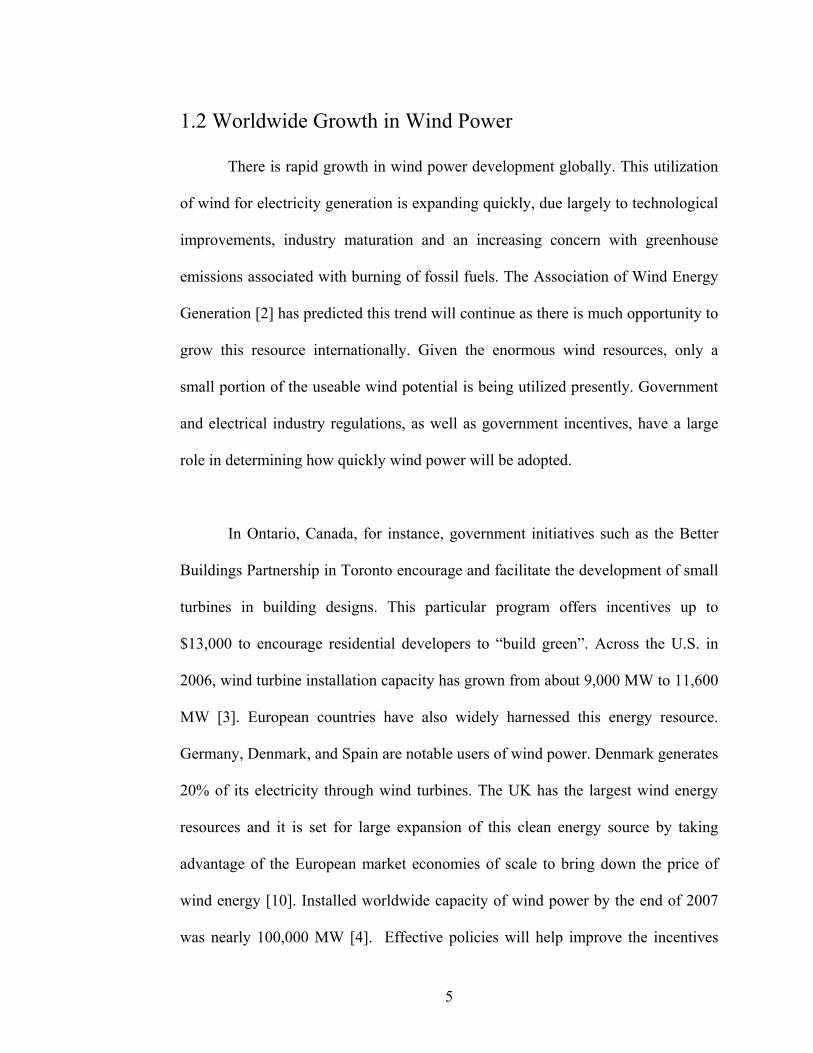
1.2 Worldwide Growth in Wind Power

There is rapid growth in wind power development globally. This utilization

of wind for electricity generation is expanding quickly, due largely to technological

improvements, industry maturation and an increasing concern with greenhouse

emissions associated with burning of fossil fuels. The Association of Wind Energy

Generation [2] has predicted this trend will continue as there is much opportunity to

grow this resource internationally. Given the enormous wind resources, only a

small portion of the useable wind potential is being utilized presently. Government

and electrical industry regulations, as well as government incentives, have a large

role in determining how quickly wind power will be adopted.

In Ontario, Canada, for instance, government initiatives such as the Better

Buildings Partnership in Toronto encourage and facilitate the development of small

turbines in building designs. This particular program offers incentives up to

$13,000 to encourage residential developers to “build green”. Across the U.S. in

2006, wind turbine installation capacity has grown from about 9,000 MW to 11,600

MW [3]. European countries have also widely harnessed this energy resource.

Germany, Denmark, and Spain are notable users of wind power. Denmark generates

20% of its electricity through wind turbines. The UK has the largest wind energy

resources and it is set for large expansion of this clean energy source by taking

advantage of the European market economies of scale to bring down the price of

wind energy [10]. Installed worldwide capacity of wind power by the end of 2007

was nearly 100,000 MW [4]. Effective policies will help improve the incentives

6

and ensure that wind power can compete fairly with other fuel sources in the

electricity market.

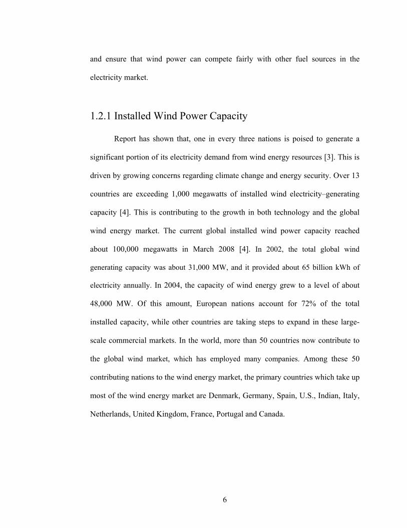
1.2.1 Installed Wind Power Capacity Report has shown that, one in every three nations is poised to generate a

significant portion of its electricity demand from wind energy resources [3]. This is

driven by growing concerns regarding climate change and energy security. Over 13

countries are exceeding 1,000 megawatts of installed wind electricity–generating

capacity [4]. This is contributing to the growth in both technology and the global

wind energy market. The current global installed wind power capacity reached

about 100,000 megawatts in March 2008 [4]. In 2002, the total global wind

generating capacity was about 31,000 MW, and it provided about 65 billion kWh of

electricity annually. In 2004, the capacity of wind energy grew to a level of about

48,000 MW. Of this amount, European nations account for 72% of the total

installed capacity, while other countries are taking steps to expand in these large-

scale commercial markets. In the world, more than 50 countries now contribute to

the global wind market, which has employed many companies. Among these 50

contributing nations to the wind energy market, the primary countries which take up

most of the wind energy market are Denmark, Germany, Spain, U.S., Indian, Italy,

Netherlands, United Kingdom, France, Portugal and Canada.

7

Country

Cumulative installed (MW) 2001




Growth rate 2003-2004 %

Germany 8,734 11,968 14,612 16,649 13.90%

Spain 3,550 5,043 6,420 8,263 28.70%

USA 4,245 4,674 6,361 6,750 6.10%

Denmark 2,456 2,880 3,076 3,083 0.20%

India 1,456 1,702 2,125 3,000 41.20%

Italy 700 806 922 1,261 36.70%

Netherlands 523 727 938 1,081 15.30%

Japan 357 486 761 991 30.20%

UK 525 570 759 889 17.10%

P.R. China 406 473 571 769 34.70%

Total 22,952 29,329 36,545 42,735 16.90%

Table 1.1: Wind power growth rate (cumulative installed in MW) [5]

Table 1.1 shows a review of the years 2001-2004 and the cumulative

installed capacity of wind turbines in the global wind energy growth rate. European

nations are leaders in the wind energy market and its development. Germany has

the largest cumulative capacity, both in Europe and worldwide, with a total of

16,649 MW by the end of the year 2004. Recently, the European Wind Energy

8

Association has revised its wind capacity projections for 2010 from 4x104MW to

6x104MW.

0

10

20

30

40

50

60

70

80

90

100

1980

1982

1984

1986

1988

1990

1992

1994

1996

1998

2000

2002

2004

2006

2008

Year

Thou

sand

s Meg

awat

ts

Figure 1.3: Global installed wind energy capacity [4]

There is a rising need for continuous development of wind power. Figure

1.3 illustrates that almost 100,000 MW of wind power is currently installed

cumulatively. The Renewable Energy Law (REL), adopted by most developed

countries is a boost to encouraging wind energy growth. Most other developing

nations of the world have completed a policy formulation that will enable similar

measures as the developed countries for full implementation and development of

this renewable energy resource. In Africa, Morocco and Egypt are leading in the

9

number of installations. Figure 1.3 shows the rapid growth of installations. In 2004,

the U. S. experienced a slight reduction during the global growth. Today its total

cumulative installed capacity has reached about 16,818 MW.

02468

1012141618202224

19801982

19841986

19881990

19921994

19961998

20002002

20042006

2008

Year

Thou

sand

s Meg

awat

ts

GermanyU.S.SpainIndiaChinaDenmark

Figure 1.4: Top cumulative installed wind power capacities (World, 1980-2007) [4]

In recent years, the cumulative generating capacity is mainly dominated by

six countries: Germany (25%), U.S. (18%), Spain (16%), Denmark (3%), China

(6%), and India (8%). Together they account for 76% of the total (see Figs. 1.4 and

1.5). This is sufficient to meet the electricity needs of over 60 million average

homes.

10

China 6%Denmark 3%

India 8% Spain 16%

U.S 18%

Germany 25%Others 24%

Figure 1.5: Top cumulative installed wind power capacity by percentage

(World, 1980-2007) Statistics have also shown that in the year 2007, in North America, the total

installed capacity increased its share of the worldwide market of wind power. The

U. S. is further concentrating and developing other sites, apart from the two states

of California and Texas, which together accounted for about two thirds of the

national total of 4,660 MW. The Canadian Wind Energy Association, CANWEA,

disclosed the total installed capacity for wind energy in 2007 at 1,846 MW. A total

11

5,244

3,522 3,449

1,730 1,667

888603 434 427 386

0

1,000

2,000

3,000

4,000

5,000

6,000

United States

SpainChin

aIndia

Germany

France Italy

Portugal

United Kingdom

Canada

MW

of about 560,000 homes now derive their electricity needs from wind power.

Canada, with one of the largest wind resources in the world, has a large potential to

expand its wind energy market. In 2004, only a total of 444 MW had been reached

[8].

Figure 1.6: Wind power capacity in 2007: Top 10 countries [4] The North American market experienced the greatest growth worldwide in

2007, with 5,244 MW of new energy capacity built in the United States alone.

Germany, the leader in Europe cumulatively, experienced a decline, while Spain

has taken the leadership in installed capacity. Canada is currently the world’s 11th

12

ranked nation for installed wind energy capacity. Given the huge potential of its

wind resources, the Canadian government believes wind energy is an important

component of its strategy to addressing climate change [8]. There is also growing

research into enhancing the wind power development. Zephyr Alternative Power, in

collaboration with the University of Ontario Institute of Technology, is developing

a novel Zephyr vertical axis wind turbine. This joint effort aims to improve upon

the existing power output from the turbine. This collaboration and turbine

development can contribute to the overall growth of wind in urban areas.

1.3 Wind Turbine Technology

Many different wind generators have evolved over the years. Whatever form

the alterations in design have taken, they normally fall into two basic

classifications: horizontal axis wind turbine (HAWT) and vertical axis wind turbine

(VAWT). Rotors that spin about a horizontal axis are called HAWT and those

whose rotors spin about a vertical axis are VAWT. The vertical axis wind turbines

are further grouped into two types: the drag–based devices that use aerodynamic

drag to extract power from the wind, and lift–based types (note: lift refers here to

the force acting perpendicular to the blade)

13

Figure 1.7: Wind turbine types

(Source: American Wind Energy Association) www.awea.org

The turbine industry today is dominated by the conventional horizontal axis

wind machines. The vertical axis wind turbines (VAWTs) are uncommon. Unlike

VAWTs, the horizontal wind turbines are not omni-directional. As the wind

direction changes, HAWTs must also change direction to continue functioning.

There must be a technique for orienting the rotor with respect to the wind. In a

HAWT, the generator directly converts the wind energy, which is extracted from

the rotor. The rotor speed and power output can be controlled by pitching the rotor

blades along the longitudinal axis. A mechanical or electronic blade pitch control

mechanism can be used, in order to control the pitch angle. An important advantage

of a HAWT is that blade pitching can also protect against extreme wind conditions

http://www.awea.org/

14

and speed. Also, the rotor blades can be shaped to achieve maximum turbine

efficiency, by exploiting the aerodynamic lift to a maximum.

The advantages of VAWTs are they can accept wind from any direction,

thus eliminating the need for re-orienting towards the wind. This simplifies their

design, reduces cost of construction, aids installation, and eliminates the problem

imposed by gyroscopic forces on the rotor of a conventional machine, as the turbine

tracks the wind. The vertical axis of rotation also permits mounting the generator

and drivetrain at ground level. However, a shortcoming is it is quite difficult to

control power output by pitching the rotor blades, as they are not self-starting and

they have a low tip-speed ratio [7]. Nevertheless, the VAWT is attracting a growing

interest globally. Its modular and scalable size, among other advantages over

conventional HAWTs, is attracting researchers and developers who are working to

improve and optimize this type of turbine.

1.4 Thesis Objectives Following the oil crisis and consequent energy problems of the 1970s, wind

turbine technology has witnessed a rapid development, amidst an urgent

requirement for sustainable alternatives to the continuous rising cost of fossil fuels.

Global warming will continue unless dependence on fossil is reduced. Wind power

has a key role in reducing greenhouse gas emissions. The Zephyr turbine is a

promising type of wind turbine that can be installed in urban area, where popular

15

HAWTs have limited capabilities. The Zephyr vertical axis wind turbine (ZVWT)

is a novel wind turbine that is capable of producing electric power for homes and

industries. The objective of this thesis is to conduct an investigation of ZVWT

model geometry modifications with CFD simulations. The performance

characteristics will be predicted. Non-dimensional relations for the efficiency of

two basic configurations will be obtained. Through these CFD simulations and

resulting non-dimensional power curves, new design tools will be developed to

improve the performance and operating capabilities of the Zephyr vertical axis wind

turbine.

16

Chapter 2

VERTICAL AXIS WIND TURBINE

HAWTs and VAWTs are both wind power generators that convert kinetic

energy of the wind into electric power. A major disadvantage with the HAWTs is

power generation ability lost when the wind speed exceeds a certain value known as

the cut-off speed. Shutting down is required due to safety and protection of the

wind turbine structures, mainly blades during high wind speed. Most HAWTs have

a rotor cut-off speed range from 20 to 25 m/s. HAWTs are therefore not suitable in

cyclone and storm prone areas. Also, they are not suitable in urban areas. The

VAWT has several advantages over HAWTs, such as suitability in urban areas, low

noise at low tip speed ratios, better esthetics to integrate into architectural

structures, insensitivity to yaw wind direction and increased power output in

skewed flow [7, 9]. These advantages have led to a growing research interest in

VAWTs, to bridge the gap of shortcomings with HAWTs. New advances in

VAWTs and the Zephyr wind turbine design will be the focus of this thesis. The

aerodynamic performance of vertical-axis wind turbines and computational

simulations will be examined.

2.1 VAWTs Background The origin of VAWTs can be traced back to roots in Persia [10, 11]. The

windmill was used as a source of mechanical power in the tenth century.

Inhabitants, who lived in Eastern Persia, utilized the windmills as vertical-axis and

17

drag type of windmills illustrated in Figure 2.1. The invention of the vertical-axis

windmills subsequently spread in the twelfth century throughout the Middle East

and beyond to the far East. The basic mechanisms of the primitive vertical-axis

windmills were used in later centuries, such as placing the sails above the

millstones, elevating the driver to a more open exposure, which improved the

output by exposing the rotor to higher wind speeds, and using reeds instead of cloth

to provide the working surface [10].

Figure 2.1: Persian windmill [11].

A transition was witnessed from windmills supplying mechanical power, to

wind turbines generating electrical power, which occurred toward the end of the

nineteenth century. The initial use of wind for electricity generation, as opposed to

mechanical power, led to the successful commercial development of small wind

18

generators, further research and experiments with large turbines. It is also worthy to

note that the development of the aircraft industry in the early part of twentieth

century facilitated rapid advances in airfoils which could immediately be applied

improvement of the wind turbine [10].

Two types of vertical axis wind turbines are commercialized today in the

wind energy market: Darrieus and Savonius types. The following section will

provide an overview of these turbines.

2.1.1 Darrieus Lift-Based VAWT Invented by F.M. Darrieus in the 1930s, Darrieus turbines are lift-based

turbines designed to function on the aerodynamic principle of airplanes [12]. The

rotor blades are designed as an airfoil in cross section, so the wind travels a longer

distance on one side (convex) than the other side (concave). As a result, the wind

speed is relatively higher on the convex side. If Bernoulli’s equation is applied, it

can be shown that the differential in wind speed over the airfoil creates a

differential pressure, which is used to pull the rotor blade around as the wind passes

through the turbine. The Darrieus VAWT is primarily a lift-based machine, which

is a feature that makes it compete in performance with the conventional HAWTs.

Figure 2.2 shows a typical Darrieus wind turbine characterized by its C-shaped

rotor. It is normally built with two or three rotor blades. It has a low starting torque,

but high rotational speed, making it suitable for coupling with an electrical

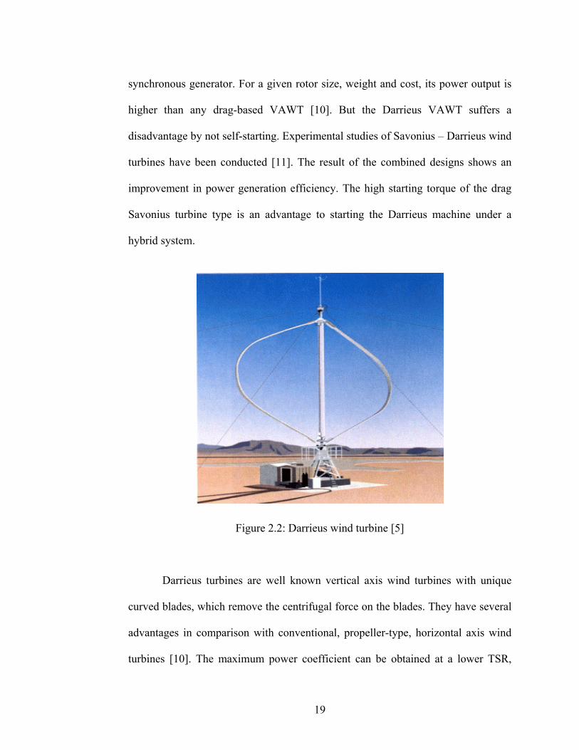
19

synchronous generator. For a given rotor size, weight and cost, its power output is

higher than any drag-based VAWT [10]. But the Darrieus VAWT suffers a

disadvantage by not self-starting. Experimental studies of Savonius – Darrieus wind

turbines have been conducted [11]. The result of the combined designs shows an

improvement in power generation efficiency. The high starting torque of the drag

Savonius turbine type is an advantage to starting the Darrieus machine under a

hybrid system.

Figure 2.2: Darrieus wind turbine [5]

Darrieus turbines are well known vertical axis wind turbines with unique

curved blades, which remove the centrifugal force on the blades. They have several

advantages in comparison with conventional, propeller-type, horizontal axis wind

turbines [10]. The maximum power coefficient can be obtained at a lower TSR,

20

compared to conventional wind turbines. Flow induced noise is therefore less than

noise from conventional turbines. Although the VAWT has high performance and

advantages in comparison with conventional wind turbines, the operations of

VAWTs in general are still limited to locations in parks, buildings, monuments or

other architectural structures in urban or rural areas.

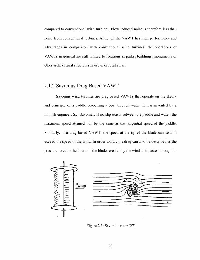
2.1.2 Savonius-Drag Based VAWT Savonius wind turbines are drag based VAWTs that operate on the theory

and principle of a paddle propelling a boat through water. It was invented by a

Finnish engineer, S.J. Savonius. If no slip exists between the paddle and water, the

maximum speed attained will be the same as the tangential speed of the paddle.

Similarly, in a drag based VAWT, the speed at the tip of the blade can seldom

exceed the speed of the wind. In order words, the drag can also be described as the

pressure force or the thrust on the blades created by the wind as it passes through it.

Figure 2.3: Savonius rotor [27]

21

Various types of drag based VAWTs have been developed in the past which use

plates, cups, buckets, oil drums, etc. as the drag device. The Savonius rotor is an S -

shaped cross section rotor (see fig. 2.2), which is predominantly drag based, but

also uses a certain amount of aerodynamic lift. Drag based VAWTs have relatively

higher starting torque and less rotational speed than their lift based counterparts.

Furthermore, their power output to weight ratio is also less [7, 10]. Because of the

low speed, these are generally considered unsuitable for producing electricity,

although it is possible by selecting proper gear trains. Drag based windmills are

useful for other applications such as grinding grain, pumping water and a small

output of electricity. A major advantage of drag based VAWTs lies in their self–

starting capacity, unlike the Darrieus lift–based vertical axis wind turbines.

2.2 Recent Developments in Modern Savonius Turbines A major disadvantage of the lift based Darrieus VAWT is its weak self-

starting capability. In the case of a low TSR, the average torque of the turbine is

almost zero or sometimes negative. Therefore, starting motors or engines are

required. The other problem of this VAWT is a small effective operation range.

Although the maximum power coefficient of the Darrieus VAWT is of the same

order of magnitude as a conventional turbine, the effective TSR operation range is

too narrow for electric power generators. This disadvantage reduces the net amount

of electricity generation from the VAWTs. The Savonius wind generators have

22

therefore attracted growing interest, due to their high starting torque, among other

reasons.

Developments in other related areas of wind technology have been adapted

to the drag based wind turbine, which will help improve its presence in the global

wind market. Some related fields that have contributed to a new generation of wind

turbines include material science, computer science, aerodynamics, analytical

methods, testing and performance estimation [10, 13]. Material science

developments have brought new composites for blades and alloys in the metal

components. Developments in computer science and CFD codes have facilitated

new design, analysis, monitoring and control. Aerodynamic design methods,

originally developed for the aerospace industry, have been extended to wind turbine

development. Analytical methods have been developed to a stage where it is

possible to have much better understanding of how a new design should perform.

Testing with a vast array of commercially available sensors, coding, data collection

and analysis equipment allows designers to better understand how the new turbines

actually perform.

Savonius turbine studies have shown efficiencies that can reach up to 37%.

Sorensen and Newman [19, 23] have conducted experiments to investigate the

effects of geometrical parameters, such as blade gap size, number and overlap.

Computational simulation software is a useful design tool to improve the turbine

performance.

23

Computational Fluid Dynamics is an important tool for the analysis,

development, and optimization of wind power systems. Various CFD techniques

have been used to simulate turbine performance, such as the viscous three-

dimensional differential/actuator disk method, adapted by Ammara, Leclerc and

Masson [14] for the aerodynamic analysis of wind farms. In order to improve

VAWT performance, CFD can be used to predict flow fields around a VAWT. The

flow field around a VAWT is complicated, because of interactions between the

large separated flow and wake itself. The flow field through a VAWT is essentially

unsteady, turbulent and separated flow. Akiyoshi et al. [13] simulated flow around a

VAWT and estimated its aerodynamic performance. The sub-grid scale turbulence

model was developed to simulate the separated flow from the turbine blades. A

sliding mesh technique was introduced to simulate flow through the rotational

blades. Numerical results were compared with predictions based on momentum

theory.

Computer simulations of the Navier-Stokes equations have been applied to

solve wind turbine problems. Blade Element Momentum (BEM) theory is a

common theoretical method developed for blade optimisation and rotor design [15,

16, 17]. With Computational Fluid Dynamics (CFD), Navier–Stokes equations are

solved together with models approximating turbulence to reveal the flow

characteristics. The results of such modelling are useful, providing large amounts of

data detailing the flow pattern. The difficulty of using such method is in computing

time, particularly when high resolution is needed near the blades [16]. Therefore,

24

when the flow pattern near the blades is modeled, theoretical methods can be used

to simplify this procedure. Numerical analyses have been carried out to investigate

the flow fields behind a small wind turbine with a flanged diffuser [15]. Wang et

al. [16] have used a scoop design with CFD as a tool for improving the turbine wind

energy capture, under low wind speed. These studies seek to enhance the wind

speed across the turbine rotor, which will be installed in built up cities. In this

thesis, the stator veins of the Zephyr turbine will be tested to improve their

performance. Similar past studies [16, 18] used a representation of the rotor using a

disk loading technique. Mandas et al. [20] modeled a three-dimensional large-scale

wind turbine using Fluent, and they compared the results with those obtained from

the BEM theory. In predicting the power characteristics of the Zephyr vertical axis

wind turbine, CFD can also be used as a modelling tool. Power output is the key

variable to be examined in this thesis by CFD modeling. A finite volume technique

will be used to analyze the performance of a two-dimensional vertical axis wind

turbine. Rajagopalan [33] developed a finite volume method to predict drag

characteristics of turbine blades.

CFD numerical techniques are useful in various flow aspects of turbine

performance. The viscous three-dimensional differential/actuator disk method has

been used for the aerodynamic analysis of wind turbine. In this approach, the rotor

is modeled as a permeable surface from which the time-averaged mechanical work

is extracted by the rotor from the air.

25

A common method for modeling the rotation of a turbine blade is the

steady-state multiple reference frame model. This method was applied by Hahm

and Kröning [21] to study the wake effects of horizontal wind turbines. The method

was also utilized by Fluent Inc. to simulate a three rotor horizontal axis wind

turbine (HAWT) at the National Wind Technology Center (NWTC). The computed

generator power and operating efficiency predicted by Fluent was within 1% of the

collected field data [22]. A more computationally demanding CFD method is the

moving mesh model. Sezer-Uzol and Long [23] developed a three-dimensional

time-accurate simulation of HAWT rotor flow fields. Results shown good

agreement exist between the simulated pressure coefficient distributions and

experimental data was achieved by the authors.

The torque and pressure on the rotors of a vertical axis wind turbine

(VAWT) are important parameters for a design. With many VAWTs, especially

designs with high rotor-stator interaction, the power output of the turbine can be

rapidly changing and diverse throughout each rotation. For such applications, an

unsteady time-dependant CFD simulation can offer a useful and straightforward

method for determining a turbine’s power output throughout each cycle. This

technique is effective even for power curves with a high level of fluctuation. This is

an important benefit of the moving mesh model, as it is the only method available

to produce reliable time-dependent results.

26

The MRF model is another alternative for obtaining transient flow

information [28]. With most VAWTs, the torque on each rotor varies significantly

throughout each cycle. Plotting the torque through a full rotation can provide the

designer with useful information about material fatigue, cyclic stresses, maximum

torque, turbine performance, and possible areas of efficiency improvements. The

MRF model also has useful applications for the analysis of VAWTs. Important data

for the understanding and optimized use of a wind turbine lies in the characteristic

power curve (power vs. rotational velocity and power vs. wind velocity). Attempts

have been made to develop effective, accurate and simplified methods to determine

a VAWT’s characteristic power curve. Camporeale, Fortunato and Marilli [24]

developed an automatic system that is automated and able to determine a larger

number of data points than a traditional system using variable resistors. A CFD

simulation can provide a useful alternative for estimating a turbine’s characteristic

power curve, with virtually any number of data points. In this thesis, CFD will be

used to predict the velocity and pressure distributions for a novel Zephyr VAWT,

from which design modifications will be made to improve the turbine’s

performance.

2.3 Zephyr VAWT.

The Zephyr VAWT is a Canadian invented wind generator. It is a special

drag based turbine with lift to boost its power output. The modular and scalable

design is quiet; visually appealing and practical for residences and institutions (see

fig. 2.4). This thesis aims to improve upon the current design, which has the

27

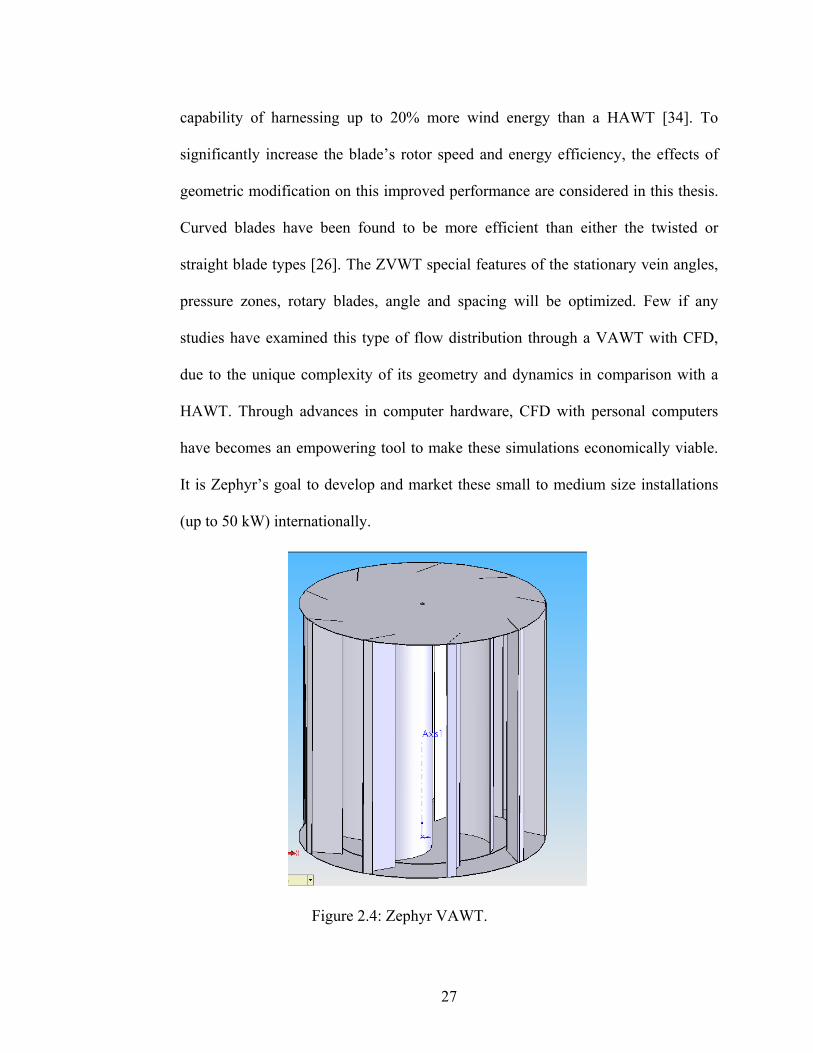
capability of harnessing up to 20% more wind energy than a HAWT [34]. To

significantly increase the blade’s rotor speed and energy efficiency, the effects of

geometric modification on this improved performance are considered in this thesis.

Curved blades have been found to be more efficient than either the twisted or

straight blade types [26]. The ZVWT special features of the stationary vein angles,

pressure zones, rotary blades, angle and spacing will be optimized. Few if any

studies have examined this type of flow distribution through a VAWT with CFD,

due to the unique complexity of its geometry and dynamics in comparison with a

HAWT. Through advances in computer hardware, CFD with personal computers

have becomes an empowering tool to make these simulations economically viable.

It is Zephyr’s goal to develop and market these small to medium size installations

(up to 50 kW) internationally.

Figure 2.4: Zephyr VAWT.

28

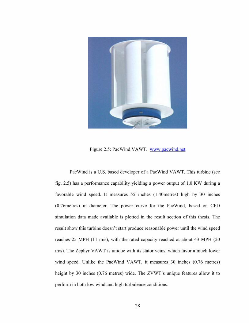
Figure 2.5: PacWind VAWT. www.pacwind.net

PacWind is a U.S. based developer of a PacWind VAWT. This turbine (see

fig. 2.5) has a performance capability yielding a power output of 1.0 KW during a

favorable wind speed. It measures 55 inches (1.40metres) high by 30 inches

(0.76metres) in diameter. The power curve for the PacWind, based on CFD

simulation data made available is plotted in the result section of this thesis. The

result show this turbine doesn’t start produce reasonable power until the wind speed

reaches 25 MPH (11 m/s), with the rated capacity reached at about 43 MPH (20

m/s). The Zephyr VAWT is unique with its stator veins, which favor a much lower

wind speed. Unlike the PacWind VAWT, it measures 30 inches (0.76 metres)

height by 30 inches (0.76 metres) wide. The ZVWT’s unique features allow it to

perform in both low wind and high turbulence conditions.

http://www.pacwind.net/

29

Chapter 3

AERODYNAMICS AND PERFORMANCE MODELS Achieving success in harvesting the power of wind requires a detailed

understanding of the physics of the interaction between the moving air and wind

turbine rotor blades. An optimum power production depends on perfect interaction.

The wind consists of a combination of the mean flow and turbulent fluctuations

about that mean flow. In this chapter, the basic prevailing aerodynamic phenomena

for the VAWT will be highlighted. Aerodynamic forces caused by wind shear, off-

axis winds, rotor rotation, randomly fluctuating forces induced by turbulence and

dynamic effects all affect the fatigue loads experience by a wind turbine. These are

very complicated for the VAWT, and they can only be predicted by understanding

the aerodynamics of steady state operation. An idealized wind turbine rotor will be

examined along with the airflow around the generator rotor. An analysis to

determine the theoretical performance limits for wind turbines by a blade-element

theory will be developed. Also, a CFD computational solution for the aerodynamic

design of a wind turbine rotor will be performed.

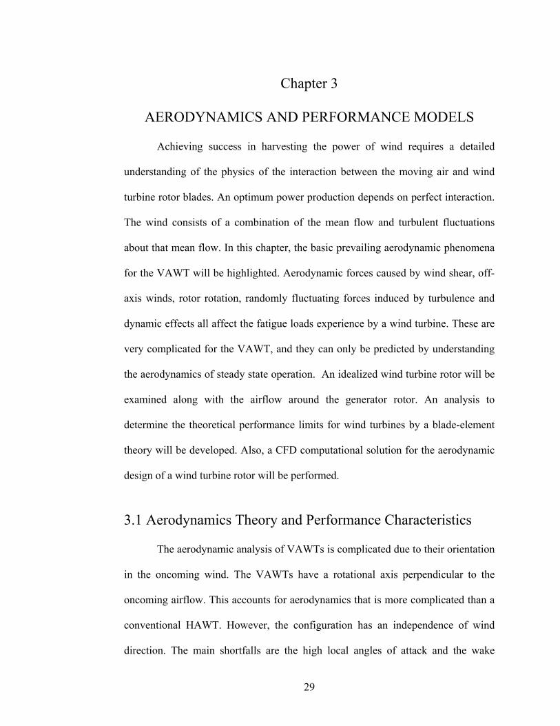
3.1 Aerodynamics Theory and Performance Characteristics The aerodynamic analysis of VAWTs is complicated due to their orientation

in the oncoming wind. The VAWTs have a rotational axis perpendicular to the

oncoming airflow. This accounts for aerodynamics that is more complicated than a

conventional HAWT. However, the configuration has an independence of wind

direction. The main shortfalls are the high local angles of attack and the wake

30

coming from the blades in the upwind part and axis. This disadvantage is more

pronounced with Savonius (pure drag) VAWTs, when compared to the Darrieus

VAWTs. The power output from the high speed lift VAWT can be appreciable.

Understanding the aerodynamics of the pure drag type of VAWT will give

important insight for improving the lift coefficient, and designing this turbine for

better and more efficient harnessing of the wind energy.

(a) 3-D (b) 2-D cross section Figure 3.1: VAWT model. [20] Figure 3.1 shows a typical VAWT model in both three and two dimensional

orientations.

3.2.1 Lift Force The lift force, L, is one of the major force components exerted on an airfoil

section inserted in a moving fluid. It acts normal to the fluid flow direction. This

31

force is a consequence of the uneven pressure distribution between the upper and

lower blade surfaces (see fig. 3.2), and can be expressed as follows:

AVCL l25.0 ρ= (3.1)

where ρ is the air density, lC is the lift coefficient and A is the blade airfoil area.

3.2.2 Drag force The drag force, D acts in the direction of the fluid flow. Drag occurs due to

the viscous friction forces on the airfoil surfaces, and the unequal pressure on

surfaces of the airfoil. Drag is a function of the relative wind velocity at the rotor

surface, which is the difference between the wind speed and the speed of the

surface, and can be expressed as

ArUCD d2)(5.0 Ω−= ρ (3.2)

where rΩ is the speed of the surface at the blade, dC is drag coefficient and V is

the wind speed.

The lift and drag coefficient values are usually obtained experimentally and

correlated against the Reynolds number. In this thesis, a CFD code will be used to

predict these coefficient values over a range of operating conditions. The amount of

power generated by the novel Zephyr vertical axis wind turbine will be analyzed. A

32

section of a blade at radius r is illustrated in Fig. 3.2, with the associated velocities,

forces and angles shown. The relative wind vector at radius r, denoted by Vrel, and

the angle of the relative wind speed to the plane of rotation, byφ . The resultant lift

and drag forces are represented by L and D, which are directed perpendicular and

parallel to the relative wind as shown

Figure 3.2: Local forces on a blade [10]

A careful choice of the rotor blades geometry and shape modification is

crucial for maximum efficiency. Wind turbines have typically used airfoils based on

the wings of airplanes, although new airfoils are specially designed for use on

rotors. Airfoils use the concept of lift, as opposed to drag, to harness the wind’s

energy. Blades that operate with lift (forces perpendicular to the direction of flow)

33

are more efficient than a drag machine. Certain curved and rounded shapes have

resulted most efficient in employing lift. Improvements of the lift coefficient for the

Zephyr turbine depend on geometry, to enhance the performance.

When the edge of the airfoil is angled slightly out of the direction of the

wind, the air moves more quickly on the downstream (upper) side creating a low

pressure. On the upstream side of airfoil, the pressure is high. Essentially, this

pressure differential lifts the airfoil upward. (see Fig. 3.3). In the case of a wind

turbine, the lift creates a turning effect. An operating condition with a low blade

angle of attack,α , thus favors lift force. An optimum design configuration of

Zephyr turbine can reduce the high blade angle of attack responsible for VAWTs

dominant drag.

Figure-3.3 Airflow around an airfoil [32].

Bernoulli’s principle indicates how faster flow implies lower pressure on the

airfoil:

vP ρ21

+ = constant (3.3)

34

The first term in equation. (3.3) is the static pressure and the second term is the

dynamic pressure. An increase in velocity leads to a corresponding decrease in the

static pressure to maintain a constant, and vice versa. The equation can be

understood through a conservation of energy as pressure work is converted to /

from kinetic energy in the flow field.

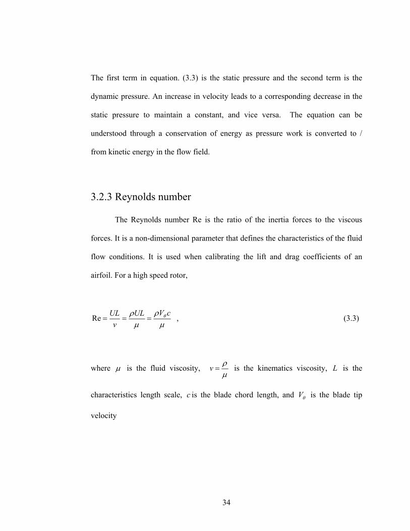
3.2.3 Reynolds number The Reynolds number Re is the ratio of the inertia forces to the viscous

forces. It is a non-dimensional parameter that defines the characteristics of the fluid

flow conditions. It is used when calibrating the lift and drag coefficients of an

airfoil. For a high speed rotor,

μρ

μρ θ cVUL

vUL

===Re , (3.3)

where μ is the fluid viscosity, μρ

=v is the kinematics viscosity, L is the

characteristics length scale, c is the blade chord length, and θV is the blade tip

velocity

35

3.2.4 Blade Solidity The blade solidity,δ , is the ratio of the blade area compared with the swept

area. For a vertical axis wind turbine, the solidity is defined as

rBcπ

δ2

= (3.4)

where B is the number of blades. Changing the number of blades or the blade chord

dimensions will alter the VAWT solidity. An increase in the chord results in a large

aerodynamics force and consequently in high power.

3.2.5 Tip speed ratio The tip speed ratio λ , is defined as the velocity at the tip of the blade, to the

free stream velocity. The rotational speed can be varied by the turbine controller for

a certain wind speed. The rotational speed, ω, is therefore represented by the tip

speed ratio, λ. This parameter gives the tip speed, Rω, as a factor of the free stream

velocity, V. It is given by

VRωλ = (3.5)

36

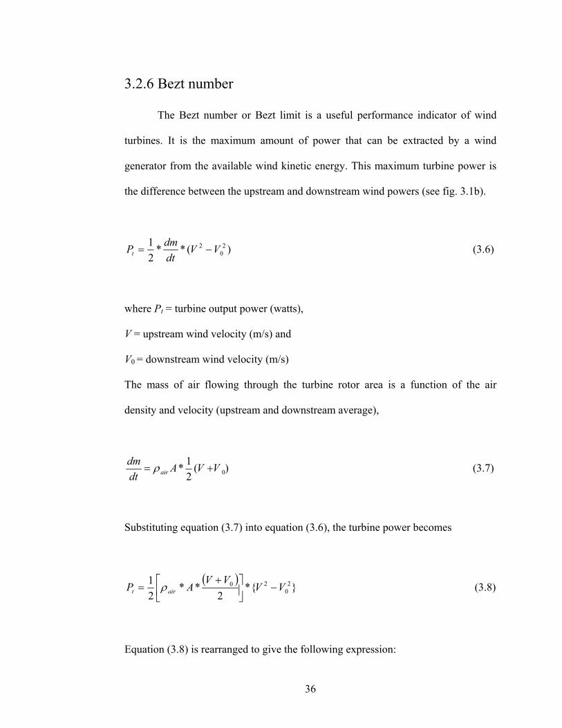
3.2.6 Bezt number The Bezt number or Bezt limit is a useful performance indicator of wind

turbines. It is the maximum amount of power that can be extracted by a wind

generator from the available wind kinetic energy. This maximum turbine power is

the difference between the upstream and downstream wind powers (see fig. 3.1b).

)(**21 2

02 VV

dtdmPt −= (3.6)

where Pt = turbine output power (watts),

V = upstream wind velocity (m/s) and

V0 = downstream wind velocity (m/s)

The mass of air flowing through the turbine rotor area is a function of the air

density and velocity (upstream and downstream average),

)(21* 0VVA

dtdm

air += ρ (3.7)

Substituting equation (3.7) into equation (3.6), the turbine power becomes

( )}{*

2**

21 2

020 VV

VVAP airt −⎥⎦

⎤⎢⎣⎡ +

= ρ (3.8)

Equation (3.8) is rearranged to give the following expression:

37

2

1*1

****21

200

3 ⎥⎥⎦

⎤

⎢⎢⎣

⎡⎟⎠⎞

⎜⎝⎛−⎟

⎠⎞

⎜⎝⎛ +

=VV

VV

VAP airt ρ (3.9)

This power from the turbine rotor can be expressed as a fraction of the upstream

wind power, i.e.,

pairt CVAP ****21 3ρ= (3.10)

where Cp is the fraction of power captured by the rotor blades also called power

coefficient or rotor efficiency.

Re-arranging the previous results, it can be shown that

2

1*12

00

⎥⎥⎦

⎤

⎢⎢⎣

⎡⎟⎠⎞

⎜⎝⎛−⎟

⎠⎞

⎜⎝⎛ +

=VV

VV

C p (3.11)

Figure 3.3 shows the variation of Cp with downstream to upstream wind speed ratio,

V0/V. The theoretical maximum rotor power coefficient is Cp = 16/27 (= 0.59),

when the downstream to upstream wind speed ratio is V0/V = 0.33, called the Betz

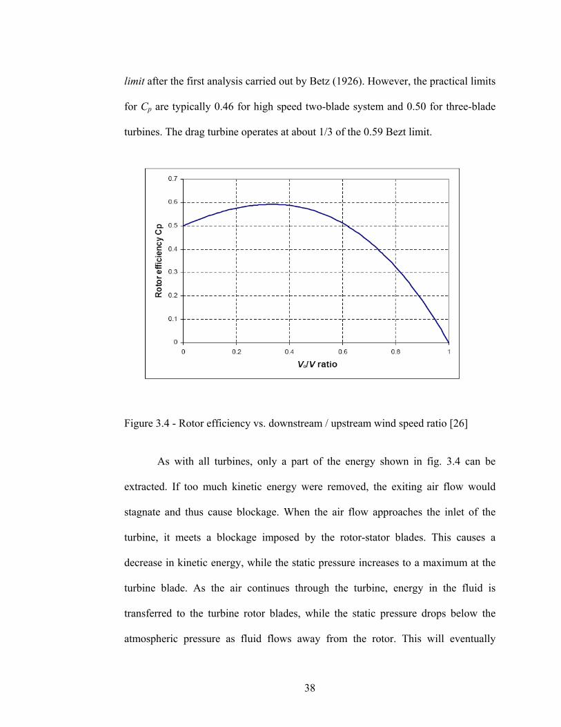
38

limit after the first analysis carried out by Betz (1926). However, the practical limits

for Cp are typically 0.46 for high speed two-blade system and 0.50 for three-blade

turbines. The drag turbine operates at about 1/3 of the 0.59 Bezt limit.

Figure 3.4 - Rotor efficiency vs. downstream / upstream wind speed ratio [26] As with all turbines, only a part of the energy shown in fig. 3.4 can be

extracted. If too much kinetic energy were removed, the exiting air flow would

stagnate and thus cause blockage. When the air flow approaches the inlet of the

turbine, it meets a blockage imposed by the rotor-stator blades. This causes a

decrease in kinetic energy, while the static pressure increases to a maximum at the

turbine blade. As the air continues through the turbine, energy in the fluid is

transferred to the turbine rotor blades, while the static pressure drops below the

atmospheric pressure as fluid flows away from the rotor. This will eventually

39

further reduce the kinetic energy. Then kinetic energy from the surrounding wind is

entrained to bring it back to the original state.

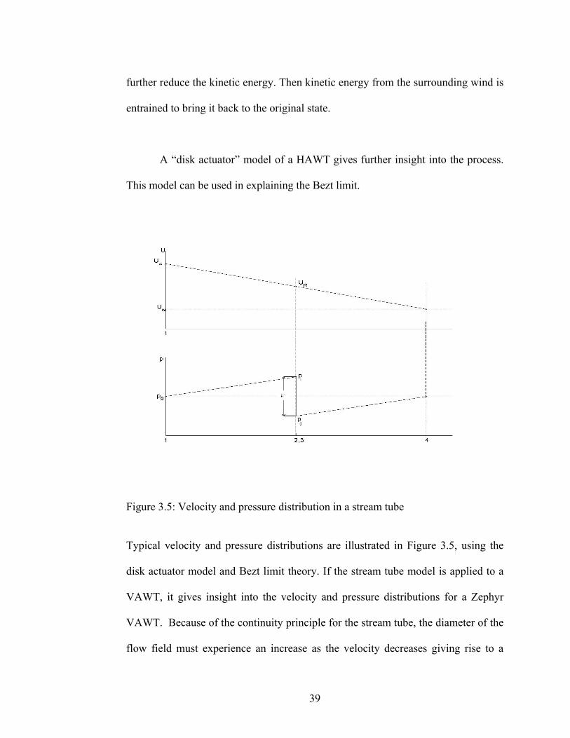
A “disk actuator” model of a HAWT gives further insight into the process.

This model can be used in explaining the Bezt limit.

Figure 3.5: Velocity and pressure distribution in a stream tube Typical velocity and pressure distributions are illustrated in Figure 3.5, using the

disk actuator model and Bezt limit theory. If the stream tube model is applied to a

VAWT, it gives insight into the velocity and pressure distributions for a Zephyr

VAWT. Because of the continuity principle for the stream tube, the diameter of the

flow field must experience an increase as the velocity decreases giving rise to a

40

sudden pressure drop, { )(' du ppp −= }, at the rotor plane. This pressure drop

contributes to the torque for rotating turbine blades.

The actuator disk theory also provides a rational basis for illustrating the

flow velocity at the rotor is different than the free-stream velocity. The Betz limit

from the actuator disk theory shows the maximum theoretically possible rotor

power coefficient (0.59) for a wind turbine. In reality, three major effects account

for a power coefficient:

• rotation of wake behind the rotor;

• finite number of blades and associated tip losses;

• non-zero aerodynamic drag.

3.3 Rotor Performance Parameters A wind turbine designed for a particular application should have its

performance characteristics tested before proceeding to prototype fabrication. A

dimensionally similar and scaled down prototype of the design model is normally

tested in a wind tunnel for this purpose. CFD commercial software is also used to

save time and cost [15, 16].

The power performance of a wind turbine is normally expressed in

dimensionless form. For a given wind speed, the power coefficient and the tip speed

ratio are good indicators to use as a performance measure. For a particular

configuration of the Zephyr VAWT, these parameters are

41

AVP

C tp 3

21 ρ

= (3.12)

where hdA = , d is the rotor diameter and h is the height of turbine. Also, pC and

λ (tip speed ratio) of equation 3.5 are dimensionless values used in predicting the

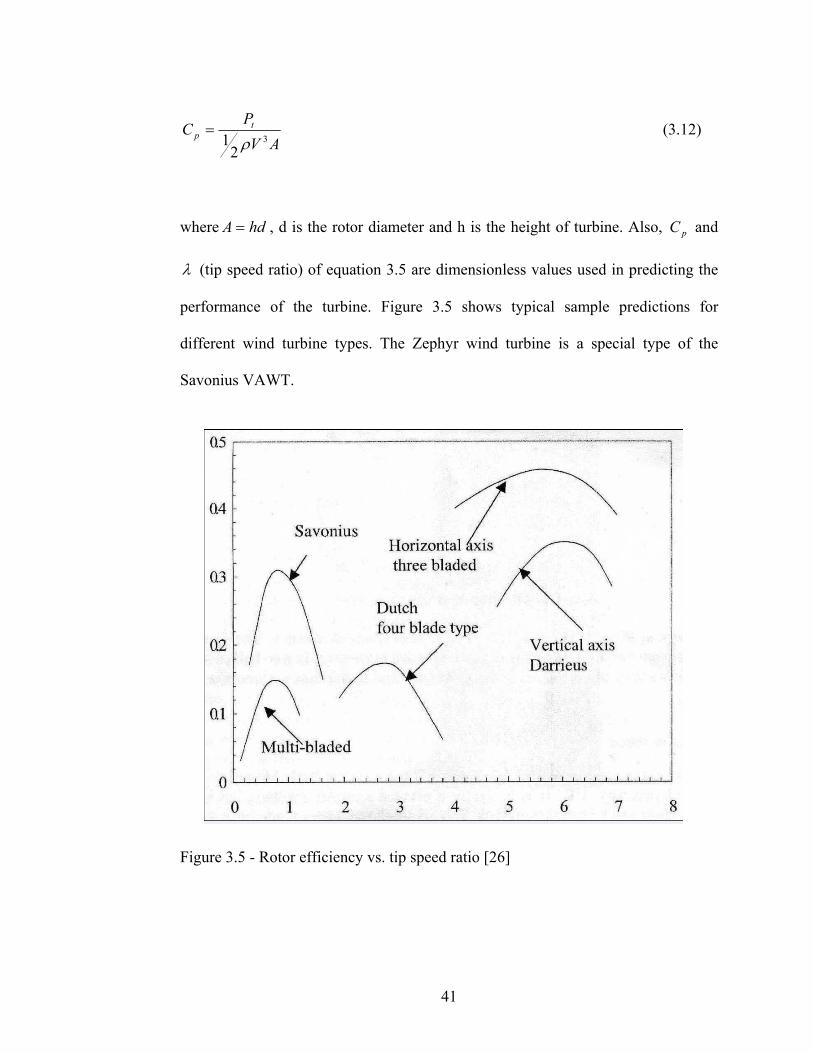
performance of the turbine. Figure 3.5 shows typical sample predictions for

different wind turbine types. The Zephyr wind turbine is a special type of the

Savonius VAWT.

Figure 3.5 - Rotor efficiency vs. tip speed ratio [26]

42

Figure 3.5 is a sample extract [26]. It is an illustration of modern turbine pC - λ

curves with pC and λ are represented on the plot as y-axis and x-axis respectively.

3.4 Blade Element Theory Blade Element Momentum (BEM) theory is a theoretical method developed

for blade optimization and rotor design. The Blade Element Momentum theory,

otherwise called strip theory, is a combination of basic momentum theory and blade

element theory. The motion of the air flow and forces acting on the blades,

determined by momentum principles are not complete without examining the shape

of blades and configuration required for optimum and improved rotor power

performance. The main principle of blade element theory is to consider the forces

experienced by the blades of the rotor in motion through the air. This theory is

therefore intimately concerned with the geometrical shape of the blade.

BEM theory becomes an essential tool that relates rotor performance to

rotor geometry. A particularly important prediction of this theory is the effect of

blade number. An assumption in BEM theory is that individual stream tubes (the

intersection of a stream tube and the surface swept by the blades) can be analyzed

independently of the remaining flow, as assumed in blade element theory.

Furthermore, an assumption associated with BEM theory is that spanwise flow is

negligible, meaning that airfoil data taken from two-dimensional tests are

acceptable as in blade element theory. Another assumption is that flow conditions

43

do not vary in the circumferential direction, i.e., axisymmetric flow. With this

assumption, the streamtube to be analyzed is a uniform annular ring centered on the

axis of revolution, as assumed in general momentum theory.

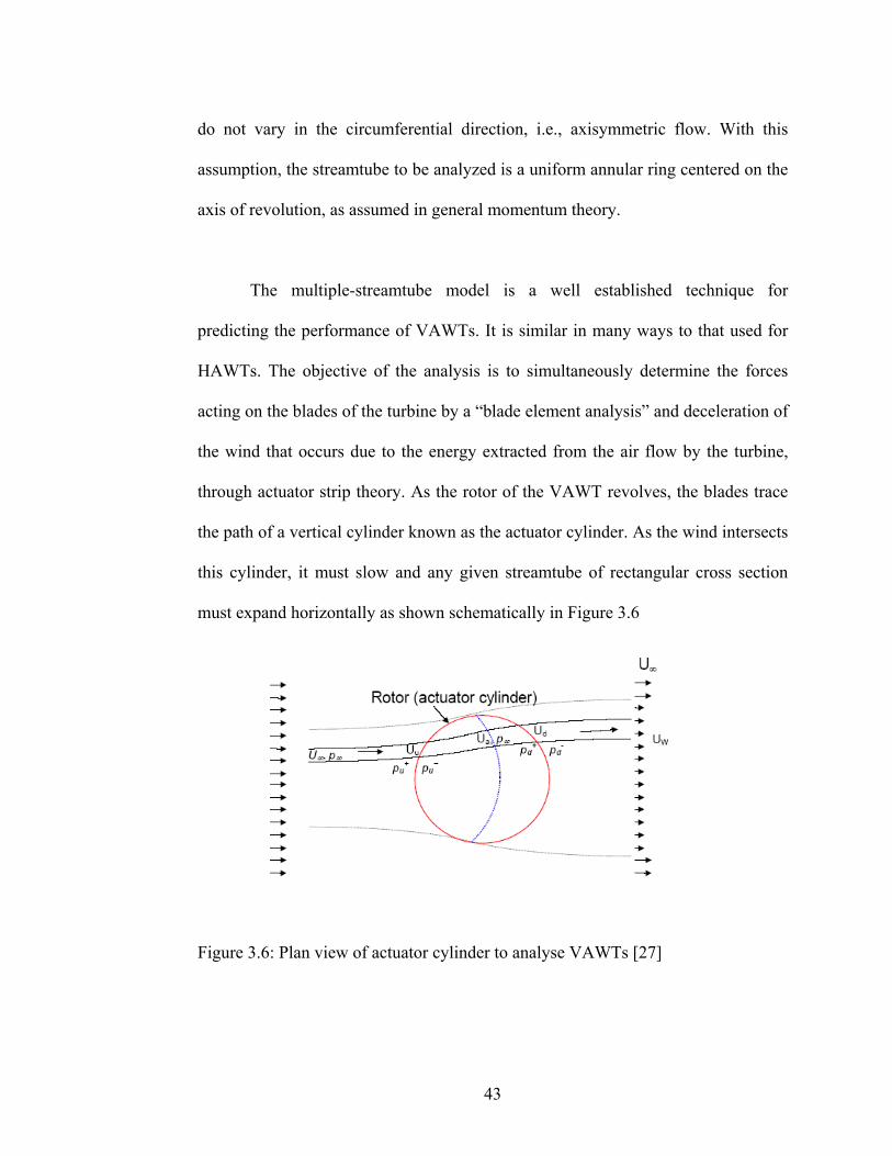
The multiple-streamtube model is a well established technique for

predicting the performance of VAWTs. It is similar in many ways to that used for

HAWTs. The objective of the analysis is to simultaneously determine the forces

acting on the blades of the turbine by a “blade element analysis” and deceleration of

the wind that occurs due to the energy extracted from the air flow by the turbine,

through actuator strip theory. As the rotor of the VAWT revolves, the blades trace

the path of a vertical cylinder known as the actuator cylinder. As the wind intersects

this cylinder, it must slow and any given streamtube of rectangular cross section

must expand horizontally as shown schematically in Figure 3.6

Figure 3.6: Plan view of actuator cylinder to analyse VAWTs [27]

44

The wind turbine blade performance is determined with BEM by combining the

equations of general momentum theory and blade element theory.

Figure 3.7 lift and drag force on VAWT [27]

Figure 3.8: Velocities at the rotor plane [10]

45

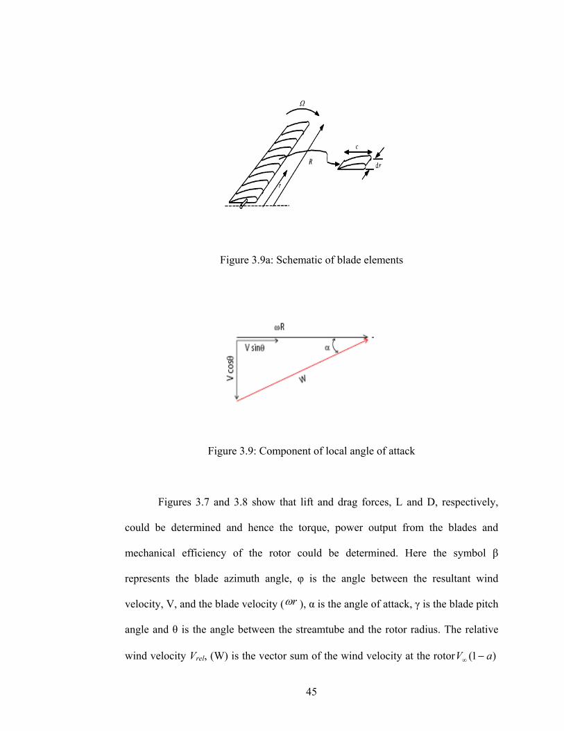
Figure 3.9a: Schematic of blade elements

Figure 3.9: Component of local angle of attack

Figures 3.7 and 3.8 show that lift and drag forces, L and D, respectively,

could be determined and hence the torque, power output from the blades and

mechanical efficiency of the rotor could be determined. Here the symbol β

represents the blade azimuth angle, φ is the angle between the resultant wind

velocity, V, and the blade velocity ( rω ), α is the angle of attack, γ is the blade pitch

angle and θ is the angle between the streamtube and the rotor radius. The relative

wind velocity Vrel, (W) is the vector sum of the wind velocity at the rotor )1( aV −∞

46

(vector sum of the free-stream wind velocity, V∞ and the induced axial velocity -

aV∞) and the wind velocity due to rotation of the blade. The rotational component is

the sum of the velocity due to the blades motion, ( )rω , and the swirl velocity of the

air, a’ ( )rω . The axial velocity V∞ (1- a), is reduced by a component V∞ a, due to

the wake effect or retardation imposed by the blades, where V∞ is the upstream

undisturbed wind speed. The relative wind velocity is shown on the velocity

diagram in Figure 3.8. The minus sign in the term V∞ (1- a) is due to retardation of

flow as the air comes into contact with the rotor. The positive sign in the term

)1(. 'ar +ω occurs due to the flow of air in the reverse direction of blade rotation,

after air particles contact the blades and yields torque. This flow ahead and behind

the rotor is not completely axial, as assumed in an ideal case. When the air exerts

torque to the rotor, as a reaction, a rotational wake is generated behind the rotor.

Depending on the wake length or separation, an energy loss is experienced, which

resulted in a reduction of the power coefficient.

3.4.1 Torque and Power The aerodynamic blade loads are transferred through the rotor and they are

converted into torque on the low speed rotor shaft. This is the primary drive train

load. The rated torque is calculated for a rated wind speed by an analysis of the

forces on the surface of the rotor blades. The torque dependence on wind speed and

rotor diameter follows a cubic law. It is inversely proportional to the rotor tip speed.

47

From the blade element analysis, the lift and drag forces acting over the

blades are estimated and integrated over the total blade span, incorporating the

velocity terms to obtain the shaft torque and power developed by the turbine. As

shown on figs 3.2, 3.7 and 3.8 for wind velocity and the force diagram, the lift and

drag forces on an element of the blade will produce a differential torque about the

axis of rotation as follows:

DL dQdQdQ += (3.13)

where LdQ is the lift torque contribution (N-m), DdQ is the drag torque

contribution (N-m) and φ is the flow angle.

Resolving the forces acting on the blade into total normal and tangential

force components yields

φφ sincos DLN dFdFdF += (3.14)

φφ cossin DLT dFdFdF −= (3.15)

Substituting the lift and drag forces eqs. (3.1) and (3.2) into eqs (3.14) and (3.15),

while considering an elemental area instead, yields

48

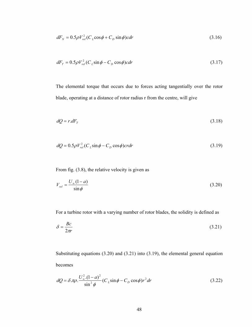
cdrCCVdF DLrelN )sincos(5.0 2 φφρ += (3.16)

cdrCCVdF DLrelT )cossin(5.0 2 φφρ −= (3.17)

The elemental torque that occurs due to forces acting tangentially over the rotor

blade, operating at a distance of rotor radius r from the centre, will give

TdFrdQ .= (3.18)

crdrCCVdQ DLrel )cossin(5.0 2 φφρ −= (3.19)

From fig. (3.8), the relative velocity is given as

φsin)1( aU

Vrel−

= ∞ (3.20)

For a turbine rotor with a varying number of rotor blades, the solidity is defined as

rBcπ

δ2

= (3.21)

Substituting equations (3.20) and (3.21) into (3.19), the elemental general equation

becomes

drrCCaUdQ DL2

2

22

)cossin(sin

)1.(.. φφφ

πρδ −−

= ∞ (3.22)

49

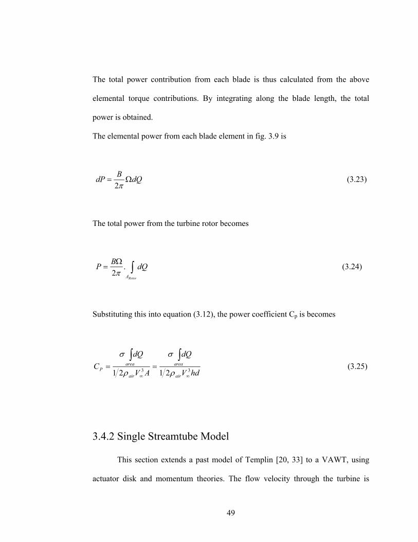
The total power contribution from each blade is thus calculated from the above

elemental torque contributions. By integrating along the blade length, the total

power is obtained.

The elemental power from each blade element in fig. 3.9 is

dQBdP Ω=π2

(3.23)

The total power from the turbine rotor becomes

dQBPRotorA∫

Ω= .

2π (3.24)

Substituting this into equation (3.12), the power coefficient Cp is becomes

AV

dQC

air

areaP 321 ∞

∫=

ρ

σ

hdV

dQ

air

area321 ∞

∫=

ρ

σ (3.25)

3.4.2 Single Streamtube Model This section extends a past model of Templin [20, 33] to a VAWT, using

actuator disk and momentum theories. The flow velocity through the turbine is

50

assumed to be constant. The application of the momentum theorem between two

sections shown in fig. 3.1b yields the drag force. This rotor aerodynamic drag is a

vectorial sum of the forces on the actuator disk in the streamwise direction.

( )21

.VVmD −= (3.26)

The power exchanged to causes the kinetic energy reduction is given as

( ) 2/22

21

.VVmP −= (3.27)

This power can also be written as follows (assuming a constant velocity):

VDP .= (3.28)

An assumption is made with the following constant velocity through the stream-

tube:

( ) 2/21 VVV += (3.29)

From blade element theory, the aerodynamic drag force is determined by

integrating the forces projected in the flow direction as follows:

θθθπ

πdFFBD TN )sincos(

22

0+= ∫ (3.30)

51

The lift and drag coefficients are two-dimensional aerofoil characteristics of

the local blade element, which are functions of the angle of attack. They can also be

resolved into normal force and thrust coefficients, CN and CT, respectively as

follows:

αα sincos dLN CCC += (3.31)

αα cossin dLT CCC −= (3.32)

where

qcCF NN = (3.33)

qcCF TT = (3.34)

The total drag force on the turbine for a given number of blades, over a complete

revolution, is

θθααθααπ

πqdCCCCBcD dldl }sin)cossin(cos)sincos{(

22

0−++= ∫ (3.35)

From fig. 3.9b, the local angle of attack is

52

⎟⎟⎟⎟

⎠

⎞

⎜⎜⎜⎜

⎝

⎛

−=

θωθαsin

cosarctan

VR

(3.27)

From equation (3.28), the average power will then be

θθααθααπ

πdCCCCqVBcP dldl }sin)cossin(cos)sincos{(

22

0−++= ∫ (3.36)

Equation (3.36) can be solved numerically, given the rotor blade chord

dimension and number of blades. It must be ensured that the blade solidity is kept

constant. The power obtained is the shaft power, when no load is placed on the

turbine. At this stage the mechanical efficiency of the turbine is determined. Then

momentum theory can be used to find the dimensionless power coefficient.

3.6 CFD Models

Either CFD or Vortex models are useful alternatives to momentum based

theory for predicting wind turbine performance. Unlike the momentum based

theoretical model, the vortex and CFD models are capable of predicting behavior of

the wake structure near the turbine rotor blades. This arises because the velocity

normal to the air flow is not neglected, as with the momentum theory.

Computational Fluid Dynamics (CFD) can yield more accurate flow patterns than

the momentum and vortex based models. Another advantage is that unsteady flow

53

calculations can be performed with CFD. Complete flow patterns around 3-D wind

turbine can be calculated. The accuracy of the results depends on the mesh spacing

and computational model. In the next chapter, this CFD model capability and

procedure in optimizing the geometry parameters, as well as predicting the power

output of the novel Zephyr vertical axis wind turbine will be outlined.

54

Chapter 4

Numerical Simulations

4.1 Introduction

After a wind turbine rotor is designed for a specific application, its

performance characteristics should be tested before a prototype is fabricated. Often,

a dimensionally similar scaled down model of the proposed design are tested in a

wind tunnel for this purpose. In this chapter, the capability of CFD commercial

software in modeling and simulating an optimum geometry configuration for

Zephyr turbine efficient performance is exploited. Numerical simulations of air

flow through the Zephyr wind turbine is carried out in this chapter. The mesh

discretization and computational model will be described for air flow through the

wind turbine. CFD will be used to predict and optimize the geometric parameters,

fluid flow and the power output of the novel Zephyr vertical axis wind turbine. The

numerical predictions will use a multiple rotating reference frame (MRF)

formulation to simulate the turbine performance. The formulation divides the

domain into two sub-domains. For the stator and surrounding domain, a stationary

reference frame will be used. The rotor reference frame rotates with respect to the

inertial frame. It provides a convenient and effective method to investigate the

characteristic power curves for the turbine. These power curves are an important

element for subsequent development, as they provide estimates of operating

55

velocities, Cp and TSR. For these simulations, the overall domain will be

discretized into quadrilateral-triangular elements due to geometry shape.

4.2 Computational Methodology and Zephyr VAWT design Small wind turbines such as the Zephyr VAWT are usually assessed by

three key parameters: safety/functionality, durability and power characteristics. The

power performance among these has a more significant role in guiding the

aerodynamic design. Wind turbine power performance before the advent of

computers was normally measured in two ways: measure data on a real site, or

testing in a wind tunnel. Field monitoring can provide more realistic results, but it

needs complicated and robust instrumentation. Furthermore, it takes a longer period

to cover various wind conditions so it becomes more expensive than wind tunnel

tests. Wind tunnel tests also have some drawbacks; there are limitations on the size

of the wind turbine that is tested inside a tunnel. To minimize the effects of

obstruction of airflow inside the tunnel, the wind turbine needs to be small enough

to ensure that its flow blockage is negligible. Wind turbines are scaled down to fit

into the wind tunnel, before testing can take place. Results of such experiments are

later extrapolated to larger size by appropriate scaling laws.

Computational Fluid Dynamics (CFD) with commercial Fluent software

will be used in this thesis. This will provide a useful wind turbine modeling tool for

56

predicting performance. Using this numerical approach, a methodology for testing

and predicting the performance of the Zephyr turbine will be developed.

4.2.1 Zephyr Turbine Design and Modifications

Zephyr Alternative Power, a Toronto based company was started by Ed

Tsang, inventor of the Zephyr turbine, a novel vertical axis wind turbine (VAWT).

Research collaboration between Zephyr and UOIT aims at developing and

improving the performance of this wind generator. In a city setting, the wind is

always changing direction and the velocity and is never consistent. The Zephyr

VAWT is an effective machine for such conditions, so it expand the wind energy

resource of a city greatly by utilizing resources that traditional horizontal axis wind

turbines cannot. It is an omni-directional design, allowing the turbine to spin and

produce power regardless of the wind direction.

The proprietary elements of the design are the stator blades, which help it

perform better in low velocity and high turbulence wind conditions. The proprietary

stator design involves an angled outer tip that creates a low pressure zone behind

and draws more air into the turbine. This also helps the turbine perform well in

close proximity to obstructions and other turbines. This is an advantage for

elimination of wake effects, where several turbines are operating in close proximity

to each other in urban areas. Figure 4.1 shows a schematic of the Zephyr turbine

with its unique patented features.

57

Figure 4.1a Design drawings of Zephyr VAWT

Figure 4.1b: Design drawings of Zephyr VAWT showing the outer vane stators.

58

The Zephyr wind turbine has several design features that can be improved

upon for further increase in performance. By allowing space in the center of the

rotor cage for air to flow, lift is enhanced across the blade profile, instead of the

usual drag forces associated with fully closed Savonius (pure drag) rotors. Zephyr

has conducted several experiments with different configurations for the top plate on

the turbine. By opening or closing the top, it will be able to promote better fluid

flow through the rotor. In this thesis, a detailed investigation of the effect of rotor

blade geometry modification will be conducted. Fig. 4.1b shows the turbine stator-

tab new dimensions set up that was used alongside the 9-blade configuration. The

length of the tab, stator, and angle between them varies from the base design (see

appendix E) chosen dimension by a margin of 30% in length and 150 in angle

between. It is assumed this could create more induce low pressure vortex the will

enhance more wind entrenchment into the turbine.

The blade geometry and its aerodynamic characteristics are crucial to

achieve maximum energy from the wind. Like all wind turbines, only a part of the

energy characterized by the Betz limit can be extracted. If too much kinetic energy

were removed, the exiting air flow would become stagnant and cause blockage. In

designing the optimum blade rotor, there are many tradeoffs. If a rotor with a small

blade area is used, a large flow rate will be experienced through the rotor, while the

pressure drop will be small. This will imply a reduction in power output. On the

other hand, if a rotor with a large blade area is used, the pressure drop is large, but

the flow rate will be low. The consequence is that power output will be reduced. A

59

good optimization and configuration of the rotor blade is therefore needed to

achieve most efficient performance. A good turbine blade arrangement reduces the

velocity of the flow to two-thirds (2/3) of the free stream velocity at the rotor and

the minimum velocity downstream is to one-third (1/3) for better energy conversion

[10].

The geometry of a turbine affects the pressure field and boundary layer

along the surface. Curved blades incrementing from the traditional 2-blades

Savonius VAWT have shown a high power coefficient [23]. The geometrical

spacing between the Zephyr turbine rotor blades will be investigated, as well as

increasing the blade number, flow and blade angle spacing. In order to keep the

blade solidity constant, the dimension of the cord will be reduced as the number of

blades increases. A higher blade number has the advantage of reducing blade tip

losses. This is particularly evident for a vertical axis wind turbine that is noted for

low rotor speed. A fast spinning rotor like the case of horizontal axis wind turbines

usually has two to three blades. Fast spinning rotors have fewer blades while a slow

spinning rotor should have more blades to save tip losses.

The Zephyr stator tab accelerates the air in a residential area and hence can

provide more energy in the lower part of the boundary layer, where wind speed is

relatively low and turbulent in a concentrated area. The other optimization of

importance is the use of tabs on the ends of the stator blades to induce low-pressure

60

vortices in certain sections of the flow, and thereby entrain more air to enter the

turbine.

4.3. Computational Procedure

A Multiple Reference Frame (MRF) will be used in the computational

model for the numerical simulations. This model uses the time averaged

information to predict the turbine performance. It analyzes the fluid flow with either

a stationary reference frame or rotating reference frame. The model provides a

convenient and effective tool to investigate the characteristic power curves for the

turbine. For the Multiple Reference Frame formulation, the model is divided into

two sub-domains, one for the rotor and another for the stator. The rotor sub-domain

is rotating with respect to the inertial frame in the model. At the boundary between

the rotor and stator sub-domains, continuity of the absolute velocity is enforced to

provide appropriate values of velocity for each sub-domain [1, 10, 13]. The features

of the Multiple Reference Frame solution parameters will be summarized in section

4.3.2. This model does have a limitation in accounting for high stator – rotor

interaction that exists. Nevertheless, it can give valuable results for flow

predictions.

4.3.1 Mathematical formulation A Computational Fluid Dynamics algorithm defines how a discrete control

volume interacts with another. The finite volume algorithm is based on a

conservation principle that relates the changes in flow variables inside a control

61

volume to the net flux of the variable through the control volume surface. The

mathematical equations are called conservation relations. The algorithms that

strictly enforce these relations are called finite volume solvers. The CFD software,

Fluent, is such a finite volume solver.

A typical problem might be characterized with a time-dependent separated

flow at a high Reynolds number. A simplified turbulence model is considered often

for the purpose of analysis. The influence of viscosity is often assumed confined to

a thin layer of fluid flow adjacent to the solid surface and the vorticity is confined

within the wake region, such as the sharp edges of a blade. In reality, the effect of

viscosity leads to finite cores of rotational fluid. An overview of how the finite

volume solver works in the computation of mathematical equations is highlighted

next.

4.3.2 Governing Equations

The fundamental objective of rotor aerodynamics is to predict the induced

velocity field and the performance of the rotor. Estimating the performance of the

Zephyr turbine, as governed by its geometry and operating conditions, requires a

CFD analysis. The velocity and pressure fields are obtained by solving the partial

differential equations representing the mass and momentum conservation, using the

finite volume technique. Other procedures are the finite difference method and the

finite element method.

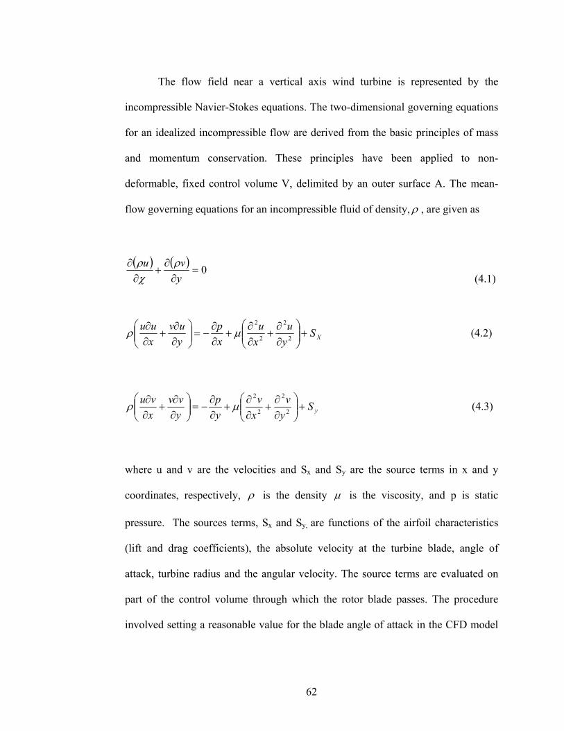
62

The flow field near a vertical axis wind turbine is represented by the

incompressible Navier-Stokes equations. The two-dimensional governing equations

for an idealized incompressible flow are derived from the basic principles of mass

and momentum conservation. These principles have been applied to non-

deformable, fixed control volume V, delimited by an outer surface A. The mean-

flow governing equations for an incompressible fluid of density, ρ , are given as

( ) ( ) 0=∂

∂+

∂∂

yvu ρ

χρ

(4.1)

XSyu

xu

xp

yuv

xuu

+⎟⎟⎠

⎞⎜⎜⎝

⎛∂∂

+∂∂

+∂∂

−=⎟⎟⎠

⎞⎜⎜⎝

⎛∂∂

+∂∂

2

2

2

2

μρ (4.2)

ySyv

xv

yp

yvv

xvu

+⎟⎟⎠

⎞⎜⎜⎝

⎛∂∂

+∂∂

+∂∂

−=⎟⎟⎠

⎞⎜⎜⎝

⎛∂∂

+∂∂

2

2

2

2

μρ (4.3)

where u and v are the velocities and Sx and Sy are the source terms in x and y

coordinates, respectively, ρ is the density μ is the viscosity, and p is static

pressure. The sources terms, Sx and Sy, are functions of the airfoil characteristics

(lift and drag coefficients), the absolute velocity at the turbine blade, angle of

attack, turbine radius and the angular velocity. The source terms are evaluated on

part of the control volume through which the rotor blade passes. The procedure

involved setting a reasonable value for the blade angle of attack in the CFD model

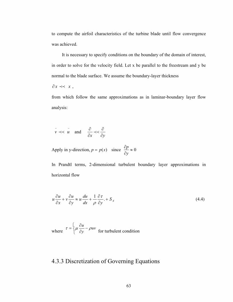
63

to compute the airfoil characteristics of the turbine blade until flow convergence

was achieved.

It is necessary to specify conditions on the boundary of the domain of interest,

in order to solve for the velocity field. Let x be parallel to the freestream and y be

normal to the blade surface. We assume the boundary-layer thickness

xx ≺≺∂ ,

from which follow the same approximations as in laminar-boundary layer flow

analysis:

−−

uv ≺≺ and yx ∂

∂∂∂ ≺≺

Apply in y-direction, )(xpp = since 0≈∂∂

yp

In Prandtl terms, 2-dimensional turbulent boundary layer approximations in

horizontal flow

XSydx

duuyuv

xuu +

∂∂

+≈∂∂

+∂∂ .1 τ

ρ (4.4)

where uv

yu ρμτ −

⎩⎨⎧

∂∂

= for turbulent condition

4.3.3 Discretization of Governing Equations

64

The numerical solution involves discretization of the problem domain and

the Navier-Stokes governing flow equations. Fluent uses the finite volume method

for its discretization. The differential form of the Navier-Stokes governing

equations is derived and transformed into an integral form. The solution domain is

subdivided into a finite number of contiguous control volumes and conservation

equations for each control volume. These equations are solved by employing

FLUENT (2005) in the two-dimensional mode with no swirl. FLUENT uses a

control-volume-based technique for converting the governing equations into

algebraic equations that can be solved numerically. In this thesis, the solution

algorithm adopted is Standard k-ε turbulence model, and a second-order upwind

scheme based on a multilinear reconstruction approach is used for all dependent

properties.

Reducing the integral form of the conservation equations to an equivalent

algebraic expression requires spatial discretization. The finite volume method has

the advantage of being applied to any type of grid, especially complex geometries.

The computational nodes are located at the centroid of a control volume, as well as

the boundaries.

QFtu

=⋅∇+∂∂ −

(4.5)

∫∫∫ Ω

−−

ΩΩ⋅=⋅+Ω

∂∂ dQsdFudt S

(4.6

65

All finite volume solvers such as Fluent have the ability to solve the Navier-Stokes

equations through an algebraic approximation. In the next section, the domain

discretization for the CFD solver will be discussed.

4.3.4 Domain Discretization A challenge in the CFD modelling was to discretize the flow domain near the

blades. The solution domain is sub-divided into set of sub control volumes. A finite

volume is established by all sub volumes associated with certain node after the

assembly of all elements. The numerical error of the scheme changes as a function

of grid spacing. Numerical error can be reduced by using a very fine grid. A

practical means of indicating grid independence is comparing solutions obtained on

different grids, then establishing the range of grid spacings where additional

refinement does not have a significant impact on results. A combination of

triangular unstructured and quadrilateral structured elements was used. Due to the

importance of the fluid interaction with the blades, a more refined quadrilateral grid

is used near the rotor blade edges. The grid should be fine enough to capture details

of flows within these critical regions but without demanding excessive computing

resources. The current method achieved a good balance between these two aspects:

fine grids at blade surfaces, where accurate resolution of pressure calculations was

required, and also at the surfaces of the rotor, but more coarse triangular elements

for other parts of the domain (Fig. 2). More specifically, the far-field layers of

elements will require less computational time than turbulent flow near the walls.

The total number of elements for both grid types is illustrated in (Fig. 4.2.)

66

Figure 4.2a: Mesh with N = 5 and 9,202 triangular and quadrilateral elements.

Figure 4.2b Mesh with N = 9 and 13,200 triangular and quadrilateral elements.

67

In mesh sensitivity studies, it is important to assess the dependence of

results on grid spacing by repeating the same simulation, but with different mesh

refinements. This is called a mesh sensitivity study that compares results at varying

grid spacings, until the pressure coefficient on other parameters becomes nearly

constant. The pressure coefficient, Kp, is defined as

)5.0/( 2∞−= UPPKp S ρ (4.7)

where P is a measured pressure on a surface and Ps is the static pressure measured in

the free stream, and ∞U is a reference velocity taken as the free stream velocity, U.

The parameter, Kp, is obtained as a CFD simulation result. The result of this grid

sensitivity analysis is shown in the result section.

4.3.5 Numerical Model

The Navier-Stokes equations consist of the continuity equation, turbulence

momentum equations for velocity, the energy equation and the turbulence transport

equations for k and ε. These are the equations solved by FLUENT. The CFD

software uses a control-volume-based technique for discretizing the fluid flow

governing equations into algebraic equations that can be solved numerically

In the Multiple Reference Frame environment, FLUENT (version 6.3) uses

a steady-state 2-D finite volume method with a segregated implicit solver. The

Reynolds stress model constants of turbulence are used. Standard wall functions are

applied for near-wall treatment and the k-ε turbulence model is used.

68

At the upstream boundary of the inlet, a uniform velocity with a turbulence

intensity of 10% was assumed at the velocity inlet. This assumption was based on

experimental data where a turbulence intensity of approximately 10% was obtained

at the designated operating wind speed (Veers, Winterstein, 1997). The turbulent

viscosity ratio is estimated at 1 to simulate a low turbulence viscosity (Saxena,

2007). At the pressure outlet, a backflow turbulence intensity of 12% is assumed, to

account for the increased turbulence caused by interaction with the turbine. The

backflow turbulence viscosity ratio was also estimated to be 1.

At the downstream boundary, the gage-pressure was assumed to be zero. On

the surface of the blades and the cylinder wall, a no-slip condition was prescribed.

Symmetric boundary conditions were used for both sides in the span wise direction.

All stator blades were set up as stationary walls, subject to a no-slip condition with

the fluid rotor modeled in the moving reference frame. The wind velocity inlet

conditions are fixed at a certain mean value, as the rotor speed changes in a

prescribed stepwise manner. The aerodynamic blade loads are transferred through

the rotor and converted into an estimated torque on the low speed rotor shaft,

resulting in energy generation from this wind turbine.

In the next chapter, 6m/s, 8 m/s, 10 m/s and 12 m/s are the selected mean

wind velocities to test the design turbine rotor efficiency. A rotational speed range

between 10 rad/s and 180 rad/s is used. The model is formulated with a standard

second-order upwind discretization scheme using a default under-relaxation

69

constant. The problem is iterated until all residuals on the turbine blade walls

converge to a value below the scale of 10-3, at which point a valid solution is

considered to be achieved. At convergence, the solution no longer changes

noticeably with further iterations. All governing equations are solved in all cells to

the specified convergence tolerance. Residuals were scaled relative to the local

value of flow properties in order to obtain a relative error.

Convergence cannot be judged only by examining the residual levels as this

could be misleading. As a secondary check for convergence, the mass and energy

balances were also examined. Numerical results will be reported in the next chapter.

Figure 4.5: Simulation iterations convergence

70

Figure 4.5 shows the residual indicator when the solver has converged. It indicates

that changes in flow variables typically became negligible after about 250

iterations.

4.3.6 Power Computations

Wind energy resides in the large mass of air moving over the earth’s

surface. This energy is available in the form of kinetic energy. Wind turbine blades

receive this kinetic energy and convert it to mechanical power, then it is further

converted to electrical energy. The efficiency of this conversion depends on how

effectively the rotor and blades interact with the wind stream. Wind turbine

technology has advanced significantly over the past few decades, and several

methods of rotor/blade optimization to extract more power from the wind have been

developed in the past. A force is experienced on the blades and rotor, whenever air

flows across the wind turbine.

In Fluent, the rotational force and torque are computed after each time step

is completed. The power extracted by the wind turbine in this CFD model is

computed during post-processing. The following steps of multiplying the torque by

the rotational speed are adopted:

Ω=→

xTPt (4.8)

→→→→→

+= VcPc FxrFxrT (4.9)

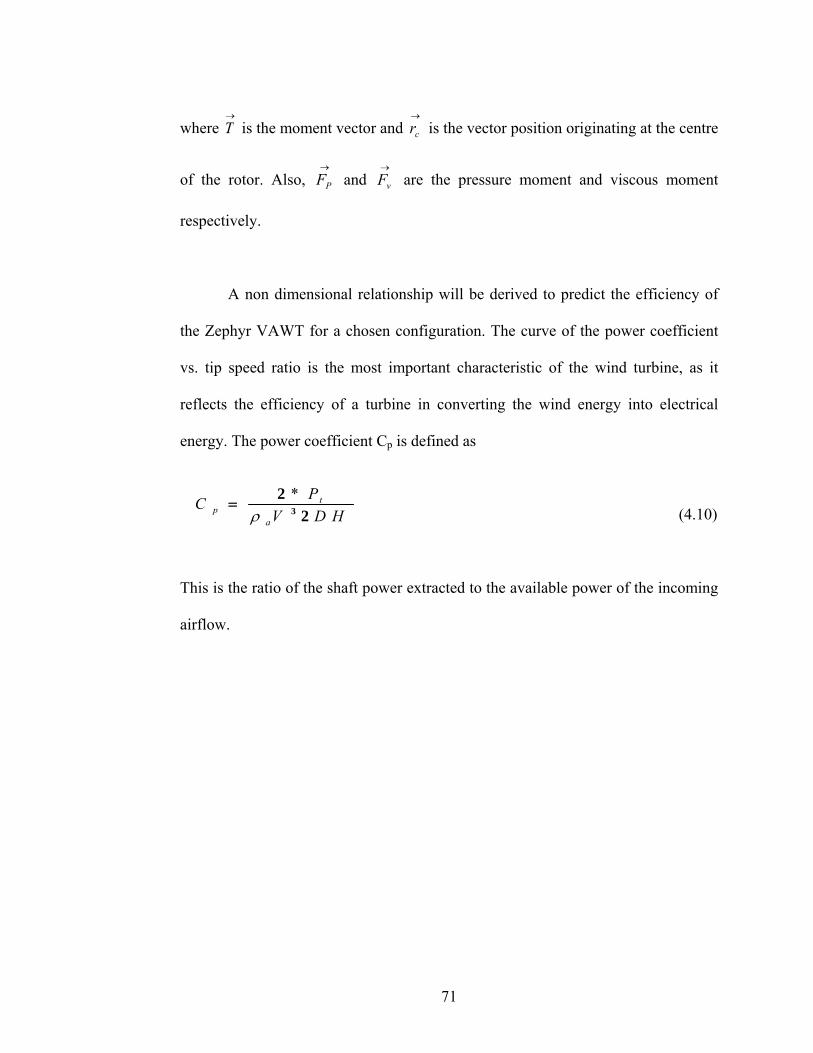
71

where →

T is the moment vector and →

cr is the vector position originating at the centre

of the rotor. Also, →

PF and →

vF are the pressure moment and viscous moment

respectively.

A non dimensional relationship will be derived to predict the efficiency of

the Zephyr VAWT for a chosen configuration. The curve of the power coefficient

vs. tip speed ratio is the most important characteristic of the wind turbine, as it

reflects the efficiency of a turbine in converting the wind energy into electrical

energy. The power coefficient Cp is defined as

(4.10)

This is the ratio of the shaft power extracted to the available power of the incoming

airflow.

tp

a

* PCV D Hρ

= 32

2

72

Chapter 5

RESULTS AND DISCUSSIONS

5.1 General

The key dimensionless variables for wind turbine problems are the Reynolds

number, power coefficient and the tip speed ratio. The tip speed ratio and power

coefficient are parameters in the thesis and they will be set within standard

operating ranges. The pressure and velocity distributions will be predicted during

each simulation and documented for future validation with wind tunnel testing. The

data obtained from the numerical computations will be analyzed by various tools

and formulae described in the previous chapters. This chapter presents simulation

results in tabular form as well as graphical form and it includes a detailed analysis

of the test results to explain the trends.

5.2 Performance Results

The efficiency of wind turbines is characterized by a parameter known as

the coefficient of performance, or Cp. This coefficient ranges from 0 to 0.59 (see

figures 3.3 and 3.5). The numerical value 0.59, or 16/27, is the Betz limit, which

represents is the maximum theoretical efficiency that any wind turbine removing

energy from a fluid can achieve. The Cp coefficient of a turbine is determined

primarily by the aerodynamic forces, which are affected by the shape of the blades.

The forces experienced by the blades will vary depending on the wind flow

conditions, namely the relative velocity of the blade to the wind, or tip speed ratio.

73

As the tip speed ratio is varied, the rotor efficiency will change, since the blades

cannot be optimized for every tip speed ratio. The curve produced by graphing the

power coefficient (Cp) vs. tip speed ratio (λ) is known as the characteristic curve of

the turbine. It displays the turbine’s ability to operate throughout a range of

conditions. The inability of VAWTs to achieve a tip speed ratio of much greater

than 1 make them unable to achieve the high Cp exhibited by HAWTs, which have

proven an almost 50% efficient. Typical values for VAWTs lie within the range

between 0.1 and 0.18 [31]. Current developments in blade profiling and other

methods are allowing vertical machines to incorporate larger lift forces, thereby

increasing their performance.

Figures 5.1a and 5.1b show the starting torque vs. rotor rotational speed for

different rotor blade configurations. These plots account for different mean wind

velocities under varying rotor loads and speeds. The torque vs. speed plot shows

agreement with the expected trends of high torque for a given VAWT rotor speed.

This high torque advantage of drag-based VAWTs can be utilized for a possible

hybrid of the Darrieus–Savonius turbine. The high torque becomes an advantage for

a much higher efficiency, but low torque starting disadvantage for the lift-based

VAWTs. The the turbine torque–speed plots are seen to be decreasing as the speed

increases until the torque is nearly zero when the rotor “floats” with the wind.

Figures 5.2a and 5.2b show the corresponding power vs. rotor speed, at a

given wind speed. The mechanical power converted into electrical power is a

74

product of the rotor torque and rotor angular speed, so it is expected from the result

that the power will be zero at a zero rotor speed, and again at a high rotor speed

with zero torque. The configuration with nine rotor blades has a maximum power at

the lower rotor speed. The speeds at maximum power are not the same speed at

which the torque is maximum in Figs. 5.1a-b. A good strategy will be to design a

wind turbine that matches the rotor speed to generate maximum power as the wind

velocity changes.

The power–speed and torque–speed characteristics are used to estimate the

power coefficient – tip speed ratio curve of the rotor, where Cp as a function of TSR

is presented. These curves are useful for predicting the turbine’s ideal TSR and also

its feasibility and adaptability to different wind conditions. The trends of the

resultant plots follow the theoretical expected trends. The curve shapes of the power

vs. function of rotor rotational velocity, and Cp vs. TSR follow a roughly parabolic

shape. Figures 5.3a and 5.3b show Cp and TSR for both configurations at different

wind velocities. The tip speed ratio of this turbine lies within the range between 0

and 1.2. Operating under the same condition, the N = 9 rotor blade performance

appears better at a lower tip speed ratio (0.6) when compared to 0.8 for the base

design with N = 5 rotor blades. The blade tip loss is minimized due to the increase

of blade number and reduction of space between blades.

Figures 5.4a and 5.4b display results of the stream-tube model. The CFD

and momentum model show reasonable agreement. On the left and rising branch,

75

there is fairly good agreement of both models, while there is some deviation in the

right and falling part. The higher tip speed ratio leads to a higher value of Cp in the

stream–tube model. For a low tip speed ratio where Cp values were close for both

cases, the computation times are comparable. Though this validation has an error of

about 20%, especially on the high TSR side, the results do follow expected trend.

The CFD model with good mesh and geometry modeling yields accurate results that

can be relied on compared to either the momentum or vortex models. It is also

worth noting that in calculating the power using the stream tube model, we have

made some assumptions in values like blade lift/drag coefficients and chord

diameter. Computed average values of lift and drag coefficients obtained from CFD

simulation results were substituted in the stream tube model analysis as no data for

this turbine could be obtained from literature.

It is desirable to obtain a single correlation for predicting the performance of

a particular turbine design at any given wind velocity. In Figs 5.3a and b, Cp and

TSR at different velocities have been predicted, but it is laborious and time-

consuming to perform simulations for all velocities. The coefficients were obtained

at various velocities for the Cp – TSR curves for both the CFD and stream tube

models. (see A .1-4 and B. 1-4) for table values. A cubic polynomial method of

fitting was adopted because of its ability to give a good approximation of the curve

shape with little error.

76

Figures 5.5a, 5.5b, 5.6a and 5.6b give the relationship between Cp and TSR

for both configurations and models respectively. This relationship at all wind

velocities converges to a single curve and one correlation equation. This non –

dimensional relationship represents the performance of any dimensionally similar

rotor, irrespective of its size, where Cp in the polynomial equation is the Zephyr

wind turbine power coefficient or rotor efficiency, while x is the rotor tip speed

ratio. At any given wind speed, these correlations for each configuration and model

will be useful in predicting the wind turbine efficiency.

Figures 5.7a and 5.7b show each model with the different geometry

modification results. The results of each model follow almost the same trend.

However, the stream tube model result appears higher toward the region of

decreasing rotor efficiency of the turbine. The rotor with the higher number of

blades gives a higher efficiency, even at a low tip speed. An increase in the tip

speed ratio that results from an incremental rotor speed favors the 5 rotor blade

configuration in utilizing the energy of the wind to enhance the performance output.

With fewer blades, there is a lower Cp for low tip-speed ratios. A reduction in the

number of blades reduces the relative wind angle at the low design tip-speed ratio.

The effect of the number of blades is negligible at the high value of design tip-

speed ratio. For this reason, the Zephyr wind turbine with more rotor blades is the

best choice for an area that favors a low tip speed ratio configuration. The low

numbers of blades, such as three or five bladed wind turbines, use a higher tip speed

ratio than the 9-blade wind turbines. This analysis will be useful when making a

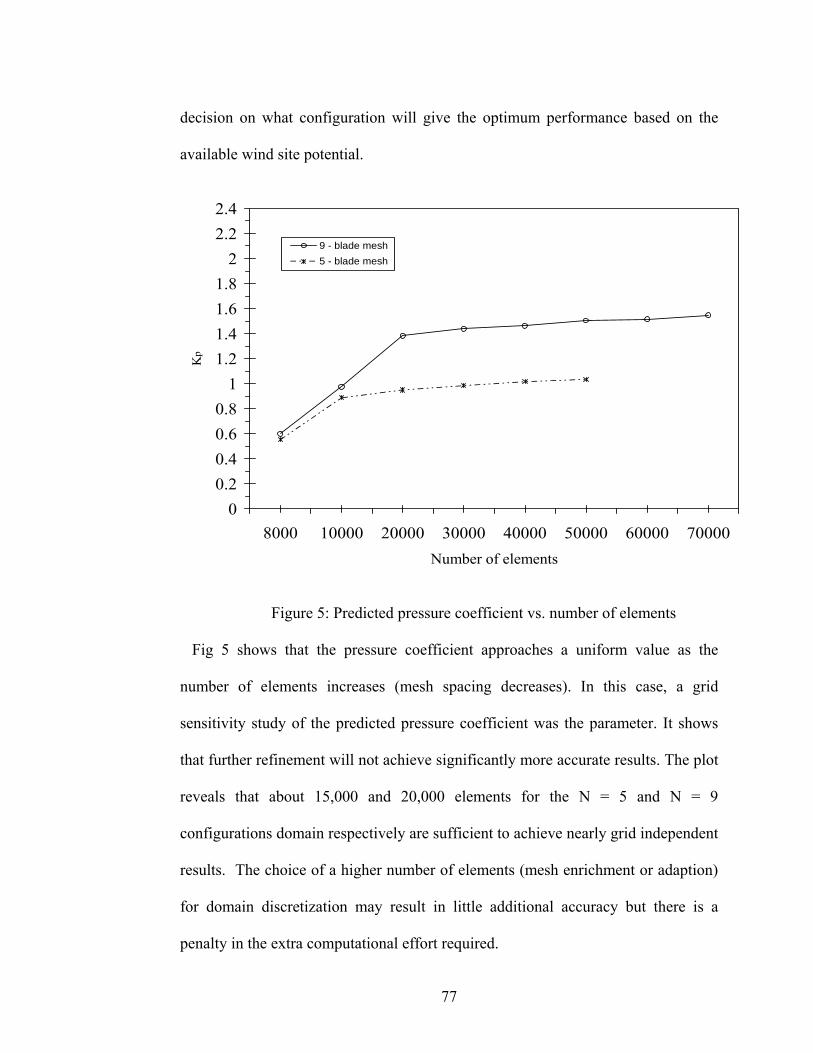
77

00.20.40.60.8

11.21.41.61.8

22.22.4

8000 10000 20000 30000 40000 50000 60000 70000Number of elements

Kp

9 - blade mesh5 - blade mesh

decision on what configuration will give the optimum performance based on the

available wind site potential.

Figure 5: Predicted pressure coefficient vs. number of elements

Fig 5 shows that the pressure coefficient approaches a uniform value as the

number of elements increases (mesh spacing decreases). In this case, a grid

sensitivity study of the predicted pressure coefficient was the parameter. It shows

that further refinement will not achieve significantly more accurate results. The plot

reveals that about 15,000 and 20,000 elements for the N = 5 and N = 9

configurations domain respectively are sufficient to achieve nearly grid independent

results. The choice of a higher number of elements (mesh enrichment or adaption)

for domain discretization may result in little additional accuracy but there is a

penalty in the extra computational effort required.

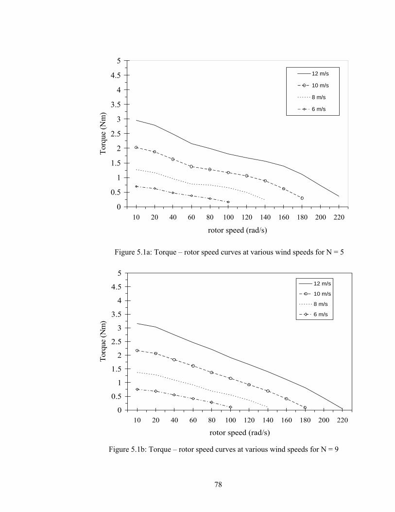
78

0

0.5

1

1.5

2

2.5

3

3.5

4

4.5

5

10 20 40 60 80 100 120 140 160 180 200 220

rotor speed (rad/s)

Torq

ue (N

m)

12 m/s

10 m/s

8 m/s

6 m/s

Figure 5.1a: Torque – rotor speed curves at various wind speeds for N = 5

0

0.5

1

1.5

2

2.5

3

3.5

4

4.5

5

10 20 40 60 80 100 120 140 160 180 200 220

rotor speed (rad/s)

Torq

ue (N

m)

12 m/s

10 m/s

8 m/s

6 m/s

Figure 5.1b: Torque – rotor speed curves at various wind speeds for N = 9

79

0

50

100

150

200

250

300

10 20 40 60 80 100 120 140 160 180 200 220

rotor speed (rad/s)

Pow

er (w

atts

)

12 m/s10 m/s8 m/s6 m/s

Figure 5.2a: Power–rotor speed curves at various wind speeds for N = 9

0

50

100

150

200

250

300

10 20 40 60 80 100 120 140 160 180 200 220

rotor speed (rad/s)

Pow

er (w

atts

)

12 m/s

10 m/s

8 m/s

6 m/s

Figure 5.2b: Power–rotor speed curves at various wind speeds for N = 5.

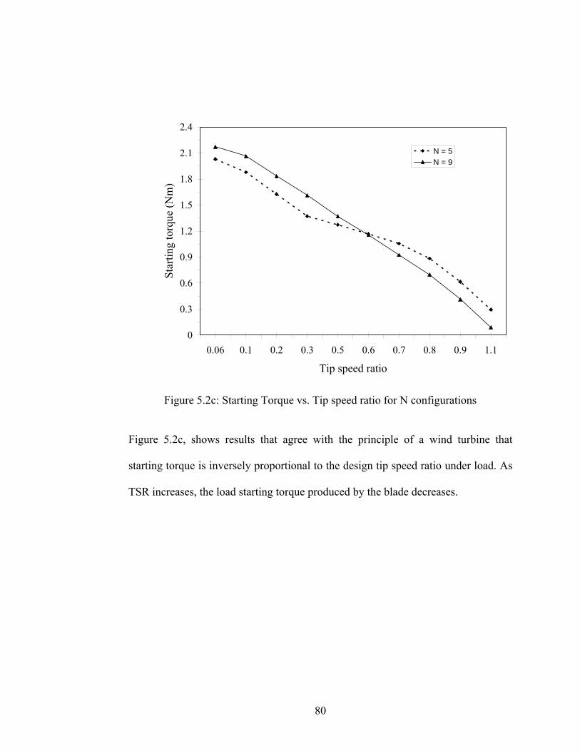
80

0

0.3

0.6

0.9

1.2

1.5

1.8

2.1

2.4

0.06 0.1 0.2 0.3 0.5 0.6 0.7 0.8 0.9 1.1

Tip speed ratio

Star

ting

torq

ue (N

m)

N = 5N = 9

Figure 5.2c: Starting Torque vs. Tip speed ratio for N configurations Figure 5.2c, shows results that agree with the principle of a wind turbine that

starting torque is inversely proportional to the design tip speed ratio under load. As

TSR increases, the load starting torque produced by the blade decreases.

81

0

0.1

0.2

0.3

0.4

0.5

0.6

0 0.1 0.2 0.3 0.4 0.5 0.6 0.7 0.8 0.9 1 1.1 1.2

Tip speed ratio

Pow

er c

oeff

icie

nt

12 m/s10 m/s8 m/s6 m/s

Figure 5.3a: CFD performance curves for N = 9 at various wind speeds

0

0.1

0.2

0.3

0.4

0.5

0.6

0 0.1 0.2 0.3 0.4 0.5 0.6 0.7 0.8 0.9 1 1.1 1.2

Tip speed ratio

Pow

er c

oeff

icie

nt

12 m/s10 m/s8 m/s6 m/s

Figure 5.3b: CFD performance curves for N = 5 at various wind speeds

82

0

0.1

0.2

0.3

0.4

0.5

0.6

0 0.1 0.2 0.3 0.4 0.5 0.6 0.7 0.8 0.9 1 1.1 1.2 1.3

Tip speed ratio

Pow

er c

oeff

icie

nt

10 m/s, CFD

10 m/s, Stream tube model

8 m/s, CFD

8 m/s, Stream tube model

Figure 5.4a: Performance curve for both models, N = 9 at given wind speeds

0

0.1

0.2

0.3

0.4

0.5

0.6

0 0.1 0.2 0.3 0.4 0.5 0.6 0.7 0.8 0.9 1 1.1 1.2 1.3Tip speed ratio

Pow

er c

oeff

icie

nt

10 m/s, CFD10 m/s, Stream tube model8 m/s, CFD8 m/s, Stream tube model

Figure 5.4b: Performance curve for both models, N = 5 at given wind speeds

83

Cp = -0.1825x3 - 0.3087x2 + 0.7848x - 0.0166

0

0.1

0.2

0.3

0.4

0.5

0.6

0 0.1 0.2 0.3 0.4 0.5 0.6 0.7 0.8 0.9 1 1.1 1.2 1.3Tip speed ratio

Pow

er c

oeff

icie

nt

Figure 5.5a: Stream tube model prediction curve at all wind velocities for N = 9

Cp = -0.4673x3 + 0.4201x2 + 0.3987x + 0.0097

0

0.1

0.2

0.3

0.4

0.5

0.6

0 0.1 0.2 0.3 0.4 0.5 0.6 0.7 0.8 0.9 1 1.1 1.2 1.3

Tip speed ratio

Pow

er c

oeff

icie

nt

Figure 5.5b: Stream tube model predictions curve at all wind velocities for N = 5

84

Cp = -0.2213x3 - 0.6897x2 + 1.0186x + 0.0075

0

0.1

0.2

0.3

0.4

0.5

0.6

0 0.1 0.2 0.3 0.4 0.5 0.6 0.7 0.8 0.9 1 1.1 1.2

Tip speed Ratio

Pow

er c

oeff

icie

nt

Figure 5.6 a: CFD performance prediction curve at all wind velocities for N = 9

Cp= -0.6119x3 + 0.2086x2 + 0.5917x + 0.0308

0

0.1

0.2

0.3

0.4

0.5

0.6

0 0.1 0.2 0.3 0.4 0.5 0.6 0.7 0.8 0.9 1 1.1 1.2

Tip speed ratio

Pow

er c

oeff

icie

nt

Figure 5.6 b: CFD performance prediction curve at all wind velocities for N = 5

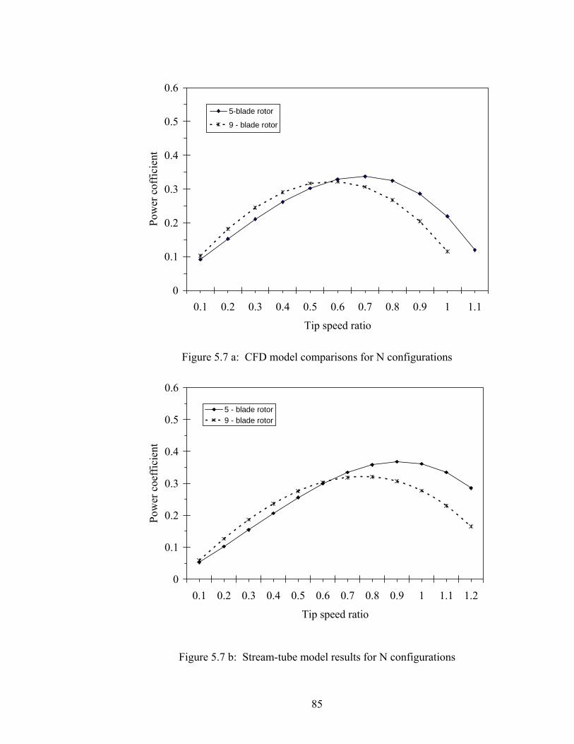
85

0

0.1

0.2

0.3

0.4

0.5

0.6

0.1 0.2 0.3 0.4 0.5 0.6 0.7 0.8 0.9 1 1.1

Tip speed ratio

Pow

er c

offic

ient

5-blade rotor

9 - blade rotor

Figure 5.7 a: CFD model comparisons for N configurations

0

0.1

0.2

0.3

0.4

0.5

0.6

0.1 0.2 0.3 0.4 0.5 0.6 0.7 0.8 0.9 1 1.1 1.2

Tip speed ratio

Pow

er c

oeff

icie

nt

5 - blade rotor9 - blade rotor

Figure 5.7 b: Stream-tube model results for N configurations

86

0

500

1000

1500

2000

2500

3000

3500

4000

4500

5000

4 5 6 7 8 9 10 11 12 13 14 15 16 17 18

Wind speed (m/s)

Pow

er (w

atts

)

PacWind max.

Zephyr max.

PacWind CFD

Zephyr N =9, CFD

Zephyr N = 5, CFD

Figure 5.8a: Maximum power curves of PacWind and Zephyr turbines

0

50

100

150

200

250

300

350

400

4 5 6 7 8 9 10 11 12 13 14 15 16 17 18

Wind speed (m/s)

Pow

er (w

atts

)

PacWind turbine

N = 9, Zephyr turbine


Figure 5.8b: Power vs. wind velocity for the configurations.

87

Results of power as a function of wind velocity are shown in Figs 5.8a and 5.8b.

This plot follows reasonably close to an expected cubic shape, as power increases

with the third power of wind velocity, i.e.,

3...21 VAP ρ= , (5.1)

where ρ is the density of the air stream flowing through the turbine, A is the

effective area of the rotor blades, and V is the velocity of the air flow stream. In

figure 5.8a, the maximum theoretical power that can be obtained from both turbines

are displayed. The PacWind maximum power curve extracts more power under the

same condition of wind velocity. However, its rotor swept area is greater than the

Zephyr rotor. The interest in the Pacwind turbine in this thesis is using it to compare

with the Zephyr design, regarding the utility of the stator–tab, which Pacwind lacks

in its configuration. Figure 5.8b indicates the unique Zephyr design has a beneficial

impact.

The 9-blade configuration gives an improved rotor power output when

compare the base 5-blade rotor design under the same operating conditions. It

exhibits an increase of about 20% percent in power output over the five rotor blade

configuration. Moreover, since the power coefficient is directly proportional to the

lift forces acting on the blade, the geometry modification of the blade flow angle,

blade spacing and chord diameter on the 9-blade turbine causes the lift forces acting

on the modified rotor to increase. Figures 2.4 and 2.5 showed the schematic of the

Zephyr vertical axis wind turbine and the Pacwind vertical axis wind turbine

respectively. They very much look and operate under the same principle. The

88

Zephyr VAWT is uniquely different by the addition of the stator vein and tab.

Given the information available from Pacwind Technology, the same conditions

were imposed as the Zephyr wind generator design. A careful observation of the

plot of figure 5.8 shows that during low wind speed conditions, the Pacwind turbine

is unable to generate appreciable power until about 12 m/s wind velocity. The

Pacwind turbine will work better in a region with high wind potential (see

Appendix C for table).

The Zephyr simulation results under the same conditions exhibit a better

design. Its ability to generate power under the same low wind velocity makes the

Zephyr design a better and improved design for harvesting the wind energy

continuously at all wind speeds. The proprietary stator blade elements of this design

help it perform in low velocity wind conditions drawing more air into the turbine. It

is important to observe from figure 5.8 of the difference in rotor power generated

among these two designs, especially between the wind velocities 13 m/s and 18

m/s. The power from the Pacwind turbine appears higher because of its area of 55

inches by 30 inches, as compared to the Zephyr turbine of 30 inches by 30 inches

for a given equal blade surface area of contact with flowing air during operation,

the rotor torque and power conversion from the Zephyr turbine design will increase

in Fig. 5.8.

The power output of a wind turbine is directly related to the swept area of

the blades. Swept area refers to the area through which the rotor blades spin. Given

89

0

50

100

150

200

250

300

350

400

4 5 6 7 8 9 10 11 12 13 14 15 16 17 18Wind speed (m/s)

Pow

er p

er s

qr m

eter

(W/m

2 )



PacWind turbine

that the swept areas of both models are not equal, comparisons are inconsistent.

However, a reasonable comparison can be made in terms of power generation per

unit area as indicated in Figure 5.9. The results clearly show that the Zephyr turbine

operates with higher power conversion efficiency at both high and low wind speed

conditions.

Figure 5.9: Power per square meter – wind speed curves

Drag and lift coefficient results are plotted against changing wind velocity

in figures 5.10 and 5.11. As expected, the drag coefficient decreases as the wind

velocity increases. The 5 rotor blade configuration has more drag force during low

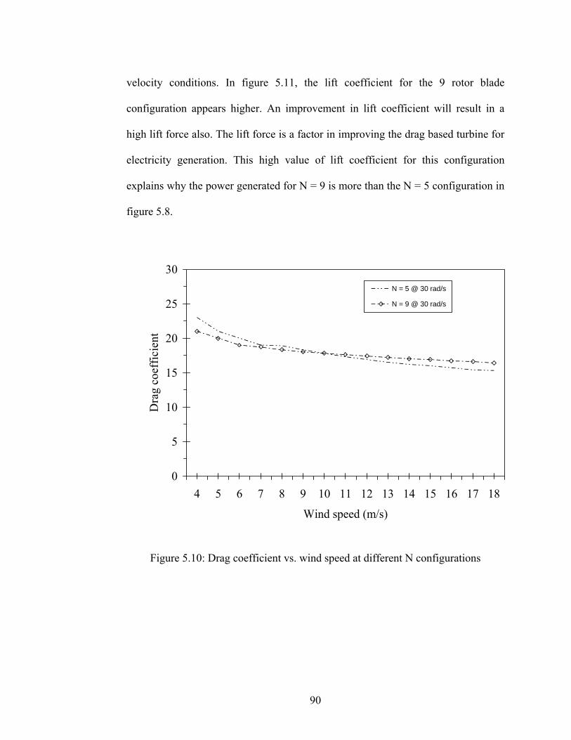
90

velocity conditions. In figure 5.11, the lift coefficient for the 9 rotor blade

configuration appears higher. An improvement in lift coefficient will result in a

high lift force also. The lift force is a factor in improving the drag based turbine for

electricity generation. This high value of lift coefficient for this configuration

explains why the power generated for N = 9 is more than the N = 5 configuration in

figure 5.8.

0

5

10

15

20

25

30

4 5 6 7 8 9 10 11 12 13 14 15 16 17 18

Wind speed (m/s)

Dra

g co

effic

ient

N = 5 @ 30 rad/s

N = 9 @ 30 rad/s

Figure 5.10: Drag coefficient vs. wind speed at different N configurations

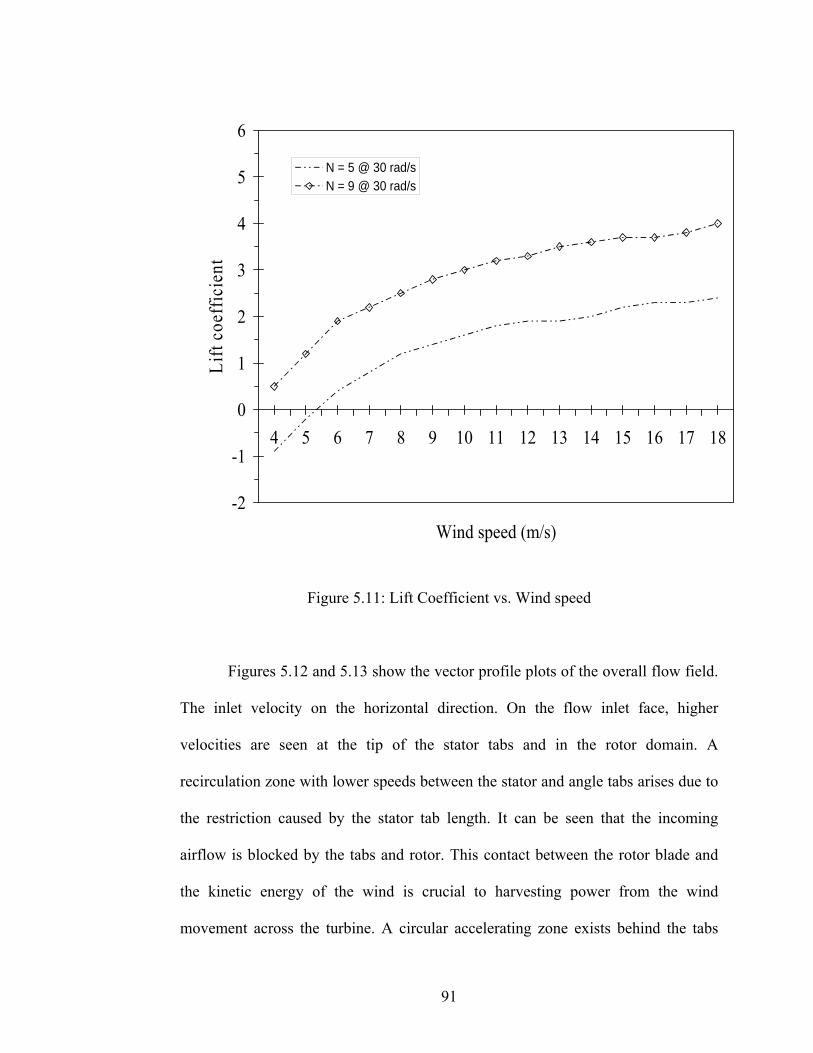
91

-2

-1

0

1

2

3

4

5

6

4 5 6 7 8 9 10 11 12 13 14 15 16 17 18

Wind speed (m/s)

Lift

coef

ficie

nt

N = 5 @ 30 rad/sN = 9 @ 30 rad/s

Figure 5.11: Lift Coefficient vs. Wind speed

Figures 5.12 and 5.13 show the vector profile plots of the overall flow field.

The inlet velocity on the horizontal direction. On the flow inlet face, higher

velocities are seen at the tip of the stator tabs and in the rotor domain. A

recirculation zone with lower speeds between the stator and angle tabs arises due to

the restriction caused by the stator tab length. It can be seen that the incoming

airflow is blocked by the tabs and rotor. This contact between the rotor blade and

the kinetic energy of the wind is crucial to harvesting power from the wind

movement across the turbine. A circular accelerating zone exists behind the tabs

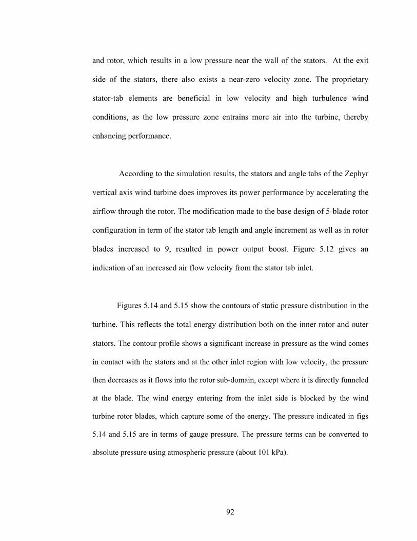
92

and rotor, which results in a low pressure near the wall of the stators. At the exit

side of the stators, there also exists a near-zero velocity zone. The proprietary

stator-tab elements are beneficial in low velocity and high turbulence wind

conditions, as the low pressure zone entrains more air into the turbine, thereby

enhancing performance.

According to the simulation results, the stators and angle tabs of the Zephyr

vertical axis wind turbine does improves its power performance by accelerating the

airflow through the rotor. The modification made to the base design of 5-blade rotor

configuration in term of the stator tab length and angle increment as well as in rotor

blades increased to 9, resulted in power output boost. Figure 5.12 gives an

indication of an increased air flow velocity from the stator tab inlet.

Figures 5.14 and 5.15 show the contours of static pressure distribution in the

turbine. This reflects the total energy distribution both on the inner rotor and outer

stators. The contour profile shows a significant increase in pressure as the wind comes

in contact with the stators and at the other inlet region with low velocity, the pressure

then decreases as it flows into the rotor sub-domain, except where it is directly funneled

at the blade. The wind energy entering from the inlet side is blocked by the wind

turbine rotor blades, which capture some of the energy. The pressure indicated in figs

5.14 and 5.15 are in terms of gauge pressure. The pressure terms can be converted to

absolute pressure using atmospheric pressure (about 101 kPa).

93

The negative pressures predicted at the centre and exit part of the turbine blades

are advantageous to the Zephyr VAWT. This is as a result of improved efficiency of

the turbine, which requires increased contribution from the lift force to generate

additional torque.

Figure 5.12: Predicted velocity vectors (m/s) for N = 5

Figure 5.13: Predicted velocity vectors (m/s) for N = 9

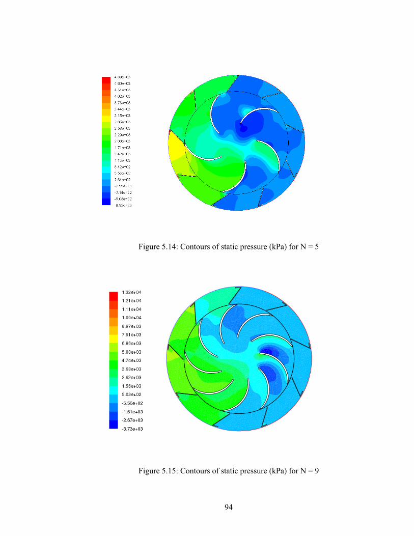
94

Figure 5.14: Contours of static pressure (kPa) for N = 5

Figure 5.15: Contours of static pressure (kPa) for N = 9

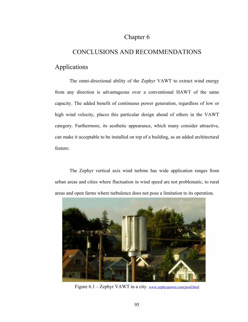
95

Chapter 6

CONCLUSIONS AND RECOMMENDATIONS

Applications The omni-directional ability of the Zephyr VAWT to extract wind energy

from any direction is advantageous over a conventional HAWT of the same

capacity. The added benefit of continuous power generation, regardless of low or

high wind velocity, places this particular design ahead of others in the VAWT

category. Furthermore, its aesthetic appearance, which many consider attractive,

can make it acceptable to be installed on top of a building, as an added architectural

feature.

The Zephyr vertical axis wind turbine has wide application ranges from

urban areas and cities where fluctuation in wind speed are not problematic, to rural

areas and open farms where turbulence does not pose a limitation to its operation.

Figure 6.1 – Zephyr VAWT in a city. www.zephyrpower.com/prod.html

http://www.zephyrpower.com/prod.html

96

6.1 Summary and Conclusions CFD has been a useful modeling tool for analyzing the performance of a

Zephyr wind turbine. It is an inexpensive and effective method of simulating and

testing a large number of models that could not be readily examined in a wind

tunnel. Small design changes can be studied with these models, and tested quickly.

In this thesis, a 2-D numerical analysis has been completed using a multiple rotating

reference frame formulation, to predict time averaged results. A grid independence

study verifies the solution independence on grid spacing. From the performance

curves, an optimum tip speed ratio was acquired. This performance characteristic

was determined based on a modified rotor blade configuration. The results are

useful in determining the optimal number of rotor blades depending on different

wind speeds. The stator of the proprietary Zephyr design enhanced the

performance, especially in low wind speed zones. Also, a stream tube momentum

model was used in a theoretical analysis to predict the VAWT performance. The

results showed close agreement with computed values from the CFD model. A

single non-dimensional polynomial correlation for different blade for configurations

was obtained. These relationships can be used to predict and represent the

performance of any dimensionally similar turbine rotor, irrespective of size. These

correlations can also be used to predict the performance without CFD simulations.

From the above studies, the newly developed Zephyr vertical axis wind

turbine was found to be unique and more efficient in harvesting wind energy. It has

an excellent self-starting ability due to its high torque value. Even at low wind

97

velocity, it does still run smoothly, high torque and high rotor speed which make it

a good choice for electricity generation in cities and rural area. The Zephyr VAWT

is a technology that favours wide applications due to its ability to be installed on

any location irrespective of prevailing changing wind speed. The rotor speed (RPM)

can be improve upon through further geometry optimization of the turbine by

enhancing it lift force contribution. The stator tab variation for optimum geometry

search does proved advantage in performance.

6.2 Recommendations

This energy conversion device is highly efficient in its ability to operate

under low or high wind operating condition. We encourage its commercialization

especially in cities. Its scalable size favors installation on building roof top to. I

strongly believe further optimizing the stator-tab of this unique VAWT will boost

its power output. Future research in this subject is very important; recommendations

listed below are focused on enhancing the performance features, modeling methods

and other validation work for the Zephyr VAWT.

6.2.1 CFD modeling

Further research should investigate the model using a sliding mesh

formulation, as this will allow for more detailed investigation into the rotor-stator

interaction. The multiple reference frame capability of Fluent is unable to account

for this effect. The sliding mesh formulation requires a high capacity computer for

98

modeling and simulation. A complete 3-D CFD simulation should be performed.

This offers the possibility of visualizing the fluid flow phenomena and more

detailed quantitative data of the flow through the turbine. Unlike the 2-D model, the

3-D modeling and simulation will help to investigate the end effects of the turbine.

Optimization of the stator tab geometry would also become possible. Given the

small margin of power output from the N = 9 rotor blade configuration over the N =

5 configuration, I recommend the optimization of the stator/tab should be done on

the N = 5 rotor blades if material and construction cost is a determining factor.

6.2.2 Wind tunnel testing There is little or no available experimental data for this type of Zephyr

VAWT. Wind tunnel testing of this turbine will give more actual data to validate

the CFD simulation. Experimental testing in a controlled condition will give results

that measure the turbine non-dimensional performance curve without, freestream

variations. Such experiments would provide more useful data on the effectiveness

of the proprietary design elements and allow recommendations to be made about

further areas of improvement for the Zephyr VAWT. These results will then be

compared with the CFD modeling simulations to verify the predictions.

99

REFERENCES

[1] Ackermann, T., So der, L., “An Overview of Wind Energy – Status 2002”

Renewable and Sustainable Energy Reviews, vol. 6, pp. 67 – 128, (2002)

[2] “Wind Energy costs”, part of the National Wind Coordinating Committee’s

Wind Energy Series, No. 11, 01 (1997)

[3] American Wind Energy Association, “Global Wind Energy Market Report”,

http://www.awea.org/pubs/documents/globalmarket2003.pdf March 7, 2002

[4] Dorn, J.G., Earth Policy Institute, “Wind Indicator Data”,

http://www.earth-policy.org/Indicators/Wind/2008.htm March 4, 2008

[5] Global Wind Energy Council, “Global Wind 2006 report”,

http://www.gwec.net/index.php?id=78 June 2006

[6] Wind Hydrogen Limited.

http://www.wind-hydrogen.com/concept_wind%20hydrogen.html Sept. 5, 2006

[7] Golding, E. W., “The Generation of Electricity by Wind Power”, London E. &

F. M. Spon Ltd, Halsted Press, 1976

[8] Canadian Wind Energy Association, “Wind Energy-Powering Canadian

Future”, http://www.canwea.ca/production.stats.cfm. Accessed Nov.22, 2006

[9] Sim˜ao, C. J., Ferreira, G., Bussel, G .V and Kuik, G. V. “Wind tunnel hotwire

measurements, flow visualization and thrust measurement of a VAWT in skew.”

44th AIAA Aerospace Sciences Meeting and Exhibit/ASME Wind Energy

Symposium, 2006.

http://www.awea.org/pubs/documents/globalmarket2003.pdf

http://www.earth-policy.org/Indicators/Wind/2008.htm

http://www.gwec.net/index.php?id=78

http://www.wind-hydrogen.com/concept_wind hydrogen.html

http://www.canwea.ca/production.stats.cfm. Accessed Nov.22, 200

100

[10] Spera, D. A., “Wind Turbine Technology”, ASME Press, 1998

[11] Manwell, J. F., McGowan, J. G., Rogers, A. L., “Wind Energy Explained;

Theory, Design and Application”, John Wiley & Sons Ltd, 2002, Amherst.

[12] Kovarik, T., Pipher, C., Hurst, J., “Wind Energy”, Prism Press, 1979

[13] Akiyoshi Iida, Akisato Mizuno, Keiko Fukudome, Numerical Simulation of

Aerodynamic Noise Radiated form Vertical Axis Wind Turbines, Proceedings of

the 18 International Congress on Acoustics, 2004, CD-ROM

[14] Ammara, I., Leclerc, L., and Masson, C., “A Viscous Three Dimensional

Differential/ Actuator-Disk Method for the Aerodynamic Analysis of Wind Farms,”

Journal of Solar Energy Engineering, vol. 124, pp. 345 - 356, November, 2002.

[15] Abe, K., Nishida, M., Sakuraia, A., Ohya, Y., Kiharaa, H., Wadad, E., Satod,

K., 2005. “Experimental and numerical investigations of flow fields behind a small

wind turbine with a flanged diffuser.” Journal of Wind Engineering and Industrial

Aerodynamics. Vol. 93, pp. 951–970.

[16] Wang, F., Bai, L., Fletcher, J., Whiteford, J., Cullen, D., “The methodology for

aerodynamic study on a small domestic wind turbine with scoop.” Journal of Wind

Engineering and Industrial Aerodynamics, vol. 96, pp. 1-24, (2008).

[17] Sim ao Ferreira, C.J., Bijl, H., Bussel, G.V., Kuik, G.V., “Simulating Dynamic

Stall in a 2D VAWT: Modeling strategy, verification and validation with Particle

Image Velocimetry data” The Science of Making Torque from Wind. Journal of

Physics: Conference Series 75, pp. 012023, (2007)

101

[18] Kume, H., Ohya, Y., Karasudani, T., Watanabe, K., “Design of a shrouded

wind turbine with brimmed diffuser using CFD.” Proceedings of the Annual

Conference of JSAS, pp. 51–54, (2003)

[19] Sorensen, J.N., Kock, C.W. “A model for unsteady rotor aerodynamics using

CFD”. Journal of Wind Engineering and Industrial Aerodynamics, vol. 92, pp.

315–330. (2004)

[20] Templin, R.J., “Aerodynamics Performance Theory for the NRC Vertical-Axis

Wind Turbine,” N.A.E. Report LTR-LA-160, June 1974

[21] Hahm, T., Kroning, J. “In the Wake of a Wind Turbine,” Fluent News,

vol. 11, no. 1, pp. 5-7, spring 2002.

[22] Kelecy, F., “Wind Turbine Blade Aerodynamics,” Fluent news, vol. 11, no.1,

pp. 7, spring 2002.

[23] Newman, B.G., “Measurements on Savonius Rotor with Variable Gap,”

Proceedings of the sherbrooke University Symposium on Wind Energy, Sherbrooke,

Canada, 1974, p. 116.

[24] Camporeale S M, Fortunato B, and Marilli G, “Automatic System for Wind

Turbine Testing,” Journal of Solar Energy Engineering, vol. 123, pp. 333-338,

2001.

[25] The Energy Blog

http://thefraserdomain.typepad.com/energy/2008/05/worlds-largest.html

May 15, 2008

[26] Patel, M.R. (1999) Wind and Solar Power Systems, CRC Press, NY.

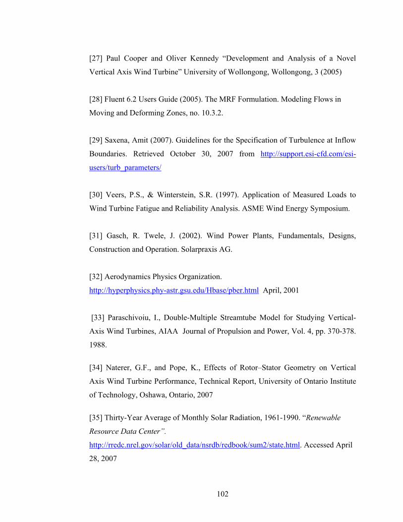
http://thefraserdomain.typepad.com/energy/2008/05/worlds-largest.html

102

[27] Paul Cooper and Oliver Kennedy “Development and Analysis of a Novel

Vertical Axis Wind Turbine” University of Wollongong, Wollongong, 3 (2005)

[28] Fluent 6.2 Users Guide (2005). The MRF Formulation. Modeling Flows in

Moving and Deforming Zones, no. 10.3.2.

[29] Saxena, Amit (2007). Guidelines for the Specification of Turbulence at Inflow

Boundaries. Retrieved October 30, 2007 from http://support.esi-cfd.com/esi-

users/turb_parameters/

[30] Veers, P.S., & Winterstein, S.R. (1997). Application of Measured Loads to

Wind Turbine Fatigue and Reliability Analysis. ASME Wind Energy Symposium.

[31] Gasch, R. Twele, J. (2002). Wind Power Plants, Fundamentals, Designs,

Construction and Operation. Solarpraxis AG.

[32] Aerodynamics Physics Organization.

http://hyperphysics.phy-astr.gsu.edu/Hbase/pber.html April, 2001

[33] Paraschivoiu, I., Double-Multiple Streamtube Model for Studying Vertical-

Axis Wind Turbines, AIAA Journal of Propulsion and Power, Vol. 4, pp. 370-378.

1988.

[34] Naterer, G.F., and Pope, K., Effects of Rotor–Stator Geometry on Vertical

Axis Wind Turbine Performance, Technical Report, University of Ontario Institute

of Technology, Oshawa, Ontario, 2007

[35] Thirty-Year Average of Monthly Solar Radiation, 1961-1990. “Renewable

Resource Data Center”.

http://rredc.nrel.gov/solar/old_data/nsrdb/redbook/sum2/state.html. Accessed April

28, 2007

http://support.esi-cfd.com/esi-users/turb_parameters/

http://support.esi-cfd.com/esi-users/turb_parameters/

http://hyperphysics.phy-astr.gsu.edu/Hbase/pber.html

http://rredc.nrel.gov/solar/old_data/nsrdb/redbook/sum2/state.html

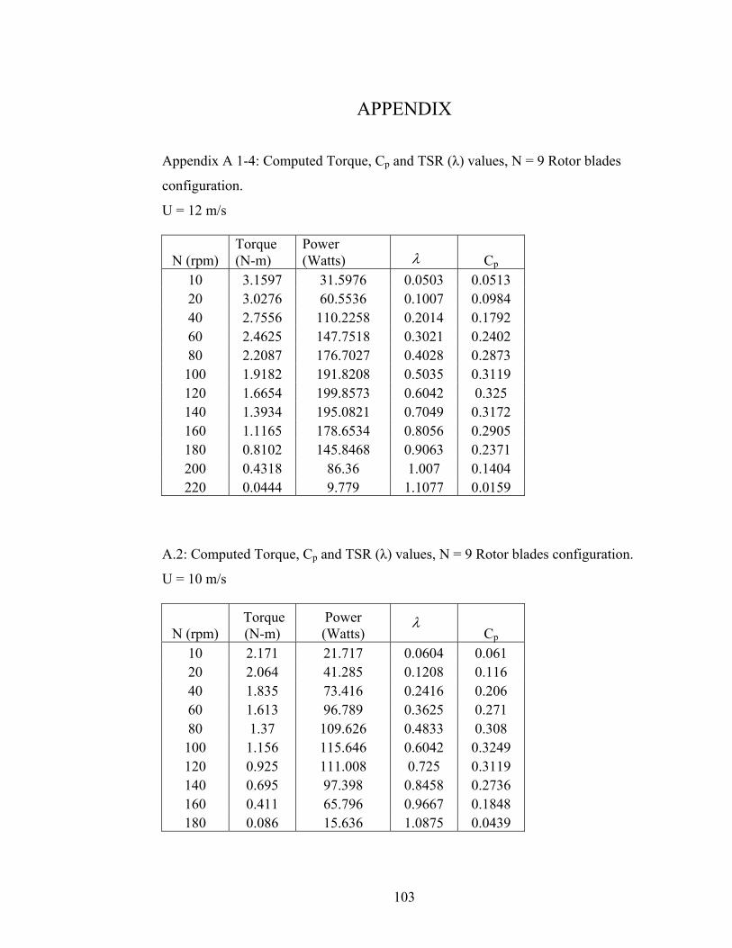
103

APPENDIX

Appendix A 1-4: Computed Torque, Cp and TSR (λ) values, N = 9 Rotor blades

configuration.

U = 12 m/s

N (rpm) Torque (N-m)

Power (Watts)

Cp

10 3.1597 31.5976 0.0503 0.0513 20 3.0276 60.5536 0.1007 0.0984 40 2.7556 110.2258 0.2014 0.1792 60 2.4625 147.7518 0.3021 0.2402 80 2.2087 176.7027 0.4028 0.2873 100 1.9182 191.8208 0.5035 0.3119 120 1.6654 199.8573 0.6042 0.325 140 1.3934 195.0821 0.7049 0.3172 160 1.1165 178.6534 0.8056 0.2905 180 0.8102 145.8468 0.9063 0.2371 200 0.4318 86.36 1.007 0.1404 220 0.0444 9.779 1.1077 0.0159

A.2: Computed Torque, Cp and TSR (λ) values, N = 9 Rotor blades configuration.

U = 10 m/s


Power (Watts)

Cp

10 2.171 21.717 0.0604 0.061 20 2.064 41.285 0.1208 0.116 40 1.835 73.416 0.2416 0.206 60 1.613 96.789 0.3625 0.271 80 1.37 109.626 0.4833 0.308 100 1.156 115.646 0.6042 0.3249 120 0.925 111.008 0.725 0.3119 140 0.695 97.398 0.8458 0.2736 160 0.411 65.796 0.9667 0.1848 180 0.086 15.636 1.0875 0.0439

λ

λ

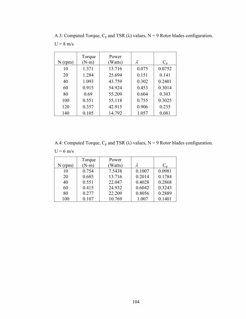
104


U = 8 m/s


Power (Watts) λ Cp

10 1.371 13.716 0.075 0.0752 20 1.284 25.694 0.151 0.141 40 1.093 43.759 0.302 0.2401 60 0.915 54.924 0.453 0.3014 80 0.69 55.209 0.604 0.303 100 0.551 55.118 0.755 0.3025 120 0.357 42.915 0.906 0.235 140 0.105 14.792 1.057 0.081


U = 6 m/s


Power (Watts) λ Cp

10 0.754 7.5438 0.1007 0.0981 20 0.685 13.716 0.2014 0.1784 40 0.551 22.047 0.4028 0.2868 60 0.415 24.932 0.6042 0.3243 80 0.277 22.209 0.8056 0.2889 100 0.107 10.769 1.007 0.1401

105

Appendix B.1: Computed Torque, Cp and TSR (λ) values, N = 5 Rotor blades

configuration.

U =12 m/s

N (rpm) Torque (N-m) Power (watts) λ Cp

10 2.954 29.54 0.05 0.048 20 2.783 55.676 0.1 0.094 40 2.494 99.771 0.201 0.1622 60 2.159 129.54 0.302 0.2106 80 1.986 158.902 0.403 0.2584 100 1.81 181 0.504 0.2943 120 1.673 200.863 0.605 0.3266 140 1.559 218.338 0.706 0.355 160 1.386 221.894 0.807 0.3608 180 1.104 198.88 0.905 0.323 200 0.721 144.27 1.009 0.2346 220 0.36 79.349 1.11 0.129


configuration.

U = 10 m/s

N (rpm) Torque (N-m) Power (watts) λ Cp

10 2.029 20.294 0.06 0.057 20 1.879 37.591 0.121 0.105 40 1.625 65.024 0.242 0.1827 60 1.371 82.296 0.363 0.231 80 1.272 101.803 0.484 0.286 100 1.167 116.713 0.605 0.327 120 1.055 126.674 0.726 0.355 140 0.884 123.855 0.848 0.348 160 0.615 98.552 0.969 0.279 180 0.294 52.943 1.09 0.148

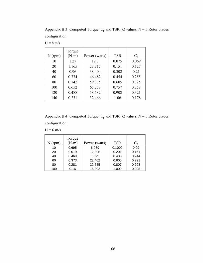
106


configuration

U = 8 m/s

N (rpm) Torque (N-m) Power (watts) TSR Cp

10 1.27 12.7 0.075 0.069 20 1.165 23.317 0.151 0.127 40 0.96 38.404 0.302 0.21 60 0.774 46.482 0.454 0.255 80 0.742 59.375 0.605 0.325 100 0.652 65.278 0.757 0.358 120 0.488 58.582 0.908 0.321 140 0.231 32.466 1.06 0.178


configuration.

U = 6 m/s

N (rpm) Torque (N-m) Power (watts) TSR Cp

10 0.695 6.959 0.1009 0.09 20 0.619 12.395 0.201 0.161 40 0.469 18.79 0.403 0.244 60 0.373 22.402 0.605 0.291 80 0.281 22.555 0.807 0.293 100 0.16 16.002 1.009 0.208

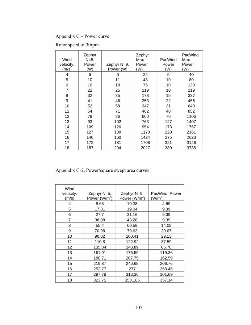
107

Appendix C – Power curve

Rotor speed of 30rpm

Wind velocity.

(m/s)

Zephyr N=5,

Power (W)

Zephyr N=9, Power (W)

Zephyr Max Power (W)

PacWind Power

(W)

PacWind Max Power (W)

4 5 6 22 5 40 5 10 11 43 10 80 6 16 18 75 10 138 7 22 25 119 10 219 8 32 35 178 15 327 9 41 46 253 22 466

10 52 58 347 31 640 11 64 71 462 40 852 12 78 86 600 70 1106 13 93 102 763 127 1407 14 109 120 954 173 1757 15 127 139 1173 220 2161 16 146 160 1424 275 2623 17 172 181 1708 321 3146 18 187 204 2027 380 3735

Appendix C-2, Power/square swept area curves

Wind velocity.

(m/s) Zephyr N=5,

Power (W/m2) Zephyr N=9,

Power (W/m2) PacWind Power (W/m2)

4 8.65 10.38 4.69 5 17.31 19.04 9.39 6 27.7 31.16 9.39 7 38.08 43.28 9.39 8 55.4 60.59 14.09 9 70.98 79.63 20.67 10 90.02 100.41 29.13 11 110.8 122.92 37.59 12 135.04 148.89 65.78 13 161.01 176.59 119.36 14 188.71 207.75 162.59 15 219.87 240.65 206.76 16 252.77 277 258.45 17 297.78 313.36 301.69 18 323.75 353.185 357.14

108

Appendix D: Design drawings of Zephyr turbine

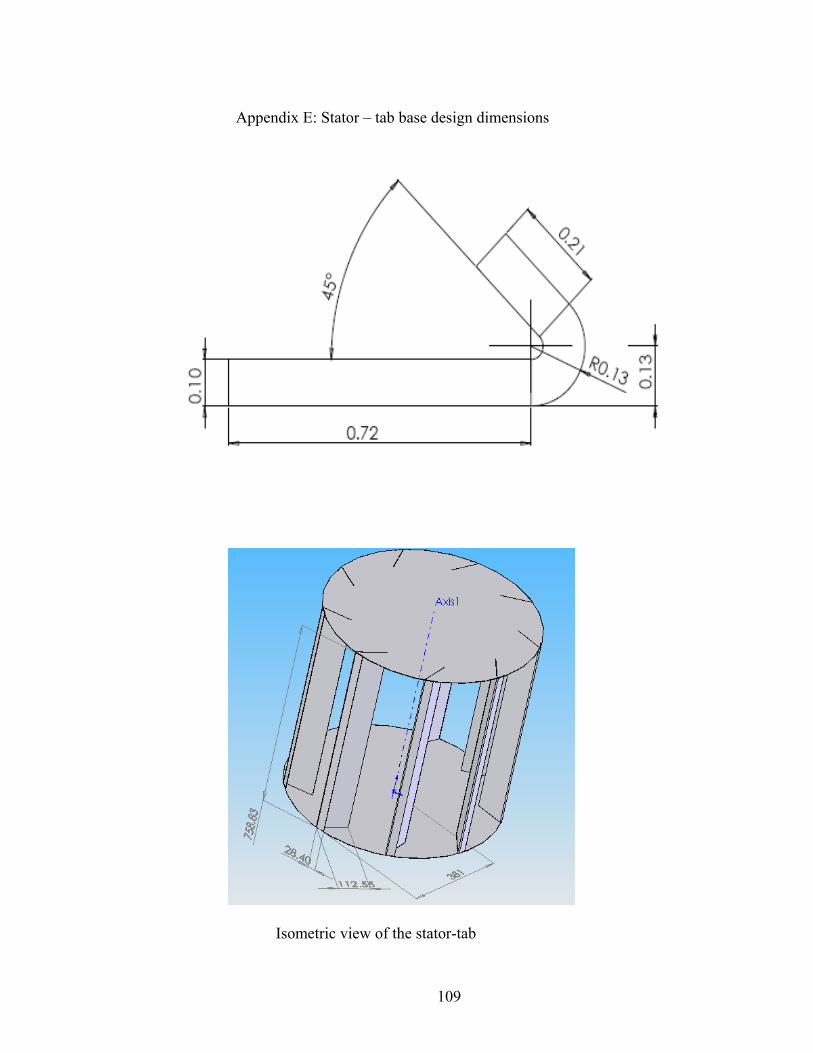
109

Appendix E: Stator – tab base design dimensions

Isometric view of the stator-tab

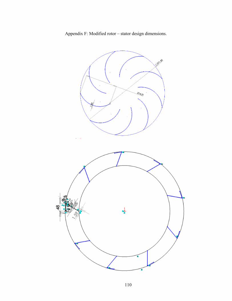
110

Appendix F: Modified rotor – stator design dimensions.

Thesis Report - Ajedegba WithRosen Comment.12doc

Documents

wind power

vertical axis wind turbines

committee signature

flow distribution

turbine rotor

wind freestream velocity

flow interaction

fluid flow