THESIS IS CHECKED ACCEPTED FOR THE DEFENSE Reviewer ...

MINISTRY OF EDUCATION AND SCIENCE OF THE RUSSIAN FEDERATION

Federal State Autonomous Educational Institution of High Education

South Ural State University (National Research University) School of Electrical Engineering and Computer Science

Department of System Programming

THESIS IS CHECKED ACCEPTED FOR THE DEFENSE

Reviewer,

Technical director

OOO "Kompaniya SG-grupp"

___________D.V. Gaponyuk

Head of the department,

Dr. Sci., Prof.

__________ L.B. Sokolinsky

“01” June 2018 “___”___________ 2018

DEVELOPMENT OF SYSTEM OF ALLOCATION SPECIFIED VOICE

IN AUDIO STREAM WITH THE USE OF NEURAL NETWORK

TECHNOLOGIES

GRADUATE QUALIFICATION WORK

SUSU–02.04.02.2018.308-589.GQW

Supervisor

Cand. Sci., Assoc. Prof.

__________ V.A. Golodov

Author,

student of the group CE-219

__________ M.A. Wahballah

Normative control

_____________ O.N. Ivanova

“___”___________ 2018

Chelyabinsk–2018

4

TABLE OF CONTENTS

ABSTRACT .............................................................................................................. 5

INTRODUCTION ..................................................................................................... 6

1. MONAURAL SOURCE SEPARATION AND SPEAKER RECOGNITION .. 10

2. MODEL DESCRIPTION ................................................................................... 12

2.1. Model: Deep Recurrent Neural Networks ....................................................... 12

2.2. Model Architecture .......................................................................................... 15

2.3. Quality metrics ................................................................................................. 17

2.4. Software environment ...................................................................................... 17

3. SOFTWARE DEVELOPMENT ......................................................................... 19

3.1. Python Application (User Interface) ................................................................ 19

3.1.1. Design of the application .............................................................................. 19

3.1.2. Functional requirements ................................................................................ 20

3.2. Preprocessing ................................................................................................... 21

3.3. Model variables List ......................................................................................... 21

3.3.1. Model parameters .......................................................................................... 21

3.3.2. Parameters meaning ...................................................................................... 24

3.4. List of issues explanation and solution ............................................................ 26

4. TESTING ............................................................................................................ 28

4.1. Testing of the neural network .......................................................................... 28

4.1.1. Using of the pretrained model ....................................................................... 28

4.1.2. Training the model on the own data set ........................................................ 28

4.1.3. Training after observation ............................................................................. 29

4.1.4. Training with one speaker and many speakers ............................................. 30

4.2. Testing of the UI .............................................................................................. 30

5. RESULT DISCUSSION ..................................................................................... 32

CONCLUSION ....................................................................................................... 35

REFERENCE LIST ................................................................................................ 36

5

ABSTRACT

Artificial Intelligence and its applications using deep learning as a very

powerful is irreplaceable nowadays, we see it all around us where we find

applications that recognizes patterns or classifies objects or automate some

tasks using deep learning, which inspired me to develop this application.

The application’s goal is to be able to separate someone’s speech from

others when combined in one audio file, it can be described using the terms:

source separation where we separate the source file into multiple files, and

speaker recognition where we want to listen to what someone is exactly saying

by extracting his speech in a separate audio file and normalizing it.

This objective is achieved by refining the work done previously [1]

because I thought about improving the results produced previously rather than

reinventing the wheel. I use a deep recurrent neural network, where I train a

model to different speakers’ voice parameters so as when I input a file with

multiple speakers and I want to listen to what my speakers are saying I do that

and separate their speech.

I modify recognized that some parameters can influence the accuracy of

the recognition so after doing many experiments I produced a final model

based on these results which has a higher accuracy that before.

Part of the future work was to produce speaker recognition as a real-time

service so I developed a Python User Interface that works as a sound player

now and I am planning to connect it to my Matlab code to allow the user to

either create their own model or use the pretrained model and produce separate

audio files for different speakers.

6

INTRODUCTION

Actuality

Artificial Intelligence (AI) is growing so fast nowadays, and many

applications already have a human-like intelligence, and this makes this field

rather interesting that challenging.

The introduction of neural networks changed the way that people think

about the limitations of intelligence of computers, now we have neural

networks that simulate the work of our brain cells, so you get it to learn things,

recognize patterns and make decisions in a humanlike way

The power of the tradition feedforward neural networks is limited

somehow because it has no notion of order in time and it does not consider the

recent past results from the previous nodes into consideration. The feedforward

networks are amnesiacs regarding their recent past; they remember

nostalgically only the formative moments of training. Recurrent neural

networks on the other hand take as their input not just the current input

example they see, but also what they have perceived previously in time.

The decision taken by a recurrent network reached at time step t-1

affects the decision it will reach one moment later at time step t. So recurrent

networks have two sources of input, the present and the recent past, which

combine to determine how they respond to new data, much as we do in life.

The term “deep” refers to the number of hidden units inside the layers which

enforces and increases the amount of learning subsequently it has a direct

effect on the results but the time and hardware requirements are fairly

increased

Speaker Recognition is one such concept which has beheld mankind’s

attention. There can be no greater testimony to the same than the fact that

people were already working on this idea – a few decades before John

McCarthy even coined the term "Artificial Intelligence", ever since, this term is

being used to refer to applications that includes learning done by the

automatically by the machines.

7

Speaker Recognition refers to the automated method of identifying or

confirming the identity of an individual based on his voice (voice biometrics).

This can then be used in numerous ways – ranging from criminal

investigations, determining the speaker, verify the identity of the speaker and

so on.

Speaker Recognition is a result of cross-linking various avenues of

technology like Machine Learning, Artificial Intelligence and Neural

Networks. I propose to develop a system based on mathematical algorithms

and principles which involve all the aforementioned technologies. That being

said, Speaker Recognition also depends on a few other factors: the level of

noise, the quality of the audio file. My software aims to address the

aforementioned problems, by developing a python user interface and a Matlab

backend that reduces the noise then uses deep recurrent Neural Network for

Speaker Recognition of the people whom you want to listen to, then the output

is the audio file after rising up the volume of some chosen people and cleaning

the noise.

Research goal and objectives

The goal of the research is to develop an application for monaural source

separation and speaker recognition

To achieve this goal we had the following objectives:

1) to analyze the contemporary speaker recognition technology and to

identify key issues that needs to be addressed in the real-world deployment of

this technology;

2) to explore alternative speech parameterization techniques and identify

the most successful ones;

3) to study ways for improving the speaker recognition performance and

noise robustness for real-world operational conditions;

4) to study alternative to the present state-of-the-art approaches for

speaker recognition, and to identify the ones that offer practical advantages

using deep recurrent neural networks;

8

5) to create a prototype of a speaker recognition system that utilizes the

consequences from the abovementioned issues 2–4;

6) test our application and improve the performance.

The practical significance

The project is beneficial as the core of source separation and speaker’s

speech identification which can have many significant uses for individuals and

organizations

This project can be used in:

1) training the model to the voice features of some speakers;

2) using the application to separate the speech of each speaker;

3) using the application to extract a speaker’s speech;

4) noise reduction and audio files normalization.

Structure of the thesis

The thesis consists of four chapters, Introduction, Conclusion, and

references list.

In chapter one, the source separation task and speaker recognition are

explained, also the various approaches to solve this task are being analyzed,

and a conclusion was made to explain why the model I used produces better

results.

In chapter two, the model is described in details by first introducing the

architecture of the deep recurrent neural network and the equations used with

their description and significance with the quality metrics being used to judge

the results. Also, the software environment used in the whole thesis is

mentioned.

In chapter three, the software development section is being discussed

where there are screen shots from the python User Interface and different

functionalities, besides, the preprocessing on the audio files and how the

dataset was produced, also it has the set of variables used in the deep recurrent

neural network and the meaning of some important variables was explained in

the form of tables. Also, we have a list of errors that we faced while using

9

Matlab and some libraries and their solutions to make it easier for anyone who

would like to continue the development in this field.

In chapter four, the most significant experiments that were done are

discussed, together with some accuracy metrices and results of these

experiments is shown in tables.

In chapter five, the results are discussed of the overall task and there are

some pictures to show the amplitude of the audio files before and after the

separation which explains the efficiency of the model.

10

1. MONAURAL SOURCE SEPARATION AND SPEAKER

RECOGNITION

Source Separation task attempts to separate different mixed audio signals

to different separate audio files which converts it back to a form where each

signal had its own file. This conversion is crucial and can be used in many

different ways, in addition, it can be extended further to have a better accuracy

in an application like speaker recognition where different sources are separated

into several denoised audio files where each file has one speaker’s speech.

Source separation can be complicated or even infeasible task if the goal

of the whole application is not well defined beforehand, as the number of

different solutions for different tasks can be uncountable. In my thesis, I try to

limit the solutions’ set by predefining the goals that includes some experiments

done to improve the accuracy of the separation.

Source separation methods can be categorized in different ways, I

believe in categorizing them to supervised-domain and unsupervised-domain

techniques. For supervised domain, models are trained based on some

corresponding targets with some assumptions made for the characteristics of

the signals and the accompanying noise, statistical model-based methods infer

speech spectral coefficients given noisy observations [2] Although these

assumptions were carefully made, it does not mean that it works correctly

when tested with real-world data to denoise an audio signal, which shows that

these models may not be very accurate because noise often tends to be

unpredictable.

When it comes to the unsupervised domain techniques, speech

characteristics are being recognized by the models without being limited by the

some domain, like in Non-negative matrix factorization (NMF) [3] and

probabilistic latent semantic indexing (PLSI) [4] and [5]. These models can be

regarded as linear transformation of some unique features set. Based on

minimum mean squared error (MMSE) these models perform well only if the

inputted and the outputted are jointly Gaussian, however, signals are not

11

always following the Gaussian distribution, subsequently I believe that this

assumption does not always have to be true, as relationship between the

inputted and outputted signals is very complicated.

Using a mixture of signals as an input, I suggest to directly recreate the

expected target sources in an end-to-end manner by generating a file for each

speaker. I propose a training criteria to improve the signal to inference ratio

given the expected different sources in the output layer which is an application

for both speech separation and speech denoising. With an extended TSP dataset

with new training parameters and new speakers from different genders, I

improve the accuracy of the training and separation task. Which is an extension

of the deep recurrent neural network approach introduced in [1], [6] and [7].

The speaker recognition part was referred to as the research consists

mainly of a Deep Recurrent Neural Network that is being trained on the voice

features of the speakers then later on, it can identify these features during the

testing process then extract voices with these features, which mean that the

speaker is being identified through the features of his/her voice then the speech

is extracted.

Based on the results that will be discussed in the next sections, the

modified version of Deep Recurrent Neural Network I used, outperform

different models like NMF and DNN models in the source separation and

speaker recognition task. This conclusion was made after trying this model on

a TrueSpeech (TSP) dataset and comparing the results.

12

2. MODEL DESCRIPTION

2.1. Model: Deep Recurrent Neural Networks

Given that audio signals are time series in nature, we propose to model

the temporal information using deep recurrent neural networks for monaural

source separation tasks. To capture the contextual information among audio

signals, one way is to concatenate neighboring audio features, e.g., magnitude

spectra, together as input features to a deep neural network. However, the

number of neural network parameters increases proportionally to the input

dimension and the number of neighbors in time. Hence, the size of the

concatenating window is limited. Another approach is to utilize recurrent

neural networks (RNNs) for modeling the temporal information [1].

More details about the model architecture and variables will be

introduced in chapter two.

Here we introduced the model used, and we will explain it more in

details with its architecture and variables, as shown in figure 1 below.

Fig. 1. Deep Recurrent Neural Network (DRNN) architectures: Arrows

represent connection matrices. Black, white, and gray circles represent input

frames, hidden states, and output frames, respectively. Where the architecture

in (a) is a standard recurrent neural network, (b) is an L hidden layer DRNN

with recurrent connection at the l-th layer (denoted by DRNN-l), and (c) is an

L hidden layer DRNN with recurrent connections at all levels (denoted by

stacked RNN).

13

An RNN can be considered as a DNN with indefinitely many layers,

which introduce the memory from previous time steps, as shown in Figure 1

(a). The potential weakness for RNNs is that RNNs lack hierarchical

processing of the input at the current time step. To further provide the

hierarchical information through multiple time scales, deep recurrent neural

networks (DRNNs) are explored [8], [9]. We formulate DRNNs in two

schemes as shown in Figure 1 (b) and Figure 1 (c). The Figure 1 (b) is an L

hidden layer DRNN with temporal connection at the l-th layer. The Figure 1 (c)

is an L hidden layer DRNN with full temporal connections (called stacked

RNN (sRNN)). Formally, we define the two DRNN schemes as follows.

Suppose there is an L hidden layer DRNN with the recurrent connection at the

l-th layer, the l-th hidden activation at time t, ℎ𝑡𝑙 , is defined as:

ℎ𝑡𝑙 = 𝑓ℎ(𝑥𝑡, ℎ𝑡−1

𝑙 )

= φ𝑙 (𝑈𝑙ℎ𝑡−1𝑙 + 𝑊φ𝑙−1

𝑙 (𝑊𝑙−1 (… φ𝑙(𝑊x𝑡

1)))) (1)

and the output 𝑦𝑡 is defined as:

𝑦𝑡 = 𝑓𝑜(ℎ𝑡𝑙 )

= 𝑊φ𝐿−1𝐿 (𝑊𝐿−1 (… φ𝑙(𝑊𝑙ℎ𝑡

𝑙 ))) (2)

where: 𝑓ℎ and 𝑓0 are a state transition function and an output function,

respectively;

𝑥𝑡 is the input to the network at time t;

φ𝑙 (·) is an element-wise nonlinear function at the l-th layer;

𝑊𝑙 is the weight matrix for the l-th layer;

𝑈𝑙 is the weight matrix for the recurrent connection at the l-th layer.

The recurrent weight matrix 𝑈𝑘 is a zero matrix for the rest of the layers

where k 6= l. The output layer is a linear layer. The stacked RNNs, as shown in

figure 1c, have multiple levels of transition functions, defined as:

ℎ𝑡𝑙 = 𝑓ℎ(ℎ𝑡

𝑙−1, ℎ𝑡−1𝑙 ) = φ𝑙(𝑈𝑙ℎ𝑡−1

𝑙 + 𝑊𝑙ℎ𝑡𝑙−1) (3)

where: ℎ𝑡𝑙 is the hidden state of the l-th layer at time t;

14

φ𝑙 (·) is an element-wise nonlinear function at the l-th layer;

𝑊𝑙 is the weight matrix for the l-th layer;

𝑈𝑙 is the weight matrix for the recurrent connection at the l-th layer.

When the layer l = 1, the hidden activation ℎ𝑡𝑙 is computed using ℎ𝑡

0= 𝑥𝑡.

For the nonlinear function φ𝑙 (·), it was found that using the rectified linear

unit φ𝑙 (x) = max(0, x) performs better compared to using a sigmoid or tanh

function in our experiments. Note that a DNN can be regarded as a DRNN with

the temporal weight matrix 𝑈𝑙 as a zero matrix.

For the computation complexity, given the same input features, during

the forward-propagation stage, a DRNN with L hidden layers, m hidden units,

and a temporal connection at the l-th layer requires an extra Θ(𝑚2) IEEE

floating point storage buffer to store the temporal weight matrix 𝑈𝑙, and extra

Θ(𝑚2) multiply-add operations to compute the hidden activations in Eq. (3) at

the l-th layer, compared to a DNN with L hidden layers and m hidden units.

During the back-propagation stage, DRNN uses back-propagation through time

(BPTT) to update network parameters. Given an input sequence with T time

steps in length, the DRNN with an l-th layer temporal connection requires an

extra Θ(Tm) space to keep hidden activations in memory and requires Θ(T𝑚2)

operations (Θ(𝑚2) operations per time step) for updating parameters, compared

to a DNN. Indeed, the only pragmatically significant computational cost of a

DRNN with respect to a DNN is that the recurrent layer limits the granularity

with which back-propagation can be parallelized. As gradient updates based on

sequential steps cannot be computed in parallel, for improving the efficiency of

DRNN training, utterances are chopped into sequences of at most 100 time

steps.

This was achieved after many trials and it appeared that chopping it for

100 times of less works the best in terms of efficiency and accuracy, although,

different time steps have different impacts on the time requirements and these

numbers can be different using different hardware.

15

2.2. Model Architecture

At a single time instance, a column can be described using the architecture

in figure 2 shown below.

Fig. 2. Proposed neural network architecture, which can be viewed as the t-th

column in Figure 1. Its proposed to jointly optimize time-frequency masking

functions as a layer with a deep recurrent neural network

The setting where there are two sources additively mixed together is

considered, though our proposed framework can be generalized to more than

two sources. At time t, the training input 𝑥𝑡 of the network is the concatenation

of features, e.g., logmel features or magnitude spectra, from a mixture within a

window. The output targets 𝑦1𝑡∈ 𝑅𝐹 and 𝑦2𝑡

∈ 𝑅𝐹 and the output predictions

�̂�1𝑡∈ 𝑅𝐹and �̂�2𝑡

∈ 𝑅𝐹 of the deep learning models are the magnitude spectra of

different sources, where F is the magnitude spectral dimension. Since our goal

is to separate different sources from a mixture, instead of learning one of the

sources as the target, we propose to simultaneously model all the sources.

figure 2 shows an example of the architecture, which can be viewed as the t-th

16

column in figure 1. Moreover, we find it useful to further smooth the source

separation results with a time-frequency masking technique, for example,

binary time-frequency masking or soft time-frequency masking [10], [11]. The

time-frequency masking function enforces the constraint that the sum of the

prediction results is equal to the original mixture. Given the input features

𝑥𝑡from the mixture, we obtain the output predictions �̂�1𝑡 and �̂�2𝑡

through the

network. The soft time-frequency mask 𝑚𝑡∈ 𝑅𝐹 is defined as follows:

𝑚𝑡 =|�̂�1𝑡

|

|�̂�1𝑡|+|�̂�2𝑡

| , (4)

where the addition and division operators are element-wise operations. A

standard approach is to apply the time-frequency masks 𝑚𝑡 and 1 – 𝑚 to the

magnitude spectra 𝑧𝑡∈ 𝑅𝐹 of the mixture signals, and obtain the estimated

separation spectra �̂�1𝑡∈ 𝑅𝐹 and �̂�2𝑡

∈ 𝑅𝐹, which correspond to sources 1 and 2,

as follows:

�̂�1𝑡= 𝑚𝑡 ⨀ 𝑧𝑡 ,

�̂�2𝑡= (1 − 𝑚𝑡 )⨀ 𝑧𝑡 , (5)

where the subtraction and (Hadamard product) operators are element-wise

operations.

Given the benefit of smoothing separation and enforcing the constraints

between an input mixture and the output predictions using time-frequency

masks, we propose to incorporate the time-frequency masking functions as a

layer in the neural network. Instead of training the neural network and applying

the time-frequency masks to the predictions separately, it’s proposed to jointly

train the deep learning model with the time- frequency masking functions. We

add an extra layer to the original output of the neural network as follows:

�̃�1𝑡=

|�̂�1𝑡|

|�̂�1𝑡|+|�̂�2𝑡

|⨀ 𝑧𝑡 ,

�̃�2𝑡=

|�̂�2𝑡|

|�̂�1𝑡|+|�̂�2𝑡

|⨀ 𝑧𝑡 , (6)

where the addition, division, and (Hadamard product) operators are element-

wise operations. The architecture is shown in figure 2. In this way, we can

17

integrate the constraints into the network and optimize the network with the

masking functions jointly. Note that although this extra layer is a deterministic

layer, the network weights are optimized for the error metric between �̃�1𝑡, �̃�2𝑡

and 𝑦1𝑡,𝑦2𝑡

, using the back propagation algorithm. The time domain signals are

reconstructed based on the inverse short-time Fourier transform (ISTFT) of the

estimated magnitude spectra along with the original mixture phase spectra.

2.3. Quality metrics

We quantitatively evaluate the source separation performance using

three metrics: Source to Interference Ratio (SIR), Source to Artifacts Ratio

(SAR), and Source to Distortion Ratio (SDR), according to the BSS-EVAL

metrics [12]. SDR is the ratio of the power of the input signal to the power of

the difference between input and reconstructed signals. SDR is therefore

exactly the same as the classical measure “signal-to-noise ratio” (SNR), and

SDR reflects the overall separation performance. In addition to SDR, SIR

reports errors caused by failures to fully remove the interfering signal, and

SAR reports errors caused by extraneous artifacts introduced during the source

separation procedure.

To make sure that we are using the right metrics with the right variables,

we decided to test our pre-trained model using a two different test sets, the first

one is for a speaker who was included in the training, the second one is for our

speaker ”Tony Robbins” who was not included in the training. The metrics had

better results while using the first speaker.

2.4. Software environment

We used Matlab 2017a and Matlab 2017b [13] for building the model,

together with BSS evaluation libraries for our error metrics, htk [14] library

which can be used for building and manipulating hidden Markov models and

labrosa [15] that can be used for extracting useful information from sound that

helps in voice extraction later on.

18

We used Python 2.7 [16] for creating the User Interface which allows

you to input an audio file and play it back. It should be our front end. We used

VLC [17] library for audio input and play back.

We used Audacity and WavePad Sound Editor in preprocessing for

audio files format conversion and for training set preparation. Audacity was

used to for format conversion and bitrate adjustment, and WavePad was used

to divide each audio file to smaller audio files.

19

3. SOFTWARE DEVELOPMENT

3.1. Python Application (User Interface)

3.1.1. Design of the application

A Graphical User Interface was developed using python. I used: PYQT,

VLC in python 2.7 to create this GUI, as shown below in figure 3.

Fig. 3. Speaker recognition GUI

In this GUI there are such functions as Browse, Save As, Exit, Play,

Pause, Stop, Recognise, Volume slide bar, Seek-bar as shown in figure 3.

The GUI includes browse that lets the user choose an audio file to be

used later on, as shown below in figure 4.

Fig. 4. Browse

20

3.1.2. Functional requirements

In the back-end, I wrote function for: Browse, Exit, Play, Stop, and

Pause. Functions:

1) Browse: choose a sound file to open. Play: play the sound file(s) in

use (you should have an opened sound file first to play it) as shown in figure 4;

2) Pause: pause the sound file, then you can play it again using the play

button (you should have a sound file playing to use this button);

3) Stop: stop the sound file, then if press play it should start from the

beginning (you should have a sound file playing to use this button);

4) Recognise: recognize the voice of the speaker(s) and using the model,

it should generate a new separated audio file(s) with the voice of the speaker(s)

raised and cleaned from noise;

5) Volume slide bar: to control the volume of the audio file;

6) Seek-bar: to scrub the audio file;

7) Exit: close the program;

8) Save As: Save the generated audio files in a specific location (you

should generate a file(s) first before using this button).

Our Python UI should allow the user to choose either to train on his/her

data and generate a new model or to user our pretrained model and input a file

with mixed signals and using our model, a file per speaker should be generated,

and the UI also has some sound player applications’ features like play, pause

and stop, to allow the user to hear the outputted and compare it to the input

without using other application.

We also plan to add some audio signal strengths visualizer to the UI, for

the user to compare the source overlapping signals of different speakers and the

resulting files, and to be able to see the difference before and after the process

of source separation, without having to use other applications for viewing the

signal amplitudes and comparing results, which can be considered as features

to make the user experience better and save the time of the user, rather than

having to use many applications for simple functions.

21

3.2. Preprocessing

For the speaker recognition task we needed to have a data set to use it in

training, validation and testing. We decided to use the audio files of a

motivational speaker called Tony Robbins, together with TSP speech database

[18] after doing some modifications to its files.

Using Audacity [19], we added his Audio files and converted it to the

needed format and also we removed the music at the beginning and end of the

files.

After this modification we had an hour and fifteen minutes file where he

is speaking.

The task is to separate the voices from a mixed Audio file to separate

Audio files for each speaker, so we found 3 other speakers and preprocessed

their files in the same way.

Then we used WavePad Sound Editor [20] to mix the 4 speakers’ Audio

files and to produce some cropped Audio files which formed the whole dataset

that we will use later on.

The files are WAVE TSP format files. The preprocessing produced 597

files of 2 seconds .WAV audio files of speaker Tony Robbins mixed with 1

female speaker, 478 files of 2 seconds .WAV audio files of speaker Tony

Robbins mixed with 3 other speakers, 2251 files of 2 seconds .WAV audio

files of speaker Tony Robbins mixed with white noise, 2251 files of 2 seconds

.WAV audio files of speaker Tony Robbins mixed with sin noise, 2251 files of

2 seconds .WAV audio files of speaker Tony Robbins.

3.3. Model variables List

3.3.1. Model parameters

A list of model parameters that were used in the process of training and

model creation, together with some meaning explanation and their possible

which can make better understanding of the model used and the parameters that

22

were modified later on to improve the accuracy of the performance of the

model in the source separation task.

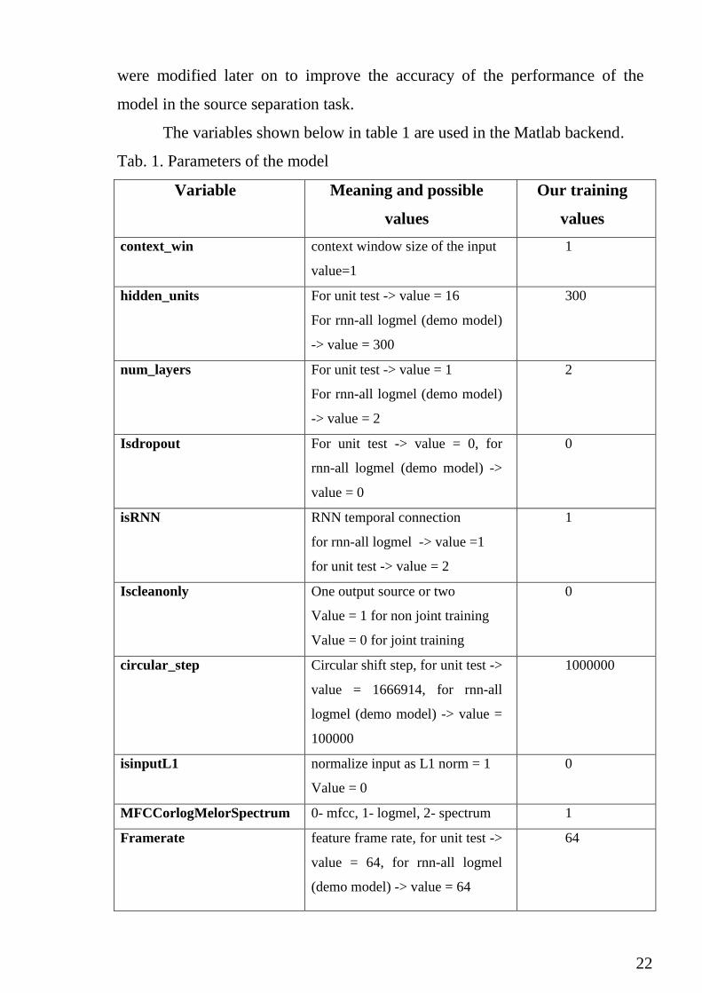
The variables shown below in table 1 are used in the Matlab backend.

Tab. 1. Parameters of the model

Variable Meaning and possible

values

Our training

values

context_win context window size of the input

value=1

1

hidden_units For unit test -> value = 16

For rnn-all logmel (demo model)

-> value = 300

300

num_layers For unit test -> value = 1


-> value = 2

2

Isdropout For unit test -> value = 0, for

rnn-all logmel (demo model) ->

value = 0

0

isRNN RNN temporal connection

for rnn-all logmel -> value =1

for unit test -> value = 2

1

Iscleanonly One output source or two

Value = 1 for non joint training

Value = 0 for joint training

0

circular_step Circular shift step, for unit test ->

value = 1666914, for rnn-all

logmel (demo model) -> value =

100000

1000000

isinputL1 normalize input as L1 norm = 1

Value = 0

0

MFCCorlogMelorSpectrum 0- mfcc, 1- logmel, 2- spectrum 1

Framerate feature frame rate, for unit test ->

value = 64, for rnn-all logmel

(demo model) -> value = 64

64

23

Continuation of tab. 1


values

Our training

values

pos_neg_r discriminative training gamma

parameter

For unit test -> value = 0.05


-> value = 0

0

Outputnonlinear Last layer - linear or nonlinear

:0,1

For unit test -> value = 0


-> value = 0

0

Opt 0: softlinear,

1: softabs,

2: softquad,

3:softabs_const,

4: softabs_k1_const

1

Act 0: logistic, 1: tanh, 2: RELU 2

train_mode 0

Const constant for avoiding numerical

problems

value = 1e-10

1e-10

const2 constant for avoiding numerical

problems, value = 0.001

0.001

isGPU 0: not using GPU, 1: using GPU 0

Batchsize For unit test -> value = 1666914


-> value = 100000

100000

MaxIter For unit test -> value = 30


-> value = 10

The iterations counter limit

10

24

End of tab. 1


values

Our training

values

bfgs_iter For unit test -> value = 30

For rnn-all logmel (demo model) -

> value = 50

50

Clip For unit test -> value = -10


-> value = 0

0

Lambda weight norm penalty values=0 0

data_mode 0: training, 1: valid, 2: testing 0

3.3.2. Parameters meaning

The explanation of the most important parameters is shown in table 2.

Tab. 2. Parameters meaning

Variable Meaning

MFCC mel-frequency cepstrum (MFC) is a representation of the short-term

power spectrum of a sound, based on a linear cosine transform of a

log power spectrum on a nonlinear mel scale of frequency.

The frequency bands are equally spaced on the mel scale, which

approximates the human auditory system's response more closely

than the linearly-spaced frequency bands used in the normal

cepstrum. This frequency warping can allow for better

representation of sound.

HTK

configuration

files

Used for customising the HTK working environment. They consist

of a list of parameter-values pairs along with an optional prefix

which limits the scope of the parameter to a specific module or tool.

Like documentation page 91.

The use of HTK differs from one task to another and we use the

most suitable parameter values to our task.

DataPath Variable that holds the path where audio files folders exist and its

used in load_data_mode.m to choose which folders to use for

training, validation and testing.

25

Continuation of tab. 2

Variable Meaning

Seqlen Unique lengths (in ascending order) files are chopped by these

lengths. (ex: [1, 10, 100])

Frame rate How many frames per second are included -> higher frame rate

means bigger winsize

Iscleanonly Determine if the training is done from different sources or only one

source

Context_win Only a portion of data is used as an input for the nueral network

Features Compute features function is used to calculate the features using htk

configuration files which generates train.fea file

Tie weights Weight Tying: Sharing the weight matrix between input-to-

embedding layer and output-to-softmax layer, The main reasons for

which tied weights are used is:

- for a linear case, the solution is Principal Component Analysis

(PCA), that can be easily obtained using tied weights.

- it regularizes meaning that less parameters need to be optimized

and it avoids out-of-range / degenerate solutions

- low memory as you will be storing less parameters

Hidden layers Layers for forward and back propagation, the numbers were chosen

based on the development set performance

Istemporal Specified by isrnn variable. It allows it to exhibit dynamic temporal

behavior for a time sequence. That’s why in training its value is 1,

testing its value is 2

Lambda Regularization strength, used regularization methods which is used

to prevent over fitting. (to control the learning rate)

Activation

function

Choose which activation function to use. activation functions are

mainly used to convert input signal of a node to an output signal

nodes. each function has its own advantages and disadvantages.

Nowadays the most popular is RELU, it rectifies linear units

because it has improved convergence thus it rectifies vanishing

gradient problem, however the limitation is that it should be used

only within the hidden layers.

We use RELU as our activation function.

26

End of tab. 2

Variable Meaning

isinputL1 If the input should be normalized first it should have the value 1 (it

happens in formulate_data.m by applying Cepstral mean and variance

normalization (CMVN)) otherwise the value should be 0

isoutputL1 If the output should be normalized (like the input), however, if

cleanonly is 1 (different sources)

discriminative

training gamma

parameter

(pos_neg_r)

0.05 in training, 0 in testing. Used by HMM in training

Isdiscrim 1 in no joint training , 2 in joint training. Used in minfunc which is an

unconstrained optimizer using a line search strategy

InputDim Dim of network input at each timestep (final size after window &

whiten) used in formulate_data.m , multiplied by the seqlen to create

a cell array of different training lengths called data_ag

3.4. List of issues explanation and solution

Installing htk

Installing htk couldn’t be done because one of the steps included running

a file called vcvars32.bat which is a visual studio batch file, then it should be

run. First we should add the path to vcvars32.bat to the system path to be able

to run it elsewhere, then we should run the cmd as an administrator. The error

was happening because we were not running the cmd as administrator as it was

not included in the installation steps in htk documentation.

Error with finding the functions while running the project

When we run the projects all the functions were not found although the

project was added to the path. To make the functions visible, you should

navigate(inside matlab solution window) to the folder where the code that you

want to run exists, then run it, then a pop message will ask if you would like to

add this file to path, you should add the file to path, then it will work.

27

Unable to save results of testing

We were unable to save the test results anywhere as we were getting an

error while using audiowrite function in labrosa.

The location where we wanted to save the output was a new folder that

should be created by matlab and it was called ”results”. It appeared that

audiowrite needs the folder to be created manually in advance before running

the code so we created a new folder in the location that it was supposed to be

created then the test results were produced successfully.

28

4. TESTING

4.1. Testing of the neural network

4.1.1. Using of the pretrained model

At the beginning we wanted to try testing the pretrained model provided

by the authors [1] and the results are shown below in table 3, and then we

tested the same model on our preprocessed data and the results are shown

below in table 4. We expected to have a poor performance concerning our data

as the model wasn’t trained on any of these speakers, so the neural network

doesn’t include any of the speakers’ voice features or paramaters.

Tab. 3. Results of testing the pretrained model with their own data

Frequency

Masking Technique SDR SIR SAR

Binary mask 0.906 3.824 0.395

Soft mask 2.097 3.672 3.331

Tab. 4. Results of testing the pretrained model with our data

Frequency


Binary mask 0.932 2.672 6.843

Soft mask 1.770 2.863 8.859

The difference in SIR while using Binary mask and soft mask, table 1

and table 2 shows that the accuracy of splitting files using pretrained model is

higher when tested with the data that the model was trained on.

4.1.2. Training the model on the own data set

We decided to create our own model, so we created our data set where

we had 4 speakers: 2 females and 2 males, for each speaker we had 61 audio

files with average length 2 s. We used 80 % of the signals for training, 10 %

for validation and 10 % for testing. The neural networks have been trained

29

using three different mixings female 1 with male 1, female 1 with female 2,

and male 1 with male 2.

The results in table 5 shows an improved SIR when compared to the

pretrained model which matches our expectations, because the model is trained

on the features of the voice of these speakers.

Tab. 5. Results of testing the trained model with our data

Frequency


Binary mask 1.916 4.450 3.303

Soft mask 2.911 3.580 9.152

4.1.3. Training after observation

We spent sometime trying to figure out what can be modified in our data

set and the parameters that can boost our accuracy, and after many

experiments, we found that the audio files’ bit rate, plays a very important role

in affecting the results. We found that the optimum bit rate is 768kbps,

however the training process takes a bit longer time, it takes around 8 hours

and 41 minutes.

In comparison to all our other experiments, we think that the results

shown in table 6 are the best in terms of numbers and accuracy of the

separation as the separated files’ produced show very well separated audio

files.

Tab. 6. Results of testing the trained model with our data with a new bit rate

Frequency


Binary mask 9.348 18.763 9.533

Soft mask 10.060 14.804 10.940

30

4.1.4. Training with one speaker and many speakers

We thought it would be interesting to try to train our model only on one

speakers’ feature and when testing to have a mixture of speakers in this audio

file and to try to detect and separate our speaker’s speech from all others. The

training process was too long and this experiment included extensive

preprocessing to produce the mixtures and to generate a data set for more than

5 speakers.

The results of this experiments shown in table 7 was not very good as the

separation accuracy was not high. I think that it can be improved by having a

bigger data set, however, it might need more hardware requirements or more

precisely, if there is a good GPU that can be used during the training process

but it might require a lot more time for training.

Tab. 7. Results of testing the trained model with multiple speakers

Frequency


Binary mask 0.666 2.302 5.169

Soft mask 2.211 2.774 9.829

4.2. Testing of the UI

Functional system testing is performed based in the specified functional

requirements, I am doing a black box testing of the functional requirements,

where I test the components of the UI as a whole, and compare the actual and

the expected output, as shown in table 8.

Tab. 8. Testing of the UI

No Test case Test steps Expected

result

Actual result

1 To open a

sound file

using

browse.

1. The user press

on File, chooses

browse then

chooses a file.

The user can

see the

opened file

and play it.

The function

works

correctly.

31

End of tab. 8

No Test case Test steps Expected

result

Actual result

2 To play and

audio file.

1. The user opens

an audio file.

2. The user press

on the button

play.

The user can

hear the

audio file

playing.

The function

works

correctly.

3 To stop the

playing file.

1. The user opens

and plays an

audio file.

2. The user press

on the button

stop.

The audio

file stops

and when

replayed it

starts from

the

beginning.

The function

works

correctly.

4 To pause the

playing file.

1. The user opens

and plays an

audio file.

2. The user press

on the button

pause.

The audio

file stops

and when

replayed it

continues

from the

previously

stopped

point.

The function

works

correctly.

5 To exit the

program

1. The user press

on File, and

chooses Exit

The program

closes.

The function

works

correctly.

32

5. RESULT DISCUSSION

After doing many experiments and having many observations, it

appeared that having a higher bit rate can result in a better model,

subsequently, the accuracy of audio files separation gets a lot better. Also

having the time frequency masks as a layer in our deep recurrent neural

network improves the performance in comparison to previous networks.

The amplitude of mixed voices of the male and the female is shown

below in figure 5, and the amplitude of the female voice’s signal only is shown

below in figure 6 which is the result of the separation process using the model

we developed earlier.

Fig. 5. The amplitude of the mixed signal of the female voice and the male

voice that was used as an input to the trained model

Fig. 6. The amplitude of the signal of the female voice which is the result of

separation using the model

33

Figure 5 shows the amplitude of the signal of the 12 s audio file that

includes a mixture of the male and female voice, the weakness of the amplitude

makes the volume very low, however it can be heard clearly. This audio file

was used as an input to our trained deep recurrent neural network model. figure

6 and figure 7, shows the amplitude of the female 12 s audio file and the male

12 s audio file respectively, which was the output. As its shown that the

amplitude of the resulting files is much stronger which makes us hear each

speaker separately very clearly and the voice of the other speaker can be barely

heard, it can be noticed that in Figure 6 there are some periods of very low

amplitude, these are the amplitudes of the male voice, which shows the

effectiveness of the produced model (the same applies to figure 7).

Fig. 7. The amplitude of the signal the male voice which is the result of

separation using the model

These experiments were done on a Dell laptop with an i7 2.10 GHz

processor and 8.00 GB RAM using Matlab 2014a [13]. It took 8 hours and 41

minutes to generate this model. However, we expect this time to be fairly

reduced if a better hardware was used especially if a fast GPU is used. It takes

around to 9.891 seconds to generate separate audio files for different speakers

using the trained model.

We suggest using source separation as a real time online service, the

input would be an audio file that has more than one speaker, and the output

would be an audio file for each speaker after the separation, so speed-

34

performance balance tuning is one of the further tasks. Moreover, working

towards this goal we already created a Python UI which was discussed in

section 3.1, that should allow users either to generate their own models by

training the DRNN with their own data, or use our pretrained model.

Although, we expect the accuracy to be better when the users generate

their own models, we decided to add the functionality of using the pretrained

model because generating a model is very time consuming even when we used

GPU, the time difference was not as big as we expected. The first stage of

creating the UI is done already and we are currently working on integrating it

with the Matlab code to make it usable. However, having an online service

would be only for source separation due to the extensive amount of resources

and time constraints. In the future we will do more time analysis and we plan to

reduce the time required for both processes, model regeneration and source

separation using pretrained model.

35

CONCLUSION

In my thesis, the application of monaural source separation and speaker

recognition using a deep recurrent neural network was demonstrated.

During the work we reached following objectives:

1) contemporary speaker recognition technology was analyzed and key

issues that needs to be addressed in the real-world deployment of this

technology was identified;

2) alternative speech parameterization techniques were explored and the

most successful ones were identified;

3) ways for improving the speaker recognition performance and noise

robustness for real-world operational conditions were studied;

4) alternative to the present state-of-the-art approaches for speaker

recognition was studied, and the ones that offer practical advantages using deep

recurrent neural networks were identified;

5) an application prototype of a speaker recognition system that utilizes

the consequences from the abovementioned issues 2–4 was created;

6) the application was tested and the performance was improved.

Jointly optimized model with time frequency masking functions

embedded to the network layers was tested. Performance of the separation

process was evaluated using three error metrics: SDR, SIR and SAR, that

shows some good results with the appropriate bitrate and the amplitude

parameters of the signals in the audio files. The overall performance of the

model outperforms the performance of NMF and normal deep neural networks.

Further work will be focused on speeding up the source separation using GPUs

and speed-performance balance tuning.

36

REFERENCE LIST

1. Huang P. S. Joint Optimization of Masks and Deep Recurrent Neural

Networks for Monaural Source Separation // IEEE/ACM Trans. Audio Speech

Lang. Process, 2015. – Vol. 23. – No. – 12. – P. 2136–2147.

2. Ephraim Y., Malah D. Speech enhancement using a minimum mean-

square error log-spectral amplitude estimator. // IEEE Trans. Acoust, 1985. –

Vol. 33. – No. 2. – P. 443–445.

3. Lee D.D., Seung H.S. Learning the parts of objects by non-negative

matrix factorization. // Nature, 1999. – Vol. 401. – No. 6755. – P. 788–791.

4. Hofmann T. Probabilistic latent semantic indexing. // Sigir, 1999. – P.

50–57.

5. Smaragdis P., Raj B., Shashanka M. A Probabilistic Latent Variable

Model for Acoustic Modeling. // Adv. Model. Acoust. Process. Work, 2006. – P.

1–7.

6. Huang P.-S. et al. Deep learning for monaural speech separation //

Proc. IEEE Int. Conf. Acoust. Speech Signal Process (ICASSP), 2014. – P.

1562–1566.

7. Huang P., Kim M. Singing-Voice Separation From Monaural

Recordings Using Deep Recurrent Neural Networks. // Target, 2014. – P. 477–

482.

8. Hermans M., Schrauwen B. Training and Analyzing Deep Recurrent

Neural Networks. // Nips, 2013. – P. 190–198.

9. Pascanu R. et al. How to Construct Deep Recurrent Neural Networks.

// ICLR, 2014. – P. 1–13.

10. Wang D. Time – Frequency Masking for Speech Hearing Aid Design.

// Trends Amplif, 2008. – Vol. 12. – P. 332–353.

11. Reju V.G. Blind Separation of Speech Mixtures. // IEEE Trans. Signal

Process, 2009. – Vol. 52. – No. 7. – P. 1830–1847.

12. Vincent E., Gribonval R., Fevotte C. Performance measurement in

blind audio source separation. // IEEE Trans. Audio, Speech Lang. Process,

37

2006 – Vol. 14. – No. 4. – P. 1462–1469.

13. MathWorks - Makers of MATLAB and Simulink [Electronic

resource] URL: https://www.mathworks.com/?s_tid=gn_logo (date of access:

06.03.2018).

14. HTK Speech Recognition Toolkit. [Electronic resource] URL:

http://htk.eng.cam.ac.uk/ (date of access: 06.03.2018).

15. The Laboratory for the Recognition and Organization of Speech and

Audio (LabROSA). [Electronic resource] URL: https://labrosa.ee.columbia.edu/

(date of access: 06.03.2018).

16. Official page of Python Programming Language. [Electronic resource]

URL: https://www.python.org/ (date of access: 06.03.2018).

17. VLC media player, Open Source player - VideoLAN. [Electronic

resource] URL: https://www.videolan.org/vlc/index.html (date of access:

06.03.2018).

18. TSP speech database. [Electronic resource] URL: http

://www-mmsp.ece.mcgill.ca/Documents/Data/ (date of access:

06.03.2018).

19. Audacity® | Free, open source, cross-platform audio software for

multi-track recording and editing. [Electronic resource] URL:

https://www.audacityteam.org/ (date of access: 06.03.2018).

20. WavePad Audio Editing Software. [Electronic resource] URL:

http://www.nch.com.au/wavepad/ (date of access: 06.03.2018).