Thesis for the degree - Weizmann Institute of Science

Thesis for the degree Master of Science

By Lior Gazit

Advisor: Prof. Roee Ozeri

May 2020

Submitted to the Scientific Council of the Weizmann Institute of Science

Rehovot, Israel

משוב קוונטי ביונים לכודים Quantum feedback on trapped ions

עבודת גמר (תזה) לתואר מוסמך למדעים

מאת ליאור גזית

אייר התש”פ

מוגשת למועצה המדעית של מכון ויצמן למדע רחובות, ישראל

מנחה: פרופ’ רועי עוזרי

To Tammy Langer & Edward Gaunt (1937-2020)

2

Acknowledgment

This work could not have been done without the support, patience, wise advice,kindness, and good friendship of several people. I would like to start by thankingthe 185 lab team: Nitzan Ackerman, Ravid Sahniv, Tom Manovitz, Lee Peleg,and Yotam Shapira for their endless patience, explaining, teaching, and alwaysconsulting with a smile and endless kindness. Thanks for the countless hoursspent together in the lab, or outside of it, thinking of solutions, talking, laughing,and just being good friends. I would like to thank the rest of the trapped ionsgroup: Ruti, Meirav, Meir, Yonathan, David, Haim & Sapir for their interest,ideas, conversations, kindness, and friendship. Moreover, I would like to expressmy love and gratitude to my parents for their endless support in every step Itake, my brothers and sister, for making my life funnier. For my partner, Gal forunderstanding, encouraging, and always asking questions. Also, Dor, Pavel, andIdo - thank you for studying beside me for the past two and a half years. Thanksfor your intelligence, friendship, being a shoulder to cry on, and always puttingthings in perspective. Finally, I want to thank my advisor Prof. Roee Ozeri for hispatience, clever questions, and mentoring and teaching me a new way of thinking.

3

Abstract

To realize and scale up a quantum information device, the implementation ofquantum error correction codes will be inevitable. The use of measurement ofthe quantum correlations between qubits to detect the errors, and correctingthem using conditional feedback, is fundamental to the experimental realizationof such a device. The following thesis reports on characterization, construction,and integration of an online analysis and feedback system for 88Sr+ions held ina linear Paul trap. Prior to this work, the analysis of the ion state was doneoffline, using post-processing of images taken from an EMCCD camera at theend of each experiment. This work presents a new addition to our lab thatallows live readout from the EMCDD, online analysis of the register state using aCamera Link protocol. This process is followed by an flexible in-sequence feedbackoperation. We have demonstrated this ability on one and two ion-qubits: on oneion-qubit, we have initialized it in an equal superposition, then, a measurementwas followed by a conditional ⇡ pulse only if the qubits measurement result was adark state; thus, the qubit always ended up in a bright state with 98.6% fidelity.Using two ion-qubits, live readout and feedback was tested and demonstratedusing a conditioned Ramsey experiment on superimposed qubits with ⇠ 82%

fidelity. Next using two ion-qubits, we have demonstrated quantum feedback.The quantum feedback was done by measuring one of two entangled qubits inthe x basis. This measurement collapsed the second ion to a superposition statealso in the x basis. The measurement was followed by a conditional Ramseysequence, achieving quantum feedback fidelity of ⇠ 85%. Moreover, in thiswork, we introduced a new set of tools that are now available in our lab: (a)Selective readout (or “hiding”) where the qubits superposition is hidden duringthe measurement thus remaining coherent despite the presence of a laser resonantwith an atomic dipole transition; (b) dynamical decoupling using RF pulses whilethe qubit is in hiding; and (c) individual addressing with negligible cross-talk dueto the use of light shift instead of a �x rotation.

4

Contents

1 Introduction 7

2 Background and theory 92.1 Motivation . . . . . . . . . . . . . . . . . . . . . . . . . . . . . . 92.2 Literature review . . . . . . . . . . . . . . . . . . . . . . . . . . . 112.3 Theory . . . . . . . . . . . . . . . . . . . . . . . . . . . . . . . . . 14

2.3.1 Ion - light interaction . . . . . . . . . . . . . . . . . . . . . 142.3.2 Gates . . . . . . . . . . . . . . . . . . . . . . . . . . . . . 16

3 Experimental Setup 213.1 The system . . . . . . . . . . . . . . . . . . . . . . . . . . . . . . 21

3.1.1 Ion Trap . . . . . . . . . . . . . . . . . . . . . . . . . . . . 213.1.2 Vacuum chamberfield, has motivated work towards optimizing

QEC methods. Although . . . . . . . . . . . . . . . . . . 223.1.3 88Sr+ as a qubit . . . . . . . . . . . . . . . . . . . . . . . 223.1.4 Lasers . . . . . . . . . . . . . . . . . . . . . . . . . . . . . 25

3.2 Imaging system . . . . . . . . . . . . . . . . . . . . . . . . . . . . 303.2.1 Optical Layout . . . . . . . . . . . . . . . . . . . . . . . . 313.2.2 The camera . . . . . . . . . . . . . . . . . . . . . . . . . . 32

3.3 State detection . . . . . . . . . . . . . . . . . . . . . . . . . . . . 353.3.1 Camera output distribution . . . . . . . . . . . . . . . . . 363.3.2 State detection algorithm . . . . . . . . . . . . . . . . . . 37

4 Live readout, analysis and feedback 414.1 Implementing live readout . . . . . . . . . . . . . . . . . . . . . . 42

4.1.1 Camera Link interface . . . . . . . . . . . . . . . . . . . . 424.1.2 Frame grabber . . . . . . . . . . . . . . . . . . . . . . . . 48

4.2 Hardware architecture . . . . . . . . . . . . . . . . . . . . . . . . 494.2.1 Communication architecture . . . . . . . . . . . . . . . . 50

4.3 Software architecture . . . . . . . . . . . . . . . . . . . . . . . . 514.3.1 Clock . . . . . . . . . . . . . . . . . . . . . . . . . . . . . 524.3.2 Live readout and image analysis . . . . . . . . . . . . . . . 534.3.3 Feedback architecture . . . . . . . . . . . . . . . . . . . . . 55

4.4 Readout, noise source and implementation bugs . . . . . . . . . . 564.4.1 readout fidelity . . . . . . . . . . . . . . . . . . . . . . . . 564.4.2 Noise . . . . . . . . . . . . . . . . . . . . . . . . . . . . . 574.4.3 Bugs . . . . . . . . . . . . . . . . . . . . . . . . . . . . . 60

5

5 Results 625.1 One qubit feedback . . . . . . . . . . . . . . . . . . . . . . . . . 625.2 Two-qubit feedback . . . . . . . . . . . . . . . . . . . . . . . . . . 64

5.2.1 Coherent feedback . . . . . . . . . . . . . . . . . . . . . . 655.2.2 Coherent feedback on entangled qubits . . . . . . . . . . . 68

6 Summary 726.1 Improvements . . . . . . . . . . . . . . . . . . . . . . . . . . . . . 726.2 Outlook . . . . . . . . . . . . . . . . . . . . . . . . . . . . . . . . 73

References 76

6

1 Introduction

“Probably never before has a theory been evolved which has giving a key to theinterpretation and calculation of a heterogeneous group of phenomena of experienceas has quantum mechanics theory”

—Albert Einstein, Out of my latter years.

Quantum mechanics describes the behavior of matter and light as a whole. Onthe atomic scale, the behavior of things can be very peculiar and counter-intuitive.Atomic physics is one of the tools that can help us to understand quantummechanics better. This understanding can be achieved by the ability to performexperiments and to control quantum systems. These kinds of experiments arefundamentally hard - the quantum mechanical phenomena that we are interestedin controlling are highly sensitive to noise such that can lead to loss of information,a procedure known as decoherence.

Trapped ions in a Paul trap are highly controllable systems yet well isolated.Moreover, the fact that an ion is inherently a quantum mechanical creature thatcan be controlled, cooled, and entangled contributes to the fact that this is aleading platform for quantum mechanics experiments.

Quantum information processing (QIP) exploits the quantum mechanics principlessuch as superposition and entanglement for different computational tasks. Abuilding block of QIP is the qubit - a quantum mechanical description of a bit.A classical bit of information can take one of two states, 0 or 1, whereas thequbit is represented by a unit vector in a 2-dimensional complex plane. Thesignificant difference comes from the fact that N qubits are represented by aunit vector in a 2

n-dimensional complex plane. The exponential growth in sizeis necessary to take into account not just the state but the correlation of theamplitude and phase of a superposition. These correlations can be utilized todescribe new types of computation algorithms that can efficiently solve someproblems that classical computers cannot efficiently solve. Quantum informationcan be used as a platform for a variety of applications: Quantum simulation,quantum cryptography, precision measurement, and quantum algorithms.

In order to perform a quantum information task, one needs to have the abilityto perform any possible rotation in the 2

N dimensional Hilbert space. Moreover,the ability to read out the quantum state of a register such that each state isuniquely identified is also necessary. In order to perform a conditional QIP tasks,where the operation depends on the outcome, one must have the ability to read

7

the register state fast enough before it will decohere, and also to be able to actupon selected scenarios.

In trapped ions, these requirements are achievable but challenging. The readoutof a qubit state (where each qubit is an ion) is done mainly using the detectionof fluorescence from the ion, using a detection scheme known as state selectivefluorescence. The fluorescence is detected using an EMCCD camera. The fluorescencedetection time has to be (a) sufficiently long to collect enough light to be ableto discriminate between states (exposure time) and (b) sufficiently fast to allowfor many iterations within the coherence lifetime of the ion. To meet theserequirements, the camera readout and state analysis need to be performed inreal-time and within the coherence time of the ions. The ability to read outthe register state and to act according to its state before the ions decohere isa prerequisite for experiments that require live feedback such as quantum errorcorrection.

This thesis will review the construction, integration, and testing of an onlinereadout system combined with a feedback system for an existing apparatus of88Sr+ ions. Before this system, the state analysis of the ions state was doneoffline using Matlab, and quantum feedback was not possible. Our solution wasimplemented using a dedicated FPGA frame grabber card that is connected usinga Camera Link protocol to and EMCCD camera that allows online access to theraw image data and fast image analysis.

8

2 Background and theory

2.1 Motivation

Quantum information processing is the result of combining quantum physics withcomputing theory. Harnessing the properties of the Hilbert space structure ofquantum physics, superposition and entanglement introduce a variety of operationsthat have no classical concept. The origin of quantum computations starts withtwo people in the early 1980s, one of them being Richard Feynman, who asked -how to simulate quantum mechanics on a classical computer. This task is hard,and not trivial due to the exponential increase in degrees of freedom. He wasthe first to suggest a computer made of quantum particles. David Deutsch is thesecond pioneer, who suggested building a universal quantum computer out of aTuring machine. In 1995 Peter Shor proposed a quantum algorithm for integerfactorization in polynomial time as opposed to sub-exponential time used in aclassical computer. This was the first suggestion that a quantum computer canout-preform a classical computer [1]. The existence of a polynomial-time quantumalgorithm for factorization suggests that one of the most widely used cryptographicprotocols (RSA) is vulnerable to an adversary who possesses a quantum computer.

The fundamental building block of QIP is the quantum bit (qubit), the quantumanalog to the classical bit. The qubit is a two-level quantum system, usuallydenoted as |0i and |1i. Most QIP involves manipulating, controlling, and measuringa register of a qubit(s). Quantum gates are the basic quantum circuit operatingon a small set of qubits, similar to classical gates except for the fact that quantumgates are unitary operators meaning they are time reversal. Qubits and quantumgates are the elements that build a quantum computer - a fully digitized controllableQIP machine. There are a set of requirements that a system needs to meet inorder to realize a quantum computer, they were listed by David DiVincenzo in1998 and are known as the five DiVincenzo criteria [2] . They include:

• A scalable physical system with well-characterized qubits

• The ability to initialize the state of the qubits to a simple fiducial state,such as |00...0i.

• Long relevant coherence time, much longer than the gate operation time.

• A ”universal” set of quantum gates.

• A qubit specific measurement capability

9

The essence of these criteria combine universality, long coherence times and scalability.It has been shown that single qubit rotations and two qubit controlled-NOT gateconstitute of a universal gate set. However, when trying to coherently controlmany qubits or maintaining long coherence times in a noisy environment, theimplementation of these operations, especially entanglement, is greatly reduced.

Trapped ions are long known to be a promising platform for constructingquantum devices with excellent coherent control capabilities and very long coherencetimes [3]. In 1995, Cirac and Zoller [4] proposed an architecture of a quantumcomputer based on trapped ions. The qubit can be encoded in the internal stateof the trapped ion. Using tightly focused laser beams, the state of an individualion (or ions) in the string can be rotated, and the interaction between two ionscan be performed by coupling the motional modes to the internal ion state toimplement an entangling gate thus satisfying the universal gate set. The rest ofthe DiVincenzo criteria accomplished using trapped ions as well: optical pumpingand laser cooling [5] satisfy the ability to initialize the qubit state, long coherencetime is a property of trapped ions which are highly isolated from the environmentand can be nicely demonstrated in highly stable atomic clock experiments, electronshelving and on resonance fluorescence are the measuring scheme.

However, the fidelity of all of the above operations is not perfect - achievingcomplete isolation from the environment is a hard task. Furthermore, the scalabilityof the quantum computer critically depends on the fidelity of quantum coherentcontrol. It is agreed that active error correction methods will be the solution toovercome these problems.

While quantum error correction (QEC) will be thoroughly discussed in thenext section, the fact that QEC codes all rely on imperfect entangling gates givesrise to the fact that a noisy quantum computer may simulate a noise-less butsmaller quantum computer as long as the noise level is below a certain threshold- the well-known fault-tolerance theorem [6]. This, among other breakthroughs inthe field, has motivated work towards optimizing QEC methods. Although someproof of concept experiments where implemented, including a new demonstrationof quantum supremacy by Google [7], realizing a large scale quantum computeris still an ongoing effort.

One of the most vital theoretical aspects of QIP are Quantum Error Correction(QEC) and fault-tolerant quantum computation. A qubit lives in a very hostileenvironment. For example vibrations (thermal phonons) can stir the qubit state,stray photons can flip the qubit state, relaxations and spontaneous scatteringcan send the qubit back to its ground state ,and a measurement will turn thequbit into no more than a conventional classical bit. All of these render the

10

survival of a single qubit superposition over long times unlikely. Quantum errorcorrection codes use groups of qubits, teamed up to mitigate the harmful effectsof the environment. By using these kinds of codes, performing complex quantumcomputations without losing coherence becomes possible. In order to do so,the interactions between the qubits need to follow well-structured fault-tolerantprotocols. The basics of quantum error correction and fault-tolerant quantumcomputation were first introduced in 1995, as a result of interest in quantumcomputations, following up the 1994 Shor’s factorization algorithm.

The theoretical results showed that building a large scale quantum computer isin principle possible. The fault-tolerant approach is the most general approach tocorrect errors. It has shown that for a long computation, it can correct arbitraryerrors (where the error threshold is 10

�4) for a single gate operation. Classicalerror correction protects information using redundancy. In quantum mechanics,the no-cloning theorem states that an unknown state cannot be cloned, makingclassical QEC through redundancy non-trivial. Luckily, encoding the informationon entangled states can protect it. QEC codes, use the fact that information canbe encoded into a subspace of a larger Hilbert space. A "smart" measurement,will collapse the wave function into one of two orthogonal subspaces - one wherethe error is corrected, or to an orthogonal subspace that outputs a syndrome thatcan be used to correct the error.

Quantum error correction requires not only the ability to manipulate thequbits via universal gate sets, but also the ability to perform smart measurements,and correct the errors (if needed) before the system completely decohere. It cancorrect trace-preserving errors but also errors that are not trace-preserving likemeasurement. This implies that the use of live feedback is needed in order toperform tasks that will allow the implementation of quantum error correctioncodes. The following section review the solutions and experiments that have beenproposed and tests for implementing QEC on trapped ions.

2.2 Literature review

quantum error correction and feedback in trapped ions

QEC codes have been demonstrated in several quantum information platforms,from superconducting qubits, nuclear magnetic resonance (NMR) systems, andtrapped ions. The first protocols demonstrated error syndrome measurementoutside of the qubit subspace. Von Neumann projective measurements of multi-qubitoperators are required [8]in order to achieve practical QEC on continuously encodedinformation. These have been realized with trapped ions [9, 10, 11], and in

11

solid-state systems [12].Implementation of quantum error correction codes is done by coding the

quantum state such that after a measurement and feedback, the errors are erased.In these procedures, using a larger subspace of the Hilbert space, errors will rotatethe state vector out of the allowed subspaces, where measurement will project itback to the allowed subspace, and the original state will be recovered. The firstimplementation of quantum error correction codes was in NMR systems [13, 14].

A reduction of high intrinsic or artificially induced errors in logical qubits hasbeen demonstrated in several experiments. However, fault-tolerant encoding oflogical qubit has not been shown yet. The next paragraph will discuss some ofthe QEC experiments demonstrated in trapped ions systems.

In 2004 [15], used trapped ions to implemented a fundamental quantum errorcorrection protocol. The authors encoded the (arbitrary) state of a source qubitin a superposition of two distinct three-qubit states (logical plus two auxiliaryqubits). They had introduced controlled spin-flip errors on all three ion-qubitsbefore they encoded the state with the inverse operation used to encode the logicalqubit. Small errors in the encoded state will rotate the states in a way thatthe errors can be corrected after decoding. The readout of the auxiliary qubitsprovided the error syndrome, based on which, the logical ion-qubit was rotatedto its original state. The stabilizer code {ZZX,ZXZ} was employed in theseexperiments. With no error, the fidelity was around 0.8, in an uncorrected state,the fidelity dropped to 0.5. In this experiment, they used individual addressing,through ion-shuttling between different trapping regions, for the preparation ofthe ion, and selective state readout for detecting the error syndrome.

In 2011 Schindler et al. have demonstrated repeated QEC with three 40Ca+

ions [10]. This experiment characterized the implementation of the QEC processin the presence of correctable errors, and concluded that QEC protocol correctssingle-qubit errors within their statistical uncertainty. The fidelity depended onthe number of QEC code repetitions, where for one sequence, they have reached90%. Following this work in 2014, the same Innsbruck group introduced animplementation of topological 7 qubit code [9]. This was the first realizationof a complete Calderbank-Shor-Steane (CSS) code. In this work, they haveconstructed a topological color code using seven trapped ions that encoded asingle logical qubit.

Recently, the [[4, 2, 2]] code implemented by [16] on a fully connected quantumcomputer, including a chain of five 171Y b+ ions confined in a Paul trap. Thissurface code is a quantum error detection code [17], contains two logical qubitconstructed out of four ions. This is a one qubit fault-tolerant code where one of

12

the qubits is protected (|Lai), and the other is not. By instead considering errorson both encoded qubits, they have highlighted the importance of fault-tolerancefor reducing intrinsic errors and managing error propagation. The non–fault-tolerantprocedures that generate the non-protected logical qubits (|Lbi still succeed inreducing added errors. The code implements |Lai and |Lbi on only four physicalqubits and hence violates the quantum Hamming bound [18], which means thatdetected errors cannot be uniquely identified and corrected. Therefore they rely onpost-selection to find and discard cases where an error occurred. The code doeshave the advantage of requiring only five physical qubits for the fault-tolerantencoding of |Lai: four data qubits and one ancilla qubit.

Not all of the above experiments demonstrated conditioned operations on thequbits. Some of them have used post-selection to match the outcome of themeasurement and the desired operation. The implementation of high-fidelity,large scale systems with the ability to perform consecutive measurements appearsto be challenging.

Continuous and conditioned operation after measurement on trapped ions waspresented in a few experiments. One of them is correcting photon scatteringerrors in atomic qubits [19]. In this experiment, polarized photons scatteredfrom a Zeeman qubit on the x direction (perpendicular to the quantization axis)were collected, using two photomultiplier tubes (PMT) and two polarizing beamsplitters (PBS). By analyzing which PMT detected the signal with a recordingof the local oscillator phase, they could correct any kind of scattering error.Conditional operation using a CCD camera has been demonstrated in [20].

Some of the experiments described above used methods such as hiding thedata qubit in an internal state that does not interact with the light used fordetection. An alternative approach that also use feedback to utilize quantumerror correction is to use two species qubits [21]. They have obtained high degreeof spectral isolation using the fact that one of the species is the auxiliary qubit,and one is the data qubit. The information is transferred in the register fromthe qubit and the auxiliary using mixed-species multi-qubit gates, enabling statedetection without crosstalk to the data qubits. A key element of the experimentalsetup is a classical control system with an in-sequence feedback control. Thereadout of the ion state was done using a PMT. Recently, more works are usinglive feedback in order to perform different QEC codes experiments such as [22, 23].Most of them are not in a trapped ions systems or using an EMCCD camera, andare out of the scope of this work.

13

2.3 Theory

2.3.1 Ion - light interaction

In our experiment, trapped ions are interacting with a classical electromagneticfield created by a laser. We can think of the ion as a Hydrogen-like ion - a chargedatom with one electron in the valance shell. We will assume that all other electronsremain in a fixed state such that the only degrees of freedom are those of thevalence electron and the center of mass coordinates of the ion. To determine howthe trapped ions act as qubits, we will consider the ion as an effective two-levelsystem since the interaction with the EM field is perturbative. The dynamics willinvolve only the levels which are in resonance with the interaction. This yieldsthe effective Hamiltonian:

ˆH (t) = ˆHion +ˆVIon�Laser (t)

ˆHion is the free Hamiltonian of a spin 1

2

connected to a 1D harmonic oscillator:

ˆHion =

1

2

~!0

�z + ~⌫✓a†a+

1

2

◆

here, !0

is the frequency separation of the qubits levels, and ⌫ is the harmonicoscillator frequency.

The time-dependent periodic potential ˆV (t) is induced by coupling to the e.m.wave:

ˆVIL(t) = ~⌦0

��+

+ ��� cos (kx� !Lt+ �)

⌦

0

is the coupling constant known as the Rabi frequency, k is the wavenumber,�± is the spin rising\lowering operators that act on the internal atomic state (inour case |Si and |Di) defined as: �±

= �x ± i�y.The position operator can be written in terms of the harmonic oscillator ladder

operators:

kx = kxeq + ⌘�a† + a

�

Where ⌘ = kx0

= k⇣

~2m!

m

⌘1/2

is the Lamb-Dicke parameter, and x0

is the groundstate width of the harmonic oscillator.

Moving to the interaction picture with respect to Hion using U = eiH0t/~,and neglecting fast terms (which oscillates at !L + !

0

) in the rotating waveapproximation (RWA) we can write the Hamiltonian as:

14

Hint = UHU †

Hint (t) =~⌦2

�+ei⌘(ae(�i⌫t)

+a†e(i⌫t)) · ei(���t)

+ h.c.

with � = !L � !0

.The laser couples the state |S, ni, to all states |D,mi (n is the vibrational

quantum number). This coupling is due to the oscillatory motion of the ion in thetrapping potential. Increasing or decreasing of the vibrational quantum numberis a result of the absorption or emission process on a sideband of the electronictransition that satisfies energy conservation. By expanding the exponent ei⌘...

(Assuming ⌘ ⌧ 1) we get the Hamiltonian

(1) Hint =~⌦2

�+

�1 + i⌘

�ae(�i⌫t)

+ a†e(i⌫t)��

e�i(�+�t)+ h.c.

We can see that the coupling of the |ni level to the |mi level of the harmonicoscillator is obtained by terms oscillating at multiples of !m. The contribution tothe time evolution comes only from the terms that are on resonance with the laserfrequency. Writing the Hamiltonian for an interaction between |g, ni and |e,miin the interaction representation :

H =

~⌦m,n

2

�+e�i(�+�t) |mi hn|+ h.c

with ⌦nm = ⌦e�⌘

2

2 ⌘m�n�n!m!

�Lm�nn ; (m � n) is the generalized Rabi frequency

(Lm�nn is the closed form of the Laguerre polynomials), and � ⌘ !L � !

0

�(m� n) ⌫.

In this Hamiltonian, all transitions can occur. But, in the Lamb-Dicke regime,the transitions amplitude scales as increasing power of ⌘, whereas the secondsidebands of the order ⌘2 are suppressed. Thus, we can understand three kinds oftransitions that depend on the effective state that are on resonance: Carrier (n, n)- Does not change the vibrational state, red sideband (RBS: n, n � 1) removesone quanta of motion following absorption, and blue sideband (BSB: n, n + 1)that adds one quanta of motion due to emission. The effective Rabi frequencydepends on the harmonic state. By measuring the population oscillations underthis Hamiltonian and using Fourier transform, one can extract the harmonic statepopulation. These resonances are observed by scanning the laser detuning � andmeasuring the population. From equation (1) we can calculate the overlap betweenthe displaced initial harmonic oscillator wave-function and some final harmonicoscillator wave-function, known as the Debye-Waller factor:

15

8<

:hD,m |Hint|S, ni = ⌦

m,n

2

e�i(��(n�m)⌫t)Dn.m

Dn,m =

Dm���ei⌘(a+a†

)

���nE= e�

⌘

2

2

⇣min(n,m)!

max(n,m)!

⌘1/2

⌘|n�m|L|n�m|min(n,m)

(⌘2)

where L↵min is the modified Laguerre polynomial. In the Lamb-Dicke regime we

obtain:8>>><

>>>:

DCarrier = 1� ⌘2�n+

1

2

�

DRSB = ipn⌘

DBSB = ipn+ 1⌘

From here the dependence of the Rabi frequency will be: ⌦n,n = ⌦

�1� ⌘2

�n+

1

2

��.

Note that the coupling for the RBS vanishes on n = 0 but will always be finitefor BSB.

2.3.2 Gates

To coherently control the state of n qubits, we need to apply the basic operationsof quantum computing known as quantum gates. A quantum gate over a set of nqubits is described by a 2

n ⇥ 2

n unitary matrix U . To allow coherent control of aquantum state, one needs to have the ability to connect any two-state vectors inthe Hilbert space. This operator can be approximated by concatenating a finitenumber of operators chosen from a small set that is called a universal gate set.A sufficient gate set for universal quantum computing consists of arbitrary singlequbit rotations and a single entangling quantum gate [24]. In the experiment thatwe have conducted in order to test the live readout performance, we used severalquantum gates that together consist of a universal gate-set. All of them involveinteraction with laser beams. The advantage of using laser-ion interaction comesfrom the fact that even closely spaced ions can be still individually addressed[3, 25].

Single qubit rotation gates:

Single unitary qubit operation can be described as a rotation of the Bloch vectoron the Bloch sphere R (�,�, ✓). Here, �,� determine the direction on the axisaround the Bloch vector is rotated: n = (cos�cos�, cos�sin�, sin�). ✓ is therotation angle. All single qubit rotations are a 2⇥2 unitary matrices with a unitydeterminant [26]. This is also known as the SU (2) representation group; thus,

16

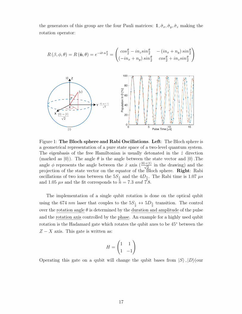
the generators of this group are the four Pauli matrices: 1, �x, �y, �z making therotation operator:

R (�,�, ✓) = R (

ˆn, ✓) = e�i�·n ✓

2=

cos ✓

2

� inzsin✓2

� (inx + ny) sin✓2

(�inx + ny) sin✓2

cos ✓2

+ inzsin✓2

!

Figure 1: The Bloch sphere and Rabi Oscillations. Left: The Bloch sphere isa geometrical representation of a pure state space of a two-level quantum system.The eigenbasis of the free Hamiltonian is usually detonated in the z direction(marked as |0i). The angle ✓ is the angle between the state vector and |0i .Theangle � represents the angle between the x axis ( |0i+|1ip

2

in the drawing) and theprojection of the state vector on the equator of the Bloch sphere. Right: Rabioscillations of two ions between the 5S 1

2and the 4D 5

2. The Rabi time is 1.07 µs

and 1.05 µs and the fit corresponds to n = 7.3 and 7.8.

The implementation of a single qubit rotation is done on the optical qubitusing the 674 nm laser that couples to the 5S 1

2$ 5D 5

2transition. The control

over the rotation angle ✓ is determined by the duration and amplitude of the pulseand the rotation axis controlled by the phase. An example for a highly used qubitrotation is the Hadamard gate which rotates the qubit axes to be 45

� between theZ �X axis. This gate is written as:

H =

1 1

1 �1

!

Operating this gate on a qubit will change the qubit bases from |Si , |Di(our

17

representation of |0i , |1i = |Si , |Di), to the x basis represented by |+\�i:

|+i = |Si+ |Dip2

|�i = |Si � |Dip2

Two optical qubit gates:

The standard universal gate set includes two main gates: single-qubit rotationsand CNOT entangling operations. A CNOT gate rotates the state of a targetqubit around the x-axis by 180

� depends on the logical state of the control qubit.When starting from two qubits at the ground state | i = |Si |Si, a CNOT willgenerate an entangled pair - a Bell state:

| i = |SSi+ |DDip2

The original proposal to generate a universal two-qubit entangling gate in trappedions systems using the interaction of the internal state coupled to the collectivemotion was initially suggested by Cirac and Zoller [4]. Since then, the implementationof entangling gates on trapped ions is usually done using a Mølmer-Sørensen (MS)gate [27]. This gate is equivalent, by a single qubit rotations, to a CNOT gatediscussed above. In this method, entangling ions is done by addressing theirharmonic trap degrees of freedom, regardless of their initial state (as long as theyare in the Lamb-Dicke regime), meaning there is no need for cooling to the groundstate. The MS entangling gate operates on the initial state | initiali = |SS, ni.Following [27], the system Hamiltonian is:

ˆH =

ˆH0

+

ˆHint

Where:8<

:ˆH0

= ~!0

Pi�(i)z

2

+ ~⌫�a†a+ 1

2

�

ˆHint =P

i⌦

2

�+

i ei⌘((

a+a†)

�!L

t)

+ h.c.

where ⌫ is the trap frequency, ~!0

is the energy difference between the groundand the excited state (S and D). !L and ⌦ are the frequency and Rabi frequencyof the laser addressing ions, ⌘ is the Lamb-Dicke parameter, and a, a† are theharmonic trap annihilation and creation operators. Moving to the interactionpicture with respect to ˆH

0

and after applying the RWA by assuming ⌦ ⌧ ⌫ weobtain the interaction Hamiltonian [28]:

18

ˆHint = ~⌦ ·�ei�t + e�i�t

�ei⌘(ae

�i⌫t

+a†ei⌫t)

X

i

�+

i + h.c.

This Hamiltonian can be approximated in the Lamb-Dicke regime by:

ˆHint (t) = �~⌘⌦�aei⇠t + a†e�i⇠t

�ˆJy

here, ⇠ = ⌫ � � denotes the laser detuning from the motional sidebands, and wedefine ˆJy as the global spin operator:

ˆJy =�y(1)

⌦ 1(2)

+ 1(1)

⌦ �y(2)

2

The propagator for the interaction Hamiltonian is represented by the unitaryoperator [27]:

ˆU (t; 0) = e�i ⌘2⌦2

⇠

(

t� sin(2⇠t)2⇠ )

ˆJ2y

ˆD⇣↵(t) ˆJy

⌘

Where ↵(t) = ⌘⌦⇠

�ei⇠t � 1

�and ˆD (↵) = e↵a

†+a⇤a is the displacement operator,

constitute a spin dependent force (See [28]).At a time t = 2⇡

⇠and ⇠ = 2⌘

⌦

, ˆU will become ˆU = ei⇡

2ˆJ2y . This means that ˆJ2

y

acts as a correlated rotation in the qubit subspace. Such that we get a rotationbetween the product state and a fully entangled state:

|SSi ! ei⇡

4(|SSi+ i |DDi)p

2

This state generated by constructive interference on the even parity, whiledestructive interference suppresses the amplitudes of the odd parity state |SDi , |DSi.This is achieved by the dependent force that derives the ions, tuning this forcemagnitude will set the phase difference. This phase is a geometric phase that eachof the ions accumulate by traveling different paths through space. Practically, itgenerates conditional displacement in phase space by application of bichromaticfield to the ions, using the 674 nm laser beam, which is red and blue detuned, closeto one of the ion crystal motional mode frequency thus the rest of the modes arenegligible. The relative phase between the frequencies will determine the phaseof the gate.

19

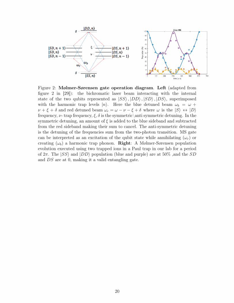
Figure 2: Mølmer-Sørensen gate operation diagram. Left (adapted fromfigure 2 in [29]): the bichromatic laser beam interacting with the internalstate of the two qubits represented as |SSi , |DDi , |SDi , |DSi, superimposedwith the harmonic trap levels |ni. Here the blue detuned beam !b = ! +

⌫ + ⇠ + � and red detuned beam !r = ! � ⌫ � ⇠ + � where ! is the |Si $ |Difrequency, ⌫- trap frequency, ⇠, � is the symmetric\anti symmetric detuning. In thesymmetric detuning, an amount of ⇠ is added to the blue sideband and subtractedfrom the red sideband making their sum to cancel. The anti-symmetric detuningis the detuning of the frequencies sum from the two-photon transition. MS gatecan be interpreted as an excitation of the qubit state while annihilating (!r) orcreating (!b) a harmonic trap phonon. Right: A Mølmer-Sørensen populationevolution executed using two trapped ions in a Paul trap in our lab for a periodof 2⇡. The |SSi and |DDi population (blue and purple) are at 50% ,and the SDand DS are at 0, making it a valid entangling gate.

20

3 Experimental Setup

3.1 The system

The strong interaction between an electric field and an electric charge allows theimplementation of very deep and tightly confined 3d charged particle traps thatprovide long trapping times. The Paul trap initially designed by Wolfgang Paul(for which he shared the 1989 physics Nobel prize (together with Dehmelt andRamsey)) as a mass filter was soon after modified to allow the confinement ofparticles in all directions. The Paul trap uses a fast oscillating electric field inorder to create a 3d harmonic pseudo-potential to trap single or few ions that canbe used as a platform for spectroscopy, precision measurements, quantum opticsand quantum information. Our experimental set up contains a Paul trap, lasersused to ionize 88Sr atoms, Doppler cool, initialize, measure, excite\de-excite, andrepump them. Here is a brief overview of the system. Extensive details regardingthe ion trap, lasers, optical paths, and electronics are discussed in [30, 31, 25]

3.1.1 Ion Trap

The ions are trapped in a linear Paul trap. Our trap has four parallel conductingtungsten electrodes that are placed in a quadrupole configuration, where twoopposite diagonal electrodes are held in a constant voltage, and the other twoconduct oscillating voltage at 21MHz that is responsible for the confinement inthe radial axis. Between the four electrodes, there are two end-caps (tungstenrods), one on each side that are held at a constant voltage to allow for axialconfinement. Below the trap, two more electrodes are placed. One is used todrive the RF magnetic field in the direction of the RF electrodes. This is usedto drive transitions in the ion’s internal level structure. The second one is tocompensate for stray electric fields in the RF electrodes direction.

The six electrodes create a (nearly) harmonic pseudo-potential. The trapspring constant and frequencies determine the confinement of the ions. The trapfrequencies are 2MHz in the radial direction and 1MHz in the axial direction.

21

Figure 3: The Paul trap in our lab (adapted from fig 1.3 of [30]) The two0.2mm end-caps rods create the trapping potential in the axial direction (typically⇠ 1.5MHz ), separated by 1.3mm which consists the trapping region of the ions.The four 0.3mm rods held in a 0.6mm square are the RF and DC electrodes thatcreate effective harmonic potential in the radial plane (typically ⇠ 2.5MHz ),which is the fast oscillating quadrupole potential.

3.1.2 Vacuum chamberfield, has motivated work towards optimizingQEC methods. Although

The Paul trap is placed in a vacuum chamber, which maintains an ultra-highvacuum of about 10�11 Torr. This is crucial for preventing collisions of room-temperaturemolecules with the ion chain that can cause chemical reactions of the Strontiumions with the background gas and lead to loss of ions from the trap or change intheir chemical identity. Moreover, it can cause heating.

3.1.3 88Sr+ as a qubit

Quantum information is encoded in the internal electron levels of the trapped ions.Ions with a single electron in the valance shell are relativity simple, thus suitedfor this purpose. Strontium is an alkaline earth metal (2nd row in the periodictable). Thus it has two electrons in the valance shell. Also, it is heavy enough tohave a D orbital in the (n� 1) shell. Stripping one electron leaves the 88Sr+ witha single electron in the valance shell and a Hydrogen-like level structure. Thedifferent states of the ion are denoted by: Angular momentum L 2 {S, P,D...};Total angular momentum J 2 {1

2

, 35

, 52

}, and the projection on the z-axis of thetotal angular momentum m 2 {0,±1

2

,±3

5

,±5

2

}. The ground state is given by5S 1

2state, which can split into two Zeeman states with magnetic susceptibility

of 2.802[ MHzGauss

]. The next lowest excited state (besides the meta-stable state)is the 5P 1

2state, which is dipole coupled to the ground state, this results in a

22

short lifetime of ⇠ 8ns. 88Sr+ also has the 4d2D 32

and the 4d2D 52

fine-structurelevels that are between the S ! P levels. Both S and D orbitals have evenparity making the electric dipole transition forbidden, so an electric quadrupoletransition couples them. This means that the D orbital has a relatively longlifetime (0.38s for the 4D 5

2before it decays back to the ground state); hence the

natural width of the 5S 12$ 4D 5

2transition is narrow.

Figure 4: Energy levels of 88Sr+ ion with the lasers used in the lab. (adaptedfrom fig 2.1 and 2.2 in [30]). Left: Energy level of 88Sr+ ion, lifetime, andlasers available in the setup. The 422 nm laser couples the dipole transition tothe short-lived 5P 1

2manifold (8ns). This transition is used for detection, Doppler

cooling, state preparation, and EIT cooling. The 674 nm narrow laser couples onelevel of the 5S 1

2manifold to one of the 4D 5

2levels through a quadrupole transition.

This transition is used as the optical qubit (marked in green) due to the longlifetime of the 4D 5

2manifold (390ms) , relative to the Rabi time (⇠ 2.8µs ). In

order to pump the system to the ground state a 1033nm laser repump the 4D 25

tothe 5P 3

2short-lived (8ns) manifold, and from there, the electron will decay back

to the ground state. The 1092nm laser repump the 4D 32

manifold to the 5P 12.

This is done because there is a branching ratio of ⇠ 1 : 16 from the 5P 12! 4D 3

2.

Right: Ionization scheme - the ionization is done using a two-photon transition.First, a 461nm laser beam excites one electron from the 5s21S

0

manifold to the5s5p1P

1

level (from S orbital to 5P orbital). Then, a 405 nm laser excites thesecond valence electron, and then through an Auger process, one of the excitedelectrons decays back to the ground state, and the other ionizes the atom.

In our system we are working with two kinds of qubits - The first is Zeemanground state qubit where the transition between the states is driven via RF fieldand the second is the 5S 1

2! 4D 5

2qubit where the transition is optical and driven

by the 674 nm laser. The Zeeman and optical qubits are both initialized usingoptical pumping with the 422 nm or the 674 nm lasers. For the Zeeman qubit,

23

the polarization of the laser set to be circular �+. This polarization correspondsto one of the Zeeman levels that can be excited to the 5P 1

2state, and from there, it

can spontaneously decay back to the ground state. The ion will end up in a darkspin state that is uncoupled from the fluorescence cycle due to angular momentumconservation. In the latter case, the narrow 674 nm quadrupole transition is usedto excite the population of one of the Zeeman states to the 5D 5

2state, and from

there the population is pumped using the 1033 nm laser to the 5P 32

then it willspontaneously decay to the both of the 5S 1

2levels. Eventually, the ion will end

up in a spin state that is uncoupled from this cycle - a dark state. In both typesof qubits, detection is done using state-selective fluorescence using the 422 nm

fluorescence on the 5S 12$ 5P 1

2transition: in both cases, we will use the optical

transition to detect. In the optical qubit, if the qubit collapses to the 5S 12

state,this means that the ion fluorescence via the 5S 1

2$ 5P 1

2transition, emit photons

that can be collected and detected. If the qubit collapses to the 4D 52

state, the5S 1

2$ 5P 1

2transition is not driven, and no photons will be emitted, scattered, or

detected. The detection time is more than two orders of magnitude shorter thanthe D level lifetime. Thus, spontaneous decay to the ground state from the D

level has a small effect on the detection fidelity.For the Zeeman qubit, the qubit state mapped onto the optical qubit using

the 674 nm narrow quadrupole transition from one of the Zeeman states to the4D 5

2state and from there using the same detection scheme as with optical qubit.

Taking into consideration the 4D 32

level and the 5P 32

level means that we needtwo more ”repump” lasers. The 1092nm laser that corresponds to the 4D 3

2$ 5P 1

2

transition, is required to maintain fluorescence from the ion due to the fact thatwhile excited to the 5P 1

2level the ion can spontaneously decay not just to the

5S 12

level and but also with a 1

16

probability to the 4D 32

level, then fluorescencewill stop for, on average, 380 ms - the lifetime of that level. The 1092 nm thusre-excites the ion to the 5P 1

2for continued fluorescence. The 1033 nm laser is tuned

to the 4D 52$ 5P 3

2transition in order to allow re-initialization to the ground state

without waiting for spontaneous decay from the long-lived level - usually after thedetection cycle is completed. Errors in state selective fluorescence will be mostlydue to initialization errors, shelving errors, laser scattering in the dark state,and the fact that the D 5

2has a finite lifetime [32]: Initialization error sources

are imperfect polarization of the optical pumping light due to polarizer qualityand stress-induced birefringence on the vacuum chamber window, and a possiblemisalignment of the optical pumping light with respect to the magnetic field.Shelving error sources are laser intensity fluctuations of the 674 nm laser, thermaloccupation of the harmonic oscillator levels (heating of the ions), frequency drifts,

24

and off-resonance coupling. Scattering in the dark state is mainly due to thescattering of the laser beam from the trap surfaces. Finally, in the case of opticalqubit, the finite lifetime of the D 5

2puts an upper bound to the time quantum

information can be stored . Moreover, it will cause the distribution functionsof the bright and dark states overlap to increase over the detection time due tothe growing tail of the dark state distribution (see section 4 in [32]). This factcan harm the discrimination efficiency, making the need to find and optimize thethreshold and the detection time used in our experiments.

3.1.4 Lasers

In order to ionize, cool, manipulate the ions, we use six different lasers: twofor photo-ionization, two ”repump” lasers, the 422 nm laser for detection, opticalpumping, and Doppler cooling and the 674 nm which is used for qubit manipulationand optical pumping.

422 nm - detection, optical pumping, electromagnetically induced transparencycooling:

The 422 nm laser is generated by an 844 nm external-cavity diode laser (ECDL)coupled to a butterfly cavity with a nonlinear crystal (BBO) as a frequencydoubler. The emission of the 844 nm laser is locked using the Pound-Drever-Hall(PDH) technique to an external cavity to give the laser short-term frequencystability. The cavity length can be tuned using a piezo-electric transducer (PZT).The cavity length is then locked by a saturation-absorption method to a 85Rb

resonance using a vapor cell. Serendipitous, this convenient atomic resonanceis of 440 MHz red-detuned from the Strontium wanted transition. In order tomitigate this difference and generate both a far-detuned off-resonance coolingbeam (360 MHz), an on-resonance beam for detection, optical pumping, andnear-resonance cooling, we are using two double-pass AOMs.

Optical pumping

Is used for state preparation. This is done by shining on the ions circular polarizedlight (parallel to the magnetic field axis which splits the S 1

2 ,±12

level). Thepolarized light only couples one of the S± 1

2levels, for example �+polarized light

only couples to the 5S 12 ,�

12! 5P 1

2 ,12

- meaning that the +

1

2

spin-state is a darkstate. From here the electron will decay quickly to both of the S levels, butthe remaining population in the S 1

2 ,�12will be excited again. The probability of

25

measuring the ion in the S 12 ,�

12

after n cycles is 1

2

n

, which means that the stateoptically pumped to the S 1

2 ,12

state.

Doppler cooling

Is implemented using a red-detuned (lower frequency) 422nm beam with a frequencyof !

422

= !0

� �. When the ions in the trap have a velocity of v towards thelaser beam’s k0s vector, the frequency in the ion frame of reference is changedby �! (v) = k · v due to the Doppler effect. The laser detuning is set to be� ⇠ �! (v) which means that now the laser is closer to resonance when the ionis oscillating towards the laser beam (i.e., has a velocity component projectedopposite to the laser k-vector) and can excite it to 5P 1

2, in this case, the absorbed

photon will have a momentum of �~k that will slightly slow down the ion. Thefact that the emission of photons from the ions (when decay back to 5S 1

2) is in

a random direction means that the average momentum given to the ion in theemission process is zero. Notice that the average k2; i.e., kinetic energy, givento the ion in the emission does not null. Instead, it diffuses and increases as thesquare of the number of photons emitted. This heating mechanism limits theDoppler cooling method to a minimal temperature of TDoppler =

~�2k

B

⇡ 0.5mKh� is the decay rate from 5S 1

2! 5P 1

2

i. To get below this temperature limit, we

are using resolved sideband ground-state cooling, and recently added EIT cooling.

Ground state cooling

The Doppler cooling limit is not sufficient to maintain high fidelity qubit operations.High fidelity operations requires n to be close to the ground state. Cooling to theground state is achieved by applying resolved sideband cooling on the narrowquadrupole transition (the transition linewidth needs to be narrower than themotional mode frequency of the mode that is cooled). The cooling is done bytuning the laser frequency to the red motional sideband of the mode to be cooled.The ion is brought from the electronic ground state

���S 12, nE

to the excited state in

the���D 5

2, n� 1

Emanifold while the number of motional excitations is reduced be

one. The 1033 nm repump laser, quenches back the electron to the ground statevia the P 3

2excited state followed by spontaneous emission. This cycle is repeated

until the ion population has been pumped to the dark state of the red sidebandexcitation, which is the ground state. For more information, see chapter 3.4 in[30].

26

Figure 5: Sideband cooling on the qubit transition. The motional states aremarked with n. The slightly red-detuned 674 nm laser excites the electron statefrom

���5S 12, nE

to���4D 5

2, n� 1

E, using the 1033 nm laser the electron will decay

back to���5S 1

2, n� 1

Evia the 5P 3

2level.

Electromagnetically induced transparency (EIT) cooling

A ground state cooling technique for trapped particles by cooling all the motionalmodes at once. EIT cooling requires a three-level ⇤ systems where the couplingof the two ground states, |gi , |ri to one short-lived excited state |ei will lead tocoherent population trapping in a superposition of the two ground states thatdoes not couple to the excited state [33]. The |gi ! |ei transition is driven witha Rabi frequency ⌦�, with a blue detuned by � laser beam. This field dressedthe ground and excited states which are light shifted up-wards or downward infrequency from the bare states with an amount of

� =1

2

⇣p⌦

2

� +�

2 � |�|⌘

A probe beam drives the |ri � |ei transition with detuning �⇡ and a Rabifrequency ⌦⇡ ⌧ ⌦�. The coupling of the second ground state to the dressed statecreates a Fano-like absorption. Usually, this absorption goes to 0 when �⇡ = �.However, since the ions are trapped in a harmonic trap with frequency !, itabsorbs light from the vibrational sidebands of the transition (instead of zeroingout). If the light shift � = !, the absorption probability on the red sidebandtransition |r, ni $ |g, n� 1i maximize. This results in a decrease of the phononnumber n by one unit for every absorption event, which leads to cooling. Onthe other hand, the only heating mechanism is due to blue sideband absorption,which is much smaller than the red sideband absorption.

A differential equation describes the cooling process dynamics for the meanphonon number n:

27

˙n = �⌘2 (A� � A+

) n+ ⌘2A+

here, ⌘ = |(k⇡ � k�) · em|q

~2m!

is the Lamb-Dicke factor with wave vector k� forthe dressing probe, and em is the unit vector describing the oscillation directionof the mode to be cooled. A± is the rate coefficients:

A± =

⌦

2

⇡

�

�

2!2

�

2!2

+ 4

⇣⌦

2�

4

� ! (! ⌥�)

⌘2

with � as the linewidth of the transition. The steady state solution of the dynamicsequation is:

hni = A+

A� + A+

and the cooling rate is :R = ⌘2 (A� � A

+

)

In Sr+, the three-level system discussed above can be approximated by using theZeeman sub levels of the S 1

2$ P 1

2dipole transition at 422 nm. The relevant

energy levels of Sr+ are shown in figure 6. The dressed states are generated bythe �

+

laser beam that is parallel to the optical pumping beam, that couplesthe

���S 12 ,�

12

Eground state to the

���P 12 ,

12

Eexcited state. The ⇡ polarized beam

(parallel to the off-resonance cooling beam) couples the���S 1

2 ,12

Eto���P 1

2 ,12

E. The

configuration of the beams are such, so the subtraction of the beams k vectors willbe in the direction of the modes that we are interested in cooling. The detuningof the dressing beam set to be around 60MHz from resonance of the S $ P

transition [34, 35].

28

Figure 6: EIT cooling. Left: scheme of the Sr+ transition used for EIT cooling.Right: EIT cooling of the radial sidebands in a four ions chain. There are eightradial sidebands (two are missing from the image) and one axial sideband. Thecool colors are the sideband without EIT cooling, where the warm colors are withEIT cooling. The one sideband that remained is the highest energy axial modethat is not cooled in the scheme that we are working with.

Detection

State selective fluorescence processes is done using the transition induced by the422 nm laser. The signal from the ions is used to detect the ions and to distinguishbetween their internal state with high detection efficiency [36]. More informationabout the detection processes is in section 3.3.

674 nm - qubit manipulations

The 674 nm laser couples the 5S 12

! 4D 52

manifolds through a quadrupoletransition and is used for coherent manipulation of the optical qubit. This isan extremely narrow linewidth laser (FMHW ⇠ 20Hz), used to selectively addressthe desired Zeeman states in the S and D manifolds and preform coherent manipulationon this optical transition. To achieve this narrow linewidth, the laser is lockedtwice using PDH schemes in series with high-finesse cavities. The light is generatedby an ECDL which is locked to a high-finesse cavity (f = 86000) by a PDH schemeusing current modulation. After the first locking circuit, the cavity transmits⇠ 200µW . The first cavity acts also as a good filter for high frequency phase-noisethat is introduced by the servo loop. To amplify the optical power of the stablelight after the cavity, the light is injected into a slave diode that optically locks itsfrequency. This light passes through an AOM and a portion of it is taken to thesecond high-finesse cavity (f = 500, 000). The 2nd cavity error signal modulatesthe AOM and corrects the frequency which provides a short term stability of

29

⇠ 20MHz [31] (although the cavity drifts on the order of kHz a day). After thelaser is locked and stabilized, a portion of it goes to the individual addressing line,and the rest is injected into a second slave diode, outputs 15mW that goes intoa tapered amplifier with a 670nm center gain frequency. The tapered amplifieramplifies the injected light to about 180mW . The light then goes through adouble pass (160 · 2MHz) AOM and a single pass AOM (80 MHz) that controlsthe frequency of the laser (they also acts as a switch of the 674nm light intothe trap). At the end of the line, the light is coupled to a single-mode fiber thatexits next to the trap with about 10 mW of power, resulting in a Rabi ⇡ timeof 1µs on the carrier transition. This is orders of magnitude faster than the D

manifold decoherence time of milliseconds, meaning that many operations can beexecuted before the ion will de-phase (it is actually limited by the magnetic noisedecoherence time).

461 nm and 405 nm - ionization lasers

In order to photo-ionize the neutral Strontium atom, we use a resonant two-photonionization process with two independent lasers (see 4). First, using a 461 nm laserthat is generated using a 2nd harmonic generation process from a 921 nm ECDLcoupled to a nonlinear crystal. Then with a 405 nm laser generated by a diode.

1033 nm and 1092 nm - repump lasers

The 1092 nm repump laser is generated by an ECDL, which is locked to a Febry-Perotcavity using a PDH method. The 1033 nm laser is generated by an ECDL andlocked to the same cavity.

3.2 Imaging system

The ions are optically imaged using a 422 nm fluorescence through a 0.34 numericalaperture objective onto a fast electron-multiplying charge-coupled device (EMCCD)camera embedded with a Camera Link connector. This imaging system, alongwith the Camera Link connector, allows high-speed imaging (less than a 1 ms),and simultaneous fast readout (< 500µs) of the state of several ions. This chapterwill discuss the technical details of the imaging system (for a detailed descriptionof the imaging system, refer to [25]) .

30

3.2.1 Optical Layout

88Sr+ ion fluorescence at 422 nm emits ⇠ 10

7 photons per second. The photonsare scattered isotropically. The portion of the light, which is directed toward thenumerical aperture, is collected by an objective. The objective positioned outsidethe vacuum chamber and focuses the light onto the Andor iXon Ultra 879 EMCCDcamera positioned ⇠ 1250mm away from the objective. The objective provides a⇥40 magnification. A Dove prism set near the camera can adjust the orientationof the ion-crystal image with respect to the EMCCD rows. Since the same imagingsystem serves both to collect 422 nm fluorescence as well as individually addressthe ions with 674 nm laser light, spectral filtering of the light reaching the camerais needed. Therefore a dichroic mirror reflects the fluorescence from the 422 nm

onto the camera (fitted with a 422 nm filter to clean unwanted background light)while allowing the 674 nm single addressing beam pass through. The fluorescencerate of the ion, simplified to a two-level system, when it is in the |Si ground-statecan be calculated as:

R = AS$P · pP1/2

where A is the Einstein coefficient for the S $ P transition and pP1/2is the

excited state P1/2 population. The excited state population can be calculated as

the steady-state solution of the optical Bloch equations:

pP1/2=

IIsat

2

⇣1 +

IIsat

⌘

Where IIsat

is defined as the saturation parameter IIsat

= s ⌘ 2

|⌦|2

�2

1+4

�

2

�2

; 2

|⌦|2�

2 ⌘ s0

is the on resonance saturation parameter, and � is the spontaneous decay ratebetween S $ P . Plugging back the full expression we get that the population ofthe excites state is:

pP1/2=

s02⇣

1 +

�2��

�2

+ s0

⌘

The objective numeric aperture is 0.34 giving an effective focal length of 30 mm

and is built from 1� inch diameter lenses making the photon collection efficiency:

Collection efficiency ⇡ ⇡R2

4⇡f 2

31

Where R =

D2

, f is the focal length working distance. Giving Df= NA :

Collection efficiency =

1

4

(NA)2 ⇠ 1

36

3.2.2 The camera

We use an Andor iXon Ultra 879 EMCCD [37]. This model has high quantumefficiency (>90%), High sensitivity (up to a single photon sensitivity for someacquisition settings), High readout speed (up to 17 MHz), low temperature thermo-electricallycooling (reduces dark counts in the CCD array), and high gain (⇥500). The CCDhas 512 ⇥ 512 pixels, each pixel is 16 ⇥ 16 µm in size. Taking into account thefact that the point spread function of the imaging system is 1µm in diameter,the magnification is ⇥40 and the pixel size - each ion occupies about 2-3 pixelsdiameter, such that it covers 4� 10 pixels on the CCD, meaning a ten ions chainwith a physical length of about ⇠ 20µm (depends on the trap frequency), willcorrespond to ⇠ 800µm on the EMCCD, which is about 50 pixels across. Thecamera is controlled via the PC through a USB 2.0 interface. The communicationis done using Matlab with an SDK library with predefined commands for thecamera supplied by Andor. The trigger for the camera is controlled by a field-programmablegate array (FPGA) card, which controls the entire experiment and lab equipment.

In a typical experiment, the camera acquisition settings are set by the PC.When the experimental sequence starts, the camera acquisition is triggered bythe FPGA, and at the end of that sequence, the data acquired by the camerais read out to the PC through the USB connection, there the data is analyzedoffline. The main focus of this thesis is the implementation of a real-time readoutsystem (described in the next chapter) that allows us to access the imaged dataduring an experiment via Camera Link interface using a dedicated FPGA thatinterfaces with the FPGA that controls the experiments.

Figure 7: System mechanical layout (figures adapted from figure 4.2 in [25]).Left: image of the experimental setup. Right: A SolidWorks model of the layout

32

Sensor architecture:

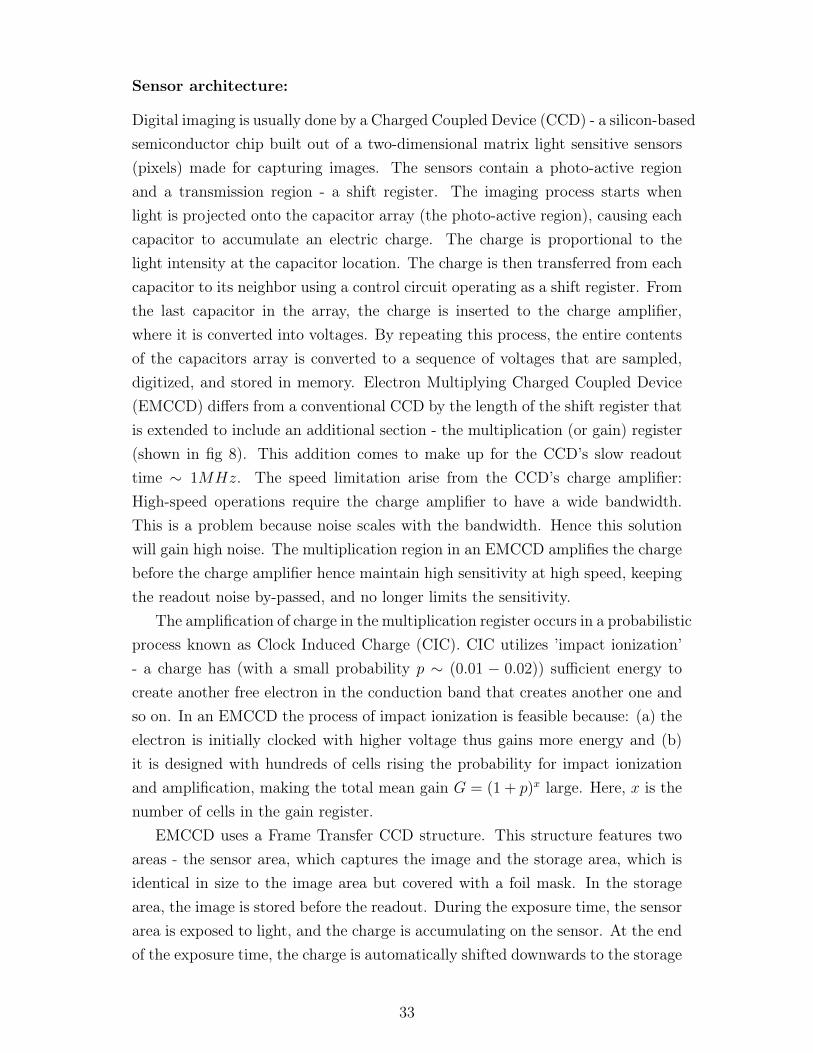
Digital imaging is usually done by a Charged Coupled Device (CCD) - a silicon-basedsemiconductor chip built out of a two-dimensional matrix light sensitive sensors(pixels) made for capturing images. The sensors contain a photo-active regionand a transmission region - a shift register. The imaging process starts whenlight is projected onto the capacitor array (the photo-active region), causing eachcapacitor to accumulate an electric charge. The charge is proportional to thelight intensity at the capacitor location. The charge is then transferred from eachcapacitor to its neighbor using a control circuit operating as a shift register. Fromthe last capacitor in the array, the charge is inserted to the charge amplifier,where it is converted into voltages. By repeating this process, the entire contentsof the capacitors array is converted to a sequence of voltages that are sampled,digitized, and stored in memory. Electron Multiplying Charged Coupled Device(EMCCD) differs from a conventional CCD by the length of the shift register thatis extended to include an additional section - the multiplication (or gain) register(shown in fig 8). This addition comes to make up for the CCD’s slow readouttime ⇠ 1MHz. The speed limitation arise from the CCD’s charge amplifier:High-speed operations require the charge amplifier to have a wide bandwidth.This is a problem because noise scales with the bandwidth. Hence this solutionwill gain high noise. The multiplication region in an EMCCD amplifies the chargebefore the charge amplifier hence maintain high sensitivity at high speed, keepingthe readout noise by-passed, and no longer limits the sensitivity.

The amplification of charge in the multiplication register occurs in a probabilisticprocess known as Clock Induced Charge (CIC). CIC utilizes ’impact ionization’- a charge has (with a small probability p ⇠ (0.01 � 0.02)) sufficient energy tocreate another free electron in the conduction band that creates another one andso on. In an EMCCD the process of impact ionization is feasible because: (a) theelectron is initially clocked with higher voltage thus gains more energy and (b)it is designed with hundreds of cells rising the probability for impact ionizationand amplification, making the total mean gain G = (1 + p)x large. Here, x is thenumber of cells in the gain register.

EMCCD uses a Frame Transfer CCD structure. This structure features twoareas - the sensor area, which captures the image and the storage area, which isidentical in size to the image area but covered with a foil mask. In the storagearea, the image is stored before the readout. During the exposure time, the sensorarea is exposed to light, and the charge is accumulating on the sensor. At the endof the exposure time, the charge is automatically shifted downwards to the storage

33

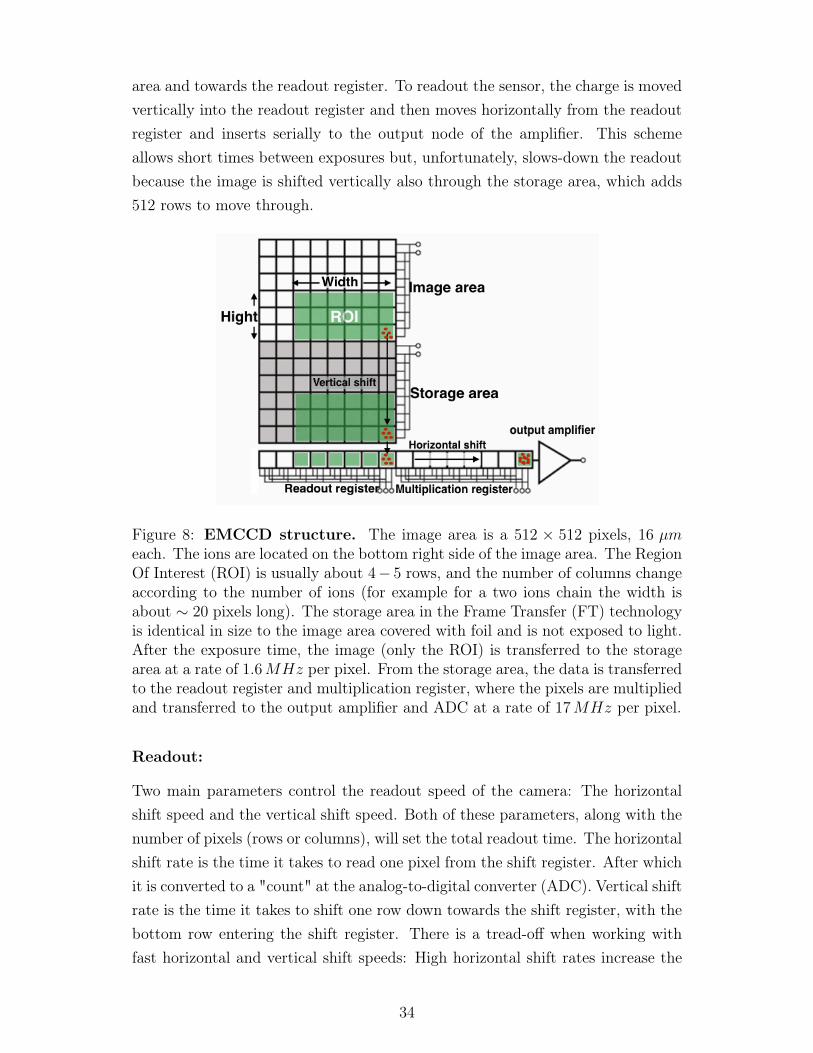
area and towards the readout register. To readout the sensor, the charge is movedvertically into the readout register and then moves horizontally from the readoutregister and inserts serially to the output node of the amplifier. This schemeallows short times between exposures but, unfortunately, slows-down the readoutbecause the image is shifted vertically also through the storage area, which adds512 rows to move through.

Figure 8: EMCCD structure. The image area is a 512 ⇥ 512 pixels, 16 µmeach. The ions are located on the bottom right side of the image area. The RegionOf Interest (ROI) is usually about 4� 5 rows, and the number of columns changeaccording to the number of ions (for example for a two ions chain the width isabout ⇠ 20 pixels long). The storage area in the Frame Transfer (FT) technologyis identical in size to the image area covered with foil and is not exposed to light.After the exposure time, the image (only the ROI) is transferred to the storagearea at a rate of 1.6MHz per pixel. From the storage area, the data is transferredto the readout register and multiplication register, where the pixels are multipliedand transferred to the output amplifier and ADC at a rate of 17MHz per pixel.

Readout:

Two main parameters control the readout speed of the camera: The horizontalshift speed and the vertical shift speed. Both of these parameters, along with thenumber of pixels (rows or columns), will set the total readout time. The horizontalshift rate is the time it takes to read one pixel from the shift register. After whichit is converted to a "count" at the analog-to-digital converter (ADC). Vertical shiftrate is the time it takes to shift one row down towards the shift register, with thebottom row entering the shift register. There is a tread-off when working withfast horizontal and vertical shift speeds: High horizontal shift rates increase the

34

read noise and reduce the available dynamic range. A disadvantage of fast verticalshift speed, is that the charge transfer efficiency is reduced, and by that reducingthe pixel potential well depth. This is mainly a problem for bright signals: ifthe vertical shift is too fast, some charge may be left behind and will result in adegraded spatial resolution.

The total readout time is calculated immediately after the exposure time untilthe CCD finishes transferring the pixels in the ROI:

treadout = H�¯W · tH + tV

�+ textra

Here: ¯W - image width , H - image height (number of rows), tH , tV�horizontaland vertical shift rates, and textra = tV ·HS+tH ·R . textra Takes in account the timedelay moving through the storage area and moving through the different registersR. In our camera, the minimum readout time that we have achieved is about 600µs(data taken from the camera during an experiment). The imaging parameterswere: ROI size 5H ⇥20W pixels, with horizontal readout rate of 17 MHz, verticalshift time - 0.3µs, number of registers, R, is 1080, and 48 over-scan pixels.

This time is long because reading out each line includes the shift of a full linewidth (512 pixels) from the sensor area to the ADC. To solve this problem, theAndor Ixon Ultra has a ”Cropped” mode option. In this mode, the camera isfooled to readout only the pixels in a specific region, defined pre-acquisition. Thiswill allow faster readout rates (around 400 µs). In order to work with this mode,we need to ensure that no stray light will fall on pixels outside the cropped moderegion. This is done with a mask placed before the camera’s EMCCD. For moredetails about our sensor, see [38, 37].

3.3 State detection

As discussed in 3.1.3, the ions are detected using the 422 nm laser that drives the5S 1

2$ 5P 1

2transition. When the electron decays back to the ground state due to

the short lifetime of the 5P 12

level, it emits a photon with the same wavelength.Applying the laser for long enough time (1000s of µs) the ion will emit a sufficientnumber of photons that the camera can collect. When the number of photonsis larger than the dark current and within photon shot-noise, the ion will bedetected and the state will be recognized as “Bright”. The 674 nm laser drivesthe 5S 1

2$ 5D 5

2transition. Shining the laser for a time corresponds to a full

population transition (a ⇡ pulse), the electron will be excited from the groundstate to the D 5

2manifold. Due to the long lifetime of this level (⇠ 0.5 seconds),

when shining the ions with a 422 nm laser while the electron is in the D manifold,

35

the electron is not coupled to the 5P 12$ 5S 1

2transition, and will not emit photons.

This state is known as a ”Dark” state. The distinction between the two internal ionstates is known as state selective fluorescence detection. Quantum mechanics hasa statistical nature, thus to infer the probabilities of the ion being in each of thetwo-qubit states with high fidelity, we repeat each experiment a multiple numberof times. The next section presents the camera output distribution, detectionalgorithm, the ability to determine the ion state, and the threshold calculation.

3.3.1 Camera output distribution

In contrast to the incoming photons that follow a Poisson distribution, the EMCCDoperation mechanism is complex thus does not follow the same distribution asthe incoming photons. The EMCCD output distribution takes into account theprobabilistic nature of light - photons Poisson distribution, the response of theimaging system to light, and some noise function. The model described herefollows [39, 40, 41]. The charge transfer along the EMCCD can be described bythe probability distribution of x electrons at the end of an ideal gain register withgain g, for n incoming photoelectrons. It can be approximated by:

pn,g(x) =

⇣xg

⌘n�1

e�x/g

g · (n� 1)!

For high gain and low light levels, this distribution mean is n · g and variancen · g2. In high light levels, it can be approximated to a Gaussian (the PSF of thecamera for varying exposure times can also describe the charge transfer efficiencyof the EMCCD).

The number of photoelectrons on a pixel is drawn from a Poisson distribution,q�(n) =

�ne��

n!of incoming photons with mean �. The distribution of electrons to

leave the gain register is a weighted sum over pn,g(x) for the different photoelectronsvalues:

h�,g (x) =1X

n=1

q� (n) · pn,g (x)

The readout process of the charge adds extra noise - readout noise, that can bemodeled by a Gaussian distribution with mean µ and variance �2:

Nreadout (x) =1

�p2⇡

e12(

(x�µ)�

)

2

The total output distribution is modeled by convolving the output distributionfrom the gain register with the readout noise to give:

36

f(x) = h�.g (x) ⇤Nreadout (x)

Note that this result can be transformed to ”counts” (digitized signal) distributionby dividing the electron numbers by a scaling factor [41]. The scaling factoralso normalizes the values of the distribution, g, µ and �, which are the cameraproperties except for �, which varies from pixel to pixel.

The mean number of photon for each pixel i is modeled as:

�brighti = texp (RB · !i +RD)

�darki = texpRD

where texp is the exposure time, RB is the detected fluorescence rate for an ionin the bright state (corresponds to |Si state), !i is the fraction of fluorescencecollected by pixel m (the total fluorescence summed over the whole image isnormalized:

Pi=1

!i = 1) , and RD is the fluorescence rate when the ion is in the dark

state (corresponds to |Distate) which contains scattered light and thermal darkcounts (discussed in section 4.1 in [32]). �brighti and �darki are taken into accountfor each pixel to build Bm and Dm - the dark and bright distributions, which hasthe shape of f (x) and will be discussed in the next section. Another possible andinteresting analysis of the camera’s output distribution is the Poisson-Gammadistribution modeled by Hirsch et al. in [42].

3.3.2 State detection algorithm

The difference in intensities between the bright and dark states during the stateselective fluorescence detection can be compared and utilized to set a discriminationthreshold. The photon emission process follows a Poisson distribution with differentdetection-time dependent means. High detection fidelity is translated to a smalloverlap of the Poisson distributions for the “dark” and “bright” scenarios. TheEMCCD output does not follow a Poisson distribution, as they are altered bycamera readout noise, dark currents, and gain (see section 4.4.2). Thus, thedifferentiation of the camera dark and bright measurements is done by comparingthe total intensity over a set of predetermined pixels of interest. A discriminationthreshold is set to each ion individually using the following process: (a) Acquiringa batch of samples (around a few thousand) of “bright” and “dark” images. (b)The pixels are ordered from the brightest to the darkest according to the averageof bright images. (c) The intensity distribution of each “dark” and “bright” images

37

compared for n brightest pixels, where n can get up to a single brightest pixelor a predetermined maximum number of pixels. (d) The optimal n (number ofbrightest pixels) is chosen by maximizing the mean distance of the distributioncompared to the minimum distance (when there is no overlap) or by the minimaldistribution overlap:

noptimal = max

¯Bn � ¯Dn

¯Bn � ¯Dn ��min( ¯Bn)�max( ¯Dn)

�!

Where ¯Bn, ¯Dn represent the bright and dark intensity distribution for n pixels.High separation of the two distributions (for the bright and dark state) implies

that discrimination errors cannot be induced, and the distributions are separatedby a large margin relative to the mean distribution. This discrimination is done foreach ion separately, setting a threshold to each ion individually in a non-dependentway [25]. Exposure time is another factor that influences the quality of thediscrimination. Shorter exposure times will decrease the distance between thedistributions because fewer photons are collected, and the difference between thehigh photon count for the dark state and the low photon count for the bright stateis getting closer. Although, for exposure time up to 700µs the discrimination erroris smaller than 1⇥ 10

�4. The number of pixels that are marked and used for theoptimal n is around 9� 12 pixels per ion. This threshold and marked pixels willlater be used in the live readout system and analysis to determine the state of theions.

38

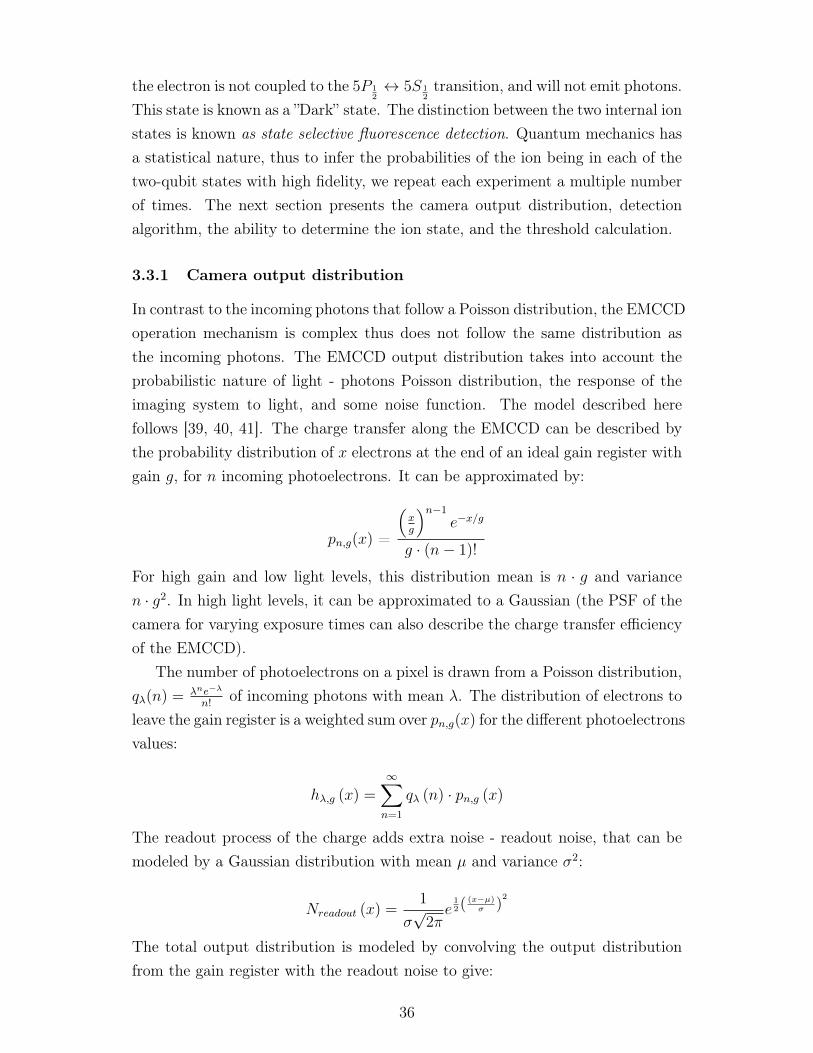
Figure 9: Dark and Bright photon count distribution in [au]. An exampleof discrimination distribution of bright and dark states for various exposure timesfrom 400µs to 1000µs . We can see that the ability to discriminate correctlywithout overlapping the distributions for short exposure times is decreasing.The red distribution is the distribution of the bright states, and the blue is forthe dark state. The dark state distribution centered around 0 photon count,where the bright state is broader and moves to higher photon count with longerexposure times. The optimal exposure time for this work is 700 µs, where we cansignificantly discriminate between both of the states.

Camera parameters:

The camera’s magnification is determined by the ratio between the distance of eachion on the EMCCD, and the real inner distance of the ions in the trap. The innerdistance between the ions is calculated in [43], using the formula l3 =

Z2e2

4⇡✏0M⌫2,

giving a trap frequency of ⇠ 600 KHz, and l = 4.68 the inter-ion distance isl · 1.077 = 5.04 µm . The pixel distance is measured using a Gaussian fit to anion image to be 13.06 pixels, which translates to 209 µm. the total magnificationwill be:

Magnification =

Pixel distanceReal distance

=

209

5.04= 41.46

39

This number agrees with the designed magnification (⇠ 40) that set by thenumerical aperture, and its distance to the ions.

Fluorescence spectra:

In Sr+ the excited state 5P 12

can decay to the 5S 12

but also to the 4D 32

meta-stablestate. This is the three-level ⇤ system. When the ion decays to the D manifold,the interaction with the laser that drives the 5S 1

2$ 5P 1

2transition stops until the

ion will decay back to the ground state. Because the D manifold is a long-livedlevel (~390 ms), a repump laser that drives the P 1

2$ D 3

2transition is needed -

the 1092 nm laser. Due to the splitting of the Zeeman levels when the externalmagnetic field is applied, the level structure of the Sr+ contains eight levels (anumerical solution of the optical-Bloch equations for the eight levels involved canbe found in [30] a much more complicated system than the canonical 3-level ⇤system. The Zeeman shift due to magnetic field B along the quantization axes is:

�! = gjmjµB |B|

~

with gj

⇣S 1

2

⌘= 2 ; gj

⇣P 1

2

⌘=

2

3

; gj

⇣D 3

2

⌘=

4

5

and mj is the projection of thetotal angular momentum on the z-axis. We can scan the fluorescence spectrumof the ion using both the 422 nm laser and the 1092 nm laser in order to finddark resonances - a deep in the fluorescence spectrum. Dark resonance can teachus in a relatively simple way about the detuning of the drive laser. When bothof the lasers are turned on, and the detuning is scanned, the dark resonance willoccur when the detuning of the two lasers is equal with respect to a specific set ofZeeman sub-levels. The polarization of the lasers determines the number of darkresonance and their shape in the spectrum. The laser line-width sets the width ofthe dark resonances in the spectrum.

40

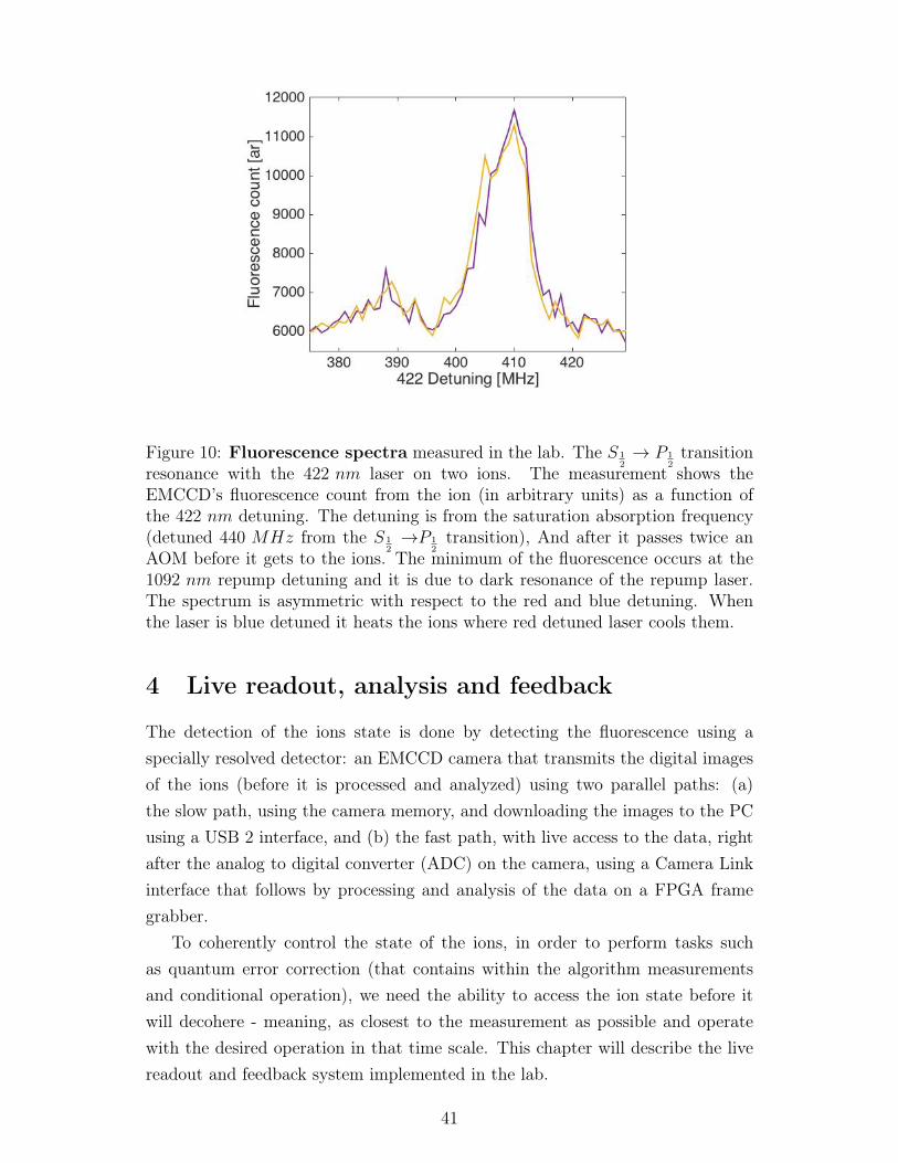
Figure 10: Fluorescence spectra measured in the lab. The S 12! P 1

2transition

resonance with the 422 nm laser on two ions. The measurement shows theEMCCD’s fluorescence count from the ion (in arbitrary units) as a function ofthe 422 nm detuning. The detuning is from the saturation absorption frequency(detuned 440 MHz from the S 1

2!P 1

2transition), And after it passes twice an

AOM before it gets to the ions. The minimum of the fluorescence occurs at the1092 nm repump detuning and it is due to dark resonance of the repump laser.The spectrum is asymmetric with respect to the red and blue detuning. Whenthe laser is blue detuned it heats the ions where red detuned laser cools them.

4 Live readout, analysis and feedback

The detection of the ions state is done by detecting the fluorescence using aspecially resolved detector: an EMCCD camera that transmits the digital imagesof the ions (before it is processed and analyzed) using two parallel paths: (a)the slow path, using the camera memory, and downloading the images to the PCusing a USB 2 interface, and (b) the fast path, with live access to the data, rightafter the analog to digital converter (ADC) on the camera, using a Camera Linkinterface that follows by processing and analysis of the data on a FPGA framegrabber.

To coherently control the state of the ions, in order to perform tasks suchas quantum error correction (that contains within the algorithm measurementsand conditional operation), we need the ability to access the ion state before itwill decohere - meaning, as closest to the measurement as possible and operatewith the desired operation in that time scale. This chapter will describe the livereadout and feedback system implemented in the lab.

41

4.1 Implementing live readout

The iXon Ultra used in the lab is equipped with a Camera Link output. CameraLink is a communication protocol that describes the transfer of a 2D data array,as pixels of an image. The camera streams the image data to an FPGA framegrabber, there we process and analyze it according to our needs. Camera Linkprovides access to the camera data output with very low latency, transferring16-bit pixels at a rate of 40MHz per pixel. Before implementing this interface,the only access to the data was at the end of each experiment (that contains manyrepetitions thus many images), suggesting that to apply conditioned operationson the ions is only possible with the use of post-processing and post-selecting ofimages.

Connector Camera Link (Base) USB 2.0Data transfer Rate 1.12 Gb/s 480 Mb/sMax cable length 10m 3mEstimated latency ~ ns 20 msCamera Control Not implemented Full control

Connector 26 pin USBCapture Board Required FPGA PC

Table 1: A comparison between the different Andor iXon Ultra 879 interfaces [44].

4.1.1 Camera Link interface

Before Camera Link, there was a lack of a communication standard in the visionindustry between a camera and a frame grabber. There was an abundance ofdifferent connectors results in many cable types. The physical communicationlayer was not well defined as well as the data transfer protocol, camera timing,and camera singling. Camera Link is a solution to all of the above as it is a robust,complete interface between a camera and a frame grabber.

Protocol description

Camera Link is a serial communication protocol standard developed for visionapplications (A full protocol description, can be found in [45]). The protocolis based on Channel Link technologies (by National Semiconductors) such asLow Voltage Differential Signaling (LVDS) as the communication channel. EachChannel Link transmmiter\reciver pair is made out of four LVDS pairs. LVDS isa physical communication channel that transmits the encoded information in thedifference between two different voltages sent to the receiver and compared there.LVDS is a useful technology for vision due to its low noise and fast data rates

42

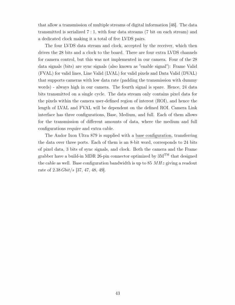
that allow a transmission of multiple streams of digital information [46]. The datatransmitted is serialized 7 : 1, with four data streams (7 bit on each stream) anda dedicated clock making it a total of five LVDS pairs.

The four LVDS data stream and clock, accepted by the receiver, which thendrives the 28 bits and a clock to the board. There are four extra LVDS channelsfor camera control, but this was not implemented in our camera. Four of the 28

data signals (bits) are sync signals (also known as ”enable signal”): Frame Valid(FVAL) for valid lines, Line Valid (LVAL) for valid pixels and Data Valid (DVAL)that supports cameras with low data rate (padding the transmission with dummywords) - always high in our camera. The fourth signal is spare. Hence, 24 databits transmitted on a single cycle. The data stream only contains pixel data forthe pixels within the camera user-defined region of interest (ROI), and hence thelength of LVAL and FVAL will be dependent on the defined ROI. Camera Linkinterface has three configurations, Base, Medium, and full. Each of them allowsfor the transmission of different amounts of data, where the medium and fullconfigurations require and extra cable.

The Andor Ixon Ultra 879 is supplied with a base configuration, transferringthe data over three ports. Each of them is an 8-bit word, corresponds to 24 bitsof pixel data, 3 bits of sync signals, and clock. Both the camera and the Framegrabber have a build-in MDR 26-pin connector optimized by 3MTM that designedthe cable as well. Base configuration bandwidth is up to 85 MHz giving a readoutrate of 2.38Gbit/s [37, 47, 48, 49].

43

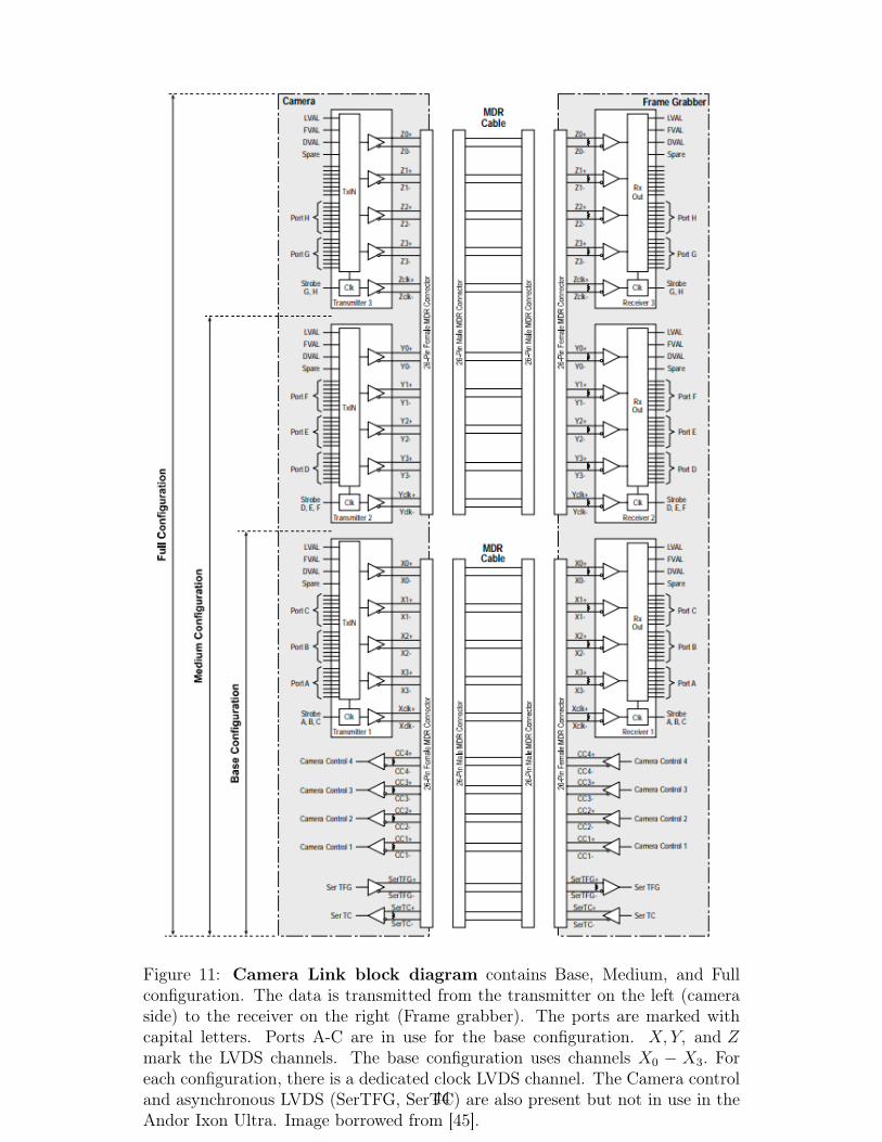
Figure 11: Camera Link block diagram contains Base, Medium, and Fullconfiguration. The data is transmitted from the transmitter on the left (cameraside) to the receiver on the right (Frame grabber). The ports are marked withcapital letters. Ports A-C are in use for the base configuration. X, Y, and Zmark the LVDS channels. The base configuration uses channels X

0

� X3

. Foreach configuration, there is a dedicated clock LVDS channel. The Camera controland asynchronous LVDS (SerTFG, SerTC) are also present but not in use in theAndor Ixon Ultra. Image borrowed from [45].

44

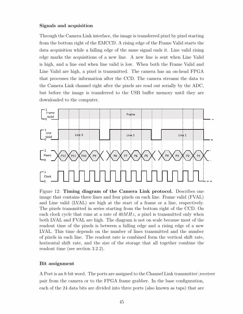
Signals and acquisition

Through the Camera Link interface, the image is transferred pixel by pixel startingfrom the bottom right of the EMCCD. A rising edge of the Frame Valid starts thedata acquisition while a falling edge of the same signal ends it. Line valid risingedge marks the acquisitions of a new line. A new line is sent when Line Validis high, and a line end when line valid is low. When both the Frame Valid andLine Valid are high, a pixel is transmitted. The camera has an on-head FPGAthat processes the information after the CCD. The camera streams the data tothe Camera Link channel right after the pixels are read out serially by the ADC,but before the image is transferred to the USB buffer memory until they aredownloaded to the computer.

Figure 12: Timing diagram of the Camera Link protocol. Describes oneimage that contains three lines and four pixels on each line. Frame valid (FVAL)and Line valid (LVAL) are high at the start of a frame or a line, respectively.The pixels transmitted in series starting from the bottom right of the CCD. Oneach clock cycle that runs at a rate of 40MHz, a pixel is transmitted only whenboth LVAL and FVAL are high. The diagram is not on scale because most of thereadout time of the pixels is between a falling edge and a rising edge of a newLVAL. This time depends on the number of lines transmitted and the numberof pixels in each line. The readout rate is combined form the vertical shift rate,horizontal shift rate, and the size of the storage that all together combine thereadout time (see section 3.2.2).

Bit assignment

A Port is an 8-bit word. The ports are assigned to the Channel Link transmitter\receiverpair from the camera or to the FPGA frame grabber. In the base configuration,each of the 24 data bits are divided into three ports (also known as taps) that are

45

assigned to pins on the Channel Link interface. The configuration will determinethe number of ports that the Camera Link uses in order to stream the data. Theport is denoted by a capital letter starting from A that contains bits 0� 7. PortsA to C are used for the base configuration. The assignment of each bit in theports is described in table 2. For images with a pixel depth of 16 bit, only portsA and B are used assigning bits 0 � 15. The value of the transmitted pixel isdivided by the two ports where port B contains the most significant bit, and Ahas the least significant bit (the building of the total pixel value is done on theframe grabber according to this logic). The bits of a pixel are not assigned to theChannel Link transmitters in a specific order but permutated as shown in 2. Thecamera pixel clock is at 40MHz, giving 1.12Gbit/s bandwidth.

46

Signal name Pin name 16 bit pixel LVDS ChannelClock TxClkIn/RxClkOut Clock ClockLVAL TX24/RX24 Enable X2FVAL TX25/RX25 Enable X2DVAL TX26/RX26 Enable X2Spare TX23/RX23 Enable X3

Port A0 TX0/RX0 Bit 0 X0Port A1 TX1/RX1 Bit 1 X0Port A2 TX2/RX2 Bit 2 X0Port A3 TX3/RX3 Bit 3 X0Port A4 TX4/RX4 Bit 4 X0Port A5 TX6/RX6 Bit 5 X0Port A6 TX27/RX27 Bit 6 X3Port A7 TX5/RX5 Bit 7 X3Port B0 TX7/RX7 Bit 8 X0Port B1 TX8/RX8 Bit 9 X1Port B2 TX9/RX9 Bit 10 X1Port B3 TX12/RX12 Bit 11 X1Port B4 TX13/RX13 Bit 12 X1Port B5 TX14/RX14 Bit 13 X1Port B6 TX10/RX10 Bit 14 X3Port B7 TX11/RX11 Bit 15 X3Port C0 TX15/RX15 nc X3Port C1 TX18/RX18 nc X2Port C2 TX19/RX19 nc X2Port C3 TX20/RX20 nc X2Port C4 TX21/RX21 nc X2Port C5 TX22/RX22 nc X3Port C6 TX16/RX16 nc X1Port C7 TX17/RX17 nc X1

Table 2: Bit assignment for a single 16-bit pixel. The information aboutthe pixel transferred to the Channel Link transmitter from three different ports,each connected to a different pin on the transmitter. A maximum of 28 bits canbe transmitted over the four different LVDS channels. For a 16 bit pixel, the datais transferred from ports A and B, where port C is not connected. For an RGBimage or a 24-bit image, port C is in use, and these pins are connected.

47

Figure 13: Bit assignment for a single 16-bit pixel. Illustration of the tableabove. Each channel contains 7 bits permutated from different ports. For example,one can see that channel X

0

contains pixels from port A and port B. The pixelstiming diagram is a 7 : 1, where the clock duty cycle is 4 : 3 , and the falling edgeis after the second bit [47, 48].

4.1.2 Frame grabber

The ability to perform live readout is possible using a Camera Link communicationprotocol that connects to a dedicated FPGA device, with a Camera Link connectorand image processing capabilities. For this task, we chose a NI-PCIe 1473R framegrabber card. This is a PCI Express (PCIe), user re-configurable Virtex-5 LX50FPGA, aimed for image acquisition. This device has two Camera Link connectionports supporting Base, Medium, and Full configurations for Camera Link cameras[50]. The FPGA contains arrays of programmable logic blocks that allow for theuser to implement programs (such as image processing) on the hardware level withrates independent of the load. The processing of information on the FPGA is doneon-the-fly as the information arrives. Hence the ions state analysis time is limitedby the readout time of the EMCCD and not by the image processing time of theFPGA. The FPGA frame-grabber is separated from the main FPGA that controlsthe experiment, implying that communication between the two FPGA’s will benecessary to perform conditional feedback on the ions. The NI-PCIe 1473R framegrabber has two internal clocks. One of them is an image clock that is dedicatedto reading the pixels coming from the camera, and its running at a 100MHz rate.This rate is 2.5 times faster than the pixel clock in the camera and promises thatthe pixels are read without loss or aliasing, following that fsampling > 2·Bandwidth

is the Nyquist rate. The second clock is a 40 MHz internal clock that runs all

48

the processing tasks of the frame grabber.

Figure 14: NI 1473R PCIe hardware. Left: the FPGA frame grabber blockdiagram. Right: NI-1473R-PCIe frame grabber connectors. The Camera Linkcable connected to 1 - Port 0, which is a Base Camera Link MDR connector. 2is the Medium/Full MDR connector, and 3 is an SMB Trigger connector that thecamera trigger connected to from the FPGA and triggers both the frame grabberand the camera together (the sketch is borrowed from [50]).

4.2 Hardware architecture

As written in 4.1, the live readout implemented using a frame grabber FPGA cardthat is external to the FGPA that controls and manages our experiments. Theintegration of the frame grabber to the main FPGA was necessary and included anew set of communication lines that were added to the existing framework. Thisarchitecture is described in the following section.

49

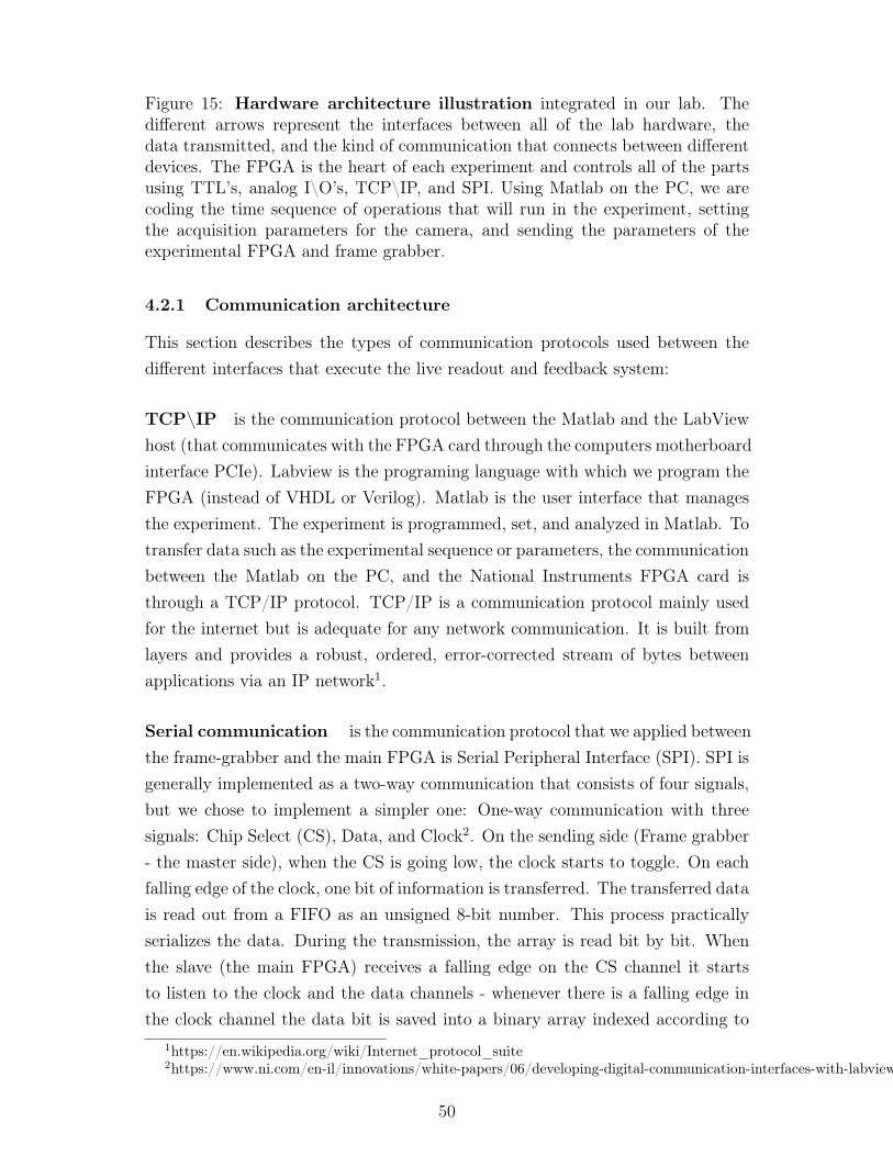
Figure 15: Hardware architecture illustration integrated in our lab. Thedifferent arrows represent the interfaces between all of the lab hardware, thedata transmitted, and the kind of communication that connects between differentdevices. The FPGA is the heart of each experiment and controls all of the partsusing TTL’s, analog I\O’s, TCP\IP, and SPI. Using Matlab on the PC, we arecoding the time sequence of operations that will run in the experiment, settingthe acquisition parameters for the camera, and sending the parameters of theexperimental FPGA and frame grabber.

4.2.1 Communication architecture

This section describes the types of communication protocols used between thedifferent interfaces that execute the live readout and feedback system:

TCP\IP is the communication protocol between the Matlab and the LabViewhost (that communicates with the FPGA card through the computers motherboardinterface PCIe). Labview is the programing language with which we program theFPGA (instead of VHDL or Verilog). Matlab is the user interface that managesthe experiment. The experiment is programmed, set, and analyzed in Matlab. Totransfer data such as the experimental sequence or parameters, the communicationbetween the Matlab on the PC, and the National Instruments FPGA card isthrough a TCP/IP protocol. TCP/IP is a communication protocol mainly usedfor the internet but is adequate for any network communication. It is built fromlayers and provides a robust, ordered, error-corrected stream of bytes betweenapplications via an IP network1.

Serial communication is the communication protocol that we applied betweenthe frame-grabber and the main FPGA is Serial Peripheral Interface (SPI). SPI isgenerally implemented as a two-way communication that consists of four signals,but we chose to implement a simpler one: One-way communication with threesignals: Chip Select (CS), Data, and Clock2. On the sending side (Frame grabber- the master side), when the CS is going low, the clock starts to toggle. On eachfalling edge of the clock, one bit of information is transferred. The transferred datais read out from a FIFO as an unsigned 8-bit number. This process practicallyserializes the data. During the transmission, the array is read bit by bit. Whenthe slave (the main FPGA) receives a falling edge on the CS channel it startsto listen to the clock and the data channels - whenever there is a falling edge inthe clock channel the data bit is saved into a binary array indexed according to

1https://en.wikipedia.org/wiki/Internet_protocol_suite

2https://www.ni.com/en-il/innovations/white-papers/06/developing-digital-communication-interfaces-with-labview-fpga.html

50

the clock counts. At the end of the transmission, we have an 8-bit binary wordthat is converted to an unsigned 8-bit number. The CS sending rate is at 4 Mhz,meaning it takes ⇠ 4µs to send the data. The reading rate is 40 MHz to avoidunder-sampling.

Figure 16: SPI communication channels. The Chip select sets the start of thedata transfer. When CS falling edge detected, the clock line is being listened to,and with every rising edge, the information from the data channel is read. Eachclock cycle is representing a different ion on the ion chain. For example, the dataregarding the first ion will read on the first clock cycle, the second ion on thesecond clock cycle, until the entire array is readout. Every time the data signalis high, the information is acquired as Boolean 1, and in our case, translated intoa “bright” state of the specific ion according to the clock cycle.

USB 2.0 is a standard specification for communication protocols, connections,and power supply between devices. USB 2.0 is the main communication layerbetween the camera and the computer: Sending through is the acquisition parametersto the camera before an experiment, setting the camera to start acquiring andreading out the images from the camera to the computer at the end of an experiment.

Camera Link The interface between the camera and the frame grabber FPGAis thoroughly described in section 4.1.1.

4.3 Software architecture

The programming of both the frame-grabber FPGA and the main FPGA isdone using LabView - a visual programming language made as a developmentenvironment and a system-design platform from National Instruments. LabViewallows us to maintain the communication with the FPGA on two levels. The higherone is the user interface (host) that runs on the PC and controls the operationof the main FPGA by reading or writing to the FPGA and communicating withMatlab (using TCP/IP). The lower level is hardcoded on the FPGA card itself,and usually, a machine type programming is needed (In our case, we have usedLabView platform to program). The following section will describe and give

51

a detailed explanation of the software that we wrote for the live readout andfeedback task.

4.3.1 Clock

FPGAs in general and frame grabbers, in particular, specialized in running computationaltasks at a high rate. The LabView FPGA interface allows us to perform moreefficient computations using a timed loop called Single-Cycle Timed Loop (SCTL).All functions inside this loop executed within one clock cycle (tick) of the FPGAselected clock. This means that not all the functions can be used inside a SCTL- a function that takes more than one tick, will not compile inside a SCTL. Notusing a SCTL, will result in a slower execution rate where the default clock rateof the card is the maximum rate. The execution of functions outside of a SCTLloop can take longer, meaning some of the function will take one or more clockticks to execute3.

Frame grabber clocks:Three main clock domains run in parallel on the frame grabber:

• Image readout and analysis - the main loop that is running on the framegrabber. Runs at a 100 MHz, 2.5 times faster than the camera pixel clockreadout rate through the Camera Link interface. This loop reads out thepixel data and executes on-the-fly image analysis state detection.

• SPI - in this loop, the SPI communication protocol is implemented, runningat a 4 MHz rate parallel to the previous loop where each tick of the loopsends 1 bit of information from the frame-grabber to the main FPGA.

• Memory readout - is a side loop that controls the reading of the pixel mapfrom the memory of the frame-grabber after the primary discriminationprocess and before the experiment begins.

Main FPGA clock

• Main loop - runs the entire experiments in the lab. This loop controls thelasers, AOM’s, trap frequencies, and the magnetic field. It also contains thecondition loop that reads the ion state and acts by the results.

• SPI slave - the loop that is responsible for reading from the SPI channels andconverts the data received from the frame-grabber into an integer numberthat corresponds to the ion state.

3https://knowledge.ni.com/KnowledgeArticleDetails?id=kA00Z000000P8sWSAS&l=en-IL

52

4.3.2 Live readout and image analysis

The image analysis is realized out on-the-fly during the readout. Before anexperiment, the frame grabber is uploaded with information about the upcomingexperiment - an updated pixel map, threshold parameters, and the number ofrepetitions uploaded to the frame grabber at the end of the discrimination process(see 3.3.2). The pixel map links between a pixel to an ion. For example, if afterthe discriminator process a pixel is relevant to ion number 3, in the pixel map,the cell that relates to this pixel location will get the number 3. If a pixel doesnot belong to an ion, it gets the number zero. The threshold is an array ofinteger numbers, each cell correspondent to an ion on the chain, and each ion isthresholded separably.

Figure 17: Pixel map example. On the top image, we can see the ions and theselected pixels that were selected to discriminate between dark and bright statesaccording to the discrimination algorithm. The pixels are sorted from brightest todarkest, and only the most relevant pixels to each ion get selected. The total signalin these pixels is calculated and compared to a threshold in order to determinewhether the ion’s state is bright or dark. The bottom image shows the pixel mapgenerated from the image above after the discrimination processes, overlayed onthe image of the ions to demonstrates the meaning of each number. The ions aresorted left to right where the left most ion gets the number 1 and so on. Thismap is sent as a vector to the frame grabber memory. The memory is read duringeach pixel acquisition to relate each pixel to a specific ion.

When an experiment begins, the camera and the frame-grabber are triggeredfrom the main FPGA with the same trigger. The camera starts to acquire theimage, and the frame grabber waits for a Frame Valid rising edge. As mentioned in4.1.1, the Camera Link sends four syncing signals. The frame grabber acquisitionloop is working at a 100 MHz rate while the camera streams the pixels at a40 MHz rate. When a Frame Valid arrives, the frame grabber knows that a newframe is now acquired. Once the Line Valid and Frame Valid are high, a new pixel

53

is acquired. Using the LVAL and FVAL signals to activate counters, each pixelhas its coordinates, that are known during the pixel processing.

The pixels are read straight from the ports of the Camera Link interface.From the iXon Ultra 879, data is sent in 2 ports, A and B; each contains 8 bitsof information, read separably, and joined to one 16-bit number where the B porthas the most significant bit. After a one pixel reading cycle (takes about 5 tickson the FPGA clock), the pixel coordinate and value are known, and the stateanalysis starts. The pixel coordinates are used to read a specific location fromthe frame grabber memory, where the pixel map is saved. As mentioned above,the information from this memory cell will link this pixel to a specific ion. Thepixel’s value is summed along with the rest of the pixels that relate to the sameion. This process is parallel to the readout. At the end of the image acquisition,the total sum of pixels for each ion is compared to a corresponding thresholdvalue. The comparison result creates a binary array: 1 if the sum is larger thanthe threshold and 0 if not. These numbers translate to a “bright” state or a “dark”state, respectively. The binary array is translated to an unsigned 8-bit numberand saved into a first in first out (FIFO) memory on the frame grabber. TheFIFO is read on the SPI domain. At the end of an image acquisition, the data isserialized, and sent via SPI to the main FPGA at 4 MHz per bit. This processrepeats until all the images in an experiment are acquired.

54

Figure 18: Live readout and image analysis scheme. The frame grabberlistens to three different lines: Data line, which contains the information of thepixel value, Frame valid, and Line valid that translate to X and Y coordinates.These coordinates are used to read from the frame grabber memory the relevantion number that links to this pixel, and then the pixel is summed with the rest ofthe related pixels. When FVAL is going low, it is the end of the image acquisition.Then the sum of the pixels is compared to a threshold value that results in a binaryarray. The array is sent to the main FPGA using the SPI interface. The entireimage analysis time depends on the number of pixels. For one pixel, it will take50 ns (t =

Ntick

2.5·fCL

). This process is bounded by the readout time because theanalysis is parallel to the readout from the camera. The readout time (~600 µs),along with the exposure time (700 µs) are almost as long as the qubit dephasingtime (about ⇠ 2 µs) making these processes as the main holdback in performingquantum feedback.

4.3.3 Feedback architecture

In the main FPGA, the main loop that is running the experiment is programmedto work as a processor. Before each experiment, the experimental sequence isdownloaded to the FPGA, row by row. The FPGA is executing the command ineach row and, when done, moving forward to the next row. This type of executionis done using different cases, where each row in the code is translated to a casein the main loop. Using this architecture, the FPGA can jump between casesand even implement logical loops by jumping back in the row number. We areusing this kind of architecture to implement the feedback option. When writing asequence to run on the FPGA, one of the commands is an IF-Do case. Applyingsuch a case, the FPGA waits for a variable contains the information about the ionstate to arrive from the serial loop. This state compared to a pre-set value thatis sent to the FPGA before the experiment. If the values are equal, a pre-definedoperation, such as a gate or a rotation, is carried out. For different values, the

55

program enters an ELSE case (nested in the IF case) that loops over all thepossible states.

4.4 Readout, noise source and implementation bugs

In order to implement the readout system in our lab, we started with a few sanitychecks to find out if the system works as we expect it to work and delivers thesame results as the offline discrimination process before integrating this into ourlab.

4.4.1 readout fidelity

Readout fidelity will limit the correctness of our discrimination possibilities, thuslimits the fidelity of any quantum algorithm we intend to execute using thissystem. The readout fidelity is calculated by comparing the results from theframe grabber discrimination processes to the results we get by post-processing theimages using Matlab. We treat the post-processing results as the reference. (Formore information about the camera’s detection and processing done by Matlabsee [25]). The fidelity is:

N � ✏

N

where N is the number of measurements, and ✏ is the number of errors. An error iscounted when a difference between the live readout and the Matlab discriminationoutputs excites. We evaluated the readout fidelity of the live readout system usinga repeated initialization of the ions to a known sate (the initialization fidelity isfrom [51]), followed by a measurement. The discrimination is done by countingthe pixels relevant to each ion. Different experimental parameters influence thereadout fidelity: (a) Geometric ensemble of our set up (magnification, numericalaperture (collection efficiency), and spot size). (b) Noise - such as readout noise,noise factor, exposure time, and the image shape on the detector. (c) Physicalproperties of the experiment - radiation rate of 88Sr+, ions state, ions distance(trap frequency), qubit coherence time, and the properties and stability of thelaser (a problem in one of the lasers can affect everything such as the ion state,fluorescence rate, qubit coherence time initialization). (d) EMCCD hardcodedparameters such as Clock Induced Charge (see 3.2.2), noise, and quantum efficiency.All of these parameters influence in the same manner on both the live readoutsystem, and the post-processing readout fidelity; thus, we expect to get identicalresults from both image processing paths. The readout fidelity of the system wastested in two ways. The first was to compare both pixel sums on each ion to make

56

sure it is identical, and the second was to compare the discrimination decisionreceived both from the frame-grabber and the post-processing image. Both resultsfound to be equal on over 2000 images, except for a bug case mentions in 4.4.3.

Figure 19: Bright and dark images. The top row shows bright images, whereasthe bottom row is for dark images. In all of the images, the exposure time is 1 ms.There is a significant difference between the two images, as can be seen using theintensity distributions for 1ms in figure 9. The image is adapted from [25].

4.4.2 Noise

Noise can cause a wrong light distribution on the EMCCD, thus affect the discriminationfidelity - the overlap of the bright and dark distributions. Noise is present in allelectronic systems. The presence of noise in an EMCCD and image processing isplacing bounds on different parameters such as exposure time and readout time,which are the main holdbacks in this work. The exposure time is bounded frombelow for a couple of reasons. One of them is the photon collection efficiency, whichis determined by the numerical aperture of the imaging system. The EMCCD’sphoton collection distribution is not Poissonian (like in Photon multiplier tubes);thus, the signal-to-noise ratio of an image is altered by the readout noise, darkcurrent, and gain. This kind of noise is a limitation on two of the most time-consumingprocesses that can influence the fidelity and the ability to perform live readoutand coherent feedback: exposure time and readout time. The numerical apertureis a giving property in our lab, and changing it is out of scope of this work. Thefeatures mentioned in this paragraph directly affect the ability to discriminatebetween the "dark" and "bright" state of the ion, and their presence may resultin detection errors. Different noise sources that are relevant to our system arelisted below.

57

Shot noise: is a statistical noise due to the particle nature of the photons. Thisnoise obeys Poisson distribution with fluctuations equals to the square root of thesignal: Nsignal = hIi. There is a signature to the shot noise both in dark andbright cases that affect the distribution of both states (see section 3.3.1).

Dark Current (thermal noise): is the thermal fluctuations within the EMCCDchip that are enough to eject electrons from the semiconductor body, which thencontributes to the EMCCD signal. This called dark current and is known asreverse bias leakage current in non-optical devices and presents in all diodes. Darkcurrent is caused by thermally generated electron-hole pairs, which build upon thepixels region even when are not exposed to light. It is one of the primary noisesources in image sensors. The sensor is cleared before an acquisition, but the darkcurrent will still build up until cleared again. Thermal fluctuations of the voltagecan be calculated using the Nyquist formula hv2i = 4RkBT�f , where R is thesilicon resistance, kB - Boltzmann constant, T - is the temperature and �f - isthe bandwidth of the EMCCD, from here we can understand that it can decreaseby cooling the camera. The cooling of our EMCCD to �80

� reduces the thermalnoise to such a low level that other mechanism dominates the dark count rate.

Clock-Induced Charge (CIC) noise: NCIC is a noise source independent ofthe exposure time and exists for every pixel that is read out from the EMCCDcamera. This noise mechanism is similar to the multiplication process, which isresponsible for the gain of the EMCCD, and after the minimization of the thermalnoise by cooling, this is the dominant noise source of the dark images. During theprocesses of moving charges from pixel to pixel, there is a probability that a holewill be accelerated by the clocked voltage and will collide with the silicon atomto produce a new electron-hole pair through impact ionization. In an EMCCD,the extra CIC electrons will be amplified by the gain register meaning there is noway to know if it is noise or photoelectrons. The probability of generating CICnoise depends on the number of transferred pixels. A small ROI, located as closeas possible to the readout register, minimizes the amount of impact ionizationpossibilities, thus reduces the CIC noise.

Readout noise: this noise, �R is introduced during the pixel and line transfertowards the readout register at the bottom of the CCD. It happens due tothe non-adiabatic excitation of electrons on the process. Readout noise can beconsidered as the CCD’s detection limit, especially in the case of fast frame rateexperiments because (a) dark current contributions will be negligible in short

58

exposures (b) faster pixel readout rates, such as 5 MHz and higher, result insignificantly higher readout noise4. Luckily one of the fundamental advantages ofEMCCD technology is that the gain -g is sufficient to reduce the readout noiseto N

Read

g. Therefore high gains eliminates the detection limit, making the readout

noise negligible.

Multiplicative noise: is the uncertainty inherent in the multiplying processthat introduces additional noise. The fact that the gain process is stochastic addsto the fact that for one electron entering the gain register may result in a varietyof possibilities for the number of electrons leaving it. This uncertainty is called"Noise Factor":

F =

Nout

g ·Nin

Where N2

in\out is the variance of the input and output signals to and from thegain register. In EMCCD technologies, the noise factor value is

p2 [52]. This

noise factor can be treated as an addition to the shot noise of the system (addingnoise sources will increase the variation of readout electron number).

Quantum efficiency: the actual signal that the EMCCD generates is the numberof electrons, or more accurately, "photoelectrons" that are created when a photonis absorbed. Photons of different wavelengths have different absorption probability,thus a different probability of generating photoelectrons. This probability isknown as quantum efficiency or spectral response. The main contribution toquantum efficiency is the absorption coefficient of the silicon that serves as thebulk material of the device.

Total noise and signal to noise ratio

The total noise sources will eventually affect the signal to noise ratio. The differentnoise sources are summed in quadrature to give the total noise per pixel:

total noise =q

F 2 · g2�N2

thermal +N2

signal +N2

CIC

�+N2

Read

The total noise is combined from the different noise sources that are amplified,thus multiplied by the multiplication noise F =

p2 and by the gain g : the thermal

noise, shot noise, and CIC noise. The signal that outputs from the camera canbe simplified to S = g · QE · p, where p is the number of photons falling on a

4https://andor.oxinst.com/learning/view/article/sensitivity

59

pixel with quantum efficiency QE and gain g. The signal-to-noise (SNR) of theEMCCD camera (per pixel) is thus:

EMCCD SNR =

SqF 2 · g2

�N2

thermal +N2

signal +N2

CIC

�+N2

Read

=

=

p ·QErF 2

�N2

thermal +N2

signal +N2

CIC

�+

⇣N

Read

g

⌘2

We assume that P photons falling on the camera’s pixel with a quantum efficiencyQE generates S electron, which will be our signal. The incoming photons havean inherent noise variation to the signal itself (that the shot noise), which is thesquare root of the signal falling on the camera Nsignal =

pp ·QE. In our camera,

due to the fact it is cooled down and operated in a low noise regime, the thermaland CIC noise can be neglected. Thus, simplifying the SNR to:

SNR =

p ·QErF 2N2

signal +

⇣N

Read

g

⌘2

From here, we can see that increasing the gain, the readout noise becomes negligible,making our system shot noise limited [37]. Note that P takes into account thephoton’s probabilistic feature, thus can also be expressed as p = RB · texp, whereRB is the detected fluorescence rate and texp is the exposure time.

4.4.3 Bugs

This is a technical section that is relevant only to specific modes of operationswhen using the live readout system. During the readout system operation, wehave noticed that for some parameters, the system is not working correctly or notat all.

Line Scan mode The camera’s ROI is defined in a portrait mode (x > y) orLine scan mode (y > x) where x,y are the number of columns and rows respectively.The geometry of our problem - a chain of trapped ions, requires us to work ina portrait mode where the number of rows is varying between 4-6 rows, and thenumber of columns is limited by the EMCCD size (or more accurately the numberof ions). When working with a single ion, the image ROI is usually a square(x = y), but sometimes y (by mistake) can be larger than x. If this happens, thecamera sends the first row data via Camera Link (LVAL) before the rising edge of

60

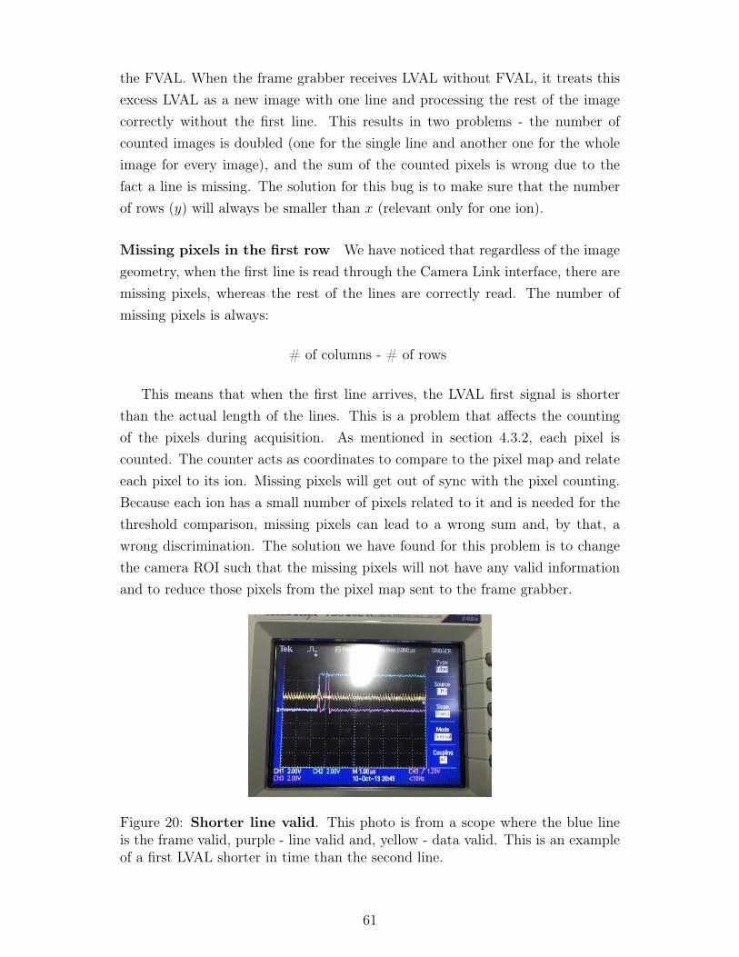
the FVAL. When the frame grabber receives LVAL without FVAL, it treats thisexcess LVAL as a new image with one line and processing the rest of the imagecorrectly without the first line. This results in two problems - the number ofcounted images is doubled (one for the single line and another one for the wholeimage for every image), and the sum of the counted pixels is wrong due to thefact a line is missing. The solution for this bug is to make sure that the numberof rows (y) will always be smaller than x (relevant only for one ion).

Missing pixels in the first row We have noticed that regardless of the imagegeometry, when the first line is read through the Camera Link interface, there aremissing pixels, whereas the rest of the lines are correctly read. The number ofmissing pixels is always:

# of columns - # of rows

This means that when the first line arrives, the LVAL first signal is shorterthan the actual length of the lines. This is a problem that affects the countingof the pixels during acquisition. As mentioned in section 4.3.2, each pixel iscounted. The counter acts as coordinates to compare to the pixel map and relateeach pixel to its ion. Missing pixels will get out of sync with the pixel counting.Because each ion has a small number of pixels related to it and is needed for thethreshold comparison, missing pixels can lead to a wrong sum and, by that, awrong discrimination. The solution we have found for this problem is to changethe camera ROI such that the missing pixels will not have any valid informationand to reduce those pixels from the pixel map sent to the frame grabber.

Figure 20: Shorter line valid. This photo is from a scope where the blue lineis the frame valid, purple - line valid and, yellow - data valid. This is an exampleof a first LVAL shorter in time than the second line.

61

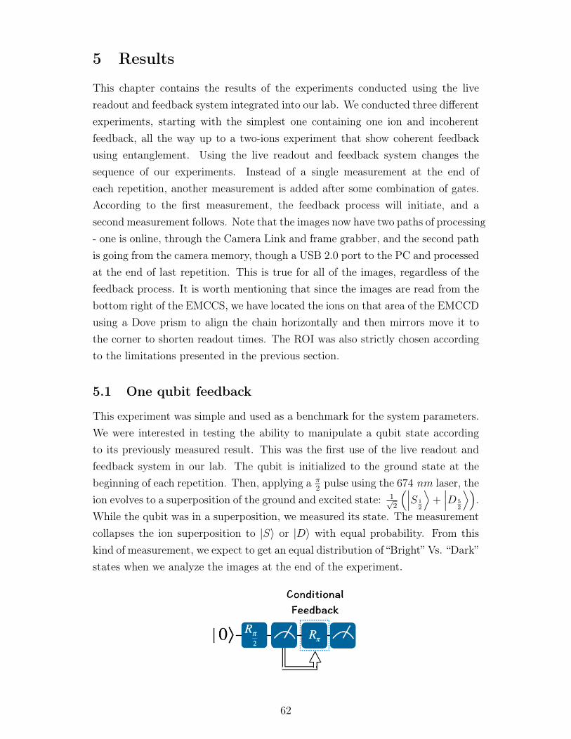
5 Results

This chapter contains the results of the experiments conducted using the livereadout and feedback system integrated into our lab. We conducted three differentexperiments, starting with the simplest one containing one ion and incoherentfeedback, all the way up to a two-ions experiment that show coherent feedbackusing entanglement. Using the live readout and feedback system changes thesequence of our experiments. Instead of a single measurement at the end ofeach repetition, another measurement is added after some combination of gates.According to the first measurement, the feedback process will initiate, and asecond measurement follows. Note that the images now have two paths of processing- one is online, through the Camera Link and frame grabber, and the second pathis going from the camera memory, though a USB 2.0 port to the PC and processedat the end of last repetition. This is true for all of the images, regardless of thefeedback process. It is worth mentioning that since the images are read from thebottom right of the EMCCS, we have located the ions on that area of the EMCCDusing a Dove prism to align the chain horizontally and then mirrors move it tothe corner to shorten readout times. The ROI was also strictly chosen accordingto the limitations presented in the previous section.

5.1 One qubit feedback

This experiment was simple and used as a benchmark for the system parameters.We were interested in testing the ability to manipulate a qubit state accordingto its previously measured result. This was the first use of the live readout andfeedback system in our lab. The qubit is initialized to the ground state at thebeginning of each repetition. Then, applying a ⇡

2

pulse using the 674 nm laser, theion evolves to a superposition of the ground and excited state: 1p

2

⇣���S 12

E+

���D 52

E⌘.

While the qubit was in a superposition, we measured its state. The measurementcollapses the ion superposition to |Si or |Di with equal probability. From thiskind of measurement, we expect to get an equal distribution of “Bright” Vs. “Dark”states when we analyze the images at the end of the experiment.

62

Figure 21: Quantum circuit diagram representing the experimentalsequence. Using these diagrams is very common and useful. In the quantumcircuit representation, each line is an ion. An operator is visualized as a squareon the ion\s and a measurement as a meter. In this experiment, the ion isinitialized to the ground state - |0i and was measured twice: the first measurementis performed after a ⇡

2

rotation around the x axis, when the qubit is in asuperposition. The second measurement is taken after the feedback - a ⇡ pulsethat is only applied if the qubit was detected in the dark state (|Di) in the firstmeasurement.

After the qubit is measured, and the image was analyzed using the live readoutsystem, feedback can be implemented. If the first measurement outcome is ”dark”,a ⇡ pulse is applied that takes the population form ”dark” to ”bright” (This isan arbitrary choice of states, the opposite experiment is possible as well). Theexpected results of the 2nd measurement (if the live feedback system is working)will be a distribution of only "bright" states.

Figure 22: One-qubit experiment results. Each experiment contained twomeasurements, and in total 500 repetitions (1000 images). At each sequence,the first measurement gives the input for the feedback. Whereas the secondmeasurement is taken in order to analyze the results and test the feedbackperformance. Figure 21 describes the experimental sequence. Left: Thefirst measurement fluorescence count distribution in arbitrary units. Themeasurements are distributed between the dark state (low fluorescence) and thebright state (high fluorescence) almost equally as expected, given the fact that a⇡2

pulse was operated before the measurement putting the ion in a superposition:|Si+|Dip

2

.

63

The solid red line represents the threshold set in the calibration stage beforethe experiment. Right: fluorescence count of the second measurement in eachrepetition. As expected after a conditioned ⇡ pulse, the qubits’ final state isalways bright, although the initial state of the qubit after the measurement canbe bright or dark. According to this result, the fidelity of the entire process is0.986 ± 0.04% (this includes ⇡ pulse errors, and detection errors form both theframe grabber and Matlab).

5.2 Two-qubit feedback

Moving from one to two qubits increases the complexity of the experiment andallows us to test more exotic properties of the system, such as coherence, entanglement,and parity. The experiments relied mostly on Ramsey spectroscopy: in a Ramseyexperiment, the state is initialized to | ii =

���S 12

E, followed by a ⇡

2

pulse thatrotates our qubit into

| t=0

i = 1p2

⇣���S 12

E+ e�i�0

���D 52

E⌘

Where �0

can be set to zero. The qubit performs precession in the rotating frameduring time evolution at a frequency equals to the detuning, making the phasedifference between the superposition states evolves at �(t), thus the state of thequbit would be

| ti =1p2

���S 12

E+ e

�i⌧R

0�(t)dt ���D 5

2

E!

Finally, a second ⇡2

pulse is applied while scanning the pulse phase and measuringthe qubit state. By scanning the phase of the pulse, we measure the direction ofthe Bloch vector in the equator plane of the Bloch sphere which results in

| fi = cos

0

BB@

�f +�i⌧R0

�(t)dt

2

1

CCA |Si+ sin

0

BB@

�f +�i⌧R0

�(t)dt

2

1

CCA ei�f |Di

From here, the probability of measuring a “dark” state will be:

P (|Di) = |hD| fi|2 = sin2

0

BB@

�f +�i⌧R0

�(t)dt

2

1

CCA

Scanning the phase will outcome a Ramsey fringe. Note that � (t) can be randomas a result of frequency noise.

64

Another technique that we have used during the two-qubits experiments isselective readout of the qubits - placing one of the qubits "in hiding". This meansthat one of the qubits’ superposition is coded in levels that are not affected duringthe detection, and by that, the information of that qubit remains protected.In our case, this superposition is coded on the 4D 5

2manifold using the ±3

2

Zeeman splitting of the level 1p2

⇣���D 52 ,�

32

E+

���D 52 ,

32

E⌘. The qubit that is put

in hiding is the one we are interested in ”protecting” - keeping its quantum state.The unprotected qubit remains in the 1p

2

⇣���S 12 ,

12

E+

���D 52 ,

32

E⌘superposition. The

sequence of selective readout starts after the qubits are in a superposition. Then,a global RF ⇡ pulse changes the population in the

���S 12 ,

12

Estate to

���S 12 ,�

12

E. This

pulse is followed by an individual addressing (IA) ⇡ pulse of the 674 nm laser(consists of a global ⇡

2

pulse with frequency corresponds to the���S 1

2 ,�12

E!���D 5

20� 3

2

E

transition, an AC stark shift pulse which is far detuned, and another global ⇡2

pulse [25]) only on the qubit we are protecting. At the end of the sequence,a global RF ⇡ pulse with the opposite phase puts back the unhidden ion in���S 1

2 ,12

Estate. After this pulse sequence, the qubits are in 1p

2

⇣���S 12 ,

12

E+

���D 52 ,

32

E⌘⌦

1p2

⇣���D 52 ,�

32

E+

���D 52 ,

32

E⌘state. In this state, the protected qubit will not be

affected during the detection time because the |Di manifold does not couple tothe 422 nm laser. During the measurement time, the hidden qubit can suffer fromdephasing due to fluctuating magnetic fields. To mitigate this effect, we added anRF ⇡ pulses at specific times on the hidden qubit during the measurement time(which contains the exposure time and the readout time) . This is a generalizationof the well known Hahn echo (for more details see [53]).

5.2.1 Coherent feedback

This experiment shows the ability to coherently control the qubits in a generalsuperposition. We have applied the experiment as a conditioned Ramsey scanwith adjustments: measuring one of the qubits followed by a conditioned operationdone on the second qubit according to the outcome of the first measurement.

The qubits are initialized to a superposition with a global ⇡2

pulse rotatingthem to the state:

|Si1

⌦ |Si2

! 1

2

(|SSi+ |DDi+ |DSi+ |DDi)

In order to enable the feedback process afterward, we want to measure only oneof the qubits and, by that, keep information regarding the superposition. This isdone by ”hiding” the second qubit in the D manifold, which is not affected by themeasurement.

65

After one of the qubits is in hiding, we measure the state of the other qubit,while during this time, four echo pulses on the hidden qubit are performed (twoduring the exposure time (700 µs) and two during the readout time (600 µs)). Themeasurement will collapse the first qubit to one of the states - |Si or |Di, while thesecond qubit remains hidden and in a superposition. After the measurement, weuse the same technique to unhide the 2nd qubit in a reverse order of operations,mapping it back to the 1p

2

(|Si+ |Di) superposition. The unhiding is followedby a conditioned ⇡

2

pulse on the second qubit (the one that we did not measure):if the measurement result is a ”bright” state (the first qubit is in the |Si level),an IA ⇡

2

pulse with scanned phase ' will follow. Whereas if a ”dark” state wasmeasured, the same IA ⇡

2

pulse is applied but with a '+⇡ phase. A measurementof the qubits will follow both options. If the qubits remain coherent during themeasurement, meaning we will still have a defined phase between the |Si+ei' |Distate and the laser, we can expect to see a Ramsey fringe. By projecting the stateon one of the outcomes of the first measurement, we can calculate the expectedoutcome of this measurement for a bright state

hS1

| i =���hS

1

|⇣i⇡

4

(1⌦ (cos (�) �x + i sin (�) �y)) |S1

S2

i+ |S1

D2

i⌘���

2

=

����1

2

+

1

2

i (cos (�) + i sin (�))

����2

Dark population = 1�����1

2

+

1

2

i (cos (�) + i sin (�))

����2

=

1

2

(1� sin (�))

(When we analyze our result we look at the dark counts thus the calculation isdone for the dark population explaining the use of 1� |h | i|2). The calculationfor measuring |Di on the first ion:

hD1

| i =���hD

1

|⇣i⇡

4

(1⌦ (cos (�+ ⇡) �x + i sin (�+ ⇡) �y)) |D1

S2

i+ |D1

D2

i⌘���

2

=

����1

2

� 1

2

i (cos (�) + i sin (�))

����2

=

1

2

(1 + sin (�))

From these results, we can expect that if the conditioned operation works properly,the measurements will yield two Ramsey fringes with the opposite phase, with an

66

even 1p2

(|SSi+ |DDi) or odd 1p2

(|SDi+ |DSi) parity.

Figure 23: Circuit representation of the experimental sequence. (a) fullexperimental sequence after the initialization of the qubits. For example, R⇡

2 ,⇡

represents a 674 nm ⇡2

pulse with phase ⇡. The double-lined arrow representsclassical information. (b) image shows the RF pulse sequence when applyingecho pulses on the second qubit during the first qubit’s measurement. ⌧ and ⌧represent the time between each pulse and is calculated as t

2·N where t is theexposure time or readout time, and N is the number of desired echo pulses. (c)Detailed individual addressing (IA) pulse. IA ⇡ pulse contains two global ⇡

2

pulseswith the same phase and in between an AC stark shift pulse to reduce crosstalkbetween the qubits (for more details see [25]).

67

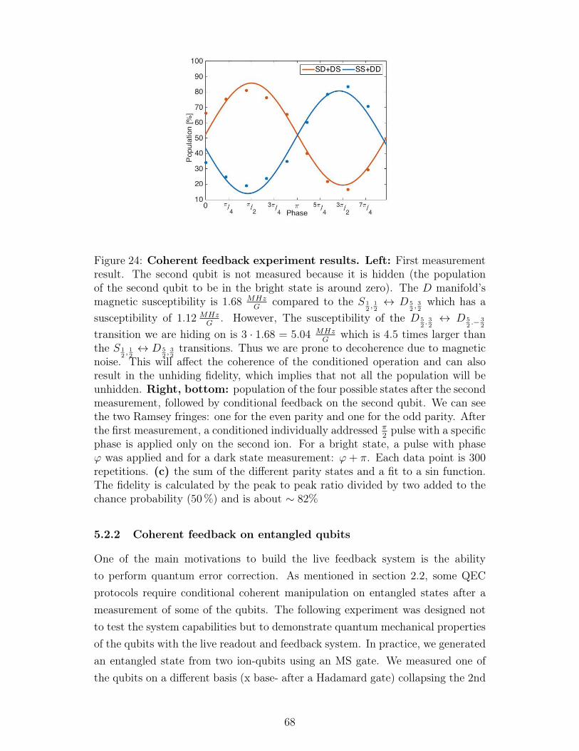
Figure 24: Coherent feedback experiment results. Left: First measurementresult. The second qubit is not measured because it is hidden (the populationof the second qubit to be in the bright state is around zero). The D manifold’smagnetic susceptibility is 1.68 MHz

Gcompared to the S 1

2 ,12$ D 5

2 ,32

which has asusceptibility of 1.12 MHz

G. However, The susceptibility of the D 5

2 .32$ D 5

2 .�32

transition we are hiding on is 3 · 1.68 = 5.04 MHzG

which is 4.5 times larger thanthe S 1

2 ,12$ D 5

2 ,32

transitions. Thus we are prone to decoherence due to magneticnoise. This will affect the coherence of the conditioned operation and can alsoresult in the unhiding fidelity, which implies that not all the population will beunhidden. Right, bottom: population of the four possible states after the secondmeasurement, followed by conditional feedback on the second qubit. We can seethe two Ramsey fringes: one for the even parity and one for the odd parity. Afterthe first measurement, a conditioned individually addressed ⇡

2

pulse with a specificphase is applied only on the second ion. For a bright state, a pulse with phase' was applied and for a dark state measurement: ' + ⇡. Each data point is 300repetitions. (c) the sum of the different parity states and a fit to a sin function.The fidelity is calculated by the peak to peak ratio divided by two added to thechance probability (50%) and is about ⇠ 82%

5.2.2 Coherent feedback on entangled qubits

One of the main motivations to build the live feedback system is the abilityto perform quantum error correction. As mentioned in section 2.2, some QECprotocols require conditional coherent manipulation on entangled states after ameasurement of some of the qubits. The following experiment was designed notto test the system capabilities but to demonstrate quantum mechanical propertiesof the qubits with the live readout and feedback system. In practice, we generatedan entangled state from two ion-qubits using an MS gate. We measured one ofthe qubits on a different basis (x base- after a Hadamard gate) collapsing the 2nd

68

qubit on the x basis, thus protecting its superposition. The results are interpretedas Ramsey interference.

The qubits are initially Doppler cooled, and optically pumped to a chosenZeeman sub-level of the 5S 1

2manifold. They are then cooled to the radial and

axial ground state using EIT cooling, and resolved sideband cooling that generatesa n < 1 state. After initialization, the entangled state |SSi+ei'|DDip

2

is preparedfrom the two qubits using an MS gate (gate fidelity of 97%). Next, we operatedwith a Hadamard gate only on one of the qubits (for example, qubit #1) usingindividual addressing that allows us to operate on each of the qubits separatelyand not just with a global beam [25]. The Hadamard gate is implemented as a⇡/2 pulse around the x-axis. After this operation, the state of the qubits will be:

(|Si+ |Di)1

|Si2

+ (|Si � |Di)1

|Di2

.

Following the Hadamard gate, we protected the second qubit state by performing ahiding sequence (as described in 5.2) followed by a measurement of the first qubit.During the measurement, we applied four echo pulses on the hidden qubit: two RF⇡ pulses with opposite phase during the exposure time (700µs), and another twoduring the readout time (600µs). The echo pulse sequence is described in figure23 (c). The magnetic susceptibility of the D manifold where the qubit is in hidingis large, and without the echo pulses, the state completely decohere. Figure 26left, shows the results from the first measurement. Since the qubits are entangled,and the first qubit was measured in the x basis (after applying the Hadamardgate) the second qubit will collapse to one of the following superpositions also inthe x basis:

(I) |Si1

�|Si+ ei' |Di

�2

(II) |Di1

�|Si � ei' |Di

�2

The phase is scanned as part of a conventional Ramsey experiment, meaning thatgiven the measurement result of qubit #1, a global ⇡

2

pulse is applied with a phasethat is different between the two states. We measure the state of both qubits againand expect to get a 50 � 50 population distribution of qubit #1 and a Ramseyfringe for qubit #2. After operating with a global ⇡

2

pulse, the second qubit stateis

ei⇡

4 (cos(')�x

+i sin(')�y

)

(|Si+ |Di)

Projecting this state on the dark state and calculating the population:

69

|hD| i|2 =��hD| ei⇡4 (cos(')�x

+i sin(')�y

)

(|Si+ |Di)��2

=

���hD| cos⇣⇡4

⌘+ i sin

⇣⇡4

⌘(cos (') �x + i sin (') �y) (|Si+ |Di)

���2

=

1

2

(1� sin ('))

doing the same with '+ ⇡ phase:

|hD| i|2 =��hD| ei⇡4 (cos('+⇡)�

x

+i sin('+⇡)�y

)

(|Si � |Di)��2

=

���hD| cos⇣⇡4

⌘+ i sin

⇣⇡4

⌘(cos ('+ ⇡) �x + i sin ('+ ⇡) �y) (|Si � |Di)

���2

=

1

2

(1� sin (�))

We can see from this calculation that for the second qubit, we expect to get afringe that will behave as a regular Ramsey fringe: a sine function with a 2⇡

periodicity. Figure 25 represents the experimental sequence and figure 26 theresults.

Figure 25: Circuit drawing of the experimental sequence.

70

(a)

Figure 26: Coherent feedback performed on entangled qubits. Left:measurement after hiding qubit #2. Right: qubit #1 is the measured qubitand after the measurement collapses to one of both states - |Si or |Di. Afterdetecting this state, a conditioned ⇡

2

pulse was applied with a phase ' or ' + ⇡according to the state. Qubit #2 is the hidden qubit and is measured only duringthe second measurement. After the second measurement, if the second ion ismeasured in the bright state - |Si (or a dark state |Di), the first ion is projectedonto 1p

2

(|Si+ |Di). This is due to the conditioned ⇡2

global pulse, thus qubit #1will be found in an equal superposition. Qubit #2, on the other hand, shows aRamsey fringe with a contrast of 70 (meaning the process’s fidelity 85%). Thefidelity is affected mainly during the time that the second qubit spends in the|Di manifold, where it can decohere due to magnetic noise. Bottom: Sumof the results for each qubit, where the y-axis represents the qubits’ dark statepopulation in percentages. We can see the Ramsey fringe of the second qubit,whereas the first qubit population is close to 50%. When no feedback is applied,we get an expected constant behavior around 50% for both qubits. Each datapoint represents the average of 300 repetitions, with 50 Hz trigger and 4 echopulses on the hidden ion during the measurement.

71

6 Summary

This work presents the integration of a new classical control system into our labthat allows us to access the ions measurement outcome in real-time, analyzes theimage data on the fly, determines the state of the ions followed by an adaptivefeedback scheme that is pre-programmed. This scheme allowed us to coherentlycontrol the ions and perform conditional experiments with a fidelity of around⇠ 82%. Prior to the building and integration of the live readout system, theprocessing of the images was limited to the end of the experiment. The ability tocoherently and conditionally control trapped ions is advancing our lab one stepcloser to performing quantum error correction protocols and to a fault-tolerantquantum computer. Although some improvements are required, the demonstrationof quantum feedback is an important milestone. Quantum error correction protocolsusually require the ability to act on a qubit according to the syndrome measurementoutcome of the auxiliary qubit within a time scale much shorter than the coherencetime of the qubits. We have demonstrated this kind of operation with twoentangled ions, where we have measured one ion that collapsed the second ion to asuperposition without losing its coherence - shown as a Ramsey fringe. Quantumerror correction is not the only QIP experiment that can enjoy the benefits ofhaving the ability to perform live feedback. Some ideas to preform experimentssuggested in 6.2.

6.1 Improvements

The system is not perfect, and in order to perform complicated and long algorithms,the quantum feedback needs to be robust and fast. During this work, we haveencountered a few major bottlenecks that affected our ability to perform very highfidelity live readout and feedback. The most significant ones are the exposure andreadout time - they are very long compared to our coherence time. Two significantphysical properties limit the exposure time: the first is the numerical aperture,which eventually sets the number of photons collected for each unit of time. Thesecond is the camera limitations such as dark current and shot noise. The solutionfor both of these problems is possible but complicated and will require a majorupgrade in the lab imaging set up (get a bigger objective lens or\and change thecamera). Another bottleneck is the readout time. Using our EMCCD camera -Andor iXon ultra 879, our readout time is limited due to the size of the CCDand the fact that the technology is a frame transfer technology. This fact putsa lower bound on the readout time at hundreds of microseconds for a minimal

72

number of rows required for the ion detection. The readout time will always bea limiting factor and can be reduced using binning, smaller ROI, or a differentEMCCD camera with a faster vertical shift rate and maybe a smaller CCD. Onemajor improvement will be increasing our coherence time by, e.g., mu-metal shieldplaced around the ion trap. Another upgrade to be done regarding the connectionsof the hardware, there is a need for a robust ”black box” hardware that will containall of the FPGA cards, cables connecting them, and RF source control.

6.2 Outlook

Live feedback can be used for more than just quantum error correction codes thatsometimes require a large number of ions, or complicated and long codes thatare hard to execute due to decoherence and noise, but also for some more exoticexperiments, that some of them are listed below.

Ramsey teleportation Quantum teleportation is the complete transfer of informationfrom one particle to another (or from Alice to Bob). Generally, this processrequires an infinite amount of information even to transfer a "simple" systemsuch as one qubit. In quantum mechanics, a measurement immediately altersthe state of the system while yielding at most one bit of information. At facevalue, teleportation seems to be impossible given these facts, but using quantumentanglement combined with classical communication, the idea of teleportinginformation came to life [54]. Three ions are needed to perform teleportation.Two of them prepared in a maximally entangled state: Alice and Bob each haveone of the pair particles. Alice possesses the third qubit (can be treated asthe auxiliary qubit), and both of Alice’s qubits are entangled. Measuring theauxiliary qubit in a Bell state basis will leave Bob with one of four possibleoutcomes. Transferring Alice’s measurement information (classically) to Bob,will allow him to reconstruct his state entirely, and by that, the teleportationwill be completed. With trapped ions, quantum teleportation has been shown inseveral experiments, such as [55, 56]. In both of these experiments, publishedback-to-cack, deterministic teleportation was demonstrated for the first time.Quantum gate teleportation was also shown in [57]. Another quantity that canbe teleported is the qubits accumulated phase due to the presence of a magneticfield. The teleportation experiment will be as a regular teleportation sequencejust that the transported information will be about the phase. The operation tocomplete the teleportation will be the correcting of the phase, and a measurementin Bob’s side after performing the correct gate with a phase scan that will result

73

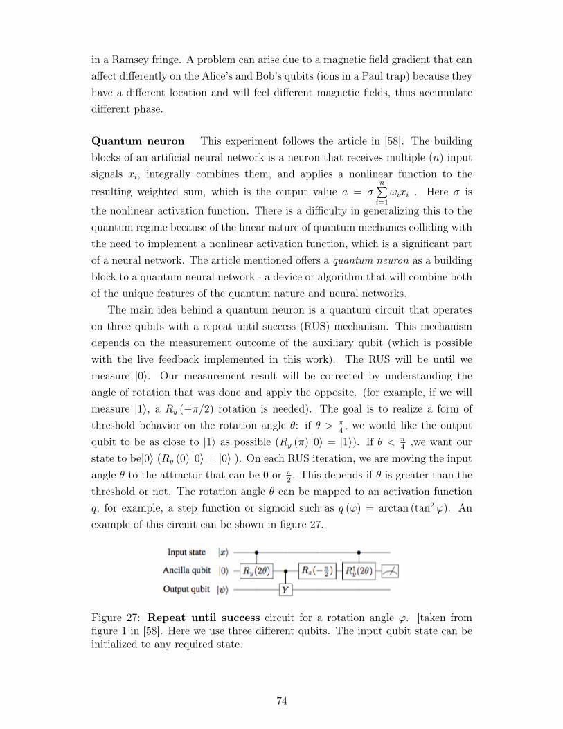
in a Ramsey fringe. A problem can arise due to a magnetic field gradient that canaffect differently on the Alice’s and Bob’s qubits (ions in a Paul trap) because theyhave a different location and will feel different magnetic fields, thus accumulatedifferent phase.

Quantum neuron This experiment follows the article in [58]. The buildingblocks of an artificial neural network is a neuron that receives multiple (n) inputsignals xi, integrally combines them, and applies a nonlinear function to theresulting weighted sum, which is the output value a = �

nPi=1

!ixi . Here � is

the nonlinear activation function. There is a difficulty in generalizing this to thequantum regime because of the linear nature of quantum mechanics colliding withthe need to implement a nonlinear activation function, which is a significant partof a neural network. The article mentioned offers a quantum neuron as a buildingblock to a quantum neural network - a device or algorithm that will combine bothof the unique features of the quantum nature and neural networks.

The main idea behind a quantum neuron is a quantum circuit that operateson three qubits with a repeat until success (RUS) mechanism. This mechanismdepends on the measurement outcome of the auxiliary qubit (which is possiblewith the live feedback implemented in this work). The RUS will be until wemeasure |0i. Our measurement result will be corrected by understanding theangle of rotation that was done and apply the opposite. (for example, if we willmeasure |1i, a Ry (�⇡/2) rotation is needed). The goal is to realize a form ofthreshold behavior on the rotation angle ✓: if ✓ > ⇡

4

, we would like the outputqubit to be as close to |1i as possible (Ry (⇡) |0i = |1i). If ✓ < ⇡

4

,we want ourstate to be|0i (Ry (0) |0i = |0i ). On each RUS iteration, we are moving the inputangle ✓ to the attractor that can be 0 or ⇡

2

. This depends if ✓ is greater than thethreshold or not. The rotation angle ✓ can be mapped to an activation functionq, for example, a step function or sigmoid such as q (') = arctan (tan

2 '). Anexample of this circuit can be shown in figure 27.

Figure 27: Repeat until success circuit for a rotation angle '. [taken fromfigure 1 in [58]. Here we use three different qubits. The input qubit state can beinitialized to any required state.

74

Shor’s three qubit repetition code This experiment was done in trappedions in [15]. The three-qubit Shor’s repetition code is a quantum error correctioncode that can correct one error. It can be done using an induced error and acorrection scheme where the measurement is at the end of each repetition. Usingmeasurement, and the live feedback system the following scheme can conduct thisexperiment: encode a logic qubit into a subspace that is spanned by {|000i , |111i}(encoding the information as ↵ |000i + � |111i). An error process will map thesub-space where the encoded information is, to an orthogonal subspace (that keepsthe orthogonality of the previous subspace such as {|100i , |011i}) for each errorthus not distorting the quantum information. Knowing which subspace the systemis, will enable the correction of the error by applying the revers error operation.This process can be also done to a linear combination of the subspace above (e.g.1p2

(|000i+ |111i) and 1p2

(|000i � |111i) ) making it possible to correct phase fliperrors.

75

References

[1] Peter W. Shor. Polynomial-time algorithms for prime factorization anddiscrete logarithms on a quantum computer. SIAM Journal on Computing,26(5):1484–1509, 1997. arXiv:9508027, doi:10.1137/S0097539795293172.

[2] David P. DiVincenzo. The physical implementation of quantum computation.Fortschritte der Physik, 48(9-11):771–783, 2000. arXiv:0002077, doi:10.1002/1521-3978(200009)48:9/11<771::AID-PROP771>3.0.CO;2-E.

[3] D J Wineland, C Monroe, W M Itano, D Leibfried, B E King, and D MMeekhof. Experimental Issues in Coherent Quantum-State Manipulationof Trapped Atomic Ions. Journal of Research of the National Institute ofStandards and Technology, 103(3):259–328, 1998. URL: http://www.nist.gov/jres, arXiv:9710025, doi:10.6028/jres.103.019.

[4] J. I. Cirac and P. Zoller. Quantum computations with cold trappedions. Physical Review Letters, 74(20):4091–4094, 1995. doi:10.1103/

PhysRevLett.74.4091.

[5] D. J. Wineland and Wayne M. Itano. Laser cooling of atoms. Physical ReviewA, 20(4):1521–1540, 1979. doi:10.1103/PhysRevA.20.1521.

[6] Dorit Aharonov and Michael Ben-Or. Fault-tolerant quantum computationwith constant overhead. Quantum Information and Computation,14(15-16):1338–1372, 2014. arXiv:1310.2984.

[7] Frank Arute, Kunal Arya, Ryan Babbush, Dave Bacon, Joseph C. Bardin,Rami Barends, Rupak Biswas, Sergio Boixo, Fernando G.S.L. Brandao,David A. Buell, Brian Burkett, Yu Chen, Zijun Chen, Ben Chiaro, RobertoCollins, William Courtney, Andrew Dunsworth, Edward Farhi, BrooksFoxen, Austin Fowler, Craig Gidney, Marissa Giustina, Rob Graff, KeithGuerin, Steve Habegger, Matthew P. Harrigan, Michael J. Hartmann, AlanHo, Markus Hoffmann, Trent Huang, Travis S. Humble, Sergei V. Isakov,Evan Jeffrey, Zhang Jiang, Dvir Kafri, Kostyantyn Kechedzhi, Julian Kelly,Paul V. Klimov, Sergey Knysh, Alexander Korotkov, Fedor Kostritsa, DavidLandhuis, Mike Lindmark, Erik Lucero, Dmitry Lyakh, Salvatore Mandrà,Jarrod R. McClean, Matthew McEwen, Anthony Megrant, Xiao Mi, KristelMichielsen, Masoud Mohseni, Josh Mutus, Ofer Naaman, Matthew Neeley,Charles Neill, Murphy Yuezhen Niu, Eric Ostby, Andre Petukhov, John C.Platt, Chris Quintana, Eleanor G. Rieffel, Pedram Roushan, Nicholas C.

76

Rubin, Daniel Sank, Kevin J. Satzinger, Vadim Smelyanskiy, Kevin J.Sung, Matthew D. Trevithick, Amit Vainsencher, Benjamin Villalonga,Theodore White, Z. Jamie Yao, Ping Yeh, Adam Zalcman, HartmutNeven, and John M. Martinis. Quantum supremacy using a programmablesuperconducting processor. Nature, 574(7779):505–510, oct 2019. arXiv:

1911.00577, doi:10.1038/s41586-019-1666-5.

[8] Daniel Gottesman. Fault-Tolerant Quantum Computation. 2007.

[9] D. Nigg, M. Müller, E. A. Martinez, P. Schindler, M. Hennrich, T. Monz,M. A. Martin-Delgado, and R. Blatt. Quantum computations on atopologically encoded qubit. Science, 345(6194):302–305, 2014. arXiv:

1403.5426v1, doi:10.1126/science.1253742.

[10] Philipp Schindler, Julio T. Barreiro, Thomas Monz, VolckmarNebendahl, Daniel Nigg, Michael Chwalla, Markus Hennrich, and RainerBlatt. Experimental repetitive quantum error correction. Science,332(6033):1059–1061, may 2011. doi:10.1126/science.1203329.

[11] Philipp Schindler, Daniel Nigg, Thomas Monz, Julio T. Barreiro, EstebanMartinez, Shannon X. Wang, Stephan Quint, Matthias F. Brandl, VolckmarNebendahl, Christian F. Roos, Michael Chwalla, Markus Hennrich, andRainer Blatt. A quantum information processor with trapped ions. NewJournal of Physics, 15, 2013. arXiv:1308.3096, doi:10.1088/1367-2630/15/12/123012.

[12] H. Bernien, B. Hensen, W. Pfaff, G. Koolstra, M. S. Blok, L. Robledo,T. H. Taminiau, M. Markham, D. J. Twitchen, L. Childress, and R. Hanson.Heralded entanglement between solid-state qubits separated by three metres.Nature, 497(7447):86–90, apr 2013. arXiv:1212.6136, doi:10.1038/

nature12016.

[13] D. G Cory, Price M.D., W. Maas, E. Knill, R. Laflamm, W. H. Zurek,T. F. Havel, and S. S. Somaroo. Experimental quantum error correction.Quantum Error Correction, 9780521897:508–518, 2012. URL: https://

www.cambridge.org/core/product/identifier/CBO9781139034807A173/

type/book{_}part, doi:10.1017/CBO9781139034807.023.

[14] E. Knill, R. Laflamm, A. Ashikhmin, H. Barnum, L. Viola, and W. H.Zurek. Introduction to quantum error correction. Quantum Error Correction,9780521897:46–77, 2012. doi:10.1017/CBO9781139034807.004.

77

[15] J Chiaverini, D Leibfried, T Schaetz, M D Barrett, R B Blakestad, J Britton,W M Itano, J D Jost, E Knill, C Langer, R Ozeri, and D J Wineland.Realization of quantum error correction. Nature, 432(7017):602–605, 2004.URL: www.nature.com/nature, doi:10.1038/nature03074.

[16] Norbert M. Linke, Mauricio Gutierrez, Kevin A. Landsman, CarolineFiggatt, Shantanu Debnath, Kenneth R. Brown, and Christopher Monroe.Fault-tolerant quantum error detection. Science Advances, 3(10), 2017.URL: http://advances.sciencemag.org/, arXiv:1611.06946, doi:10.

1126/sciadv.1701074.

[17] Daniel Gottesman. Quantum fault tolerance in small experiments. oct 2016.URL: http://arxiv.org/abs/1610.03507, arXiv:1610.03507.

[18] Daniel Gottesman. An introduction to quantum error correction andfault-tolerant quantum computation. pages 13–58, apr 2010. URL: http://arxiv.org/abs/0904.2557, arXiv:0904.2557, doi:10.1090/psapm/068/

2762145.

[19] N. Akerman, S. Kotler, Y. Glickman, and R. Ozeri. Reversal ofphoton-scattering errors in atomic qubits. Physical Review Letters, 109(10),sep 2012. arXiv:1111.1622, doi:10.1103/PhysRevLett.109.103601.

[20] M. Riebe, T. Monz, K. Kim, A. S. Villar, P. Schindler, M. Chwalla,M. Hennrich, and R. Blatt. Deterministic entanglement swapping with anion-trap quantum computer. Nature Physics, 4(11):839–842, 2008. doi:

10.1038/nphys1107.

[21] V. Negnevitsky, M. Marinelli, K. K. Mehta, H. Y. Lo, C. Flühmann, and J. P.Home. Repeated multi-qubit readout and feedback with a mixed-speciestrapped-ion register. Nature, 563(7732):527–531, nov 2018. arXiv:1804.

09703, doi:10.1038/s41586-018-0668-z.

[22] D B Hume, T Rosenband, and D J Wineland. High-fidelity adaptive qubitdetection through repetitive quantum nondemolition measurements. PhysicalReview Letters, 99(12), 2007. doi:10.1103/PhysRevLett.99.120502.

[23] J. Cramer, N. Kalb, M. A. Rol, B. Hensen, M. S. Blok, M. Markham,D. J. Twitchen, R. Hanson, and T. H. Taminiau. Repeated quantum errorcorrection on a continuously encoded qubit by real-time feedback. NatureCommunications, 7, may 2016. URL: http://arxiv.org/abs/1912.09410,arXiv:1508.01388, doi:10.1038/ncomms11526.

78

[24] Adriano Barenco, Charles H Bennett, Richard Cleve, David P Divincenzo,Norman Margolus, Peter Shor, Tycho Sleator, John A. Smolin, and HaraldWeinfurter. Elementary gates for quantum computation. Physical Review A,52(5):3457–3467, 1995. arXiv:9503016, doi:10.1103/PhysRevA.52.3457.

[25] Tom Manovitz. Individual Addressing and imaging of ions in a paul trap.PhD thesis, 2016.

[26] Roee Ozeri. The trapped-ion qubit tool box. Contemporary Physics,52(6):531–550, nov 2011. doi:10.1080/00107514.2011.603578.

[27] Anders Sørensen and Klaus Mølmer. Entanglement and quantumcomputation with ions in thermal motion. Physical Review A - Atomic,Molecular, and Optical Physics, 62(2):11, 2000. arXiv:0002024, doi:

10.1103/PhysRevA.62.022311.

[28] Yotam Shapira. Robust entanglement of trapped ion qubits. PhD thesis, 2017.

[29] Yotam Shapira, Ravid Shaniv, Tom Manovitz, Nitzan Akerman, and RoeeOzeri. Robust Entanglement Gates for Trapped-Ion Qubits. PhysicalReview Letters, 121(18), may 2018. URL: http://arxiv.org/abs/

1805.06806http://dx.doi.org/10.1103/PhysRevLett.121.180502,arXiv:1805.06806, doi:10.1103/PhysRevLett.121.180502.

[30] Nitzan Akerman. Trapped ions and free photons. PhD thesis, 2012.

[31] Ravid Shaniv. Spectral noise analysis of a narrow linewidth laser. PhD thesis,2015.

[32] Anna Keselman. High Fidelity Ion Qubit State Detection. PhD thesis, 2010.

[33] Regina Lechner, Christine Maier, Cornelius Hempel, Petar Jurcevic,Ben P. Lanyon, Thomas Monz, Michael Brownnutt, Rainer Blatt, andChristian F. Roos. Electromagnetically-induced-transparency ground-statecooling of long ion strings. Physical Review A, 93(5), 2016.URL: http://arxiv.org/abs/1603.05568{%}0Ahttp://dx.doi.org/10.

1103/PhysRevA.93.053401, arXiv:1603.05568, doi:10.1103/PhysRevA.

93.053401.

[34] J. Eschner, C. Keitel, and G. Morigi. Laser cooling using electromagneticallyinduced transparency. Conference on Quantum Electronics and Laser Science(QELS) - Technical Digest Series, pages 63–64, 2000.

79

[35] C S. Roos, D Leibfried, A Mundt, F Schmidt-Kaler, J Eschner, andR Blatt. Experimental Demonstration of Ground State Laser Coolingwith Electromagnetically Induced Transparency. Physical Review Letters,85(26):5547–5550, 2000. doi:10.1103/PhysRevLett.85.5547.

[36] D. J. Wineland and H. G. Dehmelt. Principles of the stored ion calorimeter.Journal of Applied Physics, 46(2):919–930, 1975. URL: https://doi.org/10.1063/1.321602, doi:10.1063/1.321602.

[37] Andor Technology. iXon Ultra Hardware Guide. Technical report, 2013.

[38] E2v. CCD97-00 Back Illuminated 2-Phase IMO Series Electron MultiplyingCCD Sensor. Technical report. URL: www.e2vtechnologies.com.

[39] Robert N. Tubbs. Lucky Exposures: Diffraction limited astronomical imagingthrough the atmosphere. (September), 2003. URL: http://arxiv.org/abs/astro-ph/0311481, arXiv:0311481.

[40] A. G. Basden, C. A. Haniff, and C. D. Mackay. Photon counting strategieswith low-light-level CCDs. Monthly Notices of the Royal AstronomicalSociety, 345(3):985–991, 2003. arXiv:0307305, doi:10.1046/j.1365-8711.2003.07020.x.

[41] Alice Heather Burrell. High Fidelity Readout of Trapped Ion Qubits. PhDthesis, 2010.

[42] Michael Hirsch, Richard J. Wareham, Marisa L. Martin-Fernandez,Michael P. Hobson, and Daniel J. Rolfe. A Stochastic Model for ElectronMultiplication Charge-Coupled Devices - From Theory to Practice. PLoSONE, 8(1), jan 2013. doi:10.1371/journal.pone.0053671.

[43] D. F.V. James. Quantum dynamics of cold trapped ions with application toquantum computation. Applied Physics B: Lasers and Optics, 66(2):181–190,1998. arXiv:9702053, doi:10.1007/s003400050373.

[44] Edmund Optics Inc. Imaging Electronics 101: UnderstandingCamera Sensors for Machine Vision Applications, 2014. URL:http://www.edmundoptics.com/technical-resources-center/imaging/

understanding-camera-sensors-for-machine-vision-applications/.

[45] Basler Vision Technologies. Camera Link Technology Brief. Technical report,2001. URL: www.basler-mvc.com.

80

[46] National Semiconductor’s LVDS group. LVDS Owner’s Manual Low-VoltageDifferential Signaling National Semiconductor. Technical report, 2004.

[47] Frame Grabbers. Camera Link Specifications of the Camera Link InterfaceStandard for Digital Cameras. (January):1–48, 2004.

[48] Nick Schwegler. Towards Low-Latency Parallel Readout of Multiple TrappedIons. PhD thesis, 2018.

[49] Vision-Basler. Camera Link Technology Brief Subject to Change WithoutNotice. Technical report, 2001. URL: www.basler-mvc.com.

[50] National instruments. NI PCIe-1473R User Guide and Specifications.Technical report.

[51] N. Akerman, Y. Glickman, S. Kotler, A. Keselman, and R. Ozeri. Quantumcontrol of 88Sr+ in a miniature linear Paul trap. Applied Physics B: Lasersand Optics, 107(4):1167–1174, 2012. doi:10.1007/s00340-011-4807-6.

[52] Mark Stanford Robbins and Benjamin James Hadwen. The noise performanceof electron multiplying charge-coupled devices. IEEE Transactions onElectron Devices, 50(5):1227–1232, may 2003. doi:10.1109/TED.2003.

813462.

[53] Nitzan Akerman, Nir Navon, Shlomi Kotler, Yinnon Glickman, and RoeeOzeri. Universal gate-set for trapped-ion qubits using a narrow linewidthdiode laser. New Journal of Physics, 17(11), 2015. doi:10.1088/1367-2630/17/11/113060.

[54] Charles H Bennett, Gilles Brassard, Claude Crépeau, Richard Jozsa, AsherPeres, and William K Wootters. Teleporting an unknown quantum statevia dual classical and Einstein-Podolsky-Rosen channels. Physical ReviewLetters, 70(13):1895–1899, 1993. doi:10.1103/PhysRevLett.70.1895.

[55] M. Riebe, H. Häffner, C. F. Roos, W. Hänsel, J. Benheim, G. P.T. Lancaster,T. W. Körber, C. Becher, F. Schmidt-Kaler, D. F.V. James, and R. Blatt.Deterministic quantum teleportation with atoms. Nature, 429(6993):734–737,jun 2004. doi:10.1038/nature02570.

[56] M. D. Barrett, J. Chiaverini, T. Schaetz, J. Britton, W. M. Itano, J. D. Jost,E. Knill, C. Langer, D. Leibfried, R. Ozeri, and D. J. Wineland. Deterministicquantum teleportation of atomic qubits. Nature, 429(6993):737–739, jun2004. doi:10.1038/nature02608.

81

[57] Yong Wan, Daniel Kienzler, Stephen D. Erickson, Karl H. Mayer, Ting ReiTan, Jenny J. Wu, Hilma M. Vasconcelos, Scott Glancy, Emanuel Knill,David J. Wineland, Andrew C. Wilson, and Dietrich Leibfried. Quantum gateteleportation between separated qubits in a trapped-ion processor. Science,364(6443):875–878, may 2019. arXiv:1902.02891, doi:10.1126/science.aaw9415.

[58] Francesco Tacchino, Chiara Macchiavello, Dario Gerace, and DanieleBajoni. An artificial neuron implemented on an actual quantumprocessor. npj Quantum Information, 5(1), 2019. URL: https://

doi.org/10.1038/s41534-019-0140-4, arXiv:1811.02266, doi:10.1038/s41534-019-0140-4.

82