UNIVERSITY OF CANTERBURY, NEW ZELAND The Study of Liquid/Vapour Interaction Inside a Falling Film Evaporator in the Dairy Industry Thesis submitted in fulfillment of the requirements for the degree of Doctor of Philosophy in Chemical and Process Engineering Nathan Peter Keith Bushnell 28 th October 2008

Welcome message from author
This document is posted to help you gain knowledge. Please leave a comment to let me know what you think about it! Share it to your friends and learn new things together.
Transcript
UNIVERSITY OF CANTERBURY, NEW ZELAND
The Study of Liquid/Vapour Interaction Inside a Falling Film Evaporator in the Dairy Industry
Thesis submitted in fulfillment of the requirements for the degree of
Doctor of Philosophy in Chemical and Process Engineering
Nathan Peter Keith Bushnell
28th October 2008
AbstractEvaporation is used in the dairy industry to reduce the production costs of powder
production (including milk powder) as it is more energy efficient to remove water by
evaporation than by drying. There are significant economic reasons why gaining a
greater understanding of the complex interactions occurring between the liquid and
vapour phases in evaporators is advantageous.
The multiphase flows in industrial dairy falling film evaporators were studied. Several
computational fluid dynamic (CFD) models were created using Ansys CFX 10. Two
case studies were chosen. The first case involved modelling the dispersed droplets that
require separation from the water vapour evaporated from the feed of the evaporator.
The CFD results were able to show that fouling was not caused by a lack of separation.
The predicted separation agreed with experimental measurements. The atomisation
process was found to be critical in the prediction of the separation. The atomisation
process is not well understood and introduced the greatest error to the model. A plug
flow assumption is currently used as a basis for the design the separators. The CFD
solutions found no validity to this assumption.
The second case study aimed to model and solve the distribution of the feed into the
heat transfer tubes at the top of the falling film evaporators. The goal of this study was
to be able to accurately predict wetting of the tubes. The volume of fluid (VOF) method
using the continuum surface force method (CSF) to account for surface tension was
chosen to model the system. The poor curvature estimate of the CSF method was found
to produce parasitic currents that limited the stability of the solutions. Small VOF
timesteps prevented the solver from diverging and the parasitic currents would oscillate
the interface around the correct location. The small timesteps required significantly
more computational power than was available and the model for the distribution process
could not be solved.
The CSF VOF method showed considerable promise, particularly because it can predict
free surface topography without user input. There are still questions about numerical
creeping of films, but the method was able to correctly predict several different surface
tension and contact angle dominated film flows expected to be needed to accurately
model the distribution of the falling film evaporator.
Validated solutions of jet, meniscus, sessile, “overfall” and 3-D weir models were
obtained and these agreed with published results in literature. A 2-D weir solution
showed qualitative agreement with the expected form of the film. A 2-D hydraulic
jump model without surface tension was created and agreed with experimental work in
the literature to within 22%. The 3-D hydraulic jump solution only showed partial
agreement with published experimental, the solutions were not mesh independent and
not well converged so few conclusions can be drawn.
The solutions of a rivulet model showed qualitative similarities with experimental work.
The predicted wetting rate did not agree with values in the published literature because
the spatial domain modelled was believed to be too narrow. An extended model of
rivulet flow agreed with the idealised rivulet profile in literature and the predicted
wetting rate agreed with some of the published literature. Again the solutions were not
mesh independent so few conclusions can be confirmed.

Acknowledgements
I would like to thank the people who helped me compete this project, because without
them the process would have been significantly harder if at all possible.
I would like to thank: Pat Jordan, Ken Morison and John Abrahamson who guided me
through this process; Fonterra, particularly James Winchester who gave me technical
support, access to the process equipment and the funding to undertake this project;
Tony Allen and the University of Canterbury Supercomputer staff and department who
provided access and maintained the computational resource that made this project
possible.
On a personal level I would like to thanks my parents who supported me through this
process, Mathew and Sandra who made me welcome in Christchurch and last, but not
least, Therese who followed me half way around the world.
Table of Contents
1 General Introduction .............................................................................................. 1
1.1 Project objectives.................................................................................................. 1
1.2 Dairy introduction ................................................................................................ 2
1.2.1 Product Quality .......................................................................................... 3
1.3 Evaporators........................................................................................................... 5
1.3.1 Falling film evaporators............................................................................. 6
2 Computational Fluid Dynamics Introduction ...................................................... 8
2.1 Transport equations .............................................................................................. 8
2.1.1 Mass transport equation............................................................................. 8
2.1.2 Momentum transport equation ................................................................... 9
2.2 Nature of turbulence ............................................................................................. 9
2.3 Turbulence modelling......................................................................................... 10
2.3.1 Reynolds Average Navier-Stokes equations (RANs) ................................ 10
2.3.2 Near Wall Region and y+......................................................................... 17
2.4 Multiphase Systems............................................................................................ 18
2.4.1 Lagrangian Particle Tracking .................................................................. 19
2.4.2 Volume of Fluid method (VOF)................................................................ 21
2.5 Boundary conditions........................................................................................... 23
2.5.1 VOF Homogeneous Boundary conditions ................................................ 24
2.5.2 Particle tracking ....................................................................................... 24
2.6 Computational Fluid Dynamics.......................................................................... 25
2.7 Finite Volume Method ....................................................................................... 26
2.7.1 Discretisation ........................................................................................... 27
2.8 Differencing schemes ......................................................................................... 30
2.8.1 Properties of Differencing Schemes ......................................................... 30
2.8.2 CFX differencing schemes ........................................................................ 32
2.8.3 Central difference scheme ........................................................................ 33
2.8.4 Upwind difference scheme........................................................................ 33
2.8.5 Hybrid Difference Scheme........................................................................ 34
2.8.6 High Resolution Difference Scheme ......................................................... 34
2.9 Solving................................................................................................................ 35
2.9.1 Solution Plan ............................................................................................ 36
2.9.2 Mesh adaptation ....................................................................................... 36
2.10 Model inaccuracy ............................................................................................... 37
2.10.1 Convergence and global balances............................................................ 38
2.10.2 Mesh independence................................................................................... 40
2.10.3 Validation ................................................................................................. 40
2.11 CFX Introduction................................................................................................ 41
2.11.1 General Workflow .................................................................................... 42
2.12 Similar published work....................................................................................... 45
3 Integrated Separator............................................................................................. 48
3.1 Introduction ........................................................................................................ 48
3.1.1 Separation................................................................................................. 49
3.1.2 Cyclone separators ................................................................................... 51
3.1.3 Falling Films ............................................................................................ 54
3.1.4 Droplet Distribution ................................................................................. 57
3.2 Process Flow Diagram........................................................................................ 71
3.3 Geometry of the Separator.................................................................................. 73
3.4 Mesh Generation ................................................................................................ 76
3.4.1 General grid interface (GGI) ................................................................... 80
3.5 CFD Model ......................................................................................................... 80
3.5.1 Boundary conditions................................................................................. 82
3.6 Numerical Solution............................................................................................. 88
3.6.1 Transient /Steady state ............................................................................. 89
3.6.2 y+.............................................................................................................. 93
3.6.3 Mesh Independence .................................................................................. 94
3.7 Model accuracy................................................................................................... 96
3.7.1 Isothermal and incompressible................................................................. 96
3.7.2 Droplet Distribution ................................................................................. 97
3.7.3 Reducing the detail of the separator......................................................... 97
3.7.4 Coupling of droplets ............................................................................... 100
3.7.5 Droplet wall contact ............................................................................... 103
3.7.6 Turbulence Modelling ............................................................................ 108
3.8 Results .............................................................................................................. 114
3.8.1 Effect results ........................................................................................... 114
3.8.2 Individual Pass Results........................................................................... 126
3.8.3 Grade penetration rates ......................................................................... 153
3.8.4 Mass fraction lost from each pass .......................................................... 156
3.8.5 Mass fraction lost across both effects..................................................... 161
3.9 Sensitivity Testing ............................................................................................ 162
3.9.1 Sensitivity to inlet droplet distribution ................................................... 163
3.9.2 Sensitivity to total vapour flow rate........................................................ 164
3.9.3 Sensitivity to vapour flow rate relative fraction ..................................... 176
3.9.4 Sensitivity to product density.................................................................. 178
3.9.5 Sensitivity to vapour temperature........................................................... 179
3.10 Validation ......................................................................................................... 180
3.11 Discussion......................................................................................................... 185
3.11.1 Model accuracy ...................................................................................... 185
3.11.2 Vapour paths .......................................................................................... 190
3.11.3 Droplets tracks ....................................................................................... 191
3.11.4 Droplet penetration rates ....................................................................... 195
3.11.5 Mass fraction loss................................................................................... 197
3.11.6 Validation ............................................................................................... 198
3.12 Conclusions ...................................................................................................... 199
4 Liquid Distribution: Introduction and CFD..................................................... 202
4.1 Introduction ...................................................................................................... 202
4.1.1 Distribution............................................................................................. 202
4.1.2 Fouling ................................................................................................... 204
4.2 CFD Models applicable to Distribution............................................................ 206
4.2.1 Other Methods ........................................................................................ 206
4.2.2 Boundary element method ...................................................................... 206
4.2.3 FVM methods.......................................................................................... 207
5 Free Surface Stability.......................................................................................... 213
5.1 Introduction ...................................................................................................... 213
5.1.1 Surface tension ....................................................................................... 213
5.1.2 Contact angle.......................................................................................... 213
5.1.3 Continuum surface force method (CSF)................................................. 214
5.2 Pressure drop across interface .......................................................................... 216
5.3 Curvature .......................................................................................................... 220
5.4 Volume fraction gradient.................................................................................. 223
5.5 Parasitic currents............................................................................................... 229
5.6 Meniscus model................................................................................................ 234
5.6.1 Meniscus introduction ............................................................................ 234
5.6.2 Geometry and Mesh................................................................................ 235
5.6.3 Standard model....................................................................................... 236
5.6.4 Variations to test sensitivity.................................................................... 237
5.6.5 Criteria for model performance ............................................................. 238
5.6.6 Timestep sensitivity................................................................................. 240
5.6.7 Mesh sensitivity ...................................................................................... 244
5.6.8 Ansys CFX multiphase modelling options .............................................. 249
5.6.9 Physical properties ................................................................................. 255
5.7 Discussion......................................................................................................... 262
6 Liquid Distribution: Validation models ............................................................ 266
6.1 Model definition ............................................................................................... 267
6.1.1 Materials................................................................................................. 267
6.1.2 Domain ................................................................................................... 267
6.2 Jet...................................................................................................................... 268
6.2.1 Geometry and Mesh................................................................................ 270
6.2.2 Model Boundary Conditions................................................................... 271
6.2.3 Numerical solution ................................................................................. 271
6.2.4 Mesh independence................................................................................. 272
6.2.5 Results..................................................................................................... 275
6.2.6 Validation ............................................................................................... 276
6.2.7 Discussion............................................................................................... 277
6.3 Sessile droplet................................................................................................... 277
6.3.1 Sessile droplet geometry and mesh......................................................... 278
6.3.2 Boundary conditions............................................................................... 279
6.3.3 Initial Conditions.................................................................................... 279
6.3.4 Numerical Solution................................................................................. 279
6.3.5 Mesh independence................................................................................. 280
6.3.6 Results..................................................................................................... 281
6.3.7 Validation ............................................................................................... 285
6.3.8 Discussion............................................................................................... 286
6.4 Weir .................................................................................................................. 287
6.4.1 Overfall model ........................................................................................ 288
6.4.2 2–D Weir ................................................................................................ 296
6.4.3 3–D Weir ................................................................................................ 300
6.5 Hydraulic jump................................................................................................. 308
6.5.1 2-D hydraulic jump model...................................................................... 311
6.5.2 3-D hydraulic jump model...................................................................... 329
6.6 Rivulet wetting ................................................................................................. 337
6.6.1 Introduction ............................................................................................ 337
6.6.2 Rivulet..................................................................................................... 341
6.6.3 Extended rivulet ...................................................................................... 349
6.6.4 Rivulet discussion ................................................................................... 355
6.7 Validation models discussion ........................................................................... 356
6.7.1 Timestep.................................................................................................. 356
6.7.2 Solution time........................................................................................... 357
6.7.3 Convergence ........................................................................................... 358
6.7.4 Creeping ................................................................................................. 358
6.8 Validation models conclusions......................................................................... 359
7 Tube Sheet Model................................................................................................ 363
7.1 Introduction ...................................................................................................... 363
7.2 Tube sheet model.............................................................................................. 364
7.2.1 Tube sheet geometry ............................................................................... 365
7.2.2 Mesh ....................................................................................................... 368
7.2.3 Model ...................................................................................................... 369
7.2.4 Numerical solution ................................................................................. 370
7.2.5 Results..................................................................................................... 370
7.2.6 Validation ............................................................................................... 373
7.2.7 Discussion............................................................................................... 373
7.2.8 Conclusion and Future Work ................................................................. 374
8 Discussion............................................................................................................. 376
8.1 Multiphase modelling....................................................................................... 376
8.2 Model usefulness .............................................................................................. 379
8.3 General discussion............................................................................................ 380
8.4 Future work ...................................................................................................... 381
8.4.1Lagrangian multiphase method ........................................................................ 381
8.4.2 CSF VOF multiphase method................................................................. 382
9 Conclusions .......................................................................................................... 383
10 References ............................................................................................................ 387
General Introduction 1
1 General Introduction
1.1 Project objectives
The aim of the project was to study the multiphase flows in an industrial falling film
evaporator in the dairy industry so as to gain a greater understanding of the complex
vapour/liquid interactions that occur within the evaporators.
Previously published models of falling film evaporators are based on “macro” models
(Paramalingam, 2004; Winchester, 2001). The macro models use various
simplifications and/or assumptions to reduce the numerical complexity of the model.
The macro models do not resolve the complex structures of the fluid flow and typically
assume plug flows. The validity of these assumptions is unknown.
The reduction in numerical complexity of macro models is needed to reduce the number
of equations that define the complete model so they can be solved with the current
generation of computer resources available.
This study will not attempt to model the complete evaporator, but only smaller systems
in the evaporator. These models will try to solve a more focused set of equations,
greatly reducing the simplification required by the macro models, to capture the
complex multiphase flow inside the evaporator. This increase in detail will allow for a
greater understanding of what the different fluids are doing inside an evaporator,
leading towards improvements in their design.
Two case studies were identified for modelling. The first case study involves modelling
the multiphase separation occurring in the evaporator and an integrated separator
attached to it. The models are designed to describe the amount of separation between
the two phases in the separator. Poor separation will result in fouling of downstream
processes on the vapour side.
The second study involves modelling the distribution of the feed into the heat transfer
tubes. The models are designed to predict if the heat transfer surface is fully wet or not
General Introduction 2
(refer to Section 6.6.1 for information about wetting rates). A heat transfer surface that
is not fully wet will foul significantly faster then a fully wet surface.
Reducing fouling in the dairy industry is important, as it can result in increased run
lengths. Run length is typically determined by the need to clean the equipment to
maintain product quality and hygiene requirements. Extending the interval between the
cleanings increases the productivity of the process equipment. Dairy process equipment
requires significant capital investment and any increase in productivity has a significant
positive effect on the economics of the plant. Increasing the run length also reduces the
amount of cleaning chemical required due to less frequent cleanings.
Gaining a better understanding of how the vapour and liquid flow in the falling film
evaporator could produce better designs that require less frequent cleaning. Increasing
the run length of the evaporators on the Clandeboye site by 1 hour each run would result
in saving of $5M a year.
1.2 Dairy introduction
The industries based on the processing and selling of milk are collectively called the
dairy industry. Fonterra is the largest dairy company in New Zealand and accounts for
approximately 95% of the dairy industry in New Zealand. Fonterra processes the milk
from over 3.5 million cows which produced over 14 billion litres of milk in 2006-2007.
This produces over one billion kilograms of milk solids a year. “Milk solids” is the
industrial name for the protein and fat in raw milk. Milk contains approximately 8%
milk solids with remaining 92% being lactose, minerals and water. Milk solids are the
basic economic unit of the dairy industry in New Zealand.
All mammals produce milk and there are products made from goats, sheep and other
mammals’ milk; only cows’ milk is considered in this project.
The processing of the milk begins with the milking of the cows on the farm. The milk
is then transported to the dairy factory, usually by truck. The collected milk is stored in
tanks before processing. The milk is pasteurised and then passed through a centrifugal
separator. The separator splits the milk and the fat (cream) by density. The milk is
typically homogenised and then standardised. The standardised milk can be used in
General Introduction 3
several different processes including cheese making, milk powder production and town
supply (Walstra et al., 2006)
The falling film evaporators studied are used to concentrate skim milk, whole milk or
milk protein concentrate (MPC) before they are sent for further processing in the spray
driers. The concentrated solutions are dried into milk powder products (skim, and
whole milk) or protein powder products (MPC) down-stream in the spray driers.
Evaporation is used to reduce the processing costs of the product. It is possible to
produce milk and protein powder using only drying technologies, but it is not
commonly done due to the poor economics of a drying-only process. Evaporation of
water vapour requires significantly less net energy per unit water removed than the
corresponding drying process. Drying processes cannot reuse the latent heat of
vaporisation like evaporation processes can (Kessler, 2002)
1.2.1 Product QualityProduct quality is extremely important in the food industry and the dairy industry is no
different. Poor quality products can be unfit for human consumption. Poor quality
products can also just taste different, often making them unsellable. All Fonterra
products meant for human consumption must meet various quality control criteria. Any
product that does not meet the quality control criteria is normally sold at a discount as
animal feed (Winchester, 2004-2007).
Bacterial growth and multiplicationA common product quality issue is the number of bacteria found in any product.
Multiple techniques are used to reduce or limit the number of bacteria found in any
given product. These techniques are not limited to, but include cleaning the equipment,
process equipment design, pasteurisation, drying the product, quality controls,
refrigeration, general cleanliness and changing the product (Walstra et al., 2006)
Bacteria will die when exposed to conditions that are beyond the critical conditions for
the bacteria. An example is temperature. Most bacteria have an optimal temperature
range. This is where the bacteria will grow and multiply the fastest.
General Introduction 4
Bylund (2003) states that the greatest single factor affecting the multiplication of
bacteria is temperature. He also states that bacteria will only grow between upper and
lower temperature limits. Above the maximum temperature limit the bacteria quickly
die (most bacteria die above 70 oC). Between these limits is an optimal temperature
where the bacteria multiply quickest.
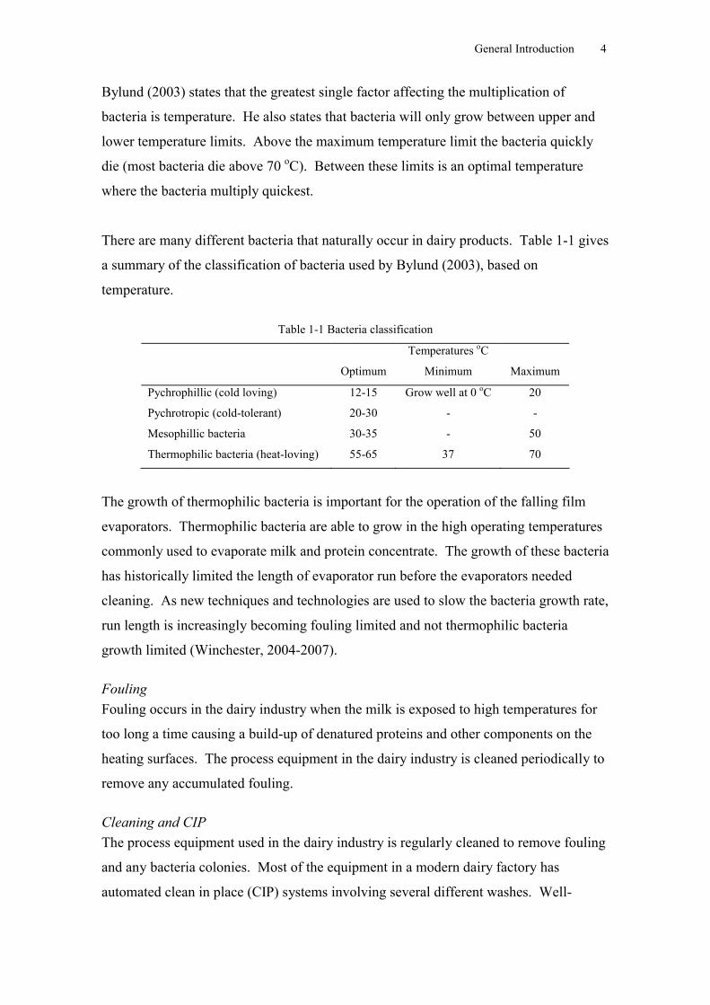
There are many different bacteria that naturally occur in dairy products. Table 1-1 gives
a summary of the classification of bacteria used by Bylund (2003), based on
temperature.
Table 1-1 Bacteria classification
Temperatures oC
Optimum Minimum Maximum
Pychrophillic (cold loving) 12-15 Grow well at 0 oC 20
Pychrotropic (cold-tolerant) 20-30 - -
Mesophillic bacteria 30-35 - 50
Thermophilic bacteria (heat-loving) 55-65 37 70
The growth of thermophilic bacteria is important for the operation of the falling film
evaporators. Thermophilic bacteria are able to grow in the high operating temperatures
commonly used to evaporate milk and protein concentrate. The growth of these bacteria
has historically limited the length of evaporator run before the evaporators needed
cleaning. As new techniques and technologies are used to slow the bacteria growth rate,
run length is increasingly becoming fouling limited and not thermophilic bacteria
growth limited (Winchester, 2004-2007).
FoulingFouling occurs in the dairy industry when the milk is exposed to high temperatures for
too long a time causing a build-up of denatured proteins and other components on the
heating surfaces. The process equipment in the dairy industry is cleaned periodically to
remove any accumulated fouling.
Cleaning and CIPThe process equipment used in the dairy industry is regularly cleaned to remove fouling
and any bacteria colonies. Most of the equipment in a modern dairy factory has
automated clean in place (CIP) systems involving several different washes. Well-
General Introduction 5
designed process equipment in the dairy industry is designed to limit the frequency of
cleaning. Process equipment must also be designed so the processing surfaces are
cleaned.
CIP systems use a combination of Alkaline, Acid and water rinses to clean the process
surfaces. Process equipment cannot be used to process milk while it is being cleaned.
Increasing the time interval between cleanings significantly reduces the cost to process
milk, as both the capital expense of not using the process equipment and the cost of the
chemical used to clean are significant.
1.3 Evaporators
Morison and Hartell (2007) give a good description of the evaporation process and this
section is based on it.
Evaporation is the technique of removing a solvent from a feed stock to produce a more
concentrated product. For the evaporator under study the solvent is water.
Evaporation is not the only method available for the removal of water, other methods
include reverse osmosis, ultrafiltration, freeze concentration and drying. These methods
are not considered in this project and more detail about them can be found in Heldman
and Lund (2007).
Modern evaporators typically reuse the large latent heat of vaporisation needed to
evaporate the water. These techniques include mechanical recompression, thermal
recompression and multistage. The resulting energy requirements are modest compared
to some other separation processes, for example drying. Evaporators can concentrate
most solutions to at least 50% total solids concentration, which is a higher than most
other liquid separation processes.
Only falling film evaporators are of interest to this project. There are also several other
standard evaporator designs used in process industries including short tube (or Robert),
rising (or climbing film), force recirculation, scraped surface thin film, plate and thin-
film spinning cone evaporators. For further information about other evaporators designs
refer to Billet (1989) and Perry et al. (1997).
General Introduction 6
1.3.1 Falling film evaporators
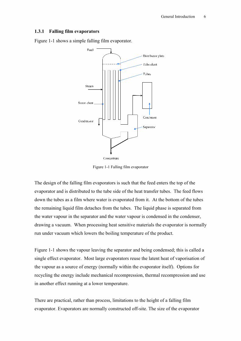
Figure 1-1 shows a simple falling film evaporator.
Figure 1-1 Falling film evaporator
The design of the falling film evaporators is such that the feed enters the top of the
evaporator and is distributed to the tube side of the heat transfer tubes. The feed flows
down the tubes as a film where water is evaporated from it. At the bottom of the tubes
the remaining liquid film detaches from the tubes. The liquid phase is separated from
the water vapour in the separator and the water vapour is condensed in the condenser,
drawing a vacuum. When processing heat sensitive materials the evaporator is normally
run under vacuum which lowers the boiling temperature of the product.
Figure 1-1 shows the vapour leaving the separator and being condensed; this is called a
single effect evaporator. Most large evaporators reuse the latent heat of vaporisation of
the vapour as a source of energy (normally within the evaporator itself). Options for
recycling the energy include mechanical recompression, thermal recompression and use
in another effect running at a lower temperature.
There are practical, rather than process, limitations to the height of a falling film
evaporator. Evaporators are normally constructed off-site. The size of the evaporator
General Introduction 7
that can be transported to the site is often limited by the roads, bridges and corners of
the road to the site.
Due to the small temperature drop across the falling film, giving low rates of
evaporation, it is common to use multi-pass falling film evaporators. This involves
returning the product stream to the top of the evaporator and running it down another set
of tubes in the same evaporator effect (stage). It is also common to use several
evaporator effects to fully concentrate the product; the current generation of falling film
evaporators use three or four effects.
Falling film evaporators in the dairy industry
Falling film evaporators are used in industry to concentrate milk products including
skim milk, whole and milk protein concentrate (MPC). The residence time of the
concentrate in a well designed falling film evaporator is short, well defined and
relativity uniform, compared to other evaporator designs. Poor design of the distribution
and separation systems at top and bottom of the heat transfer tubes respectively can
result in concentrate recirculation or holdup. This recycling and/or holdup of the
concentrate is undesirable due to the heat sensitive of dairy concentrates, such as milk.
The longer milk is exposed to the high temperatures in the evaporators, the more the
milk proteins are degraded and the more thermophilic bacteria develop.
Typical operating conditions for falling film evaporators in the dairy industry are
between 45 oC and 70 oC. Above 70 oC thermal degradation of the proteins in the
product becomes an issue. The lower temperature is set by a practicable limitation of
drawing the vacuum. The range of the viscosity of liquids processed in evaporators is
typically between 0.7 mPas and 10 mPas. The density of the feed and products is
normally between 1000 kg m-3 to 1250 kg m-3. An interfacial surface tension of
between 50 N m-1 and 70 N m-1 is common. The contact angle of the three phase
interface in evaporators is normally close to 80o. The operating temperature drop is
normally between 2 to 8 oC (Morison and Hartell, 2007).
CFD Introduction 8
2 Computational Fluid Dynamics IntroductionComputational Fluid Dynamics (CFD) is the name given to the numerical method of
solving the conservation of momentum equations, the conservation of mass (continuity)
equation, and any other required equations. These include but are not limited to the
conservation of energy equation, conservation of species and turbulence equations.
These equations are often called transport equations within the CFD environment.
A good description of CFD is given by Leal (1992), Versteeg and Malalasekera (1995),
Anderson (1995), Chung (2002) and Ansys CFX (2005) and this chapter is based on
these sources and should be referred to for any further details not included in this
chapter.
2.1 Transport equations
The following transport equations are in the form in which they are solved by Ansys
CFX. Ansys CFX solver solves the 3-D, Cartesian coordinate, finite volume transient
transport equations. Steady state solutions are obtained by false stepping the solution
through time until steady state is achieved.
2.1.1 Mass transport equation
The mass transport equation is found using the conservation of mass law that states that
mass can not be created or destroyed. For any given volume the
rate of change in mass within the volume = flux of mass across all the surfaces
This can be expressed mathematically for an infinitesimally small volume as
0 U
t (2-1)
where is the density and U is the velocity vector. This is known as the Eulerian
Continuity equation. The Eulerian method differs from the Lagrangian method in that
in the Eulerian method the control volume is constant in time and space, while with the
Lagrangian method the same mass of fluid is constant and tracked through time and
space. The Lagrangian and Eulerian methods can be shown to be mathematically
equivalent.
CFD Introduction 9
2.1.2 Momentum transport equation
Newton’s Second Law of Motion is used to obtain the momentum transport equations.
For any given volume the
rate of change in momentum within volume = flux of momentum across all the
surfaces + volume momentum forces+ surface forces on the volume
This can be expressed mathematically for an infinitesimally small volume as
TSUUtU
(2-2)
where S are the volumetric body forces (for example gravity) and the shear tensor for a
Newtonian fluid, T, is equal to
EPIT 2 (2-3)
where P is the pressure, I is the identity matrix, is the dynamic viscosity and E is the
shear deformation tensor
UIUUE T
32
21 (2-4)
Remembering that U is a vector, the resulting equation once equations 2-2, 2-3 and 2-4
are combined, is actually a set of scalar equations, one for the momentum component in
each Cartesian direction.
2.2 Nature of turbulence
Mathieu and Scott (2000) give a good explanation of the nature of turbulence and this
section is based on it.
As the fluid moves under the effect of shear the fluid can become rotational; small
initial disturbances grow into rotating eddies. Initially the eddies are close to two
dimensional. All eddies have smaller eddies within them, until the scale is small
enough that the molecular viscosity of the fluid stops the formation of smaller eddies.
The smaller eddies grow as the flow develops, eventually destroying the two-
dimensional structure of the initial eddies. As the turbulence of the flow develops, the
flow become more chaotic until finally it is fully turbulent.
CFD Introduction 10
In the laminar flow region, viscous forces dissipate any eddies formed faster than the
rate of formation, so downstream from the source of the eddies, none remain. At the low
Reynolds number end of the transitional regime a small number of large eddies start to
dominate the flow, and by the end of the transitional region smaller eddies have reduced
the large eddies into a more chaotic flow fully turbulent flow.
The energy in the large eddies is transferred to the smaller eddies, which transfer the
energy down until the smallest eddies convert the energy into heat. This process is
known as the energy cascade.
Despite a significant amount of work done to improve the understanding of turbulence,
the process is still not fully understood.
2.3 Turbulence modelling
The transport equations adequately describe all flows including laminar, transitional and
fully turbulent flows. Solving the transport equations directly is known as Direct
Numerical Solution (DNS), but unfortunately DNS for turbulent flows can only be used
when extreme computational resources are available and the problem is simple, for
example a flow around a cylinder. DNS is primarily used in research for development
of other turbulence models due to the prohibitive computational cost.
Large Eddy Simulation (LES) involves solving the largest scale eddies, while the
smaller eddies of the system are solved with a sub-grid model. Turbulence in the sub-
grid scale is more uniform than in the large eddies. LES is still extremely
computationally expensive in most industrial situations, especially when wall flow is
involved. This is due to the large differences in the length and time scales between
eddies at the walls and those eddies in the bulk flow. LES is still not a viable option for
modelling most industrial processes.
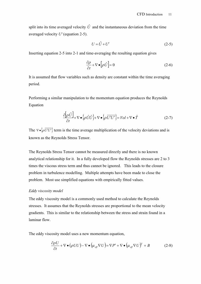
2.3.1 Reynolds Average Navier-Stokes equations (RANs)
Reynolds Average Navier-Stokes equations (RANs) are the most common methods
used to solve the problem with turbulence and are a statistical approach. The velocity is
CFD Introduction 11
split into its time averaged velocity U and the instantaneous deviation from the time
averaged velocity U′ (equation 2-5).
UUU ˆ (2-5)
Inserting equation 2-5 into 2-1 and time-averaging the resulting equation gives
0ˆ U
t
(2-6)
It is assumed that flow variables such as density are constant within the time averaging
period.
Performing a similar manipulation to the momentum equation produces the Reynolds
Equation
TVolUUUUtU ˆˆˆˆ
(2-7)
The UU term is the time average multiplication of the velocity deviations and is
known as the Reynolds Stress Tensor.
The Reynolds Stress Tensor cannot be measured directly and there is no known
analytical relationship for it. In a fully developed flow the Reynolds stresses are 2 to 3
times the viscous stress term and thus cannot be ignored. This leads to the closure
problem in turbulence modelling. Multiple attempts have been made to close the
problem. Most use simplified equations with empirically fitted values.
Eddy viscosity model
The eddy viscosity model is a commonly used method to calculate the Reynolds
stresses. It assumes that the Reynolds stresses are proportional to the mean velocity
gradients. This is similar to the relationship between the stress and strain found in a
laminar flow.
The eddy viscosity model uses a new momentum equation,
BUPUUUtU T
effeff
(2-8)
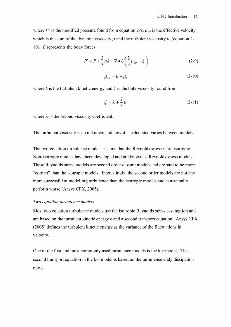
CFD Introduction 12
where P’ is the modified pressure found from equation 2-9, eff is the effective velocity
which is the sum of the dynamic viscosity and the turbulent viscosity t (equation 2-
10). B represents the body forces.
effUkPP
32
32 (2-9)
teff (2-10)
where k is the turbulent kinetic energy and is the bulk viscosity found from
32
(2-11)
where is the second viscosity coefficient.
The turbulent viscosity is an unknown and how it is calculated varies between models.
The two-equation turbulence models assume that the Reynolds stresses are isotropic.
Non-isotropic models have been developed and are known as Reynolds stress models.
These Reynolds stress models are second order closure models and are said to be more
“correct” than the isotropic models. Interestingly, the second order models are not any
more successful at modelling turbulence than the isotropic models and can actually
perform worse (Ansys CFX, 2005).
Two equation turbulence models
Most two equation turbulence models use the isotropic Reynolds stress assumption and
are based on the turbulent kinetic energy k and a second transport equation. Ansys CFX
(2005) defines the turbulent kinetic energy as the variance of the fluctuations in
velocity.
One of the first and most commonly used turbulence models is the k- model. The
second transport equation in the k- model is based on the turbulence eddy dissipation
rate .
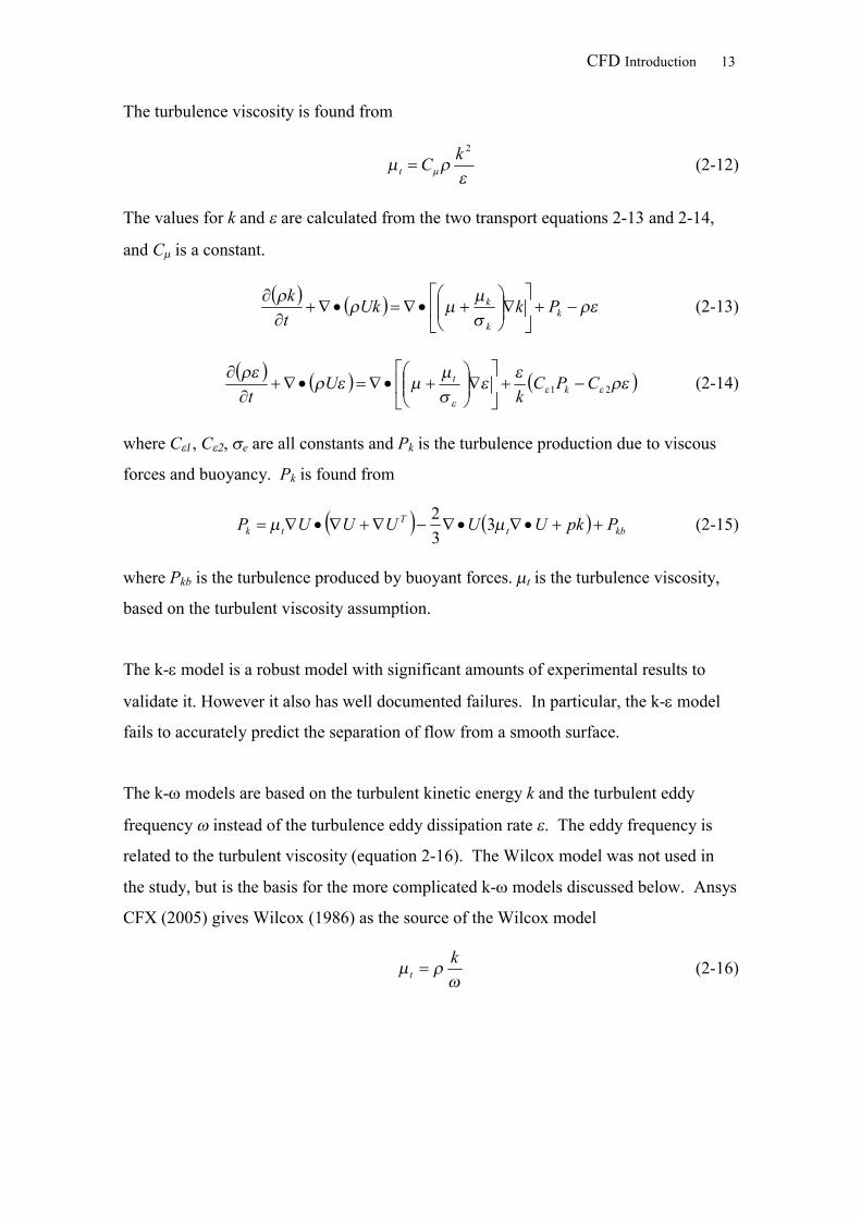
CFD Introduction 13
The turbulence viscosity is found from
2kCt (2-12)
The values for k and are calculated from the two transport equations 2-13 and 2-14,
and C is a constant.
kk
k PkUktk (2-13)
21 CPCk
Ut k
t
(2-14)
where C, C, e are all constants and Pk is the turbulence production due to viscous
forces and buoyancy. Pk is found from
kbtT
tk PpkUUUUUP 332 (2-15)
where Pkb is the turbulence produced by buoyant forces. t is the turbulence viscosity,
based on the turbulent viscosity assumption.
The k- model is a robust model with significant amounts of experimental results to
validate it. However it also has well documented failures. In particular, the k- model
fails to accurately predict the separation of flow from a smooth surface.
The k- models are based on the turbulent kinetic energy k and the turbulent eddy
frequency instead of the turbulence eddy dissipation rate . The eddy frequency is
related to the turbulent viscosity (equation 2-16). The Wilcox model was not used in
the study, but is the basis for the more complicated k- models discussed below. Ansys
CFX (2005) gives Wilcox (1986) as the source of the Wilcox model
k
t (2-16)
CFD Introduction 14
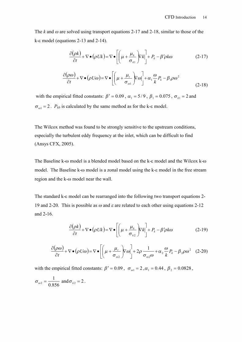
The k and are solved using transport equations 2-17 and 2-18, similar to those of the
k- model (equations 2-13 and 2-14).
kPkUktk
kk
k
1
(2-17)
211
1
kt P
kU
t (2-18)
with the empirical fitted constants: 09.0 , 9/51 , 075.01 , 21 k and
21 . Pkb is calculated by the same method as for the k- model.
The Wilcox method was found to be strongly sensitive to the upstream conditions,
especially the turbulent eddy frequency at the inlet, which can be difficult to find
(Ansys CFX, 2005).
The Baseline k- model is a blended model based on the k- model and the Wilcox k-
model. The Baseline k- model is a zonal model using the k- model in the free stream
region and the k- model near the wall.
The standard k- model can be rearranged into the following two transport equations 2-
19 and 2-20. This is possible as and are related to each other using equations 2-12
and 2-16.
kPkUktk
kk
k
2
(2-19)
222
22
12
kt P
kU
t(2-20)
with the empirical fitted constants: 09.0 , 21 , 44.01 , 0828.02 ,
856.01
2 and 22 k .
CFD Introduction 15
Equations 2-17 and 2-19 can be combined with a blending function F1 to produce a new
transport equation 2-21. The same can be done for equations 2-18 and 2-20 to produce
2-22). The blending function F1 varies from 1 near the wall to 0 in the bulk flow.
kPkUktk
kk
k
3
(2-21)
233
21
3
121
kt P
kFU
t(2-22)
The new constants are a linear interpolation between the Wilcox and Baseline model
constants. The interpolation uses
21113 1 FF (2-23)
where is a generic variable. For example:
21113 1 FF (2-24)
While the Baseline k- model combines the advantages of the k- and k- model, it
still fails to predict the onset of flow separation (Ansys CFX, 2005).
Ansys CFX recommends the use of the Shear Stress Transport (SST) model for a
general purpose model, and its superior performance has been demonstrated (Bardina et
al., 1997). The Shear Stress Transport model was developed to improve the
performance of the Baseline k- model and can accurately predict the onset of and
amount of flow separation.
The reason for the failure of the previous models to predict the onset of flow separation
is the lack of accounting for the transport of the turbulent shear stress which results in
the over-prediction of the eddy viscosity. The Shear Stress Transport model has an
eddy viscosity limiter to correct for this (Ansys, CFX).
The turbulent viscosity t is found from
tt (2-25)
and
CFD Introduction 16
21
1
,max SFaka
t (2-26)
where S is an invariant measure of the strain rate and F2 is the Shear Stress Transport
blending function.
The Shear Stress Transport model uses a blending function different from the Baseline
k- model. F1 is used to blend between the k- and k- models and F2 is required for
the eddy-viscosity limiter. The blending functions are found from equations 2-27
through to 2-31. y is distance from the closest wall.
411 argtanhF (2-27)
22
214,500,maxminarg
yCDk
yyk
k
(2-28)
10
2
100.1,12max
kCD (2-29)
222 argtanhF (2-30)
22500,2maxargyy
k (2-31)
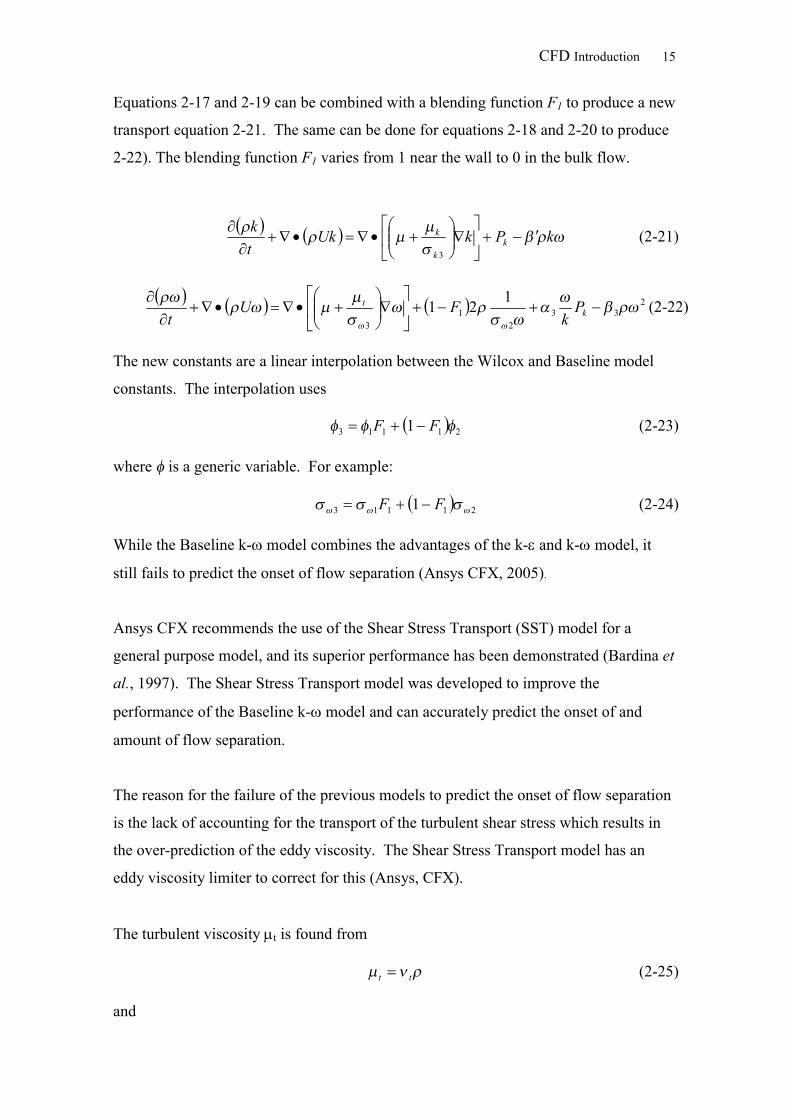
Figure 2-1 shows a typical contour plot of the first blending number. The area in red,
near the wall is where the k- model is used. In the free stream flow the blue indicates
the use of the k- model. The second blending function is also shown for completeness.
Figure 2-1 Shear Stress Transport turbulence model blending functions
CFD Introduction 17
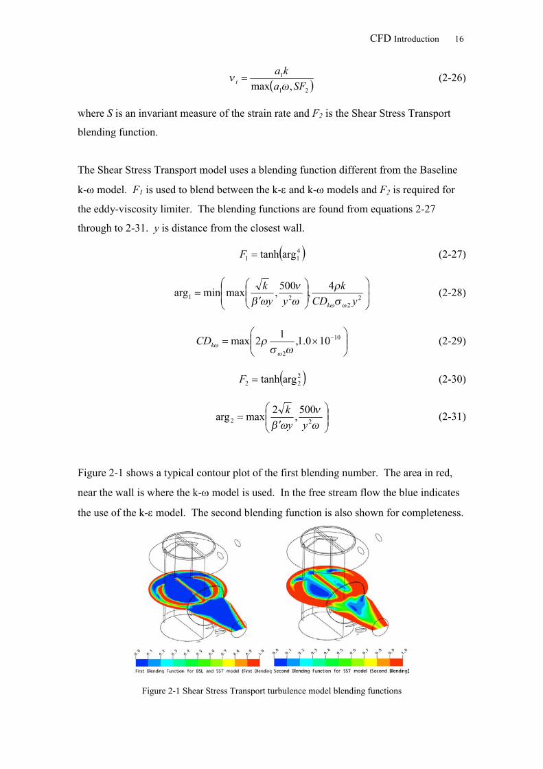
2.3.2 Near Wall Region and y+
At a non slip wall the velocity of the fluid is zero. Further out from the wall, the
velocity increases rapidly as it approaches the bulk of the fluid. In a turbulent flow the
velocity very rapidly reaches the bulk flow velocity (Figure 2-2). This rapid change
results in large shear forces acting on the fluid. This region is called the “near wall
region”.
Figure 2-2 Near wall region
Within the near wall region there are several layers where the fluid is dominated by
different effects. Very close to the wall is a laminar viscous sub-layer. This layer in a
turbulent flow is very small, typically much smaller than the mesh, especially in the
case of an inviscous fluid. Within this region the molecular viscosity dominates
momentum transfer (as well as heat transfer).
Further away from the wall, the flow changes from being laminar-dominated to being
turbulent-dominated. Past this transitional layer, turbulence dominates the flow.
Wall functions or a low Reynolds number turbulence model are two main methods used
to handle the near wall region, taking into account the viscous effects. Wall functions
impose a condition on the flow using empirically fitted data, which requires a coarser
mesh than the Low Re model. The Low Re model resolves the boundary layer through
finer element resolution.
The Shear Stress Transport model uses an automatic wall function which switches to the
Low Re model from the wall functions as the mesh is refined. For more details on near
wall modelling, refer to Ansys CFX (2005).
CFD Introduction 18
y+ is the dimensionless distance from the wall. It is a measure of the perpendicular
location within the boundary layer and is defined as
tuyy
(2-32)
where is the fluid density, is the fluid viscosity, y is the distance to the closest wall
and ut is found from using the wall shear and density. ut is calculated from
tu (2-33)
Ansys CFX (2005) claims that a y+ of less than 200 is appropriate for the automatic wall
function. It also claims that as a guideline the mesh near the wall should be resolved
through the boundary layer for a wall function with 10 nodes and 15 nodes for the Low-
Re Model, refer to Ansys CFX (2005).
2.4 Multiphase Systems
A multicomponent system involves a fluid which is the mixture of several different
components. The relative ratio of components can change over time and distance but
locally the components are mixed at the molecular level. For example air is a
multicomponent fluid make from N2, O2, CO2 and other gases.
A multiphase system is a system with at least two different phases. The phases are not
mixed at the molecular level. At any point located within the system, only one of the
phases is present.
There are numerous different methods available to model multiphase systems. The
method for each phase is typically either Lagrangian or Eulerian.
The Lagrangian method involves tracking each individual “particle” of a phase
though space and time.
Eulerian method involves solving the transport equations for each phase,
following the phase through time at a static location.
The Lagrangian methods solve a set of equations for each of the “particles” tracked.
The equations can be as simple as a straight displacement equation for each particle.
CFD Introduction 19
The “particle” can be just a single particle or droplet, or a representative particle for a
group of particles or droplets. It is also possible that the “particle” tracked is a
representative particle for a continuous phase (for example a particle to track the free
surface).
The number of calculations required to use Lagrangian methods is directly related to the
phenomena modelled and the number of “particles” tracked. As the number of
“particles” increases so the number of calculations increases.
The number of calculations required for an Eulerian method depends on the transport
equations used to describe the phenomena in the system and the mesh required to
resolve the equations. Typically, the Eulerian transport equations used have significant
assumptions or empirically fitted data. This can lead to issues with the accuracy of the
models. The Volume of Fluid (VOF) method is the Eulerian method used by Ansys
CFX. The VOF method does not track individual particles, but uses the volume fraction
of each phase as a local measure of relative amount of each phase.
Not all the phases in a multiphase model are required to be modelled with the same
method. This allows the most suitable method to be used with each phase. An example
of this is modelling of a number of droplets in a vapour flow. The Lagrangian method
is well suited to modelling the droplets and the Eulerian method is better suited to
model the vapour phase.
Ansys CFX offers a Lagrangian particle tracking method where the continuous phase
(vapour or liquid) is solved using the Eulerian method and the flow of the dispersed
phase particles or droplets is solved using a Lagrangian method.
2.4.1 Lagrangian Particle Tracking
The Lagrangian method involves introducing a particle into the problem and then
tracking where the particle moves. The particles can be either solid or liquid (droplets).
A particle is tracked until it reaches a termination condition which includes contact with
walls, exiting the problem through an opening or outlet, or reaching maximum
integration limits set by the user.
CFD Introduction 20
The displacement of the particles is evaluated using forward Euler integration.
The equation used by Ansys CFX (2005) for a spherical particle can be derived from
Newton’s second law of motion, when the particle is much denser than the fluid the
motion of a particle is described by
gDuuuucDdt
duDfppfpfdf
pp
323
61
81
6. (2-34)
where is the density, u is the velocity in either x, y or z, D is the diameter of the
particle and cd is the drag coefficient for the particle. The f subscript is the fluid phase
and p subscript is the particle.
The non-deterministic effect of turbulence needs to be taken into account for RANs
equations, because only the time averaged variables are solved for.
The dispersion model used by Ansys CFX (2005) to evaluate the instantaneous fluid
velocity, vf, assumes that each particle passes through only one eddy at a time. Each
eddy has the characteristic properties of eddy time, te, eddy length, le, and the
fluctuating velocity, vf’. All of the characteristic properties are dependent on the local
turbulent conditions (k and ). Once the particle has passed through an eddy it enters
another eddy.
'fff vvv (2-35)
32' kv f (2-36)
2/32/3 kCl ue (2-37)
32kl
t ee (2-38)
where is a normally distributed random number, Cu is a constant.
As a particle travels through a fluid it will affect the fluid field it is contained in. It is
also possible for a particle to collide with another particle. The effect of the particles on
CFD Introduction 21
the fluid and/or the number of collisions is not always significant. The level of
modelling of these interactions is known as the degree of coupling.
When only the fluid influences the particles and the influence of the particles on the
fluid is ignored, this is known as one-way coupling. When the particle on fluid
interaction without particle-particle collisions is modelled, this is known as two-way
coupling. Fully coupled or four-way coupling is when the particle collisions are
modelled as well.
It is valid to use only one-way coupling if the particle density of the particles is small
enough that the particles have an insignificant effect on the fluid field. As more effects
are modelled, so does the amount of computational power required increase. One-way
coupling allows the particle tracks to be solved after the fluid solver has finished. This
allows many different particles distributions to be run with the same fluid solution for
only small computational cost.
2.4.2 Volume of Fluid method (VOF)
The VOF method uses an interpenetrating continua assumption (Ansys CFX 2005).
This means that the phases in a multiphase problem are mixed at scales smaller than that
resolved by the mesh. The phases are not mixed at the molecular level. Ansys CFX
calls the VOF method the Eulerian-Eulerian model.
The phases are represented within each element by a volume fraction i for each of the
phases i. The volume fractions for all the phases will sum to 1.
The volume fraction is defined as the fraction of a volume occupied by a phase found
from
VV ii (2-39)
where V is the volume of the small volume of fluid around the point, Vi is the volume
occupied by the phase .
CFD Introduction 22
Homogenous Model
In the homogeneous model all the phases have the same pressure and velocity field.
The homogenous model is recommended for use with free surface models when there is
no entrainment (Ansys CFX 2005). Each phase in the homogenous model has its own
continuity equation
SUt iiii
(2-40)
where i is the density of each phase, U is the velocity for all the phases and S is the
phase mass source term.
The homogenous model has only one momentum equation
SPUUUUUt
Tbbb
(2-41)
The bulk density b is found from the sum of each phases density i weighted
proportionally to the volume fraction of each phase (equation 2-42). The bulk viscosity
b is found in a similar manner (equation 2-43).
ni
i iib 1 (2-42)
ni
i iib 1 (2-43)
Heterogeneous Model
The heterogeneous model involves solving the momentum transport equations for each
phase. The heterogeneous model was not used. Refer to Ansys CFX (2005) for more
details about the heterogeneous model.
Particle modelling
Multiphase VOF Eulerian models have been developed to model dispersed particles
using the Eulerian method instead of the Lagrangian method. The Eulerian model
calculates the velocity vector for the fluid and only one velocity vector field for each
Eulerian particle model (using a single particle diameter). To calculate more vector
fields for different particle diameters requires extra sets of Eulerian equations. This
increases the amount of calculations required.
CFD Introduction 23
When using an Eulerian VOF model, it is difficult to find the moment in time when the
dispersed phase first comes into contact with a surface, such as a wall unlike the
Lagrangian particle tracking method which does this easily. The Lagrangian method is
preferred when modelling of dispersed particles, for example the droplets in the
separator. When the particle density is high the Eulerian VOF method is often
preferable. The Eulerian VOF model computational cost is independent of the number
of particle and inter-particle collisions can be modelled. This inter-particle collision in
the Lagrangian particle tracking is not directly supported in Ansys CFX 10.0.
2.5 Boundary conditions
To define the CFD model equations correctly, the variables of the solved transport
equations must be defined, either through a known relationship or given a value at the
boundaries. The definitions of these values are called boundary conditions. Initial
conditions are also required: for transient models setting correct initial conditions is
critical. For a steady state model initial conditions are still used to give the solver a
sensible starting point.
The following is a brief description of the single phase boundary conditions and is not
meant to be a complete review. For more details refer to Ansys CFX (2005).
The inlet boundary condition can be set by either the velocity (or mass flow rate) or
through either the static or total pressure. If the velocity is set, the pressure at the inlet
is an unknown and is calculated in the solution. If the pressure is set then the flow rate
depends on the pressure drop across the interface. If the pressure drop is negative the
solver will insert a virtual wall to stop fluid flowing back out of the model. If a
turbulence model is being used, it will normally require some detail of the turbulence of
the incoming fluid, for example the turbulent intensity.
The outlet boundary condition is the opposite condition to the inlet, where fluid can
flow out of the model and not in. The outlet can be to the same conditions as the inlet
(velocity, mass flow rate, static pressure or total pressure). If the pressure field requires
fluid to flow back into the model, the solver will also make a virtual wall to stop this.
CFD Introduction 24
The opening boundary condition is similar to the outlet condition except it allows fluid
to flow back into the domain from outside.
Walls do not allow any fluid to flow through them. The tangential velocity at the wall
can be either unconstrained or constrained. When the wall velocity is unconstrained this
is a free-slip wall. When the tangential velocity at the wall is constrained, normally to
zero, this is known as a no-slip wall. The no-slip walls are used to impose the viscous
effect of the wall on the fluid. Free-slip walls do not model the viscous effect of the
wall.
Planes of symmetry are planes where the gradients of all the variables normal to the
plane equal zero.
The periodic boundary conditions are created in pairs. The boundary condition is
defined so that fluid can pass between the boundaries even though they typically are not
touching. This boundary condition is often used in turbo-machinery problems to model
a single blade passage instead of an entire set of identical blades passages.
2.5.1 VOF Homogeneous Boundary conditions
The VOF homogenous multiphase boundary conditions are similar to the single phase
boundary condition. The main difference is at the opening and inlets where the volume
fraction of the incoming fluid is required. This volume fraction can vary over the
boundary but requires user equations to do this. Refer to Ansys CFX (2005) for more
detail.
2.5.2 Particle tracking
It is possible to individually define each tracked particle, but it is simpler to group
similar particles together. When a group of particles is introduced into an Ansys CFX
model, each of the particles requires an initial starting location, velocity vector and size.
Ansys CFX (2005) has numerous built-in options for how the location, velocity vector
and size are distributed within each group.
The starting location of the particles is defined by a point, line, surface or volume.
When using a surface it is common to use the normal of the surface as the direction of
CFD Introduction 25
the velocity vector and to use either a velocity set by the user or set equal to the
surrounding vapour velocity.
The size of the particles is set by the user. If a size distribution is used, the individual
droplet size is set by randomly selecting a size within the defined range. The relative
frequency of a certain size is calculated from the size distribution used.
2.6 Computational Fluid Dynamics
There are three main CFD methods used today.
1. Finite Differences Method
2. Finite Element Method
3. Finite Volume Method
The Finite Differences method involves using Taylor series approximations to discretise
the Transport equations. The Finite Differences method requires a structured mesh and
has been superseded today by the Finite Element and Finite Volume methods.
Finite Element involves splitting the problem into elements. Each element is modelled
with a simplified model. The element models are solved simultaneously. The finite
element modelling was first developed for use in structural and mechanical modelling.
Unlike the Finite Differences and Finite Volume modelling, finite element modelling
can solve non-transport equations as well as transport equations.
The Finite Volume Method (FVM) is the more common modelling method, used by the
major generalised CFD codes (Ansys CFX and Fluent Inc). The method involves
splitting the problem into a finite number of volumes (volumes and elements are
basically the same, the difference is due to naming conventions) and numerically
solving the transport equations for each of the nodes located in the volume.
All three main methods involve solving the same basic equations and the methods
should in theory give the same results. A lot of the differences are due to who
historically had first used the different methods. For example Finite Volume has a mass
matrix whereas Finite Element has a stiffness matrix; both are very similar in design and
solving. The different names are legacies of the method origins.
CFD Introduction 26
Although the methods are converging to a certain extent, there are still significant
differences. The FVM is considered to have superior conservative properties compared
to FEM (Chung, 2002).
2.7 Finite Volume Method
Using only the Continuity equation 2-1 as an example, the model can be described as
0
geometrydVUt
(2-44)
It is possible to split dV in equation 2-44 into a discrete number of non-overlapping
volumes (known as control volumes within CFD). This creates a set of equations
containing an equation for each of the control volumes. For n control volumes (CV) the
equation set would look like
0
...
0
...
0
0
2
1
n
i
CV
CV
CV
CV
dVUt
dVUt
dVUt
dVUt
(2-45)
Considering the equation for the ith control volume, using Gauss’ theorem and then
splitting the surfaces of the control volume into m number of surfaces, after some
simple rearranging gives
mj
jCVjCV ii
dSnUdVt 1
, (2-46)
At this point there have been no assumptions, or simplifications made and the set of
equations are mathematically equivalent to the original definition of the model.
By assuming that the density is constant across the control volume, the density
derivative can be move outside the integral and equation 2-46 can be rearranged to
CFD Introduction 27
mj
jCVjCV
CVii
i dSnUVt 1
,
(2-47)
By assuming that for each surface j the variables on the surface are constant, equation 2-
47 can be rearranged to give
mj
jCVjCVjCVjCVCV
CViiiii
i AnUVt 1
,,,
(2-48)
2.7.1 Discretisation
For any control volume, equation 2-48 has variables that are dependent on the control
volume geometry (VCVi, nj,CVi and Aj,CVi) variables located within the volume (CVi) and
variables located on the surfaces (Uj,CVi).
Ansys CFX uses a different discretisation scheme called the element based finite
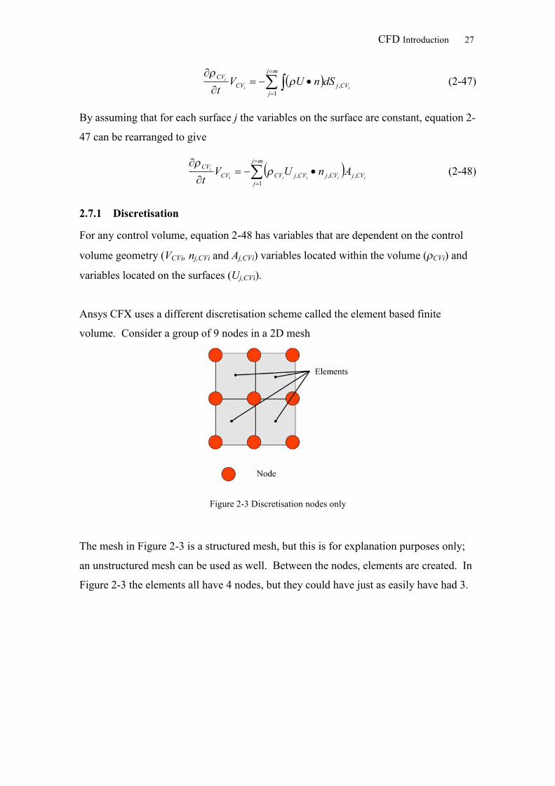
volume. Consider a group of 9 nodes in a 2D mesh
Figure 2-3 Discretisation nodes only
The mesh in Figure 2-3 is a structured mesh, but this is for explanation purposes only;
an unstructured mesh can be used as well. Between the nodes, elements are created. In
Figure 2-3 the elements all have 4 nodes, but they could have just as easily have had 3.
CFD Introduction 28
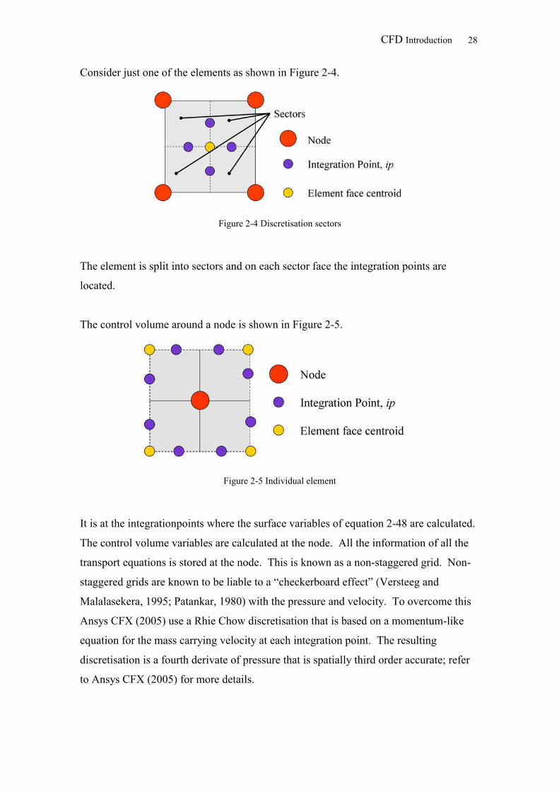
Consider just one of the elements as shown in Figure 2-4.
Figure 2-4 Discretisation sectors
The element is split into sectors and on each sector face the integration points are
located.
The control volume around a node is shown in Figure 2-5.
Figure 2-5 Individual element
It is at the integrationpoints where the surface variables of equation 2-48 are calculated.
The control volume variables are calculated at the node. All the information of all the
transport equations is stored at the node. This is known as a non-staggered grid. Non-
staggered grids are known to be liable to a “checkerboard effect” (Versteeg and
Malalasekera, 1995; Patankar, 1980) with the pressure and velocity. To overcome this
Ansys CFX (2005) use a Rhie Chow discretisation that is based on a momentum-like
equation for the mass carrying velocity at each integration point. The resulting
discretisation is a fourth derivate of pressure that is spatially third order accurate; refer
to Ansys CFX (2005) for more details.
CFD Introduction 29
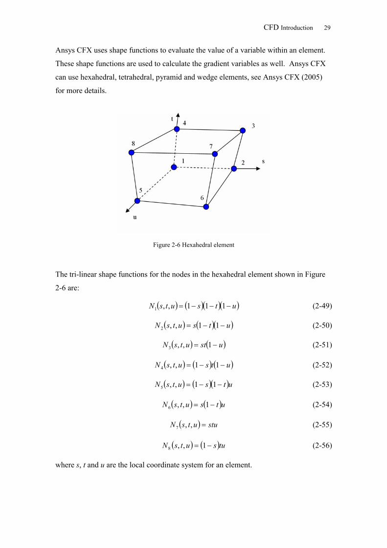
Ansys CFX uses shape functions to evaluate the value of a variable within an element.
These shape functions are used to calculate the gradient variables as well. Ansys CFX
can use hexahedral, tetrahedral, pyramid and wedge elements, see Ansys CFX (2005)
for more details.
Figure 2-6 Hexahedral element
The tri-linear shape functions for the nodes in the hexahedral element shown in Figure
2-6 are:
utsutsN 111,,1 (2-49)
utsutsN 11,,2 (2-50)
ustutsN 1,,3 (2-51)
utsutsN 11,,4 (2-52)
utsutsN 11,,5 (2-53)
utsutsN 1,,6 (2-54)
stuutsN ,,7 (2-55)
tusutsN 1,,8 (2-56)
where s, t and u are the local coordinate system for an element.
CFD Introduction 30
The value of a variable within the element can be found from
nodeN
iiiN
1
(2-57)
where i is the variable at node i.
The differential at the integration points (ip) is found by
nodeN
ii
ip
i
ip xN
x 1
(2-58)
The elements axes s, t and u are transformed into the global axes by a Jacobian
transformation.
For the advection terms it is not appropriate to use equation 2-58, due to the flow term
not being equally affected by all the nodes in an element. For this reason, a differencing
scheme is used to better mimic the transportation of variables.
2.8 Differencing schemes
There are several common differencing schemes used; all have different pros and cons.
To get a better understanding, some properties of the differencing schemes are briefly
explained below.
2.8.1 Properties of Differencing Schemes
Using an infinite set of discretisation cells will give, in theory, the exact result
independent of discretisation scheme. In practice, though, there are real limitations to
the number of calculations that can be performed and hence alternative differencing
schemes will give rise to different results. There are several properties that are
important when talking about the different discretisation schemes.
Conservativeness
Boundedness
Transportiveness
Conservativeness
Conservativeness means that the flux between two control volumes with a common face
is constant and does not vary depending on which control volume is being used.
CFD Introduction 31
Boundedness
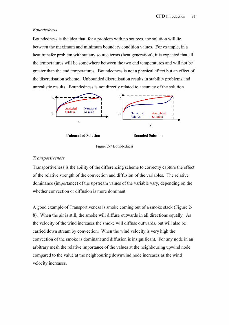
Boundedness is the idea that, for a problem with no sources, the solution will lie
between the maximum and minimum boundary condition values. For example, in a
heat transfer problem without any source terms (heat generation), it is expected that all
the temperatures will lie somewhere between the two end temperatures and will not be
greater than the end temperatures. Boundedness is not a physical effect but an effect of
the discretisation scheme. Unbounded discretisation results in stability problems and
unrealistic results. Boundedness is not directly related to accuracy of the solution.
Figure 2-7 Boundedness
Transportiveness
Transportiveness is the ability of the differencing scheme to correctly capture the effect
of the relative strength of the convection and diffusion of the variables. The relative
dominance (importance) of the upstream values of the variable vary, depending on the
whether convection or diffusion is more dominant.
A good example of Transportiveness is smoke coming out of a smoke stack (Figure 2-
8). When the air is still, the smoke will diffuse outwards in all directions equally. As
the velocity of the wind increases the smoke will diffuse outwards, but will also be
carried down stream by convection. When the wind velocity is very high the
convection of the smoke is dominant and diffusion is insignificant. For any node in an
arbitrary mesh the relative importance of the values at the neighbouring upwind node
compared to the value at the neighbouring downwind node increases as the wind
velocity increases.
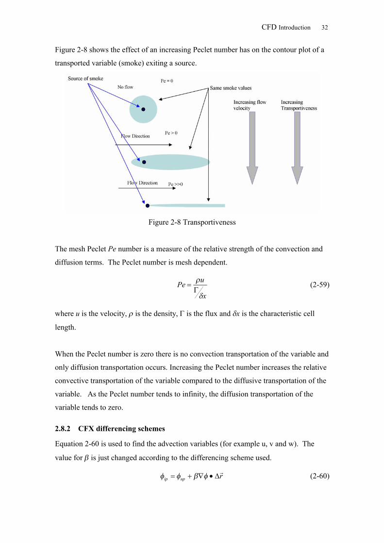
CFD Introduction 32
Figure 2-8 shows the effect of an increasing Peclet number has on the contour plot of a
transported variable (smoke) exiting a source.
Figure 2-8 Transportiveness
The mesh Peclet Pe number is a measure of the relative strength of the convection and
diffusion terms. The Peclet number is mesh dependent.
x
uPe
(2-59)
where u is the velocity, is the density, is the flux and x is the characteristic cell
length.
When the Peclet number is zero there is no convection transportation of the variable and
only diffusion transportation occurs. Increasing the Peclet number increases the relative
convective transportation of the variable compared to the diffusive transportation of the
variable. As the Peclet number tends to infinity, the diffusion transportation of the
variable tends to zero.
2.8.2 CFX differencing schemes
Equation 2-60 is used to find the advection variables (for example u, v and w). The
value for is just changed according to the differencing scheme used.
rupip
(2-60)
CFD Introduction 33
where ip is the value at the integration point, up is the value at the upstream node and
r is an anti-diffusive flux (see for more details Ansys CFX (2005)).
2.8.3 Central difference scheme
The central difference scheme is probably the conceptually simplest difference scheme;
however it does have its limitations and problems. A linear interpolation is taken for the
values at the surface from the volume values.
The central difference scheme can be shown to be:
conservative
bounded only under certain conditions (Pe <2)
not transportive
good accuracy (has second order Taylor series truncation errors)
Since the central difference scheme is only bounded on certain conditions, this makes
the problem very mesh dependent. As well, the lack of transportiveness is a problem in
many CFD simulations. The central differencing scheme can introduce non-physical
oscillations in regions with rapid solution variation that are undesirable. The central
difference scheme is less robust than the upwind and high resolution schemes. The
central difference scheme is only used with Ansys CFX for LES turbulence models.
The central difference scheme is implemented in Ansys CFX by setting to equal 1 and
is set to equal the local element gradient in equation 2-60. Both Ansys CFX,
(2005) and Versteeg and Malalasekera (1995) have good descriptions of the central
difference schemes.
2.8.4 Upwind difference scheme
The upwind scheme is a first order spatial discretisation of the advection term. The
upwind difference scheme is normally easier to solve but it can introduce diffusive
discretisation errors that can smear steep spatial gradients (Ansys CFX, 2005). The lack
of accuracy of the scheme is a problem. The upwind scheme can is implemented by
setting to equal 0 in Equation 2-60.
The Upwind scheme is said to be:
conservative
CFD Introduction 34
unconditionally bounded
transportive
only first order Taylor series correct
2.8.5 Hybrid Difference Scheme
Ansys CFX, (2005) does not use the Hybrid Scheme but it is worth including since it
similar in concept to the High Resolution Scheme used by Ansys CFX. The Hybrid
Difference Scheme was created to take the best of both the Central Difference and
Upwind Difference Scheme. It is a piecewise combination of the Upwind and Central
Differencing Schemes based on the local mesh Peclet number. Refer to Versteeg and
Malalasekera (1995) for more details.
The Hybrid scheme is said to be:
conservative
unconditionally bounded
transportive
only first order Taylor series correct
2.8.6 High Resolution Difference Scheme
The high resolution difference scheme of Ansys CFX, (2005) is based on the work of
Barth and Jesperson (1989).The scheme uses Equation 2-60 where is the gradient at
the upwind node. Ansys CFX (2005) states that the evaluation of is based on Barth
and Jesperson (1989) and is set to as close to 1 as allowed without the introduction of
non physical oscillations at location of steep gradients.
Ansys CFX, (2005) claim that the scheme is fully bounded, second order correct. They
do not given any information about the transportiveness of the scheme. The scheme is
inferred to be conservative but it is not actually stated as such, nor do they state
otherwise either. Refer to Ansys CFX, (2005) and Barth and Jesperson (1989) for more
details.
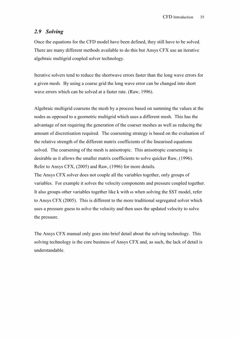
CFD Introduction 35
2.9 Solving
Once the equations for the CFD model have been defined, they still have to be solved.
There are many different methods available to do this but Ansys CFX use an iterative
algebraic multigrid coupled solver technology.
Iterative solvers tend to reduce the shortwave errors faster than the long wave errors for
a given mesh. By using a coarse grid the long wave error can be changed into short
wave errors which can be solved at a faster rate. (Raw, 1996).
Algebraic multigrid coarsens the mesh by a process based on summing the values at the
nodes as opposed to a geometric multigrid which uses a different mesh. This has the
advantage of not requiring the generation of the coarser meshes as well as reducing the
amount of discretisation required. The coarsening strategy is based on the evaluation of
the relative strength of the different matrix coefficients of the linearised equations
solved. The coarsening of the mesh is anisotropic. This anisotropic coarsening is
desirable as it allows the smaller matrix coefficients to solve quicker Raw, (1996).
Refer to Ansys CFX, (2005) and Raw, (1996) for more details.
The Ansys CFX solver does not couple all the variables together, only groups of
variables. For example it solves the velocity components and pressure coupled together.
It also groups other variables together like k with when solving the SST model, refer
to Ansys CFX (2005). This is different to the more traditional segregated solver which
uses a pressure guess to solve the velocity and then uses the updated velocity to solve
the pressure.
The Ansys CFX manual only goes into brief detail about the solving technology. This
solving technology is the core business of Ansys CFX and, as such, the lack of detail is
understandable.
CFD Introduction 36
2.9.1 Solution Plan
The outline of the algorithm used is given in Figure 2-9, reproduced from Ansys CFX
(2005).
Figure 2-9 Ansys CFX solution plan
2.9.2 Mesh adaptationFigure 2-9 does not show that it is possible to use mesh adaptation to increase the
convergence of the model. The mesh is adapted in areas of high gradient of the user
defined variable. Ansys CFX uses a hierarchical refinement technique. The meshing
technique is an incremental meshing technique where a new node is placed on the mesh
CFD Introduction 37
edge marked for adaptation. The mesh elements that share the split edge are then
reformed (Ansys CFX 2005). Ansys CFX (2005) states that the incremental technique
is much faster than re-meshing techniques, but the quality of the new mesh is limited by
the quality of the original mesh. Refer to Ansys CFX (2005) for more details on Mesh
adaptation options and implementations.
2.10 Model inaccuracy
The accuracy of the solution(s) of a model, when compared against the physical effect it
is trying to model, is dependent on the definition of the model and how it is solved.
This is true for all models (including non-numerical models) but for the purposes of this
discussion, only engineering physics-based equation models are considered.
Virtually all physical models have inaccuracies. It could be due to the choice of the
models used, the simplification of geometry, the properties of the material used, the
method used to solve them, incorrect boundary information, lack of convergence or
poor mesh.
The accuracy of some models is great enough that they can be used at conditions where
the model’s assumptions do not lead to significant errors. For example, Newton’s law
of motion that the net force is proportional to the rate of change of momentum. The law
is more than adequate in describing the interactions of a body for a great range of
distances, speed and times, but it can not accurately predict the motion of body at speed
close to light. However for most engineering problems these inaccuracies are not an
issue.
Once a set of equations have been created to define the model, they need to be solved.
If the equations have an analytic solution then solution to the equations can easily be
found to high levels of precision. Unfortunately, most complex models’ equations can
not be solved analytically and must be solved numerically. Numerical solving normally
introduces sources of inaccuracy and/or reduced precision. These include discretisation,
convergence and numerical rounding. Sometimes the numerically introduced
inaccuracy or imprecision is orders of magnitude less than the required solution
accuracy/precision and other times it is not.
CFD Introduction 38
There are several common tests used to gain an understanding of the accuracy of a CFD
solution. The first two tests: convergence and mesh independence, relate to how close
the numerical solution is to the exact solution to the equations used to mathematically
describe the CFD model. The third test, validation, is the comparison of the CFD
solution against trusted results (experimental and/or numerical results). Validation is a
check of the accuracy of the solution, including the numerical accuracy and the
accuracy of the equations chosen.
2.10.1 Convergence and global balances
The CFD solution process is iterative. This means criteria for stopping the process are
needed. Typically, if a CFD model converged to the satisfaction of the modeller it is
said to be converged. The choice of criteria depends on what the CFD model is being
used for and requires some judgment by the user. Ansys CFX (2005) produces
residuals and global balances to help judge convergence.
Residuals
The residuals are used to give a measurement of the level of convergence. The
normalised residuals are found by equation 2-61. Normalised residuals are used to
make the comparison more universal.
par
r (2-61)
where r are the normalised residuals, r are the raw residuals, pa , are
representative of the control volume coefficient and the variable range respectively.
The exact calculations of the ap and are not given but the Ansys manual does state
that:
“1. The normalised residuals are independent of timestep choice.
2. The normalised residuals are independent of the initial guess.”
Ansys CFX (2005) calculates both maximum and root mean square residuals.
Residuals are related to the inequality between the left hand and right hand sides of the
discretised equations and are not related to the differences between the numerical and
the exact solution.
CFD Introduction 39
Ansys CFX (2005) gives the following advice for the evaluation of maximum residuals:
“greater than 5 x 10⁻⁴ is very poor, global balances will be poor and quantitative
data is largely unreliable. This is good enough for getting a rough idea of flow
phenomena or making pretty pictures.
5 x 10⁻⁴ is loose convergence, but good enough for most engineering
applications.
1 x 10⁻⁴ is good convergence, often sufficient for most engineering applications.
5 x 10⁻⁵ is tight convergence. If geometry and boundary conditions are not well
defined, then this may be more than necessary (since errors in the
geometry/boundary conditions will be greater than this). It is often not possible
to achieve this level of convergence.
1 x 10⁻⁵ or lower is very tight convergence, sometimes required for
geometrically sensitive problems.
1 x 10⁻⁶ to 1 x 10⁻⁷ is machine round-off. This level of convergence is not
possible without double precision, in most cases. Convergence this tight is only
of academic interest.”
Global Balances
Global balances are generated for all of the transport variables within a model. These
variables include the three velocity components (u, v and w), mass and other transport
variables. These global balances are the summation of the variable flow across all
model boundaries into the model (outflow is a negative flux) and the amount generated
in the volume of the model (loss is a negative gain). For transient models, the global
balance includes an accumulation term. Ideally for a converged solution these balances
should sum to zero.
User-Criteria
When possible it is useful to use user-defined criteria to measure the level of
convergence. A direct measure of what the model is being used to predict is preferential
(for example lift and drag on a wing). It is not always possible to use user-criteria. This
can be because there is no obvious measure or the measure can not be easily obtained
within the solver.
CFD Introduction 40
2.10.2 Mesh independence
The upwind, central difference or high resolution (hybrid) difference schemes all use
Taylor series approximations of the transport equations. The upwind scheme is 1st order
correct while the central difference scheme is 2nd order correct. The high resolution
scheme is a combination of 1st order correct and 2nd order correct. Due to the zonal
nature of the high resolution difference scheme, the order correctness depends on the
spatial and time location of the solution.
Irrespective of whether the solution is 1st or 2nd order correct, the Taylor series
approximation will result in Taylor series truncation errors. These errors depend on the
mesh size, to the power of 1 for 1st order correct schemes and to power of 2 for the 2nd
order correct schemes. As the mesh resolution is increased (control volume size is
decreased) the Taylor series truncation for converged solutions will decrease. The
solution is said to be mesh independent if the decrease in Taylor series truncation is
insignificant when the mesh is refined.
Mesh independence is established by using two or more dissimilar meshes and
comparing the solutions. If the solutions do not show significant differences, and the
Taylor series errors are insignificant, with particular attention to the area of interest then
the solution is normally described as “mesh independent”. The definition of what is
defined as “significant differences” similarly requires some engineering judgment and
can vary depending on what the solution is used for. It is therefore more correct to say
the solution is “mesh independence for the purpose of the model” but typically the
model is described as “mesh independent “with an implied qualifier for the modelling
purpose.
2.10.3 Validation
Validation is the process of comparing CFD solution(s) against trusted information
(validation data) and looking for any significant differences. It is possible to validate
results against numerical results, but this is not common and normally involves very
simple systems. Experimental results are much more commonly used to validate CFD
models.
CFD Introduction 41
By comparing relevant validation data against the CFD solution, it is possible to infer if
the choices of model equations and boundary conditions are correct. The solution
should be well converged and the solution shown to be mesh independence before
comparing the CFD solution against the validation data. If a model is converged and
mesh independent but does not agree with the validation data, then the choice of models
and/or boundary conditions is likely to be incorrect. If it does agree, then the choice of
models is likely to have been correct.
It is important to understand the relevance of the validation data to the purpose of the
CFD model. To illustrate the point, consider a model of air flowing over a wing. If the
validation data is located in the far field away downstream from the wing and the CFD
model is to be used to predict drag, it is important to understand the importance of the
downstream location on the drag performance of the wing. The downstream conditions
may or may not have a significant effect on the drag prediction. However if the
validation data was of the boundary layer located on the wing surface it is much more
likely to be important for the correct prediction of the drag on the wing.
It is not always possible to get much or even any validation data due to experimental
limitations. It is also common for the experimental data to be located at only at a few
spatial locations and consist of values for only a few of the variables. This can limit the
confidence in the CFD solution just through lack of valid comparisons. Engineering
judgment is need when deciding if the CFD solution agrees with the validation data and
the relevance of the agreement /disagreement, keeping in mind the purpose of the CFD
model.
2.11 CFX Introduction
The CFD program used in the study of the liquid/vapour interactions in evaporators was
Ansys CFX version 10.0 (previously known as CFX-5), supplemented with the Ansys
ICEM version 10.0 advanced meshing program. Ansys CFX has the reputation as one
of the leading general purpose CFD packages available today.
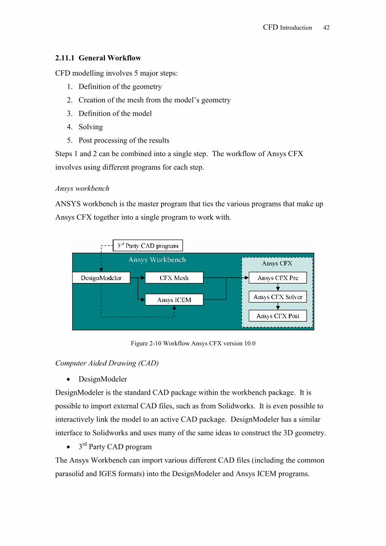
CFD Introduction 42
2.11.1 General Workflow
CFD modelling involves 5 major steps:
1. Definition of the geometry
2. Creation of the mesh from the model’s geometry
3. Definition of the model
4. Solving
5. Post processing of the results
Steps 1 and 2 can be combined into a single step. The workflow of Ansys CFX
involves using different programs for each step.
Ansys workbench
ANSYS workbench is the master program that ties the various programs that make up
Ansys CFX together into a single program to work with.
Figure 2-10 Workflow Ansys CFX version 10.0
Computer Aided Drawing (CAD)
DesignModeler
DesignModeler is the standard CAD package within the workbench package. It is
possible to import external CAD files, such as from Solidworks. It is even possible to
interactively link the model to an active CAD package. DesignModeler has a similar
interface to Solidworks and uses many of the same ideas to construct the 3D geometry.
3rd Party CAD program
The Ansys Workbench can import various different CAD files (including the common
parasolid and IGES formats) into the DesignModeler and Ansys ICEM programs.
CFD Introduction 43
Meshing
There are two alternative programs with the workbench environment that can perform
the meshing of the geometry. Both programs have their advantages and disadvantages.
CFX mesh
Ansys ICEM (advanced meshing)
CFX mesh is the standard mesh program provided with Ansys CFX. This generates a
surface mesh using either a Delaunay Surface Mesher or an Advancing Front (AF)
Surface Mesher. The surface mesh is then used to create a volume mesh either from
extruding the 2D surface mesh or by the advancing front method.
Ansys ICEM is the advanced meshing program that is an optional extra to the Ansys
CFD package. ICEM can produce both structured and unstructured meshes, as well as
combinations of both. ICEM allows greater control over the meshing process and better
visualisation of the resultant mesh. The geometry can be created with ICEM without
using DesignModeller, either by creating it within ICEM or importing it from a third
party source such as Solidworks. ICEM unstructured meshes are generated using a
number of techniques, including an Octatree method.
CFX mesh is the easier program to use and it is more integrated into the Workbench
than Ansys ICEM. Ansys ICEM is the more powerful meshing program as it can
produce meshes using several different techniques including the surface mesh to volume
mesh method use by Ansys CFX.
Pre
Pre is the program that takes the mesh generated in either CFX mesh or ICEM and
defines the model. There 3 major steps in defining the model:
1. Domain
a. Material properties
b. Model selection
c. General parameters
d. Sub domains
2. Boundary Conditions
a. Inlets
b. Outlets
CFD Introduction 44
c. Openings
d. Walls
e. Symmetry
f. Point conditions
3. Solver/Output Controls
The definition of the domain involves defining the models and materials to be
represented in the CFD modelling. For example, a model might be defined with the
fluid to be water vapour, using an isothermal energy model and with the shear stress
transport turbulence model.
The boundary conditions are where the condition on the boundaries of the model are
defined. For example, the mass flow rate of vapour flow entering through an inlet.
Solver and Output controls involve the definition of all the other variables, such as
number of iterations, termination criteria and what is produced as output at the end.
There are too many different conditions and adjustable values to go into detail here.
Refer to Ansys CFX (2005) for more details.
Solver manager
Once it has been defined in Pre, the model is solved within the Solver manager
program. Solver manager will iterate until either the maximum number of iterations has
occurred or the model has solved to the user-defined conditions.
Solver can be run either on one single computer (serial) or on multiple computers
(parallel).
It is possible to call the solver using command line commands (as is possible with both
Pre and Post). This allows for the automation of the running of a series of models after
each other.
CFD Introduction 45
Post
The results files generated by the solver manager are just matrices of numbers which are
not easily readable. The structure of the matrices is complex due to the unstructured
nature of the solver. In the Workbench environment, Post is the program used to
change the numbers into visualizations for ease of understanding.
Post can generate isosurfaces, particle tracks, streamlines, contour plots, vector plots, as
well as measures such as mass flows across boundaries. Post can also produce numbers
at user-defined locations, such as along a line. These numbers can be exported for
further post processing.
2.12 Similar published workIn the published literature no previous work was found using CFD to model either
separators in the dairy industry or integrated separators. However there numerous CFD
models of separators in the published literature including Karagoz and Kaya (2007)
modelled a reverse flow cyclone using the RNG k- turbulence model to account for the
high swirl and claimed good agreement with experimental data in literature. Veerapen
et al. (2005) used CFD simulations to design swirl separators for solid waste removal
for an aquaculture waste removal system. Narasimha et al. (2005) used a Lagrangian
CFD methodology similar to what was used in Chapter 3 to predict the cut off size in a
hydrocyclone. The CFD predictions agreed with experimental observations.
Also in the literature no previous work was found modelling the liquid distribution at
the top of an evaporator using CFD. It was surprising given the free surface flow is
basically a film flowing over a corner. This flow structure although easily defined is not
simple to model due to the highly nonlinear nature of the physics involved. Grunjal et
al. (2003) used the VOF method to model a droplet impacting on a spherical surface;
this involves basically the same physics needed for the liquid distribution. They
claimed a qualitative agreement with experimental work.
The “Teapot” effect of Reiner (1956) has similar film flow to the film flow expected for
liquid distribution. He gave a description of the “Teapot” effect, but does not produce
any analytical/CFD models. Kistler and Scriven (1994) modelled the “Teapot” effect
using a finite element methodology. They claim agreement with experimental flow
CFD Introduction 46
visualisation. Owen and Ryley (1985) looked at the shear of a uniformly thin film as it
flows around a sharp corner, which again is a similar film flow to liquid distribution.
They also compared their results with experimental work and got agreement. They
found that the surface tension was able to keep the film attached to the surface as it
flows around the sharp corner, unless the inertia was great enough to separate the film
from the surface.
There are a number of CFD models of a falling film in the published literature. These
models include Gao et al. (2003) who used a CSF VOF method to study the wavy
character of a 2D thin falling film. Kunugi and Kino (2005) also studied falling films
looking particularly looking at the heat transfer. They produced 2D and 3D model of
the film using the multi-interface advection and reconstruction solver using the CSF to
account for the surface tension force. The falling film model captured all the physics
required except for the physics at the wall adhesion location, but otherwise is similar.
It is difficult to get good current reviews about state of art CFD for several reasons. The
speed at which the field is developing, due largely to the ever increasing computational
power available solvers will date any review. An example of a good review is the work
of Orszag and Staroselsky (2000) which reviewed the state of the art CFD. It is the
author’s opinion that any review that is older than 5 years is likely to be dated by
improvements and/or computational speed increases and no longer be valid.
Another reason why review information is difficult to get is because significant amount
of the code used is commercially owned. This is particularly the case for when talking
about modelling industrial processes. Industrial processes typically require a more
complex combination of physics which normally makes commercial code better suited
than a more open source code. The proprietary nature of commercial code means not all
the details of how the code works are publicly available. The company that sell the
code also produce marketing material about their particular code which could be
mistaken for a more neutral review.
A literature search did not produce any good current general reviews about the state of
the art CFD modelling, but Norton and Sun (2006) reviewed the state of the art usage of
CFD as a design and analysis tool in the food industry. The closest work to this project

CFD Introduction 47
referenced was the modelling of spray drying in the dairy industry. The driers are used
directly downstream from the falling film evaporator. They claim many numerical
studies of the drier have been preformed and cite Langrish and Fletcher (2001), and
Huang et al. (2003), Straatsma et al. (1999) as examples of CFD used for design.
Cortes and Gil (2007) give a good review of modelling of gas and particle flow inside
cyclone separators, including a section on state of the art CFD modelling of separators.
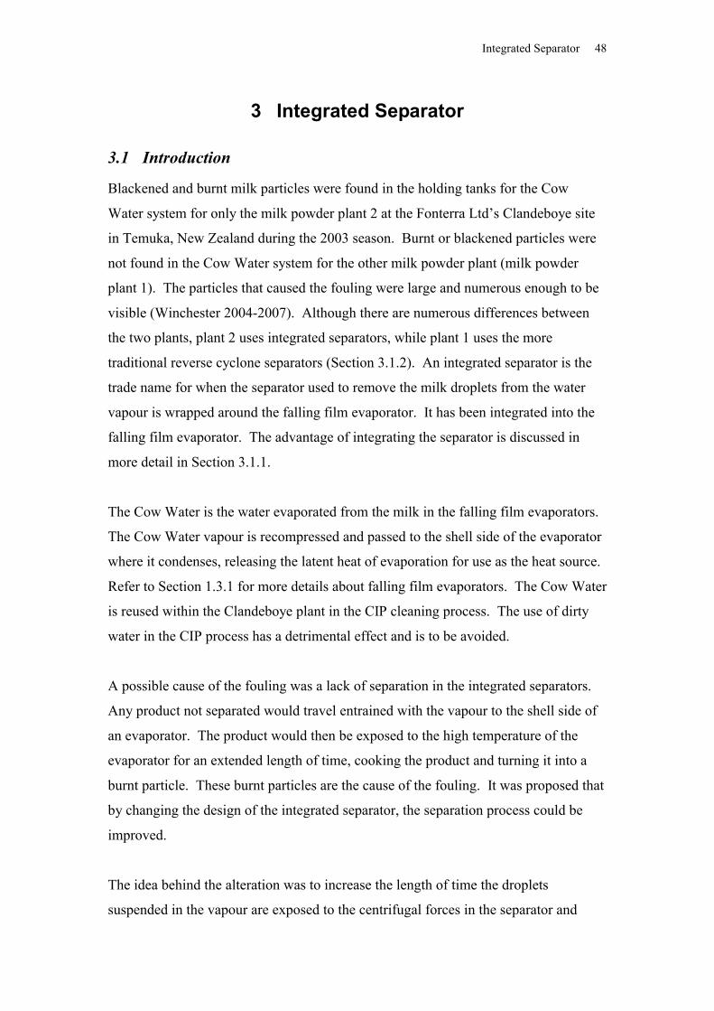
Integrated Separator 48
3 Integrated Separator
3.1 Introduction
Blackened and burnt milk particles were found in the holding tanks for the Cow
Water system for only the milk powder plant 2 at the Fonterra Ltd’s Clandeboye site
in Temuka, New Zealand during the 2003 season. Burnt or blackened particles were
not found in the Cow Water system for the other milk powder plant (milk powder
plant 1). The particles that caused the fouling were large and numerous enough to be
visible (Winchester 2004-2007). Although there are numerous differences between
the two plants, plant 2 uses integrated separators, while plant 1 uses the more
traditional reverse cyclone separators (Section 3.1.2). An integrated separator is the
trade name for when the separator used to remove the milk droplets from the water
vapour is wrapped around the falling film evaporator. It has been integrated into the
falling film evaporator. The advantage of integrating the separator is discussed in
more detail in Section 3.1.1.
The Cow Water is the water evaporated from the milk in the falling film evaporators.
The Cow Water vapour is recompressed and passed to the shell side of the evaporator
where it condenses, releasing the latent heat of evaporation for use as the heat source.
Refer to Section 1.3.1 for more details about falling film evaporators. The Cow Water
is reused within the Clandeboye plant in the CIP cleaning process. The use of dirty
water in the CIP process has a detrimental effect and is to be avoided.
A possible cause of the fouling was a lack of separation in the integrated separators.
Any product not separated would travel entrained with the vapour to the shell side of
an evaporator. The product would then be exposed to the high temperature of the
evaporator for an extended length of time, cooking the product and turning it into a
burnt particle. These burnt particles are the cause of the fouling. It was proposed that
by changing the design of the integrated separator, the separation process could be
improved.
The idea behind the alteration was to increase the length of time the droplets
suspended in the vapour are exposed to the centrifugal forces in the separator and
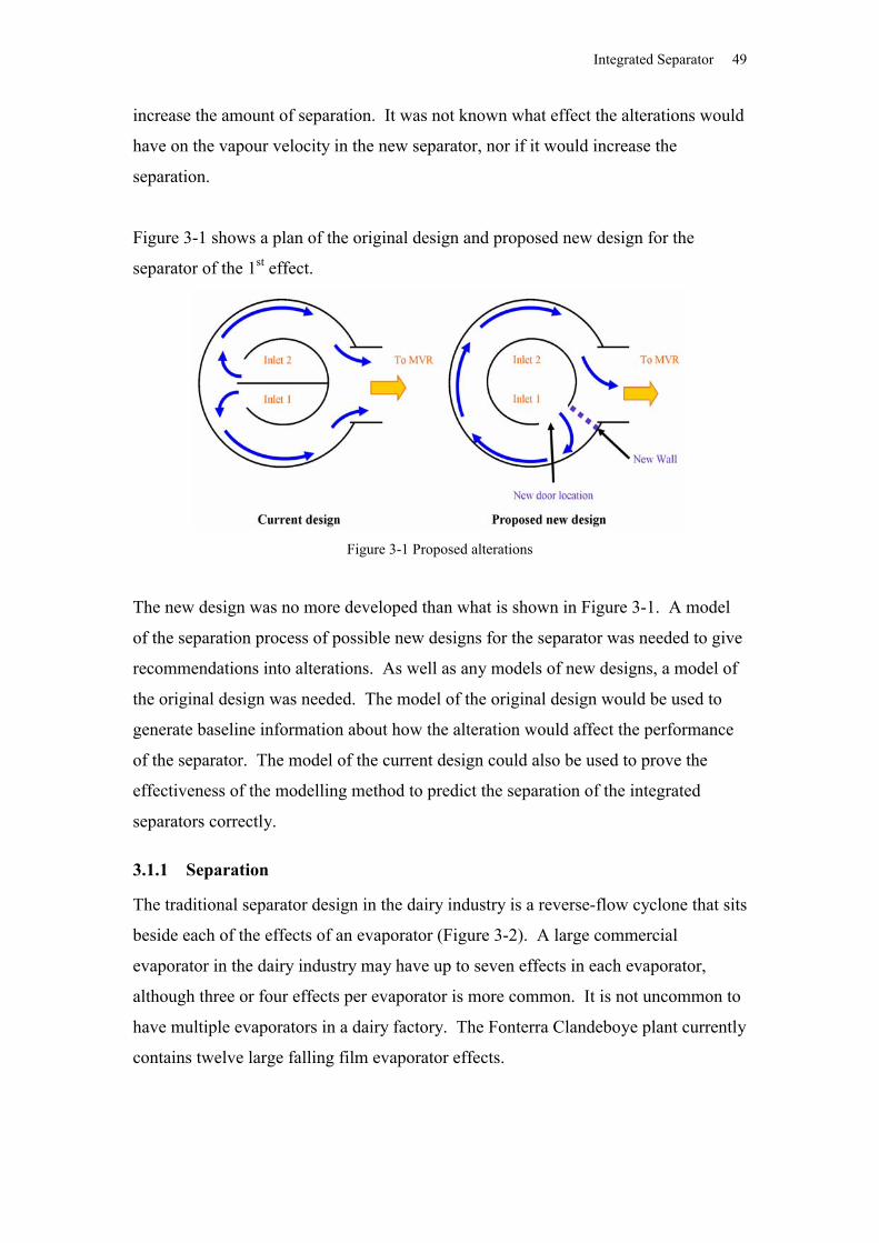
Integrated Separator 49
increase the amount of separation. It was not known what effect the alterations would
have on the vapour velocity in the new separator, nor if it would increase the
separation.
Figure 3-1 shows a plan of the original design and proposed new design for the
separator of the 1st effect.
Figure 3-1 Proposed alterations
The new design was no more developed than what is shown in Figure 3-1. A model
of the separation process of possible new designs for the separator was needed to give
recommendations into alterations. As well as any models of new designs, a model of
the original design was needed. The model of the original design would be used to
generate baseline information about how the alteration would affect the performance
of the separator. The model of the current design could also be used to prove the
effectiveness of the modelling method to predict the separation of the integrated
separators correctly.
3.1.1 Separation
The traditional separator design in the dairy industry is a reverse-flow cyclone that sits
beside each of the effects of an evaporator (Figure 3-2). A large commercial
evaporator in the dairy industry may have up to seven effects in each evaporator,
although three or four effects per evaporator is more common. It is not uncommon to
have multiple evaporators in a dairy factory. The Fonterra Clandeboye plant currently
contains twelve large falling film evaporator effects.
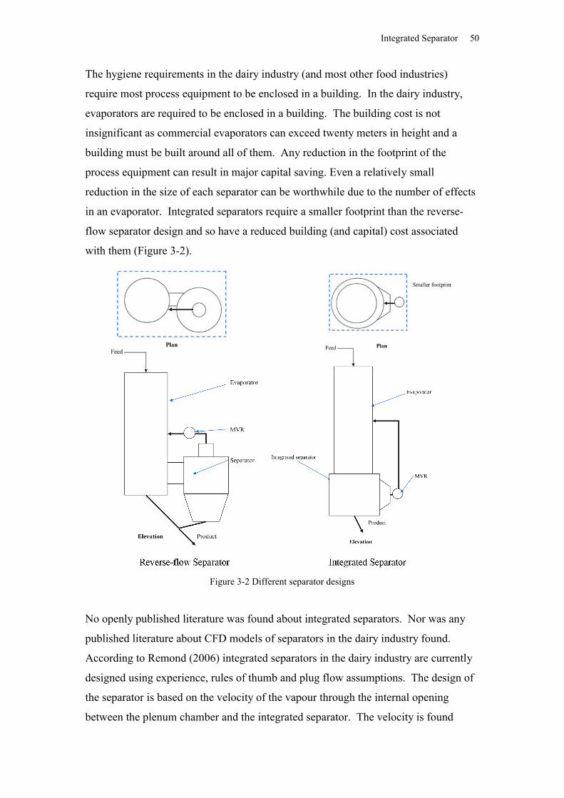
Integrated Separator 50
The hygiene requirements in the dairy industry (and most other food industries)
require most process equipment to be enclosed in a building. In the dairy industry,
evaporators are required to be enclosed in a building. The building cost is not
insignificant as commercial evaporators can exceed twenty meters in height and a
building must be built around all of them. Any reduction in the footprint of the
process equipment can result in major capital saving. Even a relatively small
reduction in the size of each separator can be worthwhile due to the number of effects
in an evaporator. Integrated separators require a smaller footprint than the reverse-
flow separator design and so have a reduced building (and capital) cost associated
with them (Figure 3-2).
Figure 3-2 Different separator designs
No openly published literature was found about integrated separators. Nor was any
published literature about CFD models of separators in the dairy industry found.
According to Remond (2006) integrated separators in the dairy industry are currently
designed using experience, rules of thumb and plug flow assumptions. The design of
the separator is based on the velocity of the vapour through the internal opening
between the plenum chamber and the integrated separator. The velocity is found
Integrated Separator 51
using a basic mass balance and by assuming plug flow through the opening.
Computational Fluid Dynamic (CFD) modelling is currently not used.
The design of these integrated separators is still evolving as new separators built for
Fonterra Ltd at their plant in Whareroa, New Zealand (2006) have a newer integrated
separator design. The new integrated separator design involves the vapour from each
pass doing a complete 360o rotation before exiting the separator. In the current
integrated separator the vapour only rotates 180o before exiting the separator.
Any CFD model of the integrated separator could greatly increase the understanding
of the complex vapour flows in separator, the separation process and could lead to
better designs.
3.1.2 Cyclone separatorsFayed and Otten (1984) describe a cyclone as a device without moving parts which
spins a gas stream to remove entrained particles/droplets by centrifugal force.
Cyclones are common in many industries. They are a robust separator design, able to
handle a range of loading. Cyclones normally are inexpensive to construct, simple to
maintain (no moving parts) and clean. Lui and Lipták (1997) and Fayed and Otten
(1984) both state that cyclones do a good job of collecting particle with diameter of
greater than 5m.
There are various cyclone designs available, but the common element is the use of
tangential velocity to produce a centrifugal force that separates the particle (or
droplets) out from the vapour. Most cyclone separators have double vapour vortexes
that expel the particles/droplets at the point where the vortex changes direction Corbitt
(1999).
The reversed-flow is probably the most common cyclone design (Figure 3-3). It is the
cyclone design which most of the experimental and theoretical cyclone work is based
on. The reverse flow cyclone is the traditional cyclone design for falling film
evaporators.
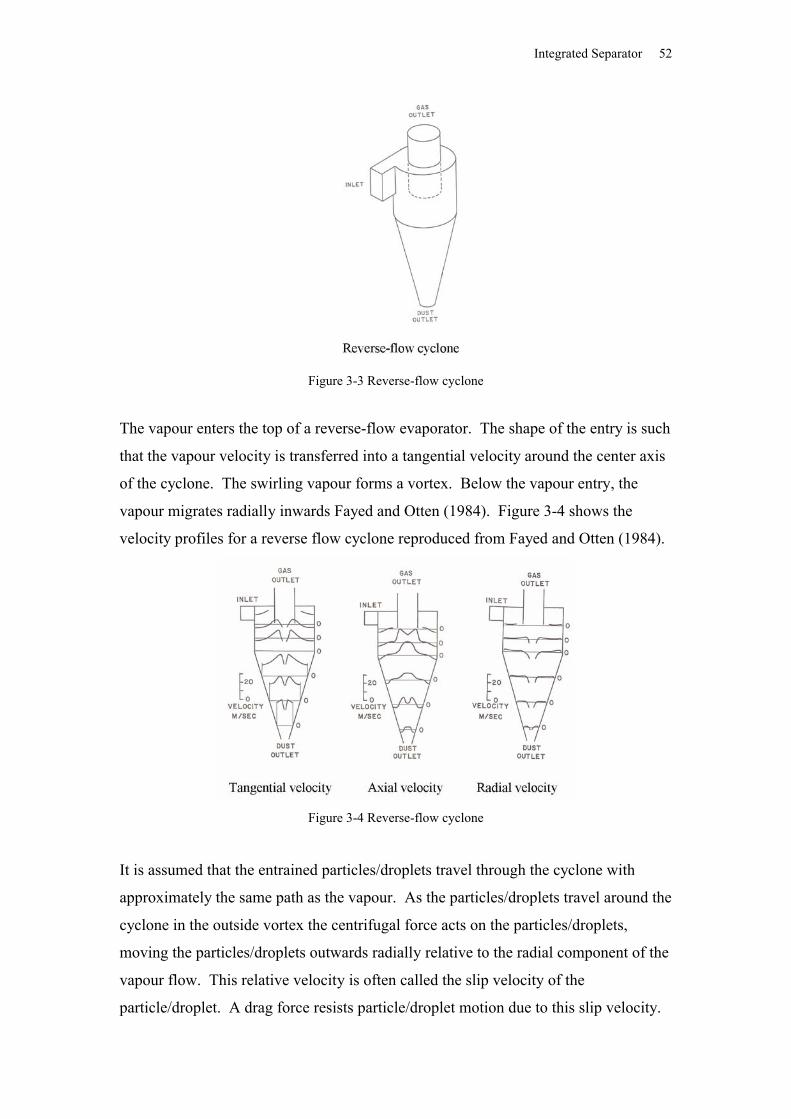
Integrated Separator 52
Figure 3-3 Reverse-flow cyclone
The vapour enters the top of a reverse-flow evaporator. The shape of the entry is such
that the vapour velocity is transferred into a tangential velocity around the center axis
of the cyclone. The swirling vapour forms a vortex. Below the vapour entry, the
vapour migrates radially inwards Fayed and Otten (1984). Figure 3-4 shows the
velocity profiles for a reverse flow cyclone reproduced from Fayed and Otten (1984).
Figure 3-4 Reverse-flow cyclone
It is assumed that the entrained particles/droplets travel through the cyclone with
approximately the same path as the vapour. As the particles/droplets travel around the
cyclone in the outside vortex the centrifugal force acts on the particles/droplets,
moving the particles/droplets outwards radially relative to the radial component of the
vapour flow. This relative velocity is often called the slip velocity of the
particle/droplet. A drag force resists particle/droplet motion due to this slip velocity.
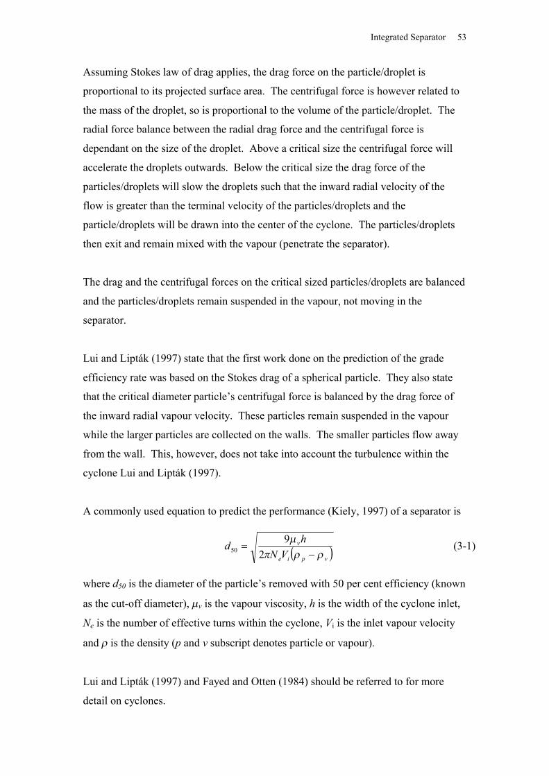
Integrated Separator 53
Assuming Stokes law of drag applies, the drag force on the particle/droplet is
proportional to its projected surface area. The centrifugal force is however related to
the mass of the droplet, so is proportional to the volume of the particle/droplet. The
radial force balance between the radial drag force and the centrifugal force is
dependant on the size of the droplet. Above a critical size the centrifugal force will
accelerate the droplets outwards. Below the critical size the drag force of the
particles/droplets will slow the droplets such that the inward radial velocity of the
flow is greater than the terminal velocity of the particles/droplets and the
particle/droplets will be drawn into the center of the cyclone. The particles/droplets
then exit and remain mixed with the vapour (penetrate the separator).
The drag and the centrifugal forces on the critical sized particles/droplets are balanced
and the particles/droplets remain suspended in the vapour, not moving in the
separator.
Lui and Lipták (1997) state that the first work done on the prediction of the grade
efficiency rate was based on the Stokes drag of a spherical particle. They also state
that the critical diameter particle’s centrifugal force is balanced by the drag force of
the inward radial vapour velocity. These particles remain suspended in the vapour
while the larger particles are collected on the walls. The smaller particles flow away
from the wall. This, however, does not take into account the turbulence within the
cyclone Lui and Lipták (1997).
A commonly used equation to predict the performance (Kiely, 1997) of a separator is
vpie
v
VNhd
29
50 (3-1)
where d50 is the diameter of the particle’s removed with 50 per cent efficiency (known
as the cut-off diameter), v is the vapour viscosity, h is the width of the cyclone inlet,
Ne is the number of effective turns within the cyclone, Vi is the inlet vapour velocity
and is the density (p and v subscript denotes particle or vapour).
Lui and Lipták (1997) and Fayed and Otten (1984) should be referred to for more
detail on cyclones.
Integrated Separator 54
3.1.3 Falling FilmsThe purpose of the separators attached to the falling film evaporators is to remove the
droplets that have formed as the falling film detaches from the tube wall and becomes
entrained in the water vapour. Knowledge about the structure of the falling film is
important for the correct prediction of the creation of droplets and their separation.
The thickness of a falling film can be described in a manner similar to that described
by Bird (1960). The shear force at the film interface is equal and opposite to the shear
force of the water vapour running co-current to the film. The shear force at the
interface is described by
tube
v
x LPD
xw
4
(3-2)
and
24 2
vvtubev
uD
fLP
(3-3)
where is the film thickness, w is the downward velocity, x is the distance inwards
from the tube wall, is the viscosity, D is the pipe diameter, Ltube is the length of tube,
Pv is the pressure drop down the pipe in the vapour phase and f is the fanning
friction factor number obtained from a pipe Moody diagram.
Under these conditions, the wetting rate (the mass flow m per unit width w) is
described by
32
2
32
l
l
l
vvl
gufwm
(3-4)
Equation 3-4 simplifies to that predicted by Nusselt’s film thickness Nusselt (Equation
3-5) when the vapour velocity is zero (Morison et al., 2006).
3/1
2.3
l
lNusselt g
(3-5)
Integrated Separator 55
Waves are known to form on laminar falling films. The Reynolds number for a film
Refilm is normally used to describe the onset of waves on falling films. Karapantsios
and Karabelas (1995) give the Reynolds number for a falling film as
lfilm
4Re (3-6)
where is the wetting rate and l is the dynamic viscosity of the liquid film.
Karapantsios and Karabelas (1995) state that regular almost sinusoidal shaped waves
are present on the film when Refilm is between ~5 and ~20 near the wave inspection
line. With increasing distance down the surface, the waves become unsteady and
irregular, eventually becoming fully developed after a distance.
Karapantsios and Karabelas (1995) carried out experimental work for films with Refilm
between 370 and 11,020 and found a film mean thickness film equal to
538.031
2
451.0
l
lmean g
(3-7)
where l is the kinematic viscosity of the liquid film and g is the gravitational
constant. Equation 3-7 predicts a lower film thickness to that predicted by equations
3-4 and 3-5.
Table 3-1 contains the minimum film thickness min, maximum film thickness max
and wave amplitude s found experimentally by Karapantsios and Karabelas (1995) at
2.5m down stream.
The evaporator’s tubes are approximately 14 meters in length, which is significantly
longer than the experimental distance. The waves should reach a fully developed
shape within this distance. Karapantsios and Karabelas (1995) concluded that the film
waves in their experimental system may not be fully developed. However, the lack of
any better experimental or theoretical work requires the use of results from
Karapantsios and Karabelas (1995).
Integrated Separator 56
Table 3-1 Data from Karapantsios and Karabelas (1995)
Refilm min, mm max, mm s, mm
370 0.1 0.5 0.07
700 0.11 1.1 0.15
830 0.11 1.5 0.20
1160 0.12 1.7 0.25
1490 0.12 2 0.30
1810 0.13 2 0.31
2470 0.13 2.5 0.40
3080 0.14 2.5 0.42
5290 0.15 3.5 0.60
7160 0.2 4.0 0.70
11020 0.3 4.5 0.75
Table 3-2 shows the different predicted film thickness for two products (skim milk
and MPC) using the wavy average thickness (equation 3-7) and the non-wavy
thickness (equations 3-4 and 3-5). The wetting rate, vapour flow rate and other
required raw data was from unpublished work of Broome (2005). The Reynolds
number for the film is shown. If the film Reynolds number is below 370, the non-
wavy thickness is used and above 370 the wavy thickness.
Table 3-2 Film thickness
Thickness mm
Effect Pass Refilm Non wavy Wavy Used
Skim 1 1 861 0.30 0.28 0.28
2 653 0.32 0.28 0.28
2 1 540 0.37 0.32 0.32
2 375 0.43 0.34 0.34
3 200 0.49 0.34 0.49
4 145 0.63 0.41 0.63
5 95 0.82 0.49 0.82
MPC 1 1 462 0.26 0.22 0.22
2 419 0.27 0.22 0.22
2 1 345 0.32 0.26 0.32
2 269 0.35 0.28 0.35
3 166 0.37 0.29 0.37
4 142 0.42 0.35 0.42
5 123 0.46 0.41 0.46
Integrated Separator 57
3.1.4 Droplet DistributionWhen the liquid film reaches the bottom of the heat transfer tubes it detaches from the
tubes. The film will break up and form droplets (Figure 3-5). The relative proportion
of the different droplet sizes is known as the droplet distribution. The separation rate
in cyclonic separators is known to be dependent on the droplet or particle size. The
prediction of the gross efficiency/penetration rate will depend on the droplet
distribution used.
The basic fluid flows for the film breakup are shown in Figure 3-5.
Figure 3-5 Falling film break up diagram
The film travels down the inside of the tube in a wavy film, with the vapour, that has
evaporated from the liquid, moving down the centre of the tube co-current to the film.
The velocity of this vapour will depend on the evaporation rate. Once the film
reaches the bottom of the tubes, it detaches from the tubes into the plenum chamber.
It is not possible to directly measure the droplet distribution because for hygiene
reasons, there is no access to sample the droplets. A literature search found no
previous experimental work describing the droplet distribution within a falling film
evaporator. GEA Process Engineering France, the design company for the
evaporators/ separators, was contacted and they have no measurements of this droplet
distribution either.
Integrated Separator 58
The film detaching from the bottom of the tubes will break up into droplets. The
process of the breakup of liquid into droplet is called atomisation. The atomisation
process is not well understood from a fundamental point of view; there is no general
theory of atomisation. A numerical simulation of the atomisation process is still not
possible, even with the high speed computers available today. There has been a
significant amount of experimental work done on the atomisation process, much of it
on particular atomisers. A review of the atomisation field is beyond the scope of the
project. Refer to Lefebrve (1989), Bayvel and Orzechowski (1993), and Schmehl et
al. (1999) for a more comprehensive review of the atomisation process.
Atomisers are used in industry and daily life to convert a liquid into droplets, for
example fuel injection in a petrol engine. There is a variety of different atomizer
designs. Typically atomisers are optimised for the production of small droplets. Most
atomisers are significantly smaller than the falling film tubes and the phases are run at
higher velocities than expected in the falling film evaporator. Most relationships
about the droplets produced by these atomisers in the published literature are based on
experimental work. The experimental work is typically used to produce empirically
fitted relationships that relates the performance of an atomiser for a given atomizer
design against the operating conditions and/or material properties.
Without the understanding of the basic principles of atomisation, it is difficult to
generalise any findings of the experimental work in the literature. The use of the
empirically fitted equations to predict a droplet distribution is limited to those cases
where the atomiser design and operating conditions are similar to the atomiser used in
the experimental work.
Several atomisation processes with experimental results were found that are similar to
the falling film atomisation.
atomisation of a planar liquid sheet
atomisation of a prefilming air-blast atomiser
round jet breakup (linear and non-linear breakup)
The three previous cases use empirically fitted relationships. Some of the fitting
parameters are specific to the geometry and/or flow rates of the atomizer used. What
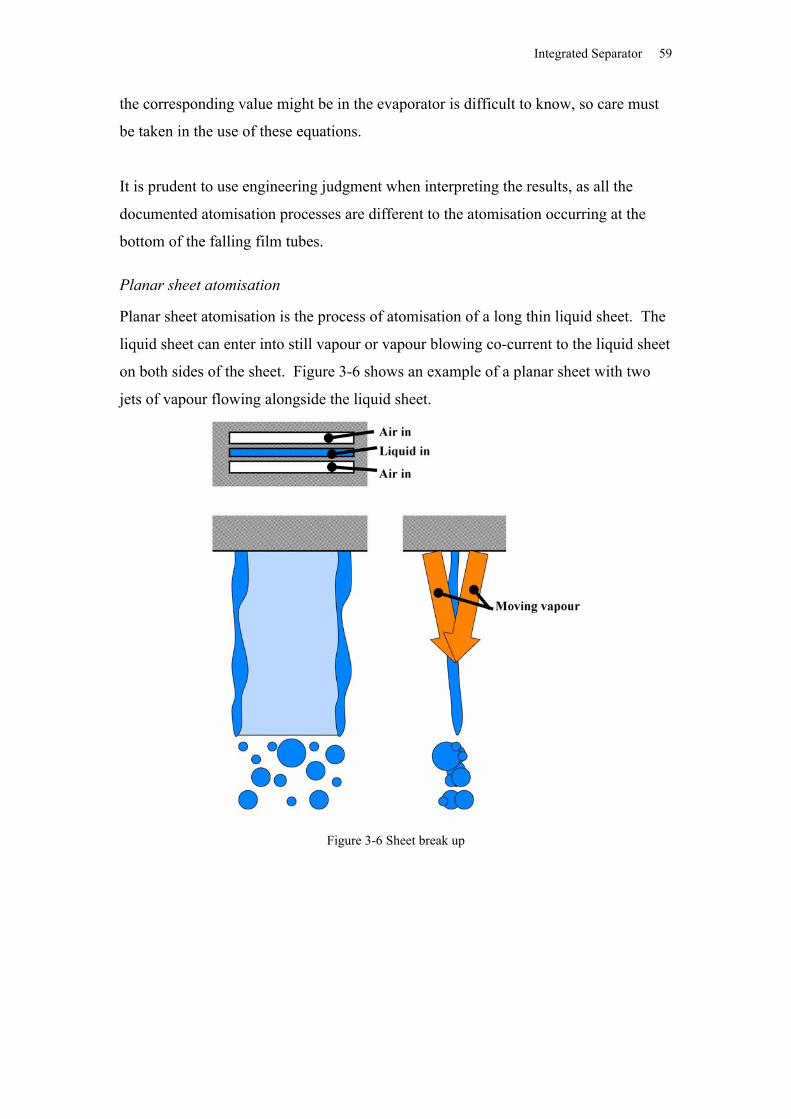
Integrated Separator 59
the corresponding value might be in the evaporator is difficult to know, so care must
be taken in the use of these equations.
It is prudent to use engineering judgment when interpreting the results, as all the
documented atomisation processes are different to the atomisation occurring at the
bottom of the falling film tubes.
Planar sheet atomisation
Planar sheet atomisation is the process of atomisation of a long thin liquid sheet. The
liquid sheet can enter into still vapour or vapour blowing co-current to the liquid sheet
on both sides of the sheet. Figure 3-6 shows an example of a planar sheet with two
jets of vapour flowing alongside the liquid sheet.
Figure 3-6 Sheet break up
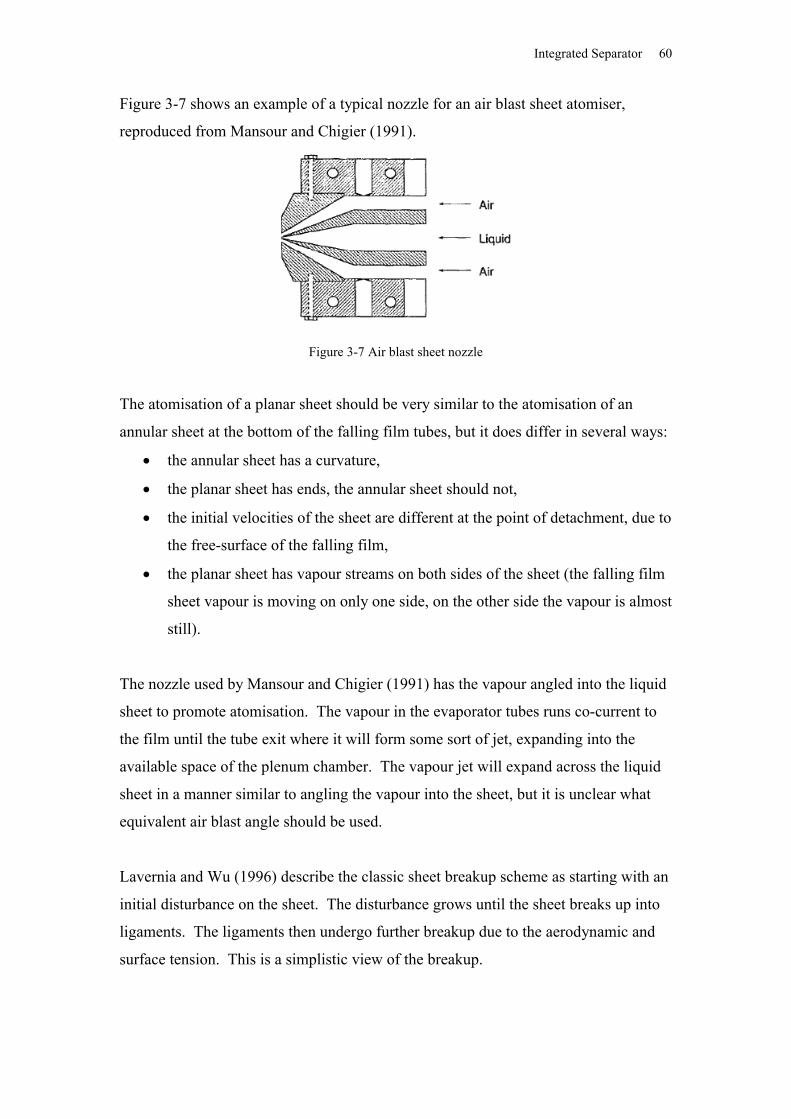
Integrated Separator 60
Figure 3-7 shows an example of a typical nozzle for an air blast sheet atomiser,
reproduced from Mansour and Chigier (1991).
Figure 3-7 Air blast sheet nozzle
The atomisation of a planar sheet should be very similar to the atomisation of an
annular sheet at the bottom of the falling film tubes, but it does differ in several ways:
the annular sheet has a curvature,
the planar sheet has ends, the annular sheet should not,
the initial velocities of the sheet are different at the point of detachment, due to
the free-surface of the falling film,
the planar sheet has vapour streams on both sides of the sheet (the falling film
sheet vapour is moving on only one side, on the other side the vapour is almost
still).
The nozzle used by Mansour and Chigier (1991) has the vapour angled into the liquid
sheet to promote atomisation. The vapour in the evaporator tubes runs co-current to
the film until the tube exit where it will form some sort of jet, expanding into the
available space of the plenum chamber. The vapour jet will expand across the liquid
sheet in a manner similar to angling the vapour into the sheet, but it is unclear what
equivalent air blast angle should be used.
Lavernia and Wu (1996) describe the classic sheet breakup scheme as starting with an
initial disturbance on the sheet. The disturbance grows until the sheet breaks up into
ligaments. The ligaments then undergo further breakup due to the aerodynamic and
surface tension. This is a simplistic view of the breakup.
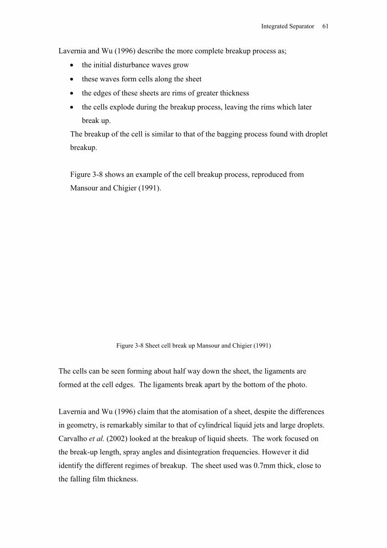
Integrated Separator 61
Lavernia and Wu (1996) describe the more complete breakup process as;
the initial disturbance waves grow
these waves form cells along the sheet
the edges of these sheets are rims of greater thickness
the cells explode during the breakup process, leaving the rims which later
break up.
The breakup of the cell is similar to that of the bagging process found with droplet
breakup.
Figure 3-8 shows an example of the cell breakup process, reproduced from
Mansour and Chigier (1991).
Figure 3-8 Sheet cell break up Mansour and Chigier (1991)
The cells can be seen forming about half way down the sheet, the ligaments are
formed at the cell edges. The ligaments break apart by the bottom of the photo.
Lavernia and Wu (1996) claim that the atomisation of a sheet, despite the differences
in geometry, is remarkably similar to that of cylindrical liquid jets and large droplets.
Carvalho et al. (2002) looked at the breakup of liquid sheets. The work focused on
the break-up length, spray angles and disintegration frequencies. However it did
identify the different regimes of breakup. The sheet used was 0.7mm thick, close to
the falling film thickness.
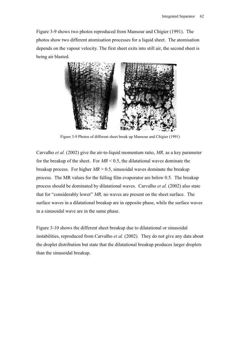
Integrated Separator 62
Figure 3-9 shows two photos reproduced from Mansour and Chigier (1991). The
photos show two different atomisation processes for a liquid sheet. The atomisation
depends on the vapour velocity. The first sheet exits into still air, the second sheet is
being air blasted.
Figure 3-9 Photos of different sheet break up Mansour and Chigier (1991)
Carvalho et al. (2002) give the air-to-liquid momentum ratio, MR, as a key parameter
for the breakup of the sheet. For MR < 0.5, the dilatational waves dominate the
breakup process. For higher MR > 0.5, sinusoidal waves dominate the breakup
process. The MR values for the falling film evaporator are below 0.5. The breakup
process should be dominated by dilatational waves. Carvalho et al. (2002) also state
that for “considerably lower” MR, no waves are present on the sheet surface. The
surface waves in a dilatational breakup are in opposite phase, while the surface waves
in a sinusoidal wave are in the same phase.
Figure 3-10 shows the different sheet breakup due to dilatational or sinusoidal
instabilities, reproduced from Carvalho et al. (2002). They do not give any data about
the droplet distribution but state that the dilatational breakup produces larger droplets
than the sinusoidal breakup.
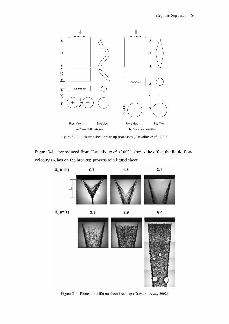
Integrated Separator 63
Figure 3-10 Different sheet break up processes (Carvalho et al., 2002)
Figure 3-11, reproduced from Carvalho et al. (2002), shows the effect the liquid flow
velocity UL has on the breakup process of a liquid sheet.
Figure 3-11 Photos of different sheet break up (Carvalho et al., 2002)
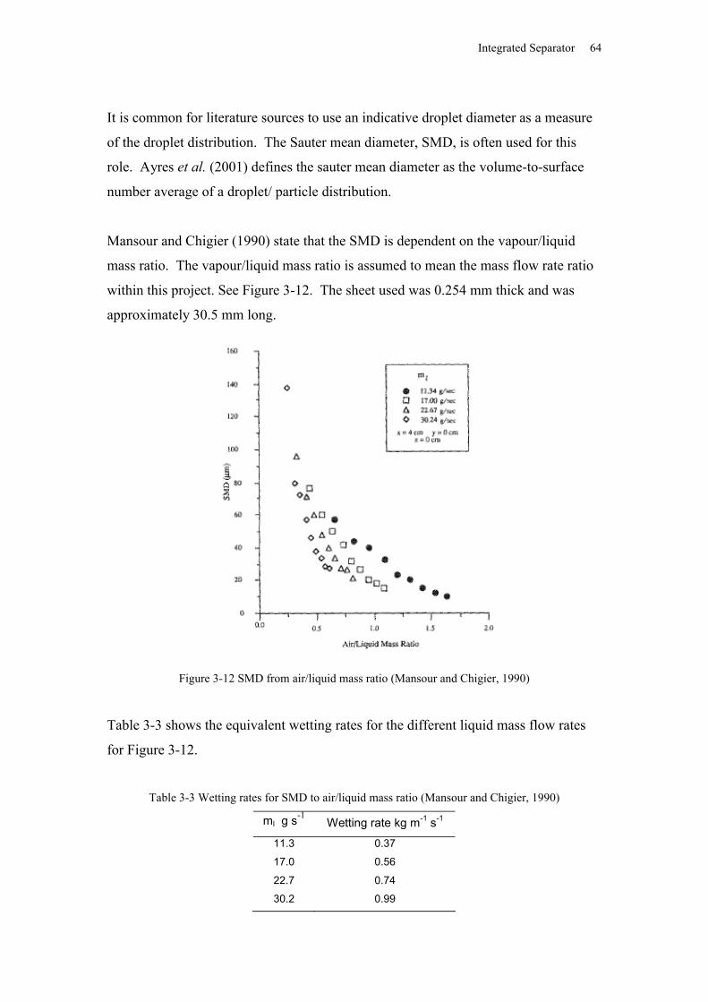
Integrated Separator 64
It is common for literature sources to use an indicative droplet diameter as a measure
of the droplet distribution. The Sauter mean diameter, SMD, is often used for this
role. Ayres et al. (2001) defines the sauter mean diameter as the volume-to-surface
number average of a droplet/ particle distribution.
Mansour and Chigier (1990) state that the SMD is dependent on the vapour/liquid
mass ratio. The vapour/liquid mass ratio is assumed to mean the mass flow rate ratio
within this project. See Figure 3-12. The sheet used was 0.254 mm thick and was
approximately 30.5 mm long.
Figure 3-12 SMD from air/liquid mass ratio (Mansour and Chigier, 1990)
Table 3-3 shows the equivalent wetting rates for the different liquid mass flow rates
for Figure 3-12.
Table 3-3 Wetting rates for SMD to air/liquid mass ratio (Mansour and Chigier, 1990)
ml g s-1Wetting rate kg m-1 s-1
11.3 0.37
17.0 0.56
22.7 0.74
30.2 0.99
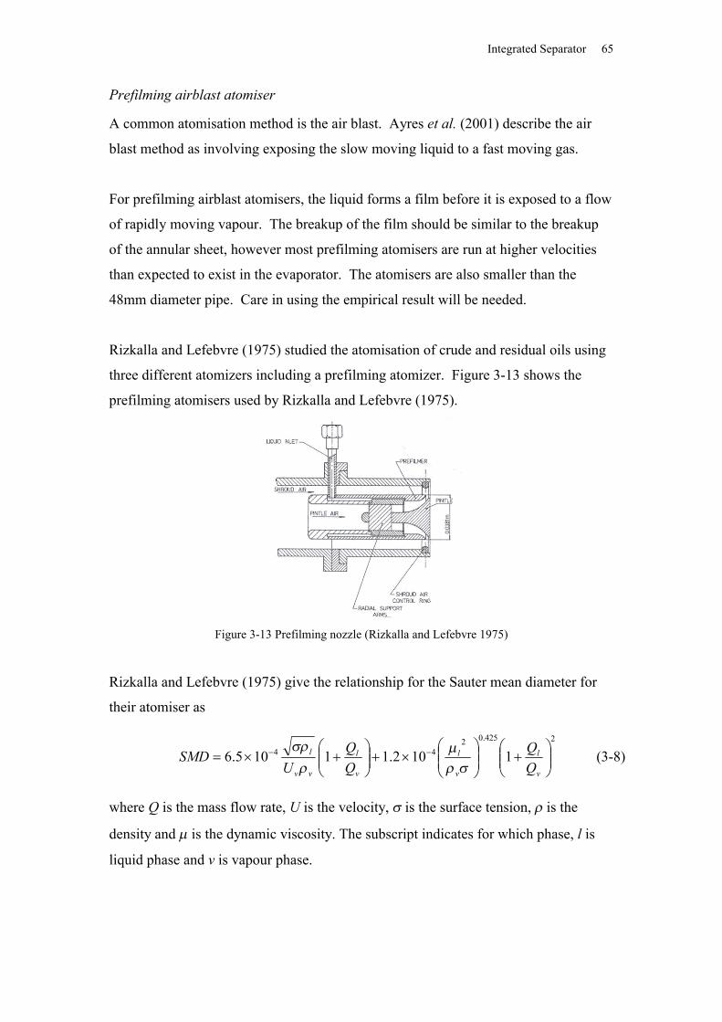
Integrated Separator 65
Prefilming airblast atomiser
A common atomisation method is the air blast. Ayres et al. (2001) describe the air
blast method as involving exposing the slow moving liquid to a fast moving gas.
For prefilming airblast atomisers, the liquid forms a film before it is exposed to a flow
of rapidly moving vapour. The breakup of the film should be similar to the breakup
of the annular sheet, however most prefilming atomisers are run at higher velocities
than expected to exist in the evaporator. The atomisers are also smaller than the
48mm diameter pipe. Care in using the empirical result will be needed.
Rizkalla and Lefebvre (1975) studied the atomisation of crude and residual oils using
three different atomizers including a prefilming atomizer. Figure 3-13 shows the
prefilming atomisers used by Rizkalla and Lefebvre (1975).
Figure 3-13 Prefilming nozzle (Rizkalla and Lefebvre 1975)
Rizkalla and Lefebvre (1975) give the relationship for the Sauter mean diameter for
their atomiser as
2425.0244 1102.11105.6
v
l
v
l
v
l
vv
l
USMD
(3-8)
where Q is the mass flow rate, U is the velocity, is the surface tension, is the
density and is the dynamic viscosity. The subscript indicates for which phase, l is
liquid phase and v is vapour phase.
Integrated Separator 66
Table 3-4 shows the cited range of experimentation used to produce equation 3-8.
The viscosity, surface tension and density of the liquids processed in the falling film
evaporator are similar to the liquids experimented on by Rizkalla and Lefebvre
(1975). The Rizkalla and Lefebvre (1975) experimented using air the falling film
equivalent is water vapour.
Table 3-4 Experimental rang of Rizkalla and Lefebvre (1975)
Variable Range Units
Liquid viscosity 0.001 to 0.044 Pa s
Surface tension 0.026 to 0.074 N m-1
Liquid density 780 to 1500 kg m-3
Air velocity 10 to 125 m s-1
Air temperature 296 to 424 K
Air pressure 105 to 8.5 x 10⁵ N m2
Air/ liquid mass flow rate ratio 2 to 6
Jasuja (1979) extended the work of Rizkalla and Lefebvre (1975) to produce
empirically fitted equations for the Sauter mean diameter,
l
v
v
ll Q
QSMD
1106.0100.1
425.0243
(3-9)
Table 3-5 shows the cited range of experimentation used to produce equation 3-9.
Table 3-5 Experimental rang of Jasuja (1979)
Variable Range Units
Liquid viscosity 0.001 to 0.086 Pa s
Air velocity 55 to 135 m s-1
Air/ liquid ratio 1 to 8
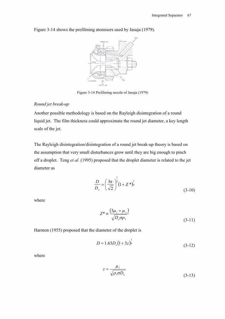
Integrated Separator 67
Figure 3-14 shows the prefilming atomisers used by Jasuja (1979).
Figure 3-14 Prefilming nozzle of Jasuja (1979)
Round jet break-up
Another possible methodology is based on the Rayleigh disintegration of a round
liquid jet. The film thickness could approximate the round jet diameter, a key length
scale of the jet.
The Rayleigh disintegration/disintegration of a round jet break-up theory is based on
the assumption that very small disturbances grow until they are big enough to pinch
off a droplet. Teng et al. (1995) proposed that the droplet diameter is related to the jet
diameter as
613
1
*12
3 ZDD
o
(3-10)
where
lo
vl
DZ
3*
(3-11)
Harmon (1955) proposed that the diameter of the droplet is
61
3163.1 zDD o (3-12)
where
ol
l
Dz
(3-13)
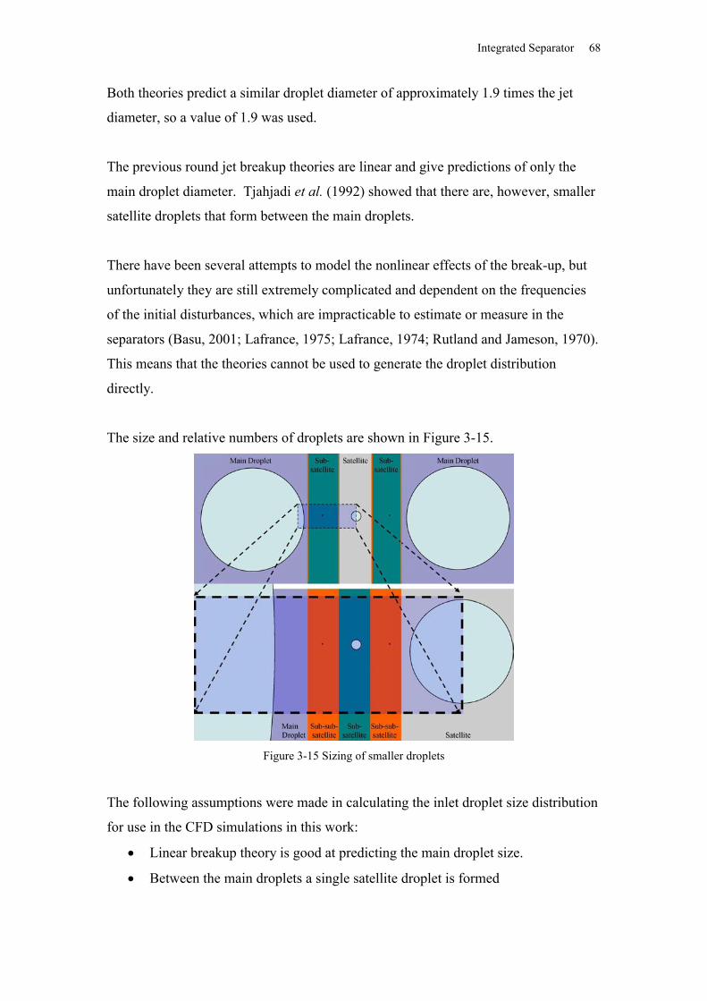
Integrated Separator 68
Both theories predict a similar droplet diameter of approximately 1.9 times the jet
diameter, so a value of 1.9 was used.
The previous round jet breakup theories are linear and give predictions of only the
main droplet diameter. Tjahjadi et al. (1992) showed that there are, however, smaller
satellite droplets that form between the main droplets.
There have been several attempts to model the nonlinear effects of the break-up, but
unfortunately they are still extremely complicated and dependent on the frequencies
of the initial disturbances, which are impracticable to estimate or measure in the
separators (Basu, 2001; Lafrance, 1975; Lafrance, 1974; Rutland and Jameson, 1970).
This means that the theories cannot be used to generate the droplet distribution
directly.
The size and relative numbers of droplets are shown in Figure 3-15.
Figure 3-15 Sizing of smaller droplets
The following assumptions were made in calculating the inlet droplet size distribution
for use in the CFD simulations in this work:
Linear breakup theory is good at predicting the main droplet size.
Between the main droplets a single satellite droplet is formed
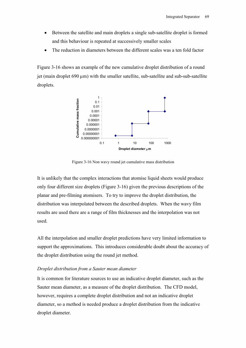
Integrated Separator 69
Between the satellite and main droplets a single sub-satellite droplet is formed
and this behaviour is repeated at successively smaller scales
The reduction in diameters between the different scales was a ten fold factor
Figure 3-16 shows an example of the new cumulative droplet distribution of a round
jet (main droplet 690 m) with the smaller satellite, sub-satellite and sub-sub-satellite
droplets.
0.0000000010.000000010.00000010.0000010.000010.00010.0010.010.1
1
0.1 1 10 100 1000
Droplet diameter m
Cum
ulat
ive
mas
s fr
actio
n
Figure 3-16 Non wavy round jet cumulative mass distribution
It is unlikely that the complex interactions that atomise liquid sheets would produce
only four different size droplets (Figure 3-16) given the previous descriptions of the
planar and pre-filming atomisers. To try to improve the droplet distribution, the
distribution was interpolated between the described droplets. When the wavy film
results are used there are a range of film thicknesses and the interpolation was not
used.
All the interpolation and smaller droplet predictions have very limited information to
support the approximations. This introduces considerable doubt about the accuracy of
the droplet distribution using the round jet method.
Droplet distribution from a Sauter mean diameter
It is common for literature sources to use an indicative droplet diameter, such as the
Sauter mean diameter, as a measure of the droplet distribution. The CFD model,
however, requires a complete droplet distribution and not an indicative droplet
diameter, so a method is needed produce a droplet distribution from the indicative
droplet diameter.
Integrated Separator 70
Semiao et al. (1996) used an informational entropy method based on the Nukiyama-
Tanasawa function to produce a droplet distribution that only requires the Sauter
Mean Diameter. The droplet distribution is from
SMDdDe
SMDDdN
SMDD 3
3
35
1
2
3
353
(3-14)
where (n) is the gamma function
0
1dxxen nx (3-15)
Microsoft Excel gives (5/3) the value of 0.902745.
The volume fraction V can be found from
SMDdDe
SMDDdV
SMDD 3
6
35
1
5
6
353
(3-16)
Walzel (1984) states that the log-normal distribution with a maximum drop size is
often used to describe the droplet distribution. The log-normal distribution f(D) is
defined as
2
lnln
21
2ln1
ABD
eAD
Df
(3-17)
where A and B are constants, and D is the droplet diameter. Equation 3-17 requires
values for both constants. If the only information known about a droplet distribution
is its SMD diameter then the log-normal distribution can not be used, as equation 3-17
will be under-constrained.
Integrated Separator 71
Droplet Deformation and secondary break-up
Droplets can undergo further atomisation after the initial atomisation at the bottom of
the tube bundle. Schmelz and Walzel (2003) cite Reinhard (1964) who gives the
critical We number between 9 and 10 for the onset of droplet breakup. Schmelz and
Walzel (2003) also cite Hinze (1955) and Hass (1964) giving a We of 13 for the onset
of droplet breakup. The Weber number, We, is a dimensionless number relating the
aerodynamic force to the surface tension forces and is found from
2V v lD U U
We
(3-18)
where D is the droplet diameter m, Uv is the velocity of the vapour, Ul is the velocity
of the droplet, v is the vapour density, is the surface tension coefficient for the
liquid vapour.
Schmelz and Walzel (2003) reports that Hsiang and Faeth (1995) give criteria for
deformation as well as the mode of breakup (see Table 3-6).
Table 3-6 Conditions for droplet breakup (Hsiang and Faeth, 1995)
Droplet condition Criteria
Undisturbed/ spherical We < 0.6
Up to 5% deformation 0.6 < We < 1
Up to 10% deformation 1 < We < 2.1
Up to 20% deformation 2.1 < We < 3
Oscillation of droplet 3 < We < 12
Bag breakup 12 < We < 20
Bag-stamen breakup 20 < We < 50
Multi-mode breakup 50 < We < 350
Shear breakup 350 < We
3.2 Process Flow DiagramThe falling film evaporator studied during this project contains four effects. Each of
the first two effects has mechanical vapour recompression (MVR), and the majority of
the Cow Water is evaporated from their feed. The recompressed vapour is used as the
heat source for the effect. A smaller percentage of the vapour is used downstream
(bypass flow) as a heat source for the next effect. The first effect also has a small
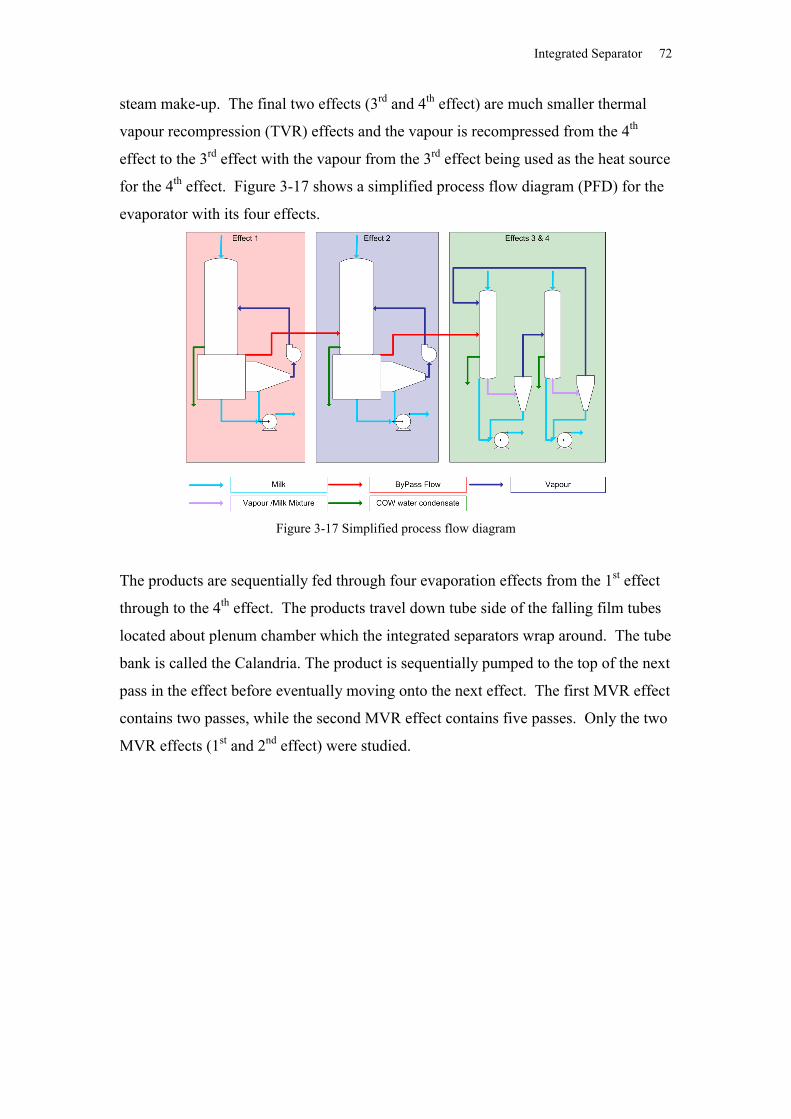
Integrated Separator 72
steam make-up. The final two effects (3rd and 4th effect) are much smaller thermal
vapour recompression (TVR) effects and the vapour is recompressed from the 4th
effect to the 3rd effect with the vapour from the 3rd effect being used as the heat source
for the 4th effect. Figure 3-17 shows a simplified process flow diagram (PFD) for the
evaporator with its four effects.
Figure 3-17 Simplified process flow diagram
The products are sequentially fed through four evaporation effects from the 1st effect
through to the 4th effect. The products travel down tube side of the falling film tubes
located about plenum chamber which the integrated separators wrap around. The tube
bank is called the Calandria. The product is sequentially pumped to the top of the next
pass in the effect before eventually moving onto the next effect. The first MVR effect
contains two passes, while the second MVR effect contains five passes. Only the two
MVR effects (1st and 2nd effect) were studied.
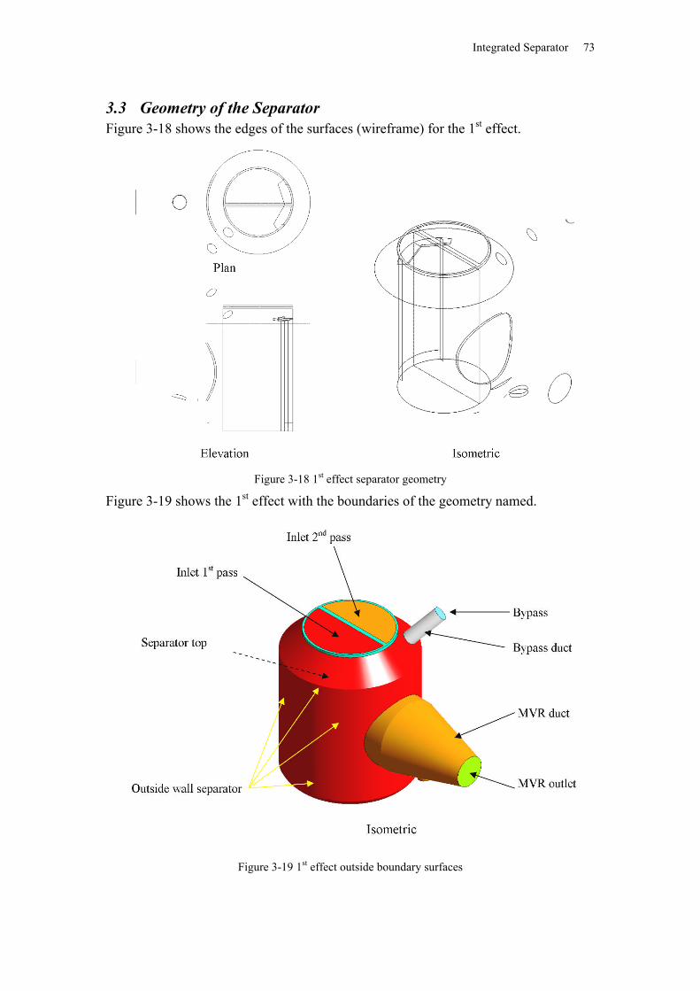
Integrated Separator 73
3.3 Geometry of the SeparatorFigure 3-18 shows the edges of the surfaces (wireframe) for the 1st effect.
Figure 3-18 1st effect separator geometry
Figure 3-19 shows the 1st effect with the boundaries of the geometry named.
Figure 3-19 1st effect outside boundary surfaces
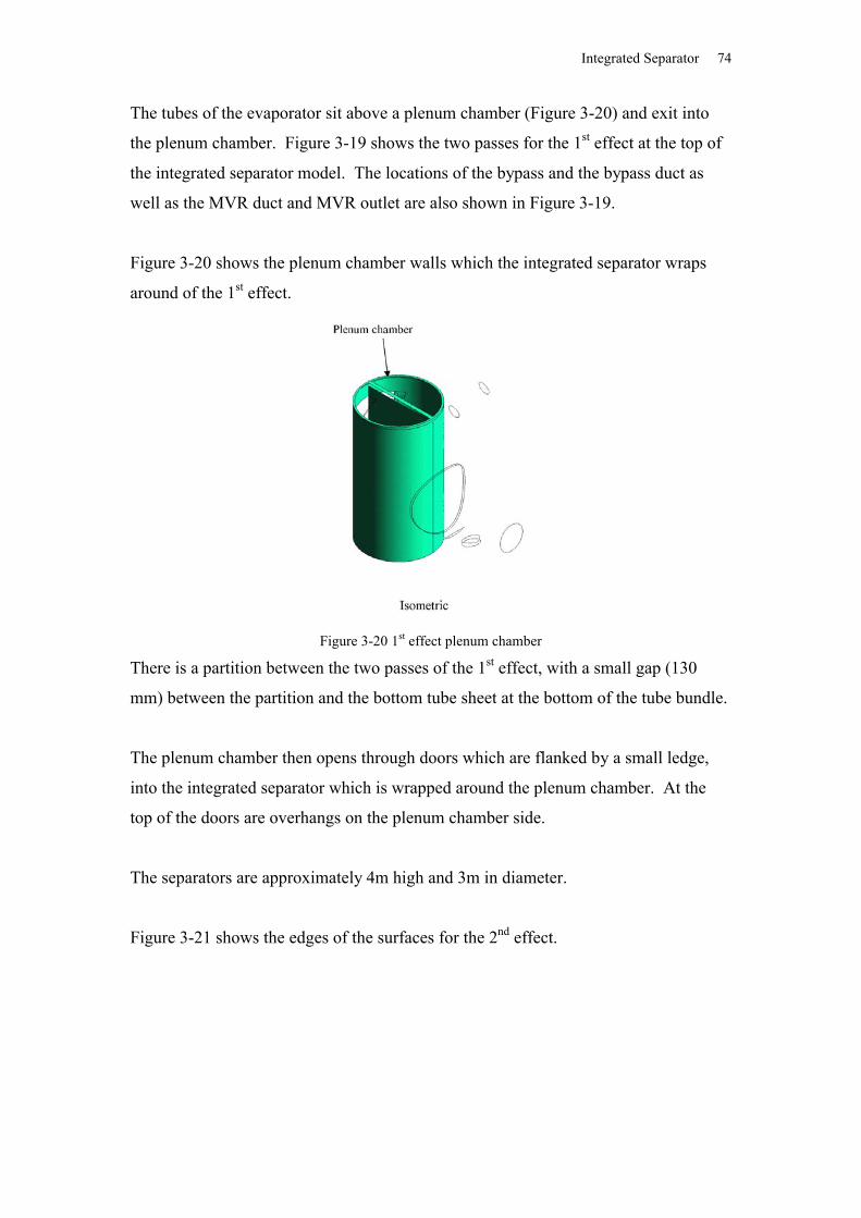
Integrated Separator 74
The tubes of the evaporator sit above a plenum chamber (Figure 3-20) and exit into
the plenum chamber. Figure 3-19 shows the two passes for the 1st effect at the top of
the integrated separator model. The locations of the bypass and the bypass duct as
well as the MVR duct and MVR outlet are also shown in Figure 3-19.
Figure 3-20 shows the plenum chamber walls which the integrated separator wraps
around of the 1st effect.
Figure 3-20 1st effect plenum chamber
There is a partition between the two passes of the 1st effect, with a small gap (130
mm) between the partition and the bottom tube sheet at the bottom of the tube bundle.
The plenum chamber then opens through doors which are flanked by a small ledge,
into the integrated separator which is wrapped around the plenum chamber. At the
top of the doors are overhangs on the plenum chamber side.
The separators are approximately 4m high and 3m in diameter.
Figure 3-21 shows the edges of the surfaces for the 2nd effect.
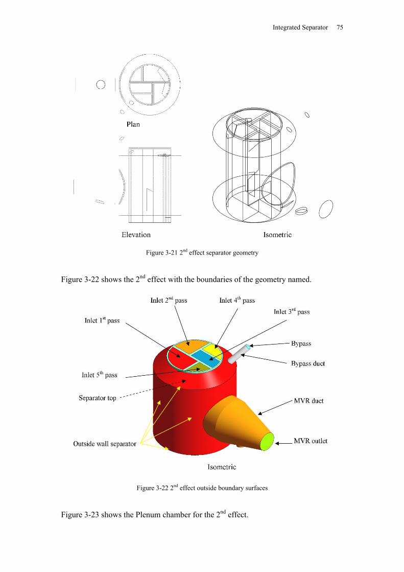
Integrated Separator 75
Figure 3-21 2nd effect separator geometry
Figure 3-22 shows the 2nd effect with the boundaries of the geometry named.
Figure 3-22 2nd effect outside boundary surfaces
Figure 3-23 shows the Plenum chamber for the 2nd effect.
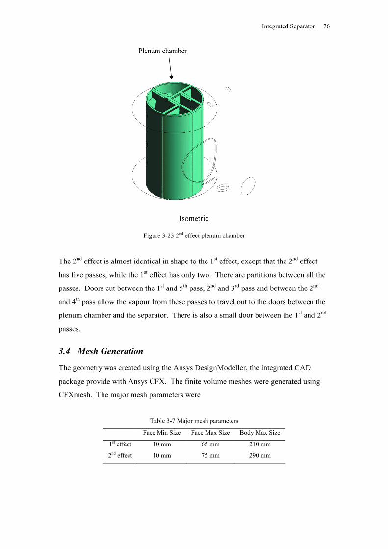
Integrated Separator 76
Figure 3-23 2nd effect plenum chamber
The 2nd effect is almost identical in shape to the 1st effect, except that the 2nd effect
has five passes, while the 1st effect has only two. There are partitions between all the
passes. Doors cut between the 1st and 5th pass, 2nd and 3rd pass and between the 2nd
and 4th pass allow the vapour from these passes to travel out to the doors between the
plenum chamber and the separator. There is also a small door between the 1st and 2nd
passes.
3.4 Mesh Generation
The geometry was created using the Ansys DesignModeller, the integrated CAD
package provide with Ansys CFX. The finite volume meshes were generated using
CFXmesh. The major mesh parameters were
Table 3-7 Major mesh parameters
Face Min Size Face Max Size Body Max Size
1st effect 10 mm 65 mm 210 mm
2nd effect 10 mm 75 mm 290 mm
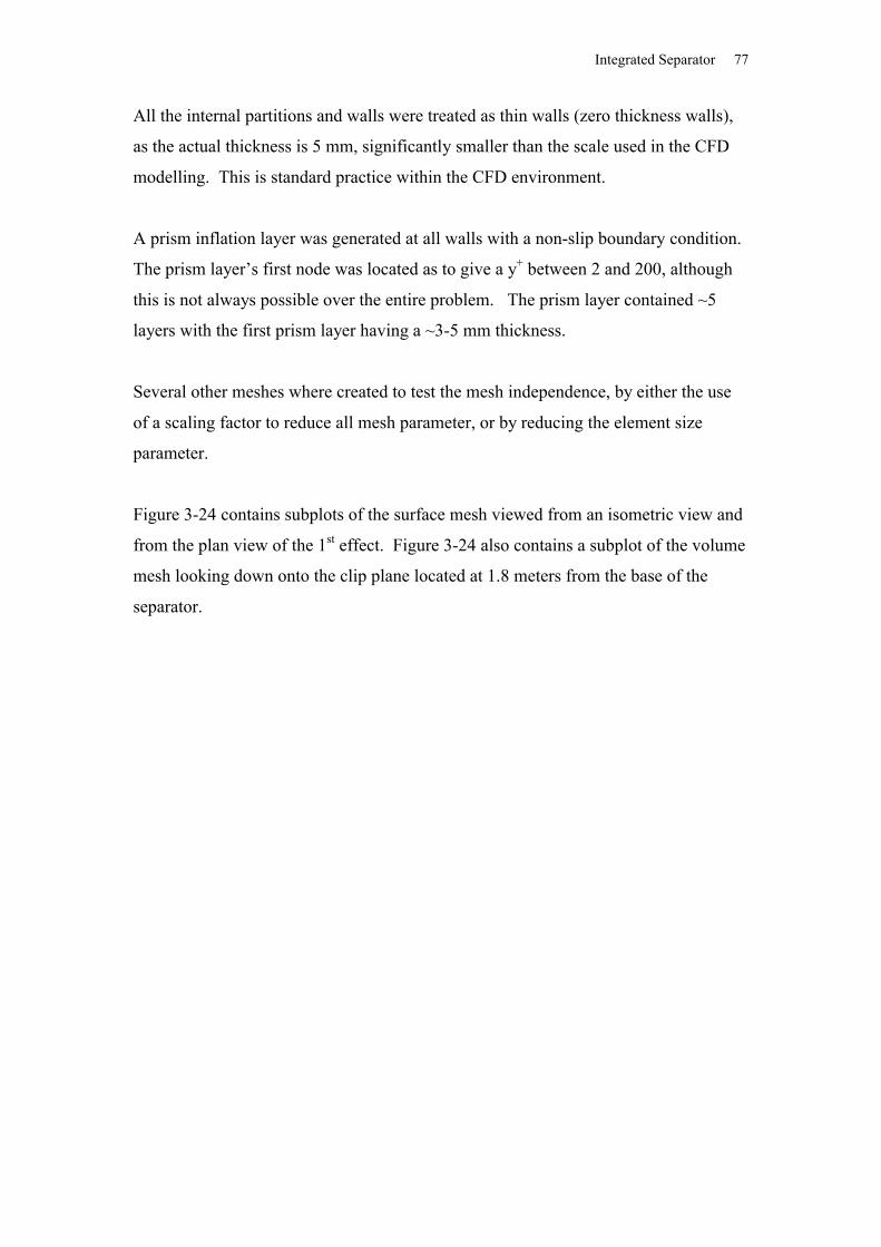
Integrated Separator 77
All the internal partitions and walls were treated as thin walls (zero thickness walls),
as the actual thickness is 5 mm, significantly smaller than the scale used in the CFD
modelling. This is standard practice within the CFD environment.
A prism inflation layer was generated at all walls with a non-slip boundary condition.
The prism layer’s first node was located as to give a y+ between 2 and 200, although
this is not always possible over the entire problem. The prism layer contained ~5
layers with the first prism layer having a ~3-5 mm thickness.
Several other meshes where created to test the mesh independence, by either the use
of a scaling factor to reduce all mesh parameter, or by reducing the element size
parameter.
Figure 3-24 contains subplots of the surface mesh viewed from an isometric view and
from the plan view of the 1st effect. Figure 3-24 also contains a subplot of the volume
mesh looking down onto the clip plane located at 1.8 meters from the base of the
separator.
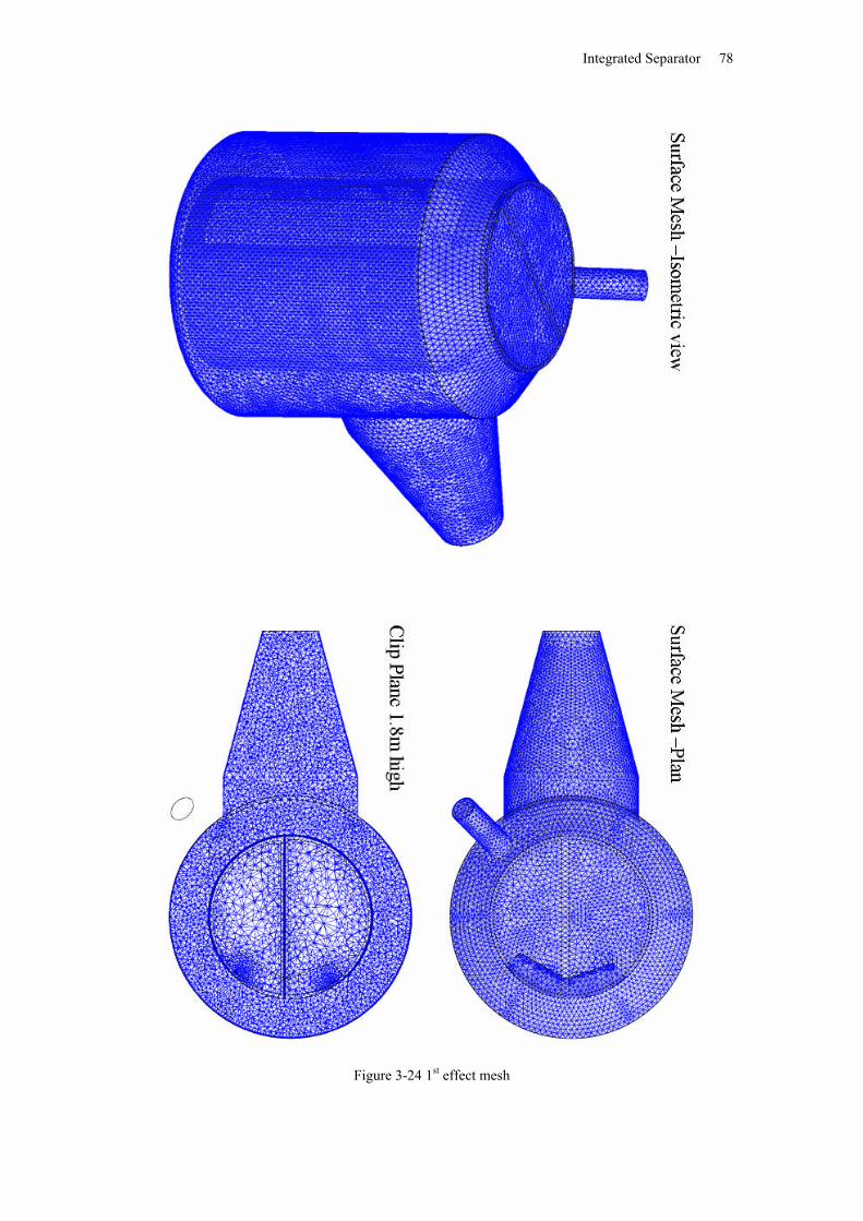
Integrated Separator 78
Figure 3-24 1st effect mesh
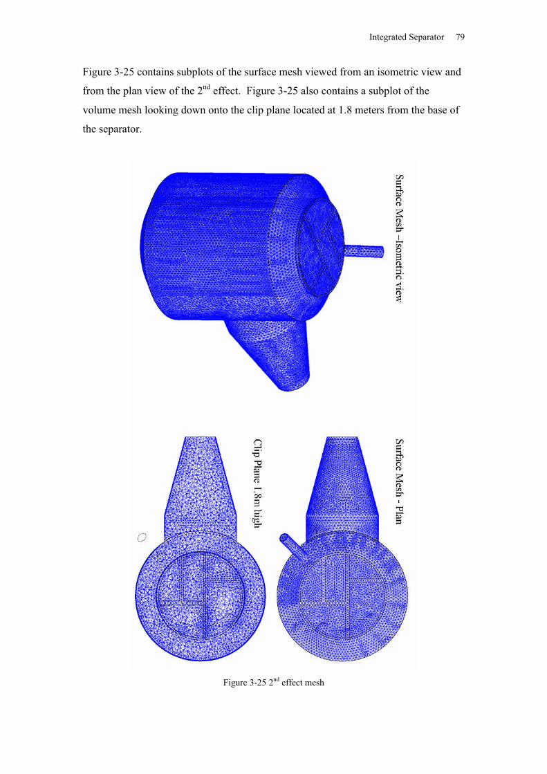
Integrated Separator 79
Figure 3-25 contains subplots of the surface mesh viewed from an isometric view and
from the plan view of the 2nd effect. Figure 3-25 also contains a subplot of the
volume mesh looking down onto the clip plane located at 1.8 meters from the base of
the separator.
Figure 3-25 2nd effect mesh
Integrated Separator 80
3.4.1 General grid interface (GGI)
Due the difficulties of generating a single mesh of the entire separator, it was decided
to split the mesh into two (or more) meshes, one for the separator and one the
calandria. The two meshes where then joined using a GGI.
GGI is an interpolation method between similar or same surfaces with different
meshes for each side of the interface.
The details of the GGI are not given in the Ansys CFX manual, however the manual
claims that GGI have the following attributes.
“
1. Strict conservation is maintained across the interface, for all fluxes of all
equations (after accounting for changes in pitch).
2. The interface treatment is fully implicit, so that the presence of an interface
does not adversely affect overall solution convergence.
3. The interface is applicable to incompressible, subsonic, transonic and
supersonic flow conditions, and all model options within ANSYS CFX (e.g.,
turbulence models, multiphase models, mixture models, CHT, reaction, etc.).
4. The interface accounts internally for pitch change by scaling up or down (as
required) the local flows as they cross the interface, for the case of frame
change interfaces.
5. Any number of GGI connection conditions are possible within a
computational domain.”
The use of the GGIs should not have an effect on the solution.
3.5 CFD Model
The CFD model was implemented using the commercial code ANSYS CFX 10. The major choices made in implementing this code were:
The separators were modelled under steady state conditions.
Isothermal conditions were assumed
Flow was incompressible
The SST turbulence model was used
The Ansys CFX 10 high-resolution differencing scheme was used
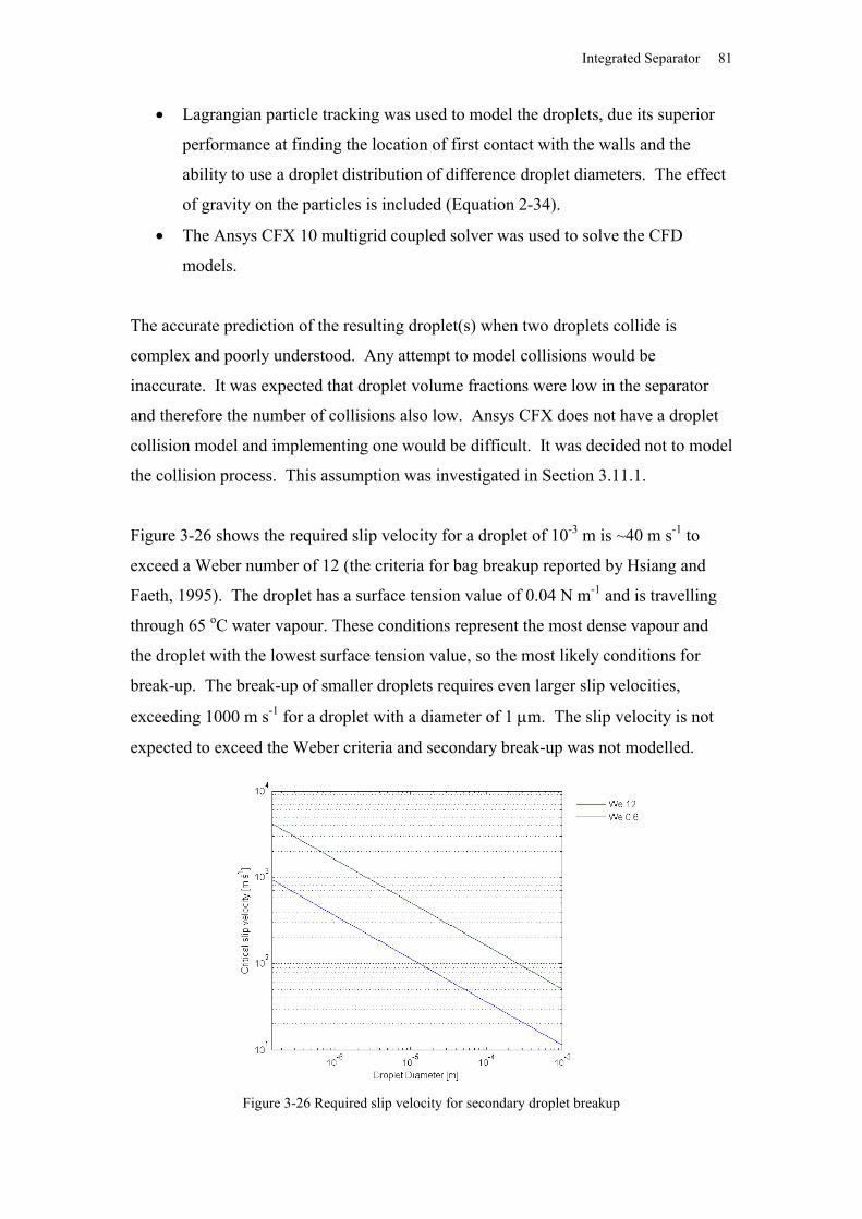
Integrated Separator 81
Lagrangian particle tracking was used to model the droplets, due its superior
performance at finding the location of first contact with the walls and the
ability to use a droplet distribution of difference droplet diameters. The effect
of gravity on the particles is included (Equation 2-34).
The Ansys CFX 10 multigrid coupled solver was used to solve the CFD
models.
The accurate prediction of the resulting droplet(s) when two droplets collide is
complex and poorly understood. Any attempt to model collisions would be
inaccurate. It was expected that droplet volume fractions were low in the separator
and therefore the number of collisions also low. Ansys CFX does not have a droplet
collision model and implementing one would be difficult. It was decided not to model
the collision process. This assumption was investigated in Section 3.11.1.
Figure 3-26 shows the required slip velocity for a droplet of 10-3 m is ~40 m s-1 to
exceed a Weber number of 12 (the criteria for bag breakup reported by Hsiang and
Faeth, 1995). The droplet has a surface tension value of 0.04 N m-1 and is travelling
through 65 oC water vapour. These conditions represent the most dense vapour and
the droplet with the lowest surface tension value, so the most likely conditions for
break-up. The break-up of smaller droplets requires even larger slip velocities,
exceeding 1000 m s-1 for a droplet with a diameter of 1 m. The slip velocity is not
expected to exceed the Weber criteria and secondary break-up was not modelled.
Figure 3-26 Required slip velocity for secondary droplet breakup
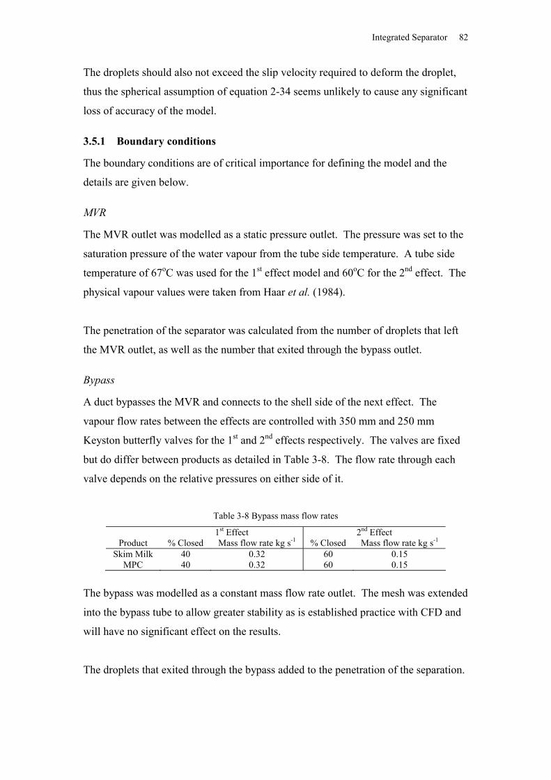
Integrated Separator 82
The droplets should also not exceed the slip velocity required to deform the droplet,
thus the spherical assumption of equation 2-34 seems unlikely to cause any significant
loss of accuracy of the model.
3.5.1 Boundary conditions
The boundary conditions are of critical importance for defining the model and the
details are given below.
MVR
The MVR outlet was modelled as a static pressure outlet. The pressure was set to the
saturation pressure of the water vapour from the tube side temperature. A tube side
temperature of 67oC was used for the 1st effect model and 60oC for the 2nd effect. The
physical vapour values were taken from Haar et al. (1984).
The penetration of the separator was calculated from the number of droplets that left
the MVR outlet, as well as the number that exited through the bypass outlet.
Bypass
A duct bypasses the MVR and connects to the shell side of the next effect. The
vapour flow rates between the effects are controlled with 350 mm and 250 mm
Keyston butterfly valves for the 1st and 2nd effects respectively. The valves are fixed
but do differ between products as detailed in Table 3-8. The flow rate through each
valve depends on the relative pressures on either side of it.
Table 3-8 Bypass mass flow rates
1st Effect 2nd EffectProduct % Closed Mass flow rate kg s-1 % Closed Mass flow rate kg s-1
Skim Milk 40 0.32 60 0.15MPC 40 0.32 60 0.15
The bypass was modelled as a constant mass flow rate outlet. The mesh was extended
into the bypass tube to allow greater stability as is established practice with CFD and
will have no significant effect on the results.
The droplets that exited through the bypass added to the penetration of the separation.
Integrated Separator 83
Inlets
Instead of modelling each individual tube for the calandria and the flow rate water
flow rate from that, each pass was modelled as a single inlet. The mass flow rates
were defined at the inlets as well as the droplet flow rates and diameters. Turbulence
intensity at the inlet was defined as 3.8% and the diameter (48mm) of the tubes was
used to define the eddy length scale.
The 1st pass of the 1st effect contained 0.63 of the total vapour mass with the 2nd pass
containing the remaining 0.37. The fractions from all the passes in each effect should
add to one. This fraction was kept constant between runs, except when testing the
sensitivity of the results to the fraction.
The fractions for the 1st, 2nd, 3rd, 4th and 5th passes of the 2nd effect were 0.38, 0.27,
0.18, 0.11 and 0.06 respectively. The fractions were obtained from Broome (2005).
The droplets were simulated in Ansys CFX as one-way coupled particle or droplets.
It is possible to solve for the path of one-way coupled droplets as a post process
operation. This allowed for flow of a greater number of grades and droplets to be run
with a given amount of computer power than would have been possible if the
droplets’ flow paths were solved with the fluid flow field.
The droplet distributions were split into typically 37 different grades (sizes) for each
pass. The droplets in each grade for each pass contained 10,000-15,000 droplets of
constant density and constant diameter.
The droplets were given a zero slip velocity relative to the inlet vapour flows. Within
the defined inlet area the droplets were randomly distributed. The mass flow rate for
each group of droplets was 1 kg s-1 to allow the results to be easily scaled depending
on the droplet distribution used.
Figure 3-27 plots the Sauter mean diameter against the air/liquid ratio produced by
Mansour and Chigier (1990). Superimposed on Mansour and Chigier (1990) results
are the values and error estimates used to evaluate the SMD used to predict the droplet
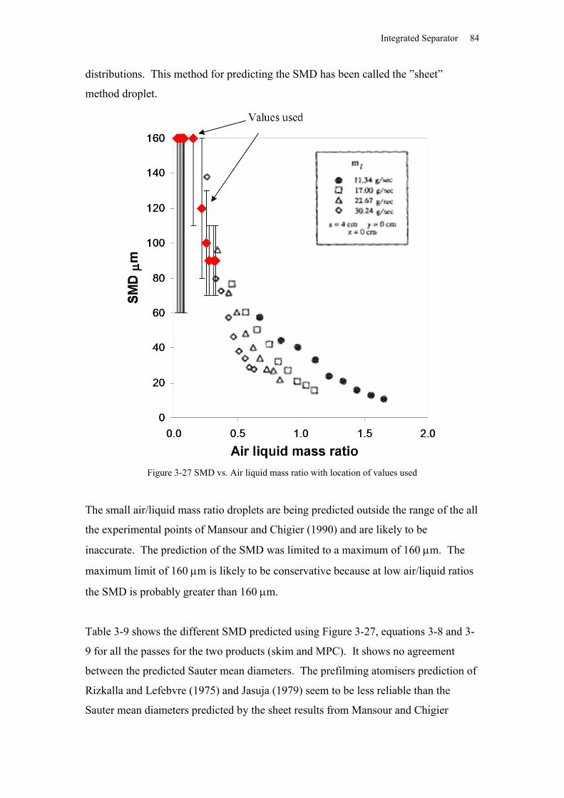
Integrated Separator 84
distributions. This method for predicting the SMD has been called the ”sheet”
method droplet.
Figure 3-27 SMD vs. Air liquid mass ratio with location of values used
The small air/liquid mass ratio droplets are being predicted outside the range of the all
the experimental points of Mansour and Chigier (1990) and are likely to be
inaccurate. The prediction of the SMD was limited to a maximum of 160 m. The
maximum limit of 160 m is likely to be conservative because at low air/liquid ratios
the SMD is probably greater than 160 m.
Table 3-9 shows the different SMD predicted using Figure 3-27, equations 3-8 and 3-
9 for all the passes for the two products (skim and MPC). It shows no agreement
between the predicted Sauter mean diameters. The prefilming atomisers prediction of
Rizkalla and Lefebvre (1975) and Jasuja (1979) seem to be less reliable than the
Sauter mean diameters predicted by the sheet results from Mansour and Chigier
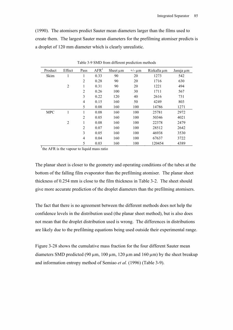
Integrated Separator 85
(1990). The atomisers predict Sauter mean diameters larger than the films used to
create them. The largest Sauter mean diameters for the prefilming atomiser predicts is
a droplet of 120 mm diameter which is clearly unrealistic.
Table 3-9 SMD from different prediction methods
Product Effect Pass AFR1 Sheet m +/- m Rizkalla m Jasuja mSkim 1 1 0.33 90 20 1273 542
2 0.28 90 20 1716 6302 1 0.31 90 20 1221 494
2 0.26 100 30 1711 5673 0.22 120 40 2616 7314 0.15 160 50 4249 8035 0.08 160 100 14786 1271
MPC 1 1 0.08 160 100 25781 29722 0.05 160 100 50346 4021
2 1 0.08 160 100 22378 24792 0.07 160 100 28512 26423 0.05 160 100 46938 35304 0.04 160 100 67637 37225 0.03 160 100 120454 4389
1the AFR is the vapour to liquid mass ratio
The planar sheet is closer to the geometry and operating conditions of the tubes at the
bottom of the falling film evaporator than the prefilming atomiser. The planar sheet
thickness of 0.254 mm is close to the film thickness in Table 3-2. The sheet should
give more accurate prediction of the droplet diameters than the prefilming atomisers.
The fact that there is no agreement between the different methods does not help the
confidence levels in the distribution used (the planar sheet method), but is also does
not mean that the droplet distribution used is wrong. The differences in distributions
are likely due to the prefilming equations being used outside their experimental range.
Figure 3-28 shows the cumulative mass fraction for the four different Sauter mean
diameters SMD predicted (90 m, 100 m, 120 m and 160 m) by the sheet breakup
and information entropy method of Semiao et al. (1996) (Table 3-9).
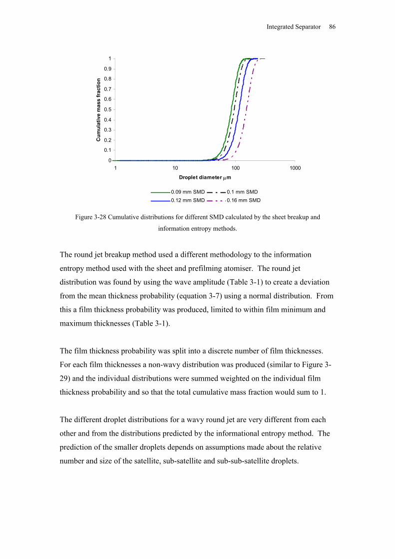
Integrated Separator 86
0
0.1
0.2
0.3
0.4
0.5
0.6
0.7
0.8
0.9
1
1 10 100 1000
Droplet diameter m
Cum
ulat
ive
mas
s fr
actio
n
0.09 mm SMD 0.1 mm SMD0.12 mm SMD 0.16 mm SMD
Figure 3-28 Cumulative distributions for different SMD calculated by the sheet breakup and
information entropy methods.
The round jet breakup method used a different methodology to the information
entropy method used with the sheet and prefilming atomiser. The round jet
distribution was found by using the wave amplitude (Table 3-1) to create a deviation
from the mean thickness probability (equation 3-7) using a normal distribution. From
this a film thickness probability was produced, limited to within film minimum and
maximum thicknesses (Table 3-1).
The film thickness probability was split into a discrete number of film thicknesses.
For each film thicknesses a non-wavy distribution was produced (similar to Figure 3-
29) and the individual distributions were summed weighted on the individual film
thickness probability and so that the total cumulative mass fraction would sum to 1.
The different droplet distributions for a wavy round jet are very different from each
other and from the distributions predicted by the informational entropy method. The
prediction of the smaller droplets depends on assumptions made about the relative
number and size of the satellite, sub-satellite and sub-sub-satellite droplets.
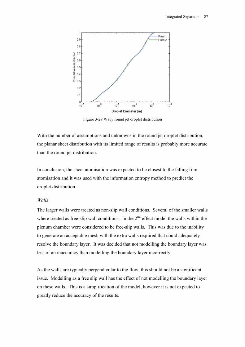
Integrated Separator 87
Figure 3-29 Wavy round jet droplet distribution
With the number of assumptions and unknowns in the round jet droplet distribution,
the planar sheet distribution with its limited range of results is probably more accurate
than the round jet distribution.
In conclusion, the sheet atomisation was expected to be closest to the falling film
atomisation and it was used with the information entropy method to predict the
droplet distribution.
Walls
The larger walls were treated as non-slip wall conditions. Several of the smaller walls
where treated as free-slip wall conditions. In the 2nd effect model the walls within the
plenum chamber were considered to be free-slip walls. This was due to the inability
to generate an acceptable mesh with the extra walls required that could adequately
resolve the boundary layer. It was decided that not modelling the boundary layer was
less of an inaccuracy than modelling the boundary layer incorrectly.
As the walls are typically perpendicular to the flow, this should not be a significant
issue. Modelling as a free slip wall has the effect of not modelling the boundary layer
on these walls. This is a simplification of the model, however it is not expected to
greatly reduce the accuracy of the results.
Integrated Separator 88
When a droplet contacted the walls, it was considered to have been collected and the
tracking of that droplet was stopped. No attempt was made to model the liquid film
formed by the droplets collected on the walls.
The wall interactions are not well understood and it was assumed that the droplets
contacting with the wall are collected. It is possible to rebound the droplets away
from the wall within CFX. The perpendicular and parallel rebound can be controlled
using coefficients of restitution. These coefficients were set to zero to collect all the
droplets on the wall.
3.6 Numerical Solution
The normalised root mean square RMS residuals for the velocity variables were
between 10-4 and 10-3 for the 1st effect and the 2nd effects residuals were 10-5 to 10-4.
The 1st effect’s residuals were adequate residuals but not great for an industrial model.
The 2nd effect’s residuals were better. The global balances for the velocity were much
better than the residuals. All the balances were out by less than 0.0001%.
The pressure RMS residuals were good, well below 3.6x10⁻⁷ and the global balances
were out by less than 0.003%. The residuals for the SST model were adequate,
between 10-3 and 10-2 for k and 10-4 and 10-5 for .
The solutions using the meshes with smaller elements had higher RMS residuals than
when using the coarser meshes. The global balances however remained about the
same. Typically smaller elements should reduce the residuals as they reduce the
Taylor series errors and are able to better resolve the changes in gradient of the solved
variables. All the solutions were solved until the residuals had maintained a near
constant value for approximately a quarter of the total number of timesteps, this was
done to ensure the best possible convergence of the model.
Reducing the timestep, a method used to improve the numerical stability of a
simulation, did not improve the convergence of the solution. When a transient
simulation was performed, the RMS residuals dropped from a typical value of 10-4 to
below 10-5.
Integrated Separator 89
On inspection of the solution, a transient flow phenomenon was observed in the MVR
duct (see transient /steady state Section 3.6.1 for more details). The transient nature
of the flow stops the steady state model from converging.
The smaller elements in the finer mesh was able to capture the transient effects that
the coarser mesh numerically diffuses over, this is why the coarser mesh converged
better then than the finer mesh.
The CFD solutions were solved on a 2.4GHz Pentium 4 with 2 GB of RAM. The
steady state solution typically took between 8 to 12 hours to solve.
3.6.1 Transient /Steady state
Transient models for both effects were created and the time dependent solution was
compared against the steady state solution (see Figures 3-30 and 3-31). Transient
timesteps of 510-3 s were used for both models.
Figure 3-30 shows the transient solutions at different cumulative times and compares
them against the steady state solution for the 1st effect. The contour plots are located
1800 mm from the bottom of the separator
Figure 3-30 Transient steady state comparison of vapour flow for the 1st effect
Integrated Separator 90
Figure 3-31 shows the transient solutions at different cumulative times and compares
them against the steady state solution for the 2nd effect.
Figure 3-31 Transient steady state comparison of vapour flow for the 2nd effect
The flow, other than in the MVR duct, in the transient solution was very similar to the
steady state solution and showed little transience. The flow in the MVR duct,
however, was quite transient and showed a periodic nature. The periodic nature
indicates that the poor residuals of the steady state solution are due to the lack of an
actual physical steady state flow, rather than to just a lack of convergence.
Transient particle tracking was not available within Ansys CFX until version 10.0,
released at the end of 2005. Prior to then, only steady state particle tracking was
available. It was decided that a steady state model could approximate the transient
model, since the transience was confined to the MVR duct which was located at the
end of the geometry. If the majority of the separation occurred before the MVR duct,
where the transient and steady state solutions were very similar, then the prediction of
the droplet collection efficiency by the model would still be valid.
Integrated Separator 91
The transience of the model is limited to within the MVR Duct and shows a periodic
nature. The period of the cycle was in the order of 1second, whereas the residence
time in the MVR is significantly less than 0.1s. The droplets travel through the duct
faster than the periodic feature. This means that an individual droplet travels through
a near-constant vapour field, because the vapour field is changing at a rate slower than
the time for which a droplet is exposed to it. It would have been more correct to
model the separator as a true transient model, but this was not a realistic option due to
the technology available to the author. Any droplets collected in the MVR duct where
assumed to have penetrated to give a more conservative estimate of the penetration
rate.
Figure 3-32 shows the grade collection rate on the MVR duct wall (the mass fraction
of any given size that collects on the MVR duct wall) against the total vapour flow
rates (10 through to 30 t h-1) for the 1st and 2nd pass of the 1st effect. The bottom
subplots of Figure 3-32 are the corresponding grade penetration rates.
Figure 3-32 Droplet collection in MVR duct, 1st effect
Figure 3-32 shows that the collection rate on the duct walls is small (<0.1) for most of
the droplet grades and total flow rates. However the results for vapour flow of 14 t h-1
are higher than the surrounding results. This could be a true reflection of what is
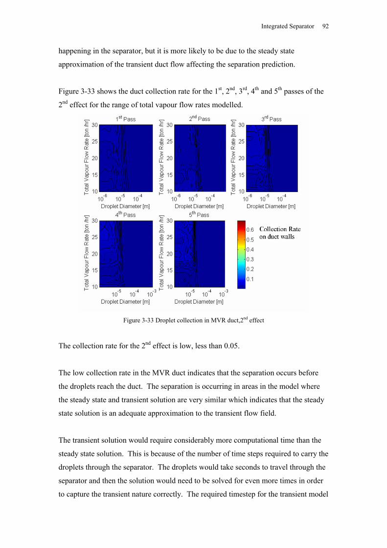
Integrated Separator 92
happening in the separator, but it is more likely to be due to the steady state
approximation of the transient duct flow affecting the separation prediction.
Figure 3-33 shows the duct collection rate for the 1st, 2nd, 3rd, 4th and 5th passes of the
2nd effect for the range of total vapour flow rates modelled.
Figure 3-33 Droplet collection in MVR duct,2nd effect
The collection rate for the 2nd effect is low, less than 0.05.
The low collection rate in the MVR duct indicates that the separation occurs before
the droplets reach the duct. The separation is occurring in areas in the model where
the steady state and transient solution are very similar which indicates that the steady
state solution is an adequate approximation to the transient flow field.
The transient solution would require considerably more computational time than the
steady state solution. This is because of the number of time steps required to carry the
droplets through the separator. The droplets would take seconds to travel through the
separator and then the solution would need to be solved for even more times in order
to capture the transient nature correctly. The required timestep for the transient model
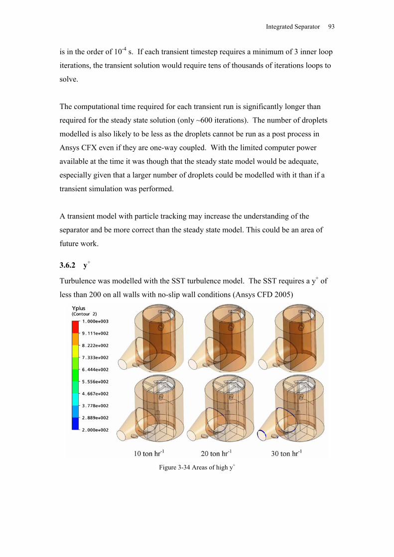
Integrated Separator 93
is in the order of 10-4 s. If each transient timestep requires a minimum of 3 inner loop
iterations, the transient solution would require tens of thousands of iterations loops to
solve.
The computational time required for each transient run is significantly longer than
required for the steady state solution (only ~600 iterations). The number of droplets
modelled is also likely to be less as the droplets cannot be run as a post process in
Ansys CFX even if they are one-way coupled. With the limited computer power
available at the time it was though that the steady state model would be adequate,
especially given that a larger number of droplets could be modelled with it than if a
transient simulation was performed.
A transient model with particle tracking may increase the understanding of the
separator and be more correct than the steady state model. This could be an area of
future work.
3.6.2 y+
Turbulence was modelled with the SST turbulence model. The SST requires a y+ of
less than 200 on all walls with no-slip wall conditions (Ansys CFD 2005)
Figure 3-34 Areas of high y+
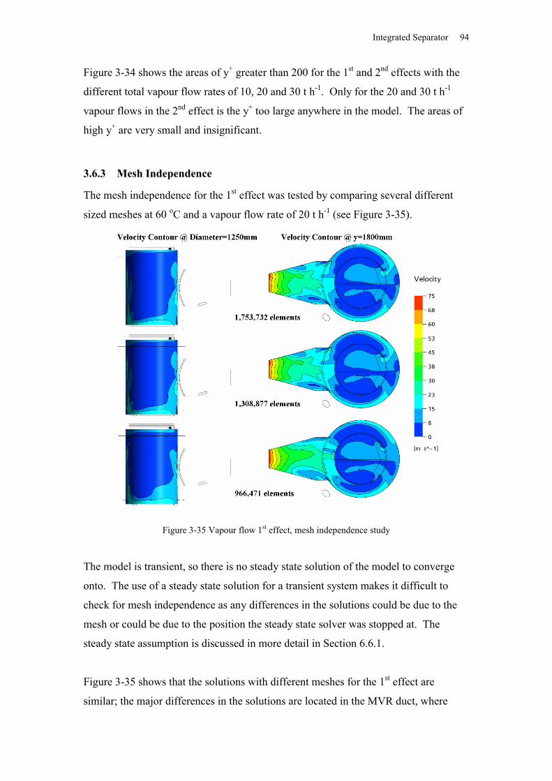
Integrated Separator 94
Figure 3-34 shows the areas of y+ greater than 200 for the 1st and 2nd effects with the
different total vapour flow rates of 10, 20 and 30 t h-1. Only for the 20 and 30 t h-1
vapour flows in the 2nd effect is the y+ too large anywhere in the model. The areas of
high y+ are very small and insignificant.
3.6.3 Mesh Independence
The mesh independence for the 1st effect was tested by comparing several different
sized meshes at 60 oC and a vapour flow rate of 20 t h-1 (see Figure 3-35).
Figure 3-35 Vapour flow 1st effect, mesh independence study
The model is transient, so there is no steady state solution of the model to converge
onto. The use of a steady state solution for a transient system makes it difficult to
check for mesh independence as any differences in the solutions could be due to the
mesh or could be due to the position the steady state solver was stopped at. The
steady state assumption is discussed in more detail in Section 6.6.1.
Figure 3-35 shows that the solutions with different meshes for the 1st effect are
similar; the major differences in the solutions are located in the MVR duct, where
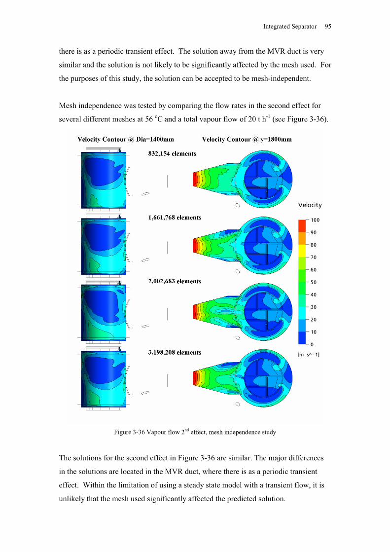
Integrated Separator 95
there is as a periodic transient effect. The solution away from the MVR duct is very
similar and the solution is not likely to be significantly affected by the mesh used. For
the purposes of this study, the solution can be accepted to be mesh-independent.
Mesh independence was tested by comparing the flow rates in the second effect for
several different meshes at 56 oC and a total vapour flow of 20 t h-1 (see Figure 3-36).
Figure 3-36 Vapour flow 2nd effect, mesh independence study
The solutions for the second effect in Figure 3-36 are similar. The major differences
in the solutions are located in the MVR duct, where there is as a periodic transient
effect. Within the limitation of using a steady state model with a transient flow, it is
unlikely that the mesh used significantly affected the predicted solution.
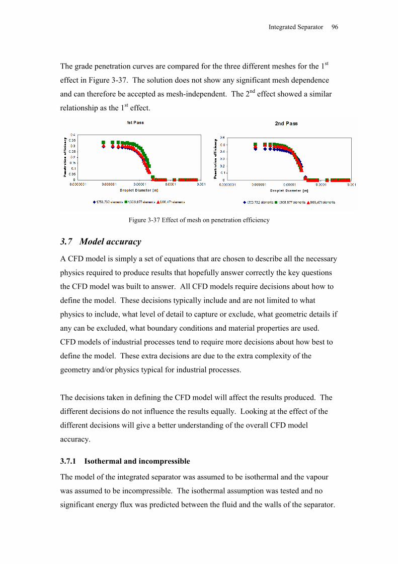
Integrated Separator 96
The grade penetration curves are compared for the three different meshes for the 1st
effect in Figure 3-37. The solution does not show any significant mesh dependence
and can therefore be accepted as mesh-independent. The 2nd effect showed a similar
relationship as the 1st effect.
Figure 3-37 Effect of mesh on penetration efficiency
3.7 Model accuracy
A CFD model is simply a set of equations that are chosen to describe all the necessary
physics required to produce results that hopefully answer correctly the key questions
the CFD model was built to answer. All CFD models require decisions about how to
define the model. These decisions typically include and are not limited to what
physics to include, what level of detail to capture or exclude, what geometric details if
any can be excluded, what boundary conditions and material properties are used.
CFD models of industrial processes tend to require more decisions about how best to
define the model. These extra decisions are due to the extra complexity of the
geometry and/or physics typical for industrial processes.
The decisions taken in defining the CFD model will affect the results produced. The
different decisions do not influence the results equally. Looking at the effect of the
different decisions will give a better understanding of the overall CFD model
accuracy.
3.7.1 Isothermal and incompressible
The model of the integrated separator was assumed to be isothermal and the vapour
was assumed to be incompressible. The isothermal assumption was tested and no
significant energy flux was predicted between the fluid and the walls of the separator.
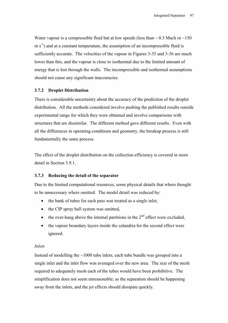
Integrated Separator 97
Water vapour is a compressible fluid but at low speeds (less than ~ 0.3 Mach or ~150
m s-1) and at a constant temperature, the assumption of an incompressible fluid is
sufficiently accurate. The velocities of the vapour in Figures 3-35 and 3-36 are much
lower than this, and the vapour is close to isothermal due to the limited amount of
energy that is lost through the walls. The incompressible and isothermal assumptions
should not cause any significant inaccuracies.
3.7.2 Droplet Distribution
There is considerable uncertainty about the accuracy of the prediction of the droplet
distribution. All the methods considered involve pushing the published results outside
experimental range for which they were obtained and involve comparisons with
structures that are dissimilar. The different method gave different results. Even with
all the differences in operating conditions and geometry, the breakup process is still
fundamentally the same process.
The effect of the droplet distribution on the collection efficiency is covered in more
detail in Section 3.9.1.
3.7.3 Reducing the detail of the separator
Due to the limited computational resources, some physical details that where thought
to be unnecessary where omitted. The model detail was reduced by:
the bank of tubes for each pass was treated as a single inlet,
the CIP spray ball system was omitted,
the over-hang above the internal partitions in the 2nd effect were excluded,
the vapour boundary layers inside the calandria for the second effect were
ignored.
Inlets
Instead of modelling the ~1000 tube inlets, each tube bundle was grouped into a
single inlet and the inlet flow was averaged over the new area. The size of the mesh
required to adequately mesh each of the tubes would have been prohibitive. The
simplification does not seem unreasonable; as the separation should be happening
away from the inlets, and the jet effects should dissipate quickly.
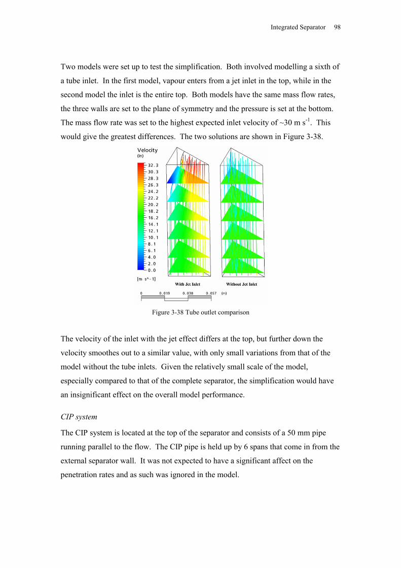
Integrated Separator 98
Two models were set up to test the simplification. Both involved modelling a sixth of
a tube inlet. In the first model, vapour enters from a jet inlet in the top, while in the
second model the inlet is the entire top. Both models have the same mass flow rates,
the three walls are set to the plane of symmetry and the pressure is set at the bottom.
The mass flow rate was set to the highest expected inlet velocity of ~30 m s-1. This
would give the greatest differences. The two solutions are shown in Figure 3-38.
Figure 3-38 Tube outlet comparison
The velocity of the inlet with the jet effect differs at the top, but further down the
velocity smoothes out to a similar value, with only small variations from that of the
model without the tube inlets. Given the relatively small scale of the model,
especially compared to that of the complete separator, the simplification would have
an insignificant effect on the overall model performance.
CIP system
The CIP system is located at the top of the separator and consists of a 50 mm pipe
running parallel to the flow. The CIP pipe is held up by 6 spans that come in from the
external separator wall. It was not expected to have a significant affect on the
penetration rates and as such was ignored in the model.
Integrated Separator 99
Figure 3-39 shows the grade efficiency for the top of the separator for both the 1st and
2nd effects, the fraction of droplets in each grade that are collected at the top of the
separator.
Figure 3-39 Collection near CIP system
Figure 3-39 shows that little separation occurs near the CIP system, so it seems
reasonable to believe that omitting it has no significant effect on the results.
Missing overhangs in the 2nd effect
The overhangs between the passes in the 2nd effect were not modelled, as they would
require too fine a mesh to do so correctly. The overhangs were located in the plenum
chamber, away from the area of separator. The lack of the overhang limits the ability
of the model to accurately predict carry-over between the passes. It was not expected
to greatly affect the prediction of separation in the overall model. Again this could be
an area for future work, especially if the model was to look at effects like carry-over
in the plenum chamber.
Treatment of walls
The walls in the second effect within the plenum chamber were treated as free slip
boundaries. This means that the boundary layers for the walls were not modelled.
When prism layers were introduced for modelling the boundary layer, it produced an
error with the Ansys CFX solver. A solution to this error was not found after
consultation with the Australian ANSYS help desk and it was hypothesised that the
boundary layers at these walls in the plenum chamber could be ignored, as it seemed
unlikely that they would play a significant part in the separation of the droplets in the
separator.
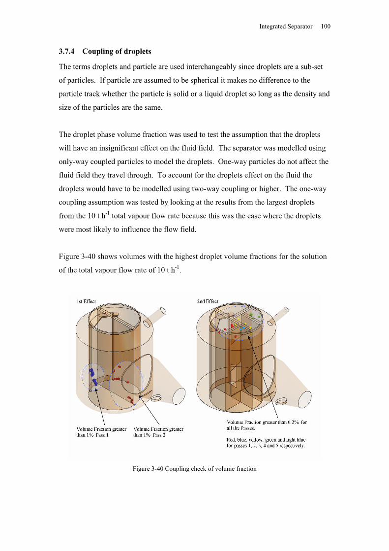
Integrated Separator 100
3.7.4 Coupling of droplets
The terms droplets and particle are used interchangeably since droplets are a sub-set
of particles. If particle are assumed to be spherical it makes no difference to the
particle track whether the particle is solid or a liquid droplet so long as the density and
size of the particles are the same.
The droplet phase volume fraction was used to test the assumption that the droplets
will have an insignificant effect on the fluid field. The separator was modelled using
only-way coupled particles to model the droplets. One-way particles do not affect the
fluid field they travel through. To account for the droplets effect on the fluid the
droplets would have to be modelled using two-way coupling or higher. The one-way
coupling assumption was tested by looking at the results from the largest droplets
from the 10 t h-1 total vapour flow rate because this was the case where the droplets
were most likely to influence the flow field.
Figure 3-40 shows volumes with the highest droplet volume fractions for the solution
of the total vapour flow rate of 10 t h-1.
Figure 3-40 Coupling check of volume fraction
Integrated Separator 101
There are only a few small volumes where the volume fractions are above 1% in the
first effect and these are in the area of low interest, away from the separator. For the
2nd effect the droplet volume fraction is above 0.2% only in some small volumes of
the solution. These small volumes and the lower volume fractions in them make it
unlikely that there would be any significant effect on the fluid field by the droplets
and therefore using only one-way coupling to model the droplets is acceptable.
Droplet collisions
The collision rate can be calculated from the number density Ni of the droplets.
Abrahamson (1975) gives equation 3-19 to predict the collision rate per unit volume
Z12 for particles of two different sizes 1 and 2 without external forces, assuming
isotropic turbulence.
22
21
2122112 5 UUdNNZ (3-19)
where N1 and N2 are the number concentration of particles per unit volume for
particles 1 and 2 respectively, d12 is found from
2112 rrd (3-20)
where r1 is the radius of the first particle group and r2 is the radius of the second
particle group.
Ui is the velocity of the particle (the subscript denotes the particle group (i)) found
from
2
22
5.11
U
UUp
i
(3-21)
where is the turbulent energy dissipation rate per unit mass, p is the stopping
distance of the particle found from the particle diameter dp, the vapour viscosity v
and the density of the vapour v and particlep, found from
v
pvpp
d
36
2 2 (3-22)
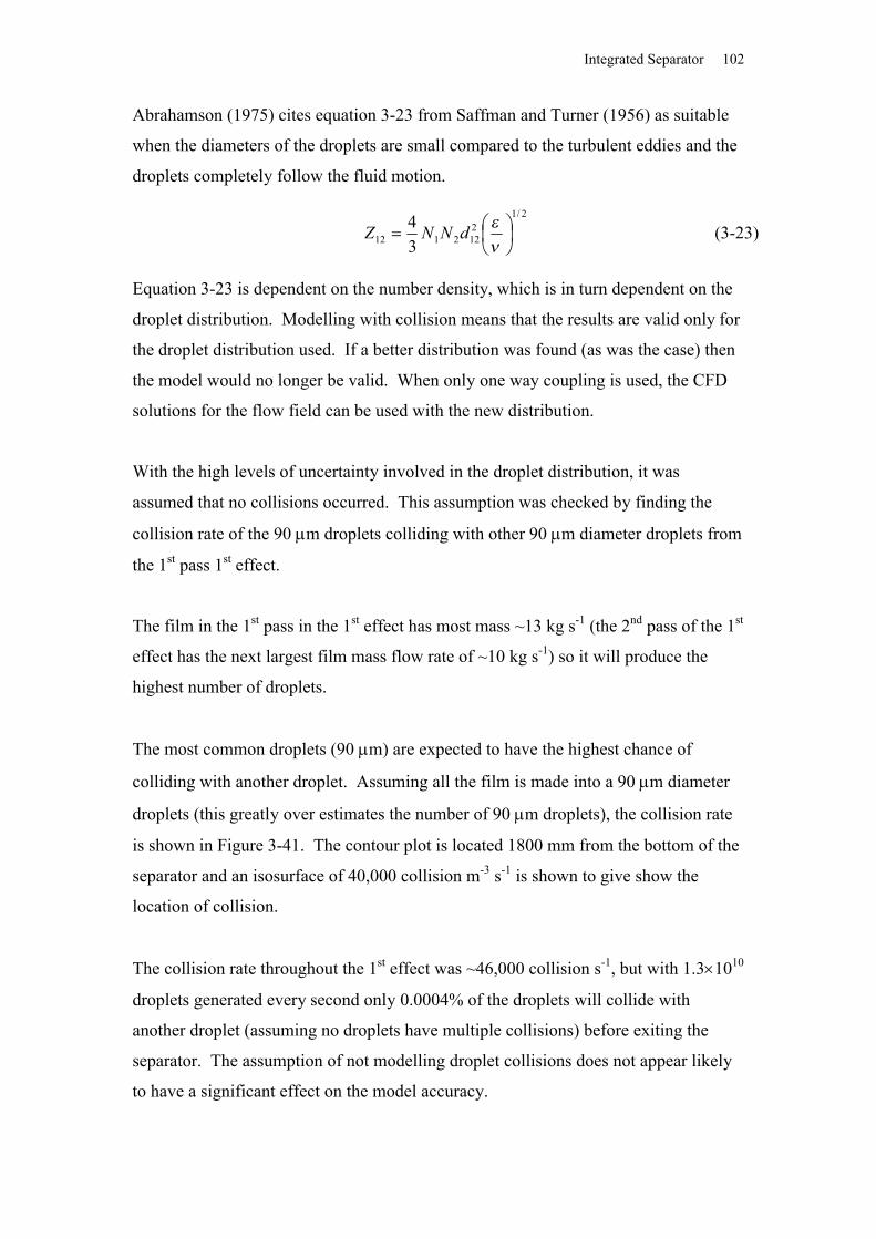
Integrated Separator 102
Abrahamson (1975) cites equation 3-23 from Saffman and Turner (1956) as suitable
when the diameters of the droplets are small compared to the turbulent eddies and the
droplets completely follow the fluid motion.
2/12122112 3
4
dNNZ (3-23)
Equation 3-23 is dependent on the number density, which is in turn dependent on the
droplet distribution. Modelling with collision means that the results are valid only for
the droplet distribution used. If a better distribution was found (as was the case) then
the model would no longer be valid. When only one way coupling is used, the CFD
solutions for the flow field can be used with the new distribution.
With the high levels of uncertainty involved in the droplet distribution, it was
assumed that no collisions occurred. This assumption was checked by finding the
collision rate of the 90 m droplets colliding with other 90 m diameter droplets from
the 1st pass 1st effect.
The film in the 1st pass in the 1st effect has most mass ~13 kg s-1 (the 2nd pass of the 1st
effect has the next largest film mass flow rate of ~10 kg s-1) so it will produce the
highest number of droplets.
The most common droplets (90 m) are expected to have the highest chance of
colliding with another droplet. Assuming all the film is made into a 90 m diameter
droplets (this greatly over estimates the number of 90 m droplets), the collision rate
is shown in Figure 3-41. The contour plot is located 1800 mm from the bottom of the
separator and an isosurface of 40,000 collision m-3 s-1 is shown to give show the
location of collision.
The collision rate throughout the 1st effect was ~46,000 collision s-1, but with 1.31010
droplets generated every second only 0.0004% of the droplets will collide with
another droplet (assuming no droplets have multiple collisions) before exiting the
separator. The assumption of not modelling droplet collisions does not appear likely
to have a significant effect on the model accuracy.
Integrated Separator 103
Figure 3-41 Collision rate 90 m diameter droplet
3.7.5 Droplet wall contact
It was assumed that any droplet that comes into contact with the wall was collected.
Complete collection is however not the only possibility for a droplet impacting onto a
surface, it can also rebound or splash. The phenomenon of rebounding and especially
splashing is not well understood (Schmehl et al. 1999).
Schmehl et al. (1999) give three categories for the droplet wall interaction, dependent
on the wall temperature relative to the droplet temperature. The temperature of the
evaporator walls, Twall, is lower than the boiling temperature of the milk droplets
Tboiling, so only the cold wall interactions are described. The condition for dry cold
wall interactions was given as boilingwall TT 05.1 .
Schmehl et al. (1999) use the Laplace number, La, and a Reynolds number, Re, based
on a modified normal velocity, un, to the wall. The modification of the normal
velocity is found from
63.0sinDn uu (3-24)
where is the impact angle (from the impaction surface), D is the droplet diameter.
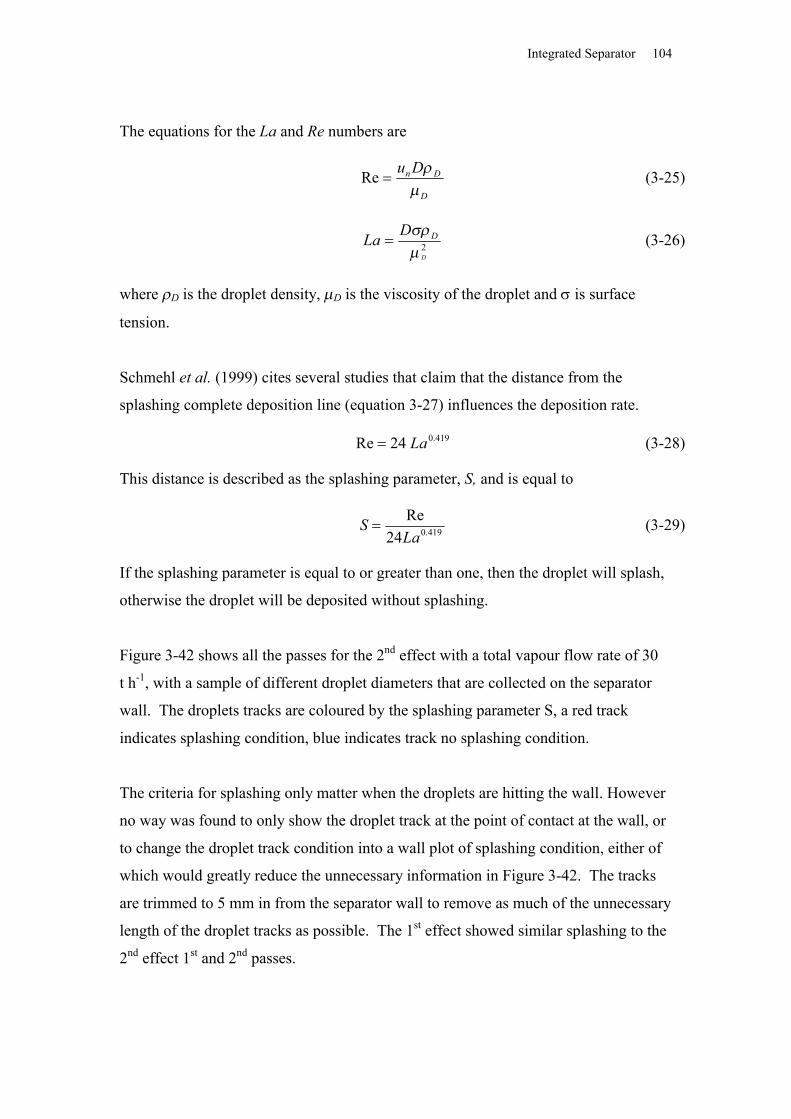
Integrated Separator 104
The equations for the La and Re numbers are
D
Dn Du
Re (3-25)
2D
DDLa
(3-26)
where D is the droplet density, D is the viscosity of the droplet and is surface
tension.
Schmehl et al. (1999) cites several studies that claim that the distance from the
splashing complete deposition line (equation 3-27) influences the deposition rate.
419.024Re La (3-28)
This distance is described as the splashing parameter, S, and is equal to
419.024ReLa
S (3-29)
If the splashing parameter is equal to or greater than one, then the droplet will splash,
otherwise the droplet will be deposited without splashing.
Figure 3-42 shows all the passes for the 2nd effect with a total vapour flow rate of 30
t h-1, with a sample of different droplet diameters that are collected on the separator
wall. The droplets tracks are coloured by the splashing parameter S, a red track
indicates splashing condition, blue indicates track no splashing condition.
The criteria for splashing only matter when the droplets are hitting the wall. However
no way was found to only show the droplet track at the point of contact at the wall, or
to change the droplet track condition into a wall plot of splashing condition, either of
which would greatly reduce the unnecessary information in Figure 3-42. The tracks
are trimmed to 5 mm in from the separator wall to remove as much of the unnecessary
length of the droplet tracks as possible. The 1st effect showed similar splashing to the
2nd effect 1st and 2nd passes.
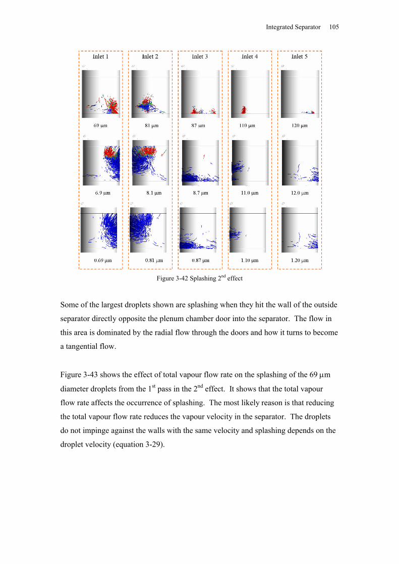
Integrated Separator 105
Figure 3-42 Splashing 2nd effect
Some of the largest droplets shown are splashing when they hit the wall of the outside
separator directly opposite the plenum chamber door into the separator. The flow in
this area is dominated by the radial flow through the doors and how it turns to become
a tangential flow.
Figure 3-43 shows the effect of total vapour flow rate on the splashing of the 69 m
diameter droplets from the 1st pass in the 2nd effect. It shows that the total vapour
flow rate affects the occurrence of splashing. The most likely reason is that reducing
the total vapour flow rate reduces the vapour velocity in the separator. The droplets
do not impinge against the walls with the same velocity and splashing depends on the
droplet velocity (equation 3-29).
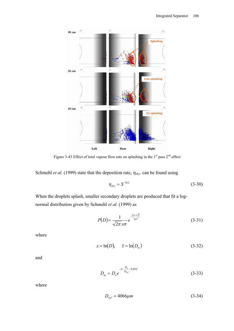
Integrated Separator 106
Figure 3-43 Effect of total vapour flow rate on splashing in the 1st pass 2nd effect
Schmehl et al. (1999) state that the deposition rate, dry, can be found using
6.0 Sdry (3-30)
When the droplets splash, smaller secondary droplets are produced that fit a log-
normal distribution given by Schmehl et al. (1999) as
2
2
2
21
xx
ex
DP
(3-31)
where
mDxDx ln,ln (3-32)
and
SDD
omref
o
eDD05.02
(3-33)
where
mDref 4066 (3-34)
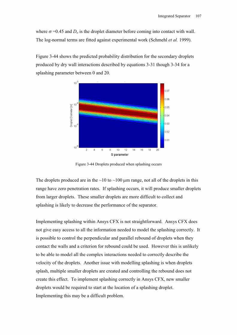
Integrated Separator 107
where =0.45 and Do is the droplet diameter before coming into contact with wall.
The log-normal terms are fitted against experimental work (Schmehl et al. 1999).
Figure 3-44 shows the predicted probability distribution for the secondary droplets
produced by dry wall interactions described by equations 3-31 though 3-34 for a
splashing parameter between 0 and 20.
Figure 3-44 Droplets produced when splashing occurs
The droplets produced are in the ~10 to ~100 m range, not all of the droplets in this
range have zero penetration rates. If splashing occurs, it will produce smaller droplets
from larger droplets. These smaller droplets are more difficult to collect and
splashing is likely to decrease the performance of the separator.
Implementing splashing within Ansys CFX is not straightforward. Ansys CFX does
not give easy access to all the information needed to model the splashing correctly. It
is possible to control the perpendicular and parallel rebound of droplets when they
contact the walls and a criterion for rebound could be used. However this is unlikely
to be able to model all the complex interactions needed to correctly describe the
velocity of the droplets. Another issue with modelling splashing is when droplets
splash, multiple smaller droplets are created and controlling the rebound does not
create this effect. To implement splashing correctly in Ansys CFX, new smaller
droplets would be required to start at the location of a splashing droplet.
Implementing this may be a difficult problem.
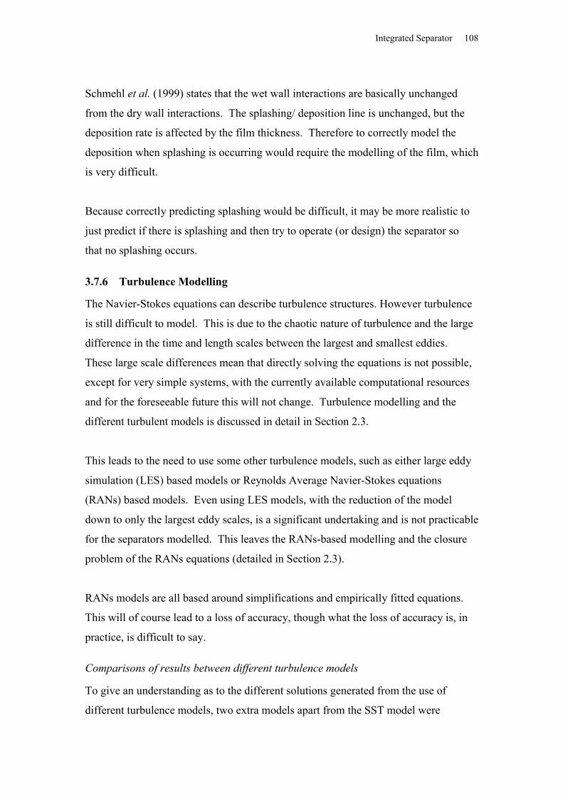
Integrated Separator 108
Schmehl et al. (1999) states that the wet wall interactions are basically unchanged
from the dry wall interactions. The splashing/ deposition line is unchanged, but the
deposition rate is affected by the film thickness. Therefore to correctly model the
deposition when splashing is occurring would require the modelling of the film, which
is very difficult.
Because correctly predicting splashing would be difficult, it may be more realistic to
just predict if there is splashing and then try to operate (or design) the separator so
that no splashing occurs.
3.7.6 Turbulence Modelling
The Navier-Stokes equations can describe turbulence structures. However turbulence
is still difficult to model. This is due to the chaotic nature of turbulence and the large
difference in the time and length scales between the largest and smallest eddies.
These large scale differences mean that directly solving the equations is not possible,
except for very simple systems, with the currently available computational resources
and for the foreseeable future this will not change. Turbulence modelling and the
different turbulent models is discussed in detail in Section 2.3.
This leads to the need to use some other turbulence models, such as either large eddy
simulation (LES) based models or Reynolds Average Navier-Stokes equations
(RANs) based models. Even using LES models, with the reduction of the model
down to only the largest eddy scales, is a significant undertaking and is not practicable
for the separators modelled. This leaves the RANs-based modelling and the closure
problem of the RANs equations (detailed in Section 2.3).
RANs models are all based around simplifications and empirically fitted equations.
This will of course lead to a loss of accuracy, though what the loss of accuracy is, in
practice, is difficult to say.
Comparisons of results between different turbulence models
To give an understanding as to the different solutions generated from the use of
different turbulence models, two extra models apart from the SST model were
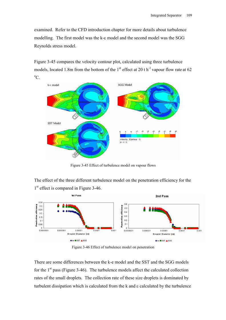
Integrated Separator 109
examined. Refer to the CFD introduction chapter for more details about turbulence
modelling. The first model was the k- model and the second model was the SGG
Reynolds stress model.
Figure 3-45 compares the velocity contour plot, calculated using three turbulence
models, located 1.8m from the bottom of the 1st effect at 20 t h-1 vapour flow rate at 62 oC.
Figure 3-45 Effect of turbulence model on vapour flows
The effect of the three different turbulence model on the penetration efficiency for the
1st effect is compared in Figure 3-46.
Figure 3-46 Effect of turbulence model on penetration
There are some differences between the k-e model and the SST and the SGG models
for the 1st pass (Figure 3-46). The turbulence models affect the calculated collection
rates of the small droplets. The collection rate of these size droplets is dominated by
turbulent dissipation which is calculated from the k and calculated by the turbulence
Integrated Separator 110
models. The penetration of these smaller droplets is insignificant to the overall
performance of the separator (see Section 3.8.4). The penetration efficiencies for the
2nd pass are very similar between the different turbulent models.
The results from the three different turbulent models are similar, but there are
differences. These are not insignificant, but some of the differences are likely to be
attributed to the periodic transient effects that occur in the separator. The flow field
prediction near the wall of the separator and in the plenum chamber is similar between
the turbulent models and these are the most important areas in the separation process.
The similarity in the model could indicate that either the turbulence models do not
dominate the flow field prediction, or that the flow fluid field is dominated by the
turbulence models but the different models are predicting the same solution. If
multiple turbulent models predict the same solution, it is not unreasonable to accept
the fluid field has a higher probability of being correctly predicted.
Due to computer resource limitations, RANs models are the only realistic option and
because of the SST superior performance, demonstrated by Bardina et al. (1997), it
was used.
Turbulence droplet dispersion modelling
It has been shown that a Lagrangian particle modelling with a RANs turbulence
model, such as the SST model, will lead to an over prediction of the deposition of
smaller particles Matida et al. (2000) when the dimensionless relaxation time, T+, is
less than 10 with the random eddy walk model. This is due to the isotropic
assumption of the turbulent droplet dispersion.
The dimensionless relaxation time T+ is found by
vv
tll udT
18
22
(3-35)
where ut is the friction velocity found by
v
walltu
(3-36)
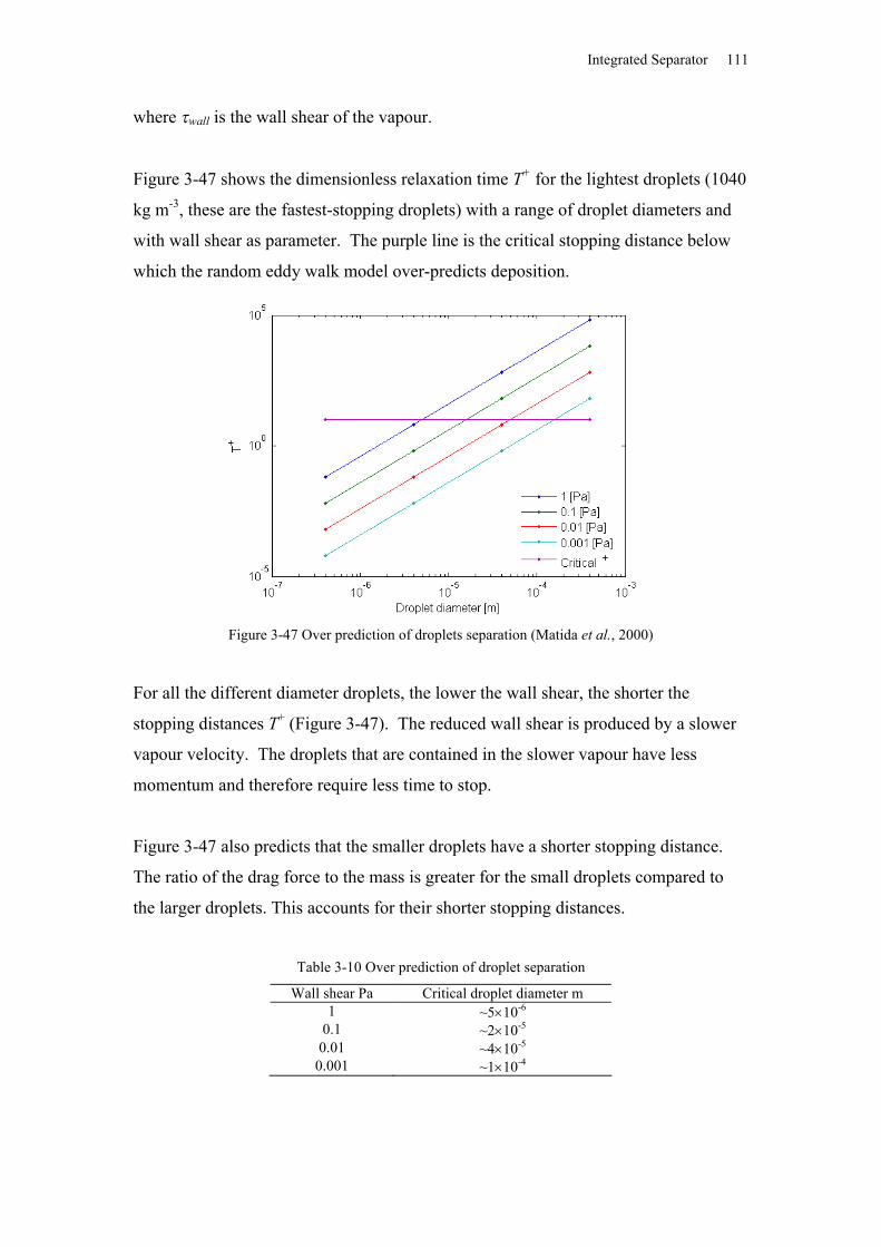
Integrated Separator 111
where wall is the wall shear of the vapour.
Figure 3-47 shows the dimensionless relaxation time T+ for the lightest droplets (1040
kg m-3, these are the fastest-stopping droplets) with a range of droplet diameters and
with wall shear as parameter. The purple line is the critical stopping distance below
which the random eddy walk model over-predicts deposition.
Figure 3-47 Over prediction of droplets separation (Matida et al., 2000)
For all the different diameter droplets, the lower the wall shear, the shorter the
stopping distances T+ (Figure 3-47). The reduced wall shear is produced by a slower
vapour velocity. The droplets that are contained in the slower vapour have less
momentum and therefore require less time to stop.
Figure 3-47 also predicts that the smaller droplets have a shorter stopping distance.
The ratio of the drag force to the mass is greater for the small droplets compared to
the larger droplets. This accounts for their shorter stopping distances.
Table 3-10 Over prediction of droplet separation
Wall shear Pa Critical droplet diameter m1 ~510-6
0.1 ~210-5
0.01 ~410-5
0.001 ~110-4
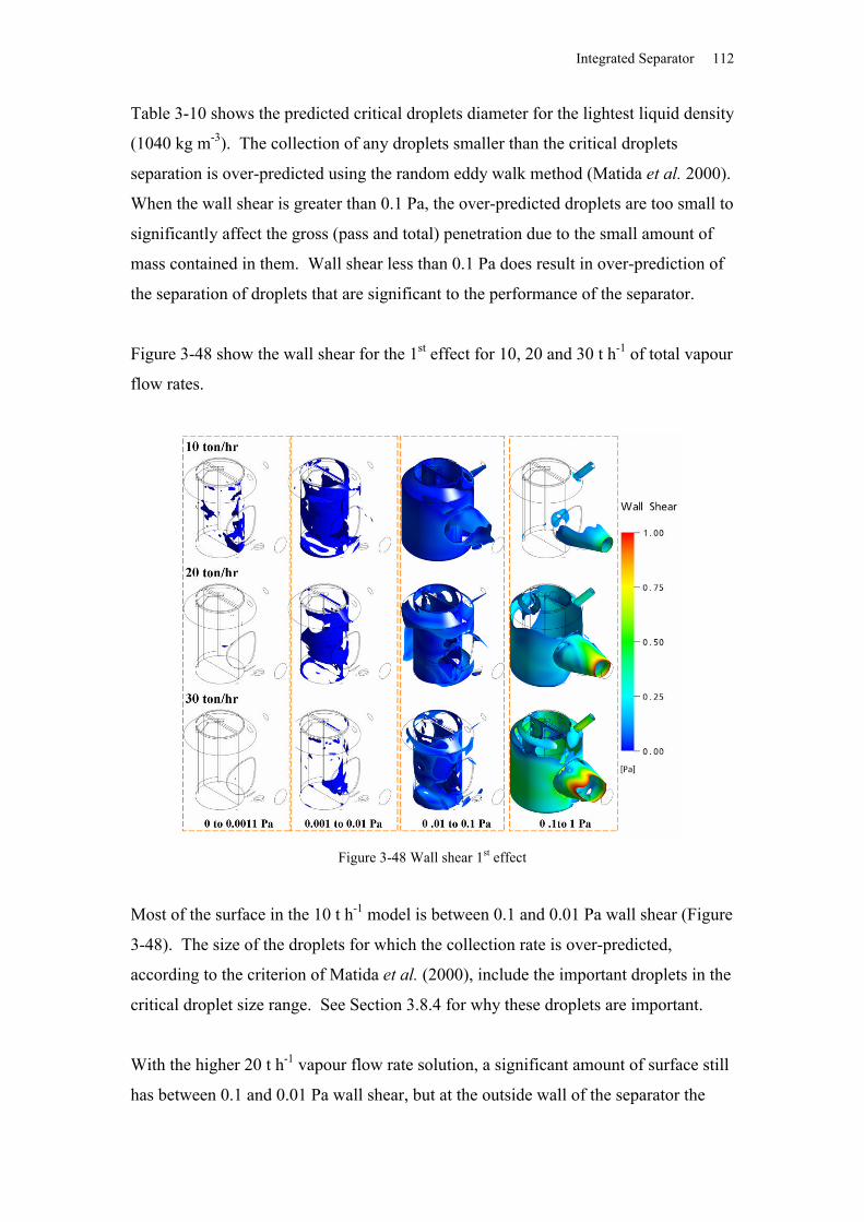
Integrated Separator 112
Table 3-10 shows the predicted critical droplets diameter for the lightest liquid density
(1040 kg m-3). The collection of any droplets smaller than the critical droplets
separation is over-predicted using the random eddy walk method (Matida et al. 2000).
When the wall shear is greater than 0.1 Pa, the over-predicted droplets are too small to
significantly affect the gross (pass and total) penetration due to the small amount of
mass contained in them. Wall shear less than 0.1 Pa does result in over-prediction of
the separation of droplets that are significant to the performance of the separator.
Figure 3-48 show the wall shear for the 1st effect for 10, 20 and 30 t h-1 of total vapour
flow rates.
Figure 3-48 Wall shear 1st effect
Most of the surface in the 10 t h-1 model is between 0.1 and 0.01 Pa wall shear (Figure
3-48). The size of the droplets for which the collection rate is over-predicted,
according to the criterion of Matida et al. (2000), include the important droplets in the
critical droplet size range. See Section 3.8.4 for why these droplets are important.
With the higher 20 t h-1 vapour flow rate solution, a significant amount of surface still
has between 0.1 and 0.01 Pa wall shear, but at the outside wall of the separator the
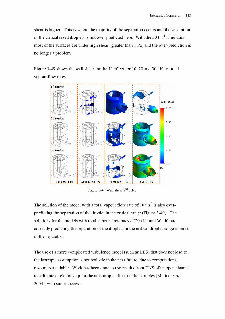
Integrated Separator 113
shear is higher. This is where the majority of the separation occurs and the separation
of the critical sized droplets is not over-predicted here. With the 30 t h-1 simulation
most of the surfaces are under high shear (greater than 1 Pa) and the over-prediction is
no longer a problem.
Figure 3-49 shows the wall shear for the 1st effect for 10, 20 and 30 t h-1 of total
vapour flow rates.
Figure 3-49 Wall shear 2nd effect
The solution of the model with a total vapour flow rate of 10 t h-1 is also over-
predicting the separation of the droplet in the critical range (Figure 3-49). The
solutions for the models with total vapour flow rates of 20 t h-1 and 30 t h-1 are
correctly predicting the separation of the droplets in the critical droplet range in most
of the separator.
The use of a more complicated turbulence model (such as LES) that does not lead to
the isotropic assumption is not realistic in the near future, due to computational
resources available. Work has been done to use results from DNS of an open channel
to calibrate a relationship for the anisotropic effect on the particles (Matida et al.
2004), with some success.
Integrated Separator 114
Extension of the random eddy walk model could be an area of future work and could
be extended using approaches from Matida et al. (2004).
Brownian diffusion was not modelled, this could have a significant effect on the total
diffusion for the very small droplets (<1 m) (Matida et al. 2004). It is unlikely that
this would have a significant effect on the penetration rates as only the smallest
droplets are smaller than 1 m, so the mass carried by these droplets is insignificant.
3.8 Results
3.8.1 Effect results
The solutions shown have total vapour flow rates of 26 t h-1 and 30 t h-1 for the 1st and
2nd effects respectively. The vapour temperatures are 68 oC and 65 oC for the 1st and
2nd effects respectively. These conditions were chosen as they are the conditions for
the separators were designed to operate at.
Velocity magnitude
Figure 3-50 shows the velocity magnitude contour plots for the 1st effect at several
different heights (800 mm, 1800 mm and 2600 mm) along with the contour for a
surface of revolution of 1500 mm diameter.
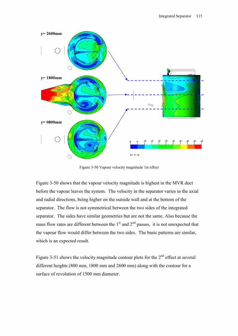
Integrated Separator 115
Figure 3-50 Vapour velocity magnitude 1st effect
Figure 3-50 shows that the vapour velocity magnitude is highest in the MVR duct
before the vapour leaves the system. The velocity in the separator varies in the axial
and radial directions, being higher on the outside wall and at the bottom of the
separator. The flow is not symmetrical between the two sides of the integrated
separator. The sides have similar geometries but are not the same. Also because the
mass flow rates are different between the 1st and 2nd passes, it is not unexpected that
the vapour flow would differ between the two sides. The basic patterns are similar,
which is an expected result.
Figure 3-51 shows the velocity magnitude contour plots for the 2nd effect at several
different heights (800 mm, 1800 mm and 2600 mm) along with the contour for a
surface of revolution of 1500 mm diameter.
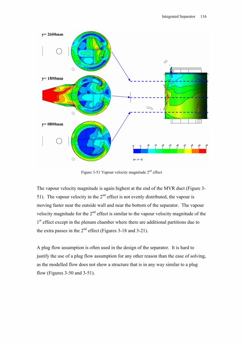
Integrated Separator 116
Figure 3-51 Vapour velocity magnitude 2nd effect
The vapour velocity magnitude is again highest at the end of the MVR duct (Figure 3-
51). The vapour velocity in the 2nd effect is not evenly distributed, the vapour is
moving faster near the outside wall and near the bottom of the separator. The vapour
velocity magnitude for the 2nd effect is similar to the vapour velocity magnitude of the
1st effect except in the plenum chamber where there are additional partitions due to
the extra passes in the 2nd effect (Figures 3-18 and 3-21).
A plug flow assumption is often used in the design of the separator. It is hard to
justify the use of a plug flow assumption for any other reason than the ease of solving,
as the modelled flow does not show a structure that is in any way similar to a plug
flow (Figures 3-50 and 3-51).
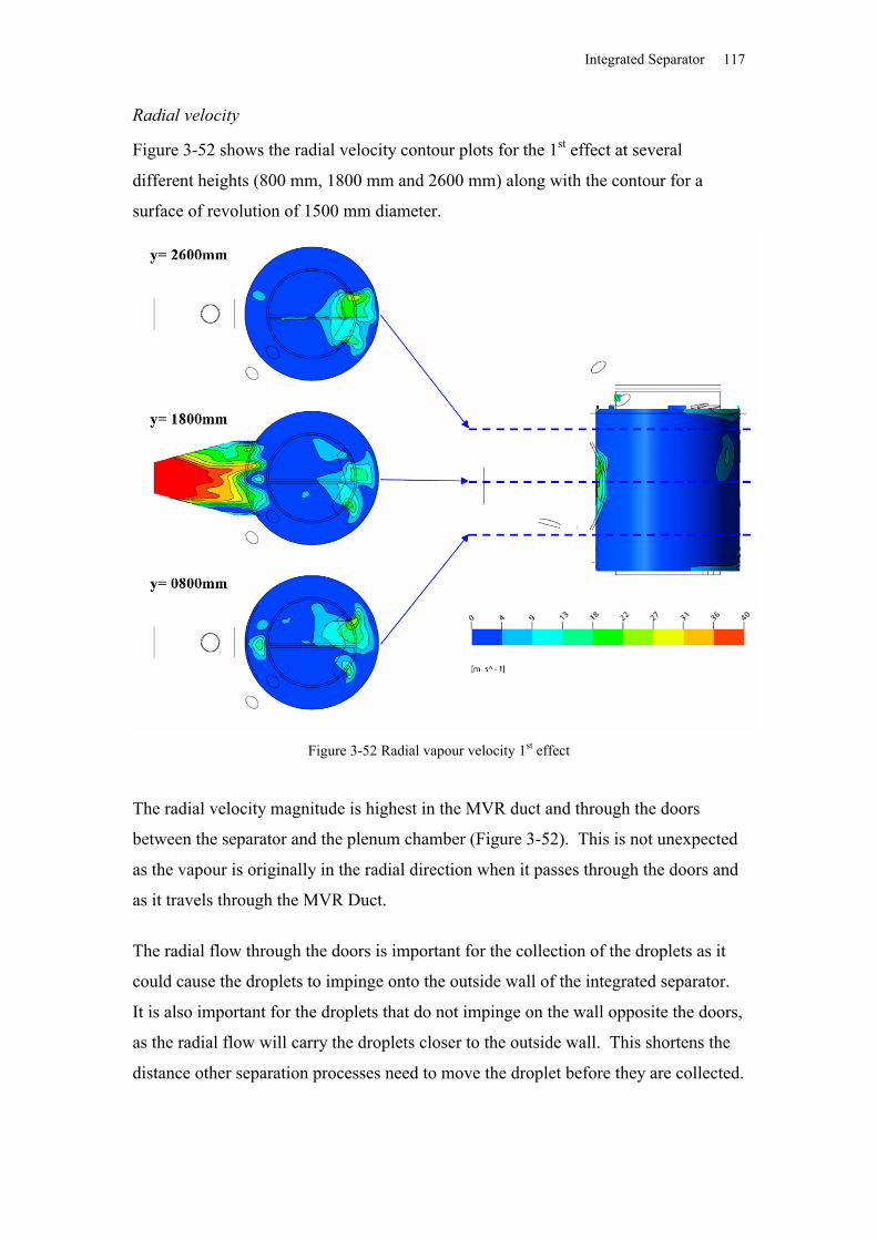
Integrated Separator 117
Radial velocity
Figure 3-52 shows the radial velocity contour plots for the 1st effect at several
different heights (800 mm, 1800 mm and 2600 mm) along with the contour for a
surface of revolution of 1500 mm diameter.
Figure 3-52 Radial vapour velocity 1st effect
The radial velocity magnitude is highest in the MVR duct and through the doors
between the separator and the plenum chamber (Figure 3-52). This is not unexpected
as the vapour is originally in the radial direction when it passes through the doors and
as it travels through the MVR Duct.
The radial flow through the doors is important for the collection of the droplets as it
could cause the droplets to impinge onto the outside wall of the integrated separator.
It is also important for the droplets that do not impinge on the wall opposite the doors,
as the radial flow will carry the droplets closer to the outside wall. This shortens the
distance other separation processes need to move the droplet before they are collected.
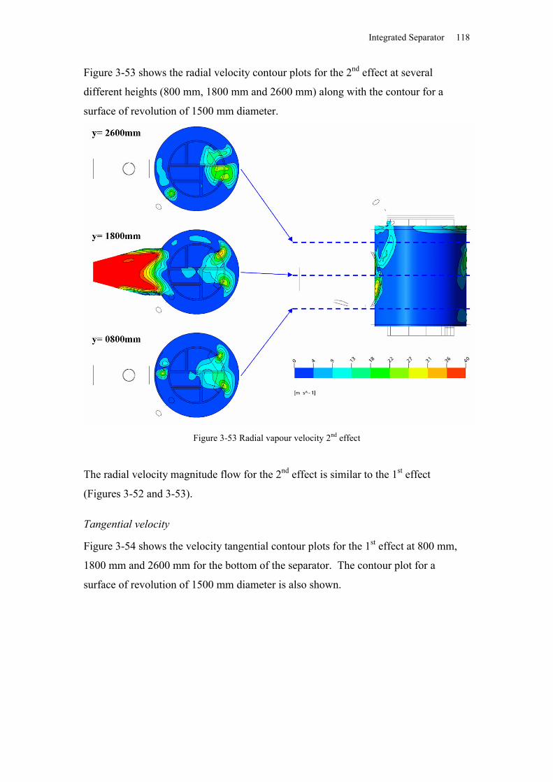
Integrated Separator 118
Figure 3-53 shows the radial velocity contour plots for the 2nd effect at several
different heights (800 mm, 1800 mm and 2600 mm) along with the contour for a
surface of revolution of 1500 mm diameter.
Figure 3-53 Radial vapour velocity 2nd effect
The radial velocity magnitude flow for the 2nd effect is similar to the 1st effect
(Figures 3-52 and 3-53).
Tangential velocity
Figure 3-54 shows the velocity tangential contour plots for the 1st effect at 800 mm,
1800 mm and 2600 mm for the bottom of the separator. The contour plot for a
surface of revolution of 1500 mm diameter is also shown.
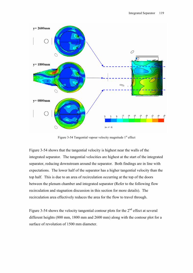
Integrated Separator 119
Figure 3-54 Tangential vapour velocity magnitude 1st effect
Figure 3-54 shows that the tangential velocity is highest near the walls of the
integrated separator. The tangential velocities are highest at the start of the integrated
separator, reducing downstream around the separator. Both findings are in line with
expectations. The lower half of the separator has a higher tangential velocity than the
top half. This is due to an area of recirculation occurring at the top of the doors
between the plenum chamber and integrated separator (Refer to the following flow
recirculation and stagnation discussion in this section for more details). The
recirculation area effectively reduces the area for the flow to travel through.
Figure 3-54 shows the velocity tangential contour plots for the 2nd effect at several
different heights (800 mm, 1800 mm and 2600 mm) along with the contour plot for a
surface of revolution of 1500 mm diameter.
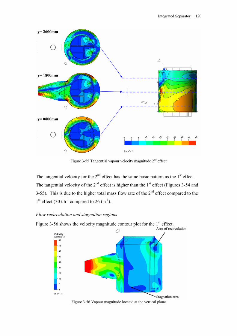
Integrated Separator 120
Figure 3-55 Tangential vapour velocity magnitude 2nd effect
The tangential velocity for the 2nd effect has the same basic pattern as the 1st effect.
The tangential velocity of the 2nd effect is higher than the 1st effect (Figures 3-54 and
3-55). This is due to the higher total mass flow rate of the 2nd effect compared to the
1st effect (30 t h-1 compared to 26 t h-1).
Flow recirculation and stagnation regions
Figure 3-56 shows the velocity magnitude contour plot for the 1st effect.
Figure 3-56 Vapour magnitude located at the vertical plane
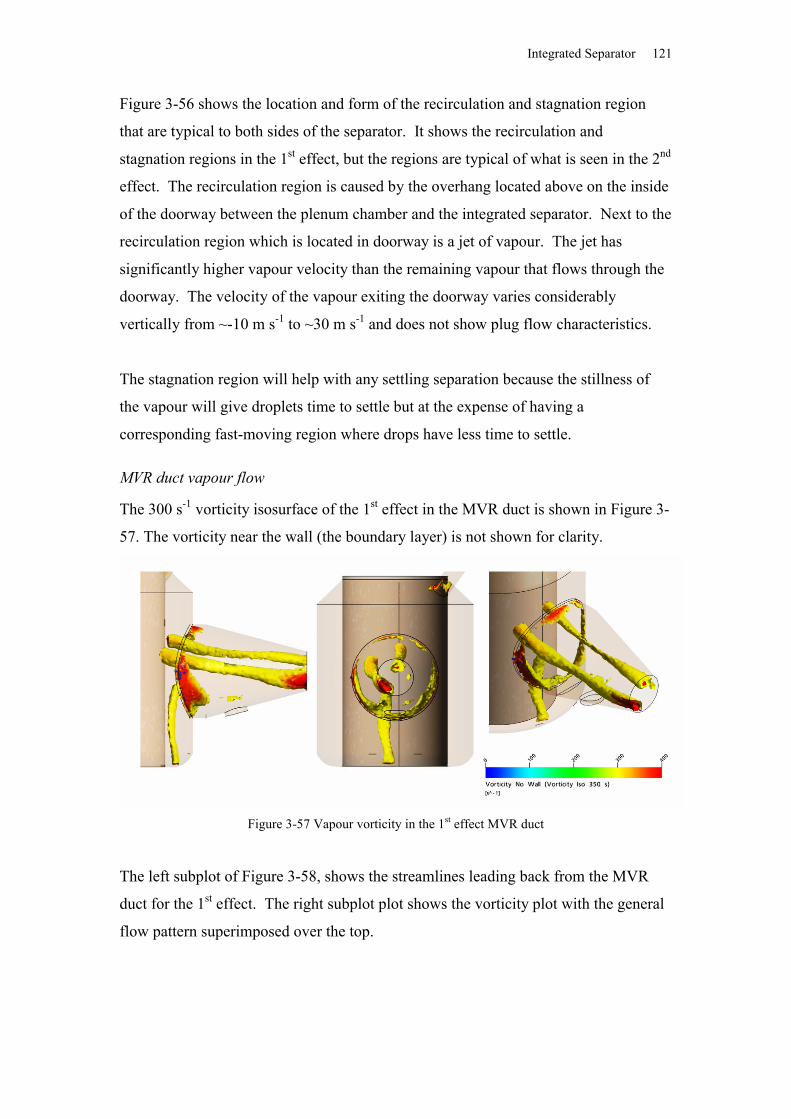
Integrated Separator 121
Figure 3-56 shows the location and form of the recirculation and stagnation region
that are typical to both sides of the separator. It shows the recirculation and
stagnation regions in the 1st effect, but the regions are typical of what is seen in the 2nd
effect. The recirculation region is caused by the overhang located above on the inside
of the doorway between the plenum chamber and the integrated separator. Next to the
recirculation region which is located in doorway is a jet of vapour. The jet has
significantly higher vapour velocity than the remaining vapour that flows through the
doorway. The velocity of the vapour exiting the doorway varies considerably
vertically from ~-10 m s-1 to ~30 m s-1 and does not show plug flow characteristics.
The stagnation region will help with any settling separation because the stillness of
the vapour will give droplets time to settle but at the expense of having a
corresponding fast-moving region where drops have less time to settle.
MVR duct vapour flow
The 300 s-1 vorticity isosurface of the 1st effect in the MVR duct is shown in Figure 3-
57. The vorticity near the wall (the boundary layer) is not shown for clarity.
Figure 3-57 Vapour vorticity in the 1st effect MVR duct
The left subplot of Figure 3-58, shows the streamlines leading back from the MVR
duct for the 1st effect. The right subplot plot shows the vorticity plot with the general
flow pattern superimposed over the top.
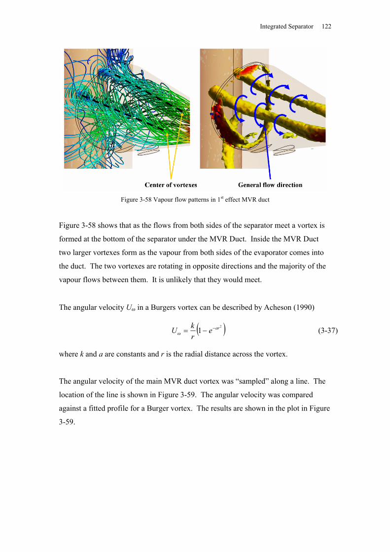
Integrated Separator 122
Figure 3-58 Vapour flow patterns in 1st effect MVR duct
Figure 3-58 shows that as the flows from both sides of the separator meet a vortex is
formed at the bottom of the separator under the MVR Duct. Inside the MVR Duct
two larger vortexes form as the vapour from both sides of the evaporator comes into
the duct. The two vortexes are rotating in opposite directions and the majority of the
vapour flows between them. It is unlikely that they would meet.
The angular velocity U in a Burgers vortex can be described by Acheson (1990)
2
1 arerkU (3-37)
where k and a are constants and r is the radial distance across the vortex.
The angular velocity of the main MVR duct vortex was “sampled” along a line. The
location of the line is shown in Figure 3-59. The angular velocity was compared
against a fitted profile for a Burger vortex. The results are shown in the plot in Figure
3-59.
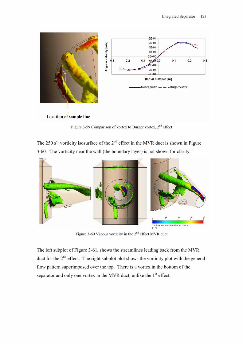
Integrated Separator 123
Figure 3-59 Comparison of vortex to Burger vortex, 2nd effect
The 250 s-1 vorticity isosurface of the 2nd effect in the MVR duct is shown in Figure
3-60. The vorticity near the wall (the boundary layer) is not shown for clarity.
Figure 3-60 Vapour vorticity in the 2nd effect MVR duct
The left subplot of Figure 3-61, shows the streamlines leading back from the MVR
duct for the 2nd effect. The right subplot plot shows the vorticity plot with the general
flow pattern superimposed over the top. There is a vortex in the bottom of the
separator and only one vortex in the MVR duct, unlike the 1st effect.
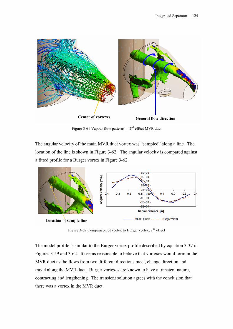
Integrated Separator 124
Figure 3-61 Vapour flow patterns in 2nd effect MVR duct
The angular velocity of the main MVR duct vortex was “sampled” along a line. The
location of the line is shown in Figure 3-62. The angular velocity is compared against
a fitted profile for a Burger vortex in Figure 3-62.
Figure 3-62 Comparison of vortex to Burger vortex, 2nd effect
The model profile is similar to the Burger vortex profile described by equation 3-37 in
Figures 3-59 and 3-62. It seems reasonable to believe that vortexes would form in the
MVR duct as the flows from two different directions meet, change direction and
travel along the MVR duct. Burger vortexes are known to have a transient nature,
contracting and lengthening. The transient solution agrees with the conclusion that
there was a vortex in the MVR duct.
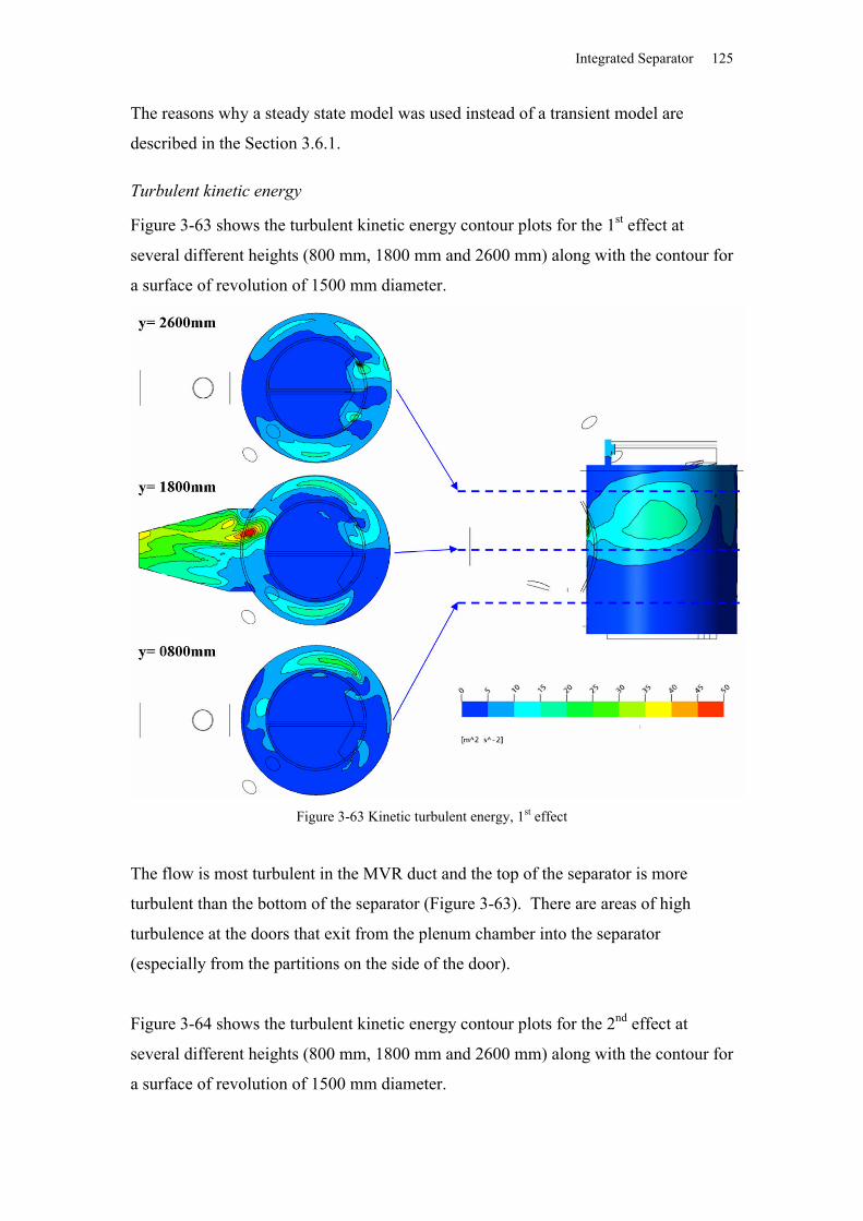
Integrated Separator 125
The reasons why a steady state model was used instead of a transient model are
described in the Section 3.6.1.
Turbulent kinetic energy
Figure 3-63 shows the turbulent kinetic energy contour plots for the 1st effect at
several different heights (800 mm, 1800 mm and 2600 mm) along with the contour for
a surface of revolution of 1500 mm diameter.
Figure 3-63 Kinetic turbulent energy, 1st effect
The flow is most turbulent in the MVR duct and the top of the separator is more
turbulent than the bottom of the separator (Figure 3-63). There are areas of high
turbulence at the doors that exit from the plenum chamber into the separator
(especially from the partitions on the side of the door).
Figure 3-64 shows the turbulent kinetic energy contour plots for the 2nd effect at
several different heights (800 mm, 1800 mm and 2600 mm) along with the contour for
a surface of revolution of 1500 mm diameter.
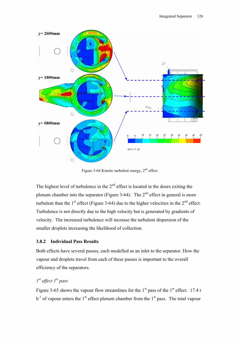
Integrated Separator 126
Figure 3-64 Kinetic turbulent energy, 2nd effect
The highest level of turbulence in the 2nd effect is located in the doors exiting the
plenum chamber into the separator (Figure 3-64). The 2nd effect in general is more
turbulent than the 1st effect (Figure 3-64) due to the higher velocities in the 2nd effect.
Turbulence is not directly due to the high velocity but is generated by gradients of
velocity. The increased turbulence will increase the turbulent dispersion of the
smaller droplets increasing the likelihood of collection.
3.8.2 Individual Pass Results
Both effects have several passes, each modelled as an inlet to the separator. How the
vapour and droplets travel from each of these passes is important to the overall
efficiency of the separators.
1st effect 1st pass
Figure 3-65 shows the vapour flow streamlines for the 1st pass of the 1st effect. 17.4 t
h-1 of vapour enters the 1st effect plenum chamber from the 1st pass. The total vapour
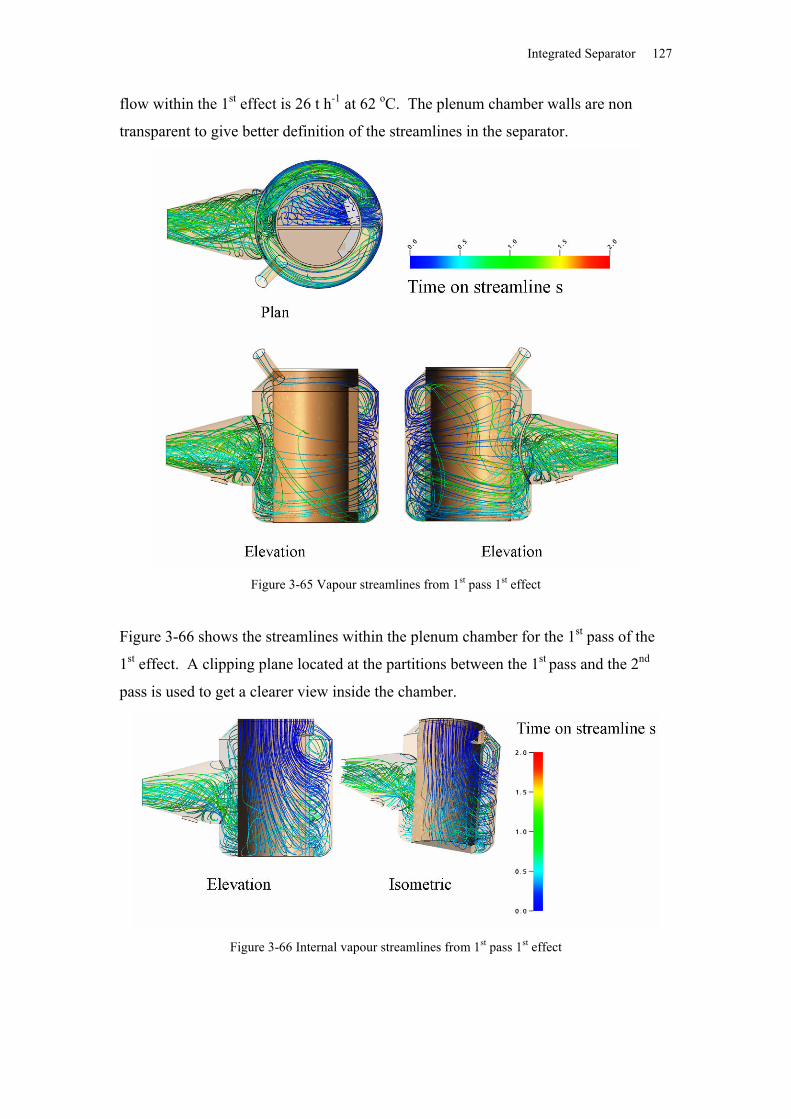
Integrated Separator 127
flow within the 1st effect is 26 t h-1 at 62 oC. The plenum chamber walls are non
transparent to give better definition of the streamlines in the separator.
Figure 3-65 Vapour streamlines from 1st pass 1st effect
Figure 3-66 shows the streamlines within the plenum chamber for the 1st pass of the
1st effect. A clipping plane located at the partitions between the 1st pass and the 2nd
pass is used to get a clearer view inside the chamber.
Figure 3-66 Internal vapour streamlines from 1st pass 1st effect
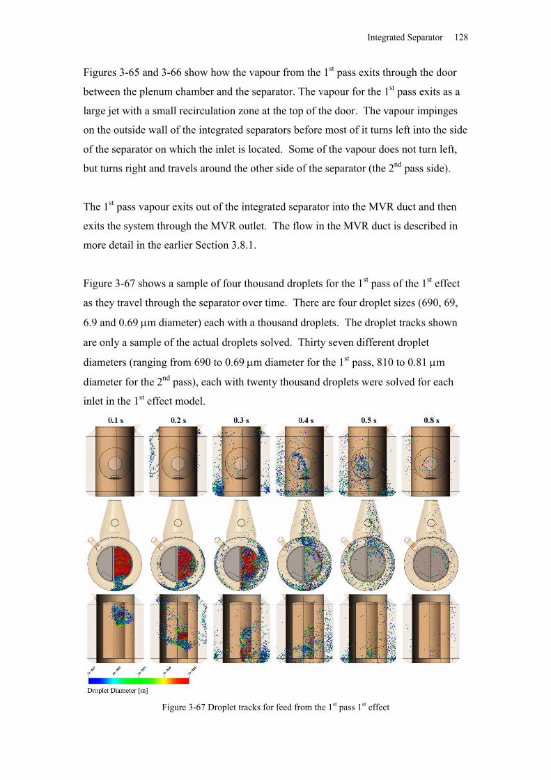
Integrated Separator 128
Figures 3-65 and 3-66 show how the vapour from the 1st pass exits through the door
between the plenum chamber and the separator. The vapour for the 1st pass exits as a
large jet with a small recirculation zone at the top of the door. The vapour impinges
on the outside wall of the integrated separators before most of it turns left into the side
of the separator on which the inlet is located. Some of the vapour does not turn left,
but turns right and travels around the other side of the separator (the 2nd pass side).
The 1st pass vapour exits out of the integrated separator into the MVR duct and then
exits the system through the MVR outlet. The flow in the MVR duct is described in
more detail in the earlier Section 3.8.1.
Figure 3-67 shows a sample of four thousand droplets for the 1st pass of the 1st effect
as they travel through the separator over time. There are four droplet sizes (690, 69,
6.9 and 0.69 m diameter) each with a thousand droplets. The droplet tracks shown
are only a sample of the actual droplets solved. Thirty seven different droplet
diameters (ranging from 690 to 0.69 m diameter for the 1st pass, 810 to 0.81 m
diameter for the 2nd pass), each with twenty thousand droplets were solved for each
inlet in the 1st effect model.
Figure 3-67 Droplet tracks for feed from the 1st pass 1st effect
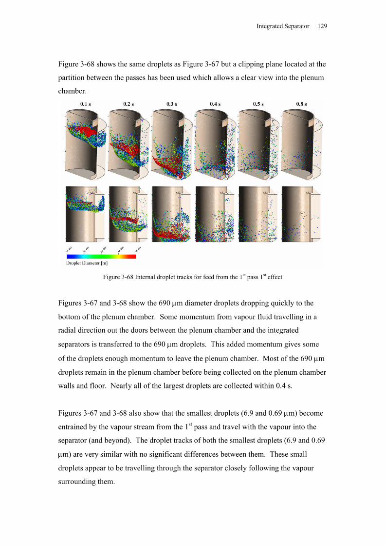
Integrated Separator 129
Figure 3-68 shows the same droplets as Figure 3-67 but a clipping plane located at the
partition between the passes has been used which allows a clear view into the plenum
chamber.
Figure 3-68 Internal droplet tracks for feed from the 1st pass 1st effect
Figures 3-67 and 3-68 show the 690 m diameter droplets dropping quickly to the
bottom of the plenum chamber. Some momentum from vapour fluid travelling in a
radial direction out the doors between the plenum chamber and the integrated
separators is transferred to the 690 m droplets. This added momentum gives some
of the droplets enough momentum to leave the plenum chamber. Most of the 690 m
droplets remain in the plenum chamber before being collected on the plenum chamber
walls and floor. Nearly all of the largest droplets are collected within 0.4 s.
Figures 3-67 and 3-68 also show that the smallest droplets (6.9 and 0.69 m) become
entrained by the vapour stream from the 1st pass and travel with the vapour into the
separator (and beyond). The droplet tracks of both the smallest droplets (6.9 and 0.69
m) are very similar with no significant differences between them. These small
droplets appear to be travelling through the separator closely following the vapour
surrounding them.
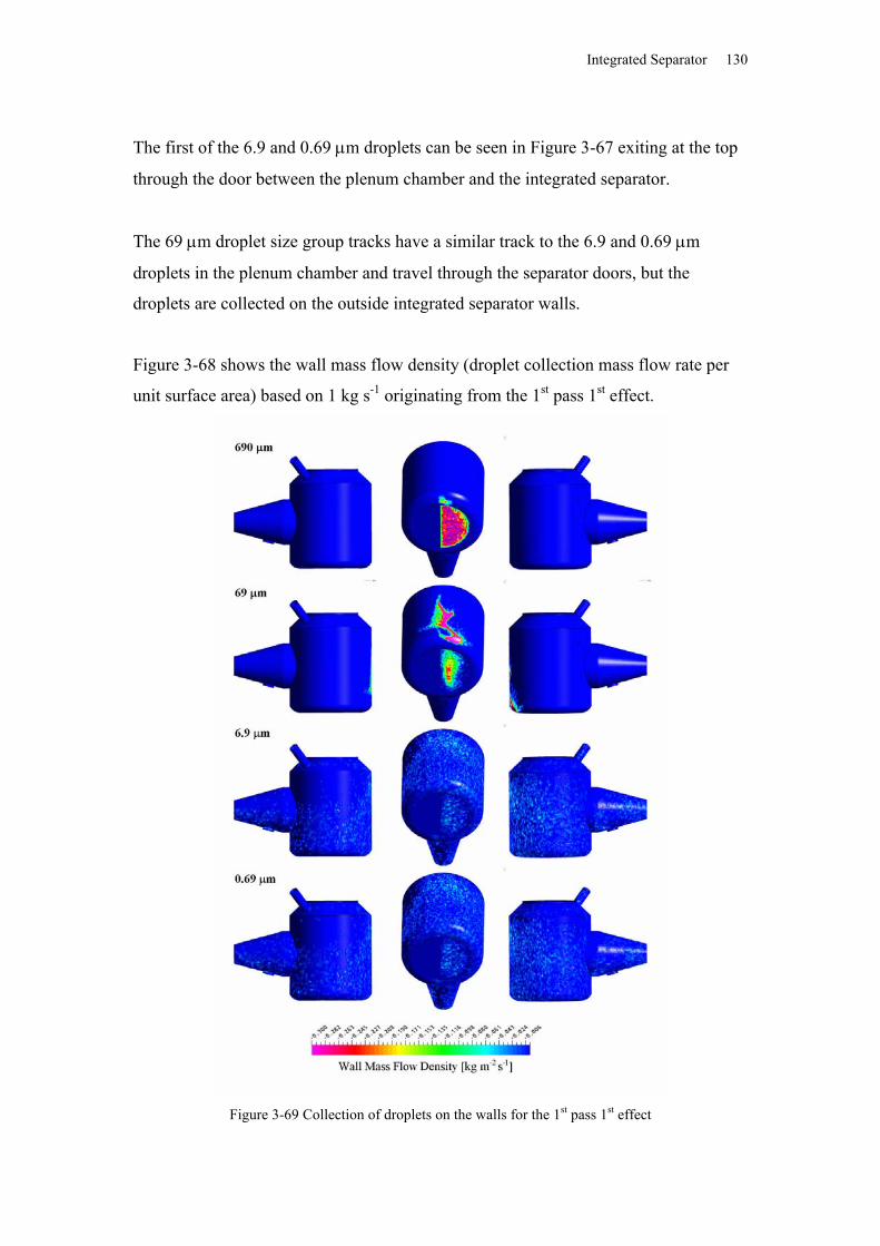
Integrated Separator 130
The first of the 6.9 and 0.69 m droplets can be seen in Figure 3-67 exiting at the top
through the door between the plenum chamber and the integrated separator.
The 69 m droplet size group tracks have a similar track to the 6.9 and 0.69 m
droplets in the plenum chamber and travel through the separator doors, but the
droplets are collected on the outside integrated separator walls.
Figure 3-68 shows the wall mass flow density (droplet collection mass flow rate per
unit surface area) based on 1 kg s-1 originating from the 1st pass 1st effect.
Figure 3-69 Collection of droplets on the walls for the 1st pass 1st effect
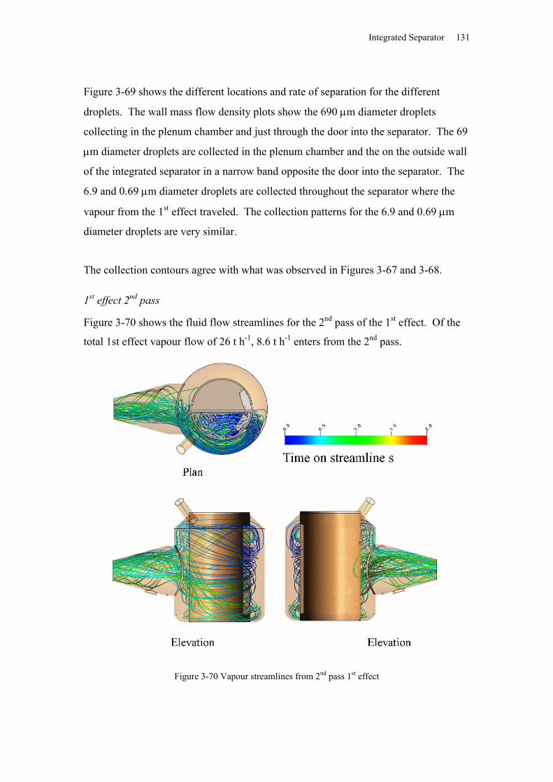
Integrated Separator 131
Figure 3-69 shows the different locations and rate of separation for the different
droplets. The wall mass flow density plots show the 690 m diameter droplets
collecting in the plenum chamber and just through the door into the separator. The 69
m diameter droplets are collected in the plenum chamber and the on the outside wall
of the integrated separator in a narrow band opposite the door into the separator. The
6.9 and 0.69 m diameter droplets are collected throughout the separator where the
vapour from the 1st effect traveled. The collection patterns for the 6.9 and 0.69 m
diameter droplets are very similar.
The collection contours agree with what was observed in Figures 3-67 and 3-68.
1st effect 2nd pass
Figure 3-70 shows the fluid flow streamlines for the 2nd pass of the 1st effect. Of the
total 1st effect vapour flow of 26 t h-1, 8.6 t h-1 enters from the 2nd pass.
Figure 3-70 Vapour streamlines from 2nd pass 1st effect
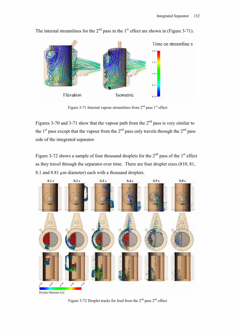
Integrated Separator 132
The internal streamlines for the 2nd pass in the 1st effect are shown in (Figure 3-71).
Figure 3-71 Internal vapour streamlines from 2nd pass 1st effect
Figures 3-70 and 3-71 show that the vapour path from the 2nd pass is very similar to
the 1st pass except that the vapour from the 2nd pass only travels through the 2nd pass
side of the integrated separator.
Figure 3-72 shows a sample of four thousand droplets for the 2nd pass of the 1st effect
as they travel through the separator over time. There are four droplet sizes (810, 81,
8.1 and 0.81 m diameter) each with a thousand droplets.
Figure 3-72 Droplet tracks for feed from the 2nd pass 2nd effect
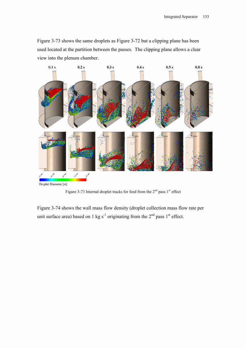
Integrated Separator 133
Figure 3-73 shows the same droplets as Figure 3-72 but a clipping plane has been
used located at the partition between the passes. The clipping plane allows a clear
view into the plenum chamber.
Figure 3-73 Internal droplet tracks for feed from the 2nd pass 1st effect
Figure 3-74 shows the wall mass flow density (droplet collection mass flow rate per
unit surface area) based on 1 kg s-1 originating from the 2nd pass 1st effect.
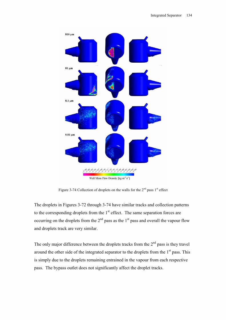
Integrated Separator 134
Figure 3-74 Collection of droplets on the walls for the 2nd pass 1st effect
The droplets in Figures 3-72 through 3-74 have similar tracks and collection patterns
to the corresponding droplets from the 1st effect. The same separation forces are
occurring on the droplets from the 2nd pass as the 1st pass and overall the vapour flow
and droplets track are very similar.
The only major difference between the droplets tracks from the 2nd pass is they travel
around the other side of the integrated separator to the droplets from the 1st pass. This
is simply due to the droplets remaining entrained in the vapour from each respective
pass. The bypass outlet does not significantly affect the droplet tracks.
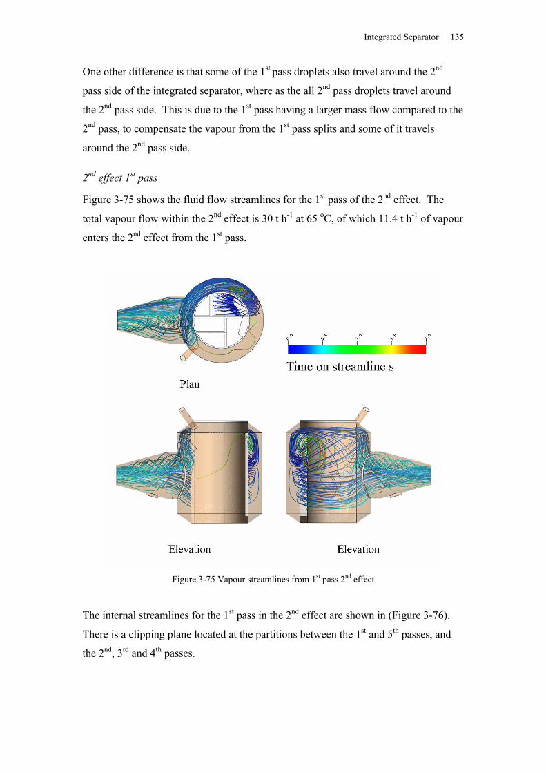
Integrated Separator 135
One other difference is that some of the 1st pass droplets also travel around the 2nd
pass side of the integrated separator, where as the all 2nd pass droplets travel around
the 2nd pass side. This is due to the 1st pass having a larger mass flow compared to the
2nd pass, to compensate the vapour from the 1st pass splits and some of it travels
around the 2nd pass side.
2nd effect 1st pass
Figure 3-75 shows the fluid flow streamlines for the 1st pass of the 2nd effect. The
total vapour flow within the 2nd effect is 30 t h-1 at 65 oC, of which 11.4 t h-1 of vapour
enters the 2nd effect from the 1st pass.
Figure 3-75 Vapour streamlines from 1st pass 2nd effect
The internal streamlines for the 1st pass in the 2nd effect are shown in (Figure 3-76).
There is a clipping plane located at the partitions between the 1st and 5th passes, and
the 2nd, 3rd and 4th passes.
Integrated Separator 136
Figure 3-76 Internal vapour streamlines from 1st pass 2nd effect
Figures 3-75 and 3-76 shows how the vapour from the 1st pass only travels a short
vertical distance down into the plenum chamber before turning outwards through the
doors into the integrated separator. There is a significant region of recirculation
located at the top of the doorway.
Once the vapour from the 1st pass exits through the doorway, virtually all of it travels
around the integrated separators through the 1st pass side of the separator. Figures 3-
75 and 3-76 show how the vapour streamlines from the 1st pass are confined to the
middle and top of the separator. This is different to the vapour streamlines for the 1st
and 2nd passes for the 1st effect, which travel through the entire vertical height of the
integrated separators.
The 2nd effect has 5 passes, compared to the 1st effect which has only 2. These extra
passes produce vapour which must travel through the 2nd effect integrated separator
which is not necessary in the 1st effect. The reason why the 1st pass is confined to the
middle and top of the integrated separator is simply because the 5th pass vapour is
travelling around the bottom of the integrated separator (Figures 3-95 and 3-96). It is
interesting that there is only limited mixing between the vapour from the two passes.
Figure 3-77 shows a sample of four thousand droplets for the 1st pass of the 2nd effect
as they travel through the separator over time. There are four droplet sizes (690, 69,
6.9 and 0.69 m diameter) diameter, each with a thousand droplets. The droplet tracks
shown are only a sample of the actual droplets solved for. Thirty seven different
droplet diameters (ranging from 690 m to 0.69 m 1st pass, 810 m to 0.81 m 2nd
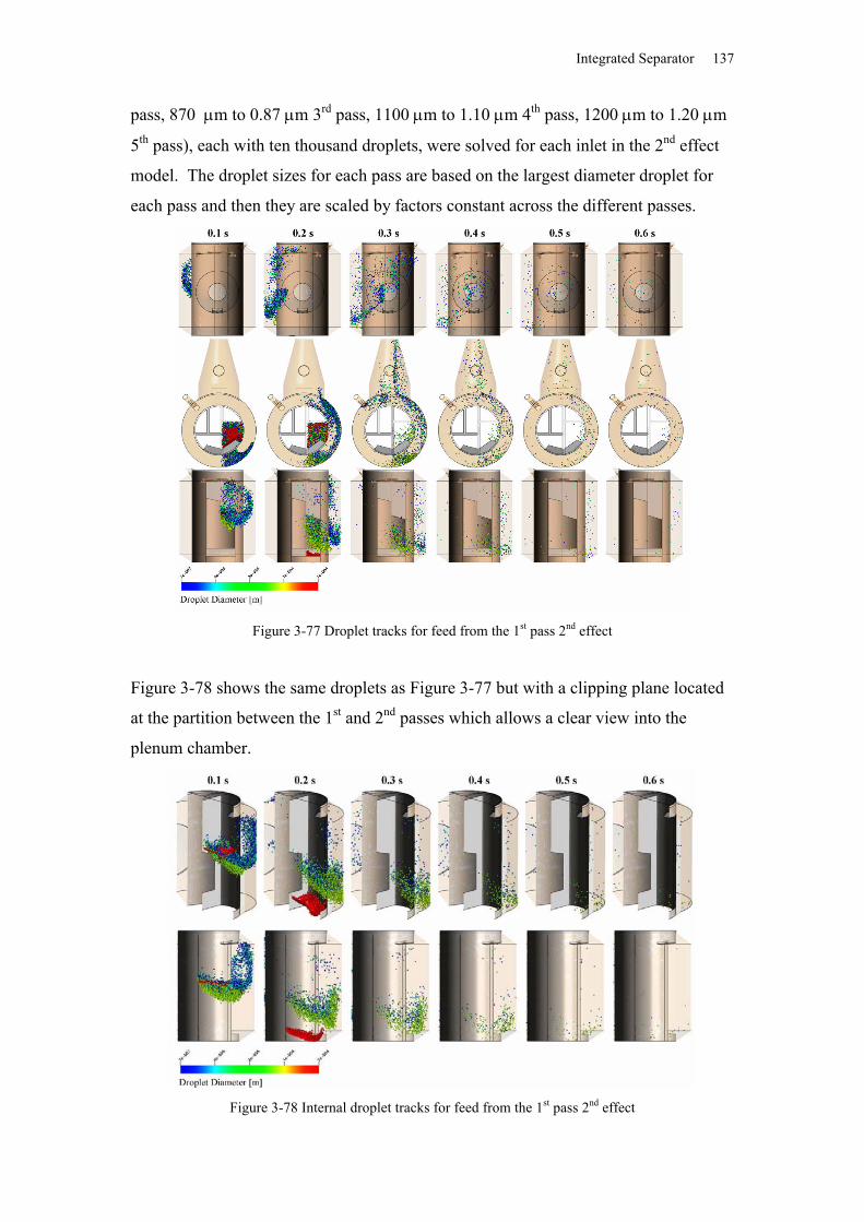
Integrated Separator 137
pass, 870 m to 0.87 m 3rd pass, 1100 m to 1.10 m 4th pass, 1200 m to 1.20 m
5th pass), each with ten thousand droplets, were solved for each inlet in the 2nd effect
model. The droplet sizes for each pass are based on the largest diameter droplet for
each pass and then they are scaled by factors constant across the different passes.
Figure 3-77 Droplet tracks for feed from the 1st pass 2nd effect
Figure 3-78 shows the same droplets as Figure 3-77 but with a clipping plane located
at the partition between the 1st and 2nd passes which allows a clear view into the
plenum chamber.
Figure 3-78 Internal droplet tracks for feed from the 1st pass 2nd effect
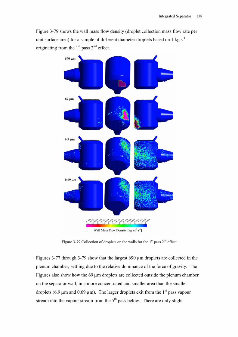
Integrated Separator 138
Figure 3-79 shows the wall mass flow density (droplet collection mass flow rate per
unit surface area) for a sample of different diameter droplets based on 1 kg s-1
originating from the 1st pass 2nd effect.
Figure 3-79 Collection of droplets on the walls for the 1st pass 2nd effect
Figures 3-77 through 3-79 show that the largest 690 m droplets are collected in the
plenum chamber, settling due to the relative dominance of the force of gravity. The
Figures also show how the 69 m droplets are collected outside the plenum chamber
on the separator wall, in a more concentrated and smaller area than the smaller
droplets (6.9 m and 0.69 m). The larger droplets exit from the 1st pass vapour
stream into the vapour stream from the 5th pass below. There are only slight
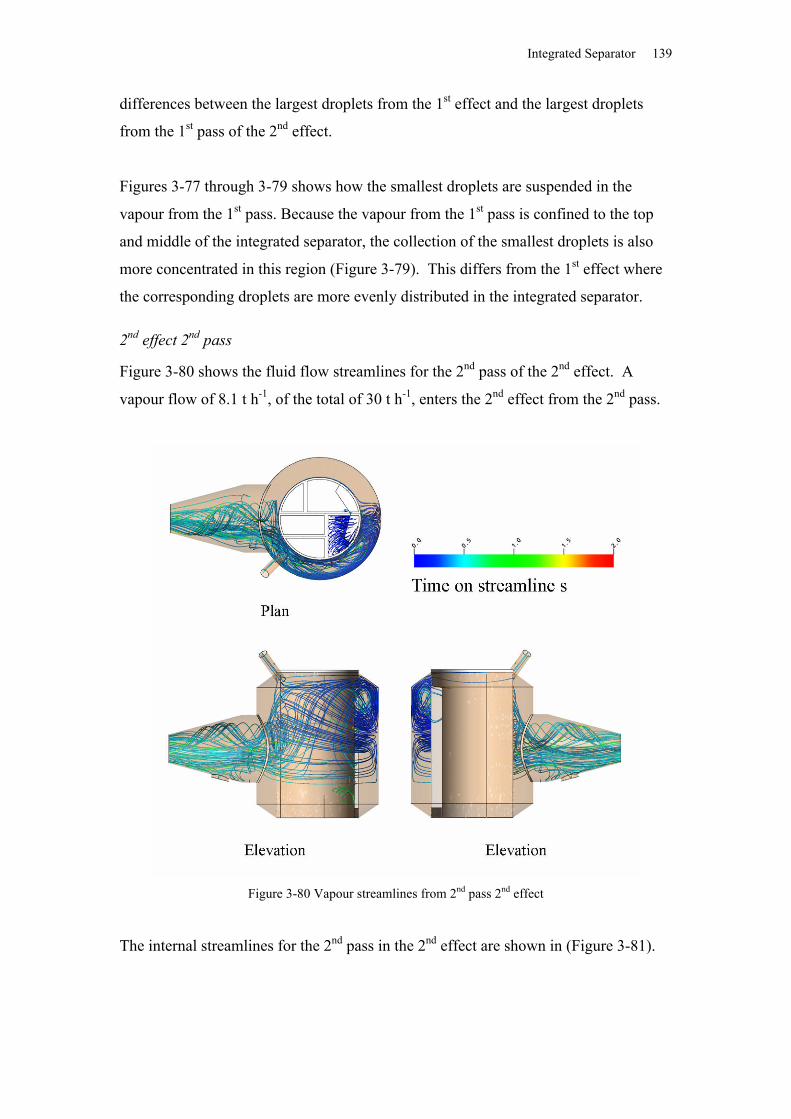
Integrated Separator 139
differences between the largest droplets from the 1st effect and the largest droplets
from the 1st pass of the 2nd effect.
Figures 3-77 through 3-79 shows how the smallest droplets are suspended in the
vapour from the 1st pass. Because the vapour from the 1st pass is confined to the top
and middle of the integrated separator, the collection of the smallest droplets is also
more concentrated in this region (Figure 3-79). This differs from the 1st effect where
the corresponding droplets are more evenly distributed in the integrated separator.
2nd effect 2nd pass
Figure 3-80 shows the fluid flow streamlines for the 2nd pass of the 2nd effect. A
vapour flow of 8.1 t h-1, of the total of 30 t h-1, enters the 2nd effect from the 2nd pass.
Figure 3-80 Vapour streamlines from 2nd pass 2nd effect
The internal streamlines for the 2nd pass in the 2nd effect are shown in (Figure 3-81).
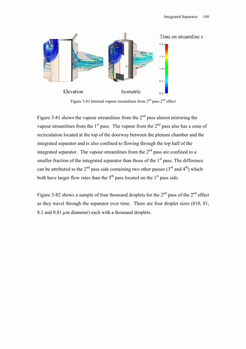
Integrated Separator 140
Figure 3-81 Internal vapour streamlines from 2nd pass 2nd effect
Figure 3-81 shows the vapour streamlines from the 2nd pass almost mirroring the
vapour streamlines from the 1st pass. The vapour from the 2nd pass also has a zone of
recirculation located at the top of the doorway between the plenum chamber and the
integrated separator and is also confined to flowing through the top half of the
integrated separator. The vapour streamlines from the 2nd pass are confined to a
smaller fraction of the integrated separator than those of the 1st pass. The difference
can be attributed to the 2nd pass side containing two other passes (3rd and 4th) which
both have larger flow rates than the 5th pass located on the 1st pass side.
Figure 3-82 shows a sample of four thousand droplets for the 2nd pass of the 2nd effect
as they travel through the separator over time. There are four droplet sizes (810, 81,
8.1 and 0.81 m diameter) each with a thousand droplets.
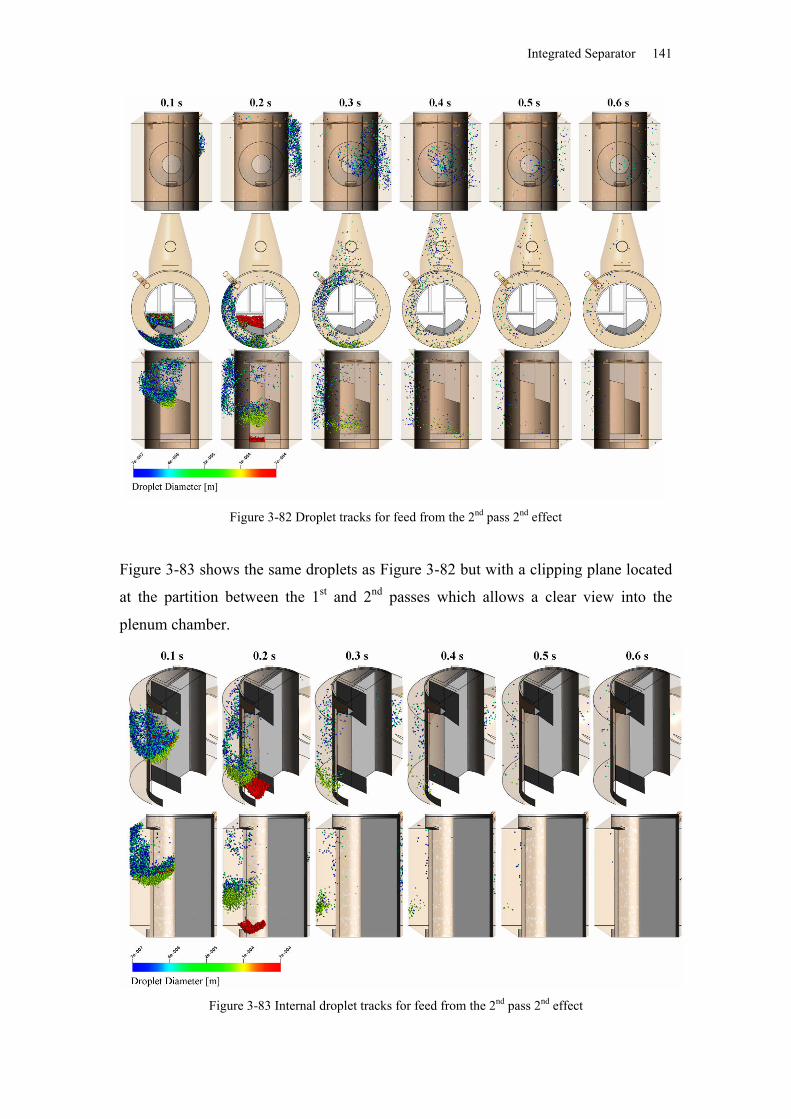
Integrated Separator 141
Figure 3-82 Droplet tracks for feed from the 2nd pass 2nd effect
Figure 3-83 shows the same droplets as Figure 3-82 but with a clipping plane located
at the partition between the 1st and 2nd passes which allows a clear view into the
plenum chamber.
Figure 3-83 Internal droplet tracks for feed from the 2nd pass 2nd effect
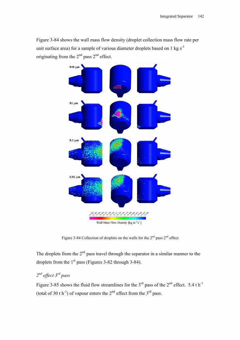
Integrated Separator 142
Figure 3-84 shows the wall mass flow density (droplet collection mass flow rate per
unit surface area) for a sample of various diameter droplets based on 1 kg s-1
originating from the 2nd pass 2nd effect.
Figure 3-84 Collection of droplets on the walls for the 2nd pass 2nd effect
The droplets from the 2nd pass travel through the separator in a similar manner to the
droplets from the 1st pass (Figures 3-82 through 3-84).
2nd effect 3rd pass
Figure 3-85 shows the fluid flow streamlines for the 3rd pass of the 2nd effect. 5.4 t h-1
(total of 30 t h-1) of vapour enters the 2nd effect from the 3rd pass.
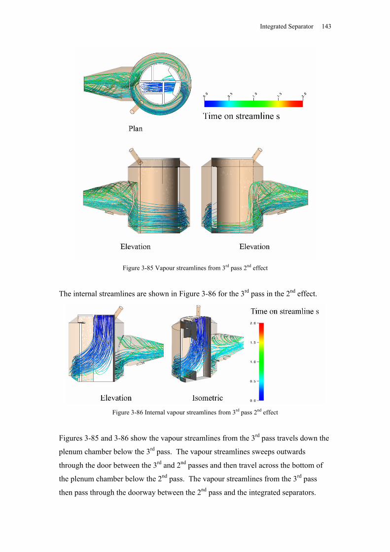
Integrated Separator 143
Figure 3-85 Vapour streamlines from 3rd pass 2nd effect
The internal streamlines are shown in Figure 3-86 for the 3rd pass in the 2nd effect.
Figure 3-86 Internal vapour streamlines from 3rd pass 2nd effect
Figures 3-85 and 3-86 show the vapour streamlines from the 3rd pass travels down the
plenum chamber below the 3rd pass. The vapour streamlines sweeps outwards
through the door between the 3rd and 2nd passes and then travel across the bottom of
the plenum chamber below the 2nd pass. The vapour streamlines from the 3rd pass
then pass through the doorway between the 2nd pass and the integrated separators.
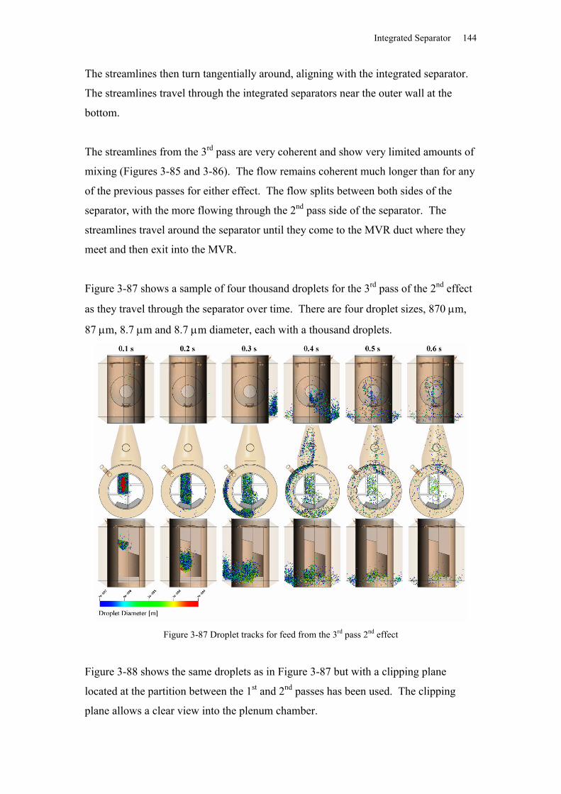
Integrated Separator 144
The streamlines then turn tangentially around, aligning with the integrated separator.
The streamlines travel through the integrated separators near the outer wall at the
bottom.
The streamlines from the 3rd pass are very coherent and show very limited amounts of
mixing (Figures 3-85 and 3-86). The flow remains coherent much longer than for any
of the previous passes for either effect. The flow splits between both sides of the
separator, with the more flowing through the 2nd pass side of the separator. The
streamlines travel around the separator until they come to the MVR duct where they
meet and then exit into the MVR.
Figure 3-87 shows a sample of four thousand droplets for the 3rd pass of the 2nd effect
as they travel through the separator over time. There are four droplet sizes, 870 m,
87 m, 8.7 m and 8.7 m diameter, each with a thousand droplets.
Figure 3-87 Droplet tracks for feed from the 3rd pass 2nd effect
Figure 3-88 shows the same droplets as in Figure 3-87 but with a clipping plane
located at the partition between the 1st and 2nd passes has been used. The clipping
plane allows a clear view into the plenum chamber.
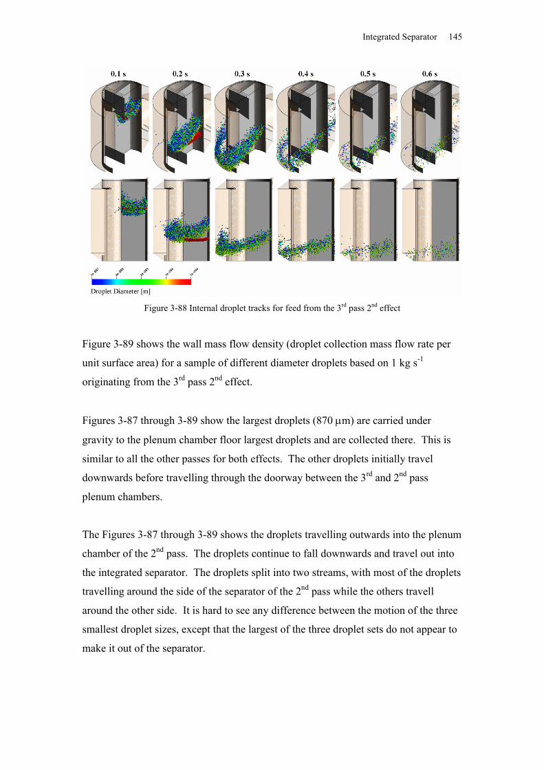
Integrated Separator 145
Figure 3-88 Internal droplet tracks for feed from the 3rd pass 2nd effect
Figure 3-89 shows the wall mass flow density (droplet collection mass flow rate per
unit surface area) for a sample of different diameter droplets based on 1 kg s-1
originating from the 3rd pass 2nd effect.
Figures 3-87 through 3-89 show the largest droplets (870 m) are carried under
gravity to the plenum chamber floor largest droplets and are collected there. This is
similar to all the other passes for both effects. The other droplets initially travel
downwards before travelling through the doorway between the 3rd and 2nd pass
plenum chambers.
The Figures 3-87 through 3-89 shows the droplets travelling outwards into the plenum
chamber of the 2nd pass. The droplets continue to fall downwards and travel out into
the integrated separator. The droplets split into two streams, with most of the droplets
travelling around the side of the separator of the 2nd pass while the others travell
around the other side. It is hard to see any difference between the motion of the three
smallest droplet sizes, except that the largest of the three droplet sets do not appear to
make it out of the separator.
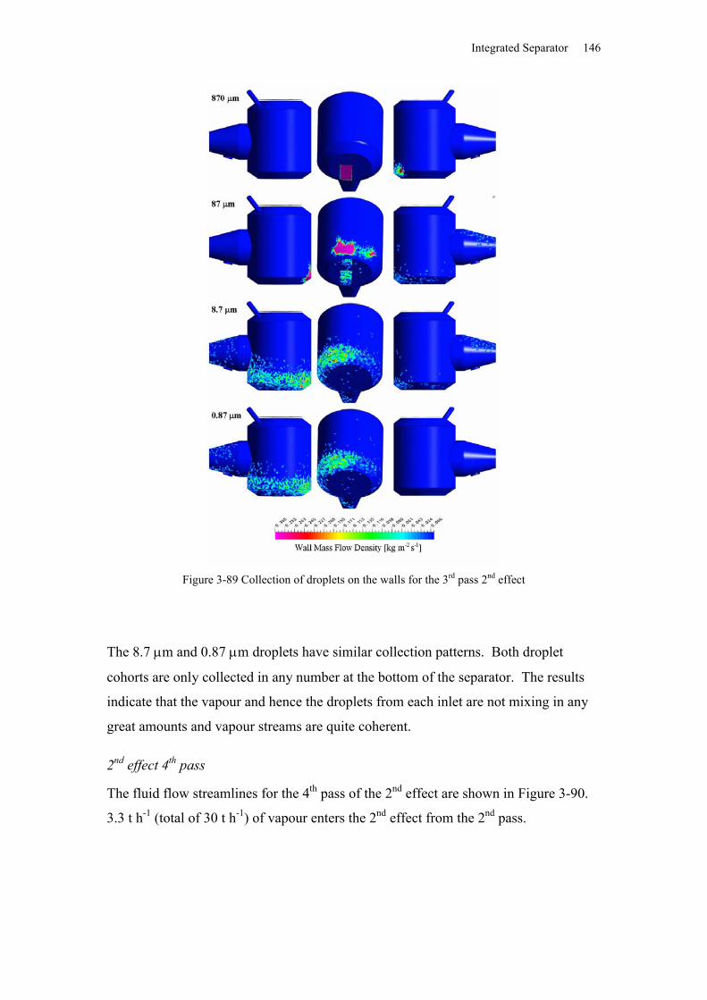
Integrated Separator 146
Figure 3-89 Collection of droplets on the walls for the 3rd pass 2nd effect
The 8.7 m and 0.87 m droplets have similar collection patterns. Both droplet
cohorts are only collected in any number at the bottom of the separator. The results
indicate that the vapour and hence the droplets from each inlet are not mixing in any
great amounts and vapour streams are quite coherent.
2nd effect 4th pass
The fluid flow streamlines for the 4th pass of the 2nd effect are shown in Figure 3-90.
3.3 t h-1 (total of 30 t h-1) of vapour enters the 2nd effect from the 2nd pass.
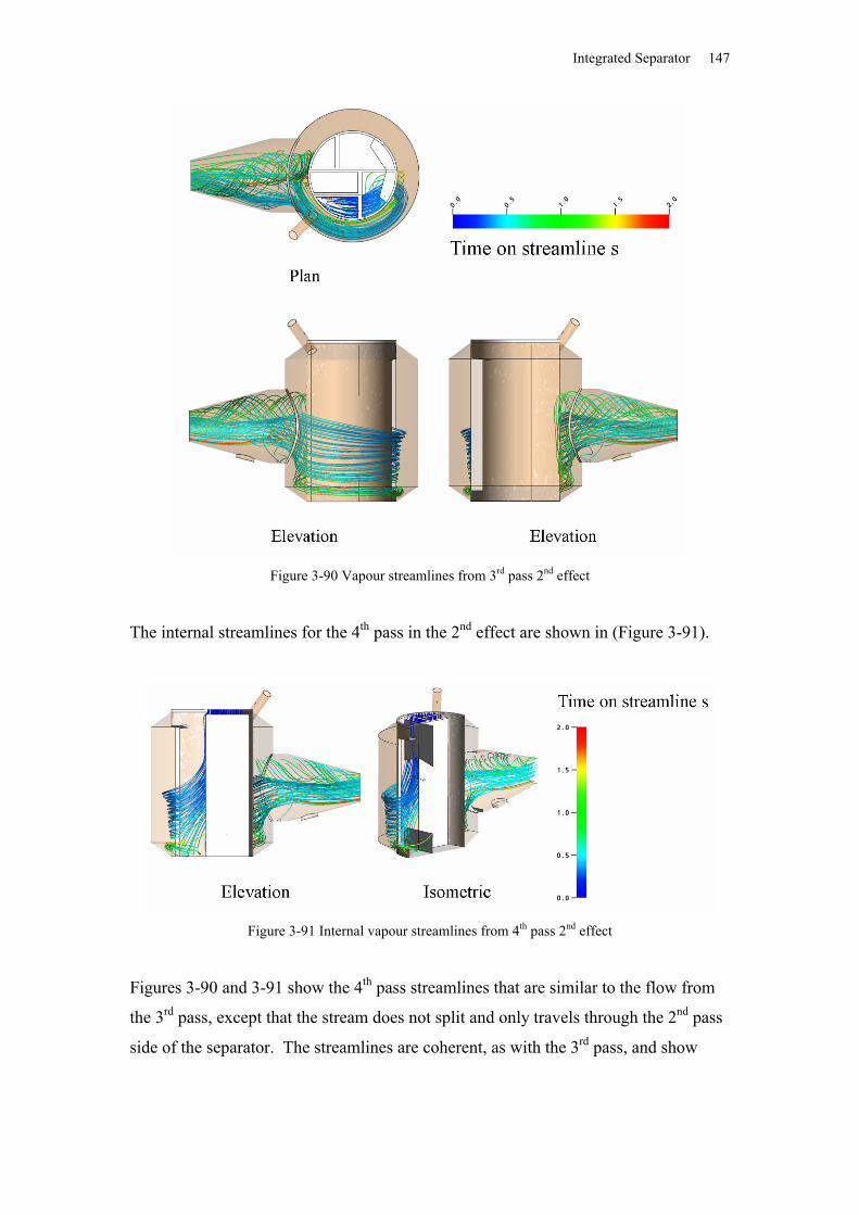
Integrated Separator 147
Figure 3-90 Vapour streamlines from 3rd pass 2nd effect
The internal streamlines for the 4th pass in the 2nd effect are shown in (Figure 3-91).
Figure 3-91 Internal vapour streamlines from 4th pass 2nd effect
Figures 3-90 and 3-91 show the 4th pass streamlines that are similar to the flow from
the 3rd pass, except that the stream does not split and only travels through the 2nd pass
side of the separator. The streamlines are coherent, as with the 3rd pass, and show
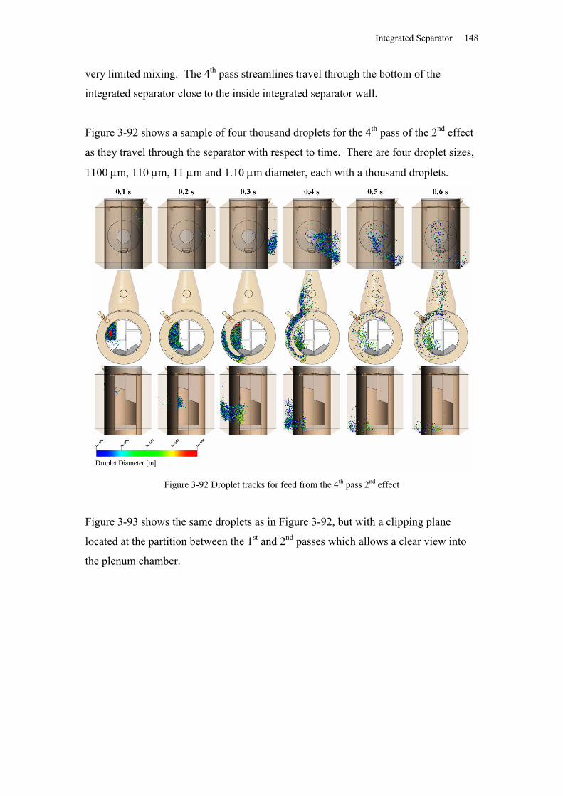
Integrated Separator 148
very limited mixing. The 4th pass streamlines travel through the bottom of the
integrated separator close to the inside integrated separator wall.
Figure 3-92 shows a sample of four thousand droplets for the 4th pass of the 2nd effect
as they travel through the separator with respect to time. There are four droplet sizes,
1100 m, 110 m, 11 m and 1.10 m diameter, each with a thousand droplets.
Figure 3-92 Droplet tracks for feed from the 4th pass 2nd effect
Figure 3-93 shows the same droplets as in Figure 3-92, but with a clipping plane
located at the partition between the 1st and 2nd passes which allows a clear view into
the plenum chamber.
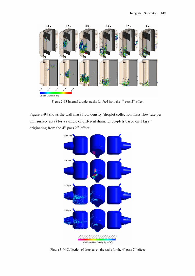
Integrated Separator 149
Figure 3-93 Internal droplet tracks for feed from the 4th pass 2nd effect
Figure 3-94 shows the wall mass flow density (droplet collection mass flow rate per
unit surface area) for a sample of different diameter droplets based on 1 kg s-1
originating from the 4th pass 2nd effect.
Figure 3-94 Collection of droplets on the walls for the 4th pass 2nd effect
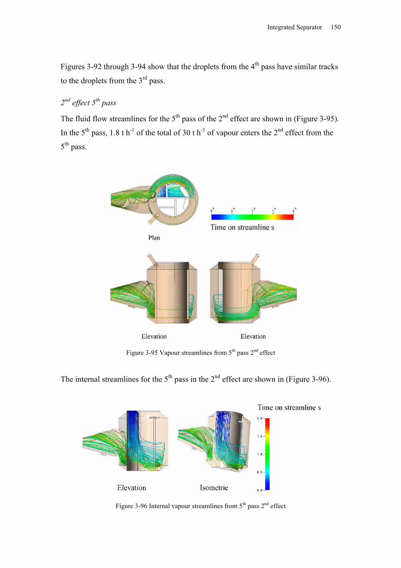
Integrated Separator 150
Figures 3-92 through 3-94 show that the droplets from the 4th pass have similar tracks
to the droplets from the 3rd pass.
2nd effect 5th pass
The fluid flow streamlines for the 5th pass of the 2nd effect are shown in (Figure 3-95).
In the 5th pass, 1.8 t h-1 of the total of 30 t h-1 of vapour enters the 2nd effect from the
5th pass.
Figure 3-95 Vapour streamlines from 5th pass 2nd effect
The internal streamlines for the 5th pass in the 2nd effect are shown in (Figure 3-96).
Figure 3-96 Internal vapour streamlines from 5th pass 2nd effect
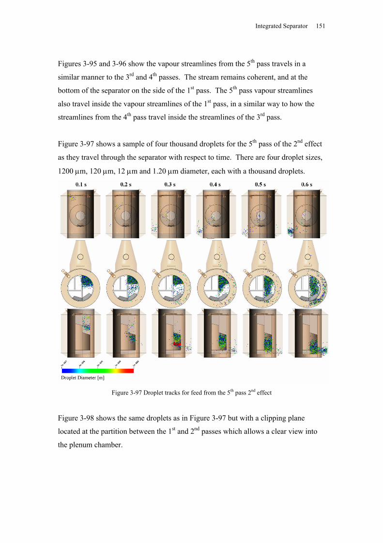
Integrated Separator 151
Figures 3-95 and 3-96 show the vapour streamlines from the 5th pass travels in a
similar manner to the 3rd and 4th passes. The stream remains coherent, and at the
bottom of the separator on the side of the 1st pass. The 5th pass vapour streamlines
also travel inside the vapour streamlines of the 1st pass, in a similar way to how the
streamlines from the 4th pass travel inside the streamlines of the 3rd pass.
Figure 3-97 shows a sample of four thousand droplets for the 5th pass of the 2nd effect
as they travel through the separator with respect to time. There are four droplet sizes,
1200 m, 120 m, 12 m and 1.20 m diameter, each with a thousand droplets.
Figure 3-97 Droplet tracks for feed from the 5th pass 2nd effect
Figure 3-98 shows the same droplets as in Figure 3-97 but with a clipping plane
located at the partition between the 1st and 2nd passes which allows a clear view into
the plenum chamber.
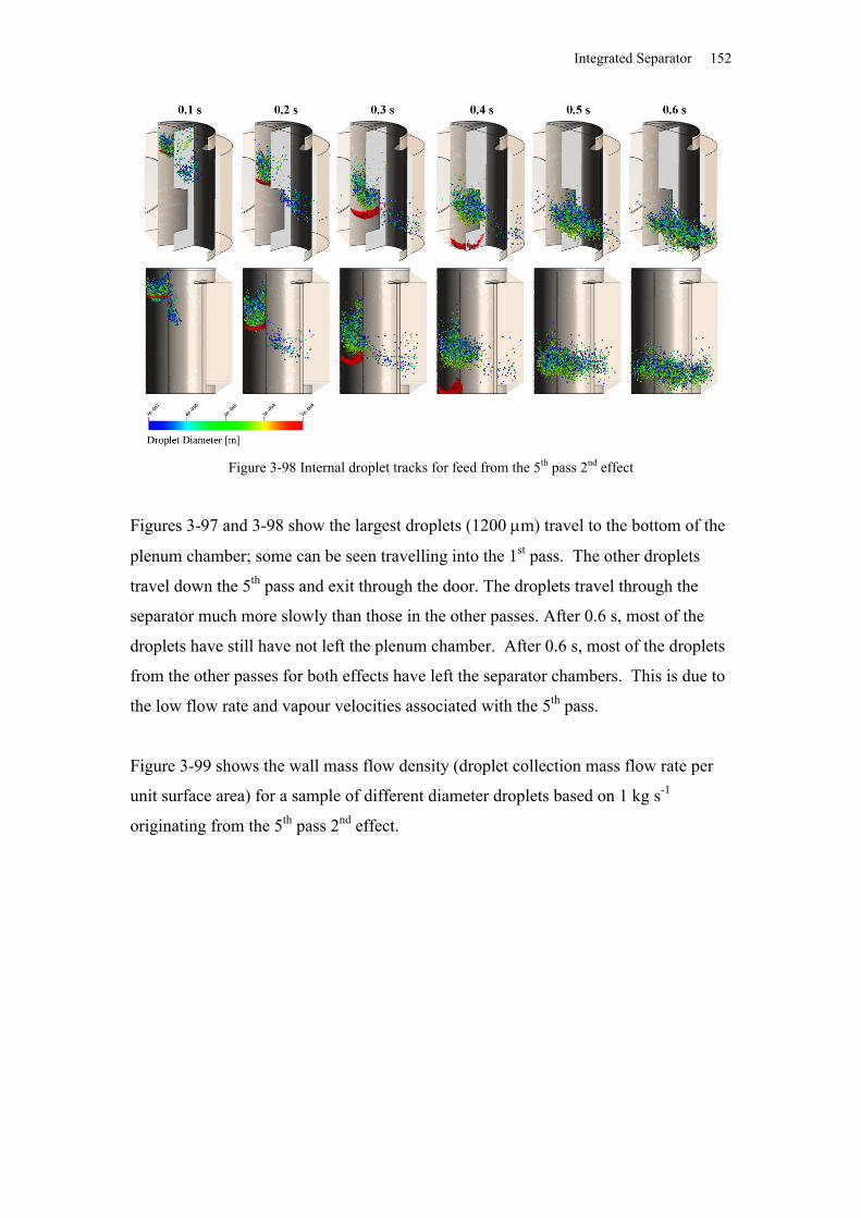
Integrated Separator 152
Figure 3-98 Internal droplet tracks for feed from the 5th pass 2nd effect
Figures 3-97 and 3-98 show the largest droplets (1200 m) travel to the bottom of the
plenum chamber; some can be seen travelling into the 1st pass. The other droplets
travel down the 5th pass and exit through the door. The droplets travel through the
separator much more slowly than those in the other passes. After 0.6 s, most of the
droplets have still have not left the plenum chamber. After 0.6 s, most of the droplets
from the other passes for both effects have left the separator chambers. This is due to
the low flow rate and vapour velocities associated with the 5th pass.
Figure 3-99 shows the wall mass flow density (droplet collection mass flow rate per
unit surface area) for a sample of different diameter droplets based on 1 kg s-1
originating from the 5th pass 2nd effect.
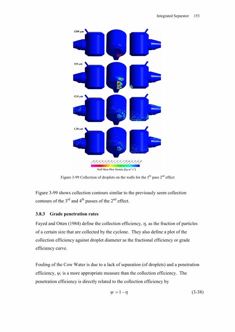
Integrated Separator 153
Figure 3-99 Collection of droplets on the walls for the 5th pass 2nd effect
Figure 3-99 shows collection contours similar to the previously seem collection
contours of the 3rd and 4th passes of the 2nd effect.
3.8.3 Grade penetration rates
Fayed and Otten (1984) define the collection efficiency, as the fraction of particles
of a certain size that are collected by the cyclone. They also define a plot of the
collection efficiency against droplet diameter as the fractional efficiency or grade
efficiency curve.
Fouling of the Cow Water is due to a lack of separation (of droplets) and a penetration
efficiency, is a more appropriate measure than the collection efficiency. The
penetration efficiency is directly related to the collection efficiency by
1 (3-38)
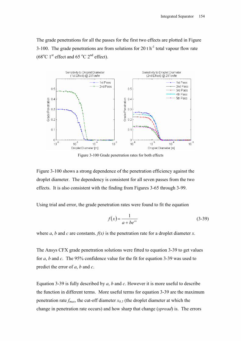
Integrated Separator 154
The grade penetrations for all the passes for the first two effects are plotted in Figure
3-100. The grade penetrations are from solutions for 20 t h-1 total vapour flow rate
(68oC 1st effect and 65 oC 2nd effect).
Figure 3-100 Grade penetration rates for both effects
Figure 3-100 shows a strong dependence of the penetration efficiency against the
droplet diameter. The dependency is consistent for all seven passes from the two
effects. It is also consistent with the finding from Figures 3-65 through 3-99.
Using trial and error, the grade penetration rates were found to fit the equation
cxbeaxf
1 (3-39)
where a, b and c are constants. f(x) is the penetration rate for a droplet diameter x.
The Ansys CFX grade penetration solutions were fitted to equation 3-39 to get values
for a, b and c. The 95% confidence value for the fit for equation 3-39 was used to
predict the error of a, b and c.
Equation 3-39 is fully described by a, b and c. However it is more useful to describe
the function in different terms. More useful terms for equation 3-39 are the maximum
penetration rate fmax, the cut-off diameter x0.5 (the droplet diameter at which the
change in penetration rate occurs) and how sharp that change (spread) is. The errors
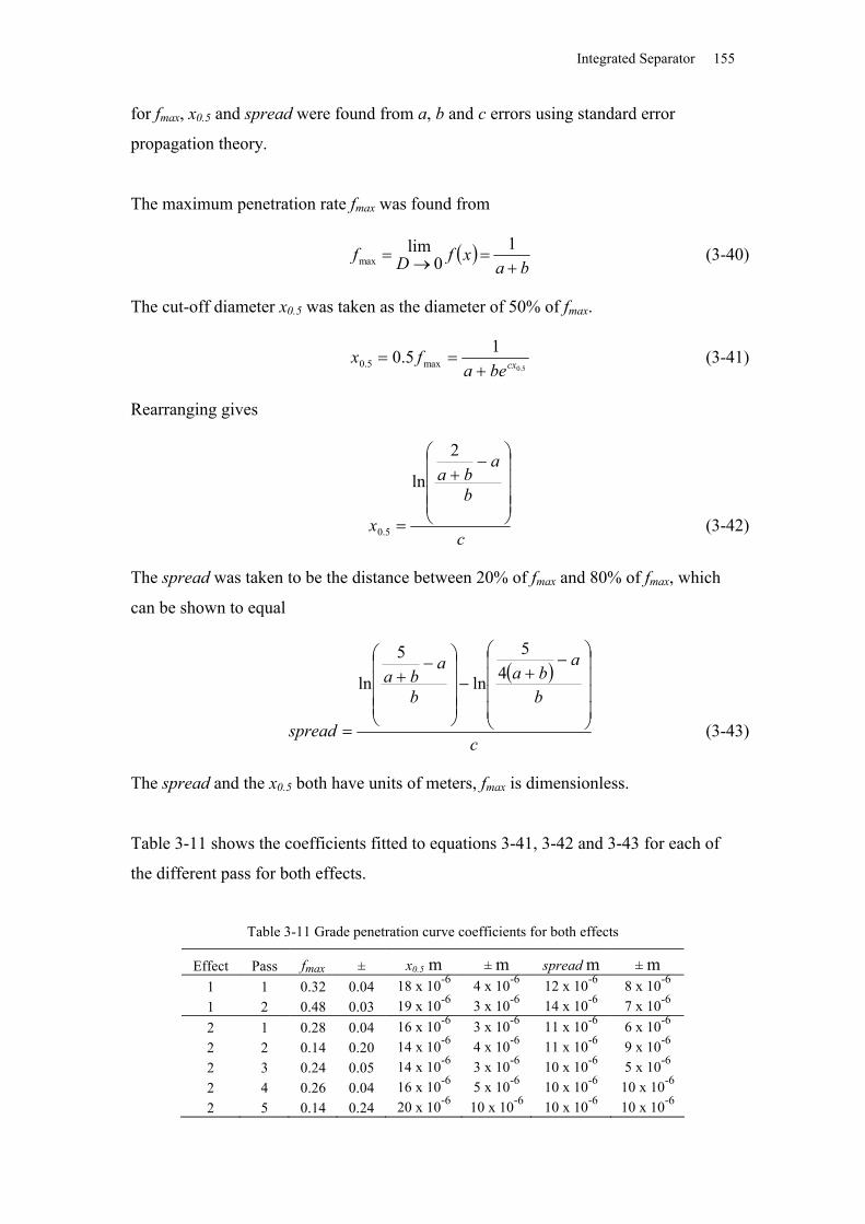
Integrated Separator 155
for fmax, x0.5 and spread were found from a, b and c errors using standard error
propagation theory.
The maximum penetration rate fmax was found from
ba
xfDf
1
0lim
max (3-40)
The cut-off diameter x0.5 was taken as the diameter of 50% of fmax.
5.0
15.0 max5.0 cxbeafx
(3-41)
Rearranging gives
c
b
aba
x
2
ln
5.0 (3-42)
The spread was taken to be the distance between 20% of fmax and 80% of fmax, which
can be shown to equal
c
b
aba
b
aba
spread
45
ln
5
ln
(3-43)
The spread and the x0.5 both have units of meters, fmax is dimensionless.
Table 3-11 shows the coefficients fitted to equations 3-41, 3-42 and 3-43 for each of
the different pass for both effects.
Table 3-11 Grade penetration curve coefficients for both effects
Effect Pass fmax ± x0.5 m ± m spread m ± m1 1 0.32 0.04 18 x 10-6 4 x 10⁻⁶ 12 x 10-6 8 x 10⁻⁶
1 2 0.48 0.03 19 x 10-6 3 x 10⁻⁶ 14 x 10-6 7 x 10⁻⁶
2 1 0.28 0.04 16 x 10-6 3 x 10⁻⁶ 11 x 10-6 6 x 10⁻⁶
2 2 0.14 0.20 14 x 10-6 4 x 10⁻⁶ 11 x 10-6 9 x 10⁻⁶
2 3 0.24 0.05 14 x 10-6 3 x 10⁻⁶ 10 x 10-6 5 x 10⁻⁶
2 4 0.26 0.04 16 x 10-6 5 x 10⁻⁶ 10 x 10-6 10 x 10-6
2 5 0.14 0.24 20 x 10-6 10 x 10-6 10 x 10-6 10 x 10-6
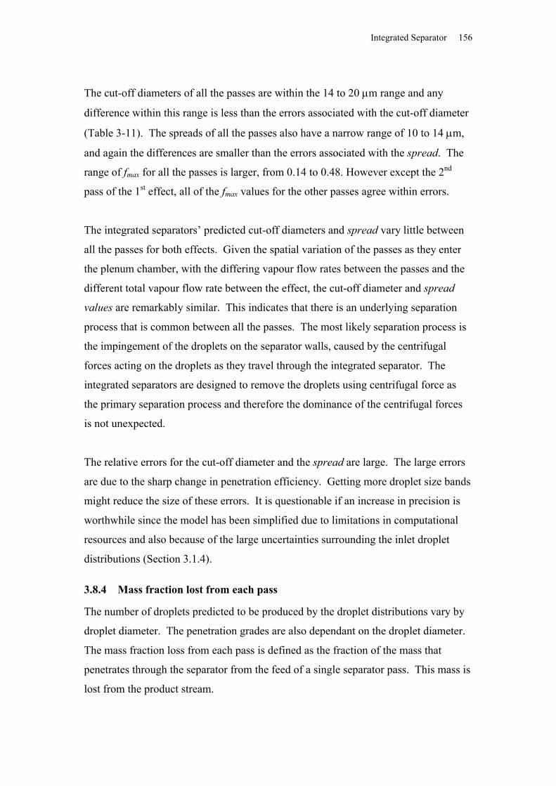
Integrated Separator 156
The cut-off diameters of all the passes are within the 14 to 20 m range and any
difference within this range is less than the errors associated with the cut-off diameter
(Table 3-11). The spreads of all the passes also have a narrow range of 10 to 14 m,
and again the differences are smaller than the errors associated with the spread. The
range of fmax for all the passes is larger, from 0.14 to 0.48. However except the 2nd
pass of the 1st effect, all of the fmax values for the other passes agree within errors.
The integrated separators’ predicted cut-off diameters and spread vary little between
all the passes for both effects. Given the spatial variation of the passes as they enter
the plenum chamber, with the differing vapour flow rates between the passes and the
different total vapour flow rate between the effect, the cut-off diameter and spread
values are remarkably similar. This indicates that there is an underlying separation
process that is common between all the passes. The most likely separation process is
the impingement of the droplets on the separator walls, caused by the centrifugal
forces acting on the droplets as they travel through the integrated separator. The
integrated separators are designed to remove the droplets using centrifugal force as
the primary separation process and therefore the dominance of the centrifugal forces
is not unexpected.
The relative errors for the cut-off diameter and the spread are large. The large errors
are due to the sharp change in penetration efficiency. Getting more droplet size bands
might reduce the size of these errors. It is questionable if an increase in precision is
worthwhile since the model has been simplified due to limitations in computational
resources and also because of the large uncertainties surrounding the inlet droplet
distributions (Section 3.1.4).
3.8.4 Mass fraction lost from each pass
The number of droplets predicted to be produced by the droplet distributions vary by
droplet diameter. The penetration grades are also dependant on the droplet diameter.
The mass fraction loss from each pass is defined as the fraction of the mass that
penetrates through the separator from the feed of a single separator pass. This mass is
lost from the product stream.
Integrated Separator 157
Table 3-12 shows the mass fraction lost from each pass for all the passes for both 1st
and 2nd effects for both Skim and MPC. The total vapour flow rate is for the 20 t h-1
and the vapour temperature for the 1st effect is 65oC and for the 2nd effect is 64oC.
The droplet distribution product differs when processing Skim or MPC, so the mass
loss fraction is dependent on the product processed.
The errors in Table 3-12 were calculated from the deviation of mass fraction lost
using the extremes of the predicted droplet distributions to find the positive and
negative the deviation of the mass fraction loss from the calculated fraction mass loss.
Table 3-12 Mass fraction loss from each effect when processing either Skim and MPC
Effect Pass SMD m +/- m Mass fraction loss + -Skim 1 1 90 20 0.005% 0.017% 0.002%
2 90 20 0.024% 0.075% 0.007%2 1 90 20 0.002% 0.008% 0.001%
2 100 30 0.0004% 0.0058% 0.0003%3 120 40 0.0003% 0.0012% 0.0002%4 160 50 0.00008% 0.00119% 0.00007%5 160 100 0.00007% 0.02393% 0.00007%
MPC 1 1 160 100 0.00017% 0.05199% 0.00015%2 160 100 0.00080% 0.22810% 0.00049%
2 1 160 100 0.00008% 0.02622% 0.00008%2 160 100 0.00003% 0.00829% 0.00002%3 160 100 0.00005% 0.01507% 0.00004%4 160 100 0.00008% 0.02560% 0.00007%5 160 100 0.00007% 0.02393% 0.00007%
Table 3-12 shows that the 2nd pass of the 1st effect had the greatest mass fraction loss
of all the passes. Figure 3-54 and 3-55 show on the 2nd pass side of the separator
lower velocities than on the 1st pass side. This is the side of the integrated separator
that the droplets from the 2nd pass travel through and this is the likely reason for the
greater mass fraction loss from this pass.
The mass fraction lost from all the passes from the 1st effect and the 1st through to 3rd
pass in the 2nd effect is worse when processing Skim compared to processing MPC.
When Skim is processed, the relative amount of mass contained in the smaller
droplets is greater than when processing MPC and it is these smaller droplets that are
responsible for the mass lost. The 4th and 5th passes for the 2nd effect have the same
Integrated Separator 158
droplet distributions for both MPC and Skim, so the mass fraction lost is the same for
both products.
More mass fraction is lost from the 1st effect than from the 2nd effect. This is due to
the lower total vapour flow rate in the 1st effect, 26 t h-1 versus 30 t h-1 for the 2nd
effect. This lower total vapour flow rate results in lower velocities in the separator
and an increasing in the cut-off diameter (larger droplets can penetrate). The effect of
the total vapour flow rate is considered in more detail in Section 3.9.2.
The inlet droplet size distributions have significant uncertainty about them and the
errors associated with the SMD diameter reflect this. The large positive mass fraction
errors are due to their extreme dependence on the droplet distribution and the non-
linear relationship between the droplet distribution and the mass fraction lost (Table
3-12). The MPC droplet distribution had the largest errors in SMD, ±100 m,
because the values were extrapolated from the experimental points. The positive error
for MPC mass fraction loss is also the largest, up to four orders of magnitude greater
than the predicted mass fraction lost. The sensitivity of the mass fraction lost to the
inlet droplet size distribution is studied in more detail in Section 3.9.1.
“Critical” droplets
The amount of mass carried by each droplet diameter size group (all the droplets
within an arbitrary diameter range) is not constant. Mass is related to diameter to the
power of 3, therefore the mass of a droplet decreases by a power of 3 as its diameter is
reduced. For an equal amount of mass to held in each droplet size group the number
of droplets in each group would have to increase to compensate for the smaller
amount of mass each of the smaller droplets contains. This does not occur. Therefore
the larger droplets carry orders of magnitude more mass than smaller droplets and the
penetration of the larger droplets is more important than the smaller droplets. The
penetration grades predicted that above a diameter limit, none of the larger droplets
penetrate. The droplets immediately below this limit have the most mass per droplet
of those that penetrate and have a disproportionate influence on the mass loss
compared to their number. The penetration rates for the largest droplets sizes that
penetrate are critical to the performance of the separator. For the purposes of this
project, the droplets with the largest sizes that penetrate with significant numbers have
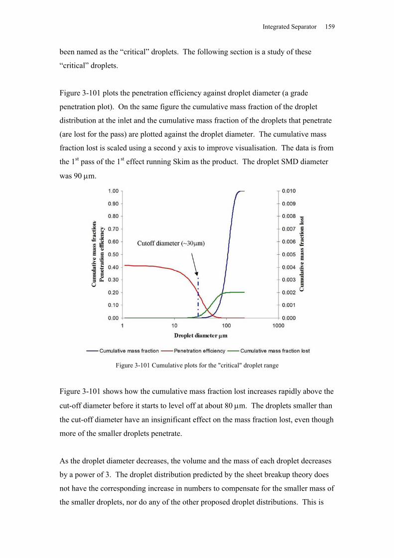
Integrated Separator 159
been named as the “critical” droplets. The following section is a study of these
“critical” droplets.
Figure 3-101 plots the penetration efficiency against droplet diameter (a grade
penetration plot). On the same figure the cumulative mass fraction of the droplet
distribution at the inlet and the cumulative mass fraction of the droplets that penetrate
(are lost for the pass) are plotted against the droplet diameter. The cumulative mass
fraction lost is scaled using a second y axis to improve visualisation. The data is from
the 1st pass of the 1st effect running Skim as the product. The droplet SMD diameter
was 90 m.
Figure 3-101 Cumulative plots for the "critical" droplet range
Figure 3-101 shows how the cumulative mass fraction lost increases rapidly above the
cut-off diameter before it starts to level off at about 80 m. The droplets smaller than
the cut-off diameter have an insignificant effect on the mass fraction lost, even though
more of the smaller droplets penetrate.
As the droplet diameter decreases, the volume and the mass of each droplet decreases
by a power of 3. The droplet distribution predicted by the sheet breakup theory does
not have the corresponding increase in numbers to compensate for the smaller mass of
the smaller droplets, nor do any of the other proposed droplet distributions. This is
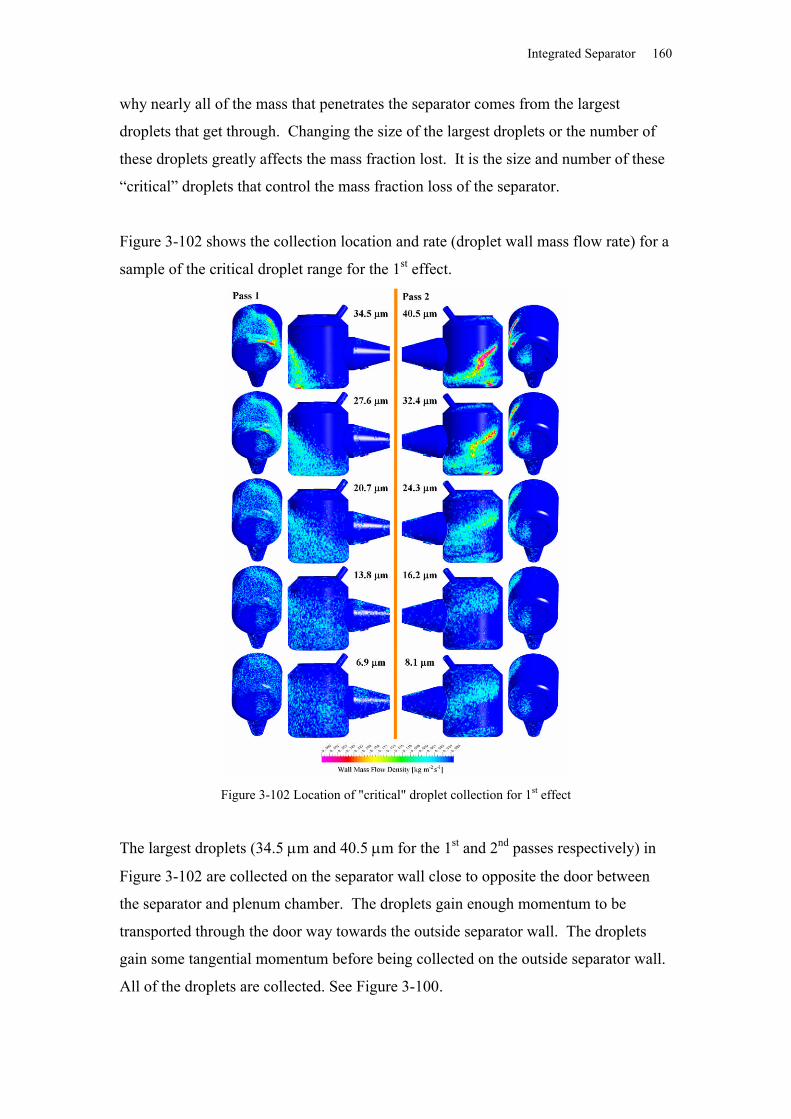
Integrated Separator 160
why nearly all of the mass that penetrates the separator comes from the largest
droplets that get through. Changing the size of the largest droplets or the number of
these droplets greatly affects the mass fraction lost. It is the size and number of these
“critical” droplets that control the mass fraction loss of the separator.
Figure 3-102 shows the collection location and rate (droplet wall mass flow rate) for a
sample of the critical droplet range for the 1st effect.
Figure 3-102 Location of "critical" droplet collection for 1st effect
The largest droplets (34.5 m and 40.5 m for the 1st and 2nd passes respectively) in
Figure 3-102 are collected on the separator wall close to opposite the door between
the separator and plenum chamber. The droplets gain enough momentum to be
transported through the door way towards the outside separator wall. The droplets
gain some tangential momentum before being collected on the outside separator wall.
All of the droplets are collected. See Figure 3-100.
Integrated Separator 161
The second largest droplets (27.6 m and 32.4 m for the 1st and 2nd passes
respectively) in Figure 3-102 are collected close to the location of the largest droplets,
but some of the droplets make it further round the separator. As smaller the droplets,
the further they travel around the separator and the more spread out and random their
separation location becomes. The amount of separation also decreases, see Figure 3-
100.
The smallest droplets (6.9 m and 8.1 m for the 1st and 2nd passes respectively) in
Figure 3-102 are not collected in a concentrated manner like the largest droplets, but
in a more random pattern throughout separator, relative to where their inlet vapour
flow has traveled. Only ~70% and ~55% of these droplets were collected in the 1st
and 2nd effects respectively, see Figure 3-102.
The separation process is changing as the droplets get smaller. Separation of the
largest droplets is dominated by the centrifugal forces in the separator, while the
smaller droplets are too small to move through the fluid and only contact the wall
under the random effect of turbulence.
The behavior for the 2nd effect critical droplets was very similar behavior to the
critical droplets from the 1st effect.
3.8.5 Mass fraction lost across both effects
The product in the evaporators runs serially through all passes in both effects. This
has a cumulative effect on the amount of product lost in the processing of the product.
The total mass fraction lost across both effects is the sum of the fraction lost in each
effect.
As the feed travels through the evaporator, water evaporates from it, concentrating the
feed. To account for the changing concentration, the mass lost is weighted by the
total solids in each pass.
Table 3-13 shows the mass fraction lost across both effects when processing Skim or
MPC. The separators have the same operating conditions (the same used for the mass
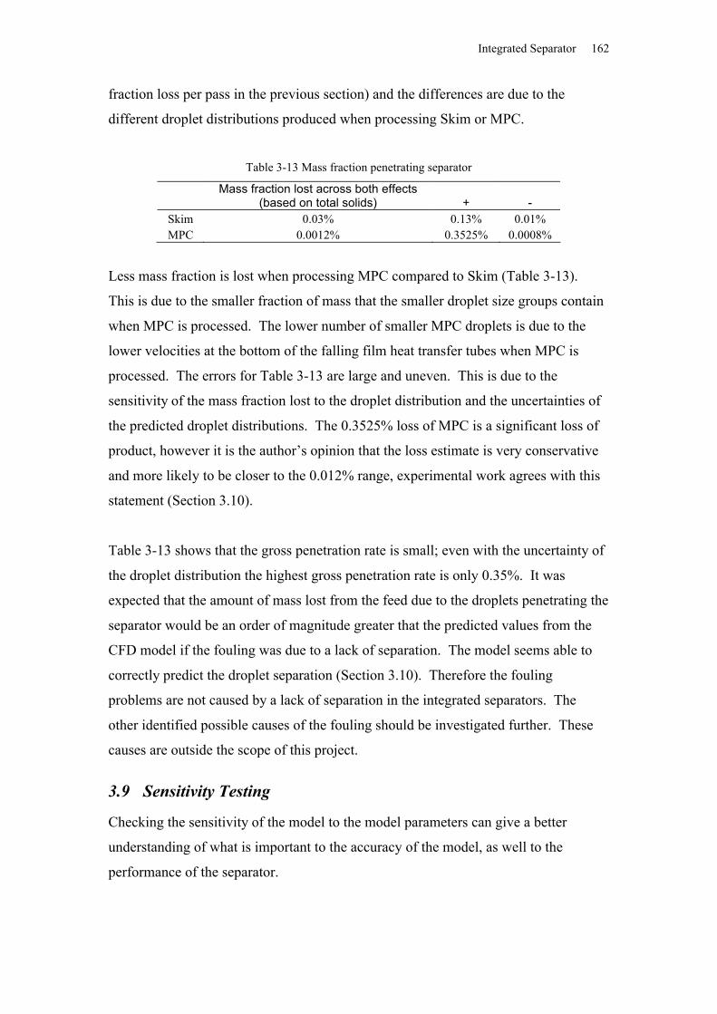
Integrated Separator 162
fraction loss per pass in the previous section) and the differences are due to the
different droplet distributions produced when processing Skim or MPC.
Table 3-13 Mass fraction penetrating separator
Mass fraction lost across both effects (based on total solids) + -
Skim 0.03% 0.13% 0.01%MPC 0.0012% 0.3525% 0.0008%
Less mass fraction is lost when processing MPC compared to Skim (Table 3-13).
This is due to the smaller fraction of mass that the smaller droplet size groups contain
when MPC is processed. The lower number of smaller MPC droplets is due to the
lower velocities at the bottom of the falling film heat transfer tubes when MPC is
processed. The errors for Table 3-13 are large and uneven. This is due to the
sensitivity of the mass fraction lost to the droplet distribution and the uncertainties of
the predicted droplet distributions. The 0.3525% loss of MPC is a significant loss of
product, however it is the author’s opinion that the loss estimate is very conservative
and more likely to be closer to the 0.012% range, experimental work agrees with this
statement (Section 3.10).
Table 3-13 shows that the gross penetration rate is small; even with the uncertainty of
the droplet distribution the highest gross penetration rate is only 0.35%. It was
expected that the amount of mass lost from the feed due to the droplets penetrating the
separator would be an order of magnitude greater that the predicted values from the
CFD model if the fouling was due to a lack of separation. The model seems able to
correctly predict the droplet separation (Section 3.10). Therefore the fouling
problems are not caused by a lack of separation in the integrated separators. The
other identified possible causes of the fouling should be investigated further. These
causes are outside the scope of this project.
3.9 Sensitivity Testing
Checking the sensitivity of the model to the model parameters can give a better
understanding of what is important to the accuracy of the model, as well to the
performance of the separator.
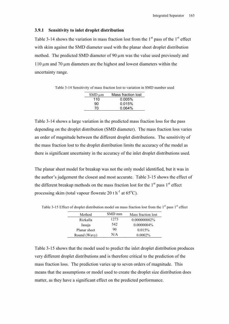
Integrated Separator 163
3.9.1 Sensitivity to inlet droplet distribution
Table 3-14 shows the variation in mass fraction lost from the 1st pass of the 1st effect
with skim against the SMD diameter used with the planar sheet droplet distribution
method. The predicted SMD diameter of 90 m was the value used previously and
110 m and 70 m diameters are the highest and lowest diameters within the
uncertainty range.
Table 3-14 Sensitivity of mass fraction lost to variation in SMD number used
SMD m Mass fraction lost110 0.005%90 0.015%70 0.064%
Table 3-14 shows a large variation in the predicted mass fraction loss for the pass
depending on the droplet distribution (SMD diameter). The mass fraction loss varies
an order of magnitude between the different droplet distributions. The sensitivity of
the mass fraction lost to the droplet distribution limits the accuracy of the model as
there is significant uncertainty in the accuracy of the inlet droplet distributions used.
The planar sheet model for breakup was not the only model identified, but it was in
the author’s judgement the closest and most accurate. Table 3-15 shows the effect of
the different breakup methods on the mass fraction lost for the 1st pass 1st effect
processing skim (total vapour flowrate 20 t h-1 at 65oC).
Table 3-15 Effect of droplet distribution model on mass fraction lost from the 1st pass 1st effect
Method SMD mm Mass fraction lostRizkalla 1273 0.000000002%Jasuja 542 0.0000004%
Planar sheet 90 0.015%Round (Wavy) N/A 0.0002%
Table 3-15 shows that the model used to predict the inlet droplet distribution produces
very different droplet distributions and is therefore critical to the prediction of the
mass fraction loss. The prediction varies up to seven orders of magnitude. This
means that the assumptions or model used to create the droplet size distribution does
matter, as they have a significant effect on the predicted performance.
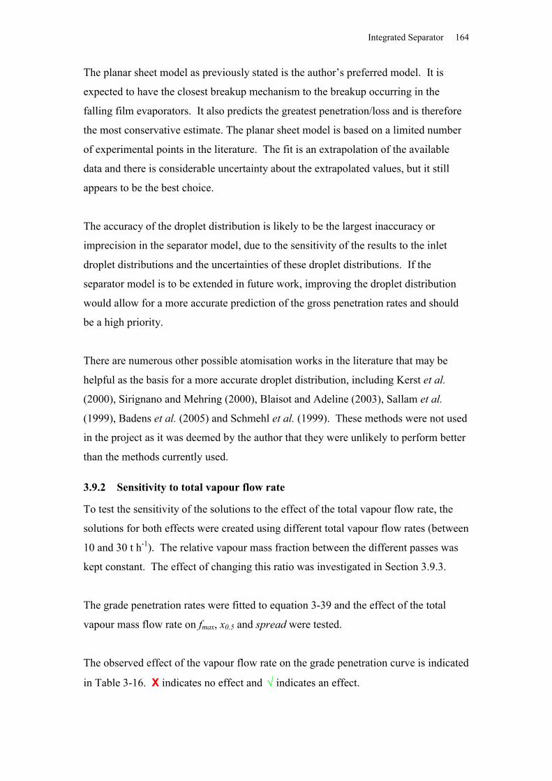
Integrated Separator 164
The planar sheet model as previously stated is the author’s preferred model. It is
expected to have the closest breakup mechanism to the breakup occurring in the
falling film evaporators. It also predicts the greatest penetration/loss and is therefore
the most conservative estimate. The planar sheet model is based on a limited number
of experimental points in the literature. The fit is an extrapolation of the available
data and there is considerable uncertainty about the extrapolated values, but it still
appears to be the best choice.
The accuracy of the droplet distribution is likely to be the largest inaccuracy or
imprecision in the separator model, due to the sensitivity of the results to the inlet
droplet distributions and the uncertainties of these droplet distributions. If the
separator model is to be extended in future work, improving the droplet distribution
would allow for a more accurate prediction of the gross penetration rates and should
be a high priority.
There are numerous other possible atomisation works in the literature that may be
helpful as the basis for a more accurate droplet distribution, including Kerst et al.
(2000), Sirignano and Mehring (2000), Blaisot and Adeline (2003), Sallam et al.
(1999), Badens et al. (2005) and Schmehl et al. (1999). These methods were not used
in the project as it was deemed by the author that they were unlikely to perform better
than the methods currently used.
3.9.2 Sensitivity to total vapour flow rate
To test the sensitivity of the solutions to the effect of the total vapour flow rate, the
solutions for both effects were created using different total vapour flow rates (between
10 and 30 t h-1). The relative vapour mass fraction between the different passes was
kept constant. The effect of changing this ratio was investigated in Section 3.9.3.
The grade penetration rates were fitted to equation 3-39 and the effect of the total
vapour mass flow rate on fmax, x0.5 and spread were tested.
The observed effect of the vapour flow rate on the grade penetration curve is indicated
in Table 3-16. X indicates no effect and indicates an effect.
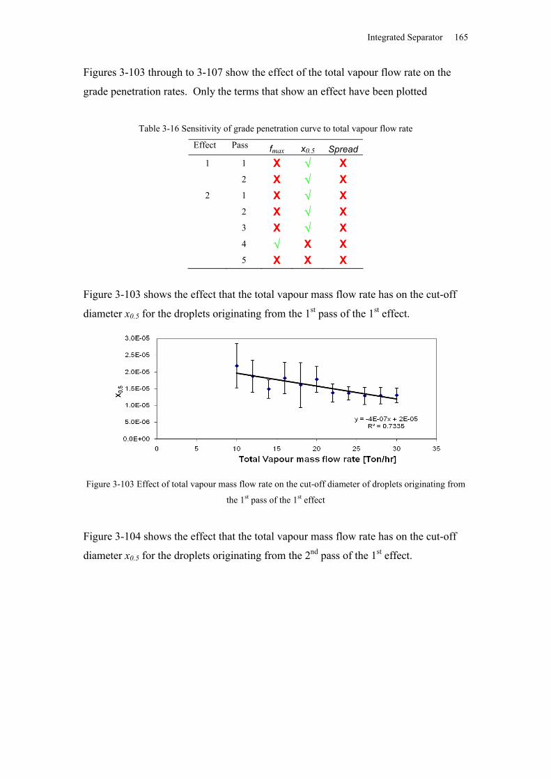
Integrated Separator 165
Figures 3-103 through to 3-107 show the effect of the total vapour flow rate on the
grade penetration rates. Only the terms that show an effect have been plotted
Table 3-16 Sensitivity of grade penetration curve to total vapour flow rate
Effect Pass fmax x0.5 Spread1 1 X X
2 X X2 1 X X
2 X X3 X X4 X X5 X X X
Figure 3-103 shows the effect that the total vapour mass flow rate has on the cut-off
diameter x0.5 for the droplets originating from the 1st pass of the 1st effect.
Figure 3-103 Effect of total vapour mass flow rate on the cut-off diameter of droplets originating from
the 1st pass of the 1st effect
Figure 3-104 shows the effect that the total vapour mass flow rate has on the cut-off
diameter x0.5 for the droplets originating from the 2nd pass of the 1st effect.
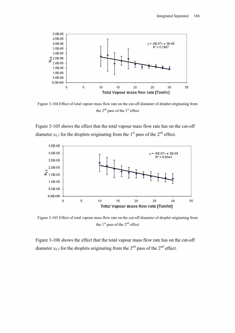
Integrated Separator 166
Figure 3-104 Effect of total vapour mass flow rate on the cut-off diameter of droplet originating from
the 2nd pass of the 1st effect
Figure 3-105 shows the effect that the total vapour mass flow rate has on the cut-off
diameter x0.5 for the droplets originating from the 1st pass of the 2nd effect.
Figure 3-105 Effect of total vapour mass flow rate on the cut-off diameter of droplet originating from
the 1st pass of the 2nd effect
Figure 3-106 shows the effect that the total vapour mass flow rate has on the cut-off
diameter x0.5 for the droplets originating from the 2nd pass of the 2nd effect.
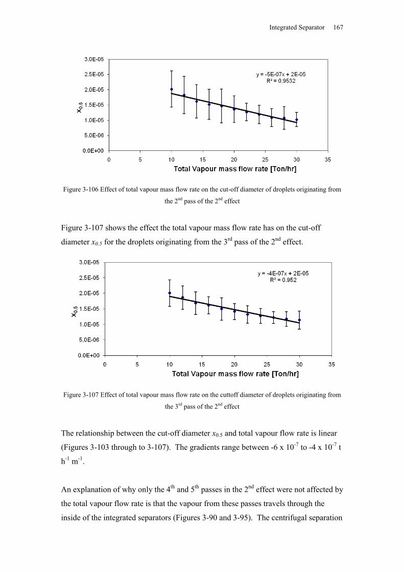
Integrated Separator 167
Figure 3-106 Effect of total vapour mass flow rate on the cut-off diameter of droplets originating from
the 2nd pass of the 2nd effect
Figure 3-107 shows the effect the total vapour mass flow rate has on the cut-off
diameter x0.5 for the droplets originating from the 3rd pass of the 2nd effect.
Figure 3-107 Effect of total vapour mass flow rate on the cuttoff diameter of droplets originating from
the 3rd pass of the 2nd effect
The relationship between the cut-off diameter x0.5 and total vapour flow rate is linear
(Figures 3-103 through to 3-107). The gradients range between -6 x 10⁻⁷ to -4 x 10⁻⁷ t
h-1 m-1.
An explanation of why only the 4th and 5th passes in the 2nd effect were not affected by
the total vapour flow rate is that the vapour from these passes travels through the
inside of the integrated separators (Figures 3-90 and 3-95). The centrifugal separation
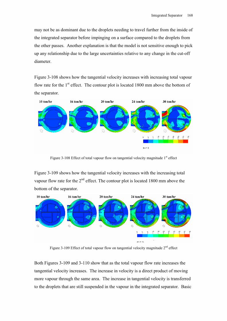
Integrated Separator 168
may not be as dominant due to the droplets needing to travel further from the inside of
the integrated separator before impinging on a surface compared to the droplets from
the other passes. Another explanation is that the model is not sensitive enough to pick
up any relationship due to the large uncertainties relative to any change in the cut-off
diameter.
Figure 3-108 shows how the tangential velocity increases with increasing total vapour
flow rate for the 1st effect. The contour plot is located 1800 mm above the bottom of
the separator.
Figure 3-108 Effect of total vapour flow on tangential velocity magnitude 1st effect
Figure 3-109 shows how the tangential velocity increases with the increasing total
vapour flow rate for the 2nd effect. The contour plot is located 1800 mm above the
bottom of the separator.
Figure 3-109 Effect of total vapour flow on tangential velocity magnitude 2nd effect
Both Figures 3-109 and 3-110 show that as the total vapour flow rate increases the
tangential velocity increases. The increase in velocity is a direct product of moving
more vapour through the same area. The increase in tangential velocity is transferred
to the droplets that are still suspended in the vapour in the integrated separator. Basic
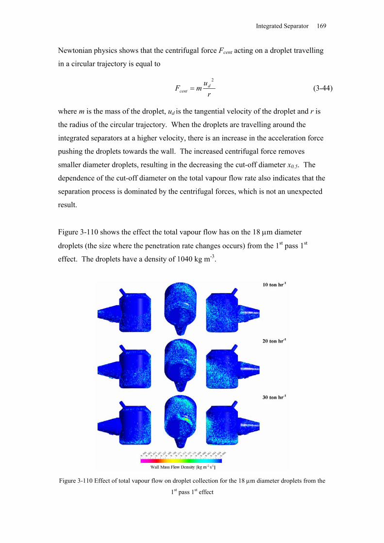
Integrated Separator 169
Newtonian physics shows that the centrifugal force Fcent acting on a droplet travelling
in a circular trajectory is equal to
ru
mF dcent
2
(3-44)
where m is the mass of the droplet, ud is the tangential velocity of the droplet and r is
the radius of the circular trajectory. When the droplets are travelling around the
integrated separators at a higher velocity, there is an increase in the acceleration force
pushing the droplets towards the wall. The increased centrifugal force removes
smaller diameter droplets, resulting in the decreasing the cut-off diameter x0.5. The
dependence of the cut-off diameter on the total vapour flow rate also indicates that the
separation process is dominated by the centrifugal forces, which is not an unexpected
result.
Figure 3-110 shows the effect the total vapour flow has on the 18 m diameter
droplets (the size where the penetration rate changes occurs) from the 1st pass 1st
effect. The droplets have a density of 1040 kg m-3.
Figure 3-110 Effect of total vapour flow on droplet collection for the 18 m diameter droplets from the
1st pass 1st effect
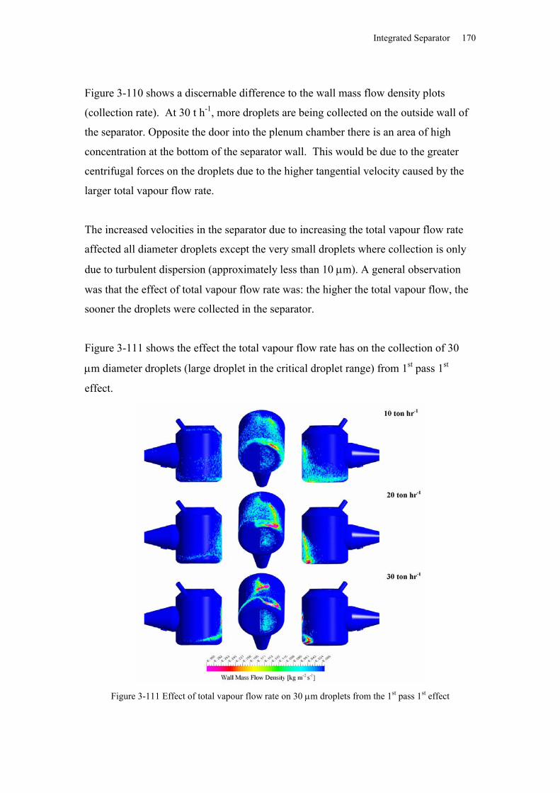
Integrated Separator 170
Figure 3-110 shows a discernable difference to the wall mass flow density plots
(collection rate). At 30 t h-1, more droplets are being collected on the outside wall of
the separator. Opposite the door into the plenum chamber there is an area of high
concentration at the bottom of the separator wall. This would be due to the greater
centrifugal forces on the droplets due to the higher tangential velocity caused by the
larger total vapour flow rate.
The increased velocities in the separator due to increasing the total vapour flow rate
affected all diameter droplets except the very small droplets where collection is only
due to turbulent dispersion (approximately less than 10 m). A general observation
was that the effect of total vapour flow rate was: the higher the total vapour flow, the
sooner the droplets were collected in the separator.
Figure 3-111 shows the effect the total vapour flow rate has on the collection of 30
m diameter droplets (large droplet in the critical droplet range) from 1st pass 1st
effect.
Figure 3-111 Effect of total vapour flow rate on 30 m droplets from the 1st pass 1st effect
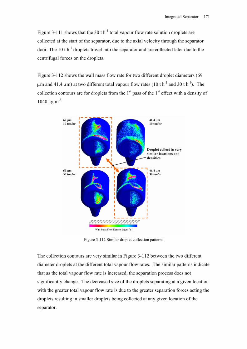
Integrated Separator 171
Figure 3-111 shows that the 30 t h-1 total vapour flow rate solution droplets are
collected at the start of the separator, due to the axial velocity through the separator
door. The 10 t h-1 droplets travel into the separator and are collected later due to the
centrifugal forces on the droplets.
Figure 3-112 shows the wall mass flow rate for two different droplet diameters (69
m and 41.4 m) at two different total vapour flow rates (10 t h-1 and 30 t h-1). The
collection contours are for droplets from the 1st pass of the 1st effect with a density of
1040 kg m-3
Figure 3-112 Similar droplet collection patterns
The collection contours are very similar in Figure 3-112 between the two different
diameter droplets at the different total vapour flow rates. The similar patterns indicate
that as the total vapour flow rate is increased, the separation process does not
significantly change. The decreased size of the droplets separating at a given location
with the greater total vapour flow rate is due to the greater separation forces acting the
droplets resulting in smaller droplets being collected at any given location of the
separator.
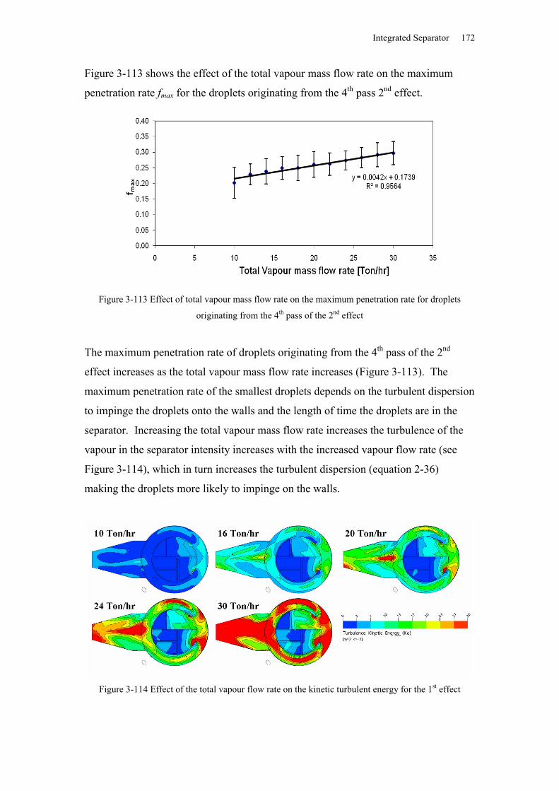
Integrated Separator 172
Figure 3-113 shows the effect of the total vapour mass flow rate on the maximum
penetration rate fmax for the droplets originating from the 4th pass 2nd effect.
Figure 3-113 Effect of total vapour mass flow rate on the maximum penetration rate for droplets
originating from the 4th pass of the 2nd effect
The maximum penetration rate of droplets originating from the 4th pass of the 2nd
effect increases as the total vapour mass flow rate increases (Figure 3-113). The
maximum penetration rate of the smallest droplets depends on the turbulent dispersion
to impinge the droplets onto the walls and the length of time the droplets are in the
separator. Increasing the total vapour mass flow rate increases the turbulence of the
vapour in the separator intensity increases with the increased vapour flow rate (see
Figure 3-114), which in turn increases the turbulent dispersion (equation 2-36)
making the droplets more likely to impinge on the walls.
Figure 3-114 Effect of the total vapour flow rate on the kinetic turbulent energy for the 1st effect
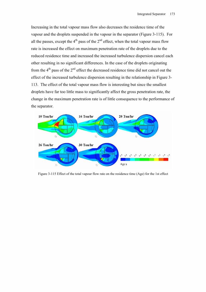
Integrated Separator 173
Increasing in the total vapour mass flow also decreases the residence time of the
vapour and the droplets suspended in the vapour in the separator (Figure 3-115). For
all the passes, except the 4th pass of the 2nd effect, when the total vapour mass flow
rate is increased the effect on maximum penetration rate of the droplets due to the
reduced residence time and increased the increased turbulence dispersion cancel each
other resulting in no significant differences. In the case of the droplets originating
from the 4th pass of the 2nd effect the decreased residence time did not cancel out the
effect of the increased turbulence dispersion resulting in the relationship in Figure 3-
113. The effect of the total vapour mass flow is interesting but since the smallest
droplets have far too little mass to significantly affect the gross penetration rate, the
change in the maximum penetration rate is of little consequence to the performance of
the separator.
Figure 3-115 Effect of the total vapour flow rate on the residence time (Age) for the 1st effect
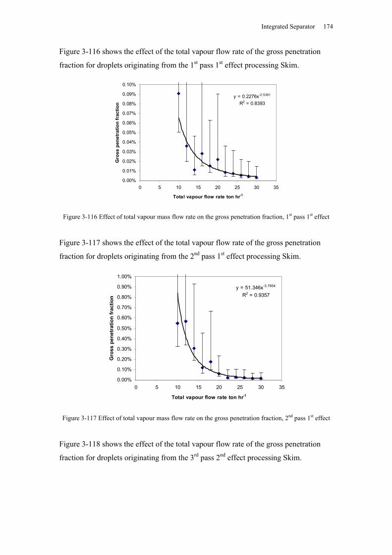
Integrated Separator 174
Figure 3-116 shows the effect of the total vapour flow rate of the gross penetration
fraction for droplets originating from the 1st pass 1st effect processing Skim.
y = 0.2276x-2.5381
R2 = 0.8393
0.00%
0.01%
0.02%
0.03%
0.04%
0.05%
0.06%
0.07%
0.08%
0.09%
0.10%
0 5 10 15 20 25 30 35
Total vapour flow rate ton hr-1
Gro
ss p
enet
ratio
n fr
actio
n
Figure 3-116 Effect of total vapour mass flow rate on the gross penetration fraction, 1st pass 1st effect
Figure 3-117 shows the effect of the total vapour flow rate of the gross penetration
fraction for droplets originating from the 2nd pass 1st effect processing Skim.
y = 51.346x-3.7854
R2 = 0.9357
0.00%
0.10%
0.20%
0.30%
0.40%
0.50%
0.60%
0.70%
0.80%
0.90%
1.00%
0 5 10 15 20 25 30 35
Total vapour flow rate ton hr-1
Gro
ss p
enet
ratio
n fr
actio
n
Figure 3-117 Effect of total vapour mass flow rate on the gross penetration fraction, 2nd pass 1st effect
Figure 3-118 shows the effect of the total vapour flow rate of the gross penetration
fraction for droplets originating from the 3rd pass 2nd effect processing Skim.
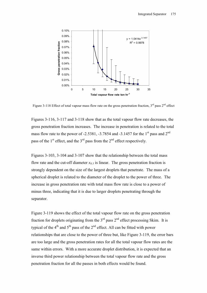
Integrated Separator 175
y = 1.0414x-3.1457
R2 = 0.9978
0.00%
0.01%
0.02%
0.03%
0.04%
0.05%
0.06%
0.07%
0.08%
0.09%
0.10%
0 5 10 15 20 25 30 35
Total vapour flow rate ton hr-1
Gro
ss p
enet
ratio
n fr
actio
n
Figure 3-118 Effect of total vapour mass flow rate on the gross penetration fraction, 3rd pass 2nd effect
Figures 3-116, 3-117 and 3-118 show that as the total vapour flow rate decreases, the
gross penetration fraction increases. The increase in penetration is related to the total
mass flow rate to the power of -2.5381, -3.7854 and -3.1457 for the 1st pass and 2nd
pass of the 1st effect, and the 3rd pass from the 2nd effect respectively.
Figures 3-103, 3-104 and 3-107 show that the relationship between the total mass
flow rate and the cut-off diameter x0.5 is linear. The gross penetration fraction is
strongly dependent on the size of the largest droplets that penetrate. The mass of a
spherical droplet is related to the diameter of the droplet to the power of three. The
increase in gross penetration rate with total mass flow rate is close to a power of
minus three, indicating that it is due to larger droplets penetrating through the
separator.
Figure 3-119 shows the effect of the total vapour flow rate on the gross penetration
fraction for droplets originating from the 3rd pass 2nd effect processing Skim. It is
typical of the 4th and 5th pass of the 2nd effect. All can be fitted with power
relationships that are close to the power of three but, like Figure 3-119, the error bars
are too large and the gross penetration rates for all the total vapour flow rates are the
same within errors. With a more accurate droplet distribution, it is expected that an
inverse third power relationship between the total vapour flow rate and the gross
penetration fraction for all the passes in both effects would be found.
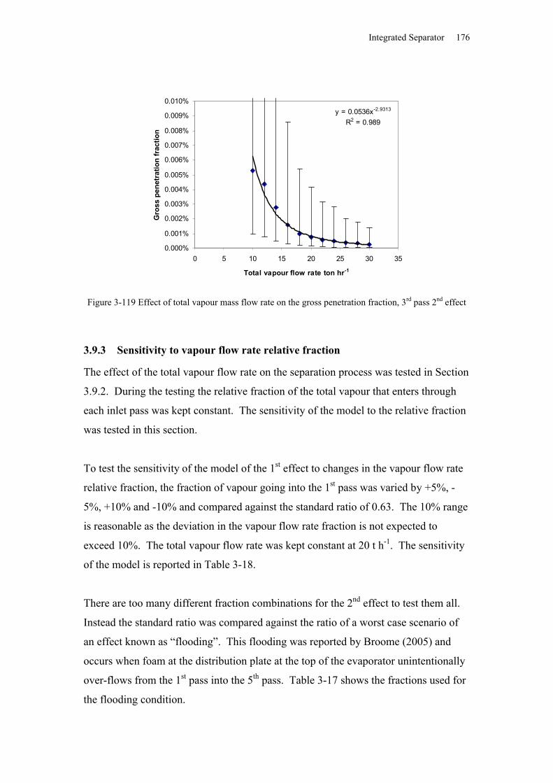
Integrated Separator 176
y = 0.0536x-2.9313
R2 = 0.989
0.000%
0.001%
0.002%
0.003%
0.004%
0.005%
0.006%
0.007%
0.008%
0.009%
0.010%
0 5 10 15 20 25 30 35
Total vapour flow rate ton hr-1
Gro
ss p
enet
ratio
n fr
actio
n
Figure 3-119 Effect of total vapour mass flow rate on the gross penetration fraction, 3rd pass 2nd effect
3.9.3 Sensitivity to vapour flow rate relative fraction
The effect of the total vapour flow rate on the separation process was tested in Section
3.9.2. During the testing the relative fraction of the total vapour that enters through
each inlet pass was kept constant. The sensitivity of the model to the relative fraction
was tested in this section.
To test the sensitivity of the model of the 1st effect to changes in the vapour flow rate
relative fraction, the fraction of vapour going into the 1st pass was varied by +5%, -
5%, +10% and -10% and compared against the standard ratio of 0.63. The 10% range
is reasonable as the deviation in the vapour flow rate fraction is not expected to
exceed 10%. The total vapour flow rate was kept constant at 20 t h-1. The sensitivity
of the model is reported in Table 3-18.
There are too many different fraction combinations for the 2nd effect to test them all.
Instead the standard ratio was compared against the ratio of a worst case scenario of
an effect known as “flooding”. This flooding was reported by Broome (2005) and
occurs when foam at the distribution plate at the top of the evaporator unintentionally
over-flows from the 1st pass into the 5th pass. Table 3-17 shows the fractions used for
the flooding condition.
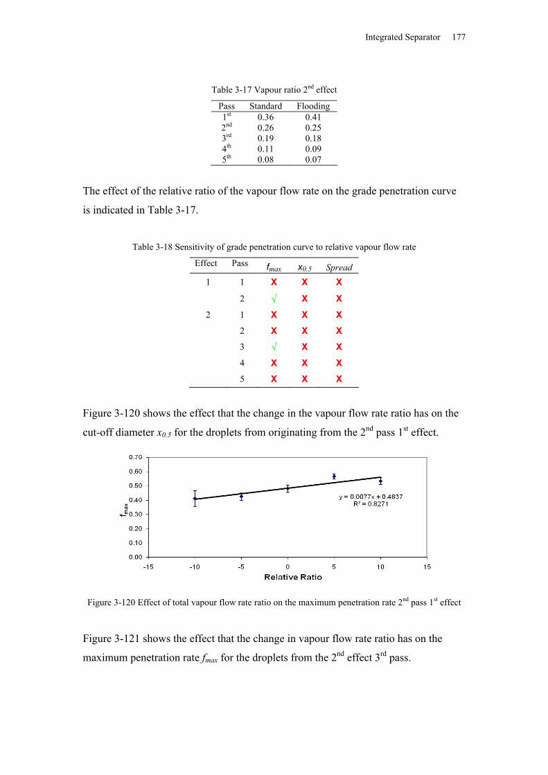
Integrated Separator 177
Table 3-17 Vapour ratio 2nd effect
Pass Standard Flooding1st 0.36 0.412nd 0.26 0.253rd 0.19 0.184th 0.11 0.095th 0.08 0.07
The effect of the relative ratio of the vapour flow rate on the grade penetration curve
is indicated in Table 3-17.
Table 3-18 Sensitivity of grade penetration curve to relative vapour flow rate
Effect Pass fmax x0.5 Spread1 1 X X X
2 X X
2 1 X X X
2 X X X
3 X X
4 X X X
5 X X X
Figure 3-120 shows the effect that the change in the vapour flow rate ratio has on the
cut-off diameter x0.5 for the droplets from originating from the 2nd pass 1st effect.
Figure 3-120 Effect of total vapour flow rate ratio on the maximum penetration rate 2nd pass 1st effect
Figure 3-121 shows the effect that the change in vapour flow rate ratio has on the
maximum penetration rate fmax for the droplets from the 2nd effect 3rd pass.
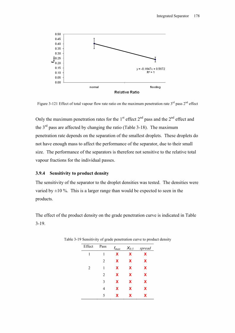
Integrated Separator 178
Figure 3-121 Effect of total vapour flow rate ratio on the maximum penetration rate 3rd pass 2nd effect
Only the maximum penetration rates for the 1st effect 2nd pass and the 2nd effect and
the 3rd pass are affected by changing the ratio (Table 3-18). The maximum
penetration rate depends on the separation of the smallest droplets. These droplets do
not have enough mass to affect the performance of the separator, due to their small
size. The performance of the separators is therefore not sensitive to the relative total
vapour fractions for the individual passes.
3.9.4 Sensitivity to product density
The sensitivity of the separator to the droplet densities was tested. The densities were
varied by ±10 %. This is a larger range than would be expected to seen in the
products.
The effect of the product density on the grade penetration curve is indicated in Table
3-19.
Table 3-19 Sensitivity of grade penetration curve to product density
Effect Pass fmax X0.5 spread1 1 X X X
2 X X X
2 1 X X X
2 X X X
3 X X X
4 X X X
5 X X X
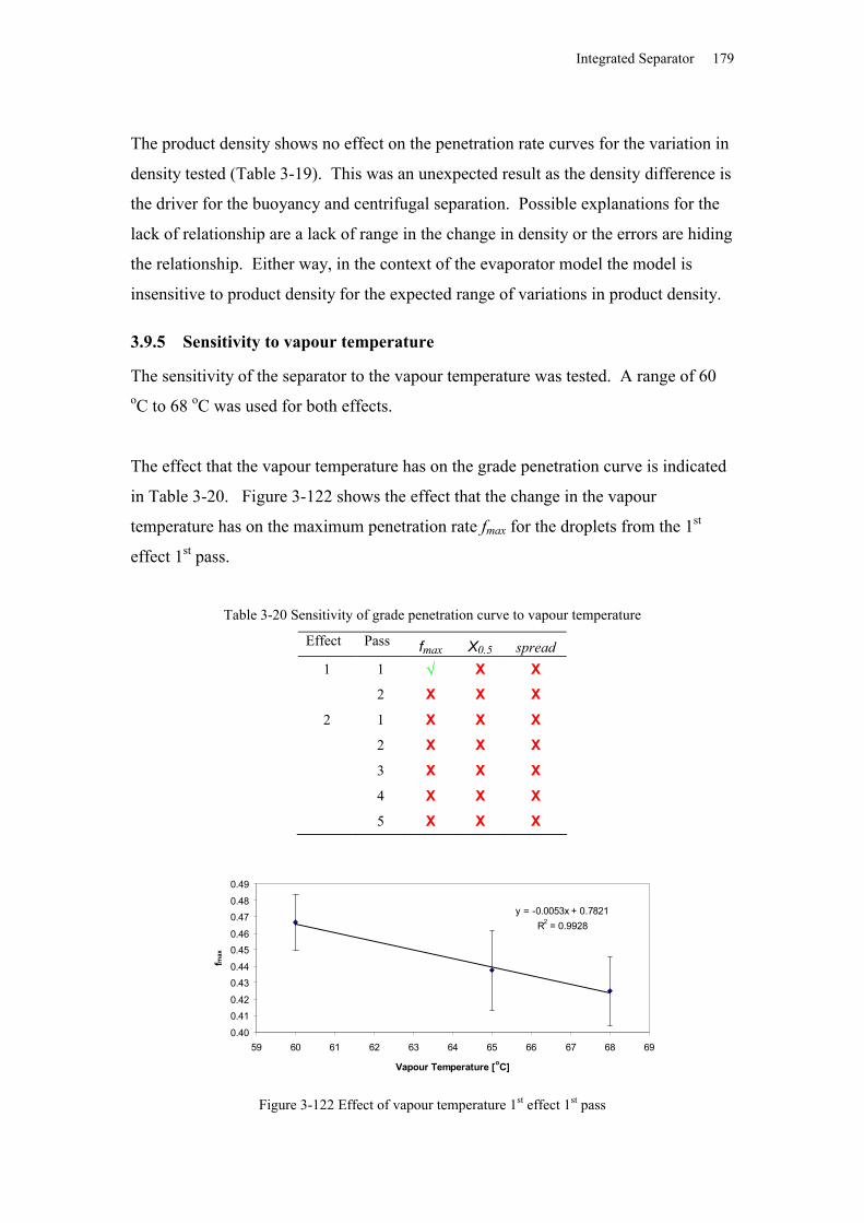
Integrated Separator 179
The product density shows no effect on the penetration rate curves for the variation in
density tested (Table 3-19). This was an unexpected result as the density difference is
the driver for the buoyancy and centrifugal separation. Possible explanations for the
lack of relationship are a lack of range in the change in density or the errors are hiding
the relationship. Either way, in the context of the evaporator model the model is
insensitive to product density for the expected range of variations in product density.
3.9.5 Sensitivity to vapour temperature
The sensitivity of the separator to the vapour temperature was tested. A range of 60 oC to 68 oC was used for both effects.
The effect that the vapour temperature has on the grade penetration curve is indicated
in Table 3-20. Figure 3-122 shows the effect that the change in the vapour
temperature has on the maximum penetration rate fmax for the droplets from the 1st
effect 1st pass.
Table 3-20 Sensitivity of grade penetration curve to vapour temperature
Effect Pass fmax X0.5 spread1 1 X X
2 X X X
2 1 X X X
2 X X X
3 X X X
4 X X X
5 X X X
y = -0.0053x + 0.7821R2 = 0.9928
0.40
0.410.42
0.430.44
0.450.46
0.470.48
0.49
59 60 61 62 63 64 65 66 67 68 69
Vapour Temperature [oC]
fmax
Figure 3-122 Effect of vapour temperature 1st effect 1st pass
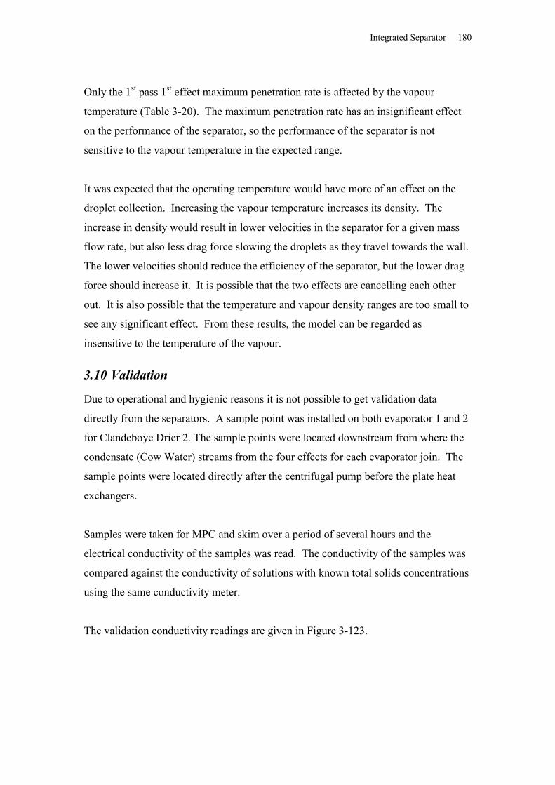
Integrated Separator 180
Only the 1st pass 1st effect maximum penetration rate is affected by the vapour
temperature (Table 3-20). The maximum penetration rate has an insignificant effect
on the performance of the separator, so the performance of the separator is not
sensitive to the vapour temperature in the expected range.
It was expected that the operating temperature would have more of an effect on the
droplet collection. Increasing the vapour temperature increases its density. The
increase in density would result in lower velocities in the separator for a given mass
flow rate, but also less drag force slowing the droplets as they travel towards the wall.
The lower velocities should reduce the efficiency of the separator, but the lower drag
force should increase it. It is possible that the two effects are cancelling each other
out. It is also possible that the temperature and vapour density ranges are too small to
see any significant effect. From these results, the model can be regarded as
insensitive to the temperature of the vapour.
3.10 Validation
Due to operational and hygienic reasons it is not possible to get validation data
directly from the separators. A sample point was installed on both evaporator 1 and 2
for Clandeboye Drier 2. The sample points were located downstream from where the
condensate (Cow Water) streams from the four effects for each evaporator join. The
sample points were located directly after the centrifugal pump before the plate heat
exchangers.
Samples were taken for MPC and skim over a period of several hours and the
electrical conductivity of the samples was read. The conductivity of the samples was
compared against the conductivity of solutions with known total solids concentrations
using the same conductivity meter.
The validation conductivity readings are given in Figure 3-123.
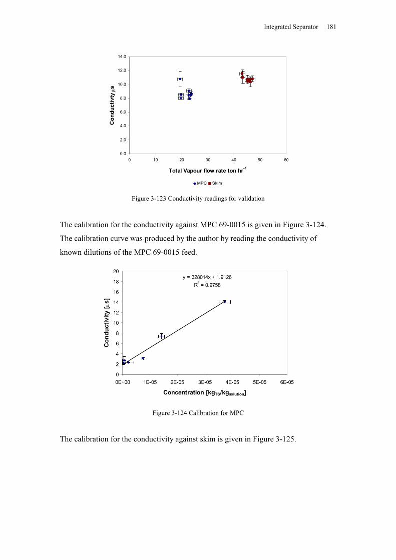
Integrated Separator 181
0.0
2.0
4.0
6.0
8.0
10.0
12.0
14.0
0 10 20 30 40 50 60
Total Vapour flow rate ton hr-1
Con
duct
ivty
s
MPC Skim
Figure 3-123 Conductivity readings for validation
The calibration for the conductivity against MPC 69-0015 is given in Figure 3-124.
The calibration curve was produced by the author by reading the conductivity of
known dilutions of the MPC 69-0015 feed.
y = 328014x + 1.9126R2 = 0.9758
0
2
4
6
8
10
12
14
16
18
20
0E+00 1E-05 2E-05 3E-05 4E-05 5E-05 6E-05
Concentration [kgTS/kgsolution]
Con
duct
ivity
[ s]
Figure 3-124 Calibration for MPC
The calibration for the conductivity against skim is given in Figure 3-125.
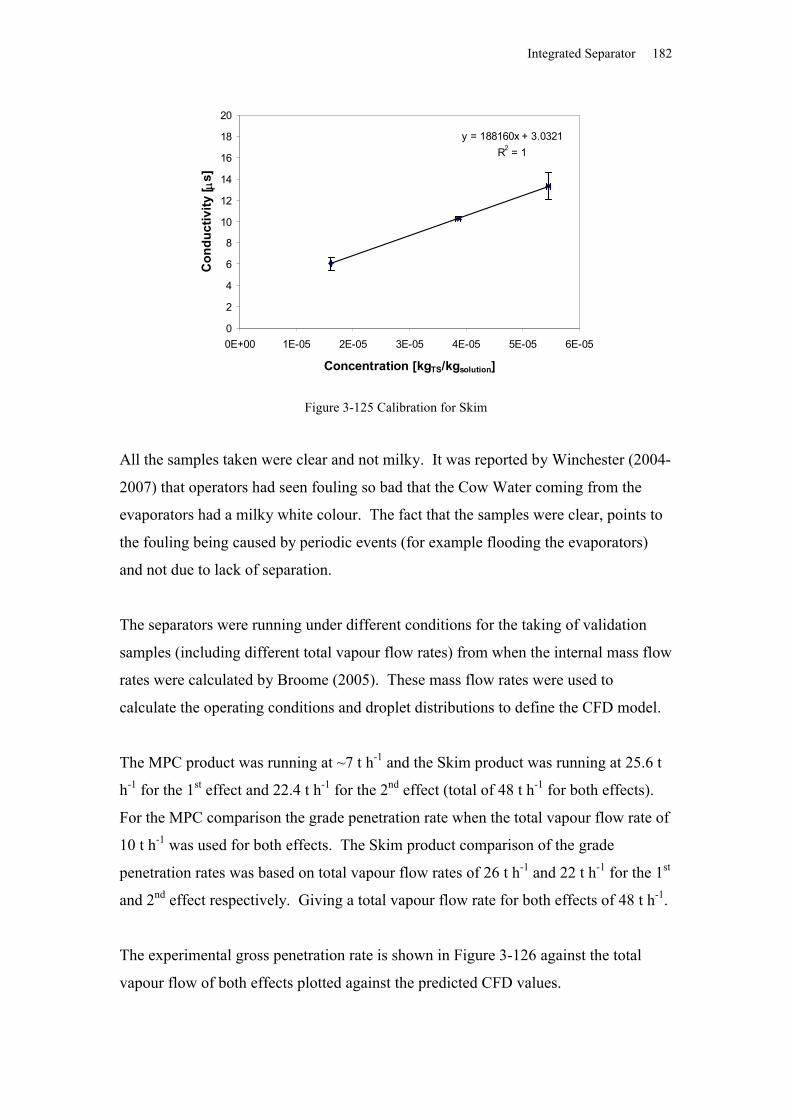
Integrated Separator 182
y = 188160x + 3.0321R2 = 1
0
2
4
6
8
10
12
14
16
18
20
0E+00 1E-05 2E-05 3E-05 4E-05 5E-05 6E-05
Concentration [kgTS/kgsolution]
Con
duct
ivity
[ s]
Figure 3-125 Calibration for Skim
All the samples taken were clear and not milky. It was reported by Winchester (2004-
2007) that operators had seen fouling so bad that the Cow Water coming from the
evaporators had a milky white colour. The fact that the samples were clear, points to
the fouling being caused by periodic events (for example flooding the evaporators)
and not due to lack of separation.
The separators were running under different conditions for the taking of validation
samples (including different total vapour flow rates) from when the internal mass flow
rates were calculated by Broome (2005). These mass flow rates were used to
calculate the operating conditions and droplet distributions to define the CFD model.
The MPC product was running at ~7 t h-1 and the Skim product was running at 25.6 t
h-1 for the 1st effect and 22.4 t h-1 for the 2nd effect (total of 48 t h-1 for both effects).
For the MPC comparison the grade penetration rate when the total vapour flow rate of
10 t h-1 was used for both effects. The Skim product comparison of the grade
penetration rates was based on total vapour flow rates of 26 t h-1 and 22 t h-1 for the 1st
and 2nd effect respectively. Giving a total vapour flow rate for both effects of 48 t h-1.
The experimental gross penetration rate is shown in Figure 3-126 against the total
vapour flow of both effects plotted against the predicted CFD values.
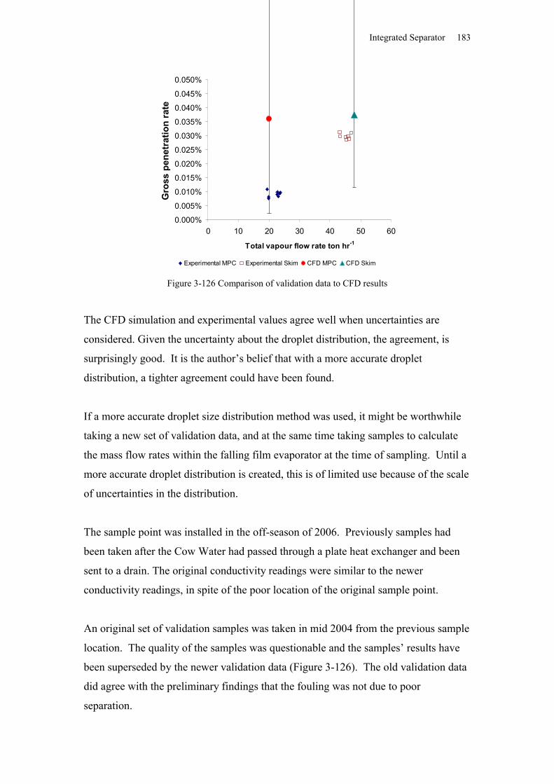
Integrated Separator 183
0.000%
0.005%
0.010%
0.015%
0.020%
0.025%
0.030%
0.035%
0.040%
0.045%
0.050%
0 10 20 30 40 50 60
Total vapour flow rate ton hr-1
Gro
ss p
enet
ratio
n ra
te
Experimental MPC Experimental Skim CFD MPC CFD Skim
Figure 3-126 Comparison of validation data to CFD results
The CFD simulation and experimental values agree well when uncertainties are
considered. Given the uncertainty about the droplet distribution, the agreement, is
surprisingly good. It is the author’s belief that with a more accurate droplet
distribution, a tighter agreement could have been found.
If a more accurate droplet size distribution method was used, it might be worthwhile
taking a new set of validation data, and at the same time taking samples to calculate
the mass flow rates within the falling film evaporator at the time of sampling. Until a
more accurate droplet distribution is created, this is of limited use because of the scale
of uncertainties in the distribution.
The sample point was installed in the off-season of 2006. Previously samples had
been taken after the Cow Water had passed through a plate heat exchanger and been
sent to a drain. The original conductivity readings were similar to the newer
conductivity readings, in spite of the poor location of the original sample point.
An original set of validation samples was taken in mid 2004 from the previous sample
location. The quality of the samples was questionable and the samples’ results have
been superseded by the newer validation data (Figure 3-126). The old validation data
did agree with the preliminary findings that the fouling was not due to poor
separation.
Integrated Separator 184
In mid 2004, a preliminary conclusion was drawn that the separators were not the
cause of the fouling. The conclusion was drawn using the round jet droplet
distribution prediction method and the results from the CFD model. The other more
accurate methods were not found until later.
During this time, plant engineers at Fonterra began looking into the other identified
possible causes of the fouling, such as flooding of the evaporators. The plant
operations were improved and the fouling problem has largely been fixed. In this
time the design of the separator remained constant.
The CFD model predicted that the separators were not the cause of the fouling, and
the plant samples agreed with the CFD model. Fouling has been reduced through
unrelated plant operations and now the fouling problem has been fixed, proving that
the cause of the fouling was not the separator design.
Although this not a typical method of validation, it does validate the models. It
demonstrates how validation is dependent on the purpose of the model. The models
were used to show how the integrated separators were not causing the fouling. The
CFD model predicted that the fouling from the separator was minor. Any higher level
of accuracy in the CFD model was not needed (although it would increase confidence
in the predictions) as the model gave the required information. However, the model
may not be sensitive enough to predict any change in gross penetration rates due to
changes in the geometry unless the changes are large.
Interestingly, it is not the CFD equations or their solution that is limiting the accuracy
of the model, but it is a boundary condition (inlet droplet size distribution).
The new validation data supports the belief the CFD model was correctly predicting
the important physics in the separation process in the integrated separators.
Remond (2006) stated that fouling can be a problem for integrated separators.
Fouling is not a problem when the total vapour flow rate is lower than the design rate.
Integrated Separator 185
Reducing the vapour flow rate decreases the separation of droplets for a constant
droplet distribution as long as no new interactions occur.
The decreased performance of the separators with higher vapour flow rate could be
caused by any combination of stripping, splashing, breaking up of the larger droplets.
Another explanation is that the droplet distribution produced with the higher vapour
flow rate has more mass in the small droplets that penetrate the separator. This is what
the author believes.
The CFD model predicts decreased performance due to droplet distributions with
more mass contained in the small droplets. This agrees with the experience of
Remond (2006). This is a good sign that the CFD model is capturing the important
physics occurring in the separator correctly.
3.11 DiscussionA literature search did not find any published CFD models of integrated separators.
No CFD model of cyclonic separators for dairy products was found either. GEA
Process Engineering France, the designing company for the integrated separator, has
stated that they do not model the separators using CFD techniques and the vapour and
droplets are modelled using very simple techniques, like plug flow assumptions. It is
quite possible that the CFD models produced in this project are the first CFD models
of integrated separators for any products. Also they could be the first CFD models of
separator processing dairy products.
The correct prediction of insufficient droplet penetration to cause the original fouling
problem has shown the usefulness of the models. The models could easily be
extended as needed for any future dairy separator modelling or integrated separator
modelling.
3.11.1 Model accuracyMost models have compromises in their accuracy. This is especially true for models
of industrial processing equipment. This is due to the complex geometries and
physics involved and the typically limited information available or measurable about
the process. The operating conditions, feed and products for industrial processes can
vary considerably over time and information about the basic processes involved can
Integrated Separator 186
also be limited. The droplet distribution formed from the break-up of the falling film
is a good examples of an industrial process where basic understanding of the physics
is limited. Another problem is that defining or measuring the physical properties of
the materials processed can be difficult. All of these factors normally limit the
accurately of any model of an industrial process.
CFD modelling is a modelling technique which uses numerical solution of partial
differential equations. The accuracy of any CFD model is thus imperfect by
definition. The numerical solution techniques used to solve a CFD model can
introduce inaccuracies or limit precision. Ideally, every CFD model would be
extremely accurate and precise. The reality is quite different. Increasing the
complexity of models increases the solution times and, even with the speed of the
computers available today, most CFD industrial models still require significant
computational resources to solve. The computational cost of solving a model can be
greater than what is available to the modeller, either in computer time or RAM to
store the data while solving.
Even if the model can be solved, the computational cost can be substantial. There is a
point where the increased accuracy has limited return on the invested cost of the
model and the computational power could be better used, for example doing greater
ranges for sensitivity studies.
To reduce the computational cost, quicker but less accurate models are normally
solved. Turbulence models are commonly used to reduce the computational cost. A
DNS or LES turbulence model is more accurate than using the SST model (a two
equation RANs model) but the DNS and LES models are still an order of magnitude
more computationally expensive than the SST model. The loss in accuracy using
simplified models can be important, but also it may not be and this can be equally as
important.
CFD solves a set of equations that mathematically define a fluid model. The accuracy
of the solution is always going to be limited by the definition of the equations
(model). The numerical solution produced is not the exact solution to the equations
Integrated Separator 187
but hopefully a close approximation of the solution. How close the numerical
solution needs to be to the actual solution is not always simple to answer.
How accurate and precise the solution to a model needs to be depends on the intended
use of the model. The accuracy of a solution and the precision of a solution both can
affect any conclusions drawn from them. The solution should be at a minimum
accurate and precise enough so that so that key conclusions, values or results do not
change significantly as the model accuracy and precision increases. Engineering
judgement is needed to decide if this is true and what significantly means.
CFD models use three standard tests to evaluate the precision and accuracy of the
solution. Convergence and mesh independence are used to understand the precision
of the solution. Validation is a measure of both the precision and accuracy of the
model. With an understanding of the precision it is possible to infer the accuracy of
the model for the validation process. All three tests should be viewed in the context of
what the model is intended for.
The convergence of the separator models was limited by the steady state assumption.
There is no steady state solution for the solver to converge to and as such the level of
convergence is limited. The transient flow occurred downstream from where
significant separation was occurred. Only insignificant amounts of separation
occurred in the transient flow region and the steady state solution was similar to the
transient model upstream from the transient flow. The use of the steady state
assumption, and the consequent loss in precision and accuracy, was not expected to be
significant.
With the recent availability of transient droplet tracking within Ansys CFX, and the
increased computational power of the equivalent class of computer (for example high
end personal computers) available today compared to three years ago, the relative cost
of modelling the integrated separator as a transient model is less and the increase in
accuracy could be worth the extra computer cost.
Solutions to test mesh independence were different in the region where the transient
phenomenon was occurring, but the remaining flow paths were similar. The
Integrated Separator 188
differences do not appear to be due to the mesh used but arise from the steady state
assumption.
The integrated separator models predicted that the gross penetration rate was too
insignificant to be the cause of the fouling. The fouling problem experienced on the
commercial evaporator was fixed by unrelated improvements to operation of the
evaporators, proving that the fouling was not being caused by lack of separation.
With the purpose of the model in mind this is the key validation of the model.
The separator models were created to predict if the fouling was occurring because too
many droplets were penetrating the integrated separators due to a lack of separation.
If the fouling was due to poor separation performance, then the models were to be
used to predict the changes in separation due to changing the geometry of the
integrated separator. The separator models need to be precise and accurate enough to
do this.
The CFD model of the separator was simplified to reduce the computational cost of
the models to a level that was solvable on a single 2.8 MHz Intel P4 with 2GB of
RAM, since these were the resources available to the author. The following are the
identified inaccuracies or imprecisions of the CFD model;
not modelling the individual falling film tubes (Section 3.7.3),
using one-way coupling (Section 3.7.4)
not modelling the boundary layer in the plenum chamber in the 2nd effect
(Section 3.7.3),
not modelling the CIP system (Section 3.7.3),
not modelling the over-hang in the 2nd effect (Section 3.7.3),
over-prediction of the diffusion into the walls of some of the droplet under low
shear (Section 3.7.5),
turbulence modelled using the SST model (Section 3.7.6),
not modelling splashing (Section 3.7.5),
limited numerical convergence (Section 3.6),
use of the steady state model instead of a transient model (Section 3.6.1),
droplet distribution (Section 3.7.2).
Integrated Separator 189
The inaccuracies are not equally important for the prediction of the droplets
penetration rates. The list however has been ordered by the author’s opinion. The
items at the top of the list are least important while the items at the bottom of the list
are most important for the prediction of the fouling. It is the author’s opinion that the
droplet distribution is the source of the greatest inaccuracy in the separator model.
It is theoretically possible to use CFD techniques to model the droplet distribution. In
the author’s opinion, this is still well beyond the ability of CFD software available
today. Even accurately modelling the distribution of a single tube is pushing the
ability of current-day CFD code and would require significant computation resources
(a larger cluster of computers). To model the tube bundles that contain approximately
a thousand tubes is not realistically possible. For the foreseeable future, the droplet
distribution needs to be set by the user for any model of the separators. If the
accuracy of the model needs to be increased, then improving the accuracy of the
prediction of the droplet distribution would be most beneficial.
Even with the identified limitations of the model, the model is accurate and precise
enough. It was able to correctly predict that the fouling was not caused by a lack of
separation. The conclusions agree with the operational and experimental validation
results. Increasing the accuracy and precision would improve the confidence in the
conclusions but would not change the conclusions and are unnecessary. This is a
good example of how a model only needs to be accurate enough for its purpose. It
would be nice to improve the accuracy or precision and all reasonable attempts should
be made to do so, so any conclusions drawn can be done with as much confidence as
possible. This is not all always possible or needed.
The model is accurate and precise enough to predict that over 99% of the feed mass is
retained and the small fraction that does penetrate is too insignificant to be the cause
of the fouling. But if the model was used to predict some other process in the
separator it may not be accurate enough. For example it may not be able to predict
the carry-over between passes due to the omission of the over-hangs. This is even
though the model is of the same piece of equipment under the same operating
conditions.
Integrated Separator 190
3.11.2 Vapour paths
The following description of the vapour path is drawn from Figures 3-65 through 3-
96.
The vapour paths are complex for both effects. This is due to the number of walls and
inlets involved in the geometries. The basic flow patterns are similar between both
effects. All the inlet jets move into the open plenum chamber below the passes. The
vapour then turns outwards and travels through the plenum chamber. There are
stagnation zones at the bottom of the plenum chambers away from the doors.
The vapour from the 3rd, 4th and 5th passes for the 2nd effect travel out through the
partition doors, then through either the 1st or 2nd pass plenum chamber before passing
into the integrated separator. When the vapour exits through the doors separating
between the plenum chamber and integrated separator, it travels as a jet located at the
bottom of the doors. The upper part of the doors for both effects is occupied by an
area of recirculation.
The jets then impinge on the outside wall of the separator before turning parallel to
the outside wall. The vapour then travels around the separator with the tangential
velocity dominating the flow. The flow is not a plug flow, but varies in both the
radial and axial directions throughout the separator. The tangential vapour flow is
fastest near the outside wall and towards the bottom of the separator.
The author was advised by Remond (2006) that currently the separators are designed
on an assumption of vapour plug flow through the doors between the plenum chamber
and the integrated separator. The door size is designed first and then the rest of the
separator is scaled based on the size of the doors. There is a recirculation zone at the
top of the door making the plug flow assumption a poor model of how the vapour
flows through the door. Designing a separator based on such a poor assumption is not
good engineering practice and should be reconsidered. A potential future CFD model
use could be used to create a better door design and hence a better separator.
Integrated Separator 191
The author was advised by Abrahamson (2005) that cyclones are normally designed
so that the vapour velocities inside the cyclone remain below 25 m s-1. Above 25 m s-
1 droplets on the wall start to strip from the walls. A literature search could not find
any contracting or confirming information about this claim. The vapour in the
separator is reaching velocities of 40 m s-1. The vapour is moving fastest near the
outside wall of the separator. This region is where separation is predicted to occur, so
there should be liquid present to strip from the walls. The author was also advised by
Remond (2006) that droplet stripping in dairy separators was not a problem.
At the end of the separator the vapour from both sides of the separator meets and
forms a vortex at the bottom of the separator under the MVR duct and two vortexes in
the MVR in the 1st effect that rotate in opposite directions, separated by a vapour
stream, and one vortex in the 2nd effect. The vortexes have similar velocity profiles to
a Burger vortex.
There is limited mixing between the vapour streams from the different passes.
3.11.3 Droplets tracksThe following description of the droplet tracks is drawn from Figures 3-67 through 3-
99.
The wide vapour jets that exit through the doors between the plenum chamber and the
separator produce a horizontal drag on the droplets. This drag gives the droplets a
radial velocity. The large droplets only gain enough momentum to exit the separator
before being collected on the separator floor near the doors due to the dominance of
the gravitational forces on these droplets. The smaller droplets gain enough
momentum to more closely follow the jets.
The vapour travels into the separator and the entrained droplets follow. The vapour
jets impinge on the outside separator wall and change direction. The radial velocity of
the jet is converted into a tangential velocity. The largest droplets that are still
entrained in the vapour are separated out against the separator wall opposite the doors.
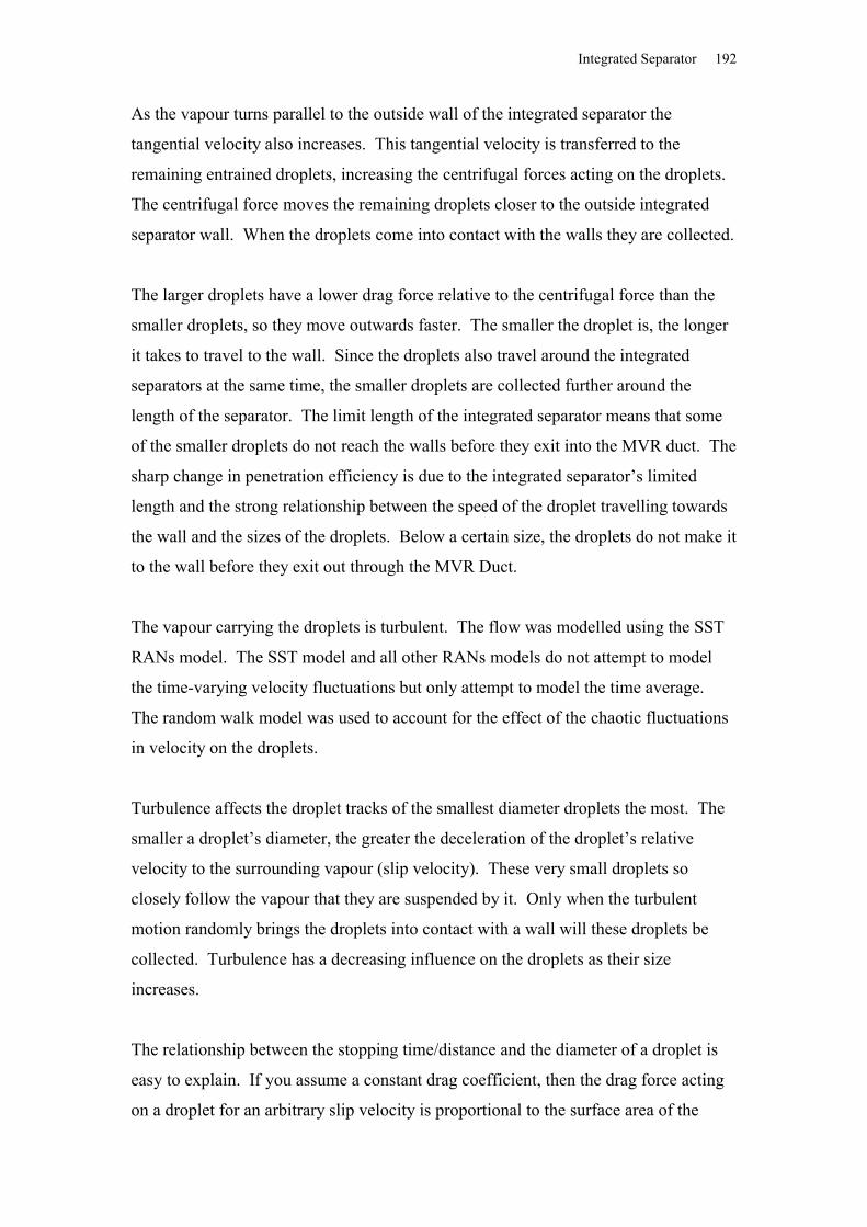
Integrated Separator 192
As the vapour turns parallel to the outside wall of the integrated separator the
tangential velocity also increases. This tangential velocity is transferred to the
remaining entrained droplets, increasing the centrifugal forces acting on the droplets.
The centrifugal force moves the remaining droplets closer to the outside integrated
separator wall. When the droplets come into contact with the walls they are collected.
The larger droplets have a lower drag force relative to the centrifugal force than the
smaller droplets, so they move outwards faster. The smaller the droplet is, the longer
it takes to travel to the wall. Since the droplets also travel around the integrated
separators at the same time, the smaller droplets are collected further around the
length of the separator. The limit length of the integrated separator means that some
of the smaller droplets do not reach the walls before they exit into the MVR duct. The
sharp change in penetration efficiency is due to the integrated separator’s limited
length and the strong relationship between the speed of the droplet travelling towards
the wall and the sizes of the droplets. Below a certain size, the droplets do not make it
to the wall before they exit out through the MVR Duct.
The vapour carrying the droplets is turbulent. The flow was modelled using the SST
RANs model. The SST model and all other RANs models do not attempt to model
the time-varying velocity fluctuations but only attempt to model the time average.
The random walk model was used to account for the effect of the chaotic fluctuations
in velocity on the droplets.
Turbulence affects the droplet tracks of the smallest diameter droplets the most. The
smaller a droplet’s diameter, the greater the deceleration of the droplet’s relative
velocity to the surrounding vapour (slip velocity). These very small droplets so
closely follow the vapour that they are suspended by it. Only when the turbulent
motion randomly brings the droplets into contact with a wall will these droplets be
collected. Turbulence has a decreasing influence on the droplets as their size
increases.
The relationship between the stopping time/distance and the diameter of a droplet is
easy to explain. If you assume a constant drag coefficient, then the drag force acting
on a droplet for an arbitrary slip velocity is proportional to the surface area of the
Integrated Separator 193
droplet. The mass and inertia of a spherical droplet is proportional to the volume of
the droplet. The drag force acts against the droplet inertia to slow it. If all other
properties remain constant the stopping distance/ length will increase proportionally
as the droplet diameter increases.
All droplet sizes are affected by gravity and turbulence. If any sized droplet travels
through the doors between the plenum chamber and the separator it is affected by the
radial velocity through the doors. Likewise, all sized droplets that travel around the
integrated separator are affected by centrifugal force acting on them. The relative
importance or dominance of various separation processes varies depending on the
droplet diameter.
Figure 3-127 indicates how the relative importance of the separation changes as the
droplet diameter changes. Figure 3-127 shows collection wall density contours for
different diameter 1040 kg m-3 droplets from the 1st pass 1st effect running at a total
vapour flow rate of 26 t h-1. The coloured area plots in the figure are to indicate the
relative importance of the separation process for the droplets above them. The plot
sizes are qualitatively produced.
Figure 3-127 Relative importance of the different separation processes
The 690 m droplets are collected at the bottom of the plenum chamber (Figure 3-
127). For these droplets, the gravitation force dominates the separation. Only a
limited amount of radial momentum is transferred to the droplets since most do not
Integrated Separator 194
travel through the doors between the plenum chamber and the integrated separator.
No centrifugal forces act on the droplets since the droplets are collected before
reaching the integrated separator.
Some of the 242 m droplets are separated due to gravitational force acting on the
droplets (Figure 3-127). The 242 m droplets that travel through the doorway gain
significant radial momentum from the vapour, enough to force the remaining
suspended droplets to impinge on the outside wall of the integrated separator directly
opposite the doorways. No centrifugal forces are acting on the 242 m droplets since
the droplets are also collected before the vapour travels tangentially around the
integrated separator.
The 48 m droplets are collected due to a combination of gravitational force, radial
momentum and centrifugal force from tangential velocity around the integrated
separator (Figure 3-127). The collection of the 19 m droplets is dominated by
centrifugal force as well as turbulent dispersion. Only turbulence dispersion is
significant in separating the 12 m diameter droplets.
The cut-off diameters of the integrated separators were ~20 m. Lui and Lipták
(1997) state that it is possible for cyclone separators have to cut-off diameters ~5 m.
This indicates that the separators could be improved. It does not seem realistic that an
integrated separator design of the dairy industry would greatly improve on the ~5 m
cut-off diameter achievable by normal cyclones, given that they must be designed
around a plenum chamber.
Interestingly, the integrated separator does not have a radial velocity into the center of
the separator like normal reverse flow cyclones. This means that all sized droplets are
move towards the outside of an integrated separator. The smaller the droplet, the
slower it travels. So with enough time/length an integrated separator could
theoretically separate smaller droplets than the reverse flow cyclone. The flow would
have to be laminar and the length/time required could easily be impracticable. If the
flow was turbulent then the smallest droplets will move randomly within the flow due
to turbulence dispersion faster than any centrifugal effect. When droplets are smaller
Integrated Separator 195
than ~1 mm Brownian motion can not be ignored and an integrated separator design
would not be able to improve on the collection of them. The theoretical potential for
the integrated separator to out perform the reverse flow cycle design is interesting and
could lead to some novel design improvements in the future.
3.11.4 Droplet penetration rates
As well as gaining an understanding of the separation and flow patterns, the separator
model was created to predict fouling from penetrating feed droplets. More
specifically it needed to be able to predict whether fouling due to a lack of separation
was occurring and, if so, what effect changes in geometry would have on the fouling.
The penetration efficiency data was fitted to equation 3-39. The fitted equations were
very similar for all the passes from both effects. The similarities indicate that the
same basic separation process is dominating which droplets penetrate and which do
not penetrate.
There are several identified separation processes occurring within the separator.
However it is the separation process from the centrifugal force that is the most
important for droplet penetration. The centrifugal force is produced from the
tangential velocity of the droplets which are at least partially suspended in the vapour
which also travels around the integrated separator.
The centrifugal separation process determines the size of the largest droplets that
penetrate. Exception for turbulent dispersion, centrifugal separation is the last
separation process as the droplets travel through the separator and it is responsible for
the collection of the smallest droplet size that is entirely collected.
Turbulent dispersion collects droplets throughout the separator and is the dominant
collection process of the smallest droplets. Turbulent dispersion is a random process
and only collects a proportion of any droplet size group. These small droplets contain
very little mass and their incomplete collection has little consequence for the fouling
problem.
Integrated Separator 196
It is the largest droplet sizes that penetrate that contain most of the penetrating mass
which causes fouling. The amount of mass in these (“critical”) droplets determines
whether significant fouling due to a lack of separation occurs or not and, if so, at what
rate. If the centrifugal separation process can collect even smaller droplets, this
greatly reduces the mass fraction lost. Any possible improvements to the integrated
separator design should be based on increases to this separation process.
There are three main mechanisms that can increase the centrifugal separation:
increase the time the droplets travel around the integrated separator, so the
droplets have a longer amount of time to travel to the walls,
increase the tangential velocity around the integrated separator to increase the
centrifugal force acting on the droplets,
decrease the radius of the integrated separator as this increases the centrifugal
force on the droplets for a given tangential velocity.
Since all three mechanisms interact with each other, consideration for how changing
one affects the other should be given.
The effect of changing the centrifugal force was detected during the sensitivity study
of the total vapour flow rate. Increasing the total vapour flow increased the tangential
velocity around the separator and hence the centrifugal separation process. The
increased centrifugal force removed smaller droplets and would reduce the mass
penetrating for a constant arbitrary droplet distribution. It is noteworthy that the
increase in centrifugal force more than compensated for the decrease in time the
droplets were exposed to the force.
There is concern that increasing the tangential velocities could cause droplet to re-
entrain into the vapour flow due to stripping from the walls. No literature was found
to back up the raised concerns and other opinions discounted this theory. This could
be an area of further investigation if needed.
The proposed new design was meant to increase the distance the droplets are in the
high tangential velocity near the separator wall (Section 3.1). The distance in the
separator where the tangential velocity is high is rather short. Approximately one third
Integrated Separator 197
of the turn of the separator is taken up by either radial velocity at the doors or the
MVR duct, leaving approximately one third of a separator turn for the droplets to
centrifugally separate out of the vapour. Increasing this distance would help
separation and the proposed alteration could increase this distance by 2-3 times. The
proposed alterations should also increase the velocities of the droplets and vapour in
the integrated separator, the increased velocity could however also decrease the time
available for collection. This also is likely to increase separation but there is a
concern that increasing the velocity by too much could start droplets to re-entrain.
The re-entrainment of droplet is not currently a problem but increasing the tangential
velocities too much could change this.
3.11.5 Mass fraction loss
There are large errors associated with the calculated mass fraction loss, both for the
individual passes and the overall loss. This is due to the sensitivity of the mass loss to
the droplet distribution feed into the separator and the underling uncertainty
associated with that distribution. This limits the mass fraction loss precision. It also
makes it difficult to accurately predict any droplet interactions with the fluid and inter
droplet collisions, as both are so dependent on the droplet distribution.
The amount of mass that penetrated was not significant and the conclusion from the
model was that the fouling in the evaporator system was not caused by penetration of
droplets.
The greatest mass fraction loss occurs from the feed from the 2nd pass in the 2nd effect.
The droplet distribution produced from this pass contains more numerous smaller
droplets than other passes and the same pass has the largest cut-off diameter of the
passes studied. This results in more mass penetrating the separator.
When MPC is processed, the mass fraction loss is less than when processing Skim.
More mass is carried by the small sized droplets when processing Skim and these
smaller droplets can penetrate the separator. The greater atomisation of the film is
caused by the greater shear acting on the film from the faster moving vapour at the
bottom of the heat transfer tubes. There is limited information to accurately predict
the droplet distribution, but the shear force mechanism of atomisation due to the
Integrated Separator 198
velocity difference between the phases is common across all atomisation processes.
For the planar sheet model this velocity difference is measured by the air/liquid mass
ratio. As this ratio decreases the mean droplet size rapidly increases. MPC had a
lower air/liquid ratio compared to Skim and this is why it had less mass fraction loss.
The current standard inner diameter of the heat transfer tubes is ~48 mm and is used
because of historical, structural, convenience and packing reasons. There is no reason
why a different diameter tube could not be used. Another option is to use a shorter
tube to reduce the vapour velocities. The shorter tube reduces the heat transfer area
and therefore the evaporation and vapour flow rate down the tube. Both of these
techniques allow for some control over the atomisation of the film and could be
considered in future evaporator design along with the standard considerations.
Cyclonic separation can separate down to certain size droplet. The size depends on
the specific design and operating conditions, but 5 m is a common limit. To stop
separation penetration problems, it may be simpler to design the evaporators to
produce larger droplets than it is to design separators that collect very small droplets.
Even though the mass fraction loss in the separator is not enough to be the cause of
fouling problem, there are still other problems associated with lack of separation in
the dairy industry. Winchester (2004-2007) indicated that droplets impacting onto the
MVR fans is one such problem. Fouling occurs on the MVR fans due to droplets
impacting on them. The added mass of the fouling causes the fans to vibrate which is
undesirable. This is a problem across the dairy industry and is not isolated to
integrated separator evaporators.
3.11.6 Validation
The validation of the CFD model is based on both qualitative results and quantitative
results. The separator model predicted that the separation was adequate and that the
fouling was due to other unrelated problems. This finding was confirmed through
changes to operator practices that did not affect the separation process. The fouling
problem that initiated the project was fixed, confirming the findings of the CFD
model.
Integrated Separator 199
The separator model predicted that when processing MPC, the separator lost less mass
than when processing Skim. This was because the lower vapour velocities at bottom
of the heat transfer tubes produced a droplet distribution with relatively more mass in
the larger droplets when processing MPC. This agreed with the experiences of the
evaporator design company.
Experimental penetration total mass fraction loss was compared against the values
predicted by the separator model. The experimental and model predictions agree
within experimental uncertainties (Figure 3-126).
3.12 Conclusions
A steady state CFD model was created of the integrated separators of the Clandeboye
Drier 2 using the finite volume method. A one-way coupled Lagrangian random eddy
walk model was used to model the droplets and the vapour phase was modelled in an
Eulerian fashion. Turbulence was modelled with the SST model. The equations were
solutions on an unstructured hybrid mesh. The solution was solved using the coupled
multigrid method of Ansys CFX version 10.0.
These are the first CFD models of an integrated separator as far as the author can find.
They also appear to be the first dairy cyclonic separator CFD models as well. The
models serve as a good starting point for any further CFD modelling of either
integrated separators or even dairy cyclonic separators.
Model precision and accuracy of the model is limited by the droplet distributions used
to predict the atomisation of the falling films as they fall from the heat transfer tubes.
There is only limited information available to predict the droplet size distributions and
hence the uncertainties involved are significant. The foulant carry-over (mass fraction
loss) predicted by the model is also very sensitive to the droplet distribution used at
the inlets. Any improvement in the droplet distribution modelling would be directly
reflected in the model accuracy.
A greater understanding of the vapour flow and droplet paths within the separator was
gained. The separation process was found to be due to several different separation
processes. A gravitational settling process was observed, so was an impingement
Integrated Separator 200
mechanism due to the radial momentum gain exiting through the doors between the
plenum chamber and integrated separators. A centrifugal separation process occurs
due to the tangential velocity of the droplets as they travel around the integrated
separator and a random turbulent dispersion separator process was observed as well.
The most important separation process for the collection of foulants is the centrifugal
separation process. This process directly determines the sizes of the largest droplets
that penetrate the separator. It is these droplets that contain the majority of the mass
that penetrates and could cause fouling.
The size of the doorways between the plenum chamber and the integrated separators
is used to scale the entire separator design. Currently this doorway is designed using
a plug flow assumption. The model predicts significant regions of recirculation
occurring at the top of the doorways. The plug flow assumption does not capture the
effects of recirculation regions on the flow rate through the doorways and is a poor
assumption.
The CFD model accurately predicted the lack of penetration of droplets through the
separator that could foul the cow water. The correct prediction of the penetration rate
was the primary objective of the model. The predicted mass fraction loss based on
total solids was 0.03% when processing Skim and 0.0012% when processing MPC.
These values agreed with experimental measurements taken from all the effects
including the 3rd and 4th effects which were not modelled. The effect of the 3rd and 4th
effects on the penetration rate is unknown.
The vapour velocity at the bottom of the heat transfer tubes has a significant effect on
the separator efficiency. A higher vapour velocity results in more numerous smaller
droplets due to the greater atomisation of the film. The higher vapour velocity
produces a larger shear force on the surface of the film and this causes the film to
break up into smaller droplets.
The more numerous small droplets are more difficult to collect than larger droplets in
the integrated separators. The small droplets are also more difficult to collect in the
traditional cyclone separators. A better design/operating practice is to limit the
Integrated Separator 201
vapour velocities and reduce the number of small droplets, rather than trying to
remove larger number of small droplets. This is valid for falling film evaporators
with either integrated separators or traditional separators.
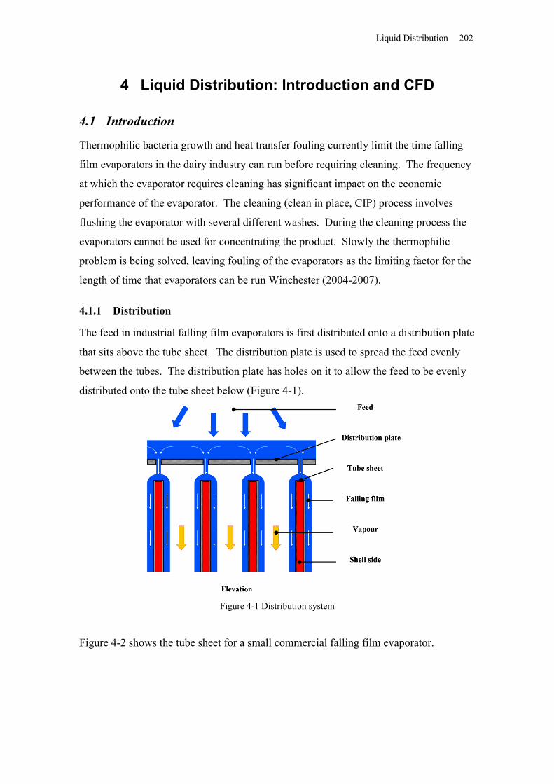
Liquid Distribution 202
4 Liquid Distribution: Introduction and CFD
4.1 Introduction
Thermophilic bacteria growth and heat transfer fouling currently limit the time falling
film evaporators in the dairy industry can run before requiring cleaning. The frequency
at which the evaporator requires cleaning has significant impact on the economic
performance of the evaporator. The cleaning (clean in place, CIP) process involves
flushing the evaporator with several different washes. During the cleaning process the
evaporators cannot be used for concentrating the product. Slowly the thermophilic
problem is being solved, leaving fouling of the evaporators as the limiting factor for the
length of time that evaporators can be run Winchester (2004-2007).
4.1.1 Distribution
The feed in industrial falling film evaporators is first distributed onto a distribution plate
that sits above the tube sheet. The distribution plate is used to spread the feed evenly
between the tubes. The distribution plate has holes on it to allow the feed to be evenly
distributed onto the tube sheet below (Figure 4-1).
Figure 4-1 Distribution system
Figure 4-2 shows the tube sheet for a small commercial falling film evaporator.
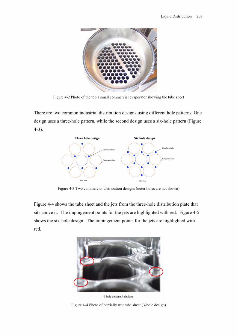
Liquid Distribution 203
Figure 4-2 Photo of the top a small commercial evaporator showing the tube sheet
There are two common industrial distribution designs using different hole patterns. One
design uses a three-hole pattern, while the second design uses a six-hole pattern (Figure
4-3).
Figure 4-3 Two commercial distribution designs (outer holes are not shown)
Figure 4-4 shows the tube sheet and the jets from the three-hole distribution plate that
sits above it. The impingement points for the jets are highlighted with red. Figure 4-5
shows the six-hole design. The impingement points for the jets are highlighted with
red.
Figure 4-4 Photo of partially wet tube sheet (3-hole design)
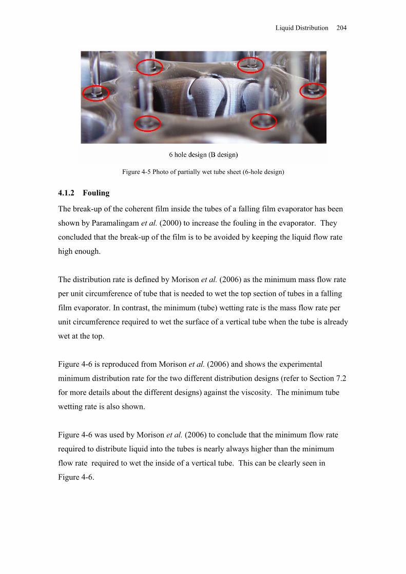
Liquid Distribution 204
Figure 4-5 Photo of partially wet tube sheet (6-hole design)
4.1.2 Fouling
The break-up of the coherent film inside the tubes of a falling film evaporator has been
shown by Paramalingam et al. (2000) to increase the fouling in the evaporator. They
concluded that the break-up of the film is to be avoided by keeping the liquid flow rate
high enough.
The distribution rate is defined by Morison et al. (2006) as the minimum mass flow rate
per unit circumference of tube that is needed to wet the top section of tubes in a falling
film evaporator. In contrast, the minimum (tube) wetting rate is the mass flow rate per
unit circumference required to wet the surface of a vertical tube when the tube is already
wet at the top.
Figure 4-6 is reproduced from Morison et al. (2006) and shows the experimental
minimum distribution rate for the two different distribution designs (refer to Section 7.2
for more details about the different designs) against the viscosity. The minimum tube
wetting rate is also shown.
Figure 4-6 was used by Morison et al. (2006) to conclude that the minimum flow rate
required to distribute liquid into the tubes is nearly always higher than the minimum
flow rate required to wet the inside of a vertical tube. This can be clearly seen in
Figure 4-6.
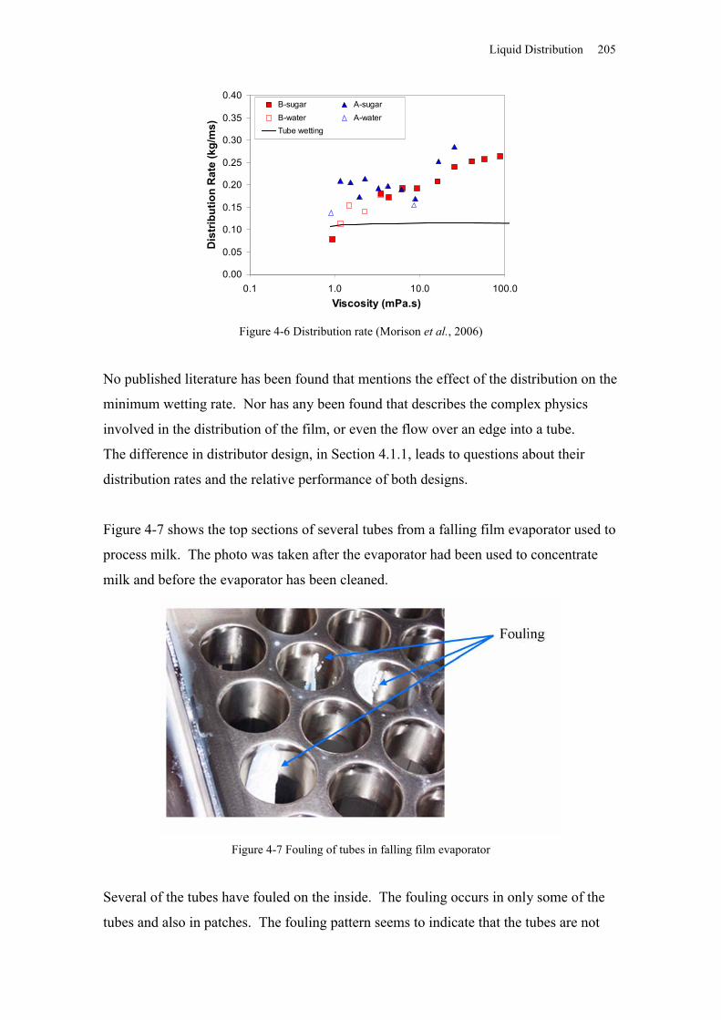
Liquid Distribution 205
Figure 4-6 Distribution rate (Morison et al., 2006)
No published literature has been found that mentions the effect of the distribution on the
minimum wetting rate. Nor has any been found that describes the complex physics
involved in the distribution of the film, or even the flow over an edge into a tube.
The difference in distributor design, in Section 4.1.1, leads to questions about their
distribution rates and the relative performance of both designs.
Figure 4-7 shows the top sections of several tubes from a falling film evaporator used to
process milk. The photo was taken after the evaporator had been used to concentrate
milk and before the evaporator has been cleaned.
Figure 4-7 Fouling of tubes in falling film evaporator
Several of the tubes have fouled on the inside. The fouling occurs in only some of the
tubes and also in patches. The fouling pattern seems to indicate that the tubes are not
0.00
0.05
0.10
0.15
0.20
0.25
0.30
0.35
0.40
0.1 1.0 10.0 100.0Viscosity (mPa.s)
Dis
trib
utio
n R
ate
(kg/
ms)
B-sugar A-sugarB-water A-waterTube wetting
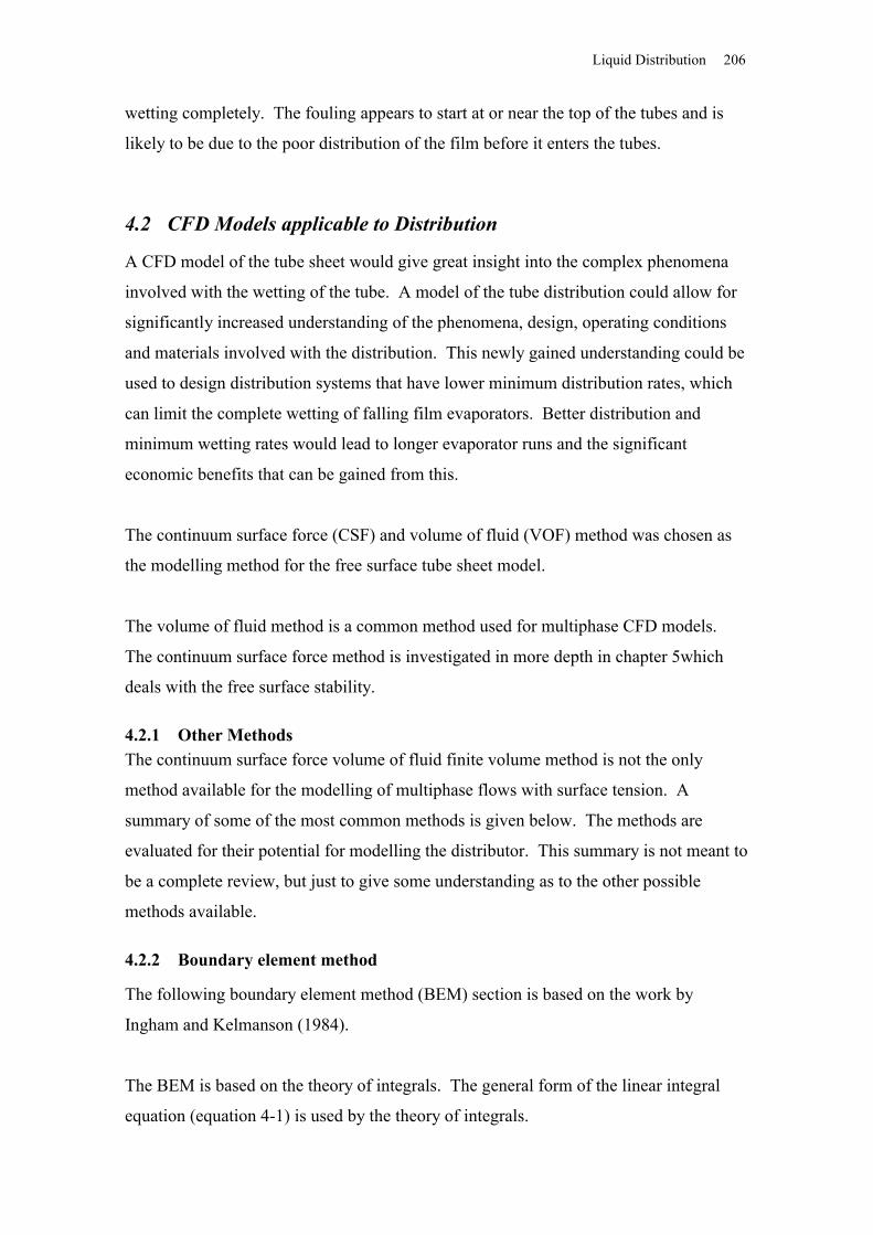
Liquid Distribution 206
wetting completely. The fouling appears to start at or near the top of the tubes and is
likely to be due to the poor distribution of the film before it enters the tubes.
4.2 CFD Models applicable to Distribution
A CFD model of the tube sheet would give great insight into the complex phenomena
involved with the wetting of the tube. A model of the tube distribution could allow for
significantly increased understanding of the phenomena, design, operating conditions
and materials involved with the distribution. This newly gained understanding could be
used to design distribution systems that have lower minimum distribution rates, which
can limit the complete wetting of falling film evaporators. Better distribution and
minimum wetting rates would lead to longer evaporator runs and the significant
economic benefits that can be gained from this.
The continuum surface force (CSF) and volume of fluid (VOF) method was chosen as
the modelling method for the free surface tube sheet model.
The volume of fluid method is a common method used for multiphase CFD models.
The continuum surface force method is investigated in more depth in chapter 5which
deals with the free surface stability.
4.2.1 Other MethodsThe continuum surface force volume of fluid finite volume method is not the only
method available for the modelling of multiphase flows with surface tension. A
summary of some of the most common methods is given below. The methods are
evaluated for their potential for modelling the distributor. This summary is not meant to
be a complete review, but just to give some understanding as to the other possible
methods available.
4.2.2 Boundary element method
The following boundary element method (BEM) section is based on the work by
Ingham and Kelmanson (1984).
The BEM is based on the theory of integrals. The general form of the linear integral
equation (equation 4-1) is used by the theory of integrals.
Liquid Distribution 207
b
axgdyyyxKxx , (4-1)
The functions g(x), (x), (x) and K(x,y) are known functions and is a constant.
It is possible for some fluid problems to convert the boundary value or even initial value
problems into the integral form given in equation 4-1. Irrotational, Stokes and potential
flows are examples of flows that can be converted to the integral form.
There are only a few models for which the integral equations can be solved analytically.
The BEM is a numerical method where the boundary is split into smaller discretised
sections, and the system of equations for each section is solved. Examples were found
of previous work where the BEM was used to solve multiphase flows with surface
tension. The work included that of Cristini et. (2001), Lu (1997) and Kim and Khayat
(2004).
The BEM method was not used as no examples of surface tension flow were found
without the Stokes assumption that inertial effects of the fluid could be neglected or
other similar simplifications. The fluid assumptions needed seemed unlikely to be
valid. There are particular concerns about the ability of the BEM to predict the
recirculating flow expected under the hydraulic jump, which was expected to be
important for the correct simulation of the liquid distribution.
4.2.3 FVM methods
The VOF CSF method is not the only FVM method available for modelling surface
tension.
Level set method
Losasso et al. (2006) cites Osher and Sethian (1988) as introducing equation 4-2 and
calling it the Level Set equation, but he also notes that interestingly 25 years earlier
Markstein et al. (1964) had used the same equation within the context of combustion.
Equation 4-2 uses a Level Set variable which has the characteristics of > 0 in one
phase, in the other phase and at the interface. The Level Set variable is
used to define the location of the free surface.
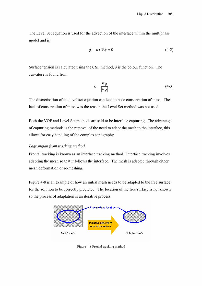
Liquid Distribution 208
The Level Set equation is used for the advection of the interface within the multiphase
model and is
0 ut (4-2)
Surface tension is calculated using the CSF method, is the colour function. The
curvature is found from
(4-3)
The discretisation of the level set equation can lead to poor conservation of mass. The
lack of conservation of mass was the reason the Level Set method was not used.
Both the VOF and Level Set methods are said to be interface capturing. The advantage
of capturing methods is the removal of the need to adapt the mesh to the interface, this
allows for easy handling of the complex topography.
Lagrangian front tracking method
Frontal tracking is known as an interface tracking method. Interface tracking involves
adapting the mesh so that it follows the interface. The mesh is adapted through either
mesh deformation or re-meshing.
Figure 4-8 is an example of how an initial mesh needs to be adapted to the free surface
for the solution to be correctly predicted. The location of the free surface is not known
so the process of adaptation is an iterative process.
Figure 4-8 Frontal tracking method
Liquid Distribution 209
Some frontal tracking methods involve adapting the mesh near the interface without
having to deform or re-mesh the remaining mesh.
The model is set up so that within a “domain” or group of elements only one phase is
present. Each phase has domain and its own fluid equations, which are only solved in
its domain.
One of the advantages of the frontal tracking methods is that the different phases can be
resolved to different resolution and complexity. For example, the Navier-Stokes
equations for a liquid phase can be fully solved while using a constant pressure for a
vapour phase.
The surface tension force uses the curvature found from the surface of the domain.
Goldman (2005) shows that the mean curvature m of an implicit surface F can be found
from
3
2
FFTraceFFFF T
m
(4-4)
Frontal tracking does not have the numerical accuracy problems that the Eulerian CSF
(VOF and Level Set) methods do, due to the problems of the curvature estimate.
The main problem with the frontal tracking is the problem surrounding the adaptation of
the mesh especially when the free surface is not simple.
The other major problem with frontal tracking methods is the requirement to re-mesh
and to redefine the boundary conditions when the topography of a problem changes.
The treatment of these changes in topography is quite complex. Examples of changes in
topography are splitting, pinching and entrainment with the free surface and in the
distribution model the creation of holes in the film.
Esmaeeli and Tryggvason (2004) give a good description of a frontal tracking method.
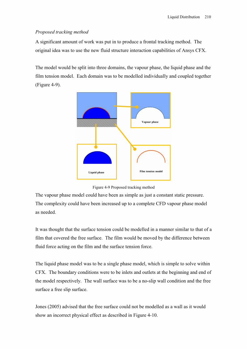
Liquid Distribution 210
Proposed tracking method
A significant amount of work was put in to produce a frontal tracking method. The
original idea was to use the new fluid structure interaction capabilities of Ansys CFX.
The model would be split into three domains, the vapour phase, the liquid phase and the
film tension model. Each domain was to be modelled individually and coupled together
(Figure 4-9).
Figure 4-9 Proposed tracking method
The vapour phase model could have been as simple as just a constant static pressure.
The complexity could have been increased up to a complete CFD vapour phase model
as needed.
It was thought that the surface tension could be modelled in a manner similar to that of a
film that covered the free surface. The film would be moved by the difference between
fluid force acting on the film and the surface tension force.
The liquid phase model was to be a single phase model, which is simple to solve within
CFX. The boundary conditions were to be inlets and outlets at the beginning and end of
the model respectively. The wall surface was to be a no-slip wall condition and the free
surface a free slip surface.
Jones (2005) advised that the free surface could not be modelled as a wall as it would
show an incorrect physical effect as described in Figure 4-10.
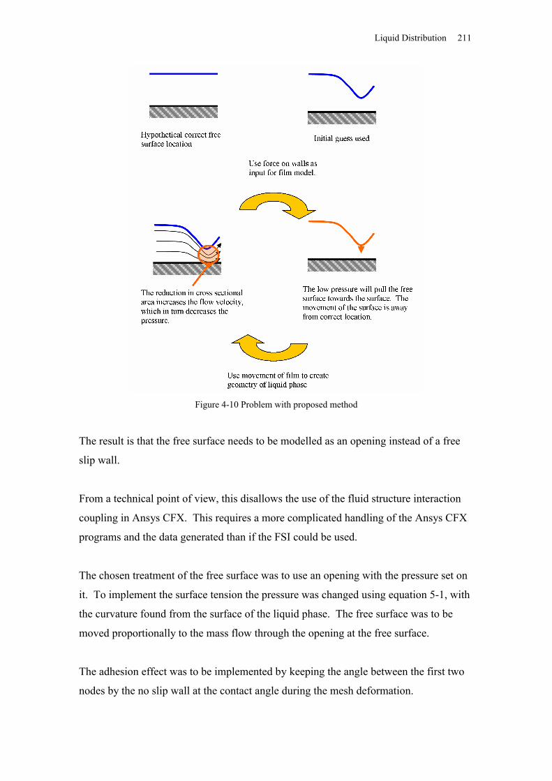
Liquid Distribution 211
Figure 4-10 Problem with proposed method
The result is that the free surface needs to be modelled as an opening instead of a free
slip wall.
From a technical point of view, this disallows the use of the fluid structure interaction
coupling in Ansys CFX. This requires a more complicated handling of the Ansys CFX
programs and the data generated than if the FSI could be used.
The chosen treatment of the free surface was to use an opening with the pressure set on
it. To implement the surface tension the pressure was changed using equation 5-1, with
the curvature found from the surface of the liquid phase. The free surface was to be
moved proportionally to the mass flow through the opening at the free surface.
The adhesion effect was to be implemented by keeping the angle between the first two
nodes by the no slip wall at the contact angle during the mesh deformation.
Liquid Distribution 212
The VOF method was improved with the new Ansys CFX version 10, bringing in the
volume fraction smoothing and the curvature under-relaxation factor. The new
functionality allowed for considerable progress to be made in the modelling of the free
surface and it appeared to be better suited for the modelling.
A frontal tracking method requires the user to define the basic topography of the model.
The VOF method does not require this. This means the VOF can spontaneously model
holes in the film. The frontal tracking could not do this. There was a concern that by
defining the topography in the initial guess with the Frontal Tracking method that the
Frontal Tracking method would give incorrect wetting results. Another reason for the
VOF method was chosen was that that it was thought to be faster and more stable than
Frontal Tracking method.
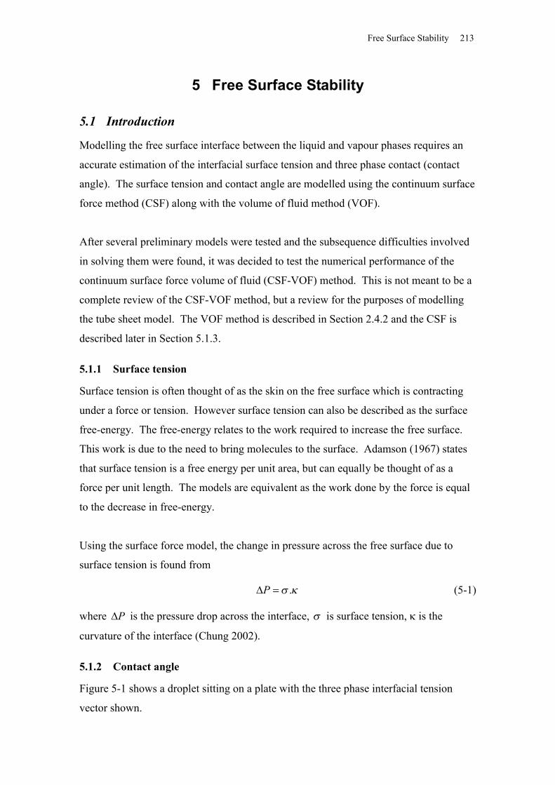
Free Surface Stability 213
5 Free Surface Stability
5.1 Introduction
Modelling the free surface interface between the liquid and vapour phases requires an
accurate estimation of the interfacial surface tension and three phase contact (contact
angle). The surface tension and contact angle are modelled using the continuum surface
force method (CSF) along with the volume of fluid method (VOF).
After several preliminary models were tested and the subsequence difficulties involved
in solving them were found, it was decided to test the numerical performance of the
continuum surface force volume of fluid (CSF-VOF) method. This is not meant to be a
complete review of the CSF-VOF method, but a review for the purposes of modelling
the tube sheet model. The VOF method is described in Section 2.4.2 and the CSF is
described later in Section 5.1.3.
5.1.1 Surface tension
Surface tension is often thought of as the skin on the free surface which is contracting
under a force or tension. However surface tension can also be described as the surface
free-energy. The free-energy relates to the work required to increase the free surface.
This work is due to the need to bring molecules to the surface. Adamson (1967) states
that surface tension is a free energy per unit area, but can equally be thought of as a
force per unit length. The models are equivalent as the work done by the force is equal
to the decrease in free-energy.
Using the surface force model, the change in pressure across the free surface due to
surface tension is found from
.P (5-1)
where P is the pressure drop across the interface, is surface tension, is the
curvature of the interface (Chung 2002).
5.1.2 Contact angle
Figure 5-1 shows a droplet sitting on a plate with the three phase interfacial tension
vector shown.
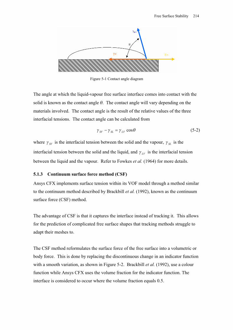
Free Surface Stability 214
Figure 5-1 Contact angle diagram
The angle at which the liquid-vapour free surface interface comes into contact with the
solid is known as the contact angle . The contact angle will vary depending on the
materials involved. The contact angle is the result of the relative values of the three
interfacial tensions. The contact angle can be calculated from
cosLVSLSV (5-2)
where SV is the interfacial tension between the solid and the vapour, SL is the
interfacial tension between the solid and the liquid, and LV is the interfacial tension
between the liquid and the vapour. Refer to Fowkes et al. (1964) for more details.
5.1.3 Continuum surface force method (CSF)
Ansys CFX implements surface tension within its VOF model through a method similar
to the continuum method described by Brackbill et al. (1992), known as the continuum
surface force (CSF) method.
The advantage of CSF is that it captures the interface instead of tracking it. This allows
for the prediction of complicated free surface shapes that tracking methods struggle to
adapt their meshes to.
The CSF method reformulates the surface force of the free surface into a volumetric or
body force. This is done by replacing the discontinuous change in an indicator function
with a smooth variation, as shown in Figure 5-2. Brackbill et al. (1992), use a colour
function while Ansys CFX uses the volume fraction for the indicator function. The
interface is considered to occur where the volume fraction equals 0.5.
Free Surface Stability 215
Figure 5-2 Interface area
The CSF method is implemented as
nBF ... (5-3)
where BF is the volumetric body force, n is the unit normal of the free surface and is
the delta function to implement the curvature force only at the free surface found from
r (5-4)
where r is the volume fraction. The curvature of the free surface is found from the rate
of change of the free surface unit normal n. The curvature can be expressed as
n (5-5)
The CSF method calculates the normal from the gradient of the colour function c,
ccn
(5-6)
Ansys CFX uses the volume fraction r, so equation 5-6 becomes
rrn
(5-7)
It can be shown that r is equal to one, so equation 5-7 becomes
rn (5-8)
Combining equations 5-5and 5-8 gives
r (5-9)
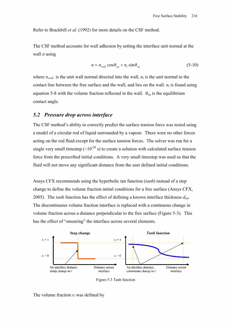
Free Surface Stability 216
Refer to Brackbill et al. (1992) for more details on the CSF method.
The CSF method accounts for wall adhesion by setting the interface unit normal at the
wall n using
eqteqwall nnn sincos (5-10)
where nwall is the unit wall normal directed into the wall, nt is the unit normal to the
contact line between the free surface and the wall, and lies on the wall. nt is found using
equation 5-8 with the volume fraction reflected in the wall. eq is the equilibrium
contact angle.
5.2 Pressure drop across interface
The CSF method’s ability to correctly predict the surface tension force was tested using
a model of a circular rod of liquid surrounded by a vapour. There were no other forces
acting on the rod fluid except for the surface tension forces. The solver was run for a
single very small timestep (~10-20 s) to create a solution with calculated surface tension
force from the prescribed initial conditions. A very small timestep was used so that the
fluid will not move any significant distance from the user defined initial conditions.
Ansys CFX recommends using the hyperbolic tan function (tanh) instead of a step
change to define the volume fraction initial conditions for a free surface (Ansys CFX,
2005). The tanh function has the effect of defining a known interface thickness dint.
The discontinuous volume fraction interface is replaced with a continuous change in
volume fraction across a distance perpendicular to the free surface (Figure 5-3). This
has the effect of “smearing” the interface across several elements.
Figure 5-3 Tanh function
The volume fraction rl was defined by
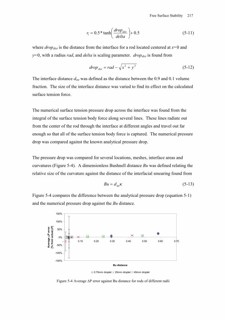
Free Surface Stability 217
5.0tanh*5.0
deltadropr dist
l (5-11)
where dropdist is the distance from the interface for a rod located centered at x=0 and
y=0, with a radius rad, and delta is scaling parameter. dropdist is found from
22 yxraddropdist (5-12)
The interface distance dint was defined as the distance between the 0.9 and 0.1 volume
fraction. The size of the interface distance was varied to find its effect on the calculated
surface tension force.
The numerical surface tension pressure drop across the interface was found from the
integral of the surface tension body force along several lines. These lines radiate out
from the center of the rod through the interface at different angles and travel out far
enough so that all of the surface tension body force is captured. The numerical pressure
drop was compared against the known analytical pressure drop.
The pressure drop was compared for several locations, meshes, interface areas and
curvatures (Figure 5-4). A dimensionless Bushnell distance Bu was defined relating the
relative size of the curvature against the distance of the interfacial smearing found from
intdBu (5-13)
Figure 5-4 compares the difference between the analytical pressure drop (equation 5-1)
and the numerical pressure drop against the Bu distance.
-150%
-100%
-50%
0%
50%
100%
150%
- 0.10 0.20 0.30 0.40 0.50 0.60 0.70
Bu distance
Ave
rage
P
erro
r [%
from
act
ual
P]
0.75mm droplet 25mm droplet 45mm droplet
Figure 5-4 Average P error against Bu distance for rods of different radii
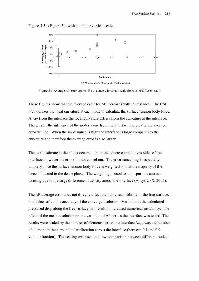
Free Surface Stability 218
Figure 5-5 is Figure 5-4 with a smaller vertical scale.
-15%
-10%
-5%
0%
5%
10%
15%
- 0.10 0.20 0.30 0.40 0.50 0.60 0.70
Bu distance
Ave
rage
P
erro
r [%
from
act
ual
P]
0.75mm droplet 25mm droplet 45mm droplet
Figure 5-5 Average P error against Bu distance with small scale for rods of different radii
These figures show that the average error for P increases with Bu distance. The CSF
method uses the local curvature at each node to calculate the surface tension body force.
Away from the interface the local curvature differs from the curvature at the interface.
The greater the influence of the nodes away from the interface the greater the average
error will be. When the Bu distance is high the interface is large compared to the
curvature and therefore the average error is also larger.
The local estimate at the nodes occurs on both the concave and convex sides of the
interface, however the errors do not cancel out. The error cancelling is especially
unlikely since the surface tension body force is weighted so that the majority of the
force is located in the dense phase. The weighting is used to stop spurious currents
forming due to the large difference in density across the interface (Ansys CFX, 2005).
The P average error does not directly affect the numerical stability of the free-surface,
but it does affect the accuracy of the converged solution. Variation in the calculated
pressured drop along the free-surface will result in increased numerical instability. The
effect of the mesh resolution on the variation of P across the interface was tested. The
results were scaled by the number of elements across the interface Noele was the number
of element in the perpendicular direction across the interface (between 0.1 and 0.9
volume fraction). The scaling was used to allow comparison between different models.
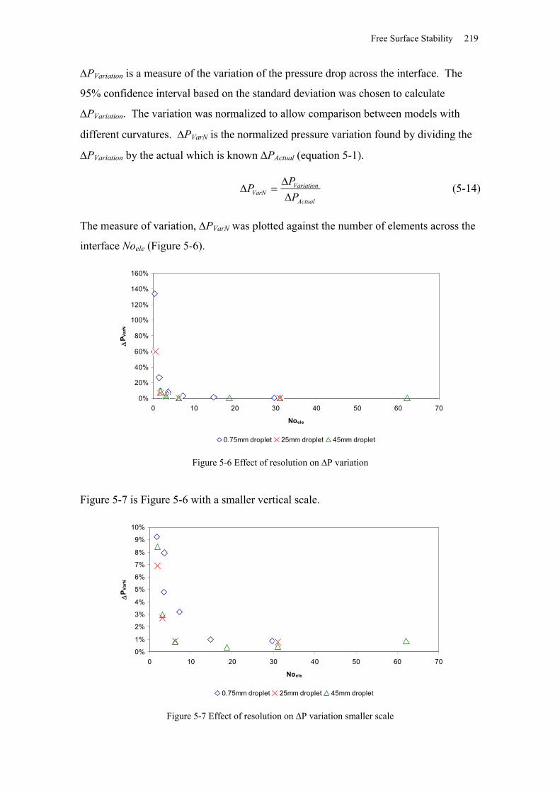
Free Surface Stability 219
PVariation is a measure of the variation of the pressure drop across the interface. The
95% confidence interval based on the standard deviation was chosen to calculate
PVariation. The variation was normalized to allow comparison between models with
different curvatures. PVarN is the normalized pressure variation found by dividing the
PVariation by the actual which is known PActual (equation 5-1).
Actual
VariationVarN P
PP
(5-14)
The measure of variation, PVarN was plotted against the number of elements across the
interface Noele (Figure 5-6).
0%
20%
40%
60%
80%
100%
120%
140%
160%
0 10 20 30 40 50 60 70
Noele
P V
arN
0.75mm droplet 25mm droplet 45mm droplet
Figure 5-6 Effect of resolution on P variation
Figure 5-7 is Figure 5-6 with a smaller vertical scale.
0%
1%
2%
3%
4%
5%
6%
7%
8%
9%
10%
0 10 20 30 40 50 60 70
Noele
P V
arN
0.75mm droplet 25mm droplet 45mm droplet
Figure 5-7 Effect of resolution on P variation smaller scale
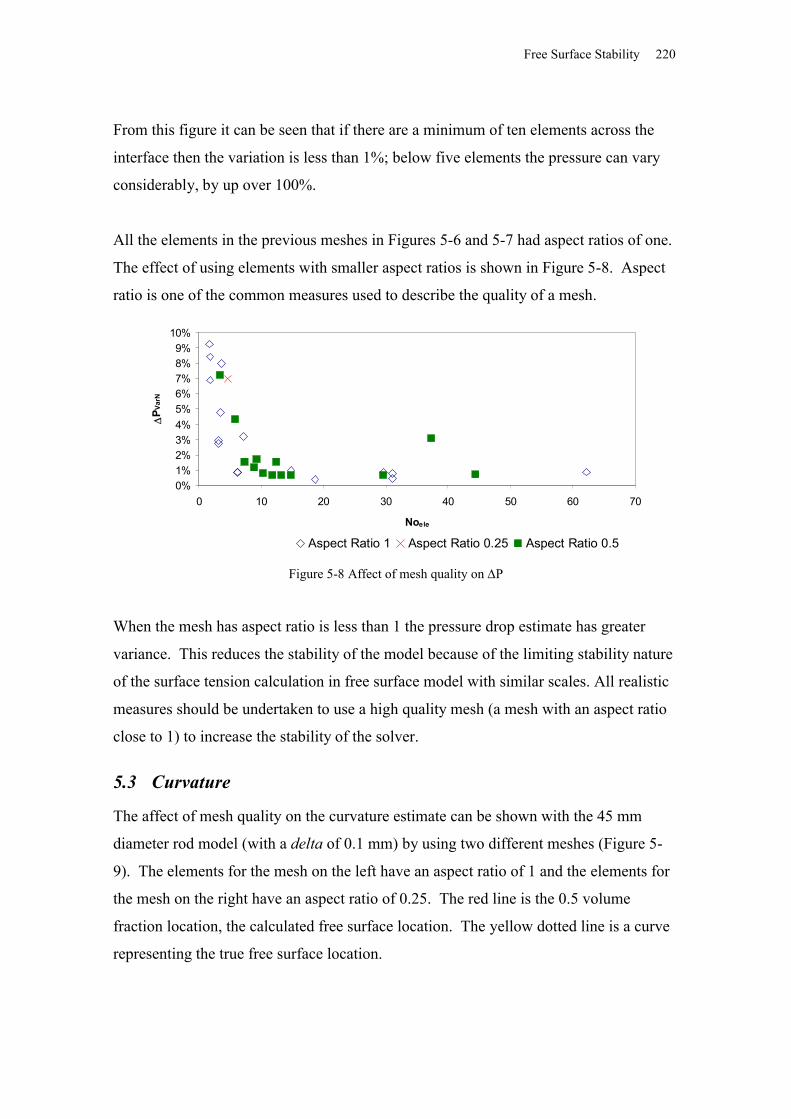
Free Surface Stability 220
From this figure it can be seen that if there are a minimum of ten elements across the
interface then the variation is less than 1%; below five elements the pressure can vary
considerably, by up over 100%.
All the elements in the previous meshes in Figures 5-6 and 5-7 had aspect ratios of one.
The effect of using elements with smaller aspect ratios is shown in Figure 5-8. Aspect
ratio is one of the common measures used to describe the quality of a mesh.
0%1%2%3%4%5%6%7%8%9%
10%
0 10 20 30 40 50 60 70
Noele
PV
arN
Aspect Ratio 1 Aspect Ratio 0.25 Aspect Ratio 0.5
Figure 5-8 Affect of mesh quality on P
When the mesh has aspect ratio is less than 1 the pressure drop estimate has greater
variance. This reduces the stability of the model because of the limiting stability nature
of the surface tension calculation in free surface model with similar scales. All realistic
measures should be undertaken to use a high quality mesh (a mesh with an aspect ratio
close to 1) to increase the stability of the solver.
5.3 Curvature
The affect of mesh quality on the curvature estimate can be shown with the 45 mm
diameter rod model (with a delta of 0.1 mm) by using two different meshes (Figure 5-
9). The elements for the mesh on the left have an aspect ratio of 1 and the elements for
the mesh on the right have an aspect ratio of 0.25. The red line is the 0.5 volume
fraction location, the calculated free surface location. The yellow dotted line is a curve
representing the true free surface location.
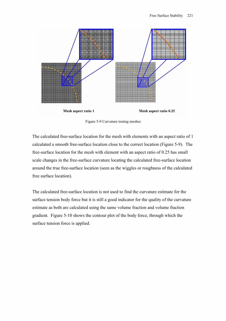
Free Surface Stability 221
Figure 5-9 Curvature testing meshes
The calculated free-surface location for the mesh with elements with an aspect ratio of 1
calculated a smooth free-surface location close to the correct location (Figure 5-9). The
free-surface location for the mesh with element with an aspect ratio of 0.25 has small
scale changes in the free-surface curvature locating the calculated free-surface location
around the true free-surface location (seen as the wiggles or roughness of the calculated
free surface location).
The calculated free-surface location is not used to find the curvature estimate for the
surface tension body force but it is still a good indicator for the quality of the curvature
estimate as both are calculated using the same volume fraction and volume fraction
gradient. Figure 5-10 shows the contour plot of the body force, through which the
surface tension force is applied.
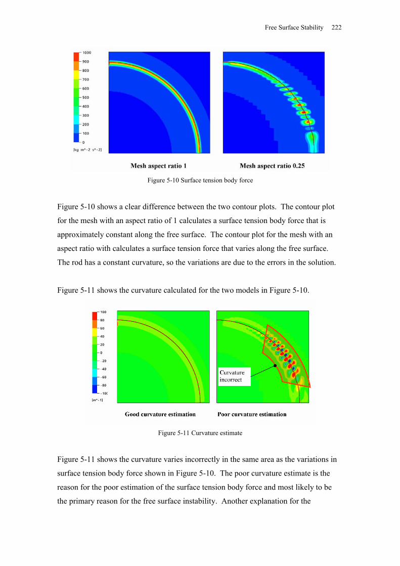
Free Surface Stability 222
Figure 5-10 Surface tension body force
Figure 5-10 shows a clear difference between the two contour plots. The contour plot
for the mesh with an aspect ratio of 1 calculates a surface tension body force that is
approximately constant along the free surface. The contour plot for the mesh with an
aspect ratio with calculates a surface tension force that varies along the free surface.
The rod has a constant curvature, so the variations are due to the errors in the solution.
Figure 5-11 shows the curvature calculated for the two models in Figure 5-10.
Figure 5-11 Curvature estimate
Figure 5-11 shows the curvature varies incorrectly in the same area as the variations in
surface tension body force shown in Figure 5-10. The poor curvature estimate is the
reason for the poor estimation of the surface tension body force and most likely to be
the primary reason for the free surface instability. Another explanation for the
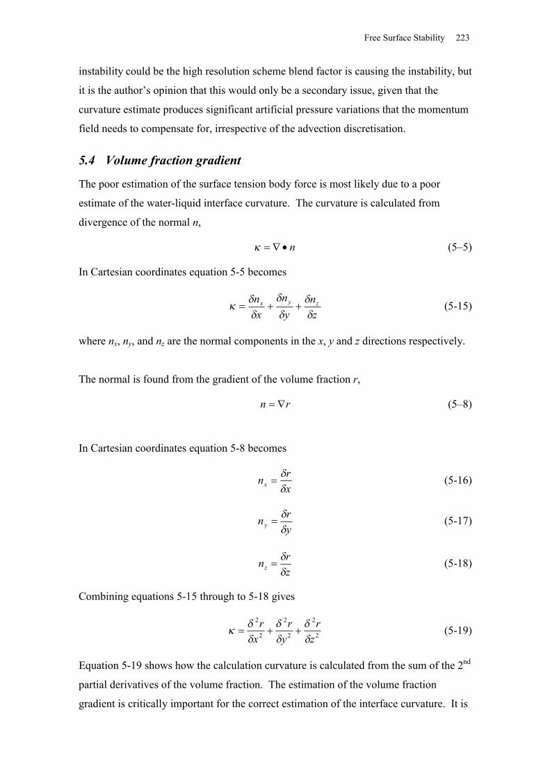
Free Surface Stability 223
instability could be the high resolution scheme blend factor is causing the instability, but
it is the author’s opinion that this would only be a secondary issue, given that the
curvature estimate produces significant artificial pressure variations that the momentum
field needs to compensate for, irrespective of the advection discretisation.
5.4 Volume fraction gradient
The poor estimation of the surface tension body force is most likely due to a poor
estimate of the water-liquid interface curvature. The curvature is calculated from
divergence of the normal n,
n (5–5)
In Cartesian coordinates equation 5-5 becomes
zn
yn
xn zyx
(5-15)
where nx, ny, and nz are the normal components in the x, y and z directions respectively.
The normal is found from the gradient of the volume fraction r,
rn (5–8)
In Cartesian coordinates equation 5-8 becomes
xrnx
(5-16)
yrn y
(5-17)
zrnz
(5-18)
Combining equations 5-15 through to 5-18 gives
2
2
2
2
2
2
zr
yr
xr
(5-19)
Equation 5-19 shows how the calculation curvature is calculated from the sum of the 2nd
partial derivatives of the volume fraction. The estimation of the volume fraction
gradient is critically important for the correct estimation of the interface curvature. It is
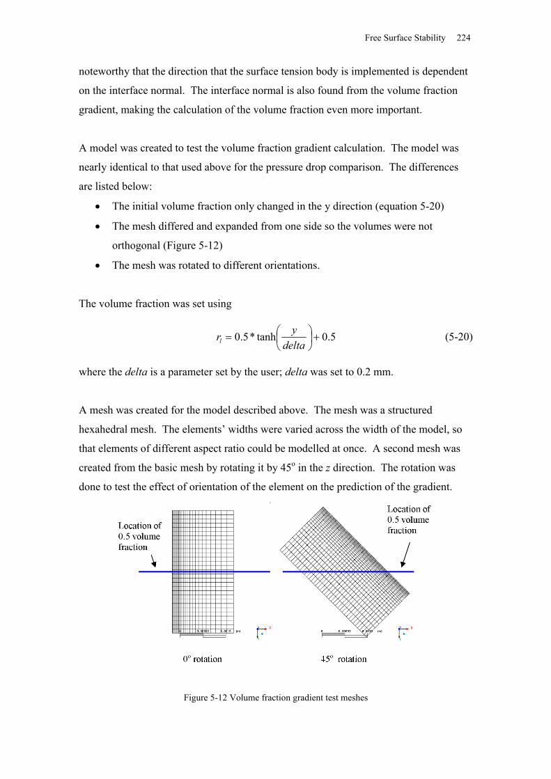
Free Surface Stability 224
noteworthy that the direction that the surface tension body is implemented is dependent
on the interface normal. The interface normal is also found from the volume fraction
gradient, making the calculation of the volume fraction even more important.
A model was created to test the volume fraction gradient calculation. The model was
nearly identical to that used above for the pressure drop comparison. The differences
are listed below:
The initial volume fraction only changed in the y direction (equation 5-20)
The mesh differed and expanded from one side so the volumes were not
orthogonal (Figure 5-12)
The mesh was rotated to different orientations.
The volume fraction was set using
5.0tanh*5.0
deltayrl (5-20)
where the delta is a parameter set by the user; delta was set to 0.2 mm.
A mesh was created for the model described above. The mesh was a structured
hexahedral mesh. The elements’ widths were varied across the width of the model, so
that elements of different aspect ratio could be modelled at once. A second mesh was
created from the basic mesh by rotating it by 45o in the z direction. The rotation was
done to test the effect of orientation of the element on the prediction of the gradient.
Figure 5-12 Volume fraction gradient test meshes
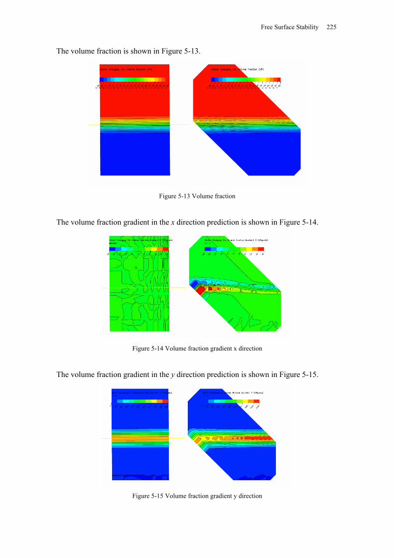
Free Surface Stability 225
The volume fraction is shown in Figure 5-13.
Figure 5-13 Volume fraction
The volume fraction gradient in the x direction prediction is shown in Figure 5-14.
Figure 5-14 Volume fraction gradient x direction
The volume fraction gradient in the y direction prediction is shown in Figure 5-15.
Figure 5-15 Volume fraction gradient y direction
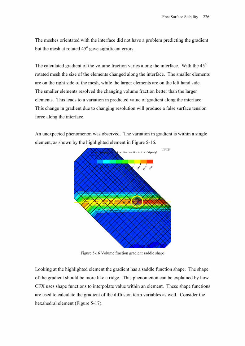
Free Surface Stability 226
The meshes orientated with the interface did not have a problem predicting the gradient
but the mesh at rotated 45o gave significant errors.
The calculated gradient of the volume fraction varies along the interface. With the 45o
rotated mesh the size of the elements changed along the interface. The smaller elements
are on the right side of the mesh, while the larger elements are on the left hand side.
The smaller elements resolved the changing volume fraction better than the larger
elements. This leads to a variation in predicted value of gradient along the interface.
This change in gradient due to changing resolution will produce a false surface tension
force along the interface.
An unexpected phenomenon was observed. The variation in gradient is within a single
element, as shown by the highlighted element in Figure 5-16.
Figure 5-16 Volume fraction gradient saddle shape
Looking at the highlighted element the gradient has a saddle function shape. The shape
of the gradient should be more like a ridge. This phenomenon can be explained by how
CFX uses shape functions to interpolate value within an element. These shape functions
are used to calculate the gradient of the diffusion term variables as well. Consider the
hexahedral element (Figure 5-17).
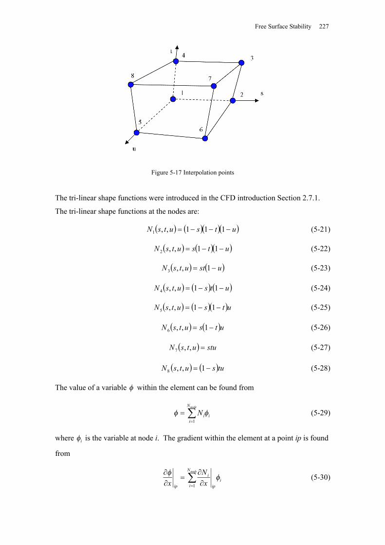
Free Surface Stability 227
Figure 5-17 Interpolation points
The tri-linear shape functions were introduced in the CFD introduction Section 2.7.1.
The tri-linear shape functions at the nodes are:
utsutsN 111,,1 (5-21)
utsutsN 11,,2 (5-22)
ustutsN 1,,3 (5-23)
utsutsN 11,,4 (5-24)
utsutsN 11,,5 (5-25)
utsutsN 1,,6 (5-26)
stuutsN ,,7 (5-27)
tusutsN 1,,8 (5-28)
The value of a variable within the element can be found from
nodeN
iiiN
1
(5-29)
where i is the variable at node i. The gradient within the element at a point ip is found
from
nodeN
ii
ip
i
ip xN
x 1
(5-30)
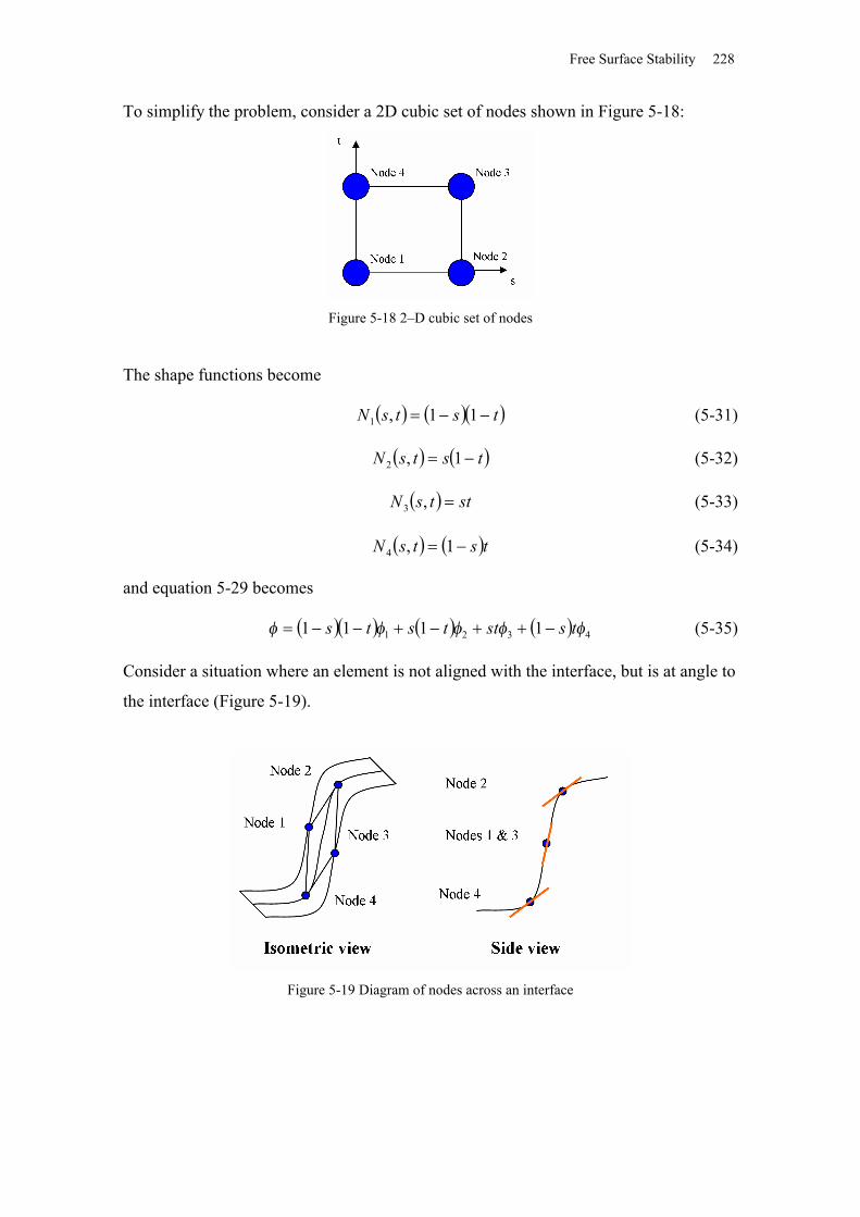
Free Surface Stability 228
To simplify the problem, consider a 2D cubic set of nodes shown in Figure 5-18:
Figure 5-18 2–D cubic set of nodes
The shape functions become
tstsN 11,1 (5-31)
tstsN 1,2 (5-32)
sttsN ,3 (5-33)
tstsN 1,4 (5-34)
and equation 5-29 becomes
4321 1111 tssttsts (5-35)
Consider a situation where an element is not aligned with the interface, but is at angle to
the interface (Figure 5-19).
Figure 5-19 Diagram of nodes across an interface
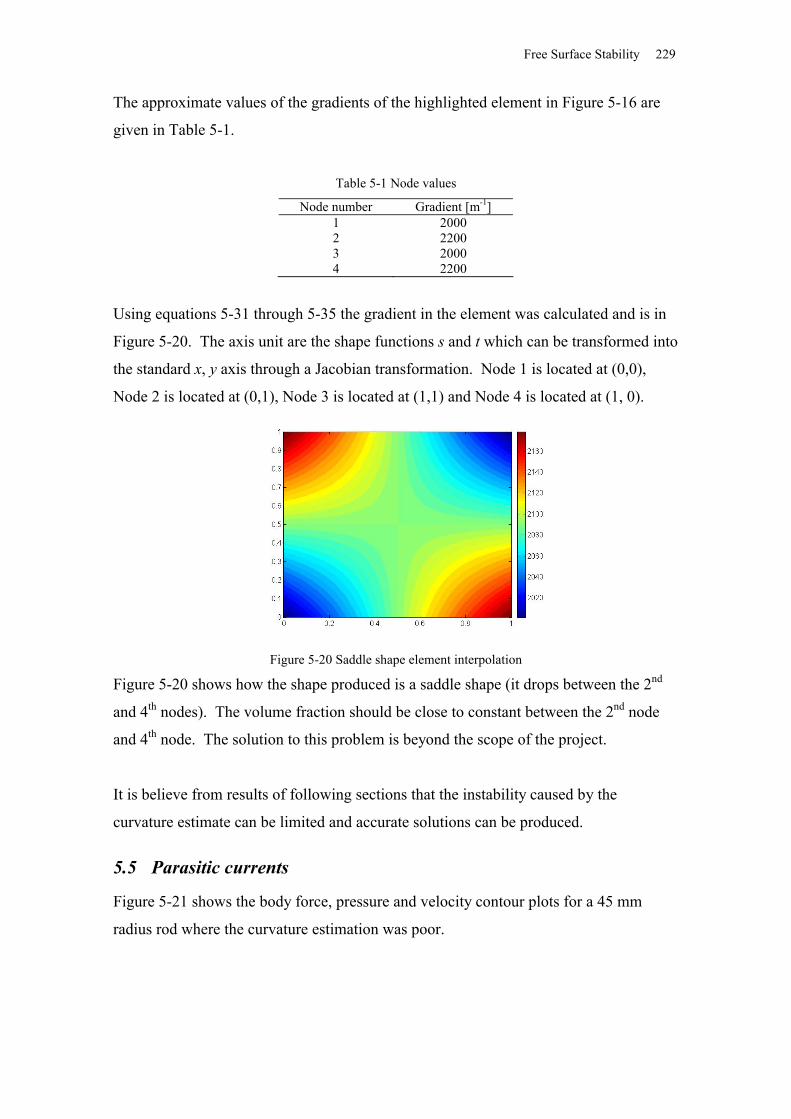
Free Surface Stability 229
The approximate values of the gradients of the highlighted element in Figure 5-16 are
given in Table 5-1.
Table 5-1 Node values
Node number Gradient [m-1]1 20002 22003 20004 2200
Using equations 5-31 through 5-35 the gradient in the element was calculated and is in
Figure 5-20. The axis unit are the shape functions s and t which can be transformed into
the standard x, y axis through a Jacobian transformation. Node 1 is located at (0,0),
Node 2 is located at (0,1), Node 3 is located at (1,1) and Node 4 is located at (1, 0).
Figure 5-20 Saddle shape element interpolation
Figure 5-20 shows how the shape produced is a saddle shape (it drops between the 2nd
and 4th nodes). The volume fraction should be close to constant between the 2nd node
and 4th node. The solution to this problem is beyond the scope of the project.
It is believe from results of following sections that the instability caused by the
curvature estimate can be limited and accurate solutions can be produced.
5.5 Parasitic currents
Figure 5-21 shows the body force, pressure and velocity contour plots for a 45 mm
radius rod where the curvature estimation was poor.
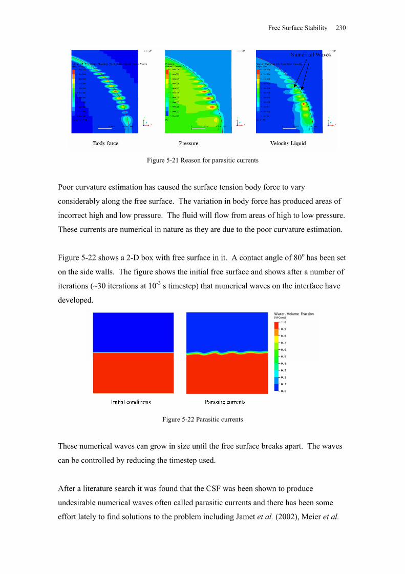
Free Surface Stability 230
Figure 5-21 Reason for parasitic currents
Poor curvature estimation has caused the surface tension body force to vary
considerably along the free surface. The variation in body force has produced areas of
incorrect high and low pressure. The fluid will flow from areas of high to low pressure.
These currents are numerical in nature as they are due to the poor curvature estimation.
Figure 5-22 shows a 2-D box with free surface in it. A contact angle of 80o has been set
on the side walls. The figure shows the initial free surface and shows after a number of
iterations (~30 iterations at 10-3 s timestep) that numerical waves on the interface have
developed.
Figure 5-22 Parasitic currents
These numerical waves can grow in size until the free surface breaks apart. The waves
can be controlled by reducing the timestep used.
After a literature search it was found that the CSF was been shown to produce
undesirable numerical waves often called parasitic currents and there has been some
effort lately to find solutions to the problem including Jamet et al. (2002), Meier et al.
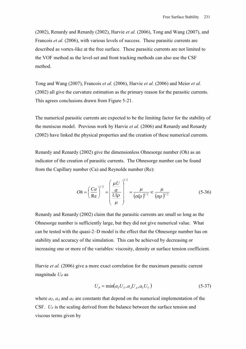
Free Surface Stability 231
(2002), Renardy and Renardy (2002), Harvie et al. (2006), Tong and Wang (2007), and
Francois et al. (2006), with various levels of success. These parasitic currents are
described as vortex-like at the free surface. These parasitic currents are not limited to
the VOF method as the level-set and front tracking methods can also use the CSF
method.
Tong and Wang (2007), Francois et al. (2006), Harvie et al. (2006) and Meier et al.
(2002) all give the curvature estimation as the primary reason for the parasitic currents.
This agrees conclusions drawn from Figure 5-21.
The numerical parasitic currents are expected to be the limiting factor for the stability of
the meniscus model. Previous work by Harvie et al. (2006) and Renardy and Renardy
(2002) have linked the physical properties and the creation of these numerical currents.
Renardy and Renardy (2002) give the dimensionless Ohnesorge number (Oh) as an
indicator of the creation of parasitic currents. The Ohnesorge number can be found
from the Capillary number (Ca) and Reynolds number (Re):
2/12/1
2/1
2/1
Re
lUl
UCaOh (5-36)
Renardy and Renardy (2002) claim that the parasitic currents are small so long as the
Ohnesorge number is sufficiently large, but they did not give numerical value. What
can be tested with the quasi-2–D model is the effect that the Ohnesorge number has on
stability and accuracy of the simulation. This can be achieved by decreasing or
increasing one or more of the variables: viscosity, density or surface tension coefficient.
Harvie et al. (2006) give a more exact correlation for the maximum parasitic current
magnitude UP as
VVAATTP UaUaUaU ,,min (5-37)
where aT, aA and aV are constants that depend on the numerical implementation of the
CSF. UV is the scaling derived from the balance between the surface tension and
viscous terms given by
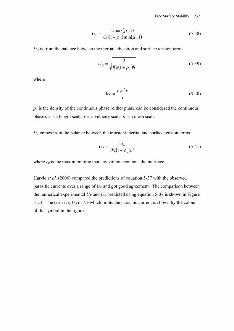
Free Surface Stability 232
1,min1
1,max2
vv
vV Ca
U
(5-38)
UA is from the balance between the inertial advection and surface tension terms,
hWeU
vA
12 (5-39)
where
xvWe l
2
(5-40)
c is the density of the continuous phase (either phase can be considered the continuous
phase), x is a length scale, v is a velocity scale, h is a mesh scale.
UT comes from the balance between the transient inertial and surface tension terms.
212
hWetU
v
mT
(5-41)
where tm is the maximum time that any volume contains the interface.
Harvie et al. (2006) compared the predictions of equation 5-37 with the observed
parasitic currents over a range of UP and got good agreement. The comparison between
the numerical experimental UP and UP predicted using equation 5-37 is shown in Figure
5-23. The term UT, UA or UV which limits the parasitic current is shown by the colour
of the symbol in the figure.
Free Surface Stability 233
Figure 5-23 Comparison between predicted UP and numeric UP (Harvie et al., 2006)
The range for terms used in Figure 5-23 above are given in Table 5-2.
Table 5-2 Range of UP comparison (Harvie et al., 2006)
Parameter RangeT 1 → 10H 1/8 → 1/256
We 10-6 →104
Ca 10-5 →104
l 10-4 →104
l 10-4 →104
The calculation of UP requires values for the three constants aT, aA and aV, which are
dependent on the numerical implementation used and for the VOF CSF method are
unknown. No attempt was made to calculate constants for the VOF CSF method as it
was unclear as to how Up was measured, since the parasitic currents did not seem to
have a constant velocity but could accelerated if the model diverged. The constants also
are related to mesh used and therefore would not be transferable.
Without the three constants aT, aA and aV, and because UP is calculated from a logic
function (minimum function) it is not possible to use the change in the UT, UA and UV
values to find the change in UP. Equations 5-42, 5-43 and 5-44 are true if the term in
question is the limiting value. If this is not the case these equations are not true.

Free Surface Stability 234
TP UU (5-42)
AP UU (5-43)
VP UU (5-44)
It is possible to look at the change in all three variables UV, UA, UT and infer the
possible effect on the parasitic currents.
Equations 5-42, 5-43 and 5-44 can be reduced by keeping the properties of the vapour
phase constant between the models to
lVU
(5-45)
hU
lA
(5-46)
2hU
lT
(5-47)
The effectiveness of these three relationships to predict the stability CSF VOF model
used by Ansys CFX 10 is tested later.
5.6 Meniscus model
A quasi 2D meniscus model of a surface tension driven multiphase flow was created to
test the performance of Ansys CFX in simulating a model dominated by surface tension
and contact angle.
The meniscus model has the advantage over more complicated models that it has a
known profile for the free surface. Since the meniscus model is relatively small, it
allows for a more complete investigation of the different solving parameters without
excessive computing time. The effect of physical properties was also investigated.
5.6.1 Meniscus introduction
An example of a meniscus can be seen when a small tube is partially filled with liquid.
The free surface of the liquid will curl upward or downwards depending on the contact
angle. The contact angle is dependent on the material of the three different phases (the
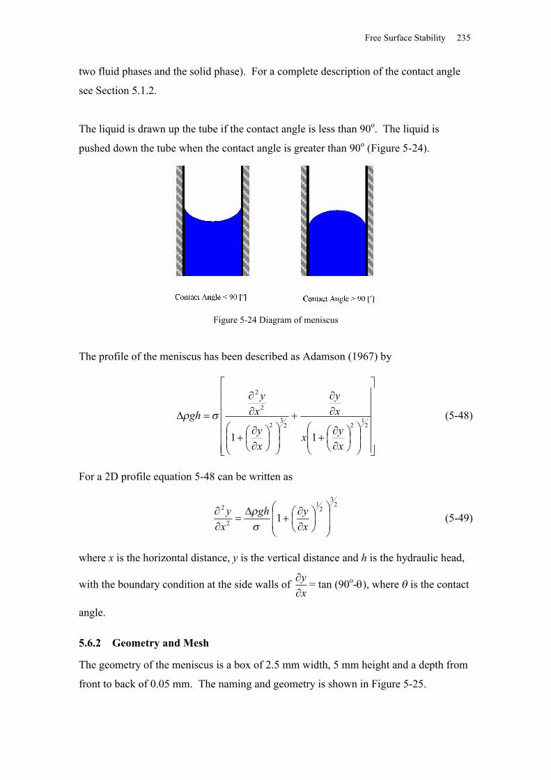
Free Surface Stability 235
two fluid phases and the solid phase). For a complete description of the contact angle
see Section 5.1.2.
The liquid is drawn up the tube if the contact angle is less than 90o. The liquid is
pushed down the tube when the contact angle is greater than 90o (Figure 5-24).
Figure 5-24 Diagram of meniscus
The profile of the meniscus has been described as Adamson (1967) by
2
122
32
2
2
11xyx
xy
xy
xy
gh (5-48)
For a 2D profile equation 5-48 can be written as
23
21
2
2
1
xygh
xy
(5-49)
where x is the horizontal distance, y is the vertical distance and h is the hydraulic head,
with the boundary condition at the side walls of xy
= tan (90o-), where is the contact
angle.
5.6.2 Geometry and Mesh
The geometry of the meniscus is a box of 2.5 mm width, 5 mm height and a depth from
front to back of 0.05 mm. The naming and geometry is shown in Figure 5-25.
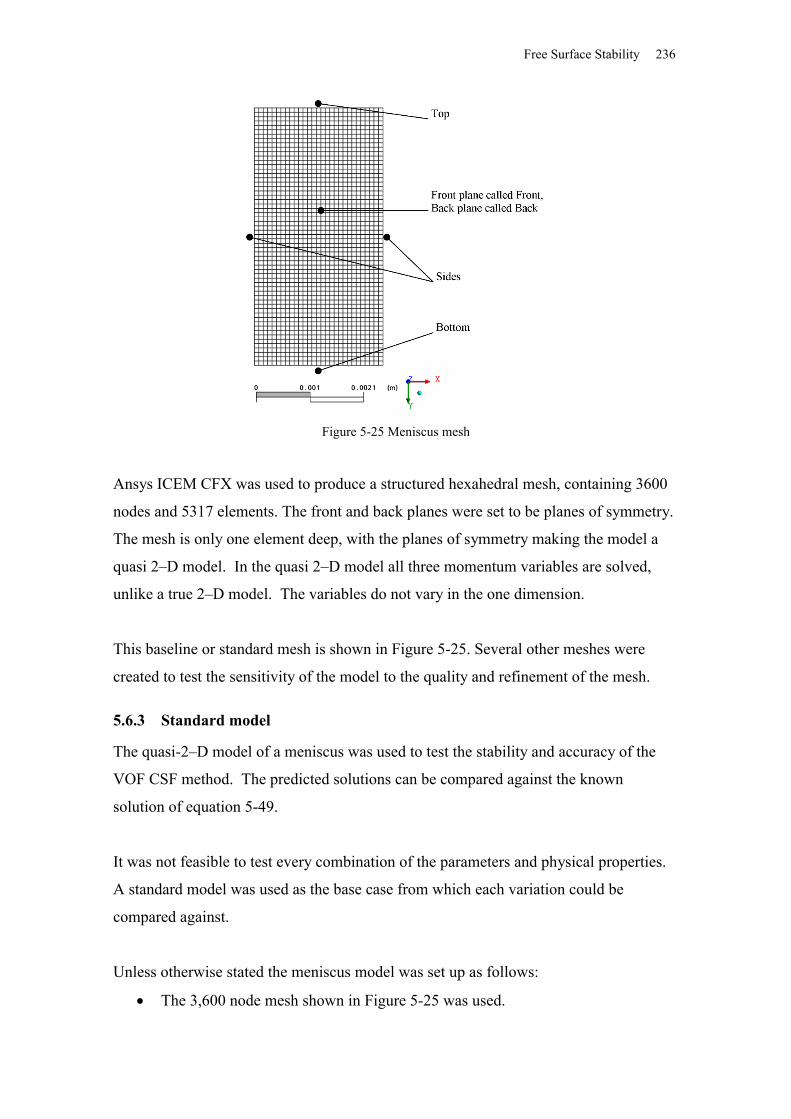
Free Surface Stability 236
Figure 5-25 Meniscus mesh
Ansys ICEM CFX was used to produce a structured hexahedral mesh, containing 3600
nodes and 5317 elements. The front and back planes were set to be planes of symmetry.
The mesh is only one element deep, with the planes of symmetry making the model a
quasi 2–D model. In the quasi 2–D model all three momentum variables are solved,
unlike a true 2–D model. The variables do not vary in the one dimension.
This baseline or standard mesh is shown in Figure 5-25. Several other meshes were
created to test the sensitivity of the model to the quality and refinement of the mesh.
5.6.3 Standard model
The quasi-2–D model of a meniscus was used to test the stability and accuracy of the
VOF CSF method. The predicted solutions can be compared against the known
solution of equation 5-49.
It was not feasible to test every combination of the parameters and physical properties.
A standard model was used as the base case from which each variation could be
compared against.
Unless otherwise stated the meniscus model was set up as follows:
The 3,600 node mesh shown in Figure 5-25 was used.
Free Surface Stability 237
The vapour phase was air at 25 oC.
The liquid phase was water with a viscosity of 10 mPa s.
The surface tension was set to 68 mN m-1.
Laplacian volume fraction smoothing and an under relaxation factor of 1 were
used.
No interface compression was used.
The timestep is different between the momentum equations and the volume
fraction equation (a split timestep). The momentum variables use an automatic
timestep selection and the volume fraction variables use a defined physical
timestep.
The boundary conditions were set to as follows:
The side walls were set to no-slip wall conditions with an 80o contact angle.
The top was defined as an opening with a static pressure of 1 atmosphere abs.,
with only vapour able to enter through the opening.
The bottom of the mesh was defined as free-slip wall with no adhesion.
The front and back were defined as planes of symmetry.
5.6.4 Variations to test sensitivity
The following CFX parameters were tested for their effect on stability and accuracy:
Timestep
Mesh
Interface compression
Volume fraction smoothing
Curvature under relaxation factor
The following physical properties of the model were tested for the effect on stability and
accuracy:
Viscosity
Surface tension
Contact angle
Density
Free Surface Stability 238
5.6.5 Criteria for model performance
Criteria for comparing the performance of the CFX were:
Model convergence and convergence rate.
Visual inspection of results.
Numerical comparison of 0.1, 0.5 and 0.9 volume fraction profile with the
theoretical meniscus profile equation 5-49.
ConvergenceThe first criterion relates to the numerical convergence of the model. The root mean
square of the individual maximum and root mean square residuals for three velocity
components, pressure and volume fraction. This was done to produce a single value
that describes the level of relative convergence compared to the other solutions.
The VOF method is known to have difficulty in converging the solution of free surface
flows. Ansys CFX (2005) gives the presence of small numerical waves at the free
surface as a possible reason for poor convergence. It is possible that a solution that is
not well converged will still predict the profile correctly.
Visual inspectionThe second criterion was the presence of a stable, tight interface. This was the most
subjective criterion. It was assessed by visual inspection of the results which were split
into three groups. Figure 5-26 contains examples.
Unstable solutions (X). The numerical waves are dominating the solution.
Stable loose solution (O). A solution where the model appears to have the
numerical waves under control, but the profile is either away from the correct
location or unlikely to be correct.
Tight solution (). A solution where the profile may be defined correctly and the
interface is sharp.
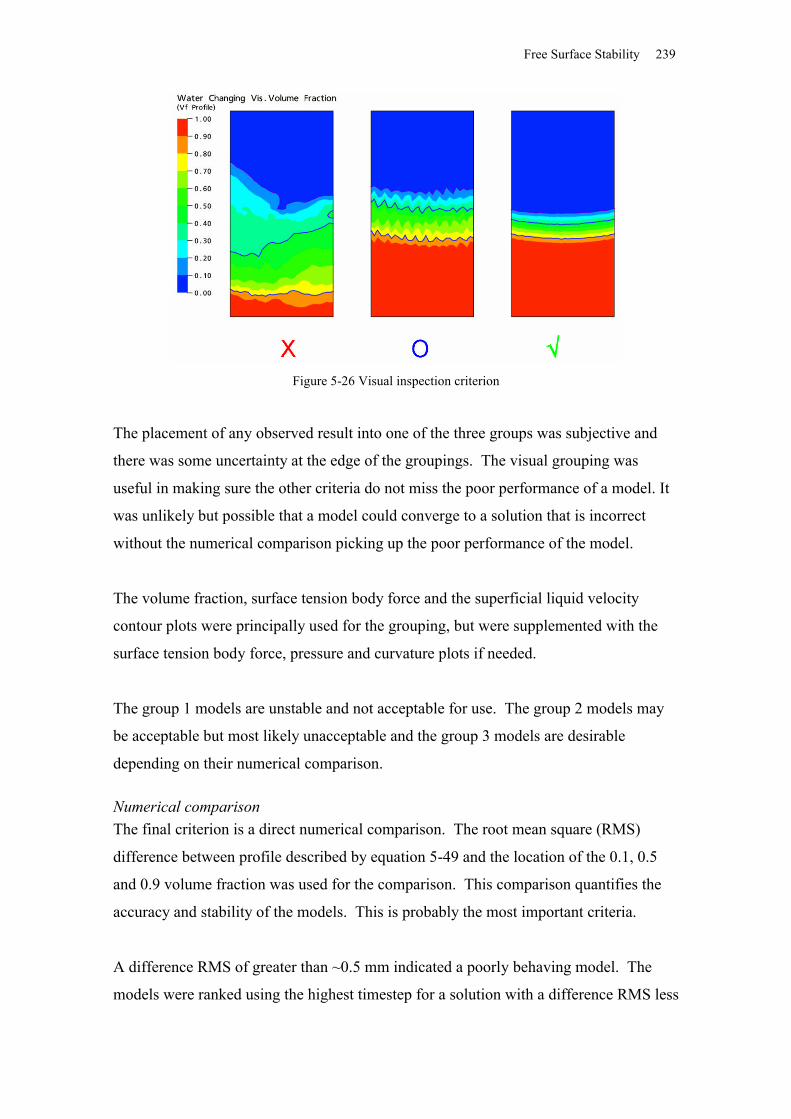
Free Surface Stability 239
Figure 5-26 Visual inspection criterion
The placement of any observed result into one of the three groups was subjective and
there was some uncertainty at the edge of the groupings. The visual grouping was
useful in making sure the other criteria do not miss the poor performance of a model. It
was unlikely but possible that a model could converge to a solution that is incorrect
without the numerical comparison picking up the poor performance of the model.
The volume fraction, surface tension body force and the superficial liquid velocity
contour plots were principally used for the grouping, but were supplemented with the
surface tension body force, pressure and curvature plots if needed.
The group 1 models are unstable and not acceptable for use. The group 2 models may
be acceptable but most likely unacceptable and the group 3 models are desirable
depending on their numerical comparison.
Numerical comparison The final criterion is a direct numerical comparison. The root mean square (RMS)
difference between profile described by equation 5-49 and the location of the 0.1, 0.5
and 0.9 volume fraction was used for the comparison. This comparison quantifies the
accuracy and stability of the models. This is probably the most important criteria.
A difference RMS of greater than ~0.5 mm indicated a poorly behaving model. The
models were ranked using the highest timestep for a solution with a difference RMS less
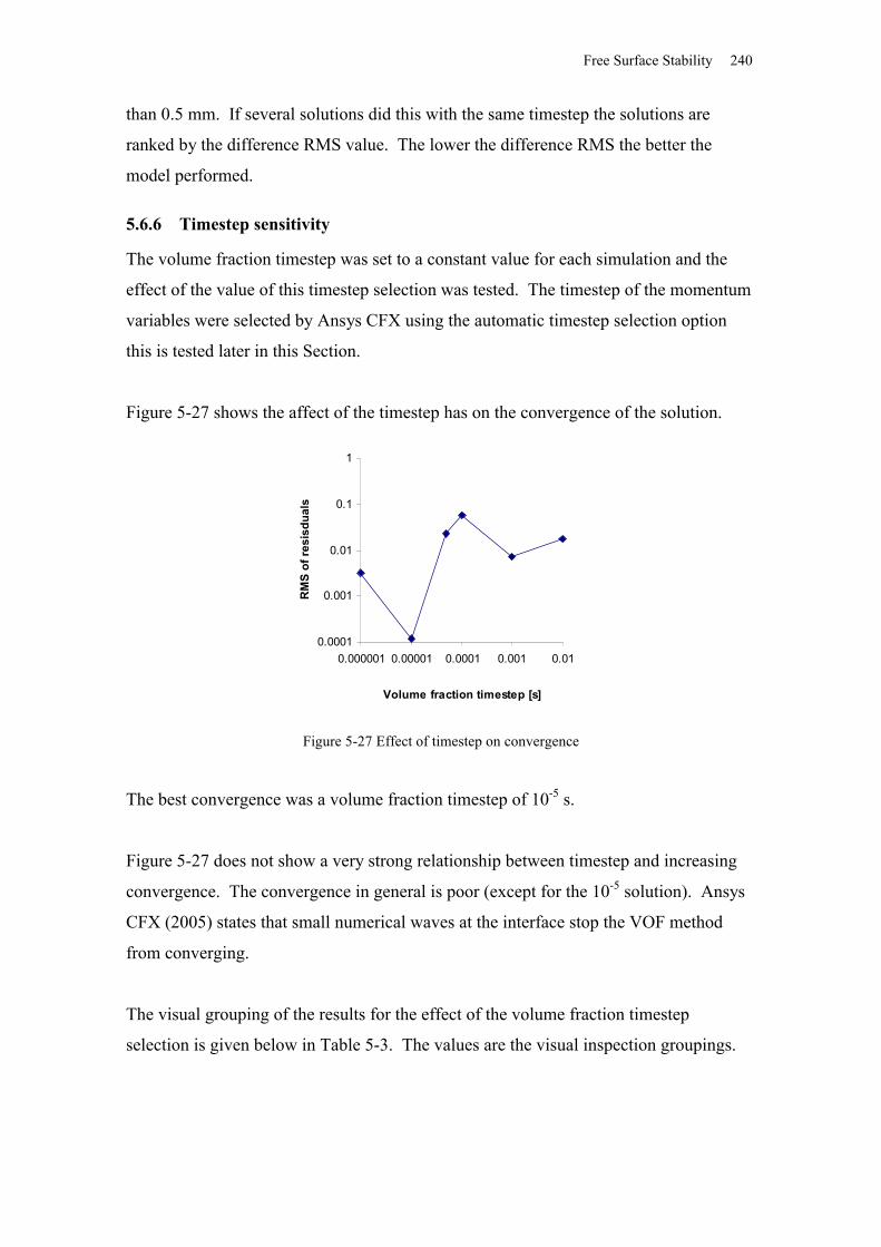
Free Surface Stability 240
than 0.5 mm. If several solutions did this with the same timestep the solutions are
ranked by the difference RMS value. The lower the difference RMS the better the
model performed.
5.6.6 Timestep sensitivity
The volume fraction timestep was set to a constant value for each simulation and the
effect of the value of this timestep selection was tested. The timestep of the momentum
variables were selected by Ansys CFX using the automatic timestep selection option
this is tested later in this Section.
Figure 5-27 shows the affect of the timestep has on the convergence of the solution.
0.0001
0.001
0.01
0.1
1
0.000001 0.00001 0.0001 0.001 0.01
Volume fraction timestep [s]
RM
S of
resi
sdua
ls
Figure 5-27 Effect of timestep on convergence
The best convergence was a volume fraction timestep of 10-5 s.
Figure 5-27 does not show a very strong relationship between timestep and increasing
convergence. The convergence in general is poor (except for the 10-5 solution). Ansys
CFX (2005) states that small numerical waves at the interface stop the VOF method
from converging.
The visual grouping of the results for the effect of the volume fraction timestep
selection is given below in Table 5-3. The values are the visual inspection groupings.
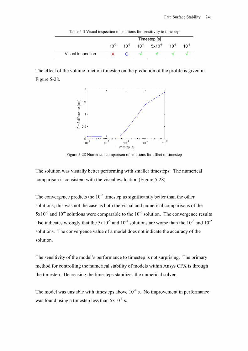
Free Surface Stability 241
Table 5-3 Visual inspection of solutions for sensitivity to timestep
Timestep [s]
10-2 10-3 10-4 5x10⁻⁵ 10-5 10-6
Visual inspection X O
The effect of the volume fraction timestep on the prediction of the profile is given in
Figure 5-28.
Figure 5-28 Numerical comparison of solutions for affect of timestep
The solution was visually better performing with smaller timesteps. The numerical
comparison is consistent with the visual evaluation (Figure 5-28).
The convergence predicts the 10-5 timestep as significantly better than the other
solutions; this was not the case as both the visual and numerical comparisons of the
5x10⁻⁵ and 10-6 solutions were comparable to the 10-5 solution. The convergence results
also indicates wrongly that the 5x10⁻⁵ and 10-4 solutions are worse than the 10-3 and 10-2
solutions. The convergence value of a model does not indicate the accuracy of the
solution.
The sensitivity of the model’s performance to timestep is not surprising. The primary
method for controlling the numerical stability of models within Ansys CFX is through
the timestep. Decreasing the timesteps stabilizes the numerical solver.
The model was unstable with timesteps above 10-4 s. No improvement in performance
was found using a timestep less than 5x10⁻⁵ s.
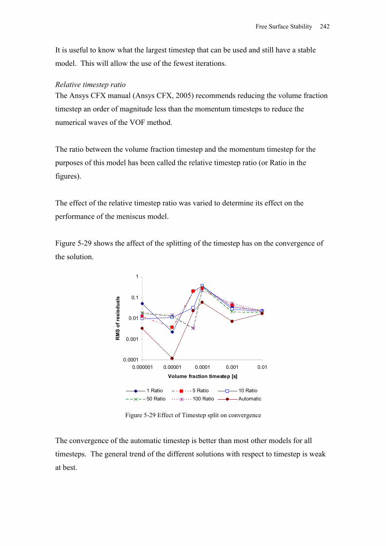
Free Surface Stability 242
It is useful to know what the largest timestep that can be used and still have a stable
model. This will allow the use of the fewest iterations.
Relative timestep ratioThe Ansys CFX manual (Ansys CFX, 2005) recommends reducing the volume fraction
timestep an order of magnitude less than the momentum timesteps to reduce the
numerical waves of the VOF method.
The ratio between the volume fraction timestep and the momentum timestep for the
purposes of this model has been called the relative timestep ratio (or Ratio in the
figures).
The effect of the relative timestep ratio was varied to determine its effect on the
performance of the meniscus model.
Figure 5-29 shows the affect of the splitting of the timestep has on the convergence of
the solution.
0.0001
0.001
0.01
0.1
1
0.000001 0.00001 0.0001 0.001 0.01
Volume fraction timestep [s]
RM
S of
resi
sdua
ls
1 Ratio 5 Ratio 10 Ratio50 Ratio 100 Ratio Automatic
Figure 5-29 Effect of Timestep split on convergence
The convergence of the automatic timestep is better than most other models for all
timesteps. The general trend of the different solutions with respect to timestep is weak
at best.
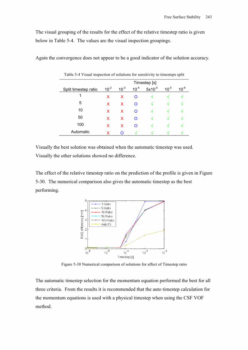
Free Surface Stability 243
The visual grouping of the results for the effect of the relative timestep ratio is given
below in Table 5-4. The values are the visual inspection groupings.
Again the convergence does not appear to be a good indicator of the solution accuracy.
Table 5-4 Visual inspection of solutions for sensitivity to timesteps split
Timestep [s]Split timestep ratio 10-2 10-3 10-4 5x10⁻⁵ 10-5 10-6
1 X X O 5 X X O 10 X X O 50 X X O 100 X X O
Automatic X O
Visually the best solution was obtained when the automatic timestep was used.
Visually the other solutions showed no difference.
The effect of the relative timestep ratio on the prediction of the profile is given in Figure
5-30. The numerical comparison also gives the automatic timestep as the best
performing.
Figure 5-30 Numerical comparison of solutions for affect of Timestep ratio
The automatic timestep selection for the momentum equation performed the best for all
three criteria. From the results it is recommended that the auto timestep calculation for
the momentum equations is used with a physical timestep when using the CSF VOF
method.
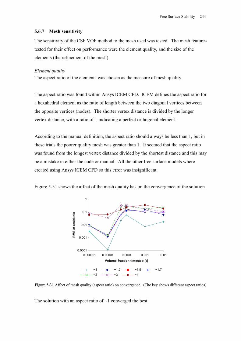
Free Surface Stability 244
5.6.7 Mesh sensitivity
The sensitivity of the CSF VOF method to the mesh used was tested. The mesh features
tested for their effect on performance were the element quality, and the size of the
elements (the refinement of the mesh).
Element qualityThe aspect ratio of the elements was chosen as the measure of mesh quality.
The aspect ratio was found within Ansys ICEM CFD. ICEM defines the aspect ratio for
a hexahedral element as the ratio of length between the two diagonal vertices between
the opposite vertices (nodes). The shorter vertex distance is divided by the longer
vertex distance, with a ratio of 1 indicating a perfect orthogonal element.
According to the manual definition, the aspect ratio should always be less than 1, but in
these trials the poorer quality mesh was greater than 1. It seemed that the aspect ratio
was found from the longest vertex distance divided by the shortest distance and this may
be a mistake in either the code or manual. All the other free surface models where
created using Ansys ICEM CFD so this error was insignificant.
Figure 5-31 shows the affect of the mesh quality has on the convergence of the solution.
0.0001
0.001
0.01
0.1
1
0.000001 0.00001 0.0001 0.001 0.01
Volume fraction timestep [s]
RM
S of
resi
dual
s
~1 ~1.2 ~1.5 ~1.7~2 ~3 ~4
Figure 5-31 Affect of mesh quality (aspect ratio) on convergence. (The key shows different aspect ratios)
The solution with an aspect ratio of ~1 converged the best.
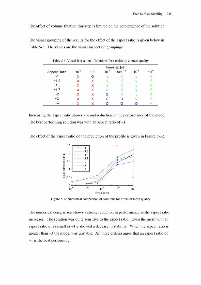
Free Surface Stability 245
The affect of volume fraction timestep is limited on the convergence of the solution.
The visual grouping of the results for the effect of the aspect ratio is given below in
Table 5-5. The values are the visual inspection groupings.
Table 5-5 Visual inspection of solutions for sensitivity to mesh quality
Timestep [s]Aspect Ratio 10-2 10-3 10-4 5x10⁻⁵ 10-5 10-6
~1 X O ~1.2 X X ~1.5 X X ~1.7 X X ~2 X X O ~3 X X O O ~4 X X O O O
Increasing the aspect ratio shows a visual reduction in the performance of the model.
The best performing solution was with an aspect ratio of ~1.
The effect of the aspect ratio on the prediction of the profile is given in Figure 5-32.
Figure 5-32 Numerical comparison of solutions for affect of mesh quality
The numerical comparison shows a strong reduction in performance as the aspect ratio
increases. The solution was quite sensitive to the aspect ratio. Even the mesh with an
aspect ratio of as small as ~1.2 showed a decease in stability. When the aspect ratio is
greater than ~3 the model was unstable. All three criteria agree that an aspect ratio of
~1 is the best performing.
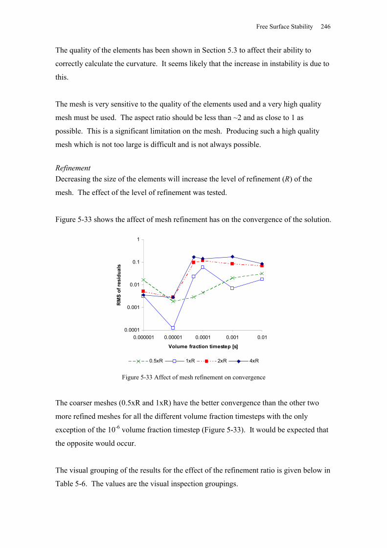
Free Surface Stability 246
The quality of the elements has been shown in Section 5.3 to affect their ability to
correctly calculate the curvature. It seems likely that the increase in instability is due to
this.
The mesh is very sensitive to the quality of the elements used and a very high quality
mesh must be used. The aspect ratio should be less than ~2 and as close to 1 as
possible. This is a significant limitation on the mesh. Producing such a high quality
mesh which is not too large is difficult and is not always possible.
RefinementDecreasing the size of the elements will increase the level of refinement (R) of the
mesh. The effect of the level of refinement was tested.
Figure 5-33 shows the affect of mesh refinement has on the convergence of the solution.
0.0001
0.001
0.01
0.1
1
0.000001 0.00001 0.0001 0.001 0.01
Volume fraction timestep [s]
RM
S of
resi
dual
s
0.5xR 1xR 2xR 4xR
Figure 5-33 Affect of mesh refinement on convergence
The coarser meshes (0.5xR and 1xR) have the better convergence than the other two
more refined meshes for all the different volume fraction timesteps with the only
exception of the 10-6 volume fraction timestep (Figure 5-33). It would be expected that
the opposite would occur.
The visual grouping of the results for the effect of the refinement ratio is given below in
Table 5-6. The values are the visual inspection groupings.
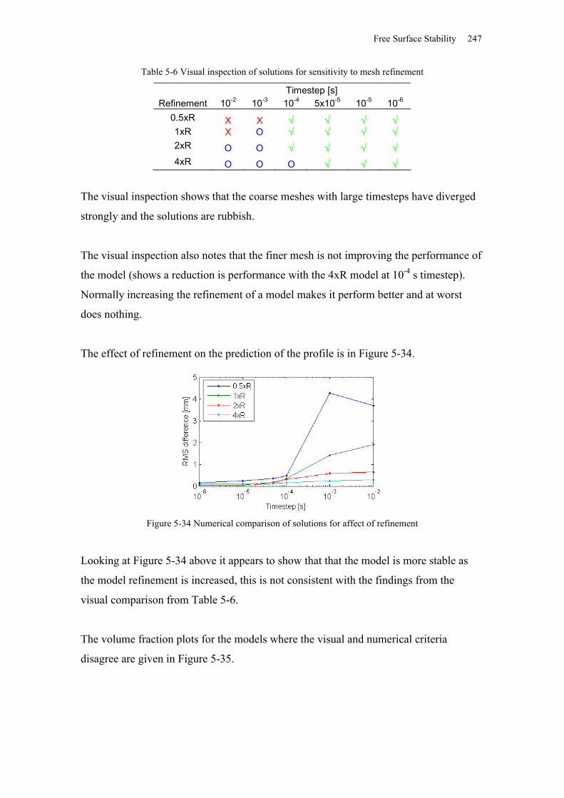
Free Surface Stability 247
Table 5-6 Visual inspection of solutions for sensitivity to mesh refinement
Timestep [s]Refinement 10-2 10-3 10-4 5x10⁻⁵ 10-5 10-6
0.5xR X X 1xR X O 2xR O O 4xR O O O
The visual inspection shows that the coarse meshes with large timesteps have diverged
strongly and the solutions are rubbish.
The visual inspection also notes that the finer mesh is not improving the performance of
the model (shows a reduction is performance with the 4xR model at 10-4 s timestep).
Normally increasing the refinement of a model makes it perform better and at worst
does nothing.
The effect of refinement on the prediction of the profile is in Figure 5-34.
Figure 5-34 Numerical comparison of solutions for affect of refinement
Looking at Figure 5-34 above it appears to show that that the model is more stable as
the model refinement is increased, this is not consistent with the findings from the
visual comparison from Table 5-6.
The volume fraction plots for the models where the visual and numerical criteria
disagree are given in Figure 5-35.
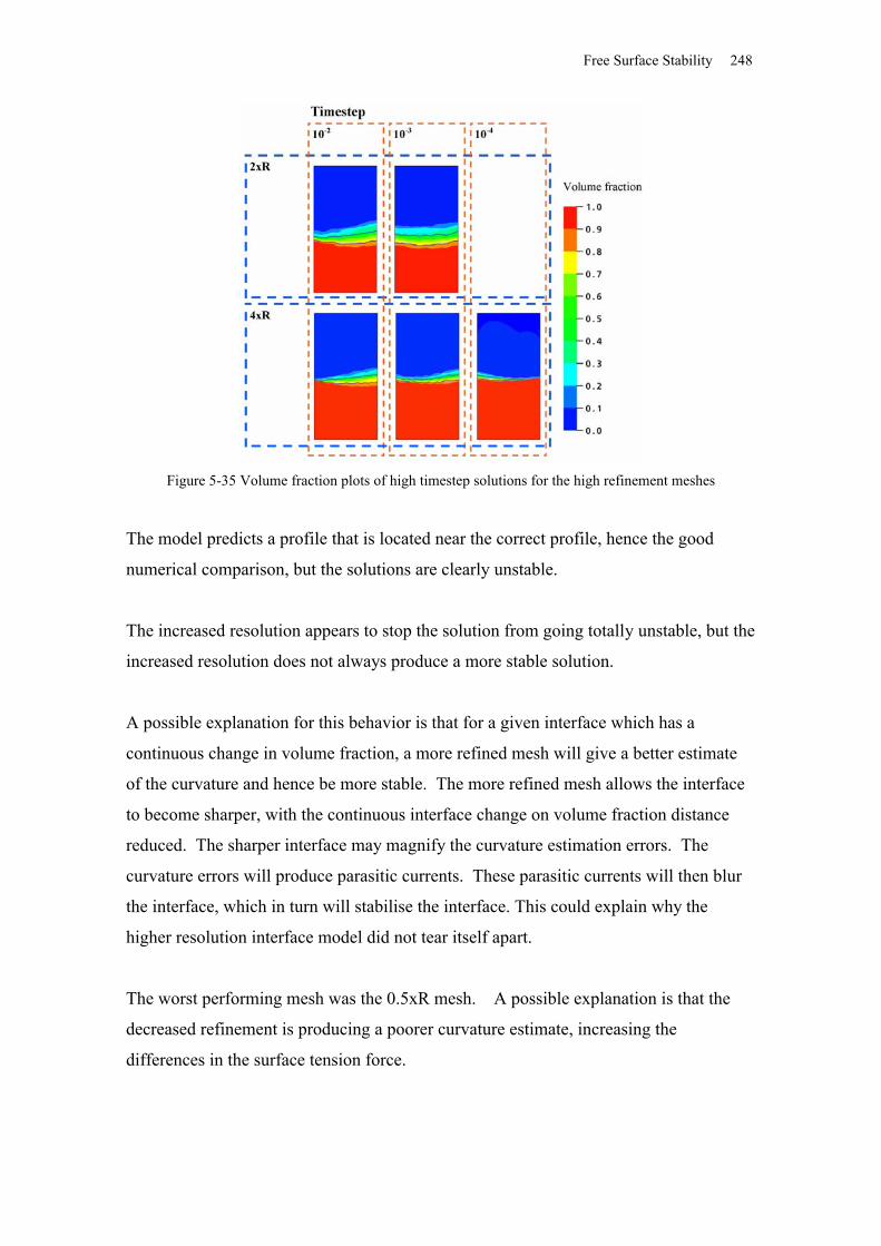
Free Surface Stability 248
Figure 5-35 Volume fraction plots of high timestep solutions for the high refinement meshes
The model predicts a profile that is located near the correct profile, hence the good
numerical comparison, but the solutions are clearly unstable.
The increased resolution appears to stop the solution from going totally unstable, but the
increased resolution does not always produce a more stable solution.
A possible explanation for this behavior is that for a given interface which has a
continuous change in volume fraction, a more refined mesh will give a better estimate
of the curvature and hence be more stable. The more refined mesh allows the interface
to become sharper, with the continuous interface change on volume fraction distance
reduced. The sharper interface may magnify the curvature estimation errors. The
curvature errors will produce parasitic currents. These parasitic currents will then blur
the interface, which in turn will stabilise the interface. This could explain why the
higher resolution interface model did not tear itself apart.
The worst performing mesh was the 0.5xR mesh. A possible explanation is that the
decreased refinement is producing a poorer curvature estimate, increasing the
differences in the surface tension force.
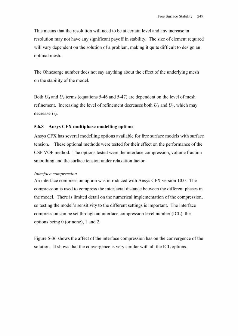
Free Surface Stability 249
This means that the resolution will need to be at certain level and any increase in
resolution may not have any significant payoff in stability. The size of element required
will vary dependent on the solution of a problem, making it quite difficult to design an
optimal mesh.
The Ohnesorge number does not say anything about the effect of the underlying mesh
on the stability of the model.
Both UA and UT terms (equations 5-46 and 5-47) are dependent on the level of mesh
refinement. Increasing the level of refinement decreases both UA and UT, which may
decrease UP.
5.6.8 Ansys CFX multiphase modelling options
Ansys CFX has several modelling options available for free surface models with surface
tension. These optional methods were tested for their effect on the performance of the
CSF VOF method. The options tested were the interface compression, volume fraction
smoothing and the surface tension under relaxation factor.
Interface compressionAn interface compression option was introduced with Ansys CFX version 10.0. The
compression is used to compress the interfacial distance between the different phases in
the model. There is limited detail on the numerical implementation of the compression,
so testing the model’s sensitivity to the different settings is important. The interface
compression can be set through an interface compression level number (ICL), the
options being 0 (or none), 1 and 2.
Figure 5-36 shows the affect of the interface compression has on the convergence of the
solution. It shows that the convergence is very similar with all the ICL options.
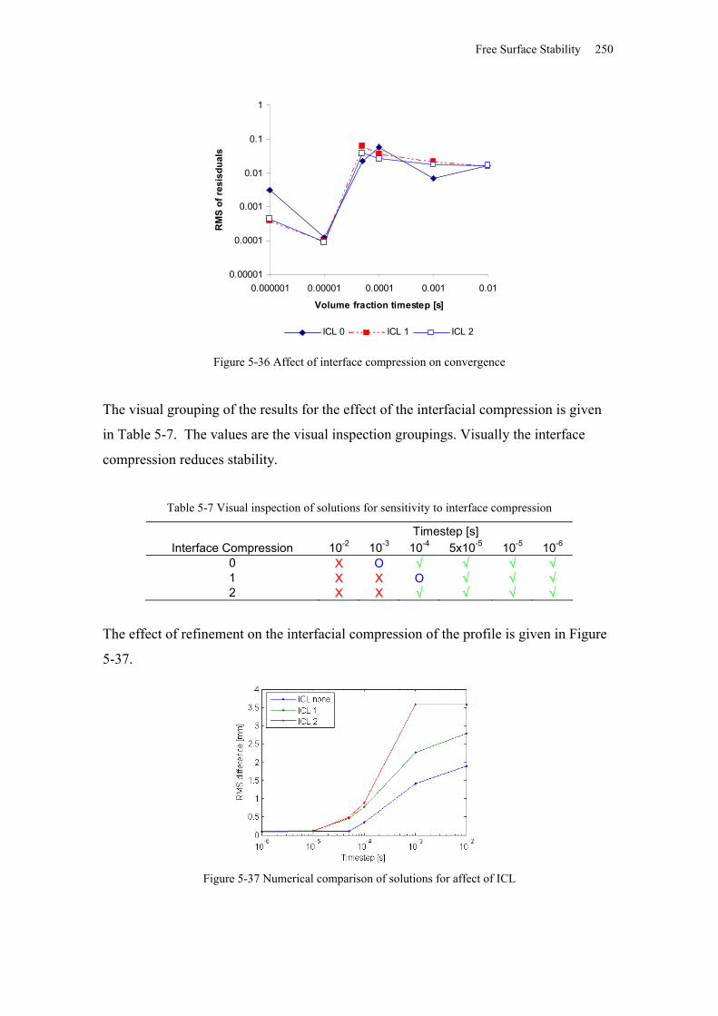
Free Surface Stability 250
0.00001
0.0001
0.001
0.01
0.1
1
0.000001 0.00001 0.0001 0.001 0.01
Volume fraction timestep [s]
RM
S of
resi
sdua
ls
ICL 0 ICL 1 ICL 2
Figure 5-36 Affect of interface compression on convergence
The visual grouping of the results for the effect of the interfacial compression is given
in Table 5-7. The values are the visual inspection groupings. Visually the interface
compression reduces stability.
Table 5-7 Visual inspection of solutions for sensitivity to interface compression
Timestep [s]Interface Compression 10-2 10-3 10-4 5x10⁻⁵ 10-5 10-6
0 X O 1 X X O 2 X X
The effect of refinement on the interfacial compression of the profile is given in Figure
5-37.
Figure 5-37 Numerical comparison of solutions for affect of ICL
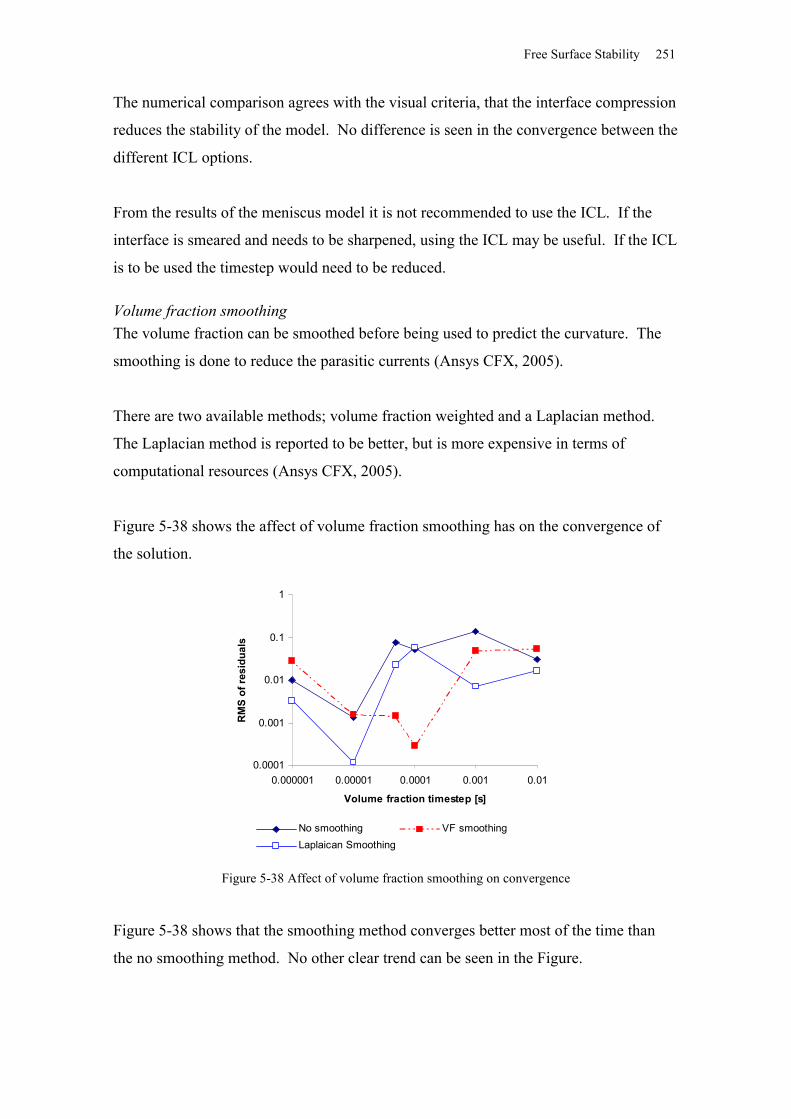
Free Surface Stability 251
The numerical comparison agrees with the visual criteria, that the interface compression
reduces the stability of the model. No difference is seen in the convergence between the
different ICL options.
From the results of the meniscus model it is not recommended to use the ICL. If the
interface is smeared and needs to be sharpened, using the ICL may be useful. If the ICL
is to be used the timestep would need to be reduced.
Volume fraction smoothingThe volume fraction can be smoothed before being used to predict the curvature. The
smoothing is done to reduce the parasitic currents (Ansys CFX, 2005).
There are two available methods; volume fraction weighted and a Laplacian method.
The Laplacian method is reported to be better, but is more expensive in terms of
computational resources (Ansys CFX, 2005).
Figure 5-38 shows the affect of volume fraction smoothing has on the convergence of
the solution.
0.0001
0.001
0.01
0.1
1
0.000001 0.00001 0.0001 0.001 0.01
Volume fraction timestep [s]
RM
S of
resi
dual
s
No smoothing VF smoothingLaplaican Smoothing
Figure 5-38 Affect of volume fraction smoothing on convergence
Figure 5-38 shows that the smoothing method converges better most of the time than
the no smoothing method. No other clear trend can be seen in the Figure.
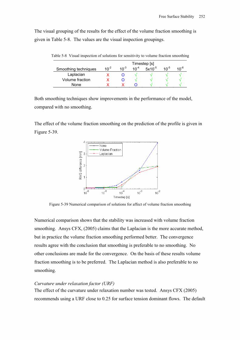
Free Surface Stability 252
The visual grouping of the results for the effect of the volume fraction smoothing is
given in Table 5-8. The values are the visual inspection groupings.
Table 5-8 Visual inspection of solutions for sensitivity to volume fraction smoothing
Timestep [s]Smoothing techniques 10-2 10-3 10-4 5x10⁻⁵ 10-5 10-6
Laplacian X O Volume fraction X O
None X X O
Both smoothing techniques show improvements in the performance of the model,
compared with no smoothing.
The effect of the volume fraction smoothing on the prediction of the profile is given in
Figure 5-39.
Figure 5-39 Numerical comparison of solutions for affect of volume fraction smoothing
Numerical comparison shows that the stability was increased with volume fraction
smoothing. Ansys CFX, (2005) claims that the Laplacian is the more accurate method,
but in practice the volume fraction smoothing performed better. The convergence
results agree with the conclusion that smoothing is preferable to no smoothing. No
other conclusions are made for the convergence. On the basis of these results volume
fraction smoothing is to be preferred. The Laplacian method is also preferable to no
smoothing.
Curvature under relaxation factor (URF)The effect of the curvature under relaxation number was tested. Ansys CFX (2005)
recommends using a URF close to 0.25 for surface tension dominant flows. The default
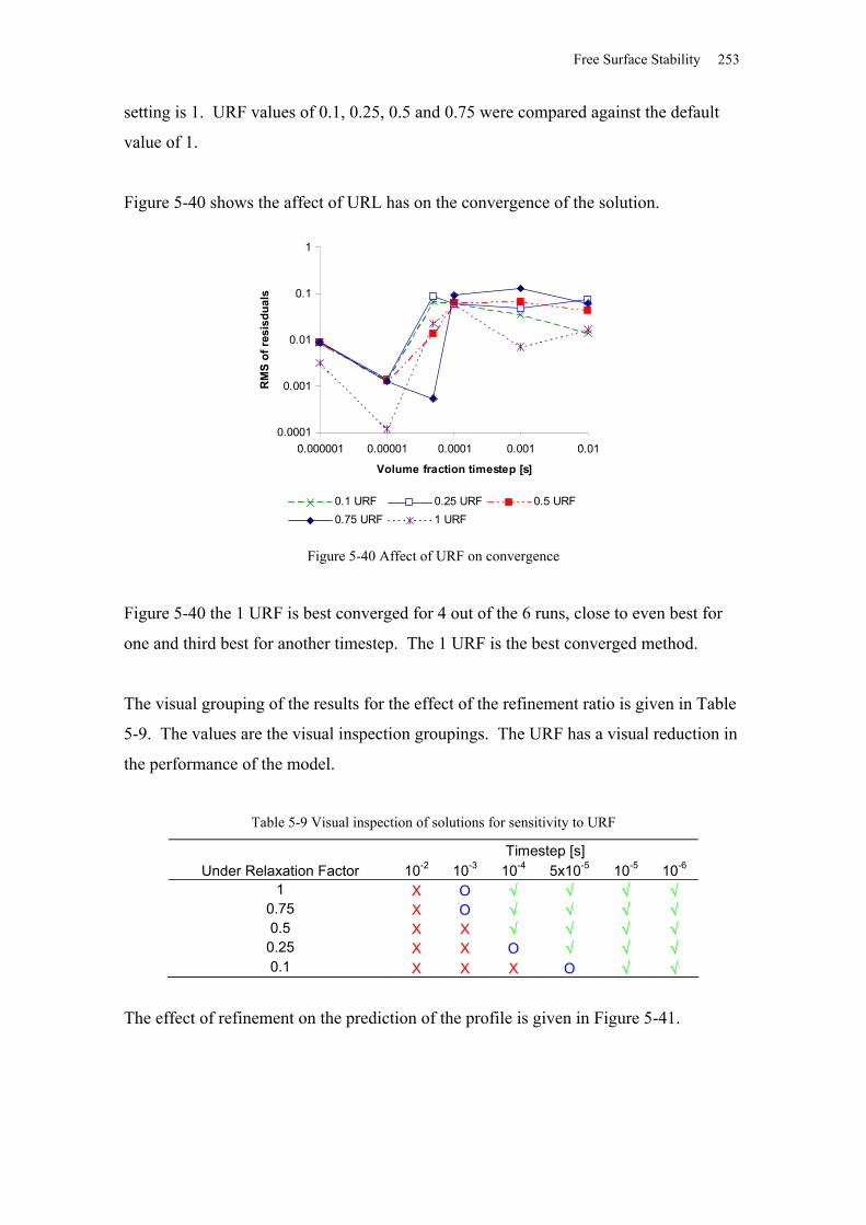
Free Surface Stability 253
setting is 1. URF values of 0.1, 0.25, 0.5 and 0.75 were compared against the default
value of 1.
Figure 5-40 shows the affect of URL has on the convergence of the solution.
0.0001
0.001
0.01
0.1
1
0.000001 0.00001 0.0001 0.001 0.01
Volume fraction timestep [s]
RM
S of
resi
sdua
ls
0.1 URF 0.25 URF 0.5 URF0.75 URF 1 URF
Figure 5-40 Affect of URF on convergence
Figure 5-40 the 1 URF is best converged for 4 out of the 6 runs, close to even best for
one and third best for another timestep. The 1 URF is the best converged method.
The visual grouping of the results for the effect of the refinement ratio is given in Table
5-9. The values are the visual inspection groupings. The URF has a visual reduction in
the performance of the model.
Table 5-9 Visual inspection of solutions for sensitivity to URF
Timestep [s]Under Relaxation Factor 10-2 10-3 10-4 5x10⁻⁵ 10-5 10-6
1 X O 0.75 X O 0.5 X X 0.25 X X O 0.1 X X X O
The effect of refinement on the prediction of the profile is given in Figure 5-41.
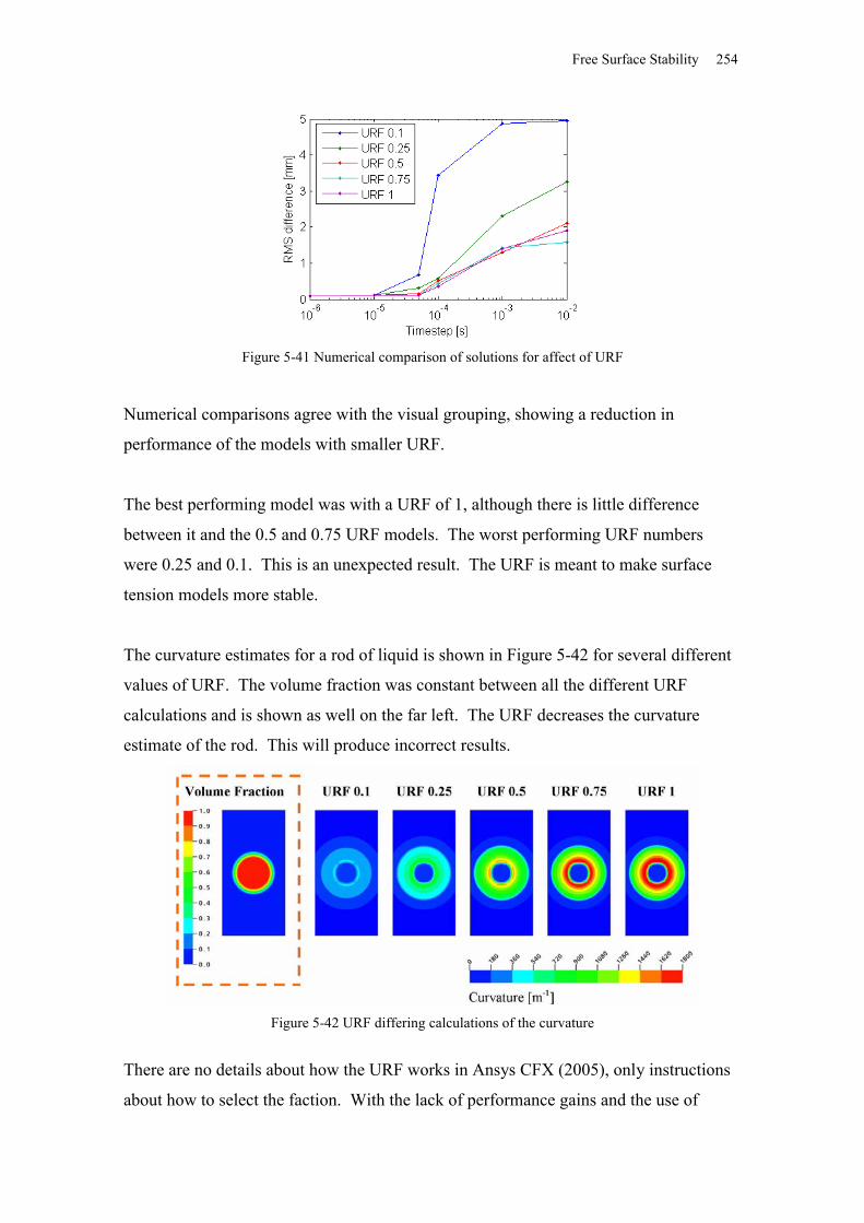
Free Surface Stability 254
Figure 5-41 Numerical comparison of solutions for affect of URF
Numerical comparisons agree with the visual grouping, showing a reduction in
performance of the models with smaller URF.
The best performing model was with a URF of 1, although there is little difference
between it and the 0.5 and 0.75 URF models. The worst performing URF numbers
were 0.25 and 0.1. This is an unexpected result. The URF is meant to make surface
tension models more stable.
The curvature estimates for a rod of liquid is shown in Figure 5-42 for several different
values of URF. The volume fraction was constant between all the different URF
calculations and is shown as well on the far left. The URF decreases the curvature
estimate of the rod. This will produce incorrect results.
Figure 5-42 URF differing calculations of the curvature
There are no details about how the URF works in Ansys CFX (2005), only instructions
about how to select the faction. With the lack of performance gains and the use of
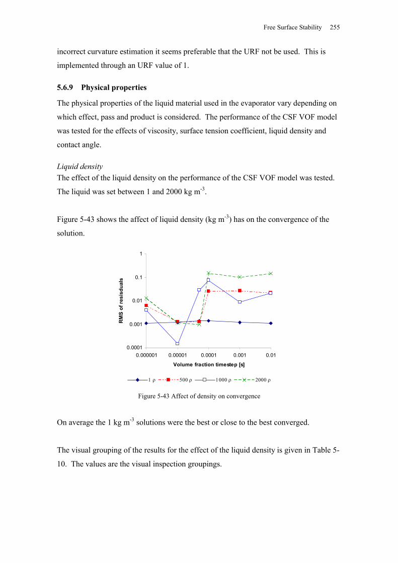
Free Surface Stability 255
incorrect curvature estimation it seems preferable that the URF not be used. This is
implemented through an URF value of 1.
5.6.9 Physical properties
The physical properties of the liquid material used in the evaporator vary depending on
which effect, pass and product is considered. The performance of the CSF VOF model
was tested for the effects of viscosity, surface tension coefficient, liquid density and
contact angle.
Liquid densityThe effect of the liquid density on the performance of the CSF VOF model was tested.
The liquid was set between 1 and 2000 kg m-3.
Figure 5-43 shows the affect of liquid density (kg m-3) has on the convergence of the
solution.
0.0001
0.001
0.01
0.1
1
0.000001 0.00001 0.0001 0.001 0.01
Volume fraction timestep [s]
RM
S of
resi
sdua
ls
Figure 5-43 Affect of density on convergence
On average the 1 kg m-3 solutions were the best or close to the best converged.
The visual grouping of the results for the effect of the liquid density is given in Table 5-
10. The values are the visual inspection groupings.
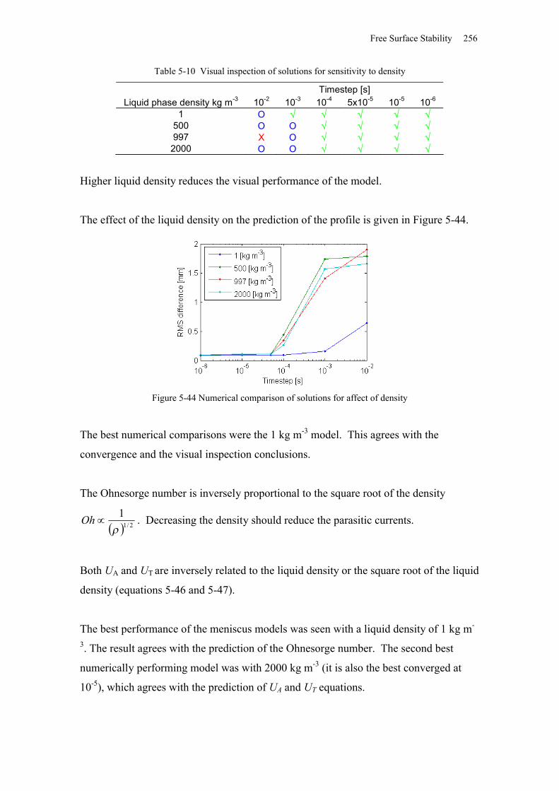
Free Surface Stability 256
Table 5-10 Visual inspection of solutions for sensitivity to density
Timestep [s]Liquid phase density kg m-3 10-2 10-3 10-4 5x10⁻⁵ 10-5 10-6
1 O 500 O O 997 X O 2000 O O
Higher liquid density reduces the visual performance of the model.
The effect of the liquid density on the prediction of the profile is given in Figure 5-44.
Figure 5-44 Numerical comparison of solutions for affect of density
The best numerical comparisons were the 1 kg m-3 model. This agrees with the
convergence and the visual inspection conclusions.
The Ohnesorge number is inversely proportional to the square root of the density
2/11
Oh . Decreasing the density should reduce the parasitic currents.
Both UA and UT are inversely related to the liquid density or the square root of the liquid
density (equations 5-46 and 5-47).
The best performance of the meniscus models was seen with a liquid density of 1 kg m-
3. The result agrees with the prediction of the Ohnesorge number. The second best
numerically performing model was with 2000 kg m-3 (it is also the best converged at
10-5), which agrees with the prediction of UA and UT equations.
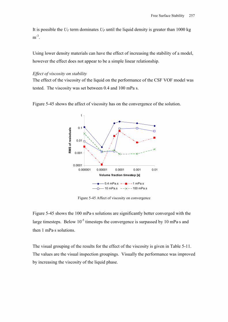
Free Surface Stability 257
It is possible the UV term dominates UP until the liquid density is greater than 1000 kg
m-3.
Using lower density materials can have the effect of increasing the stability of a model,
however the effect does not appear to be a simple linear relationship.
Effect of viscosity on stabilityThe effect of the viscosity of the liquid on the performance of the CSF VOF model was
tested. The viscosity was set between 0.4 and 100 mPa s.
Figure 5-45 shows the affect of viscosity has on the convergence of the solution.
0.0001
0.001
0.01
0.1
1
0.000001 0.00001 0.0001 0.001 0.01
Volume fraction timestep [s]
RM
S of
resi
sdua
ls
0.4 mPa.s 1 mPa.s10 mPa.s 100 mPa.s
Figure 5-45 Affect of viscosity on convergence
Figure 5-45 shows the 100 mPas solutions are significantly better converged with the
large timesteps. Below 10-5 timesteps the convergence is surpassed by 10 mPas and
then 1 mPas solutions.
The visual grouping of the results for the effect of the viscosity is given in Table 5-11.
The values are the visual inspection groupings. Visually the performance was improved
by increasing the viscosity of the liquid phase.
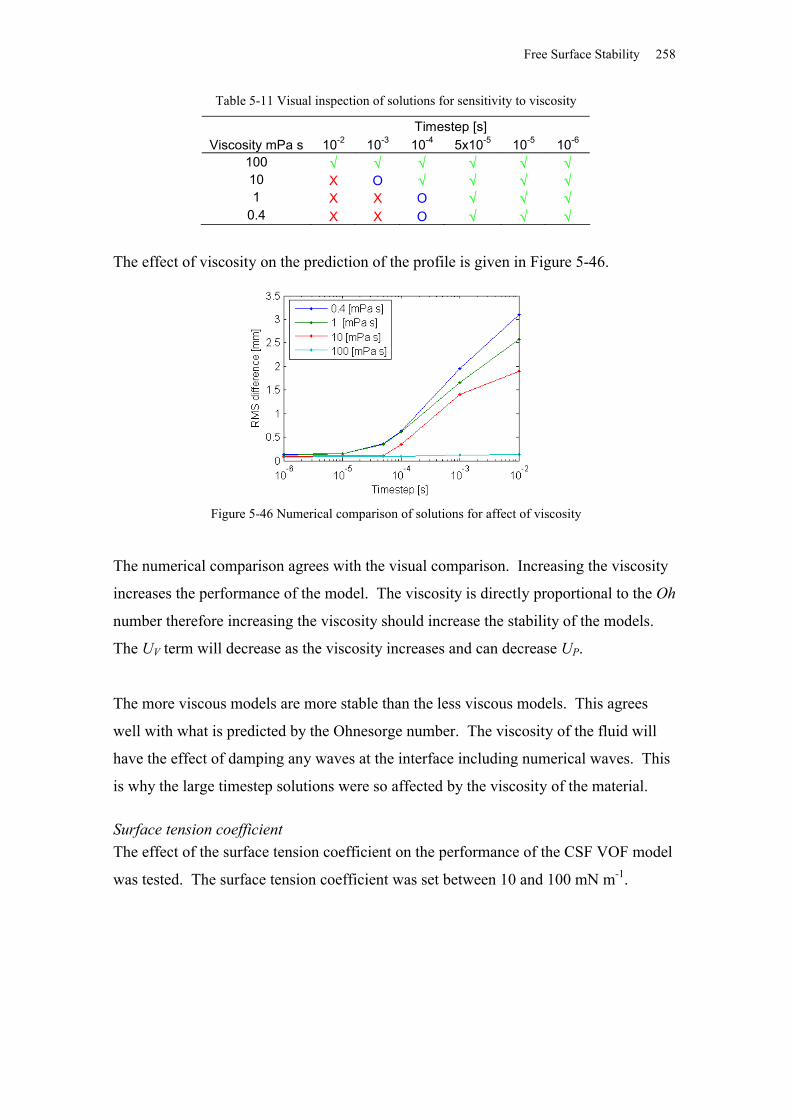
Free Surface Stability 258
Table 5-11 Visual inspection of solutions for sensitivity to viscosity
Timestep [s]Viscosity mPa s 10-2 10-3 10-4 5x10⁻⁵ 10-5 10-6
100 10 X O 1 X X O
0.4 X X O
The effect of viscosity on the prediction of the profile is given in Figure 5-46.
Figure 5-46 Numerical comparison of solutions for affect of viscosity
The numerical comparison agrees with the visual comparison. Increasing the viscosity
increases the performance of the model. The viscosity is directly proportional to the Oh
number therefore increasing the viscosity should increase the stability of the models.
The UV term will decrease as the viscosity increases and can decrease UP.
The more viscous models are more stable than the less viscous models. This agrees
well with what is predicted by the Ohnesorge number. The viscosity of the fluid will
have the effect of damping any waves at the interface including numerical waves. This
is why the large timestep solutions were so affected by the viscosity of the material.
Surface tension coefficientThe effect of the surface tension coefficient on the performance of the CSF VOF model
was tested. The surface tension coefficient was set between 10 and 100 mN m-1.
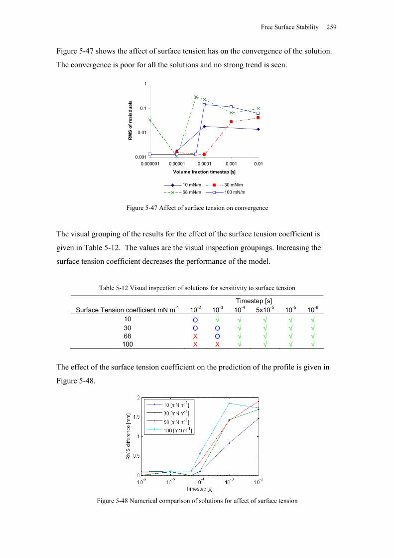
Free Surface Stability 259
Figure 5-47 shows the affect of surface tension has on the convergence of the solution.
The convergence is poor for all the solutions and no strong trend is seen.
0.001
0.01
0.1
1
0.000001 0.00001 0.0001 0.001 0.01
Volume fraction timestep [s]
RM
S of
resi
sdua
ls
10 mN/m 30 mN/m68 mN/m 100 mN/m
Figure 5-47 Affect of surface tension on convergence
The visual grouping of the results for the effect of the surface tension coefficient is
given in Table 5-12. The values are the visual inspection groupings. Increasing the
surface tension coefficient decreases the performance of the model.
Table 5-12 Visual inspection of solutions for sensitivity to surface tension
Timestep [s]Surface Tension coefficient mN m-1 10-2 10-3 10-4 5x10⁻⁵ 10-5 10-6
10 O 30 O O 68 X O 100 X X
The effect of the surface tension coefficient on the prediction of the profile is given in
Figure 5-48.
Figure 5-48 Numerical comparison of solutions for affect of surface tension
Free Surface Stability 260
The numerical comparison agrees with the visual comparison, that increasing the
surface tension coefficient decreases the performance. The surface tension coefficient
has a strong effect on the stability of the meniscus model. The models with larger
surface tension coefficients are less stable. This is in line with the work by Renardy and
Renardy (2002), since increasing the surface tension coefficient will decrease the
Ohnesorge number as 2/1
1
Oh , thus the model stability should decrease.
All three terms in equation 5-37 are related to the surface tension coefficient.
Decreasing the surface coefficient will reduce UP. The meniscus model gave the same
results.
Reducing the surface tension coefficient will reduce the surface tension force. This will
decrease the effect of errors in the curvature estimate by reducing the forces they
generate.
Contact angleAlthough the contact angle is not used to calculate the Oh number, from the work of
Harvie et al. (2006), it seems likely to have some effect on the stability of the model,
due its close relationship with the free surface location and surface tension. It is likely
that the extreme contact angle close to 0o and 180o should be the least stable.
The effect of the contact angle on the performance of the CSF VOF model was tested.
The contact angle was set between 20o and 120o.
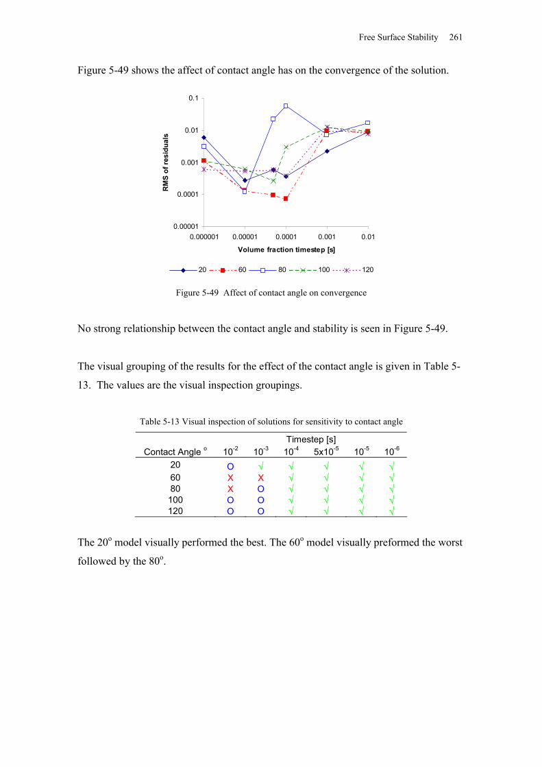
Free Surface Stability 261
Figure 5-49 shows the affect of contact angle has on the convergence of the solution.
0.00001
0.0001
0.001
0.01
0.1
0.000001 0.00001 0.0001 0.001 0.01
Volume fraction timestep [s]
RM
S of
resi
dual
s
20 60 80 100 120
Figure 5-49 Affect of contact angle on convergence
No strong relationship between the contact angle and stability is seen in Figure 5-49.
The visual grouping of the results for the effect of the contact angle is given in Table 5-
13. The values are the visual inspection groupings.
Table 5-13 Visual inspection of solutions for sensitivity to contact angle
Timestep [s]Contact Angle o 10-2 10-3 10-4 5x10⁻⁵ 10-5 10-6
20 O 60 X X 80 X O 100 O O 120 O O
The 20o model visually performed the best. The 60o model visually preformed the worst
followed by the 80o.
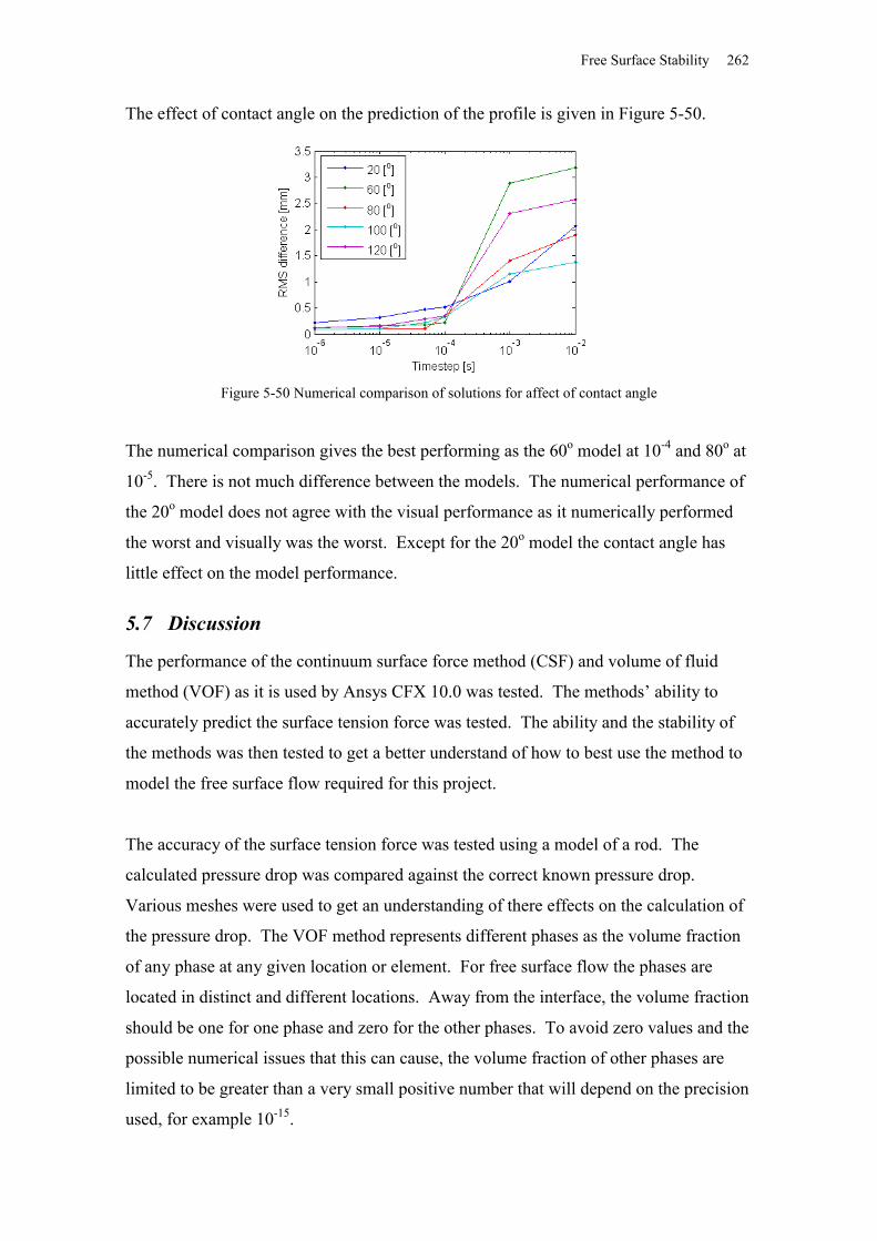
Free Surface Stability 262
The effect of contact angle on the prediction of the profile is given in Figure 5-50.
Figure 5-50 Numerical comparison of solutions for affect of contact angle
The numerical comparison gives the best performing as the 60o model at 10-4 and 80o at
10-5. There is not much difference between the models. The numerical performance of
the 20o model does not agree with the visual performance as it numerically performed
the worst and visually was the worst. Except for the 20o model the contact angle has
little effect on the model performance.
5.7 Discussion
The performance of the continuum surface force method (CSF) and volume of fluid
method (VOF) as it is used by Ansys CFX 10.0 was tested. The methods’ ability to
accurately predict the surface tension force was tested. The ability and the stability of
the methods was then tested to get a better understand of how to best use the method to
model the free surface flow required for this project.
The accuracy of the surface tension force was tested using a model of a rod. The
calculated pressure drop was compared against the correct known pressure drop.
Various meshes were used to get an understanding of there effects on the calculation of
the pressure drop. The VOF method represents different phases as the volume fraction
of any phase at any given location or element. For free surface flow the phases are
located in distinct and different locations. Away from the interface, the volume fraction
should be one for one phase and zero for the other phases. To avoid zero values and the
possible numerical issues that this can cause, the volume fraction of other phases are
limited to be greater than a very small positive number that will depend on the precision
used, for example 10-15.
Free Surface Stability 263
At interfaces at microscopic scales the volume fraction between phases has a finite
gradient and is not a discontinuity. It is not practical to model down to the microscopic
scale and at the macroscopic scale the volume fraction change is a discontinuity for free
surface flows. The change in volume fraction at the interface is continuous with the
VOF method. The distance across the interface should be small for a well converged
solution. The distance is not directly controlled but is dependent on mesh and the solver
characteristics. The effect on the accuracy of different interface distances on the model
was also tested.
The stability of Ansys CFX 10.0 CSF VOF free surface modelling technique was tested
using a model of a meniscus. The solutions were evaluated using the solution residuals,
visual inspection and comparison against the known correct profile.
It was found that the accuracy of the pressure drop across the interface decreases when
the interface distance is large relative to the curvature of the interface. It was also found
that the fewer the number of elements across the interface, the more the curvature
estimate varies along the interface. The variation is caused by calculation of the
curvature and results in nonphysical variations in the pressure drop along the interface.
The variation in pressure drop drives the parasitic currents that, if not controlled, will
cause the solver to diverge. Currents are produced between the pressure differences,
these currents are non-physical and can lead to the interface becoming unstable and the
solver will diverge. These currents produce waves on the interface. These currents have
been identified by Tong and Wang (2007), Francois et al. (2006), Harvie et al. (2006)
and Meier et al. (2002) and they all claim the curvature estimate is the primary cause of
the parasitic currents. The findings from this project agree with the previous findings
that the curvature estimate causes the parasitic currents.
The interface distance was set in the rod model by defining the volume fraction
variables in the model, normally these variables are calculated and changed by the
solver so the interface distance cannot be directly specified. However the interface
distance is limited by the mesh resolution. Controlling the size of the control volumes
the mesh can be used to indirectly set the lower limit of the interface distance.
Free Surface Stability 264
Refining the mesh reduces the minimum interface distance and this can reduce stability
of the model at the free surface interface.
It was also found that the shape function used to calculate the curvature produces
nonphysical variations in the curvature along an interface with elements of different
sizes.
It was possible to limit the effect of the parasitic currents. If the volume fraction
timestep was small the numerical waves remained small and appeared to oscillate
around the correct interface location.
The residuals of the solutions were normally higher than liked. They were found to be
bad indicator of the quality of the solution and should not be only relied on to infer a
good solution.
The numerical solver is most stable when used with elements of very high quality. The
numerical solver stability reduces significantly as the mesh is made from less ideal
quality elements. The stability reduced significantly when the elements’ aspect ratio
was only 10% greater than the ideal element aspect ratio of one. This does not allow for
the use of prism layers. Prism layer have large aspect ratios and are not recommend to
be used as they produce instability in the solver. It is also recommended that the best
quality mesh possible is used.
The following was found to increase the stability of the Ansys CFX solver:
use a small volume fraction timestep (a timestep of ~10-5 s),
use a different timestep for the momentum equations and the volume fraction
equation. The automatic timestep selection does an adequate job of selecting an
appropriate timestep for the momentum equation,
do not use interface compression,
using volume fraction smoothing, especially using the volume fraction method,
do not use the curvature under relaxation factor.
It is not possible to change the material properties of the fluid involved in this project,
however it is useful to understand how changes in the material properties effect the
Free Surface Stability 265
performance of the numerical solver. It is useful for two reasons: first to extend the
project if needed to model different fluids, secondary it help modelling of other projects
with similar physics.
It has found that the stability of the numerical solver increases when
the liquid phase is more viscous,
the interfacial surface tension coefficient is lower,
and the liquid phase density is lower.
The stability is likely due to reducing the large gradients of a variable across the
interface making the solver more stable. The findings are consistent with the work of
Renardy and Renardy (2002). The stability of the numerical solver is increased by the
increasing the Ohnesorge, Oh, number.
The three phase contact angle was found to have no consistent effect on stability so no
conclusions are drawn.
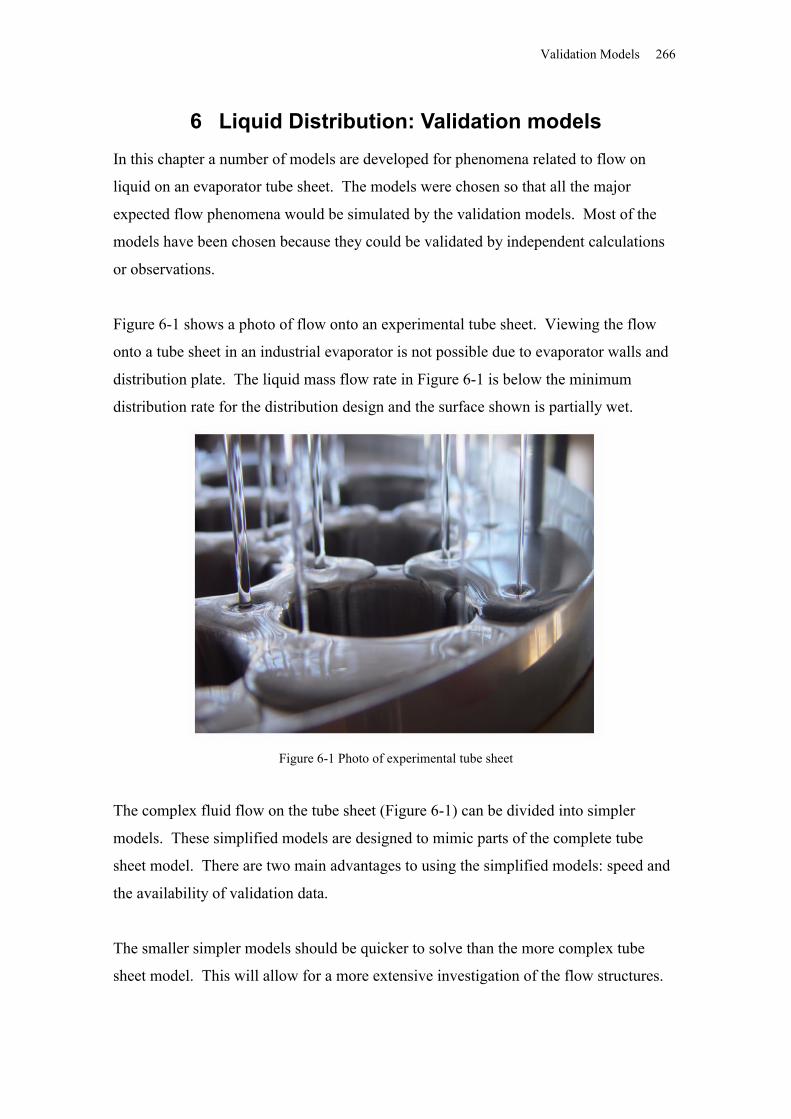
Validation Models 266
6 Liquid Distribution: Validation modelsIn this chapter a number of models are developed for phenomena related to flow on
liquid on an evaporator tube sheet. The models were chosen so that all the major
expected flow phenomena would be simulated by the validation models. Most of the
models have been chosen because they could be validated by independent calculations
or observations.
Figure 6-1 shows a photo of flow onto an experimental tube sheet. Viewing the flow
onto a tube sheet in an industrial evaporator is not possible due to evaporator walls and
distribution plate. The liquid mass flow rate in Figure 6-1 is below the minimum
distribution rate for the distribution design and the surface shown is partially wet.
Figure 6-1 Photo of experimental tube sheet
The complex fluid flow on the tube sheet (Figure 6-1) can be divided into simpler
models. These simplified models are designed to mimic parts of the complete tube
sheet model. There are two main advantages to using the simplified models: speed and
the availability of validation data.
The smaller simpler models should be quicker to solve than the more complex tube
sheet model. This will allow for a more extensive investigation of the flow structures.
Validation Models 267
The second advantage is that a greater amount of data or known relationships are
available for validation purposes for the component models than for the complete tube
sheet model. The simplified models have been named “validation models”. It must be
possible to simulate and validate each validation model before attempting a full model.
The validation of all the validation models does not guarantee the validation of a tube
sheet model, but it does increase the confidence in the modelling process and in Ansys
CFX to predict correctly.
The goal of the validation model is to show that the CSF VOF modelling technique used
can produced solutions for the validation models that could reasonable be combined
together to produce a converged, mesh independent solution that correctly predicts the
physics of the wetting occurring on the tube sheet.
6.1 Model definition
6.1.1 Materials
The same materials were used throughout the validation models and are based on water
vapour at 70 oC (used for the vapour phase) and liquid water at 70 oC (used as the liquid
phase). The physical properties were obtained from Haar et al. (1984).
The viscosity of the liquid was changed to simulate the different viscosities of the
different products used industrially.
6.1.2 Domain
The models are set up with the following model conditions:
homogeneous Eulerian-Eulerian multiphase model
no interphase compression
a curvature under-relaxation factor of 1
Laplacian volume fraction smoothing
surface tension coefficient of 68 mN m-1
contact angle of 80o
gravitation acceleration of 9.81 m s-2 downwards
Validation Models 268
buoyancy is implemented as a source term in the momentum transport equations
(Equation 2-2) and is calculated from the local fluid density difference from an
arbitrary reference density (Ansys CFX, 2005).
The models were solved in double precision with the steady state solver. Double
precision is often needed when modelling a free surface. This is to overcome the
numerical truncation errors that can occur (Ansys CFX 2005).
The steady state solver was only used because of the limitations in computer resources
available. The transient solver requires extra iterations to move through time compared
to the steady state solver. The transient also solver does not allow the volume fraction
timestep to be different for the other equations, which has been shown to increase
stability in Section 5.6.6. It was hoped that the false timestep method would develop the
solution in a similar enough to the transient solution to get meaningful steady state
results.
Laplacian smoothing of the volume fraction was used instead of volume fraction
smoothing because the volume fraction smoothing was found to be preferable after the
validation models had been completed.
6.2 Jet
When the liquid falls through the holes on the distribution plate it forms a jet. Gravity
will accelerate the jet, which contracts due to conservation of mass as the jet velocity
increases. The contraction increases the curvature and thus the surface tension force on
the free surface. The jet hits the tube sheet below and spreads radially outwards (Figure
6-2).
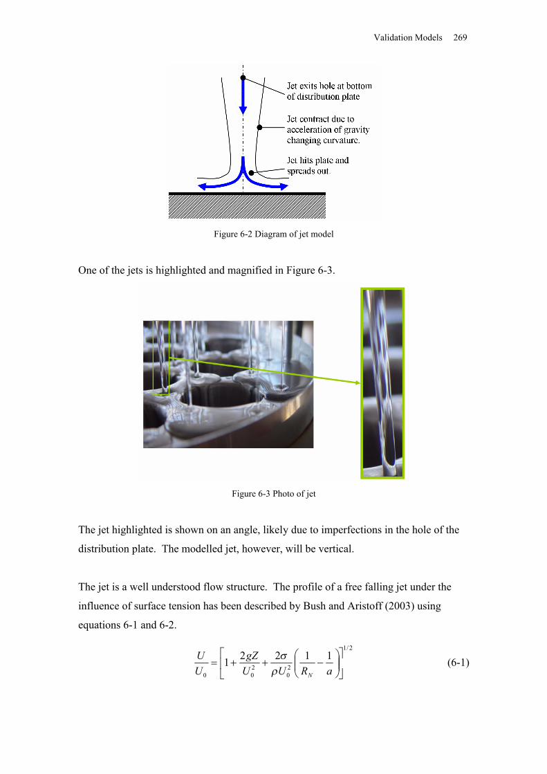
Validation Models 269
Figure 6-2 Diagram of jet model
One of the jets is highlighted and magnified in Figure 6-3.
Figure 6-3 Photo of jet
The jet highlighted is shown on an angle, likely due to imperfections in the hole of the
distribution plate. The modelled jet, however, will be vertical.
The jet is a well understood flow structure. The profile of a free falling jet under the
influence of surface tension has been described by Bush and Aristoff (2003) using
equations 6-1 and 6-2.
2/1
20
200
11221
aRUUgZ
UU
N (6-1)
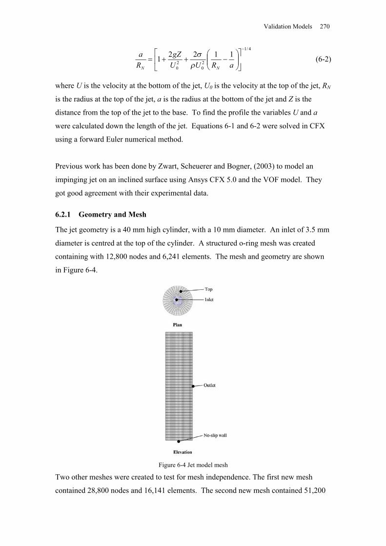
Validation Models 270
4/1
20
20
11221
aRUUgZ
Ra
NN (6-2)
where U is the velocity at the bottom of the jet, U0 is the velocity at the top of the jet, RN
is the radius at the top of the jet, a is the radius at the bottom of the jet and Z is the
distance from the top of the jet to the base. To find the profile the variables U and a
were calculated down the length of the jet. Equations 6-1 and 6-2 were solved in CFX
using a forward Euler numerical method.
Previous work has been done by Zwart, Scheuerer and Bogner, (2003) to model an
impinging jet on an inclined surface using Ansys CFX 5.0 and the VOF model. They
got good agreement with their experimental data.
6.2.1 Geometry and Mesh
The jet geometry is a 40 mm high cylinder, with a 10 mm diameter. An inlet of 3.5 mm
diameter is centred at the top of the cylinder. A structured o-ring mesh was created
containing with 12,800 nodes and 6,241 elements. The mesh and geometry are shown
in Figure 6-4.
Figure 6-4 Jet model mesh
Two other meshes were created to test for mesh independence. The first new mesh
contained 28,800 nodes and 16,141 elements. The second new mesh contained 51,200
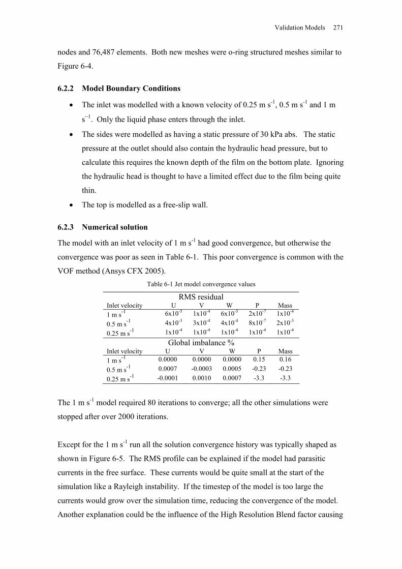
Validation Models 271
nodes and 76,487 elements. Both new meshes were o-ring structured meshes similar to
Figure 6-4.
6.2.2 Model Boundary Conditions
The inlet was modelled with a known velocity of 0.25 m s-1, 0.5 m s-1 and 1 m
s1. Only the liquid phase enters through the inlet.
The sides were modelled as having a static pressure of 30 kPa abs. The static
pressure at the outlet should also contain the hydraulic head pressure, but to
calculate this requires the known depth of the film on the bottom plate. Ignoring
the hydraulic head is thought to have a limited effect due to the film being quite
thin.
The top is modelled as a free-slip wall.
6.2.3 Numerical solution
The model with an inlet velocity of 1 m s-1 had good convergence, but otherwise the
convergence was poor as seen in Table 6-1. This poor convergence is common with the
VOF method (Ansys CFX 2005). Table 6-1 Jet model convergence values
RMS residualInlet velocity U V W P Mass1 m s-1 6x10⁻⁵ 1x10⁻⁴ 6x10⁻⁵ 2x10⁻⁷ 1x10⁻⁴
0.5 m s-1 4x10⁻³ 3x10⁻⁴ 4x10⁻⁴ 8x10⁻⁷ 2x10⁻³
0.25 m s-1 1x10⁻⁴ 1x10⁻⁴ 1x10⁻⁴ 1x10⁻⁴ 1x10⁻⁴
Global imbalance %Inlet velocity U V W P Mass1 m s-1 0.0000 0.0000 0.0000 0.15 0.160.5 m s-1 0.0007 -0.0003 0.0005 -0.23 -0.230.25 m s-1 -0.0001 0.0010 0.0007 -3.3 -3.3
The 1 m s-1 model required 80 iterations to converge; all the other simulations were
stopped after over 2000 iterations.
Except for the 1 m s-1 run all the solution convergence history was typically shaped as
shown in Figure 6-5. The RMS profile can be explained if the model had parasitic
currents in the free surface. These currents would be quite small at the start of the
simulation like a Rayleigh instability. If the timestep of the model is too large the
currents would grow over the simulation time, reducing the convergence of the model.
Another explanation could be the influence of the High Resolution Blend factor causing
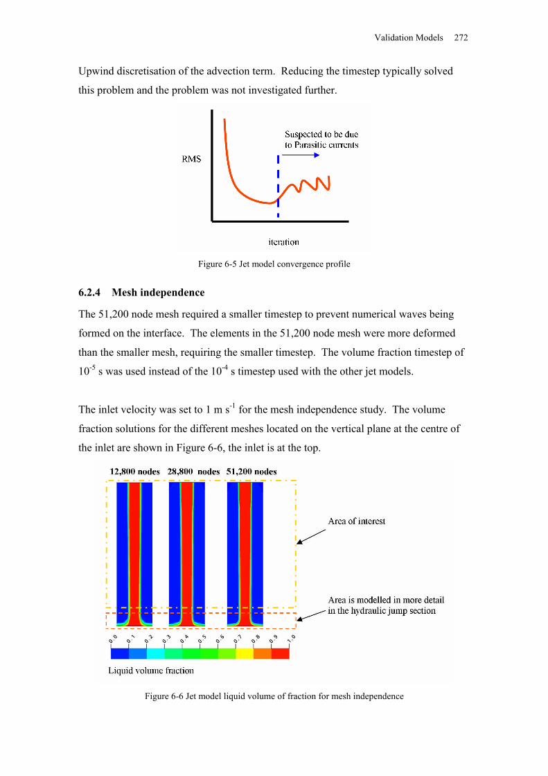
Validation Models 272
Upwind discretisation of the advection term. Reducing the timestep typically solved
this problem and the problem was not investigated further.
Figure 6-5 Jet model convergence profile
6.2.4 Mesh independence
The 51,200 node mesh required a smaller timestep to prevent numerical waves being
formed on the interface. The elements in the 51,200 node mesh were more deformed
than the smaller mesh, requiring the smaller timestep. The volume fraction timestep of
10-5 s was used instead of the 10-4 s timestep used with the other jet models.
The inlet velocity was set to 1 m s-1 for the mesh independence study. The volume
fraction solutions for the different meshes located on the vertical plane at the centre of
the inlet are shown in Figure 6-6, the inlet is at the top.
Figure 6-6 Jet model liquid volume of fraction for mesh independence
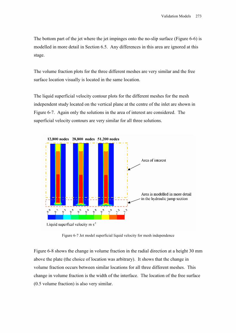
Validation Models 273
The bottom part of the jet where the jet impinges onto the no-slip surface (Figure 6-6) is
modelled in more detail in Section 6.5. Any differences in this area are ignored at this
stage.
The volume fraction plots for the three different meshes are very similar and the free
surface location visually is located in the same location.
The liquid superficial velocity contour plots for the different meshes for the mesh
independent study located on the vertical plane at the centre of the inlet are shown in
Figure 6-7. Again only the solutions in the area of interest are considered. The
superficial velocity contours are very similar for all three solutions.
Figure 6-7 Jet model superficial liquid velocity for mesh independence
Figure 6-8 shows the change in volume fraction in the radial direction at a height 30 mm
above the plate (the choice of location was arbitrary). It shows that the change in
volume fraction occurs between similar locations for all three different meshes. This
change in volume fraction is the width of the interface. The location of the free surface
(0.5 volume fraction) is also very similar.
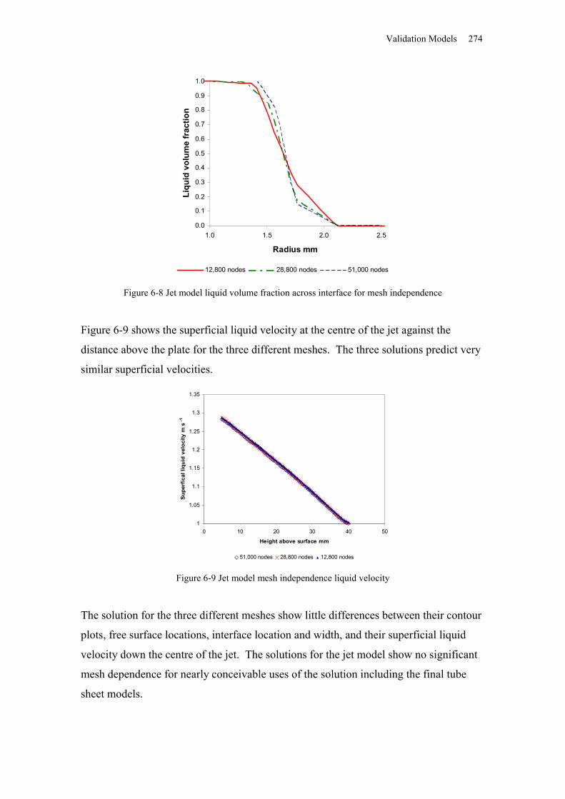
Validation Models 274
0.0
0.1
0.2
0.3
0.4
0.5
0.6
0.7
0.8
0.9
1.0
1.0 1.5 2.0 2.5
Radius mm
Liqu
id v
olum
e fr
actio
n
12,800 nodes 28,800 nodes 51,000 nodes
Figure 6-8 Jet model liquid volume fraction across interface for mesh independence
Figure 6-9 shows the superficial liquid velocity at the centre of the jet against the
distance above the plate for the three different meshes. The three solutions predict very
similar superficial velocities.
1
1.05
1.1
1.15
1.2
1.25
1.3
1.35
0 10 20 30 40 50
Height above surface mm
Supe
rfic
al li
quid
vel
ocity
m s
-1
51,000 nodes 28,800 nodes 12,800 nodes
Figure 6-9 Jet model mesh independence liquid velocity
The solution for the three different meshes show little differences between their contour
plots, free surface locations, interface location and width, and their superficial liquid
velocity down the centre of the jet. The solutions for the jet model show no significant
mesh dependence for nearly conceivable uses of the solution including the final tube
sheet models.
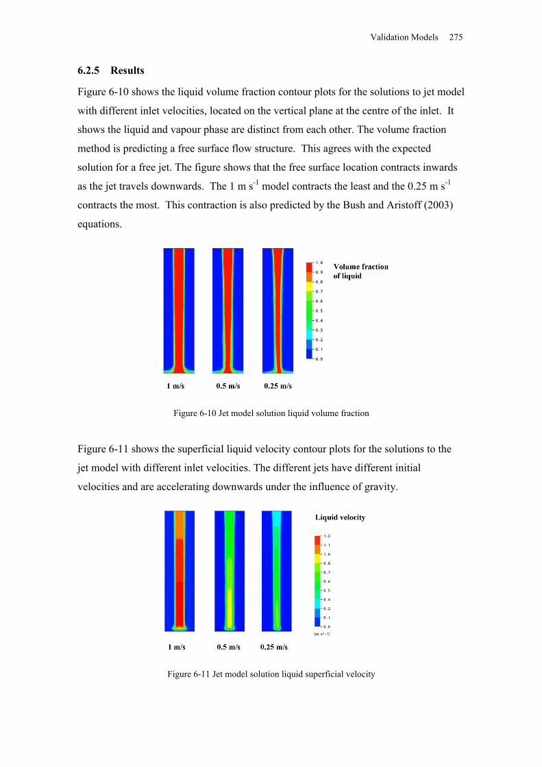
Validation Models 275
6.2.5 Results
Figure 6-10 shows the liquid volume fraction contour plots for the solutions to jet model
with different inlet velocities, located on the vertical plane at the centre of the inlet. It
shows the liquid and vapour phase are distinct from each other. The volume fraction
method is predicting a free surface flow structure. This agrees with the expected
solution for a free jet. The figure shows that the free surface location contracts inwards
as the jet travels downwards. The 1 m s-1 model contracts the least and the 0.25 m s-1
contracts the most. This contraction is also predicted by the Bush and Aristoff (2003)
equations.
Figure 6-10 Jet model solution liquid volume fraction
Figure 6-11 shows the superficial liquid velocity contour plots for the solutions to the
jet model with different inlet velocities. The different jets have different initial
velocities and are accelerating downwards under the influence of gravity.
Figure 6-11 Jet model solution liquid superficial velocity
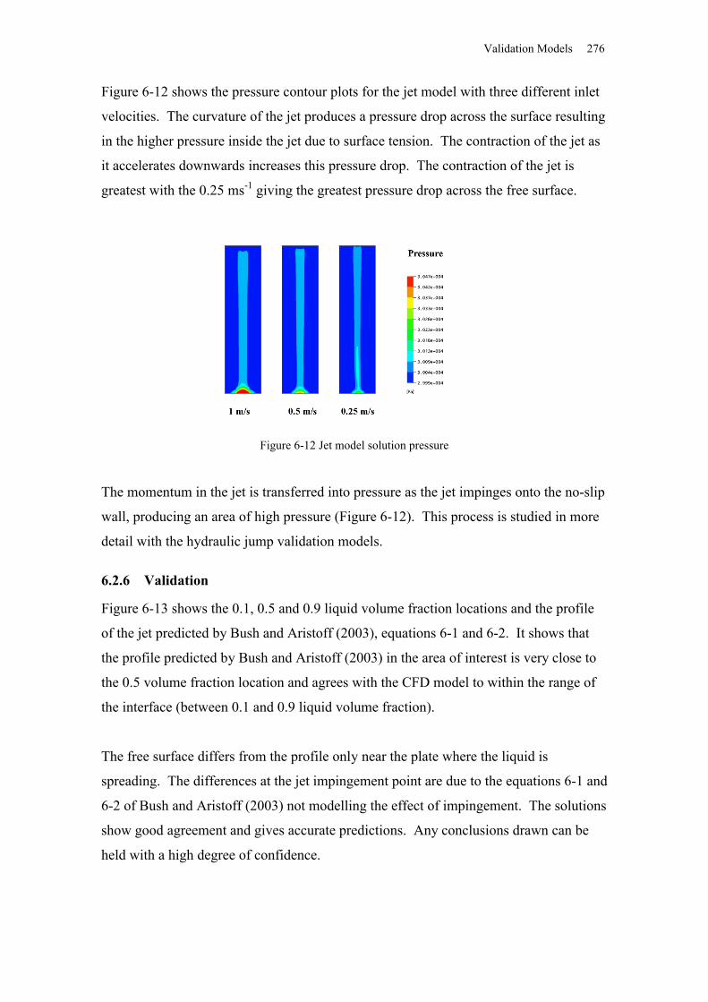
Validation Models 276
Figure 6-12 shows the pressure contour plots for the jet model with three different inlet
velocities. The curvature of the jet produces a pressure drop across the surface resulting
in the higher pressure inside the jet due to surface tension. The contraction of the jet as
it accelerates downwards increases this pressure drop. The contraction of the jet is
greatest with the 0.25 ms-1 giving the greatest pressure drop across the free surface.
Figure 6-12 Jet model solution pressure
The momentum in the jet is transferred into pressure as the jet impinges onto the no-slip
wall, producing an area of high pressure (Figure 6-12). This process is studied in more
detail with the hydraulic jump validation models.
6.2.6 Validation
Figure 6-13 shows the 0.1, 0.5 and 0.9 liquid volume fraction locations and the profile
of the jet predicted by Bush and Aristoff (2003), equations 6-1 and 6-2. It shows that
the profile predicted by Bush and Aristoff (2003) in the area of interest is very close to
the 0.5 volume fraction location and agrees with the CFD model to within the range of
the interface (between 0.1 and 0.9 liquid volume fraction).
The free surface differs from the profile only near the plate where the liquid is
spreading. The differences at the jet impingement point are due to the equations 6-1 and
6-2 of Bush and Aristoff (2003) not modelling the effect of impingement. The solutions
show good agreement and gives accurate predictions. Any conclusions drawn can be
held with a high degree of confidence.
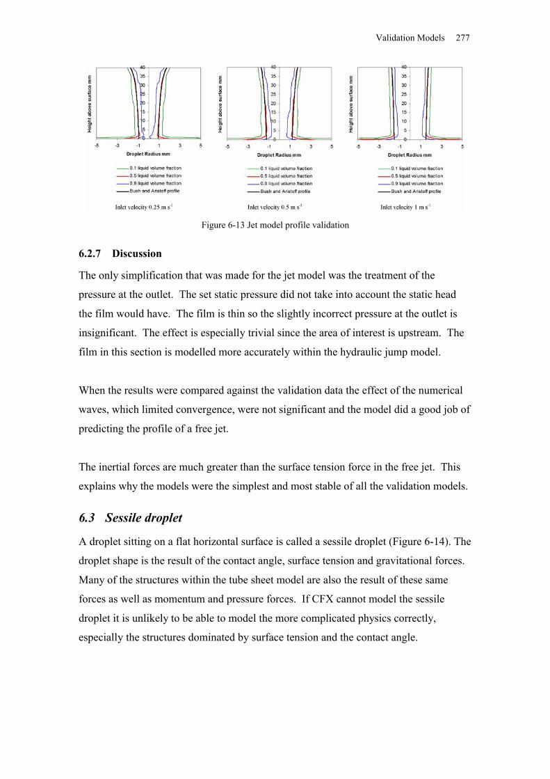
Validation Models 277
Figure 6-13 Jet model profile validation
6.2.7 Discussion
The only simplification that was made for the jet model was the treatment of the
pressure at the outlet. The set static pressure did not take into account the static head
the film would have. The film is thin so the slightly incorrect pressure at the outlet is
insignificant. The effect is especially trivial since the area of interest is upstream. The
film in this section is modelled more accurately within the hydraulic jump model.
When the results were compared against the validation data the effect of the numerical
waves, which limited convergence, were not significant and the model did a good job of
predicting the profile of a free jet.
The inertial forces are much greater than the surface tension force in the free jet. This
explains why the models were the simplest and most stable of all the validation models.
6.3 Sessile droplet
A droplet sitting on a flat horizontal surface is called a sessile droplet (Figure 6-14). The
droplet shape is the result of the contact angle, surface tension and gravitational forces.
Many of the structures within the tube sheet model are also the result of these same
forces as well as momentum and pressure forces. If CFX cannot model the sessile
droplet it is unlikely to be able to model the more complicated physics correctly,
especially the structures dominated by surface tension and the contact angle.
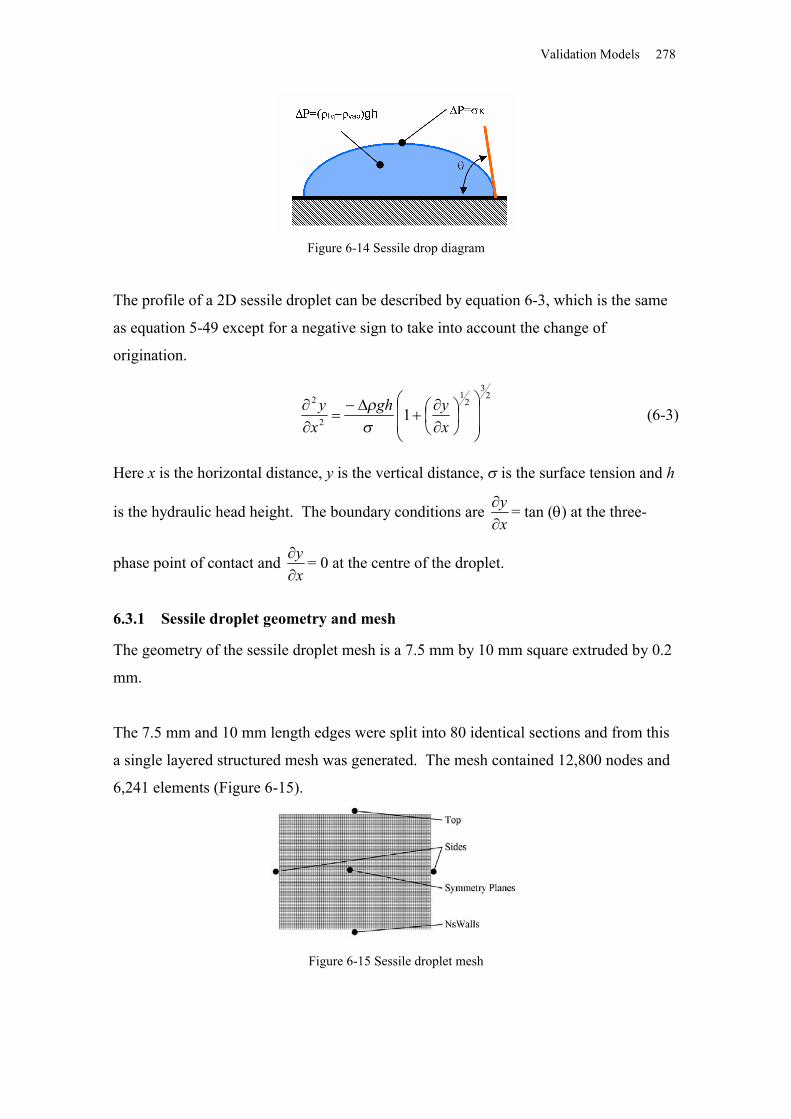
Validation Models 278
Figure 6-14 Sessile drop diagram
The profile of a 2D sessile droplet can be described by equation 6-3, which is the same
as equation 5-49 except for a negative sign to take into account the change of
origination.
23
21
2
2
1
xygh
xy
(6-3)
Here x is the horizontal distance, y is the vertical distance, is the surface tension and h
is the hydraulic head height. The boundary conditions are xy = tan () at the three-
phase point of contact and xy = 0 at the centre of the droplet.
6.3.1 Sessile droplet geometry and mesh
The geometry of the sessile droplet mesh is a 7.5 mm by 10 mm square extruded by 0.2
mm.
The 7.5 mm and 10 mm length edges were split into 80 identical sections and from this
a single layered structured mesh was generated. The mesh contained 12,800 nodes and
6,241 elements (Figure 6-15).
Figure 6-15 Sessile droplet mesh
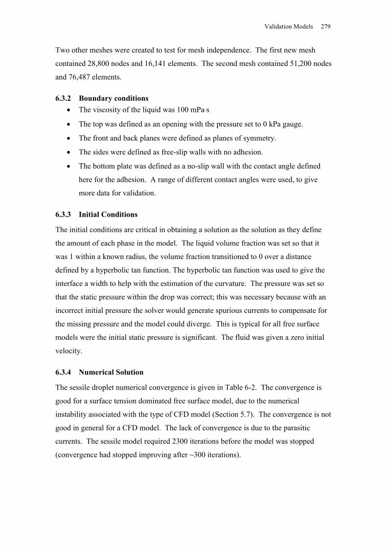
Validation Models 279
Two other meshes were created to test for mesh independence. The first new mesh
contained 28,800 nodes and 16,141 elements. The second mesh contained 51,200 nodes
and 76,487 elements.
6.3.2 Boundary conditions The viscosity of the liquid was 100 mPas
The top was defined as an opening with the pressure set to 0 kPa gauge.
The front and back planes were defined as planes of symmetry.
The sides were defined as free-slip walls with no adhesion.
The bottom plate was defined as a no-slip wall with the contact angle defined
here for the adhesion. A range of different contact angles were used, to give
more data for validation.
6.3.3 Initial Conditions
The initial conditions are critical in obtaining a solution as the solution as they define
the amount of each phase in the model. The liquid volume fraction was set so that it
was 1 within a known radius, the volume fraction transitioned to 0 over a distance
defined by a hyperbolic tan function. The hyperbolic tan function was used to give the
interface a width to help with the estimation of the curvature. The pressure was set so
that the static pressure within the drop was correct; this was necessary because with an
incorrect initial pressure the solver would generate spurious currents to compensate for
the missing pressure and the model could diverge. This is typical for all free surface
models were the initial static pressure is significant. The fluid was given a zero initial
velocity.
6.3.4 Numerical Solution
The sessile droplet numerical convergence is given in Table 6-2. The convergence is
good for a surface tension dominated free surface model, due to the numerical
instability associated with the type of CFD model (Section 5.7). The convergence is not
good in general for a CFD model. The lack of convergence is due to the parasitic
currents. The sessile model required 2300 iterations before the model was stopped
(convergence had stopped improving after ~300 iterations).
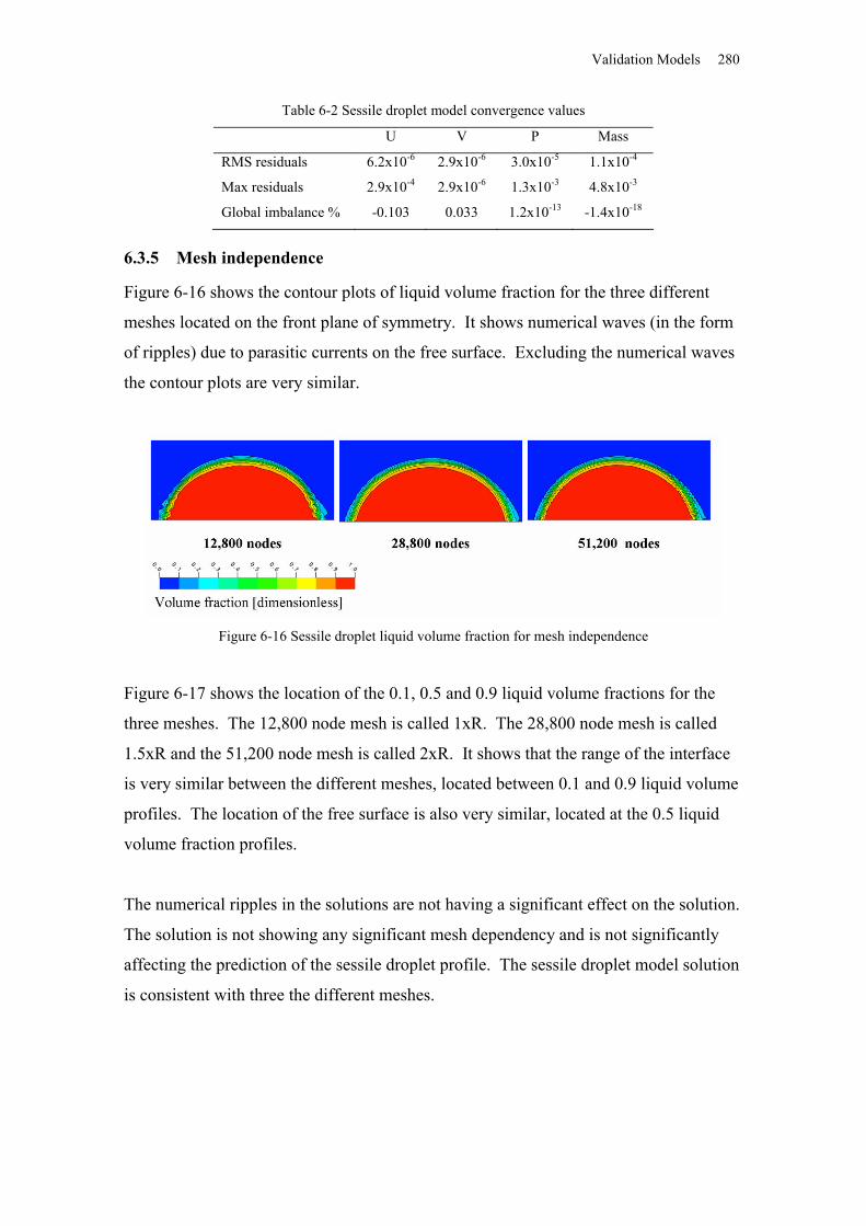
Validation Models 280
Table 6-2 Sessile droplet model convergence values
U V P Mass
RMS residuals 6.2x10⁻⁶ 2.9x10⁻⁶ 3.0x10⁻⁵ 1.1x10⁻⁴
Max residuals 2.9x10⁻⁴ 2.9x10⁻⁶ 1.3x10⁻³ 4.8x10⁻³
Global imbalance % -0.103 0.033 1.2x10⁻¹³ -1.4x10⁻¹⁸
6.3.5 Mesh independence
Figure 6-16 shows the contour plots of liquid volume fraction for the three different
meshes located on the front plane of symmetry. It shows numerical waves (in the form
of ripples) due to parasitic currents on the free surface. Excluding the numerical waves
the contour plots are very similar.
Figure 6-16 Sessile droplet liquid volume fraction for mesh independence
Figure 6-17 shows the location of the 0.1, 0.5 and 0.9 liquid volume fractions for the
three meshes. The 12,800 node mesh is called 1xR. The 28,800 node mesh is called
1.5xR and the 51,200 node mesh is called 2xR. It shows that the range of the interface
is very similar between the different meshes, located between 0.1 and 0.9 liquid volume
profiles. The location of the free surface is also very similar, located at the 0.5 liquid
volume fraction profiles.
The numerical ripples in the solutions are not having a significant effect on the solution.
The solution is not showing any significant mesh dependency and is not significantly
affecting the prediction of the sessile droplet profile. The sessile droplet model solution
is consistent with three the different meshes.
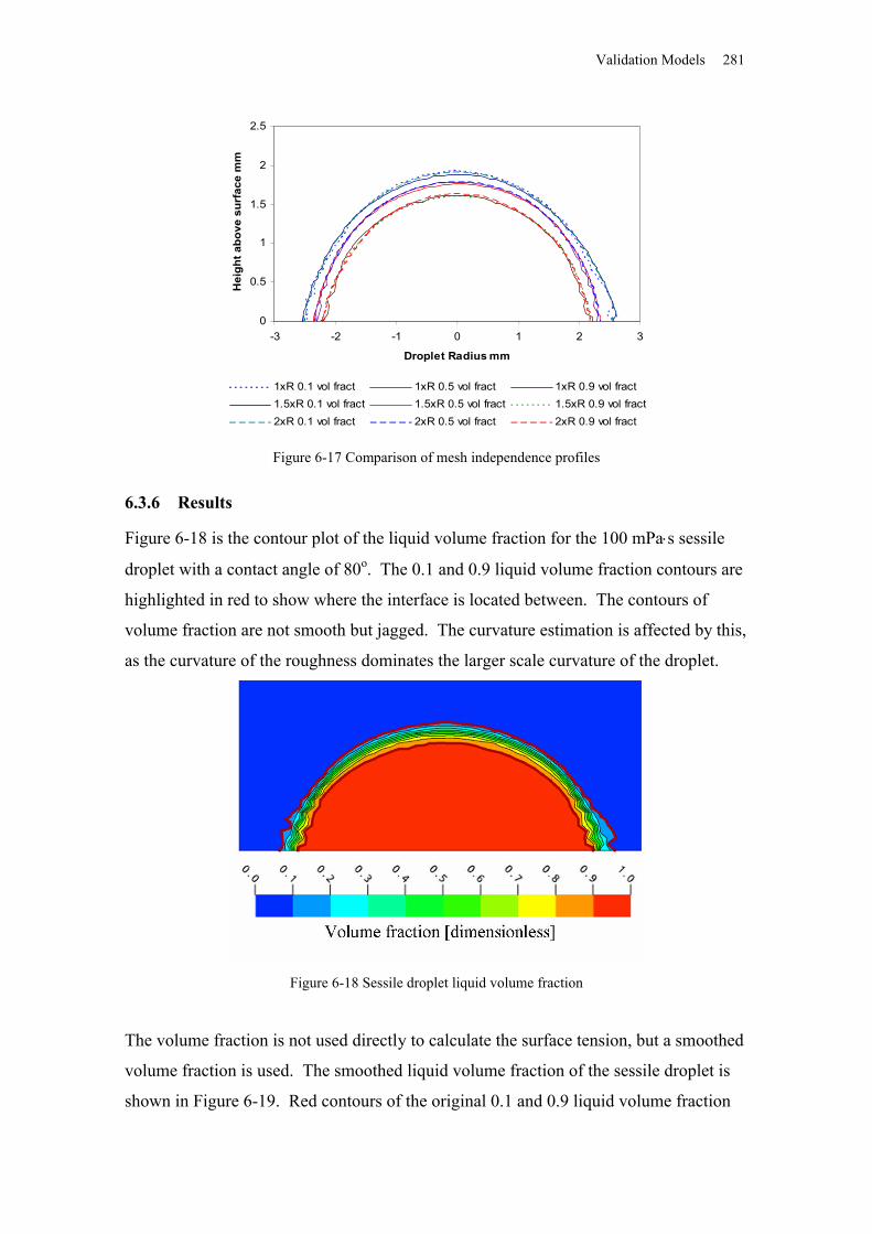
Validation Models 281
0
0.5
1
1.5
2
2.5
-3 -2 -1 0 1 2 3
Droplet Radius mm
Hei
ght a
bove
sur
face
mm
1xR 0.1 vol fract 1xR 0.5 vol fract 1xR 0.9 vol fract1.5xR 0.1 vol fract 1.5xR 0.5 vol fract 1.5xR 0.9 vol fract2xR 0.1 vol fract 2xR 0.5 vol fract 2xR 0.9 vol fract
Figure 6-17 Comparison of mesh independence profiles
6.3.6 Results
Figure 6-18 is the contour plot of the liquid volume fraction for the 100 mPas sessile
droplet with a contact angle of 80o. The 0.1 and 0.9 liquid volume fraction contours are
highlighted in red to show where the interface is located between. The contours of
volume fraction are not smooth but jagged. The curvature estimation is affected by this,
as the curvature of the roughness dominates the larger scale curvature of the droplet.
Figure 6-18 Sessile droplet liquid volume fraction
The volume fraction is not used directly to calculate the surface tension, but a smoothed
volume fraction is used. The smoothed liquid volume fraction of the sessile droplet is
shown in Figure 6-19. Red contours of the original 0.1 and 0.9 liquid volume fraction
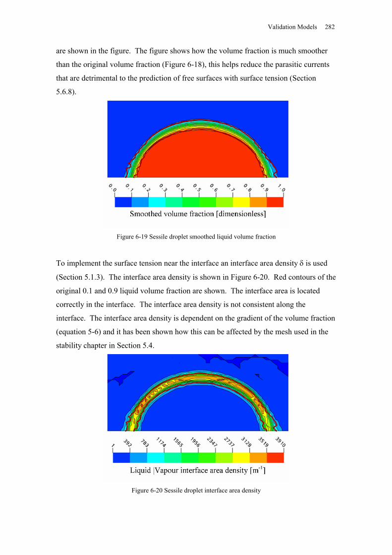
Validation Models 282
are shown in the figure. The figure shows how the volume fraction is much smoother
than the original volume fraction (Figure 6-18), this helps reduce the parasitic currents
that are detrimental to the prediction of free surfaces with surface tension (Section
5.6.8).
Figure 6-19 Sessile droplet smoothed liquid volume fraction
To implement the surface tension near the interface an interface area density is used
(Section 5.1.3). The interface area density is shown in Figure 6-20. Red contours of the
original 0.1 and 0.9 liquid volume fraction are shown. The interface area is located
correctly in the interface. The interface area density is not consistent along the
interface. The interface area density is dependent on the gradient of the volume fraction
(equation 5-6) and it has been shown how this can be affected by the mesh used in the
stability chapter in Section 5.4.
Figure 6-20 Sessile droplet interface area density
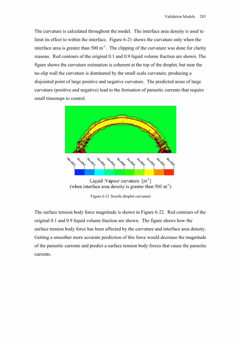
Validation Models 283
The curvature is calculated throughout the model. The interface area density is used to
limit its effect to within the interface. Figure 6-21 shows the curvature only when the
interface area is greater than 500 m-1. The clipping of the curvature was done for clarity
reasons. Red contours of the original 0.1 and 0.9 liquid volume fraction are shown. The
figure shows the curvature estimation is coherent at the top of the droplet, but near the
no-slip wall the curvature is dominated by the small scale curvature, producing a
disjointed point of large positive and negative curvature. The predicted areas of large
curvature (positive and negative) lead to the formation of parasitic currents that require
small timesteps to control.
Figure 6-21 Sessile droplet curvature
The surface tension body force magnitude is shown in Figure 6-22. Red contours of the
original 0.1 and 0.9 liquid volume fraction are shown. The figure shows how the
surface tension body force has been affected by the curvature and interface area density.
Getting a smoother more accurate prediction of this force would decrease the magnitude
of the parasitic currents and predict a surface tension body forces that cause the parasitic
currents.
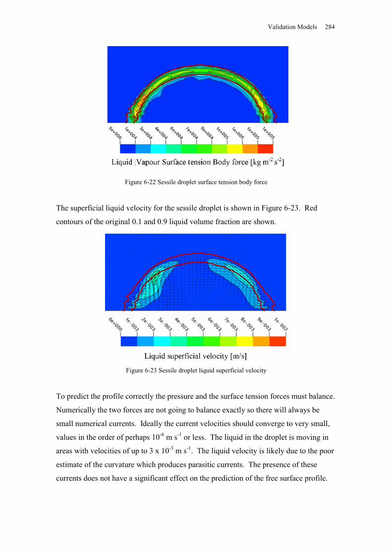
Validation Models 284
Figure 6-22 Sessile droplet surface tension body force
The superficial liquid velocity for the sessile droplet is shown in Figure 6-23. Red
contours of the original 0.1 and 0.9 liquid volume fraction are shown.
Figure 6-23 Sessile droplet liquid superficial velocity
To predict the profile correctly the pressure and the surface tension forces must balance.
Numerically the two forces are not going to balance exactly so there will always be
small numerical currents. Ideally the current velocities should converge to very small,
values in the order of perhaps 10-6 m s-1 or less. The liquid in the droplet is moving in
areas with velocities of up to 3 x 10⁻³ m s-1. The liquid velocity is likely due to the poor
estimate of the curvature which produces parasitic currents. The presence of these
currents does not have a significant effect on the prediction of the free surface profile.
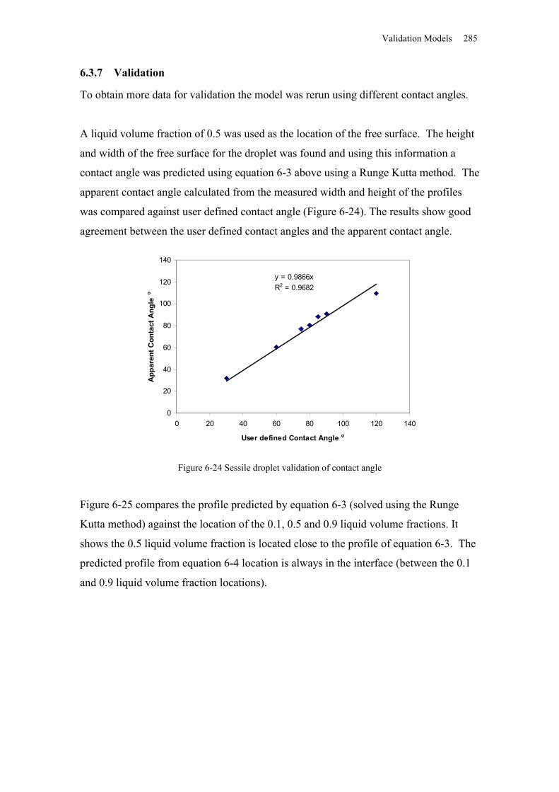
Validation Models 285
6.3.7 Validation
To obtain more data for validation the model was rerun using different contact angles.
A liquid volume fraction of 0.5 was used as the location of the free surface. The height
and width of the free surface for the droplet was found and using this information a
contact angle was predicted using equation 6-3 above using a Runge Kutta method. The
apparent contact angle calculated from the measured width and height of the profiles
was compared against user defined contact angle (Figure 6-24). The results show good
agreement between the user defined contact angles and the apparent contact angle.
y = 0.9866xR2 = 0.9682
0
20
40
60
80
100
120
140
0 20 40 60 80 100 120 140
User defined Contact Angle o
App
aren
t Con
tact
Ang
le o
Figure 6-24 Sessile droplet validation of contact angle
Figure 6-25 compares the profile predicted by equation 6-3 (solved using the Runge
Kutta method) against the location of the 0.1, 0.5 and 0.9 liquid volume fractions. It
shows the 0.5 liquid volume fraction is located close to the profile of equation 6-3. The
predicted profile from equation 6-4 location is always in the interface (between the 0.1
and 0.9 liquid volume fraction locations).
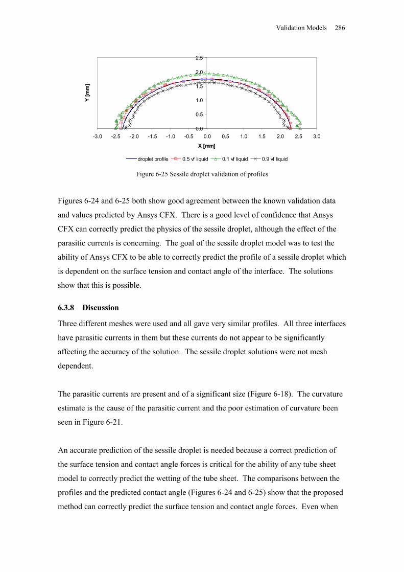
Validation Models 286
0.0
0.5
1.0
1.5
2.0
2.5
-3.0 -2.5 -2.0 -1.5 -1.0 -0.5 0.0 0.5 1.0 1.5 2.0 2.5 3.0
X [mm]
Y [m
m]
droplet profile 0.5 vf liquid 0.1 vf liquid 0.9 vf liquid
Figure 6-25 Sessile droplet validation of profiles
Figures 6-24 and 6-25 both show good agreement between the known validation data
and values predicted by Ansys CFX. There is a good level of confidence that Ansys
CFX can correctly predict the physics of the sessile droplet, although the effect of the
parasitic currents is concerning. The goal of the sessile droplet model was to test the
ability of Ansys CFX to be able to correctly predict the profile of a sessile droplet which
is dependent on the surface tension and contact angle of the interface. The solutions
show that this is possible.
6.3.8 Discussion
Three different meshes were used and all gave very similar profiles. All three interfaces
have parasitic currents in them but these currents do not appear to be significantly
affecting the accuracy of the solution. The sessile droplet solutions were not mesh
dependent.
The parasitic currents are present and of a significant size (Figure 6-18). The curvature
estimate is the cause of the parasitic current and the poor estimation of curvature been
seen in Figure 6-21.
An accurate prediction of the sessile droplet is needed because a correct prediction of
the surface tension and contact angle forces is critical for the ability of any tube sheet
model to correctly predict the wetting of the tube sheet. The comparisons between the
profiles and the predicted contact angle (Figures 6-24 and 6-25) show that the proposed
method can correctly predict the surface tension and contact angle forces. Even when
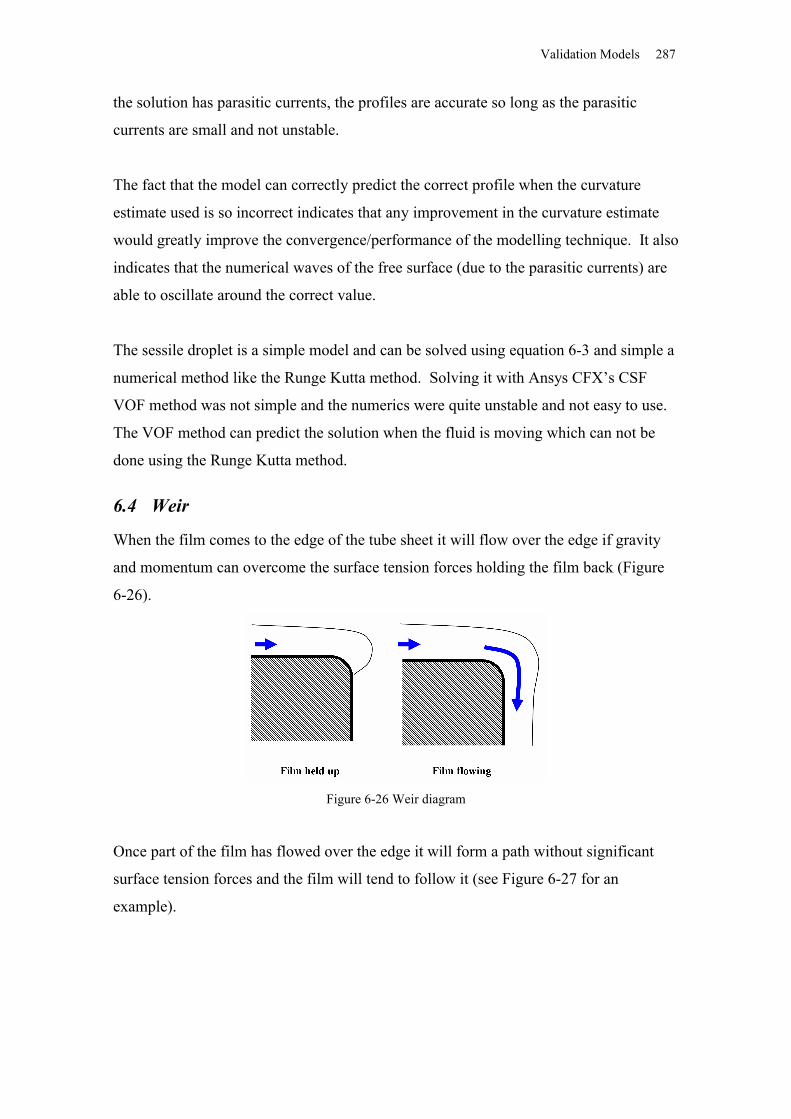
Validation Models 287
the solution has parasitic currents, the profiles are accurate so long as the parasitic
currents are small and not unstable.
The fact that the model can correctly predict the correct profile when the curvature
estimate used is so incorrect indicates that any improvement in the curvature estimate
would greatly improve the convergence/performance of the modelling technique. It also
indicates that the numerical waves of the free surface (due to the parasitic currents) are
able to oscillate around the correct value.
The sessile droplet is a simple model and can be solved using equation 6-3 and simple a
numerical method like the Runge Kutta method. Solving it with Ansys CFX’s CSF
VOF method was not simple and the numerics were quite unstable and not easy to use.
The VOF method can predict the solution when the fluid is moving which can not be
done using the Runge Kutta method.
6.4 Weir
When the film comes to the edge of the tube sheet it will flow over the edge if gravity
and momentum can overcome the surface tension forces holding the film back (Figure
6-26).
Figure 6-26 Weir diagram
Once part of the film has flowed over the edge it will form a path without significant
surface tension forces and the film will tend to follow it (see Figure 6-27 for an
example).
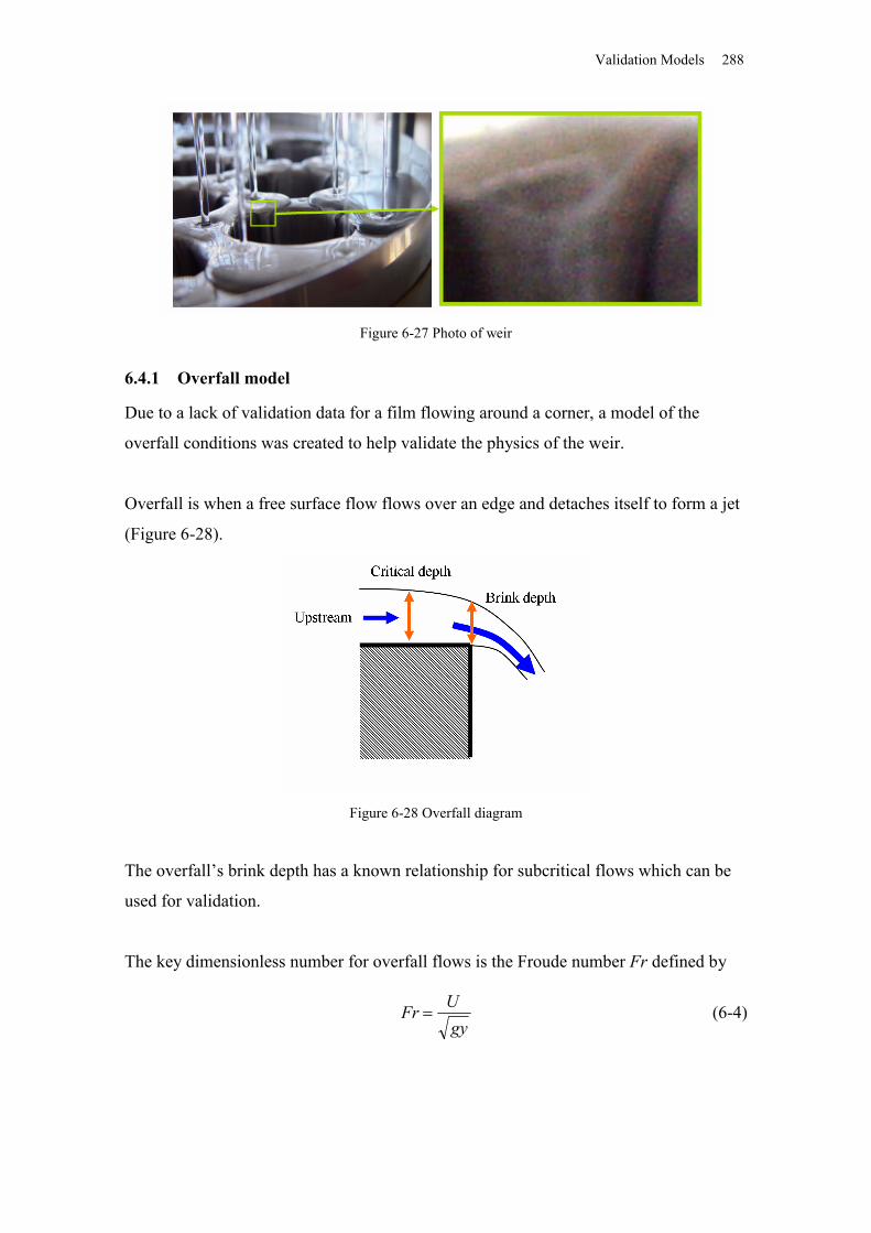
Validation Models 288
Figure 6-27 Photo of weir
6.4.1 Overfall model
Due to a lack of validation data for a film flowing around a corner, a model of the
overfall conditions was created to help validate the physics of the weir.
Overfall is when a free surface flow flows over an edge and detaches itself to form a jet
(Figure 6-28).
Figure 6-28 Overfall diagram
The overfall’s brink depth has a known relationship for subcritical flows which can be
used for validation.
The key dimensionless number for overfall flows is the Froude number Fr defined by
gyUFr (6-4)
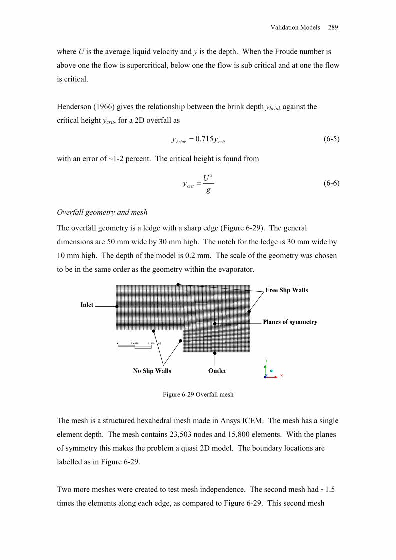
Validation Models 289
where U is the average liquid velocity and y is the depth. When the Froude number is
above one the flow is supercritical, below one the flow is sub critical and at one the flow
is critical.
Henderson (1966) gives the relationship between the brink depth ybrink against the
critical height ycrit, for a 2D overfall as
critbrink yy 715.0 (6-5)
with an error of ~1-2 percent. The critical height is found from
gUycrit
2
(6-6)
Overfall geometry and mesh
The overfall geometry is a ledge with a sharp edge (Figure 6-29). The general
dimensions are 50 mm wide by 30 mm high. The notch for the ledge is 30 mm wide by
10 mm high. The depth of the model is 0.2 mm. The scale of the geometry was chosen
to be in the same order as the geometry within the evaporator.
Figure 6-29 Overfall mesh
The mesh is a structured hexahedral mesh made in Ansys ICEM. The mesh has a single
element depth. The mesh contains 23,503 nodes and 15,800 elements. With the planes
of symmetry this makes the problem a quasi 2D model. The boundary locations are
labelled as in Figure 6-29.
Two more meshes were created to test mesh independence. The second mesh had ~1.5
times the elements along each edge, as compared to Figure 6-29. This second mesh
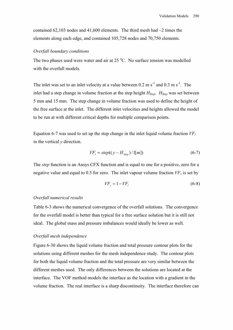
Validation Models 290
contained 62,103 nodes and 41,600 elements. The third mesh had ~2 times the
elements along each edge, and contained 105,728 nodes and 70,750 elements.
Overfall boundary conditions
The two phases used were water and air at 25 oC. No surface tension was modelled
with the overfall models.
The inlet was set to an inlet velocity at a value between 0.2 m s-1 and 0.3 m s-1. The
inlet had a step change in volume fraction at the step height HStep. HStep was set between
5 mm and 15 mm. The step change in volume fraction was used to define the height of
the free surface at the inlet. The different inlet velocities and heights allowed the model
to be run at with different critical depths for multiple comparison points.
Equation 6-7 was used to set up the step change in the inlet liquid volume fraction VFl
in the vertical y direction.
])[1/)(( mHystepVF Stepl (6-7)
The step function is an Ansys CFX function and is equal to one for a positive, zero for a
negative value and equal to 0.5 for zero. The inlet vapour volume fraction VFv is set by
lv VFVF 1 (6-8)
Overfall numerical results
Table 6-3 shows the numerical convergence of the overfall solutions. The convergence
for the overfall model is better than typical for a free surface solution but it is still not
ideal. The global mass and pressure imbalances would ideally be lower as well.
Overfall mesh independence
Figure 6-30 shows the liquid volume fraction and total pressure contour plots for the
solutions using different meshes for the mesh independence study. The contour plots
for both the liquid volume fraction and the total pressure are very similar between the
different meshes used. The only differences between the solutions are located at the
interface. The VOF method models the interface as the location with a gradient in the
volume fraction. The real interface is a sharp discontinuity. The interface therefore can
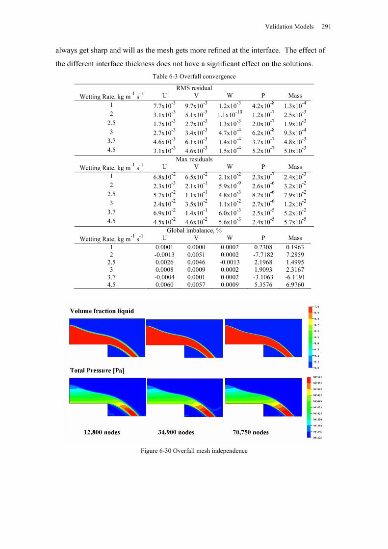
Validation Models 291
always get sharp and will as the mesh gets more refined at the interface. The effect of
the different interface thickness does not have a significant effect on the solutions.Table 6-3 Overfall convergence
RMS residualWetting Rate, kg m-1 s-1 U V W P Mass
1 7.7x10⁻³ 9.7x10⁻³ 1.2x10⁻³ 4.2x10⁻⁸ 1.3x10⁻⁴
2 3.1x10⁻³ 5.1x10⁻³ 1.1x10⁻¹⁰ 1.2x10⁻⁷ 2.5x10⁻³
2.5 1.7x10⁻³ 2.7x10⁻³ 1.3x10⁻³ 2.0x10⁻⁷ 1.9x10⁻³
3 2.7x10⁻³ 3.4x10⁻³ 4.7x10⁻⁴ 6.2x10⁻⁸ 9.3x10⁻⁴
3.7 4.6x10⁻³ 6.1x10⁻³ 1.4x10⁻⁴ 3.7x10⁻⁷ 4.8x10⁻³
4.5 3.1x10⁻³ 4.6x10⁻³ 1.5x10⁻⁴ 5.2x10⁻⁷ 5.0x10⁻³
Max residualsWetting Rate, kg m-1 s-1 U V W P Mass
1 6.8x10⁻² 6.5x10⁻² 2.1x10⁻² 2.3x10⁻⁷ 2.4x10⁻³
2 2.3x10⁻³ 2.1x10⁻¹ 5.9x10⁻⁹ 2.6x10⁻⁶ 3.2x10⁻²
2.5 5.7x10⁻² 1.1x10⁻¹ 4.8x10⁻³ 8.2x10⁻⁶ 7.9x10⁻²
3 2.4x10⁻² 3.5x10⁻² 1.1x10⁻² 2.7x10⁻⁶ 1.2x10⁻²
3.7 6.9x10⁻² 1.4x10⁻¹ 6.0x10⁻³ 2.5x10⁻⁵ 5.2x10⁻²
4.5 4.5x10⁻² 4.6x10⁻² 5.6x10⁻³ 2.4x10⁻⁵ 5.7x10⁻⁵
Global imbalance, %Wetting Rate, kg m-1 s-1 U V W P Mass
1 0.0001 0.0000 0.0002 0.2308 0.19632 -0.0013 0.0051 0.0002 -7.7182 7.2859
2.5 0.0026 0.0046 -0.0013 2.1968 1.49953 0.0008 0.0009 0.0002 1.9093 2.3167
3.7 -0.0004 0.0001 0.0002 -3.1063 -6.11914.5 0.0060 0.0057 0.0009 5.3576 6.9760
Figure 6-30 Overfall mesh independence
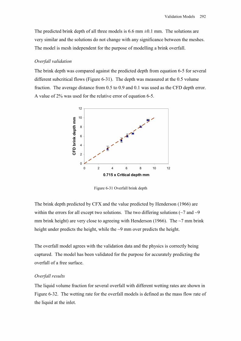
Validation Models 292
The predicted brink depth of all three models is 6.6 mm ±0.1 mm. The solutions are
very similar and the solutions do not change with any significance between the meshes.
The model is mesh independent for the purpose of modelling a brink overfall.
Overfall validation
The brink depth was compared against the predicted depth from equation 6-5 for several
different subcritical flows (Figure 6-31). The depth was measured at the 0.5 volume
fraction. The average distance from 0.5 to 0.9 and 0.1 was used as the CFD depth error.
A value of 2% was used for the relative error of equation 6-5.
0
2
4
6
8
10
12
0 2 4 6 8 10 12
0.715 x Critical depth mm
CFD
brin
k de
pth
mm
Figure 6-31 Overfall brink depth
The brink depth predicted by CFX and the value predicted by Henderson (1966) are
within the errors for all except two solutions. The two differing solutions (~7 and ~9
mm brink height) are very close to agreeing with Henderson (1966). The ~7 mm brink
height under predicts the height, while the ~9 mm over predicts the height.
The overfall model agrees with the validation data and the physics is correctly being
captured. The model has been validated for the purpose for accurately predicting the
overfall of a free surface.
Overfall results
The liquid volume fraction for several overfall with different wetting rates are shown in
Figure 6-32. The wetting rate for the overfall models is defined as the mass flow rate of
the liquid at the inlet.
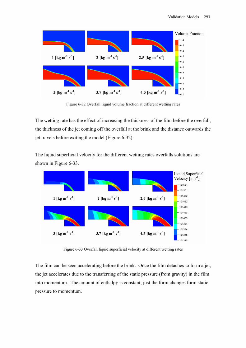
Validation Models 293
Figure 6-32 Overfall liquid volume fraction at different wetting rates
The wetting rate has the effect of increasing the thickness of the film before the overfall,
the thickness of the jet coming off the overfall at the brink and the distance outwards the
jet travels before exiting the model (Figure 6-32).
The liquid superficial velocity for the different wetting rates overfalls solutions are
shown in Figure 6-33.
Figure 6-33 Overfall liquid superficial velocity at different wetting rates
The film can be seen accelerating before the brink. Once the film detaches to form a jet,
the jet accelerates due to the transferring of the static pressure (from gravity) in the film
into momentum. The amount of enthalpy is constant; just the form changes form static
pressure to momentum.
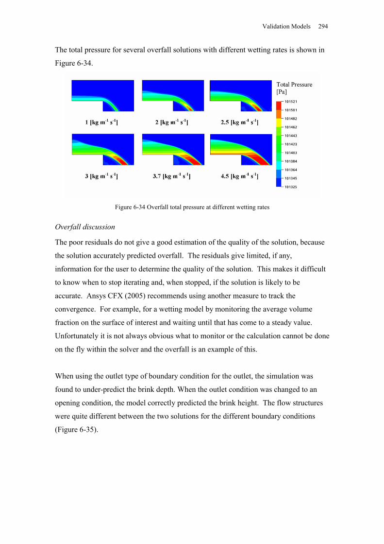
Validation Models 294
The total pressure for several overfall solutions with different wetting rates is shown in
Figure 6-34.
Figure 6-34 Overfall total pressure at different wetting rates
Overfall discussion
The poor residuals do not give a good estimation of the quality of the solution, because
the solution accurately predicted overfall. The residuals give limited, if any,
information for the user to determine the quality of the solution. This makes it difficult
to know when to stop iterating and, when stopped, if the solution is likely to be
accurate. Ansys CFX (2005) recommends using another measure to track the
convergence. For example, for a wetting model by monitoring the average volume
fraction on the surface of interest and waiting until that has come to a steady value.
Unfortunately it is not always obvious what to monitor or the calculation cannot be done
on the fly within the solver and the overfall is an example of this.
When using the outlet type of boundary condition for the outlet, the simulation was
found to under-predict the brink depth. When the outlet condition was changed to an
opening condition, the model correctly predicted the brink height. The flow structures
were quite different between the two solutions for the different boundary conditions
(Figure 6-35).
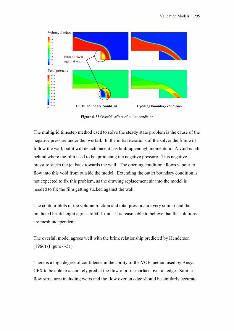
Validation Models 295
Figure 6-35 Overfall affect of outlet condition
The multigrid timestep method used to solve the steady state problem is the cause of the
negative pressure under the overfall. In the initial iterations of the solver the film will
follow the wall, but it will detach once it has built up enough momentum. A void is left
behind where the film used to be, producing the negative pressure. This negative
pressure sucks the jet back towards the wall. The opening condition allows vapour to
flow into this void from outside the model. Extending the outlet boundary condition is
not expected to fix this problem, as the drawing replacement air into the model is
needed to fix the film getting sucked against the wall.
The contour plots of the volume fraction and total pressure are very similar and the
predicted brink height agrees to ±0.1 mm. It is reasonable to believe that the solutions
are mesh independent.
The overfall model agrees well with the brink relationship predicted by Henderson
(1966) (Figure 6-31).
There is a high degree of confidence in the ability of the VOF method used by Ansys
CFX to be able to accurately predict the flow of a free surface over an edge. Similar
flow structures including weirs and the flow over an edge should be similarly accurate.
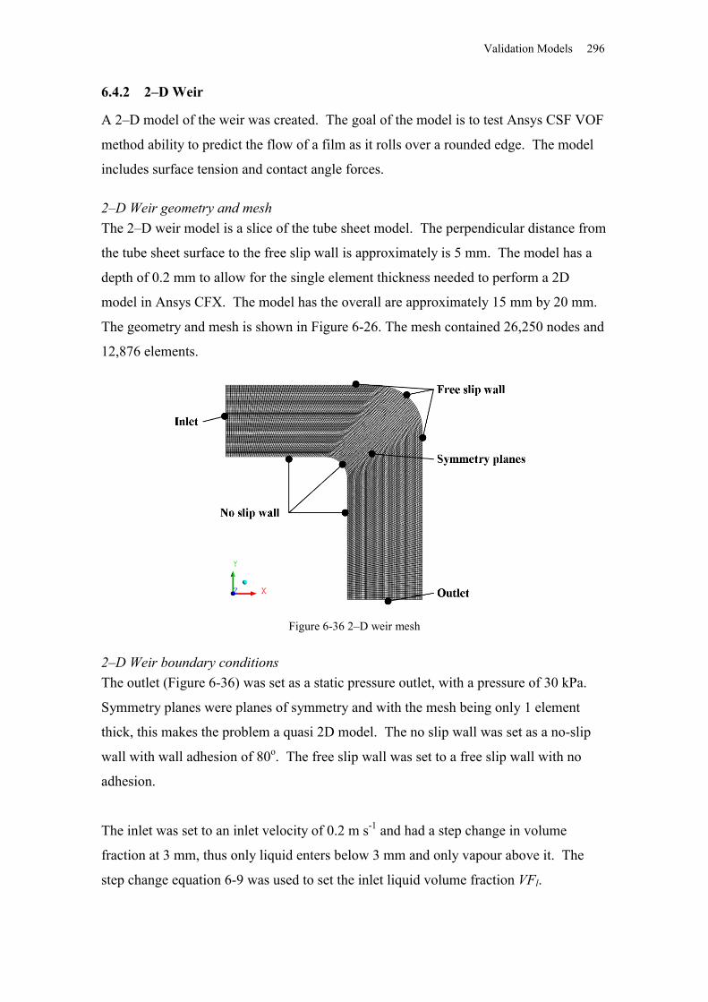
Validation Models 296
6.4.2 2–D Weir
A 2–D model of the weir was created. The goal of the model is to test Ansys CSF VOF
method ability to predict the flow of a film as it rolls over a rounded edge. The model
includes surface tension and contact angle forces.
2–D Weir geometry and meshThe 2–D weir model is a slice of the tube sheet model. The perpendicular distance from
the tube sheet surface to the free slip wall is approximately is 5 mm. The model has a
depth of 0.2 mm to allow for the single element thickness needed to perform a 2D
model in Ansys CFX. The model has the overall are approximately 15 mm by 20 mm.
The geometry and mesh is shown in Figure 6-26. The mesh contained 26,250 nodes and
12,876 elements.
Figure 6-36 2–D weir mesh
2–D Weir boundary conditionsThe outlet (Figure 6-36) was set as a static pressure outlet, with a pressure of 30 kPa.
Symmetry planes were planes of symmetry and with the mesh being only 1 element
thick, this makes the problem a quasi 2D model. The no slip wall was set as a no-slip
wall with wall adhesion of 80o. The free slip wall was set to a free slip wall with no
adhesion.
The inlet was set to an inlet velocity of 0.2 m s-1 and had a step change in volume
fraction at 3 mm, thus only liquid enters below 3 mm and only vapour above it. The
step change equation 6-9 was used to set the inlet liquid volume fraction VFl.
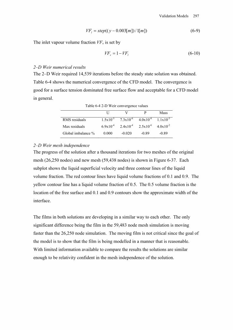
Validation Models 297
])[1/])[003.0(( mmystepVFl (6-9)
The inlet vapour volume fraction VFv is set by
lv VFVF 1 (6-10)
2–D Weir numerical resultsThe 2–D Weir required 14,539 iterations before the steady state solution was obtained.
Table 6-4 shows the numerical convergence of the CFD model. The convergence is
good for a surface tension dominated free surface flow and acceptable for a CFD model
in general.Table 6-4 2-D Weir convergence values
U V P Mass
RMS residuals 1.5x10⁻⁵ 7.3x10⁻⁶ 4.0x10⁻⁸ 1.1x10⁻³
Max residuals 6.9x10⁻⁴ 2.4x10⁻⁴ 2.5x10⁻⁶ 4.0x10⁻²
Global imbalance % 0.000 -0.020 -0.89 -0.89
2–D Weir mesh independenceThe progress of the solution after a thousand iterations for two meshes of the original
mesh (26,250 nodes) and new mesh (59,438 nodes) is shown in Figure 6-37. Each
subplot shows the liquid superficial velocity and three contour lines of the liquid
volume fraction. The red contour lines have liquid volume fractions of 0.1 and 0.9. The
yellow contour line has a liquid volume fraction of 0.5. The 0.5 volume fraction is the
location of the free surface and 0.1 and 0.9 contours show the approximate width of the
interface.
The films in both solutions are developing in a similar way to each other. The only
significant difference being the film in the 59,483 node mesh simulation is moving
faster than the 26,250 node simulation. The moving film is not critical since the goal of
the model is to show that the film is being modelled in a manner that is reasonable.
With limited information available to compare the results the solutions are similar
enough to be relativity confident in the mesh independence of the solution.
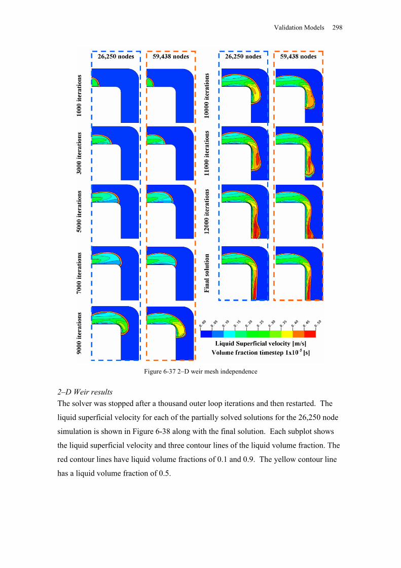
Validation Models 298
Figure 6-37 2–D weir mesh independence
2–D Weir resultsThe solver was stopped after a thousand outer loop iterations and then restarted. The
liquid superficial velocity for each of the partially solved solutions for the 26,250 node
simulation is shown in Figure 6-38 along with the final solution. Each subplot shows
the liquid superficial velocity and three contour lines of the liquid volume fraction. The
red contour lines have liquid volume fractions of 0.1 and 0.9. The yellow contour line
has a liquid volume fraction of 0.5.
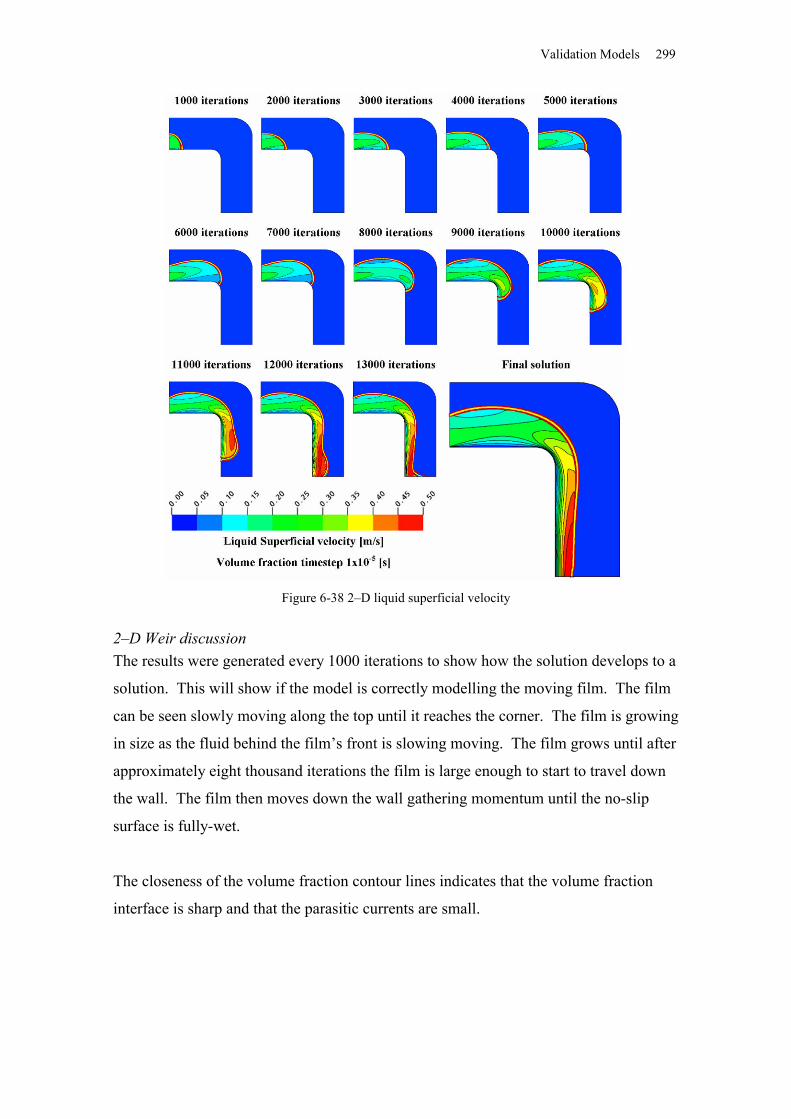
Validation Models 299
Figure 6-38 2–D liquid superficial velocity
2–D Weir discussionThe results were generated every 1000 iterations to show how the solution develops to a
solution. This will show if the model is correctly modelling the moving film. The film
can be seen slowly moving along the top until it reaches the corner. The film is growing
in size as the fluid behind the film’s front is slowing moving. The film grows until after
approximately eight thousand iterations the film is large enough to start to travel down
the wall. The film then moves down the wall gathering momentum until the no-slip
surface is fully-wet.
The closeness of the volume fraction contour lines indicates that the volume fraction
interface is sharp and that the parasitic currents are small.
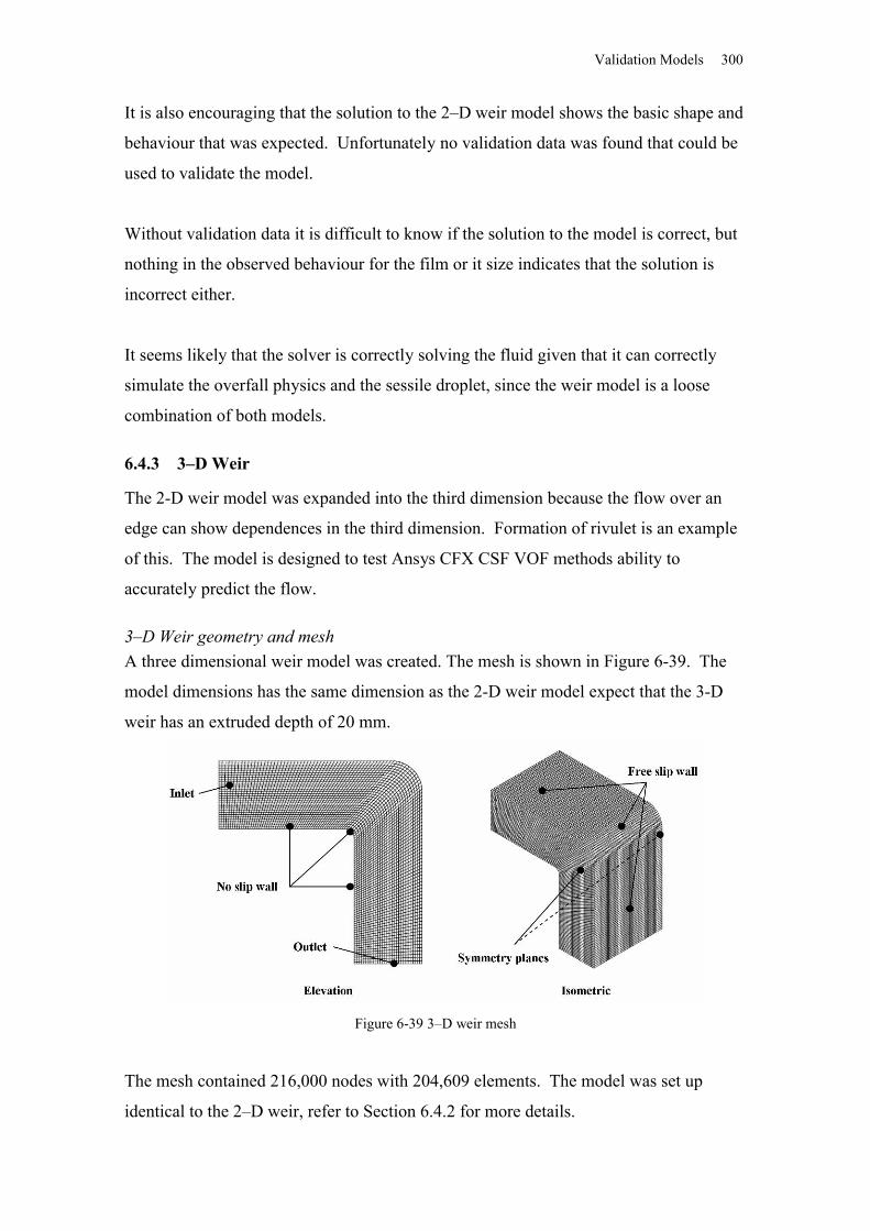
Validation Models 300
It is also encouraging that the solution to the 2–D weir model shows the basic shape and
behaviour that was expected. Unfortunately no validation data was found that could be
used to validate the model.
Without validation data it is difficult to know if the solution to the model is correct, but
nothing in the observed behaviour for the film or it size indicates that the solution is
incorrect either.
It seems likely that the solver is correctly solving the fluid given that it can correctly
simulate the overfall physics and the sessile droplet, since the weir model is a loose
combination of both models.
6.4.3 3–D Weir
The 2-D weir model was expanded into the third dimension because the flow over an
edge can show dependences in the third dimension. Formation of rivulet is an example
of this. The model is designed to test Ansys CFX CSF VOF methods ability to
accurately predict the flow.
3–D Weir geometry and meshA three dimensional weir model was created. The mesh is shown in Figure 6-39. The
model dimensions has the same dimension as the 2-D weir model expect that the 3-D
weir has an extruded depth of 20 mm.
Figure 6-39 3–D weir mesh
The mesh contained 216,000 nodes with 204,609 elements. The model was set up
identical to the 2–D weir, refer to Section 6.4.2 for more details.
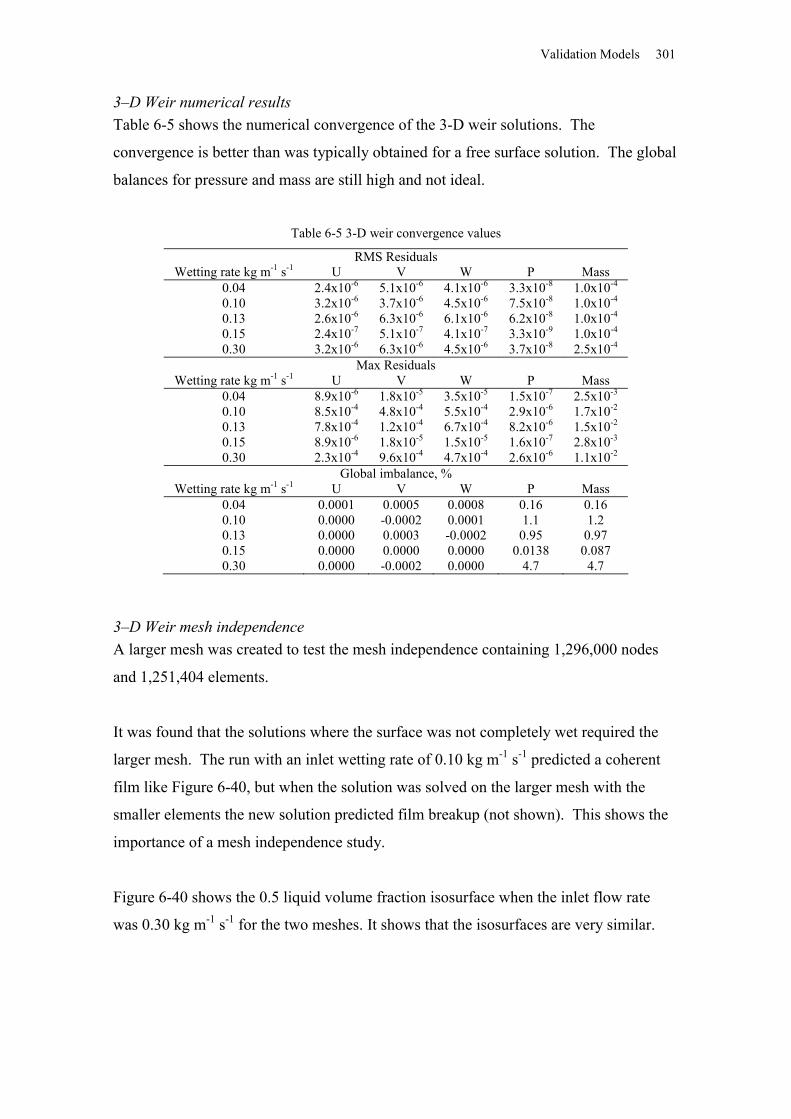
Validation Models 301
3–D Weir numerical resultsTable 6-5 shows the numerical convergence of the 3-D weir solutions. The
convergence is better than was typically obtained for a free surface solution. The global
balances for pressure and mass are still high and not ideal.
Table 6-5 3-D weir convergence values
RMS ResidualsWetting rate kg m-1 s-1 U V W P Mass
0.04 2.4x10⁻⁶ 5.1x10⁻⁶ 4.1x10⁻⁶ 3.3x10⁻⁸ 1.0x10⁻⁴
0.10 3.2x10⁻⁶ 3.7x10⁻⁶ 4.5x10⁻⁶ 7.5x10⁻⁸ 1.0x10⁻⁴
0.13 2.6x10⁻⁶ 6.3x10⁻⁶ 6.1x10⁻⁶ 6.2x10⁻⁸ 1.0x10⁻⁴
0.15 2.4x10⁻⁷ 5.1x10⁻⁷ 4.1x10⁻⁷ 3.3x10⁻⁹ 1.0x10⁻⁴
0.30 3.2x10⁻⁶ 6.3x10⁻⁶ 4.5x10⁻⁶ 3.7x10⁻⁸ 2.5x10⁻⁴
Max ResidualsWetting rate kg m-1 s-1 U V W P Mass
0.04 8.9x10⁻⁶ 1.8x10⁻⁵ 3.5x10⁻⁵ 1.5x10⁻⁷ 2.5x10⁻³
0.10 8.5x10⁻⁴ 4.8x10⁻⁴ 5.5x10⁻⁴ 2.9x10⁻⁶ 1.7x10⁻²
0.13 7.8x10⁻⁴ 1.2x10⁻⁴ 6.7x10⁻⁴ 8.2x10⁻⁶ 1.5x10⁻²
0.15 8.9x10⁻⁶ 1.8x10⁻⁵ 1.5x10⁻⁵ 1.6x10⁻⁷ 2.8x10⁻³
0.30 2.3x10⁻⁴ 9.6x10⁻⁴ 4.7x10⁻⁴ 2.6x10⁻⁶ 1.1x10⁻²
Global imbalance, %Wetting rate kg m-1 s-1 U V W P Mass
0.04 0.0001 0.0005 0.0008 0.16 0.160.10 0.0000 -0.0002 0.0001 1.1 1.20.13 0.0000 0.0003 -0.0002 0.95 0.970.15 0.0000 0.0000 0.0000 0.0138 0.0870.30 0.0000 -0.0002 0.0000 4.7 4.7
3–D Weir mesh independenceA larger mesh was created to test the mesh independence containing 1,296,000 nodes
and 1,251,404 elements.
It was found that the solutions where the surface was not completely wet required the
larger mesh. The run with an inlet wetting rate of 0.10 kg m-1 s-1 predicted a coherent
film like Figure 6-40, but when the solution was solved on the larger mesh with the
smaller elements the new solution predicted film breakup (not shown). This shows the
importance of a mesh independence study.
Figure 6-40 shows the 0.5 liquid volume fraction isosurface when the inlet flow rate
was 0.30 kg m-1 s-1 for the two meshes. It shows that the isosurfaces are very similar.
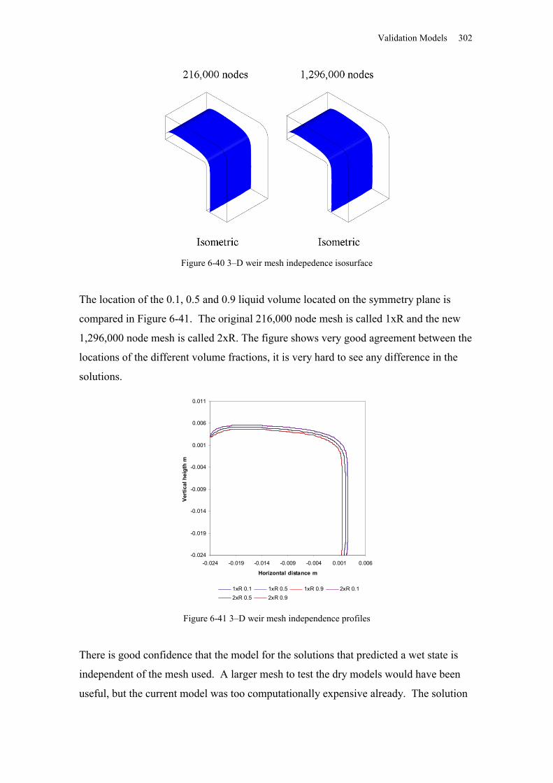
Validation Models 302
Figure 6-40 3–D weir mesh indepedence isosurface
The location of the 0.1, 0.5 and 0.9 liquid volume located on the symmetry plane is
compared in Figure 6-41. The original 216,000 node mesh is called 1xR and the new
1,296,000 node mesh is called 2xR. The figure shows very good agreement between the
locations of the different volume fractions, it is very hard to see any difference in the
solutions.
-0.024
-0.019
-0.014
-0.009
-0.004
0.001
0.006
0.011
-0.024 -0.019 -0.014 -0.009 -0.004 0.001 0.006
Horizontal distance m
Vert
ical
hei
gth
m
1xR 0.1 1xR 0.5 1xR 0.9 2xR 0.12xR 0.5 2xR 0.9
Figure 6-41 3–D weir mesh independence profiles
There is good confidence that the model for the solutions that predicted a wet state is
independent of the mesh used. A larger mesh to test the dry models would have been
useful, but the current model was too computationally expensive already. The solution
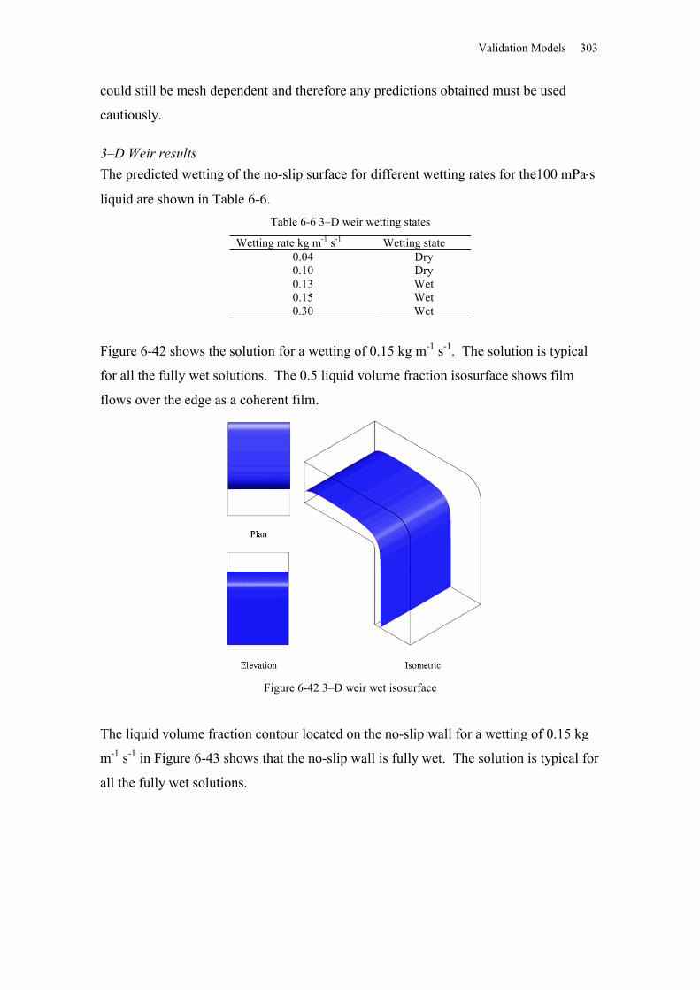
Validation Models 303
could still be mesh dependent and therefore any predictions obtained must be used
cautiously.
3–D Weir resultsThe predicted wetting of the no-slip surface for different wetting rates for the100 mPas
liquid are shown in Table 6-6. Table 6-6 3–D weir wetting states
Wetting rate kg m-1 s-1 Wetting state0.04 Dry0.10 Dry0.13 Wet0.15 Wet0.30 Wet
Figure 6-42 shows the solution for a wetting of 0.15 kg m-1 s-1. The solution is typical
for all the fully wet solutions. The 0.5 liquid volume fraction isosurface shows film
flows over the edge as a coherent film.
Figure 6-42 3–D weir wet isosurface
The liquid volume fraction contour located on the no-slip wall for a wetting of 0.15 kg
m-1 s-1 in Figure 6-43 shows that the no-slip wall is fully wet. The solution is typical for
all the fully wet solutions.
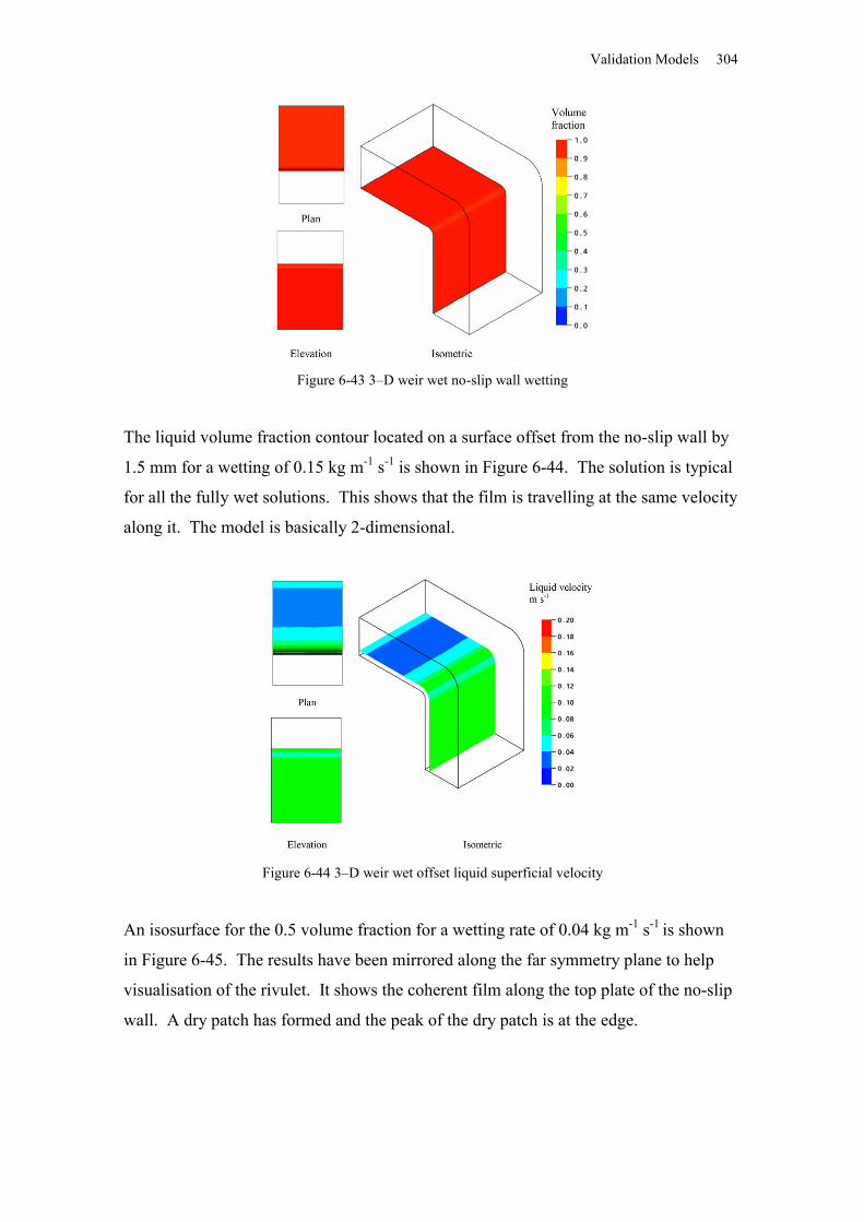
Validation Models 304
Figure 6-43 3–D weir wet no-slip wall wetting
The liquid volume fraction contour located on a surface offset from the no-slip wall by
1.5 mm for a wetting of 0.15 kg m-1 s-1 is shown in Figure 6-44. The solution is typical
for all the fully wet solutions. This shows that the film is travelling at the same velocity
along it. The model is basically 2-dimensional.
Figure 6-44 3–D weir wet offset liquid superficial velocity
An isosurface for the 0.5 volume fraction for a wetting rate of 0.04 kg m-1 s-1 is shown
in Figure 6-45. The results have been mirrored along the far symmetry plane to help
visualisation of the rivulet. It shows the coherent film along the top plate of the no-slip
wall. A dry patch has formed and the peak of the dry patch is at the edge.
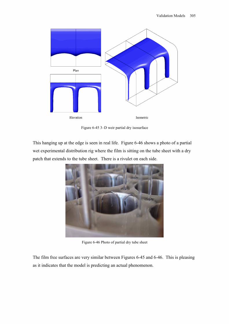
Validation Models 305
Figure 6-45 3–D weir partial dry isosurface
This hanging up at the edge is seen in real life. Figure 6-46 shows a photo of a partial
wet experimental distribution rig where the film is sitting on the tube sheet with a dry
patch that extends to the tube sheet. There is a rivulet on each side.
Figure 6-46 Photo of partial dry tube sheet
The film free surfaces are very similar between Figures 6-45 and 6-46. This is pleasing
as it indicates that the model is predicting an actual phenomenon.
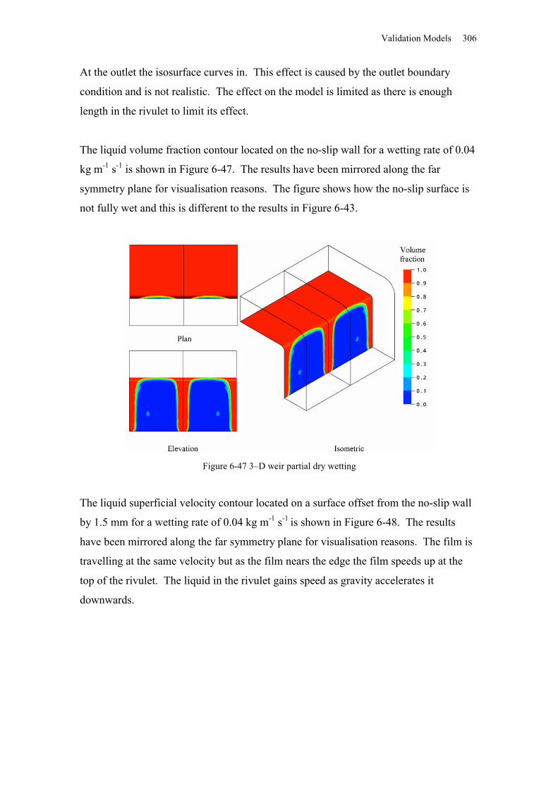
Validation Models 306
At the outlet the isosurface curves in. This effect is caused by the outlet boundary
condition and is not realistic. The effect on the model is limited as there is enough
length in the rivulet to limit its effect.
The liquid volume fraction contour located on the no-slip wall for a wetting rate of 0.04
kg m-1 s-1 is shown in Figure 6-47. The results have been mirrored along the far
symmetry plane for visualisation reasons. The figure shows how the no-slip surface is
not fully wet and this is different to the results in Figure 6-43.
Figure 6-47 3–D weir partial dry wetting
The liquid superficial velocity contour located on a surface offset from the no-slip wall
by 1.5 mm for a wetting rate of 0.04 kg m-1 s-1 is shown in Figure 6-48. The results
have been mirrored along the far symmetry plane for visualisation reasons. The film is
travelling at the same velocity but as the film nears the edge the film speeds up at the
top of the rivulet. The liquid in the rivulet gains speed as gravity accelerates it
downwards.
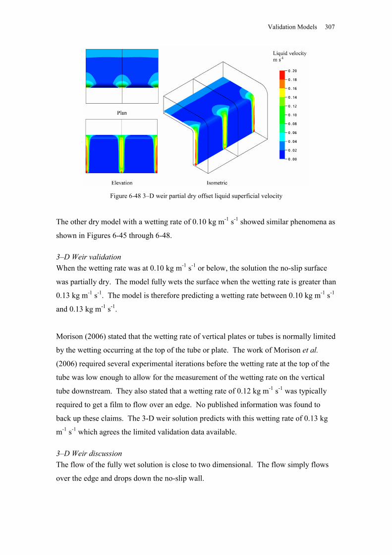
Validation Models 307
Figure 6-48 3–D weir partial dry offset liquid superficial velocity
The other dry model with a wetting rate of 0.10 kg m-1 s-1 showed similar phenomena as
shown in Figures 6-45 through 6-48.
3–D Weir validationWhen the wetting rate was at 0.10 kg m-1 s-1 or below, the solution the no-slip surface
was partially dry. The model fully wets the surface when the wetting rate is greater than
0.13 kg m-1 s-1. The model is therefore predicting a wetting rate between 0.10 kg m-1 s-1
and 0.13 kg m-1 s-1.
Morison (2006) stated that the wetting rate of vertical plates or tubes is normally limited
by the wetting occurring at the top of the tube or plate. The work of Morison et al.
(2006) required several experimental iterations before the wetting rate at the top of the
tube was low enough to allow for the measurement of the wetting rate on the vertical
tube downstream. They also stated that a wetting rate of 0.12 kg m-1 s-1 was typically
required to get a film to flow over an edge. No published information was found to
back up these claims. The 3-D weir solution predicts with this wetting rate of 0.13 kg
m-1 s-1 which agrees the limited validation data available.
3–D Weir discussionThe flow of the fully wet solution is close to two dimensional. The flow simply flows
over the edge and drops down the no-slip wall.
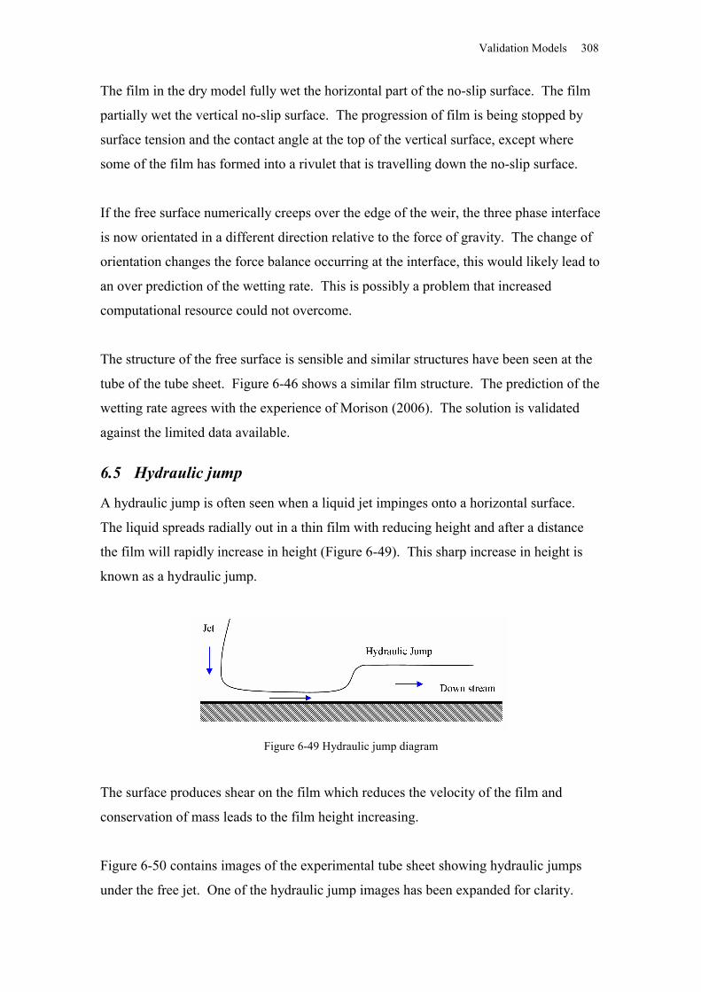
Validation Models 308
The film in the dry model fully wet the horizontal part of the no-slip surface. The film
partially wet the vertical no-slip surface. The progression of film is being stopped by
surface tension and the contact angle at the top of the vertical surface, except where
some of the film has formed into a rivulet that is travelling down the no-slip surface.
If the free surface numerically creeps over the edge of the weir, the three phase interface
is now orientated in a different direction relative to the force of gravity. The change of
orientation changes the force balance occurring at the interface, this would likely lead to
an over prediction of the wetting rate. This is possibly a problem that increased
computational resource could not overcome.
The structure of the free surface is sensible and similar structures have been seen at the
tube of the tube sheet. Figure 6-46 shows a similar film structure. The prediction of the
wetting rate agrees with the experience of Morison (2006). The solution is validated
against the limited data available.
6.5 Hydraulic jump
A hydraulic jump is often seen when a liquid jet impinges onto a horizontal surface.
The liquid spreads radially out in a thin film with reducing height and after a distance
the film will rapidly increase in height (Figure 6-49). This sharp increase in height is
known as a hydraulic jump.
Figure 6-49 Hydraulic jump diagram
The surface produces shear on the film which reduces the velocity of the film and
conservation of mass leads to the film height increasing.
Figure 6-50 contains images of the experimental tube sheet showing hydraulic jumps
under the free jet. One of the hydraulic jump images has been expanded for clarity.
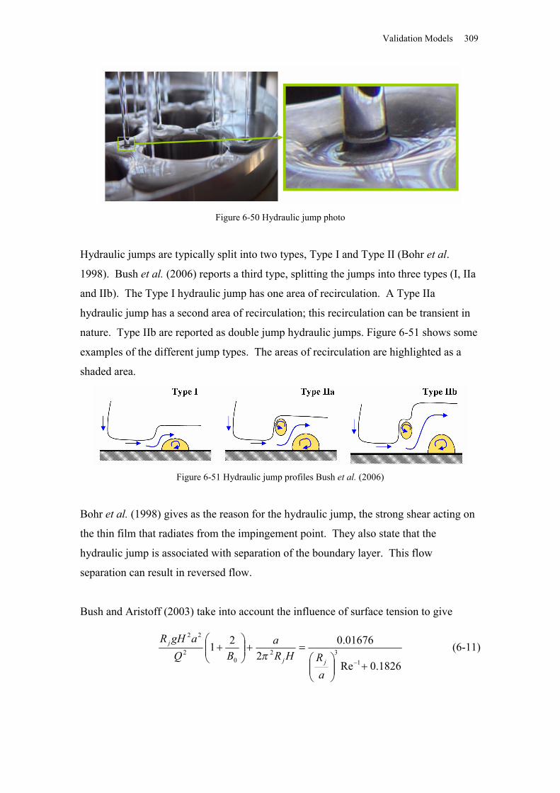
Validation Models 309
Figure 6-50 Hydraulic jump photo
Hydraulic jumps are typically split into two types, Type I and Type II (Bohr et al.
1998). Bush et al. (2006) reports a third type, splitting the jumps into three types (I, IIa
and IIb). The Type I hydraulic jump has one area of recirculation. A Type IIa
hydraulic jump has a second area of recirculation; this recirculation can be transient in
nature. Type IIb are reported as double jump hydraulic jumps. Figure 6-51 shows some
examples of the different jump types. The areas of recirculation are highlighted as a
shaded area.
Figure 6-51 Hydraulic jump profiles Bush et al. (2006)
Bohr et al. (1998) gives as the reason for the hydraulic jump, the strong shear acting on
the thin film that radiates from the impingement point. They also state that the
hydraulic jump is associated with separation of the boundary layer. This flow
separation can result in reversed flow.
Bush and Aristoff (2003) take into account the influence of surface tension to give
1826.0Re
01676.02
211
320
2
22
aRHR
aBQ
agHR
jj
j
(6-11)
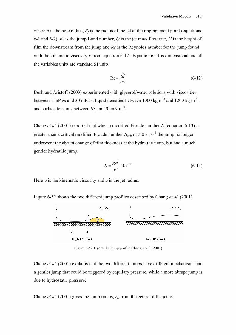
Validation Models 310
where a is the hole radius, Rj is the radius of the jet at the impingement point (equations
6-1 and 6-2), B0 is the jump Bond number, Q is the jet mass flow rate, H is the height of
film the downstream from the jump and Re is the Reynolds number for the jump found
with the kinematic viscosity from equation 6-12. Equation 6-11 is dimensional and all
the variables units are standard SI units.
aQ
Re (6-12)
Bush and Aristoff (2003) experimented with glycerol/water solutions with viscosities
between 1 mPa·s and 30 mPa·s, liquid densities between 1000 kg m-3 and 1200 kg m-3,
and surface tensions between 65 and 70 mN m-1.
Chang et al. (2001) reported that when a modified Froude number (equation 6-13) is
greater than a critical modified Froude number crit of 3.0 x 10⁻⁴ the jump no longer
underwent the abrupt change of film thickness at the hydraulic jump, but had a much
gentler hydraulic jump.
3/72
3
Reag (6-13)
Here is the kinematic viscosity and a is the jet radius.
Figure 6-52 shows the two different jump profiles described by Chang et al. (2001).
Figure 6-52 Hydraulic jump profile Chang et al. (2001)
Chang et al. (2001) explains that the two different jumps have different mechanisms and
a gentler jump that could be triggered by capillary pressure, while a more abrupt jump is
due to hydrostatic pressure.
Chang et al. (2001) gives the jump radius, rj, from the centre of the jet as
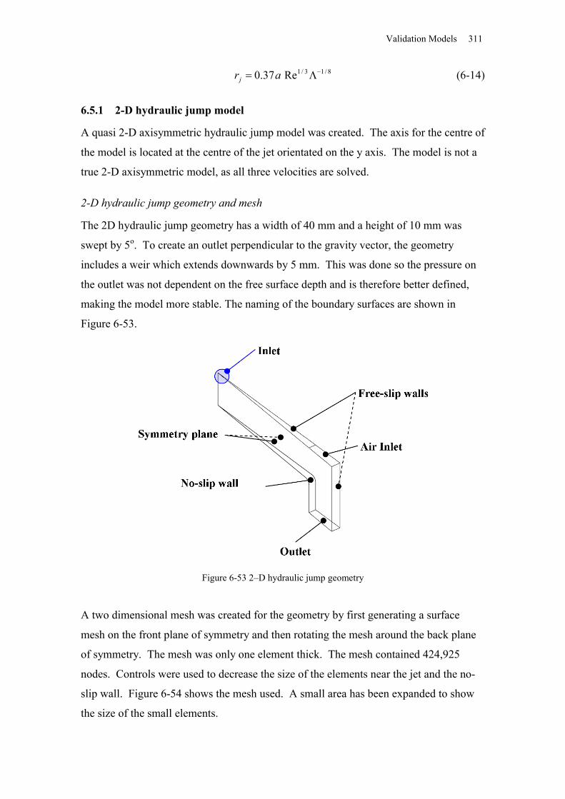
Validation Models 311
8/13/1Re37.0 ar j (6-14)
6.5.1 2-D hydraulic jump model
A quasi 2-D axisymmetric hydraulic jump model was created. The axis for the centre of
the model is located at the centre of the jet orientated on the y axis. The model is not a
true 2-D axisymmetric model, as all three velocities are solved.
2-D hydraulic jump geometry and mesh
The 2D hydraulic jump geometry has a width of 40 mm and a height of 10 mm was
swept by 5o. To create an outlet perpendicular to the gravity vector, the geometry
includes a weir which extends downwards by 5 mm. This was done so the pressure on
the outlet was not dependent on the free surface depth and is therefore better defined,
making the model more stable. The naming of the boundary surfaces are shown in
Figure 6-53.
Figure 6-53 2–D hydraulic jump geometry
A two dimensional mesh was created for the geometry by first generating a surface
mesh on the front plane of symmetry and then rotating the mesh around the back plane
of symmetry. The mesh was only one element thick. The mesh contained 424,925
nodes. Controls were used to decrease the size of the elements near the jet and the no-
slip wall. Figure 6-54 shows the mesh used. A small area has been expanded to show
the size of the small elements.
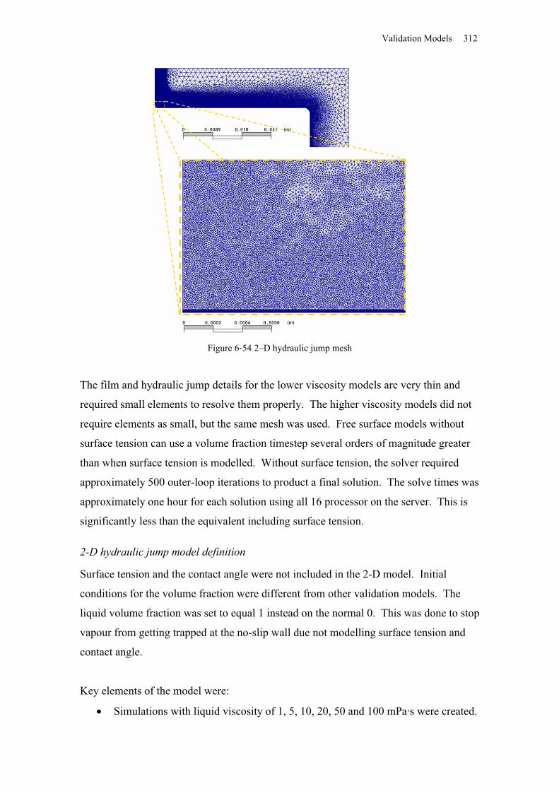
Validation Models 312
Figure 6-54 2–D hydraulic jump mesh
The film and hydraulic jump details for the lower viscosity models are very thin and
required small elements to resolve them properly. The higher viscosity models did not
require elements as small, but the same mesh was used. Free surface models without
surface tension can use a volume fraction timestep several orders of magnitude greater
than when surface tension is modelled. Without surface tension, the solver required
approximately 500 outer-loop iterations to product a final solution. The solve times was
approximately one hour for each solution using all 16 processor on the server. This is
significantly less than the equivalent including surface tension.
2-D hydraulic jump model definition
Surface tension and the contact angle were not included in the 2-D model. Initial
conditions for the volume fraction were different from other validation models. The
liquid volume fraction was set to equal 1 instead on the normal 0. This was done to stop
vapour from getting trapped at the no-slip wall due not modelling surface tension and
contact angle.
Key elements of the model were:
Simulations with liquid viscosity of 1, 5, 10, 20, 50 and 100 mPa·s were created.
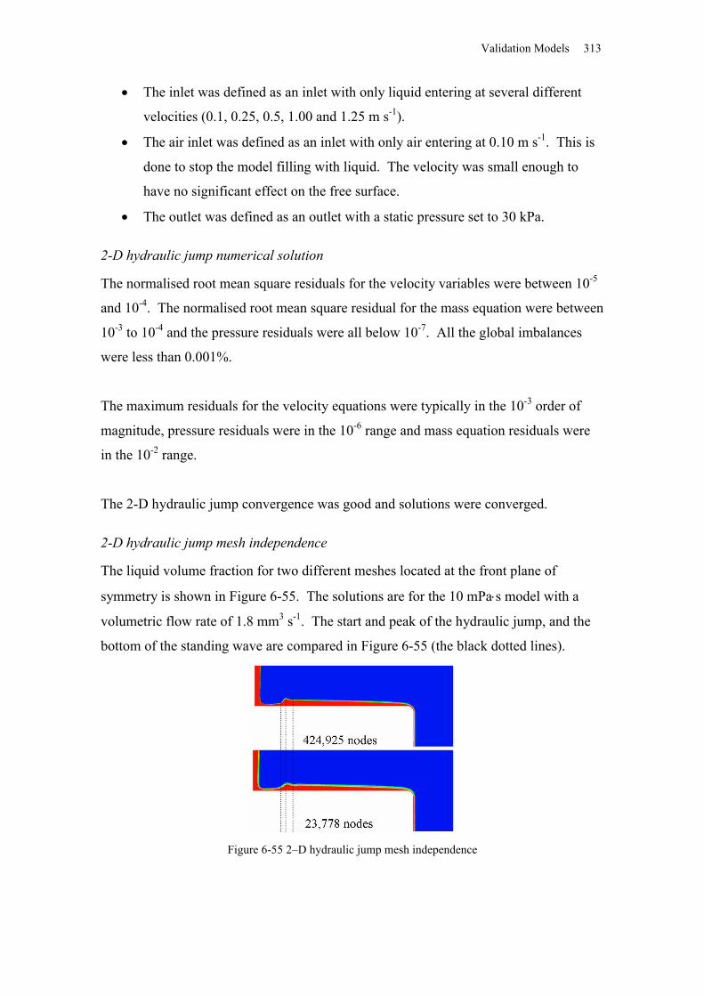
Validation Models 313
The inlet was defined as an inlet with only liquid entering at several different
velocities (0.1, 0.25, 0.5, 1.00 and 1.25 m s-1).
The air inlet was defined as an inlet with only air entering at 0.10 m s-1. This is
done to stop the model filling with liquid. The velocity was small enough to
have no significant effect on the free surface.
The outlet was defined as an outlet with a static pressure set to 30 kPa.
2-D hydraulic jump numerical solution
The normalised root mean square residuals for the velocity variables were between 10-5
and 10-4. The normalised root mean square residual for the mass equation were between
10-3 to 10-4 and the pressure residuals were all below 10-7. All the global imbalances
were less than 0.001%.
The maximum residuals for the velocity equations were typically in the 10-3 order of
magnitude, pressure residuals were in the 10-6 range and mass equation residuals were
in the 10-2 range.
The 2-D hydraulic jump convergence was good and solutions were converged.
2-D hydraulic jump mesh independence
The liquid volume fraction for two different meshes located at the front plane of
symmetry is shown in Figure 6-55. The solutions are for the 10 mPas model with a
volumetric flow rate of 1.8 mm3 s-1. The start and peak of the hydraulic jump, and the
bottom of the standing wave are compared in Figure 6-55 (the black dotted lines).
Figure 6-55 2–D hydraulic jump mesh independence
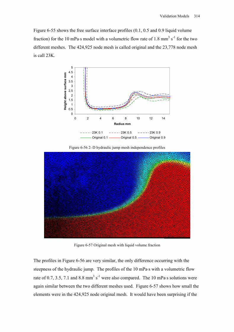
Validation Models 314
Figure 6-55 shows the free surface interface profiles (0.1, 0.5 and 0.9 liquid volume
fraction) for the 10 mPas model with a volumetric flow rate of 1.8 mm3 s-1 for the two
different meshes. The 424,925 node mesh is called original and the 23,778 node mesh
is call 23K.
00.5
11.5
22.5
33.5
44.5
5
0 2 4 6 8 10 12 14
Radius mm
Hei
ght a
bove
sur
face
mm
23K 0.1 23K 0.5 23K 0.9Original 0.1 Original 0.5 Original 0.9
Figure 6-56 2–D hydraulic jump mesh independence profiles
Figure 6-57 Original mesh with liquid volume fraction
The profiles in Figure 6-56 are very similar, the only difference occurring with the
steepness of the hydraulic jump. The profiles of the 10 mPas with a volumetric flow
rate of 0.7, 3.5, 7.1 and 8.8 mm3 s-1 were also compared. The 10 mPas solutions were
again similar between the two different meshes used. Figure 6-57 shows how small the
elements were in the 424,925 node original mesh. It would have been surprising if the
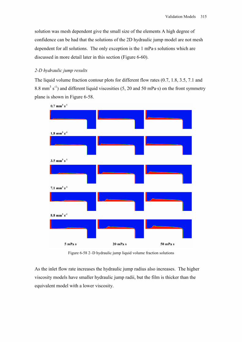
Validation Models 315
solution was mesh dependent give the small size of the elements A high degree of
confidence can be had that the solutions of the 2D hydraulic jump model are not mesh
dependent for all solutions. The only exception is the 1 mPas solutions which are
discussed in more detail later in this section (Figure 6-60).
2-D hydraulic jump results
The liquid volume fraction contour plots for different flow rates (0.7, 1.8, 3.5, 7.1 and
8.8 mm3 s-1) and different liquid viscosities (5, 20 and 50 mPa·s) on the front symmetry
plane is shown in Figure 6-58.
Figure 6-58 2–D hydraulic jump liquid volume fraction solutions
As the inlet flow rate increases the hydraulic jump radius also increases. The higher
viscosity models have smaller hydraulic jump radii, but the film is thicker than the
equivalent model with a lower viscosity.
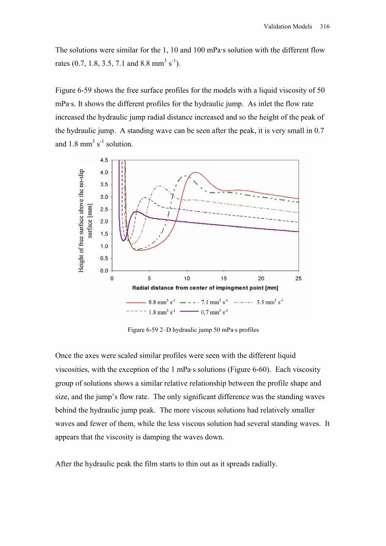
Validation Models 316
The solutions were similar for the 1, 10 and 100 mPa·s solution with the different flow
rates (0.7, 1.8, 3.5, 7.1 and 8.8 mm3 s-1).
Figure 6-59 shows the free surface profiles for the models with a liquid viscosity of 50
mPa·s. It shows the different profiles for the hydraulic jump. As inlet the flow rate
increased the hydraulic jump radial distance increased and so the height of the peak of
the hydraulic jump. A standing wave can be seen after the peak, it is very small in 0.7
and 1.8 mm3 s-1 solution.
Figure 6-59 2–D hydraulic jump 50 mPas profiles
Once the axes were scaled similar profiles were seen with the different liquid
viscosities, with the exception of the 1 mPas solutions (Figure 6-60). Each viscosity
group of solutions shows a similar relative relationship between the profile shape and
size, and the jump’s flow rate. The only significant difference was the standing waves
behind the hydraulic jump peak. The more viscous solutions had relatively smaller
waves and fewer of them, while the less viscous solution had several standing waves. It
appears that the viscosity is damping the waves down.
After the hydraulic peak the film starts to thin out as it spreads radially.
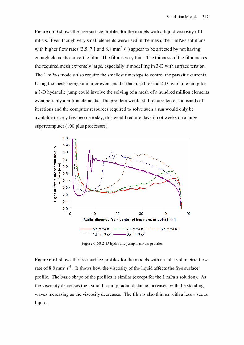
Validation Models 317
Figure 6-60 shows the free surface profiles for the models with a liquid viscosity of 1
mPa·s. Even though very small elements were used in the mesh, the 1 mPas solutions
with higher flow rates (3.5, 7.1 and 8.8 mm3 s-1) appear to be affected by not having
enough elements across the film. The film is very thin. The thinness of the film makes
the required mesh extremely large, especially if modelling in 3-D with surface tension.
The 1 mPas models also require the smallest timesteps to control the parasitic currents.
Using the mesh sizing similar or even smaller than used for the 2-D hydraulic jump for
a 3-D hydraulic jump could involve the solving of a mesh of a hundred million elements
even possibly a billion elements. The problem would still require ten of thousands of
iterations and the computer resources required to solve such a run would only be
available to very few people today, this would require days if not weeks on a large
supercomputer (100 plus processors).
Figure 6-60 2–D hydraulic jump 1 mPas profiles
Figure 6-61 shows the free surface profiles for the models with an inlet volumetric flow
rate of 8.8 mm3 s-1. It shows how the viscosity of the liquid affects the free surface
profile. The basic shape of the profiles is similar (except for the 1 mPas solution). As
the viscosity decreases the hydraulic jump radial distance increases, with the standing
waves increasing as the viscosity decreases. The film is also thinner with a less viscous
liquid.
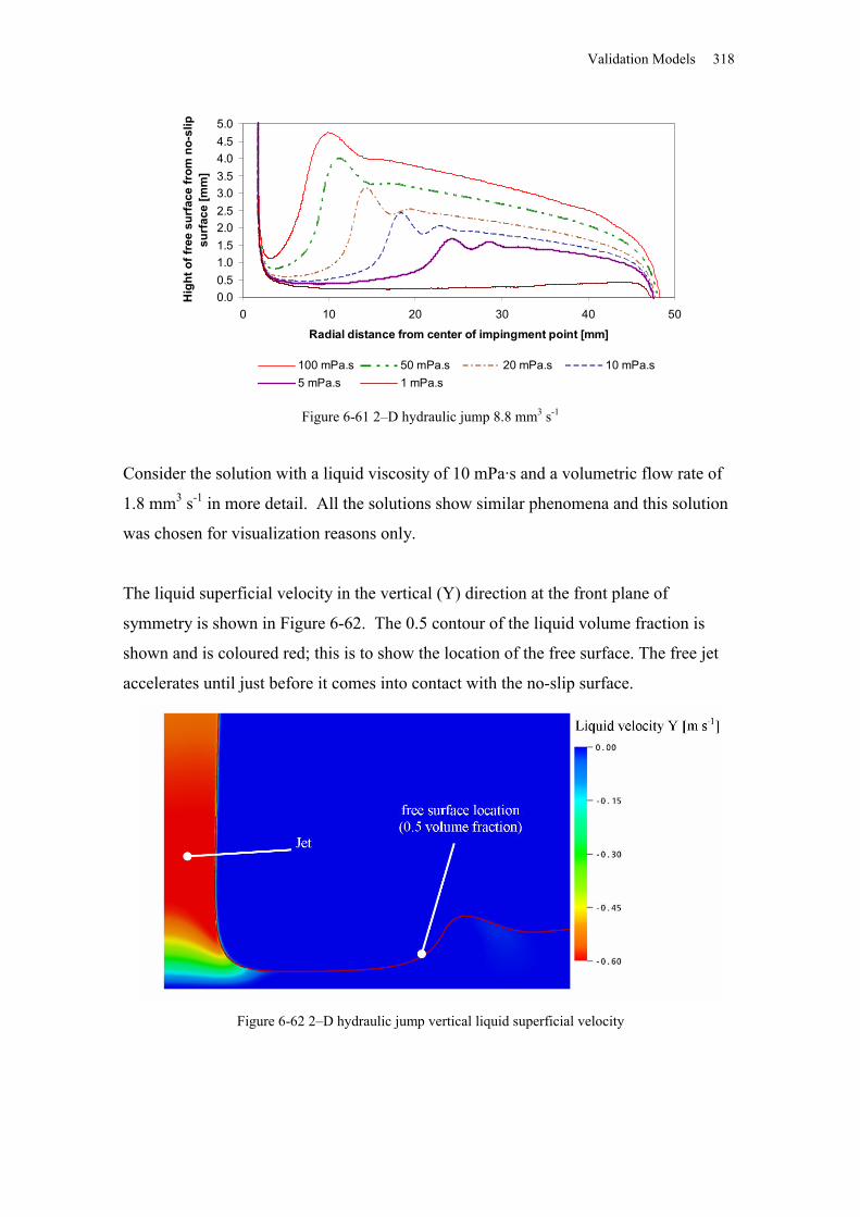
Validation Models 318
0.00.51.01.52.02.53.03.54.04.55.0
0 10 20 30 40 50
Radial distance from center of impingment point [mm]
Hig
ht o
f fre
e su
rfac
e fr
om n
o-sl
ip
surf
ace
[mm
]
100 mPa.s 50 mPa.s 20 mPa.s 10 mPa.s5 mPa.s 1 mPa.s
Figure 6-61 2–D hydraulic jump 8.8 mm3 s-1
Consider the solution with a liquid viscosity of 10 mPa·s and a volumetric flow rate of
1.8 mm3 s-1 in more detail. All the solutions show similar phenomena and this solution
was chosen for visualization reasons only.
The liquid superficial velocity in the vertical (Y) direction at the front plane of
symmetry is shown in Figure 6-62. The 0.5 contour of the liquid volume fraction is
shown and is coloured red; this is to show the location of the free surface. The free jet
accelerates until just before it comes into contact with the no-slip surface.
Figure 6-62 2–D hydraulic jump vertical liquid superficial velocity
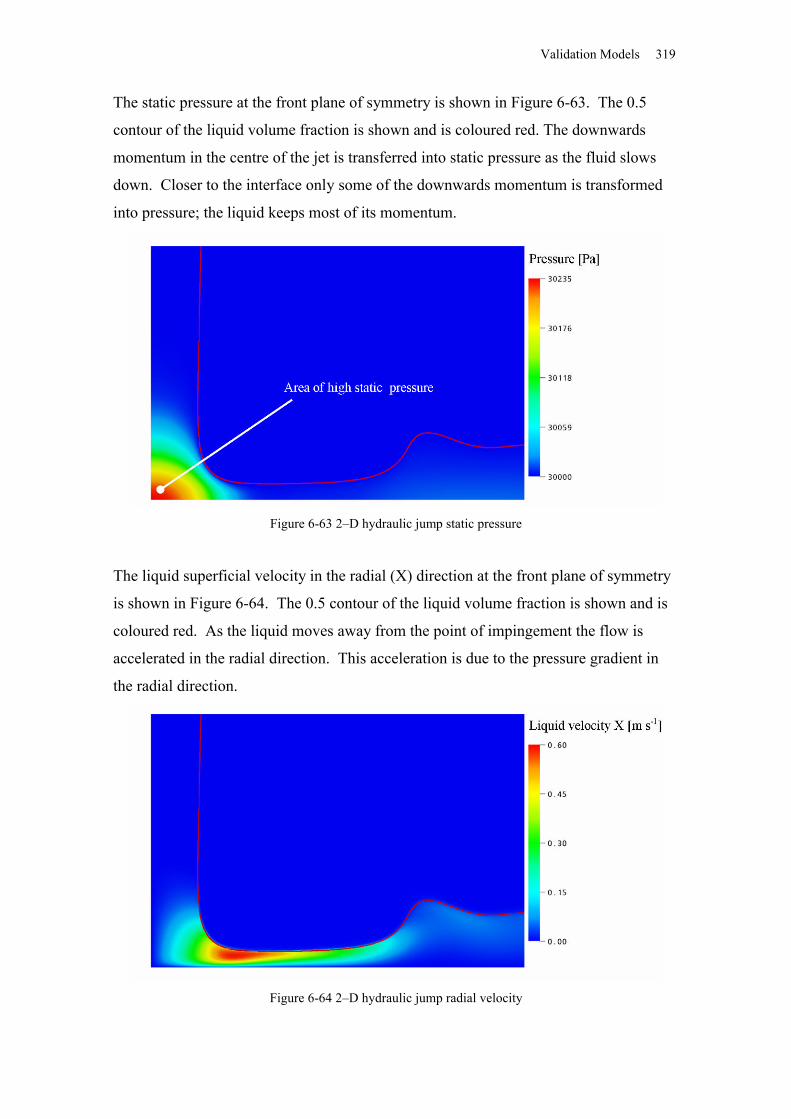
Validation Models 319
The static pressure at the front plane of symmetry is shown in Figure 6-63. The 0.5
contour of the liquid volume fraction is shown and is coloured red. The downwards
momentum in the centre of the jet is transferred into static pressure as the fluid slows
down. Closer to the interface only some of the downwards momentum is transformed
into pressure; the liquid keeps most of its momentum.
Figure 6-63 2–D hydraulic jump static pressure
The liquid superficial velocity in the radial (X) direction at the front plane of symmetry
is shown in Figure 6-64. The 0.5 contour of the liquid volume fraction is shown and is
coloured red. As the liquid moves away from the point of impingement the flow is
accelerated in the radial direction. This acceleration is due to the pressure gradient in
the radial direction.
Figure 6-64 2–D hydraulic jump radial velocity
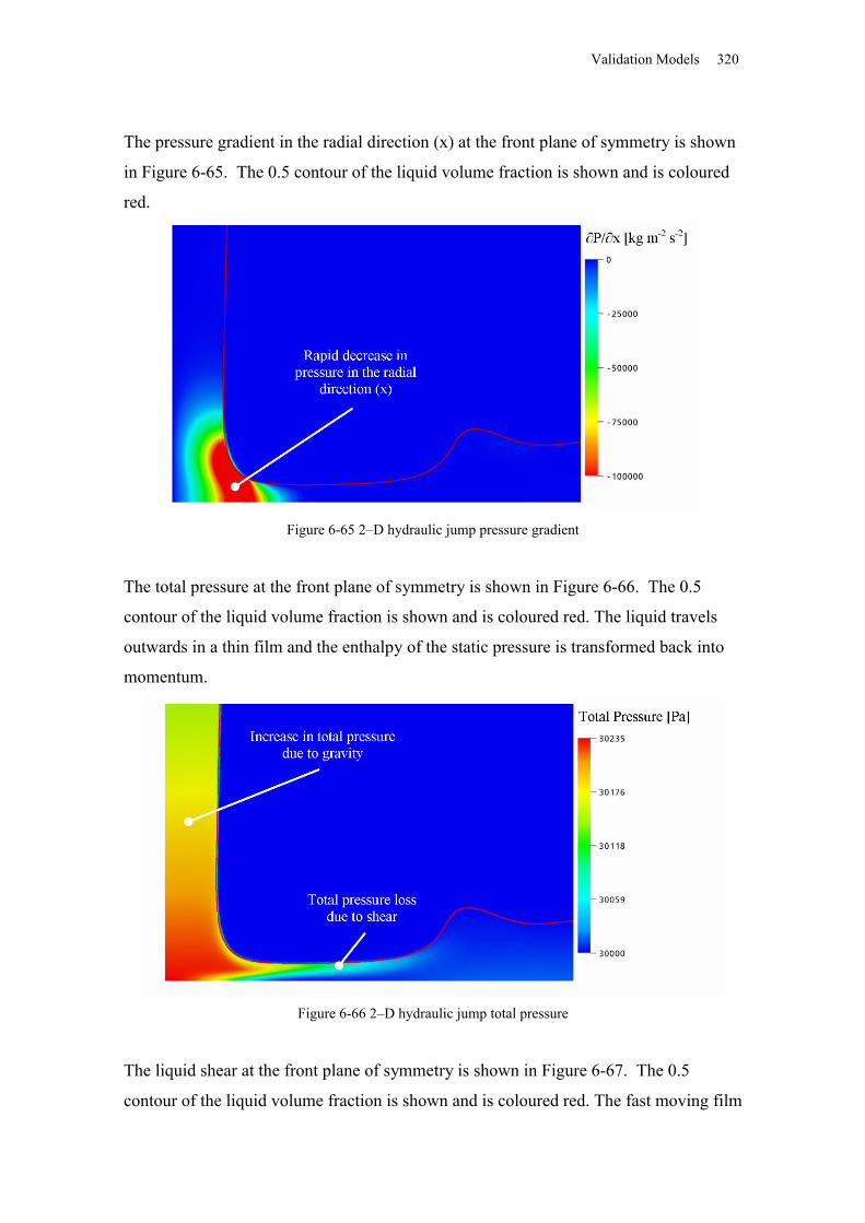
Validation Models 320
The pressure gradient in the radial direction (x) at the front plane of symmetry is shown
in Figure 6-65. The 0.5 contour of the liquid volume fraction is shown and is coloured
red.
Figure 6-65 2–D hydraulic jump pressure gradient
The total pressure at the front plane of symmetry is shown in Figure 6-66. The 0.5
contour of the liquid volume fraction is shown and is coloured red. The liquid travels
outwards in a thin film and the enthalpy of the static pressure is transformed back into
momentum.
Figure 6-66 2–D hydraulic jump total pressure
The liquid shear at the front plane of symmetry is shown in Figure 6-67. The 0.5
contour of the liquid volume fraction is shown and is coloured red. The fast moving film
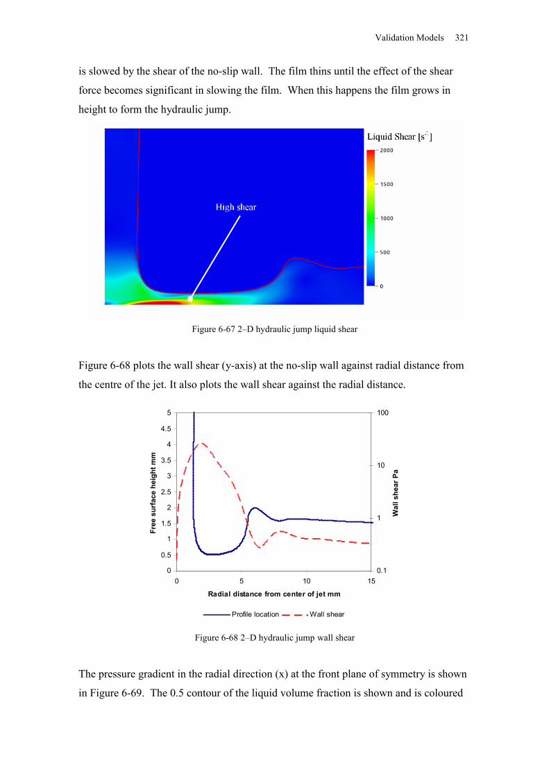
Validation Models 321
is slowed by the shear of the no-slip wall. The film thins until the effect of the shear
force becomes significant in slowing the film. When this happens the film grows in
height to form the hydraulic jump.
Figure 6-67 2–D hydraulic jump liquid shear
Figure 6-68 plots the wall shear (y-axis) at the no-slip wall against radial distance from
the centre of the jet. It also plots the wall shear against the radial distance.
0
0.5
1
1.5
2
2.5
3
3.5
4
4.5
5
0 5 10 15
Radial distance from center of jet mm
Free
sur
face
hei
ght m
m
0.1
1
10
100
Wal
l she
ar P
a
Profile location Wall shear
Figure 6-68 2–D hydraulic jump wall shear
The pressure gradient in the radial direction (x) at the front plane of symmetry is shown
in Figure 6-69. The 0.5 contour of the liquid volume fraction is shown and is coloured
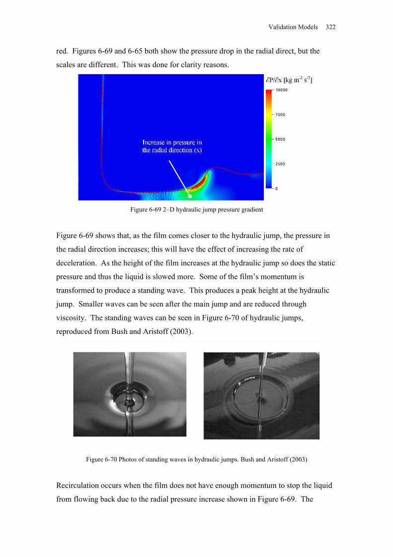
Validation Models 322
red. Figures 6-69 and 6-65 both show the pressure drop in the radial direct, but the
scales are different. This was done for clarity reasons.
Figure 6-69 2–D hydraulic jump pressure gradient
Figure 6-69 shows that, as the film comes closer to the hydraulic jump, the pressure in
the radial direction increases; this will have the effect of increasing the rate of
deceleration. As the height of the film increases at the hydraulic jump so does the static
pressure and thus the liquid is slowed more. Some of the film’s momentum is
transformed to produce a standing wave. This produces a peak height at the hydraulic
jump. Smaller waves can be seen after the main jump and are reduced through
viscosity. The standing waves can be seen in Figure 6-70 of hydraulic jumps,
reproduced from Bush and Aristoff (2003).
Figure 6-70 Photos of standing waves in hydraulic jumps. Bush and Aristoff (2003)
Recirculation occurs when the film does not have enough momentum to stop the liquid
from flowing back due to the radial pressure increase shown in Figure 6-69. The
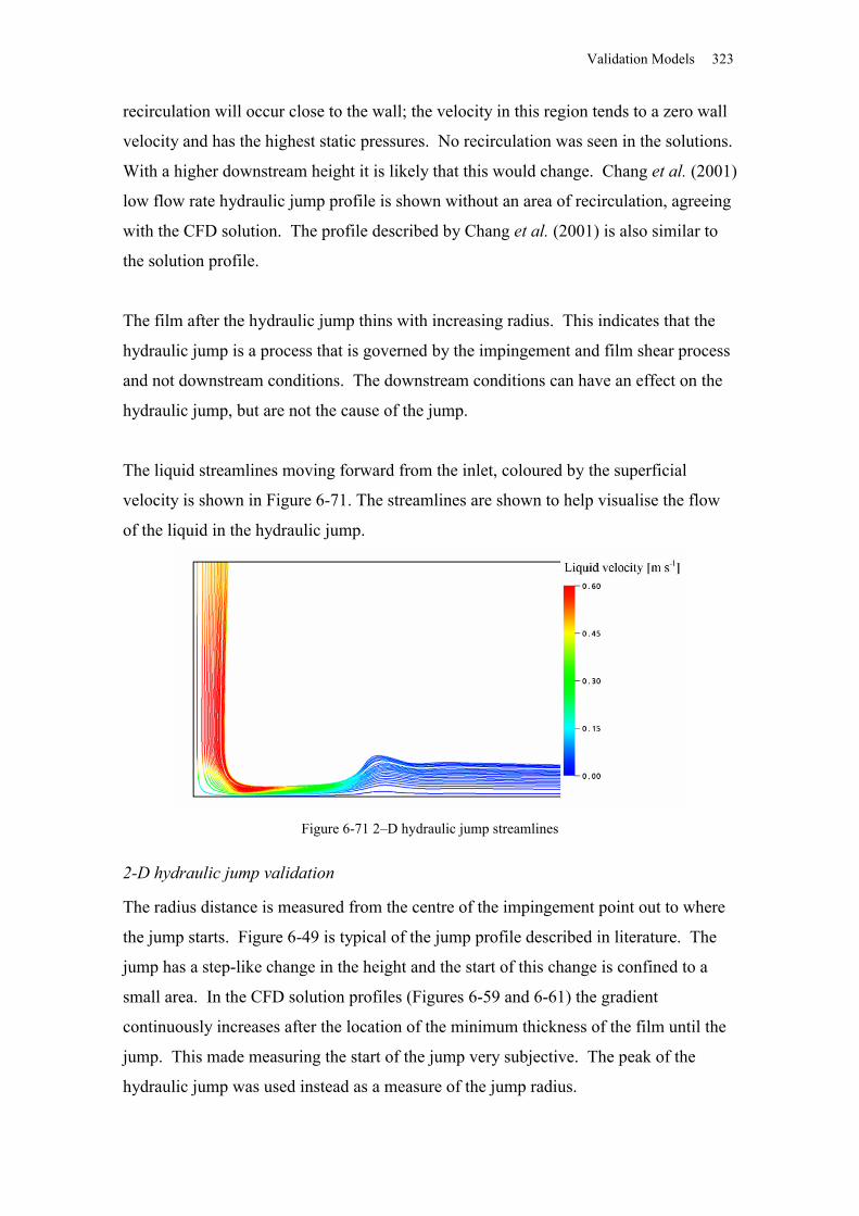
Validation Models 323
recirculation will occur close to the wall; the velocity in this region tends to a zero wall
velocity and has the highest static pressures. No recirculation was seen in the solutions.
With a higher downstream height it is likely that this would change. Chang et al. (2001)
low flow rate hydraulic jump profile is shown without an area of recirculation, agreeing
with the CFD solution. The profile described by Chang et al. (2001) is also similar to
the solution profile.
The film after the hydraulic jump thins with increasing radius. This indicates that the
hydraulic jump is a process that is governed by the impingement and film shear process
and not downstream conditions. The downstream conditions can have an effect on the
hydraulic jump, but are not the cause of the jump.
The liquid streamlines moving forward from the inlet, coloured by the superficial
velocity is shown in Figure 6-71. The streamlines are shown to help visualise the flow
of the liquid in the hydraulic jump.
Figure 6-71 2–D hydraulic jump streamlines
2-D hydraulic jump validation
The radius distance is measured from the centre of the impingement point out to where
the jump starts. Figure 6-49 is typical of the jump profile described in literature. The
jump has a step-like change in the height and the start of this change is confined to a
small area. In the CFD solution profiles (Figures 6-59 and 6-61) the gradient
continuously increases after the location of the minimum thickness of the film until the
jump. This made measuring the start of the jump very subjective. The peak of the
hydraulic jump was used instead as a measure of the jump radius.
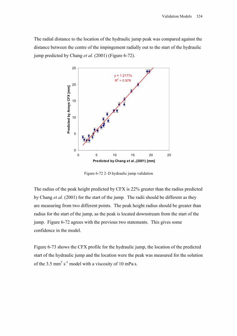
Validation Models 324
The radial distance to the location of the hydraulic jump peak was compared against the
distance between the centre of the impingement radially out to the start of the hydraulic
jump predicted by Chang et al. (2001) (Figure 6-72).
y = 1.2177xR2 = 0.979
0
5
10
15
20
25
0 5 10 15 20 25
Predicted by Chang et al.,(2001) [mm]
Pred
icte
d by
Ans
ys C
FX [m
m]
Figure 6-72 2–D hydraulic jump validation
The radius of the peak height predicted by CFX is 22% greater than the radius predicted
by Chang et al. (2001) for the start of the jump. The radii should be different as they
are measuring from two different points. The peak height radius should be greater than
radius for the start of the jump, as the peak is located downstream from the start of the
jump. Figure 6-72 agrees with the previous two statements. This gives some
confidence in the model.
Figure 6-73 shows the CFX profile for the hydraulic jump, the location of the predicted
start of the hydraulic jump and the location were the peak was measured for the solution
of the 3.5 mm3 s-1 model with a viscosity of 10 mPas.
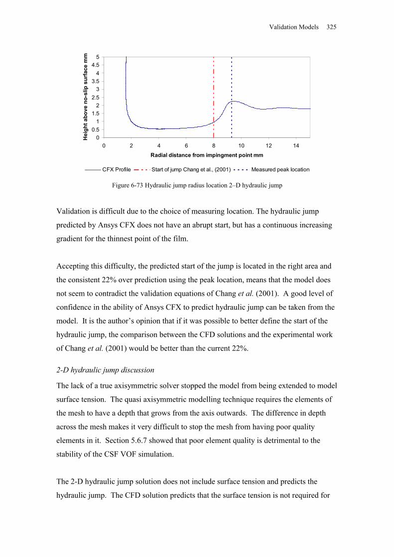
Validation Models 325
00.5
11.5
22.5
33.5
44.5
5
0 2 4 6 8 10 12 14
Radial distance from impingment point mm
Hei
ght a
bove
no-
slip
sur
face
mm
CFX Profile Start of jump Chang et al., (2001) Measured peak location
Figure 6-73 Hydraulic jump radius location 2–D hydraulic jump
Validation is difficult due to the choice of measuring location. The hydraulic jump
predicted by Ansys CFX does not have an abrupt start, but has a continuous increasing
gradient for the thinnest point of the film.
Accepting this difficulty, the predicted start of the jump is located in the right area and
the consistent 22% over prediction using the peak location, means that the model does
not seem to contradict the validation equations of Chang et al. (2001). A good level of
confidence in the ability of Ansys CFX to predict hydraulic jump can be taken from the
model. It is the author’s opinion that if it was possible to better define the start of the
hydraulic jump, the comparison between the CFD solutions and the experimental work
of Chang et al. (2001) would be better than the current 22%.
2-D hydraulic jump discussion
The lack of a true axisymmetric solver stopped the model from being extended to model
surface tension. The quasi axisymmetric modelling technique requires the elements of
the mesh to have a depth that grows from the axis outwards. The difference in depth
across the mesh makes it very difficult to stop the mesh from having poor quality
elements in it. Section 5.6.7 showed that poor element quality is detrimental to the
stability of the CSF VOF simulation.
The 2-D hydraulic jump solution does not include surface tension and predicts the
hydraulic jump. The CFD solution predicts that the surface tension is not required for
Validation Models 326
hydraulic jump occur. It is likely that surface tension would affect the shape or size of
any jump.
When using the homogeneous velocity model it was common for vapour to get
“trapped” on the no-slip wall underneath the liquid phase. At a no-slip wall the velocity
is by definition zero, therefore the vapour cannot move away from the surface. It was
possible to overcome this problem by:
using a heterogeneous model
using surface tension and wall adhesion
using an initial guess that has a liquid phase by the wall
The “trapping” of the vapour phase was only a problem for the 2-D hydraulic jump
model as all the other models were modelled with surface tension and wall adhesion,
except the overfall model (Section 6.4.1) which has only free-slip wall conditions and
therefore the vapour does not get trapped.
Chang et al. (2001) describes two different jump profiles: a “gentle” profile and a
“classical" profile. All 0.7, 1.8 and 3.5 mm3 s-1 jumps and the two highest viscosity
jumps of the 7.1 mm3 s-1 jumps Chang et al. (2001) predicts to have “gentler” jump
profiles and the remaining conditions are predicted to have “classical” jump profiles.
The CFD solutions do not agree with this conclusion as only one basic profile shape
was seen (excluding the 1 mPas solutions that required a smaller mesh).
No area of recirculation was seen in the hydraulic jumps. The downstream height for all
the jumps was less than 5 mm. The “gentler” profile of Chang et al. (2001) does not
have an area of recirculation. It is possible that there are two types of hydraulic jumps
as Chang et al. (2001) concludes and either the 2-D hydraulic jump solutions are
incorrect or the Chang et al. (2001) criteria for type of jump is incorrect.
With a higher downstream height an area of recirculation is more likely due to the
higher static pressures involved, but this was not tested here.
Validation Models 327
The 2-D hydraulic jump model shows the difficulty in validating a model against a
physical phenomenon when the phenomenon is not well understood. But some
confidence can be had in the ability of the VOF method to simulate the hydraulic jump,
as it is able to predict a hydraulic jump including predicting the standing waves that are
seen on hydraulic jumps.
Improving the validation data, especially by using a better defined location on the jump
to measure would help the validation of the 2-D hydraulic jump model. Extending the
model to simulate different downstream conditions would allow the model to be used to
gain a much better understanding of the mechanisms behind hydraulic jumps.
Hydraulic jump controlControlling the hydraulic jump radius would be useful. It is expected that the
distribution rate for a distribution design will be related to the hydraulic jump. The
CFD solutions show some agreement with the work of Chang et al. (2001). The
following shows how the hydraulic jump can be manipulated by changing the hole
radius. Ideally this study would have been complete using the CFD tools solving
including surface tension, this was not possible due to computational resource
limitations.
Combining equations 6-11, 6-12 and 6-13, and rearranging gives
8/13/7
2
33/1
37.0
aQag
aQar j (6-15)
For a given flow rate and liquid viscosity, equation 6-15 can be shown to equal
875.5arj (6-16)
This means that for a given flow rate the size of the hydraulic jump can be changed by
changing the hole radius.
Toricelli’s equation describes the flow through a hole as
ghACQ d 2 (6-17)
where h is the head above the hole and Cd is the discharge coefficient.
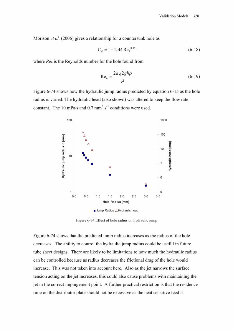
Validation Models 328
Morison et al. (2006) gives a relationship for a countersunk hole as
36.0Re44.21 hdC (6-18)
where Reh is the Reynolds number for the hole found from
gha
h22
Re (6-19)
Figure 6-74 shows how the hydraulic jump radius predicted by equation 6-15 as the hole
radius is varied. The hydraulic head (also shown) was altered to keep the flow rate
constant. The 10 mPas and 0.7 mm3 s-1 conditions were used.
1
10
100
0.0 0.5 1.0 1.5 2.0 2.5 3.0 3.5
Hole Radius [mm]
Hyd
raul
ic ju
mp
radi
us r
j [m
m]
0
0
1
10
100
1000
Hyd
raul
ic h
ead
[mm
]
Jump Radius Hydraulic head
Figure 6-74 Effect of hole radius on hydraulic jump
Figure 6-74 shows that the predicted jump radius increases as the radius of the hole
decreases. The ability to control the hydraulic jump radius could be useful in future
tube sheet designs. There are likely to be limitations to how much the hydraulic radius
can be controlled because as radius decreases the frictional drag of the hole would
increase. This was not taken into account here. Also as the jet narrows the surface
tension acting on the jet increases, this could also cause problems with maintaining the
jet in the correct impingement point. A further practical restriction is that the residence
time on the distributor plate should not be excessive as the heat sensitive feed is
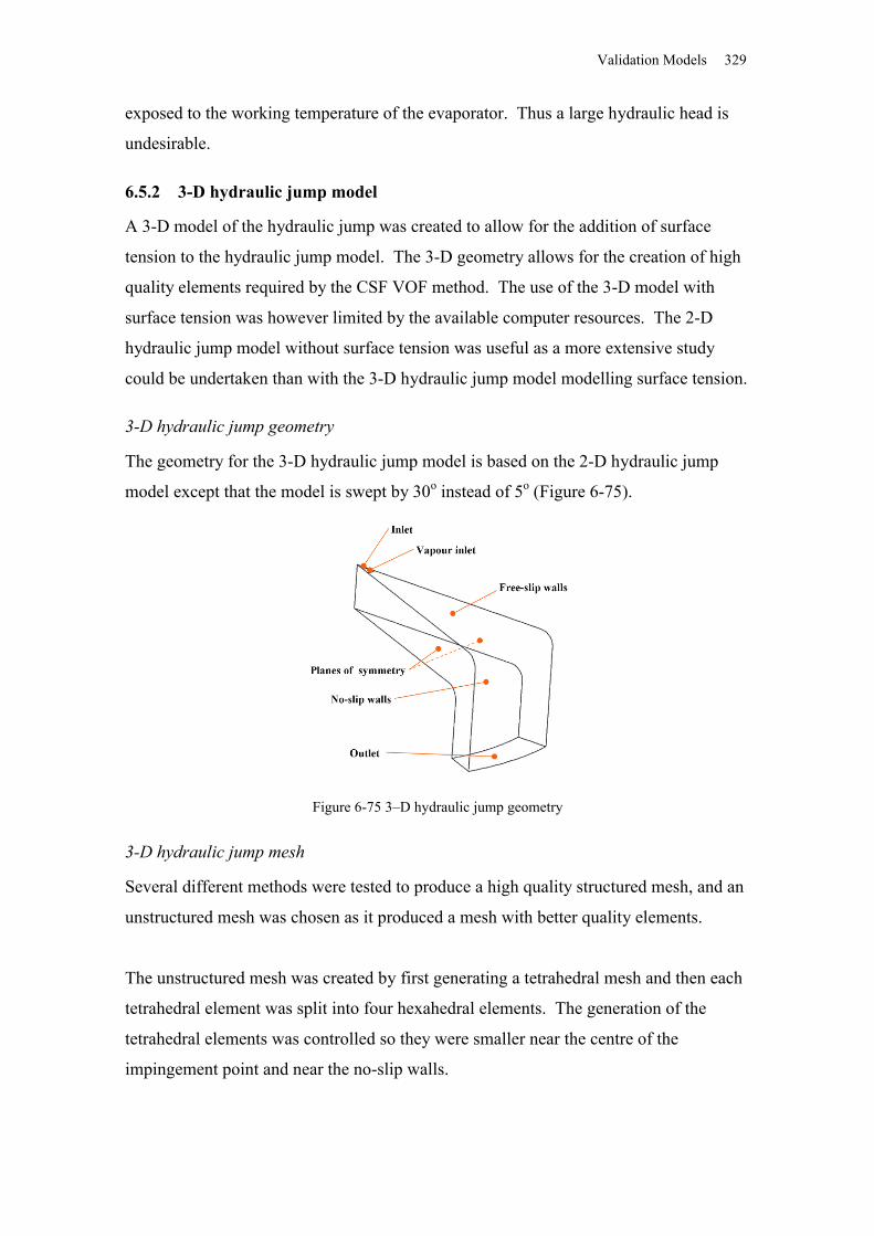
Validation Models 329
exposed to the working temperature of the evaporator. Thus a large hydraulic head is
undesirable.
6.5.2 3-D hydraulic jump model
A 3-D model of the hydraulic jump was created to allow for the addition of surface
tension to the hydraulic jump model. The 3-D geometry allows for the creation of high
quality elements required by the CSF VOF method. The use of the 3-D model with
surface tension was however limited by the available computer resources. The 2-D
hydraulic jump model without surface tension was useful as a more extensive study
could be undertaken than with the 3-D hydraulic jump model modelling surface tension.
3-D hydraulic jump geometry
The geometry for the 3-D hydraulic jump model is based on the 2-D hydraulic jump
model except that the model is swept by 30o instead of 5o (Figure 6-75).
Figure 6-75 3–D hydraulic jump geometry
3-D hydraulic jump mesh
Several different methods were tested to produce a high quality structured mesh, and an
unstructured mesh was chosen as it produced a mesh with better quality elements.
The unstructured mesh was created by first generating a tetrahedral mesh and then each
tetrahedral element was split into four hexahedral elements. The generation of the
tetrahedral elements was controlled so they were smaller near the centre of the
impingement point and near the no-slip walls.
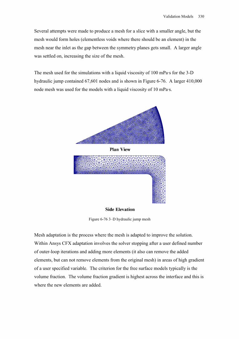
Validation Models 330
Several attempts were made to produce a mesh for a slice with a smaller angle, but the
mesh would form holes (elementless voids where there should be an element) in the
mesh near the inlet as the gap between the symmetry planes gets small. A larger angle
was settled on, increasing the size of the mesh.
The mesh used for the simulations with a liquid viscosity of 100 mPa·s for the 3-D
hydraulic jump contained 67,601 nodes and is shown in Figure 6-76. A larger 410,000
node mesh was used for the models with a liquid viscosity of 10 mPa·s.
Figure 6-76 3–D hydraulic jump mesh
Mesh adaptation is the process where the mesh is adapted to improve the solution.
Within Ansys CFX adaptation involves the solver stopping after a user defined number
of outer-loop iterations and adding more elements (it also can remove the added
elements, but can not remove elements from the original mesh) in areas of high gradient
of a user specified variable. The criterion for the free surface models typically is the
volume fraction. The volume fraction gradient is highest across the interface and this is
where the new elements are added.
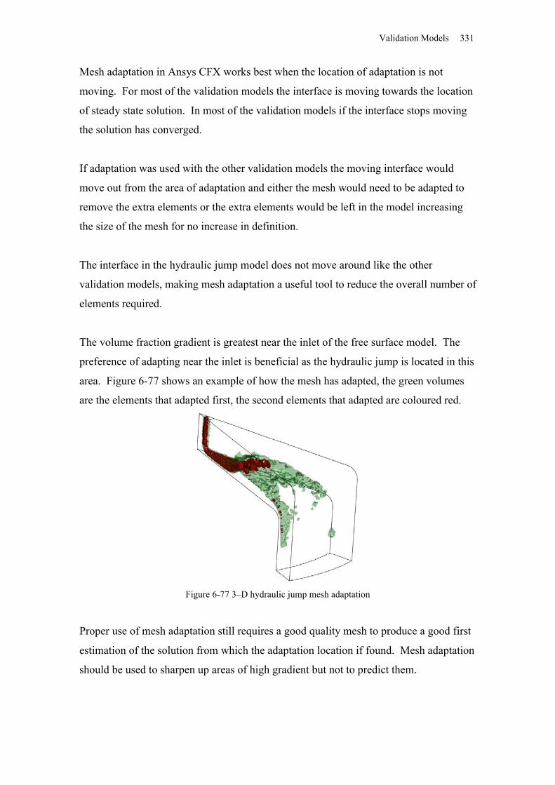
Validation Models 331
Mesh adaptation in Ansys CFX works best when the location of adaptation is not
moving. For most of the validation models the interface is moving towards the location
of steady state solution. In most of the validation models if the interface stops moving
the solution has converged.
If adaptation was used with the other validation models the moving interface would
move out from the area of adaptation and either the mesh would need to be adapted to
remove the extra elements or the extra elements would be left in the model increasing
the size of the mesh for no increase in definition.
The interface in the hydraulic jump model does not move around like the other
validation models, making mesh adaptation a useful tool to reduce the overall number of
elements required.
The volume fraction gradient is greatest near the inlet of the free surface model. The
preference of adapting near the inlet is beneficial as the hydraulic jump is located in this
area. Figure 6-77 shows an example of how the mesh has adapted, the green volumes
are the elements that adapted first, the second elements that adapted are coloured red.
Figure 6-77 3–D hydraulic jump mesh adaptation
Proper use of mesh adaptation still requires a good quality mesh to produce a good first
estimation of the solution from which the adaptation location if found. Mesh adaptation
should be used to sharpen up areas of high gradient but not to predict them.
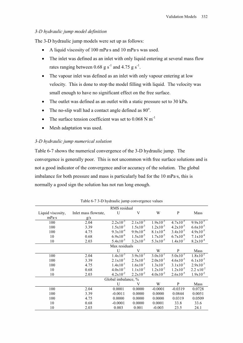
Validation Models 332
3-D hydraulic jump model definition
The 3-D hydraulic jump models were set up as follows:
A liquid viscosity of 100 mPa·s and 10 mPa·s was used.
The inlet was defined as an inlet with only liquid entering at several mass flow
rates ranging between 0.68 g s-1 and 4.75 g s-1.
The vapour inlet was defined as an inlet with only vapour entering at low
velocity. This is done to stop the model filling with liquid. The velocity was
small enough to have no significant effect on the free surface.
The outlet was defined as an outlet with a static pressure set to 30 kPa.
The no-slip wall had a contact angle defined as 80o.
The surface tension coefficient was set to 0.068 N m-1
Mesh adaptation was used.
3-D hydraulic jump numerical solution
Table 6-7 shows the numerical convergence of the 3-D hydraulic jump. The
convergence is generally poor. This is not uncommon with free surface solutions and is
not a good indicator of the convergence and/or accuracy of the solution. The global
imbalance for both pressure and mass is particularly bad for the 10 mPa·s, this is
normally a good sign the solution has not run long enough.
Table 6-7 3-D hydraulic jump convergence values
RMS residualLiquid viscosity,
mPa·sInlet mass flowrate,
g/sU V W P Mass
100 2.04 2.2x10⁻³ 2.1x10⁻³ 1.9x10⁻³ 4.7x10⁻⁵ 9.9x10⁻⁵
100 3.39 1.5x10⁻³ 1.5x10⁻³ 1.2x10⁻³ 4.2x10⁻⁵ 6.6x10⁻⁵
100 4.75 9.3x10⁻⁴ 9.9x10⁻⁴ 8.1x10⁻⁴ 3.4x10⁻⁵ 4.9x10⁻⁵
10 0.68 6.9x10⁻⁶ 1.5x10⁻⁵ 1.7x10⁻⁵ 6.7x10⁻⁸ 7.1x10⁻⁴
10 2.03 5.4x10⁻⁵ 3.2x10⁻⁵ 5.3x10⁻⁵ 1.4x10⁻⁷ 8.2x10⁻⁴
Max residualsU V W P Mass
100 2.04 1.4x10⁻³ 3.9x10⁻¹ 3.0x10⁻¹ 5.0x10⁻³ 1.8x10⁻²
100 3.39 2.1x10⁻¹ 2.5x10⁻¹ 2.0x10⁻¹ 4.6x10⁻³ 6.1x10⁻³
100 4.75 1.4x10⁻¹ 1.6x10⁻¹ 1.3x10⁻¹ 3.1x10⁻³ 2.9x10⁻³
10 0.68 4.0x10⁻³ 1.1x10⁻² 1.2x10⁻² 1.2x10⁻⁵ 2.2 x10⁻²
10 2.03 4.2x10⁻² 2.2x10⁻² 4.0x10⁻² 2.6x10⁻⁵ 1.9x10⁻²
Global imbalance, %U V W P Mass
100 2.04 0.0001 0.0000 -0.0001 -0.0319 0.0728100 3.39 -0.0011 0.0000 0.0000 0.0844 0.0051100 4.75 0.0000 0.0000 0.0000 0.0319 0.050910 0.68 -0.0001 0.0000 0.0001 33.8 33.610 2.03 0.003 0.001 -0.003 23.5 24.1
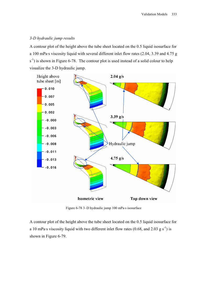
Validation Models 333
3-D hydraulic jump results
A contour plot of the height above the tube sheet located on the 0.5 liquid isosurface for
a 100 mPa·s viscosity liquid with several different inlet flow rates (2.04, 3.39 and 4.75 g
s-1) is shown in Figure 6-78. The contour plot is used instead of a solid colour to help
visualize the 3-D hydraulic jump.
Figure 6-78 3–D hydraulic jump 100 mPas isosurface
A contour plot of the height above the tube sheet located on the 0.5 liquid isosurface for
a 10 mPa·s viscosity liquid with two different inlet flow rates (0.68, and 2.03 g s-1) is
shown in Figure 6-79.
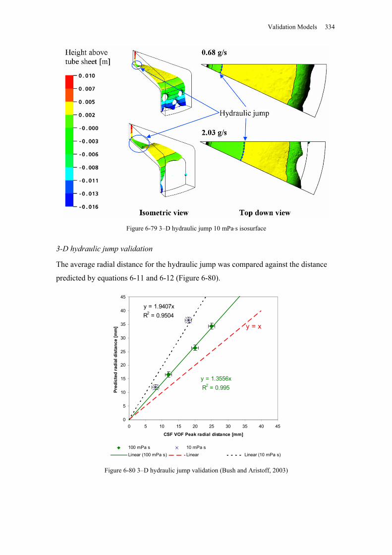
Validation Models 334
Figure 6-79 3–D hydraulic jump 10 mPas isosurface
3-D hydraulic jump validation
The average radial distance for the hydraulic jump was compared against the distance
predicted by equations 6-11 and 6-12 (Figure 6-80).
y = 1.3556xR2 = 0.995
y = x
y = 1.9407xR2 = 0.9504
0
5
10
15
20
25
30
35
40
45
0 5 10 15 20 25 30 35 40 45
CSF VOF Peak radial distance [mm]
Pred
icte
d ra
dial
dis
tanc
e [m
m]
100 mPa s 10 mPa sLinear (100 mPa s) Linear Linear (10 mPa s)
Figure 6-80 3–D hydraulic jump validation (Bush and Aristoff, 2003)
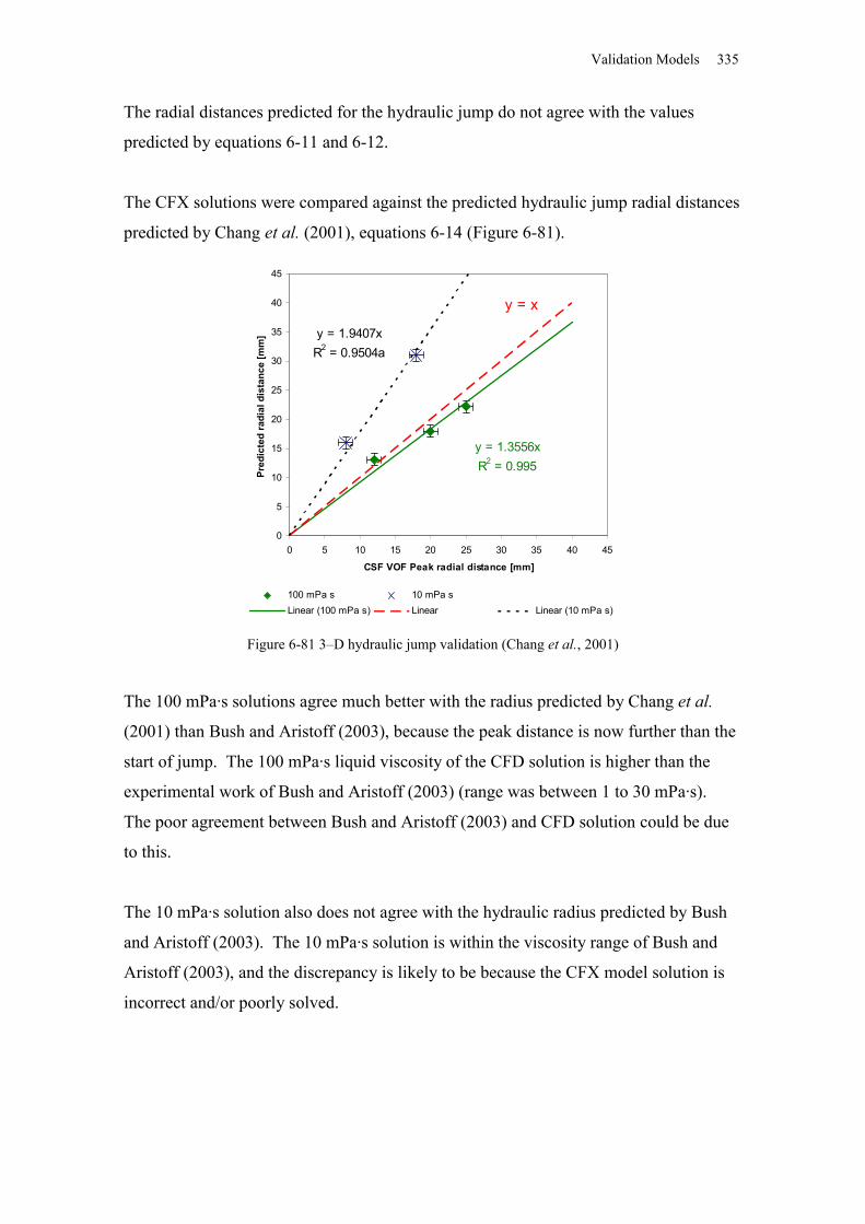
Validation Models 335
The radial distances predicted for the hydraulic jump do not agree with the values
predicted by equations 6-11 and 6-12.
The CFX solutions were compared against the predicted hydraulic jump radial distances
predicted by Chang et al. (2001), equations 6-14 (Figure 6-81).
y = 1.3556xR2 = 0.995
y = x
y = 1.9407xR2 = 0.9504a
0
5
10
15
20
25
30
35
40
45
0 5 10 15 20 25 30 35 40 45
CSF VOF Peak radial distance [mm]
Pred
icte
d ra
dial
dis
tanc
e [m
m]
100 mPa s 10 mPa sLinear (100 mPa s) Linear Linear (10 mPa s)
Figure 6-81 3–D hydraulic jump validation (Chang et al., 2001)
The 100 mPa·s solutions agree much better with the radius predicted by Chang et al.
(2001) than Bush and Aristoff (2003), because the peak distance is now further than the
start of jump. The 100 mPa·s liquid viscosity of the CFD solution is higher than the
experimental work of Bush and Aristoff (2003) (range was between 1 to 30 mPa·s).
The poor agreement between Bush and Aristoff (2003) and CFD solution could be due
to this.
The 10 mPa·s solution also does not agree with the hydraulic radius predicted by Bush
and Aristoff (2003). The 10 mPa·s solution is within the viscosity range of Bush and
Aristoff (2003), and the discrepancy is likely to be because the CFX model solution is
incorrect and/or poorly solved.
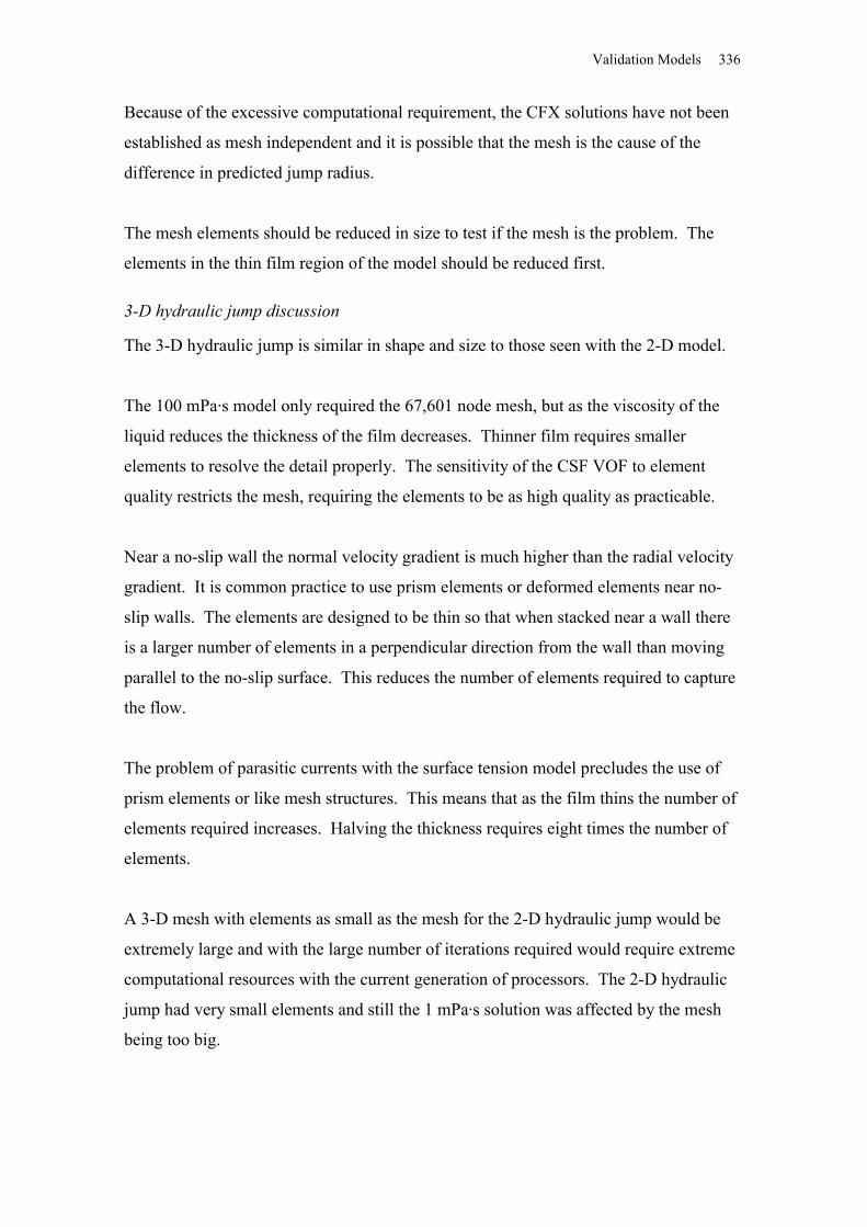
Validation Models 336
Because of the excessive computational requirement, the CFX solutions have not been
established as mesh independent and it is possible that the mesh is the cause of the
difference in predicted jump radius.
The mesh elements should be reduced in size to test if the mesh is the problem. The
elements in the thin film region of the model should be reduced first.
3-D hydraulic jump discussion
The 3-D hydraulic jump is similar in shape and size to those seen with the 2-D model.
The 100 mPa·s model only required the 67,601 node mesh, but as the viscosity of the
liquid reduces the thickness of the film decreases. Thinner film requires smaller
elements to resolve the detail properly. The sensitivity of the CSF VOF to element
quality restricts the mesh, requiring the elements to be as high quality as practicable.
Near a no-slip wall the normal velocity gradient is much higher than the radial velocity
gradient. It is common practice to use prism elements or deformed elements near no-
slip walls. The elements are designed to be thin so that when stacked near a wall there
is a larger number of elements in a perpendicular direction from the wall than moving
parallel to the no-slip surface. This reduces the number of elements required to capture
the flow.
The problem of parasitic currents with the surface tension model precludes the use of
prism elements or like mesh structures. This means that as the film thins the number of
elements required increases. Halving the thickness requires eight times the number of
elements.
A 3-D mesh with elements as small as the mesh for the 2-D hydraulic jump would be
extremely large and with the large number of iterations required would require extreme
computational resources with the current generation of processors. The 2-D hydraulic
jump had very small elements and still the 1 mPa·s solution was affected by the mesh
being too big.
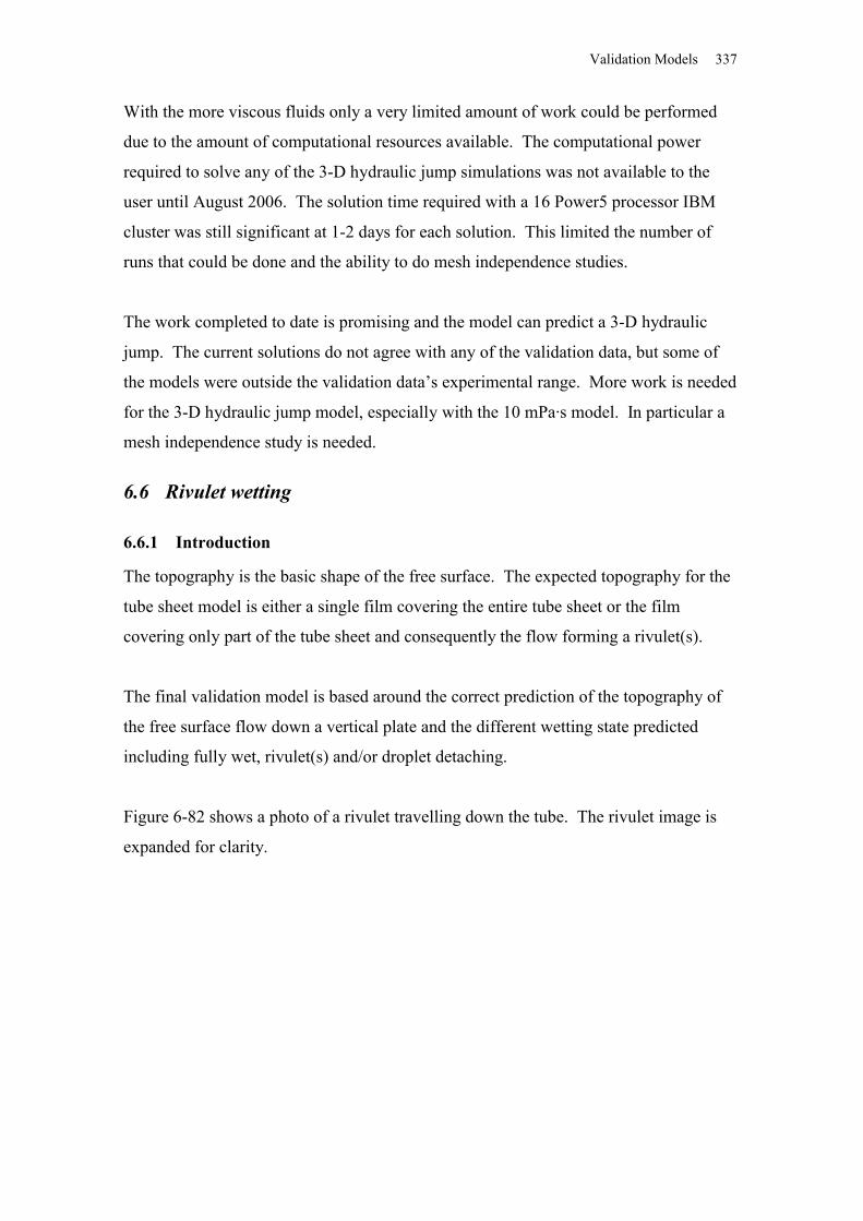
Validation Models 337
With the more viscous fluids only a very limited amount of work could be performed
due to the amount of computational resources available. The computational power
required to solve any of the 3-D hydraulic jump simulations was not available to the
user until August 2006. The solution time required with a 16 Power5 processor IBM
cluster was still significant at 1-2 days for each solution. This limited the number of
runs that could be done and the ability to do mesh independence studies.
The work completed to date is promising and the model can predict a 3-D hydraulic
jump. The current solutions do not agree with any of the validation data, but some of
the models were outside the validation data’s experimental range. More work is needed
for the 3-D hydraulic jump model, especially with the 10 mPa·s model. In particular a
mesh independence study is needed.
6.6 Rivulet wetting
6.6.1 Introduction
The topography is the basic shape of the free surface. The expected topography for the
tube sheet model is either a single film covering the entire tube sheet or the film
covering only part of the tube sheet and consequently the flow forming a rivulet(s).
The final validation model is based around the correct prediction of the topography of
the free surface flow down a vertical plate and the different wetting state predicted
including fully wet, rivulet(s) and/or droplet detaching.
Figure 6-82 shows a photo of a rivulet travelling down the tube. The rivulet image is
expanded for clarity.
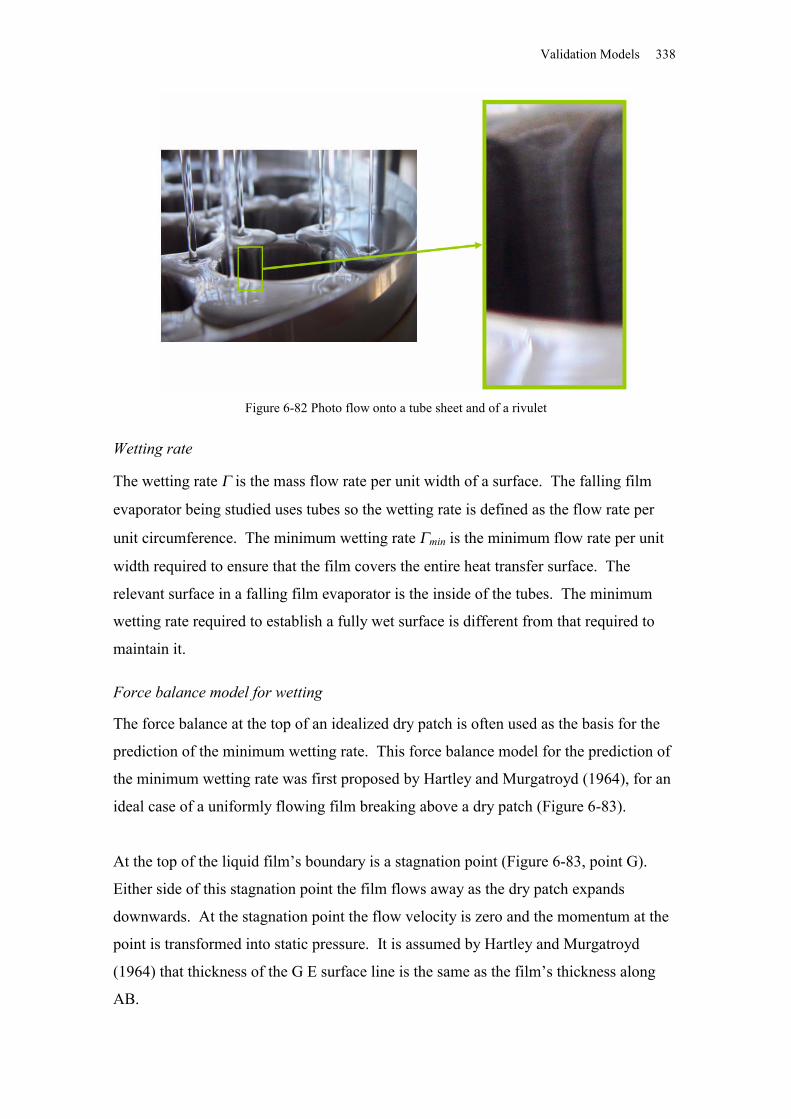
Validation Models 338
Figure 6-82 Photo flow onto a tube sheet and of a rivulet
Wetting rate
The wetting rate is the mass flow rate per unit width of a surface. The falling film
evaporator being studied uses tubes so the wetting rate is defined as the flow rate per
unit circumference. The minimum wetting rate min is the minimum flow rate per unit
width required to ensure that the film covers the entire heat transfer surface. The
relevant surface in a falling film evaporator is the inside of the tubes. The minimum
wetting rate required to establish a fully wet surface is different from that required to
maintain it.
Force balance model for wetting
The force balance at the top of an idealized dry patch is often used as the basis for the
prediction of the minimum wetting rate. This force balance model for the prediction of
the minimum wetting rate was first proposed by Hartley and Murgatroyd (1964), for an
ideal case of a uniformly flowing film breaking above a dry patch (Figure 6-83).
At the top of the liquid film’s boundary is a stagnation point (Figure 6-83, point G).
Either side of this stagnation point the film flows away as the dry patch expands
downwards. At the stagnation point the flow velocity is zero and the momentum at the
point is transformed into static pressure. It is assumed by Hartley and Murgatroyd
(1964) that thickness of the G E surface line is the same as the film’s thickness along
AB.
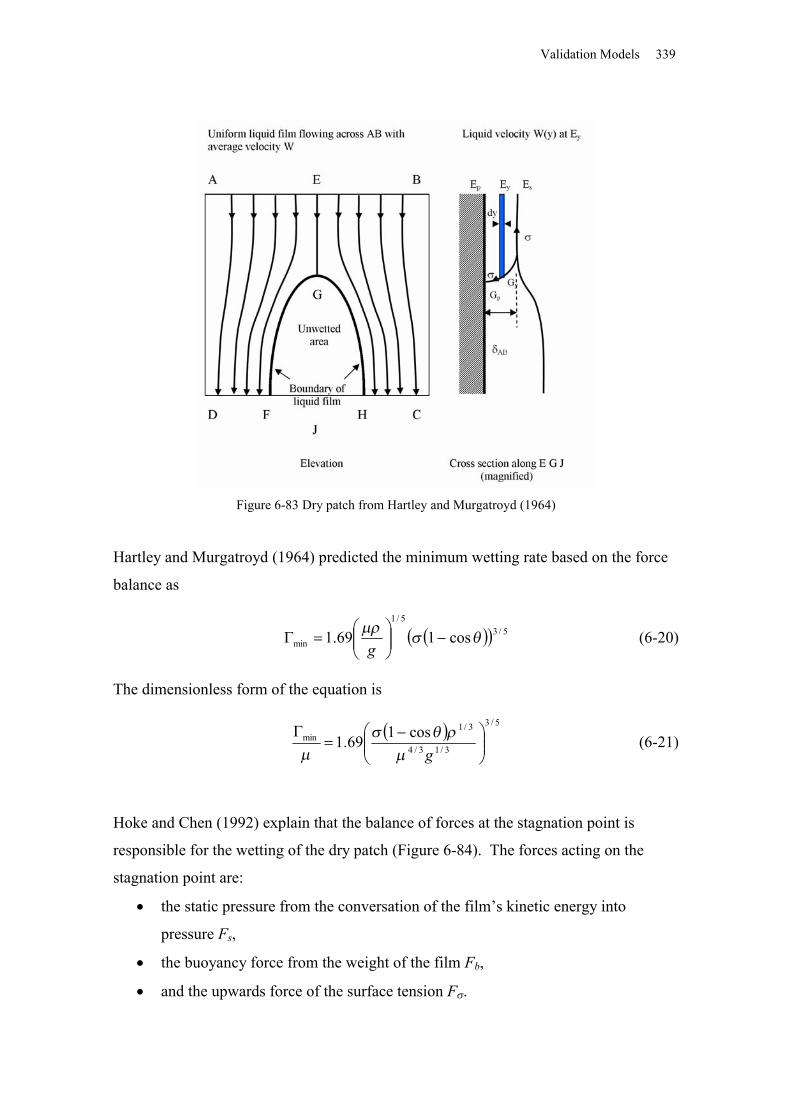
Validation Models 339
Figure 6-83 Dry patch from Hartley and Murgatroyd (1964)
Hartley and Murgatroyd (1964) predicted the minimum wetting rate based on the force
balance as
5/35/1
min cos169.1
g(6-20)
The dimensionless form of the equation is
5/3
3/13/4
3/1min cos169.1
g
(6-21)
Hoke and Chen (1992) explain that the balance of forces at the stagnation point is
responsible for the wetting of the dry patch (Figure 6-84). The forces acting on the
stagnation point are:
the static pressure from the conversation of the film’s kinetic energy into
pressure Fs,
the buoyancy force from the weight of the film Fb,
and the upwards force of the surface tension F.
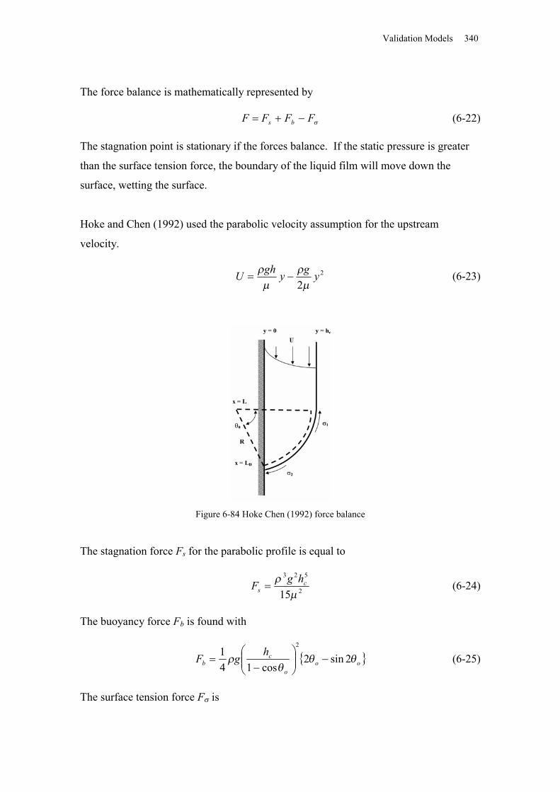
Validation Models 340
The force balance is mathematically represented by
FFFF bs (6-22)
The stagnation point is stationary if the forces balance. If the static pressure is greater
than the surface tension force, the boundary of the liquid film will move down the
surface, wetting the surface.
Hoke and Chen (1992) used the parabolic velocity assumption for the upstream
velocity.
2
2ygyghU
(6-23)
Figure 6-84 Hoke Chen (1992) force balance
The stagnation force Fs for the parabolic profile is equal to
2
523
15 c
shgF (6-24)
The buoyancy force Fb is found with
ooo
cb
hgF
2sin2cos14
12
(6-25)
The surface tension force F is
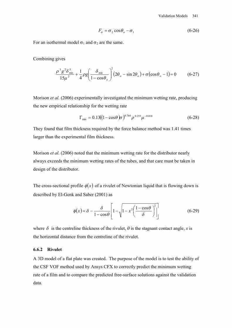
Validation Models 341
12 cos oF (6-26)
For an isothermal model 1 and 2 are the same.
Combining gives
01cos2sin2cos14
115
2
min2
5min
23
oooo
gg
(6-27)
Morison et al. (2006) experimentally investigated the minimum wetting rate, producing
the new empirical relationship for the wetting rate
018.0255.0764.0min cos113.0 (6-28)
They found that film thickness required by the force balance method was 1.41 times
larger than the experimental film thickness.
Morison et al. (2006) noted that the minimum wetting rate for the distributor nearly
always exceeds the minimum wetting rates of the tubes, and that care must be taken in
design of the distributor.
The cross-sectional profile x of a rivulet of Newtonian liquid that is flowing down is
described by El-Genk and Saber (2001) as
2
2 cos111cos1
xx (6-29)
where is the centreline thickness of the rivulet, is the stagnant contact angle, x is
the horizontal distance from the centreline of the rivulet.
6.6.2 Rivulet
A 3D model of a flat plate was created. The purpose of the model is to test the ability of
the CSF VOF method used by Ansys CFX to correctly predict the minimum wetting
rate of a film and to compare the predicted free-surface solutions against the validation
data.
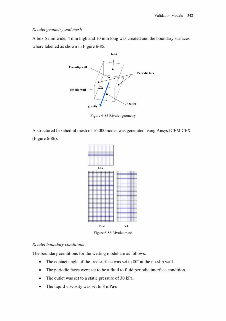
Validation Models 342
Rivulet geometry and mesh
A box 5 mm wide, 4 mm high and 10 mm long was created and the boundary surfaces
where labelled as shown in Figure 6-85.
Figure 6-85 Rivulet geometry
A structured hexahedral mesh of 16,000 nodes was generated using Ansys ICEM CFX
(Figure 6-86).
Figure 6-86 Rivulet mesh
Rivulet boundary conditions
The boundary conditions for the wetting model are as follows:
The contact angle of the free surface was set to 80o at the no-slip wall.
The periodic faces were set to be a fluid to fluid periodic interface condition.
The outlet was set to a static pressure of 30 kPa.
The liquid viscosity was set to 8 mPas
Validation Models 343
The inlet was set to a velocity between 0.025 m s-1 to 0.125 m s-1.
The inlet volume fraction was set to a step change at 1 mm away from the no-
slip wall, with a volume fraction of the liquid 1 on the no-slip walls side of the
step change and the 0 at the other.
Rivulet numerical solution
The convergence for the rivulet model solutions was poor, which is not unusual for free
surface solutions. The RMS residuals were between 10-2 and 10-3 for all the variables
except pressure. Pressure RMS residuals were in the range 10-5 to 10-7. The maximum
residuals were typically an order of magnitude larger than the RMS residuals.
Rivulet mesh independence
Mesh independent runs were not undertaken, as the model’s geometry was thought to be
too small and unduly influencing the solution. The geometry was extended (see
extended rivulet model Section 6.6.3). The extended rivulet model was not, but should
be, tested for mesh independence. If the computational limitations had allowed for a
more complete investigation on the extended rivulet model, the original rivulet solutions
would be redundant.
Rivulet results
Figure 6-87 shows how the solution is developing through the iterative solving process
(1x10⁻⁵ s volume fraction timesteps were used) for a model with a wetting rate of 0.025
kg m-1 s-1. Each subplot contains a contour plot of the distance from the no-slip wall
located on the 0.5 liquid volume isosurface. The no-slip wall is coloured by wetting
(red indicates wet and blue indicates dry).
The images show a droplet building up until it has enough mass and size to accelerate
downward. As the droplet moves away from the inlet, a bridge of liquid connects it to
the liquid left behind at the inlet. As the droplet moves further away, the bridge
contracts as, at the flow rate used, there is not enough liquid flowing into the bridge to
maintain the width as the bridge lengthens. The bridge eventually pinches off once the
bridge gets small enough. The droplet continues downwards.
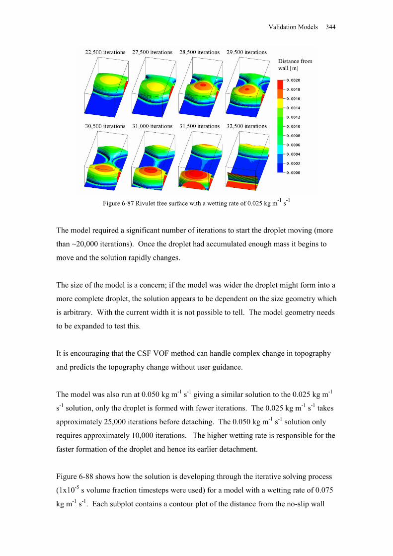
Validation Models 344
Figure 6-87 Rivulet free surface with a wetting rate of 0.025 kg m-1 s-1
The model required a significant number of iterations to start the droplet moving (more
than ~20,000 iterations). Once the droplet had accumulated enough mass it begins to
move and the solution rapidly changes.
The size of the model is a concern; if the model was wider the droplet might form into a
more complete droplet, the solution appears to be dependent on the size geometry which
is arbitrary. With the current width it is not possible to tell. The model geometry needs
to be expanded to test this.
It is encouraging that the CSF VOF method can handle complex change in topography
and predicts the topography change without user guidance.
The model was also run at 0.050 kg m-1 s-1 giving a similar solution to the 0.025 kg m-1
s-1 solution, only the droplet is formed with fewer iterations. The 0.025 kg m-1 s-1 takes
approximately 25,000 iterations before detaching. The 0.050 kg m-1 s-1 solution only
requires approximately 10,000 iterations. The higher wetting rate is responsible for the
faster formation of the droplet and hence its earlier detachment.
Figure 6-88 shows how the solution is developing through the iterative solving process
(1x10⁻⁵ s volume fraction timesteps were used) for a model with a wetting rate of 0.075
kg m-1 s-1. Each subplot contains a contour plot of the distance from the no-slip wall
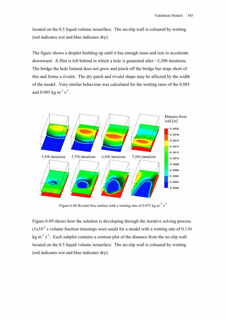
Validation Models 345
located on the 0.5 liquid volume isosurface. The no-slip wall is coloured by wetting
(red indicates wet and blue indicates dry).
The figure shows a droplet building up until it has enough mass and size to accelerate
downward. A film is left behind in which a hole is generated after ~5,500 iterations.
The bridge the hole formed does not grow and pinch off the bridge but stops short of
this and forms a rivulet. The dry patch and rivulet shape may be affected by the width
of the model. Very similar behaviour was calculated for the wetting rates of the 0.085
and 0.095 kg m-1 s-1.
Figure 6-88 Rivulet free surface with a wetting rate of 0.075 kg m-1 s-1
Figure 6-89 shows how the solution is developing through the iterative solving process
(1x10⁻⁵ s volume fraction timesteps were used) for a model with a wetting rate of 0.110
kg m-1 s-1. Each subplot contains a contour plot of the distance from the no-slip wall
located on the 0.5 liquid volume isosurface. The no-slip wall is coloured by wetting
(red indicates wet and blue indicates dry).
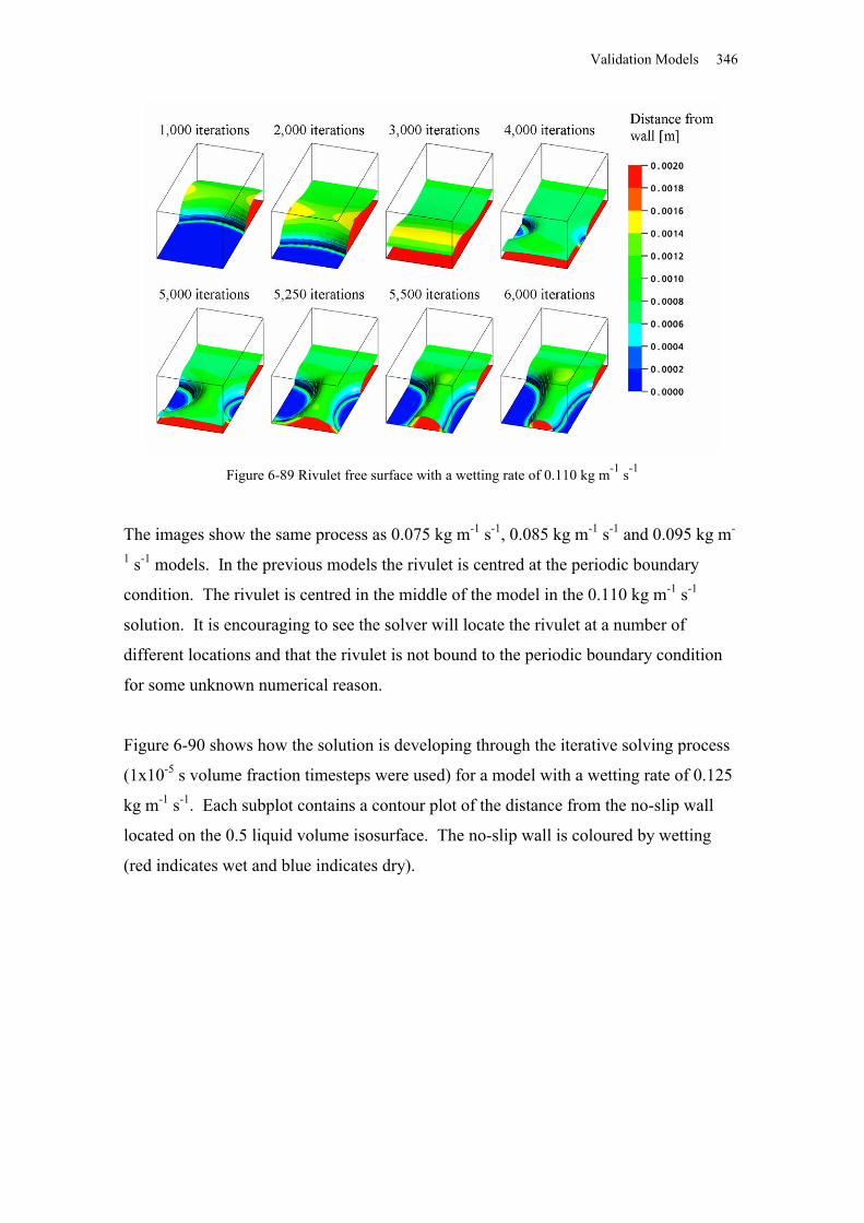
Validation Models 346
Figure 6-89 Rivulet free surface with a wetting rate of 0.110 kg m-1 s-1
The images show the same process as 0.075 kg m-1 s-1, 0.085 kg m-1 s-1 and 0.095 kg m-
1 s-1 models. In the previous models the rivulet is centred at the periodic boundary
condition. The rivulet is centred in the middle of the model in the 0.110 kg m-1 s-1
solution. It is encouraging to see the solver will locate the rivulet at a number of
different locations and that the rivulet is not bound to the periodic boundary condition
for some unknown numerical reason.
Figure 6-90 shows how the solution is developing through the iterative solving process
(1x10⁻⁵ s volume fraction timesteps were used) for a model with a wetting rate of 0.125
kg m-1 s-1. Each subplot contains a contour plot of the distance from the no-slip wall
located on the 0.5 liquid volume isosurface. The no-slip wall is coloured by wetting
(red indicates wet and blue indicates dry).
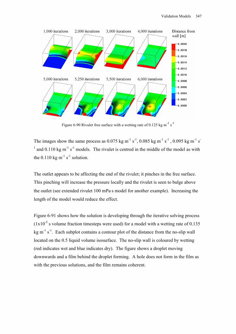
Validation Models 347
Figure 6-90 Rivulet free surface with a wetting rate of 0.125 kg m-1 s-1
The images show the same process as 0.075 kg m-1 s-1, 0.085 kg m-1 s-1 , 0.095 kg m-1 s-
1 and 0.110 kg m-1 s-1 models. The rivulet is centred in the middle of the model as with
the 0.110 kg m-1 s-1 solution.
The outlet appears to be affecting the end of the rivulet; it pinches in the free surface.
This pinching will increase the pressure locally and the rivulet is seen to bulge above
the outlet (see extended rivulet 100 mPas model for another example). Increasing the
length of the model would reduce the effect.
Figure 6-91 shows how the solution is developing through the iterative solving process
(1x10⁻⁵ s volume fraction timesteps were used) for a model with a wetting rate of 0.135
kg m-1 s-1. Each subplot contains a contour plot of the distance from the no-slip wall
located on the 0.5 liquid volume isosurface. The no-slip wall is coloured by wetting
(red indicates wet and blue indicates dry). The figure shows a droplet moving
downwards and a film behind the droplet forming. A hole does not form in the film as
with the previous solutions, and the film remains coherent.
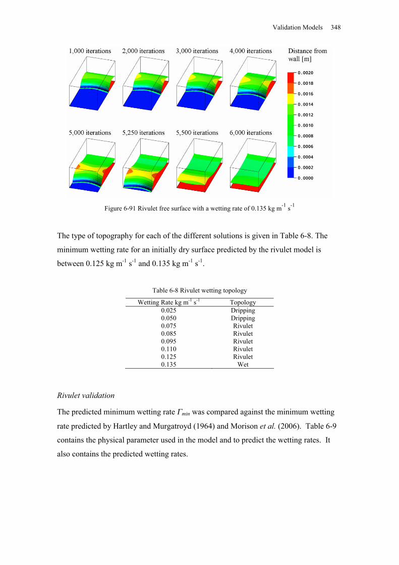
Validation Models 348
Figure 6-91 Rivulet free surface with a wetting rate of 0.135 kg m-1 s-1
The type of topography for each of the different solutions is given in Table 6-8. The
minimum wetting rate for an initially dry surface predicted by the rivulet model is
between 0.125 kg m-1 s-1 and 0.135 kg m-1 s-1.
Table 6-8 Rivulet wetting topology
Wetting Rate kg m-1 s-1 Topology0.025 Dripping0.050 Dripping0.075 Rivulet0.085 Rivulet0.095 Rivulet0.110 Rivulet0.125 Rivulet0.135 Wet
Rivulet validation
The predicted minimum wetting rate min was compared against the minimum wetting
rate predicted by Hartley and Murgatroyd (1964) and Morison et al. (2006). Table 6-9
contains the physical parameter used in the model and to predict the wetting rates. It
also contains the predicted wetting rates.
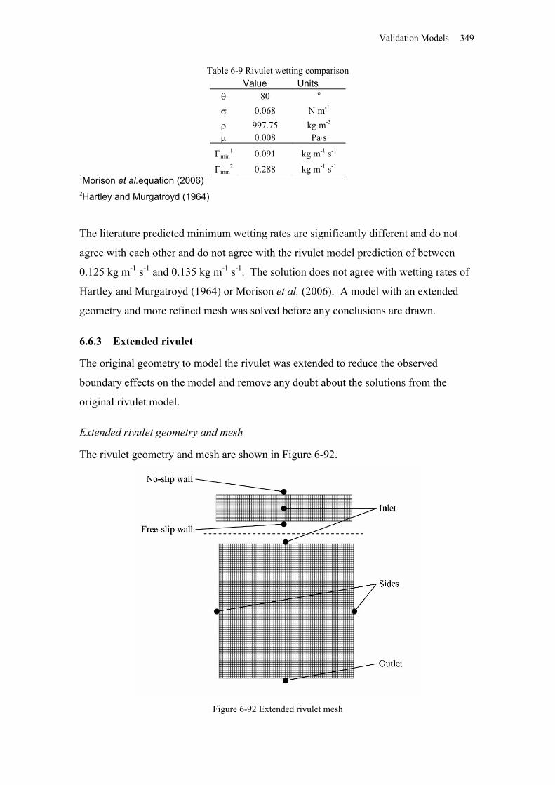
Validation Models 349
Table 6-9 Rivulet wetting comparisonValue Units
80 o
0.068 N m-1
997.75 kg m-3
0.008 Pas
min1 0.091 kg m-1 s-1
min2 0.288 kg m-1 s-1
1Morison et al.equation (2006)2Hartley and Murgatroyd (1964)
The literature predicted minimum wetting rates are significantly different and do not
agree with each other and do not agree with the rivulet model prediction of between
0.125 kg m-1 s-1 and 0.135 kg m-1 s-1. The solution does not agree with wetting rates of
Hartley and Murgatroyd (1964) or Morison et al. (2006). A model with an extended
geometry and more refined mesh was solved before any conclusions are drawn.
6.6.3 Extended rivulet
The original geometry to model the rivulet was extended to reduce the observed
boundary effects on the model and remove any doubt about the solutions from the
original rivulet model.
Extended rivulet geometry and mesh
The rivulet geometry and mesh are shown in Figure 6-92.
Figure 6-92 Extended rivulet mesh
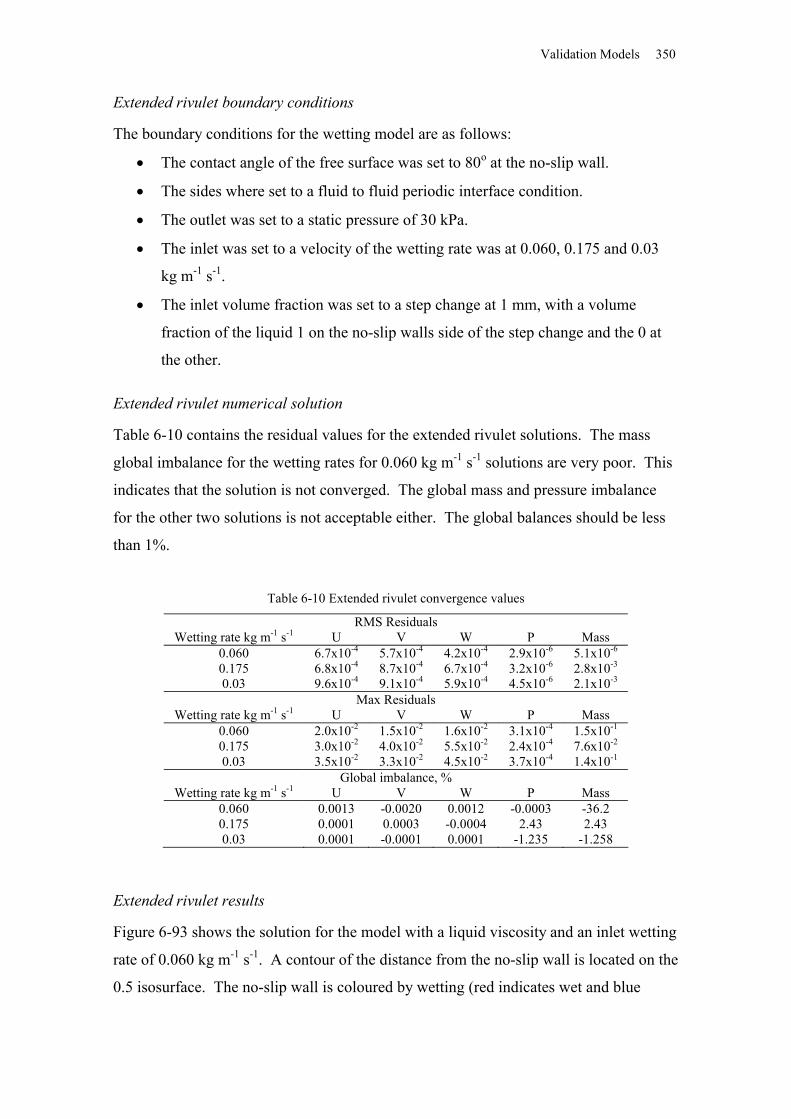
Validation Models 350
Extended rivulet boundary conditions
The boundary conditions for the wetting model are as follows:
The contact angle of the free surface was set to 80o at the no-slip wall.
The sides where set to a fluid to fluid periodic interface condition.
The outlet was set to a static pressure of 30 kPa.
The inlet was set to a velocity of the wetting rate was at 0.060, 0.175 and 0.03
kg m-1 s-1.
The inlet volume fraction was set to a step change at 1 mm, with a volume
fraction of the liquid 1 on the no-slip walls side of the step change and the 0 at
the other.
Extended rivulet numerical solution
Table 6-10 contains the residual values for the extended rivulet solutions. The mass
global imbalance for the wetting rates for 0.060 kg m-1 s-1 solutions are very poor. This
indicates that the solution is not converged. The global mass and pressure imbalance
for the other two solutions is not acceptable either. The global balances should be less
than 1%.
Table 6-10 Extended rivulet convergence values
RMS ResidualsWetting rate kg m-1 s-1 U V W P Mass
0.060 6.7x10⁻⁴ 5.7x10⁻⁴ 4.2x10⁻⁴ 2.9x10⁻⁶ 5.1x10⁻⁶
0.175 6.8x10⁻⁴ 8.7x10⁻⁴ 6.7x10⁻⁴ 3.2x10⁻⁶ 2.8x10⁻³
0.03 9.6x10⁻⁴ 9.1x10⁻⁴ 5.9x10⁻⁴ 4.5x10⁻⁶ 2.1x10⁻³
Max ResidualsWetting rate kg m-1 s-1 U V W P Mass
0.060 2.0x10⁻² 1.5x10⁻² 1.6x10⁻² 3.1x10⁻⁴ 1.5x10⁻¹
0.175 3.0x10⁻² 4.0x10⁻² 5.5x10⁻² 2.4x10⁻⁴ 7.6x10⁻²
0.03 3.5x10⁻² 3.3x10⁻² 4.5x10⁻² 3.7x10⁻⁴ 1.4x10⁻¹
Global imbalance, %Wetting rate kg m-1 s-1 U V W P Mass
0.060 0.0013 -0.0020 0.0012 -0.0003 -36.20.175 0.0001 0.0003 -0.0004 2.43 2.430.03 0.0001 -0.0001 0.0001 -1.235 -1.258
Extended rivulet results
Figure 6-93 shows the solution for the model with a liquid viscosity and an inlet wetting
rate of 0.060 kg m-1 s-1. A contour of the distance from the no-slip wall is located on the
0.5 isosurface. The no-slip wall is coloured by wetting (red indicates wet and blue
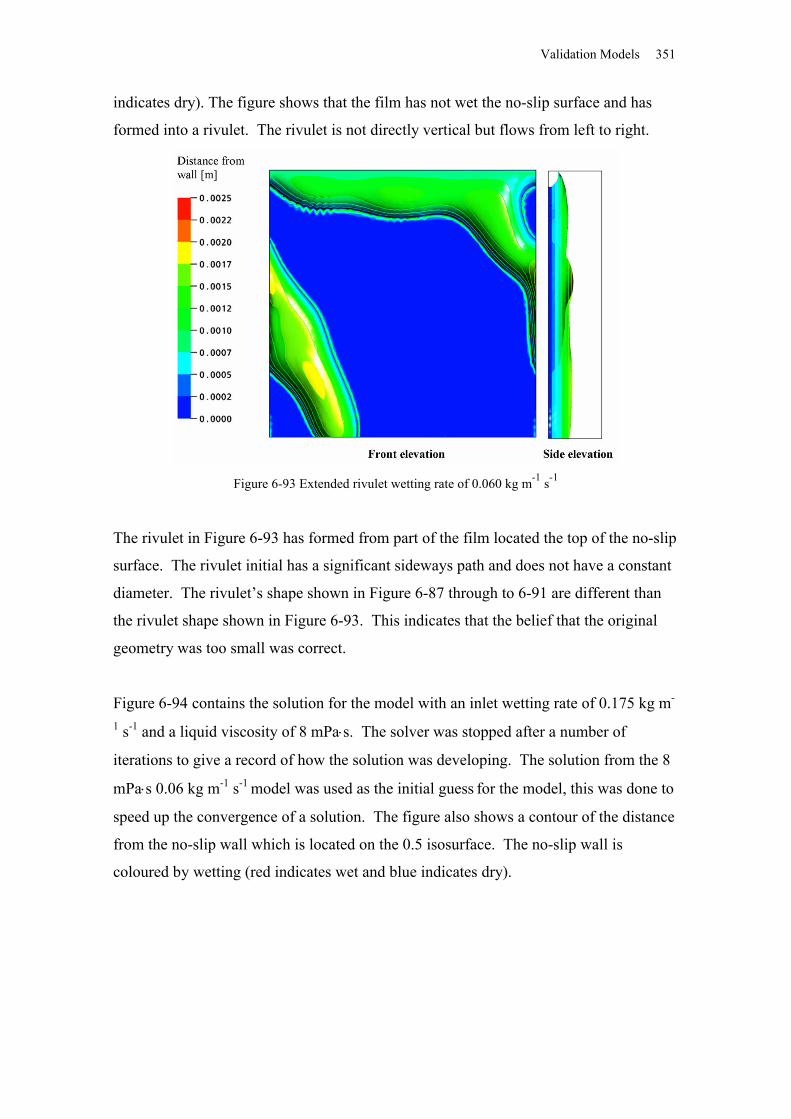
Validation Models 351
indicates dry). The figure shows that the film has not wet the no-slip surface and has
formed into a rivulet. The rivulet is not directly vertical but flows from left to right.
Figure 6-93 Extended rivulet wetting rate of 0.060 kg m-1 s-1
The rivulet in Figure 6-93 has formed from part of the film located the top of the no-slip
surface. The rivulet initial has a significant sideways path and does not have a constant
diameter. The rivulet’s shape shown in Figure 6-87 through to 6-91 are different than
the rivulet shape shown in Figure 6-93. This indicates that the belief that the original
geometry was too small was correct.
Figure 6-94 contains the solution for the model with an inlet wetting rate of 0.175 kg m-
1 s-1 and a liquid viscosity of 8 mPas. The solver was stopped after a number of
iterations to give a record of how the solution was developing. The solution from the 8
mPas 0.06 kg m-1 s-1 model was used as the initial guess for the model, this was done to
speed up the convergence of a solution. The figure also shows a contour of the distance
from the no-slip wall which is located on the 0.5 isosurface. The no-slip wall is
coloured by wetting (red indicates wet and blue indicates dry).
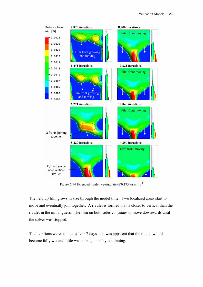
Validation Models 352
Figure 6-94 Extended rivulet wetting rate of 0.175 kg m-1 s-1
The held up film grows in size through the model time. Two localized areas start to
move and eventually join together. A rivulet is formed that is closer to vertical than the
rivulet in the initial guess. The film on both sides continues to move downwards until
the solver was stopped.
The iterations were stopped after ~7 days as it was apparent that the model would
become fully wet and little was to be gained by continuing.
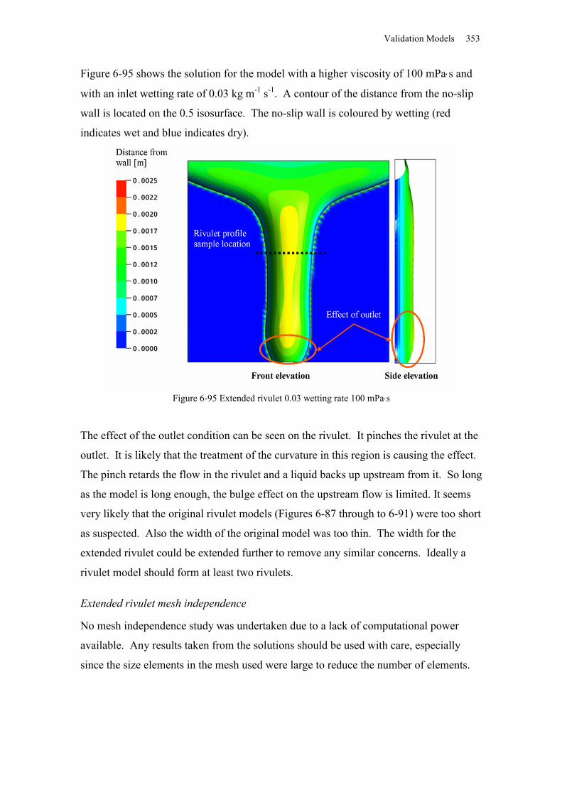
Validation Models 353
Figure 6-95 shows the solution for the model with a higher viscosity of 100 mPas and
with an inlet wetting rate of 0.03 kg m-1 s-1. A contour of the distance from the no-slip
wall is located on the 0.5 isosurface. The no-slip wall is coloured by wetting (red
indicates wet and blue indicates dry).
Figure 6-95 Extended rivulet 0.03 wetting rate 100 mPas
The effect of the outlet condition can be seen on the rivulet. It pinches the rivulet at the
outlet. It is likely that the treatment of the curvature in this region is causing the effect.
The pinch retards the flow in the rivulet and a liquid backs up upstream from it. So long
as the model is long enough, the bulge effect on the upstream flow is limited. It seems
very likely that the original rivulet models (Figures 6-87 through to 6-91) were too short
as suspected. Also the width of the original model was too thin. The width for the
extended rivulet could be extended further to remove any similar concerns. Ideally a
rivulet model should form at least two rivulets.
Extended rivulet mesh independence
No mesh independence study was undertaken due to a lack of computational power
available. Any results taken from the solutions should be used with care, especially
since the size elements in the mesh used were large to reduce the number of elements.
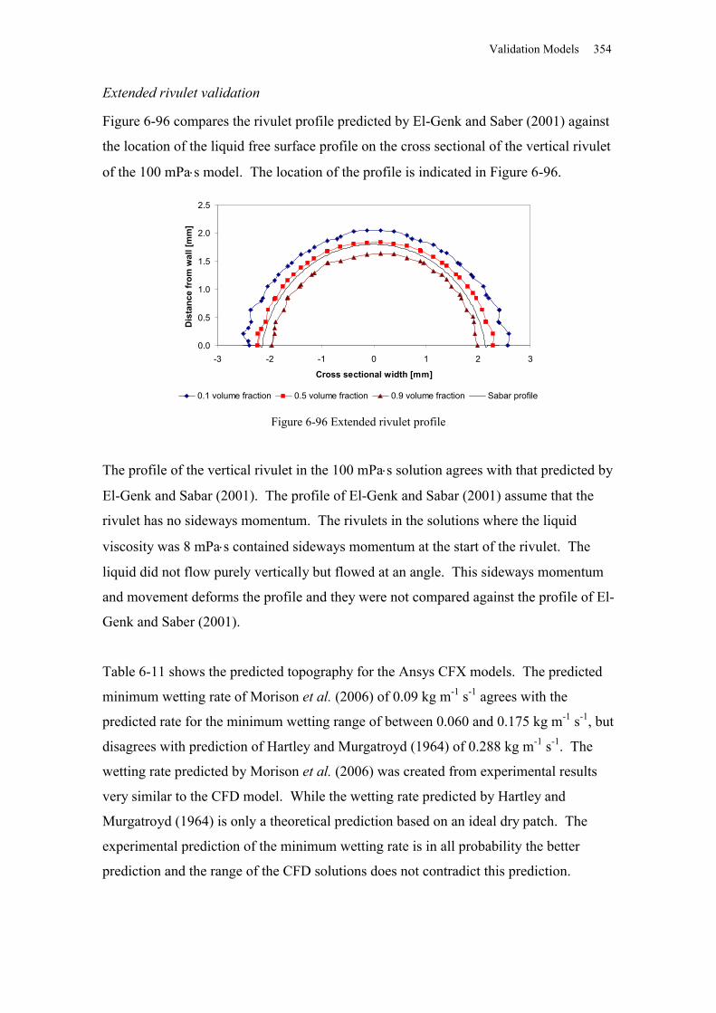
Validation Models 354
Extended rivulet validation
Figure 6-96 compares the rivulet profile predicted by El-Genk and Saber (2001) against
the location of the liquid free surface profile on the cross sectional of the vertical rivulet
of the 100 mPas model. The location of the profile is indicated in Figure 6-96.
0.0
0.5
1.0
1.5
2.0
2.5
-3 -2 -1 0 1 2 3
Cross sectional width [mm]
Dis
tanc
e fr
om w
all [
mm
]
0.1 volume fraction 0.5 volume fraction 0.9 volume fraction Sabar profile
Figure 6-96 Extended rivulet profile
The profile of the vertical rivulet in the 100 mPas solution agrees with that predicted by
El-Genk and Sabar (2001). The profile of El-Genk and Sabar (2001) assume that the
rivulet has no sideways momentum. The rivulets in the solutions where the liquid
viscosity was 8 mPas contained sideways momentum at the start of the rivulet. The
liquid did not flow purely vertically but flowed at an angle. This sideways momentum
and movement deforms the profile and they were not compared against the profile of El-
Genk and Saber (2001).
Table 6-11 shows the predicted topography for the Ansys CFX models. The predicted
minimum wetting rate of Morison et al. (2006) of 0.09 kg m-1 s-1 agrees with the
predicted rate for the minimum wetting range of between 0.060 and 0.175 kg m-1 s-1, but
disagrees with prediction of Hartley and Murgatroyd (1964) of 0.288 kg m-1 s-1. The
wetting rate predicted by Morison et al. (2006) was created from experimental results
very similar to the CFD model. While the wetting rate predicted by Hartley and
Murgatroyd (1964) is only a theoretical prediction based on an ideal dry patch. The
experimental prediction of the minimum wetting rate is in all probability the better
prediction and the range of the CFD solutions does not contradict this prediction.
Validation Models 355
Table 6-11 Extended rivulet wetting
Wetting Rate,kg m-1 s-1
Liquid Viscosity,mPas
State
0.060 8 Rivulet0.175 8 Wet1
0.03 100 Rivulet1assumed solution that the solution would continue until fully wet.
The range of the wetting rate the CFD solutions predict is relatively large and the more
solutions are needed to increase precision of the prediction. Only a limited number of
runs could be complete due to limitation on the available computer resources. There is
no guarantee that the CFD solution would accurately predict the wetting rate with more
runs, but currently it does agree with experimental of wetting rate of Morison et al.
(2006). This is at least a promising result and a good starting point for further work.
6.6.4 Rivulet discussion
Original rivulet discussion
It was believed that the size of the original rivulet model was too small as the boundary
conditions could be effecting the solutions (Section 6.62). Extending the model
geometry is a simple way of testing the boundary conditions effects and, if they are
limiting, their effect on the solution. The extended rivulet model was created to do this
and should be able to answer all these questions.
Unlike most frontal tracking methods the VOF method easily handle complex changes
in the topography (Figures 6-87 through to 6-91). The same mesh and model definition
was used with all the different topographies. The only difference was the inlet
boundary condition. This ability to correctly predict topography is critical to the study
of the wetting rate, as the predicted topography is the area of interest in the models.
If the user has to guess an initial topography, then it is more likely that the solution
method will incorrectly predict the topography due to the user influence. Likewise if
the solution method can only predict certain topographies or favours a topography, then
it is also more likely to incorrectly predict the correct topography in a solution.
The CSF VOF method used by Ansys CFX can predict dripping down a wall, formation
of a rivulet and formation of a fully wet film. All the models look qualitatively
Validation Models 356
reasonable and plausible. The predicted minimum wetting rate does not agree with the
values predicted by either Hartley and Murgatroyd (1964) or Morison et al. (2006).
No mesh independence study was undertaken so the solutions could be mesh dependent.
The mesh used was coarse and contained as few as possible elements to reduce the
computational time. It is possible that the coarse meshing has produce solutions that are
mesh dependent and this could be the reason for the lack of agreement with the
validation data.
Extended Rivulet Discussion
The minimum wetting rate was not calculated from a single CFD solution, but was
found through an iterative process. The minimum wetting rate is between the solution
with the highest flow rate that is partial wet and the solution with the lowest flow rate
that is fully wet. To accurately find the minimum wetting rate required for any given
fluid or geometry requires at least several runs and possibly many (~10 to 20 runs)
depending on the initial guess of where the minimum wetting rate is.
If computational resources had permitted it, a full investigation of the wetting process
would have been carried out, but the computer power required to solve the model was
not available.
6.7 Validation models discussionUnlike most frontal tracking methods the VOF method can easily handle complex
changes in the topography (Figures 6-87 through to 6-91). The same mesh and model
definition was used with all the different topographies. The only difference was the
inlet boundary condition. This ability to correctly predict topography is critical to the
study of the wetting rate, as the predicted topography is the area of interest in the
models.
6.7.1 TimestepThe meniscus model showed that the model performance was very dependent on the
mesh quality. The meniscus model was a very simple geometry and mesh quality could
be easily controlled. For the more complicated geometry it is quite difficult to mesh the
model entirely with high quality elements.
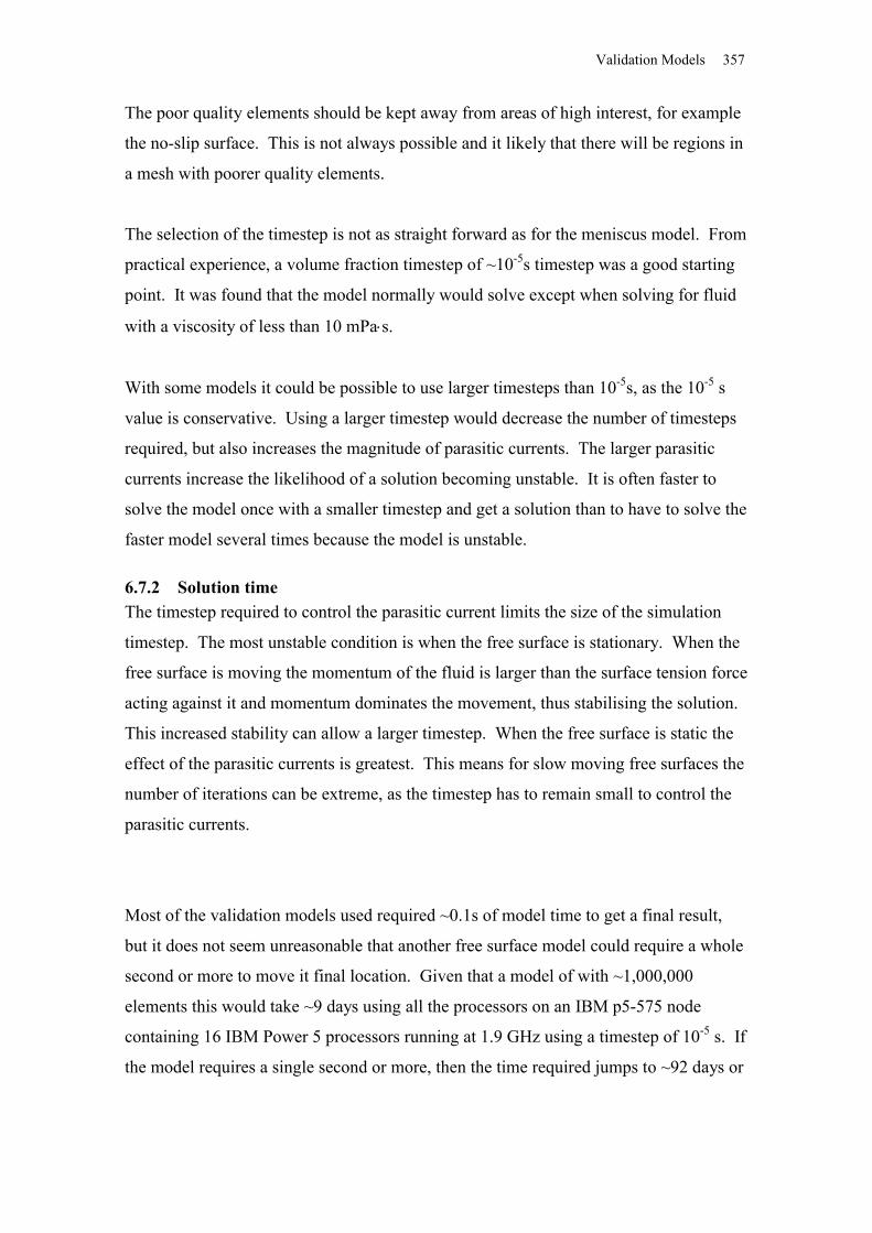
Validation Models 357
The poor quality elements should be kept away from areas of high interest, for example
the no-slip surface. This is not always possible and it likely that there will be regions in
a mesh with poorer quality elements.
The selection of the timestep is not as straight forward as for the meniscus model. From
practical experience, a volume fraction timestep of ~10-5s timestep was a good starting
point. It was found that the model normally would solve except when solving for fluid
with a viscosity of less than 10 mPas.
With some models it could be possible to use larger timesteps than 10-5s, as the 10-5 s
value is conservative. Using a larger timestep would decrease the number of timesteps
required, but also increases the magnitude of parasitic currents. The larger parasitic
currents increase the likelihood of a solution becoming unstable. It is often faster to
solve the model once with a smaller timestep and get a solution than to have to solve the
faster model several times because the model is unstable.
6.7.2 Solution timeThe timestep required to control the parasitic current limits the size of the simulation
timestep. The most unstable condition is when the free surface is stationary. When the
free surface is moving the momentum of the fluid is larger than the surface tension force
acting against it and momentum dominates the movement, thus stabilising the solution.
This increased stability can allow a larger timestep. When the free surface is static the
effect of the parasitic currents is greatest. This means for slow moving free surfaces the
number of iterations can be extreme, as the timestep has to remain small to control the
parasitic currents.
Most of the validation models used required ~0.1s of model time to get a final result,
but it does not seem unreasonable that another free surface model could require a whole
second or more to move it final location. Given that a model of with ~1,000,000
elements this would take ~9 days using all the processors on an IBM p5-575 node
containing 16 IBM Power 5 processors running at 1.9 GHz using a timestep of 10-5 s. If
the model requires a single second or more, then the time required jumps to ~92 days or
Validation Models 358
more. This is a severe limitation on what is a practicable solution using currently
available computing resources.
6.7.3 ConvergenceFree surface models often can not converge properly (Ansys CFX 2005). Free surface
models where surface tension dominates are more difficult to get proper convergence
due to the parasitic currents (Section 5.5).
Ansys CFX (2005) advises the use of a user-defined variable to help infer convergence.
For the wetting models the volume fraction on the wetting surface should be used. It is
a good indicator of convergence except when the flow is creeping. When the flow is
creeping there is no way to know the cause of the creeping. It could be due to the
numerical parasitic currents or from the fluid field.
6.7.4 CreepingThe parasitic current produces velocity noise at the free surface. That can dominate the
free surface movement when the correct velocity is small compared to the velocity of
the parasitic current. This is more likely when the free surface is at rest or slowly
creeping.
Even if the parasitic currents are random in direction over time they would not cancel
themselves out. This is due to the physical preference for a wet surface to remain wet
compared to a wet surface drying. This preference to remain wet could introduce
creeping (Figure 6-97).
Parasitic creep could produce a model that is predicting closer to the wet surface wetting
rate than the dry surface wetting rate. The two wetting rates are different. This parasitic
creep is undesirable.
It is very hard to tell the difference between the numerically induced parasitic creep and
physically correct creep. Using a conservative timestep reduces the parasitic currents
and should reduce the parasitic creep.
Validation Models 359
Figure 6-97 Parasitic creep
If the parasitic currents could be reduced through a better estimate of the curvature, not
only could bigger timesteps be used, but for a given timestep slower creeping flows
could be accurately modelled.
6.8 Validation models conclusions
The lack of information about the quality of the solution in the normal convergence
measure makes it difficult to understand the quality of any solution. This lack of the
information makes it very difficult to have any confidence in any solution. It is the
author’s opinion that the use of the CSF VOF method should be limited to experienced
users and any solution needs to be mesh independent, before any conclusions are drawn.
The CSF VOF method of Ansys CFX 10.0 shows good agreement with validation data
for the jet model (Bush and Aristoff (2003), sessile droplet model (Equation 6-3) and
overfall (Henderson, 1966). Although there is no validation data, the 2D weir model
shows the film travelling in a manner consistent with expectations. The 3D weir model
also predicted realistic topography and a minimum wetting rate that is consistent with
the limited experimental work available.
Validation Models 360
The VOF method of Ansys CFX 10.0 method without modelling surface tension was
able to produce solution that shows qualitative and qualitative agreement. The
hydraulic jump radius was measured from the start of the jump in Chang et al. (2001)
and from the peak of the jump in this project. The measured values agreed to within
22%. The difference in location was due to the solution profile predicting a gradual
changing interface height. To use the start of the hydraulic jump would require an
arbitrary selection of the start and the hydraulic peak radius was use instead. It is the
author’s opinion that the agreement is better than the current 20% (refer to Figure 6-73).
The 3-D hydraulic jump model includes surface tension. The solutions do not show
agreement with the work of Bush and Aristoff (2003). However the 100 mPas solution
is using a liquid with a viscosity outside the experimental range of Bush and Aristoff
(2003) and the 100 mPas solutions predicted hydraulic jump agrees to within 35% to
the work of Chang et al. (2001).
The 10 mPas solution is within the range of the viscosities used by Bush and Aristoff
(2003) and does not show agreement with either Bush and Aristoff (2003) or Chang et
al. (2001). The solutions are not well converged or mesh independent. Until more well
converged and mesh independent solutions are solved no conclusions can be drawn
about the ability of the CSF VOF method of Ansys CFX 10.0 to correctly predict
hydraulic jump with surface tension.
The small rivulet model shows qualitative agreement with expected results. The
predicted wetting rate does not agree with the experimental work of either Hartley and
Murgatroyd (1964) or Morison et al. (2006). The size of the small rivulet model
appears to be too small and is affecting the model. The model geometry was expanded
with the expanded rivulet model.
The 100 mPas solution to the extended rivulet model was able to predict the rivulet
profile of the idealised rivulet of El-Genk and Saber (2001). The extended rivulet
model wetting rate agrees only with the wetting rate prediction of Morison et al. (2006).
Validation Models 361
Morison et al. (2006) predicted a minimum wetting rate of 0.09 kg m-1 s-1 and the CFD
solution predicted a minimum wetting range between 0.060 and 0.175 kg m-1 s-1.
No mesh independent or well converged solutions were created for the extended rivulet
model due to the computational resource limitations. Again until more converged and
mesh independent solutions are solved and a tighter minimum wetting rate is calculated,
no final conclusions can be drawn about the ability of the CSF VOF method of Ansys
CFX 10.0 to correctly predict wetting rates, but the initial results are encouraging.
It was surprising that there was not more validation data available to compare any CFD
models solutions against, given the basic nature of the film flows. Creating more
validation data could be the basis of future work.
The goal of the validation model was to validate the CSF VOF method of Ansys CFX
10.0 before using the method to model the complete distribution plate. The method was
found to be too unstable to be used with the available computer resources but the CSF
VOF method shows promise to be able to correctly predict the wetting of the
distribution plate. The ability of the CSF VOF method to independently predict the
different topographies dependent on the flow rates without any user input is one of the
most promising characteristics of the technique.
The required computational cost of the CSF VOF method was too high to enable the
completion of the required work need to finish the initial aims of the project. If the
project was undertaken again, provisions for more computational power would be
required. Given the typical increase in computational power over time, it is not
unrealistic to believe that the project could be completed in several years time. The
increased computational resources could allow for the timely completion of any model
runs.
The physical preference of a wet surface to remain wet means that any random
numerical movement of the film across a surface will favour the wetting of the surface.
This will result in the film creeping along the surface in a non-physical manner. This
creeping is the most concerning unresolved performance characteristic of the CSF VOF
method for use in predicting wetting. The numerical creeping should be able to be
Validation Models 362
limited through a reduced timestep, however the current timestep is already small. The
effect of numerical creeping may limit or even rule out the use the CSF VOF method for
wetting problems.

Tube Sheet Model 363
7 Tube Sheet Model
7.1 Introduction
The aim of the tube sheet modelling is to be able to predict the distribution rate for a
given set of conditions and distribution design. The key ability required of a model is
the correct prediction of whether or not a tube sheet surface would be fully wetted by
the liquid flow.
The validation models (Chapter 6) were designed to replicate the expected phenomena
of free surface flow in the tube sheet and the tube sheet model is a combination of all
these phenomena.
The need for a tube sheet model is discussed in detail in Chapter 4 which should be
referred to for more details.
The following is an overview of the proposed experimental design for the tube sheet
model and the aims for the sub-model. As the sub-models were developed and
solutions were interpreted the design changes for the tube sheet were to be proposed and
evaluated.
1. Preliminary (high viscosity models)
a. 6 hole design (vertical centred jets)
b. 3 hole design (vertical centred jets)
2. Actual viscosity models
a. 6 hole (vertical centred jets)
b. 3 hole (vertical centred jets)
c. non-vertical and/or centred jets
d. effect of vapour on free surface
3. Improvement of distribution rate models
With the exception of the preliminary models the models required completion of the
validation models before they could be attempted in a serious manner. The preliminary
models were designed for learning purposes and proof of concept.
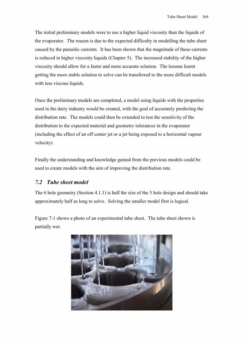
Tube Sheet Model 364
The initial preliminary models were to use a higher liquid viscosity than the liquids of
the evaporator. The reason is due to the expected difficulty in modelling the tube sheet
caused by the parasitic currents. It has been shown that the magnitude of these currents
is reduced in higher viscosity liquids (Chapter 5). The increased stability of the higher
viscosity should allow for a faster and more accurate solution. The lessons learnt
getting the more stable solution to solve can be transferred to the more difficult models
with less viscous liquids.
Once the preliminary models are completed, a model using liquids with the properties
used in the dairy industry would be created, with the goal of accurately predicting the
distribution rate. The models could then be extended to test the sensitivity of the
distribution to the expected material and geometry tolerances in the evaporator
(including the effect of an off center jet or a jet being exposed to a horizontal vapour
velocity).
Finally the understanding and knowledge gained from the previous models could be
used to create models with the aim of improving the distribution rate.
7.2 Tube sheet model
The 6 hole geometry (Section 4.1.1) is half the size of the 3 hole design and should take
approximately half as long to solve. Solving the smaller model first is logical.
Figure 7-1 shows a photo of an experimental tube sheet. The tube sheet shown is
partially wet.
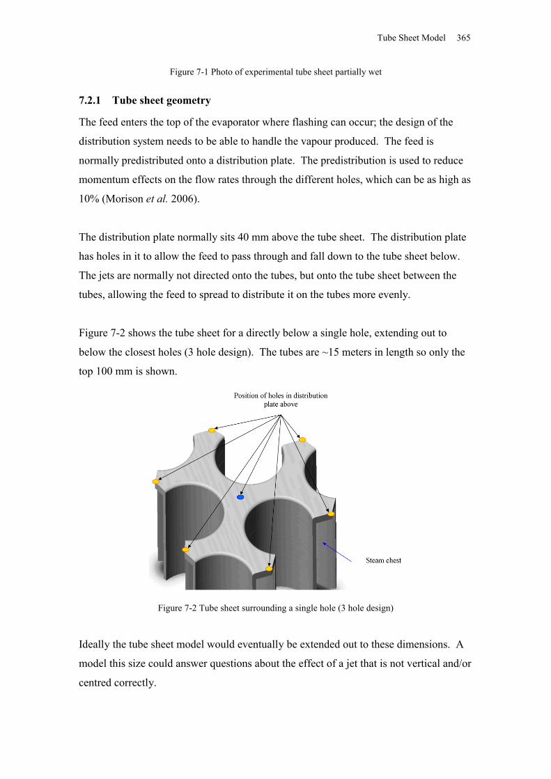
Tube Sheet Model 365
Figure 7-1 Photo of experimental tube sheet partially wet
7.2.1 Tube sheet geometry
The feed enters the top of the evaporator where flashing can occur; the design of the
distribution system needs to be able to handle the vapour produced. The feed is
normally predistributed onto a distribution plate. The predistribution is used to reduce
momentum effects on the flow rates through the different holes, which can be as high as
10% (Morison et al. 2006).
The distribution plate normally sits 40 mm above the tube sheet. The distribution plate
has holes in it to allow the feed to pass through and fall down to the tube sheet below.
The jets are normally not directed onto the tubes, but onto the tube sheet between the
tubes, allowing the feed to spread to distribute it on the tubes more evenly.
Figure 7-2 shows the tube sheet for a directly below a single hole, extending out to
below the closest holes (3 hole design). The tubes are ~15 meters in length so only the
top 100 mm is shown.
Figure 7-2 Tube sheet surrounding a single hole (3 hole design)
Ideally the tube sheet model would eventually be extended out to these dimensions. A
model this size could answer questions about the effect of a jet that is not vertical and/or
centred correctly.
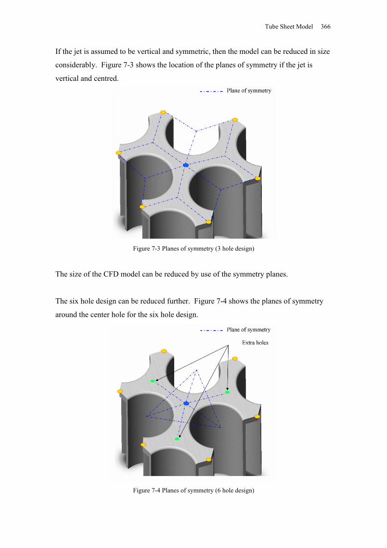
Tube Sheet Model 366
If the jet is assumed to be vertical and symmetric, then the model can be reduced in size
considerably. Figure 7-3 shows the location of the planes of symmetry if the jet is
vertical and centred.
Figure 7-3 Planes of symmetry (3 hole design)
The size of the CFD model can be reduced by use of the symmetry planes.
The six hole design can be reduced further. Figure 7-4 shows the planes of symmetry
around the center hole for the six hole design.
Figure 7-4 Planes of symmetry (6 hole design)
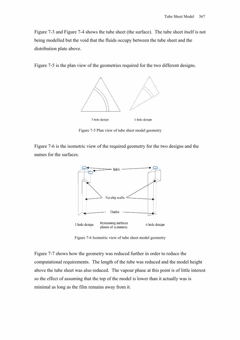
Tube Sheet Model 367
Figure 7-3 and Figure 7-4 shows the tube sheet (the surface). The tube sheet itself is not
being modelled but the void that the fluids occupy between the tube sheet and the
distribution plate above.
Figure 7-5 is the plan view of the geometries required for the two different designs.
Figure 7-5 Plan view of tube sheet model geometry
Figure 7-6 is the isometric view of the required geometry for the two designs and the
names for the surfaces.
Figure 7-6 Isometric view of tube sheet model geometry
Figure 7-7 shows how the geometry was reduced further in order to reduce the
computational requirements. The length of the tube was reduced and the model height
above the tube sheet was also reduced. The vapour phase at this point is of little interest
so the effect of assuming that the top of the model is lower than it actually was is
minimal as long as the film remains away from it.
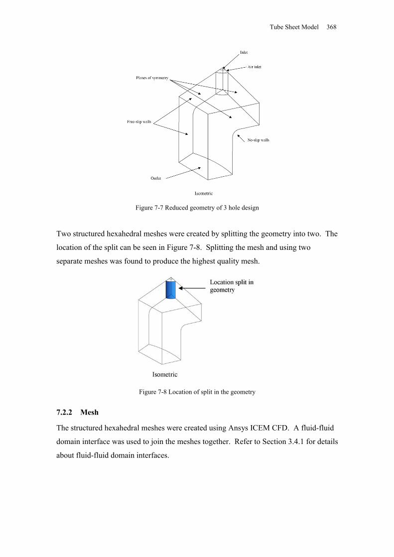
Tube Sheet Model 368
Figure 7-7 Reduced geometry of 3 hole design
Two structured hexahedral meshes were created by splitting the geometry into two. The
location of the split can be seen in Figure 7-8. Splitting the mesh and using two
separate meshes was found to produce the highest quality mesh.
Figure 7-8 Location of split in the geometry
7.2.2 Mesh
The structured hexahedral meshes were created using Ansys ICEM CFD. A fluid-fluid
domain interface was used to join the meshes together. Refer to Section 3.4.1 for details
about fluid-fluid domain interfaces.
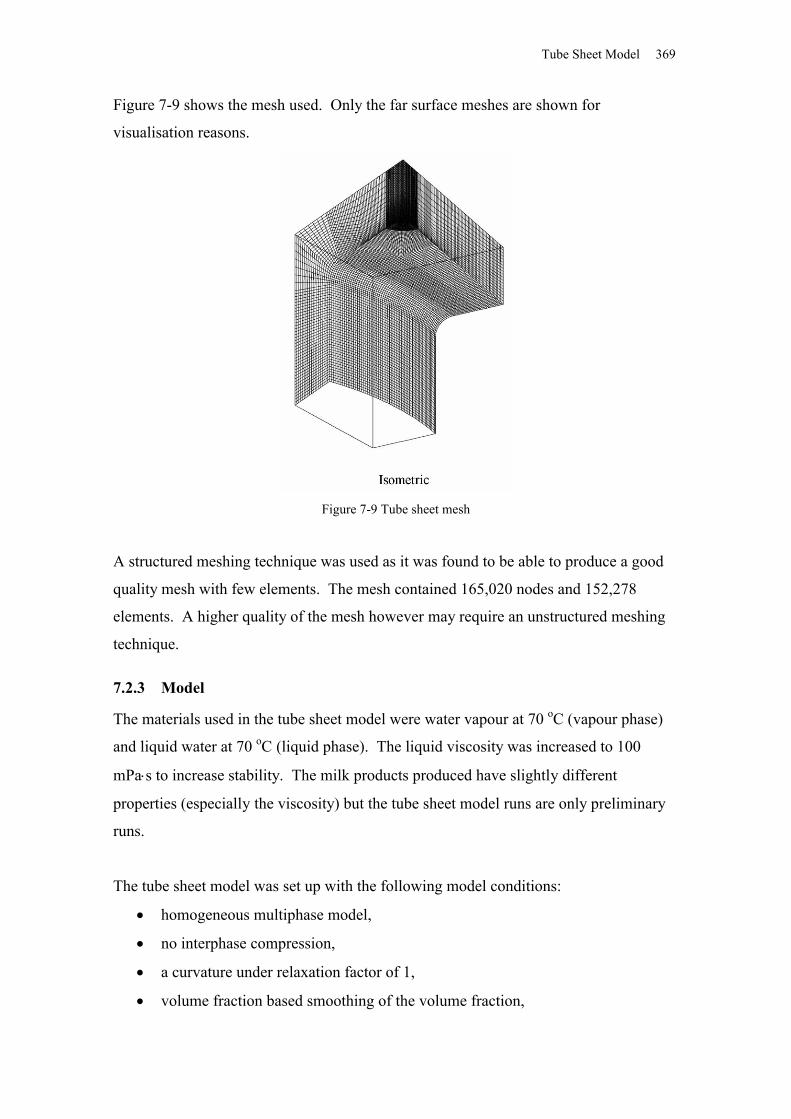
Tube Sheet Model 369
Figure 7-9 shows the mesh used. Only the far surface meshes are shown for
visualisation reasons.
Figure 7-9 Tube sheet mesh
A structured meshing technique was used as it was found to be able to produce a good
quality mesh with few elements. The mesh contained 165,020 nodes and 152,278
elements. A higher quality of the mesh however may require an unstructured meshing
technique.
7.2.3 Model
The materials used in the tube sheet model were water vapour at 70 oC (vapour phase)
and liquid water at 70 oC (liquid phase). The liquid viscosity was increased to 100
mPas to increase stability. The milk products produced have slightly different
properties (especially the viscosity) but the tube sheet model runs are only preliminary
runs.
The tube sheet model was set up with the following model conditions:
homogeneous multiphase model,
no interphase compression,
a curvature under relaxation factor of 1,
volume fraction based smoothing of the volume fraction,
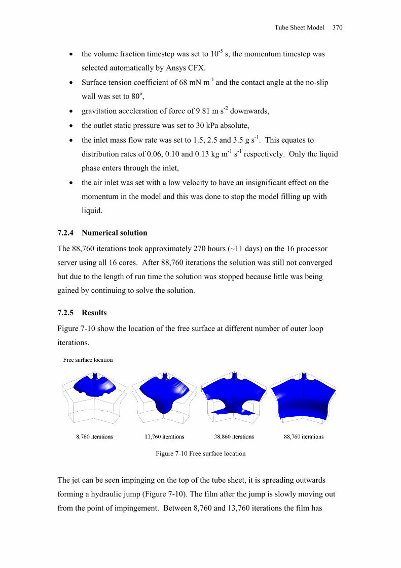
Tube Sheet Model 370
the volume fraction timestep was set to 10-5 s, the momentum timestep was
selected automatically by Ansys CFX.
Surface tension coefficient of 68 mN m-1 and the contact angle at the no-slip
wall was set to 80o,
gravitation acceleration of force of 9.81 m s-2 downwards,
the outlet static pressure was set to 30 kPa absolute,
the inlet mass flow rate was set to 1.5, 2.5 and 3.5 g s-1. This equates to
distribution rates of 0.06, 0.10 and 0.13 kg m-1 s-1 respectively. Only the liquid
phase enters through the inlet,
the air inlet was set with a low velocity to have an insignificant effect on the
momentum in the model and this was done to stop the model filling up with
liquid.
7.2.4 Numerical solution
The 88,760 iterations took approximately 270 hours (~11 days) on the 16 processor
server using all 16 cores. After 88,760 iterations the solution was still not converged
but due to the length of run time the solution was stopped because little was being
gained by continuing to solve the solution.
7.2.5 Results
Figure 7-10 show the location of the free surface at different number of outer loop
iterations.
Figure 7-10 Free surface location
The jet can be seen impinging on the top of the tube sheet, it is spreading outwards
forming a hydraulic jump (Figure 7-10). The film after the jump is slowly moving out
from the point of impingement. Between 8,760 and 13,760 iterations the film has
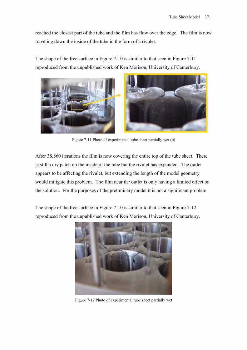
Tube Sheet Model 371
reached the closest part of the tube and the film has flow over the edge. The film is now
traveling down the inside of the tube in the form of a rivulet.
The shape of the free surface in Figure 7-10 is similar to that seen in Figure 7-11
reproduced from the unpublished work of Ken Morison, University of Canterbury.
Figure 7-11 Photo of experimental tube sheet partially wet (b)
After 38,860 iterations the film is now covering the entire top of the tube sheet. There
is still a dry patch on the inside of the tube but the rivulet has expanded. The outlet
appears to be affecting the rivulet, but extending the length of the model geometry
would mitigate this problem. The film near the outlet is only having a limited effect on
the solution. For the purposes of the preliminary model it is not a significant problem.
The shape of the free surface in Figure 7-10 is similar to that seen in Figure 7-12
reproduced from the unpublished work of Ken Morison, University of Canterbury.
Figure 7-12 Photo of experimental tube sheet partially wet
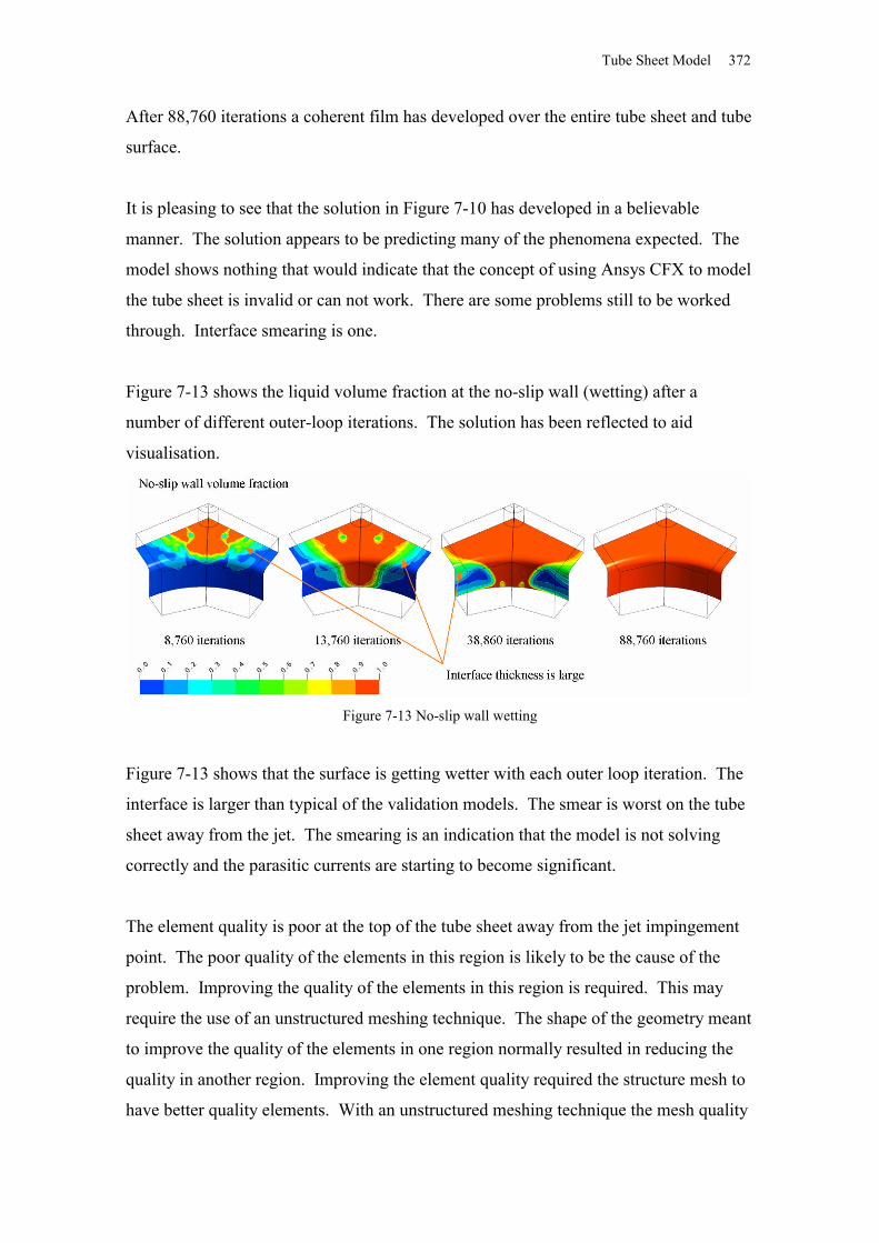
Tube Sheet Model 372
After 88,760 iterations a coherent film has developed over the entire tube sheet and tube
surface.
It is pleasing to see that the solution in Figure 7-10 has developed in a believable
manner. The solution appears to be predicting many of the phenomena expected. The
model shows nothing that would indicate that the concept of using Ansys CFX to model
the tube sheet is invalid or can not work. There are some problems still to be worked
through. Interface smearing is one.
Figure 7-13 shows the liquid volume fraction at the no-slip wall (wetting) after a
number of different outer-loop iterations. The solution has been reflected to aid
visualisation.
Figure 7-13 No-slip wall wetting
Figure 7-13 shows that the surface is getting wetter with each outer loop iteration. The
interface is larger than typical of the validation models. The smear is worst on the tube
sheet away from the jet. The smearing is an indication that the model is not solving
correctly and the parasitic currents are starting to become significant.
The element quality is poor at the top of the tube sheet away from the jet impingement
point. The poor quality of the elements in this region is likely to be the cause of the
problem. Improving the quality of the elements in this region is required. This may
require the use of an unstructured meshing technique. The shape of the geometry meant
to improve the quality of the elements in one region normally resulted in reducing the
quality in another region. Improving the element quality required the structure mesh to
have better quality elements. With an unstructured meshing technique the mesh quality
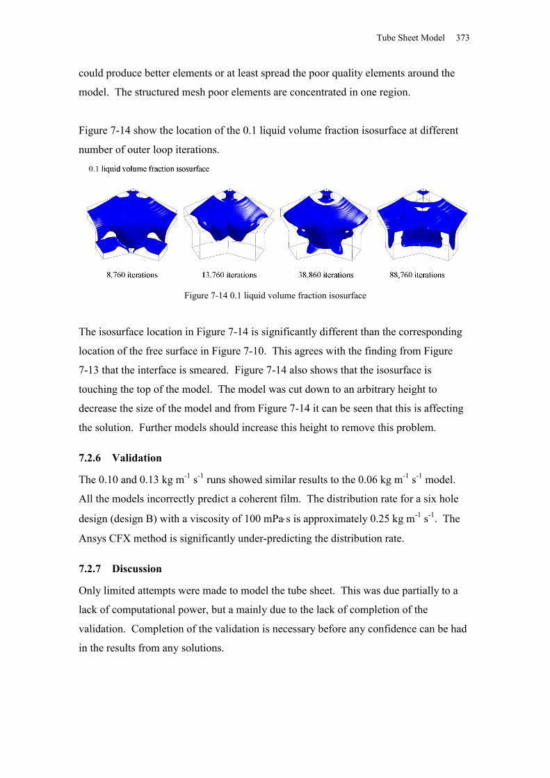
Tube Sheet Model 373
could produce better elements or at least spread the poor quality elements around the
model. The structured mesh poor elements are concentrated in one region.
Figure 7-14 show the location of the 0.1 liquid volume fraction isosurface at different
number of outer loop iterations.
Figure 7-14 0.1 liquid volume fraction isosurface
The isosurface location in Figure 7-14 is significantly different than the corresponding
location of the free surface in Figure 7-10. This agrees with the finding from Figure
7-13 that the interface is smeared. Figure 7-14 also shows that the isosurface is
touching the top of the model. The model was cut down to an arbitrary height to
decrease the size of the model and from Figure 7-14 it can be seen that this is affecting
the solution. Further models should increase this height to remove this problem.
7.2.6 Validation
The 0.10 and 0.13 kg m-1 s-1 runs showed similar results to the 0.06 kg m-1 s-1 model.
All the models incorrectly predict a coherent film. The distribution rate for a six hole
design (design B) with a viscosity of 100 mPas is approximately 0.25 kg m-1 s-1. The
Ansys CFX method is significantly under-predicting the distribution rate.
7.2.7 Discussion
Only limited attempts were made to model the tube sheet. This was due partially to a
lack of computational power, but a mainly due to the lack of completion of the
validation. Completion of the validation is necessary before any confidence can be had
in the results from any solutions.
Tube Sheet Model 374
The few solutions produced served three purposes, first to find the scale and give
information about the basic phenomena predicted on the tube sheet. This was done to
help design the validation models with similar phenomena to that in the tube sheet.
The second reason for running the tube sheet models was to get an understanding if the
different phenomena of the validation model would combine as a single model. Figure
7-10 shows the jet coming down, impinging on the top of the tube sheet forming and a
hydraulic jump. The film spreads out from the impingement point flowing over the tube
edge forming a rivulet. The film keeps spreading an eventually the entire surface is
wetted. The preliminary indications are that the method is capable of modelling all the
expected phenomena together.
The third use for the model was as a learning tool to gain insight into the possible
numerical problems causing issues throughout the project. The slow speed of the
solution limits the use to a very few number of runs. Using different but similar models
to troubleshoot a problem with a model is often useful. Seeing the same problem in
different models can help the understanding of what is going wrong.
It is believed that the geometry of the model should be extended as the outlet and the
top (which has been arbitrarily cut) are having an effect on the solution.
The numerical computational time is extreme, due to the very small timestep required to
limit the effect of the numerical parasitic currents.
7.2.8 Conclusion and Future Work
The solutions currently under-predict the distribution rate. The current solutions are not
believed to be reliable and the model is too undeveloped to be useful in the prediction or
understanding of the distribution rate.
It is encouraging to see that the free surface predicted by Ansys CFX shows all the
required phenomena expected to occur in the distribution of the film. With the
completion of the validation models, nothing seen in the current tube sheet models
indicates that the CSF VOF method can not be used to predict the distribution rate.
Tube Sheet Model 375
The cut-down geometry used is too small and needs to be expanded (Figure 7-14). The
current mesh is causing the interface to become smeared and this is a possible cause of
the under-prediction of the distribution rate. Potentially an unstructured mesh may
perform better than the current structured mesh.
The validation models need to be completed to a satisfactory level before the original
objectives for the tube sheet model can be completed.
Eventually the model needs to be expanded to take into account a non-vertical or non-
centred jet.
Discussion 376
8 DiscussionThe individual models have been discussed at length with the respective model
chapters. The following is discussion that has not been covered in the individual
chapter discussions. It concerns how the project fits into the previous work in the field
how the project could be continued is also discussed in the future work section.
8.1 Multiphase modellingAll the models created for this project involve multiphase flows of the different parts of
the same evaporators. Two distinct CFD multiphase modelling techniques were used.
The VOF model is a general model that could be used to model all multiphase situations
if the computational cost of a model was not a factor. In most situations the
computational cost of the model is important and, depending on the situations different
multiphase models are often used. It is important to know which model will give the
appropriate level of accuracy for a given problem as well as any model limitations.
When modelling the separation of the droplets, the droplets were modelled using the
one-way coupled discrete droplet using the Lagrangian modelling technique. The use of
this method was valid in part due to the low droplet volume fraction in the area of
interest (the separator). Another important factor in the valid use of the Lagrangian
model was the prior knowledge about interface shape (the droplets are close to
spherical) and how the interface did not need to the modelled directly. If the interface
needed to be modelled directly then the VOF method would need to be used.
The computational cost of using the general VOF method instead of the Lagrangian
method for the modelling of the separation would be orders of magnitude greater and
would only give a small increase in accuracy. There are several other more accurate
models (two-way and fully-coupled Lagrangian methods) that could have been used
before using the VOF model since they would be numerically less expensive than a
VOF model, but none of them were needed. The one-way coupled Lagrangian method
was shown to be able to correctly predict a lack of carry-over leading to fouling due to
insufficient separation, which was the key requirement of the model. No increase in
accuracy was need and little would be gained by using a more complex model. This is a
Discussion 377
good example of choosing a model that is accurate enough for the needs of the model
objectives.
The Lagrangian method was used in the separator model and was able to accurately
predict that the separation of the entrained droplets was not the cause of the fouling.
The Lagrangian multiphase method was only used in the separator chapter models. The
discussion and conclusion drawn are not repeated in this chapter since the method was
discussed at length in the separator chapter.
When modelling the wetting of a surface the interface location and shape is unknown
and critical since it is finding the location and shape of the interface that is objective of
the model. This is the reason that the VOF method was used. The VOF model was
supplemented by the CSF method to account for the effect of surface tension.
The CSF VOF method was found to be numerically unstable. The method was not easy
to use, requiring significant user experience, and trail and error to get any solutions.
The solver showed promise and was able to be validated against most validation data.
Following is a discussion about the difficulty of using the CSF VOF method as
implemented by Ansys CFX 10.0.
The numerical instability produced numerical currents called parasitic currents that if
could cause the solver to diverge. The numerical instability and the parasitic currents
could be controlled by using a very small volume fraction timestep, typically no larger
then 10-5 s. The very small volume fraction timestep meant that solving any models
with more than about 200,000 elements was not possible.
The need to use high quality mesh elements with the CSF VOF model means that
except for very basic geometries meshes are likely to need significantly more elements
than normally could used be used with typical CFD solutions. Prism layers are used to
capture the large gradient near the wall while keeping the number of elements down.
The CSF VOF method was found to be sensitive to the use of prism layers and their use
is not recommended with the CSF VOF. If the gradients near the wall need to be
captured: only high quality elements can be used. This can greatly increase the number
of elements in a mesh. The hydraulic jump is an example of where the film is thin and
Discussion 378
the gradient are very high. To capture the gradient without prism layers requires a
significant number of elements.
The more refined the mesh used to estimate the curvature of the free surface, the smaller
the variations in the curvature which cause the parasitic currents. Unfortunately, a more
refined mesh allows a sharper resolution of the interface which produces greater
parasitic currents since the curvature refinement is greater. This means that using more
elements in a mesh does not always increase the stability of the CSF VOF model.
Deciding the best mesh element size is very difficult and requires user experience.
The interface distance can not be controlled or set directly, however it can be influenced
indirectly. The mesh can influence the interface as was discussed above. Using
different false timesteps between the volume fraction and the momentum equations
results in the interface smearing and this smearing increases the stability of the
numerics. Interface compression reduces any interface smearing, making the interface
sharper and the model less stable. The smoothing of the interface also smears out the
interface, as well as reducing any difference along the free-surface. Volume fraction
smoothing was also found to stablise the numerics.
The normal convergence measures of the residuals were found to have limited if any use
in judging the quality of the solution. It is good practice to monitor other metrics to
measure convergence, but this is not always possible, forcing the user to only use the
residuals. The limited information in the residuals makes it difficult to decide when to
stop a simulation and to assess its accuracy.
When numerical currents are large enough the parasitic currents could cause the
interface of the film to creep across a surface due to the physical preference for a wet
surface to remain wet. Evaluating if a film is creeping due to physical or numerical
creeping is difficult and stopping undesired numerical creeping could be difficult or
computationally expensive.
The stability of the CSF VOF method was found to be dependent on the physical
material properties of the fluids. The dependency can be described by the Oh number of
the liquid fluid this agrees with the findings of Renardy and Renardy (2002).
Discussion 379
Modelling the film for the tube sheet model was particularly difficult. The liquid has
low viscosity, high density, has high surface tension and film details are small with
areas of high curvature. The features tend to make the solutions very unstable.
8.2 Model usefulnessIt is the author’s opinion that CFD modelling can be grouped into three different groups
by the ability of the code to correctly predict the correct solution, and the ease and
computational expensive of solving the models. I have named them commercial CFD
models, research CFD models and unrealistic CFD models.
Unrealistic CFD models are CFD models that should not be or cannot be solved with
the current generation of CFD technologies. This could be because the current models
incorrectly predict the critical physics of the model or the computational cost of the
correct model for the physics is beyond the current generation of computer. Research
CFD models are models that can be solved but require significant user experience with
the specific model and/or significant computer resources to get accurate solutions.
Commercial CFD models are models that an experienced CFD user could be expected
to use to get accurate solutions without any specific experience using the model and the
model can be solved using only a moderate amount of computational resources.
The particle tracking and multiphase modelling used to predict fouling with the
integrated separator is a good example of a commercial model. The model was able to
accuracy predict the correct result, in a timely manner and with only reasonable
computer resources. In contrast the distribution model should not be used without
significant resources and experience, and interpreting the result is difficult due the lack
of useful information about the quality of the model convergence. The distribution
model is either a research model or maybe even an unrealistic model.
The designation between the different groups is arbitrary and subjective but it is useful a
tool when deciding if it appropriate to use a CFD model instead of another method like
experimental work. If the purpose of using a CFD model instead of experimental work
is to shorthorn the design cycle or cheapen the process, using research CFD models may
not be appropriate, due to the long time needed to create, solve and understand them.
Discussion 380
Depending on the situation research CFD models may still be quicker, cheaper and/or
better than other methods like experimentation.
Commercial codes are continually increasing the range of models they can solve and the
ease of use of their code thus requiring fewer hours of engineering input per model.
The cost per calculation by computer continues to reduce, so that what was previously
considered to be a research CFD models is now a commercial CFD models.
Historically dairy process equipment is designed without the use of CFD techniques.
The design process is a very incremental process. New designs are typically based on
previous designs that are known to work.
The geometry of most of the process equipment in the dairy industry is 3-D and any 2-D
simplification is unrealistic. The 2-D models require meshes with significantly more
elements which, in turn, is closely related to the computational cost of the solution.
Most dairy industrial processes are multiphase flows, making the physics of any model
more complex and difficult to solve. The mesh size and complexity of the multiphase
flows could be the reason CFD techniques have not had greater penetration into the
design process. Historically the cost the model in engineering and computer time may
have been too large for the value of the information gained.
It is the author’s opinion that this is changing and that some of the complex 3-D
multiphase process equipment could be handled using only a modern workstation. This
makes the case for greater using CFD models in the dairy process more compelling,
since this project has shown how they can be used to model flows in the dairy
processing environment. This project also shows how not all flows can be modelled.
8.3 General discussionThese are the first CFD models of an integrated separator, there is no published work in
literature and nor is CFD used by the design company (Remond, 2006). They also
appear to be the first dairy cyclonic separator CFD models as well. The model serve as
a good starting point for any further CFD modelling of either integrated separator or
even dairy cyclonic separators. This would extend the use of CFD in designing and
analysing cyclone separators. The free surface models also appear to the first attempt to
Discussion 381
use CFD modelling to predict the liquid distribution rate. There has not been any
publish literature modelling the distribution rate. The lack of published work may be
explained by the numerical instability of accurately predicting the curvature and hence
surface tension.
8.4 Future workThe recommended use of the two techniques is different due to their different
performance when used to model multiphase problems.
8.4.1 Lagrangian multiphase methodThe Lagrangian method was used to accurately model the low volume fraction flow of
the atomised liquid phase in the separator at the bottom of a falling film evaporator.
The method produced accurate results and the speed, robustness and ease of use make a
good tool for design of separators in the not only the dairy industry but any other
industry where the volume fractions are low. As mentioned previously CFD, is not
currently used as a design tool for designing separators in the dairy industry and it is the
author’s opinion in the future that CFD modelling should be considered for any
separator design work or comparison between different designs.
For future models of the separation process it is recommended that the user consider
using a transient model instead of a steady state model. The transient model was not
needed since the steady state model was found to be accurate enough, however this
might not be the case for future situations. The available of a supported transient
particle tracking model and the increase in computational speed per unit cost makes
using the transient model more reasonable and the increase in accuracy might be
significant and useful.
The accuracy of the current model was limited by the lack of information about the
atomisation of the film. No information was found about the atomisation at the bottom
of the falling film evaporator tubes. Any improvement in this situation would
significantly increase the accuracy and/or confidence in the current model and any other
future models. Due to the complexity of the physics of atomisation, experimental work
would be preferable to any numerical simulation.
Discussion 382
8.4.2 CSF VOF multiphase methodThe CSF VOF method was found to be quite unstable. The instability was found to be
due to the calculation of the curvature of the free surface interface. Finding a better
numerical estimation of the curvature is an obvious area of future work and if a
significantly better estimate was found the method appears to be ideal for the prediction
of wetting rates.
The lack of validation data was surprising; given the basic and common nature of the
flows. Producing more validation data for simple models would be very useful not only
for the prediction of wetting rates in the dairy industry but any other problems involving
moving films.
The CSF VOF method was too unstable to be used in this project, however for other
projects this may not be the case. The use of the CSF VOF model should not be ruled
in cases where the Oh number is significantly smaller than the Oh number of this
project. It is likely that the CSF VOF could be used to successfully model films and
could be used for wetting rate studies.
Completing the models was not a possible due to CSF VOF method required
computational resources that were not available. The work could be continued by
someone with significantly more computational resources. In the future the
computational cost might not be as unreasonable as the computational cost continues to
decrease. As stated before the possibility of the CSF VOF method producing
unphysical creeping would still need to be solved.
Conclusions 383
9 Conclusions
A CFD model of the integrated separator attached to the falling film evaporators for the
milk powder plant 2 at Clandeboye Temuka New Zealand was created. This model
appears to be the first CFD model of an integrated separator and the first CFD model of
a separator in the dairy industry. The CFD model was able to accurately predict that
droplet penetration was not the cause of a fouling problem. The predicted mass fraction
loss based on total solids was 0.03% when processing skim milk and 0.0012% when
processing MPC. These values agreed with experimental measurements taken from the
separators in question.
The CFD model was used to gain a greater understanding of the paths of the different
phases travelling through the separator. Several separation processes act on the droplets
to separate them from the water vapour they are suspended in. The most important
separation process is due to the centrifugal forces on the droplets as they travel around
the separator. It is this process that determines the cut-off diameter and hence the size
of largest droplets that penetrate the separator. These largest droplets contain the
majority of the mass and are therefore critical for the overall mass penetration rate.
Currently the separators are designed using a plug flow assumption through the
doorways between the separator and plenum chamber. The CFD model predicted
significant areas of recirculation at the top of these doorways indicating that the plug
flow assumption was a poor assumption.
The separation rate of the separator was found to be sensitive to the atomisation process
of the falling film at the top of the plenum chamber. This atomisation process is not
well understood but when the water vapour velocity at the bottom of the tube is high,
more numerous smaller droplets are produced, decreasing the efficiency of the
separator. The more numerous smaller droplets are more difficult to collect than larger
droplets, so keeping the water vapour velocity low when exiting the calandria reduces
the number of small droplets and greatly increases the efficiency of the separator.
Conclusions 384
The CSF VOF method of Ansys CFX was proposed to model the distribution of the film
on the tube sheet at the top of the falling film evaporator. Again this appears to be the
first attempt to use CFD to model the distribution. The method was found to be
numerically unstable and difficult to work with. The difficulty of modelling what at
first look could be considered “simple” could explain why CFD modelling has no been
used before.
The numerical instability of the CSF method is due to the poor estimation of the
curvature of the free surface interface which is in agreement with Tong and Wang
(2007), Francois et al. (2006), Harvie et al. (2006) and Meier et al. (2002). The
numerical instability results in parasitic currents that can cause the model to diverge.
The stability of the CSF VOF method was found to be dependent on the physical
material properties of the fluids. The dependency can be described by the Oh number of
the liquid fluid which agrees with the findings of Renardy and Renardy (2002).
When the VOF fraction timestep is small enough (typically 10-5 s) the parasitic currents
appear to oscillate the interface around the correct location. The small volume fraction
timestep required significantly more computational resources to solve than where
available and only some of the planned simulations were completed.
The CSF VOF method shows considerable promise and has been successfully used to
predict several different surface tension and contact angle dominated film flows. There
are still questions about numerical creeping of films and how significant this effect
could be. The method agreed with the work of the Bush and Aristoff (2003) when
modelling a jet, Equation (6-3) when modelling a sessile droplet and Henderson (1966)
when modelling an overfall.
The 2-D weir model gave good qualitative agreement with expected results and the 3-D
weir model also predicts realistic topography and predicted a minimum wetting rate that
is consistent with the limit experimental work available. The small rivulet model also
showed qualitative agreement with expected results and shows how the CSF VOF
method can spontaneously predict different free surface topographies, which is a very
useful attribute for wetting studies. The predicted wetting rate did not agree with
Conclusions 385
Hartley and Murgatroyd, (1964) or Morison et al., (2006), however the model geometry
was believed to be to small and was extended.
A rivulet of the from the extended rivulet model showed agreement with the predicted
idealised rivulet profile of El-Genk and Saber (2001). The extended rivulet model
predicted a wetting rate that agreed with Morison et al. (2006). It is not known if the
solution is mesh independent or not. The range of the extended rivulet wetting rate was
not very narrow, between 0.060 and 0.175 kg m-1 s-1 compared to the wetting rate of
Morison et al. (2006) of 0.09 kg m-1 s-1.
The CSF VOF method did not agree with the work of Bush and Aristoff (2003) when it
was used to model a hydraulic jump with surface tension. The high viscosity solution
of 100 mPas was outside the experimental range of Bush and Aristoff (2003) and this
may account for the difference. The 100 mPas solution’s predicted hydraulic jump
agreed to within 35% to the work of Chang et al., (2001). The solution for the lower
viscosity liquid of 10 mPas was within the viscosity range of the work of Bush and
Aristoff (2003) but it did not agree with their results or with Chang et al. (2001). These
solutions were not well converged or mesh independent and until better converged and
mesh independent solutions are produced it is difficult to reach any conclusions.
When the hydraulic jump was modelled without surface tension the VOF method was
able to get good qualitative results and the CFD hydraulic jump radius agreed with the
work of Chang et al., (2001) to within 22%. The hydraulic jump radi were measure
from a different location to Chang et al., (2001) and the agreement is likely to be closer
than 22% (refer to Figure 6-73).
The tube sheet was modelled to prove the concept that the smaller validation models
could be combined together into a single model. The combined model was partially
solved and the results showed qualitative agreement with the previous unpublished
work of Ken Morison from the University of Canterbury. The completion of the
validation model is needed before the complete tube sheet model should be attempted.
Conclusions 386
Modelling the film of the liquid in the dairy distribution system is very difficult due to
the small scale of the topographic features and the material properties. The small
topographic features result in area of high curvature which is difficult to calculate
accurately and the thinness of the films requires especially large numbers of elements,
since prism layer or other elements with high skew cause increased numerical
instabilities with the CSF VOF method. The low viscosity, high density, high surface
tension nature of the liquid films made the CSF VOF more numerical unstable. This
resulted in large meshes requiring very small timestep to keep stable, and required very
large computational resources.
The CSF VOF model could be significantly more stable when modelling a different
surface tension driven free surface model. If the curvature of the free surface was
smaller or the material properties were more favourable, for example the liquid was
more viscous. With increased stability the CSF VOF method becomes less
computationally expensive and easier to use, making the CSF VOF method an attractive
choice for modelling of surface tension driven free surface flows. The validation
models are simple models that can be used for validation of the method for not only the
tube sheet modelling but also other similar flows and could be easily extended into the
appropriate material properties range. These other models could be outside the dairy
processing industry since film flows are common place in many different engineering
fields.
Both models created useful CFD modelling techniques in new areas. Modelling the
dispersed droplets in the separator is more advanced than the free surface modelling
required for the liquid distribution model. Using CFD techniques to model the
separator is a realistic option in both academia and commercially, due to the ability,
accuracy and relative ease of modelling. The free surface modelling of the liquid
distribution still requires work before it could be considered a “commercial” model. It
is the author’s opinion that modelling of the liquid distribution is still firmly a
“research” modelling technique.
References 387
10 References
Abrahamson, J. (1975). Collision rates of small particles in a vigorously turbulent fluid.
Chemical Engineering Science, 30(11), 1371-1379.
Abrahamson, J. (2005). Personal Communications. University of Canterbury,
Christchurch, New Zealand.
Acheson, D. J. (1990). Elementary Fluid Dynamics, Oxford University Press.
Adamson, A. W. (1967). Physical Chemistry of Surfaces, Interscience Publishers, New
York.
Anderson, J. D. (1995). Computational Fluid Dynamics : The Basics With Applications,
McGraw-Hill, New York.
Ansys CFX. (2005). Release 10.0. Ansys Inc, Southpointe, Cansonburg, PA, USA.
Ayres, D., Caldas, M., Semiao, V., and da Graca Carvalho, M. (2001). Prediction of the
droplet size and velocity joint distribution for sprays. Fuel, 80(3), 383-394.
Badens, E., Boutin, O., and Charbit, G. (2005). Laminar jet dispersion and jet
atomization in pressurized carbon dioxide. The Journal of Supercritical Fluids,
36(1), 81-90.
Bardina, J. E., Huang, P. G., and Coakley, T. J. (1997). Turbulence modelling
validation, testing, and development. NASA Technical Memorandum (110446),
1-88.
Barth, T. J., and Jesperson, D. C. (1989). The design and application of upwind schemes
on unstructured meshes. AIAA, Paper 89-0366.
Basu, S. (2001). The study of the behaviour of a disturbed semi-infinite liquid jet using
a spatial instability method. Fluid Dynamics Research, 29(5), 269-286.
Bayvel, L. P., and Orzechowski, P. (1993). Liquid atomization, Taylor and Francis.
Billet, R. (1989). Evaporation Technology: Principles, Applications, Economics,
Distribution VCH Publishers, New York, NY, USA.
Bird, R. B. (1960). Notes on Transport Phenomena, Transport Phenomena, Wiley, New
York.
Blaisot, J. B., and Adeline, S. (2003). Instabilities on a free falling jet under an internal
flow breakup mode regime. International Journal of Multiphase Flow, 29(4),
629-653.
References 388
Bohr, T., Ellegaard, C., Hansen, A. E., Hansen, K., Haaning, A., Putkaradze, V., and
Watanabe, S. (1998). Separation and pattern formation in hydraulic jumps.
Physica A: Statistical and Theoretical Physics, 249(1-4), 111-117.
Brackbill, J. U., Kothe, D. B., and Zemach, C. (1992). A continuum method for
modeling surface tension. Journal of Computational Physics, 100(2), 335-354.
Broome, S. (2005). Personal Communications. Fonterra Co-operative Group, Temuka.
Bush, J. W. M., and Aristoff, J. M. (2003). The influence of surface tension on the
circular hydraulic jump. Journal of Fluid Mechanics, 489(489), 229-238.
Bush, J. W. M., Aristoff, J. M., and Hosoi, A. E. (2006). An experimental investigation
of the stability of the circular hydraulic jump. Journal of Fluid Mechanics, 558,
33-52.
Bylund, G. (2003). Dairy Processing Handbook, Tetra Pak Processing Systems AB,
Lund, Sweden.
Carvalho, I. S., Heitoyr, M. V., and Santos, D. (2002). Liquid film disintegration
regimes and proposed correlations. International Journal of Multiphase Flow,
28(5), 773-789.
Chang, H. C., Demekhin, E. A., and Takhistov, P. V. (2001). Circular hydraulic jumps
triggered by boundary layer separation. Journal of Colloid and Interface
Science, 233(2), 329-338.
Chung, T. J. (2002). Computational Fluid Dynamics, Cambridge University Press,
Cambridge ; New York.
Corbitt, R. A. (1999). Standard Handbook of Environmental Engineering, McGraw-
Hill, New York.
Cortes, C., and Gil, A. (2007). Modeling the gas and particle flow inside cyclone
separators. Progress in Energy and Combustion Science, 33(5), 409-452.
Cristini, V., Blawzdziewicz, J., and Loewenberg, M. (2001). An adaptive mesh
algorithm for evolving surfaces: simulations of drop breakup and coalescence.
Journal of Computational Physics, 168(2), 445-463.
El-Genk, M. S., and Saber, H. H. (2001). Minimum thickness of a flowing down liquid
film on a vertical surface. International Journal of Heat and Mass Transfer,
44(15), 2809-2825.
Esmaeeli, A., and Tryggvason, G. (2004). A front tracking method for computations of
boiling in complex geometries. International Journal of Multiphase Flow, 30(7-
8), 1037-1050.
References 389
Fayed, M. E., and Otten, L. (1984). Handbook of Powder Science and Technology, Van
Nostrand Reinhold Co., New York.
Fowkes, F. M., Zisman, W. A., and American Chemical Society. Division of colloid
and surface chemistry. (1964). Contact angle, Wettability and Adhesion: The
Kendall Award Symposium Honoring William A. Zisman, Los Angeles, Calif.,
April 2-3, 1963, American Chemical Society, Washington.
Francois, M. M., Cummins, S. J., Dendy, E. D., Kothe, D. B., Sicilian, J. M., and
Williams, M. W. (2006). A balanced-force algorithm for continuous and sharp
interfacial surface tension models within a volume tracking framework. Journal
of Computational Physics, 213(1), 141-173.
Gao, D., Morley, N. B., and Dhir, V. (2003). Numerical simulation of wavy falling film
flow using VOF method. Journal of Computational Physics, 192(2), 624-642.
Goldman, R. (2005). Curvature formulas for implicit curves and surfaces. Computer
Aided Geometric Design, 22(7), 632-658.
Grunjal, P. R., Ranade, V. V., and Chaudhari, R. V. (2003). Experimental and
computational study of liquid drop over flat and spherical surfaces. Catalysis
Today, 79-80, 267-273.
Haar, L., Gallagher, J. S., Kell, G. S., and National Standard Reference Data System
(U.S.). (1984). NBS/NRC Steam Tables: Thermodynamic and Transport
Properties and Computer Programs for Vapor and Liquid States of Water in SI
Units, Hemisphere Pub. Corp, Washington, [D.C.].
Haas, F. C. (1964). Stability of droplets suddenly exposed to high velocity gas stream.
A.I.Ch.E. Journal, 10(6), 920-924.
Harmon, J. D. B. (1955). Drop sizes from low speed jets. Journal of the Franklin
Institute, 259(6), 519-522.
Hartley, D. E., and Murgatroyd, W. (1964). Criteria for break-up of thin liquid layers
flowing isothermally over solid surfaces. International Journal of Heat and
Mass Transfer, 7(9), 1003-1015.
Harvie, D. J. E., Davidson, M. R., and Rudman, M. (2006). An analysis of parasitic
current generation in volume of fluid simulations. Applied Mathematical
Modelling, 30(10), 1056-1066.
Heldman, D. R., and Lund, D. B. eds. (2007). Handbook of Food Engineering, 2nd ed,
CRC Press, Boca Raton.
Henderson, F. M. (1966). Open Channel Flow, The Macmillan Company, New York.
References 390
Hinze, J. O. (1955). Fundamentals of hydrodynamic mechanism of splitting in
dispersion processes. Chemical Engineering Progress, 1(3), 289-295.
Hoke, B. C., Jr., and Chen, J. C. (1992). Thermocapillary breakdown of subcooled
falling liquid films. Industrial & Engineering Chemistry Research, 31(3), 688-
694.
Hsiang, L. P., and Faeth, G. M. (1995). Drop deformation and breakup due to shock
wave and steady disturbances. International Journal of Multiphase Flow, 21(4),
545-560.
Huang, L. X., Kumar, K., and Mujumdar, A. S. (2003). A parametric study of the gas
flow patterns and drying performance of co-current spray dryer: results of a
computational fluid dynamics study. Drying Technology, 21, 957-978.
Ingham, D. B., and Kelmanson, M. A. (1984). Boundary Integral Equation Analyses of
Singular, Potential, and Biharmonic Problems, Springer-Verlag, Berlin ; New
York.
Jamet, D., Torres, D., and U., B. J. (2002). On the theory and computation of surface
Tension: The elimination of parasitic currents through energy conservation in
the second-gradient method. Journal of Computational Physics, 182, 262-276.
Jasuja, A. K. (1979). Atomization of crude and residual fuel oils. Journal of
Engineering for Power, Transactions ASME, 101(2), 250-258.
Jones, I. (2005). Personal Communications. CFX, Ansys Inc, Oxford, U.K.
Karagoz, I., and Kaya, F. (2007). CFD investigation of the flow and heat transfer
characteristics in a tangential inlet cyclone. International Communications in
Heat and Mass Transfer, 34(9-10), 1119-1126.
Karapantsios, T. D., and Karabelas, A. J. (1995). Longitudinal characteristics of wavy
falling films. International Journal of Multiphase Flow, 21(1), 119-127.
Kerst, A. W., Judat, B., and Schlunder, E. U. (2000). Flow regimes of free jets and
falling films at high ambient pressure. Chemical Engineering Science, 55(19),
4189-4208.
Kessler, H. G. (2002). Food and Bio Process Engineering, 5th ed, Verlag A Kessler,
Munich.
Kiely, G. (1997). Environmental engineering, McGraw-Hill, London ; New York.
Kim, K.-T., and Khayat, R. E. (2004). Three-dimensional transient free-surface rotating
creeping flow. Engineering Analysis with Boundary Elements, 28(4), 375-388.
References 391
Kistler, S. F., and Scriven, L. E. (1994). The teapot effect: sheet-forming flows with
deflection, wetting and hysteresis. Journal of Fluid Mechanics, 263, 19-62.
Kunugi, T., and Kino, C. (2005). DNS of falling film structure and heat transfer via
MARS method. Computers & Structures, 83(6-7), 455-462.
Lafrance, P. (1974). Nonlinear breakup of a liquid jet. The Physics of Fluids, 17(10),
1913-1914.
Lafrance, P. (1975). Nonlinear breakup of a laminar liquid jet. The Physics of Fluids,
18(4), 428-432.
Langrish, T. A. G., and Fletcher, D. F. (2001). Spray drying of food ingredients and
applications of CFD in spray drying. Chemical Engineering and Processing, 40,
345-354.
Lavernia, E. J., and Wu, Y. (1996). Spray atomization and deposition, John Wiley,
Chichester ; New York.
Leal, L. G. (1992). Laminar Flow and Convective Transport Processes: Scaling
Principles and Asymptotic Analysis, Butterworth-Heinemann, Boston.
Lefebrve, A. H. (1989). Atomization and Sprays, Hemisphere publishing corporation.
Liu, D., and Lipták, B. G. (1997). Environmental Engineers' Handbook, Lewis
Publishers, Boca Raton, Fla.
Losasso, F., Fedkiw, R., and Osher, S. (2006). Spatially adaptive techniques for level
set methods and incompressible flow. Computers & Fluids, 35(10), 995-1010.
Lu, W.-Q. (1997). Boundary element analysis of three kinds of gas-liquid free surface
problem. Engineering Analysis with Boundary Elements, 19(4), 269-277.
Mansour, A., and Chigier, A. (1990). Disintegration of liquid sheets. Phys. Fluids A,
2(5), 706-719.
Mansour, A., and Chigier, A. (1991). Dynamic behaviour of liquid sheets. Phys. Fluids
A, 3(12), 2971-2980.
Markstein, G. H., Guenoche, H., and Putnam, A. A. (1964). Nonsteady flame
propagation. AGARDograph 75, 328.
Mathieu, J., and Scott, J. (2000). An Introduction to Turbulent Flow, Cambridge
University Press, Cambridge ; New York.
Matida, E. A., Finlay, W. H., Lange, C. F., and Grgic, B. (2004). Improved numerical
simulation of aerosol deposition in an idealized mouth-throat. Journal of Aerosol
Science, 35(1), 1-19.
References 392
Matida, E. A., Nishino, K., and Torii, K. (2000). Statistical simulation of particle
deposition on the wall from turbulent dispersed pipe flow. International Journal
of Heat and Fluid Flow, 21(4), 389-402.
Meier, M., Yadigaroglu, G., and Smith, B. L. (2002). A novel technique for including
surface tension in PLIC-VOF methods. European Journal of Mechanics -
B/Fluids, 21(1), 61-73.
Morison, K. (2006). Personal Communications. University of Canterbury, Christchurch,
New Zealand.
Morison, K. R., and Hartell, R. W. (2007). Evaporation and Freeze Drying, in Heldman,
D. R., and Lund, D. B. eds. Handbook of Food Engineering, 2nd ed, CRC Press,
Boca Raton, 495-552 .
Morison, K. R., Worth, Q. A. G., and O'Dea, N. P. (2006). Minimum wetting and
distribution rates in falling film evaporators. Food and Bioproducts Processing,
84(C4), 302-310.
Narasimha, M., Sripriya, R., and Banerjee, P. K. (2005). CFD modelling of
hydrocyclone--prediction of cut size. International Journal of Mineral
Processing, 75(1-2), 53-68.
Norton, T., and Sun, D.-W. (2006). Computational fluid dynamics (CFD) - an effective
and efficient design and analysis tool for the food industry: A review. Trends in
Food Science & Technology, 17(11), 600-620.
Orszag, S. A., and Staroselsky, I. (2000). CFD: Progress and problems. Computer
Physics Communications, 127(1), 165-171.
Osher, S., and Sethian, J. A. (1988). Fronts propagating with curvature-dependent
speed: Algorithms based on Hamilton-Jacobi formulations. Journal of
Computational Physics, 79(1), 12-49.
Owen, I., and Ryley, D. J. (1985). The flow of thin liquid films around corners.
International Journal of Multiphase Flow, 11(1), 51-62.
Paramalingam, S. (2004). Modelling, Optimisation and Control of a Falling-Film
Evaporator, Ph.D. thesis, Massey University, Palmerston North, New Zealand.
Paramalingam, S., Winchester, J., and Marsh, C. (2000). On the fouling of falling film
evaporators due to film break-up. Food and Bioproducts Processing, 78(C2),
79-84.
Patankar, S. V. (1980). Numerical heat transfer and fluid flow, Hemisphere Pub. Corp;
McGraw-Hill, Washington, New York.
References 393
Perry, R. H., Green, D. W., and Maloney, J. O. (1997). Perry's Chemical Engineers'
Handbook, McGraw-Hill, New York.
Raw, M. J. Robustness of Coupled Algebraic Mutligrid for Navier-Stokes Equations.
AIAA 96-0297, 34th Aerospace and Sciences Meeting & Exhibit, January 15-18
1996, Reno, NV.
Reiner, M. (1956). Teapot effect ... a problem. Physics Today, 9(9), 16-20.
Reinhard, A. (1964). Das Verhalten fallender Tropfen, Dissertation No 3412,
Hochschule, Zurich.
Remond, B. (2006). Personal Communications. GEA Process Engineering,
Paris,France.
Renardy, Y., and Renardy, M. (2002). PROST: A parabolic reconstruction of surface
tension for the volume-of-fluid method. Journal of Computational Physics,
183(2), 400-421.
Rizkalla, A. A., and Lefebvre, A. H. (1975). Influence of air and liquid properties of
airblast atomization. Journal of Fluids Engineering, Transactions of the ASME,
97 Ser I(3), 316-320.
Rutland, D. F., and Jameson, G. J. (1970). Theoretical prediction of the sizes of drops
formed in the breakup of capillary jets. Chemical Engineering Science, 25(11),
1689-1698.
Saffman, P. G., and Turner, J. S. (1956). On collision of drops in turbulent clouds.
Journal of Fluid Mechanics, 1(Part 1), 16-30.
Sallam, K. A., Dai, Z., and Faeth, G. M. (1999). Drop formation at the surface of plane
turbulent liquid jets in still gases. International Journal of Multiphase Flow,
25(6-7), 1161-1180.
Schmehl, R., Rosskamp, H., Willmann, M., and Wittig, S. (1999). CFD analysis of
spray propagation and evaporation including wall film formation and spray/film
interactions. International Journal of Heat and Fluid Flow, 20(5), 520-529.
Schmelz, F., and Walzel, P. (2003). Breakup of liquid droplets in accelerated gas flows.
Atomization and Sprays, 13, 357-372.
Semiao, V., Andrade, P., and Carvalho, M. d. G. (1996). Spray characterization:
Numerical prediction of Sauter mean diameter and droplet size distribution.
Fuel, 75(15), 1707-1714.
References 394
Sirignano, W. A., and Mehring, C. (2000). Review of theory of distortion and
disintegration of liquid streams. Progress in Energy and Combustion Science,
26(4-6), 609-655.
Straatsma, J., Van Houwelingen, G., Steenbergen, A. E., and De Jong, P. (1999). Spray
drying of food products: 1. Simulation model. Journal of Food Engineering,
42(2), 67-72.
Teng, H., Kinoshita, C. M., and Masutani, S. M. (1995). Prediction of droplet size from
the breakup of cylindrical liquid jets. International Journal of Multiphase Flow,
21(1), 129-136.
Tjahjadi, M., Stone, H. A., and Ottino, J. M. (1992). Satellite and subsatellite formation
in capillary breakup. Journal of Fluid Mechanics, 243, 297-317.
Tong, A. Y., and Wang, Z. (2007). A numerical method for capillarity-dominant free
surface flows. Journal of Computational Physics, 221(2), 506-523.
Veerapen, J. P., Lowry, B. J., and Couturier, M. F. (2005). Design methodology for the
swirl separator. Aquacultural Engineering, 33(1), 21-45.
Versteeg, H., and Malalasekera, W. (1995). An Introduction to Computational Fluid
Dynamics: The Finite Volume Method, Longman Scientific & Technical, New
York.
Walstra, P., Wouters, J. T. M., and Geurts, T. J. (2006). Dairy Science and Technology,
2nd ed, CRC Press, Boca Raton, FL.
Walzel, P. (1984). Design of single substance pressure atomizers. German Chemical
Engineering, 7(1), 1-12.
Wilcox, D. C. Multiscale model for turbulent flows. In AIAA 24th Aerospace Sciences
Meeting. American Institute of Aeronautics and Astronautics.
Winchester, J. (2000). Model based anslysis of the operation and control of falling film
evaporators, Ph.D. Thesis, Massey University, Palmerston North, New Zealand.
Winchester, J. (2004-2007). Personal Communications. Fonterra Co-operative Group,
Temuka, New Zealand.
Zwart, P. J., Scheuerer M., Bogner M. (2003).”Free Surface Modelling Of An
Impinging Jet”, ASTAR International Workshop on Advanced Numerical
Methods for Multidimensional Simulation of Two-Phase Flow, September 15-
16 2003, GRS Garching, Germany.
Related Documents