THESIS EVALUATION OF A TRICKLE FLOW LEACH BED REACTOR FOR ANAEROBIC DIGESTION OF HIGH SOLIDS CATTLE MANURE Submitted by Asma Hanif Abdul Karim Department of Civil and Environmental Engineering In partial fulfillment of the requirements For the Degree of Master of Science Colorado State University Fort Collins, Colorado Fall 2013 Master’s Committee: Advisor: Sybil Sharvelle Kenneth Carlson Jessica Davis

Welcome message from author
This document is posted to help you gain knowledge. Please leave a comment to let me know what you think about it! Share it to your friends and learn new things together.
Transcript

THESIS
EVALUATION OF A TRICKLE FLOW LEACH BED REACTOR FOR ANAEROBIC
DIGESTION OF HIGH SOLIDS CATTLE MANURE
Submitted by
Asma Hanif Abdul Karim
Department of Civil and Environmental Engineering
In partial fulfillment of the requirements
For the Degree of Master of Science
Colorado State University
Fort Collins, Colorado
Fall 2013
Master’s Committee:
Advisor: Sybil Sharvelle
Kenneth Carlson
Jessica Davis

Copyright by Asma Hanif Abdul Karim 2013
All Rights Reserved

ii
ABSTRACT
EVALUATION OF A TRICKLE FLOW LEACH BED REACTOR FOR ANAEROBIC
DIGESTION OF HIGH SOLIDS CATTLE MANURE
Anaerobic digestion (AD) of cattle manure from feedlots and dairies is of increasing
interest in Colorado due to its abundant availability. Colorado is the one of the highest producer
of high solids cattle manure (HSCM) in the United States. Despite the available resources,
Colorado currently has only one operational anaerobic digester treating manure (AgSTAR EPA
2011), which is located at a hog farm in Lamar. Arid climate and limited water resources in
Colorado render the implementation of high water demanding conventional AD processes. Studies
to date have proposed high solids AD systems capable of digesting organic solid waste (OSW) not
more than 40% total solids (TS). Lab tests have shown that HSCM produced in Greeley (Colorado)
has an average of 89.6% TS. Multi-stage leach bed reactor (MSLBR) system proposed in the
current study is capable of handling HSCM of up to 90% TS. In this system, hydrolysis and
methanogenesis are carried out in separate reactors for the optimization of each stage. Hydrolysis
is carried out in a trickle flow leach bed reactor (TFLBR) and methanogenesis is carried out in a
high rate anaerobic digester (HRAD) like an upflow anaerobic sludge blanket (UASB) reactor or
a fixed film reactor. Since leach bed reactors (LBRs) are high solids reactors, studies have
indicated clogging issues in LBRs handling 26% TS. Since TFLBRs are subjected to hydrolyze
upto 90% TS, obtaining hydraulic flow through the reactor is a challenge. The objective of this
research is to (a) ensure good hydraulic flow through the TFLBRs and (b) evaluate and optimize
the performance of the TFLBR to effectively hydrolyze the HSCM. The system was operated as a
batch process with a hydraulic retention time (HRT) of 42 days without leachate recirculation. A
layer of sand was added as dispersion media on top of the manure bed in the TFLBRs. This

iii
promoted good hydraulic flow through the reactor eliminating clogging issues. Organic leaching
potential of a single pass (without leachate recirculation) TFLBR configuration was evaluated in
terms of chemical oxygen demand (COD). Manure is naturally rich in nutrients essential for
microbial growth in AD. In a typical MSLBR system, the TFLBRs are subjected to leachate
recirculation, conserving the essential nutrients in the system. However, in this single pass system,
the leachate removal would flush out the nutrients in the TFLBRs over time. So, nutrient solution
was added to the TFLBRs to provide a constant supply of essential nutrients in the reactors for the
purpose of this study and would not be necessary in a leachate recirculated TFLBR. A comparison
between nutrient dosed and non-nutrient dosed TFLBRs was performed. The non-nutrient dosed
and nutrient dosed TFLBRs indicated a COD reduction of approximately 66.3% and 73.5%
respectively, in total in terms of dry mass. A total reduction in volatile solids (VS) of approximately
46.3% and 44.7% was observed in the non-nutrient dosed and nutrient dosed TFLBRs,
respectively. Biochemical methane potential (BCMP) tests indicated a CH4 potential of
approximately 0.17 L CH4/g COD leached and 0.13 L CH4/g COD leached from the non-nutrient
dosed and nutrient dosed TFLBRs, respectively. Concentration of inorganics leached from the
TFLBR was monitored periodically.

iv
ACKNOWLEGEMENTS
I would first like to thank my adviser, Prof. Dr. Sybil Sharvelle, for having faith in me and
providing me the opportunity to work on this project. Her wisdom, persistence and attention to
detail have helped me overcome the inevitable problems that arise during research. She has been
very patient and supportive from the start. I have learned a lot working with her and it has been an
honor.
I would like to thank Colorado Agricultural Experiment Station, Colorado Natural
Resources Conservation Center, and the Colorado Biosciences Development Grant for their
research funding.
I would also like to thank Dr. Jessica Davis for her advice and guidance. I appreciate her
kindness and enthusiasm for being a part of my committee. I extend my gratitude to Dr. Kenneth
Carlson for mentoring me and providing me with necessary support. His unbound knowledge and
vast experience has been invaluable in my learning process. A special thanks to Lucas Loetscher
for his time, input and technical contributions to this research. I would also like to thank Kelly
Wasserbach for her support and help with the work.
I would like to acknowledge Paige Griffin, Margaret Hollowed, Brock Hodgson, Carlos
Quiroz and Bryan Grotz for their timely assistance. A special thanks to Ashwin Dhanasekar for
his help during system construction and maintenance.
Finally and most importantly, I would like to express my love and gratitude to my family
and friends for their undying love and support.

v
DEDICATION
I dedicate all my hard work and achievements to my beloved parents, Mumtaz and Hanif, for
without them none of this would have been possible.
A special thanks to Kamal Dave, a mentor, a friend and my ever-loving godfather.

vi
TABLE OF CONTENTS
LIST OF TABLES ......................................................................................................................x
LIST OF FIGURES .................................................................................................................. xi
LIST OF ACRONYMNS .........................................................................................................xiv
CHAPTER 1: INTRODUCTION ................................................................................................1
1.1. Research Motivation .....................................................................................................1
1.2. Thesis Overview ...........................................................................................................3
CHAPTER 2: BACKGROUND AND LITERATURE REVIEW ................................................6
2.1. Selection of OSW Management Technology .................................................................6
2.1.1. Landfills ................................................................................................................6
2.1.2. Thermal Treatment.................................................................................................6
2.1.3. Aerobic Composting ..............................................................................................7
2.1.4. AD .........................................................................................................................7
2.2. Advantages of AD.........................................................................................................8
2.3. General AD Process ......................................................................................................8
2.3.1. Hydrolysis .............................................................................................................9
2.3.2. Acidogenesis ........................................................................................................ 10
2.3.3. Acetogenesis ........................................................................................................ 10
2.3.4. Methanogenesis ................................................................................................... 11
2.4. Importance of Hydrolysis ............................................................................................ 11

vii
2.5. Uses of Produced Biogas ............................................................................................. 12
2.6. Selection of AD Technology ....................................................................................... 12
2.6.1. Covered Lagoon Digester ..................................................................................... 13
2.6.2. Complete Mix Digester ........................................................................................ 14
2.6.3. Plug Flow Reactor ............................................................................................... 15
2.6.4. Fixed Film Digester ............................................................................................. 16
2.6.5. Upflow Anaerobic Sludge Blanket Reactor (UASB) ............................................ 17
2.6.6. Digester Overview ............................................................................................... 19
2.7. Waste Management Practices in Colorado ................................................................... 19
2.8. Feasibility of AD in Colorado ..................................................................................... 20
2.9. Current Technology .................................................................................................... 21
2.9.1. Advantages of a Multi-Stage Reactor ................................................................... 22
2.9.2. Advantages of Leachate Recirculation through the TFLBR .................................. 22
2.10. History of LBRs ...................................................................................................... 23
2.10.1. LBRs Treating MSW ........................................................................................ 23
2.10.2. LBRs Treating Lignocellulosic Biomass ........................................................... 27
2.10.3. LBRs Treating Manure ..................................................................................... 30
2.11. Benefits and Limitations of LBRs ............................................................................ 34
2.12. Summary ................................................................................................................. 35
2.13. Thesis Objective ...................................................................................................... 36

viii
CHAPTER 3: MATERIALS AND METHODS ........................................................................ 37
3.1. Experiment Setup ........................................................................................................ 37
3.2. Manure Collection and Preparation ............................................................................. 38
3.2.1. Mechanical Chopping .......................................................................................... 38
3.2.2. Sorting ................................................................................................................. 39
3.3. System Construction and Set-Up ................................................................................. 39
3.4. Loading Reactors ........................................................................................................ 41
3.5. System Operation ........................................................................................................ 43
3.5.1. RO Tank .............................................................................................................. 45
3.5.2. ORP Tank ............................................................................................................ 45
3.5.3. Insulated Temperature Controlled Room .............................................................. 47
3.6. Evaluation of a TFLBR for the Hydrolysis of HSCM .................................................. 49
3.6.1. Reactor Experiment – Phase I .............................................................................. 49
3.6.2. Reactor Experiment – Phase II ............................................................................. 50
3.6.3. Reactor Experiment –Phase III ............................................................................. 50
3.7. Analytical Methods ..................................................................................................... 52
3.7.1. Solids Characterization ........................................................................................ 52
3.7.2. Leachate characterization ..................................................................................... 56
3.7.3. BCMP .................................................................................................................. 59
3.7.4. Data Analysis ....................................................................................................... 61

ix
CHAPTER 4: RESULTS AND DISCUSSION ......................................................................... 63
4.1. Reactor Experiment – Phase I ..................................................................................... 63
4.2. Reactor Experiment – Phase II .................................................................................... 64
4.3. Reactor Experiment – Phase III ................................................................................... 65
4.3.1. Leachate analysis ................................................................................................. 66
4.3.2. Solids Analysis .................................................................................................... 75
Nutrients ............................................................................................................................ 79
4.3.3. BCMP .................................................................................................................. 80
CHAPTER 5: CONCLUSIONS ................................................................................................ 86
CHAPTER 6: POTENTIAL FOR BIOGAS IN THE SHALE GAS INDUSTRY ...................... 88
6.1. Growing Shale Gas Industry ........................................................................................... 88
6.2. Process of Fracking for Natural Gas ................................................................................ 88
6.3. Problems associated with Fracking ................................................................................. 89
6.4. Biogas as ‘Renewable and Eco-Friendly Natural Gas’..................................................... 90
REFERENCES ......................................................................................................................... 91
Appendix 1: Intrinsic Permeability Tests ................................................................................... 96
Appendix 2: Sieving Tests....................................................................................................... 100
Appendix 3: Nutrient Solution Composition ............................................................................ 109
Appendix 4: Mass Balance ...................................................................................................... 110

x
LIST OF TABLES
Table 1. Comparison between digester types ............................................................................. 19
Table 2. Summary of studies conducted to date on LBRs treating MSWs. ................................ 26
Table 3. Summary of studies conducted to date on LBRs treating lignocellulosic biomass........ 29
Table 4. Summary of studies cited in literature to date for LBRs treating manure. ..................... 32
Table 5. Concentrations of nutrients in nutrient dosed TFLBRs ................................................. 51
Table 6. Particle diameters of the sieved HSCM and its corresponding mass distribution ........ 103
Table 7. Summary of the types of sieved HSCM mixtures loaded in the TFLBRs .................... 105
Table 8. Composition of salts and vitamins for the preparation of nutrient solution ................. 109

xi
LIST OF FIGURES
Figure 1. Operational anaerobic digesters in the United States .....................................................2
Figure 2. Process flow schematic for MSLBR system .................................................................4
Figure 3. Biological Processing Stages of AD .............................................................................9
Figure 4. Schematic of a Covered lagoon digester. .................................................................... 14
Figure 5. Schematic of a Complete mix digester ........................................................................ 15
Figure 6. Schematic of a Plug flow reactor ................................................................................ 16
Figure 7. Schematic of a Fixed film digester.............................................................................. 17
Figure 8. Cross-section of a UASB reactor ................................................................................ 18
Figure 9. Sorting tray ................................................................................................................ 39
Figure 10. Acrylic columns for TFLBRs. .................................................................................. 40
Figure 11. Top and bottom caps for TFLBRs. ........................................................................... 41
Figure 12. Schematic of a TFLBR ............................................................................................. 42
Figure 13. System layout as set-up in lab. .................................................................................. 44
Figure 14. Siemens lab-scale RO plant. ..................................................................................... 45
Figure 15. ORP tank .................................................................................................................. 47
Figure 16. Interior of the insulated temperature controlled room................................................ 48
Figure 17. Exterior of the insulated temperature controlled room.............................................. 48
Figure 18. Sealed 140 mL plastic syringe as a surrogate for HRAD. .......................................... 59
Figure 19. Standard curve for calibrating the GC for detecting the CH4 concentration in the
biogas produced by the BCMP test syringes. ............................................................................. 61
Figure 20. System failure .......................................................................................................... 63

xii
Figure 21. Comparison between the TFLBRs bulked with and without straw in terms of gCOD/L
leachate collected. ..................................................................................................................... 65
Figure 22. Comparison between reactor experiments in terms of leached COD in g/L. .............. 66
Figure 23. Change in COD concentration in the leachate ........................................................... 67
Figure 24. Comparison between the cumulative ratio of COD leached to the total COD present
in the non-nutrient dosed and nutrient dosed TFLBRs. .............................................................. 68
Figure 25. TS, TSS and TDS concentrations in the leachate ...................................................... 70
Figure 26. Cumulative amounts of TDS present in the leachate ................................................. 72
Figure 27. Change in TN and TP concentrations in the composited leachate collected ............... 73
Figure 28. Change in TVFA concentrations in the composited leachate collected ...................... 74
Figure 29. Comparison between non-nutrient dosed and nutrient dosed TFLBRs in terms of
COD. ........................................................................................................................................ 76
Figure 30. Comparison between non-nutrient dosed and nutrient dosed TFLBRs in terms of TS,
VS and FS. ................................................................................................................................ 77
Figure 31. Comparison between non-nutrient dosed and nutrient dosed TFLBRs in terms of total
TS, VS and FS. ......................................................................................................................... 78
Figure 32. Comparison between non-nutrient dosed and nutrient dosed TFLBRs in terms of TN,
TP and TK. ............................................................................................................................... 79
Figure 33. Volume of CH4 gas produced from the composited leachate collected ..................... 82
Figure 34. Cumulative volume of CH4 gas produced per L of weekly composited leachate ....... 83
Figure 35. Percentage of theoretical methane yield achieved from the leachate collected from the
non-nutrient dosed and nutrient dosed TFLBRs. ........................................................................ 84
Figure 36. Fracking Process ...................................................................................................... 89

xiii
Figure 37. Intrinsic permeability testing experimental set-up ..................................................... 97
Figure 38. Depiction of sieved substrate excluding the smaller particles .................................. 100
Figure 39. Depiction of unsieved substrate particles ................................................................ 100
Figure 40. Percentage of cumulative mass of HSCM passing through the sieve. ...................... 103
Figure 41. Permeability of different particle diameters under compression (47.47 J)................ 107

xiv
LIST OF ACRONYMNS
ACRONYM DEFINITION
AD Anaerobic Digestion
AF Anaerobic Filter
BCMP Biochemical Methane Potential
CH4 Methane
COD Chemical Oxygen Demand
CSTR Complete Stir Tank Reactor
FS Fixed Solids
GHG Greenhouse gas
HRAD High Rate Anaerobic Digester
HRT Hydraulic Retention Time
HSCM High Solids Cattle Manure
LBR Leach Bed Rector
MSLBR Multi-stage Leach Bed Reactor
MSW Municipal Solid Waste
ORP Oxidation Reduction Potential
OSW Organic Solid Waste
RO Reverse Osmosis
TDS Total Dissolved Solids

xv
ACRONYM DEFINITION
TFLBR Trickle flow Leach Bed Reactor
TK Total Potassium
TN Total Nitrogen
TP Total Phosphorus
TS Total Solids
TSS Total Suspended Solids
UASB Upflow Anaerobic Sludge Blanket
VFA Volatile Fatty Acid
VS Volatile Solids

1
CHAPTER 1: INTRODUCTION
1.1. Research Motivation
Growth in human population, advances in technology and higher standards of living have
led to rapid energy utilization. Depleting energy resources pose a major threat to the global energy
crisis. Limited availability of fossil energy (coal, oil and natural gas) has led to increasing energy
prices. At the same time, CO2 emissions from excessive fossil energy utilization are responsible
for a steady increase in greenhouse gas (GHG) concentrations in the atmosphere. This situation
has become the driving force for implementing renewable energy techniques. The United States is
the largest consumer of energy in the world. The nation depends heavily on fossil energy to meet
its power consumption demands. Renewable energy sources provide only about 12% of total U.S.
utility-scale electricity generation (U.S. EIA, 2011 Census).
Biomass energy is a potential source of renewable energy due to abundant organic solid
wastes (OSWs) generated in the United States. Studies have indicated that Colorado has a biomass
resource potential capable of producing 5.2 billion KWh of electricity/year (CRES 2001). If
produced, this amount of electricity would provide almost 42% of Colorado’s annual residential
electricity consumption. Biomass resources include organic farm wastes, municipal solid wastes,
yard wastes, industrial wastes, commercial wastes and sewage sludge. Biomass energy produced
from animal manure is about 4% of total biomass energy produced today. Colorado is one of the
highest producers of high solids cattle manure (HSCM) in the United States. If utilized to generate
power, manure from one cow can produce approximately 14,000 BTU/day (Sharvelle and
Loetscher, Fact Sheet # 1.227). An average sized feedlot in Colorado approximately holds 65,000
heads of cattle (Food & Water Watch, 2010) and is thus capable of producing an energy equivalent
of approximately 910 million BTU/day.

2
While animal manure has the potential to be converted into valuable resources, it can also
cause non-point source pollution of groundwater and surface water. Nitrogen and phosphorus from
cattle manure can cause large amounts of algae growth in water. Algal bloom utilizes dissolved
oxygen available in water thus posing a threat to aquatic life. Methane (CH4) and carbon dioxide
emissions from naturally biodegrading cattle manure pollute the environment by contributing to
an increase in GHGs (Johnson and Johnson 1995). CH4 emissions from anaerobically biodegrading
OSWs are 21 times more harmful than CO2 emissions. Thus, converting cattle manure to energy
reduces GHG emissions, environmental pollution and helps in producing renewable biomass
energy.
Anaerobic digestion (AD) has been widely adopted and increasingly implemented in
several parts of the world due to its advantages over other waste management processes (fig. 1)
Figure 1. Operational anaerobic digesters in the United States

3
The AD technique implemented is based on the type of OSW to be digested, total solids
(TS) content of the waste, location of implementation and water availability in the area. Arid
climate and limited water resources enable the feedlots in Colorado to collect manure by dry
scraping, resulting in HSCM. Lab tests showed that HSCM produced in Greeley, Colorado, has an
average of 89.6 ± 0.2 % TS. Conventional AD technologies are capable of treating OSW with TS
less than 10%. Studies have validated that it is difficult to mix systems handling TS more than
10% by traditional mixing technology (Callaghan et al., 1999). Implementing high solids AD
systems (also known as dry digestion systems) instead of conventional AD technologies limits the
need for extensive pumping and mixing. They also facilitate low water and energy demands.
However, studies to date have not addressed OSWs containing more than 40% TS.
1.2. Thesis Overview
The current project focuses on the design, construction and successful operation of the
proposed multi-stage leach bed reactor (MSLBR) system that can handle HSCM up to 90% TS.
The overarching objective of this research is to design and operate a TFLBR capable of handling
the HSCM produced in Colorado with minimum water requirements. The concentration of leached
organics and inorganics was monitored periodically and its effect on the system was observed.
To optimize AD of HSCM in MSLBR system (fig. 2), hydrolysis and methanogenesis are
carried out in separate stages. Hydrolysis was carried out in the trickle flow leach bed reactor
(TFLBR), where HSCM was packed in the TFLBR and water was allowed to trickle through.

4
Figure 2. Process flow schematic for MSLBR system
Due to high density of HSCM, clogging of TFLBR caused hydraulic failure in preliminary
experiments and this affected the overall performance of the leaching process. To overcome
clogging, straw was added to the TFLBR as a bulking agent (5% by mass of total HSCM). This
improved the porosity and hydraulic conductivity of the TFLBR. However, straw occupied a
Digestate Recycling
Hydrolysis Acidogenesis
+
Acetogenesis
Methanogenesis
Fresh Water
Leachate
Sampling Port
TFLBR Compositing
Tank
HRAD
Leachate Recycling
1 3 2
1 3 2
Biogas

5
substantial amount of reactor volume, reduced the quality of leachate and would add cost for full
scale implementation. Adding a layer of sand as dispersion media on top of the HSCM bed in the
TFLBR instead of straw served as a better alternative. However, results obtained from leachate
samples indicated poor leachate quality. Possible reasons included either that leachate removal
from the TFLBR lead to a deficit in nutrients in HSCM required for robust and stable digestion,
or the phenomena of leachate channeling within the TFLBR. Sand facilitated even water dispersion
through the reactor ruling out the possibility of leachate channeling. This resulted in increased
hydraulic conductivity and higher organic leaching potential of the TFLBR. Nutrient solution was
prepared (Owen et al., 1979) and added at a constant flow rate (0.54 mL/ min) to the TFLBRs in
order to supplement the nutrients flushed out due to leaching. A comparison between nutrient
dosed and non-nutrient dosed TFLBR was performed in order to analyze the difference in leachate
quality.

6
CHAPTER 2: BACKGROUND AND LITERATURE REVIEW
2.1. Selection of OSW Management Technology
As addressed earlier, OSW management is critical in order to control environmental
deterioration. Landfill, thermal treatment, aerobic composting and AD are some of the major solid
waste management technologies implemented globally. This section addresses various OSW
management technologies in detail and explains why AD is a better choice.
2.1.1. Landfills
Traditionally, OSW were dumped in large open lands and were allowed to decompose with
time. According to U.S. EPA, the United States has approximately 3,091 active landfills and over
10,000 old municipal landfills (Zero Waste Energy, 2012). Waste degradation in landfills
continues over scores of years even after the sites are closed (Belevi and Baccini 1992). Landfills
create adverse environmental impacts through land and air. Leachate from landfills contaminates
groundwater (Christensen et al., 1994) and heavy winds carry airborne litter (Belevi and Baccini
1989). Landfills also attract vermin leading to the spread of diseases and odor.
2.1.2. Thermal Treatment
To reduce the large quantities of OSW accumulation in landfills, thermal waste treatment
technology was an alternative. Thermal waste treatment technology reduces the OSW volume by
90%. The major disadvantage of this technology is the high energy required to burn the wastes.
Incineration and gasification are the two major types of thermal waste treatment but are
significantly different processes. Incineration involves burning OSW as a fuel in the presence of
air to produce heat and carbon dioxide. Produced heat is used to generate steam which in turn
produces electricity. A major disadvantage of incineration is the disposal of produced toxic fly

7
ash. Gasification, on the other hand, breaks down the complex OSW molecules with heat in the
presence of little or no air to produce syngas. Produced combustible syngas can then be used to
make transportation fuels, chemicals, fertilizers, consumer products and to generate electricity.
However, the efficiency of converting the produced syngas to electricity is very low.
2.1.3. Aerobic Composting
This technology involves the decomposing of wastes in the presence of air by aerobic
microorganisms to produce an organic and nutrient-rich stabilized end product. Produced compost
is then used for land application. The major disadvantage of aerobic digestion is that it does not
produce CH4 as a by-product. Odor and environmental pollution by air and water are additional
issues faced by the technology.
2.1.4. AD
In the process of AD, OSWs are broken down by active anaerobes to produce biogas and
nutrient rich digestate in an anaerobic environment. Produced biogas is composed of high quality
CH4 gas (75%) and carbon dioxide. This CH4 rich biogas can be used to produce heat and
electricity by cogeneration. AD can occur in ambient (15°C-20°C), mesophilic (30°C-38°C) or
thermophilic (39°C-650C) temperature ranges. Anaerobes are temperature sensitive and perform
better at higher temperatures. Digesters operating in thermophilic temperature ranges have better
biogas yields and reduction in pathogens. However, thermophilic processes are more temperature
sensitive and result in a large degree of system imbalance. Thermophilic processes are also difficult
and expensive to maintain (AgSTAR EPA, 2012). Most digesters operate at mesophilic
temperatures as it has proved to be comparatively economic.

8
2.2. Advantages of AD
AD possesses several advantages over other processes. Along with waste stabilization,
odor control and pathogen reduction, energy required by AD is comparatively low due to energy
recovery in the system. AD footprint is lower than aerobic composting or landfills. Apart from
biogas, other potentially economical by-products like high quality sanitized compost and nutrient
rich liquid fertilizers are produced and can be used for land application. Additional intermediary
valuable by-products include solvents and volatile fatty acids (VFAs), which can be extracted from
the system and converted to products such as methyl or ethyl esters. These can then be used for
commercial purposes (Brummeler et al., 1991). Biological sludge production is comparatively
reduced. Producers typically pay for transporting the wastes off-site and solids reduction through
AD processes is a major benefit. Also AD technology prevents CH4 emissions from waste into the
atmosphere, since the produced biogas is harnessed. Biogas produced during AD processes is one
of the cleanest biofuels by having a minimum impact on the environment. Biogas helps to reduce
GHGs by lowering the demand of fossil fuels. The dual benefits from environmental pollution
control and energy production serve AD as one of the most cost effective options when compared
to other waste treatment options from a lifecycle perspective (Chaudhary 2008).
2.3.General AD Process
AD is a four-part process (fig. 3), with each step interdependent on a biological
community. A functioning microbial community facilitates the removal of soluble inhibitory
products and the generation of insoluble CH4.

9
Figure 3. Biological Processing Stages of AD
2.3.1. Hydrolysis
In the process of hydrolysis, the hydrolytic bacteria hydrolyze the complex organic matter
such as carbohydrates, proteins, lipids and fat to simple soluble organic compounds like sugars,
amino acids and fatty acids. The rate of hydrolysis is a function of pH, temperature, population of
hydrolytic microorganisms and the type of OSW to be digested in the anaerobic digester. The
generalized molecular formula for organic wastes is approximated to be C6H10O4 (Ostrem et al.,
2004). Equation (1) represents a hydrolysis reaction where complex organic compounds are broken
down to simple sugars (Chaudhary 2008).
C6H10O4 + 2H2O C6H12O6 + 2H2 (1)

10
2.3.2. Acidogenesis
In this stage, the soluble hydrolyzed organic molecules are fermented by acidogens to
further break down to VFAs like propionate and butyrate, ammonia, hydrogen sulfide, neutral
compounds like ethanol and methanol, carbon dioxide and other by-products. There is a drop in
pH level with an increase in these compound concentrations. The concentrations of the products
formed in this stage vary depending on the type of fermentative bacteria (acidogens) as well as
operation conditions such as temperature and pH. Equations (2) and (3) represent the reactions that
take place in the acidogenic stage (Chaudhary 2008).
Glucose Ethanol
C6H12O6 2CH3CH2OH + 2CO2 (2)
Glucose Propionate
C6H12O6 + 2H2 2CH3CH2COOH + 2H2O (3)
2.3.3. Acetogenesis
In this stage, the simple molecules formed by the acidogenesis stage are further digested
by acetogens to mainly produce acetic acid, carbon dioxide and hydrogen. The concentration of
the products formed in this stage depends on the composition of digested OSWs, alkalinity, pH,
VFA concentration, temperature, C/N ratio, hydraulic retention time (HRT), organic loading rate
(OLR) and rate of mixing in the anaerobic digester. Equation (4) represents the reaction that takes
place in the acetogenic stage (Chaudhary 2008).
CH3CH2COO- + 3H2O CH3COO- + H+ +HCO3- + 3 H2 (4)

11
2.3.4. Methanogenesis
In this stage, methanogens utilize the intermediate products from the previous stages to
convert them into insoluble CH4, carbon dioxide and hydrogen. Hydrogen produced from
acetogenesis is known to be a critical and limiting by-product for the digestion of OSWs during
methanogenesis. This assumption is validated by studies that indicate that addition of hydrogen
producing bacteria to a methanogens community increased the overall biogas production of the
AD system (Weiland 2010). CH4 is mainly produced by utilizing acetic acid, carbon dioxide and
hydrogen. The microorganisms that consume acetic acid are known as the acetoclastic
methanogens, and the microorganisms that consume carbon dioxide and hydrogen are known as
hydrogenotrophic methanogens (Chaudhary 2008). Around 75% of the CH4 production comes
from acetic acid conversion. Equations (5) and (6) represent the reactions that take place in the
methanogenic stage.
CH3COOH CH4 + CO2 (5)
CO2 + 4H2 CH4 + 2H2O (6)
2.4. Importance of Hydrolysis
Among the four stages of digestion (fig. 3), hydrolysis is the most critical step.
Enhancement of hydrolysis leads to faster AD of OSWs (Xie et al., 2012). The extent and success
of this stage has a direct impact on biogas production. Hydrolysis does not stabilize the organics
in the OSW; instead it converts them to a form that is usable by the methanogens to produce biogas.
Water is required during hydrolysis for breaking down the OSWs into their simple soluble
constituent parts. These soluble organics are then readily available to the acidogens, acetogens and
finally the methanogens. The production and escape of CH4 causes the stabilization of the organic

12
material. Hydrolysis is the process of breaking these complex high-molecular-weight polymeric
chains to access the energy potential of the OSW. This makes hydrolysis the process-limiting step
in AD. The hydrolytic stage is faster than the methanogenic stage (Rajeshwari et al., 2000). Water
is also useful for flushing out the hydrolyzed compounds from the system (i.e., products are
removed from the active sites inside the reactor for the reaction to proceed). However, a large
amount of water is required for hydrolysis by conventional AD process.
2.5. Uses of Produced Biogas
Produced biogas is mainly composed of CH4 and carbon dioxide. It also contains small
amounts of hydrogen sulfide and ammonia, and is saturated with water vapor. Biogas is a versatile
renewable source of energy, which can be used to replace non-renewable fossil fuels in thermal
and electrical energy production. It can be used readily in all applications designed for natural gas
such as direct combustion including absorption heating and cooling, cooking, space and water
heating, drying, and gas turbines. It can also be used to fuel automobiles as a gaseous vehicle fuel.
CH4 rich biogas (75% CH4 or more) can be used to replace natural gas for producing materials and
chemicals (Weiland 2010). Finally, if cleaned up to adequate standards, biogas can be injected into
gas pipelines and provide illumination and steam production.
2.6. Selection of AD Technology
Various types of AD systems have been implemented in the United States over the last
decade. Over 192 anaerobic digesters have been installed and are operational to treat livestock
manure (AgSTAR US EPA 2012). Covered lagoons, complete stir tank reactors (CSTR), plug flow
reactors, fixed film reactors and upflow sludge blanket reactors are the major types of AD digesters
in use. Digesters can be dry or wet, single or multistage and batch or continuous fed depending on

13
the waste loading rate and size of the digester. Selection of AD technology mainly depends on the
type of OSW to be treated, the solids content of the waste, the size of facility, location of
implementation, economic feasibility and water availability in the area. Table 1 offers a
comparison between different digester types depending on %TS that the reactor can handle, water
requirements for digestion, HRT and temperature of operation. AD systems have undergone
several modifications in the last two decades, mainly to optimize the process according to the
climate and water availability in the location of implementation. To choose the most appropriate
AD reactor type, it is essential to conduct a systematic evaluation of different reactor
configurations.
2.6.1. Covered Lagoon Digester
This is the most basic digester design with low capital investment and lowest operation and
maintenance (O&M) requirements (Fig. 4). Studies have indicated that among the animal manure
processing anaerobic digesters, covered lagoon technology has the highest success rate (of 78%)
when compared to plug flow reactors and CSTR (Lusk 1991). However, covered lagoons are only
appropriate for implementation in areas with warm climates year round. Cattle manure from dairies
is flushed with water and allowed to drain into the covered lagoon digester. Flushed manure with
high dilution factor (0.5%-3% TS) is fed into the digester and is exposed to a long HRT of
approximately 35 to 60 days (Wilkie 2005). Data on %TS and HRT are present in Table 1 for a
comparison between different digester types. OSW undergoes biodegradation in the covered
lagoon digester and the produced biogas is captured by a flexible or floating gas-tight cover. This
cover is generally made of high-grade synthetic rubber or plastic. The covered lagoons operate in
ambient temperatures and are not subjected to artificial external heat. Covered lagoons can be
successfully implemented in areas that do not experience cold winters. Very large lagoons

14
operating in hot climates are capable of producing sufficient quantity, quality and consistency of
biogas to generate electricity. Waste digestion and gas production is comparatively low with this
technology. Effluent solids handling is also a major issue with this system.
Figure 4. Schematic of a Covered lagoon digester. Source: AgSTAR EPA
2.6.2. Complete Mix Digester
Complete mix digester or CSTR (Fig. 5) is suitable for OSW with 2%-10% solids content
(Hilkiah Igoni, Ayotamuno et al. 2008). Systems typically operate in mesophilic temperatures with
a hydraulic retention time between 20 to 25 days (Table 1). The mixing mechanism involves either
a motor driven mixer or a liquid circulation pump or circulating compressed biogas. Mixing in the
system is intermittent and not continuous. Mixing helps to homogenize the heavy load of influent
OSW with the available nutrients and anaerobes in the digester. However, this technology requires
more maintenance due to its moving parts and pumping requirements.

15
Figure 5. Schematic of a Complete mix digester. Source: AgSTAR EPA
2.6.3. Plug Flow Reactor
Plug flow digesters (Fig. 6) can handle OSW with 10%-14% solids content (Wilkie 2005).
This technology is suitable for treating high solids scraped manure. OSW travels through the
horizontal column reactor as a “plug” semi continuously. System typically operates at mesophilic
temperatures with a hydraulic retention time between 20 to 30 days (table 1). Plug flow systems
do not have a hyper-sensitive microbial community, unlike an upflow anaerobic sludge blanket
(UASB). This lowers the probability of system upset and lowers the frequency of maintenance.
This ease in operation and maintenance makes the implementation of plug flow digesters more
wide spread. Of all anaerobic digester implementations in the world, around 55% of the digesters
are functioning with plug flow technology. However, plug flow systems take up a larger space for
implementation. Also, gas production from the system is inconsistent as the anaerobes in the
system are not kept in the system and instead are flushed with effluent waste.

16
Figure 6. Schematic of a Plug flow reactor. Source: AgSTAR EPA.
2.6.4. Fixed Film Digester
Fixed film digesters (Fig. 7) are suitable for digesting large volumes of diluted OSW (less
than 2% solids). The system consists of a reactor filled with plastic media (Wilkie et al., 2004)
where the microbial community multiplies by attached growth. The anaerobes form a slime layer
or biofilm on the surface of the plastic media and break down the complex organics in the waste
and produce biogas. The diluted OSW flowing either upwards or downwards through the reactor
is the mobile phase of the digester and the fixed biofilm of anaerobes is the stationary phase of the
digester. Being the stationary or fixed phase of the digester, the biofilm does not get removed from
the system. This enhances the growth of the microbial community inside the reactor. This
accelerates the rate of waste degradation in the reactor thus lowering the HRT to 2-6 days (table
1). The main advantage of fixed film reactors is that they require less land space for
implementation when compared other conventional AD digesters. Also, they have lower start-up
time when compared to the upflow sludge blanket and complete mix reactors. CH4 production
efficiency is also high. The major limitation of this system is that it requires a larger reactor volume
17
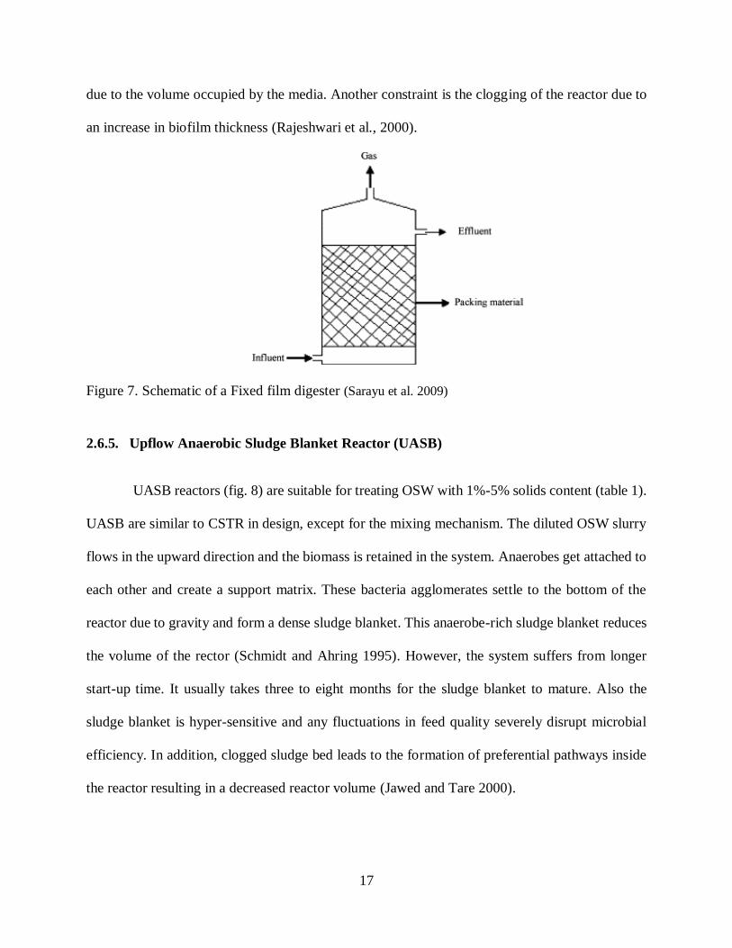
due to the volume occupied by the media. Another constraint is the clogging of the reactor due to
an increase in biofilm thickness (Rajeshwari et al., 2000).
Figure 7. Schematic of a Fixed film digester (Sarayu et al. 2009)
2.6.5. Upflow Anaerobic Sludge Blanket Reactor (UASB)
UASB reactors (fig. 8) are suitable for treating OSW with 1%-5% solids content (table 1).
UASB are similar to CSTR in design, except for the mixing mechanism. The diluted OSW slurry
flows in the upward direction and the biomass is retained in the system. Anaerobes get attached to
each other and create a support matrix. These bacteria agglomerates settle to the bottom of the
reactor due to gravity and form a dense sludge blanket. This anaerobe-rich sludge blanket reduces
the volume of the rector (Schmidt and Ahring 1995). However, the system suffers from longer
start-up time. It usually takes three to eight months for the sludge blanket to mature. Also the
sludge blanket is hyper-sensitive and any fluctuations in feed quality severely disrupt microbial
efficiency. In addition, clogged sludge bed leads to the formation of preferential pathways inside
the reactor resulting in a decreased reactor volume (Jawed and Tare 2000).

18
Figure 8. Cross-section of a UASB reactor (Chong et al., 2012).

19
2.6.6. Digester Overview
Table 1 is a comparison between various anaerobic digester types. The data below is
calculated based on a solids load of 2,000 lbs/day (Lasker 2011).
Table 1. Comparison between digester types
AD technology selection is highly dependent on the solids content of the OSWs. None of
the above-discussed AD systems can handle the HSCM generated in Colorado without diluting
with large quatities of water. Studies to date have proposed high solids AD systems like the
modified plug flow reactor and the packed bed anaerobic reactor which can handle wastes with a
maximum of 40% TS. This research focuses on AD of HSCM up to 90% TS.
2.7. Waste Management Practices in Colorado
Waste management practices in Colorado differ from the typical practices adopted in other
parts of the United States. This is due to the fact that Colorado has an arid climate and limited
Digester Type TS Water Requirement HRT (days) Temperature
Covered Lagoon < 2% High 35-60 Ambient
Fixed Film < 2% High 2-4 Ambient/Mesophilic
UASB < 5% High 1-2 Mesophilic
CSTR < 10% Medium 20-25 Mesophilic
Plug Flow < 14% Low 20-30 Mesophilic

20
water resources. For example, dairies are usually flushed with large amounts of water for manure
collection. Manure collection by flushing water not only reduces the TS but also promotes
hydrolysis of the AD process. Biodegradability of the manure increases by physical pretreatment
such as size reduction and pre-incubation with water (Gunaseelan 1997). However, due to water
scarcity in Colorado, water is often not utilized to flush manure. Instead, manure is mechanically
scraped from concrete floors or dry lots and dumped into huge manure piles. The lack of manure
dilution with water during collection results in dry HSCM. For manure containing more than 13%
TS (as in the current research), substantial quantities of water are required for the successful
operation of conventional on-farm anaerobic digester technology. This increases the operating cost
of the digester. Therefore, production of HSCM and lack of water renders the implementation of
conventional AD in Colorado a challenge. Additional problems faced due to scraping are that the
collected manure is often high in inorganic content such as gravel and sand. Gravel and sand can
cause major operational problems in the anaerobic digester. Sand has also been known to clog AD
tanks, damage pumps and corrode the interior of the tank. Some AD systems have a hyper-sensitive
microbial community which can be easily disrupted by the addition of impurities causing low
biogas yields or system failure. Removing such impurities from the manure would involve the
addition of water and subsequent settling of particles. This adds complexity, capital cost, and
additional maintenance for an AD system. Therefore, adopting conventional AD technologies are
most practical when there is an abundant source of water/wastewater to utilize.
2.8. Feasibility of AD in Colorado
AD is not always the best fit for treating all types of bio-wastes. Detailed analysis should
be conducted to ensure the feasibility of AD for an operation before installation. While the climatic
conditions and typical waste management practices in Colorado pose challenges for AD

21
installation, there are AD technologies that can prove to be successful and lucrative. Selection of
the appropriate AD technology is critical. Combining treatments of wastes generated in close
proximity to increase the CH4 yield is referred to as co-digestion. This technology is gaining
popularity due to many promising research conclusions. For example, co-digestion of swine
manure with winery wastewater showed greatly improved CH4 production potential when
compared to treating swine manure alone (Riaño et al., 2011). However, the ability to combine
manure with other wastes must be carefully evaluated prior to AD installation. Also, a waste stream
supply consistent in quality and quantity is recommended at all times. This is because slight
variations in the waste composition can easily disrupt the growth of microorganisms in the
digester.
2.9. Current Technology
Figure 2 shows the MSLBR proposed in this research. MSLBR serves as a promising
option for dry AD. To optimize AD of HSCM, a multi-stage process consisting of separate reactors
for hydrolysis and methanogenesis is recommended. HSCM is non-flowing and so high solids AD
reactors are batch processes.
In a multi-stage reactor system, the solids are hydrolyzed in the first-stage TFLBR. HSCM
is packed in the TFLBR and water is allowed to trickle through. As water passes through the
manure bed, it removes the converted soluble organic molecules from the reactor. The liquid
flowing out from the bottom of the TFLBR is termed leachate. It contains the soluble organic
molecules broken down by the microorganisms. This leachate can be recycled back into the
TFLBR to serve as inoculum and hydraulic medium optimizing the contact between the HSCM
and the anaerobes. Initially, some amount of water is absorbed by dry manure packed in the

22
TFLBR. This amount of water does not contribute to the water quantity to be recycled. Fresh water
is added to dilute the recycled leachate so as to avoid salt toxicity inside the TFLBR. The collected
leachate is then pumped to the second-stage reactor for further degradation (methanogenesis). The
first-stage reactor is a dry batch reactor (TFLBR) while the second-stage reactor is a high rate
anaerobic digester (HRAD) such as a UASB (Lehtomäki et al., 2008) or anaerobic filter (AF)
(Cysneiros et al., 2011). This method reduces the amount of water required by hydrolysis when
compared to conventional technology where complete mix and plug flow reactors are typically
applied. The system is maintained at an average temperature of 35°C.
2.9.1. Advantages of a Multi-Stage Reactor
Multi-stage reactors are better than single-stage reactors because acidogens and
methanogens differ substantially in terms of physiology, nutritional needs, growth kinetics and
sensitivity to environmental conditions (Chen et al., 2008). Failure to maintain a balance between
these two groups of bacteria is the primary cause for reactor instability. Liquefaction and
acidification of the manure is accomplished in the first reactor while only methanogenesis takes
place in the second reactor. Total digestion time in multi-stage reactors is considerably lower than
the conventional single-stage digestion (Gunaseelan 1997). Multi-stage reactors serve as a good
application for HSCM since the inorganics do not interfere if kept in the TFLBR.
2.9.2. Advantages of Leachate Recirculation through the TFLBR
Leachate carries microorganisms when passed through the manure bed in the TFLBR
which serve as reactor inoculum. Leachate recirculation helps in seeding the inoculum back into
the TFLBR thus maintaining a steady supply of anaerobes. Leachate recirculation stimulates the
overall manure degradation in the leach bed reactors (LBRs) due to enhanced manure

23
solubilization and efficient dispersion of nutrients. Recirculation of leachate also helps in
controlling the pH in the LBRs by adjusting the recirculation rate so as to maximize LBR
efficiency. Control of pH within the TFLBR during the breeding of microorganisms may reduce
ammonia toxicity thus improving system yield (Bhattacharya and Parkin 1989).
2.10. History of LBRs
This section summarizes the research in LBRs discussed in the literature to date, based on
the type of OSW that it was used to treat. LBRs have been implemented in the past to digest high
solids OSWs like municipal solid wastes (MSWs), lignocellulosic biomass and animal manure.
2.10.1. LBRs Treating MSW
Initially, LBR implementations for handling MSWs were favored in order to combat long-
term landfill management issues. The objective was to promote single-stage bioreactor practices
(which may be viable in a full scale landfill) to accelerate the biodegradability of the unsorted
MSWs and minimize environmental impact (Chugh et al., 1999). The composition of MSWs
consists of OSWs like food and green wastes, which are high in energy content and are optimal
for acedogenic fermentation (Cecchi et al., 1988). Food waste, for example, has a high CH4
potential ranging between 200-500 L CH4/kg of volatile solids (VS) (Kim and Shin 2008). The
general idea of an LBR operation is to pass water first through the packed waste bed, followed by
the leachate collection at the bottom of the reactor. Many studies have suggested several
modifications to the technology to improve the system efficiency/yield.
One such attempt was made (Dogan et al., 2009) by implementing a two-stage process with
an LBR and a methanogenic reactor for digesting the organic fraction of the MSWs. Initially, water
was added (1200mL) to the LBR to saturate the waste bed. No additional water was added in the

24
next two days nor was any leachate removed from the LBR. This was to ensure full contact of
water with the waste to optimize the hydrolysis of the LBR. After two days of complete waste
saturation, the system was operated normally for a period of 80 days. The leachate produced from
the LBR was tested for TS, VS, VFAs, total chemical oxygen demand (COD) and soluble COD.
Results showed a drastic decrease in TS and VS concentrations in leachate till day five, followed
by a gradual decrease till the end of the experiment. Approximately 57% of the initial COD was
observed to be digested and leached as soluble COD during the period of 80 days. The variations
in the leachate VFA concentration data followed a bell-shaped distribution pattern. In other words,
the VFA concentration in leachate increased and reached a maximum in the first 16 days followed
by a decrease till the end of the experiment. Additional experiment conclusions included the
importance of water volume added into the LBR since it affected the hydrolysis efficiency to a
great extent.
A hybrid anaerobic solid-liquid bioreactor was proposed (Xu et al., 2011) to accomplish a
multi-stage system (section 2.7.1). Leachate recirculation thorough the LBR was suggested to meet
the nutrient demands of the hydrolytic microbes. High density of the food wastes led to clogging
of the LBR. Bulking agents were used to overcome the clogging issue by facilitating leachate
percolation through the waste bed. Comparisons between different kinds of bulking agents
(sawdust, plastic full particles, plastic hollow spheres, bottom ash and wood chips) were carried
out to identify the best potential substitute in terms of organic leaching and CH4 yield. Results
validated the use of bottom ash and wood chips as better bulking agents when compared to saw
dust in terms of organic leaching and CH4 yield. However, addition of bulking agents to overcome
the clogging issues in the LBRs led to larger working reactor volumes. Larger reactors for digesting
the same amount of waste would result in higher costs in a large-scale implementation.

25
A comparison between leachate recycling in upflow and downflow directions in single-
stage LBRs was proposed (Uke and Stentiford, 1988) to investigate the impact of liquid
introduction inside the LBR. The aim was to reduce channeling, improve leachate production and
accelerate waste degradation in the LBR. Results indicated that the upflow water addition and
leachate recycling resulted in more leachate production when compared to downflow water
addition and leachate recycling. The variations in leachate COD concentrations were similar in
both upflow and downflow LBRs. However, leachate from the downflow LBRs had higher
concentrations of soluble COD and higher overall reduction rates in terms of TS and VS when
compared to upflow LBRs. Nevertheless, these experiments validated that water addition and
leachate recycle variation in terms of flow could be a promising solution for the clogging issues
faced in LBR operation when compared to the use of bulking agents.
A procedure of exchanging leachate between a batch of fresh waste and a batch of
previously anaerobically stabilized waste known as ‘sequencing’ was proposed (Lai et al., 2001).
The idea behind sequencing was to provide the fresh waste bed with microorganisms, moisture
and nutrients. This process also helped in flushing out any undesirable products that built up inside
the LBR. Sequencing was performed on the LBRs on a daily basis until a healthy population of
hydrolytic bacteria was developed on the reactor with a fresh waste bed. The reactors were
separated once the fresh waste bed was anaerobically stabilized. Approximately 36% of the total
initial COD was calculated to be leached as soluble COD in the period of 53 days. Table 2 provides
a summary of all the above-discussed studies cited in the literature to date for LBRs treating
MSWs.

26
Table 2. Summary of studies conducted to date on LBRs treating MSWs.
Reference Research
Objective
Approach Number
of Stages
Challenges and Successes
S.Chugh et
al., 1998
Minimizing long
term landfill
management issues
LBR implementation for minimizing
environmental impacts by landfills
One Biogas production without environmental impacts by
the implementation of the high solids bioreactor to
digest MSWs.
E.Dogan et
al., 2008
Improving biogas
yield from LBRs
treating MSWs
Optimizing LBR operation by initial
waste saturation
Two Initial waste saturation ensured full contact between
waste and water leading to improved biogas
production due to optimized hydrolysis.
S.Y.Xu et
al., 2010
Minimizing the
clogging issues in
LBR
Addition of bulking agents like saw
dust, plastic full particles, plastic
hollow spheres, bottom ash and wood
chips
Multi Bottom ash and wood chips served as better bulking
agents when compared to saw dust in terms of organic
leaching and CH4 yield. However, addition of bulking
agents led to larger reactor working volumes.
M.N.Uke et
al., 2006
Improving the
leachate quantity
and quality from
an LBR
Comparison between leachate
recycling in upflow and downflow
directions
One Upflow leachate recycle resulted in more leachate
production when compared to downflow leachate
recycle. However downflow leachate recycle LBRs
had better leaching potential.
T.E. Lai et
al., 2001
Reducing the LBR
start-up time
Exchanging leachate between a batch
of fresh waste and a batch of
previously anaerobically stabilized
waste in order to provide the LBR with
anaerobes and nutrients
Two This process helped in flushing out any undesirable
products which build up inside the LBR. Sequencing
of leachate was performed on the LBRs on a daily
basis until a healthy population of hydrolytic bacteria
was developed on the reactor with a fresh waste bed.

27
The common problems associated with LBRs identified from the above discussion are the
clogging issues and start-up time for microbial growth inside the reactor. The suggested approach
for clogging issues was the use of bulking agents or upflow water addition and leachate recycling
techniques. Overall, the LBR system has proven to be a biologically and economically feasible
approach to treat MSW with high efficiency in terms of CH4 yields. LBRs demonstrate a promising
technology for accelerating the degradation rates of the organic fraction of MSWs.
2.10.2. LBRs Treating Lignocellulosic Biomass
Lignocellulosic biomass consists of agricultural residues and energy crops. Agricultural
residues are cheap and readily available organic sources for AD with an annual yield of 220 billion
tons worldwide (Ren et al., 2009). Energy crops like maize (Zea mays) are rich in cellulose,
contributing to high CH4 yields per hectare (Bartuševics and Gaile 2010). AD of lignocellulosic
biomass with high TS (10%-50%) in a one-stage conventional system has proven to consume
excess water and energy supply (Lehtomäki et al., 2008). Therefore, LBR technology
implementation was the most economical and profitable alternative. AD in LBRs handling
lignocellulosic biomass like grass silage, sugar beet and willow showed good volumetric CH4
yields (0.2-0.4 m3 kg-1 VS) when operated at high solids concentration (Lehtomäki et al., 2008).
Additional analysis reported that post-methanogenesis of digested wastes led to minimizing the
potential CH4 emissions into the atmosphere, and also contributed to an increased CH4 yield by
trapping 15% more biogas.
Grass silage (used as fodder) serves as a OSW of interest due to its ability to conserve crop
quality, thus being available year-round irrespective of crop season. Performance of single-stage
LBRs handling grass silage and operating under leachate recirculation has been studied in detail

28
(Xie et al., 2012). The objective of the study was to understand the key factors affecting the
hydrolysis and acidification processes. An approximate hydrolysis efficiency of about 68% was
reported. Results indicated a decrease in hydrolysis and acidification yields with an increase in
OLR.
A two-stage leach bed reactor system digesting maize was operated at different batch
durations such that the digestate and leachate from previously operated LBRs served as the
acclimated inoculum supply for the current system (Cysneiros et al., 2011). This approach was
developed to achieve an overall elevated waste degradation rate. The system was subjected to
several modifications to achieve improved CH4 yields. Results indicated higher degradation rates
for longer experimental operation period; i.e., 47% of TS destruction was observed at day 28 when
compared to 22.6% of TS destruction at day seven.
Another two-stage leach bed reactor system digesting maize was proposed introducing a
hydraulic flush as a control parameter to the system (Cysneiros et al., 2012). The idea was to
mimic leachate recirculation by leachate replacement with an equal amount of 7 g/L NaHCO3
solution or tap water. This leachate replacement helped in controlling the VFA concentration in
the LBR, thus increasing the waste degradation rate. Introducing a buffer into the LBR helped in
maintaining the optimum pH for the hydrolytic bacteria. LBRs subjected to hydraulic flush with a
buffer solution exhibited higher soluble COD production when compared to un-buffered LBRs.
Results indicated that the hydraulic flush technique enhanced the VS degradation rate by 14% and
acidification process efficiency by 11 to 32%, approximately. Overall, the buffered LBRs were
reported to perform better than un-buffered LBRs. Table 3 provides a summary of all the above-
discussed studies cited in the literature to date for LBRs treating lignocellulosic biomass.

29
Table 3. Summary of studies conducted to date on LBRs treating lignocellulosic biomass.
Reference Research Objective Approach Number
of Stages
Challenges and Successes
A.Lehtomaki
et al., 2007
Minimizing the excessive
water consumption to digest
wastes using conventional
systems
LBR implementation
to treat
lignocellulosic
biomass with 10 to
50% TS
One Results indicated elevated volumetric CH4 yields (0.2-0.4 m3
kg-1 VS) with low water consumption. LBR technology
implementation proved to be an economical and profitable
alternative
S. Xie et al.,
2012
To understand the key
factors affecting the
hydrolysis and acidification
processes
Analyzing the
performance of the
LBR operating under
leachate recirculation
One An approximate hydrolysis efficiency of about 68% was
reported. Results indicated a decrease in hydrolysis and
acidification yields with an increase in OLR.
D.Cysneiros
et al., 2011
To achieve an overall
elevated waste degradation
rate in an operational LBR
The leachate from
previously digested
LBRs served as
inoculum for the
current system
Two Results indicated higher degradation rates for longer
experimental operation period; i.e. 47% of TS destruction
was observed at day 28 and 22.6% of TS destruction at day 7.
D.Cysneiros
et al., 2012
To control the VFA
concentration in the LBR for
increasing the waste
degradation rate
Mimicking the
leachate recirculation
by an equal amount of
7g/L NaHCO3
solution or tap water
Two Introducing a buffer into the LBR helped in maintaining the
optimum pH for the hydrolytic bacteria. LBRs subjected to
hydraulic flush by buffer solution exhibited higher soluble
COD production when compared to un-buffered LBRs.

30
The general research objective in studying the operation of LBRs treating lignocellulosic
biomass has been to optimize the hydrolysis and acidification processes. The goal of these attempts
on LBR optimization was to achieve better system yields. Major advances in this area of study
suggest that (a) lower OLRs lead to increased hydrolysis and acidogenesis efficiency; (b) feeding
an acclimated stream of microbes into the LBR leads to higher digestion rates; and (c) pH
maintenance by the process of hydraulic flush is recommended for enhanced LBR performance.
2.10.3. LBRs Treating Manure
Some examples of animal manure include cattle manure, horse manure, swine manure,
sheep manure and poultry litter. Manure from different animals has different qualities. Some
research has been done in the past in regard to LBRs’ handling of animal manure – especially
cattle manure. AD has been recognized as a suitable process for digesting cattle manure despite
the fact that it is a complex and naturally polymeric OSW (Myint and Nirmalakhandan 2006).
A single-stage LBR system handling cattle manure with 25% TS has been discussed in the
literature to study the effects of leachate recirculation on system performance (El-Mashad et al.,
2006). Results indicated that leachate recirculation during a batch digestion of solid manure in an
LBR provides more contact time between the anaerobes and the waste, thereby improving the
system yield. Also, an increase in system temperature resulted in elevations in leachate
recirculation volume and CH4 production.
A study on handling farmyard cattle manure with 26% TS utilized a single-stage high solids
reactor (Hall et al., 1985). Implementation of a conventional AD system instead, would require
manure dilution to reduce the TS to below 10%. This would lead to a threefold increase in reactor
volume when compared to using a high solids reactor. Co-digestion of straw with cattle manure

31
was considered in this study with the idea that the addition of carbonaceous material would
improve biogas yields. So a mixture of cattle manure and straw was packed in a high solids reactor
and subjected to leachate recirculation. Two or more reactors were linked semi-continuously in an
attempt to self-inoculate the system. Results showed an approximate TS destruction of 26.5% and
VS destruction of 31.2% over a period of 70 days in the LBR.
Another single-stage anaerobic LBR system handling undiluted dairy manure with 26%
TS was aimed at accelerating the AD process by feeding a mixture of manure, wood powder and
anaerobic seed to the system at start-up (Demirer and Chen 2008). Saw dust was used to overcome
the clogging issues in the LBRs thus improving the leachability of the system. The idea behind
feeding the anaerobes to the LBR was to overcome its continuous wash-out from the system during
the leaching process. Since an active microbial culture is vital for the successful operation of an
LBR, partial recycling of the collected leachate was the suggested approach. A comparison
between the use of wood powder (≤ 1 mm) and wood chips (2-3 mm) as bulking agents was carried
out. Results indicated that more efficient leachability was observed under the use of wood chips
as bulking agents. This study concludes that LBR implementation for cattle manure with 26% TS
can be successful with a 25% increase in system yield when compared to conventional AD
technologies.
Another study was conducted to enhance LBR operation handling cattle manure with
maximum TS of 17.7% (Myint and Nirmalakhandan 2009). The working of the LBR was observed
under the conditions of leachate recycling, addition of inert fillers (pistachios-half-shell) to the
manure bed to increase porosity and by seeding with anaerobic culture. The results showed an
increase in soluble COD by 8% and VFA yield by 15% from cattle manure used in this study.

32
Table 4. Summary of studies cited in literature to date for LBRs treating manure.
Reference Research Objective Approach Number
of Stages
Challenges and Successes
El-Mashad et
al. 2006
To maximize system
performance by optimizing
LBR operation
LBR operation under
leachate recirculation
One Results indicated that leachate recirculation during a batch
digestion of solid manure in an LBR provides more contact
time between the anaerobes and the waste, thereby
improving the system yield.
Hall et al.
1989
To improve biogas yields
from LBR systems treating
manure.
Straw was co-digested
with cattle manure.
One Addition of carbonaceous materials like straw to cattle
manure showed improved biogas yields. Results showed an
approximate TS destruction of 26.5% and VS destruction
of 31.2% over a period of 70 days in the LBR.
Demirer and
Chen 2008
To reduce the clogging
issues and start time in an
LBR.
A mixture of manure,
wood powder and
anaerobic seed was
added to the LBR at
start-up
One Results indicated that higher efficient leachability was
observed under the use of wood chips as bulking agents. This
study concluded that LBR implementation for cattle manure
with 26% TS can be successful with a 25% increase in
system yield when compared to conventional AD
technologies.
Myint and
Nirmalakhand
an 2009
To reduce the clogging
issues and to increase the
system yield in an LBR.
LBR operation under
leachate recycling and
addition of pistachios-
half-shells
One Addition of inert fillers like pistachio-half-shells increased
the porosity of the LBR. The results showed an increase in
soluble COD by 8% and VFA yield by 15% from cattle
manure used in this study.

33
The studies discussed above validate the successful implementation of LBRs for treating
manure instead of conventional anaerobic digesters. Leachate recirculation, co-digestion with high
carbonaceous materials, addition of inert fillers, and seeding with anaerobes have all been
successful techniques that have helped improve LBR yield in the past. Different research scenarios
discussed above indicate that literature to-date does not account for LBRs handling cattle manure
greater than 26% TS. However, the HSCM used in the current study has about 90% TS.
Some research has been done at Colorado State University (Fort Collins, Colorado) to
explore the possibility for AD of HSCM produced in Colorado. Paige Griffin (2012), (a) studied
the effects of operating conditions on hydrolysis efficiency for the AD of cattle manure, (b)
determined hydrolysis kinetic parameters of AD as a function of the operating conditions and (c)
identify characteristics of microbes that perform well under elevated ammonia and salinity
concentration. Results indicated a need to acclimate the microbes to high concentrations of salinity
and ammonia in order to achieve better methane yields. Thus, the anaerobes were acclimated for
two to four months to these testing conditions. The batch studies were repeated, and results
demonstrated substantial improvement in hydrolysis efficiency and methane generation based on
microbial acclamation. Additionally, microbial community composition changes in the inocula
post-acclimation indicated that reactor inoculation could help improve tolerance to elevated levels
of ammonia and salinity to minimize reactor start-up times and improve economic viability. Kelly
Wasserbach (2012) worked to obtain a better understanding of what additives will aid in better
hydraulic flow through cattle manure for successful AD and to develop a method for determining
the HRT through a reactor.

34
2.11. Benefits and Limitations of LBRs
LBRs were designed to treat high solids OSWs under high biogas production rates. The
technology serves as a promising option for dry AD of OSWs, thus making it plausible in areas of
high water demand. LBRs offer improved conversion efficiencies among AD reactors, as there is
enhanced transport of VFAs from the reactor due to the leaching process (Mata-Alvarez, Mace et
al. 2000). LBRs can handle OSWs without any pre-treatment such as particle diameter reduction
or sieving (Brummeler, Horbach et al. 1991). It is operated as a simple batch process resulting in
low costs due to lower water and energy requirements (Dogan et al., 2009). In addition to reduced
water consumption and wastewater discharge, AD in LBR also enables increased volumetric CH4
yields when operated at high solids concentration (Lehtomäki et al., 2008). However, conditions
of reduced hydrolysis rates in LBRs under high biomass concentrations have been cited in
literature (M. Myint et al. 2006). This could be due to limited waste surface area being exposed to
anaerobes leading to mass transfer limitations. High solids OSWs have low wet shear strength.
This means that the tendency of OSWs to collapse under weight is high. This property of OSWs
sometimes leads to leachate channeling inside the LBR thus leading to an inefficient leaching
process (Lissens et al., 2001). An increase in cell alignment in the direction of water flow over the
leach bed over time has been reported in the past (Fowler and Robertson 1991). A reduction in the
void ratio of the waste aggregates was observed with an electron microscope during the analysis
of hydraulic conductivity. Increase in manure density subjected to the leaching process over time
has also been observed (Chanakya et al., 1997). The combination of channeling inside the LBRs,
decreased hydraulic conductivity through the waste bed and increased density of the waste can
lead to differential degradation of the OSWs. Addition of bulking agents with high porosity and
wet shear strength is the suggested alternative to improve the porosity and hydraulic conductivity

35
of LBRs (Ghanem et al., 2001). However, bulking agents occupy substantial amount of digester
volume and incur additional costs (Demirer and Chen 2008). Another major shortcoming observed
in operational LBR systems was the clogging of the reactor outlet resulting in the blockage of the
leaching process. Perforated plates, acid washed and oven dried sand beds, stainless steel mesh
screens, polyurethane foam and glass beads are some of the media that have been tested at the
bottom of the reactor to prevent the OSWs from entering and clogging the reactor outlet port (Xu
et al., 2010; Jagadabhi et al., 2011; Dogan et al., 2008).
2.12. Summary
Discussions in section 2.1 confirm that AD offers advantages over other waste management
technologies for two main reasons: it has high energy producing potential and it contributes to
environmental pollution control. Selection of the type of AD technology to be implemented is
critical. It involves thorough analysis and decision-making based on the demands that the
technology needs to meet. Feasibility of the selected AD technology should be ensured prior to
implementation. While the suggested MSLBR technology has the capability of successfully
digesting HSCM produced in Colorado, the shortcomings of this type of system must be carefully
assessed and measures should be taken to improve the technology. Current work aims to
investigate the impact of water introduction in the LBR, reduce channeling within the LBR,
improve leachate production and accelerate waste degradation in the LBR. Comparison was made
with a nutrient dosed LBR. The goal of this study was to optimize COD generation by enhancing
hydrolysis.

36
2.13. Thesis Objective
The main objective of this study was to (a) design an LBR capable of handling the high solids
cattle manure produced in Colorado with minimum water requirements, (b) sustain good hydraulic
flow through the designed LBR throughout the period of operation, (c) evaluate the organic
leaching potential of the designed LBR to check the extent of successful hydrolysis and (d)
optimize the operation of the designed LBR to achieve maximum hydrolysis efficiency in a single
pass system (without leachate recirculation).

37
CHAPTER 3: MATERIALS AND METHODS
3.1.Experiment Setup
The objective of this research was to study and optimize the operation of a TFLBR in a
single pass system (without leachate recirculation) to anaerobically digest the HSCM. The
experiments were conducted in six identical TFLBRs, including two sets of triplicates. Reactor
replicates were made to obtain reliable results. Representative manure samples (section 3.2) were
then loaded (section 3.4) in six separate TFLBRs to conduct lab-scale experimental analysis. The
construction and set-up of the system is explained in detail under section 3.3. Intrinsic permeability
tests (Appendix 1) were conducted on these TFLBRs to evaluate how the porosity of the HSCM
in the reactor may affect hydraulic flow through it. Depending on the results of each experiment
on TFLBR operation, modifications and adjustments were made on the successive experimental
set-up to optimize the system yield. This study covers three phases of experiments on TFLBR
operation and optimization. These three experiments are explained as ‘Reactor Experiment – Phase
I’ (section 3.6.1), ‘Reactor Experiment – Phase II’ (section 3.6.2) and ‘Reactor Experiment – Phase
III’ (section 3.6.3) respectively. In Phase I experiments, the TFLBRs failed in operation due to the
inability of water to leach through the HSCM in the reactor. Straw was added as a bulking agent
to the HSCM in Phase II experiments to improve the hydraulic flow through the TFLBR. The
addition of straw improved the leachability of water through the reactor resulting in successful
hydrolysis of the TFLBR. However, it was hypothesized that TFLBRs may have become nutrient
limited over time since nutrients can quickly flush out of the system. Of note, this issue was
addressed only since the TFLBRs were operated in a single pass system (without leachate
recirculation). A layer of sand was added on top on the manure bed instead of straw in Phase III
experiments to promote water dispersion through the reactor. Anaerobes in the TFLBR require a

38
sufficient quantity of nutrients for successful digestion of HSCM. A comparison between nutrient
dosed and non-nutrient dosed TFLBRs was conducted in Phase III. These reactors were operated
for a period of 42 days (6 weeks). In the current study, HSCM prior to initiation of reactor
experiments is termed as ‘pre-digested’ manure and HSCM at completion of reactor experiments
is termed as ‘post-digested’ manure. A series of lab-scale tests were conducted on the pre-digested
and post-digested HSCM and leachate collected from the operational TFLBRs. The HSCM
samples were measured for TS, fixed solids (FS), VS, COD, TN, TP and TK. The leachate samples
were measured for TS, total suspended solids (TSS), total dissolved solids (TDS), COD, TN, TP
and TVFA. Biochemical methane potential (BCMP) tests (section 3.7.3) were conducted on
weekly composited leachate samples (section 3.6.3).
3.2. Manure Collection and Preparation
HSCM considered for this study was collected from JBS Five Rivers Feedlot (Kersey,
Colorado). In this approach, chopped (Section 3.2.1) HSCM was collected in 18.9 L (5 gal) plastic
airtight buckets and refrigerated until further use. Airtight buckets were used to make sure the
manure was kept anaerobic, and refrigeration maintained field conditions of manure. Manure was
then thoroughly sorted (section 3.2.2) to obtain homogenized representative samples.
3.2.1. Mechanical Chopping
Chopping of manure was necessary because of the waste management technique adopted
in the feedlots in Colorado. As explained in section 2.7, feedlots in Colorado usually scrape the
manure from dry feedlots and dump it into manure piles. JBS Five Rivers Feedlot used a
mechanical chopper to pre-process the produced cattle manure which helped in improving the

39
efficiency of the on-site gasifier. Any site adopting the proposed AD technology would likely
adopt the same process.
3.2.2. Sorting
Chopped feedlot manure was sorted to obtain a homogeneous and representative sample
for the experiments. Manure from each bucket was equally divided into nine parts (fig. 9) in a
2.74x2.74 meters sized wooden tray. Each divided part of the manure pile contained manure from
each of the 60 buckets. This process helped in sorting the manure, as each of the piles was a
representative batch of the others from the feedlot in terms of particle diameter distribution.
However, this would not be required in a full scale system.
Figure 9. Sorting tray containing chopped manure divided into nine parts.
3.3. System Construction and Set-Up
Experiments were conducted in six identical TFLBRs made of high-grade clear acrylic
cylindrical columns (fig. 10), including two sets of triplicates. Using clear acrylic columns enabled
ease of visual observations during TFLBR operation.

40
Figure 10. Acrylic columns for TFLBRs.
The total and working volume of each TFLBR was around 30 L and 22.65 L respectively.
The corresponding inner diameter (I.D.) and height of the TFLBRs were 20.32 cm (8 in) and 91.44
cm (3 feet), respectively. Each of these TFLBRs was fitted with plastic top and bottom caps (fig.
11). The reactor caps were equipped with an extra-large zinc wing nut, a natural rubber O-ring and
a galvanized carriage bolt. The caps were fitted onto the acrylic columns using vacuum grease and
Teflon. The top cap contained a water inlet port and an even water distribution system, while the
bottom cap contained a leachate sampling/drain port.

41
Figure 11. Top and bottom caps for TFLBRs.
All of the reactors were mounted vertically on a wooden staircase as shown in figure 10. The
wooden staircase was designed and built to allow working around the bottom of the individual
reactors with ease. Each TFLBR was filled with water up to a certain level and allowed to stand
overnight to check for leaks. Leak-free reactors were then loaded (section 3.4) with the HSCM.
3.4.Loading Reactors
The TFLBRs (fig. 12) were loaded with equal amounts of homogenized representative
HSCM samples at the start of the experiment. A layer of sieved gravel (particle diameter: approx.
1 cm) was first added to the bottom of the reactor to (a) hold the manure in the reactor in place and
(b) facilitate proper leaching by preventing the manure from clogging the sampling/draining port.
Manure was then added to the TFLBR.

42
Figure 12. Schematic of a TFLBR
Since manure in the bottom of a full scale operational TFLBR is subjected to compression
due to the addition of large quantities of manure on top, manure in the lab-scale TFLBRs was
subjected to manual compression to simulate full scale operational conditions. A known amount
of representative manure was used to fill the column to a specific height (10 cm). The known
amount of representative manure sample is called a “lift.” Weights were dropped on the manure
inside the TFLBRs for compression. Compressions on amounts were based on results from
intrinsic permeability tests (Appendix 1).
Different amounts of energy were applied to compress the manure in the TFLBRs and
tested for the change in intrinsic permeability. The adequate amount of energy applied on the
manure after which the change in manure permeability in the TFLBR was negligible was
calculated. Compression was quantified in terms of applied potential energy (Equation 7)

43
𝑃𝑜𝑡𝑒𝑛𝑡𝑖𝑎𝑙 𝐸𝑛𝑒𝑟𝑔𝑦 𝐴𝑝𝑝𝑙𝑖𝑒𝑑 𝑡𝑜 𝑡ℎ𝑒 𝑇𝐹𝐿𝐵𝑅 = 𝑀 ∗ 𝑔 ∗ ℎ ∗ 𝑁 ∗ 𝑙
Where:
M is the mass of the weight dropped = 1.525 𝑘𝑔
g is the gravitational force = 9.81 𝑚
𝑠2
h is the height from which the weights were dropped = 0.127 𝑚
N is the number of compressions per lift= 5,
l is the number of lifts per TFLBR= 5
Therefore: 𝑃. 𝐸. = 1.525 𝑘𝑔 ∗ 9.81𝑚
𝑠2 ∗ 0.127 𝑚 ∗ 5 ∗ 5
𝑃. 𝐸. = 47.47 𝐽
Energy of 47.47J was applied on the manure in the TFLBRs at all times since higher
amounts of energy did not contribute to a change in intrinsic permeability in the reactor (Appendix
1). Change in lift height before and after compression was recorded. Equal amount of manure was
taken for the next lift and subjected to compression. This method of compression was done for
every lift until the TFLBR was almost filled. Each of the lab scale TFLBRs were loaded with 6
lifts of compressed manure. A layer of gravel was added on top of the manure bed, and the top cap
then sealed the TFLBR.
3.5. System Operation
This section describes each of the system components and their respective functions in
detail. Fig. 13 represents the schematic of the system layout. An intrinsic permeability test
(Appendix 1) was conducted on the TFLBR prior to system start-up in order to check the intrinsic
permeability of the HSCM loaded in the TFLBR. The intrinsic permeability test was followed by
(7)

44
hydrolysis of the HSCM by trickling oxidant-stripped reverse osmosis (RO) water through the
TFLBR in a downflow motion. Oxidant is stripped from clean RO water (section 3.5.1) using an
oxidation reduction potential (ORP) tank (section 3.5.2). Water was then heated to 35°C and
delivered into the TFLBRs placed inside a closed, insulated room (section 3.5.3). Information on
water delivery and leachate collection is provided in section 3.5.4.
Figure 13. System layout as set-up in lab.
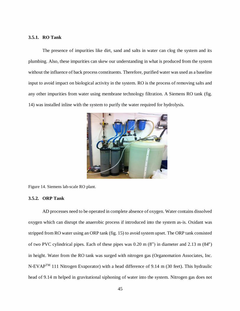
45
3.5.1. RO Tank
The presence of impurities like dirt, sand and salts in water can clog the system and its
plumbing. Also, these impurities can skew our understanding in what is produced from the system
without the influence of back process constituents. Therefore, purified water was used as a baseline
input to avoid impact on biological activity in the system. RO is the process of removing salts and
any other impurities from water using membrane technology filtration. A Siemens RO tank (fig.
14) was installed inline with the system to purify the water required for hydrolysis.
Figure 14. Siemens lab-scale RO plant.
3.5.2. ORP Tank
AD processes need to be operated in complete absence of oxygen. Water contains dissolved
oxygen which can disrupt the anaerobic process if introduced into the system as-is. Oxidant was
stripped from RO water using an ORP tank (fig. 15) to avoid system upset. The ORP tank consisted
of two PVC cylindrical pipes. Each of these pipes was 0.20 m (8”) in diameter and 2.13 m (84)
in height. Water from the RO tank was surged with nitrogen gas (Organomation Associates, Inc.
N-EVAPTM 111 Nitrogen Evaporator) with a head difference of 9.14 m (30 feet). This hydraulic
head of 9.14 m helped in gravitational siphoning of water into the system. Nitrogen gas does not

46
react with water under normal conditions; however, when water is heated, nitrogen gas replaces
dissolved oxygen and the stripped oxidant is allowed to bubble out. AD systems are usually
operated at a typical ORP of -490 to -550 mV (W.W.Eckenfelder et al., 1988). An ORP of -500
mV ± 10 mV was desired so as to render the water completely oxygen free. This could not be
achieved by purging with nitrogen alone. When aluminum reacts with water it removes oxygen by
forming aluminum oxide, therefore, aluminum chunks and coils were placed in the second ORP
tank. This reaction works better if water is heated and has high pH. Therefore, when water entered
the first PVC tank, the pH of the water was increased to 9, by using a 0.1M sodium hydroxide
(NaOH) solution. A circulation pump was placed inside the tank so that the NaOH solution was
evenly mixed with freshly incoming water. This high pH water reacted with aluminum (placed in
the second PVC tank) to form white flakes of aluminum oxide, which were then filtered out using
an inline filter (Everpure IN-15CF-S). The pH of the water was then neutralized by dosing in 0.1
M hydrochloric (HCl) acid. The flow rate of NaOH and HCl dosed into the ORP tanks was
controlled by solenoid valves (model #: RSC-2-12V) programmed to a relay in a controller unit
(Eutech Instruments, alpha pH 200). An EC probe was connected to the controller and each of the
solenoid valves dosed in the required amount of acid/base depending on the pH of water. This
anaerobic water was then re-heated to 35°C using a secondary heater and was delivered into the
reactors.

47
Figure 15. ORP tank. Idea and design by Lucas Loetcher.
3.5.3. Insulated Temperature Controlled Room
The TFLBRs, mounted on the wooden stairs, were placed inside a walk-in temperature
controlled room (fig. 16) and operated at mesophilic temperature range. The system was heated
with the help of room heaters set to 35°C ± 2oC. The reactors were insulated to prevent excessive
heat losses. This was because the temperature fluctuations during system operation can affect the
CH4 yield negatively.

48
Figure 16. Interior of the insulated temperature controlled room.
The insulated room was 2.43 m (8 feet) in length, width and height (fig. 17). A support
frame made of PVC pipes (2.54 cm in diameter) was taped to the inside of the insulated room for
stability. The insulation room floor was nailed to the lab floor for safety purposes. The room was
equipped with an electricity supply for powering room lights and space heaters.
Figure 17. Exterior of the insulated temperature controlled room.

49
3.5.4. Water Delivery and Leachate Collection
Oxidant-stripped water from ORP tank was maintained at 35oC using a secondary heater
and was delivered into the insulated temperature controlled room at the distribution manifold and
the rotameters. Water from the ORP tank was gravity fed into the temperature controlled room
with a pressure head of 30 psi. Rotameters were each individually plumbed inline to six of the
TFLBRs. The rotameters were set to flow water at a velocity of 20 mL/min. The amount of water
added to the TFLBR is an important parameter as it directly affects the hydrolysis efficiency. Water
from the rotameters entered the top distribution cap of the TFLBR and trickled through the reactor.
Leachate was collected from the bottom of the reactor through the sampling port. Kuritech vinyl
tubing (0.635cm or ¼”) was used for plumbing all water delivery and leachate collection lines.
3.6.Evaluation of a TFLBR for the Hydrolysis of HSCM
The reactor experiments were focused on sustaining good hydraulic flow through the
TFLBRs and optimizing the hydrolysis and acidification conditions in the reactor. Efficient
TFLBR operation would produce suitable acid metabolites for methanogenesis. Three series of
reactor experiments were carried out in total. Each experiment was based on the results of the
previously conducted experiment. All the experiments are described below in the order in which
they were conducted.
3.6.1. Reactor Experiment – Phase I
The Phase I experiments included three TFLBRs (triplicate) loaded with HSCM. The
difficulty encountered during this experimental run was that the flow rate of water through the
TFLBR slowed down over time and eventually dropped to zero within the first 24 hrs.

50
3.6.2. Reactor Experiment – Phase II
Due to the insufficient hydraulic flow through TFLBRs in Phase I experiments, Phase II
experiments were conducted to include bulking agents to improve hydraulic conductivity. The
Phase II experiments were conducted with six TFLBRs, including two sets of triplicates. One set
of triplicate was loaded with 100% HSCM and the other set of triplicate was loaded with HSCM
bulked with 5% straw by mass. A layer of sand (0.08 mm particle diameter) was added on top of
the manure bed in all the TFLBRs. The idea was to add a dispersion media (sand, in this case) to
improve the hydraulic leachability of the TFLBR. A comparison between two sets of triplicates
was performed to monitor hydraulic conductivity trough the TFLBRs. The leachate collected from
the TFLBRs was tested in the lab for COD. The COD data for the reactors bulked with and without
straw (5% by mass) were compared.
3.6.3. Reactor Experiment –Phase III
The Phase III experiments were conducted to analyze if the rate of hydrolysis in the
TFLBRs was inhibited due to the lack of sufficient nutrients available for microbial growth. This
could have been due to leaching of nutrients from the TFLBRs over time. The experiments were
conducted in six TFLBRs, including two sets of triplicates. Comparison between nutrient dosed
and non-nutrient dosed reactors was carried out in each triplicate. A concentrated feed solution for
nutrients was prepared (Owen et al., 1979) based on the composition in appendix 3. Table 5 shows
the concentration of the nutrients in the concentrated feed solution and the target concentrations in
the nutrient solution entering the TFLBRs after dilution.

51
Table 5. Concentrations of nutrients in nutrient dosed TFLBRs
Constituent Nutrients Concentration in feed
solution (g/L)
Target concentration after
dilution (g/L)
N 4.5 0.122
P 0.7 0.019
K 25.2 0.681
The concentrated feed solution was stored in an 18.9 L bucket and refrigerated at all times
to prevent microbial growth. The solution was delivered at a flow rate of 0.54 mL/min using a
peristaltic pump. The concentrated feed solution then merged into the water delivery line which
was set to enter the nutrient dosed TFLBRs at 20 mL/min using rotameters and ball valves. Thus
the concentrated feed solution was diluted with oxidant-stripped water and fed into the nutrient
dosed TFLBRs at the target concentration given in table 5. A composite sampling technique was
adopted due to the large variation of flow over time and pulses of leachate that would exit the
reactors (Wasserbach, 2013). Leachate from the TFLBR was collected in an 18.9 L carboy through
the sampling port in the bottom cap. An anti-siphoning tubing arrangement was used to prevent
the leachate from siphoning back into the outlet port thus facilitating easy leaching. This was done
by placing the end of the sampling port tubing at the neck of the carboy instead of running it to the
bottom. Leachate was constantly collected from the TFLBRs to obtain composite samples. The
idea behind composite sampling was to collect all of the leachate produced over a given period of
time to determine the average leachate quality. Volume of composited leachate samples produced
were measured and refrigerated at the end of the day for further lab-tests. Weekly composited
leachate samples were prepared by combining that week’s daily composited samples. Excess
leachate collected was set to drain into the discharge manifold and was collected in the leachate
storage barrel that had a capacity of 100 L. The barrel was periodically emptied by pumping to a

52
disposal area. The variation in COD, TS, TSS, TDS and VFA concentration within the system was
monitored consistently throughout the experiment. Leaching of other inorganics like TN, TP and
TK were also monitored.
3.7. Analytical Methods
Solids characterization (section 3.7.1) included elemental solids analysis on both pre-
digested and post-digested HSCM. Leachate characterization (section 3.7.2) included detailed
leachate analysis to measure the leaching potential of the TFLBR. Finally, BCMP tests (section
3.7.3) were performed on the composited leachate samples to estimate how much CH4 could be
generated from the leachate if processed through an HRAD.
3.7.1. Solids Characterization
Pre-digested and post-digested HSCM samples were placed in aluminum dishes for
conducting lab scale analysis. These dishes were labeled and heated at 550°C in an electric furnace
(Fisher Isotemp 10-550-14 Benchtop laboratory muffle furnace) for 30 minutes. Each of these
dishes was then weighed and the mass was recorded.
3.7.1.1.TS
The mass of solid material (or dry matter) remaining after removing moisture from a
sample is termed as TS. A mass of 5 to 10 grams of the homogenized representative manure sample
was placed in the pre-cooked aluminum dish. The mass of the dish before and after placing the
manure sample was recorded. The dish was then placed inside an electric oven (Thelco Lab Oven,
Precison) to dry at 103°C ± 2°C until the weight stabilized (approx. 2-6 hrs.). The final mass of
the dish was recorded.

53
Mass of TS present in per gram of manure sample
=𝑊𝑒𝑖𝑔ℎ𝑡 𝑜𝑓 𝑠𝑎𝑚𝑝𝑙𝑒 𝑤𝑖𝑡ℎ 𝑑𝑖𝑠ℎ 𝑎𝑓𝑡𝑒𝑟 103 𝐶 − 𝑤𝑒𝑖𝑔ℎ𝑡 𝑜𝑓 𝑒𝑚𝑝𝑡𝑦 𝑑𝑖𝑠ℎ
𝐼𝑛𝑖𝑡𝑖𝑎𝑙 𝑤𝑒𝑖𝑔ℎ𝑡 𝑜𝑓 𝑠𝑎𝑚𝑝𝑙𝑒 𝑖𝑛 𝑑𝑖𝑠ℎ − 𝑤𝑒𝑖𝑔ℎ𝑡 𝑜𝑓 𝑒𝑚𝑝𝑡𝑦 𝑑𝑖𝑠ℎ
3.7.1.2.FS
The residual solids that do not volatilize at 550°C are known as FS or ash. The dish from
TS (section 3.7.1.1) was placed in a 550°C furnace to obtain the amount of FS present in the
manure sample. The dish was kept in the furnace until the weight of the dish stabilized (approx. 1
hr.). The final mass of the dish was recorded.
Mass of FS present in per gram of manure sample
=𝑊𝑒𝑖𝑔ℎ𝑡 𝑜𝑓 𝑠𝑎𝑚𝑝𝑙𝑒 𝑤𝑖𝑡ℎ 𝑑𝑖𝑠ℎ 𝑎𝑓𝑡𝑒𝑟 550𝐶 − 𝑤𝑒𝑖𝑔ℎ𝑡 𝑜𝑓 𝑒𝑚𝑝𝑡𝑦 𝑑𝑖𝑠ℎ
𝐼𝑛𝑖𝑡𝑖𝑎𝑙 𝑤𝑒𝑖𝑔ℎ𝑡 𝑜𝑓 𝑠𝑎𝑚𝑝𝑙𝑒 𝑖𝑛 𝑑𝑖𝑠ℎ − 𝑤𝑒𝑖𝑔ℎ𝑡 𝑜𝑓 𝑒𝑚𝑝𝑡𝑦 𝑑𝑖𝑠ℎ
3.7.1.3.VS
VS are usually the organic portion of the manure sample that volatilizes when heated at a
temperature of 550°C. Mass difference between the dishes from TS (section 3.7.1.1) and FS
(section 3.7.1.2) was recorded. Difference in weight accounted for the mass of VS of the manure
sample.
3.7.1.4.COD
Organic content of any OSW can be accounted in terms of COD. This is the oxygen
equivalent of the organic matter which can be measured by using a strong chemical oxidizing agent
in an acidic medium. A ‘Hach test N tube kit’ was used to measure the COD of the manure samples
with a detection range of 20 – 1,500 mg/L COD. A pre-measured amount of fine pulverized manure

54
sample was used so that it could be easily oxidized in the acidic provided in the test vial to detect
the COD content. The manure sample was diluted by mass using deionized (D.I.) water to get a
COD of 20-1,500 mg/L. Typically a 1:100-1000 dilution was conducted. The samples were diluted
because the undiluted samples had very high COD values, which exceeded the detectable range of
the COD reader. A specific amount of the diluted manure sample was carefully added into each of
the COD vials. Manure sample and D.I. water were added to a combined volume of 2 mL inside
the COD vial. One control vial (with only D.I. water) was used as a blank. The vials were inverted
several times and placed into a heater at 150°C for 2 hours. After heating, the vials were allowed
to cool down and then measured for COD using the COD reader. Prior to recording the COD data
for the vials, the COD reader was zeroed using a control vial. Dilution factor was accounted for,
while recording the COD values for the manure samples.
3.7.1.5. TN
The manure samples were tested for TN at the Soil, Water and Plant Testing Laboratory at
Colorado State University in Fort Collins, Colorado. Samples were analyzed for TN content by
combustion using a Leco TruSpec CN furnace.
3.7.1.6. TP
The manure samples were tested for TP at the Soil, Water and Plant Testing Laboratory at
Colorado State University in Fort Collins, Colorado. The samples were analyzed for TP content
using inductively coupled plasma (ICP) emission spectrometry. The working principle of ICP
spectrometry is based on the fact that each element has unique characteristic emission spectra when
ionized (Plank 1992). The samples can be efficiently ionized by direct injection of argon gas
ionized in an applied radio frequency field. The resultant ionic emission spectra were monitored

55
at pre-selected wavelengths, allowing effective multi-element determination. The light intensity at
each specified wavelength was proportional to the sample element concentration. A linear dynamic
range of four to six orders of magnitude was observed for many elements, allowing for two-point
calibration.
Manure samples were air dried for about 12-24 hours depending on the initial moisture
content. If excessive residual moisture was present in the samples after air drying, the samples
were oven dried at 60oC-70oC overnight prior to analysis. Manure samples were ground and
passed through a 2 mm screen. Since this is a digestion procedure it was not necessary to keep the
samples intact with their original texture. The samples could be completely pulverized to fine
powder if possible. One gram of ground sample was weighed into a calibrated digest tube. The
sample was then digested with 5 mL of perchloric and 5 mL of nitric acid. The samples were
heated on the digestion block at 125oC-130oC for 48-60 hours, until the volume of the sample
was reduced to 5 mL (only perchloric acid remained). The temperature was increased to 200oC and
the samples were digested for 2 hours. The sample tubes were then removed from the digestion
block and allowed to cool. D.I. water was added to each sample to total 50 mL. Care was taken to
ensure that the sample tubes were completely cooled off. Addition of water to hot sample tubes
could lead to tube explosion spraying acid. The digested sample was mixed thoroughly with water
by capping the tube and inverting it at least 10 times. The samples were then filtered through
Whatman 1 or Fisher P5 filter paper and analyzed for TP by ICP emission spectrometry.
3.7.1.7. TK
The manure samples were tested for TK at the Soil, Water and Plant Testing Laboratory at
Colorado State University in Fort Collins, Colorado. The procedure analyzing TK in solid samples

56
was the same as that for TP (section 3.7.1.6). ICP spectrometry was used to detect the TK content
of the samples.
3.7.2. Leachate characterization
The volume of leachate produced from the TFLBR was monitored on a daily basis. The
collected leachate was weighed to determine the volume based on the assumption that the density
of leachate was the same as water. Composited leachate samples leached from the TFLBR were
analyzed and tested in detail to understand the leachate quality and composition.
3.7.2.1.TS
The leachate samples were tested for TS by the same procedure explained in section 3.7.1.1.
3.7.2.2.TSS
A measure of TSS is determined by the amount of non-filterable solids in any liquid
sample. A glass fiber filter with a pore size of 1.5 µm and diameter 47 mm, was placed inside the
pre-cooked dish and weighed. The filter was then placed in a vacuum filter apparatus. A volume
of 10 mL of the composited leachate sample was pipetted and placed in the filter and filtered using
the vacuum filter apparatus. The vacuum was allowed to run until the filter was relatively dry. The
dry filter containing the suspended solids was placed back into the dish and weighed. The dish was
then placed inside an electric oven (Thelco Lab Oven, Precison) to dry at 103°C ± 2°C until the
weight stabilized (approx. 2-6 hrs.) and was weighed again.
Amount of TSS (g/L)
=𝑊𝑒𝑖𝑔ℎ𝑡 𝑜𝑓 𝑠𝑎𝑚𝑝𝑙𝑒 𝑎𝑓𝑡𝑒𝑟 103𝐶 − 𝑤𝑒𝑖𝑔ℎ𝑡 𝑜𝑓 𝑠𝑎𝑚𝑝𝑙𝑒 𝑏𝑒𝑓𝑜𝑟𝑒 103𝐶
𝐼𝑛𝑖𝑡𝑖𝑎𝑙 𝑠𝑎𝑚𝑝𝑙𝑒 𝑣𝑜𝑙𝑢𝑚𝑒∗ 1000

57
3.7.2.3.TDS
Solids that can pass through a filter opening of 2 micrometer during filtration are termed
TDS. The filtrate leached through the filter after vacuuming (from section 3.7.2.1) was placed into
a pre-cooked dish and weighed. The dish was then placed inside an electric oven (Thelco Lab
Oven, Precison) to dry at 103°C ± 2°C until the weight stabilized (approx. 2-6 hrs.) and was
weighed again.
Amount of TDS (g/L)
=𝑊𝑒𝑖𝑔ℎ𝑡 𝑜𝑓 𝑠𝑎𝑚𝑝𝑙𝑒 𝑎𝑓𝑡𝑒𝑟 103𝐶 − 𝑤𝑒𝑖𝑔ℎ𝑡 𝑜𝑓 𝑠𝑎𝑚𝑝𝑙𝑒 𝑏𝑒𝑓𝑜𝑟𝑒 103𝐶
𝐼𝑛𝑖𝑡𝑖𝑎𝑙 𝑠𝑎𝑚𝑝𝑙𝑒 𝑣𝑜𝑙𝑢𝑚𝑒∗ 1000
3.7.2.4. COD
The leachate samples were tested for COD by the same procedure explained in section
3.1.7.4.
3.7.2.5. TN
The TN concentration in the leachate samples was measured by combustion and
acidification process in a Shimadzu TOC-V CSH/CSN (Columbia, Maryland). The detection range
was between 0 to 20,000 mg/L TN. The machine was calibrated every time prior to sample
analysis.
3.7.2.6. TP
TP in leachate samples was measured using Hach’s Total Phosphorus Test and Tube (TNT)
Reagent Set and a DR 2500 COD reader. The reader was calibrated by selecting program 540 P

58
React HR TNT from the list of program options. Meanwhile, a specific amount of leachate was
carefully added into each of the phosphorus TNT vials. Leachate samples and D.I. water was added
to a combined volume of 5 mL inside the COD vial. One control vial (with only D.I. water) was
used as a blank. The vials were inverted several times and placed into the reader. Timer icon in the
reader was selected, which started a 3-minute reaction period. Samples were measured within 2
minutes of when the timer expired. The control vial (blank) was placed into the cell holder after
the timer expired. When zeroed using the blank, the reading displayed in the reader was 0.0 mg/L
PO43–. The sample vial was then placed into the cell holder and measured for TP. Results appeared
in mg/L PO43–.
3.7.2.7. TVFA
TVFA in leachate samples were measured using Hach’s Total Volatile Acids Test and tube
(TNT) Reagent Set and a DR 2500 COD reader. The reader was calibrated by selecting the pre-set
TVFA program from the list of program options. Meanwhile, Hach’s reactor (Model# 45600) was
preheated to 100°C. A volume of 0.4 mL of Solution A was pipetted into the test vials (provided
in the Hach’s TVFA test kit), followed by 0.4 mL of leachate sample. One control vial (with only
D.I. water instead of leachate sample) was used as a blank. The vials were capped and inverted
several times to mix and were placed into the reactor. The reactor lid was closed and the vials were
allowed to cook for 10 minutes. After the timer expired, the hot vials were carefully removed from
the reactor and were allowed to cool down to room temperature (15ºC-25ºC). A volume of 0.4 mL
of Solution B was added into the cooled test vials, followed by 0.4 mL of Solution C and 2.0 mL
of Solution D (provided in Hach’s TVFA test kit). The vials were capped and inverted several
times for mixing. After 3 minutes, the vials were wiped dry and inserted into the cell holder. The
control vial (blank) was placed into the cell holder first to zero the reading. The sample vial was

59
then placed into the cell holder and measured for TVFAs. Values displayed were in mg/L
CH3COOH (Acetic Acid).
3.7.3. BCMP
A BCMP test is generally performed to obtain the kinetics of OSW utilization. It is a
relatively inexpensive and representative method to evaluate the potential biogas production
efficiency (methanogenic performance) of the AD process. It is critically used to determine the
amount of organic carbon present in the OSWs that can be anaerobically converted to CH4 gas.
The data obtained from BCMP tests are valuable for optimizing the design and operation of an
anaerobic digester.
BCMP tests were conducted in 140 mL luer lock plastic syringes (Fig.18) to maintain a
small-scale controllable anaerobic environment.
Figure 18. Sealed 140 mL plastic syringe as a surrogate for HRAD.
The test involved the addition of three ingredients: substrate, inoculum and nutrient
solution. Substrate is the biodegradable carbon source available (weekly composited leachate
sample), inoculum is the stream of anaerobic bacteria which utilize the substrate to produce biogas
and was provided by Drake Water Reclamation Facility, Fort Collins, CO. Nutrient solution (Owen
et al. 1978) contains all the essential nutrients required by the methanogens to efficiently grow in
the environment. The nutrient solution optimizes methanogenic growth in the lab-scale set-up.

60
Clean, dry, graduated, 140 mL luer lock plastic syringes were each fitted with a three-way
valve. The quantity of substrate added to the syringe was normalized based on COD. All tests were
performed in triplicate. Leachate sample equivalent to 1 g of COD/L was initially added
anaerobically to each of the syringes followed by 25 mL of inoculum and 25 mL of nutrient
solution. These were the sample-loaded syringes. Positive control syringes and negative control
syringes were also set up along with the sample-loaded syringes. Positive or glucose control
syringes substituted glucose as a carbon source (1g COD/L) instead of leachate sample. This was
to make sure that the syringes were working efficiently and producing biogas. Negative control
syringes or blanks did not have any substrate or carbon source in them. This was to detect the
production of gas from inoculum and nutrient solution alone. The original volume of the syringes
was recorded with a caliper. The loaded syringes were placed in an incubator (LAB-Line® Orbit
Environ-shaker ATRIX ID#0805) set to 35⁰C. Reaction period lasted for approximately 3 weeks.
The volume of biogas produced was monitored by recording the change in caliper reading.
A typical vernier caliper is a very precise measuring instrument with a maximum reading error of
±0.05 mm. However, a digital vernier caliper was used which provided better accuracy and
minimized the error to ±0.02 mm. The total percentage of error that may have occurred in gas
volume estimates is equal to 0.4%. Change in caliper reading was recorded on a daily basis. The
syringe was considered to stop producing gas when the change in caliper reading was negligible.
Biogas was periodically sampled from the syringe through the three-way valve and analyzed for
CH4 concentration using a gas chromatograph (GC) (Hewlett Packard 5890 Series II). The
working principle of the GC was based on the principle of gas isolation by flame ionization. The
GC was calibrated every time prior to sample testing to obtain accurate results. The GC was
calibrated by injecting samples with known percentages of CH4 gas and the results were set to a

61
standard curve. A standard curve with an R2 value of 0.98 to 1 was considered acceptable. Fig. 19
is one of the standard curves used to calibrate the GC. A volume of 20 µL of gas sample was
injected into the injector port. The GC detected the CH4 content in the gas mixture and conveyed
an output signal. The output signal was measured based on the previously calibrated standard
curve.
Figure 19. Standard curve for calibrating the GC for detecting the CH4 concentration in the biogas produced by the BCMP test syringes.
3.7.4. Data Analysis
a) Student’s t-test:
A student’s t-test was conducted on the data collected from Phase III experiments. The t-test is a
statistical test, which is used to determine if there is a statistical difference between two data sets.
The t-test essentially does two things: First, it determines if the averages and means of the two data
y = 12.449x - 0.3754R² = 0.9973
0
20
40
60
80
100
120
0 2 4 6 8 10
Met
han
e pre
dic
ted (
%)
Measured area under the curve, 106
Area under the curve
Linear (Area under the
curve)
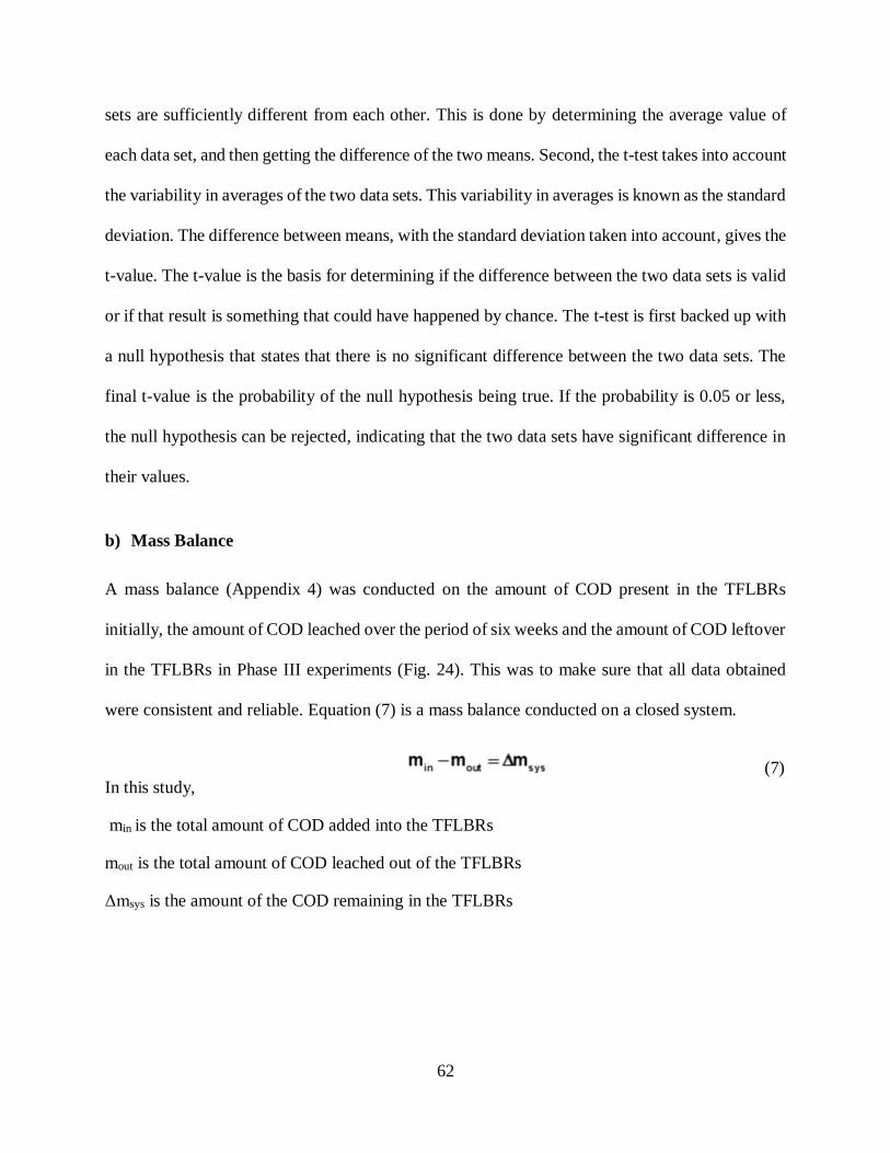
62
sets are sufficiently different from each other. This is done by determining the average value of
each data set, and then getting the difference of the two means. Second, the t-test takes into account
the variability in averages of the two data sets. This variability in averages is known as the standard
deviation. The difference between means, with the standard deviation taken into account, gives the
t-value. The t-value is the basis for determining if the difference between the two data sets is valid
or if that result is something that could have happened by chance. The t-test is first backed up with
a null hypothesis that states that there is no significant difference between the two data sets. The
final t-value is the probability of the null hypothesis being true. If the probability is 0.05 or less,
the null hypothesis can be rejected, indicating that the two data sets have significant difference in
their values.
b) Mass Balance
A mass balance (Appendix 4) was conducted on the amount of COD present in the TFLBRs
initially, the amount of COD leached over the period of six weeks and the amount of COD leftover
in the TFLBRs in Phase III experiments (Fig. 24). This was to make sure that all data obtained
were consistent and reliable. Equation (7) is a mass balance conducted on a closed system.
(7) In this study,
min is the total amount of COD added into the TFLBRs
mout is the total amount of COD leached out of the TFLBRs
Δmsys is the amount of the COD remaining in the TFLBRs

63
CHAPTER 4: RESULTS AND DISCUSSION
4.1.Reactor Experiment – Phase I
Conclusive results were not obtained from this experiment since the TFLBRs experienced
operational failure within the first 24 hours (Section 3.6.1) Leachate was not produced from the
TFLBRs due to the inability of water to flow through (Fig. 20). Thus the lab tests were not
conducted due to the lack of samples to be tested.
Figure 20. System failure: water build-up on the top of the reactor
A parameter that can enhance the performance of the TFLBR is the porosity of the HSCM
loaded in the reactor. By increasing the manure bed porosity, hydraulic leachability can be
elevated. Bulking substances like inert fillers (pistachio shells or plastic beads) or any other porous
OSWs can be co-digested with HSCM in order to improve system efficiency. Past research has
suggested co-digesting cattle manure with either chopped rice or straw residues so as to increase
the digester CH4 production per unit of leached COD (Hills and Roberts 1981).

64
4.2. Reactor Experiment – Phase II
Based on availability, straw was selected as the bulking agent for manure in an attempt to
improve the hydraulic flow in the TFLBRs. The addition of sand as a dispersion media to the top
of the manure bed in Phase II TFLBRs improved the porosity of loaded HSCM. Increases in
porosity led to continuous hydraulic conductivity thus providing successful operation of the
TFLBRs. Very good hydraulic flow was observed through the column for 30 days after which the
experiment was terminated. The flow of leachate from the TFLBRs was not obtained because all
of the leachate was not collected. This experiment proved that hydraulic flow was possible through
the TFLBR with or without the addition of bulking agent (straw), thus making it unnecessary. This
was an important finding because the need for bulking agents was an added cost to the system.
Straw takes up a lot of reactor space and so bigger reactor volumes would have been required to
digest the same amount of manure. Also, straw contains large quantities of lignin, making it
undesirable to be used in large quantities. Lignin is a complex organic material that cannot be
easily digested by anaerobes (Richard, 1996). Reactors bulked with straw experienced channeling
inside the TFLBR, indicating poor leachability. Reactors without straw displayed better leaching
potential when compared to reactors with straw. However, the anaerobes in the TFLBRs were
suspected to be nutrient limited due to leaching leading to lower leaching potential. Also, leachate
grab samples were collected at instantaneous time (t). This lead to inaccurate results as a lot of
leaching potential was missed between two time intervals.
Figure 21 is a comparison between the Phase II TFLBRs bulked with and without straw in terms
of gCOD/L leachate collected.

65
Figure 21. Comparison between the TFLBRs bulked with and without straw in terms of gCOD/L leachate
collected.
4.3.Reactor Experiment – Phase III
Nutrient solution was dosed into the operational TFLBRs to check for changes in leachate
quality that indicated the reactors were nutrient limited due to continuous leaching over time. A
comparison between nutrient dosed and non-nutrient dosed TFLBRs indicated a better leaching
potential in the nutrient dosed reactors in terms of COD data (Fig. 22). An overall increase of
leached COD was observed. Composited sampling technique enabled better quantification of COD
in leachate. This was because the flow rate of the leachate collected from the TFLBRs was not
constant. Phase III TFLBRs without nutrient dosing were packed with the same amount of HSCM
as in Phase II TFBLRs without straw.
0
2
4
6
8
10
12
14
16
18
20
0 2 4 6 8 10 12 14 16 18 20 22 24
Lea
ched
CO
D (
g/L
)
Time (days)
Phase II - Without Straw
Phase II - With Straw

66
Figure 22. Comparison between reactor experiments in terms of leached COD in g/L.
A series of lab tests were conducted on pre-digested and post-digested HSCM samples and
composited leachate samples from Phase III reactor experiments. These analyses were conducted
to better understand the operation and leaching potential of the TFLBR. The quality of the leachate
indicated the extent of successful hydrolysis of HSCM using the TFLBR.
4.3.1. Leachate analysis
The data points in graphs represent the average values and the error bars represent the
standard deviations between replicate samples.
COD
Figure 23 represents the variations in COD concentration in the leachate collected from the non-
nutrient dosed and nutrient dosed TFLBRs. The COD concentration is expressed in terms of g
COD/ L leachate collected from the TFLBRs.
0
5
10
15
20
25
30
35
40
45
50
0 2 4 6 8 10 12 14 16 18 20 22 24
Lea
ched
CO
D (
g/L
)
Time (days)
Phase II - Without Straw Phase II - With Straw
Phase III - Without Nutrient Dosing Phase III - With Nutrient Dosing
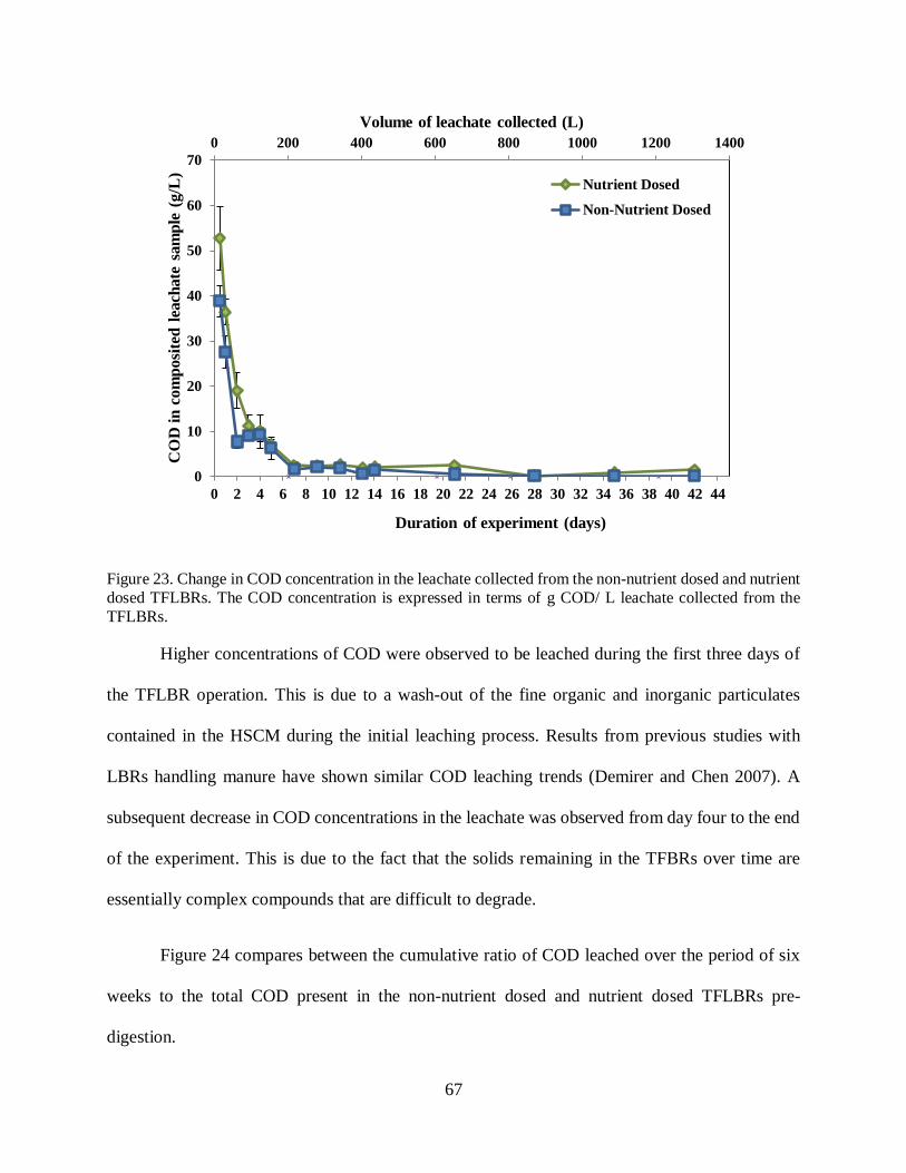
67
Figure 23. Change in COD concentration in the leachate collected from the non-nutrient dosed and nutrient
dosed TFLBRs. The COD concentration is expressed in terms of g COD/ L leachate collected from the
TFLBRs.
Higher concentrations of COD were observed to be leached during the first three days of
the TFLBR operation. This is due to a wash-out of the fine organic and inorganic particulates
contained in the HSCM during the initial leaching process. Results from previous studies with
LBRs handling manure have shown similar COD leaching trends (Demirer and Chen 2007). A
subsequent decrease in COD concentrations in the leachate was observed from day four to the end
of the experiment. This is due to the fact that the solids remaining in the TFBRs over time are
essentially complex compounds that are difficult to degrade.
Figure 24 compares between the cumulative ratio of COD leached over the period of six
weeks to the total COD present in the non-nutrient dosed and nutrient dosed TFLBRs pre-
digestion.
0 200 400 600 800 1000 1200 1400
0
10
20
30
40
50
60
70
0 2 4 6 8 10 12 14 16 18 20 22 24 26 28 30 32 34 36 38 40 42 44
Volume of leachate collected (L)
CO
D i
n c
om
po
site
d l
each
ate
sam
ple
(g
/L)
Duration of experiment (days)
Nutrient Dosed
Non-Nutrient Dosed

68
Figure 24. Comparison between the cumulative ratio of COD leached to the total COD present in the non-nutrient dosed and nutrient dosed TFLBRs.
The extent of COD leaching efficiency can be observed from Figure 24. Approximately
44% of the total COD is leached from the non-nutrient dosed TFLBRs and 62% of the total COD
is leached out of the nutrient dosed TFLBRs over the period of six weeks. The COD concentration
of the nutrient solution dosed into the TFLBRs was found to be 0.2 g/L. The increase in COD
concentration in leachate collected from the nutrient dosed TFLBRs is normalized by subtracting
the COD concentration found in the nutrient solution from each data point. So the higher COD
concentration in the leachate collected from nutrient dosed TFLBRs indicated a better leaching
potential than the non-nutrient dosed TFLBRs. In an ideal reactor, the entire manure would be
hydrolyzed resulting in 100% of the total COD being leached out. However, in reality, manure
contains many complex and inorganic substances that cannot be easily digested. The current
0.0
0.1
0.2
0.3
0.4
0.5
0.6
0.7
0.8
0.9
1.0
0 2 4 6 8 10 12 14 16 18 20 22 24 26 28 30 32 34 36 38 40 42 44 46
Cu
mu
lati
ve
rati
o o
f g C
OD
lea
ched
to t
ota
l C
OD
(g/g
)
Duration of experiment (days)
Non-Nutrient Dosed
Nutrient Dosed

69
system proves to successfully handle HSCM containing 89.6% TS in TFLBRs (without leachate
recirculation) to achieve a COD reduction between 44 – 62%. Studies have shown high solids AD
reactors digesting cattle manure containing 14.6% TS yielding approximately 45 – 66% COD
reductions (Demirer and Chen 2005); therefore, our data is similar to that found in literature with
much diluted manures.
The Student’s t-test conducted on the data from Fig.24 validated the nutrient dosed
TFLBRs to have significantly higher COD leaching when compared to non-nutrient dosed
TFLBRs, giving a probability value ≥ 0.95. This proved that there was a statistical difference
between the two data sets and that the nutrient dosed TFLBRs had better leachate quality.
A mass balance conducted on the data from Fig.24 validated that the theoretical and
experimental values of the COD leached over a period of six weeks was approximately similar to
the amount of COD reductions in the TFLBRs (Appendix 4). This indicated that the data obtained
was consistent and reliable.
TS, TSS and TDS
Figure 25 represents the variations in concentration of TS, TSS and TDS present in the
leachate collected from the non-nutrient and nutrient dosed TFLBRs. The concentration of TS,
TSS and TDS in leachate is expressed in terms of g TS/L, g TSS/L and g TDS/ L of leachate
collected.

70
Figure 25. TS, TSS and TDS concentrations in the leachate collected from the non-nutrient (a) and nutrient dosed (b) TFLBRs. TS reported in the nutrient dosed leachate (b) was normalized by subtracting the TS
concentration of the nutrient solution.
As seen in Figure 25, higher concentrations of TS, TSS and TDS were observed in the
leachate during the first week and concentrations decline thereafter. This might be due to the
washing out of the small particulates of the HSCM present in the TFLBRs. This removal of small
organic and inorganic particulates could have caused the leaching of highly turbid leachate during
the first two days. After the first week, a sudden decrease in the leachate TS concentrations is
observed. The TS concentrations decreased to 0.5 g/ L in the non-nutrient dosed leachate and 4.5
g/L in the nutrient dosed leachate by the end of the sixth week. The decrease in the TS
concentration from ‘Week 2’ to ‘Week 6’ might indicate that the hydrolysis of the HSCM by the
hydrolytic bacteria in the TFLBRs was successful. In other words, solubilization of the HSCM
occurred by the addition of water over time. Of note is that the TS concentration of the nutrient
solution dosed in the nutrient dosed TFLBRs was 0.027 g/ L and values of TS reported in Figure
25(b) were normalized by subtracting the TS concentration value for the nutrient solution from the
measured values. The TSS and TDS tests indicated the distribution of suspended and dissolved
0
4
8
12
16
20
24
0 1 2 3 4 5 6 7
Lea
chate
coll
ecte
d (
g/L
)
Duration of experiment (weeks)
TS
TSS
TDS
(a)
0
4
8
12
16
20
24
0 1 2 3 4 5 6 7
Lea
cha
te c
oll
ecte
d (
g/L
)
Duration of experiment (weeks)
TS
TSS
TDS
(b)

71
solids concentration among the TS present in the composited leachate collected from the TFLBRs.
Fig. 25 validated that most of the TS present in the leachate was in the form of TDS. The TDS
concentration of the nutrient solution dosed in the nutrient dosed TFLBRs was found to be 0.027
g/ L since all of the TS in the nutrient solution was in the form of TDS. The increase in TDS
concentration in the leachate collected from nutrient dosed TFLBRs due to the dosing of the
nutrient solution is normalized by subtracting the TDS concentration value for the nutrient solution
(based on the rate at which it is dosed into the reactors). So the higher TDS concentrations in the
leachate collected from the nutrient dosed reactors is not due to the addition of nutrient solution.
Clearly, the leachate from the nutrient dosed TFLBRs had a higher concentration of dissolved
solids, proving a better rate of biodegradability when compared to the non-nutrient dosed TFLBRs.
This indicated that TFLBRs under leachate recirculation and nutrients conserved in the system
would higher yields.
Of note is that very high concentrations of TDS in AD systems can lead to lower
methanogenesis efficiency (Chen et al., 2003). One of the most dominant cations in animal manure
is sodium. Studies have validated sodium concentrations of approximately 0.1 – 0.2 g/L to be
favorable for microbial growth in AD systems (McCarty, 1964). However, higher concentrations
at 11 g/L (or higher) can significantly inhibit kinetic rates of hydrolysis in AD systems handling
cattle manure (Griffin, 2013). Leachate collected from the TFLBRs during week 1 (Fig. 25)
displayed high concentrations of TDS (approximately 11-18 g/L) showing the possibility of
inhibited methanogenesis. Methanogenesis capacity of leachate is discussed in section 4.3.3.
Figure 26 represents the cumulative amount of TDS present in the composited leachate
from non-nutrient dosed and nutrient dosed TFLBRs. The cumulative amount of TDS is expressed

72
in terms of kg TDS present in the composite leachate collected from the TFLBRs over the period
of six weeks.
Figure 26. Cumulative amounts of TDS present in the leachate collected from the non-nutrient and nutrient dosed TFLBRs. The cumulative TDS is expressed in terms of kg TDS in composited leachate collected.
As seen in Figure 26, a larger quantity of dissolved solids was leached out from the nutrient
dosed TFLBRs when compared to the non-nutrient dosed TFLBRs over the period of six weeks.
This proves that the nutrient dosed TFLBRs had better hydrolysis efficiency when compared to
the non-nutrient dosed TFLBRs.
Nutrients
Figure 27 represents the variations in TN and TP concentrations in the composited leachate
collected from the non-nutrient dosed and nutrient dosed TFLBRs. The concentrations of TN and
TP are expressed in terms of g TN/ L leachate and g TP/ L leachate collected from the TFLBRs.
0 200 400 600 800 1000 1200 1400
0
2
4
6
8
10
12
0 1 2 3 4 5 6 7
Volume of leachate collected (L)
Cu
mu
lati
ve
TD
S in
com
posi
ted
lea
chate
sam
ple
(k
g)
Duration of experiment (weeks)
Non- Nutrient Dosed
Nutrient Dosed

73
Figure 27. Change in TN and TP concentrations in the composited leachate collected from the non-nutrient
dosed and nutrient dosed TFLBRs. The concentrations of TN and TP are expressed in terms of g TN/ L leachate and g TP/ L leachate collected from the TFLBRs.
Studies to-date have cited several occurrences of ammonia/nitrogen inhibitions in LBRs
treating manure. The inhibiting nitrogen concentrations were found to be around 1.5-3 g N/ L
(Chaudhary 2008). As seen in Figure 27, the highest TN concentrations were 1.67 g TN/ L and
1.86 g TN/ L leachate collected from the non-nutrient dosed TFLBRs and nutrient dosed TFLBRs,
respectively, during the first week. These TN concentrations fall in the potential inhibitory range
for efficient methanogenesis. These excessive nitrogen concentrations might have reduced the CH4
potential of the leachate collected during the first week of TFLBR operation. The TN and TP
concentrations for leachate collected from the second week to the end of the experiment are below
the inhibitory range and decrease gradually due to leaching. TK concentrations were not measured
0 200 400 600 800 1000 1200 1400
0.0
0.2
0.4
0.6
0.8
1.0
1.2
0.0
0.5
1.0
1.5
2.0
2.5
0 1 2 3 4 5 6 7
Volume of leachate collected (L)
TP
in
co
mp
osi
te l
each
ate
sam
ple
(g
/L)
TN
in
com
posi
te l
each
ate
sam
ple
(g/L
)
Duration of experiment (weeks)
g TN/L - Non Nutrient Dosed
g TN/L - Nutrient Dosed
g TP/L - Non Nutrient Dosed
g TP/L - Nutrient Dosed

74
in the leachate samples. However, the inhibitory range for TK concentrations in leachate was found
to be from 2.5 to 4.5 g/L (Chaudhary 2008).
VFA
VFAs are important intermediate compounds formed during the AD process, and VFA
concentrations play a vital role in the methanogenesis pathway. However, higher VFA
concentrations in the TFLBRs cause souring and eventually upset the microbial population.
Studies have shown that acetate and propionate represent the major VFA constituents (El-Mashad
et al. 2006). The VFA concentration in the leachate collected from the non-nutrient dosed and
nutrient dosed TFLBRs are represented in Fig. 28.
Figure 28. Change in TVFA concentrations in the composited leachate collected from the non-nutrient
dosed and nutrient dosed TFLBRs. The concentrations of TVFA are expressed in terms of g TVFA/L leachate from the TFLBRs.
0 200 400 600 800 1000 1200 1400
0
50
100
150
200
250
300
350
400
0 1 2 3 4 5 6 7
Volume of leachate collected, (L)
VF
A i
n c
om
posi
te l
each
ate
sam
ple
(g/L
)
Duration of experiment (weeks)
Nutrient Dosed
Non Nutrient dosed

75
Reliable results for TVFA tests were not obtained. This was because the standard method
for detection was not adopted. The results (Fig. 28) indicate VFA concentrations as high as 310
g/L leachate which is very high when compared to optimal levels of 2-3 g/L. Very high
concentrations of VFAs in the system would cause a drop in pH levels. The pH of the collected
leachate was monitored on a daily basis and was always between the 6.9 and 7.4. The desired range
for successful AD is between 6.6 and 7.6 (Rittmann and McCarty, 2001).
4.3.2. Solids Analysis
The data points in graphs represent the average values and the error bars represent the
standard deviations between replicate samples.
COD
Figure 29 represents the comparison between non-nutrient dosed and nutrient dosed
TFLBRs in terms of COD. The total COD reduction in the TFLBRs is expressed as kg COD in
terms of TS. The reduction in COD is due to the removal of solubilized COD through leaching.

76
Figure 29. Comparison between non-nutrient dosed and nutrient dosed TFLBRs in terms of COD. The total reduction in COD is expressed in terms of kg COD in terms of TS in TFLBRs.
The non-nutrient dosed and nutrient dosed TFLBRs underwent approximately 66.3% and
73.5% of total COD reduction in terms of total TS respectively, due to COD leaching during
hydrolysis. The student’s t-test conducted on the data from Fig.29 validated that the COD
reduction in the non-nutrient dosed and nutrient dosed TFLBRs were not significantly different
(p≤ 0.95).
TS, VS and FS
Figure 30 is a comparison between non-nutrient dosed and nutrient dosed TFLBRs,
depicting the changes in TS, VS and FS in the HSCM. The reduction in TS, VS and FS is due to
solubilization of HSCM from the pre-digestion stage to the post-digestion stage. Variations in TS,
VS and FS are shown in terms of g TS/g HSCM, gVS/g HSCM and gFS/g HSCM respectively.
0.0
1.0
2.0
3.0
4.0
5.0
6.0
7.0
Non-Nutrient Dosed Nutrient Dosed
Tota
l C
OD
in
term
s of
dry m
ass
in
TF
LB
R (
kg) Pre-Digestion
Post-Digestion

77
Figure 30. Comparison between non-nutrient dosed and nutrient dosed TFLBRs in terms of TS, VS and
FS. The change in TS, VS and FS are expressed in terms of g TS/g HSCM, gVS/g HSCM and gFS/g
HSCM respectively.
As seen in Figure 30, high rates of VS destruction per gram of TS indicate successful and
efficient hydrolysis of the HSCM in the TFLBR.
Figure 31 is a comparison between non-nutrient dosed and nutrient dosed TFLBRs
depicting the total reduction in TS, VS and FS in the TFLBRs. Total TS, VS and FS reductions
are shown in terms of kg TS, kg VS and kg FS in the TFLBRs respectively.
0.0
0.1
0.2
0.3
0.4
0.5
0.6
0.7
0.8
0.9
1.0
g T
S /
g H
SC
M
FS VS
Non-Nutrient Dosed Nutrient Dosed
Pre-Digestion Post-DigestionPre-DigestionPost-Digestion

78
Figure 31. Comparison between non-nutrient dosed and nutrient dosed TFLBRs in terms of total TS, VS
and FS.
.
Figure 31 represents more representative TS removal rates when compared to Figure 30.
This is because the data for TS removal from the latter was not normalized based on initial and
final weights of HSCM present in the TFLBRs. The average TS reductions in the non-nutrient
dosed and nutrient dosed TFLBRs were approximately 23.1% and 22.6% respectively. This means
that approximately 23% of HSCM was hydrolyzed in the non-nutrient dosed and nutrient dosed
TFLBRs in a single pass system (without leachate recirculation). The student’s t-test conducted on
the data from Fig.31 validated that the total TS reduction in the non-nutrient dosed and nutrient
dosed TFLBRs were not significantly different (p≤ 0.95).
The average VS reductions in the non-nutrient and nutrient dosed TFLBRs were 46.3%
and 44.7% respectively. The VS reductions are expressed in terms of TS (dry mass) present in the
TFLBRs. The estimated VS are comprised of two parts: the biodegradable VS and the refractory
0
1
2
3
4
5
6
7
8
9
To
tal
TS
in
TF
LB
Rs
(kg
)
FS VS
Non-Nutrient Dosed Nutrient Dosed
Pre-Digestion Post-DigestionPre-DigestionPost-Digestion

79
VS. Most of the biodegradable fraction of the VS was digested whereas some may have been
hydraulically inaccessible in the TFLBRs. The refractory fraction of VS remained undigested in
the TFLBRs. The nutrient dosed TFLBRs exhibit a slightly lower VS reduction rate even though
COD reduction was higher (Fig. 29). This could be due to the presence of a larger microbial
community in the nutrient dosed TFLBRs when compared to the non-nutrient dosed TFLBRs,
which would contribute to the final VS.
Nutrients
Figure 32 is a comparison between non-nutrient dosed and nutrient dosed TFLBRs in terms
of TN, TP and TK. The change in TN, TP and TK are expressed in terms of g TN/g TS, g TP/g TS
and g TK/g TS respectively. The reduction in TN, TP and TK is due to leaching.
Figure 32. Comparison between non-nutrient dosed and nutrient dosed TFLBRs in terms of TN, TP and
TK. The change in TN, TP and TK are expressed in terms of g TN/g TS, g TP/g TS and g TK/g TS
respectively. The reduction in TN, TP and TK is due leaching.
0.000
0.005
0.010
0.015
0.020
0.025
0.030
0.035
dry
mass
(g/g
)
TN
TP
TK
Non-Nutrient Dosed Nutrient Dosed
Pre-Digestion Post-DigestionPre-DigestionPost-Digestion

80
The presence of nutrients like nitrogen and phosphorus is vital for the growth and maintenance
of a stable anaerobic population in the TFLBRs. However, large quantities of salts in manure can
prove to be inhibitory to methanogenesis.
4.3.3. BCMP
Syringes loaded with weekly composited leachate samples (section 3.7.3) from non-
nutrient dosed and nutrient dosed TFLBRs along with control syringes were monitored for gas
production on a daily basis. Rapid biogas production was observed during the first four days of
syringe incubation. Biogas production from the syringes decreased slowly over time. The positive
control produced approximately an average of 0.49 L CH4/g COD which is more than the
theoretical yield of 0.35 L CH4/g COD. This may be due to the fact that the positive control
syringes were stored for a longer period time after the biogas was produced causing
physiochemical reaction forming methane from CO2. Nevertheless, this proves that the syringes
were producing gas efficiently. The negative controls produced approximately 22.04 mL of biogas.
This was the amount of biogas produced by just the inoculum and nutrient solution (without any
substrate). This value of biogas production was subtracted from the total volume of biogas
produced from the substrate-loaded syringes to report final methane generation potential values
(Fig. 33). The amount of biogas produced in each of the syringes was then used to predict the
biogas production potential for the total volume of leachate collected from the TFLBRs during that
week. Figure 33 depicts the volume of CH4 gas produced from the composited leachate collected
from the non-nutrient dosed and nutrient dosed TFLBRs depending on the corresponding
concentration of COD. The concentration of COD in composited leachate samples for the first and
second week is the average of the data points of that particular week. This was because the samples
were analyzed 7 times during the first week and 4 times during the second week. The average

81
concentrations of COD for the leachate collected from the third to sixth week are as shown in the
graph. The COD concentration is expressed in terms of g COD/ L leachate collected from the
TFLBRs. Volume of CH4 gas produced is expressed in terms of liters. Figure 34 represents the
cumulative volume of CH4 gas produced per liter of weekly composited leachate added to the
syringe. The cumulative volumes of CH4 gas produced are expressed in terms of liters. The
student’s t-test conducted on the data from Fig.34 validated that cumulative volume of CH4 gas
produced in the non-nutrient dosed and nutrient dosed TFLBRs were not significantly different
(p≤ 0.95). Approximately 401.6 L of CH4 was produced in total from the leachate collected from
the non-nutrient dosed TFLBRs and 579.5 L of CH4 was produced in total from the leachate
collected from the nutrient dosed TFLBRs.

82
Figure 33. Volume of CH4 gas produced from the composited leachate collected from the non-nutrient dosed and nutrient dosed TFLBRs depending
on the corresponding concentration of COD. The concentration of COD for the first and second week composited leachate samples is the average
of the data points of that particular week. Concentrations of COD for the leachate collected from the third to sixth week are as shown in the graph.
The COD concentration is expressed in terms of g COD/ L leachate collected from the TFLBRs. Volume of CH4 gas produced is expressed in terms of liters.
0 100 200 300 400 500 600 700 800 900 1000 1100 1200 1300 1400
0
100
200
300
400
500
600
0
10
20
30
40
50
60
70
0 2 4 6 8 10 12 14 16 18 20 22 24 26 28 30 32 34 36 38 40 42 44
Volume of leachate collected, L
Volu
me
of
CH
4 p
rod
uce
d f
rom
com
posi
ted
lea
chate
coll
ecte
d (
L)
CO
D i
n c
om
posi
ted
lea
chate
sam
ple
(g/L
)
Duration of experiment (days)
g COD/ L - Nutrient Dosed
g COD/ L - Non Nutrient Dosed
Volume of CH4 produced, L - Non Nutrient Dosed
Volume of CH4 produced, L - Nutrient dosed

83
Figure 34. Cumulative volume of CH4 gas produced per L of weekly composited leachate added to the syringe. The cumulative volumes of CH4 gas
produced are expressed in terms of L.
0.0
0.5
1.0
1.5
2.0
2.5
3.0
3.5
4.0
4.5
0 1 2 3 4 5 6 7
Cu
mu
lati
ve
volu
me
of
CH
4p
rod
uce
d p
er L
of
leach
ate
ad
ded
in t
he
syri
nge
(L/L
)
Duration of experiment (weeks)
Cumulative CH4 produced in syringe - Non Nutrient Dosed
Cumulative CH4 produced in syringe - Nutrient Dosed

84
A t-test conducted on the data from Fig. 34 indicated that volume of methane produced
from the leachate collected from non-nutrient dosed and nutrient dosed TFLBRs was significantly
different.
Fig. 35 represents the percentage of theoretical methane yield achieved from the leachate
collected from the non-nutrient dosed and nutrient dosed TFLBRs.
Figure 35. Percentage of theoretical methane yield achieved from the leachate collected from the non-nutrient dosed and nutrient dosed TFLBRs.
Fig. 35 indicates that most of the methane yield is observed during the first two weeks of
system operation. Leachate collected from the TFLBRs during week 1 may have been subjected
to inhibited methanogenesis due to high concentrations of TDS (approximately 11-18 g/L)
indicating a possibility of sodium toxicity. Of note, it is likely that high TDS concentration of 11-
0
10
20
30
40
50
60
70
80
90
100
0 1 2 3 4 5 6 7
Th
eori
tica
l m
eth
an
e yie
ld a
chie
ved
(%
)
Duration of experiment (weeks)
Non-nutrient dosed
Nutrient Dosed

85
18 mg/L might not coincide with toxic ranges of sodium concentration of 11 mg/L. The student’s
t-test conducted on the data from week 1 in Fig.35 validated that the percent theoretical methane
yield achieved in the non-nutrient dosed and nutrient dosed TFLBRs were not significantly
different (p≤ 0.95).
4.3.4. Summary
The TFLBRs in Phase III reactor experiment were successfully operated with the HRT of
42 days. Approximately 44% of the total COD is leached from the non-nutrient dosed TFLBRs
and 62% of the total COD is leached out of the nutrient dosed TFLBRs over the period of six
weeks indicating good hydrolysis rates. The average TS reductions in the non-nutrient dosed and
nutrient dosed TFLBRs were approximately 23.1% and 22.6% respectively. Approximately 401.6
L of CH4 was produced in total from the leachate collected from the non-nutrient dosed TFLBRs
and 579.5 L of CH4 was produced in total from the leachate collected from the nutrient dosed
TFLBRs indicating good system yield. Data from Fig. 23 and 35 indicate that most of the COD
leaching and methane production occurs during the first two weeks of operation suggesting an
optimal HRT for MSLBR system to be around 14 days.

86
CHAPTER 5: CONCLUSIONS
The proposed MSLBR system is the only AD technology capable of digesting OSWs that
contain up to 90% TS. This makes the MSLBR system an appropriate technology fit for digesting
HSCM produced in Colorado and the arid west region. The designed TFLBR is capable of
successfully handling HSCM with minimum water requirements. An iterative series of reactor
experiments helped in understanding the operational process in the TFLBRs. Optimization of the
TFLBRs based on this understanding helped to obtain a good hydraulic flow and excellent leaching
potential from the reactor. Obtaining a good hydraulic flow of water in the TFLBRs without the
addition of bulking agents is a crucial contribution of this study. Using sand as a dispersion media
helped to overcome clogging issues associated with high solids LBRs and facilitated even and
gradual dispersion of water through the reactor without dead zones. The leachate from the TFLBRs
is intermittent instead of a steady outflow. Adopting a composite sampling technique helped in
capturing all of the leaching potential from the TFLBRs. High concentrations of dissolved COD
in the collected leachate indicated successful hydrolysis. BCMP results indicated high biogas
yields from the weekly composited leachate collected from Phase III reactor experiments proving
successful system operation. However, the current study focused only on the optimization of a
single pass TFLBR operation. The proposed MSLBR system recommends TFLBRs operating
under leachate recirculation. The addition of nutrient solution in a leachate recirculated TFLBR
would be unnecessary since the nutrients in the system would be conserved. Hydraulic
conductivity and leaching quality in a leachate recirculated TFLBR is unknown. More research is
required to completely understand the operation and success of the MSLBR system treating
HCSM. HRAD operation along with TFLBRs should be studied to monitor the methane potential

87
from the leachate collected. Pilot scale reactor experiments should be conducted to monitor the
operation of the TFLBRs under leachate recirculation.

88
CHAPTER 6: POTENTIAL FOR BIOGAS IN THE SHALE GAS INDUSTRY
6.1. Growing Shale Gas Industry
Shale deposits are found dispersed throughout 33 states in the U.S., with a natural gas
resource potential of approximately 2,119 trillion cubic feet and is estimated to meet the country’s
needs for over 100 years. Produced natural gas was formed 150 million years ago in pockets of the
earth crust and in low-permeable rock formations. It is a non-renewable, fossil fuel often used for
heating, cooking, electricity generation and also to fuel vehicles. ‘Hydraulic fracturing’ or
‘Fracking’(fig. 36) is a technique used to extract oil and natural gas trapped thousands of feet
underground, by injecting highly pressurized fluids. While fracking technologies have caused a
major paradigm shift in the economy of the country, the extensive oil and gas extraction from the
shale gas basins has increased awareness for many environmental consequences.
6.2. Process of Fracking for Natural Gas
A central shaft is initially drilled down vertically into the ground to the depth of the shale
deposits (3,000 − 10,000 feet) followed by directional drilling to form many horizontal drills (as
much as 5, 000 feet) branching out from the same well pad to trap most of the resources. Fracking
occurs when the pressurized fluid is forced into the drilled horizontal well. The composition of a
fracking fluid depends on the type of shale formation, but typically is a mixture of water (approx.
90%), a proppant such as sand/ceramic (approx. 9%) and a small percentage of chemical additives
(< 1%). Water opens the cracks and the proppant fills them up and keeps them from collapsing.
The propping agent that remains in the fissures once the pressure is released on the well providing
a continuous pathway for oil, gas and produced water to flow to the surface of the drill site.

89
Additives often comprise of surfactants used to lower the energy requirements during in the
process.
Figure 36. Fracking Process. Source: www.ourbroomfield.org
6.3. Problems associated with Fracking
Despite the sophisticated technology measures used during fracking, discomfort associated
with some plausible risks include:
Groundwater contamination associated with well drilling and gas production
Large quantities of water consumed during fracking process

90
(US EPA reports that fracturing shale gas wells requires between 2.3 million and 3.8 million
gallons of water per well. The volume of water required annually to develop new natural gas wells
in the state could supply up to 79,000 Colorado households for a year based on average residential
use)
Handling and disposal of large quantities of wastewater generated during the process
(Wastewater from natural gas operations can be disposed of in a variety of manners. In most areas,
the primary method of disposing of wastewater from natural gas operations is by injection into a
Class II well rather than in Class I hazardous waste wells and therefore subject to less stringent
requirements than Class I wells, posing greater risk of contaminating groundwater and triggering
earthquakes (Hammer and VanBriesen 2012)
Truck traffic due to transportation of water/chemicals and its impact on water quality
6.4. Biogas as ‘Renewable and Eco-Friendly Natural Gas’
Biogas, just like natural gas consists mainly of methane which is the energy source. Raw
biogas, however, has lower energy potential than natural gas because of its lower methane content.
Methane concentration in natural gas varies between 90 to 99% whereas raw biogas has about 60
to 80% methane. To replace natural gas with biogas, impurities like CO2 and H2S must be removed.
CO2 removal is termed as biogas upgrade while the removal of H2S and other gases is often termed
biogas cleaning. If biogas is refined by removing all impurities to achieve high methane
concentration, its properties are then similar to those of natural gas. This means that the technology
that has been developed for the distribution and use of natural gas can also be used for biogas.
Biogas, being a renewable fuel that is fully interchangeable with natural gas, has the potential meet
between 4 to 10 percent of current natural gas usage in the U.S.

91
REFERENCES
AgSTAR EPA (2011), “U.S. Anaerobic Digester Status: A 2011 Snapshot”,
<http://www.epa.gov/agstar/documents/2011_digester_update.pdf>, (accessed 5.20.12).
AgSTAR EPA (2012), “Technology Market Summit: Case Study for Participant Discussion on
Biodigesters and Biogas”, < http://www.epa.gov/agstar/documents/biogas_primer.pdf>,
(accessed 8.7.12).
Bartuševics, J. and Z. Gaile (2010). Effect of silaging on chemical composition of maize substrate
for biogas production. Annual 16th International Scientific Conference Proceedings," Research
for rural development 2010", Jelgava, Latvia, 19-21 May 2010., Latvia University of Agriculture.
Belevi, H. and P. Baccini (1989). "Long-term behavior of municipal solid waste landfills." Waste
Management & Research 7(1): 43-56.
Belevi, H. and P. Baccini (1992). "4.1 Long-Term Leachate Emissions from Municipal Solid
Waste Landfills." Landfilling of waste: Leachate 1: 431.
Bhattacharya, S. K. and G. F. Parkin (1989). "The effect of ammonia on methane fermentation
processes." Journal (Water Pollution Control Federation): 55-59.
Brummeler, E. T., et al. (1991). "Dry anaerobic batch digestion of the organic fraction of municipal
solid waste." Journal of chemical technology and biotechnology 50(2): 191-209.
Callaghan, F., et al. (1999). "Co-digestion of waste organic solids: batch studies." Bioresour
Technol 67(2): 117-122.
Cecchi, F., et al. (1988). "State of the art of R&D in the anaerobic digestion process of municipal
solid waste in Europe." Biomass 16(4): 257-284.
Chanakya, H., et al. (1997). "Fermentation and methanogenic characteristics of leafy biomass
feedstocks in a solid phase biogas fermentor." Bioresour Technol 62(3): 71-78.
Chaudhary, B. K. (2008). Dry continuous anaerobic digestion of municipal solid waste in
thermophilic conditions, Asian Institute of Technology.
Chen, Y., et al. (2008). "Inhibition of anaerobic digestion process: A review." Bioresource
Technology 99(10): 4044-4064.

92
Chong, S., et al. (2012). "The performance enhancements of upflow anaerobic sludge blanket
(UASB) reactors for domestic sludge treatment–A State-of-the-art review." Water research.
Christensen, T. H., et al. (1994). "Attenuation of landfill leachate pollutants in aquifers." Critical
Reviews in Environmental Science and Technology 24(2): 119-202.
Chugh, S., et al. (1999). "Degradation of unsorted municipal solid waste by a leach-bed process."
Bioresour Technol 69(2): 103-115.
CRES (2001), “Colorado Biomass Power Resources” <http://www.cres-
energy.org/techbasics/biomass_div1.html>, (accessed 8.15.12)
Cysneiros, D., et al. (2011). "The role of phase separation and feed cycle length in leach beds
coupled to methanogenic reactors for digestion of a solid substrate (Part 1): Optimisation of
reactors’ performance." Bioresource Technology.
Cysneiros, D., et al. (2012). "The effect of pH control and ‘hydraulic flush’on hydrolysis and
Volatile Fatty Acids (VFA) production and profile in anaerobic leach bed reactors digesting a high
solids content substrate." Bioresource Technology.
Demirer, G. and S. Chen (2008). "Anaerobic biogasification of undiluted dairy manure in leaching
bed reactors." Waste Management 28(1): 112-119.
Dogan, E., et al. (2009). "Performance of leaching bed reactor converting the organic fraction of
municipal solid waste to organic acids and alcohols." Chemosphere 74(6): 797-803.
El-Mashad, H. M., et al. (2006). "Effect of inoculum addition modes and leachate recirculation on
anaerobic digestion of solid cattle manure in an accumulation system." Biosystems engineering
95(2): 245-254.
Fowler, J. D. and C. R. Robertson (1991). "Hydraulic permeability of immobilized bacterial cell
aggregates." Applied and environmental microbiology 57(1): 102-113.
Ghanem, I., et al. (2001). "Leachate production and disposal of kitchen food solid waste by dry
fermentation for biogas generation." Renewable energy 23(3): 673-684.
Hall, S., et al. (1985). "Mesophilic anaerobic digestion of high solids cattle waste in a packed bed
digester." Journal of Agricultural Engineering Research 32(2): 153-162.

93
Hilkiah Igoni, A., et al. (2008). "Designs of anaerobic digesters for producing biogas from
municipal solid-waste." Applied energy 85(6): 430-438.
Hills, D. J. and D. W. Roberts (1981). "Anaerobic digestion of dairy manure and field crop
residues." Agricultural Wastes 3(3): 179-189.
Jawed, M. and V. Tare (2000). "Post-mortem examination and analysis of anaerobic filters."
Bioresource Technology 72(1): 75-84.
Johnson, K. A. and D. E. Johnson (1995). "Methane emissions from cattle." Journal of animal
science 73(8): 2483-2492.
Kim, S. H. and H. S. Shin (2008). "Effects of base-pretreatment on continuous enriched culture
for hydrogen production from food waste." International Journal of Hydrogen Energy 33(19):
5266-5274.
Lai, T. E., et al. (2001). "Cellulolytic activity in leachate during leach-bed anaerobic digestion of
municipal solid waste." Bioresource Technology 80(3): 205-210.
Lehtomäki, A., et al. (2008). "Anaerobic digestion of grass silage in batch leach bed processes for
methane production." Bioresource Technology 99(8): 3267-3278.
Lissens, G., et al. (2001). "Solid waste digestors: process performance and practice for municipal
solid waste digestion." Water Science & Technology 44(8): 91-102.
Lusk, P. D. (1991). "Comparative economic analysis: Anaerobic digester case study." Bioresource
Technology 36(3): 223-228.
Mata-Alvarez, J., et al. (2000). "Anaerobic digestion of organic solid wastes. An overview of
research achievements and perspectives." Bioresource Technology 74(1): 3-16.
Myint, M. and N. Nirmalakhandan (2006). "Evaluation of first-order, second-order, and surface-
limiting reactions in anaerobic hydrolysis of cattle manure." Environmental engineering science
23(6): 970-980.
Myint, M. and N. Nirmalakhandan (2009). "Enhancing anaerobic hydrolysis of cattle manure in
leachbed reactors." Bioresource Technology 100(4): 1695-1699.

94
Nallathambi Gunaseelan, V. (1997). "Anaerobic digestion of biomass for methane production: a
review." Biomass and bioenergy 13(1): 83-114.
Ostrem, K. M., et al. (2004). Combining anaerobic digestion and waste-to-energy. North American
Waste to Energy Conference. Earth Engineering Center, Columbia University, New York.
Owen, W., et al. (1979). "Bioassay for monitoring biochemical methane potential and anaerobic
toxicity." Water research 13(6): 485-492.
Rajeshwari, K., et al. (2000). "State-of-the-art of anaerobic digestion technology for industrial
wastewater treatment." Renewable and Sustainable Energy Reviews 4(2): 135-156.
Ren, N., et al. (2009). "Bioconversion of lignocellulosic biomass to hydrogen: potential and
challenges." Biotechnology advances 27(6): 1051-1060.
Riaño, B., et al. (2011). "Potential for methane production from anaerobic co-digestion of swine
manure with winery wastewater." Bioresource Technology 102(5): 4131-4136.
Sharvelle, S. and Loetcher, L. (2011). “Anaerobic digestion of animal wastes in Colorado”
Livestock Series, Fact Sheet No. 1.227.
Schmidt, J. E. and B. K. Ahring (1995). "Granulation in thermophilic upflow anaerobic sludge
blanket (UASB) reactors." Antonie van Leeuwenhoek 68(4): 339-344.
Uke, M. N. and E. Stentiford "Performance of leach bed anaerobic digesters under upflow and
downflow water addition and leachate recycle."
U.S. EIA (2012), “Sources of U.S. Electricity Generarion”,
<http://www.eia.gov/energy_in_brief/article/renewable_electricity.cfm>, (accessed 5.15.13).
Weiland, P. (2010). "Biogas production: current state and perspectives." Applied microbiology
and biotechnology 85(4): 849-860.
Wilkie, A., et al. (2004). "Fixed-film anaerobic digestion of flushed dairy manure after primary
treatment: wastewater production and characterisation." Biosystems engineering 89(4): 457-471.
Wilkie, A. C. (2005). "Anaerobic digestion of dairy manure: Design and process considerations."
Dairy Manure Management: Treatment, Handling, and Community Relations: 301-312.

95
Xie, S., et al. (2012). "Hydrolysis and acidification of grass silage in leaching bed reactors."
Bioresource Technology.
Xu, S. Y., et al. (2011). "Optimization of food waste hydrolysis in leach bed coupled with
methanogenic reactor: Effect of pH and bulking agent." Bioresource Technology 102(4): 3702-
3708.
Zero Waste Energy (2012), “Landfills: Hazardous to Environment”,
<http://www.zerowasteamerica.org/landfills.htm>, (accessed 8.10.13)

96
Appendix 1: Intrinsic Permeability Tests
OSWs differ in their physical and chemical properties. This causes a change in particle
behavior (depending on the type of substrate) when they are in contact with water. Water trickles
through voids in the substrate loaded in the TFLBR. Smaller substrate particles tend to fill up all
the available voids. This reduces the flow rate of water passing through them. The parameter that
can enhance the performance of the TFLBR is the permeability of the substrate bed.
Permeability is a measure of the ability of a material to allow fluids to pass through it. The
process of passing compressed air through substrate-filled reactors is referred to as an “intrinsic
permeability test” (fig. 37). Intrinsic permeability tests were conducted in an attempt to find a
correlation between intrinsic permeability and hydraulic conductivity. Hydraulic conductivity,
which is the ease with which water can pass through the substrate-packed TFLBR, depends on the
intrinsic permeability of the substrate and on the degree of saturation. In the field, it is easier to
conduct intrinsic permeability tests (in comparison to hydraulic tests) to check the feasibility of
anaerobic digestion, depending on the substrate permeability and conditions.

97
Figure 37. Intrinsic permeability testing experimental set-up
Compressed gas was passed through the TFLBRs at a constant flow rate. The top cap held
the gas inlet as well as a secondary gas outlet, while the bottom cap held the primary gas outlet.
Once gas entered through the gas inlet valve at the top of the reactor, the outflow depended upon
the number/volume of the voids present inside the column. In order to record the pressure
difference inside the reactor, one end of a needle was inserted into the secondary gas outlet valve
and the other end was connected to a manometer. The initial pressure at the bottom of the reactor
(before passing compressed gas through the column) should have read zero. If not, the recorded
pressure was subtracted from the final pressure reading. Triplicate values were recorded and
average permeability was reported (including standard deviation). Intrinsic permeability of the
packed substrate was calculated using Equation (8)

98
Calculations for determining the intrinsic permeability of the TFLBR
(i). Equation for intrinsic permeability is
𝑘 =𝐾∗𝑢
(𝑝∗𝑔) (8)
Where
k is intrinsic permeability in the TFLBR
K is hydraulic conductivity in the TFLBR
u is viscosity of air
p is density of air
g is gravity
(ii). Darcy's law (equation 9) states that:
𝑄 = 𝐾 ∗ 𝑖 ∗ 𝐴 (9)
Where
Q is flow rate of air through the TFLBR
K is the hydraulic conductivity through the TFLBR
i is the gradient across the TFLBR
A is the cross sectional area of the TFLBR
Rewriting equation 9 to find K:
𝐾 =𝑄
𝑖∗𝐴 (10)

99
Substituting equation (10) in the equation (8) for K, we get
𝑘 =𝑄∗𝑢
(𝑖∗𝐴∗𝑝∗𝑔) (11)
Equation (11) was then used to calculate the intrinsic permeability in the TFLBR.

100
Appendix 2: Sieving Tests
The objective of conducting sieving tests was to resolve the difficulty of hydraulic flow
encountered in the TFLBRs. Since the flow rate of water through the TFLBRs depended on the
voids present, intrinsic permeability tests (Appendix 2) on these TFLBRs provided an
understanding of the sieved HSCM particle behavior. The sieving studies provided predictions of
the mass distribution between the sieved HSCM particles. Smaller substrate particles tend to fill
up all the available voids in the TFLBRs (fig. 38). This reduces the flow rate of water passing
through them. Sieving tests were conducted to analyze if eliminating small particles from the
HSCM by sieving would help in improving the hydraulic conductivity in the TFLBRs (fig. 39).
The objective of conducting sieving tests was to obtain an understanding in the relationship
between permeability of the HSCM and their corresponding particle diameter. Therefore, substrate
optimization by removing non-permeable substances (small particles) was analyzed.
Figure 39. Depiction of sieved substrate excluding the smaller particles
Figure 38. Depiction of unsieved
substrate particles

101
The HSCM was sieved into three sets depending on particle diameters as large (>1cm),
medium (0.5-1 cm) and small (<0.5cm). Figure 40 shows the three sets of sieved HSCM.
Figure 40. HSCM sieved into three sets as large, medium and small depending on particle
diameter
Results from sieving validated that the mass distribution between the sieved HSCM
particles was almost the same. Figure 41 represents the percentage mass distribution depending on
the particle diameter of the sieved HSCM.

102
Figure 41. Percentage mass distribution depending on particle diameter
Large step sizes between the substrate particles restrict the ability to obtain in-depth
analysis. So the substrate was sieved further to get particles of different sizes between each of the
pre-sieved particle diameters (table 6).
Sieve Assembly
The substrate was sieved using a stack of sieves placed on top of each other. They were
arranged in descending order depending on their mesh sizes.
The substrate was weighed and loaded on the top most sieve (mesh opening >1 cm). The
sieves were operated either manually or by using a sieve shaker. The number of shakes and the
invested time was recorded. Sieved substrate was collected from each sieve and weighed.
0 10 20 30 40
<0.5
0.5-1
>1
% Substrate Mass Retained
Su
bst
rate
Part
icle
Dia
met
er (
cm)
Particle Size Distribution

103
Table 6. Particle diameters of the sieved HSCM and its corresponding mass distribution
Particle
Diameter
(mm)
Sieve
Diameter
(mm)
Sieve
Weight
(g)
Sieve +
HSCM
(g)
HSCM
- Sieve
(g)
%
Weight
retained
in the
sieve
%
Cumulative
weight
retained in
sieve
%
Cumulativ
e weight
pass
through
sieve
19.10 19.10 725.36 780.06 54.70 2.46 2.46 97.53
13.30 13.30 598.79 697.51 98.72 4.45 6.92 93.07
6.68 6.68 588.35 1166.3 577.95 26.08 33.00 66.99
3.32 3.32 313.07 747.86 434.79 19.62 52.62 47.37
2.36 2.36 351.15 519.7 168.55 7.60 60.23 39.76
0.98 0.98 156.51 812.21 655.70 29.59 89.82 10.17
0.50 0.50 148.11 194.82 46.71 2.10 91.93 8.06
0.29 0.29 465.37 571.26 105.89 4.77 96.71 3.28
0 0 413.73 486.54 72.81 3.28 100 0
TOTAL 2215.8 100
Figure 42. Percentage of cumulative mass of HSCM passing through the sieve.
0
10
20
30
40
50
60
70
80
90
100
0 1 2 3 4 5 6 7 8 9 10 11 12 13 14 15 16 17 18 19 20
% C
um
ula
tive
mass
pass
ing t
hro
ugh
th
e
siev
e
Sieve mesh opening (mm)

104
As seen in figure 42, all particles less than 19.1 mm passed through the 19.1 mm sieve
mesh opening and the particles that were 19.1 mm or more were retained in that mesh. So finally
the amount of HSCM passing through the pan (sieve mesh opening zero) was zero. Sieving helped
to individually understand the HSCM particle behavior in detail. Excluding HSCM particles from
the smallest size (step by step) provided the exact breakpoint at which the permeability rate
considerably increased.
Equal amounts of sieved HSCM particles were collected from the different sieves. TFLBRs
were loaded (section 3.4) with the different ratios of the sieved HSCM (table 7), starting from the
largest sieved particle diameter, to perform the intrinsic permeability test (Appendix 2). After
recording the intrinsic permeability for the largest particles, the next largest set of sieved particles
was added to the same TFLBR as the largest particles and the intrinsic permeability test was
repeated. Experiments were conducted to observe the variations in permeability depending on
particle diameter. A layer of gravel was added on the top and bottom of the columns. The end caps
were fitted tight to the columns using vacuum grease and Teflon. The top cap contained the gas
inlet and the bottom cap contained the gas outlet port. The top cap also contained a secondary gas
outlet where the pressure build-up inside the TFLBR was recorded.

105
Table 7. Summary of the types of sieved HSCM mixtures loaded in the TFLBRs
TFLBR # Sieved HSCM mixture loaded in the TFLBR # Replicates
1 Sieved HCSM particles of size greater than or equal to 19.1 mm 3
2 Sieved HCSM particles of size greater than or equal to 13.3 mm 3
3 Sieved HCSM particles of size greater than or equal to 6.68 mm 3
4 Sieved HCSM particles of size greater than or equal to 3.32 mm 3
5 Sieved HCSM particles of size greater than or equal to 2.362 mm 3
6 Sieved HCSM particles of size greater than or equal to 0.98 mm 3
7 Sieved HCSM particles of size greater than or equal to 0.5 mm 3
8 Sieved HCSM particles of size greater than or equal to 0.295 mm 3
9 Sieved HCSM particles of size greater than or equal to 0 mm
(Original HCSM composition)
3
10 Sieved HCSM particles of size greater than 1cm (Sieved large
HCSM particles) with compression (47.47 J)
3
11 Sieved HCSM particles of size less than 1cm and greater than
0.5cm (Sieved medium HCSM particles) with compression
(47.47 J)
3
12 Sieved HCSM particles of size less than 0.5 cm (Sieved small
HCSM particles) with compression (47.47 J)
3
13 Mixture of large (50%) and medium (50%) sieved HCSM
particles with compression (47.47 J)
3
14 Mixture of large (33.33%), medium (33.33%) and small
(33.33%) HCSM particles with compression (47.47 J)
3
15 Mixture of large (41.66%), medium (41.66%) and small
(16.66%) HCSM particles with compression (47.47 J)
3
16 Mixture of large (33.33%), medium (33.33%) and small HCSM
particles excluding particles less than 0.295mm (33.33%) with
compression (47.47 J)
3

106
The column was initially loaded at native compression (0J) with the largest sieved HCSM
particles, and average permeability rates were obtained by conducting intrinsic permeability tests.
The next smaller size of sieved HCSM particles was then added to the same column and the
intrinsic permeability test was repeated. Gaseous tests were repeated until the smallest set of
sieved HCSM particles was added to the column (representing original unsieved substrate).
Variation in the average permeability at every addition of one size smaller sieved particles was
recorded (fig. 43).
Figure 43. Cumulative mass of substrate particles (where particles retained in the sieve were packed into
the column) and corresponding average permeability.
Thus, it was inferred that, by excluding the smaller particles (less than or equal to 2.95
mm), the permeability rates through the TFLBR can be elevated. Smaller particles tend to clog the
void spaces inside the columns thereby decreasing the gaseous permeability of the substrate. It can
0.00
0.01
0.02
0.03
0.04
0.05
0.06
0.07
0.08
0.09
0
10
20
30
40
50
60
70
80
90
100
0 1 2 3 4 5 6 7 8 9 10 11 12 13 14 15 16 17 18 19 20
Av
erag
e p
erm
eab
ilit
y (
m2)
% M
ass
of
sub
stra
te
HS
CM
part
icle
s re
tain
ed i
n
the
sie
ve
Sieve mesh diameter(mm)
%Cumulative Mass
Avg Permeability

107
be observed that even by excluding the smallest set of sieved particles (HCSM particles less than
2.95mm, approximately 15% of the total mass) the permeability of the TFLBR increases.
To support the discussions in figure 41, permeability tests were conducted individually on
large medium and small particles at 47J compression. Data from the current analysis indicates that
the permeability of the HCSM is directly proportional to its particle diameter (fig. 44).
Figure 44. Permeability of different particle diameters under compression (47.47 J)
The permeability of the large and medium particle mixture was in close proximity to the
large particles and permeability of original mixture was in close proximity to the small particles.
Removing the small particles (approx. 15% of original substrate composition) enhances the
permeability of the HCSM to a large extent. The error bars represent the standard deviation of the
0.00
0.05
0.10
0.15
0.20
0.25
0.30
0.35
0.40
Intr
insi
c P
erm
eab
ilit
y (
m2)
Large Particles >1 cm
Medium Particles 1<x<0.25 cm
Small Particles <0.25 cm
Large + Medium Particles
Large+Medium+ Small Particles
Large+Medium+ Small (50% of original mass distribution of small)
Large+Medium+ Small (smallest among the smaller excluded)

108
permeability rates. These error bars are not visible on a few columns because of their negligible
values.
Excluding HCSM particles from the smallest sieved size (step by step) provided the exact
breakpoint at which the permeability rate considerably increased. This breakpoint was observed
between the intrinsic permeability data from the TFLBR containing the original unsieved particles
and the TFLBR containing the mixture of large and medium particles (small particles excluded).
It was observed that by excluding the smallest set of sieved HCSM particles (which was
approximately 15% of the total mass) the permeability of the TFLBR increased considerably.
When permeability tests were conducted individually on large medium and small HCSM particles
under compression, it was inferred that the largest particles have maximum permeability and the
smallest particles have minimum permeability. Data from the current analysis validates that the
permeability of the substrate is directly proportional to its particle diameter. The permeability of
the large and medium particle mixture was similar to that of the large particles and permeability
of original mixture was similar to that of the small particles. Removing the small particles
(approximately 15% of the original substrate composition) enhanced the permeability of the
HCSM to a large extent.

109
Appendix 3: Nutrient Solution Composition
Concentrated nutrient solution composition (Owen et al. 1978):
Table 8. Composition of salts and vitamins for the preparation of nutrient solution
Solution Compound Concentration (gL-1)
S1 Sample <2 gL-1 biodegradable COD
S2 (1.8 mL) Resazurin 1
S3 (5.4 mL) (NH4)2HPO4 26.7
S4 (27 mL)
CaCl2·2H2O 16.7
NH4Cl 26.6
MgCl2·6H2O 120
KCl 86.7
MnCl2·4H2O 1.33
CoCl2·6H2O 2
H3BO3 0.38
CuCl2·2H2O 0.18
Na2MoO4·2H2O 0.17
ZnCl2 0.14
S5 (1.8 mL) FeCl2·4H2O 370
S6 (1.8 mL) Na2S·9H2O 500
S7 (18 mL)
Biotin 0.002
Folic acid 0.002
Pyridoxine hydrochloride 0.01
Riboflavin 0.005
Thiamin 0.005
Nicotinic acid 0.005
Pantothenic acid 0.005
B12 0.0001
ρ-aminobenzoic acid 0.005
Thioctic acid 0.005

110
Appendix 4: Mass Balance
A mass balance was conducted on the amount of COD present in the Phase III TFLBRs
(section 4.3.1) pre-digestion, post digestion and the amount of COD leached over the period of six
weeks. This was to make sure that all data obtained were consistent and reliable. Calculations on
COD mass balance are included below.
Non-Nutrient Dosed TFLBRs
Average kg COD/kg manure =0.73
Average amount of manure in the TFLBRs pre-digestion =8.96 kg
Average amount of COD present in the TFLBRs pre-digestion = 8.96*0.73 = 6.54 kg
Average amount of COD leached out from the TFLBRs over the period of six weeks = 2.29 kg
Theoretical amount of COD that should be remaining in TFLBRs post-digestion = 6.54-2.29 =
4.25 kg
Average amount of COD/kg manure post-digestion = 0.32
Average amount of manure in the TFLBRs post -digestion =13.08 kg
Experimental amount of COD remaining in the TFLBRs post-digestion = 0.32*13.08 = 4.18 kg
Theoretical and experimental values are approximately the same indicating that the data obtained
is consistent and reliable.
Nutrient Dosed TFLBRs
Average kg COD/kg manure =0.73
Average amount of manure in the TFLBRs pre-digestion =8.95 kg
Average amount of COD present in the TFLBRs pre-digestion = 8.95*0.73 = 6.53 kg
Average amount of COD leached out from the TFLBRs over the period of six weeks = 4.24 kg

111
Theoretical amount of COD that should be remaining in TFLBRs post-digestion = 6.53 – 4.24 =
2.29 kg
Average amount of COD/kg manure post-digestion = 0.25 kg
Average amount of manure in the TFLBRs post -digestion =12.65 kg
Experimental amount of COD remaining in the TFLBRs post-digestion = 0.25*12.65 = 3.16 kg
Theoretical and experimental values are approximately the same, indicating that the data obtained
is consistent and reliable.
Related Documents