UNIVERSIDAD DE CASTILLA-LA MANCHA DEPARTAMENTO DE INGENIER ´ IA EL ´ ECTRICA, ELECTR ´ ONICA, AUTOM ´ ATICA Y COMUNICACIONES STOCHASTIC BILEVEL GAMES APPLICATIONS IN ELECTRICITY MARKETS TESIS DOCTORAL AUTOR: DAVID POZO C ´ AMARA DIRECTOR: JAVIER CONTRERAS SANZ Ciudad Real, Diciembre de 2012

Thesis David Pozo
Dec 15, 2015
Thesis David Pozo
Welcome message from author
This document is posted to help you gain knowledge. Please leave a comment to let me know what you think about it! Share it to your friends and learn new things together.
Transcript

UNIVERSIDAD DE CASTILLA-LA MANCHA
DEPARTAMENTO DE INGENIERIA ELECTRICA,
ELECTRONICA, AUTOMATICA Y COMUNICACIONES
STOCHASTIC BILEVEL GAMES
APPLICATIONS IN ELECTRICITY
MARKETS
TESIS DOCTORAL
AUTOR: DAVID POZO CAMARA
DIRECTOR: JAVIER CONTRERAS SANZ
Ciudad Real, Diciembre de 2012

UNIVERSIDAD DE CASTILLA-LA MANCHA
DEPARTMENT OF ELECTRICAL ENGINEERING
STOCHASTIC BILEVEL GAMES
APPLICATIONS IN ELECTRICITY
MARKETS
PhD THESIS
AUTHOR: DAVID POZO CAMARA
SUPERVISOR: JAVIER CONTRERAS SANZ
Ciudad Real, December 2012


A mi madre.
Por su extraordinaria fuerza y coraje.


Preface
This thesis addresses the subject of bilevel games and their application for
modeling operational and planning problems in restructured power systems.
Such games are well fitted to model hierarchical competition but they are hard
to solve in general. Bilevel games set new challenges for power system operators
and planners and they constitute an ongoing topic for many researchers.
Bilevel games are generally modeled as equilibrium programs with equilib-
rium constraints (EPEC) within the operations research field. EPEC problems
are highly non-linear and non-convex, and the existence of global and unique
solutions is not guaranteed even in the simplest instances of EPECs. Hence, a
generalized theory and solution algorithms for solving EPECs have not been
firmly established so far. Only a few and specific instances of EPECs have been
shown to have equilibria. In many of these instances, the solution is stated as a
stationary equilibrium, which is not necessarily a global solution. Additionally,
most of the proposed solution techniques do not guarantee finding all pure
Nash equilibria. The difficulties both from a theoretical and a numerical point
of view arise because EPEC problems inherit the bad properties of the set of
MPEC problems that conform the corresponding EPEC.
In this thesis, we propose a special case of EPECs where leaders compete
among themselves at the upper level in a Nash equilibrium setting by making
decisions in finite strategies constrained by the solution of the lower level
problem, where the followers compete among themselves in a Nash equilibrium
setting by making continuous decisions. The upper and lower level problems
are linear and uncertainty is included at the lower level. Then, the bilevel
game is stated as a finite stochastic EPEC with the possibility of multiple
equilibria. This specific EPEC structure is appropriate for many problems
that appear in restructured power systems. We devote two chapters of this
thesis to show the applicability of this game structure in both operational and
planning frameworks.

ii
To overcome the difficulties described above, we propose a mixed integer lin-
ear reformulation (convexification) of the corresponding stochastic finite EPEC
problem. The advantage of this approach is two-fold. First, the linearized
formulation can be solved with standard mixed integer linear programming
(MILP) solvers and a global solution can be guaranteed for moderately-sized
problems. Second, the discrete strategies at the upper level problem allow us
to find all (pure) Nash equilibria. This is done by including a set of linear
constraints in the problem that represent “holes” in the feasible region for the
known Nash equilibria.
Finally, although the proposed methodology has several advantages, it is
important to recall its limitations. First, the linearization (convexification)
approach proposed in this thesis requires the inclusion of binary variables into
the model, which increases its complexity. And second, the lower-level problem
has to be a convex optimization problem (linear in this thesis) in order to
transform it into its equivalent and sufficient first-order optimality conditions.
Each chapter is fairly independent but they all share the same mathematical
notation. In Chapter 1 we give an overview of restructured power systems
and a review of the existing literature related with this thesis. In Chapter 2
we describe the mathematical framework for solving stochastic EPECs with
finite strategies. We apply the proposed stochastic EPEC models to electricity
markets in Chapters 3 and 4 in an operational and a planning framework,
respectively. In Chapter 3, a strategic bidding problem is proposed, where
electricity producers compete in the spot market. In Chapter 4 we present a
three-level problem for transmission and generation expansion. To conclude
the thesis, a short summary, conclusions and some hints on future research
topics are given in Chapter 5.

iii
Acknowledgments
This thesis would not have been possible without the financial support of
several institutions and the advice and guidance of many people.
I would like to express my deepest gratitude to my supervisor, Professor
Javier Contreras, for his excellent supervision, dedication, guidance and sup-
port over the past few years.
I am indebted to several relevant people that have helped with their sug-
gestions to add significant value to this thesis. They are not only relevant for
their suggestions, but also for their hospitality and for the exceptional human
and intellectual environment created. First of all, I wish to thank Professor
Felix F. Wu for giving me the opportunity to spend three months in 2009 and
six months in 2010 with his research group at the University of Hong Kong. I
would like to thank to Dr. Yunhe Hou for giving me the opportunity to visit
him at the University of Hong Kong for one month in 2011. I am also obliged
to Dr. Huifu Xu for receiving me in his research group at the University of
Southampton, United Kingdom, for three months in 2011. I would like to
acknowledge Antonio Canoyra, Antonio Guijarro and Angel Caballero, from
Gas Natural Fenosa company, for their suggestions at the beginning of this
thesis and their fruitful feedback to apply the models developed to the real
world. I am also obliged to Dr. Jose Ignacio Munoz and Dr. Javier Dıaz. My
sincere thanks to Professor Enzo E. Sauma for his relevant suggestions in this
work. It is also worth mentioning the contribution of Professor Sauma as a
co-author of two papers related to this thesis.
I thank several institutions that have supported my PhD studies allowing
me to spend part of this time at the University of Hong Kong, and at the
University of Southampton. First of all, I would like to thank Gas Natural
Fenosa company for their financial support at the beginning of my PhD. Also,
I wish to thank Junta de Comunidades de Castilla-La Mancha of Spain for its
financial support through the program “Formacion del Personal Investigador”

iv
grant 402/09. Additionally, I thank the University of Hong Kong for their
support during my visit. I am also indebted to the Universidad de Castilla-La
Mancha for allowing me to use its facilities and the financial support from the
program “Ayudas a la Investigacion para la realizacion de Tesis Doctorales”.
I wish to acknowledge all my colleagues and good friends I have made during
these years at the Escuela Tecnica Superior de Ingenieros Industriales at Ciu-
dad Real, at the Electrical Engineering Department of the University of Hong
Kong and at the School of Mathematics at the University of Southampton.
Claudia, Virginia, Agustın, Alberto, Rafa, Alex Street, Jesus Lopez, Cristiane,
Luis, Valentın, Juanda, Carlos Rocha, Roberto Lotero, Wilian, Rafaella, Diego,
Vıctor Hugo, Choco, Javi Fernandez, Dani, Jenny, Marco, Ali, Jalal, Benvindo,
He Yang, Kai Liu, Simon, Joshep Sun, Peter and Arash thank you for their
friendship.
To my family, Mum, Dad, Luis, Rocıo and Ramon, thank you for your
unconditional support.

Contents
Contents v
List of Figures ix
List of Tables xi
Acronyms xiv
1 Introduction 1
1.1 Electric Power Systems . . . . . . . . . . . . . . . . . . . . . . . 1
1.1.1 Power System Participants . . . . . . . . . . . . . . . . . 3
1.1.2 Electricity Markets . . . . . . . . . . . . . . . . . . . . . 4
1.1.3 Energy Transmission Activity . . . . . . . . . . . . . . . 5
1.2 Motivation, Aims and Solution Approach . . . . . . . . . . . . . 6
1.3 Literature Review . . . . . . . . . . . . . . . . . . . . . . . . . . 10
1.3.1 Equilibrium Models under Restructured Environments . 10
1.3.2 Operational Framework: The Strategic Bidding Problem 14
1.3.3 Planning Framework: Capacity Expansion Problem . . . 16
1.3.4 From Bilevel to EPEC Optimization Modeling . . . . . . 18
1.4 Thesis Objectives . . . . . . . . . . . . . . . . . . . . . . . . . . 23
1.5 Thesis Organization . . . . . . . . . . . . . . . . . . . . . . . . . 24
2 Mathematical Framework for Bilevel Games 27
2.1 Introduction . . . . . . . . . . . . . . . . . . . . . . . . . . . . . 28
2.2 Game Theory Definitions . . . . . . . . . . . . . . . . . . . . . . 32
2.3 One-Level Games . . . . . . . . . . . . . . . . . . . . . . . . . . 33
v

vi CONTENTS
2.3.1 Nash Equilibrium Problem . . . . . . . . . . . . . . . . . 33
2.3.2 Generalized Nash Equilibrium Problem . . . . . . . . . . 34
2.3.3 Generalized Nash Equilibrium Problem with Shared Con-
straints . . . . . . . . . . . . . . . . . . . . . . . . . . . 36
2.3.4 Stochastic Generalized Nash Equilibrium Problem . . . . 39
2.3.5 Finite-Strategy Nash Equilibrium Problem . . . . . . . . 41
2.3.6 Finite Generalized Nash Equilibrium Problem with Shared
Constraints . . . . . . . . . . . . . . . . . . . . . . . . . 43
2.3.7 Finding All Pure Nash Equilibria in a Finite NEP . . . . 45
2.4 Bilevel Games . . . . . . . . . . . . . . . . . . . . . . . . . . . . 47
2.4.1 Single-Leader-Single-Follower Games . . . . . . . . . . . 48
2.4.2 Single-Leader-Multiple-Follower Games . . . . . . . . . . 50
2.4.3 Multiple-Leader-Single-Follower Games . . . . . . . . . . 52
2.4.4 Multiple-Leader-Multiple-Follower Games . . . . . . . . 53
2.4.5 Stochastic Multiple-Leader-Multiple-Follower Games . . 54
2.4.6 Stochastic Multiple-Leader-Multiple-Follower Games in
Finite Strategies . . . . . . . . . . . . . . . . . . . . . . 56
2.4.7 Bilevel Games could be Special Cases of Generalized
Nash Equilibrium Problems . . . . . . . . . . . . . . . . 59
2.4.8 Other Bilevel Games Compositions . . . . . . . . . . . . 62
2.5 Solving Bilevel Games . . . . . . . . . . . . . . . . . . . . . . . 62
2.5.1 Manifolds of Lower-Level Solutions . . . . . . . . . . . . 64
2.5.2 First-Order Optimality Conditions for the Lower-Level
Problem: KKT Conditions . . . . . . . . . . . . . . . . . 65
2.5.3 First Order Optimality Conditions for the Lower-Level
Problem: Primal, Dual and Strong Duality Theorem . . 66
3 Strategic Bidding in Electricity Markets 69
3.1 Introduction . . . . . . . . . . . . . . . . . . . . . . . . . . . . . 75
3.2 Spot Market Strategic Bidding Equilibrium . . . . . . . . . . . . 76
3.2.1 Bilevel Formulation Disregarding the Network . . . . . . 76
3.2.2 MPEC Mixed Integer Linear Reformulation . . . . . . . 77
3.2.3 Stochastic EPEC MILP Formulation . . . . . . . . . . . 81

CONTENTS vii
3.2.4 Network-Constrained Stochastic EPEC Problem . . . . . 85
3.2.5 Finding All Pure Nash Equilibria . . . . . . . . . . . . . 90
3.3 Computational Complexity . . . . . . . . . . . . . . . . . . . . . 91
3.4 Illustrative Examples . . . . . . . . . . . . . . . . . . . . . . . . 92
3.4.1 Data . . . . . . . . . . . . . . . . . . . . . . . . . . . . . 92
3.4.2 Results for the Network-Unconstrained System . . . . . . 95
3.4.3 Results for the Network-Constrained System . . . . . . . 96
3.4.4 CPU Time and Computational Complexity . . . . . . . . 100
3.5 Summary and Conclusions . . . . . . . . . . . . . . . . . . . . . 100
4 Transmission and Generation Expansion 103
4.1 Introduction . . . . . . . . . . . . . . . . . . . . . . . . . . . . . 108
4.2 Transmission and Generation Expansion as a Three-Level Model 109
4.2.1 Third Level: Spot Market clearing . . . . . . . . . . . . . 110
4.2.1.1 ISO Problem Formulation . . . . . . . . . . . . 111
4.2.1.2 GENCO Problem Formulation . . . . . . . . . 113
4.2.2 Second Level: Generation Investment Equilibria . . . . . 115
4.2.3 First Level: Transmission Investment Planning . . . . . . 122
4.3 Finding All Pure Nash Equilibria at the Second Level . . . . . . 123
4.4 Methodology to Account for the Variation of the Line Impedance124
4.5 Computational Complexity . . . . . . . . . . . . . . . . . . . . . 128
4.6 Illustrative Examples . . . . . . . . . . . . . . . . . . . . . . . . 129
4.7 Case Study: The Sistema Interconectado Central (SIC) in Chile 137
4.8 Summary and Conclusions . . . . . . . . . . . . . . . . . . . . . 144
5 Summary, Conclusions, Contributions and Future Research 145
5.1 Thesis Summary . . . . . . . . . . . . . . . . . . . . . . . . . . 145
5.2 Conclusions . . . . . . . . . . . . . . . . . . . . . . . . . . . . . 147
5.3 Contributions . . . . . . . . . . . . . . . . . . . . . . . . . . . . 149
5.4 Future Research Suggestions . . . . . . . . . . . . . . . . . . . . 152
A Capacity Expansion SEPEC-MILP Formulation 155
B Main Chilean Power System (SIC) Data 159

viii CONTENTS
Bibliography 163

List of Figures
2.1 Bilevel game structure . . . . . . . . . . . . . . . . . . . . . . . 29
2.2 Example of (closed and convex) sets of strategies: Left for the
NEP defined in (2.7); Right for the GNEP defined in (2.8) . . . 35
2.3 Example of (closed and convex) sets of strategies: Left for the
GNEP with coupled constraints defined in (2.8); Right for the
GNEP with shared constraints defined in (2.11) . . . . . . . . . 37
2.4 NEP solution from equation (2.7) . . . . . . . . . . . . . . . . . 38
2.5 GNEP solution from equation (2.8) . . . . . . . . . . . . . . . . 39
2.6 GNEP with shared constraints solutions from equation (2.11) . 40
2.7 Discrete strategy set and solution for the finite NEP . . . . . . . 43
2.8 Discretized GNE with shared constraints . . . . . . . . . . . . . 45
2.9 Single-leader-single-follower game . . . . . . . . . . . . . . . . . 48
2.10 Single-leader-multiple-follower game . . . . . . . . . . . . . . . . 50
2.11 Multiple-leader-single-follower game . . . . . . . . . . . . . . . . 52
2.12 Multiple-leader-multiple-follower game . . . . . . . . . . . . . . 54
2.13 Strategies set for players x1, x2 and y . . . . . . . . . . . . . . . 61
3.1 4-node system . . . . . . . . . . . . . . . . . . . . . . . . . . . . 94
3.2 Stack offers (red) for the first equilibrium, competitive stack
offers (grey) and demand scenarios (blue) . . . . . . . . . . . . . 100
3.3 Stack offers (red) for the sixth equilibrium, competitive stack
offers (grey) and demand scenarios (blue) . . . . . . . . . . . . . 101
4.1 The three-level transmission and generation problem framework 109
4.2 Marginal generation cost functions . . . . . . . . . . . . . . . . 110
ix

x LIST OF FIGURES
4.3 Link impedance as a function of transmission capacity . . . . . 125
4.4 Discretization of the equivalent impedance as a function of in-
stalled transmission capacity . . . . . . . . . . . . . . . . . . . . 126
4.5 3-node case study . . . . . . . . . . . . . . . . . . . . . . . . . . 131
4.6 Link impedance as a function of the capacity in line 1 . . . . . . 132
4.7 Optimistic and pessimistic level 1 solutions for the case of in-
vesting only in line 1 . . . . . . . . . . . . . . . . . . . . . . . . 134
4.8 4-node case study . . . . . . . . . . . . . . . . . . . . . . . . . . 135
4.9 Stylized representation of the Chilean SIC network . . . . . . . 138

List of Tables
3.1 Computational complexity for the network-unconstrained problem 92
3.2 Computational complexity for the network-constrained problem 92
3.3 Generating units: power limits and marginal costs . . . . . . . . 93
3.4 Generating units: strategy bids . . . . . . . . . . . . . . . . . . 93
3.5 Demand scenario . . . . . . . . . . . . . . . . . . . . . . . . . . 93
3.6 PTDF matrix for the 4-node system . . . . . . . . . . . . . . . . 94
3.7 Pure Nash equilibria obtained from the payoff matrix method . 95
3.8 Thermal line limits (MW) . . . . . . . . . . . . . . . . . . . . . 96
3.9 GENCO’s expected profits for the congested network case . . . 98
3.10 Expected LMPs for the congested network case . . . . . . . . . 99
3.11 GENCO’s expected profits for the uncongested network case . . 99
3.12 Expected LMPs for the uncongested network case . . . . . . . . 99
3.13 CPU time comparison . . . . . . . . . . . . . . . . . . . . . . . 101
3.14 Case study computational complexity . . . . . . . . . . . . . . . 102
4.1 Computational complexity . . . . . . . . . . . . . . . . . . . . . 130
4.2 Order of complexity . . . . . . . . . . . . . . . . . . . . . . . . . 130
4.3 3-node case study data . . . . . . . . . . . . . . . . . . . . . . . 131
4.4 PTDFs for the four considered states in the 3-node network,
when investing in line 1 only . . . . . . . . . . . . . . . . . . . . 132
4.5 Optimal market clearing values given the solutions of level 1
and 2 in the 3-node network . . . . . . . . . . . . . . . . . . . . 133
4.6 Optimal values of the problem for level 1 of the 3-node network 133
4.7 4-node example data . . . . . . . . . . . . . . . . . . . . . . . . 135
4.8 4-node example line data . . . . . . . . . . . . . . . . . . . . . . 136
xi

xii LIST OF TABLES
4.9 Optimal values of the problem for level 1 of the 4-node network 136
4.10 CPU times and computational complexity of the 3- and 4-node
networks . . . . . . . . . . . . . . . . . . . . . . . . . . . . . . . 137
4.11 Line expansion data . . . . . . . . . . . . . . . . . . . . . . . . 139
4.12 Node expansion data: Generation limits . . . . . . . . . . . . . 140
4.13 Node expansion data: Costs . . . . . . . . . . . . . . . . . . . . 140
4.14 Transmission planner results . . . . . . . . . . . . . . . . . . . . 141
4.15 Annual profits and generation expansion results . . . . . . . . . 142
4.16 Generation capacity expansion . . . . . . . . . . . . . . . . . . . 142
4.17 Line capacity expansion . . . . . . . . . . . . . . . . . . . . . . 143
4.18 CPU times and computational complexity . . . . . . . . . . . . 143
B.1 Nodal generation data . . . . . . . . . . . . . . . . . . . . . . . 160
B.2 Nodal load demand scenarios . . . . . . . . . . . . . . . . . . . 161
B.3 Lines transmission data . . . . . . . . . . . . . . . . . . . . . . . 162

Acronyms
CV Conjectural Variation.
CVaR Conditional Value at Risk
DC Direct Current.
EPEC Equilibrium Problem with Equilibrium Constraints.
GENCO Generating Company.
GNE Generalized Nash Equilibria.
GNEP Generalized Nash Equilibrium Problem.
ISO Independent System Operator.
KKT Karush-Kuhn-Tucker.
LHS Left Hand Side
LIQC Linear Independence Constraint Qualification.
LMP Locational Marginal Price.
LP Linear Programming.
MCP Marginal Clearing Price.
MFQC Mangasarian-Fromowitz Constraint Qualification.
MILP Mixed-Integer Linear Programming.
xiii

xiv Acronyms
MPCC Mathematical Program with Complementary Constraints.
MPEC Mathematical Program with Equilibrium Constraints.
NEP Nash Equilibrium Problem.
NLP Non-Linear Programming.
PTDF Power Transfer Distribution Factors.
RHS Right Hand Side
SEPEC Stochastic Equilibrium Problem with Equilibrium Constraints.
SFE Supply Function Equilibrium.
SMPEC Stochastic Mathematical Program with Equilibrium Constraints.
SIC Sistema Interconectado Central (Mainland Chilean Power Sys-
tem).

Chapter 1
Introduction
This chapter provides a general view of restructured electric power systems to
offer state-of-the-art bibliography for this dissertation, showing the motivation
and solution approach of this thesis.
Section 1.1 outlines the power system and the electricity market models
after the restructuring process that has taken place around the world. Section
1.2 summarizes the main assumptions and the solution approach taken in this
dissertation. Section 1.3 presents the main literature directly related with this
thesis. In Section 1.4 we list the main objectives of this dissertation. Finally,
in Section 1.5 we outline the document structure.
1.1 Electric Power Systems
In the last two decades there has been a gradual process of restructuring
of the electricity sector in many countries. Electricity markets have moved
towards market liberalization by privatizing large state-owned companies, or
more often, by de-regulating privately owned regulated utilities, as in Spain
or the United States, creating organisms that promote rules for the proper
operation of these electricity markets. Sometimes organisms, as Regulatory
Commissions, have been created that may or may not have antitrust juris-
diction. Almost always already extant organisms (e.g. the Federal Energy
Regulatory Commission [1]) have seen their jurisdiction expanded. There are
1

2 1. Introduction
many countries that have joined the restructuring process, learning valuable
lessons from other countries that had liberalized their own markets [2]. As a
result, complex regulatory frameworks have been created applying new and
usually complex economic theories.
There are four main activities related to electricity: generation, transport,
distribution and commercialization [3–6]. In traditional power systems all of
these activities are regulated, and in general they are part of a single vertically-
integrated company, usually state-owned. That is, decisions are made by a
centralized planner that minimizes total operating costs, respecting all the
technical constraints and ensuring a satisfactory level of reliability. In this
sense, mathematical programming techniques and tools have played a key role
in implementing these rules.
From the early eighties there has been an undergoing deregulation process
of the electricity business with a clear tendency towards disintegration and
separation of all the activities to foster competition. The motivation for this
evolution is the search for [4]:
• Cheaper electricity.
• Efficient capacity expansion planning.
• Price reflecting the real cost of the electricity supply rather than setting
a tariff.
• Cost minimization driving the operation and planning for the partici-
pants.
• Better service due to having a reliable power system.
• Enabling third party access.
• Encouraging transparency in the market.
Under this new environment for trading energy, the operation and planning
in power systems have to be considered from a decentralized perspective. For
example, each generating company (GENCO) decide how much energy to

1.1. Electric Power Systems 3
produce by itself, the management of its water reservoirs, and the maintenance
plan for its generating units. The investment on capacity expansion is not
centralized, hence the decisions are made by the GENCO who tries to maximize
profits obtained by the investment, as they do not typically have specific
responsibilities related to system adequacy.
Thus, decision making in the operation and planning of power systems is
economically driven. To help understand the behavior of the participants in
the market it is necessary to include basic concepts of microeconomic analysis.
Within this discipline, game theory market equilibrium models have played an
important role in shaping the markets for power systems.
1.1.1 Power System Participants
The agents that participate in the electricity market are: producers, con-
sumers, retailers, the market operator and the independent system operator.
• Producers. Their role is to produce electricity to supply demand as
well as the investment, operation and maintenance of their generation
facilities. They are also called generating companies (GENCOs).
• Consumers. Consumers are the energy buyers, usually buying energy
from the retailers. Some regulatory frameworks allow large consumers
to buy energy directly from the producers or from the market.
• Retailers. Retailers trade energy between producers and consumers.
They do not own generating units, therefore, they purchase the energy
in the electricity market to sell to the consumers.
• Market Operator. The market operator is responsible for the economic
management of the power system as a function of the supply generation
offers and the demand offers received. It enforces the market rules and,
in general, the market clearing procedure is based on the maximization
of social welfare or the minimization of generation costs.
• Independent System Operator. It is responsible for the technical
management of the system. The main objective is to guarantee a reliable

4 1. Introduction
real-time energy supply service. To do so, the Independent System
Operator (ISO) needs to coordinate the production, consumption and
electricity transport.
In some power systems, such as PJM and California, the market operator
is merged with the ISO. Hence, the ISO is responsible for the economic
and the technical management of the market.
Other important participants in the power system, but not directly involved
with the wholesale energy market are:
• Transmission companies. They are responsible for building, main-
taining and operating the transmission lines that they own. In some
systems there is a single transmission company that owns most of the
transmission grid as in the Spanish power system [7].
• Distribution companies. Distribution companies receive the bulk
energy from the transmission grid and distribute it to the consumers
located at different geographical regions.
• Market regulator. The market regulator is an independent entity that
monitors the electricity market and ensures that market operations are
correct, i.e. that they are transparent, efficient and competitive.
1.1.2 Electricity Markets
The most common market mechanisms for energy trading throughout the
world are listed below. In general, they support different time frames that
suit the needs for keeping the balance between supply and demand.
• Forward market. This is a market where the energy is traded for
delivery in future periods ranging from one week to one year or more
than one year in advance. In this market transactions can be done with
a physical delivery of energy, a financial agreement or simply settled by
price differences against the day-ahead market.

1.1. Electric Power Systems 5
• Bilateral contracts. Agents can freely sign purchase contracts (called
physical bilateral contracts) with other agents as an alternative to con-
tracting in organized markets. The energy associated with this type of
contract must be communicated to the ISO to be taken into account in
the dispatch of electricity.
• Day-ahead market. This is a short-term market where energy is traded
for each of the 24 hours of the next day in a hourly basis or a 30-min
basis. The price of this market is the best reference price of electricity
and is used for the settlement of the futures market and other elements
of the regulation of the sector. One day prior to the energy delivery, the
energy production is committed in this market with economic criteria
subject to the feasibility of the scheduled energy program to meet the
demand.
• Ancillary services. Power systems require that generating units adjust
their production levels to the level of demand at any given time. To
achieve this there are ancillary services that are divided into primary,
secondary, tertiary control and imbalance management. Without going
into detail, it should be noted that, except for primary regulation, the
rest are provided at market rates through auctions, where only producers
with the ability to meet the load variation are allowed.
1.1.3 Energy Transmission Activity
The transmission of electricity can improve the reliability of the electricity
system, fostering the use of technologies for generating electricity with the
cheapest sources.
Electricity transmission is a natural monopoly in most power systems, typ-
ically managed in each political jurisdiction by a single monopolist (although
not always, see the United States). That is, the network is operated as a
whole. This feature is especially important in the current situation of most
electricity sectors where the unbundling of activities of generation and sale
of electricity has taken place. In this case, the transmission of electrical

6 1. Introduction
energy is the meeting point for the sales and purchases of energy, being of
vital importance to ensure the proper state of the power system, and being an
essential facility, therefore, access must be also regulated.
From an economic point of view, the transmission network features can be
summarized in four points: i) operating costs of the network are negligible
(approximately 3% annually) compared to investment costs; ii) transmission
costs exhibit economies of scale; iii) the relative economic of the transmission
network variable depending on the geographic extension of the country and
the dispersion of generation and consumption centers; iv) the power system,
including the transmission network should be operated as a whole.
1.2 Motivation, Aims and Solution Approach
In restructured power systems, decision making in the short-, mid- or long-term
has become market-driven. From an economic point of view, electricity mar-
kets are often characterized by perfect competition models, but oligopolistic
models better represent the behavior of the markets. Numerous publications
propose and analyze models for these behaviors. Most of them use game
theory to model the interaction of players: generators, consumers and the
market regulator.
In this dissertation we study games within a bilevel optimization frame-
work. When there is only one player (leader) at the upper level and one player
(follower) at the lower level, this problem is the so-called Stackelberg game.
When the number of players at the upper and lower levels is more than one,
the model becomes an EPEC optimization problem. Then, the problem is also
called a Nash game or, sometimes, a Nash-Stackelberg game. Such problems
are in general non-convex and finding a global optimal solution is a challenge.
Therefore, the corresponding EPEC game may not have a Nash equilibrium,
may have just one, or may have multiple equilibria. This motivates the
development of mathematical tools for solving global optimal solutions and
for finding all Nash equilibria. Until now, it has not been possible to have
a methodology to do it. In this dissertation we propose a new methodology
for finding all (pure) Nash global equilibria for a specific game structure were
1.2. Motivation, Aims and Solution Approach 7
decisions at the upper level are discrete and decisions at the lower level are
continuous within a linear optimization problem. Additionally, we include
stochasticity at the lower level.
Several problems in power systems are well represented by an EPEC model,
such as the strategic bidding problem, generation capacity expansion or an-
nual unit maintenance scheduling among others. In this dissertation we have
addressed two problems: i) the strategic bidding equilibrium in the day-ahead
or short-term market; ii) the transmission and generation capacity expansion
planning in the long term.
1. Operations framework. Finding all (pure) Nash equilibria in oligopolis-
tic pool-based markets.
We present a compact formulation to find all pure Nash equilibria in a
pool-based electricity market with stochastic demands. The equilibrium
model is formulated as a stochastic EPEC. The problem is based on
a Stackelberg game where GENCOs optimize their strategic bids an-
ticipating the solution of the ISO market clearing. A finite strategy
approach both in price and quantity offers is applied to transform the
non-linear and non-convex set of Nash inequalities into an MILP model.
A procedure to find all Nash equilibria is developed by generating “holes”
that are added as linear constraints to the feasibility region. The result
of the problem is the set of all pure Nash equilibria, the market clearing
prices and energies assigned by the ISO to the GENCOs.
2. Planning framework. Anticipative transmission planning: interaction
with generation expansion.
We formulate a three-level mixed integer linear programming optimiza-
tion model of transmission planning that is inspired in the model pro-
posed by Sauma and Oren [8], which allows us to solve the optimal
transmission expansion problem. The proposed model integrates trans-
mission planning, generation investment, and market operation decisions.
Contrary to Sauma-and-Oren’s proactive methodology, we solve the op-
timal transmission expansion problem anticipating both the equilibria

8 1. Introduction
of generation investments made by GENCOs acting in a decentralized
market and the market clearing equilibria.
As in [8], our model accounts for transmission network constraints through
a lossless DC approximation of Kirchhoff’s laws. However, unlike [8],
we assume that the electricity market is perfectly competitive in order
to guarantee that the linear transformation of the three-level problem
is convex. Within this framework we are able to solve the three-level
problem and find the optimal transmission expansion.
The lower-level model represents the equilibrium of a pool-based market;
the intermediate level represents the Nash equilibrium in generation
capacity expansion, taking into account the outcomes on the spot market;
and the upper-level model represents the anticipation of transmission ex-
pansion planning to the investment in generation capacity and the pool-
based market equilibrium. Demand has been considered as exogenous
and locational marginal prices are obtained as endogenous variables of
the model.
The model is applied to a realistic power system in Chile to illustrate
the methodology and proper conclusions are reached.
The main assumptions in this dissertation are:
• Centrally-dispatched energy market. Centralized-dispatched mar-
kets have been included into deregulated markets [3–5] for electricity
trading. The spot or pool-based market is one the most common mar-
kets where an Independent System Operator (ISO) matches the energy
demanded with the energy supplied with economic criteria (maximization
of social welfare subject to technical constraints). In this dissertation we
assume that all the traded energy takes place in the day-ahead market.
• Physical electricity product. Different products can be traded in the
electricity market, some of them require physical delivery and others do
not (financial products). We have assumed a single product (electricity)

1.2. Motivation, Aims and Solution Approach 9
which is traded in a centrally-dispatched energy market with physical
delivery.
• Marginalist theory. The market price formation is calculated based on
the marginalist theory using the Lagrange multipliers associated to the
demand balance equation per node. We have used two approaches for
the calculation of market prices: i) Single-node price or MCP (Marginal
Clearing Price), where the network is disregarded and the power balance
is constrained for the whole system; ii) Multi-node price or LMP (Lo-
cational Marginal Price), when the network is considered and the power
balance equation must hold at each node. The marginal values for the
balance equation determine the LMPs for each node, which are the prices
for trading the energy in such nodes.
• Oligopolistic vs. perfect competition. The oligopolistic market
assumption is widely used in the literature where the participants can
influence the results of the market according to their behavior. Most of
the times oligopolistic competition implies imperfect competition. Exam-
ples of oligopolistic competition are Cournot, Bertrand or SFE (supply
function equilibrium) models. Perfect competition models assume that
market participants optimize their profits without influencing the results
of the market outcomes.
We assume oligopolistic competition in Chapter 3, but perfect competi-
tion is assumed in Chapter 4.
• DC network representation. The network representation has been
made disregarding line losses. The DC representation gives a linear
approach to the Kirchhoff’s laws in power systems. Equivalent linear
representations for the network have been developed for that, such as
distribution factors. We have used power transfer distribution factors
(PTDF) throughout the text for the network representation [9].
• Finite and non-cooperative Nash games with perfect informa-
tion. The models proposed are based on a game theory framework
and they are formulated as non-cooperative games, where the players do

10 1. Introduction
not cooperate. The space of the strategies for the players is discrete,
therefore, the game is classified as finite Nash game. Perfect information
is assumed, meaning that each player knows their utility function, the
available strategies, and the sets of constraints of the competitors.
1.3 Literature Review
This section reviews the technical literature related to the topics addressed in
this dissertation.
1.3.1 Equilibrium Models under Restructured Environ-
ments
In 1950 John F. Nash provided the mathematical framework for finding the
equilibrium in an n-person game, named Nash equilibrium [10] after him.
Hundreds of publications have appeared for developing new concepts of equi-
librium, new algorithms for their resolution and new applications in almost all
areas of knowledge. Game Theory has flourished as a new branch of knowledge.
Game theory captures the strategic behavior of the individual players, where
an individual player decision depends on the choice of the other players [11].
The application of game theory to power systems has answered new ques-
tions that have arisen after the deregulation process. Searching for possible
market equilibria is a desirable objective both for market participants and
market regulators. For participants, because an equilibrium shows the strate-
gies of their rivals; for market regulators, because market power monitoring
and corrective measures are possible. The knowledge of equilibria represents
a valuable tool for electric companies to implement their strategies.
Due to the oligopolistic nature of power systems, electricity markets do not
show perfect competition and equilibrium models are desirable for analyzing
market results and the participants’ behavior. Oligopolistic competition means
that market participants are able to affect the results of the market.
When the participants make decisions simultaneously (one-shot game) the

1.3. Literature Review 11
market equilibrium can be classified as:
• Cournot equilibrium. It is one of the major techniques used by the
researchers to study the market and the participants’ behavior [12, 13].
In the Cournot equilibrium the participants choose the output quantities
to submit to the electricity market maximizing their individual profits
and assuming the competitors do not change their outputs as a function
of their other competitors’ decisions.
In [12] two Cournot models are formulated as mixed linear complemen-
tary problems including a DC network representation. The first one
is proposed for bilateral contracts and the second one for a pool-based
market. Reference [13] proposes another model similar to [12]. They
search for the equilibrium using a relaxation algorithm based on the
Nikaido-Isoda function instead of the KKT conditions used in [12].
• Bertrand equilibrium. The participants use prices as strategic vari-
ables instead of quantities. When there are no capacity or transmission
constraints and there is a unique good, this model is equivalent to perfect
competition [14]. This model is not widely applied to electricity markets
and there are not many applications.
For example, in [15] they develop a linear model for finding the electricity
market equilibrium based on price competition. In another work [16],
Bertrand equilibrium results are compared with other equilibria, where
the Nash equilibrium is formulated for a three-player game in mixed
strategies for Cournot and Bertrand games.
• Supply function equilibrium (SFE). In this approach the partici-
pants submit their bids in both price and quantity. Each participant
needs to decide their whole supply curve for different prices and for
different quantities. It provides a good model but is hard to compute
for large power systems. SFE outcomes are similar to the Cournot
equilibrium at peak demands, when generation almost reaches its upper
limit, and close to the Bertrand equilibrium at off-peak demands, when
the capacity is significantly higher than the demand [17].

12 1. Introduction
Linear [18–22], piece-wise [23] and step-wise supply function [24–27]
models have been extensively applied for finding equilibria in electricity
markets.
Note that the participants maximize their profits independently assuming
that the competitors do not change their outputs as a function of the other
competitors’ decisions. Otherwise, each participant conjectures about the
competitors’ reactions using their belief or expectation of how their rivals will
react to the change of their output. The above equilibrium approaches are
sometimes merged with the term conjectural variation (CV) equilibrium
[28]. CV in Cournot decisions is applied in [29] for the GENCOs’ bidding
problem in the day-ahead market. Conjectured SFE is applied in [20] where
producers choose their supply functions for modeling how rival firms will adjust
their sales in response to price changes.
When the participants make decisions at different stages (sequential game)
the market equilibrium can be classified as:
• Stackelberg equilibrium. The fundamental Stackelberg equilibrium
consists of a single-leader-single-follower game where a participant called
the leader decides prior to the decisions of the other market partici-
pant called the follower. The leader maximizes their profits taking into
account the best response of the follower. The decision of the leader
affects the decision of the follower and vice versa. Thus, the leader takes
advantage of being the first to make a decision.
Stackelberg games are appropriately modeled by bilevel programming
and both terms have been alternatively used to refer to the same type
of game interaction. Examples of applications to power systems include:
the strategic bidding problem [21], the generation capacity investment
problem [30], and the analysis of the vulnerability of power systems under
deliberate attacks [31].
• Multi-Leader-Multi-Follower equilibrium. This is a generalized
version of the two-level or bilevel games. In fact, the Stackelberg equi-
librium is a particular case of a multi-leader-multi-follower equilibrium.

1.3. Literature Review 13
In the latter, there is more than one leader that decides in the first stage
subject to the optimal reactions of several followers and the other leader’s
decisions. After the leaders make their decisions, the followers also make
their own decisions maximizing their profits taking into account the other
followers’ decisions. At both levels a Nash game is formed.
Sometimes, these games are called Stackelberg-Nash games [32, 33] for
a single-leader-multi-follower case. These games can be appropriately
modeled as MPECs or MPCCs.
For the case of a multi-leader-multi-follower equilibrium, EPEC opti-
mization models are good for representing the interaction between the
participants [34–36]. But in general they are hard to solve and very
difficult to compute for large problems. In Chapter 2 we develop a
framework for solving a special case of stochastic multi-leader-multi-
follower equilibrium.
• Generalized hierarchical equilibrium. It is a generalized version of
the multi-leader-multi-follower equilibrium where there are more than
two stages. The requirement is that decisions are made in a sequential
manner. This means that participants who act later in the game have
additional information about the actions of other participants or states
of the world. This also means that participants who act first can often
influence the game.
At each stage we can have a single participant or multiple participants
forming an equilibrium. The decisions of each stage are optimized ac-
cording to the participants’ best response at later stages, where these
decisions affect the later stages as well.
These models are less common in literature due to the difficulty in solving
them. In general they are well represented by hierarchical optimization
models. As an example, [8] presents a three-stage model. In the first
stage a transmission network planner decides the optimal line expansion
subject to generation expansion (at the second stage) and the market
outcomes (at the third stage). At the second stage the problem is
14 1. Introduction
stated as an EPEC where multiple GENCOs optimize their capacity
expansions subject to the market equilibrium outcomes at the third stage.
In Chapter 4 we solve an improved version of this model.
Some authors have used the Cournot, Bertrand or supply function equi-
librium terms to describe hierarchical games with more accuracy. Hence,
we can find terms such as Stackelberg-Nash-Cournot equilibrium [32, 33] to
describe a Stackelberg game where decisions are made only for quantities, or
Nash-Cournot equilibrium [12, 13, 37] for solving multi-leader-multi-follower
equilibrium with Cournot decisions.
1.3.2 Operational Framework: The Strategic Bidding
Problem
Pool-based markets are effective frameworks for trading electricity. The strate-
gic bidding problem has become a recurrent problem in literature, providing
several solutions for choosing the best offer curve to bid to the ISO. In the
strategic bidding problem, a GENCO maximizes their profit for selling energy
in a pool-based market competing with other GENCOs. The ISO aggregates
the offers and bids provided by the producers and consumers, respectively,
creating the hourly offer and demand curves, respectively. Once the bids and
offers are submitted, a market clearing algorithm matches the production and
demand curves producing a series of hourly prices and accepted quantities
[3, 38,39].
SFE models have been applied since their introduction by the seminal
paper from Klemperer and Meyer [40]. One of the first applications of SFE
models is applied to the British spot market [41]. In subsequent studies,
[23,42], uncertainty is considered in their approaches [43]. The Nash-Cournot
concept has been applied to calculate equilibria in multi-period settings either
by iterative simulation [37], or by mathematical optimization methods [19].
Finding Nash equilibria by simulation is also possible combining mathematical
optimization and game theory, several works have applied game theory models
and/or agent-based models in electricity market simulators [44,45].

1.3. Literature Review 15
In this dissertation we use a stepwise supply function for finding the equi-
librium in a pool-based market in Chapter 3. Related works to this dissertation
are: [24,46,47], where only one GENCO faces the problem of optimizing their
profits bidding to the ISO, and [25,26], where several GENCOs optimize their
bidding strategies.
When a single GENCO optimizes their offer bidding curve [24, 46, 47]
propose a bilevel model where a GENCO decides the optimal supply function
to bid in quantities and prices at the upper level [24,46] or only in prices [47].
The ISO is represented at the lower-level problem. The bilevel problem is
reformulated as a single-level problem within an MPEC optimization problem.
To avoid local solutions the three works linearize the problem using techniques
such as duality theory or discretizing some variables [48]. [24,46] uses a binary
expansion approach to discretize the quantity and price to bid. However, since
quantity offers are not decided in the optimization process by the leader, an
exact linear reformulation can be used without any discretization [47]. The
three models are finally stated as MILP optimization problems. In [24, 47]
stochastically-obtained scenarios are considered.
When several GENCOs solve the same bilevel problem or the equivalent
single-level problem at the same time, the problem can be reformulated as
an MPEC optimization problem resulting in an equilibrium problem with
equilibrium constraints (EPEC). An extension of the work in [46] to several
GENCOs is presented in [25] for finding the Nash equilibrium with strategic
bidding in short-term electricity markets. The binary expansion approach that
we use is similar to the single GENCO problem, and an equivalent MILP is
proposed to solve the equilibrium. Reference [47] is extended to equilibrium
analysis [26]. The strong stationarity conditions for all MPECs conform a
set of constraints that can be stated as an EPEC. Linearization techniques
are applied to reformulate the problem as a MILP. The solutions for such a
model identify stationary points that can be Nash equilibria, local equilibria,
or saddle points.

16 1. Introduction
1.3.3 Planning Framework: Capacity Expansion Prob-
lem
With few exceptions, the primary drivers for transmission upgrades and ex-
pansions are reliability considerations and interconnection of new generation
facilities. However, because the operating and investment decisions by GEN-
COs are market-driven, the evaluation of transmission expansions must also
anticipate the impact of such investments on the market outcomes. Such
economic assessments must be carefully scrutinized since market outcomes
are influenced by a variety of factors including the network topology and
uncertainties in the time of connection to the grid of generation facilities,
among others.
Transmission systems are costly infrastructures, implying that their plan-
ning must be assertive in technical and economic terms. Accordingly, there are
many studies that propose reaching an “optimal” grid planning. They include
the use of techniques such as linear programming [49] , mixed integer linear
programming [50, 51] or Benders decomposition [52]. Other models make use
of heuristics, in particular genetic algorithms [53], simulated annealing [54].
Game theory models have been also applied [8,55–57]. Other models integrate
transmission expansion planning within a pool-based market [58], making use
of mixed integer linear programming. In the same vein, [30] formulates a bilevel
model where the transmission planner minimizes the transmission investment
costs in the upper level and the lower level is the market clearing of the
pool. The bilevel model is reformulated as a mixed-integer linear problem
using duality theory. Additionally, multi-period models have been proposed to
characterize investments in electricity markets: [59] proposes a two-stage model
of investments in generation capacity where generation investment decisions
are made in the first stage while spot market operations occur in the second
stage. Accordingly, the first-stage equilibrium problem is solved subject to
equilibrium constraints. However, this model does not take into consideration
the transmission constraints generally present in network planning problems.
Among the aforementioned methods, [8,57] are the only ones that assess the
economic impact of transmission investment while anticipating the strategic

1.3. Literature Review 17
response of oligopolistic GENCOs investing in generation and participating
in the spot market. In both [8] and [57], the authors formulate a three-
period model to study how the exercise of market power by GENCOs af-
fects the equilibrium between generation and transmission investments and
the evaluation of different transmission expansion projects. Their model is
named “proactive network planning” since the network planner may influence
generation investment and the subsequent spot market behavior. Comparisons
of this proactive model with both an ideal integrated resource network planning
model and a reactive network planning model are shown in [8]. However, this
methodology, based on an iterative process to find the equilibrium, does not
solve the optimal transmission planning, it only evaluates the social welfare
impact of some predetermined transmission expansion projects.
To avoid the problem of computing the equilibrium of generation capacity
investments subject to the equilibrium of the market operations presented in
[8], [60] uses an agent-based system and search-based optimization techniques
to solve a similar problem. In [60], the authors model each GENCO as a Q-
learning agent and use a heuristic to solve a three-stage four-level optimization
problem. In their problem, the four levels considered are: (i) GENCOs’ bidding
strategy, (ii) market clearing, (iii) GENCOs’ generation investments, and (iv)
transmission expansion.
Other authors have proposed multi-period models to characterize invest-
ments in electricity markets. Reference [59], for instance, proposes a two-
stage model of investments in generation capacity in restructured electricity
systems. Additionally, [30] proposes a bilevel model where the transmission
planner minimizes transmission investment costs in the upper level and the
lower level represents the market clearing. The bilevel model is reformulated
as a mixed integer linear problem using duality theory.
In [61] and [62], the authors describe the “Transmission Economic As-
sessment Methodology (TEAM)”, developed by the California Independent
System Operator (CAISO) and based on the “gain from trade” economic
principle. The TEAM’s model considers that transmission planning anticipates
the equilibrium of a perfectly-competitive energy market, but it ignores the po-
tential strategic response by generation investments to transmission upgrades.
18 1. Introduction
That is, the TEAM’s model assesses the economic impact of transmission
upgrades, given the current estimation of the generation capacity.
On the other hand, [63] presents an analysis of the relationship between
transmission capacity and generation competition in the context of a two-node
network. They argue that relatively small transmission investments may yield
large payoffs in terms of increased competition.
1.3.4 From Bilevel to EPEC Optimization Modeling
In this dissertation we start modeling a single agent with a bilevel model and
move towards EPEC modeling to represent the interaction between several
agents. The bilevel model is converted into a single-level problem stated as an
MPEC and the set of MPECs faced by each agent constitutes an EPEC.
Bilevel problems have interested many researchers [64]. Seminal mono-
graphs [65, 66] and state-of-the-art papers [67, 68] have been written among
hundreds of works related to bilevel programming.
Bilevel problems model the interaction between agents taking actions ac-
cording to a predefined sequence. The first author to represent this interaction
was Stackelberg [69] in his version of the duopoly equilibrium. In this context
bilevel problems have been included in the game theory framework as a tool for
modeling such interactions. A leader, represented by an optimization problem
at the upper level, optimizes their decisions taking into account the optimal
reaction of the follower. The optimal reactions of the follower constitute the
solution of the lower-level optimization problem. These models are relevant
in those situations where the actions of the follower affect the decisions of the
leader.
The oligopolistic nature of deregulated power systems is well represented
with bilevel models. Many applications of these models to power systems can
be found. For example, in [21] electricity producers maximize their profits
under the constraint that their dispatches and prices are determined by an
optimal power flow. In [31], bilevel programming is used to analyze the
vulnerability of power systems under multiple contingencies where the system
operator (upper level) reacts by minimizing the system load shed by an optimal

1.3. Literature Review 19
operation of the power system with a set of simultaneous outages in the
transmission network (lower level). Reference [70] solves the medium-term
decision-making problem faced by a power retailer, where the retailer decides
their level of involvement in the futures market and in the pool. An optimal
transmission expansion planning within a market environment is solved in [30].
At the upper level, the transmission planner minimizes the investment and
operational cost in a pool-based market, where market operation is represented
at the lower level.
In general, bilevel models are non-convex and non-differentiable optimiza-
tion problems that are intrinsically hard to solve. It has been proven that
a bilevel problem is NP-hard [66, 71]. Most of the works for solving bilevel
problems can be classified as continuous or combinatorial approaches.
For the continuous approach, the authors characterize the necessary optimal
conditions (e.g. KKT conditions) and the algorithms to converge to local
solutions. A global solution is seldom guaranteed. Descend methods [72, 73],
penalty functions [74,75] or smoothing approaches [76,77], among others, have
been adopted for solving bilevel problems.
The combinatorial approach is based on the bilevel problem formulation
as a combinatorial problem. Consequently, global optimality is guaranteed at
the expense of the tractability of the solution. Indeed, these algorithms are
limited to solve efficiently specific problems with linear, bilinear or quadratic
objectives. The main algorithms are branch-and-bound, branch-and-cut for
bilevel problems [78], or a mixed integer linear reformulation [48,79].
Mathematical Programs with Equilibrium Constraints (MPEC)
constitute a self-contained area of Operations Research closely related to bilevel
programming. In an MPEC, the decision maker optimizes an objective func-
tion subject to their own constraints and some constraints that represent the
equilibrium with (an) other agent(s). In general, the equilibrium constraints
correspond to a parametric variational inequality [80,81] or to complementarity
constraints [81, 82] under some suitable conditions. In the latter case the
MPEC is also called mathematical program with complementarity constraints
(MPCC). We refer to the monographs of [81, 83] for detailed applications of

20 1. Introduction
MPECs and MPCCs.
MPECs and MPCCs are close to bilevel programming and the reformula-
tion of bilevel problems into single-level problems leads to MPEC or MPCC.
However, bilevel programming is not always equivalent to MPEC (or MPCC)
problems, even when the lower-level problem is a parametric convex optimiza-
tion problem, as shown in [84]. MPECs and MPCCs are non-convex and
nonlinear optimization problems and NLP algorithms fail to solve such prob-
lems because the constraints’ qualification such as LICQ (linear independence
constraint qualification) and MFCQ (Mangasarian-Fromovitz constraint qual-
ification), fail in the complementarity constraints. Hence, the global optimal
solution is seldom reached.
A wide range of papers have studied this problem and they have proposed
NLP regularization [85–87], partial penalization [88] and mixed integer pro-
gramming reformulation [48], among others.
Applications of MPECs in power systems can be found in the strategic
bidding problem [19,24,46,47], where a GENCO optimizes their profits selling
energy in a pool-based market. The decisions are the stack offers to submit to
the ISO and the equilibrium constraints are the set of optimality conditions
of the ISO. In [89], an MPEC model is presented, where a GENCO bids in a
pool-based and a contract market simultaneously. The equilibrium constraints
are given by both sets of optimality conditions in the pool-based and contract
markets. For a long-term horizon, the MPEC formulation has been applied
to generation capacity expansion planning [59,90]. A GENCO optimizes their
capacity expansion within an equilibrium solution of the pool-based market.
Spot prices and energy productions are given by the equilibrium constraints.
A yearly transmission line maintenance problem is formulated as an MPEC
in [91]. A centralized transmission system operator schedules the maintenance
outages of a set of transmission lines. The equilibrium constraints represent
the clearing process of the market for all the time periods considered.
When several agents face an MPEC and they solve their problems jointly,
an Equilibrium Program with Equilibrium Constraints (EPEC) prob-
lem arises. In essence, an EPEC is a mathematical formulation for the general-

1.3. Literature Review 21
ized two-stage (two-level) multi-leader-multi-follower game [92]. Hence, there
are some players (leaders) that make decisions before other players (followers),
which involves finding equilibria at both the lower and the upper levels. The
decisions of the followers are parameters within the decision problems of the
leaders. Consequently, EPECs encompass bilevel problems as a starting point
[34] towards an EPEC representation.
Many engineering and economic applications are best modeled with EPECs.
Particulary, in deregulated power systems, EPECs have been applied for study-
ing the strategic behavior of GENCOs in [19,25,26,34,35,93] and [94–97].
In this regard, transmission constraints and market power are analyzed in
[19] under an MPEC setting. A similar model considering network constraints
uses MILP with disjunctive constraints and a linearization [79]. A bilevel
noncooperative model with locational marginal prices and transmission line
constraints is proposed in [34] as part of an EPEC, where the conditions for
the existence of Nash equilibria are examined.
EPEC problems represent a challenge nowadays because of the major com-
plications that arise from these models, namely:
• Computation of the global equilibrium. EPEC models are non-convex
and non-linear and they inherit the “bad” properties of MPECs that
constitute an EPEC. If it is difficult to find a global solution for MPECs,
thus it is much more difficult to jointly solve MPECs parameterized by
the solutions of the other MPECs. Consequently, the global solution is
seldom reached. The obtained solution may be a Nash equilibrium, a
local equilibrium or a saddle point.
Two main algorithms have been suggested in the literature for solving
EPECs: i) diagonalization approach [19,93], solving the MPECs of each
player sequentially until convergence. This approach can be further
classified into two methods, Jacobi and Gauss-Seidel method; ii) Simul-
taneous solution methods [36, 95] propose writing the strong stationary
necessary conditions for all MPECs and solving all the constraints simul-
taneously. The solution found is known as the strong stationary solution.
Furthermore, when an EPEC is solved rewriting the strong stationary
22 1. Introduction
necessary conditions, additional solutions can be formed because some
Lagrange multipliers become unbounded due to the fact that standard
constraints’ qualifications, such as LICQ or MFCQ, do not hold [98].
To solve this problem, some authors propose to use “price consistency”
[36,96] that limits some Lagrange multipliers to take common values due
to their economic meaning, or they fix some of these Lagrange multipliers
[26]. Because of the lack of a global search for these approaches, some
hybrid methods intend to find the “best” solution between different sets
of solutions found when the problem is solved with different starting
points.
• Mixed vs. pure equilibria. EPECs may not have solutions in pure strate-
gies but may have them in mixed strategies. But computing mixed
strategies constitutes a big challenge for games with more than two
players. On the other hand, mixed strategies have no straightforward
interpretation in many contexts.
• Multiple equilibria. EPECs may have multiple equilibria, but, in general,
most algorithms are only able to find just one. For example, supply
function equilibria in the strategic bidding problem has multiple solutions
because there are multiple supply functions to reach the same results.
Algorithms to compute all equilibria are not common and, in most cases,
they need to express the game in normal form and solve a polynomial
system of equations [99,100]. This involves building the game in normal
form, which may not be possible even for discrete decisions.
• Tractability. In general, EPECs show lack of tractability for solving large
problems . It is desirable to search for new and specific decomposition
techniques [101] for EPEC problems.
• Economic consistency. Most of the work about EPEC models has some
underlying assumptions such as perfect information (the players know
about the profit function or the set of strategies of the competitors)
or rationality (a player always acts in a rational way). However, these
assumptions can be argued. Furthermore, because of the mathematical

1.4. Thesis Objectives 23
properties of the EPEC models, a solution approach should pay attention
to the Lagrange multipliers used in a market environment. In addition,
when there is uncertainty, players want to manage their risks and a
new concept of equilibria under risk [102,103] appears, complicating the
economic interpretation, the solution approach, and the tractability of
the problem.
1.4 Thesis Objectives
The general objective of this thesis is to develop a mathematical framework
to find all pure Nash equilibria in bilevel games with discrete decisions and its
application to electricity markets in power systems. As general objectives we
seek for:
1. A mathematical definition of one- and two-level games and solution of
two-level finite-strategy games based on a stochastic EPEC formulation.
2. A methodology for finding all (pure) Nash equilibria in bilevel games in
finite strategies formulated as stochastic EPECs.
3. An illustration of the methodology proposed for operation and planning
problems in power systems.
The specific objectives are stated below:
1. Objectives pertaining to the operation framework: the strategic bidding
problem.
(a) Formulation of a bilevel model focusing on the strategic price and
quantity bidding variables of a GENCO in a multi-period and multi-
block framework and its reformulation as a mixed integer linear
MPEC.
(b) Formulation of a stochastic EPEC using an MILP model with un-
certainty associated with the demand.
(c) Proposal of a methodology for finding all pure Nash equilibria.

24 1. Introduction
(d) Illustrate the model proposed through case studies, considering network-
unconstrained and network-constrained models to analyze the ef-
fects of network congestion in the equilibria.
2. Objectives pertaining to the planning framework: the transmission and
generation expansion planning problem.
(a) Formulation of an MILP model that is able to solve the optimal
transmission expansion problem anticipating generation investment
and market clearing while considering demand uncertainty.
(b) Characterization of the equilibria of generation investments (which
correspond to the solution of a stochastic EPEC where the equilib-
rium constraints come from a perfectly-competitive equilibrium) as
a set of linear inequalities.
(c) Modeling approach for representing the change of the line impedances
when the lines are constructed or expanded. Implementation on a
stochastic EPEC model.
(d) Find all pure Nash equilibria for the second level and analyze the
optimistic and pessimistic solutions for the transmission planner at
the first level.
(e) Illustrate the model proposed with a 3- and 4-node case study.
(f) Application of the model to a real system (the Sistema Interconec-
tado Central -SIC-) in mainland Chile.
1.5 Thesis Organization
This thesis consists of five chapters that address both the power systems oper-
ation and planning problems in a game theory context. They are specifically
related to the mathematical modeling based on solving equilibrium problems
with equilibrium constraints (EPEC). Chapters 2–4 are fairly independent.
Because of the large number of symbols, we have repeated some of them in
different chapters. We have included a nomenclature section at the beginning
of each chapter to avoid any misunderstanding.

1.5. Thesis Organization 25
Chapter 1 introduces the thesis framework, literature review, motivation
and structure of the document. It starts with an overview of the electricity
sector describing the electricity agents, markets and transmission activity. A
motivation of our work is presented as well as the aims and solution approaches
to deal with the problems proposed in the thesis. Next, we show state-of-the-
art literature of restructured electricity markets in an equilibrium context, the
strategic bidding problem, the transmission and generation expansion planning
problem, and several mathematical tools are analyzed. Finally, the thesis
objectives are listed.
Chapter 2 presents the mathematical framework to deal with stochastic
bilevel games. In this chapter we introduce game theory definitions for one- and
two-level games. We also describe a methodology for finding all Nash equilibria
in finite-strategy games. A special case of a stochastic EPEC is presented,
where the upper-level decisions are discrete and the lower-level decisions are
continuous. Therefore, the stochastic EPEC represents a stochastic Nash game
in finite strategies with equilibrium constraints. The solution obtained is a
pure Nash equilibrium. The last section shows a methodology for solving the
stochastic finite EPEC by recasting it as an equivalent one-level inequality
system with equilibrium constraints.
Chapter 3 applies the mathematical framework presented in Chapter 2 to
solve an operational decision problem. It consists of the strategic bidding
problem, where the GENCOs submit their offers to the spot market in quantity
and price stacks, and the ISO dispatches the energy in the day-ahead market
maximizing social welfare based on the offers submitted by all GENCOs. Start-
ing with a bilevel model for a single GENCO, we reformulate the equivalent
MPEC model and, later, the stochastic EPEC model where all GENCOs face
a single MPEC at the same time. Two models are compared in this chapter:
a network-unconstrained system vs. a network-constrained system.
The chapter is mainly based on the publication by the author [27].

26 1. Introduction
Chapter 4 applies the mathematical framework proposed to transmission
and generation capacity expansion planning. First we describe a three-level
problem where a market equilibrium with perfect competition is at the lower
level. At the mid level we calculate a Nash equilibrium of the generation
capacity investment problem, where the GENCOs expand or invest in new
generating capacity based on the profits obtained at the lower level and the
generation expansions of the competitors. At the upper level, a transmission
planner optimizes the network expansion taking into account the mid- and
lower-level problems. A stochastic EPEC formulation is proposed for the mid-
and lower-level problems to recast them as MILPs. Because the EPEC does not
have an objective function, the set of equalities and inequalities from the EPEC
reformulation are used as constraints for the upper-level problem, transforming
it into an MILP problem. Next, we include the methodology to take into
account the changes in the physical properties of the network. Finally, we
show a methodology to find all (pure) Nash equilibria at the second level. An
application to realistic system based on the main Chilean power system (SIC)
is used for illustrating the methodology proposed.
The chapter is mainly based on two papers by the author [104]– [105].
Chapter 5 provides a summary of the dissertation as well as relevant con-
clusions and contributions related to the procedures proposed in this thesis.
In addition, future research work is suggested.
Additionally, this document includes two appendixes:
Appendix A provides a detailed formulation of the transmission planning
problem formulated as an MILP subject to the SEPEC and market equilibrium
constraints presented in Chapter 4.
Appendix B shows the data and a description of the main Chilean power
system (SIC) used for the simulations in Chapter 4.

Chapter 2
Mathematical Framework for
Bilevel Games
This chapter introduces and defines some basic game theory concepts. First
we provide an introduction and a general formulation of the problem. Af-
terwards we give some game theory definitions. Then, we describe one-level
games including the standard Nash equilibrium problem, the generalized Nash
equilibrium problem, and their mathematical formulations. We also introduce
a methodology for finding all pure Nash equilibria in finite-strategies Nash
games. Then we describe bilevel games formulated as EPECs, ranging from the
single-leader-single-follower game to the multi-leader-multi-follower game. At
the end of the chapter we describe the methodology for solving stochastic finite
EPECs transforming the bilevel game into a one-level optimization problem.
27
28 2. Mathematical Framework for Bilevel Games
Notation
Most of the notations used in this chapter are explained throughout the text.
The symbol R stands for the set of real numbers, and R+ stands for the interval
[0,∞), Z stands for the set of integer numbers.
Italicized letters, e.g., x, are used to denote vectors and scalars. Bold
symbols are used to denote vectors o tuples, e.g., x is used to refer to the tuple
x = (x1, x2, . . . , xn), where xi denotes the i-th component of the x-tuple . The
x letter refers to the decisions of the leaders, the y letter is related with the
decision of the followers, and λ and µ are related with the Lagrange multipliers
of the lower-level problem. In general, Greek symbols are kept for Lagrange
multipliers or dual variables and Latin letters for primal variables.
Capital letters represent functions of the upper-level problem and small
letter functions refer to the lower-level problem, e.g., Fi(·) represents the
objective function of the i-th leader, and fj(·) refers to the objective function
of the j-th follower.
The notation x−i or y−j refers to the competitors’ actions for the i-th leader
and j-th follower, respectively. Hence, we have x−i = (x1, . . . , xi−1, xi+1, . . . , xn)
and y−j = (y1, . . . , yj−1, yj+1, . . . , ym).
The symbol ξ represents a random distribution to model uncertainty at
the lower level. E denotes the mathematical expectation with respect to the
distribution, ξ. ξ(ω) or, sometimes, ω, represent a particular realization or
scenario of the random distribution, ξ.
2.1 Introduction
The main objective of this chapter is to provide a comprehensive introduction
and the mathematical framework of the concepts necessary for solving finite-
strategies stochastic EPECs used throughout this thesis.
In this dissertation we propose solving hierarchical games, in particular
bilevel games, where, at the upper level, the leaders choose among finite
strategies in a Nash game, subject to the response of the followers at the
lower level. The followers choose their optimal strategies at the lower level

2.1. Introduction 29
with information of the leaders’ Nash equilibrium (see Figure 2.1). Therefore,
a Nash equilibrium problem is solved at the lower and upper levels.
Leader 1 Leader n
Nash Game
x1
x1
Follower 1 Follower m
Nash Game
y1
y1
xn
xn ym
ym
Figure 2.1: Bilevel game structure
We consider the following stochastic equilibrium program with equilibrium
constraints (SEPEC): find the equilibrium vector of the leader’s strategies,
xe = (xe1, . . . , xen), the optimal equilibrium decisions of the follower, ye =
(ye1, . . . , yem), and the Lagrange multipliers, λe = (λe1, . . . , λ
er),µ
e = (µe1, . . . , µes)
such as:
(xei ,ye,λe,µe) solves,
∀i = 1, . . . , n
minimize
xi,y(i),λ(i),µ(i)
E[Fi
(xi,x
e−i,y
(i),λ(i),µ(i), ξ)]
subject to: xi ∈ Xi ⊆ ZKi
(y(i),λ(i),µ(i)) ∈ S(xi,xe−i, ξ)
(2.1)
Note that lower-level primal and dual variables are parameterized by the
leader’s optimal decisions and the random distribution function, ξ, i.e., ye =
ye(xe, ξ) = (ye1(xe, ξ), . . . , yem(xe, ξ)) for the primal optimal decisions, and λe =
λe(xe, ξ) = (λe1(xe, ξ), . . . , λer(xe, ξ)), µe = µe(xe, ξ) = (µe1(xe, ξ), . . . , µes(x
e, ξ))
for the related Lagrange multipliers.
The objective function for the i-th leader consists of the minimization of
the expected payoff function, Fi, that depends on their own strategies, xi, the

30 2. Mathematical Framework for Bilevel Games
strategies their competitors, x−i, the followers’ decisions, y, and the Lagrange
multipliers of the lower-level problem, λ and µ. Leader i chooses an optimal
value, xi ∈ Xi ⊆ ZKi . The upper-level decisions are finite decisions that help
to overcome the difficulties for finding global solutions.
S(xi,xe−i, ξ) denotes the solution of the follower’s equilibrium problem pa-
rameterized by the leader’s strategies. The constraint (y(i),λ(i),µ(i)) ∈ S(xi,xe−i, ξ)
is an equilibrium constraint and it can be replaced by variational inequalities
[80], complementary constraints [81], or an optimization problem resulting in
a bilevel program [66].
The lower-level variables y(i), λ(i) and µ(i), are parameterized in terms of
the i-th leader’s decision, xi, with the competitors fixed at the equilibrium
decision, xe−i, i.e. y(i) = y(i)(xi,xe−i, ξ). Note that, although the followers
are the same for all leaders, the followers’ optimal responses (and Lagrange
multipliers) can be different for each leader.
In our problem, the leaders’ decisions are made under uncertainty at the
upper level. The followers’ decisions are made with full knowledge of the
stochastic variables at the lower level. This problem has similarities with a
two-stage stochastic optimization problem, where some decisions are made at
the first stage before knowing the scenario realization, and other decisions
are made after the scenario realization is known. In this sense, a set of m
optimization problems at the lower level is solved for each scenario and each
leader.
The followers’ equilibrium problem parameterized by the decisions of the
i-th leader can be stated as a set of optimization problems for each follower
j. Then, (y(i), λ(i), µ(i)) ∈ S(xi,x
e−i, ξ) is a solution to the lower-level Nash
equilibrium if and only if:
(y(i), λ(i), µ(i)) solves,
∀j = 1, . . . ,m
minimizey(i)j
fj
(xi,x
e−i, y
(i)j , y
(i)−j, ξ
)subject to: y
(i)j ∈ Yj(y(i)
−j) ⊆ RKj
+
(2.2)
Follower j chooses their optimal decision minimizing their payoff function,
fi, conjecturing the reactions of their competitors, y(i)−j, at the equilibrium.
2.1. Introduction 31
Note that the set of m problems for all the followers is parameterized by the
leader’s decisions, xi and xe−i.
The proposed EPEC problem (2.1)–(2.2) is highly non-linear and non-
convex, therefore, existence and uniqueness of equilibrium points rarely hap-
pens. Global solutions are seldom reached for the algorithms proposed in
literature. Therefore alternative local solutions are drawn for solving EPECs
as local Nash equilibrium or Nash stationary equilibrium. Specific equilibrium
definitions depend on the constraint qualification of the problem, such as the
W- (Weakly), C- (Clarke), B- (Bouligand), M- (Mordukhovich) or S-stationary
(Strongly stationary) equilibrium. Reference [86] defines such equilibria for
solving MPCCs.
Finding algorithms to solve EPECs constitutes an ongoing line of research.
The two main algorithms suggested for solving EPECs are based on a di-
agonalization approach or the simultaneous solution of the strong stationary
necessary conditions for all individual MPECs. But only in few special cases
global solutions are reached with these algorithms. Furthermore, multiple equi-
libria solutions are possible, but the algorithms for finding all Nash equilibria
are not implemented.
We have solved all these problems by converting the stochastic EPEC into
an MILP optimization problem. Consequently, global optimality is guaranteed
at the expense of the tractability of the problem. Indeed, the algorithm is
limited for solving problems efficiently where the lower-level problem is linear.
Our algorithm has two special features: i) finite decisions are made at
the upper-level, and ii) a combinatorial approach is used for transforming the
SEPEC into an MILP. In regards to the former, this is not always a problem,
because some problems require finite decisions, as in the transmission and
generation capacity investment problem or the annual generator maintenance
[91]. Nevertheless, other problems modeled with continuous decision variables
would require to discretize them in order to apply our approach. A fine
discretization is closer to the continuous variable case but it involves a higher
number of variables and constraints and the problem may not be tractable.
Regarding the second feature, the problem is limited to solve easy instances of
32 2. Mathematical Framework for Bilevel Games
the lower-level problem, such as linear and quadratic lower-level optimization
problems. In this thesis we deal with bilevel linear models where the upper-
level and lower-level problem are cast as LPs.
2.2 Game Theory Definitions
A game is a formal representation of a situation in which a number of players
interact in a setting of strategic interdependence [11]. This means that the
welfare of a player depends upon their own action and the actions of the
other players in the game. A game can be either cooperative, where the
players collaborate to achieve a common goal, or noncooperative, where they
act for their own benefit. Also, a game can be either of perfect or imperfect
information, and sequential or simultaneous (the players play at the same
time).
A player plays a game through actions. An action is a choice or election
that a player makes, according to their own strategy. A strategy is a rule
that tells the player which action(s) they should take, according to their own
information set at any particular stage of a game. Finally, a payoff function
expresses the utility that a player obtains given the strategy profile of all the
players.
Assume that there is a finite set of players, i = 1, . . . , n participating in
a game. Each player can take an individual strategy represented by a vector
xi. The overall strategies taken by all players are represented with the tuple
x = (x1, . . . , xn). The rivals’ strategies are represented by the tuple x−i =
(x1, . . . , xi−1, xi+1, . . . , xn) that denotes all the players strategies except for
player i. Xi denotes the strategy space of player i. Xi can be either continuous
or integer, a convex or non convex set where the strategies can take place. For
example Xi can be defined as the set Xi = xi ∈ RKi : hi(xi) = 0, gi(xi) ≤ 0,where Ki is the number of variables, xi, controlled by player i, i.e., it is the
size of vector xi.
By ui(xi,x−i) : X1×X2, . . . , Xi, . . . , Xn 7→ R we define the payoff function
for player i. In this chapter, the payoff function is considered as a cost function
or a minus profit function. Therefore, the players are interested in minimizing

2.3. One-Level Games 33
their payoff functions.
2.3 One-Level Games
2.3.1 Nash Equilibrium Problem
Amongst all the definitions of equilibria, the Nash equilibrium is the most
widely used. The pure Nash equilibrium constitutes a profile of strategies such
that each player’s strategy is the best response to the other players’ strategies
that are actually played. Therefore, no player has an incentive for changing
their strategy. More formally, a strategy vector xe = (xe1, . . . , xen) is the pure
Nash equilibrium of a game if (2.3) is satisfied for all players.
ui(xei ,x
e−i) ≤ ui(xi,x
e−i), ∀xi ∈ Xi, ∀i = 1, . . . , n (2.3)
Note that xe solves the game in the following sense: at xe no player can
improve their individual payoff unilaterally. In essence, each player faces an
optimization problem measured by their payoff function. The set of coupled
optimization problems represents a Nash equilibrium problem (NEP). Another
equivalent definition of equation (2.3) for the (pure) Nash equilibrium is given
by (2.4), where the NEP is stated as a set of coupled optimization problems.
xei solves,
∀i = 1, . . . , n
minimizexi
ui(xi,xe−i)
subject to: xi ∈ Xi
(2.4)
The NEP has been widely studied, and conclusions about its existence
and uniqueness have been drawn. In his first definition [10], Nash proved the
existence of the solutions through the Kakutani’s fixed point theorem when
the payoff functions for each player are assumed to be concave for each xi.

34 2. Mathematical Framework for Bilevel Games
2.3.2 Generalized Nash Equilibrium Problem
If the actions available for the players depend on the decisions made by their
rivals (i.e. Xi = Xi(x−i)) the game is known as generalized Nash equilibrium
problem (GNEP). This term was introduced by Harker [106]. The GNEP has
a wide range of applications but it is more difficult to solve than the standard
NEP.
Equations (2.5) and (2.6) represent the GNEP as a system of inequalities
or as a set of optimization problems, respectively.
ui(xei ,x
e−i) ≤ ui(xi,x
e−i), ∀xi ∈ Xi(x
e−i), ∀i = 1, . . . , n (2.5)
xei solves,
∀i = 1, . . . , n
minimizexi
ui(xi,xe−i)
subject to: xi ∈ Xi(xe−i)
(2.6)
In the next example we give a graphic interpretation for the NEP and
GNEP strategy spaces for a two-player game.
Example 2.1 Given a two-player game, player 1 chooses amongst the strate-
gies x1 ∈ X1 ⊆ R and player 2 chooses amongst the strategies x2 ∈ X2 ⊆ R,
given the payoff functions, u1(x1, x2) : X1×X2 7→ R for player 1 and u2(x1, x2) :
X1 ×X2 7→ R for player 2.
The NEP for the two-player game is defined as (2.7).
(xe1, xe2) solves
minimizex1
u1(x1, xe2), s.t. x1 ∈ X1 ⊆ R
minimizex2
u2(xe1, x2), s.t. x2 ∈ X2 ⊆ R
(2.7)
In the GNEP two-player game, the set of strategies of player 1 depends
on the decisions of player 2. So player 1 can choose among the strategies

2.3. One-Level Games 35
x1 ∈ X1(x2) ⊆ R, where X1(x2) represents the parameterized domain set of x1
in terms of their competitor, x2. In the same vein, player 2 chooses among the
strategies x2 ∈ X2(x1) ⊆ R. Therefore, at the (pure) Nash equilibrium point,
(xe1, xe2), the domain sets of strategies are defined as x1 ∈ X1(xe2) ⊆ R for player
1 and x2 ∈ X2(xe1) ⊆ R for player 2.
The GNEP for the two-player game is defined as a set of optimization
problems (2.8).
(xe1, xe2) solves
minimizex1
u1(x1, xe2), s.t. x1 ∈ X1(xe2) ⊆ R
minimizex2
u2(xe1, x2), s.t. x2 ∈ X2(xe1) ⊆ R
(2.8)
Figure 2.2 shows an example of the (closed and convex) space of the strate-
gies sets for the two-player game in the case of solving the NEP (left hand
side) or solving the GNEP (right hand side).
x2
x1
X1
X2
x2
x1
X1
X2
X2(x1)
X1(x2)
Figure 2.2: Example of (closed and convex) sets of strategies: Left for theNEP defined in (2.7); Right for the GNEP defined in (2.8)
Notice that a pure Nash equilibrium must always belong to the intersection
of the overall players’ strategic spaces. Therefore, the two-player equilibrium
must belong to the set X(x1, x2) ⊆ R2 = X1 ∩X2 for the NEP or X(x1, x2) ⊆R2 = X1(x2)∩X2(x1) for the GNEP. This motivates the next Nash equilibrium
definition.

36 2. Mathematical Framework for Bilevel Games
2.3.3 Generalized Nash Equilibrium Problem with Shared
Constraints
A GNEP with shared constraints is a special instance of GNEP with coupled
constraints (see equations (2.5) and (2.6)). In this game there exists a set
of common constraints that simultaneously restrict each player’s optimization
problem. Shared constraints games were introduced by Rosen in 1965 [107],
who proved the existence and uniqueness of the equilibrium when the set of
shared constraints is closed, convex and bounded and the payoff functions
satisfy diagonal strict concavity. In a recent paper [108] and a PhD dissertation
[109], Kulkarni claimed finding the global pure Nash equilibrium for bilevel
games with shared constraints and potential payoff functions [110].
Because the GNEP (with coupled constraints) is almost intractable, some
authors propose to convert the original problem into a GNEP with shared
constraints [36, 108]. The modifications consist of including the competitors’
constraints set for each player. This is equivalent to add the overall player’s
set of space constraints, X(x), to each optimization problem, that is defined as
the intersection of all the players’ strategies spaces, i.e. X(x) =⋂ni=1 Xi(x−i).
The GNEP with shared constraints is defined as a set of inequalities (2.9)
or a set of optimization problems (2.10).
ui(xei ,x
e−i) ≤ ui(xi,x
e−i), ∀xi ∈ X(xi,x
e−i), ∀i = 1, . . . , n (2.9)
xei solves,
∀i = 1, . . . , n
minimizexi
ui(xi,xe−i)
subject to: xi ∈ X(xi,xe−i)
(2.10)
We illustrate the GNEP for coupled constraints and shared constraints for
the two-player game in Example 2.2.
Example 2.2 Based on Example 2.1 for a two-player game, the equivalent
GNEP with shared constraints is defined as:

2.3. One-Level Games 37
(xe1, xe2) solves
minimizex1
u1(x1, xe2), s.t. x1 ∈ X(x1, x
e2) ⊆ R
minimizex2
u2(xe1, x2), s.t. x2 ∈ X(xe1, x2) ⊆ R
(2.11)
where X(x1, x2) = X1(x1, x2) ∩X2(x1, x2).
Figure 2.3 illustrates the strategy spaces for the GNEP at the left hand side
and for the GNEP with shared constraints at the right hand side. For both
problems a Nash equilibrium solution must hold in the X(x1, x2) space. But,
as can be seen in Figure 2.3, any player strategy space is more restricted for the
shared constraints case than for the general one. For example, when player 1
chooses xe1, player 2 optimizes their payoff function over X2(xe1) ⊆ R. This set
is more constrained for the shared constraints case than for the coupled one.
Because the space of strategies changes for both problems, the Nash equilib-
ria may differ between both game representations.
X2(x1)
X1(x2)
(xe1, x
e2)
x2
x1
X1(xe2)
X2(xe1)
x2
x1
(xe1, x
e2)
X1(xe2)
X2(xe1)
X(x1, x2)
Figure 2.3: Example of (closed and convex) sets of strategies: Left for theGNEP with coupled constraints defined in (2.8); Right for the GNEP withshared constraints defined in (2.11)
Due to the modification of the strategy space for the players in the shared
constrained case, the solutions of both problems may differ. A solution of the
GNEP with coupled constraints problem is a solution of the GNEP with shared

38 2. Mathematical Framework for Bilevel Games
constraints, but not viceversa (see [109]). Therefore the modified GNEP with
shared constraints has at least the same Nash equilibria as the GNEP with
coupled constraints. For further details about GNEP with shared constraints
see [36, 108,109].
In the next example we illustrate the solution set obtained for the NEP,
GNEP, and GNEP with shared constraints.
Example 2.3 Based on the previous two-player game from Examples 2.1 and
2.2 we define a linear payoff function for both players. The gradients of their
objective functions are ∇u1(x1, x2) for player 1 and ∇u2(x1, x2) for player 2.
They are represented in Figures 2.4, 2.5 and 2.6 with the space of strategies
for each player. The arrows point at the optimization direction of the objective
function for each player.
The NEP solution is illustrated in Figure 2.4. There is a single Nash
equilibrium located in one vertex of the space of strategies. Note that for any
other point of the strategies set, player 1 always chooses the highest value of x1,
given any competitor’s strategy. Similarly, player 2 always chooses the highest
value of x2, given any x1. From the space of strategies it is easy to deduce that
there is only one Nash equilibrium.
x2
x1
X1
X2
∇u1(x1, x2)∇u2(x1, x2)
NE
Figure 2.4: NEP solution from equation (2.7)
The GNEP is illustrated with Figure 2.5, where is also a single generalized
Nash equilibrium. Notice that for a fixed strategy of player 2, xe2, player 1

2.3. One-Level Games 39
chooses the highest value of x1 ∈ X1(xe2). And for player 1 fixed at xe1, player 2
chooses the highest value x2 ∈ X2(xe1). There is only a single point where both
players minimize their payoff functions simultaneously and they do not have
better alternatives to choose. It is the GNE shown in Figure 2.5.
x2
x1
∇u1(x1, x2)∇u2(x1, x2)
GNE
X2(x1)
X1(x2)
X2(xe1)
X1(xe2)
Figure 2.5: GNEP solution from equation (2.8)
The GNEP with shared constraints is illustrated in Figure 2.6. If player 1
is fixed at any point of the set of GNE xe1, player 2 chooses x2 ∈ X2(xe1) =
X(xe1, x2), and the point in the thick boundary is the one that minimizes the
payoff function for player 2. Analogously, player 1 does not deviate from any
fixed point of player 2 placed in the thick red line. Therefore, the thick red line
represents an infinite number of GNEs. GNEs have different objective values
for both players. The infinite number of GNEs includes the equilibrium for the
general case where the constraints are not shared.
2.3.4 Stochastic Generalized Nash Equilibrium Prob-
lem
A stochastic GNEP is an extension of the GNEP including uncertainty. Among
several possible formulations we provide one in which the payoff function is
based on the expected values and solved as a stochastic optimization problem
[111].

40 2. Mathematical Framework for Bilevel Games
∇u1(x1, x2)∇u2(x1, x2)
Set of GNE solutions
x2
x1
X(x1, x2)
X2(xe1)
X1(xe2)
Figure 2.6: GNEP with shared constraints solutions from equation (2.11)
Some stochastic optimization problems include risk measures for hedging
against uncertainty. But, in general, those problems have many Pareto-efficient
solutions. Different attitudes about risk imply different costs (or profits). Such
risk attitudes are selected by the decision maker in terms of risk aversions.
Because a risk attitude is not always evident for the decision maker and,
therefore, for their competitors, the Nash equilibrium problem including risk
hedging has a difficult economic interpretation. Some approaches for solving
stochastic Nash equilibria as robust NE problems (or worst-case) are studied
in [112] and [113] in terms of the expected values. Some authors [102] have
included risk defined as Conditional Value at Risk (CVaR) [114] in the payoff
function as a penalty term for each player, but risk aversion is assumed equal
for all players and is chosen arbitrarily.
Considering risk neutral players, the stochastic GNEP is given by:
xei solves,
∀i = 1, . . . , n
minimizexi
E[ui(xi,x
e−i, ξ)
]subject to: xi ∈ Xi(x
e−i, ξ)
(2.12)
The stochastic GNEP involves some random variables represented by ξ.
A sample average method is used for solving stochastic problems because
they have two specific features: the random variable is seldom fully known
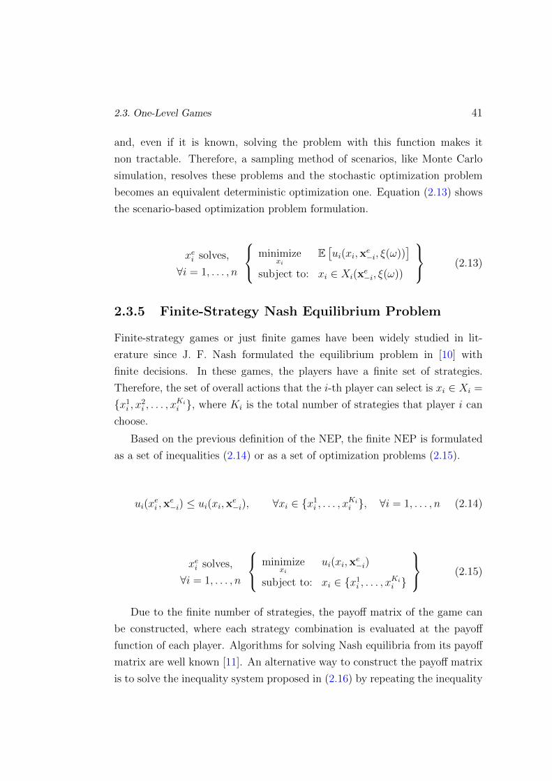
2.3. One-Level Games 41
and, even if it is known, solving the problem with this function makes it
non tractable. Therefore, a sampling method of scenarios, like Monte Carlo
simulation, resolves these problems and the stochastic optimization problem
becomes an equivalent deterministic optimization one. Equation (2.13) shows
the scenario-based optimization problem formulation.
xei solves,
∀i = 1, . . . , n
minimizexi
E[ui(xi,x
e−i, ξ(ω))
]subject to: xi ∈ Xi(x
e−i, ξ(ω))
(2.13)
2.3.5 Finite-Strategy Nash Equilibrium Problem
Finite-strategy games or just finite games have been widely studied in lit-
erature since J. F. Nash formulated the equilibrium problem in [10] with
finite decisions. In these games, the players have a finite set of strategies.
Therefore, the set of overall actions that the i-th player can select is xi ∈ Xi =
x1i , x
2i , . . . , x
Kii , where Ki is the total number of strategies that player i can
choose.
Based on the previous definition of the NEP, the finite NEP is formulated
as a set of inequalities (2.14) or as a set of optimization problems (2.15).
ui(xei ,x
e−i) ≤ ui(xi,x
e−i), ∀xi ∈ x1
i , . . . , xKii , ∀i = 1, . . . , n (2.14)
xei solves,
∀i = 1, . . . , n
minimizexi
ui(xi,xe−i)
subject to: xi ∈ x1i , . . . , x
Kii
(2.15)
Due to the finite number of strategies, the payoff matrix of the game can
be constructed, where each strategy combination is evaluated at the payoff
function of each player. Algorithms for solving Nash equilibria from its payoff
matrix are well known [11]. An alternative way to construct the payoff matrix
is to solve the inequality system proposed in (2.16) by repeating the inequality

42 2. Mathematical Framework for Bilevel Games
equation for every available strategy of each player.
ui(xei ,x
e−i) ≤ ui(x
kii ,x
e−i), ∀ki = 1, . . . , Ki, ∀i = 1, . . . , n (2.16)
The i-th payoff at the equilibrium (left hand side of (2.16)) must be less
than or equal to the i-th payoff for any other available strategy for the i-
th player, when the rest of the players have no incentives to change their
strategies, i.e., when they are at the equilibrium. The inequality system has∑ni=1Ki inequalities instead of the
∏ni=1Ki elements of the payoff matrix.
Example 2.4 Based on the previous two-player game from Example 2.1, now
the strategy space for player 1 and player 2 is discretized in 6 and 7 lev-
els respectively. Therefore, player 1 can choose amongst the strategies x1 =
x11, x
21, . . . , x
61 and player 2 can choose amongst the strategies x2 = x1
2, x22, . . . , x
72.
The finite NEP for the two-player game is defined in (2.17). Figure 2.7
shows the discrete strategy space.
(xe1, xe2) solves
u1(xe1, xe2) ≤ u1(x1
1, xe2)
. . .
u1(xe1, xe2) ≤ u1(x6
1, xe2)
u2(xe1, xe2) ≤ u2(xe1, x
12)
. . .
u2(xe1, xe2) ≤ u2(xe1, x
72)
xe1 ∈ x11, x
21, x
31, x
41, x
51, x
61
xe2 ∈ x12, x
22, x
32, x
42, x
52, x
62, x
72
(2.17)
Assume that the gradients of the payoff functions are the same as in Exam-
ple 2.3, ∇u1(x1, x2) for player 1 and ∇u2(x1, x2) for player 2, and defined only
for the discretized strategies based on the original continuous case. The finite
NEP solution is unique and located at (xe1, xe2) = (x6
1, x72). It is represented with
a red dot in Figure 2.7. In this case, the solution from the finite NEP remains

2.3. One-Level Games 43
x2
x1
x12
x72
x11 x6
1x51x4
1x31x2
1
x22
x32
x42
x52
x62
∇u1(x1, x2)∇u2(x1, x2)
NE
Figure 2.7: Discrete strategy set and solution for the finite NEP
the same as in the original continuous problem. But the NEP solution from
the discretized game may be different from the solution of the original game.
However, the discretized game could be tractable for solving global equilibria
whereas the original computational problem is not tractable, or the payoff
functions are non-convex. In general, games with non-convex payoff functions
do not find global solutions for the NEP.
The smoothness and convexity properties of the payoff function are not
necessary for finding a global solution of the proposed model (2.16), since the
inequality system checks that the equilibrium strategy is better than or equal
to other available strategies for all finite values of each player.
Converting the finite NEP into an inequality system increases the number
of equations but solves the problem of having non-convex and non-smooth
payoff functions in order to set a global NEP solution. Besides, the inequality
system can be added as a set of constraints of a more complex hierarchical
optimization problem, as will be seen in Chapter 4.
2.3.6 Finite Generalized Nash Equilibrium Problem with
Shared Constraints
The discretization approach proposed above has limitations for the GNEP
because the set of inequalities must be evaluated for all the finite strategies of

44 2. Mathematical Framework for Bilevel Games
each player when the other players are in the equilibrium. In other words, all
the finite strategies xi ∈ x1i , . . . , x
Kii must be feasible given a fixed decision
vector x−i in the equilibrium, which is more restrictive than the conventional
definition of the GNEP. The latter forces feasibility only at the equilibrium
solution, i.e., xei . Therefore, a discretization of the GNEP entails a reduction
of the original feasible region and the equilibria may be different.
In the next example we clarify this fact for a GNEP with shared constraints.
Example 2.5 Based on the previous two-player game (Example 2.4), we have
added a new shared constraint over the set of strategies of both players, x1 and
x2 (see Figure 2.8).
The payoff functions’ gradients are ∇u1(x1, x2) for player 1 and ∇u2(x1, x2)
for player 2, as in the previous examples. Then, the set of solutions for the
(continuous) GNEP with shared constraints is represented by the thick red line.
Note that there is an infinite number of GNE.
Now, we have discretized the problem with the same levels as in the previous
Example, i.e, player 1 can choose amongst the strategies x1 = x11, x
21, . . . , x
61
and player 2 can choose amongst the strategies x2 = x12, x
22, . . . , x
72. The
equivalent finite GNEP is the same as in the previous example (2.17). We
assume the payoff function is known at each discrete combination of strategies,
based on the payoff gradients from the continuous problem. Then, player
1 chooses the highest values for their own strategies, x1, while player 2 is
interested in choosing the highest values of their own strategies, x2.
Assume that if the equilibrium decision of player 1 is xe1 = x61, then,
player 2 must evaluate the payoff function, u2, at all their finite available
strategies with xe1 = x61. But, for the cases when variable x2 takes the values
x62, x
72, the problem becomes infeasible. Therefore, xe1 = x6
1 can not be solution
of the problem (2.17). Then, the solutions of the discretized GNEP with
shared constraints are searched for in a reduced feasible region represented in
Figure 2.8 in dark color. This reduced feasible region constitutes an equivalent
standard NEP feasible region, in which the decision of each player is not
constrained by the decisions of the other players.
The solution of the discretized GNEP is represented with a red dot and it

2.3. One-Level Games 45
x2
x1
x12
x72
x11 x6
1x51x4
1x31x2
1
x22
x32
x42
x52
x62
∇u1(x1, x2)∇u2(x1, x2)
Discretized GNE
Set of continuous GNE
Reduced feasible region
Figure 2.8: Discretized GNE with shared constraints
differs from the original continuous GNEP.
Discretized GNEPs have limitations using the proposed approach, as we
have illustrated in the previous example. But they can succeed with other
problems like finding global solutions for the non-linear and non-convex payoff
functions, or finding all pure Nash equilibria as will be described in the next
subsection.
2.3.7 Finding All Pure Nash Equilibria in a Finite NEP
The finite NEP problem (2.16) may have a single solution, a manifold of finite
solutions, or may have no solution. It is important to know all the solutions
because, a priori, all equilibria are possible, or some of them are more meaning-
ful. But most of the proposed solution techniques do not guarantee finding all
pure Nash equilibria. Some of the algorithms find a single equilibrium without
any meaningful criteria.
We propose an algorithm for finding all pure Nash equilibria of a finite
NEP in (2.16). Due to the fact that there is a finite number of strategies for
each player, we can create “holes” in the feasible region for each identified
Nash equilibrium. A hole is represented with a new constraint and added to
the inequality system (2.16), so that the identified Nash equilibrium cannot be
a solution of the new inequality system. In this way we can find all pure Nash

46 2. Mathematical Framework for Bilevel Games
equilibria.
In order to do this, after a solution (Nash equilibrium) for the NEP (2.16)
(characterized by x∗i for all i) is found, we impose a new constraint to avoid
that the optimal value of xei being close to the previously found solution (within
a distance of ε). We repeat this procedure with any new solution found. Thus,
given a solution vector x∗i (q) of the NEP, we include a set of new constraints
to generate holes in the space of solutions already found, as described in (2.18)
for each Nash equilibrium found (indexed by q):
√∑i
(xei − x∗i (q))> · (xei − x∗i (q)) ≥ ε, ∀q (2.18)
Equation (2.18) represents q hyperspheres with radius ε > 0 centered at
point x∗i (q). Thus, the distance between xei and x∗i (q) must be greater than
radius ε. The left hand side of the equation represents the Euclidean distance
between these two points.
We can convert the integer variables into a new binary (0/1) representation,
using binary expansion [115, 116], for example. The number of variables
increases, but this helps to linearize equation (2.18). Nevertheless, some works
[116] have provided theoretical and computational evidence demonstrating that
transforming integer problems with binary variables helps to solve the problem
more efficiently with specific algorithms.
Assume the vector of strategies, xi, is a vector of binary variables that
represents all available strategies for the i-th player. Then, equation (2.18)
can be rewritten as (2.19).
∑i
((xei )
2 + (x∗i (q))2 − 2xeix
∗i (q)
)≥ ε2, ∀q (2.19)
where the quadratic term can be converted into a linear term (2.20) by
taking into account the properties of the binary variables.

2.4. Bilevel Games 47
∑i
(xei + x∗i (q)− 2xeix∗i (q)) ≥ ε2, ∀q (2.20)
The ε2 value must be small enough so as not to lose solutions inside the
hypersphere hole, and the solution must not belong to the boundary of the
hypersphere hole. Since the variables belong to the 0-1 discrete space, the
limits of ε2 are 0 < ε2 < 1.
2.4 Bilevel Games
Bilevel games are hierarchical games where players make decisions in sequence.
The simplest bilevel game is the so-called Stackelberg game [69] or single-leader-
single-follower game, where a leader makes decisions prior to the follower ’s
decisions.
As a generalization of the two-player Stackelberg game, new bilevel games
have been proposed in game theory literature. In these generalizations, the
lower and/or upper level have more than a single player. Thus, the players
at the upper level (leaders) make decisions simultaneously competing between
them and prior to the decisions of the players at the lower level (followers).
After the leaders make their decisions, the followers make their decisions, also
competing among themselves. The decisions of the followers are made taking
into consideration the leaders’ and the other followers’ decisions. Since a
follower competes against other followers, the lower-level problem forms a Nash
game parameterized in terms of the leaders’ decisions. In a similar manner, in
the upper-level problem, the leaders make simultaneous decisions considering
the optimal response of the followers. The leaders compete against each other
in the upper-level problem in a Nash game.
In bilevel games, leaders and followers can be different players or the same
players at both levels, but making different decisions. In Chapter 3 we pose a
bilevel game where the leaders are different players from the follower, but in
Chapter 4 we propose a hierarchical game where some players are playing at
the upper and lower levels making different decisions.

48 2. Mathematical Framework for Bilevel Games
Depending on the number of players at the upper or lower levels, bilevel
games can be classified into four categories: single-leader-single-follower, single-
leader-multiple-follower, multiple-leader-single-follower and multiple-leader-multiple-
follower game.
In general, bilevel games can be solved as bilevel optimization problems.
A work related with bilevel optimization [66, 117] can be applied for solving
bilevel games. When there are multiple players at the lower-level problem, the
problem can be rewritten as a set of equilibrium constraints in the optimization
problem of the leader(s). In case of a single leader, the problem is stated as an
MPEC optimization problem [67, 81]. If, instead, there are several players at
the upper-level problem, it can be stated as an EPEC optimization problem
[6,34,35].
2.4.1 Single-Leader-Single-Follower Games
A single-leader-single-follower game is stated as a bilevel optimization problem
[66,117]. The leader’s problem is at the upper level, where the leader chooses a
decision vector, x, first. After the leader has made their decision, the follower
chooses their decision vector, y, solving the lower-level optimization problem
(see Figure 2.9).
Leader
x y
Follower
Figure 2.9: Single-leader-single-follower game
The follower’s optimization problem is parameterized in terms of the upper-
level decision, x. Formally, the follower selects a vector, y(x), in some closed
set, Y , where their objective function is minimized, f(x, y). The optimal set
of solutions of the lower-level problem is denoted by S(x). Then, a vector
y(x) belongs to the optimal set of solutions of the lower-level problem, i.e.,

2.4. Bilevel Games 49
y(x) ∈ S(x), if and only if:
y(x) solves
minimizey
f (x, y)
subject to: y ∈ Y (x)
(2.21)
On the other hand, the leader minimizes their objective function, F (x, y),
in some closed set X, taking into account the optimal response of the follower,
y(x) ∈ S(x). This is formally described as follows:
(xe, ye) solves
minimize
x,yF (x, y)
subject to: x ∈ Xy ∈ S(x)
(2.22)
In this dissertation we investigate the case where the lower-level and upper-
level constraint functions are represented by linear functions. Therefore, the
lower-level constraint set, Y , is defined as Y = y : h(x, y) = 0, g(x, y) ≤ 0,where h(x, y) and g(x, y) are linear. The upper-level constraints set, X, is
defined as X = x : H(x, y) = 0, G(x, y) ≤ 0, where H(x, y) and G(x, y) are
linear.
Here, we have used the superscript e to represent the optimal solution for
the whole problem (upper and lower level). Additionally, we have extended the
conventional definition of bilevel problems including the Lagrange multipliers
from the lower-level to the upper-level objective function and constraints. In
this sense, the Lagrange multipliers solution from the lower-level can affect the
decisions of the leader.
Then, the single-leader-single-follower optimal solution is obtained by solv-
ing the problem (2.23)–(2.24).

50 2. Mathematical Framework for Bilevel Games
(xe, ye, λe, µe) solves
minimizex,y,λ,µ
F (x, y, λ, µ)
subject to:
G(x, y, λ, µ) ≤ 0
H(x, y, λ, µ) = 0
(y, λ, µ) ∈ S(x)
(2.23)
where (y, λ, µ) ∈ S(x) if and only if:
(y, λ, µ) solves
minimize
y,λ,µf(x, y)
subject to: g(x, y) ≤ 0, µ
h(x, y) = 0, λ
(2.24)
2.4.2 Single-Leader-Multiple-Follower Games
A single-leader-multiple-follower game is a Stackelberg problem extension with
multiple followers, where the followers are competing among themselves. Fig-
ure 2.11 represents the structure of this game.
In this game a single leader makes their optimal decision, x, prior to the
decision of multiple followers, who are competing among themselves. Given
the optimal decision of the leader, x, each j-th follower makes their optimal
decision, yj, taking into account their competitors’ optimal decisions, y−j.
Leader
Follower 1 Follower m
y1
y1
x x
ym
ym
Figure 2.10: Single-leader-multiple-follower game
The single-leader-multiple-follower equilibrium solution is given by solving
the problem (2.25)–(2.26). The vector (xe,ye,λe,µe) represents the optimal

2.4. Bilevel Games 51
values of the decisions of the leader and the followers, as well as the Lagrange
multipliers of the lower-level problem.
The leader minimizes their objective function, F (·), which depends on the
leader’s decision, x, the optimal decisions of the followers, y, and the optimal
value of the Lagrange multipliers, λ and µ, from the lower-level problem. The
upper-level problem (2.25) is constrained by the functions G(·), H(·) and the
set of the optimal solutions of the followers, S(x), parameterized by the leader’s
decision, x, solving a set of m problems in the lower level (2.26).
(xe,ye,λe,µe) solves
minimizex,y,λ,µ
F (x, y, λ, µ)
subject to: G(x, y, λ, µ) ≤ 0
H(x, y, λ, µ) = 0
(y, λ, µ) ∈ S(x)
(2.25)
where (y, λ, µ) ∈ S(x) if and only if:
(yj, λj, µj) solves,
∀j = 1, . . . ,m
minimizeyj ,λj ,µj
fj(x, yj, y−j)
subject to: gj(x, yj, y−j) ≤ 0, µj
hj(x, yj, y−j) = 0, λj
(2.26)
The y-tuple is the Nash equilibrium of the followers for the leader’s deci-
sion, x. The variables λ and µ represent the Lagrange multipliers for the
equality and the inequality constraints of the followers, respectively. The
objective function, fj(·), and the constraints, gj(·) and hj(·), are defined as
linear functions for all the j-th followers’ problems. Because each j-th follower
problem is stated as an LP, global optimality can be guaranteed for each j-
th follower problem. But the simultaneous j-th followers’ problems may not
have a solution, may have only one solution, or may have multiple solutions.
The set of the solutions represented by S(x) is rewritten sometimes as an
equivalent system of constraints, e.g., KKT conditions added to the upper-
level problem (2.25). This system of constraints is the so-called equilibrium
constraints set. The single-leader-multiple-follower problem can be stated as

52 2. Mathematical Framework for Bilevel Games
an MPEC optimization problem [67,81].
2.4.3 Multiple-Leader-Single-Follower Games
A multiple-leader-single-follower game is a case when several players (leaders)
anticipate simultaneously the decisions of a single player (follower). Because
all the leaders make decisions at the same stage, the upper-level problem is
defined as a Nash equilibrium of the leaders. Figure 2.11 illustrates the game
structure. Multiple-leader-single-follower games are appropriate for represent-
ing liberalized markets, where participants have to interact with the market
submitting offers prior to the resolution of the market. Market participants
are at the upper level and market operation is at the lower level. The Lagrange
multipliers of the lower-level problem represent on many occasions the price of
the resource traded in the market.
Leader 1
Follower
y
Leader n
yx1
x1
xn
xn
Figure 2.11: Multiple-leader-single-follower game
The formulation of the multiple-leader-single-follower game is given by
(2.27)–(2.28). Solving (2.27)–(2.28) means solving a set of n bilevel problems,
one per leader. Because all leader’s problems depend on the competitors’
decisions, the set of the n problems is coupled and complicates the resolution
of this problem. EPEC techniques [6, 34, 35] can be applied to solve this kind
of problem. Note that even though the lower-level problem is common for all
leaders, the response in primal and dual variables could be different. We have
emphasized this in the notation using the superscript (i) for the lower-level
variables.

2.4. Bilevel Games 53
(xei , ye, λe, µe) solves,
∀i = 1, . . . , n
minimizexi,y(i),λ(i),µ(i)
Fi(xi,xe−i, y
(i), λ(i), µ(i))
subject to:
Gi(xi,xe−i, y
(i), λ(i), µ(i)) ≤ 0
Hi(xi,xe−i, y
(i), λ(i), µ(i)) = 0
(y(i), λ(i), µ(i)) ∈ S(xi,xe−i)
(2.27)
where (y(i), λ(i), µ(i)) ∈ S(xi,xe−i) if and only if:
(y(i), λ(i), µ(i)) solves
minimizey(i),λ(i),µ(i)
f(xi,xe−i, y
(i))
subject to: g(xi,xe−i, y
(i)) ≤ 0, µ(i)
h(xi,xe−i, y
(i)) = 0, λ(i)
(2.28)
The lower-level problem (2.28) is an optimization problem parameterized
by the upper-level decisions of each of the i-th leaders. Because the lower-level
problem is a linear optimization problem it can be reformulated either as a set
of KKT conditions or as a set composed of the primal and dual constraints and
strong duality theorem. This set of equivalent constraints could be different
for each i-th leader’s problem, and is added to each upper-level problem.
Some authors [36] have claimed that when the lower level represents the
market operation, the Lagrange multipliers should be the same for all leaders,
i.e., λ(i) = λ, ∀i and µ(i) = µ, ∀i. This is known as price consistency,
where there is no price discrimination for all the leaders. A price-consistent
formulation is more restrictive and it may not have a solution while the original
one has. However, a price-consistent formulation is easier to solve than a
general one (2.27)–(2.28) due to the reduction in the number of variables and
constraints.
2.4.4 Multiple-Leader-Multiple-Follower Games
A multiple-leader-multiple-follower game is the most general instance of a
bilevel game where several leaders competing among themselves have to make

54 2. Mathematical Framework for Bilevel Games
decisions in the first stage prior to the decisions of a set of followers competing
among themselves in the second stage (see Figure 2.12).
Leader 1 Leader n
x1
x1
Follower 1 Follower m
y1
y1
xn
xn
ym
ym
Figure 2.12: Multiple-leader-multiple-follower game
The multiple-leader-multiple-follower problem is given by a set of n coupled
MPEC problems, one for each leader, and given by (2.29)–(2.30). This problem
is stated as an EPEC [6,34,35].
(xei ,ye,λe,µe) solves,
∀i = 1, . . . , n
minimizexi,y(i),λ
(i),µ(i)
Fi(xi,xe−i, y
(i), λ(i), µ(i))
subject to: Gi(xi,xe−i, y
(i), λ(i), µ(i)) ≤ 0
Hi(xi,xe−i, y
(i), λ(i), µ(i)) = 0
(y(i), λ(i), µ(i)) ∈ S(xi,x
e−i)
(2.29)
where (y(i), λ(i), µ(i)) ∈ S(xi,x
e−i) if and only if:
(y(i)j , λ
(i)j , µ
(i)j ) solves,
∀j = 1, . . . ,m
minimizey(i)j ,λ
(i)j ,µ
(i)j
fj(xi,xe−i, y
(i)j , y
(i)−j)
subject to: gj(xi,xe−i, y
(i)j , y
(i)−j) ≤ 0, µ
(i)j
hj(xi,xe−i, y
(i)j , y
(i)−j) = 0, λ
(i)j
(2.30)
2.4.5 Stochastic Multiple-Leader-Multiple-Follower Games
The perfect information hypothesis has been assumed in the previous Nash
game definitions. This means that all players, leaders and followers, have
perfect information about their competitors’ payoff functions, available strate-
gies and constraints. Additionally, all the exogenous parameters have been

2.4. Bilevel Games 55
assumed deterministic, but some of them could be random, such as demand or
cost. In this section we introduce stochasticity to bilevel games. In particular,
we expand the general case, the multiple-leader-multiple-follower game to a
stochastic game.
We assume the stochastic bilevel game is played in two stages. At the
first stage the leaders make their decisions in a Nash equilibrium setting,
prior to the knowledge of any scenario realization and considering the best
response of the followers. After the leaders make their decisions, the scenario
realization of the random vector, ξ, is known at the second stage and the
followers make their decisions in a Nash equilibrium setting. Therefore, the
lower-level equilibrium is solved for any realization of the random process,
ξ. Then, the set of (equilibrium) solutions from the lower level are random
variables in terms of such a random process. If we define symbol ξ as a
random distribution to model uncertainty, the lower-level variables are now
(y(i)(xi,xe−i, ξ), λ
(i)(xi,x
e−i, ξ), µ
(i)(xi,xe−i, ξ)) ∈ S(xi,x
e−i, ξ).
The stochastic multiple-leader-multiple follower optimization problem is
given by (2.31)–(2.32)
(xei ,ye,λe,µe) solves,
∀i = 1, . . . , n
minimizexi,y(i),λ
(i),µ(i)
E [Fi(·)]
subject to: Gi(·) ≤ 0
Hi(·) = 0
(y(i), λ(i), µ(i)) ∈ S(xi,x
e−i, ξ)
(2.31)
where (y(i), λ(i), µ(i)) ∈ S(xi,x
e−i, ξ) are given for the random distribution,
ξ, if and only if:
(y(i), λ(i), µ(i)) solves,
∀j = 1, . . . ,m
minimizey(i)j ,λ
(i)j ,µ
(i)j
fj(·)
subject to: gj(·) ≤ 0, µ(i)j
hj(·) = 0, λ(i)j
(2.32)
and where the variables from the second stage are defined as:

56 2. Mathematical Framework for Bilevel Games
y(i) = y(i)(xi,xe−i, ξ)
λ(i)
= λ(i)
(xi,xe−i, ξ)
µ(i) = µ(i)(xi,xe−i, ξ)
(2.33)
and the payoff and constraints functions are defined as:
Fi(·) = Fi(xi,xe−i, y
(i), λ(i), µ(i), ξ)
Gi(·) = Gi(xi,xe−i, y
(i), λ(i), µ(i), ξ)
Hi(·) = Hi(xi,xe−i, y
(i), λ(i), µ(i), ξ)
fj(·) = fj(xi,xe−i, y
(i)j , y
(i)−j, ξ)
gj(·) = gj(xi,xe−i, y
(i)j , y
(i)−j, ξ)
hj(·) = hj(xi,xe−i, y
(i)j , y
(i)−j, ξ)
(2.34)
The upper-level constraints and payoff functions are defined in terms of
expectations with respect to the random variable, ξ. Other kinds of con-
straints can be used as risk measures, but this is outside the scope of this
dissertation. The lower-level constraints and payoff functions are defined for
any realization of the random variable, ξ. When a scenario-based approach
is applied, the random variable ξ is sampled in the scenarios indexed by ω
and the real distribution is substituted by the scenarios’ realizations, ξ(ω).
Then, an equivalent deterministic optimization problem is obtained replacing
the random variable ξ by the sampled one, ξ(ω).
2.4.6 Stochastic Multiple-Leader-Multiple-Follower Games
in Finite Strategies
In this dissertation we have considered games with finite strategies for the lead-
ers and continuous strategies for the followers, including uncertainty modeling.
This game is cast as a finite stochastic EPEC. In general, it is a hard-to-solve
non-convex optimization problem.
In this Section we present a special case of this setting where the leaders’
decisions do not depend on their competitors’ decisions at the upper level.

2.4. Bilevel Games 57
This stochastic multi-leader-multi-follower game setting can model hierarchical
relationships among participants.
The mathematical model is stated as a stochastic EPEC in finite strategies
and it is defined in (2.35)–(2.36).
(xei ,ye,λe,µe) solves,
∀i = 1, . . . , n
minimizexi,y(i),λ
(i),µ(i)
E[Fi
(xi,x
e−i, y
(i), λ(i), µ(i), ξ
)]subject to: Gi(xi) ≤ 0
Hi(xi) = 0
xi ∈ x1i , x
2i , . . . , x
Kii
(y(i), λ(i), µ(i)) ∈ S(xi,x
e−i, ξ)
(2.35)
where (y(i), λ(i), µ(i)) ∈ S(xi,x
e−i, ξ) for the random distribution ξ, if and
only if:
(y(i), λ(i), µ(i)) solves,
∀j = 1, . . . ,m
minimizey(i)j ,λ
(i)j ,µ
(i)j
fj(xi,xe−i, y
(i)j , y
(i)−j, ξ)
subject to: gj(xi,xe−i, y
(i)j , y
(i)−j, ξ) ≤ 0, µ
(i)j
hj(xi,xe−i, y
(i)j , y
(i)−j, ξ) = 0, λ
(i)j
y(i)j ∈ RKj
+ , µ(i)j ∈ Rs
+, λ(i)j ∈ Rp
(2.36)
Leader i can choose among a finite number of strategies, xi ∈ x1i , x
2i , . . . , x
Kii ,
which are constrained by Gi and Hi functions. Note that the decisions of each
leader do not depend on the decisions of the other leaders (Gi and Hi are
dependent only on xi). In general, this is true in many problems of power
systems, where participants act in their own interests. However, the payoff
function only is dependent on the competitors’ decisions and the lower-level
variables. Additionally, the optimal decisions at the upper level are made
before the realization of the random variable, i.e., the decisions do not depend
on each single realization of the random variables.
At the lower level (equation (2.36)), follower j makes their optimal decisions
given the leaders’ decisions, (xi,xe−i), the other followers’ optimal decisions,
y−j, with full knowledge of the realization of the random variable, ξ = ξ(ω).

58 2. Mathematical Framework for Bilevel Games
This problem can be solved applying the approach explained in Section
2.3.6. Additionally, the algorithm for finding all Nash equilibria could be
applied, as described in Section 2.3.7.
Then, the stochastic EPEC in finite strategies can be cast as a set of a
system of inequalities with equilibrium constraints (2.37).
(xei ,ye,λe,µe) solves, ∀ki = 1, . . . , Ki, ∀i = 1, . . . , n
E[Fi(xei ,x
e−i, y
e, λe, µe, ξ
)]≤ E
[Fi
(xkii ,x
e−i, y
(i,ki), λ(i,ki), µ(i,ki), ξ
)]subject to:
Gi(xei ) ≤ 0, Gi(x
kii ) ≤ 0,
Hi(xei ) = 0, Hi(x
kii ) = 0,
xei ∈ x1i , x
2i , . . . , x
Kii ,
(ye, λe, µe) ∈ S(xei ,x
e−i, ξ), (y(i,ki), λ
(i,ki), µ(i,ki)) ∈ S(xkii ,xe−i, ξ)
(2.37)
The previous formulation represents a system of inequalities with equilib-
rium constraints where the minimization operator for the upper-level problem
does not appear. This is an advantage with respect to conventional EPEC
settings. Now, instead of having a set of n coupled MPECs, one for each
leader, we have a system of n inequalities with equilibrium constraints.
On the left hand side (LHS) of the inequality, the objective function of
leader i is evaluated at the equilibrium, xei , and the constraints must hold for
each i-th leader equilibrium, i.e., Gi(xei ) and Hi(x
ei ). Additionally, the equi-
librium constraints are solved for the leaders’ equilibrium, i.e., (ye, λe, µe) ∈
S(xei ,xe−i, ξ). We have added superscript e to the lower-level variables to repre-
sent the parametrization of the lower-level equilibria in terms of the upper-level
equilibria. Then, ye is the vector of the followers’ equilibria decisions when all
leaders are in the equilibrium.
On the right hand side (RHS) of the inequality, the objective function of
leader i is evaluated for each xkii available strategy. Each finite strategy for
leader i is restricted by their own constraints, Gi(xkii ) and Hi(x
kii ), and the
equilibrium constraints. The equilibrium constraints are parameterized for

2.4. Bilevel Games 59
each xkii strategy of leader i when the competitors are fixed in the equilibrium,
xe−i. We have added superscript (i, ki) to the lower-level variables to represent
the parametrization of the lower-level equilibria in terms of the upper-level
decisions. Then, y(i,ki) is the decision vector of the followers in the equilibrium,
when the i-th leader chooses the ki-th strategy and their competitors are in
the equilibrium.
The major challenge of this formulation is to solve the equilibrium con-
straints, since they are optimization problems nested in an inequality system.
In Section 2.5 we deal with these constraints, transforming the optimization
problems into their first-order optimality conditions.
For this particular finite stochastic EPEC, there is no relationship with
the competitors’ decisions in the upper-level constraints set, the same as in
a standard NEP. But there is an extra constraint, the equilibrium constraint
coupling the leaders’ decisions. This motivates the next subsection.
2.4.7 Bilevel Games could be Special Cases of General-
ized Nash Equilibrium Problems
Bilevel games are special cases of GNEPs. In particular, multi-leader games are
GNEPs because there are constraints in each leaders’ problem that involve vari-
ables of the other leaders. These constraints could be upper-level constraints
or equilibrium constraints. Regarding the upper-level constraints, they are
easy to understand when the problem is generalized, because the constraints
for each leader depend explicitly of the competitors’ strategies. Regarding the
equilibrium constraints, it is not easy to understand their dependence on the
competitors’s decisions, because they are implicit.
This implicit dependence on the competitors’ decisions in the lower-level
problem is usual when a common resource is traded or shared in the lower-
level problem, e.g., energy demand. Leaders can submit their desires to obtain
this resource by choosing their strategies, which, at first, are not restricted.
However, the resource is distributed among leaders at the lower level, where
the desires of the leaders are linked. Their distribution represents an implicit

60 2. Mathematical Framework for Bilevel Games
coupling constraint among the leaders.
We illustrate this fact in the next example, where the interdependence
among the leaders’ decisions only occurs in the equilibrium constraints.
Example 2.6 Given a multiple-leader-single-follower game with two leaders
and one follower, leader 1 chooses amongst strategies x1 ∈ X1 ⊆ R, leader
2 chooses amongst the strategies x2 ∈ X2 ⊆ R and the follower chooses the
strategies among y ∈ Y ⊆ R. The leaders’ decisions are not dependent on
each other’s decisions.
Let the objective functions be F1(x1, x2, y) : X1×X2×Y 7→ R for leader 1,
F2(x1, x2, y) : X1×X2×Y 7→ R for leader 2, and f(x1, x2, y) : X1×X2×Y 7→ Rfor the follower.
The multiple-leader-single-follower game is composed of the optimization
problems of the two leaders:
(xe1, xe2, y
e) solves (2.38)–(2.39)
minimizex1,y(1)
F1(x1, xe2, y
(1))
subject to: x1 ∈ X1
y(1)solves
minimizey
f(x1, xe2, y)
subject to: y ∈ Y
(2.38)
minimizex2,y(2)
F2(xe1, x2, y(2))
subject to: x2 ∈ X2
y(2)solves
minimizey
f(xe1, x2, y)
subject to: y ∈ Y
(2.39)
The feasible region for leader 1 is defined as Ω1(x1, xe2, y) = (x1, y) : x1 ∈
X1, y ∈ S(x1, xe2), and for leader 2 is defined as Ω2(xe1, x2, y) = (x2, y) : x2 ∈
X2, y ∈ S(xe1, x2). Then, the multiple-leader-single-follower game is written
in a short form in equation (2.40).

2.4. Bilevel Games 61
(xe1, xe2, y
e) solves
minimizex1,y(1)
F1(x1, xe2, y
(1)), s.t. (x1, y(1)) ∈ Ω1(x1, x
e2, y
(1))
minimizex2,y(2)
F2(xe1, x2, y(2)), s.t. (x2, y
(2)) ∈ Ω2(xe1, x2, y(2))
(2.40)
Figure 2.13 illustrates the set of available strategies for the leaders and the
follower as well as the feasible regions for both optimization problems (2.40).
The optimal solution of the lower-level problem has been assumed to be unique.
Then, for any leaders’ decisions vector, (x1, x2), the optimal response of the
follower is unique. The set Ω(x1, x2, y) provides the feasible region for the
leaders and the follower for any vector (x1, x2). The set Ω1(x1, xe2, y) represents
the feasible region for leader 1 and the follower, assuming leader 2 is fixed at
the equilibrium.
x2
x1
y
X2
Y
xe2
X1
Ω1(x1, xe2, y)
Ω(x1, x2, y)
Figure 2.13: Strategies set for players x1, x2 and y
Although the leaders are not restricted to any strategy, e.g. x1 ∈ X1, the
lower-level problem restricts the strategies that the leaders can choose (dark

62 2. Mathematical Framework for Bilevel Games
area in the x1–x2 plane from Figure 2.13). In this particular case, for si-
multaneous values of x1 and x2 close to zero, the problem becomes infeasible.
Therefore, there is no solution for the EPEC. For example, this constraint
could represent a resource that should be supplied at a minimum level, such as
electricity demand.
2.4.8 Other Bilevel Games Compositions
The basic element for bilevel games consists of leaders making decisions prior to
the followers’ decisions, both competing among themselves. We have pointed
out that when several players are competing at the same level, they are doing
it in a non-cooperative Nash equilibrium setting. This holds true in many
real situations where imperfect competition arises. But different kinds of
competitive behaviors could be included at each level, as in the case of perfect
competition. When markets are not concentrated or regulators restrict the
players’ behaviors, perfect competition should be expected.
For example, the problem of generation expansion in power systems could
be interpreted in this way: first, the leaders (GENCOs) decide their optimal
generation expansions in a Nash setting anticipating the results in the spot
market. Then, the spot market clearing process takes place at the lower level
and the participants (GENCOs and ISO) act in a perfectly competitive way.
2.5 Solving Bilevel Games
Bilevel games are highly non-linear and non-convex, thus, the existence and
uniqueness of equilibrium points rarely happens. For example, in the simplest
case, the single-leader-single-follower game is modeled as a bilevel game, gen-
erally NP-hard, i.e., no numerical solution scheme exists to solve the problem
in polynomial time [66].
MPECs and MPCCs are non-convex and non-linear and NLP algorithms
fail to solve such problems because the constraints qualification, such as LICQ
and MFCQ, fail with complementary constraints. Hence the global optimal so-
lution is seldom obtained. New constraint qualification definitions are proposed

2.5. Solving Bilevel Games 63
to define new stationarity solutions (not necessarily global solutions) reached
solving MPECs or MPCC by conventional NLP algorithms. For example,
the W-, C-, B-, M- or S- constraint qualifications are used. Reference [86]
defines such constraints qualifications for solving MPCC. See the monograph
on MPECs [81] for further details.
EPECs are composed of a set of coupled MPECs and they inherit the
“bad” properties of MPECs. They are non-convex and non-linear and finding
a solution for this problem constitutes a challenge. Thus, a global solution
is seldom reached. Because the constraint qualifications do not hold for each
MPEC that composes the EPEC, the solutions obtained are usually stationary.
These stationary solutions may be Nash equilibria, local equilibria or saddle
points.
Finding algorithms to solve this problem constitutes an ongoing line of
research. Two algorithms have been suggested in the literature for solving
EPECs:
• Diagonalization approach, by solving the MPECs of each player sequen-
tially until convergence. This approach can be further classified into two
methods, Jacobi and Gauss-Seidel method. See [19,93].
• Simultaneous solution method, by writing the strong stationary necessary
conditions for all MPECs and solving all the constraints simultaneously.
The solution of this problem is known as strong stationary solution.
See [36,95].
Because of the lack of a global solution for these approaches, some hybrid
methods pretend to find the “best” solution between different sets of solutions
found when the problem is solved with different starting points.
We have overcome all of these difficulties by converting the stochastic EPEC
into an system of inequalities with equilibrium constraints, transforming the
stochastic EPEC into an MILP. Consequently, global optimality is guaranteed
for the equivalent MILP at the expense of the tractability of the problem.
To solve bilevel games, a one-level reformulation is often used. First, we
attempt to replace the lower-level problem with their equivalent first order

64 2. Mathematical Framework for Bilevel Games
optimality conditions. Because the lower-level has been assumed to be an
LP problem, the KKT conditions are sufficient optimality conditions. An
alternative way is to replace the lower-level problem by the set of primal
constraints, dual constraints and the strong duality theorem, which constitute
a set of first order optimal and sufficient conditions.
After that, the equivalent equilibrium conditions are added as constraints
to each leader’s optimization problem, becoming a set of one-level problems
(MPECs) stated as an EPEC. In the stochastic version, the lower-level prob-
lem is solved for all scenario realizations, ω. One set of equivalent optimal
conditions per scenario is added to each leader’s problem, becoming a set of
stochastic MPECs or a stochastic EPEC.
2.5.1 Manifolds of Lower-Level Solutions
In order to have a unique solution, strict convexity of the lower-level problem
for each decision of the leader, x, and each realization, ω, are required. How-
ever, when the lower-level is linear (convex and concave at the same time),
KKT conditions are applicable, but a non unique (globally) optimal solution
is reached for at least one value of x. This means that, for a given decision of
leader x, the optimal decision of the follower is a set of decisions y(x, ω) with
the same objective function value. Then, the follower is indifferent to any of
their own decisions. In other words, the first order optimality conditions from
the linear lower level are sufficient, but there could be multiple solutions.
A bilevel solution is called an optimistic solution if the leader takes an
optimistic attitude towards the outcome of the follower. On the contrary, a
solution is called a pessimistic solution if the leader takes a pessimistic attitude
towards the outcome of the follower. If the problem has multiple followers,
the solution of the lower level could have multiple equilibria (solutions), and
optimistic or pessimistic solutions could be assumed by all the leaders. In
general, most bilevel games are implicitly formulated as optimistic.

2.5. Solving Bilevel Games 65
2.5.2 First-Order Optimality Conditions for the Lower-
Level Problem: KKT Conditions
For the sake of simplicity, we have defined a deterministic linear lower-level
problem for a single follower (2.41)–(2.43). The KKT conditions are derived
from this problem. For the case of multiple followers, equivalent lower-level
conditions are formed by each individual follower’s KKT conditions.
The linear lower-level problem is defined as:
minimizey
c>x+ d(x)>y (2.41)
subject to: Ax+B(x)y ≤ b1, µ (2.42)
Cx+D(x)y = b2, λ (2.43)
where µ and λ are the Lagrange multipliers (dual variables) associated with
the inequality and equality constraints. Then, we define the Lagrange function
L(y, µ, λ), respectively.
L(y, µ, λ) =c>x+ d(x)>y
−µ>(Ax+B(x)y − b1)− λ>(Cx+D(x)y − b2) (2.44)
We have omitted the dependence of the leader’s decision, x, in the Lagrange
function and the variables because the decision is a known parameter for the
lower-level problem.
Then, the KKT conditions are given by:
∇yL(y, µ, λ) = d(x)−B(x)>µ−D(x)>λ = 0 (2.45)
∇µL(y, µ, λ) = Ax+B(x)y − b1 ≤ 0 (2.46)
∇λL(y, µ, λ) = Cx+D(x)y − b2 = 0 (2.47)
µ>(Ax+B(x)y − b1) = 0 (2.48)
µ ≥ 0, λ : free (2.49)
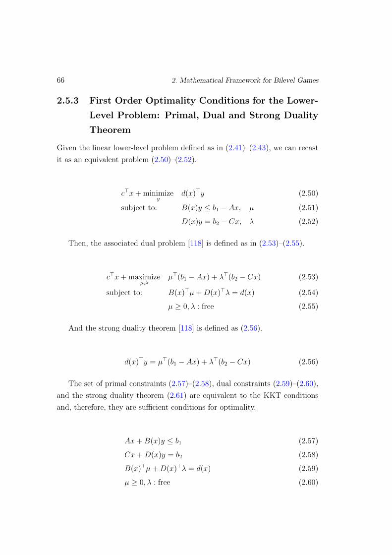
66 2. Mathematical Framework for Bilevel Games
2.5.3 First Order Optimality Conditions for the Lower-
Level Problem: Primal, Dual and Strong Duality
Theorem
Given the linear lower-level problem defined as in (2.41)–(2.43), we can recast
it as an equivalent problem (2.50)–(2.52).
c>x+ minimizey
d(x)>y (2.50)
subject to: B(x)y ≤ b1 − Ax, µ (2.51)
D(x)y = b2 − Cx, λ (2.52)
Then, the associated dual problem [118] is defined as in (2.53)–(2.55).
c>x+ maximizeµ,λ
µ>(b1 − Ax) + λ>(b2 − Cx) (2.53)
subject to: B(x)>µ+D(x)>λ = d(x) (2.54)
µ ≥ 0, λ : free (2.55)
And the strong duality theorem [118] is defined as (2.56).
d(x)>y = µ>(b1 − Ax) + λ>(b2 − Cx) (2.56)
The set of primal constraints (2.57)–(2.58), dual constraints (2.59)–(2.60),
and the strong duality theorem (2.61) are equivalent to the KKT conditions
and, therefore, they are sufficient conditions for optimality.
Ax+B(x)y ≤ b1 (2.57)
Cx+D(x)y = b2 (2.58)
B(x)>µ+D(x)>λ = d(x) (2.59)
µ ≥ 0, λ : free (2.60)

2.5. Solving Bilevel Games 67
d(x)>y = µ>(b1 − Ax) + λ>(b2 − Cx) (2.61)
Notice that equations (2.57), (2.58), (2.59) and (2.60) are equivalent to the
KKT conditions (2.46), (2.47), (2.45) and (2.49), respectively. Both sets of
conditions differ only in the complementary condition (2.48) that appears in
the KKT conditions instead of the strong duality theorem (2.61) which appears
in the latter formulation. Therefore, both equations, (2.48) and (2.61) should
be equivalent. We derive the strong duality theorem from the KKT conditions
to prove that both sets of optimality conditions are equivalent.
From equation (2.45), we have:
B(x)>µ = d(x)−D(x)>λ (2.62)
By expanding (2.48) and substituting (2.62), we get:
µ>(Ax+B(x)y − b1) = µ>Ax+ (d(x)−D(x)>λ)>y − µ>b1)
= µ>Ax+ d(x)>y − λ>D(x)y − µ>b1
= 0 (2.63)
Multiplying (2.47) by λ>, we obtain:
λ>D(x)y = λ>b2 − λ>Cx (2.64)
and substituting (2.64) into (2.63)
µ>Ax+ d(x)>y − λ>b2 + λ>Cx− µ>b1 = 0 =⇒d(x)>y = λ>(b2 − Cx) + µ>(b1 − Ax) (2.65)
which matches the strong duality theorem expression (2.61).


Chapter 3
Power System Operation
Framework: Strategic Bidding
in Electricity Markets
We present a compact formulation to find all pure Nash equilibria in a pool-
based electricity market with stochastic demand. The equilibrium model is
formulated as a stochastic Equilibrium Problem subject to Equilibrium Con-
straints (EPEC). The problem is based on a bilevel game where the generating
companies (GENCOs) optimize their strategic bids anticipating the market
clearing of the Independent System Operator (ISO). A finite strategy approach
both in prices and quantities is applied to transform the non-linear and non-
convex set of Nash inequalities into a Mixed Integer Linear Problem (MILP).
A procedure to find all Nash equilibria is developed by generating holes that
are added as linear constraints to the feasibility region. The result of the
problem is the set of all pure Nash equilibria and the market clearing prices
and assigned energies by the ISO.
Section 3.1 introduces the problem and presents the main assumptions.
In Section 3.2, we formulate the individual MPEC optimization model of a
GENCO, establish the EPEC Nash equilibrium model as a non-linear and
non-convex problem, transform it into an MILP problem, and provide an
algorithm to find all pure Nash equilibria. Section 3.3 shows the computational
69

70 3. Strategic Bidding in Electricity Markets
complexity of the model. Section 3.4 presents two illustrative examples of the
proposed methodology. The main conclusions are summarized in Section 3.5.

71
Notation
The mathematical symbols used throughout this chapter are:
Indexes
b Index of offer blocks.
j Index of nodes.
i Index of generation units.
ij Index of generation units i belonging to node j.
g Index of GENCOs (generating companies).
t Index of time periods.
mg Index of discrete strategies for generator company g.
ω Index of scenarios.
k Index of parameters used for the discretization.
n Index of all pure Nash equilibria found.
Sets
B Set of all offer blocks.
I Set of all generating units.
J Set of all nodes.
G Set of all generation companies.
Ig Set of all generation units belonging to company g.
Mg Set of all discrete strategies bidding of company g.

72 3. Strategic Bidding in Electricity Markets
MG Set of all discrete bidding strategies for all companies. This set
is given by⋃g∈GMg.
T Set of all periods.
Ω Set of all scenarios.
Constants
dt(ω)/djt(ω) Inelastic demand in period t and scenario ω / and node j.
ρ(ω) Probability of scenario ω.
cib Marginal cost of the b-th block of the i-th generating unit.
qofferibt Maximum offer quantity of the b-th block of the i-th generating
unit in period t.
qofferibt
Minimum offer quantity of the b-th block of the i-th generating
unit in period t.
λoffer
ibt Maximum offer price of the b-th block of the i-th generating unit
in period t.
λofferibt Minimum offer price of the b-th block of the i-th generating unit
in period t.
Qmaxi Maximum power capacity production of the i-th generating unit.
∆pibt Discretization gap of the offer quantity for the b-th block of the
i-th generating unit in period t.
∆λibt Discretization gap of the offer price for the b-th block of the i-th
generating unit in period t.
KΛibt Parameter used for the discretization of the offer price for the
b-th block of the i-th generating unit associated to the number of
binary variables. Note that the total number of binary variables
is KΛibt + 1.

73
KQibt Parameter used for the discretization of the offer price for the
b-th block of the i-th generating unit associated to the number of
binary variables. Note that the total number of binary variables
is KΛibt + 1.
λ0ibt Fixed offer price of the b-th block by the i-th generating unit in
period t.
q0ibt Fixed offer quantity of the b-th block by the i-th generating unit
in period t.
fl Thermal capacity limit of line l.
ϕlj Power transfer distribution factor (PTDF) associated to line l
with respect to a unit injection/withdrawal at node j.
s∗(n) = (s∗1(n), . . . , s∗g(n), . . . , s∗G(n)) Vector of pure Nash equilibrium so-
lutions.
ε Small positive value used to find all pure Nash equilibria.
M qib,M
ξib Big-M parameters used in the linearization process.
Variables
λofferibt Offer price of the b-th block by the i-th generating unit in period
t.
qofferibt Offer quantity of the b-th block by the i-th generating unit in
period t.
qibt(ω) Power assigned by the ISO to the b-th block of the i-th generating
unit in period t and scenario ω
πt(ω) Market clearing price (MCP) in period t and scenario ω.
πjt(ω) Locational marginal price (LMP) in node j, period t and scenario
ω.

74 3. Strategic Bidding in Electricity Markets
rjt(ω) Import/export power from/to node j in period t and scenario ω.
ξibt(ω) Shadow price of the constraint of the power assigned to the b-th
block of the i-th generating unit in period t and scenario ω.
µjt(ω) Dual variable associated to the balance constraint of rjt(ω).
γ+lt (ω), γ−lt (ω) Shadow price/dual variable of the thermal capacity con-
straints of line l in the period t and scenario ω.
xkibt k-th binary variable of the discretization of the continuous vari-
able λofferibt .
ykibt k-th binary variable of the discretization of the continuous vari-
able qofferibt .
sg = (xkibt, ykibt) Vector of price-quantity strategies available to the g-th
GENCO
zkibt(ω) xkibtqibt(ω) product.
wkibt(ω) ykibtξibt(ω) product.
Superscripts
[ · ]0 Fixed offer by the competitors of the g-th GENCO.
[ · ]e Variable in the equilibrium.
[ · ]mg Variable associated to the g-th generating company choosing the
mg-th offer strategy.
[ · ]∗ Variable related with the pure Nash equilibriums found.
Functions
Ug (s1, . . . , sg−1, sg, sg+1, . . . , sG, ωg) Profit of the g-th generating com-
pany per scenario.
dist(a,b) Euclidean distance between vectors a and b.

3.1. Introduction 75
3.1 Introduction
In this chapter we propose a stochastic EPEC model based on a bilevel pro-
gramming approach where the GENCOs bid strategically acting as price-
makers.
In the bilevel model, the lower-level problem represents the market clearing
mechanism and the upper level the optimal bids by the GENCOs. Uncertainty
is incorporated into the demand in the lower-level problem.
Note that stochastic EPEC models are applied when all the GENCOs
MPEC problems are solved simultaneously under uncertain demand. In gen-
eral, EPECs are non-linear and non-convex.
In our approach, the lower-level problem is transformed into a set of primal
constraints, dual constraints and the strong duality theorem, which are suffi-
cient conditions for the linear lower-level problem to have a global optimum.
A binary expansion approach as in [46] and a Big-M reformulation are applied
to express the MPEC as an MILP. Note that a fine-grained binary expansion
is able to convexify the previously non linear and non convex formulation
without losing much accuracy. We model the EPEC as a mixed integer linear
system of inequalities based upon [25]. However, not only quantities but
also prices are the strategic variables of our model, as shown in [24]. The
outcomes derived from the model are all pure Nash equilibria. This is achieved
including additional linear constraints in the feasible region centered around
the iteratively found pure Nash equilibria.
Our objectives are five-fold:
1. Formulation of a bilevel MILP model focusing on the strategic price and
quantity bidding variables of a GENCO in a multi-period and multi-block
(bid) setting.
2. Formulation of a stochastic EPEC using an MILP model with uncertainty
associated with the demand.
3. Addition of new linear constraints to find all pure Nash equilibria of the
stochastic EPEC.

76 3. Strategic Bidding in Electricity Markets
4. Formulation of a stochastic EPEC problem for the network-constrained
system as an MILP.
5. Application of the proposed model to two illustrative case studies.
3.2 Spot Market Strategic Bidding Equilibrium
3.2.1 Bilevel Formulation Disregarding the Network
We assume that the g-th GENCO optimizes their offer strategy as profit
maximizer in a pool-based market. The offer strategies are in both quantities
and prices. Assuming that the strategies of the competitors are estimated, a
GENCO can anticipate the results of the market. To consider all the above,
we use a bilevel model where the GENCO maximizes their profits in the upper
level with information from the lower level, i.e., the market clearing by the
ISO.
The resulting problem is equivalent to a Stackelberg game. In the upper
level, the GENCO acts as price taker, whilst the joint solution of both levels
is equivalent to a price-maker model. Hence, each g-th GENCO can get their
expected optimal value, E, with the following stochastic model:
maxλofferibt ,qofferibt ≥0
E [Ug(·)] = E
∑t
∑i∈Ig ,b∈B
(πt(ω)− cib) qibt(ω)
(3.1)
s.t.∑b∈B
qofferibt ≤ Qi ∀i ∈ Ig,∀t (3.2)
where πt(ω),∀t,∀ω; qibt(ω), ∀t, ∀ω solves
minqibt(ω)≥0
∑i∈Ig ,b∈B
λofferibt qibt(ω) +∑
i/∈Ig ,b∈B
λ0ibtqibt(ω)
, ∀t,∀ω (3.3)
s.t.∑i∈Ig ,b∈B
qibt(ω) +∑
i/∈Ig ,b∈B
qibt(ω) = dt(ω) : πt(ω), ∀t, ∀ω (3.4)
qibt(ω) ≤ qofferibt : ξibt(ω), ∀i ∈ Ig,∀b,∀t,∀ω (3.5)

3.2. Spot Market Strategic Bidding Equilibrium 77
qibt(ω) ≤ q0ibt : ξibt(ω), ∀i /∈ Ig,∀b,∀t,∀ω (3.6)
The model in (3.1)–(3.6) consists of: i) the upper-level problem (3.1)–(3.2)
of the GENCO, and ii) the lower-level problem (3.3)–(3.6) of the ISO for each
scenario ω. The upper-level problem (3.1) maximizes the expected profit of
the GENCO selling in the spot market for all periods. The profit comes from
the difference between the spot price, πt(ω), solved in the lower level, and the
marginal cost, cib, which depends on each production block of the GENCO.
Note that a GENCO can be the owner of several generating units. Equation
(3.2) represents the maximum production of each unit of the g-th GENCO.
The lower-level objective function (3.3) that is minimized for each scenario
is the cost of the energy dispatched. This cost minimization is equivalent to
social welfare maximization when the demand is inelastic, as it is assumed here.
Without loss of generality, demand elasticity can be included using stepwise
functions, and the lower-level problem remains linear. The constraints of the
ISO come from the energy balance (3.4) and the limits of the quantity offers,
(3.5)–(3.6), of all GENCOs. We disregard line constraints. Note that the
lower-level problem can be decoupled per scenario and per period. The price
and quantity offers of the lower-level problem are split into two parts: i) the
strategic offers of the upper-level problem solved by the g-th GENCO, and ii)
the fixed offers of their competitors.
3.2.2 MPEC Mixed Integer Linear Reformulation
We take the bilevel formulation in Section 3.2.1 and replace the lower level part
by a set of constraints composed of the primal constraints, the dual constraints
and the strong duality theorem, which yields an equivalent MPEC formulation
for the bilevel problem. Note that the lower-level problem is linear and the
KKT conditions are equivalent to this set of constraints. Then, we apply a
binary expansion and a Big-M linearization which yields an MILP formulation
of the MPEC.
The lower-level optimization problem (3.3)–(3.6) is transformed into its
equivalent representation (3.7)–(3.10), made up of the primal problem con-

78 3. Strategic Bidding in Electricity Markets
straints (3.7), the dual problem constraints (3.8)–(3.9), and the strong duality
theorem (3.10). The equivalent set of constraints is linear except for the strong
duality theorem, where there are two bilinear terms.
Lower-Level Primal Constraints:
Consists of (3.4) – (3.6). (3.7)
Lower-Level Dual Constraints:
λofferibt − πt(ω) + ξibt(ω) ≥ 0 : qibt(ω), ∀i ∈ Ig, ∀b, ∀t, ∀ω (3.8)
λ0ibt − πt(ω) + ξibt(ω) ≥ 0 : qibt(ω), ∀i /∈ Ig, ∀b, ∀t, ∀ω (3.9)
Lower-Level Strong duality Theorem:
∑t
∑i∈Ig ,b∈B
λofferibt qibt(ω) +∑
i/∈Ig ,b∈B
λ0ibtqibt(ω)
+∑t
∑i∈Ig ,b∈B
qofferibt ξibt(ω) +∑
i/∈Ig ,b∈B
q0ibtξibt(ω)
−∑t
πt(ω)dt(ω) = 0, ∀ω (3.10)
where the dual variable ξibt(ω) is a positive variable and πt(ω) is a free
variable. The bilinear terms, λofferibt qibt(ω) and qofferibt ξibt(ω),∀i ∈ Ig, are ap-
proximated by an equivalent expression of the binary expansion approach [46]
applied to the controllable variables (qofferibt , λofferibt ). The new pair of binary
variables (ykibt, xkibt) represent each discrete strategy (qofferibt , λofferibt ):
λofferibt = λofferibt + ∆λibt
KΛibt∑k=0
2kxkibt ∀i ∈ Ig,∀b,∀t (3.11)
qofferibt = qofferibt
+ ∆qibt
KQibt∑k=0
2kykibt ∀i ∈ Ig,∀b,∀t (3.12)
Substituting (3.11) and (3.12) in (3.10), the latter becomes

3.2. Spot Market Strategic Bidding Equilibrium 79
∑t
∑i∈Ig ,b∈B
λofferibt qibt(ω) + ∆λibt
KΛibt∑k=0
2kzkibt(ω) +∑
i/∈Ig ,b∈B
λ0ibtqibt(ω)
+∑t
∑i∈Ig ,b∈B
qofferibt
ξibt(ω) + ∆qibt
KQibt∑k=0
2kwkibt(ω)
+∑
i/∈Ig ,b∈B
q0ibtξibt(ω)
−∑t
πt(ω)dt(ω) = 0, ∀ω (3.13)
where we have replaced the non-linear products zkibt(ω) = xkibtqibt(ω) and
wkibt(ω) = ykibtξibt(ω). Adding up the equivalent Big-M linear constraints, this
yields:
0 ≤ qibt(ω)− zkibt(ω) ≤M qib(1− xkibt) ∀i ∈ Ig,∀k, ∀b,∀t,∀ω (3.14)
0 ≤ zkibt(ω) ≤M qib(xkibt) ∀i ∈ Ig,∀k, ∀b,∀t,∀ω (3.15)
0 ≤ ξibt(ω)− wkibt(ω) ≤M ξib(1− ykibt) ∀i ∈ Ig,∀k, ∀b,∀t,∀ω (3.16)
0 ≤ wkibt(ω) ≤M ξib(ykibt) ∀i ∈ Ig,∀k, ∀b,∀t,∀ω (3.17)
The equivalent mixed integer linear lower-level set of equalities and inequal-
ities is defined by: i) lower-level primal constraints (3.18)–(3.20); ii) lower-level
dual constraints (3.21)–(3.22); iii) lower-level strong duality theorem (3.23); iv)
binary expansion limits (3.24)–(3.25); and v) Big-M linearization (3.26).
∑i∈Ig ,b∈B
qibt(ω) +∑
i/∈Ig ,b∈B
qibt(ω) = dt(ω) ∀t,∀ω (3.18)
qibt(ω) ≤ qofferibt
+ ∆qibt
KQibt∑k=0
2kykibt ∀i ∈ Ig,∀b,∀t,∀ω (3.19)
qibt(ω) ≤ q0ibt ∀i /∈ Ig,∀b,∀t,∀ω (3.20)(
λofferibt + ∆λibt
KΛibt∑k=0
2kxkibt
)− πt(ω) + ξibt(ω) ≥ 0 ∀i ∈ Ig,∀b,∀t,∀ω (3.21)

80 3. Strategic Bidding in Electricity Markets
λ0ibt − πt(ω) + ξibt(ω) ≥ 0 ∀i /∈ Ig, ∀b, ∀t, ∀ω (3.22)
Lower-Level Strong Duality Theorem (3.13) (3.23)
λofferibt + ∆λibt
KΛibt∑k=0
2kxkibt ≤ λoffer
ibt ∀i ∈ Ig, ∀b, ∀t (3.24)
qofferibt
+ ∆qibt
KQibt∑k=0
2kykibt ≤ qofferibt ∀i ∈ Ig, ∀b, ∀t (3.25)
Big-M linearization (3.14)–(3.17) (3.26)
Using the binary expansion approach, (3.11)–(3.12), and the strong duality
theorem (3.13) in the objective function (3.1), the g-th GENCO problem yields
the following stochastic MPEC problem stated as an MILP.
SMPEC-MILP
maxE [Ug(·)] =∑ω∈Ω
ρ(ω)
∑t
∑i∈Ig ,b∈B
[λofferibt qibt(ω) + ∆λibt
KΛibt∑k=0
2kzkibt(ω) (3.27)
qofferibt
ξibt(ω) + ∆qibt
KQibt∑k=0
2kwkibt(ω)− cibqibt(ω)
](3.28)
s.t.∑b∈B
(qofferibt
+ ∆qibt
KQibt∑k=0
2kykibt
)≤ Qi, ∀i ∈ Ig,∀t (3.29)
Linearized set of lower-level constraints (3.18)–(3.26) (3.30)
The decision variables of the problem (3.28)–(3.30) are: the binary variables
xkibt,∀i ∈ Ig, k, b, t and ykibt,∀i ∈ Ig, k, b, t from the upper-level problem,
the free variable πt(ω),∀t, ω; the positive variables qibt(ω),∀i ∈ Ig, b, t, ω and
ξibt(ω),∀i ∈ Ig, b, t, ω from the lower-level problem. Variables zkibt(ω) and
wkibt(ω) result from the linearization of the bilinear term of the upper- and
lower-level variables. Only two of the decision variables of the SMPEC-MILP
model are strategic variables (xkibt, ykibt). Both variables come from the binary
expansion approach of (qofferibt , λofferibt ).
All variables are controlled by the leader. The leader’s target is to an-

3.2. Spot Market Strategic Bidding Equilibrium 81
ticipate the reaction of the other GENCOs (which have fixed bids). If the
competitors behave as rational agents, they should choose their optimal bids.
Consequently, they choose the strategies that are the best ones against all the
other ones of their competitors (also assumed fixed); this represents the set of
(pure) Nash equilibria. Thus, we use the SMPEC model within an equilibrium
setting where the competitor’s strategies are fixed to the equilibrium values.
3.2.3 Stochastic EPEC MILP Formulation
The vector of strategies available for the g-th GENCO is defined as sg =
(xkibt, ykibt),∀i ∈ Ig, k, b, t. The stochastic Nash equilibrium [113] is defined
from the set of inequalities (3.31), for any feasible strategy vector s = (s1, . . . , sg, . . . , sG) ∈S. The feasible region S is defined with the set of constraints of the SMPEC-
MILP problem.
E[Ug(se1, . . . , s
eg, . . . , s
eG, ωg
)]≥
maxsg
E[Ug(se1, . . . , s
eg−1, sg, s
eg+1 . . . , s
eG, ωg
)], ∀g ∈ G (3.31)
The resulting problem (3.31) is a non-linear and non-convex set of inequal-
ities that represents a stochastic EPEC problem. In this setting, all GENCOs
solve their SMPEC-MILP problems simultaneously, and the fixed strategies
offers in prices and quantities result from the solution of the SMPEC-MILP
problem of the other GENCOs.
For each GENCO, the strategy vector sg = (xkibt, ykibt) consists of a discrete
set of bids where Mg = card(Mg) =∏
i∈Ig(2KΛibt+1 · 2Kqibt+1) is the available
number of combinations of the set of discrete strategies. The utility function is
evaluated in the inequality system for each discrete strategy mg ∈Mg,∀g ∈ G.
See [25] for further details.
E[Ug(se1, . . . , s
eg, . . . , s
eG, ωg
)]≥
E[Ug(se1, . . . , s
eg−1, s
mgg , seg+1 . . . , s
eG, ωg
)], ∀mg ∈Mg,∀g ∈ G (3.32)

82 3. Strategic Bidding in Electricity Markets
The problem set in (3.32) can be solved by simple enumeration of the
strategies available to each GENCO. In this set, the left-hand side (LHS)
represents the equilibrium point and the right-hand side (RHS) each available
strategy of the GENCO. The number of inequalities is given by∑
g∈GMg,
which is better than solving the combinatorial game by creating∏
g∈GMg
combinations in the payoff matrix.
The LHS expected profit of the GENCOs can be transformed, as shown in
(3.33), where the expected value is given by the linear objective function of
the SMPEC-MILP in the equilibrium.
E[Ug(se1, . . . , s
eg, . . . , s
eG
)]=∑
ω∈Ω
ρ(ω)
∑t
∑i∈Ig ,b∈B
[λofferibt qeibt(ω) + ∆λibt
KΛibt∑k=0
2kzekibt(ω)
qofferibt
ξeibt(ω) + ∆qibt
KQibt∑k=0
2kwekibt(ω)− cibqeibt(ω)
], ∀g ∈ G (3.33)
where the feasibility region of the LHS is the set of constraints (3.34)–
(3.44). This constraint set is the same as the one of the SMPEC-MILP, but
for the Nash equilibrium in this case (superscript e).
∑b∈B
(qofferibt
+ ∆qibt
KQibt∑k=0
2kyekibt
)≤ Qi ∀i ∈ I,∀t (3.34)∑
i∈I,b∈B
qeibt(ω) = dt(ω) ∀t,∀ω (3.35)
qeibt(ω) ≤ qofferibt
+ ∆qibt
KQibt∑k=0
2kyekibt ∀i ∈ I, ∀b, ∀t, ∀ω (3.36)(λofferibt + ∆λibt
KΛibt∑k=0
2kxekibt
)− πet (ω) + ξeibt(ω) ≥ 0 ∀i ∈ I, ∀b, ∀t, ∀ω (3.37)
∑t
∑i∈I,b∈B
(λofferibt qeibt(ω) + ∆λibt
KΛibt∑k=0
2kzekibt(ω)

3.2. Spot Market Strategic Bidding Equilibrium 83
+ qofferibt
ξeibt(ω) + ∆qibt
KQibt∑k=0
2kwekibt(ω)
)−∑t
(πet (ω)dt(ω)) = 0 ∀ω (3.38)
λofferibt + ∆λibt
KΛibt∑k=0
2kxekibt ≤ λoffer
ibt ∀i ∈ I,∀b,∀t (3.39)
qofferibt
+ ∆qibt
KQibt∑k=0
2kyekibt ≤ qofferibt ∀i ∈ I,∀b,∀t (3.40)
0 ≤ qeibt(ω)− zekibt(ω) ≤M qib(1− xekibt) ∀i ∈ I,∀k,∀b,∀t, ∀ω (3.41)
0 ≤ zekibt(ω) ≤M qib(x
ekibt) ∀i ∈ I,∀k,∀b,∀t, ∀ω (3.42)
0 ≤ ξeibt(ω)− wekibt(ω) ≤M ξib(1− yekibt) ∀i ∈ I,∀k,∀b,∀t, ∀ω (3.43)
0 ≤ wekibt(ω) ≤M ξib(y
ekibt) ∀i ∈ I,∀k,∀b,∀t, ∀ω (3.44)
Equation (3.34) shows the maximum production of each GENCO. Con-
straints (3.35)–(3.44) are the linearized lower-level constraints in the equilib-
rium.
On the RHS, the expected profit of the GENCOs is defined in (3.45).
E[Ug(se1, . . . , s
eg−1, s
mgg , seg+1 . . . , s
eG
)]=∑
ω∈Ω
ρ(ω)
∑t
∑i∈Ig ,b∈B
[λoffer,mg
ibt qmg
ibt (ω)
+ qoffer,mg
ibt ξmg
ibt (ω)− cibqmg
ibt (ω)]
,
mg ∈Mg,∀g ∈ G (3.45)
The RHS feasibility constraints are given by (3.46)–(3.55). These con-
straints are based on the set of equations given by the SMPEC-MILP con-
straints, similar to the LHS constraints. The RHS constraints are defined for
each strategy mg available for each GENCO g who chooses this strategy when
the competitor companies are fixed in the equilibrium, e. Constraint (3.46)
models the load balance. Variable qmg
ibt represents the power assigned by the
ISO to the i-th generating unit when GENCO g chooses strategy mg. Note

84 3. Strategic Bidding in Electricity Markets
that each i-th generating unit can belong to the GENCO g or to any of their
competitors.
Equations (3.47)–(3.48) model the limits of the quantity offer: (3.47) refers
to GENCO g who chooses the (known) strategy (qoffer,mg
ibt , λoffer,mg
ibt ) indexed
by mg, and (3.48) shows the same constraint for the rest of the GENCOs
who are fixed in the equilibrium. Constraints (3.49) and (3.50) show the dual
constraint set for GENCO g and the competitors, respectively. The strong
duality constraint (3.55) consists of the terms related to GENCO g and to its
competitors. (3.51)–(3.54) set represents the Big-M linearization.
∑i∈Ig ,b∈B
qmg
ibt (ω) +∑
i/∈Ig ,b∈B
qmg
ibt (ω) = dt(ω) ∀t, ∀ω (3.46)
qmg
ibt (ω) ≤ qoffer,mg
ibt ∀i ∈ Ig,∀b, ∀t, ∀ω (3.47)
qmg
ibt (ω) ≤ qofferibt
+ ∆qibt
KQibt∑k=0
2kyekibt ∀i /∈ Ig, ∀b, ∀t, ∀ω (3.48)
λoffer,mg
ibt − πmg
t (ω) + ξmg
ibt (ω) ≥ 0 ∀i ∈ Ig, ∀b, ∀t, ∀ω (3.49)(λofferibt + ∆λibt
KΛibt∑k=0
2kxekibt
)−πmg
t (ω) + ξmg
ibt (ω) ≥ 0 ∀i /∈ Ig,∀b,∀t, ∀ω (3.50)
0 ≤ qmg
ibt (ω)− zmg
kibt(ω) ≤M qib(1− xekibt) ∀i /∈ Ig,∀k,∀b,∀t,∀ω (3.51)
0 ≤ zmg
kibt(ω) ≤M qib(x
ekibt) ∀i /∈ Ig, ∀k,∀b,∀t,∀ω (3.52)
0 ≤ ξmg
ibt (ω)− wmg
kibt(ω) ≤M ξib(1− yekibt) ∀i /∈ Ig, ∀k,∀b,∀t,∀ω (3.53)
0 ≤ wmg
kibt(ω) ≤M ξib(y
ekibt) ∀i /∈ Ig, ∀k,∀b,∀t,∀ω (3.54)
∑t
∑i/∈Ig ,b∈B
λofferibt qmg
ibt (ω) + ∆λibt
KΛibt∑k=0
2kzmg
kibt(ω) +∑
i∈Ig ,b∈B
λoffer,mg
ibt qmg
ibt (ω)
+∑t
∑i/∈Ig ,b∈B
qofferibt
ξmg
ibt (ω) + ∆qibt
KQibt∑k=0
2kwmg
kibt(ω)

3.2. Spot Market Strategic Bidding Equilibrium 85
+∑
i∈Ig ,b∈B
qoffer,mg
ibt ξmg
ibt (ω)
−∑t
πt(ω)dt(ω) = 0, ∀ω (3.55)
where equations (3.46)–(3.55) are defined ∀g ∈ G, ∀mg ∈Mg.
The stochastic EPEC-MILP model is defined by: i) the set of inequalities
in (3.32) that uses the LHS and RHS expected profits in (3.33) and (3.45), re-
spectively, and ii) the LHS and RHS feasible regions, (3.35)–(3.44) and (3.46)–
(3.55), respectively. Note that the stochastic EPEC model is represented as a
system of equations without any objective function.
3.2.4 Network-Constrained Stochastic EPEC Problem
Based on the bilevel model proposed for GENCO g in Section 3.2.1, we add
network constraints to the lower-level problem to represent the effect of includ-
ing the network. Now, nodal prices are obtained from the shadow prices of the
nodal energy balance equations. The profits for the GENCO are calculated
based on nodal prices. The strategic bidding model for a GENCO with network
constraints is given by the bilevel problem (3.56)–(3.63).
maxλofferibt ,qofferibt ≥0
E [Ug(·)] = E
∑t,j
∑ij∈Ig ,b∈B
(πjt(ω)− cib) qibt(ω)
(3.56)
s.t.∑b∈B
qofferibt ≤ Qi ∀i ∈ Ig, ∀t (3.57)
where πjt(ω), ∀j,∀t, ∀ω; qibt(ω),∀t,∀ω solves
minqibt(ω)≥0,rjt(ω)
∑i∈Ig ,b∈B
λofferibt qibt(ω) +∑
i/∈Ig ,b∈B
λ0ibtqibt(ω)
,∀t,∀ω(3.58)
s.t.∑ij∈Ig ,b∈B
qibt(ω) +∑
ij /∈Ig ,b∈B
qibt(ω) + rjt(ω) = djt(ω),
: πjt(ω), ∀j,∀t,∀ω (3.59)
86 3. Strategic Bidding in Electricity Markets
qibt(ω) ≤ qofferibt : ξibt(ω), ∀i ∈ Ig,∀b,∀t,∀ω (3.60)
qibt(ω) ≤ q0ibt : ξibt(ω), ∀i /∈ Ig,∀b,∀t,∀ω (3.61)∑
j
rjt(ω) = 0 : µt(ω), ∀t, ∀ω (3.62)
−fl ≤∑j
ϕljrjt(ω) ≤ fl : γ−lt (ω), γ+lt (ω), ∀l,∀t, ∀ω (3.63)
The objective function (3.56) of the upper-level represents the maximiza-
tion of the utility function of GENCO g, i.e. the maximization of their expected
profit from the pool . The energy is paid at the Locational Marginal Price
(LMP) πjt(ω) derived from each node, where cib is the marginal cost of the
energy for generating unit i and block b. Equation (3.57) limits the quantity
offered by the capacity of generating unit i. The set (3.56)–(3.57) represents
the upper-level problem. Note that the LMPs and quantities dispatched come
from the solution of the lower-level problem (3.58)–(3.63). Price and quantity
offers are split into two parts: i) offers from GENCO g and ii) offers from their
competitors. The offers from the competitors are assumed known. However,
the offers of GENCO g come from the optimal solution of the upper-level
problem. Dual variables are represented on the right hand side of the lower-
level constraints.
The objective function of the lower-level (3.58) represents the minimization
of the total cost of the energy dispatched. Equation (3.59) represents the en-
ergy balance at each node and period. The marginal variable associated to this
equation is the LMP and is used to calculate the GENCO’s profits. Equations
(3.60)–(3.61) show the limits of the energy dispatched must be bounded by the
quantity offered by GENCO g, (3.60), or their competitors, (3.61). Equation
(3.62) represents the energy balance of the net injections/withdrawals for the
whole electrical network (given that network losses are assumed negligible).
Finally, equation (3.63) shows the flow limits through the lines connecting the
nodes. Parameter ϕlj is the power transfer distribution factor (PTDF) and
rjt(ω) is the import/export energy from/to node j.
The bilevel network-constrained problem (3.56)–(3.63) is similar to the
network-unconstrained problem proposed in Section 3.2.1. The main dif-

3.2. Spot Market Strategic Bidding Equilibrium 87
ferences are the variables and equations that represent network constraints.
Hence, we use a similar reformulation to the above-proposed model to recast
it as a single-level problem and later we rewrite the linearized stochastic EPEC-
MILP formulation.
The problem (3.64)–(3.94) represents the stochastic EPEC-MILP network-
constrained model.
Equilibrium constraints and utility function definition:
E[Ug(se1, . . . , s
eg, . . . , s
eG, ωg
)]≥ E
[Ug(se1, . . . , s
eg−1, s
mgg , seg+1 . . . , s
eG, ωg
)],
∀mg ∈Mg,∀g ∈ G (3.64)
E[Ug(se1, . . . , s
eg, . . . , s
eG
)]=∑
ω∈Ω
ρ(ω)
∑t
∑i∈Ig ,b∈B
[λofferibt qeibt(ω) + ∆λibt
KΛibt∑k=0
2kzekibt(ω)
qofferibt
ξeibt(ω) + ∆qibt
KQibt∑k=0
2kwekibt(ω)− cibqeibt(ω)
], ∀g ∈ G (3.65)
E[Ug(se1, . . . , s
eg−1, s
mgg , seg+1 . . . , s
eG
)]=∑
ω∈Ω
ρ(ω)
∑t
∑i∈Ig ,b∈B
[λoffer,mg
ibt qmg
ibt (ω)
+ qoffer,mg
ibt ξmg
ibt (ω)− cibqmg
ibt (ω)]
,
mg ∈Mg,∀g ∈ G (3.66)
LHS upper-level constraint:
∑b∈B
(qofferibt
+ ∆qibt
KQibt∑k=0
2kyekibt
)≤ Qi ∀i ∈ I,∀t (3.67)
LHS lower-level primal constraints:∑ij∈I,b∈B
qeibt(ω) + rejt(ω) = djt(ω) ∀j,∀t,∀ω (3.68)
qeibt(ω) ≤ qofferibt
+ ∆qibt
KQibt∑k=0
2kyekibt ∀i ∈ I,∀b,∀t,∀ω (3.69)

88 3. Strategic Bidding in Electricity Markets∑j
rejt(ω) = 0 ∀t,∀ω (3.70)
−fl ≤∑j
ϕljrejt(ω) ≤ fl ∀l,∀t, ∀ω (3.71)
LHS lower-level dual constraints:(λofferibt + ∆λibt
KΛibt∑k=0
2kxekibt
)− πejt(ω) + ξeibt(ω) ≥ 0,
∀j,∀ij ∈ I,∀b,∀t,∀ω (3.72)
µet (ω) +∑l
(γ+,elt (ω)− γ−,elt (ω)
)ϕlj − πejt(ω) = 0 ∀j,∀t, ∀ω (3.73)
LHS strong duality theorem:
∑t
∑i∈I,b∈B
(λofferibt qeibt(ω) + ∆λibt
KΛibt∑k=0
2kzekibt(ω)
+ qofferibt
ξeibt(ω) + ∆qibt
KQibt∑k=0
2kwekibt(ω)
)+∑t,l
(γ+,elt (ω) + γ−,elt (ω)
)−∑t,j
(πejt(ω)djt(ω)
)= 0 ∀ω (3.74)
(3.75)
LHS binary expansion limits:
λofferibt + ∆λibt
KΛibt∑k=0
2kxekibt ≤ λoffer
ibt ∀i ∈ I,∀b,∀t (3.76)
qofferibt
+ ∆qibt
KQibt∑k=0
2kyekibt ≤ qofferibt ∀i ∈ I,∀b,∀t (3.77)
LHS Big-M linearization:
0 ≤ qeibt(ω)− zekibt(ω) ≤M qib(1− xekibt) ∀i ∈ I, ∀k,∀b,∀t,∀ω (3.78)
0 ≤ zekibt(ω) ≤M qib(x
ekibt) ∀i ∈ I, ∀k,∀b,∀t,∀ω (3.79)
0 ≤ ξeibt(ω)− wekibt(ω) ≤M ξib(1− yekibt) ∀i ∈ I, ∀k,∀b,∀t,∀ω (3.80)

3.2. Spot Market Strategic Bidding Equilibrium 89
0 ≤ wekibt(ω) ≤M ξib(y
ekibt) ∀i ∈ I,∀k,∀b, ∀t, ∀ω (3.81)
For the right hand side (RHS), the set of constraints (3.82)–(3.94) is defined
∀g ∈ G,∀mg ∈Mg.
RHS lower-level primal constraints:∑ij∈I,b∈B
qmg
ibt (ω) + rmg
jt (ω) = djt(ω) ∀j,∀t,∀ω (3.82)
qmg
ibt (ω) ≤ qoffer,mg
ibt ∀i ∈ Ig,∀b,∀t,∀ω (3.83)
qmg
ibt (ω) ≤ qofferibt
+ ∆qibt
KQibt∑k=0
2kyekibt ∀i /∈ Ig,∀b,∀t,∀ω (3.84)∑j
rmg
jt (ω) = 0 ∀t,∀ω (3.85)
−fl ≤∑j
ϕljrmg
jt (ω) ≤ fl ∀l,∀t,∀ω (3.86)
RHS lower-level dual constraints:
λoffer,mg
ibt − πmg
jt (ω) + ξmg
ibt (ω) ≥ 0 ∀j,∀ij ∈ Ig,∀b,∀t,∀ω (3.87)(λofferibt + ∆λibt
KΛibt∑k=0
2kxekibt
)− πmg
jt (ω) + ξmg
ibt (ω) ≥ 0,
∀j,∀ij /∈ Ig,∀b,∀t,∀ω (3.88)
µmg
t (ω) +∑l
(γ
+,mg
lt (ω)− γ−,mg
lt (ω))ϕlj − πmg
jt (ω) = 0 ∀j,∀t, ∀ω (3.89)
RHS strong duality theorem:
∑t
∑i/∈Ig ,b∈B
λofferibt qmg
ibt (ω) + ∆λibt
KΛibt∑k=0
2kzmg
kibt(ω) +∑
i∈Ig ,b∈B
λoffer,mg
ibt qmg
ibt (ω)
+∑t
∑i/∈Ig ,b∈B
qofferibt
ξmg
ibt (ω) + ∆qibt
KQibt∑k=0
2kwmg
kibt(ω) +∑
i∈Ig ,b∈B
qoffer,mg
ibt ξmg
ibt (ω)
+∑t,l
(γ
+,mg
lt (ω) + γ−,mg
lt (ω))−∑t,j
(πmg
jt (ω)djt(ω))
= 0, ∀ω (3.90)

90 3. Strategic Bidding in Electricity Markets
RHS Big-M linearization:
0 ≤ qmg
ibt (ω)− zmg
kibt(ω) ≤M qib(1− xekibt) ∀i /∈ Ig,∀k,∀b, ∀t, ∀ω (3.91)
0 ≤ zmg
kibt(ω) ≤M qib(x
ekibt) ∀i /∈ Ig,∀k,∀b, ∀t, ∀ω (3.92)
0 ≤ ξmg
ibt (ω)− wmg
kibt(ω) ≤M ξib(1− yekibt) ∀i /∈ Ig,∀k,∀b, ∀t, ∀ω (3.93)
0 ≤ wmg
kibt(ω) ≤M ξib(y
ekibt) ∀i /∈ Ig,∀k,∀b, ∀t, ∀ω (3.94)
3.2.5 Finding All Pure Nash Equilibria
The stochastic EPEC-MILP model solution (for the network-constrained and
unconstrained cases) is a pure Nash equilibrium but, usually, there is more
than one. We propose a new methodology to find these equilibria by creating
“holes” in the feasible region of the stochastic EPEC-MILP model. The holes
are centered around each Nash equilibrium. For each newly found equilibrium,
we add a new linear constraint (hole) in the feasible region, as shown in (3.95).
∑t,i,b,k
(xekibt + x∗kibt(n)− 2xekibtx∗kibt(n)
+ yekibt + y∗kibt(n)− 2yekibty∗kibt(n)) ≥ r2, ∀n (3.95)
Note that x∗kibt(n) and y∗kibt(n) are constant values for the stochastic EPEC-
MILP model.
The proof that equation (3.95) is held is given using the Euclidean distance
and the binary product properties: let a Nash equilibrium vector solution of
the stochastic EPEC-MILP be s∗ = (s∗1, . . . , s∗g, . . . , s
∗G) ∈M1×M2× . . .×MG.
If another feasible Nash equilibrium exists, se = (se1, . . . , seg, . . . , s
eG) ∈ M1 ×
M2×. . .×MG, it is outside the hypershpere B(r, s∗) with radius r > 0 centered
at point s∗. Thus, the distance between se and s∗ must be greater than the
radius r. We define this distance as the Euclidean distance between two points
(3.96).
dist(se, s∗) =
√(se − s∗)> · (se − s∗) ≥ r (3.96)

3.3. Computational Complexity 91
The expression in (3.96) can be recast as shown in (3.97).
∑t,i,b,k
((xekibt − x∗kibt)2 + (yekibt − y∗kibt)2) ≥ r2 (3.97)
where the quadratic term can be converted into a linear term (3.98) by
taking into account the properties of the 0-1 discrete variables.
(xekibt − x∗kibt)2 = (xekibt)2 + (x∗kibt)
2 − 2xekibtx∗kibt
= xekibt + x∗kibt − 2xekibtx∗kibt (3.98)
Using (3.98) to replace the non-linear terms in (3.97), we obtain a linear
constraint formulation (3.95).
Radius r must be small enough so as not to lose any solutions inside the
hypersphere hole and the solution must not belong to the boundary of the
hypersphere hole. Note that the strategic variables belong to the 0-1 discrete
space. Therefore, the limits of r are: 0 < r < 1.
3.3 Computational Complexity
Tables 3.1 and 3.2 summarize the computational complexity of the stochastic
EPEC-MILP models for the network-unconstrained and network-constrained
problems, respectively. We have used the symbolic sets notation to represent
the cardinality (size) of such sets. The number of discrete binary variables for
the price and quantity offers is (Kλibt + 1) and (KQibt + 1), respectively, and
they are different for each generating unit and offer block. We have assumed
that the number of binary variables for all generating units and offer blocks
is the same, (Kλ + 1) for price discretization and (KQ + 1) for quantity
discretization. Note that the number of binary variables remains the same
for both problems and does not depend on the number of scenarios.

92 3. Strategic Bidding in Electricity Markets
Table 3.1: Computational complexity for the network-unconstrained problem
Size
# of binary variables (KQ+Kλ+ 2)(IBT )# of positive variables (KQ+Kλ+ 4)(IBT Ω)(1 +MG)# of free continuous variables (T Ω)(1 +MG)# of inequality constraints 2IBT Ω(1 +MG) +MG
+ 3IBT Ω(KQ+Kλ+ 2)(1 + (I − I/G)MG)# of equality constraints (1 +MG)(Ω + T Ω)
Table 3.2: Computational complexity for the network-constrained problem
Size
# of binary variables (KQ+Kλ+ 2)(IBT )# of positive variables (KQ+Kλ+ 4)(IBT Ω)(1 +MG)
+ 2LT Ω(1 +MG)# of free continuous variables (T Ω)(1 +MG)(1 + 2J )# of inequality constraints 2IBT Ω(1 +MG) +MG + 2LT Ω(1 +MG)
+ 3IBT Ω(KQ+Kλ+ 2)(1 + (I − I/G)MG)# of equality constraints (1 +MG)(Ω + T Ω(1 + 2J ))
3.4 Illustrative Examples
3.4.1 Data
Data is presented in Tables 3.3, 3.4 and 3.5. Table 3.3 shows three GENCOs
with two generating units per company. The market is simplified to one bid
offer block (in quantities and prices) per generating unit and one period of
study. The strategic price bids range from marginal cost to the limit shown in
the second column of Table 3.4. The third column provides the strategies in
quantity, ranging from the minimum to the maximum production values. The
price and quantity bids are equally divided into 4 and 2 levels, respectively
(see Table 3.4). Thus, there are 8 different step-wise offer curves per unit and
64 combinations per GENCO. Consequently, the payoff matrix for this game
has 64× 64× 64 = 262144 combinations.
Three different scenarios are provided in Table 3.5 to describe possible
demands.
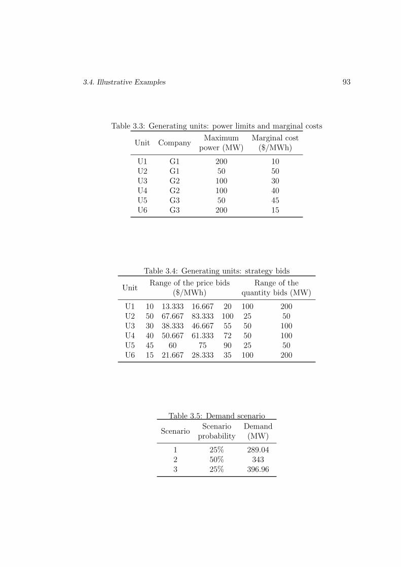
3.4. Illustrative Examples 93
Table 3.3: Generating units: power limits and marginal costs
Unit CompanyMaximum Marginal cost
power (MW) ($/MWh)
U1 G1 200 10U2 G1 50 50U3 G2 100 30U4 G2 100 40U5 G3 50 45U6 G3 200 15
Table 3.4: Generating units: strategy bids
UnitRange of the price bids Range of the
($/MWh) quantity bids (MW)
U1 10 13.333 16.667 20 100 200U2 50 67.667 83.333 100 25 50U3 30 38.333 46.667 55 50 100U4 40 50.667 61.333 72 50 100U5 45 60 75 90 25 50U6 15 21.667 28.333 35 100 200
Table 3.5: Demand scenario
ScenarioScenario Demand
probability (MW)
1 25% 289.042 50% 3433 25% 396.96

94 3. Strategic Bidding in Electricity Markets
To illustrate the network-constrained stochastic EPEC we use a 4-node net-
work (see Figure 3.1). There are 5 lines connecting the 4 nodes. The demand
(Table 3.5) is at two nodes: 60% of the load is at node 1 and 40% at node
2. The line impedance values are all the same. Therefore the PTDF matrix
is given in Table 3.6. We vary the thermal limits in the results subsection to
illustrate the network-constrained effects on Nash equilibria. Note that most
of the generating units are located in the northern area and demands are in
the southern area. In addition, the cheapest generating units are at nodes 3
and 2.
Table 3.6: PTDF matrix for the 4-node system
j1 j2 j3 j4
l1 0 0.625 0.250 0.125l2 0 -0.375 0.250 0.125l3 0 0.250 0.500 0.250l4 0 0.125 0.250 -0.375l5 0 0.125 0.250 0.625
U1 U6 U4 U2
U5
d(60%)
U3
d(40%)
l4
l1
l2l3 l5
3
2
4
1
Figure 3.1: 4-node system
The game is solved by two methods:
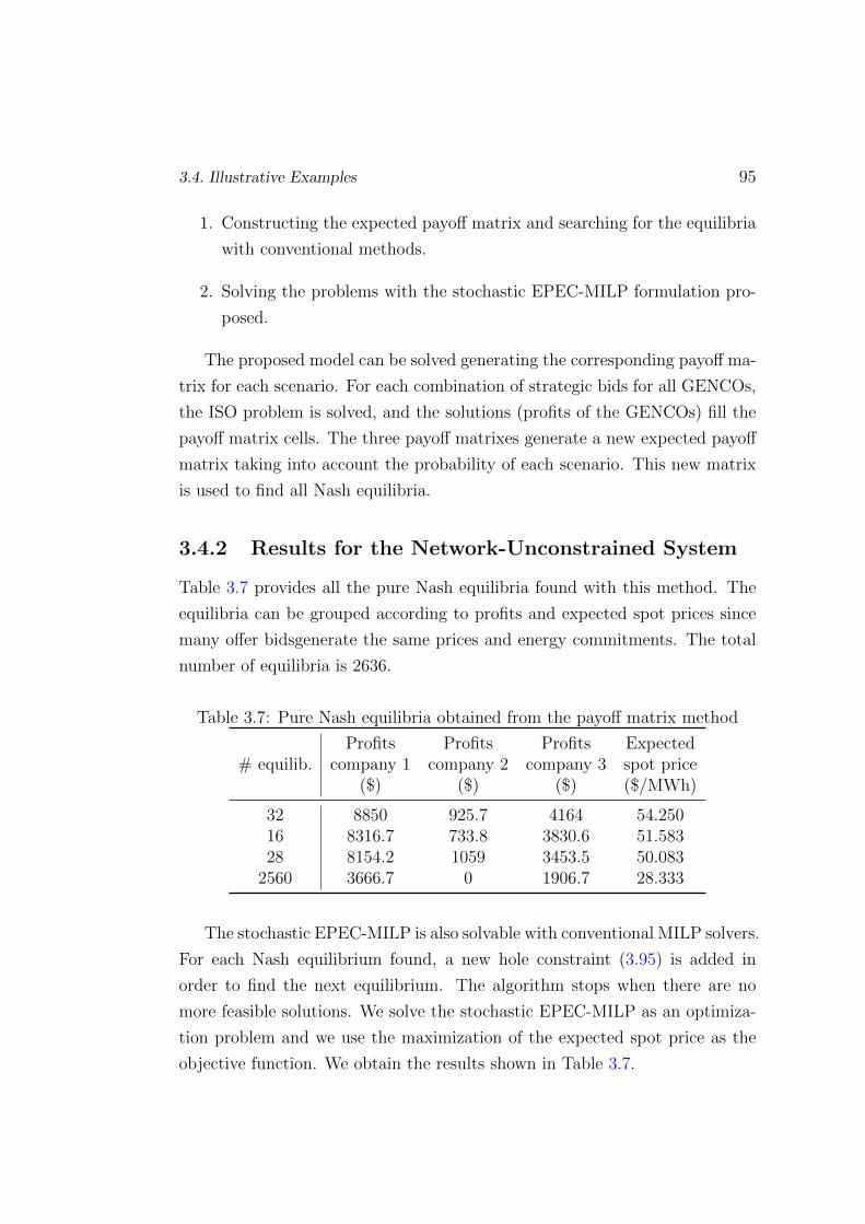
3.4. Illustrative Examples 95
1. Constructing the expected payoff matrix and searching for the equilibria
with conventional methods.
2. Solving the problems with the stochastic EPEC-MILP formulation pro-
posed.
The proposed model can be solved generating the corresponding payoff ma-
trix for each scenario. For each combination of strategic bids for all GENCOs,
the ISO problem is solved, and the solutions (profits of the GENCOs) fill the
payoff matrix cells. The three payoff matrixes generate a new expected payoff
matrix taking into account the probability of each scenario. This new matrix
is used to find all Nash equilibria.
3.4.2 Results for the Network-Unconstrained System
Table 3.7 provides all the pure Nash equilibria found with this method. The
equilibria can be grouped according to profits and expected spot prices since
many offer bidsgenerate the same prices and energy commitments. The total
number of equilibria is 2636.
Table 3.7: Pure Nash equilibria obtained from the payoff matrix method
# equilib.Profits Profits Profits Expected
company 1 company 2 company 3 spot price($) ($) ($) ($/MWh)
32 8850 925.7 4164 54.25016 8316.7 733.8 3830.6 51.58328 8154.2 1059 3453.5 50.083
2560 3666.7 0 1906.7 28.333
The stochastic EPEC-MILP is also solvable with conventional MILP solvers.
For each Nash equilibrium found, a new hole constraint (3.95) is added in
order to find the next equilibrium. The algorithm stops when there are no
more feasible solutions. We solve the stochastic EPEC-MILP as an optimiza-
tion problem and we use the maximization of the expected spot price as the
objective function. We obtain the results shown in Table 3.7.

96 3. Strategic Bidding in Electricity Markets
To reduce the CPU running time, we add a new set of constraints (3.99)
for the sets of strategies that produce the same price and energy, obtaining a
unique pure Nash equilibrium for each set. We use an ex-post heuristic method
to find all possible pure Nash equilibria given by the quantity and price offers
that are valid for the expected price found in each group of equilibria.
abs
(∑ω∈Ω
ρ(ω)πet (w)−∑ω∈Ω
ρ(ω)π∗t (ω, n)
)≥ ε, ∀t,∀n (3.99)
Equation (3.99) is transformed into a set of linear constraints using an
additional binary variable and the Big-M linearization.
3.4.3 Results for the Network-Constrained System
For the network-constrained system we have chosen the thermal line limits
shown in Table 3.8.
Table 3.8: Thermal line limits (MW)
l1 l2 l3 l4 l5
Congested network 120 120 120 70 120Uncongested network 270 240 240 170 220
Nash equilibria have been searched with the enumerative or brute-force
method and also with the stochastic EPEC-MILP proposed in Section 3.2.4.
The equilibria have been grouped by profits implying that the same energy is
dispatched by the GENCOs and the same LMPs at each node are obtained
providing the same profit for each GENCO. Table 3.9 shows the Nash equilibria
solution for the congested network case. The first column provides the number
of equilibria found by brute force. The second to fourth columns show the
profits obtained by each GENCO and the fifth shows the sum of all GENCOs’
profits. The profits remain the same per GENCO and for each group of
equilibria (in rows). For example, in the first row, the GENCOs have 32
combinations to offer their energy and they reach the same results. Note that

3.4. Illustrative Examples 97
the 32 combinations are true equilibria.
The equilibria are the same for both cases (brute-force and stochastic
EPEC-MILP), but the stochastic EPEC-MILP provides only one equilibrium
for each group. To do that, we define an objective function that disregards any
equilibrium with the same expected profits for all GENCOs. Therefore, the
objective function is set to maximize the total expected profits for all GENCOs
(3.100) subject to the stochastic EPEC-MILP constraints set (3.64)–(3.94)
and constraint (3.101) that sets that the total expected profit for all GENCOs
obtained in the equilibrium must be less than the known equilibria minus a
small epsilon value.
max∑g
E[Ug (se)] (3.100)
∑g
E[Ug (se)] ≤
∑g
E[Ug (s∗(n))]− ε, ∀n (3.101)
Table 3.10 shows the LMPs for each group of equilibria, with the equilibria
sorted in Table 3.9. The total number of equilibria is 144, a number that
is significantly lower than the one in the unconstrained network case (2636)
because the GENCOs have more difficulties to find a equilibrium without
violating network constraints. Thus, if the problem is more constrained,
the number of equilibria decreases. Furthermore, the obtained equilibria are
different from the ones in the network-unconstrained case (Table 3.7). In
general, it can be observed that prices are higher for network-constrained
systems. For this particular case, where the cheapest generating units are
in the northern area, node 3, and the demand is in the southern area, nodes
1 and 2, the thermal limit of line 3 is almost always reached and the same
happens with line 2 in some cases. This implies that there are different LMPs
at each node. But, for the highest prices (see the first equilibria group in
Table 3.10), the prices are the same for all nodes. This happens because the
GENCOs reduce their quantity offers and increase their price offers, since the

98 3. Strategic Bidding in Electricity Markets
other units can not deliver their energies to the demands (see Figure 3.2).
For example, unit U1 always offers the maximum quantity available in the
equilibria where network constraints are disregarded, but the network limits
the amount of energy delivered from node 3 to nodes 1 and 2, thus, the optimal
strategy reduces the quantity offered. Note that by decreasing the quantities
offered, the thermal line constraints are not reached. For the first equilibria
group, the overall profit is the highest, but GENCO G1 reduces their profit
compared with the network-unconstrained system because the cheapest units
of GENCO G1 are “isolated” by the line constrains. GENCO G2, which is
expensive, increases their profit dramatically because their units are located
near the demand.
Figure 3.3 shows the offer stack for the sixth group of equilibria. The offer
strategies are less “aggressive” (close to the competitive offers), the profits for
the GENCOs are lower (Table 3.9), and the energy prices are also lower (Table
3.10). The prices in this case are different because the thermal limits of the
lines are reached due to the offers by units U1 and U6 (the cheapest ones).
Table 3.9: GENCO’s expected profits for the congested network case
# equilib.Profits Profits Profits Total
company 1 company 2 company 3 Profits($) ($) ($) ($)
32 6749.5 5288.3 6718.8 18756.532 6781.3 4913.3 5972.0 17666.532 6218.8 4413.9 5275.0 15907.716 5064.18 2125.00 2185.83 9375.016 5064.18 1937.50 2115.33 9117.016 5021.39 1203.33 1854.66 8079.4
For the uncongested case we have chosen line limits according to Table 3.8.
The equilibria obtained by both methodologies are summarized in Tables 3.11
and 3.12. Profits and LMPs are the same as in the unconstrained-network
case.

3.4. Illustrative Examples 99
Table 3.10: Expected LMPs for the congested network case
Expected Expected Expected Expectedspot price N1 spot price N2 spot price N3 spot price N4
($/MWh) ($/MWh) ($/MWh) ($/MWh)
75.667 75.667 75.667 75.66772.333 72.333 72.333 72.33366.333 66.333 66.333 66.33386.667 60.833 35.000 60.83381.667 58.333 35.000 58.33358.333 46.667 35.000 46.667
Table 3.11: GENCO’s expected profits for the uncongested network case
# equilib.Profits Profits Profits Total
company 1 company 2 company 3 Profits($) ($) ($) ($)
32 8850 925.7 4164 13939.716 8316.7 733.8 3830.6 12881.128 8154.2 1059 3453.5 12666.7
2560 3666.7 0 1906.7 5573.4
Table 3.12: Expected LMPs for the uncongested network case
Expected Expected Expected Expectedspot price N1 spot price N2 spot price N3 spot price N4
($/MWh) ($/MWh) ($/MWh) ($/MWh)
54.250 54.250 54.250 54.25051.583 51.583 51.583 51.58350.083 50.083 50.083 50.08328.333 28.333 28.333 28.333

100 3. Strategic Bidding in Electricity Markets
0 100 200 300 400 500 600 7000
10
20
30
40
50
60
70
80
90
100
U1U6
U3
U4U5
U2
U1
U6
U5
U3
U4
U2
Quantity offer (MWh)
Pric
e of
fer
($/M
Wh)
competitiveoffer stack
demand scenarios
Figure 3.2: Stack offers (red) for the first equilibrium, competitive stack offers(grey) and demand scenarios (blue)
3.4.4 CPU Time and Computational Complexity
Table 3.13 shows the running time required for solving the problem. The first
column shows the traditional payoff matrix CPU time, the second one the
stochastic EPEC-MILP CPU time, and the last one the CPU time of the same
EPEC-MILP with the new constraint set, (3.99). We use MATLAB for solving
the payoff matrix and CPLEX 11 under GAMS [119] for the EPEC-MILPs.
We have used a Dell PowerEdge R910 x64 computer with 4 processors at 1.87
GHz and 32 GB of RAM. The complexity of the EPEC-MILP formulation is
shown in 3.14 for each iteration of the case study.
3.5 Summary and Conclusions
This chapter presents a compact formulation for the strategic bidding problem
in pool-based electricity markets considering joint price and quantity strategic
offers in a multi-agent, multi-period and multi-block game. In addition, we
consider stochasticity of the demand in several scenarios. Furthermore, we
propose two models for a single-node system (network-unconstrained case)

3.5. Summary and Conclusions 101
0 100 200 300 400 500 600 7000
10
20
30
40
50
60
70
80
90
100
U1
U6
U3
U4
U5
U2
U1
U6U3
U5
U2
U4
Quantity offer (MWh)
Pric
e of
fer
($/M
Wh)
competitiveoffer stack
demand scenarios
Figure 3.3: Stack offers (red) for the sixth equilibrium, competitive stack offers(grey) and demand scenarios (blue)
Table 3.13: CPU time comparison
EPEC-MILP EPEC-MILPPayoff matrix limited to 100 with the new
solution equilibria constraint set
NU† 3h 47min 25h 32min 48minNC∗, uncongested network 6h 35min 34h 5min 55min
NC, congested network 8h 14min 41h 41min 1h 18min
† : Network-Unconstrained,∗ : Network-Constrained
and for a multi-node system (network-constrained case).
The stochastic EPEC is formulated as an MILP. To do that we consider:
1) The strong duality constraint instead of the KKT conditions; 2) A binary
expansion and a Big-M linearization to eliminate the bilinear terms of the
problem.
Since multiple Nash equilibria can be expected in this problem, we propose
an iterative procedure to find all pure Nash equilibria by including successive

102 3. Strategic Bidding in Electricity Markets
Table 3.14: Case study computational complexity
NU† NC∗
# of binary variables 18 18# of positive variables 17370 23160# of free continuous variables 579 5211# of inequality constraints 131718 137508# of equality constraints 1158 5790
† : Network-unconstrained case, ∗ : Network-constrained case
linear constraints to the stochastic EPEC-MILP.
MILP models are suitable for application in medium-scale systems and
they are solvable with commercial solvers. An illustrative example shows the
results of the methodology proposed.

Chapter 4
Power System Planning
Framework: Transmission and
Generation Expansion
This chapter describes a three-level transmission and generation expansion
planning model. We formulate a mixed integer linear programming (MILP)
optimization model that integrates transmission planning, generation invest-
ment equilibria and market operation decisions and we propose a methodology
to solve it. Section 4.1 introduces the problem and presents the main assump-
tions. Section 4.2 describes a three-level transmission planning model, as well
as the linearization process to convert it into a mixed integer linear problem.
Section 4.3 presents the methodology in order to find all pure Nash equilibria
in generation investment. In Section 4.4, we introduce some changes to the
proposed mixed integer linear programming model to take into account power
transfer distribution factors (PTDFs) in a changing network. Section 4.5 shows
the computational complexity of the proposed model. Section 4.6 illustrates
our model using 3- and 4-bus examples. Section 4.7 presents a case study for
a realistic power system in Chile. The summary and conclusions are presented
in Section 4.8.
103
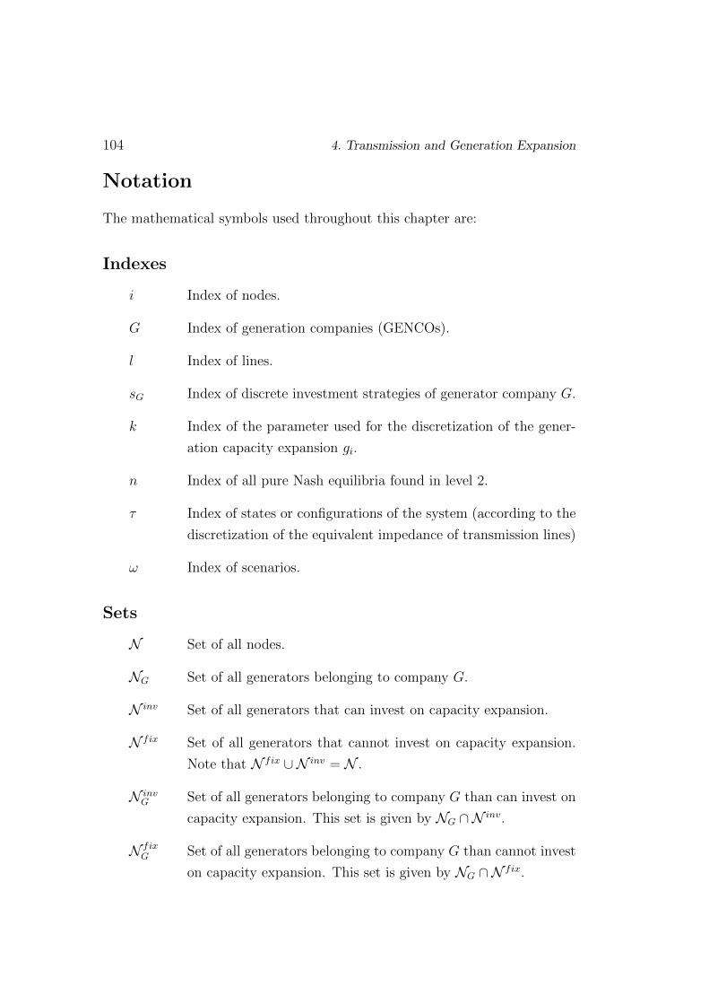
104 4. Transmission and Generation Expansion
Notation
The mathematical symbols used throughout this chapter are:
Indexes
i Index of nodes.
G Index of generation companies (GENCOs).
l Index of lines.
sG Index of discrete investment strategies of generator company G.
k Index of the parameter used for the discretization of the gener-
ation capacity expansion gi.
n Index of all pure Nash equilibria found in level 2.
τ Index of states or configurations of the system (according to the
discretization of the equivalent impedance of transmission lines)
ω Index of scenarios.
Sets
N Set of all nodes.
NG Set of all generators belonging to company G.
N inv Set of all generators that can invest on capacity expansion.
N fix Set of all generators that cannot invest on capacity expansion.
Note that N fix ∪N inv = N .
N invG Set of all generators belonging to company G than can invest on
capacity expansion. This set is given by NG ∩N inv.
N fixG Set of all generators belonging to company G than cannot invest
on capacity expansion. This set is given by NG ∩N fix.

105
N inv−G Set of all generators that do not belong to company G that can
invest on capacity expansion. This set is given by (N −NG) ∩N inv.
G Set of all generation companies.
L Set of all transmission lines.
Linv Set of all candidates transmission lines for investment.
SG Set of all discrete investment strategies of company G.
SG Set of all discrete investment strategies for all companies. This
set is given by⋃G∈G SG.
T Set of all network configurations.
Ω Set of all scenarios.
Constants
g0i Generation capacity available at node i before investment.
gmaxi Maximum generation capacity expansion at node i.
ai, bi Parameters of the generation cost function at node i.
di(ω) Inelastic demand at node i and demand scenario ω.
ρ(ω) Probability of scenario ω.
ϕli Power transfer distribution factor (PTDF) associated to line l
with respect to a unit injection/withdrawal at node i, when the
network properties (network connections and physical character-
istics) are known.
ϕτli Power transfer distribution factor (PTDF) associated to line l
with respect to a unit injection/withdrawal at node i, when the
network properties are given by configuration τ .

106 4. Transmission and Generation Expansion
Ki Annual unit cost of investment in capacity for a generation unit
at node i.
Kl Annual unit cost of investment in capacity for line l.
∆gi Size of the step used in the discretization of the generation
capacity gi at node i.
Λi Parameter used for the discretization of the generation capacity
gi expansion associated to the number of binary variables. Note
that the total number of binary variables is Λi + 1.
f 0l Thermal capacity limit of line l already installed before invest-
ment at level 1.
fmaxl Maximum thermal expansion capacity allowed for line l in level
1.
fmin,τl Minimum thermal expansion capacity allowed for line l in level
1 and network configuration τ .
fmax,τl Maximum thermal expansion capacity allowed for line l in level
1 and network configuration τ .
y∗kin Vector of pure Nash equilibrium solutions of level 2.
ε Small positive value used to find all pure Nash equilibria in level
2.
Mγi ,Mλl ,M ξi ,M gi ,M ri Big-M parameters used in the linearization pro-
cess.
Variables
qi(ω) Power generated at node i and scenario ω.
ri(ω) Import/export power from/to node i and scenario ω.

107
gi Generation capacity available at node i after the decisions of
level 2 are made. It is constant for level 3.
fl Thermal capacity limit of line l after the decisions at level 1 are
made. It is a constant for levels 2 and 3.
ξi(ω) Shadow price/dual variable of the production capacity constraint
at node i and scenario ω.
α(ω) Dual variable associated to the balance constraint of ri(ω).
λ+i (ω), λ−i (ω) Shadow price/dual variable of the thermal capacity con-
straints of line l and scenario ω.
βi(ω) Locational marginal price (LMP) / dual variable of the energy
balance at node i and scenario ω.
γi(ω) Dual variable of the non-negativity constraint of qi(ω) for node
i and scenario ω.
ηγi (ω), ηξi (ω), ηλ+
l (ω), ηλ−
l (ω) Binary variables from Big-M linearization in
level 3.
yki Binary variable used for the discretization of gi.
yki(ω) Product of ξi(ω) by yki.
yki(ω) Product of qi(ω) by yki.
uτ Binary variable that is equal to 1 for network configuration τ ,
and 0 for the rest for other configuration.
wiτ (ω) Product of uτ by ri(ω).
z+lτ (ω), z−lτ (ω) Product of uτ by λ+
i (ω) and uτ by λ−i (ω), respectively.
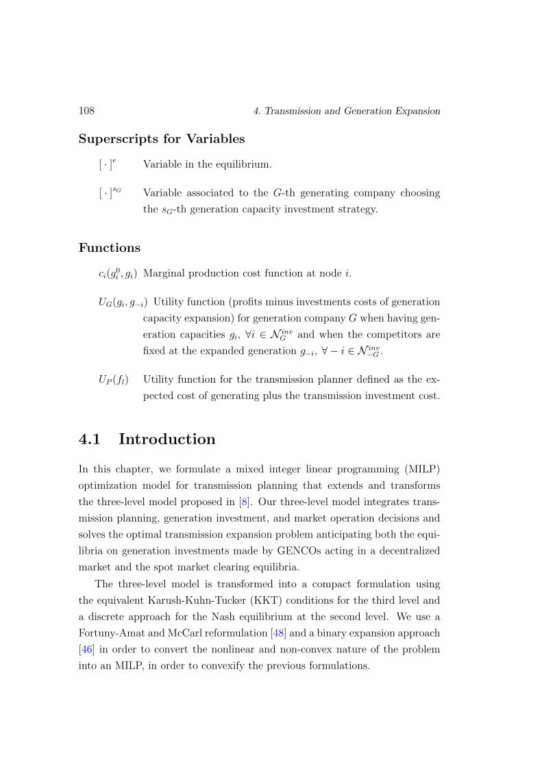
108 4. Transmission and Generation Expansion
Superscripts for Variables
[ · ]e Variable in the equilibrium.
[ · ]sG Variable associated to the G-th generating company choosing
the sG-th generation capacity investment strategy.
Functions
ci(g0i , gi) Marginal production cost function at node i.
UG(gi, g−i) Utility function (profits minus investments costs of generation
capacity expansion) for generation company G when having gen-
eration capacities gi, ∀i ∈ N invG and when the competitors are
fixed at the expanded generation g−i, ∀ − i ∈ N inv−G .
UP (fl) Utility function for the transmission planner defined as the ex-
pected cost of generating plus the transmission investment cost.
4.1 Introduction
In this chapter, we formulate a mixed integer linear programming (MILP)
optimization model for transmission planning that extends and transforms
the three-level model proposed in [8]. Our three-level model integrates trans-
mission planning, generation investment, and market operation decisions and
solves the optimal transmission expansion problem anticipating both the equi-
libria on generation investments made by GENCOs acting in a decentralized
market and the spot market clearing equilibria.
The three-level model is transformed into a compact formulation using
the equivalent Karush-Kuhn-Tucker (KKT) conditions for the third level and
a discrete approach for the Nash equilibrium at the second level. We use a
Fortuny-Amat and McCarl reformulation [48] and a binary expansion approach
[46] in order to convert the nonlinear and non-convex nature of the problem
into an MILP, in order to convexify the previous formulations.

4.2. Transmission and Generation Expansion as a Three-Level Model 109
4.2 Transmission and Generation Expansion
as a Three-Level Model
We assume that the transmission planning model consists of three levels that
are described in reverse order, as shown in Figure 4.1. Our model is of
the Stackelberg type, where the transmission planner (first level) anticipates
generation expansions (second level), and the clearing of the spot market (third
level). This three-level hierarchy is motivated by the fact that transmission
planners should consider expansions in generation that may take place, as
well as the clearing of the market related to generation expansion, in order to
make their decisions. As shown in [8], ignoring the interrelationship between
transmission and generation investments may lead to suboptimal network
plans.
Transmission Investment (Minimizing operating and line
investment costs) Level 1
Optimal decisions: transmission expansion
plan
Generation Investment (Maximize GENCOs profits minus
investment cost on capacity) Level 2
Optimal decisions: generation capacity
expansion
Level 3 Optimal decisions: market operation
Pool-Based Market Operation (Equilibrium of ISO and
GENCOs)
fl
gei
qei (ω),βe
i (ω)
Figure 4.1: The three-level transmission and generation problem framework
In the market operation level, we assume demand is exogenous and spot
prices are determined by the independent system operator (ISO) on the basis of
a dispatch model. In the generation investment level, investments in generation
capacities satisfy a Nash equilibrium taking into account the spot market prices
determined by the ISO. Finally, transmission investment is modeled as an
optimization problem for accommodating these generation capacities so that
total cost is minimized. In the third level the demand is uncertain, therefore,
the decisions at the first and second levels are made previously to the demand

110 4. Transmission and Generation Expansion
realization. The third level is solved for each demand realization.
Each of the three levels is described in detail in the following subsections.
Since the three-level problem is not convex, we use both the Fortuny-Amat
and McCarl linearization and binary expansion in order to convexify it, with
the purpose of guaranteeing a global solution of the overall problem.
4.2.1 Third Level: Spot Market clearing
The third level models the operation of the spot market. At this level we com-
pute the equilibrium that occurs when the ISO clears the perfectly competitive
market for given generation and transmission capacities. Our model accounts
for transmission network constraints through a lossless DC approximation of
the Kirchhoff’s laws. Moreover, we assume perfectly competitive generators
and inelastic demand, where nodal prices are given by the Lagrange multipliers
of the power balance constraint at every node. We assume that all nodes may
have generation and demand and all generation capacity at a node is owned by
a single GENCO (although GENCOs can own generation at multiple nodes).
In addition, marginal generation costs are constant and inversely proportional
to the installed capacity, as shown in Figure 4.2; specifically, they are defined
as: ci (g0i , gi) = ai − bi(gi − g0
i ).
ci(g0i , gi)
aibi
g0i gi
Figure 4.2: Marginal generation cost functions
The ISO problem consists of the maximization of social welfare subject
to network constraints. Since we assume both a perfectly-competitive market
and inelastic demand, this is equivalent to cost minimization. Additionally,

4.2. Transmission and Generation Expansion as a Three-Level Model 111
generators offer their power at marginal costs in our setting. In contrast, the
problem of a perfectly-competitive GENCO is to maximize their profit given
the nodal prices resulting from the spot market clearing. The models for the
ISO and the individual GENCOs follow.
4.2.1.1 ISO Problem Formulation
After the demand realization is known, the ISO problem is modeled as a cost
minimization problem for each demand scenario, as shown in (4.1)–(4.7).
minqi(ω),ri(ω)
∑i∈N
ci(gi, g
0i
)qi(ω) =
minqi(ω),ri(ω)
∑i∈N inv
(ai − bi(gi − g0
i ))qi(ω) +
∑i∈N fix
aiqi(ω) (4.1)
s.t.:
qi(ω) ≤ gi : ξi(ω) ∀i ∈ N inv, ∀ω (4.2)
qi(ω) ≤ g0i : ξi(ω) ∀i ∈ N fix, ∀ω (4.3)∑
i∈N
ri(ω) = 0 : α(ω) ∀ω (4.4)
−fl ≤∑i∈N
ϕliri(ω) ≤ fl : λ−l (ω), λ+l (ω) ∀l,∀ω (4.5)
qi(ω) + ri(ω) = di(ω) : βi(ω) ∀i ∈ N ,∀ω (4.6)
qi(ω) ≥ 0 : γi(ω) ∀i ∈ N ,∀ω (4.7)
The model is split into: i) the generating units candidates for expansion,
i ∈ N inv, and ii) the units that are not able to expand their capacities,
i ∈ N fix. LMPs are obtained from the dual variables of the demand balance
equations (4.6). Other dual variables are represented on the right hand side
of the equations. The objective function (4.1) minimizes the total cost of
generation, constraints (4.2)–(4.3) establish the maximum power that the
GENCOs can produce, constraint (4.4) represents the power balance of the
net injections/withdrawals to/from the network (given that network losses

112 4. Transmission and Generation Expansion
are assumed negligible), constraint (4.5) expresses the maximum flow through
the lines as a function of the power transfer distribution factors (PTDFs),
constraint (4.6) matches demand at every node with the nodal injection and
the flow coming through the lines connected to this node, and constraint (4.7)
forces power generation to be non negative at every node. Nodal market prices,
βi(ω), are given by the dual variables of the power balance equation (4.6).
The Karush-Kuhn-Tucker (KKT) conditions equivalent to (4.1)–(4.7) are
given by:
ai − bi(gi − g0i )− γi(ω)− βi(ω) + ξi(ω) = 0 ∀i ∈ N inv,∀ω (4.8)
ai − γi(ω)− βi(ω) + ξi(ω) = 0 ∀i ∈ N fix,∀ω (4.9)
α(ω) +∑l∈L
(λ+l (ω)− λ−l (ω))ϕli − βi(ω) = 0 ∀i ∈ N ,∀ω (4.10)
0 ≤ γi(ω) ⊥ qi(ω) ≥ 0 ∀i ∈ N ,∀ω (4.11)
0 ≤ ξi(ω) ⊥ gi − qi(ω) ≥ 0 ∀i ∈ N inv,∀ω (4.12)
0 ≤ ξi(ω) ⊥ g0i − qi(ω) ≥ 0 ∀i ∈ N fix,∀ω (4.13)
0 ≤ λ−l (ω) ⊥ fl +∑i∈N
ϕliri(ω) ≥ 0 ∀l,∀ω (4.14)
0 ≤ λ+l (ω) ⊥ fl −
∑i∈N
ϕliri(ω) ≥ 0 ∀l,∀ω (4.15)∑i∈N
ri(ω) = 0 ∀ω (4.16)
qi(ω) + ri(ω) = di(ω) ∀i ∈ N ,∀ω (4.17)
where symbol ⊥ represents a complementarity relationship (i.e., x ⊥ y
means x>y = 0). Since complementary constraints (4.11)–(4.15) are nonlinear,
they can be replaced by an equivalent set of linear constraints using the
Fortuny-Amat and McCarl linearization formula [48] in order to obtain a mixed
integer linear optimization model. This yields equations (4.35) to (4.43), shown
later in this section.

4.2. Transmission and Generation Expansion as a Three-Level Model 113
4.2.1.2 GENCO Problem Formulation
Each individual GENCO maximizes their profit considering the income from
sales at nodal market prices βi(ω) provided by the ISO’s cost minimization.
Note that, if nodal prices are equal to marginal costs, a GENCO has no profit.
Thus, a GENCO does not have an incentive to invest in generation capacity
unless generating at their maximum limit, which only takes place when qi(ω) =
gi, yielding ξi(ω) > 0. Hence, a GENCO maximizes their profits from the spot
market (4.18) subject to their generation limits (4.19)–(4.20):
maxqi(ω)
∑i∈N inv
G
βi(ω)qi(ω)− (ai − bi(gi − g0i ))qi(ω)
+∑i∈N fix
G
βi(ω)qi(ω)− aiqi(ω) (4.18)
s.t.:
qi(ω) ≤ gi : ξi(ω) ∀i ∈ N invG ,∀ω (4.19)
qi(ω) ≤ g0i : ξi(ω) ∀i ∈ N fix
G ,∀ω (4.20)
qi(ω) ≥ 0 : γi(ω) ∀i ∈ NG,∀ω (4.21)
We call the problem in (4.18)–(4.21)primal, and its dual problem is defined
as:
minξi(ω)
∑i∈N inv
G
giξi(ω) +∑i∈N fix
G
g0i ξi(ω) (4.22)
s.t.:
ξi(ω) ≥ βi(ω)− ai + bi(gi − g0i ) : qi(ω) ∀i ∈ N inv
G ,∀ω (4.23)
ξi(ω) ≥ βi(ω)− ai : qi(ω) ∀i ∈ N fixG ,∀ω (4.24)
ξi(ω) ≥ 0 ∀i ∈ NG, ∀ω (4.25)

114 4. Transmission and Generation Expansion
From the strong duality theorem [118], we know that if one of the problems,
either the primal or the dual, has an optimal solution, then, the other one has
the same optimal solution. Since both primal and dual problems are linear,
the problem is convex and we can also apply the strong duality theorem [118].
Thus, we get (4.26) from applying the strong duality theorem (which we will
use later in this section):
∑i∈N inv
G
βi(ω)qi(ω)− (ai − bi(gi − g0i ))qi(ω) +
∑i∈N fix
G
βi(ω)qi(ω)− aiqi(ω)
=∑
i∈N invG
giξi(ω) +∑i∈N fix
G
g0i ξi(ω) (4.26)
The KKT conditions for the GENCO problem (4.18)–(4.21) are defined in
(4.27)–(4.31).
ai − bi(gi − g0i )− γi(ω)− βi(ω) + ξi(ω) = 0 ∀i ∈ N inv
G ,∀ω (4.27)
ai − γi(ω)− βi(ω) + ξi(ω) = 0 ∀i ∈ N fixG ,∀ω (4.28)
0 ≤ γi(ω) ⊥ qi(ω) ≥ 0 ∀i ∈ NG,∀ω (4.29)
0 ≤ ξi(ω) ⊥ gi − qi(ω) ≥ 0 ∀i ∈ N invG ,∀ω (4.30)
0 ≤ ξi(ω) ⊥ g0i − qi(ω) ≥ 0 ∀i ∈ N fix
G ,∀ω (4.31)
Extending the problem defined in (4.27)–(4.31) to all GENCOS, we obtain
a set of KKT conditions that is equivalent to the constraints (4.8)–(4.9) and
(4.11)–(4.13). Note that the perfectly-competitive generators profit maxi-
mizing conditions are consistent with the ISO economic dispatch conditions
and, thus, (4.32)–(4.45) represent an equivalent (exact) mixed integer linear
formulation of both problems (4.1)–(4.7) and (4.18)–(4.21) for all GENCOs.
The Fortuny-Amat and McCarl linearization formula is used to transform the
slackness conditions into linear constraints.

4.2. Transmission and Generation Expansion as a Three-Level Model 115
ai − bi(gi − g0i )− γi(ω)− βi(ω) + ξi(ω) = 0 ∀i ∈ N inv,∀ω (4.32)
ai − γi(ω)− βi(ω) + ξi(ω) = 0 ∀i ∈ N fix,∀ω (4.33)
α(ω) +∑l∈L
(λ+l (ω)− λ−l (ω))ϕli − βi(ω) = 0 ∀i ∈ N ,∀ω (4.34)
0 ≤ γi(ω) ≤Mγiηγi (ω) ∀i ∈ N ,∀ω (4.35)
0 ≤ qi(ω) ≤M gi(1− ηγi (ω)) ∀i ∈ N ,∀ω (4.36)
0 ≤ ξi(ω) ≤M ξiηξi (ω) ∀i ∈ N ,∀ω (4.37)
0 ≤ gi − qi(ω) ≤M gi(1− ηξi (ω)) ∀i ∈ N inv,∀ω (4.38)
0 ≤ g0i − qi(ω) ≤M gi(1− ηξi (ω)) ∀i ∈ N fix,∀ω (4.39)
0 ≤ λ−l (ω) ≤Mλlηλ−
l (ω) ∀l,∀ω (4.40)
0 ≤ fl +∑i∈N
ϕliri(ω) ≤M fl(1− ηλ−l (ω)) ∀l,∀ω (4.41)
0 ≤ λ+l (ω) ≤Mλlηλ
+
l (ω) ∀l,∀ω (4.42)
0 ≤ fl −∑i∈N
ϕliri(ω) ≤M fl(1− ηλ+l (ω)) ∀l,∀ω (4.43)∑i∈N
ri(ω) = 0 ∀ω (4.44)
qi(ω) + ri(ω) = di(ω) ∀i ∈ N ,∀ω (4.45)
where ηγi (ω), ηξi (ω), ηλ−
l (ω) and ηλ+
l (ω) are binary variables. The Big-M
constants Mγi , M gi , M ξi , Mλl and M fl are large enough. These constants
are easy to determine because they refer to primal o dual variables (in the
superscript) that, in this particular problem, are always bounded.
4.2.2 Second Level: Generation Investment Equilibria
At the second level, each GENCO determines the generation capacity invest-
ments to increase their profits due to the linear decrease in the generation
marginal costs, as seen in Figure 4.1. Since the investments in new gener-
ation capacity reduce the marginal cost of production, the return from the
investments made at level 2 occurs at level 3. Accordingly, there are no

116 4. Transmission and Generation Expansion
spot market decisions at level 2. At this level, the spot market decisions
are given as parameterized equilibrium constraints, (4.32)–(4.45), which are
anticipated by the generation expansion investments. Moreover, a GENCO
considers their capacity expansion against the capacity expansion of their
competitors. Therefore, the utility function for the generation expansion
problem for GENCO G is defined in (4.46).
UG(gi, g−i : ∀i ∈ N inv
G ,∀ − i ∈ N inv−G)
=
E
∑i∈N inv
G
βi(ω)qi(ω)− (ai − bi(gi − g0i ))qi(ω)
+∑i∈N fix
G
βi(ω)qi(ω)− aiqi(ω)
− ∑i∈N inv
G
Ki(gi − g0i ) (4.46)
The first term of the utility function is the expected profit obtained selling
in the spot market and is split into two parts: i) the generation unit candidates
for expansion, and ii) the generation units that are not able to expand their
capacities. The second term is the cost of expanding the generation capacity.
Taking into account the strong duality theorem of the GENCO at the third
level (4.26), we can rewrite the utility function as in (4.47).
UG(gi, g−i : ∀i ∈ N inv
G ,∀ − i ∈ N inv−G)
=
E
∑i∈N inv
G
giξi(ω) +∑i∈N fix
G
g0i ξi(ω)
− ∑i∈N inv
G
Ki(gi − g0i ) (4.47)
Then, the generation expansion problem for GENCO G is defined as:
maxgi,∀i∈N inv
G
UG(·)
s.t.: g0i ≤ gi ≤ gmaxi ∀i ∈ N inv
G (4.48)
equilibrium conditions from level 3 (4.32)–(4.45) (4.49)

4.2. Transmission and Generation Expansion as a Three-Level Model 117
The problem formulated can be stated as a Stochastic Mathematical Pro-
gram subject to Equilibrium Constraints (SMPEC), where the equilibrium
constrains are defined by the linearized equivalent KKT conditions of the third-
level problem; i.e. (4.32)–(4.45). Constraint (4.48) represents the investment
capacity limits for the candidate generating units. The only non-linear term
in (4.47) is giξi(ω). Since the gi variables are controlled by the GENCOs,
it is possible for the generation expansion to be done in discrete steps. We
apply a discretization using the binary expansion proposed in [46], but other
discretizations are possible. Note that any kind of discretization implies adding
binary variables to the model. Then, the discrete generation expansion variable
gi is defined by 2k steps (or blocks) between g0i and gmaxi with a ∆gi distance
between two consecutive values of gi:
gi = g0i + ∆gi
Λi∑k=0
2kyki ∀i ∈ N invG (4.50)
Accordingly, the non-linear product giξi(ω) can be replaced by the expres-
sion:
giξi(ω) = g0i ξi(ω) + ∆gi
Λi∑k=0
2kyki(ω) ∀i ∈ N invG ,∀ω (4.51)
where we define yki(ω) by the constraints (4.52) and (4.53), using the Big-M
linearization formula:
0 ≤ ξi(ω)− yki(ω) ≤M ξi(1− yki) ∀i ∈ N invG ,∀k,∀ω (4.52)
0 ≤ yki(ω) ≤M ξiyki ∀i ∈ N invG ,∀k,∀ω (4.53)
Thus, the generation expansion problem of each GENCO can be set as a
linear SMPEC, stated as an MILP (4.54)–(4.57).

118 4. Transmission and Generation Expansion
maxyki,∀i∈N inv
G ,∀kUG(·) =
∑ω∈Ω
ρ(ω)
∑i∈N fix
G
g0i ξi(ω) +
∑i∈N inv
G
(g0i ξi(ω) + ∆gi
Λi∑k=0
2kyki(ω)
)−∑
i∈N invG
Ki
(∆gi
Λi∑k=0
2kyki
)(4.54)
s.t.:
ai − bi(
Λi∑k=0
2kyki(ω)
)− γi(ω)− βi(ω) + ξi(ω) = 0,
∀i ∈ N inv,∀ω (4.55)
0 ≤ g0i + ∆gi
Λi∑k=0
2kyki(ω)− qi(ω) ≤M gi(1− ηξi (ω)),
∀i ∈ N inv,∀ω (4.56)
constraints (4.33)–(4.37) and (4.39)–(4.45) (4.57)
Accordingly, the level 2 problem can be formulated as an Stochastic Equilib-
rium Problem with Equilibrium Constraints (SEPEC), in which each GENCO
faces a SMPEC-MILP given the other GENCOs’ commitments and the ISO’s
import/export decisions. This SEPEC represents the equilibrium when all
the GENCOs expand their capacities simultaneously subject to the market
equilibrium of level 3 in each scenario.
In [8], a similar deterministic EPEC is solved using a heuristic approach
that sequentially solves each GENCO MPEC taking the decisions of the other
GENCOs as given. Specifically, the authors solve sequentially each GENCO’s
profit maximization problem using the optimal values from previously solved
problems as known data. Thus, starting from a feasible solution, they solve
for g1 using g−1 as known data in the first firm’s optimization problem (where

4.2. Transmission and Generation Expansion as a Three-Level Model 119
g−1 means all GENCOs’ generation capacities except for GENCO 1), and then
solve for g2 using g−2 as data, and so on.
One problem of this heuristic approach is that there is no guarantee of
convergence to an equilibrium. Another (and more practical) problem of
this approach is that it does not allow characterizing the SEPEC as a set
of constraints to be imposed by the network planner at level 1. To avoid these
difficulties, we enumerate the GENCOs’ investment strategies and transform
the Nash equilibria conditions into a finite set of inequalities, which can be
used to find all the Nash equilibria. Since the GENCOs’ strategies match
the SMPEC problem decision variables, the same discretization used in the
SMPEC problem can be used to enumerate the strategies of each GENCO.
This idea of characterizing the equilibria of the GENCOs’ generation capacity
investments (which correspond to the solution of the SEPEC problem) as
a set of linear inequalities allows us to formulate the transmission planning
(level 1) problem as a mixed integer linear programming optimization problem.
We compute an optimal transmission plan that anticipates both generation
investments and spot market operations equilibria.
The Stochastic Nash Equilibrium is defined from the set of inequalities
(4.58), for any feasible capacity expansion for all GENCOS. The feasible
capacity expansion is defined by the set of constraints of the SMPEC-MILP
problem (4.54)–(4.37).
U eG(gei : ∀i ∈ N inv) ≥ max
gi,∀i∈N invG
UG(gi, g
e−i : ∀i ∈ N inv
G ,∀ − i ∈ N inv−G),
∀G ∈ G (4.58)
where, for all GENCOs, U eG(gei : ∀i ∈ N inv) is the utility function of each
GENCO G, given their strategic decision variable, gei , in the Nash equilibrium,
which is always better than any other utility resulting from a different strategy,
assuming that the other GENCOs use their Nash equilibrium strategies, ge−i.
Hence, the Nash equilibrium in (4.58) is solved by approximating its solution
using discrete strategies. In doing that, we replace expression (4.58) by a set
of inequalities, where the strategic variables gei are discretized to gsGi . Thus,

120 4. Transmission and Generation Expansion
the Nash equilibria of the GENCOs’ capacity investment decisions are given
by the following set of inequalities:
U eG(gei : ∀i ∈ N inv) ≥ U sG
G
(gsGi , ge−i : ∀i ∈ N inv
G ,∀ − i ∈ N inv−G),
∀G ∈ G,∀sG ∈ SG (4.59)
where we have to distinguish between the left hand side (LHS) and the
right hand side (RHS) of (4.59). The LHS in (4.59) is the utility function of
each GENCO given their strategic decision variable in the Nash equilibrium.
That is, the definition of the utility function for GENCO G in the equilibrium
is given by:
U eG(gei : ∀i ∈ N inv) =∑
ω∈Ω
ρ(ω)
∑i∈N fix
G
g0i ξei (ω) +
(g0i ξei (ω) + ∆gi
Λi∑k=0
2kyeki(ω)
)−∑
i∈N invG
Ki
(∆gi
Λi∑k=0
2kyeki
), ∀G ∈ G (4.60)
subject to the linearized constraints of level 3 in the equilibrium, which
correspond to constraints (4.32)–(4.45), (4.52)–(4.53) and (4.55)–(4.56), re-
placing yki, yki(ω), qi(ω), ri(ω), γi(ω), βi(ω), ξi(ω), α(ω), λ+l (ω), λ−l (ω), ηγi ,
ηλ+
i , ηλ−i and ηξi by yeki, y
eki(ω), qei (ω), rei (ω), γei (ω), βei (ω), ξei (ω), αe(ω), λ+e
l (ω),
λ−el (ω), ηγei , ηλ+ei , ηλ
−ei and ηξei , respectively, and considering (4.52)–(4.53) for
all i ∈ N inv.
The RHS in (4.59) is the utility function of each GENCO given a particular
value of the strategic decision variable. That is, we consider that GENCO G
chooses strategy sG (which involves investing in generation capacity at node
i up to the capacity gsGi , with i ∈ N invG ,∀G ∈ G), the definition of the utility
function for GENCO G is given by (4.61) 1 .
1Note that, since gsGi is known, it is possible to directly replace its value in equations(4.33)–(4.45), (4.52)–(4.53) and (4.55)–(4.56), without having the non-linear term that
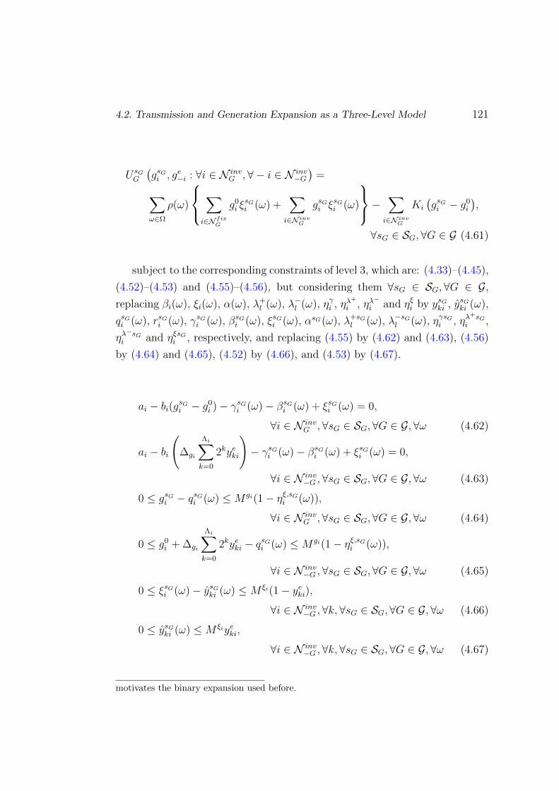
4.2. Transmission and Generation Expansion as a Three-Level Model 121
U sGG
(gsGi , ge−i : ∀i ∈ N inv
G ,∀ − i ∈ N inv−G)
=∑ω∈Ω
ρ(ω)
∑i∈N fix
G
g0i ξsGi (ω) +
∑i∈N inv
G
gsGi ξsGi (ω)
− ∑i∈N inv
G
Ki
(gsGi − g0
i
),
∀sG ∈ SG,∀G ∈ G (4.61)
subject to the corresponding constraints of level 3, which are: (4.33)–(4.45),
(4.52)–(4.53) and (4.55)–(4.56), but considering them ∀sG ∈ SG,∀G ∈ G,
replacing βi(ω), ξi(ω), α(ω), λ+l (ω), λ−l (ω), ηγi , ηλ
+
i , ηλ−i and ηξi by ysGki , ysGki (ω),
qsGi (ω), rsGi (ω), γsGi (ω), βsGi (ω), ξsGi (ω), αsG(ω), λ+sGl (ω), λ−sGl (ω), ηγsGi , ηλ
+sGi ,
ηλ−sGi and ηξsGi , respectively, and replacing (4.55) by (4.62) and (4.63), (4.56)
by (4.64) and (4.65), (4.52) by (4.66), and (4.53) by (4.67).
ai − bi(gsGi − g0i )− γsGi (ω)− βsGi (ω) + ξsGi (ω) = 0,
∀i ∈ N invG ,∀sG ∈ SG,∀G ∈ G,∀ω (4.62)
ai − bi(
∆gi
Λi∑k=0
2kyeki
)− γsGi (ω)− βsGi (ω) + ξsGi (ω) = 0,
∀i ∈ N inv−G ,∀sG ∈ SG,∀G ∈ G,∀ω (4.63)
0 ≤ gsGi − qsGi (ω) ≤M gi(1− ηξ,sGi (ω)),
∀i ∈ N invG ,∀sG ∈ SG,∀G ∈ G,∀ω (4.64)
0 ≤ g0i + ∆gi
Λi∑k=0
2kyeki − qsGi (ω) ≤M gi(1− ηξ,sGi (ω)),
∀i ∈ N inv−G ,∀sG ∈ SG,∀G ∈ G,∀ω (4.65)
0 ≤ ξsGi (ω)− ysGki (ω) ≤M ξi(1− yeki),∀i ∈ N inv
−G ,∀k,∀sG ∈ SG, ∀G ∈ G, ∀ω (4.66)
0 ≤ ysGki (ω) ≤M ξiyeki,
∀i ∈ N inv−G ,∀k,∀sG ∈ SG,∀G ∈ G, ∀ω (4.67)
motivates the binary expansion used before.

122 4. Transmission and Generation Expansion
With all these definitions, (4.59) represents the SEPEC of the GENCOs’
capacity investment decisions (level 2 equilibrium). Note that the solution of
this formulation provides a Nash equilibrium. However, we cannot guarantee
that the equilibrium is unique, since there may be more than one or even none.
See Section 4.3 for details to find all the pure Nash equilibria in a discrete game.
4.2.3 First Level: Transmission Investment Planning
In level 1, the network planner (which we model as a Stackelberg leader in our
three-level game) maximizes social welfare subject to transmission constraints
while anticipating the solutions from levels 2 and 3. Since we have considered
inelastic and stochastic demand, this problem is equivalent to minimize the
total expected cost: the sum of the expected generation dispatch costs and the
transmission investment costs. Thus, the objective function of the network
planner in level 1 is defined by (4.68).
UP (fl : ∀l ∈ Linv) =
E
∑i∈N inv
(ai − bi(gei − g0
i ))qei (ω) +
∑i∈N fix
aiqei (ω)
+∑l∈Linv
Kl(fl − f 0l ) (4.68)
The network planner problem is defined as:
maxfl,l∈Linv
UP (·)
s.t.: f 0l ≤ fl ≤ fmaxl ∀l ∈ Linv (4.69)
SEPEC-MILP solutions (4.70)
Equation (4.69) limits the transmission line expansion, and the SEPEC-
MILP equilibria solutions set from levels 2 and 3 are included as constraints.
Moreover, the variables that represent the solution to the SEPEC are equilib-
rium results, thus, having qei (ω) instead of qi(ω), and gei instead of gi. Then, a
4.3. Finding All Pure Nash Equilibria at the Second Level 123
non-linear term in the objective function, gei qei (ω), can be decomposed by using
binary expansion applied to gei and linearization, using the Big-M formulation.
This yields:
gei qei (ω) = g0
i qei (ω) + ∆gi
Λi∑k=0
2kyeki(ω) ∀i ∈ N inv,∀ω (4.71)
0 ≤ qei (ω)− yeki(ω) ≤M gi(1− yeki) ∀i ∈ N inv,∀k,∀ω (4.72)
0 ≤ yeki(ω) ≤M giyeki ∀i ∈ N inv,∀k,∀ω (4.73)
where yeki(ω) is a continuous variable taking values of either zero or qei (ω).
We have considered that there is a set of transmission lines that are candidates
for investment (Linv). That means that the previously constant maximum
active flows (fl) are now variables of the problem in level 1. Contrary to the
assumptions in [8], the network planner solves level 1 now for the optimal
transmission expansion capacities of the existing and new lines within the set
of candidate locations. Therefore, we can formulate the level 1 problem as an
MILP subject to SEPEC and other equilibrium constraints. The final complete
model is given by (A.1)–(A.45), as shown in Appendix A.
4.3 Finding All Pure Nash Equilibria at the
Second Level
The SEPEC for the level 2 problem may have multiple equilibria. The model
described in the previous section finds only one SEPEC equilibrium, but we
could be interested in detecting more than one equilibrium, or even all of them.
In this section, we modify the previous level 2 model in order to find all pure
strategy SEPEC equilibria. To do that, we generate “holes” in the feasible
region for each solution found within the set of discrete strategies, yeki. Given
a solution vector, y∗ki, of the SEPEC problem of level 2, we include a new
constraint to generate a hole in the solution already found:

124 4. Transmission and Generation Expansion
√∑i,k
(y∗kin − yeki)2 ≥ ε ∀n (4.74)
Each one of the quadratic terms in (4.74) is expanded as:
(y∗kin − yeki)2 = (y∗kin)2 + (yeki)2 − 2y∗kiny
eki (4.75)
and, using the fact that y∗kin and yeki are binary numbers, (4.75) is equivalent
to:
y∗kin + yeki − 2y∗kinyeki (4.76)
which is a linear expression. Thus, (4.74) becomes∑i,k
(y∗kin + yeki − 2y∗kinyeki) ≥ ε2 ∀n (4.77)
To account for all pure strategy Nash equilibria, we need to add (4.77)
to the set of constraints that define the SEPEC-MILP (A.5)–(A.45). Note
that this methodology to obtain all pure strategy Nash equilibria applies only
to the level 2 problem of the model presented in the previous section. Since
the level 1 problem is not an equilibrium, but an optimization problem, the
application of the methodology of creating holes in the feasible region to the
level 1 problem has no clear intuition.
4.4 Methodology to Account for the Variation
of the Line Impedance as a Function of the
Installed Transmission Capacity
The network planning model described in Section 4.2, (A.1)–(A.45), allows the
network planner to solve the optimal transmission expansion problem within
the set of candidate locations, considering that investments in transmission

4.4. Methodology to Account for the Variation of the Line Impedance 125
capacity can be done without changing the impedances of the links. This
assumption may not be realistic and we now propose an approximation of
the line impedance value as a function of the installed transmission capacity.
Assume that an existing line has an impedance whose value is xl. If another
line with the same impedance is placed in parallel, the total impedance is
xeql = xl/2. In general, if there are n lines in parallel, the equivalent impedance
is xeql = xl/n. If f 0l is the initial capacity of the link, we can express the change
in the link impedance as a function of the transmission capacity in a continuous
fashion, as shown in Figure 4.3.
Impedance
Line capacity f0l 2f0
l
xl
xl
2
Figure 4.3: Link impedance as a function of transmission capacity
If no line is installed, the impedance tends to infinity and if the installed
capacity tends to infinity, the equivalent impedance tends to zero. This approx-
imation neglects the resistances of the lines. In order to apply this modification
to the model proposed for level 1 and to keep the formulation as an MILP,
changing the PTDFs is not viable due to the nonlinearities involved. Instead,
we consider a discretization of the equivalent impedance for the potentially-
expanded lines and calculate their associated PTDFs. Thus, if the initial
transmission capacity of link l is f 0l and investments can be done up to a
capacity whose value is fmaxl , we can approximate the equivalent impedance
by performing a discrete approximation between f 0l and fmaxl , as illustrated in
Figure 4.4.
Figure 4.4 shows a 3-interval discretization where the limits of each interval
are represented by a superscript. Within this discretization, we use the average

126 4. Transmission and Generation Expansion
Equivalent impedance
Line capacity
x0l
x1l
x2l
x3l
f0l f1
l f2l f3
l = fmaxl
Figure 4.4: Discretization of the equivalent impedance as a function of installedtransmission capacity
impedance per interval. A good discretization should consider many intervals
for small investments and few intervals for large investments, in agreement
with Figure 4.4. Assume a set of lines, Linv, exists, which could be either
expanded or constructed. If Linv = card(Linv) is the number of possible
investments, and J is the number of intervals in which we divide the link
expansion, then, we have J + 1 independent investment options for the rest
of the lines (including the no-investment option). Therefore, we have (J +
1)Linv possible configurations, or states, of the system. Denoting each network
configuration by super-index τ and associating a binary variable, uτ , to each
network configuration, only one configuration can exist. That is:
∑τ
uτ = 1 (4.78)
In the MILP of level 1, (A.1)–(A.45), each of the states has an associated
PTDF matrix, ϕτli, and each transmission capacity limit after the investment
depends on the resulting state or configuration (i.e., fmax,τl ). Consequently,
(4.69) becomes:

4.4. Methodology to Account for the Variation of the Line Impedance 127
∑τ
uτfmin,τl ≤ fl ≤∑τ
uτfmax,τl ∀l ∈ Linv (4.79)
In addition, all constraints where PTDFs appear must be modified, i.e.,
(A.1)–(A.45), the constraints that must be modified are (A.10), (A.19), (A.20),
(A.22), (A.23), (A.29), (A.39), (A.40), (A.42), and (A.43). In (A.19), (A.20),
(A.22), (A.23), (A.39), (A.40), (A.42), and (A.43) the PTDFs are multiplied
by variable ri in order to compute the transmission flow limits. Due to the
similarity in the procedure, we will only explain the modifications needed in
(A.19). Equation (A.19) results in:
0 ≤ f 0l +
∑τ∈T
∑i∈N
uτϕτlirei (ω) ≤M fl(1− ηλ−el (ω)) ∀l /∈ Linv,∀ω (4.80)
Replacing the product uτrei (ω) by weiτ (ω), and using the Big-M linearization
formula, we obtain:
−M ri(1− uτ ) ≤ rei (ω)− weiτ ≤M ri(1− uτ ) ∀i ∈ N ,∀ω,∀τ ∈ T (4.81)
−M riuτ ≤ weiτ ≤M riuτ ∀i ∈ N ,∀ω,∀τ ∈ T (4.82)
Therefore, we must change (A.19) for (4.80), replacing the product uτrei (ω)
for weiτ (ω) and adding (4.81) and (4.82) as constraints. Similar changes must
be made to (A.20), (A.22), and (A.23). For (A.39), (A.40), (A.42), and (A.43),
the modifications are similar, but replacing the product uτrsGi (ω) for wsGiτ (ω).
In (A.10) and (A.29), there are terms containing the PTDFs as a result of the
KKT conditions of level 3, which involves the PTDFs multiplied by some dual
variables. Since only one state occurs from all the configurations, considering
the variable that accounts for all the possible states, (A.10) becomes:

128 4. Transmission and Generation Expansion
αe(ω) +∑τ
∑l∈L
(λ+el (ω)− λ−el (ω))uτϕτlir
ei (ω)− βei (ω) = 0,
∀i ∈ N ,∀ω (4.83)
There are two non-linear products of a binary variable multiplied by a
continuous variable. Thus, replacing the product λ+el (ω)uτ for z+e
lτ (ω) and the
product λ−el (ω)uτ for z−elτ (ω), and using the Big-M linearization formula, we
can replace (A.10) for (4.84)–(4.88).
αe(ω) +∑τ
∑l∈L
(z+elτ (ω)− z−elτ (ω))ϕτli − βei (ω) = 0 ∀i ∈ N ,∀ω (4.84)
0 ≤ λ+el (ω)− z+e
lτ ≤Mλ(1− uτ ) ∀l ∈ L,∀ω,∀τ ∈ T (4.85)
0 ≤ z+elτ ≤Mλuτ ∀l ∈ L,∀ω,∀τ ∈ T (4.86)
0 ≤ λ−el (ω)− zelτ ≤Mλ(1− uτ ) ∀l ∈ L,∀ω,∀τ ∈ T (4.87)
0 ≤ z−elτ ≤Mλuτ ∀l ∈ L,∀ω,∀τ ∈ T (4.88)
A similar change must be made for (A.29), but replacing the product
λ+sGl (ω)uτ for z+sG
lτ (ω) and the product λ−sGl (ω)uτ for z−sGlτ (ω).
With all these changes, the final MILP formulation of the level 1 problem is
the one described by equations (A.1)–(A.45) and (4.78), but replacing (A.2) for
(4.79); (A.10) for (4.84)–(4.88); (A.19) for (4.80)–(4.82) with weiτ (ω) = uτrei (ω);
(A.19), (A.20), (A.22), (A.23), (A.39), (A.40), (A.42), and (A.43) for equations
similar to (4.80)–(4.82) with weiτ (ω) = uτrei (ω) and wsGiτ (ω) = uτrsGi (ω); and
(A.10) for equations similar to (4.84)–(4.88) with z+sGlτ (ω) = λ+sG
l (ω)uτ and
z−sGlτ (ω) = λ−sGl (ω)uτ .
4.5 Computational Complexity
Multi-stage models are generally difficult to solve and the proposed model is
not an exception. Although the proposed model has many advantages (and
the fact that transmission planning is an off-line process), the model has the

4.6. Illustrative Examples 129
potential shortcoming of having an exponential number of constraints, which
makes the computational solution of large systems difficult.
Tables 4.1 and 4.2 summarize the computational complexity and the order
of complexity for the SEPEC-MILP, without considering that the PTDFs
change with increasing thermal capacity, as shown in the previous section.
Therefore, the computational complexity and the order of complexity are
measured under the hypothesis shown in Section 4.2 and fully described in
Appendix A. Note that (Λi + 1) represents the number of binary variables
used to discretize the expansion on capacity for generating unit i. We assume
that the number of discrete binary variables is the same for all generation
units, (Λ + 1). The symbols express the cardinality of the corresponding set
that they represent. Table 4.1 shows the corresponding size of the MILP model
in terms of the variables and Table 4.2 shows the order of complexity for large
systems (where the lines and nodes can be in the order of hundreds and under
the hypothesis: N inv << N , Linv << L, where (Λ + 1) and G are small).
The order of complexity of the problem grows proportionally to the number
of nodes, N , the number of lines, L, the number of scenarios, Ω, and the
total number of strategies, SG, considered. However, the total number of
strategies grows exponentially with the number of discrete values of generation
expansion, 2k, the number of candidate generation units to expand that belong
to each GENCO,N invG , and the total number of GENCOs, G. Fortunately, only
a few generation nodes are suitable for expansion.
Note that the number of candidate lines for expansion does not affect the
size of the problem for large systems because Linv does not appear in Table
4.2 .
4.6 Illustrative Examples
We illustrate the methodology with two examples: a 3-node example and a
4-node example. The first system consists of 3 nodes connected by 3 lines,
as shown in Figure 4.5. The nodal data are shown in Table 4.3. Note that
the values selected for this example are not real-life values. An inelastic and
deterministic demand is considered and it is provided in the second column,

130 4. Transmission and Generation Expansion
Table 4.1: Computational complexity
Size
# of binary variables (Λ + 1)N inv + 2NΩ(1 + SG) + 2LΩ(1 + SG)# of positive variables 2(Λ + 1)N invΩ + Linv + 3NΩ(1 + SG)
+ 2LΩ(1 + SG)# of free continuous variables G + SG + 2NΩSG + Ω(1− SG)# of inequality constraints 2LinvΩ + 5NΩ(1− SG) + 6LΩ(1− SG)
+ 6(Λ + 1)N invΩ + 5NΩSG + 6LΩSG# of equality constraints G + SG + Ω(1 + SG) + 3NΩ(1 + SG)
Table 4.2: Order of complexity
Order of complexity
# of binary variables 2NΩSG + 2LΩSG# of positive variables 3NΩSG + 2LΩSG# of free continuous variables 2NΩSG# of inequality constraints 5NΩSG + 6LΩSG# of equality constraints 3NΩSG
the initial production capacity is shown in the third column, the parameters
of the production cost functions are shown in the fourth and fifth columns,
and the unit cost of investment on capacity for each generation unit is shown
in the sixth column. Note that some parameters are transformed into their
equivalent annual hourly values (i.e., the cost of investment in capacity rep-
resents the actual value on $/MW of the annual cost divided by 8760 hours).
The three nodes are initially connected with 3 lines, which have the same
electric characteristics. The thermal capacity for each line is 7 MW and the
unit transmission investment cost (Ki) is $25/MW for each line.
We solve the level 1 problem using the methodology presented in Section
4.4 and considering 4 possibilities for transmission investment: investment in
line 1, investment in line 2, investment in line 3, and investment affecting lines
1, 2, and 3 simultaneously. In the first case, if we invest in line 1 only, the link
flow limit according to our discretization process is 14 MW and there are four
states for the expansion line capacity: no investment, line flow bound between
7 and 8.4 MW, line flow bound between 8.4 and 10.5 MW, and line flow bound

4.6. Illustrative Examples 131
l1
l2
l3
1
2
3
Figure 4.5: 3-node case study
Table 4.3: 3-node case study data
Generation units: Unit costNode Demand Production costs parameters of investment
i di g0i ai bi Ki
(MW) (MW) ($/MWh) ($/(MWMWh)) ($/MW)
1 30 30 25 0.3 0.022 25 30 24 0.3 0.023 20 30 24 0.3 0.02
between 10.5 and 14 MW. See Figure 4.6 for the relationship between the line
expansion factor (from 1 -equivalent to 7 MW- to 2 -equivalent to 14 MW)
and the impedance of line 1. In addition, the PTDFs for the corresponding
states are shown in Table 4.4, which represents each element of the PTDF
matrix: the rows correspond to transmission lines and the columns correspond
to nodes. Similar calculations are made for the other 3 transmission investment
possibilities.
For the level 2 problem, we assume the three GENCOs can invest in
generation capacity from 30 MW up to 54 MW at intervals of 1.6 MW.
Solving the level 1 problem formulated in Section 4.4 for the case of invest-
ing in line 1 only, we obtain the optimal value by investing up to 7.4 MW of
capacity for line 1. We provide the optimized solution in Table 4.5, where the
transmission planner has already anticipated the equilibrium solution for level
2. The GENCO in node 1 invests 14.4 MW in generation capacity, meaning
that its total production becomes 44.4 MW in level 3. The GENCO in node
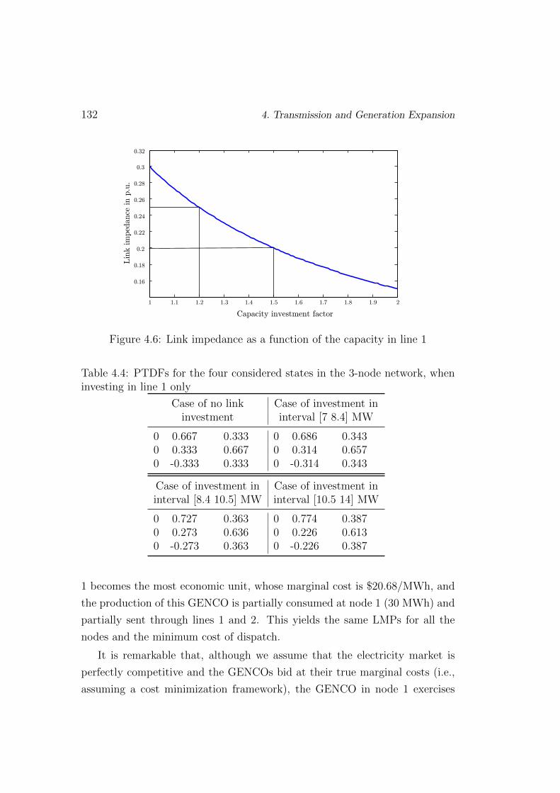
132 4. Transmission and Generation Expansion
1 1.1 1.2 1.3 1.4 1.5 1.6 1.7 1.8 1.9 2
0.16
0.18
0.2
0.22
0.24
0.26
0.28
0.3
0.32
Capacity investment factor
Lin
k im
ped
ance
in p
.u.
Figure 4.6: Link impedance as a function of the capacity in line 1
Table 4.4: PTDFs for the four considered states in the 3-node network, wheninvesting in line 1 only
Case of no link Case of investment ininvestment interval [7 8.4] MW
0 0.667 0.333 0 0.686 0.3430 0.333 0.667 0 0.314 0.6570 -0.333 0.333 0 -0.314 0.343
Case of investment in Case of investment ininterval [8.4 10.5] MW interval [10.5 14] MW
0 0.727 0.363 0 0.774 0.3870 0.273 0.636 0 0.226 0.6130 -0.273 0.363 0 -0.226 0.387
1 becomes the most economic unit, whose marginal cost is $20.68/MWh, and
the production of this GENCO is partially consumed at node 1 (30 MWh) and
partially sent through lines 1 and 2. This yields the same LMPs for all the
nodes and the minimum cost of dispatch.
It is remarkable that, although we assume that the electricity market is
perfectly competitive and the GENCOs bid at their true marginal costs (i.e.,
assuming a cost minimization framework), the GENCO in node 1 exercises

4.6. Illustrative Examples 133
market power through its generation capacity investment decision, obtaining
a profit. This implies another potential benefit to society of anticipating
generation capacity investment decisions through a proactive transmission plan
that mitigates the GENCOs’ market power.
Table 4.5: Optimal market clearing values given the solutions of level 1 and 2in the 3-node network
Available capacityNode Profit for each GENCO LMP Production
($) (MW) ($/MWh) (MWh)
1 147.41 44.4 24 44.42 0 30 24 17.8173 0 30 24 12.783
The transmission planner problem for level 1 is also solved for the other
cases: investing in line 2, investing in line 3, and investing in lines 1, 2 and 3,
jointly. The solutions are summarized in Table 4.6. The discretization applied
is the same for all cases (i.e. four configurations of investment for each line).
Table 4.6: Optimal values of the problem for level 1 of the 3-node network
CaseCost for the Line Available capacitytransmission capacity (MW)planner ($) (MW) g1 g2 g3
l1 1662.592 7.4 (l1) 44.4 30 30l2 1662.592 7.4 (l2) 44.4 30 30l3 1678.448 7 (l3) 42.8 30 30
l1, l2 & l3 1662.5927.4 (l1) 44.4 30 307.4 (l2) 44.4 30 30
From Table 4.6, we observe that the optimal solutions are either investing
0.4 MW in line 1 or investing 0.4 MW in line 2. Note that, in the case of
possible investment in lines 1, 2, and 3, jointly, there are two solutions with
identical total costs. This is due to the fact that the LMPs are equal in all the
nodes.
It is interesting to note that, if we fix the investment in line 1 and we
solve the EPEC (now the demand is deterministic) at level 2 by applying the

134 4. Transmission and Generation Expansion
methodology to find all pure Nash equilibria, we obtain two more equilibria.
Each equilibrium has a different cost of dispatch, but all of them are perfectly
valid. In the optimization process of level 1, the transmission planner attempts
to anticipate the EPEC equilibrium by choosing the best possible solution for
level 2 (minimum cost of dispatch). However, this cannot be guaranteed. This
implies that, while the methodology presented in Section 4.3 is useful for find-
ing all pure strategy Nash equilibria of the level 2 problem, it is not useful for
solving all possible instances of the level 1 problem. Hence, we solve the level 1
problem using what we call an optimistic solution for the transmission planner,
which considers that the transmission planner anticipates the best (from the
social welfare viewpoint) EPEC equilibria. There is also a pessimistic solution
for the transmission planner, which considers the worst EPEC equilibria.
Figure 4.7 depicts the whole range of equilibria seen by the transmission
planner (in the case of investing in line 1 only): the optimistic one (lower part
of Figure 4.7) and the pessimistic one (upper part of Figure 4.7) equilibria,
according to the energy dispatch plus the investment costs incurred by the
transmission planner. The values in this figure are obtained by solving the
EPEC problem for level 2, where line 1 investment is discretized using 1000
values, ranging from 7 MW of capacity to 14 MW. We observe that the optimal
optimistic solution consists of investing 0.4 MW, with a total cost of $1662.6,
and the optimal pessimistic solution is to invest 0.6 MW, with a total cost of
$1723.4, corresponding to the EPEC with the highest cost of dispatch.
7 7.4 7.6 8 9 10 11 12 13 141.650
1662.6
1723.4
1700
1.750
1.800
Capacity of line 1
Disp
atch
plu
s lin
e in
vest
men
t cos
t
Figure 4.7: Optimistic and pessimistic level 1 solutions for the case of investingonly in line 1

4.6. Illustrative Examples 135
Based on the 3-node network case study, we add a new node and a new
line. Figure 4.8 shows the 4-node system. Lines 1 to 3 have already been
built (although they can still be expanded) and line 4 can be built by the
transmission planner. Table 4.7 provides the data for the 4 nodes and Table
4.8 shows the data for the lines and the investment options.
l1
l2
l3
1
2
3
4
l4
Figure 4.8: 4-node case study
Table 4.7: 4-node example data
Node DemandProduction costs parameters Unit cost
of investment
idi g0
i ai bi Ki
(MW) (MW) ($/MWh) ($/(MWMWh)) ($/MW)1 30 30 25 0.3 0.022 25 30 24 0.3 0.023 20 30 24 0.3 0.024 25 30 24 0.3 0.02
We solve the level 1 problem considering the potential expansions of lines
l1, l2 and l3 and/or investment in the new line l4. The solutions are shown
in Table 4.9. In this case, we use a 4-step discretization for the equivalent
impedance of the existing lines (l1, l2, and l3) and a 6-step discretization for

136 4. Transmission and Generation Expansion
Table 4.8: 4-node example line data
LineInitial thermal Unit transmission Maximum thermallimit capacity investment cost limit capacity
l f 0l (MW) Kl ($/MW) fmaxl (MW)
1 7 25 142 7 25 143 7 25 144 0 25 14
the equivalent impedance of the potential new line (l4).
Table 4.9: Optimal values of the problem for level 1 of the 4-node network
CaseCost for the Line Available capacitytransmission capacity (MW)planner ($) (MW) g1 g2 g3 g4
7.4 (l1) 44.4 30 30 30l1, l2, l3 & l4 2262.592 7.4 (l2) 44.4 30 30 30
0.4 (l4) 44.4 30 30 30
From Table 4.9, we observe that there are three optimistic optimal solu-
tions: investing 0.4 MW in line 1, investing 0.4 MW in line 2, and investing
0.4 MW in line 4. These three solutions have identical total costs, which
is a consequence of the similarity in the production cost function of all the
generation units (which leads to the same LMPs in all the nodes).
All case studies have been solved using CPLEX 11 under GAMS [119]. We
have used a Dell PowerEdge R910 x64 computer with 4 processors at 1.87 GHz
and 32 GB of RAM. Table 4.10 shows the running times and computational
complexity required for solving the problems. The second to fifth columns
show the 3-node network CPU times and the computational complexity for
the cases shown in Table 4.6. The sixth column shows the CPU time and the
computational complexity to solve the 4-node network case.

4.7. Case Study: The Sistema Interconectado Central (SIC) in Chile 137
Table 4.10: CPU times and computational complexity of the 3- and 4-nodenetworks
3-node network4-node network
l1 l2 l3 l1, l2, & l3
CPU time 7.58 s 11.74 s 13.06 s 267.26 s 1 h 25 min# of binary variables 607 607 607 667 1316# of positive variables 670 670 670 672 1152# of free continuous variables 2103 2103 2103 28563 200260# of inequality constraints 14603 14603 14603 155727 1077204# of equality constraints 5834 5834 5834 85214 599954
4.7 Case Study: The Sistema Interconectado
Central (SIC) in Chile
We illustrate the proposed model using a stylized representation of the main
Chilean power network, i.e., the Sistema Interconectado Central or SIC, as
shown in Figure 4.9. The SIC is a system composed of both generation plants
and transmission lines that operates to meet most of the Chilean electricity
demand. The SIC extends over a distance of 1,740 km covering a territory of
326,412 sq. km, equivalent to 43% of the country, where 93% of the population
lives. At the end of 2010, the SIC had 12,147 MW of installed power capacity,
54.5% thermal and 44.1% hydroelectric, while the annual gross generation of
energy was around 41,062 GWh [120]. Although the decision framework spans
a lifetime of 25 years, we have considered a one-year horizon in our model,
with annualized investment costs. Nevertheless, our model can be run for
investment decisions in a year-by-year fashion. As shown in Figure 4.9, the
SIC has 34 buses and 38 transmission lines. Four existing lines are candidates
for capacity augmentation and 2 new lines are candidates for construction
(represented by the dashed lines in Figure 4.9). There are four generation
companies (corresponding to the three major generation firms in Chile and
the rest are grouped into a fourth firm), each owning generation capacity at
multiple locations. The electric characteristics (i.e., resistance, reactance, and
thermal capacity rating) of the transmission lines of the network are obtained
from [120].

138 4. Transmission and Generation Expansion
1 Diego de Almagro 2202 Carrera Pinto 220
3 Cardones 220
4 Maitencillo 220
5 Pan de Azucar 220
6 Los Vilos 220
7 Quillota 2208 Polpaico 500/220 12 Rapel 220
9 San Luis 22010 A. Santa 220
11 Cerro Navia 220
13 Chena 220
14 Alto Jahuel 500/220
34 Loaguirre 220
16 Colbún 220
20 Ancoa 500/220
15 A. Jahuel 15417 Paine154
18 Rencagua 154
19 San Fernando 154
22 Parral 154
21 Itahue 220/154
23 Chillán 154
25 Charrúa 154
24 Charrúa 500/22026 Concepción 220/154
27 San Vicente 154
28 Hualpén 220/154
29 Coronel 154
30 Temuco 220
31 Valdivia 220
32 Barrio Blanco 220
33 Puerto Montt 220
Figure 4.9: Stylized representation of the Chilean SIC network
Data
The main data are summarized in Tables 4.11, 4.12 and 4.13 2. Appendix B
contains fulls detail of the SIC. Table 4.11 provides data for the candidate lines
included in the expansion planning. The third column shows the annualized
2It is worth mentioning that Chile does not use LMPs, but a type of ’regulated LMPs’.The Chilean National Energy Commission estimates every six months the projected averageLMPs for the next 48 months, using a stochastic dual dynamic program, and fixes themuntil the next revision as ’regulated nodal prices’ [121].
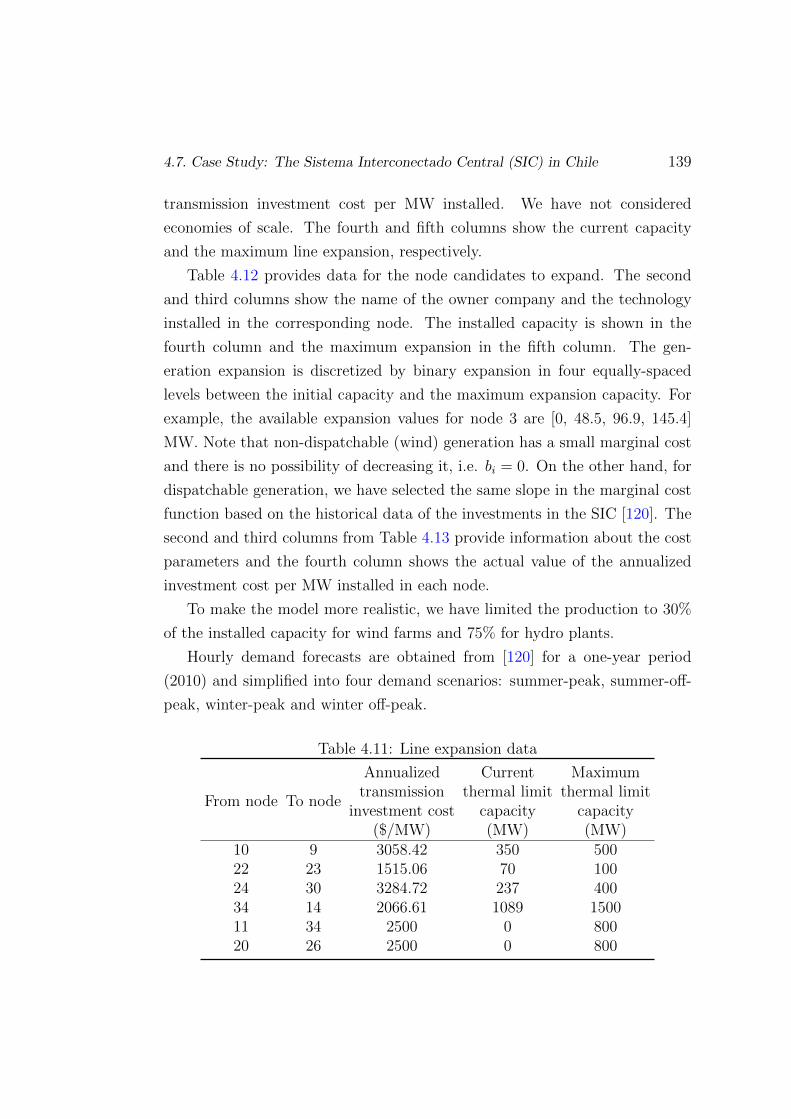
4.7. Case Study: The Sistema Interconectado Central (SIC) in Chile 139
transmission investment cost per MW installed. We have not considered
economies of scale. The fourth and fifth columns show the current capacity
and the maximum line expansion, respectively.
Table 4.12 provides data for the node candidates to expand. The second
and third columns show the name of the owner company and the technology
installed in the corresponding node. The installed capacity is shown in the
fourth column and the maximum expansion in the fifth column. The gen-
eration expansion is discretized by binary expansion in four equally-spaced
levels between the initial capacity and the maximum expansion capacity. For
example, the available expansion values for node 3 are [0, 48.5, 96.9, 145.4]
MW. Note that non-dispatchable (wind) generation has a small marginal cost
and there is no possibility of decreasing it, i.e. bi = 0. On the other hand, for
dispatchable generation, we have selected the same slope in the marginal cost
function based on the historical data of the investments in the SIC [120]. The
second and third columns from Table 4.13 provide information about the cost
parameters and the fourth column shows the actual value of the annualized
investment cost per MW installed in each node.
To make the model more realistic, we have limited the production to 30%
of the installed capacity for wind farms and 75% for hydro plants.
Hourly demand forecasts are obtained from [120] for a one-year period
(2010) and simplified into four demand scenarios: summer-peak, summer-off-
peak, winter-peak and winter off-peak.
Table 4.11: Line expansion data
From node To node
Annualized Current Maximumtransmission thermal limit thermal limit
investment cost capacity capacity($/MW) (MW) (MW)
10 9 3058.42 350 50022 23 1515.06 70 10024 30 3284.72 237 40034 14 2066.61 1089 150011 34 2500 0 80020 26 2500 0 800
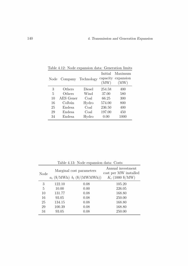
140 4. Transmission and Generation Expansion
Table 4.12: Node expansion data: Generation limits
Node Company Technology
Initial Maximumcapacity expansion(MW) (MW)
3 Others Diesel 254.58 4005 Others Wind 37.00 58010 AES Gener Coal 66.25 30016 Colbun Hydro 574.00 80025 Endesa Coal 236.50 40029 Endesa Coal 197.00 45034 Endesa Hydro 0.00 1000
Table 4.13: Node expansion data: Costs
NodeMarginal cost parameters
Annual investmentcost per MW installed
ai ($/MWh) bi ($/(MWMWh)) Ki (1000 $/MW)
3 122.10 0.08 105.205 10.00 0.00 226.0510 131.77 0.08 168.8016 93.05 0.08 250.0025 134.15 0.08 168.8029 100.39 0.08 168.8034 93.05 0.08 250.00
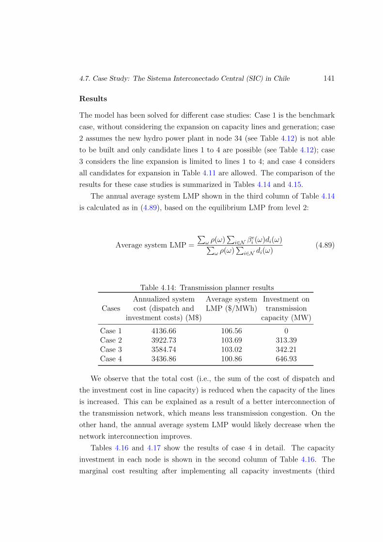
4.7. Case Study: The Sistema Interconectado Central (SIC) in Chile 141
Results
The model has been solved for different case studies: Case 1 is the benchmark
case, without considering the expansion on capacity lines and generation; case
2 assumes the new hydro power plant in node 34 (see Table 4.12) is not able
to be built and only candidate lines 1 to 4 are possible (see Table 4.12); case
3 considers the line expansion is limited to lines 1 to 4; and case 4 considers
all candidates for expansion in Table 4.11 are allowed. The comparison of the
results for these case studies is summarized in Tables 4.14 and 4.15.
The annual average system LMP shown in the third column of Table 4.14
is calculated as in (4.89), based on the equilibrium LMP from level 2:
Average system LMP =
∑ω ρ(ω)
∑i∈N β
ei (ω)di(ω)∑
ω ρ(ω)∑
i∈N di(ω)(4.89)
Table 4.14: Transmission planner results
CasesAnnualized system Average system Investment oncost (dispatch and LMP ($/MWh) transmission
investment costs) (M$) capacity (MW)
Case 1 4136.66 106.56 0Case 2 3922.73 103.69 313.39Case 3 3584.74 103.02 342.21Case 4 3436.86 100.86 646.93
We observe that the total cost (i.e., the sum of the cost of dispatch and
the investment cost in line capacity) is reduced when the capacity of the lines
is increased. This can be explained as a result of a better interconnection of
the transmission network, which means less transmission congestion. On the
other hand, the annual average system LMP would likely decrease when the
network interconnection improves.
Tables 4.16 and 4.17 show the results of case 4 in detail. The capacity
investment in each node is shown in the second column of Table 4.16. The
marginal cost resulting after implementing all capacity investments (third

142 4. Transmission and Generation Expansion
Table 4.15: Annual profits and generation expansion results
CaseAnnual profits of GENCOs (M$)
Endesa AES Gener Colbun Others
Case 1 190.27 3.71 15.34 66.86Case 2 165.78 2.88 28.21 68.30Case 3 331.57 2.69 4.82 62.53Case 4 409.65 0.65 52.24 74.11
CaseGeneration expansion (MW)
Endesa AES Gener Colbun Others
Case 1 0 0 0 0Case 2 0 0 226 542.92Case 3 1000 0 0 542.92Case 4 1000 0 226 542.92
column) is compared with the annual average LMP in each node (fourth
column). The annual average LMP is calculated by averaging the LMPs of
the four annual demand patterns of the year.
Table 4.17 shows the solutions for line capacity investments and the annu-
alized investment cost per line in the second and third columns, respectively.
The three-level model is formulated with continuous variables for line capac-
ity investments. Therefore, the optimal values correspond to the minimum
investments to comply with the thermal constraints of the candidate lines.
Table 4.16: Generation capacity expansion
NodeCapacity Marginal Average LMP Annualized
investment production cost investment cost(MW) ($/MWh) ($/MWh) (M$)
3 0 122.10 100.94 05 542.92 10.00 100.94 122.7310 0 131.77 100.94 016 226 79.49 100.05 56.525 0 134.15 100.41 029 0 100.39 98.54 034 1000 39.05 100.50 225

4.7. Case Study: The Sistema Interconectado Central (SIC) in Chile 143
Table 4.17: Line capacity expansion
From node To nodeCapacity Annualized
investment investment(MW) cost (1000$)
10 9 20.88 63.934 14 22.35 33.922 23 122.33 401.824 30 0 011 34 422.84 1057.120 26 58.53 146.3
Line investment decisions are continuous variables in the model. However,
a practical expansion project would require discrete expansion levels. For
example, an increase of 21 MW in the line connecting nodes 9 and 10 could
be achieved by changing the material of the conductor. On the other hand, an
expansion of 423 MW in the line connecting nodes 11 and 34 is big enough to
consider the construction of a 500 MW line.
The model has been formulated in the General Algebraic Modeling System
(GAMS) [119] and solved with CPLEX 11 solver in a Dell PowerEdge R910x64
computer with 4 processors at 1.87 GHz and 32 GB of RAM. Table 4.18 shows
the CPU times and computational complexities required for each case study.
Table 4.18: CPU times and computational complexity
Case 1 Case 2 Case 3 Case 4
CPU time 0.56 sec 26 h 58 min 8 h 46 min 12 h 11 min# of binary variables 584 23956 51990 53414# of positive continuous variables 720 29620 64196 65622# of free continuous variables 276 11360 24656 24656# of inequality constraints 1616 83876 188564 192852# of equality constraints 416 16936 36760 36760

144 4. Transmission and Generation Expansion
4.8 Summary and Conclusions
We have proposed a three-level MILP where a transmission planner decides on
the first level upon the best line investments, given the optimistic pure Nash
equilibria in generation investment (second level), and the market clearing
(third level).
The transmission expansion model anticipates decisions on generation in-
vestment, where the equilibrium on generation investment is modeled using a
stochastic EPEC. We propose an approximation of the line impedance values
as a function of the installed transmission capacities. This assumption allows
us to incorporate the changes in operation due to the new topology resulting
from line investments within the transmission planning level.
In this sense, if a transmission planner suggests building some lines in an-
ticipation to generation capacity investments, then this can induce generation
companies to invest in a more socially-efficient manner.
We also apply a new methodology to extract all possible pure Nash equi-
libria on generation investment by creating holes in the equilibrium solution
space.
The model is applied to 3- and 4-node illustrative examples and to a realistic
case study based on the main Chilean power system (SIC).

Chapter 5
Summary, Conclusions,
Contributions and Future
Research
This chapter summarizes this dissertation and its main conclusions. Then, the
most relevant contributions of this work are stated. Finally, future research
directions are suggested.
5.1 Thesis Summary
We have presented a mathematical framework for solving stochastic finite
bilevel games in restructured power systems and found all pure Nash equilibria
for such problems. These games are appropriate for studying strategic behavior
in restructured power systems, since they can model hierarchical competition
among the participants. We have shown the applicability of our framework
in both operations and planning. Regarding the operational framework, we
have formulated, solved and illustrated the strategic bidding problem. Re-
garding the planning framework, we have formulated, solved and illustrated
the transmission and generation expansion problem with a realistic case study.
The principal features outlined in this thesis are described below:
• First, we have described the main features of restructured power systems
145

146 5. Summary, Conclusions, Contributions and Future Research
and electricity markets. Also, we have summarized current literature
related to this thesis, namely, the strategic bidding problem, the trans-
mission and generation expansion problem, and equilibrium modeling in
electricity markets.
• Second, we have introduced game theory definitions related with one-
and two-level games. We have also described a methodology for finding
all Nash equilibria in finite-strategy games. Then, we have presented
the conversion of an EPEC into an inequality system with equilibrium
constraints due to the linear properties of the lower-level problem and
the existence of finite strategies of the leaders. The suggested linear
reformulation approach has enabled us to find global solutions.
• Third, we have proposed a bilevel game in an operational framework to
solve the strategic bidding problem. In this problem, GENCOs submit
their offers in quantities and prices to the ISO. Demand uncertainty is
considered in the lower-level problem. Therefore, each GENCO faces an
MPEC and the joint solution of all MPECs is stated as an EPEC. The
EPEC is reformulated as an MILP suitable to be solved with commercial
solvers. We have proposed two models: one with network representation
and another one disregarding the network. We have illustrated our
formulation with several case studies.
• Fourth, we have posed a three-level model within a planning framework
for transmission and generation capacity expansion. In this sense, the
transmission planner optimizes the expansion of the transmission net-
work (in the upper level) in anticipation of generation capacity invest-
ments (in the mid level). In the mid level, GENCOs compete among
themselves producing several Nash equilibria. Transmission and gener-
ation expansions are optimized in anticipation of the lower level, the
results of the spot market. The mid- and lower-level problems are stated
as stochastic EPECs in finite strategies. Then, a linearization process
to convert the original problem into an MILP is described. Also, a
methodology for finding all pure Nash equilibria in the mid level is

5.2. Conclusions 147
presented. Finally, an illustrative example and a realistic case study
based on the main Chilean power system (SIC) shows the applicability
of the proposed model.
5.2 Conclusions
The previous summary leads to relevant conclusions that can be drawn from
the research presented in this thesis. The most relevant conclusions are enu-
merated below:
1. The conclusions pertaining to bilevel games and their resolution are:
(a) Current algorithms for solving bilevel games have several shortcom-
ings. These algorithms are related with bilevel, MPEC or EPEC
optimization problems, whose solution methods have deficiencies.
(b) EPEC optimization problems lack a generalized theory for solving
them because, in general, such problems are non-linear and non-
convex and do not hold any constraint qualification. Specific meth-
ods have been proposed for solving specific instances of EPECs.
(c) Global solutions are rarely reached in EPECs. Instead of a global
solution, stationary solutions for EPECs are obtained. Such station-
ary solutions may be global, local, or saddle points. We have solved
this problem convexifying the EPEC and transforming it into an
MILP. The global solutions of the linearized problem are tractable
in moderately-sized optimization problems.
(d) In general, uniqueness is not guaranteed for EPECs. In fact, a man-
ifold of equilibria is a feature of many EPECs, but most algorithms
for solving EPECs only provide a single solution. We have solved
this problem including a new linear constraint that represents a
“hole” in the feasible region around each known Nash equilibrium.
2. The conclusions pertaining to the strategic bidding problem are:

148 5. Summary, Conclusions, Contributions and Future Research
(a) The bidding problem faced by a GENCO in an electricity spot
market can be formulated as a stochastic EPEC, modeling the
strategic behavior in a competitive setting. The problem can be
recast as a MILP. In this context, the bidding strategies and the
spot market prices are obtained from the solution of the proposed
model.
(b) The strategic bidding problem has multiple equilibria which can be
classified either by the expected profits obtained by the GENCOs
or by the expected spot market prices.
(c) In general, a network-constrained (and congested) model has less
equilibria than a network-unconstrained model. This is because the
GENCOs have more difficulties for finding a position where they
do not want to change their strategies. This happens when they
cannot deliver energy to the network without congesting any lines.
(d) The network-constrained (and congested) model provides the high-
est spot prices due to line congestion that may not enable full
dispatch of the cheap generating units.
(e) The network-constrained model equilibria without congestion are
also the same as the network-unconstrained model equilibria.
(f) The network-constrained case studies show that a GENCO may
congest the network as a mechanism to exert market power.
3. The conclusions pertaining to the transmission and generation capacity
expansion problem are:
(a) An anticipative transmission plan is important because it may in-
duce more socially-efficient (and/or environmentally-convenient) gen-
eration capacity investments.
(b) The anticipative model may help to mitigate the market power
exercised by GENCOs through their generation capacity investment
decisions, i.e., the transmission planner can trigger the construction
of some lines in anticipation of generation capacity investments,

5.3. Contributions 149
inducing generation companies to invest in a more socially-efficient
manner.
(c) Multiple generation expansion equilibria are possible for a single
transmission expansion plan, and all of them are perfectly valid.
The transmission planner can be modeled as an optimistic agent
if it anticipates the best EPEC equilibria from the social welfare
viewpoint.
(d) Finally, although the proposed methodology has several advantages,
it is important to recall its limitations. First, the model used
is static. This fact does not represent the dynamic nature of in-
vestments, but this assumption is made due to tractability issues.
Secondly, we assume perfect competition and inelastic demand (in
order to deal with convex problems), but the reader should be aware
of the possibility that GENCOs may exercise market power. And
thirdly, our model considers that transmission capacity investments
are continuous variables, although they are lumpy due to economies
of scale. In this sense, the numerical results of our model should
be taken as approximations of the transmission capacities to be
added to the network in order to produce the desired response by
generation capacity investors.
5.3 Contributions
The main contributions of this work can be summarized as follows.
1. Regarding the one- and two-level games, we have:
(a) Characterized and ranked the one- and two-level games configura-
tions as well as the mathematical formulation of each one of them.
(b) Proposed an MILP reformulation of a finite stochastic EPEC in
order to obtain global solutions.
(c) Developed a methodology for finding all pure Nash equilibria in
finite-strategy games.

150 5. Summary, Conclusions, Contributions and Future Research
2. Regarding the strategic bidding problem, we have:
(a) Formulated a bilevel game focusing on the strategic price and quan-
tity bidding variables of the GENCOs in a multi-period and multi-
block (bid) setting. In addition, we have considered stochasticity
of the demand in several scenarios. The bilevel game is stated as a
stochastic EPEC with finite strategies.
(b) Transformed the non-linear and non-convex stochastic EPEC into
an MILP.
(c) Found all the pure Nash equilibria of the stochastic EPEC by adding
new successive linear constraints to the linearized problem.
(d) Formulated the stochastic EPEC problem for a network-constrained
system and transformed it into an MILP.
(e) Applied the proposed model to two illustrative case studies.
3. Regarding the transmission and generation capacity expansion problem,
we have:
(a) Formulated a three-level model that integrates transmission plan-
ning, generation investment, and market operation decisions.
(b) Transformed the three-level model into a one-level MILP, that can
be solved with commercial solvers.
(c) Proposed and applied a methodology to solve the optimal transmis-
sion expansion problem (anticipating both generation investment
and market clearing).
(d) Characterized the equilibria in generation investment made by de-
centralized GENCOs (which corresponds to the solution of an EPEC)
as a set of linear inequalities.
(e) Computed all possible pure Nash equilibria of the generation invest-
ment problem by creating holes in the equilibrium solution space.
(f) Developed a methodology to account for the variation of line impedances
and PTDFs as functions of the installed transmission capacities.

5.3. Contributions 151
(g) Illustrated the proposed model with two case studies: 3-node and
4-node systems.
(h) Analyzed a realistic case study based on the main Chilean power
system (SIC) to show the applicability of the model.
4. The publication of the following six papers related to this dissertation
in relevant SCI-indexed international journals. The second, fourth and
fifth papers are directly related with this dissertation and the other ones
are collateral works.
(a) D. Pozo, J. Contreras, A. Caballero and A. de Andres, “Long-
term Nash equilibria in electricity markets,” Electric Power Systems
Research, vol. 81, no. 2, pp. 329–339, 2011.
(b) D. Pozo, and J. Contreras, “Finding multiple Nash equilibria in
pool-based markets: A stochastic EPEC approach,” IEEE Trans-
actions on Power Systems, vol. 26, no. 3, pp. 1744–1752, 2011.
(c) F. J. Dıaz, J. Contreras, J. I. Munoz and D. Pozo, “Optimal schedul-
ing of a price-taker cascaded reservoir system in a pool-based elec-
tricity market,” IEEE Transactions on Power Systems, vol. 26, no.
2, pp. 604–615, 2011.
(d) D. Pozo, J. Contreras, and E. E. Sauma, “A three-level static MILP
model for generation and transmission expansion planning,” IEEE
Transactions on Power Systems, in press.
(e) D. Pozo, J. Contreras, and E. E. Sauma, “If you build it, he will
come: Anticipative power transmission planning,” Energy Economics,
in press.
(f) D. Pozo, and J. Contreras, “A chance-constrained unit commitment
with an n−K security criterion and significant wind generation,”
IEEE Transactions on Power Systems, accepted for publication.

152 5. Summary, Conclusions, Contributions and Future Research
5.4 Future Research Suggestions
Suggestions for future research resulting from the work reported in this disser-
tation are listed below. They are organized into three main groups. The first
one refers to possible advances in the strategic bidding problem, the second
one focuses on the transmission and generation capacity expansion problem,
and the third one refers to the improvement of the algorithmic solutions used
in this thesis and the economic significance of bilevel games extensions.
1. Regarding the strategic bidding problem:
(a) Bilateral or forward contract markets may be included in our mod-
els. The resulting equilibria may change, but the enhanced models
could be useful tools for GENCOs, regulators and market operators.
(b) Modeling risk-adverse GENCOs may be desirable, since finding
equilibria with risk-adverse participants is a current research chal-
lenge. This is related with the previous item (1a) and item (3c).
(c) Detailed modeling of non-dispatchable renewable energy at the lower-
level problem would be valuable.
(d) The model proposed is adequate for a power system where the units
are mostly thermal generators. Hydro generators require special
treatment for water usage and this has not been included in the
models. A future extension may include specific modeling of the
water opportunity cost and hydro-cascade resource equations.
(e) The pool-market model may be extended to short-term electricity
markets such as intra-day markets or balancing markets.
(f) Demand side bidding may be considered in the market clearing
process.
(g) We have assumed demand as the single source of uncertainty, but
production costs, unit failure rates or renewable energies could also
be modeled as uncertain.
2. Regarding the transmission and generation capacity expansion problem:

5.4. Future Research Suggestions 153
(a) Development of proactive models (anticipative) for transmission
and generation expansion to model the strategic behavior of trans-
mission companies profiting from transmission rights.
(b) Modeling the GENCOs’ strategic behavior in the third level (spot
market), where the GENCOs can exert market power submitting
strategic offers to the ISO.
(c) Accurate representation of non-dispatchable renewable energies at
the lower-level would be of interest.
(d) A planning horizon spanning from 20 to 30 years, where investments
could be done in any year.
(e) Consider an n−K security criterion in transmission and generation
expansion planning.
(f) A model for the strategic behavior of demand, allowing consumers
to adapt their consumption to the resulting market prices.
3. Regarding the mathematical tools used in this thesis and the economic
significance of the bilevel games extensions:
(a) It would be of interest to apply decomposition techniques, since
the division of the main problem into subproblems could make the
problem easier to solve and the CPU time could be lower.
(b) Developing specific solution techniques for EPECs as MILPs with
a finite number of strategies may be desirable.
(c) In this thesis, we have assumed that players have a risk-neutral
attitude. It would be interesting to generalize the Nash equilibrium
problem with risk-adverse players, where risk-adverse parameters
could be included.

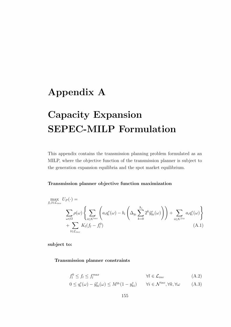
Appendix A
Capacity Expansion
SEPEC-MILP Formulation
This appendix contains the transmission planning problem formulated as an
MILP, where the objective function of the transmission planner is subject to
the generation expansion equilibria and the spot market equilibrium.
Transmission planner objective function maximization
maxfl,l∈Linv
UP (·) =
∑ω∈Ω
ρ(ω)
∑i∈N inv
(aiq
ei (ω)− bi
(∆gi
Λi∑k=0
2kyeki(ω)
))+∑i∈N fix
aiqei (ω)
+∑l∈Linv
Kl(fl − f 0l ) (A.1)
subject to:
Transmission planner constraints
f 0l ≤ fl ≤ fmaxl ∀l ∈ Linv (A.2)
0 ≤ qei (ω)− yeki(ω) ≤M gi(1− yeki) ∀i ∈ N inv,∀k,∀ω (A.3)
155

156 A. Capacity Expansion SEPEC-MILP Formulation
0 ≤ yeki(ω) ≤M giyeki ∀i ∈ N inv, ∀k,∀ω (A.4)
Definition of equilibrium in generation expansion
U eG(·) ≥ U sG
G (·) ∀sG ∈ SG,∀G ∈ G (A.5)
U eG(·) =
∑ω∈Ω
ρ(ω)
∑i∈N fix
G
g0i ξei (ω) +
(g0i ξei (ω) + ∆gi
Λi∑k=0
2kyeki(ω)
)−∑
i∈N invG
Ki
(∆gi
Λi∑k=0
2kyeki
), ∀G ∈ G (A.6)
U sGG (·) =∑ω∈Ω
ρ(ω)
∑i∈N fix
G
g0i ξsGi (ω) +
∑i∈N inv
G
gsGi ξsGi (ω)
− ∑i∈N inv
G
Ki
(gsGi − g0
i
),
∀sG ∈ SG,∀G ∈ G (A.7)
LHS constraints set. Equations (A.8)–(A.25) are defined for all scenar-
ios, ω.
ai − bi(
∆gi
Λi∑k=0
2kyeki
)− γei (ω)− βei (ω) + ξei (ω) = 0 ∀i ∈ N inv (A.8)
ai − γei (ω)− βei (ω) + ξei (ω) = 0 ∀i ∈ N fix (A.9)
αe(ω) +∑l∈L
(λ+el (ω)− λ−el (ω))ϕli − βei (ω) = 0 ∀i ∈ N (A.10)∑
i∈N
rei (ω) = 0 (A.11)
qei (ω) + rei (ω) = di(ω) ∀i ∈ N (A.12)
0 ≤ γei (ω) ≤Mγiηγei (ω) ∀i ∈ N (A.13)
0 ≤ qei (ω) ≤M gi(1− ηγei (ω)) ∀i ∈ N (A.14)
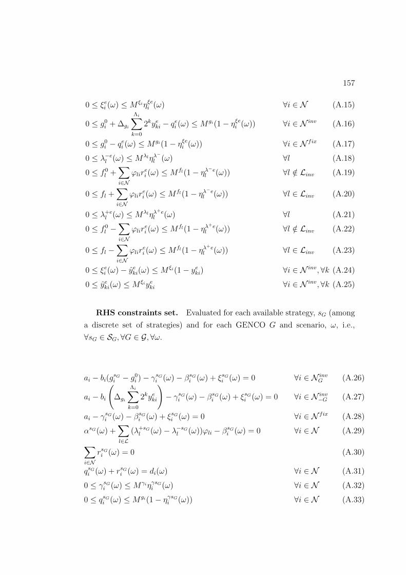
157
0 ≤ ξei (ω) ≤M ξiηξei (ω) ∀i ∈ N (A.15)
0 ≤ g0i + ∆gi
Λi∑k=0
2kyeki − qei (ω) ≤M gi(1− ηξei (ω)) ∀i ∈ N inv (A.16)
0 ≤ g0i − qei (ω) ≤M gi(1− ηξei (ω)) ∀i ∈ N fix (A.17)
0 ≤ λ−el (ω) ≤Mλlηλ−
l (ω) ∀l (A.18)
0 ≤ f 0l +
∑i∈N
ϕlirei (ω) ≤M fl(1− ηλ−el (ω)) ∀l /∈ Linv (A.19)
0 ≤ fl +∑i∈N
ϕlirei (ω) ≤M fl(1− ηλ−el (ω)) ∀l ∈ Linv (A.20)
0 ≤ λ+el (ω) ≤Mλlηλ
+el (ω) ∀l (A.21)
0 ≤ f 0l −
∑i∈N
ϕlirei (ω) ≤M fl(1− ηλ+el (ω)) ∀l /∈ Linv (A.22)
0 ≤ fl −∑i∈N
ϕlirei (ω) ≤M fl(1− ηλ+el (ω)) ∀l ∈ Linv (A.23)
0 ≤ ξei (ω)− yeki(ω) ≤M ξi(1− yeki) ∀i ∈ N inv,∀k (A.24)
0 ≤ yeki(ω) ≤M ξiyeki ∀i ∈ N inv,∀k (A.25)
RHS constraints set. Evaluated for each available strategy, sG (among
a discrete set of strategies) and for each GENCO G and scenario, ω, i.e.,
∀sG ∈ SG,∀G ∈ G,∀ω.
ai − bi(gsGi − g0i )− γsGi (ω)− βsGi (ω) + ξsGi (ω) = 0 ∀i ∈ N inv
G (A.26)
ai − bi(
∆gi
Λi∑k=0
2kyeki
)− γsGi (ω)− βsGi (ω) + ξsGi (ω) = 0 ∀i ∈ N inv
−G (A.27)
ai − γsGi (ω)− βsGi (ω) + ξsGi (ω) = 0 ∀i ∈ N fix (A.28)
αsG(ω) +∑l∈L
(λ+sGl (ω)− λ−sGl (ω))ϕli − βsGi (ω) = 0 ∀i ∈ N (A.29)∑
i∈N
rsGi (ω) = 0 (A.30)
qsGi (ω) + rsGi (ω) = di(ω) ∀i ∈ N (A.31)
0 ≤ γsGi (ω) ≤MγiηγsGi (ω) ∀i ∈ N (A.32)
0 ≤ qsGi (ω) ≤M gi(1− ηγsGi (ω)) ∀i ∈ N (A.33)
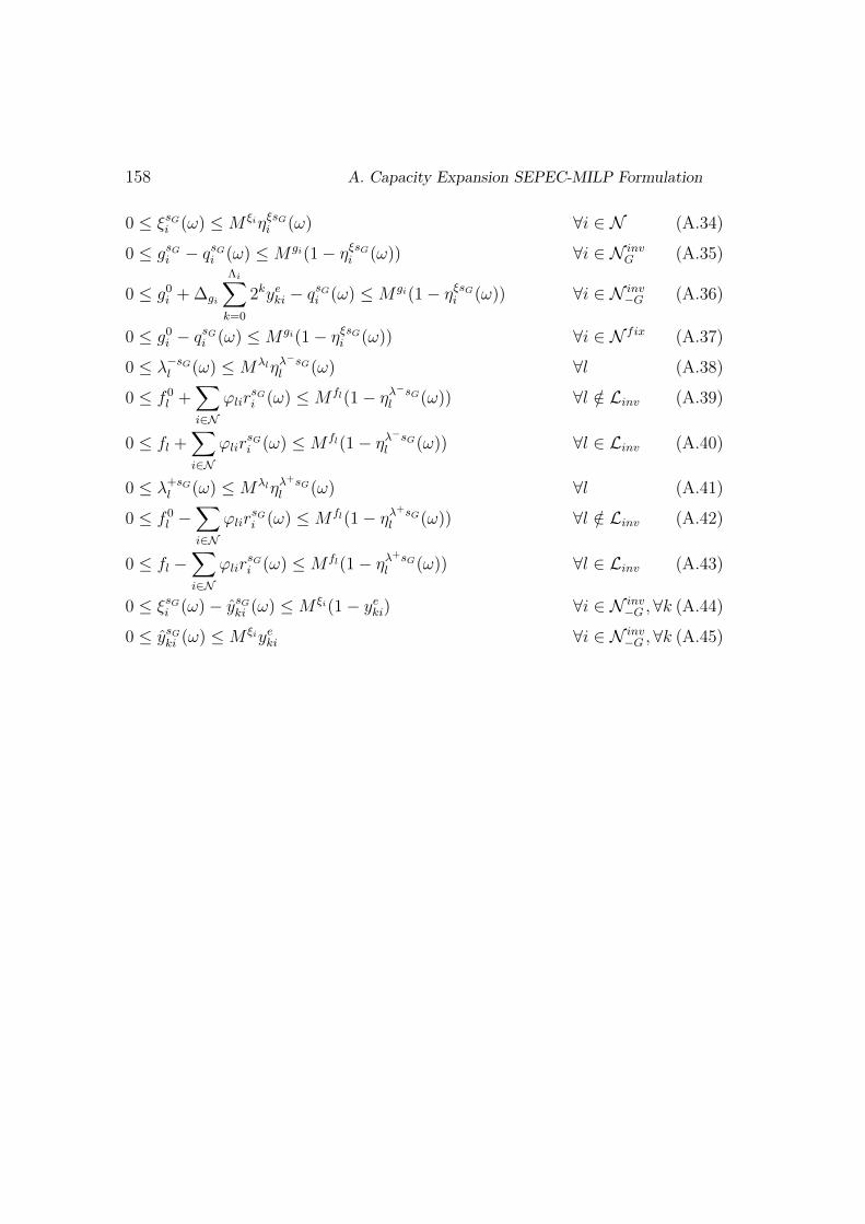
158 A. Capacity Expansion SEPEC-MILP Formulation
0 ≤ ξsGi (ω) ≤M ξiηξsGi (ω) ∀i ∈ N (A.34)
0 ≤ gsGi − qsGi (ω) ≤M gi(1− ηξsGi (ω)) ∀i ∈ N invG (A.35)
0 ≤ g0i + ∆gi
Λi∑k=0
2kyeki − qsGi (ω) ≤M gi(1− ηξsGi (ω)) ∀i ∈ N inv−G (A.36)
0 ≤ g0i − qsGi (ω) ≤M gi(1− ηξsGi (ω)) ∀i ∈ N fix (A.37)
0 ≤ λ−sGl (ω) ≤Mλlηλ−sGl (ω) ∀l (A.38)
0 ≤ f 0l +
∑i∈N
ϕlirsGi (ω) ≤M fl(1− ηλ−sGl (ω)) ∀l /∈ Linv (A.39)
0 ≤ fl +∑i∈N
ϕlirsGi (ω) ≤M fl(1− ηλ−sGl (ω)) ∀l ∈ Linv (A.40)
0 ≤ λ+sGl (ω) ≤Mλlηλ
+sGl (ω) ∀l (A.41)
0 ≤ f 0l −
∑i∈N
ϕlirsGi (ω) ≤M fl(1− ηλ+sGl (ω)) ∀l /∈ Linv (A.42)
0 ≤ fl −∑i∈N
ϕlirsGi (ω) ≤M fl(1− ηλ+sGl (ω)) ∀l ∈ Linv (A.43)
0 ≤ ξsGi (ω)− ysGki (ω) ≤M ξi(1− yeki) ∀i ∈ N inv−G ,∀k (A.44)
0 ≤ ysGki (ω) ≤M ξiyeki ∀i ∈ N inv−G ,∀k (A.45)

Appendix B
Main Chilean Power System
(SIC) Data
This appendix contains the data and the description of the main Chilean power
system (SIC) used in Chapter 4. Details of the system can be found in [120].
Table B.1 provides the location of the generating units throughout the
network as well as their respective capacities, owners, technologies and cost
parameters. Table B.2 shows four nodal demand scenarios. The demand
scenarios are based on historical data. The probabilities of each scenario
are: [0.440 0.296 0.060 0.204] for summer-peak, summer-off-peak, winter-peak
and winter-off-peak, respectively. Finally, Table B.3 shows transmission line
data: connections between nodes, annualized investment costs, candidates for
expansion, thermal limits, and maximum capacities for expansion.
159

160 B. Main Chilean Power System (SIC) Data
Tab
leB
.1:N
odal
generation
data
Node
Com
pany
Tech
nolog
yC
andid
ateIn
itialM
axim
um
Marg
inal
costp
arameters
Annu
alin
vestmen
tfo
rcap
acityex
pan
sioncost
per
MW
installed
exp
ansion
?(M
W)
(MW
)ai
($/MW
h)
bi
($/(MW
MW
h))
Ki
(1000$/MW
)
1E
ndesa
Gas
-D
iessel287.6
287.6
139.92
20
0121.6
53
Oth
ersD
iesselY
es254.58
40012
2.100.08
105.204
Oth
ersC
oal
701.8701
.8110
.78
5O
thers
Win
dY
es37.076
580
10.00
0226.05
6O
thers
352.1135
2.11116
.37
7O
thers
900.4900
.4112
.46
8A
ES
Gen
erG
as55
55
102.65
9C
olb
nG
as
2011.46201
1.46106
.9010
AE
SG
ener
Coa
lY
es66.25
300
131.77
0.08168.80
11
Oth
ersG
as
-D
iessel508.4
508.4
116.0
312
En
desa
Hydro
380380
98.69
13
00
103.5
014
Colb
nG
as
609.460
9.4106
.71
15
Colb
n192.4
192.4
104.26
16
Colb
nH
ydro
Yes
57480
093.05
0.08250.00
17
Oth
ersD
iessel0
0103.5
518
En
desa
Hydro
170.7717
0.77105
.78
19
00
97.29
20
Oth
ersH
yd
ro589
58985.93
21
En
desa
Hydro
375.356375.3
5696.45
22
00
90.10
23
Oth
ersD
iessel105.3
105.3
92.9624
En
desa
Hydro
2747274
787
.68
25
En
desa
Coa
lY
es236.5
400
134.15
0.08168.80
26
00
91.60
27
Oth
ers60.7
60.7104
.5228
Oth
ersF
uel
75.475.4
96.3829
En
desa
Coa
lY
es197.1
450
100.39
0.08168.80
30
00
102.4
031
Oth
ersF
uel
223.19223.19
107.85
32
Oth
ersH
yd
ro62.53
62.5
399.29
33
Oth
ersH
yd
ro292.7
292.7
112.47
34
En
desa
Hydro
Yes
010
0093.05
0.08250.00

161
Table B.2: Nodal load demand scenarios
NodeSummer-peak Summer-off-peak Winter-peak Winter-off-peak
(MW) (MW) (MW) (MW)
1 88.52 99.01 86.57 98.522 14.52 18.54 17.2 18.433 193.51 184.4 204.74 180.564 45.85 39.14 60.63 46.15 132.11 108.35 176.76 136.16 32.08 24.43 42.68 29.147 449.29 419.45 556.03 494.588 231.72 203.05 274.37 213.089 0 0 0 010 0 0 0 011 823.97 751.81 1097.66 1062.6712 0 0 0 013 88.5 78.81 121.1 116.5514 927.97 904.33 1164.97 1166.7115 0 0 0 016 0 0 0 017 37.61 32.48 50.1 42.7618 103.27 86.61 139.91 109.3519 59.57 49.8 81.32 65.1420 48.48 47.46 51.04 44.6621 115.43 135.75 123.69 172.8822 122.44 109.94 163 147.2223 0 0 0 024 477.16 652.28 394.96 740.2825 0 0 0 026 183.35 182.21 220.22 225.6327 243.99 233.77 268.85 250.7928 0 0 0 029 0 0 0 030 108.39 103.44 146.1 14131 56.27 56.22 69.78 70.2732 46 44.54 55.77 57.5733 107.01 97.67 135.24 126.9734 0 0 0 0

162 B. Main Chilean Power System (SIC) Data
Table B.3: Lines transmission data
From node To node
Annualized Current Maximumtransmission thermal limit thermal limit
investment cost capacity capacity($/MW) (MW) (MW)
1 2 177.62 3 177.63 4 700.34 5 710.65 6 805.26 7 805.27 8 3956.27 10 700.310 9 3058.42 350 5008 34 1088.98 11 1116.611 12 710.611 13 458.913 14 458.914 16 2447.314 20 1389.714 15 373.115 17 373.117 18 33.618 19 2619 21 149.415 19 213.321 22 96.322 23 1515.06 70 10023 25 22.720 21 1698.320 24 3196.424 26 234.224 25 234.226 27 537.727 28 270.628 29 193.328 24 204.424 30 3284.72 237 40030 31 347.131 32 173.532 33 173.530 33 173.534 14 2066.61 1089 150011 14 2500 0 80020 26 2500 0 800
Bibliography
[1] Federal Energy Regulatory Commission (FERC), “Transmission eco-
nomic assessment methodology,” 2012. [Online] https://www.ferc.gov.
[2] P. Joskow, “Lessons learned from electricity market liberalization,” The
Energy Journal, vol. 29, no. 2, pp. 9–42, 2008.
[3] M. Ilic, F. Galiana, and L. Fink, Power systems restructuring: engineer-
ing and economics, vol. 448. Springer, 1998.
[4] K. Bhattacharya, M. Bollen, and J. Daalder, Operation of Restructured
Power Systems. Kluwer international series in engineering and computer
science, Kluwer Academic Publishers, 2001.
[5] G. Sheble, Computational auction mechanisms for restructured power
industry operation, vol. 500. Springer, 1999.
[6] X. Zhang, Restructured Electric Power Systems: Analysis of Electricity
Markets With Equilibrium Models. IEEE Press Series on Power Engi-
neering, John Wiley & Sons, 2010.
[7] Spanish transmission network owner, “Red Electrica de Espana,” 2012.
[Online] www.ree.es.
[8] E. E. Sauma and S. S. Oren, “Proactive planning and valuation of
transmission investments in restructured electricity markets,” Journal
of Regulatory Economics, vol. 30, no. 3, pp. 261–290, 2006.
[9] F. Schweppe, Spot pricing of electricity. Springer, 1988.
163

164 BIBLIOGRAPHY
[10] J. Nash, “Equilibrium points in n-person games,” Proceedings of the
national academy of sciences, vol. 36, no. 1, pp. 48–49, 1950.
[11] D. Fudenberg and J. Tirole, Game Theory. MIT Press, 1991.
[12] B. Hobbs, “Linear complementarity models of Nash-Cournot competi-
tion in bilateral and POOLCO power markets,” IEEE Transactions on
Power Systems, vol. 16, no. 2, pp. 194–202, 2002.
[13] J. Contreras, M. Klusch, and J. Krawczyk, “Numerical solutions to
Nash-Cournot equilibria in coupled constraint electricity markets,” IEEE
Transactions on Power Systems, vol. 19, no. 1, pp. 195–206, 2004.
[14] A. Kumar David and F. Wen, “Market power in electricity supply,” IEEE
Transactions on Energy Conversion, vol. 16, no. 4, pp. 352–360, 2001.
[15] B. Hobbs, “Network models of spatial oligopoly with an application to
deregulation of electricity generation,” Operations Research, pp. 395–
409, 1986.
[16] K. Lee and R. Baldick, “Solving three-player games by the matrix ap-
proach with application to an electric power market,” IEEE Transactions
on Power Systems, vol. 18, no. 4, pp. 1573–1580, 2003.
[17] Y. Smeers, “Computable equilibrium models and the restructuring of
the european electricity and gas markets,” The Energy Journal, vol. 18,
no. 4, pp. 1–32, 1997.
[18] R. Baldick, R. Grant, and E. Kahn, “Theory and application of
linear supply function equilibrium in electricity markets,” Journal of
Regulatory Economics, vol. 25, no. 2, pp. 143–167, 2004.
[19] B. Hobbs, C. Metzler, and J. Pang, “Strategic gaming analysis for electric
power systems: An MPEC approach,” IEEE Transactions on Power
Systems, vol. 15, no. 2, pp. 638–645, 2000.

BIBLIOGRAPHY 165
[20] C. Day, B. Hobbs, and J. Pang, “Oligopolistic competition in power
networks: a conjectured supply function approach,” IEEE Transactions
on Power Systems, vol. 17, no. 3, pp. 597–607, 2002.
[21] J. D. Weber and T. J. Overbye, “A two-level optimization problem
for analysis of market bidding strategies,” in IEEE Power Engineering
Society Summer Meeting, vol. 2, pp. 682–687, 1999.
[22] Y. Liu, Y. Ni, and F. Wu, “Existence, uniqueness, stability of linear
supply function equilibrium in electricity markets,” in IEEE Power
Engineering Society General Meeting, 2004, pp. 249–254, 2004.
[23] R. Baldick and W. Hogan, “Capacity constrained supply function
equilibrium models of electricity markets: Stability, non-decreasing con-
straints, and function space iterations,” tech. rep., Program on Workable
Energy Regulation and University of California Energy Institute, 2001.
[24] A. Bakirtzis, N. Ziogos, A. Tellidou, and G. Bakirtzis, “Electricity
producer offering strategies in day-ahead energy market with step-wise
offers,” IEEE Transactions on Power Systems, vol. 22, no. 4, pp. 1804–
1818, 2007.
[25] L. Barroso, R. Carneiro, S. Granville, M. Pereira, and M. Fampa, “Nash
equilibrium in strategic bidding: A binary expansion approach,” IEEE
Transactions on Power Systems, vol. 21, no. 2, pp. 629–638, 2006.
[26] C. Ruiz, A. Conejo, and Y. Smeers, “Equilibria in an oligopolistic
electricity pool with stepwise offer curves,” IEEE Transactions on Power
Systems, vol. 27, no. 2, pp. 752–761, 2012.
[27] D. Pozo and J. Contreras, “Finding multiple Nash equilibria in pool-
based markets: A stochastic EPEC approach,” IEEE Transactions on
Power Systems, vol. 26, no. 3, pp. 1744–1752, 2011.
[28] A. Garcıa-Alcalde, M. Ventosa, M. Rivier, A. Ramos, and G. Relano,
“Fitting electricity market models: A conjectural variations approach,”
in 14th Power Systems Computation Conference (PSCC 2002), 2002.

166 BIBLIOGRAPHY
[29] Y. Song, Y. Ni, F. Wen, Z. Hou, and F. Wu, “Conjectural variation based
bidding strategy in spot markets: fundamentals and comparison with
classical game theoretical bidding strategies,” Electric Power Systems
Research, vol. 67, no. 1, pp. 45–51, 2003.
[30] L. Garces, A. Conejo, R. Garcıa-Bertrand, and R. Romero, “A bilevel
approach to transmission expansion planning within a market environ-
ment,” IEEE Transactions on Power Systems, vol. 24, no. 3, pp. 1513–
1522, 2009.
[31] J. Arroyo, “Bilevel programming applied to power system vulnerability
analysis under multiple contingencies,” IET Generation, Transmission
& Distribution, vol. 4, no. 2, pp. 178–190, 2010.
[32] D. De Wolf and Y. Smeers, “A stochastic version of a Stackelberg-Nash-
Cournot equilibrium model,” Management Science, pp. 190–197, 1997.
[33] H. Xu, “An MPCC approach for stochastic Stackelberg-Nash-Cournot
equilibrium,” Optimization, vol. 54, no. 1, pp. 27–57, 2005.
[34] X. Hu and D. Ralph, “Using EPECs to model bilevel games in restruc-
tured electricity markets with locational prices,” Operations research,
vol. 55, no. 5, pp. 809–827, 2007.
[35] D. Ralph and Y. Smeers, “EPECs as models for electricity markets,” in
Power Systems Conference and Exposition (PSCE’06), pp. 74–80, 2006.
[36] S. Leyffer and T. Munson, “Solving multi-leader-common-follower
games,” Optimization Methods and Software, vol. 25, no. 4, pp. 601–
623, 2010.
[37] S. de la Torre, J. Contreras, and A. Conejo, “Finding multiperiod
Nash equilibria in pool-based electricity markets,” IEEE Transactions
on Power Systems, vol. 19, no. 1, pp. 643–651, 2004.
[38] G. Sheble, Computational auction mechanisms for restructured power
industry operation, vol. 500. Springer, 1999.

BIBLIOGRAPHY 167
[39] M. Shahidehpour, H. Yamin, and Z. Li, Market operations in electric
power systems. Wiley Online Library, 2002.
[40] P. Klemperer and M. Meyer, “Supply function equilibria in oligopoly
under uncertainty,” Econometrica: Journal of the Econometric Society,
pp. 1243–1277, 1989.
[41] R. Green and D. Newbery, “Competition in the british electricity spot
market,” Journal of political economy, pp. 929–953, 1992.
[42] E. Anderson and A. Philpott, “Using supply functions for offering
generation into an electricity market,” Operations Research, vol. 50,
no. 3, pp. 477–489.
[43] E. Anderson and A. Philpott, “Optimal offer construction in electricity
markets,” Mathematics of operations research, vol. 27, no. 1, pp. 82–100,
2002.
[44] D. Bunn and F. Oliveira, “Agent-based simulation: An application to
the new electricity trading arrangements of england and wales,” IEEE
Transactions on Evolutionary Computation, vol. 5, no. 5, pp. 493–503,
2001.
[45] D. Pozo, J. Contreras, A. Caballero, and A. de Andres, “Long-term
Nash equilibria in electricity markets,” Electric Power Systems Research,
vol. 81, no. 2, pp. 329–339, 2011.
[46] M. V. Pereira, S. Granville, M. H. C. Fampa, R. Dix, and L. A. Barroso,
“Strategic bidding under uncertainty: A binary expansion approach,”
IEEE Transactions on Power Systems, vol. 20, no. 1, pp. 180–188, 2005.
[47] C. Ruiz and A. Conejo, “Pool strategy of a producer with endogenous
formation of locational marginal prices,” IEEE Transactions on Power
Systems, vol. 24, no. 4, pp. 1855–1866, 2009.
[48] J. Fortuny-Amat and B. McCarl, “A representation and economic
interpretation of a two-level programming problem,” The Journal of the
Operational Research Society, vol. 32, no. 9, pp. 783–792, 1981.

168 BIBLIOGRAPHY
[49] R. Villasana, L. Garver, and S. Salon, “Transmission network planning
using linear programming,” IEEE Transactions on Power Apparatus and
Systems, no. 2, pp. 349–356, 1985.
[50] R. Romero and A. Monticelli, “A hierarchical decomposition approach
for transmission network expansion planning,” IEEE Transactions on
Power Systems, vol. 9, no. 1, pp. 373–380, 1994.
[51] N. Alguacil, A. Motto, and A. Conejo, “Transmission expansion plan-
ning: A mixed-integer LP approach,” IEEE Transactions on Power
Systems, vol. 18, no. 3, pp. 1070–1077, 2003.
[52] S. Binato, M. Pereira, and S. Granville, “A new benders decomposition
approach to solve power transmission network design problems,” IEEE
Transactions on Power Systems, vol. 16, no. 2, pp. 235–240, 2001.
[53] R. Gallego, A. Monticelli, and R. Romero, “Transmision system ex-
pansion planning by an extended genetic algorithm,” IEE Proceedings.
Generation, Transmission and Distribution, vol. 145, no. 3, pp. 329–335,
1998.
[54] R. Romero, R. Gallego, and A. Monticelli, “Transmission system
expansion planning by simulated annealing,” IEEE Transactions on
Power Systems, vol. 11, no. 1, pp. 364–369, 1996.
[55] J. Contreras and F. Wu, “Coalition formation in transmission expansion
planning,” IEEE Transactions on Power Systems, vol. 14, no. 3,
pp. 1144–1152, 1999.
[56] J. Contreras and F. Wu, “A kernel-oriented algorithm for transmission
expansion planning,” IEEE Transactions on Power Systems, vol. 15,
no. 4, pp. 1434–1440, 2000.
[57] E. Sauma and S. Oren, “Economic criteria for planning transmission
investment in restructured electricity markets,” IEEE Transactions on
Power Systems, vol. 22, no. 4, pp. 1394–1405, 2007.
BIBLIOGRAPHY 169
[58] S. de la Torre, A. J. Conejo, and J. Contreras, “Transmission expansion
planning in electricity markets,” IEEE Transactions on Power Systems,
vol. 23, no. 1, pp. 238–248, 2008.
[59] F. Murphy and Y. Smeers, “Generation capacity expansion in im-
perfectly competitive restructured electricity markets,” Operations Re-
search, vol. 53, no. 4, pp. 646–661, 2005.
[60] A. Motamedi, H. Zareipour, M. Buygi, and W. Rosehart, “A trans-
mission planning framework considering future generation expansions
in electricity markets,” IEEE Transactions on Power Systems, vol. 25,
no. 4, pp. 1987–1995, 2010.
[61] California Independent System Operator (CAISO), “Transmission eco-
nomic assessment methodology,” 2004. [Online] http://www.caiso.
com/Documents/TransmissionEconomicAssessmentMethodology.pdf.
[62] A. Sheffrin, “Gains from trade and benefits of transmission expansion for
the IEEE Power Engineering Society,” in Proceedings of the IEEE Power
Engineering Society General Meeting 2005, vol. 16, (San Francisco,
USA), pp. 2804–2807, 2005.
[63] S. Borenstein, J. Bushnell, and S. Stoft, “The competitive effects of
transmission capacity in a deregulated electricity industry,” The Rand
Journal of Economics, pp. 294–325, 2000.
[64] C. W. and N. R., “Multilevel programming. technical report 20,” tech.
rep., World Bank Development Research Center, Washington D.C., 1977.
[65] J. Bard, Practical bilevel optimization: algorithms and applications.
Springer, 1998.
[66] S. Dempe, Foundations of bilevel programming. Springer, 2002.
[67] S. Dempe, “Annotated bibliography on bilevel programming and math-
ematical programs with equilibrium constraints,” Optimization, vol. 52,
no. 3, pp. 333–359, 2003.

170 BIBLIOGRAPHY
[68] B. Colson, P. Marcotte, and G. Savard, “An overview of bilevel
optimization,” Annals of operations research, vol. 153, no. 1, pp. 235–
256, 2007.
[69] H. von Stackelberg, The theory of the market economy. William Hodge,
1952.
[70] M. Carrion, J. Arroyo, and A. Conejo, “A bilevel stochastic programming
approach for retailer futures market trading,” IEEE Transactions on
Power Systems, vol. 24, no. 3, pp. 1446–1456, 2009.
[71] O. Ben-Ayed and C. E. Blair, “Computational difficulties of bilevel linear
programming,” Operations Research, vol. 38, no. 3, pp. 556–560, 1990.
[72] J. Falk and J. Liu, “On bilevel programming, part I: general nonlinear
cases,” Mathematical Programming, vol. 70, no. 1, pp. 47–72, 1995.
[73] L. Vicente, G. Savard, and J. Judice, “Descent approaches for quadratic
bilevel programming,” Journal of Optimization Theory and Applications,
vol. 81, no. 2, pp. 379–399, 1994.
[74] G. Anandalingam and D. White, “A solution method for the linear static
Stackelberg problem using penalty functions,” IEEE Transactions on
Automatic Control, vol. 35, no. 10, pp. 1170–1173, 1990.
[75] D. White, “Penalty function approach to linear trilevel programming,”
Journal of Optimization Theory and Applications, vol. 93, no. 1, pp. 183–
197, 1997.
[76] J. Pang and M. Fukushima, “Complementarity constraint qualifications
and simplified B-stationarity conditions for mathematical programs with
equilibrium constraints,” Computational Optimization and Applications,
vol. 13, no. 1, pp. 111–136, 1999.
[77] P. Marcotte, G. Savard, and D. Zhu, “A trust region algorithm for
nonlinear bilevel programming,” Operations research letters, vol. 29,
no. 4, pp. 171–179, 2001.

BIBLIOGRAPHY 171
[78] J. Moore and J. Bard, “The mixed integer linear bilevel programming
problem,” Operations Research, vol. 38, no. 5, pp. 911–921, 1990.
[79] S. A. Gabriel and F. U. Leuthold, “Solving discretely-constrained
MPEC problems with applications in electric power markets,” Energy
Economics, vol. 32, no. 1, pp. 3–14, 2010.
[80] F. Facchinei and J. Pang, Finite-Dimensional Variational Inequalities
and Complementarity Problems. Springer Series in Operations Research,
2003.
[81] Z. Luo, J. Pang, and D. Ralph, Mathematical Programs With Equilibrium
Constraints. Cambridge University Press, 1996.
[82] H. Scheel and S. Scholtes, “Mathematical programs with complementar-
ity constraints: Stationarity, optimality, and sensitivity,” Mathematics
of Operations Research, vol. 25, no. 1, pp. 1–22, 2000.
[83] J. Outrata, M. Kocvara, and J. Zowe, Nonsmooth approach to optimiza-
tion problems with equilibrium constraints: Theory, applications, and
numerical results, vol. 28. Springer, 1998.
[84] S. Dempe and J. Dutta, “Is bilevel programming a special case of a
mathematical program with complementarity constraints?,” Mathemat-
ical Programming: Series A and B, vol. 131, no. 1-2, pp. 37–48, 2012.
[85] S. Scholtes, “Convergence properties of a regularization scheme for math-
ematical programs with complementarity constraints,” SIAM Journal on
Optimization, vol. 11, p. 918, 2001.
[86] A. Schwartz, Mathematical Programs with Complementarity Constraints:
Theory, Methods and Applications. PhD thesis, 2011.
[87] V. DeMiguel, M. Friedlander, F. Nogales, and S. Scholtes, “A two-
sided relaxation scheme for mathematical programs with equilibrium
constraints,” SIAM Journal on Optimization, vol. 16, no. 2, pp. 587–
609, 2006.

172 BIBLIOGRAPHY
[88] G. Liu, J. Ye, and J. Zhu, “Partial exact penalty for mathematical
programs with equilibrium constraints,” Set-Valued Analysis, vol. 16,
no. 5, pp. 785–804, 2008.
[89] D. Pozo, J. Contreras, and F. Wu, “Anticipative energy allocation in
spot and contract markets via strategic bidding: A two-level stochastic
MILP approach,” submitted to Energy Economics, 2011.
[90] S. Wogrin, E. Centeno, and J. Barqun, “Generation capacity expansion
in liberalized electricity markets: A stochastic MPEC approach,” IEEE
Transactions on Power Systems, vol. 26, no. 4, pp. 2526–2532, 2011.
[91] H. Pandzic, A. Conejo, I. Kuzle, and E. Caro, “Yearly maintenance
scheduling of transmission lines within a market environment,” IEEE
Transactions on Power Systems, vol. 27, pp. 407–415, feb. 2012.
[92] J. Pang and M. Fukushima, “Quasi-variational inequalities, generalized
Nash equilibria, and multi-leader-follower games,” Computational Man-
agement Science, vol. 2, no. 1, pp. 21–56, 2005.
[93] J. Cardell, C. Hitt, and W. Hogan, “Market power and strategic
interaction in electricity networks,” Resource and Energy Economics,
vol. 19, no. 1, pp. 109–137, 1997.
[94] H. Pieper, Algorithms for mathematical programs with equilibrium con-
straints with applications to deregulated electricity markets. PhD thesis,
Stanford University, 2001.
[95] C. Su and R. Adviser-Cottle, Equilibrium problems with equilibrium
constraints: Stationarities, algorithms, and applications. PhD thesis,
Stanford University, 2005.
[96] A. Ehrenmann, Equilibrium problems with equilibrium constraints and
their application to electricity markets. PhD thesis, University of
Cambridge, 2004.

BIBLIOGRAPHY 173
[97] C. Ruiz, Strategic offering and equilibria in electricity markets with
stepwise supply functions. PhD thesis, University of Castilla-La Mancha,
2012.
[98] R. Fletcher, S. Leyffer, D. Ralph, and S. Scholtes, “Local convergence of
SQP methods for mathematical programs with equilibrium constraints,”
SIAM Journal on Optimization, vol. 17, no. 1, pp. 259–286, 2007.
[99] R. Datta, “Finding all Nash equilibria of a finite game using polynomial
algebra,” Economic Theory, vol. 42, no. 1, pp. 55–96, 2010.
[100] Y. Yang, Y. Zhang, F. Li, and H. Chen, “Computing all Nash equilibria
of multiplayer games in electricity markets by solving polynomial
equations,” IEEE Transactions on Power Systems, vol. 27, pp. 81–91,
feb. 2012.
[101] A. Conejo, E. Castillo, and R. Mınguez, Decomposition techniques in
mathematical programming. Springer-Verlag Berlin Heidelberg, 2006.
[102] A. Kannan, U. Shanbhag, and H. Kim, “Addressing supply-side risk in
uncertain power markets: Stochastic Nash models, scalable algorithms
and error analysis,” 2012.
[103] D. Ralph and Y. Smeers, “Pricing risk under risk measures: An
introduction to stochastic-endogenous equilibria,” tech. rep., 2011.
[104] D. Pozo, J. Contreras, and E. E. Sauma, “If you build it, he will come:
Anticipative power transmission planning,” Energy Economics, 2013. In
Press.
[105] D. Pozo, J. Contreras, and E. E. Sauma, “A three-level static MILP
model for generation and transmission expansion planning,” IEEE
Transactions on Power Systems, 2012. In Press.
[106] P. Harker, “Generalized Nash games and quasi-variational inequalities,”
European Journal of Operational Research, vol. 54, no. 1, pp. 81–94,
1991.

174 BIBLIOGRAPHY
[107] J. Rosen, “Existence and uniqueness of equilibrium points for concave
n-person games,” Econometrica: Journal of the Econometric Society,
pp. 520–534, 1965.
[108] A. Kulkarni and U. Shanbhag, “Global equilibria of multi-leader multi-
follower games with shared constraints,” Arxiv preprint arXiv:1206.2968,
2012.
[109] A. Kulkarni, Generalized Nash games with shared constraints: Existence,
efficiency, refinement and equilibrium constraints. PhD thesis, University
of Illinois at Urbana-Champaign, 2011.
[110] D. Monderer and L. Shapley, “Potential games,” Games and Economic
Behaivor, vol. 14, pp. 124–143, 1996.
[111] J. Birge and F. Louveaux, Introduction to Stochastic Programming.
Springer Series in Operations Research and Financial Engineering,
Springer, 2011.
[112] S. Hayashi, N. Yamashita, and M. Fukushima, “Robust Nash equilibria
and second-order cone complementarity problems,” Journal of Nonlinear
and Convex Analysis, vol. 6, no. 2, p. 283, 2005.
[113] H. Xu and D. Zhang, “Stochastic Nash equilibrium problems: sample
average approximation and applications,” Stochastic Programming E-
print, no. 14, pp. 1–36, 2010.
[114] R. Rockafellar and S. Uryasev, “Optimization of conditional value-at-
risk,” Journal of Risk, vol. 2, pp. 21–42, 2000.
[115] J. Owen and S. Mehrotra, “On the value of binary expansions for general
mixed-integer linear programs,” Operations Research, vol. 50, no. 5,
pp. 810–819, 2002.
[116] D. Quadri and E. Soutif, “Rewriting integer variables into zero-one
variables: some guidelines for the integer quadratic multi-knapsack
problem,” Operational Research, vol. 7, no. 2, pp. 299–314, 2007.

BIBLIOGRAPHY 175
[117] B. Colson, P. Marcotte, and G. Savard, “An overview of bilevel
optimization,” Annals of operations research, vol. 153, no. 1, pp. 235–
256, 2007.
[118] D. Luenberger and Y. Ye, Linear and nonlinear programming. Springer
Verlag, 2008.
[119] B. McCarl, “McCarl GAMS user guide,” 2011. [Online] www.gams.com/
dd/docs/bigdocs/gams2002/mccarlgamsuserguide.pdf.
[120] CDEC-SIC, “Calculo de peajes por el sistema de transmision troncal,”
2010. [Online] www.cdec-sic.cl/est_opera_publica.php.
[121] CNE, “Fijacion de precios de nudo, sistema interconectado central:
Informe tecnico definitivo,” 2011. [Online] http://www.cne.cl/cnewww/
opencms/07_Tarificacion/01_Electricidad/Otros/Precios_nudo/
otros_precios_de_nudo/archivos_bajar/octubre2010/SIC/ITD_
OCT_2010_SIC.rar.

Related Documents