Thesis

Analyses of water isotope diffusion in firn:

Contributions to a better palaeoclimatic

interpretation of ice cores

Lolke Geert van der Wel


Contributions to a better palaeoclimatic interpretation of ice cores


PhD Thesis

University of Groningen

The Netherlands

ISBN printed version: 978-90-367-5353-1

ISBN electronic version: 978-90-367-5354-8

Printed by: Gildeprint Drukkerijen

The work described in this thesis was performed at the Centre for Isotope

Research of the University of Groningen, the Netherlands and was financially

supported by the Netherlands Organisation for Scientific Research (NWO)

through a grant of the Netherlands Polar Programme.

RIJKSUNIVERSITEIT GRONINGEN


Contributions to a better palaeoclimatic

interpretation of ice cores

Proefschrift

ter verkrijging van het doctoraat in de

Wiskunde en Natuurwetenschappen

aan de Rijksuniversiteit Groningen

op gezag van de

Rector Magnificus, dr E. Sterken,

in het openbaar te verdedigen op

vrijdag 2 maart 2012

om 16.15 uur

door


geboren op 8 maart 1980

te Ooststellingwerf

Promotor: Prof. dr. H. A. J. Meijer

Beoordelingscommissie: Prof. dr. H. Fischer

Prof. dr. V. A. Pohjola

Prof. dr. T. Röckmann

iii

iv

Contents

1 Introduction 1

2 Background 7

2.1 Water isotopes . . . . . . . . . . . . . . . . . . . . . . . . . . . . . . . 7

2.2 Rayleigh distillation . . . . . . . . . . . . . . . . . . . . . . . . . . . . 10

2.3 Global cycle of water . . . . . . . . . . . . . . . . . . . . . . . . . . . 12

2.4 Post depositional processes . . . . . . . . . . . . . . . . . . . . . . . . 17

2.5 Solving the diffusion equation . . . . . . . . . . . . . . . . . . . . . . 20

2.5.1 Fundamental solution . . . . . . . . . . . . . . . . . . . . . . . 20

2.5.2 Separation of variables . . . . . . . . . . . . . . . . . . . . . . 25

2.5.3 Numerical method . . . . . . . . . . . . . . . . . . . . . . . . . 28

2.6 Measurement techniques . . . . . . . . . . . . . . . . . . . . . . . . . 30

2.6.1 Mass spectrometry . . . . . . . . . . . . . . . . . . . . . . . . 30

2.6.2 Pretreatment systems . . . . . . . . . . . . . . . . . . . . . . . 32

2.6.3 Calibration . . . . . . . . . . . . . . . . . . . . . . . . . . . . . 33

3 Firn diffusion as a temperature proxy 37

3.1 Introduction . . . . . . . . . . . . . . . . . . . . . . . . . . . . . . . . . 38

3.2 Diffusion theory . . . . . . . . . . . . . . . . . . . . . . . . . . . . . . . 39

3.2.1 Densification . . . . . . . . . . . . . . . . . . . . . . . . . . . . 41

3.2.2 Ice flow . . . . . . . . . . . . . . . . . . . . . . . . . . . . . . . 43

3.2.3 Diffusivity . . . . . . . . . . . . . . . . . . . . . . . . . . . . . . 47

3.2.4 Diffusion length . . . . . . . . . . . . . . . . . . . . . . . . . . 50

3.3 NorthGRIP data . . . . . . . . . . . . . . . . . . . . . . . . . . . . . . 53

v

vi CONTENTS

3.3.1 Measurements . . . . . . . . . . . . . . . . . . . . . . . . . . . 54

3.3.2 Measured diffusion length . . . . . . . . . . . . . . . . . . . . 56

3.3.3 Calculating the power spectral densities . . . . . . . . . . . . 59

3.3.4 Calculating the diffusion length . . . . . . . . . . . . . . . . . 60

3.4 Combining isotope data and model . . . . . . . . . . . . . . . . . . . 63

3.4.1 Strain corrections . . . . . . . . . . . . . . . . . . . . . . . . . 63

3.4.2 Temperature estimates . . . . . . . . . . . . . . . . . . . . . . 64

3.5 Discussion and conclusion . . . . . . . . . . . . . . . . . . . . . . . . . 66

4 Diffusion laboratory experiment 71

4.1 Introduction . . . . . . . . . . . . . . . . . . . . . . . . . . . . . . . . . 72

4.2 Theory . . . . . . . . . . . . . . . . . . . . . . . . . . . . . . . . . . . . 74

4.3 Experiment . . . . . . . . . . . . . . . . . . . . . . . . . . . . . . . . . 77

4.4 Measurements . . . . . . . . . . . . . . . . . . . . . . . . . . . . . . . . 80

4.5 Results . . . . . . . . . . . . . . . . . . . . . . . . . . . . . . . . . . . . 82

4.6 Error analysis . . . . . . . . . . . . . . . . . . . . . . . . . . . . . . . . 88

4.7 Summary and conclusion . . . . . . . . . . . . . . . . . . . . . . . . . 91

5 Tritium ice core records from Spitsbergen 95

5.1 Introduction . . . . . . . . . . . . . . . . . . . . . . . . . . . . . . . . . 96

5.2 Tritium signal in ice cores . . . . . . . . . . . . . . . . . . . . . . . . . 97

5.3 Spitsbergen ice cores . . . . . . . . . . . . . . . . . . . . . . . . . . . . 99

5.4 Measurements . . . . . . . . . . . . . . . . . . . . . . . . . . . . . . . . 100

5.5 The virtual ice core model . . . . . . . . . . . . . . . . . . . . . . . . 103

5.6 Model results . . . . . . . . . . . . . . . . . . . . . . . . . . . . . . . . 110

5.7 Discussion and conclusions . . . . . . . . . . . . . . . . . . . . . . . . 115

6 Conclusion and outlook 119

CONTENTS vii

7 Summary 125

8 Samenvatting 129

Acknowledgements 133

References 145

viii CONTENTS

List of Figures

1.1 EPICA Dome C ice core records . . . . . . . . . . . . . . . . . . . . . 3

2.1 Box model for the Rayleigh distillation process . . . . . . . . . . . . 11

2.2 Isotope concentration during a Rayleigh distillation process . . . . 12

2.3 Monthly averaged Oxygen-18 isotope ratios in precipitation waterand surface temperatures for different locations . . . . . . . . . . . . 13

2.4 Schematic representation of the Rayleigh fractionation process inthe hydrological cycle . . . . . . . . . . . . . . . . . . . . . . . . . . . 15

2.5 Schematic representation of the flow of ice in an ice sheet . . . . . . 18

2.6 Schematic representation of the structure of firn with depth . . . . 19

3.1 Schematic depiction of the Dansgaard-Johnsen model . . . . . . . . 43

3.2 Mass balance at the ice divide . . . . . . . . . . . . . . . . . . . . . . 45

3.3 Diffusion length as a function of depth . . . . . . . . . . . . . . . . . 52

3.4 Detailed plot of NorthGRIP isotope data . . . . . . . . . . . . . . . 55

3.5 MEM spectra for the measured NorthGRIP sections . . . . . . . . . 56

3.6 Ratio of the PSD’s as a function of k2 . . . . . . . . . . . . . . . . . 61

3.7 Determination of the differential diffusion length . . . . . . . . . . . 62

3.8 Differential diffusion length as a function of temperature and accu-mulation rate . . . . . . . . . . . . . . . . . . . . . . . . . . . . . . . . 65

4.1 The measured isotope profiles for experiment 1 . . . . . . . . . . . . 80

4.2 The measured isotope profiles for experiment 2 . . . . . . . . . . . . 81

4.3 Temperature data from experiment 2 . . . . . . . . . . . . . . . . . . 82

4.4 Fit of the measured profiles of experiment 1 to a Gaussian convo-lution of the initial profile . . . . . . . . . . . . . . . . . . . . . . . . . 84

ix

x LIST OF FIGURES

4.5 Data of the second sampling of the second experiment with the bestfit to the diffused initial profile . . . . . . . . . . . . . . . . . . . . . . 85

4.6 The ratio of the firn diffusivities as a function of firn temperature . 86

5.1 Map of Svalbard illustrating the location of the two drill sites onSpitsbergen . . . . . . . . . . . . . . . . . . . . . . . . . . . . . . . . . 99

5.2 The measured Tritium concentrations for the ice cores of Lomonosov-fonna and Holtedahlfonna . . . . . . . . . . . . . . . . . . . . . . . . . 102

5.3 Tritium content in precipitation water for three different GNIP sta-tions . . . . . . . . . . . . . . . . . . . . . . . . . . . . . . . . . . . . . 104

5.4 Density/depth profiles for Lomonosovfonna and Holtedahlfonna . . 106

5.5 Comparison of the measured profile with a model run for Lomonosov-fonna and Holtedahlfonna . . . . . . . . . . . . . . . . . . . . . . . . . 111

5.6 Model runs with different schemes for melt water redistribution andmelt period . . . . . . . . . . . . . . . . . . . . . . . . . . . . . . . . . 112

5.7 Model runs with varying melt and percolation depths . . . . . . . . 114

List of Tables

2.1 The natural abundance levels of the isotopes of Hydrogen and Oxygen 8

2.2 GNIP stations . . . . . . . . . . . . . . . . . . . . . . . . . . . . . . . . 14

3.1 NorthGRIP ice core sections to which the differential diffusion methodis applied . . . . . . . . . . . . . . . . . . . . . . . . . . . . . . . . . . 54

4.1 Details of the experimental set up . . . . . . . . . . . . . . . . . . . . 78

4.2 The effect of sampling and measurement errors on the calculateddiffusion lengths and ratio of diffusivities . . . . . . . . . . . . . . . . 89

xi

xii LIST OF TABLES

Chapter 1

Introduction

There is growing evidence that Earth’s climate system is undergoing rapid change

(IPCC, 2007). Understanding and predicting future change is difficult, as global

climate is a complex system with a large number of feedback processes. Gaining

insight into this system is possible by studying the evolution of past climate.

Climate models, developed for predicting future climate, are verified based on their

ability to reconstruct past climate. However, information about past climate from

instrumental measurements extends only a few hundred years in the past. Climate

information from before this period can only be obtained from observations of

processes that are in some way related to climatic parameters, such as temperature

and precipitation rate. These observations can be used as proxies for past climate

as long as the relation to the given climate parameter is well understood. Such

proxy records of climate may be geological (e.g. marine or terrestrial sediments),

biological (e.g. tree rings, pollen, plant macrofossils) or glaciological (ice cores) in

nature. This thesis is about the use of ice cores as a climate proxy.

Ice sheets, ice caps and glaciers in polar or alpine regions consist of ice that orig-

inally fell as snow. As such, these large bodies of ice are archives of past pre-

cipitation. In locations where the ice moves slow, ice cores are drilled to retrieve

information about past climate from this archive. One of the main information

carriers in the ice is the isotope concentration of the water molecules that form

the ice. The isotope concentration of an ice layer is influenced by the atmospheric

temperature at the time of snowfall (Dansgaard, 1954a, 1964; Jouzel and Merlivat,

1984). Most precipitation water originates from the (sub)tropics where ocean wa-

ter evaporates. As the water vapour is transported to higher latitudes or altitudes

it cools down resulting in a partial rain out of the cloud. During such an event

the concentration of heavy isotopes in the cloud decreases due to a fractionation

process. As this process is temperature dependent, the isotope concentration of

the rain or snow that is formed is related to temperature: in colder periods the

heavy isotope concentration in precipitation is lower than in warmer periods. By

1

2 CHAPTER 1. INTRODUCTION

drilling ice cores access to past precipitation is gained which, by measurement of

the isotope concentration, provides us with knowledge of past temperatures.

Continuous ice core records from Greenland and Antarctica provide climatic infor-

mation over the past 120,000 years and 800,000 years, respectively (e.g. NGRIP

members, 2004; Epica Community Members, 2004). Apart from the isotopic

record, many other tracers can be obtained from the ice. The dust concentra-

tion in the ice, for example, is an indicator for wind speed and desert extent.

Chemical records, such as sodium and ammonium, provide information on sea

salt content and biological activity, respectively. The air bubbles enclosed in ice

provide a record of the past composition of the atmosphere, which can be used

to relate greenhouse gas concentrations to past temperatures. Volcanic ash layers

and radioactive species are used to determine the age of the ice layer. A few of

these records for the EPICA Dome C core from Antarctica are given in Figure

1.1. (The CO2 record in this figure is a composite record of measurements on the

Dome C and Vostok ice cores.) The records clearly show the climate fluctuations

between glacials and interglacials over the past 800,000 years with isotope ratios

and greenhouse gas concentrations being higher in warmer periods and lower dur-

ing colder time intervals. The dust record shows an opposite relation with higher

concentrations in colder periods.

This thesis will focus on the stable water isotope signal in ice. The variation of

isotope concentration with depth in the ice can be used as a proxy for the variation

of temperature in time. However, after deposition of the snow on an ice cap the

isotope concentration is subject to change. One of the main processes responsible

for this change is diffusion in the firn stage (Langway, 1967; Johnsen, 1977). In

this stage the snow is not yet fully compacted to ice and contains air-filled pores

through which water vapour can be transported. This transport of water molecules

in the vapour phase causes mixing between different layers of snow leading to a

smoothing of the original isotopic signal. To relate the measured isotope concen-

tration in an ice core to past temperatures a quantitative understanding of the

firn diffusion process is essential.

This thesis begins with an overview of the use of stable isotopes in ice core research

(Chapter 2). The occurrence of abundance variations of isotopes is explained with

fractionation theory. By considering the global hydrological cycle the variations

in isotope concentration in precipitation and its dependance on temperature is

3

0100200300400500600700800

−440

−420

−400

−380

−360

δ 2 H

(‰

)age (kyrs before 1950 AD)

200

250

300

CO

2 (ppmv)

400

600

800

CH

4 (pp

bv)

200

250

300

N2 O

(ppbv)

0100200300400500600700800

101

102

103

dust

(ng

/g)

age (kyrs before 1950 AD)

Figure 1.1: Variations of Deuterium (δ2H), atmospheric concentration of the majorgreenhouse gases (carbon dioxide (CO2), nitrous oxide (N2O) and methane (CH4)) anddust concentration as measured in the Dome C ice core from Antarctica (Jouzel and oth-ers, 2007; Loulergue and others, 2008; Lüthi and others, 2008; Schilt and others, 2010;Lambert and others, 2008). Part of the CO2 record are from measurements on the Vostokice core (also Antarctica). The 800,000 year records clearly shows a cycle of glacial andinterglacial periods.

explained. Then the processes that alter the isotope signal after deposition are

shortly discussed in section 2.4. A qualitative description of firn diffusion, the main

topic of this thesis, is also given. In addition, a theoretical section on different

methods of solving the diffusion equation is presented. Finally the measurement

techniques that are used in determining the isotope concentration of a water sample

are discussed.


Chapter 3 gives a detailed theoretical overview of the diffusion of isotopes in firn.

The dependencies of the diffusion rate on the physical properties of the ice are

discussed. The different isotopes experience slightly different diffusion rates as a

result of fractionation effects. It will be shown that this difference in diffusion can

be related to the temperature of the ice in the firn stage. The surprising result

of this is that firn diffusion can be used as a proxy for past temperatures. The

theoretical background behind this differential diffusion technique will be discussed

and it will be shown how diffusion information can be retrieved from the isotope

signal of the ice. As an example the technique is applied to two different sections

of an ice core from Greenland.

For reliable reconstruction of past climate based on stable isotopes measurements

of ice core samples it is important to have a good quantitative description of

the diffusion rate. To successfully apply the differential diffusion technique this

becomes even more important, as the difference in diffusion rates between isotopes

is small. For this reason two experiments were performed in which the isotope

diffusion rates of both Oxygen-18 and Deuterium were measured in a controlled

laboratory environment. The setup and results of two of these experiment are

discussed in Chapter 4. These results serve as a test of the firn diffusion theory, as

well as of the temperature dependance of fractionation factors for the transition

between ice and water vapour.

In Chapter 5 the diffusion theory is used to compare past precipitation data with

ice core measurements. For this study Tritium, the radioactive isotope of Hydro-

gen, is used. Natural levels of Tritium are very low, but during the late 1950s and

early 1960s the Tritium concentration in precipitation water increased strongly

due to above ground nuclear bomb tests. In consequence distinct sharp peaks and

a clear annual cycle can be seen in precipitation records. For this study high res-

olution Tritium measurements were performed on two ice cores from Spitsbergen.

The high accumulation rate at these sites allowed a detailed study of the post

depositional processes that alter the isotopic concentration. At these locations the

surface temperatures are relatively high in summer and periodic melting occurs.

A model was developed to determine the influence of diffusion and melt on the

isotope record to allow for a better quantitative reconstruction of past climate.

The information in chapters 3 to 5 is presented such that these chapters can be

read independent of each other. This has also led to some overlap between them.

5

So far chapter 4 and 5 have been published in Journal of Glaciology (van der Wel

and others, 2011a,b).

Finally, in chapter 6 a summary with the main conclusion of this thesis are given.

Suggestions for possible improvements of the work presented here are made and

ideas for the future development of diffusion studies are given.


Chapter 2

Background

In many fields of science variations in natural isotope concentrations are used to

study a wide variety of processes. In the research described in this thesis, the

isotopes of water (the stable isotopes as well as Tritium, the radioactive isotope of

Hydrogen) are used to study a range of effects important for ice core research. This

chapter will provide background information on the use of stable water isotopes

for this goal. The isotopic signal measured in an ice core is influenced by many

processes, starting from evaporation of water of tropical oceans to post depositional

processes in the ice. An overview of these processes is given below. Sections

2.1 to 2.3 describe the processes that lead to the observed isotope concentration

in precipitation. The information given in these sections is taken from Mook

(2001) and Clark and Fritz (1997) which give a more detailed discussion of the

relevant processes. Additionally, this chapter will discuss different mathematical

methods used for solving the diffusion equation (section 2.5) and measurement

techniques used for determining the Oxygen-18 and Deuterium isotope ratios of a

water sample (section 2.6).

2.1 Water isotopes

Isotopes are nuclides that have the same number of protons, which means they

are the same element, but that differ in the number of neutrons. The relative

abundance of stable isotopes is almost constant over the earth and in time. Hy-

drogen and Oxygen, the atoms that form water, both have three natural occurring

isotopes (see Table 2.1). Of these, only Tritium (3H) is radioactive, with a half life

of 12.43 years (Lucas and Unterweger, 2000). Variations in isotope abundances

occur during physical or chemical transitions from one state to another. This is

(nearly always) both the direct and indirect result of mass differences between

the different isotopes. In general, molecules with heavier isotopes have a lower

mobility than those with lighter isotopes. Furthermore, binding energy, boiling

7

8 CHAPTER 2. BACKGROUND

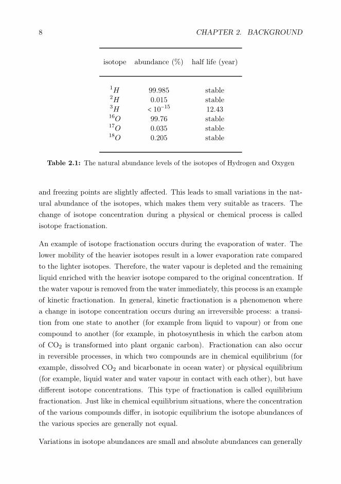
isotope abundance (%) half life (year)

1H 99.985 stable2H 0.015 stable3H < 10−15 12.4316O 99.76 stable17O 0.035 stable18O 0.205 stable

Table 2.1: The natural abundance levels of the isotopes of Hydrogen and Oxygen

and freezing points are slightly affected. This leads to small variations in the nat-

ural abundance of the isotopes, which makes them very suitable as tracers. The

change of isotope concentration during a physical or chemical process is called

isotope fractionation.

An example of isotope fractionation occurs during the evaporation of water. The

lower mobility of the heavier isotopes result in a lower evaporation rate compared

to the lighter isotopes. Therefore, the water vapour is depleted and the remaining

liquid enriched with the heavier isotope compared to the original concentration. If

the water vapour is removed from the water immediately, this process is an example

of kinetic fractionation. In general, kinetic fractionation is a phenomenon where

a change in isotope concentration occurs during an irreversible process: a transi-

tion from one state to another (for example from liquid to vapour) or from one

compound to another (for example, in photosynthesis in which the carbon atom

of CO2 is transformed into plant organic carbon). Fractionation can also occur

in reversible processes, in which two compounds are in chemical equilibrium (for

example, dissolved CO2 and bicarbonate in ocean water) or physical equilibrium

(for example, liquid water and water vapour in contact with each other), but have

different isotope concentrations. This type of fractionation is called equilibrium

fractionation. Just like in chemical equilibrium situations, where the concentration

of the various compounds differ, in isotopic equilibrium the isotope abundances of

the various species are generally not equal.

Variations in isotope abundances are small and absolute abundances can generally

2.1. WATER ISOTOPES 9

not be measured with high enough precision. In an isotope measurement the abun-

dances of the rare isotope and the abundant isotope are determined simultaneously

leading to an abundance ratio (R). For example, for Oxygen-18:

18R = number of 18O atoms

number of 16O atoms= [18O][16O] (2.1)

This abundance ratio of a sample is then compared to that of a reference material

that is measured just before or after the sample measurement. This leads to the

delta notation:

δ = Rsample

Rreference

− 1 (2.2)

As deviations from the reference material are mostly small, it is common to express

them in per mill (h). The isotope ratios determined in this way have a much

higher precision than an individual absolute measurement of an abundance level

would have. Measurement techniques used in isotope analyses are discussed in

more detail in section 2.6

To quantify fractionation effects we use expressions similar to the δ notation. If we

consider a transition from one compound to another (A → B) or two compounds

in equilibrium which each other (A ⇔ B), the isotope fractionation factor α is

defined as:

αA (B) = αB/A = RB

RA

(2.3)

The fractionation factor is mostly close to unity, which is why a second quantity,

the fractionation ǫ, is introduced:

ǫ = α − 1 (2.4)

Just as with the δ value, the value for ǫ is often small and therefore expressed in

per mill.

When an atom has more than two stable isotopes the fractionation factors for the

different isotopes are closely related. This is because fractionation is mostly caused

by the mass difference between the isotopes. For example for carbon, which has


three stable isotopes, it is often assumed that:

14α = (13α)2 (2.5)

In reality, the power in this equation slightly deviates from two. For example, for

natural water samples Meijer and Li (1998) found the following relation between

the Oxygen-17 and Oxygen-18 content in natural waters:

1 +18 δ = (1 +17 δ)(1.8935±0.005) . (2.6)

However, in most cases the approximation that the fractionation scales with the

mass difference (as in equation 2.5) is sufficient.

2.2 Rayleigh distillation

Rayleigh distillation is the process in which the isotopic composition of a substance

is followed in time during a phase transition or chemical process. It is named

after Lord Rayleigh who studied fractional distillation of mixed liquids (Rayleigh,

1896). As an example we consider a reservoir of water vapour that is subject to

condensation. As the water vapour condenses the heavy isotope concentration of

the remaining water vapour gradually decreases. If the total number of molecules

in the reservoir is N and the ratio of rare to abundant isotopic molecules is R, the

number of abundant isotopic molecules is given by:

Na = N

1 +R (2.7)

and the number of rare isotopic molecules by:

Nr = RN

1 +R (2.8)

After removing a fraction dN molecules from the reservoir with an associated

isotope fractionation factor α, the reservoir contains (N − dN) molecules with a

ratio of (R−dR), as indicated in the box model in Figure 2.1. As the total number

of rare isotopic molecules should be constant we can write the following balance

2.2. RAYLEIGH DISTILLATION 11

N R

N-dN R-dR

dN αR

Figure 2.1: Box model for the Rayleigh distillation process.

equation:RN

1 +R =(R − dR) (N − dN)

1 +R − dR + αRdN

1 + αR (2.9)

To a good approximation the denominators in this equation are all equal (dR is

small when considering small fractions and α is close to unity). This simplifies

equation 2.9 to:

RN = RN −NdR −RdN + dRdN +αRdN (2.10)

Neglecting the product of differentials this is equivalent to:

dR

R= (α − 1) dN

N(2.11)

Integrating this equation and using the initial conditions: R = R0 and N = N0 this

gives:

R

R0

= ( NN0

)α−1 (2.12)

which can be expressed in delta notation as:

δ = (1 + δ0)( NN0

)α−1 − 1 (2.13)

where δ0 is the initial isotope ratio. For the fraction removed from the reservoir

the isotopic ratio at any stage is simply given by αR, with R given by equation

2.12. Integrating this we obtain the isotope ratio for the total removed fraction:

δremoved = (1 + δ0) 1 − (NN0)α

1 − NN0

− 1 (2.14)


00.10.20.30.40.50.60.70.80.91−30

−25

−20

−15

−10

−5

0

5

10

original fraction remaining

δ 18

O (

‰)

reservoirfraction removedcumulative removed

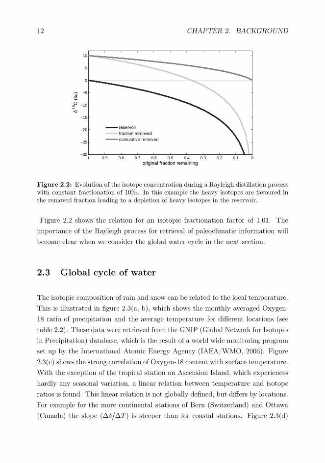
Figure 2.2: Evolution of the isotope concentration during a Rayleigh distillation processwith constant fractionation of 10h. In this example the heavy isotopes are favoured inthe removed fraction leading to a depletion of heavy isotopes in the reservoir.

Figure 2.2 shows the relation for an isotopic fractionation factor of 1.01. The

importance of the Rayleigh process for retrieval of paleoclimatic information will

become clear when we consider the global water cycle in the next section.

2.3 Global cycle of water

The isotopic composition of rain and snow can be related to the local temperature.

This is illustrated in figure 2.3(a, b), which shows the monthly averaged Oxygen-

18 ratio of precipitation and the average temperature for different locations (see

table 2.2). These data were retrieved from the GNIP (Global Network for Isotopes

in Precipitation) database, which is the result of a world wide monitoring program

set up by the International Atomic Energy Agency (IAEA/WMO, 2006). Figure

2.3(c) shows the strong correlation of Oxygen-18 content with surface temperature.

With the exception of the tropical station on Ascension Island, which experiences

hardly any seasonal variation, a linear relation between temperature and isotope

ratios is found. This linear relation is not globally defined, but differs by locations.

For example for the more continental stations of Bern (Switzerland) and Ottawa

(Canada) the slope (∆δ/∆T ) is steeper than for coastal stations. Figure 2.3(d)

2.3. GLOBAL CYCLE OF WATER 13

Ascension Island (Atlantic Ocean)Invercargill (New Zealand)Vernadsky (Antarctica Peninsula)Ottawa (Canada)Groningen (Netherlands)Bern (Switzerland)

Feb Apr Jun Aug Oct Dec

−15

−10

−5

0

δ 18

O (

‰ )

(a)

Feb Apr Jun Aug Oct Dec−10

0

10

20

Tem

pera

ture

(oC

)

(b)

−10 0 10 20

−15

−10

−5

0

δ 18O (‰

)

Temperature ( oC)

(c)

−15 −10 −5 0

−100

−50

0

δ 2H (‰

)

δ 18O (‰ )

(d)

Figure 2.3: Monthly averaged Oxygen-18 isotope ratios in precipitation water and sur-face temperatures for different locations. For all the stations the data is averaged overat least 16 years. Figures (c) and (d) illustrate linear relationships between temperatureand Oxygen-18 content and between Oxygen-18 and Deuterium. The solid line in figure(d) is the global meteoric water line defined by equation 2.15. Geographic locations ofthe stations are given in Table 2.2.

gives the relation between Oxygen-18 and Deuterium in the precipitation for the

different stations. The line on which most of the data points fall is the Global

Meteoric Water Line (GMWL) which was defined by Craig (1961) as:

δ2H = 8 ∗ δ18O + 10 h (2.15)

To be able to explain the relation between Oxygen-18 content in precipitation

and temperature and the relation between Oxygen-18 and Deuterium we need to

consider the whole hydrological cycle. The source of most precipitation water on

earth is the (sub) tropical ocean, where evaporation is high. As ocean water is used

as the international standard for water isotopes and the ocean is well mixed, the

isotope ratio for the tropical ocean is close to 0 h for both Oxygen-18 and Deu-

terium. Assuming a water temperature of 25C the isotope ratio for the formed


station Latitude Longitude Altitude(N) (E) (m)

Ascension Island -7.92 -14.42 15Invercargill -46.42 168.32 2Vernadsky -65.08 -63.98 20Ottawa 45.32 -75.67 114Groningen 53.23 6.55 1Bern 46.95 7.43 511

Table 2.2: The locations of the GNIP stations in Figure 2.3

vapour would be -9.3 h and -76 h for Oxygen-18 and Deuterium, respectively,

if the evaporation of water is accompanied by an equilibrium fractionation pro-

cess. However, Craig and Gordon (1965) showed that kinetic effects occur during

evaporation. They developed a model for evaporation that consists of several lay-

ers from the water surface to the free atmosphere. The first layer is a very thin

(∼ µm) boundary layer in which the water vapour is in isotopic equilibrium with

the liquid water. Above the boundary layer there is a transition zone in which

water vapour is transported in both vertical directions by molecular diffusion. In

this layer kinetic effects occur depending on the humidity of the layer. When the

humidity is close to 1, downward diffusion is equal to upward diffusion and no net

diffusive fractionation occurs. However, when the humidity is low there is a net

transport from the boundary layer to the free atmosphere and kinetic fractionation

will occur.

The next step in the hydrological cycle is the transport of water vapour to higher

latitudes and the formation of precipitation. As an air mass with water vapour

moves to a higher latitude, it gradually cools down. When the dew point is passed

(the temperature at which the humidity is 100%), water vapour condenses and

rain (or snow) will form. When the temperature stabilizes or increases the rain

stops and the air parcel moves further towards higher latitudes. This process,

schematically depicted in figure 2.4, is a Rayleigh type distillation. In subsequent

precipitation events a fraction of the water vapour is removed from the cloud

causing the remaining water vapour to be depleted in heavy isotopes.

2.3. GLOBAL CYCLE OF WATER 15

sub tropics polar region

ice sheet

0 h

-10 h

-5 h

-15 h

-30 h

-18 h

-40 h

-28 h

Figure 2.4: Schematic representation of the Rayleigh fractionation process in the hy-drological cycle. During transport towards the polar regions water vapour cools whichcauses the cloud to partially rain out. As heavier isotopes are favoured in the condensedphase, the cloud gets more and more depleted as it moves to higher latitudes.

Considering the processes discussed above the slope and offset of the meteoric wa-

ter line can be explained. Condensation in a cloud is an equilibrium fractionation

processes. For this process the fractionation for Deuterium is about 8 times larger

than for Oxygen-18, which explains why the meteoric water line has a slope of

8. The offset is caused by kinetic fractionation that occurs during evaporation.

For very low humidities fractionation is dominated by diffusive transport in the

transition zone. The diffusion coefficient for water vapour diffusing through air is

dependent on the molecular masses of the two diffusing species. The fractionation

of an isotopic molecule is then determined by the mass difference between the

rare molecule and the most abundant. As this mass difference is twice as high for

Oxygen-18 than it is for Deuterium, also the fractionation is twice as large. Thus,

in a δ2H - δ18O diagram, the evaporation causes the isotopic composition of the

formed vapour and residual water to move away from the GMWL with a much

lower slope. As a result the amount of Deuterium in the water vapour under con-

ditions with low humidity exceeds the amount of Deuterium that would be in the

water vapour if humidity was 100 %. For this reason Dansgaard (1964) introduced


the term deuterium excess (d) which is defined as:

d = δ2H − 8 ∗ δ18O (2.16)

The global average value for deuterium excess found in precipitation is around

10h, which corresponds to a humidity of ∼ 85%.

The relation between temperature and Oxygen-18 content in precipitation is mainly

caused by the Rayleigh process. As the temperature in a cloud decreases and the

cloud rains out the heavy isotopes are preferentially in the liquid phase, causing

a depletion in the cloud. As the air masses generally move from the tropics to

higher latitudes, the precipitation is most depleted in the high latitude regions.

This latitude effect is strong, but there are several processes that influence the

relation between temperature and isotope content. One of these processes is the

continental effect. As a vapour mass moves over a continent the isotopic compo-

sition evolves more rapidly due to topographic effects and stronger temperature

gradients. This leads to a stronger seasonality in the isotopic signal. Continen-

tal effects can also occur for stations closer to the coast when air masses move

along trajectories that cross continental regions. This illustrates the importance

of transport pathways, which also influences the amount of mixing with other air

masses in the atmosphere. Furthermore, during transport over the ocean, addi-

tional water vapour may be added to the air mass by evaporation. The last effect

discussed here that influences the δ18O - temperature relation is the altitude effect.

When an air mass moves to a higher altitude due to a rise in the landscape, the

air will cool and rain-out will occur. This is very similar to the transport from

the tropics to more temperate latitudes, but in this case it is accompanied with a

systematic decrease in air pressure. This combination leads to a depletion in δ18O

of 0.15 - 0.5 h per 100 meters elevation. All these effects come together in the

isotope signal in ice cores. The Rayleigh effect prevails, making the isotope signal

a powerful ‘proxy’ for temperature and thus climate. The word ‘proxy’ indicates

that there exists a clear relation between isotope signal and temperature, but the

relation is neither linear nor constant over time. For example, an ice cap may have

had a higher altitude in the past, causing a different isotope - temperature relation

due to the altitude effect. Also, the flow of ice within an ice sheet needs to be taken

into account as the deeper layers were deposited further towards the interior of the

ice sheet (at a different elevation). Finally we should notice that the correlation

2.4. POST DEPOSITIONAL PROCESSES 17

between temperature and isotope signal is often done with surface temperatures

(as these are easily measured), but the condensation and fractionation is driven

by the in-cloud temperature.

2.4 Post depositional processes

In polar regions or at high altitudes precipitation falls in the form of snow and when

temperatures are low enough the snow and thereby its isotopic signal are stored

in a glacier, ice cap or ice sheet. Drilling ice cores at these locations enables us to

obtain information about the climate of the past. A schematic representation of an

ice sheet and the flow patterns within it is given in figure 2.5. After precipitating

on the surface snow slowly densifies until it is compressed to ice. The layers of ice

are then further compressed due to the load of the overlying ice. This load causes a

gravitational spreading: the layers become thinner and spread out in a horizontal

direction. As a consequence, the temporal resolution of an ice core record decreases

with depth. Horizontal flow is zero at the ice divide, near the center of the ice

sheet. Most deep ice cores are drilled on the ice divide as the ice is least disturbed

here and it is the location where the oldest ice can be found. The flow of ice further

depends on the basal conditions such as the topography of the bed, temperature

of the basal ice and the presence of liquid water at the bed (Baker, 2012). All

these parameters, as well as the annual accumulation influence the choice of the

location of a deep drilling project. Smaller ice caps and glaciers are also used for

palaeoclimate studies. For these regions the retrieved climatic record does not

extent as far back in time, but they may provide detailed information over the

past decades to centuries.

For the interpretation of the isotopic signal in an ice core it is important to consider

several processes that can alter the isotopic composition of a layer after deposition.

At relatively warm locations the surface snow may be subject to melt. The melt

water then mixes with layers just below the surface where it refreezes. This mixing

of layers leads to a smoothing of the isotope profile. The effect of melt on an

isotope record is discussed in more detail in chapter 5. A second effect that

alters the isotope content at the surface is sublimation. This occurs especially

in dry regions that are exposed to high levels of solar radiation. As sublimation is

accompanied by isotope fractionation, this does not only lead to a mass loss but


Figure 2.5: Schematic representation of the flow of ice in an ice sheet. The verticaldashed line indicates the ice divide where horizontal velocity changes direction. Mostdeep ice cores are drilled close to an ice divide as the stratigraphy at these locations isleast disturbed by ice flow. The load of the overlying ice causes layers to become thinnerand to stretch in a horizontal direction.

also to an isotopic enrichment of the surface layer. As kinetic effects are strong

for these dry conditions a large change is found in the deuterium excess (see for

example Stichler and others (2001)). The opposite effect can occur as well: when

the temperature at the surface drops air moisture may condense and be deposited

on the surface. The isotopic signal in the first few meters of snow can also alter

through ventilation. The snow of the top layers has a large pore space and wind

driven ventilation carries atmospheric water vapour into the snow where it mixes

with the vapour in the pore space (Neumann and Waddington, 2004). In the pore

space the water vapour molecules can then exchange with molecules of the ice

crystals.

The main post depositional process that alters the isotopic composition of a layer

is the diffusion in the firn stage. Snow that has survived one year without being

subject to melt and before it is completely compressed to ice is defined as firn.

However, in practice the terms firn and snow are often used interchangebly (also

in this thesis). A schematic picture of the structure of firn as a function of depth

is given in figure 2.6. Fresh snow at the surface has a very open structure and is of

low density (∼ 300 kg m−3). In the top few meters of the firn pack the densification

rate is most rapid and is mainly driven by grain settling and packing of the snow

until a density of ∼ 550 kg m−3 is reached (Herron and Langway, 1980; Paterson,

1994). In the second stage of densification the firn is compacted due to the load of

the overlying ice. The interconnecting pores in the firn become smaller until they

2.4. POST DEPOSITIONAL PROCESSES 19^^ ^ ^ ^ ^^ ^ ^

Figure 2.6: Schematic representation of the structure of firn with depth. At the surfacethe density of the firn is very low and the air content is high. With increasing depth thepores reduce in size until at a depth of ∼ 60 m they close off and isolated air bubbles exist.

close off and air bubbles are formed in the ice. Pore close off typically occurs at

a density of ∼800 kg m−3. The third stage of densification is below the pore close

off depth, where the compression continues and air bubbles become smaller.

Firn diffusion takes place in the first and second stage of densification and is caused

by the random movement of water molecules in the firn. This leads to an average

displacement of molecules and thereby to a mixing within the firn. Sharp isotopic

transitions from one layer to the next are dampened as a result of this mixing.

Transport of water molecules in the firn stage occurs mainly in the vapour phase

in the pores of the snow. Transport within the matrix of the ice grains occurs as

well, but at a rate several orders of magnitude lower. As there is also an exchange

of molecules between the vapour phase and the ice matrix at the grain boundaries

essentially all molecules take part in the diffusion process in the vapour phase

(Whillans and Grootes, 1985).

The strength of diffusion depends on several physical parameters. Most of the

transport takes place in the vapour phase as this is where the molecules have

the largest mobility. Therefore, the strength of diffusion is mainly influenced


by the amount of pore space and the density of the firn. The average distance

molecules are transported also depends on the shape of the interconnecting pores.

In straight channels molecules are less restricted in their movement than in more

tortuous channels. Below pore close off depth firn diffusion stops as the movement

in the vapour phase is restricted to the air bubble. Another important factor

in the diffusion rate is the amount of molecules in the vapour phase, which is

influenced by temperature and air pressure in the pores. Finally, we should note

that diffusivity is different for different isotopes of the water molecule. In the

exchange of molecules between ice grains and vapour in the pore space equilibrium

fractionation takes place: the heavier isotopes are preferentially in the solid phase.

In addition, the transport within the water vapour is less for heavier isotopes as

they have a lower mobility. All these factors influence the firn diffusivity for which

a mathematical expression will be derived in Chapter 3.

2.5 Solving the diffusion equation

Diffusion is the process in which gradients in the concentration of particles become

smoother as a result of the random movement of these particles. Mathematically

diffusion is described by Ficks second law (Fick, 1855):

∂C

∂t=D∂2C

∂x2(2.17)

where we consider only one spatial dimension (x) and C is the concentration

which varies in space and time. The diffusion coefficient (or diffusivity) D (in m

s−1) determines the magnitude of diffusion effects. In the following sections three

different methods for solving this equation with prescribed initial and/or boundary

conditions are discussed.

2.5.1 Fundamental solution

The solution of the diffusion equation for the most general case, in which only

the initial condition is prescribed as some arbitrary function on an infinite spatial

domain, is called the fundamental solution. The derivation of this solution follows

a similar approach as described by van Duijn and de Neef (2004). We first consider

2.5. SOLVING THE DIFFUSION EQUATION 21

the special case where the initial concentration is given as a step change. The initial

value problem in that case is given as:

∂C

∂t=D∂2C

∂x2−∞ < x < ∞, t > 0

C (x,0) =⎧⎪⎪⎪⎪⎨⎪⎪⎪⎪⎩C1 x < x0C0 x > x0

(2.18)

For convenience the concentration is scaled such that:

∂u

∂t=D∂2u

∂x2−∞ < x < ∞, t > 0

u (x,0) =⎧⎪⎪⎪⎪⎨⎪⎪⎪⎪⎩1 x < x00 x > x0

(2.19)

where u is the scaled concentration and is given by:

u = C −C0

C1 −C0

(2.20)

Note that for a function u (x, t) that solves equation 2.19 all functions uk =u(kx, k2t) for all k > 0 are also solutions. Therefore, u only depends on the

combinationx√t. Substituting

x − x0√t

by a new variable ξ the partial differential

equation (2.19) can be rewritten into a normal differential equation for f (ξ):D

∂2f

∂ξ2+ 1

2ξ∂f

∂ξ= 0 −∞ < ξ < ∞

f (−∞) = 1f (∞) = 0

(2.21)

To solve this we first substitute v by∂f

∂ξ:

D∂v

∂ξ+ 1

2ξ v = 0 (2.22)


The solution for this equation is given by:

v = A exp(−ξ24D) (2.23)

Integrating this gives the solution for f :

f (ξ) = ∫ ξ

−∞A exp(−ξ2

4D)dξ +B (2.24)

where the integration constants A and B can be obtained from the boundary

conditions given in equation 2.21:

f (−∞) = ∫ −∞

−∞A exp(−ξ2

4D)dξ +B = 1

B = 1(2.25)

f (∞) = ∫ ∞

−∞A exp(−ξ2

4D)dξ + 1 = 0

A1√4D∫∞

−∞exp (−τ2)dτ = −1

A = −12√πD

(2.26)

where in equation 2.26 we used the substitution τ = ξ√4D

. Inserting these values

into equation 2.24 and using the same substitution gives:

f (ξ) = 1 − 1

2√πD∫

ξ

−∞exp(−ξ2

4D)dξ

= 1 − 1√π∫

0

−∞exp (−τ2)dτ − 1√

π∫

ξ

2√

D

0

exp (−τ2)dτ= 1

2− 1

2erf( ξ

2√D)

= 1

2erfc( ξ

2√D)

(2.27)


where we used the definitions of the error function (erf) and the complementary

error function (erfc):

erf (s) = 2√π∫

s

0

exp (−t2)dterfc (s) = 2√

π∫∞

sexp (−t2)dt (2.28)

For u the solution is then given as:

u (x, t) = 1

2erfc(x − x0

2√Dt) (2.29)

and using u = C −C0

C1 −C0

we obtain the solution for the initial value problem given

by equation 2.18:

C (x, t) = C0 + 1

2(C1 −C0) erfc(x − x0

2√Dt) (2.30)

This is the solution for a step profile as the initial concentration. The next step to-

wards finding the solution for the general case of an arbitrary initial concentration

is the case of a pulse. The problem in this case is given as:

∂C

∂t=D∂2C

∂x2−∞ < x < ∞, t > 0

C (x,0) =⎧⎪⎪⎪⎪⎪⎪⎪⎨⎪⎪⎪⎪⎪⎪⎪⎩

C1 x < −aC0 −a < x < aC1 x > a

(2.31)

The pulse can be described as a sum of two stepfunctions:

C (x,0) = Cu (x,0) +Cd (x,0) (2.32)

where Cu and Cd are given as:

Cu (x,0) =⎧⎪⎪⎪⎪⎨⎪⎪⎪⎪⎩C1 x < −aC0 x > −a

Cd (x,0) =⎧⎪⎪⎪⎪⎨⎪⎪⎪⎪⎩0 x < aC1 −C0 x > a

(2.33)


The solution for the problem in equation 2.31 is then given by the sum of the

solutions for the two step functions:

C (x, t) = C1 + 1

2(C0 −C1)⎛⎝erfc(

x − a2√Dt) − erfc( x + a

2√Dt)⎞⎠

= C1 + 1

2(C0 −C1) 2

π∫

x+a2√

Dt

x−a2√

Dt

exp (−τ2)dτ(2.34)

Choosing C1 = 0 and C0 = M

2athe initial conditions become:

C (x,0) =⎧⎪⎪⎪⎪⎪⎪⎪⎪⎨⎪⎪⎪⎪⎪⎪⎪⎪⎩

0 x < −aM

2a−a < x < a

0 x > a(2.35)

Using these values we have:

lima ↓ 0

C (x,0) = 0 for all x ≠ 0 (2.36)

and

∫∞

−∞C (x,0) =M for all a > 0 (2.37)

This means that for the limit of a towards 0, the initial concentration can be

written as a Dirac distribution:

C (x,0) =M δ (x) (2.38)

Equation 2.34 can then be written as:

C (x, t) = lima ↓ 0

M

2a√π∫

x+a2√

Dt

x−a2√

Dt

exp (−τ2)dτ= M

2√πDt

∫∞

−∞δ (τ − x

2√Dt) exp (−τ2)dτ

= M

2√πDt

exp(− x2

4Dt)

(2.39)


Using equations 2.38 and 2.39 we can construct a solution for the general case for

which the initial condition is given as:

C (x,0) = C0 (x) −∞ < x < ∞ (2.40)

This initial concentration can be seen as a infinite sum of Dirac distributions. In

fact, for any continuous function C0 we can write:

C0 (x) = ∫ ∞

−∞C0 (y) δ (y − x)dy (2.41)

Using this initial condition, we obtain the fundamental solution of the diffusion

equation:

C (x, t) = 1

2√πDt

∫∞

−∞C0 (y) exp⎛⎝−

(y − x)24Dt

⎞⎠dy (2.42)

Thus the effect of diffusion on an arbitrary initial concentration is described by the

convolution of the initial concentration with a Gaussian distribution. The width

of this distribution is determined by the diffusivity D and the time t.

2.5.2 Separation of variables

A second method for solving the diffusion equation is using separation of variables.

This method is suitable for finding a solution for a problem defined on a finite

interval:∂u

∂t=D ∂2u

∂x20 < x < L t > 0 (2.43)

For homogeneous boundary conditions we have:

u (0, t) = 0u (L, t) = 0 (2.44)

To find the solution using separation of variables we assume that the solution can

be written as the product of a time dependent function and a spatial dependent

function:

u (x, t) =X (x) T (t) (2.45)


with boundary conditions:

X (0) = 0X (L) = 0 (2.46)

Inserting this in equation 2.43 and taking the derivatives leads to:

1

D T (t)dT (t)dt

= 1

X (x)dX (x)dx

(2.47)

As the term on the left hand side of this equation only depends on time t and

the term on the right hand side only on the position x, they must both equal a

dimensionless constant k. Thus, for the time dependent part we have:

dT (t)dt

= kD T (t) (2.48)

which is solved as:

T (t) = α exp (kDt) (2.49)

where α is a constant. Using the boundary conditions (equation 2.46) we can show

that for non trivial solutions the constant k has to be negative. This also ensures

that the solution remains finite for all t > 0. Therefore, we replace k by −λ2 and

obtain the following differential equation for the space dependent part:

X (x)dx

= −λ2X (x) (2.50)

The general solution for this equation is:

X (x) = A cos (λx) +B sin (λx) (2.51)

From the boundary conditions it follows that A = 0 and:

B sin (λL) = 0 (2.52)

Excluding the trivial solution B = 0, we obtain:

λL = nπ n = 0,1,2, ...λ = nπ

L

(2.53)


The solution for a given n is then found by combining equations 2.49 and 2.51:

un (x, t) = bn sin(nπxL) exp(−n2π2Dt

L2) (2.54)

where bn = αBn. The general solution is given as a combination of all possible

solutions:

u (x, t) = ∞∑n=0

bn sin(nπxL) exp(−n2π2Dt

L2) (2.55)

The coefficients bn can be obtained from the initial conditions:

u (x,0) = ∞∑n=0

bn sin(nπxL) (2.56)

Multiplying both sides with sin(mπx

L) and integrating over the entire domain

gives:

∫L

0

u (x,0) sin(mπx

L)dx = ∞∑

n=0bn∫

L

0

sin(nπxL) sin(mπx

L)dx

= ∞∑n=0

1

2L bn δnm

= 1

2L bm

(2.57)

where δnm is the kronecker delta which equals 1 for n = m and 0 otherwise.

Rewriting this equation, the coefficients bm are given as:

bm = 2

L∫

L

0

u (x,0) sin(mπx

L)dx (2.58)

These are the Fourier coefficients of the original profile u (x,0). With equation

2.55 the profile can then be calculated for any time t. Conversely, if the profile

at some time t and the amount of diffusion is known, equation 2.55 can be used

to obtain the initial profile. This procedure is referred to as back-diffusion and

is often applied to isotope records from ice cores to reconstruct the precipitation

record. If we have a measured isotope record δm (z) over a depth interval from 0

to L, the Fourier coefficients are given by:

cm = 2

L∫

L

0

δm (z) sin(mπz

L)dz (2.59)


The total amount of diffusion is related to the product of the diffusivity and the

time of diffusion:

σ2 = 2D t (2.60)

or in the case of time varying diffusivity:

σ2 = ∫ t

0

2D (t′)dt′ (2.61)

This quantity is called the diffusion length and has units of m. It is the average

displacement of particles with respect to the original profile. If the diffusion length

is known or can be estimated from the isotope data (see Chapter 3) the original

precipitation signal δ0 can be estimated as:

δ0 = mmax

∑m=0

δm sin(mπz

L) exp(+m2π2σ

L2) (2.62)

Note that, mathematically spoken, this expression is an example of a so-called

‘ill-posed problem’: the function will go to infinity. Practically, this problem is

circumvented (or regularised) by restricting the summation to a finite number

mmax depending on the measurement noise, which at higher frequencies will dom-

inate the signal. Frequencies at which the noise is larger than the signal should

not be included in the back diffusion calculation.

2.5.3 Numerical method

The third method discussed here for solving the diffusion equation is using a

numerical approximation. This method is especially useful for situations in which

the diffusivity D is varying in space and/or time. Several methods exist for solving

a partial differential equation numerically. Here a forward difference method is

described. Numerical methods for differential equations often use a Taylor series

to approximate the derivatives. According to Taylor’s theorem, any continuous

function f (x) can be approximated as:

f (x) = f (x0) + f ′ (x0) (x − x0) + f ′′ (x0)2!

(x − x0)2 + ...= ∞∑

k=0

f (k) (x0)k!

(x − x0)k(2.63)


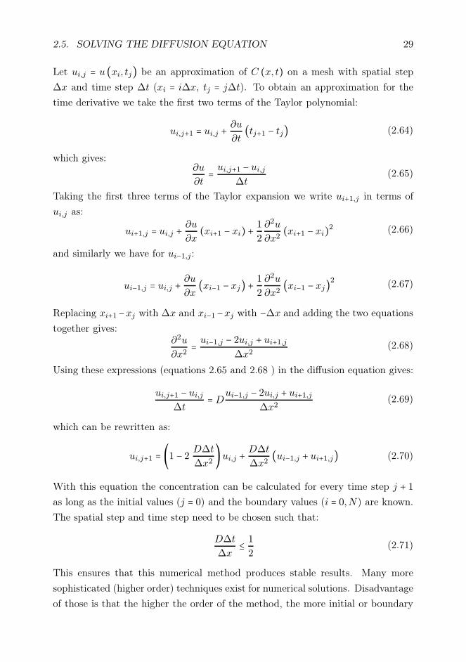
Let ui,j = u (xi, tj) be an approximation of C (x, t) on a mesh with spatial step

∆x and time step ∆t (xi = i∆x, tj = j∆t). To obtain an approximation for the

time derivative we take the first two terms of the Taylor polynomial:

ui,j+1 = ui,j + ∂u

∂t(tj+1 − tj) (2.64)

which gives:∂u

∂t= ui,j+1 − ui,j

∆t(2.65)

Taking the first three terms of the Taylor expansion we write ui+1,j in terms of

ui,j as:

ui+1,j = ui,j + ∂u

∂x(xi+1 − xi) + 1

2

∂2u

∂x2(xi+1 − xi)2 (2.66)

and similarly we have for ui−1,j:

ui−1,j = ui,j + ∂u

∂x(xi−1 − xj) + 1

2

∂2u

∂x2(xi−1 − xj)2 (2.67)

Replacing xi+1−xj with ∆x and xi−1−xj with −∆x and adding the two equations

together gives:∂2u

∂x2= ui−1,j − 2ui,j + ui+1,j

∆x2(2.68)

Using these expressions (equations 2.65 and 2.68 ) in the diffusion equation gives:

ui,j+1 − ui,j∆t

=Dui−1,j − 2ui,j + ui+1,j∆x2

(2.69)

which can be rewritten as:

ui,j+1 = (1 − 2 D∆t

∆x2)ui,j + D∆t

∆x2(ui−1,j + ui+1,j) (2.70)

With this equation the concentration can be calculated for every time step j + 1as long as the initial values (j = 0) and the boundary values (i = 0,N) are known.

The spatial step and time step need to be chosen such that:

D∆t

∆x≤ 1

2(2.71)

This ensures that this numerical method produces stable results. Many more

sophisticated (higher order) techniques exist for numerical solutions. Disadvantage

of those is that the higher the order of the method, the more initial or boundary


conditions have to be provided. Therefore, we have restricted ourselves to the

above second order method.

2.6 Measurement techniques

As explained in section 2.1 the abundance levels of heavy isotopes of water are

being measured as ratios and ratio measurements of a sample are compared with

those of a reference material. As these measurements of sample and reference are

done sequentially, any instrumental drift is negligible and the ratio of these mea-

surements is much more precise than the absolute measurement of an individual

sample.

In the following sections measurement techniques for determination of the Oxygen-

18 and Deuterium isotope ratios used at the Centre for Isotope Research in Gronin-

gen are discussed. These two isotopes are the most commonly used isotopes in ice

core research. In this thesis the radioactive isotope of Hydrogen, Tritium (3H), is

also studied. Tritium is very rare and the experimental setup to determine the

Tritium content in a water sample makes use of its radioactive decay instead of

its mass difference. This technique will be discussed in chapter 5.

2.6.1 Mass spectrometry

The traditional method for measuring the isotope concentration of a sample is iso-

tope ratio mass spectrometry (IRMS) in which the different isotopes are separated

by their mass differences. Recently, an alternative technique for isotope measure-

ments has been developed which is based on the rotational-vibrational transitions

in the near and mid infrared spectral regions of small molecules (Kerstel and oth-

ers, 1999; Kerstel, 2004). Laser spectroscopy is used to measure the absorption

signal of isotopic molecules which is directly related to their abundance levels.

However, we will not go into the details of this technique as all stable isotope

analyses discussed in this thesis used IRMS.

An IRMS instrument basically consists of three parts: the ion source in which the

molecules of the sample are converted to charged particles that are accelerated to

energies of several keV, a magnetic field which separates the particles according

2.6. MEASUREMENT TECHNIQUES 31

to their mass to charge ratio and a set of detectors. To measure an isotopic

concentration, molecules of a gaseous sample are introduced in the ion source,

where they collide with energetic electrons produced by a heated filament. As

a result, the molecules and fragments of the molecules are ionised and are then

accelerated using electric fields. The charged particles then enter a magnetic field

that deflects their pathways. For particles with a higher mass to charge ratio

(m/z) the deflection is lower than for those with a lower m/z ratio. As a result,

the particle stream is separated into several streams which are detected separately.

The detectors consist of Faraday cups that collect the positively charged particles,

which generate a small current proportional to the amount of particles that are

collected in the cup. The isotope ratio of the sample can then be calculated from

the measured currents.

Two different methods of operation can be distuingished in IRMS: the dual inlet

and the continuous flow technique. In the dual inlet (DI) technique the sample

preparation is undertaken completely separately from the isotope measurement

(off line). A gas sample is loaded into the IRMS through an inlet system. This

system consists of several valves and two gas bellows: one contains the sample

gas and one contains the reference gas. To obtain a high precision the bellows

are adjusted such that the pressure difference between them is minimal. The

measurements of a sample gas are then alternated with measurements of a reference

gas by switching the valves of the inlet system. This allows several comparisons of

the isotopic concentrations of the two gases, which improves the precision of the

measurement. In continuous flow (CF) mode the preparation of the gas sample

is done immediately before it enters the mass spectrometer. The gas sample is

introduced into the mass spectrometer using a carrier gas. Just before or after

the gas sample is fed into the analyser, a pulse of reference gas is introduced into

the IRMS. The main advantage of CF operation in comparison to DI is the higher

throughput of samples. The DI measurement technique as such yields a much

higher precision, but the total performance of a DI-based method includes the

necessary pretreatment, which in most cases is precision limiting.


2.6.2 Pretreatment systems

A sample that is introduced into an IRMS needs to be a non condensable gas to

avoid memory effects caused by molecules of the sample sticking to the walls of

the analyser. Thus, before a water sample can be measured pretreatment of the

sample is necessary. Depending on the specific isotope that is measured different

pretreatments are commonly used. Below, an outline of the pretreatment systems

that are used for the measurements of the samples discussed in this thesis is given.

For Oxygen-18 the isotope signal of the water sample is measured after it is trans-

ferred to the non condensable gas CO2. The first step in this procedure is the

removal of dissolved gases that are in the water sample. The sample (typically 0.6

ml) is frozen, after which the gas present in the vial is removed by a pump. As the

sample is melted, dissolved gases in the water are released due to the low pressure

in the vial. These gases are then removed with a second freeze-pump cycle. The

next step is to add CO2 gas to the (still frozen) water sample. The Oxygen atoms

of the gas and the water sample will then exchange, which leads to an isotopic

equilibrium. As this process is relatively slow and temperature dependent, the

CO2 gas and the water sample are kept at constant temperature (∼25C) for at

least 24 hours. After this period the gas is released and brought into the mass

spectrometer. To prevent water vapour from entering the mass spectrometer, a

water trap at ∼-60C is installed between the sample vial and the inlet of the IRMS.

The volume of the lines between the water sample and the IRMS is relatively large

compared to the volume of the sample bellow of the IRMS. To avoid a large loss of

gas in these lines an extra trap at liquid nitrogen temperature is used just before

the inlet system of the IRMS. The CO2 gas in the lines moves into the trap, after

which a valve between the lines and the trap is closed. The trap is then heated to

release the gas into the IRMS. The isotope ratios of the sample are then measured

with the mass spectrometer in dual inlet mode with respect to a reference gas from

a cylinder. The IRMS is tuned such that it measures the m/z ratios of 44, 45, and

46. For a pure CO2 sample an m/z ratio of 44 can only be formed by 12C16O2.

The signal measured at m/z = 46 is mostly caused by 12C16O18O, although there

is also a very small contribution from 12C17O2 and 13C16O17O. We can correct for

this contribution using the measured signal at m/z = 45 which is due to 13C16O2

and 12C16O17O.


The measurements of the Deuterium isotope ratio of water samples is done using

an IRMS in CF mode, where the pretreatment of the sample is done directly

before analysing the gas. The water sample (typically 0.4 µl) is injected into an

oven containing Chromium (Cr) powder that has been heated to ∼1050C. This

leads to the production of Hydrogen gas (Gehre and others, 1996):

2Cr + 3H2O→ Cr2O3 + 3H2 (2.72)

The Hydrogen gas is fed through a gas chromatographic column (GC) into the

mass spectrometer using Helium as a carrier gas. The IRMS is tuned to measure

mass to charge ratio 2 and 3 which corresponds to the 1H2 and 1H2H respectively.

Just before the Hydrogen gas from the sample reaches the mass spectrometer a

pulse of reference gas from a cylinder is measured by the spectrometer. The isotope

ratio of the sample is then calculated with respect to this reference gas. As this

system suffers from memory effects, every sample is measured several times. Most

of this memory was found to occur before the water reduction: in the syringe,

injection block and Cr oven. To reduce the memory effects the syringe is flushed

with the sample water before injecting a new sample, the injection block is heated

to 140 C and the Cr powder is replaced regularly. The memory that results after

these measures are taken typically ranges from 2 to 5 %, which can be corrected

for after the measurement.

2.6.3 Calibration

For both Deuterium and Oxygen-18, isotope ratios are measured with respect to a

reference gas from a cylinder. This reference gas can not be used to determine the

exact isotope ratio of the sample with respect to international standards. This is

because fractionation effects may occur in the pretreatment systems, which may

lead to an offset in the measured isotope ratio. To calibrate the measurements it is

necessary to measure waters of known isotopic composition using the exact same

procedure as is used for the sample measurement. For this reason after every 4

to 8 water samples (depending on the known instrumental drifts of the systems)

a local standard water is measured. A local standard is a water for which the

isotope ratio with respect to the international scale is known. At the Centre for

Isotope Research there are 7 local natural water standards which span a range of


-50.53 h to 0.39 h for Oxygen-18 and -400.8 h to 1.7 h for Deuterium. In every

measurement series at least 3 local standards are included in order to calibrate the

measurements and correct for possible drifts in the instruments. The local stan-

dards are measured regularly (every 1 - 2 years) in a series with the international

standards VSMOW (Vienna Standard Mean Ocean Water) and SLAP (Standard

Light Antarctic Precipitation) to detect possible drifts in the standard waters.

The above procedure leads to a combined uncertainty (accuracy and precision) of

0.07 h for Oxygen-18 and 0.5 h for Deuterium.



Chapter 3

Differential diffusion: using firn

diffusion as a temperature proxy

Diffusion generally results in a smoothing of a signal and thereby to

a loss of information. The stable water isotope signal in ice cores is

subject to diffusion in the firn stage, thereby hampering the interpre-

tation of the signal in terms of past climate. Surprisingly however, firn

diffusion itself also carries a climatic signal. The amount of diffusion an

ice layer has been subject to is very sensitive to changes in temperature

and accumulation rate. This climatic signal can be retrieved by compar-

ing the difference in diffusion between the isotopic molecules 1H18O1H

and 2H16O1H. In the diffusion process both molecules are subject to

the same conditions, but due to different fractionation factors the firn

diffusivity is larger for molecules with 18O than for those with 2H. This

difference in diffusivity depends on the temperature of the firn. There-

fore, a quantitave comparison between the diffusion of different isotopes

leads to a new independent proxy for past local temperatures. We will

explain how the amount of diffusion an ice layer has been subject to can

be retrieved from 18O and 2H ice core records using power spectra and

how it is influenced by the accumulation rate and firn temperature. We

will apply this new method to isotope data from two Holocene sections

of the NorthGRIP ice core.

37

38 CHAPTER 3. FIRN DIFFUSION AS A TEMPERATURE PROXY

3.1 Introduction

The stable water isotope signal in ice core records is a known proxy for past

climatic conditions. The 18O/16O and 2H/1H isotope ratios in precipitation water

depend on the temperature of the cloud during condensation (Dansgaard, 1954b,

1964). In snow and ice stored in ice caps or ice sheets this leads to a seasonal

variation in isotope ratio with depth. However there is no uniform relation between

isotope ratio and atmospheric temperature at the site of precipitation, as the

isotope concentration is also influenced by other factors, such as conditions at

the source region of precipitation, transport pathways between the source and

the precipitation site and altitude of the site. Additionally, after deposition the

isotope profile alters when fresh snow gradually transforms to firn and ice through a

densification process. Apart from a thinning of the annual layers, the amplitude of

the isotope signal is reduced due to diffusion (Langway, 1967). The original signal

is smoothed due to the random movement of water molecules in the firn. This

means that different layers slowly mix and high-frequency variations in the original

profile gradually disappear. The diffusion process is mainly caused by water vapour

moving in the pores of the snow, but as transport also takes place within the ice

matrix and on the boundary of the ice surface and the firn air, virtually all water

molecules take part in the process (Whillans and Grootes, 1985). Diffusion in firn

stops when the interconnecting pores are closed off due to compaction. Diffusion

then continues within the ice matrix at a much slower rate as the mobility of the

molecules in the solid phase is much less than in the vapour phase. Correction for

the effects of diffusion is necessary before the isotope signal can be interpreted and

related to past atmospheric temperatures. For this reason several mathematical

models describing firn diffusion have been developed (e.g. Johnsen, 1977; Whillans

and Grootes, 1985; Cuffey and Steig, 1998; Johnsen and others, 2000)).

Johnsen and others (2000) showed that firn diffusion does not only have a negative

effect on the interpretation of isotope data but also carries a temperature signal.

By comparing the diffusion of different isotopes of water it is possible to retrieve

this signal. The strength of diffusion is determined by the diffusivity, which is a

function of several parameters such as density, temperature and pressure. Most of

these parameters are the same for both isotopes, but firn diffusivity also depends

on the ice-vapour fractionation factor which is different for different isotopes. This

means that there is a difference in the degree of smoothing between δ18O and δ2H

3.2. DIFFUSION THEORY 39

isotope profiles. As the ice-vapour fractionation factors for the two isotopes depend

only on temperature, the difference in smoothing (termed differential diffusion in

the remainder of this chapter) can be used to estimate the temperature of the firn.

This makes firn diffusion a direct indicator of past local surface temperatures.

In section 3.2 we derive an expression for the diffusion length, the average dis-

placement of a molecule due to diffusion, as a function of depth. This derivation

follows from models for firn densification, ice flow and firn diffusivity, which are all

discussed in detail. In section 3.3 we show how the diffusion length can be obtained

from measured isotope records. As a test, the derived method is applied to two

sections of the NorthGRIP ice core on which high-resolution measurements have

been performed. The chosen sections represent a relatively cold and a relatively

warm period in the Holocene (dated as 9800 - 9200 b2k (before 2000 AD) and 1530

- 1630 AD, respectively) and serve as an example of the potential value of this

method. The interpretation of the obtained diffusion lengths for these sections in

terms of past temperatures follows in section 3.4. Finally, in section 3.5 results are

summarised and the benefits and limitations of differential diffusion are discussed.

3.2 Diffusion theory

Water molecules in firn can move within ice grains, exchange between neighbouring

grains, exchange with the air in the pore space and move as vapour through the

pore space. The net effect of all these processes is a Gaussian smoothing of the

original isotopic variations in the firn. Therefore, the isotopic signature at any

time t after deposition is a convolution between the original signal δ (z,0) and a

Gaussian filter:

δ (z, t) = 1

σ√2π∫∞

−∞δ (z,0) exp⎛⎝

−1

2(z − ζ)2σ2

⎞⎠dζ (3.1)

where σ is the diffusion length and z is the vertical axis with an origin that is

fixed to a layer as it moves down from the surface. A complete derivation of

this equation can be found in section 2.5.1. The layer is compressed due to the

densification of firn to ice and due to ice flow. This can be included in equation

3.1 by correcting the initial profile for the total vertical strain. This correction is


derived from the strain rate εz :

εz (t) = 1

z (t)dz (t)dt

(3.2)

Rearranging and integrating this equation we obtain the compressed vertical scale

z at time t after deposition:

z (t) = z′ exp(−∫ t

0

εz (τ)dτ) (3.3)

where z′ is the uncompressed vertical scale. In this way the effect of strain and

diffusion are treated seperately. The initial profile is compressed first, after which

the compressed profile is smoothed according to equation 3.1. In reality these

processes occur simultaneously, which means that the diffusion length σ tends to

increase due to diffusion but at the same time tends to decrease due to compression

of the firn.

The diffusion length is the average vertical distance the molecules are displaced

due to diffusion. For a constant diffusivity it can be found by realising that the

expectation value of the squared displacement is given as:

σ2 = ⟨z2⟩ = 2 Ω t (3.4)

As we will see in section 3.2.3, firn diffusivity is not constant in time but varies

mainly due to density changes. Therefore, equation 3.4 is only valid for small time

intervals with constant diffusivity:

dσ2 = 2 Ω (t)dt (3.5)

The squared length scale dσ2 in the firn is subject to compression. Using equation

3.2 we can calculate the change in a squared length scale as a consequence of strain

as:dL2

dt= 2LdL

dt= 2 L2 εz (3.6)

The change in diffusion length with time due to the combined effect of diffusion

and strain is then given as:

dσ2

dt= 2 εz(t) σ2 + 2 Ω (t) (3.7)


This equation describes the diffusion length as a function of time since deposition.

To solve this equation it is more convenient to express the diffusion length in terms

of density, which can then be related to depth and time. Therefore we rewrite the

equation as:dσ2

dρ

dρ

dz

dz

dt= 2 εz (ρ) σ2 + 2 Ω (ρ) (3.8)

The solution of this differential equation is based on three models which are dis-

cussed in the next sections. An expression for the change in density with depth is

derived from the Herron-Langway densification model (Herron and Langway, 1980)

(section 3.2.1). In section 3.2.2 a Dansgaard-Johnsen ice flow model (Johnsen and

Dansgaard, 1992) is described which will be used to find expressions for strain

rate εz and the vertical velocity w = dz/dt. An expression for diffusivity is derived

in section 3.2.3 following earlier work of Johnsen and others (2000). To obtain

the diffusion length as a function of depth the different expressions are inserted in

equation 3.8, which is then solved (section 3.2.4).

3.2.1 Densification

Density as a function of depth is described in the empirical densification model

of Herron and Langway (1980). Densification of snow to ice is divided into three

stages. In the first stage the process is dominated by grain settling and packing,

until a critical density (ρc) of 550 kg m−3 is reached. The second stage is domi-

nated by compaction where the interconnecting air channels in the firn slowly get

narrower and shorter. The second stage ends at a density of ρ ∼830 kg m−3 where

the pores are closed off and the air in the firn is only present in closed bubbles.

In the last stage the densification takes place by further compression of the air

bubbles until the ice reaches its final density of ρice ∼917 kg m−3.

The Herron-Langway model is based on the idea that the change in air space in

the firn is linearly related to the change in stress due to the weight of the overlying

snow (Robin, 1958). Mathematically, this is described in the following differential

equation:dρ

dz=Kρ (ρice − ρ) (3.9)

The value for K determines the densification rate which is different for the two


stages:dρ

dz= k0 ρ (ρice − ρ) , ρ ≤ ρc

dρ

dz= k1c−0.5w ρ (ρice − ρ) , ρc < ρ ≤ ρmax

(3.10)

where ρc = 550 kg m−3 is the critical density and ρmax = 800 kg m−3 is the

maximum density for which Herron and Langway (1980) found their model to be

in agreement with observations. The annual accumulation cw is given in meters

of water equivalent. Herron and Langway found the following values for the pa-

rameters k0 and k1 to best fit data from several Greenlandic and Antarctic ice

cores:k0 = 0.011 ⋅ e 10160

RT

k1 = 0.575 ⋅ e 21400

RT

(3.11)

To improve agreement with observations from Central Greenland density profiles

Johnsen and others (2000) scaled k0 and k1 with 0.85 and 1.15, respectively. As

we apply the model developed here to sections from the NorthGRIP ice core, we

use the same scaling factors.

Firn density as a function of depth is found by integrating equation 3.9. For the

first stage of densification the integration is from ρ0, the firn density at the surface,

to some density ρ ≤ ρc:ρ = ρice R0 exp (ρicek0z)

1 +R0 exp (ρicek0z) , R0 = ρ0

ρice − ρ0, ρ ≤ ρc (3.12)

After Johnsen and others (2000) a surface density of 360 kg m−3 is used. The

depth zc corresponding to the critical density is found by rearranging equation

3.12:

zc = lnRc/R0

ρicek0, Rc = ρc

ρice − ρc(3.13)

For the second densification stage a similar integration from the critical density to

some density ρ ≤ ρmax gives:

ρ = ρice Rc exp (ρicek1 (z − zc) c−0.5w )1 +Rc exp (ρicek1 (z − zc) c−0.5w ) , ρc < ρ ≤ ρmax (3.14)

Vinther (2003) showed that for central and southern Greenland this expression

also holds for densities higher than ρmax. Therefore the upper boundary ρmax in


x

z

H

h

0

uλH

λB

Bedrock

Figure 3.1: Schematic depiction of the Dansgaard-Johnsen ice flow model in which theflow is divided into two layers: the horizontal velocity of the top layer is constant withdepth whereas a linear decrease in velocity is assumed for the bottom layer. At the icedivide (x = 0) the horizontal component of the velocity is zero.

expression 3.14 can be removed for studies in these areas.

3.2.2 Ice flow

The vertical strain rate εz in equation 3.8 consists of two components. In the firn

stage strain is mostly due to densification, whereas deeper down strain is caused by

ice flow and deformation: due to the weight of the overlying ice a layer will stretch

out and become thinner. In this section strain due to ice flow will be described

using (a slightly adapted version of) a model derived byJohnsen and Dansgaard

(1992). This model, schematically depicted in Figure 3.1, assumes incompressible

ice (the firn stage is ignored) and flow in two dimensions only (x and z). Ice flows

from the ice divide (x = 0), where horizontal ice flow is zero, to the margins of

the ice sheet. A further assumption is that the ice sheet is in steady state with

an ice sheet thickness H that is constant in time and accumulation rate λH and

basal melt rate λB constant in space and time.

The model assumes that the ice sheet can be divided into two vertical layers. In


the top layer horizontal velocity is constant with depth. Below a certain depth,

the kink depth h, the velocity is linearly decreasing. At the bed ice moves with a

small horizontal velocity uB . Mathematically this is expressed as:

u (z) =⎧⎪⎪⎪⎪⎨⎪⎪⎪⎪⎩uH (fB + (1 − fB) z

h) z < h

uH h ≤ z ≤H (3.15)

where fB is the ratio of the horizontal velocity at the bed uB and the horizontal

velocity at the surface uH . As we assume steady state and incompressible ice, the

total volume of ice that is added as accumulation must be compensated by melt

and horizontal transport of ice. As can be seen from Figure 3.2, the total volume

of ice added by accumulation between the ice divide and a distance x from the

ice divide is given by the product of λH and the area (dy ⋅ x). Considering all the

fluxes in and out of the volume of ice shown in Figure 3.2 and realising that the

horizontal velocity u varies with depth, the mass balance equation is given as:

(λH − λB)x = ∫ H

0

u (z)dz= ∫ h

0

uH (fB + (1 − fB) zh)dz + ∫ H

huHdz

= uH (fBh + 1

2(1 − fB)h + (H − h))

(3.16)

Rewriting this equation we obtain an expression for the velocity at the ice surface

as a function of distance from the ice divide x:

uH = λH

He

x (3.17)

where He is the effective ice sheet thickness which is equal to:

He = λH

λH − λB

(H − 1

2h (1 − fB)) (3.18)

The annual layer thickness at the ice surface is equal to the annual accumulation

rate λH ; at the bottom it is given by the annual melt rate λB . At any other

depth the annual layer thickness λ can be calculated from the vertical velocity

w = dz/dt. The assumption of incompressible ice means that a change in vertical

velocity must be balanced by a change in horizontal velocity. This leads to the


x

H

00

dy

u

λH

λB

Figure 3.2: The mass balance of a column of ice at the ice divide. In steady state theflux of ice at the surface due to accumulation (λH) must be compensated by melt at thebase of the ice (λB) and lateral ice transport (u).

continuity equation:dw

dz+

du

dx= 0 (3.19)

During one year an annual layer will be vertically displaced by exactly it’s own

layer thickness:

w = −λτ, τ = 1 year (3.20)

where velocity is negative as the vertical coordinate is directed positive upwards.

Combining this with equation 3.19 gives:

dλ

dz= −dw

dz= du

dx(3.21)

The annual layer thickness at any depth z can now be obtained by integrating

the horizontal velocity gradient. Inserting equations 3.15 and 3.17 in the equation

above and integrating from the surface to a depth z ≥ h gives the annual layer


thickness as a function of depth for the layer with constant horizontal velocity.

λ (z) = λH + ∫z

H

λH

He

dz

= λH

He

(z −H +He)(3.22)

For the layer with linearly decreasing horizontal velocity we start the integration

at the bed. The annual layer thickness is then given by:

λ (z) = λB + ∫z

0

λH

He

(fB + (1 − fB) zh)dz

= λB +λH

He

(fBz + (1 − fB) z22h)

The total vertical strain εz experienced by a layer due to ice flow at a depth z

is given by the ratio of the layer thickness at this depth and the original layer

thickness at the surface:

εz (z) = λ (z)λH

(3.23)

In the Dansgaard-Johnsen ice flow model the existence of a firn layer is neglected,

which means that the strain due to firn densification is not included in the above

equation. In the remainder of this section we derive an expression for the ver-

tical strain rate in terms of the vertical velocity w, which includes densification.

Rewriting the general equation for strain rate (equation 3.2) in terms of annual

layer thicknesses leads to:

εz = dλ

λ dt(3.24)

Which, by using equation 3.20, can be rewritten in terms of the vertical velocity

as:

εz = dw

wdt= dw

wdz

dz

dt= dw

dz(3.25)

Assuming steady state the total mass in a volume element is constant. Thus, mass

transport in the horizontal direction is balanced by mass transport in the vertical

direction:d (ρu)dx

+

d (ρw)dz

= 0

udρ

dx+ ρ

du

dx+ ρ

dw

dz+w

dρ

dz= 0

(3.26)

As there is no change in density in the horizontal direction, the first term of


equation 3.26 is equal to zero. Using this together with equation 3.25 the following

expression for the strain rate is found:

εz = dw

dz= −du

dx−w

dρ

ρdz(3.27)

Inspection of these two terms leads to the conclusion that the first term on the

right-hand-side (RHS) is due to ice flow, whereas the second term is caused by

firn densification.

For shallow depths the effect of ice flow is negligible and the vertical velocity can

be expressed in terms of firn density. The vertical velocity at the ice surface is

equal to the annual accumulation rate in meters of ice (c) corrected for density:

w0 = ρice c

ρ0(3.28)

where ρ0 and ρice are the density of firn at the surface and ice, respectively. Ne-

glecting ice flow we obtain a similar relation for the vertical velocity further down

in the firn.

w = ρice c

ρ(3.29)

3.2.3 Diffusivity

The strength of diffusion is determined by the firn diffusivity Ωf , for which an

expression was derived by Johnsen and others (2000). For completeness we will

repeat their analysis here. The main mechanism for transport of water molecules

is random movement in the vapour phase through the air space of porous firn.

Therefore, we first consider the diffusion of water vapour in air. Assuming a

constant diffusivity Ωa in air the diffusion length is given by:

σ2

i = 2 ⋅Ωai ⋅ t (3.30)

For variables depending on the isotopic composition of a molecule a subscript i

is used to indicate one of the heavy molecules 1H218O or 1H16O2H (i = 18, 2).

Without subscript they refer to the most abundant water molecule 1H216O. The

diffusivity in a porous medium like firn Ωp is given as Ωp = φ Ωa/τ (Weissberg,


1963) where φ is the porosity, which for firn is given by:

φ = 1 − ρ

ρice(3.31)

The tortuosity τ accounts for the shape of the interconnecting pores. Thus, the

porosity gives the relative amount of air available in the firn and the tortuosity is a

measure for the distribution of air. In this derivation porosity is not used directly,

but is included in the mean residence times in the vapour and solid phase of the

molecules (∆tv and ∆ts, respectively). During one period in the vapour phase a

molecule will change it’s mean square vertical position by:

∆σ2

i = 2 ⋅ Ωai

τ⋅∆tvi (3.32)

Furthermore, as ∆ts >>∆tv, during one period in the solid phase most molecules

will also have spent one period in the pore space and thus have changed their

vertical position according to equation 3.32. Thus, for the squared diffusion length

as a function of time the following estimate can be obtained:

dσ2

i

dt≃ ∆σ2

i

∆tsi= 2 ⋅ Ωai

τ⋅

∆tvi

∆tsi= 2 ⋅ Ωai

τ⋅ ri (3.33)

Here ri is the ratio between the residence times of the molecule in the vapour

and solid phase, respectively. This ratio is equal to the ratio of the total number

molecules in the vapour and solid phase:

ri = ∆tvi

∆tsi= Nvi

Nsi

(3.34)

Assuming isotopic equilibrium between the vapour and ice, the ratio of heavy

isotopic molecules to the more abundant light molecules for the vapour and solid

phase are related by:Nvi

Nv

= 1

αi

Nsi

Ns

(3.35)

where αi is the fractionation factor for water vapour over ice. Combining equations

3.34 and 3.35 leads to the following expression for diffusivity in firn:

Ωfi = Ωai

τri = Ωai

τ

1

αi

Nv

Ns

(3.36)


The number of molecules in the solid phase in 1 kg of firn Ns is NA/m, where m

is the molar weight of water and NA is Avogadro’s number. For the number of

molecules in the vapour phase the ideal gas law is used to obtain:

Nv = psat Vp

k T= NA psat Vp

R T(3.37)

where k and R are the Boltzmann constant and the molar gas constant, respec-

tively. T is the temperature of the firn, Vp the volume of the pore space and psat

is the water vapour saturation pressure over ice, which is given as a function of

temperature as (Murphy and Koop, 2005):

psat = e(9.550426− 5723.265T

+3.53068 ln(T )−0.00728332 T)(3.38)

The pore space volume Vp can be expressed in terms of firn density as:

Vp = 1

ρ−

1

ρice(3.39)

Combining equations 3.36, 3.37 and 3.39 we obtain for the firn diffusivity:

Ωfi = m psat Ωai

R T τ αi

(1ρ−

1

ρice) (3.40)

For the tortuosity we will use the same parameterisation as Johnsen and others

(2000), which is based on the measured tortuosity factors of Schwander and others

(1988):

1

τ= 1 − 1.30( ρ

ρice)2 ρ ≤ 804.3 kg m−3 (3.41)

The diffusivity of water vapour in air and the ice-vapour fractionation factor are

the only parameters that depend on the isotopic composition. Hall and Pruppacher

(1976) found the following relation for the diffusivity of water vapour in air:

Ωa = 0.211 ⋅ 10−4 ( TT0

)1.94 (p0p) (3.42)

where T is the temperature (with T0 = 273.15 K) and p the ambient pressure

(p0 = 1 atm). For the two heavy isotopic molecules the diffusivities are given by


(Merlivat, 1978):

Ωa2 = Ωa

1.0251and Ωa18 = Ωa

1.0285(3.43)

The ice-vapour fractionation factors for the two isotopes can be parametrized as

a function of temperature as (Merlivat and Nief, 1967; Majoube, 1970):

α2 = 0.9098 ⋅ e16288/T 2

α18 = 0.9722 ⋅ e11.839/T (3.44)

After inserting equations 3.41 to 3.44 into equation 3.40, the diffusivity in firn

for a certain isotope is given as a function of density, temperature and ambient

pressure. The only isotope dependent parameters are the diffusivity in air Ωai

and the fractionation factor αi. As we can see from the previous equations (3.43

and 3.44) these parameters only depend on temperature and ambient pressure.

By taking the ratio of diffusivities of Deuterium and Oxygen-18 the dependence

on pressure cancels and what remains is a function of temperature only. This

illustrates that the difference in diffusion between isotopes can be used to obtain

an estimate of the temperature of firn.

3.2.4 Diffusion length

The three models for densification, ice flow and firn diffusivity discussed above are

now used to rewrite and solve equation 3.8:

dσ2

dρ

dρ

dz

dz

dt= 2εz (ρ) σ2

+ 2Ωfi (ρ) (3.8)

In solving this equation we will initially neglect vertical strain due to ice flow which

allows us to use equation 3.29 for the vertical velocity and neglect the du/dx term

in the expression for the vertical strain rate (equation 3.27). Then, after solving

the equation in this manner the calculated diffusion lengths are corrected for strain

effects caused by ice flow. The correction is based on the annual layer thicknesses

derived by the Dansgaard-Johnsen model given by equations 3.22 and 3.23.

Inserting equations 3.27 and 3.29 in the differential equation above we obtain:

dσ2

dρ

dρ

dz

ρice c

ρ= 2(−ρice c

ρ

1

ρ

dρ

dz)σ2+ 2Ωfi (3.45)


Filling in the Herron-Langway equation for the density gradient (equation 3.9)

and the expression for firn diffusivity (equation 3.40) gives:

dσ2

dρKρ (ρice − ρ) ρicec

ρ= − 2ρicec

ρ

1

ρKρ (ρice − ρ)σ2

+ 2mpΩai

RTαi

⎛⎝1 − 1.30

ρ2

ρ2ice

⎞⎠(

1

ρ−

1

ρice)

(3.46)

which can be rewritten as:

dσ2

dρ= −2

ρσ2+

2

Kc

mpΩai

RTαi

1

ρ2iceρ

⎛⎝1 − 1.30

ρ2

ρ2ice

⎞⎠ (3.47)

The general solution of a differential equation of the form:

dy

dx+ f (x) ⋅ y = g (x) (3.48)

is given as:

y = e−F (x) (∫ eF (x)g (x)dx +C) (3.49)

where F (x) is the integrand of f (x). This means that the solution of equation

3.47 is given by:

σ2 (ρ) = e−∫ ρρ0

2

ρdρ⎛⎜⎝∫

ρ

ρ0e∫

ρρ0

2

ρdρ 2

Kc

mpΩai

RTαi

1

ρ2iceρ

⎛⎝1 − 1.30

ρ2

ρ2ice

⎞⎠dρ⎞⎟⎠ (3.50)

The Herron-Langway parameter K depends on whether the density is below or

above the critical density (ρc = 550 kg m−3). For densities below the critical density

the integral in the equation above can be evaluated using K = k0:

σ2 (ρ) = ( 1

ρρice)2 2

k0c

mpΩai

RTαi

⎛⎝ρ2 − ρ2

0

2− 1.30

ρ4 − ρ40

4ρ2ice

⎞⎠ ρ ≤ ρc (3.51)

For densities above the critical density the squared diffusion length is first cal-

culated at the critical density. Then the lower limit in the integrals in equation

3.50 is replaced by ρc, after which the integrals are solved using K = k1c0.5w . The

squared diffusion length below the critical depth is then given by the sum of the


0 2 4 6 8 10 120

20

40

60

80

100

120

140

Dep

th (

m)

Diffusion length (cm)

Oxygen−18Deuterium

Figure 3.3: Theoretical profile of the diffusion length as a function of depth. The climaticconditions assumed in this calculation are similar to those currently at NorthGRIP (T= -30C, c = 0.20 m ice year−1). At the top of the firn column the increase in diffusionlength is large due to the low density of the firn. Firn diffusion stops at a depth of ∼60 mwhen the interconnecting air channels close off. The diffusion length starts to decrease ata depth of 30 m when the increase in diffusion length due to diffusion is compensated forby firn compression. The difference in diffusion length between Oxygen-18 and Deuteriumreflects the different ice-vapour fractionation factors and air diffusivities for the differentisotopes.

two integrals:

σ2 (ρ) = σ2 (ρc)(ρcρ)2

+ ( 1

ρρice)2 2

k1c0.5w c

mpΩai

RTαi

⎛⎝ρ2 − ρ2c

2− 1.30

ρ4 − ρ4c4ρ2ice

⎞⎠

ρc < ρ ≤ ρpc (3.52)

The first term on the right hand side is the diffusion length calculated at the critical

density using equation 3.51, multiplied by (ρc/ρ)2 to account for compression due

to the densification of firn.

Using annual layer thicknesses calculated with the Dansgaard-Johnsen model the

obtained diffusion lengths are corrected for strain due to ice flow. The resulting

3.3. NORTHGRIP DATA 53

diffusion lengths for present day conditions at NorthGRIP are given as a function

of depth in Figure 3.3. Close to the surface the diffusion length increases rapidly

with depth due to the low firn density, which allows an efficient transport of water

vapour in the large pores of the snow. At a depth of ∼30 meter below the surface,

the increase in diffusion length due to diffusion is balanced by a decrease due to

densification. At a density of 804.3 kg m−3 the interconnecting pores in the firn

close off and firn diffusion stops (tortuosity becomes infinite which leads to zero

firn diffusivity). This occurs at a depth of ∼60 meter. Below this depth the firn

diffusion length keeps decreasing due to further compaction of the firn to ice and

due to deformation of the ice. At every depth the diffusion length of Oxygen-18 is

larger than that of Deuterium, as a result of the larger diffusivity of Oxygen-18.

To be able to quantify this difference, which can be related to firn temperature,

we define the differential diffusion length ∆σ as:

∆σ2 = σ2

18 − σ2

2 (3.53)

Using the models discussed above the diffusion lengths can be calculated for dif-

ferent temperatures and accumulation rates. Note that the accumulation rate

influences the diffusion length as it determines the total time available for diffu-

sion. A higher accumulation rate leads to faster densification, which reduces the

time a layer is in the firn stage. In the next sections we show that comparing

these modelled lengths with those obtained from isotope data will enable us to get

estimates of past firn temperatures.

3.3 NorthGRIP data

The differential diffusion method was applied to two Holocene sections of the

NorthGRIP ice core which was sampled at high resolution (see Table 3.1). The

first section (section I) consists of 2.5 cm samples covering depths from 91.300

m to 111.100 m. Dating of the core, based on annual layer counting (Rasmussen

and others, 2006; Vinther and others, 2006) showed that the ice at this depth

originates from 1530 - 1630 AD. The second section (section II) consists of 5 cm

samples covering the depth range 1322.00 m - 1368.75 m. This corresponds to the

very early Holocene (9800 - 9200 b2k (before 2000 AD)).


Table 3.1: The sections of the NorthGRIP ice core that were used in this study. Theage of the two sections was determined by annual layer counting (Rasmussen and others,2006; Vinther and others, 2006).

depth age sample(m) (yrs b2k) length (m)

section I 91.300 - 111.100 370 - 470 0.025section II 1321.950 - 1368.750 9200 - 9800 0.050

The firn in these two periods are expected to have experienced different temper-

atures. Section I originates from the start of the Little Ice Age (a relatively cold

period in the Holocene). Borehole temperature reconstructions for GRIP for this

period are about 0.5C lower than present day values (Dahl-Jensen and others,

1998). Section II originates from the start of the Climatic Optimum for which

other proxy records indicate surface temperatures to be several degrees warmer

than present.

3.3.1 Measurements

Measurements of the isotope concentrations of samples from the two ice core sec-

tions were done in two different laboratories. The Oxygen-18 analyses were per-

formed at the Centre for Ice and Climate in Copenhagen, using a custom built

CO2 equilibration set up. The Hydrogen isotope ratios were measured at the Cen-

tre for Isotope Research in Groningen, by reduction of the water sample over hot

chromium powder using a Eurovector PyrOH furnace, connected to a GVI Iso-

prime IRMS. The combined uncertainties (accuracy and precision) of these mea-

surements are 0.06 h and 0.5 h for Oxygen-18 and Deuterium, respectively.The

estimated uncertainties are based on long term results for reference waters of these

systems.

A detailed plot of part of the measured 2H and 18O isotope signal from the

depth section 91 - 111 m is shown in Figure 3.4. The Deuterium and Oxygen-

18 records exhibit a very similar structure, but close inspection shows that some


98 98.5 99 99.5 100 100.5 101 101.5 102

−280

−272

−264

−256

−248

Depth (m)

δ 2 H

(‰

)

98 98.5 99 99.5 100 100.5 101 101.5 102

−36

−35

−34

−33

−32

δ 18O (‰

)

Figure 3.4: Detailed plot of NorthGRIP isotope data. The Deuterium isotope signal(bottom graph, left y-axis) is influenced more by diffusive smoothing than the Oxygen-18 signal (top graph, right y-axis). The vertical axes are scaled such that 1 h in δ18O

corresponds to 8 h in δ2H .

high-frequency variations in the Deuterium record are not seen in the Oxygen-

18 record. This agrees well with firn diffusion theory, which predicts stronger

smoothing for Oxygen-18.

A plot of the power spectral densities (PSD) as a function of frequency confirms

this finding. In Figure 3.5 the power spectra calculated with the Maximum En-

tropy Method (MEM) (Andersen, 1974) for the two ice core sections are shown.

Comparison of the two spectra is facilitated by multiplying the δ18O spectral val-

ues by 64 to compensate for the difference in amplitude of the signals. The larger

diffusion rate for Oxygen-18 is evident from the stronger decrease in PSD with

increasing frequency.

These two figures show that the difference in diffusion between the isotopes is

small, which implies that using this difference to obtain an estimate of firn tem-

perature requires the highest possible quality in terms of ice core sampling, isotope

measurements and data analysis.


0 5 10 15 20

0.0001

0.001

0.01

0.1

1

10

100

frequency (cycles/m)

Pow

er s

pect

ral d

ensi

ty (

‰2 m

)

section I DeuteriumOxygen−1864*Oxygen−18

0 2 4 6 8 10

0.0001

0.001

0.01

0.1

1

10

100

frequency (cycles/m)

Pow

er spectral density (‰2 m

)

section II DeuteriumOxygen−1864*Oxygen−18

Figure 3.5: MEM spectra for the measured NorthGRIP sections calculated with au-toregressive order 35 for both sections. In the 91 - 111 m depth section (left) a peakcorresponding to the seasonal cycle is found at ∼5 cycles m−1, indicating annual layerthicknesses of about 20 cm. In the MEM spectrum of depth section 1322 - 1369 m (right)the annual peak is absent. For the annual layer thickness at this depth of 8.3 cm theannual peak would be at 12 cycles m−1. Even with a higher sampling resolution, andtherefore a larger frequency domain, this peak would not be detectable due to diffusioneffects. The dashed line shows the Oxygen-18 spectral values multiplied by 64 to facilitatecomparison with Deuterium. Both lines start at the same value, but the decrease in PSDwith increasing frequency is larger for Oxygen-18 than for Deuterium, which is due todifferent diffusion rates.

3.3.2 Measured diffusion length

An estimate of the diffusion length for a measured ice core section can be obtained

by calculating the power spectral densities (PSD) of the isotope profile. Equation

3.1 showed that the diffused profile is related to the original profile by a convolution

with a Gaussian distribution. Taking the square of the absolute value of the Fourier


transform of the diffused profile gives the PSD of the isotope profile:

P (k) = ∣F δ (z, t)∣2 =RRRRRRRRRRRRRF⎧⎪⎪⎨⎪⎪⎩δ (z,0) ∗ exp(

z2

2σ2)⎫⎪⎪⎬⎪⎪⎭RRRRRRRRRRRRR2

= ∣F δ (z,0)∣2 ⋅RRRRRRRRRRRRRF⎧⎪⎪⎨⎪⎪⎩exp(

−z2

2σ2)⎫⎪⎪⎬⎪⎪⎭RRRRRRRRRRRRR2

= P0 (k) ⋅RRRRRRRRRRRexp(

−k2σ2

2)RRRRRRRRRRR

2

= P0 (k) ⋅ exp (−k2σ2)

(3.54)

where P is the power as a function of the wave number k (= 2πf) with f the

frequency of the signal in cycles per meter. P0 (k) represents the power spectrum

of the compressed profile in the absence of diffusion. In most cases depositional

noise causes this spectrum to be white (Fisher and others, 1985).

Equation 3.54 describes the power spectrum of the isotope signal as it is stored in

the ice. However, the measurement of this signal introduces an extra term due to

measurement uncertainty. As measurement errors are assumed to be uncorrelated,

this is white noise, which means that a constant term should be added to the power

spectrum:

Pm (k) = P0 (k) ⋅ exp (−k2σ2) + Pn (3.55)

where Pm is the power spectrum of the measured isotope signal and Pn the noise

term. In order to determine the diffusion length the value for Pn has to be esti-

mated and subtracted from the power spectrum. In the absence of measurement

errors, the PSD would vanish for higher frequencies. Therefore, Pn is equal to the

average of the spectral values in this frequency range. If the measurement error is

known, for example through measurements of known standards, the value for Pn

can also be determined as:

Pn = Var (δ)2fmax

= dzVar (δ)(3.56)

where Var (δ) represents the known variance of the measurement and fmax is the

highest frequency that can be resolved with sample length dz (Nyquist frequency).

Conversely, equation 3.56 can be used to check the estimated uncertainty for the

used measurement systems. For the depth section 91 - 111 m the sample resolution


of 2.5 cm enables us to estimate the noise level. The average power of 0.007 h2m in

the high frequency part (f > 15 cycles m−1) of the 2H power spectrum corresponds

to a measurement uncertainty of 0.53 h. Similarly for 18O the average power in

this frequency range of 1.37⋅10−4 h2m is caused by a measurement uncertainty of

0.074 h.

After subtracting the noise level, the squared diffusion length can be obtained

when ln (P (k)) is plotted as a function of k2:

ln (P (k)) = ln (Pm (k) − Pn) = ln (P0 (k)) − σ2k2 (3.57)

The squared diffusion length is then found as the negative slope of the data in such

a plot (in the low frequency region). Doing this for both Oxygen-18 and Deuterium

the difference in diffusion can be quantified using equation 3.53. Alternatively, the

squared differential diffusion length (∆σ2) can be estimated directly by taking the

ratio of the 2H and 18O power spectra after subtracting the noise terms for each

of them:Pm,2 −Pn,2

Pm,18 −Pn,18

= P0,2

P0,18

exp (−σ2

2k2)

exp (−σ2

18k2)

= P0,2

P0,18

exp((σ2

18 − σ2

2)k2)(3.58)

Taking the natural logarithm of this leads to:

ln( Pm,2 − Pn,2

Pm,18 − Pn,18

) = ln( P0,2

P0,18

) +∆σ2k2 (3.59)

By plotting the left hand side of this equation as a function of k2 the differential

diffusion length is found by linear regression. This more direct determination of

the differential diffusion length has the advantage that common features in the

power spectra of Oxygen-18 and Deuterium (for example a peak corresponding to

the annual cycle) will cancel. Therefore, the slope in such a plot is better defined

than the slope in the spectra for the individual isotopes, which leads to a lower

uncertainty in the estimated value for ∆σ2.


3.3.3 Calculating the power spectral densities

There are several methods to calculate the PSD of a signal. Here, the Wiener-

Khinchin theorem is used which states that the PSD of a signal are given by the

Fourier transform of the autocorrelation of that signal. The autocorrelation (AC)

of the isotope data (R) is calculated using:

R (n) =⎧⎪⎪⎪⎪⎪⎨⎪⎪⎪⎪⎪⎩

N+1∑

i=n+1d (i)d (i − n) for n = 0,1, . . . ,N

R (−n) for n = −1, . . . ,−N(3.60)

where d(i) is the discrete isotope data after subtracting its mean value. The lag

number n can be both positive and negative and runs to the maximum lag number

N . The main reason for choosing this method is that power due to measurement

noise can easily be avoided. As the measurement errors in the isotope data series

are uncorrelated they only affect the zero lag coefficient (n = 0) in the autocor-

relation series. Simply subtracting the measurement error variance from the zero

lag coefficient leads to a power spectrum with zero average power for the high

frequency region.

The autocorrelation series calculated with equation 3.60 are always symmetric real-

valued functions. Therefore, taking the fourier transform is equivalent to taking a

cosine transform. Before applying the cosine transform, a filter window is applied

on the AC series to minimize scattering in the resulting PSD. This scattering

arises as a result of including only a finite number of lags in the AC series. This

scattering is reduced when the end values of the AC series (n = ±N) are divided

by two:

C(n) =⎧⎪⎪⎪⎪⎨⎪⎪⎪⎪⎩R(n) n = 0,±1, . . . ,± (N − 1)R(n)2

n = ±N (3.61)

This leads to less of a sharp transition at either end of the AC series. The power

spectral densities are then calculated as:

P (f) = N

∑n=−N

C (n) cos (2πfndz) (3.62)

where f , the frequency in number of cycles per meter, is a discrete variable which


runs from 0 to the Nyquist frequency (fmax = 1/ (2dz )) in N steps and dz is the

sample length.

3.3.4 Calculating the diffusion length

The PSD calculated with equation 3.62 for both Oxygen-18 and Deuterium now

allows us to determine the differential diffusion length as described in equation

3.59. The noise terms in this equation can be neglected as we subtracted the

variance corresponding to measurement uncertainty from the zero lag coefficient.

This leads to:

ln( Pm,2

Pm,18

) = ln( P0,2

P0,18

) +∆σ2k2 (3.63)

In fitting the spectral values only part of the PSD can be included. Due to dif-

fusion the power spectrum of the isotope signal rapidly decreases with increasing

frequency until it reaches the noise level. Using the Wiener-Khinchin method this

leads to a PSD that varies around zero for the higher frequencies. Since this part

of the frequency spectrum does not contain any information about the signal it

should be excluded from the fit. In fact, as soon as measurement noise starts to

have a significant influence on the total signal it will also influence the linear regres-

sion. Therefore, a cut off frequency that determines which part of the spectrum is

used in the fit needs to be chosen. To determine at which frequency the influence

of measuring noise start to be significant, the diffusion length is calculated for a

range of values for the cut off frequency. For lower cut off frequencies the number

of points in the fit is less, leading to a larger uncertainty in the slope. Including

more points by increasing the cut off frequency leads to a decrease in uncertainty

in the fit. The resulting slope should not change until spectral values that are

influenced by noise are included. The optimum value for the cut off frequency is

found just before a change in the slope and increase in the uncertainty is observed.

In calculating the PSD of the isotope data the maximum lag number N used in

creating the autocorrelation series (equation 3.60) needs to be chosen. A higher

number leads to more data points in the frequency spectrum, but may also cause

larger scattering of the spectral values. It was observed that certain values for

the maximum lag number gave rise to large scattering in the frequency spectrum,

whereas other values gave a very smooth spectrum. Spectra with large scattering

appeared mostly for large values of the AC series at either end of the series (±N).


0 500 1000 15002

2.5

3

3.5

4

4.5

5

5.5

6

6.5

k2 (rad2 / m2)

ln(P

2 / P

18)

section I

0 500 1000 15002

2.5

3

3.5

4

4.5

5

5.5

6

6.5

k2 (rad2 / m2)

ln(P2 / P

18 )section II

Figure 3.6: The ratio of the power spectral densities as a function of the squaredwavenumber for the two measured sections from NorthGRIP (left: section I, right: sectionII). The PSD are determined by the cosine transform of the autocorrelation series of bothdatasets. The spectra shown here are calculated with maximum lag numbers varying from25 to 60 in steps of 5. The scattering in the PSD of section I is much larger than thatof section II, which results in a larger uncertainty in the estimated differential diffusionlength.

This was reduced to some extent by applying the filter window given by equation

3.61. Since there is no principal way of choosing the maximum lag number, we

decided to calculate the differential diffusion length for several spectra generated

with different values for the maximum lag number. Figure 3.6 shows the natural

logarithm of several of the power spectra ratios for the two NorthGRIP ice core

sections.

For section I the amount of scattering varied strongly with the chosen value for

the maximum lag number. The amplitude of this scattering increased with in-

creasing frequency, which means that only a small section of the spectrum could

be included in the fit. Therefore, the differential diffusion length was calculated

using a cut off frequency of 3.5 cycles m−1 (k2 = 484 rad2/m2). This is done 40

times, varying the maximum lag number from 21 to 60. The weighted average

of all determinations of the differential diffusion length was 11.2 cm2. This fit is

shown in Figure 3.7 together with the power spectra up to the cut-off frequency.

Our estimated uncertainty in the slope of 1.2 cm2 is also shown in the fit.

For section II the scattering in the power spectra was much less and many more

data points were included in the fit, which led to a much better defined value for


1 1.5 2 2.5 3 3.5 4

1 1.5 2 2.5 3 3.5 4

frequency (cycles m −1)

0 100 200 300 400 500 600 700

4

4.2

4.4

4.6

4.8

5

k2 (rad2 m−2)

ln(P

2 / P

18)

section I

0 100 200 300 400 500 600 7004

4.2

4.4

4.6

4.8

5

k2 (rad2 m−2)

ln(P

2 / P

18)

section II

Figure 3.7: Estimation of the differential diffusion length by determining the slope ofthe data of Figure 3.6. The black line shows the weighted average of the individual fits,with our estimated uncertainty given by the dark grey shading. For section I (top graph)a cut off frequency of 3.5 cycles m−1 (k2 = 484 rad2m−2) is chosen, whereas for section II(bottom) the cut off frequency is 4 cycles m−1 (k2 = 632 rad2m−2).

the differential diffusion length. The trend in the ratio of the PSD’s starts to drop

just before k2 = 700 rad2 m−2. Therefore, the cut off frequency is chosen as f =

4 cycles m−1 (k2 = 632 rad2 m−2) for this section. The average value for the slope

of the different spectra was 4.3 cm2 with an estimated uncertainty of 0.2 cm2.

3.4. COMBINING ISOTOPE DATA AND MODEL 63

3.4 Combining isotope data and model

The differential diffusion lengths obtained from the isotope signal of the two ice

core sections can now be compared with theoretical values. To do this we will

calculate the diffusion lengths at pore close off, as this is where firn diffusion

stops, using equation 3.52 for different temperatures and accumulation rates. The

diffusion lengths obtained from the isotope data are then corrected for strain effects

in order to be representative for the depth at pore close off.

3.4.1 Strain corrections

Strain is corrected for using annual layer thicknesses calculated by the Dansgaard-

Johnsen ice flow model that was described in section 3.2.2. The free parameters

in this model are chosen such that there is an optimal agreement between the

model and NorthGRIP data for the Holocene. In order to determine the depth

- age relation for the NorthGRIP ice core annual layers have been counted down

to a depth of 1607 m (Rasmussen and others, 2006; Vinther and others, 2006).

In the depth interval from 200 to 1200 meters depth the annual layer thicknesses

were found to be linearly decreasing with depth. Extrapolating this linear relation

to the surface gives an annual layer thickness of 0.1913 m ice. This value is

used for the annual accumulation (λH) in the Dansgaard-Johnsen model. For the

effective height He we use a value of 2825 m for which the best agreement between

observations and model is found for the Holocene.

With these parameters the model gives a strain due to ice flow of 0.972 for section

I and 0.532 for section II. However, for section I an extra correction is necessary

to account for the fact that at this depth the density is below the density of ice.

Using the Herron-Langway model we find a density of 878 kg/m−3, whereas the

Dansgaard-Johnsen model assumes solid ice at every depth. This means that

for section I one meter of ice corresponds 917 / 878 = 1.044 meters of firn. The

combined strain due to ice flow and densification is then given by 1.015. Correcting


the differential diffusion lengths of the ice core sections for strain effects leads to:

∆σ2

I = 11.2 ± 1.2

1.0152= 10.9 ± 1.2 cm2

∆σ2

II = 4.3 ± 0.2

0.5322= 15.2 ± 0.7 cm2

(3.64)

These lengths are the differential diffusion lengths in meters of ice without strain

effects. To compare these values with theoretical results the differential diffusion

lengths obtained from the model also need to be corrected. These are calculated

using equation 3.52 at the pore close off density (ρ = ρpc). The correction for strain

is then made in a similar way as was done for the measured diffusion lengths. First,

the length is converted to meters of ice by multiplying it with the ratio of the pore

close off density and ice density. Second, the strain due to ice flow is calculated

using the annual layer thicknesses calculated with the Dansgaard-Johnsen model.

Thus the strain correction is given as:

σ2

strain free ice (zpc) = σ2 (zpc)( ρpcρice)2 (λ (z)

λ0

)2 (3.65)

After these corrections the diffusion lengths obtained from the data and those

calculated with the model can be compared and used to obtain an estimate for

the firn temperature of the ice core sections.

3.4.2 Temperature estimates

The squared diffusion length is the time integrated diffusivity and therefore not

only influenced by the firn temperature but also by the time a layer has been

in the firn stage. This time, from deposition to pore close off, depends on the

rate of densification and thereby on the accumulation rate. Thus, to be able

to retrieve temperature information from the differential diffusion lengths it is

necessary to have an estimate of the accumulation rate. For section I we assume

an accumulation rate of 0.1913 m ice year−1 based on the measured annual layer

thicknesses in the depth interval from 200 to 1200 m. For section II the observed

mean annual layer thickness is 0.0827 m ice. Correcting this for strain (0.532 as

described in the previous section) this equates to an annual accumulation of 0.155

m ice for this section.

3.4. COMBINING ISOTOPE DATA AND MODEL 65

−35 −34 −33 −32 −31 −30 −29 −28 −27 −260.1

0.12

0.14

0.16

0.18

0.2

0.22

0.24

Temperature ( °C)

accu

mul

atio

n ra

te (

m ic

e a

−1)

9 10 11 12 13

14

15

16

17

18

19

20

21

22

23

Figure 3.8: Contour plot of the differential diffusion length in cm2 as a function oftemperature and accumulation rate. The lengths are calculated at pore close off andcorrected for strain as described in the main text. The circles are the differential diffusionlengths obtained from the power spectra of the isotope data. For section I (top left)a firn temperature of -31.6C is found whereas for section II (right) the temperature isestimated to be -28.7C. The square gives the current conditions at NGRIP (T = -31.5C, acc. rate = 0.194 m ice yr−1).

Modelled differential diffusion lengths are calculated for a range of firn temper-

atures and accumulation rates (using equations 3.52 and 3.53) and plotted as

contour lines in Figure 3.8. As expected, larger differential diffusion lengths are

found for higher temperatures and lower accumulation rates. The figure also shows

the two measured differential diffusion lengths plotted at the accumulation rates

of the two sections. The temperature estimate is read off from the x-axis giving

a firn temperature of -31.6C for section I and -28.7C for section II. The large

uncertainty in the differential diffusion length for section I leads to a large temper-

ature range of -33.5C to -29.9C for this section. The asymmetry in this range is

due to the non linear relationship between the differential diffusion length and the

firn temperature. Due to much lower scattering in the power spectra for section II,

the temperature estimate for this section is better defined. A temperature range

of -29.4C to -27.9C is found.

Comparison with another proxy record is the best way to verify our result and


thereby the differential diffusion method. The best candidate for this is borehole

temperature measurements, as both methods estimate local surface temperatures.

Here we compare our result for section I with a temperature reconstruction using

an inverse Monte Carlo method applied to GRIP borehole measurements (Dahl-

Jensen and others, 1998). Such a reconstruction is not done for borehole temper-

atures measured at NorthGRIP as at this site the geothermal heat flux is higher

and basal melting occurs. However, Dahl-Jensen and others (2003) showed that

the borehole temperature profiles for the top 1000 m of NorthGRIP and GRIP

are very similar. In the temperature reconstruction for GRIP the Little Ice Age is

characterised with two distinct periods with temperatures about 0.5C lower than

the current temperature (with minima at 1500 and 1850 AD). For section I we

would expect a similar deviation from present day values. This is not observed but

the large uncertainty in our temperature estimate for this ice core section prevents

us from drawing firm conclusions.

Temperature estimates from borehole data for section II are not available as the

time period for this section is too close to the Last Glacial Maximum (LGM). The

much colder ice from that period has completely obscured the borehole tempera-

ture signal from the early Holocene. However, several other studies (e.g. Johnsen

and others, 2001; Andreev and others, 2004; Kaufman and others, 2004) indicate

that in the early Holocene temperatures at high latitudes on the Northern Hemi-

sphere were several degrees (1 - 3C) higher than present. The differential diffusion

temperature estimate agrees well towards the upper bounds of these estimates.

3.5 Discussion and conclusion

We have shown how diffusion of the water isotope signal in firn leads to a signal

that can be interpreted in terms of past local temperatures. Firn diffusivity for

Oxygen-18 is slightly higher than for Deuterium due to the different ice-vapour

fractionation factor and diffusivity of water vapour in air for the two isotopes.

As this difference is a function of temperature a quantitative analysis of diffusion

rates for both isotopes leads to an estimate of firn temperatures.

In an ice core all of the diffusion information is held in the diffusion length, which

is proportional to the time integrated diffusivity. This means that the temperature

3.5. DISCUSSION AND CONCLUSION 67

derived from it is an average over the time between deposition of a layer and pore

close off. After pore close off, diffusion continues in the solid phase, but at a much

lower rate than in firn. Ramseier (1967) measured the diffusivity in ice as:

Ωice = 3.96 ⋅ 104 exp −7273T

m2/yr (3.66)

For a temperature of -30C, this means that the squared diffusion length increases

by 8.0 ⋅ 10−5 cm2 per year. The difference in diffusion length between the different

isotopes will be even smaller. For comparison, the increase in squared diffusion

length for firn with a density of 500 kg m−3 is ∼2.5 cm2 per year.

The diffusion length builds up over the time period between deposition and pore

closure. The obtained temperature estimate is therefore in principle averaged

over this period. For NorthGRIP this is typically 200 years, but in general this

depends strongly on the accumulation rate. However, most diffusion takes place

in a much shorter time period, as diffusion effects are largest for low density firn.

Also, as the layer sinks deeper into the firn pack it gets more insulated from the

surface and temperature fluctuations at the surface have almost no effect on the

temperature of the layer. Thus effectively, the diffusion length of a certain layer is

determined by the temperature at the surface at deposition and a few years after

deposition. Therefore, the temporal resolution of the differential diffusion method

mainly depends on the time period covered by the analysed section.

The estimated surface temperature will have a slight offset towards higher temper-

atures due to seasonal variations. The temperature dependence on the diffusivity

is highly non linear, which results in warmer periods having a much larger influ-

ence on the total diffusion length than colder periods. This results in a bias in the

diffusion temperature towards higher temperatures. This effect is only present in

the first few years after deposition, as at greater depth the layer is hardly influ-

enced by the temperature at the surface. An indication of the magnitude of this

bias can easily be calculated by comparing the increase in diffusion length over a

year using a varying temperature with that for a year at a constant temperature.

For example, for a layer at the surface with a firn density of 400 kg m−3 and a

sinusodial variation in temperature (average -30C, amplitude 15C) the squared

differential diffusion after one year is 0.57 cm2, whereas for a constant temperature

of -30C this would be 0.38 cm2. Thus the offset after one year with these cli-

matic conditions is 0.19 cm2. As the layer sinks down into the firn pack this effect


decreases in magnitude rapidly, due to less temperature variation and increasing

density.

Future improvements to the differential diffusion method should be focused on

developing a more robust method for choosing the cut off frequency in the linear

fit of the power spectra and the maximum lag number included in the autocorre-

lation series. In this study we have chosen relatively low values for the frequency

cut off, as scattering in the power spectra increased with increasing frequency.

The amount of scattering also varied strongly between different power spectra

calculated from AC series with varying maximum lag number. However, spectra

with large scattering did not result in significantly different values for the diffu-

sion length, indicating that the choice of maximum lag number only influences the

precision and not the accuracy of the temperature estimate.

Two sections of the NorthGRIP ice core were used to test the differential diffusion

method for a relatively warm period and a relatively cold period of the Holocene.

Although, the uncertainty in the temperature estimate for the colder section is

relatively large the obtained firn temperatures are in good agreement with other

temperature estimates from the same region. Therefore, we conclude that dif-

ferential diffusion is a promising tool for reconstructing past local temperatures.

Application on more high resolution ice core records is necessary to further verify

and develop differential diffusion.

3.5. DISCUSSION AND CONCLUSION 69


Chapter 4

Snow isotope diffusion rates

measured in a laboratory

experiment

The diffusion of stable water isotopes in snow was measured in two

controlled laboratory experiments. Two batches of snow of different

isotopic composition were stacked alternately with varying layer thick-

nesses. The stack was stored in a freezer room at constant temperature

for several months, and sampled at regular intervals to analyse the dif-

fusion. Measured isotope profiles were fitted to a theoretical model

with diffusion length as the fit parameter. In the first experiment,

we observed a difference in diffusion rates between layers of different

thicknesses, which is likely caused by layers of snow not being in proper

contact with each other. In the second experiment we found very good

agreement between measurements and model results. The measured

diffusivity is compared with theory, in which we mainly focus on the

temperature dependence of the ice-vapour fractionation factors. This

temperature dependence is slightly different for the different isotopes

of water, which leads to a difference in diffusion rates. We illustrate

how our set-up can be used to measure the ratio between ice-vapour

fractionation factors of Oxygen-18 and Deuterium, which determine the

relation between the difference in diffusion and the firn temperature.

71

72 CHAPTER 4. DIFFUSION LABORATORY EXPERIMENT

4.1 Introduction

The stable water isotope signal in ice core records is known to be a proxy for

past climatic conditions. In mid and high latitude regions there is a clear sea-

sonal cycle in the 1H16O2H and 1H18O1H isotope concentration of precipitation

water (Dansgaard, 1954b). In a cold enough environment the precipitation falls

as snow and is stored in ice masses. However, the original isotope signal in the

precipitation may not be fully preserved in the ice. The main process responsible

for changes after deposition is diffusion in the firn. This was first discovered by

Langway (1967), and is mainly due to random movement of water vapour in the

pores of the firn, leading to an overall smoothing of the original signal. Other

processes that may alter the isotopic composition of the firn include ventilation

of the top few metres of firn and sublimation at the surface of the firn. Recently,

several laboratory experiments have been performed to study these processes (e.g.

Neumann and Waddington, 2004; Neumann and others, 2008; Ekaykin and others,

2009; Sokratov and Golubev, 2009).

In our laboratory study we tried to minimize other post depositional effects and

focus on diffusion, a process for which theoretical descriptions were developed by

Johnsen (1977), Whillans and Grootes (1985) and Johnsen and others (2000).

These theories were developed to enable a correction, usually called back diffu-

sion or deconvolution, to the measured ice core signals to estimate the original

precipitation signal, which can then be used as a proxy for past climatic param-

eters. Different strategies used for back diffusing the isotope signals have been

explored by Bolzan and Pohjola (2000). Recently, the interest in water isotope

diffusion in firn increased as diffusion not only deteriorates the isotope signal but

also carries a climatic signal itself. This signal can be found by comparing the

diffusion for different isotopes. Johnsen and others (2000) showed how the dif-

ferent fractionation factors for different water isotopes lead to different diffusion

rates. As this difference in diffusion rate depends only on the temperature of the

firn, it can be used as an independent proxy for past local temperatures. This

differential diffusion method relies on an accurate quantitative description of the

isotope diffusion rates. Crucial data for the back diffusion process, and even more

so for the differential diffusion process, are the isotopic fractionation factors for

phase transitions between ice and vapour. Laboratory experiments to measure

these were performed by Merlivat and Nief (1967) and Majoube (1970). Although

4.1. INTRODUCTION 73

these were carefully performed, the system under investigation was not firn and

we found it worthwhile to check the fractionation factors in a medium that better

resembled firn.

Previous attempts have been made to measure the full diffusion process in snow in

controlled laboratory experiments. In these experiments two isotopically distinct

portions of snow are placed together and the isotopic concentrations are followed

in time. Jean-Baptiste and others (1998) used so-called diffusion couples, in which

the different portions of snow were placed next to each other, to create a step

function in the original isotope profile. Pohjola and others (2007) also studied the

influence of the wavelength of the signal: instead of a single step function they

sandwiched several layers with different thicknesses. In their experiment they

found much higher diffusion rates for the thick layers, and much lower diffusion

rates for the thin layers, than predicted by theoretical models. As wavelength

is a mathematically trivial parameter in the process, these results were puzzling,

and they concluded it was due to some artefact in the set-up of the experiment.

It was suspected that the parameterisation of the tortuosity of the snow, which

is a measure of the shape of the channels in the firn, was too simplistic as it

was a function of density only. To investigate this further we performed similar

experiments with slightly different experimental set-ups. In the studies of Jean-

Baptiste and others (1998) and Pohjola and others (2007) the snow used was

created by shaving or crushing blocks of ice to obtain grains similar in size to

real polar snow. In our study we performed two experiments with snow that was

produced with a snow gun in a cold room.

First, we discuss the diffusion process and the dependencies of the firn diffusivity

on several parameters, such as density, temperature and structure of the firn.

We also show how the difference in diffusion between different isotopes can be

related to the temperature of the firn. We go on to discuss the set-up of the

two experiments and the sampling procedure. We then present our results and

compare the measured diffusivities with the theory. We then use the ratio of the

firn diffusivities of Deuterium and Oxygen-18 to relate this to the temperature of

the firn. This illustrates how our method can be used to measure the ice-vapour

fractionation factors. Finally, we give an estimate of the uncertainties present in

our experiment and suggest how it can be improved.


4.2 Theory

Considering only one spatial dimension, the effect of diffusion on the isotope con-

centration, C, is described by Fick’s second law as:

∂C

∂t= Ω ∂2C

∂z2(4.1)

where Ω is the diffusion coefficient or diffusivity and t and z are the temporal and

spatial coordinates, respectively. Variations in the absolute isotope concentrations

are very small and difficult to measure with high precision. It is therefore common

practice to express the concentration of a sample as the deviation from a reference

material. The deviation is denoted by δ and is defined as:

δ = Rsample

Rreference

− 1 (4.2)

where R is the abundance ratio of the rare isotope with respect to the abundant

isotope (e.g.: 2H/1H). As the difference between concentration and ratio is very

small for the rare isotopes, to a good approximation the diffusion equation is also

valid using the δ notation. Thus for the diffusion of water isotopes in firn we can

write:∂δi

∂t= Ωfi

∂2δi

∂z2(4.3)

where the subscript i refers to one of the heavier isotopes (2 for Deuterium and 18

for Oxygen-18) and Ωfi is the firn diffusivity, for which an expression was derived

by Johnsen and others (2000):

Ωfi = m psat Ωai

R T τ αi

⎛⎝1

ρf−

1

ρice

⎞⎠ (4.4)

Here m is the molar mass of water, R the gas constant and T the temperature

(K). ρf and ρice are the firn and ice density, respectively. For the water vapour

saturation pressure psat, (Pa) we use the parameterisation given by Murphy and

Koop (2005):

psat = e(9.550426− 5723.265T

+3.53068 ln(T )−0.00728332 T)(4.5)

4.2. THEORY 75

Other temperature dependent factors in the diffusivity equation (4.4) are the ice-

vapour fractionation factor, αi, and the diffusivity of water vapour in air, Ωai.

These two parameters also depend on the isotope under consideration. For the

most abundant water molecule, 1H216O, the diffusivity in air (m2 s−1) is:

Ωa = 0.211 ⋅ 10−4 ( TT0

)1.94 (p0p) (4.6)

where T is temperature, T0 = 273.15 K, p the pressure and p0 = 1 atm (Hall

and Pruppacher, 1976). Cuffey and Steig (1998) use a slightly different expression

for the temperature-dependent part of this equation, which (through Whillans

and Grootes, 1985) dates back to Geiger and Poirier (1973). Their value for the

diffusivity in air is higher by 2 - 4 % in the range from 0 to -25 C.

For water molecules containing one of the heavy isotopes the diffusivity is lower

(Merlivat, 1978):

Ωa2 = Ωa

1.0251, Ωa18 = Ωa

1.0285(4.7)

The ice-vapour fractionation factors, i.e. the difference in ratio of rare and abun-

dant isotopes in ice and vapour under equilibrium conditions, are functions of

temperature and were measured by Merlivat and Nief (1967) for Deuterium and

by Majoube (1970) for Oxygen-18:

α2 = 0.9098 e16288

T2 , α18 = 0.9722 e11.839

T (4.8)

The set-up they used established an isotopic equilibrium between the ice and

vapour phases, but in a system quite different from firn. Finally, the tortuosity,

τ , depends on the structure of the open channels in the firn. We adopt the pa-

rameterisation as a function of the density of the firn given by Johnsen and others

(2000):

1

τ= 1 − 1.30( ρf

ρice)2 for ρf ≤ 804.3 kg/m3 (4.9)

The effect of diffusion is an overall smoothing of the original signal. The general

solution to equation 4.3 given an initial profile δ0(z) is a convolution of this initial


profile with a Gaussian distribution:

δ (z, t) = 1

σi (t)√2π ∫∞

−∞δ0 (z′) exp⎛⎜⎝−

(z − z′)22σi2 (t)

⎞⎟⎠dz′ (4.10)

The amount of smoothing is determined by the width of the Gaussian curve, σ.

The physical meaning of this width is the diffusion length, which is the average

displacement of the water molecules. Its squared value is directly related to the

isotopic diffusivity in firn and the elapsed time:

σi2 (t) = ∫ t

0

2 Ωfi (τ)dτ (4.11)

In our experiment we aim for constant firn diffusivities in time, which allows us

to write this as:

σi2 (t) = 2 Ωfi t (4.12)

Even when the diffusivities are not truly constant in time, as a result of small

changes in temperature or density for example, equation 4.12 can still be used

to a good approximation using the time-averaged value for the diffusivities. We

use equation 4.10 to find the diffusion length from our measurements and then

compare the diffusion lengths for the different isotopes Oxygen-18 and Deuterium.

This can then be related to the temperature of the firn by taking the ratio of the

diffusion lengths and using equation 4.12:

σ22

σ182= 2 Ωf2 t

2 Ωf18 t= Ωf2

Ωf18

(4.13)

Inserting equation 4.4 and cancelling all common terms this gives:

Ωf2

Ωf18

= Ωa2

Ωa18

α18

α2

(4.14)

Combining this with equations 4.6 - 4.8, we obtain the following expression for the

ratio of the firn diffusivities:

Ωf2

Ωf18

= 1.0285

1.0251⋅

0.9722

0.9098⋅ e

11.839T− 16288

T2 (4.15)

Thus, by taking the ratio of the firn diffusivities, all the factors common for both

isotopes (e.g. density and tortuosity) drop out of the analysis and we are left with a

4.3. EXPERIMENT 77

function of the temperature of the firn only. This illustrates how firn diffusion can

be used to obtain a proxy for past local temperatures. An important requirement

for this method is a good quantitative understanding of the diffusivity in air and

the fractionation factors, given in equations 4.7 and 4.8, respectively.

The experiments we describe here can be used to determine values for the firn

diffusivities, Ωf 2 and Ωf 18, independently, since the temperature of the firn is

measured throughout the experiment. From equation 4.4 it is clear that these val-

ues depend on a number of parameters. The isotopic fractionation factors, αi, the

air diffusivities, Ωai, and the tortuosity, τ , have been independently determined

in laboratory experiments. Their parameterisations are subject to uncertainties,

with the tortuosity likely to have the largest uncertainty. In the event of discrep-

ancies between the theoretical values of the diffusivity and those calculated from

our experiment, it will be impossible to conclusively attribute the source of such

discrepancies, but tortuosity is the most likely source. The diffusion ratio (equa-

tions 4.13 and 4.15), however, does not depend on the tortuosity or density of the

firn. Therefore, by comparing not only the firn diffusivities with literature values

but also their ratio, our experimental results check both the tortuosity parameteri-

sation (equation 4.9) and the isotopic fractionation factors involved independently.

4.3 Experiment

We measured the isotope diffusion rates in firn in two experiments, in a set-up

similar to the experiment of Pohjola and others (2007). Snow made from isotopi-

cally enriched water was interlayered with snow made from natural water. The

snow was made in a cold room (∼ -30 C) using a snow gun. The very fine spray

of water droplets produced by the snow gun precipitates as dry, fluffy snow. The

isotopically different portions of snow were stored in a box in alternating layers of

different thicknesses. The box was stored in a freezer in which the temperature

was kept approximately constant throughout the experiment. To minimize any

temperature variation of the snow due to the duty cycle of the freezer, the inside

of the box was insulated with Styrofoam plates. In the second experiment the box

was equipped with sensors, measuring the temperature at 30 min intervals. Two

sensors were placed on the outside of the box, at either end. Another two sensors

were attached inside the Styrofoam plates to measure the temperature inside the


Table 4.1: Details of the experimental set up

Experiment 1 Experiment 2

Dimensions h, w, d (cm) 50 x 39.5 x 40 40 x 75 x 40Thickness thin layers (cm) 3.3 ∼ 5Thickness thick layers (cm) 6.6 ∼ 10Number of layers 8 10Stortage temperature (C) -24 -19First sampling period (days) 2 1Second sampling period (days) 92 33Third sampling period (days) 180 136

box. Details of the experimental set-up are summarized in Table 4.1.

In both set-ups we chose to layer the snow vertically (i.e. interfaces between layers

are vertical planes), in contrast to the experiment described by Pohjola and others

(2007), where the layers were horizontal. During the experiment the snow in the

box compresses due to its own weight. The compression will be larger at the

bottom of the snow stack than at the top, which for horizontal layers means that

the thicknesses of the layers change. For vertical layers the compression does not

affect the layer thickness, facilitating comparison with theory.

To ensure no mixing of the layers during construction of the firn stack, in the

first experiment thin plates were placed in the box separating the different layers

while the box was filled. This has the advantage that the thickness of each layer

is known exactly. The plates were removed once the box was filled. This method

has the disadvantage of leaving a small gap between the snow layers after removal

of the plates, which slowly fills due to densification. This gap may have caused the

difference observed (noted below) in the diffusion rate between the thick and thin

layers. We therefore decided to fill the box with horizontal layers in the second

experiment. The snow was added by placing a portion of the created snow in a

sieve over the box. The sieve was shaken gently to let the snow fall into the box.

After applying a layer of snow the bottom plate of the box was moved down to

form the base of the next layer, and snow from the other isotopic phase was added.

4.3. EXPERIMENT 79

This ensured that the layers were completely in contact with each other, but had

the disadvantage that the thickness of each layer was not exactly known. Also,

when the bottom of the box was lowered after applying a layer of snow, small gaps

between the snow and the box occurred at the edges. These gaps might then be

filled with snow of the other isotopic composition, causing unwanted mixing of the

layers in these areas. Once filled, the box was closed and rotated 90 so the layers

were stored vertically to prevent further compression of the profile.

In the first experiment the snow was stored in four thick layers (6.6 cm) and four

thin layers (3.3 cm). Diffusivity does not depend on the thickness of the layers but

it does smooth the thinner layers more (equation 4.1), leading to a larger reduction

of the amplitude of the concentration profile. The box was stored for 180 days in a

freezer room, with the temperature controlled at -24C. In the second experiment,

thicker layers were made to reduce the influence of sampling errors. The set-up

consisted of five layers of ∼10 cm and five layers of ∼5 cm. In this experiment the

box was placed inside a freezer kept at -19C.

The snow stacks were sampled at given time intervals (Table 4.1). In the first

experiment, only the top of the diffusion box could be removed without disturbing

the snow stack. Therefore, samples were only taken from the top of the box.

However, due to densification of the snow a small air space formed at the top of

the box, so transport of water molecules will have taken place not only in the pores

of the snow but also in this air space. As the diffusivity of water vapour is larger

in air than in firn, the isotope signal measured from samples taken at the top of

the firn stack is likely to be influenced by this process. Only at the last sampling,

when the firn stack was taken apart, was it possible to take samples from below

the surface.

In the second experiment the box design was such that every side could be re-

moved from the box separately, leaving the other sides undisturbed. This allowed

sampling at multiple positions and addressed the problem of sampling in a re-

gion in which the isotope profile may be disturbed by diffusion of water molecules

through air spaces. Only the initial sampling, immediately after construction of

the snow stack, was done at the top. At this stage no diffusion had taken place.

The second and third samplings were taken halfway down the left and right side

of the box, respectively. For the fourth and final sampling it was planned to take

samples from the centre when the snow stack was taken apart. Unfortunately, the


Figure 4.1: The measured isotope profiles for experiment 1 as a function of horizontalposition. Samples were taken soon after construction of the snow stack (solid lines) andafter 92 days (black diamonds). At the end of the experiment, after 180 days, sampleswere taken from the top of the snow stack (grey squares) as well as from the bottom ofthe snow stack (white circles).

snow stack was subject to a melt event after a power outage to the freezer before

this last sampling period.

4.4 Measurements

In the first experiment the snow stack was sampled after 2 and 92 days and at the

end of the experiment after 180 days. The ∼1 cm thick samples were measured at

the Centre for Isotope Research, Groningen, using a custom built CO2 equilibra-

tion system connected to a SIRA 10 IRMS (isotope ratio mass spectrometer) for

the Oxygen-18 isotope measurements, and a chromium furnace (Eurovector Py-

rOH) connected to a Micromass Isoprime continuous flow IRMS for the Deuterium

measurements. For the samples with a natural isotope abundance the uncertainty

in the measurements is estimated to be 0.07 h and 0.6 h for Oxygen-18 and

Deuterium, respectively. For the isotopically enriched samples the uncertainty

increased to 0.2 h and 2 h.

The measured isotope profiles for the first experiment are shown in Figure 4.1.

During the final sampling, samples were taken from the top as well as from the

4.4. MEASUREMENTS 81

Figure 4.2: The isotope profiles for experiment 2: (a) Deuterium and (b) Oxygen-18.The initial sampling is represented by the solid line. These samples were taken from thetop of the snow stack. The black diamonds indicate samples taken after 33 days fromone of the sides of the stack. The next sampling was done at the opposite side of thestack after 136 days (white circles). Between 20 and 30 cm the initial profile has a loweramplitude than the profile after 33 days. This is most likely caused by mixing of snow atthe sides of the box during filling. Therefore, in the second and third sampling, sampleswere not taken directly at the surface, but a few centimetres below.

bottom of the snow stack. A difference in the isotope profiles between these two

locations can be expected as diffusion through the free air space at the top of

the snow stack will enhance the diffusion rate. Also, due to compression of the

firn, there may be a difference in the density of the snow between the top and the

bottom. Comparison of the two profiles confirms that diffusion effects are much

stronger at the top than at the bottom of the snow stack.

The measured isotope profiles for the second experiment are depicted in Figure

2. In spite of the somewhat higher temperature (-19C compared to -24C for

the first experiment), due to the larger layer thicknesses in this experiment the

relative reduction in amplitude is much smaller than in the first experiment. In

an absolute sense the reduction is larger, as a result of the much higher isotopic

gradient at the start of the experiment.

In the second experiment the temperature was measured at 30 min intervals over

the whole storage period. The estimated accuracy of the temperature sensors

is 1C. The temperature measurements are given in Figure 4.3. In the first 10


Figure 4.3: In experiment 2 the temperature was recorded throughout the whole storageperiod at four locations. (a) The temperature records from the two sensors inside thediffusion box show an almost constant temperature of -19C. (b) Temperature variationsare stronger on the outside of the box, probably because of the duty cycle of the freezerin which the box is stored. The sensor on the right side of the box is expected to havethe strongest variations as this side is closest to the fan of the freezer.

days the temperature of the snow slowly rose as it was placed in the freezer kept

at -19C, which was warmer than the room in which the snow was produced.

The temperature outside the box varied slightly due to the duty cycle of the

freezer. The insulation in the box, however, dampened these oscillations, and

the the temperature inside the box stayed constant at ∼ -19 C for most of the

experiment. During sampling of the firn the box was placed in a colder room

(at ∼ -35C), which explains the lower temperature at 33 and 136 days (Figure

4.3(a)). At the same time the temperature sensors on the outside of the box were

temporarily removed from the box and stored outside the freezer, hence the higher

temperatures recorded by these sensors at these times.

4.5 Results

Equation 4.10 relates the diffused isotope profile to the initial profile, where the

amount of smoothing is governed by the diffusion length, σ. Given the initial

profile measured at the start of the experiment and the diffused profiles at given

time intervals, this equation can be used to determine the diffusion length through

4.5. RESULTS 83

a data-fitting procedure.

The measured initial profile is subject to sampling errors, leading to some variabil-

ity in the measured values of snow from the same isotopic phase. If samples are

taken at a slight angle with respect to the surface, snow from one layer may mix

with that of a different layer. In the second experiment it is also possible that snow

from different layers mixed during creation of the snow stack. This is especially

likely at the edges of the snow stack where the samples were taken and probably

occurred for the layer between 20 and 30 cm, as can be seen in Figure 4.2. In the

second and third sampling, this contamination was minimized by removing the

first 1 cm of snow from the surface before samples were taken. To prevent these

sampling errors from propagating into our calculation of the diffusion length we

use an idealized block shaped profile as our initial profile. The isotopic values for

the maxima and minima in this idealized profile are based on the measured values.

In the second experiment the position of the boundaries between the different

layers was not fixed by the experimental set-up. Therefore, it is possible that

not all the thin or thick layers have exactly the same thickness. In addition, the

layer thickness may not be homogeneous, i.e. it may be slightly larger on one

side of the box than on the other. As sampling did not always take place at

the same location, the thickness of certain layers may differ between the different

sample locations. This may lead to a mismatch between the boundary positions

of the diffused profile and the initial profile, which can significantly influence the

obtained diffusion length. To minimize this mismatch an extra step is taken in the

fit procedure. First, an initial profile is created using an estimate of the boundary

positions. The measured diffused profile is then fitted to a Gaussian convolution

of this initial profile using equation 4.10 with the diffusion length, σ, as the free

parameter. The fit minimizes the squared deviations between the measured values

and the fitted values using a Nelder-Mead simplex method. Using the obtained

value for the diffusion length the next fit is performed with the same equation,

but now with the boundaries between the layers in the initial profile, δ0, as free

parameters. This fit is done for both isotope profiles (Oxygen-18 and Deuterium)

simultaneously, as they have the same boundary positions. The last step is another

fit with the diffusion length as the free parameter, using the new values for the

boundaries in the initial profile. In the first experiment the boundaries were well

defined by the construction of the snow stack, so these extra steps in the fit


Figure 4.4: Fit of the measured profiles of experiment 1 to a Gaussian convolution of theinitial profile. The lower data show the Oxygen-18 measurements and fit. The Deuteriummeasurements and fit are given by the upper profile. The original layering is illustratedby grey shading in the background. (a) Samples taken from the top of the firn stack after180 days. (b) Samples taken at the same time from the bottom of the firn stack. In bothprofiles the fit overestimates the diffusion in the thin layers.

procedure were unnecessary, and in the first experiment only one fit was made,

with fixed boundary positions.

Fits for the first experiment are shown in Figure 4.4. For the thick layers there

is a good match between the data and the fit. For the thin layers, however, the

fit is poor. This difference in diffusion rate between thick and thin layers was

also observed by (Pohjola and others, 2007). A large difference in temperature

or density of the snow between the thick and thin layers could account for this.

However, we have no reason to assume such a gradient. A more likely explanation

for these observations is that they are caused by the experimental set-up. The

layers were separated from each other by plates during construction of the firn

stack. Once the box was filled, these plates were removed, but the small gap left

between the layers may not have filled up quickly enough by compression of the

firn to ensure contact between the layers. Also, the removal of the plates may have

caused a blockage of the air channels at the interface, so the description for the

tortuosity (equation 4.9) is no longer valid at these locations. Pohjola and others

(2007) also suggested that the description of the tortuosity as a function of density

only is an oversimplification and that this was the main reason for the difference

they observed between the different layers. At the end of our first experiment, the

adjacent firn layers were easily separated from each other, confirming that they

had not completely sintered together. Thanks to our composition of the snow

stack, with several layers with different thicknesses, we were able to discover this

4.5. RESULTS 85

Figure 4.5: Data from the second sampling of experiment 2 with the best fit to thediffused initial profile. The lower data are the Oxygen-18 measurements and fit. TheDeuterium measurements and fit are given by the upper data. In this experiment, agree-ment between thin and thick layers is much better than in experiment 1. The fit isperformed after optimizing the positions of the boundary between the different layers(indicated by the grey shading).

flaw in the experimental set- up. A similar effect may have influenced the earlier

results of Jean-Baptiste and others (1998), but would have remained unnoticed,

as they only used diffusion couples.

In the second experiment the two snow phases were put directly in contact with

each other during construction of the snow stack, and here we find much better

agreement between the thick and thin layers (Figure 4.5). In this experiment the

layers were on average thicker, reducing the influence of sampling errors.

As the results of the second experiment are in much better agreement with theory,

we use them to compare with the literature. Using the best fit for the diffusion

length (1.99 ± 0.03 cm for Deuterium and 2.10 ± 0.03 cm for Oxygen-18) and

equation 4.12 with t = 136 days, we find:

Ωf 2 = (1.69 ± 0.05) ⋅ 10−11 m2/s (4.16)

Ωf 18 = (1.87 ± 0.05) ⋅ 10−11 m2/s (4.17)

These measured isotopic diffusivities can be compared with predicted values using


Figure 4.6: The ratio of the firn diffusivities as a function of firn temperature only.These values are calculated using equation 4.15.

equation 4.4. For these theoretical values we assume a constant temperature of -19C and a density of 415 kg/m3. The value for density is an average of values ob-

tained by weighing samples of known volume during the second and third sampling.

The estimated uncertainty in the density is ± 15 kg/m3. We assume a pressure

of 1 atm in calculating the diffusivities of water vapour in air (equation 4.6) as

the experiment took place only a few metres above sea level. Using these values

in equation 4.4 we find isotopic diffusivities in firn of (1.44 ± 0.14) ⋅ 10−11 m2/s

and (1.65 ± 0.16) ⋅ 10−11 m2/s for Deuterium and Oxygen-18, respectively. The

uncertainty in these values is based on the uncertainty in the measured density.

The deviation of the calculated values from those obtained from the experiment

is ∼15%, somewhat larger than the mutual error bars. This deviation is probably

caused by the uncertainty in the parameterisation for the tortuosity, τ , in equation

4.9, which is used to calculate the firn diffusivity (equation 4.4). If we assume that

the uncertainties in the other parameters are negligible compared to the uncer-

tainty in the tortuosity, we can use the measured values for the firn diffusivities

to estimate the tortuosity of the firn in our experiment. Rewriting equation 4.4

gives the following expression for the tortuosity:

τ = m psat Ωai

R T αi Ωfi

⎛⎝1

ρf−

1

ρice

⎞⎠ (4.18)

Using the values for diffusivity given in equations 4.16 and 4.17, together with a

4.5. RESULTS 87

temperature of -19 C and a density of 415 kg/m3 , we obtain values of 1.16 ± 0.08

and 1.20 ± 0.08 for the tortuosity (for Deuterium and Oxygen-18, respectively),

where the uncertainty in these values is based on the uncertainty in the density

of the firn. Using the same value for the density in the parameterisation for the

tortuosity (equation 4.9) we obtain a value of 1.36 ± 0.04. This value is relatively

close to those obtained with equation 4.18, which is equivalent to the fact that our

calculated firn diffusivities based on equations 4.4 - 4.9 are close to the measured

firn diffusivities. Given that the snow used in our experiment was produced in a

cold laboratory, and may therefore have a different structure to real snow, we can

conclude that even in this case the parameterisation of the tortuosity by equation

4.9 works reasonably well.

By taking the ratio of the diffusivities of the different isotopes we eliminate the

relatively high uncertainties in the density and the tortuosity. Using equation 4.13

and the values given in equations 4.16 and 4.17 we obtain:

Ωf 2

Ωf 18

= (1.69 ± 0.05) ⋅ 10−11(1.87 ± 0.05) ⋅ 10−11 = 0.90 ± 0.05 (4.19)

This value is directly comparable to the expression in equation 4.15 based on

the literature values of the fractionation values, αi and Ωai (Merlivat and Nief

(1967), Majoube (1970), Merlivat (1978)). For a constant temperature of -19C

throughout the experiment, the literature value for the ratio of diffusivities is 0.873.

This agrees within the measurement uncertainty with our findings. Our results can

also, in principle, be used to check the temperature dependence of equation 4.15,

which is of crucial importance for the differential diffusion method, in which the

firn temperature is derived from the difference in diffusion between the different

isotopes. Figure 4.6 depicts the relation between the firn diffusivity ratio and the

firn temperature calculated with equation 4.15. Clearly, the determination of the

ratio of the diffusivities needs to be much more precise than our present result to

be able to retrieve the temperature information from the ratio, or, the other way

around, to check the temperature outcome of the differential diffusion method in

an independent way.


4.6 Error analysis

To achieve results precise enough to test equation 4.15, the basis for the differential

diffusion method, it is necessary to minimize the uncertainty in the sampling

and measurement procedure. To investigate the propagation of uncertainties we

simulated the experiment by creating synthetic data. In the simulation an initial

profile similar to that of the second experiment is created and diffused using a

finite-difference numerical scheme. In this scheme the isotope ratio, δ, at every

position, j, for the next time-step, k + 1, is given as:

δj,k+1 = δj,k + Ωfi dt

dz2(δj−1,k − 2 δj,k + δj+1,k) (4.20)

The time and spatial steps, dt and dz, are set to 2 hours and 0.5 mm, respectively.

At both ends of the grid (j = 0 and j = N) we need to impose a boundary condition.

As we have a closed system, the appropriate boundary condition is to assume no

flux at these points. This implies that the gradient of the isotope ratio is zero at

the boundaries, and the isotope ratio at these points is given as:

δ0,k+1 = δ1,k+1, δN,k+1 = δN−1,k+1 (4.21)

The diffused profile is sampled by taking the average values for 1 cm intervals.

Using this synthetic dataset the diffusion lengths are calculated in exactly the same

way as was done for the measurement data. By adding uncertainties at different

steps in the creation of the synthetic data, we investigate how the fit is influenced

by the different sources of uncertainty. The first source of uncertainty investigated

is the position of the boundaries between the layers. In the second experiment

these boundaries were not completely fixed during the construction of the snow

stack. Therefore, several simulation runs were done in which the boundaries were

varied around their average position. The variation was created by adding random

errors (drawn from a Gaussian distribution) to the initial position. In a similar

way the errors introduced in sampling the snow stack were investigated. In the

sampling we distinguish two uncertainties: (1) an uncertainty in the position of

the sampling and (2) an uncertainty in the width of the sampling. The final source

of uncertainty considered is the error in the isotopic measurement of the samples.

Here, again, an error drawn from a Gaussian distribution is added.

4.6. ERROR ANALYSIS 89

Table 4.2: The effect of sampling and measurement errors for the calculated diffusionlengths and ratio of diffusivities. The upper value in each pair is calculated withoutoptimizing the boundary positions in the fit procedure. The lower value is obtained froma fit after optimizing the boundary positions in the same way as was done for the measureddata. The theoretical values are given in the first row.

Adjusted parameter Error σ2 σ18 Ω2/Ω18

cm cm

Exact value 1.811 1.938 0.873

Boundary position 0.003 m 1.869 ± 0.014 1.993 ± 0.014 0.879 ± 0.0261.831 ± 0.003 1.956 ± 0.003 0.876 ± 0.005

Sampling position 0.003 m 1.854 ± 0.040 1.978 ± 0.039 0.879 ± 0.0721.842 ± 0.034 1.966 ± 0.034 0.878 ± 0.063

Sampling width 0.001 m 1.839 ± 0.005 1.964 ± 0.005 0.876 ± 0.0091.834 ± 0.008 1.959 ± 0.008 0.877 ± 0.015

δ2H measurement 1 ‰ 1.834 ± 0.003 1.960 ± 0.003 0.876 ± 0.0061.831 ± 0.007 1.956 ± 0.007 0.876 ± 0.013

δ18O measurement 0.1 ‰ 1.834 ± 0.003 1.961 ± 0.004 0.875 ± 0.0071.832 ± 0.005 1.958 ± 0.006 0.875 ± 0.010

Combined 1.900 ± 0.061 2.023 ± 0.061 0.882 ± 0.1101.861 ± 0.036 1.979 ± 0.036 0.879 ± 0.066

The results of these simulations are summarized in Table 4.2. The attributed un-

certainty is given in the second column of the table, as the one standard deviation

value of the Gaussian distribution. The chosen values for these uncertainties are

our estimates for the real uncertainties in the second experiment. The bottom row

of the table gives the results of simulations when all uncertainties are included.

The total uncertainty of these simulated data is ∼30% higher than the uncertainty

we found in our actual experiments, indicating that our uncertainty estimates have

been on the safe side. The error budget shows that the uncertainty in the final


outcome of the experiment is mainly determined by the uncertainty in the sam-

pling position. It should be noted, however, that in the creation of synthetic data

it is assumed that the errors in the sampling positions are independent of each

other. In the actual experiment it is more likely that neighbouring samples have

similar errors, so this assumption probably leads to an overestimation of the un-

certainty. The uncertainty in the isotopic measurements has negligible influence

on the overall uncertainty. In the case where errors are only attributed to the

Deuterium measurements, one would expect to have no uncertainty in the deter-

mination of the Oxygen-18 diffusion length. The uncertainty we observe here is

caused by the 1 cm width of the samples taken. This averaging over 1 cm leads

to an uncertainty which is reflected in the diffusion length. The precision could

therefore be improved by taking smaller sample sizes, provided the same precision

in the isotopic measurements is achieved for the smaller samples.

These results also show that optimizing the boundary positions in the fit procedure

leads to a large improvement in the fit and therefore to a much lower uncertainty.

This is, of course, only true in cases where an uncertainty is added to the boundary

positions. If the positions are exactly known, the optimization of the boundary

only adds uncertainty to the final result.

We also note that the values for the diffusion lengths are slightly larger than

the exact value. This is not caused by the introduction of uncertainty in the

parameters, but by the sampling of the synthetic data. This sampling is done by

taking the average over 1 cm sections, which leads to a more smoothed profile.

As a consequence, the diffusion lengths increase and also the ratio of diffusivities

increases slightly. When the sampling is done at a higher resolution, or if the

diffusion has progressed further, the deviation from the true value decreases.

A higher precision in the determination of the diffusion lengths and, therefore, of

the ratio of diffusivities can be obtained from a more diffused profile in which the

boundaries between the layers are exactly known. The error in the determination

of the diffusion length will not increase as long as the amplitudes are well above

the measurement uncertainty. A larger diffusion length will thus lead to a lower

relative error. This also means that the relative error in the ratio of diffusivities

decreases and since the actual value for the ratio will not change, the uncertainty

in the ratio will become lower. However, the fit used to optimize the boundary

positions in the initial profile will become worse when the amplitude of the diffused

4.7. SUMMARY AND CONCLUSION 91

profile reduces. Therefore, when the boundary positions are not exactly known,

a more diffused profile will lead to a larger uncertainty in the diffusion lengths.

This was confirmed by simulation runs with a longer diffusion period. For a 6

month longer diffusion time, we obtain an uncertainty in the firn diffusivity ratio

of ±0.055 (or ±0.073 when the boundary position is not optimized). However,

if the simulation is extended for a further 6 months, the uncertainty increases

again to ±0.068. In this situation the extra fit used to determine the boundary

positions actually increases the uncertainty, as we obtain a value of ±0.059 when

this extra fit is not performed. Finally, choosing thicker layers will also decrease

the uncertainties as the relative error in the sampling position decreases, provided

the diffusion length is increased by the same factor.

4.7 Summary and conclusion

We have measured the diffusion of the stable water isotopes in snow in two labo-

ratory experiments. In the first experiment the different layers of snow were not

in proper contact with each other, causing a large difference in the diffusion rate

between the thicker and thinner layers. In the second experiment, contact between

the layers was ensured and agreement with theory was much improved. The pa-

rameterisations used for the diffusivities in air, the fractionation factors and the

tortuosity (equations 4.6, 4.8 and 4.9, respectively) are in reasonable agreement

with our results. The deviation between the tortuosity calculated from the firn

diffusivities (using equation 4.18) and the value obtained from the parameterisa-

tion (equation 4.9) using measured density values is at most 13%. The second

experiment also showed how such a set-up can be used to measure differential dif-

fusion effects. The differential diffusion method, developed by Johnsen and others

(2000), relies on the fact that the ice to vapour equilibrium fractionation factors

are different for different isotopes. The ratio of these fractionation factors is a

function of the temperature of the snow only. It should be noted that in differen-

tial diffusion studies it is common to use the squared difference of the individual

diffusion lengths as a proxy for temperature. However, this parameter depends

on all other factors in the diffusivity, such as density and tortuosity (equation

4.4). Using the diffusivity ratio avoids the use of these factors, so this technique

is potentially more suitable to recover palaeotemperatures from ice cores. This


technique must be investigated further, however. The degree to which the crucial

step in our technique, namely using the time average of the diffusivity (going from

equation 4.11 to equation 4.12) introduces (systematic) errors when applied to ice

cores needs to be studied, since time dependent temperature gradients in the firn

exist. Also kinetic fractionation effects, due to ventilation of the firn, for example,

should be considered. We intend to investigate this subject, both experimentally

and through numerical simulations.

With the experimental method presented here it is possible to measure the relation

between firn temperature and the ratio of firn diffusivities (equation 4.15), provided

the uncertainty in the experimental outcome is reduced. A set-up in which the

layers are twice as thick as those in the experiment described here will reduce the

uncertainty in the ratio of diffusivities to ±0.02, provided the diffusion length is

also increased by either allowing a longer diffusion time or a higher temperature.

If, additionally, the construction and sampling of the snow stack is improved,

the uncertainty in the final result can be further reduced. Such an experiment

should be carried out on several snow blocks simultaneously, all stored at the same

temperature, to improve the statistics of the experiment, and with several snow

blocks stored at different temperatures. Such a set-up would be an independent

check of the laboratory fractionation measurements by Merlivat and Nief (1967)

and Majoube (1970), in a context better resembling the situation in firn.

4.7. SUMMARY AND CONCLUSION 93


Chapter 5

Using high resolution Tritium

profiles to quantify the effects of

melt on two Spitsbergen ice cores

Ice cores from small ice caps provide valuable climatic information, ad-

ditional to that of Greenland and Antarctica. However, their integrity

is usually compromised by summer melt water percolation. To deter-

mine to what extent this can affect such ice cores, we have performed

high resolution Tritium measurements on samples from two ice cores

from Spitsbergen covering the period 1955 - 1975 AD. The very sharp

and distinct peaks in the Tritium precipitation record are subject to

several post-depositional processes. We developed a model that uses

the precipitation record as input and incorporates the three most im-

portant processes (radioactive decay, isotope diffusion and melt water

percolation). Results are compared with measured Tritium and density

profiles. Both ice core records contain sharp bomb peaks in the pre

1963 period. It is shown that these peaks would be much smoother in

the absence of melt. In this case the main effect of melt and the refreez-

ing of percolation water is the formation of ice layers that form barriers

for firn diffusion; thus melt paradoxically results in better preservation

of the annual isotope signals. Conversely, for the period after 1963 the

main effect of melt is a stronger smoothing of the Tritium profiles.

95

96 CHAPTER 5. TRITIUM ICE CORE RECORDS FROM SPITSBERGEN

5.1 Introduction

Ice cores provide a wealth of information about past climate. Most ice cores are

drilled on the large ice sheets of Greenland and Antarctica, at locations where melt

occurs only sporadically. There, the signals contained in the precipitation (stable

water isotopes, chemical species) are well preserved and paleoclimate information

has been retrieved for over 100.000 years in Greenland (e.g. Dansgaard and others,

1993; Grootes and others, 1993; NGRIP members, 2004) and over 800.000 years in

Antarctica (e.g. Epica Community Members, 2004). These records contain both

global and regional information; to fill in regional information we need records from

other locations. Therefore, other, smaller ice caps are also being used to retrieve

paleoclimatological information (e.g. Fisher and others, 1998; Kotlyakov and oth-

ers, 2004; Schotterer and others, 1997; Vimeux and others, 2009; Tarussov, 1992;

Isaksson and others, 2001). Here we concentrate on two ice cores from Spitsbergen,

one drilled on the Lomonosovfonna plateau and the other on Holtedahlfonna.

Ice core records from Spitsbergen have the advantage of a large annual layer thick-

ness due to the high accumulation rate in this region. This leads to a high tem-

poral resolution of the reconstructed climatic parameters. Also, the region itself

is interesting as it is sensitive to climate change. Its climate is influenced by the

relatively warm water of the North Atlantic Current, which leads to periods with

mild temperatures. As a consequence the summer temperature at the ice fields in

Spitsbergen exceeds 0C and melting of the top layer of the firn occurs on a regular

basis. The percolating melt water mixes with the lower lying firn layers, leading to

an attenuation of the original seasonal signal in the ice core. If a high percentage

of the annual accumulation is subject to melt, this can cause the seasonal signals

to completely vanish (Koerner, 1997). If that were to occur the usefulness of such

an ice core for paleoclimate information through the use of stable isotopes would

be severely diminished. Work on the influence of melt on one of the two ice cores

under study here has been performed earlier by (Pohjola and others, 2002b) and

(Moore and others, 2005) who used the stable isotope and chemical signals for

their analysis.

In this study we use Tritium as an independent tracer to determine the influence

of melt and percolation. Tritium in ice cores is very suited for studying melt

effects, provided it is measured with high depth resolution. The Tritium signal in

5.2. TRITIUM SIGNAL IN ICE CORES 97

precipitation records from the mid 1950s to the 1970s is characterised by very large

and distinct peaks due to above ground nuclear bomb tests and by a seasonal cycle

after these tests. After precipitation on the ice cap this signal is altered, not only

by melt but also by diffusion and radioactive decay. These last two effects are well

known and can easily be modelled, which, in principle, enables us to determine

the amounts of melt and percolating melt water that fit the modelled values to

the observed ones. By making assumptions about the redistribution of melt water

over the underlying firn layers we have developed a melt model and we compare

the results with both Tritium and density records to determine the effect of melt

on the ice core record.

In the next sections we first explain what is known about the Tritium signal in

precipitation, discuss the drill sites and present our Tritium measurements. Then

we explain our ‘virtual ice core’ concept, which forms the basis of the model and

discuss the effects of radioactive decay and diffusion and melt. In the section

‘Model results’ we test the melt module in the model and compare the model with

observations, both in terms of Tritium content and in firn density. Finally, we

summarise our findings and formulate conclusions.

5.2 Tritium signal in ice cores

Tritium is the radioactive isotope of Hydrogen with a half life of 12.32 years (Lu-

cas and Unterweger, 2000). As its natural concentration is extremely low it is

commonly expressed in Tritium units (TU). One TU corresponds to a 3H/1H ra-

tio of 10−18. Tritium is formed naturally in the upper atmosphere due to cosmic

rays interacting with atmospheric gases. Natural Tritium is mainly produced by

a reaction between nitrogen and thermal neutrons (Libby, 1946):

14N + n →12 C +3 H (5.1)

The Tritium formed is rapidly oxidised to H2O and enters the hydrological cycle.

The natural level of Tritium in precipitation is not well known, as measurements

started only after the first anthropogenic emissions in the early 1950s (see below).

Measurements on vintage wines indicate a natural level of about 5 TU for mid

latitude areas (Kaufman and Libby, 1954). Ice core studies indicate a higher nat-


ural level of Tritium in polar areas ranging from 10 - 20 TU for Greenland and the

Canadian Arctic and 25 - 70 TU for Vostok, Antarctica (Kotzer and others, 2000;

Fourré and others, 2006). A higher Tritium level in polar areas can be explained by

an enhanced transport of Tritium from the stratosphere to the troposphere at high

latitudes (Rozanski and others, 1991). The spatial variation of Tritium in precip-

itation is also influenced by the distance from the ocean. Water vapour exchange

with the ocean (which is low in Tritium content) leads to low concentrations for

coastal locations.

In the 1950s and early 1960s the level of Tritium in the stratosphere increased by

a factor of 103 due to above ground nuclear bomb tests. Most of the extra Tritium

is due to the direct injection of 3H into the stratosphere by thermonuclear bombs.

In addition, the bombs produce a large number of neutrons, which enhance the

occurrence of the reaction given in equation 5.1. In the Northern Hemisphere the

Tritium content of precipitation reached a peak in 1963 of ∼5000 TU. After the ban

treaty of 1963 only a few above ground tests have been performed and since that

year the Tritium activity in precipitation slowly decreased. This decrease is not

only the result of the decay of Tritium, but also (and mainly) due to the mixing

of stratospheric and tropospheric water. Once the water enters the troposphere it

precipitates and most of it is stored on Earth as groundwater and in the oceans.

Both these reservoirs have a long residence time and have taken up large amounts

of thermonuclear Tritium.

The mixing between stratosphere and troposphere is not constant throughout the

year, but has a maximum in spring. The enhanced mixing leads to a higher Tritium

content in the precipitation.This was especially so in the 1960s, since most of the

bomb Tritium was produced in the stratosphere and the stratosphere/troposphere

Tritium gradient was large. In the Tritium records this seasonal variation with a

maximum in May/June is observed. The 1963 Tritium peak in ice core records

is often used for dating purposes. Despite the radioactive decay this peak can

still easily be found and is therefore an accurate time marker (Pinglot and others,

2003).

5.3. SPITSBERGEN ICE CORES 99

Figure 5.1: Map of Svalbard illustrating the location of the two drill sites on Spitsbergen:Lomonosovfonna and Holtedahlfonna. The Tritium ice core records are compared withprecipitation data from the coastal station Isfjord. Longyearbyen and Ny-Ålesund areindicated with L and N, respectively.

5.3 Spitsbergen ice cores

In spring 1997 a 121 m long ice core was drilled at the highest point (1250 m a.s.l)

of the Lomonosovfonna Plateau (7851′53′′N, 1725′30′′E) (Isaksson and others,

2001). This location (Figure 5.1) was chosen based on results of earlier studies on

seven ice cores from the Svalbard archipelago drilled by Soviet expeditions. One of

the cores was drilled in 1976 on Lomonosovfonna at 1000 m a.s.l. Of the seven cores

this one was the least disturbed by melt water percolation. The 1997 core indicates

an average accumulation rate of 0.38 m w.e. a−1 for the period 1963 - 1997. Earlier

studies of the effect of melt on the stable isotopic and geochemical signals of this

ice core were done by Pohjola and others (2002b) and Moore and others (2005).


Both concluded that despite high melt ratios and percolation, the seasonal signals

in the core were preserved. Pohjola and others (2002b) found a melt index of 55%

for the upper 36 meters of the core, which corresponds to the time period 1920 -

1997 AD. The melt index or melt-ice percentage was introduced by Koerner and

Fisher (1990) and is defined as the ratio between ice affected by melt (clear ice)

and ice not affected by melt (bubbly ice). A 55% melt index in combination with

an accumulation rate of 0.38 m w.e. a−1 means that 0.21 m w.e. of the annual

layer is snow filled with melt water. Assuming an average snow density of 350 kg

m−3 at the surface this means that 0.37 m of snow has melted and the water has

filled the pores of the underlying 0.23 m and frozen to form an ice layer with a

density of 900 kg m−3.

The second ice core investigated in this study was drilled in April 2005 at a saddle

point on Holtedahlfonna (798′15′′N, 1316′20′′E) at 1150 m a.s.l. Due to its

location, closer to the west coast of Spitsbergen, the annual accumulation rate

at this site is higher than for Lomonosovfonna. Based on the depth of the 1963

bomb peak and density measurements we find a mean accumulation rate for the

period 1963-2005 of 0.50 m w.e. With the higher accumulation rate this ice core

is less sensitive to melt as the annual layers are thicker. However, the melt at this

location is expected to be higher, due to the slightly lower altitude and location

closer to the west coast, which lead to higher temperatures in this region.

5.4 Measurements

The Tritium activity of the ice core samples was measured using the gas pro-

portional counting system of the Centre for Isotope Research, Groningen, the

Netherlands. First, the water sample (5 ml, corresponding to a layer thickness of

5 cm) is reduced to Hydrogen gas in a magnesium furnace at 600 C:

H2O +Mg →MgO +H2 (5.2)

Using palladium as a catalyst the Hydrogen reacts with Tritium-free ethylene to

form the counting gas ethane:

C2H4 +H2 → C2H6 (5.3)

5.4. MEASUREMENTS 101

The activity of the gas samples is then counted for one day. For samples with low

activities the counting time is extended to 2 or 3 days to obtain an uncertainty in

the measured value of the samples of, at most, 2.5 TU. If the activity of the sample

is very low, as is the case for the deeper ice core samples from 1950 and earlier, it

is necessary to enrich the sample before measurement. This is done by electrolysis

of the water using Tritium-free NaOH as electrolyte (Gröning and others, 2009).

The typical enrichment achieved is a factor 9, by electrolysing typically 90% of

the water. After the enrichment the remaining water is distilled to remove the

electrolyte, and measured in the same way as described above. This results in a

typical measurement uncertainty of 0.2 TU in the original sample.

Seven samples of the Lomonosovfonna ice core dated to be from the period 1949

- 1952 AD were enriched before measurement, both as a quality control for our

measurements and in an attempt to determine the natural background level at

the time of deposition. After correcting for the decay (a factor of ∼16) we find an

average value of 48 TU (ranging from 27 to 74 TU) for the precipitation water

from this period, with a measurement uncertainty of 4 TU.

This number can also be used as a quality control as it gives an upper limit

for the level of contamination. The decay corrected value of 48 TU corresponds

to a measured value of 3 TU. This means that before enrichment the Tritium

concentration of the sample was 0.3 TU. This level of contamination is possible

as the samples (not originally meant for Tritium analysis) were stored in plastic

containers through which Tritium diffusion is possible. However, thanks to the

high levels of Tritium still in the water in the years of interest (note that these

samples did not need to be enriched), even the worst possible case of 0.3 TU

modern contamination is fully acceptable for our goals.

In total 189 samples of the Lomonosovfonna core and 196 of the Holtedahlfonna

core were analysed. Every sample covers a 5 cm thick layer. As the annual

accumulation is 0.38 and 0.50 m w.e. for Lomonosovfonna and Holtedahlfonna,

respectively, seasonal variations should be visible in the record even when the snow

is transformed to ice as a result of compression and refreezing of melt water.

The time between the first and last measurement of the ice cores samples was

several years. To ensure that the effect of decay is not larger for the samples that

are measured later, all measured values are corrected to represent the activity of


0 100 200 300 400 500

14

15

16

17

18

19

20

21

22

23

3H activity (TU)

Dep

th (

m)

1974

1972

1970

1968

1966

1964

1962

1960

1958

1956

1954

1952

Lomonosovfonna

a

0 100 200 300 400 500

24

25

26

27

28

29

30

31

32

33

3H activity (TU)

Dep

th (

m)

1972

1970

1968

1966

1964

1962

1960

1958

1956

1954

Holtedahlfonna

b

Figure 5.2: The measured Tritium concentrations for (a) Lomonosovfonna and (b)Holtedahlfonna as a function of depth. The highest peak in both profiles corresponds tothe year 1963. The 13-22 m core section of Lomonosovfonna spans the period 1975 - 1955AD. For Holtedahlfonna the 23-33.5 m section corresponds to 1973 - 1954. Correctingthe 1963 peak values for decay yields a Tritium concentration of ∼3000 TU at the timeof deposition. However, as the profile is altered as a result of diffusion and percolation ofmelt water it is likely that the Tritium concentration in the precipitation was higher.

the sample on 1 May 1997 (the time of the drilling of the Lomonosovfonna ice core,

the oldest of the two cores). Unless otherwise stated, all reported Tritium activities

in this paper refer to the activity on that date. We explicitly avoid computing the

Tritium activity at the time of deposition, as the uncertainty in the depth-age

relation would add an additional error. To facilitate a comparison between the

measurements and precipitation record, also the latter is decay-corrected to May

1997.

Figure 5.2 shows the measured Tritium profiles for the Lomonosovfonna and

Holtedahlfonna ice cores. The time scale of the cores is determined by count-

ing peaks in the stable isotope and ion records (Isaksson and others, 2001), the

Tritium data presented here as well as other radioactive measurements (Pinglot

5.5. THE VIRTUAL ICE CORE MODEL 103

and others, 2003). The 1963 bomb peaks are clearly visible in both records as

the highest peak with a Tritium ratio up to 450 TU. Correcting this value for

decay gives a value of ∼3000 TU at the time of deposition. The actual value of the

precipitation at that time will have been higher as the Tritium signal is smoothed

due to diffusion and melt water percolation. For Holtedahlfonna the 1963 peak is

found at greater depth, which is caused by a higher accumulation rate in this area

and by the 8 year time difference between the drilling of the two cores. Below the

1963 bomb peak other sharp peaks are visible in the profiles. These are caused

by bomb tests in the 1950s and early 1960s. For the period after 1963 no sharp

peaks are found in the Tritium profiles. Also, there is no clear seasonal variation

in the record for this period, which is in contrast to expectations based on the

precipitation record, as will be illustrated in the next section.

5.5 The virtual ice core model

To investigate the influence of melt on the ice core record we make a comparison

between the measured Tritium record and precipitation data. A model is con-

structed in which the main processes that alter the Tritium record after deposition

of the precipitation are included. In the model layer after layer of precipitation,

following a prescribed monthly precipitation record, is stacked upon each other.

For each time step, the Tritium activity of every layer in the core is calculated us-

ing existing theories of diffusion, decay and densification. This produces a record

which is valid for a situation where there is no melt. The effect of melt on the ice

core record is then investigated by including melt in the model, with some basic

assumptions about how melt water is redistributed over the underlying firn layers.

The output of the model is a ‘virtual ice core’, which is used for comparison with

measurements on the two Spitsbergen ice cores.

The main input of the virtual ice core is precipitation, which is added to the top of

the ice core every month. The monthly amount of precipitation and the average 3H

activity of the precipitation is retrieved from the GNIP database (IAEA/WMO,

2006). The GNIP network consists of several stations where precipitation wa-

ter is collected on a monthly basis. The total amount of precipitation water is

recorded and samples are taken for isotope analysis. The first Tritium analyses

on these samples were done in the mid 1950s on samples from Ottawa (Canada)


1954 1956 1958 1960 1962 1964 1966 1968 1970 1972 1974 1976

0

1000

2000

3000

4000

50003 H

act

ivity

(T

U)

Ottawa45.3oN, 75.7oW

0

1000

2000

3000

4000

5000

3 H a

ctiv

ity (

TU

)

Isfjord78.1oN, 13.6oE

1954 1956 1958 1960 1962 1964 1966 1968 1970 1972 1974 19760

1000

2000

3 H a

ctiv

ity (

TU

)

Year

Valentia51.9oN, 10.2oW

Figure 5.3: Tritium content in precipitation water for three different GNIP stations. Thelongest record (top) is from Ottawa (Canada). Comparing this record and those of IsfjordRadio Station (Spitsbergen, middle) and Valentia (Ireland, bottom) illustrates the largespatial variability in Tritium content in precipitation water. The Tritium concentrationsgiven here are the actual values measured at the time (not corrected for decay).

and Valentia (Ireland). However, as the Tritium content in precipitation water

varies spatially over the Earth, these samples only give an indication of the total

Tritium content in the stratosphere. Since the early 1960s, precipitation water

has also been collected at Isfjord Radio Station, a coastal station on Spitsbergen.

Tritium measurements of precipitation from this station started July 1961 and

continued until May 1975. The monthly amount of precipitation is recorded for

a slightly longer period (from January 1960 until December 1976). The Tritium

precipitation records from this station and from Ottawa and Valentia are given

in Fig. 5.3. The records show that, although the Tritium precipitation signal is

qualitatively similar for the different locations, the magnitude of the signal varies

with latitude and distance from the ocean, as discussed above.

The precipitation record used in the model is mostly based on the measured data

from Isfjord. However, the model starts just before the first major bomb tests in

1953. Therefore, for the first period (1953 - 1961) there is no data available for

Isfjord and we create an approximate precipitation record based on measurements

of Ottawa precipitation. For the period 1965 to 1971 the Tritium activity in Is-


fjord’s precipitation water is, on average, 61% of the Tritium activity of Ottawa

precipitation. Therefore, the Tritium content of Ottawa precipitation for the pe-

riod 1953 - 1961 is scaled by a factor of 0.61 to obtain an approximate record for

Isfjord for this time period.

The monthly amount of precipitation in this period is obtained from the average

annual amount of precipitation at Isfjord in the 1960s, which is 0.48 m. As there is

no clear seasonal variation present, we assume a fixed precipitation rate of 40 mm

month−1 for those months where no data are available. Using these assumptions we

have created a continuous artificial precipitation record for Isjford for the period

of interest (1953 - 1975).

We assume that the Tritium content in the precipitation is the same for the dif-

ferent locations in Spitsbergen. For the amount of precipitation we scale the con-

structed Isfjord precipitation record based on the annual layer thickness measured

in the ice core records. The average annual layer thickness in the Lomonosovfonna

ice core is 0.38 m w.e. As this is only 79% of the annual amount of precipitation

at Isfjord, the constructed Isfjord precipitation record is scaled by 0.79 to obtain

a record for Lomonosovfonna. Similarly, for the Holtedahlfonna virtual ice core

a correction of 1.04 is used to compensate for the difference between the annual

accumulation at this site (0.50 m w.e.) and the annual accumulation at Isfjord.

As precipitation is added on top of the virtual ice core, all layers below sink to

greater depth. With increasing depth, the density of the firn also increases. There-

fore, after each precipitation event a new density, and thus also a new thickness,

is assigned to every layer. The density/depth profile used is based on actual mea-

surements on the two ice cores (Pohjola and others, 2002b; Sjögren and others,

2007) (Figure 5.4). In the measured density profiles we can easily identify the lay-

ers at low depth that have been affected by melt. Layers in which melt water has

refrozen are identified by a higher density. In the model we prescribe the density

as a function of depth in the absence of melt. To obtain this function a fit of the

measurements is made excluding the higher density layers. The data are fitted to

a theoretical expression obtained from the Herron-Langway densification model

(Herron and Langway, 1980). Although the Herron-Langway model is developed

for dry snow conditions and not for sites that experience melt on a regular basis,

we find that the model fits the measured values well.


0 10 20 30 40 50300

400

500

600

700

800

900

Depth (m)

Den

sity

(kg

m−

3 )

Lomonosovfonnaa

0 10 20 30 40 50300

400

500

600

700

800

900

Depth (m)D

ensi

ty (

kg m

−3 )

Holtedahlfonnab

Figure 5.4: Density/depth profiles for (a) Lomonosovfonna and (b) Holtedahlfonna.These data are used to obtain an approximate density/depth relation in the absence ofmelt. This relation is given by the solid line which is a fit to equation 5.5. In this fit thehigh density layers at shallow depth (the grey dots in the graph) are excluded.

In the Herron-Langway model the change in firn density ρ with depth z for a

constant accumulation rate and temperature is given as:

dρ

dz=Kρ (ρice − ρ) (5.4)

where ρice is the density of ice (917 kg m−3) and K a constant. Integrating equation

5.4 from the surface to some depth, z, gives the density as a function of depth:

ρ = ρice R0 eρiceKz

1 +R0 eρiceKz, with R0 = ρ0

ρice − ρ0(5.5)

where ρ0 is the density at the surface (z = 0). In the Herron-Langway model two

values for K are used (K1 and K2 for ρ < 550 kg m−3 and 550 kg m−3 < ρ < 800 kg

m−3, respectively) to reflect a change in densification rate. As we observe no clear

difference in the densification rate at different depths K is kept constant over the

entire depth. The function is fit to the measured density profile using K and ρ0 as

the fit parameters (Figure 5.4). For Lomonosovfonna the best fit is obtained with

K = 1.16 ⋅ 10−4 m2 kg−1 and ρ0 = 317.9 kg m−3, whereas for Holtedahlfonna the

values for the fit parameters are given as K = 1.43 ⋅ 10−4 m2 kg−1 and ρ0 = 318.0


kg m−3. The fit parameters are then used in equation 5.5 to assign a density to

every layer in the model. This is, however, the density profile for the situation in

which no melt occurs. The increase in density caused by refreezing melt water is

calculated separately in the melt module of the model.

Adding precipitation and recalculating the density of the firn is done every month,

but the effects of diffusion and decay are calculated for a smaller time interval.

The effects of diffusion on the isotope ratio can be described by the following

differential equation (Johnsen, 1977):

∂δ

∂t= Ωfi

∂2δ

∂z2− εz z

∂δ

∂z(5.6)

where δ is the isotope ratio, Ωfi the firn diffusivity and εz the vertical strain. The

second term on the right hand side accounts for the thinning of the layers due to

vertical strain εz. Close to the surface the thinning of the layers is mainly caused

by densification, which is discussed above. The thinning continues at larger depth

where it is caused by gravitational spreading. To account for this effect we use a

simple linear Nye thinning model (Nye, 1963), which relates the layer thickness at

a height h from the bed, Lh, to the original layer thickness at the surface, (Ls):

Lh = Lsh

H(5.7)

where H is the ice thickness and all length scales are m w.e. This correction to

the depth scale, as well as the correction for densification, is made every month

in the model. Therefore, the second term on the right hand side of equation 5.6

is accounted for. What remains is Fick’s second law, which is solved numerically

using a forward difference method. Typical values for the time and spatial step

used in this method are 1 day and 5 mm, respectively.

The diffusion coefficient or diffusivity, Ωfi, in the diffusion equation is a function of

several parameters. A thorough description of the diffusivity and its dependancies

on the temperature and structure of the firn (density, ρ, tortuosity, τ) was given

by Johnsen and others (2000). Here, we only summarise their final result:

Ωfi = m psat Ωai

R T τ αi

(1ρ−

1

ρice) (5.8)

where m is the molar mass of the water molecule, R the gas constant and psat


the water vapour saturation pressure which can be expressed as a function of

temperature, T (Murphy and Koop, 2005):

psat = e(9.550426− 5723.265

T+3.53068 ln(T )−0.00728332 T)

(5.9)

After Johnsen and others (2000) we parametrise the tortuosity, τ , as a function of

firn density, ρ:

1

τ=⎧⎪⎪⎪⎪⎪⎪⎨⎪⎪⎪⎪⎪⎪⎩1 − 1.30( ρ

ρice)2 for ρ ≤ 804.3 kg m−3

0 for ρ > 804.3 kg m−3(5.10)

Subscript i is added to those parameters that are different for different isotopes. In

the diffusivity these are the ice-vapour fractionation factor, αi, and the diffusivity

of water vapour in air, Ωai. As both of them are not well known for tritiated

water (1H16O3H), we will use estimates based on their values for Deuterated water

(1H16O2H). The fractionation effects arise as a consequence of the mass difference

between the rare isotopic molecule and the abundant isotopic molecule. Therefore,

in general, the fractionation for the heaviest isotope is taken to be twice as large

as that for the less heavy isotope (Mook, 2001), e.g. for the Carbon isotopes:

α14 = (α13)2 (5.11)

Also here, we will assume that the fractionation for the heaviest isotope (Tritium)

is twice as large as for the less heavy isotope (Deuterium). In reality the frac-

tionation ratio may slightly deviate from 2, as was seen in the Oxygen isotopes of

water. Measurements of 17O and 18O of several natural waters by Meijer and Li

(1998) showed a fractionation ratio of 1.8935 ± 0.005.

For the diffusivity in air of the most abundant water molecule (1H216O) we have

(Hall and Pruppacher, 1976):

Ωa = 0.211 ⋅ 10−4 ( TT0

)1.94 (p0p) (5.12)

where T0 and p0 are a reference temperature and pressure and are equal to 273.15 K

and 1 atmosphere, respectively. The diffusivity decreases when one of the atoms

is replaced by a heavier isotope. For Deuterium Merlivat (1978) found Ωa2 =


Ωa/1.0251. This difference between normal and Deuterated water is mainly caused

by the mass difference between the Deuterium atom and the Hydrogen atom. As

the mass difference between 3H and 1H is twice the mass difference between 2H and1H, we assume that the reduction in diffusivity for Tritium is twice the reduction

for Deuterium. Therefore we adopt for the diffusivity of 1H16O3H in air:

Ωa3 = Ωa

1.0502(5.13)

Also for the fractionation for the phase transition from ice to vapour we assume

that fractionation effects are twice as high for Tritium compared to Deuterium.

Therefore we use:

α3 = (α2)2 = (0.9098 e16288/T2)2 (5.14)

where the parametrization of the Deuterium fractionation factor as a function of

temperature is taken from Merlivat and Nief (1967).

From the equations above it can be seen that the diffusivity strongly depends

on the temperature of the firn (mainly through the saturation pressure of water

vapour). Higher temperatures are associated with a higher diffusion coefficient,

leading to a stronger smoothing of the isotopic signal. The temperature at the top

of the firn column is influenced by the surface air temperature and by the latent

heat released by refreezing melt water. At greater depth the firn is more isolated

from the surface and changes at the surface will not affect the temperature. The

temperature profile used in this model is based on surface temperature measure-

ments in Isfjord and on measured temperatures in the borehole of the core. Below

10 meters depth the temperature in the borehole is nearly constant at -2.5C (van

de Wal and others, 2002). In the model we use this temperature for the firn below

10 meters depth. At the surface the monthly temperature record of Isfjord Radio

is used, corrected with a lapse rate of 0.44 C (100 m)−1 (Pohjola and others,

2002b). The surface and 10 meter depth temperature are linearly interpolated to

obtain a first order approximation for the temperature of the layers in between. If

the temperature obtained in this way exceeds 0C at any depth, the temperature

is set to zero. In reality the temperature profile will be affected by the release of

latent heat during refreezing of melt water (see for example Pfeffer and Humphrey,

1996), but for our purposes this simplified method is sufficient.

At every time step the effect of diffusion is calculated and the Tritium activity is


corrected for decay. The activity changes according to the formula:

act (t +∆t) = act (t) ⋅ 2 −∆tT1/2 (5.15)

where ∆t and T1/2 are the time step and the half life of Tritium respectively. The

half life of Tritium is given as 12.32 year (Lucas and Unterweger, 2000).

The effects of melt and the percolation and refreezing of melt water on the Tritium

profile can be included in the model by making some basic assumptions about the

redistribution of water. Here the aim was not to include a full melt model, but

only to quantify the effects of varying melt parameters. In the model it is assumed

that all melt water is taken up in the pores of the snow below the melting zone.

This means that there is no run-off of melt water. Melt is accounted for in the

model by removing a layer at the surface (the melt layer) and redistributing the

water and the corresponding Tritium concentration over the underlying layers of

firn (the percolation layer). The water can be redistributed over the percolation

zone evenly or in such a way that most water stays at the top. This can be varied

as a free parameter in the model, as well as the melt rate and the percolation

depth. In the next section we will explore the sensitivity of the resulting Tritium

profile to these model parameters.

5.6 Model results

Before we include melt in the model and investigate the different parameters in

the melt module, we first compare the measured data with a model run in which

no melt takes place. Any differences observed in this comparison are then in

principle due to melt effects. In Figure 5.5 the model run without melt (middle

panel) together with the measured Tritium profiles (left panel) for both ice cores

are shown. The right panels of this figure show the precipitation records that are

used as input for the model. The precipitation records shown here are corrected

for decay effects in order to facilitate comparison with the measured and modelled

data. For the same reason the depth scale of all the plots is given in m w.e. A slight

shift upward of the measured and modelled profile, compared to the precipitation

record is clearly visible. The layer thickness of a certain layer decreases with

increasing depth due to the weight of the overlying ice. This is not accounted for

5.6. MODEL RESULTS 111

in the stacked precipitation record, which explains the shift to lower depth of the

precipitation record. A smaller shift can be observed in the modelled profile with

respect to the measurements. This is the result of uncertainties in the assumptions

for the strain rate and the monthly amount of precipitation in the model.

0 100 200 300 400 500

10

11

12

13

14

15

16

3H activity (TU)

Dep

th (

m w

.e.)

Measured

a Lomonosovfonna

1974

1972

1970

1968

1966

1964

1962

1960

1958

1956

1954

0 100 200 300 400 500

10

11

12

13

14

15

16

3H activity (TU)

Model1974

1972

1970

1968

1966

1964

1962

1960

1958

1956

1954

0 200 400 600 800

10

11

12

13

14

15

16

3H activity (TU)

Precipitation1974

1972

1970

1968

1966

1964

1962

1960

1958

Yea

r

0 100 200 300 400 500

17

18

19

20

21

22

23

24

25

3H activity (TU)

Dep

th (

m w

.e.)

Measured

b Holtedahlfonna

1972

1970

1968

1966

1964

1962

1960

1958

1956

1954

0 100 200 300 400 500

17

18

19

20

21

22

23

24

25

3H activity (TU)

Model 1972

1970

1968

1966

1964

1962

1960

1958

1956

1954

0 200 400 600 800

17

18

19

20

21

22

23

24

25

3H activity (TU)

Precipitation1974

1972

1970

1968

1966

1964

1962

1960

1958

Yea

r

Figure 5.5: Comparison of the measured profile (left panel) with a model run in which nomelt is present (middle panel) for (a) Lomonosovfonna and (b) Holtedahlfonna. The rightpanels show the precipitation record that is used as input for the model. The difference indepth scale between the stacked precipitation and both the model results and measureddata is the result of strain due to ice flow, which is not present in the precipitation.


0 50 100 150 200 250

17.5

18

18.5

19

19.5

20

20.5

21

21.5

Dep

th (

m w

.e.)

3H activity (TU)

a

0 50 100 150 200 250

17.5

18

18.5

19

19.5

20

20.5

21

21.5

Dep

th (

m w

.e.)

3H activity (TU)

a

0.25 0.25 0.25 0.250.50 0.30 0.15 0.050.70 0.20 0.08 0.02

redistribution scheme layer 1 2 3 4

0 50 100 150 200 250

17.5

18

18.5

19

19.5

20

20.5

21

21.5

Dep

th (

m w

.e.)

3H activity (TU)

b

0 50 100 150 200 250

17.5

18

18.5

19

19.5

20

20.5

21

21.5

Dep

th (

m w

.e.)

3H activity (TU)

b

0.25 0.25 0.25 0.250.15 0.35 0.35 0.150.00 0.50 0.50 0.00

melt fractions May Jun Jul Aug

Figure 5.6: Model runs with different schemes for (a) redistributing the percolating meltwater over the underlying layers and (b) varying distribution of the total melt over thedifferent summer months. The numbers in the redistribution scheme indicate the fractionof the melt water assigned to layers 1-4 in the percolation layer. Here, the first layer is atthe top and the fourth at the bottom of the percolation layer. The melt fraction is themonthly melt expressed as a percentage of the annual melt. These model runs show thatboth parameters have only limited influence on the resulting Tritium profile profile.

We also observe differences in the variability of the signal between the measured

data and the model output. For the period after 1965 (depths lower than 12.5 m

w.e. for Lomonosovfonna (Figure 5.5(a)) and lower than 20 m w.e. for Holtedahl-

fonna (Figure 5.5(b))) there is a seasonal signal visible in the modelled Tritium

concentration which is not visible in the measured results. This is most obvious in

the model run for Holtedahlfonna, where the layers are thicker and therefore the

signal is better preserved in the model. On the other hand, for the deeper parts

(14 - 16 m w.e. depth for Lomonosovfonna and 21 - 24 m w.e. depth for Holtedahl-

fonna) the sharp peaks visible in the measured data are much less pronounced in

the model runs.

The melt module in the virtual ice core model has several parameters that can be

varied. In the following we will investigate the influence of these parameters in

5.6. MODEL RESULTS 113

model runs for Holtedahlfonna. Model runs for Lomonosovfonna are qualitatively

very similar to those for Holtedahlfonna. The main difference is the lower ampli-

tude in the seasonal variation for Lomonosovfonna due to the lower accumulation

rate at this location.

One of the parameters that can be varied in the melt module is the redistribution

scheme. This determines how the water from the melt layer is distributed over

the underlying layers in the percolation zone. In the model the percolation zone

is divided into 4 layers of equal thickness. A fraction of the total meltwater is

assigned to each of these layers according to the redistribution scheme. Model

runs with different distribution schemes are depicted in Figure 5.6(a). The solid

line represents the model run in which the water is equally distributed over the

percolation layer. For the other lines we assume a more realistic scenario in which

the amount of melt water assigned to a certain layer decreases with depth. From

this figure it is clear that changing the way the water is distributed over the four

layers has only limited influence. A more equal distribution of the water over the

four layers leads to a slightly higher amplitude and a small shift to larger depths,

but the results are very similar.

The second parameter that can be varied within the melt module is the period

over which melt takes place. Melt effects are calculated on a monthly basis (on

the first day of the month) for certain months of the year. The amount of melt

for each month as a percentage of the annual melt is varied between the different

model runs depicted in Figure 5.6(b). This shows that varying the melt fraction

per month has negligible influence on the Tritium profile.

Fig. 5.7(a) shows model runs in which the depth to which the melt water percolates

is varied between 0.5 and 4 m with an annual melt of 40 cm. From these runs

we can see that the annual oscillation is better preserved in the case of a shallow

percolation depth. This can be explained by the density profiles for these runs,

shown in Fig. 5.7(b). A shallow percolation depth leads to high density layers,

which effectively block the diffusion. This effect is incorporated in the model

through equations 5.8 and 5.10.

Another parameter that can be varied within the melt module is the thickness of

the melt layer. From Fig. 5.7(c) it is obvious that a change in melt depth leads

to a shift of the profile towards lower depths for increasing melt. Note that the


0 50 100 150 200 250 300

17

18

19

20

21

Dep

th (

m w

.e.)

3H activity (TU)

a

0 50 100 150 200 250 300

17

18

19

20

21

Dep

th (

m w

.e.)

3H activity (TU)

a

0.5 m2.0 m4.0 m

percolation depth

0 50 100 150 200 250 300

17

18

19

20

21D

epth

(m

w.e

.)

3H activity (TU)

c

0 50 100 150 200 250 300

17

18

19

20

21D

epth

(m

w.e

.)

3H activity (TU)

c

20 cm40 cm60 cm

melt depth

5 6 7 8 9 10

500

550

600

650

700

750

800

850

900

Depth (m)

Den

sity

(kg

m−

3 )

b

5 6 7 8 9 10

500

550

600

650

700

750

800

850

900

Depth (m)

Den

sity

(kg

m−

3 )

b

0.5 m2.0 m4.0 m

percolation depth

5 6 7 8 9 10

500

550

600

650

700

750

800

850

900

Depth (m)

Den

sity

(kg

m−

3 )

d

5 6 7 8 9 10

500

550

600

650

700

750

800

850

900

Depth (m)

Den

sity

(kg

m−

3 )

d

20 cm40 cm60 cm

melt depth

Figure 5.7: (a) Different runs of the virtual ice core model in which the maximumdepth to which the melt water percolates is varied and (c) runs in which the annual meltis varied. Panels (b) and (d) show a small section of the density profiles of the runs in(a) and (c), respectively.

depth scale in this figure is in m w.e; this shift can therefore not be explained

by a change in density. One of the reasons for this shift to occur is the melt

water redistribution. It is the summer precipitation layer that is subject to melt

5.7. DISCUSSION AND CONCLUSIONS 115

and the water in this layer is distributed over the underlying layers. As a result

the spring snow (which contains the largest Tritium concentration) is found at

shallower depth.

The density profiles of the different model runs are shown in Figure 5.7(b) and

5.7(d). The main pattern of this profile is determined by the minimum density as

a function of depth which is calculated with the Herron-Langway model. Added

to this minimum density, most layers have an additional amount of melt water

which leads to the scattering in the density profiles. In the model this extra melt

water is not allowed to increase the density of the firn over 917 kg m−3 (the density

of ice). As soon as this density is reached, adding extra melt water to the layer

will instead increase the thickness. The density profiles in Fig. 5.7(b) and 5.7(d)

illustrate how strongly the density is affected by melt. Increasing the melt depth

leads to on average higher density values, whereas increasing the percolation depth

leads to a smoother density profile.

The density profiles obtained are very useful in our interpretation of the measured

data. They show that the high density layers measured for the cores (e.g. in the

Lomonosovfonna core in the depth range of 5 to 15 meter; Figure 5.4) can only

occur with low percolation depth (Fig. 5.7(b)). Thus most of the melt water

refreezes in the layers just below the surface.

5.7 Discussion and conclusions

In the previous section we explored the sensitivity of the different parameters in

the melt module of the virtual ice core on the Tritium record. In the following

we will compare the model results with the two Spitsbergen ice core records, in

as much detail as needed, to pursue our goals: (1) to determine in how far melt

has destroyed the ability of the ice core to preserve the Tritium signal present in

precipitation and (2) to check in a semi-quantitative way the validity of our virtual

ice core concept, especially the melt module.

For the period after 1961 the Tritium content in this estimate is reliable as it is

based on Spitsbergen data (albeit at lower altitude), but for the period before 1961

we have to rely on data from stations much further away. In contrast to the Tritium

content, the monthly amount of precipitation may also vary over short distances.


Thus, the scaling of the amount of precipitation at Isfjord to represent the amount

at the drilling locations introduces extra uncertainties. Therefore, we are limited

to studying only the main features present in the record, such as the distinct

bomb peaks (mainly the 1963 peak) and the seasonal cycle in the precipitation

after 1965. Apart from the Tritium profiles, we can also use the density profile

for our comparison between the measured profile and the model results. As can

be seen from Fig 5.7(b) and 5.7(d) the density profile is strongly affected by both

the amount of melt and the percolation depth. Therefore, the distribution of the

layers with high density due to melt, percolation and subsequent refreezing is a

valuable additional tool for the measurements/model comparison.

The direct effect of melt is a broadening of the Tritium peaks to higher depths.

However, the model results show that even with high annual melt it is still possible

to have very sharp peaks. This is caused by the increased density in the layers,

which results in a lower firn diffusion rate. In the measured Tritium profiles of

the two ice core records, very distinct peaks are present for the period before

1963. The model runs show that these peaks would be much less pronounced or

completely absent if no melt had occurred (Fig. 5.5). Thus, for this period the

main effect of melt is that firn diffusion effects are reduced as a consequence of

the increased density. We conclude that for this period most melt water is stored

within the annual strata, confirming the suggestions of Pohjola and others (2002b)

and Moore and others (2005).

A clear seasonal signal is not visible in the measured Tritium profiles for Lomonosov-

fonna and Holtedahlfonna for the period 1964 - 1975. This suggests that there was

more melt in this period and melt water may have percolated deeper down into the

firn pack. The large isolated peak in the Isfjord precipitation record in September

1972 is not visible in the ice cores. As this difference can not be explained by

diffusion and melt, we conclude that this precipitation event did not occur at the

drilling locations.

The comparison between the different density profiles produced by the model and

the measured profiles point to a relatively low percolation depth. Density profiles

of model runs with high percolation depth yield only limited scattering of the

density values. Only a high percolation depth with a high value for the annual

melt can produce the same scattering as in the measured profiles (Figure 5.4).

However, if the annual melt is high, the density reaches the density of ice even at

5.7. DISCUSSION AND CONCLUSIONS 117

very shallow depths. As this is not visible in the measured profiles, we conclude

that annual melting in both cores did not exceed 40 cm of firn per year. This

means that most of the melt water is stored within the annual layers supporting

our conclusion based on the Tritium profiles.

Our main conclusion is thus that the occurrence of melt does not necessarily lead

to a strong smoothing of the Tritium profile. Depending on the annual accumu-

lation rate and the amount of melt, the occurrence of melt can lead to a better

preservation of the isotope signals. For the two ice cores discussed in this study

the refreezing of melt water seems to stop the effects of firn diffusion for the pre-

1963 period and therefore lead to a more structured signal than in the case of

no melt. Refreezing of melt water takes place mainly in the layers directly below

the surface. Thus, sub-annual signals in the core may disappear, but in general

the annual signal in the core is hardly disturbed. The same process applies to

the other isotopes of water and we can therefore conclude that the stable isotope

signal of these Spitsbergen ice cores can be used as a reliable estimate for annual

temperatures for the period 1955 - 1963 and for periods with similar or lower tem-

peratures. It would be interesting to apply the model to ice cores from different

locations to investigate how well it can simulate the real melting process in two

cases: (1) when melt is much higher and melt water percolates further down and

(2) when melt occurs less often.

The whole virtual ice core approach can then be applied to the stable isotopes2H and 18O, for which the annual signal is rather constant and well known. For

the cores discussed here the model outcome can be compared with measurements

(Pohjola and others, 2002a). Especially, the prevention of diffusion by high-density

layers caused by melt can be shown in that case. For chemical tracers (Moore

and others, 2005), the diffusion process is of an entirely different nature. Their

characteristics (diffusion through air channels and in the water and ice phases,

their co-transport with percolating melt water) need to be brought into the model

in order to interpret the measurements and the effect of percolation.


Chapter 6

Conclusion and outlook

This thesis discussed various aspects of diffusion of the (stable) water isotope

signal in the firn stage. Diffusion theory was verified and applied in several ways.

In chapter 3 the main aim was to develop the differential diffusion technique to

obtain a new proxy for past temperatures and test it by applying it to isotope data.

As differential diffusion relies on relatively small differences in diffusion between

different isotopes an accurate quantitative description of the diffusion process is

required. For this reason a controlled laboratory experiment was set up, which

was discussed in chapter 4. Finally, in chapter 5 firn diffusion theory was used to

develop a model which was used to investigate the influence of periodic surface

melting on the isotope record of an ice core. In the following the main results of

these studies are given together with suggestions for further developments.

In chapter 3 a detailed treatment of firn diffusion theory was given. The total

amount of diffusion experienced by a layer is expressed in terms of the diffusion

length. Using densification and ice flow models a theoretical description for the

diffusion length as a function of depth was derived. The diffusion length for water

molecules containing Oxygen-18 is slightly higher than for those containing Deu-

terium, due to a difference in the ice vapour fractionation factor that influences

diffusivity. As these fractionation factors are temperature dependent the differ-

ence in diffusion length is related to temperature of the firn. Thus by retrieving

both lengths from an ice core section we gain a temperature signal that only de-

pends on the firn conditions. For this reason firn diffusion can be used as a proxy

for past local temperatures. This differential diffusion technique was applied to

two sections of the NorthGRIP ice core which showed that the method is able to

produce temperature estimates that agree well with those obtained using other

proxy records. However, for the section covering the period 370 - 470 b2k (depth

91.3 - 111.1 m) the uncertainty in the obtained estimate is relatively large. This

is caused by strong variability present in the power spectrum for this data set. A

possible explanation for this is that the climate in this period experienced large

119

120 CHAPTER 6. CONCLUSION AND OUTLOOK

variability, with large fluctuations in temperature and/or accumulation rate.

From the isotope data the diffusion length was obtained by analyzing the power

spectral densities (PSD) of the isotope signal. The PSD were calculated as the

cosine transform of the auto correlation of the data according to the Wiener-

Khinchin theorem. The diffusion length is then given by the slope of a linear

fit of the logarithm of the power spectra as a function of the frequency squared.

The obtained diffusion length is influenced by the maximum frequency included

in this fit and the maximum lag number that is selected in the auto correlation

series. To minimize the influence of these effects the diffusion lengths for a large

number of power spectra with different maximum lag numbers and for different

cut off frequencies was calculated. The average of these lengths was taken as the

best estimate of the diffusion length of the sample. A more robust method to

determine the cut off frequency and the maximum lag number would improve the

application of this method.

The next step in developing the differential diffusion technique is to verify its appli-

cability to other ice core records, where the temperature estimate can be compared

to other independent proxies. Measurements of the isotope signal should be done

with a high resolution such that the baseline of the PSD can be determined from

the high frequency part of the spectrum and with high precision to ensure a low

noise level. For applications to much older ice it will be necessary to include diffu-

sion within the ice matrix in the calculations. With depth the ice diffusion length

increases for two reasons: (1) deeper layers are older and have therefore been sub-

ject to diffusion for a longer time, (2) deeper layers have a higher diffusivity as the

ice temperature increases with depth due to geothermal heat and heat generated

by friction with the bed. The exact depth at which ice diffusion starts to dominate

therefore depends on local conditions (accumulation rate, basal temperature). For

NorthGRIP it is estimated that the ice diffusion length is larger than the differ-

ential firn diffusion length for depths greater than 2000 m (Simonsen and others,

2011).

To verify the theoretical description of firn diffusion two laboratory experiments

were undertaken to measure the diffusion rate in produced snow. Isotopically

enriched snow was interlayered with snow of natural isotopic concentration and

stored in an insulated box in a freezer. In the first experiment a difference in

the diffusion rate was observed between layers of different thicknesses. This is

121

most likely due to small air gaps between the different layers. In the second

experiment the contact between the layers was much better and a good agreement

was found between the observed profile and a modelled profile. The observed

diffusion rates are slightly higher than the model predicts. This is most likely

due to uncertainties in the parameters that influence the modelled diffusivitiy. In

particular, the parameterisation of tortuosity as a function of density may be too

simplified or inapplicable to artificial snow.

Most of these uncertainties are eliminated when the ratio of diffusion lengths of

Deuterium and Oxygen-18 was taken. This ratio corresponds directly to the ratio

of firn diffusivities of the two isotopes which, through the ice-vapour fractionation

factors, is a function of temperature only. This means that a laboratory experiment

like this can in principle be used to verify the ratio of fractionation factors with

the known temperature. Such a verification is important as it is the difference

in fractionation factor between the two isotopes that determines the differential

diffusion signal. However, the results from this experiment are not precise enough

to draw firm conclusions. Error analysis has shown that the largest improvement

can be made to the precision in the obtained diffusion length when the sampling of

the snow stack can be done more accurately. Furthermore, the experiment should

be set up to include multiple experiments with several snow stacks stored at the

same temperature simultaneously to improve the statistics of the measurements

as well as with snow stacks stored at different temperatures.

The second experiment has shown good qualitative agreement with firn diffusion

theory. The next step in validating the theory would be an experiment in the field

in which the top layers of firn are sampled at the same location over a longer period

of time. This way the diffusion process is monitored in realistic field conditions.

Such an experiment is currently being undertaken by the Centre for Isotope Re-

search, where a layer of isotopically enriched snow, produced in a similar manner

as in these laboratory experiments, was deposited at two different sites in Green-

land (Meijer and others, 2010). The sites have been revisited every year since

deposition of the enriched snow layer to drill shallow cores for isotope analyses.

Firn temperature at the same depth as the enriched layer is measured at a 3 hourly

resolution and a density profile is measured every year to be able to compare the

isotope profiles with model results. The measured isotope profiles show a Gaussian

smoothing of the initial profile with increasing diffusion length from year to year.


Preliminary analysis of these results indicates a good agreement between the av-

erage observed firn diffusivity and a calculated firn diffusivity based on measured

firn temperature and density data.

In chapter 5 ice core records and precipitation records were compared to test firn

diffusion theory and to investigate the effect of periodic surface melting on the

isotope profile. For this study Tritium, the radioactive isotope of Hydrogen, was

used. A virtual ice core model was developed that simulates the main processes

responsible for changes in the isotope concentration of a layer after deposition.

The effects of firn diffusion, densification, radioactive decay and surface melt are

included in the model. The Tritium records produced by the model were compared

with high resolution Tritium measurements performed on samples from two ice

cores from Spitsbergen. In the period investigated (1955 - 1975) precipitation

records show sharp peaks due to above ground nuclear bomb tests as well as a

seasonal cycle due to increased mixing between stratosphere and troposphere in

spring and early summer. In the ice core records these features were also observed

for the period before 1965, but for the period after 1965 the records showed only

relatively small irregular variations. The vanishing of the seasonal cycle after 1965

in the ice core records is caused by surface melt in the summer months when melt

water percolates down into the firn pack where it refreezes. This redistribution

of water results in a stronger smoothing of the record than would otherwise have

been the case when only diffusion was acting on the record. For the period before

1965 the opposite occured: melt reduced the amount of smoothing due to the

formation of high density firn or ice layers. These layers act as barriers for firn

diffusion. From the modelled Tritium and density profiles we can conclude that for

the two Spitsbergen cores most melt water was refrozen within the annual layer for

the period before 1965, therefore allowing for a palaeoclimatic reconstruction on

annual resolution. For the period after 1965 melt effects were stronger and mixing

of summer and winter layers occurred. Percolation beyond the annual layer is also

possible although the density profiles suggest it is unlikely.

The main uncertainty in the outcome of the model is caused by the input data.

The constructed Tritium precipitation record used for comparison with the two

Spitsbergen ice core records is partly based on data from Ottawa, as local data is

not available. This and the fact that the GNIP database only consists of monthly

averages, limits the possibilities for a detailed comparison between model results

123

and ice core data. To further investigate how well the virtual ice core model

performs it should be applied to ice core records in locations with different melt

regimes. Improvement of the virtual ice core model should be focused on the melt

module, for which several parameters need to be estimated. The annual surface

melt, period over which melt occurs, the percolation depth and the distribution of

percolation water over the underlying layers are all user defined.

In this study the sensitivity of the system to changes in the melt parameters was

assessed. The model could be improved by basing these parameters on tempera-

ture data. For example, the amount of melt at each time step could be obtained

from a degree day model, in which melt is estimated based on the time the surface

temperature is above 0C (Braithwaite, 1995). This would require temperature

input data at much higher resolution, either from measurements or from parametri-

sations of the seasonal and daily variations in temperature. The percolation depth

and the distribution of percolating water could be determined by including an

energy balance in the model. In that case the firn temperature profile would be

determined by thermal diffusion and advection and by the latent heat released

during refreezing of melt water. The temperature of the firn would then deter-

mine the percolation depth which would lead to a more realistic calculation of melt

effects in the virtual ice core model. In the study presented in this thesis Tritium

data was used, as the precipitation record for this period contains very sharp and

distinct peaks, but the model can easily be adapted to be used with the stable

isotopes of water.

Overall the work presented here furthers our understanding of the isotope dif-

fusion process in polar firn. This enables a more precise reconstruction of the

original isotope signal in past precipitation, which in turn enables a more precise

reconstruction of past climatic conditions. Additionally, with a quantitative un-

derstanding of the difference in diffusion rates between Oxygen-18 and Deuterium

it is possible to retrieve the temperature of the firn. Thereby a new independent

proxy for past local temperatures is developed. Furthermore, for ice cores from

locations where periodic melting of the top layer of firn occurs a method was de-

veloped to estimate to what extent this affects the annual isotope signal in the firn.

Ultimately, these results will lead to a better insight in past climate and thereby

improve predictions of future climate change.


Chapter 7

Summary

In polar areas and high altitude locations ice cores are drilled to obtain informa-

tion about past climate. An ice cap or ice sheet is an archive of past precipitation,

which can extend back in time as far as 800.000 years in Antarctica or 125.000

years in Greenland. The isotopic composition of snow at the surface of an ice mass

is related to the cloud temperature when the snow was formed. Thus, by drilling

an ice core and measuring its isotopic composition an estimate of past atmospheric

temperatures can be obtained. However, the interpretation of the isotopic signal in

the ice in terms of palaeotemperatures is complicated by the fact that the isotopic

signal in the snow is not fully preserved in the ice. Especially in the firn stage,

the period in which fresh snow is slowly compressed to ice, it is subject to post-

depositional processes that alter the isotopic signal. The main process responsible

for these changes is diffusion, caused by random movement of water vapour in the

pores of the snow in combination with the continuous exchange of water molecules

between their vapour and solid phase. This results in an overall smoothing of

the original signal, which may lead to a complete vanishing of the seasonal cycle

hampering the interpretation of the ice core record in terms of past climatic con-

ditions. In this thesis the firn diffusion process is discussed theoretically, used to

obtain a new independent proxy for past temperatures, measured in a laboratory

experiment and applied to compare ice core records with precipitation data.

The strength of diffusion is given by the diffusivity (or diffusion coefficient), which

is mainly influenced by the density and temperature of the firn. Low density

snow has a high diffusivity, as the pores in the snow are large enough to allow for

an efficient transport of water vapour. A high diffusivity is also found in firn at

higher temperatures, as this leads to a larger number of water molecules in the

vapour phase. Small differences in diffusivity are observed between the different

heavy isotopic water molecules (e.g. 1H18O1H and 2H16O1H), due to differences

in the fractionation factor for the ice-vapour transition and the diffusivity of water

vapour in air. As these are dependent on temperature, it is possible to relate the

125

126 CHAPTER 7. SUMMARY

difference in firn diffusion between the isotopes to the temperature of the firn.

Thus, although diffusion causes the isotopic signal in the ice to deteriorate and

thereby distort or eliminate its climate signature, it also provides a signal that can

be used to obtain information about past temperature.

To retrieve the firn diffusion signal it is necessary to determine the total amount

of diffusion experienced by a layer of ice. This is measured in terms of the diffu-

sion length, which is the average displacement of the molecules due to diffusion.

The diffusion length can be calculated as a function of depth with the use of den-

sification and ice flow models. Due to the difference in diffusivity between the

two isotopes, the diffusion length for Oxygen-18 is longer than for Deuterium.

In chapter 3 it is shown how this difference in diffusion length is related to the

temperature of the firn. The technique is then applied to two Holocene sections

of the NorthGRIP ice core record. From the ice core records the (differential)

diffusion length can be obtained by calculating the power spectral densities of the

measured isotope signal. With knowledge of the accumulation rate, the differen-

tial diffusion length can then be related to the firn temperature. The obtained

temperature estimates for the measured sections are in reasonable agreement with

those from other proxies. For one section dated from 1530-1630 AD the observed

(strain corrected) squared differential diffusion length of 10.9 cm2 corresponds to

a temperature of -31.6C. For another section, originating from the Climatic Op-

timum (9800-9200 years before 2000 AD), the squared diffusion length was 15.2

cm2, which translates in a firn temperature of -28.7C. For the first section the

uncertainty in temperature estimate was quite large (∼ 1.8C) due to high vari-

ability in the power spectrum. For the second section a much smaller uncertainty

of ∼ 0.7C was found.

To correctly relate an ice core isotope record to the original precipitation signal a

quantitative knowledge about the diffusion process is necessary. For the differen-

tial diffusion technique this is even more important, as the difference in diffusivity

between water isotopes is small. The key parameter in the differential diffusion

technique is the temperature dependent fractionation factor. To validate current

diffusion theory and the parametrisation of the fractionation factor an experiment

was performed in which the diffusion rate in a firn pack was measured in two lab-

oratory experiments. Snow produced by a snow gun from both natural water and

isotopically enriched water was stored in layers with different thicknesses. After

127

set time intervals samples were taken from the snow stack to measure the diffusion.

In the first experiment large discrepancies in the diffusion rates were observed be-

tween layers of different thicknesses. This was most likely due to layers not being

in direct contact with each other. In the second experiment the construction of

the firn stack was modified to ensure direct contact between the layers which led

to a much better agreement between different layers. A deviation between current

theoretical models and our experiment of about 15 % was observed. This devi-

ation is most likely due to uncertainty in firn density in our experiment and in

the parametrisation of the tortuosity of the firn in terms of density in the model.

This parametrisation might be an oversimplification. Additionally, it may be that

the snow produced in this experiment has a different structure than natural snow,

leading to a difference in tortuousity. The second experiment also showed that

this setup can be used to verify the temperature dependence of the fractionation

factors. However, the uncertainty in the result of the current experiment is too

large to be able to draw firm conclusions. Error analysis shows that the main

improvement to be made to the experiment is to reduce the uncertainty in the

sampling position and in the position of the boundaries between the layers. When

these modifications are made the set up allows for a precise measurement of the

ice-vapour fractionation factor in firn.

Another way of verifying firn diffusion theory is to compare measured ice core

profiles with precipitation data. A ‘virtual ice core’ model was developed (chapter

5) that simulates the effect of diffusion on the isotope record using monthly aver-

aged precipitation data. Model results were compared with two ice core records

from Spitsbergen, on which high resolution Tritium measurements were performed.

The analysis was concentrated on the period 1955-1975 AD, during which time

the Tritium precipitation record shows large peaks due to above ground nuclear

bomb tests and a clear seasonal cycle. The high accumulation rate present at the

ice core locations should allow for reconstruction of past climate on a seasonal

resolution. However, due to relatively high temperatures experienced at the drill

sites, periodic surface melting occured which may have obscured the signal. For

this reason a simple melt module was added to the model to ascertain the effect

of melt. Furthermore, the model includes the decay of Tritium and thinning of

annual layers due to firn densification and deformation of ice. It is shown that

melt may lead to better preservation of the original isotope signal than when it is

absent. This is because the melt water percolates down into the firn pack where it

128 CHAPTER 7. SUMMARY

refreezes forming high density firn or ice layers. These layers effectively block firn

diffusion and thereby prevent further smoothing of the record. Comparison be-

tween measured ice core sections and different model runs suggest that this is the

main process for the period 1955-1963. After 1963 the amount of melt increases

and melt water percolates further down into the firn pack resulting in the elimi-

nation of the annual signal. However, comparison between the measured density

profile and the modelled densities suggest that annual melt did not exceed 40 cm

of firn per year and that most melt water was stored within the annual layers.

This means that the stable water isotope data from these two cores can be used

as a reliable proxy for annual temperatures with a slightly higher uncertainty for

the period after 1963.

To conclude, the work in this thesis has verified current firn diffusion theory and

has shown how firn diffusion can be used to estimate past local temperatures.

Furthermore a method for estimating the integrity of an ice core record that is

affected by melt was developed. Conclusions made in this work will improve

paleoclimate reconstructions based on the stable water isotopes in ice core records

and ultimately further our understanding of the climate system.

Hoofdstuk 8

Samenvatting

IJskernen worden geboord in de polaire en alpine gebieden om informatie over

het klimaat van het verleden te verkrijgen. Een ijskap bestaat uit de neerslag

van het verleden: het oudste ijs is 800.000 jaar oud in Antarctica en 125.000 jaar

oud in Groenland. De isotopische samenstelling van de sneeuw van een ijskap is

gerelateerd aan de temperatuur in de wolk waarin de sneeuw gevormd is. Door

het meten van de isotopische samenstelling van het ijs van een boorkern is het

mogelijk een indicatie van de atmosferische temperatuur in het verleden te krijgen.

De interpretatie van het isotopensignaal in de ijskern is echter bemoeilijkt doordat

het signaal in het ijs niet volledig behouden blijft. Voornamelijk in de periode

waarin de sneeuw samengeperst wordt tot ijs vinden meerdere processen plaats

die leiden tot een verandering van het signaal. In deze periode wordt de sneeuw

firn genoemd. Het belangrijkste proces dat plaatsvindt is diffusie, die veroorzaakt

wordt door de willekeurige bewegingen van waterdamp moleculen in de poriën

van de sneeuw, gecombineerd met de voortdurende uitwisseling tussen damp- en

vaste fase van de watermoleculen. Dit leidt tot een demping van het originele

signaal en kan er zelfs voor zorgen dat seizoensvariaties verdwijnen. Dit zorgt er

uiteraard voor dat de klimatologische interpretatie van het isotopensignaal in het

ijs bemoeilijkt wordt. In dit proefschrift wordt een theoretische beschrijving van

het diffusieproces in firn gegeven, wat vervolgens gebruikt wordt om een nieuwe

onafhankelijke proxy voor de temperatuur van de sneeuw te verkrijgen. Daarnaast

is firndiffusie gemeten in een laboratoriumexperiment en wordt diffusie theorie

toegepast in een vergelijking tussen ijskernen neerslagdata.

De mate waarin diffusie het isotopensignaal aantast wordt bepaald door de dif-

fusiviteit (ook wel diffusiecoëfficiënt genoemd). De diffusiviteit is voornamelijk

afhankelijk van de temperatuur en dichtheid van de firn. Sneeuw met een lage

dichtheid heeft een hoge diffusiviteit doordat waterdamp zich eenvoudig kan ver-

plaatsen in de grote poriën van de sneeuw. Ook een hogere temperatuur leidt tot

een hogere diffusiviteit omdat in dat geval meer watermoleculen zich in de damp-

129

130 HOOFDSTUK 8. SAMENVATTING

fase bevinden dan bij een lagere temperatuur. Daarnaast zijn er kleine verschillen

in diffusiviteit tussen de isotopisch verschillende watermoleculen (zoals bijvoor-

beeld 1H18O1H en 2H16O1H) door de verschillen in fractioneringsfactor voor de

overgang van ijs naar waterdamp en in de diffusiviteit van waterdamp in lucht.

Doordat deze temperatuursafhankelijk zijn is het mogelijk het verschil in diffusie

tussen de isotopen te relateren aan de temperatuur van de firn. Dus, hoewel dif-

fusie ervoor zorgt dat het isotopensignaal in het ijs uitgesmeerd wordt en daarbij

het klimaatsignaal verstoort of uitwist, creëert het diffusieproces ook een signaal

dat gebruikt kan worden om temperaturen van het verleden te verkrijgen.

Om het temperatuursignaal uit diffusie te verkrijgen is het noodzakelijk de totale

hoeveelheid diffusie die een ijslaag heeft ondergaan vast te stellen. Dit kan worden

gemeten in de diffusielengte: de gemiddelde verplaatsing van de moleculen ten

gevolge van diffusie. De diffusielengte kan worden berekend als functie van diepte

met behulp van modellen die het verdichtingsproces van de sneeuw en de stroming

van het ijs beschrijven. Door het verschil in diffusiviteit is de diffusielengte voor

Zuurstof-18 langer dan die voor Deuterium. In hoofdstuk 3 is besproken hoe dit

verschil in diffusie lengte gerelateerd is aan de temperatuur van de firn. Deze

techniek is dan toegepast op twee secties afkomstig uit het Holoceen (de periode

na de laatste ijstijd) van de NorthGRIP ijskern. De (differentiële) diffusielengte

kan worden verkregen uit de ijskern metingen door de power spectra van het

isotopensignaal te berekenen. Als daarnaast ook de jaarlijkse accumulatie bekend

is, kan de differentiële diffusielengte gerelateerd worden aan de temperatuur van

de firn.

De gevonden waarden voor de firntemperatuur voor de twee ijskern secties komen

goed overeen met die afkomstig uit andere klimaatarchieven. Voor de sectie betref-

fende de periode 1530-1630 AD, is de gevonden kwadratische differentiële diffusie

lengte 10.9 cm2 (na correctie voor lengte contractie) wat correspondeert met een

temperatuur van -31.6 C. Voor de andere sectie, afkomstig uit het Klimaat Opti-

mum (9800-9200 jaar voor 2000 AD), is de kwadratische diffusie lengte 15.2 cm2,

wat overeenkomt met een firn temperatuur van -28.7 C. De onzekerheid voor de

eerste sectie is vrij groot (∼1.8 C) als gevolg van sterke fluctuaties in het power

spectrum. Voor de tweede sectie de onzekerheid is veel kleiner (∼0.7 C).

Een kwantitatief begrip van het diffusieproces is noodzakelijk om het oorspron-

kelijke neerslag signaal te kunnen herleiden uit het gemeten isotopensignaal van

131

een ijskern. Voor de differentiële diffusie methode is het van nog groter belang

omdat het verschil in diffusiviteit tussen de isotopen erg klein is. De belangrijkste

parameter in deze methode is de temperatuursafhankelijke fractioneringsfactor.

Om de parametrisering van de fractioneringsfactor en de huidige diffusietheorie te

testen is een laboratoriumexperiment opgezet waarin de diffusie in firn is gemeten.

Sneeuw gemaakt met een sneeuwkanon van zowel natuurlijk als van isotopisch ver-

rijkt water is opgeslagen in lagen met verschillende laagdiktes. Om de diffusie te

meten zijn er op gezette tijden monsters genomen voor isotopenanalyse. Het eerste

experiment toonde grote verschillen in de diffusiesnelheden voor de verschillende

laagdiktes. Dit komt zeer waarschijnlijk doordat de lagen niet goed met elkaar in

contact gebracht waren. Het tweede experiment was zo opgezet dat de lagen in

direct contact stonden, wat resulteerde in een veel betere overeenkomst in de dif-

fusie snelheden gemeten voor verschillende laagdiktes. In dit experiment week de

gemeten diffusiesnelheid ongeveer 15 % af van huidige theoretische waarden. Deze

afwijking is zeer waarschijnlijk het gevolg van de onzekerheid in de waarde van de

firndichtheid in ons experiment en in de parametrisering van de tortuositeit van de

firn als functie van dichtheid in het model. Deze parametrisering is waarschijnlijk

een vereenvoudiging van de werkelijkheid. Daarnaast is het mogelijk dat de in

dit experiment geproduceerde sneeuw een andere structuur heeft dan natuurlijke

sneeuw en daarom een andere tortuositeit heeft. Het tweede experiment toont

aan dat de huidige opstelling gebruikt kan worden om de temperatuursafhanke-

lijkheid van de fractioneringsfactoren te meten. Voor het huidige experiment is

de onzekerheid in het resultaat te groot om conclusies daaromtrent te trekken.

Uit fouten analyse blijkt dat dit verbeterd kan worden door de onzekerheid in de

posities waar de monsters worden genomen en in de locaties van de grenslagen

te verkleinen. Wanneer deze verbeteringen in de experimentele opstelling zijn ge-

daan kan deze gebruikt worden voor een nauwkeurige meting van de ijs-waterdamp

fractioneringsfactor in firn.

Een andere manier om de firn diffusie theorie te testen is door gemeten ijskern

profielen te vergelijken met neerslag data. Hiervoor is een ‘virtuele ijskern’ model

ontwikkeld (hoofdstuk 5) dat de effecten van diffusie op een isotopensignaal geba-

seerd op maandelijkse neerslag data simuleert. De modelresultaten zijn vergeleken

met twee ijskernen afkomstig uit Spitsbergen, waaraan Tritium met hoge resolutie

is gemeten. Hierbij is gekeken naar de periode 1955-1975 AD, waarin de Tritium

neerslag data hoge pieken vertoont als gevolg van bovengrondse kernbom proeven

132 HOOFDSTUK 8. SAMENVATTING

en daarnaast een duidelijke seizoensvariatie heeft. Dankzij de hoge jaarlijkse accu-

mulatie op deze locaties zou een klimaatreconstructie op seizoensresolutie mogelijk

moeten zijn. Echter het regelmatig optreden van smelten in de toplaag, door de

relatief hoge temperaturen op deze locaties, kan het signaal verstoord hebben. Om

dit te onderzoeken is een relatief eenvoudig smeltmodel aan het virtuele ijskern

model toegevoegd. Daarnaast berekent het model het verval van tritium en de

verdunning van de lagen als gevolg van firnverdichting en de samenpersing van

het ijs. Uit de resultaten blijkt dat smelt ervoor kan zorgen dat het oorspronke-

lijke isotopensignaal beter behouden blijft dan wanneer er geen smelt is. Dit komt

doordat smeltwater in de onderliggende firnlagen percoleert waar het vervolgens

bevriest, wat leidt tot sneeuwlagen met een hoge dichtheid, of zelfs tot ijslagen.

Deze lagen blokkeren het waterdamptransport in de firn en voorkomen daarmee

een verdere versmering van het signaal. Een vergelijking van de gemeten ijskern-

profielen en verschillende simulaties laten zien dat dit het voornaamste proces is in

de periode 1955-1963. Na 1963 neemt de afsmelting toe en smeltwater percoleert

dieper in de firn, wat leidt tot het verdwijnen van de jaarlijkse variatie. Echter,

vergelijking van de gemeten dichtheidsprofielen met de gemodelleerde dichtheid

laat zien dat de jaarlijkse afsmelting van firn niet hoger is dan 40 cm en dat het

grootste deel van het smeltwater binnen de laag van hetzelfde jaar bevriest. Dit

betekent dat het stabiele water-isotopensignaal van deze twee ijskernen als een be-

trouwbare proxy voor gemiddelde jaartemperaturen kan worden gebruikt, waarbij

de onzekerheid iets toeneemt voor de periode na 1963.

Concluderend, het werk beschreven in dit proefschrift heeft de huidige firndiffusie

theorie beschreven en getest en heeft laten zien hoe firndiffusie gebruikt kan worden

als proxy voor de lokale temperatuur. Daarnaast is een methode ontwikkeld die

de mate waarin een ijskernprofiel is aangetast door afsmelting kan vaststellen.

Hiermee draagt dit werk bij aan een betere klimaatreconstructie op basis van de

stabiele waterisotopen in ijskernen en daarmee uiteindelijk tot een beter begrip

van het klimaatsysteem.

Acknowledgements

During the completion of this PhD thesis I have had support from a large number

of people. First of all I would like to thank my promoter, Harro Meijer, for his

supervision during my PhD. When I was finishing my Physics Masters in the laser

group of Erik Kerstel and was thinking about what to do next, you encouraged me

to apply for a PhD position on isotope diffusion you had available. I have never

regretted this choice. It was always pleasant working with you and I appreciate

that you always made time for me when I came to your office. You also took me to

Greenland: a wonderful experience. I will never forget the day we were standing

on the ice sheet with a snow gun and a paddling pool. Harro, thanks for all your

support and advice over the years.

I am also grateful for the help that I received from several other people at the

Centre for Isotope Research (CIO). First of all to those responsible for the stable

water isotope measurements: Henk Jansen, thanks for teaching me how to use the

mass spectrometers and your help in my fight against system memory effects, mal-

functioning autosamplers and various other things. Thanks to Janette Spriensma

for preparing many water samples for AOW analysis and to Berthe Verstappen-

Dumoulin for the Deuterium measurements. Also, thanks to Anita Aerts-Bijma

for keeping a critical eye on the quality of the measurements and the calibrations.

The time needed for measuring the stable isotopes of water is short compared

to that necessary for tritium analyses. A total of 385 samples can be measured

in about 2 weeks time for Deuterium content, but it must have taken Harm-Jan

Streurman close to 10 years to complete all the tritium analyses (besides his other

measurements). Harm-Jan, thanks for this huge effort.

Furthermore, I would like to thank Henk Been for his technical support. Whether

it comes to creating a box for snow storage or a firn core cutting setup you always

find a good solution. I also want to thank you for your help in Greenland, even

when the cold started to hurt your hands and feet. Also, you were good company

during the long days of waiting for helicopter access in Kangerlussuaq.

133

134 ACKNOWLEDGEMENTS

During my PhD I also had the opportunity to work with people from other insti-

tutes. The theory of differential diffusion was originally developed Sigfus Johnsen

and I would like to thank him and Bo Vinther for all I have learned from them.

A large number of people were involved in the Spitsbergen ice core project. I

would like to thank Roderik van de Wal, Michiel Helsen, Veijo Pohjola, John

Moore, Elisabeth Isaksson and Tõnu Martma for their input in the Tritium paper

/ chapter.

The second lab experiment was performed at Scott Polar Research Institute (SPRI)

in Cambridge. I would like to thank the people at SPRI for letting me use the cold

room and for their help in moving a large and heavy freezer. I especially thank

Adrian McCallum for his help in setting up and perfecting the snow production

system. I would also like to thank Vasileios Gkinis and Veijo Pohjola for letting

me use the data of their experiment and their input in the analysis of the data.

During my PhD I was lucky to be able to go to Greenland in 3 summers. In or-

ganising this fieldwork we were able to benefit from the experience of the Institute

for Marine and Atmospheric research Utrecht (IMAU) staff. I would like to thank

Paul Smeets, Henk Snellen and Janneke Ettema for providing dataloggers, logisti-

cal support and sharing helicopters. At Summit station and in the KISS building

in Kangerlussuaq I received help from many staff members of CH2M HILL Polar

Services. Thanks to them doing fieldwork was as easy and pleasant as a camping

trip.

I also want to thank Hubertus Fischer, Veijo Pohjola, Roderik van de Wal and

Thomas Röckmann for evaluating this thesis and for their suggestions for improve-

ment. Especially thanks to Hubertus for allowing me to start with a new project

in Bern. I’m happy to be part of your group.

I really enjoyed working at CIO and I want to thank all of my former colleagues for

the atmosphere they created. As a result, coffee and lunch breaks were often filled

with good discussions. I especially want to thank the 3 PhD students that were

at CIO for (almost) all of the period that I was doing my PhD: Sander van der

Laan, Ingrid Luijkx and Marietta de Rooy. I also want to thank Rosario Iannone,

Carmina Sirignano, Vasileios Gkinis, Swagath Navin, Maaike Wiltjer, Hendrik de

Vries, Sanne Palstra and many others that were part of our lunch group for shorter

periods.

135

The last words in this thesis I want to address to those that are closest to me. I

want to thank my direct family and especially my parents for the support they

always gave me. Even though the university may seem a completely different world

for you, you have always given me the freedom to choose my own direction.

De laatste woorden in dit proefschrift wil ik richten aan diegenen die het dichtst bij

mij staan. Ik wil mijn directe familieleden en in het bijzonder mijn ouders bedanken

voor de steun die ze mij altijd hebben gegeven. Ondanks dat de universitaire wereld

ver van jullie afstaat, hebben jullie me altijd de vrijheid gegeven mijn eigen richting

te kiezen.

Finally, thanks to my wife, Narelle. Karthaus has given me much more than I

expected. Since then life has become much more interesting and fun. And now

that both our theses are done I look forward to the next adventure together.

136 ACKNOWLEDGEMENTS

References

Andersen, N., 1974. On the calculation of filter coefficients for maximum entropy

spectral analysis. Geophysics, 39(1):69–72.

Andreev, A.; Tarasov, P.; Schwamborn, G.; Ilyashuk, B.; Ilyashuk, E.; Bobrov,

A.; Klimanov, V.; Rachold, V. and Hubberten, H. W., 2004. Holocene pale-

oenvironmental records from Nikolay Lake, Lena River Delta, Arctic Russia.

Palaeogeography, Palaeoclimatology, Palaeoecology, 209(1-4):197 – 217.

Baker, N., 2012. The influence of subglacial hydrology on the flow of West Antarc-

tic ice streams. Ph.D. thesis, University of Cambridge.

Bolzan, J. F. and Pohjola, V. A., 2000. Reconstruction of the undiffused seasonal

oxygen isotope signal in central Greenland ice cores. Journal of Geophysical

Research, 105:22095–22106.

Braithwaite, R. J., 1995. Positive degree-day factors for ablation on the Green-

land ice sheet studied by energy- balance modelling. Journal of Glaciology,

41(137):153–160.

Clark, I. D. and Fritz, P., 1997. Environmental Isotopes in Hydrogeology. CRC

press.

Craig, H., 1961. Isotopic Variations in Meteoric Waters. Science, 133:1702–1703.

Craig, H. and Gordon, L. I., 1965. Deuterium and oxygen-18 variations in the

ocean and the marine atmosphere. In: Tongiorgi, E. (Ed.), Proceedings of a

Conference on Stable Isotopes in Oceanographic Studies and Paleotemperatures.

Cuffey, K. M. and Steig, E. J., 1998. Isotopic diffusion in polar firn: implica-

tions for interpretation of seasonal climate parameters in ice-core records, with

emphasis on central Greenland. Journal of Glaciology, 44:273–284.

Dahl-Jensen, D.; Gundestrup, N.; Prasad Gogineni, S. and Miller, H., 2003. Basal

melt at NorthGRIP modeled from borehole, ice-core and radio-echo sounder

observations. Annals of Glaciology, 37:207–212.

Dahl-Jensen, D.; Mosegaard, K.; Gundestrup, N.; Clow, G. D.; Johnsen, S. J.;

Hansen, A. W. and Balling, N., 1998. Past Temperatures Directly from the

Greenland Ice Sheet. Science, 282:268–271.

137

138 REFERENCES

Dansgaard, W., 1954a. Oxygen-18 Abundance in Fresh Water. Nature, 174:234–

235.

Dansgaard, W., 1954b. The O18-abundance in fresh water. Geochimica et Cos-

mochimica Acta, 6:241–260.

Dansgaard, W., 1964. Stable isotopes in precipitation. Tellus, 16:436–468.

Dansgaard, W.; Johnsen, S. J.; Clausen, H. B.; Dahl-Jensen, D.; Gundestrup,

N. S.; Hammer, C. U.; Hvidberg, C. S.; Steffensen, J. P.; Sveinbjornsdottir,

A. E. and Jouzel, J., 1993. Evidence for general instability of past climate from

a 250-kyr ice-core record. Nature, 364:218–220.

Ekaykin, A. A.; Hondoh, T.; Lipenkov, V. Y. and Miyamoto, A., 2009. Post-

depositional changes in snow isotope content: preliminary results of laboratory

experiments. Climate of the Past Discussions, 5:2239–2267.

Epica Community Members, 2004. Eight glacial cycles from an Antarctic ice core.

Nature, 429:623–628.

Fick, A. E., 1855. On Liquid Diffusion. Philosophical Magazine, 4(10):30–39.

Fisher, D. A.; Koerner, R. M.; Bourgeois, J. C.; Zielinski, G.; Wake, C.; Ham-

mer, C. U.; Clausen, H. B.; Gundestrup, N.; Johnsen, S. J.; Goto-Azuma, K.;

Hondoh, T.; Blake, E. and Gerasimoff, M., 1998. Penny Ice Cap Cores, Baffin

Island, Canada, and the Wisconsinan Foxe Dome Connection: Two States of

Hudson Bay Ice Cover. Science, 279(5351):692–695.

Fisher, D. A.; Reeh, N. and Clausen, H. B., 1985. Stratigraphic noise in the time

series derived from ice cores. Annals of Glaciology, 7:76–83.

Fourré, E.; Jean-Baptiste, P.; Dapoigny, A.; Baumier, D.; Petit, J.-R. and Jouzel,

J., 2006. Past and recent tritium levels in Arctic and Antarctic polar caps.

Earth and Planetary Science Letters, 245:56–64.

Gehre, M.; Hoefling, R.; Kowski, P. and Strauch, G., 1996. Sample Preparation

Device for Quantitative Hydrogen Isotope Analysis Using Chromium Metal.

Analytical Chemistry, 68(24):4414–4417.

Geiger, G. H. and Poirier, D. R., 1973. Transport Phenomena in Metallurgy.

Addison-Wesley.

Gröning, M.; Auer, R.; Brummer, D.; Jaklitsch, M.; Sambandam, C.; Tanweer, A.

and Tatzber, H., 2009. Increasing the performance of tritium analysis by elec-

trolytic enrichment. Isotopes in Environmental and Health Studies, 45(2):118–

REFERENCES 139

125.

Grootes, P. M.; Stuiver, M.; White, J. W. C.; Johnsen, S. and Jouzel, J., 1993.

Comparison of oxygen isotope records from the GISP2 and GRIP Greenland ice

cores. Nature, 366:552–554.

Hall, W. D. and Pruppacher, H. R., 1976. The Survival of Ice Particles Falling from

Cirrus Clouds in Subsaturated Air. Journal of Atmospheric Sciences, 33:1995–

2006.

Herron, M. M. and Langway, C. C., Jr., 1980. Firn densification: an empirical

model. Journal of Glaciology, 25:373–385.

IAEA/WMO, 2006. Global Network of Isotopes in Precipitation. The GNIP

Database.

IPCC, 2007. Contribution of Working Group I to the Fourth Assessment Report

of the Intergovernmental Panel on Climate Change, 2007. Cambridge University

Press.

Isaksson, E.; Pohjola, V.; Jauhiainen, T.; Moore, J.; Pinglot, J.-F.; Vaikmäe, R.;

van de Wal, R. S. W.; Ove Hagen, J.; Ivask, J.; Karlöf, L.; Martma, T.; Meijer,

H. A. J.; Mulvaney, R.; Thomassen, M. and van den Broeke, M. R., 2001.

A new ice-core record from Lomonosovfonna, Svalbard: viewing the 1920-97

data in relation to present climate and environmental conditions. Journal of

Glaciology, 47:335–345.

Jean-Baptiste, P.; Jouzel, J.; Stievenard, M. and Ciais, P., 1998. Experimental

determination of the diffusion rate of deuterated water vapor in ice and applica-

tion to the stable isotopes smoothing of ice cores. Earth and Planetary Science

Letters, 158:81–90.

Johnsen, S., 1977. Stable isotope homogenization of polar firn and ice. In: Iso-

topes and Impurities in Snow and Ice (Proceedings of the Grenoble Symposium,

August-September 1975), pp. 210–219.

Johnsen, S.; Clausen, H.; Cuffey, K.; Hoffmann, G.; Schwander, J. and Creyts,

T., 2000. Diffusion of stable isotopes in polar firn and ice: the isotope effect in

firn diffusion. In: Hondoh, T. (Ed.), Physics of Ice Core Records, pp. 121–140.

Hokkaido University Press, Sapporo.

Johnsen, S. and Dansgaard, W., 1992. On flow model dating of stable isotope

records from Greenland ice cores. In: Bard, E. and Broecker, W. (Eds.), The

last deglaciation: Absolute and radiocarbon chronologies, volume 2 of I, pp.

140 REFERENCES

13–24. Springer-Verlag, New York.

Johnsen, S. J.; Dahl-Jensen, D.; Gundestrup, N.; Steffensen, J. P.; Clausen, H. B.;

Miller, H.; Masson-Delmotte, V.; Sveinbjörnsdottir, A. E. and White, J., 2001.

Oxygen isotope and palaeotemperature records from six Greenland ice-core sta-

tions: Camp Century, Dye-3, GRIP, GISP2, Renland and NorthGRIP. Journal

of Quaternary Science, 16:299–307.

Jouzel, J.; Masson-Delmotte, V.; Cattani, O.; Dreyfus, G.; Falourd, S.; Hoffmann,

G.; Minster, B.; Nouet, J.; Barnola, J. M.; Chappellaz, J.; Fischer, H.; Gal-

let, J. C.; Johnsen, S.; Leuenberger, M.; Loulergue, L.; Luethi, D.; Oerter, H.;

Parrenin, F.; Raisbeck, G.; Raynaud, D.; Schilt, A.; Schwander, J.; Selmo, E.;

Souchez, R.; Spahni, R.; Stauffer, B.; Steffensen, J. P.; Stenni, B.; Stocker, T. F.;

Tison, J. L.; Werner, M. and Wolff, E. W., 2007. Orbital and Millennial Antarc-

tic Climate Variability over the Past 800,000 Years. Science, 317(5839):793–796.

Jouzel, J. and Merlivat, L., 1984. Deuterium and oxygen 18 in precipitation:

Modeling of the isotopic effects during snow formation. Journal of Geophysical

Research, 89:11749–11758.

Kaufman, D. S.; Ager, T. A.; Anderson, N. J.; Anderson, P. M.; Andrews, J. T.;

Bartlein, P. J.; Brubaker, L. B.; Coats, L. L.; Cwynar, L. C.; Duvall, M. L.;

Dyke, A. S.; Edwards, M. E.; Eisner, W. R.; Gajewski, K.; Geirsdottir, A.;

Hu, F. S.; Jennings, A. E.; Kaplan, M. R.; Kerwin, M. W.; Lozhkin, A. V.;

MacDonald, G. M.; Miller, G. H.; Mock, C. J.; Oswald, W. W.; Otto-Bliesner,

B. L.; Porinchu, D. F.; Ruhland, K.; Smol, J. P.; Steig, E. J. and Wolfe, B. B.,

2004. Holocene thermal maximum in the western Arctic (0-180oW). Quaternary

Science Reviews, 23:529–560.

Kaufman, S. and Libby, W. F., 1954. The Natural Distribution of Tritium. Phys-

ical Review, 93(6):1337–1344.

Kerstel, E. R. T., 2004. Handbook of Stable Isotopes Analytical Techniques,

volume 1, chapter 34. Elsevier.

Kerstel, E. R. T.; van Trigt, R.; Reuss, J. and Meijer, H. A. J., 1999. Simul-

taneous Determination of the 2H/1H, 17O/16O, and 18O/16O Isotope Abun-

dance Ratios in Water by Means of Laser Spectrometry. Analytical Chemistry,

71(23):5297–5303.

Koerner, R. M., 1997. Some comments on climatic reconstructions from ice cores

drilled in areas of high melt. Journal of Glaciology, 43:90–97.

REFERENCES 141

Koerner, R. M. and Fisher, D. A., 1990. A record of Holocene summer climate

from a Canadian high-Arctic ice core. Nature, 343:630–631.

Kotlyakov, V. M.; Arkhipov, S. M.; Henderson, K. A. and Nagornov, O. V., 2004.

Deep drilling of glaciers in Eurasian Arctic as a source of paleoclimatic records.

Quaternary Science Reviews, 23:1371–1390.

Kotzer, T. G.; Kudo, A.; Zheng, J. and Workman, W., 2000. Natural and an-

thropogenic levels of tritium in a Canadian Arctic ice core, Agassiz Ice Cap,

Ellesmere Island, and comparison with other radionuclides. Journal of Glaciol-

ogy, 46:35–40.

Lambert, F.; Delmonte, B.; Petit, J. R.; Bigler, M.; Kaufmann, P. R.; Hutterli,

M. A.; Stocker, T. F.; Ruth, U.; Steffensen, J. P. and Maggi, V., 2008. Dust-

climate couplings over the past 800,000 years from the EPICA Dome C ice core.

Nature, 452:616–619.

Langway, C. C., Jr., 1967. Stratigraphic analysis of a deep ice core from Greenland.

Research Report 77, CRREL.

Libby, W. F., 1946. Atmospheric Helium Three and Radiocarbon from Cosmic

Radiation. Physical Review, 69:671–672.

Loulergue, L.; Schilt, A.; Spahni, R.; Masson-Delmotte, V.; Blunier, T.;

Lemieux, B.; Barnola, J.-M.; Raynaud, D.; Stocker, T. F. and Chappellaz,

J., 2008. Orbital and millennial-scale features of atmospheric CH4 over the past

800,000years. Nature, 453:383–386.

Lucas, L. and Unterweger, M., 2000. Comprehensive Review and Critical Evalu-

ation of the Half-Life of Tritium. Journal of Research of the National Institute

of Standards and Technology, 105(4):541–549.

Lüthi, D.; Le Floch, M.; Bereiter, B.; Blunier, T.; Barnola, J.-M.; Siegenthaler,

U.; Raynaud, D.; Jouzel, J.; Fischer, H.; Kawamura, K. and Stocker, T. F.,

2008. High-resolution carbon dioxide concentration record 650,000-800,000 years

before present. Nature, 453:379–382.

Majoube, M., 1970. Fractionation factor of 18O between water vapour and ice.

Nature, 226:1242.

Meijer, H. A.; van der Wel, G.; Gkinis, V.; Pohjola, V. A.; van de Wal, R. and

Smeets, P., 2010. Measurement of the isotope diffusion rate in firn, in the lab

and in the field (Invited). AGU Fall Meeting Abstracts.

Meijer, H. A. J. and Li, W. J., 1998. The use of electrolysis for accurate δ17O

142 REFERENCES

and δ18O isotope measurements in water. Isotopes in Environmental and Health

Studies, 34.

Merlivat, L., 1978. Molecular diffusivities of H216O, HD16O, and H2

18O in gases.

Journal of Chemical Physics, 69:2864–2871.

Merlivat, L. and Nief, G., 1967. Fractionnement isotopique lors des changements

detat solide-vapeur et liquide-vapeur de leau a des temperatures inferieures a 0

degrees C. Tellus, 19(1):122.

Mook, W. G., 2001. Environmental Isotopes in the Hydrological Cycle: Principles

and Applications. Volume 1. Introduction. Technical Documents in Hydrology,

39.

Moore, J. C.; Grinsted, A.; Kekonen, T. and Pohjola, V., 2005. Separation of

melting and environmental signals in an ice core with seasonal melt. Geophysical

research letters, 32:10501.

Murphy, D. M. and Koop, T., 2005. Review of the vapour pressures of ice and

supercooled water for atmospheric applications. Quarterly Journal of the Royal

Meteorological Society, 131(608):1539–1565.

Neumann, A. T. and Waddington, D. E., 2004. Effects of firn ventilation on

isotopic exchange. Journal of Glaciology, 50:183–194.

Neumann, T. A.; Albert, M. R.; Lomonaco, R.; Engel, C.; Courville, Z. and

Perron, F., 2008. Experimental determination of snow sublimation rate and

stable-isotopic exchange. Annals of Glaciology, 49:1–6.

NGRIP members, 2004. High-resolution record of Northern Hemisphere climate

extending into the last interglacial period. Nature, 431:147–151.

Nye, J. F., 1963. Correction factor for accumulation measured by the thickness of

the annual layers in an ice sheet. Journal of Glaciology, 4:785–788.

Paterson, W. S. B., 1994. The Physics of Glaciers. Butterworth-Heinemann, 3

edition.

Pfeffer, W. T. and Humphrey, N. F., 1996. Determination of timing and location

of water movement and ice-layer formation by temperature measurements in

sub-freezing snow. Journal of Glaciology, 42:292–304.

Pinglot, J. F.; Vaikmae, R. A.; Kamiyama, K.; Igarashi, M.; Fritzsche, D.; Wil-

helms, F.; Koerner, R.; Henderson, L.; Isaksson, E.; Winther, J.-G.; van de Wal,

R. S. W.; Fournier, M.; Bouisset, P. and Meijer, H. A. J., 2003. Ice cores from

REFERENCES 143

Arctic sub-polar glaciers: chronology and post-depositional processes deduced

from radioactivity measurements. Journal of Glaciology, 49:149–158.

Pohjola, V. A.; Martma, T. A.; Meijer, H. A. J.; Moore, J. C.; Isaksson, E.;

Vaikme, R. and van de Wal, R. S. W., 2002a. Reconstruction of three centuries

of annual accumulation rates based on the record of stable isotopes of water

from Lomonosovfonna, Svalbard. Annals of Glaciology, 35:57–62.

Pohjola, V. A.; Meijer, H. A. J. and Sjoberg, A., 2007. Controlled experiments

on the diffusion rate of stable isotopes of water in artificial firn. Journal of


Pohjola, V. A.; Moore, J. C.; Isaksson, E.; Jauhiainen, T.; van de Wal, R. S. W.;

Martma, T.; Meijer, H. A. J. and Vaikmäe, R., 2002b. Effect of periodic melt-

ing on geochemical and isotopic signals in an ice core from Lomonosovfonna,

Svalbard. Journal of Geophysical Research (Atmospheres), 107:4036.

Ramseier, R. O., 1967. Self-Diffusion of Tritium in Natural and Synthetic Ice

Monocrystals. Journal of Applied Physics, 38:2553–2556.

Rasmussen, S. O.; Andersen, K. K.; Svensson, A. M.; Steffensen, J. P.; Vinther,

B. M.; Clausen, H. B.; Siggaard-Andersen, M.-L.; Johnsen, S. J.; Larsen, L. B.;

Dahl-Jensen, D.; Bigler, M.; Röthlisberger, R.; Fischer, H.; Goto-Azuma, K.;

Hansson, M. E. and Ruth, U., 2006. A new Greenland ice core chronology for

the last glacial termination. Journal of Geophysical Research (Atmospheres),

111(D10):6102.

Rayleigh, J. W. S., 1896. Theoretical considerations respecting the separation of

gases by diffusion and similar processes. Philosophical Magazine, 42:493–499.

Robin, G. d. Q., 1958. Glaciology. III. Seismic shooting and related investigations.

Rozanski, K.; Gonfiantini, R. and Araguas-Araguas, L., 1991. Tritium in the

global atmosphere: distribution patterns and recent trends. Journal of Physics

G: Nuclear and Particle Physics, 17(S):S523.

Schilt, A.; Baumgartner, M.; Blunier, T.; Schwander, J.; Spahni, R.; Fischer, H.

and Stocker, T. F., 2010. Glacial-interglacial and millennial-scale variations

in the atmospheric nitrous oxide concentration during the last 800,000 years.

Quaternary Science Reviews, 29:182–192.

Schotterer, U.; Frohlich, K.; Gaggeler, H. W.; Sandjordj, S. and Stichler, W.,

1997. Isotope records from Mongolian and Alpine ice cores as climate indicators.

Climatic Change, 36:519–530(12).

144 REFERENCES

Schwander, J.; Stauffer, B. and Sigg, A., 1988. Air mixing in firn and the age of

the air at pore close-off. Annals of Glaciology, 10:141–145.

Simonsen, S. B.; Johnsen, S. J.; Popp, T. J.; Vinther, B. M.; Gkinis, V. and

Steen-Larsen, H. C., 2011. Past surface temperatures at the NorthGRIP drill

site from the difference in firn diffusion of water isotopes. Climate of the Past

Discussions, 7(2):921–942.

Sjögren, B.; Brandt, O.; Nuth, C.; Isaksson, E.; Pohjola, V.; Kohler, J. and van

de Wal, R. S. W., 2007. Determination of firn density in ice cores using image

analysis. Journal of Glaciology, 53:413–419(7).

Sokratov, S. A. and Golubev, V. N., 2009. Snow isotopic content change by

sublimation. Journal of Glaciology, 55:823–828.

Stichler, W.; Schotterer, U.; Fröhlich, K.; Ginot, P.; Kull, C.; Gäggeler, H. and

Pouyaud, B., 2001. Influence of sublimation on stable isotope records recov-

ered from high-altitude glaciers in the tropical Andes. Journal of Geophysical

Research, 106:22613–22620.

Tarussov, A., 1992. The Arctic from Svalbard to Severnaya Zemlya: climatic

reconstructions from ice cores. In: Bradley, R. S. and Jones, P. D. (Eds.),

Climate since AD 1500, pp. 505–516. Routledge, London.

van de Wal, R. S. W.; Mulvaney, R.; Isaksson, E.; Moore, J. C.; Pinglot, J. F.;

Pohjola, V. A. and Thomassen, M. P. A., 2002. Reconstruction of the histori-

cal temperature trend from measurements in a medium-length borehole on the

Lomonosovfonna plateau, Svalbard. Annals of Glaciology, 35:371–378.

van der Wel, L. G.; Gkinis, V.; Pohjola, V. A. and Meijer, H. A. J., 2011a.

Snow isotope diffusion rates measured in a laboratory experiment. Journal of


van der Wel, L. G.; Streurman, H. J.; Isaksson, E.; Helsen, M. M.; van de Wal,

R. S. W.; Martma, T. A.; Pohjola, V. A.; Moore, J. and Meijer, H. A. J.,

2011b. Using high resolution tritium profiles to quantify the effects of melt on

two Spitsbergen ice cores. Journal of Glaciology, 57(206):1087–1097.

van Duijn, C. and de Neef, M., 2004. Analyse van Differentiaalvergelijkingen.

VSSD.

Vimeux, F.; Ginot, P.; Schwikowski, M.; Vuille, M.; Hoffmann, G.; Thompson,

L. and Schotterer, U., 2009. Climate variability during the last 1000 years

inferred from Andean ice cores: A review of methodology and recent results.

REFERENCES 145

Palaeogeography, Palaeoclimatology, Palaeoecology, 281:229–241.

Vinther, B. M., 2003. Seasonal δ18O signals in Greenland ice cores. Master’s

thesis, University of Copenhagen.

Vinther, B. M.; Clausen, H. B.; Johnsen, S. J.; Rasmussen, S. O.; Andersen, K. K.;

Buchardt, S. L.; Dahl-Jensen, D.; Seierstad, I. K.; Siggaard-Andersen, M.-L.;

Steffensen, J. P.; Svensson, A.; Olsen, J. and Heinemeier, J., 2006. A synchro-

nized dating of three Greenland ice cores throughout the Holocene. Journal of

Geophysical Research (Atmospheres), 111(D10):13102.

Weissberg, H. L., 1963. Effective Diffusion Coefficient in Porous Media. Journal

of Applied Physics, 34(9):2636–2639.

Whillans, I. M. and Grootes, P. M., 1985. Isotopic diffusion in cold snow and firn.

Journal of Geophysical Research, 90:3910–3918.

146 REFERENCES

Thesis

Documents

spitsbergen ice cores

diusion theory

diusion equation20

diusion length50

firn diusion

virtual ice core model

isotope research

tritium ice core records