NNT : 2016SACLC066 THESE DE DOCTORAT DE L’UNIVERSITE PARIS-SACLAY PREPAREE A CENTRALESUPELEC ECOLE DOCTORALE N° 580 Science et technologies de l’information et de la communication Spécialité de doctorat : Automatique Par M. Seif Eddine Benattia Robustification de la commande prédictive non linéaire - Applications à des procédés pour le développement durable Thèse présentée et soutenue à Gif-sur-Yvette, le 21 Septembre 2016 : Composition du Jury : Mme Estelle Courtial Maître de Conférences, Université d’Orléans Examinatrice M. Didier Dumur Professeur, CentraleSupélec/L2S Directeur de thèse M. Hugues Mounier Professeur, Université Paris Sud/L2S Président M. Mohammed M’Saad Professeur, ENSICAEN Rapporteur Mme Sihem Tebbani Professeure associée, CentraleSupélec/L2S Co-encadrante M. Alain Vande Wouwer Professeur, Université de Mons Rapporteur

Welcome message from author
This document is posted to help you gain knowledge. Please leave a comment to let me know what you think about it! Share it to your friends and learn new things together.
Transcript
NNT : 2016SACLC066
THESE DE DOCTORAT DE
L’UNIVERSITE PARIS-SACLAY
PREPAREE A
CENTRALESUPELEC
ECOLE DOCTORALE N° 580
Science et technologies de l’information et de la communication
Spécialité de doctorat : Automatique
Par
M. Seif Eddine Benattia
Robustification de la commande prédictive non linéaire - Applications à des
procédés pour le développement durable
Thèse présentée et soutenue à Gif-sur-Yvette, le 21 Septembre 2016 :
Composition du Jury :
Mme Estelle Courtial Maître de Conférences, Université d’Orléans Examinatrice
M. Didier Dumur Professeur, CentraleSupélec/L2S Directeur de thèse
M. Hugues Mounier Professeur, Université Paris Sud/L2S Président
M. Mohammed M’Saad Professeur, ENSICAEN Rapporteur
Mme Sihem Tebbani Professeure associée, CentraleSupélec/L2S Co-encadrante
M. Alain Vande Wouwer Professeur, Université de Mons Rapporteur

Dédicaces
Je dédie ce modeste travail :A mes chers parents Yasmina et Djamel Eddine. Loin de vous, votre
sacrifice et votre amour m’ont toujours donné de la force pour prospérer dansla vie. J’ose espérer que ma mère verra à travers cette thèse de doctorat unesorte de concrétisation de tous les efforts qu’elle a fournis pour m’éduquertout au long de sa vie.
A tonton Mostefa paix à son âme. J’adresse une pensée toute particulièreà celui qui restera pour moi une inspiration pour donner le meilleur de moimême.
A ma deuxième mère tata Farah qui m’a accueilli à bras ouverts. Entémoignage de l’attachement et de l’affection que je te porte.
A ma tendre femme Kaouter pour son éternel soutien, sa patience etsurtout sa précieuse aide chaque fois que nécessaire.
A mes deux frères Abdelhamid et Mohamed Amine ainsi qu’à leurs femmeset ma nièce Manessa.
A ma belle famille et spécialement Djaoued, Ilyes, Asma, Alya et Mami.
i

ii
Remerciements
Le travail présenté dans ce mémoire a été mené à CentraleSupélec/Laboratoiredes Signaux et Systèmes (L2S).
Je tiens à exprimer ma profonde gratitude au Professeur Didier Dumurpour m’avoir accueilli dans son équipe au sein du L2S. Sa gentillesse, sadisponibilité sur le plan professionnel et humain, ses compétences scien-tifiques m’ont permis d’effectuer ce travail dans les meilleures conditions.Je remercie également Madame Sihem Tebbani qui a co-encadré cette thèse,pour tous les conseils qu’elle m’a prodigués, la confiance et le suivi régulierqu’elle m’a accordés qui ont largement contribué à rendre ces années de thèsetrès agréables.
Je remercie le Professeur Hugues Mounier pour avoir présidé ce jury.Je suis également honoré que les professeurs Mohammed M’Saad et AlainVande Wouwer aient accepté d’être mes rapporteurs. Malgré leurs emploisdu temps chargés, ils ont pris le temps de juger mon travail. Je les enremercie vivement. Je tiens également à adresser mes sincères remerciementsà Madame Estelle Courtial qui a accepté de faire partie du jury.
Je remercie également tout le personnel du département Automatique deCentraleSupélec et toutes les personnes qui ont contribué de près ou de loinà l’aboutissement de ce travail. Enfin, je remercie tous mes amis et collèguesqui ont été présents dans les bons moments comme dans les plus difficiles eten particulier : Sofiane, Djawad, Djamal, Zaki, Salim, Imad, Tahar, Adlene,Fethi, Mircea, Tri et Idir.
iii

iv
Résumé
Les dernières années ont permis des développements très rapides, tant auniveau de l’élaboration que de l’application, d’algorithmes de commande pré-dictive non linéaire (CPNL), avec une gamme relativement large de réalisa-tions industrielles. Un des obstacles les plus significatifs rencontré lors dudéveloppement de cette commande est lié aux incertitudes sur le modèle dusystème.
Dans ce contexte, l’objectif principal de cette thèse est la conception delois de commande prédictives non linéaires robustes vis-à-vis des incertitudessur le modèle. Classiquement, cette synthèse peut s’obtenir via la résolutiond’un problème d’optimisation min-max. L’idée est alors de minimiser l’erreurde suivi de la trajectoire optimale pour la pire réalisation d’incertitudes possi-ble. Cependant, cette formulation de la commande prédictive robuste induitune complexité qui peut être élevée ainsi qu’une charge de calcul impor-tante, notamment dans le cas de systèmes multivariables, avec un nombre deparamètres incertains élevé. Pour y remédier, la principale approche proposéedans ces travaux consiste à simplifier le problème d’optimisation min-max,via l’analyse de sensibilité du modèle vis-à-vis de ses paramètres afin d’enréduire le temps de calcul.
Dans un premier temps, le critère est linéarisé autour des valeurs nom-inales des paramètres du modèle. Les variables d’optimisation sont soit lescommandes du système soit l’incrément de commande sur l’horizon temporel.Le problème d’optimisation initial est alors transformé soit en un problèmeconvexe, soit en un problème de minimisation unidimensionnel, en fonctiondes contraintes imposées sur les états et les commandes. Une analyse de lastabilité du système en boucle fermée est également proposée.
En dernier lieu, une structure de commande hiérarchisée combinant lacommande prédictive robuste linéarisée et une commande par mode glissantintégral est développée afin d’éliminer toute erreur statique en suivi de tra-jectoire de référence. L’ensemble des stratégies proposées est appliqué à deuxcas d’études de commande de bioréacteurs de culture de microorganismes.
v

vi
Executive Summary
The last few years have led to very rapid developments, both in the formu-lation and the application of Nonlinear Model Predictive Control (NMPC)algorithms, with a relatively wide range of industrial achievements. One ofthe most significant challenges encountered during the development of thiscontrol law is due to uncertainties in the model of the system.
In this context, the thesis addresses the design of NMPC control laws ro-bust towards model uncertainties. Usually, the above design can be achievedthrough solving a min-max optimization problem. In this case, the idea isto minimize the tracking error for the worst possible uncertainty realization.However, this robust approach tends to become too complex to be solvednumerically online, especially in the case of multivariable systems with alarge number of uncertain parameters. To address this shortfall, the mainproposed approach consists in simplifying the min-max optimization problemthrough a sensitivity analysis of the model with respect to its parameters, inorder to reduce the calculation time.
First, the criterion is linearized around the model parameters nominalvalues. The optimization variables are either the system control inputs orthe control increments over the prediction horizon. The initial optimizationproblem is then converted either into a convex optimization problem, ora one-dimensional minimization problem, depending on the nature of theconstraints on the states and commands. The stability analysis of the closed-loop system is also addressed.
Finally, a hierarchical control strategy is developed, that combines a ro-bust model predictive control law with an integral sliding mode controller,in order to cancel any tracking error. The proposed approaches are appliedthrough two case studies to the control of microorganisms culture in biore-actors.
vii

viii

Contents
1 Résumé 11.1 Chapitre 3 : Commande prédictive - état de l’art et principales
stratégies . . . . . . . . . . . . . . . . . . . . . . . . . . . . . 31.1.1 Contexte . . . . . . . . . . . . . . . . . . . . . . . . . . 31.1.2 Principes de la commande prédictive . . . . . . . . . . 3
1.1.2.1 Modèle de prédiction . . . . . . . . . . . . . . 41.1.2.2 Fonction de coût . . . . . . . . . . . . . . . . 51.1.2.3 Calcul de la loi de commande . . . . . . . . . 5
1.1.3 État de l’art . . . . . . . . . . . . . . . . . . . . . . . . 61.1.3.1 Cas linéaire . . . . . . . . . . . . . . . . . . . 61.1.3.2 Cas non linéaire . . . . . . . . . . . . . . . . 6
1.1.4 Architectures de commande prédictive . . . . . . . . . 71.1.5 Robustesse . . . . . . . . . . . . . . . . . . . . . . . . . 91.1.6 Stabilité . . . . . . . . . . . . . . . . . . . . . . . . . . 9
1.1.6.1 Stabilité nominale . . . . . . . . . . . . . . . 91.1.7 Stabilité robuste . . . . . . . . . . . . . . . . . . . . . 101.1.8 Avantages et inconvénients . . . . . . . . . . . . . . . . 10
1.2 Chapitre 4 : Commande prédictive non linéaire . . . . . . . . . 111.2.1 Formulation du problème d’optimisation . . . . . . . . 111.2.2 Une variante de la CPNL . . . . . . . . . . . . . . . . 14
1.3 Chapitre 5 : Commande prédictive non linéaire robuste . . . . 151.3.1 Stratégie min-max . . . . . . . . . . . . . . . . . . . . 151.3.2 Commande prédictive robuste réduite . . . . . . . . . . 16
1.3.2.1 Analyse de sensibilité . . . . . . . . . . . . . 161.3.2.2 Reformulation du problème . . . . . . . . . . 16
1.3.3 Commande prédictive robuste linéarisée . . . . . . . . 171.3.3.1 Principe général . . . . . . . . . . . . . . . . 181.3.3.2 Analyse de la stabilité . . . . . . . . . . . . . 19
1.3.4 Implémentation de la commande prédictive robuste linéariséeen absence de contraintes (LRMPC) . . . . . . . . . . 20
ix
CONTENTS
1.3.5 Commande prédictive robuste linéarisée avec prise encompte des contraintes . . . . . . . . . . . . . . . . . . 21
1.4 Chapitre 6 : Améliorations de la commande prédictive robustelinéarisée . . . . . . . . . . . . . . . . . . . . . . . . . . . . . . 211.4.1 Commande prédictive robuste linéarisée avec incréments
de commande . . . . . . . . . . . . . . . . . . . . . . . 221.4.2 Stratégie de commande hiérarchisée . . . . . . . . . . . 23
1.5 Chapitre 7 : Application à un système de culture de microalgues 251.5.1 Modélisation du système . . . . . . . . . . . . . . . . . 251.5.2 Stratégie de commande . . . . . . . . . . . . . . . . . . 261.5.3 Résultats en simulation . . . . . . . . . . . . . . . . . . 26
1.6 Conclusions et perspectives . . . . . . . . . . . . . . . . . . . . 321.6.1 Conclusions . . . . . . . . . . . . . . . . . . . . . . . . 321.6.2 Perspectives . . . . . . . . . . . . . . . . . . . . . . . . 33
2 Introduction 352.1 Context and motivations . . . . . . . . . . . . . . . . . . . . . 352.2 Outline . . . . . . . . . . . . . . . . . . . . . . . . . . . . . . . 362.3 List of Publications . . . . . . . . . . . . . . . . . . . . . . . . 38
3 Predictive control: State of the art and main strategies 413.1 Introduction . . . . . . . . . . . . . . . . . . . . . . . . . . . . 413.2 Background . . . . . . . . . . . . . . . . . . . . . . . . . . . . 413.3 The basic principles of MPC . . . . . . . . . . . . . . . . . . . 43
3.3.1 Prediction model . . . . . . . . . . . . . . . . . . . . . 443.3.2 Cost function . . . . . . . . . . . . . . . . . . . . . . . 443.3.3 Control law calculation . . . . . . . . . . . . . . . . . . 46
3.4 Literature review . . . . . . . . . . . . . . . . . . . . . . . . . 463.4.1 Linear case . . . . . . . . . . . . . . . . . . . . . . . . 473.4.2 Nonlinear case . . . . . . . . . . . . . . . . . . . . . . . 483.4.3 Predictive Control architecture . . . . . . . . . . . . . 52
3.5 Methods for dynamic optimization . . . . . . . . . . . . . . . 543.6 Robust NMPC schemes . . . . . . . . . . . . . . . . . . . . . . 563.7 Stability . . . . . . . . . . . . . . . . . . . . . . . . . . . . . . 58
3.7.1 Nominal stability . . . . . . . . . . . . . . . . . . . . . 583.7.2 Robust stability . . . . . . . . . . . . . . . . . . . . . . 58
3.8 Advantages and drawbacks . . . . . . . . . . . . . . . . . . . . 593.9 Concluding remarks . . . . . . . . . . . . . . . . . . . . . . . . 60
x
CONTENTS
4 Nonlinear Model Predictive Control 614.1 Introduction . . . . . . . . . . . . . . . . . . . . . . . . . . . . 614.2 Problem formulation . . . . . . . . . . . . . . . . . . . . . . . 61
4.2.1 Continuous/discrete formulation . . . . . . . . . . . . . 614.2.2 Control objectives . . . . . . . . . . . . . . . . . . . . . 644.2.3 Derivation of the control law . . . . . . . . . . . . . . . 644.2.4 NMPC tuning . . . . . . . . . . . . . . . . . . . . . . . 66
4.3 A variant of NMPC . . . . . . . . . . . . . . . . . . . . . . . . 684.4 Numerical illustrative example . . . . . . . . . . . . . . . . . . 69
4.4.1 Influence of the tuning parameters . . . . . . . . . . . 724.4.2 Influence of model parameters mismatch . . . . . . . . 79
4.5 Concluding remarks . . . . . . . . . . . . . . . . . . . . . . . . 81
5 Robust Nonlinear Model Predictive Control 835.1 Introduction . . . . . . . . . . . . . . . . . . . . . . . . . . . . 835.2 Min-max strategy . . . . . . . . . . . . . . . . . . . . . . . . . 845.3 Reduced robust predictive controller . . . . . . . . . . . . . . 86
5.3.1 Sensitivity analysis . . . . . . . . . . . . . . . . . . . . 875.3.2 Problem reformulation . . . . . . . . . . . . . . . . . . 87
5.4 Linearized robust predictive controller . . . . . . . . . . . . . 885.4.1 Main principle . . . . . . . . . . . . . . . . . . . . . . . 895.4.2 Stability analysis . . . . . . . . . . . . . . . . . . . . . 92
5.4.2.1 Bound on prediction error . . . . . . . . . . . 935.4.2.2 Upper and lower bounds on the optimal cost . 955.4.2.3 Robust stability . . . . . . . . . . . . . . . . . 96
5.5 Unconstrained Linearized Robust Model Predictive Controller 1015.5.1 Robust regularized least squares problem . . . . . . . . 1015.5.2 Linearized Robust Model Predictive Control . . . . . . 105
5.6 Constrained linearized robust predictive controller . . . . . . . 1085.6.1 Bilevel optimization problem . . . . . . . . . . . . . . . 1085.6.2 Constrained Linearized Robust Model Predictive Control109
5.7 Numerical results and discussion . . . . . . . . . . . . . . . . . 1135.7.1 LRMPC tuning . . . . . . . . . . . . . . . . . . . . . . 1135.7.2 Comparison of (C)LRMPC algorithms . . . . . . . . . 1185.7.3 Comparison of predictive controllers . . . . . . . . . . . 120
5.8 Concluding remarks . . . . . . . . . . . . . . . . . . . . . . . . 123
6 Some improvements of LRMPC 1256.1 Introduction . . . . . . . . . . . . . . . . . . . . . . . . . . . . 1256.2 Variant of LRMPC . . . . . . . . . . . . . . . . . . . . . . . . 126
6.2.1 Problem formulation . . . . . . . . . . . . . . . . . . . 126
xi
CONTENTS
6.2.2 Stability analysis . . . . . . . . . . . . . . . . . . . . . 1296.2.3 Derivation of the control law . . . . . . . . . . . . . . . 130
6.2.3.1 Problem formulation . . . . . . . . . . . . . . 1306.2.3.2 Bilevel optimization problem . . . . . . . . . 130
6.2.4 Numerical results . . . . . . . . . . . . . . . . . . . . . 1326.3 Hierarchical control strategy . . . . . . . . . . . . . . . . . . . 137
6.3.1 PI controller design . . . . . . . . . . . . . . . . . . . . 1376.3.2 ISM controller design . . . . . . . . . . . . . . . . . . . 1396.3.3 Numerical results . . . . . . . . . . . . . . . . . . . . . 142
6.4 Concluding remarks . . . . . . . . . . . . . . . . . . . . . . . . 145
7 Illustrative example: Microalgae cultivation system 1477.1 Introduction . . . . . . . . . . . . . . . . . . . . . . . . . . . . 1477.2 System modelling . . . . . . . . . . . . . . . . . . . . . . . . . 148
7.2.1 Model Description . . . . . . . . . . . . . . . . . . . . 1487.2.2 Model analysis . . . . . . . . . . . . . . . . . . . . . . 1507.2.3 Determination of equilibrium . . . . . . . . . . . . . . 151
7.3 Control strategy . . . . . . . . . . . . . . . . . . . . . . . . . . 1547.4 Simulation results . . . . . . . . . . . . . . . . . . . . . . . . . 154
7.4.1 Determination of the reference . . . . . . . . . . . . . . 1557.4.2 Setpoint tracking . . . . . . . . . . . . . . . . . . . . . 1587.4.3 Reference trajectory tracking . . . . . . . . . . . . . . 1707.4.4 Disturbance rejection . . . . . . . . . . . . . . . . . . . 173
7.5 Conclusion . . . . . . . . . . . . . . . . . . . . . . . . . . . . . 176
8 General conclusions and future directions 1778.1 Thesis summary and contributions . . . . . . . . . . . . . . . 1778.2 Recommendations for future directions . . . . . . . . . . . . . 179
A 183A.1 Robust regularized Least squares problem . . . . . . . . . . . 183
B 185B.1 Biological systems modelling . . . . . . . . . . . . . . . . . . . 185B.2 Reaction kinetics modelling . . . . . . . . . . . . . . . . . . . 186
C 189C.1 Controllability . . . . . . . . . . . . . . . . . . . . . . . . . . . 189C.2 Dynamics of sensitivity functions . . . . . . . . . . . . . . . . 190C.3 Sensitivity analysis . . . . . . . . . . . . . . . . . . . . . . . . 193C.4 Additional simulation results . . . . . . . . . . . . . . . . . . . 194
xii

CONTENTS
C.4.1 Predictive controller . . . . . . . . . . . . . . . . . . . 194C.4.2 Generic model control . . . . . . . . . . . . . . . . . . 195C.4.3 Simulation results . . . . . . . . . . . . . . . . . . . . . 195
xiii

CONTENTS
xiv
List of Figures
1.1 Schéma de la structure générale de la commande prédictive. . 41.2 Architecture de la commande prédictive centralisée [34]. . . . . 71.3 Architecture de la commande prédictive décentralisée [34]. . . 81.4 Architecture de la commande prédictive distribuée [34]. . . . . 81.5 CPNL incluant le signal εs/m. . . . . . . . . . . . . . . . . . . 141.6 Schéma de la stratégie de commande hiérarchisée. . . . . . . . 231.7 Évolution temporelle de la concentration en biomasse. . . . . . 281.8 Évolution temporelle du taux de dilution. . . . . . . . . . . . . 281.9 Évolution temporelle de l’erreur de poursuite pour une varia-
tion aléatoire non-corrélée de tous les paramètres (Monte-Carlo). 291.10 Histogramme de la moyenne de l’erreur de poursuite pour une
variation aléatoire non-corrélée de tous les paramètres (Monte-Carlo). . . . . . . . . . . . . . . . . . . . . . . . . . . . . . . . 30
1.11 Évolution temporelle de la concentration en biomasse. . . . . . 311.12 Évolution temporelle du taux de dilution. . . . . . . . . . . . . 311.13 Perturbation sur l’intensité lumineuse. . . . . . . . . . . . . . 32
3.1 Structure of the Model Predictive Control strategy. . . . . . . 443.2 Receding horizon principle: the basic idea (SISO case). . . . . 453.3 Centralized MPC architecture [34]. . . . . . . . . . . . . . . . 523.4 Decentralized MPC architecture [34]. . . . . . . . . . . . . . . 533.5 Distributed MPC architecture [34]. . . . . . . . . . . . . . . . 533.6 Classification of dynamic optimization solution methods [18]. . 55
4.1 Discrete state path (SISO case). . . . . . . . . . . . . . . . . . 634.2 Principle of the NMPC (SISO case). . . . . . . . . . . . . . . 654.3 Diagram of the NMPC algorithm. . . . . . . . . . . . . . . . . 674.4 NMPC including εs/m signal. . . . . . . . . . . . . . . . . . . . 694.5 Schematic representation of a bioreactor. . . . . . . . . . . . . 704.6 Influence of the sampling time Ts on the behavior of the biomass
concentration for NMPC law. . . . . . . . . . . . . . . . . . . 73
xv
LIST OF FIGURES
4.7 Influence of the sampling time Ts on the behavior of the sub-strate concentration for NMPC law. . . . . . . . . . . . . . . . 74
4.8 Influence of the sampling time Ts on the behavior of the controlinput for NMPC law. . . . . . . . . . . . . . . . . . . . . . . . 74
4.9 Influence of the prediction horizon Np on the behavior of thebiomass concentration for NMPC law. . . . . . . . . . . . . . 75
4.10 Influence of the prediction horizon Np on the behavior of thesubstrate concentration for NMPC law. . . . . . . . . . . . . . 76
4.11 Influence of the prediction horizon Np on the behavior of thecontrol input for NMPC law. . . . . . . . . . . . . . . . . . . . 76
4.12 Influence of the weighting matrices on the biomass concentra-tion evolution with time for NMPC law. . . . . . . . . . . . . 77
4.13 Influence of the weighting matrices on the substrate concen-tration evolution with time for NMPC law. . . . . . . . . . . . 78
4.14 Influence of the weighting matrices on the control input evo-lution with time for NMPC law. . . . . . . . . . . . . . . . . . 78
4.15 Biomass concentration evolution with time for NMPC-(j)εs/mlaws in the case of parameter uncertainties. . . . . . . . . . . . 80
4.16 Substrate concentration evolution with time for NMPC-(j)εs/mlaws in the case of parameter uncertainties. . . . . . . . . . . . 80
4.17 Control input evolution with time for NMPC-(j)εs/m laws inthe case of parameter uncertainties. . . . . . . . . . . . . . . . 81
5.1 Diagram of RNMPC based on min-max optimization problem. 865.2 Predictions considered for the stability proof. . . . . . . . . . . 985.3 Diagram of the LRMPC algorithm. . . . . . . . . . . . . . . . 1075.4 Diagram of the CLRMPC algorithm. . . . . . . . . . . . . . . 1125.5 Biomass concentration evolution with time for LRMPC strat-
egy for several values of the sampling time Ts. . . . . . . . . . 1145.6 Substrate concentration evolution with time for LRMPC strat-
egy for several values of the sampling time Ts. . . . . . . . . . 1145.7 Tracking error evolution with time for LRMPC strategy for
several values of the sampling time Ts. . . . . . . . . . . . . . 1155.8 Control input evolution with time for LRMPC strategy for
several values of the sampling time Ts. . . . . . . . . . . . . . 1155.9 Biomass concentration evolution with time for LRMPC strat-
egy for several values of the prediction horizon Np. . . . . . . . 1165.10 Substrate concentration evolution with time for LRMPC strat-
egy for several values of the prediction horizon Np. . . . . . . . 1165.11 Tracking error evolution with time for LRMPC strategy for
several values of the prediction horizon Np. . . . . . . . . . . . 117
xvi
LIST OF FIGURES
5.12 Control input evolution with time for LRMPC strategy forseveral values of the prediction horizon Np. . . . . . . . . . . . 117
5.13 Biomass concentration evolution with time for (C)LRMPCstrategies. . . . . . . . . . . . . . . . . . . . . . . . . . . . . . 118
5.14 Substrate concentration evolution with time for (C)LRMPCstrategies. . . . . . . . . . . . . . . . . . . . . . . . . . . . . . 119
5.15 Control input evolution with time for (C)LRMPC strategies. . 1195.16 Biomass concentration evolution with time for NMPC, RN-
MPC and LRMPC strategies. . . . . . . . . . . . . . . . . . . 1215.17 Substrate concentration evolution with time for NMPC, RN-
MPC and LRMPC strategies. . . . . . . . . . . . . . . . . . . 1215.18 Control input evolution with time for NMPC, RNMPC and
LRMPC strategies. . . . . . . . . . . . . . . . . . . . . . . . . 122
6.1 Biomass concentration evolution with time for LRMPC andLRMPC-δu strategies (nominal case). . . . . . . . . . . . . . . 133
6.2 Substrate concentration evolution with time for LRMPC andLRMPC-δu strategies (nominal case). . . . . . . . . . . . . . . 133
6.3 Control input evolution with time for LRMPC and LRMPC-δu strategies (nominal case). . . . . . . . . . . . . . . . . . . . 134
6.4 Biomass concentration evolution with time for LRMPC andLRMPC-δu strategies (mismatched parameters). . . . . . . . . 135
6.5 Substrate concentration evolution with time for LRMPC andLRMPC-δu strategies (mismatched parameters). . . . . . . . . 135
6.6 Control input evolution with time for LRMPC and LRMPC-δu strategies (mismatched parameters). . . . . . . . . . . . . . 136
6.7 Scheme of the hierarchical control strategy [131]. . . . . . . . . 1376.8 Scheme of the hierarchical control strategy based on robust
MPC and PI controller. . . . . . . . . . . . . . . . . . . . . . . 1386.9 Scheme of the hierarchical control strategy based on robust
MPC and ISM controller. . . . . . . . . . . . . . . . . . . . . . 1396.10 Biomass concentration evolution with time for LRMPC, LRMPC-
PI and LRMPC-ISM strategies. . . . . . . . . . . . . . . . . . 1436.11 Substrate concentration evolution with time for LRMPC, LRMPC-
PI and LRMPC-ISM strategies. . . . . . . . . . . . . . . . . . 1446.12 Control input evolution with time for LRMPC, LRMPC-PI
and LRMPC-ISM strategies. . . . . . . . . . . . . . . . . . . . 144
7.1 Graphical representation of the condition (7.26). . . . . . . . . 1567.2 Graphical representation of the condition (7.28). . . . . . . . . 1577.3 Graphical representation of the condition (7.29). . . . . . . . . 157
xvii
LIST OF FIGURES
7.4 Biomass concentration evolution with time for NMPC, RN-MPC, rRNMPC and LRMPC strategies. . . . . . . . . . . . . 158
7.5 Dilution rate evolution with time for NMPC, RNMPC, rRN-MPC and LRMPC strategies. . . . . . . . . . . . . . . . . . . 159
7.6 Internal quota evolution with time for NMPC, RNMPC, rRN-MPC and LRMPC strategies. . . . . . . . . . . . . . . . . . . 159
7.7 Substrate concentration evolution with time for NMPC, RN-MPC, rRNMPC and LRMPC strategies. . . . . . . . . . . . . 160
7.8 Biomass concentration evolution with time for LRMPC-(δu)strategies. . . . . . . . . . . . . . . . . . . . . . . . . . . . . . 161
7.9 Dilution rate evolution with time for LRMPC-(δu) strategies. 1627.10 Internal quota evolution with time for LRMPC-(δu) strategies. 1627.11 Substrate concentration evolution with time for LRMPC-(δu)
strategies. . . . . . . . . . . . . . . . . . . . . . . . . . . . . . 1637.12 Temporal evolution of biomass concentration for LRMPC, LRMPC-
PI and LRMPC-ISM strategies. . . . . . . . . . . . . . . . . . 1647.13 Temporal evolution of dilution rate for LRMPC, LRMPC-PI
and LRMPC-ISM strategies. . . . . . . . . . . . . . . . . . . . 1657.14 Temporal evolution of internal quota for LRMPC, LRMPC-PI
and LRMPC-ISM strategies. . . . . . . . . . . . . . . . . . . . 1667.15 Temporal evolution of substrate concentration for LRMPC,
LRMPC-PI and LRMPC-ISM strategies. . . . . . . . . . . . . 1667.16 Output and control input evolution with time for LRMPC-PI
strategy. . . . . . . . . . . . . . . . . . . . . . . . . . . . . . . 1677.17 Time evolution of tracking error for simultaneous random non
correlated variation in all the parameters (Monte-Carlo). . . . 1687.18 Histogram of the average tracking error for simultaneous ran-
dom non correlated variation in all the parameters (Monte-Carlo). . . . . . . . . . . . . . . . . . . . . . . . . . . . . . . . 169
7.19 Biomass concentration evolution with time for NMPC-jεs/m,RNMPC, LRMPC-PI and LRMPC-ISM strategies in case oftime varying reference trajectory. . . . . . . . . . . . . . . . . 170
7.20 Dilution rate evolution with time for NMPC-jεs/m, RNMPC,LRMPC-PI and LRMPC-ISM strategies in case of time vary-ing reference trajectory. . . . . . . . . . . . . . . . . . . . . . . 171
7.21 Internal quota evolution with time for NMPC-jεs/m, RNMPC,LRMPC-PI and LRMPC-ISM strategies in case of time vary-ing reference trajectory. . . . . . . . . . . . . . . . . . . . . . . 172
7.22 Substrate concentration evolution with time for NMPC-jεs/m,RNMPC, LRMPC-PI and LRMPC-ISM strategies in case oftime varying reference trajectory. . . . . . . . . . . . . . . . . 172
xviii
LIST OF FIGURES
7.23 Biomass concentration evolution with time for LRMPC, LRMPC-PI and LRMPC-ISM strategies (disturbance rejection). . . . . 173
7.24 Control input evolution with time for LRMPC, LRMPC-PIand LRMPC-ISM strategies (disturbance rejection). . . . . . . 174
7.25 Light intensity evolution with time for LRMPC, LRMPC-PIand LRMPC-ISM strategies (disturbance rejection). . . . . . . 174
7.26 Growth rate and dilution rate evolution for LRMPC-PI strat-egy (disturbance rejection). . . . . . . . . . . . . . . . . . . . 175
C.1 Evolution of the scaled sensitivity functions (for biomass con-centration). . . . . . . . . . . . . . . . . . . . . . . . . . . . . 193
C.2 Evolution of biomass concentration and dilution rate withmeasurement affected by noise, GMC and NMPC-εs/m laws. . 196
xix

LIST OF FIGURES
xx
List of Tables
1.1 Paramètres du modèle. . . . . . . . . . . . . . . . . . . . . . . 261.2 Conditions de simulation. . . . . . . . . . . . . . . . . . . . . 271.3 Comparaison des algorithmes prédictifs en termes de temps de
calcul à chaque instant d’échantillonnage. . . . . . . . . . . . . 291.4 Comparaison des lois de commande en termes de distribution
de l’erreur de poursuite. . . . . . . . . . . . . . . . . . . . . . 30
4.1 Model parameters for system (4.15). . . . . . . . . . . . . . . . 714.2 Influence of the prediction horizon Np on the computation time. 77
5.1 Comparison of (C)LRMPC algorithms in terms of computa-tion time at each sampling time (mismatched parameters). . . 120
5.2 Comparison of the proposed algorithms in terms of computa-tion time at each sampling time (mismatched parameters). . . 122
5.3 Comparison of the proposed algorithms in terms of computa-tion time at each sampling time (nominal parameters). . . . . 123
6.1 Comparison of LRMPC and LRMPC-δu algorithms in termof parameters of the optimization problem. . . . . . . . . . . . 131
6.2 Controllers tuning parameters. . . . . . . . . . . . . . . . . . . 143
7.1 Droop model parameters. . . . . . . . . . . . . . . . . . . . . . 1507.2 Simulation conditions for the Droop model. . . . . . . . . . . . 1557.3 Comparison of the predictive algorithms in terms of computa-
tion time at each sampling time. . . . . . . . . . . . . . . . . . 1617.4 PI & ISM tuning parameters. . . . . . . . . . . . . . . . . . . 1647.5 Comparison of the proposed algorithms in terms of tracking
error distribution features. . . . . . . . . . . . . . . . . . . . . 169
C.1 The ranking of parameters according to their influence on themodel (from more to less). . . . . . . . . . . . . . . . . . . . . 194
xxi

LIST OF TABLES
xxii
Acronyms
asNMPC advanced step Nonlinear Model Predictive ControlBMI Bilinear Matrix InequalityCLRMPC Constrained Linearized Robust Model Predictive ControllerCSTR Continuous Stirred Tank ReactorCVP Control Vector ParametrizationDMC Dynamic Matrix ControlDMS Direct Multiple ShootingDPC Distributed Predictive ControlDSS Direct Simple ShootingD-RTO Dynamic Real Time OptimizationEHAC Extended Horizon Adaptive ControlEPSAC Extended Prediction Self Adaptive ControlE-NMPC Economic Nonlinear Model Predictive ControlGMC Generic Model ControlGPC Generalized Predictive ControlIMC Internal Model ControlISM Integral Sliding ModeISS Input-to-State StabilityLMI Linear Matrix InequalityLP Linear ProgrammingLPV Linear Parameter VaryingLRMPC Linearized Robust Model Predictive ControllerLRMPC-δu incremental Linearized Robust Model Predictive ControlLRMPC-ISM Linearized Robust Model Predictive Control- Integral Sliding ModeLRMPC-PI Linearized Robust Model Predictive Control-Proportional IntegralMAC Model Algorithmic ControlMIMO Multiple Input Multiple outputMPC Model Predictive Control
xxiii
NLP NonLinear ProgrammingNMPC Nonlinear Model Predictive ControlNMPC-εs/m Nonlinear Model Predictive Control with εs/m signalNMPC-jεs/m Nonlinear Model Predictive Control with jεs/m signalODE Ordinary Differential EquationOLS Ordinary Least SquaresPDE Partial Differential EquationPFC Predictive Functional ControlPI Proportional IntegralPVC PolyVinyl ChlorideQIH-NMPC Quasi-Infinite Horizon Nonlinear Model Predictive ControlQP Quadratic ProgrammingRHC Receding Horizon ControlRLS Robust Least SquaresRNMPC Robust Nonlinear Model Predictive ControlrRNMPC reduced Robust Nonlinear Model Predictive ControlRTO Real Time OptimizationSISO Single Input Single outputSMC Sliding Mode ControlSMPC Stochastic Model Predictive ControlSQP Sequential Quadratic ProgrammingUAV Unmanned Aerial VehiculeZOH Zero Order Hold
xxiv
Preliminaries
Notations, basic definitions and properties are introduced and will be furtherused in the next chapters.
Notations
Notation 1. Let N,R,R≥0,Z and Z≥0 denote natural, real, non-negativereal, integer and non-negative integer number sets, respectively.
Notation 2. 0n×m ∈ Rn×m is the zero matrix of dimension n × m andIn ∈ Rn×n is the identity matrix of dimension n× n.
Notation 3. The notation A∗ denotes the conjugate transpose of the matrixA.
Notation 4. The notation A† denotes the pseudo inverse of the matrix Asuch that
A† , limδ→0
(A∗A+ δI)−1A∗
Notation 5. Given n ∈ Z≥0, an arbitrary norm of a vector x ∈ Rn is denotedas |x|.
Notation 6. ||z||2P = z>Pz is the Euclidean norm weighted by the matrixP .
Notation 7. Matrix norm ||A|| is given by ||A|| =√σ(A∗A) with σ(A) the
maximum eigenvalue of A.
Notation 8. The signum function of a real number x (denoted sign) isdefined as follows:
sign(x) :=
−1 if x < 00 if x = 01 if x > 0
(1)
xxv
Basic definitionsDefinition 1. A symmetric n×n real matrix A is said to be positive semidef-inite if the scalar z>Az is non-negative for every non-zero column vector zof n real numbers. It is denoted A � 0
Definition 2. A symmetric n×n real matrix A is said to be positive definiteif the scalar z>Az is positive for every non-zero column vector z of n realnumbers. It is denoted A � 0
Definition 3. A matrix A ∈ Rm×n is full column rank if and only if A>A isinvertible.
Definition 4. Given an affine space A, a set B ⊆ A is said to be convex if∀x, y ∈ B, ∀t ∈ [0, 1] : (1− t)x+ ty ∈ B.
Definition 5. Let A be a convex set and let f : A −→ R. f is said to beconvex if ∀a, b ∈ A, ∀t ∈ [0, 1] : f(ta+ (1− t)b) ≤ tf(a) + (1− t)f(b).
Definition 6. An optimization problem of the form
minx
f(x)
s.t. gi(x) ≤ 0, i = 1, . . . ,m(2)
is called convex if the objective function f : Rn −→ R is convex on Rn andthe constraints g1, . . . , gm : Rn −→ R are convex.
Definition 7. A function f is said to be positive definite if f(x) > 0 for allx > 0.
Definition 8. A function f : R −→ R is said to be Cn function with n ∈ Z≥0,if the first n derivatives f ′(.), f ′′(.), . . . , f (n)(.) all exist and are continuouswith respect to their argument.
Definition 9. A function f(x) is said to be locally lipschitz with respectto its argument x if there exists a positive scalar Lfx (so-called Lipschitzconstant) such that |f(x1)−f(x2)| ≤ Lfx|x1−x2| for all x1 and x2 in a givenregion of x.
Definition 10. A function α(.): R≥0 −→ R≥0 is a K-function (or of classK) if it is continuous, positive definite, strictly increasing and α(0) = 0.
Definition 11. A function β(.): R≥0 −→ R≥0 is a K∞-function if it is aK-function and also β(s) −→∞ as s −→∞.
xxvi
Definition 12. A function γ(., .): R≥0 × Z≥0 −→ R≥0 is of class KL if, foreach fixed t ≥ 0, γ(., t) is of class K, for each fixed s ≥ 0, is decreasing andγ(s, t) −→ 0 as t −→∞.
Definition 13. Let us consider an autonomous system
xk+1 = f(xk, wk), k ≥ 0, x0 = x (3)
where xk ∈ X is the state of the system, wk ∈ W is the disturbance vector(s.t. X and W are compact set that contain the origin).A function V (.): Rn −→ R≥0 is called a Lyapunov function for system (3), ifthere exist sets X and K∞-functions τ1, τ2, τ3 s.t.
τ1(|xk|) ≤ V (xk) ≤ τ2(|xk|)∆V (xk, wk) = V (f(xk, wk))− V (xk) ≤ −τ3(|xk|) (4)
with xk ∈ X and wk ∈ W
Definition 14. Let us consider the following discrete-time nonlinear systemgiven by:
xk+1 = f(xk, wk), k ≥ 0, x0 = x (5)
with|wk| ≤ γ(|xk|) + µ (6)
where γ(.) is a K-function and µ is a modelled bound of uncertainties.A function V (.): Rn −→ R≥0 is called a robust Lyapunov function if ∃ K∞-functions α1, α2, α3 and σ, and a K-function ζ s.t.
α1(|xk|) ≤ V (xk) ≤ α2(|xk|) + σ(η)V (f(xk, wk))− V (xk) ≤ −α3(|xk|) + ζ(η)
(7)
with xk ∈ X and wk ∈ W
Definition 15. A set Φ ⊂ Rn is a robust positively invariant set for thesystem (5), if f(xk, wk) ∈ Φ, ∀xk ∈ Φ and ∀wk ∈ W .
Definition 16. Every pair (xe, ue) satisfying F (xe, ue) = 0 is called a steady-state of the ODE x(t) = F (x, u). This means that a process is at steady state(xe, ue) if and only if it remains at the same state when the input ue is applied.
Definition 17. Consider two vector fields f(x) and g(x) in Rn. The Liebracket operation generates a new vector field:
[f, g] =∂g
∂xf − ∂f
∂xg (8)
xxvii

Then, higher order Lie brackets can be defined as follows:adfg , [f, g]
ad2fg , [f, [f, g]]
...adkfg , [f, adk−1
f g]
(9)
xxviii
Chapitre 1
Résumé
La commande des systèmes non linéaires soumis à des contraintes physiquessur l’état et l’entrée prend de plus en plus d’importance aux yeux de lacommunauté de l’automatique. Les méthodes classiques de commande nonlinéaire telles que le retour d’état linéarisant et les approches fondées sur leformalisme de Lyapunov offrent des solutions élégantes. Malheureusement,le développement de telles lois de commande devient de plus en plus difficilede par la complexité croissante du modèle mathématique nécessaire à leurmise en œuvre. C’est pour cette raison que la commande prédictive nonlinéaire (CPNL, nonlinear Model Predictive Control, NMPC en anglais) estune excellente alternative dont la méthodologie de synthèse reste assez simpletout en prenant en considération les contraintes et les incertitudes du modèle.
Par ailleurs, la commande des systèmes complexes, fortement non li-néaires, incertains tels que les bioprocédés, s’avère être une tâche très délicate.En effet, dans ce cas, les paramètres du modèle sont généralement connusuniquement avec un intervalle de confiance associé (déterminé à partir d’uneprocédure d’identification par exemple). Par conséquent, toute stratégie decommande et en particulier la commande prédictive doit être robustifiée pourcompenser le manque d’information et/ou inexactitudes paramètres. Il existedeux alternatives principales pour la robustification de la commande prédic-tive : l’approche stochastique (théorie probabiliste) et l’approche détermi-niste (formulation d’un problème d’optimisation de type min-max fondé surla théorie des jeux), qui apparaissent comme des approches coûteuses entermes de temps de calcul. Ainsi, le défi qui doit être relevé dans ce tra-vail consiste à synthétiser une loi de commande prédictive robuste vis-à-visdes incertitudes paramétriques avec un temps de calcul raisonnable, pourpermettre une implémentation en temps réel. En partant de la formulationmin-max de la commande prédictive, de nouvelles structures sont dévelop-pées pour satisfaire le compromis entre la robustesse et la charge de calcul,
1
Résumé
avec une application dédiée aux bioprocédés.
Cette thèse est structurée comme suit. Le Chapitre 2, non repris et ré-sumé ci-après, propose une introduction portant sur le contexte, les motiva-tions, les contributions et les publications issues des résultats obtenus pen-dant ces travaux. Le Chapitre 3 présente un état de l’art sur les techniquesde commande prédictive existantes. Par la suite, la commande prédictive nonlinéaire permettant la poursuite d’une trajectoire de référence pour un sys-tème non linéaire avec une formulation continue/discrète est développée dansle Chapitre 4. De plus, une variante de la CPNL y est proposée pour per-mettre de tenir compte de l’écart entre la prédiction du modèle et la sortiedu système. Dans le Chapitre 5, la commande prédictive robuste vis-à-visd’incertitudes paramétriques est formulée en un problème d’optimisation dutype min-max. Cependant, cette formulation induit une complexité qui peutêtre élevée ainsi qu’une charge de calcul importante, notamment dans le casde systèmes multivariables, avec un nombre de paramètres incertains élevé.Pour y remédier, les deux approches proposées dans ces travaux consistentà simplifier le problème d’optimisation min-max, via l’analyse de sensibilitédu modèle vis-à-vis de ses paramètres et la linéarisation des sorties préditesautour des valeurs nominales des paramètres du modèle et de la séquence decommande de référence, respectivement. La deuxième approche débouche surla résolution d’un problème d’optimisation scalaire. Une analyse de la stabi-lité du système en boucle fermée est également proposée. La prise en comptede contraintes de type inégalité sur les variables d’optimisation transformele problème initial en un problème convexe à deux niveaux : un niveau hautavec une optimisation scalaire et un niveau bas avec un problème de pro-grammation quadratique. Le Chapitre 6 détaille deux améliorations de la loide commande proposée. En premier lieu, la linéarisation des sorties préditesautour des valeurs nominales des paramètres du modèle et de la séquence decommandes optimales obtenue à l’itération précédente. Cette modificationpermet de rendre la solution moins sensible aux bruits de mesure. En se-cond lieu, une structure de commande hiérarchisée combinant la commandeprédictive robuste linéarisée et une commande auxiliaire (proportionnel inté-grateur ou mode glissant intégral) est développée afin d’éliminer toute erreurstatique en suivi de trajectoire de référence. Le Chapitre 7 est dédié à l’appli-cation des lois de commande développées à un cas d’étude de commande debioréacteur de culture de microorganismes. Enfin, le Chapitre 8 reprend etrésume le contenu du manuscrit ainsi que les perspectives proposées dans lacontinuité de ce travail. Chacun de ces chapitres se trouve résumé ci-dessous.
2
Résumé
1.1 Chapitre 3 : Commande prédictive - étatde l’art et principales stratégies
Le but de ce chapitre est de donner une introduction sur l’une des stratégiesles plus puissantes permettant de résoudre les problèmes de commande non li-néaires. Nous présentons ci-dessous la formulation du problème de commandeprédictive ainsi qu’un état de l’art non exhaustif des principales stratégiesprédictives rencontrées dans la littérature.
1.1.1 Contexte
La théorie de la commande optimale non linéaire prend son essor dans lesannées 1950-1960 résultant du principe du maximum de Pontryagin [116] etde la programmation dynamique développée par Bellman [12]. Le principede l’horizon fuyant, concept clé de la commande prédictive, a été proposépar Propoi [117]. La philosophie de l’horizon fuyant est relativement prochedu problème de la commande optimale en temps minimal et de la program-mation linéaire [154]. Dans les années 70, la commande prédictive, grâce auprogrès des méthodes de résolution, est devenue populaire dans l’ingénie-rie. Richalet et al. [129] et Cutler et al. [40] ont été les premiers à proposerl’application de la commande prédictive linéaire dans l’industrie. En général,beaucoup de systèmes sont fortement non linéaires. Dans ce cas, l’utilisationd’un modèle linéaire est souvent insuffisante pour bien décrire la dynamiquedu système de sorte qu’un modèle non linéaire doit être utilisé. Divers travauxsur la commande prédictive non linéaire ont été proposés dans la littérature[31, 77, 102, 113, 2, 95, 74]. La commande prédictive a impacté significati-vement le monde des techniques de régulation industrielle. Par conséquent,de nombreuse applications se retrouvent dans différents domaines : robotique[83], anesthésie clinique [89], industrie du ciment et usines de pâte à papier[132], tours de séchage et bras de robot [35], colonnes de distillation [70, 126],systèmes biochimiques [7], secteur pétrochimique [58], aérospatial [67, 21, 39],automobile [124], etc.
1.1.2 Principes de la commande prédictive
Soit le système discret non linéaire suivant :
xk+1 = f(xk, uk) (1.1)
oú xk ∈ Rnx est l’état du système et uk ∈ Rnu est l’entrée de commande.Étant donné le système (1.1), une formulation générale du problème de com-
3
Résumé
mande prédictive non linéaire est donnée par
minuk,...,uk+Np−1
Np∑i=1
φ(xk+i, uk+i−1) (1.2)
s.c{xk+i+1 = f(xk+i, uk+i), pour i = 0, Np − 1xk = xk
(1.3)
où Np est l’horizon de prédiction, xk+i est l’état prédit, xk est la conditioninitiale correspondant à l’état du système à l’instant k et φ(., .) est le coûtinstantané (généralement un terme quadratique).
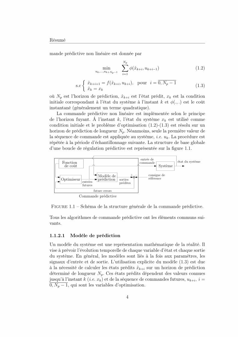
La commande prédictive non linéaire est implémentée selon le principede l’horizon fuyant. Á l’instant k, l’état du système xk est utilisé commecondition initiale et le problème d’optimisation (1.2)-(1.3) est résolu sur unhorizon de prédiction de longueur Np. Néanmoins, seule la première valeur dela séquence de commande est appliquée au système, i.e. uk. La procédure estrépétée à la période d’échantillonnage suivante. La structure de base globaled’une boucle de régulation prédictive est représentée sur la figure 1.1.
Fonction
Optimiseur prediction
Systeme
Commande predictive
Modele de
future errors
entreesfutures
sortiespredites
entree decommande etat du systeme
consigne dereference
de cout
Figure 1.1 – Schéma de la structure générale de la commande prédictive.
Tous les algorithmes de commande prédictive ont les éléments communs sui-vants.
1.1.2.1 Modèle de prédiction
Un modèle du système est une représentation mathématique de la réalité. Ilvise à prévoir l’évolution temporelle de chaque variable d’état et chaque sortiedu système. En général, les modèles sont liés à la fois aux paramètres, lessignaux d’entrée et de sortie. L’utilisation explicite du modèle (1.3) est dueà la nécessité de calculer les états prédits xk+i sur un horizon de prédictiondéterminé de longueur Np. Ces états prédits dépendent des valeurs connuesjusqu’à l’instant k (i.e. xk) et de la séquence de commandes futures, uk+i, i =0, Np − 1, qui sont les variables d’optimisation.
4
Résumé
1.1.2.2 Fonction de coût
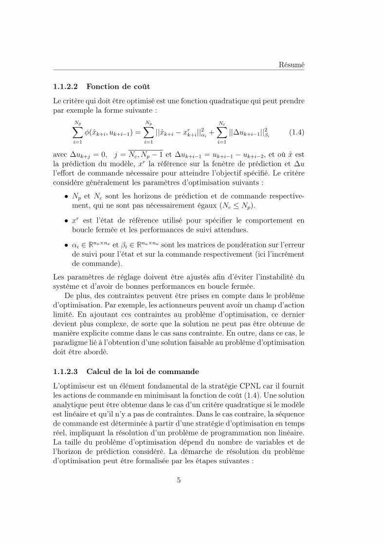
Le critère qui doit être optimisé est une fonction quadratique qui peut prendrepar exemple la forme suivante :
Np∑i=1
φ(xk+i, uk+i−1) =
Np∑i=1
||xk+i − xrk+i||2αi +Nc∑i=1
||∆uk+i−1||2βi (1.4)
avec ∆uk+j = 0, j = Nc, Np − 1 et ∆uk+i−1 = uk+i−1 − uk+i−2, et où x estla prédiction du modèle, xr la référence sur la fenêtre de prédiction et ∆ul’effort de commande nécessaire pour atteindre l’objectif spécifié. Le critèreconsidère généralement les paramètres d’optimisation suivants :
• Np et Nc sont les horizons de prédiction et de commande respective-ment, qui ne sont pas nécessairement égaux (Nc ≤ Np).
• xr est l’état de référence utilisé pour spécifier le comportement enboucle fermée et les performances de suivi attendues.
• αi ∈ Rnx×nx et βi ∈ Rnu×nu sont les matrices de pondération sur l’erreurde suivi pour l’état et sur la commande respectivement (ici l’incrémentde commande).
Les paramètres de réglage doivent être ajustés afin d’éviter l’instabilité dusystème et d’avoir de bonnes performances en boucle fermée.
De plus, des contraintes peuvent être prises en compte dans le problèmed’optimisation. Par exemple, les actionneurs peuvent avoir un champ d’actionlimité. En ajoutant ces contraintes au problème d’optimisation, ce dernierdevient plus complexe, de sorte que la solution ne peut pas être obtenue demanière explicite comme dans le cas sans contrainte. En outre, dans ce cas, leparadigme lié à l’obtention d’une solution faisable au problème d’optimisationdoit être abordé.
1.1.2.3 Calcul de la loi de commande
L’optimiseur est un élément fondamental de la stratégie CPNL car il fournitles actions de commande en minimisant la fonction de coût (1.4). Une solutionanalytique peut être obtenue dans le cas d’un critère quadratique si le modèleest linéaire et qu’il n’y a pas de contraintes. Dans le cas contraire, la séquencede commande est déterminée à partir d’une stratégie d’optimisation en tempsréel, impliquant la résolution d’un problème de programmation non linéaire.La taille du problème d’optimisation dépend du nombre de variables et del’horizon de prédiction considéré. La démarche de résolution du problèmed’optimisation peut être formalisée par les étapes suivantes :
5
Résumé
1. Obtention des mesures
2. Calcul des prédictions via le modèle du système sur un certain horizonde prédiction
3. Calcul de la séquence de commandes optimales par minimisation de lafonction de coût
4. Implémentation de la première commande au système
5. Retour à l’étape 1.
1.1.3 État de l’art
En général, la commande prédictive peut être divisée en deux classes métho-dologiques : linéaire et non linéaire. Maciejowski et Camacho donnent un bonaperçu de la théorie linéaire [90], tandis que Allgöwer et Zheng donnent unaperçu des méthodes non linéaires [3]. Les différents algorithmes de la com-mande prédictive résultent de la façon dont la fonction de coût à minimiseret les contraintes du système sont spécifiées.
1.1.3.1 Cas linéaire
En général, La Commande Prédictive Linéaire (CPL) utilise un modèle li-néaire de faible complexité pour représenter le système. En présence decontraintes linéaires, le problème d’optimisation à résoudre est de taille rai-sonnable , ce qui peut être fait assez rapidement à chaque période d’échan-tillonnage afin d’être mis en œuvre dans le cadre de l’horizon fuyant. Dans cecas, la solution du problème d’optimisation est la solution d’un problème deprogrammation linéaire ou quadratique (LP/QP), qui sont connus pour êtreconvexes, et pour lesquels il existe une variété de méthodes et de logicielsnumériques.
Selon les différentes stratégies de modélisation et de formulation du pro-blème, de nombreuses variantes de la CPL existent dans la littérature : Dyna-mic Matrix Control (DMC), Model Algorithmic Control (MAC), PredictiveFunctional Control (PFC), Extended Prediction Self Adaptive Control (EP-SAC), Extended Horizon Adaptive Control (EHAC), Generalized PredictiveControl (GPC).
1.1.3.2 Cas non linéaire
Du fait des limitations de la commande prédictive linéaire vis-à-vis des pro-cédés ayant une dynamique fortement non linéaire, soumis à des contraintes
6
Résumé
et/ou régis par un changement fréquent de régimes de fonctionnement, l’ap-plication de la commande prédictive non linéaire (CPNL) est à privilégier.L’utilisation d’un modèle non linéaire pour la prédiction transforme le pro-blème quadratique convexe en un problème non convexe, plus difficile à ré-soudre. En conséquence, la convergence vers l’optimum global va fortementdépendre de l’étape d’initialisation. La CPNL est une méthode fondée surl’optimisation pour la commande par retour d’état des systèmes non linéaires.Ses principales applications sont la stabilisation et les problèmes de suivi detrajectoires de référence. La CPNL est fondée comme la CPL sur le prin-cipe de l’horizon fuyant, où un problème de commande optimale en boucleouverte sur un horizon fini est résolu à chaque instant d’échantillonnage etla séquence de commande optimale est appliquée jusqu’à ce qu’une nouvelleséquence de commande optimale soit disponible à l’instant suivant d’échan-tillonnage. Sa philosophie est donc similaire à celle de la CPL. Les méthodesconsidérées comme les plus représentatives sont les suivantes : CPNL à hori-zon infini, CPNL à horizon fini avec contrainte terminale d’égalité, CPNL àhorizon fini avec contrainte terminale d’inégalité, CPNL à horizon fini aveccoût terminal, CPNL à horizon quasi-infini, CPNL à retour d’état/sortie,CPNL économique.
1.1.4 Architectures de commande prédictive
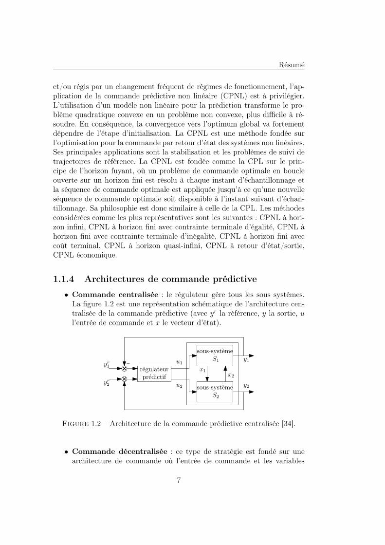
• Commande centralisée : le régulateur gère tous les sous systèmes.La figure 1.2 est une représentation schématique de l’architecture cen-tralisée de la commande prédictive (avec yr la référence, y la sortie, ul’entrée de commande et x le vecteur d’état).
sous-systemeS1
sous-systemeS2
y1
y2
x1x2
u1
u2
yr1
yr2
regulateurpredictif
Figure 1.2 – Architecture de la commande prédictive centralisée [34].
• Commande décentralisée : ce type de stratégie est fondé sur unearchitecture de commande où l’entrée de commande et les variables
7
Résumé
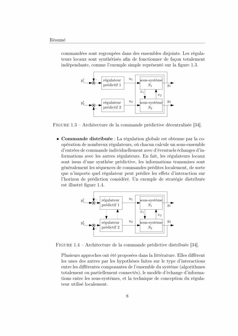
commandées sont regroupées dans des ensembles disjoints. Les régula-teurs locaux sont synthétisés afin de fonctionner de façon totalementindépendante, comme l’exemple simple représenté sur la figure 1.3.
sous-systemeS1
sous-systemeS2
y1
y2
x1x2
u1
u2
yr1
yr2
regulateurpredictif 1
regulateurpredictif 2
Figure 1.3 – Architecture de la commande prédictive décentralisée [34].
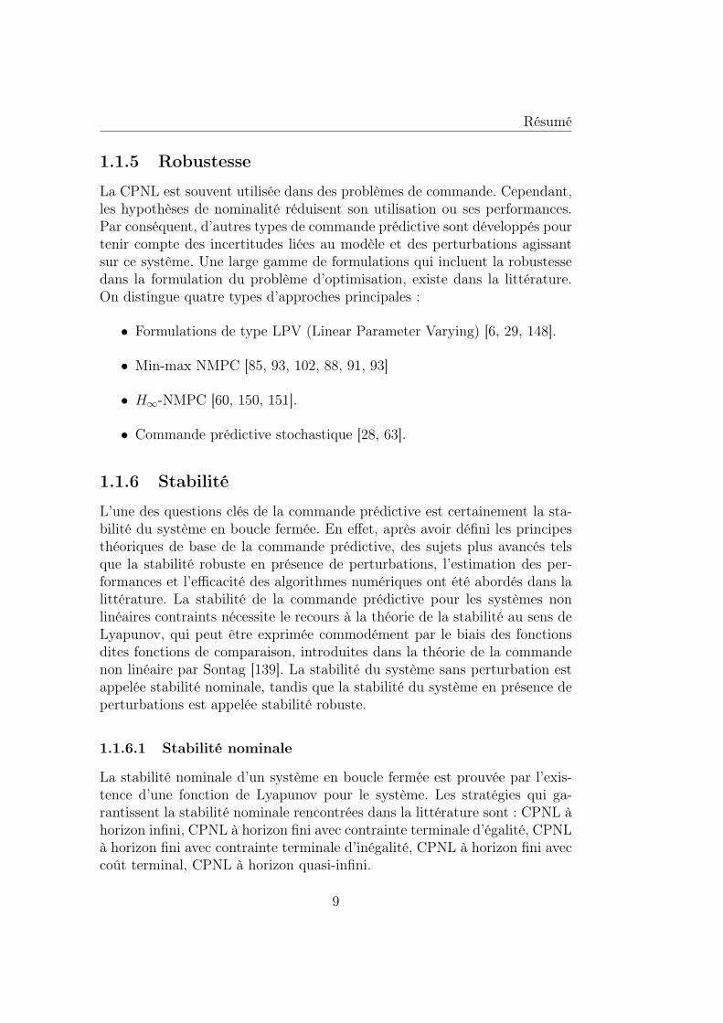
• Commande distribuée : La régulation globale est obtenue par la co-opération de nombreux régulateurs, où chacun calcule un sous-ensembled’entrées de commande individuellement avec d’éventuels échanges d’in-formations avec les autres régulateurs. En fait, les régulateurs locauxsont issus d’une synthèse prédictive, les informations transmises sontgénéralement les séquences de commandes prédites localement, de sorteque n’importe quel régulateur peut prédire les effets d’interaction surl’horizon de prédiction considéré. Un exemple de stratégie distribuéeest illustré figure 1.4.
sous-systemeS1
sous-systemeS2
y1
y2
x1x2
u1
u2yr2
yr1 regulateurpredictif 1
regulateurpredictif 2
Figure 1.4 – Architecture de la commande prédictive distribuée [34].
Plusieurs approches ont été proposées dans la littérature. Elles diffèrentles unes des autres par les hypothèses faites sur le type d’interactionsentre les différentes composantes de l’ensemble du système (algorithmestotalement ou partiellement connectés), le modèle d’échange d’informa-tions entre les sous-systèmes, et la technique de conception du régula-teur utilisé localement.
8
Résumé
1.1.5 Robustesse
La CPNL est souvent utilisée dans des problèmes de commande. Cependant,les hypothèses de nominalité réduisent son utilisation ou ses performances.Par conséquent, d’autres types de commande prédictive sont développés pourtenir compte des incertitudes liées au modèle et des perturbations agissantsur ce système. Une large gamme de formulations qui incluent la robustessedans la formulation du problème d’optimisation, existe dans la littérature.On distingue quatre types d’approches principales :
• Formulations de type LPV (Linear Parameter Varying) [6, 29, 148].
• Min-max NMPC [85, 93, 102, 88, 91, 93]
• H∞-NMPC [60, 150, 151].
• Commande prédictive stochastique [28, 63].
1.1.6 Stabilité
L’une des questions clés de la commande prédictive est certainement la sta-bilité du système en boucle fermée. En effet, après avoir défini les principesthéoriques de base de la commande prédictive, des sujets plus avancés telsque la stabilité robuste en présence de perturbations, l’estimation des per-formances et l’efficacité des algorithmes numériques ont été abordés dans lalittérature. La stabilité de la commande prédictive pour les systèmes nonlinéaires contraints nécessite le recours à la théorie de la stabilité au sens deLyapunov, qui peut être exprimée commodément par le biais des fonctionsdites fonctions de comparaison, introduites dans la théorie de la commandenon linéaire par Sontag [139]. La stabilité du système sans perturbation estappelée stabilité nominale, tandis que la stabilité du système en présence deperturbations est appelée stabilité robuste.
1.1.6.1 Stabilité nominale
La stabilité nominale d’un système en boucle fermée est prouvée par l’exis-tence d’une fonction de Lyapunov pour le système. Les stratégies qui ga-rantissent la stabilité nominale rencontrées dans la littérature sont : CPNL àhorizon infini, CPNL à horizon fini avec contrainte terminale d’égalité, CPNLà horizon fini avec contrainte terminale d’inégalité, CPNL à horizon fini aveccoût terminal, CPNL à horizon quasi-infini.
9
Résumé
1.1.7 Stabilité robuste
Comme indiqué précédemment, la conception de lois de commande prédictiverobuste se fait en prenant en compte les incertitudes d’une manière expliciteafin d’optimiser la fonction objectif pour la pire configuration des incerti-tudes. Il existe de nombreuses approches permettant d’analyser la stabilitérobuste, comme la structure entrée-état (ISS), la marge de stabilité robusteet la théorie des ensembles invariants couplée au cadre de la stabilité ISS-Lyapunov [85].
1.1.8 Avantages et inconvénients
La commande prédictive présente une série d’avantages en comparaison avecles autres lois de commandes :
• Formulation simple, basée sur des concepts bien compris et maitrisés.
• Méthodologie permettant des extensions futures.
• Applicabilité à une grande variété de systèmes, y compris les systèmesnon linéaires et des systèmes à retard.
• Preuve de la stabilité pour les systèmes linéaires et non linéaires avecdes contraintes d’entrée et d’état, sous certaines conditions spécifiques.
• Très utile quand les références futures sont connues a priori.
• Cas multivariable pouvant être facilement traité.
• Extension pour la prise en compte des contraintes (limitation des ac-tionneurs).
• Utilisation explicite du modèle.
• Facilité de maintenance et de mise en œuvre en cas de changement dumodèle ou de ses paramètres.
Cependant, la commande prédictive présente certains inconvénients :
• la commande prédictive nécessite généralement un temps de calcul plusimportant par rapport aux stratégies de commande classiques. La priseen compte des contraintes de type inégalité augmente encore plus lacharge de calcul.
• En général, elle induit un manque de preuve de stabilité (sauf cas par-ticuliers).
10
Résumé
Cependant, la plus grande exigence est la nécessité d’un modèle approprié.En effet, la stratégie de commande est fondée sur une connaissance préa-lable du modèle, mais ne dépend pas d’une structure de modèle spécifique.Il est cependant évident que les avantages obtenus seront affectés par l’écartexistant entre le processus réel et le modèle de prédiction.
1.2 Chapitre 4 : Commande prédictive non li-néaire
Dans ce chapitre, on propose la formulation et la mise en œuvre d’une stra-tégie de commande prédictive non linéaire permettant la poursuite d’unetrajectoire de référence.
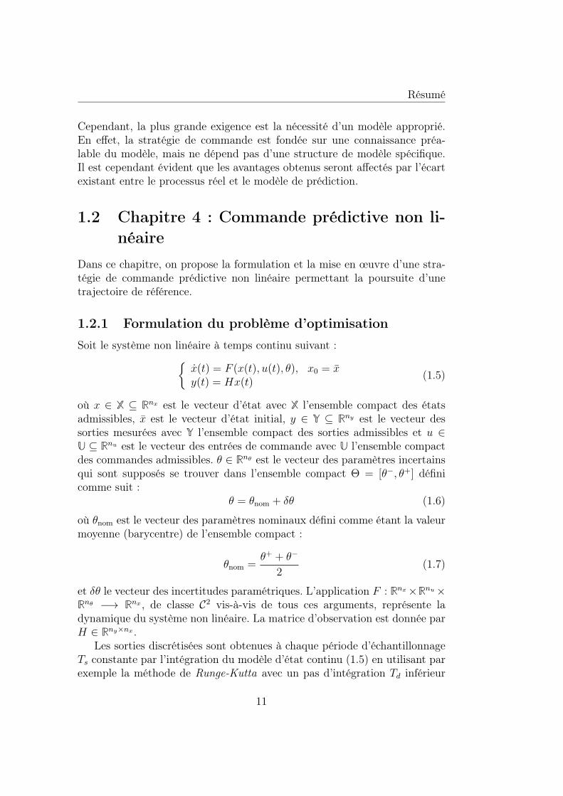
1.2.1 Formulation du problème d’optimisation
Soit le système non linéaire à temps continu suivant :{x(t) = F (x(t), u(t), θ), x0 = xy(t) = Hx(t)
(1.5)
où x ∈ X ⊆ Rnx est le vecteur d’état avec X l’ensemble compact des étatsadmissibles, x est le vecteur d’état initial, y ∈ Y ⊆ Rny est le vecteur dessorties mesurées avec Y l’ensemble compact des sorties admissibles et u ∈U ⊆ Rnu est le vecteur des entrées de commande avec U l’ensemble compactdes commandes admissibles. θ ∈ Rnθ est le vecteur des paramètres incertainsqui sont supposés se trouver dans l’ensemble compact Θ = [θ−, θ+] définicomme suit :
θ = θnom + δθ (1.6)
où θnom est le vecteur des paramètres nominaux défini comme étant la valeurmoyenne (barycentre) de l’ensemble compact :
θnom =θ+ + θ−
2(1.7)
et δθ le vecteur des incertitudes paramétriques. L’application F : Rnx×Rnu×Rnθ −→ Rnx , de classe C2 vis-à-vis de tous ces arguments, représente ladynamique du système non linéaire. La matrice d’observation est donnée parH ∈ Rny×nx .
Les sorties discrétisées sont obtenues à chaque période d’échantillonnageTs constante par l’intégration du modèle d’état continu (1.5) en utilisant parexemple la méthode de Runge-Kutta avec un pas d’intégration Td inférieur
11
Résumé
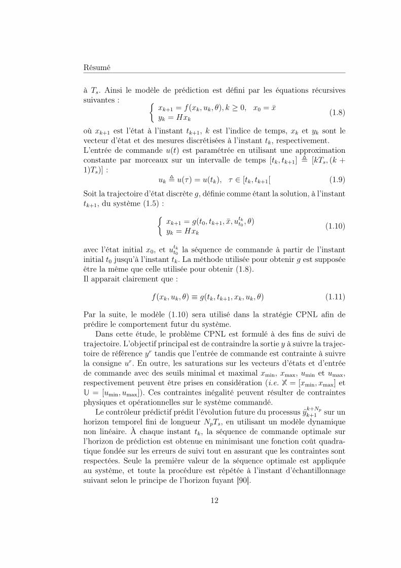
à Ts. Ainsi le modèle de prédiction est défini par les équations récursivessuivantes : {
xk+1 = f(xk, uk, θ), k ≥ 0, x0 = xyk = Hxk
(1.8)
où xk+1 est l’état à l’instant tk+1, k est l’indice de temps, xk et yk sont levecteur d’état et des mesures discrétisées à l’instant tk, respectivement.L’entrée de commande u(t) est paramétrée en utilisant une approximationconstante par morceaux sur un intervalle de temps [tk, tk+1] , [kTs, (k +1)Ts)] :
uk , u(τ) = u(tk), τ ∈ [tk, tk+1[ (1.9)
Soit la trajectoire d’état discrète g, définie comme étant la solution, à l’instanttk+1, du système (1.5) :{
xk+1 = g(t0, tk+1, x, utkt0 , θ)
yk = Hxk(1.10)
avec l’état initial x0, et utkt0 la séquence de commande à partir de l’instantinitial t0 jusqu’à l’instant tk. La méthode utilisée pour obtenir g est supposéeêtre la même que celle utilisée pour obtenir (1.8).Il apparait clairement que :
f(xk, uk, θ) ≡ g(tk, tk+1, xk, uk, θ) (1.11)
Par la suite, le modèle (1.10) sera utilisé dans la stratégie CPNL afin deprédire le comportement futur du système.
Dans cette étude, le problème CPNL est formulé à des fins de suivi detrajectoire. L’objectif principal est de contraindre la sortie y à suivre la trajec-toire de référence yr tandis que l’entrée de commande est contrainte à suivrela consigne ur. En outre, les saturations sur les vecteurs d’états et d’entréede commande avec des seuils minimal et maximal xmin, xmax, umin et umax,respectivement peuvent être prises en considération (i.e. X = [xmin, xmax] etU = [umin, umax]). Ces contraintes inégalité peuvent résulter de contraintesphysiques et opérationnelles sur le système commandé.
Le contrôleur prédictif prédit l’évolution future du processus yk+Npk+1 sur un
horizon temporel fini de longueur NpTs, en utilisant un modèle dynamiquenon linéaire. À chaque instant tk, la séquence de commande optimale surl’horizon de prédiction est obtenue en minimisant une fonction coût quadra-tique fondée sur les erreurs de suivi tout en assurant que les contraintes sontrespectées. Seule la première valeur de la séquence optimale est appliquéeau système, et toute la procédure est répétée à l’instant d’échantillonnagesuivant selon le principe de l’horizon fuyant [90].
12
Résumé
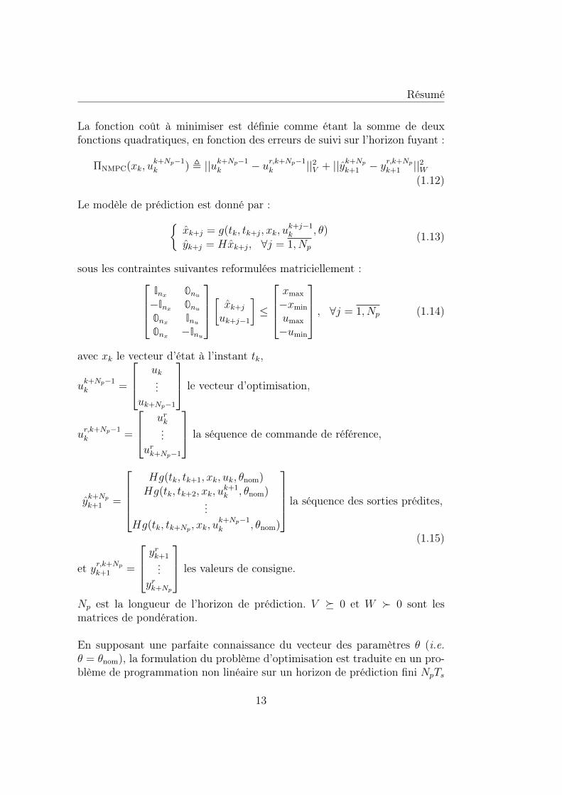
La fonction coût à minimiser est définie comme étant la somme de deuxfonctions quadratiques, en fonction des erreurs de suivi sur l’horizon fuyant :
ΠNMPC(xk, uk+Np−1k ) , ||uk+Np−1
k − ur,k+Np−1k ||2V + ||yk+Np
k+1 − yr,k+Npk+1 ||2W
(1.12)
Le modèle de prédiction est donné par :{xk+j = g(tk, tk+j, xk, u
k+j−1k , θ)
yk+j = Hxk+j, ∀j = 1, Np(1.13)
sous les contraintes suivantes reformulées matriciellement :Inx 0nu−Inx 0nu0nx Inu0nx −Inu
[ xk+j
uk+j−1
]≤
xmax
−xmin
umax
−umin
, ∀j = 1, Np (1.14)
avec xk le vecteur d’état à l’instant tk,
uk+Np−1k =
uk...
uk+Np−1
le vecteur d’optimisation,
ur,k+Np−1k =
urk...
urk+Np−1
la séquence de commande de référence,
yk+Npk+1 =
Hg(tk, tk+1, xk, uk, θnom)Hg(tk, tk+2, xk, u
k+1k , θnom)
...Hg(tk, tk+Np , xk, u
k+Np−1k , θnom)
la séquence des sorties prédites,
(1.15)
et yr,k+Npk+1 =
yrk+1...
yrk+Np
les valeurs de consigne.
Np est la longueur de l’horizon de prédiction. V � 0 et W � 0 sont lesmatrices de pondération.
En supposant une parfaite connaissance du vecteur des paramètres θ (i.e.θ = θnom), la formulation du problème d’optimisation est traduite en un pro-blème de programmation non linéaire sur un horizon de prédiction fini NpTs
13
Résumé
à chaque instant d’échantillonnage. La séquence de commande optimale estobtenue en minimisant le critère de performance (1.12) avec prise en comptedes contraintes (1.14) et de la dynamique du système comme suit :
NMPC :?uk+Np−1
k = arg minuk+Np−1
k
ΠNMPC(xk, uk+Np−1k ) (1.16)
s.c. (1.13)-(1.14)
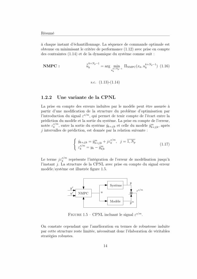
1.2.2 Une variante de la CPNL
La prise en compte des erreurs induites par le modèle peut être assurée àpartir d’une modification de la structure du problème d’optimisation parl’introduction du signal εs/m, qui permet de tenir compte de l’écart entre laprédiction du modèle et la sortie du système. La prise en compte de l’erreur,notée εs/mk , entre la sortie du système yk+j|k et celle du modèle ymk+j|k, aprèsj intervalles de prédiction, est donnée par la relation suivante :{
yk+j|k = ymk+j|k + jεs/mk , j = 1, Np
εs/mk = yk − ymk|k
(1.17)
Le terme jεs/mk représente l’intégration de l’erreur de modélisation jusqu’àl’instant j. La structure de la CPNL avec prise en compte du signal erreurmodèle/système est illustrée figure 1.5.
Systeme
Modele
NMPC
y
ym
εs/muyr
ur
Figure 1.5 – CPNL incluant le signal εs/m.
On constate cependant que l’amélioration en termes de robustesse induitepar cette structure reste limitée, nécessitant donc l’élaboration de véritablesstratégies robustes.
14
Résumé
1.3 Chapitre 5 : Commande prédictive non li-néaire robuste
Ce chapitre s’attache à proposer une nouvelle stratégie de commande pré-dictive robuste. Elle est fondée sur l’approximation du problème min-maxvia la linéarisation du modèle de prédiction et l’utilisation de la dualité La-grangienne. Dans ce contexte, deux méthodes ont été développées. Dans lapremière méthode, la séquence de commande optimale est calculée à par-tir d’un problème d’optimisation scalaire. La seconde méthode permet deprendre en considération explicitement les contraintes de type inégalité.
1.3.1 Stratégie min-max
On suppose que le vecteur des paramètres est incertain et appartient à l’en-semble Θ défini par (1.6)-(1.7). Ainsi, la robustification de la commandeprédictive non linéaire induit la formulation d’un problème d’optimisationde type min-max [4, 93, 102]. La séquence de commande qui minimise lafonction coût est la solution du problème d’optimisation suivant :
RNMPC :?uk+Np−1
k = arg minuk+Np−1
k
maxδθ
ΠRNMPC(xk, uk+Np−1k , δθ) (1.18)
soumis à
xk+j = g(tk, tk+j, xk, uk+j−1k , θ = θnom + δθ), j = 1, Np
θ ∈ ΘInx 0nu−Inx 0nu0nx Inu0nx −Inu
[ xk+j
uk+j−1
]≤
xmax
−xmin
umax
−umin
, ∀j = 1, Np
(1.19)
où θ et θnom sont donnés par (1.6) et (1.7). La fonction coût est donnée par :
ΠRNMPC(xk, uk+Np−1k , δθ) , ||uk+Np−1
k − ur,k+Np−1k ||2V + ||yk+Np
k+1 − yr,k+Npk+1 ||2W
(1.20)
Les sorties prédites yk+Npk+1 ont la mêmes formulation que dans (1.15) :
yk+Npk+1 =
Hg(tk, tk+1, xk, uk, θ)Hg(tk, tk+2, xk, u
k+1k , θ)
...Hg(tk, tk+Np , xk, u
k+Np−1k , θ)
(1.21)
15
Résumé
La séquence de commande optimale ?uk+Np−1
k est déterminée en minimisantl’erreur de suivi en considérant toutes les trajectoires possibles [54, 76].
Il apparait clairement que le temps de calcul augmente en fonction dela taille du vecteur des paramètres, du nombre d’entrée de commande et dela taille de l’horizon de prédiction pouvant vite devenir prohibitif. Ainsi, ledéfi principal est de réduire le temps de calcul tout en maintenant de bonnesperformances en termes de précision de poursuite.
1.3.2 Commande prédictive robuste réduite
Étant donné que le problème d’optimisation min-max (1.18)-(1.20) est coû-teux en termes de temps de calcul, il peut se simplifier en réduisant le nombrede paramètres θ incertains pris en compte dans l’optimisation à partir d’uneanalyse de sensibilité du modèle vis-à-vis de ses paramètres.
1.3.2.1 Analyse de sensibilité
La fonction de sensibilité Sxiθj représente la sensibilité de chaque état xi auxfaibles variations de chaque paramètre θj. Elle est donnée par l’expressionsuivante :
Sxiθj ,∂xi∂θj
, i = 1, nx et j = 1, nθ (1.22)
La dynamique des fonctions de sensibilité pour le système (1.5) est calculéecomme suit :
Sxiθj =d
dt
(∂xi∂θj
)=
∂
∂θj
(dxidt
)=∂Fi∂θj
+nx∑k=1
∂Fi∂xk
(∂xk∂θj
)(1.23)
avec la condition initiale suivante : ∂xi∂θj
= 0.L’analyse de l’évolution temporelle des fonctions de sensibilité selon l’ordrede grandeur de leurs amplitudes, permet de sélectionner les paramètres κ quiont le plus d’influence.
1.3.2.2 Reformulation du problème
Par la suite, seuls les paramètres les plus influents vont être considérés dansle problème d’optimisation min-max, au lieu de tous les paramètres (avecθ , [κ, ζ]). Les paramètres influents κ sont définis par :
κ = κnom + δκ (1.24)
κnom =κ+ + κ−
2(1.25)
16
Résumé
où κnom sont les valeurs nominales des paramètres les plus influents et δκ estle vecteur de leurs incertitudes. Les autres paramètres, ζ, sont maintenus àleurs valeurs nominales avec ζnom = (ζ+ + ζ−)/2.
Grâce à l’analyse de sensibilité, le problème d’optimisation min-max (5.1)-(5.3) est remplacé par le problème suivant :
rRNMPC :?uk+Np−1
k = arg minuk+Np−1
k
maxδκ
ΠrRNMPC(xk, uk+Np−1k , δκ) (1.26)
soumis à
xk+j = g(tk, tk+j, xk, uk+j−1k ,
[κnom + δκζnom
]), j = 1, Np
κ ∈ ΘκInx 0nu−Inx 0nu0nx Inu0nx −Inu
[ xk+j
uk+j−1
]≤
xmax
−xmin
umax
−umin
, ∀j = 1, Np
(1.27)
La nouvelle fonction coût est définie par :
ΠrRNMPC(uk+Np−1k , δκ) , ||uk+Np−1
k − ur,k+Np−1k ||2V + ||yk+Np
k+1 − yr,k+Npk+1 ||2W
(1.28)
Les sorties prédites yk+Npk+1 sont données par :
yk+Npk+1 =
Hg(tk, tk+1, xk, uk, [κ
>, ζ>nom]>)Hg(tk, tk+2, xk, u
k+1k , [κ>, ζ>nom]>)...
Hg(tk, tk+Np , xk, uk+Np−1k , [κ>, ζ>nom]>)
(1.29)
Néanmoins, cette approche ne peut pas être appliquée pour les systèmes dontles paramètres ont une influence similaire, aucune réduction des paramètresn’est alors possible. Par conséquent, cette approche ne peut pas être utiliséedans tous les cas.
1.3.3 Commande prédictive robuste linéarisée
Dans le but de réduire le temps de calcul induit par la résolution du problèmed’optimisation de type min-max, l’approche proposée ici consiste à linéari-ser les sorties prédites. En conséquence, le problème non convexe initial estapproché par un problème convexe plus facile à résoudre.
17
Résumé
1.3.3.1 Principe général
La trajectoire d’état (1.11) à l’instant tk+j est linéarisée (développement ensérie de Taylor limité au premier ordre) autour des paramètres nominauxθnom et de la séquence de commande de référence ur,k+j−1
k , pour j = 1, Np :
xk+j ≈ xnom,k+j +∇θg(tk+j)δθ +∇ug(tk+j)(uk+j−1k − ur,k+j−1
k
)(1.30)
avec
xnom,k+j = g(tk, tk+j, xk, ur,k+j−1k , θnom) (1.31)
∇θg(tk+j) =∂g(tk, tk+j, xk, u
k+j−1k , θ)
∂θ
∣∣∣∣∣∣∣∣ uk+j−1k = ur,k+j−1
kθ = θnom
(1.32)
∇ug(tk+j) =∂g(tk, tk+j, xk, u
k+j−1k , θ)
∂uk+j−1k
∣∣∣∣∣∣∣∣ uk+j−1k = ur,k+j−1
kθ = θnom
(1.33)
Ainsi, les sorties prédites sont données par l’expression suivante :
yk+Npk+1 = G
k+Npnom,k+1 +G
k+Npθ,k+1δθ +G
k+Np−1u,k (u
k+Np−1k − ur,k+Np−1
k ) (1.34)
avec
Gk+Np
nom,k+1 =
Hxnom,k+1
...Hxnom,k+j
...Hxnom,k+Np
, Gk+Np
θ,k+1 =
H∇θg(tk+1)...
H∇θg(tk+j)...
H∇θg(tk+Np)
, Gk+Np−1u,k =
H∇ug(tk+1)...
H∇ug(tk+j)...
H∇ug(tk+Np)
En utilisant l’équation (1.34), la fonction coût initiale ΠRNMPC (1.20) estapprochée par :
Π(xk, uk+Np−1k , δθ) ≈ ||uk+Np−1
k − ur,k+Np−1k ||2V +
||Gk+Npnom,k+1 − y
r,k+Npk+1 +G
k+Npθ,k+1δθ +G
k+Np−1u,k (u
k+Np−1k − ur,k+Np−1
k )||2W(1.35)
Finalement, le problème d’optimisation (1.18) devient :
?uk+Np−1
k = arg minuk+Np−1
k
maxδθ
Π(xk, uk+Np−1k , δθ) (1.36)
soumis àθ ∈ Θ, x ∈ X, u ∈ U (1.37)
18
Résumé
1.3.3.2 Analyse de la stabilité
Théorème 1.1. Soit le système non linéaire à temps discret suivant :
xk+1 = l(xk, wk), k ≥ 0, x0 = x (1.38)
où xk ∈ X est l’état du système, wk ∈ W est la perturbation (telle que West un ensemble compact contenant l’origine).Si le système (1.38) admet une fonction de Lyapunov robuste alors le systèmeest robuste stable.
Preuve. voir [86].
La stabilité du système (1.8) avec (1.36)-(1.37) en boucle fermée est ana-lysée en utilisant le théorème précédent.
Soit le système à l’instant tk+1 :
xk+1 = f(xk, uk, θnom + δθs) ,f(xk, urk, θnom) +∇uf(urk, θnom).(uk − urk)+
∇θf(urk, θnom).δθs + ϑ(|uk − urk|2) + ϑ(|δθs|2)
(1.39)
où ϑ(|.|2) est le reste du développement en série de Taylor.Soit le modèle de prédiction à l’instant tk+1 :
xk+1|k = fp(xk, uk, θnom + δθ) ,f(xk, urk, θnom) +∇uf(urk, θnom).(uk − urk)
+∇θf(urk, θnom).δθ
(1.40)
Après développement, on obtient une borne sur l’erreur de prédiction :
∃α ∈ R+,∀x,∀u,∀θ, |∇θf | ≤ α (1.41)
et
∃η ∈ R+, tel que η = max(|ϑ(|uk−urk|2)+ϑ(|δθs|2)|,max(|δθ|, |δθs|)) (1.42)
alors|xk+1 − xk+1|k| ≤ (2α + 1)η , Λ(η) (1.43)
où Λ est une fonction K∞.La fonction coût optimale Π peut être bornée comme suit :
αψ(|xk|) ≤ Π(xk,?u, δ
?
θ) ≤ βt(|xk|) + ϕ(η) +Npχ(η) (1.44)
19
Résumé
où αψ, βt, et χ sont des fonctions K∞ et ϕ est une fonction K.De plus, la variation de la fonction coût ∆Π? est donnée par l’expressionsuivante :
∆Π? , Π(xk+1, u, δ?
θ)− Π(xk,?u, δ
?
θ) ≤ −αψ(|x|) + χ(η) (1.45)
avec
χ(η) = χ(η) +
(LtxL
Np−1fx + Lψx
Np−2∑j=0
Ljfx
)Λ(η) (1.46)
où χ est une fonction K∞.On montre que la fonction coût optimale Π est une fonction de Lyapu-
nov robuste. Par conséquent, le système (1.8) commandé par π(x) =?uk est
robuste stable.
1.3.4 Implémentation de la commande prédictive ro-buste linéarisée en absence de contraintes (LRMPC)
Le problème d’optimisation (1.36)-(1.37) est résolu en utilisant la dualitéLagrangienne [23]. On se ramène alors à un problème d’optimisation scalaire[135]. Il en résulte les étapes d’implémentation suivantes :
Étape 1. Le multiplicateur de Lagrange λ? est calculé comme suit :
λ? = arg minλ≥||G
k+N>pθ,k+1 WG
k+Npθ,k+1 ||
J(λ) (1.47)
Le critère J(λ) est défini par l’expression suivante :
J(λ) = ||z(λ)||2V + λ||δθmax||2 + ||Gk+Np−1u,k z(λ)− yr,k+Np
k+1 +Gk+Npnom,k+1||2W (λ)
(1.48)avec
z(λ) = (V +Gk+Np−1>
u,k W (λ)Gk+Np−1u,k )†(G
k+Np−1>
u,k W (λ)(yr,k+Npk+1 −Gk+Np
nom,k+1))
(1.49)et
W (λ) = W +WGk+Npθ,k+1(λI−Gk+N>p
θ,k+1 WGk+Npθ,k+1)†G
k+N>pθ,k+1 W (1.50)
Étape 2. La séquence de commande ?uk+Np−1
k est donnée par :?uk+Np−1
k =ur,k+Np−1k + (V +G
k+Np−1>
u,k W (λ?)Gk+Np−1u,k )†
× (Gk+Np−1>
u,k W (λ?)(yr,k+Npk+1 −Gk+Np
nom,k+1))(1.51)
avec W (λ?) donnée par (1.50) pour λ = λ?.
20
Résumé
1.3.5 Commande prédictive robuste linéarisée avec priseen compte des contraintes
La prise en compte des contraintes inégalité sur la commande dans le pro-blème d’optimisation (1.36)-(1.37) conduit à la résolution d’un problème àdeux niveaux, selon les étapes suivantes :
Étape 1. Le scalaire λ? est calculé à partir du problème d’optimisationsuivant :
λ? = arg minλ≥||G
k+N>pθ,k+1 WG
k+Npθ,k+1 ||
J(z(λ), λ) (1.52)
La fonction J(z(λ), λ) est donnée par (1.48) et z(λ) est calculé par :
z(λ) = arg minz≤z≤z
[z>E(λ)z − 2B(λ)>z
](1.53)
où
E(λ) = V +Gk+Np−1>
u,k W (λ)Gk+Np−1u,k (1.54)
B(λ) = Gk+Np−1>
u,k W (λ)(yr,k+Npk+1 −Gk+Np
nom,k+1
)(1.55)
z = uminInu − ur,k+Np−1k (1.56)
z = umaxInu − ur,k+Np−1k (1.57)
avec W (λ) donnée par (1.50).
Étape 2. La séquence de commande ?uk+Np−1
k est calculée à partir du pro-blème d’optimisation (1.53) pour λ = λ? :
?uk+Np−1
k = ur,k+Np−1k + z(λ?) (1.58)
1.4 Chapitre 6 : Améliorations de la commandeprédictive robuste linéarisée
Ce chapitre propose deux améliorations de la loi de commande prédictiverobuste linéarisée. En premier lieu, la linéarisation des sorties prédites esteffectuée ici autour des valeurs nominales des paramètres du modèle et dela séquence de commandes optimales obtenues à l’instant d’échantillonnageprécédent. Cette modification permet de rendre la solution moins sensibleaux bruits de mesure. En second lieu, une structure de commande hiérarchi-sée combinant la commande prédictive robuste linéarisée et une commandeauxiliaire (proportionnel intégrateur ou mode glissant intégral) est dévelop-pée afin d’éliminer toute erreur statique en suivi de trajectoire de référence.
21
Résumé
1.4.1 Commande prédictive robuste linéarisée avec in-créments de commande
Afin de rendre la commande prédictive robuste linéarisée moins sensible auxbruits de mesure, par rapport au chapitre précédent, la fonction coût qua-dratique mesure les efforts de commande au lieu de la différence entre lesentrées de commande et leurs valeurs de référence. L’idée est d’utiliser unelinéarisation du modèle autour des paramètres nominaux et de la séquence decommande optimale obtenue au pas d’échantillonnage précédent. On constateque, cette approche présente l’avantage d’avoir une solution moins sensibleaux bruits de mesure. Ainsi, le nouveau problème d’optimisation est le sui-vant :
δ?uk+Np−1
k = arg minδuk+Np−1
k ∈Uδmaxδθ∈Θδ
Πδ(xk, δuk+Np−1k , δθ) (1.59)
soumis à
xk+j = g(tk, tk+j, xk, uk+j−1k , θ = θnom + δθ), j = 1, Np (1.60)
où
Πδ(xk, δuk+Np−1k , δθ) , ||δuk+Np−1
k ||2V + ||yk+Npk − yr,k+Np
k ||2W (1.61)
Les variables d’optimisation δuk+Np−1k sont définies comme suit :
δuk+Np−1k =
uk −
?uk−1...
uk+j − uk+j−1...
uk+Np−1 − uk+Np−2
,
δuk...
δuk+j...
δuk+Np−1
(1.62)
avec ?uk−1 l’entrée de commande appliquée à l’instant k − 1 (solution du
problème d’optimisation (1.59) à l’instant k − 1).Les sorties prédites sont données par l’expression suivante :
yk+Npk+1 = G
k+Npnom,k+1 +G
k+Npθ,k+1δθ +G
k+Np−1u,k (Ξ
k+Np−1k + TNpδu
k+Np−1k ) (1.63)
avec
Ξk+Np−1k =
?uk−1...
?uk−1
−
?uk−1...
?uk+Np−2
(1.64)
22
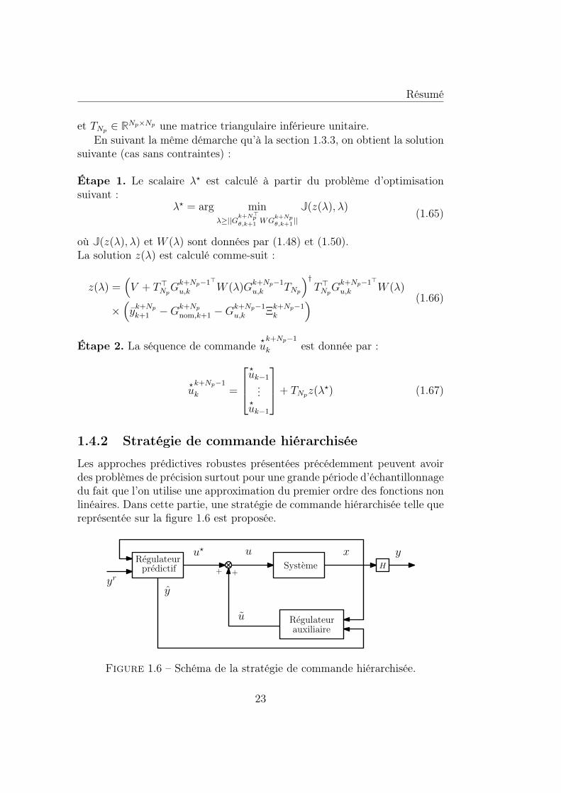
Résumé
et TNp ∈ RNp×Np une matrice triangulaire inférieure unitaire.En suivant la même démarche qu’à la section 1.3.3, on obtient la solution
suivante (cas sans contraintes) :
Étape 1. Le scalaire λ? est calculé à partir du problème d’optimisationsuivant :
λ? = arg minλ≥||G
k+N>pθ,k+1 WG
k+Npθ,k+1 ||
J(z(λ), λ) (1.65)
où J(z(λ), λ) et W (λ) sont données par (1.48) et (1.50).La solution z(λ) est calculé comme-suit :
z(λ) =(V + T>NpG
k+Np−1>
u,k W (λ)Gk+Np−1u,k TNp
)†T>NpG
k+Np−1>
u,k W (λ)
×(yk+Npk+1 −G
k+Npnom,k+1 −G
k+Np−1u,k Ξ
k+Np−1k
) (1.66)
Étape 2. La séquence de commande ?uk+Np−1
k est donnée par :
?uk+Np−1
k =
?uk−1...
?uk−1
+ TNpz(λ?) (1.67)
1.4.2 Stratégie de commande hiérarchisée
Les approches prédictives robustes présentées précédemment peuvent avoirdes problèmes de précision surtout pour une grande période d’échantillonnagedu fait que l’on utilise une approximation du premier ordre des fonctions nonlinéaires. Dans cette partie, une stratégie de commande hiérarchisée telle quereprésentée sur la figure 1.6 est proposée.
HSysteme
yr
u? u
u
x y
+ +
Regulateur
y
Regulateurauxiliaire
predictif
Figure 1.6 – Schéma de la stratégie de commande hiérarchisée.
23
Résumé
La boucle de régulation est formée par une loi de commande prédictive ro-buste (entrée de commande notée u?) combinée à un correcteur auxiliaire(entrée de commande notée u). Le régulateur prédictif permet de suivre latrajectoire de référence, alors que le régulateur supplémentaire annule touteerreur de suivi résiduelle.
Deux types de régulation additionnelle sont étudiés : une structure propor-tionnelle-intégrale (PI) et une stratégie de commande par mode glissant in-tégrateur (ISM).
En premier lieu, la loi de commande proportionnel intégrateur est choisiepour sa simplicité. Elle est donnée par l’expression suivante :
u(t) = Kp(y(t)− y(t)) +Kp
Ti
∫ t
tk−1
(y(τ)− y(τ))dτ (1.68)
où Kp et Ti sont les deux paramètres de réglage du PI et y la prédiction dumodèle.
En second lieu, on considère une loi de commande comme régulateur auxi-liaire. La loi de commande par mode glissant intégrateur présente l’avantaged’être robuste vis-à-vis des perturbations. La surface de glissement est choisiecomme suit :
φ(x, t) = Z2(t) + ξ3Z1(t) (1.69)
avec Z1(t) =
∫ ttk−1
(y(τ)− y(τ)) dτ
Z2(t) = 1ξ1
(y(t)− y(t)− ξ2Z1(t))
(1.70)
L’attractivité de la surface de glissement est donnée ci-dessous :
φ(x, t) = −Kssign(φ(x, t)), Ks ∈ R+ (1.71)
Ainsi, l’expression de la loi de commande par mode glissant intégrateur (ISM)est la suivante :
u(t) =1
η(−ϕ− χuk−1 − ξ1Kssign(φ(x, t)) + (ξ2 − ξ1ξ3)(ξ1Z2(t) + ξ2Z1(t)))
(1.72)
avec ϕ = H(fx(x(t), θ)− fx(x(t), θnom)),χ = H(fu(x(t), θ)− fu(x(t), θnom)),η = Hfu(x(t), θ)
(1.73)
et {x(t) = fx(x(t), θ) + fu(x(t), θ)u(t), ∀t > t0, x(t0) = x0
y(t) = Hx(t)(1.74)
24
Résumé
Dans (1.73), θ est remplacé par θnom (ou par une estimée de θ) car θ estincertain.
1.5 Chapitre 7 : Application à un système deculture de microalgues
Le développement des technologies environnementales a pris une place de plusen plus importante dans l’industrie. En effet, grâce à leurs caractéristiquesbiochimiques, les bioprocédés sont considérés comme une alternative promet-teuse aux sources d’énergie fossiles. Dans l’industrie des biotechnologies, lacommande des bioréacteurs est devenue un enjeu majeur du fait que ce sontdes systèmes fortement non linéaires et incertains par nature nécessitant lasynthèse d’une stratégie de commande robuste. Dans ce chapitre, l’objectifprincipal est d’appliquer les lois de commande présentées précédemment à unsystème de culture de microalgue pour la régulation de la concentration enbiomasse à une valeur de consigne en présence d’incertitudes paramétriqueset de bruit de mesure.
1.5.1 Modélisation du système
Le modèle dynamique considéré suppose que le photobioréacteur est en modecontinu (le débit moyen de soutirage est égal à celui d’alimentation, condui-sant à un volume constant), sans aucune biomasse supplémentaire dans l’ali-mentation et en négligeant l’effet des échanges gazeux. Les bilans de matièresconduisent aux équations différentielles suivantes :
X(t) = µ(Q(t), I(t))X(t)−DX(t)
Q(t) = ρ(S(t))− µ(Q(t), I(t))Q(t)
S(t) = (Sin − S(t))D − ρ(S(t))X(t)
(1.75)
avec
µ(Q, I) = µ(1− KQ
Q)µI (Droop)
ρ(S) = ρmS
S +Ks
(Michaelis-Menten)
µI =I
I +KsI +I2
KiI
(Haldane)(1.76)
où X est la concentration en biomasse (µm3 L−1), Q le quota interne (µmol-µm−3) et S la concentration en substrat (µmol L−1). D (d−1) est le taux de
25
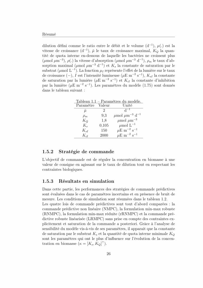
Résumé
dilution défini comme le ratio entre le débit et le volume (d−1), µ(.) est lavitesse de croissance (d−1), µ le taux de croissance maximal, KQ la quan-tité de quota interne en-dessous de laquelle les bactéries ne croissent plus(µmol µm−3), ρ(.) la vitesse d’absorption (µmol µm−3 d−1), ρm le taux d’ab-sorption maximal (µmol µm−3 d−1) et Ks la constante de saturation par lesubstrat (µmol L−1). La fonction µI représente l’effet de la lumière sur le tauxde croissance (−), I est l’intensité lumineuse (µE m−2 s−1), KsI la constantede saturation par la lumière (µE m−2 s−1) et KiI la constante d’inhibitionpar la lumière (µE m−2 s−1). Les paramètres du modèle (1.75) sont donnésdans le tableau suivant :
Tableau 1.1 – Paramètres du modèle.Paramètre Valeur Unité
µ 2 d−1
ρm 9,3 µmol µm−3 d−1
KQ 1,8 µmol µm−3
Ks 0,105 µmol L−1
KsI 150 µE m−2 s−1
KiI 2000 µE m−2 s−1
1.5.2 Stratégie de commande
L’objectif de commande est de réguler la concentration en biomasse à unevaleur de consigne en agissant sur le taux de dilution tout en respectant lescontraintes biologiques.
1.5.3 Résultats en simulation
Dans cette partie, les performances des stratégies de commande prédictivessont évaluées dans le cas de paramètres incertains et en présence de bruit demesure. Les conditions de simulation sont résumées dans le tableau 1.2.Les quatre lois de commande prédictives sont tout d’abord comparées : lacommande prédictive non linéaire (NMPC), la formulation min-max robuste(RNMPC), la formulation min-max réduite (rRNMPC) et la commande pré-dictive robuste linéarisée (LRMPC) sans prise en compte des contraintes ex-plicitement et saturation de la commande a posteriori. Grâce à l’analyse desensibilité du modèle vis-à-vis de ses paramètres, il apparait que la constantede saturation par le substrat Ks et la quantité de quota interne minimale KQ
sont les paramètres qui ont le plus d’influence sur l’évolution de la concen-tration en biomasse (κ = [Ks, KQ]>).
26
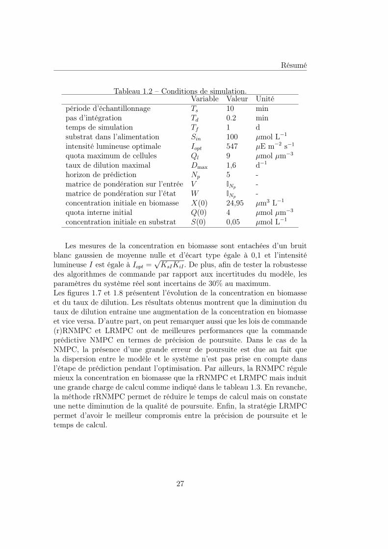
Résumé
Tableau 1.2 – Conditions de simulation.Variable Valeur Unité
période d’échantillonnage Ts 10 minpas d’intégration Td 0.2 mintemps de simulation Tf 1 dsubstrat dans l’alimentation Sin 100 µmol L−1
intensité lumineuse optimale Iopt 547 µE m−2 s−1
quota maximum de cellules Ql 9 µmol µm−3
taux de dilution maximal Dmax 1,6 d−1
horizon de prédiction Np 5 -matrice de pondération sur l’entrée V INp -matrice de pondération sur l’état W INp -concentration initiale en biomasse X(0) 24,95 µm3 L−1
quota interne initial Q(0) 4 µmol µm−3
concentration initiale en substrat S(0) 0,05 µmol L−1
Les mesures de la concentration en biomasse sont entachées d’un bruitblanc gaussien de moyenne nulle et d’écart type égale à 0,1 et l’intensitélumineuse I est égale à Iopt =
√KsIKiI . De plus, afin de tester la robustesse
des algorithmes de commande par rapport aux incertitudes du modèle, lesparamètres du système réel sont incertains de 30% au maximum.Les figures 1.7 et 1.8 présentent l’évolution de la concentration en biomasseet du taux de dilution. Les résultats obtenus montrent que la diminution dutaux de dilution entraine une augmentation de la concentration en biomasseet vice versa. D’autre part, on peut remarquer aussi que les lois de commande(r)RNMPC et LRMPC ont de meilleures performances que la commandeprédictive NMPC en termes de précision de poursuite. Dans le cas de laNMPC, la présence d’une grande erreur de poursuite est due au fait quela dispersion entre le modèle et le système n’est pas prise en compte dansl’étape de prédiction pendant l’optimisation. Par ailleurs, la RNMPC régulemieux la concentration en biomasse que la rRNMPC et LRMPC mais induitune grande charge de calcul comme indiqué dans le tableau 1.3. En revanche,la méthode rRNMPC permet de réduire le temps de calcul mais on constateune nette diminution de la qualité de poursuite. Enfin, la stratégie LRMPCpermet d’avoir le meilleur compromis entre la précision de poursuite et letemps de calcul.
27
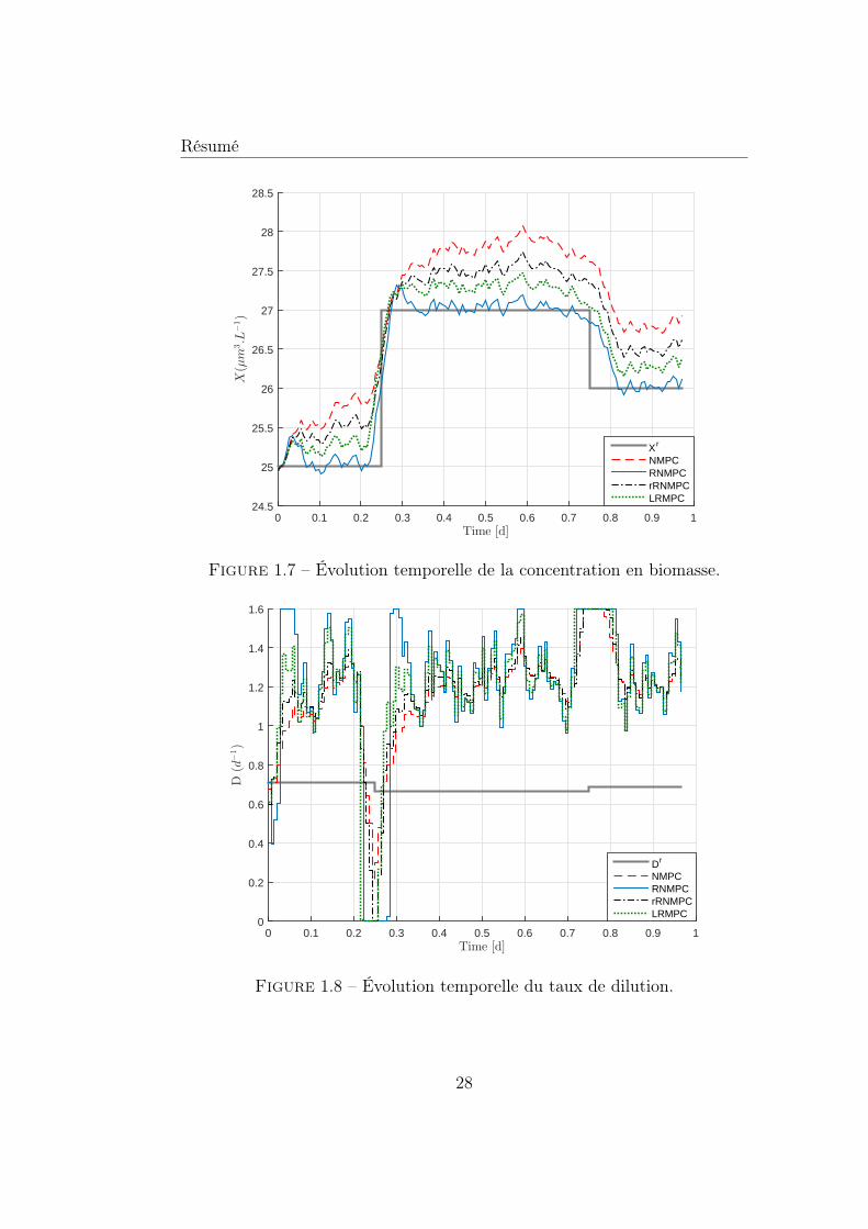
Résumé
Time [d]0 0.1 0.2 0.3 0.4 0.5 0.6 0.7 0.8 0.9 1
X(µm
3.L
−1)
24.5
25
25.5
26
26.5
27
27.5
28
28.5
X r
NMPCRNMPCrRNMPCLRMPC
Figure 1.7 – Évolution temporelle de la concentration en biomasse.
Time [d]0 0.1 0.2 0.3 0.4 0.5 0.6 0.7 0.8 0.9 1
D(d
−1)
0
0.2
0.4
0.6
0.8
1
1.2
1.4
1.6
Dr
NMPCRNMPCrRNMPCLRMPC
Figure 1.8 – Évolution temporelle du taux de dilution.
28
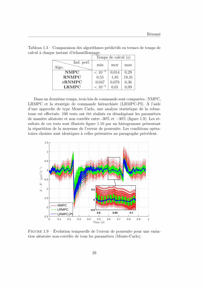
Résumé
Tableau 1.3 – Comparaison des algorithmes prédictifs en termes de temps decalcul à chaque instant d’échantillonnage.
Temps de calcul (s)XXXXXXXXXXXXAlgo.
Ind. perf. min moy max
NMPC < 10−5 0,014 0,29RNMPC 0,55 1,85 19,31rRNMPC 0,047 0,078 0,36LRMPC < 10−5 0,01 0,09
Dans un deuxième temps, trois lois de commande sont comparées : NMPC,LRMPC et la stratégie de commande hiérarchisée (LRMPC-PI). À l’aided’une approche de type Monte Carlo, une analyse statistique de la robus-tesse est effectuée. 100 tests ont été réalisés en désadaptant les paramètresde manière aléatoire et non corrélée entre -30% et +30% (figure 1.9). Les ré-sultats de ces tests sont illustrés figure 1.10 par un histogramme présentantla répartition de la moyenne de l’erreur de poursuite. Les conditions opéra-toires choisies sont identiques à celles présentées au paragraphe précédent.
Time (d)0 0.1 0.2 0.3 0.4 0.5 0.6 0.7 0.8 0.9 1
X−X
r(µm
3.L
−1)
-2.5
-2
-1.5
-1
-0.5
0
0.5
1
1.5
0.6 0.65 0.7-0.5
0
0.5
LRMPC-PI
LRMPCNMPC
Figure 1.9 – Évolution temporelle de l’erreur de poursuite pour une varia-tion aléatoire non-corrélée de tous les paramètres (Monte-Carlo).
29
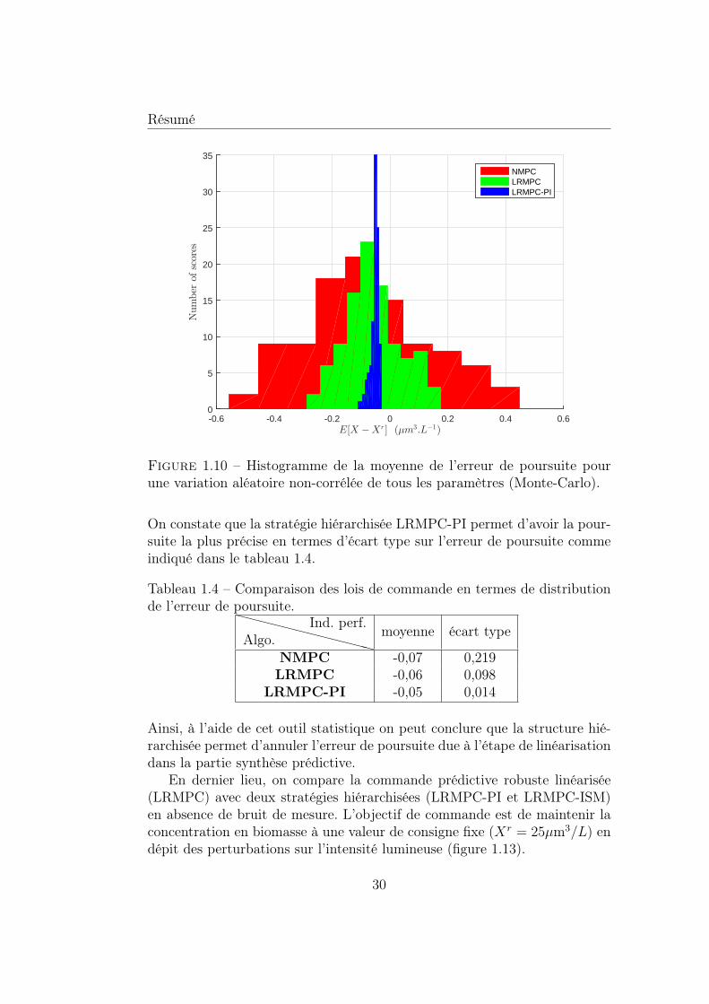
Résumé
E[X −Xr] (µm3
.L−1)
-0.6 -0.4 -0.2 0 0.2 0.4 0.6
Number
ofscores
0
5
10
15
20
25
30
35
NMPCLRMPCLRMPC-PI
Figure 1.10 – Histogramme de la moyenne de l’erreur de poursuite pourune variation aléatoire non-corrélée de tous les paramètres (Monte-Carlo).
On constate que la stratégie hiérarchisée LRMPC-PI permet d’avoir la pour-suite la plus précise en termes d’écart type sur l’erreur de poursuite commeindiqué dans le tableau 1.4.
Tableau 1.4 – Comparaison des lois de commande en termes de distributionde l’erreur de poursuite.
XXXXXXXXXXXXAlgo.Ind. perf. moyenne écart type
NMPC -0,07 0,219LRMPC -0,06 0,098
LRMPC-PI -0,05 0,014
Ainsi, à l’aide de cet outil statistique on peut conclure que la structure hié-rarchisée permet d’annuler l’erreur de poursuite due à l’étape de linéarisationdans la partie synthèse prédictive.
En dernier lieu, on compare la commande prédictive robuste linéarisée(LRMPC) avec deux stratégies hiérarchisées (LRMPC-PI et LRMPC-ISM)en absence de bruit de mesure. L’objectif de commande est de maintenir laconcentration en biomasse à une valeur de consigne fixe (Xr = 25µm3/L) endépit des perturbations sur l’intensité lumineuse (figure 1.13).
30
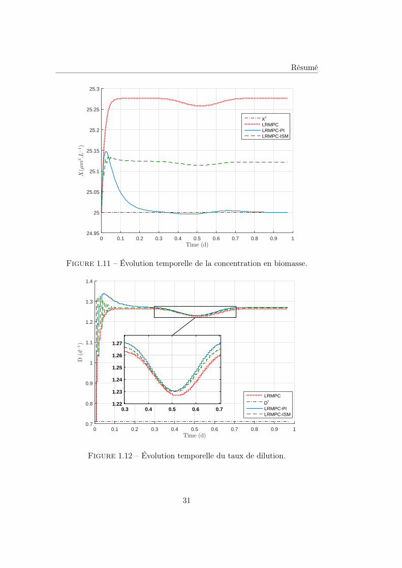
Résumé
Time (d)0 0.1 0.2 0.3 0.4 0.5 0.6 0.7 0.8 0.9 1
X(µm
3.L
−1)
24.95
25
25.05
25.1
25.15
25.2
25.25
25.3
X r
LRMPCLRMPC-PILRMPC-ISM
Figure 1.11 – Évolution temporelle de la concentration en biomasse.
Time (d)0 0.1 0.2 0.3 0.4 0.5 0.6 0.7 0.8 0.9 1
D(d
−1)
0.7
0.8
0.9
1
1.1
1.2
1.3
1.4
LRMPC
Dr
LRMPC-PILRMPC-ISM
0.3 0.4 0.5 0.6 0.71.22
1.23
1.24
1.25
1.26
1.27
Figure 1.12 – Évolution temporelle du taux de dilution.
31
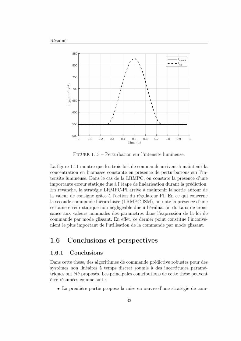
Résumé
Time (d)0 0.1 0.2 0.3 0.4 0.5 0.6 0.7 0.8 0.9 1
I(µE.m
−2.s
−1)
500
550
600
650
700
750
800
850
Inominal
Ireal
Figure 1.13 – Perturbation sur l’intensité lumineuse.
La figure 1.11 montre que les trois lois de commande arrivent à maintenir laconcentration en biomasse constante en présence de perturbations sur l’in-tensité lumineuse. Dans le cas de la LRMPC, on constate la présence d’uneimportante erreur statique due à l’étape de linéarisation durant la prédiction.En revanche, la stratégie LRMPC-PI arrive à maintenir la sortie autour dela valeur de consigne grâce à l’action du régulateur PI. En ce qui concernela seconde commande hiérarchisée (LRMPC-ISM), on note la présence d’unecertaine erreur statique non négligeable due à l’évaluation du taux de crois-sance aux valeurs nominales des paramètres dans l’expression de la loi decommande par mode glissant. En effet, ce dernier point constitue l’inconvé-nient le plus important de l’utilisation de la commande par mode glissant.
1.6 Conclusions et perspectives
1.6.1 Conclusions
Dans cette thèse, des algorithmes de commande prédictive robustes pour dessystèmes non linéaires à temps discret soumis à des incertitudes paramé-triques ont été proposés. Les principales contributions de cette thèse peuventêtre résumées comme suit :
• La première partie propose la mise en œuvre d’une stratégie de com-
32
Résumé
mande prédictive non linéaire permettant la poursuite d’une trajectoirede référence pour un système non linéaire à temps discret.
• Dans la deuxième partie, la commande prédictive robuste vis-à-vis desincertitudes paramétriques est formulée en un problème d’optimisa-tion de type min-max. Afin de réduire la charge de calcul induitepar la formulation min-max, l’approche proposée consiste à simpli-fier le problème d’optimisation initial, via l’analyse de sensibilité dumodèle vis-à-vis de ses paramètres en linéarisant les sorties préditesautour des valeurs nominales des paramètres du modèle et de la sé-quence de commande de référence. Deux méthodes d’implantation ontété développées. Dans la première méthode ne tenant pas compte descontraintes, la séquence de commande optimale est calculée à partird’un problème d’optimisation scalaire. La seconde méthode permet deprendre en compte explicitement les contraintes inégalité sur l’entréede commande.
• Deux améliorations de la loi de commande prédictive robuste linéariséeont été proposées dans la troisième partie. Tout d’abord, la linéarisa-tion des sorties prédites autour des valeurs nominales des paramètresdu modèle et de la séquence de commande optimale obtenue à l’itéra-tion précédente. Cette modification permet de rendre la solution moinssensible aux bruits de mesure. Ensuite, une structure de commande hié-rarchisée combinant la commande prédictive robuste linéarisée et unecommande auxiliaire (proportionnel intégrateur ou mode glissant inté-grateur) est développée afin d’éliminer toute erreur statique en suivi detrajectoire de référence.
• Le dernier chapitre est dédié à l’application des lois de commande déve-loppées à un cas d’étude de commande de photobioréacteur de culturede microalgues pour la régulation de la concentration en biomasse enprésence d’incertitudes paramétriques, bruit de mesure et fluctuationsde l’intensité lumineuse.
1.6.2 Perspectives
Dans la continuité de ces travaux, les perspectives suivantes peuvent êtreenvisagées :
• Application des lois de commande proposées au cas d’un système mul-tivariable comprenant un nombre de paramètres incertains plus impor-tant.
33
Résumé
• Extension de la formulation du problème d’optimisation aux cas desperturbations et des cinétiques incertaines.
• Synthèse d’un observateur afin d’estimer le vecteur d’état à partir desmesures.
• Amélioration de la qualité du modèle linéarisé en utilisant un dévelop-pement en série de Taylor limité au second ordre au lieu du premierordre.
• Étude de l’influence de la résolution du problème d’optimisation enutilisant la dualité lagrangienne sur la stabilité du système en bouclefermée.
• Analyse de la stabilité du système bouclé avec la stratégie de commandehiérarchisée.
• Détermination des conditions à satisfaire pour assurer la stabilité dusystème avec le couplage régulateur/estimateur.
34
Chapter 2
Introduction
2.1 Context and motivations
The control of nonlinear systems subject to physical constraints on the in-put and state is undoubtly a challenging and important problem. The wellknown systematic nonlinear control methods such as feedback linearizationand constructive Lyapunov-based methods lead to very elegant solutions, butthey depend on a complicated design procedure that does not scale well tolarge systems and they cannot handle constraints easily or in a systematicmanner. Based on this, the concept of optimal control and in particular theModel Predictive Control (MPC) approach and its nonlinear version NMPCappears to be an attractive alternative since the complexity of the controldesign increases moderately with the size and complexity of the system. TheNMPC strategy is therefore put forward because of its ability to deal withuncertainties and constraints. The essence of NMPC is to optimize, over anopen-loop time sequence of controls, the process response using a model ofthe system to forecast the future process behavior over a prediction horizon.
Moreover, even if NMPC strategies have proved to be efficient in manyindustrial applications due to their ability to operate the process safely underphysical constraints, the monitoring of complex, highly nonlinear, uncertainsystems becomes more and more a delicate task. This is the case for exampleof bioprocesses, that will be the application field considered in this work. In-deed, in such cases, model parameters are generally known with a confidenceinterval only (determined from an identification procedure for example). Themain objective is thus to elaborate an adequate robust control strategy inorder to guarantee that the process will yield the reference trajectory undermodel parameter uncertainties.
Therefore, NMPC strategies must be extended to provide robustness fea-
35
Introduction
tures, developing robust control strategies, which can compensate for the lackof parameters information and/or accuracy. There are two popular alterna-tives for making decision with incomplete knowledge: the stochastic solution(probabilistic theory) and the min-max solution (game theory), which appearas expensive approaches.
Indeed, the robust NMPC (RNMPC) law can be formulated as a nonlinearmin-max optimization problem where the effect of the uncertainties must betaken into account in the design procedure. However, this approach tendsto become too complex to be solved numerically online. Consequently, thetotal calculation time is an important factor that must be reduced as muchas possible.
As a consequence, the challenge that must be taken up in this work is todesign a MPC controller that would be robust against unknown but boundedmodel parameters uncertainties and computationally more tractable in calcu-lating the optimal control, which makes it suitable for online implementation.For that purpose, starting from the standard RNMPC formulations, newstructures will be developed to match this compromise between robustnessand computational load, with a dedicated application to bioprocesses.
2.2 Outline
We briefly summarize the main results of this thesis, chapter by chapter, asthe following:
• Chapter 3: In this chapter, a state of the art of existing Model Pre-dictive Control (MPC) techniques is given with a focus on nonlinearcontrol problems. It starts with the basic MPC problem formulationand provides a review of linear and nonlinear MPC schemes, addressesrobustness issues and presents briefly nominal and robust stability con-cepts.
• Chapter 4: This chapter investigates the Nonlinear MPC formulationin order to solve a trajectory tracking problem for continuous/discrete-time nonlinear systems. A continuous/discrete formulation is consid-ered in this thesis, since models of bioprocesses are time-continuous butwith discrete-time measurements. A variant of NMPC is presented insection 4.3. It consists in considering the accumulation of the gap be-tween the system and the model at each sampling time over predictionintervals. An illustrative example (for a bioprocess) is presented in sec-tion 4.4 and numerical results are provided in order to demonstrate the
36
Introduction
effectiveness of the NMPC strategy and highlight its drawbacks andlimitations, which motivate the development of RNMPC strategies.
• Chapter 5: This chapter deals with a robust formulation of the NMPCin order to take into account the model parameters mismatch. Therobust NMPC (RNMPC) law is formulated as a nonlinear min-maxoptimization problem. However, this approach tends to become toocomplex to be solved numerically online. To overcome this problem,two major solutions have been proposed. The first one consists in reduc-ing the number of uncertain parameters through a sensitivity analysis.Only the main influencial parameters on the model are considered inthe min-max problem whereas the other parameters are kept constantand equal to their nominal values. Secondly, a new approach has beenproposed, based on the linearization of the predicted trajectory to turnthe original optimization problem into a more tractable one. It consistsin simplifying the min-max optimization problem through a sensitiv-ity analysis of the model with respect to its parameters, in order toreduce the calculation time, which makes it suitable for online imple-mentation. The criterion is linearized around the model parametersnominal values and the reference control sequence (control inputs overthe prediction horizon). The derived optimization problem is an unidi-mensionnal optimization problem (referred to as LRMPC). Moreover,stability analysis of the closed-loop system while applying the LRMPClaw is established under some assumptions. Furthermore, the inequal-ity constraints on the optimization variables are taken into accountin the LRMPC problem formulation. This leads to a bilevel problem(referred to as CLRMPC), with a scalar optimization problem in theupper level, and a quadratic programming one in the lower level. Theperformances of the proposed control strategies will be illustrated insimulations (the same system as in chapter 4).
• Chapter 6: This chapter proposes two improvements for the(C)LRMPC law. The first one consists in linearizing the model at eachsampling time along the nominal trajectory which is defined based onthe nominal parameter values and the optimal control sequence ob-tained at the previous iteration, instead of reference control sequenceas done in the previous chapter. This modification is motivated by thefact that the optimal control sequence obtained at the previous iter-ation is non-model-based. As a consequence, the proposed approachappears to be less sensitive against measurement noise thanks to thepenality term on the control evolution. The derived optimization prob-
37
Introduction
lem is a bilevel one or a scalar optimization problem depending on theconsidered constraints. However, the proposed control strategies haveaccuracy issue as they deal with a first-order approximation of the non-linear system. A hierarchical control strategy is proposed in order tocancel the residual tracking error due to the linearization drawbackand possible disturbances. The proposed control strategy combines arobust model predictive control law with a Proportional Integral (PI)law or Integral Sliding Mode (ISM) controller. The predictive controllerguarantees the tracking of the reference trajectory, whereas the otherregulator ensures a good tracking accuracy. These two improvementsare applied to the illustrative example.
• Chapter 7: In this chapter, all proposed approaches in the previouschapters are applied to a case study to control of microalgae culture ina continuous photobioreactor. The aim is to regulate the microalgaeconcentrations at a given reference value, despite disturbances (lightintensity fluctuation) and model parameters uncertainties. First, themodel of the bioprocess is described and analysed. Secondly, the de-termination of the equilibrium is addressed. Finally, simulation resultsare given for reference trajectory tracking and disturbance rejection.
• Chapter 8: The last chapter summarizes the developed work in thisPhD thesis and proposes some recommendations for future directions.
2.3 List of Publications
The thesis work has resulted in several accepted/submitted publications tointernational journal and conferences. They are given hereafter:
Journal paper
• S.E. Benattia, S. Tebbani and D. Dumur. Multivariable robust MPCof heterotrophic microalgae fed-batch bioreactor. To be submitted toJournal of Process Control, 2016.
Proceedings
• S.E. Benattia, S. Tebbani and D. Dumur. Nonlinear model predictivecontrol for regulation of microalgae culture in a continuous photobiore-actor. Proceedings of the 22nd Mediterranean Conference on Controland Automation, Palermo, Italy, pp. 469-474, June 16-19, 2014.
38
Introduction
• S.E. Benattia, S. Tebbani, D. Dumur and D. Selisteanu. Robust non-linear model predictive controller based on sensitivity analysis - appli-cation to a continuous photobioreactor. Multi-Conference on Systemsand Control, Antibes/Nice, France, pp. 1705-1710, October 8-10, 2014.
• S.E. Benattia, S. Tebbani and D. Dumur. Robust nonlinear model pre-dictive control of microalgae culture in a continuous photobioreactor.1st IFAC Conference on Modelling identification and Control of Non-linear Systems, Saint-Petersburg, Russia , pp. 192-197, June 24-26,2015.
• S.E. Benattia, S. Tebbani and D. Dumur. Hierarchical control strategybased on robust MPC and integral sliding mode - application to acontinuous photobioreactor. 5th IFAC Conference on Nonlinear ModelPredictive Control, Seville, Spain, pp. 212-217, September 17-20, 2015.
• S.E. Benattia, S. Tebbani and D. Dumur. Hierarchical predictive con-trol strategy of microalgae culture in a photobioreactor. 19th Interna-tional Conference on System Theory, Control and Computing, CheileGradistei-Fundata, Romania , pp. 231-236, October 14-16, 2015.
• S.E. Benattia, S. Tebbani and D. Dumur. Robust model predictivecontrol - application to microalgae cultivation. Submitted to Conferenceon Decision and Control, Las Vegas, USA, 2016.
Conferences with abstract
• S.E. Benattia, S. Tebbani, D. Dumur. Nonlinear model predictive con-trol of microalgae culture. Young Algaeneers Symposium, Montpellier& Narbonne, France, April 3-5, 2014.
• S.E. Benattia, S. Tebbani, D. Dumur. Regulation of microalgae culturein a continuous photobioreactor. ESBES-IFIBIOP Symposium, Lille,France, September 7-10, 2014.
Others (oral presentation)
• S.E. Benattia, S. Tebbani and D. Dumur. Robust nonlinear modelpredictive control for regulation of microalgae culture in a continuousphotobioreactor. Journée du Groupe de Travail de Commande Prédic-tive Non Linéaire, Paris, June 11, 2015.
• S.E. Benattia, S. Tebbani and D. Dumur. Hierarchical robust predictivecontrol strategy of microalgae cultivation process. Journée du Groupede Travail de Commande Prédictive Non Linéaire, Paris, March 24,2016.
39

Introduction
40
Chapter 3
Predictive control: State of theart and main strategies
3.1 Introduction
The purpose of this chapter is to give an introduction to one of the mostpowerful strategies that can be used to address nonlinear control problems.We present the basic MPC problem formulation and provide a review on pre-vious works that appear in the literature. The key advantages/drawbacks ofMPC are outlined and some of the theoretical, computational and implemen-tation aspects are discussed. It also serves as a centralized literature studyfor the following chapters. In any case, this introduction does not representan exhaustive overview of predictive control, it however provides the readerwith the sufficient background for the next chapters.
3.2 Background
The nonlinear optimal control theory was developed in the 1950’s and 1960’s,resulting from the maximum principle of Pontryagin [116] and dynamic pro-gramming method developed by Bellman [12]. The receding horizon principlewas proposed by Propoi [117], within the frame of open loop optimal feed-back. The philosophy of the receding horizon problem is closely related tothe minimum time optimal control problem and to linear programming [154].In the late 1970s, due to the progress in algorithms for solving constrainedlinear and quadratic optimization problems, linear MPC, also referred to asreceding or moving horizon control, became popular in control engineering.As a consequence, the interest in MPC for process control grew quickly. Manyworks appeared principally Richalet et al. [129] and Cutler et al. [40] were
41
Predictive control: State of the art and main strategies
the first in the control community to propose industrial applications of MPCstrategy. MPC has become the de-facto standard advanced control methodin the process industries due to its ability to handle large scale multivariableprocesses. Many systems are however in general inherently nonlinear. In thiscase, linear models are often inadequate to describe the process dynamics andnonlinear models have to be used.The practical interest is driven by the fact that process nonlinearities and con-traints are explicitly considered. This motivates the use of nonlinear modelpredictive control (henceforth abbreviated as NMPC), the extension of wellestablished linear MPC. MPC involves the repetitive solution of an optimalcontrol problem at each sampling instant in a receding horizon window. Thekey challenge that has to be met is to ensure that the implementation of asequence of open-loop optimal control values will be stable, when consider-ing the closed loop system. Subsequently, NMPC problems have witnessed asteadily increasing attention from academic control theoretists. This leads toincreasing advances with focus on design that guarantee stability and robust-ness. A lot of pioneer works have emerged in this topic: Chen and Shaw [31],Keerthi and Gilbert [77], Michalska and Mayne [102], Parisini and Zoppoli[113], Alamir and Bornard [2], Magni and Sepulchre [95], Chen and Allgöwer[32], De Nicolao et al. [43], Mayne et al. [100], and Jadbabaie and Hauser[74]. In addition to the research on NMPC, researchers have developed so-called Real Time Optimization (RTO) [30] approaches which are similar toNMPC, as they are generally based on nonlinear programming, and use staticnonlinear models, while NMPC uses dynamic nonlinear models.
Receding Horizon Control (RHC) is cited as one of the most popular ad-vanced techniques for industrial process applications and has been widelyadopted in the field of process control, due to the simplicity of the algorithm.MPC has induced a significant impact on industrial control engineering world,as a consequence, there are many applications of predictive control strategyin very various domains, e.g. robot manipulators [83], clinical anesthesia [89],cement industry and pulp factories [132], drying towers and robot arms [35],distillation columns [70, 126], Polyvinyl chloride (PVC) plants, steam genera-tors and oils refining [129], solar power plant [27], thermomechanical pulping[66, 108], biochemical systems [7, 143, 141], motor control and food extruderprocess [149], petrochemical sector [58], aerospace [67, 21, 39], automotive[124], mining metallurgy [8, 109], etc.
MPC is a powerful approach of great promise that has proven itself inseveral applications for many classes of systems. On the other side, nonlinearMPC is limited in its industrial impact due to the challenges of guaranteeinga global solution to the resulting nonlinear optimization problem within thereal time requirements. For additional information about the use of linear
42
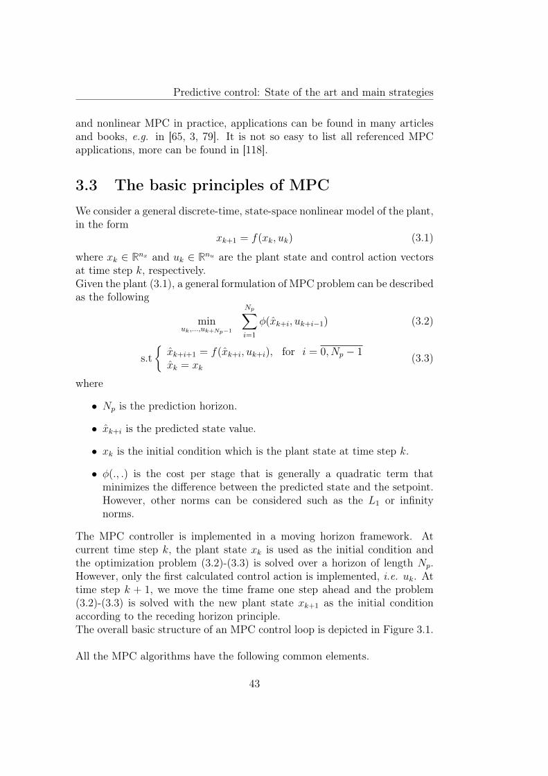
Predictive control: State of the art and main strategies
and nonlinear MPC in practice, applications can be found in many articlesand books, e.g. in [65, 3, 79]. It is not so easy to list all referenced MPCapplications, more can be found in [118].
3.3 The basic principles of MPCWe consider a general discrete-time, state-space nonlinear model of the plant,in the form
xk+1 = f(xk, uk) (3.1)
where xk ∈ Rnx and uk ∈ Rnu are the plant state and control action vectorsat time step k, respectively.Given the plant (3.1), a general formulation of MPC problem can be describedas the following
minuk,...,uk+Np−1
Np∑i=1
φ(xk+i, uk+i−1) (3.2)
s.t{xk+i+1 = f(xk+i, uk+i), for i = 0, Np − 1xk = xk
(3.3)
where
• Np is the prediction horizon.
• xk+i is the predicted state value.
• xk is the initial condition which is the plant state at time step k.
• φ(., .) is the cost per stage that is generally a quadratic term thatminimizes the difference between the predicted state and the setpoint.However, other norms can be considered such as the L1 or infinitynorms.
The MPC controller is implemented in a moving horizon framework. Atcurrent time step k, the plant state xk is used as the initial condition andthe optimization problem (3.2)-(3.3) is solved over a horizon of length Np.However, only the first calculated control action is implemented, i.e. uk. Attime step k + 1, we move the time frame one step ahead and the problem(3.2)-(3.3) is solved with the new plant state xk+1 as the initial conditionaccording to the receding horizon principle.The overall basic structure of an MPC control loop is depicted in Figure 3.1.
All the MPC algorithms have the following common elements.
43
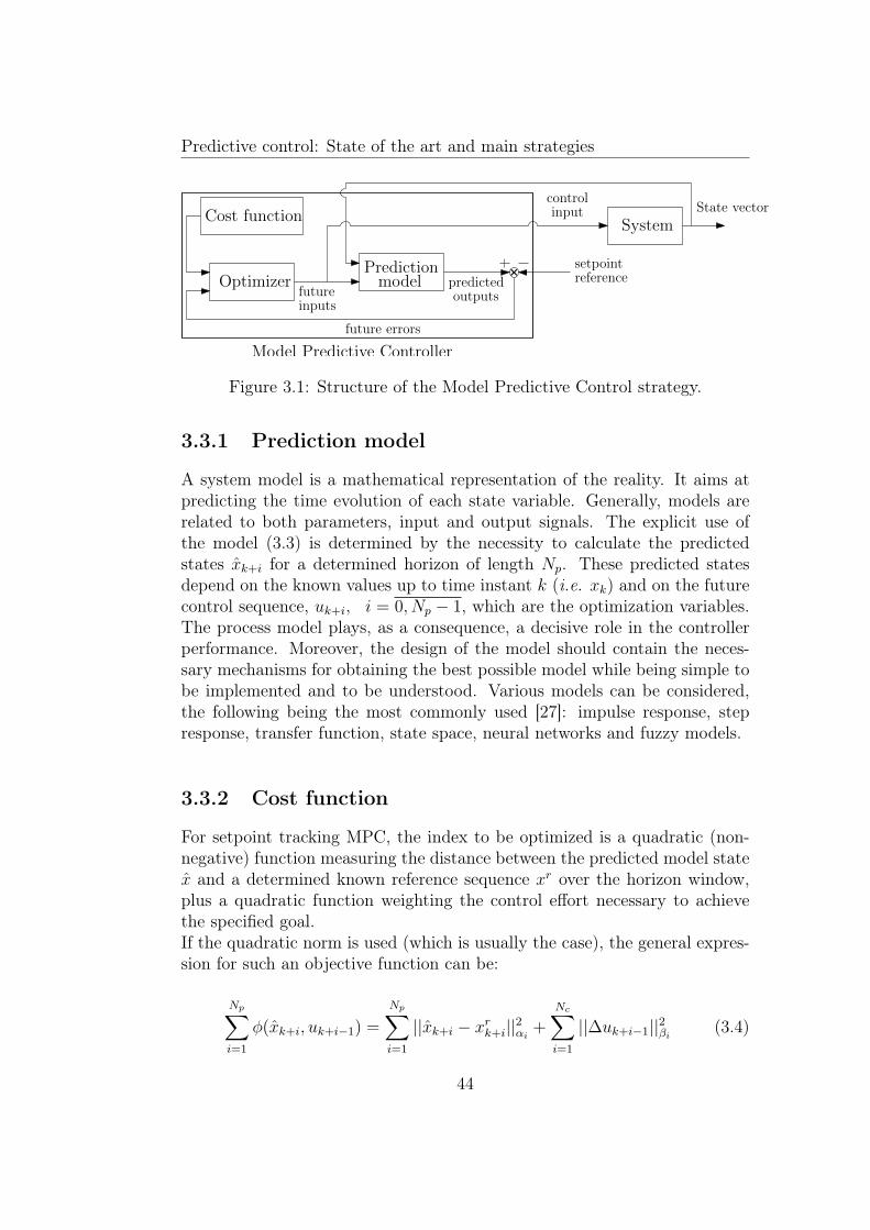
Predictive control: State of the art and main strategies
Cost function
Optimizer model
System
Model Predictive Controller
Prediction
future errors
futureinputs
predictedoutputs
controlinput State vector
setpointreference
Figure 3.1: Structure of the Model Predictive Control strategy.
3.3.1 Prediction model
A system model is a mathematical representation of the reality. It aims atpredicting the time evolution of each state variable. Generally, models arerelated to both parameters, input and output signals. The explicit use ofthe model (3.3) is determined by the necessity to calculate the predictedstates xk+i for a determined horizon of length Np. These predicted statesdepend on the known values up to time instant k (i.e. xk) and on the futurecontrol sequence, uk+i, i = 0, Np − 1, which are the optimization variables.The process model plays, as a consequence, a decisive role in the controllerperformance. Moreover, the design of the model should contain the neces-sary mechanisms for obtaining the best possible model while being simple tobe implemented and to be understood. Various models can be considered,the following being the most commonly used [27]: impulse response, stepresponse, transfer function, state space, neural networks and fuzzy models.
3.3.2 Cost function
For setpoint tracking MPC, the index to be optimized is a quadratic (non-negative) function measuring the distance between the predicted model statex and a determined known reference sequence xr over the horizon window,plus a quadratic function weighting the control effort necessary to achievethe specified goal.If the quadratic norm is used (which is usually the case), the general expres-sion for such an objective function can be:
Np∑i=1
φ(xk+i, uk+i−1) =
Np∑i=1
||xk+i − xrk+i||2αi +Nc∑i=1
||∆uk+i−1||2βi (3.4)
44
Predictive control: State of the art and main strategies
with ∆uk+j = 0, j = Nc, Np − 1 and ∆uk+i−1 = uk+i−1 − uk+i−2.The criterion usually considers the following tuning parameters:
• Np and Nc are the length of the prediction horizon and the controlhorizon respectively, which are not necessarily equal (i.e. Np ≥ Nc ≥ 1)in order to reduce the computational load.
• xr denotes the reference state trajectory which is used to specify closed-loop behavior and tracking performances.
• αi ∈ Rnx×nx and βi ∈ Rnu×nu are the weighting matrices for the statetracking error and the control, respectively. The form of the cost func-tion in (3.4) implies that the deviations of the predicted controlledstates x from a reference xr and the control moves are penalized atevery point in the prediction horizon.
A conceptual picture of the prediction horizon is shown in Figure 3.2.
Future/PredictionPast
k k + Np
Closed-loop output
Closed-loop control input
Setpoint
Control Horizon
Prediction Horizon
k + Nc
Optimal input trajectory
Re-optimal input trajectory
k + 1
(at time index k + 1)
(at time index k)
move
(at time index k + 1)
Predicted output
(at time index k)
Predicted output
Figure 3.2: Receding horizon principle: the basic idea (SISO case).
These tuning parameters should be adjusted to avoid unstability and to givesatisfactory dynamic performance, since all affect the behavior of the closed-loop combination of system and predictive controller. It should be notedthat it is possible to use a non-quadratic cost, so that e.g. absolute values oferrors can be penalized, rather than square values as detailed in [90].
45
Predictive control: State of the art and main strategies
In addition, constraints can be taken into account in the optimizationproblem. For example, the actuators may have a limited field of action. Byadding these constraints to the optimization problem, the latter becomesmore complex, so that the solution can not be obtained explicitly as in theunconstrained case. Moreover, in this case, the paradigm of finding a feasiblesolution to the optimization problem has to be addressed.
3.3.3 Control law calculation
The optimizer is a fundamental part of the MPC strategy as it provides thecontrol actions by minimizing the cost function (3.4). An analytic solutioncan be obtained for the quadratic criterion case if the model is linear andthere are no constraints. Otherwise, the control sequence results from areal-time optimization strategy, involving solving a nonlinear programmingproblem (NLP) (for more details see section 3.5). The size of the optimizationproblem depends on the number of variables and on the prediction horizonconsidered.Summarizing, the basic MPC scheme works as follows:
1. Obtain measurements
2. Compute the model prediction over a certain prediction horizon
3. Get an optimal input signal by minimizing a given cost function
4. Implement the first value of the optimal input signal until new mea-surements are available.
5. Continue with 1.
While it can be desirable for computational and performances reasons tochoose unequal lengths of the prediction and control horizon, we assume inthe following that Np = Nc for the study.
3.4 Literature reviewIn general, MPC can be split into two different classes of methodologies:linear and nonlinear. Maciejowski and Camacho provide a good overviewof linear theory [90, 27], while Allgöwer and Zheng provide an overview ofnonlinear methods [3]. The various MPC algorithms result from the way thecost function to be minimized and the constraints of the system are specified.This section aims at briefly presenting the main MPC strategies found in the
46
Predictive control: State of the art and main strategies
literature, for each of them the reader is referred to appropriate referencesfor more details.
3.4.1 Linear case
Generally, linear MPC uses a low order linear model to represent the system.In case of linear constraints, it has the advantage of solving small optimizationproblem, which can be done fast enough at each sampling time in order tobe implemented in the moving horizon framework. In this case, the solutionof the optimization problem is the solution of a quadratic or linear program(QP/LP), which is known to be convex and for which there exists a varietyof numerical methods and softwares.
Remark 3.1. An analytic solution can be obtained for the quadratic crite-rion if the model is linear and there are no constraints.
On the other hand, linear MPC also suffers from drawbacks such as plant-model mismatch because the model may be only valid around an operatingpoint. Depending on different modelling and solution strategies, there aremany variations of linear MPC, methods considered to be the most repre-sentative will be briefly cited [27]:
• Dynamic Matrix Control (DMC) [40]: the DMC uses a step re-sponse model of the process. The output of the plant is then expressedthrough the time response parameters. The setpoint trajectory can beapproached by a smoother trajectory (called projected desire trajec-tory). Shell engineers developed QDMC by posing the DMC problemas a quadratic programming (QP) problem in which constraints appearexplicitly. Formulations based on linear impulse response models canbe found in [110].
• Model Algorithmic Control (MAC) [128, 129, 121]: this approachis also known as model predictive heuristic control. It uses an impulseresponse model (only for stable processes) and introduces a referencetrajectory as the output of a first order system which evolves from theactual output to the setpoint according to a determined time constant.
• Predictive Functional Control (PFC) [127, 125]: this strategy isdedicated to fast processes although it can accomodate all kinds ofsystems and uses a state space model representation of the process.It has two distinctive characteristics: the use of coincidence points byconsidering only a subset of points in the prediction horizon and the
47
Predictive control: State of the art and main strategies
parametrization of the control signal by means of a set of polynomialbasis functions.
• Extended Prediction Self Adaptive Control (EPSAC) [41]: inthis method, the process is modelled by a discrete transfer function forprediction. The control signal is set constant over the prediction hori-zon. The feedforward effect can be included by extending the modelwith a measurable disturbance term. The control signal can be calcu-lated analytically leading to a very simple control law structure.
• Extended Horizon Adaptive Control (EHAC) [153]: the imple-mentation of EHAC is similar to the previous method but it allows alonger time to drive the plant output to its reference value. For pre-diction, the process is modelled by a transfer function without takinga model of the disturbances into account. It aims at minimizing thediscrepancy between the model and the reference at final instant of theprediction window.
• Generalized Predictive Control (GPC) [36]: the GPC calculatesa control sequence in a such way that it results from the minimizationof a multi-stage cost function defined over a prediction horizon. Ananalytic solution is derived in the unconstrained case. Unstable andnon-minimum phase plants could be dealt with.
3.4.2 Nonlinear case
There are some processes for which the nonlinearities are so crucial or soimportant that a linear model is not sufficient. For these systems, a linearMPC will not be very effective, so some solutions have been proposed to copewith this problem. Using a nonlinear model changes the problem from anonline convex quadratic problem to a repeated online possibly non-convexnonlinear problem, which is more difficult to solve. As a consequence, theconvergence and success of a given optimization problem depend largely onthe initial guess provided for the solution. Nonlinear model predictive con-trol (NMPC) is an optimization-based method for the feedback control ofnonlinear systems. Its primary applications are stabilization and trackingproblems. NMPC is based on the receding horizon principle, where a finitehorizon open-loop optimal control problem is solved at each sampling instantand the optimized control trajectory is implemented until a new optimizedcontrol trajectory is available at the next sampling instant. Its philosophy istherefore similar to linear MPC. The key characteristics of the NMPC are asfollows:
48
Predictive control: State of the art and main strategies
• it allows the use of an explicit nonlinear model for prediction.
• it allows the explicit consideration of state and input constraints.
• specified performance criteria can be minimized online.
• it requires solving online an open-loop optimal control problem.
• system states must be measured or estimated in order to perform theprediction.
Remark 3.2. It should be noted that except the first point, all others arepresent in the linear MPC law.
This subsection aims at drawing up a picture of some classical NMPC algo-rithms:
• Explicit schemes [13, 64, 112]: they compute the control sets offlineby enumerating all the possible states or their approximations. Then,online control actions are chosen from these sets based on where thestate lies.
• Infinite-horizon NMPC [77]: this problem has only theoretical sig-nificance, because an infinite horizon NMPC formulation is that atevery sampling instant an infinite dimensional optimization problemmust be solved as follows:
minuk,...,u∞
∞∑i=1
||xk+i − xrk+i||2αi + ||∆uk+i−1||2βi (3.5)
s.t{xk+i+1 = f(xk+i, uk+i), for i ≥ 0xk = xk
(3.6)
Moreover, infinite-horizon NMPC has the property that the open-looppredictions are identical to the closed-loop response in nominal applica-tion. Ideally, we would like to use infinite-horizon NMPC formulationsdue to stability properties. Unfortunately, the main problem is thatinfinite-horizon schemes can often not be applied in practice.
• Finite-horizon NMPC with terminal equality constraint [77]:the infinite horizon NMPC can be approximated by a finite horizonformulation with terminal equality constraints as follows:
minuk,...,uk+Np−1
Np∑i=1
||xk+i − xrk+i||2αi + ||∆uk+i−1||2βi (3.7)
49
Predictive control: State of the art and main strategies
s.t{xk+i+1 = f(xk+i, uk+i), for i = 0, Np − 1xk = xk, xk+Np = xrk+Np
(3.8)
The terminal equality constraint, xk+Np = xrk+Np, basically ensures that
at the end of the finite horizon, the closed-loop system approaches thesame steady state as in the infinite horizon.
• Finite-horizon NMPC with terminal inequality constraint [105,137]: in this method, a terminal constraint set at the end of the horizonis introduced in the problem formulation. The finite-horizon NMPCgoal is to steer the plant to the constraint set XNp in order to guaranteethe stability of the closed-loop system. The optimization problem isthen given by:
minuk,...,uk+Np−1
Np∑i=1
||xk+i − xrk+i||2αi + ||∆uk+i−1||2βi (3.9)
s.t{xk+i+1 = f(xk+i, uk+i), for i = 0, Np − 1xk = xk, xk+Np ∈ Xk+Np
(3.10)
• Finite-horizon NMPC with terminal cost [20]: the proposed ideato ensure the closed-loop stability is to add a terminal cost function atthe end of the finite-horizon as follows:
minuk,...,uk+Np−1
Np∑i=1
||xk+i − xrk+i||2αi + ||∆uk+i−1||2βi + T (xk+Np) (3.11)
s.t{xk+i+1 = f(xk+i, uk+i), for i = 0, Np − 1xk = xk
(3.12)
where T (xk+Np) is the terminal cost function.
• Quasi-infinite horizon NMPC (QIH-NMPC) [32]: this strategyconsists in combining both the terminal cost function and terminalinequality constraint into the finite-horizon formulation.
minuk,...,uk+Np−1
Np∑i=1
||xk+i − xrk+i||2αi + ||∆uk+i−1||2βi + T (xk+Np) (3.13)
s.t{xk+i+1 = f(xk+i, uk+i), for i = 0, Np − 1xk = xk, xk+Np ∈ Xk+Np
(3.14)
The terminal state penalty term and the terminal inequality constrainthave to be chosen in order to guarantee the asymptotic stability of theclosed-loop system [32].
50
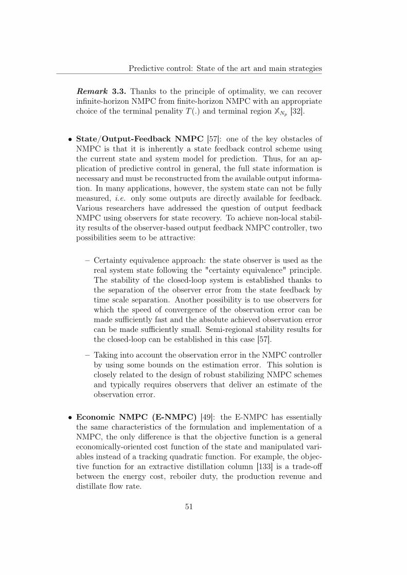
Predictive control: State of the art and main strategies
Remark 3.3. Thanks to the principle of optimality, we can recoverinfinite-horizon NMPC from finite-horizon NMPC with an appropriatechoice of the terminal penality T (.) and terminal region XNp [32].
• State/Output-Feedback NMPC [57]: one of the key obstacles ofNMPC is that it is inherently a state feedback control scheme usingthe current state and system model for prediction. Thus, for an ap-plication of predictive control in general, the full state information isnecessary and must be reconstructed from the available output informa-tion. In many applications, however, the system state can not be fullymeasured, i.e. only some outputs are directly available for feedback.Various researchers have addressed the question of output feedbackNMPC using observers for state recovery. To achieve non-local stabil-ity results of the observer-based output feedback NMPC controller, twopossibilities seem to be attractive:
– Certainty equivalence approach: the state observer is used as thereal system state following the "certainty equivalence" principle.The stability of the closed-loop system is established thanks tothe separation of the observer error from the state feedback bytime scale separation. Another possibility is to use observers forwhich the speed of convergence of the observation error can bemade sufficiently fast and the absolute achieved observation errorcan be made sufficiently small. Semi-regional stability results forthe closed-loop can be established in this case [57].
– Taking into account the observation error in the NMPC controllerby using some bounds on the estimation error. This solution isclosely related to the design of robust stabilizing NMPC schemesand typically requires observers that deliver an estimate of theobservation error.
• Economic NMPC (E-NMPC) [49]: the E-NMPC has essentiallythe same characteristics of the formulation and implementation of aNMPC, the only difference is that the objective function is a generaleconomically-oriented cost function of the state and manipulated vari-ables instead of a tracking quadratic function. For example, the objec-tive function for an extractive distillation column [133] is a trade-offbetween the energy cost, reboiler duty, the production revenue anddistillate flow rate.
51
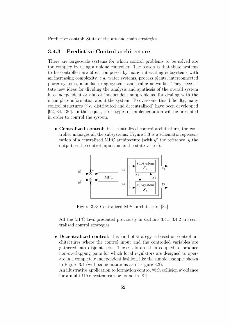
Predictive control: State of the art and main strategies
3.4.3 Predictive Control architecture
There are large-scale systems for which control problems to be solved aretoo complex by using a unique controller. The reason is that these systemsto be controlled are often composed by many interacting subsystems withan increasing complexity, e.g. water systems, process plants, interconnectedpower systems, manufacturing systems and traffic networks. They necessi-tate new ideas for dividing the analysis and synthesis of the overall systeminto independent or almost independent subproblems, for dealing with theincomplete information about the system. To overcome this difficulty, manycontrol structures (i.e. distributed and decentralized) have been developped[92, 34, 136]. In the sequel, three types of implementation will be presentedin order to control the system.
• Centralized control: in a centralized control architecture, the con-troller manages all the subsystems. Figure 3.3 is a schematic represen-tation of a centralized MPC architecture (with yr the reference, y theoutput, u the control input and x the state vector).
subsystemS1
subsystemS2
MPC
y1
y2
x1x2
u1
u2
yr1
yr2
Figure 3.3: Centralized MPC architecture [34].
All the MPC laws presented previously in sections 3.4.1-3.4.2 are cen-tralized control strategies.
• Decentralized control: this kind of strategy is based on control ar-chitectures where the control input and the controlled variables aregathered into disjoint sets. These sets are then coupled to producenon-overlapping pairs for which local regulators are designed to oper-ate in a completely independent fashion, like the simple example shownin Figure 3.4 (with same notations as in Figure 3.3).An illustrative application to formation control with collision avoidancefor a multi-UAV system can be found in [81].
52
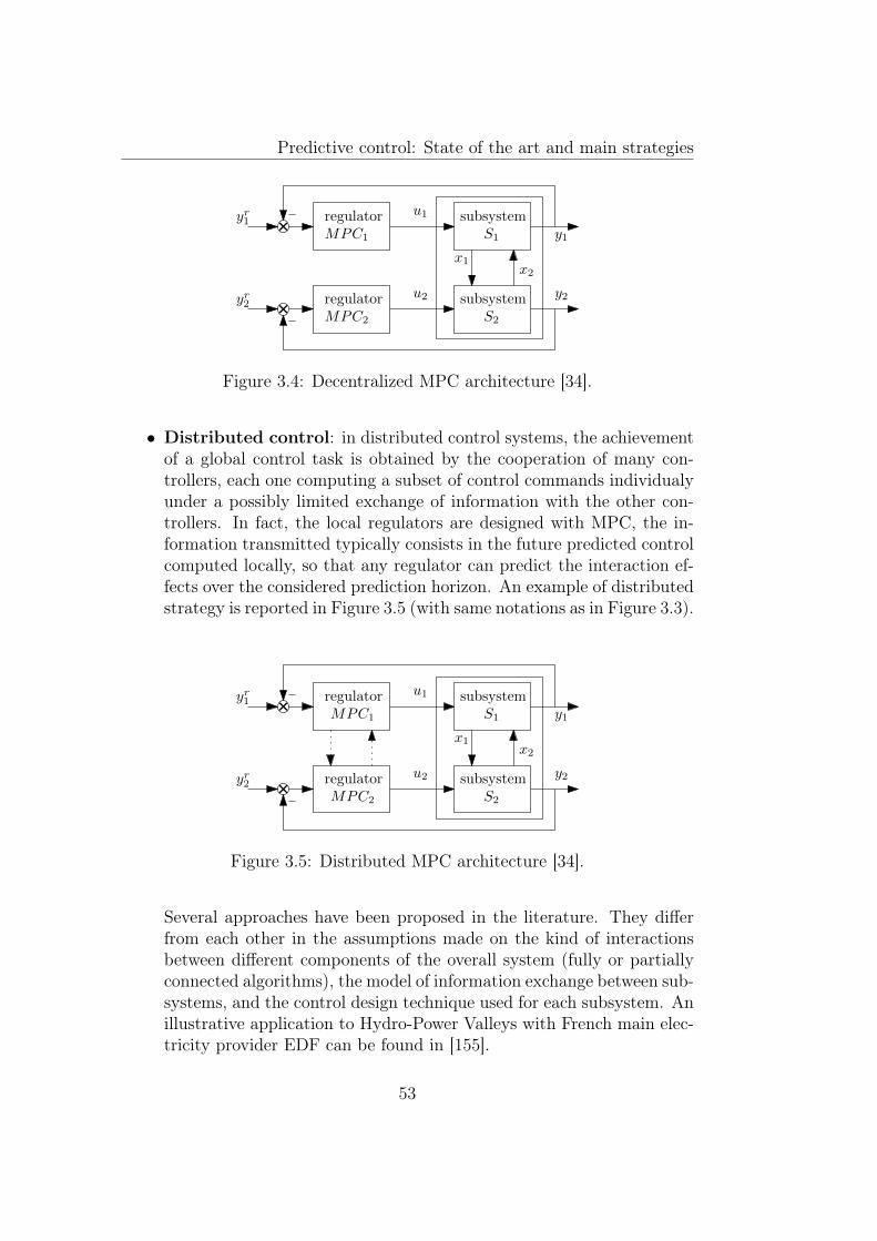
Predictive control: State of the art and main strategies
subsystemS1
subsystemS2
regulatorMPC1
regulatorMPC2
y1
y2
x1x2
u1
u2
yr1
yr2
Figure 3.4: Decentralized MPC architecture [34].
• Distributed control: in distributed control systems, the achievementof a global control task is obtained by the cooperation of many con-trollers, each one computing a subset of control commands individualyunder a possibly limited exchange of information with the other con-trollers. In fact, the local regulators are designed with MPC, the in-formation transmitted typically consists in the future predicted controlcomputed locally, so that any regulator can predict the interaction ef-fects over the considered prediction horizon. An example of distributedstrategy is reported in Figure 3.5 (with same notations as in Figure 3.3).
subsystemS1
subsystemS2
regulatorMPC1
regulatorMPC2
y1
y2
x1x2
u1
u2yr2
yr1
Figure 3.5: Distributed MPC architecture [34].
Several approaches have been proposed in the literature. They differfrom each other in the assumptions made on the kind of interactionsbetween different components of the overall system (fully or partiallyconnected algorithms), the model of information exchange between sub-systems, and the control design technique used for each subsystem. Anillustrative application to Hydro-Power Valleys with French main elec-tricity provider EDF can be found in [155].
53
Predictive control: State of the art and main strategies
3.5 Methods for dynamic optimization
The optimization problems in which the model and constraints are linear andthe objective is quadratic are a well studied class of problems, and the dy-namic optimization problem is solved using well established QP algorithms.In this section, we discuss solution strategies to efficiently solve nonlineardynamic optimization problems. In general the solution of a nonlinear (ingeneral non-convex) optimization problem can be computationally expen-sive. Methods to solve the open-loop optimal control problem (3.2-3.3) canbe classified into three different approaches (Figure 3.6):
• Hamilton-Jacobi-Bellmann partial differential equations/dyn-amic programming: this method is based on the direct solution ofso-called Hamilton-Jacobi-Bellmann partial differential equations. Thisapproach is valid only for small systems due to the curse of dimensional-ity, i.e. since the complete solution is considered at once, it is in generalcomputationally intractable. Moreover, the inequality constraints onthe state variables, as well as dynamical systems with switching points,lead to discontinuous partial derivatives and cannot be easily included.The application of this methodology is restricted to the case of contin-uous state systems.
• Euler-Lagrange differential equations/calculus of variations/m-aximum principle: classical calculus of variations is used in order toobtain an explicit solution of the input as a function of time.
• Direct solution using a finite parametrization of the controlsignal: The input is parametrized by a finite number of values allowingan approximation of the original open-loop control problem.
The basic idea behind the direct solution using a finite parametrization of thecontrols is to approximate the original infinite dimensional problem into afinite dimensional nonlinear programming problem. Then, the input controlsignals are parametrized, e.g. using a piecewise constant function over asampling time. As classified in [18, 51] there are two main strategies:
• Sequential approach: in every iteration step of the optimizationstrategy, the differential equations are solved exactly by a numericalintegration, i.e. the solution of the system dynamics is implicitly de-termined during the calculation of the cost function and only the inputvector uk+i−1 appears directly in the optimization problem while theintermediate states xk+i disappear from the problem formulation. This
54
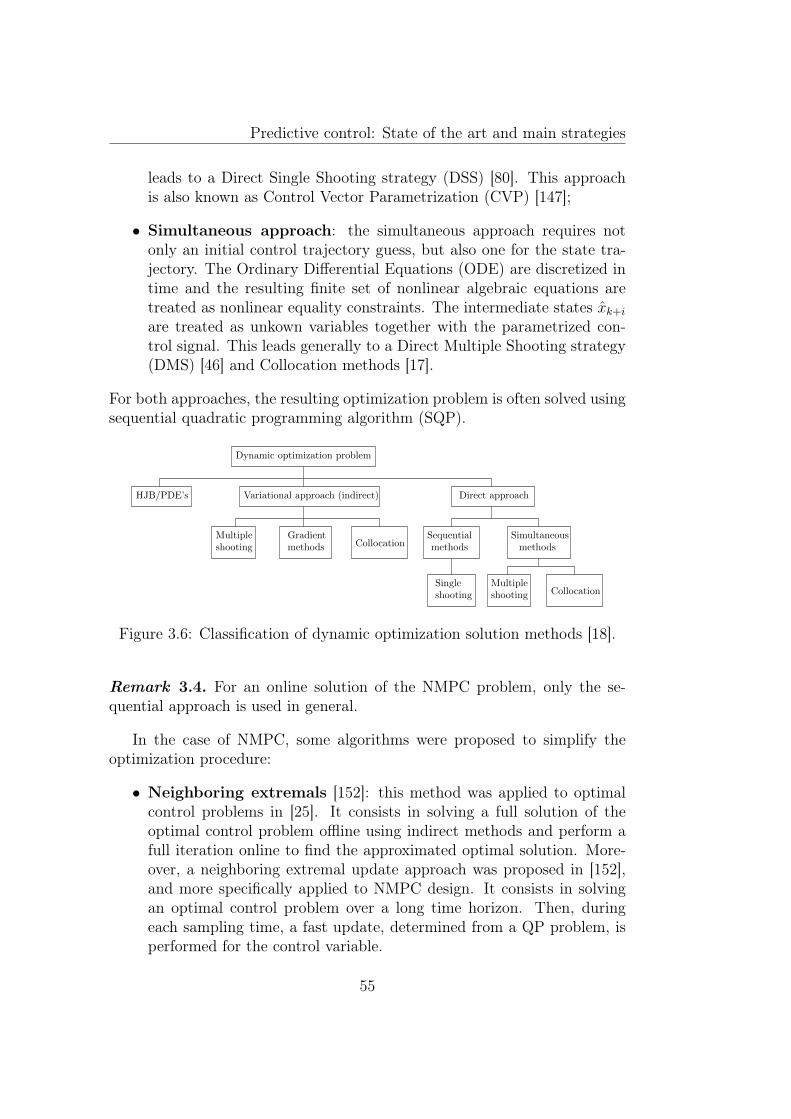
Predictive control: State of the art and main strategies
leads to a Direct Single Shooting strategy (DSS) [80]. This approachis also known as Control Vector Parametrization (CVP) [147];
• Simultaneous approach: the simultaneous approach requires notonly an initial control trajectory guess, but also one for the state tra-jectory. The Ordinary Differential Equations (ODE) are discretized intime and the resulting finite set of nonlinear algebraic equations aretreated as nonlinear equality constraints. The intermediate states xk+i
are treated as unkown variables together with the parametrized con-trol signal. This leads generally to a Direct Multiple Shooting strategy(DMS) [46] and Collocation methods [17].
For both approaches, the resulting optimization problem is often solved usingsequential quadratic programming algorithm (SQP).
Dynamic optimization problem
HJB/PDE’s Variational approach (indirect) Direct approach
GradientMultipleCollocation
Sequential Simultaneousmethods methodsmethodsshooting
Singleshooting
Multipleshooting Collocation
Figure 3.6: Classification of dynamic optimization solution methods [18].
Remark 3.4. For an online solution of the NMPC problem, only the se-quential approach is used in general.
In the case of NMPC, some algorithms were proposed to simplify theoptimization procedure:
• Neighboring extremals [152]: this method was applied to optimalcontrol problems in [25]. It consists in solving a full solution of theoptimal control problem offline using indirect methods and perform afull iteration online to find the approximated optimal solution. More-over, a neighboring extremal update approach was proposed in [152],and more specifically applied to NMPC design. It consists in solvingan optimal control problem over a long time horizon. Then, duringeach sampling time, a fast update, determined from a QP problem, isperformed for the control variable.
55
Predictive control: State of the art and main strategies
• Newton-type controller [84, 45, 50, 44]: it performs a single fullNewton step of NMPC online to allow a quick return of control action.The main advantage is that it rejects the fast disturbance quickly. TheNewton’s method is based on linearization and it is used in nonlin-ear programming to solve algebraic equations closely related to thefirst order optimality conditions of the optimization problem, knownas the Karush-Kuhn-Tucker (KKT) conditions. Obviously, the KKTconditions also involve inequalities which means that Newton’s methodcannot be applied directly.
• NLP sensitivity-based controller [26, 75]: it aims at overcomingthe drawbacks posed by the Newton-type controllers. NLP sensitivity-based controllers use a direct method to solve the optimal control prob-lem. The sensitivity analysis for NLP provides information on regular-ity and curvature conditions at KKT points, evaluates which variablesplay dominant roles in the optimization, and provides first order esti-mates for parametric nonlinear programs. In closed-loop, this approachis very effective to handle uncertainty while requiring only a minimumnumber of full real-time optimizations, reducing the online computa-tional load.
• Advanced step NMPC (asNMPC) [156]: a kind of NLP sensitivity-based NMPC which uses the current control action to predict the futureplant state in order to solve the future optimization problem in advance,while the current sampling period evolves.
3.6 Robust NMPC schemes
Nonlinear MPC is often used in control problems. However, assumptionsof nominality reduce its use or performances. This is why other kinds ofpredictive control methods are developed to take account of uncertaintiesrelated to the system model and disturbances acting on it. Hereafter, themain robust NMPC strategies will be briefly presented. There exists a widerange of NMPC formulations that include robustness into the formulation ofthe optimization problem. We distinguish four main types of approaches:
• Linear parameter varying formulations: these methods are basedon the reformulation of nonlinear models as linear parameter-varying(LPV) models which allow the use of linear and bilinear matrix inequal-ity (LMI and BMI) formulations [6, 29, 148].
56
Predictive control: State of the art and main strategies
• Min-max NMPC: in this formulation, the standard NMPC setup iskept, however, now, the cost function to be optimized considers theworst disturbance sequence occuring. The disturbance/uncertainty inthe system is considered as a player working against the input. Thus,the problem is formulated as a classical min-max problem over a finite-horizon. There are two formulations of min-max NMPC:
– Open-loop formulation: this approach guarantees the robust sta-bility of the system and the robust feasibility of the optimizationproblem, but it may be conservative since the control sequencehas to ensure constraints fulfilment for all possible uncertaintyscenarii without considering the fact that future measurementsof the state contain information about past uncertainty values[85, 93, 102]. This method may have a small feasible set and apoor performance due to the fact that it does not include the effectof feedback provided by the receding horizon framework.
– Closed-loop formulation: the min-max problem represents a dif-ferential game where the controller is the minimizing player andthe disturbance is the output of the maximizing player [88, 91, 93].The controller chooses the control input as a function of the cur-rent state so as to ensure that the effect of the disturbance onthe system output is sufficiently small for any choice made by themaximizing player. This method would guarantee a larger fea-sible set and a higher level of performances in comparison withthe open-loop min-max NMPC. By doing this, the reaction of thecontroller to the uncertainty is incorporated in the prediction andthe conservativeness is mitigated.
The robust min-max strategy and more specifically the closed-loop for-mulation, will be detailed in Chapter 5.
• H∞-NMPC : the standard H∞ problem is implemented in a recedinghorizon framework by considering a particular choice of the cost func-tion. More details concerning this approach can be found in [60, 150,151].
• Stochastic Model Predictive Control (SMPC): all previous strate-gies consider a deterministic framework by assuming that pertubationsand uncertainties belong to compact bounded sets. However, it canbe sometimes more realistic to solve problems based on a probabilisticdescription of the uncertainties and perturbations. This corresponds to
57
Predictive control: State of the art and main strategies
a stochastic approach. Thus, formulations based on a probabilistic de-scription of uncertainty can also be characterized as problems involvingrandom model uncertainty with known probability distribution. Fur-thermore, stochastic NMPC can also be characterized similarly to min-max NMPC as described above, either open-loop formulation [28] orclosed-loop formulation [63].
3.7 Stability
One of the key questions in the MPC strategy is certainly the stability of theclosed-loop system. After basic theoretical principles of MPC had been clar-ified, more advanced topics like robust stability under perturbations, perfor-mance estimates and efficiency of numerical algorithm were addressed. Thestability of MPC for constrained nonlinear systems necessitates the use ofLyapunov stability theory that can be expressed conveniently via so-calledcomparison functions, which were introduced in nonlinear control theory bySontag [139].The stability of the system without disturbances is called nominal stability,while the stability of the system in the presence of disturbances is termedrobust stability.
3.7.1 Nominal stability
Nominal stability of closed-loop system is proven if one can find a Lyapunovfunction for the system. Strategies which guarantee the nominal stability aresummarized as follows: infinite horizon NMPC, finite-horizon NMPC withterminal equality constraint, finite-horizon NMPC with terminal inequalityconstraint, finite-horizon NMPC with terminal cost, quasi-infinite horizonNMPC. Results with guaranteed nominal stability are well-addressed by ex-isting works detailed in [100, 106, 122, 123, 157, 130].
3.7.2 Robust stability
As stated before, the robust control design of NMPC is done by taking intoaccount uncertainties in an explicit manner in order to optimize the objectivefunction for the worst situation of the uncertainties. There are many ap-proaches to analyze the robust stability, such as Input-to-State (ISS) frame-work, robust stability margin and invariant set theory coupled with ISS-Lyapunov stability framework. Further details and a more comprehensive
58
Predictive control: State of the art and main strategies
treatment of this topic can be found in [94, 93, 115, 119, 85, 88, 4, 104]. Fun-damental results on stability for constrained and nonlinear predictive controlfor state-space models are well summarized and categorized in [87, 120].
3.8 Advantages and drawbacks
The RHC presents a series of advantages over the other existing controlstrategies, summarized as follows:
• Straightforward formulation, based on well understood concepts,
• Open methodology which allows future extensions,
• Compensation for dead times,
• Applicability to a great variety of systems, including nonlinear systemsand time-delayed systems,
• Proof of stability for linear and nonlinear systems with input and stateconstraints, under certain specific conditions,
• Very useful when future references are known a priori, the system canreact before the change has effectively been made inducing an anticipa-tive effect, thus minimizing the effects of delay in the process response,
• Multivariable case can easily be dealt with,
• Extension to the treatment of the constraints (take into account actu-ators limitation),
• Development time relatively shorter than for competing advanced con-trol methods.
• Easier to maintain and to implement in case of changing the model orits parameters. Indeed, model modification does not require completeredesign.
It also has its drawbacks:
• One of these is that the control law requires a longer computation timecompared with conventional control strategies, e.g. Lyapunov-baseddesign. When inequality constraints are considered, the amount ofcomputation required is even higher,
• Generally, lack of stability proof except for special cases (as mentionedin the point above in the advantage section).
59
Predictive control: State of the art and main strategies
However, the greatest requirement is the need for an appropriate model ofthe process to be available. In fact, the design algorithm is based on a priorknowledge of the model but is not dependant on a specific model structure. Itis however obvious that benefits obtained will be affected by the gap existingbetween the real process and the prediction model.
3.9 Concluding remarksThe receding horizon control is one of the most popular advanced controlstrategies due to its simplicity of implementation and interesting propertiesmentioned above. This chapter presented a general formulation of the modelpredictive control that will be used in the context of trajectory trackingproblem. The brief review focused on the area of linear and nonlinear MPCschemes, addressing robustness issues and nominal and robust stabilities.The specific task we will focus on in the next chapter is the setpoint trackingNMPC for discrete-time nonlinear systems.
60
Chapter 4
Nonlinear Model PredictiveControl
4.1 Introduction
In this chapter, we investigate the strategy that will be further considered andmodified to solve a trajectory tracking problem for continuous/discrete-timenonlinear systems. This leads to explore the NMPC formulation discussedin Chapter 3. The chapter will be organized as follows. Section 4.2 is de-voted to the NMPC problem formulation and the class of nonlinear systemsthat will be considered. A variant of NMPC is presented in section 4.3 andan illustrative example (a class of bioprocesses) is presented in section 4.4.Numerical results are provided in order to demonstrate the effectiveness andlimitations of the NMPC strategy. Finally, conclusions are stated in section4.5.
4.2 Problem formulation
This section will introduce the formulation of a basic standard nonlinearfinite-horizon optimal control problem starting from a continuous-time model.
4.2.1 Continuous/discrete formulation
As mentionned in Chapter 3, the first step to implement the NMPC strategyis achieved with the use of a prediction model. In this context, it is importantto obtain a mathematical representation as properly as possible reproducingthe behavior of the system to be controlled. In our case, we will use a
61
Nonlinear Model Predictive Control
continuous/discrete formulation: time-continuous model for prediction anddiscrete model for control.
Consider a system described by an uncertain continuous-time nonlinearmodel: {
x(t) = F (x(t), u(t), θ), x0 = xy(t) = Hx(t)
(4.1)
where
• x ∈ X ⊆ Rnx is the state vector with X the compact set of admissiblestates;
• x is the initial state vector;
• y ∈ Y ⊆ Rny is the measured output with Y the compact set of admis-sible outputs;
• u ∈ U ⊆ Rnu represents the control input with U the compact set ofadmissible controls;
• θ ∈ Rnθ is the vector of uncertain parameters that are assumed to liein the compact set Θ = [θ−, θ+] defined as follows:
θ = θnom + δθ (4.2)
where θnom is the nominal parameters vector defined as the averagevalue (centroid) of the compact set:
θnom =θ+ + θ−
2(4.3)
and δθ the parameters uncertainties vector;
• The mapping F : Rnx × Rnu × Rnθ −→ Rnx , of class C1 with respect toall its arguments, represents the nonlinear process dynamics;
• The measurement matrix is given by H ∈ Rny×nx ;
Remark 4.1. The sets X and U are generally polyhedral convex sets, takinginto account e.g. physical constraints acting on the system.
Remark 4.2. The measurement could be nonlinear with respect to the state.It is assumed linear to simplifiy mathematical developments.
62
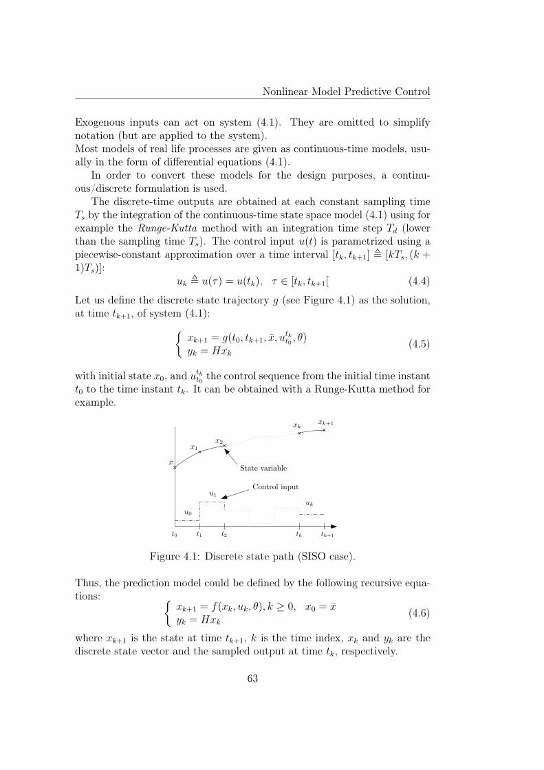
Nonlinear Model Predictive Control
Exogenous inputs can act on system (4.1). They are omitted to simplifynotation (but are applied to the system).Most models of real life processes are given as continuous-time models, usu-ally in the form of differential equations (4.1).
In order to convert these models for the design purposes, a continu-ous/discrete formulation is used.
The discrete-time outputs are obtained at each constant sampling timeTs by the integration of the continuous-time state space model (4.1) using forexample the Runge-Kutta method with an integration time step Td (lowerthan the sampling time Ts). The control input u(t) is parametrized using apiecewise-constant approximation over a time interval [tk, tk+1] , [kTs, (k +1)Ts)]:
uk , u(τ) = u(tk), τ ∈ [tk, tk+1[ (4.4)
Let us define the discrete state trajectory g (see Figure 4.1) as the solution,at time tk+1, of system (4.1):{
xk+1 = g(t0, tk+1, x, utkt0 , θ)
yk = Hxk(4.5)
with initial state x0, and utkt0 the control sequence from the initial time instantt0 to the time instant tk. It can be obtained with a Runge-Kutta method forexample.
t0 t1 t2 tk
x1
x2
xk+1
u0
u1
uk
Control input
State variable
tk+1
x
xk
Figure 4.1: Discrete state path (SISO case).
Thus, the prediction model could be defined by the following recursive equa-tions: {
xk+1 = f(xk, uk, θ), k ≥ 0, x0 = xyk = Hxk
(4.6)
where xk+1 is the state at time tk+1, k is the time index, xk and yk are thediscrete state vector and the sampled output at time tk, respectively.
63
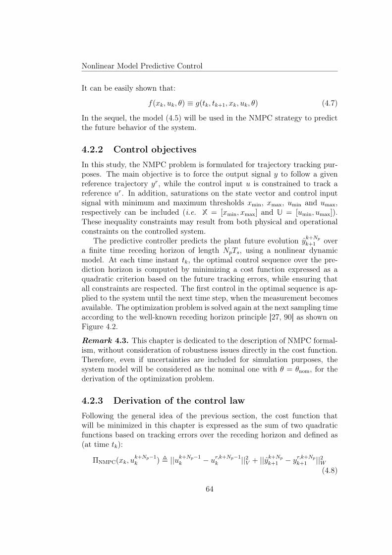
Nonlinear Model Predictive Control
It can be easily shown that:
f(xk, uk, θ) ≡ g(tk, tk+1, xk, uk, θ) (4.7)
In the sequel, the model (4.5) will be used in the NMPC strategy to predictthe future behavior of the system.
4.2.2 Control objectives
In this study, the NMPC problem is formulated for trajectory tracking pur-poses. The main objective is to force the output signal y to follow a givenreference trajectory yr, while the control input u is constrained to track areference ur. In addition, saturations on the state vector and control inputsignal with minimum and maximum thresholds xmin, xmax, umin and umax,respectively can be included (i.e. X = [xmin, xmax] and U = [umin, umax]).These inequality constraints may result from both physical and operationalconstraints on the controlled system.
The predictive controller predicts the plant future evolution yk+Npk+1 over
a finite time receding horizon of length NpTs, using a nonlinear dynamicmodel. At each time instant tk, the optimal control sequence over the pre-diction horizon is computed by minimizing a cost function expressed as aquadratic criterion based on the future tracking errors, while ensuring thatall constraints are respected. The first control in the optimal sequence is ap-plied to the system until the next time step, when the measurement becomesavailable. The optimization problem is solved again at the next sampling timeaccording to the well-known receding horizon principle [27, 90] as shown onFigure 4.2.
Remark 4.3. This chapter is dedicated to the description of NMPC formal-ism, without consideration of robustness issues directly in the cost function.Therefore, even if uncertainties are included for simulation purposes, thesystem model will be considered as the nominal one with θ = θnom, for thederivation of the optimization problem.
4.2.3 Derivation of the control law
Following the general idea of the previous section, the cost function thatwill be minimized in this chapter is expressed as the sum of two quadraticfunctions based on tracking errors over the receding horizon and defined as(at time tk):
ΠNMPC(xk, uk+Np−1k ) , ||uk+Np−1
k − ur,k+Np−1k ||2V + ||yk+Np
k+1 − yr,k+Npk+1 ||2W
(4.8)
64
Nonlinear Model Predictive Control
FuturePast
k k + 1 k + 2 k +Np − 1
yk
yk+1yk+2
yk
yk+1
yk+2
yk+Np−1
yk+Np−1
yk−1
yk−2
uk
uk+1
uk+Np−1
uk−1
uk−2
Past output
Past input
Predicted input
Predicted output
Output
Setpoint
k − 1k − 2
Prediction Horizon
yk+Np
yk+Np
Figure 4.2: Principle of the NMPC (SISO case).
The discrete-time prediction model is chosen as:{xk+j = g(tk, tk+j, xk, u
k+j−1k , θ)
yk+j = Hxk+j, ∀j = 1, Np(4.9)
subject to the constraints in a matrix form:Inx 0nu−Inx 0nu0nx Inu0nx −Inu
[ xk+j
uk+j−1
]≤
xmax
−xmin
umax
−umin
, ∀j = 1, Np (4.10)
with xk the state vector at time tk,
uk+Np−1k =
uk...
uk+Np−1
the optimization variable,
ur,k+Np−1k =
urk...
urk+Np−1
the reference control sequence,
yk+Npk+1 =
Hg(tk, tk+1, xk, uk, θnom)Hg(tk, tk+2, xk, u
k+1k , θnom)
...Hg(tk, tk+Np , xk, u
k+Np−1k , θnom)
the predicted output sequence,
(4.11)
65
Nonlinear Model Predictive Control
and yr,k+Npk+1 =
yrk+1...
yrk+Np
the setpoint values,
where the subscript is related to the time instant.
Np is the length of the prediction horizon. V � 0 and W � 0 are tun-ing weighting matrices.
As mentionned before, assuming a perfect knowledge of the parameter vectorθ (i.e. θ = θnom, determined from an identification procedure for example),the formulation of the optimization problem is moved into NLP problem overa finite prediction horizon NpTs at each sampling time tk. The optimal con-trol sequence is obtained by minimizing the performance criterion (4.8) withthe constraints (4.10) as follows:
?uk+Np−1
k = arg minuk+Np−1
k
ΠNMPC(xk, uk+Np−1k ) (4.12)
s.t. (4.9)-(4.10)
This problem is in general non-convex, it is solved classicaly using algo-rithms for constrained optimization problems. However, in the case wherethe constraints are only bounds on the optimization variables, the optimiza-tion problem is more tractable.
Remark 4.4. This formulation of the optimization problem belongs in factto the sequential family of dynamic optimization methods (as mentioned insection 3.5).
Remark 4.5. For the NMPC problem (4.12), at each sampling time (k+1)Tsthe optimization variable uk+Np
k+1 is initialized by the optimal control sequence?uk+Np−1
k+1 obtained from the optimization (4.12) at time instant k as follows:(uk+Npk+1
)ini
= [?uk+Np−1
k+1 ,?uk+Np−1], ∀k ≥ 0
The NMPC problem is implemented as stated in Figure 4.3.
4.2.4 NMPC tuning
The computational burden of a NMPC algorithm is high and there are num-bers of factors that affect it. These factors include the prediction horizonNp, the optimization method, the number of states nx and control variables
66
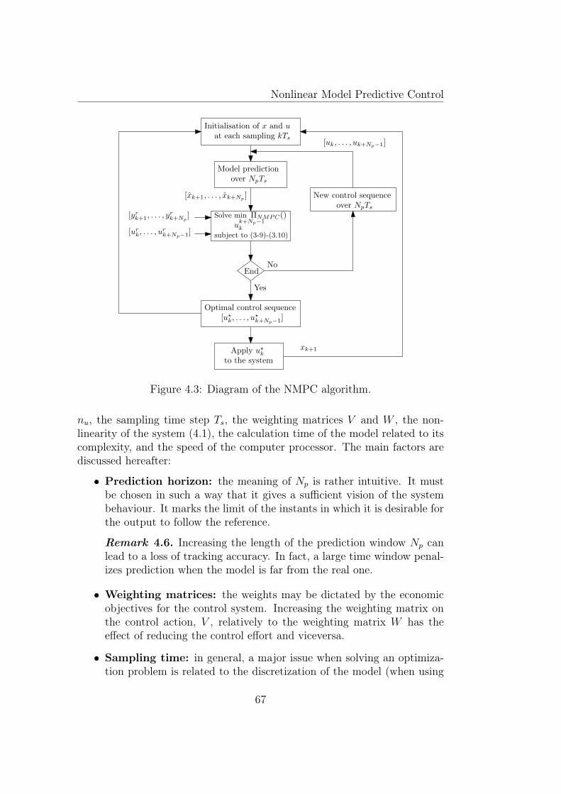
Nonlinear Model Predictive Control
Initialisation of x and uat each sampling kTs
Model prediction
End
Optimal control sequence[u?
k, . . . , u?k+Np−1]
[xk+1, . . . , xk+Np ] New control sequenceover NpTs
Apply u?k
over NpTs
[yrk+1, . . . , yrk+Np
]
[urk, . . . , u
rk+Np−1]
to the system
xk+1
[uk, . . . , uk+Np−1]
No
Yes
subject to (3-9)-(3.10)
ΠNMPC()Solve min
uk+Np−1k
Figure 4.3: Diagram of the NMPC algorithm.
nu, the sampling time step Ts, the weighting matrices V and W , the non-linearity of the system (4.1), the calculation time of the model related to itscomplexity, and the speed of the computer processor. The main factors arediscussed hereafter:
• Prediction horizon: the meaning of Np is rather intuitive. It mustbe chosen in such a way that it gives a sufficient vision of the systembehaviour. It marks the limit of the instants in which it is desirable forthe output to follow the reference.
Remark 4.6. Increasing the length of the prediction window Np canlead to a loss of tracking accuracy. In fact, a large time window penal-izes prediction when the model is far from the real one.
• Weighting matrices: the weights may be dictated by the economicobjectives for the control system. Increasing the weighting matrix onthe control action, V , relatively to the weighting matrix W has theeffect of reducing the control effort and viceversa.
• Sampling time: in general, a major issue when solving an optimiza-tion problem is related to the discretization of the model (when using
67
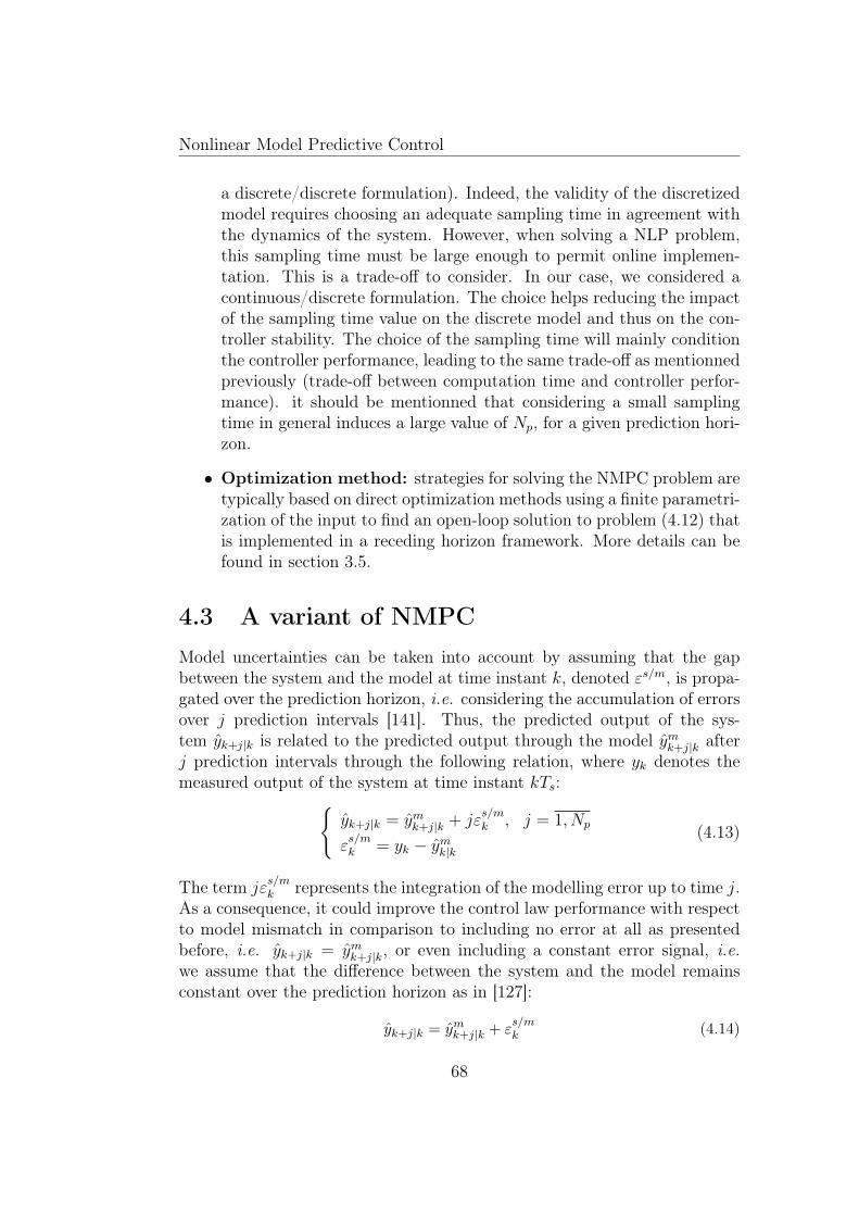
Nonlinear Model Predictive Control
a discrete/discrete formulation). Indeed, the validity of the discretizedmodel requires choosing an adequate sampling time in agreement withthe dynamics of the system. However, when solving a NLP problem,this sampling time must be large enough to permit online implemen-tation. This is a trade-off to consider. In our case, we considered acontinuous/discrete formulation. The choice helps reducing the impactof the sampling time value on the discrete model and thus on the con-troller stability. The choice of the sampling time will mainly conditionthe controller performance, leading to the same trade-off as mentionnedpreviously (trade-off between computation time and controller perfor-mance). it should be mentionned that considering a small samplingtime in general induces a large value of Np, for a given prediction hori-zon.
• Optimization method: strategies for solving the NMPC problem aretypically based on direct optimization methods using a finite parametri-zation of the input to find an open-loop solution to problem (4.12) thatis implemented in a receding horizon framework. More details can befound in section 3.5.
4.3 A variant of NMPCModel uncertainties can be taken into account by assuming that the gapbetween the system and the model at time instant k, denoted εs/m, is propa-gated over the prediction horizon, i.e. considering the accumulation of errorsover j prediction intervals [141]. Thus, the predicted output of the sys-tem yk+j|k is related to the predicted output through the model ymk+j|k afterj prediction intervals through the following relation, where yk denotes themeasured output of the system at time instant kTs:{
yk+j|k = ymk+j|k + jεs/mk , j = 1, Np
εs/mk = yk − ymk|k
(4.13)
The term jεs/mk represents the integration of the modelling error up to time j.
As a consequence, it could improve the control law performance with respectto model mismatch in comparison to including no error at all as presentedbefore, i.e. yk+j|k = ymk+j|k, or even including a constant error signal, i.e.we assume that the difference between the system and the model remainsconstant over the prediction horizon as in [127]:
yk+j|k = ymk+j|k + εs/mk (4.14)
68
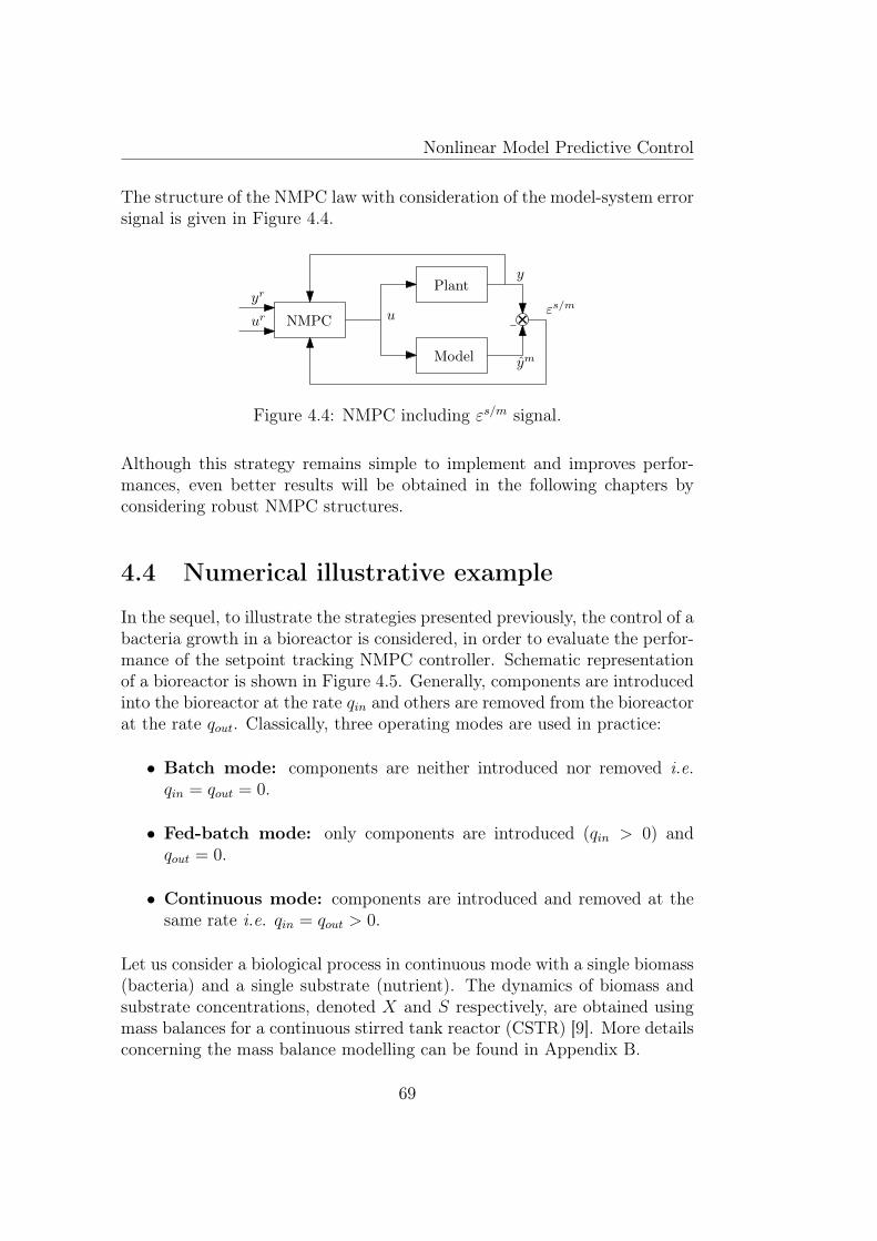
Nonlinear Model Predictive Control
The structure of the NMPC law with consideration of the model-system errorsignal is given in Figure 4.4.
Plant
Model
NMPC
y
ym
εs/muyr
ur
Figure 4.4: NMPC including εs/m signal.
Although this strategy remains simple to implement and improves perfor-mances, even better results will be obtained in the following chapters byconsidering robust NMPC structures.
4.4 Numerical illustrative example
In the sequel, to illustrate the strategies presented previously, the control of abacteria growth in a bioreactor is considered, in order to evaluate the perfor-mance of the setpoint tracking NMPC controller. Schematic representationof a bioreactor is shown in Figure 4.5. Generally, components are introducedinto the bioreactor at the rate qin and others are removed from the bioreactorat the rate qout. Classically, three operating modes are used in practice:
• Batch mode: components are neither introduced nor removed i.e.qin = qout = 0.
• Fed-batch mode: only components are introduced (qin > 0) andqout = 0.
• Continuous mode: components are introduced and removed at thesame rate i.e. qin = qout > 0.
Let us consider a biological process in continuous mode with a single biomass(bacteria) and a single substrate (nutrient). The dynamics of biomass andsubstrate concentrations, denoted X and S respectively, are obtained usingmass balances for a continuous stirred tank reactor (CSTR) [9]. More detailsconcerning the mass balance modelling can be found in Appendix B.
69
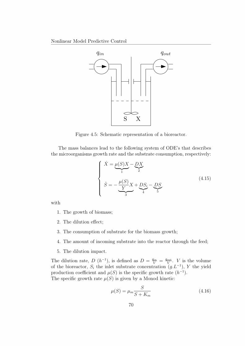
Nonlinear Model Predictive Control
qoutqin
XS
Figure 4.5: Schematic representation of a bioreactor.
The mass balances lead to the following system of ODE’s that describesthe microorganisms growth rate and the substrate consumption, respectively:
X = µ(S)X︸ ︷︷ ︸1
−DX︸︷︷︸2
S = − µ(S)
YX︸ ︷︷ ︸
3
+DSi︸︷︷︸4
− DS︸︷︷︸5
(4.15)
with
1. The growth of biomass;
2. The dilution effect;
3. The consumption of substrate for the biomass growth;
4. The amount of incoming substrate into the reactor through the feed;
5. The dilution impact.
The dilution rate, D (h−1), is defined as D = qinV
= qoutV
. V is the volumeof the bioreactor, Si the inlet substrate concentration (g.L−1), Y the yieldproduction coefficient and µ(S) is the specific growth rate (h−1).The specific growth rate µ(S) is given by a Monod kinetic:
µ(S) = µmS
S +Km
(4.16)
70
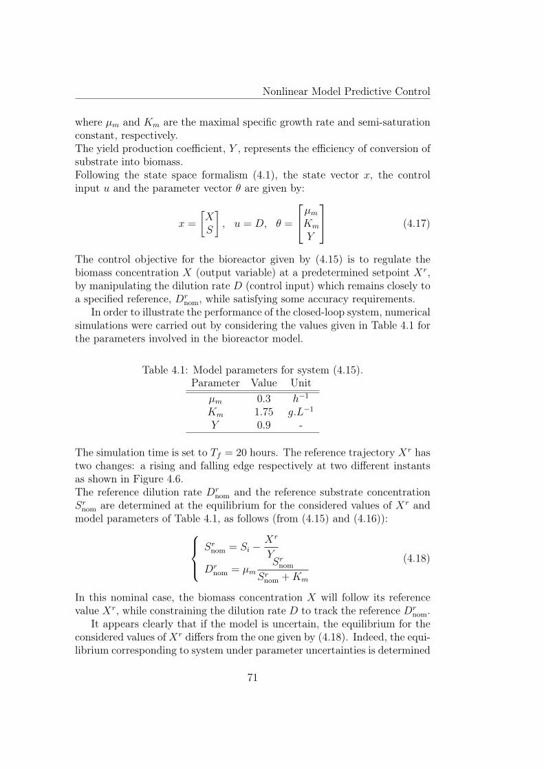
Nonlinear Model Predictive Control
where µm and Km are the maximal specific growth rate and semi-saturationconstant, respectively.The yield production coefficient, Y , represents the efficiency of conversion ofsubstrate into biomass.Following the state space formalism (4.1), the state vector x, the controlinput u and the parameter vector θ are given by:
x =
[XS
], u = D, θ =
µmKm
Y
(4.17)
The control objective for the bioreactor given by (4.15) is to regulate thebiomass concentration X (output variable) at a predetermined setpoint Xr,by manipulating the dilution rate D (control input) which remains closely toa specified reference, Dr
nom, while satisfying some accuracy requirements.In order to illustrate the performance of the closed-loop system, numerical
simulations were carried out by considering the values given in Table 4.1 forthe parameters involved in the bioreactor model.
Table 4.1: Model parameters for system (4.15).Parameter Value Unit
µm 0.3 h−1
Km 1.75 g.L−1
Y 0.9 -
The simulation time is set to Tf = 20 hours. The reference trajectory Xr hastwo changes: a rising and falling edge respectively at two different instantsas shown in Figure 4.6.The reference dilution rate Dr
nom and the reference substrate concentrationSrnom are determined at the equilibrium for the considered values of Xr andmodel parameters of Table 4.1, as follows (from (4.15) and (4.16)):
Srnom = Si −Xr
Y
Drnom = µm
Srnom
Srnom +Km
(4.18)
In this nominal case, the biomass concentration X will follow its referencevalue Xr, while constraining the dilution rate D to track the reference Dr
nom.It appears clearly that if the model is uncertain, the equilibrium for the
considered values of Xr differs from the one given by (4.18). Indeed, the equi-librium corresponding to system under parameter uncertainties is determined
71
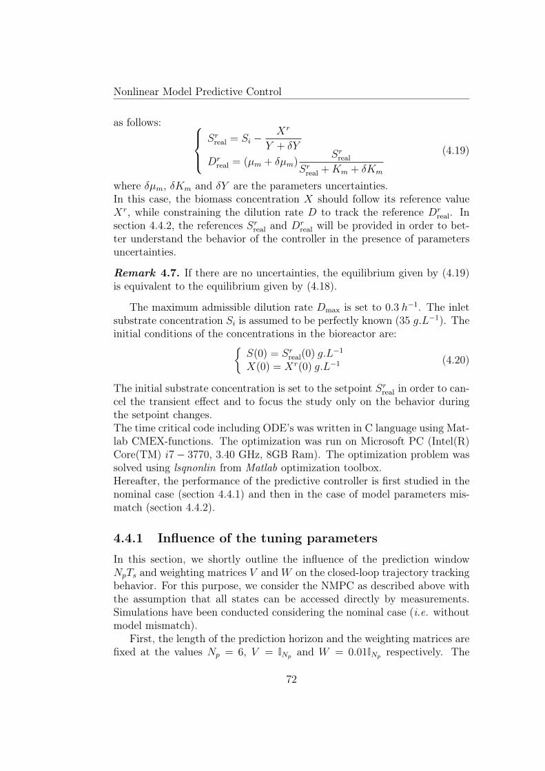
Nonlinear Model Predictive Control
as follows: Srreal = Si −
Xr
Y + δY
Drreal = (µm + δµm)
Srreal
Srreal +Km + δKm
(4.19)
where δµm, δKm and δY are the parameters uncertainties.In this case, the biomass concentration X should follow its reference valueXr, while constraining the dilution rate D to track the reference Dr
real. Insection 4.4.2, the references Srreal and Dr
real will be provided in order to bet-ter understand the behavior of the controller in the presence of parametersuncertainties.
Remark 4.7. If there are no uncertainties, the equilibrium given by (4.19)is equivalent to the equilibrium given by (4.18).
The maximum admissible dilution rate Dmax is set to 0.3 h−1. The inletsubstrate concentration Si is assumed to be perfectly known (35 g.L−1). Theinitial conditions of the concentrations in the bioreactor are:{
S(0) = Srreal(0) g.L−1
X(0) = Xr(0) g.L−1 (4.20)
The initial substrate concentration is set to the setpoint Srreal in order to can-cel the transient effect and to focus the study only on the behavior duringthe setpoint changes.The time critical code including ODE’s was written in C language using Mat-lab CMEX-functions. The optimization was run on Microsoft PC (Intel(R)Core(TM) i7− 3770, 3.40 GHz, 8GB Ram). The optimization problem wassolved using lsqnonlin from Matlab optimization toolbox.Hereafter, the performance of the predictive controller is first studied in thenominal case (section 4.4.1) and then in the case of model parameters mis-match (section 4.4.2).
4.4.1 Influence of the tuning parameters
In this section, we shortly outline the influence of the prediction windowNpTs and weighting matrices V andW on the closed-loop trajectory trackingbehavior. For this purpose, we consider the NMPC as described above withthe assumption that all states can be accessed directly by measurements.Simulations have been conducted considering the nominal case (i.e. withoutmodel mismatch).
First, the length of the prediction horizon and the weighting matrices arefixed at the values Np = 6, V = INp and W = 0.01INp respectively. The
72
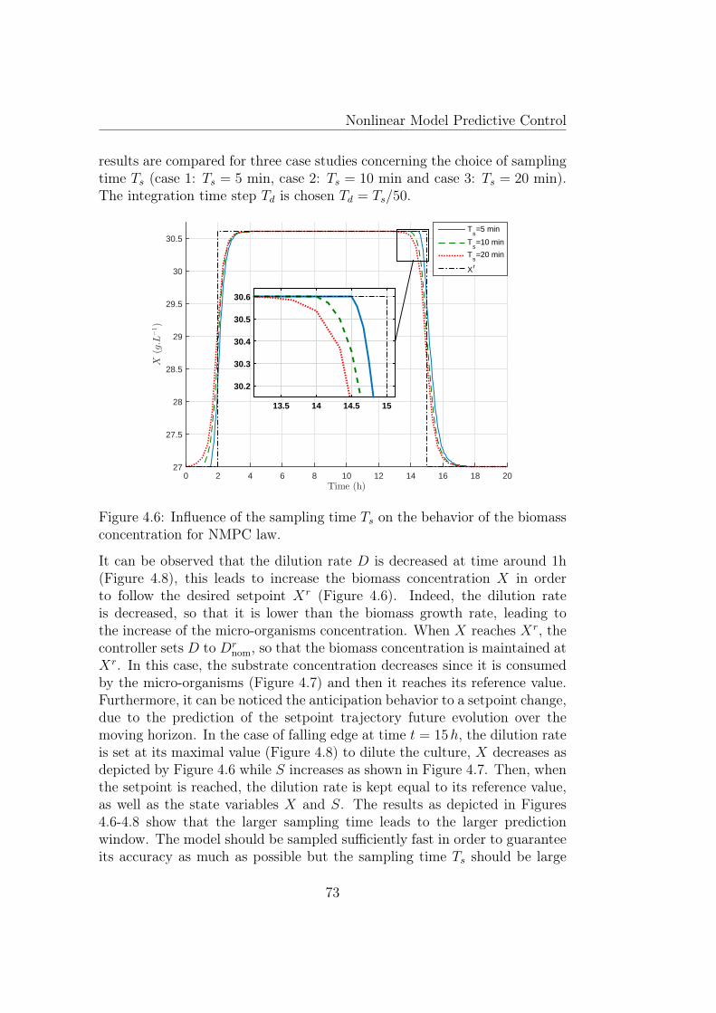
Nonlinear Model Predictive Control
results are compared for three case studies concerning the choice of samplingtime Ts (case 1: Ts = 5 min, case 2: Ts = 10 min and case 3: Ts = 20 min).The integration time step Td is chosen Td = Ts/50.
Time (h)0 2 4 6 8 10 12 14 16 18 20
X(g.L
−1)
27
27.5
28
28.5
29
29.5
30
30.5T
s=5 min
Ts=10 min
Ts=20 min
X r
13.5 14 14.5 15
30.2
30.3
30.4
30.5
30.6
Figure 4.6: Influence of the sampling time Ts on the behavior of the biomassconcentration for NMPC law.
It can be observed that the dilution rate D is decreased at time around 1h(Figure 4.8), this leads to increase the biomass concentration X in orderto follow the desired setpoint Xr (Figure 4.6). Indeed, the dilution rateis decreased, so that it is lower than the biomass growth rate, leading tothe increase of the micro-organisms concentration. When X reaches Xr, thecontroller sets D to Dr
nom, so that the biomass concentration is maintained atXr. In this case, the substrate concentration decreases since it is consumedby the micro-organisms (Figure 4.7) and then it reaches its reference value.Furthermore, it can be noticed the anticipation behavior to a setpoint change,due to the prediction of the setpoint trajectory future evolution over themoving horizon. In the case of falling edge at time t = 15h, the dilution rateis set at its maximal value (Figure 4.8) to dilute the culture, X decreases asdepicted by Figure 4.6 while S increases as shown in Figure 4.7. Then, whenthe setpoint is reached, the dilution rate is kept equal to its reference value,as well as the state variables X and S. The results as depicted in Figures4.6-4.8 show that the larger sampling time leads to the larger predictionwindow. The model should be sampled sufficiently fast in order to guaranteeits accuracy as much as possible but the sampling time Ts should be large
73
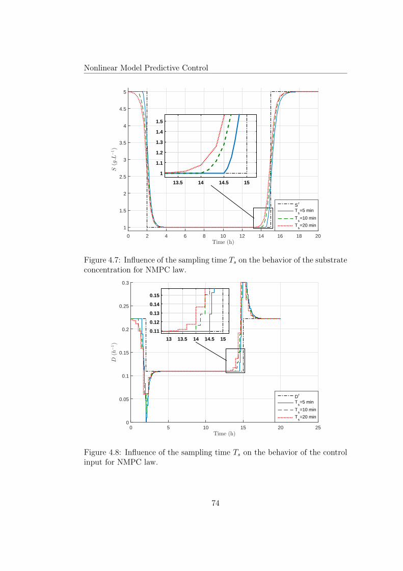
Nonlinear Model Predictive Control
Time (h)0 2 4 6 8 10 12 14 16 18 20
S(g.L
−1)
1
1.5
2
2.5
3
3.5
4
4.5
5
S r
Ts=5 min
Ts=10 min
Ts=20 min
13.5 14 14.5 15
1
1.1
1.2
1.3
1.4
1.5
Figure 4.7: Influence of the sampling time Ts on the behavior of the substrateconcentration for NMPC law.
Time (h)0 5 10 15 20 25
D(h
−1)
0
0.05
0.1
0.15
0.2
0.25
0.3
Dr
Ts=5 min
Ts=10 min
Ts=20 min
13 13.5 14 14.5 15
0.11
0.12
0.13
0.14
0.15
Figure 4.8: Influence of the sampling time Ts on the behavior of the controlinput for NMPC law.
74
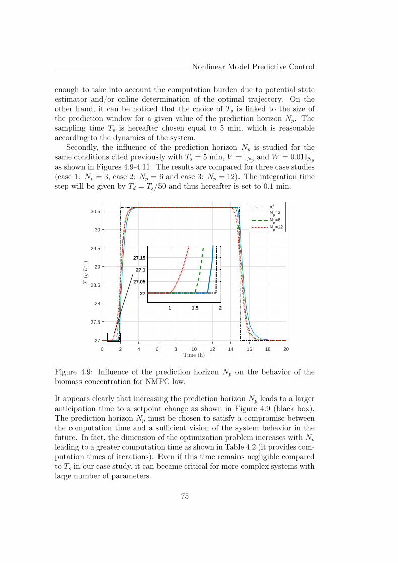
Nonlinear Model Predictive Control
enough to take into account the computation burden due to potential stateestimator and/or online determination of the optimal trajectory. On theother hand, it can be noticed that the choice of Ts is linked to the size ofthe prediction window for a given value of the prediction horizon Np. Thesampling time Ts is hereafter chosen equal to 5 min, which is reasonableaccording to the dynamics of the system.
Secondly, the influence of the prediction horizon Np is studied for thesame conditions cited previously with Ts = 5 min, V = INp and W = 0.01INpas shown in Figures 4.9-4.11. The results are compared for three case studies(case 1: Np = 3, case 2: Np = 6 and case 3: Np = 12). The integration timestep will be given by Td = Ts/50 and thus hereafter is set to 0.1 min.
Time (h)0 2 4 6 8 10 12 14 16 18 20
X(g.L
−1)
27
27.5
28
28.5
29
29.5
30
30.5X r
Np=3
Np=6
Np=12
1 1.5 2
27
27.05
27.1
27.15
Figure 4.9: Influence of the prediction horizon Np on the behavior of thebiomass concentration for NMPC law.
It appears clearly that increasing the prediction horizon Np leads to a largeranticipation time to a setpoint change as shown in Figure 4.9 (black box).The prediction horizon Np must be chosen to satisfy a compromise betweenthe computation time and a sufficient vision of the system behavior in thefuture. In fact, the dimension of the optimization problem increases with Np
leading to a greater computation time as shown in Table 4.2 (it provides com-putation times of iterations). Even if this time remains negligible comparedto Ts in our case study, it can became critical for more complex systems withlarge number of parameters.
75
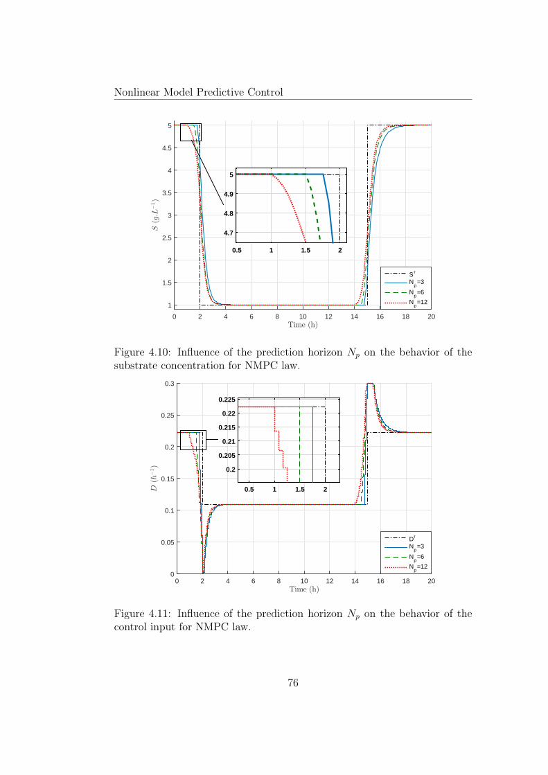
Nonlinear Model Predictive Control
Time (h)0 2 4 6 8 10 12 14 16 18 20
S(g.L
−1)
1
1.5
2
2.5
3
3.5
4
4.5
5
S r
Np=3
Np=6
Np=12
0.5 1 1.5 2
4.7
4.8
4.9
5
Figure 4.10: Influence of the prediction horizon Np on the behavior of thesubstrate concentration for NMPC law.
Time (h)0 2 4 6 8 10 12 14 16 18 20
D(h
−1)
0
0.05
0.1
0.15
0.2
0.25
0.3
Dr
Np=3
Np=6
Np=12
0.5 1 1.5 2
0.2
0.205
0.21
0.215
0.22
0.225
Figure 4.11: Influence of the prediction horizon Np on the behavior of thecontrol input for NMPC law.
76
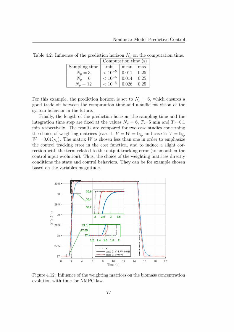
Nonlinear Model Predictive Control
Table 4.2: Influence of the prediction horizon Np on the computation time.Computation time (s)
Sampling time min mean maxNp = 3 < 10−5 0.011 0.25Np = 6 < 10−5 0.014 0.25Np = 12 < 10−5 0.026 0.25
For this example, the prediction horizon is set to Np = 6, which ensures agood trade-off between the computation time and a sufficient vision of thesystem behavior in the future.
Finally, the length of the prediction horizon, the sampling time and theintegration time step are fixed at the values Np = 6, Ts=5 min and Td=0.1min respectively. The results are compared for two case studies concerningthe choice of weighting matrices (case 1: V = W = INp and case 2: V = INpW = 0.01INp). The matrix W is chosen less than one in order to emphasizethe control tracking error in the cost function, and to induce a slight cor-rection with the term related to the output tracking error (to smoothen thecontrol input evolution). Thus, the choice of the weighting matrices directlyconditions the state and control behaviors. They can be for example chosenbased on the variables magnitude.
Time (h)0 2 4 6 8 10 12 14 16 18 20
X(g.L
−1)
27
27.5
28
28.5
29
29.5
30
30.5
X r
case 2: V=I, W=0.01Icase 1: V=W=I
1.2 1.4 1.6 1.8 2
27
27.05
27.1
2 2.5 3 3.5
30.2
30.4
30.6
Figure 4.12: Influence of the weighting matrices on the biomass concentrationevolution with time for NMPC law.
77
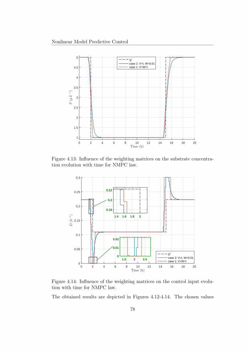
Nonlinear Model Predictive Control
Time (h)0 2 4 6 8 10 12 14 16 18 20
S(g.L
−1)
1
1.5
2
2.5
3
3.5
4
4.5
5S r
case 2: V=I, W=0.01case 1: V=W=I
Figure 4.13: Influence of the weighting matrices on the substrate concentra-tion evolution with time for NMPC law.
Time (h)0 2 4 6 8 10 12 14 16 18 20
D(h
−1)
0
0.05
0.1
0.15
0.2
0.25
0.3
Dr
case 2: V=I, W=0.01case 1: V=W=I
1.5 2 2.50
0.01
0.02
1.4 1.6 1.8 2
0.18
0.2
0.22
Figure 4.14: Influence of the weighting matrices on the control input evolu-tion with time for NMPC law.
The obtained results are depicted in Figures 4.12-4.14. The chosen values
78
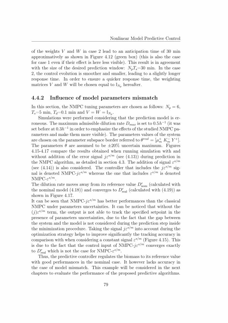
Nonlinear Model Predictive Control
of the weights V and W in case 2 lead to an anticipation time of 30 minapproximatively as shown in Figure 4.12 (green box) (this is also the casefor case 1 even if their effect is here less visible). This result is in agreementwith the size of the desired prediction window: NpTs=30 min. In the case2, the control evolution is smoother and smaller, leading to a slightly longerresponse time. In order to ensure a quicker response time, the weightingmatrices V and W will be chosen equal to INp hereafter.
4.4.2 Influence of model parameters mismatch
In this section, the NMPC tuning parameters are chosen as follows: Np = 6,Ts=5 min, Td=0.1 min and V = W = INp .
Simulations were performed considering that the prediction model is er-roneous. The maximum admissible dilution rate Dmax is set to 0.5h−1 (it wasset before at 0.3h−1 in order to emphasize the effects of the studied NMPC pa-rameters and make them more visible). The parameters values of the systemare chosen on the parameter subspace border referred to θreal = [µ+
m K−m Y +].The parameters θ are assumed to be ±20% uncertain maximum. Figures4.15-4.17 compare the results obtained when running simulation with andwithout addition of the error signal jεs/m (see (4.13)) during prediction inthe NMPC algorithm, as detailed in section 4.3. The addition of signal εs/m(see (4.14)) is also considered. The controller that includes the jεs/m sig-nal is denoted NMPC-jεs/m whereas the one that includes εs/m is denotedNMPC-εs/m.The dilution rate moves away from its reference value Dr
nom (calculated withthe nominal model (4.18)) and converges to Dr
real (calculated with (4.19)) asshown in Figure 4.17.It can be seen that NMPC-jεs/m has better performances than the classicalNMPC under parameters uncertainties. It can be noticed that without the(j)εs/m term, the output is not able to track the specified setpoint in thepresence of parameters uncertainties, due to the fact that the gap betweenthe system and the model is not considered during the prediction step insidethe minimization procedure. Taking the signal jεs/m into account during theoptimization strategy helps to improve significantly the tracking accuracy incomparison with when considering a constant signal εs/m (Figure 4.15). Thisis due to the fact that the control input of NMPC-jεs/m converges exactlyto Dr
real which is not the case for NMPC-εs/m.Thus, the predictive controller regulates the biomass to its reference value
with good performances in the nominal case. It however lacks accuracy inthe case of model mismatch. This example will be considered in the nextchapters to evaluate the performance of the proposed predictive algorithms.
79
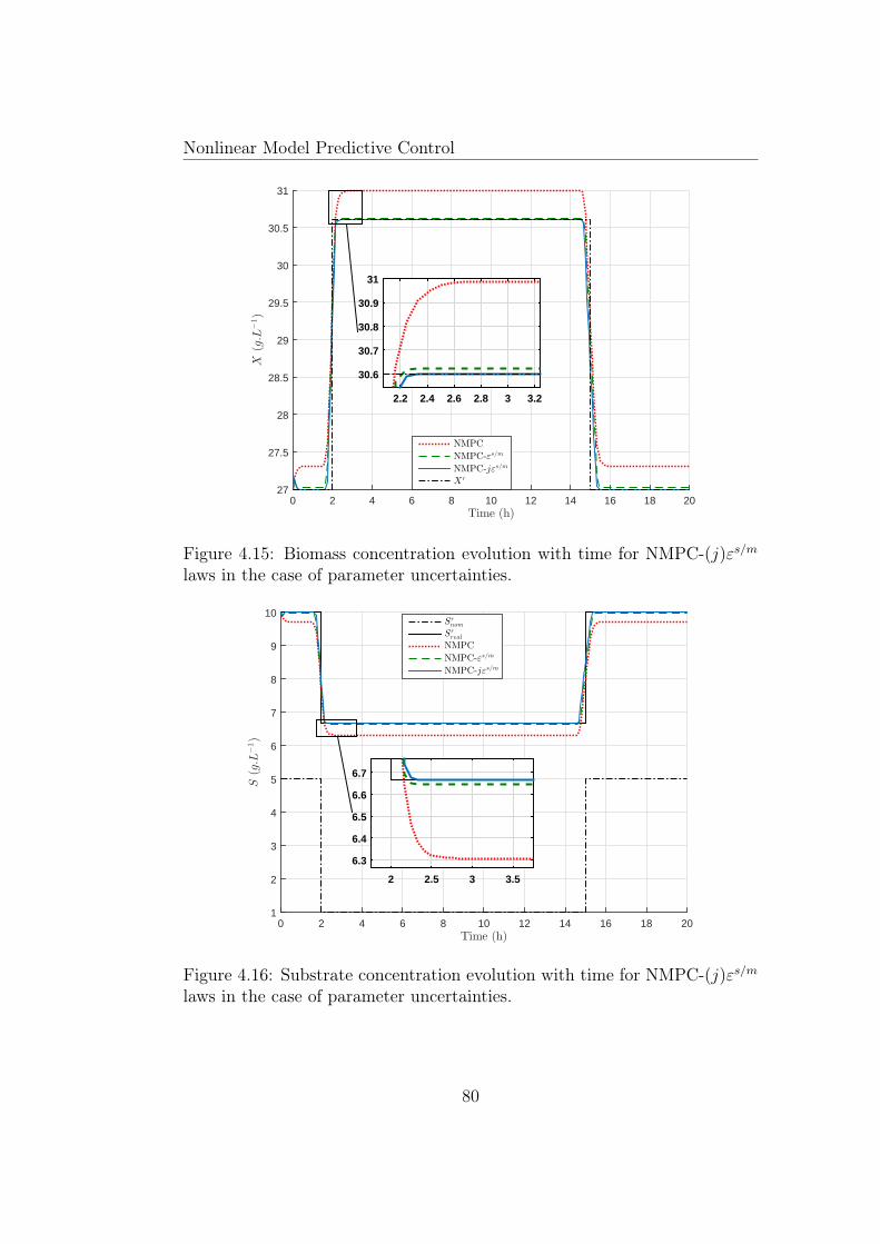
Nonlinear Model Predictive Control
Time (h)0 2 4 6 8 10 12 14 16 18 20
X(g.L
−1)
27
27.5
28
28.5
29
29.5
30
30.5
31
NMPC
NMPC-εs/m
NMPC-jεs/m
Xr
2.2 2.4 2.6 2.8 3 3.2
30.6
30.7
30.8
30.9
31
Figure 4.15: Biomass concentration evolution with time for NMPC-(j)εs/mlaws in the case of parameter uncertainties.
Time (h)0 2 4 6 8 10 12 14 16 18 20
S(g.L
−1)
1
2
3
4
5
6
7
8
9
10Srnom
Srreal
NMPC
NMPC-εs/m
NMPC-jεs/m
2 2.5 3 3.5
6.3
6.4
6.5
6.6
6.7
Figure 4.16: Substrate concentration evolution with time for NMPC-(j)εs/mlaws in the case of parameter uncertainties.
80
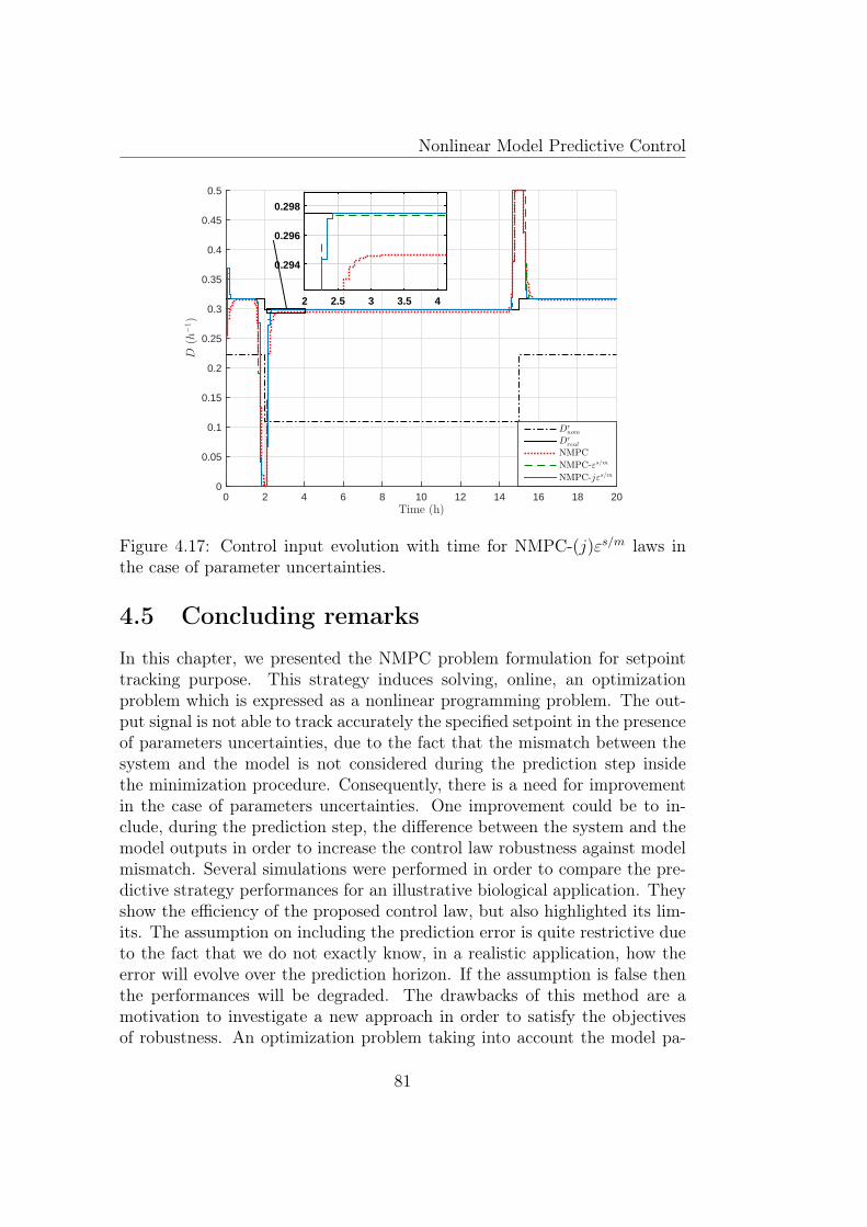
Nonlinear Model Predictive Control
Time (h)0 2 4 6 8 10 12 14 16 18 20
D(h
−1)
0
0.05
0.1
0.15
0.2
0.25
0.3
0.35
0.4
0.45
0.5
Drnom
Drreal
NMPC
NMPC-εs/m
NMPC-jεs/m
2 2.5 3 3.5 4
0.294
0.296
0.298
Figure 4.17: Control input evolution with time for NMPC-(j)εs/m laws inthe case of parameter uncertainties.
4.5 Concluding remarks
In this chapter, we presented the NMPC problem formulation for setpointtracking purpose. This strategy induces solving, online, an optimizationproblem which is expressed as a nonlinear programming problem. The out-put signal is not able to track accurately the specified setpoint in the presenceof parameters uncertainties, due to the fact that the mismatch between thesystem and the model is not considered during the prediction step insidethe minimization procedure. Consequently, there is a need for improvementin the case of parameters uncertainties. One improvement could be to in-clude, during the prediction step, the difference between the system and themodel outputs in order to increase the control law robustness against modelmismatch. Several simulations were performed in order to compare the pre-dictive strategy performances for an illustrative biological application. Theyshow the efficiency of the proposed control law, but also highlighted its lim-its. The assumption on including the prediction error is quite restrictive dueto the fact that we do not exactly know, in a realistic application, how theerror will evolve over the prediction horizon. If the assumption is false thenthe performances will be degraded. The drawbacks of this method are amotivation to investigate a new approach in order to satisfy the objectivesof robustness. An optimization problem taking into account the model pa-
81

Nonlinear Model Predictive Control
rameters uncertainties must be formulated in order to ensure the robustnessagainst model mismatch. The next chapter will be then devoted to the robustmodel predictive control.
82

Chapter 5
Robust Nonlinear ModelPredictive Control
5.1 Introduction
In the previous chapter, a predictive controller was designed to ensure a sta-ble real time operation of the plant, close to a certain state or desired profile.However, the performances of the NMPC law usually decrease when the trueplant evolution deviates significantly from the one predicted by the model.Robust variants of NMPC [78, 86] as detailed in section 3.6 are able to takeinto account set bounded disturbance and/or constraints. In addition, whenconsidering uncertain systems, or when only a limited amount of data isavailable, it is necessary to use a robust formulation of the controller wherethe effect of the uncertainties can be taken into account in the design pro-cedure. The robust NMPC (RNMPC) law can be formulated as a nonlinearmin-max optimization problem (where the objective function is minimizedfor the worst possible uncertainty realization). However, this approach tendsto become too complex to be solved numerically online. Consequently, thetotal calculation time is an important factor that must be reduced as muchas possible. We propose mainly two solutions to address this problem. Thefirst one consists in reducing the number of uncertain parameters through asensitivity analysis. Only the main influencial parameters on the model areconsidered in the min-max problem whereas the other parameters are keptconstant and equal to their nominal values. This approach will be referredto as reduced RNMPC (rRNMPC). The second approach aims at transform-ing the min-max problem into a more tractable optimization problem usinga model linearization technique. The objective is then to propose a newformulation that is computationally more tractable in calculating the opti-
83
Robust Nonlinear Model Predictive Control
mal control compared to a classical min-max robust approach, which makesit suitable for online implementation. This approach will be referred to asLinearized RMPC (LRMPC).
Stability properties of the robust model predictive control strategy takinginto account bounded uncertainties has been analyzed in [94, 99, 120, 119,100, 19, 137]. Based on work developped by [86] and [120], and taking theobjective function as the Lyapunov candidate function, the robust stability ofthe closed-loop system while applying the LRMPC law is established undersome assumptions.
The LRMPC controller represents our main contribution. Thus, the sta-bility and performances analysis will be focused on this approach.
The chapter is organized as follows. The next section is devoted to themin-max problem RNMPC formulation. A variant of RNMPC, based ona reduction of the number of the parameters θ that will be optimized, ispresented in section 5.3. Section 5.4 is dedicated to the use of a modellinearization technique in order to approach the min-max problem. Stabil-ity analysis of the closed-loop system is also discussed. The unconstrainedformulation (LRMPC) is detailed in section 5.5. In section 5.6, a robust pre-dictive controller (CLRMPC), similar to the above one with consideration ofinequality constraints on the control input, is presented. Numerical resultsare provided in section 5.7 and conclusions are stated in section 5.8.
5.2 Min-max strategy
Since the predictive controller is model-based, it is very sensitive to modeluncertainties, and more specifically to the model parameters values. In thiscontext, we will assume that the parameter vector θ is uncertain and belongsto a known set Θ as stated in section 4.2.1. Thus, robustification in the pres-ence of model uncertainties naturally leads to the formulation of a nonlinearmin-max optimization problem [4, 93, 102]. The control sequence that min-imizes a worst case cost function is derived from the following optimizationproblem (at time index k and using the same notation as in section 4.2):
?uk+Np−1
k = arg minuk+Np−1
k
maxδθ
ΠRNMPC(xk, uk+Np−1k , δθ) (5.1)
84
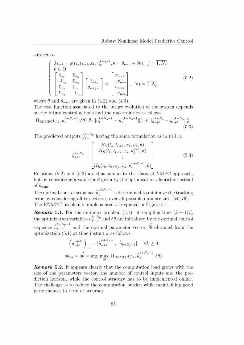
Robust Nonlinear Model Predictive Control
subject to
xk+j = g(tk, tk+j, xk, uk+j−1k , θ = θnom + δθ), j = 1, Np
θ ∈ ΘInx 0nu−Inx 0nu0nx Inu0nx −Inu
[ xk+j
uk+j−1
]≤
xmax
−xmin
umax
−umin
, ∀j = 1, Np
(5.2)
where θ and θnom are given in (4.2) and (4.3).The cost function associated to the future evolution of the system dependson the future control actions and the uncertainties as follows:ΠRNMPC(xk, u
k+Np−1k , δθ) , ||uk+Np−1
k − ur,k+Np−1k ||2V + ||yk+Np
k+1 − yr,k+Npk+1 ||2W
(5.3)
The predicted outputs yk+Npk+1 having the same formulation as in (4.11):
yk+Npk+1 =
Hg(tk, tk+1, xk, uk, θ)Hg(tk, tk+2, xk, u
k+1k , θ)
...Hg(tk, tk+Np , xk, u
k+Np−1k , θ)
(5.4)
Relations (5.2) and (5.3) are thus similar to the classical NMPC approach,but by considering a value for θ given by the optimization algorithm insteadof θnom.The optimal control sequence ?
uk+Np−1
k is determined to minimize the trackingerror by considering all trajectories over all possible data scenarii [54, 76].The RNMPC problem is implemented as depicted in Figure 5.1.
Remark 5.1. For the min-max problem (5.1), at sampling time (k + 1)Tsthe optimization variables uk+Np
k+1 and δθ are initialized by the optimal control
sequence ?uk+Np−1
k+1 and the optimal parameter vector δ?
θ obtained from theoptimization (5.1) at time instant k as follows:(
uk+Npk+1
)ini
= [?uk+Np−1
k+1 ,?uk+Np−1], ∀k ≥ 0
δθini = δ?
θ = arg maxδθ
ΠRNMPC(xk,?uk+Np−1
k , δθ)
Remark 5.2. It appears clearly that the computation load grows with thesize of the parameters vector, the number of control inputs and the pre-diction horizon, while the control strategy has to be implemented online.The challenge is to reduce the computation burden while maintaining goodperformances in term of accuracy.
85
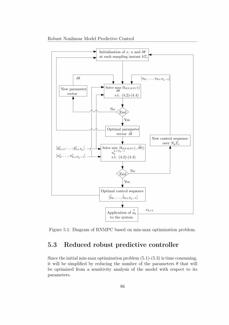
Robust Nonlinear Model Predictive Control
Initialisation of x, u and δθat each sampling instant kTs
End
Optimal control sequence
[uk, . . . , uk+Np−1]
New control sequenceover NpTs
[yrk+1, . . . , yrk+Np
]
[urk, . . . , urk+Np−1]
xk+1
[uk, . . . , uk+Np−1]
No
Yes
EndNo
Yes
New parametervector
Optimal parametervector
δθ
Solve max ΠRNMPC()δθ
s.t. (4.2)-(4.4)
s.t. (4.2)-(4.4)
Solve min ΠRNMPC(., δθ))?
δθ?
? ?
Application of ukto the system
?
uk+Np−1
k
Figure 5.1: Diagram of RNMPC based on min-max optimization problem.
5.3 Reduced robust predictive controller
Since the initial min-max optimization problem (5.1)-(5.3) is time consuming,it will be simplified by reducing the number of the parameters θ that willbe optimized from a sensitivity analysis of the model with respect to itsparameters.
86
Robust Nonlinear Model Predictive Control
5.3.1 Sensitivity analysis
The sensitivity functions Sxiθj represent the sensitivity of each state xi to(small) variations in each model parameter θj. It is defined as the partialderivatives of the state variable vector xi with respect to θj:
Sxiθj ,∂xi∂θj
, i = 1, nx and j = 1, nθ (5.5)
Different approaches are possible to determine the sensitivity functions. Themost precise method involves analytical derivation [52]. In this case, thedynamics of sensitivities are calculated as follows for system (4.1):
Sxiθj =d
dt
(∂xi∂θj
)=
∂
∂θj
(dxidt
)=∂Fi∂θj
+nx∑k=1
∂Fi∂xk
(∂xk∂θj
)(5.6)
with as an initial condition: ∂xi∂θj
= 0.From the analysis of the sensitivity functions temporal evolution, and ac-cording to their magnitude order, one can select the parameters which aresignificantly the most influential on the model [52]. These parameters willbe denoted κ.
5.3.2 Problem reformulation
In the sequel, only the most influential parameters, κ ∈ Θκ ⊆ Θ, are con-sidered in the min-max optimization, instead of the full model parameters(with θ , [κ, ζ]). The influential parameters κ are defined as follows:
κ = κnom + δκ (5.7)
κnom =κ+ + κ−
2(5.8)
where κnom is the nominal influential parameters and δκ the parametersuncertainties vector. The other parameters, ζ, are set to their nominal valueswith ζnom = (ζ+ + ζ−)/2.
Thanks to the sensitivity analysis, the min-max optimization (5.1)-(5.3)is approached by the following optimization problem (at time index k):
?uk+Np−1
k = arg minuk+Np−1
k
maxδκ
ΠrRNMPC(xk, uk+Np−1k , δκ) (5.9)
87
Robust Nonlinear Model Predictive Control
subject to
xk+j = g(tk, tk+j, xk, uk+j−1k ,
[κnom + δκζnom
]), j = 1, Np
κ ∈ ΘκInx 0nu−Inx 0nu0nx Inu0nx −Inu
[ xk+j
uk+j−1
]≤
xmax
−xmin
umax
−umin
, ∀j = 1, Np
(5.10)
where κnom and δκ are given above.The new cost function is defined as follows:
ΠrRNMPC(uk+Np−1k , δκ) , ||uk+Np−1
k − ur,k+Np−1k ||2V + ||yk+Np
k+1 − yr,k+Npk+1 ||2W
(5.11)
The predicted outputs yk+Npk+1 are given by:
yk+Npk+1 =
Hg(tk, tk+1, xk, uk, [κ
>, ζ>nom]>)Hg(tk, tk+2, xk, u
k+1k , [κ>, ζ>nom]>)...
Hg(tk, tk+Np , xk, uk+Np−1k , [κ>, ζ>nom]>)
(5.12)
This approach presents however some drawbacks:
• A sensitivity analysis of the model with respect to it parameters isrequired, leading to a more complex and time demanding developments.
• For some systems, all parameters can have high influence on the model,and thus no parameter reduction is possible (e.g. for systems with asmall number of parameters).
Consequently, this approach cannot be used in all cases (it is then equivalentto the RNMPC). Hereafter, this approach is referred to as reduced RNMPC(rRNMPC).
5.4 Linearized robust predictive controllerSince the min-max optimization problem (5.1)-(5.4) even when reducing thenumber of uncertain parameters as in (5.9)-(5.12), is time consuming, it willbe approached further by a more tractable optimization problem. This stepfocuses on reducing the computational burden of the initial problem. The
88
Robust Nonlinear Model Predictive Control
key idea is to approach the predicted outputs based on the nonlinear modelthrough linearization technique.
As a direct result of the linearization, the non-convex problem will beapproached by a convex one. So, more flexible tools will be accessible tobetter handle the optimization problem.
5.4.1 Main principle
In the following proposed approach, the outputs in the moving time frameare predicted by Taylor series expansion. A similar dual problem for robuststate estimation, consisting in the design of receding-horizon observer, waspresented in [61]. In this section, we propose to apply the same approach tothe case of NMPC law design.
Based on a first order Taylor series expansion of (4.7), the predictionmodel g for time tk+1, starting from state xk, is linearized around the referencetrajectory given by the reference control urk and for the nominal parametersθnom:
xk+1 ≈ xnom,k+1 +∇θg(tk+1)δθ +∇ug(tk+1)(uk − urk) , fp(xk, uk, θnom + δθ)(5.13)
with
δθ = θ − θnom (5.14)xnom,k+1 = g(tk, tk+1, xk, u
rk, θnom) (5.15)
∇θg(tk+1) =∂g(tk, tk+1, xk, uk, θ)
∂θ
∣∣∣∣∣∣∣ uk = urkθ = θnom
(5.16)
∇ug(tk+1) =∂g(tk, tk+1, xk, uk, θ)
∂uk
∣∣∣∣∣∣∣ uk = urkθ = θnom
(5.17)
Generalizing, the predicted state for time tk+j, starting from state at tk,is linearized around the reference trajectory given by the reference controlsequence ur,k+j−1
k and for θnom. Using the same approach as in (5.13) forj = 1, Np, it comes:
xk+j ≈ xnom,k+j +∇θg(tk+j)δθ +∇ug(tk+j)(uk+j−1k − ur,k+j−1
k
)(5.18)
89
Robust Nonlinear Model Predictive Control
with
xnom,k+j = g(tk, tk+j, xk, ur,k+j−1k , θnom) (5.19)
∇θg(tk+j) =∂g(tk, tk+j, xk, u
k+j−1k , θ)
∂θ
∣∣∣∣∣∣∣∣ uk+j−1k = ur,k+j−1
kθ = θnom
(5.20)
∇ug(tk+j) =∂g(tk, tk+j, xk, u
k+j−1k , θ)
∂uk+j−1k
∣∣∣∣∣∣∣∣ uk+j−1k = ur,k+j−1
kθ = θnom
(5.21)
Different approaches are possible for determining the sensitivity functionswith respect to the parameters vector and the control sequence, defined in(5.20) and (5.21), respectively as presented in section 5.3.1.
The dynamics of the sensitivity function with respect to θ can be com-puted for time t ∈ [tk, tk+Np ] by solving numerically the following differentialequation (from (5.6)):
d
dt(∇θg(t)) =
∂F (x(t), u(t), θnom)
∂x∇θg(t) +
∂F (x(t), u(t), θ)
∂θ|θ=θnom (5.22)
with as an initial condition:
∇θg(tk) = 0nx×nθ (5.23)
Indeed, ∇θg is the sensitivity function of the state x with respect to the pa-rameter θ.An alternative procedure is to use the finite differences in order to approx-imate numerically the derivatives ∇θg for each parameter θl, l ∈ [1, nθ] and∇ug(tk+j) for each control uj, j ∈ [k, k +Np − 1].
The finite difference method approximates the (i, j)-th element of thejacobian of a vector function g(z) as
∇g(z) ≈ gi(zj + δ)− gi(zj)δ
(5.24)
for some small δ > 0. A too large δ will induce inaccuracies due to thenonlinearity of gi, since the method computes the average slope between twopoints.
Remark 5.3. The most accurate result and computationally most efficientapproach is to calculate gradients analytically (by symbolic differentiation).Doing this by hand, or even using symbolic computations in Maple or Mathe-matica, may quickly become intractable for MPC problems that may containa large number of variables and parameters.
90
Robust Nonlinear Model Predictive Control
In order to simplify the calculation of the gradients ∇θg and ∇ug, finitedifferences are used to approximate numerically the derivatives ∇θg(tk+j)and ∇ug(tk+i).From (4.11) and (5.18), the predicted ouputs over the moving horizon areexpressed as follows:
yk+Npk+1 = G
k+Npnom,k+1 +G
k+Npθ,k+1δθ +G
k+Np−1u,k (u
k+Np−1k − ur,k+Np−1
k ) (5.25)
where
Gk+Npnom,k+1 =
Hxnom,k+1
...Hxnom,k+j
...Hxnom,k+Np
, is the column vector containing the predicted
output for the nominal case.
Gk+Npθ,k+1 =
H∇θg(tk+1)
...H∇θg(tk+j)
...H∇θg(tk+Np)
, regroups the Jacobian matrices related to the
parameters.
Gk+Np−1u,k =
H∇ug(tk+1)
...H∇ug(tk+j)
...H∇ug(tk+Np)
, regroups the Jacobian matrices related to the
control sequence.Assuming that the uncertain parameters are uncorrelated and recalling that
θ− ≤ θ ≤ θ+ (5.26)
and
θnom =θ+ + θ−
2(5.27)
Thus,θ− − θ+
2≤ θ − θnom ≤
θ+ − θ−2
(5.28)
Then, the bounded parametric error δθ can be expressed by:
δθ = γδθmax (5.29)
91
Robust Nonlinear Model Predictive Control
withδθmax = (θ+ − θ−)/2 (5.30)
and||γ|| ≤ 1 (5.31)
The initial objective function ΠRNMPC (5.3) is substituted by a cost functionusing the equation (5.25). The result is given by the following expression(with the same notations as in (4.11)):
ΠRNMPC(xk, uk+Np−1k , δθ) ≈ ||uk+Np−1
k − ur,k+Np−1k ||2V +
||Gk+Npnom,k+1 − y
r,k+Npk+1 +G
k+Npθ,k+1δθ +G
k+Np−1u,k (u
k+Np−1k − ur,k+Np−1
k )||2W, Π(xk, u
k+Np−1k , δθ)
(5.32)
The new optimization problem is given by:
?uk+Np−1
k = arg minuk+Np−1
k
maxδθ
Π(xk, uk+Np−1k , δθ) (5.33)
subject to {θ ∈ Θ, x ∈ X, u ∈ Uδθ = γδθmax
(5.34)
5.4.2 Stability analysis
In this section, the robust stability of the closed-loop system (4.6) with (5.33)-(5.34) is analysed by exploiting the results obtained in [19, 120, 86].
More specifically, we will use the following theorem:
Theorem 5.1. Consider a discrete-time nonlinear system given by:
xk+1 = l(xk, wk), k ≥ 0, x0 = x (5.35)
where xk ∈ X is the state of the system, wk ∈ W is the disturbance vector(s.t. W is a compact set that contains the origin).If system (5.35) admits a robust Lyapunov function, then it is robustly stable.
Proof. see [86].
We adapt the results in the above cited references to address the stabilityanalysis of the proposed control strategy. First, a bound on the predictionerror will be determined. Secondly, we give an upper and lower bounds on
92
Robust Nonlinear Model Predictive Control
the optimal cost. Finally, we establish the robust stability of the closed-loopsystem.
In the sequel, for the stability analysis of the closed-loop system (4.6)with (5.1)-(5.32), we need to consider the following assumptions:
Assumption 5.1. The state of the plant xk is measured at each samplingtime.
Assumption 5.2. The state x and the control u of the plant must fulfill thefollowing constraints: xk ∈ X and uk ∈ U. where X and U are compact sets,both of them contain the origin.
5.4.2.1 Bound on prediction error
In this subsection, an upper bound on the prediction error provided by thelinearization step is derived. Consider the real system for time tk+1, startingfrom state xk at time tk:
xk+1 = f(xk, uk, θnom + δθs) (5.36)
where θnom is the nominal parameters vector and δθs the real parametervalues mismatch.
Assumption 5.3. The function f is of class C2 with respect to all its argu-ments.
From Assumption 5.3, and using Taylor developments (around θnom andurk), the system dynamics can be rewritten as follows:
xk+1 = f(xk, urk, θnom) +∇uf(urk, θnom).(uk − urk) +∇θf(urk, θnom).δθs
+ ϑ(|uk − urk|2) + ϑ(|δθs|2)
(5.37)
where ϑ(|.|2) is the remainder term of the Taylor series expansion limited tothe first order.
Assumption 5.4. The error with respect to the first Taylor expansion, wp,defined as:
wp , ϑ(|uk − urk|2) + ϑ(|δθs|2) (5.38)
is assumed to be bounded as follows:
∃η1 ∈ R+, such that |wp| ≤ η1 (5.39)
93
Robust Nonlinear Model Predictive Control
Consider the prediction model (Taylor series expansion) for time tk+1,starting from state xk at time tk:
xk+1|k = fp(xk, uk, θnom + δθ)
, f(xk, urk, θnom) +∇uf(urk, θnom).(uk − urk) +∇θf(urk, θnom).δθ
(5.40)
with|δθ| ≤ |δθmax| (5.41)
with fp the prediction model such as in (5.13) (given in this case by functiong linearized as in (5.13), and using relation (4.7), with the fact that g ≡ fwhen considering the evolution between k and k + 1) and δθ the predictedparameter values mismatch.
Assumption 5.5. The uncertainty on δθ ∈ Θ, with Θ a compact set con-taining the origin, is such that ∃ η2 ∈ R+, a modelled bound of uncertainties,so that
max(|δθ|, |δθs|) ≤ η2 (5.42)
Let us define η ∈ R+ by:
η = max(η1, η2) (5.43)
From (5.37) and (5.40), the prediction error at time index k + 1 for uk =?uk
is given by:
xk+1 − xk+1|k = ∇θf(urk, θnom).(δθs − δθ) + wp (5.44)
Thanks to the triangle inequality and using the Assumptions 5.3 and 5.5,we obtain an upper bound on the prediction error as follows:
|xk+1 − xk+1|k| ≤ |∇θf(urk, θnom)|.|(δθs − δθ)|+ |wp|≤ |∇θf(urk, θnom)|. (|δθs|+ |δθ|) + |wp|
(5.45)
From Assumptions 5.2, 5.3 and 5.5, we have:
∃α ∈ R+,∀x,∀u,∀θ, |∇θf | ≤ α (5.46)
where α is an upper bound of |∇θf |.Thanks to Assumptions 5.4-5.5, (5.43) and (5.46), it comes
|xk+1 − xk+1|k| ≤ 2α.η2 + η1
≤ (2α + 1)η , Λ(η)(5.47)
where Λ is a K∞-function.
94
Robust Nonlinear Model Predictive Control
5.4.2.2 Upper and lower bounds on the optimal cost
In this subsection, we would like to find bounds on the optimal cost in orderto satisfy condition (7) in Definition 14. In the sequel, for manipulationpurposes, the optimal cost function (5.32) is rewritten as follows:
Π(xk,?uk+Np−1
k , δ?
θ) ,k+Np−1∑t=k
ψ(xt|k,?ut) + Tf (xk+Np|k) (5.48)
with xt|k = fp(xt−1|k,
?ut−1, θnom + δ
?
θ), t = k + 1, k +Np
xk|k = xkψ(xt, ut) = u>t vut + y>t wyt, t = k, k +Np − 1Tf (xk+Np|k) = y>k+Np
wyk+Np
(5.49)
and {ut = ut − urtyt = Hxt − yrt
(5.50)
The stage cost ψ(x, u) is definite positive, while the terminal cost is denotedby Tf (x) : Rnx −→ R≥0.Without any lack of generality, the weighting matrices V and W are chosenin diagonal form
V = vI and W = wI
to simplify mathematical developments hereafter.
Remark 5.4. Formulation in (5.48) and (5.32) are the same, Tf being clearlysplit in (5.48).
Remark 5.5. The terminal stage Tf is a K∞-function.
Assumption 5.6. Let assume the existence of a terminal set Φ, an admissi-ble robust positively invariant set for the system (5.36) which is controlled bythe control law uk = π(xk) ∈ U s.t. the origin is in its interior. Let assumethat Tf is an associated robust Lyapunov function s.t. for all xk ∈ Φ and forall δθ satisfying (5.42), we have that:
αt(|xk|) ≤ Tf (xk) ≤ βt(|xk|) + ϕ(η)
Tf (f(xk, uk, θnom + δθ))− Tf (xk) ≤ −ψ(xk, uk) + χ(η)(5.51)
where αt, βt, and χ are K∞-functions and ϕ is a K-function.
95
Robust Nonlinear Model Predictive Control
Lemma 1. Let us consider the system (5.36) and suppose that the uncer-tainty on θ is modelled by |δθ| ≤ γ(|x|) + η (γ is a K−function). Let Φ andTf (x) satisfy Assumption 5.6, then ∀x ∈ Φ we have that
Π(xk,?u, δ
?
θ) ≤ Tf (xk) +Npχ(η) (5.52)
Proof. see Lemma 3 of section 5 in [86].
From (5.52) and Assumption 5.6, we get
Π(xk,?u, δ
?
θ) ≤ βt(|xk|) + ϕ(η) +Npχ(η) (5.53)
Assumption 5.7. The stage cost (non-negative) is such that
ψ(x, u) ≥ αψ(|x|) (5.54)
where αψ is a K∞-function.
From (5.48) and Assumption 5.7, and since ψ and Tf are positive func-tions, then
Π(xk,?u, δ
?
θ) ≥ ψ(xk|k,?uk) ≥ αψ(|xk|k|) = αψ(|xk|) (5.55)
Thanks to (5.53) and (5.55), it comes:
αψ(|xk|) ≤ Π(xk,?u, δ
?
θ) ≤ βt(|xk|) + ϕ(η) +Npχ(η) (5.56)
Thus, the optimal cost is bounded as given by (5.56).
5.4.2.3 Robust stability
Theorem 5.2. Consider system (5.35) and suppose that uncertainties aremodelled by |wk| ≤ γ(|xk|)+η. Then, the uncertain system controlled by thecontroller uk = π(xk) is robust stable for any initial x0 ∈ XNp(Φ). XNp(Φ) isthe set of admissible states at time k+Np. Furthermore, the optimal cost isa robust Lyapunov function.
Proof. see [86].
96
Robust Nonlinear Model Predictive Control
Remark 5.6. The i-step robust stabilizable setXi(Φ) is the set of admissiblestates which can be steered to the target set Φ in i steps or less by a sequenceof admissible control law π(xk) for all possible realizations of the uncertainty.This set satisfies that Xi−1(Φ) ⊆ Xi(Φ) for i ≥ 0 with X0(Φ) = Φ. Thanks tothe invariance of the terminal set, the feasible region of the controller XNp(Φ)is a robust invariant set for the closed loop system [99].
Now, we consider Π(xk,?u, δ
?
θ) as our candidate robust Lyapunov function.Then, the optimal cost function at time index k + 1 is defined as follows:
Π(xk+1, uk+Npk+1 , δ
?
θ) ,k+Np∑t=k+1
ψ(xt|k+1, ut) + Tf (xk+Np+1|k+1) (5.57)
with
{xt|k+1 = fp(xt−1|k+1, ut−1, θnom + δ
?
θ), t = k + 2, k +Np + 1xk+1|k+1 = xk+1
(5.58)where xt|k+1 denotes the state obtained applying the input sequence ut−1
k+1 tothe prediction model with the initial condition xk+1.uk+Npk+1 denote an admissible solution of the optimization problem at time
index k + 1. In the proposed algorithm, it is based on the optimal solutionat time index k:
uk+Npk+1 = [
?uk+Np−1
k+1 ,?uk+Np−1] (5.59)
Notations used in this subsection are detailed in Figure 5.2.
Assumption 5.8. The parameters uncertainties are assumed to be constantthroughout the prediction horizon.
Assumption 5.9. The function fp is Lipschitz with respect to x with Lips-chitz constant Lfx.
Proposition 5.1. Let us define the following residual at time index l:
εx(l) , xl|k+1 − xl|k, l = k + 1, k +Np − 1 (5.60)
Then, with Assumption 5.9,
|εx(l)| ≤ Ll−k−1fx Λ(η) (5.61)
97
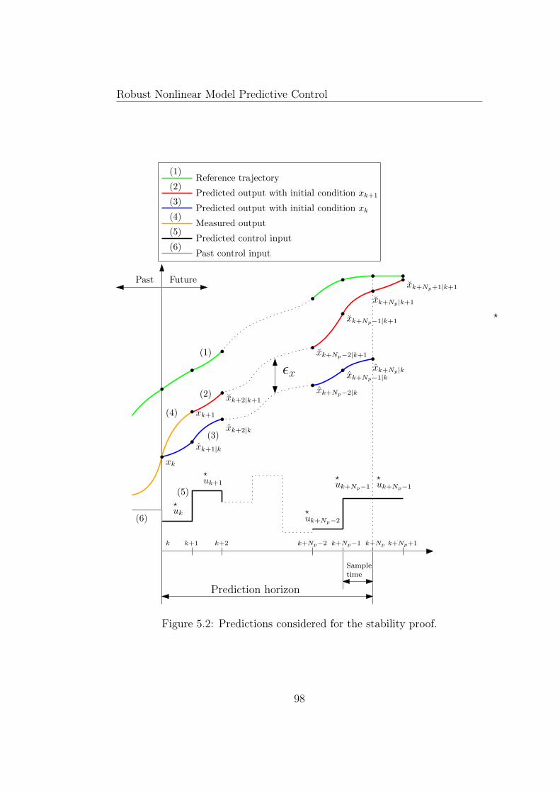
Robust Nonlinear Model Predictive Control
Prediction horizon
Sampletime
FuturePast
xk+1
xk
xk+1|k
xk+2|k
xk+Np−2|k
xk+Np−1|kxk+Np|k
xk+2|k+1
xk+Np−2|k+1
xk+Np−1|k+1
xk+Np|k+1
xk+Np+1|k+1
uk
uk+1
uk+Np−2
uk+Np−1
k k+1 k+Np−2 k+Np−1 k+Np k+Np+1k+2
Reference trajectory
Measured output
Past control input
Predicted output with initial condition xk+1
Predicted output with initial condition xk
Predicted control input
uk+Np−1
(1)
(2)
(3)
(4)
(5)
(6)
(1)
(2)
(3)
(4)
(5)
(6)
εx
?
?
?
?
? ?
Figure 5.2: Predictions considered for the stability proof.
98
Robust Nonlinear Model Predictive Control
Proof. Using the result obtained in (5.47) and Assumption 5.9, we getthat (reminding that ul =
?ul for l ∈ [k + 1, k +Np − 1] and xk+1|k+1 = xk+1)
|εx(k + 1)| = |xk+1|k+1 − xk+1|k| ≤ Λ(η)
|εx(k + 2)| = |fp(xk+1|k+1, uk+1, θnom + δ?
θ)− fp(xk+1|k,?uk+1, θnom + δ
?
θ)|≤ Lfx|xk+1|k+1 − xk+1|k|≤ LfxΛ(η)...
|εx(l)| ≤ Ll−k−1fx Λ(η)
(5.62)Now, it is easy to check the result by recurrence. We assume that the propo-sition holds for l, let us prove that it is also the case for l + 1 (from (5.62)):
|εx(l + 1)| = |fp(xl|k+1, ul, θnom + δ?
θ)− fp(xl|k,?ul, θnom + δ
?
θ)|≤ Lfx|εx(l)| ≤ Ll−kfx Λ(η)
(5.63)
Which completes the proof by recurrence.Let define the difference ∆Π? as
∆Π? , Π(xk+1, u, δ?
θ)− Π(xk,?u, δ
?
θ)
=
k+Np−1∑t=k+1
(ψ(xt|k+1, ut)− ψ(xt|k,?ut))
+ ψ(xk+Np|k+1, uk+Np)− ψ(xk,?uk) + Tf (xk+Np+1|k+1)− Tf (xk+Np|k)
(5.64)
Assumption 5.10. The stage cost ψ is Lipschitz with respect to x withLipschitz constant Lψx.
Using the Assumptions 5.9-5.10, and from (5.62) we have that
|ψ(xt|k+1, ut)− ψ(xt|k,?ut)| ≤ Lψx|xt|k+1 − xt|k| ≤ LψxL
t−k−1fx Λ(η) (5.65)
and
|k+Np−1∑t=k+1
(ψ(xt|k+1, ut)− ψ(xt|k,?ut))| ≤ Lψx
Np−2∑j=0
LjfxΛ(η) (5.66)
Assumption 5.11. The terminal function Tf is Lipschitz with respect to xwith Lipschitz constant Ltx.
99
Robust Nonlinear Model Predictive Control
Under Assumption 5.11, and from Proposition 5.1 we have that
|Tf (xk+Np|k+1)− Tf (xk+Np|k)| ≤ Ltx|εx(k +Np)| ≤ LtxLNp−1fx Λ(η) (5.67)
The last term of (5.64) is rewritten as follows:
Tf (xk+Np+1|k+1)− Tf (xk+Np|k) =Tf (xk+Np+1|k+1)− Tf (xk+Np|k+1)
+ Tf (xk+Np|k+1)− Tf (xk+Np|k)(5.68)
If the Assumption 5.6 holds, it comes
Tf (xk+Np+1|k+1)− Tf (xk+Np|k+1) ≤ −ψ(xk+Np|k+1, uk+Np) + χ(η) (5.69)
Thanks to (5.67) and (5.69) and considering the fact that for any scalarν ∈ R, ν ≤ |ν|, we have that
Tf (xk+Np+1|k+1)− Tf (xk+Np|k) ≤ −ψ(xk+Np|k+1, uk+Np) + χ(η) + LtxLNp−1fx Λ(η)
(5.70)
By substituting the equations (5.66) and (5.70) in (5.64), and using theAssumption 5.7, we get that
∆Π? ≤k+Np−1∑t=k+1
(ψ(xt|k+1, ut)− ψ(xt|k,?ut))− ψ(xk,
?uk) + χ(η) + LtxL
Np−1fx Λ(η)
≤ Lψx
Np−2∑j=0
LjfxΛ(η)− ψ(xk,?uk) + χ(η) + LtxL
Np−1fx Λ(η)
≤ −αψ(|x|) + χ(η)
(5.71)
with
χ(η) = χ(η) +
(LtxL
Np−1fx + Lψx
Np−2∑j=0
Ljfx
)Λ(η) (5.72)
where χ is a K∞-function.According to the results obtained in (5.56) (bounds on the optimal cost)
and (5.71) (evolution of the optimal cost), the optimal cost (5.48) is a robustLyapunov function (according to Definition 14).Finally, based on the Theorem 5.2, the system (5.36) controlled by π(x) =
?uk
is robustly stable in Φ for any uncertainty θ ∈ Θ and for the consideredlinearized prediction model.
100
Robust Nonlinear Model Predictive Control
5.5 Unconstrained Linearized Robust Model Pre-dictive Controller
The optimization problem (5.33)-(5.34) is solved by means of a robust reg-ularized least squares approach in the presence of uncertain data, followingan approach developed by Sayed et al. [135]. Since it is an unconstrainedformulation, the control signal will be a posteriori saturated for real-timeimplementation. This approach is thus dedicated to the case where the con-straints on the control inputs are bounds on it and there are no constraintson the state vector.
5.5.1 Robust regularized least squares problem
The different steps to solve a robust regularized least squares problem arepresented below.
step 1. Solution of the OLS problem
Let us consider first the following ordinary least squares (OLS) problem:
minz||Az − b||2W (5.73)
where
• A is a known m× n matrix;
• z is an unknown n-dimensional column vector;
• b is a known m× 1 vector;
• W � 0 is a positive-definite weighting matrix.
Assume that the matrix A is tall (m ≥ n) and of full column rank (seeDefinition 3). Then, the OLS problem (5.73) has a unique solution, givenby:
z? = (A>WA)−1A>Wb (5.74)
However, this formulation can not be used for all problems (e.g. in thecase when the matrix A is not full column rank). In order to overcome thedrawbacks, a regularized least squares (RLS) can be used instead of OLSapproach (5.73).Let us consider the following RLS problem:
minzJ (z) (5.75)
101
Robust Nonlinear Model Predictive Control
withJ (z) , ||z||2V + ||Az − b||2W (5.76)
V � 0 is a positive-definite weighting matrix.
The solution of the optimization problem (5.75) is given by
z? = (V + A>WA)−1A>Wb (5.77)
step 2. Introduction of uncertainties in the RLS problem (5.75)
The cost function (5.76) and the optimization problem (5.75) can be modifiedto take into account uncertainties on A and b as follows:
minz
maxδA,δb
[||z||2V + ||(A+ δA)z − (b+ δb)||2W
](5.78)
where uncertainties δA ∈ Rm×n and δb ∈ Rm can be structured under thefollowing factored form: {
δA = C∆Ea (5.79)δb = C∆Eb (5.80)
where ∆ denotes an arbitrary contraction term with ||∆|| ≤ 1, with a knownmatrix C ∈ Rm×nξ not identically null and where Ea and Eb are knownquantities of appropriate dimensions.In the sequel, the uncertainties δA and δb are replaced by a perturbationvector ξ ∈ Rnξ which is assumed to satisfy the following factored form:
Cξ = δAz − δb = C∆ (Eaz − Eb) (5.81)
Since ||∆|| ≤ 1, ξ is therefore constrained as follows:
||ξ|| ≤ ||Eaz − Eb|| , Γ(z) (5.82)
The nonnegative function Γ(z) is assumed to be a known bound on the per-turbation ξ and is a function of z only.Thanks to (5.81) and (5.82), the optimization problem (5.78) can be ex-pressed as follows:
minz
max||ξ||≤Γ(z)
[||z||2V + ||Az − b+ Cξ||2W
](5.83)
The maximization subproblem is transformed to a standard form, which willenable further to define the corresponding Lagrange dual problem:
minz
min||ξ||≤Γ(z)
[−||z||2V − ||Az − b+ Cξ||2W
](5.84)
102
Robust Nonlinear Model Predictive Control
step 3. Inclusion of the previous constraint (5.82) in the robust RLSproblem (5.84)
The constrained subproblem on ξ is solved by considering the Lagrangianduality [23]. We define the Lagrangian L : Rn × Rnξ × R+ −→ R associatedwith the optimization problem (5.84) as
L(z, ξ, λ) , −||z||2V − ||Az − b+ Cξ||2W + λ(||ξ||2 − Γ(z)2) (5.85)
where λ is the Lagrange multiplier associated to the inequality constraint(5.82) on ξ. Consequently, the problem (5.84) becomes equivalent to
minz
maxλ≥0
minξ
L(z, ξ, λ) (5.86)
step 4. Solving the problem (5.86)
Since L(z, ξ, λ) is a convex quadratic function of ξ, we can find an explicitsolution of ξ which depends on the two variables z and λ by cancelling thegradient of the Lagrangian with respect to ξ, leading to:
ξ?(z, λ) = (λI− C>WC)†C>W (Az − b) (5.87)
where I is the identity matrix with appropriate dimension.Due to the fact that the Hessian of the Lagrangian function (5.85) withrespect to ξ must be non-negative at the optimum:
∂2L
∂ξ2= −C>WC + λI � 0 (5.88)
It turns out that the dual variable λ must satisfy the following inequalityconstraint
λ ≥ ||C>WC|| (5.89)
Thanks to the(5.87) and (5.89), problem (5.86) becomes
minz
maxλ≥||C>WC||
L(z, λ) (5.90)
with
L(z, λ) = −||z||2V − ||Az − b||2W (λ) − λΓ(z)2 (5.91)
in which the modified weighting matrix W (λ) is derived from W via:
W (λ) = W +WC(λI− C>WC)†C>W (5.92)
103
Robust Nonlinear Model Predictive Control
Details concerning how to obtain (5.91) and (5.92) can be found in AppendixA.
The optimization problem (5.90) is further replaced by:
minz
minλ≥||C>WC||
J(z, λ)⇐⇒ minλ≥||C>WC||
minz
J(z, λ) (5.93)
where the cost function J(z, λ) is defined as follows
J(z, λ) , ||z||2V + ||Az − b||2W (λ) + λΓ(z)2 (5.94)
The optimal value of z for every fixed value of λ is determined by cancellingthe derivative of J(z, λ) with respect to z (i.e. ∇zJ(z, λ) = 0).Consequently, the minimum z must satisfy the following equation(
V + A>W (λ)A)z +
1
2λ∇z
(Γ(z)2
)= A>W (λ)b (5.95)
From (5.82), ∇z (Γ(z)2), the gradient of Γ(z)2 with respect to z is given by:
∇z
(Γ(z)2
)= 2E>a (Eaz − Eb) (5.96)
From (5.96), the solution of the equation (5.95), which dependents on λ, isgiven by:
z(λ) = E(λ)†B(λ) (5.97)
with {E(λ) = V (λ) + A>W (λ)A (5.98)B(λ) = A>W (λ)b+ λE>a Eb (5.99)
The modified weighting matrix V (λ) is obtained from V via:
V (λ) = V + λE>a Ea (5.100)
The invertibility of E(λ) is guaranteed by the positive definiteness of V .By replacing z(λ) by its optimal value given by (5.97) in the right side of(5.93), the nonnegative scalar parameter λ? ∈ R solution of (5.93) is deter-mined from the following unidimensional minimization problem:
λ? = arg minλ≥||C>WC||
[||z(λ)||2V + λ||Eaz(λ)− Eb||2 + ||Az(λ)− b||2W (λ)
](5.101)
Finally, the problem has a unique global minimum z? given by (5.97) forλ = λ?, solution of (5.101) (i.e. z? = z(λ?)).More details related to this development can be found in [135].
104
Robust Nonlinear Model Predictive Control
5.5.2 Linearized Robust Model Predictive Control
Based on this formalism, the approximated min-max optimization problemwhich is defined by problem (5.1) with criterion (5.32), is written in the form(5.78)-(5.82) with:
minz
max||ξ||≤||Eaz−Eb||
[||z||2V + ||Az − b+ Cξ||2W
](5.102)
and
z = uk+Np−1k − ur,k+Np−1
k
A = Gk+Np−1u,k
b = yr,k+Npk+1 −Gk+Np
nom,k+1
C = Gk+Npθ,k+1
∆ = γ,Ea = 0, Eb = −δθmax
(5.103)
The application of (5.97-5.101) provides the solution of (5.1) with criterion(5.32) as follows:step 1. The scalar λ? is computed from the following minimization problem:
λ? = arg minλ≥||G
k+N>pθ,k+1 WG
k+Npθ,k+1 ||
J(λ) (5.104)
where the function J(λ) is defined by (see (5.101)):
J(λ) = ||z(λ)||2V + λ||δθmax||2 + ||Gk+Np−1u,k z(λ)− yr,k+Np
k+1 +Gk+Npnom,k+1||2W (λ)
(5.105)
with (from (5.97))
z(λ) = (V +Gk+Np−1>
u,k W (λ)Gk+Np−1u,k )†(G
k+Np−1>
u,k W (λ)(yr,k+Npk+1 −Gk+Np
nom,k+1))
(5.106)
and (from (5.92))
W (λ) = W +WGk+Npθ,k+1(λI−Gk+N>p
θ,k+1 WGk+Npθ,k+1)†G
k+N>pθ,k+1 W (5.107)
step 2. The control sequence ?uk+Np−1
k is then given by (from (5.106) forλ = λ?):
?uk+Np−1
k =ur,k+Np−1k + (V +G
k+Np−1>
u,k W (λ?)Gk+Np−1u,k )†
× (Gk+Np−1>
u,k W (λ?)(yr,k+Npk+1 −Gk+Np
nom,k+1))(5.108)
105
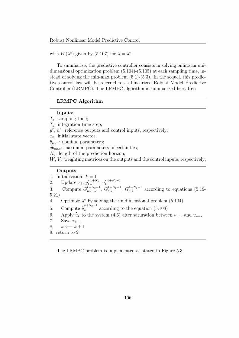
Robust Nonlinear Model Predictive Control
with W (λ?) given by (5.107) for λ = λ?.
To summarize, the predictive controller consists in solving online an uni-dimensional optimization problem (5.104)-(5.105) at each sampling time, in-stead of solving the min-max problem (5.1)-(5.3). In the sequel, this predic-tive control law will be referred to as Linearized Robust Model PredictiveController (LRMPC). The LRMPC algorithm is summarized hereafter:
LRMPC Algorithm
Inputs:Ts: sampling time;Td: integration time step;yr, ur: reference outputs and control inputs, respectively;x0: initial state vector;θnom: nominal parameters;δθmax: maximum parameters uncertainties;Np: length of the prediction horizon;W , V : weighting matrices on the outputs and the control inputs, respectively;
Outputs:1. Initialisation: k = 12. Update xk, y
r,k+Npk+1 , ur,k+Np−1
k
3. Compute Gk+Np−1nom,k , Gk+Np−1
θ,k , Gk+Np−1u,k according to equations (5.19-
5.21)4. Optimize λ? by solving the unidimensional problem (5.104)5. Compute ?
uk+Np−1
k according to the equation (5.108)6. Apply ?
uk to the system (4.6) after saturation between umin and umax
7. Save xk+1
8. k ←− k + 19. return to 2
The LRMPC problem is implemented as stated in Figure 5.3.
106
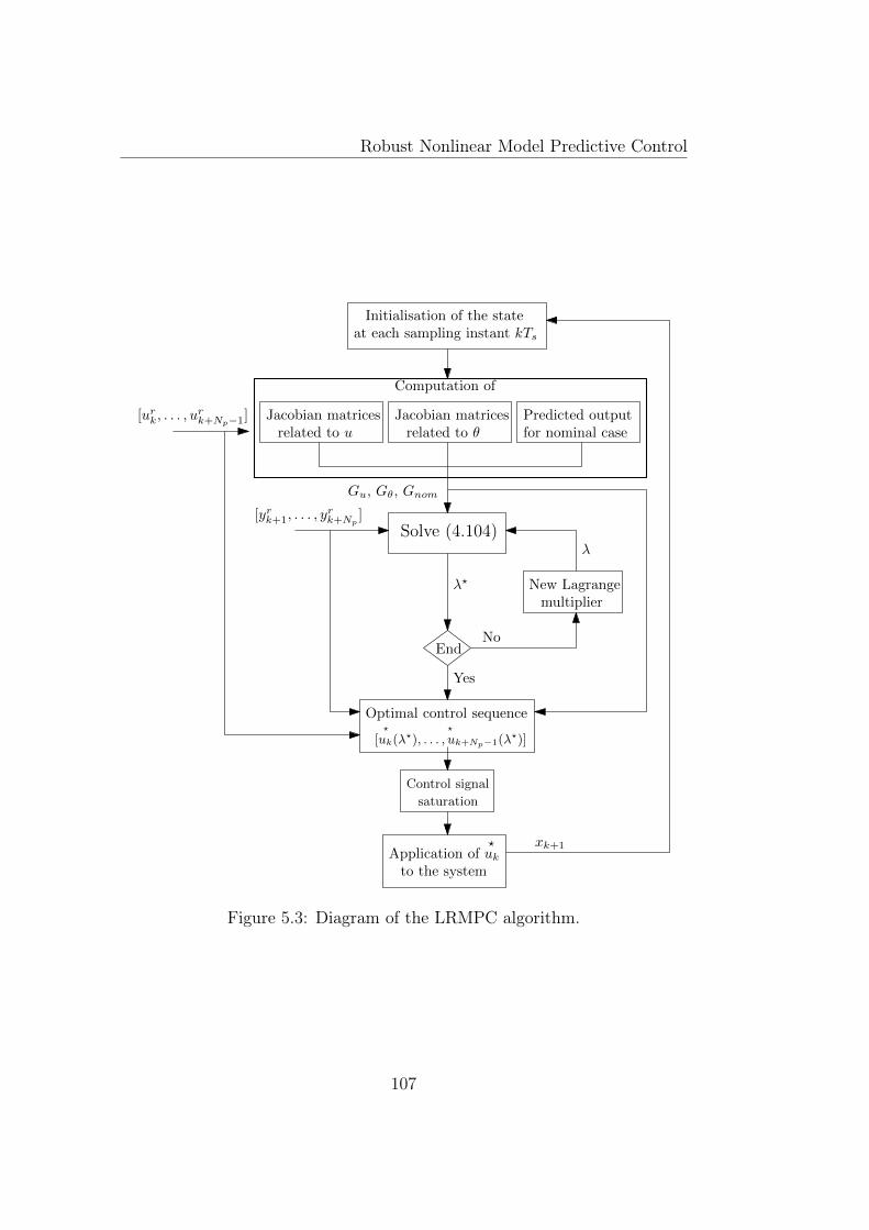
Robust Nonlinear Model Predictive Control
Initialisation of the stateat each sampling instant kTs
Computation of
End
New Lagrange
xk+1
No
Yes
Gu, Gθ, Gnom
Predicted outputJacobian matricesJacobian matricesrelated to u related to θ for nominal case
λ?
[yrk+1, . . . , yrk+Np
]
[urk, . . . , urk+Np−1]
Solve (4.104)λ
multiplier
Control signal
saturation
Optimal control sequence
[uk(λ?), . . . , uk+Np−1(λ
?)]??
Application of ukto the system
?
Figure 5.3: Diagram of the LRMPC algorithm.
107
Robust Nonlinear Model Predictive Control
5.6 Constrained linearized robust predictive con-troller
As mentionned before, the control problem that determines the control se-quence has been formulated till now in an unconstrained case, with a pos-teriori saturation of the control signal for real-time implementation. In thesequel, inequality constraints on the control input u are taken into accountin the optimization problem (e.g. corresponding to physical constraints onthe actuators).
In this section, we will therefore consider the robust nonlinear predictiveproblem which is defined by (5.33)-(5.34) subject to the following inequalityconstraint on the optimization variable uk+Np−1
k :
umin ≤ uk+j−1 ≤ umax, j = 1, Np (5.109)
where umin and umax are the lower and upper bounds on the control signal,respectively. No constraints on the state are considered.
Based on the formalism presented in section 5.5.1, the optimization prob-lem (5.1-5.3) with constraints (5.109) can be approached by the two playergame problem (5.78). In the sequel, we extend results presented in [135] tothe case of constrained robust regularized least squares. The main contribu-tion is to solve the robust regularized optimization problem (5.78) taking intoaccount constraints on the optimization variable z. Then, the unconstrainedoptimization problem defined in (5.93) with (5.94) becomes:
minλ≥||C>WC||
minz≤z≤z
J(z, λ) (5.110)
where the cost function J(z, λ) is still defined by (5.94).From (5.82), the optimization problem (5.110) is rewritten as:
minλ≥||C>WC||
minz≤z≤z
[||z||2V + λ||Eaz − Eb||2 + ||Az − b||2W (λ)
](5.111)
5.6.1 Bilevel optimization problem
The corresponding formulation of the optimization problem (5.111) into abilevel optimization problem can be written as follows:
λ? = arg minλ≥||C>WC||
J(z(λ), λ)
s.t. z(λ) = arg minz≤z≤z
J(z, λ)(5.112)
The problem (5.112) is made of two levels of optimization problems:
108
Robust Nonlinear Model Predictive Control
• Lower-levelThe minimum z(λ) is the solution of the following quadratic program-ming problem:
minz
1
2z>Hz + F>z
subject to[
I 00 −I
]z ≤
[z−z
] (5.113)
with {H = 2
(V (λ) + A>W (λ)A
)F = −2
(A>W (λ)b+ λE>a Eb
) (5.114)
where V (λ) and W (λ) are given by (5.100) and (5.92), respectively.
• Upper-levelThe nonnegative scalar parameter λ? ∈ R+ is computed from the fol-lowing unidimensional minimization problem:
λ? = arg minλ≥||C>WC||
[||z(λ)||2V + λ||Eaz(λ)− Eb||2 + ||Az(λ)− b||2W (λ)
](5.115)
Finally, the bilevel problem (5.112) has a unique global minimum ?z given by
(5.113) for λ = λ? (i.e. ?z = z(λ?)).
Remark 5.7. Of course, if there are no constraints on z, the solution ofproblem (5.112) is equivalent to the one of the problem (5.101).
5.6.2 Constrained Linearized Robust Model PredictiveControl
The application of (5.113)-(5.115) provides the solution of (5.1) with crite-rion (5.32) and inequality constraints on uk+Np−1
k as follows:
Step 1. The scalar λ? is computed from the following minimization problem:
λ? = arg minλ≥||G
k+N>pθ,k+1 WG
k+Npθ,k+1 ||
J(z(λ), λ) (5.116)
where the function J(z(λ), λ) is defined by (see (5.105)):
J(z(λ), λ) = ||z(λ)||2V + λ||δθmax||2 + ||Gk+Np−1u,k z(λ)− yr,k+Np
k+1 +Gk+Npnom,k+1||2W (λ)
(5.117)
109
Robust Nonlinear Model Predictive Control
and z(λ) is given by
z(λ?) = arg minz≤z≤z
[z>E(λ)z − 2B(λ)>z
](5.118)
where
E(λ) = V +Gk+Np−1>
u,k W (λ)Gk+Np−1u,k (5.119)
B(λ) = Gk+Np−1>
u,k W (λ)(yr,k+Npk+1 −Gk+Np
nom,k+1
)(5.120)
z = uminInu − ur,k+Np−1k (5.121)
z = umaxInu − ur,k+Np−1k (5.122)
with W (λ) given in (5.107).
Step 2. The control sequence ?uk+Np−1
k is derived from (5.118) for λ = λ?:
?uk+Np−1
k = ur,k+Np−1k + z(λ?) (5.123)
To summarize, the predictive controller consists in solving online a bileveloptimization problem (5.112) instead of solving a min-max problem (5.1-5.3): a quadratic programming problem (5.113) in the lower level, and anunidimensional optimization problem (5.115) in the upper level. Since thereare very efficient algorithms for this kind of optimization problems and thatthe two problems are convex, the obtained optimization problem remainsmore tractable than the min-max one. In the sequel, this predictive controllaw will be referred to as Constrained Linearized Robust Model PredictiveController (CLRMPC). The CLRMPC algorithm is summarized hereafter.
110
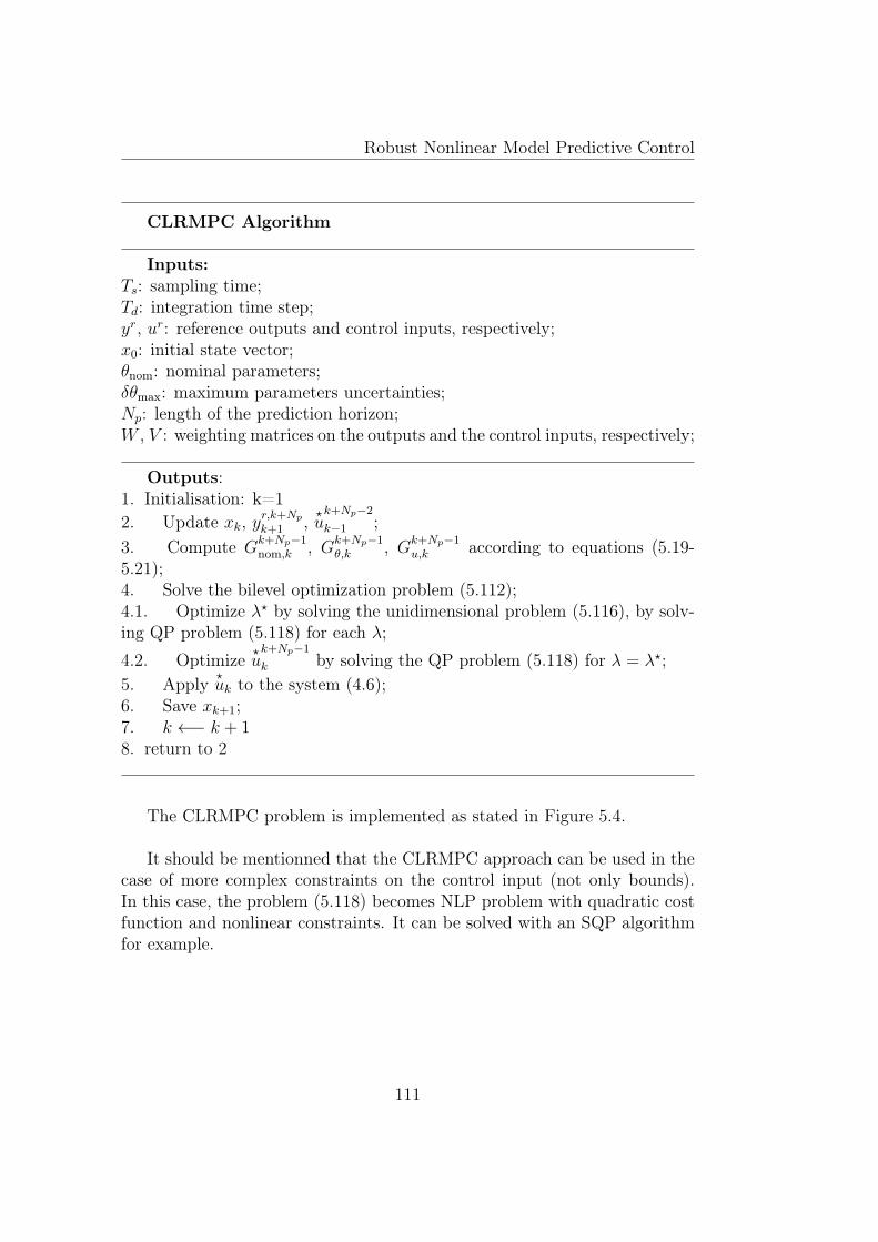
Robust Nonlinear Model Predictive Control
CLRMPC Algorithm
Inputs:Ts: sampling time;Td: integration time step;yr, ur: reference outputs and control inputs, respectively;x0: initial state vector;θnom: nominal parameters;δθmax: maximum parameters uncertainties;Np: length of the prediction horizon;W , V : weighting matrices on the outputs and the control inputs, respectively;
Outputs:1. Initialisation: k=12. Update xk, y
r,k+Npk+1 , ?u
k+Np−2
k−1 ;3. Compute Gk+Np−1
nom,k , Gk+Np−1θ,k , Gk+Np−1
u,k according to equations (5.19-5.21);4. Solve the bilevel optimization problem (5.112);4.1. Optimize λ? by solving the unidimensional problem (5.116), by solv-ing QP problem (5.118) for each λ;4.2. Optimize ?
uk+Np−1
k by solving the QP problem (5.118) for λ = λ?;5. Apply ?
uk to the system (4.6);6. Save xk+1;7. k ←− k + 18. return to 2
The CLRMPC problem is implemented as stated in Figure 5.4.
It should be mentionned that the CLRMPC approach can be used in thecase of more complex constraints on the control input (not only bounds).In this case, the problem (5.118) becomes NLP problem with quadratic costfunction and nonlinear constraints. It can be solved with an SQP algorithmfor example.
111
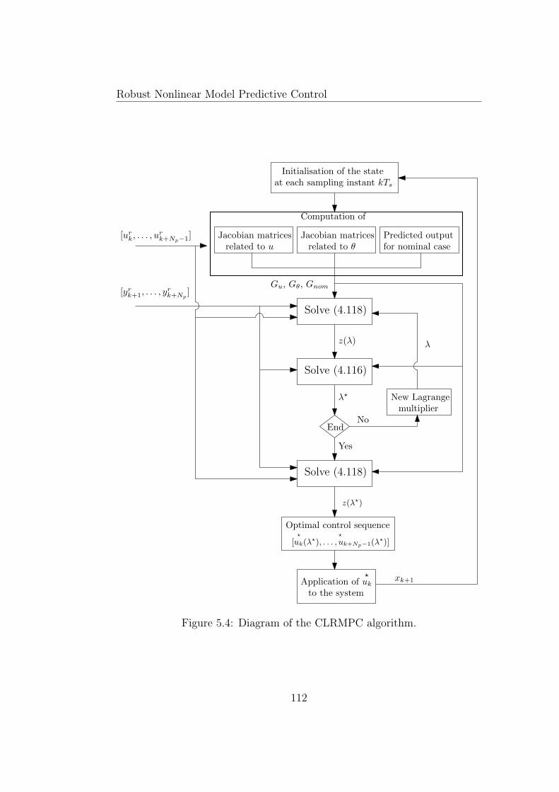
Robust Nonlinear Model Predictive Control
Initialisation of the stateat each sampling instant kTs
Computation of
Application of ukto the system
xk+1
Gu, Gθ, Gnom
Predicted outputJacobian matricesJacobian matricesrelated to u related to θ for nominal case
[urk, . . . , urk+Np−1]
Solve (4.118)
Solve (4.118)
z(λ)
EndNo
Yes
λ? New Lagrange
λ
multiplier
Solve (4.116)
[yrk+1, . . . , yrk+Np
]
z(λ?)
Optimal control sequence
[uk(λ?), . . . , uk+Np−1(λ
?)]??
?
Figure 5.4: Diagram of the CLRMPC algorithm.
112
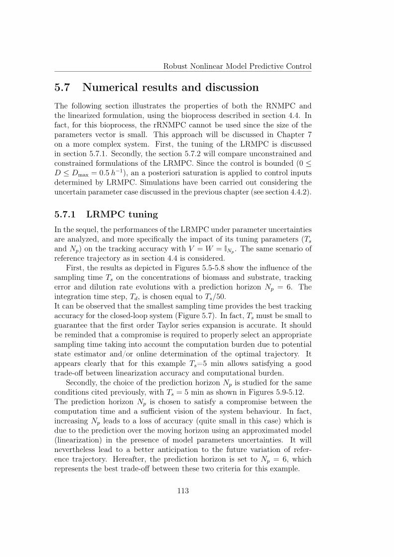
Robust Nonlinear Model Predictive Control
5.7 Numerical results and discussionThe following section illustrates the properties of both the RNMPC andthe linearized formulation, using the bioprocess described in section 4.4. Infact, for this bioprocess, the rRNMPC cannot be used since the size of theparameters vector is small. This approach will be discussed in Chapter 7on a more complex system. First, the tuning of the LRMPC is discussedin section 5.7.1. Secondly, the section 5.7.2 will compare unconstrained andconstrained formulations of the LRMPC. Since the control is bounded (0 ≤D ≤ Dmax = 0.5 h−1), an a posteriori saturation is applied to control inputsdetermined by LRMPC. Simulations have been carried out considering theuncertain parameter case discussed in the previous chapter (see section 4.4.2).
5.7.1 LRMPC tuning
In the sequel, the performances of the LRMPC under parameter uncertaintiesare analyzed, and more specifically the impact of its tuning parameters (Tsand Np) on the tracking accuracy with V = W = INp . The same scenario ofreference trajectory as in section 4.4 is considered.
First, the results as depicted in Figures 5.5-5.8 show the influence of thesampling time Ts on the concentrations of biomass and substrate, trackingerror and dilution rate evolutions with a prediction horizon Np = 6. Theintegration time step, Td, is chosen equal to Ts/50.It can be observed that the smallest sampling time provides the best trackingaccuracy for the closed-loop system (Figure 5.7). In fact, Ts must be small toguarantee that the first order Taylor series expansion is accurate. It shouldbe reminded that a compromise is required to properly select an appropriatesampling time taking into account the computation burden due to potentialstate estimator and/or online determination of the optimal trajectory. Itappears clearly that for this example Ts=5 min allows satisfying a goodtrade-off between linearization accuracy and computational burden.
Secondly, the choice of the prediction horizon Np is studied for the sameconditions cited previously, with Ts = 5 min as shown in Figures 5.9-5.12.The prediction horizon Np is chosen to satisfy a compromise between thecomputation time and a sufficient vision of the system behaviour. In fact,increasing Np leads to a loss of accuracy (quite small in this case) which isdue to the prediction over the moving horizon using an approximated model(linearization) in the presence of model parameters uncertainties. It willnevertheless lead to a better anticipation to the future variation of refer-ence trajectory. Hereafter, the prediction horizon is set to Np = 6, whichrepresents the best trade-off between these two criteria for this example.
113

Robust Nonlinear Model Predictive Control
Time (h)0 2 4 6 8 10 12 14 16 18 20
X(g.L
−1)
27
27.5
28
28.5
29
29.5
30
30.5
31
31.5T
s=5 min
Ts=10 min
Ts=20 min
X r
8 8.5 9 9.5
30.6
30.8
31
31.2
Figure 5.5: Biomass concentration evolution with time for LRMPC strategyfor several values of the sampling time Ts.
Time (h)0 2 4 6 8 10 12 14 16 18 20
S(g.L
−1)
1
2
3
4
5
6
7
8
9
10
S rnom
S rreal
Ts=5 min
Ts=10 min
Ts=20 min8.5 9 9.5 10
6.2
6.4
6.6
Figure 5.6: Substrate concentration evolution with time for LRMPC strategyfor several values of the sampling time Ts.
114
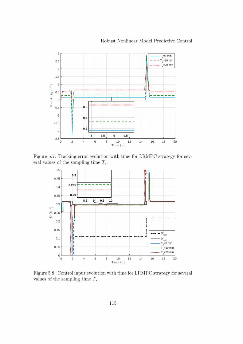
Robust Nonlinear Model Predictive Control
Time (h)0 2 4 6 8 10 12 14 16 18 20
X−X
r(g.L
−1)
-2.5
-2
-1.5
-1
-0.5
0
0.5
1
1.5
2
2.5
3T
s=5 min
Ts=10 min
Ts=20 min
8 8.5 9 9.5
0.2
0.4
0.6
Figure 5.7: Tracking error evolution with time for LRMPC strategy for sev-eral values of the sampling time Ts.
Time (h)0 2 4 6 8 10 12 14 16 18 20
D(h
−1)
0
0.05
0.1
0.15
0.2
0.25
0.3
0.35
0.4
0.45
0.5
Drnom
Drreal
Ts=5 min
Ts=10 min
Ts=20 min
8.5 9 9.5 10
0.29
0.295
0.3
Figure 5.8: Control input evolution with time for LRMPC strategy for severalvalues of the sampling time Ts.
115
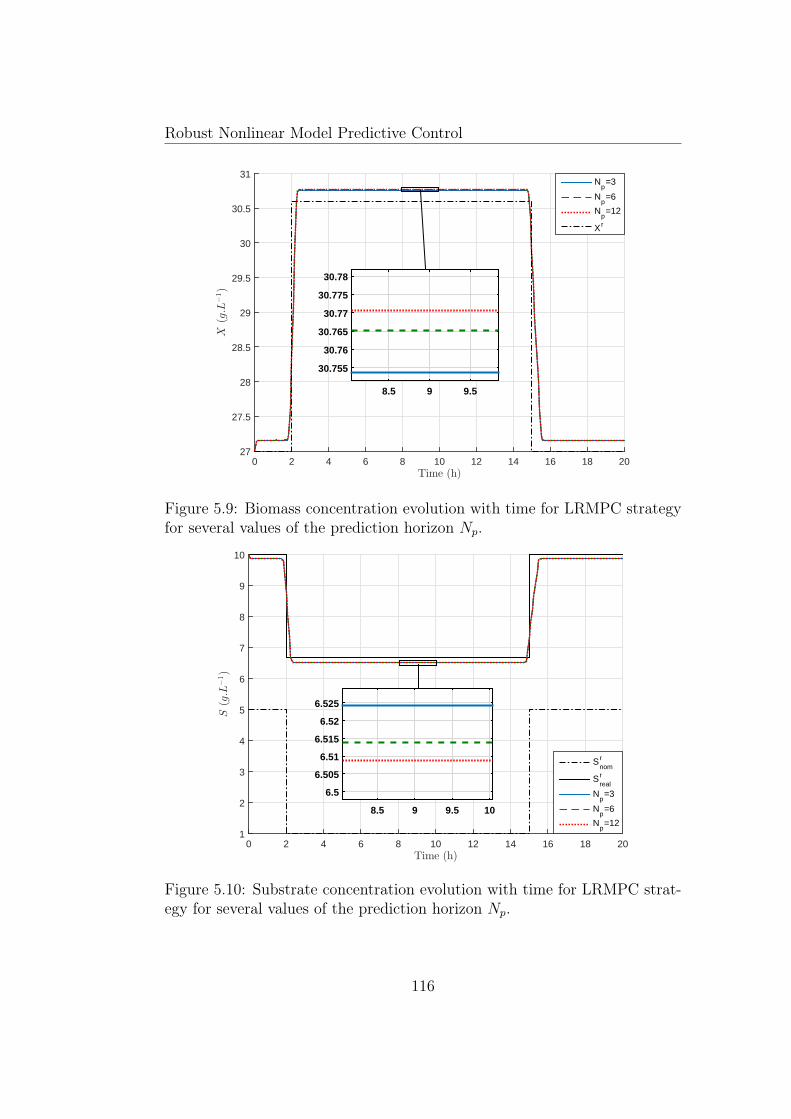
Robust Nonlinear Model Predictive Control
Time (h)0 2 4 6 8 10 12 14 16 18 20
X(g.L
−1)
27
27.5
28
28.5
29
29.5
30
30.5
31N
p=3
Np=6
Np=12
X r
8.5 9 9.5
30.755
30.76
30.765
30.77
30.775
30.78
Figure 5.9: Biomass concentration evolution with time for LRMPC strategyfor several values of the prediction horizon Np.
Time (h)0 2 4 6 8 10 12 14 16 18 20
S(g.L
−1)
1
2
3
4
5
6
7
8
9
10
S rnom
S rreal
Np=3
Np=6
Np=12
8.5 9 9.5 10
6.5
6.505
6.51
6.515
6.52
6.525
Figure 5.10: Substrate concentration evolution with time for LRMPC strat-egy for several values of the prediction horizon Np.
116
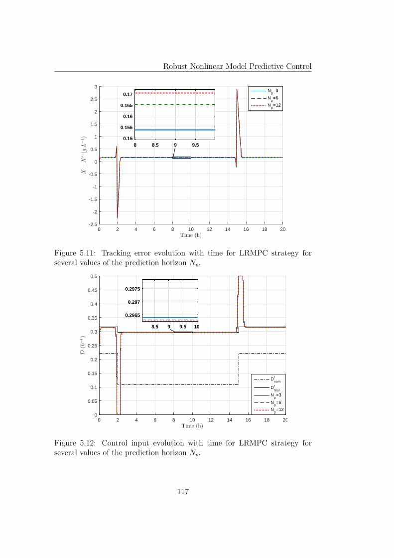
Robust Nonlinear Model Predictive Control
Time (h)0 2 4 6 8 10 12 14 16 18 20
X−X
r(g.L
−1)
-2.5
-2
-1.5
-1
-0.5
0
0.5
1
1.5
2
2.5
3N
p=3
Np=6
Np=12
8 8.5 9 9.50.15
0.155
0.16
0.165
0.17
Figure 5.11: Tracking error evolution with time for LRMPC strategy forseveral values of the prediction horizon Np.
Time (h)0 2 4 6 8 10 12 14 16 18 20
D(h
−1)
0
0.05
0.1
0.15
0.2
0.25
0.3
0.35
0.4
0.45
0.5
Drnom
Drreal
Np=3
Np=6
Np=12
8.5 9 9.5 10
0.2965
0.297
0.2975
Figure 5.12: Control input evolution with time for LRMPC strategy forseveral values of the prediction horizon Np.
117
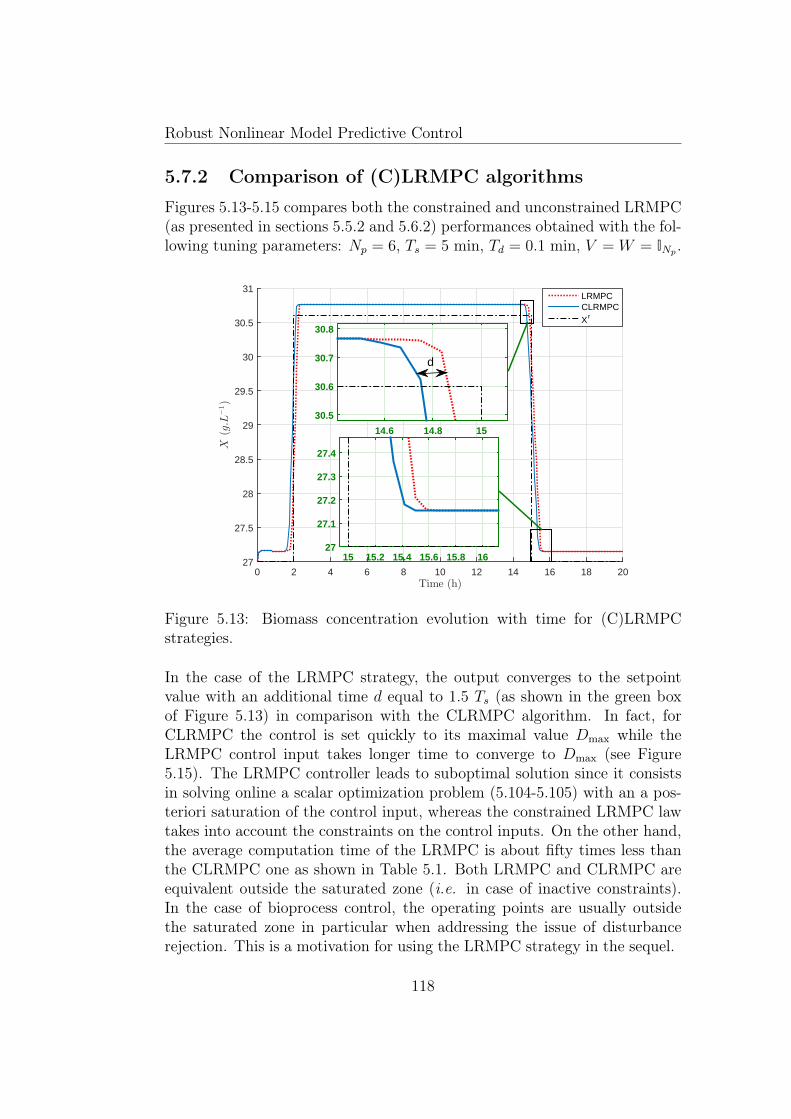
Robust Nonlinear Model Predictive Control
5.7.2 Comparison of (C)LRMPC algorithms
Figures 5.13-5.15 compares both the constrained and unconstrained LRMPC(as presented in sections 5.5.2 and 5.6.2) performances obtained with the fol-lowing tuning parameters: Np = 6, Ts = 5 min, Td = 0.1 min, V = W = INp .
Time (h)0 2 4 6 8 10 12 14 16 18 20
X(g.L
−1)
27
27.5
28
28.5
29
29.5
30
30.5
31LRMPCCLRMPC
X r
14.6 14.8 15
30.5
30.6
30.7
30.8
15 15.2 15.4 15.6 15.8 1627
27.1
27.2
27.3
27.4
d
Figure 5.13: Biomass concentration evolution with time for (C)LRMPCstrategies.
In the case of the LRMPC strategy, the output converges to the setpointvalue with an additional time d equal to 1.5 Ts (as shown in the green boxof Figure 5.13) in comparison with the CLRMPC algorithm. In fact, forCLRMPC the control is set quickly to its maximal value Dmax while theLRMPC control input takes longer time to converge to Dmax (see Figure5.15). The LRMPC controller leads to suboptimal solution since it consistsin solving online a scalar optimization problem (5.104-5.105) with an a pos-teriori saturation of the control input, whereas the constrained LRMPC lawtakes into account the constraints on the control inputs. On the other hand,the average computation time of the LRMPC is about fifty times less thanthe CLRMPC one as shown in Table 5.1. Both LRMPC and CLRMPC areequivalent outside the saturated zone (i.e. in case of inactive constraints).In the case of bioprocess control, the operating points are usually outsidethe saturated zone in particular when addressing the issue of disturbancerejection. This is a motivation for using the LRMPC strategy in the sequel.
118
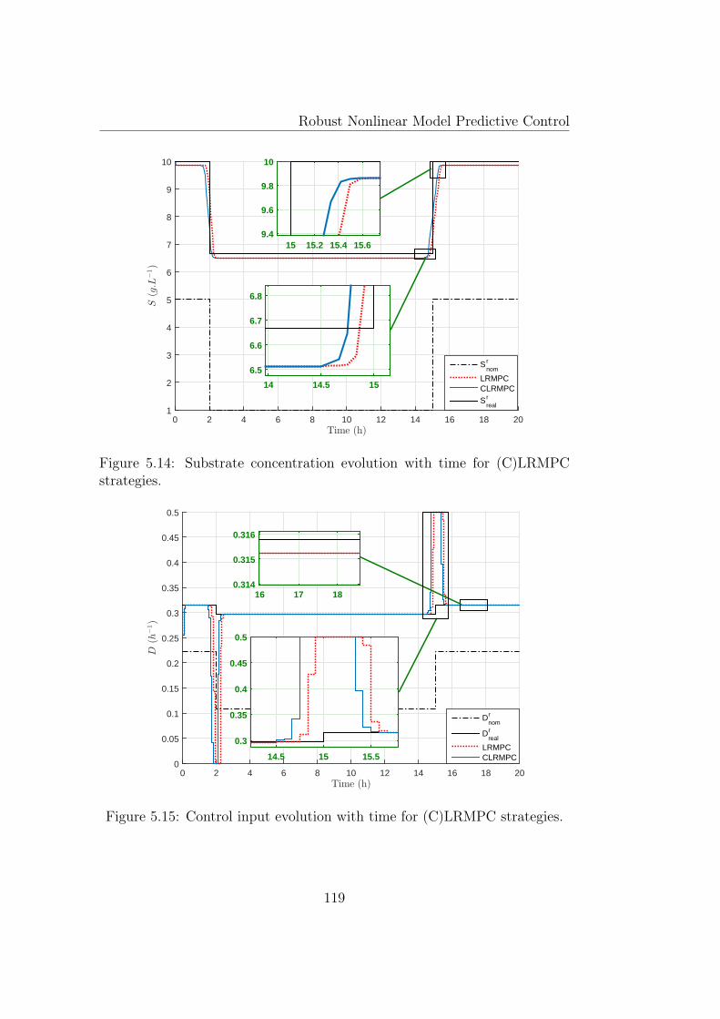
Robust Nonlinear Model Predictive Control
Time (h)0 2 4 6 8 10 12 14 16 18 20
S(g.L
−1)
1
2
3
4
5
6
7
8
9
10
S rnom
LRMPCCLRMPC
S rreal
14 14.5 15
6.5
6.6
6.7
6.8
15 15.2 15.4 15.69.4
9.6
9.8
10
Figure 5.14: Substrate concentration evolution with time for (C)LRMPCstrategies.
Time (h)0 2 4 6 8 10 12 14 16 18 20
D(h
−1)
0
0.05
0.1
0.15
0.2
0.25
0.3
0.35
0.4
0.45
0.5
Drnom
Drreal
LRMPCCLRMPC14.5 15 15.5
0.3
0.35
0.4
0.45
0.5
16 17 180.314
0.315
0.316
Figure 5.15: Control input evolution with time for (C)LRMPC strategies.
119
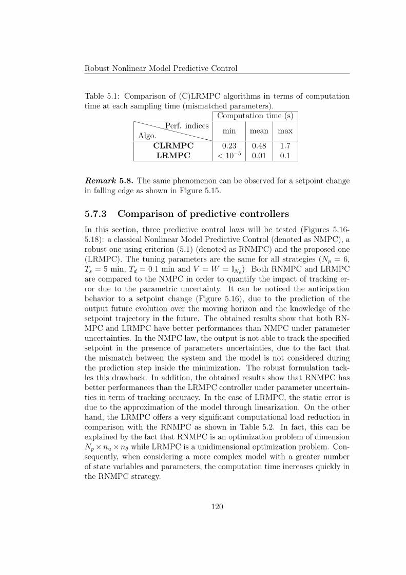
Robust Nonlinear Model Predictive Control
Table 5.1: Comparison of (C)LRMPC algorithms in terms of computationtime at each sampling time (mismatched parameters).
Computation time (s)XXXXXXXXXXXXAlgo.
Perf. indices min mean max
CLRMPC 0.23 0.48 1.7LRMPC < 10−5 0.01 0.1
Remark 5.8. The same phenomenon can be observed for a setpoint changein falling edge as shown in Figure 5.15.
5.7.3 Comparison of predictive controllers
In this section, three predictive control laws will be tested (Figures 5.16-5.18): a classical Nonlinear Model Predictive Control (denoted as NMPC), arobust one using criterion (5.1) (denoted as RNMPC) and the proposed one(LRMPC). The tuning parameters are the same for all strategies (Np = 6,Ts = 5 min, Td = 0.1 min and V = W = INp). Both RNMPC and LRMPCare compared to the NMPC in order to quantify the impact of tracking er-ror due to the parametric uncertainty. It can be noticed the anticipationbehavior to a setpoint change (Figure 5.16), due to the prediction of theoutput future evolution over the moving horizon and the knowledge of thesetpoint trajectory in the future. The obtained results show that both RN-MPC and LRMPC have better performances than NMPC under parameteruncertainties. In the NMPC law, the output is not able to track the specifiedsetpoint in the presence of parameters uncertainties, due to the fact thatthe mismatch between the system and the model is not considered duringthe prediction step inside the minimization. The robust formulation tack-les this drawback. In addition, the obtained results show that RNMPC hasbetter performances than the LRMPC controller under parameter uncertain-ties in term of tracking accuracy. In the case of LRMPC, the static error isdue to the approximation of the model through linearization. On the otherhand, the LRMPC offers a very significant computational load reduction incomparison with the RNMPC as shown in Table 5.2. In fact, this can beexplained by the fact that RNMPC is an optimization problem of dimensionNp×nu×nθ while LRMPC is a unidimensional optimization problem. Con-sequently, when considering a more complex model with a greater numberof state variables and parameters, the computation time increases quickly inthe RNMPC strategy.
120
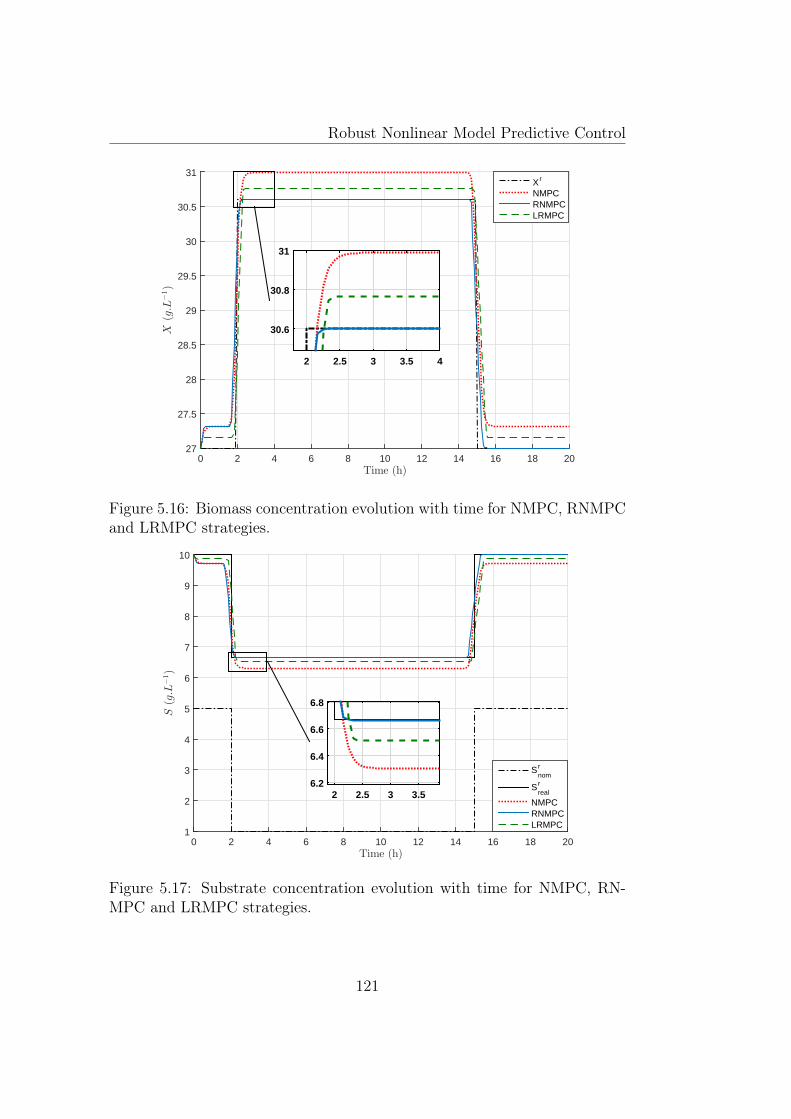
Robust Nonlinear Model Predictive Control
Time (h)0 2 4 6 8 10 12 14 16 18 20
X(g.L
−1)
27
27.5
28
28.5
29
29.5
30
30.5
31X r
NMPCRNMPCLRMPC
2 2.5 3 3.5 4
30.6
30.8
31
Figure 5.16: Biomass concentration evolution with time for NMPC, RNMPCand LRMPC strategies.
Time (h)0 2 4 6 8 10 12 14 16 18 20
S(g.L
−1)
1
2
3
4
5
6
7
8
9
10
S rnom
S rreal
NMPCRNMPCLRMPC
2 2.5 3 3.56.2
6.4
6.6
6.8
Figure 5.17: Substrate concentration evolution with time for NMPC, RN-MPC and LRMPC strategies.
121
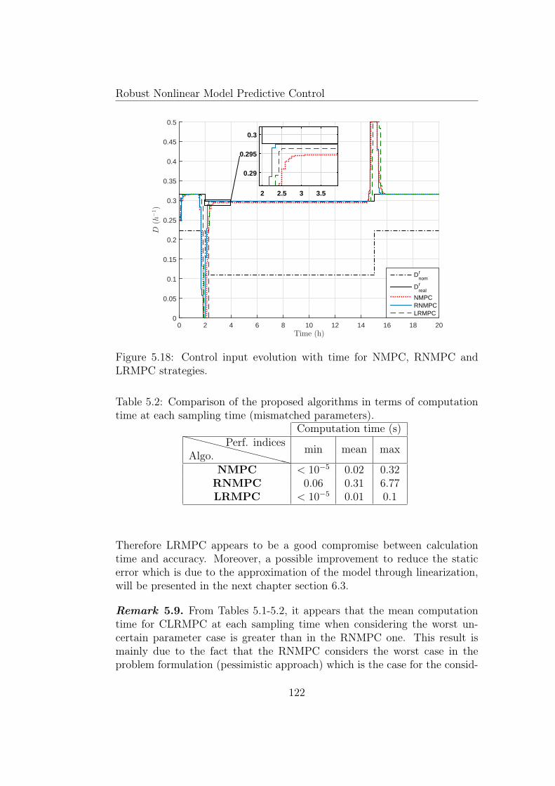
Robust Nonlinear Model Predictive Control
Time (h)0 2 4 6 8 10 12 14 16 18 20
D(h
−1)
0
0.05
0.1
0.15
0.2
0.25
0.3
0.35
0.4
0.45
0.5
Drnom
Drreal
NMPCRNMPCLRMPC
2 2.5 3 3.5
0.29
0.295
0.3
Figure 5.18: Control input evolution with time for NMPC, RNMPC andLRMPC strategies.
Table 5.2: Comparison of the proposed algorithms in terms of computationtime at each sampling time (mismatched parameters).
Computation time (s)XXXXXXXXXXXXAlgo.
Perf. indices min mean max
NMPC < 10−5 0.02 0.32RNMPC 0.06 0.31 6.77LRMPC < 10−5 0.01 0.1
Therefore LRMPC appears to be a good compromise between calculationtime and accuracy. Moreover, a possible improvement to reduce the staticerror which is due to the approximation of the model through linearization,will be presented in the next chapter section 6.3.
Remark 5.9. From Tables 5.1-5.2, it appears that the mean computationtime for CLRMPC at each sampling time when considering the worst un-certain parameter case is greater than in the RNMPC one. This result ismainly due to the fact that the RNMPC considers the worst case in theproblem formulation (pessimistic approach) which is the case for the consid-
122
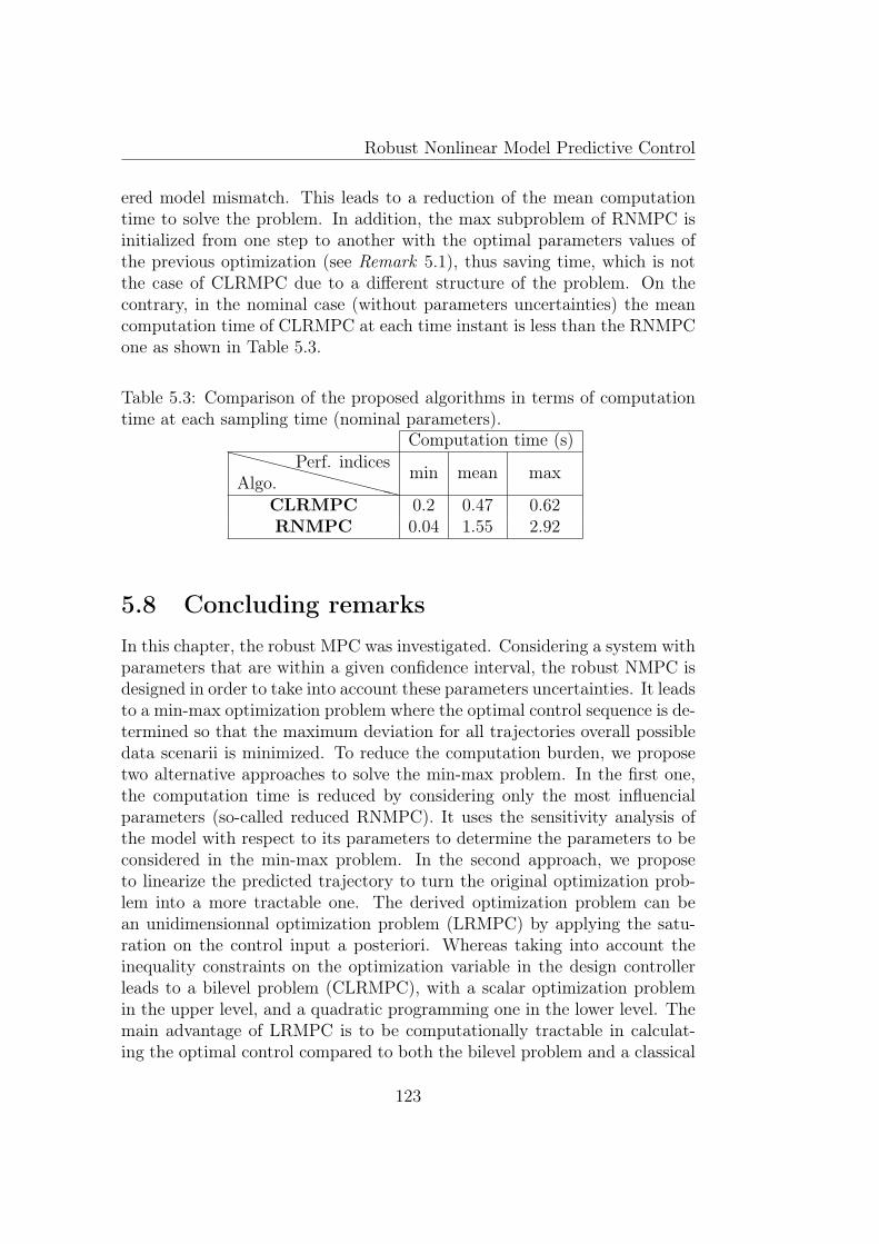
Robust Nonlinear Model Predictive Control
ered model mismatch. This leads to a reduction of the mean computationtime to solve the problem. In addition, the max subproblem of RNMPC isinitialized from one step to another with the optimal parameters values ofthe previous optimization (see Remark 5.1), thus saving time, which is notthe case of CLRMPC due to a different structure of the problem. On thecontrary, in the nominal case (without parameters uncertainties) the meancomputation time of CLRMPC at each time instant is less than the RNMPCone as shown in Table 5.3.
Table 5.3: Comparison of the proposed algorithms in terms of computationtime at each sampling time (nominal parameters).
Computation time (s)XXXXXXXXXXXXAlgo.
Perf. indices min mean max
CLRMPC 0.2 0.47 0.62RNMPC 0.04 1.55 2.92
5.8 Concluding remarksIn this chapter, the robust MPC was investigated. Considering a system withparameters that are within a given confidence interval, the robust NMPC isdesigned in order to take into account these parameters uncertainties. It leadsto a min-max optimization problem where the optimal control sequence is de-termined so that the maximum deviation for all trajectories overall possibledata scenarii is minimized. To reduce the computation burden, we proposetwo alternative approaches to solve the min-max problem. In the first one,the computation time is reduced by considering only the most influencialparameters (so-called reduced RNMPC). It uses the sensitivity analysis ofthe model with respect to its parameters to determine the parameters to beconsidered in the min-max problem. In the second approach, we proposeto linearize the predicted trajectory to turn the original optimization prob-lem into a more tractable one. The derived optimization problem can bean unidimensionnal optimization problem (LRMPC) by applying the satu-ration on the control input a posteriori. Whereas taking into account theinequality constraints on the optimization variable in the design controllerleads to a bilevel problem (CLRMPC), with a scalar optimization problemin the upper level, and a quadratic programming one in the lower level. Themain advantage of LRMPC is to be computationally tractable in calculat-ing the optimal control compared to both the bilevel problem and a classical
123
Robust Nonlinear Model Predictive Control
min-max robust approach, which makes it suitable for online implementation(even if in our case, all calculation times remain much smaller than the sam-pling period, this should not be the same for a more complex system, withmore uncertain parameters). Several simulations were performed in order tocompare the LRMPC strategy to the classical RNMPC law in the case ofmodel parameters uncertainties to control bacteria growth in a bioreactor.The LRMPC was shown to ensure a good trade-off between computationalload and tracking trajectory accuracy. However, there are several issues thatdeserve further investigation (e.g. non-zero tracking error). Some improve-ments of this control law are detailed in the next chapter.
124
Chapter 6
Some improvements of LRMPC
6.1 Introduction
In the previous chapter, in the LRMPC strategy, the min-max optimizationproblem was approached by a more tractable formulation, derived from thelinearization of the system around nominal values of the parameters andreference control inputs. In this chapter, some improvements are proposedfor the LRMPC controller.
A first proposed idea consists in linearizing the model around the nominalparameter values and the optimal control sequence obtained at the previousiteration instead of a reference control sequence determined at the steadystate behavior. This modification is motivated by the fact that the opti-mal control sequence obtained at the previous iteration is non-model-based,and thus the controller robustness with respect to model uncertainties isincreased. As in the case of LRMPC presented in Chapter 5, the derivedoptimization problem is here a bilevel one or a scalar optimization problemdepending on the considered constraints. This controller will be referred asincremental LRMPC.
Furthermore, as highlighted in section 5.7.1, the LRMPC accuracy canbe an issue (depending on the choice of the sampling period) as it dealswith a first-order approximation of nonlinear functions. To go further withmodel uncertainties and linearization drawbacks, the idea here is to develop ahierarchical control scheme. The proposed control strategy combines a robustmodel predictive control law with a Proportional Integral (PI) law or IntegralSliding Mode (ISM) controller regulator. The predictive controller guaranteesthe tracking of the reference trajectory, whereas the other regulator (PI orISM) ensures cancellation of any residual error.
The chapter is organized as follows. The section 6.2 deals with the de-
125
Some improvements of LRMPC
sign of the incremental LRMPC. Section 6.3 presents the hierarchical controlscheme that combines a robust predictive law with an auxiliary controller.Performances of the two controllers mentionned above will be illustrated onthe illustrative example studied in the previous chapters. Finally, conclusionsare summarized in section 6.4.
6.2 Variant of LRMPC
This section is motivated by the problem of designing a predictive controllerin the presence of bounded uncertainties and inputs. In comparison withthe previous chapter, the robust cost that will be minimized is expressed asa quadratic function measuring the control efforts instead of the differencebetween the control inputs and their reference values which are model-based.The idea is to use a model linearization along the nominal parameters valueand the optimal control sequence obtained at the previous iteration. Inaddition to be more robust to errors in the determination of the referencetrajectory than the previous approach, it presents the advantage to lead to asolution less sensitive to noise measurements, due to the fact that the controlincrements are explicitly considered in the cost function [141].
6.2.1 Problem formulation
The control sequence that minimizes a worst case cost function is derivedfrom the following optimization problem (at time index k) instead of theoptimization problem (5.1):
δ?uk+Np−1
k = arg minδuk+Np−1
k ∈Uδmaxδθ∈Θδ
Πδ(xk, δuk+Np−1k , δθ) (6.1)
Subject to
xk+j = g(tk, tk+j, xk, uk+j−1k , θ = θnom + δθ), j = 1, Np (6.2)
where the robust cost function is defined as
Πδ(xk, δuk+Np−1k , δθ) , ||δuk+Np−1
k ||2V + ||yk+Npk − yr,k+Np
k ||2W (6.3)
126
Some improvements of LRMPC
The optimization variables δuk+Np−1k are defined as the control increments as
follows:
δuk+Np−1k =
uk −
?uk−1...
uk+j − uk+j−1...
uk+Np−1 − uk+Np−2
,
δuk...
δuk+j...
δuk+Np−1
(6.4)
with ?uk−1 the control input applied at time index k−1 (i.e. solution of (6.1)
at time index k − 1).As in Chapter 5, the predicted outputs over the receding horizon are givenby:
yk+Npk+1 =
Hg(tk, tk+1, xk, uk, θ)
...Hg(tk, tk+j, xk, u
k+j−1k , θ)
...Hg(tk, tk+Np , xk, u
k+Np−1k , θ)
(6.5)
and yr,k+Npk =
yrk...
yrk+Np
the setpoint values.
U δ and Θδ are compact sets that contains the origin, defined as follows:{Θδ = [−δθmax, δθmax] with δθmax = (θ+ − θ−)/2 (6.6)U δ = [δu, δu] (6.7)
V � 0 and W � 0 are tuning weighting matrices.
The predicted state for time tk+j, starting from state at tk, is linearizedaround the trajectory given for the nominal parameters θnom and a controlsequence uk+Np−1
k defined as the optimal control sequence of the optimizationproblem (6.1) obtained at the previous sampling time (at time index k− 1):
uj =?uj−1, j = k, k +Np − 1 (6.8)
As for LRMPC, a first order Taylor series (local) expansion of (4.5) for j =1, Np is used:
xk+j ≈ xnom,k+j +∇θg(tk+j)δθ +∇ug(tk+j)(uk+j−1k − uk+j−1
k
)(6.9)
127
Some improvements of LRMPC
with
xnom,k+j = g(tk, tk+j, xk, uk+j−1k , θnom) (6.10)
∇θg(tk+j) =∂g(tk, tk+j, xk, u
k+j−1k , θ)
∂θ
∣∣∣∣∣∣∣∣ uk+j−1k = uk+j−1
kθ = θnom
(6.11)
∇ug(tk+j) =∂g(tk, tk+i, xk, u
k+j−1k , θ)
∂uk+j−1k
∣∣∣∣∣∣∣∣ uk+j−1k = uk+j−1
kθ = θnom
(6.12)
The dynamics of sensitivity function with respect to θ and u, defined in (6.11-6.12), can be computed for time t ∈ [tk, tk+Np ] as detailed in section 5.4.1.From (6.5) and (6.9), it comes:
xk+1 ≈ xnom,k+1 +∇θg(tk+1)δθ +∇ug(tk+1)(uk − uk)...xk+j ≈ xnom,k+j +∇θg(tk+j)δθ +∇ug(tk+j)(u
k+j−1k − uk+j−1
k ) (6.13)...xk+Np ≈ xnom,k+Np +∇θg(tk+Np)δθ +∇ug(tk+Np)(u
k+Np−1k − uk+Np−1
k )
Using (6.4) and (6.8), the terms uk+j − uk+j, j = 1, Np − 1 are written asfunctions of ∆uj, j = 1, Np − 1 as follows:
uk − uk = uk −?uk−1 = δuk
uk+1 − uk+1 = ︸ ︷︷ ︸δuk+1
uk+1
0︷ ︸︸ ︷− uk + uk −
?uk−1︸ ︷︷ ︸
δuk
+?uk−1 −
?uk = δuk+1 + δuk +
?uk−1 −
?uk
...uk+j − uk+j = δuk+j + . . .+ δuk +
?uk−1 −
?uk+j−1 (6.14)
...uk+Np−1 − uk+Np−1 = δuk+Np−1 + . . .+ δuk +
?uk−1 −
?uk+Np−2
And thus:
uk+Np−1k − uk+Np−1
k =
δuk
δuk+1 + δuk +?uk−1 −
?uk
...δuk+Np−1 + . . .+ δuk +
?uk−1 −
?uk+Np−2
(6.15)
128
Some improvements of LRMPC
Finally, it comes
uk+Np−1k − uk+Np−1
k =
?uk−1...
?uk−1
−
?uk−1...
?uk+Np−2
+
Inu 0 . . . 0... . . . . . . ...... . . . 0
Inu . . . . . . Inu
δuk+Np−1k
, Ξk+Np−1k + TNpδu
k+Np−1k
(6.16)
where
Ξk+Np−1k =
?uk−1...
?uk−1
−
?uk−1...
?uk+Np−2
(6.17)
andTNp ∈ RNp×Np : unitary lower triangular matrix (6.18)
From (4.11), (6.9) and (6.16), the predicted ouputs yk+Npk+1 over the moving
horizon are expressed as follows:
yk+Npk+1 = G
k+Npnom,k+1 +G
k+Npθ,k+1δθ +G
k+Np−1u,k (Ξ
k+Np−1k + TNpδu
k+Np−1k ) (6.19)
with Gk+Npnom,k+1, G
k+Npθ,k+1 and Gk+Np−1
u,k defined as in section 5.4.1 (see (5.25)).Consequently, the linearized prediction outputs have similar structure as inthe LRMPC (5.25), only the last term differs. This controller will be referredto as incremental LRMPC (LRMPC-δu).
6.2.2 Stability analysis
In the previous chapter, the stability analysis has been addressed for theclosed-loop with the LRMPC law. The same methodology could be used forthe LRMPC-δu under the same assumptions as in section 5.4.2.
The difference is that the model is linearized around θnom and u insteadof θnom and ur.
Consequently, the bound on the prediction error given by (5.47) as wellas upper and lower bounds on the optimal cost given by (5.56) as still valid.
For the robust stability (as in section 5.4.2.3), the admissible control inputis still chosen as:
uk+Npk+1 = [
?uk+Np−1
k+1 ,?uk+Np−1] (6.20)
and the relation (5.71) is still valid.Consequently, considering the control sequence u instead of ur do not
change the stability of the controller (which is in this case mainly linked tothe considered prediction model).
129
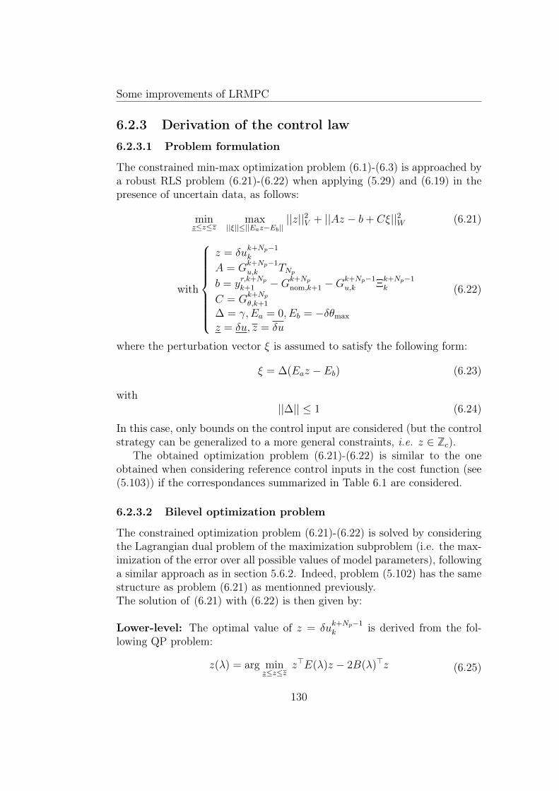
Some improvements of LRMPC
6.2.3 Derivation of the control law
6.2.3.1 Problem formulation
The constrained min-max optimization problem (6.1)-(6.3) is approached bya robust RLS problem (6.21)-(6.22) when applying (5.29) and (6.19) in thepresence of uncertain data, as follows:
minz≤z≤z
max||ξ||≤||Eaz−Eb||
||z||2V + ||Az − b+ Cξ||2W (6.21)
with
z = δuk+Np−1k
A = Gk+Np−1u,k TNp
b = yr,k+Npk+1 −Gk+Np
nom,k+1 −Gk+Np−1u,k Ξ
k+Np−1k
C = Gk+Npθ,k+1
∆ = γ,Ea = 0, Eb = −δθmax
z = δu, z = δu
(6.22)
where the perturbation vector ξ is assumed to satisfy the following form:
ξ = ∆(Eaz − Eb) (6.23)
with||∆|| ≤ 1 (6.24)
In this case, only bounds on the control input are considered (but the controlstrategy can be generalized to a more general constraints, i.e. z ∈ Zc).
The obtained optimization problem (6.21)-(6.22) is similar to the oneobtained when considering reference control inputs in the cost function (see(5.103)) if the correspondances summarized in Table 6.1 are considered.
6.2.3.2 Bilevel optimization problem
The constrained optimization problem (6.21)-(6.22) is solved by consideringthe Lagrangian dual problem of the maximization subproblem (i.e. the max-imization of the error over all possible values of model parameters), followinga similar approach as in section 5.6.2. Indeed, problem (5.102) has the samestructure as problem (6.21) as mentionned previously.The solution of (6.21) with (6.22) is then given by:
Lower-level: The optimal value of z = δuk+Np−1k is derived from the fol-
lowing QP problem:
z(λ) = arg minz≤z≤z
z>E(λ)z − 2B(λ)>z (6.25)
130
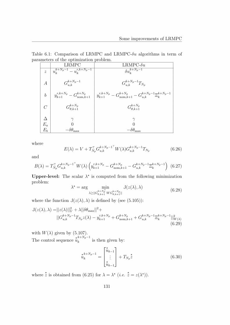
Some improvements of LRMPC
Table 6.1: Comparison of LRMPC and LRMPC-δu algorithms in term ofparameters of the optimization problem.
LRMPC LRMPC-δuz u
k+Np−1k − ur,k+Np−1
k δuk+Np−1k
A Gk+Np−1u,k G
k+Np−1u,k TNp
b yr,k+Npk+1 −Gk+Np
nom,k+1 yr,k+Npk+1 −Gk+Np
nom,k+1 −Gk+Np−1u,k Ξ
k+Np−1k
C Gk+Npθ,k+1 G
k+Npθ,k+1
∆ γ γEa 0 0Eb −δθmax −δθmax
whereE(λ) = V + T>NpG
k+Np−1>
u,k W (λ)Gk+Np−1u,k TNp (6.26)
and
B(λ) = T>NpGk+Np−1>
u,k W (λ)(yr,k+Npk+1 −Gk+Np
nom,k+1 −Gk+Np−1u,k Ξ
k+Np−1k
)(6.27)
Upper-level: The scalar λ? is computed from the following minimizationproblem:
λ? = arg minλ≥||G
k+N>pθ,k+1 WG
k+Npθ,k+1 ||
J(z(λ), λ) (6.28)
where the function J(z(λ), λ) is defined by (see (5.105)):
J(z(λ), λ) =||z(λ)||2V + λ||δθmax||2+
||Gk+Np−1u,k TNpz(λ)− yr,k+Np
k+1 +Gk+Npnom,k+1 +G
k+Np−1u,k Ξ
k+Np−1k ||2W (λ)
(6.29)
with W (λ) given by (5.107).The control sequence ?
uk+Np−1
k is then given by:
?uk+Np−1
k =
?uk−1...
?uk−1
+ TNp?z (6.30)
where ?z is obtained from (6.25) for λ = λ? (i.e. ?
z = z(λ?)).
131

Some improvements of LRMPC
Remark 6.1. The same methodology could be applied for the unconstrainedproblem. Then, the resulting optimization problem will be an unidimensionalproblem as presented in section 5.5.2:step 1. The scalar λ? is computed from the following minimization problem:
λ? = arg minλ≥||G
k+N>pθ,k+1 WG
k+Npθ,k+1 ||
J(z(λ), λ) (6.31)
where J(z(λ), λ) andW (λ) are given by (6.29) and (5.107), respectively, with(from (5.97))
z(λ) =(V + T>NpG
k+Np−1>
u,k W (λ)Gk+Np−1u,k TNp
)†T>NpG
k+Np−1>
u,k W (λ)
×(yk+Npk+1 −G
k+Npnom,k+1 −G
k+Np−1u,k Ξ
k+Np−1k
) (6.32)
step 2. The control sequence ?uk+Np−1
k is then given by (from (6.32) forλ = λ?):
?uk+Np−1
k = [?u>k−1, . . . ,
?u>k−1]> + TNpz(λ?) (6.33)
The saturation is then applied a posteriori to the first control input beforeits application to the plant.
6.2.4 Numerical results
The following section illustrates the properties of the modified LRMPC for-mulation using the process described in section 4.4. To illustrate its benefitswith respect to measurement noise rejection, a uniform random noise of mag-nitude 0.2 g.L−1 at the maximum is added to the biomass measurements.The predictive tuning parameters are chosen as follows: Np=6, Ts=5 min,Td = 0.1 min, V = INp and W = 0.01INp . In this example, more weight isgiven to V in order to promote the smoothness of the control input. Thechosen values of V and W take into account the magnitude order of thecontrol evolution in the cost function (smaller than the tracking error on theoutput).
First, simulations have been carried out considering the nominal case (nouncertainties) in order to focus only on the effect of the measurement noise.The achieved results are shown in Figures 6.1-6.3.The obtained results in Figure 6.3 show that the control evolution is smootherwhen considering a penality on the control evolution (LRMPC vs LRMPC-δu). The tracking performances are quite similar.
132
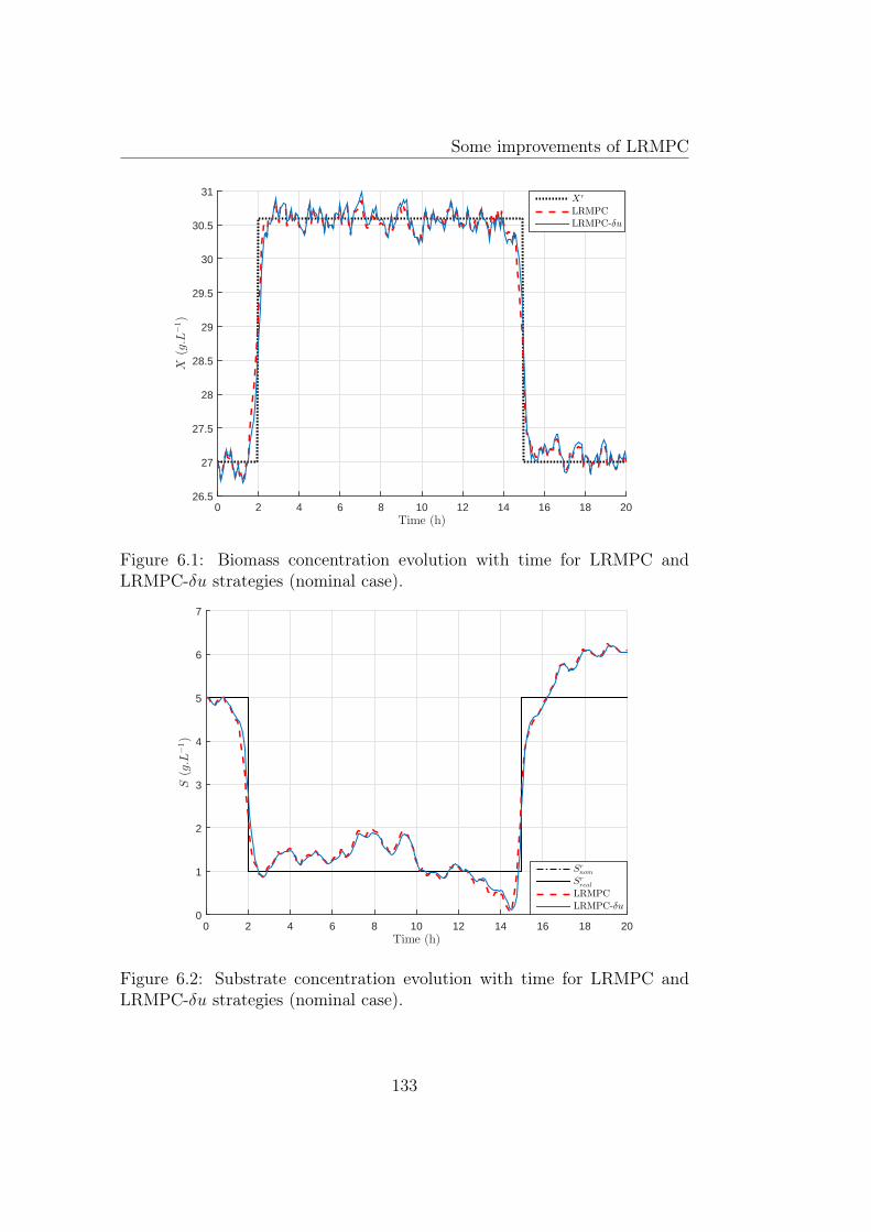
Some improvements of LRMPC
Time (h)0 2 4 6 8 10 12 14 16 18 20
X(g.L
−1)
26.5
27
27.5
28
28.5
29
29.5
30
30.5
31Xr
LRMPC
LRMPC-δu
Figure 6.1: Biomass concentration evolution with time for LRMPC andLRMPC-δu strategies (nominal case).
Time (h)0 2 4 6 8 10 12 14 16 18 20
S(g.L
−1)
0
1
2
3
4
5
6
7
Srnom
Srreal
LRMPC
LRMPC-δu
Figure 6.2: Substrate concentration evolution with time for LRMPC andLRMPC-δu strategies (nominal case).
133
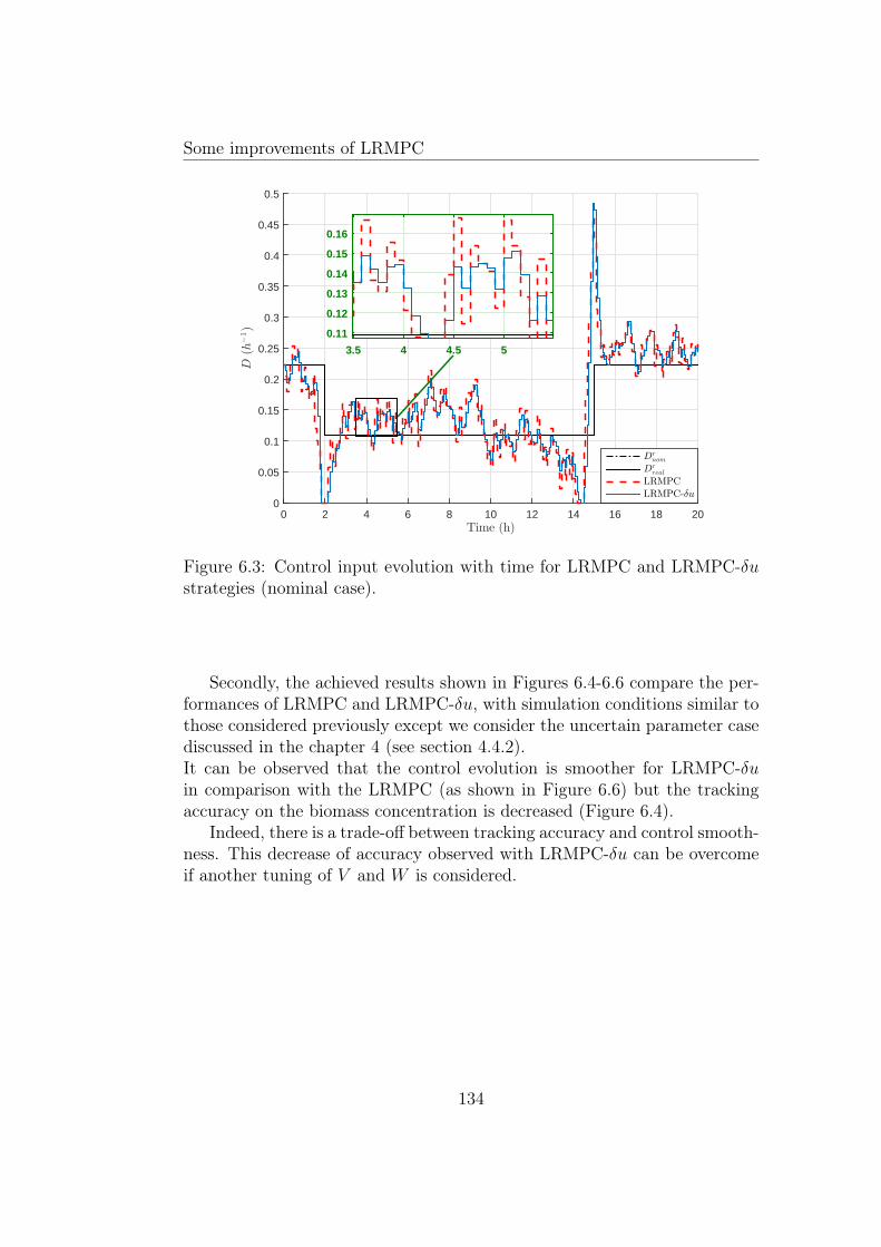
Some improvements of LRMPC
Time (h)0 2 4 6 8 10 12 14 16 18 20
D(h
−1)
0
0.05
0.1
0.15
0.2
0.25
0.3
0.35
0.4
0.45
0.5
Dr
nom
Dr
real
LRMPC
LRMPC-δu
3.5 4 4.5 5
0.11
0.12
0.13
0.14
0.15
0.16
Figure 6.3: Control input evolution with time for LRMPC and LRMPC-δustrategies (nominal case).
Secondly, the achieved results shown in Figures 6.4-6.6 compare the per-formances of LRMPC and LRMPC-δu, with simulation conditions similar tothose considered previously except we consider the uncertain parameter casediscussed in the chapter 4 (see section 4.4.2).It can be observed that the control evolution is smoother for LRMPC-δuin comparison with the LRMPC (as shown in Figure 6.6) but the trackingaccuracy on the biomass concentration is decreased (Figure 6.4).
Indeed, there is a trade-off between tracking accuracy and control smooth-ness. This decrease of accuracy observed with LRMPC-δu can be overcomeif another tuning of V and W is considered.
134
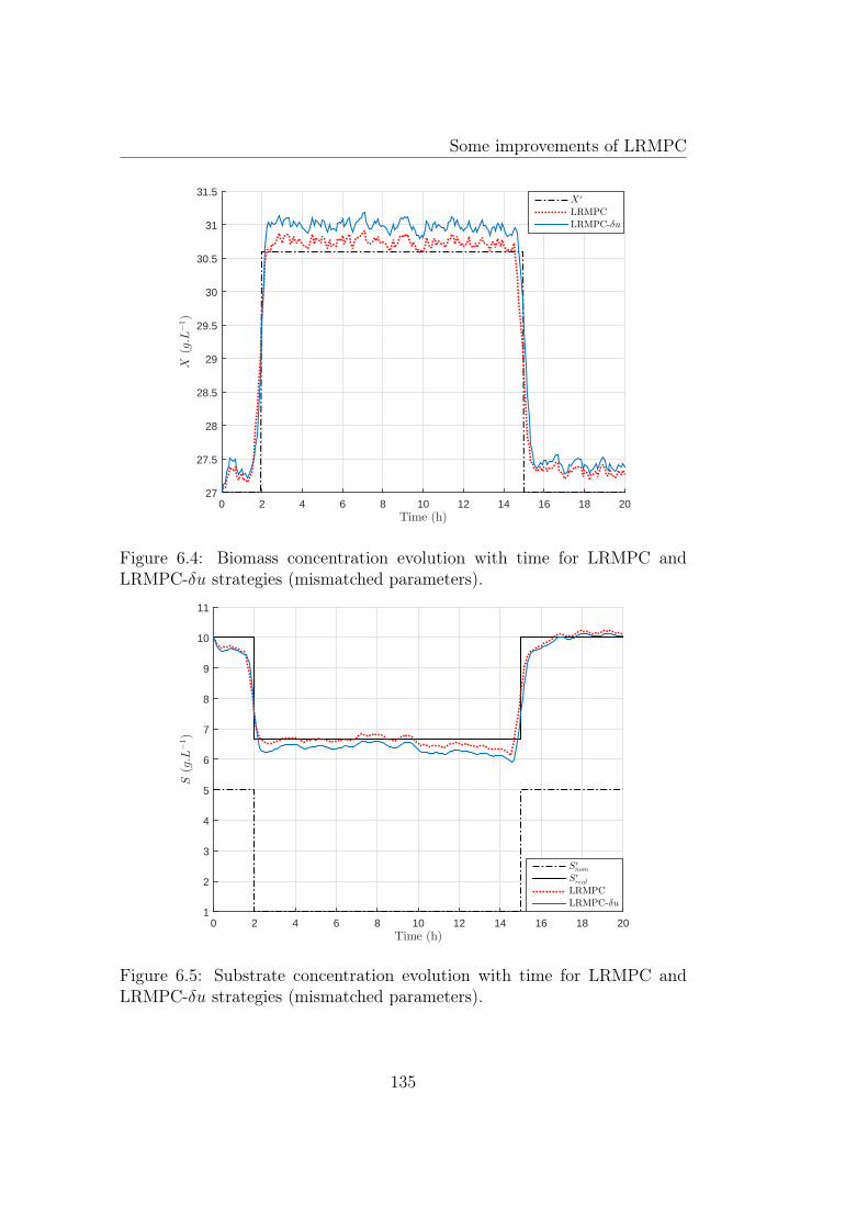
Some improvements of LRMPC
Time (h)0 2 4 6 8 10 12 14 16 18 20
X(g.L
−1)
27
27.5
28
28.5
29
29.5
30
30.5
31
31.5Xr
LRMPC
LRMPC-δu
Figure 6.4: Biomass concentration evolution with time for LRMPC andLRMPC-δu strategies (mismatched parameters).
Time (h)0 2 4 6 8 10 12 14 16 18 20
S(g.L
−1)
1
2
3
4
5
6
7
8
9
10
11
Srnom
Srreal
LRMPC
LRMPC-δu
Figure 6.5: Substrate concentration evolution with time for LRMPC andLRMPC-δu strategies (mismatched parameters).
135
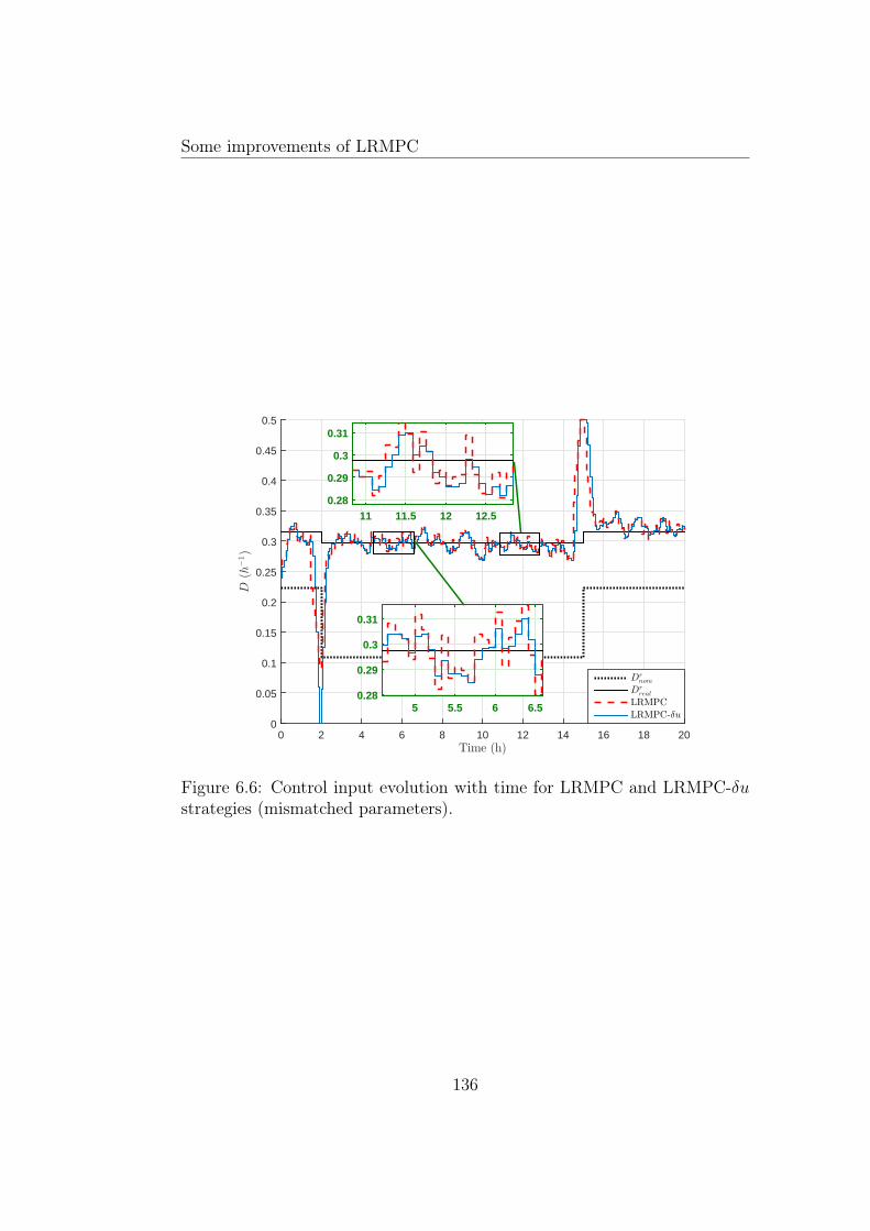
Some improvements of LRMPC
Time (h)0 2 4 6 8 10 12 14 16 18 20
D(h
−1)
0
0.05
0.1
0.15
0.2
0.25
0.3
0.35
0.4
0.45
0.5
Dr
nom
Dr
real
LRMPC
LRMPC-δu
11 11.5 12 12.50.28
0.29
0.3
0.31
5 5.5 6 6.50.28
0.29
0.3
0.31
Figure 6.6: Control input evolution with time for LRMPC and LRMPC-δustrategies (mismatched parameters).
136
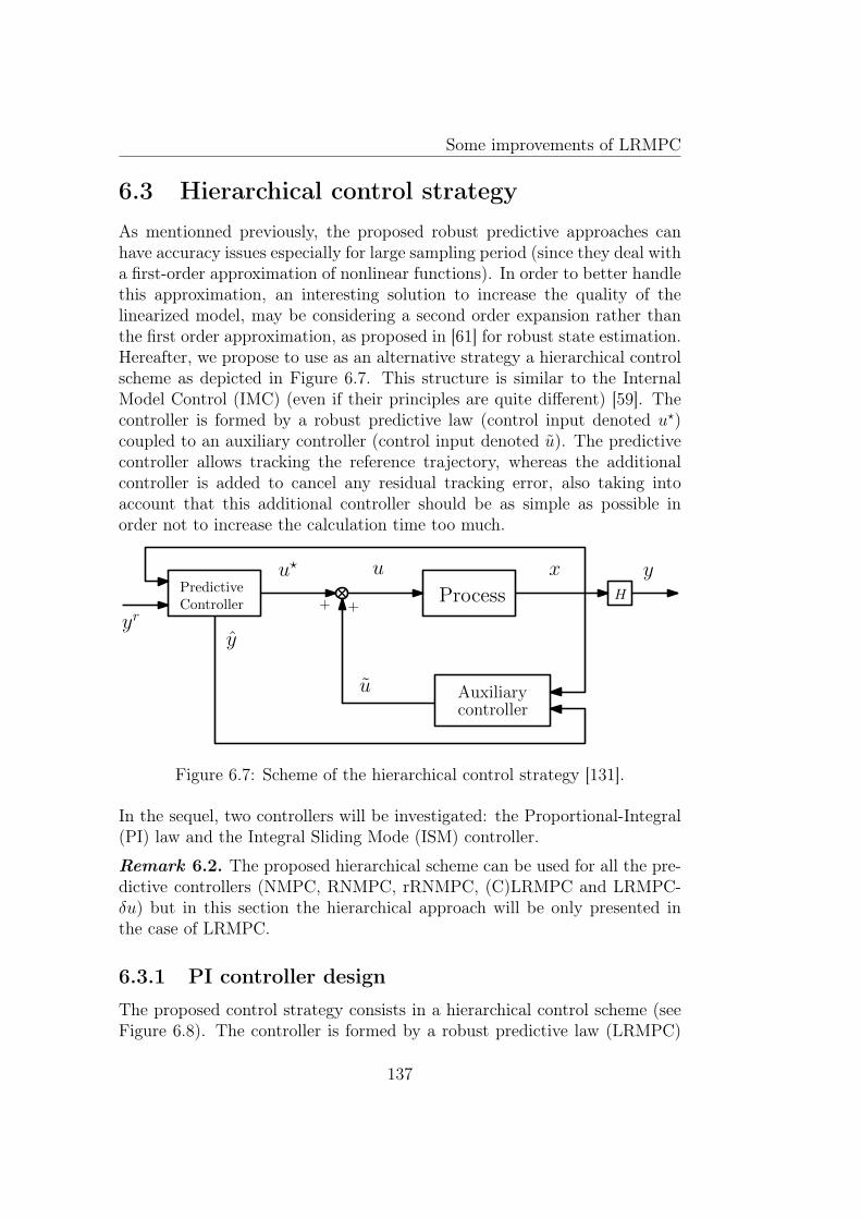
Some improvements of LRMPC
6.3 Hierarchical control strategyAs mentionned previously, the proposed robust predictive approaches canhave accuracy issues especially for large sampling period (since they deal witha first-order approximation of nonlinear functions). In order to better handlethis approximation, an interesting solution to increase the quality of thelinearized model, may be considering a second order expansion rather thanthe first order approximation, as proposed in [61] for robust state estimation.Hereafter, we propose to use as an alternative strategy a hierarchical controlscheme as depicted in Figure 6.7. This structure is similar to the InternalModel Control (IMC) (even if their principles are quite different) [59]. Thecontroller is formed by a robust predictive law (control input denoted u?)coupled to an auxiliary controller (control input denoted u). The predictivecontroller allows tracking the reference trajectory, whereas the additionalcontroller is added to cancel any residual tracking error, also taking intoaccount that this additional controller should be as simple as possible inorder not to increase the calculation time too much.
HProcess
yr
u? u
u
x y
+ +
PredictiveController
y
Auxiliarycontroller
Figure 6.7: Scheme of the hierarchical control strategy [131].
In the sequel, two controllers will be investigated: the Proportional-Integral(PI) law and the Integral Sliding Mode (ISM) controller.
Remark 6.2. The proposed hierarchical scheme can be used for all the pre-dictive controllers (NMPC, RNMPC, rRNMPC, (C)LRMPC and LRMPC-δu) but in this section the hierarchical approach will be only presented inthe case of LRMPC.
6.3.1 PI controller design
The proposed control strategy consists in a hierarchical control scheme (seeFigure 6.8). The controller is formed by a robust predictive law (LRMPC)
137
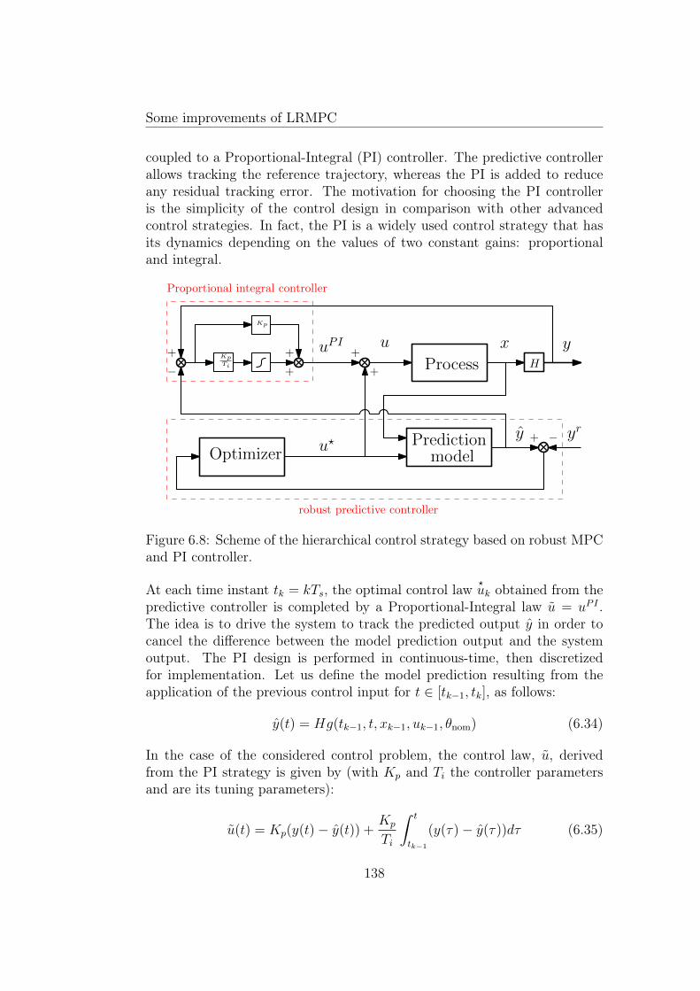
Some improvements of LRMPC
coupled to a Proportional-Integral (PI) controller. The predictive controllerallows tracking the reference trajectory, whereas the PI is added to reduceany residual tracking error. The motivation for choosing the PI controlleris the simplicity of the control design in comparison with other advancedcontrol strategies. In fact, the PI is a widely used control strategy that hasits dynamics depending on the values of two constant gains: proportionaland integral.
HProcess
x y
PredictionmodelOptimizer
Kp
yry + −
+
++
+
+
−
u?
uPI u
robust predictive controller
Proportional integral controller
KpTi
Figure 6.8: Scheme of the hierarchical control strategy based on robust MPCand PI controller.
At each time instant tk = kTs, the optimal control law ?uk obtained from the
predictive controller is completed by a Proportional-Integral law u = uPI .The idea is to drive the system to track the predicted output y in order tocancel the difference between the model prediction output and the systemoutput. The PI design is performed in continuous-time, then discretizedfor implementation. Let us define the model prediction resulting from theapplication of the previous control input for t ∈ [tk−1, tk], as follows:
y(t) = Hg(tk−1, t, xk−1, uk−1, θnom) (6.34)
In the case of the considered control problem, the control law, u, derivedfrom the PI strategy is given by (with Kp and Ti the controller parametersand are its tuning parameters):
u(t) = Kp(y(t)− y(t)) +Kp
Ti
∫ t
tk−1
(y(τ)− y(τ))dτ (6.35)
138
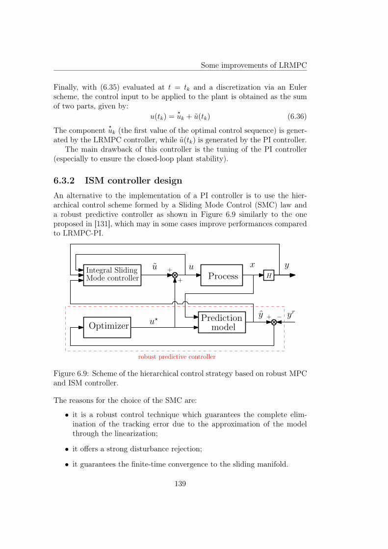
Some improvements of LRMPC
Finally, with (6.35) evaluated at t = tk and a discretization via an Eulerscheme, the control input to be applied to the plant is obtained as the sumof two parts, given by:
u(tk) =?uk + u(tk) (6.36)
The component ?uk (the first value of the optimal control sequence) is gener-
ated by the LRMPC controller, while u(tk) is generated by the PI controller.The main drawback of this controller is the tuning of the PI controller
(especially to ensure the closed-loop plant stability).
6.3.2 ISM controller design
An alternative to the implementation of a PI controller is to use the hier-archical control scheme formed by a Sliding Mode Control (SMC) law anda robust predictive controller as shown in Figure 6.9 similarly to the oneproposed in [131], which may in some cases improve performances comparedto LRMPC-PI.
HProcess
x y
PredictionmodelOptimizer
yry + −
+
+
u?
u u
robust predictive controller
Integral SlidingMode controller
Figure 6.9: Scheme of the hierarchical control strategy based on robust MPCand ISM controller.
The reasons for the choice of the SMC are:
• it is a robust control technique which guarantees the complete elim-ination of the tracking error due to the approximation of the modelthrough the linearization;
• it offers a strong disturbance rejection;
• it guarantees the finite-time convergence to the sliding manifold.
139
Some improvements of LRMPC
Details related to SMC can be found in [146]. The SMC considered in thisstudy is designed according to the so-called Integral Sliding Mode (ISM)approach. In the latter case, an integral action is included in the SMC.
Let us assume that the considered system has a single output y and singleinput u and is control-affine, which is a special case of (4.1). We will thenconsider for the ISM development, the following model:{
x(t) = fx(x(t), θ) + fu(x(t), θ)u(t), ∀t > t0, x(t0) = x0
y(t) = Hx(t)(6.37)
At each time instant t = kTs, the goal is to complete the optimal controllaw ?
u obtained from the predictive controller by an Integral Sliding modecontrol law u(t) in order to cancel the error between the predicted output andthe system output (same philosophy as LRMPC-PI). In this study, the ISMdesign is performed in continuous-time, then discretized for implementation.
The sliding mode control design consists in choosing the control inputin such a way that the system is driven to reach a sliding manifold and bemaintained there for all future time. The goal is to track the predicted outputy in order to cancel the difference between the model prediction output andthe system output.
Let us define the modelling error variables for t ∈ [tk−1, tk] [145]:Z1(t) =
∫ ttk−1
(y(τ)− y(τ)) dτ
Z2(t) = 1ξ1
(y(t)− y(t)− ξ2Z1(t))
(6.38)
where the model prediction y resulting from the application of the previouscontrol input uk−1 is given by (6.34). ξ1 ∈ R and ξ2 ∈ R are the ISM tuningparameters.Differentiating (6.38) with respect to time and rearanging (6.38), we obtain:
Z1(t) = ξ1Z2 + ξ2Z1
Z2(t) = 1ξ1
(y(t)− ˙y(t)− ξ2Z1(t))(6.39)
A time-varying sliding surface φ(x, t) is defined in the state space Rnx as
φ(x, t) = Z2(t) + ξ3Z1(t) (6.40)
The ISM control law needs to be designed so that the invariance of the slidingmanifold is satisfied, i.e.:
∀x ∈ Rnx , φ(x, t) = 0 (6.41)
140
Some improvements of LRMPC
Furthermore, the local attractivity of the sliding surface φ can be expressedby the condition:
∀x ∈ Rnxφ(x, t)φ(x, t) < 0 (6.42)
Hence, the sliding surface (6.40) is made attractive by choosing [146]:
φ(x, t) = −Kssign(φ(x, t)) (6.43)
where the switching gain Ks is a strictly positive constant.Then, the attractive equation which implies that the distance to the slidingsurface decreases along all system trajectories is satisfied since (from (6.42)-(6.43)):
φ(x, t)φ(x, t) = −Ks|φ(x, t)| < 0 (6.44)
From (6.40) and (6.41), it comes:
Z2(t) + ξ3Z1(t) = 0 (6.45)
Thanks to (6.39), equation (6.45) becomes:
1
ξ1
Z1(t)− ξ2
ξ1
Z1(t) + ξ3Z1(t) = 0 (6.46)
Then, we have thatZ1(t) = (ξ2 − ξ1ξ3)Z1(t) (6.47)
In order to ensure the convergence of Z1, the following condition must besatisfied:
ξ2 − ξ1ξ3 < 0 (6.48)
Consequently, differentiating the sliding surface vector (6.40), we obtain:
φ(x, t) = 1ξ1
(y(t)− ˙y(t)− (ξ2 − ξ1ξ3)(ξ1Z2(t) + ξ2Z1(t))) (6.49)
The system output is obtained by the application of the previous controlinput uk−1 (reminding that a ZOH is applied, i.e. u(t) = uk−1, ∀t ∈ [tk−1, tk])combined with the sliding mode control law u(t) and the predicted output iscalculated by applying only the previous input uk−1 as follows:{
y(t) = H (fx(x(t), θ) + fu(x(t), θ)(uk−1 + u(t)))˙y(t) = H (fx(x(t), θnom) + fu(x(t), θnom)uk−1)
(6.50)
where the difference between the system output and the nominal model pre-diction output is due only to parameters uncertainties:
y(t)− ˙y(t) = ϕ+ χuk−1 + ηu(t) (6.51)
141
Some improvements of LRMPC
with ϕ = H(fx(x(t), θ)− fx(x(t), θnom)),χ = H(fu(x(t), θ)− fu(x(t), θnom)),η = Hfu(x(t), θ)
(6.52)
From (6.51), it is deduced that the control law can be accordingly found as:
u(t) =1
η
(y(t)− ˙y(t)− ϕ− χuk−1
)(6.53)
Note that the term η must be regular. And from (6.49),
y(t)− ˙y(t) = ξ1φ+ (ξ2 − ξ1ξ3)(ξ1Z2(t) + ξ2Z1(t)) (6.54)
By replacing φ by (6.43), the control law can then be found as
u(t) = 1η(−ϕ− χuk−1 − ξ1Kssign(φ(x, t)) + (ξ2 − ξ1ξ3)(ξ1Z2(t) + ξ2Z1(t)))
(6.55)In (6.52), θ is replaced by θnom since θ is uncertain. It could be replacedby an estimate of θ (with the use of an estimation algorithm). The use of θin (6.55) is the main drawback of this approach. It should be recalled thatthe proposed controller can only be used to control-affine system which isanother limitation of this strategy.
Another drawback of the ISM is the presence of a chattering phenomenon.In order to reduce it, a hyperbolic function can be used instead of the switch-ing function sign(φ(x, t)).
Finally, with (6.55) evaluated at t = tk, the control input is obtained asthe sum of two parts, given by:
u(tk) =?uk + u(tk) (6.56)
The component ?uk (the first value of the optimal control sequence) is gen-
erated by the LRMPC controller, while u(tk) is generated by the Integralsliding mode controller (6.55).
6.3.3 Numerical results
In this section, the efficiency of the proposed hierarchical control strategiesis evaluated in simulation. The performances of both the LRMPC-PI andLRMPC-ISM are compared for the worst uncertain parameters case discussedin the previous chapter (see section 4.4.2). The sampling time Ts is chosenequal to 5 min and Td the integration time step to 0.1 min. The controllerstuning parameters are given in Table 6.2. They were obtained by a trial-and-error technique (the best setting found).
142
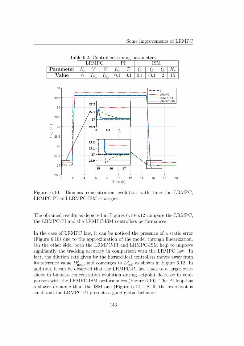
Some improvements of LRMPC
Table 6.2: Controllers tuning parameters.LRMPC PI ISM
Parameter Np V W Kp Ti ξ1 ξ2 ξ3 Ks
Value 6 INp INp 0.1 0.1 0.1 -0.1 2 15
Time (h)0 2 4 6 8 10 12 14 16 18 20
X(g.L
−1)
26.5
27
27.5
28
28.5
29
29.5
30
30.5
31X r
LRMPCLRMPC-PILRMPC-ISM
0 0.5 126.9
27
27.1
27.2
15 16 17
26.9
27
27.1
27.2
Figure 6.10: Biomass concentration evolution with time for LRMPC,LRMPC-PI and LRMPC-ISM strategies.
The obtained results as depicted in Figures 6.10-6.12 compare the LRMPC,the LRMPC-PI and the LRMPC-ISM controllers performances.
In the case of LRMPC law, it can be noticed the presence of a static error(Figure 6.10) due to the approximation of the model through linearization.On the other side, both the LRMPC-PI and LRMPC-ISM help to improvesignifiantly the tracking accuracy in comparison with the LRMPC law. Infact, the dilution rate given by the hierarchical controllers moves away fromits reference value Dr
nom, and converges to Drreal as shown in Figure 6.12. In
addition, it can be observed that the LRMPC-PI law leads to a larger over-shoot in biomass concentration evolution during setpoint decrease in com-parison with the LRMPC-ISM performances (Figure 6.10). The PI loop hasa slower dynamic than the ISM one (Figure 6.12). Still, the overshoot issmall and the LRMPC-PI presents a good global behavior.
143
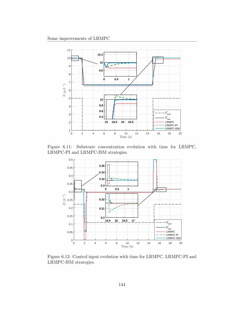
Some improvements of LRMPC
Time (h)0 2 4 6 8 10 12 14 16 18 20
S(g.L
−1)
1
2
3
4
5
6
7
8
9
10
11
S rnom
S rreal
LRMPCLRMPC-PILRMPC-ISM
0 0.5 1
9.8
10
10.2
15 15.5 16 16.5
9.4
9.6
9.8
10
Figure 6.11: Substrate concentration evolution with time for LRMPC,LRMPC-PI and LRMPC-ISM strategies.
Time (h)0 2 4 6 8 10 12 14 16 18 20
D(h
−1)
0
0.05
0.1
0.15
0.2
0.25
0.3
0.35
0.4
0.45
0.5
Drnom
Drreal
LRMPCLRMPC-PILRMPC-ISM
0 0.5 10.3
0.32
0.34
0.36
15.5 16 16.5 170.3
0.31
0.32
Figure 6.12: Control input evolution with time for LRMPC, LRMPC-PI andLRMPC-ISM strategies.
144
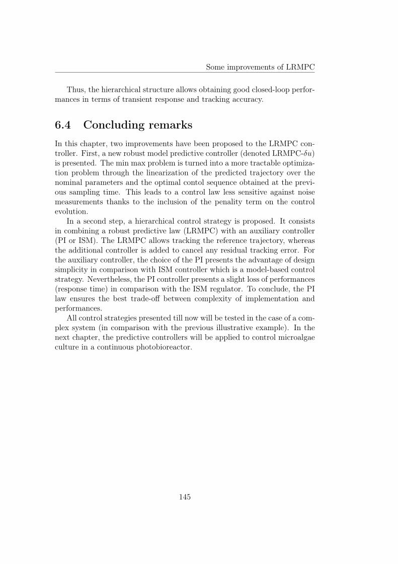
Some improvements of LRMPC
Thus, the hierarchical structure allows obtaining good closed-loop perfor-mances in terms of transient response and tracking accuracy.
6.4 Concluding remarksIn this chapter, two improvements have been proposed to the LRMPC con-troller. First, a new robust model predictive controller (denoted LRMPC-δu)is presented. The min max problem is turned into a more tractable optimiza-tion problem through the linearization of the predicted trajectory over thenominal parameters and the optimal contol sequence obtained at the previ-ous sampling time. This leads to a control law less sensitive against noisemeasurements thanks to the inclusion of the penality term on the controlevolution.
In a second step, a hierarchical control strategy is proposed. It consistsin combining a robust predictive law (LRMPC) with an auxiliary controller(PI or ISM). The LRMPC allows tracking the reference trajectory, whereasthe additional controller is added to cancel any residual tracking error. Forthe auxiliary controller, the choice of the PI presents the advantage of designsimplicity in comparison with ISM controller which is a model-based controlstrategy. Nevertheless, the PI controller presents a slight loss of performances(response time) in comparison with the ISM regulator. To conclude, the PIlaw ensures the best trade-off between complexity of implementation andperformances.
All control strategies presented till now will be tested in the case of a com-plex system (in comparison with the previous illustrative example). In thenext chapter, the predictive controllers will be applied to control microalgaeculture in a continuous photobioreactor.
145

Some improvements of LRMPC
146

Chapter 7
Illustrative example: Microalgaecultivation system
7.1 Introduction
One of the most important challenges of this century is to satisfy our energeticneeds while addressing environemental issues. In the mean time, the influenceof climate change, and the decline of fossil fuels have motivated a growinginterest in the search of renewable sources of energy. The biotechnologyindustry is an important sector due to its economical, societal and environ-mental potential. Microalgae culture are among the most interesting types ofbiocultures. A microalga is a microscopic plant living mainly in aquatic en-vironment, representing the basic level of the food chain in the ocean. Theseorganisms have an increasing interest due to their ability to fix CO2 [111]and to produce lipid or hydrogen that can be used as biofuel [33, 71, 101].The industrial success of the microalgae cultivation is due to its biochem-ical characteristics. The microalga is of particular interest for the growingdemand of organic products intended to a large number of industrial appli-cations: feed, food, pharmacology, chemistry, cosmetics production [55, 140],and has recently emerged as an interesting source for sustainable energy pro-duction at large scale, such as wastewater treatment [56] or decompositionof different classes of toxic compounds [22]. For these reasons, microalgaecultivation attracted the interest from large companies. In this context, thecontrol strategy of microalgae culture is becoming a key research topic andconsequently it received high attention from scientific community leadingto many studies. This requires first the design of mathematical models todescribe more accurately the system behavior. It is however quite delicateto derive a simple model which can be exploited during online optimization
147
Illustrative example: Microalgae cultivation system
phases because the microalgae are living organisms and their characteristicscan evolve in time (mutation, biofilm formation, stress, etc.). Biochemicalprocesses are systems where nonlinear effects are significant enough to justifythe use of nonlinear model to give a sufficiently adequate representation ofthe system behavior. In addition, generally, the process model is identifiedand uncertain parameters are estimated with evaluated confidence intervals,which motivates the development of robust control laws in the presence ofmodelling uncertainties.
In industrial applications, the control of bioreactors is most often lim-ited to simple regulation loops like: partial pressure of dissolved oxygen anddissolved carbon dioxide [48], pH and temperature. Hence, to increase sig-nificantly the process performances, new challenges emerge related to thecontrol of the biological variables. In the literature of microalgae cultiva-tions, several nonlinear control strategies have been developed: predictive[1, 10, 143, 134, 47], adaptive [97, 38, 96], sliding mode [138], feedback lin-earization [11, 72, 142], and backstepping [53, 145] approaches. They howeverdo not specifically focus on robustness features. Our aim is therefore to de-sign a robust predictive controller which would be able to find an optimalfeeding strategy in order to guarantee that the process will yield the desiredamount of biomass along the cultivation period under model parameter un-certainties. Here, the challenge is to lay down a stable real-time operation,insensitive to various disturbances, then, close to a certain state or desiredprofile. This requires the application of advanced optimal control strategiesto ensure the bioprocess efficiency.
In this chapter, the proposed approaches developped in the previous chap-ters are applied to control microalgae culture in photobioreactor through aspecific case study: the cultivation of I. galbana in a continuous photobioreac-tor [98]. A Droop model is used to describe the internal nutrient quantity perunit of biomass evolution. The aim here is to control biomass concentrationin the photobioreactor through the dilution rate.
7.2 System modelling
7.2.1 Model Description
The specificity of microalgae is that inorganic substrate uptake and growthare decoupled thanks to an intracellular storage of nutrients [15]. In order totake into account this phenomenon, the growth of microalgae is representedby a Droop model [16, 15] which uncouples growth from substrate uptake,leading to the definition of an internal cell quota (i.e., the internal nutrient
148
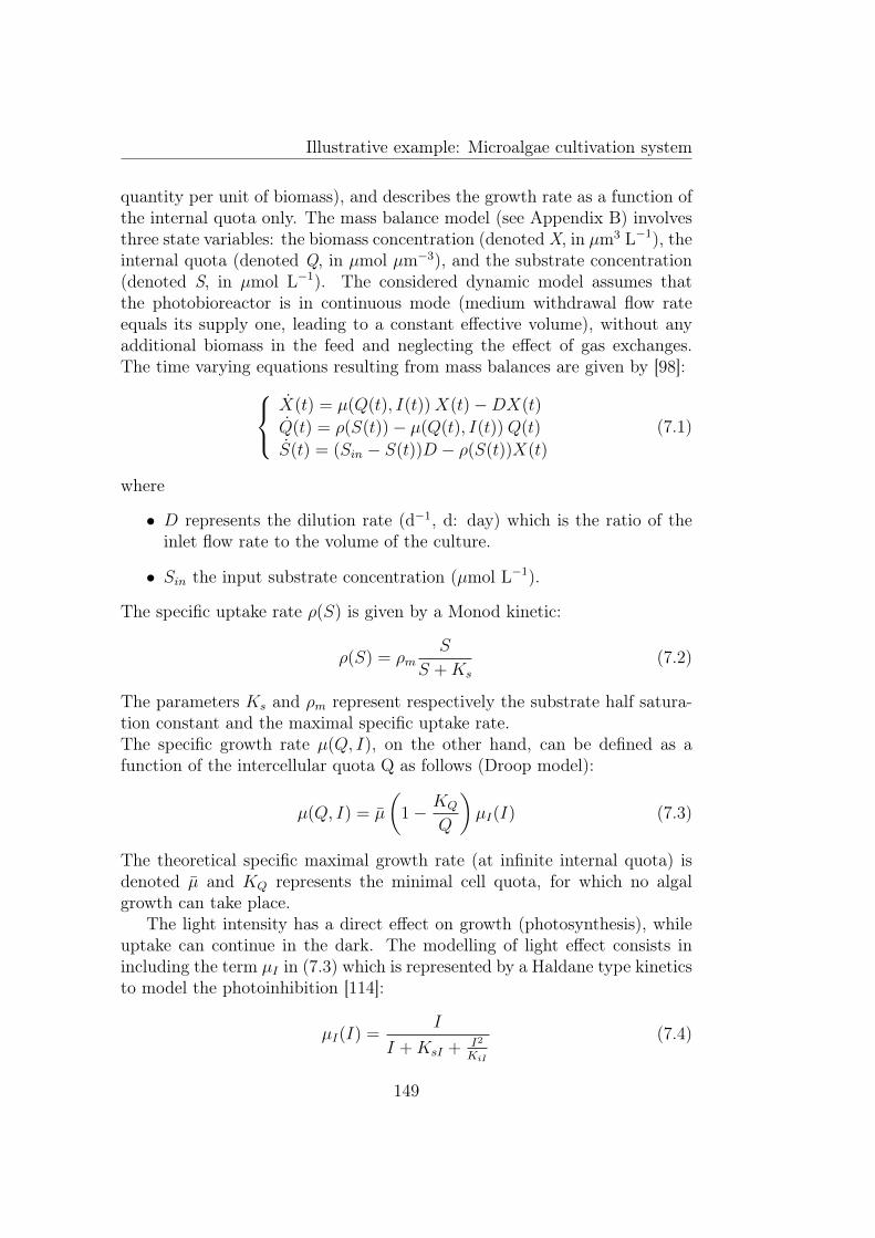
Illustrative example: Microalgae cultivation system
quantity per unit of biomass), and describes the growth rate as a function ofthe internal quota only. The mass balance model (see Appendix B) involvesthree state variables: the biomass concentration (denoted X, in µm3 L−1), theinternal quota (denoted Q, in µmol µm−3), and the substrate concentration(denoted S, in µmol L−1). The considered dynamic model assumes thatthe photobioreactor is in continuous mode (medium withdrawal flow rateequals its supply one, leading to a constant effective volume), without anyadditional biomass in the feed and neglecting the effect of gas exchanges.The time varying equations resulting from mass balances are given by [98]:
X(t) = µ(Q(t), I(t))X(t)−DX(t)
Q(t) = ρ(S(t))− µ(Q(t), I(t))Q(t)
S(t) = (Sin − S(t))D − ρ(S(t))X(t)
(7.1)
where
• D represents the dilution rate (d−1, d: day) which is the ratio of theinlet flow rate to the volume of the culture.
• Sin the input substrate concentration (µmol L−1).
The specific uptake rate ρ(S) is given by a Monod kinetic:
ρ(S) = ρmS
S +Ks
(7.2)
The parameters Ks and ρm represent respectively the substrate half satura-tion constant and the maximal specific uptake rate.The specific growth rate µ(Q, I), on the other hand, can be defined as afunction of the intercellular quota Q as follows (Droop model):
µ(Q, I) = µ
(1− KQ
Q
)µI(I) (7.3)
The theoretical specific maximal growth rate (at infinite internal quota) isdenoted µ and KQ represents the minimal cell quota, for which no algalgrowth can take place.
The light intensity has a direct effect on growth (photosynthesis), whileuptake can continue in the dark. The modelling of light effect consists inincluding the term µI in (7.3) which is represented by a Haldane type kineticsto model the photoinhibition [114]:
µI(I) =I
I +KsI + I2
KiI
(7.4)
149
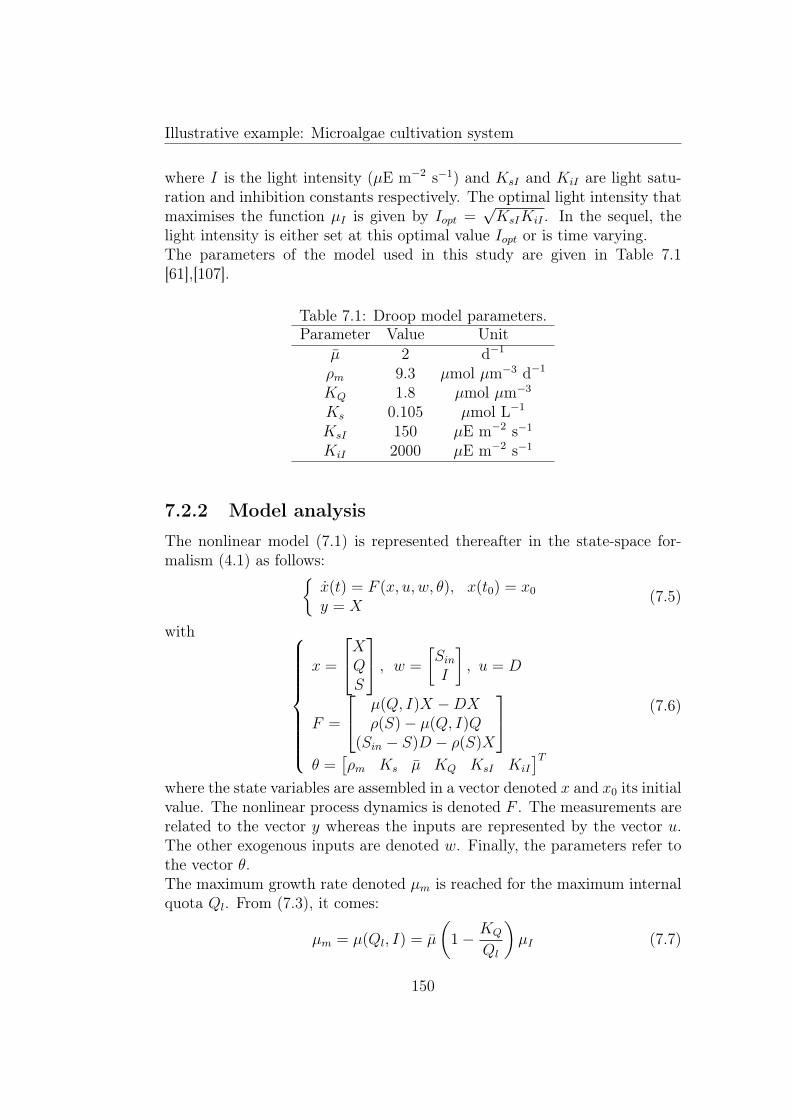
Illustrative example: Microalgae cultivation system
where I is the light intensity (µE m−2 s−1) and KsI and KiI are light satu-ration and inhibition constants respectively. The optimal light intensity thatmaximises the function µI is given by Iopt =
√KsIKiI . In the sequel, the
light intensity is either set at this optimal value Iopt or is time varying.The parameters of the model used in this study are given in Table 7.1[61],[107].
Table 7.1: Droop model parameters.Parameter Value Unit
µ 2 d−1
ρm 9.3 µmol µm−3 d−1
KQ 1.8 µmol µm−3
Ks 0.105 µmol L−1
KsI 150 µE m−2 s−1
KiI 2000 µE m−2 s−1
7.2.2 Model analysis
The nonlinear model (7.1) is represented thereafter in the state-space for-malism (4.1) as follows:{
x(t) = F (x, u, w, θ), x(t0) = x0
y = X(7.5)
with
x =
XQS
, w =
[SinI
], u = D
F =
µ(Q, I)X −DXρ(S)− µ(Q, I)Q
(Sin − S)D − ρ(S)X
θ =
[ρm Ks µ KQ KsI KiI
]T(7.6)
where the state variables are assembled in a vector denoted x and x0 its initialvalue. The nonlinear process dynamics is denoted F . The measurements arerelated to the vector y whereas the inputs are represented by the vector u.The other exogenous inputs are denoted w. Finally, the parameters refer tothe vector θ.The maximum growth rate denoted µm is reached for the maximum internalquota Ql. From (7.3), it comes:
µm = µ(Ql, I) = µ
(1− KQ
Ql
)µI (7.7)
150
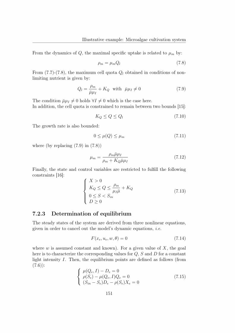
Illustrative example: Microalgae cultivation system
From the dynamics of Q, the maximal specific uptake is related to µm by:
ρm = µmQl (7.8)
From (7.7)-(7.8), the maximum cell quota Ql obtained in conditions of non-limiting nutrient is given by:
Ql =ρmµµI
+KQ with µµI 6= 0 (7.9)
The condition µµI 6= 0 holds ∀I 6= 0 which is the case here.In addition, the cell quota is constrained to remain between two bounds [15]:
KQ ≤ Q ≤ Ql (7.10)
The growth rate is also bounded:
0 ≤ µ(Q) ≤ µm (7.11)
where (by replacing (7.9) in (7.8))
µm =ρmµµI
ρm +KQµµI(7.12)
Finally, the state and control variables are restricted to fulfill the followingconstraints [16]:
X > 0
KQ ≤ Q ≤ ρmµI µ
+KQ
0 ≤ S < SinD ≥ 0
(7.13)
7.2.3 Determination of equilibrium
The steady states of the system are derived from three nonlinear equations,given in order to cancel out the model’s dynamic equations, i.e.
F (xe, ue, w, θ) = 0 (7.14)
where w is assumed constant and known). For a given value of X, the goalhere is to characterize the corresponding values for Q, S and D for a constantlight intensity I. Then, the equilibrium points are defined as follows (from(7.6)):
µ(Qe, I)−De = 0ρ(Se)− µ(Qe, I)Qe = 0(Sin − Se)De − ρ(Se)Xe = 0
(7.15)
151
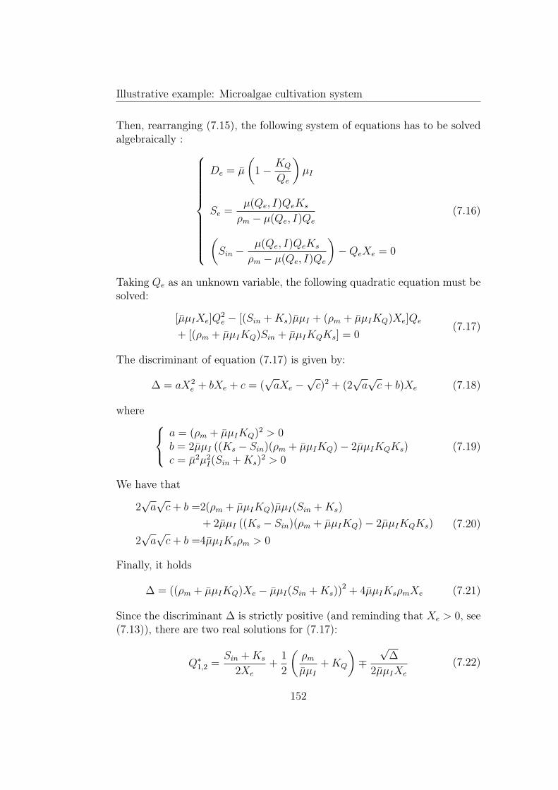
Illustrative example: Microalgae cultivation system
Then, rearranging (7.15), the following system of equations has to be solvedalgebraically :
De = µ
(1− KQ
Qe
)µI
Se =µ(Qe, I)QeKs
ρm − µ(Qe, I)Qe(Sin −
µ(Qe, I)QeKs
ρm − µ(Qe, I)Qe
)−QeXe = 0
(7.16)
Taking Qe as an unknown variable, the following quadratic equation must besolved:
[µµIXe]Q2e − [(Sin +Ks)µµI + (ρm + µµIKQ)Xe]Qe
+ [(ρm + µµIKQ)Sin + µµIKQKs] = 0(7.17)
The discriminant of equation (7.17) is given by:
∆ = aX2e + bXe + c = (
√aXe −
√c)2 + (2
√a√c+ b)Xe (7.18)
where a = (ρm + µµIKQ)2 > 0b = 2µµI ((Ks − Sin)(ρm + µµIKQ)− 2µµIKQKs)c = µ2µ2
I(Sin +Ks)2 > 0
(7.19)
We have that
2√a√c+ b =2(ρm + µµIKQ)µµI(Sin +Ks)
+ 2µµI ((Ks − Sin)(ρm + µµIKQ)− 2µµIKQKs)
2√a√c+ b =4µµIKsρm > 0
(7.20)
Finally, it holds
∆ = ((ρm + µµIKQ)Xe − µµI(Sin +Ks))2 + 4µµIKsρmXe (7.21)
Since the discriminant ∆ is strictly positive (and reminding that Xe > 0, see(7.13)), there are two real solutions for (7.17):
Q∗1,2 =Sin +Ks
2Xe
+1
2
(ρmµµI
+KQ
)∓√
∆
2µµIXe
(7.22)
152
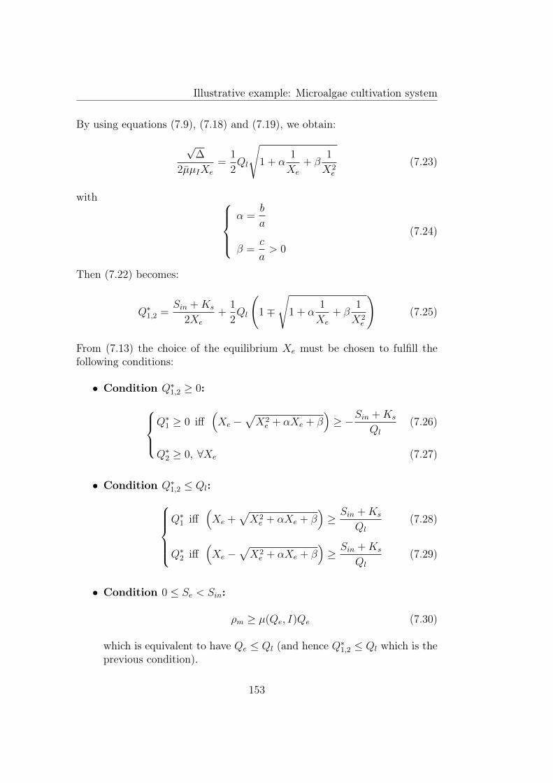
Illustrative example: Microalgae cultivation system
By using equations (7.9), (7.18) and (7.19), we obtain:
√∆
2µµIXe
=1
2Ql
√1 + α
1
Xe
+ β1
X2e
(7.23)
with α =
b
a
β =c
a> 0
(7.24)
Then (7.22) becomes:
Q∗1,2 =Sin +Ks
2Xe
+1
2Ql
(1∓
√1 + α
1
Xe
+ β1
X2e
)(7.25)
From (7.13) the choice of the equilibrium Xe must be chosen to fulfill thefollowing conditions:
• Condition Q∗1,2 ≥ 0:Q∗1 ≥ 0 iff
(Xe −
√X2e + αXe + β
)≥ −Sin +Ks
Ql
(7.26)
Q∗2 ≥ 0, ∀Xe (7.27)
• Condition Q∗1,2 ≤ Ql:Q∗1 iff
(Xe +
√X2e + αXe + β
)≥ Sin +Ks
Ql
(7.28)
Q∗2 iff(Xe −
√X2e + αXe + β
)≥ Sin +Ks
Ql
(7.29)
• Condition 0 ≤ Se < Sin:
ρm ≥ µ(Qe, I)Qe (7.30)
which is equivalent to have Qe ≤ Ql (and hence Q∗1,2 ≤ Ql which is theprevious condition).
153
Illustrative example: Microalgae cultivation system
7.3 Control strategy
The main objective of the controller is to regulate the biomass concentrationX to a reference value Xr in the presence of parameters uncertainties andnoise measurement, while the dilution rate D is constrained to track thereference Dr where 0 ≤ D ≤ Dmax (Dmax is the maximal dilution rate).
The controllability of this model was checked (See Appendix C).The NMPC problem is then formulated as:
min0≤Dk+Np−1
k ≤Dmax
||Dk+Np−1k −Dr,k+Np−1
k ||2V + ||Xk+Npk+1 −X
r,k+Npk+1 ||2W (7.31)
and the RNMPC by:
min0≤Dk+Np−1
k ≤Dmax
maxθ∈[θ−,θ+]
||Dk+Np−1k −Dr,k+Np−1
k ||2V + ||Xk+Npk+1 −X
r,k+Npk+1 ||2W
(7.32)where the uncertain parameters subspace [θ−, θ+] is given by [0.7θnom, 1.3θnom]with θnom given in Table 7.1. This 30% mismatch has been chosen as a ratherclassical percenttage. A more rigourous approach could be to proceed withan identification procedure as in [24] to determine the confidence intervalsfor all parameters.
The performance of the controllers in case of disturbances (here the lightintensity fluctations) will be also studied and evaluated.
7.4 Simulation results
The efficiency of the proposed control strategies is validated in simulation.The initial biomass concentration value is set close to the setpoint in orderto cancel the transient effect and focus only on the behavior during setpointchanges (rising and falling edge respectively). The light intensity is assumedto be non-measured, non-corrupted with noise. In sections 7.4.2 and 7.4.3,it is constant, equal to Iopt that maximizes µ(Q, I) defined in (7.3). In sec-tion 7.4.4, it is time-varying. The performances of the predictive algorithmspresented in chapters 4, 5 and 6 are compared in a worst uncertain param-eters case. Thanks to the monotonocity properties of the Droop model asdiscussed in [61], the worst-case prediction can be generated using parame-ters bounds {θ−, θ+} only, rather than by exploring the full parameter space[θ−, θ+]. The parameters values of the system are chosen on the parame-ter subspace border (θreal = [ρ+
m, K−s , µ
+, K−Q , K−sI , K
+iI ]). All the simulation
conditions are summarized in Table 7.2.
154
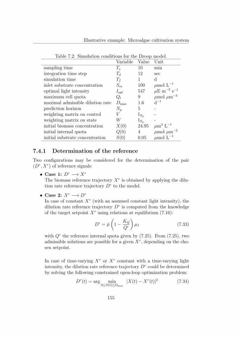
Illustrative example: Microalgae cultivation system
Table 7.2: Simulation conditions for the Droop model.Variable Value Unit
sampling time Ts 10 minintegration time step Td 12 secsimulation time Tf 1 dinlet substrate concentration Sin 100 µmol L−1
optimal light intensity Iopt 547 µE m−2 s−1
maximum cell quota Ql 9 µmol µm−3
maximal admissible dilution rate Dmax 1.6 d−1
prediction horizon Np 5 -weighting matrix on control V INp -weighting matrix on state W INp -initial biomass concentration X(0) 24.95 µm3 L−1
initial internal quota Q(0) 4 µmol µm−3
initial substrate concentration S(0) 0.05 µmol L−1
7.4.1 Determination of the reference
Two configurations may be considered for the determination of the pair(Dr, Xr) of reference signals:
• Case 1: Dr −→ Xr
The biomass reference trajectory Xr is obtained by applying the dilu-tion rate reference trajectory Dr to the model.
• Case 2: Xr −→ Dr
In case of constant Xr (with an assumed constant light intensity), thedilution rate reference trajectory Dr is computed from the knowledgeof the target setpoint Xr using relations at equilibrium (7.16):
Dr = µ
(1− KQ
Qr
)µI (7.33)
with Qr the reference internal quota given by (7.25). From (7.25), twoadmissible solutions are possible for a given Xr, depending on the cho-sen setpoint.
In case of time-varying Xr or Xr constant with a time-varying lightintensity, the dilution rate reference trajectory Dr could be determinedby solving the following constrained open-loop optimization problem:
Dr(t) = arg min0≤D(t)≤Dmax
|X(t)−Xr(t)|2 (7.34)
155
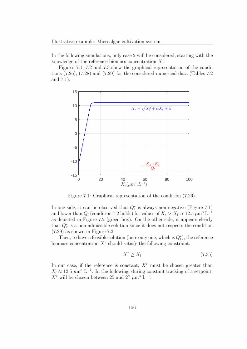
Illustrative example: Microalgae cultivation system
In the following simulations, only case 2 will be considered, starting with theknowledge of the reference biomass concentration Xr.
Figures 7.1, 7.2 and 7.3 show the graphical representation of the condi-tions (7.26), (7.28) and (7.29) for the considered numerical data (Tables 7.2and 7.1).
Xe(µm3.L−1)
0 20 40 60 80 100-15
-10
-5
0
5
10
15
−
Sin+Ks
Ql
Xe −
√
X2e + αXe + β
Figure 7.1: Graphical representation of the condition (7.26).
In one side, it can be observed that Q∗1 is always non-negative (Figure 7.1)and lower than Ql (condition 7.2 holds) for values ofXe > Xl ≈ 12.5 µm3 L−1
as depicted in Figure 7.2 (green box). On the other side, it appears clearlythat Q∗2 is a non-admissible solution since it does not respects the condition(7.29) as shown in Figure 7.3.
Then, to have a feasible solution (here only one, which isQ∗1), the referencebiomass concentration Xr should satisfy the following constraint:
Xr ≥ Xl (7.35)
In our case, if the reference is constant, Xr must be chosen greater thanXl ≈ 12.5 µm3 L−1. In the following, during constant tracking of a setpoint,Xr will be chosen between 25 and 27 µm3 L−1.
156
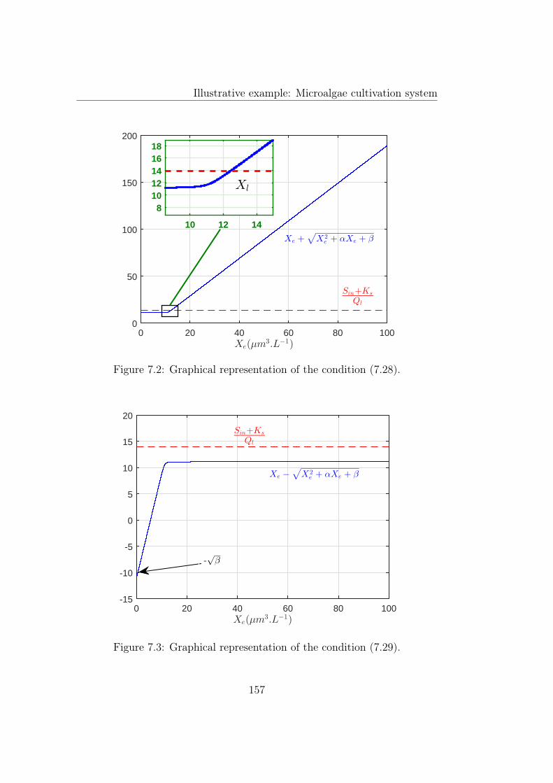
Illustrative example: Microalgae cultivation system
Xe(µm3.L−1)
0 20 40 60 80 1000
50
100
150
200
10 12 14
81012141618
Sin+Ks
Ql
Xl
Xe +√
X2e + αXe + β
Figure 7.2: Graphical representation of the condition (7.28).
Xe(µm3.L−1)
0 20 40 60 80 100-15
-10
-5
0
5
10
15
20
-√
β
Sin+Ks
Ql
Xe −
√
X2e + αXe + β
Figure 7.3: Graphical representation of the condition (7.29).
157
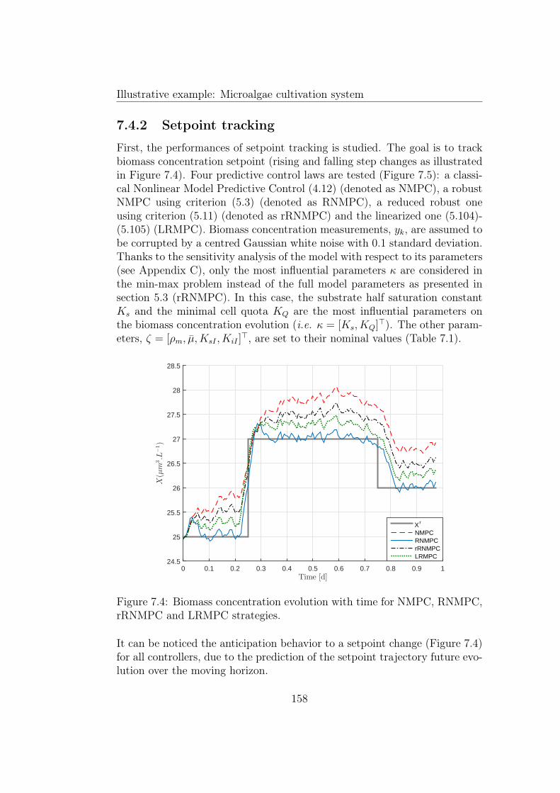
Illustrative example: Microalgae cultivation system
7.4.2 Setpoint tracking
First, the performances of setpoint tracking is studied. The goal is to trackbiomass concentration setpoint (rising and falling step changes as illustratedin Figure 7.4). Four predictive control laws are tested (Figure 7.5): a classi-cal Nonlinear Model Predictive Control (4.12) (denoted as NMPC), a robustNMPC using criterion (5.3) (denoted as RNMPC), a reduced robust oneusing criterion (5.11) (denoted as rRNMPC) and the linearized one (5.104)-(5.105) (LRMPC). Biomass concentration measurements, yk, are assumed tobe corrupted by a centred Gaussian white noise with 0.1 standard deviation.Thanks to the sensitivity analysis of the model with respect to its parameters(see Appendix C), only the most influential parameters κ are considered inthe min-max problem instead of the full model parameters as presented insection 5.3 (rRNMPC). In this case, the substrate half saturation constantKs and the minimal cell quota KQ are the most influential parameters onthe biomass concentration evolution (i.e. κ = [Ks, KQ]>). The other param-eters, ζ = [ρm, µ, KsI , KiI ]
>, are set to their nominal values (Table 7.1).
Time [d]0 0.1 0.2 0.3 0.4 0.5 0.6 0.7 0.8 0.9 1
X(µm
3.L
−1)
24.5
25
25.5
26
26.5
27
27.5
28
28.5
X r
NMPCRNMPCrRNMPCLRMPC
Figure 7.4: Biomass concentration evolution with time for NMPC, RNMPC,rRNMPC and LRMPC strategies.
It can be noticed the anticipation behavior to a setpoint change (Figure 7.4)for all controllers, due to the prediction of the setpoint trajectory future evo-lution over the moving horizon.
158
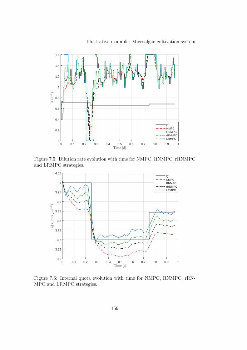
Illustrative example: Microalgae cultivation system
Time [d]0 0.1 0.2 0.3 0.4 0.5 0.6 0.7 0.8 0.9 1
D(d
−1)
0
0.2
0.4
0.6
0.8
1
1.2
1.4
1.6
Dr
NMPCRNMPCrRNMPCLRMPC
Figure 7.5: Dilution rate evolution with time for NMPC, RNMPC, rRNMPCand LRMPC strategies.
Time [d]0 0.1 0.2 0.3 0.4 0.5 0.6 0.7 0.8 0.9 1
Q(µmol.µm
−3)
3.6
3.65
3.7
3.75
3.8
3.85
3.9
3.95
4
4.05Qr
NMPCRNMPCrRNMPCLRMPC
Figure 7.6: Internal quota evolution with time for NMPC, RNMPC, rRN-MPC and LRMPC strategies.
159
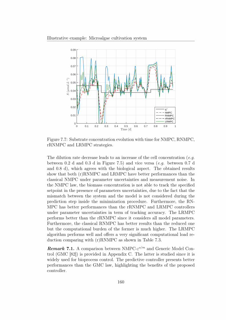
Illustrative example: Microalgae cultivation system
Time [d]0 0.1 0.2 0.3 0.4 0.5 0.6 0.7 0.8 0.9 1
S(µmol.L−1)
0
0.01
0.02
0.03
0.04
0.05
0.06
0.07
0.08
0.09
S r
NMPCRNMPCrRNMPCLRMPC
Figure 7.7: Substrate concentration evolution with time for NMPC, RNMPC,rRNMPC and LRMPC strategies.
The dilution rate decrease leads to an increase of the cell concentration (e.g.between 0.2 d and 0.3 d in Figure 7.5) and vice versa (e.g. between 0.7 dand 0.8 d), which agrees with the biological aspect. The obtained resultsshow that both (r)RNMPC and LRMPC have better performances than theclassical NMPC under parameter uncertainties and measurement noise. Inthe NMPC law, the biomass concentration is not able to track the specifiedsetpoint in the presence of parameters uncertainties, due to the fact that themismatch between the system and the model is not considered during theprediction step inside the minimization procedure. Furthermore, the RN-MPC has better performances than the rRNMPC and LRMPC controllersunder parameter uncertainties in term of tracking accuracy. The LRMPCperforms better than the rRNMPC since it considers all model parameters.Furthermore, the classical RNMPC has better results than the reduced onebut the computational burden of the former is much higher. The LRMPCalgorithm performs well and offers a very significant computational load re-duction comparing with (r)RNMPC as shown in Table 7.3.
Remark 7.1. A comparison between NMPC-εs/m and Generic Model Con-trol (GMC [82]) is provided in Appendix C. The latter is studied since it iswidely used for bioprocess control. The predictive controller presents betterperformances than the GMC law, highlighting the benefits of the proposedcontroller.
160
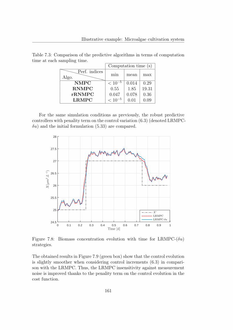
Illustrative example: Microalgae cultivation system
Table 7.3: Comparison of the predictive algorithms in terms of computationtime at each sampling time.
Computation time (s)XXXXXXXXXXXXAlgo.
Perf. indices min mean max
NMPC < 10−5 0.014 0.29RNMPC 0.55 1.85 19.31rRNMPC 0.047 0.078 0.36LRMPC < 10−5 0.01 0.09
For the same simulation conditions as previously, the robust predictivecontrollers with penality term on the control variation (6.3) (denoted LRMPC-δu) and the initial formulation (5.33) are compared.
Time [d]0 0.1 0.2 0.3 0.4 0.5 0.6 0.7 0.8 0.9 1
X(µm
3.L
−1)
24.5
25
25.5
26
26.5
27
27.5
28
Xr
LRMPC
LRMPC-δu
Figure 7.8: Biomass concentration evolution with time for LRMPC-(δu)strategies.
The obtained results in Figure 7.9 (green box) show that the control evolutionis slightly smoother when considering control increments (6.3) in compari-son with the LRMPC. Thus, the LRMPC insensitivity against measurementnoise is improved thanks to the penality term on the control evolution in thecost function.
161
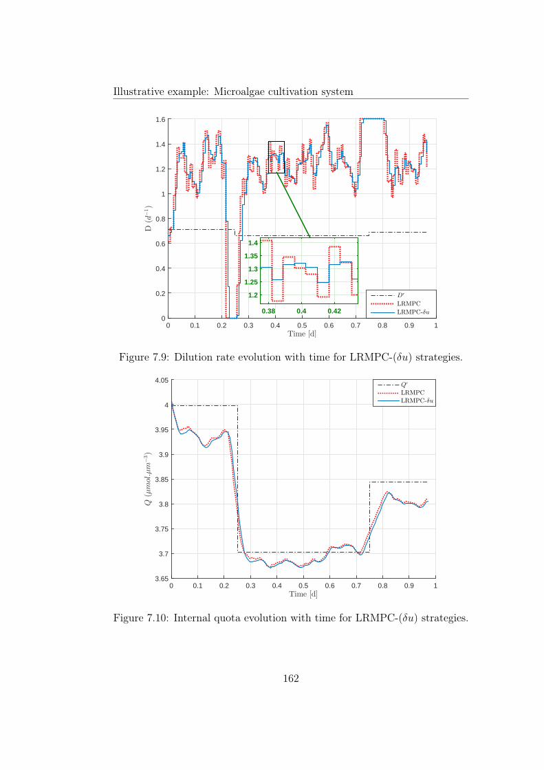
Illustrative example: Microalgae cultivation system
Time [d]0 0.1 0.2 0.3 0.4 0.5 0.6 0.7 0.8 0.9 1
D(d
−1)
0
0.2
0.4
0.6
0.8
1
1.2
1.4
1.6
Dr
LRMPC
LRMPC-δu0.38 0.4 0.42
1.2
1.25
1.3
1.35
1.4
Figure 7.9: Dilution rate evolution with time for LRMPC-(δu) strategies.
Time [d]0 0.1 0.2 0.3 0.4 0.5 0.6 0.7 0.8 0.9 1
Q(µmol.µm
−3)
3.65
3.7
3.75
3.8
3.85
3.9
3.95
4
4.05Qr
LRMPC
LRMPC-δu
Figure 7.10: Internal quota evolution with time for LRMPC-(δu) strategies.
162
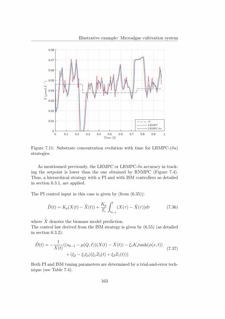
Illustrative example: Microalgae cultivation system
Time [d]0 0.1 0.2 0.3 0.4 0.5 0.6 0.7 0.8 0.9 1
S(µmol.L−1)
0
0.01
0.02
0.03
0.04
0.05
0.06
0.07
0.08
Sr
LRMPC
LRMPC-δu
Figure 7.11: Substrate concentration evolution with time for LRMPC-(δu)strategies.
As mentionned previously, the LRMPC or LRMPC-δu accuracy in track-ing the setpoint is lower than the one obtained by RNMPC (Figure 7.4).Thus, a hierarchical strategy with a PI and with ISM controllers as detailedin section 6.3.1, are applied.
The PI control input in this case is given by (from (6.35)):
D(t) = Kp(X(t)− X(t)) +Kp
Ti
∫ t
tk−1
(X(τ)− X(τ))dτ (7.36)
where X denotes the biomass model prediction.The control law derived from the ISM strategy is given by (6.55) (as detailedin section 6.3.2):
D(t) = − 1
X(t)((uk−1 − µ(Q, I))(X(t)− X(t))− ξ1Kstanh(φ(x, t))
+ (ξ2 − ξ1ξ3)(ξ1Z2(t) + ξ2Z1(t)))
(7.37)
Both PI and ISM tuning parameters are determined by a trial-and-error tech-nique (see Table 7.4).
163
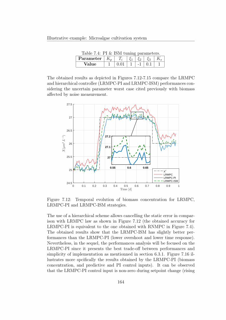
Illustrative example: Microalgae cultivation system
Table 7.4: PI & ISM tuning parameters.Parameter Kp Ti ξ1 ξ2 ξ3 Ks
Value 1 0.01 1 -1 0.1 1
The obtained results as depicted in Figures 7.12-7.15 compare the LRMPCand hierarchical controller (LRMPC-PI and LRMPC-ISM) performances con-sidering the uncertain parameter worst case cited previously with biomassaffected by noise measurement.
Time [d]0 0.1 0.2 0.3 0.4 0.5 0.6 0.7 0.8 0.9 1
X(µm
3.L
−1)
24.5
25
25.5
26
26.5
27
27.5
X r
LRMPCLRMPC-PILRMPC-ISM
0.55 0.6 0.65
27
27.1
27.2
Figure 7.12: Temporal evolution of biomass concentration for LRMPC,LRMPC-PI and LRMPC-ISM strategies.
The use of a hierarchical scheme allows cancelling the static error in compar-ison with LRMPC law as shown in Figure 7.12 (the obtained accuracy forLRMPC-PI is equivalent to the one obtained with RNMPC in Figure 7.4).The obtained results show that the LRMPC-ISM has slightly better per-formances than the LRMPC-PI (lower overshoot and lower time response).Nevertheless, in the sequel, the performances analysis will be focused on theLRMPC-PI since it presents the best trade-off between performances andsimplicity of implementation as mentionned in section 6.3.1. Figure 7.16 il-lustrates more spcifically the results obtained by the LRMPC-PI (biomassconcentration, and predictive and PI control inputs). It can be observedthat the LRMPC-PI control input is non-zero during setpoint change (rising
164
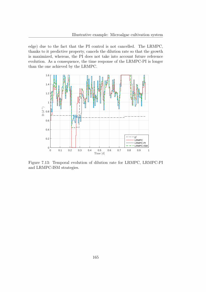
Illustrative example: Microalgae cultivation system
edge) due to the fact that the PI control is not cancelled. The LRMPC,thanks to it predictive property, cancels the dilution rate so that the growthis maximized, whereas, the PI does not take into account future referenceevolution. As a consequence, the time response of the LRMPC-PI is longerthan the one achieved by the LRMPC.
Time [d]0 0.1 0.2 0.3 0.4 0.5 0.6 0.7 0.8 0.9 1
D(d
−1)
0
0.2
0.4
0.6
0.8
1
1.2
1.4
1.6
Dr
LRMPCLRMPC-PILRMPC-ISM
Figure 7.13: Temporal evolution of dilution rate for LRMPC, LRMPC-PIand LRMPC-ISM strategies.
165
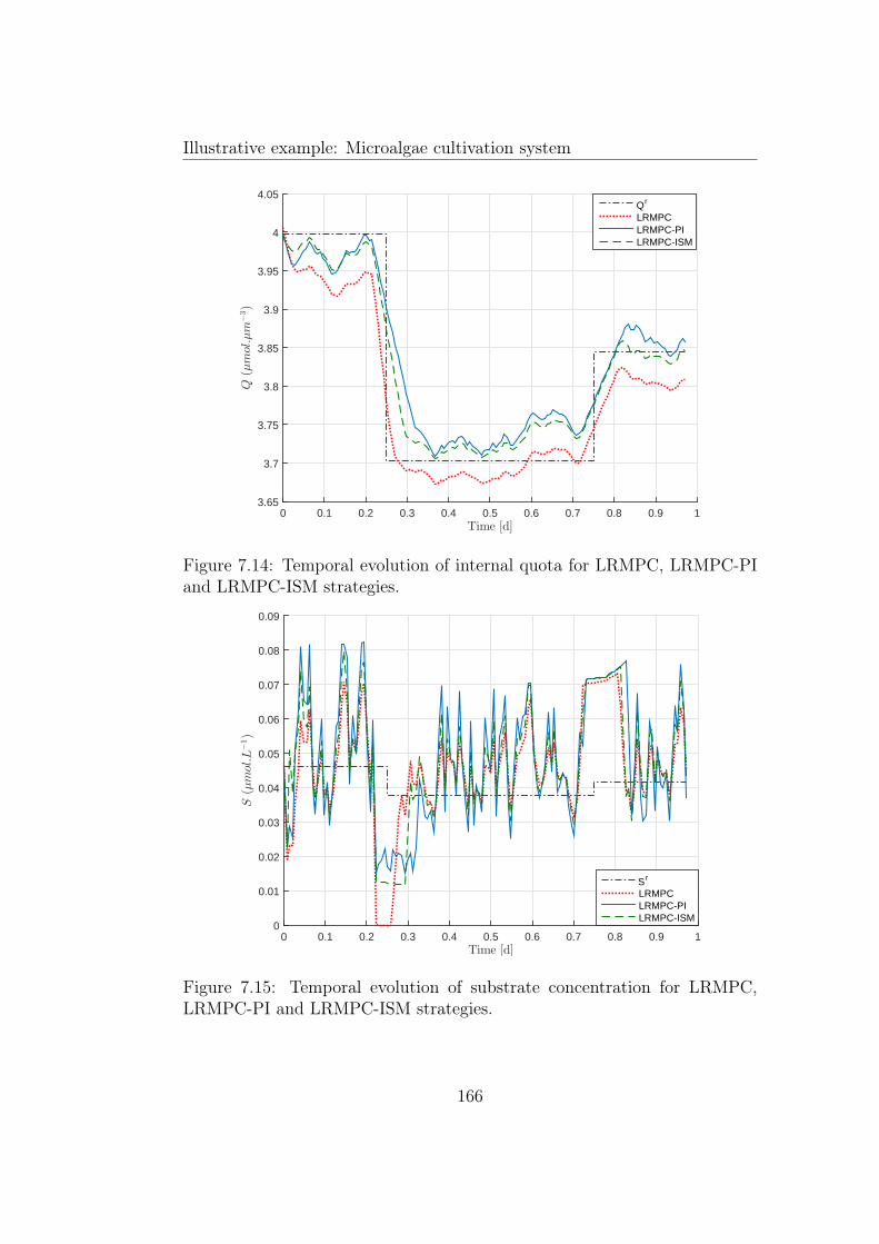
Illustrative example: Microalgae cultivation system
Time [d]0 0.1 0.2 0.3 0.4 0.5 0.6 0.7 0.8 0.9 1
Q(µmol.µm
−3)
3.65
3.7
3.75
3.8
3.85
3.9
3.95
4
4.05Qr
LRMPCLRMPC-PILRMPC-ISM
Figure 7.14: Temporal evolution of internal quota for LRMPC, LRMPC-PIand LRMPC-ISM strategies.
Time [d]0 0.1 0.2 0.3 0.4 0.5 0.6 0.7 0.8 0.9 1
S(µmol.L−1)
0
0.01
0.02
0.03
0.04
0.05
0.06
0.07
0.08
0.09
S r
LRMPCLRMPC-PILRMPC-ISM
Figure 7.15: Temporal evolution of substrate concentration for LRMPC,LRMPC-PI and LRMPC-ISM strategies.
166
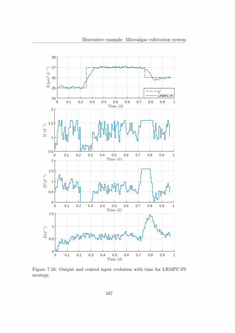
Illustrative example: Microalgae cultivation system
Time (d)0 0.1 0.2 0.3 0.4 0.5 0.6 0.7 0.8 0.9 1
X(µm
3.L
−1)
24
25
26
27
28
X r
LRMPC-PI
Time (d)0 0.1 0.2 0.3 0.4 0.5 0.6 0.7 0.8 0.9 1
D(d
−1)
0.5
1
1.5
2
Time (d)0 0.1 0.2 0.3 0.4 0.5 0.6 0.7 0.8 0.9 1
D⋆(d
−1)
0
0.5
1
1.5
2
Time (d)0 0.1 0.2 0.3 0.4 0.5 0.6 0.7 0.8 0.9 1
D(d
−1)
0
0.5
1
1.5
Figure 7.16: Output and control input evolution with time for LRMPC-PIstrategy.
167
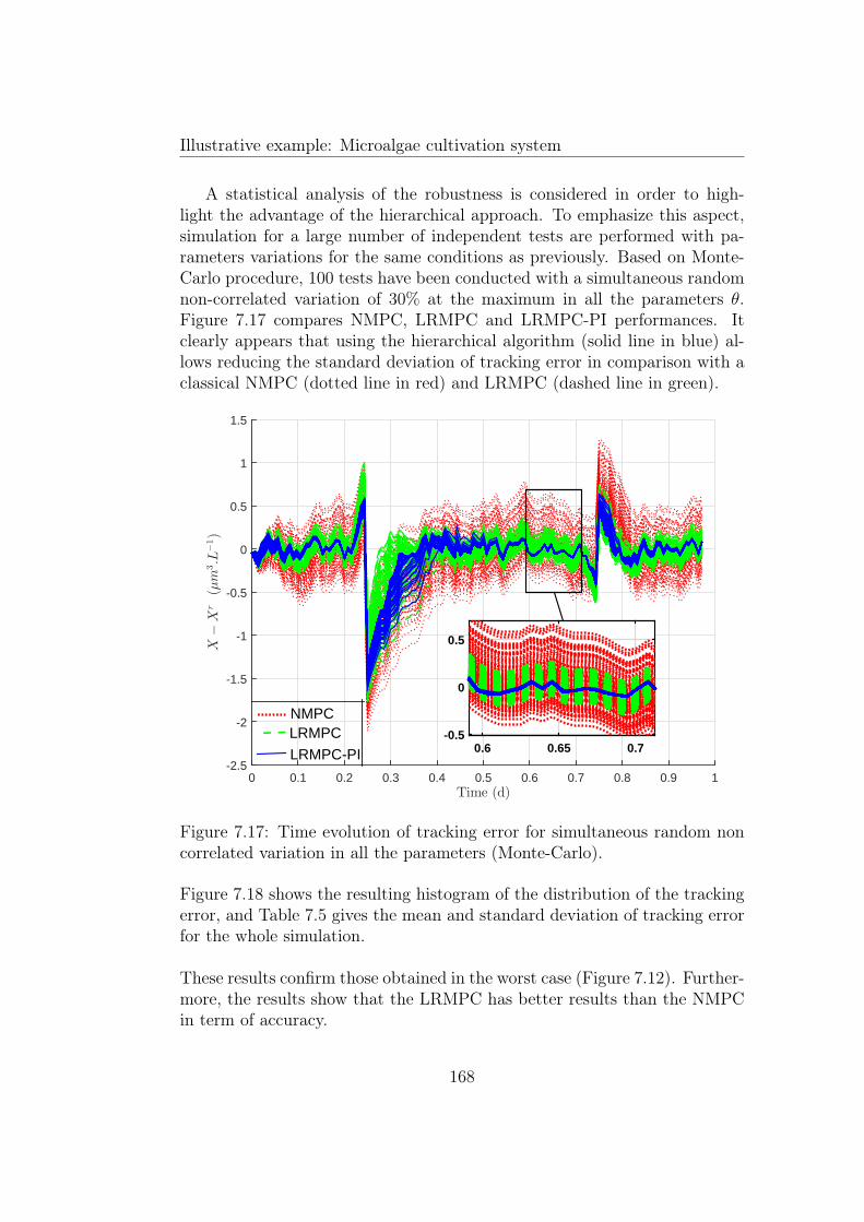
Illustrative example: Microalgae cultivation system
A statistical analysis of the robustness is considered in order to high-light the advantage of the hierarchical approach. To emphasize this aspect,simulation for a large number of independent tests are performed with pa-rameters variations for the same conditions as previously. Based on Monte-Carlo procedure, 100 tests have been conducted with a simultaneous randomnon-correlated variation of 30% at the maximum in all the parameters θ.Figure 7.17 compares NMPC, LRMPC and LRMPC-PI performances. Itclearly appears that using the hierarchical algorithm (solid line in blue) al-lows reducing the standard deviation of tracking error in comparison with aclassical NMPC (dotted line in red) and LRMPC (dashed line in green).
Time (d)0 0.1 0.2 0.3 0.4 0.5 0.6 0.7 0.8 0.9 1
X−X
r(µm
3.L
−1)
-2.5
-2
-1.5
-1
-0.5
0
0.5
1
1.5
0.6 0.65 0.7-0.5
0
0.5
LRMPC-PI
LRMPCNMPC
Figure 7.17: Time evolution of tracking error for simultaneous random noncorrelated variation in all the parameters (Monte-Carlo).
Figure 7.18 shows the resulting histogram of the distribution of the trackingerror, and Table 7.5 gives the mean and standard deviation of tracking errorfor the whole simulation.
These results confirm those obtained in the worst case (Figure 7.12). Further-more, the results show that the LRMPC has better results than the NMPCin term of accuracy.
168
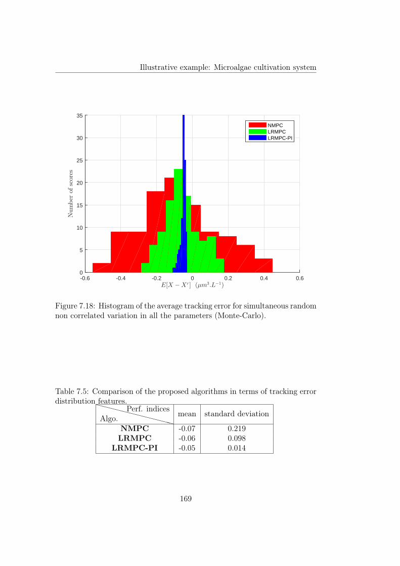
Illustrative example: Microalgae cultivation system
E[X −Xr] (µm3
.L−1)
-0.6 -0.4 -0.2 0 0.2 0.4 0.6
Number
ofscores
0
5
10
15
20
25
30
35
NMPCLRMPCLRMPC-PI
Figure 7.18: Histogram of the average tracking error for simultaneous randomnon correlated variation in all the parameters (Monte-Carlo).
Table 7.5: Comparison of the proposed algorithms in terms of tracking errordistribution features.XXXXXXXXXXXXAlgo.
Perf. indices mean standard deviation
NMPC -0.07 0.219LRMPC -0.06 0.098
LRMPC-PI -0.05 0.014
169
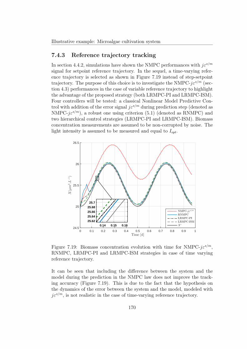
Illustrative example: Microalgae cultivation system
7.4.3 Reference trajectory tracking
In section 4.4.2, simulations have shown the NMPC performances with jεs/msignal for setpoint reference trajectory. In the sequel, a time-varying refer-ence trajectory is selected as shown in Figure 7.19 instead of step-setpointtrajectory. The purpose of this choice is to investigate the NMPC-jεs/m (sec-tion 4.3) performances in the case of variable reference trajectory to highlightthe advantage of the proposed strategy (both LRMPC-PI and LRMPC-ISM).Four controllers will be tested: a classical Nonlinear Model Predictive Con-trol with addition of the error signal jεs/m during prediction step (denoted asNMPC-jεs/m), a robust one using criterion (5.1) (denoted as RNMPC) andtwo hierarchical control strategies (LRMPC-PI and LRMPC-ISM). Biomassconcentration measurements are assumed to be non-corrupted by noise. Thelight intensity is assumed to be measured and equal to Iopt.
Time [d]0 0.1 0.2 0.3 0.4 0.5 0.6 0.7 0.8 0.9 1
X(µm
3.L
−1)
24.5
25
25.5
26
26.5
NMPC-jεs/m
RNMPC
LRMPC-PI
LRMPC-ISM
Xr0.14 0.15 0.1625.62
25.64
25.66
25.68
25.7
Figure 7.19: Biomass concentration evolution with time for NMPC-jεs/m,RNMPC, LRMPC-PI and LRMPC-ISM strategies in case of time varyingreference trajectory.
It can be seen that including the difference between the system and themodel during the prediction in the NMPC law does not improve the track-ing accuracy (Figure 7.19). This is due to the fact that the hypothesis onthe dynamics of the error between the system and the model, modeled withjεs/m, is not realistic in the case of time-varying reference trajectory.
170

Illustrative example: Microalgae cultivation system
On the other hand, both RNMPC and the hierarchical approaches (LRMPC-PI and LRMPC-ISM) have similar performances and lead to a slight dynamicerror. The RNMPC leads to the most accurate tracking but presents strongcomputation time. The above case study highlights the limits to the appli-cability of the NMPC with jεs/m signal.
Time [d]0 0.1 0.2 0.3 0.4 0.5 0.6 0.7 0.8 0.9 1
D(d
−1)
0.4
0.6
0.8
1
1.2
1.4
1.6
Dr
NMPC-jεs/m
RNMPC
LRMPC-PI
LRMPC-ISM
Figure 7.20: Dilution rate evolution with time for NMPC-jεs/m, RNMPC,LRMPC-PI and LRMPC-ISM strategies in case of time varying referencetrajectory.
171
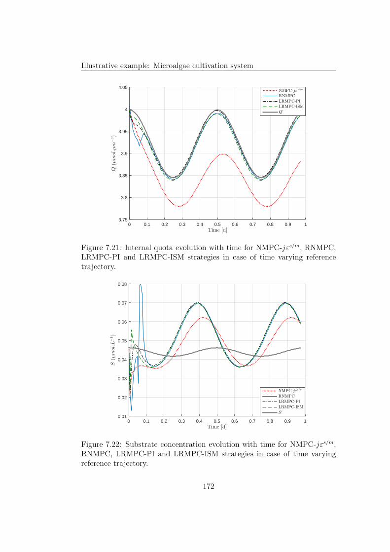
Illustrative example: Microalgae cultivation system
Time [d]0 0.1 0.2 0.3 0.4 0.5 0.6 0.7 0.8 0.9 1
Q(µmol.µm
−3)
3.75
3.8
3.85
3.9
3.95
4
4.05NMPC-jεs/m
RNMPCLRMPC-PILRMPC-ISMQr
Figure 7.21: Internal quota evolution with time for NMPC-jεs/m, RNMPC,LRMPC-PI and LRMPC-ISM strategies in case of time varying referencetrajectory.
Time [d]0 0.1 0.2 0.3 0.4 0.5 0.6 0.7 0.8 0.9 1
S(µmol.L
−1)
0.01
0.02
0.03
0.04
0.05
0.06
0.07
0.08
NMPC-jεs/m
RNMPC
LRMPC-PI
LRMPC-ISM
Sr
Figure 7.22: Substrate concentration evolution with time for NMPC-jεs/m,RNMPC, LRMPC-PI and LRMPC-ISM strategies in case of time varyingreference trajectory.
172
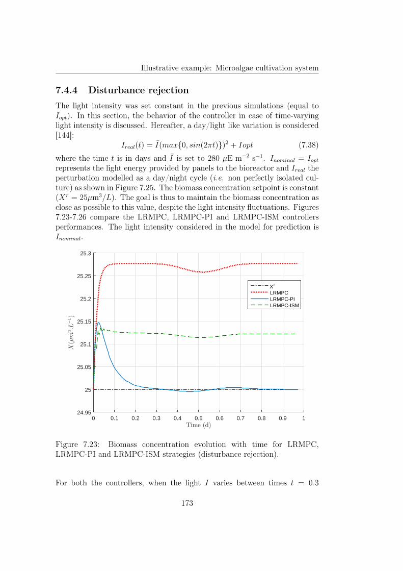
Illustrative example: Microalgae cultivation system
7.4.4 Disturbance rejection
The light intensity was set constant in the previous simulations (equal toIopt). In this section, the behavior of the controller in case of time-varyinglight intensity is discussed. Hereafter, a day/light like variation is considered[144]:
Ireal(t) = I(max{0, sin(2πt)})2 + Iopt (7.38)
where the time t is in days and I is set to 280 µE m−2 s−1. Inominal = Ioptrepresents the light energy provided by panels to the bioreactor and Ireal theperturbation modelled as a day/night cycle (i.e. non perfectly isolated cul-ture) as shown in Figure 7.25. The biomass concentration setpoint is constant(Xr = 25µm3/L). The goal is thus to maintain the biomass concentration asclose as possible to this value, despite the light intensity fluctuations. Figures7.23-7.26 compare the LRMPC, LRMPC-PI and LRMPC-ISM controllersperformances. The light intensity considered in the model for prediction isInominal.
Time (d)0 0.1 0.2 0.3 0.4 0.5 0.6 0.7 0.8 0.9 1
X(µm
3.L
−1)
24.95
25
25.05
25.1
25.15
25.2
25.25
25.3
X r
LRMPCLRMPC-PILRMPC-ISM
Figure 7.23: Biomass concentration evolution with time for LRMPC,LRMPC-PI and LRMPC-ISM strategies (disturbance rejection).
For both the controllers, when the light I varies between times t = 0.3
173
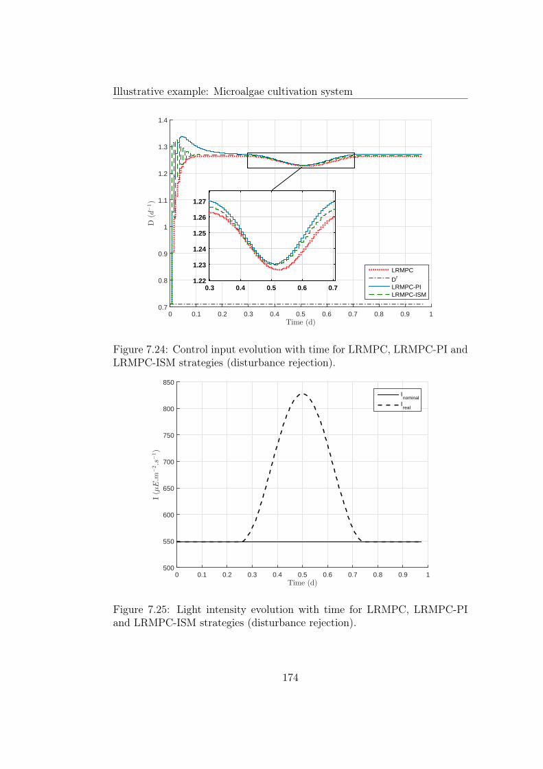
Illustrative example: Microalgae cultivation system
Time (d)0 0.1 0.2 0.3 0.4 0.5 0.6 0.7 0.8 0.9 1
D(d
−1)
0.7
0.8
0.9
1
1.1
1.2
1.3
1.4
LRMPC
Dr
LRMPC-PILRMPC-ISM
0.3 0.4 0.5 0.6 0.71.22
1.23
1.24
1.25
1.26
1.27
Figure 7.24: Control input evolution with time for LRMPC, LRMPC-PI andLRMPC-ISM strategies (disturbance rejection).
Time (d)0 0.1 0.2 0.3 0.4 0.5 0.6 0.7 0.8 0.9 1
I(µE.m
−2.s
−1)
500
550
600
650
700
750
800
850
Inominal
Ireal
Figure 7.25: Light intensity evolution with time for LRMPC, LRMPC-PIand LRMPC-ISM strategies (disturbance rejection).
174
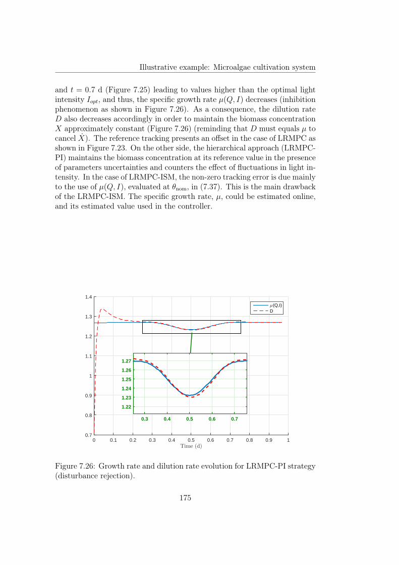
Illustrative example: Microalgae cultivation system
and t = 0.7 d (Figure 7.25) leading to values higher than the optimal lightintensity Iopt, and thus, the specific growth rate µ(Q, I) decreases (inhibitionphenomenon as shown in Figure 7.26). As a consequence, the dilution rateD also decreases accordingly in order to maintain the biomass concentrationX approximately constant (Figure 7.26) (reminding that D must equals µ tocancel X). The reference tracking presents an offset in the case of LRMPC asshown in Figure 7.23. On the other side, the hierarchical approach (LRMPC-PI) maintains the biomass concentration at its reference value in the presenceof parameters uncertainties and counters the effect of fluctuations in light in-tensity. In the case of LRMPC-ISM, the non-zero tracking error is due mainlyto the use of µ(Q, I), evaluated at θnom, in (7.37). This is the main drawbackof the LRMPC-ISM. The specific growth rate, µ, could be estimated online,and its estimated value used in the controller.
Time (d)0 0.1 0.2 0.3 0.4 0.5 0.6 0.7 0.8 0.9 1
0.7
0.8
0.9
1
1.1
1.2
1.3
1.4
µ(Q,I)D
0.3 0.4 0.5 0.6 0.7
1.22
1.23
1.24
1.25
1.26
1.27
Figure 7.26: Growth rate and dilution rate evolution for LRMPC-PI strategy(disturbance rejection).
175
Illustrative example: Microalgae cultivation system
7.5 ConclusionIn this chapter, predictive controllers were applied to control microalgae cul-ture in a continuous photobioreactor (Droop model). First, the obtainedresults show that both RNMPC and LRMPC have better than the classi-cal NMPC performances under parameters uncertainties and measurementsaffected by noise. The LRMPC accuracy in tracking the setpoint is lowerthan the one obtained by RNMPC due to the linearization of the predictionmodel. However, the RNMPC suffers from the difficulty to derive a solu-tion as quickly as possible. The LRMPC offers a strong computational loadreduction. Secondly, the use of a hierarchical scheme allows cancelling thestatic error in comparison with LRMPC law. For a time-varying referencetrajectory, the hierarchical control scheme ensures a good tracking accuracywhich is not the case for the NMPC-jεs/m. Thus, it highlights the limits tothe applicability of the latter approach. Finally, for time-varying light in-tensity, the hierarchical approach (LRMPC-PI) maintains the output at itsreference value in the presence of parameters uncertainties and counters theeffect of fluctuations in light intensity.
This example illustrated and highlighted the advantages of the proposedpredictive controllers. More specifically, the hierarchical structure that com-bines a linearized robust predictive controller with a PI controller proposesa good solution for microalgae cultivation control.
The applicability of this control strategy to other bioprocesses and itspossible theoretical and numerical improvements will be discussed in thenext chapter.
176
Chapter 8
General conclusions and futuredirections
This thesis has investigated new structures of robust nonlinear predictive con-trol, which are able to deal with the compromise between robustness features,tracking accuracy and dynamic performances, on the one hand, and reducedcomputational load on the other hand. This aspect of computational burdenis indeed of major concern, when applying the control strategy in real-time.Even if the bioprocess considered in this work for the application frameworkhas limited real-time constraints, this may not be the case in particular forsystems with higher number of uncertain parameters. Therefore the aspectis crucial for RNMPC.
Based on this, the proposed structure, combining a linearized MPC con-troller with an additional one to deal with residual tracking accuracy, appearsto be a good candidate to the paradigm mentioned above.
This development has been elaborated in a progressive way, through thecontribution of successive chapters, and assessed through simulations resultsin the case of bioprocesses.
In this chapter, we summarize the thesis contributions and present rec-ommendations for future work.
8.1 Thesis summary and contributions
Chapter 3 reviewed previous works in the area of predictive control strate-gies and presents their key advantages and drawbacks. Theoretical, compu-tational and implementation aspect were briefly discussed. It served as acentralized literature study in the thesis.
177
General conclusions and future directions
Chapter 4 made use of the Nonlinear Model Predictive Control (NMPC)discussed in Chapter 3 and appplied it in the context of trajectory track-ing problem for continuous/discrete-time nonlinear systems. This strategyinduces solving, online, an optimization problem which is expressed as a non-linear programming problem. This formulation highlighted its limits in thecase of plant-model mismatch. One studied improvement consisted to in-clude, during the prediction step, the difference between the system and themodel outputs. Unfortunately, the assumption on including the predictionerror is quite restrictive due to the fact that we do not know, in a realisticapplication, how the error will evolve over the prediction horizon.
Chapter 5 focused on the Robust Model Predictive Control. Robust vari-ants of NMPC are able to take into account set bounded uncertainties in thedesign procedure. In this study, the robust NMPC law was formulated asa min-max optimization problem where the objective function is minimizedfor the worst possible uncertainty realization. In order to reduce the com-putation burden, two solutions have been proposed. On one side, thanksto a sensitivity analysis, a reduction of the number of uncertain parame-ters is performed. Only the main influencial parameters on the model areconsidered in the min-max problem whereas the other parameters are keptconstant and equal to their nominal values. This approach cannot be al-ways used due to two major drawbacks: the necessity to consider a studyof the respective impact of the parameters through a sensitivity analysis,leading to a more complex and time demanding study and its applicabilityonly in some cases (when all parameters have high influence on the model,no parameter reduction is possible). On th other side, a new approach basedon a model linearization technique (first-order Taylor series expansion) hasbeen developed. It aims to turn the min-max problem into a more tractableoptimization problem in order to reduce the computation time as much aspossible and to make it suitable for online implementation. The derived op-timization problem is an unidimensional optimization (so-called LRMPC).Taking into account the inequality constraints on the optimization variableleads to a bilevel problem (so-called CLRMPC), with a quadratic program-ming problem in the lower level, and a scalar one in the upper level. Thisapproach leads to a loss of accuracy (linearizaton drawback) but it is com-putationally tractable in calculating the optimal control compared to themin-max optimization, which makes it suitable for online implementation.Moreover, stability properties of the proposed LRMPC approach has beenanalyzed.
Chapter 6 proposed two improvements for the developed method. The first
178
General conclusions and future directions
idea deals with the linearization of the model around the nominal parametervalues and the optimal control sequence obtained at the previous iteration.This modification led to an optimal control sequence less sensitive ato noisemeasurements thanks to the inclusion of the penality term on the controlevolution. The derived optimization problem is a bilevel one or a scalar min-imization, depending on the considered constraints. In a second step, to gofurther with linearization drawback, a hiearchical control scheme has beenproposed. It combines a robust model predictive control law with a propor-tional Integral (PI) law or Integral Sliding Mode (ISM) controller. The pre-dictive controller guarantees the tracking of the reference trajectory, whereasthe additional regulator ensures cancelling any residual tracking error. Forthe auxiliary controller, the PI law ensures the best trade-off between designcomplexity and performances, without requiring specific knowledge on thesystem parameters.
Chapter 7 was devoted to the case study of the control of microalgae culturein continuous photobioreactor. Simulations have been carried out in the caseof constant and time-varying reference trajectories to highlight the advantageof the proposed control approach under parameters uncertainities, externalperturbation and measurement affected by noise.
8.2 Recommendations for future directionsIn this work, the obtained results have highlighted many issues that have tobe considered as perspectives of this work. Some recommendations for futurework in which further research may be carried out are proposed below, withdifferent time scales.
Short term issues are more related to the application field considered inthis work:
• In this dissertation, the proposed control strategies were applied in thecase of Single Input Single Output (SISO) system with a small num-ber of uncertain parameters. The application of the proposed meth-ods to a highly nonlinear multivariable system with much more uncer-tain parameters is under progress (based on the experimental work of[42]). The studied MIMO sytem is a heterotrophic microalgae fed-batchbioreactor. The aim is to control biomass and product concentrationsthrough two substrate feed rates. This objevtive has to be finalized.
• Based on results on the robustness of the LRMPC with respect to modelparameters uncertainties, future work can consider extending the study
179
General conclusions and future directions
to the case of disturbances and unmodeled uncertainties (e.g. modelmismatch of the growth kinetics). In fact, these unmodeled mismatchesin the kinetic part could come from the difficulty to select an accuratemodel structure, a possible evolution of the model parameters and/ora metabolic change over time.
• The biological variables are sometimes not accessible to be measuredonline and usually measured offline using expensive sensors. In thiscontext, it is important to design an estimation algorithm or so-calledsoft sensors to rebuild time evolution of the state and to develop a con-structive procedure for designing controllers robust against additionalestimation errors. Contributions in this area are particularly impor-tant.
On top of that, the experimental validation of the proposed robust hierarchi-cal structure on a real bioreactor, either lab-scale or industrial, would be thebest validation to fully assess the theoretical developments. This is howevera complex task, starting first, for a dedicated benchmark, with the modeldefinition, the parameters identification with their confidence intervals, thenthe implementation of the control law (coupled to soft sensors) in a dedi-cated software. This perspective is a really important one to demonstratethe efficiency and advantages of the proposed control strategies.
Long term issues are more related to theoretical developments:
• In order to improve the performances of the LRMPC-δu in the presenceof model mismatch and measurements affected by noise (section 6.2.4),an alternative would be to include the penalty term on the controlvariation (defined in (6.3)) as an additional term in the criterion (5.3)(i.e. to consider simultaneously penalty on the control increments andon the difference between u and its reference ur). We already appliedthis strategy in the case of NMPC law, leading to good performances(see example in Appendix C). This new criterion should be consideredfor LRMPC and the control input calculation extended to this newoptimization problem.
• In order to increase the quality of the linearized model, there are severalissues that deserve further investigation. An interesting perspectivemay be considering a second order expansion rather than the first orderapproximation to improve the robustness and accuracy of the LRMPCas in [62].
180
General conclusions and future directions
• In particular, theoretical questions like stability need to be addressed.In fact, stability analysis of the closed-loop system as presented in sec-tion 5.4.2 leads to an open question related to the impact of solvingthe optimization problem by using the Lagrangian duality on the sta-bility of the closed-loop system. Nevertheless, the derived optimizationproblem being a convex one, leading to better convergence propertiesthan the original min-max problem, an interesting idea is to focus theanalysis on the impact of the convergence of the optimization algorithmon the stability of the closed-loop system.
• On the other side, an interesting perspective may be the determinationof sufficient conditions ensuring robust stability of the overall hierarchi-cal control scheme, presented in Chapter 6, in case of bounded uncer-tainties and/or trajectory constraints, starting from the work alreadydone in [131].
• It would be also interesting to analyse the robust stability of the closedloop system (LRMPC strategy coupled with the observer,e.g., Ex-tended Kalman Filter) as done in [69].
181

General conclusions and future directions
182
Appendix A
A.1 Robust regularized Least squares problemThis part details the development from (5.85) to (5.91) in section 5.5.
Let us consider the Lagrangian given by (5.85):
L(z, ξ, λ) = −||z||2V − ||Az − b+ Cξ||2W + λ(||ξ||2 − Γ(z)2) (A.1)
The above equation (A.1) can be expressed as:
L(z, ξ, λ) =− ||z||2V − λΓ(z)2 − ||Az − b||2W − (Az − b)>WCξ
− ξ>C>W (Az − b) + ξ>(λI− C>WC)ξ(A.2)
The optimal solution ξ? that minimizes L is given by:
ξ? = (λI− C>WC)†C>W (Az − b) (A.3)
Replacing (A.3) in (A.2) and after some mathematical manipulationsn, itcomes:
L(z, ξ?, λ) =− ||z||2V − λΓ(z)2 − ||Az − b||2W − (Az − b)>WC(λI− C>WC)†
× C>W (Az − b)− (Az − b)>WC(λI− C>WC)†C>W (Az − b)+ (Az − b)>WC(λI− C>WC)† (λI− C>WC)(λI− C>WC)†︸ ︷︷ ︸
I
× C>W (Az − b)(A.4)
Then, we have that:
L(z, ξ?, λ) =− ||z||2V − λΓ(z)2 − (Az − b)>(W +WC(λI− C>WC)†C>W
+WC(λI− C>WC)†C>W −WC(λI− C>WC)†C>W︸ ︷︷ ︸0
)(Az − b)
(A.5)
183
Finally, the Lagrangian (A.1) becomes a function of z and λ as follows:
L(z, λ) =− ||z||2V − λΓ(z)2
− (Az − b)>(W +WC(λI− C>WC)†C>W
)(Az − b)
(A.6)
Let us define W (λ) = W +WC(λI− C>WC)†C>W .Then, (A.6) becomes:
L(z, λ) = −||z||2V − λΓ(z)2 − ||Az − b||2W (λ) (A.7)
which is the expression (5.91).
184
Appendix B
B.1 Biological systems modelling
This section summarizes general principles in bioprocess modelling. More de-tails can be found in [9]. Biological systems are described by a set of macro-scopic components such as biomass, substrates and metabolic products. Themechanistic approach is the most popular bioprocess modelling technique.For optimization, monitoring and control purposes, this approach is usuallymacroscopic in essence, i.e., it makes use of the concept of macroscopic reac-tion scheme involving a few reactants, products and catalysts considered asmacroscopic entities. The material flow set that defines the transformationof reactants into products is represented in the following form [9]:
ns∑i=1
ΠSi,kSirk(.)→
np∑j=1
ΠPj ,kPj, k ∈ 1, nr (B.1)
where
• Π.,k is the kth pseudo stoichiometric coefficient or yields coefficients.They are negative when they relate to a reactant and positive whenthey relate to a product.
• rk(.) is the kth reaction rate.
• The constants nr, ns and np are respectively the number of reactions,substrates and products.
• Si and Pj represent respectively the ith component consumed and jthcomponent produced.
185
Mass balance modellingAssuming that the reactor is homogeneous, the macroscopic mass balancesfor each component involved in the reaction network (B.1) lead to a generaldifferential state-space model [9]:
dΛ
dt= Kr(.) +D(Λin − Λ(t))−G(Λ(t)) (B.2)
where
• r(.) is the reaction rate vector, (made of rk(.)).
• K the matrix of yields coefficients, (made of Π.,k).
• Λ the vector of components concentrations.
• Λin the vector of feed concentrations.
• D the dilution rate which is defined as the medium feed rate over theeffective reactor volume.
• G(Λ) describes the exchange between the gas and the liquid phases.
B.2 Reaction kinetics modellingThe reaction rates describes how the compenents interact in the reactor basedon activation, limitation and inhibition phenomena. The expression of thereaction rates is typically a nonlinear function depending on the componentsconcentrations and some kinetic parameters. As an example, for the reactionsassociated with a biomass X, the growth reaction is expressed as follows [9]:
rk(.) = µk(.)X (B.3)
where µk denotes the specific growth rate, which is used to describe thebacterial growth. In the literature, commonly used laws, that describe thereaction kinetics, are determined by the biologists. The most cited one arepresented below:
• Monod model [103]:
µ = µmS
S +Ks
(B.4)
where µm is the maximum specifi growth rate (h−1) and Ks is the halfsaturation constant (g.L−1). It models the limitation of the growth bythe substrate S.
186
• Haldane kinetics [5]:
µ = µmS
S +Ks +S2
Ki
(B.5)
where Ki is the inhibition constant (g.L−1). The growth is inhibitedby the substrate S.
• Cantois kinetics [37]:
µ = µmS
S +XKc
(B.6)
whereKc is the Contois saturation constant . The growth depends uponthe concentrations of both substrate S and biomass X with growthbeing inhibited at high concentrations of biomass.
These kinetics are also used to model substrate uptake.In the case of microalgae, the above laws that describe reaction kinet-
ics are used to model both the limitation and the inhibition by the lightintensity.
187

188
Appendix C
In this section, additional results for the Droop model studied in Chapter 7are proposed. First, the controllability of model is discussed. Secondly, thedynamics of the sensitivity functions is detailed. Finally, the NMPC-εs/mperformances are compared to those obtained with the GMC law.
C.1 Controllability
Controllability is concerned with whether one can design control input tosteer the state to arbitrary values. Then, in the next, the controllability ofthe studied system is checked.
The nonlinear system (7.5) is expressed as a control-affine system as fol-lows: {
x = fx(x) + fu(x)uy = h(x)
(C.1)
with
fx =
µ(Q, I)Xρ(S)− µ(Q, I)Q−ρ(S)X
, fu =
−X0
(Sin − S)
, h(x) = X (C.2)
Theorem C.1. The nonlinear system (C.1) is locally controllable at x if andonly if the following Lie algebra rank condition is satisfied:
rank(Co) = nx (C.3)
withCo =
[fu(x) adfxfu(x) . . . adnx−1
fxfu(x)
](C.4)
Proof. see [73].
189
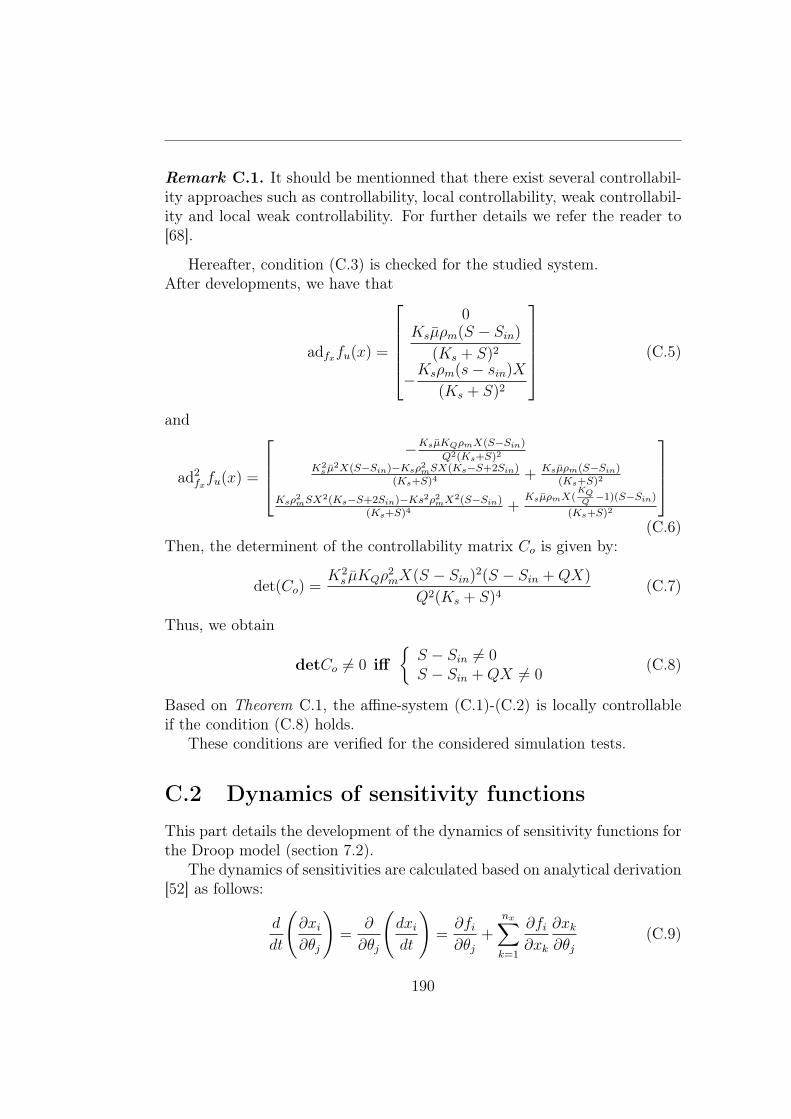
Remark C.1. It should be mentionned that there exist several controllabil-ity approaches such as controllability, local controllability, weak controllabil-ity and local weak controllability. For further details we refer the reader to[68].
Hereafter, condition (C.3) is checked for the studied system.After developments, we have that
adfxfu(x) =
0
Ksµρm(S − Sin)
(Ks + S)2
−Ksρm(s− sin)X
(Ks + S)2
(C.5)
and
ad2fxfu(x) =
−KsµKQρmX(S−Sin)
Q2(Ks+S)2
K2s µ
2X(S−Sin)−Ksρ2mSX(Ks−S+2Sin)(Ks+S)4
+ Ksµρm(S−Sin)(Ks+S)2
Ksρ2mSX2(Ks−S+2Sin)−Ks2ρ2mX2(S−Sin)
(Ks+S)4+
KsµρmX(KQQ−1)(S−Sin)
(Ks+S)2
(C.6)
Then, the determinent of the controllability matrix Co is given by:
det(Co) =K2s µKQρ
2mX(S − Sin)2(S − Sin +QX)
Q2(Ks + S)4(C.7)
Thus, we obtain
detCo 6= 0 iff{S − Sin 6= 0S − Sin +QX 6= 0
(C.8)
Based on Theorem C.1, the affine-system (C.1)-(C.2) is locally controllableif the condition (C.8) holds.
These conditions are verified for the considered simulation tests.
C.2 Dynamics of sensitivity functionsThis part details the development of the dynamics of sensitivity functions forthe Droop model (section 7.2).
The dynamics of sensitivities are calculated based on analytical derivation[52] as follows:
d
dt
(∂xi∂θj
)=
∂
∂θj
(dxidt
)=∂fi∂θj
+nx∑k=1
∂fi∂xk
∂xk∂θj
(C.9)
190
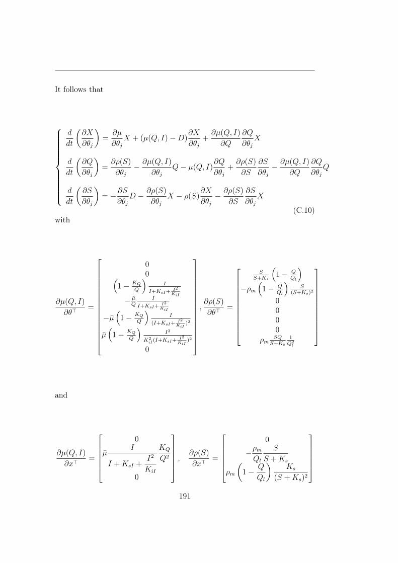
It follows that
d
dt
(∂X
∂θj
)=∂µ
∂θjX + (µ(Q, I)−D)
∂X
∂θj+∂µ(Q, I)
∂Q
∂Q
∂θjX
d
dt
(∂Q
∂θj
)=∂ρ(S)
∂θj− ∂µ(Q, I)
∂θjQ− µ(Q, I)
∂Q
∂θj+∂ρ(S)
∂S
∂S
∂θj− ∂µ(Q, I)
∂Q
∂Q
∂θjQ
d
dt
(∂S
∂θj
)= − ∂S
∂θjD − ∂ρ(S)
∂θjX − ρ(S)
∂X
∂θj− ∂ρ(S)
∂S
∂S
∂θjX
(C.10)with
∂µ(Q, I)
∂θ>=
00(
1− KQQ
)I
I+KsI+ I2
KiI
− µQ
I
I+KsI+ I2
KiI
−µ(
1− KQQ
)I
(I+KsI+ I2
KiI)2
µ(
1− KQQ
)I3
K2iI(I+KsI+ I2
KiI)2
0
,∂ρ(S)
∂θ>=
SS+Ks
(1− Q
Ql
)−ρm
(1− Q
Ql
)S
(S+Ks)2
0000
ρmSQS+Ks
1Q2l
and
∂µ(Q, I)
∂x>=
0
µI
I +KsI +I2
KiI
KQ
Q2
0
, ∂ρ(S)
∂x>=
0
−ρmQl
S
S +Ks
ρm
(1− Q
Ql
)Ks
(S +Ks)2
191
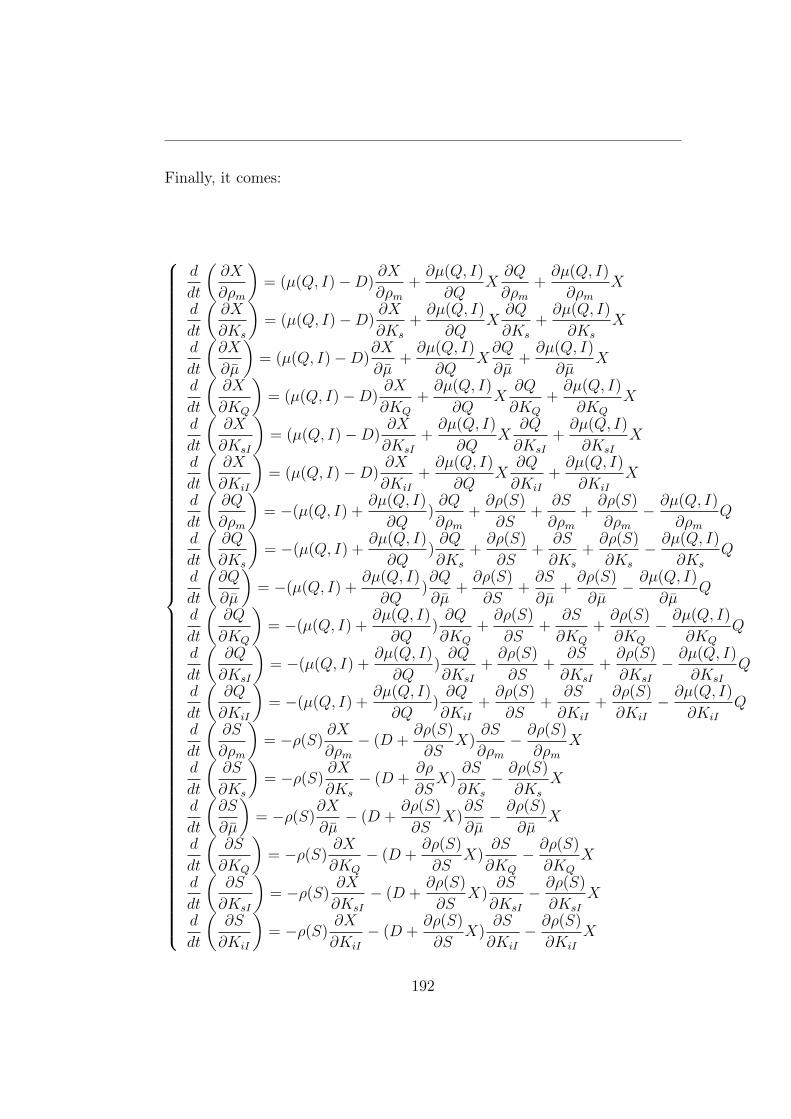
Finally, it comes:
d
dt
(∂X
∂ρm
)= (µ(Q, I)−D)
∂X
∂ρm+∂µ(Q, I)
∂QX∂Q
∂ρm+∂µ(Q, I)
∂ρmX
d
dt
(∂X
∂Ks
)= (µ(Q, I)−D)
∂X
∂Ks
+∂µ(Q, I)
∂QX∂Q
∂Ks
+∂µ(Q, I)
∂Ks
X
d
dt
(∂X
∂µ
)= (µ(Q, I)−D)
∂X
∂µ+∂µ(Q, I)
∂QX∂Q
∂µ+∂µ(Q, I)
∂µX
d
dt
(∂X
∂KQ
)= (µ(Q, I)−D)
∂X
∂KQ
+∂µ(Q, I)
∂QX
∂Q
∂KQ
+∂µ(Q, I)
∂KQ
X
d
dt
(∂X
∂KsI
)= (µ(Q, I)−D)
∂X
∂KsI
+∂µ(Q, I)
∂QX
∂Q
∂KsI
+∂µ(Q, I)
∂KsI
X
d
dt
(∂X
∂KiI
)= (µ(Q, I)−D)
∂X
∂KiI
+∂µ(Q, I)
∂QX
∂Q
∂KiI
+∂µ(Q, I)
∂KiI
X
d
dt
(∂Q
∂ρm
)= −(µ(Q, I) +
∂µ(Q, I)
∂Q)∂Q
∂ρm+∂ρ(S)
∂S+
∂S
∂ρm+∂ρ(S)
∂ρm− ∂µ(Q, I)
∂ρmQ
d
dt
(∂Q
∂Ks
)= −(µ(Q, I) +
∂µ(Q, I)
∂Q)∂Q
∂Ks
+∂ρ(S)
∂S+
∂S
∂Ks
+∂ρ(S)
∂Ks
− ∂µ(Q, I)
∂Ks
Q
d
dt
(∂Q
∂µ
)= −(µ(Q, I) +
∂µ(Q, I)
∂Q)∂Q
∂µ+∂ρ(S)
∂S+∂S
∂µ+∂ρ(S)
∂µ− ∂µ(Q, I)
∂µQ
d
dt
(∂Q
∂KQ
)= −(µ(Q, I) +
∂µ(Q, I)
∂Q)∂Q
∂KQ
+∂ρ(S)
∂S+
∂S
∂KQ
+∂ρ(S)
∂KQ
− ∂µ(Q, I)
∂KQ
Q
d
dt
(∂Q
∂KsI
)= −(µ(Q, I) +
∂µ(Q, I)
∂Q)∂Q
∂KsI
+∂ρ(S)
∂S+
∂S
∂KsI
+∂ρ(S)
∂KsI
− ∂µ(Q, I)
∂KsI
Q
d
dt
(∂Q
∂KiI
)= −(µ(Q, I) +
∂µ(Q, I)
∂Q)∂Q
∂KiI
+∂ρ(S)
∂S+
∂S
∂KiI
+∂ρ(S)
∂KiI
− ∂µ(Q, I)
∂KiI
Q
d
dt
(∂S
∂ρm
)= −ρ(S)
∂X
∂ρm− (D +
∂ρ(S)
∂SX)
∂S
∂ρm− ∂ρ(S)
∂ρmX
d
dt
(∂S
∂Ks
)= −ρ(S)
∂X
∂Ks
− (D +∂ρ
∂SX)
∂S
∂Ks
− ∂ρ(S)
∂Ks
X
d
dt
(∂S
∂µ
)= −ρ(S)
∂X
∂µ− (D +
∂ρ(S)
∂SX)
∂S
∂µ− ∂ρ(S)
∂µX
d
dt
(∂S
∂KQ
)= −ρ(S)
∂X
∂KQ
− (D +∂ρ(S)
∂SX)
∂S
∂KQ
− ∂ρ(S)
∂KQ
X
d
dt
(∂S
∂KsI
)= −ρ(S)
∂X
∂KsI
− (D +∂ρ(S)
∂SX)
∂S
∂KsI
− ∂ρ(S)
∂KsI
X
d
dt
(∂S
∂KiI
)= −ρ(S)
∂X
∂KiI
− (D +∂ρ(S)
∂SX)
∂S
∂KiI
− ∂ρ(S)
∂KiI
X
192
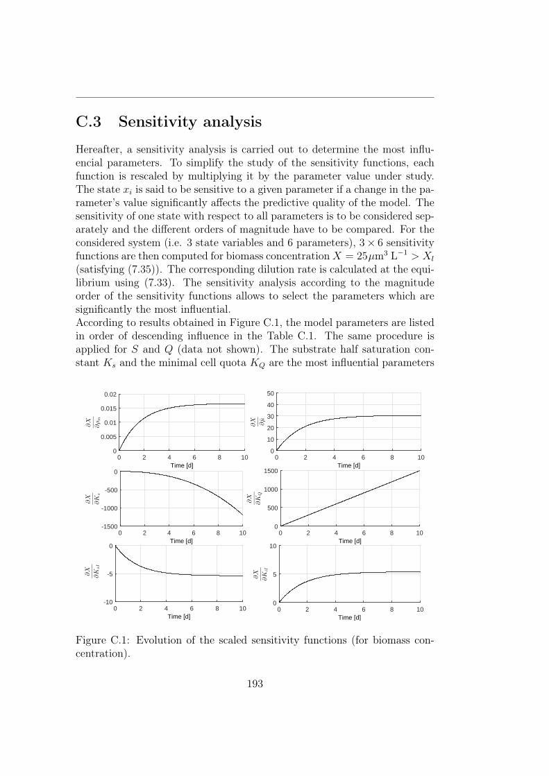
C.3 Sensitivity analysis
Hereafter, a sensitivity analysis is carried out to determine the most influ-encial parameters. To simplify the study of the sensitivity functions, eachfunction is rescaled by multiplying it by the parameter value under study.The state xi is said to be sensitive to a given parameter if a change in the pa-rameter’s value significantly affects the predictive quality of the model. Thesensitivity of one state with respect to all parameters is to be considered sep-arately and the different orders of magnitude have to be compared. For theconsidered system (i.e. 3 state variables and 6 parameters), 3× 6 sensitivityfunctions are then computed for biomass concentrationX = 25µm3 L−1 > Xl
(satisfying (7.35)). The corresponding dilution rate is calculated at the equi-librium using (7.33). The sensitivity analysis according to the magnitudeorder of the sensitivity functions allows to select the parameters which aresignificantly the most influential.According to results obtained in Figure C.1, the model parameters are listedin order of descending influence in the Table C.1. The same procedure isapplied for S and Q (data not shown). The substrate half saturation con-stant Ks and the minimal cell quota KQ are the most influential parameters
Time [d]0 2 4 6 8 10
∂X
∂ρm
0
0.005
0.01
0.015
0.02
Time [d]0 2 4 6 8 10
∂X
∂K
s
-1500
-1000
-500
0Time [d]
0 2 4 6 8 10
∂X ∂µ
0
10
20
30
40
50
Time [d]0 2 4 6 8 10
∂X
∂K
Q
0
500
1000
1500
Time [d]0 2 4 6 8 10
∂X
∂K
sI
-10
-5
0
Time [d]0 2 4 6 8 10
∂X
∂K
iI
0
5
10
Figure C.1: Evolution of the scaled sensitivity functions (for biomass con-centration).
193
on the biomass concentration evolution (100 times higher than the other pa-rameters).
Table C.1: The ranking of parameters according to their influence on themodel (from more to less).
X Q S
KQ KQ KQ
Ks Ks Ks
µ µ ρmKsI KsI µKiI KiI KsI
ρm ρm KiI
Thereafter, only these two parameters (Ks,KQ) are considered in the min-max optimization problem, instead of the 6 model parameters (the 4 otherparameters are set to their nominal values).
C.4 Additional simulation resultsIn this section, the NMPC-εs/m and Generic Model Control (GMC) perfor-mances for reference tracking are compared in the case of model mismatchand measurement noise.
C.4.1 Predictive controller
The formulation of the NMPC-εs/m optimization problem at each samplinginstant kTs is as follows:
?
Dk+Np−1
k = arg minDk+Np−1
k
Np∑j=1
((Xr
k+j − Xk+j|k)2
+λ(Drk+j−1 −Dk+j−1)2
)+β
Np−1∑j=1
(Dk+j −Dk+j−1)2
(C.11)
subject to{Xk+j|k = Hg(tk, tk+j, xk, D
k+j−1k , θnom), j = 1, Np
Dk ≥ 0, Xk ≥ 0, ∀k ∈ N(C.12)
where λ is the control weighting factor ensuring that D remains close to itsreferenceDr, β is a penalty weighting factor on the control variation term and
194
Xk+j|k is the predicted biomass concentration. Model uncertainties are takeninto account by assuming that the gap between the system and the modelat sample time k, denoted εs/m, is included in the prediction as detailed insection 4.3.
C.4.2 Generic model control
The GMC is a kind of Nonlinear Proportional Integral regulator. It includesproportional and integral actions, cancelling static errors, and performs aninput/output linearization of the system. Details related to the GMC lawcan be found in [82]. In the case of the considered control problem, thedilution rate derived from the GMC law is given by:
D = − 1
X
(G1(Xr −X) +G2
∫ t
0
(Xr −X)dτ − µ(Q, I)X
)(C.13)
The GMC tuning parameters (G1 = 2ξω0 and G2 = ω20) are chosen based on
the fact that a second order behavior is specified for the closed-loop system.The damping factor ξ gives a desired shape of response, and the naturalfrequency ω0 an appropriate settling time.
C.4.3 Simulation results
The initial biomass concentration value is set close to the setpoint in order tocancel the transient effect and to focus only on the behavior during setpointchanges. The simulation time is fixed at 3 d, the sample time Ts is chosenequal to 30 min. Only uncertainties on the first four parameters of vectorθ are considered. In this case, the four first parameters of the mismatchedmodel are chosen on the parameter subspace border (θreal = [θ+
1 , θ−2 , θ
+3 , θ
−4 ]),
where the uncertain parameters subspace [θ−, θ+] is given by [ θnom2, 3θnom
2].
The two last parametersKsI andKiI are set to their nominal values. Biomassconcentration measurements, yk, are assumed to be corrupted by a Gaussianwhite noise of zero mean and 0.05 standard deviation. The light intensity isassumed to be measured online, non-corrupted with noise.
The tuning parameters of the NMPC are determined by a trial-and-errortechnique. The prediction horizon of the NMPC law is set to Np=10, chosento satisfy a compromise between the computation time and a sufficient visionof the system behaviour in the future. The weighting factor λ is selected at1 to promote the tracking error on biomass concentration relatively to thetracking error on dilution rate in the objective function. In addition, thepenalty weighting factor on the control variation β is chosen equal to 10λ.
195
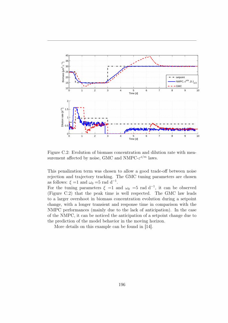
0 1 2 3 4 5 6 7 8 9 1010
15
20
25
30
35
40
Time [d]
Bio
mas
s [µ
m3 .L
−1 ]
0 1 2 3 4 5 6 7 8 9 100
0.5
1
1.5
2
Time [d]
Dilu
tion
rate
[d−
1 ]
setpoint
NMPC, εs/m, β J∆ D
GMC
Figure C.2: Evolution of biomass concentration and dilution rate with mea-surement affected by noise, GMC and NMPC-εs/m laws.
This penalization term was chosen to allow a good trade-off between noiserejection and trajectory tracking. The GMC tuning parameters are chosenas follows: ξ =1 and ω0 =5 rad d−1.For the tuning parameters ξ =1 and ω0 =5 rad d−1, it can be observed(Figure C.2) that the peak time is well respected. The GMC law leadsto a larger overshoot in biomass concentration evolution during a setpointchange, with a longer transient and response time in comparison with theNMPC performances (mainly due to the lack of anticipation). In the caseof the NMPC, it can be noticed the anticipation of a setpoint change due tothe prediction of the model behavior in the moving horizon.
More details on this example can be found in [14].
196
Bibliography
[1] J. Abdollahi and S. Dubljevic. Lipid production optimization and op-timal control of heterotrophic microalgae fed-batch bioreactor. Chem.Eng. Sci, 84:619–627, 2012.
[2] M. Alamir and G. Bornard. Stability of a truncated infinite constrainedreceding horizon scheme: the general discrete nonlinear case. Automat-ica, 31(9):1353–1356, 1995.
[3] F. Allgöwer and A. Zheng. Nonlinear Model Predictive Control.Progress in Systems and Control Theory. Birkhäuser Basel, 2012.
[4] J.C. Allwright. Advances in Model-Based Predictive Control, chapteron min-max Model-Based Predictive Control. Oxford University Press,1994.
[5] J.F. Andrews. A mathematical model for continuous culture of mi-croorganism utilizing inhibitory substrate. Biotechnology and Bioengi-neering, 10:707 – 723, 1968.
[6] D. Angeli, A. Casavola, and E. Mosca. Constrained predictive control ofnonlinear plants via polytopic linear system embedding. InternationalJournal of Robust and Nonlinear Control, 10(13):1091–1103, 2000.
[7] A. Ashoori, B. Moshiri, A. Khaki-Sedigh, and M. R. Bakhtiari. Opti-mal control of a nonlinear fed-batch fermentation process using modelpredictive approach. Journal of Process Control, 9:1162–1173, 2009.
[8] J. G. Balchen, D. Ljungquist, and S. Strand. State space model pre-dictive control of a multi stage electro-metallurgical process. Modeling,Identification and Control, 10(1):35–51, 1989.
[9] G. Bastin and D. Dochain. On-line estimation and adaptive control ofbioreactors. Elsevier, 1990.
197
[10] G. Becerra-Celis, G. Hafidi, S. Tebbani, and D. Dumur. Nonlinearpredictive control for continuous microalgae cultivation process in aphotobioreactor. Proc. of the 10th ICARV Conference, pages 1373–1378, 2008.
[11] G. Becerra-Celis, S. Tebbani, C. Joannis-Cassan, A. Isambert, andH. Siguerdidjane. Control strategy for continuous microalgae cultiva-tion process in a photobioreactor. Proc. of the 17th IEEE CCA, pages684–689, 2008.
[12] R. Bellman. The theory of dynamic programming. Bull. Amer. Math.Soc., 60(6):503–515, 11 1954.
[13] A. Bemporad, M. Morari, V. Dua, and E. N. Pistikopoulos. The explicitlinear quadratic regulator for constrained systems. Automatica, 38(1):3– 20, 2002.
[14] S. E. Benattia, S. Tebbani, and D. Dumur. Nonlinear model predictivecontrol for regulation of microalgae culture in a continuous photobiore-actor. Proc. of the 22nd MED Conference, pages 469–474, 2014.
[15] O. Bernard. Hurdles and challenges for modelling and control of mi-croalgae for CO2 mitigation and biofuel production. J. of Process Con-trol, 21(10):1378–1389, 2011.
[16] O. Bernard and J-L. Gouzé. Transient behavior of biological loop mod-els, with application to the droop model. Mathematical Biosciences,127, 1995.
[17] L. T. Biegler. Solution of dynamic optimization problems by succes-sive quadratic programming and orthogonal collocation. Computers &Chemical Engineering, 8(3–4):243–247, 1984.
[18] L.T. Biegler. An overview of simultaneous strategies for dynamic op-timization. Chemical Engineering and Processing: Process Intensifica-tion, 46(11):1043 – 1053, 2007.
[19] L.T. Biegler, X. Yang, and G.A.G Fischer. Advances in sensitivity-based nonlinear model predictive control and dynamic real time opti-mization. J. of Process Control, 30:104–116, 2015.
[20] R. Bitmead, V. Wertz, and M. Gevers. Adaptive Optimal Control: TheThinking Man’s GPC. Prentice Hall Professional Technical Reference,1991.
198
[21] E. Bourgeois, S. Tebbani, and A. Ramos Espinosa. Launcher atmo-spheric guidance based on nonlinear model predictive control. In GNC2014, pages CD–Rom, 2014.
[22] S. Boussiba and S. Leu. Microalgal biotechnology for environmental re-mediation. 7th European Workshop Biotechnology of Microalgae, 2007.
[23] S.P. Boyd and L. Vandenberghe. Convex Optimization. CambridgeUniversity Press, 2004.
[24] F. Breitenecker, A. Kugi, I. Troch, M. Benavides, D. Telen, J. Lauw-ers, F. Logist, J. Van Impe, and A. Vande Wouwer. Parameter iden-tification of the droop model using optimal experiment design. IFAC-PapersOnLine 8th Vienna International Conference on MathematicalModelling, 48(1):586 – 591, 2015.
[25] A.E. Bryson and Y.C. Ho. Applied Optimal Control: Optimization,Estimation and Control. Halsted Press book. Taylor & Francis, 1975.
[26] C. Büskens and H. Maurer. Online Optimization of Large Scale Sys-tems, chapter Sensitivity Analysis and Real-Time Control of Paramet-ric Optimal Control Problems Using Nonlinear Programming Methods,pages 57–68. Springer Berlin Heidelberg, Berlin, Heidelberg, 2001.
[27] E. F. Camacho and C. Bordons. Model Predictive Control. SpringerLondon, 2004.
[28] M. Cannon, D. Ng, and B. Kouvaritakis. Nonlinear Model PredictiveControl: Towards New Challenging Applications, chapter SuccessiveLinearization NMPC for a Class of Stochastic Nonlinear Systems, pages249–262. Springer Berlin Heidelberg, Berlin, Heidelberg, 2009.
[29] A. Casavola, D. Famularo, and G. Franze. Predictive control of con-strained nonlinear systems via LPV linear embedding. InternationalJournal of Robust and Nonlinear Control, 13:281–294, 2003.
[30] B. Chachuat, B. Srinivasan, and D. Bonvin. Adaptation strate-gies for real-time optimization. Computers & Chemical Engineering,33(10):1557 – 1567, 2009.
[31] C.C. Chen and L. Shaw. On receding horizon feedback control. Auto-matica, 18(3):349 – 352, 1982.
199
[32] H. Chen and F. Allgöwer. A quasi-infinite horizon nonlinear modelpredictive control scheme with guaranteed stability. Automatica,34(10):1205–1217, 1998.
[33] Y. Chisti. Biodiesel from microalgae. Biotechnology Advances, 25:294–306, 2007.
[34] P.D. Christofides, R. Scattolini, D. Muñoz de la Peña, and J. Liu. Dis-tributed model predictive control: A tutorial review and future researchdirections. Computers & Chemical Engineering, 51:21 – 41, 2013.
[35] D. W. Clarke. Application of generalized predictive control to industrialprocesses. IEEE Control Systems Magazine, 8(2):49–55, 1988.
[36] D.W. Clarke, C. Mohtadi, and P.S. Tuffs. Generalized predictivecontrol-Part I. the basic algorithm. Automatica, 23(2):137–148, 1987.
[37] D.E. Contois. Kinetics of bacterial growth: Relationship between pop-ulation density and specific growth rate of continuous cultures. Journalof General Microbiology, 21:40 – 50, 1959.
[38] P. Cougnon, D. Dochain, M. Guay, and M. Perrier. Online optimizationof fedbatch bioreactors by adaptive extremum seeking control. J. ofProcess Control, 21:1526–1532, 2011.
[39] J. Crassidis, F. Markley, T. C Anthony, and S. Andrews. Nonlinearpredictive control of spacecraft. Journal of Guidance, Control, andDynamics, 20(6):1096–1103, 1997.
[40] C.R. Cutler and B.C. Ramaker. Dynamic matrix control- a computercontrol algorithm. In Automatic Control Conference, 1980.
[41] R.M.C. De keyser and A.R. Van Cauwenberghe. Extended predictionself-adaptive control. In In IFAC Symp. on Identification and SystemParameter Estimation, pages 1317–1322, 1985.
[42] H. De la Hoz Siegler. Optimization of biomass and lipid production inheterotrophic microalgal cultures. University of Alberta, 2012.
[43] G. De Nicolao, L. Magni, and R. Scattolini. Stabilizing recedin-horizoncontrol of nonlinear time-varying systems. IEEE Transactions on Au-tomatic Control, 43(7):1030–1036, 1998.
200
[44] N. M.C. De Oliveira and L. T. Biegler. An extension of Newton-typealgorithms for nonlinear process control. Automatica, 31(2):281 – 286,1995.
[45] D. DeHaan and M. Guay. A new real-time perspective on non-linearmodel predictive control. Journal of Process Control, 16(6):615 – 624,2006.
[46] P. Deuflhard. A modified newton method for the solution of ill-conditioned systems of nonlinear equations with application to multipleshooting. Numerische Mathematik, 22(4):289–315.
[47] L. Dewasme, S. Fernandes, Z. Amribt, L.O. Santos, Ph. Bogaerts, andA. Vande Wouwer. State estimation and predictive control of fed-batchcultures of hybridoma cells. Journal of Process Control, 30:50 – 57,2015.
[48] C. Diaz, P. Dieu, C. Feuillerat, P. Lelong, and M. Salome. Adaptivepredictive control of dissolved oxygen concentration in a laboratory-scale bioreactor. J. of Biotechnol., 43:21–32, 1995.
[49] M. Diehl, R. Amrit, and J. B. Rawlings. A lyapunov function foreconomic optimizing model predictive control. IEEE Transactions onAutomatic Control, 56(3):703–707, 2011.
[50] M. Diehl, H. G. Bock, and J. P. Schlöder. A real-time iteration schemefor nonlinear optimization in optimal feedback control. SIAM Journalon Control and Optimization, 43(5):1714–1736, 2005.
[51] M. Diehl, H. J. Ferreau, and N. Haverbeke. Nonlinear Model PredictiveControl: Towards New Challenging Applications, chapter Efficient Nu-merical Methods for Nonlinear MPC and Moving Horizon Estimation,pages 391–417. Springer Berlin Heidelberg, Berlin, Heidelberg, 2009.
[52] D. Dochain. Automatic control of bioprocesses. Editor. John Wiley &Sons, 2008.
[53] D. Dochain and M. Perrier. Adaptive backstepping nonlinear control ofbioprocesses. 7th International Symposium, Advanced control of chem-ical processes, pages 77–82, 2004.
[54] D.Z. Du and P.M. Pardalos. Minimax and Applications. NonconvexOptimization and Its Applications. Springer US, 2013.
201
[55] C. Enzing, M. Ploeg, M. Barbosa, and L. Sijtsma. Microalgae-basedproducts for the food and feed sector: an outlook for Europe. Technicalreport, European comission, 2014.
[56] C.D.M. Filipe and C.P.L. Grady Jr. Biological Wastwater Treatment.Marcel Dekker, 1998.
[57] R. Findeisen, L. Imsland, F. Allgöwer, and B.A. Foss. State and outputfeedback nonlinear model predictive control: An overview. EuropeanJournal of Control, 9(2):190 – 206, 2003.
[58] C. E. García, D. M. Prett, and M. Morari. Model predictive control:Theory and practice-a survey. Automatica, 25(3):335 – 348, 1989.
[59] C.E. Garcia and M. Morari. Internal model control. a.
[60] A. Gautam, Y. C. Chu, and Y. C. Soh. Robust H∞ receding horizoncontrol for a class of coordinated control problems involving dynami-cally decoupled subsystems. IEEE Transactions on Automatic Control,59(1):134–149, 2014.
[61] G. Goffaux and A. Vande Wouwer. Design of a robust nonlinearreceding-horizon observer-Application to a biological system. Proc. ofthe 17th IFAC World Congress, pages 15553–15558, 2008.
[62] G. Goffaux and A. Vande Wouwer. Design of a Robust NonlinearReceding-Horizon Observer - First-Order and Second-Order Approxi-mations, pages 295–304. 2009.
[63] G. C. Goodwin, J. Østergaard, D. E. Quevedo, and A. Feuer. Nonlin-ear Model Predictive Control: Towards New Challenging Applications,chapter A Vector Quantization Approach to Scenario Generation forStochastic NMPC, pages 235–248. Springer Berlin Heidelberg, 2009.
[64] A. Grancharova, T. A. Johansen, and P. Tøndel. Explicit NonlinearModel Predictive Control. Springer Berlin Heidelberg, Berlin, Heidel-berg, 2007.
[65] E. Gyurkovics and A. M. Elaiw. Assessment and Future Directionsof Nonlinear Model Predictive Control, chapter Conditions for MPCBased Stabilization of Sampled-Data Nonlinear Systems Via Discrete-Time Approximations. Springer Berlin Heidelberg, 2007.
202
[66] E. Harinath, L.T. Biegler, and G. A. Dumont. Control and opti-mization strategies for thermo-mechanical pulping processes: Nonlinearmodel predictive control. Journal of Process Control, 21(4):519 – 528,2011.
[67] E. N. Hartley, J. L. Jerez, A. Suardi, J. M. Maciejowski, E. C. Kerrigan,and G. A. Constantinides. Predictive control using an FPGA withapplication to aircraft control. IEEE Transactions on Control SystemsTechnology, 22(3):1006–1017, 2014.
[68] R. Hermann and A. Krener. Nonlinear controllability and observability.IEEE Transactions on Automatic Control, 22(5):728–740, 1977.
[69] R. Huang, S. C. Patwardhan, and L. T. Biegler. Robust stability ofnonlinear model predictive control with extended Kalman filter andtarget setting. International Journal of Robust and Nonlinear Control,23:1240 – 1264, 2013.
[70] R. Huang, V. M. Zavala, and L. T. Biegler. Advanced step nonlinearmodel predictive control for air separation units. Journal of ProcessControl, 19(4):678 – 685, 2009.
[71] M. Huntley and D.G. Redalje. CO2 mitigation and renewable oil fromphotosynthetic microbes: A new appraisal. Mitigation and AdaptationStrategies for Global Change, 12:573–608, 2007.
[72] G. A. Ifrim, M. Titica, M. Barbu, L. Boillereaux, G. Cogne, S. Cara-man, and J. Legrand. Multivariable feedback linearizing control ofchlamydomonas reinhardtii photoautotrophic growth process in a torusphotobioreactor. Chem. Eng. J., 218:191–203, 2013.
[73] A. Isidori. Nonlinear Control Systems: An Introduction. Communica-tions and Control Engineering. Springer Berlin Heidelberg, 2013.
[74] A. Jadbabaie and J. Hauser. On the stability of receding horizon controlwith a general terminal cost. IEEE Transactions on Automatic Control,50(5):674–678, 2005.
[75] J. V. Kadam and W. Marquardt. Sensitivity-based solution updates inclosed-loop dynamic optimization; 1. ed. Elsevier, Oxford, 2005.
[76] A. Kasperski. Discrete Optimization with Interval Data: Minmax Re-gret and Fuzzy Approach. Studies in Fuzziness and Soft Computing.Springer Berlin Heidelberg, 2008.
203
[77] S. S. Keerthi and E. G. Gilbert. Optimal infinite-horizon feedback lawsfor a general class of constrained discrete-time systems: Stability andmoving-horizon approximations. Journal of Optimization Theory andApplications, 57(2):265–293.
[78] E. C. Kerrigan and J. Maciejowski. Feedback min-max model predictivecontrol using a single linear program: Robust stability and the explicitsolution. Int. J. Robust Nonlinear Control, 14:395–413, 2004.
[79] B. Kouvaritakis and M. Cannon, editors. Non-linear Predictive Control:Theory and Practice. Institution of Engineering and Technology, 2001.
[80] D. Kraft. Computational Mathematical Programming, chapter On Con-verting Optimal Control Problems into Nonlinear Programming Prob-lems, pages 261–280. Springer Berlin Heidelberg, Berlin, Heidelberg,1985.
[81] Y. Kuriki and T. Namerikawa. Formation control with collision avoid-ance for a multi-UAV system using decentralized MPC and consensus-based control. In 2015 European Control Conference (ECC), pages3079–3084, 2015.
[82] P. L. Lee and G. R. Sullivan. Generic model control (GMC). Comput.Chem. Eng., 12:6:573–580, 1988.
[83] M. A. Lelić and M. B. Zarrop. Generalized pole-placement self-tuningcontroller part 1, basic algorithm. International Journal of Control,46(2):547–568, 1987.
[84] W. C. Li and L. T. Biegler. Process control strategies for constrainednonlinear systems. Industrial & Engineering Chemistry Research,27(8):1421–1433, 1988.
[85] D. Limon, T. Alamo, and E. F. Camacho. Input-to-state stable MPCfor constrained discrete-time nonlinear systems with bounded additiveuncertainties. In Decision and Control, 2002, Proceedings of the 41stIEEE Conference on, volume 4, pages 4619–4624, 2002.
[86] D. Limon, T. Alamo, and E.F. Camacho. Robust stability of min-max MPC controllers for nonlinear systems with bounded uncertain-ties. Proceeding of the mathematical Theory of Networks and Systems,2004.
204
[87] D. Limon, T. Alamo, D. M. Raimondo, D. Muñoz Peña, J. M. Bravo,A. Ferramosca, and E. F. Camacho. Nonlinear Model Predictive Con-trol: Towards New Challenging Applications, chapter Input-to-StateStability: A Unifying Framework for Robust Model Predictive Con-trol, pages 1–26. Springer Berlin Heidelberg, Berlin, Heidelberg, 2009.
[88] D. Limon, T. Alamo, F. Salas, and E.F. Camacho. Input to state sta-bility of min-max MPC controllers for nonlinear systems with boundeduncertainties. Automatica, 42(5):797 – 803, 2006.
[89] D. A. Linkers and M. Mahfonf. Advances in Model-Based PredictiveControl, chapter Generalized Predictive Control in Clinical Anesthesia.Oxford University Press, 1994.
[90] J.M. Maciejowski. Predictive Control: With Constraints. Prentice Hall,2002.
[91] L. Magni, G. De Nicolao, R. Scattolini, and F. Allgöwer. Robust modelpredictive control for nonlinear discrete time systems. InternationalJournal of Robust and Nonlinear Control, 13:229–246, 2003.
[92] L. Magni and R. Scattolini. Stabilizing decentralized model predictivecontrol of nonlinear systems. Automatica, 42(7):1231 – 1236, 2006.
[93] L. Magni and R. Scattolini. Assessment and Future Directions of Non-linear Model Predictive Control, chapter Robustness and Robust Designof MPC for Nonlinear Discrete-Time Systems, pages 239–254. SpringerBerlin Heidelberg, 2007.
[94] L. Magni and R. Scattolini. Robustness and robust design of MPC fornonlinear discrete-time systems, volume 358. Springer-Verlag, 2007.
[95] L. Magni and R. Sepulchre. Stability margins of nonlinear receding-horizon control via inverse optimality. Systems & Control Letters,32(4):241 – 245, 1997.
[96] L. Mailleret, O. Bernard, and J. P. Steyer. Nonlinear adaptive con-trol for bioreactors with unknown kinetics. Automatica, 40:1379–1385,2004.
[97] N. I. Marcos, M. Guay, and D. Dochain. Output feedback adaptiveextremum seeking control of a continuous stirred tank bioreactor withmonod’s kinetics. J. of Process Control, 14:807–818, 2004.
205
[98] P. Masci, F. Grognard, and O. Bernard. Microalgal biomass surfaceproductivity optimization based on a photobioreactor model. In 11thIFAC Symposium on Computer Applications in Biotechnology, pages180–185, 2010.
[99] D.Q. Mayne. Control of constrained dynamic systems. European Jour-nal of Control, 7:87–99, 2001.
[100] D.Q. Mayne, J.B. Rawlings, C.V. Rao, and P.O.M. Scokaert. Con-strained model predictive control: Stability and optimality. Automat-ica, 36:789–814, 2000.
[101] F.B. Metting. Biodiversity and application of microalgae. J. of Ind.Microbiology & Biotechnology, 17:477–489, 1996.
[102] H. Michalska and D. Q. Mayne. Robust receding horizon control of con-strained nonlinear systems. IEEE Transactions on Automatic Control,38(11):1623–1633, 1993.
[103] J. Monod. Recherches sur la croissance des cultures bactériennes. Ac-tualités scientifiques et industrielles. Hermann, 1958.
[104] M. Morari and P.J. Campo. Robust model predictive control. In Amer-ican Control Conference, pages 1021–1026, 1987.
[105] M. Morari and J. H. Lee. Model predictive control: past, present andfuture. Computers & Chemical Engineering, 23(4):667–682, 1999.
[106] E. Mosca, J. M. Lemos, and J. Zhang. Stabilizing I/O receding horizoncontrol. In Decision and Control, 1990., Proceedings of the 29th IEEEConference on, volume 4, pages 2518–2523, 1990.
[107] R. Munoz-Tamayo, P. Martinon, G. Bougaran, F. Mairet, andO. Bernard. Getting the most out of it: optimal experiments for pa-rameter estimation of microalgae growth models. J. of Process Control,24(6):991–1001, 2014.
[108] Z. K. Nagy and R. D. Braatz. Robust nonlinear model predictive controof fedbatches processes. AIChE Journal, 49(7):1776–1786, 2009.
[109] X. M. Nguyen, F. Lawayeb, P. Rodriguez-Ayerbe, D. Dumur, andA. Mouchette. Nonlinear model predictive control of steel slab walking-beam reheating furnace based on a numerical model. In Proc. of the2014 IEEE MSC, pages 191–196, 2014.
206
[110] J. E. Normey-Rico, J. Gómez-Ortega, and E. F. Camacho. A smith-predictor-based generalised predictive controller for mobile robot path-tracking. Control Engineering Practice, 7(6):729–740, 1999.
[111] M. Olaizola. Commercial development of microalgal biotechnology:from the test tube to the marketplace. Biomolecular Eng., 20:459–466,2003.
[112] S. Olaru and D. Dumur. A parameterized polyhedra approach forexplicit constrained predictive control. In 43rd IEEE Conference onDecision and Control, volume 2, pages 1580–1585 Vol.2, 2004.
[113] T. Parisini and R. Zoppoli. A receding-horizon regulator for nonlinearsystems and a neural approximation. Automatica, 31(10):1443 – 1451,1995.
[114] J. C. H. Peeters and P. H. C. Eilers. The relationship between light in-tensity and photosynthesis. Hydrobiological Bulletin, 12:134–136, 1978.
[115] G. Pin, D.M. Raimondo, L. Magni, and T. Parisini. Robust model pre-dictive control of nonlinear systems with bounded and state-dependentuncertainties. IEEE Trans. on Auto. Cont., 54(7):1681–1687, 2009.
[116] L.S Pontryagin, V.G. Boltyanskii, R.V. Gamkrelidze, , and E.F.Mishchenko. The Mathematical Theory of Optimal Processes. NewYork, 1964.
[117] A. I. Propoi. Automn Remote Control, 24, 1963.
[118] S.J. Qin and T.A. Badgwell. A survey of industrial model predictivecontrol technology. Control Engineering Practice, 11:733–764, 2003.
[119] D.M. Raimondo, D. Limon, T. Alamo, and L. Magni. Robust ModelPredictive Control Algorithms for Nonlinear Systems: An Input-to-State Stability Approach. Model Predictive Control, Tao Zheng (Ed.),2010.
[120] D.M. Raimondo, D. Limon, M. Lazar, L. Magni, and E.F. Camachp.Min-max model predictive control of nonlinear systems: A unifyingoverview on stability. European Journal of Control, 5:5–21, 2009.
[121] R. Ramine and K. M. Raman. Model algorithmic control (MAC); basictheoretical properties. Automatica, 18(4):401 – 414, 1982.
207
[122] J. B. Rawlings and K. R. Muske. The stability of constrained re-ceding horizon control. IEEE Transactions on Automatic Control,38(10):1512–1516, 1993.
[123] J.B. Rawlings and D.Q. Mayne. Model Predictive Control: Theory andDesign. Nob Hill Pub., 2009.
[124] L.D. Re, F. Allgöwer, L. Glielmo, C. Guardiola, and I. Kolmanovsky.Automotive Model Predictive Control: Models, Methods and Applica-tions. Springer London, 2010.
[125] J. Richalet. Pratique de la commande prédictive. Hermes, 1992.
[126] J. Richalet. Industrial applications of model based predictive control.Automatica, 29(5):1251 – 1274, 1993.
[127] J. Richalet, S. Abu el Ata-Doss, C. Arber, H.B. Kuntze, A. Jacubash,and W. Schill. Predictive functional control application to fast andaccurate robots. In In Proc. 10th IFAC Congress, 1987.
[128] J. Richalet, A. Rault, J.L. Testud, and J. Papon. Algorithmic controlof industrial processes. In 4th IFAC Symposium on Identification andSystem Parameter Estimation, 1976.
[129] J. Richalet, A. Rault, J.L. Testud, and J. Papon. Model predictiveheuristic control: Application to industrial processes. Automatica,14(2):413–428, 1978.
[130] J. A. Rossiter and B. Kouvaritakis. Constrained stable generalised pre-dictive control. IEE Proceedings D - Control Theory and Applications,140(4):243–254, 1993.
[131] M. Rugabotti, D.M. Raimondo, A. Ferrara, and L. Magni. Robustmodel predictive control of continuous-time sampled data nonlinearsystems with interval sliding mode. IEEE Transaction on AutomaticControl, 56(3):556–570, 2010.
[132] J.M.M. Sánchez and J. Rodellar. Adaptive Predictive Control: Fromthe Concepts to Plant Optimization. Prentice-Hall international seriesin systems and control engineering. Prentice Hall, 1996.
[133] F.L. Santamaria and J.M. Gómez. Economic oriented nmpc for anextractive distillation column using an index hybrid dae model based onfundamental principles. Industrial & Engineering Chemistry Research,54(24):6344–6354, 2015.
208
[134] L.O. Santos, L. Dewasme, D. Coutinho, and A. Vande Wouwer. Non-linear model predictive control of fed-batch cultures of micro-organismsexhibiting overflow metabolism: Assessment and robustness. Comput-ers & Chemical Engineering, 39:143 – 151, 2012.
[135] A. H. Sayed, V. H. Nascimento, and F. A. M. Cipparrone. A regularizedrobust design criterion for uncertain data. SIAM J. MAT. ANAL.APPL., 32:4:1120–1142, 2002.
[136] R. Scattolini. Architectures for distributed and hierarchical model pre-dictive control-A review. Journal of Process Control, 19(5):723 – 731,2009.
[137] P.O.M. Scokaert, D.Q. Mayne, and J.B. Rawlings. Suboptimal modelpredictive control (feasibility implies stability). IEEE Transactions onAutomatic Control, 44(3):648–654, 1999.
[138] D. Selisteanu, E. Petre, and V. Rasvan. Sliding mode and adaptivesliding mode control of a class of nonlinear bioprocesses. Inter. J. ofAdap. Contr. and Sig. Proc., 21:795–822, 2007.
[139] E.D. Sontag. Smooth stabilization implies coprime factorization. IEEETransactions on Automatic Control, 34(4):435–443, 1989.
[140] P. Spolaore, C. Joannis-Cassan, E. Duran, and A. Isambert. Commer-cial applications of microalgae. J Biosci. Bioeng., 101:87–96, 2006.
[141] S. Tebbani, D. Dumur, G. Hafidi, and A. Vande Wouwer. NonlinearPredictive Control of fed-batch Cultures of E. coli. Chem. Eng. &Tech., 33:1112–1124, 2010.
[142] S. Tebbani, F. Lopes, and G. Becerra-Celis. Nonlinear control of contin-uous cultures of Porphyridium purpureum in a photobioreactor. Chem.Eng. Sci., 123:207–219, 2015.
[143] S. Tebbani, F. Lopes, R. Filali, D. Dumur, and D. Pareau. Nonlinearpredictive control for maximization of CO2 bio-fixation by microalgaein a photobioreactor. Bioprocess Biosyst. Eng., 37:83–97, 2014.
[144] S. Tebbani, M. Titica, C. Join, M. Fliess, and D. Dumur. Model-basedversus model-free control designs for improving microalgae growth in aclosed photobioreactor: Some preliminary comparisons. In 22nd MEDConference, pages –, 2016.
209
[145] M. K. Toroghi, G. Goffaux, and M. Perrier. Observer based backstep-ping controller for microalgae cultivation. Ind. & Eng. Chem. Res.,52:7482–7491, 2013.
[146] V. Utkin and J. Shi. Integral sliding mode in systems operating underuncertainty conditions. Proc. of the 35th Conference on Decision andControl, 4:4591–4596, 1996.
[147] V.S. Vassiliadis. Computational solution of dynamic optimization prob-lems with general differential algebric constraints. PhD thesis, Univer-sity of London, 1993.
[148] Z. Y. Wan and M. V. Kothare. Efficient scheduled stabilizing outputfeedback model predictive control for constrained nonlinear systems.IEEE Transactions on Automatic Control, 49(10):1172–1177, 2004.
[149] L. Wang. Model Predictive Control System Design and ImplementationUsing MATLAB R©. Advances in Industrial Control. Springer, 2009.
[150] R. Wang, G. P. Liu, W. Wang, D. Rees, and Y. B. Zhao. h∞ controlfor networked predictive control systems based on the switched lya-punov function method. IEEE Transactions on Industrial Electronics,57(10):3565–3571, 2010.
[151] R. Wang, B. Wang, G. P. Liu, W. Wang, and D. Rees. h∞ controllerdesign for networked predictive control systems based on the averagedwell-time approach. IEEE Transactions on Circuits and Systems II:Express Briefs, 57(4):310–314, 2010.
[152] L. Wurth, R. Hannemann, and W Marquardt. Neighboring-extremalupdates for nonlinear model-predictive control and dynamic real-timeoptimization. Journal of Process Control, 19(8):1277 – 1288, 2009.
[153] B.E. Ydstie. Extended horizon adaptive control. In In Proc. 9th IFACWorld Congress, 1984.
[154] L.A. Zadeh and B.H. Whalen. On optimal contro and linear program-ming. IRE Trans. Aut. Control, 7(4):729 – 740, 1962.
[155] J. Zarate Florez, J.J. Martinez, G. Besancon, and D. Faille. Explicit co-ordination for mpc-based distributed control with application to hydro-power valleys. In 2011 50th IEEE Conference on Decision and Controland European Control Conference, pages 830–835, 2011.
210

[156] V. M. Zavala and L. T. Biegler. The advanced-step NMPC controller:Optimality, stability and robustness. Automatica, 45(1):86 – 93, 2009.
[157] A. Zheng and M. Morari. Stability of model predictive control withsoft constraints. Internal Report. California Institute of Technology,7(4):729 – 740, 1994.
211
Université Paris-Saclay Espace Technologique / Immeuble Discovery Route de l’Orme aux Merisiers RD 128 / 91190 Saint-Aubin, France
Titre : Robustification de la commande prédictive non linéaire - Application à des procédés pour le
développement durable
Mots clés : Commande prédictive non linéaire, Robustesse, Systèmes incertains, Bioprocédé
Résumé : Les dernières années ont permis des
développements très rapides, tant au niveau de
l'élaboration que de l'application, d’algorithmes de
commande prédictive non linéaire (CPNL), avec
une gamme relativement large de réalisations
industrielles. Un des obstacles les plus
significatifs rencontré lors du développement de
cette commande est lié aux incertitudes sur le
modèle du système. Dans ce contexte, l’objectif
principal de cette thèse est la conception de lois de
commande prédictives non linéaires robustes vis-
à-vis des incertitudes sur le modèle.
Classiquement, cette synthèse peut s’obtenir via la
résolution d’un problème d’optimisation min-max.
L’idée est alors de minimiser l’erreur de suivi de
la trajectoire optimale pour la pire réalisation
d'incertitudes possible. Cependant, cette
formulation de la commande prédictive robuste
induit une complexité qui peut être élevée ainsi
qu’une charge de calcul importante, notamment
dans le cas de systèmes multivariables, avec un
nombre de paramètres incertains élevé. Pour y
remédier, la principale approche proposée dans
ces travaux consiste à simplifier le problème
d'optimisation min-max, via l’analyse de
sensibilité du modèle vis-à-vis de ses paramètres
afin d'en réduire le temps de calcul. Dans un
premier temps, le critère est linéarisé autour des
valeurs nominales des paramètres du modèle. Les
variables d'optimisation sont soit les commandes
du système soit l'incrément de commande sur
l'horizon temporel. Le problème d'optimisation
initial est alors transformé soit en un problème
convexe, soit en un problème de minimisation
unidimensionnel, en fonction des contraintes
imposées sur les états et les commandes. Une
analyse de la stabilité du système en boucle
fermée est également proposée. En dernier lieu,
une structure de commande hiérarchisée
combinant la commande prédictive robuste
linéarisée et une commande par mode glissant
intégral est développée afin d'éliminer toute erreur
statique en suivi de trajectoire de référence.
L'ensemble des stratégies proposées est appliqué à
deux cas d'études de commande de bioréacteurs de
culture de microorganismes.
Title : Robustification of Nonlinear Model Predictive Control - Application to sustainable development
processes
Keywords : Nonlinear model predictive control, Robustness, Uncertain Systems, Bioprocess
Abstract : The last few years have led to very
rapid developments, both in the formulation and
the application of Nonlinear Model Predictive
Control (NMPC) algorithms, with a relatively
wide range of industrial achievements. One of the
most significant challenges encountered during the
development of this control law is due to
uncertainties in the model of the system. In this
context, the thesis addresses the design of NMPC
control laws robust towards model uncertainties.
Usually, the above design can be achieved through
solving a min-max optimization problem. In this
case, the idea is to minimize the tracking error for
the worst possible uncertainty realization.
However, this robust approach tends to become
too complex to be solved numerically online,
especially in the case of multivariable systems
with a large number of uncertain parameters. To
address this shortfall, the main proposed approach
consists in simplifying the min-max optimization
problem through a sensitivity analysis of the
model with respect to its parameters, in order to
reduce the calculation time. First, the criterion is
linearized around the model parameters nominal
values. The optimization variables are either the
system control inputs or the control increments
over the prediction horizon. The initial
optimization problem is then converted either into
a convex optimization problem, or a one-
dimensional minimization problem, depending on
the nature of the constraints on the states and
commands. The stability analysis of the closed-
loop system is also addressed. Finally, a
hierarchical control strategy is developed, that
combines a robust model predictive control law
with an integral sliding mode controller, in order
to cancel any tracking error. The proposed
approaches are applied through two case studies to
the control of microorganisms culture in
bioreactors.
Related Documents