Thèse de Doctorat Mention Sciences et technologies de l’information et de la communication Spécialité Informatique, Automatique présentée à l’École Doctorale en Sciences Technologie et Santé (ED 585) de l’Université du Littoral Côte d’Opale par Farouk YAHAYA pour obtenir le grade de Docteur de l’Université du Littoral Côte d’Opale Compressive informed (semi-)non-negative matrix factorization methods for incomplete and large-scale data, with application to mobile crowd-sensing data Soutenue le 19/11/2021, après avis des rapporteurs, devant le jury d’examen : M. R. Boyer, Professeur, Université de Lille Président M. A. Ferrari, Professeur, Université Côte d’Azur Rapporteur M. O. Michel, Professeur, Grenoble–INP Rapporteur M me E. Chouzenoux, Chargée de recherche HDR, Inria Examinatrice M. G. Roussel, Professeur, Université du Littoral Côte d’Opale Directeur de thèse M. M. Puigt, Maître de conférences, Université du Littoral Côte d’Opale Co-encadrant M. G. Delmaire, Maître de conférences, Université du Littoral Côte d’Opale Invité

Welcome message from author
This document is posted to help you gain knowledge. Please leave a comment to let me know what you think about it! Share it to your friends and learn new things together.
Transcript
Thèse de Doctorat
Mention Sciences et technologies de l’information et de la communicationSpécialité Informatique, Automatique
présentée à l’École Doctorale en Sciences Technologie et Santé (ED 585)
de l’Université du Littoral Côte d’Opale
par
Farouk YAHAYA
pour obtenir le grade de Docteur de l’Université du Littoral Côte d’Opale
Compressive informed (semi-)non-negative matrixfactorization methods for incomplete and large-scale data, with
application to mobile crowd-sensing data
Soutenue le 19/11/2021, après avis des rapporteurs, devant le jury d’examen :
M. R. Boyer, Professeur, Université de Lille PrésidentM. A. Ferrari, Professeur, Université Côte d’Azur RapporteurM. O. Michel, Professeur, Grenoble–INP RapporteurMme E. Chouzenoux, Chargée de recherche HDR, Inria ExaminatriceM. G. Roussel, Professeur, Université du Littoral Côte d’Opale Directeur de thèseM. M. Puigt, Maître de conférences, Université du Littoral Côte d’Opale Co-encadrantM. G. Delmaire, Maître de conférences, Université du Littoral Côte d’Opale Invité

2
Thèse de Doctorat
Mention Sciences et technologies de l’information et de la communicationSpécialité Informatique, Automatique
présentée à l’École Doctorale en Sciences Technologie et Santé (ED 585)
de l’Université du Littoral Côte d’Opale
par
Farouk YAHAYA
pour obtenir le grade de Docteur de l’Université du Littoral Côte d’Opale
Méthodes étendues de factorisation informée de matrices outenseurs (semi-)non-négatifs pour l’analyse de données
incomplètes et de grande dimension. Application au traitementde données issues du mobile crowdsensing
Soutenue le 19/11/2021, après avis des rapporteurs, devant le jury d’examen :
M. R. Boyer, Professeur, Université de Lille PrésidentM. A. Ferrari, Professeur, Université Côte d’Azur RapporteurM. O. Michel, Professeur, Grenoble–INP RapporteurMme E. Chouzenoux, Chargée de recherche HDR, Inria ExaminatriceM. G. Roussel, Professeur, Université du Littoral Côte d’Opale Directeur de thèseM. M. Puigt, Maître de conférences, Université du Littoral Côte d’Opale Co-encadrantM. G. Delmaire, Maître de conférences, Université du Littoral Côte d’Opale Invité

2
Abstract
Air pollution poses substantial health issues with several hundred thousands of premature deaths
in Europe each year. Effective air quality monitoring is thus an major task for environmental
agencies. It is usually carried out by some highly accurate monitoring stations. However, these
stations are expensive and limited in number, thus providing a low spatio-temporal resolution. The
deployment of low-cost sensors (LCS) promises a complementary solution with lower cost and
higher spatio-temporal resolution. Unfortunately, LCS tend to drift over time and their high number
prevents regular in-lab calibration. Data-driven techniques named in-situ calibration have thus
been proposed. In particular, revisiting mobile sensor calibration as a matrix factorization problem
seems promising. However, existing approaches are based on slow methods—and are not suited for
large-scale problems involving hundreds of sensors deployed over a large area—and are designed
for short-term deployments. To solve both issues, compressive non-negative matrix factorization
have been proposed in this thesis, which is divided into two parts. In the first part, we investigate the
enhancement provided by random projections for weighted non-negative matrix factorization. We
show that these techniques can significantly speed-up large-scale and low-rank matrix factorization
methods, thus allowing the fast estimation of missing entries in low-rank matrices. In the second
part, we revisit mobile heterogeneous sensor calibration as an informed factorization of large
matrices with missing entries. We thus propose fast informed matrix factorization approaches, and
in particular informed extensions of compressive methods proposed in the first part, which are found
to be well-suited for the considered problem.
Keywords: Compressive learning; Random projections; Big data; Matrix factorization; Missing
data estimation; In situ sensor calibration; Mobile crowdsensing.
3
Résumé
La pollution de l’air pose d’importants problèmes de santé avec plusieurs centaines de milliers de
décès prématurés en Europe chaque année. Une surveillance efficace de la qualité de l’air est donc
une tâche majeure pour les agences environnementales. Elle est généralement effectuée par des
stations de surveillance très précises. Cependant, ces stations sont coûteuses et en nombre limité,
offrant ainsi une faible résolution spatio-temporelle. Le déploiement de capteurs low-cost (LCS)
promet une solution complémentaire à moindre coût et à plus haute résolution spatio-temporelle.
Malheureusement, les LCS ont tendance à dériver avec le temps et leur nombre élevé empêche un
étalonnage régulier en laboratoire. Des techniques basées sur les données nommées étalonnage
in situ ont ainsi été proposées. En particulier, revisiter l’étalonnage des capteurs mobiles comme
un problème de factorisation matricielle semble prometteur. Cependant, les approches existantes
sont basées sur des méthodes lentes – elles ne sont pas adaptées aux problèmes à grande échelle
impliquant des centaines de capteurs déployés sur une vaste zone – et sont conçues pour des
déploiements à court terme. Pour résoudre ces deux problèmes, des factorisations matricielles
non-négatives comprimées ont été proposées dans cette thèse, qui est divisée en deux parties.
Dans la première partie, nous étudions l’amélioration apportée par les projections aléatoires pour
la factorisation matricielle non-négative pondérée. Nous montrons que ces techniques peuvent
accélérer considérablement les méthodes de factorisation matricielle à grande échelle et de faible
rang, permettant ainsi l’estimation rapide des entrées manquantes dans les matrices de faible rang.
Dans la deuxième partie, nous revisitons l’étalonnage de capteurs hétérogènes mobiles comme
une factorisation informée de grandes matrices avec des entrées manquantes. Nous proposons
ainsi des approches de factorisation matricielle informées rapides, et en particulier des extensions
informées des méthodes comprimées proposées dans la première partie, qui s’avèrent bien adaptées
au problème considéré.
Mots clés : Apprentissage comprimé ; Projections aléatoires ; Données massives ; Factorisation
matricielle ; Estimation de données manquantes ; Étalonnage in situ de capteurs ; Mobile crowdsens-
ing.
4

5

Dedication
I dedicate this dissertation to my parents Dr. Yahaya Adam and Fati Mahama Kuyini, and also to
my siblings Dr. Shekira, Muiz and Ziad for their endless love, support and encouragement.
6

Acknowledgements
First of all I would say Alhamdulillah, for a successful realization of this milestone. Several
individuals have contributed one way or the other in the realization of this PhD thesis and for that I
am extremely thankful.
Let me start with Pr. Gilles Roussel. I’m deeply grateful for your support both professionally
and unprofessionally. From the first day you picked me up from the train station to my dormitory
through to the end of my studies in Calais. I thank you for your kind words of encouragement,
constructive criticisms and explanations of concepts related to my topic.
My utmost gratitude goes to Assoc. Pr. Matthieu Puigt. Indeed, no words can explain my
gratitude for all the assistance you gave me throughout the three years working under your research
guidance. Your painstaking attention to detail, constructive criticisms and encouragement have
hugely impacted me in a lot of positive ways. I have become a better researcher under your
supervision and anyone would be lucky to be your student. For that, I say a big thank you from the
bottom of my heart.
A word of thanks and appreciation also goes out to Gilles Delmaire for all his collaborations in
our research work. his comments and inputs on all the projects we have worked together on were
very useful.
I would like to also thank the members of the thesis committee, Pr. André Ferrari, Pr. Olivier.
Michel, Pr. Rémy Boyer, and Dr. Emilie Chouzenoux for taking a leaf from their busy schedule and
accepting to review my thesis work. I greatly appreciate your insightful comments, suggestions and
constructive criticisms which has hugely improved the thesis.
Thank you to the LISIC Secretariat office, Gaëlle and Isabelle for all the help they gave me
relating to administrative activities. They made things easier than they normally are and made sure I
had all items in check to ensure a smooth continuation of my studies every year. I also thank my
friends and office colleagues, Samah, Pierre, Hiba, Ali, Williams, Hamza, and Pamela for providing
a conducive environment where we interact and share ideas relating to science.
A special wholehearted appreciation and gratitude to my family for their support. I could not
have reached this far without them. Due to their love and prayers, I have been able to achieve this
7

milestone.
Lastly, I thank the Région Hauts-de-France for partly funding my Ph.D. fellowship. Experiments
presented in this thesis were carried out using the CALCULCO computing platform, supported by
SCoSI/ULCO.
8

Contents
List of Figures 18
List of Tables 19
List of Algorithms 20
List of Acronyms 21
Mathematical Notations 24
Résumé étendu 26
List of the Author’s Publications and Communications During the Ph.D Thesis 44
1 General Introduction 461.1 General Framework . . . . . . . . . . . . . . . . . . . . . . . . . . . . . . . . . . 46
1.2 Thesis Motivation and Objectives . . . . . . . . . . . . . . . . . . . . . . . . . . . 47
1.2.1 Accelerated Methods . . . . . . . . . . . . . . . . . . . . . . . . . . . . . 48
1.2.2 Multiple Scene Scenario . . . . . . . . . . . . . . . . . . . . . . . . . . . 49
1.3 Thesis Structure . . . . . . . . . . . . . . . . . . . . . . . . . . . . . . . . . . . . 49
2 State of the Art on Sensor Calibration 522.1 Introduction . . . . . . . . . . . . . . . . . . . . . . . . . . . . . . . . . . . . . . 52
2.2 The why of low cost sensors . . . . . . . . . . . . . . . . . . . . . . . . . . . . . 54
2.3 Types of Sensors . . . . . . . . . . . . . . . . . . . . . . . . . . . . . . . . . . . 55
2.3.1 Particulate Matter Sensors . . . . . . . . . . . . . . . . . . . . . . . . . . 56
2.3.2 Gas sensors . . . . . . . . . . . . . . . . . . . . . . . . . . . . . . . . . . 56
2.3.2.1 Solid-state Gas Sensor . . . . . . . . . . . . . . . . . . . . . . . 57
2.3.2.2 Electrochemical Gas Sensor . . . . . . . . . . . . . . . . . . . . 57
9
2.4 Error Sources . . . . . . . . . . . . . . . . . . . . . . . . . . . . . . . . . . . . . 57
2.4.1 Internal Errors . . . . . . . . . . . . . . . . . . . . . . . . . . . . . . . . 57
2.4.2 External Errors . . . . . . . . . . . . . . . . . . . . . . . . . . . . . . . . 58
2.5 Key Aspects of Sensor Calibration . . . . . . . . . . . . . . . . . . . . . . . . . . 58
2.5.1 Models for Calibration . . . . . . . . . . . . . . . . . . . . . . . . . . . . 59
2.5.1.1 Single variable without time . . . . . . . . . . . . . . . . . . . . 60
2.5.1.2 Single variable with time . . . . . . . . . . . . . . . . . . . . . 60
2.5.1.3 Multiple variables without time . . . . . . . . . . . . . . . . . . 61
2.5.1.4 Multiple variables with time . . . . . . . . . . . . . . . . . . . . 62
2.5.2 In Situ Calibration Strategies . . . . . . . . . . . . . . . . . . . . . . . . . 62
2.5.2.1 Macro-calibration . . . . . . . . . . . . . . . . . . . . . . . . . 63
2.5.2.2 Micro-calibration . . . . . . . . . . . . . . . . . . . . . . . . . 64
2.5.2.3 Calibration Transfer . . . . . . . . . . . . . . . . . . . . . . . . 66
2.5.3 Calibration Methods . . . . . . . . . . . . . . . . . . . . . . . . . . . . . 67
2.5.3.1 Least Square Methods . . . . . . . . . . . . . . . . . . . . . . . 67
2.5.3.2 Neural Networks . . . . . . . . . . . . . . . . . . . . . . . . . . 68
2.5.3.3 Other Machine Learning techniques . . . . . . . . . . . . . . . 69
2.6 Discussion . . . . . . . . . . . . . . . . . . . . . . . . . . . . . . . . . . . . . . . 69
I Randomized (Weighted) Non-negative Matrix Factorization 71
3 Non-negative Matrix Factorization (NMF) 723.1 Background . . . . . . . . . . . . . . . . . . . . . . . . . . . . . . . . . . . . . 74
3.1.1 Applications . . . . . . . . . . . . . . . . . . . . . . . . . . . . . . . . . 75
3.1.2 Challenges . . . . . . . . . . . . . . . . . . . . . . . . . . . . . . . . . . 77
3.1.2.1 NP-hardness . . . . . . . . . . . . . . . . . . . . . . . . . . . . 77
3.1.2.2 Initialization . . . . . . . . . . . . . . . . . . . . . . . . . . . . 78
3.1.2.3 Ill-posedness . . . . . . . . . . . . . . . . . . . . . . . . . . . . 78
3.1.2.4 Choice of the NMF rank k . . . . . . . . . . . . . . . . . . . . . 79
3.1.2.5 Stopping Criteria and Stationary Points . . . . . . . . . . . . . 79
3.1.2.6 Uniqueness of NMF . . . . . . . . . . . . . . . . . . . . . . . . 80
3.2 Classical NMF Cost Functions . . . . . . . . . . . . . . . . . . . . . . . . . . . . 80
3.2.1 Discrepancy Measures . . . . . . . . . . . . . . . . . . . . . . . . . . . . 80
3.2.1.1 The Frobenius Norm . . . . . . . . . . . . . . . . . . . . . . . . 81
10
3.2.1.2 The Kullback-Leibler Divergence . . . . . . . . . . . . . . . . . 81
3.2.1.3 The Itakura-Saito Divergence . . . . . . . . . . . . . . . . . . . 81
3.2.1.4 Parametric Divergences . . . . . . . . . . . . . . . . . . . . . . 82
3.2.1.5 Weighted Models . . . . . . . . . . . . . . . . . . . . . . . . . 83
3.2.1.6 Equality and Bound Constraints . . . . . . . . . . . . . . . . . . 83
3.2.1.7 Structural Constraints . . . . . . . . . . . . . . . . . . . . . . . 84
3.2.2 Regularization for NMF . . . . . . . . . . . . . . . . . . . . . . . . . . . 85
3.2.2.1 Smoothness Regularization . . . . . . . . . . . . . . . . . . . . 85
3.2.2.2 Sparsity-promoting Regularization . . . . . . . . . . . . . . . . 86
3.2.2.3 Graph / Manifold Regularization . . . . . . . . . . . . . . . . . 86
3.2.2.4 Smooth Evolution Constraint . . . . . . . . . . . . . . . . . . . 87
3.2.2.5 Volume Constraint . . . . . . . . . . . . . . . . . . . . . . . . . 87
3.3 NMF Optimization Strategies . . . . . . . . . . . . . . . . . . . . . . . . . . . . . 87
3.3.1 Standard Nonlinear Optimization Schemes . . . . . . . . . . . . . . . . . 88
3.3.1.1 BCD with Two Matrix Blocks: . . . . . . . . . . . . . . . . . . 88
3.3.1.2 BCD with 2k Vector Blocks: . . . . . . . . . . . . . . . . . . . 89
3.3.2 Separable Schemes . . . . . . . . . . . . . . . . . . . . . . . . . . . . . . 89
3.4 Classical NMF Algorithms . . . . . . . . . . . . . . . . . . . . . . . . . . . . . . 90
3.4.1 Multiplicative Updates (MU) . . . . . . . . . . . . . . . . . . . . . . . . . 90
3.4.1.1 Majorization Minimization . . . . . . . . . . . . . . . . . . . . 90
3.4.1.2 Heuristic Approach . . . . . . . . . . . . . . . . . . . . . . . . 91
3.4.2 Projected Gradient (PG) . . . . . . . . . . . . . . . . . . . . . . . . . . . 92
3.4.3 Alternating Least Squares (ALS) . . . . . . . . . . . . . . . . . . . . . . . 93
3.4.4 Alternating Non-negative Least Squares (ANLS) . . . . . . . . . . . . . . 93
3.4.5 Hierarchical Alternating Least Squares (HALS) . . . . . . . . . . . . . . 94
3.5 Extensions of NMF . . . . . . . . . . . . . . . . . . . . . . . . . . . . . . . . . . 95
3.5.1 Semi-Non-negative Matrix Factorization . . . . . . . . . . . . . . . . . . 95
3.5.2 Non-negative Matrix Co-Factorization . . . . . . . . . . . . . . . . . . . . 95
3.5.3 Multi-layered and Deep (Semi-)NMF . . . . . . . . . . . . . . . . . . . . 97
3.6 Discussion . . . . . . . . . . . . . . . . . . . . . . . . . . . . . . . . . . . . . . . 97
4 Accelerating non-Negative Matrix Factorization 994.1 Introduction . . . . . . . . . . . . . . . . . . . . . . . . . . . . . . . . . . . . . . 99
4.2 Distributed computing . . . . . . . . . . . . . . . . . . . . . . . . . . . . . . . . 100
4.3 Online Schemes . . . . . . . . . . . . . . . . . . . . . . . . . . . . . . . . . . . . 100
11
4.4 Extrapolation . . . . . . . . . . . . . . . . . . . . . . . . . . . . . . . . . . . . . 101
4.5 Compressed NMF . . . . . . . . . . . . . . . . . . . . . . . . . . . . . . . . . . . 102
4.5.1 Random Projections Random Projections (RP) . . . . . . . . . . . . . . . 103
4.5.2 Designing Random Projection . . . . . . . . . . . . . . . . . . . . . . . . 104
4.5.2.1 Gaussian Compression . . . . . . . . . . . . . . . . . . . . . . 106
4.5.2.2 CountSketch . . . . . . . . . . . . . . . . . . . . . . . . . . . . 106
4.5.2.3 CountGauss . . . . . . . . . . . . . . . . . . . . . . . . . . . . 107
4.5.2.4 (Very) Sparse Random Projections . . . . . . . . . . . . . . . . 108
4.5.2.5 Subsampled Randomized Hadamard Transform . . . . . . . . . 109
4.5.2.6 Structured random Projections [105] . . . . . . . . . . . . . . . 110
4.5.3 Applying Random Projection to NMF . . . . . . . . . . . . . . . . . . . . 111
4.6 Discussion . . . . . . . . . . . . . . . . . . . . . . . . . . . . . . . . . . . . . . . 112
5 Randomized (Weighted) Non-negative Matrix Factorization 1145.1 Complete versus Incomplete Data . . . . . . . . . . . . . . . . . . . . . . . . . . 115
5.2 Weighted Non-negative Matrix Factorization . . . . . . . . . . . . . . . . . . . . . 116
5.2.1 Direct Computation . . . . . . . . . . . . . . . . . . . . . . . . . . . . . . 116
5.2.2 Expectation-Maximization (Expectation-Maximization (EM)) . . . . . . . 117
5.2.3 Stochastic Gradient Descent (Stochastic Gradient Descent (SGD)) . . . . . 118
5.3 Proposed Randomized WNMF Framework . . . . . . . . . . . . . . . . . . . . . 119
5.4 Proposed Compression Techniques for (W)NMF . . . . . . . . . . . . . . . . . . 121
5.4.1 A Modified Structured Compression Scheme . . . . . . . . . . . . . . . . 121
5.4.2 Random Projection Streams . . . . . . . . . . . . . . . . . . . . . . . . . 124
5.5 Discussion . . . . . . . . . . . . . . . . . . . . . . . . . . . . . . . . . . . . . . . 127
6 Experimental Performance of the Proposed REM-WNMF methods 1296.1 Performance of REM-WNMF with (A)RPIs/(A)RSIs on Synthetic Data . . . . . . 130
6.1.1 Experiments with Fixed Rank . . . . . . . . . . . . . . . . . . . . . . . . 130
6.1.1.1 Effect Due to Gaussian Compression on WNMF Performance . . 133
6.1.1.2 Effect Due to State-of-the-art Structured Compression on WNMF
Performance . . . . . . . . . . . . . . . . . . . . . . . . . . . . 135
6.1.1.3 Effect Due to Accelerated Structured Compression on WNMF
Performance . . . . . . . . . . . . . . . . . . . . . . . . . . . . 137
6.1.2 Influence of Noise on the Performance . . . . . . . . . . . . . . . . . . . 139
6.1.3 Influence of the NMF rank on the performance . . . . . . . . . . . . . . . 142
12
6.2 Enhancement Provided by RPS . . . . . . . . . . . . . . . . . . . . . . . . . . . . 143
6.2.1 NMF Experiments . . . . . . . . . . . . . . . . . . . . . . . . . . . . . . 143
6.2.1.1 Noiseless Configurations . . . . . . . . . . . . . . . . . . . . . 143
6.2.1.2 Noisy Configurations . . . . . . . . . . . . . . . . . . . . . . . 145
6.2.2 WNMF Experiments . . . . . . . . . . . . . . . . . . . . . . . . . . . . . 147
6.2.2.1 Noiseless Configurations . . . . . . . . . . . . . . . . . . . . . 147
6.2.2.2 Noisy configurations . . . . . . . . . . . . . . . . . . . . . . . . 148
6.3 Application to Image Completion Problems . . . . . . . . . . . . . . . . . . . . . 149
6.3.1 State-of-the-art Methods . . . . . . . . . . . . . . . . . . . . . . . . . . . 149
6.3.2 Parameter settings . . . . . . . . . . . . . . . . . . . . . . . . . . . . . . 150
6.3.3 Experiments . . . . . . . . . . . . . . . . . . . . . . . . . . . . . . . . . 150
6.3.3.1 Random Sampling . . . . . . . . . . . . . . . . . . . . . . . . . 151
6.3.3.2 Text mask . . . . . . . . . . . . . . . . . . . . . . . . . . . . . 152
6.4 Discussion . . . . . . . . . . . . . . . . . . . . . . . . . . . . . . . . . . . . . . . 154
II Fast Informed Matrix Factorization for Mobile Sensor Calibration 156
7 Short-term and Long-term Sensor Calibration in Mobile Sensor Arrays 1577.1 Introduction . . . . . . . . . . . . . . . . . . . . . . . . . . . . . . . . . . . . . . 157
7.2 Modelling the Calibration Relationship . . . . . . . . . . . . . . . . . . . . . . . . 159
7.2.1 Calibration using informed matrix factorization . . . . . . . . . . . . . . . 162
7.2.2 MU-based IN-Cal method [74] . . . . . . . . . . . . . . . . . . . . . . . 163
7.3 Cross-sensitive sensor calibration modeling . . . . . . . . . . . . . . . . . . . . . 164
7.3.1 Modeling the Scene for the k-th sensed phenomenon . . . . . . . . . . . . 164
7.3.2 Modeling of a poorly selective sensor . . . . . . . . . . . . . . . . . . . . 165
7.3.3 Modeling of a group of heterogeneous sensors . . . . . . . . . . . . . . . 166
7.4 Proposed Informed NMF Methods . . . . . . . . . . . . . . . . . . . . . . . . . . 167
7.4.1 F-IN-Cal Method . . . . . . . . . . . . . . . . . . . . . . . . . . . . . . . 168
7.4.2 Randomized F-IN-Cal . . . . . . . . . . . . . . . . . . . . . . . . . . . . 170
7.5 Extension to Multiple Scenes . . . . . . . . . . . . . . . . . . . . . . . . . . . . . 172
8 Experimental Validation 1748.1 Simulations for a single scene . . . . . . . . . . . . . . . . . . . . . . . . . . . . 174
8.1.1 Small Scene Size . . . . . . . . . . . . . . . . . . . . . . . . . . . . . . . 177
8.1.2 Larger Scene Size . . . . . . . . . . . . . . . . . . . . . . . . . . . . . . 178
13
8.1.3 Influence of Noise . . . . . . . . . . . . . . . . . . . . . . . . . . . . . . 179
8.1.4 Influence of ρMV . . . . . . . . . . . . . . . . . . . . . . . . . . . . . . . 179
8.1.5 Influence of ρRV . . . . . . . . . . . . . . . . . . . . . . . . . . . . . . . 181
8.2 Simulations for multiple scenes . . . . . . . . . . . . . . . . . . . . . . . . . . . . 182
8.2.1 Individual Small Scene Size . . . . . . . . . . . . . . . . . . . . . . . . . 183
8.2.2 Individual Large Scene Size . . . . . . . . . . . . . . . . . . . . . . . . . 184
8.2.3 Experiments with only 1 sensor per array . . . . . . . . . . . . . . . . . . 185
8.3 Discussion . . . . . . . . . . . . . . . . . . . . . . . . . . . . . . . . . . . . . . . 186
9 General Conclusion 1879.1 Conclusion . . . . . . . . . . . . . . . . . . . . . . . . . . . . . . . . . . . . . . 187
9.2 Perspectives . . . . . . . . . . . . . . . . . . . . . . . . . . . . . . . . . . . . . . 188
9.2.1 Randomized WNMF . . . . . . . . . . . . . . . . . . . . . . . . . . . . . 188
9.2.2 Random Projection Streams . . . . . . . . . . . . . . . . . . . . . . . . . 189
9.2.3 Short-term and Long-term Sensor Calibrations . . . . . . . . . . . . . . . 189
Appendix A Addional Results for WNMF 190A.1 Influence of the value of ν on GC . . . . . . . . . . . . . . . . . . . . . . . . . . 190
Appendix B Random Projection Stream 192B.1 Noiseless Case . . . . . . . . . . . . . . . . . . . . . . . . . . . . . . . . . . . . 192
B.1.1 Performance of the CountSketchS Method . . . . . . . . . . . . . . . . . . 192
B.1.2 Performance of the CountGaussS Method . . . . . . . . . . . . . . . . . . 193
B.1.3 Performance of the VSRPS Method . . . . . . . . . . . . . . . . . . . . . 193
B.2 Noisy Configurations . . . . . . . . . . . . . . . . . . . . . . . . . . . . . . . . . 194
B.2.1 Results of CountSketchS Method . . . . . . . . . . . . . . . . . . . . . . 194
B.2.2 Results of CountGaussS Method . . . . . . . . . . . . . . . . . . . . . . . 195
B.2.3 Results of VSRPS method . . . . . . . . . . . . . . . . . . . . . . . . . . 197
14

List of Figures
1.1 From a scene S (with n = 16 spatial samples, m+1 = 3 sensors and 2 rendezvous)
to the data matrix X (white pixels mean no observed value). . . . . . . . . . . . . 47
1.2 From a single to multiple scenes. . . . . . . . . . . . . . . . . . . . . . . . . . . . 49
2.1 Slight smog in the Hauts-de-France region of France . . . . . . . . . . . . . . . . 53
2.2 A monitoring station in Lille, France (©ATMO Hauts-de-France). . . . . . . . . . 56
2.3 An illustration of a sensor network. . . . . . . . . . . . . . . . . . . . . . . . . . . 63
2.4 An illustration of micro-calibration [Inspired by: [186]] . . . . . . . . . . . . . . . 65
2.5 An illustration of calibration transfer [Inspired by: [186]] . . . . . . . . . . . . . . 66
3.1 A basic illustration of NMF. . . . . . . . . . . . . . . . . . . . . . . . . . . . . . 74
3.2 A general framework for 2 matrix blocks. . . . . . . . . . . . . . . . . . . . . . . 88
3.3 A general framework for 2k vector blocks. . . . . . . . . . . . . . . . . . . . . . . 89
3.4 Majorization-Minimization Principle. . . . . . . . . . . . . . . . . . . . . . . . . 91
4.1 A general illustration of online scheme: on the left plot (resp. right plot), only one
row of X (resp. one column of X) is used to update W and H at each iteration. . . . 101
4.2 Minimal value of s with respect to n when ε = 0.1 according to the JLL. . . . . . . 104
6.1 Plots for the AS-NMF Solver: (Top row): RREs vs Missing Value Proportions
(Middle row): SIR vs Missing Value Proportions. (Bottom row): MER vs Missing
Value Proportions. (Left column): η = 1 iteration. (Middle column): η = 20
iterations. (Right column): η = 50 iterations. . . . . . . . . . . . . . . . . . . . . 133
6.2 Plots for the NeNMF Solver: (Top row): RREs vs Missing Value Proportions
(Middle row): SIR vs Missing Value Proportions. (Bottom row): MER vs Missing
Value Proportions. (Left column): η = 1 iteration. (Middle column): η = 20
iterations. (Right column): η = 50 iterations. . . . . . . . . . . . . . . . . . . . . 135
15
6.3 Plots for the AS-NMF Solver: (Top row): RREs vs Missing Value Proportions
(Middle row): SIR vs Missing Value Proportions. (Bottom row): MER vs Missing
Value Proportions. (Left column): η = 1 iteration. (Middle column): η = 20
iterations. (Right column): η = 50 iterations. . . . . . . . . . . . . . . . . . . . . 136
6.4 Plots for the NeNMF Solver: (Top row): RREs vs Missing Value Proportions
(Middle row): SIR vs Missing Value Proportions. (Bottom row): MER vs Missing
Value Proportions. (Left column): η = 1 iteration. (Middle column): η = 20
iterations. (Right column): η = 50 iterations. . . . . . . . . . . . . . . . . . . . . 137
6.5 Plots for the AS-NMF Solver: (Top row): RREs vs Missing Value Proportions
(Middle row): SIR vs Missing Value Proportions. (Bottom row): MER vs Missing
Value Proportions. (Left column): η = 1 iteration. (Middle column): η = 20
iterations. (Right column): η = 50 iterations. . . . . . . . . . . . . . . . . . . . . 138
6.6 Plots for the AS-NMF Solver: (Top row): RREs vs Missing Value Proportions
(Middle row): SIR vs Missing Value Proportions. (Bottom row): MER vs Missing
Value Proportions. (Left column): η = 1 iteration. (Middle column): η = 20
iterations. (Right column): η = 50 iterations. . . . . . . . . . . . . . . . . . . . . 139
6.7 Plots for the AS-NMF Solver: (Top row): RREs vs Missing Value Proportions
(Middle row): SIR vs Missing Value Proportions. (Bottom row): MER vs Missing
Value Proportions. (Left column): SNRin = 0 dB. (Middle column): SNRin = 5 dB.
(Right column): SNRin = 10 dB. . . . . . . . . . . . . . . . . . . . . . . . . . . . 140
6.8 Plots for the NeNMF Solver: (Top row): RREs vs Missing Value Proportions
(Middle row): SIR vs Missing Value Proportions. (Bottom row): MER vs Missing
Value Proportions. (Left column): SNRin = 0 dB. (Middle column): SNRin = 5 dB.
(Right column): SNRin = 10 dB. . . . . . . . . . . . . . . . . . . . . . . . . . . . 141
6.9 (Top row:) AS-NMF Solver: (Bottom row:) NeNMF solver. (Left Column:)
Evolution of RRE with k = 20 (Middle Column:) Evolution of RRE with k = 50.
(Right Column:) Evolution of RRE with k = 100. . . . . . . . . . . . . . . . . . . 142
6.10 Performance of Gaussian Compression Stream. Top row: AS-NMF solver, Bottom
row: NeNMF solver. . . . . . . . . . . . . . . . . . . . . . . . . . . . . . . . . . 144
6.11 NMF performance with respect to compression techniques. . . . . . . . . . . . . . 144
6.12 Performance of GCS with an input SNR of 20 dB. Top row: AS-NMR solver,
Bottom row: NeNMF solver. . . . . . . . . . . . . . . . . . . . . . . . . . . . . . 145
6.13 Performance of GCS with an input SNR of 40 dB. Top row: AS-NMF solver, Bottom
row: NeNMF solver. . . . . . . . . . . . . . . . . . . . . . . . . . . . . . . . . . 146
16
6.14 Performance of GCS with an input SNR of 60 dB. Top row: AS-NMF solver, Bottom
row: NeNMF solver. . . . . . . . . . . . . . . . . . . . . . . . . . . . . . . . . . 146
6.15 WNMF performance vs the missing value proportion. . . . . . . . . . . . . . . . 147
6.16 Performance of WNMF with noise. Each plot is of RRE vs the missing value
proportion. Left Column: Results with SNRin = 20 dB, Middle Column: Results
with SNRin = 40 dB, Right Column: Results with SNRin = 60 dB. . . . . . . . . . 148
6.17 Randomly removing some pixels of an image. . . . . . . . . . . . . . . . . . . . 151
6.18 First column: shows the original image along with the different levels of loss—i.e.
10%, 50% 90%. Subsequent columns correspond to the the recovered images by
each of the methods per proportion of missing pixels. . . . . . . . . . . . . . . . . 152
6.19 An image corrupted by some text. . . . . . . . . . . . . . . . . . . . . . . . . . . 153
6.20 Reconstructed images from an image initially masked with text. . . . . . . . . . . 154
7.1 Evolution of the RMSE of the estimate of the offset and of the gain as a function of
time with or without the stop condition of [99],20 realizations for each condition. . 169
8.1 (a) A simulated S scene of size 20× 20; (b) Initialization of g1 by averaging
according to the columns of X1 for γ = 15 dB. . . . . . . . . . . . . . . . . . . . . 176
8.2 Plots of RMSEs versus CPU time (s) for the various methods: We set m = 25, p = 2,
n = 100, ρRV = 0.3, ρMV = 0.5 and reference sensor arrays = 2. . . . . . . . . . . 177
8.3 Plots of RMSEs versus CPU time (s) of the various methods: We set: m = 100,
p = 2, n = 400, ρRV = 0.3, ρMV = 0.5 and 4 reference sensor arrays. . . . . . . . . 178
8.4 Evolution of the RMSE as a function of the SNR after 30 seconds of calculation.
ρMV = 0.5, ρRV = 0.3, n = 400, m = 100, 4 reference sensors. . . . . . . . . . . . 180
8.5 Evolution of the RMSE SIR according to the proportion of missing value ρMV after
60 seconds of calculation. ρRV = 0.3, n = 400, m = 100, p = 2, 4 reference sensors
sensor arrays. . . . . . . . . . . . . . . . . . . . . . . . . . . . . . . . . . . . . . 181
8.6 Evolution of the RMSE and SIR according to the proportion of rendezvous value
ρRV after 60 seconds of calculation. ρMV = 0.5, n = 400, m = 100, 4 reference
sensor arrays. . . . . . . . . . . . . . . . . . . . . . . . . . . . . . . . . . . . . . 182
8.7 An illustration of a multiple scene scenario. . . . . . . . . . . . . . . . . . . . . . 183
8.8 Multiple Scene Scenario: T = 15, m = 1500, n = 100. Left: 2 reference sensor
arrays. Right: 8 reference sensor arrays. . . . . . . . . . . . . . . . . . . . . . . . 183
8.9 Test with 15 scenes, n = 6000, m = 200, ρRV = 0.3, ρMV = 0.5. . . . . . . . . . . 184
17
8.10 Multiple scene scenario: T = 15, m = 1500, n = 100, 1 sensor per array, and 2
reference sensor arrays. Left: 1 sensor per reference sensor array. Right: 2 sensors
per reference sensor array. . . . . . . . . . . . . . . . . . . . . . . . . . . . . . . 186
A.1 Plot of RRE vs Missing Value proportions for AS-NMF solver with GC compression.
Left: η = 1 Middle: η = 20 Right: η = 50. . . . . . . . . . . . . . . . . . . . . . 190
A.2 Plot of RRE vs Missing Value proportions for NeNMF solver with GC compression.
Left: η = 1 Middle: η = 20 Right: η = 50. . . . . . . . . . . . . . . . . . . . . . 191
B.1 Top row: AS-NMF solver, Bottom row: NeNMF solver. . . . . . . . . . . . . . . . 192
B.2 Top row: AS-NMF solver, Bottom row: NeNMF solver. . . . . . . . . . . . . . . . 193
B.3 Top row: AS-NMF solver, Bottom row: NeNMF solver. . . . . . . . . . . . . . . . 193
B.4 Performance of CountSketchS in 20 dB noisy configurations. Top row: Active-Set
method, Bottom row: NeNMF solver . . . . . . . . . . . . . . . . . . . . . . . . . 194
B.5 Performance of CountSketchS in 40 dB noisy configurations. Top row: Active-Set
method, Bottom row: NeNMF solver. . . . . . . . . . . . . . . . . . . . . . . . . 194
B.6 Performance of CountSketchS in 60 dB noisy configurations. Top row: Active-Set
method, Bottom row: NeNMF solver . . . . . . . . . . . . . . . . . . . . . . . . . 195
B.7 Performance of CountGaussS in 20 dB noisy configurations. Top row: Active-Set
method, Bottom row: NeNMF solver. . . . . . . . . . . . . . . . . . . . . . . . . 195
B.8 Performance of the CountGaussS in 40 dB noisy configurations. Top row: Active-
Set method, Bottom row: NeNMF solver. . . . . . . . . . . . . . . . . . . . . . . 196
B.9 Performance of CountGaussS in 60 dB noisy configurations. Top row: Active-Set
method, Bottom row: NeNMF solver. . . . . . . . . . . . . . . . . . . . . . . . . 196
B.10 Performance of VSRPS in 20 dB noisy configurations. Top row: Active-Set method,
Bottom row: NeNMF solver. . . . . . . . . . . . . . . . . . . . . . . . . . . . . . 197
B.11 Performance of VSRPS in 40 dB noisy configurations. Top row: Active-Set method,
Bottom row: NeNMF solver. . . . . . . . . . . . . . . . . . . . . . . . . . . . . . 197
B.12 Performance of VSRPS in 60 dB noisy configurations. Top row: Active-Set method,
Bottom row: NeNMF solver. . . . . . . . . . . . . . . . . . . . . . . . . . . . . . 198
18

List of Tables
4.1 Time complexity of major random projection algorithms. . . . . . . . . . . . . . . 111
6.1 Median CPU time (in seconds) reached with the different tested solvers. . . . . . . 132
6.2 PSNR and MAE values of the tested algorithms . . . . . . . . . . . . . . . . . . . 152
6.3 PSNR and CPU values of the tested algorithms for the experiment with text mask . 154
7.1 Summary table of the complexity of matrix operations without compression or with
rank compression ν . The absence of · means that the matrix product has already
been carried out beforehand and therefore does not intervene in the computation of
the complexity. No worries about brevity, the notation Xcomp has been replaced by
X . This does not change the complexity results. . . . . . . . . . . . . . . . . . . . 171
19

List of Algorithms
1 Nesterov Accelerated Gradient [209] to update H in NeNMF [99]. . . . . . . . . . . 102
2 Gaussian Compression (GC) [261] . . . . . . . . . . . . . . . . . . . . . . . . . . . 106
3 CountSketch . . . . . . . . . . . . . . . . . . . . . . . . . . . . . . . . . . . . . . 107
4 CountGauss . . . . . . . . . . . . . . . . . . . . . . . . . . . . . . . . . . . . . . 108
5 (Very) Sparse Random Projection . . . . . . . . . . . . . . . . . . . . . . . . . . . 109
6 Compressed NMF strategy . . . . . . . . . . . . . . . . . . . . . . . . . . . . . . . 111
7 EM algorithm . . . . . . . . . . . . . . . . . . . . . . . . . . . . . . . . . . . . . . 118
8 Proposed REM-WNMF . . . . . . . . . . . . . . . . . . . . . . . . . . . . . . . . 120
9 SC:RPI [241] . . . . . . . . . . . . . . . . . . . . . . . . . . . . . . . . . . . . . 121
10 SC:RSI [277] . . . . . . . . . . . . . . . . . . . . . . . . . . . . . . . . . . . . . . 122
11 ARPIs for NMF . . . . . . . . . . . . . . . . . . . . . . . . . . . . . . . . . . . . 123
12 RPS for NMF . . . . . . . . . . . . . . . . . . . . . . . . . . . . . . . . . . . . . 126
13 Proposed REM-WNMF using RPS . . . . . . . . . . . . . . . . . . . . . . . . . . 127
14 Informed NMF with MU (IN-cal) . . . . . . . . . . . . . . . . . . . . . . . . . . . 164
15 Update H with Nesterov Gradient . . . . . . . . . . . . . . . . . . . . . . . . . . . 168
16 RF-IN-Cal . . . . . . . . . . . . . . . . . . . . . . . . . . . . . . . . . . . . . . . 171
20

List of Acronyms
AASQA Associations Agréées de Surveillance de la Qualité de l’Air
ALS Alternating Least Squares
ARPIs Accelerated Randomized Power Iterations
ARSIs Accelerated Randomized Subspace Iterations
ANLS Alternating Non-negative Least Squares
AS ActiveSet Method
AS-NMF ActiveSet NMF
BCD Block Coordinate Descent
BPP block Principal Pivoting
BRT Boosted Regression Trees
BSS Blind Source Separation
CountGaussS CountGauss Stream
CountSketchS CountSketch Stream
EEA European Environmental Agency
EM Expectation-Maximization
EM-WNMF EM-based Weighted NMF method
F-IN-Cal Fast IN-Cal
GC Gaussian Compression
21

GCS Gaussian Stream
GPUs Graphical Process Unit(s)
HALS Hierarchical Alternating Least Squares
IN-Cal Informed NMF-based Calibration
JLL Johnson-Lindenstrauss Lemma
KKT Karush–Kuhn–Tucher
LCS Low Cost Sensors
LDR Linear Dimensionality Reduction
MM Majorization Minimization
MU Multiplicative Updates
NMCF Non-negative Matrix Co-Factorization
NMF Non-negative Matrix Factorization
NeNMF Nesterov Optimal Gradient NMF
PG Projected Gradient
PM Particulate Matter
PSNR Peak Signal-to-Noise Ratio
RandNLA Randomized Numerical Linear Algebra
RF-IN-Cal Randomized F-IN-Cal
RPIs Randomized Power Iterations
RPS Random Projection Streams
RRE Relative Reconstruction Error
RRI Rank-one Residue Iteration
RSIs Randomized Subspace Iterations
22

RS Recommender Systems
SEMI Standardization Error-based Model Improvement
SGD Stochastic Gradient Descent
SIR Signal-to-Interference Ratio
SNRs Signal-to-Noise Ratios
MER Mixing Error Ratio
SRHT Subsampled Randomized Hadamard Transform
SRP Sparse Random Projections
SRPS SRP Stream
SURE Stein’s Unbiased Risk Estimator
SVD Singular Value Decomposition
REM-WNMF Randomized EM-WNMF
RP Random Projections
VSRP Very Sparse Random Projections
VSRPS VSRP Stream
RMSE Root Mean Square Error
WNMF Weighted NMF
RPS Random Projection Scheme
23

Mathematical Notations
• N is the set of integers
• v1,v2, . . . ,vn is a finite set of n entries denoted v1, v2, ..., vn, respectively
• R is the real set
• R+ is the set of real positive numbers
• A ∈ Rm×n is a m×n matrix of real values
• 1n,m is the m×n matrix of ones
• ai j the (i, j)-th entry of a matrix A
• a ∈ Rm a column vector containing m entries
• a j is the j-th column of a matrix A =[a1,a2, . . . ,an
]
• a j is an estimate of the column vector a j
• a j = acollj + aorth
j where acollj and aorth
j are collinear and orthogonal to a j, respectively
• a ∈ Rn is a row vector containing n entries
• ai is the i-th row of a matrix A =
a1
a2...
an
• ai is an estimate of the row vector ai
• ai = acolli + aorth
i where acolli and aorth
i are collinear and orthogonal to ai, respectively
• C = A ·B is a matrix equal to the matrix product between the matrices A and B
24

• C = AB is a matrix equal to the Hadamard product between the matrices A and B
• A≥ 0 means that A is nonnegative, i.e., any entry ai j of A satisfies ai j ≥ 0
• AT is the transpose of a matrix A
• ||·|| is a norm
• ||·||F is the Frobenius norm
• ||·||2 is the `2 norm (aka the Euclidian norm) for vectors and the spectral norm for matrices
• ||·||1 is the `1 norm
• ||·||? is the spectral norm
• D(·, ·) is a discrepancy measure (typically, a divergence or a norm)
• B = QR(A) is the orthonormal matrix obtained by the QR decomposition of a matrix A
• log(·) is the logarithmic function
• E. is the expectation function
• P. is the probability function
25
Résumé étendu
Chapitre 1 : Introduction
En France, la qualité de l’air est surveillée par le réseau AASQA (associations agréées de surveillance
de la qualité de l’air), qui réalise des évaluations de la qualité de l’air (mesures et modélisation
de la qualité de l’air) afin d’informer en toute transparence les autorités et les citoyens. Outre
les instruments conventionnels, normalisés, encombrants et coûteux utilisés dans les stations des
AASQA, des capteurs miniaturisés de gaz et de particules sont de plus en plus développés. Ils
constituent un moyen complémentaire et peu coûteux de surveiller la qualité de l’air, avec une limite
de détection et une précision suffisantes. Leur faible coût permet un déploiement massif sur le
terrain, offrant une haute résolution spatiale et temporelle. Cependant, les problèmes d’étalonnage
restent à résoudre.
Habituellement, l’étalonnage du capteur de qualité de l’air est effectué en laboratoire et consiste
en une régression des sorties du capteur – par exemple, la tension de sortie du capteur – avec la
concentration connue du gaz mesuré par ce capteur, vue comme une entrée. Un tel étalonnage est
long et coûteux. En pratique, bien qu’il puisse encore être effectué pour étalonner les capteurs
des ASQAA, peu nombreux mais précis, il n’est pas bien adapté à une multitude de capteurs de
gaz miniaturisés pour des raisons évidentes de coût et de disponibilité. En conséquence, certaines
techniques d’étalonnage dites "aveugles", "d’auto-étalonnage", "in situ" ou "sur le terrain" – c’est-
à-dire des techniques basées sur les données – ont été proposées pour résoudre ce problème. La
principale motivation de cette thèse est d’utiliser des techniques basées sur les données pour les
étalonnages de capteurs mobiles. Cette thèse s’inscrit dans la continuité des travaux initiés par
C. Dorffer et al., dans lesquels ils ont revisité l’étalonnage des capteurs mobiles en tant que
factorisation matricielle (Semi-)Non-négative informée (ou (Semi-)NMF pour (Semi-)Nonnegative
Matrix Factorization en anglais). La NMF consiste à estimer deux matrices non-négatives W et H,
respectivement de dimension n× k et k×m, à partir d’une matrice non-négative X de dimension
n×m telles que X 'W ·H. Dans les problèmes de Semi-NMF, on autorise certains des facteurs
26
matriciels d’avoir des valeurs négatives.
Lorsque la NMF est appliquée au problème d’étalonnage du capteur proposé, la matrice X est
partiellement observée et une incertitude de mesure peut être associée à chaque point de données
observé, fournissant ainsi une matrice de poids Q associée à X . Cela entraîne que l’on vise à
résoudre un problème de (Semi-)NMF pondérée, c’est-à-dire, Q X ' Q (W ·H), où désigne
le produit de Hadamard. De plus, la matrice W est structurée par la fonction d’étalonnage des
capteurs du réseau. Par exemple, dans le cas d’une fonction d’étalonnage affine, W est définie
comme la concaténation d’une colonne de nombres un et d’une colonne contenant le phénomène
physique déplié observé lors de la scène. Ceci correspond à un cas particulier d’une matrice de
Vandermonde qui est rencontrée pour toute fonction de calibration polynomiale. Enfin, H contient
les paramètres d’étalonnage de chacun de ces capteurs. De plus, les méthodes proposées par C.
Dorffer et al. prennent en charge des capteurs supplémentaires tels que ceux fournis par le réseau
ASQAA, supposés être parfaitement étalonnés et fournir des estimations précises du phénomène
détecté. Ces approches prennent également en compte les paramètres d’étalonnage moyens fournis
par le fabricant des capteurs et supposent une approximation parcimonieuse du phénomène physique
à détecter selon un dictionnaire de motifs préalablement appris.
Cependant, les méthodes développées par C. Dorffer et al. ne convergent par rapidement et sont
donc limitées à des scènes de petite taille. De plus, elle n’ont été développées que pour le cas d’une
unique scène, c’est à dire pour des observations obtenues durant un intervalle de temps relativement
court. La thèse vise ainsi à (i) accélérer significativement les techniques ci-dessus afin de traiter de
grandes matrices et (ii) les étendre au cas de scènes multiples observées dans le temps.
Chapitre 2 : État de l’art sur l’étalonnage du capteur
La qualité de l’air est définie comme le niveau de "propreté" de l’air. Un environnement sain et sûr
est l’objectif principal de nombreuses agences environnementales renommées comme l’European
Environmental Agency (EEA). La pollution atmosphérique a toujours des répercussions importantes
sur le bien-être de la vaste population européenne. Les zones urbaines de la plupart des pays de
l’UE en particulier sont les plus touchées par la pollution atmosphérique. Les principaux polluants
dangereux connus pour causer de graves problèmes de santé sont le dioxyde d’azote (NO2), les
particules fines (PM), l’ozone (O3) et le monoxyde de carbone (CO). En particulier, des recherches
substantielles se sont concentrées sur les PM. Les particules présentes dans l’environnement trouvent
leurs origines dans les activités industrielles, le transport, le chauffage ou même venant du sol
par le réenvol. Parmi ces particules, certaines sont également issues de matériaux utilisant des
27
nano-particules dont les diamètres sot notablement inférieurs à 100 nm (PM1). Leurs propriétés
ont tendance à provoquer des interactions chimiques dangereuses avec l’environnement et, par
conséquent, à poser de graves complications pour la santé.
Au cours de la seule année 2018, l’AEE a signalé un record de 417 000 de décès prématurés
dus à l’exposition à la pollution par les particules d’un diamètre de 2,5 µm ou moins (PM2.5) La
surveillance efficace de la qualité de l’air a gagné en pertinence et figure en tête des priorités de la
plupart des agences environnementales pour accroître la sensibilisation du public aux mesures strictes.
Les moyens traditionnels d’effectuer une surveillance environnementale se font principalement au
moyen de capteurs spécialisés.
Types de capteurs et sources d’erreur
L’urbanisation et l’augmentation exponentielle de la population mondiale ont indirectement affecté
la qualité de vie, en ce qui concerne l’environnement. Plusieurs facteurs contribuent à la pollution
de l’air, y compris les facteurs naturels et artificiels. Parmi ceux-ci, les activités industrielles ont été
identifiées comme le facteur le plus contributif. Selon l’AEE, 90% de l’ammoniac et du méthane
proviennent des activités agricoles, tandis que les transports représentent à eux seuls 40% des
NO2 et PM2.5 dans l’environnement. Les règles standard pour le contrôle des niveaux d’émission
admissibles n’ont pas été respectées ces derniers temps. Les technologies émergentes pour réduire
les émissions de polluants ont également été insuffisantes [3]. Les polluants nocifs tels que les gaz
et les particules fines ont tendance à migrer. Dans les abords urbains, les concentrations de ces
phénomènes fluctuent principalement en raison de l’influence des vents forts et de la proximité des
industries, ce qui rend difficile leur suivi. La surveillance de la qualité de l’air est généralement
effectuée par des stations de surveillance très sophistiquées. Cependant, leur insuffisance, leurs
coûts élevés et leur faible résolution spatio-temporelle sont les moteurs de la recherche de meilleures
alternatives. À cette fin, les capteurs bas-coût LCS (pour Low cost sensors en anglais) ont été
considérés et largement utilisés récemment. Les principales raisons pour lesquelles les LCS sont de
plus en plus utilisés sont dues à :
1. leur coût : les LCS ont en effet tendance à coûter de 10 à plus de 1000 fois moins cher que les
capteurs des stations de surveillance des ASQAA, permettant ainsi leur déploiement massif.
La différence de coût peut s’expliquer par le niveau de miniaturisation des LCS ainsi que par
leur sensibilité et leur précision.
2. La mobilité : La plupart des LCS ont tendance à être (très) petits, avec des surfaces allant de
quelques millimètres carrés à quelques centimètres carrés. Cela permet leur installation dans
28
des dispositifs de détection mobiles très portables.
3. La résolution : Idéalement, la diffusion des activités de surveillance doit être suffisamment
dense pour obtenir une bonne connaissance statistique de la qualité de l’air.
4. La disponibilité des données : les LCS offrent des données en quasi temps réel et à haute
résolution spatio-temporelle. Ces données sont collectées, horodatées et géolocalisées à l’aide,
par exemple, d’une foule de smartphones.
Le choix du type de capteur pour toute surveillance environnementale dépend des phénomènes
physiques visés. Nous discutons ici des différents types de capteurs. La plupart de ces capteurs
peuvent être regroupés en deux types. Ceux qui ciblent les particules fines (PM) et ceux qui mesurent
les phénomènes gazeux. Les particules fines sont un mélange de particules solides et de gouttelettes
liquides qui polluent l’air. Les capteurs qui ciblent les PM sont appelés capteurs PM et le principe
de la plupart des capteurs PM est basé sur l’optique, c’est-à-dire la diffusion de la lumière. D’autre
part, les polluants gazeux – tels que CO2,O3, et SO2 – sont mesurés par des capteurs de gaz. Les
capteurs de gaz varient en fonction du polluant et du milieu. Des exemples de capteurs de gaz sont
les capteurs à oxyde métallique et le capteur de gaz électrochimique.
Le principal attribut des LCS est leur compromis entre précision et faible coût. Ils peuvent être
très abordables, même à très grande échelle, mais leur précision de mesure est limitée par rapport à
leurs homologues haut de gamme. Les inexactitudes dans leurs lectures peuvent être causées par
plusieurs facteurs. Selon les auteurs de [61], ces inexactitudes ou erreurs peuvent être regroupées
principalement en deux catégories, à savoir les erreurs internes et les erreurs externes. Les erreurs qui
se rapportent à la façon dont le capteur fonctionne et qui se manifestent dans le cadre du capteur sont
appelées erreurs internes. Ces erreurs concernent notamment les erreurs systématiques du capteur
telles que la dérive de sa réponse au cours du temps. D’autre part, les sources d’erreurs provenant de
l’environnement autour du capteur sont appelées capteurs externes, comme par exemple la faible
sélectivité des capteurs (due à la présence d’un autre polluant qui le perturbe) et les influences
environnementales, comme la température et l’humidité par exemple.
Aspects clés de l’étalonnage du capteur
L’étalonnage est une "opération qui, dans des conditions spécifiées, établit en une première étape
une relation entre les valeurs et les incertitudes de mesure associées qui sont fournies par des étalons
et les indications correspondantes avec les incertitudes associées, puis utilise en une seconde étape
cette information pour établir un résultat de mesure à partir d’une indication" [20].
29
Traditionnellement, l’étalonnage est généralement effectué en laboratoire, c’est-à-dire dans un
environnement contrôlé où nous supposons connaître le phénomène d’entrée détecté. A partir de
plusieurs mesures – disons un nombre n – dans un tel environnement contrôlé, il est alors possible
de déduire une fonction F (.) qui relie ces phénomènes d’entrée x = [x1,x2, . . . ,xn]T aux sorties de
capteur correspondantes y = [y1,y2, . . . ,yn]T , c’est-à-dire y = F (x). En supposant que F (.) soit
inversible, on peut alors estimer les mesures à partir des sorties du capteur [61]. Lorsque les LCS
sont étalonnés avant leur déploiement sur le terrain, cela s’appelle l’étalonnage en pré-déploiement.
Dans le cadre d’un déploiement à long terme, la réponse des LCS peut éventuellement évoluer
dans le temps et les capteurs doivent être ré-étalonnés. Cela peut s’effectuer in situ, c’est-à-dire à
partir des données du capteur elles-mêmes dans un environnement non-contrôlé. Pour effectuer un
étalonnage in situ, il est nécessaire de connaître un modèle d’étalonnage – c’est à dire le modèle qui
définit F (.) – et d’estimer les "paramètres d’étalonnage", c’est à dire, les paramètres qui permettent
d’adapter les lectures du capteur au phénomène détecté selon le modèle d’étalonnage [61].
Modèle et méthodes d’étalonnage
Un modèle d’étalonnage est une fonction mathématique qui relie la sortie du capteur à l’entrée
mesurée et éventuellement à d’autres quantités. Le but d’un tel modèle est donc de trouver une
fonction d’étalonnage appropriée F (.) qui lie une valeur d’entrée brute– notée ici x(t)– à une valeur
de sortie notée y(t). Ici, t désigne l’indice temporel car la fonction d’étalonnage est spécifique au
capteur et éventuellement dépendante du temps. Les modèles d’étalonnage peuvent être regroupés
en fonction du nombre de variables d’entrée et du fait que le modèle dépend ou non du temps,
c’est-à-dire [61] :
1. Modèle ne dépendant que d’une grandeur physique et indépendant du temps : ici la relation
du modèle d’étalonnage ne prend en compte qu’une seule variable – par exemple, une
concentration de CO2 – et ne dépend pas du temps.
2. Modèle ne dépendant que d’une grandeur physique et dépendant du temps : ce modèle étend
le précédent. Dans ce cas, le temps est pris en compte en raison de certaines erreurs internes
décrites précédemment. Par exemple, selon le type de déploiement, les réponses des capteurs
peuvent dériver dans le temps.
3. Modèle dépendant de plusieurs grandeurs physiques et indépendant du temps : ici la relation
du modèle d’étalonnage accepte deux ou plus de deux variables d’entrées mais les paramètres
d’étalonnage ne dépendent pas du temps. Ce modèle permet notamment de gérer la sensibilité
croisée de capteurs à plusieurs polluants cibles.
30

4. Modèle dépendant de plusieurs grandeurs physiques et dépendant du temps : ce modèle étend
le précédent en autorisant les paramètres du modèle à évoluer au cours du temps.
Stratégies d’étalonnage in situ
En ce qui concerne la surveillance environnementale de la qualité de l’air, dans cette thèse, nous nous
concentrons sur les réseaux de capteurs mobile. Nous discutons des différents types de stratégies
pour étalonner un réseau de capteurs environnementaux, c’est-à-dire [61] :
1. le macro-étalonnage : cette famille de méthodes vise à étalonner l’ensemble du réseau de
capteurs en même temps. La plupart de ces approches ne reposent pas sur l’existence de
capteurs de référence, d’où leur nom de "techniques aveugles d’étalonnage".
2. le micro-étalonnage : cette famille de méthodes ne cherche à étalonner qu’un capteur à la fois.
Pour ce faire, les techniques de micro-étalonnage supposent généralement l’existence d’un
capteur de référence de plus grande précision.
3. l’étalonnage par transfert : il consiste à effectuer un étalonnage relatif entre un ensemble de
capteurs non-étalonnés, c’est-à-dire de leur faire fournir des sorties de capteurs cohérentes.
Puis, lorsqu’un de ces capteurs est ré-étalonné par rapport à un capteur de référence, il transmet
aux autres ses nouveaux paramètres d’étalonnage.
Plusieurs méthodes ont été proposées pour les stratégies d’étalonnage ci-dessus. Certaines
méthodes comme celles basées sur la régression par moindres carrés [236] ou sur l’ajustement
de courbes [66] visent généralement à établir une relation linéaire ou non linéaire entre le pol-
luant mesuré et la sortie du capteur associé. Dans certains cas, des méthodes d’étalonnage plus
sophistiquées – par exemple, des réseaux de neurones, des forêts aléatoires et d’autres méthodes
d’apprentissage automatique [186] – sont nécessaires pour gérer plusieurs polluants cibles afin de
résoudre le problème de la faible sélectivité. Cependant, des méthodes basées sur la factorisation
matricielle non-négative (NMF pour Non-negative Matrix Factorization en anglais) combinent les
stratégies du micro-étalonnage et du macro-étalonnage [75]. Elles sont suffisamment flexibles pour
gérer les incertitudes de mesures, des modèles linéaires ou non-linéaires et permettent aussi de
générer des cartographies. Elles souffrent cependant d’une certaine lenteur de convergence, du fait
qu’elles ne peuvent traiter que des modèles ne dépendant que d’une grandeur physique et du fait
qu’elles ont été développées pour traiter des données sur un court intervalle de temps. L’objectif de
cette thèse est de proposer de nouvelles approches de NMF pour résoudre ces problèmes.
31
Chapitre 3 : Factorisation matricielle non-négative
Dans cette thèse, nous citons la NMF comme la principale technique de réduction de dimensionnalité
linéaire à utiliser tout au long de ce manuscrit. La NMF est l’une des nombreuses techniques qui
relèvent de l’apprentissage non-supervisé. Elle cherche principalement à approcher une matrice de
faible rang comme le produit de deux matrices, sous contrainte de non-négativité. Contrairement
à l’analyse en composantes principales (ACP) qui génère des céléments positifs et négatifs, la
contrainte de non-négativité de la NMF lui permet de fournir des décompositions par parties,
naturellement parcimonieuses, et plus faciles à interpréter.
Le contexte de la NMF
Mathématiquement, la NMF vise à estimer deux matrices non-négatives W ∈ Rm×k+ et H ∈ Rk×n
+ à
partir d’une matrice non-négative X ∈ Rm×n+ telles que : X 'W ·H, où W est une matrice de type
dictionnaire/base et H est une matrice de poids. La NMF trouve des applications dans de nombreux
domaines tels que la modélisation de topics, le regroupement de documents, le traitement d’images,
l’analyse de signaux audio, les systèmes de recommandation et bien d’autres. Malgré la longue
liste d’avantages et d’applications pour lesquels la NMF est connue, elle présente aussi sa part de
difficultés. Certains des problèmes clés rencontrés par NMF sont les suivants :
1. la NMF est NP-difficile [252]. On peut vérifier une solution en un temps polynomial mais
à ce stade on ne sait pas encore trouver une solution en un temps polynomial de la taille
de l’instance. Mis à part sous certaines conditions spécifiques dites de presque-séparabilité
[69], on se contente souvent de trouver une solution approchée avec des algorithmes non-
déterministes [94].
2. La vitesse de convergence et la précision de la solution fournie par de nombreux algorithmes
de NMF dépendent énormément de la qualité de l’initialisation. Les méthodes d’initialisation
classiques sont purement aléatoires [147], où les matrices sont initialisées avec des nombres
aléatoires uniformément distribués, par exemple, entre 0 et 1. Ce type d’initialisation bien
que simple peut ne pas toujours fournir une bonne solution. Une variante de l’initialisation
aléatoire est random Acol [147]. Cette approche est utile pour les données parcimonieuse et
vise à trouver une moyenne de k lignes aléatoires de X qui est utilisée pour initialiser chaque
colonne de la matrice W . D’autres initialisations plus complexes sont, par exemple, basées sur
la décomposition en valeurs singulières [23], la sortie d’une technique de clustering [270], de
séparation de source [16] ou de modèle physique [214].
32
3. Un autre problème lié à la NMF est le caractère mal posé car elle n’a pas de solution unique.
Ceci est notamment du aux indéterminations de permutation et de facteur d’échelle qu’on
retrouve aussi en séparation de sources [52], qui peuvent être résolus en forçant certains
facteurs à respecter des contraintes de somme à 1 [19, 62] ou en rajoutant des informations
supplémentaires dans la NMF [166].
4. Le choix du rang k de la NMF est aussi un problème. Il s’agit de l’estimation du nombre de
colonnes dans W et du nombre de lignes dans H. La plupart des stratégies pour estimer k sont
basées sur la décomposition en valeurs singulières de X et/ou sur la connaissance expert du
problème considéré [94].
5. Comme beaucoup d’approches itératives, la NMF a besoin d’un critère d’arrêt pour s’arrêter.
Dans de nombreux cas, ce critère d’arrêt est basé sur le nombre d’itérations [86] ou sur
le temps de calcul CPU [72]. Cependant, des critères d’arrêts, basés sur les conditions de
Karush-Kuhn-Tucher (KKT) ont été proposées [139, 172]. Ces critères permettent de montrer
la convergence de la NMF vers un point stationnaire, qui peut être un minimum local.
Stratégies d’optimisation NMF
La fonction de coût du NMF comporte deux aspects, à savoir les mesures de divergence et la
régularisation.
1. Le premier mesure la qualité de l’approximation entre la matrice originale X et le produit des
matrices W ·H. Le choix du type de mesure dépend fortement de l’application. Dans cette
thèse, nous avons choisi d’utiliser la norme de Frobenius comme mesure d’écart entre X et
W ·H. La norme de Frobenius est analogue à la norme `2 pour les vecteurs, est classique en
algèbre linéaire et est parfois appelée norme euclidienne [157]. Elle se lit comme la racine
carrée de la somme des carrés des valeurs absolues de ses éléments. Il existe d’autres mesures
telles que la divergence Itakura-Saito [86], la divergence Kullback-Leibler [155] et plusieurs
autres divergences paramétriques [6, 14, 47].
2. Ce dernier est un moyen d’ajouter des propriétés supplémentaires sur les matrices W et
H. La régularisation est classique en apprentissage automatique, en problèmes inverses, en
traitement de signal et des images et en statistiques. L’objectif est généralement d’éviter le
sur-ajustement ou de trouver l’optimalité pour des problèmes mal posés. Des exemples de
techniques de régularisation sont par exemple la douceur [211], la parcimonie [117], le graphe
/ la variété [30], le volume [226] et la contrainte d’évolution lisse [263].
33
Algorithmes classiques de NMF
Il existe deux classes principales de NMF, à savoir l’optimisation non linéaire standard et les schémas
séparables [94]. La plupart des algorithmes NMF sont basés sur un cadre unifié, c’est-à-dire le
Block Coordinate Descent (BCD) qui implique alternativement des mises à jour d’un facteur tout en
gardant l’autre constant et vice versa. Cette idée alternative est due au fait que la minimisation de la
fonction de perte NMF pour un seul facteur est convexe.
L’une des premières méthodes du cadre BCD a permis l’obtention des mises à jour multiplica-
tives (MU) [157]. Elles peuvent être dérivées via des méthodes heuristiques ou des stratégies de
majoration-minimisation. Les MU partent d’une solution initiale et se déplacent dans la direction
d’un gradient redimensionné avec une taille de pas soigneusement sélectionnée pour s’assurer que
les facteurs matriciels approchés restent positifs tout au long des itérations. Les règles MU sont
généralement lentes à converger mais très faciles à mettre en œuvre. Une autre méthode est la
méthode du gradient projeté (PG) [170]. Contrairement aux règles de mise à jour multiplicatives
décrites ci-dessus, les méthodes PG ont des mises à jour additives. Il existe de nombreuses méthodes
dans ce schéma qui sont uniques à leur manière (par exempl, celles qui utilisent la recherche linéaire
comme l’algorithme PG de Lin et d’autres qui utilisent des approches à gradient proximal comme
celle de Nesterov (NeNMF) [99], le split-gradient [148] ou la projection oblique [202]. L’algorithme
des moindres carrés alternés [18] est également considéré comme un algorithme NMF classique.
Il est très simple à mettre en œuvre et consiste à résoudre une approximation des moindres carrés
sans contrainte puis à projeter toutes les entrées négatives sur l’orthant positif. Ensuite, nous avons
également les moindres carrés non négatifs alternés (ANLS) [37] qui est le nom d’une classe de
méthodes qui divise généralement le problème en deux blocs, de sorte que chacun de ces sous-
problèmes peut être divisé en k sous problèmes indépendants sous-problèmes. Une façon de résoudre
ces sous-problèmes consiste à utiliser la méthode des ensembles actifs [138]. Enfin, la méthode
hiérarchique des moindres carrés alternés (HALS) [95] est également une méthode de résolution
de NMF. HALS est une méthode BCD, qui partitionne le problème en blocs vectoriels de 2k. Le
problème sans contrainte est alors résolu pour chaque bloc vectoriel et une projection à zéro suit.
Chapitre 4 : Accélération de la NMF
Le volume des données aujourd’hui a explosé de façon exponentielle, ce qui rend difficile leur
analyse et leur utilisation. En effet, plus les données augmentent en dimension, plus elles sont
difficiles pour le matériel de stockage moderne et pour les techniques d’optimisation. Pour cette
raison, dans la littérature, il existe plusieurs façons de traiter ce problème de déluge de données, en
34

accélérant notamment les calculs de NMF :
1. Calcul distribué : Dans le calcul des mises à jour de la NMF, la factorisation peut également
être mise à l’échelle, en partitionnant la matrice de données puis en distribuant les calculs
associés. Cette technique peut être réalisée grâce à ce que l’on appelle MapReduce [176].
MapReduce est un modèle de programmation qui offre un moyen efficace de partitionner les
calculs à exécuter sur plusieurs machines.
2. NMF en ligne : contrairement au problème général de NMF qui traite les données de manière
holistique, dans le cadre de la NMF en ligne, les données sont fournies par flux (c’est-à-dire
en ligne). Dans ce cas, une seule ligne ou une colonne de X est utilisée pour (partiellement)
mettre à jour une matrice de facteurs tout en évaluant complètement la seconde [100].
3. Méthodes extrapolées : L’extrapolation découle des idées de la méthode du gradient accéléré
de Nesterov et de la méthode du gradient conjugué. L’extrapolation a été aussi proposée pour
accélérer la NMF [7, 99].
4. La dernière famille de méthodes que nous mettons en évidence dans cette thèse est la projection
aléatoire [105]. Nous utilisons particulièrement cette méthode tout au long de la thèse. Les
projections aléatoires sont un outil puissant en algèbre linéaire numérique aléatoire pour
réduire la taille volumineuse des données à traiter tout en préservant les informations utiles
à un coût de calcul relativement bas. Les projections aléatoires sont fondées sur les preuves
du lemme de Johnson-Lindenstrauss, qui incorpore tous les points d’un espace euclidien
supérieur à un espace euclidien beaucoup plus bas tout en préservant les distances par paires
entre les points.
Combiner des projections aléatoires avec la NMF
Il existe plusieurs façons de concevoir des projections aléatoires, mais toutes n’ont pas été appliquées
à la NMF. Ces schémas de projection aléatoire peuvent être largement divisés en deux groupes,
c’est-à-dire les projections dépendantes ou indépendantes des données. Les schémas dépendants
des données utilisent les données lors de la conception des matrices de projection, tandis que
les schémas indépendants des données ne le font pas et reposent uniquement sur des matrices
aléatoires. Un exemple de schémas de projection aléatoire dépendant des données est la projection
aléatoire structurée, [105], c’est-à-dire l’itération de puissance aléatoire (RPI) [241] et l’itération de
sous-espace aléatoire (RSI) [277]. Au contraire, des stratégies classiques de projection aléatoire
indépendante des données sont la compression gaussienne [261], la projection aléatoire (très)
35
parcimonieuse [1, 162], CountSktech [15] et CountGauss [132]. La compression de NMF consiste
alors à construire deux matrices de compression, notée par exemple L et R, qui sont respectivement
multipliées à gauche et à droite de la matrice de données X , afin d’obtenir une matrice compressée
permettant respectivement la mise à jour de H et de W . Grâce à la compression, les matrices en
jeu dans la mise à jour sont plus petites comme leur version non-compressée, permettant ainsi
d’accélérer les calculs.
Chapitre 5 : Méthodes proposées
WNMF randomisée
Comme la NMF, la WNMF est également exécutée de manière itérative en mettant à jour alter-
nativement les facteurs W et H à l’aide de calculs directs ou de la stratégie de maximisation de
l’espérance (EM pour Expectation-Maximization en anglais). La stratégie EM se compose d’une
étape E et d’une étape M et s’est avérée bien adaptée lorsqu’elle est combinée au gradient optimal
Nesterov [72]. En effet, l’extension pondérée directe de la méthode NeNMF – utilisant le gradient
de Nesterov dans le calcul direct de la WNMF – que nous avons notée W-NeNMF dans cette thèse a
été montrée être peu rapide [72] à cause de certains produits de Hadamard impliquant la matrice de
poids qui ralentissaient considérablement la méthode. Au contraire, la version EM de W-NeNMF –
notée EM-W-NeNMF – est bien plus rapide et efficace, sauf lorsque la proportion d’entrées man-
quantes dans X est importante, c’est-à-dire 90% [72]. Dans cette thèse, nous proposons d’utiliser la
stratégie EM qui fournit un moyen propre d’appliquer la compression par projection aléatoire et
qui nous permet également d’utiliser n’importe quel algorithme de NMF durant l’étape M [279].
Nous combinons donc particulièrement la méthode EM-W-NeNMF avec les schémas de projection
aléatoire structurée. En pratique, la méthode proposée consiste en une boucle alternant des étapes
E et M. Chaque étape M consiste en une boucle externe de NMF qui est exécutée MaxOutIter fois.
Alors, chaque mise à jour des matrices W et H peut être traitée par n’importe quel algorithme NMF.
Soulignons qu’à notre connaissance, cette stratégie est la toute première à appliquer des projections
aléatoires à la factorisation matricielle pondérée.
Flux de projection aléatoire (RPS)
Dans la thèse, nous proposons un autre cadre nommé flux de projection aléatoire (RPS pour Random
Projection Streams en anglais) comme alternative aux stratégies randomisées de compression
précédemment proposées. Les RPS visent à trouver des alternatives aux schémas de projection
36
aléatoire dépendant des données. Contrairement aux configurations de streaming classiques où les
données changent dans le temps, nous supposons ici que la matrice de données originale X n’évolue
pas dans le temps. Cependant, nous supposons que les projections aléatoires changent au cours du
temps. Cette torsion permet à la (W)NMF compressée avec le nouveau RPS d’être aussi précise que
le (W)NMF avec des projections aléatoires structurées, pour un coût de calcul possiblement inférieur,
par exemple en utilisant un calculateur dédié et optimisé pour le calcul de ces projections. Dans cette
thèse, nous avons testé l’idée proposée sur plusieurs autres techniques randomisées. Nous supposons
que les matrices de compression L et R – qui sont dessinés selon un schéma de projection aléatoire –
ne peuvent pas tenir en mémoire. On suppose donc que ces matrices sont observées en flux, c’est
à dire que lors d’une itération NMF, on n’observe que deux sous-matrices de taille (k+νi)×n et
m× (k+νi) de L et R, notées respectivement L(i) et R(i). En conséquence, le long des itérations
NMF, les mises à jour de W et H sont effectuées en utilisant différentes matrices compressées X (i)R
et X (i)L , respectivement. En pratique, L(i) et R(i) sont mis à jour toutes les ω itérations, où ω est le
nombre défini par l’utilisateur de passages de l’algorithme NMF en utilisant le mêmes matrices de
compression dans les flux.
Chapitre 6 : Performances expérimentales des méthodes ran-
domisées de WNMF proposées
En ce qui concerne les expériences menées, nous testons nos méthodes en utilisant les algorithmes
de NMF utilisant les solveurs Active-set [138] et Nesterov [99].
Résultats avec la WNMF randomisée
Nous avons montré les performances des méthodes proposées sur des données synthétiques et
réelles. Nous avons d’abord appliqué nos méthodes à de grandes données synthétiques m×n et testé
différentes valeurs d’entrées manquantes et de rang cible. Nous étudions également l’influence du
nombre η d’itérations réalisées entre deux étapes E, dans le cadre de la stratégie EM considérée.
Ensuite, nous testons toutes les méthodes en présence de bruit, où nous faisons varier le bruit
d’entrée à SNRin = 20, 40 et 60 dB. Dans toutes ces expériences, nous avons constaté qu’après
un temps fixe de 60 s, nos variantes REM-WNMF offraient une meilleure performance que leurs
équivalents non-randomisés d’EM-WNMF, en particulier lorsque η = 50. Ensuite, nous avons
adopté la complétion d’images en tant qu’application de notre cadre proposé. Nous avons testé les
méthodes sur des images en suivant deux scénarios, à savoir, (i) suppression aléatoire de pixels
37
et (ii) masquage d’images avec du texte. Pour les deux scénarios, nous utilisons des méthodes de
REM-WNMF et EM-WNMF et comparons les résultats avec des méthodes de complétion d’images
de pointe. Nous avons trouvé les PSNR de REM-WNMF et EM-WNMF étaient similaires mais
les premières méthodes obtenaient ces résultats avec des temps CPU inférieurs. Fait intéressant,
nos méthodes proposées surpassent une technique de complétion d’image de pointe – c’est-à-dire
OptSpace [135] – à la fois en termes de vitesse et de précision d’estimation des entrées manquantes.
Cependant, TNNR-ADMM [120] – qui implique une fonction de coût beaucoup plus complexe –
fournit une meilleure estimation des entrées manquantes, au prix de calculs extrêmement longs.
Résultats avec les RPS
Dans cette partie, nous commençons d’abord par étudier l’apport des RPS à la NMF et nous testons
plusieurs paramètres de l’approche de compression proposée. En particulier, nous étudions en
profondeur l’influence des paramètres ω – indiquant la fréquence de mise à jour de L(i) et R(i) – et
νi qui est le paramètre de sur-échantillonnage de la compression. En particulier, nous étudions la
décroissance de la fonction de coût de la NMF pour νi = 10, 50, 100 ou 150 et ω = 1, 2, 5, 10 ou ∞.
Nos investigations montrent plusieurs résultats intéressants. Nous avons vu que les performances
des méthodes étaient sensibles aux valeurs de νi et ω . Nous avons trouvé que fixer les valeurs à
νi = 150 et ω = 1 apportait un bon compromis. Nous faisons également des expériences similaires
pour la WNMF et avons trouvé des résultats qui sont cohérents avec ceux obtenus pour la NMF.
Chapitre 7 : Étalonnage des capteurs mobiles à court et à long
terme
Dans cette thèse, nous supposons qu’un ensemble de m boîtiers de mesure mobiles géolocalisés et
horodatés observent une zone au fil du temps. Chacun de ces boîtiers se compose de p capteurs
qui sont à sensibilité croisée, c’est à dire que la sortie, notée xk, du capteur d’indice k dépend
de divers phénomènes physiques notés g1, . . . ,gp selon la relation xk ≈ f k0 +∑
pi=1 f k
i · gi, où f k0
représente un offset et f ki représente le i-ième paramètre de gain du k-ième capteur du réseau de
capteurs, gi représente la i-ième variable physique détectée. Veuillez noter que si nous supposons
que ∀i 6= k, f ki = 0, ce modèle se réduit à un modèle d’étalonnage affine plus simple, comme proposé
dans certaines études précédentes. Nous supposons également obtenir les sorties d’instruments de
référence fixes détectant les mêmes phénomènes que les capteurs mobiles. Ensuite, nous modélisons
ces réseaux de capteurs fixes comme le (m+1)-ième boîtier de mesure du réseau. Nous supposons
38
enfin que tous les boîtiers sont capables d’envoyer leurs mesures de capteurs géolocalisées et
horodatées à un serveur de confiance unique, ce qui est une stratégie courante dans le crowdsensing
environnemental mobile.
Pour expliquer les approches proposées, nous introduisons quelques définitions :
1. Un rendez-vous est un voisinage spatio-temporel entre deux capteurs. Un rendez-vous est
donc caractérisé par une distance ∆d et une durée ∆T . Lorsque deux capteurs ont un rendez-
vous, les fluctuations du phénomène entre deux emplacements plus proches que∆d pendant un
intervalle de temps de durée ∆T sont négligeables. Cependant, les deux dépendent fortement
du phénomène physique obsservé. En conséquence, dans notre réseau considéré, chaque
capteur du boîtier de mesure est associé à ses propres paramètres de rendez-vous, notés ∆dk
et ∆Tk pour le capteur k.
Deux boîtiers de mesures ont un rendez-vous si ∀k ∈ 1, . . . , p, leurs k-ième capteurs respec-
tifs ont un rendez-vous. En pratique, deux boîtiers de mesure ont donc un rendez-vous si leur
distance est inférieure à ∆d = min1≤k≤p∆dk et la durée entre leurs mesures est inférieure à
∆T = min1≤k≤p∆Tk. Un rendez-vous peut avoir lieu entre un capteur mobile (respectivement
un boîtier de mesure mobile) et un capteur fixe ou mobile (respectivement un boîtier de mesure
fixe ou mobile).
2. Une scene S est une zone discrétisée observée pendant un intervalle de temps de durée ∆T .
La taille des pixels spatiaux est définie de sorte que tout couple de points à l’intérieur du
même pixel ait une distance inférieure à ∆d.
Comme une scène est échantillonnée spatialement, les échantillons spatiaux peuvent être empilés
pour former une matrice observée Xk, liée au k-ième capteur des boîtiers. Chaque ligne de Xk
représente un pixel spatial de la scène S vu par chaque capteur k des différents boîtiers. Rappelons
que toutes les différentes mesures d’une scène sont effectuées pendant un intervalle de temps ∆T .
Pendant cette durée, les capteurs mobiles sont libres de se déplacer. Cela signifie que le même
capteur peut fournir des mesures dans plusieurs zones d’une scène. Chaque colonne de Xk contient
alors toutes les mesures effectuées par un capteur. Par choix arbitraire, la dernière colonne de Xk
contient toujours les mesures effectuées par les capteurs de référence. En fait, puisque les capteurs
de référence sont fixes, ils sont modélisés comme un seul capteur de référence mobile qui ne peut
faire que quelques mesures où les références fixes sont situées. Si nous supposons que tous les
boîtiers de mesure fournissent des mesures dans tous les pixels spatiaux d’une scène, alors la scène
peut être formulée comme un produit matriciel : Xktheo ≈W ·Hk
39
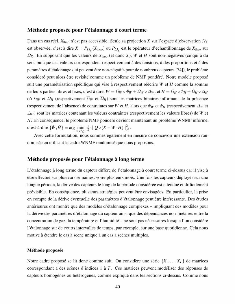
Méthode proposée pour l’étalonnage à court terme
Dans un cas réel, Xtheo n’est pas accessible. Seule sa projection X sur l’espace d’observation ΩX
est observée, c’est à dire X = PΩX(Xtheo) où PΩX
est le opérateur d’échantillonnage de Xtheo sur
ΩX . En supposant que les valeurs de Xtheo (et donc X), W et H sont non-négatives (ce qui a du
sens puisque ces valeurs correspondent respectivement à des tensions, à des proportions et à des
paramètres d’étalonnage qui peuvent être non-négatifs pour de nombreux capteurs [74]), le problème
considéré peut alors être revisité comme un problème de NMF pondéré. Notre modèle proposé
suit une paramétrisation spécifique qui vise à respectivement réécrire W et H comme la somme
de leurs parties libres et fixes, c’est à dire, W =ΩW ΦW +ΩW ∆W , et H =ΩH ΦH +ΩH ∆H
où ΩW et ΩH (respectivement ΩW et ΩH) sont les matrices binaires informant de la présence
(respectivement de l’absence) de contraintes sur W et H, alors que ΦW et ΦH (respectivement ∆W et
∆H) sont les matrices contenant les valeurs contraintes (respectivement les valeurs libres) de W et
H. En conséquence, le problème NMF pondéré devient maintenant un problème WNMF informé,
c’est-à-dire W , H= arg minW,H≥0
12 · ||Q (X−W ·H)||2F .
Avec cette formulation, nous sommes également en mesure de concevoir une extension ran-
domisée en utilisant le cadre WNMF randomisé que nous proposons.
Méthode proposée pour l’étalonnage à long terme
L’étalonnage à long terme du capteur diffère de l’étalonnage à court terme ci-dessus car il vise à
être effectué sur plusieurs semaines, voire plusieurs mois. Une fois les capteurs déployés sur une
longue période, la dérive des capteurs le long de la période considérée est attendue et difficilement
prévisible. En conséquence, plusieurs stratégies peuvent être envisagées. En particulier, la prise
en compte de la dérive éventuelle des paramètres d’étalonnage peut être intéressante. Des études
antérieures ont montré que des modèles d’étalonnage complexes – impliquant des modèles pour
la dérive des paramètres d’étalonnage du capteur ainsi que des dépendances non-linéaires entre la
concentration de gaz, la température et l’humidité – ne sont pas nécessaires lorsque l’on considère
l’étalonnage sur de courts intervalles de temps, par exemple, sur une base quotidienne. Cela nous
motive à étendre le cas à scène unique à un cas à scènes multiples.
Méthode proposée
Notre cadre proposé se lit donc comme suit. On considère une série X1, . . . ,XT de matrices
correspondant à des scènes d’indices 1 à T . Ces matrices peuvent modéliser des réponses de
capteurs homogènes ou hétérogènes, comme expliqué dans les sections ci-dessus. Comme nous
40
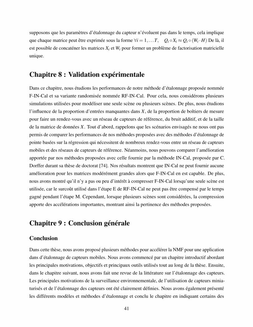
supposons que les paramètres d’étalonnage du capteur n’évoluent pas dans le temps, cela implique
que chaque matrice peut être exprimée sous la forme ∀i = 1, . . .T, Qi Xi ≈ Qi (Wi ·H) De là, il
est possible de concaténer les matrices Xi et Wi pour former un problème de factorisation matricielle
unique.
Chapitre 8 : Validation expérimentale
Dans ce chapitre, nous étudions les performances de notre méthode d’étalonnage proposée nommée
F-IN-Cal et sa variante randomisée nommée RF-IN-Cal. Pour cela, nous considérons plusieurs
simulations utilisées pour modéliser une seule scène ou plusieurs scènes. De plus, nous étudions
l’influence de la proportion d’entrées manquantes dans X , de la proportion de boîtiers de mesure
pour faire un rendez-vous avec un réseau de capteurs de référence, du bruit additif, et de la taille
de la matrice de données X . Tout d’abord, rappelons que les scénarios envisagés ne nous ont pas
permis de comparer les performances de nos méthodes proposées avec des méthodes d’étalonnage de
pointe basées sur la régression qui nécessitent de nombreux rendez-vous entre un réseau de capteurs
mobiles et des réseaux de capteurs de référence. Néanmoins, nous pouvons comparer l’amélioration
apportée par nos méthodes proposées avec celle fournie par la méthode IN-Cal, proposée par C.
Dorffer durant sa thèse de doctorat [74]. Nos résultats montrent que IN-Cal ne peut fournir aucune
amélioration pour les matrices modérément grandes alors que F-IN-Cal en est capable. De plus,
nous avons montré qu’il n’y a pas ou peu d’intérêt à compresser F-IN-Cal lorsqu’une seule scène est
utilisée, car le surcoût utilisé dans l’étape E de RF-IN-Cal ne peut pas être compensé par le temps
gagné pendant l’étape M. Cependant, lorsque plusieurs scènes sont considérées, la compression
apporte des accélérations importantes, montrant ainsi la pertinence des méthodes proposées.
Chapitre 9 : Conclusion générale
Conclusion
Dans cette thèse, nous avons proposé plusieurs méthodes pour accélérer la NMF pour une application
dans d’étalonnage de capteurs mobiles. Nous avons commencé par un chapitre introductif abordant
les principales motivations, objectifs et principaux outils utilisés tout au long de la thèse. Ensuite,
dans le chapitre suivant, nous avons fait une revue de la littérature sur l’étalonnage des capteurs.
Les principales motivations de la surveillance environnementale, de l’utilisation de capteurs minia-
turisés et de l’étalonnage des capteurs ont été clairement définies. Nous avons également présenté
les différents modèles et méthodes d’étalonnage et conclu le chapitre en indiquant certains des
41
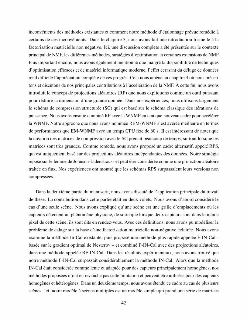
inconvénients des méthodes existantes et comment notre méthode d’étalonnage prévue remédie à
certains de ces inconvénients. Dans le chapitre 3, nous avons fait une introduction formelle à la
factorisation matricielle non négative. Ici, une discussion complète a été présentée sur le contexte
principal de NMF, les différentes méthodes, stratégies d’optimisation et certaines extensions de NMF.
Plus important encore, nous avons également mentionné que malgré la disponibilité de techniques
d’optimisation efficaces et de matériel informatique moderne, l’effet écrasant du déluge de données
rend difficile l’appréciation complète de ces progrès. Cela nous amène au chapitre 4 où nous présen-
tons et discutons de nos principales contributions à l’accélération de la NMF. À cette fin, nous avons
introduit le concept de projections aléatoires (RP) que nous expliquons comme un outil puissant
pour réduire la dimension d’une grande donnée. Dans nos expériences, nous utilisons largement
le schéma de compression structurée (SC) qui est basé sur le schéma classique des itérations de
puissance. Nous avons ensuite combiné RP avec la WNMF en tant que nouveau cadre pour accélérer
la WNMF. Notre approche que nous avons nommée REM-WNMF s’est avérée meilleure en termes
de performances que EM-WNMF avec un temps CPU fixe de 60 s. Il est intéressant de noter que
la création des matrices de compression avec le SC prenait beaucoup de temps, surtout lorsque les
matrices sont très grandes. Comme remède, nous avons proposé un cadre alternatif, appelé RPS,
qui est uniquement basé sur des projections aléatoires indépendantes des données. Notre stratégie
repose sur le lemme de Johnson-Lidenstrauss et peut être considérée comme une projection aléatoire
traitée en flux. Nos expériences ont montré que les schémas RPS surpassaient leurs versions non
compressées.
Dans la deuxième partie du manuscrit, nous avons discuté de l’application principale du travail
de thèse. La contribution dans cette partie était en deux volets. Nous avons d’abord considéré le
cas d’une seule scène. Nous avons expliqué qu’une scène est une grille d’emplacements où les
capteurs détectent un phénomène physique, de sorte que lorsque deux capteurs sont dans le même
pixel de cette scène, ils sont dits en rendez-vous. Avec ces définitions, nous avons pu modéliser le
problème de calage sur la base d’une factorisation matricielle non-négative éclairée. Nous avons
examiné la méthode In-Cal existante, puis proposé une méthode plus rapide appelée F-IN-Cal –
basée sur le gradient optimal de Nesterov – et combiné F-IN-Cal avec des projections aléatoires,
dans une méthode appelée RF-IN-Cal. Dans les résultats expérimentaux, nous avons trouvé que
notre méthode F-IN-Cal surpassait considérablement la méthode IN-Cal. Alors que la méthode
IN-Cal était considérée comme lente et adaptée pour des capteurs principalement homogènes, nos
méthodes proposées n’ont en revanche pas cette limitation et peuvent être utilisées pour des capteurs
homogènes et hétérogènes. Dans un deuxième temps, nous avons étendu ce cadre au cas de plusieurs
scènes. Ici, notre modèle à scènes multiples est un modèle simple qui prend une série de matrices
42
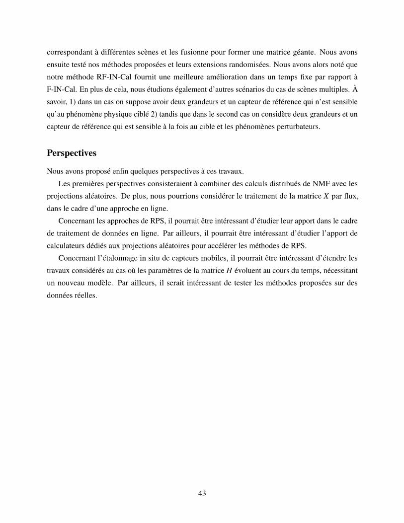
correspondant à différentes scènes et les fusionne pour former une matrice géante. Nous avons
ensuite testé nos méthodes proposées et leurs extensions randomisées. Nous avons alors noté que
notre méthode RF-IN-Cal fournit une meilleure amélioration dans un temps fixe par rapport à
F-IN-Cal. En plus de cela, nous étudions également d’autres scénarios du cas de scènes multiples. À
savoir, 1) dans un cas on suppose avoir deux grandeurs et un capteur de référence qui n’est sensible
qu’au phénomène physique ciblé 2) tandis que dans le second cas on considère deux grandeurs et un
capteur de référence qui est sensible à la fois au cible et les phénomènes perturbateurs.
Perspectives
Nous avons proposé enfin quelques perspectives à ces travaux.
Les premières perspectives consisteraient à combiner des calculs distribués de NMF avec les
projections aléatoires. De plus, nous pourrions considérer le traitement de la matrice X par flux,
dans le cadre d’une approche en ligne.
Concernant les approches de RPS, il pourrait être intéressant d’étudier leur apport dans le cadre
de traitement de données en ligne. Par ailleurs, il pourrait être intéressant d’étudier l’apport de
calculateurs dédiés aux projections aléatoires pour accélérer les méthodes de RPS.
Concernant l’étalonnage in situ de capteurs mobiles, il pourrait être intéressant d’étendre les
travaux considérés au cas où les paramètres de la matrice H évoluent au cours du temps, nécessitant
un nouveau modèle. Par ailleurs, il serait intéressant de tester les méthodes proposées sur des
données réelles.
43
List of the Author’s Publications andCommunications During the Ph.D Thesis
In Proceedings of Peer-reviewed International Conferences
O. Vu thanh, M. Puigt, F. Yahaya, G. Delmaire, G. Roussel, In situ calibration of cross-
sensitive sensors in mobile sensor arrays using fast informed non-negative matrix factorization,
Proceedings of the 46th IEEE International Conference on Acoustics, Speech, and Signal
Processing (ICASSP 2021), Toronto, Canada / Virtual, pp. 3515-3519, June 6-11, 2021.
F. Yahaya, M. Puigt, G. Delmaire, G. Roussel, Random projection streams for (weighted)
nonnegative matrix factorization, Proceedings of the 46th IEEE International Conference on
Acoustics, Speech, and Signal Processing (ICASSP 2021), pp. 3280-3284, Toronto, Canada /
Virtual, June 6-11, 2021.
F. Yahaya, M. Puigt, G. Delmaire, G. Roussel, Gaussian compression stream: principle and
preliminary results, Proceedings of iTWIST: international Traveling Workshop on Interactions
between low-complexity data models and Sensing Techniques, Nantes, France / Virtual,
December 2-4, 2020.
F. Yahaya, M. Puigt, G. Delmaire, G. Roussel, How to apply random projections to nonnegative
matrix factorization with missing entries?, Proceedings of 27th European Signal Processing
Conference (EUSIPCO), A Coruña, Spain, September 2-6, 2019.
F. Yahaya, M. Puigt, G. Delmaire, G. Roussel, Faster-than-fast NMF using random projec-
tions and Nesterov iterations, Proceedings of iTWIST: international Traveling Workshop on
Interactions between low-complexity data models and Sensing Techniques, Marseille, France,
November 21-23, 2018.
44
In Proceedings of Peer-reviewed National Conferences
F. Yahaya, M. Puigt, G. Delmaire, G. Roussel, Accélération de la factorisation pondérée en
matrices non-négatives par projections aléatoires, Actes du GRETSI, Lille, France, 22-27
août 2019.
In International Conferences without Proceedings
F. Yahaya, M. Puigt, G. Delmaire, G. Roussel, Fast & furious: accelerating weighted NMF
using random projections, Workshop on Low-Rank Models and Applications (LRMA), Mons,
Belgium, September 12-13, 2019.
F. Yahaya, C. Dorffer, M. Puigt, G. Delmaire, G. Roussel, Online calibration of a mobile
sensor network by matrix factorization, presented during the international Symposium entitled
"Individual Air Pollution Sensors: Innovation or Revolution?", Villeneuve-d’Ascq, France,
November 29-30, 2018.
In National Conferences without Proceedings
F. Yahaya, M. Puigt, G. Delmaire, G. Roussel, NMF for big data with missing entries: a
random projection based approach, Journée Régionale des Doctorants en Automatique, Lille,
France, 9 juillet 2019. Best poster award.
F. Yahaya, M. Puigt, G. Delmaire, G. Roussel, Non-negative matrix factorization with missing
entries: a random projection based approach, Journée des jeunes chercheurs en traitement du
signal et/ou de l’image, GRAISyHM, Amiens, France, 17 juin 2019.
M. Puigt, C. Dorffer, F. Yahaya, G. Delmaire, G. Roussel, Cartographie et étalonnage de
capteurs conjoints par traitement des données issues de capteurs mobiles, Colloque National
Capteurs et Sciences Participatives, Paris, France, 1-4 avril 2019.
F. Yahaya, M. Puigt, G. Delmaire, G. Roussel, Do random projections fasten an already
fast NMF technique using Nesterov optimal gradient?, Journée Régionale des Doctorants en
Automatique, Amiens, France, 3 juillet 2018.
45
Chapter 1
General Introduction
1.1 General Framework . . . . . . . . . . . . . . . . . . . . . . . . . . . . . . . . . . . . . . . . . . 46
1.2 Thesis Motivation and Objectives . . . . . . . . . . . . . . . . . . . . . . . . . . . . . . . . . . 47
1.2.1 Accelerated Methods . . . . . . . . . . . . . . . . . . . . . . . . . . . . . . . . . . . . . . 48
1.2.2 Multiple Scene Scenario . . . . . . . . . . . . . . . . . . . . . . . . . . . . . . . . . . . . 49
1.3 Thesis Structure . . . . . . . . . . . . . . . . . . . . . . . . . . . . . . . . . . . . . . . . . . . . 49
1.1 General Framework
In France, air quality is monitored by the Associations Agréées de Surveillance de la Qualité de
l’Air (AASQA) network (associations agréées de surveillance de la qualité de l’air), which provides
air quality assessments (measurements and air quality modelling) in order to inform authorities
and citizens with full transparency. Alongside the conventional, normalized, bulky, and expensive
instruments used in AASQA stations, miniaturized gas and particle sensors are being increasingly
developed. They provide a supplementary, low-cost way to monitor air quality, with sufficient
detection limit and accuracy. Their low cost allows for a massive field deployment, providing a high
spatial and temporal resolution. However, calibration issues remain to be solved.
Usually, air quality sensor calibration is performed in-lab and consists of inferring the sensor
outputs—e.g., the sensor output voltage—with the known gas concentration input. Such a calibration
is time consuming and costly. In practice, while it still can be performed for calibrating the few but
accurate ASQAA sensors, it is not well-suited to a crowd of miniaturized gas sensors for obvious cost
and availability reasons. As a consequence, some blind, self, in-situ, or field calibration techniques—
46
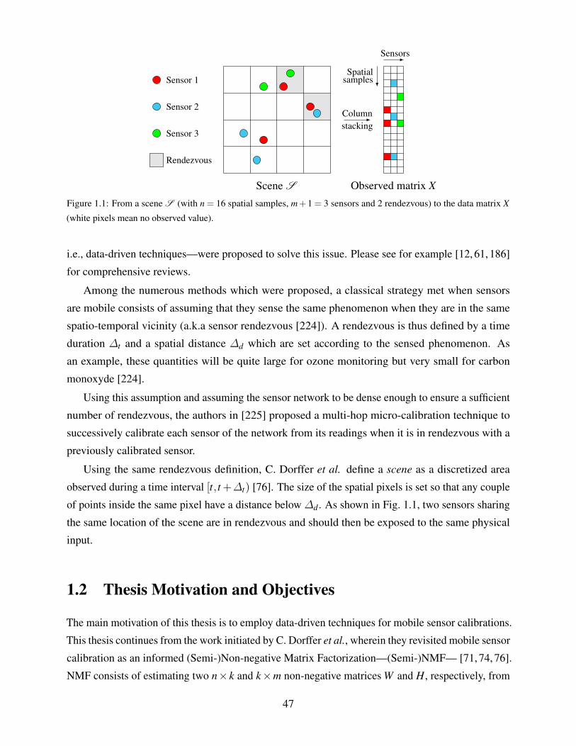
Sensor 1
Sensor 2
Sensor 3
Rendezvous
Scene S
stackingColumn
Observed matrix X
Sensors
Spatialsamples
Figure 1.1: From a scene S (with n = 16 spatial samples, m+1 = 3 sensors and 2 rendezvous) to the data matrix X
(white pixels mean no observed value).
i.e., data-driven techniques—were proposed to solve this issue. Please see for example [12, 61, 186]
for comprehensive reviews.
Among the numerous methods which were proposed, a classical strategy met when sensors
are mobile consists of assuming that they sense the same phenomenon when they are in the same
spatio-temporal vicinity (a.k.a sensor rendezvous [224]). A rendezvous is thus defined by a time
duration ∆t and a spatial distance ∆d which are set according to the sensed phenomenon. As
an example, these quantities will be quite large for ozone monitoring but very small for carbon
monoxyde [224].
Using this assumption and assuming the sensor network to be dense enough to ensure a sufficient
number of rendezvous, the authors in [225] proposed a multi-hop micro-calibration technique to
successively calibrate each sensor of the network from its readings when it is in rendezvous with a
previously calibrated sensor.
Using the same rendezvous definition, C. Dorffer et al. define a scene as a discretized area
observed during a time interval [t, t +∆t) [76]. The size of the spatial pixels is set so that any couple
of points inside the same pixel have a distance below ∆d . As shown in Fig. 1.1, two sensors sharing
the same location of the scene are in rendezvous and should then be exposed to the same physical
input.
1.2 Thesis Motivation and Objectives
The main motivation of this thesis is to employ data-driven techniques for mobile sensor calibrations.
This thesis continues from the work initiated by C. Dorffer et al., wherein they revisited mobile sensor
calibration as an informed (Semi-)Non-negative Matrix Factorization—(Semi-)NMF— [71, 74, 76].
NMF consists of estimating two n× k and k×m non-negative matrices W and H, respectively, from
47
a n×m non-negative matrix X such that [265]
X 'W ·H. (1.1)
In Semi-NMF, one allows some of the matrices in Eq (1.1) to get negative entries. When applied to
the proposed sensor calibration problem:
m X is partially observed and a measurement uncertainty can be associated with each observed
data point, hence providing a weight matrix Q to X . This implies that the authors aim to solve
a weigthed (Semi-)NMF problem, i.e.,
QX ' Q (W ·H), (1.2)
where denotes the Hadamard product.
m W is structured by the calibration function of the sensors of the network. For example, in the
case of an affine calibration function [74,76], W is defined as the concatenation of one column
of ones and one column containing the unfolded physical phenomenon observed during the
scene. This corresponds to a specific case of a Vandermonde matrix which is met for any
polynomial calibration function [71].
m H contains the calibration parameters of each of these sensors.
Moreover, their proposed methods take care of additional sensors such as those provided by the
ASQAA network, assumed to be perfectly calibrated and to provide accurate estimates of the sensed
phenomenon. The proposed methods also take into account the average calibration parameters pro-
vided by the sensors manufacturer and assume a sparse approximation of the physical phenomenon
to sense according to a previously learnt dictionary of patterns [74].
This Ph.D. thesis thus aims to:
m significantly accelerate the above techniques in order to process large matrices,
m and extend them to the case of multiple scenes observed along time.
1.2.1 Accelerated Methods
The aforementioned methods were shown to be more versatile than state-of-the-art multi-hop
techniques and to allow a much less dense network to perform calibration. However, the update
rules of these techniques are based on multiplicative updates [74, 76] or projected gradient [71],
which are known for their low speed of convergence. As a consequence, they can hardly be applied
as is to monitor a quite large area. The first objective of this thesis is to formulate robust and optimal
frameworks to accelerate these informed NMF techniques in order to process large matrices.
48
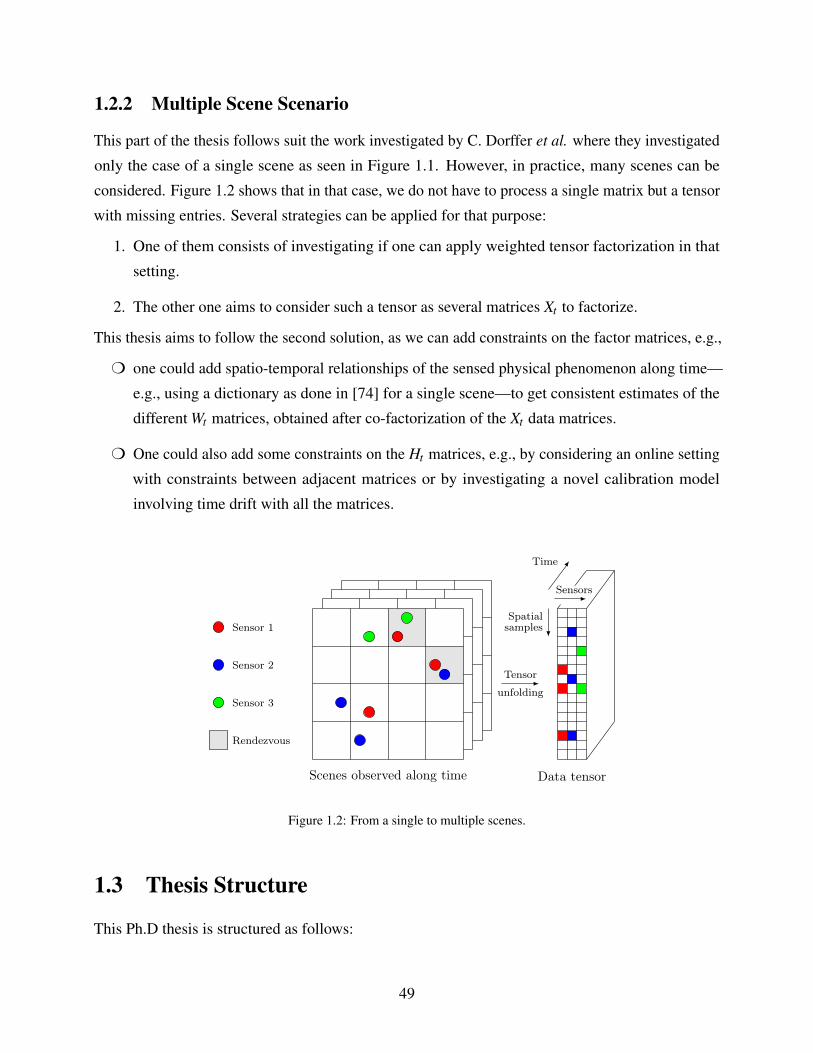
1.2.2 Multiple Scene Scenario
This part of the thesis follows suit the work investigated by C. Dorffer et al. where they investigated
only the case of a single scene as seen in Figure 1.1. However, in practice, many scenes can be
considered. Figure 1.2 shows that in that case, we do not have to process a single matrix but a tensor
with missing entries. Several strategies can be applied for that purpose:
1. One of them consists of investigating if one can apply weighted tensor factorization in that
setting.
2. The other one aims to consider such a tensor as several matrices Xt to factorize.
This thesis aims to follow the second solution, as we can add constraints on the factor matrices, e.g.,
m one could add spatio-temporal relationships of the sensed physical phenomenon along time—
e.g., using a dictionary as done in [74] for a single scene—to get consistent estimates of the
different Wt matrices, obtained after co-factorization of the Xt data matrices.
m One could also add some constraints on the Ht matrices, e.g., by considering an online setting
with constraints between adjacent matrices or by investigating a novel calibration model
involving time drift with all the matrices.
Sensor 1
Sensor 2
Sensor 3
Rendezvous
Scenes observed along time
unfolding
Tensor
Data tensor
Sensors
Spatialsamples
Time
Figure 1.2: From a single to multiple scenes.
1.3 Thesis Structure
This Ph.D thesis is structured as follows:
49
Chapter 2: We make a comprehensive discussion on air quality monitoring. We discuss in de-
tail its importance, instrumentation, strategies and challenges. Particularly we discuss several
calibration models, different calibration strategies, and in-situ calibration methods. In the latter part
we restate the motivations, and solutions we offer as a contribution to this line of work.
Chapter 3: Non-negative Matrix Factorization (Non-negative Matrix Factorization (NMF)) is the
main tool used extensively in this work. In this chapter we formally introduce the concepts of
NMF, it applications and challenges. We extensively discuss the formulations of NMF, the dif-
ferent NMF algorithms, optimization techniques, discrepancy measures and some of their extensions.
Chapter 4: In this chapter we discuss the various ways to accelerate (W)NMF. We focus on
Random projection and make a review of the existing techniques. In particular we discuss the
different random projection schemes which are data-dependent or data-independent and offer their
time complexities.
Chapter 5: In this chapter, we discuss the idea of missing entries in data. We show how to re-
formulate our NMF model into a Weighted NMF (WNMF) version. Then we make a quick review
on existing methods for performing WNMF. We then present the main contributions in two folds: 1)
we present a novel framework that combines random projections with WNMF, and 2) we proposed a
random projection scheme as an alternative to the existing schemes based on data streaming.
Chapter 6: In this chapter we present all the results from our experiments in Chapter 5. We
make tests using two main solvers, i.e., AS-NMF and NeNMF. Then we compare their randomized
extensions to the vanilla (no compression) version. We also make tests in the presence of noise, and
lastly we conduct experiments on real data images as an application of our proposed framework.
Chapter 7: This chapter begins the second part of the thesis were we focus mainly on the ap-
plication aspect—i.e. sensor calibration. In this chapter we introduce our proposed calibration
method. This method is a faster method to the existing IN-Cal and is based on the nesterov acceler-
ated gradient method. Then we make its extension with random projections. These methods are
then tested in two scenarios: 1) Short term considerations, and 2) Long term considerations.
Chapter 8: In this chapter we present the results of the experiments related to chapter 7. We
compare all the tested methods and interpret their results.
50

Chapter 9: This is the last chapter of the thesis. Here we make a general conclusion where
we recap on the motivation, methods, experiments, results, contributions, and perspectives for future
work.
51

Chapter 2
State of the Art on Sensor Calibration
2.1 Introduction . . . . . . . . . . . . . . . . . . . . . . . . . . . . . . . . . . . . . . . . . . . . . . 52
2.2 The why of low cost sensors . . . . . . . . . . . . . . . . . . . . . . . . . . . . . . . . . . . . . . 54
2.3 Types of Sensors . . . . . . . . . . . . . . . . . . . . . . . . . . . . . . . . . . . . . . . . . . . . 55
2.3.1 Particulate Matter Sensors . . . . . . . . . . . . . . . . . . . . . . . . . . . . . . . . . . . 56
2.3.2 Gas sensors . . . . . . . . . . . . . . . . . . . . . . . . . . . . . . . . . . . . . . . . . . . 56
2.4 Error Sources . . . . . . . . . . . . . . . . . . . . . . . . . . . . . . . . . . . . . . . . . . . . . 57
2.4.1 Internal Errors . . . . . . . . . . . . . . . . . . . . . . . . . . . . . . . . . . . . . . . . . 57
2.4.2 External Errors . . . . . . . . . . . . . . . . . . . . . . . . . . . . . . . . . . . . . . . . . 58
2.5 Key Aspects of Sensor Calibration . . . . . . . . . . . . . . . . . . . . . . . . . . . . . . . . . . 58
2.5.1 Models for Calibration . . . . . . . . . . . . . . . . . . . . . . . . . . . . . . . . . . . . . 59
2.5.2 In Situ Calibration Strategies . . . . . . . . . . . . . . . . . . . . . . . . . . . . . . . . . . 62
2.5.3 Calibration Methods . . . . . . . . . . . . . . . . . . . . . . . . . . . . . . . . . . . . . . 67
2.6 Discussion . . . . . . . . . . . . . . . . . . . . . . . . . . . . . . . . . . . . . . . . . . . . . . . 69
2.1 Introduction
Definition 2.1 (Air quality). Air quality is defined as the level of purity of the atmospheric air in a
particular location.
A pristine and safe environment is the principal objective of many renowned environmental
agencies like the EEA.
52

Figure 2.1: Slight smog in the Hauts-de-France region of France
Air pollution still pose substantial ramifications on the wealth-being of the vast European
populace. Urban areas of most EU countries in particular are the most affected by air pollution.
The predominant hazardous pollutants notable for causing serious health problems are nitrogen
dioxide (NO2), particulate matter (PM), ozone (O3) and carbon monoxide (CO). In particular,
substantial research have focused on PM. Particulate matter occur in the environment as a result of
commercial activities that use nanomaterials. These materials span dimensions notably less than
100 nm [206]. Their properties tend to kindle hazardous chemical interactions with the environment
and consequently posing grave health complications [92]. In the year 2018 alone, the EEA reported
a record of 417 000 premature deaths from exposure to PM pollution with a diameter of 2.5 µm or
less (PM2.5) [82].
Effective air quality monitoring has gained relevance and at the top of priorities of most envi-
ronmental agencies. Traditional ways to carry out environmental monitoring are mostly through
specialized sensors.
Definition 2.2 (Sensor). In the context of this thesis, a sensor can be defined as an instrument
used for monitoring the quality of the air by quantifying concentration levels of one or several
atmospheric phenomena, e.g., CO, SO2, or O3.
Outputs from these sensors may also be used to modulate the activities of other systems to
improve the quality of life and daily activities [223]. Sensors tend to vary in size, particularly,
53
authoritative sensors—which are very accurate—are usually bulky and very expensive. As a
consequence, they are stored in monitoring stations which are sparsely deployed in areas of interest—
i.e., a few ones per large cities—because of cost reasons. Moreover, almost none of these stations
are mobile—see Figure 2.2. As a consequence, AASQA cannot monitor some very local phenomena
which are also hard to model in near-real time. For this reason there has been a surge in the efforts
to find some complementary information. This has led to the adoption of Low Cost Sensors (LCS).
These LCS are cheap to produce, but they come with some drawbacks. Notably,they are not as
efficient as the high-end sensors in terms of accuracy as reported by several researchers due to
several interfering factors [125, 236]. These interfering factors adversely affect the accuracy of the
sensed phenomena along time. To solve this issue the sensors need to be calibrated.
Sensor calibration aims at fine tuning one or several sensor parameters to improve its accuracy
or remove errors. Sensor calibration is usually done in the presence of a reference, e.g., in a
controlled environment for air quality sensors. Calibration is done prior to deployment on the field
and also post-deployment to remove initial errors and maintain a consistent monitoring quality in
the long-term.
There are several ways to perform sensor calibration. Traditional methods involves unmounting
and sending the sensors from the field to a laboratory. These laboratories are equipped with highly
accurate reference sensors to simulate a controlled environment. This calibration method is however
unsuitable when the number of sensors to unmount and calibrate is high. The task becomes expensive
and very time consuming. A solution is the use of “blind”, “self”, “in-situ”, or “field” calibration
techniques—i.e., data-driven techniques— we discuss them in detail in the next sections.
2.2 The why of low cost sensors
Urbanization and the exponential increase in the world population has indirectly affected the quality
of life as far as the environment is concerned. Several factors contribute to air pollution including
natural and man-made ones. Among these, industrial activities have been identified to be the most
contributing factor. According to the EEA, 90% of ammonia and methane come from agricultural
activities, while the transport section alone accounts for 40% of NO2 and PM2.5 in the environment.
Standard rules for the control of allowable emission levels have in recent times not been met.
Emerging technologies to reduce emission of pollutants have been insufficient as well [3]. Harmful
pollutants such as the gaseous ones and particulate matter tend to migrate. In the urban vicinities,
concentrations of these phenomena fluctuate mainly due to the influence of strong winds and
proximity of industries thus making it difficult to monitor. Air quality monitoring is usually carried
54
out by some highly sophisticated monitoring stations. However their inadequacy, high costs and low
spatio-temporal resolution are the driving forces for the quest to find better alternatives. To this end,
LCS have been considered and widely used recently. The main reasons why LCS are inceasingly
sought are as follows:
m Cost: The first and perhaps the most crucial reason for LCS is their cost. Indeed, they tend
to cost 10 to more than 1000 times less than those in authoritative monitoring stations, thus
allowing their massive deployment. The difference of cost may be explained by the level of
miniaturization of LCS as well as by their sensitivity and accuracy.
m Mobility: Most LCS tend to be (very) small, with surfaces ranging from a few squared
millimeters to a few squared centimeters. This allows their installation in very portable mobile
sensing devices They are thus regarded as “mobile sensors” in opposition to the monitoring
stations which are mostly fixed. The portability of these LCS makes deployment easier. They
can easily monitor locations such as busy streets, traffic jams, and urban vicinities where air
pollution is earnest.
m Resolution: Ideally the dissemination of monitoring activities ought to be dense enough to
obtain a good statistical knowledge on the quality of air. One main reason is the fact that
concentrations of environmental phenomena tend to be unstable and may depend on both the
time of the day and the location [203]. This level of coverage requires several sensors to be
deployed for air quality monitoring [191]. Unfortunately, their high cost and their size limit
their deployment, hence a very low spatial resolution. LCS offer a solution to this problem.
Several sensors can be deployed at once throughout the vicinity with relative ease, offering
higher spatio-temporal resolutions.
m Availability of Data: LCS offer near-real time [146] high spatio-temporal resolution data.
This data is collected time-stamped and geolocalized using, e.g., a crowd of smartphones. In
this consideration the mobile sensors are usually worn by volunteer citizens and connected to
a central server thanks to smartphone communication facilities. The collected data may be
used to build data-driven calibration models and also give insights to the quality.
2.3 Types of Sensors
The choice of the sensor type for any environmental monitoring depends on the target physical
phenomena. We discuss herein the different types of sensors. Most of these sensors can be grouped
55
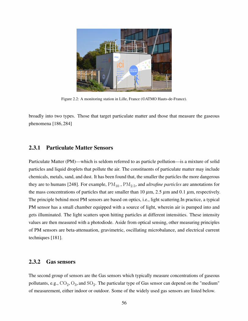
Figure 2.2: A monitoring station in Lille, France (©ATMO Hauts-de-France).
broadly into two types. Those that target particulate matter and those that measure the gaseous
phenomena [186, 284]
2.3.1 Particulate Matter Sensors
Particulate Matter (PM)—which is seldom referred to as particle pollution—is a mixture of solid
particles and liquid droplets that pollute the air. The constituents of particulate matter may include
chemicals, metals, sand, and dust. It has been found that, the smaller the particles the more dangerous
they are to humans [248]. For example, PM10 , PM2.5, and ultrafine particles are annotations for
the mass concentrations of particles that are smaller than 10 µm, 2.5 µm and 0.1 µm, respectively.
The principle behind most PM sensors are based on optics, i.e., light scattering.In practice, a typical
PM sensor has a small chamber equipped with a source of light, wherein air is pumped into and
gets illuminated. The light scatters upon hitting particles at different intensities. These intensity
values are then measured with a photodiode. Aside from optical sensing, other measuring principles
of PM sensors are beta-attenuation, gravimetric, oscillating microbalance, and electrical current
techniques [181].
2.3.2 Gas sensors
The second group of sensors are the Gas sensors which typically measure concentrations of gaseous
pollutants, e.g., CO2,O3, and SO2. The particular type of Gas sensor can depend on the "medium"
of measurement, either indoor or outdoor. Some of the widely used gas sensors are listed below.
56
2.3.2.1 Solid-state Gas Sensor
These type of sensors are also known as Metal oxide sensors [260]. As the name suggests, these
sensors are made up of one or more metal oxides, e.g., an oxide of aluminum, and a heating element.
There are 2 types of solid-state sensors depending on how the metal oxide is utilized, i.e., chip-type
and bead-type. The former relates to those sensors with a metal oxide in the form of a paste, while
the latter has the metal oxide planted on a silica chip. The principle behind solid-state sensors
involves a direct exposure of the metal oxides to the associated gases. The gases then split into
charged ions and attach themselves to surface of the metal oxides and alters their conductivity.
The conductivity are measured and then used to approximate the concentrations of the associated
ambient gases [41, 186, 260].
2.3.2.2 Electrochemical Gas Sensor
Electrochemical gases senosors are build on the principle of electrochemical reactions. There are
two main components of these sensors, i.e. working electrode, and a counter electrode. Although
some variants may include an additional Electrode, serving as a reference. These sensors react with
the present gas to give off a voltage, which is proportional to the gas concentration [186, 195].
2.4 Error Sources
The main attribute of low cost sensors is their trade-off of accuracy for low-cost. They might be
very affordable even on a very large scale but their accuracy of measurement is limited as compared
to high-end counterparts. The inaccuracies in their readings may be caused by several factors.
Following the survey presented [186] these inaccuracies or errors can be grouped mainly into two,
i.e., internal errors and external errors.
2.4.1 Internal Errors
Errors that pertain to how the sensor functions and manifests within the sensor framework are termed
as internal errors. One of the commonest errors is signal-to-noise ratio. A sensor that measures a
physical phenomenon like CO2 gas, typically has a defined range of concentration of the associated
gas. Concentration outliers of this range may thus increase the noise of the sensor signal, e.g.,
some solid-state gas sensors are known to incur this kind of error. Another example of an internal
error are the systematic errors. Systematic errors arise when the concentrations of the measured
phenomena are deviated consistently from the actual values. The deviation could be either an offset
57
or overestimation of concentration values. Signal drift is another type of internal error. Indeed, LCS
response typically drifts over time which is one of the main reasons for calibration [76]. This drift is
mainly due to sensor ageing, especially when they are left deployed or used for long periods. Lastly,
nonlinear response is another source of error of low-cost sensors. In an ideal case, a sensor shares a
linear relationship with a reference sensor. However this maybe not be the case in some scenarios,
e.g., PM and solid-state gas sensors may present a nonlinear response which arises due to certain
environmental factors [125].
2.4.2 External Errors
The second group of errors sources are the external ones, e.g., environmental dependencies like those
that arise from the environment or the surroundings of the sensor. Most often hash environmental
conditions like temperature and humidity could affect the sensitivity of the sensor. Another crucial
example of an external error source is low sensor selectivity [186]. This type of error occurs when a
different physical phenomena interferes with the actual phenomena being measured by the sensor.
For example, certain solid-side gas sensors may also be sensitive to other gases aside from the gas it
is meant to measure
2.5 Key Aspects of Sensor Calibration
The most crucial aspect of low-cost air quality sensors lies in improving their sensitivity. Low-cost
sensors are inherently less sensitive as compared to high-end sensors. Moreover their responses are
also worsened by errors from several sources, e.g., solid-state gas sensors have signal drift and the
magnitude is hugely dependent on the sensor components and working principle (See Section 2.4). To
solve this issue, several studies have focused on in situ calibration techniques [61,174,186,225,274].
Definition 2.3 (Calibration [20]). Calibration is the “operation that, under specified conditions,
in a first step, establishes a relation between the quantity values with measurement uncertainties
provided by measurement standards and corresponding indications with associated measurement
uncertainties and, in a second step, uses this information to establish a relation for obtaining a
measurement result from an indication.”
In practice, this implies that calibration must be performed in-lab, i.e., in a controlled environment
where we assume to know the sensed input phenomenon. From several—say n—measurements in
such a controlled environment, it is then possible to derive a function F (.) which links these input
58
phenomena x = [x1,x2, . . . ,xn]T to the corresponding sensor outputs y = [y1,y2, . . . ,yn]
T , i.e.,
y = F (x). (2.1)
Assuming F (.) to be invertible, one can then estimate the measurements from the sensor outputs.
In most work with LCS, an in-lab calibration is not always possible. More precisely, several
authors assume their LCS to be calibrated before they are deployed on the field, which is termed
pre-deployment calibration. Then, the LCS response may evolve along time and sensors need to be
recalibrated. This is usually done in situ, i.e., from the sensor data themselves in an uncontrolled
environment. Most in situ calibration methods aim to estimate the above function F (.)—and not
its inverse—hence the fact it is usually named “calibration function” while it is not according to
Definition 2.3. To perfom in situ calibration, it is necessary to know a calibration model—i.e., the
model which defines F (.)—and to estimate “calibration parameters”, i.e., the intrinsic parameters
which allow to fit the sensor readings to the sensed phenomenon according to the calibration model.
2.5.1 Models for Calibration
In this subsection we make a summary of some of the most popular calibration models used for in
situ sensor calibration. We especially focus on calibration models pertaining to low-cost air quality
sensors.
Definition 2.4 (Calibration Model [199]). A calibration model is a mathematical function which
links the sensor outputs to the measured input and possibly other quantities.
The purpose of a calibration model is thus to find a suitable calibration function F (.) which
draws a map of a raw input value—here denoted x(t)—to an output value denoted y(t). Here, t
denotes the time index as the calibration function is sensor-specific and possibly time dependent.
More precisely, we provide below a brief review of the different calibration models available in
literature. We here follow the review presented in [61]. In their findings, the authors categorized
calibration models based on the number of input variables and whether or not the model depends on
time. The categories are:
• single variable without time: For this type, it means that the calibration model relationship
take in only one variable, e.g., one input CO2 concentration and does not depend on time.
• single variable with time: An extension of the single variable is to augment it to depend
on time. In this case time is considered due to some internal errors discussed earlier—e.g.
depending on on the type of deployment, sensor responses may drift over time.
59
• multiple variables without time: This category means that the calibration model relationship
accepts two or more input variables and does not depend on time. This is to solve the issue of
cross-sensitivity of several target pollutants.
• multiple variables with time: Then an extension can be made to consider time, when the
model relationship takes multiple input variables.
2.5.1.1 Single variable without time
Many calibration models are based on the single variable without time. This is the simplest and
most poplar model investigated in literature and used for many calibration tasks. In particular, this
states that the parameters needed by F are only the sensed phenomenon, i.e.,
y(t)'F (x(t)). (2.2)
Considered models for F (.) include an affine relationship [76], i.e.,
y(t)' f1 · x(t)+ f0, (2.3)
where f0 and f1 denote the sensor offset and gain, respectively. Simplified versions of this model
have been considered in the literature, i.e., a linear model which assume the offset to be either
known, null, or a posteriori estimated [11]. This models then reads
y(t)' f1 · x(t). (2.4)
Other authors, e.g., [154], assume the gain coefficient to be f1 = 1, hence considering a model
involving only an offset, i.e.,
y(t)' x(t)+ f0. (2.5)
While the above linear or affine models are the most studied, some authors also considered nonlinear
sensor responses. In particular, the authors in [259] assumed that the nonlinear sensor model could
be approximated as piecewise linear models (2.3) while others, e.g., [71], approximated the nonlinear
function by a polynomial, i.e.,
y(t)' f0 + f1 · x(t)+ f2 · x2(t)+ . . .+ fn · xn(t). (2.6)
2.5.1.2 Single variable with time
The need for in situ calibration is partially due to sensor drift, which affects the sensor along time.
As a consequence it makes sense to consider that the model of F (.) also depends on the time index
t, i.e.,
y(t)'F (x(t), t). (2.7)
60
In particular, the time-dependent extensions of Eqs. (2.3) and (2.6) read
y(t)' f1(t) · x(t)+ f0(t) (2.8)
and
y(t)' f0(t)+ f1(t) · x(t)+ . . .+ fn(t) · xn(t), (2.9)
respectively. The main differences between Eqs. (2.3) and (2.8) (Eqs. (2.6) and (2.9), respectively)
lies in the fact that the calibrations parameters fi evolve with time in the latter while they are fixed in
the former. In order to tackle such a problem, some authors assumed the evolution of the calibration
parameters along time followed an affine model [109], i.e., we can, e.g., write the parameters f0(t)
and f1(t) in Eq. (2.8) as
f0(t) ' α0 +α1 · t, (2.10)
f1(t) ' β0 +β1 · t. (2.11)
2.5.1.3 Multiple variables without time
Ideally, sensors are made to measure a specific target pollutant, irrespective of the presence of other
pollutants. However in many real world deployments, there is usually an interference from other
constituents of the surrounding air mixture [195], e.g., temperature or humidity. Moreover, some
gas sensors tend not to be selective enough and to be perturbated by other gas concentrations, which
is particularly challenging, especially for the metal-oxide sensosr [179, 260]. For this reason, as
LCS are usually miniaturized, it became classical to put in the same sensing device several sensors
whose concentrations influence each others [13, 188]. The sensor array thus houses two or more
sensors sensing different physical phenomena. Then the calibration function of this model will be a
culmination of all the associated calibration parameters of the different sensors. This is sometimes
referred as cross-sensitive sensor calibration [188].
If we consider a sensor array with n cross-sensitive sensors, the calibration function of one sensor
reads:
y(t)'F (x1(t),x2(t), . . . ,xn(t)), (2.12)
where x1(t),x2(t), . . . ,xn(t) denote the n phenomena assumed to be sensed while y(t) is the sensor
output of one of the sensors sensing one of these n phenomena.
Many expressions for F have been considered. The most classical one consists of assuming that
it is time-independent multilinear with respect to the different sensed phenomena, i.e.,
y(t)' f0 + f1 · x1(t)+ f2 · x2(t)+ . . .+ fn · xn(t). (2.13)
61
However, it is worth mentioning that more complex models involving possibly strong nonlinearities
were also considered in, e.g., [8, 205].
2.5.1.4 Multiple variables with time
As for models involving one variable, time-dependent extensions of the calibration model (2.12)
have been also considered, which implies that time also appears as a parameter of the function F ,
i.e.,
y(t)'F (x1(t),x2(t), . . . ,xn(t), t). (2.14)
In particular, in the multilinear model, a classical assumption consists of assuming the sensor drift to
affect the offset according to an affine mode, as in Eq. (2.10) [213]. In that case, the model reads
y(t)' α0 +α1 · t + f1 · x1(t)+ f2 · x2(t)+ . . .+ fn · xn(t). (2.15)
However, please note that complex time-dependent nonlinear models were also proposed in, e.g., [8].
2.5.2 In Situ Calibration Strategies
Environmental monitoring spans an extensive literature over several decades. Earlier forms of
monitoring were mainly done through analogue systems in order to measure physical environmental
phenomena. This was however inefficient as these measurements needed the engineer to retrieved
them manually. These days digitized versions of such systems are increasingly sought, e.g., the
digitized data loggers are complimented with GSM communication networks [210].
Definition 2.5 (Sensor Network [193]). A sensor network can be defined as a framework com-
prising of one or more sensing instruments—i.e., an array of sensors—designed to relay all the
corresponding sensor measurement data to a central server for storage.
Figure 2.3 shows a generic illustration of a sensor network. A typical sensor network is made
up of nodes. These nodes are made up of low-cost sensors. Nodes may contain one or an array of
sensors. Once deployed and after the sensors have sensed the targeted pollutant concentrations, the
data is then transmitted to a central sensor network server. In most cases, LCS can be mobile or
static. Moreover, the network may contain sensors of heterogeneous accuracy, i.e., reference and
low-cost sensors. This has an influence on the network configuration and on the chosen calibration
methods, as highlighted in [186] whose authors state that there is no universal calibration method
which could be applied to any network configuration.
In regards to environmental monitoring for air quality, in this section we focus on mobile sensor
networks. We discuss the different types of strategies for calibrating an environmental sensor
network, i.e., blind calibration, collaborative calibration, and calibration transfer.
62
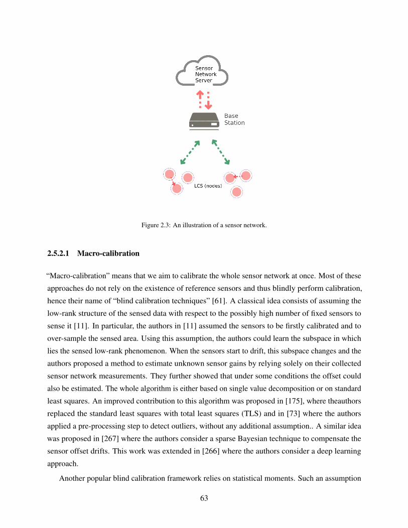
Figure 2.3: An illustration of a sensor network.
2.5.2.1 Macro-calibration
“Macro-calibration” means that we aim to calibrate the whole sensor network at once. Most of these
approaches do not rely on the existence of reference sensors and thus blindly perform calibration,
hence their name of “blind calibration techniques” [61]. A classical idea consists of assuming the
low-rank structure of the sensed data with respect to the possibly high number of fixed sensors to
sense it [11]. In particular, the authors in [11] assumed the sensors to be firstly calibrated and to
over-sample the sensed area. Using this assumption, the authors could learn the subspace in which
lies the sensed low-rank phenomenon. When the sensors start to drift, this subspace changes and the
authors proposed a method to estimate unknown sensor gains by relying solely on their collected
sensor network measurements. They further showed that under some conditions the offset could
also be estimated. The whole algorithm is either based on single value decomposition or on standard
least squares. An improved contribution to this algorithm was proposed in [175], where theauthors
replaced the standard least squares with total least squares (TLS) and in [73] where the authors
applied a pre-processing step to detect outliers, without any additional assumption.. A similar idea
was proposed in [267] where the authors consider a sparse Bayesian technique to compensate the
sensor offset drifts. This work was extended in [266] where the authors consider a deep learning
approach.
Another popular blind calibration framework relies on statistical moments. Such an assumption
63
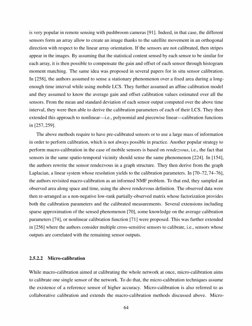
is very popular in remote sensing with pushbroom cameras [91]. Indeed, in that case, the different
sensors form an array allow to create an image thanks to the satellite movement in an orthogonal
direction with respect to the linear array orientation. If the sensors are not calibrated, then stripes
appear in the images. By assuming that the statistical content sensed by each sensor to be similar for
each array, it is then possible to compensate the gain and offset of each sensor through histogram
moment matching. The same idea was proposed in several papers for in situ sensor calibration.
In [258], the authors assumed to sense a stationary phenomenon over a fixed area during a long-
enough time interval while using mobile LCS. They further assumed an affine calibration model
and they assumed to know the average gain and offset calibration values estimated over all the
sensors. From the mean and standard deviation of each sensor output computed over the above time
interval, they were then able to derive the calibration parameters of each of their LCS. They then
extended this approach to nonlinear—i.e., polynomial and piecewise linear—calibration functions
in [257, 259].
The above methods require to have pre-calibrated sensors or to use a large mass of information
in order to perform calibration, which is not always possible in practice. Another popular strategy to
perform macro-calibration in the case of mobile sensors is based on rendezvous, i.e., the fact that
sensors in the same spatio-temporal vicinity should sense the same phenomenon [224]. In [154],
the authors rewrite the sensor rendezvous in a graph structure. They then derive from the graph
Laplacian, a linear system whose resolution yields to the calibration parameters. In [70–72, 74–76],
the authors revisited macro-calibration as an informed NMF problem. To that end, they sampled an
observed area along space and time, using the above rendezvous definition. The observed data were
then re-arranged as a non-negative low-rank partially-observed matrix whose factorization provides
both the calibration parameters and the calibrated measurements. Several extensions including
sparse approximation of the sensed phenomenon [70], some knowledge on the average calibration
parameters [74], or nonlinear calibration function [71] were proposed. This was further extended
in [256] where the authors consider multiple cross-sensitive sensors to calibrate, i.e., sensors whose
outputs are correlated with the remaining sensor outputs.
2.5.2.2 Micro-calibration
While macro-calibration aimed at calibrating the whole network at once, micro-calibration aims
to calibrate one single sensor of the network. To do that, the micro-calibration techniques assume
the existence of a reference sensor of higher accuracy. Micro-calibration is also referred to as
collaborative calibration and extends the macro-calibration methods discussed above. Micro-
64
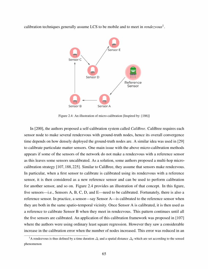
calibration techniques generally assume LCS to be mobile and to meet in rendezvous1.
Figure 2.4: An illustration of micro-calibration [Inspired by: [186]]
In [200], the authors proposed a self-calibration system called CaliBree. CaliBree requires each
sensor node to make several rendezvous with ground-truth nodes, hence its overall convergence
time depends on how densely deployed the ground-truth nodes are. A similar idea was used in [29]
to calibrate particulate matter sensors. One main issue with the above micro-calibration methods
appears if some of the sensors of the network do not make a rendezvous with a reference sensor
as this leaves some sensors uncalibrated. As a solution, some authors proposed a multi-hop micro-
calibration strategy [107, 188, 225]. Similar to CaliBree, they assume that sensors make rendezvous.
In particular, when a first sensor to calibrate is calibrated using its rendezvous with a reference
sensor, it is then considered as a new reference sensor and can be used to perform calibration
for another sensor, and so on. Figure 2.4 provides an illustration of that concept. In this figure,
five sensors—i.e., Sensors A, B, C, D, and E—need to be calibrated. Fortunately, there is also a
reference sensor. In practice, a sensor—say Sensor A—is calibrated to the reference sensor when
they are both in the same spatio-temporal vicinity. Once Sensor A is calibrated, it is then used as
a reference to calibrate Sensor B when they meet in rendezvous. This pattern continues until all
the five sensors are calibrated. An application of this calibration framework was proposed in [107]
where the authors were using ordinary least square regression. However they saw a considerable
increase in the calibration error when the number of nodes increased. This error was reduced in an
1A rendezvous is thus defined by a time duration ∆t and a spatial distance ∆d which are set according to the sensed
phenomenon
65
improved finding by the same authors in [225] where they were using geometric mean regression.
Lastly, they extended the above framework to the case of multiple cross-sensitive sensors in [188].
2.5.2.3 Calibration Transfer
A third type of sensor network calibration is calibration transfer. The calibration transfer method is
increasingly sought especially when the availability of reference sensors is unguaranteed. It consists
of performing relative calibration between a set of uncalibrated sensors, i.e., to make them provide
consistent sensor outputs. Then, when one of these sensors is calibrated with respect to a reference
sensor, it transmits to the remaining ones its new calibration parameters.
Figure 2.5: An illustration of calibration transfer [Inspired by: [186]]
An illustration of calibration transfer can be seen in Figure 2.5. The figure shows several
uncalibrated sensors, i.e., Sensors A, B, C, and D. Sensors B, C, and D are slave sensors which are
standardized to a master sensor, i.e., Sensor A. In a first stage, Sensor outputs are made consistent
between Sensors A to D, i.e., a “relative” calibration is performed using one of the methods discussed
in the above subsections. Then, Sensor A is calibrated with respect to a reference and transfers its
calibration parameters to the slave ones. Thus the main principle behind this method is the transfer
of calibration parameters from reference sensors to the low-cost mobile sensors [40]. Many related
works on calibration transfer are seen to be more related to electronic noses (e-nose) which are
sensor arrays targeting hazardous gas odour [150]. Many e-noses produce varying responses unlike
other sensor arrays as posited by authors in to [287]. As a consequence, calibrating such sensor
arrays becomes more tedious as each sensor needs to be calibrated separately. For these reasons,
calibration transfer is mostly a preferred method for performing the calibration. It must be noted
that calibration transfer is not specific to only e-noses as it can be applied to other sensors as well.
66
For example, the authors in [63] proposed to solve the inherent sensor array variability of e-noses
using a robust regression approach. Two e-nose systems were used, one for training via an artificial
neural network model, so that the predicted models are transferred to the other for system. Their
results showed a relatively low absolute mean error between the predicted and actual measurements.
Using the master and slave approach, the authors in [287] build their calibration transfer model
using robust weighted least squares. Their method is evaluated using e-noses with metal oxygen
semiconductor sensors. They however fail to provide validation for real applications and other
target pollutants. Further, the work in [90] showed that their authors are able to cut calibration
costs in mass production and re-calibration using their proposed calibration transfer model. Using
direct standardization, their approach involves mapping signals of one unit onto a reference unit. A
similar work was done in [282], but their authors used an improved method called Standardization
Error-based Model Improvement (SEMI). The main advantage of SEMI is that it makes training
models more reliant on variables with lower standardization errors and consequently less sensitive to
device variability. Some techniques also combine the slave and master approach into one framework,
see, e.g., [25, 40] using transfer learning and multi-task learning.
2.5.3 Calibration Methods
In this section we review some of the various methods that have been used in the calibration models
and calibration strategies discussed above. Some of the methods like those related to least square
regression or curve fitting generally aims to build a linear or nonlinear relationship between the
measured pollutant and the associated sensor output. In some cases more sophisticated calibration
methods—e.g., neural networks, random forests, and other machine learning methods—are necessary
to handle several target pollutants to tackle the problem of low selectivity [186]. These are all
discussed below.
2.5.3.1 Least Square Methods
Least square methods are standard approaches in regression analysis. They are the simplest and most
widely used methods for calibration. In particular, these approaches are the standard techniques
for in-lab calibration. They were also proposed for in situ calibration, for both single-variable and
multiple-variable calibration models. Two types of least squares have been used in literature, i.e.,
the standard least squares and multiple least squares.
m Standard Least Squares: When it comes to standard or ordinary least squares especially those
used for regression, there are several usage in literature. Several field calibration methods for
67
low-cost sensors were explored and compared in [236] including those that apply standard
least squares. In [66], the authors used polynomials to fit the nonlinear sensor output to the
calibration reference for each of the calibration points using ordinary least-squares fit. In [115],
the authors used standard least square regression models to fit their data when calibrating their
proposed optical aerosol sensors. Similarly in [35], the authors show they are able to obtain a
better correlation of several electrochemical sensors when targeting several gas pollutants.
m Multiple Least Squares: The multiple least squares method has been found to yield better
results than the standard least squares irrespective of the kind of low-cost sensor used. The
idea is to make linear combinations of target pollutant concentrations that optimally matches
the associated reference measurement. In [81], the authors use a linear regression approach
for the estimation of methane concentration. Another interesting finding can be found in [240]
where the authors show that their zero-calibration protocol—which is based on multiple
least-squares—efficiently corrected the observed drift of the low-cost sensor output. Other
findings can be seen in [13, 125, 192, 213].
2.5.3.2 Neural Networks
Most of the already discussed models are considered to be linearized calibration models. However
as posited by [236], nonlinear types—particularly those that rely on supervised learning—provided
better agreement between the low-cost sensors and the reference measurements. Artificial neural
networks is increasingly becoming a popular technique used for sensor calibration. Using neural
networks one can easily make relationships between raw sensor responses with pollutant concen-
trations. In parallel works, some authors have used neural networks for estimation of pollutant
concentrations but they present fair to middling results for short deployments and even weaker
findings for longer deployments, e.g., in [122] where a concurrent estimation of CO and CH4 in
a humid air mixture were made using neural networks, the results obtained were moderate with a
relative error of 5%. For calibration purposes several researchers have tried to use neural networks
for different sensors. It is worth mentioning that—when calibrated with neural networks—sensors
like the solid-state gas sensors may present some instabilities with spun-out time responses [235].
The authors in [129] complemented previous works aimed at improving selectivity of many industrial
analysers by proposing two ways to calibrate a multi-sensor, one of which was done via a neural
network algorithm. The author in [4] made a fuzzy logic based neural network algorithm to find
a model that can predict a membership degree for several target pollutants. Many other findings
related to neural networks can be seen in [58, 59, 78, 79]
68

2.5.3.3 Other Machine Learning techniques
Aside from regression methods with least squares and neural networks, several authors have tried
other machine learning techniques, e.g., Some authors explored the concepts of matrix factorization
in [76]. Further, the authors in [161] presented a method based on Boosted Regression Trees (BRT)
which is a machine learning method that learns from target pollutant source characteristics when
the complexity of the source is high. Interestingly, the authors in [8] showed that the complexity of
the calibration model may be linked with the time interval used to learn the calibration function. In
particular, they show that when calibration is performed on a daily basis, a simple linear model is
more efficient (and provides a better performance) than a more complex model applied on a weekly
to monthly basis.
2.6 Discussion
In this chapter, we recalled the reasons why air quality is monitored, we explained why LCS may
provide some complementary information to the authoritative sensors and which issues they also
provide. In particular, we showed that sensors tend to drift over time. This issue is particularly
important with LCS as it is usually not possible to calibrate them in-lab, which requires to perform
calibration in situ. We discussed several calibration models, different calibration strategies, and in
situ calibration methods. It is worth mentioning that, according to [186], the choice of a calibration
strategy depends on the network configuration. Indeed, there is no universal strategy even if some
authors already started to investigate this point. In particular, the authors in [186] refer to the work
done by C. Dorffer et al. [70,71,74–76], i.e., the research group I belong. Indeed, the latter proposed
an informed (semi-)non-negative matrix factorization framework for mobile sensor calibration
which:
• can tackle linear [76] or nonlinear [71] calibration models2;
• combine the data from authoritative sensors and from LCS, while taking into account their
difference in terms of accuracy [74];
• eventually take into account some additional information about the LCS to calibrate, i.e., the
average calibration parameters [74];
• allow to perform at the same time the estimation of the calibration parameters and the mapping
of the sensed phenomenon by completing the missing information using a dictionary-based
2Moreover, we extended in [256] this framework to a multi-linear multiple-variable calibration model.
69

approach [70, 74].
However, the above methods also suffer from some drawbacks.
1. First of all, the methods proposed by C. Dorffer et al. were based on multiplicative updates
or on a standard gradient descent. As as consequence, they are slow and not well-suited to
large-scale problems involving hundreds of sensors deployed over a large area.
2. Moreover, they could process in situ calibration when the sensors are observed during a short
time duration. We thus aim to extend the techniques to longer duration scenarios.
As a consequence, in this Ph.D. thesis, we aim to extend C. Dorffer’s work and to fix the above
drawbacks. The structure of the Ph.D. thesis is divided into two main parts. In the first part, we
explore the use of random projections to fasten (weighted) non-negative matrix factorization (NMF).
In particular, we propose several strategies to be combined with weighted NMF in a general case. In
the second part, we finally aim to integrate the findings of the first part into an informed framework,
with application to in situ sensor calibration.
70
Part I
Randomized (Weighted) Non-negativeMatrix Factorization
71
Chapter 3
Non-negative Matrix Factorization (NMF)
3.1 Background . . . . . . . . . . . . . . . . . . . . . . . . . . . . . . . . . . . . . . . . . . . . . . 74
3.1.1 Applications . . . . . . . . . . . . . . . . . . . . . . . . . . . . . . . . . . . . . . . . . . 75
3.1.2 Challenges . . . . . . . . . . . . . . . . . . . . . . . . . . . . . . . . . . . . . . . . . . . 77
3.2 Classical NMF Cost Functions . . . . . . . . . . . . . . . . . . . . . . . . . . . . . . . . . . . . 80
3.2.1 Discrepancy Measures . . . . . . . . . . . . . . . . . . . . . . . . . . . . . . . . . . . . . 80
3.2.2 Regularization for NMF . . . . . . . . . . . . . . . . . . . . . . . . . . . . . . . . . . . . 85
3.3 NMF Optimization Strategies . . . . . . . . . . . . . . . . . . . . . . . . . . . . . . . . . . . . . 87
3.3.1 Standard Nonlinear Optimization Schemes . . . . . . . . . . . . . . . . . . . . . . . . . . 88
3.3.2 Separable Schemes . . . . . . . . . . . . . . . . . . . . . . . . . . . . . . . . . . . . . . . 89
3.4 Classical NMF Algorithms . . . . . . . . . . . . . . . . . . . . . . . . . . . . . . . . . . . . . . 90
3.4.1 Multiplicative Updates (MU) . . . . . . . . . . . . . . . . . . . . . . . . . . . . . . . . . . 90
3.4.2 Projected Gradient (PG) . . . . . . . . . . . . . . . . . . . . . . . . . . . . . . . . . . . . 92
3.4.3 Alternating Least Squares (ALS) . . . . . . . . . . . . . . . . . . . . . . . . . . . . . . . . 93
3.4.4 Alternating Non-negative Least Squares (ANLS) . . . . . . . . . . . . . . . . . . . . . . . 93
3.4.5 Hierarchical Alternating Least Squares (HALS) . . . . . . . . . . . . . . . . . . . . . . . 94
3.5 Extensions of NMF . . . . . . . . . . . . . . . . . . . . . . . . . . . . . . . . . . . . . . . . . . 95
3.5.1 Semi-Non-negative Matrix Factorization . . . . . . . . . . . . . . . . . . . . . . . . . . . 95
3.5.2 Non-negative Matrix Co-Factorization . . . . . . . . . . . . . . . . . . . . . . . . . . . . . 95
3.5.3 Multi-layered and Deep (Semi-)NMF . . . . . . . . . . . . . . . . . . . . . . . . . . . . . 97
3.6 Discussion . . . . . . . . . . . . . . . . . . . . . . . . . . . . . . . . . . . . . . . . . . . . . . . 97
72
In many disciplines, generated data are usually in very high dimensions. A good example
is data generated from the health sector. A typical healthcare data could span several variables,
e.g., allergies, weight, blood pressure, mineral levels. The complexity of this kind of data often
thus requires more sophisticated algorithms and specific hardware to process it. These algorithms
typically aim to transform the data from the inherent high dimension to that of a lower one so
that efficient data analysis, information retrieval, and decision making can be realized. Dimension
reduction techniques can be group mainly into two types, i.e., linear and non-linear [249]. In this
section and the thesis at large, we will however only focus on linear dimensionality reduction and
the algorithms, particularly the non-negative matrix factorization.
Linear Dimensionality Reduction (LDR) is a well-known dimension reduction tool used in many
fields such as machine learning, statistics, and other applied fields.
Definition 3.1 (Linear Dimensionality Reduction [249]). Given a set A =[a1 a2 . . . an
]∈Rm×n
of n points in Rm, and a target low dimension s < m, LDR aims to optimize a given objective
function fX(·) which draws a linear transformation S ∈ Rs×m such that a low dimensional data
C = S ·A ∈ Rs×n can be obtained.
From Definition 3.1, LDR draws a linear map of data points from a high dimensional data space
onto a lower-dimensional one while preserving most of the important features. Numerous LDR
methods exist in the literature. One of the most popular one is principal component analysis (PCA).
It was first introduced by Pearson in [212], later popularized by contributions from several scientists,
e.g., in [21]. PCA makes projections onto a lower dimensional space by finding some orthogonal
directions that maximize the variance of an underlying high dimensional data. This means that the
target low dimensional subspace preserves the variability of the data. A similar technique to PCA
is the Linear discriminant analysis (LDA), which is said to extend the famous Fisher discriminant
analysis [89]. LDA aims to make a projection that maximizes the separability of classes in a feature
subspace. Independent component analysis (ICA) [53] is yet another LDA method which treats the
data matrix X as an unknown combination of unknown source signals assumed to be statistically
independent.
Other LDA techniques are multidimensional scaling (MDS) [243], Single Value Decomposition
(SVD) [128] and non-negative matrix factorization [157]. In this manuscript we have adopted the
NMF technique used throughout this thesis and discuss its background and concepts in much detail
in this chapter.
73
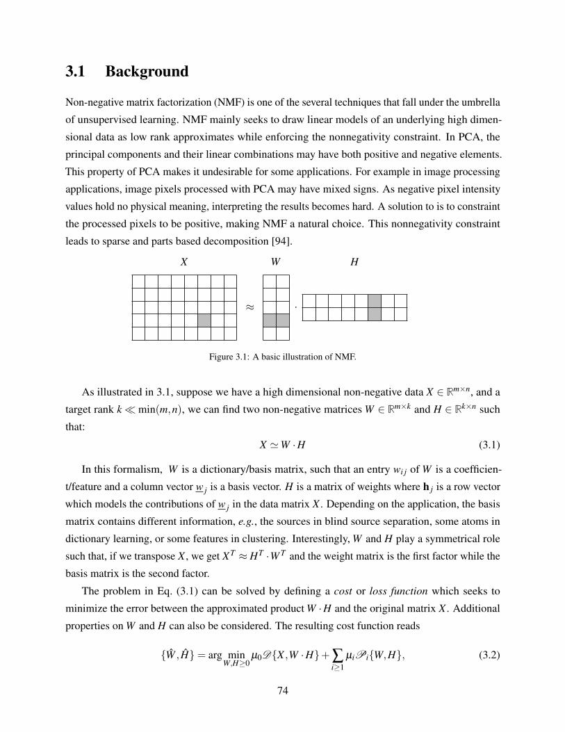
3.1 Background
Non-negative matrix factorization (NMF) is one of the several techniques that fall under the umbrella
of unsupervised learning. NMF mainly seeks to draw linear models of an underlying high dimen-
sional data as low rank approximates while enforcing the nonnegativity constraint. In PCA, the
principal components and their linear combinations may have both positive and negative elements.
This property of PCA makes it undesirable for some applications. For example in image processing
applications, image pixels processed with PCA may have mixed signs. As negative pixel intensity
values hold no physical meaning, interpreting the results becomes hard. A solution to is to constraint
the processed pixels to be positive, making NMF a natural choice. This nonnegativity constraint
leads to sparse and parts based decomposition [94].
X W H
≈ ·
Figure 3.1: A basic illustration of NMF.
As illustrated in 3.1, suppose we have a high dimensional non-negative data X ∈ Rm×n, and a
target rank kmin(m,n), we can find two non-negative matrices W ∈ Rm×k and H ∈ Rk×n such
that:
X 'W ·H (3.1)
In this formalism, W is a dictionary/basis matrix, such that an entry wi j of W is a coefficien-
t/feature and a column vector w j is a basis vector. H is a matrix of weights where h j is a row vector
which models the contributions of w j in the data matrix X . Depending on the application, the basis
matrix contains different information, e.g., the sources in blind source separation, some atoms in
dictionary learning, or some features in clustering. Interestingly, W and H play a symmetrical role
such that, if we transpose X , we get XT ≈HT ·W T and the weight matrix is the first factor while the
basis matrix is the second factor.
The problem in Eq. (3.1) can be solved by defining a cost or loss function which seeks to
minimize the error between the approximated product W ·H and the original matrix X . Additional
properties on W and H can also be considered. The resulting cost function reads
W , H= arg minW,H≥0
µ0DX ,W ·H+∑i≥1
µiPiW,H, (3.2)
74
where D·, · denotes a loss function—and more particularly a discrepancy measure between X and
its approximation W ·H—the Pi·, · expressions denote some penalization terms, and µ0,µ1, . . .
are weights to balance the different objective functions. Classical loss and penalization functions
used in NMF are discussed further in Subsection 3.2.
In this chapter we discuss the main algorithms for NMF, some of its challenges, applications and
relevant variants pertinent to the objectives of the present work, i.e., sensor calibration.
3.1.1 Applications
NMF is today one of the very popular unsupervised machine learning techniques. Its part-based
decomposition makes it well-suited for many applications. We discuss some of them below.
The authors in [67] used NMF in conjunction with Probabilistic Latent Semantic Indexing
(PLSI) for topic modelling. By running the two algorithms alternately, a better final solution is
achieved than when they are used separately. In document clustering [275], NMF was applied to
a term-document matrix. Their method was experimentally shown to outperform classical latent
semantic indexing and spectral clustering methods in terms of accuracy and clustering outputs. The
authors in [228] also made contributions in the same area using a hybrid method based on several
NMF algorithm. In their application they are able to identify and cluster topics or semantic features
in heterogeneous text. Sparse and weakly-supervised NMF extensions were also used for document
clustering in [144] for fast convergence and clustering accuracy.
Let us take a look at some contributions to image processing tasks as well. In [163] a local
non-negative matrix factorization (LNMF) was presented. Their proposed method is a variant of
standard NMF which adds a localization constraint for part-based rendering and spatially localized
learning of visual patterns. Experimental findings when comparing their LNMF to NMF and PCA
showed the superiority of the presented method with better face representation and recognition.
Shortly after this LNMF was combined with a learning algorithm based on AdaBoost [39] for face
detection. New findings related to this method were presented in later studies. In [27,28], the authors
found that in similar feature extraction tasks, different metric-based classifiers led to different results.
NMF was thus found to be more robust than LNMF, i.e., in the presence of illumination. Other face
recognition applications can be found in [103], where the authors applied NMF for face classification.
They further showed NMF to provide better recognition rates than principal component analysis due
to its part-based decomposition.
NMF has also been for a long time the state-of-the-art for audio signal analysis [88, 254]. In
that case, NMF is usually applied to time-frequency representations of one or several audio signals.
The matrix factors obtained through NMF then contain some frequency patterns and some temporal
75
activation of these frequency patterns, respectively. The phase information of the audio signals—not
used in the NMF procedure—is then estimated from the original observed signals and the estimated
source amplitudes.
In the context of Recommender Systems (RS), several advancements have been made with NMF
after the success story of the famous Netflix prize competition. In RS we are merely interested in
predicting ratings or preferences which a set of users would have provided to some items. In [142],
comprehensive studies on algorithms for matrix factorization applied to RS are presented. According
to [136], sparsity reduces the accuracy of recommender systems. Their authors thus propose a
collaborative filtering method based on NMF with an improved embedding scheme. Other findings
for collaborative filtering can be found in [184]. However, this work is based on on single-element
approach, i.e., each involved feature. It is interesting to notice that in situ mobile sensor calibration
revisited as an informed matrix factorization problem [76] meets similarities with RS, except that the
focus in [76] is the estimation of W and H while in RS, we focus on the estimation of the missing
entries of X .
Hyperspectral unmixing is also a major application of NMF. In that case, the observed data
is a cube with two spatial dimensions and one spectral one. NMF is a very popular method as it
allows to estimate the source spectra (aka endmembers) and their associated mixing parameters (aka
abundances). NMF was used for unmixing hyperspectral data provided by satellites observing space,
e.g., [17, 216], or earth [19]. Moreover, joint unmixing through NMF is also a classical strategy to
perfom multi-sharpening [5, 285], i.e., the fusion of multispectral images—which provide a fine
spatial sampling but a coarse spectral one—and hyperspectral images—which provide a fine spectral
sampling but a coarse spatial one—in order to provide new hyperspectral images with the spatial
and spectral information of multispectral and hyperspectral images, respectively.
NMF has also been extensively employed in source apportionment problems [116]. Source
apportionment is one of the most popular paradigms in many environmental monitoring tasks. The
main aim is to estimate profiles of pollution sources and their contribution in the breathed particulate
matter concentrations, i.e., their level of impact on air pollution. Due to its nature, this problem may
be solved by weighted NMF with a sum-to-one constraint applied to the rows of W . In [43,166], the
authors proposed an informed NMF method for source apportionment. In particular, they proposed
a parameterization which allows an expert to freeze some entries in H. This was then extended in
several papers by considering outlier-robust cost functions [44, 46, 62, 165, 168], by adding bounded
constraints [62, 169]—allowing an expert to provide intervals of admissible values for some entries
in H—by combining NMF with a physical model which helps to decide whether or not a local
source is sensed in a given sample [214], and through a split-gradient strategy which automatically
76
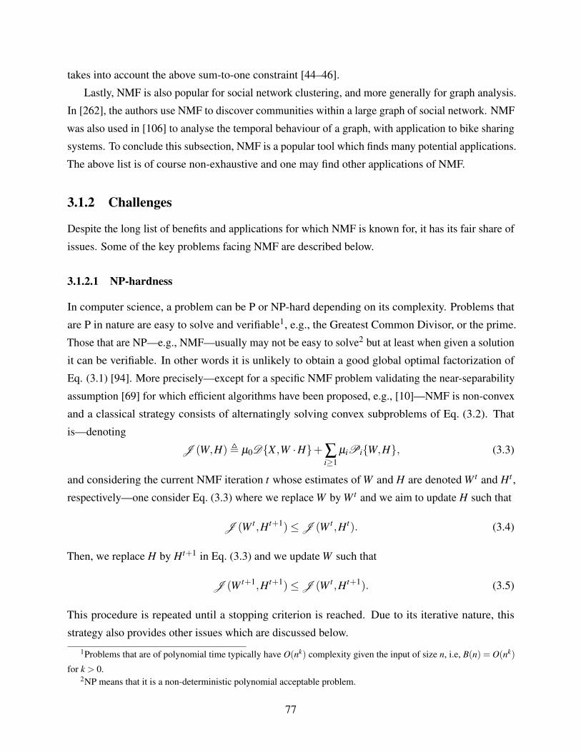
takes into account the above sum-to-one constraint [44–46].
Lastly, NMF is also popular for social network clustering, and more generally for graph analysis.
In [262], the authors use NMF to discover communities within a large graph of social network. NMF
was also used in [106] to analyse the temporal behaviour of a graph, with application to bike sharing
systems. To conclude this subsection, NMF is a popular tool which finds many potential applications.
The above list is of course non-exhaustive and one may find other applications of NMF.
3.1.2 Challenges
Despite the long list of benefits and applications for which NMF is known for, it has its fair share of
issues. Some of the key problems facing NMF are described below.
3.1.2.1 NP-hardness
In computer science, a problem can be P or NP-hard depending on its complexity. Problems that
are P in nature are easy to solve and verifiable1, e.g., the Greatest Common Divisor, or the prime.
Those that are NP—e.g., NMF—usually may not be easy to solve2 but at least when given a solution
it can be verifiable. In other words it is unlikely to obtain a good global optimal factorization of
Eq. (3.1) [94]. More precisely—except for a specific NMF problem validating the near-separability
assumption [69] for which efficient algorithms have been proposed, e.g., [10]—NMF is non-convex
and a classical strategy consists of alternatingly solving convex subproblems of Eq. (3.2). That
is—denoting
J (W,H), µ0DX ,W ·H+∑i≥1
µiPiW,H, (3.3)
and considering the current NMF iteration t whose estimates of W and H are denoted W t and Ht ,
respectively—one consider Eq. (3.3) where we replace W by W t and we aim to update H such that
J (W t ,Ht+1)≤J (W t ,Ht). (3.4)
Then, we replace H by Ht+1 in Eq. (3.3) and we update W such that
J (W t+1,Ht+1)≤J (W t ,Ht+1). (3.5)
This procedure is repeated until a stopping criterion is reached. Due to its iterative nature, this
strategy also provides other issues which are discussed below.
1Problems that are of polynomial time typically have O(nk) complexity given the input of size n, i.e, B(n) = O(nk)
for k > 0.2NP means that it is a non-deterministic polynomial acceptable problem.
77
3.1.2.2 Initialization
The speed of convergence and the accuracy of the solution provided by many NMF algorithms
hugely depends on the quality of the initialization. As NMF is an iterative technique, many NMF
solvers are very sensitive to the initialization of the matrix factors W,H.Classical initialization methods are purely random [147] where the matrices are initialized with
uniformly distributed random numbers, e.g., between 0 and 1. This type of initialization although
simple might not always provide a good solution. An easy fix is to run NMF several times with
different initializations and to find their median or the best value A variant of random initialization
is random Acol [147]. This approach is useful for sparse data and aims to find an average of k
random rows of X which is used to initialize each column of the W matrix. Some authors also found
that adding structure to the initialization model provides a better solution. To this end, centroid
initialization was proposed in [269, 271]. However, it can be computational expensive as a pre-
processing method. In [23], W can also be initialized with a Singular Value Decomposition (SVD)
of X . Some authors also consider initialization using the output of a clustering technique [270], of a
source separation output [16], or using a physical model [214].
3.1.2.3 Ill-posedness
Since NMF has no unique solution, it is said to be ill-posed3. Indeed from Eq. (3.1) and given any
k× k invertible matrix B such that,
W ·B≥ 0, (3.6)
and
B−1 ·H ≥ 0, (3.7)
where the symbol ≥ here denotes the element-wise inequality, it is easy to see that (W ·B) and
(B−1 ·H) are also solutions of Eq. (3.1). Such a property is also classical in many source separation
problems with the well-known gain and permutation ambiguities [52]. The gain ambiguity may be
solved by adding normalization constraints either of W or H. Such a constrain naturally appears in
some NMF applications such as hyperspectral unmixing [19] or source apportionment [62], where
the weight coefficients in, e.g., W can be seen as proportions which sum to 1. The permutation
ambiguity may be solved in informed NMF [166] where some additional knowledge allows to fix
the order of the components in either W or H.
3Most ill-posed problems can be re-structured numerically by imposing additional assumptions like sparsity and
smoothness [182, 239].
78
3.1.2.4 Choice of the NMF rank k
The choice of the NMF rank k which is the number of columns in W and of rows in H plays a big
role in the NMF formulation with respect to the application and data used. Indeed, the bigger the
rank the closer you are to the true data and the smaller the rank the less complex the model. So
how can we choose the best value of k? One popular way is the hit-or-miss approach. In practice
several ranks are tested to determine the one that gives the most desirable results. SVD and expert
intuition—as pointed out by Gillis in [94]—may also help in rank selection. More complex methods
are, Bayesian non-parametric method [114], cross-validation in NMF [130], and Stein’s Unbiased
Risk Estimator (SURE) [247].
3.1.2.5 Stopping Criteria and Stationary Points
Like many iterative techniques, NMF requires a condition to be satisfied in order for it to terminate.
This termination usually signifies that some local minium to Eq. (3.2) has been reached. NMF
stopping criteria is very crucial to the accuracy of the final solution. In many practical applications
of NMF, the stopping criterion may be based on the total number of NMF iterations [86] or on a
specified CPU time [72]. Note that these techniques are quite trivial and may lead to inaccuracies.
This is because the evolution of the error might be stopped too early before reaching the optimal final
solution. Another technique which was used in [26] finds the difference between two successive
iterates, i.e., the t-th and (t + 1)-th iterations. A more efficient method which has been used for
NMF can be seen in [138, 172] where the authors use the so called Karush–Kuhn–Tucher (KKT)
conditions as a inequality-constrained optimization approach.
The KKT conditions are first order necessary conditions of optimality in nonlinear programming.
When used for NMF, for instance given the problem
W , H= arg minW,H≥0
DX ,W ·H, (3.8)
and denoting the Hadamard product, a stationary point W , H is attained if and only if:
W ≥ 0
H ≥ 0
(3.9)
(3.10)
∇W DX ,W ·H ≥ 0
∇HDX ,W ·H ≥ 0
(3.11)
(3.12)
W∇W DX ,W ·H= 0
H∇HDX ,W ·H= 0
(3.13)
(3.14)
79
Stationarity is only a necessary condition to find a local minimum. In particular, Eqs. (3.13) and
(3.14) state that if W or H are not null, the gradient of the cost function is null. Lin reported that
some limit points obtained from multiplicative updates which are not stationary may exist [172],
especially if some components of W and H are initialized to zero.
3.1.2.6 Uniqueness of NMF
Indeed as the problem in Eq. (3.2) is not convex, it often leads to many solutions. In other words,
it may exhibit more than one optimal solution. For this reason, some conditions that guarantee a
unique solution have been studied in literature. Studies in [69] posited that, up to some permutation
matrix the uniqueness of the NMF solution is possible if certain conditions of joint parsimony of the
matrix factors which are called near-separability are satisfied. Studies in [38] also posited that, we
can obtain a product W ·H as a unique decomposition of X if and only if the simplicial cone4 CH
such that X ⊂ CH is unique.
Other studies by [204] also provided some information on uniqueness of NMF using some
separability conditions later proposed in [93, 94]. They explain that, an NMF decomposition
X =W ·H is unique if there exist monomial5 sub-matrices of W and H, each of size k× k. This sort
of assumption is also encountered in Hyperspectral Unmixing as pure pixel assumption.
Another alternative approach to limit the multiple solutions is to provide additional constraints
to the initial NMF problem, as already explained in the previous subsections.
3.2 Classical NMF Cost Functions
In this section, we review some classical cost functions used in Eq. (3.2). let us recall that the latter
comprises of a discrepancy measure D(X ,W ·H) and regularization/penalization terms Pi(W,H).
3.2.1 Discrepancy Measures
The discrepancy measure in our NMF formulation in Eq. (3.2) typically measures the goodness of
the approximation between the original matrix X and the product of the factor matrices (W ,H). The
choice of the type of measure highly depends on the application.
4the simplicial cone generated by a set of vectors h1, ...,hk ∈Rm is defined as the set CH = x|x=k∑j=1
w jh j, w j >
0.5A monomial matrix is a permutation of a diagonal matrix with positive diagonal elements.
80
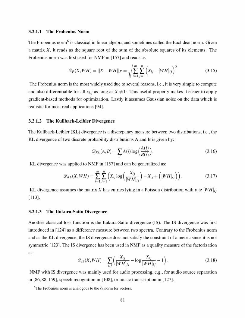
3.2.1.1 The Frobenius Norm
The Frobenius norm6 is classical in linear algebra and sometimes called the Euclidean norm. Given
a matrix X , it reads as the square root of the sum of the absolute squares of its elements. The
Frobenius norm was first used for NMF in [157] and reads as
DF(X ,WH) = ||X−WH||F =
√m
∑i=1
n
∑j=1
(Xi j− [WH]i j
)2(3.15)
The Frobenius norm is the most widely used due to several reasons, i.e., it is very simple to compute
and also differentiable for all xi, j as long as X 6= 0. This useful property makes it easier to apply
gradient-based methods for optimization. Lastly it assumes Gaussian noise on the data which is
realistic for most real applications [94].
3.2.1.2 The Kullback-Leibler Divergence
The Kullback-Leibler (KL) divergence is a discrepancy measure between two distributions, i.e., the
KL divergence of two discrete probability distributions A and B is given by:
DKL(A,B) = ∑i
A(i) log(A(i)
B(i)
). (3.16)
KL divergence was applied to NMF in [157] and can be generalized as:
DKL(X ,WH) =m
∑i=1
n
∑j=1
(Xi j log
( Xi j
[WH]i j
)−Xi j +
([WH]i j
)). (3.17)
KL divergence assumes the matrix X has entries lying in a Poisson distribution with rate [WH]i j
[113].
3.2.1.3 The Itakura-Saito Divergence
Another classical loss function is the Itakura-Saito divergence (IS). The IS divergence was first
introduced in [124] as a difference measure between two spectra. Contrary to the Frobenius norm
and as the KL divergence, the IS divergence does not satisfy the constraint of a metric since it is not
symmetric [123]. The IS divergence has been used in NMF as a quality measure of the factorization
as:
DIS(X ,WH) = ∑i, j
( Xi j
[WH]i j− log
Xi j
[WH]i j−1). (3.18)
NMF with IS divergence was mainly used for audio processing, e.g., for audio source separation
in [86, 88, 159], speech recognition in [108], or music transcription in [127].6The Frobenius norm is analogous to the `2 norm for vectors.
81
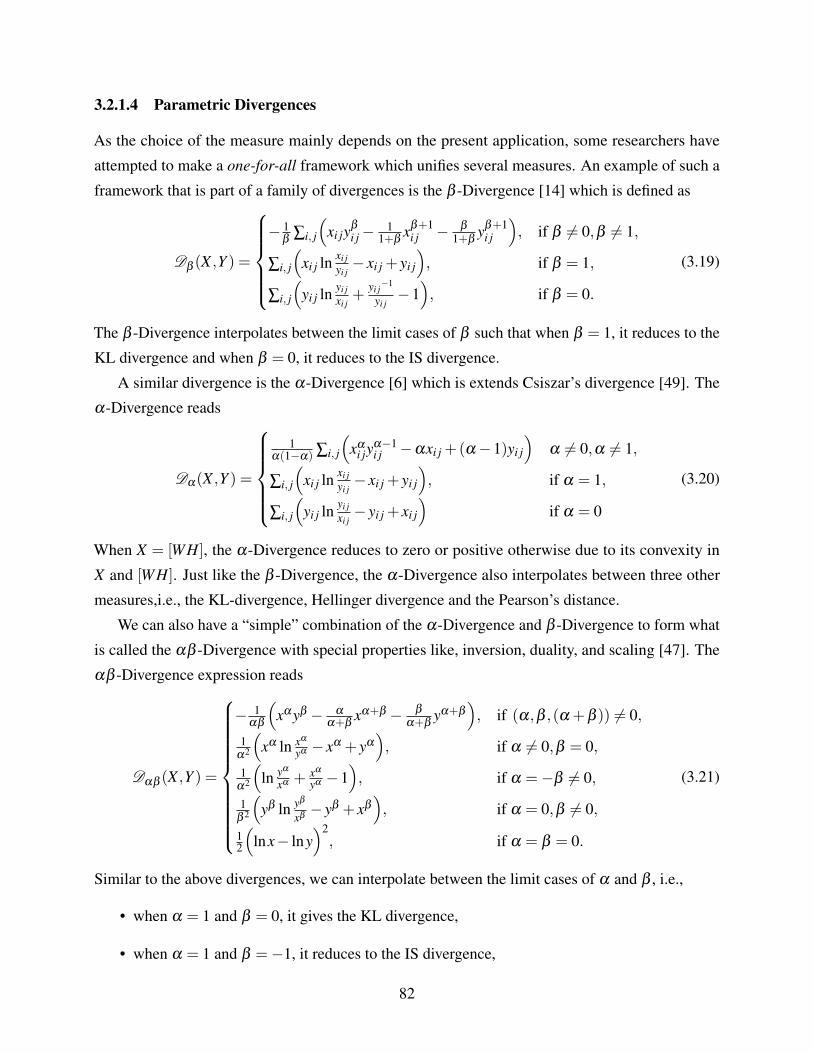
3.2.1.4 Parametric Divergences
As the choice of the measure mainly depends on the present application, some researchers have
attempted to make a one-for-all framework which unifies several measures. An example of such a
framework that is part of a family of divergences is the β -Divergence [14] which is defined as
Dβ (X ,Y ) =
− 1β
∑i, j
(xi jy
β
i j− 11+β
xβ+1i j − β
1+βyβ+1
i j
), if β 6= 0,β 6= 1,
∑i, j
(xi j ln xi j
yi j− xi j + yi j
), if β = 1,
∑i, j
(yi j ln yi j
xi j+
yi j−1
yi j−1), if β = 0.
(3.19)
The β -Divergence interpolates between the limit cases of β such that when β = 1, it reduces to the
KL divergence and when β = 0, it reduces to the IS divergence.
A similar divergence is the α-Divergence [6] which is extends Csiszar’s divergence [49]. The
α-Divergence reads
Dα(X ,Y ) =
1α(1−α) ∑i, j
(xα
i jyα−1i j −αxi j +(α−1)yi j
)α 6= 0,α 6= 1,
∑i, j
(xi j ln xi j
yi j− xi j + yi j
), if α = 1,
∑i, j
(yi j ln yi j
xi j− yi j + xi j
)if α = 0
(3.20)
When X = [WH], the α-Divergence reduces to zero or positive otherwise due to its convexity in
X and [WH]. Just like the β -Divergence, the α-Divergence also interpolates between three other
measures,i.e., the KL-divergence, Hellinger divergence and the Pearson’s distance.
We can also have a “simple” combination of the α-Divergence and β -Divergence to form what
is called the αβ -Divergence with special properties like, inversion, duality, and scaling [47]. The
αβ -Divergence expression reads
Dαβ (X ,Y ) =
− 1αβ
(xαyβ − α
α+βxα+β − β
α+βyα+β
), if (α,β ,(α +β )) 6= 0,
1α2
(xα ln xα
yα − xα + yα
), if α 6= 0,β = 0,
1α2
(ln yα
xα + xα
yα −1), if α =−β 6= 0,
1β 2
(yβ ln yβ
xβ− yβ + xβ
), if α = 0,β 6= 0,
12
(lnx− lny
)2, if α = β = 0.
(3.21)
Similar to the above divergences, we can interpolate between the limit cases of α and β , i.e.,
• when α = 1 and β = 0, it gives the KL divergence,
• when α = 1 and β =−1, it reduces to the IS divergence,
82
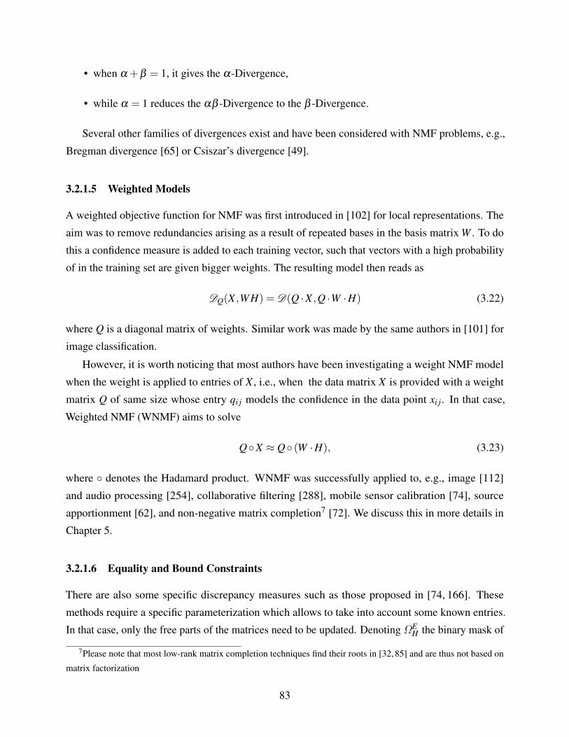
• when α +β = 1, it gives the α-Divergence,
• while α = 1 reduces the αβ -Divergence to the β -Divergence.
Several other families of divergences exist and have been considered with NMF problems, e.g.,
Bregman divergence [65] or Csiszar’s divergence [49].
3.2.1.5 Weighted Models
A weighted objective function for NMF was first introduced in [102] for local representations. The
aim was to remove redundancies arising as a result of repeated bases in the basis matrix W . To do
this a confidence measure is added to each training vector, such that vectors with a high probability
of in the training set are given bigger weights. The resulting model then reads as
DQ(X ,WH) = D(Q ·X ,Q ·W ·H) (3.22)
where Q is a diagonal matrix of weights. Similar work was made by the same authors in [101] for
image classification.
However, it is worth noticing that most authors have been investigating a weight NMF model
when the weight is applied to entries of X , i.e., when the data matrix X is provided with a weight
matrix Q of same size whose entry qi j models the confidence in the data point xi j. In that case,
Weighted NMF (WNMF) aims to solve
QX ≈ Q (W ·H), (3.23)
where denotes the Hadamard product. WNMF was successfully applied to, e.g., image [112]
and audio processing [254], collaborative filtering [288], mobile sensor calibration [74], source
apportionment [62], and non-negative matrix completion7 [72]. We discuss this in more details in
Chapter 5.
3.2.1.6 Equality and Bound Constraints
There are also some specific discrepancy measures such as those proposed in [74, 166]. These
methods require a specific parameterization which allows to take into account some known entries.
In that case, only the free parts of the matrices need to be updated. Denoting ΩEH the binary mask of
7Please note that most low-rank matrix completion techniques find their roots in [32, 85] and are thus not based on
matrix factorization
83
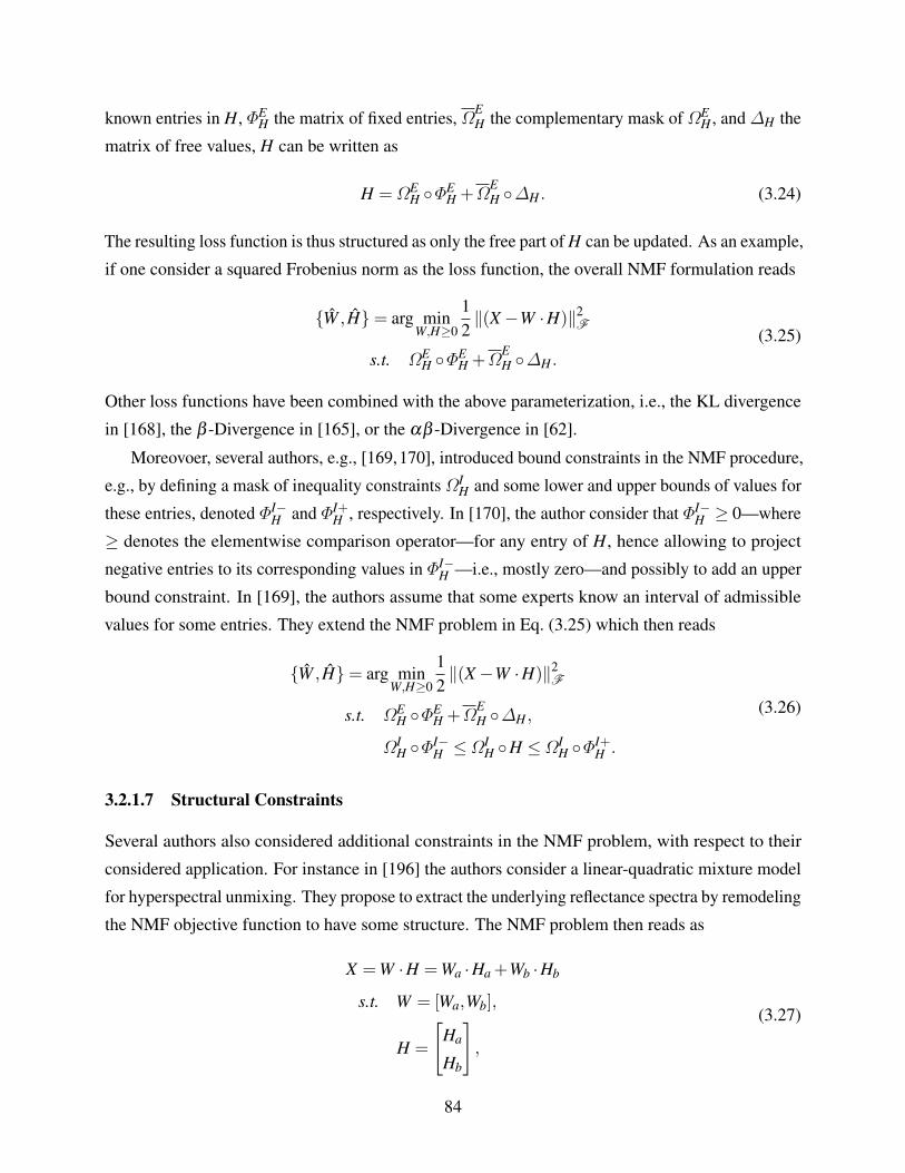
known entries in H, ΦEH the matrix of fixed entries, ΩE
H the complementary mask of ΩEH , and ∆H the
matrix of free values, H can be written as
H =ΩEH ΦE
H +ΩEH ∆H . (3.24)
The resulting loss function is thus structured as only the free part of H can be updated. As an example,
if one consider a squared Frobenius norm as the loss function, the overall NMF formulation reads
W , H= arg minW,H≥0
12‖(X−W ·H)‖2
F
s.t. ΩEH ΦE
H +ΩEH ∆H .
(3.25)
Other loss functions have been combined with the above parameterization, i.e., the KL divergence
in [168], the β -Divergence in [165], or the αβ -Divergence in [62].
Moreovoer, several authors, e.g., [169,170], introduced bound constraints in the NMF procedure,
e.g., by defining a mask of inequality constraints ΩIH and some lower and upper bounds of values for
these entries, denoted ΦI−H and ΦI+
H , respectively. In [170], the author consider that ΦI−H ≥ 0—where
≥ denotes the elementwise comparison operator—for any entry of H, hence allowing to project
negative entries to its corresponding values in ΦI−H —i.e., mostly zero—and possibly to add an upper
bound constraint. In [169], the authors assume that some experts know an interval of admissible
values for some entries. They extend the NMF problem in Eq. (3.25) which then reads
W , H= arg minW,H≥0
12‖(X−W ·H)‖2
F
s.t. ΩEH ΦE
H +ΩEH ∆H ,
ΩIH ΦI−
H ≤ΩIH H ≤ΩI
H ΦI+H .
(3.26)
3.2.1.7 Structural Constraints
Several authors also considered additional constraints in the NMF problem, with respect to their
considered application. For instance in [196] the authors consider a linear-quadratic mixture model
for hyperspectral unmixing. They propose to extract the underlying reflectance spectra by remodeling
the NMF objective function to have some structure. The NMF problem then reads as
X =W ·H =Wa ·Ha +Wb ·Hb
s.t. W = [Wa,Wb],
H =
[Ha
Hb
],
(3.27)
84
where W is the mixing matrix and H contains the sources. In their formalism, Ha is the matrix of
sources while Hb is the matrix of pseudo-sources—i.e., variations of the real sources—which is
fully derived from Ha. As a consequence, the authors in [196] solve Eq. (3.27) by considering Ha as
a master matrix and Hb as a slave of Ha. The update rule of H is thus based on the update of Ha
only. A similar strategy with master and slave columns of W is proposed in [71] for nonlinear sensor
calibration as W is assumed to be Vandermonde, i.e., only one vector of W allows to derive the full
matrix.
3.2.2 Regularization for NMF
As discussed previously, for NMF applications some additional properties on the factor matrices W
and H can also be considered as a regularization or penalization term. This is classical in machine
learning, inverse problems, signal/image processing, and statistics. The aim is usually to prevent
overfitting or to find optimality for ill-posed problems. We discuss some of the popular methods
below and assume, for the sake of simplicity, that the discrepancy measure is the squared Frobenius
norm8.
3.2.2.1 Smoothness Regularization
The `2 norm—aka the Euclidian norm—is a classical norm used in many problems. It is usually
considered in its quadratic form and allows to easily derive solutions. Regularizing a problem with
an `2-norm constraint—or a squared Frobenius norm in the case of the regularization of a matrix—is
thus extremely classical. Such a strategy is also widely known as Tikhonov regularization. Applied
to NMF, `2-norm regularization allows to add smoothness in one of the matrix factors [99, 137, 211].
For example, if one adds such a constraint on H and considering the Frobenius norm as a discrepancy
measure, Eq. (3.2) reads
W , H= arg minW,H≥0
||X−W ·H||2F +λ
2||H||2F , (3.28)
where λ is a user-defined threshold. Another use of such a regularization arises in low-rankness
penalization. Low-rankness is a very desirable property in many problems, such as matrix completion
for example [31, 32]. It allows to reduce the number of latent variables which explain the observed
data. It may be useful when combined with (non-negative) matrix factorization in order to avoid
overfitting of X . In that case, adding a low-rank structure on the approximation of X reads
W , H= arg minW,H≥0
||X−W ·H||2F +λ ||W ·H||? , (3.29)
8Of course, penalization terms may also been applied to NMF problems involving other discrepancy measures.
85
where λ is a user-defined weight and where ||·||? denotes the nuclear norm of a matrix, i.e., the sum
of its eigenvalues. Interestingly, minimizing the nuclear norm of the product W ·H is equivalent to
minimizing the sum of their squared Frobenius norm [237], i.e., Eq. (3.29) is equivalent to
W , H= arg minW,H≥0
||X−W ·H||2F +λ
2||W ||2F +
λ
2||H||2F (3.30)
which can be easily solved as alternating `2-norm regularized NMF problems.
3.2.2.2 Sparsity-promoting Regularization
Despite NMF inherent property of producing sparse and part-based decomposition [157], the
sparsity of the resulting matrix factors is not always guaranteed according to [118]. The `1-norm
regularization is then desired for promoting sparsity of one matrix factor. As an example, if one adds
such a constraint on H and considering the Frobenius norm as a discrepancy measure, the objective
function in Eq. (3.2) can be reformulated as:
W , H= arg minW,H≥0
||X−W ·H||2F +λ ||H||1 , (3.31)
where ||·||1 denotes the `1-norm and λ is a trade-off parameter. Examples of this type of regulariza-
tion can be seen in [99,118,152] for example. Please note that column sparsity according to a known
dictionary was also proposed in, e.g., [70, 74] for sensor calibration or in [229] for compressive
NMF.
The `1,2 norm or the group lasso penalization has been proposed in [197] for regression problems
to overcome some limitations of the `1 and `2 regularizations. Defined as
||H||1,2 = ∑i||hi||2 , (3.32)
where hi here denotes the i-th row of H, it offers a trade-off between the smoothness due to the `2
norm and the sparsity due to the `1 one.
3.2.2.3 Graph / Manifold Regularization
In several problems, additional structure can be added to the data. As an example, a graph structure
can be added into the NMF problem. In that case, a Laplacian matrix can be derived from the graph
and used to regularize the problem [30]. The so-called manifold penalization then reads
W , H= arg minW,H≥0
||X−W ·H||2F +λ
2Tr(HT LH) (3.33)
where L is the graph Laplacian, and λ is the regularization parameter for controlling smoothness.
86
3.2.2.4 Smooth Evolution Constraint
In some problems like audio or video processing, it might be interesting to constrain adjacent lines
or columns of a factor matrix to be close. For example, in [263], the authors constrain to smooth the
difference of adjacent columns in H for a video processing application. The corresponding NMF
problem then reads
W , H= arg minW,H≥0
||X−W ·H||2F +λ ||RH||1,2 , (3.34)
with
R =
−1 0 0 . . . 0
1 −1 0 . . . 0
0 1 −1 . . . 0...
... . . . . . . ...
0 0 0 . . . −1
0 0 0 . . . 1
. (3.35)
A similar approach was proposed in [80] where the authors replace the Frobenius norm in the loss
function by a KL divergence.
3.2.2.5 Volume Constraint
Another interesting technique is the volume constraint. Indeed, the NMF solution is not unique in the
general case but we discussed some conditions to reach a unicity in exact NMF in Subsection 3.1.2.6.
The authors in [226] thus propose to add the minimum-volume criteria to the NMF problem where
by the volume of one of the factors is minimized. With the influence of some noise, the penalized
objective function reads
W , H= arg minW,H≥0
||X−W ·H||2F +α
2logdet(W T ·W +σ · Ik), (3.36)
where Ik is a k× k identity matrix, α is the trade-off parameter and σ is a small security parameter.
3.3 NMF Optimization Strategies
There are two main classes of NMF according to [96] namely, standard nonlinear optimization
and separable schemes which we summarize below. For the sake of simplicity, we introduce these
strategies in the simplest form of NMF problem, i.e., with the Frobenius norm as a loss function and
without any penalization term. Eq. (3.2) then reads
W , H= arg minW,H≥0
12||X−W ·H||2F , (3.37)
87
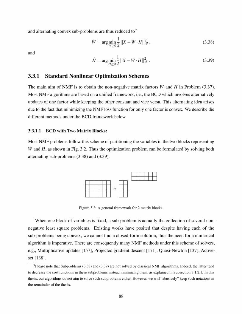
and alternating convex sub-problems are thus reduced to9
W = arg minW≥0
12||X−W ·H||2F , (3.38)
and
H = argminH≥0
12||X−W ·H||2F . (3.39)
3.3.1 Standard Nonlinear Optimization Schemes
The main aim of NMF is to obtain the non-negative matrix factors W and H in Problem (3.37).
Most NMF algorithms are based on a unified framework, i.e., the BCD which involves alternatively
updates of one factor while keeping the other constant and vice versa. This alternating idea arises
due to the fact that minimizing the NMF loss function for only one factor is convex. We describe the
different methods under the BCD framework below.
3.3.1.1 BCD with Two Matrix Blocks:
Most NMF problems follow this scheme of partitioning the variables in the two blocks representing
W and H, as shown in Fig. 3.2. Thus the optimization problem can be formulated by solving both
alternating sub-problems (3.38) and (3.39).
≈ ·
Figure 3.2: A general framework for 2 matrix blocks.
When one block of variables is fixed, a sub-problem is actually the collection of several non-
negative least square problems. Existing works have posited that despite having each of the
sub-problems being convex, we cannot find a closed-form solution, thus the need for a numerical
algorithm is imperative. There are consequently many NMF methods under this scheme of solvers,
e.g., Multiplicative updates [157], Projected gradient descent [171], Quasi-Newton [137], Active-
set [138].9Please note that Subproblems (3.38) and (3.39) are not solved by classical NMF algorithms. Indeed, the latter tend
to decrease the cost functions in these subproblems instead minimizing them, as explained in Subsection 3.1.2.1. In this
thesis, our algorithms do not aim to solve such subproblems either. However, we will “abusively” keep such notations in
the remainder of the thesis.
88
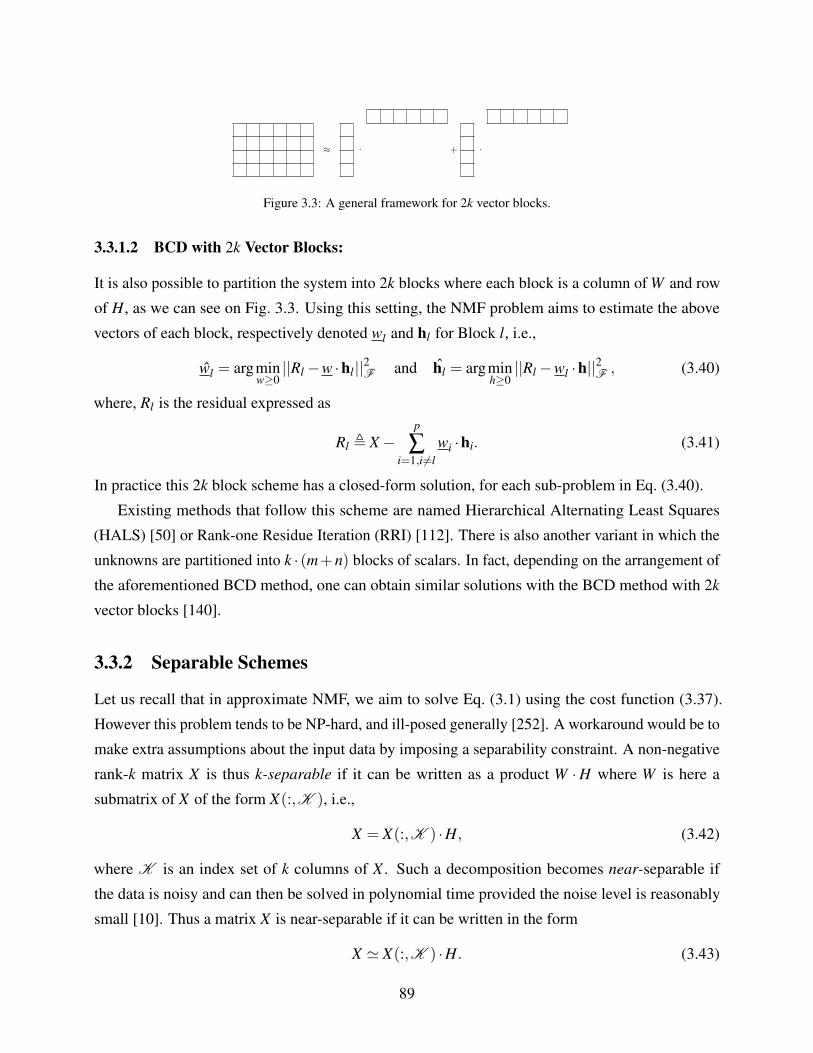
≈ · + ·
Figure 3.3: A general framework for 2k vector blocks.
3.3.1.2 BCD with 2k Vector Blocks:
It is also possible to partition the system into 2k blocks where each block is a column of W and row
of H, as we can see on Fig. 3.3. Using this setting, the NMF problem aims to estimate the above
vectors of each block, respectively denoted wl and hl for Block l, i.e.,
wl = argminw≥0||Rl−w ·hl||2F and hl = argmin
h≥0||Rl−wl ·h||2F , (3.40)
where, Rl is the residual expressed as
Rl , X−p
∑i=1,i6=l
wi ·hi. (3.41)
In practice this 2k block scheme has a closed-form solution, for each sub-problem in Eq. (3.40).
Existing methods that follow this scheme are named Hierarchical Alternating Least Squares
(HALS) [50] or Rank-one Residue Iteration (RRI) [112]. There is also another variant in which the
unknowns are partitioned into k · (m+n) blocks of scalars. In fact, depending on the arrangement of
the aforementioned BCD method, one can obtain similar solutions with the BCD method with 2k
vector blocks [140].
3.3.2 Separable Schemes
Let us recall that in approximate NMF, we aim to solve Eq. (3.1) using the cost function (3.37).
However this problem tends to be NP-hard, and ill-posed generally [252]. A workaround would be to
make extra assumptions about the input data by imposing a separability constraint. A non-negative
rank-k matrix X is thus k-separable if it can be written as a product W ·H where W is here a
submatrix of X of the form X(:,K ), i.e.,
X = X(:,K ) ·H, (3.42)
where K is an index set of k columns of X . Such a decomposition becomes near-separable if
the data is noisy and can then be solved in polynomial time provided the noise level is reasonably
small [10]. Thus a matrix X is near-separable if it can be written in the form
X ' X(:,K ) ·H. (3.43)
89
Then the optimization problem in Eq. (3.37) becomes
arg minK ⊂1,...,m
H∈k×n
||X−X(:,K )H||F . (3.44)
(Near-)separable NMF has been widely studied in the literature, as it finds several applications in,
e.g., hyperspectral unmixing with the well-known “pure pixel” assumption [185], or text mining
in [9, 145].
3.4 Classical NMF Algorithms
Since the problem in Eq. (3.2) is non-convex in nature, convergence to a global minimum is not
always guaranteed thus making it an NP-hard problem [156]. To solve it, several techniques have
been proposed, the most popular ones are described below.
3.4.1 Multiplicative Updates (MU)
To better understand how the Multiplicative Updates (MU) work, its important to know the different
optimization techniques from which it is derived. There a couple of ways to do multiplicative
updates, i.e,. the Majorization Minimization (MM) method and the heuristic approach.
3.4.1.1 Majorization Minimization
The MM algorithm is a popular technique in many optimization problems first introduced in [57] for
line-search problems but later popularized by several others in, e.g., [22, 110, 121].
Figure 3.4 illustrates a simple MM algorithm. Given a fixed point θ k of a parameter θ , MM
aims to find a surrogate function whose form depends on θ k and majorizes the cost function at the
point θ k if and only if:
f(θ
k)= g(θ
k | θ k), (3.45)
f(θ)≥ g(θ | θ k), ∀θ . (3.46)
In practice, the MM algorithm minimizes the auxiliary function rather than the true function f(θ)
yielding the next point θ k+1, i.e.,
f(θ
k+1)≤ g(θ
k+1 | θ k)≤ g(θ
k | θ k)= f(θ
k). (3.47)
MM is known to be an iterative method and converges to a stationary point when k approaches
infinity [273]. MM has also been applied to NMF in many studies like those in [87, 157, 165].
90
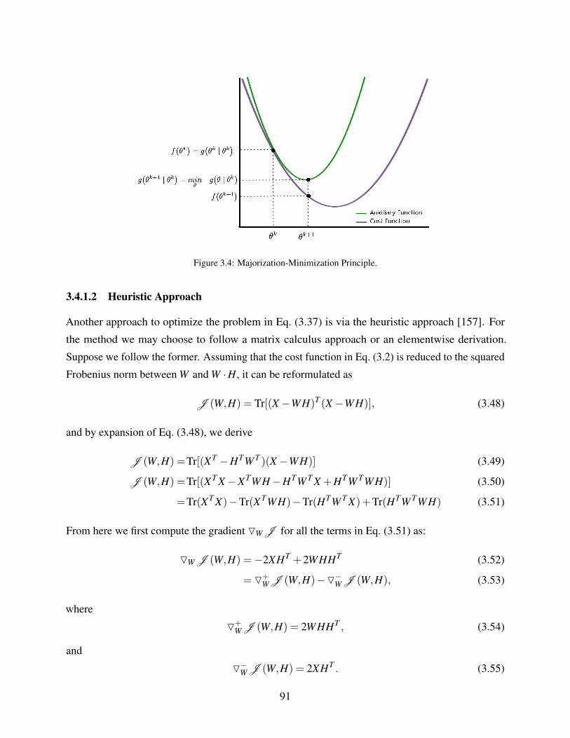
Figure 3.4: Majorization-Minimization Principle.
3.4.1.2 Heuristic Approach
Another approach to optimize the problem in Eq. (3.37) is via the heuristic approach [157]. For
the method we may choose to follow a matrix calculus approach or an elementwise derivation.
Suppose we follow the former. Assuming that the cost function in Eq. (3.2) is reduced to the squared
Frobenius norm between W and W ·H, it can be reformulated as
J (W,H) = Tr[(X−WH)T (X−WH)], (3.48)
and by expansion of Eq. (3.48), we derive
J (W,H) =Tr[(XT −HTW T )(X−WH)] (3.49)
J (W,H) =Tr[(XT X−XTWH−HTW T X +HTW TWH)] (3.50)
=Tr(XT X)−Tr(XTWH)−Tr(HTW T X)+Tr(HTW TWH) (3.51)
From here we first compute the gradient OW J for all the terms in Eq. (3.51) as:
OW J (W,H) =−2XHT +2WHHT (3.52)
= O+W J (W,H)−O−W J (W,H), (3.53)
where
O+W J (W,H) = 2WHHT , (3.54)
and
O−W J (W,H) = 2XHT . (3.55)
91
We follow analogously to compute the gradient OHJ for all terms as:
OHJ (W,H) =−2W T X +2W TWH (3.56)
= O+HJ (W,H)−O−HJ (W,H), (3.57)
where
O+HJ (W,H) = 2W TWH, (3.58)
and
O−HJ (W,H) = 2W T X . (3.59)
At this point the update rules following the heuristic method can be formulated as [157]:
W ←W O−W J (W,H)
O+W J (W,H)
, (3.60)
H← H O−HJ (W,H)
O+HJ (W,H)
, (3.61)
where the division symbol denotes the elementwise division.
Both the MM and the heuristic methods can be used to derive the final update rules of the
MU algorithm. The MU algorithm was pioneered by Lee and Sung [157] and can be considered
as a block coordinate gradient descent based approach. It follows that we move in the direction
of a re-scaled gradient with a carefully selected step size to ensure that the approximated matrix
factors remain positive along the iterations. MU rules are usually slow to converge but very easy to
implement. They read
W ←W X ·HT
W ·H ·HT , (3.62)
and
H← H W T ·XW T ·W ·H . (3.63)
3.4.2 Projected Gradient (PG)
There are a lot of methods under this scheme which are unique in their own way. As such their
common features will be reviewed. In contrast to the multiplicative update rules discussed above,
Projected Gradient (PG) methods have additive updates. The aim usually consist of alternately
minimizing, e.g., Eqs. (3.38) and (3.39), by updating successively, W and H. From the partial
derivatives (3.52) and (3.56) of J (W,H) with respect to W and H, respectively. The update rules
read
W ← [W −ηW ·∇W J (W,H)]+ , (3.64)
92
and
H← [H−ηH ·∇HJ (W,H)]+ , (3.65)
where ηW and ηH are the learning rate scalars, and [·]+ denotes the projection operator which can
either replaces negative entries by zero, or for practical purposes, by a small positive number ε ,
in order to avoid numerical instabilities10. The most popular method is Lin’s projected gradient
in [170]: Lin proposed to successively update the two factors but also discussed about the strategy
to simultaneous update both factors. It must be noted that, in this work the descent direction
corresponds exactly to the opposite of the gradient. Lin further introduced a way to update the step
size ηW and ηH using a modified Armijo rule and explained that it does not necessarily reduce the
computational cost. Some methods use the so-called proximal—or extrapolated—method which
follows from Nesterov’s work in [209] by introducing an inner iterative gradient descent. In [99],
the authors have successfully applied this idea to NMF, named NeNMF. An extension of this work
is presented in [72] for non-negative matrix completion.
Several other gradient methods exist, like the split gradient method [44, 45, 149], the oblique
projection [202], or the method of potential directions [42, 51].
3.4.3 Alternating Least Squares (ALS)
The alternating least squares method Alternating Least Squares (ALS) [18] is one of the easiest and
cheapest method to implement. It simply solves an unconstrained least square approximation and
then project all negative entries to positive orthant, i.e.,
W ←[(X ·HT ) · (H ·HT )−1]
+, (3.66)
and
H←[(W T ·W )−1 · (W T ·X)
]+. (3.67)
ALS is usually faster but less accurate than other state-of-the-art NMF methods. As a consequence,
it may be use as a precursory algorithm—i.e., as the initialization—for other relatively more efficient
methods [51].
3.4.4 Alternating Non-negative Least Squares (ANLS)
Alternating Non-negative Least Squares (ANLS) is a name of a class of methods which typically
divide the problem into two blocks. Then, each of these sub-problems can be split into k independent
10It should be noticed that in [170], the projection operator allows to project any entries outside a given interval.
93
non-negative least square sub-problems [37]. One way to solve such problems is the active set
method in [138], which iteratively separates the indexes into two sets, i.e., the free and active sets.
The unconstrained problem is solved following a variable swap between the two sets.
The active set (ActiveSet Method (AS)) technique is normally performed for minimizing the
least square error with an alternative approach. Given the minimization problem below:
arg minW,H≥0
||X−W ·H||F (3.68)
The first step of the algorithm is to split Eq. (3.68) into k separate sub-problems as:
wi← arg minwi≥0
, ||xi−wi ·H||F , 1≤ i≤ k, (3.69)
and
hi← argminhi≥0
, ||xi−W ·hi||F , 1≤ i≤ k. (3.70)
The updates of both W and H follows a series of k sub-problems to be solved independently using
the active set method of Lawson and Hanson in [151]. It can also be called using the lsqnonneg
function [250] when using Matlab.
Indeed, when we know the partitioning index, classically, the solution becomes a least square
solution with a close form expression. To this end, an accelerated variant was later proposed in [139]
as block Principal Pivoting (BPP). It is worth mentioning that the idea of ANLS was first presented
in [151]
3.4.5 Hierarchical Alternating Least Squares (HALS)
HALS is a BCD method, which partitions the problem into 2k vector blocks. The unconstrained
problem is then solved for each vector block and a projection to zero follows. The computational
cost of HALS has been studied in [95] which they posit to be almost similar to the MU. The update
rules read as follows, i.e.,
w j←[
w j +[X ·HT ](:, j)−W [H ·HT ](:, j)
[H ·HT ]( j, j)
]
+
, (3.71)
and
h j←[
h j +[XT ·W ](:, j)−HT [W T ·W ](:, j)
[W T ·W ]( j, j)
]
+
, (3.72)
where (:, j) and ( j, :) denote the j-th column and row of a matrix, respectively.
In fact, HALS has several other ways of updating the matrix factors, i.e., alternating updates of
the rows of W and the columns of H, a modified ordering of the updates—i.e., several updates of the
rows of W before updating a column of H [97]—or by using the Gauss-Southwell-type rule [119]
where we select entries of W to update before H.
94
3.5 Extensions of NMF
In this section we discuss some important and popular extensions of of NMF and offer a summary
their usage in the NMF literature.
3.5.1 Semi-Non-negative Matrix Factorization
In many of the NMF variants summarized earlier, the nonnegativity constraint is highly enforced,
i.e., both the data matrix and the factor matrices. However in some considerations, the data matrix
does not necessarily need to be non-negative and thus can have mixed signs. Semi-NMF was first
introduced in [68] and motivated from the ideas of clustering. For instance computing a k-means
clustering yields a formalization similar to the NMF model, except that in this case the data matrix
X and one of the matrix factors say W have no sign constraint.
It is worth mentioning that the authors in [68] proposed some specific multiplicative update rules
for the positive matrix in the problem. These update rules were also used for, e.g., Compressive
NMF11 [241].
Lastly, semi-NMF was also considered for in situ sensor calibration in [71]. Indeed, in that
configuration, the data matrix X and one factor matrix, say W , contain non-negative entries which
correspond to sensor voltages and physical concentrations, respectively. However, the entries of
H which correspond some calibration parameters of the considered calibration function might get
negative entries.
3.5.2 Non-negative Matrix Co-Factorization
Unlike standard NMF where we are interested in decomposing one matrix into 2 factors, Non-
negative Matrix Co-Factorization (NMCF) extends this idea to multiple problems. The aim is
to jointly decompose two or more matrices that share some factor matrices [232]. The idea of
co-factorization has used in many clustering and feature extraction problems. The authors in [286]
applied co-factorization on music spectrograms where the side information is a drum-only matrix.
The authors in [227] investigated NMCF for multimodal or multisensor data configurations, where
there is a shared information between related parallel streams. Co-factorization also appeared
in other findings with alternative name like group factorization in [158] for feature extraction
of electroencephalogram data, or joint factorization in [178] for retrieving embedded clustering
structure in multiple views.
11This introduced in details in Section 4.5 and several extensions are proposed in the first part of this thesis.
95
In practice, there are several ways to perform matrix co-factorization, depending on the applica-
tion. For the sake of simplicity, let us assume that we aim to jointly factorize two matrices denoted
X1 and X2 of size m1× n and m2× n, respectively. Performing NMF on each of them allows to
derive factor matrices W1, H1, W2, H2 which satisfy
X1 ≈W1 ·H1, (3.73)
X2 ≈W2 ·H2. (3.74)
If we assume that H1 and H2 are of same size and are equal, i.e.,
H , H1 = H2, (3.75)
then jointly solving Eqs. (3.73) and (3.74) may read
minW1,W2,H≥0
DX1,W1 ·H+DX2,W2 ·H, (3.76)
where D., . is a discrepancy measure discussed in Section 3.2, say the Frobenius norm. A very
simple way to solve Eq. (3.76) consists of stacking X1 and X2 to form a (m1 +m2)× n matrix X
which reads
X ,
[X1
X2
]≈[
W1
W2
]·H. (3.77)
Such a simple model was extended in [178] where H1 and H2 are assumed to be close (but not equal)
to a consensus matrix H?. In that case, jointly solving Eqs. (3.73) and (3.74) may read
minW1,W2,H1,H2,H?≥0
DX1,W1 ·H1+DX2,W2 ·H2+2
∑j=1
λ jDH j,H?, (3.78)
where λ j are weights to control the discrepancy between H j and H?. A variant of Eq. (3.78) was
proposed in [227]. In their formalism, the authors only consider two matrices to jointly factorize12
and add a discrepancy13 between H1 and H2, i.e.,
minW1,W2,H1,H2≥0
D1X1,W1 ·H1+D1X2,W2 ·H2+λD2H1,H2, (3.79)
where the discrepancies D1 and D2 are not necessarily the same, i.e., D2 might be a Frobenius or an
`1 norm.
12Indeed, Eq. (3.78) can be easily extended to many matrices to jointly factorize.13Please notice that the authors in [227] also take into account the permutation and scale ambiguities between H1 and
H2, which is implicitly assumed to be performed in Eq. (3.79).
96
3.5.3 Multi-layered and Deep (Semi-)NMF
Multi-layered NMF aims to decompose X in a multi-stage and hierarchical fashion such that, the
decomposition is sequential [48]. To do this, an initial decomposition is made, i.e.,
X =W1 ·H1. (3.80)
Assuming that H1 can be decomposed as well, i.e.,
H1 ≈W2 ·H2, (3.81)
one may obtain a tri-factorization model of X , i.e.,
X ≈W1 ·W2 ·H2. (3.82)
Multi-layered NMF aims to repeat this strategy several times, so that X can be decomposed as the
factorization of z+1 matrix factors, i.e.,
X ≈W1W2 · · ·WzHz. (3.83)
Multi-layered NMF was introduced to improve the performance and convergence rate of many
NMF solvers. It is particularly usual for ill-posed optimization problems and poorly scaled data
matrix [48].
The model (3.83) has seen renewed interest with the massive “boom” of deep learning, hence
its name of Deep NMF. Indeed, the authors in, e.g., [153, 242, 244] aimed to replace the deep
neural network by several matrix factorizations. The main difference between the above deep
approaches and the earlier multi-layered NMF method lies in the optimization strategy to solve
Eq. (3.83). Indeed, multi-layered NMF is purely sequential, i.e., it first solves Eq. (3.80), then
Eq. (3.81), and so on. The main breakthrough of Deep (Semi-)NMF—initially proposed in [244] in
a Semi-NMF framework—reads as follows. Their authors first propose to follow the multi-layered
strategy—propagating updated information from the first to the last layer—but they also consider
the reverse direction. Deep NMF is still a recent topic and we invite the reader to read [56] to get a
recent overview of this topic.
3.6 Discussion
This Chapter begun with a brief introduction to the concept Linear dimensionality reduction (LDR),
which is a well-known dimension reduction tool used in many fields such as machine learning and
97

other applied fields. We gave a brief review of some of the LDR techniques and piqued NMF as the
main LDR method to be used throughout this thesis. NMF seeks to decompose a high dimensional
non-negative matrix into two smaller non-negative matrices whose product approximates the true
data. Despite its success story, NMF also faces some challenges which we discussed in detail. In the
subsequent sections we gave a comprehensive account of the formulations of NMF, the different
NMF algorithms, optimization techniques, discrepancy measures and some of their extensions
to jointly factorize matrices or to apply a hierarchical decomposition of a matrix. However, as
explained in Chapter 1, we need to propose fast techniques to process a possibly large mass of data,
which we did not discuss yet. These aspects are introduced in the next chapter.
98
Chapter 4
Accelerating non-Negative MatrixFactorization
4.1 Introduction . . . . . . . . . . . . . . . . . . . . . . . . . . . . . . . . . . . . . . . . . . . . . . 99
4.2 Distributed computing . . . . . . . . . . . . . . . . . . . . . . . . . . . . . . . . . . . . . . . . . 100
4.3 Online Schemes . . . . . . . . . . . . . . . . . . . . . . . . . . . . . . . . . . . . . . . . . . . . 100
4.4 Extrapolation . . . . . . . . . . . . . . . . . . . . . . . . . . . . . . . . . . . . . . . . . . . . . . 101
4.5 Compressed NMF . . . . . . . . . . . . . . . . . . . . . . . . . . . . . . . . . . . . . . . . . . . 102
4.5.1 Random Projections RP . . . . . . . . . . . . . . . . . . . . . . . . . . . . . . . . . . . . 103
4.5.2 Designing Random Projection . . . . . . . . . . . . . . . . . . . . . . . . . . . . . . . . . 104
4.5.3 Applying Random Projection to NMF . . . . . . . . . . . . . . . . . . . . . . . . . . . . . 111
4.6 Discussion . . . . . . . . . . . . . . . . . . . . . . . . . . . . . . . . . . . . . . . . . . . . . . . 112
4.1 Introduction
Contemporary data has skyrocketed exponentially making it difficult for analysis and usage. Indeed
the more data grows in dimension, the more challenging it is for modern hardware and optimization
techniques. Consequently in NMF, minimizing the optimization problem in Eq. (3.37) tends to be
more costly and restrictive in the general case. For this reason, in literature there are several ways to
deal with this issue of data deluge. In this chapter we discuss some of the popular ways to accelerate
NMF.
99
4.2 Distributed computing
Most NMF algorithms discussed in the previous chapter suffice when the mass of data is “reasonable”,
i.e., data that could possibly be stored on a single computing unit. However for some forms of data
that could span millions by millions in dimension, often termed as web-scale—i.e., web dyadic
data—scalability becomes crucial. One way to achieve this is through data locality tricks [176].
In the contest of NMF, the factorization can also be scaled, by partitioning the data matrix X and
parallelizing the associated computations. This technique can be achieved through what is known as
MapReduce.
MapReduce [60] is a programming model that offers an efficient way of partitioning computations
to be run on multiple machines.When scaling-up NMF on MapReduce, the most crucial step is
how the data X and the associated matrix factors W and H are partitioned and distributed among
the available machines. The authors in [176] discussed the two ways to do so. If one considers a
tall and skinny data matrix X—i.e., a m×n matrix with m n—one may decide to split X along
columns—as proposed in, e.g., [221]—or rows.
In the first way, the corresponding columns of W are stored in a shared memory and then
computing W T ·W within the MU rules (see Sect. 3.4.1) consequently gets parallelized as well.
However if the matrices are very huge, this might not suffice as a good strategy since the individual
columns can be quite large as well and difficult to be made available to all machines.
The row split solves the drawback of the first approach. In this approach the matrices are
partitioned along the shortest dimension. Since we consider several rows of W which are relatively
smaller than taking entire columns of W , it becomes easier to pass the pieces among the machines.
However, most MapReduce frameworks require data to be read from and written to disk at every
iteration, which involves intense communication input-data shuffles across machines [131].
The authors in [131] minimized the above communication cost and partitioned W and H into p
multiple blocks of size m/p× k and k×n/p, respectively. Their distributed strategy was based on
MPI—a well-known message passing library—which manages collective communication operations.
As an alternative, other authors investigated the use of (multiple) Graphical Process Unit(s) (GPUs)
[180, 198].
4.3 Online Schemes
As we have seen in the previous schemes above, generally NMF algorithms analyze data holistically,
i.e., the full matrix is shown from the start. However this may not be so practical in some scenarios
where data is too big to fit into memory, or when the data is only shown in a streaming fashion (a.k.a
100
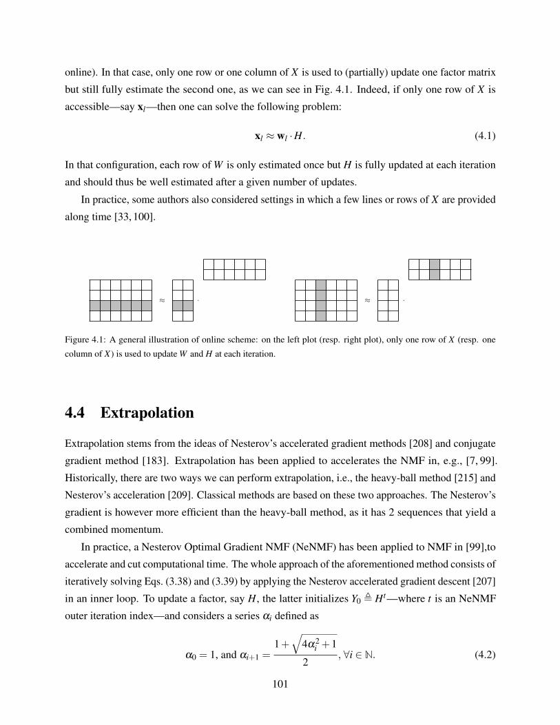
online). In that case, only one row or one column of X is used to (partially) update one factor matrix
but still fully estimate the second one, as we can see in Fig. 4.1. Indeed, if only one row of X is
accessible—say xl—then one can solve the following problem:
xl ≈ wl ·H. (4.1)
In that configuration, each row of W is only estimated once but H is fully updated at each iteration
and should thus be well estimated after a given number of updates.
In practice, some authors also considered settings in which a few lines or rows of X are provided
along time [33, 100].
≈ · ≈ ·
Figure 4.1: A general illustration of online scheme: on the left plot (resp. right plot), only one row of X (resp. one
column of X) is used to update W and H at each iteration.
4.4 Extrapolation
Extrapolation stems from the ideas of Nesterov’s accelerated gradient methods [208] and conjugate
gradient method [183]. Extrapolation has been applied to accelerates the NMF in, e.g., [7, 99].
Historically, there are two ways we can perform extrapolation, i.e., the heavy-ball method [215] and
Nesterov’s acceleration [209]. Classical methods are based on these two approaches. The Nesterov’s
gradient is however more efficient than the heavy-ball method, as it has 2 sequences that yield a
combined momentum.
In practice, a Nesterov Optimal Gradient NMF (NeNMF) has been applied to NMF in [99],to
accelerate and cut computational time. The whole approach of the aforementioned method consists of
iteratively solving Eqs. (3.38) and (3.39) by applying the Nesterov accelerated gradient descent [207]
in an inner loop. To update a factor, say H, the latter initializes Y0 , Ht—where t is an NeNMF
outer iteration index—and considers a series αi defined as
α0 = 1, and αi+1 =1+√
4α2i +1
2, ∀i ∈ N. (4.2)
101
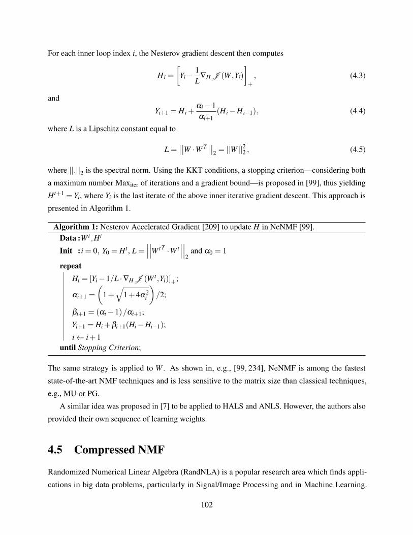
For each inner loop index i, the Nesterov gradient descent then computes
H i =
[Yi−
1L
∇HJ (W ,Yi)
]
+
, (4.3)
and
Yi+1 = H i +αi−1αi+1
(H i−H i−1), (4.4)
where L is a Lipschitz constant equal to
L =∣∣∣∣W ·W T ∣∣∣∣
2 = ||W ||22 , (4.5)
where ||.||2 is the spectral norm. Using the KKT conditions, a stopping criterion—considering both
a maximum number Maxiter of iterations and a gradient bound—is proposed in [99], thus yielding
Ht+1 = Yi, where Yi is the last iterate of the above inner iterative gradient descent. This approach is
presented in Algorithm 1.
Algorithm 1: Nesterov Accelerated Gradient [209] to update H in NeNMF [99].Data :W t ,Ht
Init : i = 0, Y0 = Ht , L =∣∣∣∣∣∣W tT ·W t
∣∣∣∣∣∣2
and α0 = 1
repeatHi = [Yi−1/L ·∇HJ (W t ,Yi)]+;
αi+1 =
(1+√
1+4α2i
)/2;
βi+1 = (αi−1)/αi+1;
Yi+1 = Hi +βi+1(Hi−Hi−1);
i← i+1until Stopping Criterion;
The same strategy is applied to W . As shown in, e.g., [99, 234], NeNMF is among the fastest
state-of-the-art NMF techniques and is less sensitive to the matrix size than classical techniques,
e.g., MU or PG.
A similar idea was proposed in [7] to be applied to HALS and ANLS. However, the authors also
provided their own sequence of learning weights.
4.5 Compressed NMF
Randomized Numerical Linear Algebra (RandNLA) is a popular research area which finds appli-
cations in big data problems, particularly in Signal/Image Processing and in Machine Learning.
102
Indeed, big data problems all tend to be approximately low-rank [246], for which computing LDR is
time consuming. Moreover, because such data are usually noisy, an extreme computational precision
is not necessary. RandNLA consists of reducing the size of the data to process while preserving
the information they contain, at a cheap computational cost. For that purpose, random projections
and random sampling appeared as powerful tools to design a sketch of a low-rank matrix. In the
framework of this Ph.D. thesis, we will focus on the former.
4.5.1 Random Projections RP
A projection onto a one-dimensional vector y ∈ Rm is said to be a random projection if the vector
has been chosen by some random process. More generally, supposed we have a set of points y1 · · ·yn
∈ Rm, we can find a mapping ξ : Rm 7→ Rs such that the distances between any yi pairs are preserved:
∣∣∣∣∣∣yi− y j
∣∣∣∣∣∣Rm≈∣∣∣∣∣∣ξ (yi)−ξ (y j)
∣∣∣∣∣∣Rs. (4.6)
This makes it interesting as we can obtain very low dimensions without losing a lot of information
because the distances between points only change by a small amount. In theory it can be proven that
such an isometric projection is grounded on what is popularly known as the Johnson-Lindenstrauss
Lemma (JLL) [126] which is provided in Lemma 4.1.
Lemma 4.1. Johnson-Lindenstrauss [126] Given a distortion ε ∈ (0,1), and a set of n points
y1 · · ·yn in Rm space, there exists a (linear) embedding ξ : Rm 7→ Rs, where s > 8(log(n)/ε2),
such that, ∀1≤ i≤ j ≤ n,
(1− ε
)∣∣∣∣∣∣yi− y j
∣∣∣∣∣∣2≤∣∣∣∣∣∣ξ (yi)−ξ (y j)
∣∣∣∣∣∣2≤(
1+ ε
)∣∣∣∣∣∣yi− y j
∣∣∣∣∣∣2. (4.7)
The proof of JLL is such that to build the map ξ : Rm 7→ Rs—which embeds all points from a
higher euclidean space to a much lower euclidean space while preserving the pairwise distances
between the points—their authors use a scaled Gaussian random matrix. More importantly the
target lower dimension s must be greater than 8(log(n)/ε2) and such a projection is bounded by(1− ε
)and
(1+ ε
)level of distortion. It is worth mentioning that the projection provided by this
lemma only depends on the number n of data points and on a specified level of distortion, but not
on the true dimension d. In practice, when the number of data points is reduced, i.e., n is small,
then a small distortion ε yields a (possibly much) larger target dimension s than the original one,
i.e., s d. To illustrate this behaviour, Fig. 4.2 shows the minimum value of s with respect to n,
according to Lemma 4.1 when ε = 0.1. One can see for example that when we only observe n = 10
points, the target dimension s should be equal to or above 1843. Depending on the considered
103
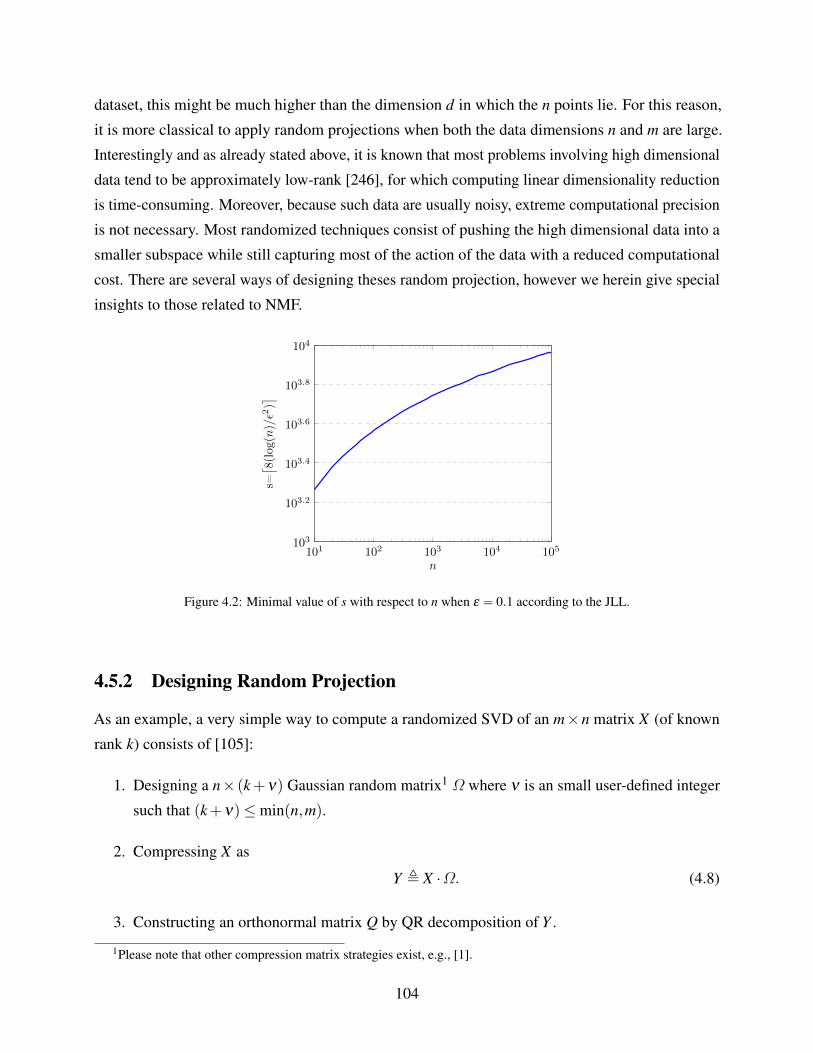
dataset, this might be much higher than the dimension d in which the n points lie. For this reason,
it is more classical to apply random projections when both the data dimensions n and m are large.
Interestingly and as already stated above, it is known that most problems involving high dimensional
data tend to be approximately low-rank [246], for which computing linear dimensionality reduction
is time-consuming. Moreover, because such data are usually noisy, extreme computational precision
is not necessary. Most randomized techniques consist of pushing the high dimensional data into a
smaller subspace while still capturing most of the action of the data with a reduced computational
cost. There are several ways of designing theses random projection, however we herein give special
insights to those related to NMF.
101 102 103 104 105103
103.2
103.4
103.6
103.8
104
n
s=⌈ 8(log
(n)/ε2)⌉
Figure 4.2: Minimal value of s with respect to n when ε = 0.1 according to the JLL.
4.5.2 Designing Random Projection
As an example, a very simple way to compute a randomized SVD of an m×n matrix X (of known
rank k) consists of [105]:
1. Designing a n× (k+ν) Gaussian random matrix1 Ω where ν is an small user-defined integer
such that (k+ν)≤min(n,m).
2. Compressing X as
Y , X ·Ω. (4.8)
3. Constructing an orthonormal matrix Q by QR decomposition of Y .
1Please note that other compression matrix strategies exist, e.g., [1].
104
At this stage, it should be noticed that the SVD of X ,UΣV T can be computed as follows [105]:
B = QT ·X , (4.9)
= UΣV T , (4.10)
and
U = Q ·U . (4.11)
Moreover, the approximation error due to the randomized QR decomposition—to obtain Q—is low
and can be bounded in practice2 [105]. Such a way to compress the data matrix was combined with
NMF using MU or HALS update rules in [289]. To that end, the authors proposed to replace X in the
update rules by its randomized truncated SVD. However, please note that most authors considered
bilateral compression to fasten NMF. This is discussed in details in Subsect. 4.5.3. However, in
order to introduce the main random compression techniques, we consider below a (non-negative)
least-square regression problem
X ≈W ·H (4.12)
where W is assumed to be known and X to be “tall and skinny”, i.e., the number of rows in H is
assumed to be much lower than then number of rows in X or W . As a consequence, it is possible to
compress X by left-multiplying it by a “compression matrix” denoted L hereafter. Denoting
XL , L ·X , (4.13)
and
WL , L ·W, (4.14)
the combination of Eq. (4.12) with Eqs. (4.13) and (4.14) yields
XL ≈WL ·H. (4.15)
If L is “well” designed, the compressed versions of X and W should contain almost the same amount
of information than their plain versions. This is the main assumption behind random projections.
In the concepts introduced below, we assume that the dimensions of X , W , and H are m×n, m× k,
and k×n, respectively. The compression matrix L is assumed to be of size (k+ν)×m where ν is a
small integer value.
We provide below some information on the various ways to design these compression/ random
projection matrices as well as the time complexities in Table 4.1.2More precisely, it can be shown [105] that—denoting σk+1 the (k + 1)-th singular value of X , and E· and
P· the expectation and the probability, respectively—E∣∣∣∣X−Q ·QT ·X
∣∣∣∣ ≤[1+ 4
√k+ν
ν−1 ·√
min(n,m)]·σk+1 and
P∣∣∣∣X−Q ·QT ·X
∣∣∣∣≤[1+9
√k+ν ·
√min(n,m)
]·σk+1
≥ 1−3 ·ν−ν .
105
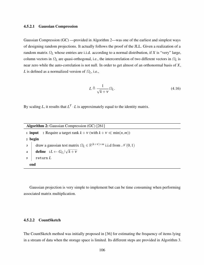
4.5.2.1 Gaussian Compression
Gaussian Compression (GC) —provided in Algorithm 2—was one of the earliest and simplest ways
of designing random projections. It actually follows the proof of the JLL. Given a realization of a
random matrix ΩL whose entries are i.i.d. according to a normal distribution, if X is “very” large,
column vectors in ΩL are quasi-orthogonal, i.e., the intercorrelation of two different vectors in ΩL is
near zero while the auto-correlation is not null. In order to get almost of an orthonormal basis of X ,
L is defined as a normalized version of ΩL, i.e.,
L ,1√
k+νΩL. (4.16)
By scaling L, it results that LT ·L is approximately equal to the identity matrix.
Algorithm 2: Gaussian Compression (GC) [261]
1 input : Require a target rank k+ν (with k+ν min(n,m))
2 begin3 draw a gaussian test matrix ΩL ∈ R(k+ν)×m i.i.d from N (0,1)
4 define :L← GL/√
k+ν
5 return L
end
Gaussian projection is very simple to implement but can be time consuming when performing
associated matrix multiplication.
4.5.2.2 CountSketch
The CountSketch method was initially proposed in [36] for estimating the frequency of items lying
in a stream of data when the storage space is limited. Its different steps are provided in Algorithm 3.
106
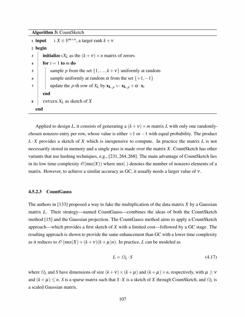
Algorithm 3: CountSketch
1 input : X ∈ Rm×n, a target rank k+ν
2 begin3 initialize :XL as the (k+ν)×n matrix of zerors
4 for i = 1 to m do5 sample p from the set 1, . . . ,k+ν uniformly at random
6 sample uniformly at random α from the set +1,−17 update the p-th row of XL by xL,p← xL,p +α ·xi
end8 return XL as sketch of X
end
Applied to design L, it consists of generating a (k+ν)×m matrix L with only one randomly-
chosen nonzero entry per row, whose value is either +1 or −1 with equal probability. The product
L ·X provides a sketch of X which is inexpensive to compute. In practice the matrix L is not
necessarily stored in memory and a single pass is made over the matrix X . CountSketch has other
variants that use hashing techniques, e.g., [231, 264, 268]. The main advantage of CountSketch lies
in its low time complexity O(nnz(X)) where nnz(.) denotes the number of nonzero elements of a
matrix. However, to achieve a similar accuracy as GC, it usually needs a larger value of ν .
4.5.2.3 CountGauss
The authors in [133] proposed a way to fake the multiplication of the data matrix X by a Gaussian
matrix L. Their strategy—named CountGauss—combines the ideas of both the CountSketch
method [15] and the Gaussian projection. The CountGauss method aims to apply a CountSketch
approach—which provides a first sketch of X with a limited cost—followed by a GC stage. The
resulting approach is shown to provide the same enhancement than GC with a lower time complexity
as it reduces to O (nnz(X)+(k+ν)(k+µ)n). In practice, L can be modeled as
L =ΩL ·S (4.17)
where ΩL and S have dimensions of size (k+ν)× (k+µ) and (k+µ)×n, respectively, with µ ≥ ν
and (k+µ)≤ n. S is a sparse matrix such that S ·X is a sketch of X through CountSketch, and ΩL is
a scaled Gaussian matrix.
107

Algorithm 4: CountGauss
1 input : X ∈ Rm×n
2 output : L ∈ R(k+ν)×m
3 begin4 draw a gaussian test matrix ΩL ∈ R(k+ν)×(k+µ)
5 form : GL =ΩL/√
s
6 draw a random vector c ∈ Rm
7 draw a random vector r ∈ Rm in the range of (k+µ)
8 draw d uniformly and randomly from the set +1,−19 form :S ∈ R(k+µ)×m from the triplets c, r, and d 3 S(c(i),r(i)) = d(i)
10 return L← GL×S
end
4.5.2.4 (Very) Sparse Random Projections
The work by Johnson and Lindestrauss led to several authors attempting to simplify the Lemma and
provide more efficient ways of doing random projections. One major contribution was the work by
Achlioptas [1] who replaced the (k+ν)×m Gaussian random matrix by another random matrix
whose entries are i.i.d random variables set to
li j =√
s ·
+1 with prob. 1/(2s),
0 with prob. (s−1)/s,
−1 with prob. 1/(2s),
(4.18)
with s = 2 or s = 3. In the latter case, 2/3 of the entries of L are zeros, hence the name of Sparse
Random Projections (SRP).
This was further improved by Li et al. in [162] where the authors designed AL according to Eq.
(4.18) with s 3. While such a compression matrix is even cheaper to compute than Achliotipas’
one—hence its name of Very Sparse Random Projections (VSRP)—it remains asymptotically
equivalent to GC when the dimension of the data is large [162]. The whole method is presented in
Algorithm 5.
108
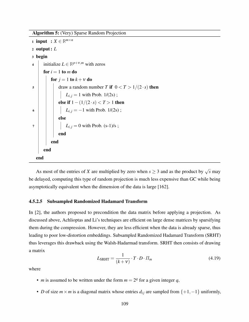
Algorithm 5: (Very) Sparse Random Projection
1 input : X ∈ Rm×n
2 output : L
3 begin4 initialize L ∈ Rp+ν ,m with zeros
for i = 1 to m dofor j = 1 to k+ν do
5 draw a random number T if 0< T > 1/(2 · s) thenLi, j = 1 with Prob. 1/(2s) ;
else if 1− (1/(2 · s)< T > 1 then6 Li, j =−1 with Prob. 1/(2s) ;
else7 Li, j = 0 with Prob. (s-1)/s ;
end
end
end
end
As most of the entries of X are multiplied by zero when s ≥ 3 and as the product by√
s may
be delayed, computing this type of random projection is much less expensive than GC while being
asymptotically equivalent when the dimension of the data is large [162].
4.5.2.5 Subsampled Randomized Hadamard Transform
In [2], the authors proposed to precondition the data matrix before applying a projection. As
discussed above, Achlioptas and Li’s techniques are efficient on large dense matrices by sparsifying
them during the compression. However, they are less efficient when the data is already sparse, thus
leading to poor low-distortion embeddings. Subsampled Randomized Hadamard Transform (SRHT)
thus leverages this drawback using the Walsh-Hadarmad transform. SRHT then consists of drawing
a matrix
LSRHT =1
(k+ν)·T ·D ·Πm (4.19)
where
• m is assumed to be written under the form m = 2q for a given integer q,
• D of size m×m is a diagonal matrix whose entries di j are sampled from +1,−1 uniformly,
109
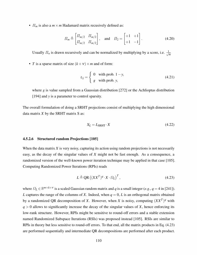
• Πm is also a m×m Hadamard matrix recusively defined as:
Πm ,
[Πm/2 Πm/2
Πm/2 Πm/2
], and Π2 =
[+1 +1
+1 −1
]. (4.20)
Usually Πn is drawn recursively and can be normalized by multiplying by a score, i.e. 1√m
• T is a sparse matrix of size (k+ν)×m and of form:
ti j =
0 with prob. 1− y,
g with prob. y,(4.21)
where g is value sampled from a Gaussian distribution [272] or the Achlioptas distribution
[194] and y is a parameter to control sparsity.
The overall formulation of doing a SRHT projections consist of multiplying the high dimensional
data matrix X by the SRHT matrix S as:
XL = LSRHT ·X (4.22)
4.5.2.6 Structured random Projections [105]
When the data matrix X is very noisy, capturing its action using random projections is not necessarily
easy, as the decay of the singular values of X might not be fast enough. As a consequence, a
randomized version of the well-known power iteration technique may be applied in that case [105].
Computing Randomized Power Iterations (RPIs) reads
L , QR((XXT )q ·X ·ΩL
)T, (4.23)
whereΩL ∈Rm×k+ν is a scaled Gaussian random matrix and q is a small integer (e.g., q = 4 in [241]).
L captures the range of the columns of X . Indeed, when q = 0, L is an orthogonal matrix obtained
by a randomized QR decomposition of X . However, when X is noisy, computing (XXT )q with
q > 0 allows to significantly increase the decay of the singular values of X , hence enforcing its
low-rank structure. However, RPIs might be sensitive to round-off errors and a stable extension
named Randomized Subspace Iterations (RSIs) was proposed instead [105]. RSIs are similar to
RPIs in theory but less sensitive to round-off errors. To that end, all the matrix products in Eq. (4.23)
are performed sequentially and intermediate QR decompositions are performed after each product.
110
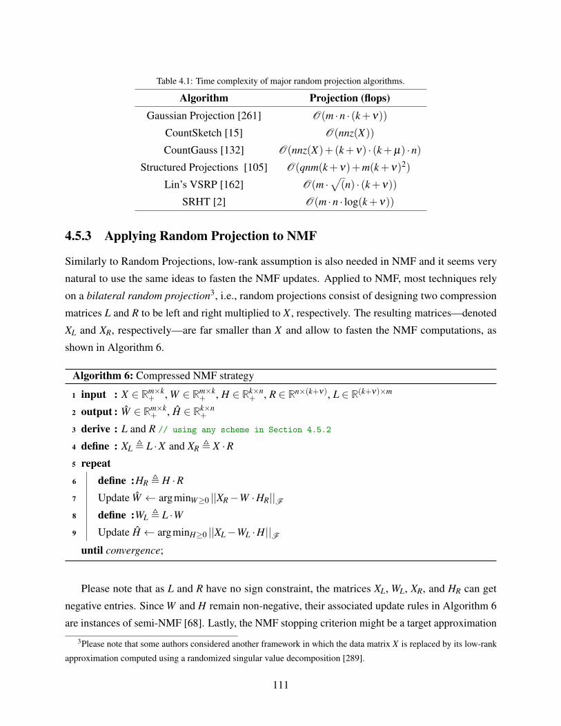
Table 4.1: Time complexity of major random projection algorithms.
Algorithm Projection (flops)Gaussian Projection [261] O(m ·n · (k+ν))
CountSketch [15] O(nnz(X))
CountGauss [132] O(nnz(X)+(k+ν) · (k+µ) ·n)Structured Projections [105] O(qnm(k+ν)+m(k+ν)2)
Lin’s VSRP [162] O(m ·√(n) · (k+ν))
SRHT [2] O(m ·n · log(k+ν))
4.5.3 Applying Random Projection to NMF
Similarly to Random Projections, low-rank assumption is also needed in NMF and it seems very
natural to use the same ideas to fasten the NMF updates. Applied to NMF, most techniques rely
on a bilateral random projection3, i.e., random projections consist of designing two compression
matrices L and R to be left and right multiplied to X , respectively. The resulting matrices—denoted
XL and XR, respectively—are far smaller than X and allow to fasten the NMF computations, as
shown in Algorithm 6.
Algorithm 6: Compressed NMF strategy
1 input : X ∈ Rm×k+ , W ∈ Rm×k
+ , H ∈ Rk×n+ , R ∈ Rn×(k+ν), L ∈ R(k+ν)×m
2 output : W ∈ Rm×k+ , H ∈ Rk×n
+
3 derive : L and R // using any scheme in Section 4.5.2
4 define : XL , L ·X and XR , X ·R5 repeat6 define :HR , H ·R7 Update W ← argminW≥0 ||XR−W ·HR||F8 define :WL , L ·W9 Update H ← argminH≥0 ||XL−WL ·H||F
until convergence;
Please note that as L and R have no sign constraint, the matrices XL, WL, XR, and HR can get
negative entries. Since W and H remain non-negative, their associated update rules in Algorithm 6
are instances of semi-NMF [68]. Lastly, the NMF stopping criterion might be a target approximation
3Please note that some authors considered another framework in which the data matrix X is replaced by its low-rank
approximation computed using a randomized singular value decomposition [289].
111
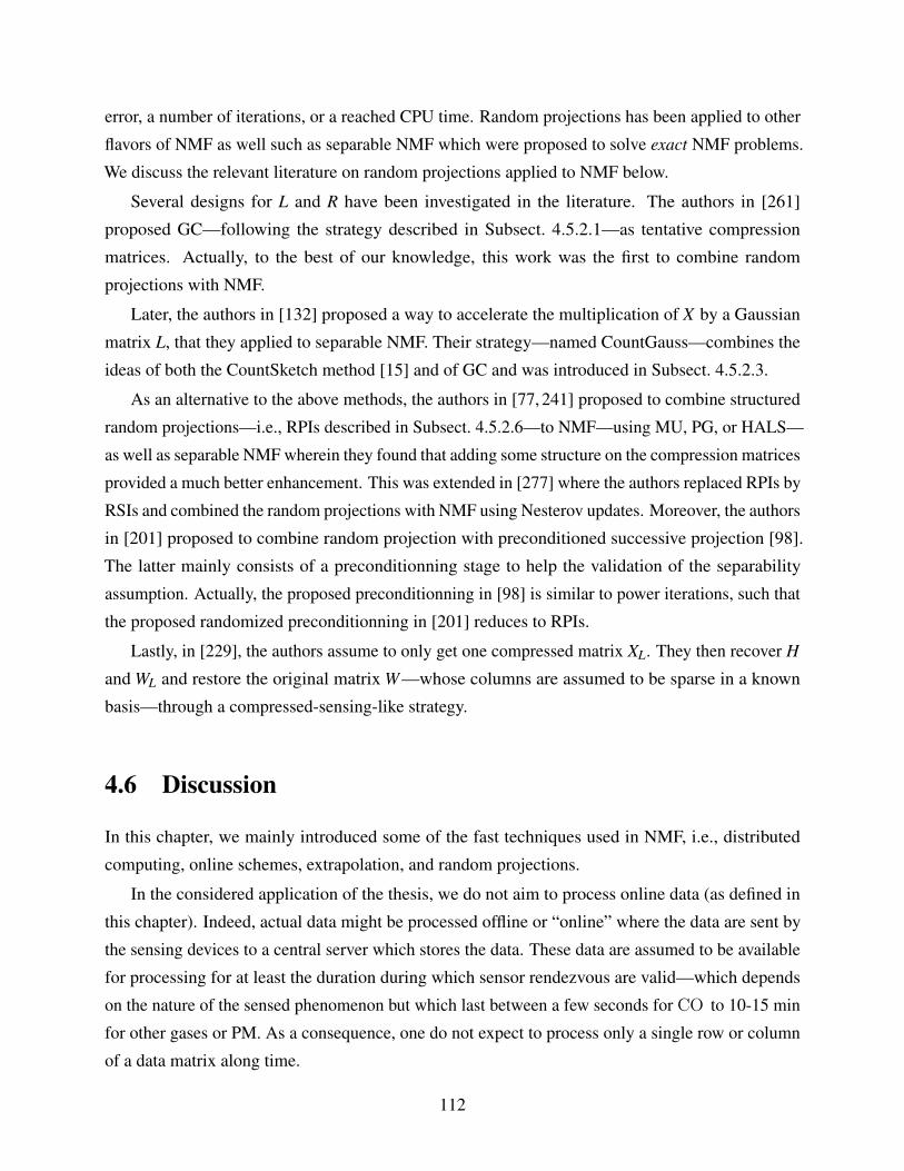
error, a number of iterations, or a reached CPU time. Random projections has been applied to other
flavors of NMF as well such as separable NMF which were proposed to solve exact NMF problems.
We discuss the relevant literature on random projections applied to NMF below.
Several designs for L and R have been investigated in the literature. The authors in [261]
proposed GC—following the strategy described in Subsect. 4.5.2.1—as tentative compression
matrices. Actually, to the best of our knowledge, this work was the first to combine random
projections with NMF.
Later, the authors in [132] proposed a way to accelerate the multiplication of X by a Gaussian
matrix L, that they applied to separable NMF. Their strategy—named CountGauss—combines the
ideas of both the CountSketch method [15] and of GC and was introduced in Subsect. 4.5.2.3.
As an alternative to the above methods, the authors in [77, 241] proposed to combine structured
random projections—i.e., RPIs described in Subsect. 4.5.2.6—to NMF—using MU, PG, or HALS—
as well as separable NMF wherein they found that adding some structure on the compression matrices
provided a much better enhancement. This was extended in [277] where the authors replaced RPIs by
RSIs and combined the random projections with NMF using Nesterov updates. Moreover, the authors
in [201] proposed to combine random projection with preconditioned successive projection [98].
The latter mainly consists of a preconditionning stage to help the validation of the separability
assumption. Actually, the proposed preconditionning in [98] is similar to power iterations, such that
the proposed randomized preconditionning in [201] reduces to RPIs.
Lastly, in [229], the authors assume to only get one compressed matrix XL. They then recover H
and WL and restore the original matrix W—whose columns are assumed to be sparse in a known
basis—through a compressed-sensing-like strategy.
4.6 Discussion
In this chapter, we mainly introduced some of the fast techniques used in NMF, i.e., distributed
computing, online schemes, extrapolation, and random projections.
In the considered application of the thesis, we do not aim to process online data (as defined in
this chapter). Indeed, actual data might be processed offline or “online” where the data are sent by
the sensing devices to a central server which stores the data. These data are assumed to be available
for processing for at least the duration during which sensor rendezvous are valid—which depends
on the nature of the sensed phenomenon but which last between a few seconds for CO to 10-15 min
for other gases or PM. As a consequence, one do not expect to process only a single row or column
of a data matrix along time.
112
Then, it is worth mentioning that revisiting in situ calibration as an NMF problem provides
an extremely low-rank matrix to factor, i.e., an NMF rank equal to k = 2 [76] or k = 3 [71].
According to [76], the dimension m and n of the matrix to factor correspond to the size of the
discretized observed area and to the number of sensors to calibrate, respectively. This means that
minm,n k and one may expect random projections to provide a significant speed-up. Moreover,
random projections can be combined with extrapolation—as proposed in [277]—and distributed
computing. As a consequence, we aim to investigate the enhancement provided by random projection
within the considered application.
Lastly, in the considered in situ calibration problem, the data matrix X is partially unknown, as it
contains missing entries and as the observed data are associated with a confidence measure. This
implies that WNMF must be used to perform calibration. However, to the best of our knowldege,
combining random projections with WNMF was not proposed prior to this Ph.D. thesis. This is the
reason why we focus on the combination of random projections with WNMF in the remainder of the
first part of this thesis. More specifically, we propose in Chapter 5 a framework to combine random
projections with WNMF. We then introduce fastened random projection techniques.
113
Chapter 5
Randomized (Weighted) Non-negativeMatrix Factorization
5.1 Complete versus Incomplete Data . . . . . . . . . . . . . . . . . . . . . . . . . . . . . . . . . . 115
5.2 Weighted Non-negative Matrix Factorization . . . . . . . . . . . . . . . . . . . . . . . . . . . . 116
5.2.1 Direct Computation . . . . . . . . . . . . . . . . . . . . . . . . . . . . . . . . . . . . . . . 116
5.2.2 Expectation-Maximization (EM) . . . . . . . . . . . . . . . . . . . . . . . . . . . . . . . . 117
5.2.3 Stochastic Gradient Descent (SGD) . . . . . . . . . . . . . . . . . . . . . . . . . . . . . . 118
5.3 Proposed Randomized WNMF Framework . . . . . . . . . . . . . . . . . . . . . . . . . . . . . 119
5.4 Proposed Compression Techniques for (W)NMF . . . . . . . . . . . . . . . . . . . . . . . . . . 121
5.4.1 A Modified Structured Compression Scheme . . . . . . . . . . . . . . . . . . . . . . . . . 121
5.4.2 Random Projection Streams . . . . . . . . . . . . . . . . . . . . . . . . . . . . . . . . . . 124
5.5 Discussion . . . . . . . . . . . . . . . . . . . . . . . . . . . . . . . . . . . . . . . . . . . . . . . 127
As explained in the conclusion of Chapter 4, we aim to combine random projections with
WNMF. To the best of our knowledge, such a combination was never proposed prior to this thesis.
The findings in this chapter were partly proposed in [278–281]. Before introducing our proposed
framework, we recall the concepts of missing entries in NMF and of WNMF.
114
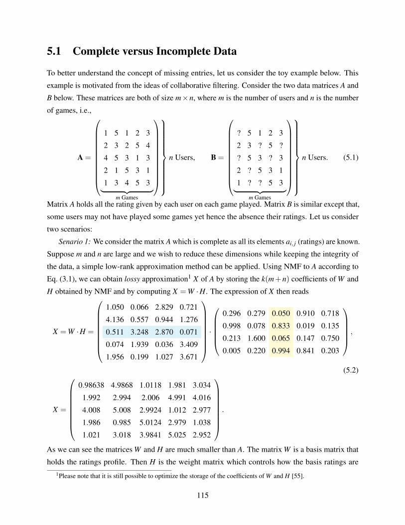
5.1 Complete versus Incomplete Data
To better understand the concept of missing entries, let us consider the toy example below. This
example is motivated from the ideas of collaborative filtering. Consider the two data matrices A and
B below. These matrices are both of size m×n, where m is the number of users and n is the number
of games, i.e.,
A =
1 5 1 2 3
2 3 2 5 4
4 5 3 1 3
2 1 5 3 1
1 3 4 5 3︸ ︷︷ ︸
m Games
n Users, B =
? 5 1 2 3
2 3 ? 5 ?
? 5 3 ? 3
2 ? 5 3 1
1 ? ? 5 3︸ ︷︷ ︸
m Games
n Users. (5.1)
Matrix A holds all the rating given by each user on each game played. Matrix B is similar except that,
some users may not have played some games yet hence the absence their ratings. Let us consider
two scenarios:
Senario 1: We consider the matrix A which is complete as all its elements ai, j (ratings) are known.
Suppose m and n are large and we wish to reduce these dimensions while keeping the integrity of
the data, a simple low-rank approximation method can be applied. Using NMF to A according to
Eq. (3.1), we can obtain lossy approximation1 X of A by storing the k(m+n) coefficients of W and
H obtained by NMF and by computing X =W ·H. The expression of X then reads
X =W ·H =
1.050 0.066 2.829 0.721
4.136 0.557 0.944 1.276
0.511 3.248 2.870 0.071
0.074 1.939 0.036 3.409
1.956 0.199 1.027 3.671
·
0.296 0.279 0.050 0.910 0.718
0.998 0.078 0.833 0.019 0.135
0.213 1.600 0.065 0.147 0.750
0.005 0.220 0.994 0.841 0.203
,
(5.2)
X =
0.98638 4.9868 1.0118 1.981 3.034
1.992 2.994 2.006 4.991 4.016
4.008 5.008 2.9924 1.012 2.977
1.986 0.985 5.0124 2.979 1.038
1.021 3.018 3.9841 5.025 2.952
.
As we can see the matrices W and H are much smaller than A. The matrix W is a basis matrix that
holds the ratings profile. Then H is the weight matrix which controls how the basis ratings are1Please note that it is still possible to optimize the storage of the coefficients of W and H [55].
115
summed up to approximate A. Intuitively, it is easy to see that a column in X—say x j—is calculated
as x j =W ·hi, i.e., every column of X is the sum of each column of W weighted by an associated
row in H. This is an easy task that can be solved by minimizing Eq. (3.37).
Scenario 2: In the matrix B, several of the games have no ratings, making the matrix incomplete.
Interestingly, this is far to be uncommon in real-life scenarios. Several issues can affect the integrity
of a data. For example, in image processing, missing pixel intensity values may be present due to
aging, artifacts, or corruption. In practice, applying low rank approximations directly on such a
model is not as straightforward as that in our scenario 1. From this knowledge it becomes expedient
to remodel our NMF problem to take into account the missing values as weighted NMF. Aside from
WNMF, better objection function and optimization scheme can be formulated via stochastic gradient
optimization. These are discussed in detail in the next sections.
5.2 Weighted Non-negative Matrix Factorization
As briefly introduced in Section 3.5, WNMF is iteratively performed by alternating updates of
W and H just like standard NMF, except that a weight matrix Q is considered inside the NMF
formulation. Principally three main strategies allow to take into account this weight matrix W ,
i.e., (i) direct computation [112], (ii) Expectation-Maximization (EM) technique [288] , and (iii)
Stochastic Gradient Descend (SGD) in the case of binary weight [220].
5.2.1 Direct Computation
In the direct computation technique, weights are directly incorporated into the NMF problem. For
example, incorporating weights in the multiplicative update rules have been proposed in [112, 190],
providing the following update rules of the method denoted WNMF-MU:
W =W (QX) ·HT
(Q (W ·H)) ·HT , (5.3)
and
H = H W T · (QX)
W T · (Q (W ·H)), (5.4)
where the ratio symbol here denotes the elementwise division. Please note that the update rules
provided in Eqs. (5.3) and (5.4) are derived from Eq. (3.23) when the loss function D between
QX and Q (W ·H) is the Frobenius norm (and no penalization term Pi is applied to the factor
matrices). Other loss functions may be chosen instead, e.g., parametric divergences [62, 169]. While
the above rules are very easy to implement, they are slow to converge. Moreover, the authors in [72]
116
found that using the Nesterov optimal gradient [207]—i.e., a fast solver—was not allowing a fast
decrease of the cost function using this strategy.
5.2.2 Expectation-Maximization (EM)
The EM framework is a powerful approach for problems related to mixture models and non-mixture
density estimation problems. EM involves two steps, i.e., an expectation step and a maximization
step. One interesting property of EM is monotonicity which implies that the estimates along each
iteration of the algorithm will not deviate in terms of their likelihood [104]. Generally there is no
theoretical proof of convergence of the EM strategy as posited by some authors in, e.g., [24, 273].
EM is thus applicable to learning from incomplete dataset in a WNMF setting (EM-based Weighted
NMF method (EM-WNMF)) by removing the associated weight matrix Q via the aforementioned
two-step procedure. Indeed, the entries of Q are assumed to be between 0 and 1. Indeed, such an
assumption is not an issue, as it is possible to scale any non-null matrix Q so that its maximum
value is 1 and we define Q , (1m,n−Q)—where 1m,n is the m× n matrix of ones—Xtheo as the
theoretical matrix of data—i.e., without missing entries or uncertainties—and (t−1) the current
iteration. Denoting E [·] the expectation and P(·) the probability symbols, the EM strategy aims to
maximize [288]
Θ([WH], [WH](t−1)
)= E
[logP
(QX ,QXtheo | [WH]
)| QX , [WH](t−1)
], (5.5)
which is solved in a two-step approach, i.e., an Expectation-step (E-step) and a Maximization-step
(M-step). In the E-step, the data matrix Xtheo is estimated from X and its estimation—denoted
Xcomp—reads
Xcomp = QX +Q (W ·H)(t−1). (5.6)
Then in the M-step, we can simply apply NMF to Xcomp by minimizing 12 ||Xcomp−WH||2F . Note
that in this M-step any standard NMF update rules can be applied. The whole algorithm is presented
117
in Algorithm 7.
Algorithm 7: EM algorithmData :Initialize matrices W and H
while Stopping Criteria not satisfied doE-Step ;
Xcomp = QX +Q (W ·H);
M-Step;
while Stopping Criteria not satisfied doUpdate of W by solving Eq. (3.38);
Update of H by solving Eq. (3.39);
end
end
Once NMF converged to a given solution [288] or after a given number of iterations [72], Xcomp
is updated in another E-step using the last estimates of W and H in Eq. (5.6). Such an EM strategy
was found to be less sensitive to initialization than the direct incorporation of weights in the update
rules [288]. It was also found to suffer slow convergence when combined with multiplicative
updates [288]. This drawback was solved in [72] by using the Nesterov accelerated gradient [207]
to update the matrix factors. This strategy was also found to be much more efficient than using
Nesterov gradient descent with the original weighted NMF optimization problem.
5.2.3 Stochastic Gradient Descent (SGD)
SGD is a widely used strategy for optimization. It may be seen as a stochastic approximation of
a gradient descent, as it replaces the gradient computation (estimated from the full data) by an
estimation of itself (estimated from a randomly chosen subset of the data). SGD was applied to
NMF [134, 233] and its extension to WNMF is straightforward when Q is binary. Indeed, in that
case, SGD randomly selects some entries among those available only. From a mathematical point of
view, considering the Frobenius norm as a loss function, no additional penalization function, and
denoting Ω the set of entries of X for which Q is equal to 1, SGD aims to minimize
12 ∑(i, j)∈Ω
(xi j−wi ·h j)2, (5.7)
where xi j is the (i, j)-th entry of X , wi is the i-th row of W and h j is the j-th column of H. In practice,
at each SGD-NMF iteration, one or several couples of points in Ω are selected to update W and H
and has a time complexity of O(|Ω|k).
118
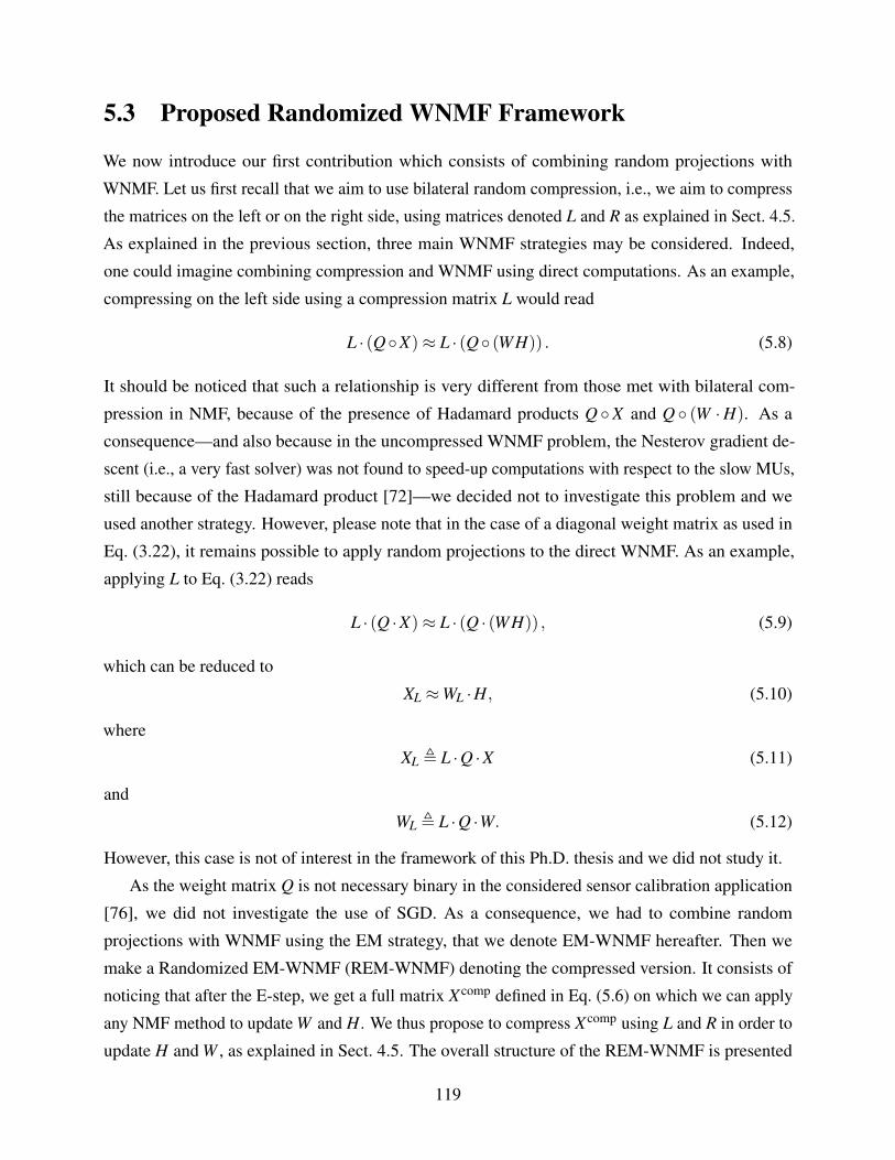
5.3 Proposed Randomized WNMF Framework
We now introduce our first contribution which consists of combining random projections with
WNMF. Let us first recall that we aim to use bilateral random compression, i.e., we aim to compress
the matrices on the left or on the right side, using matrices denoted L and R as explained in Sect. 4.5.
As explained in the previous section, three main WNMF strategies may be considered. Indeed,
one could imagine combining compression and WNMF using direct computations. As an example,
compressing on the left side using a compression matrix L would read
L · (QX)≈ L · (Q (WH)) . (5.8)
It should be noticed that such a relationship is very different from those met with bilateral com-
pression in NMF, because of the presence of Hadamard products Q X and Q (W ·H). As a
consequence—and also because in the uncompressed WNMF problem, the Nesterov gradient de-
scent (i.e., a very fast solver) was not found to speed-up computations with respect to the slow MUs,
still because of the Hadamard product [72]—we decided not to investigate this problem and we
used another strategy. However, please note that in the case of a diagonal weight matrix as used in
Eq. (3.22), it remains possible to apply random projections to the direct WNMF. As an example,
applying L to Eq. (3.22) reads
L · (Q ·X)≈ L · (Q · (WH)) , (5.9)
which can be reduced to
XL ≈WL ·H, (5.10)
where
XL , L ·Q ·X (5.11)
and
WL , L ·Q ·W. (5.12)
However, this case is not of interest in the framework of this Ph.D. thesis and we did not study it.
As the weight matrix Q is not necessary binary in the considered sensor calibration application
[76], we did not investigate the use of SGD. As a consequence, we had to combine random
projections with WNMF using the EM strategy, that we denote EM-WNMF hereafter. Then we
make a Randomized EM-WNMF (REM-WNMF) denoting the compressed version. It consists of
noticing that after the E-step, we get a full matrix Xcomp defined in Eq. (5.6) on which we can apply
any NMF method to update W and H. We thus propose to compress Xcomp using L and R in order to
update H and W , as explained in Sect. 4.5. The overall structure of the REM-WNMF is presented
119
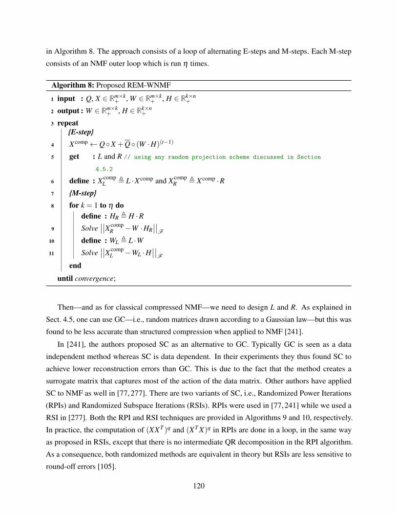
in Algorithm 8. The approach consists of a loop of alternating E-steps and M-steps. Each M-step
consists of an NMF outer loop which is run η times.
Algorithm 8: Proposed REM-WNMF
1 input : Q, X ∈ Rm×k+ , W ∈ Rm×k
+ , H ∈ Rk×n+
2 output : W ∈ Rm×k+ , H ∈ Rk×n
+
3 repeatE-step
4 Xcomp← QX +Q (W ·H)(t−1)
5 get : L and R // using any random projection scheme discussed in Section
4.5.2
6 define : XcompL , L ·Xcomp and Xcomp
R , Xcomp ·R7 M-step8 for k = 1 to η do
define : HR , H ·R9 Solve
∣∣∣∣XcompR −W ·HR
∣∣∣∣F
10 define : WL , L ·W11 Solve
∣∣∣∣XcompL −WL ·H
∣∣∣∣F
end
until convergence;
Then—and as for classical compressed NMF—we need to design L and R. As explained in
Sect. 4.5, one can use GC—i.e., random matrices drawn according to a Gaussian law—but this was
found to be less accurate than structured compression when applied to NMF [241].
In [241], the authors proposed SC as an alternative to GC. Typically GC is seen as a data
independent method whereas SC is data dependent. In their experiments they thus found SC to
achieve lower reconstruction errors than GC. This is due to the fact that the method creates a
surrogate matrix that captures most of the action of the data matrix. Other authors have applied
SC to NMF as well in [77, 277]. There are two variants of SC, i.e., Randomized Power Iterations
(RPIs) and Randomized Subspace Iterations (RSIs). RPIs were used in [77, 241] while we used a
RSI in [277]. Both the RPI and RSI techniques are provided in Algorithms 9 and 10, respectively.
In practice, the computation of (XXT )q and (XT X)q in RPIs are done in a loop, in the same way
as proposed in RSIs, except that there is no intermediate QR decomposition in the RPI algorithm.
As a consequence, both randomized methods are equivalent in theory but RSIs are less sensitive to
round-off errors [105].
120
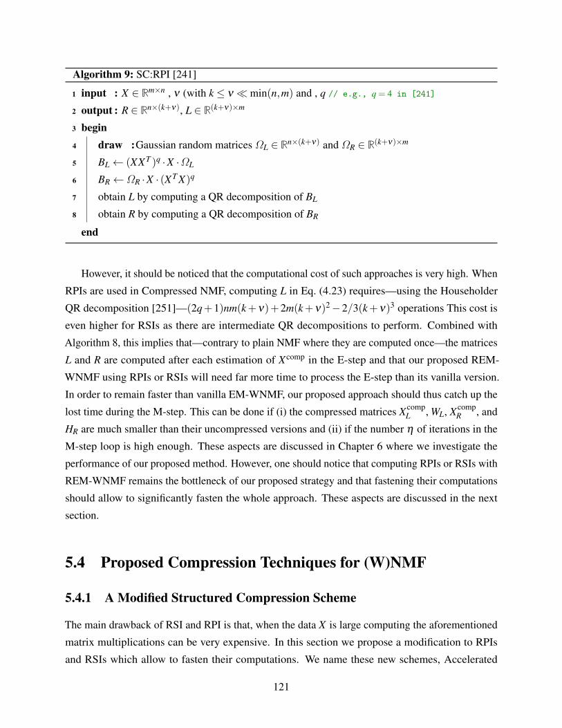
Algorithm 9: SC:RPI [241]
1 input : X ∈ Rm×n , ν (with k ≤ ν min(n,m) and , q // e.g., q = 4 in [241]
2 output : R ∈ Rn×(k+ν), L ∈ R(k+ν)×m
3 begin4 draw :Gaussian random matrices ΩL ∈ Rn×(k+ν) and ΩR ∈ R(k+ν)×m
5 BL← (XXT )q ·X ·ΩL
6 BR←ΩR ·X · (XT X)q
7 obtain L by computing a QR decomposition of BL
8 obtain R by computing a QR decomposition of BR
end
However, it should be noticed that the computational cost of such approaches is very high. When
RPIs are used in Compressed NMF, computing L in Eq. (4.23) requires—using the Householder
QR decomposition [251]—(2q+1)nm(k+ν)+2m(k+ν)2−2/3(k+ν)3 operations This cost is
even higher for RSIs as there are intermediate QR decompositions to perform. Combined with
Algorithm 8, this implies that—contrary to plain NMF where they are computed once—the matrices
L and R are computed after each estimation of Xcomp in the E-step and that our proposed REM-
WNMF using RPIs or RSIs will need far more time to process the E-step than its vanilla version.
In order to remain faster than vanilla EM-WNMF, our proposed approach should thus catch up the
lost time during the M-step. This can be done if (i) the compressed matrices XcompL , WL, Xcomp
R , and
HR are much smaller than their uncompressed versions and (ii) if the number η of iterations in the
M-step loop is high enough. These aspects are discussed in Chapter 6 where we investigate the
performance of our proposed method. However, one should notice that computing RPIs or RSIs with
REM-WNMF remains the bottleneck of our proposed strategy and that fastening their computations
should allow to significantly fasten the whole approach. These aspects are discussed in the next
section.
5.4 Proposed Compression Techniques for (W)NMF
5.4.1 A Modified Structured Compression Scheme
The main drawback of RSI and RPI is that, when the data X is large computing the aforementioned
matrix multiplications can be very expensive. In this section we propose a modification to RPIs
and RSIs which allow to fasten their computations. We name these new schemes, Accelerated
121
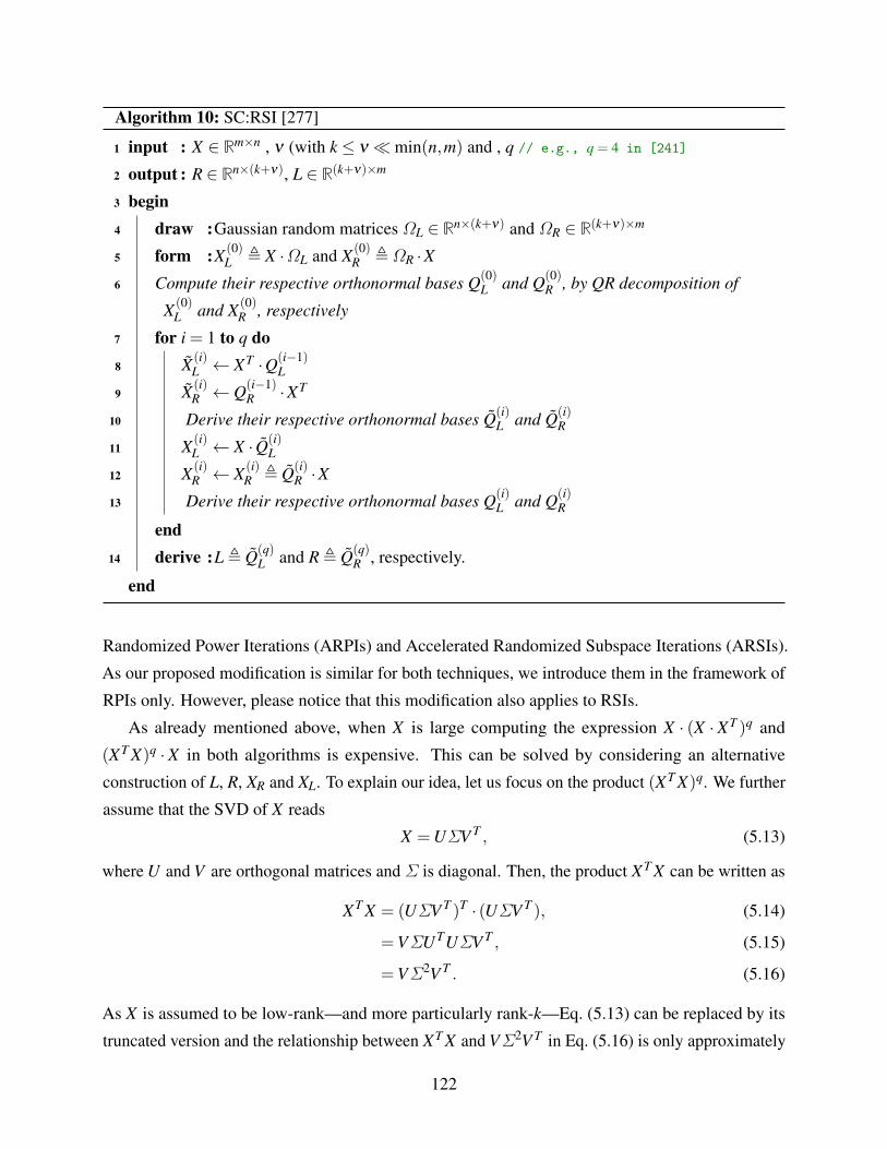
Algorithm 10: SC:RSI [277]
1 input : X ∈ Rm×n , ν (with k ≤ ν min(n,m) and , q // e.g., q = 4 in [241]
2 output : R ∈ Rn×(k+ν), L ∈ R(k+ν)×m
3 begin4 draw :Gaussian random matrices ΩL ∈ Rn×(k+ν) and ΩR ∈ R(k+ν)×m
5 form :X (0)L , X ·ΩL and X (0)
R ,ΩR ·X6 Compute their respective orthonormal bases Q(0)
L and Q(0)R , by QR decomposition of
X (0)L and X (0)
R , respectively
7 for i = 1 to q do8 X (i)
L ← XT ·Q(i−1)L
9 X (i)R ← Q(i−1)
R ·XT
10 Derive their respective orthonormal bases Q(i)L and Q(i)
R
11 X (i)L ← X · Q(i)
L
12 X (i)R ← X (i)
R , Q(i)R ·X
13 Derive their respective orthonormal bases Q(i)L and Q(i)
R
end14 derive :L , Q(q)
L and R , Q(q)R , respectively.
end
Randomized Power Iterations (ARPIs) and Accelerated Randomized Subspace Iterations (ARSIs).
As our proposed modification is similar for both techniques, we introduce them in the framework of
RPIs only. However, please notice that this modification also applies to RSIs.
As already mentioned above, when X is large computing the expression X · (X · XT )q and
(XT X)q ·X in both algorithms is expensive. This can be solved by considering an alternative
construction of L, R, XR and XL. To explain our idea, let us focus on the product (XT X)q. We further
assume that the SVD of X reads
X =UΣV T , (5.13)
where U and V are orthogonal matrices and Σ is diagonal. Then, the product XT X can be written as
XT X = (UΣV T )T · (UΣV T ), (5.14)
=VΣUTUΣV T , (5.15)
=VΣ2V T . (5.16)
As X is assumed to be low-rank—and more particularly rank-k—Eq. (5.13) can be replaced by its
truncated version and the relationship between XT X and VΣ2V T in Eq. (5.16) is only approximately
122
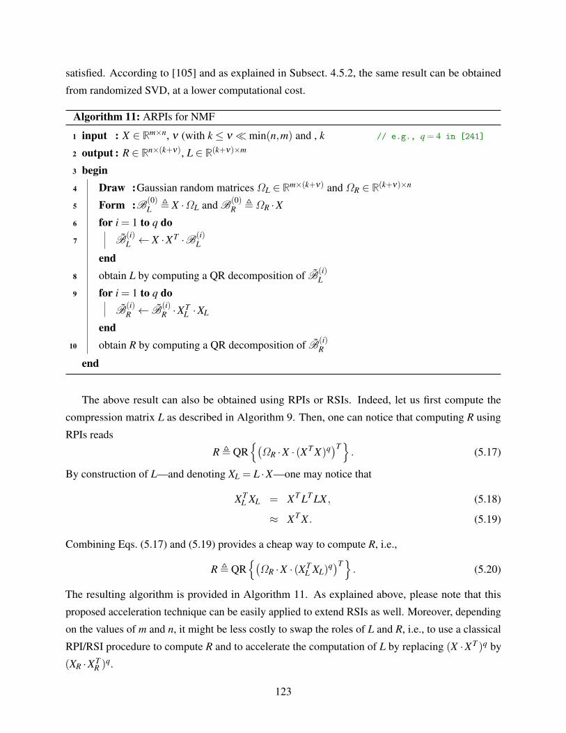
satisfied. According to [105] and as explained in Subsect. 4.5.2, the same result can be obtained
from randomized SVD, at a lower computational cost.
Algorithm 11: ARPIs for NMF
1 input : X ∈ Rm×n, ν (with k ≤ ν min(n,m) and , k // e.g., q = 4 in [241]
2 output : R ∈ Rn×(k+ν), L ∈ R(k+ν)×m
3 begin4 Draw :Gaussian random matrices ΩL ∈ Rm×(k+ν) and ΩR ∈ R(k+ν)×n
5 Form :B(0)L , X ·ΩL and B
(0)R ,ΩR ·X
6 for i = 1 to q do7 B
(i)L ← X ·XT ·B(i)
L
end8 obtain L by computing a QR decomposition of B
(i)L
9 for i = 1 to q doB
(i)R ← B
(i)R ·XT
L ·XL
end10 obtain R by computing a QR decomposition of B
(i)R
end
The above result can also be obtained using RPIs or RSIs. Indeed, let us first compute the
compression matrix L as described in Algorithm 9. Then, one can notice that computing R using
RPIs reads
R , QR(ΩR ·X · (XT X)q)T
. (5.17)
By construction of L—and denoting XL = L ·X—one may notice that
XTL XL = XT LT LX , (5.18)
≈ XT X . (5.19)
Combining Eqs. (5.17) and (5.19) provides a cheap way to compute R, i.e.,
R , QR(ΩR ·X · (XT
L XL)q)T. (5.20)
The resulting algorithm is provided in Algorithm 11. As explained above, please note that this
proposed acceleration technique can be easily applied to extend RSIs as well. Moreover, depending
on the values of m and n, it might be less costly to swap the roles of L and R, i.e., to use a classical
RPI/RSI procedure to compute R and to accelerate the computation of L by replacing (X ·XT )q by
(XR ·XTR )q.
123
Still, this fastened technique requires one full RPI or RSI procedure. As this remains costly, we
propose an alternative compression strategy in the next section.
5.4.2 Random Projection Streams
As already discussed above, structured compression using RPIs or RSIs are the state-of-the-art
in NMF. They allow a much more accurate NMF performance than classical GC for example.
This is mainly due to the fact that both RPIs and RSIs are data-dependent techniques. That is,
the construction of their associated compression matrices fully depends on the data itself. This
idea of data dependency is similar to the so-called training data in machine learning, where
algorithms learn and make predictions from the data. On the other hand, all the other random
projection schemes that we introduced in Sect. 4.5.2—are data-independent. This means that,
irrespective of the size or structure of the data, the construction of their respective compression
matrices are always done in the same way. For this reason designing the compression matrices
using data-independent schemes are faster than when using (A)RPIs and (A)RSIs. Moreover,
some authors fastened the computations of data-independent random projection techniques—e.g.,
CountGauss [132] as discussed in Subsect. 4.5.2—or proposed specific hardware dedicated to
compute random projections [111, 222]. However, all these alternatives just aim to fasten GC and
provide a similar performance. As a consequence, their use in (W)NMF should be less accurate than
using (A)RPIs/(A)RSIs. Moreover, as these techniques only allow to fasten the products XΩL and
ΩRX , they will not have an effect on the computations of (XXT )q and (XT X)q in SC and one not
may expect a significant speed-up of (A)RPIs/(A)RSIs by using them.
As a consequence, we propose in this section a new data-independent strategy which aims to
be as accurate as SC while not using data. As they are data-independent, they should fully benefits
from the fast strategies to perform random projections, e.g., dedicated hardware [111]. Hence, in
this subsection, we propose a new paradigm that we name Random Projection Scheme (RPS) in
which we assume the data-independent random projection matrices to be of infinite size and to be
processed as streams where only a subset of the random projection matrices are processed. Please
note that RPS significantly differ from classical streaming data processing, e.g., [189]. Indeed,
the latter assumes to see a subset of the data matrix at each iteration—i.e., the data to process
evolve with time—while this not necessarily the case for the former. However, one may consider
“double” streaming in which data sub-matrices are processed through mini-batch gradient while
being compressed using streams of random projections. This is however out of the scope of the
thesis.
We now introduce our proposed RPS concept, that we firstly illustrate with GC, hence its name
124
Gaussian Stream (GCS). Let us go back to the JLL described in Lemma 4.1. Applied to NMF, the
linear mapping ξ is a compression matrix, i.e., L or R. In [241], the authors chose d , k+ν where
ν was set to a small value, i.e., ν = 10. This led to a poor NMF performance. However, the JLL
implies that by increasing d (or ν), we can reduce the distortion parameter ε , as we less compress
the data, at the price of a reduced computation speed-up.
Our proposed GCS approach thus reads as follows. We assume that ν is extremely large (or even
infinite), so that L and R cannot fit in memory. We thus assume these matrices to be observed in a
streaming fashion, i.e., during an NMF iteration, we only observe two (k+νi)×m and n× (k+νi)
sub-matrices of L and R, denoted L(i) and R(i), respectively. As a consequence, along the NMF
iterations, the updates of W and H are done using different compressed matrices X (i)R and X (i)
L ,
respectively. In practice, L(i) and R(i) are updated every ω iterations, where ω is the user-defined
number of passes of the NMF algorithm using the same compression matrices in the streams.
The same strategy can be applied with any data-independent random projection discussed in
Subsect. 4.5.2. In particular—except SRHT which was designed to process sparse matrices and in
addition to GC—we derive streamed version of:
• CountSketch (Algorithm 3) denoted CountSketch Stream (CountSketchS),
• CountGauss (Algorithm 4) denoted CountGauss Stream (CountGaussS),
• SRP (Algorithm 5 with s = 3) denoted SRP Stream (SRPS),
• VSRP (Algorithm 5 with s 3) denoted VSRP Stream (VSRPS).
The global algorithm for applying RPS to NMF is provided in Algorithm 12. Please notice that the
computational cost for applying RPS linearly increases with the NMF iteration index modulo ω .
This implies that its global cost might be higher than RPIs/RSIs or than our proposed accelerated
extensions. However, these projections could also be performed using some dedicated hardware
[111], which can be done for a possibly negligible computational time. Unfortunately, the use of
such an hardware with our proposed strategy is out of the scope of this thesis. However, we will aim
to study its efficiency in terms of decrease of the cost function along iterations. Such aspects are
125
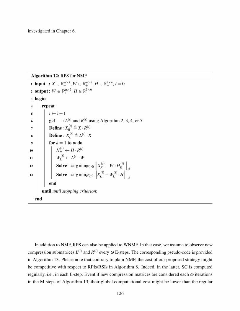
investigated in Chapter 6.
Algorithm 12: RPS for NMF
1 input : X ∈ Rm×k+ , W ∈ Rm×k
+ , H ∈ Rk×n+ , i = 0
2 output : W ∈ Rm×k+ , H ∈ Rk×n
+
3 begin4 repeat5 i← i+1
6 get :L(i) and R(i) using Algorithm 2, 3, 4, or 5
7 Define :X (i)R , X ·R(i)
8 Define : X (i)L , L(i) ·X
9 for k = 1 to ω do10 H(i)
R ← H ·R(i)
11 W (i)L ← L(i) ·W
12 Solve :argminW≥0
∣∣∣∣∣∣X (i)
R −W ·H(i)R
∣∣∣∣∣∣F
13 Solve :argminH≥0
∣∣∣∣∣∣X (i)
L −W (i)L ·H
∣∣∣∣∣∣F
end
until until stopping criterion;
end
In addition to NMF, RPS can also be applied to WNMF. In that case, we assume to observe new
compression submatrices L(i) and R(i) every ω E-steps. The corresponding pseudo-code is provided
in Algorithm 13. Please note that contrary to plain NMF, the cost of our proposed strategy might
be competitive with respect to RPIs/RSIs in Algorithm 8. Indeed, in the latter, SC is computed
regularly, i.e., in each E-step. Event if new compression matrices are considered each ω iterations
in the M-steps of Algorithm 13, their global computational cost might be lower than the regular
126
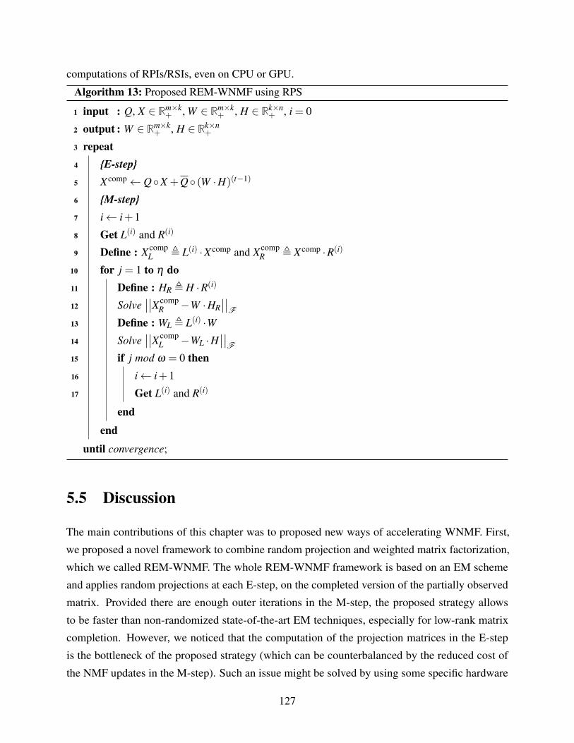
computations of RPIs/RSIs, even on CPU or GPU.
Algorithm 13: Proposed REM-WNMF using RPS
1 input : Q, X ∈ Rm×k+ , W ∈ Rm×k
+ , H ∈ Rk×n+ , i = 0
2 output : W ∈ Rm×k+ , H ∈ Rk×n
+
3 repeat4 E-step5 Xcomp← QX +Q (W ·H)(t−1)
6 M-step7 i← i+1
8 Get L(i) and R(i)
9 Define : XcompL , L(i) ·Xcomp and Xcomp
R , Xcomp ·R(i)
10 for j = 1 to η do11 Define : HR , H ·R(i)
12 Solve∣∣∣∣Xcomp
R −W ·HR∣∣∣∣
F
13 Define : WL , L(i) ·W14 Solve
∣∣∣∣XcompL −WL ·H
∣∣∣∣F
15 if j mod ω = 0 then16 i← i+1
17 Get L(i) and R(i)
end
end
until convergence;
5.5 Discussion
The main contributions of this chapter was to proposed new ways of accelerating WNMF. First,
we proposed a novel framework to combine random projection and weighted matrix factorization,
which we called REM-WNMF. The whole REM-WNMF framework is based on an EM scheme
and applies random projections at each E-step, on the completed version of the partially observed
matrix. Provided there are enough outer iterations in the M-step, the proposed strategy allows
to be faster than non-randomized state-of-the-art EM techniques, especially for low-rank matrix
completion. However, we noticed that the computation of the projection matrices in the E-step
is the bottleneck of the proposed strategy (which can be counterbalanced by the reduced cost of
the NMF updates in the M-step). Such an issue might be solved by using some specific hardware
127
providing optical random projections [222]. As a second contribution, we slightly modified the
the structured random projections schemes. We proposed the Accelerated Random projection
scheme as an improved alternative, which in theory computes the compression matrices L and R
faster. Lastly, we proposed an alternative to structured random projections which is only based on
data-independent random projections. Our strategy is built on the Johnson-Lidenstrauss Lemma
and can be seen as a streamed random projection. RPS should allow a similar randomized NMF or
WNMF enhancement when compared to data-dependent RPIs/RSIs. Even if its computational cost
may remain expensive on a CPU implementation—as compression matrices are updated each ω
iterations—RPS should significantly benefit from new strategies to compute random projections—
e.g., from specific hardwares—while structured random projections techniques should not.
128
Chapter 6
Experimental Performance of the ProposedREM-WNMF methods
6.1 Performance of REM-WNMF with (A)RPIs/(A)RSIs on Synthetic Data . . . . . . . . . . . . . 130
6.1.1 Experiments with Fixed Rank . . . . . . . . . . . . . . . . . . . . . . . . . . . . . . . . . 130
6.1.2 Influence of Noise on the Performance . . . . . . . . . . . . . . . . . . . . . . . . . . . . 139
6.1.3 Influence of the NMF rank on the performance . . . . . . . . . . . . . . . . . . . . . . . . 142
6.2 Enhancement Provided by RPS . . . . . . . . . . . . . . . . . . . . . . . . . . . . . . . . . . . . 143
6.2.1 NMF Experiments . . . . . . . . . . . . . . . . . . . . . . . . . . . . . . . . . . . . . . . 143
6.2.2 WNMF Experiments . . . . . . . . . . . . . . . . . . . . . . . . . . . . . . . . . . . . . . 147
6.3 Application to Image Completion Problems . . . . . . . . . . . . . . . . . . . . . . . . . . . . . 149
6.3.1 State-of-the-art Methods . . . . . . . . . . . . . . . . . . . . . . . . . . . . . . . . . . . . 149
6.3.2 Parameter settings . . . . . . . . . . . . . . . . . . . . . . . . . . . . . . . . . . . . . . . 150
6.3.3 Experiments . . . . . . . . . . . . . . . . . . . . . . . . . . . . . . . . . . . . . . . . . . 150
6.4 Discussion . . . . . . . . . . . . . . . . . . . . . . . . . . . . . . . . . . . . . . . . . . . . . . . 154
In Chapter 5 we proposed a new REM-WNMF strategy which can be combined with bilateral
random projection. Moreover, we proposed two main alternatives to classical RPIs/RSIs, i.e.,
accelerated RPIs/RSIs and Random Projection Streams. In this chapter, we aim to investigate their
enhancement with respect to vanilla EM-WNMF methods. The remainder of the chapter reads as
follows: We discuss the performance of our randomized methods in Section 6.1 for a fixed rank,
varying rank and in the presence of additive noise. Then in Section 6.2 we discuss the performance
129
of the RPS methods on both standard NMF and WNMF. Similarly we discuss its performance in the
presence of additive noise. Lastly, in 6.3 we apply our proposed REM-WNMF to image completion
problems, where we compare them to state-of-the-art methods.
6.1 Performance of REM-WNMF with (A)RPIs/(A)RSIs on Syn-
thetic Data
In this section, we aim to assess the performance of the proposed strategy combined with state-of-
the-art random projections as well as with our proposed ARPIs. For that purpose, consider the case
of synthetic data. These tests are investigated with both a non-negative matrix completion point of
view—as in [72]—and a Blind Source Separation (BSS) one. Indeed, while the former focuses on
the estimation of the missing entries of X from W and H, BSS investigates the quality of estimation
of each matrix factor. The latter is challenging as a good low-rank approximation of X does not
necessarily implies good estimates of W and H.
6.1.1 Experiments with Fixed Rank
We first test the performance of the various solvers with a fixed rank, i.e., k = 5. Our choice of
such a small rank is because we aim to extend the present methodology to mobile sensor calibration
where the rank of X is known and even smaller than in these experiments, i.e, k = 2 in [74] and k = 3
in [71], as already explained. For that purpose, we repeat 15 times the following experiment: we
randomly generate non-negative factor matrices W theo and H theo, with n = m = 10000. Its product
provides the whole observed data matrix X theo that we randomly sample with a sampling rate varying
from 10 to 90% (with a step-size of 20%). Except when we state it, we do not consider additive
noise in the tests below. We compare the proposed REM-W-NMF strategy to the uncompressed
EM-W-NMF using two solvers, i.e., the NeNMF and ActiveSet NMF (AS-NMF). The Nesterov
inner loop herein is set to Maxiter = 500.
In this section, we aim to investigate the enhancement provided by random projection when
classical strategies are used, i.e., GC, RPIs, RSIs, and our proposed accelerated SC methods. All
these methods need a small oversampling parameter ν that we set to ν = 10, except for GC where this
parameters has an influence—see, e.g., Appendix A—and for which we also show the performance
when ν = 150. The performance reached with other values of ν may be found in Appendix A. Then,
all SC methods need to set a parameter q—see, e.g., Algorithms 9, 10, and 11—that we set to
q = 4 [241]. All the tests are done in Matlab R2016a on a laptop with an Intel Core i7-4800MQ
130
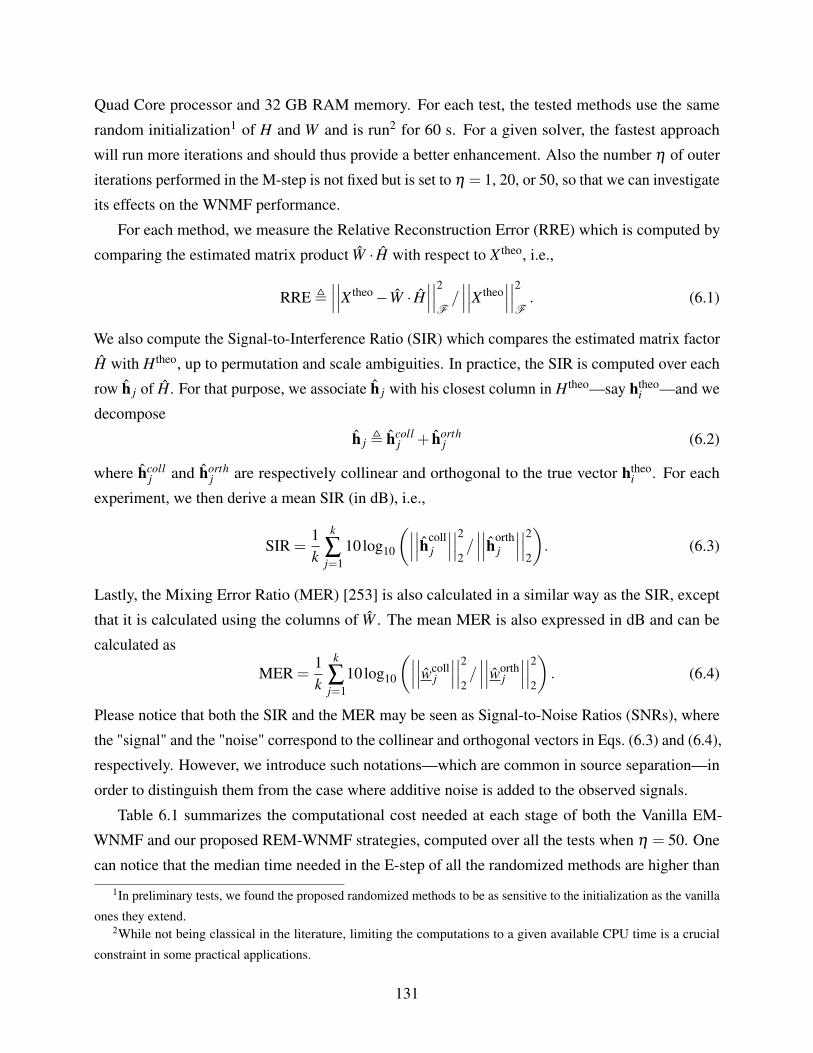
Quad Core processor and 32 GB RAM memory. For each test, the tested methods use the same
random initialization1 of H and W and is run2 for 60 s. For a given solver, the fastest approach
will run more iterations and should thus provide a better enhancement. Also the number η of outer
iterations performed in the M-step is not fixed but is set to η = 1, 20, or 50, so that we can investigate
its effects on the WNMF performance.
For each method, we measure the Relative Reconstruction Error (RRE) which is computed by
comparing the estimated matrix product W · H with respect to X theo, i.e.,
RRE ,∣∣∣∣∣∣X theo−W · H
∣∣∣∣∣∣2
F/∣∣∣∣∣∣X theo
∣∣∣∣∣∣2
F. (6.1)
We also compute the Signal-to-Interference Ratio (SIR) which compares the estimated matrix factor
H with H theo, up to permutation and scale ambiguities. In practice, the SIR is computed over each
row h j of H. For that purpose, we associate h j with his closest column in H theo—say htheoi —and we
decompose
h j , hcollj + horth
j (6.2)
where hcollj and horth
j are respectively collinear and orthogonal to the true vector htheoi . For each
experiment, we then derive a mean SIR (in dB), i.e.,
SIR =1k
k
∑j=1
10log10
(∣∣∣∣∣∣hcoll
j
∣∣∣∣∣∣2
2/∣∣∣∣∣∣horth
j
∣∣∣∣∣∣2
2
). (6.3)
Lastly, the Mixing Error Ratio (MER) [253] is also calculated in a similar way as the SIR, except
that it is calculated using the columns of W . The mean MER is also expressed in dB and can be
calculated as
MER =1k
k
∑j=1
10log10
(∣∣∣∣∣∣wcoll
j
∣∣∣∣∣∣2
2/∣∣∣∣∣∣worth
j
∣∣∣∣∣∣2
2
). (6.4)
Please notice that both the SIR and the MER may be seen as Signal-to-Noise Ratios (SNRs), where
the "signal" and the "noise" correspond to the collinear and orthogonal vectors in Eqs. (6.3) and (6.4),
respectively. However, we introduce such notations—which are common in source separation—in
order to distinguish them from the case where additive noise is added to the observed signals.
Table 6.1 summarizes the computational cost needed at each stage of both the Vanilla EM-
WNMF and our proposed REM-WNMF strategies, computed over all the tests when η = 50. One
can notice that the median time needed in the E-step of all the randomized methods are higher than
1In preliminary tests, we found the proposed randomized methods to be as sensitive to the initialization as the vanilla
ones they extend.2While not being classical in the literature, limiting the computations to a given available CPU time is a crucial
constraint in some practical applications.
131

Table 6.1: Median CPU time (in seconds) reached with the different tested solvers.
RP Scheme None (vanilla) GC (ν = 10) GC (ν = 150) RPI ARPI RSI
Algorithms E-step M-step E-step M-step E-step M-step E-step M-step E-step M-step E-step M-step
REM-W-NeNMF 2.642 0.161 2.455 0.075 2.830 0.045 4.606 0.038 3.750 0.034 4.704 0.0375
REM-W-AS-NMF 2.674 0.1612 2.378 0.034 2.961 0.032 4.702 0.040 3.724 0.029 4.759 0.033
those obtained with the Vanilla techniques. In particular, the median times of the E-Step for all
state-of-the-art SC methods (RPIs, RSIs) and our ARPI approach are almost two times higher than
the vanilla variant. This is expected since the computation of the projection matrices takes more
than than when using GC. Still, performing 1 E-step with ARPI takes around 1 s less than with
RPI and RSI, which shows the relevance of the proposed accelerated scheme. Generally one can
notice that the bottleneck of our proposed framework is the repetitive use of random projections
when the matrix Xcomp is re-estimated. However and as expected, performing one outer loop in
REM-WNMF is 2 to 5 times faster than one in EM-WNMF3. This implies that the higher η , the
more benefits there are to apply random projections. However, in practice, a trade-off must be found
and an appropriate choice of the η parameter in the M-steps must be set.
3In [279], we investigated the performance reached with more solvers. We actually found that performing one outer
loop in REM-WNMF could be 9 to 110 faster than with EM-WNMF. However, we did not reproduced these experiments
here as most of the solvers used were slow to converge and, even if they were significantly sped-up, they finally did not
provide the same enhancement than the solvers we here use.
132
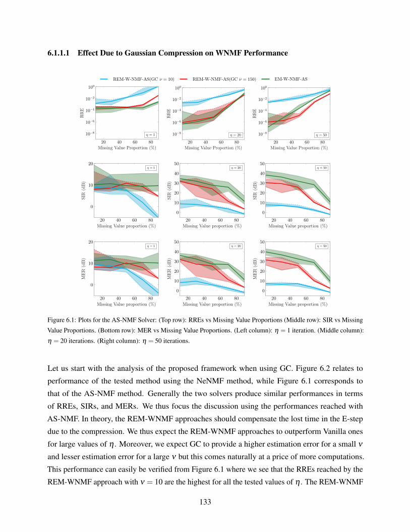
6.1.1.1 Effect Due to Gaussian Compression on WNMF Performance
REM-W-NMF-AS(GC ν = 10) REM-W-NMF-AS(GC ν = 150) EM-W-NMF-AS
20 40 60 80
100
10−2
10−4
10−6
10−8
Missing Value Proportion (%)
RR
E
η = 1
20 40 60 80
100
10−2
10−4
10−6
10−8
Missing Value Proportion (%)
RR
E
η = 20
20 40 60 80
100
10−2
10−4
10−6
10−8
Missing Value Proportion (%)
RR
E
η = 50
20 40 60 80
0
10
20
Missing Value proportion (%)
SIR
(dB
)
η = 1
20 40 60 80
0
10
20
30
40
50
Missing Value proportion (%)
SIR
(dB
)η = 20
20 40 60 80
0
10
20
30
40
50
Missing Value proportion (%)
SIR
(dB
)
η = 50
20 40 60 80
0
10
20
Missing Value proportion (%)
ME
R(d
B)
η = 1
20 40 60 80
0
10
20
30
40
50
Missing Value proportion (%)
ME
R(d
B)
η = 20
20 40 60 80
0
10
20
30
40
50
Missing Value proportion (%)
ME
R(d
B)
η = 50
Figure 6.1: Plots for the AS-NMF Solver: (Top row): RREs vs Missing Value Proportions (Middle row): SIR vs Missing
Value Proportions. (Bottom row): MER vs Missing Value Proportions. (Left column): η = 1 iteration. (Middle column):
η = 20 iterations. (Right column): η = 50 iterations.
Let us start with the analysis of the proposed framework when using GC. Figure 6.2 relates to
performance of the tested method using the NeNMF method, while Figure 6.1 corresponds to
that of the AS-NMF method. Generally the two solvers produce similar performances in terms
of RREs, SIRs, and MERs. We thus focus the discussion using the performances reached with
AS-NMF. In theory, the REM-WNMF approaches should compensate the lost time in the E-step
due to the compression. We thus expect the REM-WNMF approaches to outperform Vanilla ones
for large values of η . Moreover, we expect GC to provide a higher estimation error for a small ν
and lesser estimation error for a large ν but this comes naturally at a price of more computations.
This performance can easily be verified from Figure 6.1 where we see that the RREs reached by the
REM-WNMF approach with ν = 10 are the highest for all the tested values of η . The REM-WNMF
133

with ν = 150 on the other hand achieves slightly higher to similar RREs when η = 1 or 20. Then
when η increases to η = 50, it provides lower RREs than its vanilla counterpart, except when there
are 10% of missing entries in the data matrix. Aside from the RREs we can also see from the
same figure that the SIRs and MERs are also affected by the value of η . The first observation is
that the REM-WNMF method with ν = 10 provides, for a given missing value proportion, similar
SIRs and MERs for all the tested values of η . Moreover, these values are very low with respect to
those reached by the other approaches, signifying a poorly estimated W and H matrix, respectively.
Then, for the other tested methods, we can see that the values of the SIRs and MERs grow as η
increases. However, while the REM-WNMF approach with ν = 150 was slightly outperforming its
EM-WNMF variant in terms or RREs, this is not the case when we focus on SIRs and MERs. One
possible explanation might be due to the fact these NMF techniques are not sure to converge to a
global minimum while still ensuring the decrease of the cost function. Another explanation might
be due to the properties of GC. Indeed and as stated by the JLL, GC is know to be very selective
with the choice of ν in order to reach a desired level of accuracy. As a consequence, it might be
necessary to increase ν again in order to provide higher SIRs and MERs. This further motivates us
to consider more accurate schemes.
134
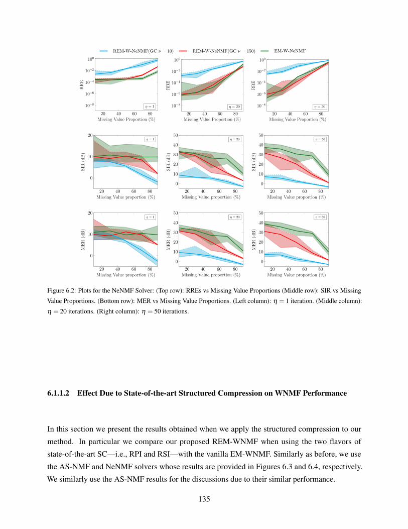
REM-W-NeNMF(GC ν = 10) REM-W-NeNMF(GC ν = 150) EM-W-NeNMF
20 40 60 80
100
10−2
10−4
10−6
10−8
Missing Value Proportion (%)
RR
E
η = 1
20 40 60 80
100
10−2
10−4
10−6
10−8
Missing Value Proportion (%)
RR
E
η = 20
20 40 60 80
100
10−2
10−4
10−6
10−8
Missing Value Proportion (%)
RR
E
η = 50
20 40 60 80
0
10
20
Missing Value proportion (%)
SIR
(dB
)
η = 1
20 40 60 80
0
10
20
30
40
50
Missing Value proportion (%)
SIR
(dB
)
η = 20
20 40 60 80
0
10
20
30
40
50
Missing Value proportion (%)
SIR
(dB
)
η = 50
20 40 60 80
0
10
20
Missing Value proportion (%)
ME
R(d
B)
η = 1
20 40 60 80
0
10
20
30
40
50
Missing Value proportion (%)
ME
R(d
B)
η = 20
20 40 60 80
0
10
20
30
40
50
Missing Value proportion (%)
ME
R(d
B)
η = 50
Figure 6.2: Plots for the NeNMF Solver: (Top row): RREs vs Missing Value Proportions (Middle row): SIR vs Missing
Value Proportions. (Bottom row): MER vs Missing Value Proportions. (Left column): η = 1 iteration. (Middle column):
η = 20 iterations. (Right column): η = 50 iterations.
6.1.1.2 Effect Due to State-of-the-art Structured Compression on WNMF Performance
In this section we present the results obtained when we apply the structured compression to our
method. In particular we compare our proposed REM-WNMF when using the two flavors of
state-of-the-art SC—i.e., RPI and RSI—with the vanilla EM-WNMF. Similarly as before, we use
the AS-NMF and NeNMF solvers whose results are provided in Figures 6.3 and 6.4, respectively.
We similarly use the AS-NMF results for the discussions due to their similar performance.
135
REM-W-NMF-AS(RSI) REM-W-NMF-AS(RPI) EM-W-NMF-AS
20 40 60 80
100
10−2
10−4
10−6
10−8
Missing Value Proportion (%)
RR
E
η = 1
20 40 60 80
100
10−2
10−4
10−6
10−8
Missing Value Proportion (%)
RR
E
η = 20
20 40 60 80
100
10−2
10−4
10−6
10−8
Missing Value Proportion (%)
RR
E
η = 50
20 40 60 800
10
20
Missing Value proportion (%)
SIR
(dB
)
η = 1
20 40 60 800
10
20
30
40
50
Missing Value proportion (%)
SIR
(dB
)
η = 20
20 40 60 800
10
20
30
40
50
Missing Value proportion (%)
SIR
(dB
)
η = 50
20 40 60 800
10
20
Missing Value proportion (%)
ME
R(d
B)
η = 1
20 40 60 800
10
20
30
40
50
Missing Value proportion (%)
ME
R(d
B)
η = 20
20 40 60 800
10
20
30
40
50
Missing Value proportion (%)
ME
R(d
B)
η = 50
Figure 6.3: Plots for the AS-NMF Solver: (Top row): RREs vs Missing Value Proportions (Middle row): SIR vs Missing
Value Proportions. (Bottom row): MER vs Missing Value Proportions. (Left column): η = 1 iteration. (Middle column):
η = 20 iterations. (Right column): η = 50 iterations.
Let us first look at the various RREs of methods in Figure 6.3. The performance of the REM-
WNMF approaches using RPIs and RSIs are very similar, which confirms our assertion in the
theoretical section. Next we can also observe that when η = 1, the RREs provided by the REM-
WNMF approaches are higher than those provided by the vanilla one. This was expected as the
REM-WNMF methods cannot compensate the lost CPU time in the E-step with the earned one in a
unique pass in the loop of the M-step. Again, in regards to the influence of η , we can observe that
the REM-WNMF approaches begin to significantly outperform the vanilla version for η = 20 and
η = 50, with the latter yielding the best performance. Then, in terms of the SIRs and MERs, we can
see that, they do not monotonically vary with the missing value proportion. While one might expect
to get better estimates of W and H when more entries in X are available, this is not always the case.
This behavior is especially visible when η is equal to 20 or 50. This might be due to the fact that
NMF is NP-hard and that a unique solution is not guaranteed in the general case
136
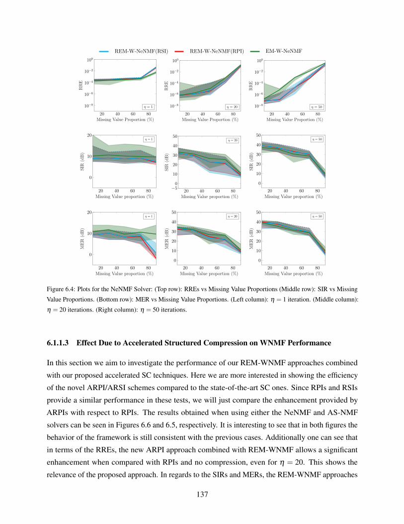
REM-W-NeNMF(RSI) REM-W-NeNMF(RPI) EM-W-NeNMF
20 40 60 80
100
10−2
10−4
10−6
10−8
Missing Value Proportion (%)
RR
E
η = 1
20 40 60 80
100
10−2
10−4
10−6
10−8
Missing Value Proportion (%)
RR
E
η = 20
20 40 60 80
100
10−2
10−4
10−6
10−8
Missing Value Proportion (%)
RR
E
η = 50
20 40 60 80
0
10
20
Missing Value proportion (%)
SIR
(dB
)
η = 1
20 40 60 80−50
10
20
30
40
50
Missing Value proportion (%)
SIR
(dB
)
η = 20
20 40 60 80
0
10
20
30
40
50
Missing Value proportion (%)
SIR
(dB
)
η = 50
20 40 60 80
0
10
20
Missing Value proportion (%)
ME
R(d
B)
η = 1
20 40 60 80
0
10
20
30
40
50
Missing Value proportion (%)
ME
R(d
B)
η = 20
20 40 60 80
0
10
20
30
40
50
Missing Value proportion (%)
ME
R(d
B)
η = 50
Figure 6.4: Plots for the NeNMF Solver: (Top row): RREs vs Missing Value Proportions (Middle row): SIR vs Missing
Value Proportions. (Bottom row): MER vs Missing Value Proportions. (Left column): η = 1 iteration. (Middle column):
η = 20 iterations. (Right column): η = 50 iterations.
6.1.1.3 Effect Due to Accelerated Structured Compression on WNMF Performance
In this section we aim to investigate the performance of our REM-WNMF approaches combined
with our proposed accelerated SC techniques. Here we are more interested in showing the efficiency
of the novel ARPI/ARSI schemes compared to the state-of-the-art SC ones. Since RPIs and RSIs
provide a similar performance in these tests, we will just compare the enhancement provided by
ARPIs with respect to RPIs. The results obtained when using either the NeNMF and AS-NMF
solvers can be seen in Figures 6.6 and 6.5, respectively. It is interesting to see that in both figures the
behavior of the framework is still consistent with the previous cases. Additionally one can see that
in terms of the RREs, the new ARPI approach combined with REM-WNMF allows a significant
enhancement when compared with RPIs and no compression, even for η = 20. This shows the
relevance of the proposed approach. In regards to the SIRs and MERs, the REM-WNMF approaches
137
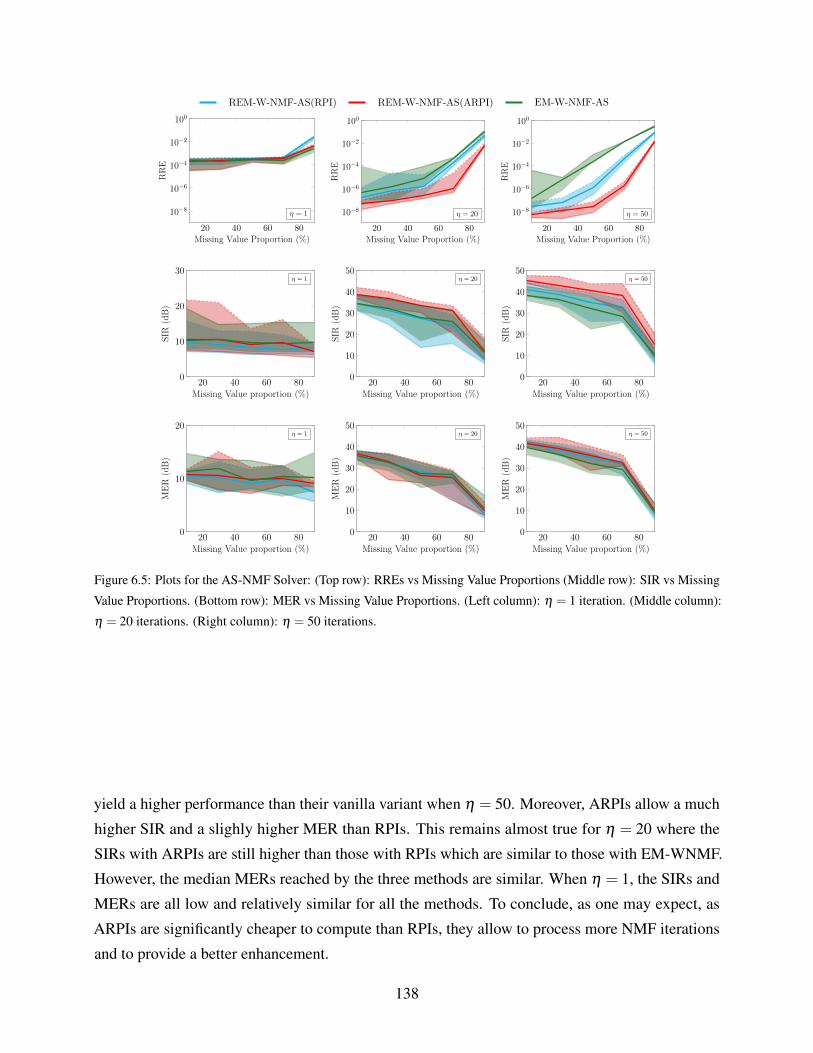
REM-W-NMF-AS(RPI) REM-W-NMF-AS(ARPI) EM-W-NMF-AS
20 40 60 80
100
10−2
10−4
10−6
10−8
Missing Value Proportion (%)
RR
E
η = 1
20 40 60 80
100
10−2
10−4
10−6
10−8
Missing Value Proportion (%)
RR
E
η = 20
20 40 60 80
100
10−2
10−4
10−6
10−8
Missing Value Proportion (%)
RR
E
η = 50
20 40 60 800
10
20
30
Missing Value proportion (%)
SIR
(dB
)
η = 1
20 40 60 800
10
20
30
40
50
Missing Value proportion (%)
SIR
(dB
)
η = 20
20 40 60 800
10
20
30
40
50
Missing Value proportion (%)
SIR
(dB
)
η = 50
20 40 60 800
10
20
Missing Value proportion (%)
ME
R(d
B)
η = 1
20 40 60 800
10
20
30
40
50
Missing Value proportion (%)
ME
R(d
B)
η = 20
20 40 60 800
10
20
30
40
50
Missing Value proportion (%)
ME
R(d
B)
η = 50
Figure 6.5: Plots for the AS-NMF Solver: (Top row): RREs vs Missing Value Proportions (Middle row): SIR vs Missing
Value Proportions. (Bottom row): MER vs Missing Value Proportions. (Left column): η = 1 iteration. (Middle column):
η = 20 iterations. (Right column): η = 50 iterations.
yield a higher performance than their vanilla variant when η = 50. Moreover, ARPIs allow a much
higher SIR and a slighly higher MER than RPIs. This remains almost true for η = 20 where the
SIRs with ARPIs are still higher than those with RPIs which are similar to those with EM-WNMF.
However, the median MERs reached by the three methods are similar. When η = 1, the SIRs and
MERs are all low and relatively similar for all the methods. To conclude, as one may expect, as
ARPIs are significantly cheaper to compute than RPIs, they allow to process more NMF iterations
and to provide a better enhancement.
138
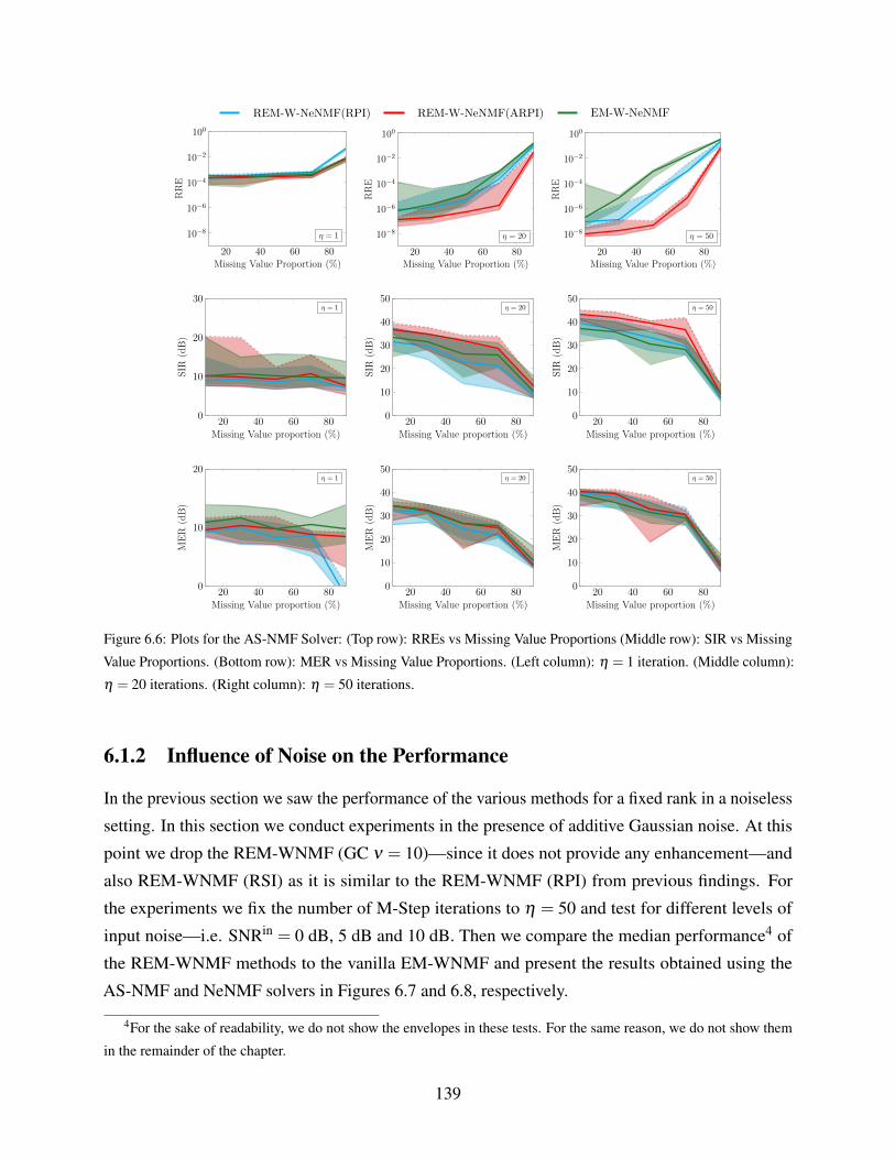
REM-W-NeNMF(RPI) REM-W-NeNMF(ARPI) EM-W-NeNMF
20 40 60 80
100
10−2
10−4
10−6
10−8
Missing Value Proportion (%)
RR
E
η = 1
20 40 60 80
100
10−2
10−4
10−6
10−8
Missing Value Proportion (%)
RR
E
η = 20
20 40 60 80
100
10−2
10−4
10−6
10−8
Missing Value Proportion (%)
RR
E
η = 50
20 40 60 800
10
20
30
Missing Value proportion (%)
SIR
(dB
)
η = 1
20 40 60 800
10
20
30
40
50
Missing Value proportion (%)
SIR
(dB
)
η = 20
20 40 60 800
10
20
30
40
50
Missing Value proportion (%)
SIR
(dB
)
η = 50
20 40 60 800
10
20
Missing Value proportion (%)
ME
R(d
B)
η = 1
20 40 60 800
10
20
30
40
50
Missing Value proportion (%)
ME
R(d
B)
η = 20
20 40 60 800
10
20
30
40
50
Missing Value proportion (%)
ME
R(d
B)
η = 50
Figure 6.6: Plots for the AS-NMF Solver: (Top row): RREs vs Missing Value Proportions (Middle row): SIR vs Missing
Value Proportions. (Bottom row): MER vs Missing Value Proportions. (Left column): η = 1 iteration. (Middle column):
η = 20 iterations. (Right column): η = 50 iterations.
6.1.2 Influence of Noise on the Performance
In the previous section we saw the performance of the various methods for a fixed rank in a noiseless
setting. In this section we conduct experiments in the presence of additive Gaussian noise. At this
point we drop the REM-WNMF (GC ν = 10)—since it does not provide any enhancement—and
also REM-WNMF (RSI) as it is similar to the REM-WNMF (RPI) from previous findings. For
the experiments we fix the number of M-Step iterations to η = 50 and test for different levels of
input noise—i.e. SNRin = 0 dB, 5 dB and 10 dB. Then we compare the median performance4 of
the REM-WNMF methods to the vanilla EM-WNMF and present the results obtained using the
AS-NMF and NeNMF solvers in Figures 6.7 and 6.8, respectively.
4For the sake of readability, we do not show the envelopes in these tests. For the same reason, we do not show them
in the remainder of the chapter.
139
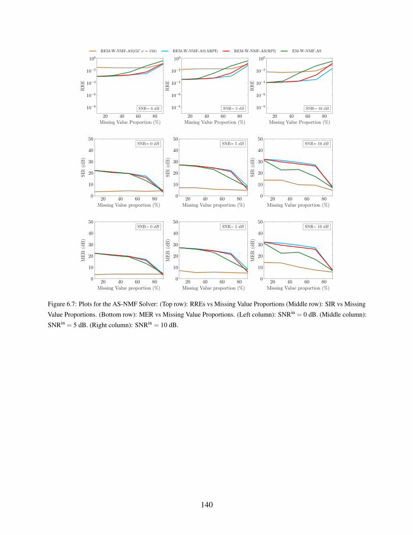
REM-W-NMF-AS(GC ν = 150) REM-W-NMF-AS(ARPI) REM-W-NMF-AS(RPI) EM-W-NMF-AS
20 40 60 80
100
10−2
10−4
10−6
10−8
Missing Value Proportion (%)
RR
E
SNR= 0 dB
20 40 60 80
100
10−2
10−4
10−6
10−8
Missing Value Proportion (%)
RR
E
SNR= 5 dB
20 40 60 80
100
10−2
10−4
10−6
10−8
Missing Value Proportion (%)
RR
E
SNR= 10 dB
20 40 60 800
10
20
30
40
50
Missing Value proportion (%)
SIR
(dB
)
SNR= 0 dB
20 40 60 800
10
20
30
40
50
Missing Value proportion (%)
SIR
(dB
)
SNR= 5 dB
20 40 60 800
10
20
30
40
50
Missing Value proportion (%)
SIR
(dB
)
SNR= 10 dB
20 40 60 800
10
20
30
40
50
Missing Value proportion (%)
ME
R(d
B)
SNR= 0 dB
20 40 60 800
10
20
30
40
50
Missing Value proportion (%)
ME
R(d
B)
SNR= 5 dB
20 40 60 800
10
20
30
40
50
Missing Value proportion (%)
ME
R(d
B)
SNR= 10 dB
Figure 6.7: Plots for the AS-NMF Solver: (Top row): RREs vs Missing Value Proportions (Middle row): SIR vs Missing
Value Proportions. (Bottom row): MER vs Missing Value Proportions. (Left column): SNRin = 0 dB. (Middle column):
SNRin = 5 dB. (Right column): SNRin = 10 dB.
140
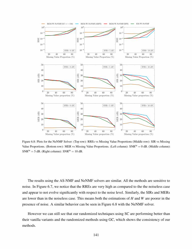
REM-W-NeNMF(GC ν = 150) REM-W-NeNMF(ARPI) REM-W-NeNMF(RPI) EM-W-NeNMF
20 40 60 80
100
10−2
10−4
10−6
10−8
Missing Value Proportion (%)
RR
E
SNR= 0 dB
20 40 60 80
100
10−2
10−4
10−6
10−8
Missing Value Proportion (%)
RR
E
SNR= 5 dB
20 40 60 80
100
10−2
10−4
10−6
10−8
Missing Value Proportion (%)
RR
E
SNR= 10 dB
20 40 60 800
10
20
30
40
50
Missing Value proportion (%)
SIR
(dB
)
SNR= 0 dB
20 40 60 800
10
20
30
40
50
Missing Value proportion (%)
SIR
(dB
)
SNR= 5 dB
20 40 60 800
10
20
30
40
50
Missing Value proportion (%)
SIR
(dB
)
SNR= 10 dB
20 40 60 800
10
20
30
40
50
Missing Value proportion (%)
ME
R(d
B)
SNR= 0 dB
20 40 60 800
10
20
30
40
50
Missing Value proportion (%)
ME
R(d
B)
SNR= 5 dB
20 40 60 800
10
20
30
40
50
Missing Value proportion (%)
ME
R(d
B)
SNR= 10 dB
Figure 6.8: Plots for the NeNMF Solver: (Top row): RREs vs Missing Value Proportions (Middle row): SIR vs Missing
Value Proportions. (Bottom row): MER vs Missing Value Proportions. (Left column): SNRin = 0 dB. (Middle column):
SNRin = 5 dB. (Right column): SNRin = 10 dB.
The results using the AS-NMF and NeNMF solvers are similar. All the methods are sensitive to
noise. In Figure 6.7, we notice that the RREs are very high as compared to the the noiseless case
and appear to not evolve significantly with respect to the noise level. Similarly, the SIRs and MERs
are lower than in the noiseless case. This means both the estimations of H and W are poorer in the
presence of noise. A similar behavior can be seen in Figure 6.8 with the NeNMF solver.
However we can still see that our randomized techniques using SC are performing better than
their vanilla variants and the randomized methods using GC, which shows the consistency of our
methods.
141
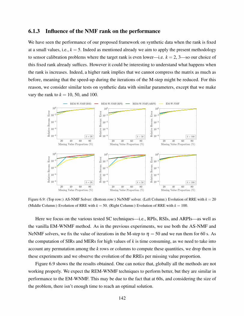
6.1.3 Influence of the NMF rank on the performance
We have seen the performance of our proposed framework on synthetic data when the rank is fixed
at a small values, i.e., k = 5. Indeed as mentioned already we aim to apply the present methodology
to sensor calibration problems where the target rank is even lower—i.e. k = 2, 3—so our choice of
this fixed rank already suffices. However it could be interesting to understand what happens when
the rank is increases. Indeed, a higher rank implies that we cannot compress the matrix as much as
before, meaning that the speed-up during the iterations of the M-step might be reduced. For this
reason, we consider similar tests on synthetic data with similar parameters, except that we make
vary the rank to k = 10, 50, and 100.
REM-W-NMF(RSI) REM-W-NMF(RPI) REM-W-NMF(ARPI) EM-W-NMF
20 40 60 80
100
10−2
10−4
10−6
10−8
Missing Value Proportion (%)
Rel
ativ
eR
econ
s.E
rror
k = 20
20 40 60 80
100
10−2
10−4
10−6
10−8
Missing Value Proportion (%)
Rel
ativ
eR
econ
s.E
rror
k = 50
20 40 60 80
100
10−2
10−4
10−6
10−8
Missing Value Proportion (%)
Rel
ativ
eR
econ
s.E
rror
k = 100
20 40 60 80
100
10−2
10−4
10−6
10−8
Missing Value Proportion (%)
Rel
ativ
eR
econ
s.E
rror
k = 20
20 40 60 80
100
10−2
10−4
10−6
10−8
Missing Value Proportion (%)
Rel
ativ
eR
econ
s.E
rror
k = 50
20 40 60 80
100
10−2
10−4
10−6
10−8
Missing Value Proportion (%)
Rel
ativ
eR
econ
s.E
rror
k = 100
Figure 6.9: (Top row:) AS-NMF Solver: (Bottom row:) NeNMF solver. (Left Column:) Evolution of RRE with k = 20
(Middle Column:) Evolution of RRE with k = 50. (Right Column:) Evolution of RRE with k = 100.
Here we focus on the various tested SC techniques—i.e., RPIs, RSIs, and ARPIs—as well as
the vanilla EM-WNMF method. As in the previous experiments, we use both the AS-NMF and
NeNMF solvers, we fix the value of iterations in the M-step to η = 50 and we run them for 60 s. As
the computation of SIRs and MERs for high values of k is time consuming, as we need to take into
account any permutation among the k rows or columns to compute these quantities, we drop them in
these experiments and we observe the evolution of the RREs per missing value proportion.
Figure 6.9 shows the the results obtained. One can notice that, globally all the methods are not
working properly. We expect the REM-WNMF techniques to perform better, but they are similar in
performance to the EM-WNMF. This may be due to the fact that at 60s, and considering the size of
the problem, there isn’t enough time to reach an optimal solution.
142
6.2 Enhancement Provided by RPS
We proposed in the previous chapter a novel framework for performing random projections. As this
framework is novel, we first investigate its efficiency, i.e., how it allows to decrease the RREs along
iterations with NMF. We then investigate its performance when combined with REM-WNMF.
6.2.1 NMF Experiments
In this subsection, we aim to investigate the enhancement provided by RPS on NMF. For that purpose,
we consider two different NMF solvers, i.e., AS-NMF [139] and Nesterov gradient (NeNMF) [99].
Further, we consider two state-of-the-art compression strategies—i.e., RSIs and GC—through which
the NMF performance is assessed when compared with our proposed RPS and their vanilla versions.
In practice, we consider 15 simulations where we draw random non-negative matrices W theo and
H theo such that n = m = 10000 and k = 5. As a consequence, their product X theo is a 10000×10000
rank-5 matrix. Moreover, we investigate the effects of several parameters, i.e., the oversampling
parameter νi and the number ω of NMF iterations before new compression submatrices L(i) and R(i)
are used. The performance criterion used in this section is the RRE defined in Eq. (6.1). In each
simulation, we consider the same random initialization for each tested method. All the experiments
are conducted using Matlab R2018b on a computer equipped with 2.5 GHz Intel Xeon E5-2620.
6.2.1.1 Noiseless Configurations
We investigate the performance achieved by our proposed RPS methods. For the sake of clarity in
the discussion, we focus on the performance reached with GCS. The rest of the results—reached
with the other RPS techniques—are provided in B.
Figure 6.10 provides the median performance reached by both AS-NMF and NeNMF when
combined with GCS for different values of the parameters used in Algorithm 12, i.e., νi = 10, 50,
100, or 150, and ω = 1, 2, 5, 10, or ∞ (in the last case, GCS reduces to GC). These plots show
several interesting results. First of all, GC is not stable when combined with AS-NMF or NeNMF:
the RRE is not always decreasing along iterations. This is particularly visible when νi = 10 and 100.
However, the global NMF performance reached with GCS after 100 iterations significantly decreases
when νi increases. Such a result was expected as GC follows the proof of the JLL. Then, GCS
always outperforms GC, even for high values of νi. When νi = 10, the plotted RREs are not always
decreasing along iterations, which means that the methods are not always stable. However, this effect
is reduced (or cancelled) by increasing νi. Lastly, we can see that over all the considered values of
νi, setting ω to 1 appears to be a good trade-off. A similar behavior—shown in Appendix B.1 to
143
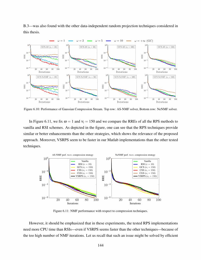
B.3—was also found with the other data-independent random projection techniques considered in
this thesis.
ω = 1 ω = 2 ω = 5 ω = 10 ω = +∞ (GC)
20 40 60 80 100
100
10−2
10−4
10−6
Iterations
RR
E
GCS-AS (νi = 10)
20 40 60 80 100
100
10−2
10−4
10−6
Iterations
RR
E
GCS-AS (νi = 50)
20 40 60 80 100
100
10−2
10−4
10−6
Iterations
RR
E
GCS-AS (νi = 100)
20 40 60 80 100
100
10−2
10−4
10−6
Iterations
RR
E
GCS-AS (νi = 150)
20 40 60 80 100
100
10−2
10−4
10−6
Iterations
RR
E
GCS-NeNMF (νi = 10)
20 40 60 80 100
100
10−2
10−4
10−6
Iterations
RR
E
GCS-NeNMF (νi = 50)
20 40 60 80 100
100
10−2
10−4
10−6
IterationsR
RE
GCS-NeNMF (νi = 100)
20 40 60 80 100
100
10−2
10−4
10−6
Iterations
RR
E
GCS-NeNMF (νi = 150)
Figure 6.10: Performance of Gaussian Compression Stream. Top row: AS-NMF solver, Bottom row: NeNMF solver.
In Figure 6.11, we fix ω = 1 and νi = 150 and we compare the RREs of all the RPS methods to
vanilla and RSI schemes. As depicted in the figure, one can see that the RPS techniques provide
similar or better enhancements than the other strategies, which shows the relevance of the proposed
approach. Moreover, VSRPS seem to be faster in our Matlab implementations than the other tested
techniques.
20 40 60 80 100
100
10−2
10−4
10−6
Iterations
RR
E
AS-NMF perf. w.r.t. compression strategy
VanillaRSI (ν = 10)
GCS (νi = 150)CSS (νi = 150)CGS (νi = 150)
VSRPS (νi = 150)
20 40 60 80 100
100
10−2
10−4
10−6
Iterations
RR
E
NeNMF perf. w.r.t. compression strategy
VanillaRSI (ν = 10)
GCS (νi = 150)CSS (νi = 150)CGS (νi = 150)
VSRPS (νi = 150)
Figure 6.11: NMF performance with respect to compression techniques.
However, it should be emphasized that in these experiments, the tested RPS implementations
need more CPU time than RSIs—even if VSRPS seems faster than the other techniques—because of
the too high number of NMF iterations. Let us recall that such an issue might be solved by efficient
144
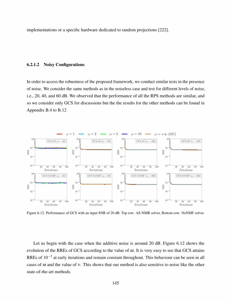
implementations or a specific hardware dedicated to random projections [222].
6.2.1.2 Noisy Configurations
In order to access the robustness of the proposed framework, we conduct similar tests in the presence
of noise. We consider the same methods as in the noiseless case and test for different levels of noise,
i.e., 20, 40, and 60 dB. We observed that the performance of all the RPS methods are similar, and
so we consider only GCS for discussions but the the results for the other methods can be found in
Appendix B.4 to B.12
ω = 1 ω = 2 ω = 5 ω = 10 ω = +∞ (GC)
20 40 60 80 100
100
10−2
10−4
10−6
Iterations
RR
E
GCS-AS (νi = 10)
20 40 60 80 100
100
10−2
10−4
10−6
Iterations
RR
E
GCS-AS (νi = 50)
20 40 60 80 100
100
10−2
10−4
10−6
Iterations
RR
E
GCS-AS (νi = 100)
20 40 60 80 100
100
10−2
10−4
10−6
Iterations
RR
E
GCS-AS (νi = 150)
20 40 60 80 100
100
10−2
10−4
10−6
Iterations
RR
E
GCS-NeNMF (νi = 10)
20 40 60 80 100
100
10−2
10−4
10−6
Iterations
RR
E
GCS-NeNMF (νi = 50)
20 40 60 80 100
100
10−2
10−4
10−6
Iterations
RR
E
GCS-NeNMF (νi = 100)
20 40 60 80 100
100
10−2
10−4
10−6
Iterations
RR
E
GCS-NeNMF (νi = 150)
Figure 6.12: Performance of GCS with an input SNR of 20 dB. Top row: AS-NMR solver, Bottom row: NeNMF solver.
Let us begin with the case when the additive noise is around 20 dB. Figure 6.12 shows the
evolution of the RREs of GCS according to the value of ω . It is very easy to see that GCS attains
RREs of 10−2 at early iterations and remain constant throughout. This behaviour can be seen in all
cases of ω and the value of ν . This shows that our method is also sensitive to noise like the other
state-of-the-art methods.
145
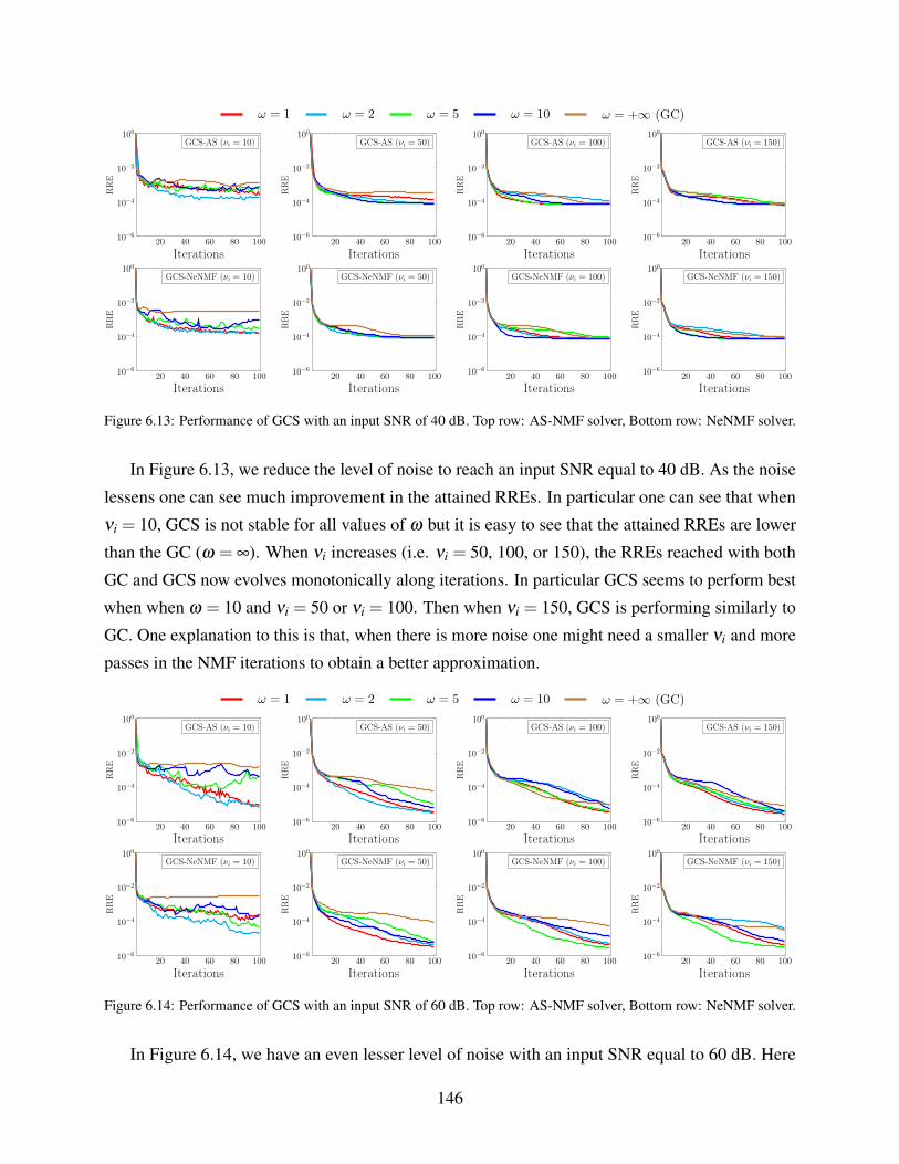
ω = 1 ω = 2 ω = 5 ω = 10 ω = +∞ (GC)
20 40 60 80 100
100
10−2
10−4
10−6
Iterations
RR
E
GCS-AS (νi = 10)
20 40 60 80 100
100
10−2
10−4
10−6
Iterations
RR
E
GCS-AS (νi = 50)
20 40 60 80 100
100
10−2
10−4
10−6
Iterations
RR
E
GCS-AS (νi = 100)
20 40 60 80 100
100
10−2
10−4
10−6
Iterations
RR
E
GCS-AS (νi = 150)
20 40 60 80 100
100
10−2
10−4
10−6
Iterations
RR
E
GCS-NeNMF (νi = 10)
20 40 60 80 100
100
10−2
10−4
10−6
Iterations
RR
EGCS-NeNMF (νi = 50)
20 40 60 80 100
100
10−2
10−4
10−6
Iterations
RR
E
GCS-NeNMF (νi = 100)
20 40 60 80 100
100
10−2
10−4
10−6
Iterations
RR
E
GCS-NeNMF (νi = 150)
Figure 6.13: Performance of GCS with an input SNR of 40 dB. Top row: AS-NMF solver, Bottom row: NeNMF solver.
In Figure 6.13, we reduce the level of noise to reach an input SNR equal to 40 dB. As the noise
lessens one can see much improvement in the attained RREs. In particular one can see that when
νi = 10, GCS is not stable for all values of ω but it is easy to see that the attained RREs are lower
than the GC (ω = ∞). When νi increases (i.e. νi = 50, 100, or 150), the RREs reached with both
GC and GCS now evolves monotonically along iterations. In particular GCS seems to perform best
when when ω = 10 and νi = 50 or νi = 100. Then when νi = 150, GCS is performing similarly to
GC. One explanation to this is that, when there is more noise one might need a smaller νi and more
passes in the NMF iterations to obtain a better approximation.
ω = 1 ω = 2 ω = 5 ω = 10 ω = +∞ (GC)
20 40 60 80 100
100
10−2
10−4
10−6
Iterations
RR
E
GCS-AS (νi = 10)
20 40 60 80 100
100
10−2
10−4
10−6
Iterations
RR
E
GCS-AS (νi = 50)
20 40 60 80 100
100
10−2
10−4
10−6
Iterations
RR
E
GCS-AS (νi = 100)
20 40 60 80 100
100
10−2
10−4
10−6
Iterations
RR
E
GCS-AS (νi = 150)
20 40 60 80 100
100
10−2
10−4
10−6
Iterations
RR
E
GCS-NeNMF (νi = 10)
20 40 60 80 100
100
10−2
10−4
10−6
Iterations
RR
E
GCS-NeNMF (νi = 50)
20 40 60 80 100
100
10−2
10−4
10−6
Iterations
RR
E
GCS-NeNMF (νi = 100)
20 40 60 80 100
100
10−2
10−4
10−6
Iterations
RR
E
GCS-NeNMF (νi = 150)
Figure 6.14: Performance of GCS with an input SNR of 60 dB. Top row: AS-NMF solver, Bottom row: NeNMF solver.
In Figure 6.14, we have an even lesser level of noise with an input SNR equal to 60 dB. Here
146
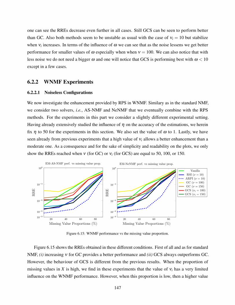
one can see the RREs decrease even further in all cases. Still GCS can be seen to perform better
than GC. Also both methods seem to be unstable as usual with the case of νi = 10 but stabilize
when νi increases. In terms of the influence of ω we can see that as the noise lessens we get better
performance for smaller values of ω especially when when ν = 100. We can also notice that with
less noise we do not need a bigger ω and one will notice that GCS is performing best with ω < 10
except in a few cases.
6.2.2 WNMF Experiments
6.2.2.1 Noiseless Configurations
We now investigate the enhancement provided by RPS in WNMF. Similary as in the standard NMF,
we consider two solvers, i.e., AS-NMF and NeNMF that we eventually combine with the RPS
methods. For the experiments in this part we consider a slightly different experimental setting.
Having already extensively studied the influence of η on the accuracy of the estimations, we herein
fix η to 50 for the experiments in this section. We also set the value of ω to 1. Lastly, we have
seen already from previous experiments that a high value of νi allows a better enhancement than a
moderate one. As a consequence and for the sake of simplicity and readability on the plots, we only
show the RREs reached when ν (for GC) or νi (for GCS) are equal to 50, 100, or 150.
20 40 60 80
100
10−3
10−6
10−8
10−9
Missing Value Proportions (%)
RR
E
EM-AS-NMF perf. vs missing value prop.
20 40 60 80
100
10−3
10−6
10−8
10−9
Missing Value Proportions (%)
RR
E
EM-NeNMF perf. vs missing value prop.
VanillaRSI (ν = 10)
ARPI (ν = 10)GC (ν = 100)GC (ν = 150)
GCS (νi = 100)GCS (νi = 150)
Figure 6.15: WNMF performance vs the missing value proportion.
Figure 6.15 shows the RREs obtained in these different conditions. First of all and as for standard
NMF, (i) increasing ν for GC provides a better performance and (ii) GCS always outperforms GC.
However, the behaviour of GCS is different from the previous results. When the proportion of
missing values in X is high, we find in these experiments that the value of νi has a very limited
influence on the WNMF performance. However, when this proportion is low, then a higher value
147
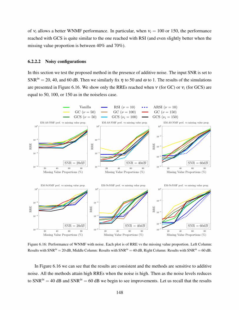
of νi allows a better WNMF performance. In particular, when νi = 100 or 150, the performance
reached with GCS is quite similar to the one reached with RSI (and even slightly better when the
missing value proportion is between 40% and 70%).
6.2.2.2 Noisy configurations
In this section we test the proposed method in the presence of additive noise. The input SNR is set to
SNRin = 20, 40, and 60 dB. Then we similarly fix η to 50 and ω to 1. The results of the simulations
are presented in Figure 6.16. We show only the RREs reached when ν (for GC) or νi (for GCS) are
equal to 50, 100, or 150 as in the noiseless case.
Vanilla RSI (ν = 10) ARSI (ν = 10)GC (ν = 50) GC (ν = 100) GC (ν = 150)GCS (ν = 50) GCS (νi = 100) GCS (νi = 150)
20 40 60 80
100
10−2
10−4
10−6
Missing Value Proportions (%)
RR
E
EM-AS-NMF perf. vs missing value prop.
SNR = 20dB
20 40 60 80
100
10−2
10−4
10−6
Missing Value Proportions (%)
RR
E
EM-AS-NMF perf. vs missing value prop.
SNR = 40dB
20 40 60 80
100
10−2
10−4
10−6
10−8
Missing Value Proportions (%)
RR
E
EM-AS-NMF perf. vs missing value prop.
SNR = 60dB
20 40 60 80
100
10−2
10−4
10−6
Missing Value Proportions (%)
RR
E
EM-NeNMF perf. vs missing value prop.
SNR = 20dB
20 40 60 80
100
10−2
10−4
10−6
Missing Value Proportions (%)
RR
E
EM-NeNMF perf. vs missing value prop.
SNR = 40dB
20 40 60 80
100
10−2
10−4
10−6
10−7
Missing Value Proportions (%)
RR
E
EM-NeNMF perf. vs missing value prop.
SNR = 60dB
Figure 6.16: Performance of WNMF with noise. Each plot is of RRE vs the missing value proportion. Left Column:
Results with SNRin = 20 dB, Middle Column: Results with SNRin = 40 dB, Right Column: Results with SNRin = 60 dB.
In Figure 6.16 we can see that the results are consistent and the methods are sensitive to additive
noise. All the methods attain high RREs when the noise is high. Then as the noise levels reduces
to SNRin = 40 dB and SNRin = 60 dB we begin to see improvements. Let us recall that the results
148
obtained in the noiseless and noisy settings is done with GCS with ω = 1, which is the most
computational demanding scenario. We can also observe GCS outperforms RPIs and ARPIs when
the proportion of missing entries is low and the input SNR is lower or equal to 40 dB. Due to the
huge time complexity of GCS and the other RPS variants, we do not aim to test this in the remainder
of the Ph.D. thesis. However, combining them with some dedicated hardware looks as a promising
way to fasten them. This should allow to use them in an efficient way, which is let as a perspective
of this thesis.
6.3 Application to Image Completion Problems
In this section, we investigate the performance of our randomized framework applied to image
completion. Indeed, low-rank approximation has been extensively studied for image completion. In
that case, the weight matrix Q is binary depending if the entries of X are known or not. Denoting
Ω the set of known entries of X , low-rank matrix completion can be seen as the estimation of a
low-rank matrix M whose rank is minimal and whose entries are equal to those of X in Ω [32]. As
minimizing the rank of M is NP-hard, this problem can be relaxed by minimizing its nuclear norm,
denoted ||M||? and defined as the sum of its singular values. Assuming M to be non-negative, the
low-rank matrix completion problem aims to solve
minM≥0
12
∣∣∣∣PΩ(X)−PΩ(M)∣∣∣∣2
F+µ ||M||? , (6.5)
where PΩ is the sampling operator of X .
Moreover, as M is assumed to be low-rank, it can be replaced by a matrix product—say
M =W ·H—and solving Eq. (6.5) is similar to solving [276]
minW≥0,H≥0
12||W X−W (W ·H)||2F +
µ
2(||W ||2F + ||H||2F ), (6.6)
that is, a specific weighted version of Eq. (3.2). Our proposed framework to combine random
projections to an EM procedure can be straightforwardly extended to this situation, when some
penalization terms are added in the cost function.
6.3.1 State-of-the-art Methods
The choice of a state-of-the art method to compare to was a rather a harder task. The optimiza-
tion problems of most matrix completion problems are slightly different from our framework.
Nonetheless for these comparisons we piqued two methods to compare to. We consider:
149
1. OptSpace [135] which is a low-rank matrix completion algorithm based on simple singular
value decomposition and manifold optimization. It consist performing a single value decom-
position and then a manifold optimization such that, Eq. (6.5) has a basic model that reads
U ,V= minS∈Rk×k
12
∣∣∣∣PΩ(X)−PΩ(U ·S ·V T )∣∣∣∣2
F(6.7)
OptSpace is much more related to our proposed methods as it is also based on matrix factor-
ization.
2. TNNR-ADMM [120] which is based on the alternating direction method of multipliers
optimization and nuclear norm regularization. As ADMM is seen to be a tool for solving
separable convex optimization problems [120], thus, this method is slightly different from our
method. Moreover, the TNNR-ADMM imposes a lot of constraints and parameters and for
that matter computing a simple SVD several times increases the time complexity especially
when the data is in high dimensions. TNNR-ADMM aims to minimize:
minX ,W||X ||∗−Tr(UWV T ) (6.8)
s.t. X =W,PΩ(W ) = PΩ(M)
where U = [u1, ...,uk]T and V = [v1, ...,vk]
T are the right and left eigenvectors. Then the
constraint PΩ(W ) means that the sampled entries with noise in PΩ(M) is retained exactly
in X [164].
6.3.2 Parameter settings
For all the tested methods, we fix the rank to be k= 5, and the number of iterations to be maxiter = 100.
We then tweak each method to achieve the best results. For our REM-WNMF and EM-NMF methods,
we set the M-Step iterations to η = 50, and the penelization term µ to µ = 10−3. For the OptSpace
method, we set tol = 10−5 and ρ = 10−3. For TNNR-ADMM, we set β = 0.001, tol = 10−3,
tolouter = 10−5, and outeriter = 10.
6.3.3 Experiments
In most real life scenarios, images can be exposed to different conditions that can damage them or
hide important information/features. We thus model such conditions by considering two cases, i.e.,
(i) random loss, and (ii) corruption with texts. To measure the accuracy of the reconstruction of
150
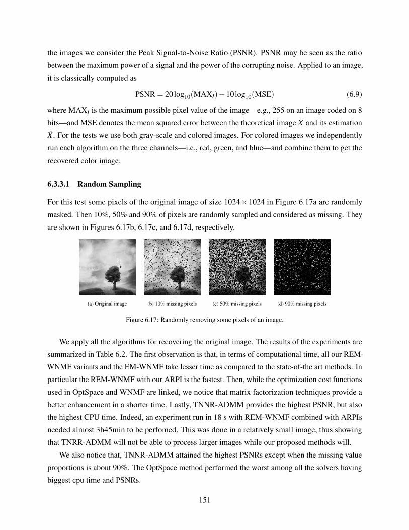
the images we consider the Peak Signal-to-Noise Ratio (PSNR). PSNR may be seen as the ratio
between the maximum power of a signal and the power of the corrupting noise. Applied to an image,
it is classically computed as
PSNR = 20log10(MAXI)−10log10(MSE) (6.9)
where MAXI is the maximum possible pixel value of the image—e.g., 255 on an image coded on 8
bits—and MSE denotes the mean squared error between the theoretical image X and its estimation
X . For the tests we use both gray-scale and colored images. For colored images we independently
run each algorithm on the three channels—i.e., red, green, and blue—and combine them to get the
recovered color image.
6.3.3.1 Random Sampling
For this test some pixels of the original image of size 1024×1024 in Figure 6.17a are randomly
masked. Then 10%, 50% and 90% of pixels are randomly sampled and considered as missing. They
are shown in Figures 6.17b, 6.17c, and 6.17d, respectively.
(a) Original image (b) 10% missing pixels (c) 50% missing pixels (d) 90% missing pixels
Figure 6.17: Randomly removing some pixels of an image.
We apply all the algorithms for recovering the original image. The results of the experiments are
summarized in Table 6.2. The first observation is that, in terms of computational time, all our REM-
WNMF variants and the EM-WNMF take lesser time as compared to the state-of-the art methods. In
particular the REM-WNMF with our ARPI is the fastest. Then, while the optimization cost functions
used in OptSpace and WNMF are linked, we notice that matrix factorization techniques provide a
better enhancement in a shorter time. Lastly, TNNR-ADMM provides the highest PSNR, but also
the highest CPU time. Indeed, an experiment run in 18 s with REM-WNMF combined with ARPIs
needed almost 3h45min to be perfomed. This was done in a relatively small image, thus showing
that TNRR-ADMM will not be able to process larger images while our proposed methods will.
We also notice that, TNNR-ADMM attained the highest PSNRs except when the missing value
proportions is about 90%. The OptSpace method performed the worst among all the solvers having
biggest cpu time and PSNRs.
151
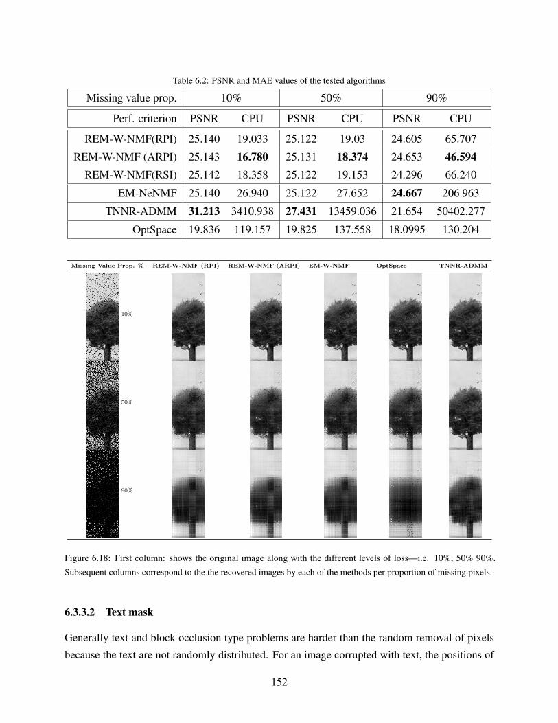
Table 6.2: PSNR and MAE values of the tested algorithms
Missing value prop. 10% 50% 90%
Perf. criterion PSNR CPU PSNR CPU PSNR CPU
REM-W-NMF(RPI) 25.140 19.033 25.122 19.03 24.605 65.707
REM-W-NMF (ARPI) 25.143 16.780 25.131 18.374 24.653 46.594REM-W-NMF(RSI) 25.142 18.358 25.122 19.153 24.296 66.240
EM-NeNMF 25.140 26.940 25.122 27.652 24.667 206.963
TNNR-ADMM 31.213 3410.938 27.431 13459.036 21.654 50402.277
OptSpace 19.836 119.157 19.825 137.558 18.0995 130.204
Missing Value Prop. % REM-W-NMF (RPI) REM-W-NMF (ARPI) EM-W-NMF OptSpace TNNR-ADMM
10%
50%
90%
Figure 6.18: First column: shows the original image along with the different levels of loss—i.e. 10%, 50% 90%.
Subsequent columns correspond to the the recovered images by each of the methods per proportion of missing pixels.
6.3.3.2 Text mask
Generally text and block occlusion type problems are harder than the random removal of pixels
because the text are not randomly distributed. For an image corrupted with text, the positions of
152

the text is regarded as missing pixels since they cover those areas of the image. Figure 6.19a shows
the original image of size 1,024×1,024 used for this test, then some text is placed on it in Figure
6.19b. We again apply all the algorithms to reconstruct the original image.
(a) Original image (b) 10% missing pixels
Figure 6.19: An image corrupted by some text.
The reconstructed images of the various algorithms are shown in Figure 6.20. As we would
see in the accompanying figure, our REM-WNMF and EM-WNMF methods both achieve similar
PSNR values. The image used in this experiment is relatively smaller in dimension as compared
to the dimension of our our synthetic data used in previous sections. For this reason we do not see
a huge influence of the use of random projections. Nonetheless one can still see that according
to Table 6.3, the REM-WNMF methods have lower CPU times than the EM-WNMF. Particularly
the REM-WNMF with ARPI has the lowest CPU time. Then compared to the other techniques,
Optspace performs the worst in terms of PSNR, while the TNNR-ADMM attains the best PSNR
value. In regards to their CPU times, they both attain much higher CPU times than the WNMF
methods. In Figure 6.20, we can see all the reconstructed images. By visual inspection one can see
that the reconstruction with our method is closer to that of the TNNR-ADMM than the OptSpace
which shows more visible texts.
153
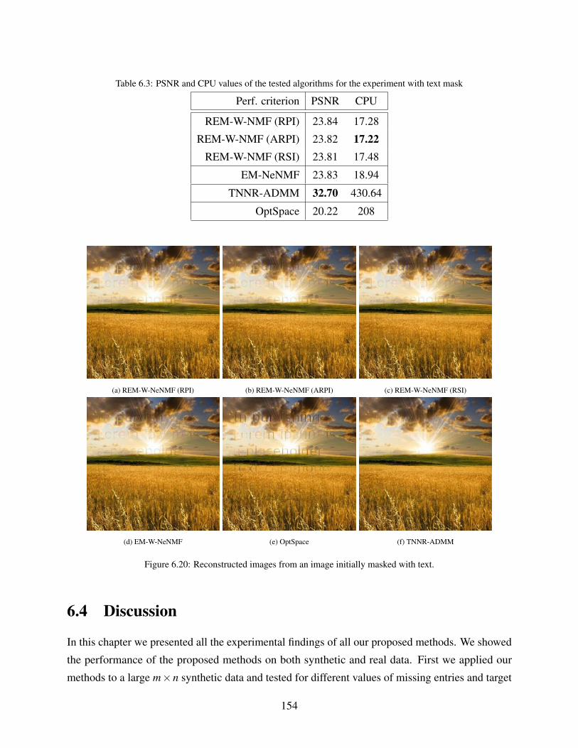
Table 6.3: PSNR and CPU values of the tested algorithms for the experiment with text mask
Perf. criterion PSNR CPU
REM-W-NMF (RPI) 23.84 17.28
REM-W-NMF (ARPI) 23.82 17.22REM-W-NMF (RSI) 23.81 17.48
EM-NeNMF 23.83 18.94
TNNR-ADMM 32.70 430.64
OptSpace 20.22 208
(a) REM-W-NeNMF (RPI) (b) REM-W-NeNMF (ARPI) (c) REM-W-NeNMF (RSI)
(d) EM-W-NeNMF (e) OptSpace (f) TNNR-ADMM
Figure 6.20: Reconstructed images from an image initially masked with text.
6.4 Discussion
In this chapter we presented all the experimental findings of all our proposed methods. We showed
the performance of the proposed methods on both synthetic and real data. First we applied our
methods to a large m×n synthetic data and tested for different values of missing entries and target
154
rank. We also investigate the influence of the number E-step iterations η of the proposed framework.
Then we test all the methods in the presence of noise, were we vary the input noise to SNRin = 20,
40, and 60 dB. In all these experiments, we found that after a fixed time of 60 s our REM-WNMF
variants provide a better performance than the vanilla EM-WNMF, especially when η = 50. Next
we piqued image completion as an application of our proposed framework. We tested the methods
on images following two scenarios, i.e., (i) random pixel removal and (ii) masking the images with
some text. For both scenarios we run out methods and compare the results with state-of-the-art
image completion methods. We found the PSNRs of REM-WNMF and EM-WNMF with the former
yielding lower CPU times. Interestingly, our proposed methods outperform one state-of-the-art
image completion technique—i.e., OptSpace—both in terms of speed and of accuracy of estimation
of the missing entries. However, TNNR-ADMM—which involves a much more complex cost
function—provides a better estimation of missing entries, at the price of extremely time consuming
computations. These experiments motivate us to investigate the enhancement provided by REM-
WNMF when extended to in situ calibration. Such an investigation is provided in the next part of the
thesis. Lastly, it is worth mentioning that RPS were investigated in this chapter and provided some
interesting results. However, as they are not well-suited to CPUs—because of the repeated cost of
random projections along iterations—we do not aim to test them in the remainder of the thesis.
155
Part II
Fast Informed Matrix Factorization forMobile Sensor Calibration
156

Chapter 7
Short-term and Long-term SensorCalibration in Mobile Sensor Arrays
7.1 Introduction . . . . . . . . . . . . . . . . . . . . . . . . . . . . . . . . . . . . . . . . . . . . . . 157
7.2 Modelling the Calibration Relationship . . . . . . . . . . . . . . . . . . . . . . . . . . . . . . . 159
7.2.1 Calibration using informed matrix factorization . . . . . . . . . . . . . . . . . . . . . . . . 162
7.2.2 MU-based IN-Cal method [74] . . . . . . . . . . . . . . . . . . . . . . . . . . . . . . . . 163
7.3 Cross-sensitive sensor calibration modeling . . . . . . . . . . . . . . . . . . . . . . . . . . . . . 164
7.3.1 Modeling the Scene for the k-th sensed phenomenon . . . . . . . . . . . . . . . . . . . . . 164
7.3.2 Modeling of a poorly selective sensor . . . . . . . . . . . . . . . . . . . . . . . . . . . . . 165
7.3.3 Modeling of a group of heterogeneous sensors . . . . . . . . . . . . . . . . . . . . . . . . 166
7.4 Proposed Informed NMF Methods . . . . . . . . . . . . . . . . . . . . . . . . . . . . . . . . . . 167
7.4.1 F-IN-Cal Method . . . . . . . . . . . . . . . . . . . . . . . . . . . . . . . . . . . . . . . . 168
7.4.2 Randomized F-IN-Cal . . . . . . . . . . . . . . . . . . . . . . . . . . . . . . . . . . . . . 170
7.5 Extension to Multiple Scenes . . . . . . . . . . . . . . . . . . . . . . . . . . . . . . . . . . . . . 172
7.1 Introduction
Environmental pollution is a major issue facing the world today and remains at the apex of priorities
of many international environmental protection agencies. Many of the current studies in this
domain are geared towards ways of monitoring the environment in order to understand and quantify
157
concentration levels of various harmful phenomena using environmental sensors. However, one of
the main challenges stalling significant progress in this direction is calibration [219]. According
to Definition 2.3, sensor calibration aims to match the response of an uncalibrated sensor with the
ground-truth. To this end, there are many scenarios that warrant the calibration of a sensor—e.g.
when the physical phenomenon can evolve fast enough to require online processing [160] or when
the sensors are no longer accessible, as in satellite imagery for example [34]. There are different
calibration models with different methods of performing the calibration which also depends on
several factors. One crucial factor is the presence or absence of reference sensors which directly
determines the difficulty of calibrating a sensor network, see, e.g., [83, 173, 290]. Unfortunately,
in real life, the availability of a sensor is not always guaranteed. For this reason other studies have
introduced the so-called "blind" calibration methods, e.g., a blind calibration model based on data
projection [11], statistical moments [258] or graph analysis [154]. In practice, these generally
require a dense network of sensors [75]. Finally, there is a so-called "partially blind" hybrid
calibration strategy where only some of the sensors to be calibrated can be based on a reference, see,
e.g., [74, 225, 245]. Another factor influencing the choice of the calibration model is sensor mobility.
Generally a sensor can be either static or mobile. When sensors are static, their dissemination is
restricted. Mobile sensors on the other hand are easier to move from one point to another and allow
to cover large areas [283].
In this chapter we will focus on the proposed fast in situ calibration method. In Chapter 2, we
have discussed extensively the different kinds of network calibration models and methods. We
also learnt that there is no one for all calibration method that unified the different types, i.e., micro
calibration, macro calibration, and transfer calibration. However, the authors in [186] posit that
one could achieve a unified framework if we combine the ideas of the various methods. They also
make references to the studies made by C. Dorffer et al. in [70, 71, 74, 76] where they propose the
Informed NMF-based Calibration (IN-Cal) method as an attempt to combine two main ideas, i.e., a
macro-calibration technique with micro-calibration assumptions. In this thesis, we therefore follow
the direction initiated by these authors and we propose novel methods and extensions. Another
major motivation is that many existing studies have focused mainly on methods involving one
kind of sensor, i.e., homogeneous sensors. This means that the sensors target only one type of
physical phenomenon. These types of methods usually face challenges when there is interference
between co-existing physical phenomena. In fact several studies in [13,143,187] observed that some
measured quantities could be correlated, e.g., many gas sensors have a response which depends on
both temperature and humidity. They further posit that extending in situ calibration approaches to
heterogeneous measurements could improve calibration quality compared to approaches that only
158
take into account homogeneous measurements. In this chapter we thus extend the IN-Cal approach
initially proposed for homogeneous sensors to heterogeneous sensors. This work was mainly done
by Olivier Vu Thah, whom I co-supervised during his M.Sc thesis [255] and presented in [256].
7.2 Modelling the Calibration Relationship
To build up to our proposed informed NMF methods we first introduce some key terminologies,
assumptions and the principles of the IN-Cal method. We remind the reader that, in the first part of
this thesis, we assumed X to be of size m×n with rank k. In the remainder of the thesis, we use
different notations which depend on the model used for revisiting mobile sensor calibration as an
informed matrix factorization problem.
Definition 7.1 (Rendezvous [224]). A rendezvous is a temporal and spatial vicinity between two
sensors.
A rendezvous is thus defined by a time duration ∆t and a distance ∆d . For two sensors to be in
rendezvous, they do not necessarily have to be "exactly" at the same place. This distance is the radius
of any two sensors at times [t, t +∆t ] apart. The duration ∆t is defined by the temporal variability of
the physical phenomenon while the distance ∆d is defined by the spatial variability of the physical
phenomenon. These parameter highly depend on the type of physical phenomena. As an example,
the values of ∆t and ∆d are much smaller for carbon monoxide than for temperature [224].
Definition 7.2 (Scene [76]). A scene S is a discretized area observed during a time interval
[t, t +∆t). The size of the spatial pixels is set so that any couple of points inside the same pixel have
a distance below ∆d .
Thus a scene is merely a grid of locations where sensors sense a physical phenomenon. When
two sensors are in a same pixel of the scene they are said to make a rendezvous. Data from the entire
network of sensors in the scene during a time ∆t is collected and can be interpreted in the form of a
large matrix X ∈ Rn×(m+1) where m+1 is the total number of sensors and n is the number of spatial
samples.
The main aim is to calibrate a network composed of m+1 localized and time-stamped mobile
sensors. It is assumed that each sensor of the network provides a reading x linked to an input
phenomenon w through a calibration function F (·) which is considered to be affine in [74], i.e.,
x≈F (y)≈ f1 + f2 ·w (7.1)
159
where f1 and f2 are the unknown sensor offset and gain, respectively. The observed matrix X is a
data matrix denoting [xi, j] such that each of its column contains the measurement of one sensor at
each location and each line contains the measurement of each sensor at one location. Assuming that
each sensor of the network gets a measurement in each cell of the scene, Xtheo can be modeled as:
Xtheo ≈W ·H (7.2)
with
W =
1 w1...
...
1 wn
and H =
(h0,1 . . . h0,m+1
h1,1 . . . h1,m+1
). (7.3)
where ∀ j = 1, . . . ,m+1, h1, j and h2, j are the unknown offset and gain associated with the j-th sensor,
respectively. Both factor matrices W and H thus contain the calibration model structure—hence
the column of ones in W to handle the offset in the calibration function of the sensors—and the
calibration parameters, respectively. Calibrating the network using factorization then consists of
estimating the matrices W and H which provide the best low-rank estimation of X , while keeping
the constrained structure in W .
x1,1 . . . x1,m w1...
......
xn,1 . . . xn,m wn
︸ ︷︷ ︸Xtheo
≈
1 w1...
...
1 wn
︸ ︷︷ ︸W
·(
h0,1 . . . h0,m 0
h1,1 . . . h1,m 1
)
︸ ︷︷ ︸H
(7.4)
From Eq. (7.4), solving the sensor array calibration problem can be seen as a matrix factorization
problem. Ideally, if we had all information—i.e., if we knew Xtheo—we would aim to solve
W , H = arg minW, H
12‖Xtheo−W ·H‖2
F (7.5)
s.t. w1 = 1n,
hm+1 =
(0
1
).
Given that ∀ (i, j)∈ Rn×(m+1), xi, j is a voltage produced by a sensor, we can assume that xi, j ≥ 0.
W is composed of a column of 1 and a column directly containing the physical phenomenon to be
measured. This phenomenon is either a concentration or a temperature (preferably in Kelvin). We
can therefore assume that W ≥ 0. The last column of Xtheo is equal to the second column of W , so
we can also assume that Xtheo ≥ 0. Finally, H contains the calibration parameters for all sensors. It
is possible that these parameters are negative. For example, a temperature sensor operating with a
160
resistor may have negative gain. On the contrary, some sensors may have non-negative calibration
parameters [74]. To simplify the modeling of our problem, we will only take this case into account
and assume that all the parameters are positive. With these assumptions, the matrix factorization is
in fact a non-negative matrix factorization1. With these new positivity constraints, Equation (7.5)
becomes
W , H = arg minW≥0, H≥0
12‖Xtheo−W ·H‖2
F (7.6)
s.t. w1 = 1n,
hm+1 =
(0
1
).
In reality, we only have the projection X of Xtheo on the space of observations, which is made
up of only a few elements of Xtheo. If the area is measured by sensor j, then Eq. (7.2) is verified.
Otherwise, it means that the information is not available and it is replaced by a 0. Let us denote
ΩX as the domain on which Xtheo is observed and introduce PΩXas the projection operator on this
domain, i.e.,
PΩX(Xtheo)≈ X . (7.7)
Several designs for the projection operator are possibles. As a first approximation, we could replace
it by a binary matrix Q ∈ Rn×(m+1), such that ∀ (i, j) ∈ Rn×(m+1),qi, j ∈ 0;1, or qi, j = 1, where
qi, j = 1 means that the sensor has taken a measurement in the i-th area of the scene S and qi, j = 0
otherwise. However, in practice, one may extend Q to a confidence matrix rather than an observation
matrix. In this case, ∀ (i, j) ∈ Rn×(m+1),qi, j ∈ [0,1] and qi, j represents the confidence that can be
given to the measurement carried out in the i-th zone of the scene by the j-th sensor. The hypothesis
made in [74] is that each sensor has its own uncertainty, denoted ρ j for Sensor j. Concretely, solving
Eq. (7.6) using Q instead of PΩX(·) reads
W , H = arg minW,H≥0
12‖Q (Xtheo−W ·H)‖2
F (7.8)
s.t. w1 = 1n,
∀ i ∈I , wi,2 = xi,m+1,
hm+1 =
(0
1
),
where I is the subset made up of the indices of the zones where a reference is located.1If we assume that the values of H can be negative, the problem corresponds to a semi-non-negative matrix
factorization problem which is solved in a relatively similar way.
161
In the field of blind source separation [141], the use of NMF only allows sources to be recovered
up to a gain factor and a permutation. While this is not a drawback for source separation, note
that the use of NMF in our calibration problem cannot afford such ambiguities on H. Fortunately,
the constraints in the structures of H and W allow to avoid these ambiguities2. These constraints
are necessary but are not sufficient. It is necessary to have enough reference measurements—with
enough diversity between these measurements—and rendezvous between mobile sensors with those
references in order to resolve scale ambiguities.
7.2.1 Calibration using informed matrix factorization
One way to incorporate all the constraints discussed above into the so called informed NMF problem
is via the parameterization approach proposed in [167] and used extensively in [74, 76]. The idea
consist of decomposing W and H into a sum of free and known parts. The free parts are just the
elements which are not under any constraint while the known parts contain known values of both
factor matrices. W and H can then be rewritten as
W =ΩW ΦW +ΩW ∆W, (7.9)
and
H =ΩH ΦH +ΩH ∆H, (7.10)
where
• ΩW and ΩH (ΩW and ΩH, respectively) are the binary matrices informing of the presence
(the absence, respectively) of constraints on W and H ;
• ΦW and ΦH are the matrices containing the values to be constrained W and H ;
• ∆W and ∆H are the matrices containing unconstrained values to W and H.
ΩW et ΩW on one hand and ΩH and ΩH on the other hand are built in such a way that there is
no possible intersection between them, i.e.,
ΩW ΩW = 0n,2, (7.11)
ΩH ΩH = 02,m+1. (7.12)
2On the other hand, the scale factor ambiguity still allows to perform a relative calibration of the sensor network: we
can thus make the responses of the sensors consistent with each other [75].
162
With this re-parameterization, Eq. (7.8) becomes
W , H = arg minW,H≥0
12‖Q (Xtheo−W ·H)‖2
F , (7.13)
s.t. W =ΩW ΦH +ΩW ∆W,
H =ΩH ΦH +ΩH ∆H.
Since the optimization problem presented in the Eq. (7.13) is not convex for the pair of variables
(W,H), it is common to separate this type of problem into two sub- convex problems, i.e.,
W = arg minW≥0
12‖Q (Xtheo−W ·H)‖2
F (7.14)
s.t. W =ΩW ΦH +ΩW ∆W,
H =ΩH ΦH +ΩH ∆H,
and
H = argminH≥0
12‖Q (Xtheo−W ·H)‖2
F (7.15)
s.t. W =ΩW ΦH +ΩW ∆W,
H =ΩH ΦH +ΩH ∆H.
The global strategy that we will find in all the proposed methods consists in solving alternately
both Eqs. (7.14) and (7.15). In the following, we will consider directly that
ΦW =ΩW ΦW, ∆W =ΩW ∆W, (7.16)
ΦH =ΩH ΦH, ∆H =ΩH ∆H. (7.17)
7.2.2 MU-based IN-Cal method [74]
The IN-Cal method is mainly based on the multiplicative updates rules. However for the considered
application, a weighted version of the MU update rules (WNMF-MU) in Eqs. (5.3) and (5.4) was
used. Consequently IN-Cal solves Eqs. (7.14) and (7.15), by modifying WNMF MU rules to take
into account the aforementioned constraints as [167]:
W ← ΦW +∆W (Q (X−ΦW ·H)+) ·HT
(Q (∆W ·H)) ·HT , (7.18)
and
H← ΦH +∆H W T · (Q (X−W ·ΦH)
+)
W T · (Q (W ·∆H)), (7.19)
where the operator + in the operation (z)+ corresponds to the operation max(ε,z), where ε is a value
close to precision machine. The whole IN-Cal algorithm is presented in Algorithm 14.
163
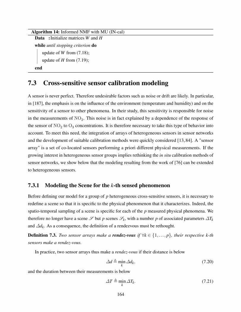
Algorithm 14: Informed NMF with MU (IN-cal)Data :Initialize matrices W and H
while until stopping criterion doupdate of W from (7.18);
update of H from (7.19);
end
7.3 Cross-sensitive sensor calibration modeling
A sensor is never perfect. Therefore undesirable factors such as noise or drift are likely. In particular,
in [187], the emphasis is on the influence of the environment (temperature and humidity) and on the
sensitivity of a sensor to other phenomena. In their study, this sensitivity is responsible for noise
in the measurements of NO2. This noise is in fact explained by a dependence of the response of
the sensor of NO2 to O3 concentrations. It is therefore necessary to take this type of behavior into
account. To meet this need, the integration of arrays of heterogeneous sensors in sensor networks
and the development of suitable calibration methods were quickly considered [13, 84]. A "sensor
array" is a set of co-located sensors performing a priori different physical measurements. If the
growing interest in heterogeneous sensor groups implies rethinking the in situ calibration methods of
sensor networks, we show below that the modeling resulting from the work of [76] can be extended
to heterogeneous sensors.
7.3.1 Modeling the Scene for the k-th sensed phenomenon
Before defining our model for a group of p heterogeneous cross-sensitive sensors, it is necessary to
redefine a scene so that it is specific to the physical phenomenon that it characterizes. Indeed, the
spatio-temporal sampling of a scene is specific for each of the p measured physical phenomena. We
therefore no longer have a scene S but p scenes Sk, with a number p of associated parameters ∆Tk
and ∆dk. As a consequence, the definition of a rendezvous must be rethought.
Definition 7.3. Two sensor arrays make a rendez-vous if ∀k ∈ 1, . . . , p, their respective k-th
sensors make a rendez-vous.
In practice, two sensor arrays thus make a rendez-vous if their distance is below
∆d , mink∆dk, (7.20)
and the duration between their measurements is below
∆T , mink∆Tk. (7.21)
164
Definition 7.3 thus allows to define a common scene with heterogeneous sensors. Please note that
it is also possible to relax the spatial constraints ∆dk if some spatial a priori are available. For
example in [74, 75] the spatial constraints are relaxed thanks to the availability of dictionaries of
spatial patterns for each quantity among the p to be considered. Such assumptions are not considered
in this thesis but extensions combining them with our proposed approaches can be straightforwardly
derived.
7.3.2 Modeling of a poorly selective sensor
Suppose now that we have a poorly selective sensor whose response depends on p latent variables.
We can rethink the model resulting from Eq. (7.1) to take this effect into accountWe would therefore
go from an affine relation to a multi-linear relation between the voltage delivered by a sub-sensor
and the p physical variables on which the sensor depends. If among these p physical variables, the
sensor aims to measure the k-th, the multi-linear relation is as follows:
Given(i, j,k) ∈ Rn×m+1×p ∃ (hk0, j,h
k1, j, . . . ,h
kp, j) ∈ Rp
+,
xki, j ≈ hk
0, j +hk1, j ·wi,1 + . . .+hk
p, j ·wi,p, (7.22)
where hki, j is the i-th calibration parameter of the sensor j which measures the magnitude k
To take into account Eq. (7.22) in our modeling, it suffices to complete the previous structure of
W by taking into account the p physical variables on which the sensor depends, namely:
W =(
1n w1 . . . wp
). (7.23)
The column wk therefore contains the values of the k physical phenomenon on all the n pixels of the
scene. The measurements made by the not very selective sensor can therefore always be interpreted
in the form of a matrix factorization, i.e.,
Xktheo ≈W ·Hk (7.24)
165
where
Hk =
hk0,1 hk
0,2 . . . hk0,m 0
hk1,1 hk
1,2 . . . hk1,m 0
......
......
hkk−1,1 hk
k−1,2 . . . hkk−1,m 0
hkk,1 hk
k,2 . . . hkk,m 1
hkk+1,1 hk
k+1,2 . . . hkk+1,m 0
......
......
hkp,1 hk
p,2 . . . hkp,m 0
. (7.25)
and where
Xktheo =
xk1,1 . . . xk
1,m w1,k...
......
xkn,1 . . . xk
n,m wn,k
(7.26)
The last column vector of Hk is therefore modeled as a Kronecker which is equal to 1 on the k-th
row of Hk and 0 elsewhere.
Note that for the moment we only have one type of sensor, so only one physical measurement is
performed. We simply took into account low selectivity that a sensor could demonstrate thanks to
a multi-linear calibration relationship. This implies that with this modeling, it is possible to try to
calibrate a network of non-selective sensors without having the other measurements on which the
low-selective sensor depends. It is interesting to note that unlike the multi-linear approaches based
on regression [187], this formalism makes it possible to estimate the calibration parameters using
a single type of sensors, i.e., to estimate Hk and W , up to a scale and permutation factor. Except
if p = 2—where the inherent scale and permutation ambiguities may be solved—the resolution of
these uncertainties can in particular be resolved by taking into account other measures, as we will
see below.
7.3.3 Modeling of a group of heterogeneous sensors
In this part, we suppose to have a group of heterogeneous sensors. If the sensor performing the
physical measurement of interest seems to depend in fact on p physical variables, then this group of
sensors consists of p low-selective sensors, each of these sensors being supposed to measure one
physical variables, i.e., one may write a relationship like Eq. (7.24) for each of these sensors. As all
these equations share the same matrix W , it is then possible to take all of them into consideration
166
under a matrix relationship by concatenating the data and calibration parameter matrices, i.e.,
H =(
H1 . . . H p)
(7.27)
and
Xtheo =(
X1theo . . . X p
theo
). (7.28)
As for homogeneous sensor calibration, not all the entries of Xtheo are known and the missing entries
can be handled by a weight matrix Q. Moreover, several entries of W and H are known and it
remains possible to take them into account using the same parameterization as for homogeneous
sensor calibration. As a consequence, solving in situ calibration of heterogeneous mobile sensors
yields the same informed NMF problem as for homogeneous sensors—i.e., one aim to solve Eq.
(7.13)—except that the size of X , W , and H are now bigger in the former than in the latter, i.e., their
respective dimensions are n× p(m+1), n× (p+1), and (p+1)× p(m+1). As IN-Cal was based
on MUs—which are known to be slow to converge when applied to large-scale problems—we need
to propose novel methods to solve Eq. (7.13).
7.4 Proposed Informed NMF Methods
We present in this section the first method that we propose, which is called Fast IN-Cal (F-IN-Cal).
F-IN-Cal is based based on extension of the EM strategy where we imposed additional constraints
on matrix factors according to the parametization mentioned in Section 7.2.1. Following such a
formulation the M-Step of Algorithm 7 after taking all contraints into account then reads as:
W = arg minW≥0
12‖Xcomp−W ·H‖2
F (7.29)
W=ΩW ΦH +ΩW ∆W
and
H = argminH≥0
12‖Xcomp−W ·H‖2
F (7.30)
H=ΩH ΦH +ΩH ∆H.
Once W and H have been estimated, we can repeat the E-step to update Xcomp.
167
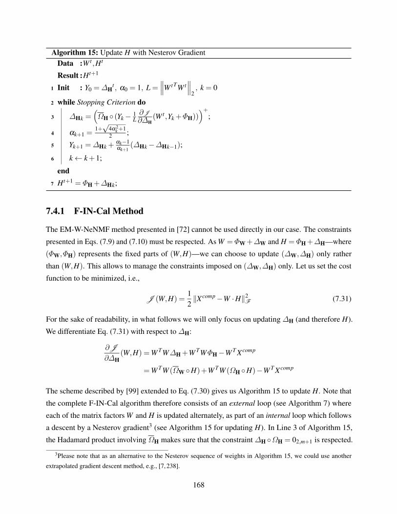
Algorithm 15: Update H with Nesterov GradientData :W t ,Ht
Result :Ht+1
1 Init : Y0 =∆Ht , α0 = 1, L =
∥∥∥W tTW t∥∥∥
2, k = 0
2 while Stopping Criterion do
3 ∆Hk =(ΩH (Yk− 1
L∂J
∂∆H(W t ,Yk +ΦH))
)+;
4 αk+1 =1+√
4α2k +1
2 ;
5 Yk+1 =∆Hk +αk−1αk+1
(∆Hk−∆Hk−1);
6 k← k+1;
end7 Ht+1 = ΦH +∆Hk;
7.4.1 F-IN-Cal Method
The EM-W-NeNMF method presented in [72] cannot be used directly in our case. The constraints
presented in Eqs. (7.9) and (7.10) must be respected. As W = ΦW+∆W and H = ΦH+∆H—where
(ΦW,ΦH) represents the fixed parts of (W,H)—we can choose to update (∆W,∆H) only rather
than (W,H). This allows to manage the constraints imposed on (∆W,∆H) only. Let us set the cost
function to be minimized, i.e.,
J (W,H) =12‖Xcomp−W ·H‖2
F (7.31)
For the sake of readability, in what follows we will only focus on updating ∆H (and therefore H).
We differentiate Eq. (7.31) with respect to ∆H:
∂J
∂∆H(W,H) =W TW∆H +W TWΦH−W T Xcomp
=W TW (ΩW H)+W TW (ΩH H)−W T Xcomp
The scheme described by [99] extended to Eq. (7.30) gives us Algorithm 15 to update H. Note that
the complete F-IN-Cal algorithm therefore consists of an external loop (see Algorithm 7) where
each of the matrix factors W and H is updated alternately, as part of an internal loop which follows
a descent by a Nesterov gradient3 (see Algorithm 15 for updating H). In Line 3 of Algorithm 15,
the Hadamard product involving ΩH makes sure that the constraint ∆H ΩH = 02,m+1 is respected.
3Please note that as an alternative to the Nesterov sequence of weights in Algorithm 15, we could use another
extrapolated gradient descent method, e.g., [7, 238].
168
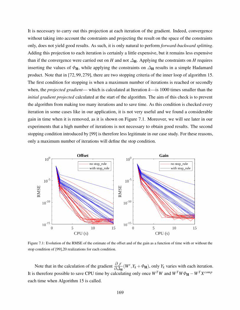
It is necessary to carry out this projection at each iteration of the gradient. Indeed, convergence
without taking into account the constraints and projecting the result on the space of the constraints
only, does not yield good results. As such, it is only natural to perform forward-backward splitting.
Adding this projection to each iteration is certainly a little expensive, but it remains less expensive
than if the convergence were carried out on H and not ∆H. Applying the constraints on H requires
inserting the values of ΦH, while applying the constraints on ∆H results in a simple Hadamard
product. Note that in [72, 99, 279], there are two stopping criteria of the inner loop of algorithm 15.
The first condition for stopping is when a maximum number of iterations is reached or secondly
when, the projected gradient— which is calculated at Iteration k—is 1000 times smaller than the
initial gradient projected calculated at the start of the algorithm. The aim of this check is to prevent
the algorithm from making too many iterations and to save time. As this condition is checked every
iteration in some cases like in our application, it is not very useful and we found a considerable
gain in time when it is removed, as it is shown on Figure 7.1. Moreover, we will see later in our
experiments that a high number of iterations is not necessary to obtain good results. The second
stopping condition introduced by [99] is therefore less legitimate in our case study. For these reasons,
only a maximum number of iterations will define the stop condition.
Figure 7.1: Evolution of the RMSE of the estimate of the offset and of the gain as a function of time with or without the
stop condition of [99],20 realizations for each condition.
Note that in the calculation of the gradient ∂J
∂∆H(W t ,Yk +ΦH), only Yk varies with each iteration.
It is therefore possible to save CPU time by calculating only once W TW and W TWΦH−W T Xcomp
each time when Algorithm 15 is called.
169
7.4.2 Randomized F-IN-Cal
We present in this section a second calibration method that we propose: Randomized F-IN-Cal
(RF-IN-Cal). This approach can be seen as an extension of F-IN-Cal using random projections to
speed up calculations.
By construction and according to, e.g., Eq. (7.22), we know that the rank of X is small with
respect to its dimensions. Indeed, X is rank p+1, e.g., rank 2 in the case of homogeneous sensor
networks. This makes min(n,m) p highly probable. The use of random projection therefore
seems to be entirely justified in this context. According to [279], in our calibration problem the
integration of the random projection in F-IN-Cal consists of
1. calculating the matrices L and R at each E-Step from the new estimate Xcomp,
2. defining XcompR , Xcomp ·R and HR , H×R, and solving
W = arg minW≥0
12
∥∥XcompR −W ·HR
∥∥2F, (7.32)
s.t. W=ΩW ΦH +ΩW ∆W,
instead of Eq. (7.29),
3. defining XcompL , L ·Xcomp and WL , L ·W , and solving
H = argminH≥0
12
∥∥XcompL −WL ·H
∥∥2F, (7.33)
s.t. H=ΩH ΦH +ΩH ∆H,
instead of Eq. (7.30).
Table 7.1 lists the complexity of the various cost operations with or without compression.
Note that the two gradient calculations ∂J
∂∆H(W,H) = (W TW ) ·∆H +(W TWΦH−W T Xcomp) and
∂J
∂∆W(W,H) =∆W ·(HHT )+(ΦWHHT −XcompHT ) do not appear in Table 7.1 because, except for
the initial computation of W TW and W T Xcomp (HHT and XcompHT , respectively), the computational
costs are the same in both cases. Usually the values n,m, and p will be such that n ≥ m p. In
practice, the number m of groups of sensors will probably not be able to exceed 100. The dimension
n of the matrix X on the other hand , grows quadratically with the size of the scene. For a very low
resolution scene in 10×10, n is already equal to 100. By multiplying the size of the scene by 2,
ie., with a scene of size 20×20, n has been multiplied by 4 and is equal to 400. We can therefore
corroborate that as soon as an operation involves n in terms of complexity, the compression will be
profitable. Note also that the product HHT does not involve n. Thus the use of compression for this
170
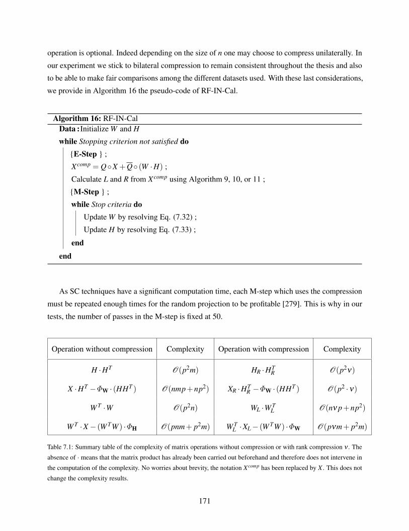
operation is optional. Indeed depending on the size of n one may choose to compress unilaterally. In
our experiment we stick to bilateral compression to remain consistent throughout the thesis and also
to be able to make fair comparisons among the different datasets used. With these last considerations,
we provide in Algorithm 16 the pseudo-code of RF-IN-Cal.
Algorithm 16: RF-IN-CalData :Initialize W and H
while Stopping criterion not satisfied doE-Step ;
Xcomp = QX +Q (W ·H) ;
Calculate L and R from Xcomp using Algorithm 9, 10, or 11 ;
M-Step ;
while Stop criteria doUpdate W by resolving Eq. (7.32) ;
Update H by resolving Eq. (7.33) ;
end
end
As SC techniques have a significant computation time, each M-step which uses the compression
must be repeated enough times for the random projection to be profitable [279]. This is why in our
tests, the number of passes in the M-step is fixed at 50.
Operation without compression Complexity Operation with compression Complexity
H ·HT O(p2m) HR ·HTR O(p2ν)
X ·HT −ΦW · (HHT ) O(nmp+np2) XR ·HTR −ΦW · (HHT ) O(p2 ·ν)
W T ·W O(p2n) WL ·W TL O(nν p+np2)
W T ·X− (W TW ) ·ΦH O(pnm+ p2m) W TL ·XL− (W TW ) ·ΦW O(pνm+ p2m)
Table 7.1: Summary table of the complexity of matrix operations without compression or with rank compression ν . The
absence of · means that the matrix product has already been carried out beforehand and therefore does not intervene in
the computation of the complexity. No worries about brevity, the notation Xcomp has been replaced by X . This does not
change the complexity results.
171
7.5 Extension to Multiple Scenes
We proposed in the above sections our proposed fast in situ calibration methods for cross-sensitive
sensors. Our proposed F-IN-Cal and RF-IN-Cal variants directly solve the drawback of IN-Cal
in terms of speed of convergence, and more importantly, extend IN-Cal to the case of cross-
sensitive/heterogeneous sensors. Still, these approaches are designed to perform calibration over
one single scene. We thus aim to discuss about strategies to perform long-term calibration, i.e.,
calibration over multiple scenes, as illustrated in Figure 1.2.
Long-term sensor calibration differs from the above short-term calibration as it aims to be
performed over several weeks to months. Once sensors are deployed over a long period, the drift
of the sensors along the considered period is expected and hardly predictable. As a consequence,
several strategies can be taken into consideration.
As explained in Chapter 2, several calibration models might be considered for lon-term calibra-
tion. In particular, taking into account the possible drift of the calibration parameters might be of
interest. However, the authors in [8] showed that complex calibration models—involving models
for the drift of the sensor calibration parameters as well as nonlinear dependencies between gas
concentration, temperature, and humidity–are not needed when considering calibration over short
time intervals, e.g., on a daily basis. This motivates us to consider the above affine or multi-linear
calibration models used in (R)F-IN-Cal and to extend them to the multiple scene case.
One may thus consider the matrix factorization model for each scene. Taking into account
multiple scenes can be performed through several strategies:
1. Figure 1.2 shows that the different observed matrices can be re-arranged as a tensor. It might
then make sense to perform in situ calibration using weighted tensor factorization.
2. Another strategy might consist of grouping several adjacent scenes/matrices for which the
calibration parameters are assumed not to evolve along time and to unfold them as a very large
matrix. Each of these large matrices could then be processed independently, as it was done
with multiple regression in [8].
3. Lastly, we may refine the above strategy by considering constrains between adjacent factor
matrices estimated from the above large data matrices, thus extending some work on matrix
co-factorization, e.g., [177, 227, 232].
All three approaches seem to be good ways to deal with the multiple scene problem. However in
this thesis, we propose to focus on the second strategy. Indeed, this allows us to easily extend the
above (R)F-IN-Cal method while keeping a low-rank structure from tall and skinny data matrices, for
172
which it makes even more sense to apply random projections. Still, it will allow to propose extensions
using co-factorization, as proposed in the above third strategy. However, such an extension remains
out of the scope of this thesis and is let for future work.
Our proposed framework thus reads as follows. We consider a series X1, . . . ,XT of matrices
corresponding to scenes with indices 1 to T . These matrices might either model homogeneous
sensor responses or heterogeneous ones, as explained in the above sections. As we assume the sensor
calibration parameters not to evolve along time, this implies that each matrix can be expressed as
∀i = 1, . . .T, Qi Xi ≈ Qi (Wi ·H), (7.34)
where the Wi matrices follow the structure introduced in Eqs. (7.3) or (7.23), depending on the
considered calibration model. Then, it is possible to concatenate the matrices Xi and Wi to form a
unique matrix factorization problem from Eq. (7.34). In practice, we define
X ,
X1...
XT
, (7.35)
Q ,
Q1...
QT
, (7.36)
W ,
W1...
WT
, (7.37)
and combining the above definitions with Eq. (7.34) yield
QX ≈ Q (W ·H). (7.38)
As already explained, this model is similar to those considered for the single scene, except that the
number of rows in X , Q, and W is much higher. Still, we may be able to apply RF-IN-Cal to that
configuration.
173
Chapter 8
Experimental Validation
8.1 Simulations for a single scene . . . . . . . . . . . . . . . . . . . . . . . . . . . . . . . . . . . . . 174
8.1.1 Small Scene Size . . . . . . . . . . . . . . . . . . . . . . . . . . . . . . . . . . . . . . . . 177
8.1.2 Larger Scene Size . . . . . . . . . . . . . . . . . . . . . . . . . . . . . . . . . . . . . . . 178
8.1.3 Influence of Noise . . . . . . . . . . . . . . . . . . . . . . . . . . . . . . . . . . . . . . . 179
8.1.4 Influence of ρMV . . . . . . . . . . . . . . . . . . . . . . . . . . . . . . . . . . . . . . . . 179
8.1.5 Influence of ρRV . . . . . . . . . . . . . . . . . . . . . . . . . . . . . . . . . . . . . . . . 181
8.2 Simulations for multiple scenes . . . . . . . . . . . . . . . . . . . . . . . . . . . . . . . . . . . . 182
8.2.1 Individual Small Scene Size . . . . . . . . . . . . . . . . . . . . . . . . . . . . . . . . . . 183
8.2.2 Individual Large Scene Size . . . . . . . . . . . . . . . . . . . . . . . . . . . . . . . . . . 184
8.2.3 Experiments with only 1 sensor per array . . . . . . . . . . . . . . . . . . . . . . . . . . . 185
8.3 Discussion . . . . . . . . . . . . . . . . . . . . . . . . . . . . . . . . . . . . . . . . . . . . . . . 186
In this chapter, we investigate the performance of our proposed (R)F-IN-Cal methods when
applied to single-scene or multiple-scene calibration problems. We first focus on the former before
investigating the latter.
8.1 Simulations for a single scene
Having discussed the theoretical aspects in the previous chapter, we herein validate the performance
of the various methods proposed and compare them to existing methods. For all the tests conducted
in this section we first generate the theoretical factor matrices W and H, then we calculate Xtheo
174
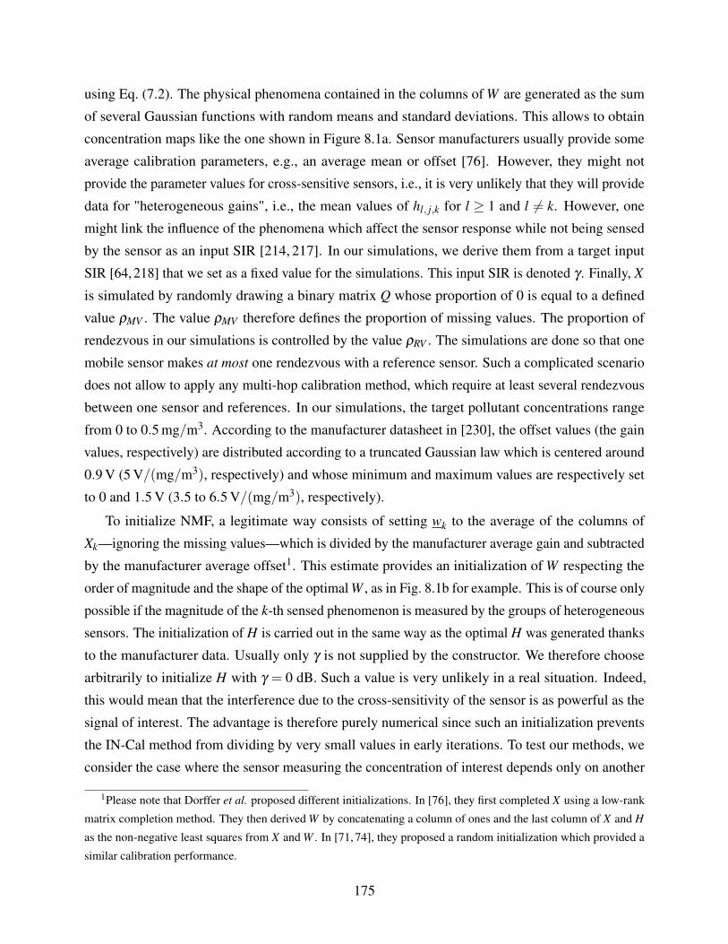
using Eq. (7.2). The physical phenomena contained in the columns of W are generated as the sum
of several Gaussian functions with random means and standard deviations. This allows to obtain
concentration maps like the one shown in Figure 8.1a. Sensor manufacturers usually provide some
average calibration parameters, e.g., an average mean or offset [76]. However, they might not
provide the parameter values for cross-sensitive sensors, i.e., it is very unlikely that they will provide
data for "heterogeneous gains", i.e., the mean values of hl, j,k for l ≥ 1 and l 6= k. However, one
might link the influence of the phenomena which affect the sensor response while not being sensed
by the sensor as an input SIR [214, 217]. In our simulations, we derive them from a target input
SIR [64, 218] that we set as a fixed value for the simulations. This input SIR is denoted γ . Finally, X
is simulated by randomly drawing a binary matrix Q whose proportion of 0 is equal to a defined
value ρMV . The value ρMV therefore defines the proportion of missing values. The proportion of
rendezvous in our simulations is controlled by the value ρRV . The simulations are done so that one
mobile sensor makes at most one rendezvous with a reference sensor. Such a complicated scenario
does not allow to apply any multi-hop calibration method, which require at least several rendezvous
between one sensor and references. In our simulations, the target pollutant concentrations range
from 0 to 0.5 mg/m3. According to the manufacturer datasheet in [230], the offset values (the gain
values, respectively) are distributed according to a truncated Gaussian law which is centered around
0.9 V (5 V/(mg/m3), respectively) and whose minimum and maximum values are respectively set
to 0 and 1.5 V (3.5 to 6.5 V/(mg/m3), respectively).
To initialize NMF, a legitimate way consists of setting wk to the average of the columns of
Xk—ignoring the missing values—which is divided by the manufacturer average gain and subtracted
by the manufacturer average offset1. This estimate provides an initialization of W respecting the
order of magnitude and the shape of the optimal W , as in Fig. 8.1b for example. This is of course only
possible if the magnitude of the k-th sensed phenomenon is measured by the groups of heterogeneous
sensors. The initialization of H is carried out in the same way as the optimal H was generated thanks
to the manufacturer data. Usually only γ is not supplied by the constructor. We therefore choose
arbitrarily to initialize H with γ = 0 dB. Such a value is very unlikely in a real situation. Indeed,
this would mean that the interference due to the cross-sensitivity of the sensor is as powerful as the
signal of interest. The advantage is therefore purely numerical since such an initialization prevents
the IN-Cal method from dividing by very small values in early iterations. To test our methods, we
consider the case where the sensor measuring the concentration of interest depends only on another
1Please note that Dorffer et al. proposed different initializations. In [76], they first completed X using a low-rank
matrix completion method. They then derived W by concatenating a column of ones and the last column of X and H
as the non-negative least squares from X and W . In [71, 74], they proposed a random initialization which provided a
similar calibration performance.
175
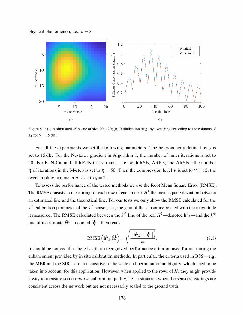
physical phenomenon, i.e., p = 3.
(a) (b)
Figure 8.1: (a) A simulated S scene of size 20×20; (b) Initialization of g1 by averaging according to the columns of
X1 for γ = 15 dB.
For all the experiments we set the following parameters. The heterogeneity defined by γ is
set to 15 dB. For the Nesterov gradient in Algorithm 1, the number of inner iterations is set to
20. For F-IN-Cal and all RF-IN-Cal variants—i.e. with RSIs, ARPIs, and ARSIs—the number
η of iterations in the M-step is set to η = 50. Then the compression level ν is set to ν = 12, the
oversampling parameter q is set to q = 2.
To assess the performance of the tested methods we use the Root Mean Square Error (RMSE).
The RMSE consists in measuring for each row of each matrix Hk the mean square deviation between
an estimated line and the theoretical line. For our tests we only show the RMSE calculated for the
kth calibration parameter of the kth sensor, i.e., the gain of the sensor associated with the magnitude
it measured. The RMSE calculated between the kth line of the real Hk—denoted hkk—and the kth
line of its estimate Hk—denoted hkk —then reads
RMSE(
hkk, hk
k
)=
√∣∣∣∣hkk− hk
k
∣∣∣∣22
m. (8.1)
It should be noticed that there is still no recognized performance criterion used for measuring the
enhancement provided by in situ calibration methods. In particular, the criteria used in BSS—e.g.,
the MER and the SIR—are not sensitive to the scale and permutation ambiguity, which need to be
taken into account for this application. However, when applied to the rows of H, they might provide
a way to measure some relative calibration quality, i.e., a situation when the sensors readings are
consistent across the network but are not necessarily scaled to the ground truth.
176
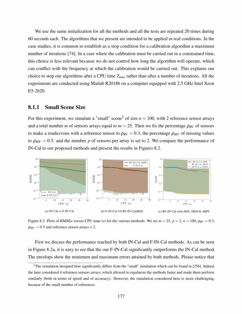
We use the same initialization for all the methods and all the tests are repeated 20 times during
60 seconds each. The algorithms that we present are intended to be applied in real conditions. In the
case studies, it is common to establish as a stop condition for a calibration algorithm a maximum
number of iterations [74]. In a case where the calibration must be carried out in a constrained time,
this choice is less relevant because we do not control how long the algorithm will operate, which
can conflict with the frequency at which the calibration would be carried out. This explains our
choice to stop our algorithms after a CPU time Tmax rather than after a number of iterations. All the
experiments are conducted using Matlab R2018b on a computer equipped with 2.5 GHz Intel Xeon
E5-2620.
8.1.1 Small Scene Size
For this experiment, we simulate a "small" scene2 of size n = 100, with 2 reference sensor arrays
and a total number m of sensors arrays equal to m = 25. Then we fix the percentage ρRV of sensors
to make a rendezvous with a reference sensor to ρRV = 0.3, the percentage ρMV of missing values
to ρMV = 0.5. and the number p of sensors per array is set to 2. We compare the performance of
IN-Cal to our proposed methods and present the results in Figures 8.2.
5 10 15 20 25 30
100
10−3
10−6
10−9
10−12
10−15
CPU (s)
RMSE
IN-CalF-IN-Cal
(a) IN-Cal vs F-IN-Cal
5 10 15 20 25 30
100
10−3
10−6
10−9
10−12
10−15
CPU (s)
RMSE
RF-IN-Cal (RSI)F-IN-Cal
(b) F-IN-Cal VS RF-IN-Cal(RSI)
5 10 15 20 25 30
100
10−3
10−6
10−9
10−12
10−15
CPU (s)
RMSE
RF-IN-Cal (RSI)
RF-IN-Cal (ARPI)
RF-IN-Cal (ARSI)
(c) RF-IN-Cal with (RSI, ARSI & ARPI
Figure 8.2: Plots of RMSEs versus CPU time (s) for the various methods: We set m = 25, p = 2, n = 100, ρRV = 0.3,
ρMV = 0.5 and reference sensor arrays = 2.
First we discuss the performance reached by both IN-Cal and F-IN-Cal methods. As can be seen
in Figure 8.2a, it is easy to see that the our F-IN-Cal significantly outperforms the IN-Cal method.
The envelops show the minimum and maximum errors attained by both methods. Please notice that
2The simulation designed here significantly differs from the "small" simulation which can be found in [256]. Indeed,
the later considered 4 reference sensors arrays, which allowed to regularize the methods faster and made them perform
similarly (both in terms of speed and of accuracy). However, the simulation considered here is more challenging,
because of the small number of references.
177
the highest part of both envelopes are reached when both reference measurements are similar. In that
case, they are not diverse enough to remove the scale ambiguity, hence the high RMSEs. However,
computing the SIRs on the rows of H shows that they allow to perform relative calibration. After 1
min of computations, F-IN-Cal and IN-Cal attain a median RMSE approximately equal to 10−5 and
10−2, respectively. This gap in performance justifies our motivation to explore faster methods.
Then in Figure 8.2b, we compare the performance reached by F-IN-Cal with respect to its
randomized extension using the RSI scheme, denoted RF-IN-Cal (RSI). Both methods provide
a similar performance, which might be due to the low dimensions of the matrices. In that case,
applying random projections come at a cost which is manifested in the overall performance of the
randomized extensions of the F-IN-Cal.
We also compare in Figure 8.2c the performance reached by the accelerated randomized exten-
sions proposed in the first part of this thesis. Again, there is no significant difference of performance
(even if ARPIs and ARSIs seem to slighly outperform RSIs in the late NMF iterations).
8.1.2 Larger Scene Size
Now let us conduct similar experiments on a larger scene. For this purpose we simulate the scene
area to be of size n = 400, with 4 reference sensors arrays and a total number m of sensor arrays
m = 100. Each array contains p = 2 sensors. Then we fix ρRV and ρMV to ρRV = 0.3 and ρMV = 0.5,
respectively. We compare the performance of IN-Cal to our proposed methods and present the
results in Figures 8.3.
10 20 30 40 50 60
100
10−3
10−6
10−9
10−12
10−15
CPU (s)
RMSE
IN-CalF-IN-Cal
(a) IN-Cal VS F-IN-Cal
10 20 30 40 50 60
100
10−3
10−6
10−9
10−12
10−15
CPU (s)
RMSE
RF-IN-Cal (RSI)F-IN-Cal
(b) F-IN-Cal VS RF-IN-Cal(RSI)
10 20 30 40 50 60
100
10−3
10−6
10−9
10−12
10−15
CPU (s)
RMSE
RF-IN-Cal (RSI)
RF-IN-Cal (ARPI)
RF-IN-Cal (ARSI)
(c) RF-IN-Cal with (RSI, ARSI & ARPI
Figure 8.3: Plots of RMSEs versus CPU time (s) of the various methods: We set: m = 100, p = 2, n = 400, ρRV = 0.3,
ρMV = 0.5 and 4 reference sensor arrays.
178
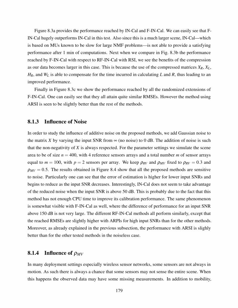
Figure 8.3a provides the performance reached by IN-Cal and F-IN-Cal. We can easily see that F-
IN-Cal hugely outperforms IN-Cal in this test. Also since this is a much larger scene, IN-Cal—which
is based on MUs known to be slow for large NMF problems—is not able to provide a satisfying
performance after 1 min of computations. Next when we compare in Fig. 8.3b the performance
reached by F-IN-Cal with respect to RF-IN-Cal with RSI, we see the benefits of the compression
as our data becomes larger in this case. This is because the use of the compressed matrices XR, XL,
HR, and WL is able to compensate for the time incurred in calculating L and R, thus leading to an
improved performance.
Finally in Figure 8.3c we show the performance reached by all the randomized extensions of
F-IN-Cal. One can easily see that they all attain quite similar RMSEs. However the method using
ARSI is seen to be slightly better than the rest of the methods.
8.1.3 Influence of Noise
In order to study the influence of additive noise on the proposed methods, we add Gaussian noise to
the matrix X by varying the input SNR from ∞ (no noise) to 0 dB. The addition of noise is such
that the non-negativity of X is always respected. For the parameter settings we simulate the scene
area to be of size n = 400, with 4 reference sensors arrays and a total number m of sensor arrays
equal to m = 100, with p = 2 sensors per array. We keep ρRV and ρMV fixed to ρRV = 0.3 and
ρMV = 0.5. The results obtained in Figure 8.4 show that all the proposed methods are sensitive
to noise. Particularly one can see that the error of estimation is higher for lower input SNRs and
begins to reduce as the input SNR decreases. Interestingly, IN-Cal does not seem to take advantage
of the reduced noise when the input SNR is above 50 dB. This is probably due to the fact that this
method has not enough CPU time to improve its calibration performance. The same phenomenon
is somewhat visible with F-IN-Cal as well, where the difference of performance for an input SNR
above 150 dB is not very large. The different RF-IN-Cal methods all perform similarly, except that
the reached RMSEs are slightly higher with ARPIs for high input SNRs than for the other methods.
Moreover, as already explained in the previous subsection, the performance with ARSI is slighly
better than for the other tested methods in the noiseless case.
8.1.4 Influence of ρMV
In many deployment settings especially wireless sensor networks, some sensors are not always in
motion. As such there is always a chance that some sensors may not sense the entire scene. When
this happens the observed data may have some missing measurements. In addition to mobility,
179
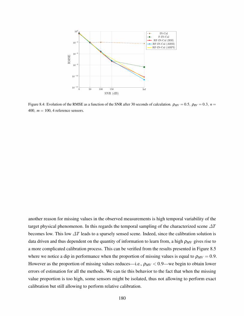
0 50 100 150 Inf
100
10−3
10−6
10−9
10−12
10−15
SNR (dB)
RMSE
IN-CalF-IN-Cal
RF-IN-Cal (RSI)
RF-IN-Cal (ARSI)
RF-IN-Cal (ARPI)
Figure 8.4: Evolution of the RMSE as a function of the SNR after 30 seconds of calculation. ρMV = 0.5, ρRV = 0.3, n =
400, m = 100, 4 reference sensors.
another reason for missing values in the observed measurements is high temporal variability of the
target physical phenomenon. In this regards the temporal sampling of the characterized scene ∆T
becomes low. This low ∆T leads to a sparsely sensed scene. Indeed, since the calibration solution is
data driven and thus dependent on the quantity of information to learn from, a high ρMV gives rise to
a more complicated calibration process. This can be verified from the results presented in Figure 8.5
where we notice a dip in performance when the proportion of missing values is equal to ρMV = 0.9.
However as the proportion of missing values reduces—i.e., ρMV < 0.9—we begin to obtain lower
errors of estimation for all the methods. We can tie this behavior to the fact that when the missing
value proportion is too high, some sensors might be isolated, thus not allowing to perform exact
calibration but still allowing to perform relative calibration.
180
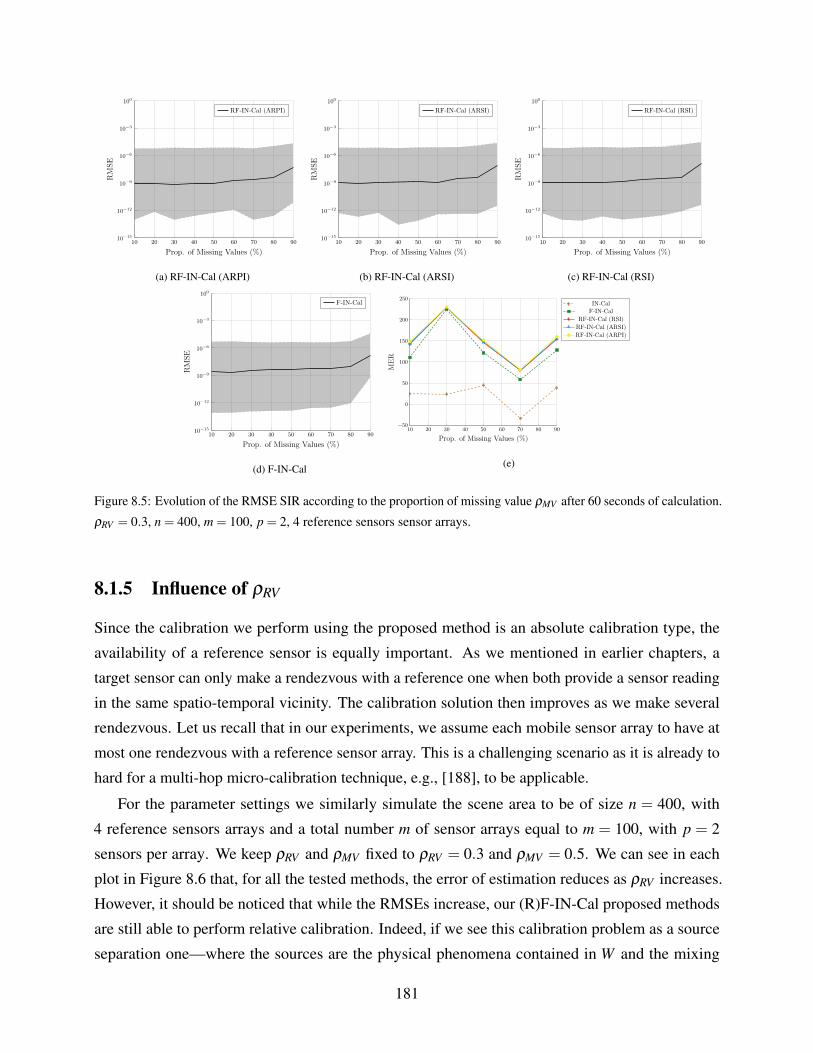
10 20 30 40 50 60 70 80 90
100
10−3
10−6
10−9
10−12
10−15
Prop. of Missing Values (%)
RMSE
RF-IN-Cal (ARPI)
(a) RF-IN-Cal (ARPI)
10 20 30 40 50 60 70 80 90
100
10−3
10−6
10−9
10−12
10−15
Prop. of Missing Values (%)
RMSE
RF-IN-Cal (ARSI)
(b) RF-IN-Cal (ARSI)
10 20 30 40 50 60 70 80 90
100
10−3
10−6
10−9
10−12
10−15
Prop. of Missing Values (%)
RMSE
RF-IN-Cal (RSI)
(c) RF-IN-Cal (RSI)
10 20 30 40 50 60 70 80 90
100
10−3
10−6
10−9
10−12
10−15
Prop. of Missing Values (%)
RMSE
F-IN-Cal
(d) F-IN-Cal
10 20 30 40 50 60 70 80 90−50
0
50
100
150
200
250
Prop. of Missing Values (%)
MER
IN-CalF-IN-Cal
RF-IN-Cal (RSI)
RF-IN-Cal (ARSI)
RF-IN-Cal (ARPI)
(e)
Figure 8.5: Evolution of the RMSE SIR according to the proportion of missing value ρMV after 60 seconds of calculation.
ρRV = 0.3, n = 400, m = 100, p = 2, 4 reference sensors sensor arrays.
8.1.5 Influence of ρRV
Since the calibration we perform using the proposed method is an absolute calibration type, the
availability of a reference sensor is equally important. As we mentioned in earlier chapters, a
target sensor can only make a rendezvous with a reference one when both provide a sensor reading
in the same spatio-temporal vicinity. The calibration solution then improves as we make several
rendezvous. Let us recall that in our experiments, we assume each mobile sensor array to have at
most one rendezvous with a reference sensor array. This is a challenging scenario as it is already to
hard for a multi-hop micro-calibration technique, e.g., [188], to be applicable.
For the parameter settings we similarly simulate the scene area to be of size n = 400, with
4 reference sensors arrays and a total number m of sensor arrays equal to m = 100, with p = 2
sensors per array. We keep ρRV and ρMV fixed to ρRV = 0.3 and ρMV = 0.5. We can see in each
plot in Figure 8.6 that, for all the tested methods, the error of estimation reduces as ρRV increases.
However, it should be noticed that while the RMSEs increase, our (R)F-IN-Cal proposed methods
are still able to perform relative calibration. Indeed, if we see this calibration problem as a source
separation one—where the sources are the physical phenomena contained in W and the mixing
181
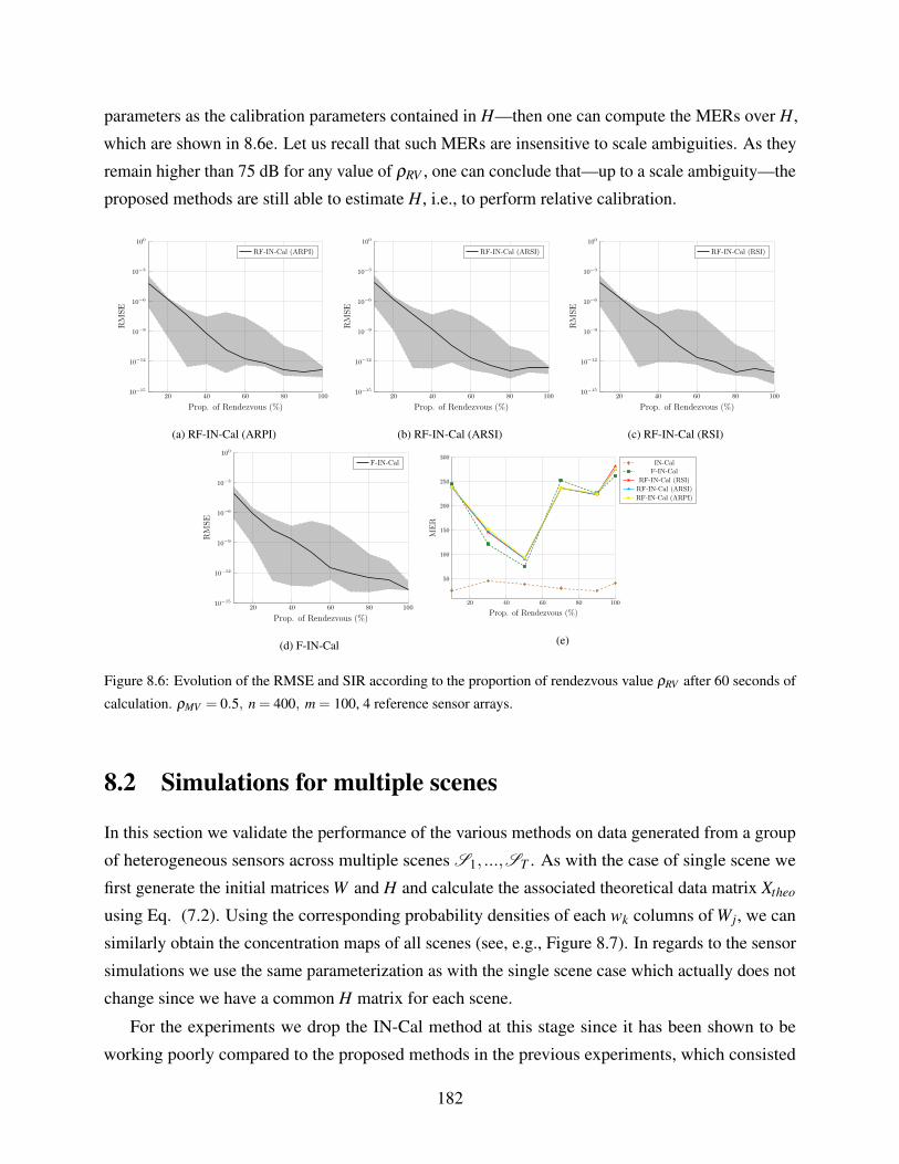
parameters as the calibration parameters contained in H—then one can compute the MERs over H,
which are shown in 8.6e. Let us recall that such MERs are insensitive to scale ambiguities. As they
remain higher than 75 dB for any value of ρRV , one can conclude that—up to a scale ambiguity—the
proposed methods are still able to estimate H, i.e., to perform relative calibration.
20 40 60 80 100
100
10−3
10−6
10−9
10−12
10−15
Prop. of Rendezvous (%)
RMSE
RF-IN-Cal (ARPI)
(a) RF-IN-Cal (ARPI)
20 40 60 80 100
100
10−3
10−6
10−9
10−12
10−15
Prop. of Rendezvous (%)
RMSE
RF-IN-Cal (ARSI)
(b) RF-IN-Cal (ARSI)
20 40 60 80 100
100
10−3
10−6
10−9
10−12
10−15
Prop. of Rendezvous (%)
RMSE
RF-IN-Cal (RSI)
(c) RF-IN-Cal (RSI)
20 40 60 80 100
100
10−3
10−6
10−9
10−12
10−15
Prop. of Rendezvous (%)
RMSE
F-IN-Cal
(d) F-IN-Cal
20 40 60 80 100
50
100
150
200
250
300
Prop. of Rendezvous (%)
MER
IN-CalF-IN-Cal
RF-IN-Cal (RSI)
RF-IN-Cal (ARSI)
RF-IN-Cal (ARPI)
(e)
Figure 8.6: Evolution of the RMSE and SIR according to the proportion of rendezvous value ρRV after 60 seconds of
calculation. ρMV = 0.5, n = 400, m = 100, 4 reference sensor arrays.
8.2 Simulations for multiple scenes
In this section we validate the performance of the various methods on data generated from a group
of heterogeneous sensors across multiple scenes S1, ...,ST . As with the case of single scene we
first generate the initial matrices W and H and calculate the associated theoretical data matrix Xtheo
using Eq. (7.2). Using the corresponding probability densities of each wk columns of Wj, we can
similarly obtain the concentration maps of all scenes (see, e.g., Figure 8.7). In regards to the sensor
simulations we use the same parameterization as with the single scene case which actually does not
change since we have a common H matrix for each scene.
For the experiments we drop the IN-Cal method at this stage since it has been shown to be
working poorly compared to the proposed methods in the previous experiments, which consisted
182
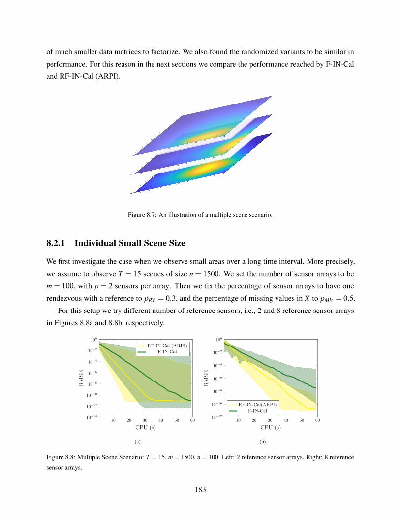
of much smaller data matrices to factorize. We also found the randomized variants to be similar in
performance. For this reason in the next sections we compare the performance reached by F-IN-Cal
and RF-IN-Cal (ARPI).
Figure 8.7: An illustration of a multiple scene scenario.
8.2.1 Individual Small Scene Size
We first investigate the case when we observe small areas over a long time interval. More precisely,
we assume to observe T = 15 scenes of size n = 1500. We set the number of sensor arrays to be
m = 100, with p = 2 sensors per array. Then we fix the percentage of sensor arrays to have one
rendezvous with a reference to ρRV = 0.3, and the percentage of missing values in X to ρMV = 0.5.
For this setup we try different number of reference sensors, i.e., 2 and 8 reference sensor arrays
in Figures 8.8a and 8.8b, respectively.
10 20 30 40 50 60
100
10−2
10−4
10−6
10−8
10−10
10−12
10−14
CPU (s)
RMSE
RF-IN-Cal (ARPI)F-IN-Cal
(a)
10 20 30 40 50 60
100
10−2
10−4
10−6
10−8
10−10
10−12
CPU (s)
RMSE
RF-IN-Cal(ARPI)F-IN-Cal
(b)
Figure 8.8: Multiple Scene Scenario: T = 15, m = 1500, n = 100. Left: 2 reference sensor arrays. Right: 8 reference
sensor arrays.
183
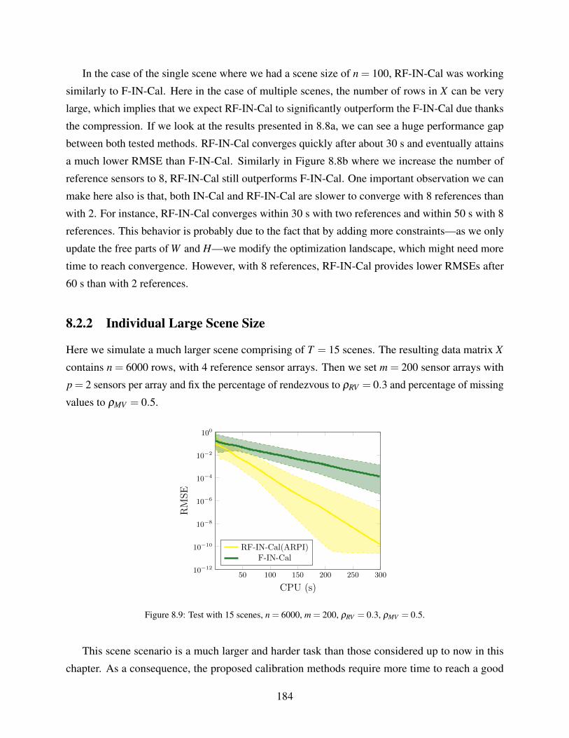
In the case of the single scene where we had a scene size of n = 100, RF-IN-Cal was working
similarly to F-IN-Cal. Here in the case of multiple scenes, the number of rows in X can be very
large, which implies that we expect RF-IN-Cal to significantly outperform the F-IN-Cal due thanks
the compression. If we look at the results presented in 8.8a, we can see a huge performance gap
between both tested methods. RF-IN-Cal converges quickly after about 30 s and eventually attains
a much lower RMSE than F-IN-Cal. Similarly in Figure 8.8b where we increase the number of
reference sensors to 8, RF-IN-Cal still outperforms F-IN-Cal. One important observation we can
make here also is that, both IN-Cal and RF-IN-Cal are slower to converge with 8 references than
with 2. For instance, RF-IN-Cal converges within 30 s with two references and within 50 s with 8
references. This behavior is probably due to the fact that by adding more constraints—as we only
update the free parts of W and H—we modify the optimization landscape, which might need more
time to reach convergence. However, with 8 references, RF-IN-Cal provides lower RMSEs after
60 s than with 2 references.
8.2.2 Individual Large Scene Size
Here we simulate a much larger scene comprising of T = 15 scenes. The resulting data matrix X
contains n = 6000 rows, with 4 reference sensor arrays. Then we set m = 200 sensor arrays with
p = 2 sensors per array and fix the percentage of rendezvous to ρRV = 0.3 and percentage of missing
values to ρMV = 0.5.
50 100 150 200 250 300
100
10−2
10−4
10−6
10−8
10−10
10−12
CPU (s)
RMSE
RF-IN-Cal(ARPI)F-IN-Cal
Figure 8.9: Test with 15 scenes, n = 6000, m = 200, ρRV = 0.3, ρMV = 0.5.
This scene scenario is a much larger and harder task than those considered up to now in this
chapter. As a consequence, the proposed calibration methods require more time to reach a good
184
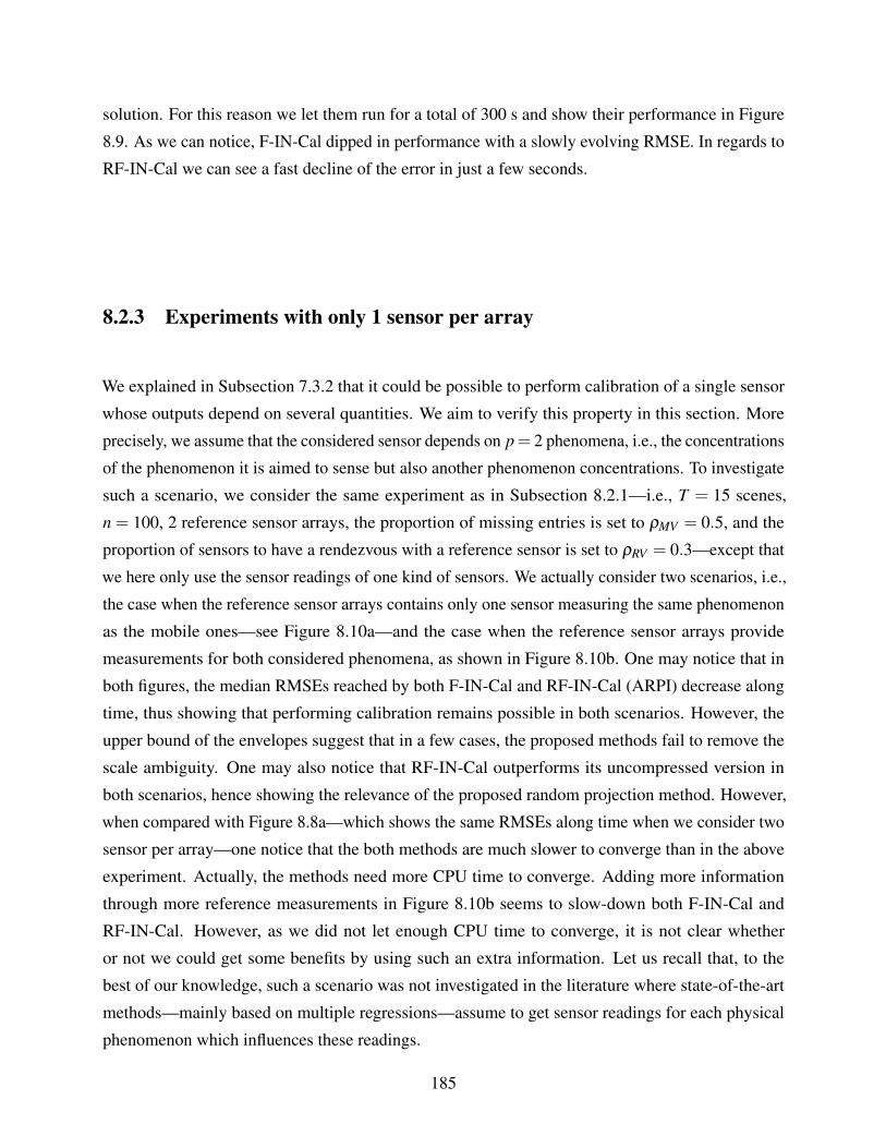
solution. For this reason we let them run for a total of 300 s and show their performance in Figure
8.9. As we can notice, F-IN-Cal dipped in performance with a slowly evolving RMSE. In regards to
RF-IN-Cal we can see a fast decline of the error in just a few seconds.
8.2.3 Experiments with only 1 sensor per array
We explained in Subsection 7.3.2 that it could be possible to perform calibration of a single sensor
whose outputs depend on several quantities. We aim to verify this property in this section. More
precisely, we assume that the considered sensor depends on p= 2 phenomena, i.e., the concentrations
of the phenomenon it is aimed to sense but also another phenomenon concentrations. To investigate
such a scenario, we consider the same experiment as in Subsection 8.2.1—i.e., T = 15 scenes,
n = 100, 2 reference sensor arrays, the proportion of missing entries is set to ρMV = 0.5, and the
proportion of sensors to have a rendezvous with a reference sensor is set to ρRV = 0.3—except that
we here only use the sensor readings of one kind of sensors. We actually consider two scenarios, i.e.,
the case when the reference sensor arrays contains only one sensor measuring the same phenomenon
as the mobile ones—see Figure 8.10a—and the case when the reference sensor arrays provide
measurements for both considered phenomena, as shown in Figure 8.10b. One may notice that in
both figures, the median RMSEs reached by both F-IN-Cal and RF-IN-Cal (ARPI) decrease along
time, thus showing that performing calibration remains possible in both scenarios. However, the
upper bound of the envelopes suggest that in a few cases, the proposed methods fail to remove the
scale ambiguity. One may also notice that RF-IN-Cal outperforms its uncompressed version in
both scenarios, hence showing the relevance of the proposed random projection method. However,
when compared with Figure 8.8a—which shows the same RMSEs along time when we consider two
sensor per array—one notice that the both methods are much slower to converge than in the above
experiment. Actually, the methods need more CPU time to converge. Adding more information
through more reference measurements in Figure 8.10b seems to slow-down both F-IN-Cal and
RF-IN-Cal. However, as we did not let enough CPU time to converge, it is not clear whether
or not we could get some benefits by using such an extra information. Let us recall that, to the
best of our knowledge, such a scenario was not investigated in the literature where state-of-the-art
methods—mainly based on multiple regressions—assume to get sensor readings for each physical
phenomenon which influences these readings.
185

10 20 30 40 50 60
100
10−2
10−4
10−6
CPU (s)
RMSE
RF-IN-Cal(ARPI)F-IN-Cal
(a)
10 20 30 40 50 60
100
10−2
10−4
10−6
CPU (s)
RMSE
RF-IN-Cal(ARPI)F-IN-Cal
(b)
Figure 8.10: Multiple scene scenario: T = 15, m = 1500, n = 100, 1 sensor per array, and 2 reference sensor arrays.
Left: 1 sensor per reference sensor array. Right: 2 sensors per reference sensor array.
8.3 Discussion
In this chapter, we investigated the enhancement provided by F-IN-Cal and the several RF-IN-Cal
approaches that we proposed. For that purpose, we considered several simulations used to model a
single scene or multiple scenes. Moreover, we investigated the influence of the proportion of missing
entries in X , of the proportion of mobile sensor arrays to make a rendezvous with a reference sensor
array, of the additive noise, and on the size of the data matrix X .
First of all, let us recall that the considered scenarios did not allow us to compare the performance
of our proposed methods with regression-based state-of-the-art calibration methods which require
numerous rendezvous between one mobile sensor array and reference sensor arrays. Still, we could
compare the enhancement provided by our proposed methods with the one provided by the IN-Cal
method proposed by C. Dorffer during his Ph.D. thesis. Our results show that IN-Cal cannot provide
any enhancement for moderately large matrices while F-IN-Cal is able. Moreover, we showed
that there is no to little interest to compress F-IN-Cal when only one scene is used, because of
the extra-cost used in the E-step of RF-IN-Cal cannot be compensated by the earned time during
the M-step. However, when several scenes are considered, compression provides some significant
speed-up, thus showing the relevance of the proposed methods.
Unfortunately, we could not get some real-life data to investigate the enhancement provided by
our proposed methods. This is let for future work.
186
Chapter 9
General Conclusion
9.1 Conclusion
The present thesis is an embodiment of several contributions to accelerating non-negative matrix
factorization for application in mobile sensor calibration. We begun with an introductory chapter
discussing the main motivations, objectives and principal tools use throughout the thesis. Then
in next chapter we made a literature review on sensor calibration. The main motivations behind
environmental monitoring, the use of miniaturized sensors and sensor calibration were made clear.
We also presented the different calibration models and methods and concluded the chapter by
indicating some of the drawbacks of existing methods and how our anticipated calibration method
remedies some of these drawbacks. In Chapter 2, we made a formal introduction to non-negative
matrix factorization. Here a comprehensive discussion was presented about the main background of
NMF, the different methods, optimization strategies, and some extensions of NMF. More importantly
we also mentioned that despite the availability of efficient optimization techniques and modern
computer hardware, the overwhelming effect of data deluge make it difficult to fully appreciate these
advancements. This leads us to Chapter 3 where we present and discuss our main contributions to
accelerating NMF. For that purpose we introduced the concept of Random projections (RP) which
we explain as a powerful tool for reducing the dimension of a large data. In our experiments we
extensively use the structured compression (SC) scheme which is based on the classical power
iterations scheme. We then combined RP with WNMF as a novel framework to accelerate WNMF.
Our approach which we named as REM-WNMF were seen to be better in terms of performance than
the vanilla EM-WNMF within a fixed CPU time of 60s. Interestingly we observed that, creating
the compression matrices with the SC were very time consuming especially when the matrices are
very large. As a remedy we proposed an alternative framework, called RPS which is only based on
187
data-independent random projections. Our strategy is built on the Johnson-Lidenstrauss Lemma
and can be seen as a streamed random projection. RPS should allow a similar randomized NMF
or WNMF enhancement. Our experiments showed the RPS schemes to outperform their vanilla
versions. In the second part of the manuscript we discussed the main application of the thesis
work. The contribution in this part was in two folds. First we considered the case of a single scene.
We explained that a scene is a grid of locations where sensors sense a physical phenomenon, so
that when two sensors are in the same pixel of that scene they are said to be in rendezvous. With
these definitions we were able to model the calibration problem based on informed non-negative
matrix factorization. We reviewed the existing In-Cal method and then proposed a faster method
called F-IN-Cal which is based on Nesterov Accelerated Gradient and later combine F-IN-Cal with
random projections called RF-IN-Cal. In experimental findings, we found our F-IN-Cal method
to significantly outperform the IN-Cal. While IN-Cal was seen to be slow and tailored for mostly
homogeneous sensors, our proposed methods on the other hand does not have this limitation and can
be used for both homogeneous and heterogeneous sensors. Secondly, we extended this framework to
the case of multiple scenes. Here our multiple scene model is a simple model that takes a series of
matrices corresponding to different scenes and fuses them together to form a giant matrix. We then
tested our proposed methods and their randomized extensions and noted our RF-IN-Cal to provide
better enhancement withing a fixed time as compared to the F-IN-Cal. In addition to this we also
studies some other scenarios of the Multiple scene case. Namely, 1) in one case we assume to have
two quantities and a reference sensor that is sensitive to only the targeted physical phenomenon 2)
while in the second case we consider two quantities and a reference sensor that is sensitive to both
the target and the interfering phenomena
9.2 Perspectives
9.2.1 Randomized WNMF
We proposed a framework that combines random projections with WNMF. Indeed for most of our
experiments, we made in-core computations. However realistically, we could have arbitrarily large
matrices that might require using out-of-core methods. In such a case as a possible future work
could extend the framework to perform out-of-core matrix computations. One way to do this is
to parallellize the computations, e.g., using dask [54] to scale the data on a multi-core and large
memory computer or on large distributed cloud clusters. Aside from parallelism an alternative will
be do design some online extension of REM-WNMF. In this case we will be able to process the
compression matrices L and R faster since we do not keep the whole matrix in memory.
188
9.2.2 Random Projection Streams
The RPS method was a framework that extended existing data-independent random projection
schemes to process the compression matrices in streams. As a perspective for future work we
could imagine a double streaming procedure, where both the data matrix X and the compression
matrices arrive in streams.This can be useful when the matrices are arbitrary large. Additionally the
compression matrices could also be processed with some specific hardware like an optical processing
unit at a much faster speed.
9.2.3 Short-term and Long-term Sensor Calibrations
Having proposed our calibration method to replace the existing IN-Cal method and to offer the
capability of processing heterogeneous sensors, there are several perspectives we could consider.
Thus far, the calibration functions of our methods for both the single scene and the multiple scene
scenarios are time independent. In future we could extend the calibration function to the case of
multiple variables with time. In our multiple scene model, we assumed a common H among adjacent
scenes. However in some real scenarios H could also evolve along time. For this we could remodel
the calibration method as a non-negative matrix co-factorization of all adjacent scenes. Also we
could use some extra information, e.g. spatial a priori, known average calibration parameters. Lastly,
in our formulations, we perform sampling of an area with square cells, so that two sensors sharing
one cell are assume to sense the same phenomenom. In future we could propose a different sampling
method. In some literature work some authors propose that sensors are assumed to sense the same
phenomena if they are in the same street. Other consider irregularly shaped locations. Lastly, it
would be interesting to investigate the enhancement provided by the proposed methods—or the
possible extensions discussed above—in real-life scenaraios.
189
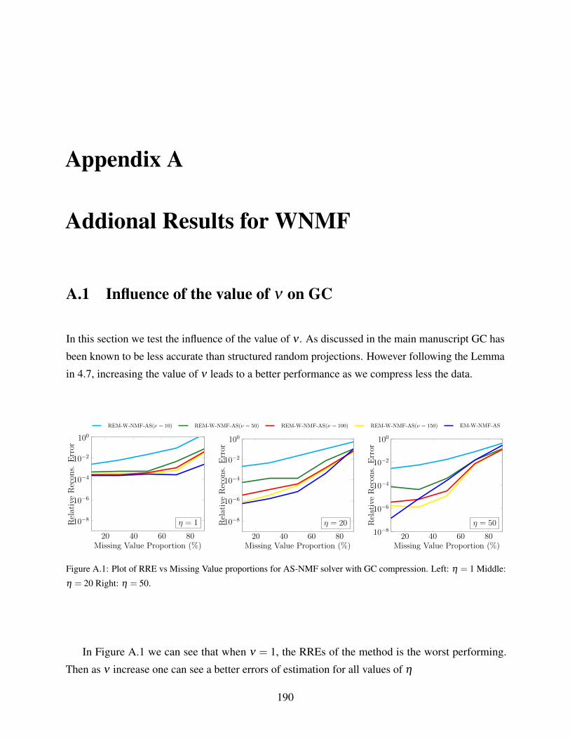
Appendix A
Addional Results for WNMF
A.1 Influence of the value of ν on GC
In this section we test the influence of the value of ν . As discussed in the main manuscript GC has
been known to be less accurate than structured random projections. However following the Lemma
in 4.7, increasing the value of ν leads to a better performance as we compress less the data.
REM-W-NMF-AS(ν = 10) REM-W-NMF-AS(ν = 50) REM-W-NMF-AS(ν = 100) REM-W-NMF-AS(ν = 150) EM-W-NMF-AS
20 40 60 80
100
10−2
10−4
10−6
10−8
Missing Value Proportion (%)
RelativeRecon
s.Error
η = 1
20 40 60 80
100
10−2
10−4
10−6
10−8
Missing Value Proportion (%)
RelativeRecon
s.Error
η = 20
20 40 60 80
100
10−2
10−4
10−6
10−8
Missing Value Proportion (%)
RelativeRecon
s.Error
η = 50
Figure A.1: Plot of RRE vs Missing Value proportions for AS-NMF solver with GC compression. Left: η = 1 Middle:
η = 20 Right: η = 50.
In Figure A.1 we can see that when ν = 1, the RREs of the method is the worst performing.
Then as ν increase one can see a better errors of estimation for all values of η
190
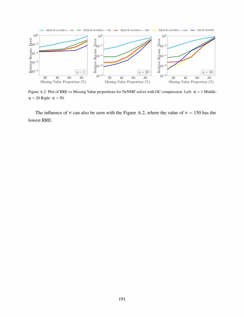
REM-W-NeNMF(ν = 10) REM-W-NeNMF(ν = 50) REM-W-NeNMF(ν = 100) REM-W-NeNMF(ν = 150) EM-W-NeNMF
20 40 60 80
100
10−2
10−4
10−6
10−8
Missing Value Proportion (%)
RelativeRecon
s.Error
η = 1
20 40 60 80
100
10−2
10−4
10−6
10−8
Missing Value Proportion (%)
RelativeRecon
s.Error
η = 20
20 40 60 80
100
10−2
10−4
10−6
10−8
Missing Value Proportion (%)
RelativeRecon
s.Error
η = 50
Figure A.2: Plot of RRE vs Missing Value proportions for NeNMF solver with GC compression. Left: η = 1 Middle:
η = 20 Right: η = 50.
The influence of ν can also be seen with the Figure A.2, where the value of ν = 150 has the
lowest RRE.
191
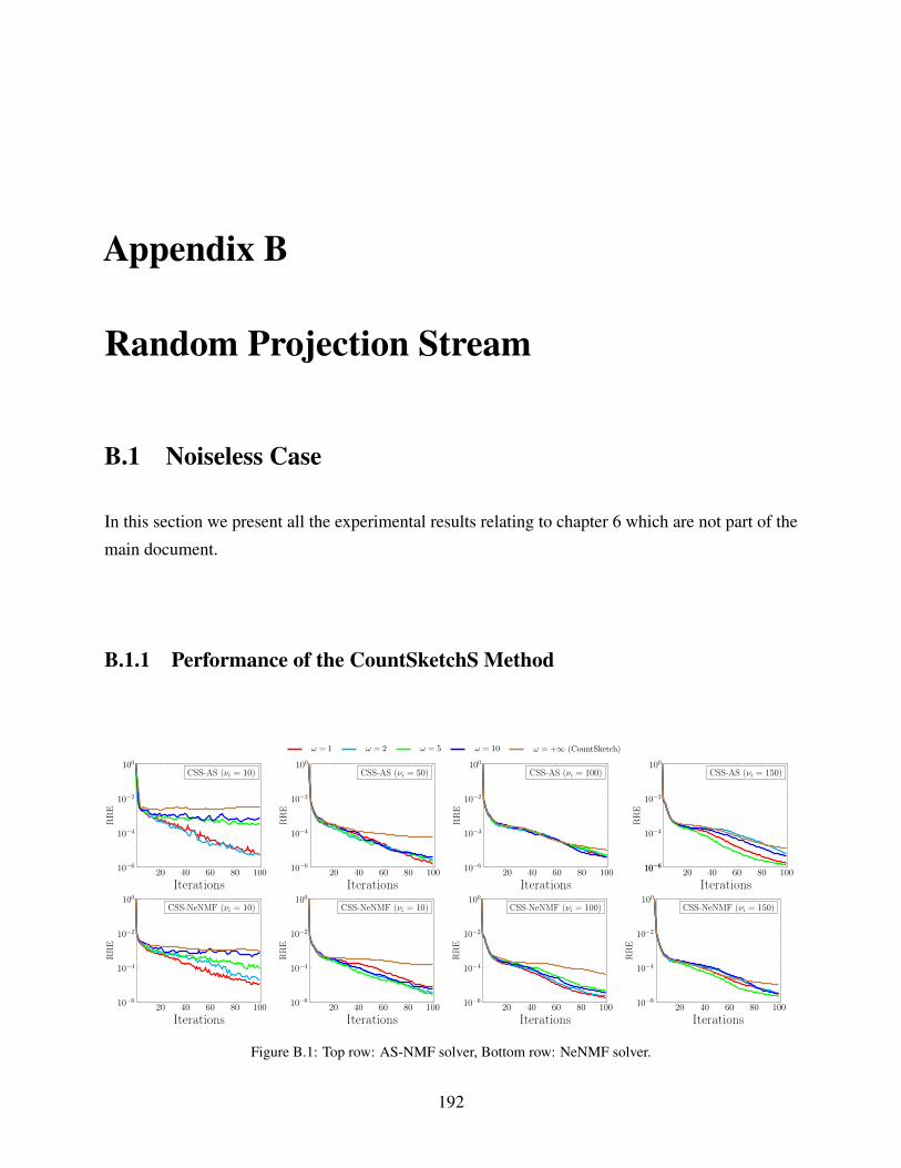
Appendix B
Random Projection Stream
B.1 Noiseless Case
In this section we present all the experimental results relating to chapter 6 which are not part of the
main document.
B.1.1 Performance of the CountSketchS Method
ω = 1 ω = 2 ω = 5 ω = 10 ω = +∞ (CountSketch)
20 40 60 80 100
100
10−2
10−4
10−6
Iterations
RR
E
CSS-AS (νi = 10)
20 40 60 80 100
100
10−2
10−4
10−6
Iterations
RR
E
CSS-AS (νi = 50)
20 40 60 80 100
100
10−2
10−4
10−6
Iterations
RR
E
CSS-AS (νi = 100)
20 40 60 80 100
100
10−2
10−4
10−610−6
Iterations
RR
E
CSS-AS (νi = 150)
20 40 60 80 100
100
10−2
10−4
10−6
Iterations
RR
E
CSS-NeNMF (νi = 10)
20 40 60 80 100
100
10−2
10−4
10−6
Iterations
RR
E
CSS-NeNMF (νi = 10)
20 40 60 80 100
100
10−2
10−4
10−6
Iterations
RR
E
CSS-NeNMF (νi = 100)
20 40 60 80 100
100
10−2
10−4
10−6
Iterations
RR
E
CSS-NeNMF (νi = 150)
Figure B.1: Top row: AS-NMF solver, Bottom row: NeNMF solver.
192
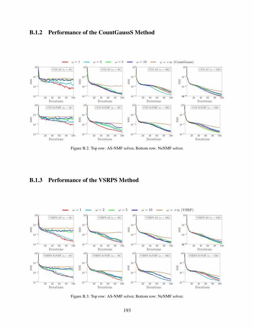
B.1.2 Performance of the CountGaussS Method
ω = 1 ω = 2 ω = 5 ω = 10 ω = +∞ (CountGauss)
20 40 60 80 100
100
10−2
10−4
10−6
Iterations
RR
E
CGS-AS (νi = 10)
20 40 60 80 100
100
10−2
10−4
10−6
Iterations
RR
E
CGS-AS (νi = 50)
20 40 60 80 100
100
10−2
10−4
10−6
Iterations
RR
E
CGS-AS (νi = 100)
20 40 60 80 100
100
10−2
10−4
10−610−6
Iterations
RR
E
CGS-AS (νi = 150)
20 40 60 80 100
100
10−2
10−4
10−6
Iterations
RR
E
CGS-NeNMF (νi = 10)
20 40 60 80 100
100
10−2
10−4
10−6
Iterations
RR
E
CGS-NeNMF (νi = 50)
20 40 60 80 100
100
10−2
10−4
10−6
Iterations
RR
E
CGS-NeNMF (νi = 100)
20 40 60 80 100
100
10−2
10−4
10−6
Iterations
RR
E
CGS-NeNMF (νi = 150)
Figure B.2: Top row: AS-NMF solver, Bottom row: NeNMF solver.
B.1.3 Performance of the VSRPS Method
ω = 1 ω = 2 ω = 5 ω = 10 ω = +∞ (VSRP)
20 40 60 80 100
100
10−2
10−4
10−6
Iterations
RR
E
VSRPS-AS (νi = 10)
20 40 60 80 100
100
10−2
10−4
10−6
Iterations
RR
E
VSRPS-AS (νi = 50)
20 40 60 80 100
100
10−2
10−4
10−6
Iterations
RR
E
VSRPS-AS (νi = 100)
20 40 60 80 100
100
10−2
10−4
10−610−6
Iterations
RR
E
VSRPS-AS (νi = 150)
20 40 60 80 100
100
10−2
10−4
10−6
Iterations
RR
E
VSRPS-NeNMF (νi = 10)
20 40 60 80 100
100
10−2
10−4
10−6
Iterations
RR
E
VSRPS-NeNMF (νi = 50)
20 40 60 80 100
100
10−2
10−4
10−6
Iterations
RR
E
VSRPS-NeNMF (νi = 100)
20 40 60 80 100
100
10−2
10−4
10−6
Iterations
RR
E
VSRPS-NeNMF (νi = 150)
Figure B.3: Top row: AS-NMF solver, Bottom row: NeNMF solver.
193
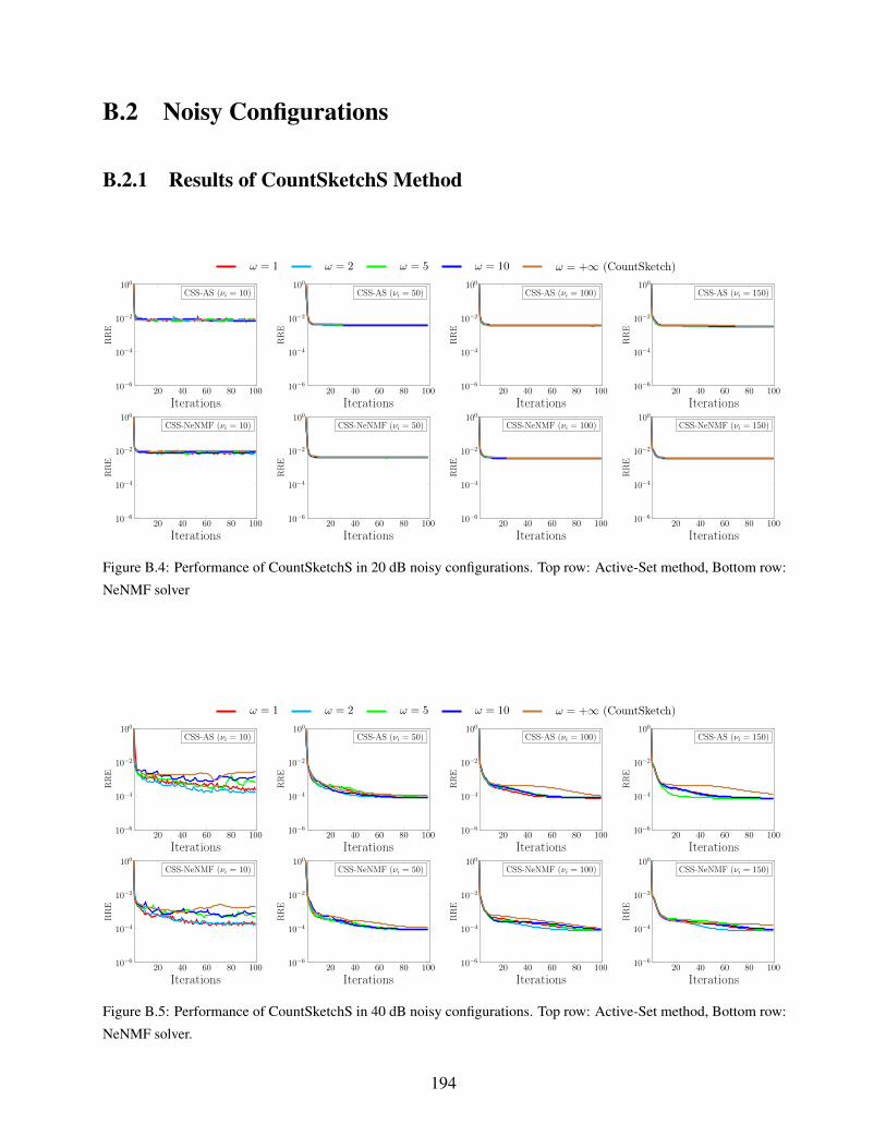
B.2 Noisy Configurations
B.2.1 Results of CountSketchS Method
ω = 1 ω = 2 ω = 5 ω = 10 ω = +∞ (CountSketch)
20 40 60 80 100
100
10−2
10−4
10−6
Iterations
RR
E
CSS-AS (νi = 10)
20 40 60 80 100
100
10−2
10−4
10−6
Iterations
RR
ECSS-AS (νi = 50)
20 40 60 80 100
100
10−2
10−4
10−6
Iterations
RR
E
CSS-AS (νi = 100)
20 40 60 80 100
100
10−2
10−4
10−6
Iterations
RR
E
CSS-AS (νi = 150)
20 40 60 80 100
100
10−2
10−4
10−6
Iterations
RR
E
CSS-NeNMF (νi = 10)
20 40 60 80 100
100
10−2
10−4
10−6
Iterations
RR
E
CSS-NeNMF (νi = 50)
20 40 60 80 100
100
10−2
10−4
10−6
Iterations
RR
E
CSS-NeNMF (νi = 100)
20 40 60 80 100
100
10−2
10−4
10−6
Iterations
RR
E
CSS-NeNMF (νi = 150)
Figure B.4: Performance of CountSketchS in 20 dB noisy configurations. Top row: Active-Set method, Bottom row:
NeNMF solver
ω = 1 ω = 2 ω = 5 ω = 10 ω = +∞ (CountSketch)
20 40 60 80 100
100
10−2
10−4
10−6
Iterations
RR
E
CSS-AS (νi = 10)
20 40 60 80 100
100
10−2
10−4
10−6
Iterations
RR
E
CSS-AS (νi = 50)
20 40 60 80 100
100
10−2
10−4
10−6
Iterations
RR
E
CSS-AS (νi = 100)
20 40 60 80 100
100
10−2
10−4
10−6
Iterations
RR
E
CSS-AS (νi = 150)
20 40 60 80 100
100
10−2
10−4
10−6
Iterations
RR
E
CSS-NeNMF (νi = 10)
20 40 60 80 100
100
10−2
10−4
10−6
Iterations
RR
E
CSS-NeNMF (νi = 50)
20 40 60 80 100
100
10−2
10−4
10−6
Iterations
RR
E
CSS-NeNMF (νi = 100)
20 40 60 80 100
100
10−2
10−4
10−6
Iterations
RR
E
CSS-NeNMF (νi = 150)
Figure B.5: Performance of CountSketchS in 40 dB noisy configurations. Top row: Active-Set method, Bottom row:
NeNMF solver.
194
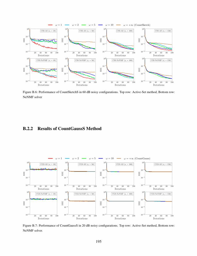
ω = 1 ω = 2 ω = 5 ω = 10 ω = +∞ (CountSketch)
20 40 60 80 100
100
10−2
10−4
10−6
Iterations
RR
E
CSS-AS (νi = 10)
20 40 60 80 100
100
10−2
10−4
10−6
Iterations
RR
E
CSS-AS (νi = 50)
20 40 60 80 100
100
10−2
10−4
10−6
Iterations
RR
E
CSS-AS (νi = 100)
20 40 60 80 100
100
10−2
10−4
10−6
Iterations
RR
E
CSS-AS (νi = 150)
20 40 60 80 100
100
10−2
10−4
10−6
Iterations
RR
E
CSS-NeNMF (νi = 10)
20 40 60 80 100
100
10−2
10−4
10−6
Iterations
RR
ECSS-NeNMF (νi = 50)
20 40 60 80 100
100
10−2
10−4
10−6
Iterations
RR
E
CSS-NeNMF (νi = 100)
20 40 60 80 100
100
10−2
10−4
10−6
Iterations
RR
E
CSS-NeNMF (νi = 150)
Figure B.6: Performance of CountSketchS in 60 dB noisy configurations. Top row: Active-Set method, Bottom row:
NeNMF solver
B.2.2 Results of CountGaussS Method
ω = 1 ω = 2 ω = 5 ω = 10 ω = +∞ (CountGauss)
20 40 60 80 100
100
10−2
10−4
10−6
Iterations
RR
E
CGS-AS (νi = 10)
20 40 60 80 100
100
10−2
10−4
10−6
Iterations
RR
E
CGS-AS (νi = 50)
20 40 60 80 100
100
10−2
10−4
10−6
Iterations
RR
E
CGS-AS (νi = 100)
20 40 60 80 100
100
10−2
10−4
10−6
Iterations
RR
E
CGS-AS (νi = 150)
20 40 60 80 100
100
10−2
10−4
10−6
Iterations
RR
E
CGS-NeNMF (νi = 10)
20 40 60 80 100
100
10−2
10−4
10−6
Iterations
RR
E
CGS-NeNMF (νi = 50)
20 40 60 80 100
100
10−2
10−4
10−6
Iterations
RR
E
CGS-NeNMF (νi = 100)
20 40 60 80 100
100
10−2
10−4
10−6
Iterations
RR
E
CGS-NeNMF (νi = 150)
Figure B.7: Performance of CountGaussS in 20 dB noisy configurations. Top row: Active-Set method, Bottom row:
NeNMF solver.
195
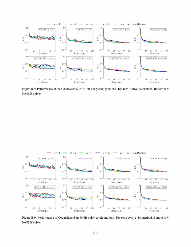
ω = 1 ω = 2 ω = 5 ω = 10 ω = +∞ (CountGauss)
20 40 60 80 100
100
10−2
10−4
10−6
Iterations
RR
E
CGS-AS (νi = 10)
20 40 60 80 100
100
10−2
10−4
10−6
Iterations
RR
E
CGS-AS (νi = 50)
20 40 60 80 100
100
10−2
10−4
10−6
Iterations
RR
E
CGS-AS (νi = 100)
20 40 60 80 100
100
10−2
10−4
10−6
Iterations
RR
E
CGS-AS (νi = 150)
20 40 60 80 100
100
10−2
10−4
10−6
Iterations
RR
E
CGS-NeNMF (νi = 10)
20 40 60 80 100
100
10−2
10−4
10−6
Iterations
RR
ECGS-NeNMF (νi = 50)
20 40 60 80 100
100
10−2
10−4
10−6
Iterations
RR
E
CGS-NeNMF (νi = 100)
20 40 60 80 100
100
10−2
10−4
10−6
Iterations
RR
E
CGS-NeNMF (νi = 150)
Figure B.8: Performance of the CountGaussS in 40 dB noisy configurations. Top row: Active-Set method, Bottom row:
NeNMF solver.
ω = 1 ω = 2 ω = 5 ω = 10 ω = +∞ (CountGauss)
20 40 60 80 100
100
10−2
10−4
10−6
Iterations
RR
E
CGS-AS (νi = 10)
20 40 60 80 100
100
10−2
10−4
10−6
Iterations
RR
E
CGS-AS (νi = 50)
20 40 60 80 100
100
10−2
10−4
10−6
Iterations
RR
E
CGS-AS (νi = 100)
20 40 60 80 100
100
10−2
10−4
10−6
Iterations
RR
E
CGS-AS (νi = 150)
20 40 60 80 100
100
10−2
10−4
10−6
Iterations
RR
E
CGS-NeNMF (νi = 10)
20 40 60 80 100
100
10−2
10−4
10−6
Iterations
RR
E
CGS-NeNMF (νi = 50)
20 40 60 80 100
100
10−2
10−4
10−6
Iterations
RR
E
CGS-NeNMF (νi = 100)
20 40 60 80 100
100
10−2
10−4
10−6
Iterations
RR
E
CGS-NeNMF (νi = 150)
Figure B.9: Performance of CountGaussS in 60 dB noisy configurations. Top row: Active-Set method, Bottom row:
NeNMF solver.
196
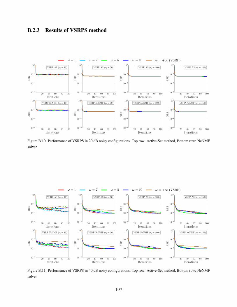
B.2.3 Results of VSRPS method
ω = 1 ω = 2 ω = 5 ω = 10 ω = +∞ (VSRP)
20 40 60 80 100
100
10−2
10−4
10−6
Iterations
RR
E
VSRP-AS (νi = 10)
20 40 60 80 100
100
10−2
10−4
10−6
Iterations
RR
E
VSRP-AS (νi = 50)
20 40 60 80 100
100
10−2
10−4
10−6
Iterations
RR
E
VSRP-AS (νi = 100)
20 40 60 80 100
100
10−2
10−4
10−6
Iterations
RR
E
VSRP-AS (νi = 150)
20 40 60 80 100
100
10−2
10−4
10−6
Iterations
RR
E
VSRP-NeNMF (νi = 10)
20 40 60 80 100
100
10−2
10−4
10−6
Iterations
RR
E
VSRP-NeNMF (νi = 50)
20 40 60 80 100
100
10−2
10−4
10−6
Iterations
RR
E
VSRP-NeNMF (νi = 100)
20 40 60 80 100
100
10−2
10−4
10−6
Iterations
RR
E
VSRP-NeNMF (νi = 150)
Figure B.10: Performance of VSRPS in 20 dB noisy configurations. Top row: Active-Set method, Bottom row: NeNMF
solver.
ω = 1 ω = 2 ω = 5 ω = 10 ω = +∞ (VSRP)
20 40 60 80 100
100
10−2
10−4
10−6
Iterations
RR
E
VSRP-AS (νi = 10)
20 40 60 80 100
100
10−2
10−4
10−6
Iterations
RR
E
VSRP-AS (νi = 50)
20 40 60 80 100
100
10−2
10−4
10−6
Iterations
RR
E
VSRP-AS (νi = 100)
20 40 60 80 100
100
10−2
10−4
10−6
Iterations
RR
E
VSRP-AS (νi = 150)
20 40 60 80 100
100
10−2
10−4
10−6
Iterations
RR
E
VSRP-NeNMF (νi = 10)
20 40 60 80 100
100
10−2
10−4
10−6
Iterations
RR
E
VSRP-NeNMF (νi = 50)
20 40 60 80 100
100
10−2
10−4
10−6
Iterations
RR
E
VSRP-NeNMF (νi = 100)
20 40 60 80 100
100
10−2
10−4
10−6
Iterations
RR
E
VSRP-NeNMF (νi = 150)
Figure B.11: Performance of VSRPS in 40 dB noisy configurations. Top row: Active-Set method, Bottom row: NeNMF
solver.
197
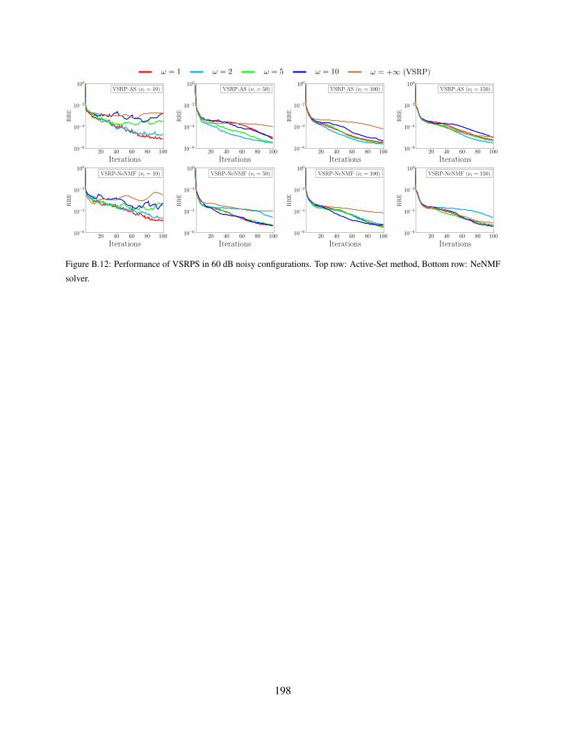
ω = 1 ω = 2 ω = 5 ω = 10 ω = +∞ (VSRP)
20 40 60 80 100
100
10−2
10−4
10−6
Iterations
RR
E
VSRP-AS (νi = 10)
20 40 60 80 100
100
10−2
10−4
10−6
Iterations
RR
E
VSRP-AS (νi = 50)
20 40 60 80 100
100
10−2
10−4
10−6
Iterations
RR
E
VSRP-AS (νi = 100)
20 40 60 80 100
100
10−2
10−4
10−6
Iterations
RR
E
VSRP-AS (νi = 150)
20 40 60 80 100
100
10−2
10−4
10−6
Iterations
RR
E
VSRP-NeNMF (νi = 10)
20 40 60 80 100
100
10−2
10−4
10−6
Iterations
RR
EVSRP-NeNMF (νi = 50)
20 40 60 80 100
100
10−2
10−4
10−6
Iterations
RR
E
VSRP-NeNMF (νi = 100)
20 40 60 80 100
100
10−2
10−4
10−6
Iterations
RR
E
VSRP-NeNMF (νi = 150)
Figure B.12: Performance of VSRPS in 60 dB noisy configurations. Top row: Active-Set method, Bottom row: NeNMF
solver.
198

Bibliography
[1] D. Achlioptas, “Database-friendly random projections,” in Proceedings of the twentieth ACM SIGMOD-
SIGACT-SIGART symposium on Principles of database systems. ACM, 2001, pp. 274–281.
[2] N. Ailon and B. Chazelle, “Approximate nearest neighbors and the fast johnson-lindenstrauss transform,”
in Proceedings of the thirty-eighth annual ACM symposium on Theory of computing, 2006, pp. 557–563.
[3] H. Akimoto, “Global air quality and pollution,” Science, vol. 302, no. 5651, pp. 1716–1719, 2003.
[4] Z. Al Barakeh, P. Breuil, N. Redon, C. Pijolat, N. Locoge, and J.-P. Viricelle, “Development of a
normalized multi-sensors system for low cost on-line atmospheric pollution detection,” Sensors and
Actuators B: Chemical, vol. 241, pp. 1235–1243, 2017.
[5] A. Alboody, M. Puigt, G. Roussel, V. Vantrepotte, C. Jamet, and T. K. Tran, “Experimental comparison
of multi-sharpening methods applied to sentinel-2 MSI and sentinel-3 OLCI images,” in Proc. IEEE
WHISPERS’21, March 2021.
[6] S. Amari, “alpha-divergence is unique, belonging to both f-divergence and bregman divergence classes.”
IEEE Trans. Inf. Theory, vol. 55, no. 11, pp. 4925–4931, 2009.
[7] A. M. S. Ang and N. Gillis, “Accelerating nonnegative matrix factorization algorithms using extrapola-
tion,” Neural computation, vol. 31, no. 2, pp. 417–439, 2019.
[8] A. Arfire, A. Marjovi, and A. Martinoli, “Model-based rendezvous calibration of mobile sensor
networks for monitoring air quality,” in 2015 IEEE SENSORS. IEEE, 2015, pp. 1–4.
[9] S. Arora, R. Ge, Y. Halpern, D. Mimno, A. Moitra, D. Sontag, Y. Wu, and M. Zhu, “A practical
algorithm for topic modeling with provable guarantees,” in International Conference on Machine
Learning. PMLR, 2013, pp. 280–288.
[10] S. Arora, R. Ge, R. Kannan, and A. Moitra, “Computing a nonnegative matrix factorization—provably,”
in 44th Annual ACM Symposium on Theory of Computing, STOC’12, 2012, pp. 145–161.
[11] L. Balzano and R. Nowak, “Blind calibration of sensor networks,” in Proceedings of the 6th interna-
tional conference on Information processing in sensor networks, 2007, pp. 79–88.
199
[12] J. M. Barcelo-Ordinas, M. Doudou, J. Garcia-Vidal, and N. Badache, “Self-calibration methods for
uncontrolled environments in sensor networks: A reference survey,” Ad Hoc Networks, vol. 88, pp.
142–159, 2019.
[13] J. M. Barcelo-Ordinas, J. Garcia-Vidal, M. Doudou, S. Rodrigo-Muñoz, and A. Cerezo-Llavero,
“Calibrating low-cost air quality sensors using multiple arrays of sensors,” in 2018 IEEE Wireless
Communications and Networking Conference (WCNC). IEEE, 2018, pp. 1–6.
[14] A. Basu, I. R. Harris, N. L. Hjort, and M. Jones, “Robust and efficient estimation by minimising a
density power divergence,” Biometrika, vol. 85, no. 3, pp. 549–559, 1998.
[15] A. Ben-Israel and T. N. Greville, Generalized inverses: theory and applications. Springer Science &
Business Media, 2003, vol. 15.
[16] D. Benachir, Y. Deville, S. Hosseini, M. S. Karoui, and A. Hameurlain, “Hyperspectral image unmixing
by non-negative matrix factorization initialized with modified independent component analysis,” in
Proc. WHISPERS’13, 2013.
[17] O. Berné, C. Joblin, Y. Deville, J. Smith, M. Rapacioli, J. Bernard, J. Thomas, W. Reach, and A. Abergel,
“Analysis of the emission of very small dust particles from spitzer spectro-imagery data using blind
signal separation methods,” Astronomy & Astrophysics, vol. 469, no. 2, pp. 575–586, 2007.
[18] M. W. Berry, M. Browne, A. N. Langville, V. P. Pauca, and R. J. Plemmons, “Algorithms and
applications for approximate nonnegative matrix factorization,” Computational statistics & data
analysis, vol. 52, no. 1, pp. 155–173, 2007.
[19] J. M. Bioucas-Dias, A. Plaza, N. Dobigeon, M. Parente, Q. Du, P. Gader, and J. Chanussot, “Hyper-
spectral unmixing overview: Geometrical, statistical, and sparse regression-based approaches,” IEEE J.
Sel. Topics Appl. Earth Observ. Remote Sens., vol. 5, no. 2, pp. 354–379, 2012.
[20] BIPM, IEC, IFCC, ILAC, IUPAC, IUPAP, ISO, and OIML, “International vocabulary of metrology –
basic and general concepts and associated terms (VIM),” 3rd edn. JCGM200:2012, 2012.
[21] C. M. Bishop, Pattern recognition and machine learning. springer, 2006.
[22] D. Böhning and B. G. Lindsay, “Monotonicity of quadratic-approximation algorithms,” Annals of the
Institute of Statistical Mathematics, vol. 40, no. 4, pp. 641–663, 1988.
[23] C. Boutsidis and E. Gallopoulos, “SVD based initialization: A head start for nonnegative matrix
factorization,” Pattern recognition, vol. 41, no. 4, pp. 1350–1362, 2008.
[24] R. A. Boyles, “On the convergence of the em algorithm,” Journal of the Royal Statistical Society:
Series B (Methodological), vol. 45, no. 1, pp. 47–50, 1983.
200
[25] M. Bruins, J. W. Gerritsen, W. W. Van De Sande, A. Van Belkum, and A. Bos, “Enabling a transferable
calibration model for metal-oxide type electronic noses,” Sensors and Actuators B: Chemical, vol. 188,
pp. 1187–1195, 2013.
[26] J.-P. Brunet, P. Tamayo, T. R. Golub, and J. P. Mesirov, “Metagenes and molecular pattern discovery
using matrix factorization,” Proceedings of the national academy of sciences, vol. 101, no. 12, pp.
4164–4169, 2004.
[27] I. Buciu, N. Nikolaidis, and I. Pitas, “A comparative study of nmf, dnmf, and lnmf algorithms
applied for face recognition,” in Proc. Second IEEE-EURASIP International Symposium on Control,
Communications, and Signal Processing (ISCCSP), 2006.
[28] I. Buciu and I. Pitas, “Application of non-negative and local non negative matrix factorization to facial
expression recognition,” in Proceedings of the 17th International Conference on Pattern Recognition,
2004. ICPR 2004., vol. 1. IEEE, 2004, pp. 288–291.
[29] M. Budde, R. El Masri, T. Riedel, and M. Beigl, “Enabling low-cost particulate matter measurement
for participatory sensing scenarios,” in Proceedings of the 12th international conference on mobile and
ubiquitous multimedia, 2013, pp. 1–10.
[30] D. Cai, X. He, J. Han, and T. S. Huang, “Graph regularized nonnegative matrix factorization for data
representation,” IEEE transactions on pattern analysis and machine intelligence, vol. 33, no. 8, pp.
1548–1560, 2010.
[31] E. J. Candès and Y. Plan, “Matrix completion with noise,” Proc. of the IEEE, vol. 98, no. 6, pp.
925–936, June 2010.
[32] E. J. Candès and B. Recht, “Exact matrix completion via convex optimization,” Foundations of
Computational Mathematics, vol. 9, no. 6, pp. 717–772, 2009.
[33] B. Cao, D. Shen, J.-T. Sun, X. Wang, Q. Yang, and Z. Chen, “Detect and track latent factors with
online nonnegative matrix factorization.” in IJCAI, vol. 7, 2007, pp. 2689–2694.
[34] H. Carfantan and J. Idier, “Statistical linear destriping of satellite-based pushbroom-type images,” IEEE
transactions on geoscience and remote sensing, vol. 48, no. 4, pp. 1860–1871, 2009.
[35] N. Castell, F. R. Dauge, P. Schneider, M. Vogt, U. Lerner, B. Fishbain, D. Broday, and A. Bartonova,
“Can commercial low-cost sensor platforms contribute to air quality monitoring and exposure estimates?”
Environment international, vol. 99, pp. 293–302, 2017.
[36] M. Charikar, K. Chen, and M. Farach-Colton, “Finding frequent items in data streams,” in International
Colloquium on Automata, Languages, and Programming. Springer, 2002, pp. 693–703.
201
[37] D. Chen and R. J. Plemmons, “Nonnegativity constraints in numerical analysis,” in The birth of
numerical analysis. World Scientific, 2010, pp. 109–139.
[38] J. C. Chen, “Non-negative rank factorization of non-negative matrices,” Linear Algebra and its
Applications, vol. 62, pp. 207–217, 1984.
[39] X. Chen, L. Gu, S. Z. Li, and H.-J. Zhang, “Learning representative local features for face detection,”
in Proceedings of the 2001 IEEE Computer Society Conference on Computer Vision and Pattern
Recognition. CVPR 2001, vol. 1. IEEE, 2001, pp. I–I.
[40] Y. Cheng, X. He, Z. Zhou, and L. Thiele, “Ict: In-field calibration transfer for air quality sensor
deployments,” Proceedings of the ACM on Interactive, Mobile, Wearable and Ubiquitous Technologies,
vol. 3, no. 1, pp. 1–19, 2019.
[41] J. Chou, Hazardous gas monitors: a practical guide to selection, operation and applications. McGraw-
Hill Professional Publishing, 2000.
[42] E. Chouzenoux, “Recherche de pas par majoration-minoration. application à la résolution de problèmes
inverses.” Ph.D. dissertation, Ecole Centrale de Nantes (ECN), 2010.
[43] R. Chreiky, “Informed non-negative matrix factorization for source apportionment,” Ph.D. dissertation,
Université du Littoral Côte d’Opale and University of Balamand, 2017.
[44] R. Chreiky, G. Delmaire, C. Dorffer, M. Puigt, G. Roussel, and A. Abche, “Robust informed split
gradient NMF using αβ -divergence for source apportionment,” in Proc. MLSP’16, 2016.
[45] R. Chreiky, G. Delmaire, M. Puigt, G. Roussel, D. Courcot, and A. Abche, “Split gradient method
for informed non-negative matrix factorization,” in Proc. LVA/ICA’15, vol. LNCS 9237, 2015, pp.
376–383.
[46] R. Chreiky, G. Delmaire, M. Puigt, G. Roussel, and A. Abche, “Informed split gradient non-negative
matrix factorization using huber cost function for source apportionment,” in 2016 IEEE International
Symposium on Signal Processing and Information Technology (ISSPIT). IEEE, 2016, pp. 69–74.
[47] A. Cichocki, S. Cruces, and S. Amari, “Generalized alpha-beta divergences and their application to
robust nonnegative matrix factorization,” Entropy, vol. 13, pp. 134–170, 2011.
[48] A. Cichocki and R. Zdunek, “Multilayer nonnegative matrix factorisation,” ELECTRONICS LETTERS-
IEE, vol. 42, no. 16, p. 947, 2006.
[49] A. Cichocki, R. Zdunek, and S.-i. Amari, “Csiszar’s divergences for non-negative matrix factorization:
Family of new algorithms,” in International Conference on Independent Component Analysis and
Signal Separation. Springer, 2006, pp. 32–39.
202
[50] A. Cichocki, R. Zdunek, and S.-I. Amari, “Hierarchical ALS algorithms for nonnegative matrix and
3D tensor factorization,” in Proc. ICA’07, 2007, pp. 169–176.
[51] A. Cichocki, R. Zdunek, A. H. Phan, and S.-i. Amari, Nonnegative matrix and tensor factorizations:
applications to exploratory multi-way data analysis and blind source separation. John Wiley & Sons,
2009.
[52] P. Comon and C. Jutten, Handbook of blind source separation. Independent component analysis and
applications. Academic press, 2010.
[53] P. Comon, “Independent component analysis, a new concept?” Signal processing, vol. 36, no. 3, pp.
287–314, 1994.
[54] Dask Development Team, Dask: Library for dynamic task scheduling, 2016. [Online]. Available:
https://dask.org
[55] R. de Fréin, “Learning and storing the parts of objects: Imf,” in 2014 IEEE International Workshop on
Machine Learning for Signal Processing (MLSP). IEEE, 2014, pp. 1–6.
[56] P. De Handschutter, N. Gillis, and X. Siebert, “Deep matrix factorizations,” arXiv preprint
arXiv:2010.00380, 2020.
[57] J. De Leeuw and W. J. Heiser, “Convergence of correction matrix algorithms for multidimensional
scaling,” Geometric representations of relational data, vol. 36, pp. 735–752, 1977.
[58] S. De Vito, E. Massera, M. Piga, L. Martinotto, and G. Di Francia, “On field calibration of an electronic
nose for benzene estimation in an urban pollution monitoring scenario,” Sensors and Actuators B:
Chemical, vol. 129, no. 2, pp. 750–757, 2008.
[59] S. De Vito, M. Piga, L. Martinotto, and G. Di Francia, “CO, NO2 and NOx urban pollution monitoring
with on-field calibrated electronic nose by automatic Bayesian regularization,” Sensors and Actuators
B: Chemical, vol. 143, no. 1, pp. 182–191, 2009.
[60] J. Dean and S. Ghemawat, “Mapreduce: Simplified data processing on large clusters,” To appear in
OSDI, p. 1, 2004.
[61] F. Delaine, B. Lebental, and H. Rivano, “In situ calibration algorithms for environmental sensor
networks: a review,” IEEE Sensors Journal, 2019.
[62] G. Delmaire, M. Omidvar, M. Puigt, F. Ledoux, A. Limem, G. Roussel, and D. Courcot, “Informed
weighted non-negative matrix factorization using op-divergence applied to source apportionment,”
Entropy, vol. 21, p. 253, 2019.
203
[63] S. Deshmukh, K. Kamde, A. Jana, S. Korde, R. Bandyopadhyay, R. Sankar, N. Bhattacharyya, and
R. Pandey, “Calibration transfer between electronic nose systems for rapid in situ measurement of pulp
and paper industry emissions,” Analytica chimica acta, vol. 841, pp. 58–67, 2014.
[64] Y. Deville and M. Puigt, “Temporal and time-frequency correlation-based blind source separation
methods. part I: Determined and underdetermined linear instantaneous mixtures,” Signal Processing,
vol. 87, no. 3, pp. 374–407, 2007.
[65] I. S. Dhillon and S. Sra, “Generalized nonnegative matrix approximations with bregman divergences,”
in NIPS, vol. 18. Citeseer, 2005.
[66] A. Dickow and G. Feiertag, “A systematic mems sensor calibration framework,” Journal of Sensors
and Sensor Systems, vol. 4, no. 1, pp. 97–102, 2015.
[67] C. Ding, T. Li, and W. Peng, “Nonnegative matrix factorization and probabilistic latent semantic
indexing: Equivalence chi-square statistic, and a hybrid method,” in AAAI, vol. 42, 2006, pp. 137–43.
[68] C. H. Ding, T. Li, and M. I. Jordan, “Convex and semi-nonnegative matrix factorizations,” IEEE Trans.
Pattern Anal. Mach. Intell., vol. 32, no. 1, pp. 45–55, 2010.
[69] D. Donoho and V. Stodden, “When does non-negative matrix factorization give a correct decomposition
into parts?” in Advances in neural information processing systems, 2004, pp. 1141–1148.
[70] C. Dorffer, M. Puigt, G. Delmaire, and G. Roussel, “Blind mobile sensor calibration using a nonnegative
matrix factorization with a relaxed rendezvous model,” in Proc. ICASSP’16, Mar. 2016, pp. 2941–2945.
[71] ——, “Nonlinear mobile sensor calibration using informed semi-nonnegative matrix factorization with
a Vandermonde factor,” in Proc. SAM’16, 2016.
[72] ——, “Fast nonnegative matrix factorization and completion using Nesterov iterations,” in Proc.
LVA/ICA’17, vol. LNCS 10179, 2017, pp. 26–35.
[73] ——, “Outlier-robust calibration method for sensor networks,” in Proc. ECMSM’17, 2017.
[74] ——, “Informed nonnegative matrix factorization methods for mobile sensor network calibration,”
IEEE Trans. Signal Inf. Process. Netw., vol. 4, no. 4, pp. 667–682, Dec 2018.
[75] C. Dorffer, “Méthodes informées de factorisation matricielle pour l’étalonnage de réseaux de capteurs
mobiles et la cartographie de champs de pollution,” Thèse de doctorat, Université du Littoral Côte
d’Opale, Dec. 2017. [Online]. Available: https://tel.archives-ouvertes.fr/tel-02074686
[76] C. Dorffer, M. Puigt, G. Delmaire, and G. Roussel, “Blind calibration of mobile sensors using informed
nonnegative matrix factorization,” in International Conference on Latent Variable Analysis and Signal
Separation. Springer, 2015, pp. 497–505.
204
[77] N. B. Erichson, A. Mendible, S. Wihlborn, and J. N. Kutz, “Randomized nonnegative matrix factoriza-
tion,” Pattern Recognition Letters, 2018.
[78] E. Esposito, S. De Vito, M. Salvato, V. Bright, R. Jones, and O. Popoola, “Dynamic neural network
architectures for on field stochastic calibration of indicative low cost air quality sensing systems,”
Sensors and Actuators B: Chemical, vol. 231, pp. 701–713, 2016.
[79] E. Esposito, S. De Vito, M. Salvato, G. Fattoruso, and G. Di Francia, “Computational intelligence for
smart air quality monitors calibration,” in International Conference on Computational Science and Its
Applications. Springer, 2017, pp. 443–454.
[80] S. Essid and C. Févotte, “Smooth nonnegative matrix factorization for unsupervised audiovisual
document structuring,” IEEE Transactions on Multimedia, vol. 15, no. 2, pp. 415–425, 2012.
[81] W. Eugster and G. Kling, “Performance of a low-cost methane sensor for ambient concentration
measurements in preliminary studies,” Atmospheric Measurement Techniques, vol. 5, no. 8, pp. 1925–
1934, 2012.
[82] European Environment Agency, “Air quality in europe — 2020 report,” EEA Report No 9/2020,
https://www.eea.europa.eu/publications/air-quality-in-europe-2020-report.
[83] X. Fang and I. Bate, “Using multi-parameters for calibration of low-cost sensors in urban environment,”
in networks, vol. 7, 2017, pp. 33–43.
[84] ——, “Using multi-parameters for calibration of low-cost sensors in urban environment,” in INTER-
NATIONAL CONFERENCE ON EMBEDDED WIRELESS SYSTEMS AND NETWORKS (EWSN),
2017.
[85] M. Fazel, “Matrix rank minimization with applications,” Ph.D. dissertation, Stanford University, 2002.
[86] C. Févotte, N. Bertin, and J.-L. Durrieu, “Nonnegative matrix factorization with the itakura-saito
divergence. with application to music analysis,” Neural Computation, vol. 21, no. 3, pp. 793–830, Mar.
2009.
[87] C. Févotte, “Majorization-minimization algorithm for smooth itakura-saito nonnegative matrix factor-
ization,” in 2011 IEEE International Conference on Acoustics, Speech and Signal Processing (ICASSP).
IEEE, 2011, pp. 1980–1983.
[88] C. Févotte, E. Vincent, and A. Ozerov, “Single-channel audio source separation with NMF: divergences,
constraints and algorithms,” in Audio Source Separation. Springer, 2018, pp. 1–24.
[89] R. A. Fisher, “The use of multiple measurements in taxonomic problems,” Annals of eugenics, vol. 7,
no. 2, pp. 179–188, 1936.
205
[90] J. Fonollosa, L. Fernandez, A. Gutiérrez-Gálvez, R. Huerta, and S. Marco, “Calibration transfer and
drift counteraction in chemical sensor arrays using direct standardization,” Sensors and Actuators B:
Chemical, vol. 236, pp. 1044–1053, 2016.
[91] F. L. Gadallah, F. Csillag, and E. J. M. Smith, “Destriping multisensor imagery with moment matching,”
International Journal of Remote Sensing, vol. 21, no. 12, pp. 2505–2511, 2000.
[92] J. Garcia, F. Teodoro, R. Cerdeira, L. Coelho, P. Kumar, and M. Carvalho, “Developing a methodol-
ogy to predict pm10 concentrations in urban areas using generalized linear models,” Environmental
technology, vol. 37, no. 18, pp. 2316–2325, 2016.
[93] N. Gillis, “Sparse and unique nonnegative matrix factorization through data preprocessing,” Journal of
Machine Learning Research, vol. 13, pp. 3349–3386, Nov. 2012.
[94] ——, “The why and how of nonnegative matrix factorization,” in Regularization, Optimization, Kernels,
and Support Vector Machines. Chapman and Hall/CRC, 2014, pp. 257–291.
[95] ——, “Nonnegative matrix factorization: complexity, algorithms and applications,” Ph.D. dissertation,
UCL-Université Catholique de Louvain, 2011.
[96] ——, “Introduction to nonnegative matrix factorization,” arXiv preprint arXiv:1703.00663, 2017.
[97] N. Gillis and F. Glineur, “Accelerated multiplicative updates and hierarchical als algorithms for
nonnegative matrix factorization,” Neural computation, vol. 24, no. 4, pp. 1085–1105, 2012.
[98] N. Gillis and S. A. Vavasis, “Semidefinite programming based preconditioning for more robust near-
separable nonnegative matrix factorization,” SIAM Journal on Optimization, vol. 25, no. 1, pp. 677–698,
2015.
[99] N. Guan, D. Tao, Z. Luo, and B. Yuan, “NeNMF: An optimal gradient method for nonnegative matrix
factorization,” IEEE Trans. Signal Process., vol. 60, no. 6, pp. 2882–2898, 2012.
[100] ——, “Online nonnegative matrix factorization with robust stochastic approximation,” IEEE Transac-
tions on Neural Networks and Learning Systems, vol. 23, no. 7, pp. 1087–1099, 2012.
[101] D. Guillamet, J. Vitria, and B. Schiele, “Introducing a weighted non-negative matrix factorization for
image classification,” Pattern Recognition Letters, vol. 24, no. 14, pp. 2447–2454, 2003.
[102] D. Guillamet, M. Bressan, and J. Vitria, “A weighted non-negative matrix factorization for local
representations,” in Proceedings of the 2001 IEEE Computer Society Conference on Computer Vision
and Pattern Recognition. CVPR 2001, vol. 1. IEEE, 2001, pp. I–I.
[103] D. Guillamet and J. Vitria, “Non-negative matrix factorization for face recognition,” in Catalonian
Conference on Artificial Intelligence. Springer, 2002, pp. 336–344.
206
[104] M. R. Gupta and Y. Chen, Theory and use of the EM algorithm. Now Publishers Inc, 2011.
[105] N. Halko, P.-G. Martinsson, and J. A. Tropp, “Finding structure with randomness: Probabilistic
algorithms for constructing approximate matrix decompositions,” SIAM review, vol. 53, no. 2, pp.
217–288, 2011.
[106] R. Hamon, P. Borgnat, P. Flandrin, and C. Robardet, “Nonnegative matrix factorization to find fea-
tures in temporal networks,” in 2014 IEEE international conference on acoustics, speech and signal
processing (ICASSP). IEEE, 2014, pp. 1065–1069.
[107] D. Hasenfratz, O. Saukh, and L. Thiele, “On-the-fly calibration of low-cost gas sensors,” in European
Conference on Wireless Sensor Networks. Springer, 2012, pp. 228–244.
[108] N. Hashimoto, S. Nakano, K. Yamamoto, and S. Nakagawa, “Speech recognition based on itakura-saito
divergence and dynamics/sparseness constraints from mixed sound of speech and music by non-negative
matrix factorization,” in Fifteenth Annual Conference of the International Speech Communication
Association, 2014.
[109] J.-E. Haugen, O. Tomic, and K. Kvaal, “A calibration method for handling the temporal drift of solid
state gas-sensors,” Analytica chimica acta, vol. 407, no. 1-2, pp. 23–39, 2000.
[110] W. J. Heiser, “Correspondence analysis with least absolute residuals,” Computational Statistics & Data
Analysis, vol. 5, no. 4, pp. 337–356, 1987.
[111] D. Hesslow, A. Cappelli, I. Carron, L. Daudet, R. Lafargue, K. Müller, R. Ohana, G. Pariente, and
I. Poli, “Photonic co-processors in hpc: using lighton opus for randomized numerical linear algebra,”
arXiv preprint arXiv:2104.14429, 2021.
[112] N.-D. Ho, “Non negative matrix factorization algorithms and applications,” Phd Thesis, Université
Catholique de Louvain, 2008.
[113] A. Hobolth, Q. Guo, A. Kousholt, and J. L. Jensen, “A unifying framework and comparison of
algorithms for non-negative matrix factorisation,” International Statistical Review, vol. 88, no. 1, pp.
29–53, 2020.
[114] M. D. Hoffman, D. M. Blei, and P. R. Cook, “Bayesian nonparametric matrix factorization for recorded
music,” in ICML, 2010.
[115] D. M. Holstius, A. Pillarisetti, K. Smith, and E. Seto, “Field calibrations of a low-cost aerosol sensor at
a regulatory monitoring site in california,” Atmospheric Measurement Techniques, vol. 7, no. 4, pp.
1121–1131, 2014.
[116] P. K. Hopke, “Review of receptor modeling methods for source apportionment,” Journal of the Air &
Waste Management Association, vol. 66, no. 3, pp. 237–259, 2016.
207
[117] P. O. Hoyer, “Non-negative matrix factorization with sparseness constraints,” J. Mach. Learn. Res.,
vol. 5, pp. 1457–1469, Dec. 2004.
[118] ——, “Non-negative matrix factorization with sparseness constraint,” Journal of Machine Learning
Research, vol. 5, pp. 1457–1469, November 2004.
[119] C.-J. Hsieh and I. S. Dhillon, “Fast coordinate descent methods with variable selection for non-negative
matrix factorization,” in Proceedings of the 17th ACM SIGKDD international conference on Knowledge
discovery and data mining. ACM, 2011, pp. 1064–1072.
[120] Y. Hu, D. Zhang, J. Ye, X. Li, and X. He, “Fast and accurate matrix completion via truncated nuclear
norm regularization,” IEEE Trans. Pattern Anal. Mach. Intell., vol. 35, no. 9, pp. 2117–2130, 2012.
[121] P. J. Huber, Robust statistical procedures. SIAM, 1996.
[122] G. Huyberechts, P. Szecowka, J. Roggen, and B. Licznerski, “Simultaneous quantification of carbon
monoxide and methane in humid air using a sensor array and an artificial neural network,” Sensors and
Actuators B: Chemical, vol. 45, no. 2, pp. 123–130, 1997.
[123] B. Iser, G. Schmidt, and W. Minker, Bandwidth extension of speech signals. Springer Science &
Business Media, 2008, vol. 13.
[124] F. Itakura, “Analysis synthesis telephony based on the maximum likelihood method,” in The 6th
international congress on acoustics, 1968, 1968, pp. 280–292.
[125] W. Jiao, G. Hagler, R. Williams, R. Sharpe, R. Brown, D. Garver, R. Judge, M. Caudill, J. Rickard,
M. Davis et al., “Community air sensor network (cairsense) project: evaluation of low-cost sensor
performance in a suburban environment in the southeastern united states,” Atmospheric Measurement
Techniques, vol. 9, no. 11, pp. 5281–5292, 2016.
[126] W. B. Johnson and J. Lindenstrauss, “Extensions of Lipschitz mappings into a Hilbert space,” Contem-
porary mathematics, vol. 26, no. 189-206, p. 1, 1984.
[127] H. Kagami and M. Yukawa, “Supervised nonnegative matrix factorization with dual-itakura-saito
and kullback-leibler divergences for music transcription,” in 2016 24th European Signal Processing
Conference (EUSIPCO). IEEE, 2016, pp. 1138–1142.
[128] D. Kalman, “A singularly valuable decomposition: the svd of a matrix,” The college mathematics
journal, vol. 27, no. 1, pp. 2–23, 1996.
[129] M. Kamionka, P. Breuil, and C. Pijolat, “Calibration of a multivariate gas sensing device for atmospheric
pollution measurement,” Sensors and Actuators B: Chemical, vol. 118, no. 1-2, pp. 323–327, 2006.
208
[130] B. Kanagal and V. Sindhwani, “Rank selection in low-rank matrix approximations: A study of cross-
validation for nmfs,” in Proc Conf Adv Neural Inf Process, vol. 1, 2010, pp. 10–15.
[131] R. Kannan, G. Ballard, and H. Park, “A high-performance parallel algorithm for nonnegative matrix
factorization,” in Proc. ACM SIGPLAN’16, 2016, p. 9.
[132] M. Kapralov, V. Potluru, and D. Woodruff, “How to fake multiply by a gaussian matrix,” in International
Conference on Machine Learning, 2016, pp. 2101–2110.
[133] ——, “How to fake multiply by a gaussian matrix,” in International Conference on Machine Learning,
2016, pp. 2101–2110.
[134] H. Kasai, “Stochastic variance reduced multiplicative update for nonnegative matrix factorization,” in
2018 IEEE International Conference on Acoustics, Speech and Signal Processing (ICASSP). IEEE,
2018, pp. 6338–6342.
[135] R. H. Keshavan, A. Montanari, and S. Oh, “Matrix completion from a few entries,” IEEE transactions
on information theory, vol. 56, no. 6, pp. 2980–2998, 2010.
[136] Z. Khan, N. Iltaf, H. Afzal, and H. Abbas, “Enriching non-negative matrix factorization with contextual
embeddings for recommender systems,” Neurocomputing, vol. 380, pp. 246–258, 2020.
[137] D. Kim, S. Sra, and I. S. Dhillon, “Fast newton-type methods for the least squares nonnegative matrix
approximation problem,” in Proceedings of the 2007 SIAM international conference on data mining.
SIAM, 2007, pp. 343–354.
[138] H. Kim and H. Park, “Nonnegative matrix factorization based on alternating nonnegativity constrained
least squares and active set method,” SIAM journal on matrix analysis and applications, vol. 30, no. 2,
pp. 713–730, 2008.
[139] J. Kim and H. Park, “Toward faster nonnegative matrix factorization: A new algorithm and comparisons,”
in Proc. ICDM’08, Dec 2008, pp. 353–362.
[140] J. Kim, Y. He, and H. Park, “Algorithms for nonnegative matrix and tensor factorizations: A unified
view based on block coordinate descent framework,” Journal of Global Optimization, vol. 58, no. 2, pp.
285–319, 2014.
[141] D. Kitamura, N. Ono, H. Sawada, H. Kameoka, and H. Saruwatari, “Determined blind source separation
unifying independent vector analysis and nonnegative matrix factorization,” IEEE/ACM Transactions
on Audio, Speech, and Language Processing, vol. 24, no. 9, pp. 1626–1641, 2016.
[142] Y. Koren, R. Bell, and C. Volinsky, “Matrix factorization techniques for recommender systems,”
Computer, vol. 42, no. 8, pp. 30–37, 2009.
209
[143] A. Kotsev, S. Schade, M. Craglia, M. Gerboles, L. Spinelle, and M. Signorini, “Next generation air
quality platform: Openness and interoperability for the internet of things,” Sensors, vol. 16, no. 3, p.
403, 2016.
[144] D. Kuang, J. Choo, and H. Park, “Nonnegative matrix factorization for interactive topic modeling and
document clustering,” in Partitional Clustering Algorithms. Springer, 2015, pp. 215–243.
[145] A. Kumar, V. Sindhwani, and P. Kambadur, “Fast conical hull algorithms for near-separable non-
negative matrix factorization,” in International Conference on Machine Learning. PMLR, 2013, pp.
231–239.
[146] P. Kumar, L. Morawska, C. Martani, G. Biskos, M. Neophytou, S. Di Sabatino, M. Bell, L. Norford, and
R. Britter, “The rise of low-cost sensing for managing air pollution in cities,” Environment international,
vol. 75, pp. 199–205, 2015.
[147] A. N. Langville, C. D. Meyer, R. Albright, J. Cox, and D. Duling, “Algorithms, initializations, and
convergence for the nonnegative matrix factorization,” arXiv preprint arXiv:1407.7299, 2014.
[148] H. Lantéri, C. Theys, C. Richard, and C. Févotte, “Split gradient method for nonnegative matrix
factorization,” in Proc. EUSIPCO’10, 2010.
[149] H. Lantéri, C. Theys, C. Richard, and C. Févotte, “Split gradient method for nonnegative matrix
factorization,” in 2010 18th European Signal Processing Conference. IEEE, 2010, pp. 1199–1203.
[150] R. Laref, E. Losson, A. Sava, and M. Siadat, “Support vector machine regression for calibration transfer
between electronic noses dedicated to air pollution monitoring,” Sensors, vol. 18, no. 11, p. 3716, 2018.
[151] C. L. Lawson and R. J. Hanson, Solving least squares problems. SIAM, 1995.
[152] J. Le Roux, F. J. Weninger, and J. R. Hershey, “Sparse NMF—half-baked or well done?” Mitsubishi
Electric Research Labs, Tech. Rep. TR2015-023, 2015.
[153] J. Le Roux, J. R. Hershey, and F. Weninger, “Deep nmf for speech separation,” in Proc. ICASSP’15.
IEEE, 2015, pp. 66–70.
[154] B.-T. Lee, S.-C. Son, and K. Kang, “A blind calibration scheme exploiting mutual calibration rela-
tionships for a dense mobile sensor network,” IEEE Sensors Journal, vol. 14, no. 5, pp. 1518–1526,
2014.
[155] D. D. Lee and H. S. Seung, “Algorithms for non-negative matrix factorization,” in NIPS 13, T. K. Leen,
T. G. Dietterich, and V. Tresp, Eds. MIT Press, 2001, pp. 556–562.
[156] ——, “Algorithms for non-negative matrix factorization,” in Advances in neural information processing
systems, 2001, pp. 556–562.
210
[157] D. Lee and H. Seung, “Learning the parts of objects by non negative matrix factorization,” Nature, vol.
401, no. 6755, pp. 788–791, 1999.
[158] H. Lee and S. Choi, “Group nonnegative matrix factorization for eeg classification,” in Artificial
Intelligence and Statistics. PMLR, 2009, pp. 320–327.
[159] A. Lefevre, F. Bach, and C. Févotte, “Itakura-saito nonnegative matrix factorization with group sparsity,”
in 2011 IEEE International Conference on Acoustics, Speech and Signal Processing (ICASSP). IEEE,
2011, pp. 21–24.
[160] I. Lemammer, O. Michel, H. Ayasso, S. Zozor, and G. Bernard, “Online mobile c-arm calibration
using inertial sensors: a preliminary study in order to achieve cbct,” International journal of computer
assisted radiology and surgery, vol. 15, no. 2, pp. 213–224, 2020.
[161] A. C. Lewis, J. D. Lee, P. M. Edwards, M. D. Shaw, M. J. Evans, S. J. Moller, K. R. Smith, J. W.
Buckley, M. Ellis, S. R. Gillot et al., “Evaluating the performance of low cost chemical sensors for air
pollution research,” Faraday discussions, vol. 189, pp. 85–103, 2016.
[162] P. Li, T. J. Hastie, and K. W. Church, “Very sparse random projections,” in Proc. ACM SIGKDD’06,
2006, pp. 287–296.
[163] S. Z. Li, X. W. Hou, H. J. Zhang, and Q. S. Cheng, “Learning spatially localized, parts-based
representation,” in Proceedings of the 2001 IEEE Computer Society Conference on Computer Vision
and Pattern Recognition. CVPR 2001, vol. 1. IEEE, 2001, pp. I–I.
[164] X. P. Li, L. Huang, H. C. So, and B. Zhao, “A survey on matrix completion: Perspective of signal
processing,” arXiv preprint arXiv:1901.10885, 2019.
[165] A. Limem, G. Delmaire, M. Puigt, G. Roussel, and D. Courcot, “Non-negative matrix factorization
using weighted beta divergence and equality constraints for industrial source apportionment,” in Proc.
MLSP’13, 2013.
[166] ——, “Non-negative matrix factorization under equality constraints—a study of industrial source
identification,” Applied Numerical Mathematics, vol. 85, pp. 1–15, Nov. 2014.
[167] ——, “Non-negative matrix factorization under equality constraints—a study of industrial source
identification,” Applied Numerical Mathematics, vol. 85, pp. 1 – 15, 2014. [Online]. Available:
http://www.sciencedirect.com/science/article/pii/S0168927414001007
[168] A. Limem, G. Delmaire, G. Roussel, and D. Courcot, “Kullback-Leibler NMF under linear equality
constraints. application to pollution source apportionment,” in Proc. ISSPA’12, 2012, pp. 752–757.
[169] A. Limem, M. Puigt, G. Delmaire, G. Roussel, and D. Courcot, “Bound constrained weighted NMF for
industrial source apportionment,” in Proc. MLSP’14, 2014.
211
[170] C.-J. Lin, “Projected gradients methods for non-negative matrix factorization,” Neural Computation,
vol. 19, pp. 2756–2779, 2007.
[171] ——, “Projected gradients methods for non-negative matrix factorization,” Neural Computation,
vol. 19, pp. 2756–2779, 2007.
[172] ——, “On the convergence of multiplicative update algorithms for nonnegative matrix factorization,”
IEEE Trans. Neural Netw., vol. 18, no. 6, pp. 1589–1596, 2007.
[173] C. Lin, N. Masey, H. Wu, M. Jackson, D. J. Carruthers, S. Reis, R. M. Doherty, I. J. Beverland, and
M. R. Heal, “Practical field calibration of portable monitors for mobile measurements of multiple air
pollutants,” Atmosphere, vol. 8, no. 12, p. 231, 2017.
[174] Y. Lin, W. Dong, and Y. Chen, “Calibrating low-cost sensors by a two-phase learning approach
for urban air quality measurement,” Proceedings of the ACM on Interactive, Mobile, Wearable and
Ubiquitous Technologies, vol. 2, no. 1, pp. 1–18, 2018.
[175] J. Lipor and L. Balzano, “Robust blind calibration via total least squares,” in 2014 IEEE International
Conference on Acoustics, Speech and Signal Processing (ICASSP). IEEE, 2014, pp. 4244–4248.
[176] C. Liu, H.-c. Yang, J. Fan, L.-W. He, and Y.-M. Wang, “Distributed nonnegative matrix factorization
for web-scale dyadic data analysis on mapreduce,” in Proceedings of the 19th international conference
on World wide web, 2010, pp. 681–690.
[177] J. Liu, C. Wang, J. Gao, and J. Han, “Multi-view clustering via joint nonnegative matrix factorization,”
in Proc. SDM’13, vol. 13, 2013, pp. 252–260.
[178] ——, “Multi-view clustering via joint nonnegative matrix factorization,” in Proceedings of the 2013
SIAM International Conference on Data Mining. SIAM, 2013, pp. 252–260.
[179] X. Liu, S. Cheng, H. Liu, S. Hu, D. Zhang, and H. Ning, “A survey on gas sensing technology,” Sensors,
vol. 12, no. 7, pp. 9635–9665, 2012.
[180] N. Lopes and B. Ribeiro, “Non-negative matrix factorization implementation using graphic processing
units,” in International Conference on Intelligent Data Engineering and Automated Learning. Springer,
2010, pp. 275–283.
[181] S. D. Lowther, K. C. Jones, X. Wang, J. D. Whyatt, O. Wild, and D. Booker, “Particulate matter
measurement indoors: A review of metrics, sensors, needs, and applications,” Environmental science &
technology, vol. 53, no. 20, pp. 11 644–11 656, 2019.
[182] X. Lu, H. Wu, Y. Yuan, P. Yan, and X. Li, “Manifold regularized sparse NMF for hyperspectral
unmixing,” IEEE Transactions on Geoscience and Remote Sensing, vol. 51, no. 5, pp. 2815–2826,
2012.
212
[183] D. G. Luenberger and Y. Ye, “Linear and nonlinear programming, vol. 116,” 2008.
[184] X. Luo, M. Zhou, Y. Xia, and Q. Zhu, “An efficient non-negative matrix-factorization-based approach
to collaborative filtering for recommender systems,” IEEE Transactions on Industrial Informatics,
vol. 10, no. 2, pp. 1273–1284, 2014.
[185] W.-K. Ma, J. M. Bioucas-Dias, T.-H. Chan, N. Gillis, P. Gader, A. J. Plaza, A. Ambikapathi, and C.-Y.
Chi, “A signal processing perspective on hyperspectral unmixing,” IEEE Signal Proc. Mag., pp. 67–81,
Jan. 2014.
[186] B. Maag, Z. Zhou, and L. Thiele, “A survey on sensor calibration in air pollution monitoring deploy-
ments,” IEEE Internet of Things Journal, vol. 5, no. 6, pp. 4857–4870, 2018.
[187] B. Maag, O. Saukh, D. Hasenfratz, and L. Thiele, “Pre-deployment testing, augmentation and calibra-
tion of cross-sensitive sensors.” in EWSN, 2016, pp. 169–180.
[188] B. Maag, Z. Zhou, O. Saukh, and L. Thiele, “Scan: Multi-hop calibration for mobile sensor arrays,”
Proceedings of the ACM on Interactive, Mobile, Wearable and Ubiquitous Technologies, vol. 1, no. 2,
pp. 1–21, 2017.
[189] J. Mairal, F. Bach, J. Ponce, and G. Sapiro, “Online learning for matrix factorization and sparse coding,”
Journal of Machine Learning Research, vol. 11, no. Jan, pp. 19–60, 2010.
[190] Y. Mao and L. K. Saul, “Modeling distances in large-scale networks by matrix factorization,” in
Proceedings of the 4th ACM SIGCOMM conference on Internet measurement, 2004, pp. 278–287.
[191] A. Marjovi, A. Arfire, and A. Martinoli, “High resolution air pollution maps in urban environments
using mobile sensor networks,” in 2015 International Conference on Distributed Computing in Sensor
Systems. IEEE, 2015, pp. 11–20.
[192] C. R. Martin, N. Zeng, A. Karion, R. R. Dickerson, X. Ren, B. N. Turpie, and K. J. Weber, “Evaluation
and environmental correction of ambient co 2 measurements from a low-cost ndir sensor,” Atmospheric
measurement techniques, vol. 10, no. 7, pp. 2383–2395, 2017.
[193] K. Martinez, J. K. Hart, and R. Ong, “Environmental sensor networks,” Computer, vol. 37, no. 8, pp.
50–56, 2004.
[194] J. Matoušek, “On variants of the johnson–lindenstrauss lemma,” Random Structures & Algorithms,
vol. 33, no. 2, pp. 142–156, 2008.
[195] M. Mead, O. Popoola, G. Stewart, P. Landshoff, M. Calleja, M. Hayes, J. Baldovi, M. McLeod,
T. Hodgson, J. Dicks et al., “The use of electrochemical sensors for monitoring urban air quality in
low-cost, high-density networks,” Atmospheric Environment, vol. 70, pp. 186–203, 2013.
213
[196] I. Meganem, Y. Deville, S. Hosseini, P. Déliot, and X. Briottet, “Linear-quadratic blind source separation
using NMF to unmix urban hyperspectral images,” IEEE Trans. Signal Process., vol. 62, no. 7, pp.
1822–1833, Apr. 2014.
[197] L. Meier, S. Van De Geer, and P. Bühlmann, “The group lasso for logistic regression,” Journal of the
Royal Statistical Society: Series B (Statistical Methodology), vol. 70, no. 1, pp. 53–71, 2008.
[198] E. Mejía-Roa, D. Tabas-Madrid, J. Setoain, C. García, F. Tirado, and A. Pascual-Montano, “NMF-
mGPU: non-negative matrix factorization on multi-GPU systems,” BMC bioinformatics, vol. 16, no. 1,
pp. 1–12, 2015.
[199] M. Meloun and J. Militky, “Statistical data analysis: A practical guide,” 2011.
[200] E. Miluzzo, N. D. Lane, A. T. Campbell, and R. Olfati-Saber, “Calibree: A self-calibration system for
mobile sensor networks,” in International Conference on Distributed Computing in Sensor Systems.
Springer, 2008, pp. 314–331.
[201] T. Mizutani and M. Tanaka, “Efficient preconditioning for noisy separable nonnegative matrix factor-
ization problems by successive projection based low-rank approximations,” Machine Learning, vol.
107, no. 4, pp. 643–673, 2018.
[202] N. Mohammadiha and A. Leijon, “Nonnegative matrix factorization using projected gradient algo-
rithms with sparseness constraints,” in 2009 IEEE International Symposium on Signal Processing and
Information Technology (ISSPIT). IEEE, 2009, pp. 418–423.
[203] C. Monn, “Exposure assessment of air pollutants: a review on spatial heterogeneity and indoor/out-
door/personal exposure to suspended particulate matter, nitrogen dioxide and ozone,” Atmospheric
environment, vol. 35, no. 1, pp. 1–32, 2001.
[204] S. Moussaoui, “Séparation de sources non-négatives. application au traitement des signaux de spectro-
scopie,” Thèse de doctorat, Université Henri Poincaré, Nancy 1, 2005.
[205] M. Mueller, J. Meyer, and C. Hueglin, “Design of an ozone and nitrogen dioxide sensor unit and
its long-term operation within a sensor network in the city of zurich,” Atmospheric Measurement
Techniques, vol. 10, no. 10, pp. 3783–3799, 2017.
[206] A. Nel, T. Xia, L. Mädler, and N. Li, “Toxic potential of materials at the nanolevel,” science, vol. 311,
no. 5761, pp. 622–627, 2006.
[207] Y. Nesterov, “A method of solving a convex programming problem with convergence rate O(1/k2),” in
Soviet Mathematics Doklady, vol. 27, no. 2, 1983, pp. 372–376.
[208] ——, Introductory lectures on convex optimization: A basic course. Springer Science & Business
Media, 2013, vol. 87.
214
[209] Y. E. Nesterov, “A method for solving the convex programming problem with convergence rate o (1/kˆ
2),” in Dokl. akad. nauk Sssr, vol. 269, 1983, pp. 543–547.
[210] L. M. Oliveira and J. J. Rodrigues, “Wireless sensor networks: A survey on environmental monitoring.”
JCM, vol. 6, no. 2, pp. 143–151, 2011.
[211] V. P. Pauca, F. Shahnaz, M. W. Berry, and R. J. Plemmons, “Text mining using non-negative matrix
factorizations,” in Proceedings of the 2004 SIAM International Conference on Data Mining. SIAM,
2004, pp. 452–456.
[212] K. Pearson, “Liii. on lines and planes of closest fit to systems of points in space,” The London,
Edinburgh, and Dublin Philosophical Magazine and Journal of Science, vol. 2, no. 11, pp. 559–572,
1901.
[213] R. Piedrahita, Y. Xiang, N. Masson, J. Ortega, A. Collier, Y. Jiang, K. Li, R. P. Dick, Q. Lv, M. Han-
nigan et al., “The next generation of low-cost personal air quality sensors for quantitative exposure
monitoring,” Atmospheric Measurement Techniques, vol. 7, no. 10, pp. 3325–3336, 2014.
[214] M. Plouvin, A. Limem, M. Puigt, G. Delmaire, G. Roussel, and D. Courcot, “Enhanced NMF initial-
ization using a physical model for pollution source apportionment,” in Proc. ESANN’14, 2014, pp.
261–266.
[215] B. T. Polyak, “Some methods of speeding up the convergence of iteration methods,” USSR Computa-
tional Mathematics and Mathematical Physics, vol. 4, no. 5, pp. 1–17, 1964.
[216] M. Puigt, O. Berné, R. Guidara, Y. Deville, S. Hosseini, and C. Joblin, “Cross-validation of blindly
separated interstellar dust spectra,” in Proc. ECMS’09, 2009, pp. 41–48.
[217] M. Puigt and Y. Deville, “Time-frequency ratio-based blind separation methods for attenuated and
time-delayed sources,” Mechanical Systems and Signal Processing, vol. 19, pp. 1348–1379, 2005.
[218] M. Puigt, “Méthodes de séparation aveugle de sources fondées sur des transformées temps-fréquence.
application à des signaux de parole.” Ph.D. dissertation, Université Paul Sabatier-Toulouse III, 2007.
[219] M. Puigt, G. Delmaire, and G. Roussel, “Environmental signal processing: new trends and applications,”
in 25th European Symposium on Artificial Neural Networks, Computational Intelligence and Machine
Learning (ESANN 2017), 2017.
[220] H. Robbins and S. Monro, “A stochastic approximation method,” The annals of mathematical statistics,
pp. 400–407, 1951.
[221] S. A. Robila and L. G. Maciak, “A parallel unmixing algorithm for hyperspectral images,” in Intelligent
Robots and Computer Vision XXIV: Algorithms, Techniques, and Active Vision, vol. 6384. International
Society for Optics and Photonics, 2006, p. 63840F.
215
[222] A. Saade, F. Caltagirone, I. Carron, L. Daudet, A. Drémeau, S. Gigan, and F. Krzakala, “Random
projections through multiple optical scattering: Approximating kernels at the speed of light,” in Proc.
ICASSP’16, 2016, pp. 6215–6219.
[223] D. Sanders, “Environmental sensors and networks of sensors,” Sensor Review, 2008.
[224] O. Saukh, D. Hasenfratz, C. Walser, and L. Thiele, “On rendezvous in mobile sensing networks,” in
Proc. REALWSN’14, ser. LNCS, vol. 281, 2014, pp. 29–42.
[225] O. Saukh, D. Hasenfratz, and L. Thiele, “Reducing multi-hop calibration errors in large-scale mobile
sensor networks,” in Proceedings of the 14th International Conference on Information Processing in
Sensor Networks, 2015, pp. 274–285.
[226] R. Schachtner, G. Pöppel, and E. W. Lang, “Towards unique solutions of non-negative matrix factor-
ization problems by a determinant criterion,” Digital Signal Processing, vol. 21, no. 4, pp. 528–534,
2011.
[227] N. Seichepine, S. Essid, C. Févotte, and O. Cappé, “Soft nonnegative matrix co-factorization,” IEEE
Transactions on Signal Processing, vol. 62, no. 22, pp. 5940–5949, 2014.
[228] F. Shahnaz, M. W. Berry, V. P. Pauca, and R. J. Plemmons, “Document clustering using nonnegative
matrix factorization,” Information Processing & Management, vol. 42, no. 2, pp. 373–386, 2006.
[229] V. Sharan, K. S. Tai, P. Bailis, and G. Valiant, “Compressed factorization: Fast and accurate low-rank
factorization of compressively-sensed data,” in International Conference on Machine Learning, 2019,
pp. 5690–5700.
[230] GP2Y1010AU0F compact optical dust sensor, Sharp Corp., 2006.
[231] Q. Shi, J. Petterson, G. Dror, J. Langford, A. Smola, and S. Vishwanathan, “Hash kernels for structured
data.” Journal of Machine Learning Research, vol. 10, no. 11, 2009.
[232] A. P. Singh and G. J. Gordon, “Relational learning via collective matrix factorization,” in Proceedings
of the 14th ACM SIGKDD international conference on Knowledge discovery and data mining, 2008,
pp. 650–658.
[233] M. Slavin, “Applications of stochastic gradient descent to nonnegative matrix factorization,” Master’s
thesis, University of Waterloo, 2019.
[234] A. Sobral, T. Bouwmans, and E.-H. Zahzah, “LRSLibrary: Low-rank and sparse tools for back-
ground modeling and subtraction in videos,” in Robust Low-Rank and Sparse Matrix Decomposition:
Applications in Image and Video Processing. CRC Press, Taylor and Francis Group., 2015.
216
[235] L. Spinelle, M. Gerboles, M. G. Villani, M. Aleixandre, and F. Bonavitacola, “Calibration of a cluster
of low-cost sensors for the measurement of air pollution in ambient air,” in SENSORS, 2014 IEEE.
IEEE, 2014, pp. 21–24.
[236] ——, “Field calibration of a cluster of low-cost commercially available sensors for air quality monitor-
ing. part b: No, co and co2,” Sensors and Actuators B: Chemical, vol. 238, pp. 706–715, 2017.
[237] N. Srebro, J. Rennie, and T. S. Jaakkola, “Maximum-margin matrix factorization,” in Advances in
neural information processing systems, 2005, pp. 1329–1336.
[238] W. Su, S. Boyd, and E. J. Candès, “A differential equation for modeling nesterov’s accelerated gradient
method: Theory and insights,” Journal of Machine Learning Research, vol. 17, no. 153, pp. 1–43,
2016.
[239] D. L. Sun and R. Mazumder, “Non-negative matrix completion for bandwidth extension: A convex
optimization approach,” in 2013 IEEE International Workshop on Machine Learning for Signal
Processing (MLSP). IEEE, 2013, pp. 1–6.
[240] L. Sun, D. Westerdahl, and Z. Ning, “Development and evaluation of a novel and cost-effective
approach for low-cost no2 sensor drift correction,” Sensors, vol. 17, no. 8, p. 1916, 2017.
[241] M. Tepper and G. Sapiro, “Compressed nonnegative matrix factorization is fast and accurate,” IEEE
Trans. Signal Process., vol. 64, no. 9, pp. 2269–2283, May 2016.
[242] M. Tong, Y. Chen, L. Ma, H. Bai, and X. Yue, “Nmf with local constraint and deep nmf with temporal
dependencies constraint for action recognition,” Neural Computing and Applications, vol. 32, no. 9, pp.
4481–4505, 2020.
[243] W. S. Torgerson, “Multidimensional scaling: I. theory and method,” Psychometrika, vol. 17, no. 4, pp.
401–419, 1952.
[244] G. Trigeorgis, K. Bousmalis, S. Zafeiriou, and B. W. Schuller, “A deep matrix factorization method for
learning attribute representations,” IEEE transactions on pattern analysis and machine intelligence,
vol. 39, no. 3, pp. 417–429, 2016.
[245] W. Tsujita, H. Ishida, and T. Moriizumi, “Dynamic gas sensor network for air pollution monitoring and
its auto-calibration,” in SENSORS, 2004 IEEE. IEEE, 2004, pp. 56–59.
[246] M. Udell and A. Townsend, “Why are big data matrices approximately low rank?” SIAM Journal on
Mathematics of Data Science, vol. 1, no. 1, pp. 144–160, 2019.
[247] M. O. Ulfarsson and V. Solo, “Tuning parameter selection for nonnegative matrix factorization,” in
2013 IEEE International Conference on Acoustics, Speech and Signal Processing. IEEE, 2013, pp.
6590–6594.
217
[248] United States Environmental Protection Agency, “What is particulate matter,” https://www3.epa.gov/
region1/eco/uep/particulatematter.html, accessed: 2021-02-12.
[249] L. Van Der Maaten, E. Postma, and J. Van den Herik, “Dimensionality reduction: a comparative review,”
J Mach Learn Res, vol. 10, no. 66-71, p. 13, 2009.
[250] C. F. Van Loan and G. H. Golub, Matrix computations. Johns Hopkins University Press Baltimore,
1983.
[251] L. Vandenberghe, “Applied numerical computing – QR factorizations,” Lectures notes available at
http://www.seas.ucla.edu/~vandenbe/ee133a.html.
[252] S. A. Vavasis, “On the complexity of nonnegative matrix factorization,” SIAM Journal on Optimization,
vol. 20, no. 3, pp. 1364–1377, 2009.
[253] E. Vincent, S. Araki, and P. Bofill, “The 2008 signal separation evaluation campaign: A community-
based approach to large-scale evaluation,” in Proc. ICA’09, 2009, pp. 734–741.
[254] T. O. Virtanen, “Monaural sound source separation by perceptually weighted non-negative matrix
factorization,” Tampere University of Technology, Tech. Rep, 2007.
[255] O. Vu thanh, “Méthodes rapides d’étalonnage in situ de réseaux de capteurs mobiles hétérogènes,”
Master’s thesis, ENSE3, INP Grenoble, 2020.
[256] O. Vu thanh, M. Puigt, F. Yahaya, G. Delmaire, and G. Roussel, “In situ calibration of cross-sensitive
sensors in mobile sensor arrays using fast informed non-negative matrix factorization,” in IEEE ICASSP
2021, Toronto, Canada, Jun. 2021. [Online]. Available: https://hal.archives-ouvertes.fr/hal-03126481
[257] C. Wang, P. Ramanathan, and K. K. Saluja, “Calibrating nonlinear mobile sensors,” in 2008 5th
Annual IEEE Communications Society Conference on Sensor, Mesh and Ad Hoc Communications and
Networks. IEEE, 2008, pp. 533–541.
[258] ——, “Moments based blind calibration in mobile sensor networks,” in 2008 IEEE International
Conference on Communications. IEEE, 2008, pp. 896–900.
[259] ——, “Blindly calibrating mobile sensors using piecewise linear functions,” in 2009 6th Annual IEEE
Communications Society Conference on Sensor, Mesh and Ad Hoc Communications and Networks.
IEEE, 2009, pp. 1–9.
[260] C. Wang, L. Yin, L. Zhang, D. Xiang, and R. Gao, “Metal oxide gas sensors: sensitivity and influencing
factors,” sensors, vol. 10, no. 3, pp. 2088–2106, 2010.
[261] F. Wang and P. Li, “Efficient nonnegative matrix factorization with random projections,” in Proc. SIAM
ICDM’10. SIAM, 2010, pp. 281–292.
218
[262] F. Wang, T. Li, X. Wang, S. Zhu, and C. Ding, “Community discovery using nonnegative matrix
factorization,” Data Mining and Knowledge Discovery, vol. 22, no. 3, pp. 493–521, 2011.
[263] J. Wang, F. Tian, C. H. Liu, H. Yu, X. Wang, and X. Tang, “Robust nonnegative matrix factorization with
ordered structure constraints,” in 2017 International Joint Conference on Neural Networks (IJCNN).
IEEE, 2017, pp. 478–485.
[264] J. Wang, T. Zhang, N. Sebe, H. T. Shen et al., “A survey on learning to hash,” IEEE transactions on
pattern analysis and machine intelligence, vol. 40, no. 4, pp. 769–790, 2017.
[265] Y. X. Wang and Y. J. Zhang, “Nonnegative matrix factorization: A comprehensive review,” IEEE Trans.
Knowl. Data Eng., vol. 25, no. 6, pp. 1336–1353, June 2013.
[266] Y. Wang, A. Yang, X. Chen, P. Wang, Y. Wang, and H. Yang, “A deep learning approach for blind drift
calibration of sensor networks,” IEEE Sensors Journal, vol. 17, no. 13, pp. 4158–4171, 2017.
[267] Y. Wang, A. Yang, Z. Li, X. Chen, P. Wang, and H. Yang, “Blind drift calibration of sensor networks
using sparse bayesian learning,” IEEE Sensors Journal, vol. 16, no. 16, pp. 6249–6260, 2016.
[268] K. Weinberger, A. Dasgupta, J. Langford, A. Smola, and J. Attenberg, “Feature hashing for large scale
multitask learning,” in Proceedings of the 26th annual international conference on machine learning,
2009, pp. 1113–1120.
[269] S. Wild, J. Curry, and A. Dougherty, “Motivating nonnegative matrix factorizations,” in In Proc. SIAM
Applied Linear Algebra Conf. Citeseer, 2003.
[270] ——, “Improving non-negative matrix factorizations through structured initialization,” Pattern recogni-
tion, vol. 37, no. 11, pp. 2217–2232, 2004.
[271] S. Wild, W. S. Wild, J. Curry, A. Dougherty, and M. Betterton, “Seeding non-negative matrix factoriza-
tions with the spherical k-means clustering,” Ph.D. dissertation, University of Colorado, 2003.
[272] D. P. Woodruff, “Sketching as a tool for numerical linear algebra,” arXiv preprint arXiv:1411.4357,
2014.
[273] C. J. Wu, “On the convergence properties of the em algorithm,” The Annals of statistics, pp. 95–103,
1983.
[274] Y. Xiang, L. S. Bai, R. Pledrahita, R. P. Dick, Q. Lv, M. Hannigan, and L. Shang, “Collaborative
calibration and sensor placement for mobile sensor networks,” in 2012 ACM/IEEE 11th International
Conference on Information Processing in Sensor Networks (IPSN). IEEE, 2012, pp. 73–83.
219
[275] W. Xu, X. Liu, and Y. Gong, “Document clustering based on non-negative matrix factorization,” in
Proceedings of the 26th annual international ACM SIGIR conference on Research and development in
informaion retrieval, 2003, pp. 267–273.
[276] Y. Xu, W. Yin, Z. Wen, and Y. Zhang, “An alternating direction algorithm for matrix completion with
nonnegative factors,” Frontiers of Mathematics in China, vol. 7, no. 2, pp. 365–384, 2012.
[277] F. Yahaya, M. Puigt, G. Delmaire, and G. Roussel, “Faster-than-fast NMF using random projections
and nesterov iterations,” in Proceedings of iTWIST: international Traveling Workshop on Interactions
between low-complexity data models and Sensing Techniques, Marseille, France, November 21–23
2018.
[278] ——, “Accélération de la factorisation pondérée en matrices non-négatives par projections aléatoires,”
in Actes du GRETSI, Lille, France, August 2019.
[279] ——, “How to apply random projections to nonnegative matrix factorization with missing entries?” in
Proceedings of the European Signal Processing Conference (EUSIPCO’19), Coruna, Spain, 2019.
[280] ——, “Gaussian compression stream: principle and preliminary results,” in Proceedings of iTWIST:
international Traveling Workshop on Interactions between low-complexity data models and Sensing
Techniques, Nantes, France, December 2–4 2020.
[281] ——, “Random projection stream for (weighted) nonnegative matrix factorization,” in Proceedings of
the 46th IEEE International Conference on Acoustics, Speech, and Signal Processing (ICASSP 2021),
Toronto, Canada / Virtual, June 6–11 2021, pp. 3280–3284.
[282] K. Yan and D. Zhang, “Improving the transfer ability of prediction models for electronic noses,”
Sensors and Actuators B: Chemical, vol. 220, pp. 115–124, 2015.
[283] H. Ye, X. Li, and K. Dong, “Crowdsensing based barometer sensor calibration using smartphones,”
in 2018 IEEE SmartWorld, Ubiquitous Intelligence & Computing, Advanced & Trusted Computing,
Scalable Computing & Communications, Cloud & Big Data Computing, Internet of People and Smart
City Innovation (SmartWorld/SCALCOM/UIC/ATC/CBDCom/IOP/SCI). IEEE, 2018, pp. 1555–1562.
[284] W. Y. Yi, K. M. Lo, T. Mak, K. S. Leung, Y. Leung, and M. L. Meng, “A survey of wireless sensor
network based air pollution monitoring systems,” Sensors, vol. 15, no. 12, pp. 31 392–31 427, 2015.
[285] N. Yokoya, T. Yairi, and A. Iwasaki, “Coupled nonnegative matrix factorization unmixing for hyper-
spectral and multispectral data fusion,” IEEE Geosci. Remote Sens. Lett., vol. 50, no. 2, pp. 528–537,
Feb 2012.
220
[286] J. Yoo, M. Kim, K. Kang, and S. Choi, “Nonnegative matrix partial co-factorization for drum source
separation,” in 2010 IEEE International Conference on Acoustics, Speech and Signal Processing.
IEEE, 2010, pp. 1942–1945.
[287] L. Zhang, F. Tian, C. Kadri, B. Xiao, H. Li, L. Pan, and H. Zhou, “On-line sensor calibration transfer
among electronic nose instruments for monitoring volatile organic chemicals in indoor air quality,”
Sensors and Actuators B: Chemical, vol. 160, no. 1, pp. 899–909, 2011.
[288] S. Zhang, W. Wang, J. Ford, and F. Makedon, “Learning from incomplete ratings using non-negative
matrix factorization,” in Proc. SIAM ICDM’06. SIAM, 2006, pp. 549–553.
[289] G. Zhou, A. Cichocki, and S. Xie, “Fast nonnegative matrix/tensor factorization based on low-rank
approximation,” IEEE Trans. Signal Process., vol. 60, no. 6, pp. 2928–2940, June 2012.
[290] N. Zimmerman, A. A. Presto, S. P. Kumar, J. Gu, A. Hauryliuk, E. S. Robinson, A. L. Robinson,
and R. Subramanian, “A machine learning calibration model using random forests to improve sensor
performance for lower-cost air quality monitoring,” Atmospheric Measurement Techniques, vol. 11,
no. 1, pp. 291–313, 2018.
221
Related Documents