ISBN 978-82-326-2702-8 (printed ver.) ISBN 978-82-326-2703-5 (electronic ver.) ISSN 1503-8181 Doctoral theses at NTNU, 2017:317 Joakim Johnsen Thermomechanical behaviour of semi-crystalline polymers: experiments, modelling and simulation Doctoral thesis Doctoral theses at NTNU, 2017:317 Joakim Johnsen NTNU Norwegian University of Science and Technology Thesis for the Degree of Philosophiae Doctor Faculty of Engineering Department of Structural Engineering

Welcome message from author
This document is posted to help you gain knowledge. Please leave a comment to let me know what you think about it! Share it to your friends and learn new things together.
Transcript
ISBN 978-82-326-2702-8 (printed ver.)ISBN 978-82-326-2703-5 (electronic ver.)
ISSN 1503-8181
Doctoral theses at NTNU, 2017:317
Joakim Johnsen
Thermomechanical behaviourof semi-crystalline polymers:experiments, modelling andsimulation
Doc
tora
l the
sis
Doctoral theses at N
TNU
, 2017:317Joakim
Johnsen
NTN
UN
orw
egia
n U
nive
rsity
of S
cien
ce a
nd T
echn
olog
yTh
esis
for
the
Deg
ree
ofP
hilo
soph
iae
Doc
tor
Facu
lty
of E
ngin
eeri
ngD
epar
tmen
t of S
truc
tura
l Eng
inee
ring
Thesis for the Degree of Philosophiae Doctor
Trondheim, November 2017
Norwegian University of Science and TechnologyFaculty of EngineeringDepartment of Structural Engineering
Joakim Johnsen
Thermomechanical behaviour ofsemi-crystalline polymers:experiments, modelling andsimulation

NTNUNorwegian University of Science and Technology
Thesis for the Degree of Philosophiae Doctor
Faculty of EngineeringDepartment of Structural Engineering
© Joakim Johnsen
ISBN 978-82-326-2702-8 (printed ver.)ISBN 978-82-326-2703-5 (electronic ver.)ISSN 1503-8181
Doctoral theses at NTNU, 2017:317
Printed by NTNU Grafisk senter

Preface
This thesis is submitted in partial fulfilment of the requirements for the degree of Philosophiae
Doctor in Structural Engineering at the Norwegian University of Science and Technology (NTNU).
The work has been conducted at the Structural Impact Laboratory (SIMLab) at the Department
of Structural Engineering, NTNU. Funding was provided by the Arctic Materials II programme,
hosted by SINTEF Materials and Chemistry. The work was supervised by Professor Arild Holm
Clausen, Dr. Frode Grytten and Professor Odd Sture Hopperstad.
The thesis consists of three main parts which are referred to as Parts 1-3. Each part contains a
journal article, Parts 1 and 2 are already published, while Part 3 is in preparation for submission to
an international peer-reviewed journal. As such, each part can be read separately. Part 1 presents
the experimental set-up, Part 2 contains the experimental results, and Part 3 presents the proposed
material model. A synopsis binds the individual parts together.
The first author has been responsible for the experimental work, material modelling, numerical
work and the preparation of all the manuscripts.
Joakim Johnsen
Trondheim, Norway
October 18, 2017
i

Abstract
This work presents experimental investigations on two semi-crystalline materials: a rubber-
modified polypropylene (PP) and a cross-linked low density polyethylene (XLPE). Uniaxial tension
and compression tests were performed at different temperatures and strain rates using a novel
experimental set-up that involves optical measurements of the deformation. A thermomechanical
constitutive model was developed, implemented and used to describe the mechanical behaviour
of the XLPE material. The thesis is organized as follows: A synopsis presents the background,
motivation, objectives and scope along with a summary of the work, while the three journal
articles in Parts 1 to 3 describe the scientific contributions in detail.
Part 1 presents the experimental set-up established to conduct tests at low temperatures. The
experimental set-up consists of a transparent polycarbonate (PC) temperature chamber which,
in contrast to conventional temperature chambers, allows the use of several digital cameras to
monitor the test specimen during experiments. Consequently, local strain measurements could be
performed by using for example digital image correlation (DIC). To facilitate instrumentation with
an infrared thermal camera, a slit was added in the front window of the PC temperature chamber
to obtain a free line-of-sight between the test specimen and the infrared camera. Utilizing this
experimental set-up, a semi-crystalline XLPE under quasi-static tensile loading was successfully
analysed using DIC at four different temperatures, T = 25 ◦C, T = 0 ◦C, T = −15 ◦C and T = −30◦C. At the lower temperatures, the conventional spray-paint speckle became brittle and cracked
during deformation. An alternative method was developed using white grease with a black powder
added for contrast. It was shown that neither the PC chamber nor replacing the conventional
spray-paint speckle pattern with grease and black powder influenced the stress-strain curves as
determined by DIC.
Part 2 presents uniaxial tension and compression experiments performed on both materials: the
semi-crystalline rubber-modified polypropylene (PP) and the semi-crystalline cross-linked low
density polyethylene (XLPE). The experimental set-up presented in Part 1 was used to perform
uniaxial tension and compression tests at four different temperatures (T = 25 ◦C, T = 0 ◦C,
T = −15 ◦C and T = −30 ◦C) and three initial nominal strain rates (e = 0.01 s−1, e = 0.1 s−1 and
e = 1.0 s−1). DIC was used to obtain local stress-strain data from the tension experiments, while
a combination of point tracking and edge tracing was used in the compression experiments. A
scanning electron microscopy (SEM) study was performed to give a qualitative understanding
of the substantial volumetric strain observed in the PP material and the small volumetric strains
iii

in the XLPE material. The mechanical behaviour of both materials was shown to be dependent
on temperature and strain rate. More specifically, Young’s modulus increased for decreasing
temperatures in both materials and for increasing strain rate in the XLPE material. The Ree-
Eyring flow theory was used to successfully capture the temperature and strain rate dependent
yield stress in both materials. In terms of volume change, the XLPE material was found to be
nearly incompressible at room temperature, while it became slightly compressible at the lower
temperatures. For the PP material the observed volumetric strains were substantial, ranging from
approximately 0.5 to 0.9.
Part 3 presents the proposed thermoelastic-thermoviscoplastic constitutive model consisting
of two parts: an intermolecular part described by an elastic Hencky spring coupled with two
Ree-Eyring dashpots augmented with kinematic hardening from an inelastic Hencky spring, and
an orientational part capturing entropic strain hardening due to alignment of the polymer chains
using an eight chain spring. The objective of the study is to describe the effect of temperature
and strain rate on the mechanical behaviour of the XLPE material investigated in Parts 1 and
2. The constitutive model was implemented in the commercial finite element (FE) program
Abaqus/Standard as a UMAT subroutine. A numerical method was used to establish the consistent
tangent operator together with a sub-stepping scheme to ensure convergence. The FE model
yields accurate predictions of the stress-strain behaviour of the material, along with the volumetric
strains, self-heating, strain rate and force vs. global displacement.
iv
Acknowledgements
First of all I would like to thank my supervisors: Professor Arild Holm Clausen, Dr. Frode
Grytten and Professor Odd Sture Hopperstad. Your knowledge of the field, attention to detail and
mathematical rigour have been truly inspiring. I could not have asked for better guidance.
The financial support for this project comes from Arctic Materials II, a programme consisting of a
consortium of companies and with substantial funding from the Research Council of Norway. I
am forever grateful for being given the opportunity to do academic research.
This thesis could never have been finished without the outstanding working environment at SIMLab.
A big thank you to all who made, and continue to make, this a truly wonderful place to work –
both at the office and outside. A special thanks goes to Dr. Jens Kristian Holmen for providing
inside information from SIMLab while I lived in Oslo – thus easing my worries regarding the
Ph.D. life, for all the time you have spent giving advice regarding my work and for putting up
with me for 10 years. Mr. Lars Edvard Dæhli deserves honorable mention for enduring 2.5 years
sharing an office with me, thank you for always taking the time to answer my questions, for talking
to yourself as much as I do, and for all the interesting (and not so interesting) discussions at the
office. I also wish to acknowledge Mr. Christian Oen Paulsen for his help procuring the SEM
micrographs of my materials. I will always be indebted to Dr. Marius Andersen for all the help
related to my work. Your DIC program and your tensile specimen design were game changers.
Mr. Tore Wisth and Mr. Trond Auestad were invaluable in the development of the experimental
set-up, in the machining of the test specimens and in the execution of the experimental programme
– thank you for all your help. I would also like to thank Dr. Norbert Jansen and Mr. Thomas Stark
at Borealis, without whom the polypropylene testing campaign would have been devastating.
The help from Associate Professor David Didier Morin and Dr. Torodd Berstad regarding the
implementation of the constitutive model is greatly appreciated. Thank you for taking time for all
the discussions and for the sporadic debugging (even though you added an Easter egg in my code,
David).
I would also like to thank my family for always being there for me and for all the encouragement
and support. I am also thankful for my friends for being persistent in the claim that there is more
to life than work.
v


Contents
1 Synopsis 11.1 Introduction . . . . . . . . . . . . . . . . . . . . . . . . . . . . . . . . . . . . . 1
1.2 Objectives and scope . . . . . . . . . . . . . . . . . . . . . . . . . . . . . . . . 4
1.3 Summary . . . . . . . . . . . . . . . . . . . . . . . . . . . . . . . . . . . . . . 4
1.3.1 Part 1 . . . . . . . . . . . . . . . . . . . . . . . . . . . . . . . . . . . . 5
1.3.2 Part 2 . . . . . . . . . . . . . . . . . . . . . . . . . . . . . . . . . . . . 7
1.3.3 Part 3 . . . . . . . . . . . . . . . . . . . . . . . . . . . . . . . . . . . . 9
1.4 Concluding remarks . . . . . . . . . . . . . . . . . . . . . . . . . . . . . . . . . 11
1.5 Suggestions for further work . . . . . . . . . . . . . . . . . . . . . . . . . . . . 12
References . . . . . . . . . . . . . . . . . . . . . . . . . . . . . . . . . . . . . . . . . 13
Part 1
2 Experimental set-up for determination of the large-strain tensile behaviour ofpolymers at low temperatures 212.1 Introduction . . . . . . . . . . . . . . . . . . . . . . . . . . . . . . . . . . . . . 21
2.2 Material and method . . . . . . . . . . . . . . . . . . . . . . . . . . . . . . . . 22
2.2.1 Material . . . . . . . . . . . . . . . . . . . . . . . . . . . . . . . . . . . 22
2.2.2 Tensile specimen . . . . . . . . . . . . . . . . . . . . . . . . . . . . . . 23
2.2.3 Temperature chamber . . . . . . . . . . . . . . . . . . . . . . . . . . . . 23
2.2.4 Experimental set-up . . . . . . . . . . . . . . . . . . . . . . . . . . . . 24
2.2.5 Thermal conditioning . . . . . . . . . . . . . . . . . . . . . . . . . . . . 26
2.2.6 Determination of true stress and logarithmic strain . . . . . . . . . . . . 27
2.3 Results and discussion . . . . . . . . . . . . . . . . . . . . . . . . . . . . . . . 28
2.3.1 Evaluation of experimental set-up . . . . . . . . . . . . . . . . . . . . . 28
2.3.2 Stress-strain behaviour at different temperatures . . . . . . . . . . . . . . 30
2.3.3 Volumetric strains at different temperatures . . . . . . . . . . . . . . . . 32
2.3.4 Self-heating at different temperatures . . . . . . . . . . . . . . . . . . . 34
2.4 Concluding remarks . . . . . . . . . . . . . . . . . . . . . . . . . . . . . . . . . 34
Acknowledgements . . . . . . . . . . . . . . . . . . . . . . . . . . . . . . . . . . . . 34
vii

References . . . . . . . . . . . . . . . . . . . . . . . . . . . . . . . . . . . . . . . . . 35
Part 2
3 Influence of strain rate and temperature on the mechanical behaviour of rubber-modified polypropylene and cross-linked polyethylene 413.1 Introduction . . . . . . . . . . . . . . . . . . . . . . . . . . . . . . . . . . . . . 41
3.2 Materials and methods . . . . . . . . . . . . . . . . . . . . . . . . . . . . . . . 43
3.2.1 Materials . . . . . . . . . . . . . . . . . . . . . . . . . . . . . . . . . . 43
3.2.2 Test specimens . . . . . . . . . . . . . . . . . . . . . . . . . . . . . . . 44
3.2.3 Experimental set-up and program . . . . . . . . . . . . . . . . . . . . . 45
3.2.4 Calculation of Cauchy stress and logarithmic strain . . . . . . . . . . . . 48
3.2.5 Calculation of self-heating . . . . . . . . . . . . . . . . . . . . . . . . . 49
3.3 Results . . . . . . . . . . . . . . . . . . . . . . . . . . . . . . . . . . . . . . . . 50
3.3.1 Cross-linked low-density polyethylene (XLPE) . . . . . . . . . . . . . . 50
3.3.2 Rubber-modified polypropylene (PP) . . . . . . . . . . . . . . . . . . . . 56
3.4 Discussion . . . . . . . . . . . . . . . . . . . . . . . . . . . . . . . . . . . . . . 62
3.4.1 Temperature measurements . . . . . . . . . . . . . . . . . . . . . . . . . 62
3.4.2 Young’s modulus . . . . . . . . . . . . . . . . . . . . . . . . . . . . . . 63
3.4.3 Yield stress and pressure sensitivity . . . . . . . . . . . . . . . . . . . . 65
3.4.4 Volumetric strain . . . . . . . . . . . . . . . . . . . . . . . . . . . . . . 67
3.4.5 Network hardening and locking stretch . . . . . . . . . . . . . . . . . . 68
3.5 Conclusions . . . . . . . . . . . . . . . . . . . . . . . . . . . . . . . . . . . . . 70
Acknowledgements . . . . . . . . . . . . . . . . . . . . . . . . . . . . . . . . . . . . 70
References . . . . . . . . . . . . . . . . . . . . . . . . . . . . . . . . . . . . . . . . . 71
Part 3
4 A thermoelastic-thermoviscoplastic constitutive model for semi-crystalline polymers 774.1 Introduction . . . . . . . . . . . . . . . . . . . . . . . . . . . . . . . . . . . . . 77
4.2 Material, experimental set-up, methods and experimental results . . . . . . . . . 80
4.3 Constitutive model . . . . . . . . . . . . . . . . . . . . . . . . . . . . . . . . . 83
4.3.1 Overview . . . . . . . . . . . . . . . . . . . . . . . . . . . . . . . . . . 83
4.3.2 Numerical integration . . . . . . . . . . . . . . . . . . . . . . . . . . . 90
4.4 Material model calibration . . . . . . . . . . . . . . . . . . . . . . . . . . . . . 93
4.4.1 Shear modulus . . . . . . . . . . . . . . . . . . . . . . . . . . . . . . . 93
4.4.2 Flow stress . . . . . . . . . . . . . . . . . . . . . . . . . . . . . . . . . 94
4.4.3 Strain hardening . . . . . . . . . . . . . . . . . . . . . . . . . . . . . . 94
4.4.4 Orientational hardening . . . . . . . . . . . . . . . . . . . . . . . . . . 95
4.4.5 Material parameters . . . . . . . . . . . . . . . . . . . . . . . . . . . . 96
4.5 Finite element model . . . . . . . . . . . . . . . . . . . . . . . . . . . . . . . . 96
4.6 Results and discussion . . . . . . . . . . . . . . . . . . . . . . . . . . . . . . . 97
viii

4.6.1 Stress-strain curves . . . . . . . . . . . . . . . . . . . . . . . . . . . . . 98
4.6.2 Volume change . . . . . . . . . . . . . . . . . . . . . . . . . . . . . . . 99
4.6.3 Self-heating . . . . . . . . . . . . . . . . . . . . . . . . . . . . . . . . . 101
4.6.4 Force-displacement curves . . . . . . . . . . . . . . . . . . . . . . . . . 102
4.6.5 Strain rate . . . . . . . . . . . . . . . . . . . . . . . . . . . . . . . . . . 104
4.6.6 Strain-displacement curves . . . . . . . . . . . . . . . . . . . . . . . . . 105
4.6.7 Comparison of deformed shape . . . . . . . . . . . . . . . . . . . . . . 106
4.7 Concluding remarks . . . . . . . . . . . . . . . . . . . . . . . . . . . . . . . . . 106
References . . . . . . . . . . . . . . . . . . . . . . . . . . . . . . . . . . . . . . . . . 108
4.A Algorithm . . . . . . . . . . . . . . . . . . . . . . . . . . . . . . . . . . . . . . 113
4.B Dissipation and heat equation . . . . . . . . . . . . . . . . . . . . . . . . . . . . 117
4.C Derivation of Cauchy stress from the isochoric eight chain potential . . . . . . . 120
4.D Derivation of Cauchy stress from the isochoric Hencky potential . . . . . . . . . 121
ix


Chapter 1
Synopsis
1.1 Introduction
The use of polymeric materials in industrial applications is widespread. In the automotive industry
for instance, polymers are used in a variety of applications – ranging from components in the
interior to pedestrian safety devices designed to dissipate energy during impacts. A potential
problem in this regard is that material characterization and impact tests are frequently performed
close to room temperature, thus failing to account for the change in material behaviour as the
temperature is decreased. It is likely that cars in arctic environments will encounter low air
temperatures, and since polymeric materials tend to become stiffer and more brittle when cooled,
the ramifications of a collision with a pedestrian may be devastating. Another industry where the
use of polymeric materials is manifold is the oil and gas industry. Here polymeric materials can be
used as gaskets, shock-absorbers in load bearing structures and coatings on pipelines and umbilicals.
Estimates from The United States Geological Survey (USGS) indicate that large amounts of the
world’s oil and gas reserves are located north of the Arctic Circle [1]. Consequently, the oil and
gas industry continue to explore and search for oil reserves further north. This expansion into
colder and harsher climates presents challenges concerning design rules and design qualification
procedures. Therefore, new knowledge regarding material behaviour at low temperatures is
needed.
A crucial step in gaining knowledge is of course good and reliable experimental data. At room
temperature, non-contact measuring devices, such as digital image correlation (DIC) or point
tracking, are widely utilized to obtain local stress-strain data from experiments on polymers [2–9].
However, when a temperature chamber is introduced to conduct experiments at high [10–16]
or low temperatures [17–26], many researchers rely on mechanical measuring devices such as
extensometers and/or machine displacement. The disadvantage of using mechanical measuring
devices, as opposed to optical devices, is that the strains will be obtained as average values over
a large section of the specimen. This is especially problematic in uniaxial tension tests where
1

1.1 Introduction Chapter 1
the material necks and the strains localize, but it is also the case in uniaxial compression when,
or if, barreling occurs. Another limitation imposed by conventional temperature chambers is
that they inhibit the use of a thermal camera to record self-heating in the test specimen during
deformation. The ability to measure the surface temperature of the test specimen is vital to separate
the competing contributions from strain rate, which tends to stiffen the material, and self-heating,
which leads to thermal softening.
Material modelling of polymers has been an active research area for many years. Most available
material models can be broken down into two parts (Figure 1.1): (1) a (visco)elastic-viscoplastic
part where viscoplasticity is governed by, e.g., the transition state theory proposed by Eyring
[27] and later modified by Ree and Eyring [28], the conformational change theory presented
by Robertson [29], or the model given by Argon [30] accounting for the intermolecular shear
resistance, and (2) an entropic spring derived from non-Gaussian (e.g. Langevin) chain statistics,
for instance the three chain model by Wang and Guth [31] and the more recent eight chain model
by Arruda and Boyce [32]. Haward and Thackray [33] were the first to propose this split into an
(1)
(2)
Figure 1.1: A typical rheological model showing (1) the elastic-viscoplastic part and (2) the orientational
hardening part.
intermolecular part and an entropic part. Their model was extended to a three dimensional (3D)
formulation by Boyce et al. [34]. The Boyce, Parks and Argon (BPA) model [34] also included
strain softening and pressure sensitivity. Alternative methods to include strain hardening were
incorporated in the Eindhoven Glassy Polymer (EGP) model [35, 36], where a Neo-Hookean
spring was used as a backstress. Hoy and Robbins [37] proposed to scale the hardening modulus
of the backstress by the flow stress, while Govaert et al. [38] advocated the use of a backstress in
addition to viscous strain hardening modelled by either a stress-scaling of the hardening modulus
as proposed by Hoy and Robbins [37], or a non-constant deformation dependent activation volume
as in the work by Wendlandt et al. [39]. The latter approach, along with an alternative of making
the reference plastic strain rate non-constant, was evaluated in detail by Senden et al. [40].
The Ree-Eyring [28] model is adopted in this study. In the Ree-Eyring model molecules slide with
respect to each other by passing through a so-called transition state or an activated state. Finally,
by overcoming an energy barrier which depends on temperature and the applied stress a chain
segment may move from one site to another [41], see Figure 1.2. Using an Arrhenius law the
frequency of a chain segment moving from site A to site B, or from site B to site A, by thermal
2

Chapter 1 1.1 Introduction
Site A Site B Site A Site B Site A Site B
Shear direction Shear direction
Dim
ensi
onle
ss e
nerg
y
ΔHRθ ΔH
Rθ − σVactkBθ
ΔHRθ +
σVactkBθ
Figure 1.2: Illustration of the principle of the Ree-Eyring model. Adapted from Halary et al. [41].
activation without any applied stresses is given as
vA→B = vB→A = v0 exp(−ΔH
Rθ
)(1.1)
where ΔH is the activation enthalpy in Joule per mole, v0 is a pre-exponential factor, R is the
universal gas constant and θ is the absolute temperature. As evident from Figure 1.2, the required
energy to move a chain segment under the application of a stress is decreased in the direction of
the stress, and increased in the opposite direction. The associated frequencies are then given as
vA→B = v0 exp[−(ΔHRθ− σVact
kBθ
)]and vB→A = v0 exp
[−(ΔHRθ+σVactkBθ
)](1.2)
where σ is the stress, Vact is the activation volume and kB is Boltzmann’s constant. The total
frequency of a chain segment moving from site A then becomes
vA = vA→B − vB→A = v0 exp(−ΔH
Rθ
) [exp(σVactkBθ
)− exp
(−σVactkBθ
)](1.3)
or
vA = 2v0 exp(−ΔH
Rθ
)sinh(σVactkBθ
)(1.4)
Assuming that the strain rate, ε, is a linear function of the frequency we arrive at
ε = ε0 exp(−ΔH
Rθ
)sinh(σVactkBθ
)(1.5)
which is similar to the expression used in Parts 2 and 3 of this work.
Due to the strong influence of temperature and strain rate on the mechanical behaviour of
polymeric materials, thermomechanical coupling is essential to accurately describe, and decouple,
the competition between hardening due to increasing strain rate, and softening due to self-heating.
There are many examples of thermomechanical models. Arruda et al. [10] and Boyce et al. [42]
obtained good results with an elastic-thermoviscoplastic model where the elasticity was described
by a Hookean (Hencky) spring and the thermoviscoplasticity was governed by non-Newtonian flow
with strain hardening from an entropic backstress. Richeton et al. [43] used a similar approach, but
3

1.2 Objectives and scope Chapter 1
extended the model to span the glass transition temperature. The isothermal elastic-viscoplastic
model developed by Polanco-Loria et al. [44] was recently extended by Garcia-Gonzalez et
al. [45] to include thermomechanical coupling by introducing thermal expansion and thermal
softening through a yield stress dependent on the homologous temperature. Anand et al. [46]
and Ames et al. [47] presented a rather complex thermomechanical model to describe large
deformations of amorphous polymers. The proposed model was successfully applied to complex
loading modes such as loading/unloading and torsion. This model was further developed to span
the glass transition temperature by Srivastava et al. [15].
In the study performed by Adams and Farris [48] it was found that approximately 50 to 80% of
the mechanical work was converted into heat, a result that was corroborated by Boyce et al. [42].
However, in our study it will be shown that the total mechanical work has to contribute to heat
generation. In order to achieve this without having to introduce isotropic hardening, entropic
springs are used. Consequently, the free energy functions are cast in the same form as proposed by
Miehe [49] and comprise three parts: an isochoric contribution, a purely thermal contribution and
a volumetric contribution.
1.2 Objectives and scope
The objectives of the work in this thesis were to (1) establish an experimental set-up allowing
for non-contact optical devices to measure the local stress-strain data from experiments at low
temperatures and at different strain rates. Due to the link between self-heating and softening in
polymeric materials, it was also desirable to instrument the experiments with a device able to
measure the change of surface temperature of the test sample, e.g. an infrared thermal camera.
(2) Establish an experimental database for two semi-crystalline materials relevant for use in cold
conditions, and (3) to develop and implement a new constitutive model incorporating the effects
of temperature and strain rate on the mechanical behaviour of the materials in the commercial
finite element (FE) program Abaqus.
The scope was defined together with the partners in the Arctic Materials II programme: The
investigated temperatures should lie above the glass transition temperatures of the two materials: a
cross-linked low density polyethylene (XLPE) [50] used as, e.g., electrical insulation in high-voltage
cables, and a rubber-modified polypropylene (PP) [51] used as for instance thermal insulation of
offshore pipelines. In addition, the range of investigated strain rates should correspond to those
obtained in for example reeling/unreeling of a pipeline or a cable. Consequently, it was determined
to investigate temperatures from T = −30 ◦C to room temperature and nominal strain rates in the
range e ∈ [0.01, 1.0] s−1.
1.3 Summary
The works in this PhD thesis have been published in peer-reviewed international journals (Parts 1
and 2) or is in preparation for submission to an international peer-reviewed journal (Part 3). The
three journal articles are summarized below.
4

Chapter 1 1.3 Summary
1.3.1 Part 1
Johnsen, J., Grytten, F., Hopperstad, O. S., and Clausen, A. H. (2016). Experimental set-up fordetermination of the large-strain tensile behaviour of polymers at low temperatures. Polymer
Testing, 53, 305–313.
The first article in this thesis presents the experimental set-up which was used to determine the
material behaviour at low temperatures. Over the years, many studies have been performed on
the mechanical behaviour of polymers at elevated temperatures, e.g., [10–16]. On the other
hand, fewer studies have been devoted to the behaviour at low temperatures – especially for large
strains. The early work by Bauwens and Bauwens-Crowet with co-workers [17–20] focused on
the relation between yield stress and temperature, while more recent studies such as Şerban et
al. [6], Brown et al. [25] and Cao et al. [23] conducted uniaxial tension tests using incremental
extensometers to determine the stress-strain curves. This brings us to the crux of the problem:
when a temperature chamber is involved in the mechanical testing, researchers often rely on
mechanical measuring devices such as an extensometer and/or machine displacement to estimate
the longitudinal strains. Some studies even assume incompressibility in order to calculate the
current area of the cross-section. Since the true stress-strain behaviour is of utmost importance as
input to subsequent numerical simulations with the finite element method, we have suggested a
novel experimental method to obtain local strain measurements in the necked region of the tensile
specimen.
In our approach we have replaced the conventional temperature chamber, usually equipped with
only one window, with a transparent polycarbonate (PC) temperature chamber, see Figures 1.3 and
1.4. The transparency of the chamber allows for multiple digital cameras to monitor the specimen
Figure 1.3: Picture showing the experimental set-up. Note that neither the front window nor the tensile
specimen is mounted.
5

1.3 Summary Chapter 1
during deformation – enabling measurement of the longitudinal strain and both transverse strain
components. Knowing all three coordinate strains, also the volumetric strain is easily found. A
slit was added in the front window of the chamber to obtain a free line-of-sight between the
test specimen and an infrared thermal camera. The desired temperature inside the chamber was
maintained by a thermocouple temperature sensor controlling the influx of liquid nitrogen, while
fans blowing air over the outside of the chamber walls were used to prevent icing.
1
1
2
2
3
4 5
6
1
1
Digital camera
Thermal camera
7
8
1 Clamp screws
2 Clamps
4 Temperature sensor
5
Legend
3
7
7
8
99
A A
Section A-A
320
180
10
10
600
320
5 1011
11
10
Machine displacement
3 Specimen 6 Liquid nitrogen inlet 9 Air flow
10 11 12Sheet of paper Light source
12
Slit
Temperature chamber
Figure 1.4: Illustration of the experimental set-up. The back-lighted sheets of paper were used to obtain
good contrast between the specimen and the surroundings. All measures are in mm.
A prerequisite for using digital image correlation (DIC) to acquire local measurement of the
strains on the surface of the test specimen is a high contrast (e.g. black and white) speckle pattern.
Preliminary tests with a black and white speckle pattern applied with spray-paint revealed that the
spray-paint became brittle and cracked during deformation. The spray-paint speckle pattern was
thus replaced by a low temperature white grease (Molykote 33 Medium [52]) with a black powder
added for contrast, see Figure 1.5.
Figure 1.5: Image series illustrating the superior performance of grease compared to the conventional
spray-paint speckle at −30 ◦C.
6

Chapter 1 1.3 Summary
First we conducted an investigation to determine if 2×2D DIC could be used instead of 3D DIC.
A quasi-static uniaxial tension test was conducted at room temperature and the strains obtained
from 2D DIC were compared to those from 3D DIC. The difference between 2D and 3D DIC was
found to be negligible and thus 2×2D DIC was used, a result that greatly reduces the complexity
involved in post-processing of the digital images from experiments. To validate that replacing the
black and white spray-paint speckle pattern with grease and that the introduction of the transparent
PC temperature chamber did not introduce any errors in the DIC calculations, three benchmark
tests on a rubber-modified polypropylene (PP) material were performed at room temperature: (1)
a tensile test where we used the regular spray-paint speckle pattern, (2) a test with the spray-paint
speckle behind a PC window, and (3) a tensile test where the spray-paint was replaced with the
grease/black powder speckle pattern. The stress-strain curves along with the volumetric strain
obtained from the three configurations were then compared. The comparison showed that the
difference between the three configurations was small – making the experimental set-up a viable
alternative to conventional methods.
Quasi-static stress-strain curves together with the volumetric strains were then presented for
uniaxial tension tests performed on cross-linked low density polyethylene (XLPE) at four different
temperatures: T = 25 ◦C, T = 0 ◦C, T = −15 ◦C and T = −30 ◦C. Both Young’s modulus, E,
and the flow stress, σ20, were found to increase exponentially with decreasing temperature. In
terms of the volumetric strain, the XLPE material was found to be close to incompressible at room
temperature, while changing to become compressible at the lower temperatures. The temperature
chamber presented in Part 1 was used in a more comprehensive experimental campaign on PP and
XLPE in Part 2.
1.3.2 Part 2
Johnsen, J., Grytten, F., Hopperstad, O. S., and Clausen, A. H. (2017). Influence of strain rateand temperature on the mechanical behaviour of rubber-modified polypropylene and cross-linkedpolyethylene. Mechanics of Materials, 114, 40–56.
Experimental results obtained from uniaxial tension and compression tests on rubber-modified
polypropylene (PP) and cross-linked low density polyethylene (XLPE) were presented in this
study. Utilizing the experimental set-up outlined in Part 1 (Section 1.3.1), uniaxial tension and
compression experiments were conducted at four temperatures: T = 25 ◦C, T = 0 ◦C, T = −15◦C and T = −30 ◦C and four initial nominal strain rates: e = 0.01 s−1, e = 0.1 s−1 and e = 1.0s−1. Cylindrical test specimens were used in both the tension and compression experiments, see
Figure 1.6. Young’s modulus of the XLPE material was found to be dependent on strain rate,
in addition to the temperature dependence established in Part 1. For the PP material, Young’s
modulus was not as dependent on strain rate, but showed a strong dependence on temperature. The
following phenomenological expression was demonstrated to capture the temperature dependence
of Young’s modulus:
E(θ) = E0 exp [−a (θ − θ0)] (1.6)
7

1.3 Summary Chapter 1
20 5
2054
M106
R3
(a)
25
254
106
R3
(b)
6
6
(c)
Figure 1.6: Schematics of (a) tensile test specimen for the PP material, (b) tensile test specimen for the
XLPE material, and (c) compression test specimen for both materials. All measures are in mm.
where E0 is Young’s modulus at the reference temperature θ0, θ is the current absolute temperature,
and a is a parameter governing the temperature sensitivity. The flow stress, calculated as the
Cauchy stress at a longitudinal strain of 15%, was found to be dependent on temperature and strain
rate in a similar manner as Young’s modulus. The Ree-Eyring [28] flow model including both the
main α relaxation and the secondary β relaxation was successfully used to describe how the flow
stress was affected by strain rate and temperature, see Figure 1.7.
10−2 10−1 100
Initial nominal strain rate, e (s−1)
10
15
20
25
30
35
40
45
50
Yie
ldst
ress
,σ 0
(MP
a)
T =−30 ◦C
T =−15 ◦C
T = 0 ◦C
T = 25 ◦C
Equation (6)Equation (1.7)
(a)
10−2 10−1 100
Initial nominal strain rate, e (s−1)
15
20
25
30
35
40
45
50
Yie
ldst
ress
,σ 0
(MP
a)
T =−30 ◦C
T =−15 ◦C
T = 0 ◦C
T = 25 ◦C
Equation (6)Equation (1.7)
(b)
Figure 1.7: Influence of temperature and strain rate on the yield stress of (a) the XLPE material and (b) the
PP material.
Assuming that the contribution from each relaxation process is additive [40], the equivalent viscous
stress may be expressed as:
σ(p, θ) =∑x=α,β
kBθVx
arcsinh(
pp0,x
exp[ΔHx
Rθ
])(1.7)
where kB is Boltzmann’s constant, θ is the absolute temperature, Vx are the activation volumes, p
8

Chapter 1 1.3 Summary
is the equivalent plastic strain rate, p0,x are the reference equivalent plastic strain rates and R is
the universal gas constant.
The compression tests revealed that the XLPE material was close to pressure insensitive, where
the pressure sensitivity was defined as αp = σC/σT with σC and σT being the yield stress in
compression and tension, respectively. For the PP material, however, the pressure sensitivity was
found to be large – ranging from 1.22 to 1.71. The pressure dependency of the PP material was
attributed to the voids formed due to cavitation in the rubbery phase during tension, resulting
in large volumetric strains. Scanning electron microscopy (SEM) micrographs were presented
to give a qualitative explanation of the difference between the XLPE and PP materials. The
micrographs showed that the XLPE material was without voids and contained few particles, while
the micrographs from the PP material demonstrated that it contained many voids, which became
elongated during deformation and ultimately started to close.
Another observation was that the locking stretch, defined as the point at which there was an abrupt
change in strain hardening, increased at elevated strain rates. This was explained by self-heating in
the materials at elevated strain rates, which in effect increases the chain mobility. In the isothermal
uniaxial tension tests, i.e., the tests performed at the lowest strain rate, the locking stretch was
seen to decrease as a function of initial temperature in the PP material, while the effect of initial
temperature on the locking stretch in the XLPE material was less important. This is believed to be
an effect of the physical cross-links in the XLPE material as opposed to the entanglements in the
PP material.
Substantial self-heating was observed in both materials, ranging from 20 to 30 ◦C in the XLPE
material and from 40 to 50 ◦C in the PP material at the highest strain rate. At the highest strain rate,
the temperature was also observed to increase continuously with deformation, indicating close to
adiabatic conditions. At the intermediate strain rate, the duration of the test was sufficiently long
to allow heat convection and heat conduction, causing the temperature in the materials to decrease
at the end of the tensile test. Isothermal conditions were met for all tensile tests conducted at the
lowest strain rate.
Part 2 contains an extensive database of experimental results. One dimensional (1D) models were
shown to be capable of describing the observed trends regarding the flow stress and Young’s
modulus. In Part 3 a three dimensional (3D) model will be used to describe the material behaviour
of XLPE.
1.3.3 Part 3Johnsen, J., Clausen, A. H., Grytten, F., Benallal, A. and Hopperstad, O. S. (2017) Thermo-mechanical modelling of temperature and strain rate effects in semi-crystalline polymers. To be
submitted for possible journal publication.
The third, and last, study in this thesis focuses on modelling the mechanical behaviour of the
cross-linked polyethylene (XLPE) material in uniaxial tension at the investigated temperatures
9

1.3 Summary Chapter 1
(T = 25 ◦C, T = 0 ◦C, T = −15 ◦C and T = −30 ◦C) and nominal strain rates (e = 0.01 s−1,
e = 0.1 s−1 and e = 1.0 s−1). This material was chosen because the volume change was less
severe compared to the polypropylene material, as reported in Part 2. A thermomechanical model
is proposed to capture the effects of temperature and strain rate on the observed mechanical
behaviour. The material model was implemented in the commercial finite element (FE) software
Abaqus/Standard as a UMAT subroutine. Following the work of Miehe [53] and Sun [54],
a numerical method to obtain the consistent tangent operator was employed. In addition, a
sub-stepping procedure limiting the effective strain increment to be less than a user-specified value
(e.g. strain-to-yield) was used to ensure convergence. The proposed model consists of two parts:
(1) an intermolecular part comprised of an elastic Hencky spring [55] coupled with a plastic part
governed by two Ree-Eyring [28] dashpots modeling the main α relaxation and the secondary
β relaxation with the plastic flow assumed isochoric, and kinematic hardening described by a
deviatoric Hencky spring, and (2) an eight chain spring [32] describing entropic strain hardening
caused by alignment of the polymer chains during stretching.
All free energy functions were formulated in a similar manner as proposed by Miehe [49], i.e., we
used entropic springs where the free energy function has been split into three parts: (1) an isochoric
(deviatoric) part, (2) a purely thermal contribution, and (3) a volumetric part. Additionally, the
locking stretch was allowed to evolve with deformation using a modified version of the expression
proposed by Cho et al. [56]. The evolution of the locking stretch also affected the shear modulus
associated with the eight chain spring by enforcing the product between the chain density per unit
volume n and the number of rigid links between entanglements N to remain constant [10, 57]. In
extension this means that the product between the shear modulus, or rubbery modulus, μ = nkBθ,where kB is Boltzmann’s constant, and the number of rigid links N also has to remain constant
[56].
Using the same expression for the temperature dependent shear modulus as in Part 2 (Equation (1.6)),
the Cauchy stress vs. longitudinal logarithmic strain was successfully predicted by the numerical
model. A qualitative agreement of the volumetric strain at the three lowest temperatures was also
obtained, while the volumetric strain was overestimated at room temperature due to the assumption
of a constant Poisson’s ratio. The self-heating in the XLPE material was also predicted fairly
well by the model, even though the temperature evolution was too rapid in the numerical model
compared to the experimental findings. Force vs. global displacement was also well captured,
with a near perfect match in the beginning before the numerical model started to diverge from the
experiments, an observation which is believed to be caused by the asymptotic strain hardening
introduced by the eight chain spring. The local strain rate in the FE model was also shown to be
comparable to that obtained from experiments.
10

Chapter 1 1.4 Concluding remarks
Other contributions
Contributions not included in this thesis.
The following studies have been conducted in parallel with the work on the thesis, but have not
been included for various reasons.
• Holmen, J. K., Johnsen, J., Hopperstad, O. S., and Børvik, T. (2016). Influence of fragmenta-tion on the capacity of aluminum alloy plates subjected to ballistic impact. European Journal
of Mechanics, A/Solids, 55, 221–233. https://doi.org/10.1016/j.euromechsol.2015.09.009
• Johnsen, J., Holmen, J. K., Warren, T., and Børvik, T. (2017). Cylindrical cavity expansionapproximations using different constitutive models for the target material. Accepted for
publication in International Journal of Protective Structures.
• Johnsen, J., Grytten, F., Hopperstad, O. S., and Clausen, A. H. (2016). Large strain tensilebehaviour of rubber-modified polypropylene at low temperatures. Presented at the 15th
European Mechanics of Materials Conference, EMMC15, Brussel, Belgium.
• Johnsen, J., Grytten, F., Hopperstad, O. S., and Clausen, A. H. (2017). Numerical simulationof cross-linked polyethylene at different ambient temperatures and strain rates. Presented at
the 9th National Conference on Computational Mechanics, MekIT’17, Trondheim, Norway.
1.4 Concluding remarks
This thesis deals with the effects of low temperature and varying strain rate on the mechanical
behaviour of two commercially available polymers: a rubber-modified polypropylene (PP), and a
cross-linked low density polyethylene (XLPE). The main scientific contributions are summarized
in the following bullet-points:
• A novel experimental set-up was developed to enable material testing at low temperatures.
The set-up allowed for digital cameras to monitor the test specimens during the experiments,
thus facilitating optical measurement of local strains as opposed to relying on mechanical
measurements such as extensometers and/or machine displacement. It was also possible to
monitor self-heating of the test specimens using an infrared thermal camera.
• An extensive experimental database was established for the two materials. The experimental
campaign consisted of uniaxial tension and compression tests conducted at four temperatures
(25 ◦C, 0 ◦C, −15 ◦C and −30 ◦C) and three initial nominal strain rates (0.01 s−1, 0.1 s−1
and 1.0 s−1). 2 × 2D digital image correlation (DIC) was used to obtain local measurement
of the strains in the tension experiments, while point tracking in combination with edge
tracing was used to calculate the strains in the compression tests. The tension tests were
also monitored by an infrared thermal camera recording the surface temperature of the
11

1.5 Suggestions for further work Chapter 1
test specimens. Scanning electron microscopy (SEM) was used to obtain a qualitative
understanding of the observed volumetric strains in both materials.
• A new thermomechanical constitutive model was developed and implemented in the
commercial finite element program Abaqus/Standard through a user subroutine (UMAT).
The constitutive model is comprised of two parts: Part A governing the thermoelastic and
thermoviscoplastic response using modified entropic Hencky springs and two Ree-Eyring
dashpots, and Part B describing the abrupt change in strain hardening due to the alignment
of the polymer chains using a modified entropic eight chain spring. The new constitutive
model was shown to adequately predict the stress-strain response, the volumetric strains,
self-heating, force vs. displacement, local strain rate, and the overall deformed shape of the
tensile specimen of the XLPE material.
1.5 Suggestions for further work
One obvious suggestion for further work is to do numerical modelling of the PP material. Due to
the substantial volumetric strains and the evolution of the void shape, a porous plasticity approach
should be adopted. We give the following suggestions:
• Extend the presented constitutive model to include plastic dilatation by e.g. the Gurson
model [58], and an evolving void shape similar to the work by for example Kitamura [59].
• To calibrate the porous plasticity parameters in the Gurson model, unit cell simulations (see
e.g. Steenbrink and Van der Giessen [60]) can be performed.
• Perform notched tensile tests on both materials to gain insight into the effect of stress
triaxiality on e.g. yield, volumetric strain and fracture.
• In connection to the previous bullet-point, it would be interesting to look into modelling of
ductile failure.
• Expand the investigated deformation modes to include for instance biaxial tension, bending
and component tests. It would also be interesting to increase the range of investigated strain
rates and/or temperatures, and especially to investigate strain rate effects under isothermal
conditions. This would remove the convoluted interaction between hardening due to strain
rate and softening due to temperature.
• It would also be interesting to use the established experimental set-up to investigate the
material behaviour at elevated temperatures.
• An effort should be put into further increasing the understanding of strain hardening and
heat generation in semi-crystalline polymers.
12
Chapter 1 References
References
[1] Gautier, D. L., Bird, K. J., Charpentier, R. R., Grantz, A., Houseknecht, D. W., Klett, T. R.,
Moore, T. E., Pitman, J. K., Schenk, C. J., Schuenemeyer, J. H., Sørensen, K., Tennyson,
M. E., Valin, Z. C., and Wandrey, C. J. “Assessment of Undiscovered Oil and Gas in the
Arctic”. Science 324 (2009), pp. 1175–1179. doi: 10.1126/science.1169467.
[2] Grytten, F., Daiyan, H., Polanco-Loria, M., and Dumoulin, S. “Use of digital image
correlation to measure large-strain tensile properties of ductile thermoplastics”. PolymerTesting 28 (2009), pp. 653–660. doi: 10.1016/j.polymertesting.2009.05.009.
[3] Delhaye, V., Clausen, A. H., Moussy, F., Othman, R., and Hopperstad, O. S. “Influence of
stress state and strain rate on the behaviour of a rubber-particle reinforced polypropylene”.
International Journal of Impact Engineering 38 (2011), pp. 208–218. doi: 10.1016/j.ijimpeng.2010.11.004.
[4] Jerabek, M., Major, Z., and Lang, R. W. “Strain determination of polymeric materials
using digital image correlation”. Polymer Testing 29 (2010), pp. 407–416. doi: 10.1016/j.polymertesting.2010.01.005.
[5] Ognedal, A. S., Clausen, A. H., Polanco-Loria, M., Benallal, A., Raka, B., and Hopperstad,
O. S. “Experimental and numerical study on the behaviour of PVC and HDPE in biaxial
tension”. Mechanics of Materials 54 (2012), pp. 18–31. doi: 10.1016/j.mechmat.2012.05.010.
[6] Şerban, D. A., Weber, G., Marşavina, L., Silberschmidt, V. V., and Hufenbach, W. “Tensile
properties of semi-crystalline thermoplastic polymers: Effects of temperature and strain
rates”. Polymer Testing 32 (2013), pp. 413–425. doi: 10.1016/j.polymertesting.2012.12.002.
[7] Heinz, S. R. and Wiggins, J. S. “Uniaxial compression analysis of glassy polymer
networks using digital image correlation”. Polymer Testing 29 (2010), pp. 925–932. doi:10.1016/j.polymertesting.2010.08.001.
[8] Ponçot, M., Addiego, F., and Dahoun, A. “True intrinsic mechanical behaviour of
semi-crystalline and amorphous polymers: Influences of volume deformation and cavities
shape”. International Journal of Plasticity 40 (2013), pp. 126–139. doi: 10.1016/j.ijplas.2012.07.007.
[9] Addiego, F., Dahoun, A., G’Sell, C., and Hiver, J. M. “Characterization of volume strain
at large deformation under uniaxial tension in high-density polyethylene”. Polymer 47
(2006), pp. 4387–4399. doi: 10.1016/j.polymer.2006.03.093.
[10] Arruda, E. M., Boyce, M. C., and Jayachandran, R. “Effects of strain rate, temperature
and thermomechanical coupling on the finite strain deformation of glassy polymers”.
Mechanics of Materials 19 (1995), pp. 193–212. doi: 10.1016/0167-6636(94)00034-E.
13

References Chapter 1
[11] Zaroulis, J. and Boyce, M. “Temperature, strain rate, and strain state dependence of the
evolution in mechanical behaviour and structure of poly(ethylene terephthalate) with
finite strain deformation”. Polymer 38 (1997), pp. 1303–1315. doi: 10.1016/S0032-3861(96)00632-5.
[12] van Breemen, L. C. A., Engels, T. A. P., Klompen, E. T. J., Senden, D. J. A., and
Govaert, L. E. “Rate- and temperature-dependent strain softening in solid polymers”.
Journal of Polymer Science, Part B: Polymer Physics 50 (2012), pp. 1757–1771. doi:10.1002/polb.23199.
[13] Zaïri, F., Naït-Abdelaziz, M., Gloaguen, J. M., and Lefebvre, J. M. “Constitutive
modelling of the large inelastic deformation behaviour of rubber-toughened poly(methyl
methacrylate): effects of strain rate, temperature and rubber-phase volume fraction”.
Modelling and Simulation in Materials Science and Engineering 18 (2010), p. 055004.
doi: 10.1088/0965-0393/18/5/055004.
[14] Nasraoui, M., Forquin, P., Siad, L., and Rusinek, A. “Influence of strain rate, temperature
and adiabatic heating on the mechanical behaviour of poly-methyl-methacrylate: Exper-
imental and modelling analyses”. Materials and Design 37 (2012), pp. 500–509. doi:10.1016/j.matdes.2011.11.032.
[15] Srivastava, V., Chester, S. A., Ames, N. M., and Anand, L. “A thermo-mechanically-
coupled large-deformation theory for amorphous polymers in a temperature range which
spans their glass transition”. International Journal of Plasticity 26 (2010), pp. 1138–1182.
doi: 10.1016/j.ijplas.2010.01.004.
[16] Llana, P. and Boyce, M. “Finite strain behavior of poly(ethylene terephthalate) above the
glass transition temperature”. Polymer 40 (Nov. 1999), pp. 6729–6751. doi: 10.1016/S0032-3861(98)00867-2.
[17] Bauwens-Crowet, C., Bauwens, J. C., and Homès, G. “Tensile yield-stress behavior
of glassy polymers”. Journal of Polymer Science Part A-2: Polymer Physics 7 (1969),
pp. 735–742. doi: 10.1002/pol.1969.160070411.
[18] Bauwens-Crowet, C., Bauwens, J. C., and Homès, G. “The temperature dependence of
yield of polycarbonate in uniaxial compression and tensile tests”. Journal of MaterialsScience 7 (1972), pp. 176–183. doi: 10.1007/BF00554178.
[19] Bauwens-Crowet, C. “The compression yield behaviour of polymethyl methacrylate over
a wide range of temperatures and strain-rates”. Journal of Materials Science 8 (1973),
pp. 968–979. doi: 10.1007/BF00756628.
[20] Bauwens, J. C. “Relation between the compression yield stress and the mechanical loss
peak of bisphenol-A-polycarbonate in the β transition range”. Journal of MaterialsScience 7 (1972), pp. 577–584. doi: 10.1007/BF00761956.
[21] Jordan, J. L., Casem, D. T., Bradley, J. M., Dwivedi, A. K., Brown, E. N., and Jordan, C. W.
“Mechanical Properties of Low Density Polyethylene”. Journal of Dynamic Behavior ofMaterials 2 (2016), pp. 411–420. doi: 10.1007/s40870-016-0076-0.
14

Chapter 1 References
[22] Jang, B. Z., Uhlmann, D. R., and Sande, J. B. V. “Ductile–brittle transition in polymers”.
Journal of Applied Polymer Science 29 (1984), pp. 3409–3420. doi: 10.1002/app.1984.070291118.
[23] Cao, K., Wang, Y., and Wang, Y. “Effects of strain rate and temperature on the tension
behavior of polycarbonate”. Materials and Design 38 (2012), pp. 53–58. doi: 10.1016/j.matdes.2012.02.007.
[24] Richeton, J., Ahzi, S., Vecchio, K., Jiang, F., and Adharapurapu, R. “Influence of
temperature and strain rate on the mechanical behavior of three amorphous polymers:
Characterization and modeling of the compressive yield stress”. International Journal ofSolids and Structures 43 (2006), pp. 2318–2335. doi: 10.1016/j.ijsolstr.2005.06.040.
[25] Brown, E. N., Rae, P. J., and Orler, E. B. “The influence of temperature and strain rate on
the constitutive and damage responses of polychlorotrifluoroethylene (PCTFE, Kel-F
81)”. Polymer 47 (2006), pp. 7506–7518. doi: 10.1016/j.polymer.2006.08.032.
[26] Brown, E. N., Willms, R. B., Gray, G. T., Rae, P. J., Cady, C. M., Vecchio, K. S.,
Flowers, J., and Martinez, M. Y. “Influence of molecular conformation on the constitutive
response of polyethylene: A comparison of HDPE, UHMWPE, and PEX”. ExperimentalMechanics 47 (2007), pp. 381–393. doi: 10.1007/s11340-007-9045-9.
[27] Eyring, H. “Viscosity, Plasticity, and Diffusion as Examples of Absolute Reaction Rates”.
The Journal of Chemical Physics 4 (1936), pp. 283–291. doi: 10.1063/1.1749836.
[28] Ree, T. and Eyring, H. “Theory of non-Newtonian flow. I. Solid plastic system”. Journalof Applied Physics 26 (1955), pp. 793–800. doi: 10.1063/1.1722098.
[29] Robertson, R. E. “Theory for the Plasticity of Glassy Polymers”. The Journal of ChemicalPhysics 44 (1966), p. 3950. doi: 10.1063/1.1726558.
[30] Argon, A. S. “A theory for the low-temperature plastic deformation of glassy polymers”.
Philosophical Magazine 28 (1973), pp. 839–865. doi: 10.1080/14786437308220987.
[31] Wang, M. C. and Guth, E. “Statistical Theory of Networks of Non-Gaussian Flexible
Chains”. The Journal of Chemical Physics 20 (1952), pp. 1144–1157. doi: 10.1063/1.1700682.
[32] Arruda, E. M. and Boyce, M. C. “A three-dimensional constitutive model for the large
stretch behavior of rubber elastic materials”. Journal of the Mechanics and Physics ofSolids 41 (1993), pp. 389–412. doi: 10.1016/0022-5096(93)90013-6.
[33] Haward, R. and Thackray, G. “The use of a mathematical model to describe isothermal
stress-strain curves in glassy thermoplastics”. Proceedings of the Royal Society of London302 (1968), pp. 453–472. doi: 10.1098/rspa.1968.0029.
[34] Boyce, M. C., Parks, D. M., and Argon, A. S. “Large inelastic deformation of glassy
polymers. Part I: Rate dependent constitutive model”. Mechanics of Materials 7 (1988),
pp. 15–33. doi: 10.1016/0167-6636(88)90003-8.
15

References Chapter 1
[35] Govaert, L. E., Timmermans, P. H. M., and Brekelmans, W. “The Influence of Intrinsic
Strain Softening on Strain Localization in Polycarbonate: Modeling and Experimental
Validation”. Journal of Engineering Materials and Technology 122 (2000), p. 177. doi:10.1115/1.482784.
[36] Klompen, E. T. J., Engels, T. A. P., Govaert, L. E., and Meijer, H. E. H. “Modeling
of the postyield response of glassy polymers: Influence of thermomechanical history”.
Macromolecules 38 (2005), pp. 6997–7008. doi: 10.1021/ma050498v.
[37] Hoy, R. S. and Robbins, M. O. “Strain Hardening of Polymer Glasses: Effect of
Entanglement Density, Temperature, and Rate”. Journal of Polymer Science, Part B:Polymer Physics 44 (2006), pp. 3487–3500. doi: 10.1002/polb.21012.
[38] Govaert, L. E., Engels, T. A. P., Wendlandt, M., Tervoort, T. A., and Suter, U. W.
“Does the Strain Hardening Modulus of Glassy Polymers Scale with the Flow Stress?”
Journal of Polymer Science Part B: Polymer physics 46 (2008), pp. 2475–2481. doi:10.1002/polb.21579.
[39] Wendlandt, M., Tervoort, T. A., and Suter, U. W. “Non-linear, rate-dependent strain-
hardening behavior of polymer glasses”. Polymer 46 (2005), pp. 11786–11797. doi:10.1016/j.polymer.2005.08.079.
[40] Senden, D. J. A., van Dommelen, J. A. W., and Govaert, L. E. “Strain Hardening and Its
Relation to Bauschinger Effects in Oriented Polymers”. Journal of Polymer Science PartB: Polymer Physics 48 (2010), pp. 1483–1494. doi: 10.1002/polb.22056.
[41] Halary, J. L., Laupretre, F., and Monnerie, L. “Polymer Materials: Macroscopic Properties
and Molecular Interpretations”. Hoboken, New Jersey: John Wiley & Sons Inc, 2011.
Chap. 1, p. 17.
[42] Boyce, M. C., Montagut, E. L., and Argon, A. S. “The effects of thermomechanical
coupling on the cold drawing process of glassy polymers”. Polymer Engineering &Science 32 (1992), pp. 1073–1085. doi: 10.1002/pen.760321605.
[43] Richeton, J., Ahzi, S., Vecchio, K. S., Jiang, F. C., and Makradi, A. “Modeling and
validation of the large deformation inelastic response of amorphous polymers over a wide
range of temperatures and strain rates”. International Journal of Solids and Structures44 (2007), pp. 7938–7954. doi: 10.1016/j.ijsolstr.2007.05.018.
[44] Polanco-Loria, M., Clausen, A. H., Berstad, T., and Hopperstad, O. S. “Constitutive
model for thermoplastics with structural applications”. International Journal of ImpactEngineering 37 (2010), pp. 1207–1219. doi: 10.1016/j.ijimpeng.2010.06.006.
[45] Garcia-Gonzalez, D., Zaera, R., and Arias, A. “A hyperelastic-thermoviscoplastic
constitutive model for semi-crystalline polymers: Application to PEEK under dynamic
loading conditions”. International Journal of Plasticity 88 (2017), pp. 27–52. doi:10.1016/j.ijplas.2016.09.011.
16

Chapter 1 References
[46] Anand, L., Ames, N. M., Srivastava, V., and Chester, S. A. “A thermo-mechanically
coupled theory for large deformations of amorphous polymers. Part I: Formulation”.
International Journal of Plasticity 25 (2009), pp. 1474–1494. doi: 10.1016/j.ijplas.2008.11.004.
[47] Ames, N. M., Srivastava, V., Chester, S. A., and Anand, L. “A thermo-mechanically
coupled theory for large deformations of amorphous polymers. Part II: Applications”.
International Journal of Plasticity 25 (2009), pp. 1495–1539. doi: 10.1016/j.ijplas.2008.11.005.
[48] Adams, G. W. and Farris, R. J. “Latent Energy of Deformation of Bisphenol A Polycar-
bonate”. Journal of Polymer Science Part B: Polymer Physics 26 (1988), pp. 433–445.
doi: 10.1002/polb.1988.090260216.
[49] Miehe, C. “Entropic thermoelasticity at finite strains. Aspects of the formulation and
numerical implementation”. Computer Methods in Applied Mechanics and Engineering120 (1995), pp. 243–269. doi: 10.1016/0045-7825(94)00057-T.
[50] Borlink LS4201S. http://www.borealisgroup.com/en/polyolefins/products/
Borlink/Borlink-LS4201S/. Accessed:2016-1116.
[51] Borcoat EA165E. http://www.borealisgroup.com/en/polyolefins/products/
Borcoat/Borcoat-EA165E/. Accessed:2016-1116.
[52] Molykote 33 Extreme Low Temp. Bearing Grease, Medium. https://www.dowcorning.
com/applications/search/products/Details.aspx?prod=01889788&type=
PROD. Accessed:2016-04-04.
[53] Miehe, C. “Numerical computation of algorithmic (consistent) tangent moduli in large-
strain computational inelasticity”. Computer Methods in Applied Mechanics and Engi-neering 134 (1996), pp. 223–240. doi: 10.1016/0045-7825(96)01019-5.
[54] Sun, W., Chaikof, E. L., and Levenston, M. E. “Numerical approximation of tangent
moduli for finite element implementations of nonlinear hyperelastic material models.”
Journal of Biomechanical Engineering 130 (2008), pp. 061003-1–061003-7. doi: 10.1115/1.2979872.
[55] Anand, L. “On H. Hencky’s Approximate Strain-Energy Function for Moderate Defor-
mations”. Journal of Applied Mechanics 46 (1979), p. 78. doi: 10.1115/1.3424532.
[56] Cho, H., Rinaldi, R. G., and Boyce, M. C. “Constitutive modeling of the rate-dependent
resilient and dissipative large deformation behavior of a segmented copolymer polyurea”.
Soft Matter 9 (2013), pp. 6319–6330. doi: 10.1039/c3sm27125k.
[57] Boyce, M. C. “Large inelastic deformation of glassy polymers”. PhD thesis. The
Massachusetts Institute of Technology, 1986.
[58] Gurson, A. L. Continuum Theory of Ductile Rupture by Void Nucleation and Growth:Part I–Yield Criteria and Flow Rules for Porous Ductile Media. 1977. doi: 10.1115/1.3443401.
17

References Chapter 1
[59] Kitamura, H., Tsukiyama, K., Kuroda, M., and Ishikawa, M. “Constitutive modeling
for rubber-toughened polymers with evolutional anisotropy and volume expansion”.
Modelling and Simulation in Materials Science and Engineering 16 (2008). doi: 10.1088/0965-0393/16/2/025003.
[60] Steenbrink, A. and van der Giessen, E. “On cavitation, post-cavitation and yield in
amorphous polymer–rubber blends”. Journal of the Mechanics and Physics of Solids 47
(1999), pp. 843–876. doi: 10.1016/S0022-5096(98)00075-1.
18

Part 1
The content of this part was published in:
Johnsen, J., Grytten, F., Hopperstad, O. S., and Clausen, A. H. (2016). Experimental set-up fordetermination of the large-strain tensile behaviour of polymers at low temperatures. Polymer
Testing, 53, 305–313.
https://doi.org/10.1016/j.polymertesting.2016.06.011
Abstract
In this study, we present a method to determine the large-strain tensile behaviour of polymers at
low temperatures using a purpose-built temperature chamber made of polycarbonate (PC). This
chamber allows for several cameras during testing. In our case, two digital cameras were utilized
to monitor the two perpendicular surfaces of the test sample. Subsequently, the pictures were
analysed with digital image correlation (DIC) software to determine the strain field on the surface
of the specimen. In addition, a thermal camera was used to monitor self-heating during loading. It
is demonstrated that the PC chamber does not influence the stress-strain curve as determined by
DIC. Applying this set-up, a semi-crystalline cross-linked low-density polyethylene (XLPE) under
quasi-static tensile loading has been successfully analysed using DIC at four different temperatures
(25 ◦C, 0 ◦C, −15 ◦C, −30 ◦C). At the lower temperatures, the conventional method of applying a
spray-paint speckle failed due to embrittlement and cracking of the spray-paint speckle when the
tensile specimen deformed. An alternative method was developed utilizing white grease with a
black powder added as contrast. The results show a strong increase in both the Young’s modulus
and the flow stress for decreasing temperatures within the experimental range. We also observe
that although the XLPE material is practically incompressible at room temperature, the volumetric
strains reach a value of about 0.1 at the lower temperatures.


Chapter 2
Experimental set-up for determination of thelarge-strain tensile behaviour of polymers at lowtemperatures
2.1 Introduction
Polymeric materials are used in a variety of applications in the oil industry, e.g. thermal
insulation coatings of pipelines, pressure barriers, and insulation of umbilical cables. Estimates
from The United States Geological Survey (USGS) indicate that large amounts of the world’s
undiscovered oil and gas resources are located north of the Arctic Circle [1]. Consequently, the
material behaviour at low temperatures is of increasing interest for the oil industry. The effect
of temperature on the material behaviour needs to be understood for different complex load
cases, such as reeling/unreeling of pipelines, and impact on various structures and components
involving polymeric materials. It is therefore necessary to obtain reliable material data even at
lower temperatures, because a reduction in temperature tends to reduce the ductility. Relevant
input, such as true stress-strain curves for large deformations, volumetric strain to incorporate
damage, temperature to include material softening, and rate effects on flow stress, is needed for
the material models implemented in finite element (FE) software to predict the material response
as accurately as possible. It is therefore essential to obtain precise data at large deformations from
experiments in order to analyse such complex load cases successfully.
Several studies have been conducted addressing the performance of polymeric materials at elevated
temperatures [2–8]. Fewer studies have been carried out with emphasis on the material behaviour at
low temperatures, in particular with attention to the material response at large strains. Bauwens and
Bauwens-Crowet with co-workers [9–12] published a series of papers on the relation between yield
stress and temperature. Jang et al. [13] investigated the ductile-brittle transition in polypropylene
and reported relevant stress-strain data. Şerban et al. [14], Brown et al. [15] and Cao et al. [16]
conducted uniaxial tensile experiments on different polymers using an incremental extensometer.
In addition, Richeton et al. [17] determined true stress-strain compression data for three different

2.2 Material and method Chapter 2
materials at −40 ◦C using a deflectometer. Common for all the mentioned studies investigating
the material response at low temperatures is that they have used a non-transparent temperature
chamber, relying on mechanical measuring devices to calculate the strains instead of optical
alternatives, like for example digital image correlation (DIC).
A typical feature with uniaxial tension and compression tests on polymers is that the stress and
strain fields remain homogeneous only for small deformations. Localization occurs at the onset of
necking in a tension test, meaning that the stress and strain fields become heterogeneous. After this
stage, extensometer data are no longer useful and DIC, or another method for local measurement
of the deformation in the neck, is needed to obtain the true stress-strain relationship. Another
argument for instrumenting material tests on polymers with cameras for subsequent DIC analysis,
is that such materials are susceptible to volume change during plastic deformation. Hence, the
transverse strains have to be measured in order to calculate the true stress. It follows that DIC is
an essential tool to extract accurate data from mechanical tests of polymers [14, 18–22].
Given that the material is isotropic, one can make due with only one DIC camera, while transversely
anisotropic materials call for determination of both transverse strain components, and two cameras
are required. Strong curvature of the deformed section would also normally call for two cameras
and stereo (3D) DIC [23–25]. This issue is considered in Section 2.3.1.
In the present work, a temperature chamber was made of transparent polycarbonate (PC) to allow
two digital cameras and a thermal camera to monitor the tensile specimens during experiments.
The two digital cameras were mounted in two perpendicular directions, while a rectangular slit
was added in one of the temperature chamber walls to obtain a free line-of-sight between the
thermal camera and the test sample. The images obtained from the two digital cameras were
analysed using DIC to obtain the strain fields on the two surfaces of the sample. As shown in
the tests at low temperatures reported by Ilseng et al. [26], the usual spray-paint speckle, which
is required for DIC analysis after the test, became brittle and cracked under deformation at low
temperatures, rendering DIC analysis impossible. To remedy this a low temperature white grease
(Molykote 33 Medium [27]) was applied evenly onto the specimen surface, and the speckle was
added in the form of a black powder with a grain size between 75 μm and 125 μm.
2.2 Material and method
2.2.1 Material
The material, an extruded cross-linked low-density polyethylene (XLPE), was supplied by Nexans
Norway as 128 mm long cable segments with an external diameter of 73 mm and a thickness of 21mm. It was produced by Borealis under the product name Borlink LS4201S [28], a semi-crystalline
thermoset polymer intended for use as electrical insulation of high-voltage cables, e.g. electric
cables connecting the offshore platform to an onshore power plant.
22
Chapter 2 2.2 Material and method
2.2.2 Tensile specimen
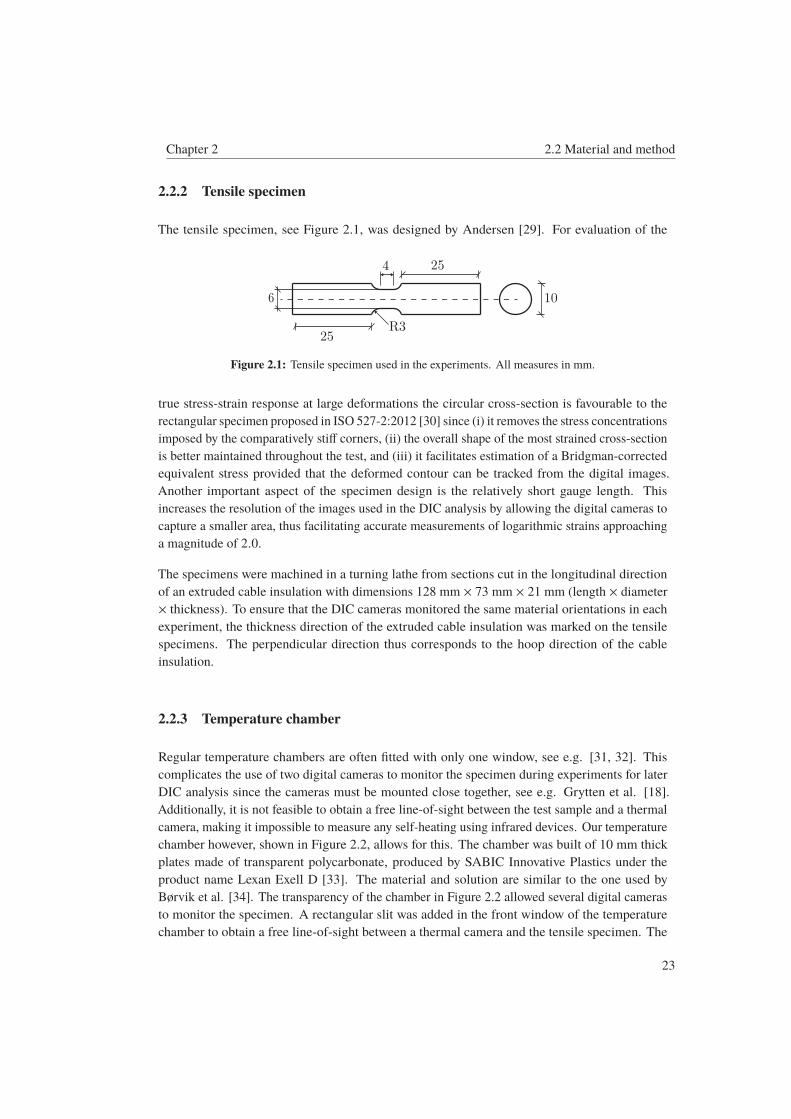
The tensile specimen, see Figure 2.1, was designed by Andersen [29]. For evaluation of the
25
25
106
4
R3
Figure 2.1: Tensile specimen used in the experiments. All measures in mm.
true stress-strain response at large deformations the circular cross-section is favourable to the
rectangular specimen proposed in ISO 527-2:2012 [30] since (i) it removes the stress concentrations
imposed by the comparatively stiff corners, (ii) the overall shape of the most strained cross-section
is better maintained throughout the test, and (iii) it facilitates estimation of a Bridgman-corrected
equivalent stress provided that the deformed contour can be tracked from the digital images.
Another important aspect of the specimen design is the relatively short gauge length. This
increases the resolution of the images used in the DIC analysis by allowing the digital cameras to
capture a smaller area, thus facilitating accurate measurements of logarithmic strains approaching
a magnitude of 2.0.
The specimens were machined in a turning lathe from sections cut in the longitudinal direction
of an extruded cable insulation with dimensions 128 mm × 73 mm × 21 mm (length × diameter
× thickness). To ensure that the DIC cameras monitored the same material orientations in each
experiment, the thickness direction of the extruded cable insulation was marked on the tensile
specimens. The perpendicular direction thus corresponds to the hoop direction of the cable
insulation.
2.2.3 Temperature chamber
Regular temperature chambers are often fitted with only one window, see e.g. [31, 32]. This
complicates the use of two digital cameras to monitor the specimen during experiments for later
DIC analysis since the cameras must be mounted close together, see e.g. Grytten et al. [18].
Additionally, it is not feasible to obtain a free line-of-sight between the test sample and a thermal
camera, making it impossible to measure any self-heating using infrared devices. Our temperature
chamber however, shown in Figure 2.2, allows for this. The chamber was built of 10 mm thick
plates made of transparent polycarbonate, produced by SABIC Innovative Plastics under the
product name Lexan Exell D [33]. The material and solution are similar to the one used by
Børvik et al. [34]. The transparency of the chamber in Figure 2.2 allowed several digital cameras
to monitor the specimen. A rectangular slit was added in the front window of the temperature
chamber to obtain a free line-of-sight between a thermal camera and the tensile specimen. The
23

2.2 Material and method Chapter 2
600
320180
Figure 2.2: Temperature chamber used in the experiments. All measures in mm.
temperature in the chamber was governed by a thermocouple temperature sensor controlling the
flow of liquid nitrogen through the small hole in one of the narrow side walls of the chamber. To
ensure that the desired temperature was obtained at the most critical cross-section of the tensile
specimen, the sensor was mounted close to the gauge section.
Circular holes were added in the top and in the bottom of the chamber to allow mounting of the
test specimen in the tensile rig without impairing the seal of the chamber.
2.2.4 Experimental set-up
The test set-up is illustrated in Figures 2.3 and 2.4. In addition to the temperature chamber and an
Nitrogeninlet
Tensile specimen
Temperaturechamber
320
180
10Therm
al
camera
DIC
cam
era
DICcamera
Air flowfrom fan
SlitAir flowfrom fan
Figure 2.3: Section view of the set-up used in the experiments. All measures in mm. The distance to the
three cameras is not drawn in scale.
24

Chapter 2 2.2 Material and method
Instron 5944 testing machine with a 2 kN load cell, it involves two Prosilica GC2450 cameras
equipped with Sigma 105 mm and Nikon 105 mm macrolenses. Both cameras were positioned at
a distance of approximately 25-35 cm from the tensile specimen, giving a resolution of roughly
60 pixels/mm. The two cameras were used to measure the transverse strain in both the thickness
Figure 2.4: Picture showing the experimental set-up. Note that neither the front window nor the tensile
specimen is mounted.
direction and the hoop direction of the cable insulation, in addition to the longitudinal strain.
Moreover, a FLIR SC 7500 thermal camera was used to measure any possible self-heating in the
specimen during the test. It also served to check that the surface temperature of the sample was
the same as the gas temperature in the chamber.
Traditionally, a spray paint is used to apply a random black and white speckle which deforms
along with the specimen. This deformation is monitored by the DIC cameras and transformed into
strain by correlating the current deformed speckle to a reference. However, when the temperature
drops, the spray paint becomes brittle and cracks even at relatively small strains, as illustrated
in Figure 2.5. To prevent this, the spray paint was replaced by white grease, with black powder
added to follow the deformation, see Figure 2.5. The black powder had a grain size from 75 μm to
125 μm. This set-up showed no signs of cracking, even at large strains.
In the preliminary experiments there were also problems with icing due to condensation on the
outside of the chamber. The solution was to mount fans in the positions indicated in Figure
2.3. The continuous flow of air over the transparent walls of the chamber successfully prevented
condensation and icing.
The tensile tests were carried out at four different temperatures; 25 ◦C, 0 ◦C, −15 ◦C and −30 ◦C;
with two repetitions per test configuration. All experiments were conducted at an initial nominal
strain rate of 10−2 s−1, translating to a cross-head velocity of 2.4 mm/min.
25
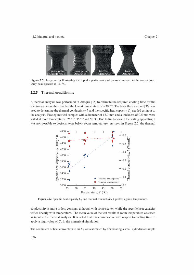
2.2 Material and method Chapter 2
Figure 2.5: Image series illustrating the superior performance of grease compared to the conventional
spray-paint speckle at −30 ◦C.
2.2.5 Thermal conditioning
A thermal analysis was performed in Abaqus [35] to estimate the required cooling time for the
specimens before they reached the lowest temperature of −30 ◦C. The laser flash method [36] was
used to determine the thermal conductivity k and the specific heat capacity Cp needed as input to
the analysis. Five cylindrical samples with a diameter of 12.7 mm and a thickness of 0.5 mm were
tested at three temperatures: 25 ◦C, 35 ◦C and 50 ◦C. Due to limitations in the testing apparatus, it
was not possible to perform tests below room temperature. As seen in Figure 2.6, the thermal
25 30 35 40 45 50 55
Temperature, T (◦C)
3000
3200
3400
3600
3800
4000
4200
4400
4600
4800
Spec
ific
hea
tca
pac
ity,
Cp
(J/(
kgK
))
Specific heat capacity
Thermal conductivity
0.0
0.1
0.2
0.3
0.4
0.5
0.6
Ther
mal
conduct
ivit
y,k
(W/(
mK
))
Figure 2.6: Specific heat capacity Cp and thermal conductivity k plotted against temperature.
conductivity is more or less constant, although with some scatter, while the specific heat capacity
varies linearly with temperature. The mean value of the test results at room temperature was used
as input to the thermal analysis. It is noted that it is conservative with respect to cooling time to
apply a high value of Cp in the numerical simulation.
The coefficient of heat convection to air hc was estimated by first heating a small cylindrical sample
26

Chapter 2 2.2 Material and method
with dimensions 20 mm × 5 mm (diameter × height) in boiling water, followed by monitoring
the temperature decrease in the specimen using an infrared thermometer. From the recorded
temperature history the heat convection to air was found to be about 21 W/(m2K).
A 3D model of the tensile specimen was made in Abaqus, consisting of 51728 DC3D8 elements.
Input parameters used in the Abaqus analysis are given in Table 2.1. The interior of the specimen
Table 2.1: Input parameters used in thermal analysis.
Specific heat capacity, Cp Thermal conductivity, k Heat convection to air, hc Density, ρ(J/(kg·K)) (W/(m·K)) (W/(m2·K)) (kg/m3)
3546 0.56 21.0 922
was given an initial temperature of 25 ◦C, while at the exterior a thermal boundary condition of
−30 ◦C was applied as a surface film. Analysis results showed that a preconditioning time of 30min was sufficient to cool the specimen. Thus, each sample was put in the chamber 30 min before
it was tested.
2.2.6 Determination of true stress and logarithmic strain
True stress, σ, is defined as
σ =FA
(2.1)
where F is the applied force and A is the current cross-section area. The current cross-section
area is calculated from the assumption that the transverse stretches in the thickness direction and
in the hoop direction of the cable insulation represent the stretches along the minor and major axis
of an elliptical cross-section, i.e.:
A = πλTλ⊥r20 (2.2)
where λT = rT/r0 is the stretch in the thickness direction, λ⊥ = r⊥/r0 is the stretch in the hoop
direction and r0 is the initial radius of the undeformed specimen in the gauge area. The transverse
stretches in both the thickness direction and the hoop direction are calculated as the average value
over the cross-section in the neck.
The images from the tensile tests were post-processed using an in-house DIC software [29] written
in MATLAB [37]. From this software we obtain the deformation gradient F, which enables the
calculation of the stretch tensor U from the polar decomposition F = RU. Now we can calculate
the logarithmic strain tensor by taking the logarithm of the stretch tensor, viz.
εε = ln (U) = N ln(U)NT (2.3)
27

2.3 Results and discussion Chapter 2
where N contains the eigenvectors of U and U is the eigentensor. Note that for uniaxial tension
U = U such that
εε =
⎡⎢⎢⎢⎢⎢⎢⎣εL 0 00 εT 00 0 ε⊥
⎤⎥⎥⎥⎥⎥⎥⎦=
⎡⎢⎢⎢⎢⎢⎢⎣ln (λL) 0 0
0 ln (λT) 00 0 ln (λ⊥)
⎤⎥⎥⎥⎥⎥⎥⎦(2.4)
where λL = L/L0 is the longitudinal stretch.
The logarithmic volumetric strain is defined as the trace of the logarithmic strain tensor. However,
as the logarithmic strain tensor estimated here represents an average over the gauge volume, it has
been found necessary to correct the volumetric strain for the non-uniformity of the strain field.
An appropriate correction was proposed by Andersen [29], which takes the heterogeneity of the
longitudinal strain in the neck into account. The corrected volumetric strain reads
εV,corr = ln(
VV0
)= ln
[λLλTλ⊥ ·
(1 +
κR4
)](2.5)
= tr (εε) + ln(1 +
κR4
)
where κ is the external curvature of the neck, and R is the current radius in the neck. The current
values of κ and R are found from the digital images taken during the tests. This correction removes
the unphysical negative volumetric strain in the beginning of the tension test, as shown in Section
2.3.3.
2.3 Results and discussion
2.3.1 Evaluation of experimental set-up
When the tensile specimen deforms, and eventually necks, the surface of the sample translates and
rotates in the out-of-plane direction. A quasi-static tensile test was conducted at room temperature
to compare the calculated strains from 2D DIC and 3D DIC. An in-house DIC software [29]
applying a higher-order element for description of the deformation field, was employed in the 2D
case. The analysis with 3D DIC was carried out using the in-house DIC software eCorr [38].
Based on the DIC analysis we obtain the displacement field u, enabling the calculation of the
deformation gradient F. From the deformation gradient the strains are calculated following the
procedure outlined in Section 2.2.6. The interested reader is referred to Fagerholt et al. [39, 40]
for a thorough explanation of how the displacement field u is found from the digital images.
The representative strain was calculated from the average value of the longitudinal stretch for the
elements highlighted in Figure 2.7.
28

Chapter 2 2.3 Results and discussion
Figure 2.7: Front and side view of the 3D DIC mesh at a maximal stretch in the neck of about 1.55. The
elements used in the strain calculations are highlighted by the white box.
Figure 2.8 shows that the difference between 2D (both cameras) and 3D DIC remains below
1.0% during the experiment, meaning that the error introduced in 2D DIC by the out-of-plane
translation of the specimen during deformation is acceptable. Therefore 2D DIC was chosen for
0 200 400 600 800 1000 1200 1400
Time (s)
1
2
3
4
5
6
Lo
ng
itu
din
alst
retc
h,λ L
3D DIC
2D DIC Camera 1
2D DIC Camera 2
diff(3D & Cam1)
diff(3D & Cam2)
0.0
0.2
0.4
0.6
0.8
1.0
Rel
ativ
ed
iffe
ren
ce(%
)
Figure 2.8: Comparison of longitudinal stretch for XLPE calculated by 3D and 2D DIC. The dashed lines
give the relative percentage difference between 3D DIC and 2D DIC for camera 1 and camera 2.
the subsequent data processing.
To verify that there was no influence on the DIC results neither by the replacement of spray-paint
with grease nor by introducing the polycarbonate window between the cameras and the sample,
three tests were conducted at room temperature on a rubber modified polypropylene (PP) material:
29

2.3 Results and discussion Chapter 2
First a test with a traditional spray-paint speckle, then a test with the spray-paint speckle behind a
polycarbonate window, and finally a test where the spray-paint speckle was replaced with white
grease and black powder. Using the transverse strains and the relation λi = exp (εi), the true stress
was calculated following the procedure given in Section 2.2.6. The DIC analyses of the three tests
revealed only negligible differences, illustrated by the three stress-strain curves in Figure 2.9a
and the three curves representing the trace of the logarithmic strain tensor versus the logarithmic
longitudinal strain in Figure 2.9b.
0.0 0.5 1.0 1.5 2.0
Logarithmic longitudinal strain, εL
0
20
40
60
80
100
120
140
Tru
est
ress
,σ
(MP
a)
Spray-paint
Spray-paint + polycarbonate window
Grease
(a)
0.0 0.5 1.0 1.5 2.0
Logarithmic longitudinal strain, εL
0.0
0.1
0.2
0.3
0.4
0.5
0.6
Tra
ceof
logar
ithm
icst
rain
tenso
r,tr(εε ε)
Spray-paint
Spray-paint + polycarbonate window
Grease
(b)
Figure 2.9: (a) True stress vs. logarithmic strain for the three benchmark tests performed on a polypropylene
copolymer material. (b) Trace of the logarithmic strain tensor vs. logarithmic longitudinal strain for the three
benchmark tests performed on a polypropylene copolymer material.
2.3.2 Stress-strain behaviour at different temperatures
The transverse strains, εt, as a function of longitudinal strain at room temperature are shown
in Figure 2.10 for the XLPE material, where εt is either equal to εT or ε⊥. Both transverse
strains have a close to linear relation with the longitudinal strain, but with different slopes. This
quasi-linear relation is also reflected in the moderate variation of the transverse strain ratios
r = ε⊥/εT shown in the same figure, which lies between approximately 1.1 and 1.0 for the four
investigated temperatures. These results demonstrate the transverse anisotropy of XLPE and the
necessity of using two cameras to capture this effect. The stress-strain curves for XLPE at the
four investigated temperatures are presented in Figure 2.11, where the true stress is calculated
with Equations (2.1) and (2.2). It appears that Young’s modulus and the flow stress increase with
decreasing temperature. Another observation from Figure 2.11 is that the ductility of the material
30

Chapter 2 2.3 Results and discussion
0.0 0.2 0.4 0.6 0.8 1.0 1.2 1.4 1.6
Logarithmic longitudinal strain, εL
0.0
0.1
0.2
0.3
0.4
0.5
0.6
0.7
0.8
0.9
Logar
ithm
ictr
ansv
erse
stra
in,| ε t|
Hoop dir. (25 ◦C)
Thickness dir. (25 ◦C)
Transverse strain ratios25 ◦C
0 ◦C
−15 ◦C
−30 ◦C
0.5
0.6
0.7
0.8
0.9
1.0
1.1
1.2
Tra
nsv
erse
stra
inra
tio,r=
ε ⊥/ε
T
Figure 2.10: Logarithmic transverse strain for XLPE in the hoop (⊥) and in the thickness direction (T) at
room temperature, and the transverse strain ratios for all investigated temperatures plotted against logarithmic
longitudinal strain.
is more or less independent of temperature in the experimental range, making it well suited for
low temperature applications. The uniaxial tension tests performed at −15 ◦C and −30 ◦C have a
fracture strain of about 1.4, while the fracture strain in the tests carried out at 0 ◦C and 25 ◦C is
roughly 1.6, i.e., 14% increase compared to the two lower temperatures. It is however noted that
the network hardening occurring at strains larger than approximately 1.3 is less prominent at the
two lowest temperatures, and that the initial strain hardening clearly has increased compared to the
two highest temperatures.
0.0 0.2 0.4 0.6 0.8 1.0 1.2 1.4 1.6
Logarithmic longitudinal strain, εL
0
20
40
60
80
100
Tru
est
ress
,σ
(MP
a)
−30 ◦C
−15 ◦C
0 ◦C
25 ◦C
Figure 2.11: True stress vs. logarithmic longitudinal strain for XLPE at different temperatures.
31

2.3 Results and discussion Chapter 2
Both the flow stress, σ20, defined as the stress magnitude at a longitudinal strain of 0.2 (= 20%),
and the initial stiffness, E, can be represented through the exponential relations
E(θ) = E0 exp (a/θ) (2.6)
σ20(θ) = C exp (b/θ) (2.7)
where a, b, E0 and C are material parameters and θ is the absolute temperature. Figure 2.12 shows
the calculated Young’s modulus and flow stress versus temperature as well as the least square
fits of Equations (2.6) and (2.7). Note that these expressions are valid only for the investigated
temperature range.
240 250 260 270 280 290 300
Absolute temperature, θ (K)
10
15
20
25
30
35
Flo
wst
ress
,σ 2
0(θ
)(M
Pa)
Flow stress
Young’s modulus
σ20(θ) = 0.114exp(1359/θ)E(θ) = 0.049exp(2380/θ)
100
200
300
400
500
600
700
800
900
1000
Young’s
modulu
s,E(θ
)(M
Pa)
Figure 2.12: Evolution of flow stress and Young’s modulus as a function of temperature for XLPE.
2.3.3 Volumetric strains at different temperatures
The logarithmic volumetric strain for XLPE calculated as the trace of the logarithmic strain tensor
is given in Figure 2.13a, while the corrected volumetric strain calculated according to Equation
(2.5) is given in Figure 2.13b. Since the grease was applied by hand, it was impossible to distribute
it evenly over the gauge section. This made it difficult to approximate the curvature, κ, by tracing
the edges of the specimen, which is needed in Equation (2.5). As an alternative method, we chose
to fit a second-order polynomial to the element boundaries of the DIC mesh, and to calculate
the curvature by taking the second-order derivative of this polynomial. Since the curvature is
zero in the cold drawing phase at the end of the test (Figure 2.14), this approximation will not
affect the final volumetric strain, but it removes the unphysical negative volumetric strain seen
in Figure 2.13a. This approximation of the curvature might be the explanation for the minor
difference between the volumetric strain at small εL for the test performed at −15 ◦C and the tests
32

Chapter 2 2.3 Results and discussion
0.0 0.2 0.4 0.6 0.8 1.0 1.2 1.4 1.6 1.8
Logarithmic longitudinal strain, εL
−0.04
−0.02
0.00
0.02
0.04
0.06
0.08
0.10
0.12
Tra
ceof
logar
ithm
icst
rain
tenso
r,tr(εε ε) −30 ◦C
−15 ◦C
0 ◦C
25 ◦C
(a)
0.0 0.2 0.4 0.6 0.8 1.0 1.2 1.4 1.6 1.8
Logarithmic longitudinal strain, εL
0.00
0.02
0.04
0.06
0.08
0.10
0.12
Logar
ithm
icvolu
met
ric
stra
in,ε V
,corr
−30 ◦C
−15 ◦C
0 ◦C
25 ◦C
(b)
Figure 2.13: (a) Trace of the logarithmic strain tensor vs. logarithmic longitudinal strain for XLPE. (b)
Corrected logarithmic volumetric strain using Equation (2.5) vs. logarithmic longitudinal strain for XLPE.
at 0 ◦C and −30 ◦C in Figure 2.13b. Nevertheless, in both figures we see that the volumetric strain
increases for the lower temperatures compared to the response at room temperature where the
volumetric strain is close to 0 at all deformation levels. Since there was no stress whitening during
deformation, and that this material is tailored to include as few free particles as possible, it is
not obvious that the increase in volumetric strain is caused by material damage. However, how
much of this volumetric strain that is recoverable has not been investigated. Therefore, it would be
Figure 2.14: Time lapse showing the deformation history of the tensile specimen.
33

2.4 Concluding remarks Chapter 2
interesting to perform loading/unloading tests at lower temperatures in further work.
2.3.4 Self-heating at different temperatures
The temperature data recorded by the thermal camera showed no significant self-heating of the
specimen at the applied nominal strain rate of 10−2 s−1, indicating isothermal loading conditions.
However, if the experiments had been conducted at higher strain rates, there would most likely
have been a substantial temperature increase in the specimen. This experimental set-up could
provide important input to any numerical model incorporating thermal softening.
2.4 Concluding remarks
A non-contact optical method for determining the large-strain tensile behaviour of polymers at
low temperatures has been presented. The method successfully enables multiple DIC camera
instrumentation during experiments, as well as the possibility to monitor self-heating in the
specimen using a thermal camera. Since any temperature increase in the material due to self-
heating introduces material softening, the ability to measure this using for instance a thermal camera
is highly relevant for the development of material models to be used in numerical simulations.
The experimental set-up enables calculation of the true stress vs. logarithmic strain curve and
the volumetric strain at low temperatures. Although the XLPE material exhibits rather small
volumetric strain, this is not necessarily the case for all polymeric materials. In addition to this,
the ability to monitor self-heating underlines the relevance of the presented experimental set-up,
especially when considering how important volumetric strain and self-heating is in material models
that include damage and thermal softening.
The investigated material (XLPE) exhibits an exponential increase in both the initial stiffness and
the flow stress when the temperature is reduced within the experimental range. In addition, the
reduction of temperature changes the material from nearly incompressible at room temperature to
compressible at lower temperatures.
Acknowledgements
The authors wish to thank the Research Council of Norway for funding through the Petromaks 2
Programme, Contract No.228513/E30. The financial support from ENI, Statoil, Lundin, Total,
Scana Steel Stavanger, JFE Steel Corporation, Posco, Kobe Steel, SSAB, Bredero Shaw, Borealis,
Trelleborg, Nexans, Aker Solutions, FMC Kongsberg Subsea, Marine Aluminium, Hydro and
Sapa are also acknowledged. Special thanks is given to Nexans Norway and Borealis for providing
the material. Mr. Trond Auestad and Mr. Tore Wisth are acknowledged for their invaluable help
in developing the experimental set-up and performing the experiments.
34

Chapter 2 References
References
[1] Gautier, D. L., Bird, K. J., Charpentier, R. R., Grantz, A., Houseknecht, D. W., Klett, T. R.,
Moore, T. E., Pitman, J. K., Schenk, C. J., Schuenemeyer, J. H., Sørensen, K., Tennyson,
M. E., Valin, Z. C., and Wandrey, C. J. “Assessment of Undiscovered Oil and Gas in the
Arctic”. Science 324 (2009), pp. 1175–1179. doi: 10.1126/science.1169467.
[2] Arruda, E. M., Boyce, M. C., and Jayachandran, R. “Effects of strain rate, temperature
and thermomechanical coupling on the finite strain deformation of glassy polymers”.
Mechanics of Materials 19 (1995), pp. 193–212. doi: 10.1016/0167-6636(94)00034-E.
[3] Zaroulis, J. and Boyce, M. “Temperature, strain rate, and strain state dependence of the
evolution in mechanical behaviour and structure of poly(ethylene terephthalate) with
finite strain deformation”. Polymer 38 (1997), pp. 1303–1315. doi: 10.1016/S0032-3861(96)00632-5.
[4] van Breemen, L. C. A., Engels, T. A. P., Klompen, E. T. J., Senden, D. J. A., and
Govaert, L. E. “Rate- and temperature-dependent strain softening in solid polymers”.
Journal of Polymer Science, Part B: Polymer Physics 50 (2012), pp. 1757–1771. doi:10.1002/polb.23199.
[5] Zaïri, F., Naït-Abdelaziz, M., Gloaguen, J. M., and Lefebvre, J. M. “Constitutive
modelling of the large inelastic deformation behaviour of rubber-toughened poly(methyl
methacrylate): effects of strain rate, temperature and rubber-phase volume fraction”.
Modelling and Simulation in Materials Science and Engineering 18 (2010), p. 055004.
doi: 10.1088/0965-0393/18/5/055004.
[6] Nasraoui, M., Forquin, P., Siad, L., and Rusinek, A. “Influence of strain rate, temperature
and adiabatic heating on the mechanical behaviour of poly-methyl-methacrylate: Exper-
imental and modelling analyses”. Materials and Design 37 (2012), pp. 500–509. doi:10.1016/j.matdes.2011.11.032.
[7] Srivastava, V., Chester, S. A., Ames, N. M., and Anand, L. “A thermo-mechanically-
coupled large-deformation theory for amorphous polymers in a temperature range which
spans their glass transition”. International Journal of Plasticity 26 (2010), pp. 1138–1182.
doi: 10.1016/j.ijplas.2010.01.004.
[8] Llana, P. and Boyce, M. “Finite strain behavior of poly(ethylene terephthalate) above the
glass transition temperature”. Polymer 40 (Nov. 1999), pp. 6729–6751. doi: 10.1016/S0032-3861(98)00867-2.
[9] Bauwens-Crowet, C., Bauwens, J. C., and Homès, G. “Tensile yield-stress behavior
of glassy polymers”. Journal of Polymer Science Part A-2: Polymer Physics 7 (1969),
pp. 735–742. doi: 10.1002/pol.1969.160070411.
[10] Bauwens-Crowet, C., Bauwens, J. C., and Homès, G. “The temperature dependence of
yield of polycarbonate in uniaxial compression and tensile tests”. Journal of MaterialsScience 7 (1972), pp. 176–183. doi: 10.1007/BF00554178.
35

References Chapter 2
[11] Bauwens, J. C. “Relation between the compression yield stress and the mechanical loss
peak of bisphenol-A-polycarbonate in the β transition range”. Journal of MaterialsScience 7 (1972), pp. 577–584. doi: 10.1007/BF00761956.
[12] Bauwens-Crowet, C. “The compression yield behaviour of polymethyl methacrylate over
a wide range of temperatures and strain-rates”. Journal of Materials Science 8 (1973),
pp. 968–979. doi: 10.1007/BF00756628.
[13] Jang, B. Z., Uhlmann, D. R., and Sande, J. B. V. “Ductile–brittle transition in polymers”.
Journal of Applied Polymer Science 29 (1984), pp. 3409–3420. doi: 10.1002/app.1984.070291118.
[14] Şerban, D. A., Weber, G., Marşavina, L., Silberschmidt, V. V., and Hufenbach, W. “Tensile
properties of semi-crystalline thermoplastic polymers: Effects of temperature and strain
rates”. Polymer Testing 32 (2013), pp. 413–425. doi: 10.1016/j.polymertesting.2012.12.002.
[15] Brown, E. N., Rae, P. J., and Orler, E. B. “The influence of temperature and strain rate on
the constitutive and damage responses of polychlorotrifluoroethylene (PCTFE, Kel-F
81)”. Polymer 47 (2006), pp. 7506–7518. doi: 10.1016/j.polymer.2006.08.032.
[16] Cao, K., Wang, Y., and Wang, Y. “Effects of strain rate and temperature on the tension
behavior of polycarbonate”. Materials and Design 38 (2012), pp. 53–58. doi: 10.1016/j.matdes.2012.02.007.
[17] Richeton, J., Ahzi, S., Vecchio, K., Jiang, F., and Adharapurapu, R. “Influence of
temperature and strain rate on the mechanical behavior of three amorphous polymers:
Characterization and modeling of the compressive yield stress”. International Journal ofSolids and Structures 43 (2006), pp. 2318–2335. doi: 10.1016/j.ijsolstr.2005.06.040.
[18] Grytten, F., Daiyan, H., Polanco-Loria, M., and Dumoulin, S. “Use of digital image
correlation to measure large-strain tensile properties of ductile thermoplastics”. PolymerTesting 28 (2009), pp. 653–660. doi: 10.1016/j.polymertesting.2009.05.009.
[19] Delhaye, V., Clausen, A. H., Moussy, F., Othman, R., and Hopperstad, O. S. “Influence of
stress state and strain rate on the behaviour of a rubber-particle reinforced polypropylene”.
International Journal of Impact Engineering 38 (2011), pp. 208–218. doi: 10.1016/j.ijimpeng.2010.11.004.
[20] Ognedal, A. S., Clausen, A. H., Polanco-Loria, M., Benallal, A., Raka, B., and Hopperstad,
O. S. “Experimental and numerical study on the behaviour of PVC and HDPE in biaxial
tension”. Mechanics of Materials 54 (2012), pp. 18–31. doi: 10.1016/j.mechmat.2012.05.010.
[21] Jerabek, M., Major, Z., and Lang, R. W. “Strain determination of polymeric materials
using digital image correlation”. Polymer Testing 29 (2010), pp. 407–416. doi: 10.1016/j.polymertesting.2010.01.005.
36

Chapter 2 References
[22] Heinz, S. R. and Wiggins, J. S. “Uniaxial compression analysis of glassy polymer
networks using digital image correlation”. Polymer Testing 29 (2010), pp. 925–932. doi:10.1016/j.polymertesting.2010.08.001.
[23] Besnard, G., Hild, F., Lagrange, J.-M., Martinuzzi, P., and Roux, S. “Analysis of
necking in high speed experiments by stereocorrelation”. International Journal of ImpactEngineering 49 (2012), pp. 179–191. doi: 10.1016/j.ijimpeng.2012.03.005.
[24] Gilat, A., Schmidt, T. E., and Walker, A. L. “Full Field Strain Measurement in Compression
and Tensile Split Hopkinson Bar Experiments”. Experimental Mechanics 49 (2 2009),
pp. 291–302. doi: 10.1007/s11340-008-9157-x.
[25] Sutton, M. A., Yan, J. H., Tiwari, V., Schreier, H. W., and Orteu, J. J. “The effect of out-of-
plane motion on 2D and 3D digital image correlation measurements”. Optics and Lasersin Engineering 46 (2008), pp. 746–757. doi: 10.1016/j.optlaseng.2008.05.005.
[26] Ilseng, A., Skallerud, B. H., and Clausen, A. H. “Tension behaviour of HNBR and FKM
elastomers for a wide range of temperatures”. Polymer Testing 49 (2016), pp. 128–136.
doi: 10.1016/j.polymertesting.2015.11.017.
[27] Molykote 33 Extreme Low Temp. Bearing Grease, Medium. https://www.dowcorning.
com/applications/search/products/Details.aspx?prod=01889788&type=
PROD. Accessed:2016-04-04.
[28] Borlink LS4201S. http://www.borealisgroup.com/en/polyolefins/products/
Borlink/Borlink-LS4201S/. Accessed:2016-1116.
[29] Andersen, M. “An experimental and numerical study of thermoplastics at large de-
formations”. PhD thesis. Norwegian University of Science and Technology, NTNU,
2016.
[30] ISO527-2:2012. Plastics - Determination of tensile properties - Part 2: Test conditionsfor moulding and extrusion plastics. Feb. 2012.
[31] Zwick, Temperature chambers. https://www.zwick.com/en/systems- for-climate-and-temperature-testing/temperature-chamber-80-to-250-c.
Accessed:2017-01-17.
[32] Zhang, H., Yao, Y., Zhu, D., Mobasher, B., and Huang, L. “Tensile mechanical properties
of basalt fiber reinforced polymer composite under varying strain rates and temperatures”.
Polymer Testing 51 (2016), pp. 29–39. doi: 10.1016/j.polymertesting.2016.02.006.
[33] Lexan Exell D. http://sfs.sabic.eu/product/lexan- solid- sheet/uv-
protected/. Accessed:2016-03-21.
[34] Børvik, T., Lange, H., Marken, L. A., Langseth, M., Hopperstad, O. S., Aursand, M., and
Rørvik, G. “Pipe fittings in duplex stainless steel with deviation in quality caused by sigma
phase precipitation”. Materials Science and Engineering A 527 (2010), pp. 6945–6955.
doi: 10.1016/j.msea.2010.06.087.
[35] Abaqus. 6.13-1. Dassault Systemes, 2013.
37
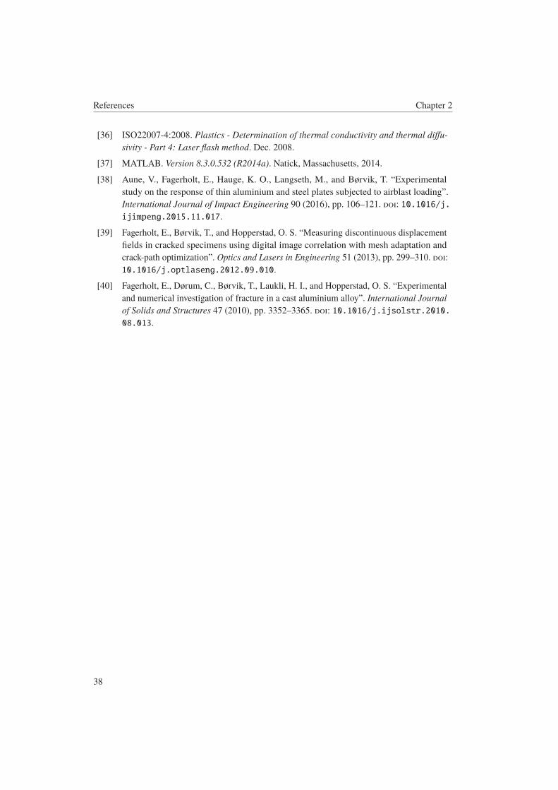
References Chapter 2
[36] ISO22007-4:2008. Plastics - Determination of thermal conductivity and thermal diffu-sivity - Part 4: Laser flash method. Dec. 2008.
[37] MATLAB. Version 8.3.0.532 (R2014a). Natick, Massachusetts, 2014.
[38] Aune, V., Fagerholt, E., Hauge, K. O., Langseth, M., and Børvik, T. “Experimental
study on the response of thin aluminium and steel plates subjected to airblast loading”.
International Journal of Impact Engineering 90 (2016), pp. 106–121. doi: 10.1016/j.ijimpeng.2015.11.017.
[39] Fagerholt, E., Børvik, T., and Hopperstad, O. S. “Measuring discontinuous displacement
fields in cracked specimens using digital image correlation with mesh adaptation and
crack-path optimization”. Optics and Lasers in Engineering 51 (2013), pp. 299–310. doi:10.1016/j.optlaseng.2012.09.010.
[40] Fagerholt, E., Dørum, C., Børvik, T., Laukli, H. I., and Hopperstad, O. S. “Experimental
and numerical investigation of fracture in a cast aluminium alloy”. International Journalof Solids and Structures 47 (2010), pp. 3352–3365. doi: 10.1016/j.ijsolstr.2010.08.013.
38

Part 2
The content of this part was published in:
Johnsen, J., Grytten, F., Hopperstad, O. S., and Clausen, A. H. (2017). Influence of strain rate andtemperature on the mechanical behaviour of rubber-modified polypropylene and cross-linkedpolyethylene. Mechanics of Materials, 114, 40–56.
https://doi.org/10.1016/j.mechmat.2017.07.003
Abstract
In the present work, we investigate the effects of strain rate (e = 0.01 s−1, 0.1 s−1, and 1.0 s−1)
and low temperature (T = −30 ◦C, −15 ◦C, 0 ◦C, and 25 ◦C) on the mechanical behaviour in
tension and compression of two materials: a rubber-modified polypropylene copolymer (PP) and a
cross-linked low-density polyethylene (XLPE). Local stress-strain data for large deformations are
obtained using digital image correlation (DIC) in the uniaxial tension tests and point tracking in the
compression tests. Since both materials exhibit slight transverse anisotropy, two digital cameras are
used to capture the strains on two perpendicular surfaces. Self-heating resulting from the elevated
strain rates is monitored using an infrared (IR) camera. To enable the application of multiple
digital cameras and an IR camera, a purpose-built transparent polycarbonate temperature chamber
is used to create a cold environment for the tests. The mechanical behaviour of both materials,
including the true stress-strain response and the volume change, is shown to be dependent on the
temperature and strain rate. The dependence of the yield stress on the temperature and strain rate
follows the Ree-Eyring flow theory for both materials, whereas Young’s modulus increases with
decreasing temperature for PP and XLPE and with increasing strain rate for XLPE. Furthermore,
a scanning electron microscope (SEM) study was performed on both materials to get a qualitative
understanding of the volumetric strains.


Chapter 3
Influence of strain rate and temperature on themechanical behaviour of rubber-modifiedpolypropylene and cross-linked polyethylene
3.1 Introduction
In recent years, there has been increased interest in using polymeric materials in structural
applications. The automotive industry, for example, is using polymeric materials in their
pedestrian safety devices as sacrificial components that are designed to dissipate energy during
impacts. An important point in this context is that material characterization and impact tests are
performed close to room temperature, thus failing to account for changes in material behaviour as
the temperature decreases. At low temperatures, polymeric materials tend to be both stiffer and
more brittle, which could have severe consequences in a collision between a car and a pedestrian.
Considering the cost of conducting prototype testing, it is clear that increased knowledge regarding
the material behaviour at different temperatures is highly relevant.
The oil and gas industry is also interested in polymeric materials. As they continue to explore and
search for oil and gas in harsher climates, new classification rules for materials are needed. There
is an increasing need to understand how polymers behave at low temperatures due to this industry’s
expansion into the arctic region. There are various relevant structural applications for polymers in
the oil industry, ranging from polymeric shock absorbers in load-bearing structures to gaskets used
in pressurized components. In particular, for the two materials considered in this work, cross-linked
low-density polyethylene (XLPE) is used as electrical insulation in high-voltage cables and as
a liner material in flexible risers, while one application for rubber-modified polypropylene (PP)
is thermal insulation of pipelines. As in the automotive industry, prototype testing is expensive;
therefore, there is a demand for validated material models in finite element codes to reduce the
number of experiments necessary to qualify a given material.
Reliable and good experimental data are a prerequisite for developing and improving phenomeno-

3.1 Introduction Chapter 3
logical material models. At room temperature, the use of non-contact measuring devices to extract
local stress-strain data from mechanical tests on polymeric materials has become widespread
[1–3]. Digital image correlation (DIC) is an important tool because it enables local measurements
of the strains (both longitudinal and transverse) in the neck of a tension test, which differs from
an extensometer that provides average strains over a section. Therefore, by using DIC, local
measurements of the volumetric strain are obtainable – a quantity that is useful for determining the
plastic potential and for including damage modelling. However, when a temperature chamber is
introduced, either to increase or decrease the temperature, the view of the specimen is obstructed.
Most commercially available temperature chambers have only one window. This limits the number
of possible digital cameras in the experimental set-up to one, thereby making the monitoring
technique suitable only for isotropic materials. Consequently, many researchers use mechanical
measuring devices such as extensometers or machine displacement to obtain stress-strain data
when using a temperature chamber. Such instrumentation protocols will only reveal the average
strain over the gauge length. Nevertheless, using these measurement techniques, a number of
studies [4–9] have investigated the effects of increased temperature and strain rate on the material
behaviour. In all these studies, the typical polymer behaviour is observed, i.e., increasing the
strain rate increases the yield stress, whereas increasing the temperature decreases the yield stress.
However, only the study by Arruda et al. [4] was conducted using an infrared (IR) sensor to
measure self-heating at elevated strain rates, while none of the studies [4–9] report the volumetric
strain. Similar studies considering the material behaviour at low temperatures [10–14] report the
same trend – decreasing the temperature and increasing the strain rate increases the yield stress. As
for the studies at elevated temperatures, the strain calculation relies on mechanical measurement
techniques. Neither self-heating nor change in volume is reported in any of these studies.
Previous studies have been conducted on materials comparable to the two materials of interest in
our study. For instance, Ponçot et al. [15] studied the volumetric strain at different strain rates in a
polypropylene/ethylene-propylene rubber using a VideoTraction system. Their results are similar
to the results obtained for the rubber-modified polypropylene material investigated in our study.
Using a linear variable differential transformer to measure the cross-head displacement, Jordan
et al. [16] conducted compression tests on low density polyethylene (LDPE) at four different
temperatures and eight strain rates. Considering the effect on the yield stress, they found that
an order of magnitude change in strain rate is approximately equal to a 10 degree change in
temperature. An extensive study on a cross-linked polyethylene (PEX) was conducted by Brown
et al. [17] utilizing a displacement extensometer. In their study, compression tests were conducted
at temperatures ranging from −75 ◦C to 100 ◦C, and strain rates from 10−4 s−1 to 2650 s−1.
Addiego et al. [18] characterized the volumetric strain in HDPE through uniaxial tension and
loading/unloading experiments at room temperature and strain rates from 10−4 s−1 to 5 · 10−3 s−1,
using the same VideoTraction system as Ponçot et al. [15].
Conventional temperature chambers also exclude the possibility of using an IR camera because
a free line-of-sight between the specimen and the IR camera is required. Since polymers
become softer at elevated temperatures, monitoring self-heating during a test is essential to
successfully separate the effects of strengthening due to rate sensitivity and softening due to
42
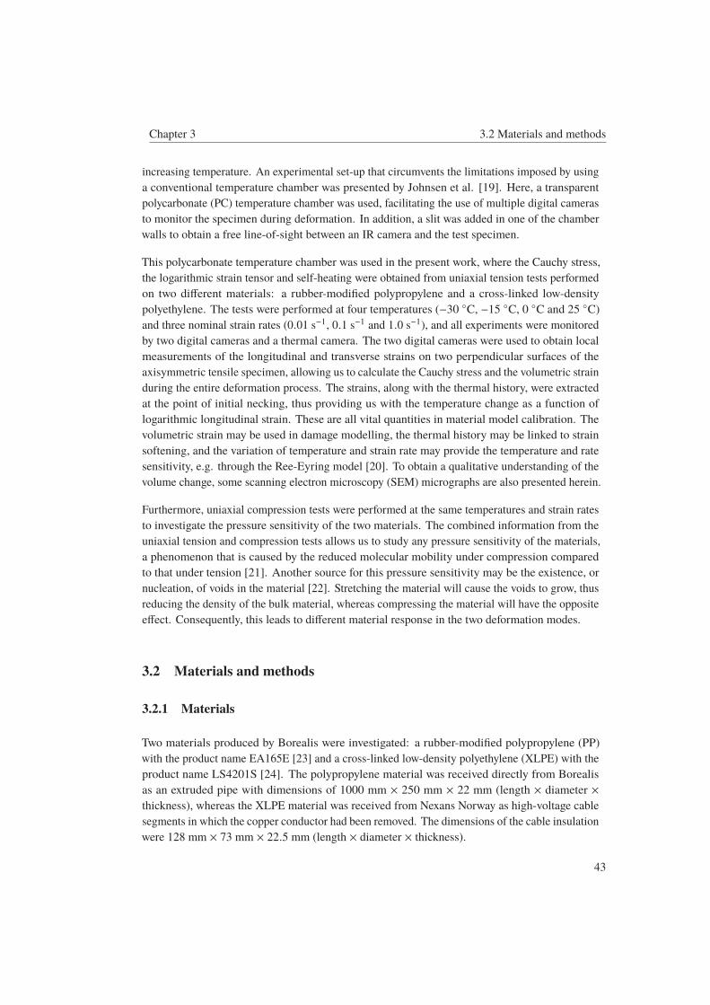
Chapter 3 3.2 Materials and methods
increasing temperature. An experimental set-up that circumvents the limitations imposed by using
a conventional temperature chamber was presented by Johnsen et al. [19]. Here, a transparent
polycarbonate (PC) temperature chamber was used, facilitating the use of multiple digital cameras
to monitor the specimen during deformation. In addition, a slit was added in one of the chamber
walls to obtain a free line-of-sight between an IR camera and the test specimen.
This polycarbonate temperature chamber was used in the present work, where the Cauchy stress,
the logarithmic strain tensor and self-heating were obtained from uniaxial tension tests performed
on two different materials: a rubber-modified polypropylene and a cross-linked low-density
polyethylene. The tests were performed at four temperatures (−30 ◦C, −15 ◦C, 0 ◦C and 25 ◦C)
and three nominal strain rates (0.01 s−1, 0.1 s−1 and 1.0 s−1), and all experiments were monitored
by two digital cameras and a thermal camera. The two digital cameras were used to obtain local
measurements of the longitudinal and transverse strains on two perpendicular surfaces of the
axisymmetric tensile specimen, allowing us to calculate the Cauchy stress and the volumetric strain
during the entire deformation process. The strains, along with the thermal history, were extracted
at the point of initial necking, thus providing us with the temperature change as a function of
logarithmic longitudinal strain. These are all vital quantities in material model calibration. The
volumetric strain may be used in damage modelling, the thermal history may be linked to strain
softening, and the variation of temperature and strain rate may provide the temperature and rate
sensitivity, e.g. through the Ree-Eyring model [20]. To obtain a qualitative understanding of the
volume change, some scanning electron microscopy (SEM) micrographs are also presented herein.
Furthermore, uniaxial compression tests were performed at the same temperatures and strain rates
to investigate the pressure sensitivity of the two materials. The combined information from the
uniaxial tension and compression tests allows us to study any pressure sensitivity of the materials,
a phenomenon that is caused by the reduced molecular mobility under compression compared
to that under tension [21]. Another source for this pressure sensitivity may be the existence, or
nucleation, of voids in the material [22]. Stretching the material will cause the voids to grow, thus
reducing the density of the bulk material, whereas compressing the material will have the opposite
effect. Consequently, this leads to different material response in the two deformation modes.
3.2 Materials and methods
3.2.1 Materials
Two materials produced by Borealis were investigated: a rubber-modified polypropylene (PP)
with the product name EA165E [23] and a cross-linked low-density polyethylene (XLPE) with the
product name LS4201S [24]. The polypropylene material was received directly from Borealis
as an extruded pipe with dimensions of 1000 mm × 250 mm × 22 mm (length × diameter ×thickness), whereas the XLPE material was received from Nexans Norway as high-voltage cable
segments in which the copper conductor had been removed. The dimensions of the cable insulation
were 128 mm × 73 mm × 22.5 mm (length × diameter × thickness).
43

3.2 Materials and methods Chapter 3
The physical properties of both materials are presented in Table 3.1. The densities were found
Table 3.1: Material properties for the PP and XLPE materials. All parameters are given for room temperature.
Material Density, ρ Specific heat capacity, Cp Thermal conductivity, k Heat convection to air, hc
(kg/m3) (J/(kg·K)) (W/(m·K)) (W/(m2·K))
XLPE 922 3546 0.56 21
PP 900 2756 0.31 18
from the datasheets supplied with the materials, whereas the specific heat capacity Cp and the
thermal conductivity k were determined using the laser flash method [25]. Five circular samples
with dimensions of 12.7 mm × 0.5 mm (diameter × thickness) of each material were heated to
three temperatures: 25 ◦C, 35 ◦C, and 50 ◦C. Subsequently, the specific heat capacity and thermal
conductivity were measured at each temperature level. The specific heat capacity increased almost
linearly with temperature, whereas the thermal conductivity exhibited little variation. The values
presented in Table 3.1 are the values obtained at room temperature. Heat convection to air, hc , was
determined by heating a small cylindrical sample with dimensions of 20 mm × 5 mm (diameter ×height) in boiling water. The temperature decay was monitored using an infrared thermometer,
and the heat convection to air was then calculated from the temperature-time history.
3.2.2 Test specimens
Axisymmetric specimens were used for both the tensile tests and the compression tests on the
PP and XLPE materials. However, since the XLPE is softer than the PP, it was not possible to
machine threads into the grips of the XLPE tensile specimens. The test specimens are illustrated
in Figure 3.1.
20 5
2054
M106
R3
(a)
25
254
106
R3
(b)
6
6
(c)
Figure 3.1: Schematics of (a) tensile test specimen for the PP material, (b) tensile test specimen for the
XLPE material, and (c) compression test specimen for both materials. All measures are in mm.
All specimens were machined in a turning lathe from sections cut from the longitudinal direction of
the extruded PP pipe and the extruded XLPE cable insulation. The radial direction was marked on
the test specimens such that it could be distinguished from the hoop direction when the specimen
was mounted in the test rig, see Figure 3.2.
44

Chapter 3 3.2 Materials and methods
LLLLLLLLLLLL
R
H
Figure 3.2: Illustration of the different directions used for the tension and compression specimens, where L,
R, and H are the longitudinal, radial and hoop directions, respectively.
3.2.3 Experimental set-up and program
All experiments were performed in an Instron 5944 testing machine with a 2 kN load cell. A
key component in the experimental set-up, see Figure 3.3, was a transparent polycarbonate (PC)
1
1
2
2
3
4 5
6
1
1
Digital camera
Thermal camera
7
8
1 Clamp screws
2 Clamps
4 Temperature sensor
5
Legend
3
7
7
8
99
A A
Section A-A
320
180
10
10
600
320
5 1011
11
10
Machine displacement
3 Specimen 6 Liquid nitrogen inlet 9 Air flow
10 11 12Sheet of paper Light source
12
Slit
Temperature chamber
Figure 3.3: Illustration of the experimental set-up. The back-lighted sheets of paper were used to obtain
good contrast between the specimen and the surroundings. All measures are in mm.
chamber, which allowed for non-contact optical devices to monitor local deformations during
testing. Two Prosilica GC2450 digital cameras equipped with Sigma 105 mm and Nikon 105 mm
lenses were used in this study. Both cameras were mounted between 25 cm and 35 cm from the
45

3.2 Materials and methods Chapter 3
tensile specimen, equating to a resolution of approximately 60 pixels/mm. For the compression
tests, the cameras were mounted approximately 10 cm away from the specimens, yielding a
resolution of approximately 190 pixels/mm. Due to slight transverse anisotropy, see Figure 3.4,
the two digital cameras, mounted perpendicular to each other, were used to monitor the surfaces
0.0 0.4 0.8 1.2 1.6 2.0 2.4
Longitudinal logarithmic strain, εL
0.0
0.1
0.2
0.3
0.4
0.5
0.6
0.7
0.8
0.9
Tra
nsv
erse
logar
ithm
icst
rain
XLPE
PP
|εR||εH|
Figure 3.4: Absolute logarithmic transverse strains in the radial (|εR |) and the hoop (|εH |) directions as
functions of logarithmic longitudinal strain (εL) for both materials. All curves are from tension experiments
at room temperature and the lowest strain rate.
normal to the radial and hoop directions of the specimens, see Figures 3.2 and 3.3. Consequently,
it was possible to obtain the longitudinal strain and the transverse strain in the radial and hoop
directions of the extruded PP pipe and the XLPE cable insulation. In addition, a FLIR SC 7500
thermal camera, measuring temperatures down to −20 ◦C, was used to monitor self-heating in
the test specimens during all uniaxial tension tests. A slit was added in the front window of the
chamber (as indicated in Figure 3.3) to obtain a free line-of-sight between the test specimen and
the thermal camera. A thermocouple temperature sensor mounted close to the test specimen was
used to control the flow of liquid nitrogen into the chamber, and fans continuously blew air over
the chamber walls to prevent condensation. The test specimens were thermally conditioned at the
desired temperature for a minimum of 30 minutes prior to testing. A detailed description of the
temperature chamber along with the experimental set-up is given by Johnsen et al. [19].
In the uniaxial tension tests at room temperature, a black and white spray-paint speckle was applied
on the specimen surface. However, at the lower temperatures, the spray-paint speckle cracked
and was therefore replaced with white grease and black powder. The black and white speckle is
needed to perform digital image correlation (DIC) analyses of the images after the experiment.
All uniaxial tension tests were post-processed using the in-house DIC code μDIC [26]. In the
46
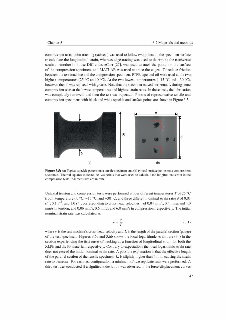
Chapter 3 3.2 Materials and methods
compression tests, point tracking (subsets) was used to follow two points on the specimen surface
to calculate the longitudinal strain, whereas edge tracing was used to determine the transverse
strains. Another in-house DIC code, eCorr [27], was used to track the points on the surface
of the compression specimen, and MATLAB was used to trace the edges. To reduce friction
between the test machine and the compression specimen, PTFE tape and oil were used at the two
highest temperatures (25 ◦C and 0 ◦C). At the two lowest temperatures (−15 ◦C and −30 ◦C),
however, the oil was replaced with grease. Note that the specimen moved horizontally during some
compression tests at the lowest temperatures and highest strain rates. In these tests, the lubrication
was completely removed, and then the test was repeated. Photos of representative tensile and
compression specimens with black and white speckle and surface points are shown in Figure 3.5.
(a) (b)
Figure 3.5: (a) Typical speckle pattern on a tensile specimen and (b) typical surface points on a compression
specimen. The red squares indicate the two points that were used to calculate the longitudinal strain in the
compression tests. All measures are in mm.
Uniaxial tension and compression tests were performed at four different temperatures T of 25 ◦C(room temperature), 0 ◦C, −15 ◦C, and −30 ◦C, and three different nominal strain rates e of 0.01s−1, 0.1 s−1, and 1.0 s−1, corresponding to cross-head velocities v of 0.04 mm/s, 0.4 mm/s and 4.0mm/s in tension, and 0.06 mm/s, 0.6 mm/s and 6.0 mm/s in compression, respectively. The initial
nominal strain rate was calculated as
e =v
L(3.1)
where v is the test machine’s cross-head velocity and L is the length of the parallel section (gauge)
of the test specimen. Figures 3.6a and 3.6b shows the local logarithmic strain rate (εL) in the
section experiencing the first onset of necking as a function of longitudinal strain for both the
XLPE and the PP material, respectively. Contrary to expectations the local logarithmic strain rate
does not exceed the initial nominal strain rate. A possible explanation is that the effective length
of the parallel section of the tensile specimen, L, is slightly higher than 4 mm, causing the strain
rate to decrease. For each test configuration, a minimum of two replicate tests were performed. A
third test was conducted if a significant deviation was observed in the force-displacement curves
47

3.2 Materials and methods Chapter 3
0.0 0.5 1.0 1.5 2.0
Longitudinal logarithmic strain, εL
10−4
10−3
10−2
10−1
100
Longit
udin
allo
gar
ithm
icst
rain
rate
,ε L
(s−1
)
e = 1.00 s−1
e = 0.10 s−1
e = 0.01 s−1
Repeat tests
(a)
0.0 0.5 1.0 1.5 2.0
Longitudinal logarithmic strain, εL
10−4
10−3
10−2
10−1
100
Longit
udin
allo
gar
ithm
icst
rain
rate
,ε L
(s−1
)
e = 1.00 s−1
e = 0.10 s−1
e = 0.01 s−1
Repeat tests
(b)
Figure 3.6: Longitudinal logarithmic strain rate (εL) at room temperature for (a) the XLPE material and (b)
the PP material as a function of longitudinal logarithmic strain.
between the two replicate tests. Although there was some variation in the fracture strain between
the replicate tensile tests, there were only small differences in the stress-strain curve. In the
replicate compression tests, there was some variation in the stress-strain curve after yielding but
close to no variation in the magnitude of the yield stress. The clamping length of the specimens in
the uniaxial tension tests was approximately 20 mm.
3.2.4 Calculation of Cauchy stress and logarithmic strain
Two digital cameras were used to monitor the deformation in the radial and hoop directions of the
test specimen, with respect to the extruded PP pipe and XLPE cable insulation, see Figure 3.2.
In the tension experiments, the section of initial necking was found on each surface, and the
strain components were extracted at this section throughout the test. This ensured that the same
point was tracked throughout the experiment, and that the strains from the two surfaces were
obtained from the same point on the specimen. In the compression tests, the longitudinal strain
was obtained from the distance between the highlighted points in Figure 3.5b, while the transverse
strain on each surface was found by identifying the section of maximum diameter throughout the
experiment. For both loading modes, the transverse stretches measured by each of the digital
cameras were assumed to represent the stretches along the minor and major axes of an elliptical
cross-section, enabling the calculation of the current cross-sectional area of the specimen as
A = πr20 ·
rRr0· rH
r0= πr2
0λRλH (3.2)
48

Chapter 3 3.2 Materials and methods
where r0 is the initial radius of the specimen; rR and rH are the radii in the radial and hoop
directions, respectively; λR is the transverse stretch in the radial direction; and λH is the transverse
stretch in the perpendicular hoop direction, see Figure 3.2. Using the transverse stretches from
each camera, the volumetric strain is determined as
εV = ln (λLλRλH) (3.3)
where λL is the longitudinal stretch. The logarithmic strain components are calculated by taking
the natural logarithm of the corresponding stretch component, i.e., εi = ln (λi). Note that we only
obtain the strains on the surface of the specimen from the experiments. Thus, using Equation (3.3)
to calculate the volumetric strain, we assume a homogeneous strain field over the cross-section.
This assumption is only valid until the point of necking, where the strain field (and the stress field)
becomes heterogeneous. The implications of this assumption are further discussed in Section 3.4.
Using the expression for the area in Equation (3.2), the average Cauchy stress can be calculated as
σ =FA
(3.4)
where F is the force measured by the testing machine.
Note that the yield stress (σ0) throughout this study is taken to be equal to the flow stress at a
longitudinal logarithmic strain of 0.15 (15%). A logarithmic strain of 0.15 was chosen because the
material exhibits plastic flow at that point, while it is still close to the yield point. This definition
of the yield stress applies for both tension and compression.
3.2.5 Calculation of self-heating
A MATLAB routine was established to obtain the temperature change on the surface of the tensile
specimen at approximately the same position as the strains were extracted. Figure 3.7 shows a
snapshot of the temperature field alongside the strain field for the PP material tested at room
temperature and the highest strain rate. As indicated in the figure, the temperature gradient,
∇T , is calculated along a row of pixels (denoted row A in Figure 3.7) containing the top and
bottom of the specimen, with air in-between. Since the temperature of the surrounding air is
constant, an abrupt change in the temperature gradient will occur when transitioning from air to
the specimen in the considered row of pixels. This allowed us to obtain the position of the top and
bottom of the tensile specimen numerically, which again gave us the vertical coordinate, yc , of
the centre of the specimen during the experiment. The temperature is then extracted at the point
(xc, yc) highlighted with a square in Figure 3.7, where xc is the horizontal coordinate of the centre
provided as user input. Note that the symbol T is used for all temperatures measured in degrees
Celsius (◦C) throughout the paper, while θ is applied for temperatures measured in Kelvin (K).
49
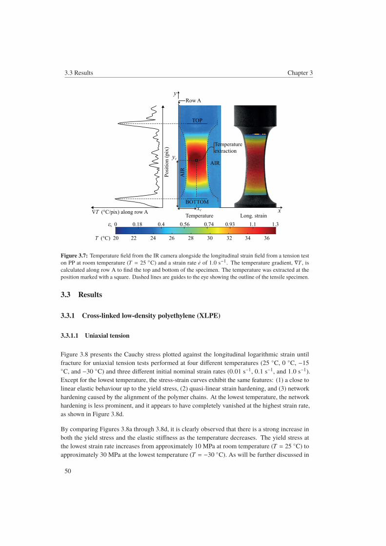
3.3 Results Chapter 3
x xc
y
y
c
20 22 24 26 28 30 32 34 36
0 0.18 0.4 0.56 0.74 0.93 1.1 1.3
T (°C)
L
Temperature
extraction
TOP
AIR
BOTTOM
Temperature Long. strainT (°C/pix) along row A
Po
siti
on
(p
ix)
AIR
Row A
Figure 3.7: Temperature field from the IR camera alongside the longitudinal strain field from a tension test
on PP at room temperature (T = 25 ◦C) and a strain rate e of 1.0 s−1. The temperature gradient, ∇T , is
calculated along row A to find the top and bottom of the specimen. The temperature was extracted at the
position marked with a square. Dashed lines are guides to the eye showing the outline of the tensile specimen.
3.3 Results
3.3.1 Cross-linked low-density polyethylene (XLPE)
3.3.1.1 Uniaxial tension
Figure 3.8 presents the Cauchy stress plotted against the longitudinal logarithmic strain until
fracture for uniaxial tension tests performed at four different temperatures (25 ◦C, 0 ◦C, −15◦C, and −30 ◦C) and three different initial nominal strain rates (0.01 s−1, 0.1 s−1, and 1.0 s−1).
Except for the lowest temperature, the stress-strain curves exhibit the same features: (1) a close to
linear elastic behaviour up to the yield stress, (2) quasi-linear strain hardening, and (3) network
hardening caused by the alignment of the polymer chains. At the lowest temperature, the network
hardening is less prominent, and it appears to have completely vanished at the highest strain rate,
as shown in Figure 3.8d.
By comparing Figures 3.8a through 3.8d, it is clearly observed that there is a strong increase in
both the yield stress and the elastic stiffness as the temperature decreases. The yield stress at
the lowest strain rate increases from approximately 10 MPa at room temperature (T = 25 ◦C) to
approximately 30 MPa at the lowest temperature (T = −30 ◦C). As will be further discussed in
50

Chapter 3 3.3 Results
0.0 0.4 0.8 1.2 1.6 2.0
Longitudinal logarithmic strain, εL
0
20
40
60
80
100
120
Cau
chy
stre
ss,σ
(MP
a)
e = 1.00 s−1
e = 0.10 s−1
e = 0.01 s−1
Repeat tests
λlock (e = 1.00 s−1)
λlock (e = 0.10 s−1)
λlock (e = 0.01 s−1)
(a) T = 25 ◦C
0.0 0.4 0.8 1.2 1.6 2.0
Longitudinal logarithmic strain, εL
0
20
40
60
80
100
120
Cau
chy
stre
ss,σ
(MP
a)
e = 1.00 s−1
e = 0.10 s−1
e = 0.01 s−1
Repeat tests
(b) T = 0 ◦C
0.0 0.4 0.8 1.2 1.6 2.0
Longitudinal logarithmic strain, εL
0
20
40
60
80
100
120
Cau
chy
stre
ss,σ
(MP
a)
e = 1.00 s−1
e = 0.10 s−1
e = 0.01 s−1
Repeat tests
(c) T = −15 ◦C
0.0 0.4 0.8 1.2 1.6 2.0
Longitudinal logarithmic strain, εL
0
20
40
60
80
100
120
Cau
chy
stre
ss,σ
(MP
a)
e = 1.00 s−1
e = 0.10 s−1
e = 0.01 s−1
Repeat tests
(d) T = −30 ◦C
Figure 3.8: Cross-linked low-density polyethylene (XLPE): Cauchy stress vs. longitudinal logarithmic strain
from uniaxial tension tests at three different nominal strain rates, e = 0.01 s−1, e = 0.1 s−1, and e = 1.0 s−1,
at four different temperatures, (a) T = 25 ◦C, (b) T = 0 ◦C, (c) T = −15 ◦C, and (d) T = −30 ◦C. Note that
the repeat tests at the two highest strain rates in (a) were performed with only one digital camera.
Section 3.4, the dependence of the yield stress on strain rate and temperature obeys the Ree-Eyring
flow theory [20]. The same trend is observed for the elastic stiffness: decreasing the temperature
increases Young’s modulus from approximately 200 MPa at room temperature to approximately
800 MPa at −30 ◦C. As for the yield stress, a dependence on strain rate is also evident for Young’s
modulus.
The locking stretch is taken as the stretch where the slope of the strain hardening curve increases
51
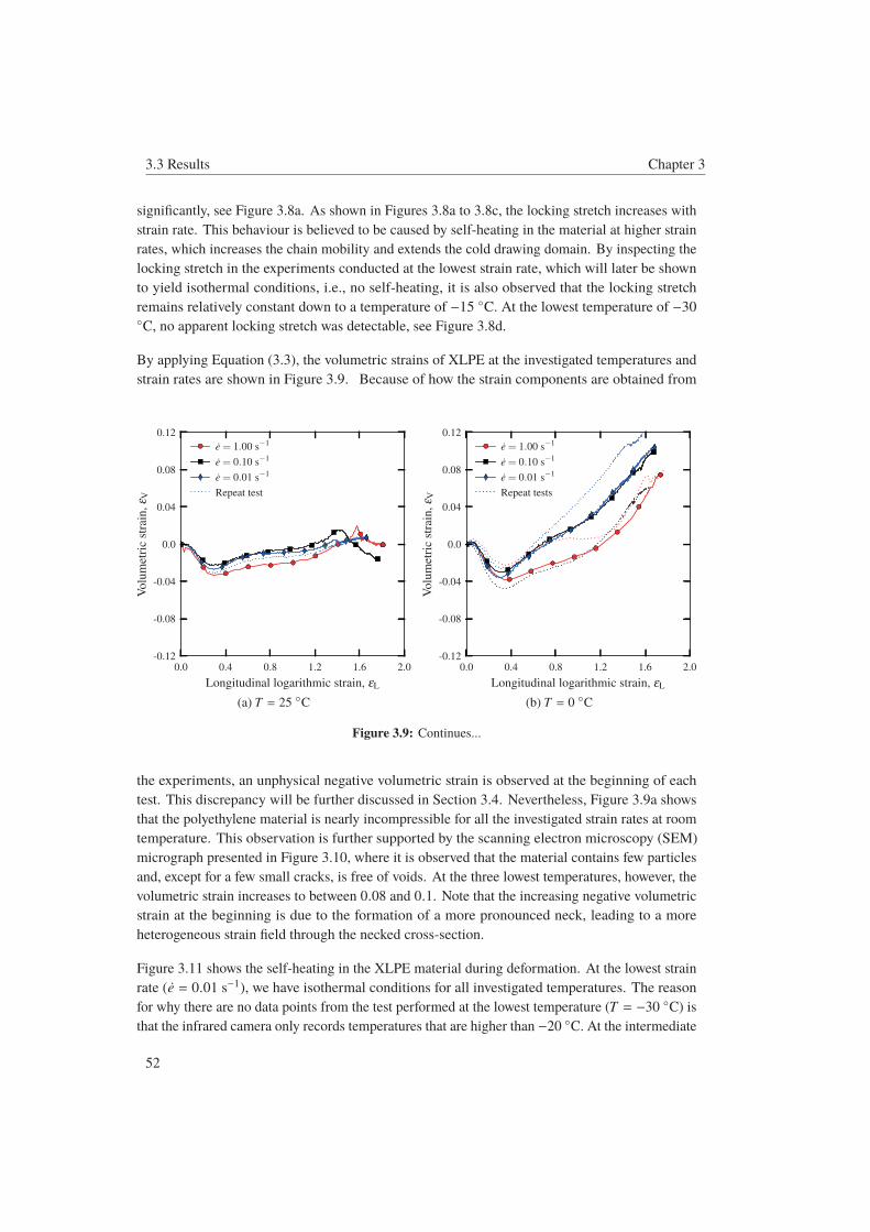
3.3 Results Chapter 3
significantly, see Figure 3.8a. As shown in Figures 3.8a to 3.8c, the locking stretch increases with
strain rate. This behaviour is believed to be caused by self-heating in the material at higher strain
rates, which increases the chain mobility and extends the cold drawing domain. By inspecting the
locking stretch in the experiments conducted at the lowest strain rate, which will later be shown
to yield isothermal conditions, i.e., no self-heating, it is also observed that the locking stretch
remains relatively constant down to a temperature of −15 ◦C. At the lowest temperature of −30◦C, no apparent locking stretch was detectable, see Figure 3.8d.
By applying Equation (3.3), the volumetric strains of XLPE at the investigated temperatures and
strain rates are shown in Figure 3.9. Because of how the strain components are obtained from
0.0 0.4 0.8 1.2 1.6 2.0
Longitudinal logarithmic strain, εL
-0.12
-0.08
-0.04
0.0
0.04
0.08
0.12
Volu
met
ric
stra
in,ε V
e = 1.00 s−1
e = 0.10 s−1
e = 0.01 s−1
Repeat test
(a) T = 25 ◦C
0.0 0.4 0.8 1.2 1.6 2.0
Longitudinal logarithmic strain, εL
-0.12
-0.08
-0.04
0.0
0.04
0.08
0.12V
olu
met
ric
stra
in,ε V
e = 1.00 s−1
e = 0.10 s−1
e = 0.01 s−1
Repeat tests
(b) T = 0 ◦C
Figure 3.9: Continues...
the experiments, an unphysical negative volumetric strain is observed at the beginning of each
test. This discrepancy will be further discussed in Section 3.4. Nevertheless, Figure 3.9a shows
that the polyethylene material is nearly incompressible for all the investigated strain rates at room
temperature. This observation is further supported by the scanning electron microscopy (SEM)
micrograph presented in Figure 3.10, where it is observed that the material contains few particles
and, except for a few small cracks, is free of voids. At the three lowest temperatures, however, the
volumetric strain increases to between 0.08 and 0.1. Note that the increasing negative volumetric
strain at the beginning is due to the formation of a more pronounced neck, leading to a more
heterogeneous strain field through the necked cross-section.
Figure 3.11 shows the self-heating in the XLPE material during deformation. At the lowest strain
rate (e = 0.01 s−1), we have isothermal conditions for all investigated temperatures. The reason
for why there are no data points from the test performed at the lowest temperature (T = −30 ◦C) is
that the infrared camera only records temperatures that are higher than −20 ◦C. At the intermediate
52

Chapter 3 3.3 Results
0.0 0.4 0.8 1.2 1.6 2.0
Longitudinal logarithmic strain, εL
-0.12
-0.08
-0.04
0.0
0.04
0.08
0.12
Volu
met
ric
stra
in,ε V
e = 1.00 s−1
e = 0.10 s−1
e = 0.01 s−1
Repeat tests
(c) T = −15 ◦C
0.0 0.4 0.8 1.2 1.6 2.0
Longitudinal logarithmic strain, εL
-0.12
-0.08
-0.04
0.0
0.04
0.08
0.12
Volu
met
ric
stra
in,ε V
e = 1.00 s−1
e = 0.10 s−1
e = 0.01 s−1
Repeat tests
(d) T = −30 ◦C
Figure 3.9: Cross-linked low-density polyethylene (XLPE): Volumetric strain vs. longitudinal logarithmic
strain from uniaxial tension tests at three different nominal strain rates, e = 0.01 s−1, e = 0.1 s−1, and e = 1.0s−1, at four different temperatures, (a) T = 25 ◦C, (b) T = 0 ◦C, (c) T = −15 ◦C, and (d) T = −30 ◦C.
Figure 3.10: Cross-linked low-density polyethylene (XLPE): Scanning electron microscopy (SEM) micro-
graph of a tensile specimen loaded to a longitudinal strain of 1.1 and then unloaded.
strain rate (e = 0.1 s−1), we observe a temperature increase due to self-heating of approximately
10 ◦C, whereas at the highest strain rate a temperature increase of approximately 20 ◦C to 30 ◦C is
observed. The self-heating increases with reduced initial temperature.
53

3.3 Results Chapter 3
0.0 0.4 0.8 1.2 1.6 2.0
Longitudinal logarithmic strain, εL
-5
0
5
10
15
20
25
30
35
Tem
per
ature
chan
ge,
Δθ(K
)
e = 1.00 s−1
e = 0.10 s−1
e = 0.01 s−1
Repeat tests
(a) T = 25 ◦C
0.0 0.4 0.8 1.2 1.6 2.0
Longitudinal logarithmic strain, εL
-5
0
5
10
15
20
25
30
35
Tem
per
ature
chan
ge,
Δθ(K
)
e = 1.00 s−1
e = 0.10 s−1
e = 0.01 s−1
Repeat tests
(b) T = 0 ◦C
0.0 0.4 0.8 1.2 1.6 2.0
Longitudinal logarithmic strain, εL
-5
0
5
10
15
20
25
30
35
Tem
per
ature
chan
ge,
Δθ(K
)
e = 1.00 s−1
e = 0.10 s−1
e = 0.01 s−1
Repeat tests
(c) T = −15 ◦C
0.0 0.4 0.8 1.2 1.6 2.0
Longitudinal logarithmic strain, εL
-5
0
5
10
15
20
25
30
35
Tem
per
ature
chan
ge,
Δθ(K
)
No measurements
e = 1.00 s−1
Repeat test
(d) T = −30 ◦C
Figure 3.11: Cross-linked low-density polyethylene (XLPE): Self-heating vs. longitudinal logarithmic strain
from uniaxial tension tests at three different nominal strain rates, e = 0.01 s−1, e = 0.1 s−1, and e = 1.0 s−1
at four different temperatures; (a) T = 25 ◦C, (b) T = 0 ◦C, (c) T = −15 ◦C, and (d) T = −30 ◦C.
54

Chapter 3 3.3 Results
3.3.1.2 Uniaxial compression
Uniaxial compression tests were performed at the same temperatures (25 ◦C, 0 ◦C, −15 ◦C, and
−30 ◦C) and initial nominal strain rates (0.01 s−1, 0.1 s−1, and 1.0 s−1) as the tension tests. A
comparison of the Cauchy stress vs. logarithmic strain curves for uniaxial compression and tension
at T = 25 ◦C is presented in Figure 3.12. As shown, the pressure sensitivity, defined as the ratio
0.00 0.05 0.10 0.15 0.20 0.25 0.30 0.35 0.40
Longitudinal logarithmic strain, |εL|
0
5
10
15
20
25
30
Cau
chy
stre
ss,|σ|(M
Pa)
e = 1.00 s−1
e = 0.10 s−1
e = 0.01 s−1
Compression
Repeat tests (tension)
Figure 3.12: Cross-linked low-density polyethylene (XLPE): Comparison of Cauchy stress vs. longitudinal
logarithmic strain curves in compression and tension at T = 25 ◦C. Note that two repeat tests are given for
the compression stress-strain curves.
between the compressive and tensile yield stress, αp = σC/σT, is negligible for the polyethylene
material. Conversely, the hardening is slightly higher in compression than in tension. However,
note that barrelling occurred quite early in all the compression tests. Thus, the only purpose of
the compression tests was to investigate the pressure sensitivity of the material in terms of the
yield stress. A comparison of the compressive and tensile yield stress as functions of temperature
and strain rate is shown in Figure 3.13. Similar to the observations from the uniaxial tension
experiments, there is an increase in the compressive yield stress when decreasing the temperature
and when increasing the strain rate.
55

3.3 Results Chapter 3
240 250 260 270 280 290 300
Absolute temperature, θ (K)
10
15
20
25
30
35
40
45
Yie
ldst
ress
,|σ
0|(M
Pa)
Filled markers: tension
Empty markers: compression
e = 1.00 s−1
e = 0.10 s−1
e = 0.01 s−1
Figure 3.13: Cross-linked low-density polyethylene (XLPE): Comparison of the tensile and compressive
yield stress as a function of temperature and strain rate.
The pressure sensitivity parameter αp = σC/σT is presented in Table 3.2 for all combinations of
temperature and strain rate. Because αp is consistently close to unity, the pressure sensitivity of
the XLPE material is low.
Table 3.2: Pressure sensitivity parameter, αp = σC/σT, for the XLPE material.
e (s−1)
T (◦C) 0.01 0.1 1.0
25 1.08 1.02 0.980 1.13 1.09 1.08−15 1.13 1.08 1.09−30 1.08 1.02 0.98
3.3.2 Rubber-modified polypropylene (PP)
3.3.2.1 Uniaxial tension
The Cauchy stress vs. logarithmic strain curves from the tension tests of the polypropylene material
are presented in Figure 3.14. Similar to the experiments conducted on the XLPE material, four
temperatures (25 ◦C, 0 ◦C, −15 ◦C, and −30 ◦C) and three initial nominal strain rates (0.01 s−1,
0.1 s−1, and 1.0 s−1) were investigated. The shape of the stress-strain curve for the two lowest
56

Chapter 3 3.3 Results
0.0 0.4 0.8 1.2 1.6 2.0 2.4
Longitudinal logarithmic strain, εL
0
20
40
60
80
100
120
140
160
180
Cau
chy
stre
ss,σ
(MP
a)
e = 1.00 s−1
e = 0.10 s−1
e = 0.01 s−1
Repeat tests
(a) T = 25 ◦C
0.0 0.4 0.8 1.2 1.6 2.0 2.4
Longitudinal logarithmic strain, εL
0
20
40
60
80
100
120
140
160
180
Cau
chy
stre
ss,σ
(MP
a)
e = 1.00 s−1
e = 0.10 s−1
e = 0.01 s−1
Repeat tests
(b) T = 0 ◦C
0.0 0.4 0.8 1.2 1.6 2.0 2.4
Longitudinal logarithmic strain, εL
0
20
40
60
80
100
120
140
160
180
Cau
chy
stre
ss,σ
(MP
a)
e = 1.00 s−1
e = 0.10 s−1
e = 0.01 s−1
Repeat tests
(c) T = −15 ◦C
0.0 0.4 0.8 1.2 1.6 2.0 2.4
Longitudinal logarithmic strain, εL
0
20
40
60
80
100
120
140
160
180
Cau
chy
stre
ss,σ
(MP
a)
e = 1.00 s−1
e = 0.10 s−1
e = 0.01 s−1
Repeat tests
(d) T = −30 ◦C
Figure 3.14: Rubber-modified polypropylene (PP): Cauchy stress vs. longitudinal logarithmic strain from
uniaxial tension tests at three different nominal strain rates, e = 0.01 s−1, e = 0.1 s−1, and e = 1.0 s−1, at
four different temperatures, (a) T = 25 ◦C, (b) T = 0 ◦C, (c) T = −15 ◦C, and (d) T = −30 ◦C.
strain rates is relatively the same for all temperatures: first a close to linear elastic behaviour up to
a yield point, followed by strain hardening and ultimately asymptotic network hardening. At the
highest strain rate and the three lowest temperatures, however, the material fractured before the
locking stretch was reached.
In terms of the yield stress, the equivalence principle [28] holds, i.e., either reducing the temperature
or increasing the strain rate increases the yield stress. At room temperature and for the lowest
57

3.3 Results Chapter 3
strain rate, the yield stress is approximately 20 MPa, while it has increased to approximately
24 MPa for the highest strain rate. At the lowest temperature, the quasi-static yield stress is
approximately 35 MPa and increases to approximately 45 MPa for the highest strain rate, indicating
that the rate-sensitivity is slightly higher at lower temperatures. The elastic modulus, however,
exhibits little dependence on the strain rate, but it changes drastically with temperature. At
room temperature, Young’s modulus is approximately 850 MPa, whereas it has increased to
approximately 2600 MPa at the lowest temperature.
As shown in Figure 3.15, the volumetric strains for the polypropylene material are considerably
0.0 0.4 0.8 1.2 1.6 2.0 2.4
Longitudinal logarithmic strain, εL
0.0
0.1
0.2
0.3
0.4
0.5
0.6
0.7
0.8
0.9
Volu
met
ric
stra
in,ε V
e = 1.00 s−1
e = 0.10 s−1
e = 0.01 s−1
Repeat tests
(a) T = 25 ◦C
0.0 0.4 0.8 1.2 1.6 2.0 2.4
Longitudinal logarithmic strain, εL
0.0
0.1
0.2
0.3
0.4
0.5
0.6
0.7
0.8
0.9
Volu
met
ric
stra
in,ε V
e = 1.00 s−1
e = 0.10 s−1
e = 0.01 s−1
Repeat tests
(b) T = 0 ◦C
0.0 0.4 0.8 1.2 1.6 2.0 2.4
Longitudinal logarithmic strain, εL
0.0
0.1
0.2
0.3
0.4
0.5
0.6
0.7
0.8
0.9
Volu
met
ric
stra
in,ε V
e = 1.00 s−1
e = 0.10 s−1
e = 0.01 s−1
Repeat tests
(c) T = −15 ◦C
0.0 0.4 0.8 1.2 1.6 2.0 2.4
Longitudinal logarithmic strain, εL
0.0
0.1
0.2
0.3
0.4
0.5
0.6
0.7
0.8
0.9
Volu
met
ric
stra
in,ε V
e = 1.00 s−1
e = 0.10 s−1
e = 0.01 s−1
Repeat tests
(d) T = −30 ◦C
Figure 3.15: Rubber-modified polypropylene (PP): Volumetric strain vs. longitudinal logarithmic strain
from uniaxial tension tests at three different nominal strain rates, e = 0.01 s−1, e = 0.1 s−1, and e = 1.0 s−1,
at four different temperatures, (a) T = 25 ◦C, (b) T = 0 ◦C, (c) T = −15 ◦C, and (d) T = −30 ◦C.
58

Chapter 3 3.3 Results
larger than those for XLPE and attain values between 0.5 and 0.9. At the two lowest strain rates,
the shape of the curve is the same for all temperatures: first a significant evolution of volumetric
strain up to a peak value followed by decreasing volumetric strain. Ponçot et al. [15] reported a
similar observation on a comparable material (polypropylene/ethylene-propylene rubber). This
result is due to the formation of voids in the material, believed to be initiated by cavitation in the
rubbery phase of the rubber-modified polypropylene. Since there are no particles in these voids,
they are not restrained against collapsing, which explains the decreasing volumetric strains after
the peak value is reached. To investigate this assumption, two specimens were loaded in uniaxial
tension at room temperature and a strain rate of 0.01 s−1 and thereafter unloaded; one specimen
was unloaded before the maximum volumetric strain was reached, and the other one was unloaded
after the maximum volumetric strain. SEM micrographs of the two samples are presented in
Figures 3.16a and 3.16b. It appears from Figure 3.16 that the voids become elongated and start
to close after the maximum volumetric strain is reached. At the highest strain rate, however, it
seems that the voids do not collapse at the three lowest temperatures, leading to a monotonically
increasing volumetric strain up to fracture, as shown in Figures 3.15b to 3.15d.
(a) (b)
Figure 3.16: Rubber-modified polypropylene (PP): Scanning electron microscopy (SEM) micrographs of
tensile specimens unloaded (a) before and (b) after peak volumetric strain.
The self-heating during the tensile experiments is presented in Figure 3.17. At the lowest strain
rate, isothermal conditions prevail at all temperatures. As previously mentioned, there are no data
points for the temperature change in the material at the lowest temperature (T = −30 ◦C) and
the lowest strain rate due to the infrared camera being limited to temperatures above −20 ◦C. At
the intermediate strain rate (e = 0.10 s−1), a temperature increase between 15 ◦C and 30 ◦C is
observed before the temperature begins to decrease in the material. This decrease in temperature
is due to the formation of a stable neck leading to cold drawing. This provides the material
with enough time to conduct heat within the specimen and to convect heat to the surroundings.
Although we have cold drawing at the highest strain rate (e = 1.0 s−1) at room temperature, the
duration of the test is too short to allow for heat conduction or convection. This leads to the
continuously increasing temperature for the highest strain rate at all temperatures in Figure 3.17.
59

3.3 Results Chapter 3
0.0 0.4 0.8 1.2 1.6 2.0 2.4
Longitudinal logarithmic strain, εL
0
10
20
30
40
50
Tem
per
ature
chan
ge,
Δθ(K
)
e = 1.00 s−1
e = 0.10 s−1
e = 0.01 s−1
Repeat tests
(a) T = 25 ◦C
0.0 0.4 0.8 1.2 1.6 2.0 2.4
Longitudinal logarithmic strain, εL
0
10
20
30
40
50
60
Tem
per
ature
chan
ge,
Δθ(K
)
e = 1.00 s−1
e = 0.10 s−1
e = 0.01 s−1
Repeat tests
(b) T = 0 ◦C
0.0 0.4 0.8 1.2 1.6 2.0 2.4
Longitudinal logarithmic strain, εL
0
10
20
30
40
50
Tem
per
ature
chan
ge,
Δθ(K
)
e = 1.00 s−1
e = 0.10 s−1
e = 0.01 s−1
Repeat tests
(c) T = −15 ◦C
0.0 0.4 0.8 1.2 1.6 2.0 2.4
Longitudinal logarithmic strain, εL
0
10
20
30
40
50
Tem
per
ature
chan
ge,
Δθ(K
)
No measurements
e = 1.00 s−1
e = 0.10 s−1
Repeat tests
(d) T = −30 ◦C
Figure 3.17: Rubber-modified polypropylene (PP): Self-heating vs. longitudinal logarithmic strain from
uniaxial tension tests at three different nominal strain rates, e = 0.01 s−1, e = 0.1 s−1, and e = 1.0 s−1, at
four different temperatures, (a) T = 25 ◦C, (b) T = 0 ◦C, (c) T = −15 ◦C, and (d) T = −30 ◦C.
In contrast to XLPE, the temperature increase is approximately the same for all temperatures, i.e.,
between 40 and 50 ◦C, when adiabatic heating conditions are met.
Another observation is that the self-heating introduces a softening in the material, as indicated by
the crossing of the stress-strain curves observed, for instance in Figure 3.14a. The self-heating
increases the locking stretch for higher strain rates. Unlike XLPE, however, the opposite effect is
observed when decreasing the temperature at the lowest strain rate, i.e., there is a reduction of the
60

Chapter 3 3.3 Results
locking stretch for PP with decreasing temperature.
3.3.2.2 Uniaxial compression
Similar to the XLPE material, compression tests were performed for the PP material at four
temperatures (25 ◦C, 0 ◦C, −15 ◦C, and −30 ◦C) and three initial nominal strain rates (0.01 s−1, 0.1s−1 and 1.0 s−1). Figure 3.18 compares the stress-strain curves in uniaxial compression and tension
0.0 0.2 0.4 0.6 0.8 1.0 1.2 1.4
Longitudinal logarithmic strain, |εL|
0
10
20
30
40
Cau
chy
stre
ss,|σ|(M
Pa)
e = 1.00 s−1
e = 0.10 s−1
e = 0.01 s−1
Repeat tests (tension)
Compression
Figure 3.18: Rubber-modified polypropylene (PP): Comparison of Cauchy stress vs. longitudinal logarithmic
strain curves in compression and tension at T = 25 ◦C. Note that two repeat tests are given for the compression
stress-strain curves.
at room temperature. It is clearly observed from the difference in compressive and tensile yield
stress that the pressure sensitivity of the PP material is strong. Similar to the compression tests
performed on the XLPE material, the onset of barrelling occurred for quite small deformations.
Consequently, the compression tests were only conducted to determine the yield stress. As in
tension, it is observed that higher strain rates and lower temperatures increase the yield stress in
compression. The yield stresses in compression and tension are plotted as functions of temperature
in Figure 3.19 for all the investigated strain rates.
61

3.4 Discussion Chapter 3
240 250 260 270 280 290 300
Absolute temperature, θ (K)
10
20
30
40
50
60
70
80
Yie
ldst
ress
,|σ
0|(M
Pa)
Filled markers: tension
Empty markers: compression
e = 1.00 s−1
e = 0.10 s−1
e = 0.01 s−1
Figure 3.19: Rubber-modified polypropylene (PP): Comparison of the tensile and compressive yield stress
as a function of temperature and strain rate.
The pressure sensitivity parameter αp = σC/σT is presented in Table 3.3 for all combinations of
temperature and strain rate. In contrast to the XLPE material, the pressure sensitivity is very high
for the rubber-modified polypropylene. It is also observed that the pressure sensitivity increases at
low temperatures.
Table 3.3: Pressure sensitivity parameter, αp = σC/σT, for the PP material.
e (s−1)
T (◦C) 0.01 0.1 1.0
25 1.22 1.33 1.430 1.54 1.56 1.65−15 1.71 1.67 1.60−30 1.66 1.69 1.61
3.4 Discussion
3.4.1 Temperature measurements
An infrared camera was employed to measure self-heating during the tests, see Section 3.2.3. In
all experiments an emissivity of 0.95 was used. As validation, a uniaxial tension test at room
62

Chapter 3 3.4 Discussion
temperature (T = 25 ◦C) and at the highest strain rate (e = 1.0 s−1) was performed on the XLPE
material where the surface facing the thermal camera was coated with a black paint with an
emissivity close to 1.0. The temperature as a function of longitudinal strain was then compared
with a similar experiment where only a black and white speckle was applied. As evident from
Figure 3.11a the difference between the measured self-heating for the two tests at the highest
strain rate is minimal. Another possible issue is that the grease applied to the samples tested
at low temperatures may affect thermal measurements. To validate the calculated self-heating
from tests performed on materials coated with white grease, two tests at the highest strain rate
were performed on the PP material at room temperature. In one of the tests a black and white
spray paint speckle was applied, while in the other a white grease was used. The difference in
self-heating, as shown in Figure 3.17a, was found to be negligible.
3.4.2 Young’s modulus
Young’s modulus as a function of temperature and strain rate is presented in Figures 3.20 and
3.21 for XLPE and PP, respectively. Young’s modulus of the XLPE material was found through a
linear fit of the stress-strain curve up to a longitudinal strain of εL = 0.025. For the PP material,
Young’s modulus was obtained by a linear fit of the stress-strain curve for σ ∈ [0, 0.5σ0], where
σ0 is the quasi-static yield stress at the investigated temperature. Due to noise in the strain values
obtained from DIC, it was necessary to average the strain values over a larger area of the parallel
section of the tensile specimen for the PP material. This can be done since the strain field remains
homogeneous for the part of the stress-strain curve used to obtain Young’s modulus.
For both materials, the elastic stiffness was found to be strongly dependent on the temperature.
In XLPE, the elastic stiffness increases by a factor of four: from approximately 200 MPa at
room temperature to 800 MPa at −30 ◦C. For the PP material, Young’s modulus increases more
than threefold: from approximately 850 MPa at room temperature to 2600 MPa at −30 ◦C. The
temperature dependence within the experimental range is described using the same expression as
Arruda et al. [4], i.e.
E(θ) = E0 · exp [−a (θ − θ0)] (3.5)
where θ0 is the reference temperature, E0 is Young’s modulus at the reference temperature, a is a
material parameter, and θ is the absolute temperature. The least squares fits of Equation (3.5) to
the experimentally obtained Young’s modulus for the materials at the lowest strain rate are shown
in Figures 3.20 and 3.21, with E0 = 141 MPa and a = 0.03 K−1 for the XLPE material, E0 = 842MPa and a = 0.021 K−1 for the PP material, and θ0 = 298.15 K (room temperature) for both
materials.
Young’s modulus was also found to be influenced by strain rate for the XLPE material, as shown
in Figure 3.20. The trend of the elastic stiffness with respect to the rate sensitivity is not as clear
for the PP material, as indicated in Figure 3.21. Since both Young’s modulus and the yield stress
is higher in PP compared to XLPE, this observation could be an artefact of the acceleration of the
63

3.4 Discussion Chapter 3
240 250 260 270 280 290 300
Absolute temperature, θ (K)
0
200
400
600
800
1000
1200
Young’s
modulu
s,E
(MP
a)
e = 1.00 s−1
e = 0.10 s−1
e = 0.01 s−1
Equation (5)Equation (3.5)
Figure 3.20: Cross-linked low-density polyethylene (XLPE): Influence of strain rate and temperature on
Young’s modulus. Equation (3.5) is fitted only to the Young’s moduli at the lowest strain rate. The empty
markers are from the repeat tests in Figure 3.8.
test machine, meaning that some time is needed before the cross-head reaches the desired velocity,
or due to some slack in, e.g., the load cell or the grip. These factors, combined with a limited
240 250 260 270 280 290 300
Absolute temperature, θ (K)
500
1000
1500
2000
2500
3000
Young’s
modulu
s,E
(MP
a)
e = 1.00 s−1
e = 0.10 s−1
e = 0.01 s−1
Equation (5)
����
�����
Discarded data points
Equation (3.5)
Figure 3.21: Rubber-modified polypropylene (PP): Influence of strain rate and temperature on Young’s
modulus. Equation (3.5) is fitted only to the Young’s moduli at the lowest strain rate. The empty markers are
from the repeat tests in Figure 3.14.
64

Chapter 3 3.4 Discussion
number of data points before yield for the two highest strain rates, could explain the discrepancies
observed in Figure 3.21. Nevertheless, given that the most influential factor for both materials was
the temperature, the strain rate dependence has been omitted in Equation (3.5).
3.4.3 Yield stress and pressure sensitivity
The Ree-Eyring flow theory [20] is frequently applied to model the influence of temperature and
strain rate on the yield stress. Following the work of Senden et al. [29], a double Ree-Eyring
model that includes both the main α relaxation and the secondary β relaxation is employed for
evaluation and discussion of the experimental findings herein. Assuming that the contributions
from each relaxation process are additive, the equivalent stress is given as
σ(p, θ) =∑x=α,β
kBθVx
arcsinh(
pp0,x
exp[ΔHx
Rθ
])(3.6)
Here, kB is Boltzmann’s constant, R is the gas constant, p is the equivalent plastic strain rate,
θ is the absolute temperature, Vx (x = {α, β}) is the activation volume, p0,x is a local reference
plastic strain rate, and ΔHx is the activation enthalpy. For the purpose of obtaining the relation
between the yield stress, temperature and strain rate, the equivalent stress σ is taken to be equal to
the yield stress σ0, and p is assumed to be equal to the initial nominal strain rate e. The material
parameters obtained from a least squares fit of Equation (3.6) to the experimental data are presented
in Table 3.4. All material parameters from the least squares fit appear to be reasonable from a
Table 3.4: Material parameters of the Ree-Eyring model, Equation (3.6).
kB R Vα p0,α ΔHα Vβ p0,β ΔHβ
Material (J/K) (J/(mol·K)) (nm3) (s−1) (kJ/mol) (nm3) (s−1) (kJ/mol)
XLPE 1.38 · 10−23 8.314 3.77 2.48 · 1031 211.8 3.14 6.07 · 1037 194.8PP 1.38 · 10−23 8.314 1.37 3.09 · 1017 86.4 4.95 3.62 · 1038 286.0
physical perspective: the activation volume is between 1 nm3 and 5 nm3, the activation enthalpy
ranges from 100 kJ/mol to 300 kJ/mol, and the local reference plastic strain rate attains values
between 1017 s−1 and 1038 s−1. The orders of magnitude are comparable to those of parameters
reported for other materials in the literature, e.g. [10, 29]. Addressing the yield stress in tension,
it appears from Figures 3.22 and 3.23 that the model captures the temperature and strain rate
dependence of both materials excellently. Thus, the double Ree-Eyring model appears to be a
promising choice for a thermomechanical description of the flow process of the materials at hand.
65
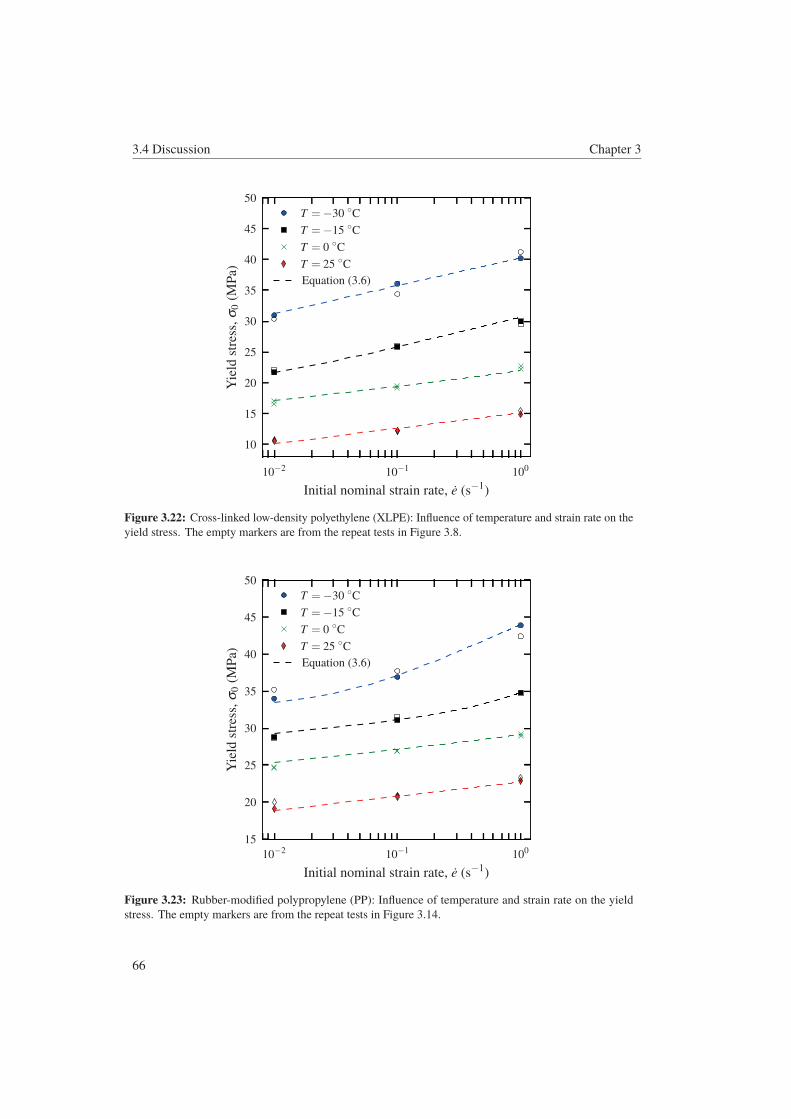
3.4 Discussion Chapter 3
10−2 10−1 100
Initial nominal strain rate, e (s−1)
10
15
20
25
30
35
40
45
50
Yie
ldst
ress
,σ 0
(MP
a)
T =−30 ◦C
T =−15 ◦C
T = 0 ◦C
T = 25 ◦C
Equation (6)Equation (3.6)
Figure 3.22: Cross-linked low-density polyethylene (XLPE): Influence of temperature and strain rate on the
yield stress. The empty markers are from the repeat tests in Figure 3.8.
10−2 10−1 100
Initial nominal strain rate, e (s−1)
15
20
25
30
35
40
45
50
Yie
ldst
ress
,σ 0
(MP
a)
T =−30 ◦C
T =−15 ◦C
T = 0 ◦C
T = 25 ◦C
Equation (6)Equation (3.6)
Figure 3.23: Rubber-modified polypropylene (PP): Influence of temperature and strain rate on the yield
stress. The empty markers are from the repeat tests in Figure 3.14.
66
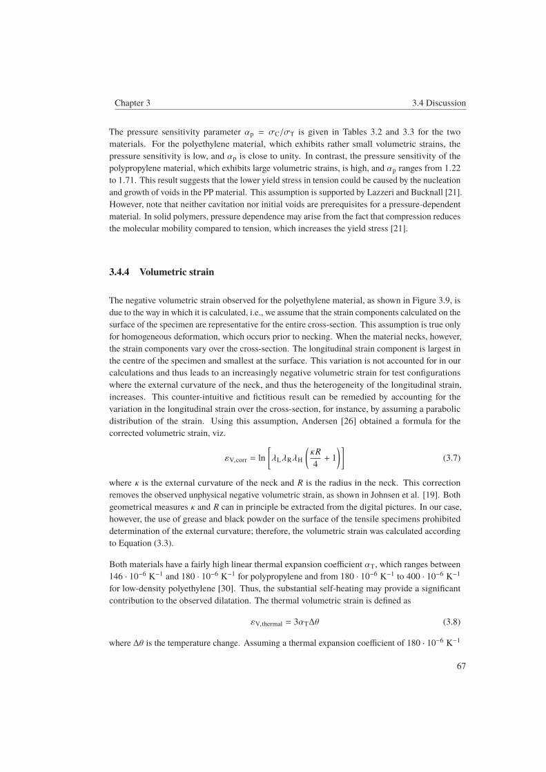
Chapter 3 3.4 Discussion
The pressure sensitivity parameter αp = σC/σT is given in Tables 3.2 and 3.3 for the two
materials. For the polyethylene material, which exhibits rather small volumetric strains, the
pressure sensitivity is low, and αp is close to unity. In contrast, the pressure sensitivity of the
polypropylene material, which exhibits large volumetric strains, is high, and αp ranges from 1.22to 1.71. This result suggests that the lower yield stress in tension could be caused by the nucleation
and growth of voids in the PP material. This assumption is supported by Lazzeri and Bucknall [21].
However, note that neither cavitation nor initial voids are prerequisites for a pressure-dependent
material. In solid polymers, pressure dependence may arise from the fact that compression reduces
the molecular mobility compared to tension, which increases the yield stress [21].
3.4.4 Volumetric strain
The negative volumetric strain observed for the polyethylene material, as shown in Figure 3.9, is
due to the way in which it is calculated, i.e., we assume that the strain components calculated on the
surface of the specimen are representative for the entire cross-section. This assumption is true only
for homogeneous deformation, which occurs prior to necking. When the material necks, however,
the strain components vary over the cross-section. The longitudinal strain component is largest in
the centre of the specimen and smallest at the surface. This variation is not accounted for in our
calculations and thus leads to an increasingly negative volumetric strain for test configurations
where the external curvature of the neck, and thus the heterogeneity of the longitudinal strain,
increases. This counter-intuitive and fictitious result can be remedied by accounting for the
variation in the longitudinal strain over the cross-section, for instance, by assuming a parabolic
distribution of the strain. Using this assumption, Andersen [26] obtained a formula for the
corrected volumetric strain, viz.
εV,corr = ln[λLλRλH
(κR4+ 1)]
(3.7)
where κ is the external curvature of the neck and R is the radius in the neck. This correction
removes the observed unphysical negative volumetric strain, as shown in Johnsen et al. [19]. Both
geometrical measures κ and R can in principle be extracted from the digital pictures. In our case,
however, the use of grease and black powder on the surface of the tensile specimens prohibited
determination of the external curvature; therefore, the volumetric strain was calculated according
to Equation (3.3).
Both materials have a fairly high linear thermal expansion coefficient αT, which ranges between
146 · 10−6 K−1 and 180 · 10−6 K−1 for polypropylene and from 180 · 10−6 K−1 to 400 · 10−6 K−1
for low-density polyethylene [30]. Thus, the substantial self-heating may provide a significant
contribution to the observed dilatation. The thermal volumetric strain is defined as
εV,thermal = 3αTΔθ (3.8)
where Δθ is the temperature change. Assuming a thermal expansion coefficient of 180 · 10−6 K−1
67

3.4 Discussion Chapter 3
and a temperature increase of 50 K in the PP material, the volumetric strain due to self-heating is
determined to be 0.9%, which is negligible compared to the substantial volumetric strain from
deformation. Considering XLPE, we assume a thermal expansion coefficient of 200 · 10−6 K−1
and a temperature increase of 30 K. This assumption provides a thermal volumetric strain of
0.6%, which is approximately 30% of the maximum volumetric strain (≈ 2%) at room temperature
(Figure 3.9a).
3.4.5 Network hardening and locking stretch
An interesting observation for the PP material is that the characteristic network hardening, caused
by the alignment of the polymer chains, does not occur for the highest strain rate (e = 1.0 s−1) at
the two lowest temperatures (T = −15 ◦C and T = −30 ◦C). This result is due to the formation of
an unstable neck, as shown by the Considère construction in Figure 3.24, which presents graphs of
the functions σ(εL) and Θ(εL), where Θ = dσ/dεL is the hardening modulus.
0.0 0.4 0.8 1.2 1.6 2.0 2.4
Longitudinal logarithmic strain, εL
0
20
40
60
80
100
120
Cau
chy
stre
ss,σ
(MP
a)
T =−30 ◦C
T =−15 ◦C
T = 0 ◦C
T = 25 ◦C
dσ/dεL
Figure 3.24: Rubber-modified polypropylene (PP): Considère construction for the uniaxial tension tests at
all temperatures for the strain rate e = 1.0 s−1.
The functionΘ(εL) is found by numerical differentiation of σ(εL) and then smoothed. It is evident
that the graph of Θ(εL) crosses the graph of σ(εL) twice for the uniaxial tension test performed
at room temperature, whereas for the three lower temperatures, there is only one intersection
– indicating an unstable neck. An explanation for this result may be found by examining the
volumetric strain vs. longitudinal strain curves in Figure 3.15. At room temperature, a peak value
is reached before the volumetric strain decreases. This result indicates, as previously depicted in
68

Chapter 3 3.4 Discussion
Figure 3.16, that voids in the material grow up to a certain point before they are stabilized or start
to collapse. At the lower temperatures, however, the voids only continue to grow up to fracture,
which in effect inhibits the formation of a stable neck. This is also supported by the observed
reduction in the overall ductility of the tensile specimen, as shown by the two photographs in
Figure 3.25.
Figure 3.25: Rubber-modified polypropylene (PP): Comparison of deformed specimens just before fracture
in uniaxial tension at T = 25 ◦C (room temperature) and T = −30 ◦C at a strain rate of e = 1.0 s−1.
The influence of rate and temperature on the locking stretch can be analyzed by application of the
expression proposed by Arruda et al. [4], viz.
μ(θ)N (θ) = constant (3.9)
where μ(θ) is the temperature-dependent shear modulus and N (θ) is the temperature-dependent
number of statistical rigid links per chain. Equation (3.9) also conserves the number of rigid links
(cross-links in the XLPE material and entanglements in the PP material), and hence preserves the
mass of the system. The number of statistical rigid links per chain, N , is related to the locking
stretch as λlock =√
N . Young’s modulus, and consequently the shear modulus, increases with
decreasing temperature for both materials, as shown in Figures 3.20 and 3.21. Equation (3.9) then
implies that the locking stretch increases with temperature. Investigating the locking stretch at
increasing strain rates while keeping the temperature fixed, we see from Figures 3.8 and 3.14
that the implication of Equation (3.9) holds, i.e., the locking stretch increases at elevated strain
rates due to self-heating in the material (Figures 3.11 and 3.17). Exceptions are PP at the highest
strain rate, which fails to form a stable neck below a temperature of T = 0 ◦C, and XLPE at a
temperature of −30 ◦C, where network hardening does not occur at the two highest strain rates.
Considering isothermal conditions (e = 0.01 s−1), the implications of Equation (3.9) hold for
PP, where we find that the locking stretch decreases and Young’s modulus increases when the
temperature decreases. However, for XLPE, we find that Young’s modulus increases for decreasing
69

3.5 Conclusions Chapter 3
temperatures, but a less significant effect is observed in terms of the locking stretch.
3.5 Conclusions
The following conclusions are drawn:
• The influence of strain rate and temperature on the mechanical behaviour of PP and XLPE
in tension and compression was studied experimentally. We observed that the yield stress in
tension relates to the temperature and strain rate through the Ree-Eyring flow theory and
that Young’s modulus follows an exponential relation with decreasing temperature within
the experimental range. This finding holds for both materials.
• In terms of self-heating, a substantial temperature increase is observed in both materials at
the elevated strain rates. At the highest strain rate (e = 1.0 s−1), a continuous temperature
increase indicates that we have close to adiabatic conditions, whereas for the lowest strain
rate (e = 0.01 s−1) isothermal conditions are met.
• The polypropylene material exhibits substantial volumetric strains, ranging from 0.6 to 0.9.
This is believed to be caused by cavitation in the rubbery phase of the material. A change
in the evolution of the volumetric strain is also observed at the highest strain rates when
decreasing the temperature. At room temperature, the volumetric strain increases until it
reaches a maximum value, after which it starts to decrease. SEM micrographs suggest that
this behaviour is caused by the stabilization of the growing voids when the material hardens
due to large strains, causing the voids to collapse. However, this does not occur at the lower
temperatures, which could be caused by the loss of ductility, facilitating coalescence rather
than void collapse. In the polyethylene material, the volumetric strain remains small at room
temperature but increases when the temperature is lowered.
• Pressure sensitivity, defined as the ratio between the compressive and tensile yield stress
(αp = σC/σT), is found to be substantial for the PP material, ranging from a minimum
value of 1.22 at room temperature and the lowest strain rate to 1.71 at a temperature of
−15 ◦C and the highest strain rate. This difference in yield stress in the two deformation
modes is due to the formation of voids in tension, a phenomenon that does not occur in
compression. In the XLPE material, however, where the volumetric strain remains small,
the pressure sensitivity parameter is close to unity for all test configurations.
Acknowledgements
The authors wish to thank the Research Council of Norway for funding through the Petromaks 2
programme, Contract No. 228513/E30. The financial support from ENI, Statoil, Lundin, Total,
Scana Steel Stavanger, JFE Steel Corporation, Posco, Kobe Steel, SSAB, Bredero Shaw, Borealis,
Trelleborg, Nexans, Aker Solutions, FMC Kongsberg Subsea, Marine Aluminium, Hydro and
70

Chapter 3 References
Sapa are also acknowledged. Special thanks is given to Nexans Norway and Borealis for providing
the materials. Mr. Trond Auestad and Mr. Tore Wisth are acknowledged for their invaluable
help in developing the experimental set-up and performing the experiments. Mr. Christian Oen
Paulsen’s help with the SEM micrographs is also greatly appreciated.
References
[1] Grytten, F., Daiyan, H., Polanco-Loria, M., and Dumoulin, S. “Use of digital image
correlation to measure large-strain tensile properties of ductile thermoplastics”. PolymerTesting 28 (2009), pp. 653–660. doi: 10.1016/j.polymertesting.2009.05.009.
[2] Delhaye, V., Clausen, A. H., Moussy, F., Othman, R., and Hopperstad, O. S. “Influence of
stress state and strain rate on the behaviour of a rubber-particle reinforced polypropylene”.
International Journal of Impact Engineering 38 (2011), pp. 208–218. doi: 10.1016/j.ijimpeng.2010.11.004.
[3] Jerabek, M., Major, Z., and Lang, R. W. “Strain determination of polymeric materials
using digital image correlation”. Polymer Testing 29 (2010), pp. 407–416. doi: 10.1016/j.polymertesting.2010.01.005.
[4] Arruda, E. M., Boyce, M. C., and Jayachandran, R. “Effects of strain rate, temperature
and thermomechanical coupling on the finite strain deformation of glassy polymers”.
Mechanics of Materials 19 (1995), pp. 193–212. doi: 10.1016/0167-6636(94)00034-E.
[5] Zaroulis, J. and Boyce, M. “Temperature, strain rate, and strain state dependence of the
evolution in mechanical behaviour and structure of poly(ethylene terephthalate) with
finite strain deformation”. Polymer 38 (1997), pp. 1303–1315. doi: 10.1016/S0032-3861(96)00632-5.
[6] van Breemen, L. C. A., Engels, T. A. P., Klompen, E. T. J., Senden, D. J. A., and
Govaert, L. E. “Rate- and temperature-dependent strain softening in solid polymers”.
Journal of Polymer Science, Part B: Polymer Physics 50 (2012), pp. 1757–1771. doi:10.1002/polb.23199.
[7] Zaïri, F., Naït-Abdelaziz, M., Gloaguen, J. M., and Lefebvre, J. M. “Constitutive
modelling of the large inelastic deformation behaviour of rubber-toughened poly(methyl
methacrylate): effects of strain rate, temperature and rubber-phase volume fraction”.
Modelling and Simulation in Materials Science and Engineering 18 (2010), p. 055004.
doi: 10.1088/0965-0393/18/5/055004.
[8] Nasraoui, M., Forquin, P., Siad, L., and Rusinek, A. “Influence of strain rate, temperature
and adiabatic heating on the mechanical behaviour of poly-methyl-methacrylate: Exper-
imental and modelling analyses”. Materials and Design 37 (2012), pp. 500–509. doi:10.1016/j.matdes.2011.11.032.
71

References Chapter 3
[9] Srivastava, V., Chester, S. A., Ames, N. M., and Anand, L. “A thermo-mechanically-
coupled large-deformation theory for amorphous polymers in a temperature range which
spans their glass transition”. International Journal of Plasticity 26 (2010), pp. 1138–1182.
doi: 10.1016/j.ijplas.2010.01.004.
[10] Richeton, J., Ahzi, S., Vecchio, K., Jiang, F., and Adharapurapu, R. “Influence of
temperature and strain rate on the mechanical behavior of three amorphous polymers:
Characterization and modeling of the compressive yield stress”. International Journal ofSolids and Structures 43 (2006), pp. 2318–2335. doi: 10.1016/j.ijsolstr.2005.06.040.
[11] Cao, K., Wang, Y., and Wang, Y. “Effects of strain rate and temperature on the tension
behavior of polycarbonate”. Materials and Design 38 (2012), pp. 53–58. doi: 10.1016/j.matdes.2012.02.007.
[12] Brown, E. N., Rae, P. J., and Orler, E. B. “The influence of temperature and strain rate on
the constitutive and damage responses of polychlorotrifluoroethylene (PCTFE, Kel-F
81)”. Polymer 47 (2006), pp. 7506–7518. doi: 10.1016/j.polymer.2006.08.032.
[13] Şerban, D. A., Weber, G., Marşavina, L., Silberschmidt, V. V., and Hufenbach, W. “Tensile
properties of semi-crystalline thermoplastic polymers: Effects of temperature and strain
rates”. Polymer Testing 32 (2013), pp. 413–425. doi: 10.1016/j.polymertesting.2012.12.002.
[14] Bauwens-Crowet, C. “The compression yield behaviour of polymethyl methacrylate over
a wide range of temperatures and strain-rates”. Journal of Materials Science 8 (1973),
pp. 968–979. doi: 10.1007/BF00756628.
[15] Ponçot, M., Addiego, F., and Dahoun, A. “True intrinsic mechanical behaviour of
semi-crystalline and amorphous polymers: Influences of volume deformation and cavities
shape”. International Journal of Plasticity 40 (2013), pp. 126–139. doi: 10.1016/j.ijplas.2012.07.007.
[16] Jordan, J. L., Casem, D. T., Bradley, J. M., Dwivedi, A. K., Brown, E. N., and Jordan, C. W.
“Mechanical Properties of Low Density Polyethylene”. Journal of Dynamic Behavior ofMaterials 2 (2016), pp. 411–420. doi: 10.1007/s40870-016-0076-0.
[17] Brown, E. N., Willms, R. B., Gray, G. T., Rae, P. J., Cady, C. M., Vecchio, K. S.,
Flowers, J., and Martinez, M. Y. “Influence of molecular conformation on the constitutive
response of polyethylene: A comparison of HDPE, UHMWPE, and PEX”. ExperimentalMechanics 47 (2007), pp. 381–393. doi: 10.1007/s11340-007-9045-9.
[18] Addiego, F., Dahoun, A., G’Sell, C., and Hiver, J. M. “Characterization of volume strain
at large deformation under uniaxial tension in high-density polyethylene”. Polymer 47
(2006), pp. 4387–4399. doi: 10.1016/j.polymer.2006.03.093.
[19] Johnsen, J., Grytten, F., Hopperstad, O. S., and Clausen, A. H. “Experimental set-up
for determination of the large-strain tensile behaviour of polymers at low temperatures”.
Polymer Testing 53 (2016), pp. 305–313. doi: 10.1016/j.polymertesting.2016.06.011.
72

Chapter 3 References
[20] Ree, T. and Eyring, H. “Theory of non-Newtonian flow. I. Solid plastic system”. Journalof Applied Physics 26 (1955), pp. 793–800. doi: 10.1063/1.1722098.
[21] Lazzeri, A. and Bucknall, C. B. “Dilatational bands in rubber-toughened polymers”.
Journal of Materials Science 28 (1993), pp. 6799–6808. doi: 10.1007/BF00356433.
[22] Steenbrink, A. and van der Giessen, E. “On cavitation, post-cavitation and yield in
amorphous polymer–rubber blends”. Journal of the Mechanics and Physics of Solids 47
(1999), pp. 843–876. doi: 10.1016/S0022-5096(98)00075-1.
[23] Borcoat EA165E. http://www.borealisgroup.com/en/polyolefins/products/
Borcoat/Borcoat-EA165E/. Accessed:2016-1116.
[24] Borlink LS4201S. http://www.borealisgroup.com/en/polyolefins/products/
Borlink/Borlink-LS4201S/. Accessed:2016-1116.
[25] ISO22007-4:2008. Plastics - Determination of thermal conductivity and thermal diffu-sivity - Part 4: Laser flash method. Dec. 2008.
[26] Andersen, M. “An experimental and numerical study of thermoplastics at large de-
formations”. PhD thesis. Norwegian University of Science and Technology, NTNU,
2016.
[27] Fagerholt, E., Børvik, T., and Hopperstad, O. S. “Measuring discontinuous displacement
fields in cracked specimens using digital image correlation with mesh adaptation and
crack-path optimization”. Optics and Lasers in Engineering 51 (2013), pp. 299–310. doi:10.1016/j.optlaseng.2012.09.010.
[28] Halary, J. L., Laupretre, F., and Monnerie, L. “Polymer Materials: Macroscopic Properties
and Molecular Interpretations”. Hoboken, New Jersey: John Wiley & Sons Inc, 2011.
Chap. 1, p. 17.
[29] Senden, D. J. A., Krop, S., van Dommelen, J. A. W., and Govaert, L. E. “Rate- and
temperature-dependent strain hardening of polycarbonate”. Journal of Polymer Science,Part B: Polymer Physics 50 (2012), pp. 1680–1693. doi: 10.1002/polb.23165.
[30] Callister Jr., W. D. and Rethwisch, D. G. “Materials Science and Engineering”. 8th ed.
John Wiley & Sons, Inc., 2011. Chap. Appendix B, A19.
73


Part 3
The content of this part is to be submitted to a peer-reviewed international journal.
Johnsen, J., Clausen, A. H., Grytten, F., Benallal, A., and Hopperstad, O. S. (2017).
A thermoelastic-thermoviscoplastic constitutive model for semi-crystalline polymers.
Abstract
Tensile tests conducted at different temperatures and strain rates on a low density cross-linked
polyethylene (XLPE) have shown that increasing the strain rate raises the yield stress in a similar
manner as decreasing the temperature. The locking stretch also increases as a function of the
strain rate, but not to the same extent by decreasing the temperature. The volumetric strain and
self-heating of the specimens were also measured in the experimental campaign. In this study,
a thermoelastic-thermoviscoplastic model is developed for XLPE in an attempt to describe the
combined effects of temperature and strain rate on the stress-strain response. The proposed model
consists of two parts. Part A models the thermoelastic and thermoviscoplastic response, and
incorporates an elastic Hencky spring in series with two Ree-Eyring dashpots and an inelastic
Hencky spring coupled in parallel. The two Ree-Eyring dashpots represent the effects of the main αrelaxation and the secondary β relaxation processes on the plastic flow, while the inelastic Hencky
spring introduces a backstress on the dashpots and describes the first stage of strain hardening.
Part B consists of an eight chain spring capturing the entropic strain hardening due to alignment
of the polymer chains during deformation. To capture the self-heating at elevated strain rates, also
the elastic and inelastic Hencky springs of Part A are assumed to be entropic. The constitutive
model was implemented in a nonlinear finite element (FE) code using a semi-implicit stress update
algorithm combined with sub-stepping and a numerical scheme to calculate the consistent tangent
operator. After calibration to available experimental data, FE simulations with the constitutive
model are shown to successfully describe the stress-strain curves, the volumetric strain, the local
strain rate and the self-heating observed in the tensile tests. In addition, the FE simulations
adequately predict the global response of the tensile tests, such as the force-displacement curves,
the deformed shape of the tensile specimen and local strain as a function of global displacement.

Is not included due to copyright


Related Documents


![Liquid Crystalline Polymers XIII Main Chain Thermotropic ... · uid phases [4]. These thermotropic liquid crystalline (mesomorphic) polymers have two basic types [5]: one type has](https://static.cupdf.com/doc/110x72/5f1f2364952a4c4f081add18/liquid-crystalline-polymers-xiii-main-chain-thermotropic-uid-phases-4-these.jpg)