NISTIR 6659 Thermodynamic, Transport, and Chemical Properties of “Reference” JP-8 Thomas J. Bruno Marcia Huber Arno Laesecke Eric Lemmon Mark McLinden Stephanie L. Outcalt Richard Perkins Beverly L. Smith Jason A. Widegren National Institute of Standards and Technology United States Department of Commerce

Welcome message from author
This document is posted to help you gain knowledge. Please leave a comment to let me know what you think about it! Share it to your friends and learn new things together.
Transcript

NISTIR 6659
Thermodynamic, Transport, and Chemical Properties of “Reference” JP-8
Thomas J. BrunoMarcia Huber
Arno LaeseckeEric Lemmon
Mark McLindenStephanie L. Outcalt
Richard PerkinsBeverly L. Smith
Jason A. Widegren
National Institute of Standards and TechnologyUnited States Department of Commerce


NISTIR 6659
Thermodynamic, Transport, and Chemical Properties of “Reference” JP-8
Thomas J. BrunoMarcia Huber
Arno LaeseckeEric Lemmon
Mark McLindenStephanie L. Outcalt
Richard PerkinsBeverly L. Smith
Jason A. Widegren
Physical and Chemical Properties DivisionNational Institute of Standards and Technology
325 BroadwayBoulder, CO 80305-3337
July 2010
U.S. DEPARTMENT OF COMMERCEGary Locke, Secretary
NATIONAL INSTITUTE OF STANDARDS AND TECHNOLOGYPatrick D. Gallagher, Director


Table of Contents
Accomplishments and New Findings……………………………………………………… ... 1Chemical Analyses of JP-8 and Jet-A samples …………………………………………… .... 1Thermal Decomposition………………………………………………………………….. ...... 6Thermal Decomposition of Jet-A-4658………………………………………………. ........... 6Thermal Decomposition of Propylcyclohexane ………………………………… ................. 13Thermophysical Property Measurements on Methylcyclohexane ..............................................and Propylcyclohexane……………………………………………………… ....................... 17Compressed Liquid Density Measurements for Methyl- and Propylcyclohexane……………………………………………………… ....................... 17Viscosity Measurements of Methyl- and Propylcyclohexane……………………….. ........... 24Sound Speed Measurements of Methyl- and Propylcyclohexane……………………. .......... 28Thermal Conductivity of Methyl- and Propylcyclohexane …………………………... ........ 31Thermophysical Property Measurements on Jet-A, JP-8 and S-8……………………….. .... 34Distillation Curves of Jet-A, JP-8 and S-8………………………………………… .............. 34Density Measurements of Compressed Liquid Jet-A, JP-8 and S-8………………….. ......... 59Viscosity Measurements of Jet-A Fuels at Ambient Pressure…………………… ................. 71Thermal Conductivity Measurements of the Compressed Liquid Aviation Fuels ………………………………………………………… .................... 80Heat Capacities of Jet Fuels S-8 and JP-8……………………………………. ..................... 83Development of the Thermodynamic and Transport Model……………………….. ............. 86References…………………………………………………………………………. .............. 98Appendix 1: Thermal Conductivity Measurements for Aviation Fuels …………. .............. 102

Accomplishments and New Findings: This report will not necessarily be presented in the order in which work was performed, but rather we will progress from the general topics to the more specific topics. Thus, the chemical analysis and the thermal decomposition measurements that were made, which necessarily affect all conclusions that can be drawn from all subsequent measurements, will be presented first. Then, we will present the property measurement work on the pure fluids that were needed to support model development. Subsequent to this section, we present the measurements on the actual aviation fuels, and then finally the thermodynamic and transport modeling results. Chemical Analyses of JP-8 and Jet-A samples: A total of five individual samples of representative aviation fuels (one JP-8, three Jet-A, one Fischer Tropsch synthetic fuel, S-8) were obtained from the Air Force Research Laboratory for this work. The sample of JP-8 was POSF-3773, directly from the Wright Patterson Air Force Base flight line. The three samples of Jet-A were POSF -3602, -3638 and -4658, the latter being a composite mixture prepared by AFRL. The synthetic Fischer Tropsch fuel was POSF-4734. A chemical analysis was done on each of the fluid samples by gas chromatography mass spectrometry (30 m capillary column of 5% phenyl polydimethyl siloxane having a thickness of 1 µm, temperature program from 90 to 250 °C, 10 °C per minute). Mass spectra were collected for each peak from 15 to 550 RMM (relative molecular mass) units1, 2. Chromatographic peaks made up of individual mass spectra were examined for peak purity, then the mass spectra were used for qualitative identification. Components in excess of 0.5 mole percent were selected for identification and tabulated for each fluid. In addition to this detailed analysis, the hydrocarbon type classification based on ASTM D-2789 was performed. These results figure in the overall mixture characterization, and are also used for comparisons with the chemical analyses of individual distillate fractions (discussed in the section on distillation curves). In addition, this approach to characterizing the mixtures allows the development of fluid mixture files for equation of state development, which will be described later. The chemical analysis typically allows the identification of between 40 and 60 percent (by mass) of the fluid components. There are usually numerous minor components that cannot be identified because of their low concentrations, and other cases in which chromatographic peak overlap prevents reliable identification of even the more abundant components. An example of the summary of a chemical analysis for Jet-A (the results for Jet-A-4658) is provided in Table 1. Since this fluid represents a composite of samples of Jet-A, additional information is provided for this fluid. In this table, peaks are labeled by numbers or letters. Lettered peaks are relatively minor but are included for a specific reason, such as to provide a budget for the highly volatile components. The peak profile describes how the peak was handled for mass spectral determination. This is typically a single (S) point, an average (A) or both. The correlation coefficient is a numerical figure of merit describing the match of the analyte peak with a library entry. It is important to

2
understand that this number is not necessarily the best measure of the “goodness of fit”. The confidence indicator, ranging from high (H), moderate (M) to uncertain (U) is a more reliable indicator, since it is based on more factors, including chromatographic behavior. The area percentages provided are uncalibrated, raw area counts on the total ion chromatogram. For comparison, the summary analyses for S-8-4734 is provided in Table 2, and for JP-8-3773 is provided in Table 3. For these fluids we provide a synopsis only, without the chromatographic details. We note that occasionally, it is not possible to determine the isomerization of a branched hydrocarbon on the basis of the mass spectrum of the chromatographic peak. In these cases, we have used the variable “x” to note the uncertainty. For example, x-methyl dodecane simply indicates uncertainty in the position of the methyl group on the hydrocarbon backbone.
Table 1: A chemical analysis for Jet-A-4658 performed with gas chromatography – mass spectrometry, used for fuel characterization, and for the development of mixture equations of state.
Peak No.
Retention Time, min
Peak Profile
Correlation Coefficient
Confidence Name CAS No. Area Percentage
a 1.726 S 72.9 H n-heptane 142-82-5 0.125 b 1.878 S 76.9 H methyl cyclohexane 108-87-2 0.198 c 2.084 S 71.6 H 2-methyl heptane 592-27-8 0.202 1 2.144 S 29.2 H Toluene 108-88-3 0.320 d 2.223 S 41.9 H cis-1,3-dimethyl
cyclohexane 638-04-0 0.161
2 2.351 S 44.0 H n-octane 111-65-9 0.386 e 2.945 S 31.1 H 1,2,4-trimethyl
cyclohexane 2234-75-5 0.189
3 3.036 S 12.4 H 4-methyl octane 2216-34-4 0.318 4 3.169 S 37.6 H 1,2-dimethyl benzene 95-47-6 0.575 5 3.527 S 33.9 H n-nonane 111-84-2 1.030 6 3.921 S NA U ? 0.321 7 4.066 S & A NA H x-methyl nonane NA 0.597 8 4.576 S & A 7.97 M1 4-methyl nonane 17301-94-9 0.754 9 4.655 S 35.8 H 1-ethyl-3-methyl
benzene 620-14-4 1.296
10 4.764 S 10.7 H 2,6-dimethyl octane 2051-30-1 0.749 11 4.836 A 5.27 U2 1-methyl-3-(2-
methylpropyl) cyclopentane
29053-04-1 0.285
12 5.012 S 27.8 M2 1-ethyl-4-methyl benzene
622-96-8 0.359
13 5.049 A 13.7 M2 1-methyl-2-propyl cyclohexane
4291-79-6 0.370

3
14 5.291 S 26.3 H 1,2,4-trimethyl benzene 95-63-6 1.115 15 5.325 S 37.7 H n-decane 124-18-5 1.67 16 5.637 S 36 H 1-methyl-2-propyl
benzene 1074-17-5 0.367
17 5.825 S 36 H 4-methyl decane 2847-72-5 0.657 18 5.910 S 26.9 H 1,3,5-trimethyl benzene 108-67-8 0.949 19 6.073 S & A NA M x-methyl decane NA 0.613 20 6.176 S 5.01 M2 2,3-dimethyl decane 17312-44-6 0.681 21 6.364 S & A 25.7 M2 1-ethyl-2,2,6-trimethyl
cyclohexane 71186-27-1 0.364
22 6.516 S & A 35.6 H 1-methyl-3-propyl benzene
1074-43-7 0.569
f 6.662 S & A NA U2 aromatic NA 0.625 23 6.589 S 20.4 M3 5-methyl decane 13151-35-4 0.795 24 6.728 S 22.9 H 2-methyl decane 6975-98-0 0.686 25 6.862 A 23.2 H 3-methyl decane 13151-34-3 0.969 26 7.110 S NA U Aromatic NA 0.540 27 7.159 S NA U Aromatic NA 0.599 28 7.310 S 17.9 M 1-methyl-(4-
methylethyl) benzene 99-87-6 0.650
29 7.626 A 22.0 H n-undecane 1120-21-4 2.560 29 7.971 A NA M x-methyl undecane NA 1.086 30 8.875 A 22.3 M 1-ethyl-2,3-dimethyl
benzene 933-98-2 1.694
31 9.948 A 19.6 H n-dodecane 112-40-3 3.336 32 10.324 S 19.0 H 2,6-dimethyl undecane 17301-23-4 1.257 33 12.377 S & A 10.8 H n-tridecane 629-50-5 3.998 33a 12.901 S 24.1` M 1,2,3,4-tetrahydro-2,7-
dimethyl naphthalene 13065-07-1 0.850
33b 13.707 S 3.5 M 2,3-dimethyl dodecane 6117-98-2 0.657 33c 14.138 S 14.5 M 2,6,10-trimethyl
dodecane 3891-98-3 0.821
33d 13.834 S NA M x-methyl tridecane NA 0.919 33e 13.998 S NA M x-methyl tridecane NA 0.756 34 14.663 S 29.8 H n-tetradecane 629-59-4 1.905 35 16.86 S 24.7 H n-pentadecane 629-62-9 1.345
1 trailing impurity 2 highly impure composite peak 3 there is evidence of an aromatic impurity in this peak The meaning of the confidence and profile indicators (H, M,U, S, A) are discussed in the text.

4
Table 2: A listing of the major components found in the sample of S-8-4734. The area percentages provided are from raw uncorrected areas resulting from the integration of the GC-MS total ion chromatogram. When ambiguity exists regarding isomerization, the substituent position is indicated as a general variable, x.
Name CAS No. Area Percentage
Name CAS No. Area Percentage
2-methyl heptane
592-27-8 0.323 n-undecane 1120-21-4 2.420
3-methyl heptane
589-81-1 0.437 x-methyl undecane
NA 1.590
1,2,3-trimethyl
cyclopentane
15890-40-1 0.965 3-methyl undecane
1002-43-3 1.15
2,5-dimethyl heptane
2216-30-0 1.131 5-methyl undecane
1632-70-8 1.696
4-methyl octane
2216-34-4 2.506 4-methyl undecane
2980-69-0 1.045
3-methyl octane
2216-33-3 1.323 2-methyl undecane
7045-71-8 1.072
n-nonane 111-84-2 1.623 2,3-dimethyl undecane
17312-77-5 1.213
3,5-dimethyl octane
15869-96-9 1.035 n-dodecane 112-40-3 2.595
2,6-dimethyl octane
2051-30-1 0.756 4-methyl dodecane
6117-97-1 0.929
4-ethyl octane
15869-86-0 1.032 x-methyl dodecane
NA 0.744
4-methyl nonane
17301-94-9 1.904 2-methyl dodecane
1560-97-0 1.293
2-methyl nonane
871-83-0 1.019 x-methyl dodecane
NA 1.281
3-methyl nonane
5911-04-6 1.385 n-tridecane 629-50-5 1.739
n-decane 124-18-5 2.050 4-methyl tridecane
26730-12-1 0.836
2-5-dimethyl nonane
17302-27-1 1.175 6-propyl tridecane
55045-10-8 1.052
5-ethyl-2-methyl octane
62016-18-6 1.015 x-methyl tridecane
NA 1.066
5-methyl decane
13151-35-4 1.315 n-tetradecane
629-59-4 1.562
4-methyl decane
2847-72-5 1.134 x-methyl tetradecane
NA 1.198
2-methyl 6975-98-0 1.529 5-methyl 25117-32-2 0.720
5
decane tetradecane 3-methyl decane
13151-34-3 1.583 n-pentadecane
629-62-9 1.032
x-methyl tetradecane
NA 0.727
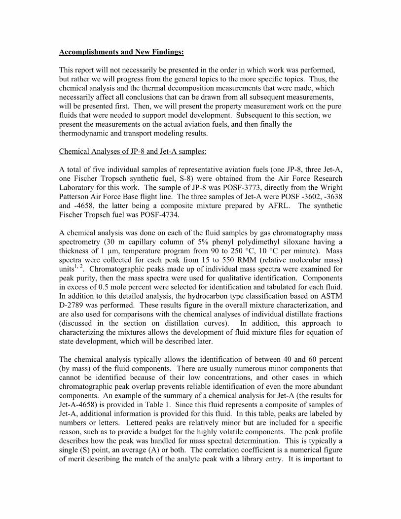
Table 3: A listing of the major components found in the sample of JP-8-3773. The area percentages provided are from raw uncorrected areas resulting from the integration of the GC-MS total ion chromatogram. When ambiguity exists regarding isomerization, the substituent position is indicated as a general variable, x.
Compound CAS No. Area % Compound CAS No. Area % n-heptane 142-82-5 0.125 2,3-dimethyl
decane 17312-44-6 0.681
methyl cyclohexane
108-87-2 0.198 1-ethyl-2,2,6-trimethyl
cyclohexane
71186-27-1 0.364
2-methylheptane
592-27-8 0.202 1-methyl-3-propyl
benzene
1074-43-7 0.569
toluene 108-88-3 0.320 aromatic unknown
NA 0.625
cis-1,3-dimethyl
cyclohexane
638-04-0 0.161 5-methyldecane
13151-35-4 0.795
n-octane 111-65-9 0.386 2-methyldecane
6975-98-0 0.686
1,2,4-trimethyl
cyclohexane
2234-75-5 0.189 3-methyldecane
13151-34-3 0.969
4-methyl octane
2216-34-4 0.318 aromatic unknown
NA 0.540
1,2-dimethyl benzene
95-47-6 0.575 aromatic unknown
NA 0.599
n-nonane 111-84-2 1.030 1-methyl-(4-methylethyl)
benzene
99-87-6 0.650
x-methylnonane
NA 0.597 n-undecane 1120-21-4 2.560
4-methylnonane
17301-94-9 0.754 x-methyl undecane
NA 1.086
1-ethyl-3-methyl benzene
620-14-4 1.296 1-ethyl-2,3-dimethyl benzene
933-98-2 1.694

6
2,6-dimethyl octane
2051-30-1 0.749 n-dodecane 112-40-3 3.336
1-methyl-3-(2-
methylpropyl) cyclopentane
29053-04-1 0.285 2,6-dimethyl undecane
17301-23-4 1.257
1-ethyl-4-methyl benzene
622-96-8 0.359 n-tridecane 629-50-5 3.998
1-methyl-2-propyl
cyclohexane
4291-79-6 0.370 1,2,3,4-tetrahydro-
2,7-dimethyl naphthalene
13065-07-1 0.850
1,2,4-trimethyl benzene
95-63-6 1.115 2,3-dimethyl dodecane
6117-98-2 0.657
n-decane 124-18-5 1.67 2,6,10-trimethyl dodecane
3891-98-3 0.821
1-methyl-2-propyl
benzene
1074-17-5 0.367 x-methyl tridecane
NA 0.919
4-methyl decane
2847-72-5 0.657 x-methyl tridecane
NA 0.756
1,3,5-trimethyl benzene
108-67-8 0.949 n-tetradecane 629-59-4 1.905
x-methyl decane
NA 0.613 n-pentadecane
629-62-9 1.345
Thermal Decomposition: Thermal Decomposition of Jet-A-4658: The thermal decomposition of the aviation fuels has been assessed with an ampoule testing instrument and approach that has been developed at NIST3, 4. We note that this work is meant strictly to support the physical property measurement work, and not to delineate reaction mechanisms. The instrument, shown schematically in Figure 1, consists of a 304L stainless steel thermal block that is heated to the desired experimental temperature (here, between 250 and 450 °C, although our rate constants were measured between 375 and 450 °C). The block is supported in an insulated box with carbon rods; the temperature is maintained and controlled (by a PID controller) to within 0.1 °C in response to a platinum resistance sensor embedded in the thermal block. The ampoule cells consist of 6.4 cm lengths of ultrahigh pressure 316L stainless steel tubing (0.64 cm

7
external diameter, 0.18 cm internal diameter) that are sealed on one end with a TIG welded stainless steel plug. Each cell is connected to a high-pressure high-temperature
PID temperature controller
insulation
graphite supports
heaters
temperature probe
stainless steel block (one of two)
slots for reactors
ampoule reactor
high-pressure
valve
high-pressure
cell
thermostat
Figure 1: A schematic diagram showing the ampoule thermal decomposition apparatus that was developed at NIST to assess the thermal stability of the aviation fuels studied in this work. valve at the other end with a short length of 0.16 cm diameter 316 stainless steel tubing with an internal diameter of 0.02 cm, also TIG welded to the cell. Each cell and valve is capable of withstanding a pressure in excess of 105 MPa at the desired temperature. The internal volume of each cell is known and remains constant at a given temperature. Fluid is added to the individual cell by mass (as determined by an approximate equation of state calculation) to give a total pressure of 34 MPa at the final fluid temperature. Measurements are done by measuring the integrated area of an emergent chromatographic peak suite that results from the decomposition. This is illustrated in Figure 2, in which a representative chromatogram of Jet-A is shown along with magnified insets of the emergent peak zone. In the “as received” sample, there are no peaks in the emergent zone, while after thermal stress, the suite develops and is seen to grow into the chromatogram as a function of increasing exposure time and temperature. During the course of this work, we performed kinetic studies on two samples that are relevant to the development of the surrogate model for JP-8. First, we measured Jet-A-4658, which is the composite Jet-A sample5. Next, in order to facilitate the modeling process, we found it necessary to measure propylcyclohexane6. This became important because of the need to represent this class of cycloalkane. Before doing any property measurements, we needed to assess the thermal stability.

8
Figure 2: Representative chromatograms showing the usual kerosene component distribution, with the insets showing the very early eluting region. Upon thermal stress, one notes the development of emergent decomposition peaks. The simplest type of decomposition is a first-order reaction in which a reactant (A) thermally decomposes into a product (B), equation 1. The rate law for such a reaction can be written in terms of the reactant or the product, equation 2, where [A] is the concentration of A, [B] is the concentration of B, k is the reaction rate constant, and t is the time. Equation 3 shows the integrated expression in terms of the reactant, where [A]t is the concentration of reactant at time t and [A]0 is the initial reactant concentration:
A B, (1)
−d[A]/dt = d[B]/dt = kt, (2)
ln[A]t = ln[A]0 − kt. (3)
Specifically, for a first-order reaction, a plot of ln[A] as a function of t should result in a straight line. Additionally, an Arrhenius plot should also yield a straight line.
9
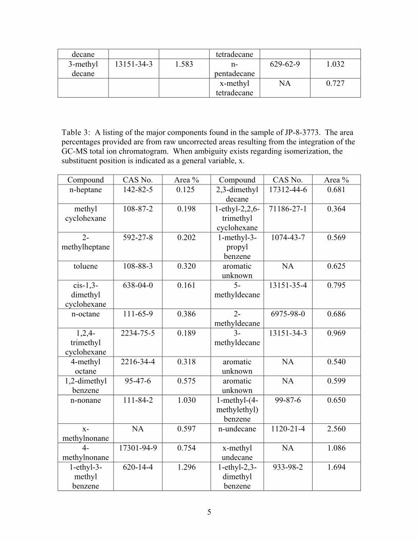
The half-life, t0.5, of a decomposition reaction is the time required for half of the reactants to become products. For a first-order reaction such as the one shown in equation 1, the half-life can be calculated directly from the rate constant, equation 4. A related quantity is the time it takes for 1% of the reactants to become products, t0.01. For first-order reactions, t0.01 also can be calculated directly from the rate constant, equation 5. The t0.5 and t0.01 of thermal decomposition are useful because they give a direct measure of the time period over which the concentration of thermal decomposition products will reach an unacceptable level. Hence, they are useful when deciding what conditions and protocols are to be used for property measurements. These quantities are given by:
t0.5 = 0.6931/k, (4)
t0.01 = 0.01005/k. (5)
In addition to calculating values for t0.5 and t0.01, rate constants determined over a temperature range can be used to evaluate the parameters of the Arrhenius equation, equation 6, where A is the pre-exponential factor, Ea is the activation energy, R is the gas constant, and T is the temperature. The Arrhenius parameters can then be used to predict rate constants at temperatures other than those examined experimentally:
k = A exp(−Ea/RT). (6) Samples of Jet-A-4658 were decomposed in the stainless steel ampoule reactors at 375, 400, 425 and 450 °C. This temperature range was chosen because it allowed for reaction times of a convenient length. At 375 °C the reaction is relatively slow, so reaction times ranged from 4 to 24 h. At 450 °C the reaction is much faster, so reaction times ranged from 10 to 120 min. The unreacted Jet A was clear and nearly colorless. Mild thermal stress (i.e., the shortest reaction times at the lower temperatures) caused the liquid to become pale yellow. Severe thermal stress (i.e., the longest reaction times at the higher temperatures) caused the liquid to become very dark brown, opaque, and viscous. A small amount of dark particulate was regularly seen in the more thermally stressed samples. Additionally, low-molecular-weight decomposition products caused a pressurized vapor phase to develop inside the reactors. For the more severely stressed samples, it was common for the entire liquid sample to be expelled under pressure when the reactor valve was opened. A separate analysis of this vapor phase was desired, and to accomplish this a gas-liquid separator designed at NIST for such work was employed7. This device is shown in Figure 3. The gas phase was then analyzed using a gas chromatograph with MS detection. Over 30 compounds were identified in the gas phase, with light alkanes being the most abundant. Table 4 shows the 10 most abundant compounds, based on total ion current in the MS detector. Note that the MS method employed precludes observation of methane. The apparent lack of alkene decomposition products is somewhat surprising, although it is known that high pressures and long reaction times decrease the yield of alkenes from the decomposition of alkanes. The rate of decomposition from alkanes

10
Figure 3: A schematic diagram of the gas-liquid separator that was used to examine the vapor phase of the thermally stressed Jet-A-4658. More details regarding this device can be found in ref 5. Table 4: A listing of the most abundant compounds found in the vapor phase of thermally stressed Jet-A-4658, maintained for 2 hrs. at 450 °C.
Compound % of Total Ion Current
butane 13.0
pentane 10.6
propane 10.4
2-methylpropane 8.6
2-methylbutane 8.1
ethane 6.6
hexane 6.4
2-methylpentane 5.9
methylcyclopentane 3.3
3-methylpentane 3.2
are also known to depend on the material used to construct the reactor.
11
The thermally stressed liquid phase of each sample was analyzed by a gas chromatograph equipped with a flame ionization detector. An easily identifiable suite of decomposition products had retention times between 2.3 and 2.8 min, Figure 4. The kinetic analysis was done based on this suite of peaks. We did not identify all of the individual compounds responsible for these peaks, but it is worth noting that pentane and hexane had retention times of 2.4 min and 2.5 min under these conditions, which suggests that most of these decomposition products had 5-7 carbon atoms. The observed product suite was essentially the same at all temperatures, with retention times that were constant to within 0.01 min. Undoubtedly, there were peaks for decomposition products in the broad kerosene “hump” that began around 2.9 min, but use of them for the kinetic analysis was impractical because of peak overlap and the lack of baseline resolution. Additionally, we did not routinely monitor compounds that were not retained in the liquid phase, including vapor-phase products and potential coke deposits. As mentioned above, the kinetic analysis was done using the emergent suite of decomposition products in the liquid phase with retention times between 2.3 and 2.8 min. The rate constant, k, at each temperature was determined from data collected at four different reaction times, with 3 to 6 replicate decomposition reactions run at each reaction time. The value of k was obtained from a nonlinear least-squares fit of these data to equation 3. For example, Figure 4 is a plot of the data and curve-fit for 425 °C. Note that data were collected at seven time points, but only the first four data points in Figure 4 were used to determine k. The reason for excluding the later time points was to limit the influence of any secondary decomposition reactions on the kinetics. Even though it is unlikely that measurements would intentionally be carried out with instrumental residence times in excess of the first four time points, this area of the plot is still useful in that it represents the chemical decomposition regime that is possible if an instrument or engine enters an upset condition resulting in long residence times. Values for t0.5 and t0.01
are calculated from k by use of equations 4 and 5. The decomposition rate constants at all four temperatures, along with values of t0.5 and t0.01, are presented in Table 5. The standard uncertainties given were calculated from the standard deviation of replicate measurements and from the standard error in the nonlinear fit. The values of t0.01 show that physical property measurements at ≥400 °C would require apparatus residence times on the order of 5 min or less. On the other hand, at 375 °C a residence time of about half an hour may be acceptable. First order rate constants reported for the decomposition of n-tetradecane are k = 1.78 10−5 s−1 at 400 °C, k = 1.01 10−4 s−1 at 425 °C, and k = 4.64 10−4 s−1 at 450 °C. Within our experimental uncertainty, these are the same as the values in Table 5 for Jet A.
An Arrhenius plot of the rate constants is shown in Figure 5. The Arrhenius parameters determined from a linear regression of the data are A = 4.1 1012 s−1 and Ea = 220 kJ·mol−1. The standard uncertainty in Ea, calculated from the standard error in the slope of the regression, is 10 kJ·mol−1. The linearity of the Arrhenius plot (r2 > 0.9978) over the 75 °C temperature range is an important validation that the assumption of first-order kinetics is reasonable. Note that the activation energy for the decomposition of Jet A is slightly lower than the values reported for pure C10–C14 n-alkanes; for example, for n-dodecane Ea is 260 kJ·mol−1 (with a reported uncertainty of 8 kJ·mol−1).

12
0
50
100
150
200
0 100 200 300 400 500
Reaction Time / min
Pro
du
ct
Su
ite
Are
a
Figure 4: Plot of the corrected area counts of the decomposition product suite as a function of time at 425 °C. Only the data at short reaction times (solid symbols) were used to determine the rate constant. The error bars represent the standard deviation for replicate decomposition reactions at each time point. Table 5: Kinetic data for the thermal decomposition of Jet-A-4658.
T / °C k / s−1 Uncertainty in k / s−1 t0.5 / h t0.01 / min
375 5.9 10−6 3.9 10−6 33 28
400 3.3 10−5 1.8 10−5 5.8 5.0
425 1.2 10−4 0.6 10−4 1.7 1.4
450 4.4 10−4 2.3 10−4 0.44 0.38

13
-13
-11
-9
-7
1.35 1.40 1.45 1.50 1.551000/T
ln k
Figure 5: Arrhenius plot for the decomposition of Jet-A-4658. The Arrhenius parameters determined from the fit to the data are A = 4.1 1012 s−1 and Ea = 220 kJ·mol−1.
Thermal Decomposition of Propylcyclohexane: As mentioned above, we also found it necessary to incorporate some pure component property measurements into the model development. Two fluids were chosen to represent cyclic branched alkanes: methylcyclohexane and propylcyclohexane. Because adequate thermal stability data could be found for methyl cyclohexane, no additional measurements were done on this fluid. Propylcyclohexane required measurements, however, since no thermal decomposition data could be found. The ampoule reactors were filled with propylcyclohexane by use of a procedure designed to achieve an initial pressure of 34.5 MPa (5000 psi) for all of the decomposition reactions. This is important because it mimics the high-pressure conditions during some physical property measurements, and it helps ensure that differences in observed decomposition rates are not due to differences in pressure. It also allows comparability with the jet-A-4658 measurements described above. After filling, air in the void space of the reactor was removed by one freeze-pump-thaw cycle. The loaded reactors were then inserted into the thermostatted stainless steel block and maintained at the reaction temperature for a period of time ranging from 10 min to 32 h. After decomposition, the reactors were removed from the thermostatted block and immediately cooled in room-temperature water. The thermally stressed propylcyclohexane was recovered and analyzed as described below. After each run, the cells and valves were carefully cleaned and dried. Blank experiments, in which the cell was loaded as described above but not heated, confirmed the effectiveness of the cleaning protocol.

14
The products of a 40 min decomposition reaction at 450 °C were identified by GC-MS. To accomplish this, a short length of glass capillary tubing was connected to the outlet on the reactor valve. The valve on the reactor was opened just enough to allow the pressurized mixture of gas and liquid in the reactor to escape slowly. Then the end of the capillary was briefly pushed through the inlet septum of the split/splitless injection port of the GC-MS, directly introducing the decomposed sample by flowing capillary injection. The components of the sample were then separated on a 30 m capillary column coated with a 0.25 m film of (5%-phenyl)-methylpolysiloxane. The temperature program for the separation started with an initial isothermal separation at 35 °C for 6 min, followed by a 20 °C/min ramp to 175 °C. The most abundant decomposition products identified in this manner are listed in Table 6. Table 6. Summary of the most abundant decomposition products after 40 min at 450 °C.
Compound % of Total Ion Abundance
ethane + propane (not resolved) 2.3 pentane 0.7 methylcyclopentane 1.1 cyclohexane 5.5 cyclohexene 3.8 methylcyclohexane 2.1 methylenecyclohexane 3.4 1-methylcyclohexene 4.7 ethylcyclohexane 0.7 1-methyl-2-propylcyclopentane 6.9 propylcyclohexene (all isomers) 2.1 butylcyclohexane 1.1 1,3-diisopropylcyclohexane 2.8
In order to determine the kinetics of decomposition, the thermally stressed liquid phase of every decomposition reaction was analyzed by a gas chromatograph equipped with a flame ionization detector (GC-FID). Evaporative losses were minimized by transferring the liquid phase into a chilled (7 °C) glass vial and immediately diluting it with a known amount of n-dodecane. The resulting n-dodecane solution was typically 5% reacted propylcyclohexane (mass/mass). The sample was then analyzed by GC-FID using a 30 m capillary column coated with a 0.1 m film of (5 %-phenyl)-methylpolysiloxane. The temperature program for the chromatographic separation consisted of an initial isothermal separation at 80 °C for 4 min, followed by a 30 °C/min gradient to 250 °C, with an additional minute at the final temperature. Figure 6 shows the suite of decomposition products that was seen in the chromatograms. The decomposition products were essentially the same at all temperatures, with retention times that were constant to within

15
0.01 min. Although we did not attempt to identify the individual peaks, the product suite observed by GC-FID is consistent with the product suite identified by GC-MS. These routine GC-FID analyses allowed us to track the extent of decomposition for each reaction. For example, about 20% of the propylcyclohexane had decomposed after 40 min at 450 °C, but only about 4% of the propylcyclohexane had decomposed after 32 h at 375 °C.
unheated propylcyclohexane
after 40 min at 450 °C
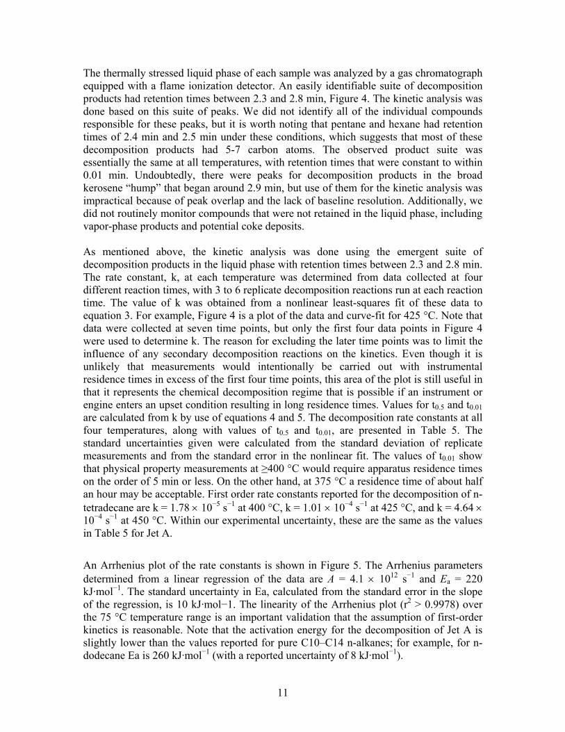
Figure 6: Chromatograms obtained by gas chromatography for unheated propylcyclohexane and for decomposed propylcyclohexane. The decomposed sample had been maintained at 450 °C for 40 min, which caused about 20 % of the propylcyclohexane to decompose. The kinetic analysis was done by monitoring the relative decrease in the chromatographic signal of propylcyclohexane compared to the chromatographic signals for decomposition products. At each temperature data were collected at four or five different reaction times, with 3 to 5 replicate decomposition reactions at each reaction time. Following equation 3, the value of k at each temperature was obtained from the slope of a linear fit of ln(propylcyclohexane peak area %) as a function of t. Figure 7 shows such a plot obtained from the data at 450 °C. The linearity of the data justifies the assumption of first-order kinetics. The first-order rate constant obtained from the plot is 8.63 10−5 s−1, with a standard uncertainty of 0.18 10−5 s−1. The rate constants measured for all temperatures are provided in Table 7. An Arrhenius plot of the rate constants is shown in Figure 8. The Arrhenius parameters determined from a linear regression of the data are A = 2.56 1016 s−1 and Ea = 283 kJ·mol−1. The standard uncertainty in Ea, calculated from the standard error in the slope of the regression, is 6 kJ·mol−1. The linearity of the Arrhenius plot (r2 = 0.9999) over the 75 °C temperature range is an important validation that the assumption of first-order kinetics is reasonable. Note that the activation energy for the decomposition of propylcyclohexane is slightly higher than the values reported for C10–C14 n-alkanes; for example, for n-dodecane Ea is 260 kJ·mol−1 (with a reported uncertainty of 8 kJ·mol−1)6.
16
-0.25
-0.2
-0.15
-0.1
-0.05
0
0 10 20 30 40 50
time (min)
ln(p
rop
ylc
yclo
he
xa
ne
pea
k a
rea
%)
Figure 7: A plot of the ln(propylcyclohexane peak area %) as a function of time at 450 °C. The first-order rate constant for the decomposition reaction was determined from the slope of the linear fit to the data. Table 7: Kinetic data for the thermal decomposition of propylcyclohexane.
T / °C k / s−1 Uncertainty in k / s−1 t0.5 / h t0.01 / min 375 3.66 10−7 0.12 10−7 526 458 400 2.67 10−6 0.09 10−6 72.2 62.8 425 1.59 10−5 0.04 10−5 12.1 10.5 450 8.63 10−5 0.18 10−5 2.23 1.94

17
-16
-14
-12
-10
-8
1.35 1.40 1.45 1.50 1.55
1000/T
lnk
Figure 8: The Arrhenius plot for the decomposition of propylcyclohexane. The Arrhenius parameters determined from the linear fit are A = 2.56 1016 s−1 and Ea = 283 kJ·mol−1. Thermophysical Property Measurements on Methylcyclohexane and Propylcyclohexane: Compressed Liquid Density Measurements for Methyl- and Propylcyclohexane: A schematic of the apparatus used to measure compressed liquid densities over the temperature range of 270 K to 470 K and to pressures of 50 MPa is illustrated in Figure 9.8 The heart of the apparatus is a commercial vibrating tube densimeter, however, several physical and procedural improvements have been implemented beyond that of the commercial instrument operated in a stand-alone mode. The densimeter is housed in a specially designed two-stage thermostat for improved temperature control. The uncertainty in the temperature is 0.02 K with short-term stability of 0.005 K. Pressures are measured with an oscillating quartz crystal pressure transducer with an uncertainty of 10 kPa. The densimeter is calibrated with measurements of vacuum, propane and toluene, over the temperature and pressure range of the apparatus to achieve an uncertainty in density of 1 kg/m3. The apparatus has been designed, and software has been written so that the operation and data acquisition are fully automated. Data are taken along isotherms over a temperature/pressure matrix programmed by the operator prior to the start of measurements. Electronically actuated pneumatic valves, and a programmable syringe pump are used to move from one pressure to the next and/or flush fresh sample through

18
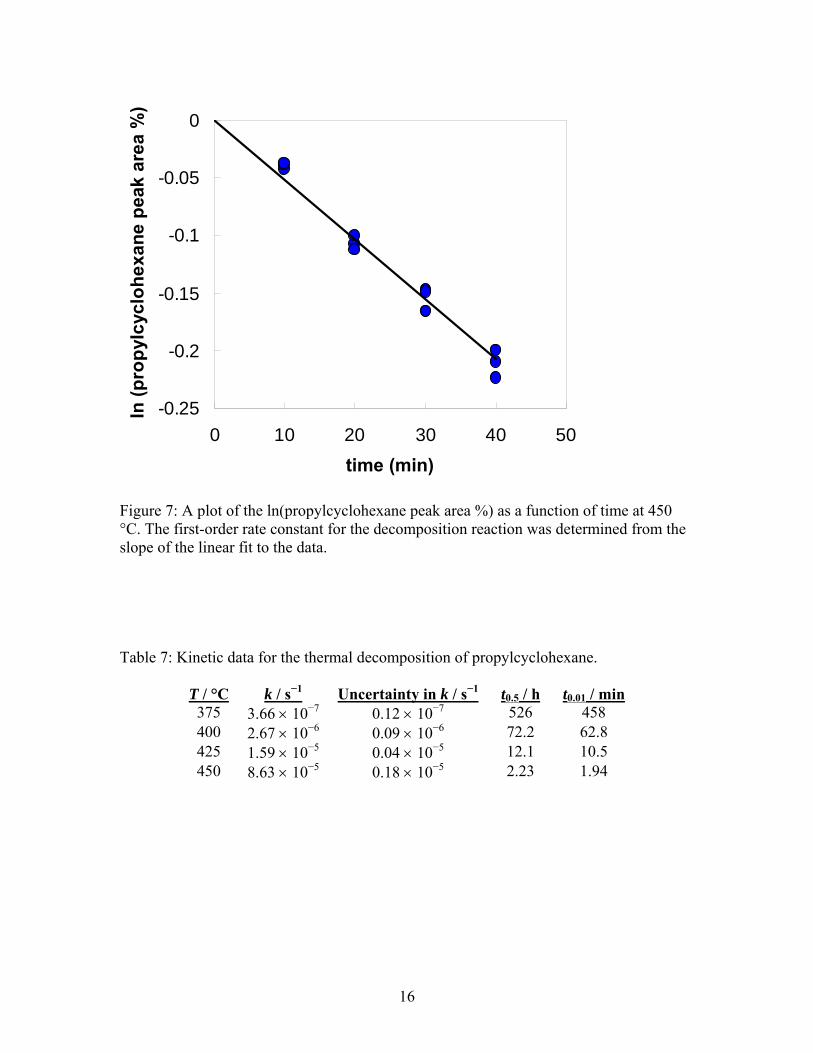
the system. Operation of the densimeter in this manner allows for measurements to be made 24 hours a day. Compressed liquid densities of methylcyclohexane have been measured along eleven isotherms from 270 K to 470 K at pressures from 0.5 MPa to 40 MPa. A total of 140 points are reported in Table 8 and shown graphically in Figure 10.9
Figure 9. Schematic of the Compressed Liquid Density Apparatus. Table 8. Compressed liquid densities of methylcyclohexane Temperature
(K) Pressure (MPa)
Density (kg/m3)
Temperature (K)
Pressure (MPa)
Density (kg/m3)
270.00 40.007 814.61 390.00 40.003 731.07270.00 35.009 811.80 390.00 35.004 726.33270.00 30.008 808.90 390.00 29.996 721.31

19
270.00 25.004 805.91 390.00 25.009 715.97270.00 20.008 802.83 390.00 20.007 710.24270.00 15.006 799.63 390.00 15.001 704.06270.00 10.005 796.31 390.00 10.003 697.32270.00 5.007 792.85 390.00 5.011 689.86270.00 4.004 792.13 390.00 4.003 688.24270.00 2.998 791.41 390.00 3.004 686.61270.00 2.005 790.68 390.00 2.008 684.95270.00 1.003 789.96 390.00 0.999 683.2270.00 0.502 789.59 390.00 0.502 682.32290.00 39.998 800.66 410.00 39.999 717.45290.00 34.996 797.59 410.00 35.003 712.28290.00 29.996 794.41 410.00 30.002 706.79290.00 24.995 791.12 410.00 25.002 700.89290.00 20.007 787.71 410.00 19.997 694.5290.00 14.995 784.14 410.00 15.004 687.54290.00 9.999 780.43 410.00 10.006 679.84290.00 5.004 776.54 410.00 5.002 671.17290.00 3.994 775.73 410.00 4.003 669.29290.00 3.007 774.91 410.00 3.000 667.35290.00 2.000 774.08 410.00 2.003 665.35290.00 1.003 773.25 410.00 1.000 663.27290.00 0.497 772.82 410.00 0.507 662.23310.00 40.034 786.33 430.00 40.017 703.89310.00 34.999 782.89 430.00 34.998 698.25310.00 30.014 779.38 430.00 30.000 692.21310.00 25.007 775.73 430.00 25.005 685.69310.00 20.006 771.95 430.00 19.999 678.55310.00 15.009 767.98 430.00 14.997 670.67310.00 10.007 763.81 430.00 10.006 661.83310.00 5.016 759.43 430.00 4.999 651.64310.00 3.997 758.50 430.00 3.997 649.38310.00 2.999 757.59 430.00 3.003 647.06310.00 2.005 756.66 430.00 2.002 644.62310.00 1.009 755.72 430.00 0.493 640.64310.00 0.500 755.22 450.00 39.991 690.35330.00 40.011 772.18 450.00 34.996 684.22330.00 35.006 768.48 450.00 29.995 677.59330.00 30.003 764.63 450.00 24.995 670.36330.00 25.001 760.61 450.00 20.003 662.4330.00 20.006 756.40 450.00 15.001 653.46330.00 15.009 752.00 450.00 10.004 643.22330.00 10.001 747.31 450.00 4.999 631.1330.00 5.003 742.35 450.00 4.000 628.37330.00 4.000 741.29 450.00 3.001 625.51330.00 3.012 740.25 450.00 1.999 622.5

20
330.00 2.002 739.17 450.00 1.000 619.32330.00 1.000 738.08 470.00 39.994 676.99330.00 0.501 737.54 470.00 35.000 670.31350.00 40.000 758.41 470.00 30.009 663.05350.00 35.003 754.41 470.00 25.005 655.04350.00 30.011 750.22 470.00 19.995 646.07350.00 25.004 745.82 470.00 14.995 635.87350.00 20.001 741.17 470.00 9.995 623.93350.00 15.005 736.24 470.00 5.001 609.33350.00 10.006 730.97 470.00 4.003 605.94350.00 5.000 725.31 470.00 2.999 602.32350.00 4.007 724.13 470.00 1.999 598.46350.00 3.009 722.92 470.00 1.002 594.33350.00 2.003 721.69 350.00 1.004 720.45 350.00 0.500 719.79 370.00 39.999 744.71 370.00 34.994 740.36 370.00 29.997 735.78 370.00 25.005 730.95 370.00 19.994 725.79 370.00 15.007 720.28 370.00 10.006 714.34 370.00 5.000 707.86 370.00 3.995 706.48 370.00 3.000 705.08 370.00 2.001 703.65 370.00 0.994 702.17 370.00 0.499 701.44
21
Methylcyclohexane
580
600
620
640
660
680
700
720
740
760
780
800
820
250 270 290 310 330 350 370 390 410 430 450 470 490
Temperature [K]
Den
sity
[k
g/m
3]
Figure 10. Compressed liquid densities of methylcyclohexane as a function of temperature. Compressed liquid densities of propylcyclohexane have been measured along eleven isotherms from 270 K to 470 K at pressures from 0.5 MPa to 40 MPa. A total of 143 points are reported in Table 9 and are shown graphically in Figure 11. Table 9. Compressed liquid densities of propylcyclohexane. Temperature
(K) Pressure (MPa)
Density (kg/m3)
Temperature (K)
Pressure (MPa)
Density (kg/m3)
270.00 39.959 834.41 390.00 39.989 756.91 270.00 35.005 831.91 390.00 35.002 752.82 270.00 30.003 829.32 390.00 29.998 748.51 270.00 25.001 826.66 390.00 25.002 743.97 270.00 19.995 823.91 390.00 20.002 739.14 270.00 15.004 821.08 390.00 15.000 734.00 270.00 10.003 818.11 390.00 10.005 728.48 270.00 5.009 815.01 390.00 5.003 722.49 270.00 4.004 814.35 390.00 4.003 721.22 270.00 2.987 813.68 390.00 3.003 719.93 270.00 2.001 813.03 390.00 2.009 718.64 270.00 1.001 812.37 390.00 1.002 717.29 270.00 0.497 812.02 390.00 0.504 716.61

22
290.00 40.005 821.46 410.00 39.998 744.41 290.00 35.005 818.73 410.00 35.005 739.97 290.00 29.995 815.90 410.00 30.003 735.27 290.00 25.004 812.98 410.00 25.002 730.28 290.00 19.998 809.96 410.00 19.998 724.97 290.00 15.011 806.81 410.00 14.998 719.26 290.00 10.002 803.50 410.00 10.008 713.07 290.00 5.002 800.04 410.00 5.008 706.29 290.00 4.007 799.31 410.00 4.003 704.83 290.00 3.003 798.58 410.00 2.994 703.34 290.00 2.013 797.84 410.00 2.005 701.86 290.00 1.000 797.09 410.00 0.994 700.28 290.00 0.506 796.73 410.00 0.506 699.52 310.00 39.979 807.65 430.00 39.996 731.95 310.00 35.008 804.71 430.00 35.004 727.15 310.00 29.997 801.64 430.00 30.006 722.05 310.00 24.999 798.47 430.00 24.999 716.59 310.00 20.004 795.18 430.00 19.996 710.74 310.00 14.996 791.73 430.00 15.011 704.40 310.00 10.004 788.15 430.00 10.005 697.42 310.00 5.013 784.41 430.00 4.999 689.66 310.00 3.999 783.61 430.00 3.993 687.98 310.00 3.004 782.83 430.00 3.002 686.29 310.00 2.007 782.04 430.00 1.988 684.51 310.00 0.999 781.23 430.00 0.998 682.73 310.00 0.505 780.83 430.00 0.516 681.83 330.00 39.988 794.75 450.00 39.992 719.57 330.00 35.002 791.53 450.00 35.009 714.38 330.00 30.000 788.17 450.00 30.007 708.83 330.00 25.001 784.69 450.00 25.013 702.87 330.00 20.004 781.06 450.00 19.999 696.38 330.00 15.009 777.27 450.00 15.008 689.31 330.00 10.001 773.27 450.00 9.999 681.42 330.00 5.001 769.08 450.00 4.999 672.53 330.00 3.994 768.20 450.00 3.995 670.59 330.00 3.000 767.32 450.00 3.001 668.60 330.00 2.004 766.43 450.00 1.993 666.53 330.00 0.999 765.52 450.00 0.999 664.39 330.00 0.498 765.06 450.00 0.506 663.31 350.00 40.001 782.15 470.00 40.004 707.37 350.00 35.003 778.64 470.00 35.004 701.75 350.00 30.001 774.98 470.00 30.002 695.70 350.00 25.007 771.17 470.00 25.001 689.15 350.00 20.005 767.18 470.00 20.004 682.01 350.00 15.006 762.98 470.00 14.994 674.08 350.00 10.006 758.54 470.00 10.006 665.17

23
350.00 4.999 753.83 470.00 5.003 654.87 350.00 4.003 752.86 470.00 4.003 652.59 350.00 2.996 751.85 470.00 3.000 650.21 350.00 1.992 750.83 470.00 2.002 647.76 350.00 1.000 749.82 470.00 0.991 645.18 350.00 0.500 749.30 470.00 0.496 643.86 370.00 39.998 769.44 370.00 34.998 765.65 370.00 30.001 761.68 370.00 25.001 757.53 370.00 20.007 753.15 370.00 15.011 748.51 370.00 10.006 743.56 370.00 5.003 738.27 370.00 4.003 737.16 370.00 3.002 736.02 370.00 2.005 734.87 370.00 1.006 733.71 370.00 0.496 733.11

24
Propylcyclohexane
640
660
680
700
720
740
760
780
800
820
840
250 270 290 310 330 350 370 390 410 430 450 470 490
Temperature [K]
Den
sity
[k
g/m
3]
Figure 11. Compressed liquid densities of propylcyclohexane as a function of temperature. Viscosity Measurements of Methyl- and Propylcyclohexane: Viscosity measurements of methyl- and propylcyclohexane were carried out at ambient pressure in the temperature range 293.15 K to 373.15 K. These measurements are presented in Table 10. The instrument used was a commercial device consisting of an automated open gravitational flow viscometer with a suspended-level Ubbelohde glass capillary of 200 mm length with upper reservoir bulbs for a kinematic viscosity range from 0.3 mm2·s-1 to 30 mm2·s-1. As shown in the photograph of Figure 12, the glass capillary is mounted in a thermostatting bath filled with silicone oil. The thermostat includes a stirrer, a heat pipe to a thermoelectric Peltier cooler at the top of the instrument (not visible), and a platinum 100 Ω resistance temperature probe (PRT). The bath temperature is set with the operating software that is an integral part of the viscosity measurement system and it is controlled within 0.02 K between 293.15 K and 373.15 K. The resistance of the PRT is measured with an ac bridge. The calibration of the PRT on the International Temperature Scale of 1990 was checked by comparison with a water triple point cell. The estimated uncertainty of the temperature measurement system is 0.02 K.

25
Figure 12: A photograph of the viscometer used for the measurement of methyl- and propylcyclohexane. The instrument allows viscosity measurements relative to liquids with well known viscosities. Calibrations were performed with certified viscosity standards to determine the constants C and E of the working equation: = C·t - E / t2. (7) The first term on the right hand side of this equation is the reformulated Hagen-Poiseuille expression for laminar flow in a circular tube whereas the second term is the Hagenbach correction for kinetic energy losses. Symbol denotes the kinematic viscosity in mm2·s-1 and t the efflux time in seconds of a known volume of liquid through the capillary. Efflux times are measured with three thermistor sensors on the outside of the capillary above and below the two measuring bulbs. The thermistors detect the passing of the liquid meniscus at their locations and trigger an internal stopwatch. Depending on the viscosity range the two upper or the two lower thermistors are used to time the efflux of the test liquid through the respective measuring bulb of known volume.

26
The viscosity measurement system includes components to pump the test liquid into the upper measuring bulbs for repetitive efflux timings and to flush the capillary tube with two different solvents when the test liquid is changed. The operating software was set to perform five measurement runs at the most of which the three that agreed within 0.5% repeatability were averaged to calculate the viscosity. The uncertainty of the viscosity measurements reported here is estimated at 1.5 % to account for variations in the constants C and E that occurred for calibrations with different viscosity standards and to a lesser degree for calibrations at different temperatures. The ambient pressure during the measurements was 83 kPa. Due to this, methyl cyclo-hexane could not be measured at 373.15 K because it evaporated at that temperature. The design of the instrument, its calibration, and operation conform to the following stan-dards: - ASTM D 445 Standard Test Method for Kinematic Viscosity of Transparent and Opaque Liquids (and the Calculation of Dynamic Viscosity), - ASTM D 446 Standard Specifications and Operating Instructions for Glass Capillary Kinematic Viscometers, - D 2162 Test Method for Basic Calibration of Master Viscometers and Viscosity
Oil Standards, and the corresponding ISO standards 3104 and 3105.

27
Table 10: Kinematic viscosity of methyl- and propylcyclohexane measured in the open gravitational capillary viscometer system.
Methylcyclohexane Propylcyclohexane
Temperature T
Kinematic viscosity
TemperatureT
Kinematic viscosity
K mm2·s-1 K mm2·s-1 363.15
353.16
343.15
333.15
323.15
313.15
303.21
293.23
0.4707
0.5113
0.5568
0.6107
0.6736
0.7488
0.8387
0.9480
303.15
293.15
313.15
373.15
363.15
353.15
343.15
333.15
323.15
1.112
1.277
0.9830
0.5500
0.5966
0.6499
0.7140
0.7877
0.8759

28
Sound Speed Measurements of Methyl- and Propylcyclohexane: A commercial density and sound speed analyzer was used to determine the sound speed of methyl- and propylcyclohexane at ambient pressure.9 Temperature scans were programmed from 70 °C to 10 °C in decrements of 10 °C followed by a single measurement at 5 °C. The device contains a sound speed cell and a vibrating quartz tube densimeter in series. Temperature is measured with an integrated Pt-100 thermometer with an estimated uncertainty of 0.01 K. The sound speed cell has a circular cylindrical cavity of 8 mm diameter and 5 mm thickness that is sandwiched between the transmitter and receiver. The speed of sound is determined by measuring the time of flight of signals between the transmitter and receiver. The instrument was calibrated with air and deionized water at 20 °C. The reproducibility of the sound speed of water at 20 °C to within 0.01 % was checked before and after measurements of the test liquids. Careful cleaning of the sound speed cell with suitable solvents was found critical to avoid contaminations and to ensure this level of performance. For the same reason, fresh samples of test liquids were injected for each temperature scan instead of performing repetitive measurements on the same sample. At least four temperature scans were performed for each test liquid. The relative standard deviation of these repeated sound speed measurements was lower than 0.013 %. The manufacturer quoted uncertainty of sound speed measurements with this instrument is 0.1 %. The speeds of sound measured in this work (along with the density) are provided in Table 11, and shown graphically in Figure 13. Table 11: Density, speed of sound, and adiabatic compressibility of methyl- and
propylcyclohexane measured in the commercial density and sound speed analyzer. The ambient pressure during the measurements was 83 kPa.
Methylcyclohexane Propylcyclohexane
Temp-erature T
Density
Speed of
sound w
Adiab. compressibility
s Density
Speed of
sound w
Adiab. compres-sibility s
K kg·m-3 m·s-1 TPa-1 kg·m-3 m·s-1 TPa-1
278.15
283.15
293.15
303.15
313.15
323.15
333.15
343.15
782.3
778.0
769.3
760.7
751.9
743.1
734.3
725.3
1304.7
1281.9
1236.9
1192.9
1149.7
1107.4
1065.6
1024.5
750.94
782.27
849.67
923.93
1006.1
1097.4
1199.3
1313.6
805.4
801.5
793.7
785.9
778.1
770.2
762.3
754.4
1371.3
1349.6
1307.1
1265.5
1224.7
1184.7
1145.4
1106.9
660.26
685.01
737.38
794.47
856.81
925.02
999.94
1081.9

29
Figure 13: Measured speed of sound data for methyl- and propylcyclohexane Adiabatic compressibilities at ambient pressure were obtained from the measured densities and speeds of sound via the thermodynamic relation κs = -(∂V/∂p)s/V = 1 / (ρw2), where V denotes volume, p is pressure, is the density, and w the speed of sound. Subscript s indicates “at constant entropy s.” For convenience, the calculated adiabatic compressibilities are included in Table 11. The speed of sound and adiabatic compressibility data of the two liquids at ambient pressure are plotted in Figure 14 as a function of temperature. Comparing the plots illustrates how changing the molecular structure of methylcyclohexane by adding an ethyl-group -CH2-CH2- to the aliphatic side chain to form propylcyclohexane influences the macroscopic properties of the two compounds. The speed of sound increases between
1000
1050
1100
1150
1200
1250
1300
1350
1400
270 280 290 300 310 320 330 340 350
Methylcyclohexane
Propylcyclohexane
T / K
w / m·s-1

30
5.1 % at 273.15 K and 8.1 % at 343.15 K whereas the adiabatic compressibility increases between 13.8 % and 21.4 %. The densities of the test liquids at these two state points differ only by 3 % and 4 %, respectively. Thus, the adiabatic compressibility appears to reflect structural changes on the molecular scale with higher resolution than the other two properties.
Figure 14: Measured adiabatic compressibility of methyl- and propylcyclohexane as a function of temperature at ambient pressure
600
650
700
750
800
850
900
950
1000
1050
1100
1150
1200
1250
1300
1350
270 280 290 300 310 320 330 340 350
Methylcyclohexane
Propylcyclohexane
T / K
s / TPa-1

31
Thermal Conductivity of Methyl- and Propylcyclohexane: Transient hot-wire measurements of the thermal conductivity of the samples of methylcyclohexane and propylcyclohexane were made in the liquid and vapor phases; up to 600 K for propylcyclohexane. In addition, a supercritical isotherm at 593 K was measured for methylcyclohexane. Measurements for both fluids cover temperatures from 300 to 600 K with pressures up to 70 MPa. The transient hot-wire instrument has been described in detail elsewhere.10, 11 The measurement cell is designed to closely approximate transient heating from a line source into an infinite fluid medium. The ideal (line source) temperature rise Tid is given by:
,lnln10
1w
02id T + T = Cr
4a + (t)
4
q = T i
=i
(8)
where q is the power applied per unit length, is the thermal conductivity of the fluid, t is the elapsed time, a = /Cp is the thermal diffusivity of the fluid, is the density of the fluid, Cp is the isobaric specific heat capacity of the fluid, r0 is the radius of the hot wire, C = 1.781... is the exponential of Euler's constant, Tw is the measured temperature rise of the wire, and Ti are corrections to account for deviations from ideal line-source conduction. The only significant correction for the measurements is for the finite wire dimensions. A plot of ideal temperature rise versus logarithm of elapsed time should be linear, such that thermal conductivity can be found from the slope and thermal diffusivity can be found from the intercept of a line fit to the data. At time zero, a fixed voltage is applied to heat the small diameter wire that is immersed in the fluid of interest. The wire is used as an electrical heat source while its resistance increase allows determination of the transient temperature rise as a function of elapsed time. Two platinum wires of 12.7 m diameter were used for most of the measurements. The two wires, one about 18 cm long and one about 4 cm long, were used with a differential technique to eliminate axial conduction errors. A similar cell with anodized tantalum hot wires of 25 m diameter was used for some measurements on liquid methylcyclohexane at temperatures from 300 K to 400 K. Short experiment times (nominally 1 s) and small temperature rises (nominally 1 to 4 K) were selected to eliminate heat transfer by free convection. Experiments at several different heating powers (and temperature rises) provide verification that free convection is not significant. Heat transfer due to thermal radiation is more difficult to detect and correct when the fluid can absorb and re-emit infrared radiation as these hydrocarbons do. Thermal radiation heat transfer will increase roughly in proportion to the absolute temperature cubed and can be characterized from an increase in the apparent thermal conductivity as experiment time increases since radiation emission from the fluid increases as the thermal wave diffuses outward.
At very low pressures, the steady-state hot-wire technique has the advantage of not requiring significant corrections. The working equation for the steady-state mode is based on a

32
different solution of Fourier's law but the geometry is still that of concentric cylinders. This equation can be solved for the thermal conductivity of the fluid, ,
where q is the applied power per unit length, r2 is the internal radius of the outer cylinder, r1 is the external radius of the inner cylinder (hot wire), and T = (T1 - T2) is the measured temperature difference between the hot wire and its surrounding cavity. A total of 1389 points are reported in Appendix I (the lengths of these tables preclude inclusion within the body of the report) for the thermal conductivity of methylcyclohexane in the liquid, vapor and supercritical regions at pressures to 60 MPa. These data for methylcyclohexane are shown in Figure 15. A total of 668 points are reported in appendix I for the thermal conductivity of propylcyclohexane in the liquid and vapor regions at pressures to 60 MPa. Note that within the appendix, the thermal conductivity tables are divided into vapor and liquid, and by wire material. These data for propylcyclohexane are shown in Figure 16. Each experiment is characterized by the initial cell temperature T0 and the mean experiment temperature Te. There are generally 5 experiments at each initial cell temperature to verify that convection was not significant, since convection depends strongly on the temperature rise (T = Te - T0). The conditions of the fluid during each measurement are given by the experimental temperature Te, pressure Pe, and density e. The thermal conductivity without correction for thermal radiation is given by e.. The thermal conductivity data for these fluids have an uncertainty of less than 1 % for measurements removed from the critical point and for gas at pressures above 1 MPa, increasing to 3 % at the highest temperatures (near 600 K) and for gas at low pressures (<1 MPa) at a 95 % confidence level. A significant critical enhancement is observed in the thermal conductivity data near the critical point. There is likely a residual contribution due to emission of thermal radiation by the fluid that increases in proportion to temperature cubed up to 2 % to 3 % near 600 K.
,
ln
)T - T(2r
r q
= 21
1
2
(9)

33
0.02
0.04
0.06
0.08
0.10
0.12
0 100 200 300 400 500 600 700 800
/ kg.m-3
e
/ W
. m-1
K-1
Figure 15: Thermal conductivity of methylcyclohexane at temperatures from 300 K to 595 K and pressures up to 60 MPa: , transient (Pt); , transient (Ta); , steady state (Pt); solid line given by the correlation developed in this work.

34
0.02
0.04
0.06
0.08
0.10
0.12
0 100 200 300 400 500 600 700 800
/ kg.m-3
e
/W
. m-1
K-1
Figure 16: Thermal conductivity of propylcyclohexane at temperatures from 300 K to 600 K and pressures up to 60 MPa: , transient (Pt); , steady state (Pt); solid line given by the correlation developed in this work.
Thermophysical Property Measurements on Jet-A, JP-8 and S-8: Distillation Curves of Jet-A, JP-8 and S-8: A new advanced method for the measurement of distillation curves of complex fluids has recently been introduced. The modifications to the classical measurement provide for (1) temperature and volume measurements of low uncertainty, (2) temperature control based upon fluid behavior, and most important, (3) a composition-explicit data channel in addition to the usual temperature-volume relationship12-14. This latter modification is achieved with a new sampling approach that allows precise qualitative as well as quantitative analyses of each fraction, on the fly. Any composition dependent property can be enhanced by combining it with the distillation curve information. For example, and especially relevant to fuels, we have shown that it is possible to obtain heat of combustion data for each distillate fraction15. In the advanced method, the temperature is logged in two locations. First, the temperature is measured directly in the fluid, which provides a true thermodynamic state point and true initial boiling temperature. This temperature is referred to as Tk. Second, the temperature is also measured in the distillation head, referred to at Th. This temperature is directly comparable to historical

35
data. We have applied this method to a wide variety of fuels and complex fluids16-31. A schematic diagram of the advanced apparatus is provided in Figures 17 - 19.
Figure 17: Schematic diagram of the overall apparatus used for the measurement of distillation curves.

36
Figure 18: Schematic diagram of the receiver adapter to provide on-the-fly sampling of distillate cuts for subsequent analysis.

37
Figure 19: Schematic diagram of the level-stabilized receiver for distillation curve measurement.
38
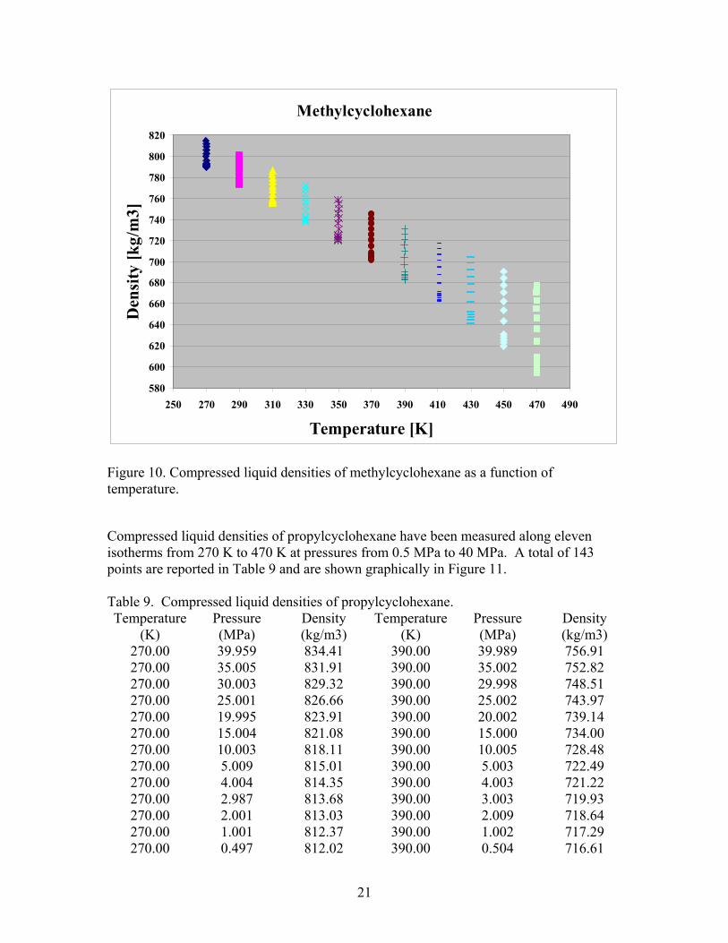
During the initial heating of each sample in the distillation instrument, the behavior of the fluid was observed. Direct observation through the flask window or through the illuminated bore scope allowed measurement of the onset of boiling for each of the mixtures. Typically, during the early stages of a measurement the first bubbles will appear intermittently, and this action will quell if the stirrer is stopped momentarily. Sustained vapor bubbling is then observed. In the context of the advanced distillation curve measurement, sustained bubbling is also somewhat intermittent, but it is observable even when the stirrer is momentarily stopped. Finally, the temperature at which vapor is first observed to rise into the distillation head is observed. This is termed the vapor rise temperature. These observations are important because they are the initial boiling temperatures (IBT) of each fluid. The initial behaviors of three samples of Jet-A and the synthetic S-8 are provided in Table 12. These temperatures have been corrected to 1 atm. with the modified Sydney Young equation.32 Table 12: A summary of the initial behavior of the three individual samples of Jet-A, and the sample of S-8. In keeping with our advanced distillation curve protocol, the onset temperature is the temperature at which the first bubbles are observed. The sustained bubbling temperature is that at which the bubbling persists. The vapor rise temperature is that at which vapor is observed to rise into the distillation head, considered to be the initial boiling temperature of the fluid (highlighted in bold print). The temperatures have been adjusted to 1 atm with the modified Sydney Young equation; uncertainties are discussed in the text.
Observed Temperature
Jet-A-3602, °C, 82.82 kPa
Jet-A-3638, °C, 82.11 kPa
Jet-A-4658, °C, 83.63 kPa
S-8, °C, 83.27 kPa
onset 150.9 148.4 139.9 163.0 sustained 183.6 176.9 185.6 168.6
vapor rising 191.0 184.2 190.5 181.9 Representative distillation curve data for the three samples of Jet-A, presented in both Tk and Th, are provided in Table 13. In this table, the estimated uncertainty (with a coverage factor k=2) in the temperatures is 0.1 °C. Note that the experimental uncertainty of Tk is somewhat lower than that of Th, but as a conservative position, we use the higher value for both temperatures. The uncertainty in the volume measurement that is used to obtain the distillate volume fraction is 0.05 mL in each case. The same data are provided graphically in Figure 20.

39
Table 13: Representative distillation curve data for the three individual samples of Jet-A and the sample of S-8 measured in this work. The temperatures have been adjusted to 1 atm. with the modified Sydney Young equation; uncertainties are discussed in the text. These data are plotted in Figure 20. Distillate Volume
Fraction, %
Jet-A-3602 82.82 kPa
Jet-A-3638 82.11 kPa
Jet-A-4658 83.63 kPa
S-8 83.27 kPa
Tk, °C Th, °C Tk, °C Th, °C Tk, °C Th, °C Tk, °C Th, °C
5 194.8 179.3 186.8 179.9 195.4 174.7 183.6 169.2 10 197.7 186.7 188.7 184.2 198.5 183.3 185.0 173.9 15 200.7 189.9 191.1 187.0 201.5 187.0 187.7 179.1 20 203.5 194.7 192.9 185.8 204.7 189.1 190.2 173.6 25 206.4 196.9 194.9 189.5 208.1 190.6 193.0 175.5 30 209.7 198.7 196.6 191.6 211.3 192.8 196.2 181.9 35 212.1 199.2 198.5 193.9 214.3 194.6 199.5 187.7 40 214.8 201.5 200.3 196.0 217.6 199.1 202.9 192.0 45 217.3 204.5 202.1 197.9 220.7 202.6 207.1 196.2 50 220.1 206.4 204.0 199.8 224.2 205.4 211.0 200.3 55 222.5 208.8 205.9 202.4 227.6 208.6 215.3 205.2 60 225.1 213.6 208.0 204.0 231.2 212.4 219.6 209.3 65 227.9 213.7 210.5 205.1 234.7 214.9 224.2 213.6 70 230.7 218.4 213.6 207.6 239.4 216.6 229.4 219.1 75 233.9 223.2 216.2 210.6 243.3 218.7 235.2 224.3 80 237.9 226.4 219.4 210.2 247.9 220.8 240.1 231.4 85 242.7 225.6 222.9 215.3 253.6 224.1 246.8 236.8

40
180
190
200
210
220
230
240
250
260
0 10 20 30 40 50 60 70 80 90
Volume Fraction, %
Te
mp
era
ture
(oC
)
3638
3602
4658
S-8
Figure 20: Representative distillation curves for each of the three samples of Jet-A and the sample of S-8 that have been measured as part of this work. The temperatures have been adjusted to 1 atm with the modified Sydney Young equation; uncertainties are discussed in the text. The shapes of all of the curves are of the subtle sigmoid or growth curve type that one would expect for a highly complex fluid with many components, distributed over a large range of relative molecular mass. There is no indication of the presence of azeotropic constituents, since there is an absence of multiple inflections and curve flattening. As an example of typical repeatability of these curves, we show in Figure 21 six curves measured for Jet-A-4658. We note that in the latter stages of the distillations, the repeatability suffers slightly.

41
185
195
205
215
225
235
245
255
0 10 20 30 40 50 60 70 80 90
Volume Fraction, %
Tem
per
atu
re,
Tk,
°C
Figure 21: Plot showing the repeatability of the distillation curve measurement. Here, six measurements of the curve for Jet-A-4658 are provided. The uncertainty bars of the individual temperatures are of the same size as the plotting symbols. The plotted curves are particularly instructive since the difference presented by Jet-A-3838 with respect to Jet-A-3602 and Jet-A-4658 is clearly shown. It is also clear from the curves that the differences are not merely in the early parts of the curves, but rather the difference persists throughout the curve and is in fact magnified at higher distillate volume fraction values. This behavior is indicative of fluids that differ in overall composition or chemical family throughout the entire composition range of the fluid. This is in contrast to differences that result from one fluid merely having somewhat more volatile constituents that boil off in the early stages of the distillation curve measurement, and is often caused by the presence of a different distribution of components within a chemical family. Indeed, this observation was found to be consistent with a gas chromatographic analysis of the three fuel samples (the procedure for which was described in the experimental section), since Jet-A-3602 and Jet-A-4658 appear to contain much higher concentrations of heavier components. This can be shown by examining the total area of chromatographic peaks that elute subsequent to the emergence of n-tetradecane, for each sample. For Jet-A-3638, this comprises 2.47 % of the total peak areas, while for Jet-A-3602 and Jet-A-4658, this comprises 12.07 and 17.57 %, respectively. Note that these peak areas are the raw, uncalibrated values, and are used only for comparison among the three fluids.
42
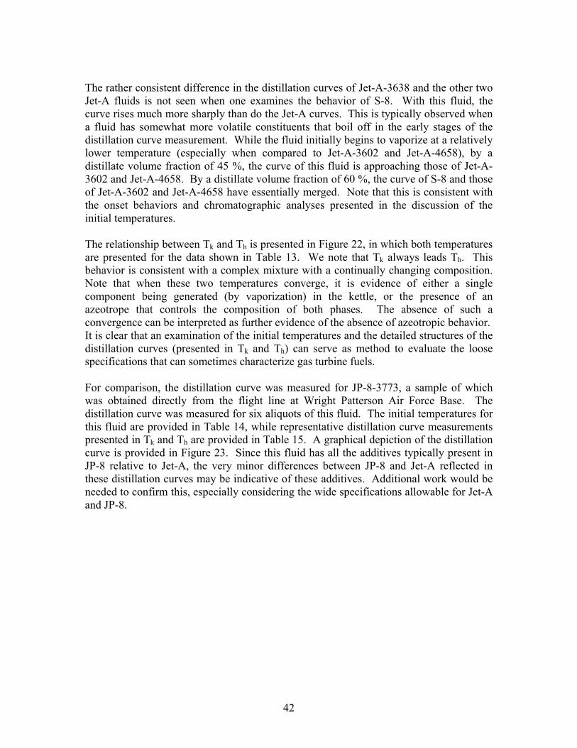
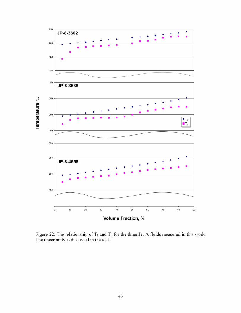
The rather consistent difference in the distillation curves of Jet-A-3638 and the other two Jet-A fluids is not seen when one examines the behavior of S-8. With this fluid, the curve rises much more sharply than do the Jet-A curves. This is typically observed when a fluid has somewhat more volatile constituents that boil off in the early stages of the distillation curve measurement. While the fluid initially begins to vaporize at a relatively lower temperature (especially when compared to Jet-A-3602 and Jet-A-4658), by a distillate volume fraction of 45 %, the curve of this fluid is approaching those of Jet-A-3602 and Jet-A-4658. By a distillate volume fraction of 60 %, the curve of S-8 and those of Jet-A-3602 and Jet-A-4658 have essentially merged. Note that this is consistent with the onset behaviors and chromatographic analyses presented in the discussion of the initial temperatures. The relationship between Tk and Th is presented in Figure 22, in which both temperatures are presented for the data shown in Table 13. We note that Tk always leads Th. This behavior is consistent with a complex mixture with a continually changing composition. Note that when these two temperatures converge, it is evidence of either a single component being generated (by vaporization) in the kettle, or the presence of an azeotrope that controls the composition of both phases. The absence of such a convergence can be interpreted as further evidence of the absence of azeotropic behavior. It is clear that an examination of the initial temperatures and the detailed structures of the distillation curves (presented in Tk and Th) can serve as method to evaluate the loose specifications that can sometimes characterize gas turbine fuels. For comparison, the distillation curve was measured for JP-8-3773, a sample of which was obtained directly from the flight line at Wright Patterson Air Force Base. The distillation curve was measured for six aliquots of this fluid. The initial temperatures for this fluid are provided in Table 14, while representative distillation curve measurements presented in Tk and Th are provided in Table 15. A graphical depiction of the distillation curve is provided in Figure 23. Since this fluid has all the additives typically present in JP-8 relative to Jet-A, the very minor differences between JP-8 and Jet-A reflected in these distillation curves may be indicative of these additives. Additional work would be needed to confirm this, especially considering the wide specifications allowable for Jet-A and JP-8.
43
Figure 22: The relationship of Tk and Th for the three Jet-A fluids measured in this work. The uncertainty is discussed in the text.

44
Table 14: A summary of the initial behavior of JP-8-3773, obtained directly from the flight line of Wright Patterson Air Force Base. In keeping with our advanced distillation curve protocol, the onset temperature is the temperature at which the first bubbles are observed. The sustained bubbling temperature is that at which the bubbling persists. The vapor rise temperature is that at which vapor is observed to rise into the distillation head, considered to be the initial boiling temperature of the fluid (highlighted in bold print). These temperatures have been corrected to 1 atm. with the Sidney Young equation. The uncertainties are discussed in the text.
Observed Temperature
JP-8-3773, °C, 83.86
kPa onset 132.4
sustained 179.9 vapor rising 182.8
Table 15: Distillation curve data of JP-8-3773, obtained directly from the flight line of Wright Patterson Air Force Base. The temperatures have been adjusted to 1 atm with the modified Sydney Young equation; uncertainties are discussed in the text. Distillate Volume
Fraction, %
JP-8-3773 83.86 kPa Tk, °C
Th, °C
5 185.6 174.7 10 187.9 179.2 15 190.3 182.2 20 192.7 184.8 25 195.1 186.7 30 197.6 185.1 35 200.4 188.7 40 203.3 194.1 45 206.1 196.2 50 209.3 199.9 55 213.5 201.2 60 216.4 203.8 65 220.6 209.4 70 224.8 212.1 75 229.4 215.8 80 234.6 219.3 85 240.3 225.5
45
180.0
190.0
200.0
210.0
220.0
230.0
240.0
250.0
0 10 20 30 40 50 60 70 80 90 100
Distillate Volume Fraction, %
Tk, o
C
JP-8-3773 (flight line)
Figure 23: Distillation curve of JP-8-3773, obtained directly from the flight line of Wright Patterson Air Force Base. The temperatures have been adjusted to 1 atm with the modified Sydney Young equation; uncertainties are discussed in the text. While the gross examination of the distillation curves is instructive and valuable for many design purposes, the composition channel of the advanced approach can provide even greater understanding and information content. One can sample and examine the individual fractions as they emerge from the condenser, as discussed in the introduction. Following the analytical procedure described, samples were collected and prepared for analysis. Chemical analyses of each fraction were done by gas chromatography with flame ionization detection and mass spectrometric detection. Representative chromatograms (measured by flame ionization detection) for each fraction of Jet-A-4658 are shown in Figure 24. The time axis is from 0 to 12 minutes for each chromatogram, and the abundance axis is presented in arbitrary units of area counts. It is clear that although there are many peaks on each chromatogram (30 – 40 major peaks, and 60 – 80 minor and trace peaks), these chromatograms are much simpler than those of the neat fluids, which can contain 300 - 400 peaks. At the very start of each chromatogram is the solvent front, which does not interfere with the sample. One can follow the progression of the chromatograms in Figure 24 as the distillate fraction becomes richer in the heavier components. This figure illustrates just one chemical analysis strategy that can be

46
applied to the distillate fractions. It is possible to use any analytical technique that is applicable to solvent born liquid samples that might be desirable for a given application.
Figure 24: Chromatograms of distillate fractions of a typical Jet-A sample, in this case Jet-A-4658, presented in arbitrary units of intensity (from a flame ionization detector) plotted against time. One can see the solvent peaks very early in the chromatograms. The details of the chromatography are discussed in the text.

47
The distillate fractions of the three Jet-A samples and the S-8 sample were examined for hydrocarbon types by use of a mass spectrometric classification method summarized in ASTM Method D-278933. In this method, one uses mass spectrometry (or gas chromatography – mass spectrometry) to characterize hydrocarbon samples into six types. The six types or families are paraffins, monocycloparaffins, dicycloparaffins, alkylbenzenes (or aromatics), indanes and tetralins (grouped as one classification), and naphthalenes. Although the method is specified only for application to low olefinic gasolines, and is subject to numerous interferences and uncertainties, it is of practical relevance to many complex fluid analyses, and is often applied to gas turbine fuels, rocket propellants and missile fuels. For the hydrocarbon type analysis of the distillate fraction samples, 1 μL injections were made into the GC-MS. Because of this consistent injection volume, no corrections were needed for sample volume. The results of these hydrocarbon type analyses for the Jet-A and S-8 samples are presented in Tables 16a to 16e, and plotted in Figure 25. The first line in each of the tables reports the results of the analysis as applied to the entire sample (called the composite) rather than to distillate fractions. The data listed in this line are actually an average of two separate determinations; one done with a neat sample of the fuel (that is, with no added solvent) and the other with the sample in n-hexane. The volume of the neat sample was 0.2 μL, and only these mass spectra were corrected for sample volume. All of the distillate fractions presented in the table were measured in the same way as the composite (m/z range from 15 to 550 relative molecular mass units gathered in scanning mode, each spectrum corrected by subtracting trace air and water peaks). In general, the hydrocarbon type fractions for the composite (the first row in each table) are consistent with the compositions obtained for the distillate fractions (the remaining rows of each table). Thus, taking the S-8 fluid as an example, the paraffin fraction for the composite sample was found to be 80.0 percent, while that of the distillate fractions ranged from 79.1 to 87.8. We have noted, however, that with the composite samples (which naturally produce a much more complex total ion chromatogram), one obtains many more non-integral m/z peaks on the mass spectrum. Thus, for a distillate fraction, one might obtain a peak at m/z = 43.0, while for the composite one might obtain m/z = 43.0, 43.15, etc., despite the resolution of the instrument being only 1 unit of mass. Our practice has been to round the fractional masses to the nearest integral mass, a practice that can sometimes cause bias. This is an unavoidable vagary of the instrument that can potentially be remedied with a higher resolution mass spectrometer. We maintain that the comparability among the distillate fractions is not affected by this characteristic, although the intercomparability between the distillate fractions and the composite should be approached with a bit more caution.

48
Table 16: Summary of the results of hydrocarbon family calculations based on the method of ASTM D-2789. The first three tables are for the individual lots of Jet-A, while the last is for the synthetic S-8. Table 16a: Jet-A-3602: Distillate Volume Fraction,
%
Paraffins
Vol %
Monocyclo-paraffins
Vol %
Dicyclo-paraffins
Vol %
Alkyl-aromatics
Vol %
Indanes and
Tetralins Vol %
Naphth-alenes
Vol %
composite 36.0 26.9 4.5 20.6 6.9 1.7 0.025 25.5 30.3 6.1 34.7 2.9 0.4
10 27.5 27.0 7.4 33.2 4.3 0.7 20 27.5 26.7 10.4 28.4 5.9 1.0 30 28.2 26.6 10.8 27.0 6.3 1.1 35 30.0 26.4 9.6 26.4 6.5 1.2 40 29.1 26.6 11.6 24.3 7.0 1.4 45 30.1 26.9 11.0 23.4 7.2 1.5 50 32.9 26.6 8.8 22.8 7.4 1.5 60 28.9 26.8 13.3 19.9 9.0 2.1 70 31.0 28.3 12.4 17.1 9.1 2.2 80 31.5 29.0 12.8 14.0 10.0 2.8
Residue 34.3 32.5 13.9 6.8 7.9 4.5 Table 16b: Jet-A-3638: Distillate Volume Fraction,
%
Paraffins
Vol %
Monocyclo-paraffins
Vol %
Dicyclo-paraffins
Vol %
Alkyl-aromatics
Vol %
Indanes and
Tetralins Vol %
Naphth-alenes
Vol %
composite 49.6 24.9 7.4 12.5 2.9 2.8 0.025 36.9 30.0 6.2 24.6 1.3 1.0
10 42.6 26.1 4.2 25.0 0.9 1.3 20 45.4 25.0 4.1 23.3 0.8 1.4 30 42.2 26.6 6.7 21.0 1.7 1.9 35 42.9 26.4 7.1 19.1 1.8 2.6 40 41.0 26.7 8.4 19.5 2.2 2.2 45 40.9 27.0 9.0 18.5 2.4 2.3 50 42.0 27.0 8.7 17.6 2.3 2.5 60 42.5 27.3 9.0 15.8 2.5 2.9 70 44.8 27.4 8.1 13.7 2.5 3.5 80 44.6 27.6 9.5 11.1 2.9 4.3
Residue 43.2 27.7 12.0 3.9 3.1 10.1

49
Table 16c: Jet-A-4658: Distillate Volume Fraction,
%
Paraffins
Vol %
Monocyclo-paraffins
Vol %
Dicyclo-paraffins
Vol %
Alkyl-aromatics
Vol %
Indanes and
Tetralins Vol %
Naphth-alenes
Vol %
composite 46.5 22.5 5.4 18.4 4.5 2.4 0.025 40.4 27.3 3.4 27.3 1.2 0.5
10 39.8 25.1 4.5 27.2 2.6 0.8 20 41.2 24.6 4.4 25.6 3.1 1.1 30 40.9 25.2 5.8 22.1 4.3 1.6 35 43.2 24.5 4.3 21.9 4.2 1.8 40 43.3 25.3 4.8 20.0 4.6 2.0 45 41.7 25.9 6.4 18.7 5.0 2.3 50 42.9 25.8 5.6 18.1 5.1 2.4 60 43.1 26.4 6.7 15.0 5.9 2.9 70 43.8 27.1 7.4 11.8 6.3 3.6 80 48.7 29.9 7.0 6.3 4.6 3.3
Residue 49.7 31.9 7.0 3.4 3.4 4.5 Table 16d: S-8: Distillate Volume Fraction,
%
Paraffins
Vol %
Monocyclo-paraffins
Vol %
Dicyclo-paraffins
Vol %
Alkyl-aromatics
Vol %
Indanes and
Tetralins Vol %
Naphth-alenes
Vol %
composite 80.0 17.3 0.9 0.1 0 1.9 0.025 79.1 18.4 0.1 1.8 0.0 0.6
10 81.2 16.4 0.0 1.9 0.0 0.5 20 81.0 18.0 0.1 0.0 0.0 0.9 30 80.8 17.9 0.3 0.0 0.0 1.1 35 82.0 16.8 0.1 0.0 0.0 1.1 40 85.8 13.7 0.0 0.0 0.0 0.5 45 87.8 11.9 0.0 0.0 0.0 0.3 50 85.3 13.8 0.0 0.0 0.0 0.9 60 85.1 13.9 0.0 0.0 0.0 1.1 70 85.1 13.7 0.0 0.0 0.0 1.2 80 83.6 15.0 0.0 0.0 0.0 1.4
Residue 84.8 14.7 0.0 0.0 0.0 0.5

50
Table 16e: JP-8 3773: Distillate Volume Fraction,
%
Paraffins
Vol %
Monocyclo-paraffins
Vol %
Dicyclo-paraffins
Vol %
Alkyl-aromatics
Vol %
Indanes and
Tetralins Vol %
Naphth-alenes
Vol %
0.025 40.8 30.3 11.4 16.8 0.5 0.3
10 49.0 27.0 2.3 20.7 0.7 0.320 45.9 28.1 4.7 18.0 1.9 1.330 47.4 27.4 3.6 19.2 1.5 1.035 48.6 26.8 3.1 19.4 1.3 0.740 52.1 24.8 2.1 18.8 1.2 0.945 57.6 21.8 1.0 18.4 0.2 1.050 56.1 23.5 1.6 17.0 0.8 1.160 57.2 23.5 1.7 14.9 1.0 1.870 61.4 22.2 1.0 11.0 1.7 2.680 56.3 26.6 2.5 8.0 2.5 4.0
Residue 56.0 30.9 4.0 1.2 0.5 7.3

51
Figure 25: A plot of the hydrocarbon types resulting from the ASTM D-2789 analysis performed on Jet-A-3602, Jet-A-3638, Jet-A-4658 and S-8. The left side of the figure presents the aliphatic constituents, while the right side presents the cyclic constituents. The uncertainties are discussed in the text.

52
Figure 26: A plot of the hydrocarbon types resulting from the ASTM D-2789 analysis performed on JP-8-3773. The left side of the figure presents the aliphatic constituents, while the right side presents the cyclic constituents. The uncertainties are discussed in the text. The distribution of hydrocarbon type as a function of distillate fraction is particularly instructive among the different Jet-A samples and with reference to Jet-A as compared to the synthetic S-8. We note from the data of Table 16a – 16d that Jet-A-3638 and Jet-A-4658 have very similar hydrocarbon family distributions. Moreover, the paraffin fractions of these fluids are significantly higher than those of Jet-A-3602. We also note that for Jet-A-3638 and Jet-A-4658, the alkylaromatic content is relatively close, while for the Jet-A-3602 it is much higher. This behavior is in striking contrast to the behavior apparent on the distillation curves, in which the curves of Jet-A-3602 and Jet-A-4658 appeared to be very similar, and the curve for Jet-A-3638 was at a lower temperature. This observation illustrates the importance of the composition channel of our distillation curve approach. Note also that this does not represent an inconsistency, since it is clear that differing distributions of hydrocarbon types can give rise to different volatilities. Despite having very similar volatility characteristics, Jet-A-3602 and Jet-A-4658 are very different chemically, a fact that would not be noted without the composition channel. As a function of distillate volume fraction, one can see from Figure 25 that in general for the Jet-A fluids, the paraffin, monocycloparaffin and dicycloparaffin content remains essentially constant or increases very slightly. The alkylaromatic content decreases markedly, while the concentrations of the indanes and tetralins, and the naphthalenics compounds increase. When one compares the Jet-A fluids with the synthetic S-8, the difference is very significant. Table 16d clearly shows that S-8 has a much higher paraffinic content than any of the Jet-A fluids. Moreover, the alkylaromatic content is very small. Indeed, the only aromatic constituents could be found in the very early emerging distillate fractions.
53
These two facts are consistent with the composition of the synthetic feed stock of this fluid, namely natural gas. One also notes the clear similarity of the Jet-A fluids with the JP-8, shown in Figure 26. These fluids differ only in the additive package, and this is not reflected in the volatility behavior. Distillation Curve Measurements on Mixtures of Jet-A and S-8: As part of the property measurement program for aviation fuels, we prepared mixtures of Jet-A-4658 with S-8, and made distillation curve measurements to examine how the properties would change.18, 29 Mixtures were prepared volumetrically in mixing cylinders at ambient temperature and pressure. Mixtures of 25/75, 50/50, and 75/25 (vol/vol) of Jet-A with S-8 were prepared and measured. Typically, between four and six distillation curves were measured for each mixture with the same apparatus and approach as has been described in detail earlier. In Table 17, we present the initial boiling behaviors for these mixtures and in Table 18 we present the distillation curve data. The distillation curves are presented graphically in Figure 27. Table 17: A summary of the initial behavior of the three mixtures (prepared on a volume basis) of Jet-A + S-8, along with the initial behaviors of the starting fluids. The temperatures have been adjusted to 1 atm with the modified Sydney Young equation; uncertainties are discussed in the text.
Observed Temperature,
°C
S-8
83.27 kPa
75/25 S-8 + Jet-A
83.67 kPa
50/50 S-8 + Jet-A
82.38 kPa
25/75 S-8 + Jet-A
83.51 kPa
Jet-A 4658
83.63 kPa Onset 163.0 160.9 154.9 161.8 139.9
Sustained 168.6 182.3 178.6 178.9 185.6 Vapor Rising 181.9 184.8 186.6 189.1 190.5
These data are presented graphically in Figure 27. As with the as-delivered aviation fuels discussed earlier, the composition explicit data channel provided a chemical analysis of selected distillate cuts. The hydrocarbon type breakdown resulting from the ASTM D-2789 type analysis is presented in Table 19a-d and Figure 28.

54
Table 18: Representative distillation curve data for the three mixtures (prepared on a volume basis) of S-8 + Jet-A-4658 measured in this work. For reference, the data for the individual components, S-8 and Jet-A-4658, are also provided. These data are plotted in Figure 27. The temperatures have been adjusted to 1 atm with the modified Sydney Young equation; uncertainties are discussed in the text. Distillate Volume
Fraction, %
S-8
83.27 kPa
75/25 S-8 + Jet-A
83.67 kPa
50/50 S-8 + Jet-A
82.38 kPa
25/75 S-8 + Jet-A
83.51 kPa
Jet-A 4658
83.63 kPa
Tk, °C Th, °C
Tk, °C
Th, °C
Tk, °C
Th, °C
Tk, °C
Th, °C
Tk, °C
Th, °C
5 183.6 169.2 187.8 176.2 190.2 171.0 193.3 174.7 195.4 174.710 185.0 173.9 190.4 180.8 192.8 177.6 196.4 183.2 198.5 183.315 187.7 179.1 193.4 184.2 196.4 183.6 199.9 189.3 201.5 187.020 190.2 173.6 196.3 182.6 199.9 188.9 202.9 192.5 204.7 189.125 193.0 175.5 199.8 187.5 203.5 184.8 206.6 189.6 208.1 190.630 196.2 181.9 202.8 191.1 206.3 192.7 209.6 193.1 211.3 192.835 199.5 187.7 206.3 194.5 209.9 193.3 212.7 196.5 214.3 194.640 202.9 192.0 209.9 197.5 213.3 193.8 216.4 198.4 217.6 199.145 207.1 196.2 213.7 198.1 217.1 196.6 219.7 200.8 220.7 202.650 211.0 200.3 218.2 205.8 221.1 201.8 223.6 207.2 224.2 205.455 215.3 205.2 222.4 210.4 225.1 206.9 227.5 211.3 227.6 208.660 219.6 209.3 226.6 214.6 228.8 208.1 231.0 215.3 231.2 212.465 224.2 213.6 231.6 219.4 233.3 213.1 235.0 219.9 234.7 214.970 229.4 219.1 236.4 225.8 237.2 220.0 238.9 221.2 239.4 216.675 235.2 224.3 241.8 229.2 242.3 221.1 243.7 226.5 243.3 218.780 240.1 231.4 247.5 233.9 247.2 225.8 248.8 233.2 247.9 220.885 246.8 236.8 255.4 240.7 254.4 231.5 255.7 235.5 253.6 224.1

55
180
190
200
210
220
230
240
250
260
0 10 20 30 40 50 60 70 80 90
Distillate Volume Fraction, %
Te
mp
erat
ure
, T
k, o
C
Jet A-4658
25/75 S-8/Jet-A
50/50 S-8/Jet-A
75/25 S-8/Jet-A
S-8
Figure 27: Representative distillation curves for each of the three mixtures of S-8 + Jet-A-4658 (prepared on a volume basis) measured in this work. For reference, the curves for the individual components, S-8 and Jet-A-4658, are also provided. The temperatures have been adjusted to 1 atm with the modified Sydney Young equation; uncertainties are discussed in the text. Table 19: Summary of the results of hydrocarbon family calculations based on the method of ASTM D-2789. Table 19a: 75/25 S-8/Jet-A: Distillate Volume Fraction,
%
Paraffins
Vol %
Monocyclo-paraffins
Vol %
Dicyclo-paraffins
Vol %
Alkyl-aromatics
Vol %
Indanes and
Tetralins Vol %
Naphth-alenes
Vol %
composite 75.3 22.0 0.4 1.2 0.2 0.9 0.025 74.1 22.2 0.2 3.2 0.0 0.3
10 77.9 19.1 0.1 2.6 0.0 0.3 20 76.7 19.9 0.1 2.9 0.0 0.4 30 76.6 20.0 0.1 2.9 0.0 0.5 35 77.6 19.2 0.1 2.7 0.0 0.4 40 75.9 20.1 0.3 3.0 0.2 0.6
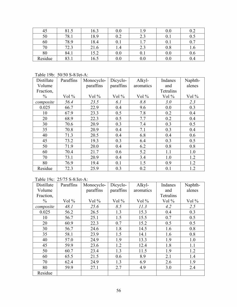
56
45 81.5 16.3 0.0 1.9 0.0 0.2 50 78.1 18.9 0.2 2.3 0.1 0.5 60 78.9 18.4 0.1 1.7 0.1 0.7 70 72.3 21.6 1.4 2.3 0.8 1.6 80 84.1 15.2 0.0 0.1 0.0 0.6
Residue 83.1 16.5 0.0 0.0 0.0 0.4 Table 19b: 50/50 S-8/Jet-A: Distillate Volume Fraction,
%
Paraffins
Vol %
Monocyclo-paraffins
Vol %
Dicyclo-paraffins
Vol %
Alkyl-aromatics
Vol %
Indanes and
Tetralins Vol %
Naphth-alenes
Vol %
composite 56.4 23.5 6.1 8.8 3.0 2.3 0.025 66.7 22.9 0.4 9.6 0.0 0.3
10 67.9 23.3 0.5 7.8 0.2 0.4 20 68.9 22.3 0.5 7.7 0.2 0.4 30 70.6 20.9 0.3 7.4 0.3 0.5 35 70.8 20.9 0.4 7.1 0.3 0.4 40 71.3 20.5 0.4 6.8 0.4 0.6 45 73.2 19.3 0.3 6.4 0.3 0.5 50 71.9 20.0 0.4 6.2 0.8 0.8 60 70.4 21.7 0.6 5.2 1.1 1.0 70 73.1 20.9 0.4 3.4 1.0 1.2 80 76.9 19.4 0.1 1.5 0.9 1.2
Residue 72.3 25.9 0.3 0.2 0.1 1.2 Table 19c: 25/75 S-8/Jet-A: Distillate Volume Fraction,
%
Paraffins
Vol %
Monocyclo-paraffins
Vol %
Dicyclo-paraffins
Vol %
Alkyl-aromatics
Vol %
Indanes and
Tetralins Vol %
Naphth-alenes
Vol %
composite 48.1 25.6 8.5 11.3 4.2 2.5 0.025 56.2 26.5 1.3 15.3 0.4 0.3
10 56.7 25.1 1.5 15.5 0.7 0.5 20 60.9 22.3 0.7 15.2 0.5 0.5 30 56.7 24.6 1.8 14.5 1.6 0.8 35 58.1 23.9 1.5 14.1 1.6 0.8 40 57.0 24.9 1.9 13.3 1.9 1.0 45 59.9 23.6 1.2 12.4 1.8 1.1 50 60.7 23.4 1.3 11.5 1.9 1.2 60 65.5 21.5 0.6 8.9 2.1 1.4 70 62.4 24.9 1.3 6.9 2.6 1.9 80 59.9 27.1 2.7 4.9 3.0 2.4
Residue

57
Table 19d: Jet-A 4658: Distillate Volume Fraction,
%
Paraffins
Vol %
Monocyclo-paraffins
Vol %
Dicyclo-paraffins
Vol %
Alkyl-aromatics
Vol %
Indanes and
Tetralins Vol %
Naphth-alenes
Vol %
composite 46.5 22.5 5.4 18.4 4.5 2.4 0.025 40.4 27.3 3.4 27.3 1.2 0.5
10 39.8 25.1 4.5 27.2 2.6 0.8 20 41.2 24.6 4.4 25.6 3.1 1.1 30 40.9 25.2 5.8 22.1 4.3 1.6 35 43.2 24.5 4.3 21.9 4.2 1.8 40 43.3 25.3 4.8 20.0 4.6 2.0 45 41.7 25.9 6.4 18.7 5.0 2.3 50 42.9 25.8 5.6 18.1 5.1 2.4 60 43.1 26.4 6.7 15.0 5.9 2.9 70 43.8 27.1 7.4 11.8 6.3 3.6 80 48.7 29.9 7.0 6.3 4.6 3.3
Residue 49.7 31.9 7.0 3.4 3.4 4.5

58
Figure 28: A plot of the hydrocarbon types resulting from the ASTM D-2789 analysis performed on three mixtures of Jet-A-4658 and S-8. The left side of the figure presents the aliphatic constituents, while the right side presents the cyclic constituents. The uncertainties are discussed in the text.

59
Density Measurements of Compressed Liquid Jet-A, JP-8 and S-8: The apparatus described earlier8 for the compressed liquid density measurements on methyl- and propylcyclohexane was used to measure the compressed liquid density for Jet-A, JP-8 and S-8.34 these measurements were made over the temperature range of 270 K to 470 K and pressures to 50 MPa. We present these measurements in Tables 20 – 24, and Figures 29 - 33, which follow. Tables list compressed liquid densities of Jet-A-3602, Jet-A-3638 and Jet-A-4658, JP-8-3773 and S-8, respectively. The density measurements have an estimated uncertainty of 1.0 kg/m3 which includes the uncertainty in temperature 0.03 K and pressure 0.01 MPa. Table 20: Compressed liquid densities of Jet-A-3602 Temperature
[K] Pressure [MPa]
Density [kg/m3]
Temperature [K]
Pressure [MPa]
Density [kg/m3]
270.00 30.770 850.67 350.00 4.478 779.05 270.00 25.606 848.05 350.00 3.281 777.97 270.00 20.663 845.45 350.00 2.206 776.98 270.00 15.925 842.88 350.00 1.095 775.96 270.00 11.308 840.33 350.00 0.555 775.45 270.00 6.061 837.34 370.00 31.929 787.77 270.00 4.923 836.67 370.00 25.704 783.1 270.00 3.742 835.97 370.00 20.960 779.32 270.00 2.518 835.23 370.00 16.114 775.28 270.00 1.319 834.5 370.00 11.021 770.78 290.00 31.570 838.62 370.00 5.488 765.55 290.00 25.590 835.32 370.00 4.354 764.42 290.00 20.646 832.51 370.00 3.228 763.26 290.00 15.967 829.77 370.00 2.162 762.17 290.00 11.244 826.91 370.00 1.090 761.05 290.00 5.974 823.62 370.00 0.589 760.53 290.00 4.779 822.84 390.00 31.808 775.21 290.00 3.597 822.07 390.00 25.736 770.24 290.00 2.423 821.3 390.00 21.012 766.14 310.00 31.934 826.25 390.00 16.082 761.61 310.00 25.572 822.48 390.00 10.876 756.53 310.00 20.758 819.48 390.00 5.410 750.78 310.00 16.002 816.47 390.00 4.277 749.52 310.00 11.259 813.25 390.00 3.239 748.33 310.00 5.758 809.31 390.00 2.163 747.09 310.00 4.674 808.51 390.00 1.255 746.02 310.00 3.500 807.64 390.00 0.659 745.28 310.00 2.304 806.68 410.00 31.747 762.63 310.00 1.720 806.26 410.00 25.841 757.38 330.00 31.638 812.73 410.00 21.034 752.82 330.00 25.593 808.76 410.00 16.035 747.76
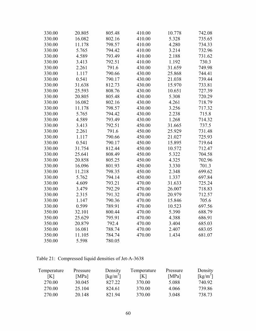
60
330.00 20.805 805.48 410.00 10.778 742.08 330.00 16.082 802.16 410.00 5.328 735.65 330.00 11.178 798.57 410.00 4.280 734.33 330.00 5.765 794.42 410.00 3.214 732.96 330.00 4.589 793.49 410.00 2.188 731.62 330.00 3.413 792.51 410.00 1.192 730.3 330.00 2.261 791.6 430.00 31.659 749.98 330.00 1.117 790.66 430.00 25.868 744.41 330.00 0.541 790.17 430.00 21.038 739.44 330.00 31.638 812.73 430.00 15.970 733.81 330.00 25.593 808.76 430.00 10.651 727.39 330.00 20.805 805.48 430.00 5.308 720.29 330.00 16.082 802.16 430.00 4.261 718.79 330.00 11.178 798.57 430.00 3.256 717.32 330.00 5.765 794.42 430.00 2.238 715.8 330.00 4.589 793.49 430.00 1.268 714.32 330.00 3.413 792.51 450.00 31.665 737.5 330.00 2.261 791.6 450.00 25.929 731.48 330.00 1.117 790.66 450.00 21.027 725.93 330.00 0.541 790.17 450.00 15.895 719.64 330.00 31.754 812.44 450.00 10.572 712.47 330.00 25.641 808.49 450.00 5.322 704.58 330.00 20.858 805.25 450.00 4.325 702.96 330.00 16.096 801.93 450.00 3.330 701.3 330.00 11.218 798.35 450.00 2.348 699.62 330.00 5.762 794.14 450.00 1.337 697.84 330.00 4.609 793.21 470.00 31.633 725.24 330.00 3.479 792.29 470.00 26.007 718.83 330.00 2.315 791.32 470.00 20.979 712.57 330.00 1.147 790.36 470.00 15.846 705.6 330.00 0.599 789.91 470.00 10.523 697.56 350.00 32.101 800.44 470.00 5.390 688.79 350.00 25.629 795.91 470.00 4.388 686.91 350.00 20.879 792.4 470.00 3.404 685.03 350.00 16.081 788.74 470.00 2.407 683.05 350.00 11.105 784.74 470.00 1.434 681.07 350.00 5.598 780.05
Table 21: Compressed liquid densities of Jet-A-3638 Temperature
[K] Pressure [MPa]
Density [kg/m3]
Temperature[K]
Pressure [MPa]
Density [kg/m3]
270.00 30.045 827.22 370.00 5.088 740.92 270.00 25.104 824.61 370.00 4.066 739.86 270.00 20.148 821.94 370.00 3.048 738.73

61
270.00 15.155 819.16 370.00 2.027 737.62 270.00 10.128 816.28 370.00 1.006 736.51 270.00 5.058 813.27 390.00 30.017 750.57 270.00 4.043 812.66 390.00 25.082 746.29 270.00 3.019 812.03 390.00 20.133 741.78 270.00 1.994 811.40 390.00 15.156 736.95 270.00 0.971 810.76 390.00 10.141 731.75 290.00 30.076 814.46 390.00 5.075 726.09 290.00 25.140 811.64 390.00 4.062 724.89 290.00 20.184 808.73 390.00 3.047 723.67 290.00 15.201 805.71 390.00 2.027 722.43 290.00 10.175 802.55 390.00 1.006 721.17 290.00 5.109 799.24 410.00 30.020 738.07 290.00 4.093 798.55 410.00 25.080 733.42 290.00 3.072 797.86 410.00 20.128 728.48 290.00 2.050 797.16 410.00 15.147 723.16 290.00 1.028 796.45 410.00 10.131 717.38 310.00 30.079 801.81 410.00 5.066 711.01 310.00 25.134 798.75 410.00 4.050 709.64 310.00 20.174 795.57 410.00 3.029 708.24 310.00 15.187 792.26 410.00 2.008 706.81 310.00 10.159 788.77 410.00 0.985 705.36 310.00 5.090 785.07 430.00 30.008 725.40 310.00 4.075 784.30 430.00 25.067 720.35 310.00 3.053 783.51 430.00 20.112 714.93 310.00 2.031 782.73 430.00 15.129 709.05 310.00 1.009 781.93 430.00 10.111 702.59 330.00 30.043 788.77 430.00 5.049 695.38 330.00 25.110 785.43 430.00 4.028 693.82 330.00 20.156 781.94 430.00 3.009 692.23 330.00 15.172 778.28 430.00 1.984 690.59 330.00 10.148 774.42 430.00 0.960 688.90 330.00 5.084 770.34 450.00 29.957 712.75 330.00 4.069 769.48 450.00 25.019 707.25 330.00 3.050 768.61 450.00 20.073 701.31 330.00 2.031 767.74 450.00 15.096 694.80 330.00 1.010 766.85 450.00 10.079 687.56 350.00 30.055 775.92 450.00 5.020 679.37 350.00 25.118 772.28 450.00 4.003 677.59 350.00 20.163 768.48 450.00 2.985 675.74 350.00 15.181 764.48 450.00 1.964 673.84 350.00 10.159 760.23 450.00 0.939 671.87 350.00 5.092 755.70 470.00 29.936 700.26

62
350.00 4.073 754.74 470.00 25.002 694.28 350.00 3.059 753.78 470.00 20.051 687.75 350.00 2.037 752.80 470.00 15.078 680.53 350.00 1.017 751.81 470.00 10.062 672.39 370.00 30.053 763.11 470.00 4.997 662.99 370.00 25.114 759.16 470.00 3.981 660.92 370.00 20.159 755.03 470.00 2.957 658.76 370.00 15.176 750.65 470.00 1.941 656.54 370.00 10.157 745.98 470.00 0.922 654.23
Table 22: Compressed liquid densities of Jet-A-4658 Temperature
[K] Pressure [MPa]
Density [kg/m3]
Temperature [K]
Pressure [MPa]
Density [kg/m3]
270.00 30.015 837.52 370.00 4.010 751.72 270.00 25.010 834.93 370.00 3.011 750.70 270.00 20.002 832.28 370.00 2.006 749.66 270.00 15.007 829.56 370.00 1.013 748.61 270.00 10.007 826.76 370.00 0.499 748.06 270.00 4.999 823.86 390.00 30.008 761.81 270.00 4.010 823.27 390.00 25.012 757.62 270.00 2.999 822.67 390.00 20.018 753.21 270.00 2.005 822.07 390.00 15.007 748.52 270.00 1.007 821.46 390.00 10.009 743.54 270.00 0.508 821.16 390.00 5.007 738.18 290.00 30.001 824.78 390.00 4.008 737.05 290.00 25.002 822.00 390.00 3.008 735.91 290.00 19.999 819.11 390.00 2.001 734.74 290.00 15.002 816.15 390.00 1.009 733.55 290.00 10.004 813.08 390.00 0.503 732.93 290.00 5.005 809.92 410.00 30.004 749.32 290.00 4.005 809.26 410.00 25.012 744.75 290.00 3.009 808.60 410.00 20.013 739.94 290.00 2.009 807.94 410.00 15.000 734.79 290.00 1.010 807.27 410.00 10.009 729.27 290.00 0.507 806.93 410.00 5.007 723.26 310.00 30.013 811.77 410.00 4.008 721.99 310.00 25.011 808.70 410.00 3.008 720.69 310.00 20.013 805.54 410.00 2.002 719.37 310.00 15.010 802.27 410.00 1.013 718.05 310.00 10.009 798.88 410.00 0.516 717.36 310.00 5.006 795.34 430.00 29.999 736.86 310.00 3.999 794.61 430.00 25.007 731.93 310.00 3.006 793.87 430.00 20.009 726.68 310.00 2.009 793.13 430.00 15.005 721.00

63
310.00 1.009 792.38 430.00 10.023 714.88 310.00 0.508 792.00 430.00 5.012 708.11 330.00 29.999 799.02 430.00 4.017 706.66 330.00 25.010 795.71 430.00 3.004 705.17 330.00 20.007 792.28 430.00 2.010 703.68 330.00 15.012 788.72 430.00 1.012 702.13 330.00 10.013 784.99 430.00 0.508 701.34 330.00 5.006 781.09 450.00 29.996 724.54 330.00 4.015 780.29 450.00 25.003 719.19 330.00 3.008 779.48 450.00 20.006 713.44 330.00 2.005 778.65 450.00 15.002 707.18 330.00 1.014 777.81 450.00 10.002 700.31 330.00 0.513 777.39 450.00 5.018 692.70 350.00 29.995 786.59 450.00 4.002 691.02 350.00 25.009 783.03 450.00 3.010 689.34 350.00 20.013 779.32 450.00 2.013 687.61 350.00 15.006 775.43 450.00 1.006 685.81 350.00 10.005 771.34 450.00 0.508 684.89 350.00 5.012 767.03 470.00 29.993 712.33 350.00 4.010 766.12 470.00 25.002 706.52 350.00 3.005 765.20 470.00 20.012 700.22 350.00 2.007 764.28 470.00 15.020 693.32 350.00 1.005 763.34 470.00 10.016 685.63 350.00 0.504 762.87 470.00 5.005 676.93 370.00 30.005 774.22 470.00 4.002 675.03 370.00 25.011 770.35 470.00 3.001 673.07 370.00 20.009 766.29 470.00 2.008 671.06 370.00 15.010 762.03 470.00 1.014 668.98 370.00 10.015 757.53 470.00 0.514 667.89 370.00 5.007 752.72
Table 23: Compressed-liquid densities of JP-8-3773 Temperature
[K] Pressure [MPa]
Density [kg/m3]
Temperature [K]
Pressure [MPa]
Density [kg/m3]
270.0 39.99 833.2 330.0 5.01 771.1 270.0 35.00 830.8 330.0 4.00 770.3 270.0 30.00 828.2 330.0 2.99 769.4 270.0 24.99 825.6 330.0 1.99 768.6 270.0 20.00 823.0 330.0 1.00 767.7 270.0 15.00 820.2 330.0 0.49 767.2 270.0 10.00 817.4 350.0 40.00 783.9 270.0 4.99 814.4 350.0 35.00 780.5 270.0 3.99 813.8 350.0 30.00 777.0 270.0 3.00 813.2 350.0 25.00 773.3

64
270.0 1.99 812.6 350.0 19.99 769.5 270.0 1.01 812.0 350.0 15.00 765.5 270.0 0.50 811.6 350.0 9.99 761.2 290.0 39.97 821.0 350.0 5.00 756.7 290.0 35.00 818.3 350.0 3.99 755.8 290.0 30.00 815.6 350.0 2.99 754.8 290.0 24.98 812.7 350.0 2.00 753.9 290.0 20.00 809.8 350.0 1.01 752.9 290.0 15.00 806.8 350.0 0.50 752.4 290.0 9.99 803.7 370.0 40.00 771.8 290.0 5.00 800.4 370.0 35.00 768.2 290.0 3.99 799.7 370.0 30.00 764.4 290.0 3.00 799.0 370.0 24.99 760.4 290.0 1.99 798.4 370.0 19.99 756.2 290.0 1.00 797.7 370.0 14.99 751.7 290.0 0.49 797.3 370.0 10.01 747.0 310.0 39.99 808.7 370.0 4.99 742.0 310.0 35.00 805.7 370.0 3.99 740.9 310.0 29.99 802.7 370.0 2.99 739.9 310.0 25.00 799.5 370.0 1.99 738.8 310.0 20.00 796.2 370.0 0.99 737.7 310.0 14.99 792.8 370.0 0.49 737.1 310.0 10.00 789.3 390.0 39.99 759.9 310.0 4.99 785.7 390.0 35.00 755.9 310.0 4.00 784.9 390.0 29.99 751.8 310.0 3.00 784.2 390.0 25.00 747.5 310.0 1.99 783.4 390.0 20.00 742.9 310.0 1.00 782.6 390.0 14.99 738.0 310.0 0.50 782.2 390.0 10.00 732.6 330.0 40.00 796.0 390.0 4.99 727.0 330.0 35.00 792.9 390.0 4.00 725.8 330.0 29.99 789.6 390.0 3.00 724.6 330.0 24.99 786.2 390.0 2.00 723.4 330.0 19.99 782.7 390.0 1.00 722.1 330.0 14.98 779.0 390.0 0.49 721.5 330.0 10.00 775.2 410.0 39.99 747.9 410.0 35.00 743.7 450.0 34.99 719.2 410.0 29.98 739.2 450.0 29.99 714.0 410.0 25.01 734.5 450.0 24.99 708.4 410.0 20.00 729.5 450.0 19.99 702.3 410.0 14.99 724.1 450.0 15.00 695.7 410.0 10.00 718.2 450.0 10.00 688.4 410.0 4.99 711.9 450.0 5.00 680.3 410.0 3.99 710.5 450.0 4.00 678.5 410.0 2.99 709.1 450.0 3.00 676.7 410.0 1.99 707.7 450.0 1.99 674.8

65
410.0 0.99 706.3 450.0 0.99 672.9 410.0 0.49 705.5 450.0 0.49 671.9 430.0 39.98 736.0 470.0 40.01 712.5 430.0 34.99 731.4 470.0 34.99 707.2 430.0 29.99 726.6 470.0 29.99 701.5 430.0 25.00 721.4 470.0 24.99 695.4 430.0 19.99 715.9 470.0 20.01 688.7 430.0 15.00 709.9 470.0 15.00 681.4 430.0 10.00 703.4 470.0 9.99 673.3 430.0 5.00 696.2 470.0 4.99 664.0 430.0 4.00 694.7 470.0 4.00 661.9 430.0 2.99 693.1 470.0 2.99 659.8 430.0 2.00 691.5 470.0 1.99 657.6 430.0 0.99 689.9 470.0 0.99 655.3 430.0 0.49 689.0 470.0 0.49 654.2 450.0 40.02 724.2
Table 24: Compressed-liquid densities of S-8 Temperature
[K] Pressure [MPa]
Density [kg/m3]
Temperature [K]
Pressure [MPa]
Density [kg/m3]
270.0 30.09 786.2 330.0 1.01 725.1 270.0 25.15 783.6 330.0 0.51 724.7 270.0 20.20 780.9 350.0 30.01 735.5 270.0 15.21 778.1 350.0 25.01 731.7 270.0 10.19 775.1 350.0 20.01 727.7 270.0 5.12 772.1 350.0 15.00 723.5 270.0 4.10 771.4 350.0 10.01 719.1 270.0 3.07 770.8 350.0 5.00 714.3 270.0 2.05 770.1 350.0 4.01 713.4 270.0 1.02 769.5 350.0 3.01 712.3 270.0 0.51 769.1 350.0 2.00 711.3 290.0 30.04 773.6 350.0 1.01 710.3 290.0 25.10 770.7 350.0 0.50 709.8 290.0 20.14 767.7 370.0 30.02 723.2 290.0 15.15 764.6 370.0 25.02 719.0 290.0 10.13 761.3 370.0 20.01 714.7 290.0 5.06 757.8 370.0 15.02 710.1 290.0 4.05 757.1 370.0 10.00 705.1 290.0 3.02 756.4 370.0 5.01 699.9 290.0 2.00 755.6 370.0 4.01 698.8 290.0 0.97 754.9 370.0 3.01 697.6 290.0 0.46 754.5 370.0 2.00 696.4 310.0 29.97 760.5 370.0 1.01 695.3 310.0 25.03 757.3 370.0 0.50 694.7

66
310.0 20.07 754.0 390.0 30.02 711.0 310.0 15.09 750.6 390.0 25.00 706.5 310.0 10.07 747.0 390.0 20.01 701.7 310.0 5.00 743.1 390.0 15.01 696.6 310.0 3.98 742.3 390.0 10.00 691.1 310.0 2.96 741.5 390.0 5.00 685.2 310.0 1.94 740.7 390.0 4.00 683.9 310.0 0.92 739.8 390.0 3.00 682.6 310.0 0.40 739.4 390.0 2.01 681.3 310.0 2.99 741.4 390.0 1.00 680.0 310.0 2.01 740.5 390.0 0.50 679.3 310.0 1.01 739.7 410.0 30.01 698.7 310.0 0.51 739.3 410.0 25.01 693.8 330.0 30.00 747.9 410.0 20.01 688.6 330.0 25.01 744.4 410.0 15.00 683.0 330.0 20.01 740.8 410.0 10.01 676.9 330.0 15.01 737.0 410.0 5.00 670.1 330.0 10.01 733.0 410.0 4.00 668.7 330.0 5.01 728.7 410.0 3.00 667.2 330.0 4.01 727.9 410.0 2.01 665.7 330.0 3.01 727.0 410.0 1.00 664.1 330.0 2.01 726.1 410.0 0.50 663.3 430.0 29.99 686.4 450.0 4.00 636.9 430.0 25.02 681.1 450.0 3.00 634.9 430.0 20.00 675.3 450.0 2.01 632.9 430.0 15.00 669.1 450.0 1.01 630.8 430.0 10.01 662.2 450.0 0.50 629.7 430.0 5.00 654.6 470.0 30.01 662.2 430.0 4.01 653.0 470.0 25.01 655.9 430.0 3.01 651.3 470.0 20.01 649.0 430.0 2.00 649.5 470.0 15.01 641.3 430.0 1.01 647.7 470.0 10.01 632.6 430.0 0.49 646.8 470.0 5.01 622.7 450.0 30.02 674.3 470.0 4.02 620.5 450.0 25.01 668.4 470.0 3.01 618.1 450.0 20.02 662.1 470.0 2.00 615.7 450.0 15.00 655.2 470.0 1.00 613.2 450.0 10.00 647.5 470.0 0.50 611.9 450.0 5.01 638.8
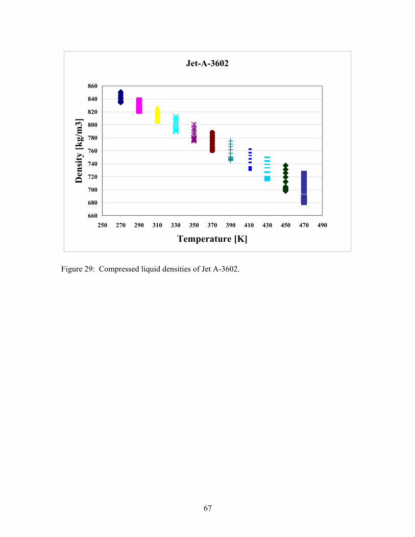
67
Jet-A-3602
660
680
700
720
740
760
780
800
820
840
860
250 270 290 310 330 350 370 390 410 430 450 470 490
Temperature [K]
Den
sity
[k
g/m
3]
Figure 29: Compressed liquid densities of Jet A-3602.

68
Jet-A-3638
660
680
700
720
740
760
780
800
820
840
860
250 270 290 310 330 350 370 390 410 430 450 470 490
Temperature [K]
Den
sity
[k
g/m
3]
Figure 30: Compressed liquid densities of Jet A-3638.
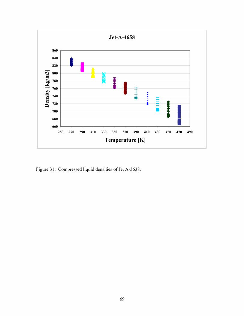
69
Jet-A-4658
660
680
700
720
740
760
780
800
820
840
860
250 270 290 310 330 350 370 390 410 430 450 470 490
Temperature [K]
Den
sity
[k
g/m
3]
Figure 31: Compressed liquid densities of Jet A-3638.
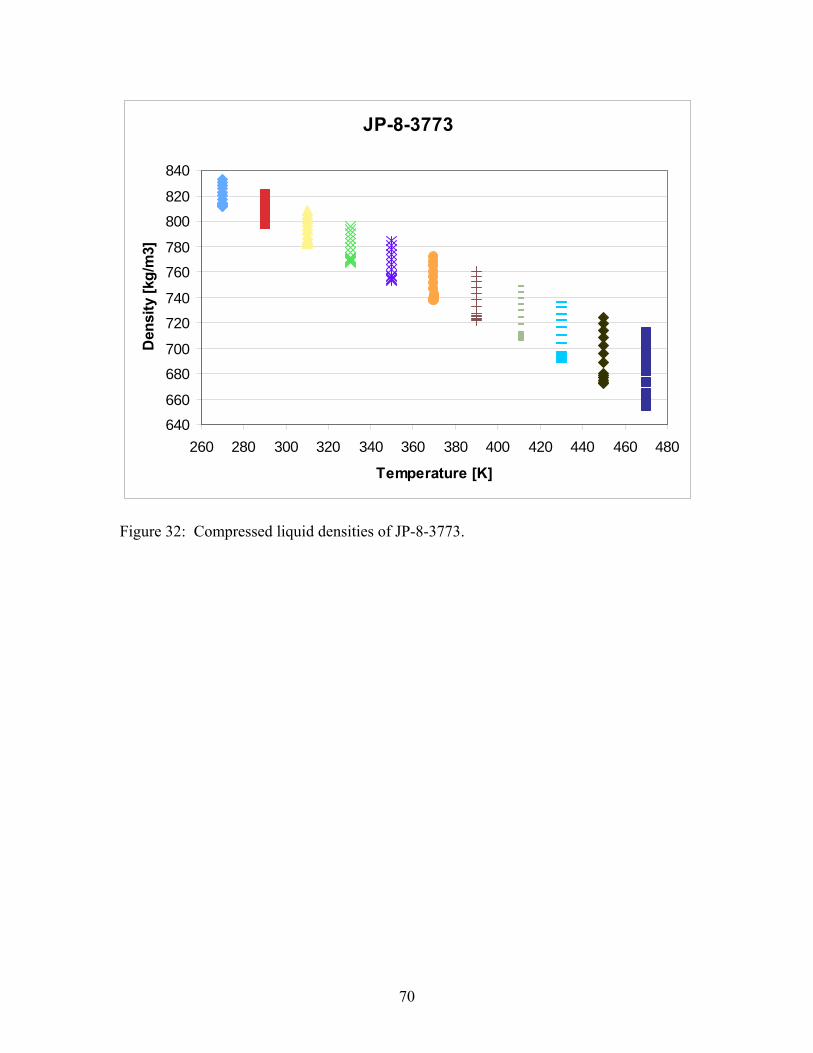
70
JP-8-3773
640
660
680
700
720
740
760
780
800
820
840
260 280 300 320 340 360 380 400 420 440 460 480
Temperature [K]
Den
sity
[kg
/m3]
Figure 32: Compressed liquid densities of JP-8-3773.

71
S-8
600
620
640
660
680
700
720
740
760
780
800
260 280 300 320 340 360 380 400 420 440 460 480
Temperature [K]
Den
sity
[kg
/m3]
c
Figure 33: Compressed liquid densities of S-8. Viscosity Measurements of Jet-A Fuels at Ambient Pressure: The viscosities of two samples of Jet-A (3638 and 4658) was measured with a commercial viscodensimeter in the temperature range from 263.15 K to 373.15 K. The performance of the instrument hardware and firmware was examined by comparisons with certified viscosity standard liquids. The reference viscosities of two appropriate calibration liquids were reproduced by the instrument within 0.4 % and 0.8 %, respectively. Together, these two viscosity standards span the entire range of measured Jet-A fuel samples. The estimated uncertainty of the Jet-A fuel measurements reported here is deduced from this comparison. Above a viscosity of 0.94 mPa·s the reported uncertainty is 0.4 %; however, below this viscosity threshold the reported uncertainty is expanded to 1 % to match the more conservative manufacturer’s estimate. We note that the reported uncertainty estimates are not derived from a strict statistical treatment. The measured absolute and kinematic viscosities of Jet-A-3638 and Jet-A-4658 are tabulated in Tables 25 and 26, respectively. Also included in Tables 25 and 26 are the measured densities and the estimated uncertainty value for each measured quantity. In addition to the tabulated data, the measured absolute and kinematic viscosities are illustrated in Figures 34 - 37.

72
Table 25: Viscosity Measurements for Jet-A-3638.
Temperature
K
mPa·s
u[]
mPa·s
mm2·s-1
u[]
mm2·s-1
kg·m-3
u[]
kg·m-3
373.150 0.47418 0.00474 0.64796 0.00648 731.78 0.51
368.150 0.49836 0.00498 0.67746 0.00678 735.64 0.50
363.150 0.52412 0.00524 0.70877 0.00709 739.46 0.50
358.150 0.55200 0.00552 0.74261 0.00743 743.32 0.50
353.150 0.58223 0.00582 0.77927 0.00779 747.14 0.50
348.150 0.61503 0.00615 0.81899 0.00819 750.94 0.50
343.150 0.65078 0.00651 0.86223 0.00862 754.74 0.50
338.150 0.68986 0.00690 0.90944 0.00910 758.54 0.50
333.150 0.73269 0.00733 0.96111 0.00961 762.34 0.50
328.150 0.77984 0.00780 1.0179 0.0102 766.10 0.50
323.150 0.83198 0.00832 1.0807 0.0046 769.90 0.50
318.150 0.88983 0.00890 1.1502 0.0049 773.64 0.50
313.150 0.95426 0.00392 1.2275 0.0052 777.38 0.50
308.150 1.0264 0.0042 1.3140 0.0056 781.14 0.50
303.150 1.1076 0.0046 1.4112 0.0060 784.90 0.50
298.150 1.1995 0.0050 1.5210 0.0065 788.62 0.50
293.150 1.3041 0.0054 1.6458 0.0071 792.36 0.50
288.150 1.4240 0.0059 1.7887 0.0077 796.10 0.50
283.150 1.5624 0.0065 1.9535 0.0084 799.82 0.50
278.150 1.7235 0.0072 2.1449 0.0093 803.56 0.50
273.150 1.9134 0.0081 2.3703 0.0104 807.26 0.50
268.150 2.1393 0.0090 2.6380 0.0116 810.96 0.51
263.150 2.4106 0.0102 2.9590 0.0130 814.68 0.51

73
Table 26: Viscosity Measurements for Jet-A-4658
Temperature
K
mPa·s
u[]
mPa·s
mm2·s-1
u[]
mm2·s-1
kg·m-3
u[]
kg·m-3
373.150 0.53287 0.00533 0.71680 0.00717 743.38 0.51
368.150 0.56121 0.00561 0.75113 0.00751 747.16 0.50
363.150 0.59165 0.00592 0.78785 0.00788 750.96 0.50
358.150 0.62466 0.00625 0.82765 0.00828 754.74 0.50
353.150 0.66055 0.00661 0.87086 0.00871 758.50 0.50
348.150 0.69968 0.00700 0.91789 0.00919 762.26 0.50
343.150 0.74245 0.00743 0.96926 0.00970 765.98 0.51
338.150 0.78941 0.00790 1.0256 0.0103 769.76 0.50
333.150 0.84115 0.00842 1.0876 0.0109 773.46 0.50
328.150 0.89844 0.00900 1.1561 0.0116 777.16 0.50
323.150 0.96220 0.00397 1.2322 0.0053 780.88 0.51
318.150 1.0335 0.0043 1.3172 0.0056 784.56 0.50
313.150 1.1136 0.0046 1.4126 0.0061 788.26 0.50
308.150 1.2041 0.0050 1.5203 0.0065 791.98 0.50
303.150 1.3070 0.0054 1.6426 0.0071 795.68 0.50
298.150 1.4249 0.0059 1.7825 0.0077 799.38 0.50
293.150 1.5608 0.0065 1.9436 0.0084 803.06 0.50
288.150 1.7188 0.0072 2.1306 0.0092 806.72 0.51
283.150 1.9043 0.0079 2.3498 0.0101 810.40 0.50
278.150 2.1239 0.0088 2.6089 0.0112 814.10 0.50
273.150 2.3878 0.0100 2.9199 0.0127 817.78 0.50
268.150 2.7078 0.0113 3.2966 0.0143 821.40 0.50
263.150 3.1011 0.0130 3.7586 0.0163 825.08 0.50

74
0.0
0.5
1.0
1.5
2.0
2.5
3.0
250 260 270 280 290 300 310 320 330 340 350 360 370 380
/ mPa·s
T / K
Figure 34: Measurements of the absolute viscosity of Jet-A-3638. The uncertainty is discussed in the text.

75
0.0
0.5
1.0
1.5
2.0
2.5
3.0
3.5
250 260 270 280 290 300 310 320 330 340 350 360 370 380
/ mm2·s-1
T / K
Figure 35: Measurements of the kinematic viscosity of Jet-A-3638. The uncertainty is discussed in the text.

76
0.0
0.5
1.0
1.5
2.0
2.5
3.0
3.5
250 260 270 280 290 300 310 320 330 340 350 360 370 380
/ mPa·s
T / K
Figure 36: Measurements of the absolute viscosity of Jet-A-4648. The uncertainty is discussed in the text.

77
0.0
0.5
1.0
1.5
2.0
2.5
3.0
3.5
4.0
250 260 270 280 290 300 310 320 330 340 350 360 370 380
/ mm2·s-1
T / K
Figure 37: Measurements of the kinematic viscosity of Jet-A-4648. The uncertainty is discussed in the text.

78
The kinematic viscosity of JP-8-3773 was measured at ambient pressure in the temperature range 293.15 K to 373.15 K. These measurements are presented in Table 27. The instrument used was a commercial automated open gravitational flow viscometer with a suspended-level Ubbelohde glass capillary of 200 mm length with upper reservoir bulbs for a kinematic viscosity range from 0.3 mm2·s-1 to 30 mm2·s-1. This instrument was described earlier for the measurements done on methyl- and propylcyclohexane. These data are presented graphically in Figure 38. Table 27: The kinematic viscosity of JP-8-3773 at an ambient pressure of 83 kPa.
JP-8 3773 Temperature
T Kinematic viscosity
K mm2·s-1
293.15
303.15
313.15
323.15
333.15
343.15
353.15
363.15
373.15
1.692
1.442
1.250
1.099
0.9775
0.8768
0.7889
0.7172
0.6559

79
Figure 38: Measurements of the kinematic viscosity of JP-8-3773. The uncertainty is discussed in the text.

80
Thermal Conductivity Measurements of the Compressed Liquid Aviation Fuels: Transient hot-wire measurements of the thermal conductivity were made on each of the three liquid samples of Jet-A-3602, Jet-A-3638, Jet-A-4658, JP-8-3773 and S-8. For each sample, measurements were made along 11 isotherms at temperatures from 300 to 500 K with pressures up to 70 MPa. The transient hot-wire instrument has been described in detail above in the treatment of the measurements on methyl- and propylcyclohexane. The tabulated thermal conductivity measurements are extensive and are therefore provided in Appendix I. The measurements are depicted graphically in Figures 39 - 43.
0.080
0.085
0.090
0.095
0.100
0.105
0.110
0.115
0.120
0.125
0.00 5.00 10.00 15.00 20.00 25.00 30.00 35.00 40.00 45.00 50.00
P / MPa
/
W. m
-1K
-1 300 K
320 K340 K
360 K
380 K400 K
420 K440 K
460 K480 K
500 K
Figure 39: Thermal conductivity of Jet-A-3602 in the liquid phase.

81
0.080
0.085
0.090
0.095
0.100
0.105
0.110
0.115
0.120
0.125
0.00 5.00 10.00 15.00 20.00 25.00 30.00 35.00 40.00 45.00 50.00
P / MPa
/
W. m
-1K
-1
300 K
320 K
340 K360 K
380 K400 K
420 K440 K
460 K
480 K500 K
Figure 40: Thermal conductivity of Jet-A-3638 in the liquid phase.
0.080
0.085
0.090
0.095
0.100
0.105
0.110
0.115
0.120
0.125
0.00 5.00 10.00 15.00 20.00 25.00 30.00 35.00 40.00 45.00 50.00
P / MPa
/
W. m
-1K
-1 300 K320 K
340 K
360 K380 K
400 K420 K
440 K
460 K480 K
500 K
Figure 41: Thermal conductivity of Jet-A-4658 in the liquid phase.

82
0.075
0.080
0.085
0.090
0.095
0.100
0.105
0.110
0.115
0.120
0.125
0.130
0.135
0.00 10.00 20.00 30.00 40.00 50.00 60.00 70.00
P / MPa
/
W. m
-1K
-1
300 K
355 K405 K
452 K
496 K547 K
Figure 42: Thermal conductivity of JP-8-3773 from 0.1 MPa to 70 MPa.
0.080
0.090
0.100
0.110
0.120
0.130
0.140
3.30 3.50 3.70 3.90 4.10 4.30 4.50
/ mol.L-1
/
W. m
-1K
-1
300 K320 K
340 K360 K
380 K
400 K420 K
440 K460 K
480 K500 K
REFPROP
Figure 43: Thermal conductivity of S-8 at pressures from 0.1 MPa to 70 MPa.

83
Heat Capacities of Jet Fuels S-8 and JP-8:
The heat capacities of jet fuels JP-8-3373 and S-8 were measured with a commercial differential scanning calorimeter. Samples were contained in high-pressure sample containers during the measurements. These high-pressure containers are constructed of stainless steel, and are plated with gold on internal surfaces. These containers are sealed with a gold disk sandwiched between the upper lid and the lower portion of the vessel. The cells are rated for pressures of approximately 15 MPa. The internal volumes of these cells are approximately 30 µl. The high-pressure cells were used because the heat capacity measurements extended to above the normal boiling point of the jet fuels. In practice, measurements can be made at different filled fractions of the internal volume of the cells and these values can be extrapolated to complete filling to eliminate contributions from the vaporization of the liquid in the cells. The vaporization enthalpy was sufficiently negligible throughout the temperature range, that the larger fractions-filled measurements could be taken as being free of vapor-space. The capsules were filled and sealed within a glove bag that had been swept with dry nitrogen gas for at least an hour prior to cell filling. The sealed vessels were weighed on a microbalance with resolution of 1 μg.
Crushed pieces of SRM 720, synthetic sapphire, were used to calibrate the heat flux of the calorimeter with the same high-pressure cell that was used for the fluid heat capacity measurements. The mass of fluid sealed in the high-pressure cell was always much smaller than the mass of the cell. The empty cell parts had a mass of approximately 0.66 g and the sample masses ranged from 5 mg to 19 mg.
If vaporization enthalpies are significant, then the observed specific heat capacity of the two phase system will decrease with a decrease of vapor space in the sample vessel; or equivalently, the observed two phase heat capacity would decrease with increasing filled fraction of the sample cell. This behavior was not observed to temperatures of up to 473 K. In fact slight increases in the observed two phase heat capacity were observed with increasing filled fraction of the vessel.
Using a vapor volume of 5 µl, the ideal gas law, a representative enthalpy of vaporization of 50 kJ·mol-1, and a hypothetical increase in pressure of 0.1 MPa over 50 K, the contribution of the vaporization enthalpy to the observed two-phase heat capacity would be 0.0074 J·K-1·g-1, which is less than the run-to-run irreproducibility. Observed heat capacities were obtained by equilibrating the calorimeter at 223 K for 10 min or longer, scanning at 5 K·min-1 to 473 K and equilibrating at 473 K for 10 min. The equilibration periods were used to establish a baseline that was subtracted from the heat-flux against time thermal curve. Heat flux curves for the empty high-pressure cells in the reference and sample sides of the calorimeter were determined and averaged. The average heat flux curve for the empty vessel was subtracted from baseline-adjusted heat flux curves for the vessel filled with either sapphire or one of the jet fuels.

84
A correction factor for the heat flux was determined as a ratio of the true heat capacity of SRM 720 to that obtained from the average of several heat flux curves. This ratio was then multiplied by the observed heat capacity for the jet fuels to correct for heat-flux error (as in ASTM International Standard Method E968). The calorimeter obtains approximately 3000 readings for each thermal scan, not including the equilibration periods. With four or five replicates per filling and an average over three fillings, close to half a million data points might be processed to obtain a heat capacity curve. These are shown for JP-8-3773 and S-8 in figures 44 and 45. In order to reduce this number individual data points were collated near nominal temperatures. A single curve was then fitted to all these collated readings to obtain the heat capacity of each of the jet fuels. The statistics calculated for the fitted curve thus include the variances due to: 1) irreproducibility in vessel filling and sealing; 2) calorimetric noise; 3) run-to-run variability for the same vessel filling; 4) vessel placement irreproducibilities. The last two are the largest contributors to imprecision.
The least-squares generated equation for the heat capacity at ambient pressure of JP-8 is:
Cp/Cp° = (2.193 ± 0.0055) + (3.996 ± 0.0011) x 10-3(T/T° – 363.15)
The least-squares generated equation for the heat capacity of S-8 at ambient pressure is:
Cp/Cp° = (2.527 ± 0.0118) + (2.804 ± 0.0024) x 10-3(T/T° – 363.15)
where T° is 1 K, Cp° is 1 (J·K-1·g-1), and the difference between the saturation heat capacity and the constant pressure heat capacity was assumed to be negligible. The uncertainties attached to the parameters are 1 standard deviation. The random factors that contribute to those uncertainties of the parameters were stated in a previous paragraph.

85
Figure 44: Heat capacity at constant pressure of JP-8-3773 as a function of temperature.
Figure 45: Heat capacity at constant pressure of JP-8-3773 as a function of temperature.

86
Development of the Thermodynamic and Transport Model: The procedure for developing a surrogate mixture can be summarized as follows. First, a chemical analysis is performed to identify the composition of the fuel sample. From this analysis, a list of candidate fluids is constructed, including compounds representative of the various chemical families (branched or linear paraffins, alkenes, aromatics, mono or polycyclic paraffins, etc.) found in the sample. For each of these possible pure-fluid constituents, an equation of state, a viscosity surface and a thermal conductivity surface are developed, and a mixture model is used that incorporates the pure-fluid equations for both thermodynamic and transport properties. The fluids in the surrogate mixture and their compositions are then chosen by determining the composition that minimizes the difference between the predicted and experimental data for the distillation curve, density, sound speed, viscosity and thermal conductivity. From the gas chromatography and mass spectrometry analysis of the Jet-A samples, we compiled a list of potential candidate fluids for a surrogate model. These fluids are listed in Table 28, along with their normal boiling point and their boiling points at an atmospheric pressure of 83 kPa (the typical local pressure of our laboratory, located at 1655 m above sea level). The list contains fluids used in our earlier work on RP-1, RP-2, and S-8, but in addition includes aromatic compounds such as toluene, o-xylene and tetralin that were not used in model for either S-8 or RP-1 and RP-2.35, 36 For each mono-branched alkane identified in the chemical analysis, a representative species was selected as a candidate constituent fluid for the surrogates. In other words, for our purposes, all x-methylnonanes are represented as a single methylnonane. Similarly, we used a particular x,y-dimethylnonane to represent the dimethylnonane family. A major factor governing the specific choice of compound to represent a moiety was the availability of property data: priority was given to compounds for which the most abundant and reliable experimental measurements were available. For each possible constituent fluid, we searched the open literature as well as databases such as the NIST TDE program, DIPPR, and Landolt-Börnstein for experimental physical property data. For some of the fluids, the data were sparse and were supplemented with predicted values from the TDE and DIPPR Diadem programs37. Because our modeling approach requires thermophysical property models for all pure constituent fluids, it was necessary to have available equations of state and surfaces for the viscosity and thermal conductivity for each of the potential constituent pure fluids. Details of this procedure are available in other work, so we provide only a brief summary here35, 36, 38, 39. With the available experimental data supplemented with predictions obtained from the TDE program, we developed Helmholtz-form equations of state similar to the form developed by Span and Wagner that can represent not only the vapor pressure and density, but also other properties such as the speed of sound and heat capacity40. For viscosity and thermal conductivity, we primarily used an extended corresponding-states model, with n-dodecane as a reference fluid. When sufficient data were available, the representation of the viscosity or thermal conductivity was improved by fitting the data to correction functions for the shape factors. In the absence of experimental data, we used the predictive method of Van Velzen for viscosity, and the method of Baroncini for thermal conductivity (as implemented in the DIPPR Diadem program). Additionally, we

87
incorporated earlier work on the thermal conductivity of methyl and propylcyclohexane to represent the alkyl cyclohexane family in terms of a scaled form of the thermal conductivity correlation developed for propylcyclohexane. For calculations of the thermodynamic properties of mixtures, we used the mixture model incorporated into the REFPROP41 computer program. This model includes an algorithm for estimating binary interaction parameters when data are unavailable for a particular fluid pair. The model for calculating the transport properties of a mixture is an extended corresponding-states method. In addition, we used an algorithm developed in earlier work to compute the distillation curve; this procedure incorporates data from an improved advanced distillation curve metrology.35, 36, 38, 39 The properties measurements discussed earlier formed the basis of the experimental data set used to obtain the surrogate models. We then used a multi-property, nonlinear regression procedure to minimize the differences between the experimental data and the predictions of the model. This is used to determine the components and their relative abundances to define the surrogate fluid mixtures for each aviation fuel sample. The objective function was the sum of the squared percentage differences between the experimental data and the predicted value. The independent variables were the compositions of the fluid mixture. Our initial guess included all of the components in Table 28. Successive calculations gave very small concentrations of some components. These were removed from the mixture and the minimization process was repeated until further reductions in the number of components resulted in unacceptably large deviations with the experimental data. The final compositions of the surrogate mixtures are summarized in Table 29. Each surrogate model contains eight components. The surrogate for the composite Jet-A-4658 contains more of the heavier cycloalkanes than the Jet-A-3638 sample, and also contains hexadecane. The Jet-A-3638 sample contains some propylcyclohexane, and more of the lighter components. This is not unexpected because the distillation curves indicate that the Jet-A-4658 sample contains more of the higher boiling components.
In Figures 46 to 52, we present comparisons of our surrogate models with experimental data. Figure 46 shows the density as a function of temperature at atmospheric pressure (83 kPa). The models agree with the data to within their experimental uncertainty (0.1 %). The density of the two different samples differs from each other by approximately 1.5 %. Figures 47 and 48 show the deviations in density between the experimental measurements as a function of pressure, over the temperature range 270 K to 470 K for the Jet-A-3638 and the Jet-A-4658 samples. The experimental uncertainty of these data is 0.1 %. The models both show increasing deviations as the pressure increases, but remain within 0.5 %.

88
Table 28. Potential constituent fluids for the surrogate fuel mixtures
Compound CAS no. Class No. of
carbon atoms
Boiling point at 83 kPa (K)
Normal boiling
point (K) heptane 142-82-5 linear paraffin 7 364.90 371.53 toluene 108-88-3 aromatic 7 376.87 383.75 octane 111-65-9 linear paraffin 8 391.75 398.77
ortho-xylene 95-47-6 aromatic 8 410.16 417.54 nonane 111-84-2 linear paraffin 9 416.54 423.81
propylcyclohexane 1678-92-8 monocyclic
paraffin 9 422.13 429.86 5-methylnonane 15869-85-9 branched paraffin 10 430.7 438.3
decane 124-18-5 linear paraffin 10 439.6 447.3 trans-decalin 493-02-7 dicyclic paraffin 10 452.0 460.4
tetralin 119-64-2 aromatic 10 472.31 480.75 2-methyldecane 6975-98-0 branched paraffin 11 454.4 462.3
2,4-dimethylnonane
17302-24-8 branched paraffin
11 437.6 445.4 undecane 1120-21-4 linear paraffin 11 461.1 469.0
pentylcyclohexane 4292-92-6 monocyclic
paraffin 11 468.3 476.7 1-methyldecalin 2958-75-0 dicyclic paraffin 11 469.6 478.2
3-methylundecane 1002-43-3 branched paraffin 12 478.1 486.3 dodecane 112-40-3 linear paraffin 12 481.2 489.4
hexylcyclohexane 4292-75-5 monocyclic
paraffin 12 489.7 498.4 5-methyldodecane 17453-93-9 branched paraffin 13 494.7 503.2
tridecane 629-50-5 linear paraffin 13 500.2 508.7
heptylcyclohexane 5617-41-4 monocyclic
paraffin 13 509.2 517.9 2-methyltridecane 1560-96-9 branched paraffin 14 512.7 521.1
tetradecane 629-59-4 linear paraffin 14 518.1 526.7 pentadecane 629-62-9 linear paraffin 15 535.0 543.8 hexadecane 544-76-3 linear paraffin 16 551.0 560.1

89
Table 29. Composition of the Surrogate Mixtures
Fluid Name Jet-A-4658 surrogate composition, mole
fraction
Jet-A-3638 surrogate composition, mole
fraction
propylcylcohexane 0.000 0.009
hexylcyclohexane 0.000 0.275
heptylcyclohexane 0.255 0.000
methyldecalin 0.081 0.014
5-methylnonane 0.148 0.068
2-methyldecane 0.164 0.347
n-tetradecane 0.068 0.027
n-hecadecane 0.030 0.000
ortho-xylene 0.055 0.120
tetralin 0.199 0.140
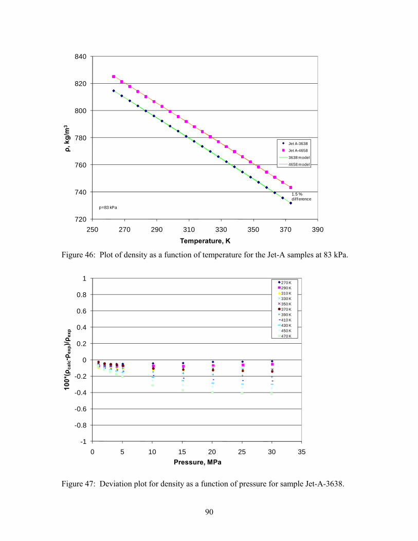
90
720
740
760
780
800
820
840
250 270 290 310 330 350 370 390
ρ, k
g/m
3
Temperature, K
Jet A-3638
Jet A-4658
3638 model
4658 model
p=83 kPa
1.5 % dif ference
Figure 46: Plot of density as a function of temperature for the Jet-A samples at 83 kPa.
-1
-0.8
-0.6
-0.4
-0.2
0
0.2
0.4
0.6
0.8
1
0 5 10 15 20 25 30 35
10
0*(ρ
ca
lc-ρ
ex
p)/ρ
ex
p
Pressure, MPa
270 K290 K310 K330 K350 K370 K390 K410 K430 K450 K470 K
Figure 47: Deviation plot for density as a function of pressure for sample Jet-A-3638.

91
-1
-0.8
-0.6
-0.4
-0.2
0
0.2
0.4
0.6
0.8
1
0 5 10 15 20 25 30 35
10
0*(ρ
ca
lc-ρ
ex
p)/ρ
ex
p
Pressure, MPa
270 K290 K310 K330 K350 K370 K390 K410 K430 K450 K470 K
Figure 48: Deviation plot for density as a function of pressure for sample Jet-A-4658
1100
1150
1200
1250
1300
1350
1400
250 270 290 310 330 350
So
un
d S
pe
ed
, m
/s
Temperature, K
Jet A-3638
Jet A-4658
3638 model
4658 model
p=83 kPa
Figure 49: Calculated and experimental speed of sound for the Jet-A samples at 83 kPa
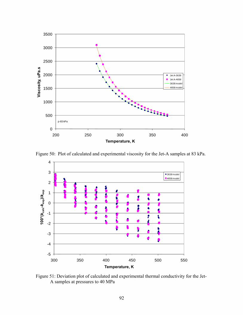
92
0
500
1000
1500
2000
2500
3000
3500
200 250 300 350 400
Vis
co
sit
y, u
Pa
.s
Temperature, K
Jet A-3638
Jet A-4658
3638 model
4658 model
p-83 kPa
Figure 50: Plot of calculated and experimental viscosity for the Jet-A samples at 83 kPa.
-5
-4
-3
-2
-1
0
1
2
3
4
300 350 400 450 500 550
10
0*(k
ca
lc-k
ex
p)/k
ex
p
Temperature, K
3638 model
4658 model
Figure 51: Deviation plot of calculated and experimental thermal conductivity for the Jet-
A samples at pressures to 40 MPa
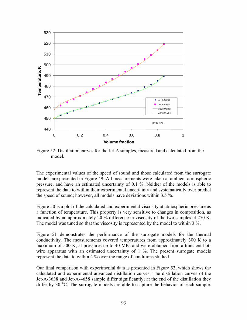
93
440
450
460
470
480
490
500
510
520
530
0 0.2 0.4 0.6 0.8 1
Te
mp
era
ture
, K
Volume fraction
Jet A-3638
Jet A-4658
3638 Model
4658 Model
p=83 kPa
Figure 52: Distillation curves for the Jet-A samples, measured and calculated from the
model. The experimental values of the speed of sound and those calculated from the surrogate models are presented in Figure 49. All measurements were taken at ambient atmospheric pressure, and have an estimated uncertainty of 0.1 %. Neither of the models is able to represent the data to within their experimental uncertainty and systematically over predict the speed of sound; however, all models have deviations within 3.5 %. Figure 50 is a plot of the calculated and experimental viscosity at atmospheric pressure as a function of temperature. This property is very sensitive to changes in composition, as indicated by an approximately 20 % difference in viscosity of the two samples at 270 K. The model was tuned so that the viscosity is represented by the model to within 3 %. Figure 51 demonstrates the performance of the surrogate models for the thermal conductivity. The measurements covered temperatures from approximately 300 K to a maximum of 500 K, at pressures up to 40 MPa and were obtained from a transient hot-wire apparatus with an estimated uncertainty of 1 %. The present surrogate models represent the data to within 4 % over the range of conditions studied Our final comparison with experimental data is presented in Figure 52, which shows the calculated and experimental advanced distillation curves. The distillation curves of the Jet-A-3638 and Jet-A-4658 sample differ significantly; at the end of the distillation they differ by 30 oC. The surrogate models are able to capture the behavior of each sample.

94
The volatility, as indicated by the advanced distillation curve, and the viscosity are very sensitive to changes in composition of the fuels. Our surrogate models represent the thermophysical properties of the two samples studied. Work is in progress to develop a methodology to represent the Jet-A fuels as a single model that will characterize the fuels in terms of compositionally sensitive properties such as points on the distillation curve and viscosities. In addition, comparisons with existing surrogate models are in progress, and also further development of the equation of state models to improve the representation of the properties. The composition of the surrogate mixture model for S-8, containing seven components, is summarized in Table 30. The computed distillation curve and the experimental data are shown in Figure 53. The difference between the calculated and experimental distillation temperatures is always within 1 %. The lightest (n-nonane) and heaviest fluids (n-hexadecane) are present only in small amounts and determine the initial boiling behavior and the tail of the distillation curve. The overall shape of the distillation curve is due primarily to only four major components: 2,6-dimethyloctane, 3-methyldecane, n-tridecane and n-tetradecane. In Figures 54 to 57, we present comparisons of the S-8 surrogate model with experimental data. Figure 54 shows deviations of experimental and calculated surrogate density for S-8. The measurements cover the temperature range 233 K to 470 K at pressures to 30 MPa, and have an average absolute deviation (AAD) of 1.5 % Figure 55 shows the deviations of experimental and calculated sound speeds for S-8. All of the sound speed measurements were made at local atmospheric pressure. The deviations are within 2.5 %, which exceeds the experimental uncertainty but is acceptable given the uncertainties in the constituent fluids and the mixture model. Figure 56 shows the deviations of experimental and calculated viscosity at atmospheric pressure for S-8. The deviations are within about 5 % over the temperature range investigated. Figure 57 shows the deviations of experimental and calculated thermal conductivity over pressures from atmospheric to 70 MPa at temperatures to 500 K. The predictions from the surrogate model are within 6 %, with the largest deviations at the lower temperatures.

95
Table 30. Composition of surrogate mixture for S-8
Fluid S-8 surrogate composition, mole fraction
n-nonane 0.03
2,6-dimethyloctane 0.28
3-methyldecane 0.34
n-tridecane 0.13
n-tetradecane 0.20
n-pentadecane 0.015
n-hexadecane 0.005
440
450
460
470
480
490
500
510
520
530
0.0 0.2 0.4 0.6 0.8 1.0
Te
mp
era
ture
, K
Volume fraction
Experimental data
7 component surrogate, this work
Figure 53. Distillation curve for S-8, showing the experimental and modeled curves.

96
0
0.5
1
1.5
2
2.5
200 250 300 350 400 450 500
10
0*(ρ
ex
p-ρ
su
rro
ga
te)/ρ
ex
p
Temperature, K
Deviations in Density for S-8 Surrogate Fuel
series 1, atmospheric pressure
series 2, atmospheric pressure
series 3, pressures to 30 MPa
Figure 54: Deviations of experimental and calculated surrogate density for S-8.
0
0.5
1
1.5
2
2.5
260 270 280 290 300 310 320 330 340 350
10
0*(w
ex
p-w
su
rro
ga
te)/w
ex
p
Temperature, K
Deviations in Sound Speed for S-8 Surrogate Fuel
Figure 55: Deviations of experimental and calculated surrogate sound speed for S-8.

97
-1
0
1
2
3
4
5
6
7
260 280 300 320 340 360 380
10
0*(η
ex
p-η
su
rro
ga
te)/η
ex
p
Temperature, K
Deviations in Viscosity for S-8 Surrogate Fuel
Figure 56: Deviations of experimental and calculated viscosity for S-8.
-10
-8
-6
-4
-2
0
2
4
200 250 300 350 400 450 500 550
10
0*(k
ex
p-k
su
rro
ga
te)/k
ex
p)
Temperature, K
Deviations in Thermal Conductivity for S-8 Surrogate Fuel
Figure 57: Deviations of experimental and calculated thermal conductivity for S-8.
98
References: 1. Bruno, T. J., Svoronos, P.D.N., CRC Handbook of Basic Tables for Chemical Analysis, 2nd. ed. Taylor and Francis CRC Press: Boca Raton, 2004.
2. Bruno, T. J., Svoronos, P.D.N., CRC Handbook of Fundamental Spectroscopic Correlation Charts. Taylor and Francis CRC Press: Boca Raton, 2005.
3. Andersen, P. C., Bruno, T.J., Thermal decomposition kinetics of RP-1 rocket propellant. Ind. Eng. Chem. Res. 2005, 44, (6), 1670-1676.
4. Andersen, W. A., Bruno, T.J., Rapid screening of fluids for chemical stability in organic Rankine cycle applications. Ind. Eng. Chem. Res. 2005, 44, 5560-5566.
5. Widegren, J. A., Bruno, T.J., Thermal decomposition kinetics of the aviation fuel Jet-A. Ind. Eng. Chem. Res. 2008, 47, (13), 4342-4348.
6. Widegren, J. A., Bruno, T.J., Thermal decomposition kinetics of propylcyclohexane. Ind. Eng. Chem. Res. 2009, 48, (2), 654-659.
7. Bruno, T. J., Conditioning of flowing multiphase samples for chemical analysis. Sep. Sci. Technol. 2005, 40, (8), 1720-1732.
8. Outcalt, S. L., McLinden, M.O., Automated densimeter for the rapid characterization of industrial fluids. Ind. Eng. Chem. Res. 2007, 46, 8264 - 8269.
9. Laesecke, A., Outcalt, S.L. and Brumback, K., Density and Speed of Sound Measurements of Methyl- and Propylcyclohexane. Energy and Fuels 2008, 22, 2629 - 2636.
10. Perkins, R. A.; Huber, M. L., Measurement and correlation of the thermal conductivity of pentafluoroethane (R125) from 190 K to 512 K at pressures to 70 MPa. Journal of Chemical and Engineering Data 2006, 51, (3), 898-904.
11. Perkins, R. A.; Laesecke, A.; Nieto de Castro, C. A., Polarized Transient Hot Wire Thermal Conductivity Measurements. Fluid Phase Equilibria 1992, 80, 275-286.
12. Bruno, T. J., Improvements in the measurement of distillation curves - part 1: a composition-explicit approach. Ind. Eng. Chem. Res. 2006, 45, 4371-4380.
13. Bruno, T. J., Method and apparatus for precision in-line sampling of distillate. Sep. Sci. Technol. 2006, 41, (2), 309-314.
14. Smith, B. L., Bruno, T.J., Advanced distillation curve measurement with a model predictive temperature controller. Int. J. Thermophys. 2006, 27, 1419-1434.

99
15. Bruno, T. J.; Smith, B. L., Enthalpy of combustion of fuels as a function of distillate cut: application of an advanced distillation curve method. Energy & Fuels 2006, 20, 2109-2116.
16. Bruno, T. J., Thermodynamic, transport and chemical properties of "reference" JP-8. Book of Abstracts, Army Research Office and Air Force Office of Scientific Research, 2006 Contractor's meeting in Chemical Propulsion 2006, 15-18.
17. Bruno, T. J., The properties of S-8. In Final Report for MIPR F4FBEY6237G001, Air Force Research Laboratory: 2006.
18. Bruno, T. J., Laesecke, A., Outcalt, S.L., Seelig, H-D, Smith, B.L., Properties of a 50/50 Mixture of Jet-A + S-8, NIST-IR-6647. 2007.
19. Bruno, T. J., Wolk, A., Naydich, A., Stabilization of biodiesel fuel at elevated Temperature with Hydrogen Donors: evaluation with the advanced distillation curve method. Energy & Fuels 2008, in press.
20. Bruno, T. J., Wolk, A., Naydich, A., Composition-explicit distillation curves for mixtures of gasoline with four-carbon alcohols (butanols). Energy & Fuels 2008, in press.
21. Ott, L. S., Smith, B.L., Bruno, T.J., Advanced distillation curve measurements for corrosive fluids: application to two crude oils. Fuel 2008, 87, 3055-3064.
22. Ott, L. S., Smith, B.L., Bruno, T.J., Advanced distillation curve measurement: application to a bio-derived crude oil prepared from swine manure. Fuel 2008, 87, 3379-3387.
23. Ott, L. S., Smith, B.L., Bruno, T.J., Composition-explicit distillation curves of mixtures of diesel fuel with biomass-derived glycol ester oxygenates: a fuel design tool for decreased particulate emissions. Energy and Fuels 2008, 22, 2518-2526.
24. Ott, L. S., Hadler, A., Bruno, T.J., Variability of the rocket propellants RP-1, RP-2, and TS-5: application of a composition- and enthalpy-explicit distillation curve method. Ind. Eng. Chem. Res. 2008, 47 (23), 9225-9233.
25. Ott, L. S., Bruno, T.J., Variability of biodiesel fuel and comparison to petroleum-derived diesel fuel: application of a composition and enthalpy explicit distillation curve method. Energy & Fuels 2008, 22, 2861-2868.
26. Smith, B. L., Bruno, T.J., Improvements in the measurement of distillation curves: part 3 - application to gasoline and gasoline + methanol mixtures. Ind. Eng. Chem. Res. 2007, 46, 297-309.
27. Smith, B. L., Bruno, T.J., Improvements in the measurement of distillation curves: part 4- application to the aviation turbine fuel Jet-A. Ind. Eng. Chem. Res. 2007, 46, 310-320.

100
28. Smith, B. L., Bruno, T.J., Composition-explicit distillation curves of aviation fuel JP-8 and a coal based jet fuel. Energy & Fuels 2007, 21, 2853-2862.
29. Smith, B. L., Bruno, T.J., Application of a Composition-Explicit Distillation Curve Metrology to Mixtures of Jet-A + Synthetic Fischer-Tropsch S-8. J. Propul. Power 2008, 24, (3), 619 - 623.
30. Smith, B. L., Ott, L.S., Bruno, T.J., Composition-explicit distillation curves of diesel fuel with glycol ether and glycol ester oxygenates: a design tool for decreased particulate emissions. Environ. Sci. Tech. 2008, 42, (20), 7682-7689.
31. Smith, B. L., Ott, L.S., Bruno, T.J., Composition-explicit distillation curves of commercial biodiesel fuels: comparison of petroleum derived fuel with B20 and B100. Ind. Eng. Chem. Res. 2008, 47, (16), 5832-5840.
32. Ott, L. S., Smith, B.L., Bruno, T.J., Experimental test of the Sydney Young equation for the presentation of distillation curves. J. Chem. Thermodynam. 2008, 40, 1352-1357.
33. Standard Test Method for Boiling Range Distribution of Petroleum Fractions by Gas Chromatography, ASTM Standard D2887-02, ASTM Annual Book of Standards, 2004. In 2004.
34. Outcalt, S. L., Laesecke, A., Freund, M.B., Density and speed of sound measurements of Jet A and S 8 aviation turbine fuels. Energy & Fuels 2009, 23, (3), 1626-1633.
35. Huber, M. L., Smith, B.L., Ott, L.S., Bruno, T.J., Surrogate Mixture Model for the Thermophysical Properties of Synthetic Aviation Fuel S-8: Explicit Application of the Advanced Distillation Curve. Energy & Fuels 2008, 22, 1104 - 1114.
36. Huber, M. L., Lemmon, E.W., Diky, V., Smith, B.L., Bruno, T.J., Chemically authentic surrogate mixture model for the thermophysical properties of a coal-derived-liquid fuel. Energy and Fuels 2008, 22, 3249-3257.
37. Rowley, R. L., Wilding, W.V., Oscarson, J.L., Zundel, N.A., Marshall, T.L., Daubert, T.E., Danner, R.P., , DIPPR Data Compilation of Pure Compound Properties, Design Institute for Physical Properties AIChE, New York, NY, 2004. In.
38. Huber, M. L., Lemmon, E., Ott, L.S., Bruno, T.J., Preliminary surrogate mixture models for rocket propellants RP-1 and RP-2. Energy & Fuels 2009, 23, 3083-3088.
39. Huber, M. L., Lemmon, E., Bruno, T.J., Effect of RP-1 compositional variability on thermophysical properties. Energy & Fuels 2009, 23, 5550-5555.
40. Span, R.; Wagner, W., Equations of state for technical applications. I. Simultaneously optimized functional forms for nonpolar and polar fluids. International Journal of Thermophysics 2003, 24, (1), 1-39.

101
41. Lemmon, E. W., McLinden, M.O., Huber, M.L., REFPROP, Reference fluid thermodynamic and transport properties, NIST Standard Reference Database 23. National Institute of Standards and Technology, Gaithersburg, MD, 2005: 2005.

102
Appendix I: Thermal Conductivity Measurements for Aviation Fuels

103
Table A1. Thermal conductivity of Jet-A-3602 in the liquid phase.
Point ID T0 Te Pe e q (K) (K) (MPa) (W·m-1K-1) (W·m-1)
1001 298.295 296.274 1.984 0.1108 0.4694 1003 298.672 296.292 1.968 0.1106 0.5496 1005 299.099 296.325 1.961 0.1106 0.6375 1007 299.543 296.349 1.948 0.1105 0.7320 1009 300.022 296.374 1.939 0.1105 0.8329 1011 301.639 299.624 0.174 0.1099 0.4651 1013 301.987 299.627 0.174 0.1098 0.5446 1015 302.367 299.627 0.175 0.1097 0.6317 1017 302.774 299.622 0.170 0.1098 0.7254 1019 303.214 299.627 0.163 0.1096 0.8254 1021 301.619 299.634 4.975 0.1113 0.4651 1023 301.964 299.636 4.980 0.1112 0.5446 1025 302.346 299.639 4.984 0.1112 0.6316 1027 302.750 299.642 4.983 0.1110 0.7252 1029 303.180 299.640 4.971 0.1111 0.8253 1031 301.609 299.651 10.178 0.1127 0.4654 1033 301.951 299.654 10.176 0.1126 0.5450 1035 302.316 299.651 10.187 0.1125 0.6320 1037 302.713 299.650 10.197 0.1126 0.7254 1039 303.138 299.649 10.198 0.1126 0.8253 1041 301.570 299.672 20.550 0.1153 0.4651 1043 301.900 299.670 20.553 0.1153 0.5446 1045 302.265 299.672 20.554 0.1154 0.6317 1047 302.653 299.670 20.555 0.1154 0.7253 1049 303.070 299.672 20.549 0.1153 0.8253 1051 301.529 299.686 30.277 0.1178 0.4651 1053 301.859 299.689 30.274 0.1178 0.5447 1055 302.206 299.683 30.275 0.1178 0.6317 1057 302.590 299.682 30.278 0.1178 0.7253 1059 303.003 299.685 30.282 0.1178 0.8252 1061 301.527 299.694 40.263 0.1201 0.4653 1063 301.842 299.688 40.266 0.1202 0.5448 1065 302.199 299.693 40.251 0.1203 0.6320 1067 302.576 299.694 40.236 0.1201 0.7258 1069 302.972 299.689 40.224 0.1202 0.8259 2001 321.196 319.226 0.225 0.1072 0.4427 2003 321.505 319.239 0.249 0.1075 0.5181 2005 321.891 319.253 0.261 0.1075 0.6009 2007 322.305 319.266 0.273 0.1074 0.6899 2009 322.750 319.280 0.290 0.1073 0.7849 2011 321.338 319.407 5.164 0.1090 0.4424 2013 321.693 319.425 5.179 0.1091 0.5179 2015 322.008 319.426 5.194 0.1090 0.6006 2017 322.419 319.441 5.207 0.1089 0.6895 2019 322.853 319.454 5.218 0.1089 0.7845 2021 321.614 319.717 10.194 0.1107 0.4420 2023 321.952 319.724 10.206 0.1106 0.5174 2025 322.320 319.731 10.216 0.1105 0.6002 2027 322.722 319.745 10.222 0.1105 0.6891 2029 323.143 319.750 10.228 0.1104 0.7840 2031 321.722 319.865 20.180 0.1137 0.4419

104
2033 322.056 319.876 20.156 0.1136 0.5177 2035 322.403 319.872 20.157 0.1135 0.6005 2037 322.796 319.885 20.158 0.1134 0.6895 2039 323.204 319.887 20.169 0.1134 0.7844 2041 321.702 319.958 30.172 0.1163 0.4417 2043 322.025 319.967 30.161 0.1161 0.5174 2045 322.366 319.966 30.155 0.1162 0.6002 2047 322.745 319.978 30.158 0.1160 0.6891 2049 323.148 319.980 30.154 0.1162 0.7841 2051 321.861 320.074 40.148 0.1187 0.4418 2053 322.169 320.078 40.154 0.1188 0.5173 2055 322.514 320.084 40.161 0.1188 0.6000 2057 322.883 320.088 40.170 0.1188 0.6889 2059 323.263 320.086 40.178 0.1187 0.7837 3001 341.527 339.564 0.293 0.1049 0.4213 3003 341.762 339.569 0.303 0.1049 0.4932 3005 342.136 339.581 0.312 0.1049 0.5720 3007 342.535 339.593 0.320 0.1047 0.6567 3009 342.953 339.599 0.327 0.1048 0.7472 3011 341.537 339.694 5.129 0.1067 0.4211 3013 341.871 339.700 5.135 0.1066 0.4931 3015 342.231 339.708 5.142 0.1065 0.5719 3017 342.624 339.717 5.150 0.1064 0.6566 3019 343.036 339.724 5.154 0.1064 0.7471 3021 341.610 339.798 10.188 0.1084 0.4210 3023 341.932 339.803 10.183 0.1083 0.4930 3025 342.286 339.805 10.173 0.1084 0.5720 3027 342.669 339.815 10.171 0.1081 0.6569 3029 343.081 339.822 10.170 0.1082 0.7474 3031 341.664 339.918 20.026 0.1115 0.4212 3033 341.980 339.921 20.019 0.1115 0.4934 3035 342.323 339.928 20.050 0.1115 0.5718 3037 342.688 339.930 20.056 0.1114 0.6565 3039 343.084 339.935 20.066 0.1113 0.7469 3041 341.704 339.991 30.148 0.1143 0.4212 3043 342.013 339.996 30.153 0.1143 0.4932 3045 342.347 340.000 30.179 0.1145 0.5717 3047 342.703 339.998 30.188 0.1144 0.6564 3049 343.088 340.005 30.194 0.1143 0.7468 3051 341.750 340.067 40.334 0.1174 0.4209 3053 342.047 340.068 40.339 0.1174 0.4928 3055 342.372 340.071 40.336 0.1173 0.5717 3057 342.724 340.073 40.341 0.1173 0.6564 3059 343.098 340.080 40.349 0.1172 0.7468 4001 360.637 358.790 0.166 0.1022 0.4031 4003 360.911 358.795 0.175 0.1023 0.4719 4005 361.273 358.804 0.171 0.1021 0.5474 4007 361.655 358.810 0.167 0.1021 0.6287 4009 362.064 358.817 0.169 0.1021 0.7154 4011 360.656 358.894 5.232 0.1042 0.4031 4013 360.979 358.902 5.238 0.1041 0.4719 4015 361.327 358.908 5.242 0.1041 0.5474 4017 361.704 358.912 5.247 0.1040 0.6285 4019 362.105 358.921 5.251 0.1040 0.7151 4021 360.745 358.982 10.164 0.1061 0.4030 4023 361.062 358.988 10.169 0.1060 0.4719

105
4025 361.405 358.992 10.175 0.1060 0.5474 4027 361.774 359.000 10.182 0.1059 0.6285 4029 362.163 359.000 10.190 0.1058 0.7150 4031 360.798 359.072 20.275 0.1095 0.4029 4033 361.097 359.074 20.279 0.1095 0.4718 4035 361.433 359.079 20.278 0.1094 0.5472 4037 361.789 359.079 20.267 0.1093 0.6285 4039 362.173 359.087 20.268 0.1093 0.7152 4041 360.765 359.136 30.385 0.1128 0.4028 4043 361.111 359.137 30.390 0.1127 0.4718 4045 361.438 359.143 30.392 0.1126 0.5472 4047 361.785 359.145 30.380 0.1127 0.6285 4049 362.149 359.143 30.372 0.1126 0.7152 4051 360.846 359.196 40.225 0.1158 0.4030 4053 361.133 359.200 40.223 0.1157 0.4720 4055 361.443 359.199 40.234 0.1157 0.5473 4057 361.786 359.205 40.246 0.1156 0.6283 4059 362.149 359.211 40.250 0.1156 0.7148 5001 380.967 379.179 0.263 0.0995 0.3856 5003 381.285 379.183 0.259 0.0996 0.4516 5005 381.632 379.192 0.257 0.0994 0.5239 5007 382.008 379.199 0.258 0.0993 0.6015 5009 382.401 379.203 0.258 0.0994 0.6845 5011 380.987 379.257 5.121 0.1015 0.3855 5013 381.303 379.264 5.115 0.1015 0.4516 5015 381.644 379.268 5.114 0.1015 0.5238 5017 382.011 379.272 5.116 0.1014 0.6014 5019 382.397 379.278 5.117 0.1013 0.6842 5021 381.059 379.335 10.120 0.1035 0.3857 5023 381.369 379.345 10.123 0.1034 0.4516 5025 381.697 379.346 10.132 0.1034 0.5237 5027 382.053 379.348 10.136 0.1033 0.6012 5029 382.431 379.351 10.143 0.1033 0.6840 5031 381.064 379.398 20.233 0.1074 0.3857 5033 381.357 379.402 20.245 0.1073 0.4514 5035 381.683 379.406 20.250 0.1072 0.5236 5037 382.022 379.406 20.255 0.1072 0.6011 5039 382.385 379.405 20.260 0.1072 0.6840 5041 381.066 379.457 30.226 0.1107 0.3855 5043 381.351 379.458 30.231 0.1106 0.4514 5045 381.660 379.459 30.236 0.1106 0.5235 5047 381.996 379.464 30.236 0.1106 0.6011 5049 382.353 379.466 30.239 0.1106 0.6840 5051 381.067 379.512 40.517 0.1140 0.3855 5053 381.341 379.514 40.520 0.1140 0.4513 5055 381.646 379.516 40.523 0.1141 0.5235 5057 381.963 379.513 40.527 0.1140 0.6011 5059 382.314 379.516 40.511 0.1140 0.6841 6001 401.768 399.994 0.177 0.0966 0.3696 6003 402.070 399.990 0.180 0.0965 0.4328 6005 402.405 399.993 0.182 0.0965 0.5019 6007 402.761 399.991 0.183 0.0963 0.5763 6009 403.144 399.993 0.175 0.0964 0.6558 6011 401.679 400.005 5.188 0.0988 0.3695 6013 401.979 400.006 5.189 0.0988 0.4327 6015 402.306 400.008 5.189 0.0988 0.5018
106
6017 402.656 400.007 5.190 0.0987 0.5762 6019 403.022 400.004 5.193 0.0987 0.6556 6021 401.697 400.022 10.130 0.1010 0.3696 6023 401.986 400.019 10.134 0.1011 0.4327 6025 402.304 400.017 10.137 0.1010 0.5019 6027 402.655 400.022 10.139 0.1009 0.5763 6029 403.013 400.016 10.141 0.1008 0.6556 6031 401.635 400.041 20.129 0.1050 0.3698 6033 401.916 400.040 20.139 0.1051 0.4330 6035 402.219 400.038 20.144 0.1049 0.5021 6037 402.550 400.036 20.145 0.1048 0.5765 6039 402.906 400.039 20.149 0.1050 0.6558 6041 401.612 400.056 30.252 0.1087 0.3697 6043 401.880 400.053 30.252 0.1087 0.4329 6045 402.178 400.052 30.255 0.1087 0.5020 6047 402.500 400.052 30.257 0.1086 0.5764 6049 402.845 400.056 30.258 0.1085 0.6558 6051 401.546 400.067 40.273 0.1122 0.3699 6053 401.823 400.072 40.275 0.1120 0.4331 6055 402.108 400.067 40.273 0.1122 0.5023 6057 402.416 400.068 40.276 0.1122 0.5767 6059 402.751 400.066 40.287 0.1121 0.6560 7001 421.914 420.177 0.184 0.0938 0.3547 7003 422.223 420.186 0.188 0.0938 0.4153 7005 422.558 420.190 0.190 0.0938 0.4817 7007 422.914 420.191 0.188 0.0938 0.5532 7009 423.301 420.201 0.188 0.0936 0.6294 7011 421.903 420.239 5.025 0.0963 0.3546 7013 422.192 420.238 5.029 0.0964 0.4152 7015 422.525 420.246 5.031 0.0962 0.4815 7017 422.866 420.244 5.030 0.0962 0.5529 7019 423.244 420.251 5.032 0.0961 0.6291 7021 421.997 420.334 10.039 0.0988 0.3547 7023 422.291 420.340 10.040 0.0986 0.4153 7025 422.609 420.341 10.039 0.0985 0.4817 7027 422.946 420.345 10.039 0.0986 0.5531 7029 423.299 420.340 10.036 0.0985 0.6293 7031 422.289 420.384 20.334 0.1029 0.3542 7033 422.558 420.382 20.336 0.1028 0.4147 7035 422.860 420.382 20.337 0.1029 0.4810 7037 423.187 420.387 20.337 0.1030 0.5523 7039 423.531 420.386 20.331 0.1028 0.6285 7041 422.000 420.422 20.356 0.1031 0.3538 7043 422.277 420.423 20.354 0.1030 0.4144 7045 422.580 420.424 20.348 0.1029 0.4807 7047 422.904 420.427 20.345 0.1029 0.5520 7049 423.252 420.429 20.340 0.1029 0.6282 7051 421.974 420.463 30.268 0.1070 0.3540 7053 422.237 420.462 30.265 0.1070 0.4145 7055 422.531 420.464 30.265 0.1067 0.4808 7057 422.842 420.464 30.262 0.1069 0.5521 7059 423.171 420.461 30.259 0.1067 0.6282 7061 421.925 420.484 40.327 0.1106 0.3540 7063 422.180 420.482 40.327 0.1107 0.4144 7065 422.512 420.483 40.330 0.1105 0.4808 7067 422.812 420.482 40.316 0.1106 0.5522

107
7069 423.137 420.483 40.306 0.1104 0.6284 8001 441.838 440.120 0.223 0.0913 0.3407 8003 442.140 440.122 0.223 0.0913 0.3989 8005 442.412 440.122 0.224 0.0913 0.4626 8007 442.758 440.124 0.223 0.0914 0.5312 8009 443.121 440.124 0.218 0.0914 0.6044 8011 441.768 440.142 5.197 0.0941 0.3405 8013 442.051 440.142 5.198 0.0941 0.3987 8015 442.358 440.138 5.198 0.0940 0.4625 8017 442.702 440.144 5.192 0.0941 0.5311 8019 443.056 440.140 5.189 0.0939 0.6044 8021 441.769 440.152 10.163 0.0967 0.3406 8023 442.045 440.151 10.164 0.0965 0.3987 8025 442.347 440.148 10.165 0.0966 0.4625 8027 442.680 440.155 10.165 0.0966 0.5311 8029 443.028 440.152 10.164 0.0965 0.6043 8031 441.711 440.183 20.255 0.1012 0.3406 8033 441.977 440.185 20.254 0.1011 0.3988 8035 442.265 440.181 20.254 0.1011 0.4626 8037 442.585 440.187 20.256 0.1010 0.5311 8039 442.915 440.179 20.259 0.1010 0.6042 8041 441.635 440.197 30.162 0.1052 0.3408 8043 441.897 440.201 30.172 0.1051 0.3990 8045 442.176 440.198 30.178 0.1053 0.4627 8047 442.476 440.198 30.182 0.1052 0.5312 8049 442.792 440.190 30.183 0.1051 0.6044 8051 441.591 440.197 40.247 0.1090 0.3408 8053 441.892 440.196 40.249 0.1093 0.3991 8055 442.168 440.196 40.257 0.1089 0.4628 8057 442.462 440.199 40.261 0.1090 0.5314 8059 442.769 440.191 40.264 0.1090 0.6045 9001 461.280 459.599 0.148 0.0893 0.3283 9003 461.578 459.603 0.145 0.0893 0.3845 9005 461.902 459.607 0.138 0.0891 0.4462 9007 462.247 459.612 0.135 0.0891 0.5124 9009 462.610 459.612 0.138 0.0891 0.5829 9011 461.254 459.647 5.152 0.0923 0.3283 9013 461.544 459.654 5.144 0.0920 0.3845 9015 461.851 459.648 5.140 0.0921 0.4461 9017 462.186 459.655 5.134 0.0921 0.5124 9019 462.543 459.658 5.134 0.0920 0.5830 9021 461.240 459.693 10.181 0.0949 0.3284 9023 461.512 459.693 10.174 0.0948 0.3847 9025 461.815 459.698 10.172 0.0947 0.4462 9027 462.137 459.697 10.175 0.0948 0.5123 9029 462.479 459.701 10.182 0.0948 0.5827 9031 461.164 459.730 20.252 0.0995 0.3283 9033 461.416 459.725 20.253 0.0995 0.3845 9035 461.706 459.726 20.256 0.0994 0.4459 9037 462.012 459.726 20.260 0.0994 0.5120 9039 462.384 459.722 20.262 0.0994 0.5826 9041 461.193 459.750 30.196 0.1038 0.3286 9043 461.448 459.753 30.195 0.1037 0.3848 9045 461.724 459.752 30.199 0.1037 0.4462 9047 462.020 459.758 30.206 0.1036 0.5123 9049 462.322 459.747 30.209 0.1035 0.5828

108
9051 461.127 459.771 40.275 0.1076 0.3284 9053 461.412 459.770 40.269 0.1076 0.3846 9055 461.678 459.771 40.258 0.1077 0.4462 9057 461.973 459.775 40.248 0.1076 0.5125 9059 462.280 459.778 40.244 0.1075 0.5831 10001 482.140 480.490 0.183 0.0871 0.3163 10003 482.424 480.488 0.183 0.0871 0.3704 10005 482.742 480.496 0.183 0.0872 0.4297 10007 483.033 480.497 0.184 0.0869 0.4933 10009 483.391 480.498 0.184 0.0871 0.5611 10011 482.078 480.517 5.144 0.0903 0.3162 10013 482.341 480.510 5.145 0.0903 0.3702 10015 482.642 480.510 5.146 0.0902 0.4294 10017 482.966 480.513 5.146 0.0902 0.4931 10019 483.312 480.511 5.147 0.0901 0.5610 10021 482.227 480.677 5.215 0.0903 0.3160 10023 482.511 480.684 5.214 0.0903 0.3700 10025 482.806 480.680 5.210 0.0903 0.4292 10027 483.138 480.686 5.210 0.0902 0.4929 10029 483.481 480.686 5.209 0.0902 0.5608 10031 482.183 480.688 10.157 0.0931 0.3160 10033 482.446 480.684 10.158 0.0931 0.3700 10035 482.738 480.686 10.159 0.0931 0.4292 10037 483.049 480.687 10.160 0.0930 0.4927 10039 483.380 480.683 10.161 0.0930 0.5606 10041 481.966 480.703 20.361 0.0975 0.3161 10043 482.213 480.697 20.361 0.0977 0.3701 10045 482.494 480.698 20.361 0.0977 0.4293 10047 482.982 480.693 20.360 0.0975 0.4931 10049 483.304 480.699 20.359 0.0975 0.5611 10051 482.044 480.705 30.461 0.1022 0.3162 10053 482.282 480.698 30.461 0.1021 0.3702 10055 482.650 480.698 30.461 0.1020 0.4295 10057 482.933 480.694 30.460 0.1020 0.4932 10059 483.244 480.699 30.460 0.1019 0.5611 10061 482.044 480.700 40.419 0.1060 0.3162 10063 482.282 480.703 40.419 0.1061 0.3703 10065 482.544 480.705 40.419 0.1061 0.4295 10067 482.815 480.699 40.421 0.1060 0.4932 10069 483.115 480.703 40.421 0.1061 0.5611 11001 502.136 500.513 0.435 0.0850 0.3053 11003 502.423 500.518 0.436 0.0849 0.3575 11005 502.729 500.523 0.444 0.0849 0.4145 11007 503.059 500.522 0.446 0.0848 0.4759 11009 503.416 500.524 0.448 0.0848 0.5414 11011 502.132 500.548 5.197 0.0880 0.3052 11013 502.409 500.554 5.190 0.0880 0.3574 11015 502.708 500.555 5.188 0.0881 0.4147 11017 503.028 500.554 5.186 0.0881 0.4761 11019 503.370 500.558 5.191 0.0880 0.5416 11021 502.074 500.580 10.192 0.0911 0.3051 11023 502.329 500.576 10.193 0.0911 0.3572 11025 502.630 500.589 10.195 0.0911 0.4144 11027 502.935 500.583 10.196 0.0910 0.4758 11029 503.273 500.589 10.194 0.0910 0.5414 11031 501.983 500.625 20.349 0.0965 0.3051

109
11033 502.232 500.622 20.338 0.0966 0.3574 11035 502.537 500.625 20.333 0.0965 0.4146 11037 502.832 500.626 20.331 0.0964 0.4761 11039 503.146 500.627 20.334 0.0964 0.5417 11041 501.790 500.637 30.448 0.1010 0.3051 11043 502.027 500.636 30.449 0.1010 0.3572 11045 502.296 500.641 30.451 0.1010 0.4144 11047 502.580 500.646 30.451 0.1009 0.4758 11049 503.060 500.637 30.452 0.1009 0.5415 11051 501.948 500.658 40.475 0.1052 0.3053 11053 502.176 500.659 40.477 0.1051 0.3574 11055 502.436 500.663 40.478 0.1050 0.4146 11057 502.703 500.658 40.479 0.1049 0.4761 11059 502.992 500.661 40.480 0.1049 0.5417
Table A2. Thermal conductivity for Jet-A-3638 in the liquid phase.
Point ID T0 Te Pe e q (K) (K) (MPa) (W·m-1K-1) (W·m-1)
1001 299.529 301.523 0.139 0.1117 0.4632 1003 299.531 301.866 0.140 0.1116 0.5423 1005 299.527 302.236 0.140 0.1116 0.6291 1007 299.530 302.637 0.140 0.1115 0.7223 1009 299.530 303.069 0.127 0.1114 0.8221 1011 299.541 301.455 5.175 0.1133 0.4631 1013 299.541 301.793 5.170 0.1132 0.5423 1015 299.542 302.160 5.164 0.1132 0.6290 1017 299.537 302.552 5.162 0.1131 0.7222 1019 299.538 302.976 5.158 0.1130 0.8216 1021 299.545 301.430 9.801 0.1147 0.4631 1023 299.549 301.767 9.739 0.1146 0.5423 1025 299.545 302.175 9.678 0.1145 0.6291 1027 299.545 302.567 9.619 0.1145 0.7223 1029 299.541 302.982 9.563 0.1144 0.8218 1031 299.557 301.435 14.851 0.1160 0.4633 1033 299.554 301.773 14.119 0.1159 0.5424 1035 299.550 302.138 13.551 0.1157 0.6291 1037 299.548 302.529 13.074 0.1155 0.7223 1039 299.548 302.949 12.663 0.1152 0.8217 2001 317.067 319.004 0.189 0.1092 0.4431 2003 317.087 319.364 0.211 0.1092 0.5187 2005 317.102 319.748 0.227 0.1091 0.6016 2007 317.120 320.165 0.242 0.1091 0.6907 2009 317.132 320.601 0.256 0.1091 0.7858 2011 317.272 319.133 5.134 0.1111 0.4427 2013 317.289 319.483 5.148 0.1108 0.5183 2015 317.303 319.862 5.163 0.1110 0.6012 2017 317.316 320.265 5.178 0.1109 0.6902 2019 317.328 320.695 5.184 0.1108 0.7854 2021 317.532 319.448 10.150 0.1125 0.4428 2023 317.541 319.782 10.176 0.1125 0.5182 2025 317.555 320.153 10.194 0.1125 0.6010 2027 317.563 320.549 10.207 0.1124 0.6900
110
2029 317.578 320.976 10.218 0.1124 0.7851 2031 317.685 319.483 20.061 0.1157 0.4425 2033 317.698 319.819 20.045 0.1156 0.5180 2035 317.707 320.181 20.024 0.1156 0.6008 2037 317.719 320.568 20.007 0.1155 0.6898 2039 317.730 320.979 19.988 0.1155 0.7848 2041 317.831 319.597 26.754 0.1175 0.4425 2043 317.836 320.009 24.973 0.1170 0.5180 2045 317.835 320.372 23.951 0.1167 0.6008 2047 317.844 320.761 23.234 0.1164 0.6898 2049 317.853 321.174 22.684 0.1163 0.7848 3001 338.468 340.321 0.207 0.1062 0.4206 3003 338.473 340.647 0.212 0.1062 0.4925 3005 338.478 341.008 0.209 0.1060 0.5713 3007 338.488 341.403 0.204 0.1060 0.6561 3009 338.492 341.818 0.203 0.1060 0.7466 3011 338.636 340.492 5.414 0.1081 0.4206 3013 338.640 340.813 5.403 0.1081 0.4927 3015 338.644 341.163 5.407 0.1080 0.5714 3017 338.652 341.546 5.416 0.1081 0.6560 3019 338.661 341.951 5.425 0.1079 0.7463 3021 338.700 340.494 10.105 0.1099 0.4204 3023 338.709 340.821 10.092 0.1100 0.4925 3025 338.710 341.164 10.079 0.1097 0.5714 3027 338.717 341.539 10.083 0.1097 0.6560 3029 338.716 341.932 10.091 0.1097 0.7463 3031 338.769 340.523 20.136 0.1132 0.4204 3033 338.773 340.831 20.134 0.1135 0.4922 3035 338.773 341.165 20.120 0.1135 0.5712 3037 338.773 341.527 20.110 0.1132 0.6560 3039 338.782 341.918 20.106 0.1132 0.7464 3041 338.824 340.487 30.069 0.1165 0.4204 3043 338.825 340.787 30.046 0.1165 0.4922 3045 338.829 341.114 30.015 0.1164 0.5709 3047 338.832 341.468 29.965 0.1163 0.6558 3049 338.837 341.848 29.932 0.1164 0.7463 3051 338.851 340.561 30.996 0.1167 0.4204 3053 338.853 340.861 30.654 0.1166 0.4922 3055 338.857 341.192 30.363 0.1165 0.5709 3057 338.857 341.547 30.107 0.1162 0.6555 3059 338.861 341.924 29.862 0.1161 0.7462 4001 358.082 359.910 0.281 0.1033 0.4023 4003 358.089 360.234 0.287 0.1033 0.4710 4005 358.091 360.587 0.293 0.1032 0.5463 4007 358.097 360.960 0.300 0.1032 0.6272 4009 358.101 361.361 0.305 0.1031 0.7135 4011 358.150 359.922 5.079 0.1053 0.4021 4013 358.153 360.235 5.084 0.1054 0.4709 4015 358.156 360.575 5.090 0.1053 0.5461 4017 358.164 360.948 5.094 0.1052 0.6270 4019 358.164 361.338 5.097 0.1051 0.7133 4021 358.222 359.987 10.072 0.1073 0.4021 4023 358.225 360.296 10.075 0.1072 0.4708 4025 358.229 360.633 10.059 0.1072 0.5464 4027 358.228 360.991 10.055 0.1071 0.6274 4029 358.235 361.379 10.056 0.1070 0.7138

111
4031 358.276 359.984 20.197 0.1111 0.4021 4033 358.279 360.281 20.200 0.1109 0.4708 4035 358.279 360.602 20.203 0.1109 0.5461 4037 358.282 360.955 20.187 0.1109 0.6273 4039 358.284 361.328 20.184 0.1108 0.7137 4041 358.321 359.970 30.400 0.1144 0.4021 4043 358.322 360.259 30.403 0.1145 0.4708 4045 358.322 360.569 30.396 0.1145 0.5463 4047 358.325 360.911 30.398 0.1143 0.6271 4049 358.322 361.269 30.387 0.1145 0.7138 4051 358.350 359.945 39.278 0.1175 0.4021 4053 358.350 360.225 39.136 0.1174 0.4709 4055 358.347 360.531 39.002 0.1173 0.5462 4057 358.354 360.868 38.876 0.1172 0.6271 4059 358.352 361.221 38.753 0.1171 0.7135 5001 378.914 380.728 0.241 0.1005 0.3849 5003 378.916 381.040 0.238 0.1003 0.4507 5005 378.914 381.370 0.241 0.1001 0.5227 5007 378.916 381.732 0.247 0.1000 0.6000 5009 378.918 382.123 0.251 0.1000 0.6826 5011 378.953 380.690 5.093 0.1025 0.3847 5013 378.955 380.990 5.098 0.1023 0.4504 5015 378.952 381.315 5.100 0.1024 0.5223 5017 378.954 381.672 5.103 0.1022 0.5997 5019 378.951 382.047 5.104 0.1021 0.6824 5021 378.969 380.661 10.042 0.1046 0.3848 5023 378.966 380.954 10.049 0.1044 0.4504 5025 378.970 381.279 10.052 0.1044 0.5224 5027 378.970 381.628 10.054 0.1044 0.5997 5029 378.969 381.995 10.055 0.1043 0.6824 5031 378.996 380.608 20.271 0.1086 0.3846 5033 378.995 380.892 20.266 0.1085 0.4503 5035 378.993 381.204 20.257 0.1087 0.5225 5037 378.993 381.538 20.249 0.1085 0.6000 5039 378.996 381.953 20.241 0.1084 0.6829 5041 379.013 380.596 30.354 0.1124 0.3847 5043 379.011 380.867 30.353 0.1123 0.4504 5045 379.010 381.172 30.355 0.1123 0.5224 5047 379.005 381.495 30.345 0.1122 0.6000 5049 379.012 381.851 30.337 0.1120 0.6828 5051 379.023 380.533 40.332 0.1157 0.3847 5053 379.028 380.805 40.332 0.1156 0.4504 5055 379.022 381.097 40.332 0.1157 0.5224 5057 379.025 381.414 40.324 0.1155 0.5999 5059 379.021 381.751 40.308 0.1155 0.6828 6001 397.146 398.949 0.309 0.0974 0.3704 6003 397.154 399.261 0.317 0.0975 0.4336 6005 397.164 399.606 0.325 0.0975 0.5029 6007 397.171 399.973 0.332 0.0974 0.5774 6009 397.182 400.367 0.338 0.0973 0.6569 6011 397.207 398.971 0.132 0.0975 0.3700 6013 397.223 399.296 0.129 0.0975 0.4333 6015 397.227 399.638 0.131 0.0972 0.5026 6017 397.231 399.996 0.136 0.0973 0.5770 6019 397.238 400.388 0.145 0.0973 0.6564 6021 397.311 398.985 5.093 0.1001 0.3699

112
6023 397.324 399.294 5.092 0.0999 0.4332 6025 397.327 399.625 5.093 0.0998 0.5025 6027 397.335 399.977 5.098 0.0997 0.5768 6029 397.336 400.353 5.106 0.0997 0.6562 6031 397.394 399.055 10.156 0.1023 0.3699 6033 397.398 399.351 10.160 0.1023 0.4331 6035 397.406 399.675 10.160 0.1022 0.5024 6037 397.410 400.023 10.162 0.1021 0.5768 6039 397.415 400.391 10.170 0.1021 0.6562 6041 397.466 399.068 20.278 0.1064 0.3698 6043 397.473 399.354 20.272 0.1064 0.4331 6045 397.470 399.659 20.271 0.1062 0.5024 6047 397.477 399.996 20.274 0.1063 0.5768 6049 397.481 400.355 20.279 0.1062 0.6563 6051 397.558 399.115 30.305 0.1104 0.3698 6053 397.561 399.390 30.307 0.1103 0.4329 6055 397.557 399.682 30.309 0.1102 0.5021 6057 397.564 400.006 30.310 0.1103 0.5766 6059 397.569 400.352 30.312 0.1102 0.6561 6061 397.633 399.142 40.400 0.1138 0.3698 6063 397.631 399.405 40.402 0.1138 0.4329 6065 397.637 399.699 40.401 0.1138 0.5021 6067 397.642 400.009 40.400 0.1140 0.5766 6069 397.636 400.335 40.400 0.1139 0.6561 7001 418.050 419.815 0.253 0.0948 0.3548 7003 418.054 420.122 0.261 0.0947 0.4153 7005 418.061 420.455 0.265 0.0947 0.4817 7007 418.072 420.720 0.270 0.0946 0.5529 7009 418.077 421.104 0.278 0.0945 0.6290 7011 418.139 419.756 5.182 0.0973 0.3547 7013 418.147 420.046 5.186 0.0974 0.4152 7015 418.150 420.372 5.190 0.0973 0.4816 7017 418.155 420.721 5.194 0.0973 0.5529 7019 418.166 421.098 5.200 0.0972 0.6291 7021 418.275 419.897 10.180 0.0998 0.3546 7023 418.277 420.191 10.178 0.0998 0.4152 7025 418.285 420.511 10.177 0.0997 0.4816 7027 418.286 420.847 10.173 0.0996 0.5531 7029 418.289 421.205 10.178 0.0996 0.6292 7031 418.343 419.902 20.267 0.1044 0.3545 7033 418.336 420.166 20.271 0.1043 0.4150 7035 418.342 420.475 20.266 0.1043 0.4815 7037 418.346 420.801 20.259 0.1042 0.5530 7039 418.350 421.148 20.260 0.1043 0.6292 7041 418.396 419.896 30.283 0.1083 0.3546 7043 418.403 420.166 30.280 0.1084 0.4152 7045 418.401 420.451 30.280 0.1084 0.4816 7047 418.404 420.764 30.283 0.1083 0.5530 7049 418.406 421.093 30.286 0.1084 0.6292 7051 418.442 419.873 40.318 0.1123 0.3545 7053 418.439 420.123 40.313 0.1122 0.4151 7055 418.442 420.406 40.307 0.1124 0.4816 7057 418.446 420.714 40.306 0.1122 0.5530 7059 418.446 421.030 40.301 0.1123 0.6292 8001 439.401 441.055 0.283 0.0922 0.3402 8003 439.414 441.365 0.287 0.0922 0.3983
113
8005 439.412 441.678 0.290 0.0921 0.4619 8007 439.412 442.024 0.293 0.0920 0.5304 8009 439.416 442.391 0.294 0.0919 0.6035 8011 439.451 441.068 5.095 0.0949 0.3402 8013 439.455 441.357 5.099 0.0949 0.3983 8015 439.455 441.669 5.100 0.0949 0.4619 8017 439.454 441.997 5.101 0.0948 0.5304 8019 439.455 442.360 5.103 0.0947 0.6035 8021 439.485 441.057 10.102 0.0976 0.3402 8023 439.490 441.338 10.103 0.0975 0.3983 8025 439.492 441.642 10.106 0.0974 0.4620 8027 439.493 441.972 10.106 0.0975 0.5305 8029 439.497 442.323 10.109 0.0974 0.6036 8031 439.534 441.016 20.423 0.1025 0.3402 8033 439.542 441.285 20.425 0.1024 0.3983 8035 439.539 441.572 20.427 0.1024 0.4620 8037 439.538 441.883 20.428 0.1023 0.5304 8039 439.540 442.217 20.427 0.1023 0.6035 8041 439.570 440.969 30.537 0.1068 0.3402 8043 439.571 441.221 30.538 0.1068 0.3983 8045 439.571 441.501 30.538 0.1068 0.4620 8047 439.572 441.803 30.532 0.1068 0.5306 8049 439.575 442.125 30.529 0.1068 0.6037 8051 439.599 440.964 40.385 0.1108 0.3402 8053 439.597 441.209 40.387 0.1108 0.3983 8055 439.594 441.479 40.387 0.1109 0.4620 8057 439.600 441.770 40.382 0.1107 0.5306 8059 439.597 442.079 40.377 0.1106 0.6038 9001 459.926 461.620 0.176 0.0894 0.3276 9003 459.929 461.857 0.180 0.0894 0.3835 9005 459.936 462.183 0.185 0.0894 0.4447 9007 459.937 462.512 0.188 0.0893 0.5106 9009 459.938 462.877 0.189 0.0892 0.5809 9011 459.977 461.576 5.141 0.0926 0.3276 9013 459.972 461.848 5.147 0.0925 0.3835 9015 459.981 462.160 5.151 0.0925 0.4447 9017 459.983 462.487 5.154 0.0925 0.5106 9019 459.982 462.840 5.157 0.0924 0.5809 9021 459.999 461.512 10.160 0.0951 0.3275 9023 460.004 461.789 10.158 0.0950 0.3835 9025 460.003 462.083 10.159 0.0949 0.4448 9027 460.006 462.405 10.165 0.0949 0.5106 9029 460.009 462.753 10.168 0.0949 0.5809 9031 460.042 461.486 20.580 0.1004 0.3276 9033 460.047 461.750 20.587 0.1004 0.3834 9035 460.048 462.033 20.587 0.1003 0.4447 9037 460.043 462.334 20.589 0.1003 0.5106 9039 460.042 462.656 20.592 0.1002 0.5810 9041 460.086 461.498 30.374 0.1050 0.3275 9043 460.087 461.749 30.376 0.1048 0.3835 9045 460.082 462.014 30.377 0.1048 0.4448 9047 460.078 462.302 30.378 0.1049 0.5107 9049 460.079 462.613 30.378 0.1047 0.5810 9051 460.094 461.416 40.317 0.1089 0.3275 9053 460.089 461.652 40.318 0.1090 0.3835 9055 460.082 461.903 40.317 0.1089 0.4448

114
9057 460.087 462.193 40.316 0.1089 0.5107 9059 460.084 462.490 40.318 0.1088 0.5811 10001 479.411 481.097 0.336 0.0871 0.3161 10003 479.412 481.381 0.340 0.0870 0.3700 10005 479.415 481.696 0.343 0.0870 0.4291 10007 479.415 482.031 0.345 0.0870 0.4926 10009 479.420 482.389 0.347 0.0870 0.5605 10011 479.438 481.018 5.174 0.0904 0.3159 10013 479.441 481.295 5.176 0.0904 0.3699 10015 479.438 481.591 5.178 0.0903 0.4290 10017 479.441 481.917 5.180 0.0903 0.4926 10019 479.437 482.255 5.182 0.0903 0.5604 10021 479.457 480.979 10.139 0.0936 0.3159 10023 479.460 481.249 10.141 0.0934 0.3699 10025 479.458 481.540 10.143 0.0934 0.4290 10027 479.458 481.849 10.144 0.0933 0.4926 10029 479.465 482.187 10.145 0.0933 0.5605 10031 479.480 480.776 20.316 0.0984 0.3159 10033 479.479 481.025 20.317 0.0983 0.3699 10035 479.479 481.307 20.320 0.0983 0.4290 10037 479.480 481.604 20.323 0.0983 0.4926 10039 479.477 481.922 20.325 0.0981 0.5605 10041 479.520 480.915 30.444 0.1032 0.3160 10043 479.521 481.159 30.446 0.1032 0.3700 10045 479.521 481.428 30.443 0.1031 0.4292 10047 479.517 481.709 30.430 0.1030 0.4930 10049 479.523 482.019 30.426 0.1030 0.5610 10051 479.537 480.848 40.385 0.1075 0.3161 10053 479.543 481.093 40.375 0.1075 0.3702 10055 479.537 481.339 40.372 0.1073 0.4294 10057 479.537 481.617 40.369 0.1073 0.4931 10059 479.533 481.903 40.373 0.1072 0.5610 11001 498.852 500.487 0.272 0.0847 0.3054 11003 498.859 500.779 0.272 0.0846 0.3575 11005 498.860 501.086 0.272 0.0846 0.4146 11007 498.868 501.425 0.273 0.0845 0.4761 11009 498.865 501.775 0.273 0.0845 0.5416 11011 498.891 500.429 5.205 0.0883 0.3053 11013 498.890 500.696 5.207 0.0883 0.3574 11015 498.891 500.993 5.209 0.0882 0.4146 11017 498.894 501.317 5.210 0.0882 0.4760 11019 498.892 501.649 5.210 0.0881 0.5416 11021 498.917 500.411 10.153 0.0913 0.3053 11023 498.922 500.676 10.156 0.0914 0.3575 11025 498.917 500.955 10.159 0.0914 0.4146 11027 498.920 501.269 10.159 0.0914 0.4760 11029 498.918 501.594 10.157 0.0914 0.5417 11031 498.959 500.316 20.481 0.0971 0.3053 11033 498.959 500.567 20.481 0.0972 0.3574 11035 498.952 500.827 20.483 0.0971 0.4146 11037 498.952 501.120 20.485 0.0971 0.4760 11039 498.956 501.437 20.487 0.0971 0.5416 11041 498.980 500.173 30.448 0.1016 0.3053 11043 498.983 500.414 30.450 0.1015 0.3575 11045 498.980 500.669 30.452 0.1016 0.4146 11047 498.976 500.951 30.451 0.1016 0.4761

115
11049 498.979 501.252 30.444 0.1013 0.5419 11051 498.975 500.341 30.450 0.1011 0.3055 11053 498.980 500.585 30.444 0.1014 0.3577 11055 498.979 500.846 30.440 0.1016 0.4149 11057 498.989 501.139 30.440 0.1014 0.4765 11059 498.982 501.429 30.445 0.1014 0.5420 11061 498.998 500.288 40.475 0.1061 0.3054 11063 498.996 500.510 40.477 0.1059 0.3576 11065 498.995 500.762 40.474 0.1061 0.4148 11067 498.992 501.029 40.465 0.1060 0.4764 11069 499.002 501.329 40.464 0.1059 0.5421
Table A3. Thermal conductivity Jet-A-4658 in the liquid phase.
Point ID T0 Te Pe e q (K) (K) (MPa) (W·m-1K-1) (W·m-1)
1001 300.096 301.759 0.169 0.1119 0.3909 1003 300.100 302.080 0.173 0.1120 0.4654 1005 300.103 302.430 0.175 0.1120 0.5451 1007 300.102 302.800 0.177 0.1119 0.6322 1009 300.100 303.201 0.178 0.1118 0.7259 1011 300.131 301.771 5.661 0.1135 0.3913 1013 300.131 302.085 5.660 0.1137 0.4658 1015 300.130 302.421 5.669 0.1136 0.5453 1017 300.132 302.789 5.677 0.1135 0.6323 1019 300.131 303.186 5.683 0.1135 0.7260 1021 300.120 301.726 10.376 0.1151 0.3910 1023 300.121 302.035 10.377 0.1149 0.4654 1025 300.124 302.371 10.378 0.1150 0.5451 1027 300.120 302.734 10.378 0.1149 0.6322 1029 300.125 303.132 10.379 0.1148 0.7258 1031 300.144 301.699 20.338 0.1178 0.3911 1033 300.144 302.000 20.341 0.1177 0.4655 1035 300.144 302.325 20.345 0.1177 0.5450 1037 300.138 302.674 20.346 0.1177 0.6321 1039 300.140 303.062 20.345 0.1176 0.7258 1041 300.157 301.659 29.673 0.1202 0.3911 1043 300.153 301.950 29.503 0.1202 0.4655 1045 300.153 302.273 29.339 0.1200 0.5450 1047 300.154 302.629 29.142 0.1199 0.6327 1049 300.153 303.008 28.981 0.1200 0.7267 1051 300.151 301.688 30.288 0.1204 0.3916 1053 300.154 301.993 30.042 0.1202 0.4661 1055 300.149 302.307 29.829 0.1202 0.5455 1057 300.148 302.658 29.623 0.1201 0.6324 1059 300.145 303.033 29.424 0.1200 0.7260 2001 318.502 320.420 0.261 0.1097 0.4444 2003 318.500 320.745 0.253 0.1095 0.5205 2005 318.502 321.108 0.248 0.1095 0.6038 2007 318.501 321.498 0.248 0.1094 0.6932 2009 318.506 321.919 0.257 0.1094 0.7884 2011 318.517 320.396 5.594 0.1114 0.4441 2013 318.517 320.722 5.595 0.1112 0.5200

116
2015 318.519 321.081 5.594 0.1113 0.6032 2017 318.523 321.471 5.592 0.1112 0.6926 2019 318.518 321.876 5.573 0.1112 0.7884 2021 318.537 320.389 10.323 0.1129 0.4441 2023 318.535 320.709 10.324 0.1128 0.5200 2025 318.536 321.067 10.317 0.1128 0.6033 2027 318.536 321.447 10.301 0.1127 0.6929 2029 318.544 321.859 10.292 0.1127 0.7885 2031 318.557 320.350 20.726 0.1161 0.4441 2033 318.561 320.669 20.710 0.1161 0.5202 2035 318.557 321.009 20.696 0.1159 0.6036 2037 318.558 321.381 20.690 0.1159 0.6931 2039 318.558 321.778 20.685 0.1159 0.7886 2041 318.570 320.306 30.271 0.1187 0.4445 2043 318.577 320.621 30.268 0.1188 0.5205 2045 318.574 320.955 30.267 0.1187 0.6037 2047 318.567 321.309 30.274 0.1187 0.6930 2049 318.571 321.698 30.284 0.1186 0.7882 2051 318.585 320.312 39.924 0.1214 0.4446 2053 318.582 320.611 39.862 0.1213 0.5206 2055 318.580 320.941 39.802 0.1211 0.6038 2057 318.584 321.300 39.744 0.1211 0.6933 2059 318.581 321.678 39.692 0.1212 0.7887 3001 337.063 339.014 0.430 0.1070 0.4248 3003 337.079 339.362 0.446 0.1070 0.4973 3005 337.095 339.640 0.461 0.1070 0.5767 3007 337.117 340.054 0.474 0.1070 0.6621 3009 337.134 340.487 0.449 0.1069 0.7542 3011 337.462 339.323 0.216 0.1070 0.4249 3013 337.476 339.664 0.248 0.1070 0.4972 3015 337.492 340.035 0.280 0.1069 0.5763 3017 337.503 340.432 0.298 0.1068 0.6615 3019 337.520 340.862 0.315 0.1069 0.7526 3021 337.672 339.502 5.177 0.1089 0.4241 3023 337.686 339.839 5.191 0.1088 0.4965 3025 337.693 340.197 5.201 0.1088 0.5759 3027 337.710 340.596 5.214 0.1086 0.6612 3029 337.721 341.011 5.227 0.1086 0.7522 3031 337.815 339.635 10.394 0.1106 0.4242 3033 337.826 339.962 10.410 0.1106 0.4966 3035 337.833 340.316 10.427 0.1105 0.5759 3037 337.847 340.701 10.441 0.1104 0.6611 3039 337.859 341.112 10.453 0.1104 0.7521 3041 337.956 339.722 20.258 0.1139 0.4242 3043 337.969 340.044 20.271 0.1139 0.4966 3045 337.970 340.383 20.287 0.1138 0.5758 3047 337.982 340.755 20.303 0.1136 0.6610 3049 337.998 341.157 20.316 0.1137 0.7519 3051 338.080 339.801 30.330 0.1170 0.4241 3053 338.088 340.107 30.334 0.1170 0.4966 3055 338.102 340.453 30.346 0.1170 0.5758 3057 338.106 340.808 30.358 0.1168 0.6610 3059 338.114 341.191 30.373 0.1168 0.7519 3061 338.207 339.894 40.361 0.1200 0.4240 3063 338.219 340.199 40.382 0.1198 0.4963 3065 338.223 340.524 40.397 0.1199 0.5755

117
3067 338.230 340.876 40.410 0.1197 0.6607 3069 338.233 341.246 40.420 0.1197 0.7516 4001 358.387 360.194 0.259 0.1041 0.4043 4003 358.400 360.527 0.264 0.1040 0.4734 4005 358.412 360.887 0.253 0.1039 0.5494 4007 358.416 361.266 0.252 0.1038 0.6310 4009 358.430 361.680 0.259 0.1039 0.7179 4011 358.553 360.358 5.239 0.1061 0.4043 4013 358.563 360.628 5.250 0.1060 0.4732 4015 358.571 360.980 5.259 0.1060 0.5489 4017 358.577 361.353 5.257 0.1058 0.6304 4019 358.586 361.753 5.249 0.1058 0.7175 4021 358.679 360.458 10.300 0.1079 0.4042 4023 358.689 360.774 10.296 0.1079 0.4735 4025 358.695 361.119 10.295 0.1079 0.5493 4027 358.707 361.488 10.298 0.1078 0.6307 4029 358.712 361.830 10.310 0.1078 0.7173 4031 358.804 360.472 20.139 0.1115 0.4043 4033 358.810 360.776 20.145 0.1114 0.4734 4035 358.819 361.107 20.154 0.1115 0.5490 4037 358.827 361.463 20.168 0.1114 0.6301 4039 358.830 361.840 20.179 0.1114 0.7168 4041 358.923 360.572 30.297 0.1149 0.4040 4043 358.928 360.866 30.306 0.1150 0.4730 4045 358.932 361.185 30.313 0.1148 0.5486 4047 358.938 361.533 30.318 0.1147 0.6299 4049 358.945 361.904 30.302 0.1147 0.7171 4051 359.000 360.569 40.347 0.1181 0.4039 4053 359.007 360.857 40.354 0.1180 0.4730 4055 359.005 361.211 40.359 0.1180 0.5487 4057 359.014 361.553 40.364 0.1179 0.6300 4059 359.019 361.913 40.355 0.1179 0.7170 5001 377.692 379.446 0.229 0.1013 0.3878 5003 377.700 379.761 0.233 0.1013 0.4541 5005 377.707 380.107 0.248 0.1012 0.5265 5007 377.711 380.473 0.258 0.1011 0.6044 5009 377.716 380.867 0.266 0.1010 0.6876 5011 377.778 379.525 5.242 0.1034 0.3876 5013 377.786 379.837 5.230 0.1034 0.4541 5015 377.793 380.176 5.229 0.1033 0.5268 5017 377.799 380.540 5.230 0.1033 0.6049 5019 377.808 380.926 5.249 0.1033 0.6878 5021 377.863 379.557 10.147 0.1055 0.3876 5023 377.864 379.856 10.158 0.1054 0.4538 5025 377.871 380.189 10.166 0.1054 0.5264 5027 377.878 380.546 10.173 0.1053 0.6043 5029 377.882 380.925 10.170 0.1052 0.6877 5031 377.966 379.571 20.199 0.1094 0.3877 5033 377.969 379.861 20.212 0.1094 0.4539 5035 377.976 380.230 20.223 0.1093 0.5263 5037 377.980 380.572 20.229 0.1093 0.6043 5039 377.986 380.942 20.235 0.1092 0.6875 5041 378.047 379.657 30.249 0.1130 0.3875 5043 378.054 379.945 30.254 0.1129 0.4538 5045 378.051 380.246 30.259 0.1129 0.5263 5047 378.059 380.584 30.265 0.1128 0.6043

118
5049 378.062 380.940 30.262 0.1128 0.6877 5051 378.108 379.669 40.426 0.1164 0.3875 5053 378.107 379.941 40.430 0.1163 0.4538 5055 378.113 380.244 40.435 0.1163 0.5263 5057 378.116 380.569 40.438 0.1162 0.6043 5059 378.119 380.914 40.426 0.1162 0.6878 6001 397.892 399.625 0.179 0.0984 0.3716 6003 397.897 399.933 0.183 0.0984 0.4351 6005 397.899 400.268 0.185 0.0984 0.5047 6007 397.905 400.631 0.176 0.0983 0.5797 6009 397.908 401.012 0.177 0.0982 0.6596 6011 397.959 399.671 5.265 0.1009 0.3715 6013 397.965 399.974 5.261 0.1008 0.4352 6015 397.972 400.261 5.259 0.1007 0.5048 6017 397.975 400.615 5.261 0.1007 0.5796 6019 397.983 400.993 5.262 0.1006 0.6594 6021 398.036 399.691 10.282 0.1030 0.3716 6023 398.045 399.990 10.281 0.1030 0.4351 6025 398.047 400.307 10.283 0.1030 0.5047 6027 398.052 400.655 10.286 0.1030 0.5795 6029 398.062 401.032 10.291 0.1029 0.6593 6031 398.229 399.826 20.219 0.1072 0.3715 6033 398.229 400.107 20.221 0.1073 0.4350 6035 398.237 400.419 20.221 0.1070 0.5046 6037 398.236 400.750 20.224 0.1071 0.5794 6039 398.243 401.106 20.229 0.1070 0.6592 6041 398.290 399.833 30.311 0.1110 0.3715 6043 398.290 400.103 30.310 0.1110 0.4350 6045 398.297 400.408 30.312 0.1109 0.5046 6047 398.299 400.727 30.315 0.1109 0.5794 6049 398.296 401.065 30.314 0.1108 0.6592 6051 398.348 399.834 40.459 0.1146 0.3715 6053 398.352 400.102 40.459 0.1146 0.4350 6055 398.349 400.385 40.459 0.1145 0.5046 6057 398.353 400.701 40.459 0.1146 0.5794 6059 398.354 401.032 40.465 0.1145 0.6591 7001 418.962 420.670 0.329 0.0960 0.3563 7003 418.961 420.965 0.334 0.0959 0.4171 7005 418.962 421.286 0.335 0.0959 0.4838 7007 418.961 421.633 0.337 0.0958 0.5555 7009 418.963 422.007 0.338 0.0957 0.6320 7011 418.980 420.586 5.253 0.1001 0.3562 7013 418.986 420.935 5.257 0.0984 0.4171 7015 418.984 421.248 5.258 0.0984 0.4838 7017 418.981 421.586 5.252 0.0984 0.5556 7019 418.983 421.953 5.242 0.0982 0.6323 7021 419.002 420.619 10.394 0.1010 0.3563 7023 419.004 420.905 10.383 0.1009 0.4173 7025 419.008 421.218 10.382 0.1008 0.4841 7027 419.007 421.543 10.380 0.1008 0.5559 7029 419.008 421.901 10.378 0.1007 0.6325 7031 419.043 420.573 20.240 0.1053 0.3562 7033 419.043 420.844 20.243 0.1052 0.4171 7035 419.039 421.137 20.245 0.1051 0.4838 7037 419.041 421.459 20.246 0.1050 0.5555 7039 419.043 421.802 20.241 0.1049 0.6322

119
7041 419.062 420.509 30.369 0.1092 0.3562 7043 419.059 420.770 30.371 0.1092 0.4171 7045 419.061 421.057 30.370 0.1092 0.4838 7047 419.063 421.370 30.356 0.1091 0.5557 7049 419.059 421.696 30.352 0.1091 0.6324 7051 419.086 420.506 40.407 0.1128 0.3564 7053 419.085 420.758 40.406 0.1129 0.4174 7055 419.081 421.031 40.410 0.1129 0.4840 7057 419.085 421.334 40.416 0.1129 0.5556 7059 419.081 421.649 40.419 0.1128 0.6322 8001 439.283 440.964 0.387 0.0934 0.3425 8003 439.293 441.265 0.398 0.0933 0.4009 8005 439.293 441.586 0.406 0.0933 0.4650 8007 439.301 441.938 0.410 0.0933 0.5338 8009 439.313 442.319 0.403 0.0931 0.6076 8011 439.364 440.972 5.234 0.0962 0.3423 8013 439.370 441.265 5.232 0.0960 0.4009 8015 439.372 441.579 5.224 0.0961 0.4651 8017 439.386 441.924 5.225 0.0960 0.5341 8019 439.386 442.279 5.227 0.0959 0.6076 8021 439.437 441.020 10.276 0.0988 0.3425 8023 439.439 441.299 10.277 0.0987 0.4010 8025 439.446 441.604 10.282 0.0986 0.4650 8027 439.446 441.930 10.290 0.0986 0.5338 8029 439.452 442.284 10.294 0.0985 0.6073 8031 439.515 441.025 20.367 0.1035 0.3423 8033 439.522 441.299 20.371 0.1035 0.4008 8035 439.522 441.588 20.374 0.1034 0.4649 8037 439.522 441.903 20.375 0.1034 0.5338 8039 439.523 442.240 20.367 0.1033 0.6075 8041 439.576 441.017 30.385 0.1075 0.3425 8043 439.579 441.278 30.380 0.1077 0.4011 8045 439.578 441.555 30.380 0.1077 0.4652 8047 439.584 441.859 30.386 0.1075 0.5340 8049 439.579 442.175 30.396 0.1076 0.6074 8051 439.620 440.989 40.408 0.1117 0.3423 8053 439.616 441.229 40.412 0.1116 0.4008 8055 439.616 441.502 40.416 0.1116 0.4649 8057 439.616 441.790 40.418 0.1115 0.5338 8059 439.617 442.102 40.419 0.1115 0.6073 9001 459.247 460.894 0.411 0.0903 0.3299 9003 459.244 461.181 0.413 0.0904 0.3863 9005 459.249 461.498 0.415 0.0903 0.4480 9007 459.257 461.847 0.422 0.0902 0.5142 9009 459.256 462.208 0.428 0.0901 0.5850 9011 459.309 460.902 5.251 0.0933 0.3297 9013 459.314 461.190 5.254 0.0933 0.3860 9015 459.323 461.506 5.254 0.0932 0.4478 9017 459.326 461.838 5.246 0.0932 0.5144 9019 459.328 462.191 5.244 0.0931 0.5853 9021 459.365 460.887 10.221 0.0965 0.3297 9023 459.372 461.163 10.224 0.0964 0.3860 9025 459.374 461.463 10.227 0.0964 0.4477 9027 459.376 461.784 10.221 0.0963 0.5142 9029 459.383 462.133 10.218 0.0963 0.5852 9031 459.510 460.871 20.444 0.1015 0.3296

120
9033 459.515 461.138 20.446 0.1014 0.3859 9035 459.516 461.423 20.449 0.1014 0.4477 9037 459.520 461.734 20.449 0.1014 0.5141 9039 459.518 462.056 20.449 0.1013 0.5849 9041 459.550 460.915 30.365 0.1057 0.3298 9043 459.548 461.183 30.370 0.1058 0.3861 9045 459.550 461.455 30.373 0.1057 0.4478 9047 459.552 461.753 30.375 0.1057 0.5142 9049 459.553 462.064 30.377 0.1057 0.5850 9051 459.582 460.934 40.496 0.1100 0.3300 9053 459.579 461.169 40.502 0.1100 0.3863 9055 459.576 461.429 40.506 0.1099 0.4480 9057 459.580 461.714 40.511 0.1098 0.5143 9059 459.581 462.015 40.513 0.1098 0.5852 10001 479.309 480.930 0.226 0.0881 0.3182 10003 479.313 481.219 0.227 0.0880 0.3726 10005 479.319 481.535 0.234 0.0880 0.4320 10007 479.327 481.875 0.242 0.0880 0.4959 10009 479.331 482.237 0.248 0.0879 0.5641 10011 479.386 480.981 5.186 0.0914 0.3180 10015 479.395 481.566 5.193 0.0913 0.4320 10017 479.400 481.898 5.188 0.0912 0.4962 10019 479.404 482.251 5.184 0.0911 0.5647 10021 479.433 480.924 10.302 0.0944 0.3182 10023 479.435 481.193 10.308 0.0944 0.3725 10025 479.433 481.478 10.311 0.0943 0.4321 10027 479.441 481.801 10.314 0.0943 0.4961 10029 479.444 482.138 10.318 0.0943 0.5644 10031 479.489 480.767 20.363 0.0997 0.3181 10033 479.494 481.024 20.365 0.0997 0.3726 10035 479.486 481.291 20.369 0.0997 0.4321 10037 479.493 481.596 20.371 0.0997 0.4962 10039 479.497 481.918 20.373 0.0996 0.5645 10041 479.297 480.657 30.321 0.1043 0.3184 10043 479.281 480.862 30.301 0.1043 0.3729 10045 479.249 481.079 30.286 0.1043 0.4326 10047 479.243 481.352 30.274 0.1042 0.4967 10049 479.228 481.632 30.264 0.1042 0.5652 10051 479.242 480.566 40.454 0.1085 0.3184 10053 479.245 480.802 40.455 0.1085 0.3729 10055 479.248 481.059 40.456 0.1085 0.4325 10057 479.252 481.337 40.463 0.1084 0.4966 10059 479.256 481.636 40.468 0.1084 0.5650 11001 499.690 501.277 0.450 0.0858 0.3068 11003 499.693 501.560 0.450 0.0857 0.3593 11005 499.687 501.861 0.453 0.0856 0.4167 11007 499.696 502.203 0.456 0.0856 0.4783 11009 499.692 502.547 0.460 0.0856 0.5441 11011 499.737 501.289 5.240 0.0892 0.3068 11013 499.745 501.573 5.244 0.0891 0.3591 11015 499.749 501.873 5.250 0.0890 0.4165 11017 499.748 502.183 5.253 0.0890 0.4782 11019 499.756 502.535 5.257 0.0889 0.5440 11021 499.795 501.311 10.272 0.0922 0.3068 11023 499.793 501.566 10.280 0.0922 0.3591 11025 499.799 501.860 10.284 0.0922 0.4164

121
11027 499.803 502.171 10.287 0.0922 0.4781 11029 499.808 502.459 10.290 0.0921 0.5440 11031 499.857 501.081 20.483 0.0978 0.3066 11033 499.853 501.517 20.486 0.0977 0.3591 11035 499.860 501.798 20.486 0.0977 0.4166 11037 499.860 502.092 20.477 0.0977 0.4785 11039 499.866 502.408 20.474 0.0976 0.5445 11043 499.919 501.459 30.417 0.1028 0.3593 11045 499.918 501.717 30.421 0.1026 0.4166 11047 499.911 501.988 30.425 0.1026 0.4784 11049 499.919 502.296 30.428 0.1026 0.5443 11051 499.945 501.211 40.398 0.1069 0.3069 11053 499.947 501.442 40.397 0.1070 0.3593 11055 499.946 501.692 40.391 0.1070 0.4167 11057 499.945 501.961 40.381 0.1069 0.4785 11059 499.945 502.249 40.369 0.1069 0.5444
Table A4. Thermal conductivity for JP-8-3773 in the liquid phase.
Point ID T0 Te Pe e q (K) (K) (MPa) (W·m-1K-1) (W·m-1)
1001 300.750 302.502 0.781 0.1157 0.3448 1002 300.748 302.502 0.781 0.1157 0.3448 1003 300.750 302.731 0.782 0.1158 0.3893 1004 300.748 302.727 0.782 0.1158 0.3893 1005 300.748 302.969 0.782 0.1157 0.4364 1006 300.749 302.971 0.783 0.1157 0.4364 1007 300.748 303.226 0.783 0.1155 0.4863 1008 300.749 303.225 0.783 0.1155 0.4862 1009 300.747 303.495 0.783 0.1154 0.5387 1010 300.751 303.497 0.783 0.1151 0.5387 1011 300.758 302.486 5.400 0.1173 0.3448 1012 300.747 302.475 5.400 0.1173 0.3448 1013 300.753 302.709 5.402 0.1173 0.3893 1014 300.754 302.708 5.403 0.1173 0.3893 1015 300.755 302.948 5.404 0.1173 0.4365 1016 300.752 302.945 5.405 0.1172 0.4364 1017 300.752 303.195 5.406 0.1172 0.4863 1018 300.751 303.196 5.406 0.1172 0.4863 1019 300.756 303.467 11.733 0.1171 0.5388 1020 300.755 303.465 11.736 0.1168 0.5388 1021 300.759 302.449 11.738 0.1187 0.3448 1022 300.750 302.444 11.740 0.1187 0.3448 1023 300.755 302.671 11.742 0.1187 0.3893 1024 300.755 302.670 11.743 0.1187 0.3893 1026 300.753 302.907 11.743 0.1181 0.4365 1027 300.756 303.159 11.742 0.1180 0.4862 1029 300.755 303.422 11.741 0.1187 0.5388

122
1030 300.752 303.416 11.740 0.1187 0.5388 1031 300.771 302.410 20.455 0.1218 0.3448 1032 300.771 302.409 20.455 0.1218 0.3448 1033 300.766 302.623 20.454 0.1218 0.3893 1034 300.769 302.623 20.454 0.1218 0.3893 1035 300.766 302.853 20.454 0.1219 0.4364 1036 300.770 302.855 20.455 0.1220 0.4364 1037 300.765 303.094 20.455 0.1219 0.4862 1038 300.771 303.099 20.456 0.1219 0.4863 1039 300.767 303.354 20.457 0.1218 0.5387 1041 300.785 302.393 30.829 0.1245 0.3448 1042 300.782 302.389 30.829 0.1245 0.3448 1043 300.784 302.606 30.829 0.1244 0.3893 1044 300.785 302.606 30.828 0.1244 0.3893 1045 300.781 302.830 30.830 0.1242 0.4364 1046 300.783 302.831 30.831 0.1237 0.4364 1047 300.785 303.076 30.834 0.1243 0.4862 1048 300.783 303.074 40.906 0.1243 0.4862 1049 300.784 303.326 40.909 0.1238 0.5387 1050 300.781 303.322 40.912 0.1239 0.5387 1051 300.789 302.364 40.912 0.1271 0.3448 1052 300.787 302.363 40.916 0.1271 0.3448 1053 300.791 302.577 40.918 0.1270 0.3893 1054 300.792 302.576 40.919 0.1270 0.3892 1055 300.783 302.793 40.921 0.1272 0.4364 1056 300.787 302.796 40.923 0.1272 0.4364 1057 300.788 303.031 40.923 0.1271 0.4862 1058 300.788 303.029 50.744 0.1271 0.4862 1059 300.785 303.274 50.744 0.1270 0.5387 1060 300.787 303.276 50.748 0.1264 0.5387 1061 300.796 302.359 50.750 0.1296 0.3447 1062 300.792 302.354 50.749 0.1296 0.3447 1063 300.794 302.572 50.750 0.1297 0.3891 1064 300.796 302.572 50.751 0.1297 0.3892 1065 300.793 302.787 60.438 0.1298 0.4363 1066 300.792 302.787 60.426 0.1299 0.4363 1067 300.795 303.020 60.413 0.1296 0.4861 1068 300.791 303.014 60.400 0.1295 0.4861 1069 300.794 303.262 60.389 0.1294 0.5386 1070 300.788 303.255 60.376 0.1293 0.5386 1071 300.798 302.319 60.366 0.1319 0.3447 1072 300.795 302.317 60.356 0.1319 0.3447 1073 300.797 302.522 60.346 0.1317 0.3892 1074 300.798 302.524 60.334 0.1317 0.3892 1075 300.795 302.734 0.781 0.1318 0.4363 1076 300.795 302.734 0.781 0.1317 0.4363 1077 300.798 302.963 0.782 0.1317 0.4861 1078 300.795 302.960 0.782 0.1317 0.4861

123
1079 300.796 303.199 0.782 0.1316 0.5386 1080 300.790 303.196 0.783 0.1314 0.5386 2003 355.094 357.010 0.783 0.1050 0.3506 2004 355.098 357.013 0.783 0.1049 0.3506 2005 355.100 357.256 0.783 0.1053 0.3930 2006 355.099 357.253 0.783 0.1053 0.3930 2007 355.102 357.508 5.400 0.1054 0.4379 2008 355.105 357.513 5.400 0.1054 0.4379 2009 355.107 357.778 5.402 0.1054 0.4851 2010 355.110 357.781 5.403 0.1053 0.4851 2011 355.146 356.812 5.404 0.1076 0.3105 2012 355.144 356.813 5.405 0.1076 0.3105 2015 355.150 357.276 5.406 0.1072 0.3930 2016 355.150 357.274 5.406 0.1072 0.3930 2017 355.147 357.520 11.733 0.1073 0.4379 2018 355.157 357.527 11.736 0.1073 0.4379 2019 355.149 357.780 11.738 0.1072 0.4851 2020 355.154 357.783 11.740 0.1071 0.4851 2021 355.183 356.825 11.742 0.1093 0.3105 2022 355.182 356.828 11.743 0.1087 0.3105 2023 355.186 357.051 11.743 0.1085 0.3505 2024 355.183 357.048 11.742 0.1086 0.3506 2025 355.188 357.283 11.741 0.1093 0.3930 2026 355.186 357.283 11.740 0.1092 0.3930 2027 355.191 357.529 20.455 0.1093 0.4378 2028 355.193 357.529 20.455 0.1092 0.4379 2029 355.188 357.784 20.454 0.1088 0.4851 2030 355.194 357.787 20.454 0.1087 0.4851 2031 355.242 356.830 20.454 0.1135 0.3105 2032 355.237 356.826 20.455 0.1135 0.3105 2033 355.241 357.040 20.455 0.1133 0.3505 2034 355.242 357.040 20.456 0.1132 0.3506 2035 355.244 357.265 20.457 0.1127 0.3930 2036 355.236 357.257 30.829 0.1128 0.3930 2037 355.245 357.501 30.829 0.1126 0.4378 2038 355.240 357.495 30.829 0.1125 0.4379 2039 355.244 357.749 30.828 0.1128 0.4851 2040 355.249 357.754 30.830 0.1129 0.4851 2043 355.278 357.015 30.831 0.1166 0.3505 2044 355.286 357.023 30.834 0.1166 0.3506 2045 355.278 357.228 40.906 0.1168 0.3930 2046 355.282 357.233 40.909 0.1167 0.3930 2047 355.285 357.466 40.912 0.1155 0.4378 2048 355.284 357.463 40.912 0.1158 0.4379 2049 355.282 357.706 40.916 0.1156 0.4851 2050 355.288 357.710 40.918 0.1156 0.4851 2051 355.307 356.806 40.919 0.1200 0.3105 2052 355.311 356.808 40.921 0.1199 0.3105

124
2053 355.304 357.001 40.923 0.1193 0.3505 2054 355.311 357.008 40.923 0.1193 0.3505 2055 355.307 357.216 50.744 0.1187 0.3930 2056 355.307 357.216 50.744 0.1192 0.3930 2057 355.311 357.443 50.748 0.1197 0.4378 2058 355.304 357.435 50.750 0.1198 0.4378 2059 355.308 357.675 50.749 0.1193 0.4851 2060 355.301 357.668 50.750 0.1192 0.4851 2063 355.318 356.963 50.751 0.1229 0.3505 2064 355.323 356.969 60.438 0.1229 0.3505 2065 355.322 357.174 60.426 0.1222 0.3930 2066 355.317 357.179 60.413 0.1222 0.3930 2067 355.321 357.401 60.400 0.1229 0.4378 2068 355.315 357.395 60.389 0.1226 0.4378 2069 355.319 357.628 60.376 0.1225 0.4851 2070 355.319 357.626 60.366 0.1225 0.4851 2072 355.331 356.765 60.356 0.1248 0.3104 2073 355.331 356.955 60.346 0.1247 0.3505 2074 355.334 356.954 60.334 0.1247 0.3505 2075 355.336 357.161 0.781 0.1249 0.3929 2076 355.327 357.152 0.781 0.1247 0.3929 2077 355.335 357.375 0.782 0.1254 0.4378 2078 355.328 357.364 0.782 0.1254 0.4378 2079 355.331 357.594 0.782 0.1261 0.4850 2080 355.330 357.590 0.783 0.1261 0.4851 3001 404.755 406.536 0.783 0.0967 0.3003 3003 404.757 406.775 0.783 0.0965 0.3391 3004 404.754 406.776 0.783 0.0964 0.3391 3005 404.759 407.027 0.783 0.0961 0.3801 3006 404.762 407.033 5.400 0.0957 0.3801 3007 404.760 407.294 5.400 0.0952 0.4235 3009 404.769 407.586 5.402 0.0961 0.4691 3010 404.764 407.581 5.403 0.0962 0.4692 3011 404.792 406.526 5.404 0.0993 0.3003 3012 404.795 406.528 5.405 0.0994 0.3003 3013 404.797 406.760 5.406 0.0986 0.3391 3014 404.791 406.754 5.406 0.0986 0.3391 3015 404.797 407.002 11.733 0.0992 0.3801 3016 404.792 406.995 11.736 0.0991 0.3801 3017 404.799 407.260 11.738 0.0990 0.4235 3019 404.792 407.525 11.740 0.0991 0.4692 3021 404.816 406.498 11.742 0.1011 0.3003 3022 404.810 406.493 11.743 0.1011 0.3003 3027 404.808 407.210 11.743 0.1007 0.4235 3028 404.811 407.213 11.742 0.1000 0.4235 3030 404.809 407.474 11.741 0.1000 0.4692 3031 404.814 406.514 11.740 0.1011 0.3003 3032 404.815 406.515 20.455 0.1012 0.3004

125
3035 404.815 406.980 20.455 0.1006 0.3801 3036 404.810 406.958 20.454 0.1001 0.3801 3037 404.814 407.234 20.454 0.1005 0.4235 3038 404.813 407.233 20.454 0.1001 0.4235 3039 404.815 407.500 20.455 0.1002 0.4692 3040 404.816 407.499 20.455 0.0999 0.4692 3041 404.840 406.453 20.456 0.1061 0.3004 3042 404.842 406.458 20.457 0.1061 0.3003 3043 404.837 406.671 30.829 0.1062 0.3391 3044 404.837 406.665 30.829 0.1060 0.3391 3047 404.835 407.136 30.829 0.1056 0.4235 3048 404.836 407.137 30.828 0.1055 0.4236 3049 404.835 407.390 30.830 0.1058 0.4692 3050 404.833 407.387 30.831 0.1058 0.4692 3053 404.853 406.616 30.834 0.1099 0.3391 3054 404.851 406.616 40.906 0.1100 0.3392 3055 404.851 406.834 40.909 0.1101 0.3802 3056 404.852 406.835 40.912 0.1100 0.3802 3057 404.851 407.067 40.912 0.1100 0.4235 3058 404.850 407.061 40.916 0.1100 0.4235 3059 404.852 407.309 40.918 0.1099 0.4693 3060 404.849 407.306 40.919 0.1100 0.4693 3061 404.861 406.367 40.921 0.1139 0.3004 3062 404.854 406.356 40.923 0.1139 0.3004 3063 404.866 406.571 40.923 0.1139 0.3391 3064 404.857 406.562 50.744 0.1139 0.3391 3065 404.861 406.777 50.744 0.1138 0.3802 3066 404.859 406.772 50.748 0.1137 0.3802 3067 404.854 406.993 50.750 0.1137 0.4235 3068 404.862 407.001 50.749 0.1138 0.4236 3069 404.857 407.231 50.750 0.1137 0.4692 3070 404.859 407.232 50.751 0.1137 0.4692 3071 404.870 406.332 60.438 0.1174 0.3003 3072 404.865 406.359 60.426 0.1174 0.3003 3073 404.868 406.558 60.413 0.1174 0.3390 3074 404.862 406.550 60.400 0.1173 0.3390 3075 404.864 406.757 60.389 0.1173 0.3801 3076 404.865 406.759 60.376 0.1173 0.3801 3077 404.861 406.971 60.366 0.1172 0.4235 3078 404.863 406.973 60.356 0.1172 0.4234 3079 404.865 407.204 60.346 0.1172 0.4692 3080 404.860 407.199 60.334 0.1172 0.4692 3081 404.874 406.290 0.781 0.1206 0.3003 3082 404.866 406.284 0.781 0.1205 0.3003 3083 404.870 406.476 0.782 0.1205 0.3391 3084 404.873 406.524 0.782 0.1204 0.3390 3085 404.868 406.723 0.782 0.1203 0.3801 3086 404.863 406.718 0.783 0.1203 0.3800

126
3087 404.864 406.928 0.783 0.1203 0.4234 3088 404.869 406.932 0.783 0.1203 0.4235 3089 404.867 407.156 0.783 0.1202 0.4691 3090 404.864 407.152 0.783 0.1202 0.4691 3091 404.736 406.460 5.400 0.1024 0.3002 3092 404.740 406.425 5.400 0.1029 0.3002 3093 404.740 406.645 5.402 0.1030 0.3389 3094 404.745 406.654 5.403 0.1030 0.3389 3095 404.748 406.888 5.404 0.1027 0.3799 3096 404.742 406.881 5.405 0.1024 0.3799 3097 404.744 407.134 5.406 0.1028 0.4233 3098 404.750 407.140 5.406 0.1027 0.4233 3099 404.745 407.394 11.733 0.1028 0.4690 3100 404.758 407.411 11.736 0.1029 0.4690 4001 451.962 453.817 11.738 0.0877 0.2878 4002 451.965 453.825 11.740 0.0873 0.2878 4003 451.964 454.068 11.742 0.0879 0.3249 4004 451.968 454.072 11.743 0.0871 0.3249 4005 451.970 454.336 11.743 0.0883 0.3642 4006 451.972 454.340 11.742 0.0880 0.3642 4007 451.972 454.613 11.741 0.0882 0.4058 4008 451.973 454.614 11.740 0.0884 0.4058 4009 451.980 454.908 20.455 0.0879 0.4496 4010 451.980 454.904 20.455 0.0881 0.4496 4011 451.988 453.763 20.454 0.0908 0.2878 4012 451.995 453.770 20.454 0.0914 0.2878 4013 451.991 454.001 20.454 0.0913 0.3249 4014 451.993 454.002 20.455 0.0913 0.3249 4015 451.994 454.250 20.455 0.0919 0.3642 4016 451.993 454.249 20.456 0.0919 0.3642 4017 451.991 454.507 20.457 0.0913 0.4058 4018 451.990 454.507 30.829 0.0915 0.4058 4021 452.021 453.726 30.829 0.0957 0.2878 4022 452.016 453.719 30.829 0.0956 0.2878 4023 452.021 453.949 30.828 0.0958 0.3249 4024 452.021 453.950 30.830 0.0958 0.3249 4025 452.026 454.196 30.831 0.0957 0.3642 4027 452.022 454.451 30.834 0.0949 0.4058 4028 452.027 454.459 40.906 0.0948 0.4058 4029 452.021 454.720 40.909 0.0948 0.4496 4030 452.024 454.715 40.912 0.0945 0.4496 4031 452.055 453.727 40.912 0.0990 0.2877 4033 452.051 453.934 40.916 0.0998 0.3249 4034 452.047 453.927 40.918 0.0998 0.3248 4035 452.046 454.157 40.919 0.0989 0.3642 4036 452.052 454.164 40.921 0.0997 0.3642 4037 452.056 454.410 40.923 0.0998 0.4057 4038 452.054 454.408 40.923 0.0998 0.4058
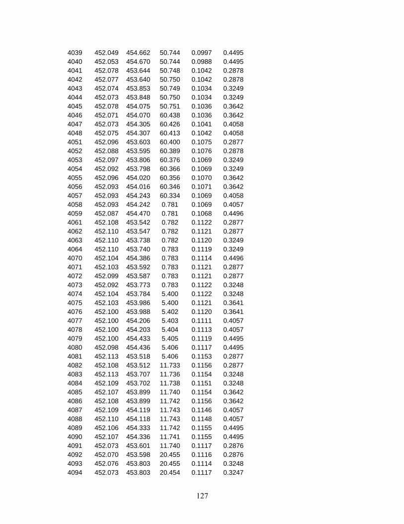
127
4039 452.049 454.662 50.744 0.0997 0.4495 4040 452.053 454.670 50.744 0.0988 0.4495 4041 452.078 453.644 50.748 0.1042 0.2878 4042 452.077 453.640 50.750 0.1042 0.2878 4043 452.074 453.853 50.749 0.1034 0.3249 4044 452.073 453.848 50.750 0.1034 0.3249 4045 452.078 454.075 50.751 0.1036 0.3642 4046 452.071 454.070 60.438 0.1036 0.3642 4047 452.073 454.305 60.426 0.1041 0.4058 4048 452.075 454.307 60.413 0.1042 0.4058 4051 452.096 453.603 60.400 0.1075 0.2877 4052 452.088 453.595 60.389 0.1076 0.2878 4053 452.097 453.806 60.376 0.1069 0.3249 4054 452.092 453.798 60.366 0.1069 0.3249 4055 452.096 454.020 60.356 0.1070 0.3642 4056 452.093 454.016 60.346 0.1071 0.3642 4057 452.093 454.243 60.334 0.1069 0.4058 4058 452.093 454.242 0.781 0.1069 0.4057 4059 452.087 454.470 0.781 0.1068 0.4496 4061 452.108 453.542 0.782 0.1122 0.2877 4062 452.110 453.547 0.782 0.1121 0.2877 4063 452.110 453.738 0.782 0.1120 0.3249 4064 452.110 453.740 0.783 0.1119 0.3249 4070 452.104 454.386 0.783 0.1114 0.4496 4071 452.103 453.592 0.783 0.1121 0.2877 4072 452.099 453.587 0.783 0.1121 0.2877 4073 452.092 453.773 0.783 0.1122 0.3248 4074 452.104 453.784 5.400 0.1122 0.3248 4075 452.103 453.986 5.400 0.1121 0.3641 4076 452.100 453.988 5.402 0.1120 0.3641 4077 452.100 454.206 5.403 0.1111 0.4057 4078 452.100 454.203 5.404 0.1113 0.4057 4079 452.100 454.433 5.405 0.1119 0.4495 4080 452.098 454.436 5.406 0.1117 0.4495 4081 452.113 453.518 5.406 0.1153 0.2877 4082 452.108 453.512 11.733 0.1156 0.2877 4083 452.113 453.707 11.736 0.1154 0.3248 4084 452.109 453.702 11.738 0.1151 0.3248 4085 452.107 453.899 11.740 0.1154 0.3642 4086 452.108 453.899 11.742 0.1156 0.3642 4087 452.109 454.119 11.743 0.1146 0.4057 4088 452.110 454.118 11.743 0.1148 0.4057 4089 452.106 454.333 11.742 0.1155 0.4495 4090 452.107 454.336 11.741 0.1155 0.4495 4091 452.073 453.601 11.740 0.1117 0.2876 4092 452.070 453.598 20.455 0.1116 0.2876 4093 452.076 453.803 20.455 0.1114 0.3248 4094 452.073 453.803 20.454 0.1117 0.3247

128
4095 452.073 453.975 20.454 0.1120 0.3641 4096 452.076 453.978 20.454 0.1121 0.3641 4097 452.071 454.191 20.455 0.1120 0.4057 4098 452.076 454.196 20.455 0.1119 0.4056 4099 452.075 454.425 20.456 0.1119 0.4494 4100 452.071 454.422 20.457 0.1117 0.4495 4101 452.048 453.618 30.829 0.1071 0.2877 4102 452.050 453.620 30.829 0.1069 0.2876 4103 452.052 453.801 30.829 0.1075 0.3248 4104 452.053 453.801 30.828 0.1072 0.3248 4105 452.050 454.012 30.830 0.1079 0.3641 4106 452.053 454.016 30.831 0.1078 0.3641 4107 452.050 454.240 30.834 0.1073 0.4056 4108 452.056 454.248 40.906 0.1069 0.4056 4109 452.051 454.481 40.909 0.1074 0.4494 4110 452.051 454.480 40.912 0.1072 0.4494 5003 495.464 497.561 40.912 0.0826 0.3002 5004 495.466 497.567 40.916 0.0818 0.3002 5006 495.473 497.832 40.918 0.0817 0.3366 5007 495.475 498.107 40.919 0.0818 0.3749 5008 495.472 498.106 40.921 0.0819 0.3750 5009 495.478 498.397 40.923 0.0820 0.4154 5010 495.484 498.402 40.923 0.0820 0.4154 5011 495.490 497.336 50.744 0.0818 0.2659 5015 495.494 497.847 50.744 0.0817 0.3366 5016 495.494 497.848 50.748 0.0816 0.3366 5019 495.497 498.403 50.750 0.0824 0.4154 5020 495.502 498.408 50.749 0.0821 0.4154 5021 495.527 497.280 50.750 0.0863 0.2659 5022 495.529 497.280 50.751 0.0863 0.2659 5023 495.529 497.510 60.438 0.0862 0.3002 5024 495.525 497.504 60.426 0.0862 0.3002 5026 495.530 497.768 60.413 0.0857 0.3366 5027 495.527 498.035 60.400 0.0852 0.3750 5028 495.525 498.015 60.389 0.0859 0.3750 5033 495.543 497.452 60.376 0.0904 0.3002 5034 495.546 497.454 60.366 0.0903 0.3002 5035 495.545 497.686 60.356 0.0899 0.3366 5036 495.546 497.684 60.346 0.0896 0.3366 5037 495.541 497.929 60.334 0.0894 0.3750 5038 495.542 497.927 0.781 0.0893 0.3750 5039 495.548 498.194 0.781 0.0900 0.4154 5041 495.556 497.131 0.782 0.0946 0.2659 5042 495.557 497.131 0.782 0.0944 0.2659 5043 495.561 497.373 0.782 0.0946 0.3002 5044 495.558 497.368 0.783 0.0946 0.3002 5045 495.556 497.593 0.783 0.0948 0.3366 5046 495.552 497.586 0.783 0.0939 0.3366
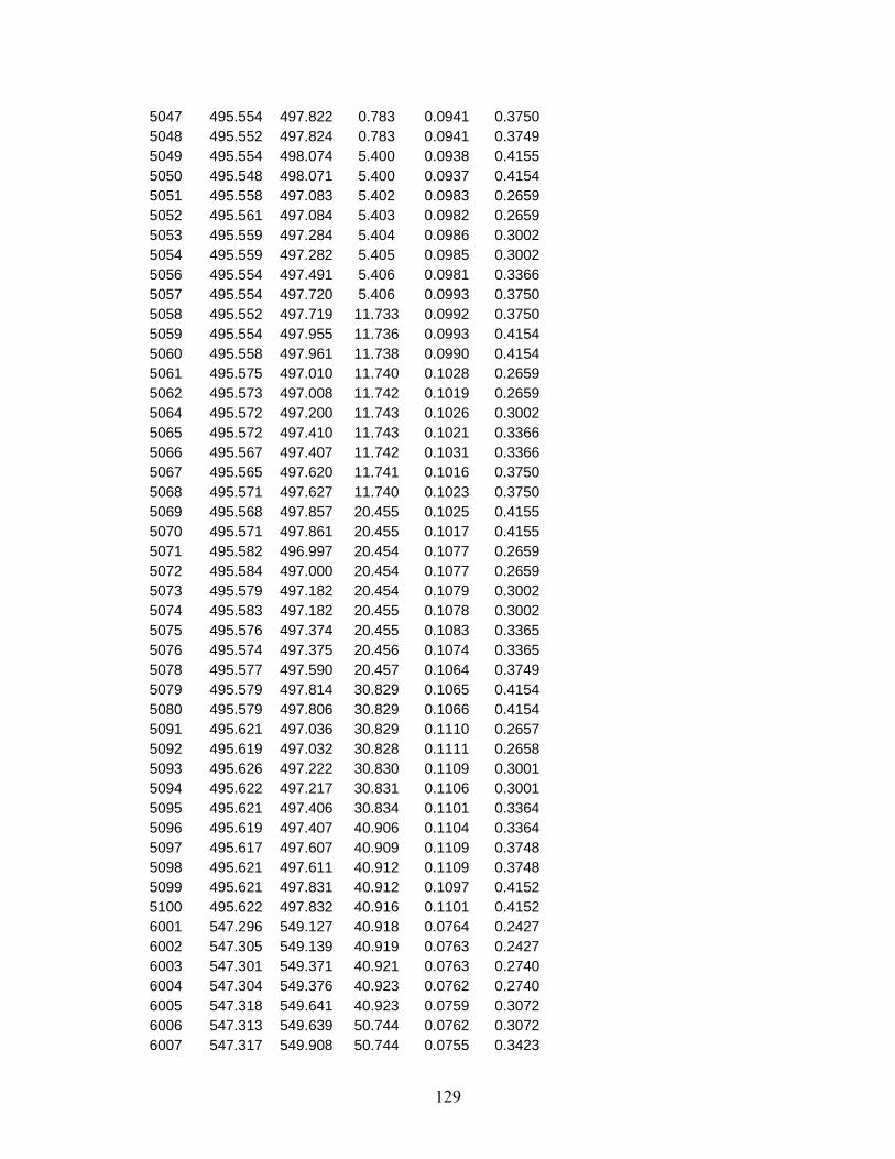
129
5047 495.554 497.822 0.783 0.0941 0.3750 5048 495.552 497.824 0.783 0.0941 0.3749 5049 495.554 498.074 5.400 0.0938 0.4155 5050 495.548 498.071 5.400 0.0937 0.4154 5051 495.558 497.083 5.402 0.0983 0.2659 5052 495.561 497.084 5.403 0.0982 0.2659 5053 495.559 497.284 5.404 0.0986 0.3002 5054 495.559 497.282 5.405 0.0985 0.3002 5056 495.554 497.491 5.406 0.0981 0.3366 5057 495.554 497.720 5.406 0.0993 0.3750 5058 495.552 497.719 11.733 0.0992 0.3750 5059 495.554 497.955 11.736 0.0993 0.4154 5060 495.558 497.961 11.738 0.0990 0.4154 5061 495.575 497.010 11.740 0.1028 0.2659 5062 495.573 497.008 11.742 0.1019 0.2659 5064 495.572 497.200 11.743 0.1026 0.3002 5065 495.572 497.410 11.743 0.1021 0.3366 5066 495.567 497.407 11.742 0.1031 0.3366 5067 495.565 497.620 11.741 0.1016 0.3750 5068 495.571 497.627 11.740 0.1023 0.3750 5069 495.568 497.857 20.455 0.1025 0.4155 5070 495.571 497.861 20.455 0.1017 0.4155 5071 495.582 496.997 20.454 0.1077 0.2659 5072 495.584 497.000 20.454 0.1077 0.2659 5073 495.579 497.182 20.454 0.1079 0.3002 5074 495.583 497.182 20.455 0.1078 0.3002 5075 495.576 497.374 20.455 0.1083 0.3365 5076 495.574 497.375 20.456 0.1074 0.3365 5078 495.577 497.590 20.457 0.1064 0.3749 5079 495.579 497.814 30.829 0.1065 0.4154 5080 495.579 497.806 30.829 0.1066 0.4154 5091 495.621 497.036 30.829 0.1110 0.2657 5092 495.619 497.032 30.828 0.1111 0.2658 5093 495.626 497.222 30.830 0.1109 0.3001 5094 495.622 497.217 30.831 0.1106 0.3001 5095 495.621 497.406 30.834 0.1101 0.3364 5096 495.619 497.407 40.906 0.1104 0.3364 5097 495.617 497.607 40.909 0.1109 0.3748 5098 495.621 497.611 40.912 0.1109 0.3748 5099 495.621 497.831 40.912 0.1097 0.4152 5100 495.622 497.832 40.916 0.1101 0.4152 6001 547.296 549.127 40.918 0.0764 0.2427 6002 547.305 549.139 40.919 0.0763 0.2427 6003 547.301 549.371 40.921 0.0763 0.2740 6004 547.304 549.376 40.923 0.0762 0.2740 6005 547.318 549.641 40.923 0.0759 0.3072 6006 547.313 549.639 50.744 0.0762 0.3072 6007 547.317 549.908 50.744 0.0755 0.3423

130
6008 547.320 549.917 50.748 0.0753 0.3422 6009 547.322 550.197 50.750 0.0756 0.3792 6010 547.329 550.207 50.749 0.0757 0.3792 6013 547.357 549.306 50.750 0.0796 0.2740 6014 547.356 549.301 50.751 0.0806 0.2740 6015 547.352 549.539 60.438 0.0805 0.3072 6016 547.356 549.549 60.426 0.0799 0.3072 6017 547.357 549.802 60.413 0.0802 0.3422 6018 547.358 549.802 60.400 0.0799 0.3422 6019 547.365 550.078 60.389 0.0802 0.3791 6020 547.359 550.076 60.376 0.0800 0.3792 6021 547.374 548.996 60.366 0.0838 0.2427 6022 547.372 548.992 60.356 0.0838 0.2427 6023 547.367 549.210 60.346 0.0833 0.2740 6024 547.371 549.214 60.334 0.0837 0.2740 6025 547.372 549.437 0.781 0.0833 0.3072 6026 547.374 549.437 0.781 0.0829 0.3072 6027 547.372 549.682 0.782 0.0837 0.3422 6028 547.371 549.681 0.782 0.0835 0.3422 6029 547.377 549.942 0.782 0.0840 0.3792 6030 547.378 549.943 0.783 0.0839 0.3792 6031 547.403 548.960 0.783 0.0887 0.2427 6032 547.388 548.952 0.783 0.0883 0.2428 6033 547.399 549.163 0.783 0.0885 0.2741 6034 547.400 549.164 0.783 0.0889 0.2740 6035 547.397 549.373 5.400 0.0895 0.3072 6036 547.395 549.379 5.400 0.0896 0.3072 6037 547.393 549.607 5.402 0.0882 0.3423 6039 547.394 549.861 5.403 0.0883 0.3793 6040 547.393 549.845 5.404 0.0882 0.3792 6042 547.405 548.875 5.405 0.0947 0.2428 6045 547.401 549.274 5.406 0.0943 0.3073 6046 547.402 549.268 5.406 0.0945 0.3073 6047 547.400 549.483 11.733 0.0948 0.3424 6048 547.406 549.490 11.736 0.0946 0.3424 6049 547.404 549.717 11.738 0.0948 0.3793 6050 547.398 549.712 11.740 0.0943 0.3793 6051 547.418 548.769 11.742 0.0985 0.2428 6052 547.427 548.776 11.743 0.0997 0.2428 6053 547.421 548.955 11.743 0.0990 0.2741 6054 547.425 548.956 11.742 0.0989 0.2742 6055 547.427 549.206 11.741 0.0994 0.3073 6056 547.425 549.200 11.740 0.0995 0.3073 6057 547.424 549.408 20.455 0.1000 0.3423 6058 547.426 549.411 20.455 0.0990 0.3424 6059 547.431 549.634 20.454 0.0997 0.3793 6060 547.426 549.634 20.454 0.0982 0.3793 6061 547.459 548.770 20.454 0.1044 0.2428

131
6062 547.453 548.761 20.455 0.1043 0.2428 6063 547.452 548.939 20.455 0.1042 0.2741 6064 547.456 548.941 20.456 0.1035 0.2741 6065 547.460 549.132 20.457 0.1043 0.3073 6066 547.456 549.132 30.829 0.1037 0.3073 6067 547.458 549.333 30.829 0.1028 0.3424 6071 547.481 548.778 30.829 0.1080 0.2428 6072 547.485 548.783 30.828 0.1079 0.2428 6073 547.483 548.947 30.830 0.1079 0.2741 6074 547.489 548.957 30.831 0.1080 0.2741 6075 547.488 549.132 30.834 0.1080 0.3073 6076 547.489 549.138 40.906 0.1076 0.3073 6077 547.489 549.324 40.909 0.1076 0.3424 6078 547.487 549.323 40.912 0.1079 0.3424 6079 547.484 549.520 40.912 0.1078 0.3794 6080 547.489 549.529 40.916 0.1078 0.3793
Table A5. Thermal conductivity of liquid S-8. Point ID T0 Te Pe e e q
(K) (K) (MPa) (mol·L-1) (W·m-1K-1) (W·m-1) 1013 301.957 303.640 0.095 4.245 0.1169 0.3730 1015 301.929 303.922 0.095 4.244 0.1176 0.4439 1017 301.909 304.236 0.095 4.243 0.1179 0.5199 1019 301.885 304.575 0.095 4.241 0.1176 0.6032 1021 301.671 303.087 0.510 4.250 0.1168 0.3085 1023 301.662 303.369 0.502 4.248 0.1170 0.3734 1025 301.655 303.686 0.498 4.247 0.1169 0.4445 1027 301.648 304.022 0.497 4.245 0.1175 0.5205 1029 301.643 304.388 0.501 4.244 0.1171 0.6035 1031 301.441 302.846 0.342 4.250 0.1166 0.3086 1033 301.437 303.137 0.333 4.249 0.1170 0.3736 1035 301.434 303.459 0.325 4.247 0.1173 0.4447 1037 301.434 303.803 0.319 4.246 0.1167 0.5207 1039 301.430 304.180 0.312 4.244 0.1176 0.6040 1041 301.547 302.957 5.249 4.271 0.1201 0.3086 1043 301.562 303.222 5.266 4.270 0.1189 0.3734 1045 301.584 303.574 5.278 4.269 0.1190 0.4445 1047 301.605 303.947 5.292 4.267 0.1188 0.5205 1049 301.620 304.346 5.305 4.266 0.1184 0.6037 1051 301.743 303.175 10.283 4.291 0.1199 0.3085 1053 301.750 303.478 10.286 4.290 0.1204 0.3734 1055 301.754 303.807 10.286 4.289 0.1210 0.4444 1057 301.764 304.156 10.287 4.287 0.1211 0.5204 1059 301.764 304.530 10.289 4.286 0.1203 0.6037

132
1061 301.816 303.449 20.266 4.330 0.1244 0.3732 1063 301.819 303.767 20.259 4.328 0.1234 0.4443 1065 301.826 304.107 20.258 4.327 0.1242 0.5203 1067 301.832 304.474 20.258 4.326 0.1241 0.6035 1069 301.833 304.867 20.260 4.324 0.1236 0.6929 1071 301.975 303.572 30.348 4.366 0.1281 0.3730 1073 301.998 303.909 30.369 4.365 0.1274 0.4440 1075 302.019 304.260 30.390 4.363 0.1274 0.5199 1077 302.043 304.647 30.412 4.362 0.1269 0.6030 1079 302.067 305.070 30.434 4.360 0.1267 0.6924 1081 302.364 303.977 40.266 4.398 0.1294 0.3729 1083 302.369 304.280 40.265 4.397 0.1290 0.4439 1085 302.370 304.606 40.265 4.395 0.1295 0.5198 1087 302.365 304.952 40.269 4.394 0.1300 0.6028 1089 302.361 305.320 40.275 4.393 0.1301 0.6921 1091 302.342 303.768 50.044 4.429 0.1329 0.3725 1093 302.330 304.045 50.033 4.428 0.1314 0.4434 1095 302.322 304.348 50.023 4.427 0.1332 0.5192 1097 302.311 304.821 50.010 4.426 0.1327 0.6025 1099 302.297 305.173 49.995 4.424 0.1330 0.6918 1101 302.144 303.689 58.820 4.456 0.1354 0.3731 1103 302.130 303.956 58.602 4.454 0.1346 0.4441 1105 302.109 304.240 58.405 4.453 0.1350 0.5200 1107 302.095 304.560 58.216 4.451 0.1353 0.6031 1109 302.082 304.905 58.039 4.449 0.1341 0.6924 1111 302.126 303.623 65.938 4.476 0.1376 0.3730 1113 302.141 303.944 64.626 4.471 0.1368 0.4439 1115 302.151 304.278 63.559 4.467 0.1353 0.5198 1117 302.168 304.650 62.667 4.464 0.1353 0.6029 1119 302.178 305.028 61.911 4.460 0.1365 0.6923 2001 321.327 322.975 0.135 4.162 0.1145 0.3556 2003 321.330 323.297 0.136 4.161 0.1145 0.4233 2005 321.324 323.627 0.133 4.160 0.1138 0.4957 2007 321.319 323.941 0.129 4.158 0.1150 0.5749 2009 321.312 324.328 0.123 4.157 0.1140 0.6601 2011 320.975 322.406 5.148 4.190 0.1162 0.3556 2013 320.960 322.692 5.124 4.189 0.1160 0.4234 2015 320.951 323.222 5.105 4.186 0.1162 0.4963 2017 320.945 323.572 5.094 4.185 0.1161 0.5757 2019 320.947 323.960 5.091 4.183 0.1157 0.6610 2021 321.084 322.709 10.277 4.213 0.1175 0.3560 2023 321.103 323.045 10.289 4.211 0.1180 0.4238 2025 321.123 323.400 10.300 4.210 0.1178 0.4963 2027 321.144 323.783 10.316 4.209 0.1171 0.5756 2029 321.162 324.191 10.334 4.207 0.1187 0.6608 2031 320.956 322.481 19.958 4.256 0.1208 0.3562

133
2033 320.952 322.769 19.953 4.255 0.1216 0.4240 2035 320.954 323.090 19.953 4.253 0.1212 0.4964 2037 320.968 323.454 19.959 4.252 0.1214 0.5758 2039 320.973 323.831 19.971 4.251 0.1210 0.6610 2041 321.196 322.736 30.236 4.296 0.1253 0.3560 2043 321.219 323.061 30.248 4.294 0.1245 0.4238 2045 321.235 323.400 30.258 4.293 0.1247 0.4963 2047 321.251 323.764 30.269 4.292 0.1247 0.5757 2049 321.268 324.159 30.280 4.291 0.1251 0.6610 2051 321.207 322.736 40.378 4.333 0.1285 0.3561 2053 321.185 322.993 40.359 4.332 0.1283 0.4239 2055 321.167 323.271 40.341 4.331 0.1281 0.4964 2057 321.151 323.585 40.332 4.329 0.1274 0.5756 2059 321.131 323.912 40.323 4.328 0.1283 0.6608 2061 321.286 322.764 50.582 4.367 0.1315 0.3560 2063 321.309 323.076 50.601 4.366 0.1311 0.4237 2065 321.328 323.407 50.620 4.365 0.1313 0.4961 2067 321.345 323.764 50.636 4.364 0.1303 0.5754 2069 321.359 324.139 50.652 4.363 0.1314 0.6607 2071 321.419 322.936 60.482 4.398 0.1338 0.3559 2073 321.406 323.197 60.463 4.397 0.1337 0.4236 2075 321.392 323.474 60.441 4.396 0.1343 0.4960 2077 321.371 323.768 60.420 4.395 0.1340 0.5754 2079 321.357 324.091 60.395 4.394 0.1346 0.6606 2081 321.163 322.519 69.044 4.425 0.1360 0.3562 2083 321.159 322.785 69.016 4.424 0.1375 0.4239 2085 321.160 323.069 68.990 4.423 0.1364 0.4964 2087 321.167 323.392 68.969 4.422 0.1360 0.5758 2089 321.179 323.753 68.947 4.421 0.1358 0.6611 3001 337.824 339.476 0.188 4.092 0.1106 0.3422 3003 337.828 339.786 0.193 4.091 0.1116 0.4074 3005 337.834 340.125 0.197 4.089 0.1117 0.4771 3007 337.838 340.487 0.202 4.088 0.1117 0.5533 3009 337.843 340.874 0.205 4.086 0.1118 0.6353 3011 337.913 339.475 5.412 4.121 0.1139 0.3422 3013 337.917 339.778 5.415 4.120 0.1138 0.4073 3015 337.917 340.102 5.418 4.118 0.1139 0.4769 3017 337.922 340.460 5.421 4.117 0.1141 0.5532 3019 337.925 340.842 5.424 4.115 0.1136 0.6352 3021 337.965 339.518 10.140 4.145 0.1156 0.3421 3023 337.969 339.817 10.141 4.144 0.1157 0.4072 3025 337.970 340.136 10.128 4.142 0.1161 0.4770 3027 337.977 340.490 10.124 4.141 0.1159 0.5534 3029 337.979 340.866 10.122 4.139 0.1162 0.6355 3031 338.036 339.548 20.415 4.193 0.1197 0.3423 3033 338.037 339.836 20.412 4.192 0.1199 0.4075

134
3035 338.039 340.147 20.410 4.191 0.1201 0.4772 3037 338.040 340.490 20.409 4.190 0.1199 0.5535 3039 338.043 340.854 20.408 4.189 0.1194 0.6356 3041 338.095 339.574 30.197 4.235 0.1233 0.3423 3043 338.098 339.859 30.204 4.234 0.1236 0.4074 3045 338.102 340.163 30.213 4.233 0.1237 0.4770 3047 338.098 340.487 30.222 4.232 0.1231 0.5531 3049 338.100 340.844 30.228 4.231 0.1237 0.6351 3051 338.131 339.566 40.187 4.274 0.1267 0.3423 3053 338.138 339.848 40.184 4.273 0.1274 0.4075 3055 338.138 340.141 40.182 4.272 0.1269 0.4772 3057 338.142 340.468 40.180 4.271 0.1268 0.5535 3059 338.137 340.812 40.181 4.270 0.1268 0.6355 3061 338.173 339.564 50.546 4.312 0.1299 0.3423 3063 338.173 339.834 50.541 4.311 0.1298 0.4075 3065 338.176 340.125 50.536 4.310 0.1299 0.4771 3067 338.180 340.447 50.534 4.309 0.1295 0.5535 3069 338.177 340.783 50.531 4.308 0.1290 0.6355 3072 338.203 339.554 60.331 4.345 0.1335 0.3420 3074 338.208 339.823 60.331 4.344 0.1333 0.4071 3076 338.202 340.100 60.328 4.343 0.1328 0.4768 3078 338.203 340.412 60.309 4.342 0.1329 0.5532 3080 338.207 340.751 60.296 4.341 0.1329 0.6354 3082 338.226 339.537 69.455 4.374 0.1352 0.3424 3084 338.231 339.848 69.449 4.373 0.1355 0.4075 3086 338.229 340.130 69.449 4.372 0.1360 0.4771 3088 338.232 340.432 69.448 4.371 0.1350 0.5533 3090 338.229 340.756 69.447 4.370 0.1353 0.6351 4001 357.955 359.827 0.147 4.004 0.1084 0.3896 4003 357.975 360.169 0.159 4.003 0.1080 0.4562 4005 357.987 360.540 0.168 4.001 0.1079 0.5291 4007 357.999 360.932 0.178 4.000 0.1084 0.6076 4009 358.015 361.359 0.191 3.998 0.1075 0.6912 4011 358.334 360.181 0.397 4.004 0.1083 0.3891 4013 358.346 360.515 0.406 4.003 0.1089 0.4556 4015 358.358 360.885 0.412 4.001 0.1083 0.5285 4017 358.373 361.279 0.417 4.000 0.1082 0.6069 4019 358.388 361.697 0.429 3.998 0.1078 0.6904 4021 358.506 360.379 5.123 4.033 0.1103 0.3891 4023 358.516 360.707 5.130 4.032 0.1102 0.4556 4025 358.528 360.968 5.137 4.031 0.1105 0.5283 4027 358.538 361.351 5.144 4.029 0.1104 0.6067 4029 358.549 361.756 5.156 4.028 0.1104 0.6902 4031 358.653 360.455 10.216 4.062 0.1128 0.3889 4033 358.664 360.782 10.222 4.061 0.1128 0.4554 4035 358.669 361.128 10.228 4.060 0.1122 0.5282

135
4037 358.681 361.505 10.216 4.058 0.1126 0.6069 4039 358.690 361.902 10.217 4.057 0.1124 0.6906 4041 358.788 360.533 19.951 4.113 0.1167 0.3892 4043 358.797 360.846 19.952 4.112 0.1166 0.4557 4045 358.812 361.190 19.963 4.111 0.1168 0.5285 4047 358.812 361.543 19.973 4.110 0.1171 0.6067 4049 358.828 361.934 19.987 4.108 0.1163 0.6902 4051 358.909 360.580 30.512 4.163 0.1210 0.3889 4053 358.913 360.877 30.520 4.162 0.1208 0.4553 4055 358.923 361.206 30.519 4.161 0.1208 0.5282 4057 358.925 361.552 30.509 4.159 0.1214 0.6068 4059 358.928 361.924 30.512 4.158 0.1208 0.6904 4061 359.024 360.680 40.478 4.205 0.1249 0.3892 4063 359.028 360.971 40.480 4.204 0.1239 0.4557 4065 359.034 361.285 40.484 4.203 0.1247 0.5286 4067 359.038 361.630 40.497 4.202 0.1244 0.6067 4069 359.038 361.987 40.511 4.201 0.1244 0.6901 4071 359.104 360.680 50.282 4.243 0.1276 0.3891 4073 359.105 361.014 50.282 4.242 0.1277 0.4557 4075 359.107 361.322 50.283 4.241 0.1278 0.5286 4077 359.110 361.650 50.292 4.240 0.1272 0.6068 4079 359.116 362.007 50.303 4.239 0.1272 0.6903 4081 359.187 360.744 60.423 4.280 0.1312 0.3890 4083 359.190 361.021 60.432 4.279 0.1312 0.4554 4085 359.192 361.324 60.444 4.278 0.1311 0.5282 4087 359.190 361.643 60.450 4.278 0.1300 0.6064 4089 359.195 361.988 60.457 4.276 0.1316 0.6899 4091 359.234 360.768 68.584 4.308 0.1338 0.3891 4093 359.237 361.040 68.585 4.307 0.1337 0.4556 4095 359.240 361.339 68.587 4.306 0.1331 0.5283 4097 359.253 361.666 68.592 4.305 0.1336 0.6064 4099 359.253 362.000 68.591 4.304 0.1339 0.6899 5001 377.752 379.509 8.533 3.976 0.1089 0.3737 5003 377.766 379.832 8.545 3.975 0.1096 0.4376 5005 377.775 380.174 8.554 3.974 0.1091 0.5075 5007 377.788 380.549 8.539 3.972 0.1088 0.5832 5009 377.801 380.946 8.535 3.970 0.1084 0.6637 5011 377.851 379.684 0.270 3.919 0.1048 0.3736 5013 377.860 380.004 0.253 3.917 0.1045 0.4379 5015 377.872 380.368 0.256 3.916 0.1048 0.5080 5017 377.886 380.704 0.259 3.914 0.1046 0.5832 5019 377.893 381.104 0.265 3.913 0.1044 0.6635 5021 377.992 379.748 5.185 3.953 0.1072 0.3735 5023 378.004 380.074 5.191 3.952 0.1077 0.4374 5025 378.011 380.418 5.178 3.950 0.1075 0.5077 5027 378.023 380.795 5.179 3.949 0.1068 0.5830

136
5029 378.035 381.195 5.181 3.947 0.1064 0.6633 5031 378.135 379.869 10.373 3.986 0.1097 0.3734 5033 378.143 380.177 10.379 3.985 0.1096 0.4373 5035 378.152 380.519 10.384 3.984 0.1101 0.5072 5037 378.163 380.890 10.379 3.982 0.1096 0.5826 5039 378.179 381.282 10.373 3.981 0.1102 0.6631 5041 378.268 379.931 20.142 4.043 0.1146 0.3733 5043 378.275 380.230 20.150 4.042 0.1144 0.4371 5045 378.285 380.561 20.156 4.041 0.1139 0.5070 5047 378.296 380.916 20.156 4.039 0.1139 0.5823 5049 378.298 381.286 20.141 4.038 0.1140 0.6629 5051 378.383 379.974 30.345 4.095 0.1183 0.3733 5053 378.389 380.261 30.353 4.094 0.1179 0.4371 5055 378.398 380.582 30.360 4.093 0.1188 0.5070 5057 378.401 380.920 30.367 4.092 0.1185 0.5821 5059 378.408 381.278 30.373 4.091 0.1184 0.6623 5061 378.503 380.072 40.331 4.141 0.1226 0.3733 5063 378.499 380.343 40.338 4.140 0.1225 0.4371 5065 378.513 380.659 40.343 4.139 0.1215 0.5070 5067 378.514 380.983 40.339 4.138 0.1222 0.5822 5069 378.525 381.344 40.323 4.137 0.1225 0.6628 5071 378.590 380.128 50.227 4.182 0.1260 0.3733 5073 378.587 380.392 50.231 4.182 0.1260 0.4371 5075 378.594 380.699 50.237 4.181 0.1261 0.5070 5077 378.596 381.020 50.242 4.180 0.1261 0.5821 5079 378.601 381.358 50.246 4.179 0.1263 0.6623 5081 378.658 380.162 60.412 4.222 0.1295 0.3733 5083 378.657 380.425 60.420 4.221 0.1289 0.4371 5085 378.664 380.720 60.425 4.220 0.1295 0.5070 5087 378.668 381.032 60.429 4.219 0.1298 0.5821 5089 378.672 381.362 60.432 4.218 0.1291 0.6623 5091 378.716 380.191 67.328 4.247 0.1307 0.3735 5093 378.714 380.450 67.139 4.246 0.1307 0.4373 5095 378.717 380.745 66.955 4.244 0.1309 0.5070 5097 378.719 381.050 66.766 4.242 0.1309 0.5822 5099 378.722 381.379 66.576 4.241 0.1310 0.6624 6001 399.395 401.184 0.108 3.823 0.1016 0.3570 6003 399.392 401.486 0.108 3.821 0.1006 0.4181 6005 399.389 401.817 0.114 3.820 0.1009 0.4847 6007 399.391 402.177 0.119 3.818 0.1015 0.5565 6009 399.391 402.561 0.120 3.817 0.1010 0.6332 6011 399.665 401.413 0.268 3.823 0.1013 0.3566 6013 399.668 401.726 0.268 3.822 0.1008 0.4176 6015 399.669 402.067 0.253 3.820 0.1010 0.4847 6017 399.667 402.424 0.248 3.818 0.1007 0.5566 6019 399.675 402.822 0.245 3.817 0.1008 0.6333
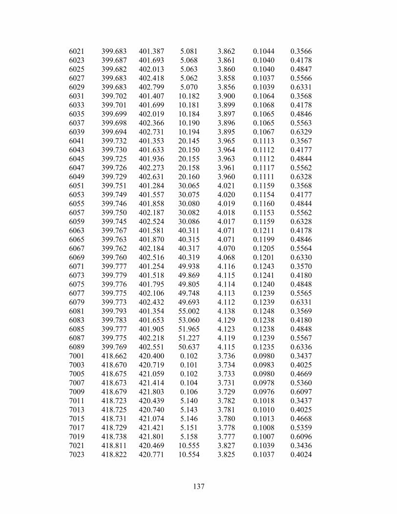
137
6021 399.683 401.387 5.081 3.862 0.1044 0.3566 6023 399.687 401.693 5.068 3.861 0.1040 0.4178 6025 399.682 402.013 5.063 3.860 0.1040 0.4847 6027 399.683 402.418 5.062 3.858 0.1037 0.5566 6029 399.683 402.799 5.070 3.856 0.1039 0.6331 6031 399.702 401.407 10.182 3.900 0.1064 0.3568 6033 399.701 401.699 10.181 3.899 0.1068 0.4178 6035 399.699 402.019 10.184 3.897 0.1065 0.4846 6037 399.698 402.366 10.190 3.896 0.1065 0.5563 6039 399.694 402.731 10.194 3.895 0.1067 0.6329 6041 399.732 401.353 20.145 3.965 0.1113 0.3567 6043 399.730 401.633 20.150 3.964 0.1112 0.4177 6045 399.725 401.936 20.155 3.963 0.1112 0.4844 6047 399.726 402.273 20.158 3.961 0.1117 0.5562 6049 399.729 402.631 20.160 3.960 0.1111 0.6328 6051 399.751 401.284 30.065 4.021 0.1159 0.3568 6053 399.749 401.557 30.075 4.020 0.1154 0.4177 6055 399.746 401.858 30.080 4.019 0.1160 0.4844 6057 399.750 402.187 30.082 4.018 0.1153 0.5562 6059 399.745 402.524 30.086 4.017 0.1159 0.6328 6063 399.767 401.581 40.311 4.071 0.1211 0.4178 6065 399.763 401.870 40.315 4.071 0.1199 0.4846 6067 399.762 402.184 40.317 4.070 0.1205 0.5564 6069 399.760 402.516 40.319 4.068 0.1201 0.6330 6071 399.777 401.254 49.938 4.116 0.1243 0.3570 6073 399.779 401.518 49.869 4.115 0.1241 0.4180 6075 399.776 401.795 49.805 4.114 0.1240 0.4848 6077 399.775 402.106 49.748 4.113 0.1239 0.5565 6079 399.773 402.432 49.693 4.112 0.1239 0.6331 6081 399.793 401.354 55.002 4.138 0.1248 0.3569 6083 399.783 401.653 53.060 4.129 0.1238 0.4180 6085 399.777 401.905 51.965 4.123 0.1238 0.4848 6087 399.775 402.218 51.227 4.119 0.1239 0.5567 6089 399.769 402.551 50.637 4.115 0.1235 0.6336 7001 418.662 420.400 0.102 3.736 0.0980 0.3437 7003 418.670 420.719 0.101 3.734 0.0983 0.4025 7005 418.675 421.059 0.102 3.733 0.0980 0.4669 7007 418.673 421.414 0.104 3.731 0.0978 0.5360 7009 418.679 421.803 0.106 3.729 0.0976 0.6097 7011 418.723 420.439 5.140 3.782 0.1018 0.3437 7013 418.725 420.740 5.143 3.781 0.1010 0.4025 7015 418.731 421.074 5.146 3.780 0.1013 0.4668 7017 418.729 421.421 5.151 3.778 0.1008 0.5359 7019 418.738 421.801 5.158 3.777 0.1007 0.6096 7021 418.811 420.469 10.555 3.827 0.1039 0.3436 7023 418.822 420.771 10.554 3.825 0.1037 0.4024

138
7025 418.831 421.100 10.554 3.824 0.1037 0.4668 7027 418.831 421.439 10.555 3.823 0.1036 0.5360 7029 418.839 421.814 10.559 3.821 0.1036 0.6098 7031 418.918 420.525 20.239 3.895 0.1094 0.3436 7033 418.922 420.806 20.235 3.894 0.1093 0.4025 7035 418.926 421.116 20.234 3.893 0.1090 0.4669 7037 418.933 421.456 20.237 3.892 0.1088 0.5360 7039 418.936 421.808 20.243 3.891 0.1087 0.6098 7041 418.999 420.554 30.475 3.958 0.1139 0.3437 7043 419.010 420.833 30.474 3.957 0.1134 0.4025 7045 419.009 421.128 30.477 3.956 0.1136 0.4669 7047 419.012 421.444 30.482 3.955 0.1135 0.5359 7049 419.014 421.786 30.489 3.954 0.1129 0.6097 7051 419.079 420.583 40.435 4.012 0.1179 0.3436 7053 419.081 420.849 40.442 4.011 0.1178 0.4023 7055 419.084 421.137 40.448 4.010 0.1170 0.4666 7057 419.086 421.451 40.452 4.009 0.1174 0.5357 7059 419.092 421.790 40.456 4.008 0.1171 0.6095 7061 419.136 420.591 49.169 4.054 0.1220 0.3435 7063 419.142 420.856 48.957 4.053 0.1215 0.4022 7065 419.138 421.136 48.747 4.051 0.1209 0.4665 7067 419.143 421.446 48.536 4.049 0.1200 0.5357 7069 419.145 421.767 48.316 4.047 0.1205 0.6098 8001 439.886 441.678 0.247 3.638 0.0949 0.3305 8003 439.890 441.940 0.248 3.637 0.0948 0.3869 8005 439.893 442.271 0.249 3.635 0.0950 0.4488 8007 439.895 442.630 0.253 3.634 0.0945 0.5153 8009 439.905 442.968 0.257 3.632 0.0943 0.5862 8011 439.983 441.663 5.101 3.690 0.0978 0.3302 8013 439.988 441.957 5.106 3.689 0.0976 0.3866 8015 439.988 442.275 5.111 3.688 0.0981 0.4484 8017 439.993 442.627 5.114 3.686 0.0978 0.5149 8019 439.998 442.998 5.117 3.685 0.0980 0.5858 8021 440.042 441.693 10.160 3.738 0.1007 0.3303 8023 440.042 441.979 10.164 3.737 0.1014 0.3867 8025 440.047 442.295 10.168 3.735 0.1011 0.4485 8027 440.050 442.631 10.174 3.734 0.1010 0.5149 8029 440.056 442.997 10.178 3.733 0.1010 0.5858 8031 440.105 441.633 20.377 3.820 0.1073 0.3303 8033 440.100 441.901 20.375 3.819 0.1065 0.3868 8035 440.104 442.198 20.371 3.818 0.1066 0.4487 8037 440.107 442.522 20.371 3.816 0.1063 0.5152 8039 440.111 442.868 20.376 3.815 0.1066 0.5861 8041 440.153 441.664 30.286 3.886 0.1116 0.3304 8043 440.148 441.920 30.286 3.885 0.1116 0.3869 8045 440.154 442.210 30.290 3.884 0.1118 0.4487

139
8047 440.149 442.511 30.295 3.883 0.1119 0.5151 8049 440.149 442.835 30.301 3.882 0.1119 0.5860 8051 440.185 441.620 40.345 3.945 0.1156 0.3304 8053 440.187 441.875 40.332 3.944 0.1162 0.3869 8055 440.190 442.152 40.321 3.944 0.1159 0.4487 8057 440.186 442.446 40.315 3.943 0.1157 0.5151 8059 440.182 442.757 40.307 3.942 0.1160 0.5860 8061 440.195 441.649 41.920 3.954 0.1166 0.3303 8063 440.185 441.897 41.449 3.951 0.1161 0.3868 8065 440.179 442.172 41.049 3.947 0.1168 0.4486 8067 440.177 442.471 40.704 3.945 0.1159 0.5150 8069 440.175 442.789 40.401 3.942 0.1159 0.5859 9001 460.245 461.930 0.191 3.539 0.0917 0.3185 9003 460.235 462.212 0.192 3.538 0.0915 0.3728 9005 460.228 462.532 0.193 3.536 0.0917 0.4323 9007 460.218 462.861 0.194 3.535 0.0914 0.4963 9009 460.216 463.227 0.194 3.533 0.0914 0.5646 9011 460.218 461.822 5.456 3.605 0.0952 0.3182 9013 460.220 462.105 5.458 3.604 0.0956 0.3726 9015 460.220 462.416 5.462 3.603 0.0959 0.4322 9017 460.217 462.748 5.463 3.601 0.0955 0.4963 9019 460.219 463.107 5.460 3.600 0.0953 0.5647 9021 460.289 461.908 10.329 3.657 0.0991 0.3183 9023 460.295 462.193 10.334 3.656 0.0988 0.3727 9025 460.297 462.496 10.338 3.655 0.0987 0.4322 9027 460.298 462.827 10.341 3.653 0.0989 0.4963 9029 460.302 463.179 10.344 3.652 0.0984 0.5647 9031 460.365 461.853 20.311 3.746 0.1053 0.3182 9033 460.368 462.123 20.315 3.745 0.1043 0.3726 9035 460.372 462.421 20.317 3.744 0.1038 0.4321 9037 460.370 462.728 20.312 3.743 0.1047 0.4963 9039 460.384 463.074 20.305 3.741 0.1044 0.5649 9041 460.426 461.837 30.198 3.819 0.1095 0.3182 9043 460.422 462.092 30.202 3.818 0.1094 0.3726 9045 460.425 462.374 30.204 3.817 0.1099 0.4322 9047 460.424 462.669 30.201 3.816 0.1097 0.4963 9049 460.427 462.996 30.193 3.815 0.1098 0.5649 9055 460.479 462.392 39.784 3.878 0.1141 0.4324 9057 460.484 462.687 39.721 3.876 0.1139 0.4966 9059 460.485 462.993 39.661 3.875 0.1141 0.5650 9061 460.535 461.966 42.387 3.894 0.1158 0.3184 9063 460.531 462.217 41.417 3.888 0.1146 0.3729 9065 460.530 462.503 40.644 3.882 0.1144 0.4325 9067 460.525 462.792 40.011 3.878 0.1141 0.4966 9069 460.522 463.106 39.488 3.874 0.1145 0.5650 10001 480.862 482.558 0.238 3.435 0.0890 0.3068

140
10003 480.867 482.860 0.237 3.433 0.0889 0.3593 10005 480.871 483.185 0.238 3.432 0.0885 0.4167 10007 480.877 483.536 0.237 3.430 0.0887 0.4785 10009 480.884 483.913 0.238 3.428 0.0886 0.5444 10011 480.929 482.553 5.166 3.508 0.0925 0.3069 10013 480.929 482.830 5.169 3.507 0.0929 0.3593 10015 480.932 483.146 5.175 3.505 0.0926 0.4167 10017 480.932 483.468 5.178 3.504 0.0928 0.4784 10019 480.935 483.830 5.181 3.502 0.0925 0.5443 10021 480.979 482.557 10.227 3.570 0.0962 0.3070 10023 480.976 482.826 10.228 3.569 0.0957 0.3594 10025 480.978 483.127 10.229 3.568 0.0964 0.4169 10027 480.978 483.446 10.233 3.566 0.0960 0.4786 10029 480.980 483.787 10.239 3.565 0.0964 0.5445 10042 481.072 482.521 20.214 3.670 0.1023 0.3197 10044 481.072 482.776 20.215 3.669 0.1021 0.3744 10046 481.073 483.049 20.216 3.668 0.1022 0.4343 10048 481.070 483.337 20.219 3.667 0.1022 0.4986 10050 481.076 483.661 20.222 3.666 0.1020 0.5672 10052 481.134 482.424 30.227 3.751 0.1078 0.3197 10054 481.129 482.655 30.227 3.750 0.1077 0.3744 10056 481.130 482.916 30.222 3.749 0.1079 0.4344 10058 481.131 483.194 30.220 3.748 0.1077 0.4987 10060 481.125 483.534 30.218 3.747 0.1075 0.5676 10062 481.147 482.429 38.228 3.806 0.1116 0.3199 10064 481.146 482.659 37.952 3.803 0.1114 0.3745 10066 481.136 482.901 37.705 3.801 0.1113 0.4344 10068 481.130 483.169 37.478 3.799 0.1111 0.4988 10070 481.125 483.452 37.265 3.796 0.1110 0.5676 11001 501.375 503.024 0.450 3.328 0.0858 0.3080 11003 501.377 503.253 0.451 3.327 0.0857 0.3607 11005 501.380 503.568 0.453 3.325 0.0857 0.4183 11007 501.387 503.900 0.451 3.323 0.0857 0.4804 11009 501.387 504.255 0.450 3.321 0.0855 0.5466 11011 501.401 502.944 5.134 3.412 0.0899 0.3079 11013 501.399 503.212 5.135 3.410 0.0898 0.3607 11015 501.400 503.506 5.135 3.409 0.0898 0.4183 11017 501.399 503.819 5.136 3.408 0.0897 0.4803 11019 501.401 504.162 5.137 3.406 0.0897 0.5465 11021 501.412 502.906 10.181 3.483 0.0936 0.3079 11023 501.412 503.165 10.182 3.482 0.0936 0.3607 11025 501.408 503.446 10.183 3.481 0.0935 0.4183 11027 501.406 503.750 10.183 3.480 0.0934 0.4803 11029 501.407 504.076 10.183 3.478 0.0934 0.5465 11031 501.406 502.853 15.115 3.542 0.0970 0.3080 11033 501.401 503.103 15.115 3.541 0.0969 0.3607

141
11035 501.409 503.383 15.116 3.540 0.0969 0.4183 11037 501.400 503.671 15.117 3.539 0.0968 0.4803 11039 501.405 503.988 15.118 3.538 0.0968 0.5465 11041 501.410 502.814 20.195 3.595 0.1001 0.3081 11043 501.410 503.060 20.197 3.594 0.1000 0.3607 11045 501.405 503.317 20.199 3.593 0.1000 0.4183 11047 501.401 503.600 20.199 3.592 0.1000 0.4803 11049 501.399 503.898 20.199 3.591 0.0999 0.5465 11051 501.398 502.754 25.203 3.642 0.1030 0.3080 11053 501.401 502.993 25.200 3.641 0.1029 0.3608 11055 501.402 503.252 25.199 3.640 0.1028 0.4185 11057 501.395 503.526 25.198 3.639 0.1027 0.4805 11059 501.391 503.824 25.199 3.638 0.1028 0.5466 11061 501.381 502.704 30.260 3.684 0.1057 0.3080 11063 501.380 502.934 30.256 3.683 0.1057 0.3608 11065 501.375 503.183 30.255 3.682 0.1057 0.4185 11067 501.375 503.456 30.253 3.681 0.1055 0.4805 11069 501.375 503.745 30.254 3.681 0.1056 0.5466 11071 501.376 502.588 35.386 3.724 0.1083 0.3079 11073 501.375 502.812 35.385 3.723 0.1082 0.3606 11075 501.370 503.056 35.384 3.722 0.1083 0.4183 11077 501.370 503.327 35.376 3.721 0.1081 0.4804 11079 501.367 503.609 35.372 3.720 0.1084 0.5466 11081 501.373 502.620 39.367 3.752 0.1103 0.3079 11083 501.372 502.848 39.213 3.750 0.1100 0.3607 11085 501.376 503.100 39.068 3.748 0.1101 0.4184 11087 501.375 503.356 38.930 3.746 0.1101 0.4804 11089 501.371 503.639 38.799 3.745 0.1101 0.5465


Related Documents