Thermodynamic instability of rotating black holes

Thermodynamic instability of rotating black holes

R. Monteiro,∗ M. J. Perry,† and J. E. Santos‡

DAMTP, Centre for Mathematical Sciences, University of Cambridge,

Wilberforce Road, Cambridge CB3 0WA, UK

(Dated: July 30, 2009)

We show that the quasi-Euclidean sections of various rotating black holes in different

dimensions possess at least one non-conformal negative mode when thermodynamic insta-

bilities are expected. The boundary conditions of fixed induced metric correspond to the

partition function of the grand-canonical ensemble. Indeed, in the asymptotically flat cases,

we find that a negative mode persists even if the specific heat at constant angular momenta

is positive, since the stability in this ensemble also requires the positivity of the isothermal

moment of inertia. We focus in particular on Kerr black holes, on Myers-Perry black holes

in five and six dimensions, and on the Emparan-Reall black ring solution. We go on further

to consider the richer case of the asymptotically AdS Kerr black hole in four dimensions,

where thermodynamic stability is expected for a large enough cosmological constant. The

results are consistent with previous findings in the non-rotation limit and support the use of

quasi-Euclidean instantons to construct gravitational partition functions.

I. INTRODUCTION

Gravitation is a purely attractive force, which has led to a number of conundrums revolving

around questions of stability. In classical physics, it seems that the question is settled. Gravitational

collapse cannot, under a wide range of circumstances, be prevented. Although collapse to form

a singularity happens, it is believed that these singularities will be isolated from observation by

horizons. Thus the end-point of gravitational collapse is believed to always result in black holes.

Classically, many black hole solutions are stable, in particular the ones of astrophysical relevance

[1, 2, 3, 4, 5, 6, 7].

Quantum mechanics changes this. In 1974, Hawking discovered that black holes have a tem-

perature, the Hawking temperature TH , given by

TH =κ

2π,

∗Electronic address: [email protected]†Electronic address: [email protected]‡Electronic address: [email protected]

arX

iv:0

903.

3256

v2 [

gr-q

c] 3

0 Ju

l 200

9

2

where κ is the surface gravity of the black hole [8] (we use natural units, so that G = c = ~ = kB = 1

throughout). For non-rotating black holes, this gives rise to a new instability. Since

κ =1

4M,

where M is the black hole mass, isolated black holes will radiate and lose energy. This will cause

them to heat up. Since conservation of energy leads to

M ∼ − 1M2

we see this is a runaway process. When the black hole reaches zero mass, it is presumed to disappear

completely. The specific heat of the black hole is negative

C = − 18πM2

,

a typical sign of instability [9].

It is a sign that the canonical ensemble breaks down for such objects leading to doubts as to

whether a conventional thermodynamic interpretation is possible. However, if instead one looks at

the microcanonical ensemble, one discovers that it is well-defined.

If one includes the possibility that the black holes are rotating with angular momentum J or

have an electric charge Q, one finds that if

J4 + 6J2M4 + 4Q2M6 − 3M8 > 0

then the specific heat at constant J and Q turns out to be positive.

One expects that these difficulties will be reflected in the path-integral treatment of gravitation.

Suppose one tries to calculate the canonical, or grand-canonical, partition function. Then one

needs to integrate over all physical fields subject to certain boundary conditions. Generally for

the grand-canonical ensemble, one integrates over quasi-Euclidean configurations (see section II B

for a more complete description of what this means). So, the field configurations must be periodic

in imaginary time, with periodicity equal to the inverse temperature, and quasi-periodic in the

complexified azimuthal angle generated by any conserved angular momenta, or quasi-periodic under

complexified gauge transformations associated to any conserved charge.

The gravitational path integral based on the Einstein action is not well-defined because of

its lack of renormalizability. However, at the semi-classical level, it makes sense as an effective

field theory, perhaps derived from some more fundamental theory such as string theory. This path

integral has, at first sight, a big difficulty with stability, as the kinetic energy operator for conformal

3

transformations has the wrong sign. However, it turns out that fluctuations in the path integral of

such a type are gauge artifacts. Much more serious and interesting is the possibility that the gauge

invariant parts of the fluctuations contribute with the ‘wrong’ sign to the partition function. This

is a sign of instability. For the four-dimensional non-rotating black holes, these negative modes

have been known for some time [10, 11].

In this paper, we extend our knowledge of this type of instability. In Section II, we describe the

formalism required to identify the gauge invariant negative modes. In Section III, we describe a

way of finding gauge invariant deformations of a specified field configuration. These deformations

are not themselves the negative mode, but since they decrease the Euclidean action, they prove

that negative modes exist. In Section IV, we apply our technique to the four-dimensional Kerr

solution, five and six-dimensional Myers-Perry metrics, the singly-spinning five-dimensional black

ring and the four-dimensional Kerr-AdS solution. In every case, we find negative modes, except

for large Kerr-AdS black holes. In Section V, we look at the thermodynamics of the black holes or

rings, and see how it matches up with the existence of our negative modes. We use this to make

speculations about when the thermodynamic approximation is, or is not, valid.

II. THE GRAVITATIONAL PATH INTEGRAL

A. The decomposition theorem

The path integral of Euclidean quantum gravity,

Z =∫

D[g]e−I[g], (1)

is constructed from the action

I[g] = − 116π

∫M

ddx√g (R− 2Λ)− 1

8π

∫∂M

dd−1x

√g(d−1)K − I0. (2)

The first term is the usual Einstein-Hilbert action and the second is the York-Gibbons-Hawking

boundary term [12, 13], where K is the trace of the extrinsic curvature on ∂M. This term is

required for non-compact manifolds M, as the ones we will study, so that the boundary condition

on ∂M is a fixed induced metric, and not fixed derivatives of the metric normal to ∂M.

The term I0 can depend only on g(d−1)ab , the induced metric on ∂M, and not on the bulk

metric gab, so that it can be absorbed into the measure of the path integral. However, since we are

interested in the partition functions of black holes, it is convenient to choose it so that I = 0 for the

4

background spacetime that the black hole solution approaches asymptotically. For asymptotically

flat black holes [13], the Einstein-Hilbert term is zero and the action becomes

− 18π

∫∂M

dd−1x

√g(d−1) (K −K0), (3)

where K0 is the trace of the extrinsic curvature of the flat spacetime matching the black hole metric

on the boundary ∂M at infinity. This subtraction renders the action of the black hole finite. For

asymptotically AdS black holes [14, 15], the boundary terms cancel when the background subtrac-

tion is performed, but the bulk volume integral diverges and requires an analogous subtraction that

sets the action of AdS space to zero. An alternative view is that I0 should be seen as a counterterm,

corresponding to the counterterm of a dual conformal field theory (see [16, 17, 18, 19, 20]).

The gravitational path integral (1) is non-renormalisable but we expect meaningful results in

an effective field theory approach. A different issue is that the action (2) can be made arbitrarily

negative so that the path integral appears to be always divergent even at tree-level. These problems

can be addressed in the semiclassical approximation, where the path integral is dealt with by saddle-

point methods. We consider a saddle-point gab, i.e. a non-singular solution of the equations of

motion,

Rab =2Λd− 2

gab, (4)

usually referred to as a gravitational instanton. We then treat as a quantum field hab the small

perturbations about the saddle-point,

gab = gab + hab. (5)

This leads to a perturbative expansion of the action,

I[g] = I[g] + I2[h; g] +O(h3). (6)

The first order action I1 vanishes since gab obeys the equations of motion, while the second order

action I2, which gives the one-loop correction, is the action for the quantum field hab on the

background geometry gab.

The effective field theory is valid if the background geometry gab has a curvature nowhere near

the Planck scale. We can also address the issue of the arbitrarily negative action geometries in

the path integral, called ‘conformal factor problem’ since it is the conformal direction in the space

of metrics that is responsible for the divergence. Perturbatively, this corresponds to trace-like

perturbations hab which lead to a negative I2. The prescription of [21] is that the integration

5

contour for those perturbations is imaginary. They can then be seen to be irrelevant and don’t

represent physical instabilities. Of physical interest are the instabilities studied firstly in [10], the

analysis of which we wish to extend to rotating black holes.

We follow here the procedure in [22], straightforwardly extended to higher dimensions. We will

decompose the second order action, applying a standard gauge fixing procedure, and show that

the unphysical divergent modes do not contribute to the one-loop partition function.

The partition function is

Z1−loop = e−I[bg] ∫ D[h](G.F.)e−I2[h;bg], (7)

where (G.F.) denotes all contributions induced by fixing the gauge in the path integral. Hereafter,

gab is relabelled as gab and all metric operations are performed with it. The second order action is

given by

I2[h; g] = − 116π

∫ddx√g

[−1

4h ·Gh+

12

(δh)2

], (8)

where · denotes the metric contraction of tensors. We have defined

hab = hab −12gabh

cc (9)

and

(Gh)ab = −∇c∇chab − 2R c da b hcd, (10)

where the operator G is related to the Lichnerowicz Laplacian ∆L by G = ∆L − 4Λ/(d − 2). We

also define the operations on tensors T

(δT )b...c = −∇aTab...c, (11a)

(αT )ab...c = ∇(aTb...c). (11b)

The second order action I2[h; g] is invariant for the diffeomorphism transformations

hab → hab +∇aVb +∇bVa = (h+ 2αV )ab. (12)

Following the Feynman-DeWitt-Faddeev-Popov gauge fixing method,

(G.F.) = (detC) δ(Ca[h]− wa). (13)

6

We consider the linear class of gauges

Cb[h] = ∇a(hab −

1βgabh

cc

), (14)

where β is an arbitrary constant, so that the Fadeev-Popov determinant (detC) is given by the

spectrum of the operator

(CV )a = −∇b∇bVa −RabV b +(

2β− 1)∇a∇bV b. (15)

To study the spectrum, let us consider the Hodge-de Rham decomposition of the gauge vector V

into harmonic (H), exact (E) and coexact (C) parts,

V = VH + VE + VC. (16)

This induces a decomposition of the action of C, which we denote by CH for harmonic vectors, CE

for exact vectors and CC for coexact vectors.

The harmonic part satisfies dVH = 0 and δVH = 0. We can check that

CVH = − 4Λd− 2

VH. (17)

The spectrum is positive for Λ < 0 and zero for Λ = 0, with multiplicity given by the number

of linearly independent harmonic vector fields. For Λ > 0, the background solution satisfying (4)

does not allow for harmonic vector fields if assumed to be compact and orientable [23]. Thus, the

spectrum of CH is never negative.

The exact part is such that VE = dχ, where χ is a scalar. We can show that

spec CE = spec(

2[(

1β− 1)− 2Λ

d− 2

]), (18)

where the operator on the RHS acts on scalars, and is the Laplacian. For Λ < 0, the operator

is positive for β > 1, being positive semi-definite for Λ = 0. For Λ > 0, the Lichnerowicz-Obata

theorem tells us that the spectrum of the Laplacian on a compact and orientable manifold satisfying

(4) is bounded from above by −2dΛ/((d − 1)(d − 2)), the saturation of the bound corresponding

to the sphere [23]. This implies that, for Λ > 0, the spectrum of CE is positive for β > d.

The coexact part is such that δVC = 0. Hence

CVC = 2δαVC (19)

and the spectrum of CC can be shown to be positive semi-definite,∫ddx√g [VC · CVC] = 2

∫ddx√g [αVC · αVC] ≥ 0, (20)

7

with equality for coexact Killing vectors.

The Faddeev-Popov determinant contribution to the partition function is then

det C ∼ (det CE)(det CC), (21)

the tilde denoting that the zero modes have been projected out. The harmonic contribution is not

explicitly considered because, if it exists (Λ < 0), it is a positive factor dependent only on Λ and

on the dimension of the space of harmonic vector fields, as mentioned above; it will not be relevant

to our discussion. The contribution from the exact part is fundamental since it will cancel the

divergent modes of the field hab.

In order to make the results independent of the arbitrary vector w in the gauge fixing (13),

the ’t Hooft method of averaging over gauges is adopted. The arbitrariness is then expressed in

terms of a constant γ introduced by the weighting factor of the averaging. The final result will be

independent of γ, as required. The unconstrained effective action for the perturbations is given by

Ieff2 [h; g] = I2[h; g] +

γ

32π

∫ddx√g Ca[h]Ca[h] =

=− 116π

∫ddx√g

[−1

4h ·Gh+

12

(1− γ)(δh)2 +γ

2

(1− 2

β

)δh · dh− γ

8

(1− 2

β

)2

(dh)2

], (22)

where we denote h ≡ hcc.

We now decompose the quantum field hab into a traceless-transverse (TT) part, a traceless-

longitudinal (TL) part, built from a vector η, and a trace part,

hab = hTTab + hTLab +1dgabh, (23)

with

hTLab = 2(αη)ab +2dgabδη. (24)

The constant β, unspecified in the gauge condition (14), can be chosen so that the trace h and

the longitudinal vector η decouple. This requires

β = 2(

1− d− 2d

γ − 1γ

)−1

. (25)

The effective action becomes

Ieff2 [h; g] = − 1

16π

∫ddx√g

[− 1

4hTT ·GhTT − αη · α∆1η −

1dδηδη+

+ 2(1− γ)(δαη · δαη +

1d2αδη · αδη − 2

dδαη · αδη

)+

+4

d− 2Λ(αη · αη − 1

d(δη)2

)+

12hF h

], (26)

8

where the operator F is given by

F = −d− 24d

(1 +

d− 2d

γ − 1γ

)− 1

dΛ. (27)

Recalling the choice of β (25), we find that the operator on the RHS of the expression (18) is given

by 4dF/(d− 2). The contribution of the ghosts (21) can be recast as

det C ∼ (det F )(det CC). (28)

For the vector η, as we did for V in the ghost part, we perform a Hodge-de Rham decomposition

into harmonic, coexact and exact parts,

η = ηH + ηC + ηE, (29)

respectively. Using ηE = dχ, the result for the effective action is then

Ieff2 [h; g] =− 1

16π

∫ddx√g[− 1

4hTT ·GhTT +

12hF h+

+4

d− 2γΛαηH · αηH − γαηC · αCCηC −

4dd− 2

γDχ ·DFχ], (30)

where we defined the operator

Dab = ∇a∇b −1dgab. (31)

Notice that the Hodge-de Rham decomposition of η in harmonic, coexact and exact parts gives,

for hTLab , a decomposition in 2αηH, 2αηC and 2Dχ, respectively.

Finally, we can evaluate the Gaussian integrals in the partition function to show the dependence

Z1−loop ∼ (det C)(det G)−1/2(det F )−1/2(det CC)−1/2(det F )−1/2

∼ (det G)−1/2(det CC)1/2. (32)

Again, the tilde on the operators denotes that the zero modes have been projected out. The

Gaussian integrals are regularised by ζ-function methods [22]. It is understood that the spectrum

of G here is restricted to traceless-transverse normalisable modes.

Let us review the treatment of the ‘conformal factor problem’. Trace-type perturbations make

the action (8) negative. But a detailed analysis showed that these modes do not contribute to the

path integral. The two factors (DetF )−1/2 arising from the Gaussian integrals in h and χ cancel

with the DetF factor arising from the exact part of the Fadeev-Popov determinant. This makes the

unphysical character of the divergence obvious, at least in perturbation theory. The conclusion is

9

that the non-positivity of the action (2) and the resulting apparent divergence of the gravitational

path integral are fixed by projecting out this contribution.

The relevant operators are then CC and G. For a real metric, the operator CC is positive

semi-definite, as we have shown above. Once its zero modes are projected out, it contributes a

positive factor to the final result. The physical instabilities, identified by imaginary contributions

to the partition function, are only possible if there are negative eigenvalues of the operator G,

GhTT = λhTT . This was the problem studied in [10] for the Schwarzschild black hole. We intend

to extend this treatment to rotating black holes, which requires addressing the problem of complex

instantons.

B. Quasi-Euclidean geometries

The partition function is usually defined as a Euclidean path integral, a sum over real geome-

tries for which imaginary time τ = it is used. However, while static geometries remain real for

this analytical continuation, the same does not hold for stationary geometries. In the canonical

formalism, where γij is the metric on a constant time slice, N is the lapse function and N i is the

shift vector required for rotating spacetimes, we have

ds2 = N2dτ2 + γij(dxi − iN idτ)(dxj − iN jdτ). (33)

These geometries have been called quasi-Euclidean. The question is then whether one should

analytically continue the shift vector (e.g. through the rotation parameters for a Kerr black hole)

in order to get a real geometry. This is trivial when one considers the instanton approximation to

the path integral, because the parameters made imaginary can simply be made real again in the

final result. But when one goes beyond leading order, as is the case in this paper, and considers

metrics that do not satisfy the equations of motion but are also included in the sum, the choice

affects the positivity properties of the second order action and thus the convergence of the path

integral.

We share the view of [24] and [25] that the continuations other than the usual τ = it lead to

unphysical parameters. As those authors point out, the leading order instanton action is real in

spite of being constructed with a complex metric, and it corresponds to the physical free energy.

The charges and the horizon locus remain the same as in the Lorentzian case. Studying the

convergence of the path integral for particular imaginary values of the Kerr rotation parameters,

for instance, bears no relation to the actual black holes. A further argument can be made based

10

on the black ring case. As opposed to the Kerr geometry, the black ring does not possess a real

section with imaginary time that is regular, since conical singularities cannot be removed [26, 27].

The results in the previous decomposition of the metric were obtained for real Euclidean metrics.

However, the expression (32) should still hold for an appropriate complex contour of integration.

This contour is specified in a standard way by the steepest descent method. The relevant eigenvalues

of CC and G are now determined with respect to a complex metric, i.e. to the physical Lorentzian

rotation parameters. The semi-positivity of CC is no longer obvious and we have nothing more to

say about it. Still, a negative eigenvalue of G is sufficient to cause problems in the definition of

the path integral and herald an instability.

III. THE PROBE PERTURBATION

As was discussed in the previous section, the Euclidean path integral only depends on the

spectrum of two operators: CC and G. The latter acts on traceless-transverse (TT) perturbations

of the metric and will be the object of our attention in this section. In the Schwarzschild case,

mostly due to the spherical symmetry of the problem, it was possible to determine the negative

mode by a straightforward method [10]. However, for solutions such as Kerr, Myers-Perry or the

black ring, this seems challenging, due to the lack of symmetry of the background geometry.

The approach that we will adopt here is somehow different. To prove that G possesses at least

one negative mode we only need to show that a particular TT probe perturbation renders the

operator negative. In order to visualise this more clearly, pick an arbitrary TT perturbation and

decompose it in eigenmodes of G,

φab =∑n

anφ(n)ab . (34)

We can now construct the Rayleigh-Ritz functional, given by

I =

∫ddx√g φab(Gφ)ab∫

ddx√g φceφce

=∑

n λna2n∑

p a2p

. (35)

If a perturbation φab is found such that I is negative, then it must be the case that at least one

of the λn is negative. This reasoning can be used to prove that a given instanton has a negative

mode, but cannot be used to prove the converse. In fact, if I is positive for a particular φab, it

might be the case that the an corresponding to the negative eigenmode is small, or even absent, in

the expansion (34).

We also have to check that our particular perturbation lies along the path of steepest descent.

Since we will consider only perturbations that preserve the symmetries of the background, it suffices

11

to check that the components (Gφ)ab are real or imaginary if and only if the components hab are,

i.e. if and only if the components of the metric gab are. This will indeed be the case for our

perturbations: the components (τ, xi) are imaginary and the others are real. Then, each term of

the sum φab(Gφ)ab is real and this particular direction in the space of perturbations keeps the phase

of the integrand functional constant, since the second order action is real. This is the condition for

the steepest descent path.

It is the objective of this section to construct a TT perturbation that will render I negative,

starting with a Killing vector field ka. We will focus on pure Einstein gravity, with Λ = 0, in an

arbitrary number of dimensions d, where the background field equations are

Rab = 0. (36)

For such a class of spacetimes we can construct a probe Maxwell field satisfying Maxwell’s

equations. Since ka is a Killing vector, it obeys to

∇akb +∇bka = 0, (37)

from which we construct the following two-form components

Fab = ∇akb −∇bka = 2∇akb. (38)

This field strength Fab trivially obeys to the Bianchi identities and also satisfies Maxwell’s

equations, since

∇aF ab = −2Rbaka = 0. (39)

In four dimensions, there exists a TT tensor that can be associated with such a field strength, the

electromagnetic energy-momentum tensor,

Tab = F ca Fbc −

14gabF

pqFpq. (40)

The energy-momentum tensor defined in Eq. (40) is transverse in any dimension, since that only

depends on the Bianchi identities associated with Fab and on Eq. (39), but the traceless condition

is only valid in four dimensions. The strategy is to add a transverse component to Eq. (40), which

will remove the trace. This can be accomplished by introducing an auxiliary scalar field σ, and by

defining

φab = Tab − (∇a∇bσ − gabσ), (41)

12

so that

∇aφab = −Rba∇aσ = 0. (42)

Requiring the tracelessness of φab in Eq. (41) gives

σ =14

(d− 4d− 1

)F pqFpq =

(d− 4d− 1

)(∇pkq)(∇pkq), (43)

For an arbitrary ka, Eq. (43) seems hopeless to invert. However, because ka is a Killing vector,

there is a simple particular solution,

σ =12

(d− 4d− 1

)kaka. (44)

The strategy is now clear: given ka we can construct Fab and σ by using Eqs. (38) and (44),

respectively. These quantities are the only ingredients in the construction of φab, see Eqs. (40) and

(41). We thus conclude that for each ka we can associate a TT probe perturbation, in an arbitrary

number of dimensions.

We are only interested in perturbations that are normalisable, in the sense that∫ddx√gφabφab < +∞. The obvious candidates for the Killing vector fields in a black hole back-

ground are either the time translational Killing vector ∂τ , or the azimuthal Killing vector ∂φ,

both guaranteed in the case of an arbitrary black hole solution in pure d−dimensional Einstein

gravity [28, 29]. ∂φ leads to a non-normalisable perturbation, whereas ∂τ leads to normalisable

perturbations. Let us prove the last statement. If the spacetime is asymptotically flat, then

gττ ' 1 + O(1/rd−3) and gτxi ' O(1/rd−3), which means that ka − δτa ' O(1/rd−3) and thus

F ab ' O(1/rd−2). The last statement implies that√gφabφab ' O(1/r3(d−2)), from which we can

see that this mode is normalisable as long as d ≥ 3.

We also generalised the construction above to include a cosmological constant. However, we were

only able to check for the particular cases of d = 4, 5 and 6 that the perturbation was TT, in the

background of Kerr-AdS and Myers-Perry-AdS in the corresponding dimensions. Unfortunately,

in d = 5 the perturbation turns out to be non-normalisable, and d = 6 is computationally too

challenging, so that we will only focus on the Kerr-AdS case. The form of the TT perturbation is

more involved,

φab = Tab − (∇a∇bσ − gabσ)− d− 44

Fc

(a Fb)c, (45)

where

Tab = F ca Fbc −

gab4F pqFpq, σ =

12

(d− 4d− 1

)kaka, (46a)

13

Fab = ∇akb −∇bka, Fab = ∇akb −∇bka, (46b)

and

ka = ka − ka, ka = gabkb. (46c)

In the expressions above, ka is a Killing vector of the original metric gab and gab is a reference

metric, obtained from the original metric by setting the mass of the black hole to zero, that is, the

AdS metric. Note that ka is a Killing vector of gab, but ka is not a Killing vector field of either

metrics gab or gab. Moreover, Fab satisfies the sourceless Maxwell’s equations. The authors strongly

believe that the perturbation described above should be TT for all Kerr-Schild spacetimes in any

dimension, whose reference metric gab is that of a maximally symmetric spacetime.

In the next Sections, we will be able to identify negative modes using this probe perturbation.

IV. NEGATIVE MODES OF GRAVITATIONAL INSTANTONS

We will now apply the method described in the previous section to the Kerr black hole [30],

the Myers-Perry black hole in five and six dimensions [31], and the five dimensional black ring of

Emparan and Reall [32]. All asymptotically flat black holes that we have studied have at least one

normalisable negative mode, which suggests it may be a universal feature. In the last subsection,

we study the Kerr-AdS black hole.

A. Kerr black hole

The complexified version of the Kerr metric is given by

ds2 =Σ2∆dτ2

ρ2+ρ2 sin2 θ

Σ2

[dφ+

ia(r2 + a2 −∆)dτρ2

]2+

Σ2

∆dr2 + Σ2dθ2, (47)

where

Σ2 = r2 + a2 cos2 θ, (48a)

∆ = r2 − r0r + a2 (48b)

and

ρ2 = (r2 + a2)2 −∆a2 sin2 θ. (48c)

14

The Kerr metric written in this way is already in the canonical (ADM) form. Here, r0 is a mass

scale, and is related to the black hole mass by r0 = 2M . Black holes require a ≤ r0/2, where

the inequality is saturated in the extremal limit. The complementary limit corresponds to naked

singularities. The avoidance of a conical singularity at r+ = r0/2 +√

(r20/4)− a2 requires the

coordinate identification (τ, φ) = (τ + β, φ − iβΩ), where β = (r2+

+ a2)/[2π(r+ − r0/2)] and

Ω = a/(r2+

+ a2) are the black hole inverse temperature and angular velocity, respectively.

For this particular case, due to its simplicity, we will present the explicit expression of the TT

perturbation that we used to prove that I is negative,

φab =r2

0

2Σ4

1 +2a2 sin2 θ

Σ20 0 −2ia(r2 + a2) sin2 θ

Σ2

0 1 0 0

0 0 −1 0

−2iaΣ2

0 0 −(

1 +2a2 sin2 θ

Σ2

)

. (49)

This perturbation is clearly traceless and can be checked to be transverse and normalisable. The

Rayleigh-Ritz functional defined in Eq. (35), evaluated for the perturbation (49), is

I =(8a4 − 50r2

0a2 + 15r4

0)a− 15r20[2a2 + (2r+ − r0)2](2r+ − r0) arctan

(ar+

)2a2r2

+

[(4a2 − 3r2

0)a+ 3r20(2r+ − r0) arctan

(ar+

)] . (50)

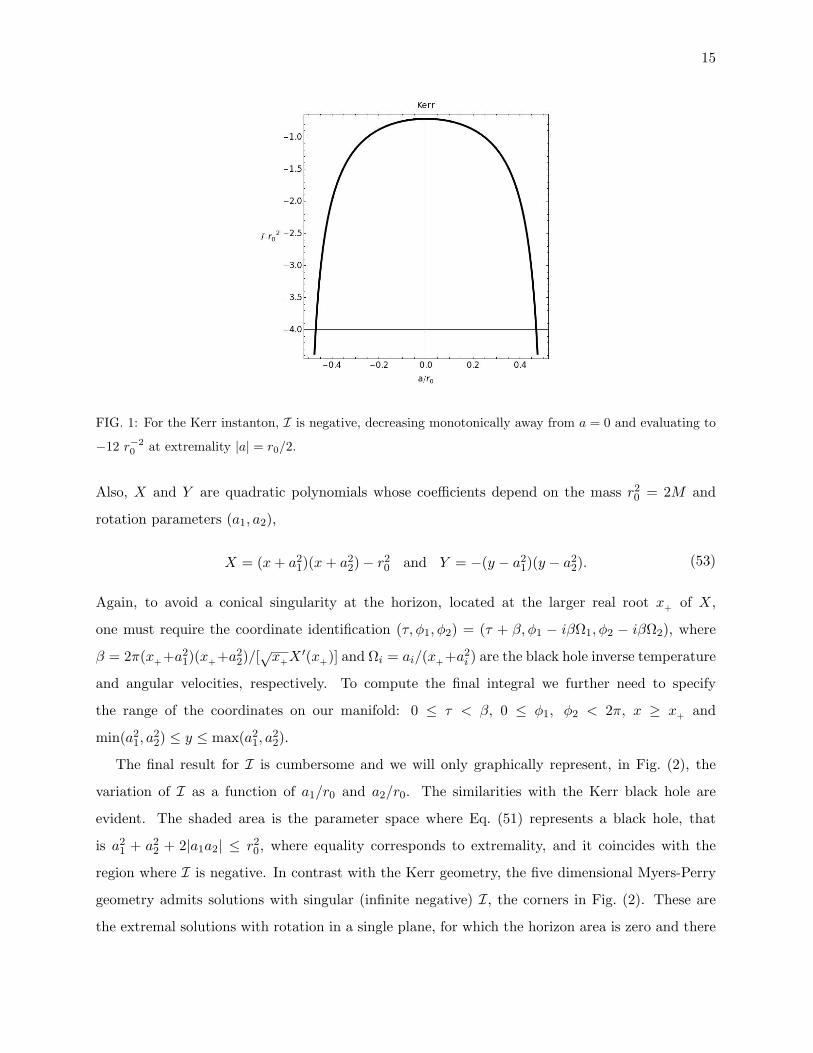
This expression is always negative and finite, as can be seen in Fig. 1. We conclude that the

Kerr instanton is unstable for non-conformal perturbations. It is fortunate that this particular

probe perturbation was able to identify the negative mode. Note that I(a = 0) = −5/(7r20) '

−0.71r−20 & −0.76r−2

0 , the negative eigenmode of the Lichnerowicz operator found in [10].

B. Five dimensional Myers-Perry

We will use the complexified form of the line element of the five dimensional Myers-Perry

solution in the coordinates introduced in [33],

ds2 = (x+y)(

dx2

4X+

dy2

4Y

)−Y (dτ − ixdφ1)2

y(x+ y)+

(dτ + iydφ1)2X

x(x+ y)− a

21a

22

xy[dτ−ixydφ2−i(x−y)dφ1]2,

(51)

where the coordinates (τ , φ, ψ) are related to the canonically defined coordinates (τ, φ, ψ) via

τ = τ + i(a21 + a2

2)φ1 + ia21a

22φ2, φ1 = a1φ1 + a1a

22φ2 and φ2 = a2φ1 + a2a

21φ2. (52)

15

FIG. 1: For the Kerr instanton, I is negative, decreasing monotonically away from a = 0 and evaluating to

−12 r−20 at extremality |a| = r0/2.

Also, X and Y are quadratic polynomials whose coefficients depend on the mass r20 = 2M and

rotation parameters (a1, a2),

X = (x+ a21)(x+ a2

2)− r20 and Y = −(y − a2

1)(y − a22). (53)

Again, to avoid a conical singularity at the horizon, located at the larger real root x+ of X,

one must require the coordinate identification (τ, φ1, φ2) = (τ + β, φ1 − iβΩ1, φ2 − iβΩ2), where

β = 2π(x++a21)(x++a2

2)/[√x+X′(x+)] and Ωi = ai/(x++a2

i ) are the black hole inverse temperature

and angular velocities, respectively. To compute the final integral we further need to specify

the range of the coordinates on our manifold: 0 ≤ τ < β, 0 ≤ φ1, φ2 < 2π, x ≥ x+ and

min(a21, a

22) ≤ y ≤ max(a2

1, a22).

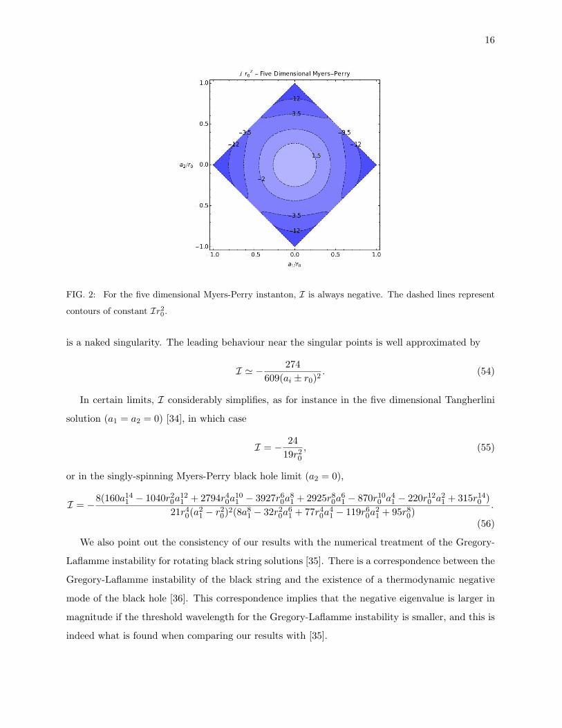
The final result for I is cumbersome and we will only graphically represent, in Fig. (2), the

variation of I as a function of a1/r0 and a2/r0. The similarities with the Kerr black hole are

evident. The shaded area is the parameter space where Eq. (51) represents a black hole, that

is a21 + a2

2 + 2|a1a2| ≤ r20, where equality corresponds to extremality, and it coincides with the

region where I is negative. In contrast with the Kerr geometry, the five dimensional Myers-Perry

geometry admits solutions with singular (infinite negative) I, the corners in Fig. (2). These are

the extremal solutions with rotation in a single plane, for which the horizon area is zero and there

16

FIG. 2: For the five dimensional Myers-Perry instanton, I is always negative. The dashed lines represent

contours of constant Ir20.

is a naked singularity. The leading behaviour near the singular points is well approximated by

I ' − 274609(ai ± r0)2

. (54)

In certain limits, I considerably simplifies, as for instance in the five dimensional Tangherlini

solution (a1 = a2 = 0) [34], in which case

I = − 2419r2

0

, (55)

or in the singly-spinning Myers-Perry black hole limit (a2 = 0),

I = −8(160a141 − 1040r2

0a121 + 2794r4

0a101 − 3927r6

0a81 + 2925r8

0a61 − 870r10

0 a41 − 220r12

0 a21 + 315r14

0 )21r4

0(a21 − r2

0)2(8a81 − 32r2

0a61 + 77r4

0a41 − 119r6

0a21 + 95r8

0).

(56)

We also point out the consistency of our results with the numerical treatment of the Gregory-

Laflamme instability for rotating black string solutions [35]. There is a correspondence between the

Gregory-Laflamme instability of the black string and the existence of a thermodynamic negative

mode of the black hole [36]. This correspondence implies that the negative eigenvalue is larger in

magnitude if the threshold wavelength for the Gregory-Laflamme instability is smaller, and this is

indeed what is found when comparing our results with [35].

17

C. Singly-spinning black ring

The complexified singly-spinning black ring line element is [26]

ds2 =F (y)F (x)

[dτ − iCR1 + y

F (y)dψ]2

+R2F (x)(x− y)2

[−G(y)F (y)

dψ2 − dy2

G(y)+

dx2

G(x)+G(x)F (x)

dφ2

], (57)

where

F (ξ) = 1 + λξ, G(ξ) = (1− ξ2)(1 + νξ), and C =√λ(λ− ν)1+λ

1−λ , (58)

and the dimensionless parameters ν and λ lie in the range 0 < ν ≤ λ < 1. As it stands, the line

element defined above has conical singularities at y = −1, x = −1 and x = 1. In order to remove

the first two one must choose the periodicity of φ and ψ to be

∆φ = ∆ψ = 2π√

1− λ1− ν

. (59)

The solution still has a conical singularity at x = 1, and is often referred to in the literature as the

unbalanced black ring. To obtain the physically acceptable black ring one must remove the conical

singularity at x = 1 by choosing λ to be a function of ν, leaving our solution dependent on two

parameters (R, ν),

λ =2ν

1 + ν2. (60)

The remaining parameters uniquely specify the mass and angular momentum of the black ring [32].

The singly-spinning Myers-Perry solution is obtained by taking the limit R → 0 and λ, ν → 1 in

the unbalanced solution, while keeping fixed a, r0 given by

r20 =

2R2

1− νand a2 = 2R2 λ− ν

(1− ν)2. (61)

Following [26], we note that the black ring instanton has another conical singularity located at the

horizon y = −1/ν, which is removed if we make the periodic identification (τ, φ) = (τ+β, φ− iβΩ),

where β = 4πR√λν(1 + λ)/[

√1− λ(1 + ν)] and Ω =

√λ− ν/[R

√λ(1 + λ)].

Again it is important to clearly state the range of coordinates in our manifold, which are given

in the patch that we are interested in by τ ∈ [0, β), φ, ψ ∈ [0, 2π√

1− λ/(1 − ν)), y ∈ [−1/ν,−1)

and x ∈ [−1, 1). We chose to determine I as a function of (R, ν, λ) and only latter imposing either

relation (60) or the limit (61). The expressions for both φab and I are complicated, but in the limit

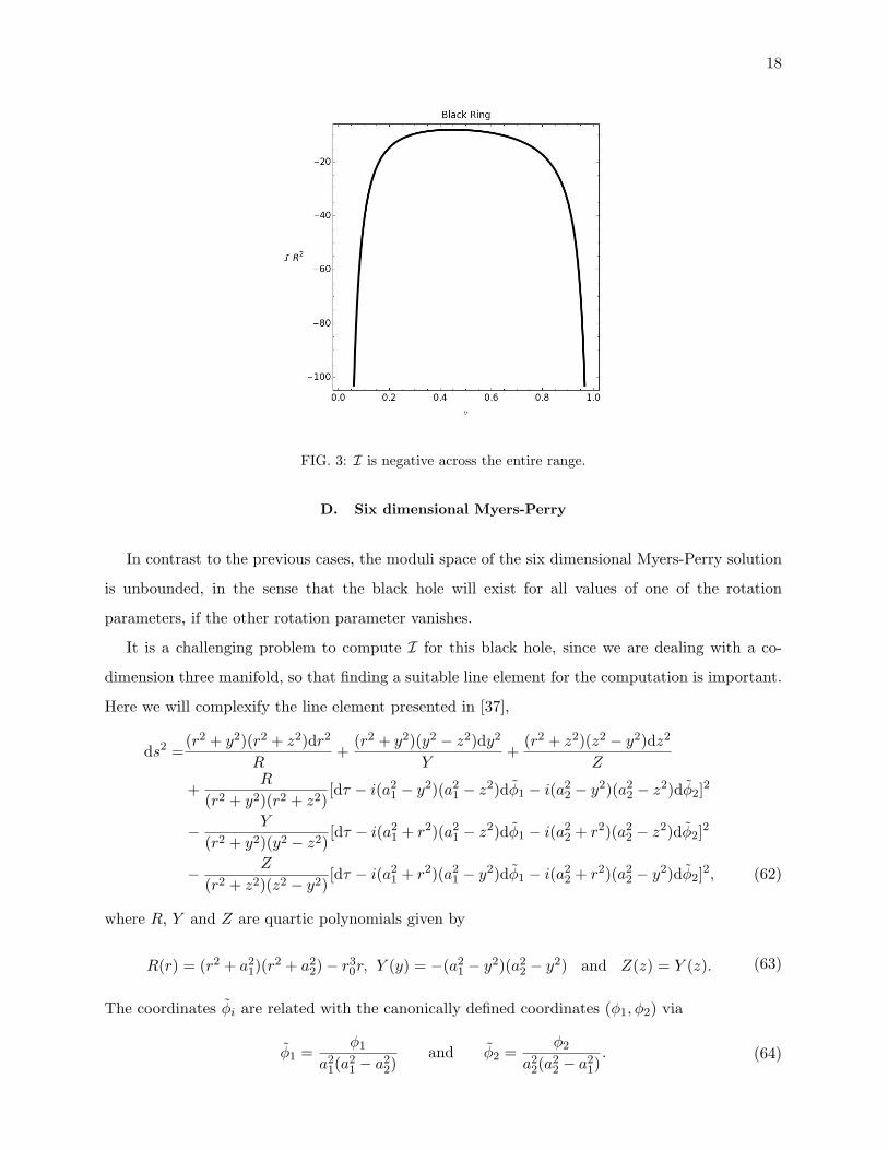
(61) I does reproduce Eq. (56). Again we evaluated I using the relation (60), see Fig. (3), and we

found that the black ring also exhibits an unstable behaviour against non-conformal perturbations.

18

FIG. 3: I is negative across the entire range.

D. Six dimensional Myers-Perry

In contrast to the previous cases, the moduli space of the six dimensional Myers-Perry solution

is unbounded, in the sense that the black hole will exist for all values of one of the rotation

parameters, if the other rotation parameter vanishes.

It is a challenging problem to compute I for this black hole, since we are dealing with a co-

dimension three manifold, so that finding a suitable line element for the computation is important.

Here we will complexify the line element presented in [37],

ds2 =(r2 + y2)(r2 + z2)dr2

R+

(r2 + y2)(y2 − z2)dy2

Y+

(r2 + z2)(z2 − y2)dz2

Z

+R

(r2 + y2)(r2 + z2)[dτ − i(a2

1 − y2)(a21 − z2)dφ1 − i(a2

2 − y2)(a22 − z2)dφ2]2

− Y

(r2 + y2)(y2 − z2)[dτ − i(a2

1 + r2)(a21 − z2)dφ1 − i(a2

2 + r2)(a22 − z2)dφ2]2

− Z

(r2 + z2)(z2 − y2)[dτ − i(a2

1 + r2)(a21 − y2)dφ1 − i(a2

2 + r2)(a22 − y2)dφ2]2, (62)

where R, Y and Z are quartic polynomials given by

R(r) = (r2 + a21)(r2 + a2

2)− r30r, Y (y) = −(a2

1 − y2)(a22 − y2) and Z(z) = Y (z). (63)

The coordinates φi are related with the canonically defined coordinates (φ1, φ2) via

φ1 =φ1

a21(a2

1 − a22)

and φ2 =φ2

a22(a2

2 − a21). (64)

19

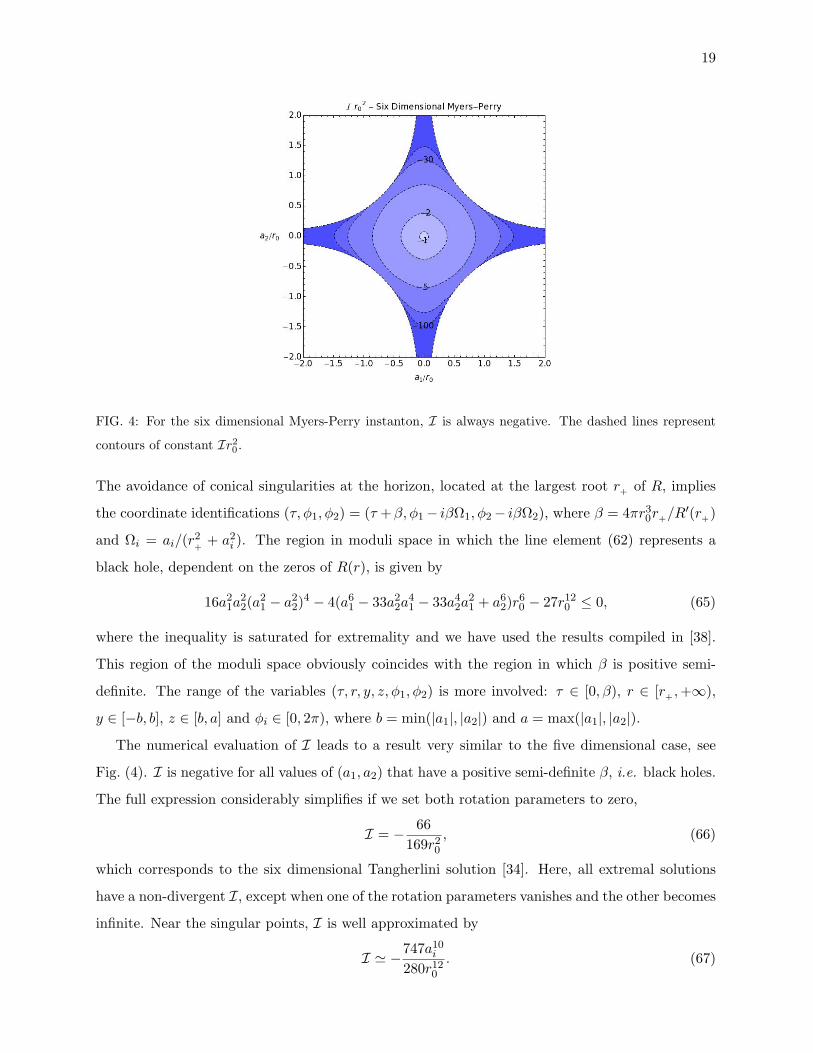
FIG. 4: For the six dimensional Myers-Perry instanton, I is always negative. The dashed lines represent

contours of constant Ir20.

The avoidance of conical singularities at the horizon, located at the largest root r+ of R, implies

the coordinate identifications (τ, φ1, φ2) = (τ +β, φ1− iβΩ1, φ2− iβΩ2), where β = 4πr30r+/R

′(r+)

and Ωi = ai/(r2+

+ a2i ). The region in moduli space in which the line element (62) represents a

black hole, dependent on the zeros of R(r), is given by

16a21a

22(a2

1 − a22)4 − 4(a6

1 − 33a22a

41 − 33a4

2a21 + a6

2)r60 − 27r12

0 ≤ 0, (65)

where the inequality is saturated for extremality and we have used the results compiled in [38].

This region of the moduli space obviously coincides with the region in which β is positive semi-

definite. The range of the variables (τ, r, y, z, φ1, φ2) is more involved: τ ∈ [0, β), r ∈ [r+ ,+∞),

y ∈ [−b, b], z ∈ [b, a] and φi ∈ [0, 2π), where b = min(|a1|, |a2|) and a = max(|a1|, |a2|).

The numerical evaluation of I leads to a result very similar to the five dimensional case, see

Fig. (4). I is negative for all values of (a1, a2) that have a positive semi-definite β, i.e. black holes.

The full expression considerably simplifies if we set both rotation parameters to zero,

I = − 66169r2

0

, (66)

which corresponds to the six dimensional Tangherlini solution [34]. Here, all extremal solutions

have a non-divergent I, except when one of the rotation parameters vanishes and the other becomes

infinite. Near the singular points, I is well approximated by

I ' −747a10i

280r120

. (67)

20

E. Kerr-AdS black hole

The Kerr-AdS instanton is given by

ds2 =∆Σ2

(dτ − i a

Ξsin2 θdφ

)2+ Σ2

(dr2

∆+

dθ2

∆θ

)− ∆θ sin2 θ

Σ2

(adτ − ir

2 + a2

Ξdφ)2

(68)

with

∆ = (r2 + a2)(1 + r2`−2)− r0r, Σ2 = r2 + a2 cos2 θ, ∆θ = 1− a2`−2 cos2 θ, and Ξ = 1− a2`−2,

(69)

where ` is the curvature radius of AdS and is related to the cosmological constant as `2 = 3/|Λ|.

The Kerr solution is recovered in the usual limit ` → +∞. The line element (68) only represents

a physical solution for |a| < `, being singular in the limit |a| → ` for which the 3-dimensional

Einstein universe at infinity rotates at the speed of light [39].

The avoidance of a conical singularity at the horizon, located at r = r+ , the largest root of ∆,

requires, as in the Kerr case, the coordinate identification (τ, φ) = (τ + β, φ− iβΩrot). Here,

β =4π(r2

++ a2)

r+(1 + a2`−2 + 3r2+`−2 − a2r−2

+)

(70)

and

Ωrot =a(1− a2`−2)r2+

+ a2. (71)

The angular velocity Ωrot here is measured relative to a frame rotating at infinity. It is convenient

to choose a coordinate system that is not rotating at infinity (φ → φ − ia`−2τ), for which the

angular coordinate identification depends instead on the angular velocity

Ω =a(1 + r2

+`−2)

r2+

+ a2. (72)

The reason for this is that Ωrot is not the appropriate thermodynamic variable. It cannot be used

to formulate the first law of thermodynamics [15]. The issue is irrelevant in this Section, as we

are interested only in the coordinate independent quantity I, but will be very important for the

thermodynamic interpretation of the results.

The expression for the TT perturbation φab is remarkably simple, and is given by

φab =r2

0

2Σ4

1 +2a2 sin2 θ

Σ20 0 −2ia(r2 + a2) sin2 θ

Σ2Ξ0 1 0 0

0 0 −1 0

−2iaΞΣ2

0 0 −(

1 +2a2 sin2 θ

Σ2

)

. (73)

21

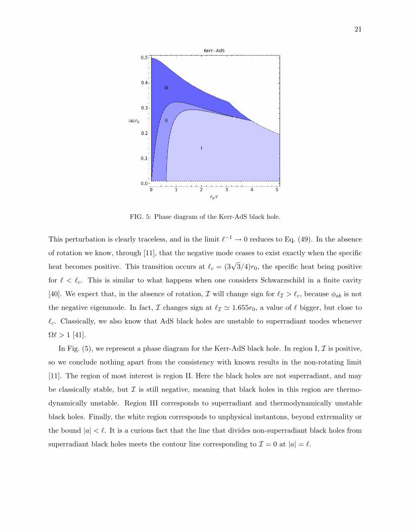
FIG. 5: Phase diagram of the Kerr-AdS black hole.

This perturbation is clearly traceless, and in the limit `−1 → 0 reduces to Eq. (49). In the absence

of rotation we know, through [11], that the negative mode ceases to exist exactly when the specific

heat becomes positive. This transition occurs at `c = (3√

3/4)r0, the specific heat being positive

for ` < `c. This is similar to what happens when one considers Schwarzschild in a finite cavity

[40]. We expect that, in the absence of rotation, I will change sign for `I > `c, because φab is not

the negative eigenmode. In fact, I changes sign at `I ' 1.655r0, a value of ` bigger, but close to

`c. Classically, we also know that AdS black holes are unstable to superradiant modes whenever

Ω` > 1 [41].

In Fig. (5), we represent a phase diagram for the Kerr-AdS black hole. In region I, I is positive,

so we conclude nothing apart from the consistency with known results in the non-rotating limit

[11]. The region of most interest is region II. Here the black holes are not superradiant, and may

be classically stable, but I is still negative, meaning that black holes in this region are thermo-

dynamically unstable. Region III corresponds to superradiant and thermodynamically unstable

black holes. Finally, the white region corresponds to unphysical instantons, beyond extremality or

the bound |a| < `. It is a curious fact that the line that divides non-superradiant black holes from

superradiant black holes meets the contour line corresponding to I = 0 at |a| = `.

22

V. THERMODYNAMIC INTERPRETATION

A. Ensembles and stability

The partition functions studied here have boundary conditions that impose periodicities both

in time and in the rotation angles. This corresponds to fixing the temperature T = β−1 and the

angular velocities Ωi, i.e. to the grand-canonical ensemble. The canonical ensemble would require

fixing the angular momenta J i, which includes specifying normal derivatives of the metric on the

boundary. We expect a correspondence between the stability of the ensemble and the problem of

non-conformal perturbations about the gravitational instanton. If there is a negative mode in the

path integral, the partition function is ill-defined and the ensemble should not be stable.

In this section, we recall the conditions for the thermodynamic stability of a system described by

the grand-canonical ensemble. The laws of thermodynamics imply that, for a system in equilibrium

at given temperature and angular velocities, any deviation from equilibrium, not necessarily small,

obeys [42]

δE − TδS − ΩiδJi > 0. (74)

Here, the angular velocities Ωi play the usual role of chemical potentials and the angular momenta

J i are the respective charges (conserved in the canonical ensemble). Expanding δE(S, J i) to second

order and using the first law of thermodynamics,

dE = TdS + ΩidJ i, (75)

we arrive at the conclusion that the stability relies only on the Hessian of the energy

g(W )µν =

∂2E

∂xµ∂xν, xµ = (S, J i), (76)

being positive definite. This Hessian matrix defines the so-called Weinhold metric [43]. Its inverse

is given by

g(W )µν = − ∂2G

∂yµ∂yν, yµ = (T,Ωi), (77)

where G is the Gibbs free energy,

G = E − TS − ΩiJi. (78)

The positivity of the inverse Weinhold metric gives the same stability condition. Notice that the

first law is equivalent to

dG = −SdT − J idΩi, (79)

23

so that the coordinate systems xµ and yµ are related by yµ = ∂E/∂xµ and xµ = −∂G/∂yµ. A

third alternative is the positivity of the Ruppeiner metric [44],

g(R)µν = − ∂2S

∂uµ∂uν, uµ = (E, J i), (80)

which is easily shown to be conformal to the Weinhold metric,

ds2R = − ∂2S

∂uµ∂uνduµduν = β

∂2E

∂xµ∂xνdxµdxν = βds2

W . (81)

Let us now look at how the stability conditions relate to the usual linear response functions,

like the specific heat. First, notice that

− ∂2G

∂yµ∂yν=

βCΩ ηj

ηi εij

, (82)

where

CΩ = T

(∂S

∂T

)Ω

(83)

is the specific heat at constant angular velocities (all Ωi fixed). The isothermal differential moment

of inertia tensor is

εij =(∂J i

∂Ωj

)T

= εji. (84)

There is also the vector

ηi =(∂S

∂Ωi

)T

=(∂J i

∂T

)Ω

, (85)

where the second equality, given by the symmetry of the Hessian matrix, corresponds to a Maxwell

relation. The ηi dependence can be dealt with if we use the relation between the specific heat at

constant angular velocities CΩ and the specific heat at constant angular momenta CJ , defined as

CJ = T

(∂S

∂T

)J

, (86)

which gives

CΩ = CJ + T (ε−1)ijηiηj . (87)

Hence

ds2W = − ∂2G

∂yµ∂yνdyµdyν = βCJdy2

0 + εijωiωj , (88)

where ωi = dyi + (ε−1)ijηjdy0.

From Eq. (88), we conclude that the thermodynamic stability is given by CJ and the spectrum

of εij , the condition being

CJ > 0 and spec(εij) > 0. (89)

24

B. Stability and negative modes

We expect that the partition function correctly reproduces the thermodynamic features of a

system. In particular, we expect that the partition function, which we associate with a system in

equilibrium, has some sort of pathology if thermodynamic stability does not hold. In this section,

we will extend a result by Reall [36] (based on previous contributions [11, 45]) on the relation

between thermodynamic stability and the existence of a negative mode. He showed that a negative

specific heat implied the existence of a negative mode in the action, in the case of the canonical

ensemble. We wish to extend this argument to the grand-canonical ensemble. The converse result

- to show that negative modes can only originate from thermodynamic instability - has not been

proven, and we have found a counter-example (Section V C 5).

The proof has two steps. The first step is to consider a path of geometries, intersecting a

black hole saddle-point solution, on which the action functional has a certain dependence. That

dependence implies an explicit relation between negative modes and thermodynamic stability. The

second step is to show that the construction is possible, i.e. that such a path indeed exists.

Consider paths of geometries, parametrised by variables zµ for given temperature T and angular

velocities Ωj , for which the action takes the form

I(zµ, T,Ωj) = βE(zµ)− S(zµ)− βΩiJi(zµ). (90)

These paths intersect black hole solutions with temperature T and angular velocities Ωj , which are

given by zµ = zµ∗ (T,Ωi). For the black hole geometries, I = βG, so that

E(zµ∗ ) = E(T,Ωi), S(zµ∗ ) = S(T,Ωi), J i(zµ∗ ) = J i(T,Ωj). (91)

The index in zµ has the same range as the index in yµ = (T,Ωi), the coordinates used in the

last section to define the inverse Weinhold metric. The invertibility of zµ∗ (yν) is assumed in the

following. The argument works because the functions that only depend on zµ can be thought of

as depending on yµ(zν).

At saddle points of I, i.e. for black hole solutions,

∂I

∂zµ(zα∗ ) =

∂yν∂zµ

(β∂E

∂yν− ∂S

∂yν− βΩi

∂J i

∂yν

)= 0, (92)

which implies the first law of thermodynamics (75). The Hessian of I at these points takes the

form

∂2I

∂zµ∂zν(zα∗ ) = β

[∂T

∂zµ∂Ωi

∂zµ

] βCΩ ηj

ηi εij

∂T

∂zν

∂Ωi

∂zν

. (93)

25

This result means that the negative modes of I given by this class of geometries have their origin

in the non-positivity of the Weinhold metric,

δI =12

∂2I

∂zµ∂zν

∣∣∣z∗δzµδzν =

β

2δsW

2. (94)

Notice that the path integral includes geometries that might not fall into this class. That is the

reason why the proof of the converse result does not follow from the construction above.

It would now be necessary to show that a path of geometries satisfying (92) is possible. Fortu-

nately, this problem was addressed already by Brown, Martinez and York [24] for the Kerr black

hole, and the extension to higher dimensional cases should present no difficulty. They consider four

dimensional axisymmetric geometries which satisfy the Einstein constraints and have the appro-

priate boundary conditions on the wall of a finite cavity. In a such a cavity, it is possible to have

thermodynamically stable black holes which are asymptotically flat (in this work, we consider the

technically simpler boundary conditions imposed at infinity). The final result of the construction,

their expression (43) for the gravitational action, exactly reproduces our assumption (92).

C. Particular cases

We have seen in Section V A that the linear response functions that characterise the stability are

the specific heat at constant angular momenta and the moment of inertia tensor. In this section,

we will calculate such quantities and interpret the results obtained with I.

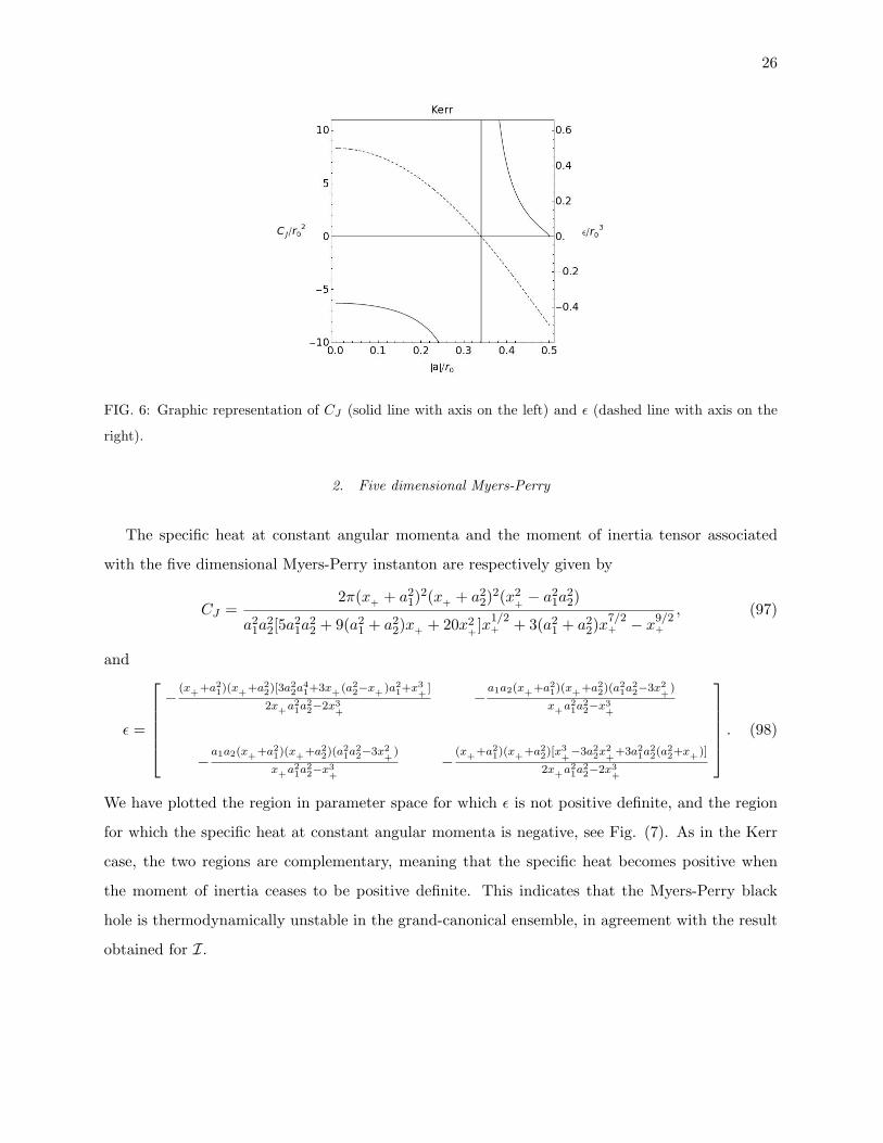
1. Kerr black hole

Here the specific heat is given by

CJ =2π(r2

+− a2)(r2

++ a2)2

3a4 + 6r2+a2 − r4

+

, (95)

where CJ is negative for small values of |a|, but becomes positive for |a| >√

2√

3− 3r0/2. The

moment of inertia can be expressed as

CJε = −π(r2

++ a2)2(r2

+− a2)

r+

, (96)

which is negative definite for black hole solutions. We conclude that, when CJ is negative, ε is

positive, and vice versa. From the grand-canonical point of view, the Kerr black hole is thermo-

dynamically unstable, justifying why I was negative for all values of |a| < r0/2. We have plotted

both quantities in Fig. (6). Furthermore, in the absence of rotation, ε is positive, meaning that the

Schwarzschild black hole is stable against perturbations in the angular velocity.

26

FIG. 6: Graphic representation of CJ (solid line with axis on the left) and ε (dashed line with axis on the

right).

2. Five dimensional Myers-Perry

The specific heat at constant angular momenta and the moment of inertia tensor associated

with the five dimensional Myers-Perry instanton are respectively given by

CJ =2π(x+ + a2

1)2(x+ + a22)2(x2

+− a2

1a22)

a21a

22[5a2

1a22 + 9(a2

1 + a22)x+ + 20x2

+]x1/2

+ + 3(a21 + a2

2)x7/2+ − x9/2

+

, (97)

and

ε =

−

(x++a21)(x++a2

2)[3a22a

41+3x+ (a2

2−x+ )a21+x3

+]

2x+a21a

22−2x3

+

−a1a2(x++a2

1)(x++a22)(a2

1a22−3x2

+)

x+a21a

22−x3

+

−a1a2(x++a2

1)(x++a22)(a2

1a22−3x2

+)

x+a21a

22−x3

+

−(x++a2

1)(x++a22)[x3

+−3a2

2x2+

+3a21a

22(a2

2+x+ )]

2x+a21a

22−2x3

+

. (98)

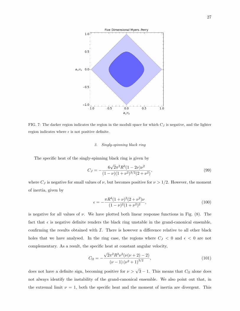
We have plotted the region in parameter space for which ε is not positive definite, and the region

for which the specific heat at constant angular momenta is negative, see Fig. (7). As in the Kerr

case, the two regions are complementary, meaning that the specific heat becomes positive when

the moment of inertia ceases to be positive definite. This indicates that the Myers-Perry black

hole is thermodynamically unstable in the grand-canonical ensemble, in agreement with the result

obtained for I.

27

FIG. 7: The darker region indicates the region in the moduli space for which CJ is negative, and the lighter

region indicates where ε is not positive definite.

3. Singly-spinning black ring

The specific heat of the singly-spinning black ring is given by

CJ = − 6√

2π2R3(1− 2ν)ν2

(1− ν)(1 + ν2)3/2(2 + ν2), (99)

where CJ is negative for small values of ν, but becomes positive for ν > 1/2. However, the moment

of inertia, given by

ε = −πR4(1 + ν)2(2 + ν2)ν

(1− ν)2(1 + ν2)2, (100)

is negative for all values of ν. We have plotted both linear response functions in Fig. (8). The

fact that ε is negative definite renders the black ring unstable in the grand-canonical ensemble,

confirming the results obtained with I. There is however a difference relative to all other black

holes that we have analysed. In the ring case, the regions where CJ < 0 and ε < 0 are not

complementary. As a result, the specific heat at constant angular velocity,

CΩ = −√

2π2R3ν2(ν(ν + 2)− 2)

(ν − 1) (ν2 + 1)3/2, (101)

does not have a definite sign, becoming positive for ν >√

3 − 1. This means that CΩ alone does

not always identify the instability of the grand-canonical ensemble. We also point out that, in

the extremal limit ν = 1, both the specific heat and the moment of inertia are divergent. This

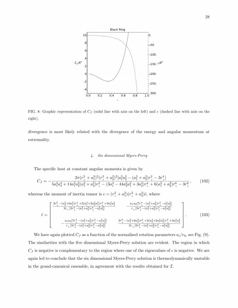
28

FIG. 8: Graphic representation of CJ (solid line with axis on the left) and ε (dashed line with axis on the

right).

divergence is most likely related with the divergence of the energy and angular momentum at

extremality.

4. Six dimensional Myers-Perry

The specific heat at constant angular momenta is given by

CJ = −2π(r2

++ a2

1)2(r2+

+ a22)2[a2

1a22 − (a2

1 + a22)r2

+− 3r4

+]

5a41a

42 + 14a2

1a22(a2

1 + a22)r2

+− (3a4

1 − 44a22a

21 + 3a4

2)r4+

+ 6(a21 + a2

2)r6+− 3r8

+

, (102)

whereas the moment of inertia tensor is ε = (r2+

+ a21)(r2

++ a2

2)ε, where

ε =

3r6

+−(a2

2+6a21)r4

++3(a4

1+2a22a

21)r2

++3a4

1a22

2r+ [3r4+−(a2

1+a22)r2

+−a2

1a22]

−a1a2[7r4

+−(a2

1+a22)r2

+−a2

1a22]

r+ [3r4+−(a2

1+a22)r2

+−a2

1a22]

−a1a2[7r4

+−(a2

1+a22)r2

+−a2

1a22]

r+ [3r4+−(a2

1+a22)r2

+−a2

1a22]

3r6+−(a2

1+6a22)r4

++3(a4

2+2a21a

22)r2

++3a2

1a42

2r+ [3r4+−(a2

1+a22)r2

+−a2

1a22]

. (103)

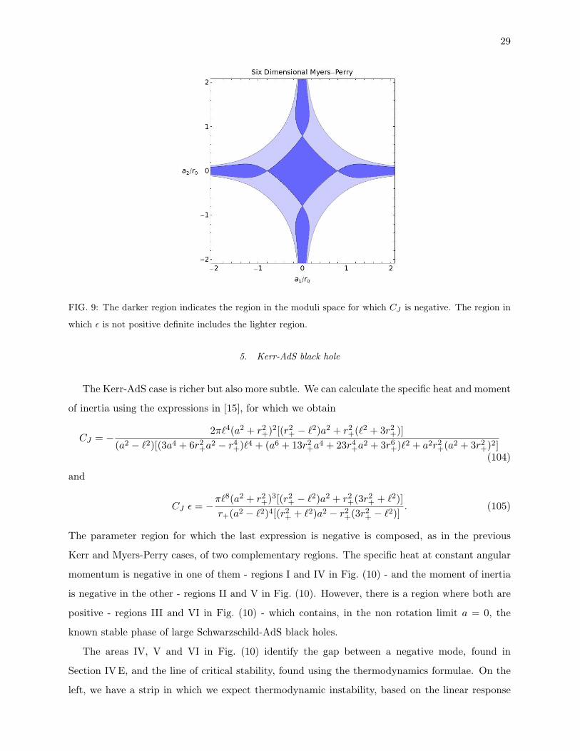
We have again plotted CJ as a function of the normalised rotation parameters ai/r0, see Fig. (9).

The similarities with the five dimensional Myers-Perry solution are evident. The region in which

CJ is negative is complementary to the region where one of the eigenvalues of ε is negative. We are

again led to conclude that the six dimensional Myers-Perry solution is thermodynamically unstable

in the grand-canonical ensemble, in agreement with the results obtained for I.

29

FIG. 9: The darker region indicates the region in the moduli space for which CJ is negative. The region in

which ε is not positive definite includes the lighter region.

5. Kerr-AdS black hole

The Kerr-AdS case is richer but also more subtle. We can calculate the specific heat and moment

of inertia using the expressions in [15], for which we obtain

CJ = −2π`4(a2 + r2

+)2[(r2+ − `2)a2 + r2

+(`2 + 3r2+)]

(a2 − `2)[(3a4 + 6r2+a

2 − r4+)`4 + (a6 + 13r2

+a4 + 23r4

+a2 + 3r6

+)`2 + a2r2+(a2 + 3r2

+)2](104)

and

CJ ε = −π`8(a2 + r2

+)3[(r2+ − `2)a2 + r2

+(3r2+ + `2)]

r+(a2 − `2)4[(r2+ + `2)a2 − r2

+(3r2+ − `2)]

. (105)

The parameter region for which the last expression is negative is composed, as in the previous

Kerr and Myers-Perry cases, of two complementary regions. The specific heat at constant angular

momentum is negative in one of them - regions I and IV in Fig. (10) - and the moment of inertia

is negative in the other - regions II and V in Fig. (10). However, there is a region where both are

positive - regions III and VI in Fig. (10) - which contains, in the non rotation limit a = 0, the

known stable phase of large Schwarzschild-AdS black holes.

The areas IV, V and VI in Fig. (10) identify the gap between a negative mode, found in

Section IV E, and the line of critical stability, found using the thermodynamics formulae. On the

left, we have a strip in which we expect thermodynamic instability, based on the linear response

30

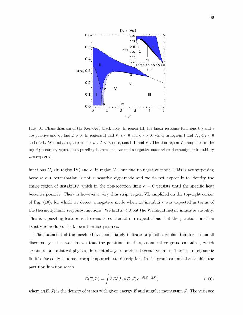
FIG. 10: Phase diagram of the Kerr-AdS black hole. In region III, the linear response functions CJ and ε

are positive and we find I > 0. In regions II and V, ε < 0 and CJ > 0, while, in regions I and IV, CJ < 0

and ε > 0. We find a negative mode, i.e. I < 0, in regions I, II and VI. The thin region VI, amplified in the

top-right corner, represents a puzzling feature since we find a negative mode when thermodynamic stability

was expected.

functions CJ (in region IV) and ε (in region V), but find no negative mode. This is not surprising

because our perturbation is not a negative eigenmode and we do not expect it to identify the

entire region of instability, which in the non-rotation limit a = 0 persists until the specific heat

becomes positive. There is however a very thin strip, region VI, amplified on the top-right corner

of Fig. (10), for which we detect a negative mode when no instability was expected in terms of

the thermodynamic response functions. We find I < 0 but the Weinhold metric indicates stability.

This is a puzzling feature as it seems to contradict our expectations that the partition function

exactly reproduces the known thermodynamics.

The statement of the puzzle above immediately indicates a possible explanation for this small

discrepancy. It is well known that the partition function, canonical or grand-canonical, which

accounts for statistical physics, does not always reproduce thermodynamics. The ‘thermodynamic

limit’ arises only as a macroscopic approximate description. In the grand-canonical ensemble, the

partition function reads

Z(T,Ω) =∫

dEdJ ω(E, J) e−β(E−ΩJ), (106)

where ω(E, J) is the density of states with given energy E and angular momentum J . The variance

31

of the statistical distribution is given by

〈E2〉 − 〈E〉2

〈E〉2=

T 2

〈E〉2

(∂〈E〉∂T

)(βΩ)

, (107)

〈J2〉 − 〈J〉2

〈J〉2=

T

〈J〉2

(∂〈J〉∂Ω

)T

. (108)

These variances are not small in most of the parameter space and diverge along the critical line

of stability if we take 〈E〉 and 〈J〉 to be the thermodynamic quantities E and J used before. The

derivative factor on the RHS of (108) is then the moment of inertia ε, and the quantity held fixed

in the derivative on the RHS of (107) is related to the so-called fugacity in the statistical mechanics

of systems of particles. We saw that the RHS of (108) changes sign across the divergence on the

line of critical stability, but the RHS of (107) is always positive in spite of the divergence.

In the region close to a phase transition, a careful study of the contribution of fluctuations is

essential. If the thermodynamic description breaks down near a critical point, the precise deter-

mination of quantities like the critical temperature Tc requires the contribution of higher order

corrections to the partition function. A well understood example is the two-dimensional zero-field

Ising model, which can be solved exactly. The exact critical temperature corresponds to almost half

of the naıve leading order result, and the first correction is already very important (see Fig. (9.5)

of [46]; the van der Waals gas is another good example described in this reference). In our case, the

one loop contribution is the first quantum correction and thus it is not surprising that the critical

line, as predicted by the zero-th order quantities, will suffer a small correction.

We must point out that a linear response function, namely the specific heat at constant charge,

also diverges in other known cases and the negative mode still disappears when expected. This hap-

pens for the Schwarzschild-AdS black hole, for which the specific heat diverges at `c = (3√

3/4)r0,

where the negative mode has numerically been shown to disappear [11]. It also occurs in the case of

the Reissner-Nordstrom black hole, for which the specific heat at constant electromagnetic charge

CQ diverges at Q =√

3M/2, where the negative mode has analytically been shown to disappear

[47] (the latter work focuses on the canonical ensemble, so that both the stability and the validity

of the thermodynamic limit are given by CQ). In the Kerr-AdS case studied here, we are looking

at the grand-canonical ensemble. The specific heat at constant angular momentum CJ is finite at

the transition, which is signalled instead by the quantities on the RHS of (107) and (108). Since(∂〈E〉∂T

)(βΩ)

=(∂〈E〉∂T

)〈J〉

+ β

(∂〈J〉∂Ω

)T

(∂〈E〉∂〈J〉

)2

T

, (109)

32

or, taking 〈E〉 and 〈J〉 to be the thermodynamic quantities E and J used before,(∂E

∂T

)(βΩ)

= CJ + β ε

(∂E

∂J

)2

T

. (110)

Now, CJ is divergent and ε = 0 along the line separating the regions I-IV and II-V in Fig. (10). This

corresponds to the transition in the canonical ensemble. In the grand-canonical ensemble, this line

has no special interest and the LHS of the latter expression is still finite, because the divergence in

(∂E/∂J)T cancels the divergence in CJ . On the other hand, the line of critical stability, separating

regions III-VI from the rest, is marked by a divergence in ε that also causes the divergence on the

LHS, while the other quantities are finite. The exception is the single point for which a = 0, the

Schwarzschild-AdS case. There, the transition is signalled by the divergence of the specific heat

since the moment of inertia is actually finite for a = 0, ε = r3+/2.

We conclude that the phase transition in the grand-canonical ensemble can be traced back to

the divergence of the moment of inertia ε only. We speculate that this transition may have different

quantum properties such that the critical stability line is corrected by the one loop contribution,

while the same does not happen in the canonical case with the specific heat at constant charge, in

the cases known.

To complete the discussion of the transitions, let us consider the critical exponents. Notice

that these too can be corrected by higher order contributions to the partition function, but we

are only able to study them here for the zero-th order semiclassical result corresponding to our

thermodynamics formulae.

We analysed, in the canonical ensemble (charges J or Q fixed), the cases of Kerr black hole,

with or without cosmological constant, and of the Reissner-Nordstrom black hole. We use the

definitions C ∼ ±|T − Tc|−α, for the phase T > Tc, and C ∼ ±|T − Tc|−α′, for the phase T < Tc.

We will actually find that the critical temperature Tc is a local maximum or minimum as a function

of the energy E, for fixed charges J or Q. This means that only one of the exponents α and α′ is

relevant. In a physical situation, on one side of the phase transition there is the stable black hole,

while on the other side there is a different stable configuration (eg. spacetime with radiation [40])

the specific heat of which would contribute with the other critical exponent. In the asymptotically

flat cases, Tc is a maximum of the temperature as a function of the energy E, for fixed J or Q,

which means that the relevant exponent is α′. In the Schwarzschild-AdS case, Tc is a minimum of

the temperature as a function of the energy E, so that the relevant exponent is α. In the Kerr-AdS

case, both situations can occur depending on the parameter region, as can be seen in Fig. (11).

Since, in all cases, the temperature varies quadratically with the energy around the critical point,

33

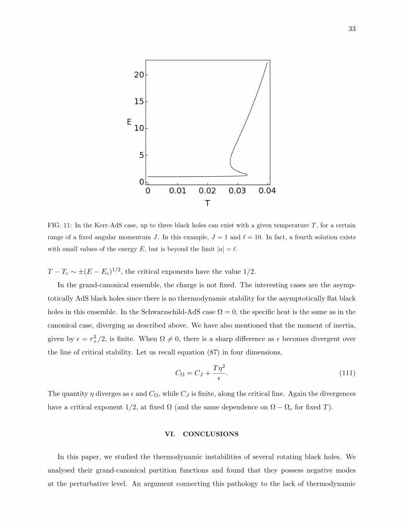
FIG. 11: In the Kerr-AdS case, up to three black holes can exist with a given temperature T , for a certain

range of a fixed angular momentum J . In this example, J = 1 and ` = 10. In fact, a fourth solution exists

with small values of the energy E, but is beyond the limit |a| = `.

T − Tc ∼ ±(E − Ec)1/2, the critical exponents have the value 1/2.

In the grand-canonical ensemble, the charge is not fixed. The interesting cases are the asymp-

totically AdS black holes since there is no thermodynamic stability for the asymptotically flat black

holes in this ensemble. In the Schwarzschild-AdS case Ω = 0, the specific heat is the same as in the

canonical case, diverging as described above. We have also mentioned that the moment of inertia,

given by ε = r3+/2, is finite. When Ω 6= 0, there is a sharp difference as ε becomes divergent over

the line of critical stability. Let us recall equation (87) in four dimensions,

CΩ = CJ +Tη2

ε. (111)

The quantity η diverges as ε and CΩ, while CJ is finite, along the critical line. Again the divergences

have a critical exponent 1/2, at fixed Ω (and the same dependence on Ω− Ωc for fixed T ).

VI. CONCLUSIONS

In this paper, we studied the thermodynamic instabilities of several rotating black holes. We

analysed their grand-canonical partition functions and found that they possess negative modes

at the perturbative level. An argument connecting this pathology to the lack of thermodynamic

34

stability is extended here to the grand-canonical ensemble.

The method we applied to look for negative modes avoids the complications due to the lack of

symmetry of these solutions. Instead of addressing the full problem, we construct a non-conformal

probe perturbation which lies along the stationary phase path. If the probe perturbation decreases

the Euclidean action, then a negative mode exists. We also clarified the issue of using Euclidean

methods for rotating spacetimes, leading to complex (quasi-Euclidean) instantons which should

present no difficulty of principle.

We found our results for the negative modes to be consistent with the standard conditions of

thermodynamical stability in the grand-canonical ensemble, with the exception of the Kerr-AdS

black hole. In the latter case, a small parameter region near the line of critical stability presents

a negative mode when the zero-th order conditions of stability are satisfied. This feature suggests

that the thermodynamic limit is ill-defined near the critical line in this case, so that the location

of the phase transition is corrected by quantum perturbations.

Possible future work linked to these results includes: (i) studying the partition function of a dual

conformal field theory and comparing with the gravitational case; (ii) studying the full negative

modes problem numerically, with special focus on the phase transition of the asymptotically AdS

black holes; (iii) formulating the canonical ensemble perturbations problem, which would require

fixing the angular momenta J i, i.e. writing the second-order action in terms of perturbations that

would specify derivatives of the metric normal to the boundary.

VII. ACKNOWLEDGMENTS

We are grateful to Gary Gibbons, Stephen Hawking, Gustav Holzegel, Hari Kunduri and Claude

Warnick for valuable discussions. RM and JES acknowledge support from the Fundacao para

a Ciencia e Tecnologia (FCT, Portugal) through the grants SFRH/BD/22211/2005 (RM) and

SFRH/BD/22058/2005 (JES).

[1] T. Regge and J. A. Wheeler, Phys. Rev. 108, 1063 (1957).

[2] F. J. Zerilli, Phys. Rev. Lett. 24, 737 (1970).

[3] C. V. Vishveshwara, Phys. Rev. D 1, 2870 (1970).

[4] S. A. Teukolsky, Phys. Rev. Lett. 29, 1114 (1972).

[5] S. Chandrasekhar, The mathematical theory of black holes (Oxford, UK: Clarendon, 1992).

35

[6] B. F. Whiting, J. Math. Phys. 30, 1301 (1989).

[7] A. Ishibashi and H. Kodama, Prog. Theor. Phys. 110, 901 (2003), hep-th/0305185.

[8] S. W. Hawking, Nature 248, 30 (1974).

[9] S. W. Hawking, Phys. Rev. D13, 191 (1976).

[10] D. J. Gross, M. J. Perry, and L. G. Yaffe, Phys. Rev. D25, 330 (1982).

[11] T. Prestidge, Phys. Rev. D61, 084002 (2000), hep-th/9907163.

[12] J. York, James W., Phys. Rev. Lett. 28, 1082 (1972).

[13] G. W. Gibbons and S. W. Hawking, Phys. Rev. D15, 2752 (1977).

[14] S. W. Hawking and D. N. Page, Commun. Math. Phys. 87, 577 (1983).

[15] G. W. Gibbons, M. J. Perry, and C. N. Pope, Class. Quant. Grav. 22, 1503 (2005), hep-th/0408217.

[16] V. Balasubramanian and P. Kraus, Commun. Math. Phys. 208, 413 (1999), hep-th/9902121.

[17] P. Kraus, F. Larsen, and R. Siebelink, Nucl. Phys. B563, 259 (1999), hep-th/9906127.

[18] R. Olea, JHEP 06, 023 (2005), hep-th/0504233.

[19] R. Olea, JHEP 04, 073 (2007), hep-th/0610230.

[20] K. Skenderis, Int. J. Mod. Phys. A16, 740 (2001), hep-th/0010138.

[21] G. W. Gibbons, S. W. Hawking, and M. J. Perry, Nucl. Phys. B138, 141 (1978).

[22] G. W. Gibbons and M. J. Perry, Nucl. Phys. B146, 90 (1978).

[23] K. Yano, Integral Formulas in Riemannian Geometry (Marcel Dekker, New York, 1970).

[24] J. D. Brown, E. A. Martinez, and J. York, James W., Annals N. Y. Acad. Sci. 631, 225 (1991).

[25] J. D. Brown, E. A. Martinez, and J. W. York, Phys. Rev. Lett. 66, 2281 (1991).

[26] D. Astefanesei and E. Radu, Phys. Rev. D73, 044014 (2006), hep-th/0509144.

[27] A. Schelpe, PhD Thesis, University of Cambridge (to be published).

[28] S. W. Hawking, Comm. Math. Phys. 25, 167 (1972).

[29] S. W. Hawking and G. F. R. Ellis, The Large scale structure of space-time (Cambridge University Press,

1973).

[30] R. P. Kerr, Phys. Rev. Lett. 11, 237 (1963).

[31] R. C. Myers and M. J. Perry, Ann. Phys. 172, 304 (1986).

[32] R. Emparan and H. S. Reall, Phys. Rev. Lett. 88, 101101 (2002), hep-th/0110260.

[33] W. Chen, H. Lu, and C. N. Pope, Nucl. Phys. B762, 38 (2007), hep-th/0601002.

[34] F. R. Tangherlini, Nuovo Cim. 27, 636 (1963).

[35] B. Kleihaus, J. Kunz, and E. Radu, JHEP 05, 058 (2007), hep-th/0702053.

[36] H. S. Reall, Phys. Rev. D64, 044005 (2001), hep-th/0104071.

[37] W. Chen, H. Lu, and C. N. Pope, Class. Quant. Grav. 23, 5323 (2006), hep-th/0604125.

[38] L. Yang, J. Symb. Comput. 28, 225 (1999), ISSN 0747-7171.

[39] S. W. Hawking, C. J. Hunter, and M. M. Taylor-Robinson, Phys. Rev. D59, 064005 (1999), hep-

th/9811056.

[40] J. W. York, Phys. Rev. D33, 2092 (1986).

36

[41] S. W. Hawking and H. S. Reall, Phys. Rev. D61, 024014 (1999), hep-th/9908109.

[42] L. D. Landau and E. M. Lifschitz, Statistical Physics, Part 1 (Pergamon Press, Oxford, 1958).

[43] F. Weinhold, J. Chem. Phys. 63, 2479, 2484, 2488, 2486 (1975).

[44] G. Ruppeiner, Rev. Mod. Phys. 67, 605 (1995).

[45] B. F. Whiting and J. W. York, Phys. Rev. Lett. 61, 1336 (1988).

[46] H. E. Stanley, Introduction to Phase Transitions and Critical Phenomena (Oxford University Press,

1971).

[47] R. Monteiro and J. E. Santos, Phys. Rev. D79, 064006 (2009), 0812.1767.