Thermal Line Model and Control - IEA - Lund University document/5324_full... · Thermal Line Model and Control Martin Andersson Ljus Divisionof Industrial Electrical Engineering and

Ind

ust

rial E

lectr

ical En

gin

eerin

g a

nd

A

uto

matio

n

CODEN:LUTEDX/(TEIE-5324)/1-49/(2013)

Dynamic Line RatingThermal Line Model and Control

Martin Andersson Ljus

Division of Industrial Electrical Engineering and Automation Faculty of Engineering, Lund University

i

Abstract In times of increased environmental awareness, there exists a desire to not only build new

environmentally friendly and renewable power generating units, but also to increase the efficiency of

all existing technology. Wind power is such a renewable and environmentally friendly technology.

Wind turbines and wind power have made giant leaps in the world in the past years, with an almost

exponential growth in production and number of units. This increased utilization puts a lot of stress

on the already existing grids, which were oftentimes built without this power increase in mind. To

further add to these problems, wind power particularly is something that is not always readily

available, neither is it stored.

Dynamic line rating is a way of optimizing the power throughput through the distribution and

transmission lines, by not only looking at the current through them as a way to determine its rating,

but also by measuring how the weather affects the thermal system. In reality, several factors decide

the line rating, which is how much current a line can carry. These weather impacting parameters

include; wind speed, wind direction, solar irradiation and ambient temperature, not only the current

through the conductor. Normally, the rating of the line is decided conservatively with a fixed value

for the maximum current so as to make sure the surface temperature and resulting sag is always

within acceptable boundaries. With these additional parameters however, a higher line rating can

often be used. Considering the cooling effect of the wind means dynamic line rating is ideal for wind

power, since in that case, the wind both produces power while allowing for a higher power

throughput on the line. By continuously measuring all of these parameters, one can more effectively

determine the rating of a line and the available amount of additional power it can carry, while still

meeting regulations.

This thesis explores dynamic line rating in connection with an E.ON offshore wind farm project at

Kårehamn near Öland in Sweden. This is done by first building a Simulink computer model for the

continuous determination of the conductor surface temperature – and based on this implementing

an algorithm for controlling the output of Kårehamn wind farm. Rather than calculating the

ampacity, the line rating, which is often done, this model will focus on explicitly controlling the

temperature – since it is the temperature requirements that must be met in order to meet

regulations regarding the line sag, the height of the lines above ground.

A model and a control method were produced, that successfully controlled the surface temperature

of the most critical conductor by sending a reference value to control the output of the wind farm. By

building thermal models with input parameters such as current (converted from the power value),

wind speed, wind direction and ambient temperatures, the surface temperature could be accurately

calculated. The control algorithm developed in this work is compared to and found superior to an

existing prototype solution used by E.ON. This thesis also successfully incorporated error handling

and ways of controlling additional power generating units on the grid.

ii

Table of Contents

ABSTRACT ......................................................................................................................................................... I

CHAPTER 1. INTRODUCTION ............................................................................................................................. 1

1.1 BACKGROUND ................................................................................................................................................... 1

1.2 AIMS ............................................................................................................................................................... 2

1.3 LIMITATIONS ..................................................................................................................................................... 2

CHAPTER 2. THEORY ......................................................................................................................................... 3

2.1 OVERHEAD LINES ............................................................................................................................................... 3

2.2 HEAT BALANCE IN AN OVERHEAD LINE .................................................................................................................... 3

2.2.1 Current heating ..................................................................................................................................... 4

2.2.2 Solar heating ......................................................................................................................................... 4

2.2.3 Convective cooling ................................................................................................................................. 4

2.2.4 Radiative cooling ................................................................................................................................... 6

2.3 TIME-DEPENDENT HEATING .................................................................................................................................. 6

2.4 TIME-DEPENDENT COOLING ................................................................................................................................. 7

2.5 AMPACITY ........................................................................................................................................................ 8

2.6 CURRENT CONVERSION........................................................................................................................................ 8

2.6.1 Skin effect .............................................................................................................................................. 8

2.7 ÖLAND, LOCATION-SPECIFIC VALUES ...................................................................................................................... 9

CHAPTER 3. THERMAL MODEL ....................................................................................................................... 11

3.1 INDIVIDUAL MEASURING STATION ........................................................................................................................ 11

3.2 GRID MODEL ................................................................................................................................................... 13

CHAPTER 4. VERIFICATION OF THERMAL MODEL ........................................................................................... 16

4.1 VERIFICATION AGAINST CIGRE REPORT ................................................................................................................ 16

4.1.1 Surface temperature calculations for the steady state, example 1 ..................................................... 16

4.1.2 Surface temperature calculations for the steady state, example 2 ..................................................... 17

4.1.3 Calculations for the unsteady state, example 1 .................................................................................. 18

4.1.4 Calculations for the unsteady state, example 2 .................................................................................. 18

4.1.5 Conclusion and discussion on verification ........................................................................................... 19

4.2 TESTING THE THERMAL MODEL ........................................................................................................................... 19

4.2.1 Output change: 35- 48 MW, no loads ................................................................................................. 19

4.2.2 Output change: 48-0 MW, no loads .................................................................................................... 21

4.3 IMPACT OF SOLAR IRRADIATION........................................................................................................................... 21

CHAPTER 5. CONTROLLING THE THERMAL MODEL ......................................................................................... 23

5.1 TUNING THE CONTROLLER .................................................................................................................................. 23

5.2 SIMULATIONS WITH CONTROL ............................................................................................................................. 26

5.2.1 Changing wind speed on the conductor .............................................................................................. 27

5.2.2 Changing wind direction in relation to conductor ............................................................................... 29

5.2.3 Changing ambient temperature at conductor location ....................................................................... 31

CHAPTER 6. ALTERNATIVE INCREMENTAL CONTROL ...................................................................................... 33

6.1 SIMULATIONS .................................................................................................................................................. 34

6.1.1 Changing wind speed on the conductor .............................................................................................. 34

6.1.2 Changing wind direction in relation to conductor ............................................................................... 36

6.1.3 Changing ambient temperature at conductor location ....................................................................... 37

CHAPTER 7. SECONDARY AIMS ....................................................................................................................... 39

7.1 ADDITIONAL SOLAR AND WIND POWER GENERATION UNITS ...................................................................................... 39

7.2 GIVING KÅREHAMN PRESET OUTPUT VALUE ........................................................................................................... 40

7.3 KÅREHAMN EMERGENCY SHUTDOWN ................................................................................................................... 41

7.4 COMMISSIONING – KÅREHAMN .......................................................................................................................... 42

CHAPTER 8. CONCLUSIONS ............................................................................................................................. 43

CHAPTER 9. CONTINUED WORK ..................................................................................................................... 45

REFERENCES ................................................................................................................................................... 46

APPENDIX A, CABLE DATA .............................................................................................................................. 47

APPENDIX B, SIMULINK MODEL M-FILE .......................................................................................................... 48

1

Chapter 1. Introduction This chapter aims at giving a background to the work conducted in this thesis, so it is understood

what is done and why. The chapter also establishes the aims of the thesis and limitations of the work.

1.1 Background Renewable energy is on the rise in Sweden and in the world, with wind power amongst the most

expansive risers nationally, with an increase of 74 % in wind power production between 2010 and

2011 [1]. The Swedish government has, in accordance with EU regulations, set environmental targets

which amongst others include that 50 % of total energy usage shall come from renewable energy [2].

To meet these targets as well as a possible future increase in energy demand, the distribution

network is possibly changing from passive to active with an increasing amount of Distributed

Generation such as wind farms being connected to the network. Wind farms tend to be built where

there is most wind, wherever it may be. These farms are often located on the edges of the

distributions systems, where it may be most convenient to connect them to a local grid, one often

not rated to carry the extra loading [3]. There is a desire to increase the power transferred by

transmission and distribution lines, though that is not always feasible with existing lines. One solution

would be to simply build new lines; overhead conductors or underground cables, though this is

expensive.

Dynamic line rating is the continuous measurement of conductor conditions to allow for maximum

power throughput. It is the sag of a line section that will determine the maximum permissible

temperature of the conductor. Sag of an overhead line is the difference in height between the

highest and lowest point of a line section, i.e. between two poles. When the temperature of an

overhead line increases, annealing of the metal causes the line section to change in length which

changes the sag. The temperature of a conductor depends on the load current, as well as other

parameters acting on the conductor, such as ambient temperature, wind speed, wind direction and

solar radiation. In the past, default and often relatively conservative values have been set to make

sure the temperatures of the conductors are within the desired limits at all times. That means that

the lines for the most part would be limited well below their capacity. To actively measure the lines

rating, instead of using default conservative values, means the power throughput can be increased

most of the time. This is ideal for wind power, because having strong winds allows for higher power

output from the generation site, but also allows for more power on the grid, due to the cooling effect

of the wind on the conductor.

E.ON wind is building a new offshore wind farm, Kårehamn, east of Föra on Öland, consisting of 16 3

MW wind turbines with a maximal output of 48 MW. The 50 kV-grid on Öland can currently only

handle about 20 MW of that power without modifications [4]. As a result, the grid would get

overloaded by the new wind farm at certain times, such as when the ambient temperature is high or

the local load is at a minimum. This means that the temperature and resulting sag in the line will

reach unacceptable levels. Dynamic line rating would allow the lines to carry the maximum amount

of power at any given time, minimizing grid curtailment; which is used when more wind power is

available than is allowed on the grid.

2

To accomplish this, E.ON has installed measurement equipment on the lines at three different

locations on the grid; at Köping, Högsrum and Linsänkan. The equipment at Köping and Linsänkan will

measure the current through the conductors, while the equipment in Högsrum directly measures the

surface temperature.

1.2 Aims The aim of this master thesis is to develop a method for controlling the output of the wind farm

Kårehamn, a control algorithm, to make sure that the impact of the wind farm on the local grid never

causes the conductor surface temperatures to exceed 50 °C. This will be done by building a model in

Simulink, with a thermal model as well as a PID regulator. The regulator will control the surface

temperature of the conductor. In the real world application, physical connections will send a power

reference value generated by the model to the wind farm.

By measuring the current and temperature of the overhead lines at the three different locations,

with each site measuring the two different conductors, the output should be controlled so that the

temperature requirements for the conductors are always met. It is furthermore the aim of this thesis

to produce methods for handling errors in the system, and to find a way to deal with additional

power acting on the grid. These secondary objectives include:

To develop a method for controlling additional generation units connected to the grid. The

additional power, in this case, is one solar park and a wind turbine. Their needs are

secondary to Kårehamn, and are thus not allowed to compromise the output from the wind

farm. It is desirable to be able to send a control signal, one which will tell them if they are

allowed to be connected to the grid or not. This will happen when the conductor surface

temperature at one or several of the monitored line sections surpasses 50 °C, as these

should always turn off before Kårehamn itself lowers its output.

To develop a method where preset values are sent as reference values to the wind turbines

in case the system is unresponsive and surface temperature gets too high yet not critical.

To develop an emergency shutdown procedure for Kårehamn, should the surface

temperature surpass a preset critical value during a period of time without it reacting to a

change in the reference signal being sent.

To build and test an alternative model which incrementally controls the output of Kårehamn

and compare it with the model developed in this thesis

To investigate if the control system can be tested this early on when just a part of the wind

farm is completed.

1.3 Limitations Since time is limited, focus will primarily be on the thermal model itself and control of the

temperature. The secondary aims will be met if there is additional time.

This thesis will be limited to computer models, and thus no concern will be given to the physical

implementation. Furthermore, the model will use the temperature to control, and not the current.

3

Chapter 2. Theory This chapter introduces the theory behind and regarding the heat balance in an overhead conductor,

the physics and equations of them. It also explains data specific to Öland as well as ampacity and

current conversion equations.

2.1 Overhead Lines There are several different types of conductors on Öland, of which only two are relevant for further

studies in this thesis; the 159 Al59 and 329 Al59 conductors. That is because only these conductor

types are used on the line sections where the measuring stations are located. For detailed

information regarding each conductor, please refer to Appendix A.

2.2 Heat balance in an overhead line The sections herein about the thermal balance on the overhead conductors and its different

parameters closely follow those in the CIGRE technical brochure 207, Thermal Behaviour of Overhead

Conductors [5], unless stated otherwise. There is another commonly used standard for these

calculations, namely the IEEE 738 [6]. Comparisons made between these two standards, show slight

differences in ampacity, ranging from 1% to 8.5% [3]. Given that small difference, as well as the fact

the CIGRE technical brochure was initially available, that standard was used.

The relationship between the current and temperature in the lines is shown below. It applies for the

unsteady state, when the temperature of the conductor is not in thermal equilibrium.

Where:

m = Conductor mass density per unit length (kg/m)

c = Conductor specific heat capacity (J/(kg*K))

Tav = Conductor average temperature (°C)

PJ = Current heating per unit length (W/m)

PM = Magnetic heating per unit length (W/m)

Pi = Corona heating per unit length (W/m)

PS = Solar heating per unit length (W/m)

PC = Convective cooling per unit length (W/m)

PR = Radiative cooling per unit length (W/m)

PW = Evaporative cooling per unit length (W/m)

Some of these parameters are commonly neglected, such as Pi and PW.

“Pi and PW are commonly neglected. For example, for the Lynx conductor, PM can be neglected

because the two layers of Aluminum strand spiral in opposite directions around the steel core, and the

magnetic fields largely cancel out. Pi, PW and PM are not considered in the P341 DLR calculations.” [3]

Pi and PW will be excluded here as well. The magnetic heating PM is included in the formula for

calculating the current heating PJ. The resulting differential equation is then:

4

The calculations of the individual terms on the right-hand side of above equation are given below.

According to [5], it is generally sufficient to assume that the average temperature of the conductor is

equal to its surface temperature Ts, that is; Tav=Ts. This will be assumed here as well, since the surface

temperature is what will be measured in the real case on Öland.

2.2.1 Current heating

Current heating is the heating of the conductor due to the effects of load current and includes both

the joule heating as well as magnetic heating. The heat gain is given by:

( ( ))

Where:

kj = Rac/ Rdc = Factor which takes into account the magnetic heating (unitless)

Idc = Effective current (A)

Rdc = Dc resistance (Ω/m), at 20 °C

α = Temperature coefficient of resistance per degree Kelvin (1/K)

Ts = Conductor surface temperature (°C)

2.2.2 Solar heating

Solar heating is the heating of the conductor as a consequence of incoming solar irradiation. The

effect of solar heating will not be measured on site, which means that it is not something that will be

used in calculations in the real case. However, it is the aim of this thesis to test two cases in the

simulations; a case of no solar heating as well as a simplified case of solar heating, to investigate the

effects of the solar heating. The simplified equation for calculating the solar heating gain is given

below.

Where:

αS = Absorptivity of conductor surface (unitless)

S = global solar radiation (W/m2)

D = external diameter of conductor (m)

2.2.3 Convective cooling

The heat loss due to convective cooling is a major factor in the thermal heat balance. Overhead

conductors heat the surrounding air, and as the air heats up, its density decreases, causing it to rise.

There are several cases of convective heat loss, depending on wind speed and angle. Forced

convection, with wind speeds above zero, causes the heated air to be forcefully carried away, whilst

natural convection, with no wind, causes the heated air to naturally rise. There is also a corrective

convective cooling, which deals with the cooling at low wind speeds.

For higher wind speeds (i.e. ≥0.5 m/s), the forced convective formula will be used. For lower wind

speeds (i.e. <0.5 m/s), the values for the natural, the corrected as well as the forced convective with

an assumed angle of 45 ° will be computed, and the largest of them be used.

The convective heat loss is given by:

5

( )

Nu is the Nusselt number, and it is the one that changes depending on which kind of convection is in

effect. The equations for convective cooling below are all taken from the MiCOM P341 Application

Guide [3], though rewriting the equations in [5] would give the same equations.

For forced convection, the heat loss is given by:

( ) (

*

( ( ))

For natural convection, the heat loss is given by:

( ) ( ( )

( ) *

The corrected convective heat loss is given by:

( ) (

*

Where:

( )

( ) ( )

( ( )⁄ )

( )

( )

( ⁄ )

( ⁄ )

( )

( )

( )

( )

( )

( )

( ) ( )

6

2.2.4 Radiative cooling

Radiative heat loss in a conductor is the process by which it loses heat due to thermal radiation. The

equation for the radiative cooling is given by:

(( ) ( )

)

Where:

( )

( ( )⁄ )

( )

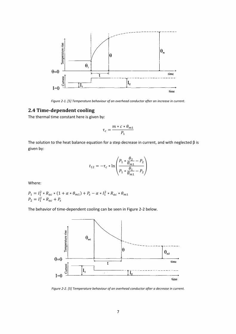
2.3 Time-dependent heating The thermal time constant is the time interval for the temperature rise of the conductor, to that

of 63.2 % of its final steady state value when subjected to a step change in e.g. current.

The solution to the equation for an increase in current is given by:

( ( ) ( ) (

**

However, since β – which is the temperature coefficient of specific heat capacity – is so small (refer

to appendix A), it can and will be neglected here [5], resulting in the simplified equation below:

(

*

Where:

= average temperature rise of conductor

= initial average temperature rise of conductor at time t1

= asymptotic average temperature rise of conductor

The behavior of the time-dependent heating can be seen below in Figure 2-1.

7

Figure 2-1. [5] Temperature behaviour of an overhead conductor after an increase in current.

2.4 Time-dependent cooling The thermal time constant here is given by:

The solution to the heat balance equation for a step decrease in current, and with neglected β is

given by:

(

)

Where:

( )

The behavior of time-dependent cooling can be seen in Figure 2-2 below.

Figure 2-2. [5] Temperature behaviour of an overhead conductor after a decrease in current.

8

2.5 Ampacity Ampacity, or the thermal rating of the line, is the maximum current a conductor can carry without

exceeding its sag temperature. The sag temperature is the temperature at which the legislated

height of the conductor above ground is met.

The ampacity can be measured either directly, or indirectly by measuring ambient weather

conditions and then solving equations. The ampacity equation is given below.

√

( ( ))

The ampacity in dc can then be converted if needed according to the equations in section 2.6.

2.6 Current conversion It is vital that models for converting between alternating and direct current be implemented, since

the thermal model, or current heating model, requires direct current as an input. Meanwhile, the

real world application – where Kårehamn feeds the grid on Öland – functions with alternating

current. Below are equations regarding current conversion, according to IEC 60287 [7].

( ( ))

Where:

Rdc = Conductor resistance at temperature T (Ω)

R20 = Conductor resistance at 20 °C (Ω)

T = Operating temperature of the conductor (°C)

α = Temperature coefficient of resistance per degree Kelvin (1/K)

( )

Where:

ys = Skin effect factor

yp = Proximity effect factor (0 in case of overhead lines)

2.6.1 Skin effect

As the frequency of the current increases, the flow of electricity tends to become more concentrated

around the outside of a conductor. At very high frequencies, hollow conductors are often used

primarily for this reason. At power frequencies (typically 50 or 60 Hz), while less pronounced the

change in resistance due to skin effect is still noticeable. The skin effect factor is given by:

Where:

√

9

f = Supply frequency (Hz)

ks = Skin effect coefficient (=1 for bare conductors)

It is known [5], that:

This yields the following equations:

√

√

When testing the above equations for current conversion, they produced different results, when they

should give the same answer. That might be related to the numbers given by E.ON for the

resistances, and that the dc resistance given was not specified for any specific temperature, while the

ac resistance was specified for 50 °C. The model used the first equation above for the current

conversion calculations, since both values for resistances were given.

2.7 Öland, location-specific values Surface temperature of the conductors will be calculated at three different locations on Öland as

mentioned before. Each location will measure both lines, thus giving a total of six different values for

the temperature.

Köping and Linsänkan will both have Alstom protective relays and weather stations installed, while

Högsrum only have Power Donuts installed. The Alstom relays measure the line current, which

means that the temperature will have to be calculated using the current input, as well as weather

parameters collected from the weather stations. The power donuts however, measure the surface

temperatures directly, meaning it will be readily available to use in the model.

The general theory with all its equations that are going to be used in the thesis, was shown earlier in

the chapter. For the specific case on Öland, several additional parameters were needed. Cable

specific numbers were provided by E.ON and can be found in Appendix A. In order to calculate the

effect of the solar heating, both the global irradiation and the absorptivity of aluminum were

needed. Looking at a solar heating map, the worst case scenario for Öland in terms of irradiation was

found to be 560 W/m2 [8], which was the average value at noon for a hot day in June, calculated on a

horizontal plane in Öland, near Linsänkan. The value of the absorptivity for aluminum varies widely,

as does the emissivity. The emissivity is needed in order to calculate the radiative cooling. Values for

these were chosen to be 0.5 and 0.07 respectively (which was the number for rough aluminum) [9],

[10]. According to Thermal Behaviour of Overhead Conductors a value of 0.5 can be chosen for most

purposes, which is in line with what was found on the webpage. The values E.ON themselves use are

0.7 for both absorptivity and emissivity [11].

A number for the relative air density, which is related to the height above sea level, is needed to

calculate the convective cooling gains. The height above sea level on Öland was found to be between

5-55 m, with an average of about 35 m [12]. The conductors, in turn, are at a height of about 7 m

above ground. So, y = 35 + 7 m = 42 m.

10

Lastly and also needed to calculate convective cooling, is the roughness of the conductor surface. As

can be seen in Appendix A, the conductors are made up of several smaller aluminum strands. The

total diameter of the 157 al59 and 329 al59 cables are 16.3 mm and 23.6 mm respectively. The outer

layer wire diameter, d, is 3.26 mm. So, the value for Rf is:

( )

( )

( )

( )

The value for both cables is larger than 0.05. This is critical in deciding which values are being used in

the convective cooling equations, as seen earlier.

11

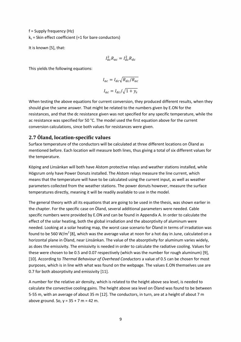
Chapter 3. Thermal model To be able to simulate, test for different values, and eventually realize a control method, a Simulink

model for the thermal heat balance had to be made. The thermal system created is shown in Figure

3-1.

Figure 3-1. Thermal model as seen in Simulink.

The figure shows the model of the larger thermal system, with subsystems containing the individual

line stations and the heat balance within them, as well as models of the grid between the three

measurement stations. A more in-depth look at those subsystems can be found under the following

subheadings.

At the far left of the model is the power input, which is the power in MW coming from Kårehamn. It

is divided into two lines, both sharing an equal amount of the power. This signal is fed through the

grid models, and then into the six different line models, each representing one measurement station,

which can be seen in Figure 3-2. There are two subsystems just before going in to these line models,

which contain equations, converting the power value to current and also converting it from

alternating to direct current, ultimately sending it into the thermal models. Out from these

subsystem come signals containing values both that of the surface temperatures, as well as that of

the ampacity differences. The six different temperature values are then compared, and the highest

temperature, the most critical, is then selected and sent as an output with which the whole system

will be controlled. Values for the ampacity difference are also compared, but there the smallest value

is sent out.

To be able to keep track of all the different parameters, and to not have to go through the model

doing constant small changes to individual parameters, a MATLAB m-file was written. The complete

m-file can be studied in Appendix B.

3.1 Individual measuring station In Figure 3-2 is a picture of the model for the thermal heat balance at an individual lines

measurement location. In reality there are two for this model relevant line sections on Öland, but

12

they only differ in values such as diameter, dc resistance etc., and therefore it is sufficient to only

show a figure of one of the two line models, since they are equal in everything except those certain

parameters.

Figure 3-2. Model of individual lines measurement station, as seen in Simulink.

As stated before, this subsystem contains the thermal heat balance, and its main function is to

compute the conductor surface temperature, according to the following equation, derived from the

equation in section 2.2:

∫

The four subsystems contain the different thermal gains, color-coded to be able to easily see if it is a

heating gain or cooling gain. They are, in order from top to bottom; current heating, solar heating,

convective cooling and radiative cooling. These are added and their sum later divided by the specific

heat gain and mass of the conductor. The integrator outputs the surface temperature, and feeds it

back into the thermal gains. It requires a selectable starting value. These subsystems contain only

mathematical operations, but the “Convective cooling with selectors”-block can be interesting to

study further, since its operation depends on several factors, most notably the wind speed on the

conductor. Figure 3-3 shows part of that subsystem.

13

Figure 3-3. Model of part of the convective cooling gain subsystem, as seen in Simulink.

What can be seen in Figure 3-3 is the model of the convective cooling equations in section 2.2.3.

There are really two almost identical systems in the model. The second one, outputs a value with an

input surface temperature of 50 °C, whilst the one shown in the figure uses the real surface

temperature input, fed back from the complete model. Green blocks here contain selectors that

select miscellaneous values based on inputs. These equations and the selection criteria can be

viewed in section 2.2.3. The blue blocks contain the mathematical equations.

In Figure 3-2 the ampacity is also calculated, and is later used to handle the additional wind and solar

power. There are two values for the ampacity, one for the actual surface temperature, and one for

the ampacity at a surface temperature of 50 °C. These two values are subtracted and the difference

outputted. When the output from Kårehamn is restricted below its maximum, the difference

between the two values is zero. When the output from Kårehamn is at its maximum, however, and

there is room for more power, this ampacity difference rises above zero. There is a saturation block

here as well, to prevent error with ampacity differences below zero.

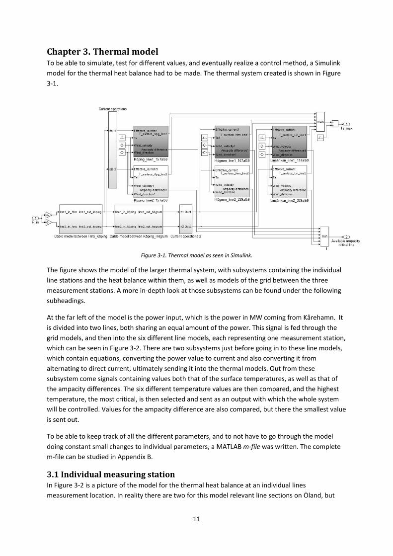
3.2 Grid model To simulate the grid on Öland, two blocks with line models were used, so that external power inputs,

representing different power generating stations or farms on Öland - and outputs, representing loads

- could easily be added to the model. What has been done in this model is basically adding the

external power and subtracting the external load. They were assumed to load each of the two lines

equally unless stated otherwise. The document [13] provided by E.ON, has been used as a reference

for determining how to construct these grid models. Figure 3-4 shows the grid model for northern

Öland.

14

Figure 3-4. [13] A simplified model of the grid on northern Öland.

In the figure, which is a simplified picture of the one found in [13], we can see all the locations on the

grid. The picture shows the grid upside down, meaning LIN is the furthest south, while BDA is the

furthest north. The green lines represents the connection of Kårehamn to Föra. The stations that are

relevant for surface temperature measurments in this thesis are KPG which is Köping, HRM which is

Högsrum, and LIN, which is Linsänkan. In truth, these sections are all relevant, as each location is a

load and/or contains some form of power generation.

From the same document, the value for all these external power generation units was also taken.

The maximal output for these were, which can also be seen in Appendix B, the following:

Wind power Löttorp: 3 MW

Wind power sid: 16 MW

Wind power Köping: unknown (assumed 0 MW)

Wind power Köping (O62 rail): 20 MW

Wind power Borgholm: 7.7 MW

Wind power Högsrum: 20 MW

15

These maximal output values were used throughout this thesis. It is impossible that these external

sources would output this power constantly, but since they increased the surface temperature if

anything and it was thought best to test something more considered worst case, rather than some

other lower number or mean output which wasn’t known.

As opposed to the wind power feeding the grid, the loads were chosen with a minimal value, for the

same reason the max values were chosen for the external power sources. According to the document

[14] provided by E.ON, the load on the line varies significantly during the year, even during shorter

time spans. The information provided in the document only highlighted the load in a section of the

line, rather than the local loads. To find out the local loads, and their minimum, a list was compiled

showcasing the difference in load at two sections, for example sections Linsänkan-Borgholm and

Borgholm-Köping. From that list the minimum value for the load was selected. This value was close

to 0 MW on all places. The exact values can be seen below, or in Appendix B.

Load Föra: 0 MW

Load Djupvik: 2.75*10-4 MW

Load sid: 0 MW

Load Köping line 1: 0.76 MW

Load Köping line 2: 2.09*10-3 MW

Load Borgholm: 7.55*10-4 MW

Load Högsrum: 1.65*10-3 MW

As stated, a constant maximum external power feeding the grid as well as a constant minimum load

on the grid is hardly plausible - but going forward, it was thought best to have this kind of worst case

setup and design the model and control such that it could better handle any difficulties that could

arise.

16

Chapter 4. Verification of thermal model For verification purposes, the model had to be tested. The first and most obvious way, was to verify it

against the many examples in [5]. During verification, a modified model of only one line was used,

without all other external loads and wind power, to simulate the line type used in the report as

accurately as possible.

4.1 Verification against CIGRE report The overhead cable used in all of these examples is the 428-A1/S1A-54/7 “ZEBRA”, which is a

conductor with a steel core, surrounded by aluminum.

Its characteristics are [5], [15]:

D = 28.6 mm

d = 3.18 mm

Rdc= 0.0674 Ω/km (at 20 °C)

To account for the fact that the cable is aluminum-clad with a steel core, the equation

was used, with the following values:

ma = 0.43 kg/m

ca = 481 J/(kg*K)

ms = 1.16 kg/m

cs = 897 J/(kg*K)

Characteristics that could not be found, were set according to the Öland case and its conductors.

Other values that had to be computed or changed for these tests were:

Gravity of earth: 9.807

Absorptivity of ZEBRA conductor: 0.500

Emissivity of ZEBRA conductor: 0.456

All temperature values and other values in their examples were calculated numerically, whereas the

answers produced by the model in this thesis were obtained visually, by looking at the relevant

graphs.

4.1.1 Surface temperature calculations for the steady state, example 1

This example calculated the surface temperature of the conductor, with the following parameters:

Global solar radiation: 980 W/m2

Wind speed: 2 m/s

Wind angle: 45 °

Ambient temperature: 40 °C

Height above sea level: 1600 m

Iac: 600 A

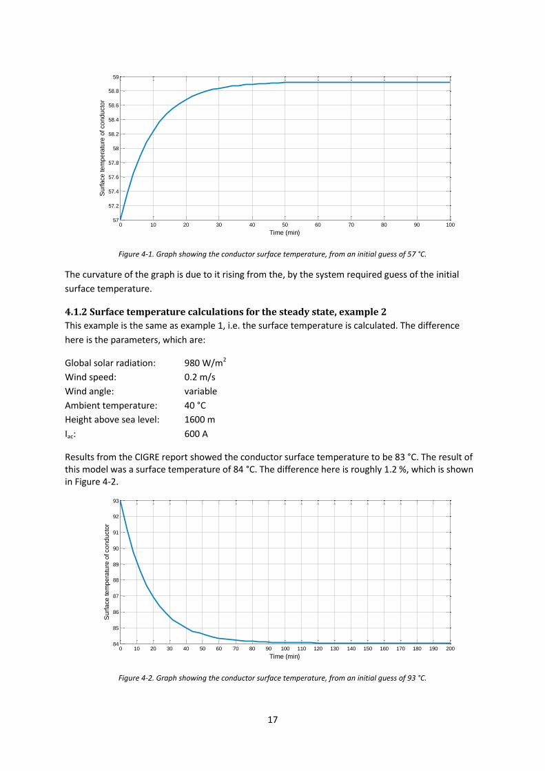
According to the example, the final surface temperature was ca. 58.5 °C. Results from the model showed a surface temperature of 58.9 °C, as shown in Figure 4-1. That’s a difference of less than 1 %.

17

Figure 4-1. Graph showing the conductor surface temperature, from an initial guess of 57 °C.

The curvature of the graph is due to it rising from the, by the system required guess of the initial

surface temperature.

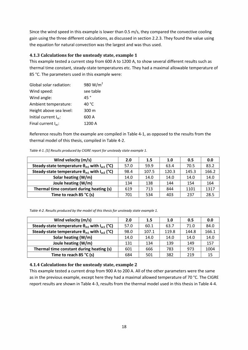
4.1.2 Surface temperature calculations for the steady state, example 2

This example is the same as example 1, i.e. the surface temperature is calculated. The difference

here is the parameters, which are:


Wind speed: 0.2 m/s

Wind angle: variable



Iac: 600 A

Results from the CIGRE report showed the conductor surface temperature to be 83 °C. The result of this model was a surface temperature of 84 °C. The difference here is roughly 1.2 %, which is shown in Figure 4-2.

Figure 4-2. Graph showing the conductor surface temperature, from an initial guess of 93 °C.

0 10 20 30 40 50 60 70 80 90 10057

57.2

57.4

57.6

57.8

58

58.2

58.4

58.6

58.8

59

Time (min)

Su

rfa

ce

te

mp

era

ture

of co

nd

ucto

r

0 10 20 30 40 50 60 70 80 90 100 110 120 130 140 150 160 170 180 190 20084

85

86

87

88

89

90

91

92

93

Time (min)

Su

rfa

ce

te

mp

era

ture

of co

nd

ucto

r

18

Since the wind speed in this example is lower than 0.5 m/s, they compared the convective cooling

gain using the three different calculations, as discussed in section 2.2.3. They found the value using

the equation for natural convection was the largest and was thus used.

4.1.3 Calculations for the unsteady state, example 1

This example tested a current step from 600 A to 1200 A, to show several different results such as

thermal time constant, steady-state temperatures etc. They had a maximal allowable temperature of

85 °C. The parameters used in this example were:


Wind speed: see table

Wind angle: 45 °



Initial current Iac: 600 A

Final current Iac: 1200 A

Reference results from the example are compiled in Table 4-1, as opposed to the results from the

thermal model of this thesis, compiled in Table 4-2.

Table 4-1. [5] Results produced by CIGRE report for unsteady state example 1.

Wind velocity (m/s) 2.0 1.5 1.0 0.5 0.0

Steady-state temperature θm1 with Iac1 (°C) 57.0 59.9 63.4 70.5 83.2


Solar heating (W/m) 14.0 14.0 14.0 14.0 14.0

Joule heating (W/m) 134 138 144 154 164

Thermal time constant during heating (s) 619 713 844 1101 1317

Time to reach 85 °C (s) 701 534 403 237 28.5

Table 4-2. Results produced by the model of this thesis for unsteady state example 1.

Wind velocity (m/s) 2.0 1.5 1.0 0.5 0.0



Solar heating (W/m) 14.0 14.0 14.0 14.0 14.0

Joule heating (W/m) 131 134 139 149 157

Thermal time constant during heating (s) 601 666 783 973 1004

Time to reach 85 °C (s) 684 501 382 219 15

4.1.4 Calculations for the unsteady state, example 2

This example tested a current drop from 900 A to 200 A. All of the other parameters were the same

as in the previous example, except here they had a maximal allowed temperature of 70 °C. The CIGRE

report results are shown in Table 4-3, results from the thermal model used in this thesis in Table 4-4.

19

Table 4-3. [5] Results produced by CIGRE report for unsteady state example 2.

Wind velocity (m/s) 2.0 1.5 1.0 0.5 0.0


P1 (W/m) 82.3 83.6 85.2 88.5 92.6

P2 (W/m) 17.0 17.0 17.0 17.0 17.0

Thermal time constant during cooling (s) 520 597 691 867 1071

Time to reach 70 °C (s) 57 190 380 824 1479

Table 4-4. Results produced by the model of this thesis for unsteady state example 1.

Wind velocity (m/s) 2.0 1.5 1.0 0.5 0.0


Thermal time constant during cooling (s) 525 586 693 875 1070

Time to reach 70 °C (s) 71 207 395 864 1909

4.1.5 Conclusion and discussion on verification

From what can be seen, the results from the first two tests, section 4.1.1 & 4.1.2 closely agrees with the result from the report. As mentioned, the curvature in Figure 4-1 and Figure 4-2 is just the surface temperature correcting from an initial guess. We can see that they have reached steady state temperatures after approximately 60 and 100 minutes respectively.

The results from example 1 and 2 in appendix 2 with the unsteady state however, differ quite a bit in

some aspects, notably the time it takes to reach the maximal allowable temperatures, as well as the

thermal time constants. As stated before, results from the thermal model were all obtained visually

whereas in the CIGRE report, they were all calculated numerically.

When it was calculated numerically as well with the steady state temperatures from simulation

results, the numbers much more closely resembled what their results showed - for example a

thermal time constant of 1125 and 1354 seconds, with wind speeds 0.5 and 0.0 respectively,

compare Table 4-1 and Table 4-2. Errors from visually obtaining the results were surely present, even

though they were carefully obtained, and would certainly not result in a difference of 10-30 % as it

was in a few cases. This could probably mean there is some error in the way the thermal time

constant is calculated, but when checked against the equations in sections 2.3 and 2.4, which were

taken from said report, the results were in line with its.

4.2 Testing the thermal model When the verification against the CIGRE report was completed and it was shown that the model of

the thermal heat balance worked as intended, it was time to modify its parameters and establish that

it would perform correctly or rather as expected, before moving forward and tailoring it around the

Kårehamn and Öland case. Two tests were carried out, both with changing power, a current step.

This was meant to resemble a change in the output from Kårehamn, as a way to see how the surface

temperature of the conductors, at all six stations, behaved.

4.2.1 Output change: 35- 48 MW, no loads

In this initial test, a power output increase from 35 MW to 48 MW was simulated, in which Kårehamn

goes from a less than maximal output, to full output. The location-specific parameters were taken

arbitrarily to resemble a normal spring or summer day and their values can be seen below, other

fixed parameters in the m-file in Appendix B. The initial guess for the temperature here was 40 °C.

20

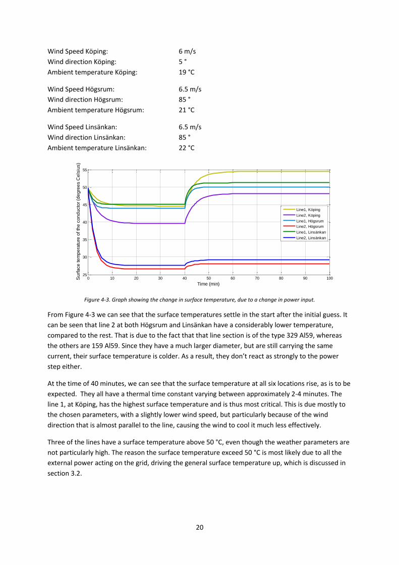
Wind Speed Köping: 6 m/s

Wind direction Köping: 5 °

Ambient temperature Köping: 19 °C

Wind Speed Högsrum: 6.5 m/s

Wind direction Högsrum: 85 °

Ambient temperature Högsrum: 21 °C

Wind Speed Linsänkan: 6.5 m/s

Wind direction Linsänkan: 85 °

Ambient temperature Linsänkan: 22 °C

Figure 4-3. Graph showing the change in surface temperature, due to a change in power input.

From Figure 4-3 we can see that the surface temperatures settle in the start after the initial guess. It

can be seen that line 2 at both Högsrum and Linsänkan have a considerably lower temperature,

compared to the rest. That is due to the fact that that line section is of the type 329 Al59, whereas

the others are 159 Al59. Since they have a much larger diameter, but are still carrying the same

current, their surface temperature is colder. As a result, they don’t react as strongly to the power

step either.

At the time of 40 minutes, we can see that the surface temperature at all six locations rise, as is to be

expected. They all have a thermal time constant varying between approximately 2-4 minutes. The

line 1, at Köping, has the highest surface temperature and is thus most critical. This is due mostly to

the chosen parameters, with a slightly lower wind speed, but particularly because of the wind

direction that is almost parallel to the line, causing the wind to cool it much less effectively.

Three of the lines have a surface temperature above 50 °C, even though the weather parameters are

not particularly high. The reason the surface temperature exceed 50 °C is most likely due to all the

external power acting on the grid, driving the general surface temperature up, which is discussed in

section 3.2.

0 10 20 30 40 50 60 70 80 90 10025

30

35

40

45

50

55

Time (min)

Su

rfa

ce

te

mp

era

ture

of th

e c

on

du

cto

r (d

eg

ree

s C

els

ius)

Line1, Köping

Line2, Köping

Line1, Högsrum

Line2, Högsrum

Line1, Linsänkan

Line2, Linsänkan

21

4.2.2 Output change: 48-0 MW, no loads

In this simulation, Kårehamn gets completely shut off. That means the output goes from 48 MW to 0

MW. The location-specific weather parameters used here were the same as in the previous

simulation.

Figure 4-4. Graph showing the change in surface temperature, due to a change in power input.

Here too, we can see the initial settling of the surface temperatures from the initial guess at the

start. They should be expected to have the same steady-state temperature as that of the lines in

Figure 4-3 after the power increase, as they do. After the power change at time 40 minutes, the

surface temperatures all drop, which is expected. One would expect they drop to about ambient

temperature when Kårehamn doesn’t deliver power. They don’t, and that is partly because of

external power feeding the grid.

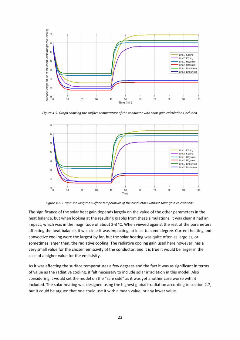
4.3 Impact of solar irradiation No solar irradiation measurement equipment is currently installed or planned to be installed at any

of the measurement locations. However, the thermal heat balance and the model use solar radiation

as part of its equations. This led to the question if it should be included in the model going forward at

all.

To get a better picture of the significance that solar radiation has on the surface temperature of the

overhead conductors using the simplified method in section 2.2.2, simulations with and without solar

heat gain were made. These simulation results can be seen in Figure 4-5 and Figure 4-6.

0 10 20 30 40 50 60 70 80 90 10020

25

30

35

40

45

50

55

Time (min)

Su

rfa

ce

te

mp

era

ture

of th

e c

on

du

cto

rs (

de

gre

es C

els

ius)

Line1, Köping

Line2, Köping

Line1, Högsrum

Line2, Högsrum

Line1, Linsänkan

Line2, Linsänkan

22

Figure 4-5. Graph showing the surface temperature of the conductor with solar gain calculations included.

Figure 4-6. Graph showing the surface temperature of the conductors without solar gain calculations.

The significance of the solar heat gain depends largely on the value of the other parameters in the

heat balance, but when looking at the resulting graphs from these simulations, it was clear it had an

impact; which was in the magnitude of about 2-3 °C. When viewed against the rest of the parameters

affecting the heat balance, it was clear it was impacting, at least to some degree. Current heating and

convective cooling were the largest by far, but the solar heating was quite often as large as, or

sometimes larger than, the radiative cooling. The radiative cooling gain used here however, has a

very small value for the chosen emissivity of the conductor, and it is true it would be larger in the

case of a higher value for the emissivity.

As it was affecting the surface temperatures a few degrees and the fact it was as significant in terms

of value as the radiative cooling, it felt necessary to include solar irradiation in this model. Also

considering it would set the model on the “safe side” as it was yet another case worse with it

included. The solar heating was designed using the highest global irradiation according to section 2.7,

but it could be argued that one could use it with a mean value, or any lower value.

0 10 20 30 40 50 60 70 80 90 10020

25

30

35

40

45

50

55

Time (min)

Su

rfa

ce

te

mp

era

ture

of th

e c

on

du

cto

rs (

de

gre

es C

els

ius)

Line1, Köping

Line2, Köping

Line1, Högsrum

Line2, Högsrum

Line1, Linsänkan

Line2, Linsänkan

0 10 20 30 40 50 60 70 80 90 10020

25

30

35

40

45

50

55

Time

Line1, Köping

Line2, Köping

Line1, Högsrum

Line2, Högsrum

Line1, Linsänkan

Line2, Linsänkan

23

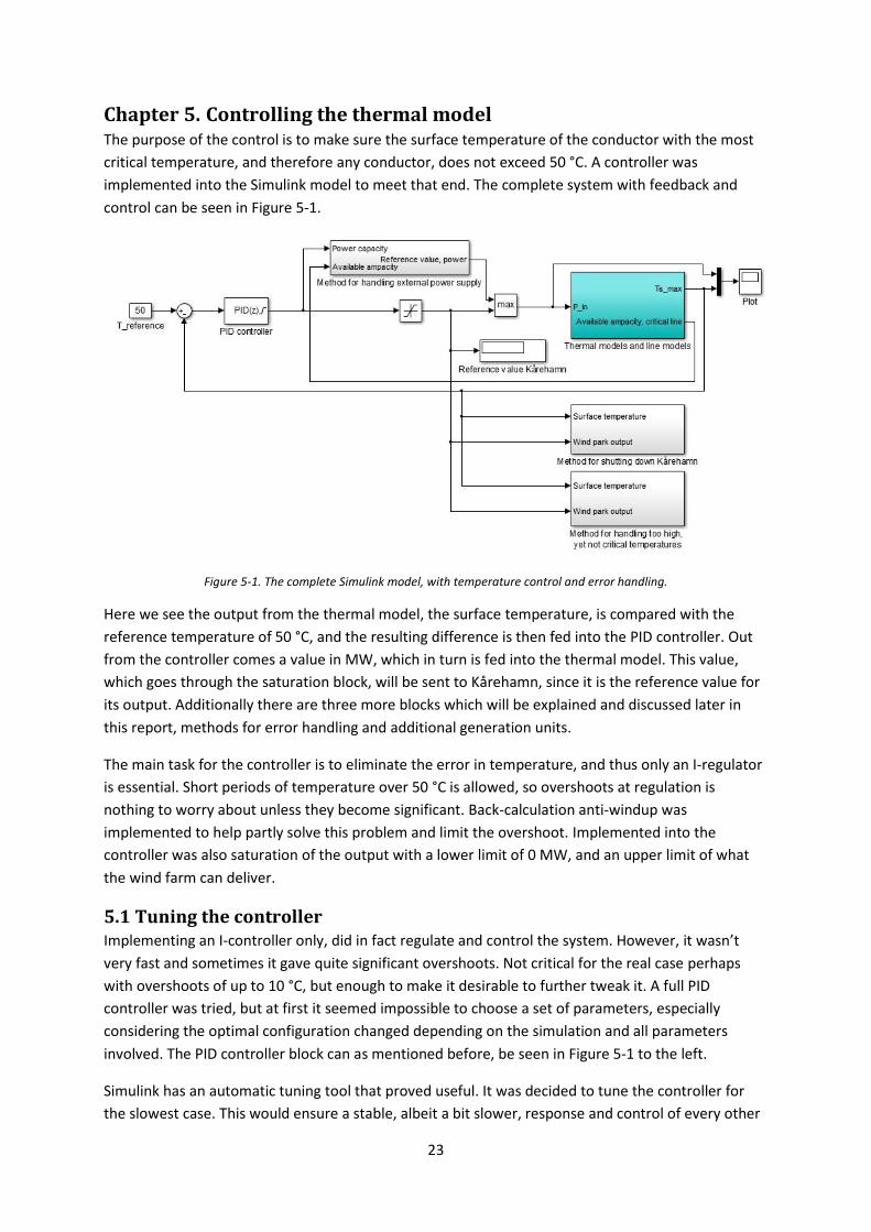
Chapter 5. Controlling the thermal model The purpose of the control is to make sure the surface temperature of the conductor with the most

critical temperature, and therefore any conductor, does not exceed 50 °C. A controller was

implemented into the Simulink model to meet that end. The complete system with feedback and

control can be seen in Figure 5-1.

Figure 5-1. The complete Simulink model, with temperature control and error handling.

Here we see the output from the thermal model, the surface temperature, is compared with the

reference temperature of 50 °C, and the resulting difference is then fed into the PID controller. Out

from the controller comes a value in MW, which in turn is fed into the thermal model. This value,

which goes through the saturation block, will be sent to Kårehamn, since it is the reference value for

its output. Additionally there are three more blocks which will be explained and discussed later in

this report, methods for error handling and additional generation units.

The main task for the controller is to eliminate the error in temperature, and thus only an I-regulator

is essential. Short periods of temperature over 50 °C is allowed, so overshoots at regulation is

nothing to worry about unless they become significant. Back-calculation anti-windup was

implemented to help partly solve this problem and limit the overshoot. Implemented into the

controller was also saturation of the output with a lower limit of 0 MW, and an upper limit of what

the wind farm can deliver.

5.1 Tuning the controller Implementing an I-controller only, did in fact regulate and control the system. However, it wasn’t

very fast and sometimes it gave quite significant overshoots. Not critical for the real case perhaps

with overshoots of up to 10 °C, but enough to make it desirable to further tweak it. A full PID

controller was tried, but at first it seemed impossible to choose a set of parameters, especially

considering the optimal configuration changed depending on the simulation and all parameters

involved. The PID controller block can as mentioned before, be seen in Figure 5-1 to the left.

Simulink has an automatic tuning tool that proved useful. It was decided to tune the controller for

the slowest case. This would ensure a stable, albeit a bit slower, response and control of every other

24

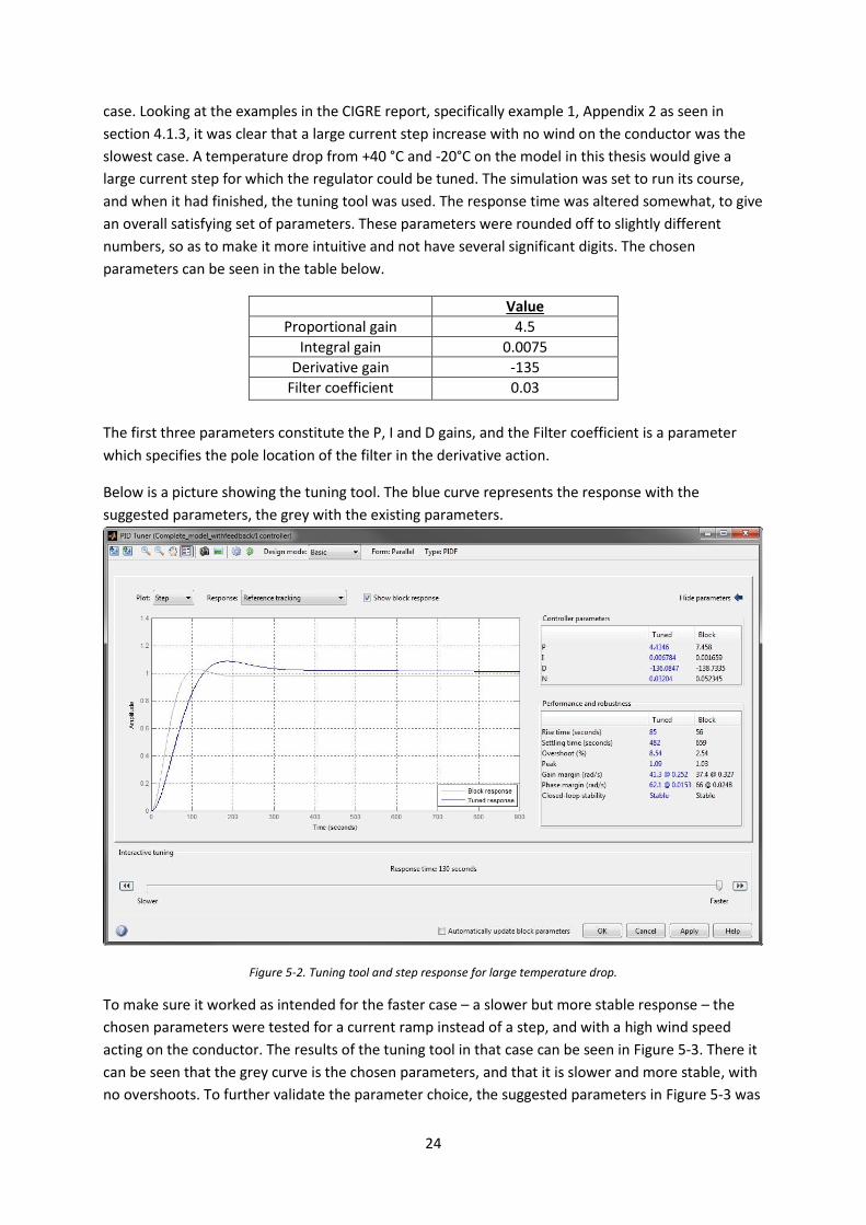
case. Looking at the examples in the CIGRE report, specifically example 1, Appendix 2 as seen in

section 4.1.3, it was clear that a large current step increase with no wind on the conductor was the

slowest case. A temperature drop from +40 °C and -20°C on the model in this thesis would give a

large current step for which the regulator could be tuned. The simulation was set to run its course,

and when it had finished, the tuning tool was used. The response time was altered somewhat, to give

an overall satisfying set of parameters. These parameters were rounded off to slightly different

numbers, so as to make it more intuitive and not have several significant digits. The chosen

parameters can be seen in the table below.

Value

Proportional gain 4.5

Integral gain 0.0075

Derivative gain -135

Filter coefficient 0.03

The first three parameters constitute the P, I and D gains, and the Filter coefficient is a parameter

which specifies the pole location of the filter in the derivative action.

Below is a picture showing the tuning tool. The blue curve represents the response with the

suggested parameters, the grey with the existing parameters.

Figure 5-2. Tuning tool and step response for large temperature drop.

To make sure it worked as intended for the faster case – a slower but more stable response – the

chosen parameters were tested for a current ramp instead of a step, and with a high wind speed

acting on the conductor. The results of the tuning tool in that case can be seen in Figure 5-3. There it

can be seen that the grey curve is the chosen parameters, and that it is slower and more stable, with

no overshoots. To further validate the parameter choice, the suggested parameters in Figure 5-3 was

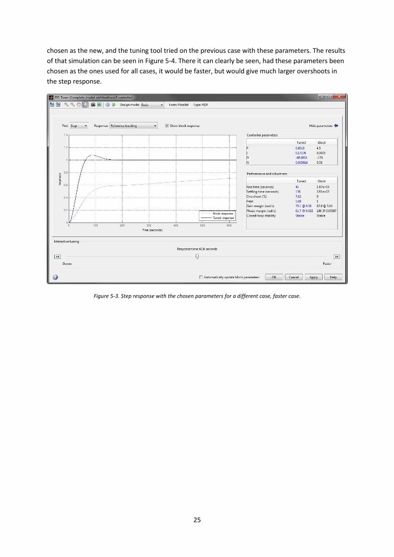
25

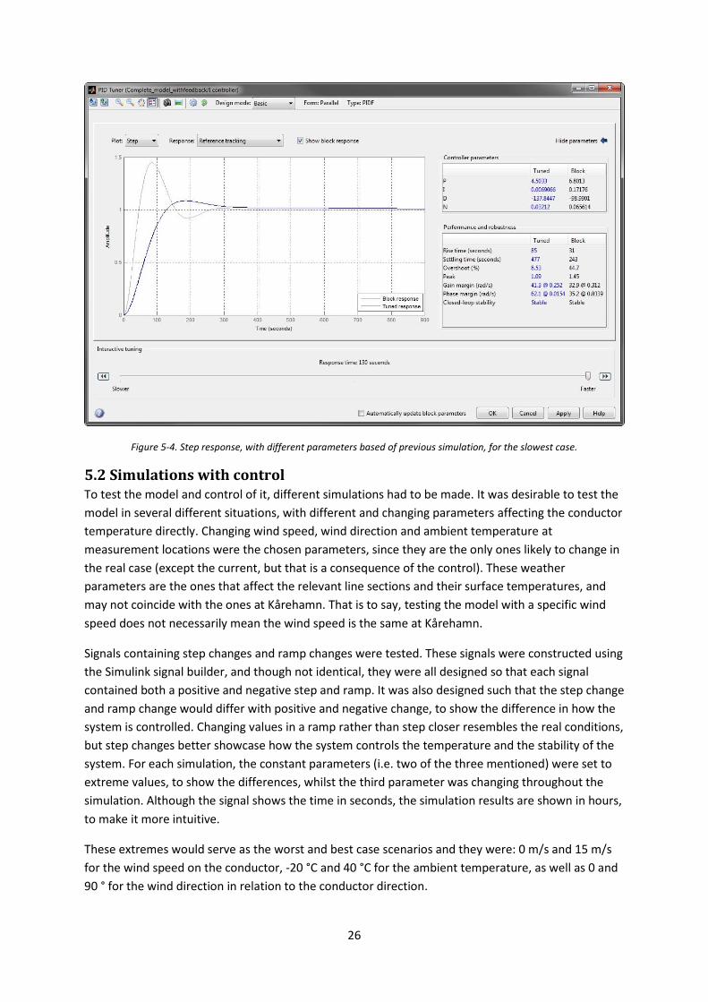
chosen as the new, and the tuning tool tried on the previous case with these parameters. The results

of that simulation can be seen in Figure 5-4. There it can clearly be seen, had these parameters been

chosen as the ones used for all cases, it would be faster, but would give much larger overshoots in

the step response.

Figure 5-3. Step response with the chosen parameters for a different case, faster case.

26

Figure 5-4. Step response, with different parameters based of previous simulation, for the slowest case.

5.2 Simulations with control To test the model and control of it, different simulations had to be made. It was desirable to test the

model in several different situations, with different and changing parameters affecting the conductor

temperature directly. Changing wind speed, wind direction and ambient temperature at

measurement locations were the chosen parameters, since they are the only ones likely to change in

the real case (except the current, but that is a consequence of the control). These weather

parameters are the ones that affect the relevant line sections and their surface temperatures, and

may not coincide with the ones at Kårehamn. That is to say, testing the model with a specific wind

speed does not necessarily mean the wind speed is the same at Kårehamn.

Signals containing step changes and ramp changes were tested. These signals were constructed using

the Simulink signal builder, and though not identical, they were all designed so that each signal

contained both a positive and negative step and ramp. It was also designed such that the step change

and ramp change would differ with positive and negative change, to show the difference in how the

system is controlled. Changing values in a ramp rather than step closer resembles the real conditions,

but step changes better showcase how the system controls the temperature and the stability of the

system. For each simulation, the constant parameters (i.e. two of the three mentioned) were set to

extreme values, to show the differences, whilst the third parameter was changing throughout the

simulation. Although the signal shows the time in seconds, the simulation results are shown in hours,

to make it more intuitive.

These extremes would serve as the worst and best case scenarios and they were: 0 m/s and 15 m/s

for the wind speed on the conductor, -20 °C and 40 °C for the ambient temperature, as well as 0 and

90 ° for the wind direction in relation to the conductor direction.

27

It should be reminded that these simulations not only include the power from Kårehamn which can

deliver no more than 48 MW, but also the external power generating units acting on the grid as well

as local loads that drive up the surface temperatures in many cases. This is further mentioned in the

relevant simulations.

5.2.1 Changing wind speed on the conductor

The signal used for simulating the changing of the wind speed while keeping both the wind direction

and ambient temperature at constant values can be seen in Figure 5-5.

Figure 5-5. Signal used to simulate varying wind speeds.

As can be seen, the signal starts with no wind and then goes up to 15 m/s in steps of 5 m/s. At time

8000 seconds, it again descends, this time in a step with smaller decrements. This process is later

repeated with a ramp change. This signal is built so that it is given time to stabilize at times 1000

seconds and 13000 seconds. That is because there the thermal model changes for the wind speed at

0.5 m/s, according to what is described in section 2.2.3. It is thus interesting to see how the model

behaves here.

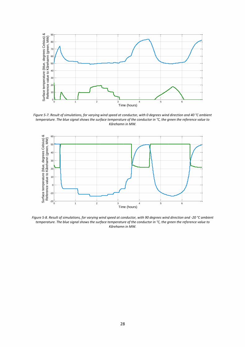
Figure 5-6. Result of simulations, for varying wind speed at conductor, with 0 degrees wind direction and -20 °C ambient temperature. The blue signal shows the surface temperature of the conductor in °C, the green the reference value to

Kårehamn in MW.

0 1 2 3 4 5 6-10

0

10

20

30

40

50

60

Time (hours)

Surf

ace tem

pera

ture

(blu

e, degre

es C

els

ius)

&R

efe

rence v

alu

e to K

åre

ham

n (

gre

en, M

W)

28

Figure 5-7. Result of simulations, for varying wind speed at conductor, with 0 degrees wind direction and 40 °C ambient temperature. The blue signal shows the surface temperature of the conductor in °C, the green the reference value to

Kårehamn in MW.

Figure 5-8. Result of simulations, for varying wind speed at conductor, with 90 degrees wind direction and -20 °C ambient temperature. The blue signal shows the surface temperature of the conductor in °C, the green the reference value to

Kårehamn in MW.

0 1 2 3 4 5 60

10

20

30

40

50

60

70

80

90

Time (hours)

Surf

ace tem

pera

ture

(blu

e, degre

es C

els

ius)

&R

efe

rence v

alu

e to K

åre

ham

n (

gre

en, M

W)

0 1 2 3 4 5 6-20

-10

0

10

20

30

40

50

60

Time (hours)

Surf

ace tem

pera

ture

(blu

e, degre

es C

els

ius)

&R

efe

rence v

alu

e to K

åre

ham

n (

gre

en, M

W)

29

Figure 5-9. Result of simulations, for varying wind speed at conductor, with 90 degrees wind direction and 40 °C ambient temperature. The blue signal shows the surface temperature of the conductor in °C, the green the reference value to

Kårehamn in MW.

From all the pictures above, we can see that the wind speed has a profound effect on the surface

temperature of the conductor. We can clearly see the temperature is highest with no or little wind,

right at the beginning as well as at around four hours into the simulation. This means the reference

value for Kårehamn is at its lowest, and in the cases with 40 °C ambient temperature, very low or

completely shut off. The two simulations with an ambient temperature of -20 °C have no problem

keeping the temperature within its regulation temperature, though the reference power value has to

adjust at times when the wind speed drops to 0.

We can also see in the cases with high ambient temperature, the surface temperature of the

conductors soars with little wind. This is, as stated many times before, due to external power on the

grid. There are no real surprises in these simulations, although the most interesting parts are when

the wind power crosses 0.5 m/s, which is especially apparent in Figure 5-6 at just before four hours,

five hours and just after six hours into the simulation.

5.2.2 Changing wind direction in relation to conductor

The signal used for simulating a change in the wind direction while keeping both the wind speed and

ambient temperature at constant values can be seen in Figure 5-10.

0 1 2 3 4 5 60

10

20

30

40

50

60

70

80

90

Time (hours)

Surf

ace tem

pera

ture

(blu

e, degre

es C

els

ius)

&R

efe

rence v

alu

e to K

åre

ham

n (

gre

en, M

W)

30

Figure 5-10. Signal used to simulate varying wind directions.

The signal used here starts with a positive ladder from 0 to 90 degrees, with 15 degrees increments.

Then it goes down to 0 degrees, in 30 degrees decrements. At the second half of the simulation there

are two ramp changes, with different inclinations.

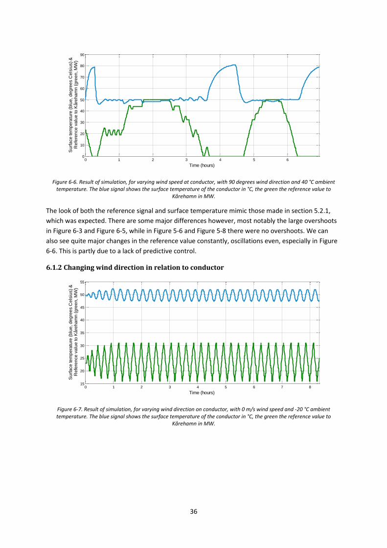
Figure 5-11. Result of simulation, for varying wind direction on conductor, with 15 m/s wind speed and 40 °C ambient temperature. The blue signal shows the surface temperature of the conductor in °C, the green the reference value to

Kårehamn in MW.

The simulations with changing wind direction showed that its impact is not quite as significant as the

wind speed on the conductor, though it definitely affects how effectively the wind cools the

conductor. The three first simulations; two with no wind and different ambient temperature, and

one with a wind speed of 15 m/s and -20 °C ambient temperature, are not shown in pictures, since

their results were uninteresting with pretty much steady state values regarding the reference value.

With no wind, the reference signal being sent to Kårehamn was either 24 MW or 0 MW, at -20 °C and

40 °C ambient temperature respectively. With full wind speed, and low temperature, the reference

value was at its maximum constantly.

Figure 5-11 is more interesting however, and we can clearly see the effect on the direction of the

wind cooling the conductor. As expected, the cooling effect of the wind is best when perpendicular

to the conductor. There is, except small overshoots at just before four and eight hours in the

0 1 2 3 4 5 6 7 820

25

30

35

40

45

50

55

Time (hours)

Surf

ace tem

pera

ture

(blu

e, degre

es C

els

ius)

&R

efe

rence v

alu

e to K

åre

ham

n (

gre

en, M

W)

31

simulation, no problem for the model to keep the surface temperature within regulation

temperature. It is also interesting to note the external power sources connecting and disconnecting,

visible shortly after seven hours.

5.2.3 Changing ambient temperature at conductor location

The signal used for simulating a change in the ambient temperature while keeping both the wind

speed and wind direction at constant values can be seen in Figure 5-12.

Figure 5-12. Signal used to simulate varying ambient temperature.

The signal and appearance of the signal for the ambient temperature should come as no surprise as it

is very similar to the two previous, albeit with a slightly higher inclination of the ramp changes.

Figure 5-13. Result of simulation, for varying ambient temperature at conductor, with 0 m/s wind speed and varying wind direction. The blue signal shows the surface temperature of the conductor in °C, the green the reference value to Kårehamn

in MW.

0 1 2 3 4 5 6 7 8 9 10 11 12 13 14 15 16 17 18 19 20 21 22 23 24 25 26 270

10

20

30

40

50

60

70

80

90

Time (hours)

Surf

ace tem

pera

ture

(blu

e, degre

es C

els

ius)

&R

efe

rence v

alu

e to K

åre

ham

n (

gre

en, M

W)

32

Figure 5-14. Result of simulation, for varying ambient temperature at conductor, with 15 m/s wind speed and 0 degrees wind direction. The blue signal shows the surface temperature of the conductor in °C, the green the reference value to

Kårehamn in MW.

Figure 5-15. Result of simulation, for varying ambient temperature at conductor, with 15 m/s wind speed and 90 degrees wind direction. The blue signal shows the surface temperature of the conductor in °C, the green the reference value to

Kårehamn in MW.

Figure 5-13 shows the simulation result when there is no wind. Varying the wind direction when

there is now wind, does not change anything. Therefore, those two first simulations produced the

same results. The two latter simulations share a similar appearance, and the effect of the wind

direction can clearly be seen. We can see that with a wind speed of 15 m/s, the ambient temperature

in this case becomes critical at about 30 °C, and then the reference value has to change. Additionally,

with a wind direction perpendicular to the conductor, Kårehamn is at its maximal output almost all

the time, except small dips between six and nine hours, which happens because of the derivative

part of the control, the system “braces” for a step change that could push the temperature up.

0 1 2 3 4 5 6 7 8 9 10 11 12 13 14 15 16 17 18 19 20 21 22 23 24 25 26 27-10

0

10

20

30

40

50

60

Time (hours)

Surf

ace tem

pera

ture

(blu

e, degre

es C

els

ius)

&R

efe

rence v

alu

e to K

åre

ham

n (

gre

en, M

W)

0 1 2 3 4 5 6 7 8 9 10 11 12 13 14 15 16 17 18 19 20 21 22 23 24 25 26 27-20

-10

0

10

20

30

40

50

60

Time (hours)

Surf

ace tem

pera

ture

(blu

e, degre

es C

els

ius)

&R

efe

rence v

alu

e to K

åre

ham

n (

gre

en, M

W)

33

Chapter 6. Alternative incremental control A secondary objective in this thesis was the modeling of an alternative control method currently used

by E.ON, where the surface temperature would be controlled by changing the reference signal in

steps, with a set wait time between changes. There were several different flowcharts given; for

controlling the current, the temperature as well as handling errors. Since this thesis and the model

are limited to controlling the temperature, it was natural to test only their temperature regulation.

Current control would be similar, just with a different setup in the model so that the ampacity and

ampacity difference would be controlled, i.e. as input into the PID controller.

The method of this control was that the reference value to Kårehamn should be changed in small

increments - as opposed to continuously changing as in the controller developed in this thesis - whilst

waiting a set period of time in between reference value changes so that they could be sent and to

allow for the temperature to change. By default, the number by which the reference value was to be

changed each iteration, was 1 MW with a 30 second delay between changes. The modified system to

accommodate this can be seen below, in Figure 6-1.

Figure 6-1. The complete Simulink model based with alternate control.

The difference between this model and the main regulated model in Figure 5-1 is the addition of the

subsystem named “Relational Operators”, as well as an integrator. The Relational Operators

subsystem can be seen in Figure 6-2. The flowchart stated that only when the temperature is higher

than 50 °C or lower than 49.5 °C, the regulation be instated. That is what this subsystem checks; if

the temperature needs to be corrected. If the surface temperature is below 49.5 °C it outputs 1 and

if it is higher than 50 °C, -1. This number, 1 or -1, is then fed into the integrator, which in turn

changes the reference value by a positive or negative increment. Inside the integrator, both the size

of the change of the reference value and the wait time is given. The minus 1 mathematical operation

in Figure 6-1 is because the integrator had to be given a lower saturation limit of 1 instead of 0 to

avoid an error.

34

Figure 6-2. Subsystem with relational operators for handling changes in reference value.

6.1 Simulations The purpose of implementing the alternative control method was to test it against the continuously

regulated system built for this thesis. Therefore, it was natural to run the same type of simulations

on the model in Figure 6-1, as those done in section 5.2. The three signals used in simulations can be

seen in chapter 5 (Figure 5-5, Figure 5-10 & Figure 5-12).

6.1.1 Changing wind speed on the conductor

Figure 6-3. Result of simulation, for varying wind speed at conductor, with 0 degrees wind direction and -20 °C ambient temperature. The blue signal shows the surface temperature of the conductor in °C, the green the reference value to

Kårehamn in MW.

0 1 2 3 4 5 6-10

0

10

20

30

40

50

60

70

Time (hours)

Su

rfa

ce

te

mp

era

ture

(b

lue

, d

eg

ree

s C

els

ius)

&R

efe

ren

ce

va

lue

to

Kå

reh

am

n (

gre

en

, M

W)

35

Figure 6-4. Result of simulation, for varying wind speed at conductor, with 0 degrees wind direction and 40 °C ambient temperature. The blue signal shows the surface temperature of the conductor in °C, the green the reference value to

Kårehamn in MW.

Figure 6-5. Result of simulation, for varying wind speed at conductor, with 90 degrees wind direction and -20 °C ambient temperature. The blue signal shows the surface temperature of the conductor in °C, the green the reference value to

Kårehamn in MW.

0 1 2 3 4 5 60

10

20

30

40

50

60

70

80

90

Time (hours)

Su

rfa

ce

te

mp

era

ture

(b

lue

, d

eg

ree

s C

els

ius)

&R

efe

ren

ce

va

lue

to

Kå

reh

am

n (

gre

en

, M

W)

0 1 2 3 4 5 6-20

-10

0

10

20

30

40

50

60

70

Time (hours)

Su

rfa

ce

te

mp

era

ture

(b

lue

, d

eg

ree

s C

els

ius)

&R

efe

ren

ce

va

lue

to

Kå

reh

am

n (

gre

en

, M

W)

36

Figure 6-6. Result of simulation, for varying wind speed at conductor, with 90 degrees wind direction and 40 °C ambient temperature. The blue signal shows the surface temperature of the conductor in °C, the green the reference value to

Kårehamn in MW.

The look of both the reference signal and surface temperature mimic those made in section 5.2.1,

which was expected. There are some major differences however, most notably the large overshoots

in Figure 6-3 and Figure 6-5, while in Figure 5-6 and Figure 5-8 there were no overshoots. We can

also see quite major changes in the reference value constantly, oscillations even, especially in Figure

6-6. This is partly due to a lack of predictive control.

6.1.2 Changing wind direction in relation to conductor

Figure 6-7. Result of simulation, for varying wind direction on conductor, with 0 m/s wind speed and -20 °C ambient temperature. The blue signal shows the surface temperature of the conductor in °C, the green the reference value to

Kårehamn in MW.

0 1 2 3 4 5 60

10

20

30

40

50

60

70

80

90

Time (hours)

Su

rfa

ce

te

mp

era

ture

(b

lue

, d

eg

ree

s C

els

ius)

&R

efe

ren

ce

va

lue

to

Kå

reh

am

n (

gre

en

, M

W)

0 1 2 3 4 5 6 7 815

20

25

30

35

40

45

50

55

Time (hours)

Su

rfa

ce

te

mp

era

ture

(b

lue

, d

eg

ree

s C

els

ius)

&R

efe

ren

ce

va

lue

to

Kå

reh

am

n (

gre

en

, M

W)

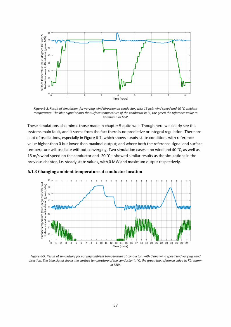
37

Figure 6-8. Result of simulation, for varying wind direction on conductor, with 15 m/s wind speed and 40 °C ambient temperature. The blue signal shows the surface temperature of the conductor in °C, the green the reference value to

Kårehamn in MW.

These simulations also mimic those made in chapter 5 quite well. Though here we clearly see this

systems main fault, and it stems from the fact there is no predictive or integral regulation. There are

a lot of oscillations, especially in Figure 6-7, which shows steady-state conditions with reference

value higher than 0 but lower than maximal output; and where both the reference signal and surface

temperature will oscillate without converging. Two simulation cases – no wind and 40 °C, as well as

15 m/s wind speed on the conductor and -20 °C – showed similar results as the simulations in the

previous chapter, i.e. steady state values, with 0 MW and maximum output respectively.

6.1.3 Changing ambient temperature at conductor location

Figure 6-9. Result of simulation, for varying ambient temperature at conductor, with 0 m/s wind speed and varying wind direction. The blue signal shows the surface temperature of the conductor in °C, the green the reference value to Kårehamn

in MW.

0 1 2 3 4 5 6 7 815

20

25

30

35

40

45

50

55

Time (hours)

Su

rfa

ce

te

mp

era

ture

(b

lue

, d

eg

ree

s C

els

ius)

&R

efe

ren

ce

va

lue

to

Kå

reh

am

n (

gre

en

, M

W)

0 1 2 3 4 5 6 7 8 9 10 11 12 13 14 15 16 17 18 19 20 21 22 23 24 25 26 270

10

20

30

40

50

60

70

80

90

Time (hours)

Su

rfa

ce

te

mp

era

ture

(b

lue

, d

eg

ree

s C

els

ius)

&R

efe

ren

ce

va

lue

to

Kå

reh

am

n (

gre

en

, M

W)

38

Figure 6-10. Result of simulation, for varying ambient temperature at conductor, with 15 m/s wind speed and 0 degrees direction. The blue signal shows the surface temperature of the conductor in °C, the green the reference value to Kårehamn

in MW.

Figure 6-11. Result of simulation, for varying ambient temperature at conductor, with 15 m/s wind speed and 90 degrees direction. The blue signal shows the surface temperature of the conductor in °C, the green the reference value to Kårehamn

in MW.

Here it again becomes apparent that this model can’t converge, as both signals oscillate. In Figure

6-11 we do see a positive effect of this model however, in that the reference value stays at a

constant max, as opposed to Figure 5-15 in section 5.2.3, where the reference value signal had slight

dips between six and eight hours in. This is because the surface temperature doesn’t exceed 49.5 °C,

thus not triggering any control action.

0 1 2 3 4 5 6 7 8 9 10 11 12 13 14 15 16 17 18 19 20 21 22 23 24 25 26 27-10

0

10

20

30

40

50

60

Time (hours)

Su

rfa

ce

te

mp

era

ture

(b

lue

, d

eg

ree

s C

els

ius)

&R

efe

ren

ce

va

lue

to

Kå

reh

am

n (

gre

en

, M

W)

0 1 2 3 4 5 6 7 8 9 10 11 12 13 14 15 16 17 18 19 20 21 22 23 24 25 26 27-20

-10

0

10

20

30

40

50

60

Time (hours)

Su

rfa

ce

te

mp

era

ture

(b

lue

, d

eg

ree

s C

els

ius)

&R

efe

ren

ce

va

lue

to

Kå

reh

am

n (

gre

en

, M

W)

39

Chapter 7. Secondary aims As stated in section 1.2, it was also the aim of this thesis to implement error handling in different

ways. This included not just errors in the system, but also to find a way to handle the additional

generation units, which in this case is a solar power unit and a wind power unit.

Controlling these additional units would be done by sending them a binary signal, telling them if they

were allowed to be connected to the grid or not.

The control of the output of Kårehamn by this model will not be needed most of the time, according

to E.ON themselves [4] and also seen when looking at the simulation results during this thesis,

especially in Figure 4-3 and Figure 4-4 ,which are meant to resemble a normal case. Some of the

temperatures are driven up because of the external power and configurations in the model, but they

still support that the model would ideally not be used during normal operations.

When the surface temperature of the conductor gets too high however and the model needs to

regulate, it is expected to work and reduce the output of the wind turbines. Should it not work – if

the turbines don’t respond to the signal sent by the model or any other similar error – there must be

steps taken so that the surface temperatures of the conductors does not reach critical levels. These

include the ability to instead send signals with preset values as reference values if the temperature

gets too high but not yet critical; and the ability to send a signal for a hard shut-off signal should the

temperature reach critical levels.

7.1 Additional solar and wind power generation units The power generation sites in question lie north of Föra, and they feed the grid from there. As stated,

it is desirable to be able to send a signal, telling them if they can be connected or not. They are

private units connected to the grid, and not necessarily delivering power at all times which means

their priority as opposed to Kårehamn is lower. This means they should be the first to be

disconnected in the case of too high a surface temperature, and subsequently be the last to be

connected again. Only when Kårehamn is at unlimited operation and there is room for more power,

should they be allowed to be connected to the grid.

To be able to meet that criterion, two parts were added to the model in Figure 5-1. The subsystem

block called “Subsystem for handling external power”, and several different mathematical operations

to calculate the ampacity as well as the ampacity difference. The ampacity calculations are briefly

shown and explained in chapter 3. The reason for calculating the difference is the idea that there is a

capacity surplus when the surface temperature is below 50 °C yielding a positive ampacity difference,

a difference that decreases to 0 when the temperature reaches 50 °C. The most critical line and

measurement station thus has the smallest ampacity difference, and it is that number that is being

used and that will determine if it is okay to have the additional power connected to the grid.

The subsystem for handling the additional power can be seen below in Figure 7-1:

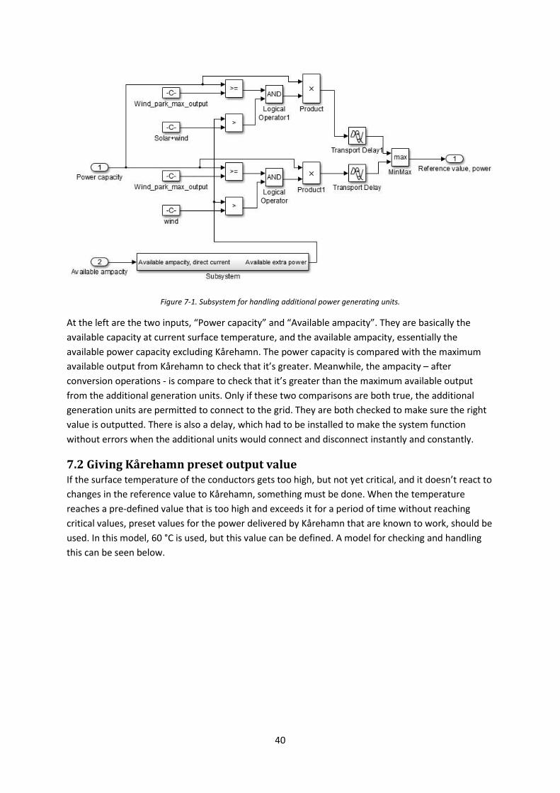
40

Figure 7-1. Subsystem for handling additional power generating units.

At the left are the two inputs, “Power capacity” and “Available ampacity”. They are basically the

available capacity at current surface temperature, and the available ampacity, essentially the

available power capacity excluding Kårehamn. The power capacity is compared with the maximum

available output from Kårehamn to check that it’s greater. Meanwhile, the ampacity – after

conversion operations - is compare to check that it’s greater than the maximum available output

from the additional generation units. Only if these two comparisons are both true, the additional

generation units are permitted to connect to the grid. They are both checked to make sure the right

value is outputted. There is also a delay, which had to be installed to make the system function

without errors when the additional units would connect and disconnect instantly and constantly.

7.2 Giving Kårehamn preset output value If the surface temperature of the conductors gets too high, but not yet critical, and it doesn’t react to

changes in the reference value to Kårehamn, something must be done. When the temperature

reaches a pre-defined value that is too high and exceeds it for a period of time without reaching

critical values, preset values for the power delivered by Kårehamn that are known to work, should be

used. In this model, 60 °C is used, but this value can be defined. A model for checking and handling

this can be seen below.

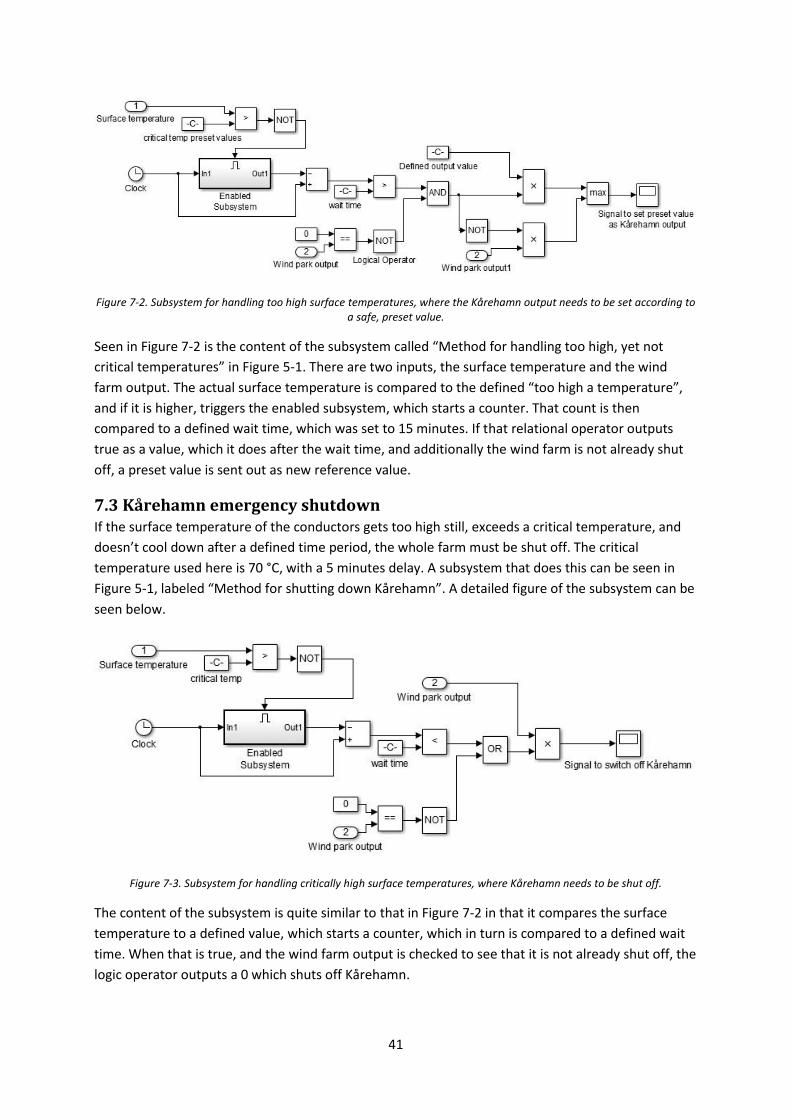
41

Figure 7-2. Subsystem for handling too high surface temperatures, where the Kårehamn output needs to be set according to a safe, preset value.

Seen in Figure 7-2 is the content of the subsystem called “Method for handling too high, yet not

critical temperatures” in Figure 5-1. There are two inputs, the surface temperature and the wind

farm output. The actual surface temperature is compared to the defined “too high a temperature”,

and if it is higher, triggers the enabled subsystem, which starts a counter. That count is then

compared to a defined wait time, which was set to 15 minutes. If that relational operator outputs

true as a value, which it does after the wait time, and additionally the wind farm is not already shut

off, a preset value is sent out as new reference value.

7.3 Kårehamn emergency shutdown If the surface temperature of the conductors gets too high still, exceeds a critical temperature, and

doesn’t cool down after a defined time period, the whole farm must be shut off. The critical

temperature used here is 70 °C, with a 5 minutes delay. A subsystem that does this can be seen in

Figure 5-1, labeled “Method for shutting down Kårehamn”. A detailed figure of the subsystem can be

seen below.

Figure 7-3. Subsystem for handling critically high surface temperatures, where Kårehamn needs to be shut off.

The content of the subsystem is quite similar to that in Figure 7-2 in that it compares the surface

temperature to a defined value, which starts a counter, which in turn is compared to a defined wait

time. When that is true, and the wind farm output is checked to see that it is not already shut off, the

logic operator outputs a 0 which shuts off Kårehamn.

42

7.4 Commissioning – Kårehamn The wind farm is expected to be commissioned in late 2013. The wind turbines themselves will be

installed during a period of time, so it desirable to be able to test the model built in this thesis on

only one wind turbine initially to determine its effectiveness and that it works.

Since the model is built around the complete farm with an output of 48 MW though, adjustments

would have to be made. An easy way of implementing this, given the time constraints and the fact

that this was not the primary goal of the thesis, would be to simply adjust the power to and from

Kårehamn. Upon completion, Kårehamn will comprise of 16 separate 3 MW wind turbines, which

means the power values could simply be adjusted a factor 16 so that the system could be tested on

one wind turbine initially. This would also mean the current - converted from the wind farm power

output – through the line, had to be scaled up in the control model, so the regulator would function

correctly, since only adjusting the power output by a factor 16, would not affect the thermal model

in a way that the surface temperature would reach high enough values.

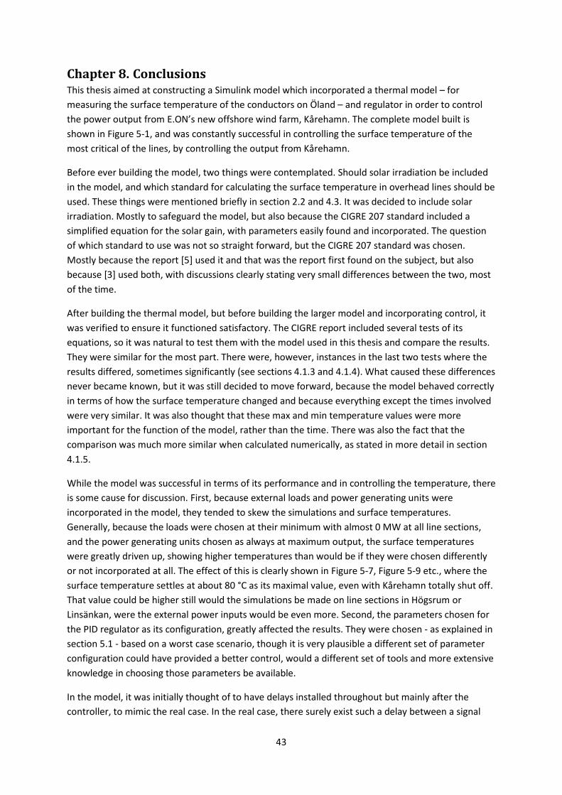
43

Chapter 8. Conclusions This thesis aimed at constructing a Simulink model which incorporated a thermal model – for

measuring the surface temperature of the conductors on Öland – and regulator in order to control

the power output from E.ON’s new offshore wind farm, Kårehamn. The complete model built is

shown in Figure 5-1, and was constantly successful in controlling the surface temperature of the

most critical of the lines, by controlling the output from Kårehamn.

Before ever building the model, two things were contemplated. Should solar irradiation be included

in the model, and which standard for calculating the surface temperature in overhead lines should be

used. These things were mentioned briefly in section 2.2 and 4.3. It was decided to include solar

irradiation. Mostly to safeguard the model, but also because the CIGRE 207 standard included a

simplified equation for the solar gain, with parameters easily found and incorporated. The question

of which standard to use was not so straight forward, but the CIGRE 207 standard was chosen.

Mostly because the report [5] used it and that was the report first found on the subject, but also

because [3] used both, with discussions clearly stating very small differences between the two, most

of the time.

After building the thermal model, but before building the larger model and incorporating control, it

was verified to ensure it functioned satisfactory. The CIGRE report included several tests of its

equations, so it was natural to test them with the model used in this thesis and compare the results.

They were similar for the most part. There were, however, instances in the last two tests where the

results differed, sometimes significantly (see sections 4.1.3 and 4.1.4). What caused these differences

never became known, but it was still decided to move forward, because the model behaved correctly

in terms of how the surface temperature changed and because everything except the times involved

were very similar. It was also thought that these max and min temperature values were more

important for the function of the model, rather than the time. There was also the fact that the

comparison was much more similar when calculated numerically, as stated in more detail in section

4.1.5.

While the model was successful in terms of its performance and in controlling the temperature, there

is some cause for discussion. First, because external loads and power generating units were

incorporated in the model, they tended to skew the simulations and surface temperatures.

Generally, because the loads were chosen at their minimum with almost 0 MW at all line sections,

and the power generating units chosen as always at maximum output, the surface temperatures

were greatly driven up, showing higher temperatures than would be if they were chosen differently

or not incorporated at all. The effect of this is clearly shown in Figure 5-7, Figure 5-9 etc., where the

surface temperature settles at about 80 °C as its maximal value, even with Kårehamn totally shut off.

That value could be higher still would the simulations be made on line sections in Högsrum or

Linsänkan, were the external power inputs would be even more. Second, the parameters chosen for

the PID regulator as its configuration, greatly affected the results. They were chosen - as explained in

section 5.1 - based on a worst case scenario, though it is very plausible a different set of parameter

configuration could have provided a better control, would a different set of tools and more extensive

knowledge in choosing those parameters be available.

In the model, it was initially thought of to have delays installed throughout but mainly after the

controller, to mimic the real case. In the real case, there surely exist such a delay between a signal

44

sent from the model, to an actual, physical change in the wind turbines output. Such delays were not

included in the model however, as the placement and magnitude of the delays could not be easily

decided. It is worth mentioning here though.

During the building and testing of the alternative incremental control design in chapter 6, there were

no real surprises. The model functioned correctly, and controlled the surface temperature based on

the Kårehamn output. There were however, several concerns. The biggest concern was the fact that

it was oscillating at steady-state temperature, which would certainly cause stress on the wind

turbines as the reference signal varied as wildly as up to 15-20 MW in some cases, albeit with

relatively small temperature variations. The second concern was the parameters in the integrator, or

more generally, the wait time between output changes, and the size of the output changes. These

parameters directly affected the model’s performance, and also the severity of the oscillations.

Default values were 30 seconds and 1 MW respectively. Higher output change and/or lower wait

time would make the control faster with generally smaller overshoots, but would cause more severe

oscillations in the reference output value. Lower output change and/or higher wait time on the other

hand, would make the control slower with more severe overshoots, but would limit the degree of

oscillations, sometimes even eliminating them.

When comparing the two control algorithms, that of this thesis’ and that of the alternative

incremental one, it was clear the one constructed here is better. Its main drawbacks are described

above, and the simulations clearly confirm that the controller constructed here is superior. This is

evident when viewing the simulations made for the two methods. Looking at Figure 6-7 or comparing

Figure 5-13 and Figure 6-9, it can be seen that the alternative control method oscillates greatly. And

when comparing Figure 5-6 and Figure 6-3 for example, the lack of predictive regulations mean the

alternative control creates major overshoots that are almost non-existent in the model used in this

thesis.

Lastly, there was some cause for concern about the two additional power generating units discussed

in section 7.1. As stated, this model simply checked if Kårehamn was at its maximum output and if

there was enough available ampacity. There were no real smart system, and in several cases, they

would be connected to the model, only to drive up the surface temperature to the degree they

would have to be immediately disconnected, after which they were connected again, and so on. A

model with some sort of predictive element or some sort of wait time after being connected or

disconnected would possibly solve this problem.

45

Chapter 9. Continued Work While this model is very much complete and functional in the task defined for it, there is room for

improvement in some aspects. These mainly regard the PID controller and the method for handling

the additional generation units on the grid.

As discussed briefly in the conclusion, there is almost certainly a better configuration for the

parameters in the PID controller, and if one were to have better tools or more extensive knowledge,

it could surely be improved upon.

Regarding the additional wind and solar power; the main problem is the lack of any predictive

element, which (as discussed in the conclusion) would cause these power generating units to be

connected and immediately disconnected, only to immediately be connected again, until changes in

external parameters changed the surface temperature in either direction. A delay of some sort could

possibly be installed, to partly solve this problem.

It would have been desirable to implement some sort of method for verifying the incoming data, the

weather parameters as well as the current and surface temperature measured at the three line

sections; however there was no time to develop such a method. The weather parameters could

possibly be compared to nearby weather stations if such exist. One could also compare the values for

the data received at both Linsänkan and Högsrum, because they lie very close to each other

geographically, their measured data should be very similar. This would definitely be ground for

further work.

46

References *1+. B. Lundkvist et al., ”Energiläget 2012”, Energimyndigheten, Eskilstuna, Oct. 2012.

[2]. Stadsrådsberedningen. (2005, March 16). Europa 2020 – EU:s gemensamma tillväxt- och

sysselsättningsstrategi [Online]. Available: http://www.regeringen.se/sb/d/2504

[3]. AREVA, “MiCOM P341, Dynamic Line Rating Protection Relay”, Application Guide, AREVA, 2010.

[4]. C. Ahlrot, E.ON, private communication, January 2013.

[5]. Working Group 22.12, “Thermal behaviour of overhead conductors”, Technical brochure #207,

CIGRE, 2002.

*6+. IEEE Power Engineering Society, “IEEE Standard for Calculating the Current-Temperature of Bare

Overhead Conductors”, Standard 738, IEEE, Jan. 2013.

*7+. British Standards, “Electric cables – Calculations of the current rating”, IEC 60287, British

Standards, July 2002.

[8]. European Commission Joint Research Centre, Institute for Energy and Transport. PV potential

estimation utility [Online]. Available: http://re.jrc.ec.europa.eu/pvgis/apps4/pvest.php

[9]. The Engineering Toolbox. Surface Absorptivities [Online]. Available:

http://www.engineeringtoolbox.com/radiation-surface-absorptivitie-d_1805.html

[10]. The Engineering Toolbox. Emissivity Coefficients of some common Materials [Online]. Available:

http://www.engineeringtoolbox.com/emissivity-coefficients-d_447.html

[11]. C. Ahlrot, private communication, February 2013.

[12]. Google. (2010). Google höjdkarta [Online]. Available: http://www.sk6lk.se/elev_path.html

[13]. C. Ahlrot, E.ON, private communication, February 2013.

[14]. C. Ahlrot, E.ON, private communication, May 2013.

[15]. KHCK. BARE CONDUCTOR AND WIRES [online]. Available:

http://www.khck.hk/Catalog/ENERGY&POWER-PRODUCT/Power-Equipment/bare-conductor-and-

wires.pdf

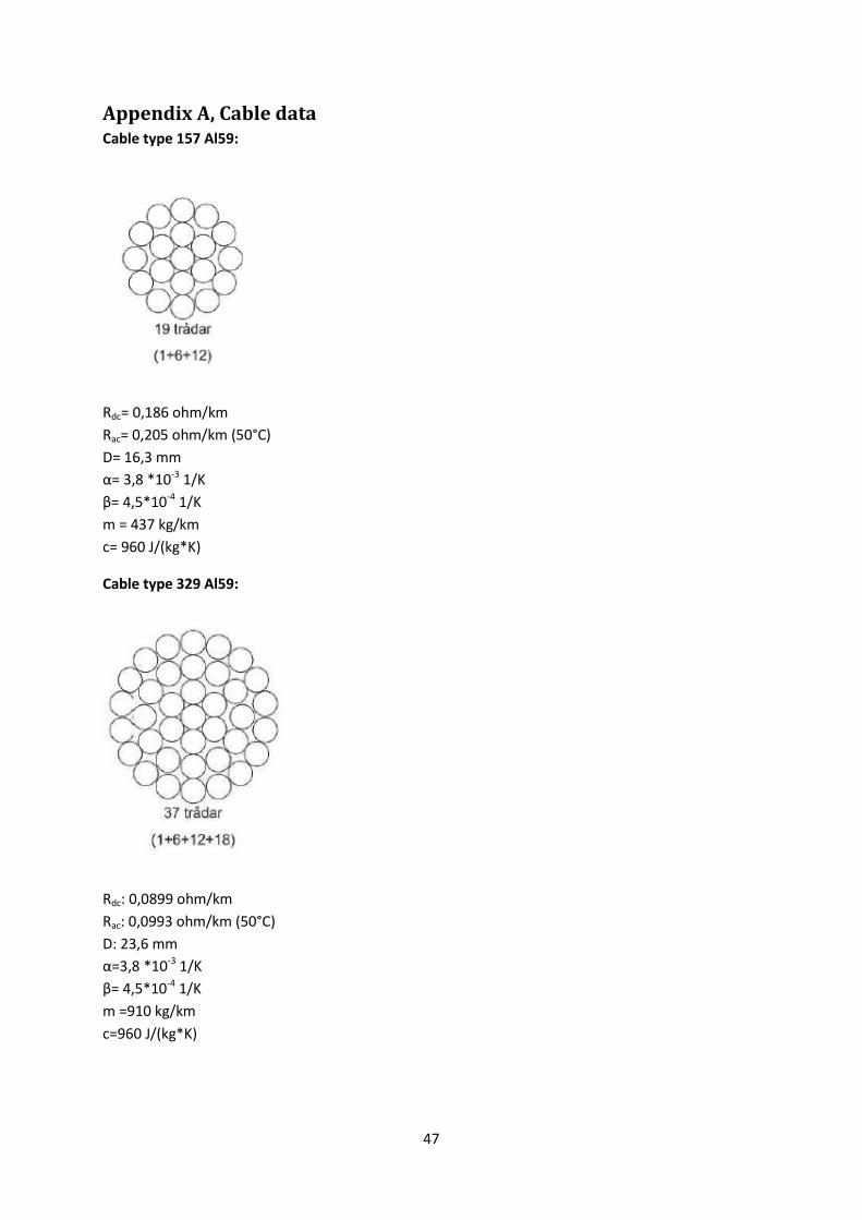
47

Appendix A, Cable data Cable type 157 Al59:

Rdc= 0,186 ohm/km

Rac= 0,205 ohm/km (50°C)

D= 16,3 mm

α= 3,8 *10-3 1/K

β= 4,5*10-4 1/K

m = 437 kg/km

c= 960 J/(kg*K)

Cable type 329 Al59:

Rdc: 0,0899 ohm/km

Rac: 0,0993 ohm/km (50°C)

D: 23,6 mm

α=3,8 *10-3 1/K

β= 4,5*10-4 1/K

m =910 kg/km

c=960 J/(kg*K)

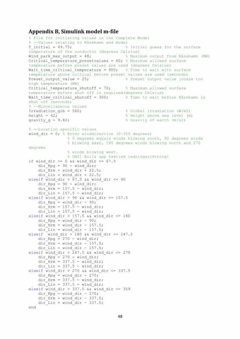
48

Appendix B, Simulink model m-file % File for initiating values in the Complete Model % --Values relating to Kårehamn and model T_initial = 49.75; % Initial guess for the surface

temperature of the conductor (degrees Celsius) Wind_park_max_output = 48; % Maximum output from Kårehamn (MW) Critical_temperature_presetvalues = 60; % Maximum allowed surface

temperature before preset values are used (degrees Celsius) Wait_time_critical_temperature = 900; % Time to wait with surface

temperature above critical before preset values are used (seconds) Preset_output_value = 25; % Preset output value incase too

high temperature (MW) Critical_temperature_shutoff = 70; % Maximum allowed surface

temperature before shut off is required(degrees Celsius) Wait_time_critical_shutoff = 300; % Time to wait before Kårehamn is

shut off (seconds) % --Miscellaneous values Irradiation_glb = 560; % Global irradiation (W/m2) height = 42; % Height above sea level (m) gravity_g = 9.82; % Gravity of earth (m/s2)

% --Location specific values wind_dir = 0; % Enter winddirection (0-359 degrees) % 0 degrees equals winds blowing south, 90 degrees winds % blowing east, 180 degrees winds blowing north and 270

degrees % winds blowing west. % OBS! Kolla upp faktisk ledningsriktning! if wind_dir >= 0 && wind_dir <= 67.5 dir_Kpg = 90 - wind_dir; dir_Hrm = wind_dir + 22.5; dir_Lin = wind_dir + 22.5; elseif wind_dir > 67.5 && wind_dir <= 90 dir_Kpg = 90 - wind_dir; dir_Hrm = 157.5 - wind_dir; dir_Lin = 157.5 - wind_dir; elseif wind_dir > 90 && wind_dir <= 157.5 dir_Kpg = wind_dir - 90; dir_Hrm = 157.5 - wind_dir; dir_Lin = 157.5 - wind_dir; elseif wind_dir > 157.5 && wind_dir <= 180 dir_Kpg = wind_dir - 90; dir_Hrm = wind_dir - 157.5; dir_Lin = wind_dir - 157.5; elseif wind_dir > 180 && wind_dir <= 247.5 dir_Kpg = 270 - wind_dir; dir_Hrm = wind_dir - 157.5; dir_Lin = wind_dir - 157.5; elseif wind_dir > 247.5 && wind_dir <= 270 dir_Kpg = 270 - wind_dir; dir_Hrm = 337.5 - wind_dir; dir_Lin = 337.5 - wind_dir; elseif wind_dir > 270 && wind_dir <= 337.5 dir_Kpg = wind_dir - 270; dir_Hrm = 337.5 - wind_dir; dir_Lin = 337.5 - wind_dir; elseif wind_dir > 337.5 && wind_dir <= 359 dir_Kpg = wind_dir - 270; dir_Hrm = wind_dir - 337.5; dir_Lin = wind_dir - 337.5; end

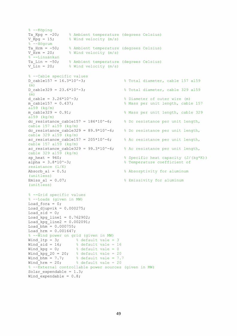
49

% --Köping Ta_Kpg = -20; % Ambient temperature (degrees Celsius) V_Kpg = 15; % Wind velocity (m/s) % --Högrum Ta_Hrm = -50; % Ambient temperature (degrees Celsius) V_Hrm = 20; % Wind velocity (m/s) % --Linsänkan Ta_Lin = -50; % Ambient temperature (degrees Celsius) V_Lin = 20; % Wind velocity (m/s)

% --Cable specific values D_cable157 = 16.3*10^-3; % Total diameter, cable 157 al59

(m) D_cable329 = 23.6*10^-3; % Total diameter, cable 329 al59

(m) d_cable = 3.26*10^-3; % Diameter of outer wire (m) m_cable157 = 0.437; % Mass per unit length, cable 157

al59 (kg/m) m_cable329 = 0.91; % Mass per unit length, cable 329

al59 (kg/m) dc_resistance_cable157 = 186*10^-6; % Dc resistance per unit length,

cable 157 al59 (kg/m) dc_resistance_cable329 = 89.9*10^-6; % Dc resistance per unit length,

cable 329 al59 (kg/m) ac_resistance_cable157 = 205*10^-6; % Ac resistance per unit length,

cable 157 al59 (kg/m) ac_resistance_cable329 = 99.3*10^-6; % Ac resistance per unit length,

cable 329 al59 (kg/m) sp_heat = 960; % Specific heat capacity (J/(kg*K)) alpha = 3.8*10^-3; % Temperature coefficient of

resistance (1/K) Absorb_al = 0.5; % Absorptivity for aluminum

(unitless) Emiss_al = 0.07; % Emissivity for aluminum

(unitless)

% --Grid specific values % --Loads (given in MW) Load_fora = 0; Load_djupvik = 0.000275; Load_sid = 0; Load_kpg_line1 = 0.762902; Load_kpg_line2 = 0.002091; Load_bhm = 0.000755; Load_hrm = 0.001647; % --Wind power on grid (given in MW) Wind_ltp = 3; % default vale = 3 Wind_sid = 16; % default vale = 16 Wind_kpg = 0; % default vale = 0 Wind_kpg_20 = 20; % default vale = 20 Wind_bhm = 7.7; % default vale = 7.7 Wind_hrm = 20; % default vale = 20 % --External controllable power sources (given in MW) Solar_expendable = 1.3; Wind_expendable = 0.8;

Thermal Line Model and Control - IEA - Lund University document/5324_full... · Thermal Line Model and Control Martin Andersson Ljus Divisionof Industrial Electrical Engineering and

Documents