WORCESTER POLYTECHNIC INSTITUTE THERMAL CONDUCTIVITY OF NANOWIRES, NANOTUBES AND POLYMER-NANOTUBE COMPOSITES by Nihar R. Pradhan A thesis submitted in partial fulfillment for the degree of Doctor of Philosophy in the Worcester Polytechnic Institute Department of Physics April 2010

Welcome message from author
This document is posted to help you gain knowledge. Please leave a comment to let me know what you think about it! Share it to your friends and learn new things together.
Transcript
WORCESTER POLYTECHNIC INSTITUTE
THERMAL CONDUCTIVITY OF
NANOWIRES, NANOTUBES AND
POLYMER-NANOTUBE
COMPOSITES
by
Nihar R. Pradhan
A thesis submitted in partial fulfillment for the
degree of Doctor of Philosophy
in the
Worcester Polytechnic Institute
Department of Physics
April 2010

iii
WORCESTER POLYTECHNIC INSTITUTE
Abstract
Worcester Polytechnic Institute
Department of Physics
Doctor of Philosophy
by Nihar R. Pradhan
The primary goal of this dissertation is to present an experimental study of heat trans-
port properties in Nanowires, Nanotubes, and Polymer-nanotube composites. In addi-
tion, thermal relaxation behavior of these nanocomposites were also investigated.
The dissertation consists of six chapters. Chapter 1 is an Introduction, in which the
discovery, structure and physical properties of Nanowires and Nanotubes are outlined.
In Chapter 2, overview of some of the well known synthesis technique of nanotubes
and nanowires were described. The phonon transport in nanowires and nanotubes with
their bulk counterpart is shortly discussed. The phonon scattering mechanism plays an
important role in low-dimensional materials and is one of the main foci of this chapter.
Chapter 3 contains the Experimental details of high-resolution AC Calorimetry that was
used to measure the specific heat and thermal conductivity of these nano composites.
In this chapter, we briefly described the theoretical and the experimental construction,
how we estimate the specific heat and thermal conductivity. In this method one end
of the sample is heated by a known oscillating field and in the other end oscillation
of temperature was measured. The relaxation thermal properties of PMMA+SWCNT
composites studied by Modulated Differential Scanning Calorimetry was another exper-
imental technique discussed in this chapter.
Chapter 4 presents specific heat and thermal conductivity measurements of Cobalt
Nanowires (Co NWs). Measurements were done on anisotropic and randomly ori-
ented composite samples. Anisotropic composite samples were made by growing the
nanowires inside the highly ordered parallel cylindrical porous structures of an Anodic
Aluminum Oxide (AAO) template. Randomly oriented samples were made by releas-
ing the nanowires from the template by dissolving the AAO and drop cast on a silver
sheet. The detail about the sample preparation of this directional measurement is one
of the challenging problems discussed here. X-Ray Diffraction experiment and mor-
phology study are also discussed with the thermal properties. Bulk cobalt powder was

iv
also chosen to compare with nanowires. The result shows a high reduction of thermal
conductivity of nanowire compared to the bulk counterparts.
Chapter 5 describes the study of thermal properties of anisotropic Multi-Wall Carbon
Nanotubes (MWCNTs) and randomly oriented MWCNTs and Single-Wall Carbon Nan-
otubes (SWCNTs) from 300 to 400 K. Measurements on a randomly oriented sample
were done by depositing a thin film of CNTs suspended in a solvent solution within a
calorimetric cell and then allowing the solvent to evaporate. Anisotropic samples were
made by growing the nanotubes inside the highly ordered, packed AAO nanochannels.
The specific heat of anisotropic MWCNTs (Cp) and randomly oriented MWCNTs (Cmp )
and SWCNTs (Csp) shows strong deviations above room temperature from graphite pow-
der. Specific heat of randomly oriented MWCNTs and SWCNTs shows similar behavior
with the specific heat of bulk graphite powder (CBp ). Thermal conductivity of randomly
oriented MWCNTs (κmR ) and SWCNTs (κs
R) followed similar behavior of the thermal
conductivity of graphite powder κB, exhibiting a maximum value near 364 K indicating
the onset of boundary-phonon scattering. The thermal conductivity (κ‖) of anisotropic
MWCNTs increased smoothly with the increase in temperature over all the temperature
ranges studied, which indicated the one dimensional nature of heat flow.
Chapter 6 contains dynamics of thermal properties, such as specific heat, enhancement
of thermal conductivity, and glass transitions of Carbon nanotubes polymer nano com-
posites. The inherently high thermal conductivity of many nano-materials has great
potential for enhancing heat transfer applications. For example, the thermal conductiv-
ity of a single Single-Wall Carbon Nanotube (SWCNT) was found to be 6600Wm−1K−1,
twice that of diamond. When such high thermal conductivity materials were dispersed
in a low thermal conducting polymer, the effective thermal conductivity of the com-
posite can change dramatically. In this paper, an AC calorimetric technique is used to
measure the specific heat (Cp) and effective thermal conductivity (κeff ) of composites
containing a dispersion of SWCNT in Polymethyl Metha Acralite (PMMA) from 300
to 400 K as a function of SWCNT volume fraction. The composites are prepared by
dispersing SWCNTs with PMMA in chloroform solution thoroughly by ultra-sonication
at elevated temperatures then removing the solvent by degassing. A large enhancement
of effective thermal conductivity is observed as SWCNT content increases from 0.5 to
7.93 vol%, reaching 130% of pure PMMA at room temperature. These results are found
to be in good agreement with the theoretical model proposed by Nelsen, Hamilton-
Crosser, Geometric, and Xue. Additional experiments using a Modulated Differential
Scanning Calorimetry (MDSC) technique as a function of scan rate were combined with
the AC measurements to track the slowing dynamics of the glass transition for these
nano-composites.
v
After studying the dynamics of polymer-carbon nanotube composites with temperature
in chapter 6, we decided to study the dynamics of glass transition temperature of these
composite materials not only as a function of temperature but also with frequency of
temperature modulation by MDSC. So, chapter 7 contains the dynamics of thermal study
as a function of temperature, frequency of temperature modulation, carbon nanotube
concentration and scan rate of temperature.
Chapter 8 contains the filling of carbon nanotubes/nanopipes channel with liquid crystal,
then studies the Imaging and dynamics of the confined liquid crystal phase transitions
by MDSC method.
It is shown that carbon nanotubes as components of various nanocomposites have a
significant effect on the mechanical, electrical, and thermal properties of these hybrid
materials. The results of these chapters of thesis indicate the potential of utilizing CNT-
based nanocomposites towards mechanical, electrical, and thermal applications in many
different technological fields. This study also helps to understand the many basic physics
in the molecular level of the phonon transport mechanism in nanostructures, and the
dynamics of molecules of polymers in composite systems, in a confined nanochannel.
Chapter 9 and 10 contains the conclusion and appendix of this thesis.
Acknowledgements
There are a few people I would like to thank for this great success. Firstly, I would like
to express my extreme gratefulness to my Supervisor, Prof. Germano S. Iannacchione
for leading me into the exciting nanoscience field, for encouraging me to be creative and
think deeper, and advising me to try different ideas. His softness and humor along with
the excellent guidance in research not only made me learn many techniques and under-
standing in research but also, I enjoyed the work in the Laboratory. I am indebted to
our collaborator, Prof. Jianyu Liang, from the Department of Mechanical Engineering,
WPI. Her ideas, encouragement and help to do the best research cannot be eclipsed. I
would like to thank Prof. Liangs group for fabricating the high quality nanostructures
which I studied. I really enjoyed the collaboration and sitting in group meetings.
I would also like to thank Mr. Roger W. Steele, technical operation manager. He was
one of the people who was very keen to help when I needed any technical help with
experiments during my research work.
I would like to express my thanks to our department secretaries, Jackie Malone and
Margaret Caisse for their kind help throughout my research career in WPI and all other
members from the WPI Physics Department. I would like to give my special thanks to
the Physics department for supporting my Teaching Assistantship throughout the stay
in WPI. Without this, it may not be possible for me to achieve this highest degree.
I am thankful to my friends and colleagues for sharing their valuable time with me
around the WPI campus. I enjoyed staying near WPI.
Finally, I would like to express my deepest gratitude to my parents and my sisters for
their love and support throughout my student life.
vi
Contents
GRADUATE COMMITTEE APPROVAL i
Abstract iii
Acknowledgements vi
List of Figures x
List of Tables xii
Abbreviations xiii
Physical Constants xv
Symbols xvi
1 INTRODUCTION 1
1.1 Introduction of Carbon Nanotubes . . . . . . . . . . . . . . . . . . . . . . 1
1.1.1 Discovery of Carbon nanotubes . . . . . . . . . . . . . . . . . . . . 1
1.1.2 Structure and General Properties . . . . . . . . . . . . . . . . . . . 2
1.1.3 Physical Properties . . . . . . . . . . . . . . . . . . . . . . . . . . . 4
1.1.4 Introduction to Thermal Transport in Low-dimensional Materials . 5
1.2 Thermal Properties of CNTs . . . . . . . . . . . . . . . . . . . . . . . . . 9
1.3 Thermal Properties of Polymer-Nanocomposites . . . . . . . . . . . . . . . 10
1.4 Review of CNT based Composites . . . . . . . . . . . . . . . . . . . . . . 12
1.5 Properties of Polymer Nanocomposites . . . . . . . . . . . . . . . . . . . . 12
1.5.1 Mechanical Properties . . . . . . . . . . . . . . . . . . . . . . . . . 13
1.5.2 Thermal Properties . . . . . . . . . . . . . . . . . . . . . . . . . . 13
1.5.3 Electrical Conductivity . . . . . . . . . . . . . . . . . . . . . . . . 13
1.5.4 Automotive . . . . . . . . . . . . . . . . . . . . . . . . . . . . . . . 14
1.6 Dispersion of Carbon Nanotubes . . . . . . . . . . . . . . . . . . . . . . . 14
1.7 Thesis Overview . . . . . . . . . . . . . . . . . . . . . . . . . . . . . . . . 16
2 PHONON TRANSPORT IN NANOWIRES AND NANOTUBES 25
2.1 Heat Transport in Nanotubes and Nanowires . . . . . . . . . . . . . . . . 25
vii

Contents viii
2.1.1 Phonon Transport in Bulk Materials . . . . . . . . . . . . . . . . . 25
2.1.2 Phonon Transport in Nanotubes . . . . . . . . . . . . . . . . . . . 26
2.2 Phonon Transport in Nanowires . . . . . . . . . . . . . . . . . . . . . . . . 28
2.3 Phonon Scattering . . . . . . . . . . . . . . . . . . . . . . . . . . . . . . . 28
2.3.1 Normal and Umklapp Scattering . . . . . . . . . . . . . . . . . . . 29
2.3.2 Scattering by Defects, Dislocations and Impurities . . . . . . . . . 31
2.3.3 Temperature dependence of Phonon Scattering . . . . . . . . . . . 32
2.4 Summary . . . . . . . . . . . . . . . . . . . . . . . . . . . . . . . . . . . . 33
3 EXPERIMENTAL METHODS FOR THERMAL MEASUREMENT 37
3.1 Materials and Synthesis . . . . . . . . . . . . . . . . . . . . . . . . . . . . 37
3.1.1 Nanowires and Synthesis Technique . . . . . . . . . . . . . . . . . 37
3.2 CVD Methods, Template-Assisted Synthesis . . . . . . . . . . . . . . . . 39
3.3 Vapor-Liquid-Solid (VLS) Methods . . . . . . . . . . . . . . . . . . . . . . 40
3.4 AC Calorimetry . . . . . . . . . . . . . . . . . . . . . . . . . . . . . . . . . 42
3.4.1 Theory . . . . . . . . . . . . . . . . . . . . . . . . . . . . . . . . . 42
3.4.2 Construction of AC Calorimeter . . . . . . . . . . . . . . . . . . . 46
3.4.3 Electronic . . . . . . . . . . . . . . . . . . . . . . . . . . . . . . . . 48
3.5 Modulated Differential Scanning Calorimeter . . . . . . . . . . . . . . . . 49
3.5.1 Heat-Flux DSC: . . . . . . . . . . . . . . . . . . . . . . . . . . . . 50
3.5.2 Power-Compensated DSC . . . . . . . . . . . . . . . . . . . . . . . 50
3.5.3 Temperature Modulated Differential Scanning Calorimeter . . . . 52
3.5.4 Components of DSC Q200 . . . . . . . . . . . . . . . . . . . . . . . 53
3.6 Overview . . . . . . . . . . . . . . . . . . . . . . . . . . . . . . . . . . . . 58
4 THERMAL CONDUCTIVITY OF COBALT NANOWIRES 61
4.1 Introduction of Co NWs . . . . . . . . . . . . . . . . . . . . . . . . . . . . 61
4.2 Synthesis and Characterization of Cobalt Nanowires . . . . . . . . . . . . 63
4.2.1 AC Calorimetry . . . . . . . . . . . . . . . . . . . . . . . . . . . . 65
4.2.2 Sample Configurations . . . . . . . . . . . . . . . . . . . . . . . . . 66
4.3 Results and Discussion . . . . . . . . . . . . . . . . . . . . . . . . . . . . . 70
4.3.1 Morphology and microstructure study of Co NWs . . . . . . . . . 70
4.3.2 Specific heat of Co NWs . . . . . . . . . . . . . . . . . . . . . . . . 71
4.3.3 Thermal Conductivity of Co NWs . . . . . . . . . . . . . . . . . . 73
4.3.4 Phonon Mean-Free-Path . . . . . . . . . . . . . . . . . . . . . . . . 76
4.4 Summary . . . . . . . . . . . . . . . . . . . . . . . . . . . . . . . . . . . . 79
5 THERMAL CONDUCTIVITY OF SINGLE-WALL AND MULTI-WALLCARBON NANOTUBES COMPOSITES 83
5.1 Introduction of Carbon Nanotubes . . . . . . . . . . . . . . . . . . . . . . 83
5.2 Experimental . . . . . . . . . . . . . . . . . . . . . . . . . . . . . . . . . . 85
5.2.1 Synthesis of Carbon Nanotubes and Samples . . . . . . . . . . . . 85
5.2.2 Sample+Cell Configurations . . . . . . . . . . . . . . . . . . . . . . 87
5.2.3 AC-Calorimetric Technique . . . . . . . . . . . . . . . . . . . . . . 89
5.3 Results and Discussion . . . . . . . . . . . . . . . . . . . . . . . . . . . . . 90
5.3.1 Morphology Study . . . . . . . . . . . . . . . . . . . . . . . . . . . 90
5.3.2 Specific heat of CNT composites . . . . . . . . . . . . . . . . . . . 91

Contents ix
5.3.3 Thermal Conductivity of CNTs . . . . . . . . . . . . . . . . . . . . 93
5.4 Summary . . . . . . . . . . . . . . . . . . . . . . . . . . . . . . . . . . . . 97
6 THERMAL PROPERTIES AND GLASS TRANSITION IN PMMA+SWCNTCOMPOSITES 102
6.1 Introduction of Polymer-Carbon Nanotubes Composite . . . . . . . . . . . 102
6.2 Experimental . . . . . . . . . . . . . . . . . . . . . . . . . . . . . . . . . . 104
6.2.1 Modulation Calorimetry (ACC): . . . . . . . . . . . . . . . . . . . 104
6.2.2 Preparation of PMMA+SWCNT Composites: . . . . . . . . . . . . 106
6.3 Results and Discussion . . . . . . . . . . . . . . . . . . . . . . . . . . . . . 108
6.3.1 Specific heat of PMMA+SWCNT composites . . . . . . . . . . . . 108
6.3.2 Thermal Conductivity of PMMA+SWCNT Composites . . . . . . 110
6.3.3 Composite Thermal Conductivity Models . . . . . . . . . . . . . . 113
6.3.4 MDSC Study of PMMA+SWCNT Composites . . . . . . . . . . . 116
6.4 Summary . . . . . . . . . . . . . . . . . . . . . . . . . . . . . . . . . . . . 119
7 RELAXATION DYNAMICS OF THE GLASS TRANSITION IN PMMA+SWCNTCOMPOSITES BY TEMPERATURE MODULATED DSC 125
7.1 Introduction . . . . . . . . . . . . . . . . . . . . . . . . . . . . . . . . . . . 125
7.2 Experimental . . . . . . . . . . . . . . . . . . . . . . . . . . . . . . . . . . 128
7.2.1 Modulated Differential-Scanning Calorimetry (MDSC): . . . . . . 128
7.2.2 Preparation of PMMA+SWCNT Composites: . . . . . . . . . . . . 131
7.3 Results and Discussion . . . . . . . . . . . . . . . . . . . . . . . . . . . . . 132
7.4 Summary . . . . . . . . . . . . . . . . . . . . . . . . . . . . . . . . . . . . 139
8 IMAGING AND DYNAMICS OF LIQUID CRYSTALS CONFINEDINSIDE CARBON NANOPIPES 143
8.1 Introduction of Nanofluid Device . . . . . . . . . . . . . . . . . . . . . . . 143
8.1.1 SWCNTs and MWCNTs for Nanofluidic Applications . . . . . . . 145
8.1.2 Behavior of Liquids Inside CNPs . . . . . . . . . . . . . . . . . . . 146
8.1.3 Nanofludic and Energy Storage Applications . . . . . . . . . . . . 146
8.2 Experimental . . . . . . . . . . . . . . . . . . . . . . . . . . . . . . . . . . 148
8.2.1 Synthesis of MWCNPs . . . . . . . . . . . . . . . . . . . . . . . . . 148
8.2.2 Filling of LCs inside Carbon Nanopipes . . . . . . . . . . . . . . . 148
8.3 Imaging of LCs Confined inside MWCNPs . . . . . . . . . . . . . . . . . . 150
8.4 Study of Phase Transition of 8CB and 10CB Liquid crystals inside MWC-NPs by Modulated DSC: . . . . . . . . . . . . . . . . . . . . . . . . . . . . 151
8.4.1 Frequency dependent Study: . . . . . . . . . . . . . . . . . . . . . 155
8.5 Summary . . . . . . . . . . . . . . . . . . . . . . . . . . . . . . . . . . . . 157
9 CONCLUSIONS 164
9.1 Conclusions . . . . . . . . . . . . . . . . . . . . . . . . . . . . . . . . . . . 164
10 APPENDIX 169
10.1 PUBLICATIONS . . . . . . . . . . . . . . . . . . . . . . . . . . . . . . 169
10.2 PUBLICATIONS PENDING . . . . . . . . . . . . . . . . . . . . . . . 172
Index 173
List of Figures
1.1 CNT Chiral vector figure . . . . . . . . . . . . . . . . . . . . . . . . . . . 3
1.2 Density of States . . . . . . . . . . . . . . . . . . . . . . . . . . . . . . . . 8
2.1 Normal and Umklap Phonon Scattering . . . . . . . . . . . . . . . . . . . 30
2.2 Temperature dependent phonon thermal conductivity . . . . . . . . . . . 31
3.1 All kappa . . . . . . . . . . . . . . . . . . . . . . . . . . . . . . . . . . . . 40
3.2 VLSSynthesis . . . . . . . . . . . . . . . . . . . . . . . . . . . . . . . . . . 41
3.3 AC Thermal Model . . . . . . . . . . . . . . . . . . . . . . . . . . . . . . . 43
3.4 Design of AC Calorimeter for thermal measurement . . . . . . . . . . . . 47
3.5 Electronic connection of AC Calorimeter . . . . . . . . . . . . . . . . . . . 49
3.6 DSC Pan, heater and sample squizer . . . . . . . . . . . . . . . . . . . . . 52
3.7 MDSC temperature and heating rate Signals . . . . . . . . . . . . . . . . 53
4.1 Synthesis process of CoNWs . . . . . . . . . . . . . . . . . . . . . . . . . . 64
4.2 Frequency Scan of AAO membrane . . . . . . . . . . . . . . . . . . . . . . 67
4.3 Sample + Cell configuration for thermal study . . . . . . . . . . . . . . . 68
4.4 3D Sample + Cell configuration for thermal study . . . . . . . . . . . . . 68
4.5 SEM images of CoNWs . . . . . . . . . . . . . . . . . . . . . . . . . . . . 71
4.6 X-Ray Diffraction graph of CoNWs . . . . . . . . . . . . . . . . . . . . . . 72
4.7 Specific heat of CoNWs and bulk cobalt . . . . . . . . . . . . . . . . . . . 73
4.8 Thermal conductivity of CoNWs and bulk Cobalt . . . . . . . . . . . . . . 74
4.9 Normalized thermal conductivity of CoNWs and bulk cobalt . . . . . . . . 76
4.10 Thermal diffusivity of bulk cobalt and CoNws . . . . . . . . . . . . . . . . 78
5.1 Synthesis procedure of MWCNTs . . . . . . . . . . . . . . . . . . . . . . . 86
5.2 Sample+Cell arrangement of MWCNTs for thermal study . . . . . . . . . 88
5.3 SEM micrographs of MW, SW CNTs and graphite powder . . . . . . . . 91
5.4 Specific heat of MW,SW CNTs and graphite powders . . . . . . . . . . . 92
5.5 Thermal conductivity of MW,SW CNTs and graphite powders . . . . . . 94
5.6 Normalized thermal conductivity of MW,SW CNTs and graphite powders 96
6.1 Specific heat and thermal conductivity of PMMA+SWCNT composites . 107
6.2 Specific heat and thermal conductivity of PMMA+SWCNT composites . 109
6.3 Enhance ment of thermal conductivity . . . . . . . . . . . . . . . . . . . . 112
6.4 Thermalconductivity of PMMA+SWCNTs filled with theoretical models . 114
6.5 Rev. heat capacity with heating and Cooling by MDSC . . . . . . . . . . 117
6.6 Hysteresis between heating and cooling run by MDSC . . . . . . . . . . . 118
6.7 Rev cooling scan with scan rate by MDSC . . . . . . . . . . . . . . . . . . 119
x

List of Figures xi
6.8 Glass Transition with scan rate by MDSC . . . . . . . . . . . . . . . . . . 120
6.9 Heating effect of glass transition by MDSC . . . . . . . . . . . . . . . . . 121
7.1 Modulated heat flow and Modulated rate . . . . . . . . . . . . . . . . . . 129
7.2 Corrected Ohase angle . . . . . . . . . . . . . . . . . . . . . . . . . . . . . 130
7.3 Real and Imaginary part of specific heat of PMMA and PMMA+SWCNTs133
7.4 Delta Cp as with Frequency of temperature modulation . . . . . . . . . . 134
7.5 Tg with Frequency of temperature modulation . . . . . . . . . . . . . . . . 135
7.6 Tmax and Tg with frequency of temperature modulation . . . . . . . . . . 136
7.7 Arhenius - Law . . . . . . . . . . . . . . . . . . . . . . . . . . . . . . . . . 137
7.8 Enthalpy as a function of frequency of temperature modulation . . . . . . 139
8.1 Synthesis of Multiwall Carbon nanopipes (MWCNPs) . . . . . . . . . . . 149
8.2 AAO Template and embedded MWCNPs . . . . . . . . . . . . . . . . . . 150
8.3 HRTEM images of MWCNPs inside AAO template filled with 10CB Liq-uid Crystal . . . . . . . . . . . . . . . . . . . . . . . . . . . . . . . . . . . 151
8.4 HRTEM images of MWCNPs filled 10CB bulk LCs . . . . . . . . . . . . . 152
8.5 Normalized reversible heat capacity of 8CB LCs confined inside MWCNPs 153
8.6 Normalized heat capacity of pure 8CB LCs . . . . . . . . . . . . . . . . . 154
8.7 Reversible heat capacity of 10CB LCs and confined inside MWCNPs . . . 155
8.8 Frequency dependent specific heat of pure 8CB LCs . . . . . . . . . . . . 156
8.9 Frequency dependent specific heat of 8CB LCs confined inside MWCNPs 157

List of Tables
6.1 Specific heat and thermal conductivity results at 300 K and 399 K for purePMMA and PMMA+SWCNT samples determined by ACC. An effectivescan rate of 0.04 K min−1 was used with Cp given in J g−1 K−1 and κ inW m−1 K−1. . . . . . . . . . . . . . . . . . . . . . . . . . . . . . . . . . . 108
6.2 Glass transition temperatures Tg, the inflection point of the Cp step,in Kelvin and enthalpy hysteresis ∆Hhyst, difference in ∆H betweenheating and cooling, in J g−1 determined by ACC at 0.04 K min−1
and by MDSC extrapolated to zero-scan rate (T 0g ) for pure PMMA and
PMMA+SWCNT samples. . . . . . . . . . . . . . . . . . . . . . . . . . . 110
7.1 Activation Energy (E) and characteristic time (τ0) in two different scanrates of PMMA and PMMA+SWCNT composites. . . . . . . . . . . . . 138
xii

Abbreviations
CNT Carbon Nano Tubes
SW Single Wall
SWCNT Single Wall Carbon Nano Tubes
MWCNT Multi Wall Carbon Nano Tubes
STM Scanning Tunneling Microscope
MIT Massachusetts Institute Technology
PMMA Poly Methyl Metha Acralite
PS Poly Styrene
PP Poly Propylene
PANI Polyaniline
LBL Layer By Layer Assembly
AC Alternating Current
ACC Alternating Current Calorimeter
TIM Thermoal Interface Materials
TE Thermo Electrics
SEM Scanning Electron Microscope
XRD X Ray Diffraction
DSC Differential Scanning Calorimeter
MDSC Modulated Differential Scanning Calorimeter
TMDSC Temperature Modulated Differential Scanning Calorimeter
CVD Chemical Vapor Deposition
LC Liquid Crystal
CNPs Carbon Nanopipes
MWCNPs Multi Wall Carbon Nano Pipes
DOS Density Of States
xiii

Abbreviations xiv
CoNWs Cobalt Nano Wires
AAO Anodic Aluminum Oxide
VLS Vapor Liquid Solid
GE General Electric
DMM Digital Multi Meter
PRT Platinum Resistance Thermometer
RTD Resistive Temperature Device
PID Propertional Integral Derivative
GPIB General Purpose Interface Bus
TA Thermal Analysis
RCS Refrigerated Cooling System
EDS Energy Dispersion Spectroscopy
NMR Nuclear Magnetic Resonance

Physical Constants
Speed of Light c = 2.997 924 58 × 108 ms−s
Pi π = 3.14
Carbon 60 C60
Plank constant h = 6.626068 × 10⁻³⁴ m2 kg s−1
Boltzmann constant kB = 1.3806503 × 10⁻²³ m2kg s−2K−1
xv

Symbols
a atomic spacing distance m
P power Ws−1
ω angular frequency rad s−1
f frequency s−1
κ thermal conductivity Wm−1K−1
Cp specific heat Jg−1K−1
C∗ heat capacity JK−1
Ch heat capacity of heater JK−1
Cs heat capacity of sample JK−1
Cθ heat capacity of thermister JK−1
K thermal conductance WK−1
T Temperature K
Tac Oscillating temperature K
C chiral vector ms−1
λ wave length m
vg group velocity ms−1
ZT thermoelectric figure of merit
S Seebeck coefficient VK−1
ρ electrical resistivity Ωm
κp, κph thermal conductivity of phonon Wm−1K−1
κe thermal conductivity of electron Wm−1K−1
l mean free path m
ν phonon velocity ms−1
τ time constant s
xvi

Symbols xvii
K wave vector m−1
λdom dominant wavelength of phonon m
θD Debye temperature K
ωD Debye cut off frequency m−1
Q heating voltage V
τi Internal relaxation time constant s
τe External relaxation time constant s
Φ phase shift rad
φ reduced phase shift rad
A Area m2
R resistance Ω
λBp Bulk phonon mean free path m
c‖p specific heat in parallel direction Jg−1K−1
cRp specific heat in random oriented sample Jg−1K−1
cBp specific heat of bulk sample Jg−1K−1
cMp specific heat of MWCNT Jg−1K−1
cSp specific heat of SWCNT Jg−1K−1
c∗p complex specific heat capacity Jg−1K−1
c′
p real specific heat capacity Jg−1K−1
c′′
p imaginary specific heat capacity Jg−1K−1
κ‖ thermal conductivity along the axis Wm−1K−1
κR thermal conductivity in random sample Wm−1K−1
φm mass fraction
φv volume fraction
ρp density of polymer gcm−3
ρf density of fill gcm−3
Tg glass transition temperature K
TNI isotropic to nematic transition temperature K

Dedicated to my
Lovely Parents. . .
xviii

Chapter 1
INTRODUCTION
1.1 Introduction of Carbon Nanotubes
1.1.1 Discovery of Carbon nanotubes
Carbon is a special element in nature, whose chemical versatility makes it the central
agent in most applications. Until recently it has been well known that the pure carbon
exists in two forms: diamonds and graphite. In 1985, Harold Kroto, Robert Curl, and
Richard E. Smally discovered a new form of carbon, the fullerenes, which are molecules
of pure carbon atoms bonded together forming geometrically regular structures [1]. The
best known is the C60, which has precisely the same geometry as the soccer ball, total
60 carbon atoms. Due to the similarity of structure developed by American architect,
Buckminster Fuller, this new molecule was named the buckminster fullerene, or bucky-
ball.
The Carbon Nanotubes (CNTs) were first prepared by M. Endo in 1978, as part of his
PhD studies at the University of Orleans in France. He was able to produce very small
diameter filaments (about 7 nm) using a vapour-growth technique, but these fibers
were not recognized as nanotubes and were not studied systematically. It was only
after the discovery of fullerenes, C60 in 1985 by Kroto [1], that researchers started to
explore carbon structures further. In 1991, when the Japanese electron microscopist
Sumio Iijima observed CNTs [2], the field really started to advance. He was studying
the material deposited on the cathode during an arc-evaporation synthesis of fullerenes
1
Chapter 1. INTRODUCTION 2
when he observed CNTs. A short time later, Thomas Ebbesen and Pulickel Ajayan, from
Iijima’s lab, showed how nanotubes could be produced in bulk quantities by varying the
arc-evaporation conditions [4]. But the standard arc-evaporation method had produced
only multiwall nanotubes. After some research, it was found that the addition of metals
such as cobalt to the graphite electrodes resulted in extremely fine single-wall nanotubes.
The synthesis in 1993 of SWNTs was a major event in the development of CNTs [3, 5].
Although the discovery of CNTs was an accidental event, it opened the way to flourishing
research into the properties of CNTs in labs all over the world, with many scientists
demonstrating promising physical, chemical, structural, electronic, thermal and optical
properties of CNTs.
1.1.2 Structure and General Properties
Carbon nanotubes are made up of one or more wrapped seamless concentric cylindrical
carbon honeycomb lattice or graphene sheet. The theoretically smallest nanotubes have
diameters equal to diameters of C60 (d = 0.7 nm). The most important structures are
single wall (SW) and multi walled carbon nanotubes (MWCNTs). Multi walls are con-
centric circles of SWCNTs. The primary symmetry classification of CNT is divided into
two parts , achiral and chiral. An achiral nanotube is defined by a nanotube whose mir-
ror image has an indistinguishable structure to the original one. And, as a consequence,
it is superimposable to it. There are only two cases of achiral nanotubes: armchair and
zig-zag nanotubes. Single walled carbon nanotubes are completely described, except for
their length, by a single vector ~C pointing from the first atom towards the second one
and is defined by the relation:
~C = n~a1 +m~a2 (1.1)
where n and m are integers. ~a1 and ~a2 are the unit cell vectors of the two-dimensional
lattice formed by the graphene sheets. The direction of the nanotube axis is perpendicu-
lar to this chiral vector. The length of the chiral vector ~C [Fig. 1.1] is the circumference
of the nanotube and is given by the corresponding relationship:
c = |~C| = a√
(n2 + nm+m2) (1.2)

Chapter 1. INTRODUCTION 3
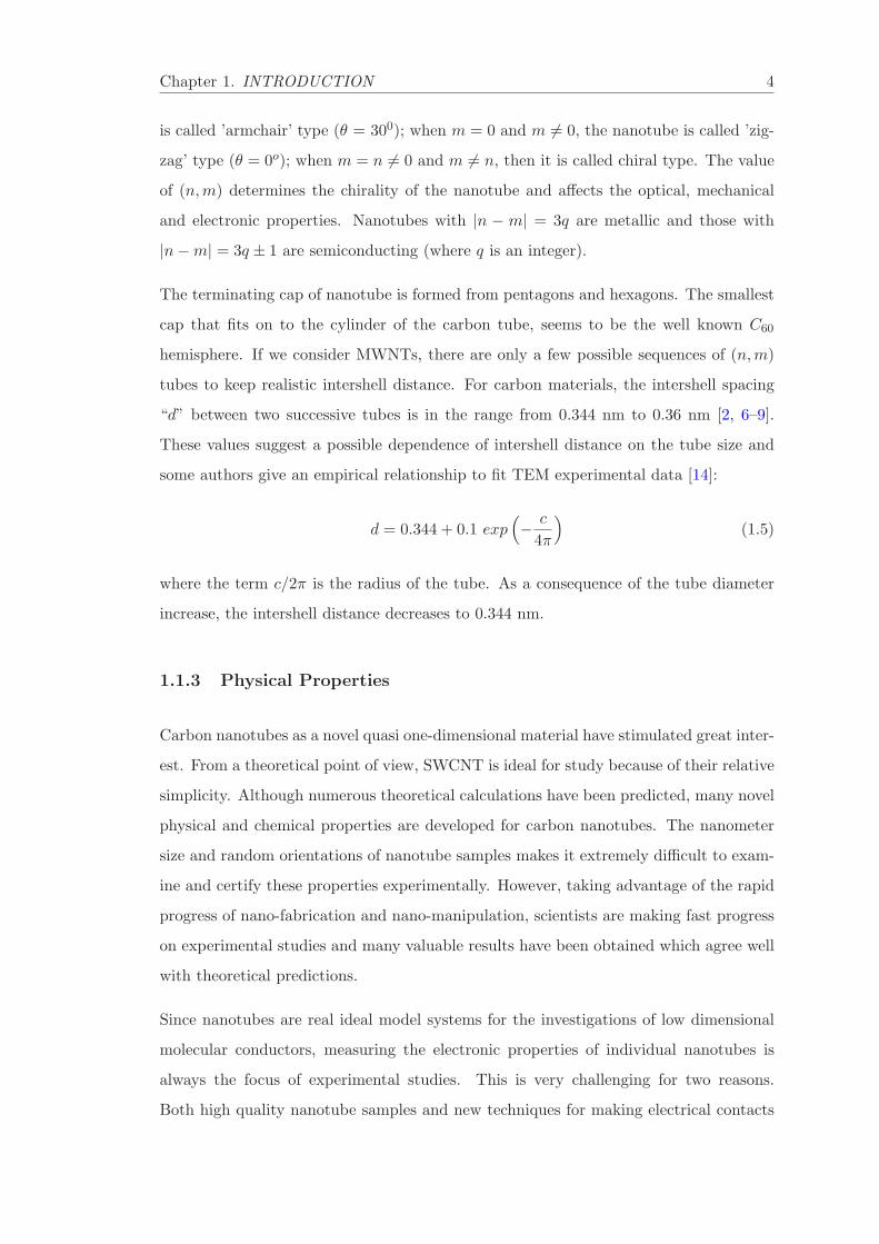
Figure 1.1: Chiral vector ~C and chiral angle θ with unit vectors shown in (A). (B) isarmchair type m = n, (C) is zig-zag m = 0, n 6= 0, (D) is chiral type m 6= n, (E) showssingle-wall and (F) Multi-wall carbon nanotubes. ~a1 and ~a2 are the unit cell vectors ofthe two-dimensional hexagonal graphene sheet. The circumference of nanotube is givenby the length of chiral vector. The chiral angle θ is defined as the angle between chiral
vector ~C and the zigzag axis [16].
where the value a is the length of the unit cell vector a1 or a2. This length a is related
to the carbon-carbon bond length acc by the relation:
a = | ~a1| = | ~a2| = acc
√3 (1.3)
Using the circumferential length c, the diameter of the carbon nanotube is thus given
by the relation: D = c/π.
The angle between the chiral vector and zigzag nanotube axis is the chiral angle θ
[Fig. 1.1]. With the integers n and m already introduced before, this angle can be
defined by:
θ = tan−1
(
m√
3
m+ 2n
)
(1.4)
Nanotubes are only described by the pair of integers (n,m) which is related to the chiral
vector. Three types of CNTs are revealed with these values: when n = m, the nanotube
Chapter 1. INTRODUCTION 4
is called ’armchair’ type (θ = 300); when m = 0 and m 6= 0, the nanotube is called ’zig-
zag’ type (θ = 0o); when m = n 6= 0 and m 6= n, then it is called chiral type. The value
of (n,m) determines the chirality of the nanotube and affects the optical, mechanical
and electronic properties. Nanotubes with |n − m| = 3q are metallic and those with
|n−m| = 3q ± 1 are semiconducting (where q is an integer).
The terminating cap of nanotube is formed from pentagons and hexagons. The smallest
cap that fits on to the cylinder of the carbon tube, seems to be the well known C60
hemisphere. If we consider MWNTs, there are only a few possible sequences of (n,m)
tubes to keep realistic intershell distance. For carbon materials, the intershell spacing
“d” between two successive tubes is in the range from 0.344 nm to 0.36 nm [2, 6–9].
These values suggest a possible dependence of intershell distance on the tube size and
some authors give an empirical relationship to fit TEM experimental data [14]:
d = 0.344 + 0.1 exp(
− c
4π
)
(1.5)
where the term c/2π is the radius of the tube. As a consequence of the tube diameter
increase, the intershell distance decreases to 0.344 nm.
1.1.3 Physical Properties
Carbon nanotubes as a novel quasi one-dimensional material have stimulated great inter-
est. From a theoretical point of view, SWCNT is ideal for study because of their relative
simplicity. Although numerous theoretical calculations have been predicted, many novel
physical and chemical properties are developed for carbon nanotubes. The nanometer
size and random orientations of nanotube samples makes it extremely difficult to exam-
ine and certify these properties experimentally. However, taking advantage of the rapid
progress of nano-fabrication and nano-manipulation, scientists are making fast progress
on experimental studies and many valuable results have been obtained which agree well
with theoretical predictions.
Since nanotubes are real ideal model systems for the investigations of low dimensional
molecular conductors, measuring the electronic properties of individual nanotubes is
always the focus of experimental studies. This is very challenging for two reasons.
Both high quality nanotube samples and new techniques for making electrical contacts
Chapter 1. INTRODUCTION 5
to individual tubes are necessary. Langer et al. reported the first measurement in
MWCNT by using Scanning Tunneling Microscope (STM) lithography techniques [15].
They found that transport properties of MWCNT are consistent with the quantum
transport behavior. Ebbesen systematically measured the conductance by four-probe
measurement and observed both metallic and non-metallic behaviors [17]. Another
versatile method of electrical contact was used by Frank et al. [18], where a single
MWCNT attached to a STM tip was repeatedly immersed and pulled out of liquid
metal like mercury. Surprisingly, a universal quantized conductance is measured at
room temperature, providing evidence that transport in MWCNTs is ballistic over the
distance of order of ≥ 1 µm.
Single wall nanotubes have well defined structures and relatively less defects. The suc-
cess of synthesis of high-quality SWCNTs with uniform structures greatly stimulated
experimental studies. The first results on individual SWNTs were obtained by Tans et
al. [19], where they observed single electron transport with Columb blockade and reso-
nant tunneling through single molecular orbitals. The STM was also used to measure
the tunneling spectroscopy of nanotubes and found to be both metallic and semiconduct-
ing [20, 21]. Their data provided the first experimental verification of the bandstructure
predictions. Their observed band structures quantitatively agree with the calculations.
1.1.4 Introduction to Thermal Transport in Low-dimensional Materi-
als
Thermal transport in low dimensional systems has recently become a subject of con-
sideration and much interest in the area of research. Due to the changing of length
scale in electronics and optoelectronics devices from micro to nano scale length, there
is much more interest to look at the properties of these materials for their outstanding
applications.
The interest is drawn to new thermal transport science, that is operative at these small
length scales and where quantum mechanical phenomena become significant and applied
as different than the bulk counterpart. M. S. Dresselhaus and her groups from MIT have
studied and made advancements in the field of thermal transport of low dimensional
materials. At small length scales, the number of atoms or the number of electrons in the
system become small, so that continuum mechanics and elastic continuum models have

Chapter 1. INTRODUCTION 6
to be replaced by models that take into account the discrete nature of the electronic and
vibrational states and their distribution in energy. In this realm, we can expect devices
to be much smaller and faster, but to exhibit new unexpected phenomena of scientific
interest and technological importance.
Two interesting limits of the thermal conductivity in nano-systems can be considered. In
the high thermal conductivity limit, one might consider a single wall carbon nanotube,
with cylindrical wall, one atom in thickness, 1 nm in diameter, and tens of microns in
length. Advances in nanotechnology now are allowing measurements to be made for
such a small object, which is expected to act like a heat pipe and to provide the highest
thermal conductivity, exceeding that of any presently known material. In the opposite
limit, effort is going into developing very low thermal conductivity nanostructures which
might be used for thermoelectric devices, across which measurably large temperature
gradients must be maintained and measured over submicron length scales. Thermoelec-
tric properties are discussed briefly later.
Low-dimensional structures, such as quantum wells, superlattices, quantum wires, and
quantum dots, offer new ways to manipulate the electron and phonon properties of a
given material. In the regime where quantum effects are dominant, the energy spectra
of electrons and phonons can be controlled through altering the size of the structures,
leading to new ways to manipulate the properties of these materials, especially their ther-
mal transport properties for selected applications. In this regime, each low-dimensional
structure can be considered to give rise to a new material, even though the material may
be made of the same atomic structure as its parent material. Each set of size parameters
thus provides a new material that can be examined, both theoretically and experimen-
tally, in terms of its thermal transport properties. Thus searching for materials with
low-dimensional structures can be regarded as the equivalent of synthesizing many differ-
ent materials from a small set of bulk materials and then measuring and optimizing their
thermal transport properties for specific applications. Because the constituent parent
materials of low-dimensional structures are typically simple materials with well-known
properties, the low dimensional structures are amenable to a certain degree of analysis,
prediction and optimization, while theoretical predictions for novel bulk materials are
difficult. And each new material presents a different set of experimental and theoretical
challenges, because it is often the case that neither their materials science nor their
physical properties are adequately known.
Chapter 1. INTRODUCTION 7
There are several concepts behind using low-dimensional materials for thermoelectric
performance. Thermoelectric performance depends upon three parameters S, σ and κ.
The parameter which defined the thermoelectric materials is known as thermoelectric
figure of merits and is defined as:
ZT =S2σT
κ(1.6)
where S is Seebeck coefficient (= −∆V∆T ) in Volt K−1, σ is electrical conductivity in S m−1
and κ is thermal conductivity in W m−1 K−1. Since these quantities in bulk materials
are interrelated, its very difficult to vary/control each parameter independently without
changing other parameters so that we can increase the value of ZT . This is because an
increase in S usually results in a decrease in σ, and a decrease in σ produces a decrease
in the electronic contributions to κ, following the WiedemannFranz Law [22] i,e.
At a given temperature, the thermal and electrical conductivities of metals are propor-
tional, but raising the temperature increases the thermal conductivity while increases
the electrical conductivity. This behavior is quantified in the Wiedemann-Franz Law:
κ
σ= LT ⇒ L =
κ
σT(1.7)
where the constant of proportionality L is called Lorenz number. If the dimensionality of
the material is decreased, the new variable of length scale becomes available for the con-
trol of materials properties. Then as the system size decreases and approaches nanometer
length scales, it is possible to cause dramatic differences in the density of electronic states
shown in Fig. 1.2, allowing new opportunities to vary S, σ, and κ quasi-independently
when the length scale is small enough to give rise to quantum-confinement effects as
the number of atoms in any direction. In addition, as the dimensionality is decreased
from 3D crystalline solids to 2D (quantum wells) to 1D (quantum wires) and finally to
0D (quantum dots), new physical phenomena are also introduced and these phenomena
may also create new opportunities to vary S, σ, and κ independently. These phenomena
are discussed below. Furthermore, the introduction of many interfaces, which scatter
phonons more effectively than electrons, or serve to filter out the low-energy electrons
at the interfacial energy barriers, allows the development of nanostructured materials
with enhanced ZT , suitable for thermoelectric applications.

Chapter 1. INTRODUCTION 8
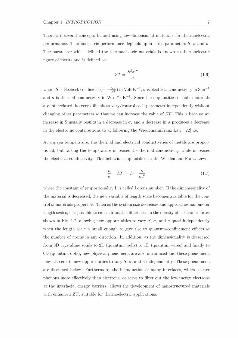
(a)(a) (b)
(c) (d)
Figure 1.2: Electronic density of states for (a) bulk 3D crystalline semiconductor, (b)2D quantum well, (c) 1D nanowire or nanotube, and (d) 0D quantum dot [23]. Materialssystems with low dimensionality also exhibit physical phenomena, other than a highdensity of electronic states (DOS), that may be useful for enhancing thermoelectric
performance.
For many years Bi is an attractive thermoelectric material because of the large anisotropy
of constant energy surface of electrons, their high carrier mobility, high effective mass
components that can be exploited for achieving a high electrical conductivity, and the
heavy mass components that can be exploited to obtain a heavy DOS. Since Bi is a semi
metal it has low Seeback coefficient S, because of the approximate cancellation of the
electron and hole contributions to S [23, 24].
To achieve high thermo-electric figure of merits (ZT ), we need to reduce the thermal
conductivity without reducing electrical conductivity and its possible in nanostructure
materials such as nanowires, described above. The first strategy to reduce thermal
conductivity is to reduce the specific heat by altering the phonon dispersion relation,
possibly through phonon confinement in super lattice and nanowires [25]. The second
strategy is to reduce the lattice/phonon mean free path by scattering at boundaries,
interface or phonon-phonon in nanowires, superlattices and nano-composites. This is
because thermal conductivity is proportional to velocity of phonon (v), specific heat
(Cp) and mean free path (λ).
κ =1
3Cpvλ (1.8)

Chapter 1. INTRODUCTION 9
The first strategy is known as wave, coherent or quantum size effects [26, 27]. There is
a key distinction between confinement by interfaces parallel to the transport direction
(for example, nanowires and superlattices with in-plane transport) and confinement
by interfaces perpendicular to the transport direction (superlattices with cross plane
transport). For transport both parallel and perpendicular to the interfaces, the practical
difficulty is maintaining phonon coherence. In a nanostructure the unit cell is much
larger than in bulk, while after accounting for additional boundary scattering the mean
free path is shorter than in bulk. With addition to this diffuse scattering reduce the
interface scattering due to the randomizing the direction of scattered phonons.
The second strategy to reduce thermal conductivity is to reduce the mean free path by
random scattering at boundaries and interfaces. This is known as particle or classical
size effects, and coherent wave effects are ignored [28].
1.2 Thermal Properties of CNTs
The thermal wave propagation differs in carbon nanotubes from metal nanowires. Due
to their unique crystalline structure, boundary scattering is nearly absent in CNTs.
Thus CNTs show high thermal and electrical conductivity and this makes CNTs an
ideal candidate for promising applications in nanoelectronics.
The potential applications and intriguing nanoscale thermal conduction physics has in-
spired several groups to measure CNTs thermophysical properties. Hone group [10]
measured the temperature dependent thermoelectric power (TEP) of crystalline ropes
of SWCNTs by simply applying a small temperature difference of maximum ±0.2 K and
measuring the voltage induced in the sample. They got moderately large holelike TEP
at high temperature and the TEP approaches zero as T → 0. Thermal conductivities of
SWCNTs bundles and mats were measured by Hone group [11, 12]. The measured ther-
mal conductance of millimeter size mat samples made of CNTs shows linear temperature
dependence below 25 K and extrapolates to zero at zero temperature. The measurement
results have advanced our understanding of thermal conduction in CNTs. However its
very difficult to extract the thermal conductivity of single carbon nanotubes, due to
the difficulty of measurement, tube-tube junction and tube-interface contact resistance.
This is the primary reason theoretical values are always higher, an order of magnitude
Chapter 1. INTRODUCTION 10
from the experimental values. Below room temperature Umklapp phonon-phonon scat-
tering became very low or did even not occur [12, 13]. This indicates that the dominant
scattering mechanism is phonon scattering by defects and boundaries of nanotubes wall.
There are not too many but quite a lot of experimental and theoretical work has been
done in low temperature thermal study, but there is no significant information avail-
able in high temperature thermal study of CNTs. Our work is based on above room
temperature thermal properties of well aligned and random macroscopic composites of
MW and SW carbon nanotubes. The phonon scattering mechanism depends upon the
sample geometry, contact surface and interface roughness.
1.3 Thermal Properties of Polymer-Nanocomposites
A nanocomposite is defined as a material of more than one solid phase, where at least
one dimension falls into the nanometer scale. The fabrication of nanocomposites opens
up an attractive route to obtain novel, optimized, and miniaturized compounds that
can meet a broad range of applications. In this context, the exceptional properties of
nanoparticles have made them a focus of widespread research in nanocomposite tech-
nology. Since composites consist of several different components, superior physical and
chemical characteristics of novel materials can be achieved. Therefore, the develop-
ment of nanoparticle modified composites is presently one of the most explored areas in
materials science and engineering [29].
Nowadays polymers play a very important role in numerous fields of everyday life due to
their advantages over conventional materials (e.g. wood, clay, metals) such as lightness,
resistance to corrosion, ease of processing, and low cost production. Besides, polymers
are easy to handle and have many degrees of freedom for controlling their properties.
Further improvement of their performance, including composite fabrication, still remains
under intensive investigation. The altering and enhancement of the polymers proper-
ties can occur through doping with various nano-fillers such as metals, semiconductors,
organic and inorganic particles and fibers, as well as carbon structures and ceramics [30–
33]. Such additives are used in polymers for a variety of reasons, for example: improved
processing, density control, optical effects, thermal conductivity, control of the ther-
mal expansion, electrical properties that enable charge dissipation or electromagnetic
Chapter 1. INTRODUCTION 11
interference shielding, magnetic properties, flame resistance, and improved mechanical
properties, such as hardness, elasticity, and tear resistance [34–36].
Unique properties of carbon nanotubes (CNT) such as extremely high strength, lightweight,
elasticity, high thermal and air stability, high electric and thermal conductivity, and high
aspect ratio offer crucial advantages over other nano-fillers. The potential utility of car-
bon nanotubes in a variety of technologically important applications such as molecular
wires and electronics, sensors, high strength materials, and field emission has been well
established. Recently, much attention has been paid to the use of carbon nanotubes
in conjugated polymer nanocomposite materials to harness their exceptional proper-
ties [18, 37]. CNT-based composites have attracted great interest due to an increasing
technological demand for multifunctional materials with improved mechanical, electrical,
thermal and optical performance, complex shapes, and patterns manufactured in an easy
way at low costs. However, several fundamental processing challenges must be overcome
to enable applicable composites with carbon nanotubes. The main problems with CNTs
are connected to their production, purification, process ability, manipulation and solu-
bility. Because of these difficulties, to date, the potential of using nanotubes as polymer
composite has not been fully realized. There are only few nanotube-based commercial
products on the market at present, which are in fact CNT/polymer composites with
improved electrical conductivity [Hyperion Catalysis International]. This still requires
intensive studies in order to compromise expectations with technological achievements in
CNT composites. Since 1994, when Ajayan et al. [39] first introduced multiwall carbon
nanotubes (MWCNTs) as filler materials in a polymer matrix, numerous projects have
been focused on the fabrication, improvement, modeling, and characterization of such
heterostructures [40–42].
The main objective of this study was to produce and investigate SWCNT-based nanocom-
posites as candidates for next generation of high-strength, light-weight, and conduc-
tive polymers. However, the effective utilization of CNTs in composite applications
strongly depends on the ability to disperse them homogeneously throughout the ma-
trix [18, 40, 41]. The surface of CNTs has to be modified in order to overcome their
poor solubility. In this context, we used the well-known technique to disperse SWCNTs
in solvents and polymers and then measured the specific heat and thermal conductivity
with the different vol % of CNTs loading.

Chapter 1. INTRODUCTION 12
1.4 Review of CNT based Composites
These nanocomposite based polymers have been widely used for various products from
automotive parts, electronics to commodities due to wealth of polymers suitable for
each specific application. Nanotube based polymer composites, particularly CNT based,
have a very rich application in the technological field due to their strength, stiffness
and heat resistance. These properties depend upon the aspect ratios of fillers and the
adhesive strength between filler and polymer matrix. The outstanding thermal and
electrical conductivity of the carbon nanotubes make them promising filling material for
the fabrication of new advanced composite systems for a broad range of technological
applications. Efficient chemical functionalization of CNTs, homogeneous dispersions
in solvents and supporting media, and good interconnectivity with matrix still remain
very important issues that must be considered in order to achieve heterostructures with
enhanced or even new properties. There are numerous methods and approaches for
functionalization and further efficient dispersion of the carbon nanotubes in different
media, as well as in literature. More details on the chemical modification of CNTs,
the fabrication of various CNT-based composites, and their possible applications are
presented below.
1.5 Properties of Polymer Nanocomposites
Polymers have been widely used for various products from automotive parts, electronic
and commodities due to a wealth of polymers suitable for each specific application.
Such polymers are usually reinforced with fillers such as glass, carbon fibers, carbon
nanocomposites etc. to improve their properties (strength, stiffness, thermal conductiv-
ity, electrical conductivity etc.). The conventional micro filler polymer composites often
result in phase separation and the degradation in polymer properties such as decrease
ductile, poor moldability and surface smoothless of molded products. Therefore it is
expected that the interface deficiency can be reduced and thermal properties can be
improved by replacing these microfillers with extremely small nanofillers.
Chapter 1. INTRODUCTION 13
1.5.1 Mechanical Properties
The enhancement of mechanical properties of polymer nano composites can be attributed
to the high rigidity and aspect ratio together with the favoring affinity between polymer
and nanofillers. Some of the manufacturing companies have stepped forward to make
novel nanocomposite products. The Toyota research laboratory first demonstrated the
enhancement of nylon-nanocomposites. They observed and improved 40 % in tensile
strength, 68 % in flexural strength, 68 % in tensile modulus and 120% in flexural mod-
ulus [68]. A dramatic enhancement was observed in exfoliated nanostructures such
as thermoset amine-cured epoxy based MMT (mono-montmorillonite) nanocomposites
and elastomeric epoxy [69, 70]. In contrast a relatively weak increase was reported for
the intercalated nanocomposites such as those from clay and PMMA/PS (Polymethyl
Metha-acralyte/Polystyrene) [67, 71]. The impact properties for nylon-6 nanocompos-
ites was not affected too much as shown by whatever exfoliation process was used [73].
In the case of polypropylene (PP) nanocomposites [72], the slight enhancement in ten-
sile strength is due to the lack of interfacial adhesion. The tensile strength decreased
even more in PS intercalated nanocomposites due to the weak interaction at PS and
clay interface [78].
1.5.2 Thermal Properties
The thermal properties can be characterized by different ways such as specific heat, ther-
mal conductivity, thermal stability and so on. Thermal stability of polymer composites
is generally estimated from the weight loss which comes from the formation of voltaic
products. Recently there are many reports available on the improved thermal stability
of nanocomposites [74–77].
The high thermal conductivity can be achieved by dispersing the nanoparticles in suit-
able methods. The high aspects ratio, high quality and well dispersed filler materials
have much more enhancement in thermal conductivity.
1.5.3 Electrical Conductivity
Polymer nanocomposites exhibit unique electrical properties, which is mainly attributed
to their ionic conductivity. The ionic conductivity of the polymer nanocomposites is

Chapter 1. INTRODUCTION 14
strongly affected by the crystallinity of the materials.
Nanocomposites with conducting polymers have also been reported including polymers
such as PANI [79–81], polypyrrole [82, 83] and polythiophene [82].
1.5.4 Automotive
Polymer nanocomposites offer higher performance with much less nanoparticles. This in
turn results in significant affordable materials for automotive, aerospace, military, and
sports equipment applications. The first commercial product of polymer nanocomposites
is the timing-belt cover made from nylon 6 nanocomposites in Toyota Motors in the
early 1990s [73]. Such timing-belt covers not only showed good thermal stability but
also saved the weight up to 25 %. Besides that nylon 6 nanocomposites have also been
used in engine covers, oil reservoir tanks and fuel hoses in the automotive industry.
General Motors employed the thermoplastics Olefin nanocomposites for step-assist on
Safari and Chevrolet in 2002. Such polymer nanocomposites can also be utilized as
potential materials in various vehicles for external and internal parts such as mirror
housings, door handles and under the hood parts.
1.6 Dispersion of Carbon Nanotubes
Due to the strong van der Waals attraction forces between carbon nanotubes, they tend
to aggregate together inside the solution and form ropes, usually with highly entangled
network structures. Thats why it is difficult to disperse CNT inside the polymers. But
by careful procedure we can mix these two components without severe aggregation of
nanotubes. The attractive forces also arise due to an entropic effect inside the polymer
matrix [43]. Polymer chains in the region of the colloidal filler suffer an entropic penalty
since roughly half of their configurations are precluded. Therefore, there is a depletion
of the polymer in this region, resulting in an osmotic pressure forcing the filler particles
to come together [18, 44–46].
The method of functionalizing nanotubes is a good choice. It requires chemical modifi-
cations of their surrounding surface supported by mechanical agitation methods such as
ultrasonication and shear mixing [47–50]. Several functionalization methods are already

Chapter 1. INTRODUCTION 15
reported. They are mainly based on the covalent (grafting-to and grafting-from) [51–53],
and noncovalent (polymer wrapping) [51, 54–56], and non-covalent (polymer wrapping,
π - π stacking interaction), adsorption of surfactants [58] coupling of surfactants and
functionalities to CNTs described as follows:
(A) Covalent functionalization: Covalent methods refer to a treatment that involves
bond breaking across the surface of the CNTs (e.g. by oxidation) which disrupts the
delocalized π-electron systems and fracture of σ-bonds and hence leads to incorporation
of other species across the CNTs surface. Introducing defects to the CNTs shell signifi-
cantly alters the optical, mechanical and electrical properties of the nanotubes and leads
to an inferior performance of the composites [57]. The advantage is that this kind of
modification may improve the efficiency of the bonding between nanotubes and the host
material (cross-linking). Therefore, the interfacial stress transfer between the matrix
and CNTs may be enhanced leading to better mechanical performance.
(B) Non-covalent functionalization: This modification of the carbon nanotubes is
of great advantage because no disruption of the sp2 graphene structure occurs and the
CNT properties are preserved. Its disadvantage concerns weak forces between wrapped/-
coupled molecules that may lower the load transfer in the composite.
Various approaches for the fabrication of CNT-polymer composites were shown includ-
ing different functionalization and dispersion methods of nanotubes [66]. The most
important were:
1. Solution processing of composites: The most common method based on the mixing of
the CNTs and a polymer in a suitable solvent before evaporating the solvent to form a
composite film. The dispersion of components in a solvent, mixing, and evaporation are
often supported by mechanical agitation (e.g. ultrasonication, magnetic stirring, shear
mixing) [59, 60, 66].
2. Melt processing of bulk composites: This method concerns polymers that are insoluble
in any solvent, like thermoplastic polymers [48, 61, 66]. It involves the melting of the
polymers to form viscous liquids to which the CNTs can be added and mixed.
3. Melt processing of composite fibers: CNTs are added to the melts of the polymers.
The formation of CNT/polymer fibers from their melts occurs through e.g. the melt-
spinning process [62].

Chapter 1. INTRODUCTION 16
4. Composites based on thermosets: A thermoset polymer is one that does not melt when
heated, such as epoxy resins. The composite is formed from a monomer (usually liquid)
and CNTs, the mixture which is cured with crosslinking/catalyzing agents [63, 64].
5. Layer-by-layer assembly (LBL): CNTs and polyelectrolytes are used to form a highly
homogeneous composite, with a good dispersion, good interpenetration, and a high
concentration of CNTs. This method involves alternating adsorptions of a monolayer of
components which are attracted to each other by electrostatic interactions resulting in
a uniform growth of the films [65].
6. In-situ polymerization: The polymer macromolecules are directly grafted onto the
walls of carbon nanotubes. This technique is often used for insoluble and thermally
unstable polymers which cannot be melt processed. Polymerization occurs directly on
the surface of CNTs [18, 41].
In general, all of these different techniques give various results in terms of the efficiency
of the nanotubes dispersion, interfacial interaction between components, properties of
the composites, and possible promising applications.
1.7 Thesis Overview
The major part of motivation for this thesis work is to understand and measure the
thermal transport phenomena of nanotubes, nanowires and polymer nano-composites
by using AC calorimetric techniques. In addition to this other physical properties of the
materials are also discussed by other techniques. AC calorimetric techniques have been
utilized to measure specific heat and thermal conductivity of these nano-composites.
The main focus of this study is thermal characterization of novel nanostructures for
TIM (Thermal interface materials) and TE (thermoelectric materials). There is not
enough evidence about the thermal properties of nanostructures and this is one of the
growing fields of research. So there is lot of experimental and theoretical evidence needed
by the scientific community to apply these nanostructures in electronic, optoelectronic,
sensors, and space applications. The other motivation for this thesis is to understand the
thermal properties such as thermal conductivity and glass transition of carbon nanotubes
dispersed polymer composites. The last part of thesis is the filling of liquid crystals inside
carbon nanotubes/nanopipes and their alignment inside nanopipes. This work not only

Chapter 1. INTRODUCTION 17
supports and helps us to understand the confinement effect of liquid crystal, but it also
gives important information about the flow of liquid inside the nano-channel for potential
applications to use nanopippets in drug delivery system inside the cell.
The different characterization fields of this work are: (a) specific and thermal conductiv-
ity of nanowires, carbon nanotubes and polymer nanotubes composite; (b) SEM, TEM,
XRD, Optical characterization; (c) Electrical characterizations and (d) AC calorimetric
techniques, (e) Modulated Differential Calorimetric (MDSC) study of glass transition of
polymer nanocomposites, (f) imaging and studying dynamic properties of Liquid crystal
confined inside carbon nanopipes. All these materials are presented in the following
chapters.
After this introduction, Chapter 2 reviews the phonon transport in nanotubes and
nanowires. Electron and phonons are the major heat careers in the materials. The
role of phonon transport in bulk materials, nanowires and nanotubes are discussed. The
effect of scattering of phonons plays an important role in the nanostructures thermal
transport and these effects are analyzed with the quality of samples. It is very difficult
to synthesize good quality or defectless nanowires or nanotubes. These defect occupied
nanowires became aspects of reducing thermal conductivity of materials, suitable for
thermoelectric application. The phonon scattering by defects produced in materials,
dislocations and impurities are different in nanostructures.
Chapter 3 describes some of the methods of synthesis and thermal conductivity measure-
ments of Nanowires and Nanotubes. The relevant methods of nanotubes and nanowires
synthesis such as CVD, liquid-vapor deposition, and laser-ablation methods are shortly
discussed. The AC calorimetric measurement and MDSC techniques are briefly discussed
to measure specific heat and thermal conductivity of nano-composites.
Chapter 4 describes experimental methods to measure specific heat and thermal con-
ductivity of Co NWs. Two different directional measurements of specific heat and ther-
mal conductivity such as randomly oriented nanowires and anisotropic measurement
are discussed. The phonon contribution in specific heat and thermal conductivity in
nanowires is the main scientific evidence and the scattering mechanism holds during
thermal wave propagation in these nanostructures are discussed. This chapter also de-
scribes the overview of some of the synthesis route for nanowires/nanotubes as desired
configuration.

Chapter 1. INTRODUCTION 18
Chapter 5 contains results and discussion of specific heat and thermal conductivity of
carbon allotropes, such as MW and SW carbon nanotubes, compared with micron size
bulk graphite powders, The conductivity and temperature dependent resistivity are also
measured and discussed in detail.
Chapter 6 contains measurement, results and discussions of specific heat and thermal
conductivities of polymer SW carbon nanotubes composite. The enhancement of ther-
mal conductivity is studied in PMMA polymers. Carbon nanotubes in different vol% are
dispersed with PMMA in the most relevant and easy method, such that there is no ag-
glomeration of nanotubes observed and then cast on to a silver sheet to make a thin film
to study specific heat and thermal conductivities. The specific heat, thermal conductiv-
ity and behavior of glass transition were discussed with respect to different parameters
such as temperature, scan rate of heating or cooling and nanotube concentrations.
Chapter 7 describes the dynamics of glass transition of PMMA+SWCNTs composites
with temperature, frequency of applied temperature modulation, scan rate of tempera-
ture and different vol% of carbon nanotubes composites.
In chapter 8 we described how a small amount of LCs can be filled inside the MWC-
NPs. We studied the molecular behavior of these confined LCs by MDSC to know their
orientations and dynamics inside the CNP channels with different applied frequency of
temperature modulation.
Chapter 9 summarizes the thesis work and chapter 10 contains the appendix.

Bibliography
[1] H. W. Kroto, J. R. Heath, S. C. O’Brain, R. F. Curl, and R. E. Smalley, Nature
318, 162 (1985).
[2] S. Ijima, Nature 354, 56 (1991).
[3] S. Ijima and T. Ichihashi, Nature 363, 603 (1993).
[4] T.W. Ebbesen and P.M. Ajayan, Nature 358, 220 (1992).
[5] D. S. Bethune, C. H. Klang, M. S. de Vries, G. Gorman, R. Savoy, J. Vazquez, and
R. Beyers, Nature 363, 605 (1993).
[6] X. F. Zhang, X. B. Zhang, G. Van Tendeloo,S. Amelinckx, M. Op de Beeck, and
J. Van Landuyt, Journal of Crystal Growth 130, 368 (1993).
[7] Y. Saito, T. Y oshokawa, S. Bandow, M. Tomita, and T. Hayashi, Phys. Rev. B
48, 1907,(1993).
[8] M. Bretz, B. Demczyk, and L. Zhang, Journal of Crystal Growth 141, 304 (1994).
[9] X. Sun, C. Kiang, M. Endo, K. Takeuchi, T. Furuta, and M. Dresselhaus, Phys.
Rev. B 54, R12629 (1996).
[10] J. Hone, I. Ellwood, M. Muno, Ari Mizel, Marvin L. Cohen, A. Zettl, Andrew
G. Rinzler, and R. E. Smalley, Phys. Rev. Lett. 80, 1042 (1998).
[11] J. Hone, M. Whitney, C. Piskoti, and A. Zettl, Phys. Rev. B. 59, R2514 (1999).
[12] J. Hone, M. C. Llaguno, N. M. Nemes, A. T. Johnson, J. E. Fischer, D. A. Walters,
M. J. Casavant, J. Schmidt, and R. E. Smalley, Appl. Phys. Lett. 77, 666 (2000).
[13] S. Berber, Y. K. Kwon, and D. Tomanek, Phys. Rev. Lett. 84, 4613-4616 (2000).
19

Chapter 1. INTRODUCTION 20
[14] C. Kiang, M. Endo, P. Ajayan, G. Dresselhaus, and M. Dresselhaus, Phys Rev Lett.
81, 1869,(1998).
[15] L. Langer, V. BaBayot, E. Grivei, J. P. Essi, J. P. Heramans, C. H. Olk, L. Stock-
man, C. Van Hasendonck, and Y. Bruynseraede, Nature 76, 476 (1996).
[16] http://commons.wikimedia.org/wiki/File:Types−of− Carbon−Nanotubes.png .
[17] T. W. Ebbesen, H. J. Lezec, H. Hiura, J. W. Bennett, H. F. Ghaemi, and T. Thio,
Nature 381, 678 (1996).
[18] S. Frank, P. Poncharal, Z. L. Wang, and W. A. de Heer, Science 280, 1744 (1998).
[19] S. J. Trans, M. H. Devoret, H. Dai, A. Theses, R. E. Smalley, L. J. Geerligs, and
C. Dekker, Nature 386, 474 (1997).
[20] J. W. G. Wildoer, L. C. Venema, A. G. Rinzler, R. E. Smalley, and C. Dekker,
Nature 391, 59 (1998).
[21] T. W. Odom, J. Huang, P. kim, and C. M. Lieber, Nature 391, 62 (1998).
[22] A. Bejan and A. D. Allan, Heat Transfer Handbook, NewYork, Weily, 1338 (2003).
[23] M. Dresselhaus, G. Chen, M. Y. Tang, R. Yang, H. Lee, D. Wang, Z. Ren, J. P.
Fleurial, and P. Gogna, Advanced Materials 19, 1-12 (2007).
[24] M. Dresselhaus and J. P. Heremans, Thermoelectrics Hand Book: Macro to Nano,
Chapter 39, (by Taylor and Francis Group, LLC 2006).
[25] C. Dames and G. Chen, Thermoelectrics Hand Book: Macro to Nano, Chapter
42, Taylor and Francis Group, LLC (2006).
[26] G. Chen, “Phonon transport in low-dimensional structures”, Semicond. Semimetals
71, 203 (2001).
[27] B. Yang and G. Chen, “Phonon heat conduction in superlattice. In Chemistry,
Physics, and Materials Science of Thermoelectric materials: Beyond Bismuth Tel-
luride”, M.G. Kanatzidis, S.D. Mahanti and T.P. Hogan, Kluwer Academic/Plenum
Publishers, New York (2003).
[28] G. Chen, “Nanoscale Energy Transport and Conversion”, Oxford Univeristy Press,
Oxford (2004).

Chapter 1. INTRODUCTION 21
[29] P. M. Ajayan, P. V. Braun, and L. S. Schadler, “Nanocomposites science and tech-
nology”, Wiley VCH: Weinheim,, GR (2003).
[30] S. Glushanin, V. Y. Topolov, and A. V. Krivoruchko, Materials Chemistry and
Physics 97(2-3), 357-364 (2006).
[31] P. Hine, V. Broome, and I. Ward, Polymer 46(24), 10936-10944 (2005).
[32] N. Cioffi, L. Torsi, N. Ditaranto, G. Tantillo, L. Ghibelli, L. Sabbatini, T. Bleve-
Zacheo, M. D’Alessio, P. G. Zambonin, and E. Traversa, Chemistry of Materials
17(21), 5255-5262 (2005).
[33] A. Pelaiz-Barranco and P. Marin-Franch, Journal of Applied Physics 97(3), 45
(2005).
[34] Z. M. Huang, Y. Z. Zhang, M. Kotaki, and S. Ramakrishna, Composite Science
and Technology 63(15), 2223-2253 (2003).
[35] J. Jordan, K. I. Jacob, R. Tannenbaum, M. A. Sharaf, and I. Jasiuk, Materi-
als Science and Engineering A-Structural Materials Properties Microstructure and
Processing 393(1-2), 1-11 (2005).
[36] J. F. Gerard, “Fillers and filled polymers”, Wiley-VCH: Weinheim (2001).
[37] L. N. An, W. X. Xu, S. Rajagopalan, C. M. Wang, H. Wang, Y. Fan, L. G. Zhang,
D. P. Jiang, J. Kapat, L. Chow, B. H. Guo, J. Liang, and R. Vaidyanathan,
Advanced Materials 16(22), 2036-2040 (1004).
[38] “Carbon nanotubes science and applications”; CRC Press: Boca Raton, FL (2005).
[39] P. M. Ajayan, O. Stephan, C. Colliex, and D. Trauth, Science 265, 1212-1214
(1994).
[40] P. J.F. Harris, “Carbon nanotubes and related structures new materials for the
twenty-first century”, Cambridge University Press: Cambridge (2001).
[41] M. J. O’Connell, “Carbon nanotubes properties and applications”; CRC Taylor and
Francis: Boca Raton (2006).
[42] M. Moniruzzaman and K. I. Winey, Macromolecules 39(16), 5194-5205 (2006).

Chapter 1. INTRODUCTION 22
[43] C. Bechinger, D. Rudhardt, P. Leiderer, R. Roth, and S. Dietrich, Physical
Review Letters 83(19), 3960-3963 (1999).
[44] A. Hirsch and O. Vostrowsky, Functional Molecular Nanostructures 245, 193-237
(2005).
[45] S. Banerjee, M. G.C. Kahn, and S. S. Wong, Chemistry-A European Journal 9(9),
1899-1908 (2003).
[46] K. Balasubramanian and M. Burghard, Small 1(2), 180-192 (2005).
[47] H. L. Wu, C. C.M. Ma, Y. T. Yang, H. C. Kuan, C. C. Yang, and C. L. Chiang,
Journal of Polymer Science Part B-Polymer Physics 44(7), 1096-1105 (2006).
[48] M. L. Shofner, V. N. Khabashesku, and E. V. Barrera, Chemistry of Materials
18(4), 906-913 (2006).
[49] P. Poncharal, C. Berger, Y. Yi, Z. L. Wang, and W. A. de Heer, Journal of
Physical Chemistry B 106(47), 12104-12118 (2002).
[50] W. Z. Tang, M. H. Santare, and S. G. Advani, Carbon 41(14), 2779-2785 (2003).
[51] D. Baskaran, J. W. Mays, and M. S. Bratcher, Polymer 46(14), 5050-5057 (2005).
[52] J. J. Ge, D. Zhang, Q. Li, H. Q. Hou, M. J Graham, L. M. Dai, F. W. Harris, and
S. Z.D. Cheng, Journal of the American Chemical Society 127(28), 59984-9985
(2005).
[53] Y. Liu, D. C. Wu, and W. D, Angewandte Chemie-International Edition 44(30),
4782-4785 (2005).
[54] M. J. O’Connell, P. Boul, L. M. Ericson, C. Huffman, Y. H. Wang, E. Haroz,
C. Kuper, J. Tour, K. D. Ausman, and R. E. Smalley, Chemical Physics Letters
342(3-4), 265-271 (2001).
[55] A. Star, J. F. Stoddart, D. Steuerman, M. Diehl, A. Boukai, E. W. Wong,
X. Yang, S. W. Chung, H. Choi, and J. R. Heath, Angewandte Chemie-
International Edition 40(9), 1721-1725 (2001).
[56] X. D. Lou, R. Daussin, S. Cuenot, A. S. Duwez, C. Pagnoulle, C. Detrembleur,
C. Bailly, and R. Jerome, Chemistry of Materials 16(21), 4005-4011 (2004).

Chapter 1. INTRODUCTION 23
[57] S. Ravindran, S. Chaudhary, B. Colburn, M. Ozkan, and C. S. Ozkan, Nano
Letters 3(4), 447-453 (2003).
[58] J. Chen, H. Y. Liu, W. A. Weimer, M. D. Halls, D. H. Waldeck, and G. C. Walker,
Journal of the American Chemical Society 124(31), 9034-9035 (2002).
[59] B. Safadi, R. Andrews, and E. A. Grulke, Journal of Applied Polymer Science
84(14), 2660-2669 (2002).
[60] D. Qian, E. C. Dickey, R. Andrews, and T. Rantell, Applied Physics Letters
76(20), 2868-2870 (2002).
[61] Q. H. Zhang, S. Rastogi, D. J. Chen, D. Lippits, and P. J. Lemstra, Carbon 44(4),
778-785 (2006).
[62] T. D. Fornes, J. W. Baur, Y. Sabba, and E. L. Thomas, Polymer 47(5), 1704-1714
(2006).
[63] A. Moisala, Q. Li, I. A. Kinloch, and A. H. Windle, Composites Science and
Technology 66(10), 1285-1288 (2006).
[64] J. A.Kim, D. G. Seong, T. J. Kang, and J. R. Youn, Carbon 44(10), 1898-1905
(2006).
[65] A. A. Mamedov, N. A. Kotov, M. Prato, D. M. Guldi, J. Wicksted, and A. Hirsch,
Nature Materials 1(3), 190-194 (2002).
[66] J. N. Coleman, U. Khan, W. Blau, and Y. K. Gun’ko, Carbon 44(9), 1624-1652
(2006).
[67] M. W. Noh and D. C. Lee, Polymer Bull. 42, 619-626 (1999).
[68] Usuki, Kojima, A. Kawasumi, A. Okada, A. Fukusima, Y. Kurauchi, and
O. Kamigaito, Mater. Res. 8, 1185-1198 (1993).
[69] C. Zilg, R. Mulhaupt, and J. Finter, J. Macromol. Chem. Phys. 200, 661-670
(1999).
[70] Z. Wang and T. Pinnavaia, J. Chem. Mater. 10, 1820-1826 (1998).
[71] D. C. Lee and L. W. Jang, J. Appl. Polym. Sci. 61, 1117-1122 (1996).
Chapter 1. INTRODUCTION 24
[72] N. Hasegawa, M. Kawasumi, M. Kato, A. Usuki, and A. Okada, Journal of
Applied Polymer Science 67(1), 87-92 (1998).
[73] A. Okada and A. Usuki, Mater. Sci. Eng. C3, 109-115 (1995).
[74] J. W. Gilman, Appl. Clay Sci. 15, 31-49 (1999).
[75] J. Zhu, A. B. Morgan, F. J. Lamelas, and C. A. Wilkie, Chem. Mater. 13, 3774-
3780 (2001).
[76] M. Zanetti, G. Cammino, G. Thomann, and R. Mulhaupt Polymer 42, 4501-4507
(2001).
[77] S. T. Lim, Y. H. Hyun, H. J. Choi, and M. S. Jhon, Chem. Mater. 14, 1839-1844
(2002).
[78] A. Akelah and A. Moet, J. Mater. Sci. 31, 3589-3596 (1996).
[79] V. Mehrota and E. P. Gianelis, Solid State Communication 77, 155-158 (1991).
[80] Q. H. Zeng, D. Z. Wang, A. B. Yu, and G. Q. Lu, “Synthesis and Charateriza-
tion of Polyaniline-Montmorillonite Intercalation Nanocomposites”. In Proceedings
of Chemeca 2000: Oppertunities and challenges for the Resource and Processing
Industries. Perth, Australia 9-12 July (2000).
[81] Q. H. Zeng, D. Z. Wang, A. B. Yu, and G. Q. Lu, Nanotechnology 13, 549-553(2002).
[82] C. O. Oriakhi and M. M. Lerner, Mater Res. Bull. 30, 723-729 (1995).
[83] V. Mehrotra and E. P. Giannelis, Solid State Ionics 51, 115-122 (1992).
[84] C. Guthy, F. Gu, S. Brand, K. I. Winey, and J. E Fischer, Transaction of the
ASME 129, 1097-1099 (2007).

Chapter 2
PHONON TRANSPORT IN
NANOWIRES AND
NANOTUBES
2.1 Heat Transport in Nanotubes and Nanowires
2.1.1 Phonon Transport in Bulk Materials
In a solid, heat is transported by lattice/atomic vibrations called phonons and by charge
carriers such as electrons and holes. This electronic contribution to thermal conductivity
is the reason that materials that are good electrical conductors, such as metals, also have
a high thermal conductivity. While the electronic component of the thermal conductivity
may be significant for moderate to heavily doped semiconductors, the lattice contribution
to heat transport typically dominates. Therefore, the focus of this work is on heat
transport by the lattice.
The atoms in a solid crystal are held together in the form of a lattice by the chemical
bonds between the atoms. These bonds are not rigid, but act like springs which connect
the atoms, creating a spring-mass system. When an atom or plane of atoms is displaced,
this displacement can travel as a wave through the crystal, transporting energy as it
propagates. These waves can either be longitudinal where the displacement of the atom
is in the same direction as the propagation of the wave, or they can be transverse where
25

Chapter 2. PHONON TRANSPORT IN NANOWIRES AND NANOTUBES 26
the atomic displacement is perpendicular to the direction of propagation. These lattice
vibrations are quantized and are known as phonons.
By solving the equations of motion for these waves, one can determine the angular
frequency (ω) of the waves as a function of their wavelength (λ) or their wavenumber
(also called wavevector, k), where k = 2π/λ. The relationship between ω and k may
then be plotted in the form of a dispersion relation. One important parameter that can
be found from the dispersion relation is the group velocity (vg), or speed of sound, of
the phonons. The group velocity is defined as
vg =dω
dK(2.1)
which is simply the slope of the branch on the dispersion relation.
There are two distinct phonon branches in the dispersion relation. The lower branch
is known as the acoustic branch since its group velocity is linear over a large range of
wavenumbers, which is similar to sound waves. The upper branch is called the optical
branch since this branch interacts with electromagnetic radiation and is responsible for
the infrared properties of the crystal [26]. Since the group velocity in the acoustic branch
is considerably larger than in the optical branch, the acoustic phonons contribute to the
thermal conductivity to a much greater extent [27].
2.1.2 Phonon Transport in Nanotubes
The importance of phonons and their interactions in bulk materials is well known to
those working in the fields of solid state physics, solid state electronic devices, opto-
electronics, heat transport, quantum electronics and superconductivity. Phonons, i.e.,
quanta of lattice vibrations inside the materials medium, manifest themselves practically
in all electrical, thermal and optical phenomena in semiconductors and other material
systems. Phonon transport in nanostructures offers the opportunity to understand the
basic science of phonon dynamics and transport, while allowing the ability to manipu-
late thermal properties. Reduction of the size of electronic devices below the acoustic
phonon mean free path creates a new situation for phonon propagation and interac-
tion. From one side, it complicates heat removal from the downsized devices. Optical
phonons strongly influence optical properties of semiconductors while acoustic phonons

Chapter 2. PHONON TRANSPORT IN NANOWIRES AND NANOTUBES 27
are dominant heat carriers in insulators and technologically important semiconductors.
Confinement of phonons in nanostructures and thin film can strongly affect the phonon
group velocity, polarization, density of states and affect phonon interaction with elec-
trons, defects and other phonons etc. The density of states in carbon nanotubes is very
different than the bulk graphite in low energy states. The phonon density of states
is calculated through band structure of isolated nanotubes, which is studied in Saito
et al. [12–14] and Sanchez-Portal et al. [15] When a graphene sheet is rolled into a
nanotube, the 2-D band structure folds into a large number of 1-D subbands. In a
(10,10) tube, for instance, the six phonon bands (three acoustic and three optical) of
the graphene sheet become 66 separate 1-D sub-bands. A direct result of this folding is
that the nanotube density of states has a number of sharp peaks due to 1-D van Hove
singularities, which are absent in graphene and graphite. Despite the presence of these
singularities, the overall density of states is similar at high energies, so that the high
temperature specific heat should be roughly equal as well. This is to be expected: the
high-energy phonons are more reflective of carboncarbon bonding than the geometry of
the graphene sheet. The phonon lifetime also changes and this arises from two sources.
First, the phonon-phonon interactions can change because selection rules based on en-
ergy conservation and wave-vector relations depend on the dispersion relation. Second,
boundary scattering can also affect thermal transport. Acoustic phonon dispersion is
particularly strong in freestanding thin films or in nanostructures embedded into elas-
tically dissimilar materials. Such modification may turn out to be desirable for some
applications while detrimental for others. Thus, nanostructures offer a new way of con-
trolling phonon transport via tuning its dispersion relation, i.e., phonon engineering [8].
It was reported [8] that cross-plane confinement of acoustic phonon modes leads to an
in-plane decrease of the average phonon group velocity with a corresponding increase of
the phonon scattering and reduction in the in-plane thermal conductivity. Before that,
the acoustic phonon confinement was only considered in the context of its effect on the
charge carrier mobility and electrical conductivity. Decreased averaged phonon group
velocity in freestanding thin films or nanowires leads to the increased acoustic phonon
relaxation on point defects (vacancies, impurities, isotopes, etc.), dislocations, as well
as changes in three-phonon Umklapp processes. [29]. Thermal conductivity reduction,
being bad news for the thermal management of downsized electronic devices, is good
news for the thermoelectric devices, which require materials with high electrical conduc-
tivity and low thermal conductivity [9]. Thermal conductivity is the main parameter

Chapter 2. PHONON TRANSPORT IN NANOWIRES AND NANOTUBES 28
influenced by phonon propagation and this, in plane of thin films or along the length
of nanowires, can decrease for two basic reasons. The first is the so-called classical size
effect on thermal conductivity which is related to the increased phonon-rough boundary
scattering [10]. This effect is pronounced when the feature size (size of the device) is
on the order of phonon mean-free path [11].
2.2 Phonon Transport in Nanowires
Phonon transport is expected to be greatly impeded in thin (i.e., d < λ, where d is the
diameter and λ is the phonon mean-free path) one-dimensional nanostructures as a result
of increased boundary scattering and reduced phonon group velocities stemming from
phonon confinement. Detailed models of phonon heat conduction in cylindrical [29] and
rectangular [30] semiconducting nanowires that consider modified dispersion relations
and all important scattering processes predict a large decrease (> 90%) in the lattice
thermal conductivity of wires tens of nanometers in diameter. Size-dependent thermal
conductivity in nanostructures presents a major hurdle in the drive toward miniaturiza-
tion in the semiconductor industry. Yet poor heat transport is advantageous for thermo-
electric materials, which are characterized by a figure of merit (ZT = S2T/[ρ(κp + κe)],
with S, T , ρ, κp, and κe the Seebeck coefficient, absolute temperature, electronic resis-
tivity, lattice thermal conductivity, and electronic thermal conductivity, respectively.
Typically, the conductivities improve as phonon transport worsens. A decade ago,
the Dresselhaus group predicted that ZT can be increased above bulk values in thin
nanowires by carefully tailoring their diameters, compositions, and carrier concentra-
tions [31].
2.3 Phonon Scattering
When discussing heat transport in solids by phonons, an important factor is the degree
to which these lattice waves are disrupted, or scattered. Phonons can be scattered by
defects or dislocations in the crystal, crystal boundaries, impurities such as dopants or
alloying species, or by interactions with other phonons. These scattering mechanisms can
be grouped into two categories: elastic scattering between a phonon and an imperfection
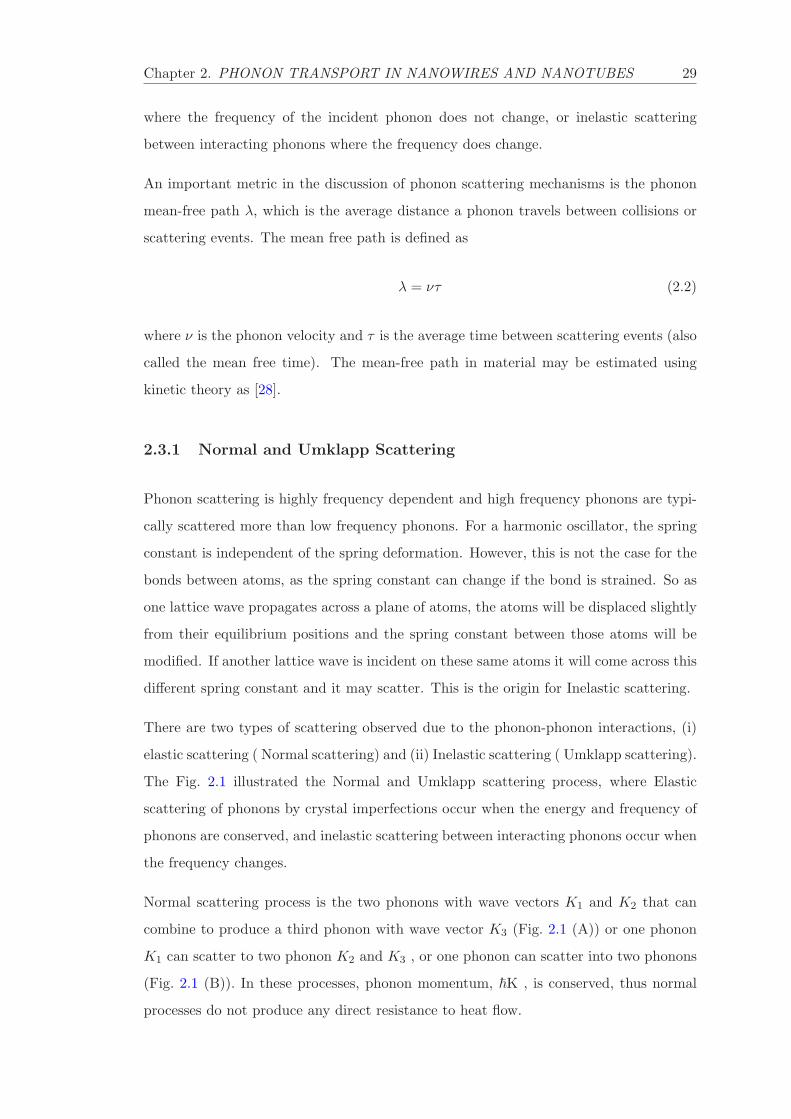
Chapter 2. PHONON TRANSPORT IN NANOWIRES AND NANOTUBES 29
where the frequency of the incident phonon does not change, or inelastic scattering
between interacting phonons where the frequency does change.
An important metric in the discussion of phonon scattering mechanisms is the phonon
mean-free path λ, which is the average distance a phonon travels between collisions or
scattering events. The mean free path is defined as
λ = ντ (2.2)
where ν is the phonon velocity and τ is the average time between scattering events (also
called the mean free time). The mean-free path in material may be estimated using
kinetic theory as [28].
2.3.1 Normal and Umklapp Scattering
Phonon scattering is highly frequency dependent and high frequency phonons are typi-
cally scattered more than low frequency phonons. For a harmonic oscillator, the spring
constant is independent of the spring deformation. However, this is not the case for the
bonds between atoms, as the spring constant can change if the bond is strained. So as
one lattice wave propagates across a plane of atoms, the atoms will be displaced slightly
from their equilibrium positions and the spring constant between those atoms will be
modified. If another lattice wave is incident on these same atoms it will come across this
different spring constant and it may scatter. This is the origin for Inelastic scattering.
There are two types of scattering observed due to the phonon-phonon interactions, (i)
elastic scattering ( Normal scattering) and (ii) Inelastic scattering ( Umklapp scattering).
The Fig. 2.1 illustrated the Normal and Umklapp scattering process, where Elastic
scattering of phonons by crystal imperfections occur when the energy and frequency of
phonons are conserved, and inelastic scattering between interacting phonons occur when
the frequency changes.
Normal scattering process is the two phonons with wave vectors K1 and K2 that can
combine to produce a third phonon with wave vector K3 (Fig. 2.1 (A)) or one phonon
K1 can scatter to two phonon K2 and K3 , or one phonon can scatter into two phonons
(Fig. 2.1 (B)). In these processes, phonon momentum, ~K , is conserved, thus normal
processes do not produce any direct resistance to heat flow.

Chapter 2. PHONON TRANSPORT IN NANOWIRES AND NANOTUBES 30
Figure 2.1: (A) and (B) are two processes known as A Normal process is when onephonon scatters into two phonons. (C) Umklapp process where two phonons combineto create a third. Due to the discrete nature of the atomic lattice there is a minimumphonon wavelength, which corresponds to a maximum allowable wavevector. If twophonons combine to create a third phonon which has a wavevector greater than thismaximum, the direction of the phonon will be reversed or flipped over with a reciprocal
lattice vector G, such that its wavevector is allowed.
The Umklapp process is very important to study in nanostructures. In this case K1
and K2 combine to form a third phonon K3 = K1 +K2, but due to the discrete nature
of atomic arrangement in crystal there is a minimum wavelength of phonon which can
propagate through the crystal of 2a, where a is atomic spacing. Since k = 2π/λ, hence
upper limit of k is π/a. If the sum of K1 and K2 is greater than this maximum, the
process can only be completed with the addition of what is known as the reciprocal
lattice vector [32? , 33]. This reciprocal lattice vector flips the phonon over to a lower
frequency and wave vector, and reverses the direction of the phonon as illustrated in
Fig. 2.1 (C). Phonon momentum is not conserved during the umklap process, therefore
producing a resistance to heat flow.

Chapter 2. PHONON TRANSPORT IN NANOWIRES AND NANOTUBES 31
kl
Temperature, T/D
Increasing Defect Concentration
Boundary Defect Phonon Scattering
kl Td
0.01 0.1 1
Figure 2.2: Temperature dependence of lattice thermal conductivity of solids. Bound-ary scattering dominates at lower temperatures, while impurity scattering becomessignificant at intermediate temperatures. At high temperatures, inelastic scattering
contributes considerably towards the overall thermal resistance.
2.3.2 Scattering by Defects, Dislocations and Impurities
When phonon propagates inside the material medium, in addition to the phonon-phonon
interactions, phonon may scatter due to many parameters such as crystal imperfection,
defects, dislocation, impurities etc.
Defects or dislocations in the atomic lattice have the effect of acting as a different mass
and/or spring constant to the incident phonons. Impurity atoms will have a differ-
ent mass and spring constant from the host atoms, thus disrupting phonon transport
in a similar manner as described above. These impurity atoms can be in the form of
dopant atoms or they can be species introduced to form an alloy. Alloying is a partic-
ularly effective way to reduce thermal conductivity. A good example could be, at room
temperature, silicon [34] has a thermal conductivity of approximately 140 W/m-K and
Chapter 2. PHONON TRANSPORT IN NANOWIRES AND NANOTUBES 32
germanium [35] has a thermal conductivity of roughly 60 W/m-K. However, SixGe1−x
alloys [36] have a room temperature thermal conductivity of approximately 510 W/m-K,
for Ge concentrations of 10 to 90%. A typical plot of phonon thermal conductivity of a
material vs. temperature is shown in Fig. 2.2.
2.3.3 Temperature dependence of Phonon Scattering
Described above all different scattering processes in nanostructures or bulk materials
may dominate heat transport in a material depending on temperature. This is due to
the fact that the dominant wavelength of the phonon, λdom, and the temperature are
related by an analogous Wien’s displacement for phonons: λdom = hν3kBT , where h is
Planck’s constant. At low temperatures, the dominant phonon wavelength is so large
that the phonons are not scattered by the defects. Moreover, as the dominant wavelength
is large, corresponding wavevectors are small. Since large wavevectors are required for
Umklapp scattering, this mechanism becomes unimportant, and phonon-phonon scat-
tering is frozen out. Therefore, boundary scattering is the dominating mechanism at
low temperatures as shown in Fig. 2.2. The phonon component of thermal conductivity,
κph, is defined as κph = 13cphνphlph, where cph is the phonon heat capacity, νph is the
speed of sound in the material, and λph is the mean free path of the phonons. At low
temperatures, νph and lph are constant, and cph ∝ T 3. Therefore, κph also varies as T 3.
As the temperature increases, defect scattering becomes more dominant. This is due to
the fact that the dominant phonon wavelength decreases as the temperature increases,
and gradually becomes comparable to the size of the defects. This causes phonons to
be scattered at the defect sites. For further increases in the temperature, wavevectors
become so large that Umklapp scattering starts to play an important role.
A typical plot of phonon thermal conductivity of a material vs. temperature is shown in
Fig. 2.2. For temperatures much smaller than the Debye temperature, as other scattering
mechanisms are frozen out, boundary scattering is the dominating mechanism for heat
transport. Debye temperature, θD, is defined as θD = hωD
kB, where ωD is the Debye
cutoff frequency. In the middle range, where κph plateaus, impurity scattering is more
important. At higher temperatures, Umklapp-scattering becomes dominant and we
observe a decline in the thermal conductivity. It is to be noted that impurity scattering

Chapter 2. PHONON TRANSPORT IN NANOWIRES AND NANOTUBES 33
may dominate over much of the temperature range for alloys and doped semiconductors
as they have a large number of defects and impurities.
2.4 Summary
The phonon transport in nanostructure is different than their bulk materials. When
we go from bulk to nanostructure, the materials structure and lattice arrangement are
not exactly the same as bulk structure. There are a large number of defects produced
during the nanostructure formation which significantly changes the phonon transport as
compared to their bulk counterpart. Due to the high defects level inside the nanowires,
thermal conductivity was drastically reduced compared to their bulk materials.

Bibliography
[1] G. A. Ozin, Adv. Mater. 4, 612-649 (1992).
[2] R. J. Tonucci, B. J. Justus, A. J. Campillo, and C. E. Ford, Science 258, 783-785
(1992).
[3] J. Y. Ying, Science 18, 56 -63 (1999).
[4] J. Ling, H. Chi, A. Yin, and J. M. Xu, Journal of Appl. Phys. 91, 2544 (2002).
[5] R. S. Wagner and W. C. Ellis, Appl. Phys. Lett. 4, 89-90 (1964).
[6] E. I.Givargizov, J. Cryst. Growth 31, 20-30 (1975).
[7] Y. Wu and P. Yang, Chem. Mater. 12, 605-7 (2000).
[8] A. A. Balandin, J. Nanosci. Nanotech. 5(7), 1015-1022 (2005).
[9] A. A. Balandin, Phys. Low-Dim. Structures. 73(5/6), 73 (2000).
[10] A. A. Balandin, Int. J. Therm. Sci. 39, 47 (2000).
[11] J. M. Ziman, “Electrons and Phonons”, University Press, Oxford (1979).
[12] J. Hone, Dekker Encyclopedia of Nanoscience and Nanotechnology., DOI:
10:108/E-ENN 120009128,, 60, (2004).
[13] R. T. Saito, T. Takeya, H. Kimura, M. S. Dresselhaus, and G. Dresselhaus, Phys.
Rev. Lett. 57, 4145-5 (2008).
[14] R. T. Saito, G. Dresselhaus, and M. S. Dresselhaus, London: Imperial College Press.
(1998).
[15] Sanchez-Portal, D.; E. Artacho, J. M. Solar, A. Rubio, and P. Ordejon, Phys. Rev.
B. 19, 12678-88 (1999).
34
Chapter 2. PHONON TRANSPORT IN NANOWIRES AND NANOTUBES 35
[16] Y. J. Zhang, Q. Zhang, N. L. Wang, Y. J Yan, H. H. Zhou, and J. Zhu, J. Cryst.
Growth. 226, 185-91 (2001).
[17] J. Westwater, D. P. Gosain, S. Tomiya, S. Usui, and H. Ruda, J. Vac. Sci. Technol.
B 15, 554-57 (1997).
[18] Y. Wu and P. Yang, J. Am. Chem. Soc. 123, 3165-66 (2001).
[19] M. S. Gudiksen and C. M. Lieber, J. Am. Chem. Soc. 122, 8801-2 (2000).
[20] Y. Wu, H. Yan, M. Huang, B. Messer, J. H. Song, and P. Yang, Chem. Eur. J.
8, 1260-68 (2002).
[21] X. Duan and C. M. Lieber, Adv. Mater. 12, 298-302 (2000).
[22] C. C. Chen, C. C. Yeh, C. H. Chen, Yu MY, and Liu HL, J. Am. Chem. Soc. 123,
2791-98 (2001).
[23] J. Zhang, X. S. Peng, X. F. Wang, Y. W. Wang, and L. D, Zhang, Chem. Phys.
Lett. 345, 372-76 (2001).
[24] M. He, P. Zhou, S. N. Mohammad, G. L. Harris, and J. B. Halpern, J. Cryst.
Growth 231, 357-65 (2001).
[25] W. S. Shi, Y. F Zheng, N. Wang, C. S. Lee, and S. T. Lee, J. Vac. Sci. Technol.
B 19, 1115-18 (2001).
[26] N. W. Ashcroft and D. N. Mermin, Solid State Physics, Saunders College Publish-
ing, Fort Worth (1976).
[27] C. L. Tien, A. Majumdar, and F. M. Gerner, Microscale Energy Transport, Taylor
and Francis, Bristol, (1998).
[28] C. Kittel, “Introduction to Solid State Physics”, John Willey and Sons, New York
1996.
[29] J. Zou and A. Balandin, J. Appl. Phys. 89, 293238 (2001).
[30] X. Lu, J. H. Chu, and W. H. Shen, J. Appl. Phys. 93, 121929 (2003).
[31] L. D. Hicks and M. S. Dresselhaus, Phys. Rev. B 47, 12727 (1993).

Chapter 2. PHONON TRANSPORT IN NANOWIRES AND NANOTUBES 36
[32] N. W. Ashcroft and D. N. Mermin, “Solid State Physics”, Saunders College Pub-
lishing, FortWorth, (1976).
[33] C. L. Tien, A. Majumdar, and F. M. Gerner, “Microscale Energy Transport”,
Bristol, Taylor and Francis, Bristol, (1998).
[34] Y. S. Touloukian, Thermophysical Properties of Matter 2, 326-338 (1970).
[35] Y. S. Touloukian, Thermophysical Properties of Matter, 2, 108-111 (1970).
[36] J. P. Dismukes, L. Ekstrom, E. F. Steigmeier, I. Kudman, and D. S. Beers, Journal
of Applied Physics 35, 2899-2970 (1964).

Chapter 3
EXPERIMENTAL METHODS
FOR THERMAL
MEASUREMENT
3.1 Materials and Synthesis
3.1.1 Nanowires and Synthesis Technique
Nanowires are especially very attractive for nanoscience studies as well as for nan-
otechnology applications. Nanowires have many advantages over bulk counterparts.
Nanowires, compared to other low dimensional systems, have two quantum confined
directions, while still leaving one unconfined direction for electrical conduction. This
allows nanowires to be used in applications where electrical conduction, rather than
tunneling transport, is required. Because of their unique density of electronic states (
DOS), nanowires in the limit of small diameters are expected to exhibit significantly dif-
ferent optical, electrical, thermal and magnetic properties from their bulk 3D crystalline
counterparts. The increased surface area, enhanced diameter-dependent bandgap, exci-
ton binding energy, and increased surface scattering for electrons and phonons are just
some of the ways in which nanowires differ from their corresponding bulk materials.
Yet the sizes of nanowires are typically large enough (> 1 nm in the quantum con-
fined direction) to have local crystal structures closely related to their parent materials,
37
Chapter 3. EXPERIMENTAL METHODS 38
thereby allowing theoretical predictions about their properties to be made on the basis
of an extensive literature relevant to their bulk properties. Not only do nanowires ex-
hibit many properties that are similar to, and others that are distinctly different from,
those of their bulk counterparts, nanowires have the advantage from an applications
standpoint that some of the materials parameters that are critical for certain proper-
ties can be independently controlled in nanowires, but not in their bulk counterparts,
such as, for example, their thermal conductivity. Also certain properties can be en-
hanced non-linearly in small diameter nanowires, by exploiting the singular aspects of
the 1D electronic density of states. Furthermore, nanowires have been shown to provide
a promising framework for applying the “bottom-up” approach (Feynman, 1959) for
the design of nanostructures for nanoscience investigations and for potential nanotech-
nology applications. From all these aspects: (1) these new research and development
opportunities nanowires/nanotubes driven by, (2) the smaller and smaller length scales
now being used in the semiconductor, opto-electronics and magnetics industries, and (3)
the dramatic development of the biotechnology industry where the action is also at the
nanoscale, the nanowire/nanotubes research field has developed with exceptional speed
in the last few years. Therefore a review of the current status of nanowire/nanotubes
research is of significant broad interest at the present time. It is the aim of this study
to focus on nanowire properties that differ from those of their parent crystalline bulk
materials, with an eye toward possible applications that might emerge from the unique
properties of nanowires/nanotubes and from future discoveries in this field.
Before discussing some specific strategies for growing one-dimensional nanostructures, it
is interesting to know the difference between growth methods and growth mechanisms.
Growth mechanisms are the general phenomenon whereby a one-dimensional morphol-
ogy is obtained, and the growth methods are the experimentally employed chemical
processes that incorporate the underlying mechanism to realize the synthesis of these
nanostructures. A novel growth mechanism should satisfy three conditions: It must (a)
explain how one-dimensional growth occurs, (b) provide a kinetic and thermodynamic
rationale, and (c) be predictable and applicable to a wide variety of systems. Growth
of many one-dimensional systems has been experimentally achieved without satisfactory
elucidation of the underlying mechanism, as is the case for oxide nanoribbons. Nev-
ertheless, understanding the growth mechanism is an important aspect of developing
a synthetic method for generating one-dimensional nanostructures of desired material,

Chapter 3. EXPERIMENTAL METHODS 39
size, and morphology. This knowledge imparts the ability to assess which of the exper-
imental parameters controls the size, shape, and monodispersity of the nanowires, as
well as the ease of tailoring the synthesis to form higher-ordered heterostructures. In
general, one-dimensional nanostructures are synthesized by promoting the crystalliza-
tion of solid-state structures along one direction. The actual mechanisms of coaxing this
type of crystal growth include (a) growth of an intrinsically anisotropic crystallographic
structure, and (b) the use of various templates with one-dimensional morphologies to
direct the formation of one-dimensional nanostructures.
In this chapter we have discussed (1) some common synthesis techniques that have suc-
cessfully afforded high quality nanowires of large variety of materials, and (2) Phonon
transport and mechanism inside the nanowires and nanotubes. There was also a short
overview of synthesis methods approached by many groups to grow well defined, high
quality and desired shapes and sizes of nanostructures. The synthesis methods of
nanowires/nanotubes used for our study was described briefly in the next two chap-
ters and more detail can be found in the Huanan Duan thesis [24].
3.2 CVD Methods, Template-Assisted Synthesis
The template-assisted synthesis of nanowires and nanotubes is a conceptually simple
and intuitive way to fabricate highly ordered anisotropic nanostructures [1–3, 12]. These
templates contain very small cylindrical pores or voids within the host material, and the
empty spaces are filled with the chosen material, which adopts the pore morphology, to
form nanowires. This method provides well aligned, densely packed and desirable sizes
of nanowires/nanotubes.
Template Synthesis
In template-assisted synthesis of nanostructures, the chemical stability and mechanical
properties of the template, as well as the diameter, uniformity and density of the pores
are important characteristics to consider. Templates frequently used for nanowire syn-
thesis include anodic alumina (Al2O3), nano-channel glass, ion track-etched polymers
and mica films.

Chapter 3. EXPERIMENTAL METHODS 40
Figure 3.1: Synthesis method used for Co Nws.
Porous anodic alumina templates were produced by anodizing pure Al films in various
acids [12]. Under careful chosen anodization conditions, the resulting oxide film possesed
a regular hexagonal array of parallel and nearly cylindrical channels, as shown in Fig. 4.1
Co NWs were synthesized by electrodeposition assisted by a homemade anodic aluminum
oxide (AAO) template. Fig. 4.1 provides a schematic of the synthesis steps. The AAO
templates were obtained by a well-established two-step anodization process [4, 29]. The
detail of anodization of nanowires was described in the experimental part of the next
chapter and also can be found elsewhere [24].
3.3 Vapor-Liquid-Solid (VLS) Methods
This process was originally developed by Wagner and Ellis to produce micrometer-sized
whiskers in the 1960s [5], later justified thermodynamically and kinetically [6], and
recently reexamined by Lieber, Yang, and other researchers to generate nanowires and
nanorods from a rich variety of inorganic materials [7–16]. Several years ago, people used
in situ transmission electron microscopy (TEM) techniques to monitor the VLS growth
mechanism in real time [17]. A typical VLS process starts with the dissolution of gaseous
reactants into nanosized liquid droplets of a catalyst metal, followed by nucleation and
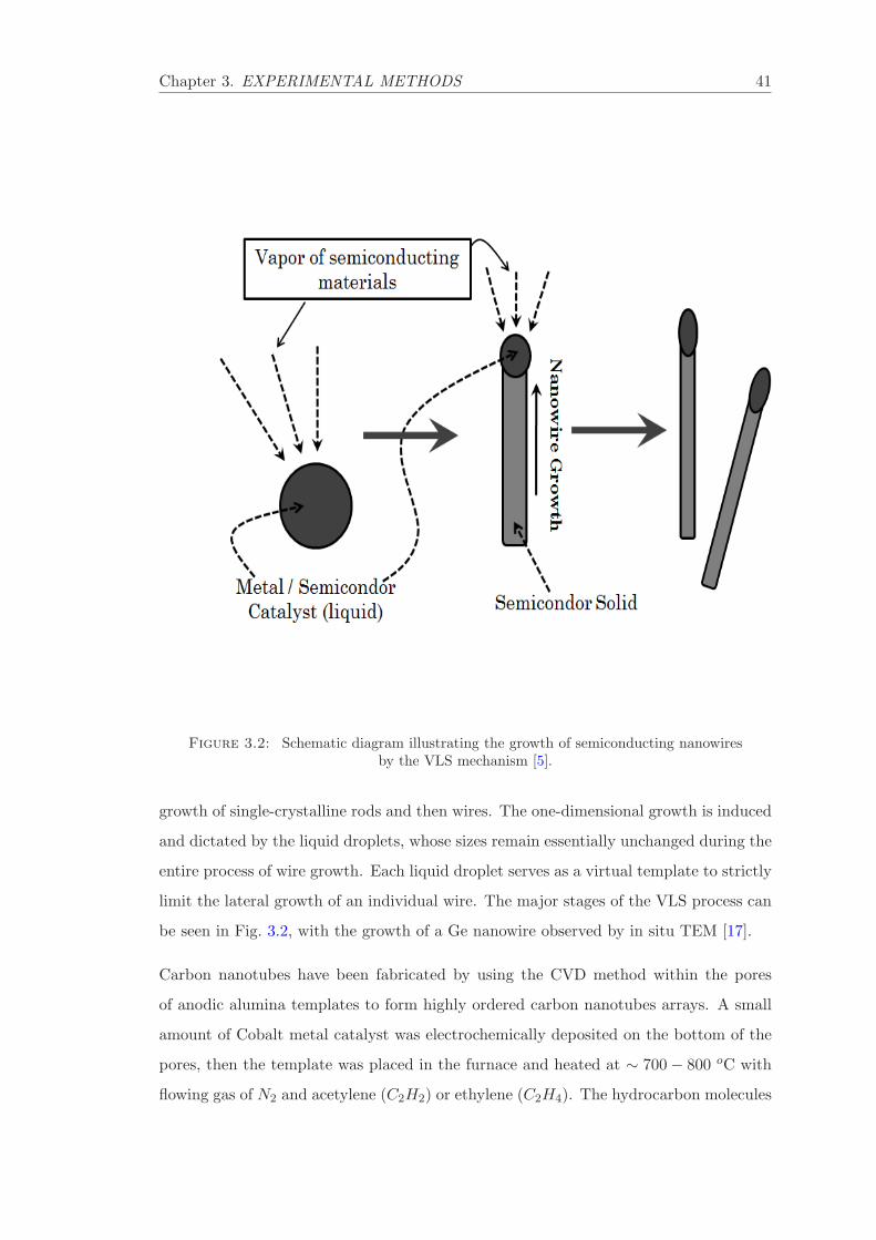
Chapter 3. EXPERIMENTAL METHODS 41
Figure 3.2: Schematic diagram illustrating the growth of semiconducting nanowiresby the VLS mechanism [5].
growth of single-crystalline rods and then wires. The one-dimensional growth is induced
and dictated by the liquid droplets, whose sizes remain essentially unchanged during the
entire process of wire growth. Each liquid droplet serves as a virtual template to strictly
limit the lateral growth of an individual wire. The major stages of the VLS process can
be seen in Fig. 3.2, with the growth of a Ge nanowire observed by in situ TEM [17].
Carbon nanotubes have been fabricated by using the CVD method within the pores
of anodic alumina templates to form highly ordered carbon nanotubes arrays. A small
amount of Cobalt metal catalyst was electrochemically deposited on the bottom of the
pores, then the template was placed in the furnace and heated at ∼ 700 − 800 oC with
flowing gas of N2 and acetylene (C2H2) or ethylene (C2H4). The hydrocarbon molecules

Chapter 3. EXPERIMENTAL METHODS 42
are polarized and form carbon nanotubes inside the pores of the AAO template with
the help of metal catalysts. The detail about carbon nanotube synthesis is described in
Chapter 5.
3.4 AC Calorimetry
The AC Calorimetry technique is ideal for the study of phase transition and thermal
measurement for several important reasons. Measurements of heat capacity are made
at near equilibrium conditions. This is crucial since much of the thermodynamic theory
of phase transitions is based on equilibrium considerations. It also allows the use of
averaging routines and total automation thus resolving remarkably small heat capacity
changes. In most cases, only a small amount of material is required to achieve a high
resolution. Finally, strict thermal isolation of the sample from the surroundings (as
in an adiabatic technique) is not required. Its implementation is straightforward and
adaptable to a variety of physical systems over a wide temperature range.
3.4.1 Theory
The AC Calorimetry technique was originally introduced by Sullivan and Seidel [1] in
1968. In this technique, sinusoidal heating by a voltage of frequency fv is applied to the
sample of interest inducing temperature oscillations of frequency 2fv. The heat capacity
of the sample is inversely proportional to the magnitude of the temperature oscillations.
The derivation given below is geometry independent, i.e., the locations of the applied
heat and the sensing of the resulting temperature oscillations is unimportant provided
certain requirements are met. A schematic representation of the thermal model is shown
in Fig. 3.3
The fundamental principle of the AC calorimetry technique consists of applying period-
ically modulated, sinusoidal power, and measuring the resulting sinusoidal temperature
response. As we will show later, the heat capacity of the sample is inversely proportional
to the amplitude of the temperature oscillations. The derivation of the basic operat-
ing equations based on a simplified thermal model of the system is meeting certain
requirements geometry independent.
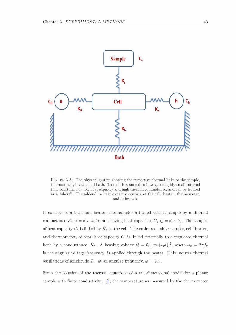
Chapter 3. EXPERIMENTAL METHODS 43
Figure 3.3: The physical system showing the respective thermal links to the sample,thermometer, heater, and bath. The cell is assumed to have a negligibly small internaltime constant, i.e., low heat capacity and high thermal conductance, and can be treatedas a “short”. The addendum heat capacity consists of the cell, heater, thermometer,
and adhesives.
It consists of a bath and heater, thermometer attached with a sample by a thermal
conductance Ki (i = θ, s, h, b), and having heat capacities Cj (j = θ, s, h). The sample,
of heat capacity Cs is linked by Ks to the cell. The entire assembly: sample, cell, heater,
and thermometer, of total heat capacity C, is linked externally to a regulated thermal
bath by a conductance, Kb. A heating voltage Q = Q0[cos(ωvt)]2, where ωv = 2πfv
is the angular voltage frequency, is applied through the heater. This induces thermal
oscillations of amplitude Tac at an angular frequency, ω = 2ωv.
From the solution of the thermal equations of a one-dimensional model for a planar
sample with finite conductivity [2], the temperature as measured by the thermometer

Chapter 3. EXPERIMENTAL METHODS 44
is given by
Tac = Tb +Q0
2Kb+
Q0
2ωC
[
1 +1
(ωτe)2+ ω2(τ2
θ + τ2h + τ2
s )
]− 1
2
cos(ωt− α). (3.1)
Tb is the bath temperature; the second term is identified as Tdc, the sample temper-
ature resulting from the rms heating, while the last term is the induced temperature
oscillations. The amplitude of the oscillations can be written in the simple form as
Tac =Q0
2ωC
[
1 +1
(ωτe)2+ ω2τ2
i
]− 1
2
, (3.2)
with the relaxation times defined by
τe =C
Kb, τθ =
Cθ
Kθ, τh =
Ch
Kh, τs =
Cs
Ks, (3.3)
There are two important thermal relaxation time constants contained in Eq. (5.1), the
external τe = ReC and the internal τ2ii = τ2
s + τ2c and τii = (τθ + τh + τs). That is the
sum of the squared thermal relaxation times for the sample (τs) and cell (τc). Here,
Rs is the sample’s thermal resistance and Re is the external thermal resistance to the
bath. There is also a phase shift Φ between the applied heat and resulting temperature
oscillations but it is more convenient to define a reduced phase shift φ = Φ + π/2 for
heating frequencies between 1τe
and 1τii
, Φ ≈ −π2 . The reduced phase shift, to the same
accuracy as Eq. (5.1), is given by
tan(φ) = (ωτe)−1 − ωτi (3.4)
where here τi = τs + τc. Since τc is typically small compared to τs such that τi ∼= τii,
Eq. (5.2) can be rewritten to give τs ≡ RsCs∼= 1
ω2τe− tan φ
ω . The measured reduced
phase shift φ also contains a linear ω dependence due to the fixed digitization rate of
the thermal oscillation as the heating frequency increases. The observed φ is then given
by
φexp = arctan((ωτe)−1 − ωτi) + aω + φ0 (3.5)
where a is determined by the digitization rate (in our case, a ≈ 1) and φ0 is the resulting
phase shift due to the digitizing dead-time (delay), which for our apparatus is negligible.
The phase shift is related to both the heat capacity and the thermal conductive properties
Chapter 3. EXPERIMENTAL METHODS 45
of the entire system. Using Eqs. 3.3 and Eqs. 3.5 and since the external time constant
is typically temperature independent and can be measured separately, one can solve for
Ks, the sample thermal conductance. If the thermal conductances and heat capacities of
the thermometer and heater are small and nearly constant, i.e., B = τθ + τh ≡ constant,
then Ks may be written as
Ks = Cs
[(
1
ω2τe−B
)
− 1
ωtanφ
]−1
, (3.6)
Equation 5.1 is an exact expression for the total heat capacity. However, by operating
at a frequency such that the internal and external time constant do not dominate Tac,
an approximation can be made which greatly simplifies the relation between Tac and C.
This approximation may lead to a small error in the absolute heat capacity without loss
of sensitivity to small changes. If the imposed oscillations are at a frequency “slower”
than the sample internal equilibration time but “faster” than the external equilibration
time (so that a negligible amount of heat is lost to the bath), then
1
τe< ω <
1
τi, (3.7)
Now by solving equation 5.1
C ≈ 1
ωTac, (3.8)
The external time constant is controlled by tailoring the thermal link to the bath. It is
usually made by thermally anchoring the heater and thermometer electrical leads to a
temperature controlled reservoir. This thermal link, on the order of 10 to 100 seconds,
is easily adjusted by selecting the appropriate material, length and cross-section for the
leads.
Adjustment of the internal time constant is not as straightforward as it strongly depends
on the thickness of the sample (the time constants of the thermometer and heater links
are again neglected). If the sample thickness is less than the thermal diffusion length
given by
l =
√
2KsA
ωCs, (3.9)
where Ks, is the sample thermal conductance, Cs, its heat capacity and A is the cross-
sectional area of the sample, then, the right hand side of Eq. 3.7 is satisfied. Once

Chapter 3. EXPERIMENTAL METHODS 46
satisfied, the location of the applied heat and the measurement of temperature becomes
unimportant, i.e., the system is now geometry independent.
Experimentally, it is possible to verify if the requirements of Eq. 3.7 are satisfied by
means of a frequency scan. Such a frequency profile is determined by maintaining
the same voltage amplitude oscillations at constant temperature while sweeping the
frequency and measuring the resulting temperature oscillations. A plot of ωTac vs ω,
for a well designed cell, will typically show a “plateau” shown in frequency scan data of
chapter 4. The plateau indicates the region where the heat capacity will be frequency
independent and neither time constant plays a major role (see figure of frequency scan
in chapter 4). The wider the plateau, the smaller the error associated with the use of
Eq. 3.8.
Now going back to Eq. 5.1, the total heat capacity C = Cs + Cc refers here to the
combination of the sample and other cell components associated with the sample cell.
Here, Cc = CH + CGE + CAAO + CAg accounts for the contributions to the cell heat
capacity by the heater (H), General Electric #7031 varnish (GE), silver cell container
(Ag), and the AAO template (for the parallel measurement). By subtracting the cell
contributions, the heat capacity of the sample may be isolated CSample = C − Cc and
by dividing by the mass of the sample yields the desired specific heat. Note that the
contribution of the carbon-flake thermistor (θ) is much smaller than all these elements
and is typically ignored.
The effective thermal conductance, the inverse of the thermal resistance, of the sample
can then be evaluated from the AC-calorimetric parameters as
Ks∼= ω2τeCs
1 − ωτe tanφ(3.10)
where Ks is in units of W K−1. With the geometric dimensions of sample+cell config-
uration, the effective thermal conductivity κs in units of W m−1 K−1 can be calculated
directly as κs = KsL/A, where L is the thickness and A is the area of the sample.
3.4.2 Construction of AC Calorimeter
The Fig. 3.4 shows the construction of the AC Calorimeter. The cell which holds the
sample is supported by the temperature controlled enclosed bath made by Cu. Sample
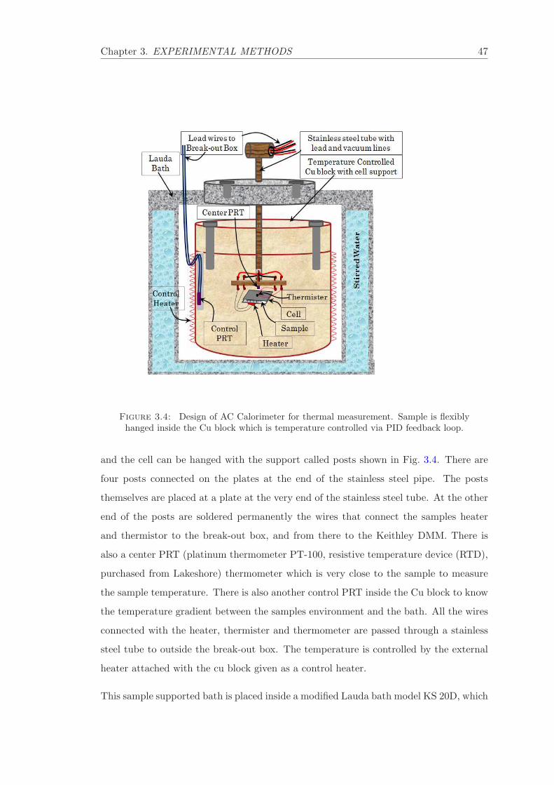
Chapter 3. EXPERIMENTAL METHODS 47
Figure 3.4: Design of AC Calorimeter for thermal measurement. Sample is flexiblyhanged inside the Cu block which is temperature controlled via PID feedback loop.
and the cell can be hanged with the support called posts shown in Fig. 3.4. There are
four posts connected on the plates at the end of the stainless steel pipe. The posts
themselves are placed at a plate at the very end of the stainless steel tube. At the other
end of the posts are soldered permanently the wires that connect the samples heater
and thermistor to the break-out box, and from there to the Keithley DMM. There is
also a center PRT (platinum thermometer PT-100, resistive temperature device (RTD),
purchased from Lakeshore) thermometer which is very close to the sample to measure
the sample temperature. There is also another control PRT inside the Cu block to know
the temperature gradient between the samples environment and the bath. All the wires
connected with the heater, thermister and thermometer are passed through a stainless
steel tube to outside the break-out box. The temperature is controlled by the external
heater attached with the cu block given as a control heater.
This sample supported bath is placed inside a modified Lauda bath model KS 20D, which

Chapter 3. EXPERIMENTAL METHODS 48
provides a first temperature control stage with a stability of ±0.1 K. The temperature of
the copper block is controlled from a Lakeshore temperature controller, model No 340.
via Proportional-Integral-Derivative ( PID) feedback loop [18]. The stable temperature
inside the cavity where the sample is situated is ≈ 100 µK and in the cylindrical bath
±1 mK.
A Kapton insulated flexible heater from Omega Engineering with exact dimension with
the Cu block are purchased and attached with glue on the outside of Cu block cylinder.
3.4.3 Electronic
Figure 3.5 shows the whole electronic diagram of instruments used for thermal char-
acterization by AC Calorimeter. All the instruments are connected with the computer
(Windows XP) via GPIB (General Purpose Interface Bus) interfaces of National Instru-
ment software. The C++ program used to run the experiment was written by Alex
Roshi and Germano Iannacchione. All the wires from the heater, thermister, and ther-
mometers are connected with proper conductivity with the outside instrument.
The system makes full use of the Keithley DMM, Model 2002, with 812 digits of resolution,
a 128 kB on board memory card, and a multiplex scanner card model 2001-SCAN [19].
The scanner card gives the possibility to completely automate the measurements. The
card was configured to do 4-wire or 2-wire measurements. The resistance measurements
of the center PRT and the thermistor are configured as 4-wire, while the voltage and
resistance measurements, across the strain-gauge heater and the standard resistor, are
configured as 2-wire measurements. The latter two measurements are needed in order
to accurately determine the ac power applied at the cell.
Care was taken while measuring the PRT thermometer to minimize the self heating
that comes as a consequence of current passing through the resistance from the mea-
surement itself. This was seen to be very small and furthermore, would remain almost
constant during the measurement. Thus it can safely be neglected as a correction to the
temperature of the bath.
The electrical power dissipated in the strain-gauge heater is provided by an Hewlett
Packard Function Generator, model HP 33120A [20]. The strain-gauge is connected
in series with a high precision standard resistor RSTD. The purpose of this resistor is

Chapter 3. EXPERIMENTAL METHODS 49
Figure 3.5: Electronic connection with the instrument used in Calore A. The in-struments are controlled by C programming with the interface of GPIB and National
Instrument software.
twofold. First it reduces the voltage across the strain gauge heater, and secondly, it is
used to accurately measure the current through the heater, since IHTR = ISTD (by virtue
of the series connection). As already mentioned, the bath temperature is controlled by
the Lakeshore model 340 temperature controller. The cables for the heater and the
control PRT pass through a hole at the top of the Lauda bath directly to the Lakeshore
terminals.
3.5 Modulated Differential Scanning Calorimeter
The Differential Scanning Calorimeter ( DSC) is a thermal analysis instrument that
determines the temperature and heat flow associated with material transitions as a

Chapter 3. EXPERIMENTAL METHODS 50
function of time and temperature. There are number of applications and DSC can be
used to measure the following properties:
1. Glass transition
2. Melting temperature
3. Heat of fusion
4. Percent crystallinity
5. Crystallization kinetics and phase transitions
6. Oxidative stability
7. Curing kinetics
There are two kinds of DSC (i) Heat-Flux DSC and (ii) Power Compensated DSC
3.5.1 Heat-Flux DSC:
In a heat flux DSC, the sample material, enclosed in a pan and an empty reference pan
are placed on a thermoelectric disk surrounded by a furnace. The furnace is heated at a
linear heating rate and the heat is transferred to the sample and reference pan through
thermoelectric disk. However owing to the heat capacity of the sample there exists a
temperature difference between the sample and reference pans which is measured by area
thermocouples and the consequent heat flow is determined by the thermal equivalent of
Ohm’s law,
q =∆T
R(3.11)
where q = sample heat flow, ∆T = temperature difference between sample and reference
and R = resistance of thermoelectric disk.
3.5.2 Power-Compensated DSC
In power compensated calorimeters, the sample and reference pan are in separate fur-
naces heated by separate heaters. Both the sample and reference are maintained at the
same temperature and the difference in thermal power required to maintain them at the
same temperature is measured and plotted as a function of temperature or time. We
have the model Q200 DSC with the Tzero technology.
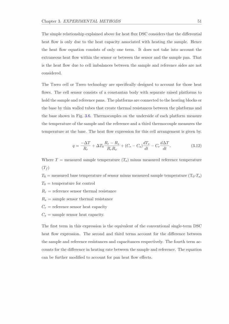
Chapter 3. EXPERIMENTAL METHODS 51
The simple relationship explained above for heat flux DSC considers that the differential
heat flow is only due to the heat capacity associated with heating the sample. Hence
the heat flow equation consists of only one term. It does not take into account the
extraneous heat flow within the sensor or between the sensor and the sample pan. That
is the heat flow due to cell imbalances between the sample and reference sides are not
considered.
The Tzero cell or Tzero technology are specifically designed to account for those heat
flows. The cell sensor consists of a constantan body with separate raised platforms to
hold the sample and reference pans. The platforms are connected to the heating blocks or
the base by thin walled tubes that create thermal resistances between the platforms and
the base shown in Fig. 3.6. Thermocouples on the underside of each platform measure
the temperature of the sample and the reference and a third thermocouple measures the
temperature at the base. The heat flow expression for this cell arrangement is given by.
q =−∆T
Rr+ ∆T0
Rr −Rs
RrRs+ (Cr − Cs)
dTs
dt− Cr
d∆T
dt. (3.12)
Where T = measured sample temperature (Ts) minus measured reference temperature
(Tf )
T0 = measured base temperature of sensor minus measured sample temperature (T0-Ts)
T0 = temperature for control
Rr = reference sensor thermal resistance
Rs = sample sensor thermal resistance
Cr = reference sensor heat capacity
Cs = sample sensor heat capacity.
The first term in this expression is the equivalent of the conventional single-term DSC
heat flow expression. The second and third terms account for the difference between
the sample and reference resistances and capacitances respectively. The fourth term ac-
counts for the difference in heating rate between the sample and reference. The equation
can be further modified to account for pan heat flow effects.

Chapter 3. EXPERIMENTAL METHODS 52
Figure 3.6: (A) DSC sample stage connected with the heater, (B) Hermetic pan and(C) Hermetic pan attached with lead, (D) Pans on the sample stage shown on (A),one is the sample pan and other is the reference pan nad (E) DSC Tzero press, whichtakes sample encapsulation to a new level of performance and convenience in crimpand hermetic sealing of a wide variety of materials [25]. This new universal press has a
smooth operating mechanism and automated force adjustment.
3.5.3 Temperature Modulated Differential Scanning Calorimeter
Differential scanning calorimetry (DSC) involves heating and cooling a sample at a
constant rate. This technique was established during the 1960s and remained unchanged
for almost three decades. During the 1990s, a new technique, temperature modulated
differential scanning calorimeter ( TMDSC) was developed. The concept behind TMDSC
has been around since 1910 [21, 22], although no concrete model existed at the time.
Gobrecht et al. [23] first introduced a model for TMDSC and cited several technical
limitations. In 1993, the concept was reintroduced by Reading, who had overcome the
limitations observed by Gobrecht.
The basic principle behind TMDSC is quite simple. A constant heating rate, similar

Chapter 3. EXPERIMENTAL METHODS 53
300 301 302 303 304-9
-6
-3
0
3
6
9299
300
301
302
303
304
305
T
T(K)
Modulated Heating rate
Average Heating rate
Period
Average Temperature
Modulated Temperature
Amplitude of Modulation
(b)
T (K
)(a)
Figure 3.7: (a) Temperature evolution of MDSC signal contains (a) raw data of mod-ulated temperature with amplitude showing in inset and (b) derivative of modulated
temperature is equivalent to modulated heating rate with temperature scan.
to the one used in conventional DSC, is modulated by superimposing upon it a peri-
odic temperature modulation of a certain amplitude and frequency. This results in a
simultaneous introduction of two different time scales in the experiment: a long time
scale corresponding to the underlying heating rate, and a shorter time scale (or cycle)
corresponding to the period of the modulation [23]. Figure 3.7 illustrates an example
of temperature evolution of the MDSC signals as a function of temperature scan. (a)
MDSC raw data, modulated temperature and average temperature and (b) is the deriva-
tive of temperature modulation known as modulated heating/cooling rate and average
signals.
3.5.4 Components of DSC Q200
The Q200 DSC consists of 3 basic units:

Chapter 3. EXPERIMENTAL METHODS 54
Furnace: This is the main assembly where the sample and reference are heated as per
the set temperature program.
Cooling system: This unit enables to cool the sample and assist in achieving the desired
temperature program.
Computer: This serves as an interface between the user and the instrument and enables
automatic control of instrument as per the parameters set.
The furnace or DSC cell dissipates heat to the specimens via a constantan disc. The disc
has two raised platforms on which the sample and reference pans are placed. The plat-
forms are connected to the heating block (base) by thin walled tubes that create thermal
resistances between the platforms and the base. A chromel disc and connecting wire are
attached to the underside of each platform, and the resulting chromel- constantan ther-
mocouples are used to determine the differential temperatures of interest. Alumel wires
attached to the chromel discs provide the chromel-alumel junctions for independently
measuring the sample and reference temperature. A separate thermocouple embedded
in the heating block measures the temperature of the base and serves as a temperature
controller for the programmed heating cycle. An inert gas is passed through the cell at
a constant low rate of about 50 ml/min.
There are different types of cooling system that can be used in conjunction with DSC.
The choice of cooling system depends on the temperature range that you wish to use
for your experiments. Details of the types of cooling systems and their usage conditions
can be found in the online TA Instrument website or DSC manual.
We have a refrigerated cooling system (RCS) in our lab with DSC Q200, which is used
to cool DSC experiments. It consists of a two-stage, cascade, vapor compression refrig-
eration system and can be used for experiments requiring cooling within an operating
range of −90 oC to 550 oC. The maximum rate of cooling depends on the temperature
range of the bexperiment. The flange temperature used to be ≈ −90 oC.
Using the instrument:
In order to perform DSC experiments you have to follow this general outline. In some
cases, not all of these steps are required. The majority of these steps are performed
using the instrument control software. The instructions needed to perform these actions

Chapter 3. EXPERIMENTAL METHODS 55
can be found in detail in the online help in the instrument control program; therefore
they will be discussed briefly here
1. Calibrating the instrument
2. Selecting the pan type and material
3. Preparing the sample
4. Creating or choosing the test procedure and entering sample and instrument infor-
mation through the TA instrument control software
5. Setting the purge gas flow rate
6. Loading the sample and closing the cell lid (Automated opening and closing in DSC
Q200)
7. Starting the experiment
To obtain accurate results, the following procedures can be carefully applied.
Sample Preparation:
Doing this before setting up the instrument is a good idea so you can run the experiment
as soon as the instrument is ready; in fact, make up all your samples so they are ready
to run before you waste machine time by trying to weigh and run the DSC at the same
time.
Selecting pan type:
Samples to be used in differential scanning calorimetry are small pieces that are enclosed
in special aluminum pans for experiments up to 6000C. Pans made of gold, copper, plat-
inum or graphite are used for high temperature runs (up to 7250C ) . Pans are crimped
closed using TA’s Blue DSC sample Press. Crimped pans improve the thermal contact
between the sample, pan and disc, reduce thermal gradients in the sample, minimize
spillage, and enable retention of the sample for further study. For most experiments
on solid polymeric materials, non-hermetic pans (ones that don’t seal airtight) are ap-
propriate. Hermetic pans are normally used only for special applications like studies
of volatile liquids including specific heat, studies of materials that sublime, studies of
aqueous solutions above 1000C, examinations of materials generating corrosive or con-
densable gases, and examinations of materials in self-generating atmospheres and also

Chapter 3. EXPERIMENTAL METHODS 56
for liquid crystals. We used hermetically sealed pans for polymer-carbon nanotube com-
posites and liquid crystal sample. Our sample press is normally set up for non-hermetic
pans, but a few simple adjustments can be made for others.
Generally the appropriate mass range for samples in DSC is 1 mg to 10 mg. If you have
a bulk piece of material, it is necessary to convert this to a form that can be used in
the DSC. No matter what, you should never touch a sample, pan or lid with your bare
hands, oils from your skin can give their own results in the DSC. Use gloves and goggles
while preparing samples. It is important to accurately measure its mass because this is
entered into the DSC so that it can give you data that is independent of sample size.
• Start by placing a pan and a lid (they look very similar but the lid is in fact slightly
smaller) open-side-up on the microbalance and note down its mass.
• Weigh your sample separately and note its mass
• Then, using tweezers place your sample in the pan and place the lid on top.
• Place them in the sample press as shown in Fig. 3.6.
• Pull the lever down. If the press is set up correctly, it should press the lid down
onto the pan and the side walls will wrap around the top
• Place the sample pan in the auto sampler tray and note the position number
• You need a reference pan. For T4P heat flow we have a reference pan in the R2
position in the auto sampler tray. Take it out with tweezers, weigh it and place it
back in the tray. You need to do it only once. For subsequent runs you can use
the same reading. If you don’t find a reference pan you can make one by taking
an empty pan and lid, weighing it and then crimping it as explained above.
• You need to enter the sample and reference pan weights in the test procedure.
Hence note it in your notebook during sample preparation.

Chapter 3. EXPERIMENTAL METHODS 57
Purge gas:
Sample atmosphere during DSC experiments can be controlled by connecting purge
gases to the system.
1. Turn on the nitrogen cylinder. Make sure that the pressure of your purge gas source
is regulated between 100 and 140 kPa gauge (15 and 20 psi) before you turn on the
cooler, otherwise the sample part will get frigid.
2. Set the flow rate to the recommended value of 50 mL per minute for your experiments
on the Notes Page of the Experiment View. Click Apply to save the changes
Calibration:
The Instrument needs to be calibrated in equal environmental conditions and parameters
of the experiment needed to run. There are two different calibration methods to do,
one is for DSC calibration and the other one is for MDSC calibration for doing MDSC
experiments. The Auto calibration wizard method works very well to do the calibration.
We just need to follow the procedure as you start calibrating.
For running the heating/cooling of the sample for DSC measurement, the following steps
can be edited in the procedure list.
Now say you want to heat the sample and cool it again over the same range. You would
simply insert another ramp line after the isothermal, enter your ramp rate again and
enter the end temperature. So the editor will look something like this
1. Equilibrate at temperature T1
2. isothermal for 10 min
3. ramp at 20C/min to Temperature T2
4. Equilibrate at temperature T2
5. isothermal for 10 min
6. ramp at 20C/min to Temperature T1
For MDSC run the procedure in editor to look something like this
1. Equilibrate at temperature T1
2. isothermal for 10 min
3. Modulate at 60 sec/min
4. ramp at 20C/min to Temperature T2
Chapter 3. EXPERIMENTAL METHODS 58
5. Equilibrate at temperature T2
6. isothermal for 10 min
7. Modulate at 60 sec/min
8. ramp at 20C/min to Temperature T1
Scan rates:
The whole concept of DSC is that the sample remains in thermal equilibrium, which
is clearly not possible while changing temperature. The only way to achieve this is
to have an infinitely slow heating rate. So the slower the heating rate the better the
results. However the runs need to completed in practical time also. For standard DSC I
have found that 100C/min seems to be a reasonable value which is also mostly used for
polymeric materials. But we measure glass transition of polymers in a different scan rate
dependent, so we went with 100C/min to 0.010C/min. If you want really good results
for a single scan you can go down to 20C/min, or less. But then the run takes longer,
so usually you want to find the medium that gives you run times that are reasonable
but still give you good results. And this is dependent upon materials to materials. Scan
rate is something you can play with when you first start running experiments.
3.6 Overview
In this experimental chapter, we focused on the different major experimental techniques
used for thermal characterization. These techniques are also described with more detail
in some of the other chapters. Different techniques shortly mention the fabrication
procedure of Carbon nanotubes and nanowires people generally used. Some of the
techniques give a large quantity of samples with different diameters and lengths, like in
the laser ablation method. Some of the methods are very slow, expensive and not suitable
to produce a large quantity of materials in a small time interval like in the CVD grown
method, Electro Chemical Anodization technique etc. But the quality could be better.
The experimental procedure in the AC Calorimeter and DSC or MDSC procedure is
thoroughly described.
Bibliography
[1] P.F. Sullivan and G. Seide1, Phys. Rev. 173, 679 (1968).
[2] H.S. Caarslaw and J.C. Jaeger, Conduction of Heat in Solids, Oxford Press (1959).
[3] L. D. Hicks and M. S. Dresselhaus, Phys. Rev. B 47, 12727 (1993).
[4] J. Ling, H. Chi, A. Yin, and J. M. XuJournal of Appl. Phys. 91, 2544 (2002).
[5] R. S. Wagner and W. C. Ellis, Appl. Phys. Lett. 4, 89-90 (1964).
[6] E. I.Givargizov, J. Cryst. Growth 31, 20-30 (1975).
[7] Y. Wu and P. Yang, Chem. Mater. 12, 605-7 (2000).
[8] Y. J. Zhang, Q. Zhang, N. L. Wang, Y. J Yan, H. H. Zhou, and J. Zhu, J. Cryst.
Growth. 226, 185-91 (2001).
[9] J. Westwater, D. P. Gosain, S. Tomiya, S. Usui, and H. Ruda, J. Vac. Sci. Technol.
B 15, 554-57 (1997).
[10] M. S. Gudiksen and C. M. Lieber, J. Am. Chem. Soc. 122, 8801-2 (2000).
[11] Y. Wu, H. Yan, M. Huang, B. Messer, J. H. Song, and P. Yang, Chem. Eur. J.
8, 1260-68 (2002).
[12] X. Duan and C. M. Lieber, Adv. Mater. 12, 298-302 (2000).
[13] C. C. Chen, C. C. Yeh, C. H. Chen, Yu MY, and Liu HL, J. Am. Chem. Soc. 123,
2791-98 (2001).
[14] J. Zhang, X. S. Peng, X. F. Wang, Y. W. Wang, and L. D, Zhang, Chem. Phys.
Lett. 345, 372-76 (2001).
59

Chapter 3. EXPERIMENTAL METHODS 60
[15] M. He, P. Zhou, S. N. Mohammad, G. L. Harris, and J. B. Halpern, J. Cryst.
Growth 231, 357-65 (2001).
[16] W. S. Shi, Y. F Zheng, N. Wang, C. S. Lee, and S. T. Lee, J. Vac. Sci. Technol.
B 19, 1115-18 (2001).
[17] Y. Wu and P. Yang, J. Am. Chem. Soc. 123, 3165-66 (2001).
[18] Lakeshore Cryotronics, http://www.lakeshore.com
[19] Keithley Instruments, Inc., http://www.keithley.com
[20] Agilent Technologies, Inc., http://www.agilent.com
[21] O. M. Corbino, Physikalische Zeitschrift 11, 413-417 (1910).
[22] O. M. Corbino, Physikalische Zeitschrift 12, 292-295 (1911).
[23] H. Gobrecht, K Hamann, and G. Willers, Journal of Physics E-Scientific Instru-
ments 4(1), 21 (1971).
[24] Huanan Duan, (PhD Thesis: Available in WPI library), URN:etd-052809-
122349 (2009).
[25] TA Instrument, New Castle, Delaware USA, http://www.tainstruments.com
Chapter 4
THERMAL CONDUCTIVITY
OF COBALT NANOWIRES
4.1 Introduction of Co NWs
Rapid progress in the synthesis, characterization, and processing of materials on the
nanometer scale has created promising applications for industry and science. Com-
mensurate in the reduction of size is the reduction of dimensionality. One-dimensional
(1-D) materials, such as nanowires and nanotubes, attract substantial interest due to the
constraints that dimensionality places on physical properties, which is an area of great
scientific research. Also, such systems are important for their potential in optoelectron-
ics, sensing, energy conversion, as well as electronic and computing devices [1–7]. While
most of the current research effort has been focused on electronic and optical properties,
thermal transport properties are starting to attract great interest for basic science and
intriguing technical applications [8].
When crystalline solids are confined to the nanometer scale, phonon transport can be
significantly altered due to various effects such as increased boundary scattering, change
in phonon dispersion, and quantization of phonon transport [5, 6]. Many materials with
high thermal conductivity, such as diamond, graphite, natural graphite/epoxy, copper,
carbon, as well as SiC and carbon nanotubes, have been investigated and demonstrated
promising potential for electronic and optoelectronic devices. Many of these materials
can be used in commercial and aerospace applications, including power systems, servers,
61

Chapter 4. THERMAL CONDUCTIVITY OF CoNWs 62
notebook computers, aircraft, spacecraft and defense electronics [9]. Predicting the
thermal conductivity of nanowires plays a crucial role in two important fields: (i) heat
dissipation, which is essential for designing future microprocessors, where nanowires
may be used as heat drains [6] and (ii) new thermoelectric materials, in which a small
thermal conductivity combined with high electronic conductivity typically yields high
thermo-power. Because of the unique properties of nanowires, better performance of
thermoelectric refrigeration could be realized [8–10, 14]. Knowledge of nanowire thermal
and thermoelectric properties is critical for the thermal management of nanowire devices
and essential for the design of nanowire thermoelectric devices.
Several theoretical studies on the thermal conductivity (κ) of nanowires [5, 15–21] have
shed light on the physics of their basic properties. It is generally understood that
nanoscale porosity decreases the permittivity of amorphous dielectrics. But porosity
also strongly decreases thermal conductivity [15, 22]. For nanowires with diameters
smaller than the bulk phonon mean-free-path (λBp ), theory suggests that the thermal
conductivity of nanowires will be reduced when compared to the bulk [5, 15, 17, 19–21].
However, there are no predictions regarding the influence of confinement on the behavior
of the specific heat (cp). Knowledge of both cp and κ is important in determining the
thermal relaxation time of materials. It is notable that there have been comparatively
few experimental investigations at room temperature and above. The lack of experimen-
tal data is due to the difficulty in preparing single nanowire samples with the required
specifications. Moreover, measurements made parallel or perpendicular to the long axis
of a single nanowire or nanotube are difficult. The use of these materials are more likely
in large macroscopic composites where their distribution can be controlled.
Cobalt is a magnetic material and Co nanowires (Co NWs) have distinctive magnetic
properties, displaying promising use in applications such as recording media, nanosensors
and nanodevices. There are a few experimental investigations of Co NWs magnetic
properties [23, 25]. So far to our knowledge there is no experimental work done in
measuring thermal conductivity of Co NWs.
This work employs an AC (modulation)-calorimetric technique to measure simultane-
ously the specific heat (cp) and thermal conductivity (κ) as a function of temperature
on composite samples containing Co NWs from 300 to 400 K. Anisotropic composites
of Co NW consist of nanowires grown within the highly ordered, densely packed array
Chapter 4. THERMAL CONDUCTIVITY OF CoNWs 63
of parallel nanochannels in anodized aluminum-oxide. Random composites are formed
by drop-casting a thin film of randomly oriented Co NWs, removed from the anodized
aluminum-oxide host, within a calorimetric cell. The specific heat measured with the
heat flow parallel to the Co NW alignment (c||p) and in the random sample (cRp ) deviates
strongly in temperature dependence from that measured for bulk, amorphous, powder
cobalt under identical experimental conditions. The thermal conductivity for random
composites (κR) follows a bulk-like behavior though it is greatly reduced in magnitude,
exhibiting a broad maximum near 365 K indicating the onset of boundary-phonon scat-
tering. The thermal conductivity in the anisotropic sample (κ‖) is equally reduced in
magnitude but increases smoothly with increasing temperature and appears to be dom-
inated by phonon-phonon scattering. By utilizing both a thin film of randomly oriented
Co NWs between thin silver sheets and a composite material containing highly ordered
Co NWs array embedded in an aluminum oxide matrix (also sandwiched between thin
silver sheets), measurements were made over randomly oriented Co NWs and parallel
to the long-axis of Co NWs. For comparison a thin film of bulk cobalt in the form of an
amorphous powder was also studied under identical experimental conditions.
Following this introduction, Sec. 4.2 describes the synthesis of the samples and the
experimental technique. The results and discussions for the bulk cobalt and Co NWs
samples are presented in Sec. 4.3. Section 5.4 draws conclusions and presents possible
future directions.
4.2 Synthesis and Characterization of Cobalt Nanowires
Co NWs were synthesized by electrodeposition assisted by a homemade anodic aluminum
oxide (AAO) template. Fig. 4.1 provides a schematic of the synthesis steps. The AAO
templates were obtained by a well-established two-step anodization process [24, 27–
29]. Briefly, the first anodic oxidation of aluminum (99.999% pure, Electronic Space
Products International) was carried out in a 0.3 M oxalic acid solution at 40 V and
10 C for 16 − 20 hr. The porous alumina layer formed during this first anodization
step was completely dissolved by chromic acid at 70 C. The treated sample was then
subjected to a second anodization with the same conditions as the first. The thickness
of the anodic film was adjusted by varying the time of the second anodization step. The
resulted AAO templates can be further treated by acid etching to widen the nanopores.
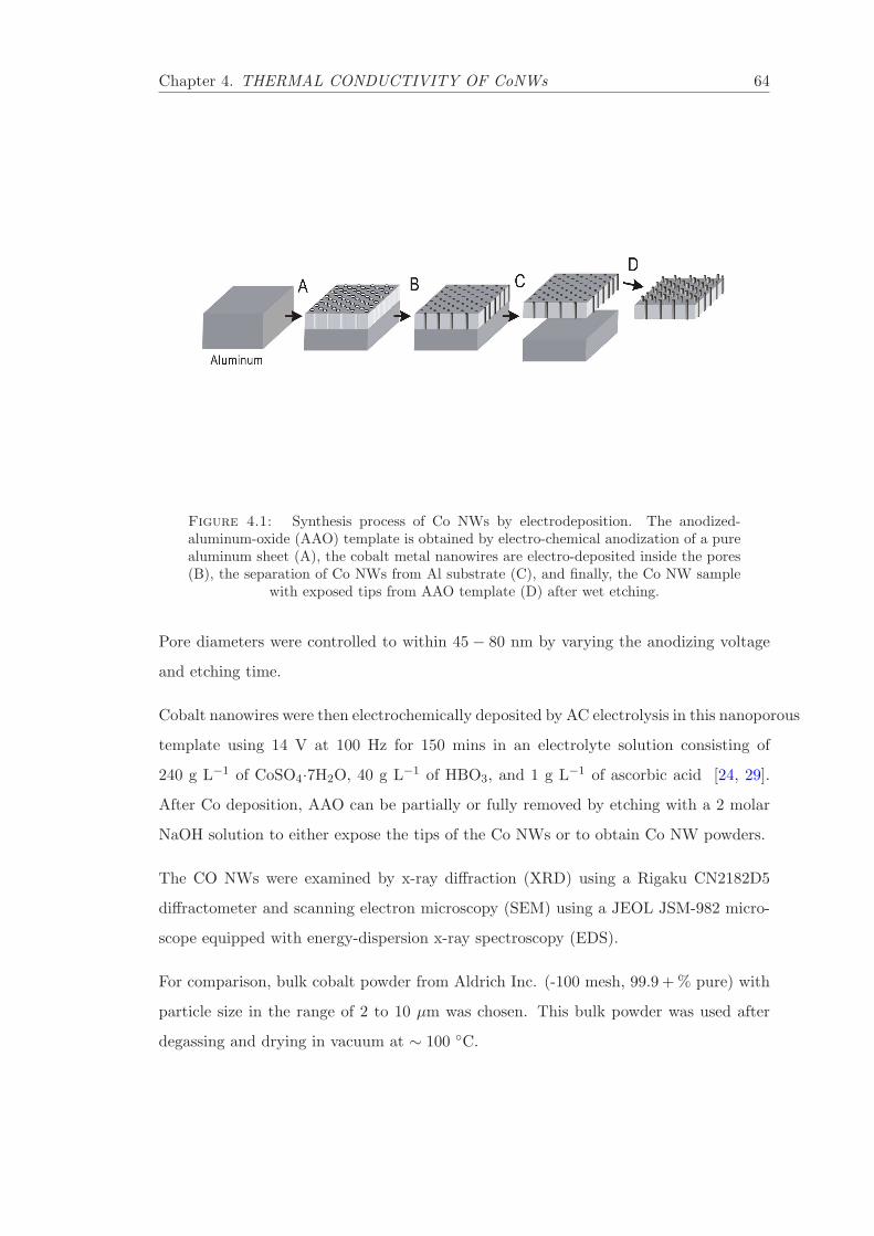
Chapter 4. THERMAL CONDUCTIVITY OF CoNWs 64
Figure 4.1: Synthesis process of Co NWs by electrodeposition. The anodized-aluminum-oxide (AAO) template is obtained by electro-chemical anodization of a purealuminum sheet (A), the cobalt metal nanowires are electro-deposited inside the pores(B), the separation of Co NWs from Al substrate (C), and finally, the Co NW sample
with exposed tips from AAO template (D) after wet etching.
Pore diameters were controlled to within 45 − 80 nm by varying the anodizing voltage
and etching time.
Cobalt nanowires were then electrochemically deposited by AC electrolysis in this nanoporous
template using 14 V at 100 Hz for 150 mins in an electrolyte solution consisting of
240 g L−1 of CoSO4·7H2O, 40 g L−1 of HBO3, and 1 g L−1 of ascorbic acid [24, 29].
After Co deposition, AAO can be partially or fully removed by etching with a 2 molar
NaOH solution to either expose the tips of the Co NWs or to obtain Co NW powders.
The CO NWs were examined by x-ray diffraction (XRD) using a Rigaku CN2182D5
diffractometer and scanning electron microscopy (SEM) using a JEOL JSM-982 micro-
scope equipped with energy-dispersion x-ray spectroscopy (EDS).
For comparison, bulk cobalt powder from Aldrich Inc. (-100 mesh, 99.9 + % pure) with
particle size in the range of 2 to 10 µm was chosen. This bulk powder was used after
degassing and drying in vacuum at ∼ 100 C.
Chapter 4. THERMAL CONDUCTIVITY OF CoNWs 65
4.2.1 AC Calorimetry
A modulated (AC) heating technique is used to measure the heat capacity of the Co
NWs and bulk powder cobalt samples. In this technique, the sample and cell, loosely
coupled to a constant thermal bath, are subjected to a small, oscillatory, heat input. The
specific heat and the thermal conductivity can be determined by measuring the frequency
dependence of the amplitude and phase of the resulting temperature oscillation. The
heat input P0e−ωt with P0 ≈ 0.5 mW is supplied to the sample+cell typically results in
a modulated temperature having an amplitude Tac ≈ 5 mK. The experimental details
of our application of AC-calorimetry can be found elsewhere [23–25].
The amplitude Tac is inversely proportional to the heat capacity of the sample. The
measured Tac is related to the applied power, heating frequency, total heat capacity, and
the various thermal relaxation times by
Tac =P0
2ωC
(
1 + (ωτe)−2 + ω2τ2
ii +2Rs
3Re
)−1/2
(4.1)
where P0 is the power amplitude, ω is the angular frequency of the applied heating
power, and C = Cs + Cc is the total heat capacity of the sample+cell. Here, Cc =
CH +CGE +CAAO +CAg accounts for the contributions to the cell heat capacity by the
heater (H), General Electric #7031 varnish (GE), silver cell container (Ag), and the
AAO template (for the parallel measurement). By subtracting the cell contributions,
the heat capacity of the Co NWs may be isolated CCoNW = C − Cc and by dividing
by the mass of Co NWs yields the desired specific heat. Note that the contribution of
the carbon-flake thermistor (θ) is much smaller than all these elements and is typically
ignored.
There are two important thermal relaxation time constants contained in Eq. (5.1), the
external τe = ReC and the internal τ2ii = τ2
s + τ2c that is the sum of the squared thermal
relaxation times for the sample (τs) and cell (τc). Here, Rs is the sample’s thermal
resistance and Re is the external thermal resistance to the bath. There is also a phase
shift Φ between the applied heat and resulting temperature oscillations but it is more
convenient to define a reduced phase shift φ = Φ + π/2 since for heating frequencies
between 1/τe and 1/τii, Φ ≈ −π/2. The reduced phase shift, to the same accuracy as

Chapter 4. THERMAL CONDUCTIVITY OF CoNWs 66
Eq. (5.1), is given by
tan(φ) = (ωτe)−1 − ωτi (4.2)
where here τi = τs + τc. Since τc is typically small compared to τs such that τi ∼= τii,
Eq. (5.2) can be rewritten to give τs ≡ RsCs∼= 1/(ω2τe) − (tanφ)/ω. The measured
reduced phase shift φ also contains a linear ω dependence due to the fixed digitization
rate of the thermal oscillation as the heating frequency increases. The observed φ is
then given by
φexp = arctan((ωτe)−1 − ωτi) + aω + φ0 (4.3)
where a is determined by the digitization rate (in our case, a ≈ 1) and φ0 is the resulting
phase shift due to the digitizing dead-time (delay), which for our apparatus is negligible.
Figure 4.2 shows a typical frequency scan of an AAO only sample at 340 K and illustrates
the two relaxation time constants. The solid lines are fits using Eqs. (5.1) and (4.3)
and indicate the quality of this thermal model. Several such scans were performed at
various temperatures to ensure the applicability of thermal analysis. The temperature
dependent data shown below were done at a fixed frequency of ω = 0.1885 s−1, which
is above but close to 1/τe. In Fig. 4.2 at frequencies near twice 1/τi, a pronounced dip
in the temperature amplitude occurs at 3.13 s−1 as well at multiples of this frequency.
These features are likely due to the formation of standing waves within the cell and
occur when the thermal diffusion length are multiple fractions of the physical thickness
of the cell.
The effective thermal conductance, the inverse of the thermal resistance, of the sample
can then be evaluated from the AC-calorimetric parameters as
Ks∼= ω2τeCs
1 − ωτe tanφ(4.4)
where Ks is in units of W K−1. With the geometric dimensions of sample+cell config-
uration, the effective thermal conductivity κs in units of W m−1 K−1 can be calculated
directly as κs = KsL/A, where L is the thickness and A is the area of the CoNWs.
4.2.2 Sample Configurations
The cell and Co NWs samples were prepared in two different ways for measurements
with the heat flow parallel to the long-axis (anisotropic, denoted with superscript ‖)

Chapter 4. THERMAL CONDUCTIVITY OF CoNWs 67
10-2 10-1 100 101-14-12-10-8-6-4-202
10-5
10-4
10-3
10-2
exp (
rad
)
( rad s )
T ac (
K s
)
Figure 4.2: Typical frequency scan of an AAO sample at 340 K representative ofall scans performed for all samples. Top: traditional view of the amplitude frequencydependence using a log-log plot of ωTac versus ω. Bottom: semi-log plot of the observedφ versus ω where the horizontal dashed lines indicate ±π/2. The solid lines are fits tothese data using Eqs. (5.1) and (4.3), respectively, yielding consistent time constants.The resulting internal and external time constants are denoted in the plots as the ver-tical dotted lines. Note that the operating frequency for temperature scans is indicated
by the arrow. See text for details.
and through a randomly oriented (denoted with superscript R) film of nanowires. The
sample+cell configuration for the anisotropic measurement is shown in Fig. 4.3(a) and
Fig. 4.4. The general sample+cell configuration consists of a sandwich arrangement of
heater, thin silver sheet (0.1 mm thick and 5 mm square), sample, thin silver sheet, and
thermistor, all held together by thin applications of GE varnish.
For the anisotropic configuration, the Co NWs embedded in an AAO template were first
separated from the Al substrate by wet etching in a 0.1% HgCl2 solution, and the barrier
layer was removed by wet etching in 0.5% H3PO4 for 30 mins. To ensure a good thermal
contact between the Co NWs and the silver sheets, the AAO template was etched by
0.1 M NaOH solution to expose about 2 µm Co NWs on both ends. The typical thickness
of Co NWs-AAO sample is about 20 µm. It was carefully sandwiched between the two
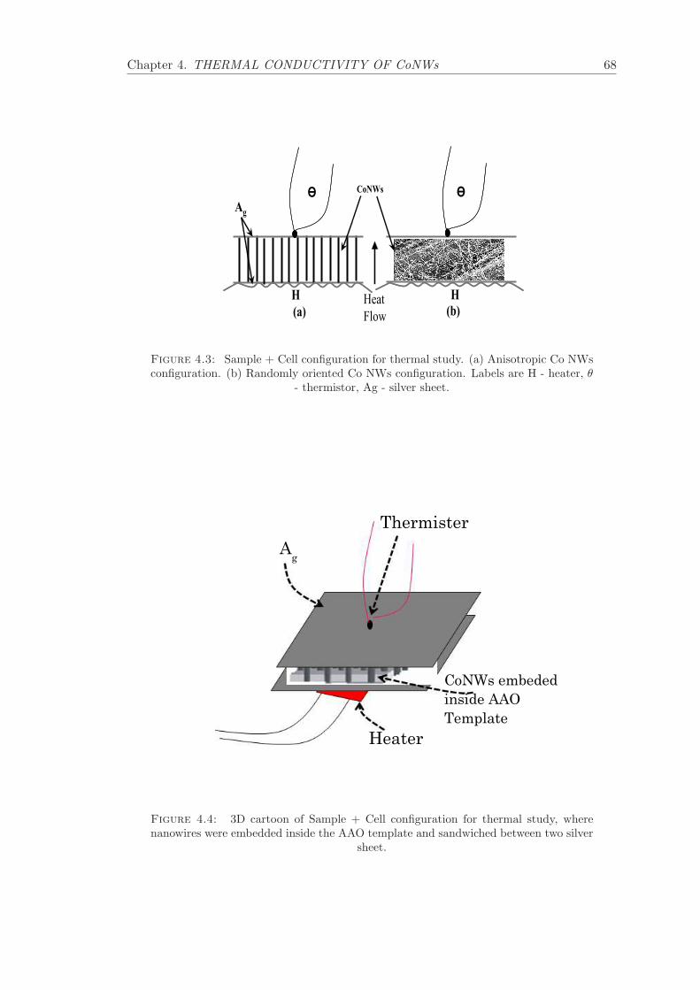
Chapter 4. THERMAL CONDUCTIVITY OF CoNWs 68
0.0 0.5 1.0 1.5 2.0
0.0
0.5
1.0
1.5
2.0
H
Ag
H
Ө ӨCoNWs
(a) (b)Heat
Flow
Figure 4.3: Sample + Cell configuration for thermal study. (a) Anisotropic Co NWsconfiguration. (b) Randomly oriented Co NWs configuration. Labels are H - heater, θ
- thermistor, Ag - silver sheet.
Ag
Thermister
CoNWs embededinside AAO Template
Heater
Figure 4.4: 3D cartoon of Sample + Cell configuration for thermal study, wherenanowires were embedded inside the AAO template and sandwiched between two silver
sheet.
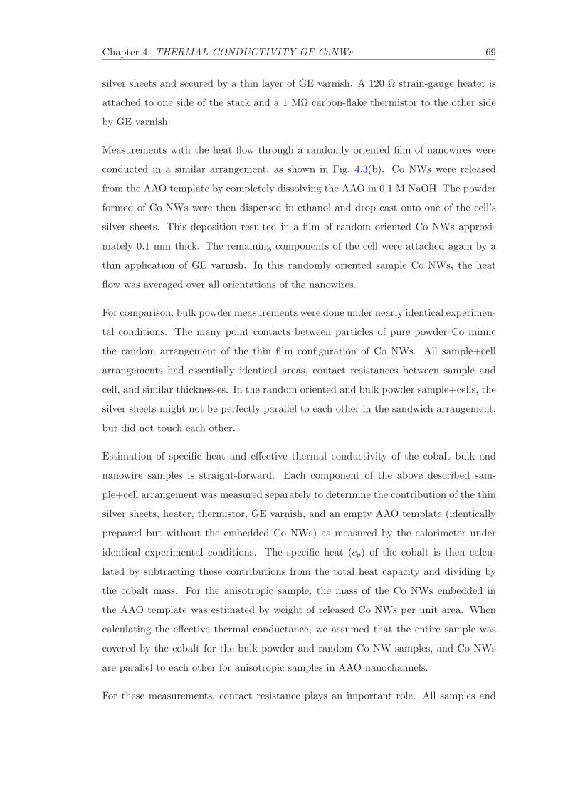
Chapter 4. THERMAL CONDUCTIVITY OF CoNWs 69
silver sheets and secured by a thin layer of GE varnish. A 120 Ω strain-gauge heater is
attached to one side of the stack and a 1 MΩ carbon-flake thermistor to the other side
by GE varnish.
Measurements with the heat flow through a randomly oriented film of nanowires were
conducted in a similar arrangement, as shown in Fig. 4.3(b). Co NWs were released
from the AAO template by completely dissolving the AAO in 0.1 M NaOH. The powder
formed of Co NWs were then dispersed in ethanol and drop cast onto one of the cell’s
silver sheets. This deposition resulted in a film of random oriented Co NWs approxi-
mately 0.1 mm thick. The remaining components of the cell were attached again by a
thin application of GE varnish. In this randomly oriented sample Co NWs, the heat
flow was averaged over all orientations of the nanowires.
For comparison, bulk powder measurements were done under nearly identical experimen-
tal conditions. The many point contacts between particles of pure powder Co mimic
the random arrangement of the thin film configuration of Co NWs. All sample+cell
arrangements had essentially identical areas, contact resistances between sample and
cell, and similar thicknesses. In the random oriented and bulk powder sample+cells, the
silver sheets might not be perfectly parallel to each other in the sandwich arrangement,
but did not touch each other.
Estimation of specific heat and effective thermal conductivity of the cobalt bulk and
nanowire samples is straight-forward. Each component of the above described sam-
ple+cell arrangement was measured separately to determine the contribution of the thin
silver sheets, heater, thermistor, GE varnish, and an empty AAO template (identically
prepared but without the embedded Co NWs) as measured by the calorimeter under
identical experimental conditions. The specific heat (cp) of the cobalt is then calcu-
lated by subtracting these contributions from the total heat capacity and dividing by
the cobalt mass. For the anisotropic sample, the mass of the Co NWs embedded in
the AAO template was estimated by weight of released Co NWs per unit area. When
calculating the effective thermal conductance, we assumed that the entire sample was
covered by the cobalt for the bulk powder and random Co NW samples, and Co NWs
are parallel to each other for anisotropic samples in AAO nanochannels.
For these measurements, contact resistance plays an important role. All samples and

Chapter 4. THERMAL CONDUCTIVITY OF CoNWs 70
the components of the sample+cell, were measured under identical configurations (thick-
ness, area, mass, and external thermal link). All have the sample, Co powder or NWs,
attached to the silver cell with GE varnish as the thermal contact. Thus, the contact
resistance contribution should be essentially the same for all measurements. This crucial
similarity as well as the choice of bulk Co powder for comparison, allows the behavior
of Co NW in the macroscopic samples to be isolated.
4.3 Results and Discussion
4.3.1 Morphology and microstructure study of Co NWs
Fig. 4.5 shows SEM images of Co NWs embedded in the AAO templates. In Fig. 4.5(a),
an oblique view of the sample before etching by NaOH solution shows the highly ordered
hexagonal pattern of the nanopores. The pore diameter and interpore separation are
about 80 and 40 nm, respectively. Fig. 4.5(b) is an SEM image of the Co NWs with the
tips exposed by about 2 µm and Fig. 4.5(c) is a high-magnification image of the cobalt
nanowires.
With careful control of the etching process, etching in NaOH solution for 10 minutes is
sufficient to expose all of the NWs tips. The majority of the Co NWs stood straight
upward without severe agglomeration. If etching for prolonged time, the exposed Co
NWs tended to bend and bundle together, forming islands.
A microstructure study of the as-prepared Co NWs was performed by x-ray diffraction
( XRD) and shown in Fig. 4.6. The results demonstrate that the Co NWs consists of a
mixture of fcc and hcp structures. This is consistent with a nuclear magnetic resonance
(NMR) study by Strijkers. et al. [26] on Co NWS synthesized by direct current method.
The XRD peaks near 41.685 and 47.57 correspond to the (1010) and (1011) planes
of the hcp structure. The peak near 51.522 is attributed to the (200) plane of the fcc
structure. The peak near 44 could be a combination of the diffraction from the (0002)
plane of the hcp structure and the (111) plane of the fcc structure; that near 75 could
be a combination of the diffraction from the (1120) plane of the hcp structure and the
(220) plane of the fcc structure. It is also shown that the fabricated Co nanowires have
a preferential orientation of direction (0002). The preferred orientation of the nanowires
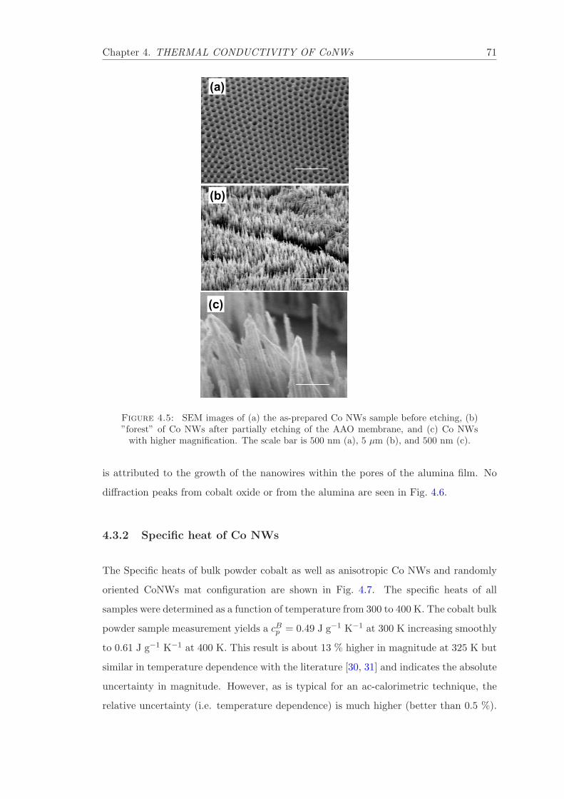
Chapter 4. THERMAL CONDUCTIVITY OF CoNWs 71
(a)
(b)
(c)
Figure 4.5: SEM images of (a) the as-prepared Co NWs sample before etching, (b)”forest” of Co NWs after partially etching of the AAO membrane, and (c) Co NWs
with higher magnification. The scale bar is 500 nm (a), 5 µm (b), and 500 nm (c).
is attributed to the growth of the nanowires within the pores of the alumina film. No
diffraction peaks from cobalt oxide or from the alumina are seen in Fig. 4.6.
4.3.2 Specific heat of Co NWs
The Specific heats of bulk powder cobalt as well as anisotropic Co NWs and randomly
oriented CoNWs mat configuration are shown in Fig. 4.7. The specific heats of all
samples were determined as a function of temperature from 300 to 400 K. The cobalt bulk
powder sample measurement yields a cBp = 0.49 J g−1 K−1 at 300 K increasing smoothly
to 0.61 J g−1 K−1 at 400 K. This result is about 13 % higher in magnitude at 325 K but
similar in temperature dependence with the literature [30, 31] and indicates the absolute
uncertainty in magnitude. However, as is typical for an ac-calorimetric technique, the
relative uncertainty (i.e. temperature dependence) is much higher (better than 0.5 %).

Chapter 4. THERMAL CONDUCTIVITY OF CoNWs 72
40 45 50 55 60 65 70 75 800
500
1000
1500
2000
2500
M
M
(200)(1011)
Inte
nsity
(cou
nts)
2 (degrees)
(1010)
Figure 4.6: XRD pattern of Co NWs showing different planes.
The magnitude of the specific heat for the two CoNW samples are c||p = 0.53 J g−1 K−1
and cRp = 0.50 J g−1 K−1 at 300 K. For the anisotropic Co NW configuration, c||p increases
linearly from room temperature to ∼ 320 K in a fashion similar to bulk sample. Above
320 K, c||p increases much more rapidly with temperature than the bulk. In the case
of randomly oriented mat sample, cRp increases more rapidly than that of either the
anisotropic or the bulk sample from 318 to 387 K, above which it begins to decrease.
In principle, since the specific heat is a scalar quantity related to the thermal fluctuations
of internal energy, one would expect that cp should be independent of heat-flow geometry
for a given structure of the cobalt. The differences observed here are likely due to
the composite nature of the sample+cell configuration. The similarity, at least just
above room temperature, between c||p and cBp is understandable as in this heat-flow
configuration, the length of the Co NWs is comparable to the size of the bulk powder
sample. The deviation beginning at ∼ 320 K may be a consequence of the 1-D nature
of the nanowires since one might expect “bunching” of the phonons (phonon-phonon
scattering) to dominate at some elevated temperature. For the random Co NW film
sample, there is likely a very large number of contacts, on the nanometer scale, between
individual Co NWs. Thus, the cRp measured is almost certainly an effective value for

Chapter 4. THERMAL CONDUCTIVITY OF CoNWs 73
300 320 340 360 380 4000.4
0.6
0.8
1.0
1.2
1.4
1.6
c p ( J
g K
)
T ( K )
Bulk ||
Figure 4.7: Specific heat of bulk powder cobalt (solid triangles) and randomly ori-ented Co NWs samples (dots) and anisotropic Co NWs samples (open circles) from 300
to 400 K.
the sample+cell composite. However, the observed strong temperature dependence and
maximum at ∼ 370 K for cRp is an intriguing indication of engineering materials with
specific thermal properties.
4.3.3 Thermal Conductivity of Co NWs
Fig. 4.8(a) shows the effective thermal conductivity of bulk powder cobalt at 300 K to
be κB ≈ 67 W m−1 K−1 with a strong temperature dependence reaching a maximum at
∼ 360 K. The literature value for pure cobalt at 300 K is 90 W m−1 K−1 and displays only
a weak temperature dependence [32]. The extracted thermal conductivity κB is lower by
20 % which is most likely due to incomplete filling of the cell. The maximum observed
is also likely due to the powder nature of micron sized amorphous particles sandwiched
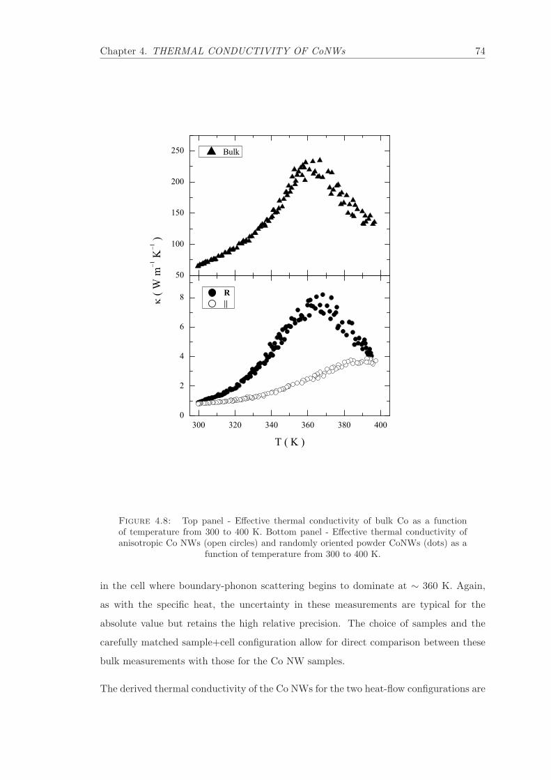
Chapter 4. THERMAL CONDUCTIVITY OF CoNWs 74
300 320 340 360 380 4000
2
4
6
8
50
100
150
200
250
( W
m K
)
T ( K )
R ||
Bulk
Figure 4.8: Top panel - Effective thermal conductivity of bulk Co as a functionof temperature from 300 to 400 K. Bottom panel - Effective thermal conductivity ofanisotropic Co NWs (open circles) and randomly oriented powder CoNWs (dots) as a
function of temperature from 300 to 400 K.
in the cell where boundary-phonon scattering begins to dominate at ∼ 360 K. Again,
as with the specific heat, the uncertainty in these measurements are typical for the
absolute value but retains the high relative precision. The choice of samples and the
carefully matched sample+cell configuration allow for direct comparison between these
bulk measurements with those for the Co NW samples.
The derived thermal conductivity of the Co NWs for the two heat-flow configurations are

Chapter 4. THERMAL CONDUCTIVITY OF CoNWs 75
shown in Fig. 4.8(b). Both κ‖ and κR have values 83 times less than the bulk at 300 K.
However, for increasing temperatures, κ‖(T ) behaves quite differently from the observed
bulk trend, increasing in a smooth manner up to ∼ 380 K at which a small ”kink” is
seen to a nearly constant value of κ‖ ≈ 4 W m−1 K−1. Although the uncertainty in
absolute values is higher for the measured κ compared to cp, the marked reduction of
magnitude of κ in both configurations with respect to the bulk is consistent with the 1-D
nature of the materials, in which phonon boundary scattering dominates the phonon -
phonon scattering. Very similar results are reported in bismuth telluride nanowires by
Zhou et al. [33]. However, for κ‖, the kink to a constant value at ∼ 380 K may be an
indication of a cross-over from phonon-phonon to defect-phonon scattering within the
NWs. For the random Co NW sample, κR exhibits a similar temperature dependence as
the bulk, although of greatly reduced magnitude. As with κB, the observed maximum
for κR seen at ∼ 360 K is again likely due to the composite nature of the sample+cell
arrangement and the onset of boundary-phonon scattering. The junctions between the
nanowires dominant the heat transfer for κR just as the contacts between bulk powder
particles were for κB. The slight difference in temperature for the observed maximum is
consistent with the bulk powder particles being of much larger size (microns) compared
to the diameter of the nanowires.
To better compare the temperature dependence of the effective thermal conductivity,
normalized values (to that observed at 300 K, i.e. κ/κ300K) are shown in Fig. 4.9 for
the bulk powder and the Co NWs in the two heat-flow configurations. The fractional
change of κ is much larger in the randomly oriented Co NWs samples and, as mentioned
previously, is likely due to the enormous number of wire-wire junctions. The fractional
change of the anisotropic configuration matches closely up to 360 K with the bulk cobalt
powder. Above 360 K the bulk begins to decrease. Although study on Co NW with
different diameters is still on-going in our lab, it has been recently found that the thermal
conductivity of silicon nanowires increases with increasing diameter [34], consistent with
a cross-over to bulk-like behavior seen in our investigation between the random film of
Co NW and bulk-powder Co.
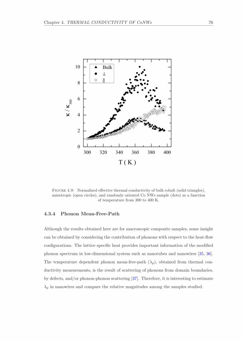
Chapter 4. THERMAL CONDUCTIVITY OF CoNWs 76
300 320 340 360 380 4000
2
4
6
8
10
/
T ( K )
Bulk ||
Figure 4.9: Normalized effective thermal conductivity of bulk cobalt (solid triangles),anisotropic (open circles), and randomly oriented Co NWs sample (dots) as a function
of temperature from 300 to 400 K.
4.3.4 Phonon Mean-Free-Path
Although the results obtained here are for macroscopic composite samples, some insight
can be obtained by considering the contribution of phonons with respect to the heat-flow
configurations. The lattice specific heat provides important information of the modified
phonon spectrum in low-dimensional system such as nanotubes and nanowires [35, 36].
The temperature dependent phonon mean-free-path (λp), obtained from thermal con-
ductivity measurements, is the result of scattering of phonons from domain boundaries,
by defects, and/or phonon-phonon scattering [37]. Therefore, it is interesting to estimate
λp in nanowires and compare the relative magnitudes among the samples studied.
Chapter 4. THERMAL CONDUCTIVITY OF CoNWs 77
The phonon mean-free-path may be calculated from the experimentally measured ther-
mal conductivity and specific heat using
λp =3κ
vpcpρ, (4.5)
where ρ is the mass density of the cobalt sample and vp is the velocity of phonons in cobalt
(here taken as that for pure cobalt 4700 m s−1 and a constant). The values estimated
for anisotropic Co NW is λ‖p ≈ 485 nm and in the random configuration is λR
p ≈ 203 nm
at 300 K. For the bulk powder cobalt sample, λBp ≈ 40 µm at 300 K. Since the cobalt
nanowires are 20 µm long, 80 nm in diameter, and that bulk particles are 2 - 10 µm
in size, one would expect that boundary scattering would dominate for the randomly
oriented Co NWs samples (λRp > 80 nm) and bulk powder (λB
p > 10 µm) beginning at
the lowest temperatures. Conversely, one would not expect boundary-phonon scattering
to play a significant role for the anisotropic configuration since λ‖p ≪ 20 µm, instead one
can consider phonon-phonon or defect-phonon scattering mechanisms. The maximums
observed in κ for the bulk and randomly oriented Co NW configuration could be the
result of the onset of additional scattering mechanisms.
It is interesting to note that the maximums in κ and cp seen for the randomly oriented
mat sample of Co NWs do not occur at the same temperatures, being ∼ 365 K and
∼ 382 K, respectively. Also, the maximum in κ observed in the bulk are not reflected by a
similar feature in cp just as the plateau in κ seen for the anisotropic Co NW configuration
has no companion feature in its cp. These observations indicate that the fluctuations in
internal energy reflected in cp are independent to the scattering mechanisms responsible
for the κ results in these macroscopic composite sample+cell arrangements.
The assumption of using the pure cobalt phonon velocity as a constant in temperature
and the same for all samples is a weak one. From the definition of the thermal diffusivity,
α = κ/cpρ, one can estimate the temperature dependence of the product of the phonon
mean-free-path and the phonon velocity as
αρ = λpvpρ/3 =κ
cp(4.6)
where α is the thermal diffusivity. Here, we assume that the mass density ρ is taken as
constant and so, from Eq. (4.6) gives λpvp ∝ κ/cp. Fig. 4.10 shows the result for the

Chapter 4. THERMAL CONDUCTIVITY OF CoNWs 78
300 320 340 360 380 4001
2
3
4
5
6
7
8100
150
200
250
300
350
400
450
500
||
(
g m
s )
T ( K )
Bulk
Figure 4.10: Plot of the product of mass density (ρ) and thermal diffusivity (α)over the temperature range 300 to 400 K. Top panel - Bulk cobalt. Bottom panel -anisotropic (open circles) and randomly oriented Co NWs sample (dots). Note that
αρ ∝ λpνp, see text for details.
bulk powder and the Co NW configurations studied as a function of temperature. A
broad maximum centered at ∼ 350 K is seen for the Co NW(random mat) sample and
a much sharper “peak” is seen at a slightly higher temperature of 360 K for the bulk
cobalt. For Co NW(‖), only a plateau is revealed beginning at 380 K. These results
suggest that the phonon mean-free-path and velocity are not trivially related and have
complex temperature dependence for these macroscopic composite samples.

Chapter 4. THERMAL CONDUCTIVITY OF CoNWs 79
4.4 Summary
We report the experimental results of the specific heat and effective thermal conductivity
of two types of arrangement of Co NWs, i.e. randomly oriented and anisotropic, and
compare them with bulk cobalt powders. The particle nature of the bulk-powder and
randomly orientated Co NWs leads to strong deviations of both κ and cp from that of
pure solid cobalt. The κ and Cp exhibit a much stronger temperature dependence and
show peak-like maximums versus temperature. The results suggest the dominance of
phonon-boundary scattering in the temperature range 300 to 400 K, whereas the thermal
properties of the more uniform and confined anisotropic Co NWs samples demonstrate
smooth temperature dependence, which suggests the dominance of phonon-phonon or
phonon-defect scattering. These results suggest that the composite materials containing
nanowires can be engineered for a wide range of applications.

Bibliography
[1] P. G. Collins, H. Bando and A. Zettl, Nanotechnology, 9 153 (1998).
[2] Y. Cui and M. Lieber, Science, 291 851 (2001).
[3] M. S. Dresselhaus, Y-M. Lin, S. B. Cronin, O. Rabin, M. R. Black, G. Dresselhaus
and T. Koga, Semicond. Semimet, 71 1 (2001).
[4] Y. Wu, R. Fan and P. Yang, Int. J. Nanosci, 1 1 (2002).
[5] Ronggui Yang and Gang Chen and M. S. Dresselhaus Phys. Rev. B, 72, 125418
(2005).
[6] N. Mingo and L. Yang and D. Li and A. Majumdar Nanoletters, 132, 12, 1713
(2003).
[7] A. D. McConnel and K. E. Goodson Ann. Rev. Heat Transfer, 14, 129 (2005).
[8] D. G. Cahill, W. K. Ford, K. E. Goodson, G. D. Mahan, A. Majumdar, H. J.
Maris, R. Merlin and S. R. Phillpot, J. Appl. Phys., 93, 2, 793 (2002).
[9] J. Zou and A. Balandin, Proc. Electrochem. Soc., 2001, 19, 70 (2001).
[10] G. Mahan, B. Sales, J. Sharp, Physics Today, 50, 42 (1997).
[11] S. Brands, B. Leven, and G. Dumpich, J. Appl. Phys., 97, 114311 (2006).
[12] U. Ebels, A. Radulescu, Y. Henry, L. Piraux, and K. Ounadjela, Phys. Rev.
Lett., 84, 983 (2000).
[13] S. Mani, T. Saif, and J. H. Han, IEEE Trans. Nanotechnol., 5, 138 (2006).
[14] L. D. Hicks, M. S. Dresselhaus, Phys. Rev. B, 47, 12727 (1993).
80

Chapter 4. THERMAL CONDUCTIVITY OF CoNWs 81
[15] D. Li, Y. Wu, P. Kim, L. Shi, P. Yang and A. Majumdar, Appl. Phys. Lett.,
14, 2934 (2003).
[16] S. Barman and G. P. Srivastava, Phys. Rev. B, 73, 205308, (2006).
[17] Y. Chena, D. Lib, J. Yangc, Y. Wuc, J. R. Lukesd, A. Majumdare, Physica B,
349, 270 (2004).
[18] Y. Chen, D. Li, J. R. Lukes and A. Majumdar, J. Heat Trans.,127, 1129 (2005).
[19] S. Volz and G. Chen, Appl. Phys. Lett., 75, 2056 (1999).
[20] R Prasher, Phys. Rev. B, 74, 165413 (2006).
[21] K-Q Chen, W-X Li, W. Duan, Z. Shuai, B-L Gu, Phys. Rev. B, 72, 045422 (2005).
[22] T. M. Trit, Science, 283, 804 (1999).
[23] J. Xu, X. Huang, G. Xie, Y. Fang and D. Liu, Material Letters, 59, 981-4
(2005).
[24] J. Liang, H. Chik, A. Yin and J. M. Xu, J. Appl. Physics, 91, 2544 (2002).
[25] L. Vila, J. M. George, G. Faini, A. Popa, U. Ibels, K. Ounadjea and L. Paux,
IEEE Trans. on Mag., 38, 5, 185 (2002).
[26] G. J. Strijkers, J. H.J. Dalderop, M. A.A. Broeksteeg, H. J.M. Swagten and W. J.M.
de Jonge, J. Appl. Phys., 86, 9, 5141-5145 (1999).
[27] Z. F. Zhou, Y. C. Zhou, Y. Pan and X. G. Wang, Mat. Lett., 62, 3419-3421 (2008).
[28] J. Liang, H. Chik and J. M. Xu, IEEE J. Select. Top. Quant. Electron., 8, 998
(2002).
[29] J. Li, C. Papadopoulos, J. M. Xu and M. Moskovits, Appl. Phys. Lett., 75, 367
(1999).
[30] R. RamjiRao and A. Ramanand, Phys. Rev. B, 19, 4, 1972 (1979).
[31] W. Bendick and W. J. Pepperhoff, J. Phys. F: Metal Phys., 11, 11, 2185 (1979).
[32] Terry M Tritt, ,Thermal conductivity: Theory Properties and Application, Kluwer
Academyc/Plenum Publishers, 4 (2004).

Chapter 4. THERMAL CONDUCTIVITY OF CoNWs 82
[33] J. Zhou, C. Jin, J. Seol, X. Li and L. Shi, Appl. Phys. Lett., 87, 133109 (2005).
[34] A. Hochbaum, R. Chen, R. D. Delgado, W. Liang, E. C. Garnett, M. Najarian,
A. Majumdar and P. Yang, Nature,451, 163 (2008).
[35] C. Dames, B. Powdel, W. Z. Wang, J. Y. Huang, Z. F. Ren, Y. Sun, J. I. Oh and
G. Chen, Appl. Phys. Lett.,87, 031901 (2005).
[36] J. Hone, B. Batlogg, Z. Benes, A. T. Johnson and J. E. Fischer, Science,289,
1730 (2000).
[37] J. Hone, M. Whitney, C. Piskoti and A. Zettl, Phys. Rev. B,59, 4, R2514 (1999).

Chapter 5
THERMAL CONDUCTIVITY
OF SINGLE-WALL AND
MULTI-WALL CARBON
NANOTUBES COMPOSITES
5.1 Introduction of Carbon Nanotubes
Since their discovery in 1991 by Sumio Ijima [1], carbon nanotubes ( CNTs) have been
the focus of intense research and have many potential applications in electronic, optical,
thermal management and energy conversion devices because of their unique proper-
ties. The electrical and mechanical properties of CNTs have been extensively investi-
gated [2, 3], while the thermal properties of CNTs are of interest in basic science as
nanotubes are model systems for low-dimensional materials. However, for large scale
technical applications, the manipulation of single nanotubes becomes impractical. Sev-
eral groups have measured the thermal properties of millimeter sized thin CNT films
and packed carbon fibers [4–10]. Current efforts to exploit the attractive properties
of carbon nanotubes have focused on macroscopic composites containing engineered or
self-assembled arrays of CNTs. One route has been to order the CNTs through the
interaction of an anisotropic liquid crystalline host [11] while another route has been to
grow the CNT within the ordered porous structures of a host matrix [12].
83
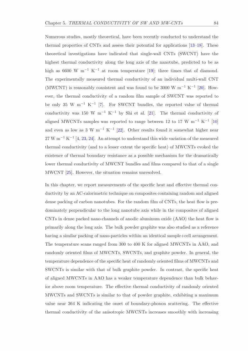
Chapter 5. THERMAL CONDUCTIVITY OF SW AND MW-CNTs 84
Numerous studies, mostly theoretical, have been recently conducted to understand the
thermal properties of CNTs and assess their potential for applications [13–18]. These
theoretical investigations have indicated that single-wall CNTs (SWCNT) have the
highest thermal conductivity along the long axis of the nanotube, predicted to be as
high as 6600 W m−1 K−1 at room temperature [19]; three times that of diamond.
The experimentally measured thermal conductivity of an individual multi-wall CNT
(MWCNT) is reasonably consistent and was found to be 3000 W m−1 K−1 [20]. How-
ever, the thermal conductivity of a random film sample of SWCNT was reported to
be only 35 W m−1 K−1 [7]. For SWCNT bundles, the reported value of thermal
conductivity was 150 W m−1 K−1 by Shi et al. [21]. The thermal conductivity of
aligned MWCNTs samples was reported to range between 12 to 17 W m−1 K−1 [10]
and even as low as 3 W m−1 K−1 [22]. Other results found it somewhat higher near
27 W m−1 K−1 [4, 23, 24]. An attempt to understand this wide variation of the measured
thermal conductivity (and to a lesser extent the specific heat) of MWCNTs evoked the
existence of thermal boundary resistance as a possible mechanism for the dramatically
lower thermal conductivity of MWCNT bundles and films compared to that of a single
MWCNT [25]. However, the situation remains unresolved.
In this chapter, we report measurements of the specific heat and effective thermal con-
ductivity by an AC-calorimetric technique on composites containing random and aligned
dense packing of carbon nanotubes. For the random film of CNTs, the heat flow is pre-
dominately perpendicular to the long nanotube axis while in the composites of aligned
CNTs in dense packed nano-channels of anodic aluminum oxide (AAO) the heat flow is
primarily along the long axis. The bulk powder graphite was also studied as a reference
having a similar packing of nano-particles within an identical sample+cell arrangement.
The temperature scans ranged from 300 to 400 K for aligned MWCNTs in AAO, and
randomly oriented films of MWCNTs, SWCNTs, and graphite powder. In general, the
temperature dependence of the specific heat of randomly oriented films of MWCNTs and
SWCNTs is similar with that of bulk graphite powder. In contrast, the specific heat
of aligned MWCNTs in AAO has a weaker temperature dependence than bulk behav-
ior above room temperature. The effective thermal conductivity of randomly oriented
MWCNTs and SWCNTs is similar to that of powder graphite, exhibiting a maximum
value near 364 K indicating the onset of boundary-phonon scattering. The effective
thermal conductivity of the anisotropic MWCNTs increases smoothly with increasing

Chapter 5. THERMAL CONDUCTIVITY OF SW AND MW-CNTs 85
temperature and is indicative of the one-dimensional nature of the heat flow.
Following this introduction, the experimental details including material synthesis, com-
posite sample fabrication, and calorimetric details are shown in Sec. 7.2. The resulting
data are presented and discussed in Sec. 5.3. Conclusions are drawn and future work
outlined in Sec. 5.4.
5.2 Experimental
5.2.1 Synthesis of Carbon Nanotubes and Samples
Multi-wall carbon nanotubes were synthesized by a chemical vapor deposition (CVD)
technique in an AAO template as shown in Fig. 5.1. The AAO template was obtained
by a two-step anodization process; details of which have been previously published [12,
26, 27]. Briefly, the first-step anodization of aluminum (99.999 % pure, Electronic Space
Products International) was carried out in a 0.3 Molar oxalic acid solution under 40 V
at 10 0C for 16 − 20 hr. The porous alumina layer formed during this first anodization
step was completely dissolved by chromic acid at 70 0C. The sample was then subjected
to a second anodization step under the same conditions as the first. The thickness of the
porous anodic film was adjusted by varying the time of the second anodization step. The
resulted AAO templates can be further treated by acid etching to widen the nanopores.
For the samples used in this work, the pore diameter was controlled to within 45−80 nm
by varying the anodizing voltage and etching time.
Cobalt particles, used as catalysts for the carbon nanotube growth, were electrochem-
ically deposited at the bottom of the pores using AC electrolysis (14 V at 100 Hz)
for 30 sec in an electrolyte consisting of CoSO47H2O (240 g/L), HBO3 (40 g/L), and
ascorbic acid (1 g/L). The ordered array of nanotubes were grown by first reducing the
catalyst by heating the cobalt-loaded templates in a tube furnace at 550 0C for 4 hr
under a CO flow (60 cm3 min−1). The CO flow was then replaced by a mixture of 10 %
acetylene in nitrogen at the same flow rate. In a typical synthesis, the acetylene flow
was maintained for 1 hr at 600 0C. The as-prepared MWCNTs embedded in the AAO
template were used as the aligned MWCNT sample. The MWCNTs can be released
from the template by removing the aluminum oxide in a 0.1 Molar NaOH solution at

Chapter 5. THERMAL CONDUCTIVITY OF SW AND MW-CNTs 86
Figure 5.1: Diagram of the synthesis steps of CNTs by chemical vapor deposi-tion. The anodized-aluminum-oxide (AAO) template is obtained by electro-chemicalanodization of a pure aluminum sheet, the cobalt catalyst are electro-deposited insidethe pores and the CNT is grown by CVD method. The CNTs are separated from Al
substrate by dissolving AAO template with NaOH solution.
60 − 80 0C for 3 hr. The released MWCNTs were used to make a randomly oriented
MWCNT film sample. From a 3 cm2 MWCNT+AAO sample, 1.82 mg of MWCNTs
were released corresponding to an embedded mass of MWCNT of 0.61 mg cm−2. From
the dimensional information of the MWCNT and assuming an AAO pore density of
about 1010 cm−2, a theoretical value of the MWCNT mass per area of MWCNT+AAO
is 0.86 mg cm−2, reasonably close to the measured value. The mass of the MWCNTs
embedded inside the AAO template sample was thus estimated by using the measured
mass of released CNTs per unit area of composite.
Single-wall carbon nanotubes ( SWCNT) were obtained from Helix Material Solutions,
Inc. [28] and used without further processing. The reference graphite powder was ob-
tained from AGS and has the following composition; 95.2 % carbon, 4.7 % ash, and
0.1 % moisture and other volatiles. The graphite powder was used after degassing at
100 0C under vacuum for 2 hr. Morphology of the MWCNTs, SWCNTs and graphite
particles were examined by a JEOL JSM-7000F scanning electron microscope ( SEM)
and a Philips CM12 transmission electron microscope ( TEM) before the calorimetric

Chapter 5. THERMAL CONDUCTIVITY OF SW AND MW-CNTs 87
measurements. Aspects of the sample morphology, particularly the diameters of the
CNTs, were analyzed using the Image J processing software. The dimensions were mea-
sured 10 times from multiple TEM images for all samples and the average and standard
deviations were reported.
For the calorimetric measurements, contact resistance plays an important role. All sam-
ples and the components of the sample+cell, were measured under identical experimental
conditions (e.g. thickness, area, mass, and external thermal link), and were similarly
configured in a sandwiched pattern between two silver or silver and aluminum oxide (for
aligned MWCNTs) samples. Although the similarity of construction should result in
similar contact resistance, due to local variation of surface roughness, sample-to-sample
variations, and uncertainties in particle geometries, the contact resistance should be
considered averaged over the ∼cm in-plane length-scale of the composite sample and
thus lead to large uncertainties in the absolute magnitude of the derived thermal con-
ductivity. However, the relative precision of the temperature dependence of the thermal
conductivity should be comparable.
5.2.2 Sample+Cell Configurations
Details of the experimental sample+cell configuration have been reported elsewhere [12]
and also shown in Fig. 5.2.
Briefly, the aligned MWCNT+AAO sample were in excellent thermal contact on one end
by their anchoring to the Al base of the AAO and contact on the other end was made
to a thin silver sheet by a thin layer of GE varnish (General Electric #7031 varnish).
The typical thickness of MWCNT+AAO sample was about 20 µm. This aligned sample
was arranged as a silver sheet/GE varnish/MWCNT+AAO/Al sandwich. One side of
the ‘stack’ has attached a 120 Ω strain-gauge heater and the other a 1 MΩ carbon-flake
thermister. For the randomly oriented thin film samples, the powder-form MWCNTs,
separately obtained SWCNTs, and graphite powders were drop cast on a thin silver
sheet then sandwiched by another identical silver sheet on top by a thin layer of GE
varnish forming a nearly identical ‘stack’ (in dimension and total mass) as the aligned
sample. All components of all sample+cells were carefully massed in order to perform
background subtractions.
Chapter 5. THERMAL CONDUCTIVITY OF SW AND MW-CNTs 88
Figure 5.2: In (a) and (b), a cartoon depicting the sample cell configuration for thealigned MWCNT+AAO sample (a) and for the random film of MWCNT, SWCNT, orgraphite powder samples (b). In (c) a typical TEM of a MWCNT is shown with thebar in the lower left of the micrograph representing 100 nm. Image analysis of such
micrographs yield the geometric properties of the CNTs.

Chapter 5. THERMAL CONDUCTIVITY OF SW AND MW-CNTs 89
5.2.3 AC-Calorimetric Technique
An AC (modulated) heating technique is used for the measurements presented in this
paper. A sinusoidal heat input P0e−wt with P0 ≈ 0.5 mW was supplied to one side and
the resulting modulated temperature oscillation Tac was measured at the opposite side
of the sample+cell. The experimental technique details can also found elsewhere [12].
The amplitude Tac can be expressed as:
Tac =P0
2ωC
(
1 + (ωτe)−2 + ω2τ2
ii +2Rs
3Re
)−1/2
, (5.1)
where ω is the applied heating frequency, C = Cs + Cc is the total heat capacity (Cs
is the heat capacity of sample and Cc is the heat capacity of cell). Here, Cc = CH +
CGE +CAAO +CAg +CAl for the aligned MWCNT+AAO sample and Cc = CH +CGE +
CAg for randomly oriented MWCNT, SWCNT, and bulk powder graphite samples. By
subtracting the cell contribution, the heat capacity of the carbon nanotubes may be
isolated as CCNT = Cs = C−Cc and Cp = Cs/m, where m is the mass of the nanotubes
or graphite powder. The contribution of the carbon-flake thermister is negligible, having
a very weak temperature dependence, and so, is ignored.
There are two important thermal relaxation time constants in Eq. (5.1), τe = ReC and
τ2ii = τ2
s + τ2c , the external and internal respectively, where τs refers to sample relaxation
and τc refers to cell relaxation time constants. Here, Rs is the sample internal thermal
resistance and Re is the external thermal resistance linking the sample+cell to the bath.
The reduced phase shift (φ) between the input heat and resulting temperature oscillation
as a function of heating frequency scan can directly measure τe and τi using:
tan(φ) = (ωτe)−1 − ωτi, (5.2)
where τi = τs+τc and typically τc ≪ τs, hence τi ≃ τii. Eq. (5.2) can be rewritten to give
τs ≡ RsCs∼= 1/(ω2τe)−(tanφ)/ω. The effective thermal conductance, the inverse of the
effective thermal resistance, of the sample can then be evaluated from the experimental
parameters as:
Ks∼= ω2τeCs
1 − ωτe tanφ(5.3)
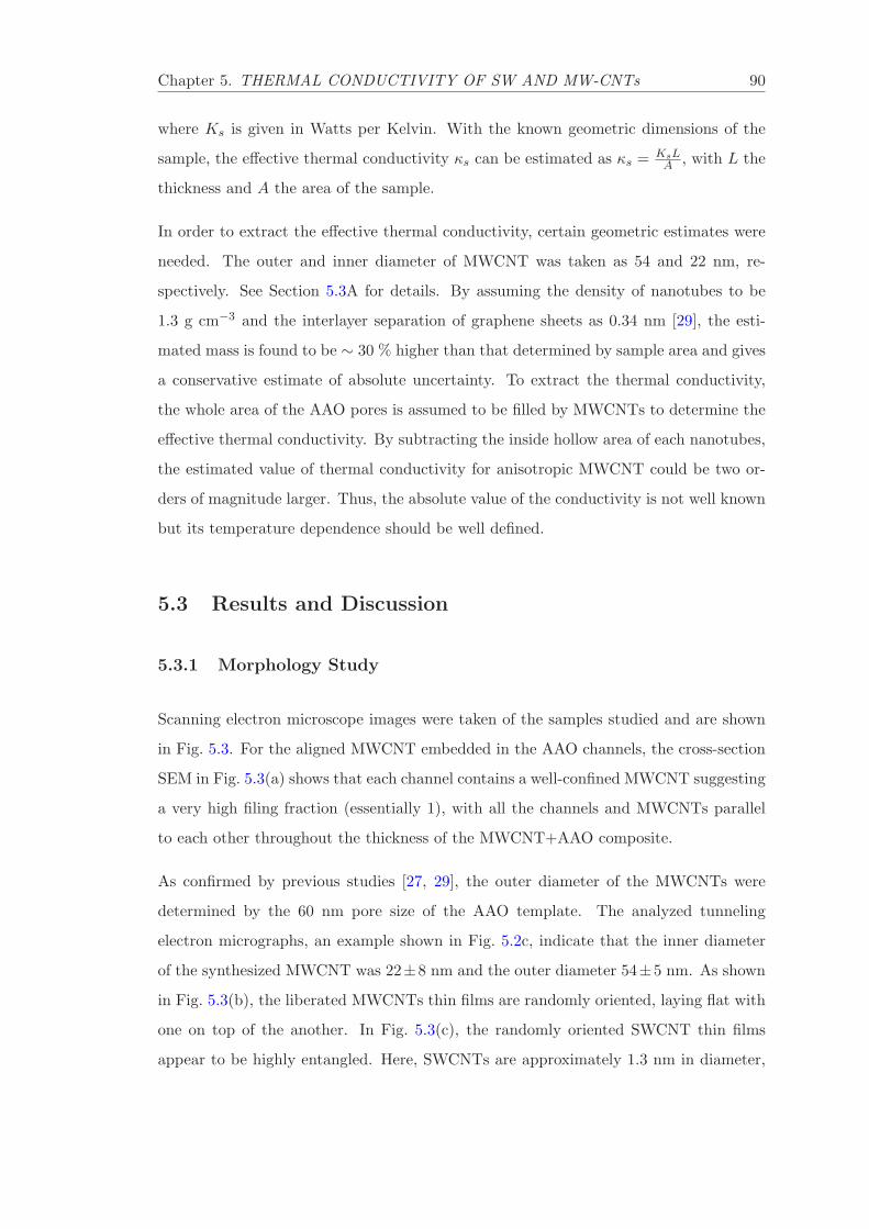
Chapter 5. THERMAL CONDUCTIVITY OF SW AND MW-CNTs 90
where Ks is given in Watts per Kelvin. With the known geometric dimensions of the
sample, the effective thermal conductivity κs can be estimated as κs = KsLA , with L the
thickness and A the area of the sample.
In order to extract the effective thermal conductivity, certain geometric estimates were
needed. The outer and inner diameter of MWCNT was taken as 54 and 22 nm, re-
spectively. See Section 5.3A for details. By assuming the density of nanotubes to be
1.3 g cm−3 and the interlayer separation of graphene sheets as 0.34 nm [29], the esti-
mated mass is found to be ∼ 30 % higher than that determined by sample area and gives
a conservative estimate of absolute uncertainty. To extract the thermal conductivity,
the whole area of the AAO pores is assumed to be filled by MWCNTs to determine the
effective thermal conductivity. By subtracting the inside hollow area of each nanotubes,
the estimated value of thermal conductivity for anisotropic MWCNT could be two or-
ders of magnitude larger. Thus, the absolute value of the conductivity is not well known
but its temperature dependence should be well defined.
5.3 Results and Discussion
5.3.1 Morphology Study
Scanning electron microscope images were taken of the samples studied and are shown
in Fig. 5.3. For the aligned MWCNT embedded in the AAO channels, the cross-section
SEM in Fig. 5.3(a) shows that each channel contains a well-confined MWCNT suggesting
a very high filing fraction (essentially 1), with all the channels and MWCNTs parallel
to each other throughout the thickness of the MWCNT+AAO composite.
As confirmed by previous studies [27, 29], the outer diameter of the MWCNTs were
determined by the 60 nm pore size of the AAO template. The analyzed tunneling
electron micrographs, an example shown in Fig. 5.2c, indicate that the inner diameter
of the synthesized MWCNT was 22±8 nm and the outer diameter 54±5 nm. As shown
in Fig. 5.3(b), the liberated MWCNTs thin films are randomly oriented, laying flat with
one on top of the another. In Fig. 5.3(c), the randomly oriented SWCNT thin films
appear to be highly entangled. Here, SWCNTs are approximately 1.3 nm in diameter,
Chapter 5. THERMAL CONDUCTIVITY OF SW AND MW-CNTs 91
Figure 5.3: SEM micrographs of arrays of MWCNTs inside AAO template (a),released MWNTs from AAO template (b), SWCNTs (c), and graphite powder (d).MWCNTs are 20 µm long with 60 nm outside and 25 nm outer diameter. The scale
bar in (a), (b) and (c) are 100 nm and in (d) is 1 µm.
0.5−40 µm long, and & 90 % pure [28]. The reference sample of graphite powder shown
in Fig. 5.3(d) has a large particle size of ∼ 1 µm and a wide particle size distribution.
5.3.2 Specific heat of CNT composites
The anisotropic measurement of specific heat (c||p) and randomly oriented specific heat
(cMp ) for MWCNT, randomly oriented specific heat (cSp ) for SWCNT, and that of bulk
graphite powder (cBp ) are shown in Fig. 5.4. The specific heat of all samples were deter-
mined as a function of temperature from 300 to 400 K on heating. The bulk graphite
powder sample yields a cBp = 0.73 J g−1 K−1 at 300 K and a weak, nearly-linear, temper-
ature dependence up to 360 K reaching 0.80 J g−1 K−1. These values obtained from our
experimental arrangements are 2.1% higher and 5.5% lower, respectively, from literature
values [30] and indicate in absolute value uncertainty of about 5% (conservatively) and
an uncertainty in slope of about 7%.
For the aligned MWCNT composite sample c||p = 0.74 J g−1 K−1 while for the randomly
oriented thin film sample cMp = 0.75 J g−1 K−1 at 300 K, very similar to bulk graphite

Chapter 5. THERMAL CONDUCTIVITY OF SW AND MW-CNTs 92
300 320 340 360 380 4000.70
0.75
0.80
0.85
0.90
0.95
1.00
1.05
Cp (
J / g
K)
T (K)
Graphite SWCNT(R) MWCNT(R) MWCNT(A)
Figure 5.4: The measured specific heat of bulk graphite powder (solid squares),SWCNT (open squares) and MWCNT (open circles) random thin film samples (labeledR), and aligned MWCNTs measured parallel to the long axis (solid circles - labeled A)
from 300 to 400 K.
with similar temperature dependence. For the randomly oriented SWCNT thin film
sample, cSp = 0.72 J g−1 K−1 at 300 K and increases linearly up to 362 K similar to
bulk graphite, but then exhibits a much stronger temperature dependence up to 385 K,
reaching cSp = 1.02 J g−1 K−1. There are few experimental or theoretical investigations
of the specific heat or thermal conductivity reported in the literature at these high
temperatures. One of the few, Yi et al [4], reported the specific heat of a single aligned
MWCNT at 300 K to be ≈ 0.5 J g−1 K−1 while similar temperature dependence up to
400 K have been observed [31]. Several studies at lower temperatures have shown that
nanowires and nanotubes can have very different phonon dispersion than in the bulk
due to phonon confinement, wave-guiding effects, and increased elastic modulus, that
effectively determine phonon velocity [32–35].
It is expected that the magnitude of the specific heat of graphite and carbon nanotube

Chapter 5. THERMAL CONDUCTIVITY OF SW AND MW-CNTs 93
samples would be the same at high temperatures, as seen from low temperatures up
to 200 K [36]. This is generally true for our results, to within 7% for the reference
graphite powder and the random films of SWCNT and MWCNT samples. Variations
among these samples of the magnitude of cp is likely due to the composite nature of the
sample arrangement. However, the temperature dependence of the aligned MWCNT in
the AAO channels is much weaker than can be explained by experimental uncertainties.
5.3.3 Thermal Conductivity of CNTs
Fig. 5.5 shows the effective thermal conductivity of bulk graphite powder, randomly
oriented thin films of SWCNTs and MWCNTs (labeled with an R extension), as well as
aligned arrays of MWCNT in AAO (labeled with an A extension) from 300 to 400 K.
The bulk graphite and MWCNT(R) samples are nearly identical up to about 360 K
after which, near 365 K, a broad peak is observed (slightly sharper for the graphite).
The SWCNT(R) sample has a higher magnitude and weaker temperature dependence
as bulk graphite and MWCNT(R) but reaches the same magnitude at a broad peak
or plateau near 365 K. These results are similar to a broad peak-like behavior in the
thermal conductivity simulated by Osman [37] with the heat flow perpendicular to the
nanotube long axis. These results are also consistent with measurements for bulk powder
cobalt and random thin films of cobalt nanowires [12]. It is likely that the thermal
conductivity of these structures over this temperature range is dominated by phonon-
boundary scattering. Basically, the randomly oriented thin films of CNTs behave similar
to the graphite powder due to the large number particle boundary contacts/junctions.
The broad peak near 365 K can be understood as due to the phonon-phonon bunching at
these boundaries, which can cause a dramatic reduction of the thermal conductivity. For
SWCNT(R) thin films, the effective thermal conductivity is 0.8 W m−1 K−1 at 300 K
and increases linearly up to 360 K, then its decreases slowly with further increasing
temperature. This is consistent with that observed by Hone’s group [5–8] on a similar
sample arrangement finding κ = 0.7 W m−1 K−1 at 300 K. The uncertainty of the
absolute magnitude depends strongly on the density of CNTs per unit area of film
and the results presented here likely underestimate the true value. However, the larger
magnitude of κ for the SWCNT(R) sample would be expected from the smaller diameter
of the SWCNTs compared to the studied MWCNTs or the size of the graphite powder
particles.

Chapter 5. THERMAL CONDUCTIVITY OF SW AND MW-CNTs 94
300 320 340 360 380 400
1
10
(W /
m K
)
T (K)
Graphite SWCNT(R) MWCNT(R) MWCNT(A)
Figure 5.5: A semi-log plot of the derived effective thermal conductivity of bulkgraphite powder (solid squares), random thin films of SWCNT (open squares) andMWCNT (open circles), as well as aligned MWCNT (solid circles) as function of tem-
perature from 300 to 400 K.
The observed temperature dependence of the effective thermal conductivity of aligned
MWCNT inside the AAO nanochannel, MWCNT(A) is quite different than the random
thin film samples as seen in Fig. 5.5. The derived MWCNT(A) κ is about 23 times
that of bulk graphite powder or MWCNT(R) thin films and 8 times that of SWCNT(R)
thin film at 300 K. Unlike the random thin film samples, κ of MWCNT(A) increases
smoothly from 300 to 400 K without any indications of a plateau or broad peak. Sim-
ilar observations of a smoothly increasing thermal conductivity have been reported for
CNTs aligned by a magnetic field [38] and supports the one-dimensional nature of the
heat flow in our sample. From purely geometric considerations, the estimated value of
thermal conductivity for a single MWCNT along the long axis at 300 K is approximately
700 W m−1 K−1. While the uncertainty of the absolute magnitude of these measured
effective κ are large, perhaps as large as an order of magnitude, it cannot explain the

Chapter 5. THERMAL CONDUCTIVITY OF SW AND MW-CNTs 95
difference with that expected for a ‘scaled-up’ geometric estimate of κ along the long
axis. Similarly for random thin film samples, an estimate assuming the whole sample
area is filled completely by sample (a filling fraction of 1) yields a value at least two or-
ders of magnitude or larger than that derived here. Thus, the composite nature of these
macroscopic samples must be intrinsically different than simply scaling up the behavior
of a single nanotube to these dimensions.
To better compare the temperature dependence of the effective thermal conductivity,
normalized values (to that observed for each sample at 300 K, i.e. κ/κ300K) of the
bulk graphite powder, the random thin films of SWCNT(R) and MWCNT(R), as well
as aligned MWCNT(A) in AAO a shown in Fig. 5.6. This construction illustrates the
fractional change of the observed κ and indicates that the random thin film samples are
all dominated by its granular nature while the aligned MWCNT sample, though higher
in magnitude, has a much smaller fractional change up to 400 K.
The effective thermal conductivity is greatly affected by the interface contact resis-
tance between surfaces and sample as well as among the sample particles (nanotubes or
graphite powder) [39, 40]. The results presented in this work reveal that the heat trans-
fer in aligned nanotubes is dominated by the nanotube-nanotube interfacial resistance,
nanotube length, diameter, and spacing. Paradoxically, the nanotube thermal resis-
tance decreases with increasing nanotube length [39, 41]. For aligned MWCNT+AAO,
the heat flow is essentially one-dimensional across each single nanotube, but their cou-
pling to the AAO matrix and the cell surfaces leads to increased thermal resistance.
However, in the case of a randomly oriented thin film sample, the nanotube-nanotube
resistance decreases due to the proliferation of contacts among nanotubes improving the
heat exchange. In all samples, the interfacial resistance also depends upon the geometry
of the contacting surfaces through surface roughness [42]. Anharmonic phonons can be
created, destroyed or scattered from each other leading to a finite mean-free-path and
so, limiting the thermal conductivity [43].
The heat transfer across interfaces can be represented by a single parameter known as
the thermal interfacial resistance R [39] and is given by
R = A∆T/Q = t/(κA); (5.4)

Chapter 5. THERMAL CONDUCTIVITY OF SW AND MW-CNTs 96
300 320 340 360 380 4001
10
/ 30
0K
T (K)
Graphite SWCNT(R) MWCNT(R) MWCNT(A)
Figure 5.6: A semi-log plot of the effective thermal conductivity normalized to thatdetermined for each sample at 300 K to reveal the fractional change as a function oftemperature. Shown are the bulk graphite powder (solid squares), random thin filmsof SWCNT (open squares) and MWCNT (open circles), along with aligned MWCNT
(solid circles) from 300 to 400 K.
where A is the area of the interface contact, ∆T is the steady-state temperature jump
between two surfaces of contact, Q is the rate of heat flow across the interface, t is
the thickness of sample, and κ is the thermal conductivity. Equation (5.4) applies to
one-dimensional heat flow through the area A across the thickness t.
Since the heat flow in these measurements across the randomly oriented and aligned
samples are the same, the thermal contact resistance between nanotubes or powders (in
randomly oriented sample), nanotubes-matrix (in aligned sample), as well as between
contact areas plays an important role and induces temperature gradients. Recently
reported calculations describe the effect of thermal contact resistance on a random film
sample of carbon nanotubes and obtained a very low thermal conductivity as compared
to that along the long axis of a single nanotube [44]. The energy transfer between carbon
Chapter 5. THERMAL CONDUCTIVITY OF SW AND MW-CNTs 97
nanotubes in van der Waals contact is limited by a large contact resistance [39] arising
from weak inter-particle bonding. The contact resistance for larger diameter CNT is
smaller than the smaller diameter CNT due to larger contact area, whereas the number
of contacts per unit volume will be larger for smaller nanotubes due to large aspect ratio.
5.4 Summary
In this work, experimental results of the specific heat and effective thermal conductivity
of a macroscopic composite containing randomly oriented single-wall and multi-wall
carbon nanotubes, graphite powder, and aligned multi-wall carbon nanotube embedded
in a porous aluminum matrix are reported from 300 to 400 K. The specific heat is
generally consistent among all carbon samples with the graphite powder and random
thin film of MWCNT being most similar. The random thin film of SWCNT has a
stronger while the aligned MWCNT in AAO has a weaker temperature dependence than
the bulk behavior measured here. Though small, these differences are due to the intrinsic
properties of SWCNT for the former and the macroscopic arrangement in the composite
for the latter sample. The effective thermal conductivity reveals the most striking effect
of composite construction. In all the random thin film samples of SWCNT, MWCNT,
and graphite powder, a broad peak like feature is seen in κ near 365 K, similar to that
seen in similar cobalt-based composites [12]. The absolute value of effective thermal
conductivity measured here of the single-wall and multi-wall CNTs are expected to be
different because of their differences in length, diameter, and overall purity. Given that
all three random thin film sample+cell configuration of SWCNT(R), MWCNT(R), and
graphite powder are nearly identical, the phonon-boundary scattering mechanism is the
most likely and the difference in absolute value is likely due to uncertainties in mass
approximation and sample purity.
These results on how the thermal properties of carbon nanotube composites vary with
construction can be combined with the recent work of Hone’s group [7, 8] on the thermal
conductivity for an unaligned SWCNT sample in the presence of a magnetic field finding
≈ 25 W m−1 K−1 at 300 K and increases with increasing temperature until saturating
at ≈ 35 W m−1 K−1 near 400 K. Thus, detailed engineering of thermal properties is a
strong possibility. Future work on more complex composite arrangements would further

Chapter 5. THERMAL CONDUCTIVITY OF SW AND MW-CNTs 98
detail the possible variations and should hopefully inspire complimentary theoretical or
computational work to better understand such systems.

Bibliography
[1] Ijima Sumio, Nature., 354, 8, No.56 (1991).
[2] C. H. Olk and J. P. Heremans, J. Mater Res., 9, 259 (1994).
[3] C. Dekker, Physics Today., 52, 22 (1999).
[4] W. Yi, L. Lu, Z. Dian-Lin, Z. W. Pan and S. S. Xie, Phys. Rev. B., 59, R9015
(1999).
[5] J. Hone, M. Whitney, C. Piskoti and A. Zettl, Phys. Rev. B., 59, R2514 (1999).
[6] J. Hone, M. Whitney, C. Piskoti and A. Zettl, Synthetic Metals., 103, 2495 (1999).
[7] J. Hone, B. Batlogg, Z. Benes, A. T. Johnson and J. E. Fischer,Science, 289, 1730
(2000).
[8] J. Hone, M. C. Llaguno, N. M. Nemes, A. T. Johnson, J. E. Fisher, D. A. Walters,
M. J. Casavant, J. Schmidt and R. E. Smalley, Appl. Phys. Lett., 77,, 666 (2000).
[9] J. Hone, M. C. Llaguno, M. J. Biercuk, A. T. Johnson, B. Batlogg, Z. Benes and
J. E. Fisher, Appl. Phys. A: Mater Sci. Process., 74, 339 (2002).
[10] D. J. Yang, Q. Zhang, G. Chen, S. F. Yoon, J. Ahn, S. G. Wang, Q. Zhou, Q. Wang
and J. Q. Li, Phys. Rev. B., 66, 165440,(2002).
[11] R. Basu and G. S. Iannacchione, Appl. Phys. Lett., 93, 183105 (2008).
[12] N. R. Pradhan, D. Huanan, J. Liang and G. S. Iannacchione, Nanotechnology, 19,
No.48, 485712 (2008).
[13] T. Tong, A. Majumdar, Y. Zhao, A. Akashi, L. Delzeit and M. Meyapan, IEEE., ,
1406-1411 (2006).
99
Chapter 5. THERMAL CONDUCTIVITY OF SW AND MW-CNTs 100
[14] K. Zhang, Y. Chai, M. M. F. Yuan, D. G. W. Xio and P. C. H. Chan, Nanotech-
nology., 19, 215706 (2008).
[15] Y. Xu, C. Leong, D. D. L. Chung, Journal of Electronic Materials., 36, No.9, 1181
(2007).
[16] Jong-Jin Park and M. Taya, Journal of Electronic Packaging, 128, 46, May (2006).
[17] P. B. Amama, B. A. Cola, T. D. Sands, X. Xu and T. S. Fisher, Nanotechnology.,
18, 385303 (2007).
[18] J. Xu and T. S. Fisher, International Journal of Heat transfer., 49, 1658 (2006).
[19] S. Berber, Y. K. Kwon, and D. Tomanek, 84 (2000)., Phys. Rev. Lett., 84, No.20,
4313-6 (2000).
[20] P. Kim, L. Shi, A. Majumdar, and P. L. McEuen, Phys. Rev. Lett., 87, 215502
(2001).
[21] L. Shi, D. Li, C. Yu, W. Jang, D. Kim, Z. Yao, P. Kim, and A. Majumdar, J. Heat
Transfer., 125, 881 (2003).
[22] H.-L. Zhang, J.-F. Li, B.-P. Zhang, K.-F. Yao, W.-S. Liu, and H. Wang, Phys. Rev.
B, 75, 205407 (2007).
[23] S. Xie, W. Li, Z. Pan, B. Chang, and L. Sun, 61, 1153 (2000). J. Phys. Chem.
Solids., 61, 1153 (2000).
[24] L. Lu, W. Yi, and D. L. Zhang, Rev. Sci. Instrum., 72, 2996 (2001).
[25] R. Prasher, Phys. Rev. B, 77, 075424 (2008).
[26] J. Li, C. Papadopoulos, J. M. Xu and M. Moskovits, Appl. Phys. Lett., 75, 367
(1999).
[27] J. Liang, H. Chik, A. Yin, and J. M. Xu, J. Appl. Phys., 91, 2544 (2002).
[28] http://www.helixmaterial.com (2009).
[29] J. G. Lavin, S. Subramoney, R. S. Rou, S. Berber, and D. Tomanek, Carbon, 40,
1123 (2002).
[30] T. Nihira and T. Iwata, Phys. Rev. B, 68, 134305 (2003).

Chapter 5. THERMAL CONDUCTIVITY OF SW AND MW-CNTs 101
[31] H. Xie, J Mater Sci., 42, 3695 (2007).
[32] M. S. Dresselhaus, Y. -M. Lin, S. B. Cronin, O. Rabin, M. R. Black, G. Dresselhaus,
and T. Koga, Semicond. Semimetals, 71, 1 (2001).
[33] M. X. Gu, T. C. Yeung, C. M. Tan, and V. Nosik, J. Appl. Phys., 100, 094304
(2006).
[34] L. G. C. Rego and G. Kirczenow, Phys. Rev. Lett., 81, 232 (1998).
[35] G. Mahan, Phys. Rev. B, 65, 235402 (2002).
[36] A. Mizel, L. X. Benedict, M. L. Cohen, S. G. Louie, A. Zettl, N. K. Budraa, and
W. P. Beyermann, Phys. Rev. B, 60, 3264 (1999).
[37] M. A. Osman and D. Srivastava, Nanotechnology, 12, 21 (2001).
[38] J. E. Fischer, W. Zhou, J. Vavro, M. C. Liaguno, C. Guthey, R. Haggenmuller, M. J.
Cassavant, D. E. Walters, and R. E. Smalley, J. Appl. Phys., 93, 2157 (2003).
[39] H. Zhong and J. R. Lukes, (2006). Phys. Rev. B, 74, 125403 (2006).
[40] S. Shenogin, L. Xue, R. Oziski, P. Keblinski, and D. G. Cahill, J. Appl. Phys., 95,
8136-44 (2004).
[41] S. T. Huxtable, D. G. Cahill, S. Shenogin, L. Xue, R. Ozisiki, P. Barone, M. Usrey,
M. S. Strano, G. Siddons, M. Shim, Nat. Mater., 2, 731 (2003).
[42] G. L. Pollack, Rev. Mod. Phys., 41, 48 (1969).
[43] F. Y. Meng, S. Ogata, D. S. Xu, Y. Shibutani, and S. Q. Shi, (2007). Phys. Rev.
B, 75, 205403 (2007).
[44] R. S. Prasher, X. J. Hu, Y. Chalopin, N. Mingo, K. Lofgreen, S. Volz, F. Cleri, and
P. Keblinski, Phys. Rev. Lett., 102, 105902 (2009).

Chapter 6
THERMAL PROPERTIES AND
GLASS TRANSITION IN
PMMA+SWCNT COMPOSITES
6.1 Introduction of Polymer-Carbon Nanotubes Compos-
ite
Carbon nanotubes ( CNTs) have outstanding electrical, mechanical, optical, and ther-
mal properties with significant promise in a vast range of applications such as quantum
wires [1], tips for scanning probe microscope [2], and molecular diodes [11]. Polymers
play an important role in numerous fields due to their advantages in lightness, ease of
processing, resistance to corrosion, and low cost production. To improve the perfor-
mance of polymers, composites of polymers and a filler, namely micron-scale aggregate
or fibers, have been extensively used and studied. The use of nano-scale fillers such as
metals, semiconductors, organic and inorganic particles, and fibers, especially carbon
structures [5–8], are of particular interest and the subject of intense investigation. The
unique properties of carbon nanotubes offer crucial advantages over other nano-fillers.
The potential of using carbon nanotubes as filler in polymer composite has not been
fully realized because of processing difficulties. Currently, there are only a few carbon
102

Chapter 6. Thermal Properties in PMMA+SWCNTs Composites 103
nanotube-based, commercial products on the market with improved electrical conductiv-
ity [Hyperion Catalysis International]. Thermal management such as heat removal from
ICs is a critical problem that limits potential miniaturization, speed and reliability [9]
of micro electronics. For most modern microelectronic devices, cooling is restricted by
the thermal conductivity of the polymeric packaging materials, since polymers typically
have low thermal conductivity as compared to other materials. To enhance the ther-
mal conductivity of polymers, fillers with higher thermal conductivity is required. The
thermal conductivities of composites (polymer+fillers) is controlled by (i) filler concen-
tration, (ii) filler conductivity, (iii) filler geometry, (iv) interface conductance between
filler and polymer, and (v) homogeneity of the filler dispersion. The small particle sizes
of nano-fillers are expected to disperse more homogeneously within a polymer host than
larger micro/milli-fillers. However, there remains serious gaps in the fundamental under-
standing of the interaction between nano-fillers and polymers that lead to the properties
of the composite materials.
Relaxation processes in amorphous materials are particularly important to understand-
ing macroscopic properties. Calorimetry, such as DSC, has revealed enthalpic (energy)
relaxations occurring near the glass transition Tg in polymers aged after a variety of heat-
ing treatments. It is well known that annealing or variation of heating and cooling rates
leads to significant hysteresis in Tg because of structural relaxations [10, 11]. The in-
troduction of nano-fillers are expected to strongly influence these short-range structural
relaxations. However, the effective utilization of CNTs in polymer composite applica-
tions strongly depend upon the quality/uniformity of the nanotubes and the ability to
disperse them homogeneously throughout the polymer host [12, 13]. Thus, the main ob-
jective of this work is to produce and investigate polymer+Single-wall CNT (SWCNT)
nano-composites materials, which are candidates for next-generation of high-strength,
light weight, and enhanced thermal conducting materials.
This report describes a simple yet effective method to controllably disperse SWCNTs in
the polymer polymethyl-metha-acralyte (PMMA) and presents a detailed calorimetric
study using modulation (ACC) and modulation-differential-scanning (MDSC) calorimet-
ric techniques. The PMMA+SWCNT composites were prepared by dispersing SWCNTs
and PMMA in a chloroform solution using sonication then slowly evaporating the chlo-
roform leaving a homogeneous dispersion. The specific heat and effective thermal con-
ductivity of the composites were determined by ACC from 300 to 400 K as a function of

Chapter 6. Thermal Properties in PMMA+SWCNTs Composites 104
SWCNT content. An enhancement of the effective thermal conductivity is observed as
the mass fraction of SWCNTs (φm) increases from 0.014 to 0.083. These experimental
results are in good agreement with a simple geometric model [17] at low SWCNT con-
tent but are better described by more sophisticated models [19–21] above φm ∼ 0.034.
The glass transition dynamics of pure PMMA and PMMA+SWCNT samples were stud-
ied by MDSC as a function of temperature scan rate. The hysteresis between heating
and cooling of the reversible specific heat decreases with decreasing scan rate for pure
PMMA but is essentially unchanged in the composites, indicating the SWCNT may be
quenching glassy structural dynamics. In all samples, the effective glass transition tem-
perature, Tg increases with increasing scan rate (though less so for higher φm SWCNTs)
but the MDSC determined Tg are consistently below the scattered values determined
by the ACC method. This discrepancy is attributed to the effect of prolonged heat
treatment of the composite for the ACC measurements.
Following this introduction, we describe the experimental procedures for the calorimetric
methods and sample preparation and this again follows results and discussion with
theoretical models for thermal conductivity in composite systems. A general conclusion
in the end describes future directions.
6.2 Experimental
6.2.1 Modulation Calorimetry (ACC):
In the ACC technique, the sample and cell, loosely coupled to a constant thermal bath,
are subjected to a small oscillatory heat input. The specific heat and the effective thermal
conductivity can be determined by measuring the frequency dependence of the amplitude
and phase of the resulting temperature oscillation. The heat input, P0e−ωt with P0 ≈
0.5 mW, is supplied to the sample+cell and typically results in a modulated temperature
having an amplitude Tac ≈ 5 mK. In the sample+cell “sandwich” or “stack” arrangement
used in this study, the total measured heat capacity is written as C = Cs +Cc, where Cs
is the heat capacity of the PMMA or PMMA+SWCNT composite sample and Cc is the
heat capacity of cell. The cell heat capacity consists of Cc = CH + CAg + CGE , where
CH is the heater, CAg is the silver sheets, and CGE is the GE varnish (used to attach all
the components) contribution. The heat capacity of the PMMA or PMMA+SWCNT

Chapter 6. Thermal Properties in PMMA+SWCNTs Composites 105
composite is Cs = C −Cc and specific heat capacity determined as Cp = Cs/ms, where
ms is the mass of the sample. The contribution of the carbon-flake thermister, used to
measure the temperature, is small compared to all other components and is neglected.
The ACC experimental procedure details can be found elsewhere [22–25] and the method
to estimate the effective thermal conductivity can be found in Refs. [22, 26, 27]. The
effective thermal conductanceKs in units of WK−1, the inverse of the thermal resistance,
of the sample is given by
Ks∼= ω2τeCs
1 − ωτe tanφ(6.1)
where τe = ReCs is the external thermal relaxation time constant, Re the external
thermal resistance, ω the oscillatory frequency, and φ = Φ + π/2 is determined from
the phase shift Φ between the heat input and resulting temperature change. With the
geometric dimensions of sample+cell configuration, the effective thermal conductivity
κs in units of W m−1 K−1 can be calculated directly as κs = KsL/A, where L is the
thickness and A is the cross-sectional area of the sample.
High-resolution ACC was performed using a home-built calorimeter. The general sam-
ple+cell configuration consisted of a “sandwich” or “stack” arrangement of heater, thin
silver sheet (0.1 mm thick, 5 mm square), PMMA/SWCNT/PMMA+SWCNT sample,
thin silver sheet, and thermistor, all held together by thin applications of GE varnish.
Here, the two silver sheets do not directly contact each other. The sample area closely
matches the dimensions of the heater attached to one silver sheet. A 120 Ω strain-gauge
heater is attached to one side of the “stack” and a 1 MΩ carbon-flake thermistor to
the other side by GE varnish. The sample was kept inside a thermal bath maintained
at a controlled fixed temperature. By supplying an oscillating voltage to the heater,
small temperature oscillations are induced in the sample+cell detected by the thermis-
ter. Scanning temperature is accomplished by changing the bath temperature. The
resolution of the sample+cell and bath temperatures are in µK range.
Modulated (temperature) differential scanning calorimetry (MTDSC/MDSC) allows for
simultaneous measurements of the heat flow and heat capacity. This is a more refined
version of the conventional DSC method. MDSC differs from conventional DSC in that
the sample is subjected to a more complex heating program, incorporating a sinusoidal
temperature modulation onto an underlying linear heating ramp. Whereas DSC is only

Chapter 6. Thermal Properties in PMMA+SWCNTs Composites 106
capable of measuring the total heat flow, MDSC can simultaneously determine the non-
reversible (kinetic component) and the reversible (heat capacity component) heat flows.
In this MDSC technique, the reversible heat capacity signal was determined automat-
ically by integrating the total heat flow rates over time. A detailed description of the
MDSC method can be found elsewhere [28, 29].
The MDSC experiment was performed using a Model Q200 MDSC from TA Instruments,
Inc. Samples were heated for 15 min at 127 0C in vacuum to remove any trapped
chloroform, prior to mounting in the MDSC, and subjected to underlying heating and
cooling rates of 10, 5, 1, 0.5, and 0.1 K/min and a temperature modulation amplitude
of 0.6 K with a period of 60 s. Dry ultra pure Nitrogen gas was purged through the
sample holder in a rate of 50 ml/min during the experiment.
6.2.2 Preparation of PMMA+SWCNT Composites:
The polymer PMMA (Mn = 120, 000 g mol−1, obtained from Aldrich) was first dissolved
in a dilute chloroform solution. The required amount of SWCNTs (Helix Materials Solu-
tions, TX, purity > 90 %, ash ≈ 5 %) was also dispersed into a dilute chloroform solution
and sonicated for 12 hr to separate the bundles of nanotubes into individual particles.
Scanning electron micrographs of the SWCNT material used in this work, presented in
a previous report [26], found the diameter to be 1.3 nm and the length varying from 0.5
to 50 µm. Both the PMMA+chloroform dilute solution and the SWCNT dispersed in
chloroform solution were then mixed together and again kept ≈ 6 hr in an ultrasonic
bath. After the PMMA+SWCNT+chloroform dilute solution was finally mixed with a
touch mixer (Fisher Touch-Mixer model 12-810) for 10 mins, no detectable precipitation
was observed. Immediately after this final mixing, the solution was drop cast onto a
thin silver sheet to form a thin film of PMMA+SWCNT and placed for 6 hrs under
vacuum to remove the chloroform. The typical thickness of the sample film is between
150 to 200 µm. The sample was then sandwiched between two thin silver sheets with
GE varnish (General Electric #7031 varnish) and again dried under vacuum to remove
any solvents from the varnish.
A description of the ACC sample+cell preparation used here have been previously re-
ported [22, 26, 27]. All five PMMA+SWCNT and pure PMMA samples were prepared
using this same method/conditions and used for both ACC and MDSC measurement.
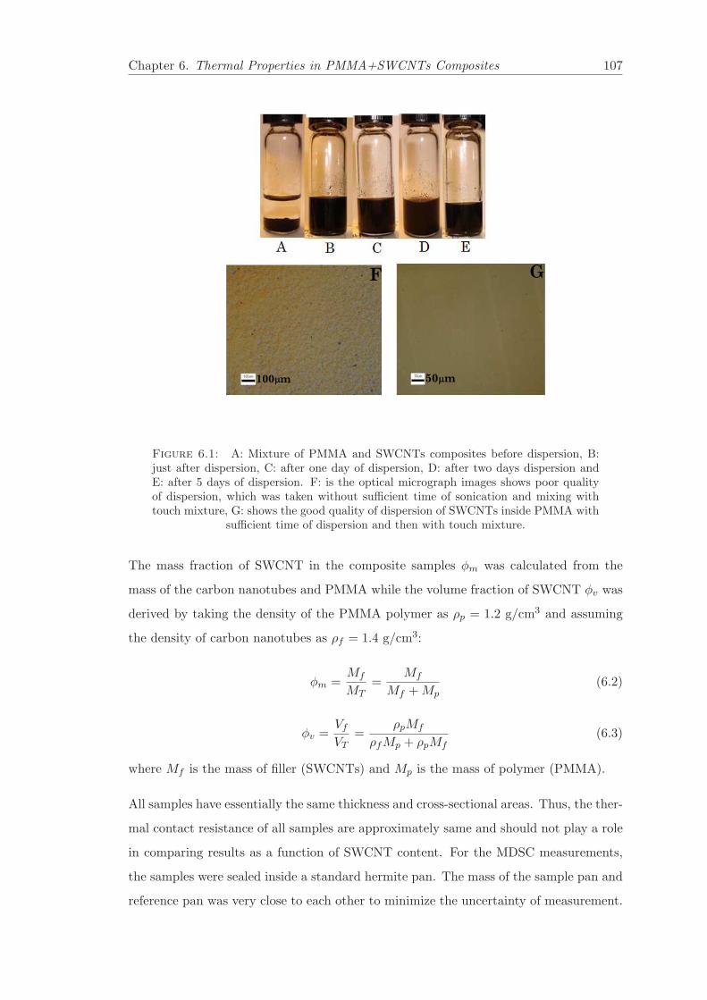
Chapter 6. Thermal Properties in PMMA+SWCNTs Composites 107
100 m100 m100 m 50 m
F G
Figure 6.1: A: Mixture of PMMA and SWCNTs composites before dispersion, B:just after dispersion, C: after one day of dispersion, D: after two days dispersion andE: after 5 days of dispersion. F: is the optical micrograph images shows poor qualityof dispersion, which was taken without sufficient time of sonication and mixing withtouch mixture, G: shows the good quality of dispersion of SWCNTs inside PMMA with
sufficient time of dispersion and then with touch mixture.
The mass fraction of SWCNT in the composite samples φm was calculated from the
mass of the carbon nanotubes and PMMA while the volume fraction of SWCNT φv was
derived by taking the density of the PMMA polymer as ρp = 1.2 g/cm3 and assuming
the density of carbon nanotubes as ρf = 1.4 g/cm3:
φm =Mf
MT=
Mf
Mf +Mp(6.2)
φv =Vf
VT=
ρpMf
ρfMp + ρpMf(6.3)
where Mf is the mass of filler (SWCNTs) and Mp is the mass of polymer (PMMA).
All samples have essentially the same thickness and cross-sectional areas. Thus, the ther-
mal contact resistance of all samples are approximately same and should not play a role
in comparing results as a function of SWCNT content. For the MDSC measurements,
the samples were sealed inside a standard hermite pan. The mass of the sample pan and
reference pan was very close to each other to minimize the uncertainty of measurement.

Chapter 6. Thermal Properties in PMMA+SWCNTs Composites 108
Table 6.1: Specific heat and thermal conductivity results at 300 K and 399 K forpure PMMA and PMMA+SWCNT samples determined by ACC. An effective scan rate
of 0.04 K min−1 was used with Cp given in J g−1 K−1 and κ in W m−1 K−1.
wt% vol% C300p C399
p κ300 κ399
PMMA 0.00 1.61 2.31 0.172 0.2451.40 1.27 1.68 2.35 0.192 0.2671.98 1.79 1.68 2.37 0.202 0.2854.46 3.90 1.69 2.45 0.275 0.3986.00 5.20 1.69 2.46 0.330 0.4819.33 7.93 1.70 2.47 0.395 0.555
The mass of the pan used was 50.4 ± 0.4 mg with the mass difference between sample
and reference pans between 0.3 to 0.5 mg. After casting the required amount of sample,
the remaining solution of PMMA+SWCNT+choloform was stored in a tightly capped
bottle. No significant segregation occurred over several days indicating the quality of
the dispersions.
6.3 Results and Discussion
6.3.1 Specific heat of PMMA+SWCNT composites
Figure 6.2 (top panel) presents ACC determined specific heat of pure PMMA and five
PMMA+SWCNT samples ranging from φm = 0.014 to 0.086 mass fraction of SWCNTs.
The specific heat of all samples exhibit a similar temperature dependence from ≈ 300 to
400 K with only a small change in its absolute value. Since φm is small, Cp is not expected
to vary substantially and so these results more reflect the reproducibility of the absolute
value of Cp measurements by the ACC technique. The experimental Cp value for pure
PMMA is found to be 1.61 J g−1 K−1, about 10 % above the literature value [14, 16]
and within 18 % at 307 K of the value reported by Assael et.al [15]. Specific heat values
of pure PMMA and PMMA+SWCNT composites at 300 K (glass state) and 399 K
(liquid state) are given in Table 6.1. The Cp values of PMMA+SWCNT composites
vary slightly from pure PMMA at room temperature and in a manner similar to that
reported for composites of nanotubes dispersed in polystyrene [18]. The variation of Cp
values between PMMA and PMMA+SWCNT composites is likely due to experimental
uncertainty, especially in the mass measurements of the sample+cell components.
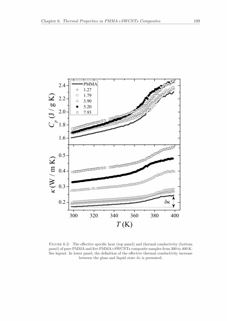
Chapter 6. Thermal Properties in PMMA+SWCNTs Composites 109
300 320 340 360 380 400
0.2
0.3
0.4
0.5
1.6
1.8
2.0
2.2
2.4
(W /
m K
)
T (K)
Cp (
J / g
K)
PMMA 1.27 1.79 3.90 5.20 7.93
Figure 6.2: The effective specific heat (top panel) and thermal conductivity (bottompanel) of pure PMMA and five PMMA+SWCNTs composite samples from 300 to 400 K.See legend. In lower panel, the definition of the effective thermal conductivity increase
between the glass and liquid state δκ is presented.
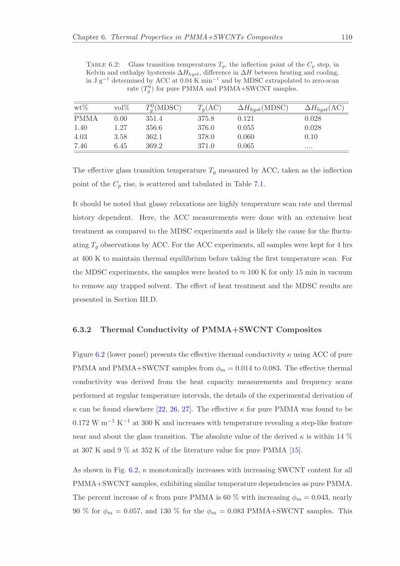
Chapter 6. Thermal Properties in PMMA+SWCNTs Composites 110
Table 6.2: Glass transition temperatures Tg, the inflection point of the Cp step, inKelvin and enthalpy hysteresis ∆Hhyst, difference in ∆H between heating and cooling,in J g−1 determined by ACC at 0.04 K min−1 and by MDSC extrapolated to zero-scan
rate (T 0g ) for pure PMMA and PMMA+SWCNT samples.
wt% vol% T 0g (MDSC) Tg(AC) ∆Hhyst(MDSC) ∆Hhyst(AC)
PMMA 0.00 351.4 375.8 0.121 0.0281.40 1.27 356.6 376.0 0.055 0.0284.03 3.58 362.1 378.0 0.060 0.107.46 6.45 369.2 371.0 0.065 ....
The effective glass transition temperature Tg measured by ACC, taken as the inflection
point of the Cp rise, is scattered and tabulated in Table 7.1.
It should be noted that glassy relaxations are highly temperature scan rate and thermal
history dependent. Here, the ACC measurements were done with an extensive heat
treatment as compared to the MDSC experiments and is likely the cause for the fluctu-
ating Tg observations by ACC. For the ACC experiments, all samples were kept for 4 hrs
at 400 K to maintain thermal equilibrium before taking the first temperature scan. For
the MDSC experiments, the samples were heated to ≈ 100 K for only 15 min in vacuum
to remove any trapped solvent. The effect of heat treatment and the MDSC results are
presented in Section III.D.
6.3.2 Thermal Conductivity of PMMA+SWCNT Composites
Figure 6.2 (lower panel) presents the effective thermal conductivity κ using ACC of pure
PMMA and PMMA+SWCNT samples from φm = 0.014 to 0.083. The effective thermal
conductivity was derived from the heat capacity measurements and frequency scans
performed at regular temperature intervals, the details of the experimental derivation of
κ can be found elsewhere [22, 26, 27]. The effective κ for pure PMMA was found to be
0.172 W m−1 K−1 at 300 K and increases with temperature revealing a step-like feature
near and about the glass transition. The absolute value of the derived κ is within 14 %
at 307 K and 9 % at 352 K of the literature value for pure PMMA [15].
As shown in Fig. 6.2, κ monotonically increases with increasing SWCNT content for all
PMMA+SWCNT samples, exhibiting similar temperature dependencies as pure PMMA.
The percent increase of κ from pure PMMA is 60 % with increasing φm = 0.043, nearly
90 % for φm = 0.057, and 130 % for the φm = 0.083 PMMA+SWCNT samples. This
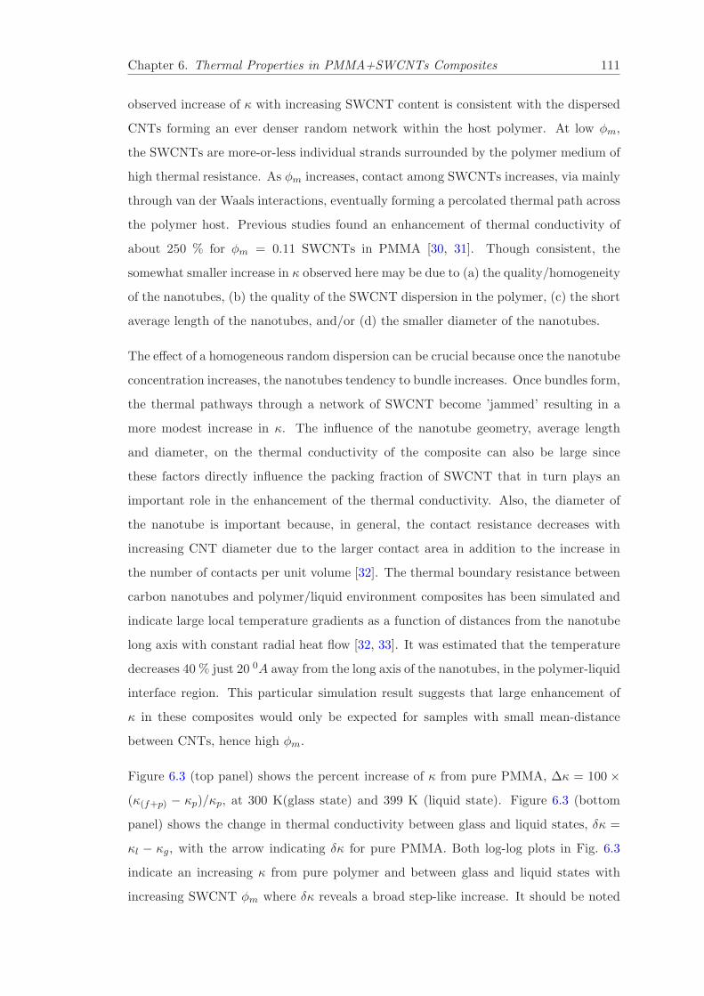
Chapter 6. Thermal Properties in PMMA+SWCNTs Composites 111
observed increase of κ with increasing SWCNT content is consistent with the dispersed
CNTs forming an ever denser random network within the host polymer. At low φm,
the SWCNTs are more-or-less individual strands surrounded by the polymer medium of
high thermal resistance. As φm increases, contact among SWCNTs increases, via mainly
through van der Waals interactions, eventually forming a percolated thermal path across
the polymer host. Previous studies found an enhancement of thermal conductivity of
about 250 % for φm = 0.11 SWCNTs in PMMA [30, 31]. Though consistent, the
somewhat smaller increase in κ observed here may be due to (a) the quality/homogeneity
of the nanotubes, (b) the quality of the SWCNT dispersion in the polymer, (c) the short
average length of the nanotubes, and/or (d) the smaller diameter of the nanotubes.
The effect of a homogeneous random dispersion can be crucial because once the nanotube
concentration increases, the nanotubes tendency to bundle increases. Once bundles form,
the thermal pathways through a network of SWCNT become ’jammed’ resulting in a
more modest increase in κ. The influence of the nanotube geometry, average length
and diameter, on the thermal conductivity of the composite can also be large since
these factors directly influence the packing fraction of SWCNT that in turn plays an
important role in the enhancement of the thermal conductivity. Also, the diameter of
the nanotube is important because, in general, the contact resistance decreases with
increasing CNT diameter due to the larger contact area in addition to the increase in
the number of contacts per unit volume [32]. The thermal boundary resistance between
carbon nanotubes and polymer/liquid environment composites has been simulated and
indicate large local temperature gradients as a function of distances from the nanotube
long axis with constant radial heat flow [32, 33]. It was estimated that the temperature
decreases 40 % just 20 0A away from the long axis of the nanotubes, in the polymer-liquid
interface region. This particular simulation result suggests that large enhancement of
κ in these composites would only be expected for samples with small mean-distance
between CNTs, hence high φm.
Figure 6.3 (top panel) shows the percent increase of κ from pure PMMA, ∆κ = 100 ×(κ(f+p) − κp)/κp, at 300 K(glass state) and 399 K (liquid state). Figure 6.3 (bottom
panel) shows the change in thermal conductivity between glass and liquid states, δκ =
κl − κg, with the arrow indicating δκ for pure PMMA. Both log-log plots in Fig. 6.3
indicate an increasing κ from pure polymer and between glass and liquid states with
increasing SWCNT φm where δκ reveals a broad step-like increase. It should be noted
Chapter 6. Thermal Properties in PMMA+SWCNTs Composites 112
1 2 3 4 5 6 7 8 9 100.06
0.09
0.12
0.15
0.1810
100
(W /
m K
)
V (%)
(%)
300 K 399 K
Figure 6.3: Log-log plot of the percent enhancement of the thermal conductivity,∆κ from pure PMMA (top panel) and the change in thermal conductivity δκ (bottompanel) of PMMA+SWCNT composites between the glass (300 K) and liquid states(399 K), as a function of SWCNT mass fraction φm. Arrow indicates the δκ for pure
PMMA.

Chapter 6. Thermal Properties in PMMA+SWCNTs Composites 113
that the thermal conductivity in the glass state is largely dependent on the vibrational
modes and in the liquid state is dominated by translational motion of the molecules.
This suggests that the phonon propagation is much stronger through nanotubes in the
liquid state than in the glass state for these composites.
6.3.3 Composite Thermal Conductivity Models
There have been many theoretical models reported in the literature for polymer nanocom-
posites, nanofluids, and carbon nanotubes or nanofibers in oil systems. Among the most
relevant models are Lewis/Nielsen [19], Hamilton/Crosser [20], Geometrical [17], and
Xue [21] models. Each are described below and compared to the observed κ for the
PMMA+SWCNT samples.
The Lewis/Nielsen model was initially proposed to estimate electrical and thermal con-
ductivities for a two-component system [19]. Since the thermal conductivity of the
filler (nanotubes) is much higher than that of the polymer, the shape and size of the
filler becomes significant. The Lewis/Nielsen model considered the shape of the dis-
persed particle (their anisotropic character) and the particle packing. It has since been
shown that the nanoparticle shape and dimensions play an important role [34, 35]. The
Lewis/Nielsen model for the effective κ of a two-component system is given by
κc
κp=
1 +ABφv
1 −Bψφv(6.4)
where ψ = 1 +(
1−ρρ2
)
φv, and κc, κp, and κf are the thermal conductivities of the
composite (PMMA+SWCNTs), polymer (PMMA), and f iller (SWCNTs), respectively.
The parameter A = K − 1 depends primarily upon the shape of the dispersed particles
and how they are oriented with respect to the direction of thermal or electric current,
aspect ratio, and is related to the generalized Einstein coefficients KE . The parameter
B = (κf/κp−1)/(κf/κp +A) describes the relative conductivity of the two components.
The parameter ψ is determined by the maximum packing fraction ρ. In the original
Nielsen model [19], ρ for a randomly oriented rod-like filler is ρ = 0.52 irrespective of the
filler’s aspect ratio. This is a reasonable result for fillers with relatively small aspects
ratio (< 10). However, nanotubes have much larger aspect ratios. An experimental
study of the packing fraction on aspect ratio was conducted by J. V. Millewski [36] that

Chapter 6. Thermal Properties in PMMA+SWCNTs Composites 114
1 2 3 4 5 6 7 8 9 10
0.2
0.25
0.3
0.35
0.4
0.45
(W
/ m
K)
V (%)
Experiment (300 K) Geometric Lewis-Nielsen Hamilton-Crosser Xue,
f = 800
Xue, f = 3000
Figure 6.4: Log-log plot of the measured effective thermal conductivity of PMMAand PMMA+SWCNT composites for different vol% SWCNTs at 300 K compared tothe various theoretical models of Lewis/Nielsen, Hamilton/Crosser, Geometric(series),and Xue as listed in the legend. See text for details. The arrow indicates the thermal
conductivity of pure PMMA as measured in this work.
yielded a relationship between the maximum packing fraction and the aspects ratio of
the filler, which was used for our estimate of ρ. The Lewis/Nielsen model can then be
simplified as
κc(φv) = κp
κf +Aκp −Aφv(κp − κf )
κf +Aκp + φvψ(κp − κf )
. (6.5)
by substituting for the parameter B explicitly.
The Hamilton/Crosser model [20] accounts for the particle shape in determining the
thermal conductivity of composite materials differently. The Hamilton/Crosser model
for the effective κc of a composite two-component system is given by
κc(φv) = κp
κf + (n− 1)κp − (n− 1)φv(κp − κf )
κf + (n− 1)κp + φv(κp − κf )
(6.6)
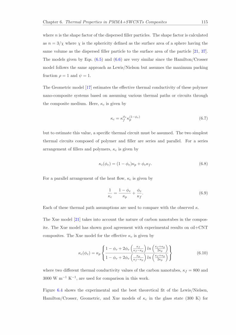
Chapter 6. Thermal Properties in PMMA+SWCNTs Composites 115
where n is the shape factor of the dispersed filler particles. The shape factor is calculated
as n = 3/χ where χ is the sphericity defined as the surface area of a sphere having the
same volume as the dispersed filler particle to the surface area of the particle [21, 37].
The models given by Eqs. (6.5) and (6.6) are very similar since the Hamilton/Crosser
model follows the same approach as Lewis/Nielson but assumes the maximum packing
fraction ρ = 1 and ψ = 1.
The Geometric model [17] estimates the effective thermal conductivity of these polymer
nano-composite systems based on assuming various thermal paths or circuits through
the composite medium. Here, κc is given by
κc = κφv
f κ(1−φv)p (6.7)
but to estimate this value, a specific thermal circuit must be assumed. The two simplest
thermal circuits composed of polymer and filler are series and parallel. For a series
arrangement of fillers and polymers, κc is given by
κc(φv) = (1 − φv)κp + φvκf . (6.8)
For a parallel arrangement of the heat flow, κc is given by
1
κc=
1 − φv
κp+φv
κf. (6.9)
Each of these thermal path assumptions are used to compare with the observed κ.
The Xue model [21] takes into account the nature of carbon nanotubes in the compos-
ite. The Xue model has shown good agreement with experimental results on oil+CNT
composites. The Xue model for the effective κc is given by
κc(φv) = κp
1 − φv + 2φv
(
κf
κf−κp
)
ln(
κf+κp
2κp
)
1 − φv + 2φv
(
κp
κf−κp
)
ln(
κf+κp
2κp
)
(6.10)
where two different thermal conductivity values of the carbon nanotubes, κf = 800 and
3000 W m−1 K−1, are used for comparison in this work.
Figure 6.4 shows the experimental and the best theoretical fit of the Lewis/Nielsen,
Hamilton/Crosser, Geometric, and Xue models of κc in the glass state (300 K) for

Chapter 6. Thermal Properties in PMMA+SWCNTs Composites 116
the PMMA+SWCNT samples. The aspect ratio of 15 and maximum packing fraction
ρ = 0.6 was used for the Lewis/Nielsen model. This aspect ratio is small compared to
that expected for a single nanotube, and likely due to aggregation of many nanotubes
forming bundles. Guthy et.al, [30] reported an aspect ratio as 26 for a bundle of SWCNTs
consisting ∼ 92 nanotubes of 1.3 nm diameter each. However the aspect ratio depends
upon the quality of the dispersion of nanotubes inside polymers matrix. Typically, as
the nanotubes aggregate their aspect ratio should decrease. The thermal conductivity
of the SWCNT filler was assumed to be κf = 3000 W m−1 K−1 for the models used
here. However, the Xue model gave better agreement to the experimental results using
a lower value of κf = 800 W m−1 K−1.
The Geometric model using a series thermal path assumption agrees well with the ob-
served κ for low SWCNT volume fraction (pure PMMA to φm ≈ 0.034). However, this
model strongly deviates from the measured values for larger mass fraction while the
parallel thermal path assumption underestimates κ over the whole range of φm. Recall
that the Geometric model depends only on the amount of fillers and does not account
for the geometry or size of the filler particles, which is apparently a valid assumption
for low SWCNT volume fraction. For SWCNTs, φm > 0.034, the Lewis/Nielsen and
Hamilton/Crosser models are both equally consistent with measurements and indicate
the need to take into account details of the particle size and filler packing within the
polymer. These results essentially indicate that the onset of significant SWCNT inter-
actions, perhaps resulting in a spanning thermal path across the sample, occurs near
φm ≈ 0.034 for PMMA+SWCNT composites.
6.3.4 MDSC Study of PMMA+SWCNT Composites
Because the nanofiller of SWCNT can influence the structural relaxations for glass form-
ing materials like PMMA, dynamics play an important role. For dynamic thermal
measurements, the control parameter is the temperature scan rate. Fig. 6.5 shows the
reversible heat capacity, Rev∆Cp as measured by MDSC normalized to the value deep in
the liquid state (at 405 K) of pure PMMA (left panels) and φm = 0.070 PMMA+SWCNT
composite sample (right panels) for scan rates of 10, 5, 1, 0.5, and 0.1 K/min.
Here, the heating scan at the indicated rate was immediately followed by the cooling
scan. For pure PMMA, a progressively larger hysteresis between heating and cooling

Chapter 6. Thermal Properties in PMMA+SWCNTs Composites 117
-0.18
-0.09
0.00
0.5
0.1
PMMA
0.1
0.5
1 1
5
6.45%
10
-0.18
-0.09
0.00
-0.18
-0.09
0.00
Rev
Cp (
J / g
K)
5
-0.18
-0.09
0.00
330 345 360 375
-0.18
-0.09
0.00
10
T (K)345 360 375 390
Figure 6.5: Difference of the reversible specific heat, Rev∆Cp from the high-temperature liquid state dependence for pure PMMA (left panels) and φm = 0.070composite (right panels) for scan rates from 0.1 (top) to 10 K/min (bottom) on heating
(solid line) and cooling (dashed line).
is seen as the scan rates increase to 10 K/min. For the φm = 0.070 PMMA+SWCNT
sample, very little hysteresis, except in the temperature region near and about the glass
transition, is seen for even the highest scan rate. Similar results were seen for the other
PMMA+SWCNT samples. The suppression of hysteresis in the composites suggests the
partial quenching of structural relaxations of PMMA by the nanotubes. The difference
in enthalpy between heating and cooling ∆Hhyst = Hcool−Hheat extracted from Fig. 6.5
is shown in a log-log plot in Fig. 6.6. Although this plot minimizes the difference among
the samples, it highlights the significant increase in hysteresis for scan rates higher than
about 0.5 K/min.
Because of the scan rate dependent hysteresis, the glass transition temperature is de-
termined from cooling scans shown in Fig. 6.7 and taken as the inflection point of the
Rev∆Cp step-like temperature dependence. The resulting values of Tg are shown in

Chapter 6. Thermal Properties in PMMA+SWCNTs Composites 118
0.1 1 100.01
0.1
1
Hhy
st (J
/ g)
(K/min)
PMMA 1.27 3.58 6.45
Figure 6.6: Log-log plot of the hysteresis between Rev∆Cp areas, ∆Hhyst, for heatingand cooling runs taken by integrating the data in Fig. 6.5 from 300 to 400 K for pure
PMMA and PMMA+SWCNT samples. See legend.
Fig. 6.8 as a function of scan rate for pure PMMA and three composite samples. When
Tg is extrapolated to zero scan rate, the resulting glass transition temperature T 0g is
shown in the inset of Fig. 6.8 as a function of φm revealing a nearly linear increase.
All MDSC measurements employed identical sample treatments and history. However,
heat treatment or annealing can significantly alter the behavior of polymer composites.
The MDSC experiments utilized a protocol where the samples were heated into the
liquid state for 15 min prior loading but the ACC experiments annealed the samples at
400 K for 3 − 4 hr before collecting data.
To explore the effect of heat treatment, MDSC scans were performed on pure PMMA
and the φm = 0.014 PMMA+SWCNT sample after heating into the liquid state (400 K)
for 15, 30, 45, and 60 min prior to a cooling scan at 1 K/min. The resulting Rev∆Cp
for pure PMMA (top panel) and the φm = 0.014 sample (bottom panel) are shown in

Chapter 6. Thermal Properties in PMMA+SWCNTs Composites 119
320 340 360 380 400
-0.28
-0.21
-0.14
-0.07
0.00-0.28
-0.21
-0.14
-0.07
0.00
Rev
Cp (
J / g
K)
T (K)
(K/min) 10 5 1 0.5 0.1
PMMA
6.45%
10
0.1
10
0.1
Figure 6.7: The Rev∆Cp of cooling scans for pure PMMA (top panel) and φm = 0.070composite (bottom panel) for scan rates from 0.1 to 10 K/min. The arrow indicates
order of scan rate commensurate with the inset legend.
Fig. 6.9. Heat treatment of pure PMMA shifts Tg towards higher temperature and tends
to sharpen the step-like behavior in Rev∆Cp. The introduction of SWCNT appears not
to affect both trends, consistent with that observed in the thermal hysteresis results.
6.4 Summary
This work presents a detailed calorimetric study of the specific heat and effective ther-
mal conductivity of a macroscopic arrangement of randomly dispersed SWCNTs inside
a polymer host. Using ACC and MDSC techniques, the enhancement of the effective
thermal conductivity is significant with increased loading of SWCNTs. Higher thermal
conductivity of polymer+CNT composites can be achieved by using suitable dispersion

Chapter 6. Thermal Properties in PMMA+SWCNTs Composites 120
0.1 1 10350
360
370
380
390
T g (K
)
(K/min)
PMMA 1.27 3.58 6.45
0 2 4 6350
357
364
371
T 0 g (K
)
V (%)
Figure 6.8: Semi-log plot of the glass transition temperature, Tg, as a function of scanrate for pure PMMA and three PMMA+SWCNT samples. See legend. Inset showsthe glass transition temperature extrapolated to zero-scan rate, T 0
g , as a function ofSWCNT mass fraction φm.
methods and higher quality nanofiller materials. The glass transition characteristics,
thermal conductivity, electrical conductivity, and mechanical properties of polymer com-
posites can be controlled by adjusting the properties of the nanofillers. The increase in κ
with increasing φm of SWCNT is consistent with essentially independent particles for low
concentration that is describable by a simple Geometric model. For SWCNT higher than
φm ∼ 0.034, a model that takes into account the packing fraction as well as nanoparticle
shape is needed and indicates the onset of interactions among SWCNT, suggesting the
presence of a spanning network. The increase in the zero-scan rate glass transition tem-
perature and suppression of the enthalpic hysteresis supports the view that the random
inclusions of SWCNT in PMMA quenches structural relaxations and stabilizes the glass
state. Continued experimental study, specifically by rheological techniques, is required

Chapter 6. Thermal Properties in PMMA+SWCNTs Composites 121
320 340 360 380 400
-0.3
-0.2
-0.1
0.0
T (K)
Heat (min) 15 30 45 60
-0.3
-0.2
-0.1
0.0
60
15
60
1.27 %
Rev
Cp (
J / g
K)
PMMA15
Figure 6.9: Aging effect on the Rev∆Cp cooling scans (1 K/min) of freshly mountedpure PMMA (top panel) and φm = 0.014 composite sample (bottom panel) after an-
nealing for 15, 30, 45, and 60 min at 400 K. See legend for data labels.
for these types of complex composite systems as well as a more comprehensive modeling
to properly understand and calibrate/engineer the macroscopic properties.
Bibliography
[1] S. J. Tans, M. H. Devoret, H. Dai, A. Theses and R. E. Smalley, Nature., 386, 474
(1997).
[2] H. Dai, J. H. Hafner, A. G. Rinzler, D. T. Colbert, and R. E. Smalley, Nature.,
384, 147 (1996).
[3] S. J. Sander, J. Tans, A. R. M. Verschueren, and C. Dekker, Nature., 393, 49
(1999).
[4] Ijima Sumio, Helical microtubules of graphitic carbon,Nature., 354, 8, No.56
(1991).
[5] S. Glushanin, V. Y. Topolov, and A. V. Krivoruchko, Materials Chemistry and
Physics., 97, 357 (2006).
[6] P. Hine, V. Broome, and I. Ward, Polymer., 46, 10935 (2005).
[7] N. Cioffi, L. Torsi, N. Ditaranto, G. Tantillo, L. Ghibelli, L. Sabbatini, T. Bleve-
Zacheo, M. D. Alessio, P. G. Zambonin, and E. Traversa, Chemistry of Materials.,
317, 5255 (2005).
[8] A. Pelaiz-Barranco and P. Marin-Franch, J. Appl. Phys., 97, 034104 (2005).
[9] A. Bar-Cohen, A. Watwe, and K. N. Seetharamu, Fundamentals of Thermal Man-
agement in Fundamentals of Microsystems Packaging, Chapter 6, Ed., R.R. Tum-
mala, McGraw Hill, New York (2001).
[10] B. Wunderlich, Thermal Analysis of Polymeric Materials. Springer-Velag: Berlin,
Heidelberg, (2005).
[11] B. Wunderlich, Thermal analysis. New York: Academic Press., 135, 205 (1990).
122

Chapter 6. Thermal Properties in PMMA+SWCNTs Composites 123
[12] M. Meyyappan, Carbon nanotubes science and applications, CRC Press: Boca
Raton, FL (2005).
[13] P. J. F. Harris, Carbon nanotubes and related structures new materials for the
twenty-first century;Cambridge University Press: Cambridge (2001).
[14] www.pageout.net/user/www/l/y/lyee/specificheat.pdf.
[15] M. J. Assael, S. Botsios, K. Gialou and N. Metaxa,International Journal of Ther-
mophysics,26, ,1995 (2005).
[16] C. Rauwendal,Polymer Extrusion,PUBLISHER - HanserMunich, GDR (1986).
[17] S. Agarwal, M. Mashud, K. Khan, and R. K. Gupta, Polymer Eng and Science.,
129, 1 (2008).
[18] Y. Yang, M. C. Gupta, J. N. Zalameda and W. P. Winfree, Micro and Nano Letters,
3, No.2, 35-40 (2008).
[19] L. E. Nielsen, Ind. Eng. Chem. Fundam., 13, 17 (1974).
[20] R. L. Hamilton and O. K. Crosser, Ind. Eng. Chem. Fundamen., 1, 187 (1962).
[21] Q. Z. Xue, 368, 302 (2005).,Physica B., 368, 302 (2005).
[22] N. R. Pradhan, H. Duan, J. Liang, and G. S. Iannacchione, Vol-I, 159 (2008).,Pro-
ceedings: Materials Processing and Properties TMS., Vol-I, 159 (2008).
[23] S. Sinha, S. Barjami, G. Iannacchione, A. Schwab, and G. Muench, J. Nanopart.
Res., 7, 651 (2005).
[24] P. S. Clegg, C. Stock, R. J. Birgeneau, C. W. Garland, A. Roshi, and G. S. Iannac-
chione, Phys. Rev. E., 67, 021703 (2003).
[25] A. Roshi, G. S. Iannacchione, P. S. Clegg, and R. J. Birgeneau, Phys. Rev. E., 69,
031703 (2004).
[26] N. R. Pradhan, D. Huanan, J. Liang, and G. S. Iannacchione, Nanotechnology., 19,
485712 (2008).
[27] N. R. Pradhan, H. Duan, J. Liang, and G. S. Iannacchione, Nanotechnology., 20,
245705 (2009).

Chapter 6. Thermal Properties in PMMA+SWCNTs Composites 124
[28] N. J. Coleman and D. Q. M. Craig, International Journal of Pharaceutics., 135, 13
(1996).
[29] Y. Jin, J. Bonilla, Y-G. Lin, J. Morgan, L. McCracken and J Carnahan, Journal of
Thermal Analysis and Calorimetry, 46, No.3-4, 1047-1059 (2005).
[30] C. Guthy, F. Gu, S. Brand, K. I. Winey, and J. E. Fischer, Transaction of the
ASME., 129, 1097 (2007).
[31] C. Guthy, F. Du, S. Brand, K. I. Wieny, and J. E. Fischer,J. Heat Transfer., 129,
1096 (2007).
[32] H. Zhong and J. R. Lukes, Phys. Rev. B., 74, 125403 (2006).
[33] S. Shenogin, L. Xue, R. Oziski, P. Keblinski, and D. G. Cahill, J. Appl. Phys., 95,
8136 (2004).
[34] C. W. Nan and R. Birringer, 81, 6692 (1997)., J. Appl. Phys., 81, 6692 (1997).
[35] P. H. Hasselman, J. Composites Materials., 21, 508 (1987).
[36] J. V. Millewski, Ind. Eng. Chem. Prod. Res. Dev., 17, No.4, 363 (1978).
[37] I. Tavman, A. Turgut, M. Chirtoc, H. P. Schuchmann and S. Tavman, Archives of
Materials Science and Engineering, 34, 99-104 (2008).
Chapter 7
RELAXATION DYNAMICS OF
THE GLASS TRANSITION IN
PMMA+SWCNT COMPOSITES
BY TEMPERATURE
MODULATED DSC
7.1 Introduction
Recently the modulated differential scanning calorimetry (MDSC) [1–3] study has been
widely used to investigate the dynamics of glass transitions of polymer composites and
related materials. In MDSC analysis, the sample is decomposed into reversing and non-
reversing signals, is widely used and appears to avoid the uncertain meaning of dynamic
thermal analyses in analogy to, e.g., dynamic mechanical or dielectric spectroscopies. In
recent studies it has been commonly accepted to present the dynamic thermal properties
in terms of the complex, real (storage), and imaginary (loss) heat capacities (C∗p , C
′
p
and C′′
p ). The concept of frequency-dependent specific heat C∗p(ω,T) (= C∗
p(ω)) was
introduced and the first measurement performed in the 1980s [4–7] with an alternating
current calorimeter technique. After that it has been widely used to study the dynamics
of glass transition of different polymer systems. From a statistical point of view, C∗p(ω)
125

Chapter 7. Relaxation Dynamics of the Glass Transition in PMMA+SWCNTs 126
appears as a consequence of entropy fluctuations [8]. One advantage of the dynamic heat
capacity in comparison to other techniques is the fact that C∗p(ω) reflects the contribution
of all modes, orientational and translational, providing global and direct information of
the slow dynamics associated with the glass transition. Thus MDSC is a widely used
technique to study the phase transition, glass transition and specific heat measurement
of widely available polymeric systems. But the concept of frequency-dependent specific
heat is not widely held. It is especially the case in the application fields of polymers,
food sciences, pharmaceuticals etc. where it could be of most interest to characterize
the molecular mobility.
Carbon nanotubes ( CNTs) have outstanding electrical, mechanical, optical and thermal
properties. These properties have significant promise in a vast range of applications such
as quantum wires [9], tips for scanning probe microscope [10], and molecular diodes [11].
Polymers play a very important role in numerous fields of everyday life due to their ad-
vantages in lightness, ease of processing, resistance to corrosion, and low cost production.
To improve the performance of polymers, composites of polymers and a filler have been
extensively used and studied. The use of various nano-fillers such as metals, semicon-
ductors, organic and inorganic particles and fibers, especially carbon structures [12–15],
are of particular interest and the subject of intense investigation. The unique properties
of carbon nanotubes; extremely high strength, lightweight, elasticity, high thermal and
air stability, high electric and thermal conductivity, and high aspect ratio, offer crucial
advantages over other nano-fillers.
The potential of using nanotubes as filler in polymer composite has not been fully re-
alized because of processing difficulties. Structural relaxation is the process by which
amorphous materials in the glassy state approach a state of thermodynamic equilib-
rium. Calorimetry, such as DSC, has revealed enthalpic relaxations occurring near the
glass transition Tg in glassy polymers aged after a variety of heating treatments. It
is well known that annealing or variation of heating and cooling rates leads to signifi-
cant hysteresis in Tg because of these structural relaxations [16, 17]. The introduction of
nano-fillers is expected to interact strongly with these short-range structural relaxations.
However, the effective utilization of CNTs in polymer composite applications strongly
depends upon the quality/uniformity of the nanotubes and the ability to disperse them
homogeneously throughout the polymer host [18, 19]. Our previous work was to pro-
duce and investigate SWCNT-based nano-composite polymer materials as candidates
Chapter 7. Relaxation Dynamics of the Glass Transition in PMMA+SWCNTs 127
for next generation of high-strength, light weight and enhanced thermal conducting ma-
terials [17]. The structural relaxation has been characterized for many polymers by
Dielectric spectroscopy method, but this method is versatile and widely used to see the
dynamics of the sample in high frequency, where it is found likely that the calorimetric
results are on the extension of dielectric results. The calorimetric Tg includes total degree
of freedom such as rotation, diffusion and vibration, while the dielectric Tg originates
only from the reorientation of molecules.
The main objective of this report is to study the relaxation dynamics of the glass transi-
tion in PMMA+SWCNTs composites at very low frequencies using MDSC and presents
a detailed frequency dependent MDSC technique. There are many studies that have
been done to describe relaxation behavior, glass transition for pure polymer in fre-
quency domain but so far no results reported in Carbon nanotube polymer composites.
The PMMA+SWCNT composites were prepared by dispersing SWCNTs and PMMA
in a chloroform solution using sonication then slowly evaporating the solvent leaving
a homogeneous dispersion. The complex heat capacity was measured as a function of
temperature and different frequency of temperature modulation from 0.0138 to 0.0826
s−1. Then the real and imaginary parts of heat capacity were estimated with the phase
between input heat flow and heating rate. In all samples, we observed the peak max-
imum in imaginary part of heat capacity. The effective glass transition temperature,
Tg, activation energy and dynamics observed in real and imaginary part are dependent
upon the applied modulated frequency of temperature oscillation. The measurement
was reported in the region of glass transition of polymers and composites and other
regions are not of interest in this study as the dynamics do not change with frequency.
Following this introduction, Section 7.2 describes some of the basic experimental pro-
cedures for the MDSC and sample preparation. Section 7.3 presents the experimental
results and discussion followed by a general conclusion with future directions presented
in Section 8.5.

Chapter 7. Relaxation Dynamics of the Glass Transition in PMMA+SWCNTs 128
7.2 Experimental
7.2.1 Modulated Differential-Scanning Calorimetry (MDSC):
Modulated (temperature) differential scanning calorimetry (MTDSC/MDSC) allows for
simultaneous measurement of the evolution of both heat flow and heat capacity. MDSC
differs from conventional DSC where the sample is subjected to a more complex heating
program incorporating a sinusoidal temperature modulation accompanied by an under-
lying linear heating ramp. Whereas DSC is only capable of measuring the total heat
flow, MDSC can simultaneously determine the non-reversible (kinetic component) and
the reversible (heat capacity component) heat flows. A detailed description of the MDSC
method can be found elsewhere [3, 20–25].
The MDSC experiment was performed using a Model Q200 from TA Instruments, USA.
Prior to doing the experiment with our sample, temperature calibration was done with
a sapphire disk, in the same condition of the measurements we have used for our sample
studied. Q200 is an extension of heat flux type of a conventional DSC. The method to
obtain complex specific heat has been proposed by Schawe based on the linear response
theory [3, 21]. In general a temperature oscillation is described as:
T = T0 + q0t+AT sin(ωt) (7.1)
where T0 is the initial temperature at time t = 0, T is the temperature at time t, q0 is
the underlying scan rate, AT the temperature amplitude and ω (ω = 2πf) the angular
frequency of the temperature modulation. f = 1/τ is the frequency in s−1 where τ was
taken as period of modulation.
The results are plotted in the scale of frequency f instead of ω. The heating rate is given
by:
q =dT
dt= q0 +Aqcos(ωt) (7.2)
where Aq is the amplitude of the heating rate (Aq = ATω). Since the applied heating
rate in MDSC consists of two components: q0 underlying heating rate and Aq cos(ωt)
periodic heating rate, the measured heat flow also can be separated into two components,
i.e, the response to the underlying heating rate and response to the periodic heating rate.

Chapter 7. Relaxation Dynamics of the Glass Transition in PMMA+SWCNTs 129
320 340 360 380 4000.20
0.21
0.22
-0.2
0.0
T(K)
<Q>
T
-10
0
10
T
Figure 7.1: (Top): Modulated heat flow raw data and (Middle): modulated heatin PMMA+SWCNT composites. (Bottom) and their temporal average (Blue lines):Phase angle raw data, which allow the determination of the complex heat capacity (thephase lag φ is not corrected). The phase lag exhibits a peak at a temperature Tω where
the amplitude of the modulated heat flow Q strongly decreases.
The latter can be described by
HFperiod = AHF cos(ωt− φ) (7.3)
where HFperiod is the heat flow response to the periodic heating rate, AHF is the ampli-
tude of the heat flow and φ is the phase angle between heat flow and heating rate. An
absolute value of complex specific heat can be obtained by:
∣
∣C∗p
∣
∣ =AHF
mAq(7.4)
where m is the mass of a sample.

Chapter 7. Relaxation Dynamics of the Glass Transition in PMMA+SWCNTs 130
340 350 360 370 380 390 400
0.000
0.002
0.004-0.012
-0.006
0.000
T(K)
T
Cor
rect
ed
(rad
)
U
ncor
rect
ed
(rad
) phase angle adjusted C
p
Tg
Figure 7.2: (Top): Uncorrected phase angle (thick line) with adjusted Cp (thinline) and (Bottom): Corrected phase angle. Tω is not necessarily equal with the glasstransition temperature Tg. his temperature Tω is not equal with the calorimetric glass
transition temperature Tg.
The data was analyzed with correcting the phase shift between heating rate and heat
flow rate signal. The imaginary part of the complex heat capacity was calculated by
correcting the phase angle. The detail correction procedure can be found elsewhere [26].
By the proper calibration for a raw phase angle, we can obtain real C′
p and imaginary
C′′
p parts by
C′
p =∣
∣C∗p
∣
∣ cos(φ), (7.5)
C′′
p =∣
∣C∗p
∣
∣ sin(φ) (7.6)
Measured phase angle was corrected by using the reported method [26], then the real
and imaginary part of the complex heat capacity was estimated.
Examples of the signals obtained on PMMA+SWCNTs in our experiment during the
Chapter 7. Relaxation Dynamics of the Glass Transition in PMMA+SWCNTs 131
glass transformation range are shown in fig. 7.1. Figure 7.2 shows the how uncorrected
phase angle (Top) has corrected (Bottom).
7.2.2 Preparation of PMMA+SWCNT Composites:
The required amount of polymer PMMA (Mn = 120, 000 g mol−1, obtained from
Aldrich) and SWCNTs (Obtained from Helix materials solution Texas, purity > 90 %,
ash 5 %) was first dissolved in chloroform, in a separate container. Then the SWCNT
contained chloroform solution was sonicated for 8 hrs to separate the bundles of nan-
otubes into individual particles. Then both of the PMMA dissolved with chloroform and
SWCNT dispersed with chloroform mixed together and again was kept 6 hrs in an ultra-
sonic bath. Scanning electron micrographs of the SWCNTs used in this work are given
in a previous report [27]. After that the PMMA+SWCNT solution was finally mixed
with touch mixer (Fisher Touch-Mixer model 12-810) for 10 mins. Optical micrograph
studies have been done to clarify the good dispersion of SWCNTs inside host PMMA.
The mass fraction was calculated with the following formula from the mass of the car-
bon nanotubes and PMMA. The volume fraction was derived by taking the density of
PMMA as 1.2 g/cm3 and assuming the density of carbon nanotubes as 1.4 g/cm3:
φm =Mf
Mf +Mp=Mf
MT(7.7)
φv =ρpMf
ρfMp + ρpMf(7.8)
where, φm is the mass fraction, Mf is the mass of filler (SWCNTs), Mp is the mass of
polymer (PMMA), φv is the volume fraction of SWCNTs, ρp is the density of PMMA
and ρf is the density of filler (SWCNTs).
Due to high van der Wall attraction, carbon nanotubes get bundled together in high
mass fraction, which prevent the dispersion quality of nanotubes inside polymer matrix.
In our case, after casting the required amount of sample on a silver sheet, the remaining
solution of PMMA+SWCNT+choloform was stored in a tightly capped bottle and no
significant segregation occurred over several days indicating the quality of dispersions.
For the MDSC measurements, the samples were sealed inside a standard hermetically
sealed pan.

Chapter 7. Relaxation Dynamics of the Glass Transition in PMMA+SWCNTs 132
Before sealed in a hermite pan, each sample is heated for 15 min at 127 0C in vacuum
to remove the trapped chloroform. The MDSC experiment was carried out with under-
lying heating and cooling rates of 2.0, 0.4 and 0.1 K/min with dry ultra pure Nitrogen
gas with flow rate 50ml/min that was purged through the DSC cell. For accurate mea-
surement of specific heat or to decrease the uncertainty, the reference and the sample
hermite pan were chosen carefully. The mass of the pan used as (0.0504±0.0004)g, here
the 0.0004 is the standard deviation of the pan for three different sample pans (three
different mass fractions of PMMA+SWCNT) and a reference pan used for this study.
The mass of the three samples taken in all the measurements are ∼ 10±0.2 mg. The
temperature modulation amplitude was chosen to 1.2 K. We have studied three distinct
samples, pure PMMA, and 0.014 and 0.080 mass fractions of SWCNTs dispersed with
PMMA composites. Each sample was scanned with the above three different scan rates
mentioned and with modulation frequency ranges from 1/160 to 1/30 s−1.
7.3 Results and Discussion
Figure 7.3 shows the real (UP) and imaginary (Bottom) part of the complex specific
heat capacity of 0.014 mass fraction SWCNTs inside PMMA matrix under heating (Left
panel) and cooling (Right panel) rate at 0.40 K/min from 1/30 to 1/150 s−1 frequency
of temperature modulation.
The real part of specific heat (∆C′
p) was normalized to zero far above the glass transition,
at 405 K and the imaginary part was also normalized by subtracting a base line. It is
observed that the maximum rate of change of C′
p occurs in the region of glass transition
and is dependent upon the applied frequency of temperature modulation. Similar change
of ∆C′
p observed during heating and cooling of real part of heat capacity. The change
in magnitude of imaginary part of heat capacity ∆C′′
p , shows different during heating
and cooling with frequency of temperature modulation. This explains the difference of
structural relaxation and the mobility of the sample during heating and cooling. There
is no difference in the real part of specific heat observed in SWCNTs+PMMA composite
samples during heating and cooling. The magnitude of ∆C′
p between liquid and glass
region i.e., ∆C(L−G)p = ∆C
′
p(405) - ∆C′
p(340) shows in Fig. 7.4.

Chapter 7. Relaxation Dynamics of the Glass Transition in PMMA+SWCNTs 133
-0.25
-0.20
-0.15
-0.10
-0.05
0.00
341 352 363 374 385 396
0.000
0.002
0.004
0.006
0.008
0.010
341 352 363 374 385 396
CpL-G
Cp' (f)
(J /
g K
) f (s-1)
1/30 1/40 1/50 1/60 1/70 1/85 1/100 1/115 1/130 1/150
Cp" (f)
(J /
g K
)Cooling
T(K)
Heating
Figure 7.3: The normalized real part of the heat capacity ∆C′
p(f) (top panel) and
imaginary heat capacity ∆C”p)(f) (bottom panel) of a PMMA+SWCNT composites φm
= 0.014 sample from 340 to 405 K, for different applied heating frequencies from 1/30to 1/150 s−1, (see legend). In top panel, the difference between liquid and glass heat
capacity ∆CL−Gp is defined.
This shows, ∆C(L−G)p increases with decreasing frequency of temperature modulation.
Figure 7.4, shows ∆C(L−G)p for the pure PMMA (Upper), 0.014 (Middle) and 0.080
(Bottom) mass fraction of SWCNT in PPMA composites with frequency of temperature
modulation. For PMMA, ∆C(L−G)p increases with decreasing scan rate all over the
frequency range studied except at higher frequency 0.035 s−1, which seems to be equal.
This change of ∆C(L−G)p with respect to scan rate disappears as the mass fraction
of SWCNT increases inside the host polymer. The 0.080 mass fraction of SWCNT
does not show any difference of ∆C(L−G)p with respect to the scan rate all over the
frequency range studied. The imaginary part of the complex specific heat capacity,
during heating ∆C′′
p (ω) (Fig. 7.3, Bottom panel), is characterized by an asymmetric
peak with a smaller slope at the low temperature side than at the high temperature side,

Chapter 7. Relaxation Dynamics of the Glass Transition in PMMA+SWCNTs 134
0.01 0.02 0.03 0.040.06
0.12
0.18
0.24
0.06
0.12
0.18
0.24
0.06
0.12
0.18
0.24
log(f)(s-1)
CpL-
G(f
) (J/
g K
)
0.080
0.014
Scan rate 2.0 0.4 0.1
PMMA
Figure 7.4: Semi-logrithmic plot of ∆CL−Gp as a function of temperature modulation
frequency f for scan rates 2.0, 0.4, and 0.1 K/min, for PMMA (top), 0.014 (middle),and 0.080 (bottom) mass fraction of SWCNTs.
which can be characterized by the molecular distribution of intrinsic structural relaxation
and related to the dynamic glass transition. The slope increases with decreasing the
frequency of temperature modulation in low temperature without changing the high
temperature slope during heating. The temperature where imaginary specific heat shows
maximum value (Tmax) shifted towards lower temperature with decreasing frequency
indicating the dynamics of the systems slowing down. The cooling ∆C′′
p shows similar
peak maximum shifted to lower temperature from 1/30 to 1/70 s−1 and less change
in magnitude than heating results. After 1/70 s−1, there is no significant change of
peak maximum observed during cooling as compared to heating. The ∆C′′
p peak during
cooling shows very symmetric without any change of slope in high and low temperature
side.
In our previous study [17], we experimented with the glass transition temperature, which

Chapter 7. Relaxation Dynamics of the Glass Transition in PMMA+SWCNTs 135
0.01 0.02 0.03 0.04
369
372
375
378
369
372
375
378
0.080
0.014
Scan rate 2.0 0.4 0.1
Log (f) (s-1)
PMMA
369
372
375
378
T g (K)
Figure 7.5: Semi-log plot of the glass transition temperature (Tg) as a function oftemperature modulation frequency for pure PMMA (top), 0.014 (middle) and 0.080(bottom) mass fraction of SWCNTs at scan rates 2.0, 0.4, and 0.1 K/min. Lines are
given to the eye and arrows indicate the zero-frequency extrapolated Tg.
shows Tg increases with scan rate. Figure 7.5 shows the glass transition temperature for
PMMA, 0.014 and 0.080 mass fraction of SWCNT+PMMA composites with frequency
of temperature modulation.
In all of these three samples, highly dependent Tg increases with the increasing fre-
quency of temperature modulation and scan rate. But this shows that in all PMMA
and SWCNT+PMMA composites, Tg of a different scan rate approaches to the same
value as the frequency of temperature modulation increases, and after certain frequency
of modulation, the lower scan rate becomes higher Tg than higher scan rate. This
crossover of Tg between different scan rates with frequency of modulation shifted to a
lower frequency as φm increases. This shows that the dynamics of the glass transition
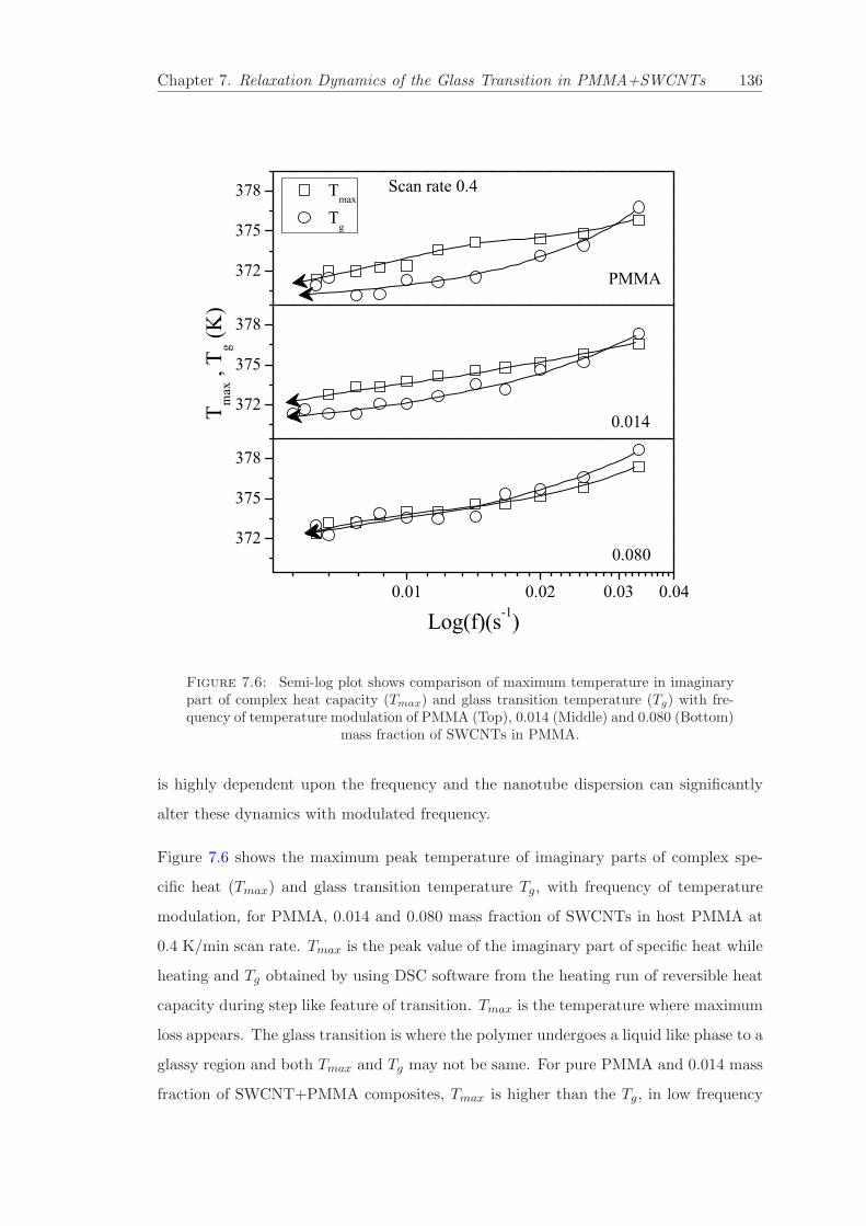
Chapter 7. Relaxation Dynamics of the Glass Transition in PMMA+SWCNTs 136
0.01 0.02 0.03 0.04
372
375
378
372
375
378
372
375
378
0.080
0.014
Log(f)(s-1)
PMMA
T max
, T g (K
)
Tmax
Tg
Scan rate 0.4
Figure 7.6: Semi-log plot shows comparison of maximum temperature in imaginarypart of complex heat capacity (Tmax) and glass transition temperature (Tg) with fre-quency of temperature modulation of PMMA (Top), 0.014 (Middle) and 0.080 (Bottom)
mass fraction of SWCNTs in PMMA.
is highly dependent upon the frequency and the nanotube dispersion can significantly
alter these dynamics with modulated frequency.
Figure 7.6 shows the maximum peak temperature of imaginary parts of complex spe-
cific heat (Tmax) and glass transition temperature Tg, with frequency of temperature
modulation, for PMMA, 0.014 and 0.080 mass fraction of SWCNTs in host PMMA at
0.4 K/min scan rate. Tmax is the peak value of the imaginary part of specific heat while
heating and Tg obtained by using DSC software from the heating run of reversible heat
capacity during step like feature of transition. Tmax is the temperature where maximum
loss appears. The glass transition is where the polymer undergoes a liquid like phase to a
glassy region and both Tmax and Tg may not be same. For pure PMMA and 0.014 mass
fraction of SWCNT+PMMA composites, Tmax is higher than the Tg, in low frequency

Chapter 7. Relaxation Dynamics of the Glass Transition in PMMA+SWCNTs 137
2.652 2.658 2.664 2.670 2.676 2.682 2.688 2.6941.4
1.6
1.8
2.0
2.21.4
1.6
1.8
2.0
2.2
1000/[Tmax
(K)]
PMMA 0.014 0.080
Log[
(s)]
0.4K/min
2.0K/min
Figure 7.7: Arrhenius plot of logarithm of time period of temperature oscillationwith inverse of the peak C
′′
p temperature obtain at rate 2.0, and 0.4 K/min for PMMA,0.014 and 0.080 mass fraction of PMMA+SWCNTs composites.
region and both the Tmax and Tg value approach each other as frequency increases and
at particular frequency (0.029 s−1 for PMMA) they cross each other and become Tg
higher than Tmax. As SWCNTs mass fraction increases, for 0.080 mass fraction, Tmax
and Tg values overlap up to 0.17 s−1 and then cross each other to become Tg value
higher than the Tmax. It indicates that the crossover point between Tg and Tmax shifted
towards the lower frequency as φm increases.
The frequency dependence glass transition can also be interpreted by Arhenius Law.
Figure 7.7 shows the relaxation time (τ in s−1: τ is the modulation time period) in log
scale, versus inverse peak temperature of the imaginary part of complex heat capacity
(1000/Tmax). Figure 7.7 shows from two different scan rates 2.0 K/min (Upper) and
0.4 K/min (Bottom) for PMMA, 0.014 and 0.080 mass fraction of SWCNT+PMMA

Chapter 7. Relaxation Dynamics of the Glass Transition in PMMA+SWCNTs 138
Table 7.1: Activation Energy (E) and characteristic time (τ0) in two different scanrates of PMMA and PMMA+SWCNT composites.
Sample 2D/min 0.4D/minφm E(K) τ0(s) E(K) τ0(s)PMMA 25,600 1.18×10⁻²⁸ 23,000 8.87×10⁻²⁷
0.014 26,000 5.54×10⁻³⁰ 27,000 3.98×10⁻³¹
0.080 29,000 3.62×10⁻³⁴ 29,200 1.10×10⁻³³
composites. The fitted Arhenius Law is given as:
τ =1
ω= τ0 × exp
(
E
Tmax
)
(7.9)
where E is the activation energy and τ0 is the characteristic time. Deviations with
regards to the Arhenius behavior are shown in case of 2 K/min scan rate. The pure
PMMA data follows better the Arhenius behavior than the nanotube composite sample.
It is clear from the fitting that the slope increases with the nanotubes volume fraction
in PMMA+SWCNT composites. Fitted values of activation energy and characteristic
time are given in Table 7.1. The activation energy in 2.0 and 0.4 K/min scan rates,
for pure PMMA, 0.014 and 0.080 mass fraction of SWCNT+PMMA composites were
25600, 26000, 29000 K and 23000, 27000, 29200 K respectively.
This shows that activation energy increases as the volume fraction of nanotubes in-
creases inside the polymer systems. In other words, during the process of formation of
a continuous network, polymer chains stack over the carbon nanotubes to form a strong
network, thus there is a significant increase in the activation energy, and since this fol-
lows arhenius behavior, materials become stronger. On the other hand the characteristic
time decreases with increases the mass fraction of SWCNTs for both scan rates, shown
in Table 7.1.
Fig. 7.8 shows the enthalpy (∆H′′
) of PMMA and 0.080 mass fraction of SWCNT+PMMA
composite with frequency of temperature modulation. This Enthalpy was estimated by
integrating the imaginary part of complex specific heat C′′
p . In low frequency range,
∆ H′′
heating and ∆ H′′
cooling shows a large deviation in both PMMA and 0.080 mass frac-
tion of SWCNT+PMMA composite. Both the cooling and heating enthalpy approach
each other as the frequency of modulation increases. This deviation of ∆H′′
between
heating and cooling at low frequency decreases with scan rate. For a very low scan rate
at 0.1 K/min, there was no significant deviation observed between heating and cooling
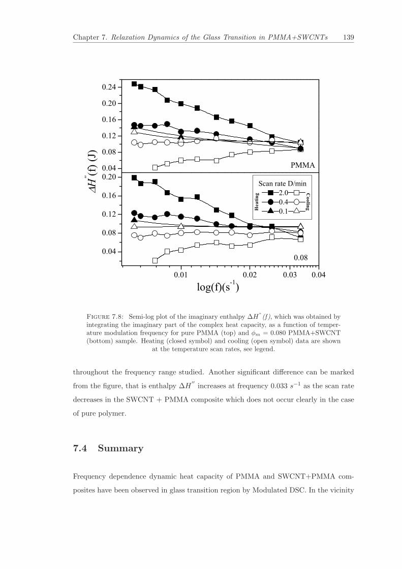
Chapter 7. Relaxation Dynamics of the Glass Transition in PMMA+SWCNTs 139
0.01 0.02 0.03 0.04
0.04
0.08
0.12
0.16
0.200.04
0.08
0.12
0.16
0.20
0.24
log(f)(s-1)
Hea
ting
0.08
H'' (f
) (J)
Scan rate D/min 2.0 0.4 0.1
PMMA
Hea
ting C
ooling
Figure 7.8: Semi-log plot of the imaginary enthalpy ∆H”(f), which was obtained byintegrating the imaginary part of the complex heat capacity, as a function of temper-ature modulation frequency for pure PMMA (top) and φm = 0.080 PMMA+SWCNT(bottom) sample. Heating (closed symbol) and cooling (open symbol) data are shown
at the temperature scan rates, see legend.
throughout the frequency range studied. Another significant difference can be marked
from the figure, that is enthalpy ∆H′′
increases at frequency 0.033 s−1 as the scan rate
decreases in the SWCNT + PMMA composite which does not occur clearly in the case
of pure polymer.
7.4 Summary
Frequency dependence dynamic heat capacity of PMMA and SWCNT+PMMA com-
posites have been observed in glass transition region by Modulated DSC. In the vicinity

Chapter 7. Relaxation Dynamics of the Glass Transition in PMMA+SWCNTs 140
of Tg, the remarkable temperature dependence is clearly observed in the real and imag-
inary part of complex heat capacity. The interesting relaxation phenomena observed in
the imaginary part and dynamics of glass transition obtained from the real part of heat
capacity were discussed with frequency of temperature modulation, when the polymers
undergo a transition from a solid like region to a liquid like state. The Activation en-
ergy calculated from Arhenius behavior increases with mass fraction of nanotubes. The
change of Enthalpy between heating and cooling data was discussed with different scan
rates to understand the molecular behavior during glass transition. This experimental
study must be helpful to understand thermal properties such as glass transition, fragility,
relaxation behavior, Enthalpy loss and mechanical properties of polymer-carbon nan-
otube based composites. These parameters can be controlled by adjusting the properties
of the nanofillers, applied frequency and rate of heating and cooling the materials.

Bibliography
[1] M. Reading, D. Elliott and V. L. Hill, J. Thermal Anal., 40 , 949 (1993).
[2] B. Wunderlich, Y. Jin and A. Boller, Thermochim. Acta, 238, 277 (1994).
[3] J. E. K. Schawe, Thermochim. Acta., 271, 127 (1996).
[4] N. O. Birge and S. R. Nagel, Phys. Rev. Lett., 54, 2674 (1985).
[5] N. O. Birge, Phys. Rev. B, 34, 1631 (1986).
[6] P. K. Dixon, Phys. Rev. B, 42, 8179 (1990).
[7] T. Christensen, J. Physics (Paris Colloq), 46, C8-635 (1985).
[8] N. O. Birge, P. Dixon and N. Menon,Thermochim. Acta, 304, No.305, 51 (1997).
[9] S. J. Tans, M. F. Devoret, H. D. A. Theses and R. E. Smalley, Nature, 386,, 474
(1997).
[10] H. Dai, J. H. Hafner, A. G. Rinzler, D. T. Colbert and R. E. Smalley, Nature, 384,
147 (1996).
[11] S. J. Sander, J. Tans, A. R. M. Verschueren and C. Dekker, Nature, 393, 49 (1998).
[12] S. Glushanin, V. Y. Topolov and A. V. Krivoruchko, Materials Chemistry and
Physics, 97, No.2-3, 357-364 (2006).
[13] P. Hine, V. Broome and I. Ward, Polymer, 46, No.24, 10936-10944 (2005).
[14] N. Cioffi, L. Torsi, N. Ditaranto, G. Tantillo, L. Ghibelli, L. Sabbatini, T. Bleve-
Zacheo, M. D. Alessio, P. G. Zambonin and E. Traversa, Chemistry of Materials,
17, No.21 5255-5262 (2005).
141

Chapter 7. Relaxation Dynamics of the Glass Transition in PMMA+SWCNTs 142
[15] A. Pelaiz-Barranco and P. Marin-Franch, Journal of Applied Physics, 97, No.3, 97
(2005).
[16] B. Wunderlich, Thermal analysis. New York: Academic Press, 135, 135, 205 (1990).
[17] N. R. Pradhan and G. S. Iannacchione, Submitted to ournal of Physical Chem B,
(2009).
[18] M.Meyyappan05, Carbon nanotubes science and applications, CRC Press: Boca
Raton, FL (2005).
[19] P. J. F. Harris, Carbon nanotubes and related structures new materials for the
twenty-first century;Cambridge University Press: Cambridge (2001).
[20] Nichola J. Coleman and Duncan Q. M. Craig, International journal of pharaceutics,
135, 13-29 (1996).
[21] J. E. K. Schawe, Thermochim. Acta, 261, 183 (1995).
[22] J. M. Hutchinson and S. Montserrat, J. Thermal Anal., 47, 103 (1996).
[23] A. Hensel, J. Dobbertin, A. Boller and J. E. K. Schawe, J. Thermal Anal., 46,
935 (1996).
[24] B. Wunderlich, J. Thermal Anal., 48, 207 (1997).
[25] S. R. Aubuchon and P. S. Gill, J. Thermal Anal., 49, 1039 (1997).
[26] S. Weyer, A. Hensel and C. Schick, Thermochimica Acta, 304/305, 267-275
(1997).
[27] N. R. Pradhan, H. Duan, J. Liang and G. S. Iannacchione, Nanotechnology, 20,
No.24, 245705 (2009).

Chapter 8
IMAGING AND DYNAMICS
OF LIQUID CRYSTALS
CONFINED INSIDE CARBON
NANOPIPES
8.1 Introduction of Nanofluid Device
The study of liquid crystals (LCs) began in 1888 when an Austrian botanist named
Friedrich Reinitzer observed that a material known as cholesteryl benzoate had two
distinct melting points. In his experiments, Reinitzer increased the temperature of
a solid sample and watched the crystal change into a hazy liquid. As he increased the
temperature further, the material changed again into a clear, transparent liquid. Because
of this early work, Reinitzer is often credited with discovering a new phase of matter -
the liquid crystal phase. A liquid crystal is a thermodynamic stable phase characterized
by anisotropy of properties without the existence of a three-dimensional crystal lattice,
generally lying in the temperature range between the solid and isotropic liquid phase,
hence the term mesophase. Liquid crystal materials are unique in their properties and
uses. As research into this field continues and as new applications are developed, liquid
crystals will play an important role in modern technology.
143

Chapter 8. Imaging and Dynamics of LC inside CNPs 144
There are different phases in existence of liquid crystals, according to their orientation
from the direction of director of LC molecules. This orientation of molecules depends
upon the temperature, pressure, external applied field, interaction with other molecules
in the environment and also the surface interactions on which it is placed, etc. These
novel properties of LCs make todays technology much more sophisticated than the last
decades. Much research work has been done in the past and much more advanced
research work is going on to enhance the technological application of liquid crystal. In
recent years, scientists were much more focused on the polymer - carbon nanotubes
based research.
Carbon nanotubes (CNTs) are excellent candidates in the application of electronics,
opto-electronics, optics, and the hollow cylinders of pure carbon and the nanochannels
within them are big enough to accommodate various atoms and even small molecules.
Little work has been done on liquid crystals mixed with carbon nanotubes. Now sci-
entists are very keen to study the liquids and other particles confined inside carbon
nanotubes or carbon nanopipes (CNPs). CNPs are long carbon nanotubes with a diam-
eter from 150 - 200 nm, and both ends are open like hollow bamboo shapes. This chapter
contains the dynamic behavior of liquids inside CNPs and is pretty broad, comprising
the investigation of liquid entering inside the nanotubes, and the subsequent filling of
them. The overall flow inside the carbontubes/nanopipes, wetting the nanotubes wall,
and molecular arrangement inside the nanotubes were discussed. Another important
parameter is represented by the diameter of nanotubes: on one hand the interest has
been placed in liquids inside nanotubes having a diameter of a few nanometers with
the promise of observing non-continuum fluid dynamics effects due to confinement in-
side the nano channel. On the other hand, now many of the researchers are focused
on larger nanotubes (diameters > 10 nm) for applications where handling of large vol-
ume of materials is required, with the liquid not necessarily experiencing non-continuum
behavior. Non-continuum behavior is expected to be observed below 10 nm diameter
nanotubes [1].
Interest in nanofluidics increased with more widespread availability of carbon nanotubes,
which appeared to have the ideal characteristics for these kinds of studies. The natural
scale of nanotube channels appeared to yield the possibility of bypassing the complex-
ities of microfabrication and obtaining tubular structures with diameters as small as

Chapter 8. Imaging and Dynamics of LC inside CNPs 145
1 nm. In reality, numerous obstacles inherent to the structure and synthesis process
of carbon nanotubes have been encountered for their use as nanoscale fluid channels:
the presence of kinks and bends, internal closures and caps or catalyst particles [2], all
represent obstacles to the flow of fluids inside the tubes. Some efforts have been directed
towards the development of carbon nanotubes with structure and properties tailored for
nanofluidic studies [3].
The use of nanotubes for nanoscale fluidic studies has also raised the interest in the
nature of the interactions between the nanotube walls and the fluid molecules and effect
on the flow. Understanding the interactions between the fluid and the tube, or the
tubes wettability, will prove to be one of the fundamental aspects of nanofluidics, and
an important step towards the development of nanofluidic devices.
8.1.1 SWCNTs and MWCNTs for Nanofluidic Applications
Carbon nanotubes have been identified traditionally as single-wall nanotubes (SWNT).
In reality, CNTs are a large family of materials with different sizes, structures, and prop-
erties, which are largely determined by their synthesis techniques [2, 4] also mentioned
in chapter 1. SWCNTs, with typical diameters in the range 0.62 nm and comprised
of a single shell, have semiconducting or metallic properties, depending on their chiral-
ity (Chapter-1). CNTs can have two (double-wall nanotubes, DWNT) or more coaxial
shells (multi-wall nanotubes, MWNT), with diameters ranging from 2 to 100 nm and
even more. Noncoaxial CNTs have also been produced, having a so-called herringbone
structure [5, 6], with the graphitic shells placed at an angle with respect to the axis.
Nanotubes with internal closures, dubbed bamboo-like have also been demonstrated [7].
Tens of synthesis techniques have been developed, from arc discharge [8, 9] to hydrother-
mal synthesis [10–12] and catalytic chemical vapor deposition (cCVD) [13–18], most of
them employing a metal catalyst. For storing large amounts of liquid or other molecules
or nanoparticles, the SWCNT or DWCNTs cannot be suitable [19, 20]. A different
class of nanotubes is based on the concept of template-assisted synthesis of nanomate-
rials [21]: chemical vapor deposition (CVD) of carbon has been performed inside the
pores of commercial alumina membranes [22–24], previously used as filters. These mem-
branes initially had pores with an average diameter of 100 - 250 nm in the middle of the
membrane and pore branching close to the two surfaces. With progress in membrane
Chapter 8. Imaging and Dynamics of LC inside CNPs 146
production, nanotubes with diameters as small as 10 nm have been synthesized [3, 25].
Template-grown nanotubes have many characteristics that make them better suited for
nanofluidic studies: straight, long walls, with open ends and small wall thickness com-
pared to the internal diameter of the bore, similar to a macroscopic pipe. In this method
we can easily produce forests of well aligned and excellent quality MWCNTs.
8.1.2 Behavior of Liquids Inside CNPs
One of the first proofs that carbon nanotubes (CNTs) were indeed hollow was obtained
by filling carbon nanotubes with molten metals, salts [26, 27] and oxides, through metal
evaporation [28, 29], melting [30, 31], and capillary filling [32], with subsequent obser-
vation under the TEM. After a few years of initial experiments with molten metals and
salts, the first high resolution transmission electron microscopy (TEM) micrographs of
aqueous fluids trapped inside CNTs suggested that water could indeed wet the internal
cavity of CNTs [10]. Water, along with gases, was trapped inside the nanotubes during
the synthesis process [11, 33]. Later by using an autoclave system, it has been reported
that, water was forced inside 25 nm closed MWNTs through its walls and observed using
high resolution TEM [5, 6, 34]. It has been shown that water preferentially condenses
inside the CNPs when the appropriate temperature and pressure conditions are reached
inside the chamber of an environmental scanning electron microscope (ESEM)[35, 36].
Carbon nanopipes have also been filled with magnetic [37] and fluorescent [38] particles
dispersed in liquid media which penetrated the tubes and then dried up by evapora-
tion. Experimentally dynamic studies of liquids inside CNPs have been done much less
compared to the static studies. The main reason is the high complexity of experimental
setup to perform such experiments, such as miniaturizing a liquid pumping system to
fit a TEM stage. Few dynamic studies can be seen in literature by molecular dynamic
simulation methods [39, 40].
8.1.3 Nanofludic and Energy Storage Applications
Although no nanofluidic devices have reached the commercial stage, there are promising
applications that have already been reported in literature. There is the possibility of
using CNPs/CNTs as the nanoscale equivalent to syringe needles for interrogation of
cells and sub cellular entities. The first result shows MWCNTs about diameter 100 nm

Chapter 8. Imaging and Dynamics of LC inside CNPs 147
attached to AFM tips could poke the cellular membrane of a cell without destroying
it [41], but in this case no liquid transfer was possible. This was achieved by magnetic
assembly of carbon nanotubes loaded with magnetic particles inside a glass micropipette
with a tip tapered down to 300 - 400 nm [19]. Later it was shown to be possible with
200 nm diameter CNPs by using fluorescent dye [42].
CNT-tipped pipettes for cell interrogation appears, to date, as the most promising
nanofluidic application of carbon nanotubes, and the one which is closer to commer-
cialization than other biomedical applications of nanotubes. Other major topics, at
different stages of investigation and development, concern DNA translocation and anal-
ysis, and nanotube-based membranes.
Carbon nanotube-based membranes are also attracting much interest for their charac-
teristic ultra-fast liquid flow, as mentioned earlier. Water filtration and desalination as
well as separation of many other liquids and gases could be the most promising appli-
cations of nanotube membranes. Fundamental studies of chemistry at liquid-liquid and
liquid-gas interfaces, and nano- and microscale chemical reactors on a chip will both be
enabled by the availability of nanotube fluid conduits.
Recently published results show that SWCNTs filled C60 exhibit unusual electronic and
mechanical properties when compared to empty SWCNTs [43–47]. Selective incorpora-
tion of foreign carbons into CNTs could indeed improve the spatial occupancy inside the
CNT channels in a controlled manner, thereby providing a potential way to optimize
their porosities for various applications such as gas adsorption, heavy metal ion removal,
and energy storage.
Liquid crystalline materials offered a promising application in the last few decades for
their application in electro-optic, Optic and display technology. Interest in liquid crys-
talline materials confined to restrictive geometries has expanded in recent years because
of their interesting physical phenomena and their potential use in a plethora of electro-
optic applications [48]. During the last two decades, there have been numerous basic
studies of liquid crystals confined to a restrictive environment. These studies are most
conveniently classified according to the confining template: random porous glass [49–51],
aerosol and aerogel dispersions [52–59], cylindrical confinement [60–65], and spherical
containment [66, 67]. As the size of confinement shrinks to the nanoscale, it becomes
Chapter 8. Imaging and Dynamics of LC inside CNPs 148
extremely difficult to image the molecular ordering within the cavities with experimen-
tal techniques. Confinement of discotic liquid crystal has been studied recently [68] by
High Resolution TEM. They successfully filled the liquid crystal by a capillary filtration
process and visualize the director inside the 5 nm cavity of MWCNT. Another study
shows the filling of 5CB liquid crystal confined inside 200 nm diameter CNPs [69].
In this chapter we studied the filling of 8CB and 10CB liquid crystals inside the ∼200 nm
diameter MWCNPs. The filling in our study refers to complete filling of LCs inside the
MWCNTs and also coating the inside wall of MWCNTs. These two different types of
coating and complete filling are achieved by different types of filling techniques. The
other aspects of this chapter are to study the dynamics of phase transition of these con-
fined liquid crystals inside CNPs by the Modulated Differential Scanning Calorimeter
(MDSC) technique. This technique is already described in detail in previous chapters.
Here, experimental section contains the synthesis of MWCNPs and filling of liquid crys-
tals, then the imaging and MDSC results are discussed.
8.2 Experimental
8.2.1 Synthesis of MWCNPs
CNPs are synthesized with a noncatalytic chemical vapor deposition (CVD) method
using commercially available Anodic Aluminum Oxide (AAO) membranes, a porous
template (Whatman Anodic, average pore diameter: 200 nm±10%, thickness: 60 µm)
described in chapters 4 and 5. These grown MWCNPs inside an AAO template were
taken and the excess amount of carbon layer on the top and/or back surface was removed
by a thermal treatment process. By thermally treating we obtained the well aligned
MWCNPs with both ends opened.
Figure 8.1 shows the cartoon of synthesis procedure how it looks after growing MWCNPs
inside the AAO channel and after dissolving the AAO template.
8.2.2 Filling of LCs inside Carbon Nanopipes
The opened ended MWCNPs grown inside the AAO template were taken for the filling
of liquid crystals. A small quantity of LCs materials were mixed with the acetone solvent

Chapter 8. Imaging and Dynamics of LC inside CNPs 149
Figure 8.1: Synthesis procedure of MWCNPs by CVD method. A: is the CVD grownof MWCNP inside AAO nano-pores, B: Free standing MWCNPs obtained by dissolving
the AAO template with NaOH solution.
to make a solution of LCs and directly dropped on the top of AAO+MWCNP template,
then placed on the hot plate [temperature slightly greater than the Nematic to Isotropic
transition temperature (TNI)] in vacuum environment immediately after pouring, for 1 -
2 minutes. Then we observed that the top surface of the sample covered with a thin layer
of liquid crystals sucked inside the nanopipes. There was also an excess amount of LCs
layer lying on the top surface of the AAO+MWCNPs sample. This liquid crystal layer
was cleaned with filter paper or bird feather very smoothly without breaking the sample.
The SEM micrograph observed that the top surface of the sample was clean of the liquid
crystal. The liquid crystal was confined inside the MWCNPs, where the MWCNPs were
arranged parally inside the AAO template and named later as an aligned sample. Then
the confined liquid crystal inside the aligned MWCNPs was taken and dissolved with
NaOH solution to remove the AAO part. Then we had the randomly oriented MWCNPs
contained liquid crystals. These randomly oriented MWCNPs were imaged by HRTEM
to confirm the presence of liquid crystal inside the MWCNPs. These two types of LCs
confined inside the MWCNPs were taken to be experimented in MDSC studies for their
phase transition.
The other types of filling went through a similar procedure with bulk liquid crystal (no
solvent added) dropped on the top of the MWCNP grown AAO sample then placed on
the hot plate and kept in vacuum, then heated for 3 - 4 mins just above TNI . The
liquid crystal then melted and entered inside the MWCNPs in vacuum. Then the above
similar procedure followed to clean the surface of sample to remove excess LCs and again

Chapter 8. Imaging and Dynamics of LC inside CNPs 150
Figure 8.2: Top: Commercially purchased AAO template of average diameter 200 nmand thickness 60 µm. Bottom: SEM image of grown MWCNPs inside AAO template
of average diameter 190 nm and length 60 µm.
dissolved the AAO template to extract only MWCNP contained LCs.
8.3 Imaging of LCs Confined inside MWCNPs
Figure 8.2 (TOP) shows the SEM images of the commercially purchased AAO template
(200 nm diameter pore sizes and 60 µm thickness of template or length of the pores)
and (Bottom) MWCNPs, average diameter 190 nm and 60 µm long grown inside the
AAO template. MWCNPs tips very clearly show that the quality of the nanotubes
were good and straight inside the nanochannel. Almost all the nanopores are filled with
nanotubes and all the tips are opened on both ends by a thermal cleaning process. This
configuration of the sample was taken for the filling of liquid crystal.
Figure 8.3 shows the filling of solution cast LCs. In this way we have achieved the
coating of the inner surface of the MWCNP’s wall. Both the left and right side of

Chapter 8. Imaging and Dynamics of LC inside CNPs 151
Figure 8.3: HRTEM images of 10CB Liquid Crystals filled inside MWCNPs bysolvent+LC mixture. 30-40nm thick layer of LCs was seen to be coated in inner surface
of the nanopipes.
Fig. 8.3 shows the 10CB LCs are coated on the inner wall surface of CNPs making the
middle/axial part of the nanopipes empty. The coating thickness ranges from 30-40 nm
inside the tube. We can also see the bubble formed on one of the nanopipes by blocking
the LCs in one end Figure 8.3 (right, TOP). The filling of bulk LCs shows complete
filling of LCs inside the nanopipes shown in Fig. 8.4. In this case no inner-wall coating
was observed and the LCs easily filled completely inside the nanotubes. The reason of
coating observed in case of solution cast LC filling was due to the evaporation of solvent
(acetone) in vacuum after completely filling the LC solution inside nanopipes.
8.4 Study of Phase Transition of 8CB and 10CB Liquid
crystals inside MWCNPs by Modulated DSC:
Modulated Differential Calorimetric study has been carried out to confirm the existence
of LCs inside carbon nanopipes and also to learn some of the dynamics of molecules

Chapter 8. Imaging and Dynamics of LC inside CNPs 152
Figure 8.4: HRTEM images of filled 10CB liquid crystal inside MWCNPs by directlyusing bulk 10CB. Complete/partially filling of nanopipes shows in this case.
inside confined space.
The experimental details of MDSC are described in previous chapters. Figure 8.5 shows
the normalized reversible heat capacity of pure 8CB (red color) and 8CB liquid crys-
tal confined inside MWCNPs. The data was normalized at TNI transition tempera-
ture. MDSC has done with different modulated frequency of temperature oscillation
and 0.3 D/min scan rate.
Bulk 8CB shows the strong Smectic-A to Nematic at 305.3 K and Nematic to Isotropic
transition at 312.6 K as expected and also has been checked with high resolution AC
Calorimeter technique. 8CB, confined inside MWCNPs does not show suppression of
Nematic to Isotropic transition completely, but the transition temperature shifted to-
wards the higher temperature to 312.8 K. The Isotropic to Nematic transition shows
drastic suppression or no transition observed.
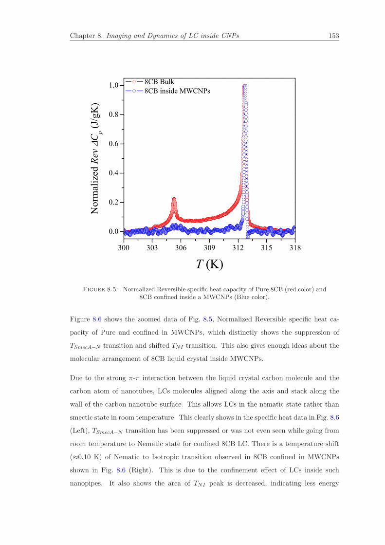
Chapter 8. Imaging and Dynamics of LC inside CNPs 153
300 303 306 309 312 315 318
0.0
0.2
0.4
0.6
0.8
1.0N
orm
aliz
ed R
ev
Cp (J
/gK
)
8CB Bulk 8CB inside MWCNPs
T (K)
Figure 8.5: Normalized Reversible specific heat capacity of Pure 8CB (red color) and8CB confined inside a MWCNPs (Blue color).
Figure 8.6 shows the zoomed data of Fig. 8.5, Normalized Reversible specific heat ca-
pacity of Pure and confined in MWCNPs, which distinctly shows the suppression of
TSmecA−N transition and shifted TNI transition. This also gives enough ideas about the
molecular arrangement of 8CB liquid crystal inside MWCNPs.
Due to the strong π-π interaction between the liquid crystal carbon molecule and the
carbon atom of nanotubes, LCs molecules aligned along the axis and stack along the
wall of the carbon nanotube surface. This allows LCs in the nematic state rather than
smectic state in room temperature. This clearly shows in the specific heat data in Fig. 8.6
(Left), TSmecA−N transition has been suppressed or was not even seen while going from
room temperature to Nematic state for confined 8CB LC. There is a temperature shift
(≈0.10 K) of Nematic to Isotropic transition observed in 8CB confined in MWCNPs
shown in Fig. 8.6 (Right). This is due to the confinement effect of LCs inside such
nanopipes. It also shows the area of TNI peak is decreased, indicating less energy
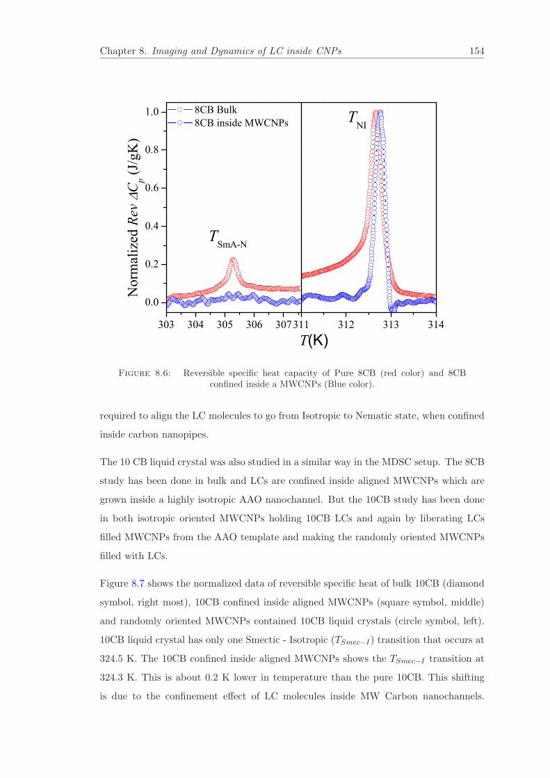
Chapter 8. Imaging and Dynamics of LC inside CNPs 154
303 304 305 306 307
0.0
0.2
0.4
0.6
0.8
1.0
Nor
mal
ized
Rev
C
p (J/g
K)
T(K)
TSmA-N
311 312 313 314
TNI
8CB Bulk 8CB inside MWCNPs
Figure 8.6: Reversible specific heat capacity of Pure 8CB (red color) and 8CBconfined inside a MWCNPs (Blue color).
required to align the LC molecules to go from Isotropic to Nematic state, when confined
inside carbon nanopipes.
The 10 CB liquid crystal was also studied in a similar way in the MDSC setup. The 8CB
study has been done in bulk and LCs are confined inside aligned MWCNPs which are
grown inside a highly isotropic AAO nanochannel. But the 10CB study has been done
in both isotropic oriented MWCNPs holding 10CB LCs and again by liberating LCs
filled MWCNPs from the AAO template and making the randomly oriented MWCNPs
filled with LCs.
Figure 8.7 shows the normalized data of reversible specific heat of bulk 10CB (diamond
symbol, right most), 10CB confined inside aligned MWCNPs (square symbol, middle)
and randomly oriented MWCNPs contained 10CB liquid crystals (circle symbol, left).
10CB liquid crystal has only one Smectic - Isotropic (TSmec−I) transition that occurs at
324.5 K. The 10CB confined inside aligned MWCNPs shows the TSmec−I transition at
324.3 K. This is about 0.2 K lower in temperature than the pure 10CB. This shifting
is due to the confinement effect of LC molecules inside MW Carbon nanochannels.
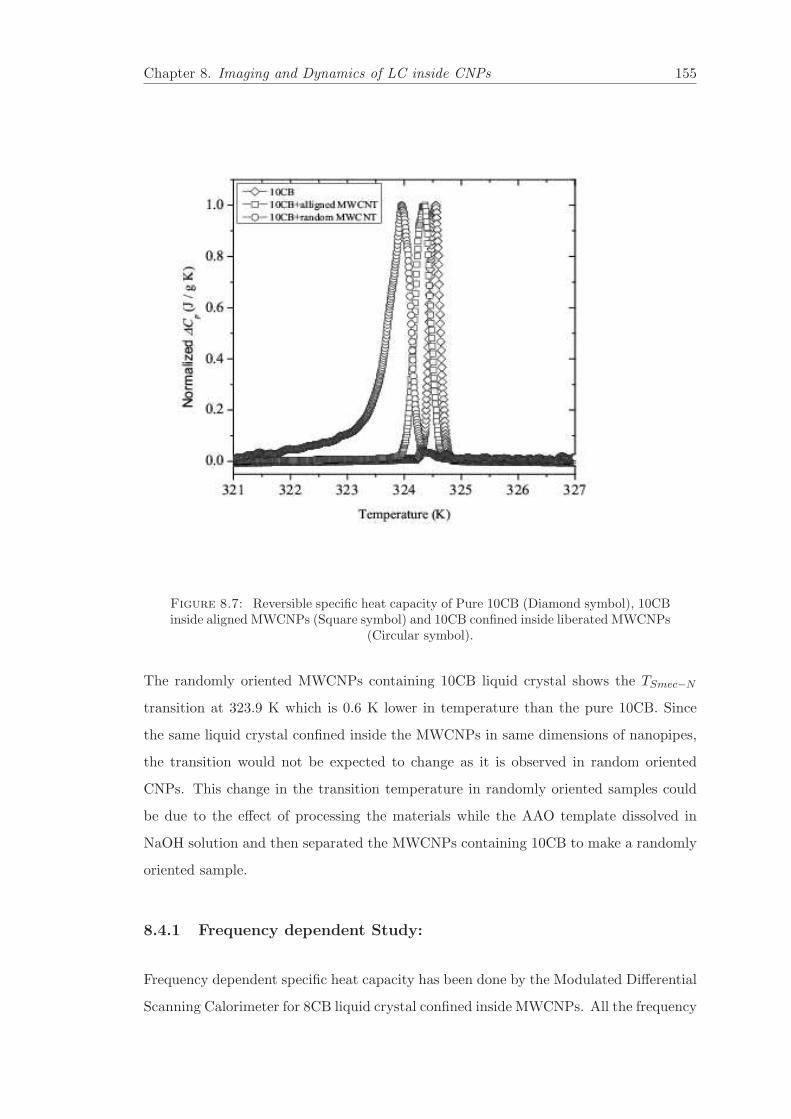
Chapter 8. Imaging and Dynamics of LC inside CNPs 155
Figure 8.7: Reversible specific heat capacity of Pure 10CB (Diamond symbol), 10CBinside aligned MWCNPs (Square symbol) and 10CB confined inside liberated MWCNPs
(Circular symbol).
The randomly oriented MWCNPs containing 10CB liquid crystal shows the TSmec−N
transition at 323.9 K which is 0.6 K lower in temperature than the pure 10CB. Since
the same liquid crystal confined inside the MWCNPs in same dimensions of nanopipes,
the transition would not be expected to change as it is observed in random oriented
CNPs. This change in the transition temperature in randomly oriented samples could
be due to the effect of processing the materials while the AAO template dissolved in
NaOH solution and then separated the MWCNPs containing 10CB to make a randomly
oriented sample.
8.4.1 Frequency dependent Study:
Frequency dependent specific heat capacity has been done by the Modulated Differential
Scanning Calorimeter for 8CB liquid crystal confined inside MWCNPs. All the frequency

Chapter 8. Imaging and Dynamics of LC inside CNPs 156
310 311 312 313 314 3150
1
2
3
4
5
6
7
8
1/30
f (1/s) 1/30 1/45 1/60 1/75
Rev
Cp (J
/gK
)
T (K)
1/75
Figure 8.8: Frequency dependent Reversible specific heat capacity of Pure 8CB from1/30 to 1/75 s−1.
scans plotted here are at a scan rate at 0.3D/min, from 1/30 to 1/120 s−1 frequency of
temperature modulation.
Figure 8.8 shows the normalized specific heat capacity with temperature in different
frequency of temperature oscillation for pure 8CB during TNI transition. It was observed
that the magnitude of specific heat increases as the frequency of temperature modulation
decreases while going from frequency 1/30 to 1/60 s−1, and specific heat does not increase
as the frequency further decreases. The transition temperature (TNI) remains unchanged
with the frequency of temperature modulation. This behavior of increasing specific heat
does not show up during TSmecA−N transition.
The opposite behavior of change in magnitude of specific heat during TNI transition
with frequency of temperature modulation was observed in 8CB liquid crystal confined
inside aligned MWCNPs and shown in Fig. 8.9. The magnitude of specific heat increases

Chapter 8. Imaging and Dynamics of LC inside CNPs 157
310 311 312 313 314 315
0.0
0.2
0.4
0.6
0.8
1.0 1/30
1/120
f (1/s) 1/30 1/45 1/60 1/75 1/120
Rev
Cp(J
/gK)
T (K)
Figure 8.9: Frequency dependent Reversible specific heat capacity of 8CB confinedinside aligned MWCNPs from 1/30 to 1/120 s−1.
as the frequency of temperature modulation increases, where the opposite behavior was
observed during pure 8CB liquid crystal.
This opposite behavior of frequency dependent shows quite an interesting molecular
interaction of LC molecules with the surface of carbon nanotubes. The simulation
study might makes us better understanding of the interaction between LCs and the
nanotubes wall when LCs molecules confined inside CNPs with frequency of temperature
modulation.
8.5 Summary
The filling, imaging and dynamics of the phase transition of liquid crystal inside the
carbon nanopipes/carbon nanotubes have been studied for 8CB and 10CB molecular
structures. We were successfully able to fill the liquid crystal inside MWCNPs in two
Chapter 8. Imaging and Dynamics of LC inside CNPs 158
different approaches and both approaches showed quite a different filling of LCs inside
the MWCNPs. The solution mixed LCs filling shows the filling of innerwall coating
and the filling pure bulk liquid crystal shows complete or partial filling of MWCNPs.
These filling were confirmed by TEM images and also with the calorimetric techniques
of phase transition. The dynamics of these confined liquid crystal molecules studied
by this MDSC technique shows more dramatic changes than pure liquid crystals. The
frequency dependent studied showed one of the exciting phenomena of molecules of LCs
and their interaction with the surface of carbon nanotubes due to confinement. This
study tells us some of the rich physics of liquids confined inside carbon nanopipes. This
also provides some understanding of the flow of liquids inside nanopipes for application
of nanofluidic devices.
Bibliography
[1] M. Whitby and N. Quirke, Nat Nanotechnology, 2, 87-94 (2007).
[2] P. J.F. Harris, Cambridge University Press, Cambridge, (1999).
[3] D. Mattia, Templated growth and characterization of carbon nan-
otubes for nanofluidic applications. PhD Thesis, Drexel University,
http://dspace.library.drexel.edu/bitstream/1860/1772/1/Mattia−Davide.pdf.
(2007).
[4] Y. Gogotsi, Nanotubes and nanofibers, CRC Press, Boca Raton, (2006).
[5] H. Ye, N. Naguib, Y. Gogotsi, TEM study of water in carbon nanotubes. JEOL
News, 39, 38-43 (2004).
[6] H. Ye, N. Naguib, Y. Gogotsi,Y, A. G. Yazicioglu and C. M. Megaridis, Nan-
otechnology, 15, 232-236 (2004).
[7] D. H. Jung,Y. K. Ko, H. T. Jung, Mater Sci Eng C, , 117-121 (2004).
[8] J. L. Hutchison, N. A. Kiselev, E. P. Krinichnay, A. V. Krestinin, R. O. Loutfy,
A. P. Morawsky, V. E. Muradyan, E. D. Obraztsova, J. Sloan, S. V. Terekhov
and D. N. Zakharov, Carbon, 39, 761-770 (2001).
[9] J. C. Bae, Y. J. Yoon, S. J. Lee, K. M. Song, H. K. Baik, Carbon, 40,, 2905-2911
(2002).
[10] Y. Gogotsi, J. A. Libera and M. Yoshimura, J Mater Res, 15, 2591-2594 (2000).
[11] J. A. Libera and Y. Gogotsi, Carbon, 39, 1307-1308 (2001).
[12] J. M. Calderon Moreno, S. S. Swamy, T. Fujino and M. Yoshimura, Chem Phys
Lett, 329, 317-322 (2000).
159
Chapter 8. Imaging and Dynamics of LC inside CNPs 160
[13] M. Su, B. Zheng and J. Liu,Chem Phys Lett, 322, 321326 (2000).
[14] L. Ci, Z. Rao, Z. Zhou, D. S. Tang, X. Yan, Y. Liang, D. Liu, H. Yuan,
W. Zhou and Gea Wang, Chem Phys Lett, 359, 6367 (2002).
[15] Z. Kang, E. Wang, L. Gao, S. Lian, M. Jiang, C. Hu and L. Xu, J Am Chem
Soc., 125, 13652-13653 (2003).
[16] V. L. Kuznetsov, A. N. Usoltseva, A. L. Chuvilin, E. D. Obraztsova and J-
M. Bonard, Phys Rev B, 64, 235401235407 (2001).
[17] J. H. Hafner, M. J. Bronikowski, B. R. Azamian, P. Nikolaev, A. G. Rinzler, D. T.
Colbert, K. A. Smith and R. E. Smalley, Chem Phys Lett, 296, 195-202 1998).
[18] A. M. Cassell, J. A. Raymakers, J. Kong and H. Dai, J Phys Chem B., 103,
6484-6492 (1999).
[19] J. R. Freedman, D. Mattia, G. Korneva, Y. Gogotsi, G. Friedman and A. K.
Fontecchio, Appl Phys Lett, 90, 103108 (2007).
[20] B. M. Kim, S. Sinha S and and H. H. Bau, Nano Lett, 4, 2203-2208 (2004).
[21] C. R. Martin, Science, 266, 1961-1966 (1994).
[22] T. Kyotani, L. F. Tsai and A. Tomita, Chem Mater, 7, 1427-1428 (1995).
[23] T. Kyotani, L. F. Tsai and A. Tomita, Chem Mater, 8, 2109-2113 (1996).
[24] T. Kyotani, J. Chmiola and Y. Gogotsi, Carbons and composites for electrochem-
ical energy storage systems, Press Taylor and Francis, London (2008).
[25] D. Mattia, H. H. Bau and Y. Gogotsi, Langmuir, 22, 1789-1794 (2006).
[26] D. Ugarte, T. Stockli, J. M. Bonard, A. Chatelain, W. Ad. Heer, Appl Phys A,
67, 101-105 (1998).
[27] C. Xu, J. Sloan, G. Brown, S. R. Bailey, V. C Williams, S. Friedrichs, K. S.
Coleman, E. Flahaut, J. L. Hutchison, R. E. Dunin-Borkowski and M. L. H. Green,
Nat Nanotechnology, Chem Commun, , 2427-2428 (2000).
[28] P. M. Ajayan and S. Iijima, Nature, 361, 333 (1993).
[29] S. Iijima, Nature, 354, 56-58 (1991).

Chapter 8. Imaging and Dynamics of LC inside CNPs 161
[30] T. Ebbesen, J Phys Chem Solids, 57, 951955 (1996).
[31] E. Dujardin, T. Ebbesen, H. Hiura and K. Tanigaki, Science, 265, 1850 (1994).
[32] J. Mittal, M. Monthioux, H. Allouche and O. Stephan,Chem Phys Lett, 339, 311318
(2001).
[33] Y. Gogotsi, J. A. Libera, A. G. Yazicioglu and C. M. Megaridis, Appl Phys Lett,
79, 1021-1023 (2001).
[34] N. Naguib, H. Ye, Y. Gogotsi, A. G. Yazicioglu, C. M. Megaridis and M. Yoshimura,
Nano Lett, 4, 22372243 (2004).
[35] M. P. Rossi, H. Ye and Y. Gogotsi, In ASME Heat Transfer/Fluid Engineering
Summer Conference Charlotte, USA, (2004).
[36] M. P. Rossi, H. Ye, Y. Gogotsi, S. Babu, P. Ndungu and J. C. Bradley, Nano Lett.,
4, 989-993 (2004).
[37] G. Korneva, H. Ye, Y. Gogotsi, D. Halverson, G. Friedman, J. C. Bradley and K. G.
Kornev, Nano Lett., 5, 879884 (2005).
[38] B. M. Kim, S. Qian and H. H. Bau, Nano Lett., 5, 87378 (2005).
[39] A. G. Yazicioglu, C. M. Megaridis and Y. Gogotsi, J Heat Transfer, 126, 506-606
(2004).
[40] A. G. Yazicioglu, C. M. Megaridis, A. Nicholls and Y. Gogotsi, J Vis, 8, 137144
(2005).
[41] N. A. Kouklin, W. E. Kim, A. D. Lazareck and J. M. Xu, Appl Phys Lett, 87,
173901 (2005).
[42] M. G. Schrlau, E. M. Falls, B. L. Ziober and H. H. Bau, Nanotechnology, , 015101
(2008).
[43] J. Zhang, Y. S. Hu, J. P. Tessonnier, G. Weinberg, J. Maier,R. Schlogl and D. S.
Su, Advanced Materials, 20, 1450-1455 (2008).
[44] B. W. Smith, M. Monthioux and D. E. Luzzi, Nature, 396, 323 (1998).
[45] J. Sloan, A. I. Kirkland, J. L. Hutchison and M. L. H. Green, Chem. Comm., , 1319
(2002).

Chapter 8. Imaging and Dynamics of LC inside CNPs 162
[46] I. V. Krive, R. I. Shekhter and, M. Jonson, Low Temp. Phys., 32, 887 (2006).
[47] J. W. Kang and H. J. Hwang, Nanotechnology, 15, 1825 (2004).
[48] G. P. Crawford and S. Zumer, Liquid Crystals in Complex Geometries Formed By
Polymer and Porous Networks, Taylor and Francis, London (1996).
[49] J. Leys, G. Sinha, C. Glorieux, and J. Thoen, Phys. Rev. E, 71, 051709 (2005).
[50] G. S. Iannacchione, G. P. Crawford, S. Qian, J. W. Doane, and D. Finotello, Phys.
Rev. E, 53, 2402 (2004).
[51] D. E. Feldman and R. A. Pelcovits, Phys. Rev. E, 70, 040702 (2004).
[52] M. K. Ramazanoglu, P. S. Clegg, R. J. Birgeneau, C. W. Garland, M. E. Neubert,
and J. M. Kim, Phys. Rev. E, 69, 061706 (2004).
[53] L. O. Dolgov and O. V. Yaroshchuk, Colloid Polym. Sci., 282, 1403 (2004).
[54] R. Bandyopadhyay, D. Liang, R. H. Colby, J. L. Harden, and R. L. Leheny, Phys.
Rev. Lett., 94, 10781 (2005).
[55] F. Mercuri, S. Paoloni, U. Zammit, and M. Marinelli, Phys. Rev. Lett., 94, 247801
(2005).
[56] A. V. Zakharov and J. Thoen, Eur. Phys. J. E, 17, 447 (2005).
[57] R. L. Leheny, S. Park, R. J. Birgeneau, J. L. Gallani, C. W. Garland, and G. S.
Iannacchione, Phys. Rev. E, 67, 011708 (2003).
[58] A. Zidansek, G. Lahajnar, and S. Kralj, Appl. Magn. Reson., 27, 311 (2004).
[59] L. M. Chen and J. Toner, Phys. Rev. Lett., 94, 137803 (2005).
[60] R. J. Ondris-Crawford, G. P. Crawford, S. Zummer, and J. W. Doane, Phys. Rev.
Lett., 70, 194 (1993).
[61] G. P. Crawford, D. W. Allender, and J. W. Doane, Phys. Rev. A, 45, 8693 (1992).
[62] G. P. Crawford, R. J. Ondris-Crawford, S. Zummer, and J. W. Doane, Phys. Rev.
Lett., 70, 1838 (1993).
[63] T. Jin, G. P. Crawford, R. J. Crawford, S. Zumer, and D. Finotello, Phys. Rev.
Lett., 90, 015504 (2003).

Chapter 8. Imaging and Dynamics of LC inside CNPs 163
[64] B. Zalar, R. Blinc, S. Zummer, T. Jin, and D. Finotello, Phys. Rev. E, 65, 041703
(2002).
[65] T. Jin, B. Zalar, A. Lebar, S. Zumer, and D. Finotello, Eur. Phys. J. E, 16, 159
(2005).
[66] M. Vilfan, N. vrbancic-Kpoac, B. Zalar, S. Zumer, and G. P. Crawford, Phys. Rev.
E, 59, R4754 (1999).
[67] A. Golemme, S. Zumer, J. W. Doane, and M. E. Neubert, Phys. Rev. A, 37, 559
(1988).
[68] K. Jian, R. H. Hurt, B. W. Sheldon and G. P. Crawford, Appl. Phys. Lett., 88,
163110 (2006).
[69] Hemang J. Sahah and Adam K. Fontecchio, Appl. Phys. Lett., 89, 043123 (2006).

Chapter 9
CONCLUSIONS
9.1 Conclusions
This dissertation presents an experimental study of the thermal transport of metal
nanowires, carbon nanotubes and polymer-carbon nanotubes composites. The filling
mechanism of Liquid crystals inside small nanopipes is also included in last chapter
which provides physics of dynamics of liquids inside small carbon nanopipes.
The major part of this thesis work was to understand the fundamental phonon transport
phenomena in the one dimensional system of nanowires/nanotubes in different orienta-
tions. These experimental measurements and results resemble the promising applica-
tions of these materials in electronic, optoelectronic, sensors, photonics, thermoelectrics,
thermal management, high thermal stability and display technology. This thesis work
definitely replaces some of the existing materials for higher efficient device production.
This chapter will summarize the experimental measurement work done in this thesis and
some of the future directions to expand this study.
CoNWs and MWCNTs were grown by electro chemical deposition and CVD techniques
inside an AAO template. The diameter of fabricated CoNWs and MWCNTs were 80 nm
and length 20 µm. The well aligned CoNWs and MWCNTs inside the AAO template
were used to study the anisotropic measurement of thermal properties. The same batch
of CoNWs and MWCNTs were taken and dissolved in the AAO by NaOH to obtain pure
CoNWs and MWCNTs in powder form, where the nanowires and nanotubes are ran-
domly oriented. These randomly oriented nanowires and nanotubes are taken to make
164

Chapter 9. Conclusions 165
a thin film of respective sample. This sample was used for the same thermal properties
measurement called thermal conductivity in randomly oriented direction, where heat
transfer is across the randomly oriented nanowires/nanotubes. The measured specific
heat and extracted thermal conductivities in anisotropic and randomly oriented direc-
tions were compared with their respective bulk sample of Cobalt and graphite powder
(particle sizes ∼micro meter order). The SWCNTs were also purchased from the Helix
materials solution company and used for the same thermal study in randomly oriented
mat sample and compared with MWCNTs.
The high resolution AC Calorimeter technique has been successfully used to measure the
heat capacity of the sample. The sample was sandwiched between two silver sheets in
such a way that, both the top and bottom silver sheet did not electrically connect with
each other. Heater (120Ω) was attached on the top of one silver sheet and a thermister
of 1MΩ was attached on the top of the other silver sheet. In this configuration of sample
arrangement, we can achieve the thermal wave propagation only through the sample,
and the result gives the intrinsic thermal properties of materials.
The particle nature of the bulk powder and randomly orientated CoNWs found devia-
tions of both κ and Cp from that of pure solid cobalt. The κ and Cp exhibit a much
stronger temperature dependence and show peak-like maximums and explain the dom-
inance of phonon-boundary scattering in the temperature range 300-400 K. Thermal
conductivity of CoNWs was 83 times less than the bulk cobalt, which suggests the dom-
inance of phonon-phonon or phonon-defect scattering. The phonon mean free path in
nanowires also describes the anisotropic and scattering propagation of phonon waves.
Further study is needed with diameter dependent thermal conductivity to understand
much of the basics and insight of phonon transport inside these nanostructures. Dif-
ferent diameter and length dependent thermal studies will give more insight into the
science which will help to make promising nanowire based devices.
In the case of MW and SW carbon annotubes measurement, specific heat of all the sam-
ples shows very similar behavior from 300-400 K. But thermal conductivity of anisotropic
MWCNTs was much higher than the random mat sample of MWCNTs, SWCNTs and
graphite powder. This suggested that the phonon propagation along the long axis of
carbon nanotubes is one dimensional in nature. There is less or no phonon-boundary
scattering. The random composite sample shows a peak-like feature, indicating the

Chapter 9. Conclusions 166
phonon-phonon scattering inside the nanotubes, which decreases thermal conductivity
as temperature increases. Thermal conductivity also depends upon the diameter of the
nanotubes, the smaller the diameter the larger the thermal conductivity as the contact
resistance between nanotubes decreases in the mat sample. This was clearly shown in
our result. The SWCNTs diameter was less than the MWCNTs, and thus observed
higher thermal conductivity. The calculated thermal conductivity along the long axis of
MWCNTs was about 700 W m−1 K−1, much higher than the random mat sample. The
theoretical prediction of thermal conductivity of single nanotubes (10,10 nanotubes)
along the long-axis was found to be 6600 W m−1 K−1, and the experimental results
seems to be very less. So there is more research needed in experimental and simulation
to understand the parameters involved in thermal transport in the different configuration
of nanotubes heat flow.
The thermal conductivity of PMMA and SWCNTs composites has been measured from
300 - 400 K with different vol% of nanotubes inside polymer matrix. We used a very
simple method of dispersion of nanotubes inside the polymer matrix which showed very
good dispersion quality. The result shows 130% increase of thermal conductivity with
7.9 vol% dispersion of carbon nanotubes inside polymer matrix. The observed enhanced
thermal conductivity has been studied by some theoretical models such as Lewis-Nielsen,
Hamilton-Crosse, Xue and the Geometric model. Some of the models closely predict our
experimental results, which suggested the good dispersion of carbon nanotubes inside
the polymer matrix. The main focus of this polymer composite thermal study was to
create high thermal stability materials with dispersing an ultra-low quantity of high
thermal, and mechanical stability carbon nanotubes. Not only did the thermal proper-
ties of the polymer-nanotube composites change, but also the strength of the materials
increased and the electrical conductivity showed percolation behavior, which was studied
by many groups and excluded in this thesis. The glass transition (Tg ) study done with
the MDSC experiment suggested that, Tg value increases with increasing vol% of carbon
nanotubes, temperature scan rate and time of heat treatment of the sample prior to do
the measurement. These results firmly suggest the higher thermal stability of these nan-
otube composite systems than the pure polymer. One of the general problems to achieve
good dispersion of nanotubes inside the polymers is, when the nanotubes vol% increases,
the nanotubes get agglomerate. This makes the composites properties limited in their
quality of uses. So a novel method needs to be discovered to overcome such difficulty
Chapter 9. Conclusions 167
in dispersion when vol% of carbon nanotubes increases. There is also a more thor-
ough theoretical/simulation study needed to understand the nanotubes thermal wave
propagation inside the polymers when vol% of nanotubes increases.
The relaxation dynamic of glass transitions of these polymer-nanocomposites (PMMA
+ SWCNTs) has been studied with frequency of temperature oscillation by Modulated
DSC. The effective glass transition temperature Tg depends upon the frequency of tem-
perature oscillation applied to the sample and also depends on nanotube concentration
and rate of heating or cooling the materials. In the vicinity of Tg, a remarkable tem-
perature dependence is clearly observed in the real and imaginary parts of complex heat
capacity. The interesting relaxation phenomena observed in the imaginary part and the
dynamics of glass transition obtained from the real part of heat capacity are discussed
with frequency of temperature modulation, when the polymers undergo a transition
from the solid-like region to the liquid-like state. The Tg and Tmax value are not neces-
sarily equal during heating or cooling but these two values show very differently/similar
with the applied frequency of temperature modulation. This experimental study must
be helpful in understanding the thermal properties such as glass transition, fragility,
relaxation behavior, enthalpy loss and mechanical properties of polymer-CNT based
composites. These parameters can be controlled by adjusting the properties and quan-
tity of the nanofillers, applied frequency and rate of heating and cooling the materials.
There has been so much interesting phenomena observed in carbon nanotubes in many
different fields of application. In the last chapter we have successfully shown the filling
of carbon nanotubes (∼190 nm diameter and 60 µm length) with liquid crystals. Two
different ways of filling result in the different structures/molecular arrangement of LCs
inside carbon nanopipes. The solvent mixture LCs filling results coating the entire in-
side wall of the nanotubes and the bulk pure LCs filling, filled the nanopipes completely
without any gaps. We also studied the dynamics of phase transition of these liquid crys-
tals confined inside nanopipes. These results predict quite interesting phase transition
phenomena of liquid crystals. This study also helps us to understand the liquid flow
inside small nanopipes for future nano devices such as nanopippets for drug delivery
systems inside the cells. There is further simulation study required to understand the
interaction of LC molecules within the confined carbon nanopipes, which can improve
the design of future nanofluidic devices.

Chapter 9. Conclusions 168
It is shown that nanowires and carbon nanotubes as components of various nanocom-
posites have a significant effect on the mechanical, electrical, and thermal properties of
these hybrid materials. This study indicates the potential of utilizing nanowires/CNT-
based nanocomposites towards electronic, optoelectronic, sensors, and display technol-
ogy. This study also helps to understand the many basic physics in molecular level of
the phonon transport mechanism in nanostructures, dynamics of molecules in polymer
nanocomposite systems and in confined nanochannels.

Chapter 10
APPENDIX
10.1 PUBLICATIONS
1. N.R. Pradhan, H. Duan, J. Liang and G.S. Iannacchione, Specific heat
and thermal conductivity measurements for anisotropic and random macro-
scopic composites of cobalt nanowires. Nanotechnology, 19, 485712-485712
(2008).
Abstract: We report simultaneous specific heat (Cp) and thermal conductivity (κ) mea-
surements for anisotropic and random macroscopic composites of cobalt nanowires (Co
NWs), from 300 to 400 K. Anisotropic composites of Co NW consist of nanowires grown
within the highly ordered, densely packed array of parallel nanochannels in anodized alu-
minum oxide. Random composites are formed by drop-casting a thin film of randomly
oriented Co NWs, removed from the anodized aluminum oxide host, within a calorimet-
ric cell. The specific heat measured with the heat flow parallel to the Co NW alignment
(C‖p) and that for the random sample (CR
p ) deviate strongly in temperature dependence
from that measured for bulk, amorphous, powder cobalt under identical experimental
conditions. The thermal conductivity for random composites (κR) follows a bulk-like
behavior though it is greatly reduced in magnitude, exhibiting a broad maximum near
365 K indicating the onset of boundaryphonon scattering. The thermal conductivity in
the anisotropic sample (κ‖) is equally reduced in magnitude but increases smoothly with
169
Chapter 10. APPENDIX 170
increasing temperature and appears to be dominated by phononphonon scattering.
2. N.R. Pradhan, H. Duan, J. Liang and G.S. Iannacchione, The specific
heat and effective thermal conductivity of composites containing single-wall
and multi-wall carbon nanotubes, Nanotechnology 20, 245705-245705 (2009).
Abstract : We present a study of the specific heat and effective thermal conductivity
in anisotropic and randomly oriented multi-wall carbon nanotube (MWCNT) and ran-
domly oriented single-wall carbon nanotube (SWCNT) composites from 300 to 400 K.
Measurements on randomly oriented MWCNTs and SWCNTs were made by depositing
a thin film of CNTs within a calorimetric cell. Anisotropic measurements were made on
MWCNTs grown inside the highly ordered, densely packed nanochannels of anodic alu-
minum oxide. The specific heat of randomly oriented MWCNTs and SWCNTs showed
similar behavior to the specific heat of bulk graphite powder. However, the specific heat
of aligned MWCNTs is smaller and has weaker temperature dependence than that of the
bulk above room temperature. The effective thermal conductivity of randomly oriented
MWCNTs and SWCNTs is similar to that of powder graphite, exhibiting a maximum
value near 364 K indicating the onset of phononphonon scattering. The effective thermal
conductivity of the anisotropic MWCNTs increased smoothly with increasing tempera-
ture and is indicative of the one-dimensional nature of the heat flow.
3. N.R. Pradhan, H. Duan, J. Liang and G.S. Iannacchione, Relaxation dy-
namics of glass transition in PMMA + SWCNT composites by temperature-
modulated DSC. J. Phys. D: Appl. Phys. 43, 105401 (2010).
Abstract:
The experimental technique offered by temperature-modulated differential scanning calorime-
ter (TMDSC) used to investigate the thermal relaxation dynamics through the glass
transition as a function of frequency was studied for pure PMMA and PMMA-single
wall carbon nanotubes (SWCNTs) composites. A strong dependence of the tempera-
ture dependence peak in the imaginary part of complex heat capacity (Tmax) is found

Chapter 10. APPENDIX 171
during the transition from the glass-like to the liquid-like region. The frequency depen-
dence of Tmax of the imaginary part of heat capacity (Cp) is described by Arrhenius
law. The activation energy obtained from the fitting shows increases while the charac-
teristic relaxation time decreases with increasing mass fraction (φm) of SWCNTs. The
dynamics of the composites during glass transition, at slow and high scan rates, are also
the main focus of this experimental study. The change in enthalpy during heating and
cooling is also reported as a function of scan rate and frequency of temperature modu-
lation. The glass transition temperature (Tg) shows increases with increasing frequency
of temperature modulation and m of SWCNTs inside the polymer host. Experimental
results show that Tg is higher at higher scan rates but as the frequency of temperature
modulation increases, the Tg values of different scan rates coincide with each other and
alter the scan rate dependence. From the imaginary part of heat capacity, it is obvious
that Tmax is not the actual glass transition temperature of pure polymer but Tmax and
Tg values can be superimposed when m increases in the polymer host or when the sample
undergoes a transition with a certain frequency of temperature modulation.
4. N.R. Pradhan, H. Duan, J. Liang and G.S. Iannacchione, Specific heat
and thermal conductivity measurements parallel and perpendicular to the
long-axis of Cobalt Nanowires. Supplemental Proceedings: Volume I: Mate-
rials Processing and Properties TMS (The Minerals, Metals and Materials
Society), Page 159-164 (2008).
Abstract: This paper reports the synthesis and sample construction as well as mea-
surements of the specific heat and thermal conductivity of cobalt nanowires (CoNWs).
Specific heat (Cp) and thermal conductivity (κ) is measured by an AC calorimetric tech-
nique from 300 to 400 K parallel and perpendicular to the CoNW long-axis. The specific
heat both parallel (C‖p) and perpendicular (C⊥
p ) to the long-axis deviates strongly from
the bulk amorphous powder behavior above room temperature. The perpendicular ther-
mal conductivity (κ⊥) of CoNWs follows a bulk-like behavior revealing a maximum value
near 365 K, indicating the onset of boundary-phonon scattering. The parallel thermal
conductivity (κ‖) increases smoothly with the increase of temperature from 300 to 380 K
and appears to be dominated by phonon-phonon scattering.

Chapter 10. APPENDIX 172
10.2 PUBLICATIONS PENDING
1. N.R. Pradhan and G.S. Iannacchione, Thermal Properties and Glass
Transition in PMMA+SWCNT Composites.
2. N.R. Pradhan, Q. Yang, J. Liang and G.S. Iannacchione, Imaging and
Dynamics study of Liquid Crystals Confined Inside Carbon Nanopipes.
Specific heat and thermal conductivity measurements for anisotropic and random
macroscopic composites of cobalt nanowires
This article has been downloaded from IOPscience. Please scroll down to see the full text article.
2008 Nanotechnology 19 485712
(http://iopscience.iop.org/0957-4484/19/48/485712)
Download details:
IP Address: 130.215.96.137
The article was downloaded on 13/11/2008 at 16:38
Please note that terms and conditions apply.
The Table of Contents and more related content is available
HOME | SEARCH | PACS & MSC | JOURNALS | ABOUT | CONTACT US

IOP PUBLISHING NANOTECHNOLOGY
Nanotechnology 19 (2008) 485712 (8pp) doi:10.1088/0957-4484/19/48/485712
Specific heat and thermal conductivitymeasurements for anisotropic and randommacroscopic composites of cobaltnanowiresN R Pradhan1, H Duan2, J Liang2 and G S Iannacchione1
1 Department of Physics, Worcester Polytechnic Institute, Worcester, MA 01609, USA2 Department of Mechanical Engineering, Worcester Polytechnic Institute, Worcester,MA 01609, USA
Received 12 September 2008, in final form 16 October 2008Published 12 November 2008Online at stacks.iop.org/Nano/19/485712
AbstractWe report simultaneous specific heat (cp) and thermal conductivity (κ) measurements foranisotropic and random macroscopic composites of cobalt nanowires (Co NWs), from 300 to400 K. Anisotropic composites of Co NW consist of nanowires grown within the highlyordered, densely packed array of parallel nanochannels in anodized aluminum oxide. Randomcomposites are formed by drop-casting a thin film of randomly oriented Co NWs, removedfrom the anodized aluminum oxide host, within a calorimetric cell. The specific heat measuredwith the heat flow parallel to the Co NW alignment (c‖
p) and that for the random sample (cRp)
deviate strongly in temperature dependence from that measured for bulk, amorphous, powdercobalt under identical experimental conditions. The thermal conductivity for randomcomposites (κR) follows a bulk-like behavior though it is greatly reduced in magnitude,exhibiting a broad maximum near 365 K indicating the onset of boundary–phonon scattering.The thermal conductivity in the anisotropic sample (κ‖) is equally reduced in magnitude butincreases smoothly with increasing temperature and appears to be dominated byphonon–phonon scattering.
1. Introduction
Rapid progress in the synthesis, characterization, and process-ing of materials on the nanometer scale has created promisingapplications for industry and science. Commensurate inthe reduction of size is the reduction of dimensionality.One-dimensional (1D) materials, such as nanowires andnanotubes, attract substantial interest due to the constraintsthat dimensionality places on physical properties, which isan area of great scientific research. Also, such systems areimportant for their potential in optoelectronics, sensing, energyconversion, as well as electronic and computing devices [1–7].While most of the current research effort has been focused onelectronic and optical properties, thermal transport propertiesare starting to attract great interest for basic science andintriguing technical applications [8].
When crystalline solids are confined to the nanometerscale, phonon transport can be significantly altered due to var-
ious effects such as increased boundary scattering, change inphonon dispersion, and quantization of phonon transport [5, 6].Many materials with high thermal conductivity, such asdiamond, graphite, natural graphite/epoxy, copper, carbon, aswell as SiC and carbon nanotubes, have been investigatedand demonstrated promising potential for electronic andoptoelectronic devices. Many of these materials can be usedin commercial and aerospace applications, including powersystems, servers, notebook computers, aircraft, spacecraft anddefense electronics [9]. Predicting the thermal conductivityof nanowires plays a crucial role in two important fields:(i) heat dissipation, which is essential for designing futuremicroprocessors, where nanowires may be used as heatdrains [6] and (ii) new thermoelectric materials, in whicha small thermal conductivity combined with high electronicconductivity typically yields high thermo-power. Becauseof the unique properties of nanowires, better performanceof thermoelectric refrigeration could be realized [8–11].
0957-4484/08/485712+08$30.00 © 2008 IOP Publishing Ltd Printed in the UK1

Nanotechnology 19 (2008) 485712 N R Pradhan et al
Knowledge of nanowire thermal and thermoelectric propertiesis critical for the thermal management of nanowire devices andessential for the design of nanowire thermoelectric devices.
Several theoretical studies on the thermal conductivity(κ) of nanowires [5, 12–18] have shed light on the physicsof their basic properties. It is generally understood thatnanoscale porosity decreases the permittivity of amorphousdielectrics. But porosity also strongly decreases thermalconductivity [12, 19]. For nanowires with diameters smallerthan the bulk phonon mean-free-path (λB
p ), theory suggeststhat the thermal conductivity of nanowires will be reducedwhen compared to the bulk [5, 12, 14, 16–18]. However,there are no predictions regarding the influence of confinementon the behavior of the specific heat (cp). Knowledge ofboth cp and κ is important in determining the thermalrelaxation time of materials. It is notable that there havebeen comparatively few experimental investigations at roomtemperature and above. The lack of experimental data is dueto the difficulty in preparing single nanowire samples withthe required specifications. Moreover, measurements madeparallel or perpendicular to the long axis of a single nanowireor nanotube are difficult. The use of these materials are morelikely in large macroscopic composites where their distributioncan be controlled.
Cobalt is a magnetic material and Co nanowires (Co NWs)have distinctive magnetic properties, displaying promising usein applications such as recording media, nanosensors andnanodevices. There are a few experimental investigation of CoNWs magnetic properties [20, 21]. So far to our knowledgethere is no experimental work done in measuring thermalconductivity of Co NWs.
This work employs an AC (modulation)-calorimetrictechnique to measure simultaneously the specific heat andthermal conductivity as a function of temperature on compositesamples containing Co NWs from 300 to 400 K. By utilizingboth a thin film of randomly oriented Co NWs betweenthin silver sheets and a composite material containing highlyordered Co NWs array embedded in an aluminum oxide matrix(also sandwiched between thin silver sheets), measurementswere made over randomly oriented Co NWs and parallel tothe long axis of Co NWs. For comparison a thin film of bulkcobalt in the form of an amorphous powder was also studiedunder identical experimental conditions.
Following this introduction, section 2 describes thesynthesis of the samples and the experimental technique.The results and discussions for the bulk cobalt and CoNWs samples are presented in section 3. Section 4 drawsconclusions and presents possible future directions.
2. Experimental procedure
2.1. Synthesis of cobalt nanowires
Co NWs were synthesized by electrodeposition assistedby a homemade anodic aluminum oxide (AAO) template.Figure 1 provides a schematic of the synthesis steps. TheAAO templates were obtained by a well-established two-step anodization process [22–25]. Briefly, the first anodic
Figure 1. Synthesis process of Co NWs by electrodeposition. Theanodized aluminum oxide (AAO) template is obtained byelectro-chemical anodization of a pure aluminum sheet (A), thecobalt metal nanowires are electro-deposited inside the pores (B), theseparation of Co NWs from Al substrate (C), and finally, the Co NWsample with exposed tips from AAO template (D) after wet etching.
oxidation of aluminum (99.999% pure, Electronic SpaceProducts International) was carried out in a 0.3 M oxalicacid solution at 40 V and 10 C for 16–20 h. The porousalumina layer formed during this first anodization step wascompletely dissolved by chromic acid at 70 C. The treatedsample was then subjected to a second anodization with thesame conditions as the first. The thickness of the anodic filmwas adjusted by varying the time of the second anodizationstep. The resulted AAO templates can be further treatedby acid etching to widen the nanopores. Pore diameterswere controlled to within 45–80 nm by varying the anodizingvoltage and etching time.
Cobalt nanowires were then electrochemically depositedby AC electrolysis in this nanoporous template using 14 V at100 Hz for 150 min in an electrolyte solution consisting of240 g l−1 of CoSO4·7H2O, 40 g l−1 of HBO3, and 1 g l−1
of ascorbic acid [23, 25]. After Co deposition, AAO canbe partially or fully removed by etching with a 2 M NaOHsolution to either expose the tips of the Co NWs or to obtainCo NW powders.
The CO NWs were examined by x-ray diffraction(XRD) using a Rigaku CN2182D5 diffractometer andscanning electron microscopy (SEM) using a JEOL JSM-982 microscope equipped with energy-dispersion x-rayspectroscopy (EDS).
For comparison, bulk cobalt powder from Aldrich Inc.(−100 mesh, 99.9 + % pure) with particle size in the rangeof 2–10 μm was chosen. This bulk powder was used afterdegassing and drying in vacuum at ∼100 C.
2.2. AC-calorimetry
A modulated (AC) heating technique is used to measurethe heat capacity of the Co NWs and bulk powder cobaltsamples. In this technique, the sample and cell, looselycoupled to a constant thermal bath, are subjected to a small,oscillatory, heat input. The specific heat and the thermalconductivity can be determined by measuring the frequencydependence of the amplitude and phase of the resultingtemperature oscillation. The heat input P0e−ωt with P0 ≈0.5 mW is supplied to the sample + cell typically results in amodulated temperature having an amplitude Tac ≈ 5 mK. Theexperimental details of our application of AC-calorimetry canbe found elsewhere [26–28].
The amplitude Tac is inversely proportional to the heatcapacity of the sample. The measured Tac is related to the
2

Nanotechnology 19 (2008) 485712 N R Pradhan et al
applied power, heating frequency, total heat capacity, and thevarious thermal relaxation times by
Tac = P0
2ωC
(1 + (ωτe)
−2 + ω2τ 2ii + 2Rs
3Re
)−1/2
(1)
where P0 is the power amplitude, ω is the angular frequency ofthe applied heating power, and C = Cs + Cc is the total heatcapacity of the sample + cell. Here, Cc = CH +CGE +CAAO +CAg accounts for the contributions to the cell heat capacityby the heater (H), general electric #7031 varnish (GE), silvercell container (Ag), and the AAO template (for the parallelmeasurement). By subtracting the cell contributions, the heatcapacity of the Co NWs may be isolated CCoNW = C − Cc andby dividing by the mass of Co NWs yields the desired specificheat. Note that the contribution of the carbon-flake thermistor(θ ) is much smaller than all these elements and is typicallyignored.
There are two important thermal relaxation time constantscontained in equation (1), the external τe = ReC and theinternal τ 2
ii = τ 2s + τ 2
c that is the sum of the squared thermalrelaxation times for the sample (τs) and cell (τc). Here, Rs isthe sample’s thermal resistance and Re is the external thermalresistance to the bath. There is also a phase shift betweenthe applied heat and resulting temperature oscillations but it ismore convenient to define a reduced phase shift φ = + π/2since for heating frequencies between 1/τe and 1/τii, ≈−π/2. The reduced phase shift, to the same accuracy asequation (1), is given by
tan(φ) = (ωτe)−1 − ωτi (2)
where here τi = τs + τc. Since τc is typically small comparedto τs such that τi
∼= τii, equation (2) can be rewritten to giveτs ≡ RsCs
∼= 1/(ω2τe) − (tan φ)/ω. The measured reducedphase shift φ also contains a linear ω dependence due to thefixed digitization rate of the thermal oscillation as the heatingfrequency increases. The observed φ is then given by
φexp = arctan((ωτe)−1 − ωτi) + aω + φ0 (3)
where a is determined by the digitization rate (in our case, a ≈1) and φ0 is the resulting phase shift due to the digitizing dead-time (delay), which for our apparatus is negligible. Figure 2shows a typical frequency scan of an AAO only sample at340 K and illustrates the two relaxation time constants. Thesolid lines are fits using equations (1) and (3) and indicatethe quality of this thermal model. Several such scans wereperformed at various temperatures to ensure the applicabilityof thermal analysis. The temperature dependent data shownbelow were done at a fixed frequency of ω = 0.1885 s−1,which is above but close to 1/τe. In figure 2 at frequenciesnear twice 1/τi, a pronounced dip in the temperature amplitudeoccurs at 3.13 s−1 as well at multiples of this frequency. Thesefeatures are likely due to the formation of standing waveswithin the cell and occur when the thermal diffusion lengthare multiple fractions of the physical thickness of the cell.
The effective thermal conductance, the inverse of thethermal resistance, of the sample can then be evaluated from
Figure 2. Typical frequency scan of an AAO sample at 340 Krepresentative of all scans performed for all samples. Top: traditionalview of the amplitude frequency dependence using a log–log plot ofωTac versus ω. Bottom: semi-log plot of the observed φ versus ωwhere the horizontal dashed lines indicate ±π/2. The solid lines arefits to these data using equations (1) and (3), respectively, yieldingconsistent time constants. The resulting internal and external timeconstants are denoted in the plots as the vertical dotted lines. Notethat the operating frequency for temperature scans is indicated by thearrow. See text for details.
the AC-calorimetric parameters as
Ks∼= ω2τeCs
1 − ωτe tan φ(4)
where Ks is in units of W K−1. With the geometricdimensions of sample + cell configuration, the effectivethermal conductivity κs in units of W m−1 K−1 can becalculated directly as κs = Ks L/A, where L is the thicknessand A is the area of the Co NWs.
2.3. Sample configurations
The cell and Co NWs samples were prepared in twodifferent ways for measurements with the heat flow parallelto the long axis (anisotropic, denoted with superscript ‖)and through a randomly oriented (denoted with superscriptR) film of nanowires. The sample + cell configuration forthe anisotropic measurement is shown in figure 3(a). Thegeneral sample + cell configuration consists of a sandwicharrangement of heater, thin silver sheet (0.1 mm thick and5 mm square), sample, thin silver sheet, and thermistor, all heldtogether by thin applications of GE varnish.
For the anisotropic configuration, the Co NWs embeddedin an AAO template were first separated from the Al substrate
3

Nanotechnology 19 (2008) 485712 N R Pradhan et al
Figure 3. Sample + cell configuration for thermal study.(a) Anisotropic Co NWs configuration. (b) Randomly oriented CoNWs configuration. Labels are H—heater, θ—thermistor, Ag—silversheet.
by wet etching in a 0.1% HgCl2 solution, and the barrier layerwas removed by wet etching in 0.5% H3PO4 for 30 min. Toensure a good thermal contact between the Co NWs and thesilver sheets, the AAO template was etched by 0.1 M NaOHsolution to expose about 2 μm Co NWs on both ends. Thetypical thickness of Co NWs-AAO sample is about 20 μm. Itwas carefully sandwiched between the two silver sheets andsecured by a thin layer of GE varnish. A 120 strain-gaugeheater is attached to one side of the stack and a 1 M carbon-flake thermistor to the other side by GE varnish.
Measurements with the heat flow through a randomlyoriented film of nanowires were conducted in a similararrangement, as shown in figure 3(b). Co NWs were releasedfrom the AAO template by completely dissolving the AAOin 0.1 M NaOH. The powder formed of Co NWs were thendispersed in ethanol and drop cast onto one of the cell’s silversheets. This deposition resulted in a film of random oriented CoNWs approximately 0.1 mm thick. The remaining componentsof the cell were attached again by a thin application of GEvarnish. In this randomly oriented sample Co NWs, the heatflow was averaged over all orientations of the nanowires.
For comparison, bulk powder measurements were doneunder nearly identical experimental conditions. The manypoint contacts between particles of pure powder Co mimicthe random arrangement of the thin film configuration ofCo NWs. All sample + cell arrangements had essentiallyidentical areas, contact resistances between sample and cell,and similar thicknesses. In the random oriented and bulkpowder sample + cells, the silver sheets might not be perfectlyparallel to each other in the sandwich arrangement, but did nottouch each other.
Estimation of specific heat and effective thermalconductivity of the cobalt bulk and nanowire samples isstraightforward. Each component of the above describedsample + cell arrangement was measured separately todetermine the contribution of the thin silver sheets, heater,thermistor, GE varnish, and an empty AAO template(identically prepared but without the embedded Co NWs)as measured by the calorimeter under identical experimentalconditions. The specific heat (cp) of the cobalt is thencalculated by subtracting these contributions from the total heatcapacity and dividing by the cobalt mass. For the anisotropic
sample, the mass of the Co NWs embedded in the AAOtemplate was estimated by weight of released Co NWs perunit area. When calculating the effective thermal conductance,we assumed that the entire sample was covered by the cobaltfor the bulk powder and random Co NW samples, and CoNWs are parallel to each other for anisotropic samples in AAOnanochannels.
For these measurements, contact resistance plays animportant role. All samples and the components of thesample + cell, were measured under identical configurations(thickness, area, mass, and external thermal link). All havethe sample, Co powder or NWs, attached to the silver cellwith GE varnish as the thermal contact. Thus, the contactresistance contribution should be essentially the same for allmeasurements. This crucial similarity as well as the choice ofbulk Co powder for comparison, allows the behavior of Co NWin the macroscopic samples to be isolated.
3. Results and discussion
3.1. Morphology and microstructure study of Co NWs
Figure 4 shows SEM images of Co NWs embedded in the AAOtemplates. In figure 4(a), an oblique view of the sample beforeetching by NaOH solution shows the highly ordered hexagonalpattern of the nanopores. The pore diameter and interporeseparation are about 80 and 40 nm, respectively. Figure 4(b)is an SEM image of the Co NWs with the tips exposed byabout 2 μm and figure 4(c) is a high-magnification image of thecobalt nanowires. With careful control of the etching process,etching in NaOH solution for 10 min is sufficient to expose allof the NWs tips. The majority of the Co NWs stood straightupward without severe agglomeration. If etching for prolongedtime, the exposed Co NWs tended to bend and bundle together,forming islands.
A microstructure study of the as-prepared Co NWs wasperformed by x-ray diffraction (XRD) and shown in figure 5.The results demonstrates that the Co NWs consists of a mixtureof fcc and hcp structures. This is consistent with a nuclearmagnetic resonance (NMR) study by Strijkers et al [29] on CoNWS synthesized by direct current method. The XRD peaksnear 41.685 and 47.57 correspond to the (1010) and (1011)planes of the hcp structure. The peak near 51.522 is attributedto the (200) plane of the fcc structure. The peak near 44could be a combination of the diffraction from the (0002) planeof the hcp structure and the (111) plane of the fcc structure;that near 75 could be a combination of the diffraction fromthe (1120) plane of the hcp structure and the (220) plane ofthe fcc structure. It is also shown that the fabricated Conanowires have a preferential orientation of direction (0002).The preferred orientation of the nanowires is attributed to thegrowth of the nanowires within the pores of the alumina film.No diffraction peaks from cobalt-oxide or from the alumina areseen in figure 5.
3.2. Specific heat of Co NWs
The Specific heats of bulk powder cobalt as well as anisotropicCo NWs and randomly oriented Co NWs mat configuration
4

Nanotechnology 19 (2008) 485712 N R Pradhan et al
Figure 4. SEM images of (a) the as-prepared Co NWs sample beforeetching, (b) ‘forest’ of Co NWs after partially etching of the AAOmembrane, and (c) Co NWs with higher magnification. The scale baris 500 nm (a), 5 μm (b), and 500 nm (c).
are shown in figure 6. The specific heats of all sampleswere determined as a function of temperature from 300 to400 K. The cobalt bulk powder sample measurement yieldsa cB
p = 0.49 J g−1 K−1 at 300 K increasing smoothlyto 0.61 J g−1 K−1 at 400 K. This result is about 13%higher in magnitude at 325 K but similar in temperaturedependence with the literature [30, 31] and indicates theabsolute uncertainty in magnitude. However, as is typicalfor an AC-calorimetric technique, the relative uncertainty(i.e. temperature dependence) is very higher (better than 0.5%).The magnitude of the specific heat for the two Co NW samplesare c‖
p = 0.53 J g−1 K−1 and cRp = 0.50 J g−1 K−1 at 300 K.
For the anisotropic Co NW configuration, c‖p increases linearly
from room temperature to ∼320 K in a fashion similar to bulk
Figure 5. XRD pattern of Co NWs showing different planes.
Figure 6. Specific heat of bulk powder cobalt (solid triangles) andrandomly oriented Co NWs samples (dots) and anisotropic Co NWssamples (open circles) from 300 to 400 K.
sample. Above 320 K, c‖p increases much more rapidly with
temperature than the bulk. In the case of randomly orientedmat sample, cR
p increases more rapidly than that of either theanisotropic or the bulk sample from 318 to 387 K, above whichit begins to decrease.
In principle, since the specific heat is a scalar quantityrelated to the thermal fluctuations of internal energy, onewould expect that cp should be independent of heat-flowgeometry for a given structure of the cobalt. The differencesobserved here are likely due to the composite nature of thesample + cell configuration. The similarity, at least just aboveroom temperature, between c‖
p and cBp is understandable as
in this heat-flow configuration, the length of the Co NWsis comparable to the size of the bulk powder sample. The
5

Nanotechnology 19 (2008) 485712 N R Pradhan et al
deviation beginning at ∼320 K may be a consequence of the1D nature of the nanowires since one might expect ‘bunching’of the phonons (phonon–phonon scattering) to dominate atsome elevated temperature. For the random Co NW filmsample, there is likely a very large number of contacts, onthe nanometer scale, between individual Co NWs. Thus,the cR
p measured is almost certainly an effective value forthe sample + cell composite. However, the observed strongtemperature dependence and maximum at ∼370 K for cR
p isan intriguing indication of engineering materials with specificthermal properties.
3.3. Thermal conductivity of Co NWs
Figure 7(a) shows the effective thermal conductivity of bulkpowder cobalt at 300 K to be κB ≈ 67 W m−1 K−1 witha strong temperature dependence reaching a maximum at∼360 K. The literature value for pure cobalt at 300 Kis 90 W m−1 K−1 and displays only a weak temperaturedependence [32]. The extracted thermal conductivity κB islower by 20 % is most likely due to incomplete filling of thecell. The maximum observed is also likely due to the powdernature of micron sized amorphous particles sandwiched in thecell where boundary–phonon scattering begins to dominateat ∼360 K. Again, as with the specific heat, the uncertaintyin these measurements are typical for the absolute value butretains the high relative precision. The choice of samplesand the carefully matched sample + cell configuration allowfor direct comparison between these bulk measurements withthose for the Co NW samples.
The derived thermal conductivity of the Co NWs forthe two heat-flow configurations are shown in figure 7(b).Both κ‖ and κR have values 83 times less than the bulk at300 K. However, for increasing temperatures, κ‖(T ) behavesquite differently from the observed bulk trend, increasing ina smooth manner up to ∼380 K at which a small ‘kink’is seen to a nearly constant value of κ‖ ≈ 4 W m−1 K−1.Although the uncertainty in absolute values is higher forthe measured κ compared to cp, the marked reduction ofmagnitude of κ in both configurations with respect to the bulkis consistent with the 1D nature of the materials, in whichphonon–boundary scattering dominates the phonon–phononscattering. Very similar results are reported in bismuth telluridenanowires by Zhou et al [33]. However, for κ‖, the kinkto a constant value at ∼380 K may be an indication of across-over from phonon–phonon to defect–phonon scatteringwithin the NWs. For the random Co NW sample, κR
exhibits a similar temperature dependence as the bulk, althoughof greatly reduced magnitude. As with κB, the observedmaximum for κR seen at ∼360 K is again likely due to thecomposite nature of the sample + cell arrangement and theonset of boundary–phonon scattering. The junctions betweenthe nanowires dominant the heat transfer for κR just as thecontacts between bulk powder particles were for κB. Theslight difference in temperature for the observed maximum isconsistent with the bulk powder particles being of much largersize (microns) compared to the diameter of the nanowires.
To better compare the temperature dependence of theeffective thermal conductivity, normalized values (to that
Figure 7. Top panel—effective thermal conductivity of bulk Co as afunction of temperature from 300 to 400 K. Bottom panel—effectivethermal conductivity of anisotropic Co NWs (open circles) andrandomly oriented powder Co NWs (dots) as a function oftemperature from 300 to 400 K.
observed at 300 K, i.e. κ/κ300 K) are shown in figure 8for the bulk powder and the Co NWs in the two heat-flowconfigurations. The fractional change of κ is much larger inthe randomly oriented Co NWs samples and, as mentionedpreviously, is likely due to the enormous number of wire–wire junctions. The fractional change of the anisotropicconfiguration matches closely up to 360 K with the bulk cobaltpowder. Above 360 K the bulk begins to decrease. Althoughstudy on Co NW with different diameters is still in-going in ourlab, it has been recently found that the thermal conductivityof silicon nanowires increases with increasing diameter [34],consistent with a cross-over to bulk-like behavior seen in ourinvestigation between the random film of Co NW and bulkpowder Co.
3.4. Phonon mean-free-path
Although the results obtained here are for macroscopiccomposite samples, some insight can be obtained byconsidering the contribution of phonons with respect tothe heat-flow configurations. The lattice specific heatprovides important information of the modified phononspectrum in low-dimensional system such as nanotubes andnanowires [35, 36]. The temperature dependent phononmean-free-path (λp), obtained from thermal conductivitymeasurements, is the result of scattering of phonons fromdomain boundaries, by defects, and/or phonon–phononscattering [37]. Therefore, it is interesting to estimate λp in
6

Nanotechnology 19 (2008) 485712 N R Pradhan et al
Figure 8. Normalized effective thermal conductivity of bulk cobalt(solid triangles), anisotropic (open circles), and randomly orientedCo NWs sample (dots) as a function of temperature from 300 to400 K.
a nanowires and compare the relative magnitudes among thesamples studied.
The phonon mean-free-path may be calculated from theexperimentally measured thermal conductivity and specificheat using
λp = 3κ
vpcpρ, (5)
where ρ is the mass density of the cobalt sample and vp isthe velocity of phonons in cobalt (here taken as that for purecobalt 4700 m s−1 and a constant). The values estimatedfor anisotropic Co NW is λ‖
p ≈ 485 nm and in the randomconfiguration is λR
p ≈ 203 nm at 300 K. For the bulk powdercobalt sample, λB
p ≈ 40 μm at 300 K. Since the cobaltnanowires are 20 μm long, 80 nm in diameter, and that bulkparticles are 2–10 μm in size, one would expect that boundaryscattering would dominate for the randomly oriented Co NWssamples (λR
p > 80 nm) and bulk powder (λBp > 10 μm)
beginning at the lowest temperatures. Conversely, one wouldnot expect boundary–phonon scattering to play a significantrole for the anisotropic configuration since λ‖
p 20 μminstead one can consider phonon–phonon or defect–phononscattering mechanisms. The maximums observed in κ for thebulk and randomly oriented Co NW configuration could be theresult of the onset of additional scattering mechanisms.
It is interesting to note that the maximums in κ andcp seen for the randomly oriented mat sample of Co NWsdo not occur at the same temperatures, being ∼365 K and∼382 K, respectively. Also, the maximum in κ observed inthe bulk are not reflected by a similar feature in cp just asthe plateau in κ seen for the anisotropic Co NW configurationhas no companion feature in its cp. These observationsindicates that the fluctuations in internal energy reflected incp are independent to the scattering mechanisms responsible
Figure 9. Plot of the product of mass density (ρ) and thermaldiffusivity (α) over the temperature range 300–400 K. Toppanel—bulk cobalt. Bottom panel—anisotropic (open circles) andrandomly oriented Co NWs sample (dots). Note that αρ ∝ λpνp; seetext for details.
for the κ results in these macroscopic composite sample + cellarrangements.
The assumption of using the pure cobalt phonon velocityas a constant in temperature and the same for all samples isa weak one. From the definition of the thermal diffusivity,α = κ/cpρ, one can estimate the temperature dependenceof the product of the phonon mean-free-path and the phononvelocity as
αρ = λpvpρ/3 = κ
cp(6)
where α is the thermal diffusivity. Here, we assume that themass density ρ is taken as constant and so, from equation (6)gives λpvp ∝ κ/cp. Figure 9 shows the result for the bulkpowder and the Co NW configurations studied as a functionof temperature. A broad maximum centered at ∼350 K is seenfor the Co NW(random mat) sample and a much sharper ‘peak’is seen at a slightly higher temperature of 360 K for the bulkcobalt. For Co NW (‖), only a plateau is revealed beginningat 380 K. These results suggest that the phonon mean-free-path and velocity are not trivially related and have complextemperature dependence for these macroscopic compositesamples.
4. Conclusion
We report the experimental results of the specific heat andeffective thermal conductivity of two types of arrangement of
7

Nanotechnology 19 (2008) 485712 N R Pradhan et al
Co NWs, i.e. randomly oriented and anisotropic, and comparethem with bulk cobalt powders. The particle nature of thebulk powder and randomly orientated Co NWs leads to strongdeviations of both κ and cp from that of pure solid cobalt. Theκ and Cp exhibit a much stronger temperature dependence andshow peak-like maximums versus temperature. The resultssuggest the dominance of phonon–boundary scattering in thetemperature range 300–400 K. Whereas the thermal propertiesof the more uniform and confined anisotropic Co NWs samplesdemonstrate smooth temperature dependence, which suggeststhe dominance of phonon–phonon or phonon-defect scattering.These results suggest that the composite materials containingnanowires can be engineered for a wide range of applications.
Acknowledgments
H Duan and J Liang would like to thank the National Nan-otechnology Infrastructure Network/Center for NanostructuredSystems at Harvard University for use of their nanofabricationand microscopy facilities.
References
[1] Collins P G, Bando H and Zettl A 1998 Nanotechnology 9 153[2] Cui Y and Lieber M 2001 Science 291 851[3] Dresselhaus M S, Lin Y-M, Cronin S B, Rabin O, Black M R,
Dresselhaus G and Koga T 2001 Semicond. Semimet. 71 1[4] Wu Y, Fan R and Yang P 2002 Int. J. Nanosci. 1 1[5] Yang R, Chen G and Dresselhaus M S 2005 Phys. Rev. B
72 125418[6] Mingo N, Yang L, Li D and Majumdar A 2003 Nano Lett.
3 1713[7] McConnel A D and Goodson K E 2005 Ann. Rev. Heat
Transfer 14 129[8] Cahill D G, Ford W K, Goodson K E, Mahan G D,
Majumdar A, Maris H J, Merlin R and Phillpot S R 2002J. Appl. Phys. 93 793
[9] Zou J and Balandin A 2001 Proc. Electrochem. Soc. 2001 70[10] Mahan G, Sales B and Sharp J 1997 Phys. Today 50 42[11] Hicks L D and Dresselhaus M S 1993 Phys. Rev. B 47 12727[12] Li D, Wu Y, Kim P, Shi L, Yang P and Majumdar A 2003
Appl. Phys. Lett. 14 2934
[13] Barman S and Srivastava G P 2006 Phys. Rev. B 73 205308[14] Chena Y, Lib D, Yangc J, Wuc Y and Majumdare J R L A 2004
Physica B 349 270[15] Chen Y, Li D, Lukes J R and Majumdar A 2005 J. Heat
Transfer 127 1129[16] Volz S and Chen G 1999 Appl. Phys. Lett. 75 2056[17] Prasher R 2006 Phys. Rev. B 74 165413[18] Chen K-Q, Li W-X, Duan W, Shuai Z and Gu B-L 2005
Phys. Rev. B 72 045422[19] Trit T M 1999 Science 283 804[20] Xu J, Huang X, Xie G, Fang Y and Liu D 2005 Mater. Lett.
59 981[21] Vila L, George J M, Faini G, Popa A, Ibels U, Ounadjea K and
Paux L 2002 IEEE Trans. Mag. 38 185[22] Zhou Z F, Zhou Y C, Pan Y and Wang X G 2008 Mater. Lett.
62 3419[23] Liang J, Chik H, Yin A and Xu J M 2002 J. Appl. Phys.
91 2544[24] Liang J, Chik H and Xu J M 2002 IEEE J. Sel. Top. Quantum
Electron. 8 998[25] Li J, Papadopoulos C, Xu J M and Moskovits M 1999
Appl. Phys. Lett. 75 367[26] Sinha S, Barjami S, Iannacchione G, Schwab A and
Muench G 2005 J. Nanopart. Res. 7 651[27] Clegg P S, Stock C, Birgeneau R J, Garland C W, Roshi A and
Iannacchione G S 2003 Phys. Rev. E 67 021703[28] Roshi A, Iannacchione G S, Clegg P S and Birgeneau R J 2004
Phys. Rev. E 69 031703[29] Strijkers G J, Dalderop J H J, Broeksteeg M A A,
Swagten H J M and de Jonge W J M 1999 J. Appl. Phys.86 5141
[30] Ramji Rao R and Ramanand A 1979 Phys. Rev. B 19 1972[31] Bendick W and Pepperhoff W J 1979 J. Phys. F: Met. Phys.
11 2185[32] Tritt T M 2004 Thermal Conductivity: Theory Properties and
Application vol 4 (Dordrecht/New York: KluwerAcademic/Plenum)
[33] Zhou J, Jin C, Seol J, Li X and Shi L 2005 Appl. Phys. Lett.87 133109
[34] Hochbaum A, Chen R, Delgado R D, Liang W, Garnett E C,Najarian M, Majumdar A and Yang P 2008 Nature 451 163
[35] Dames C, Powdel B, Wang W Z, Huang J Y, Ren Z F, Sun Y,Oh J I and Chen G 2005 Appl. Phys. Lett. 87 031901
[36] Hone J, Batlogg B, Benes Z, Johnson A T and Fischer J E 2000Science 289 1730
[37] Hone J, Whitney M, Piskoti C and Zettl A 1999 Phys. Rev. B59 R2514
8

The specific heat and effective thermal conductivity of composites containing single-wall and
multi-wall carbon nanotubes
This article has been downloaded from IOPscience. Please scroll down to see the full text article.
2009 Nanotechnology 20 245705
(http://iopscience.iop.org/0957-4484/20/24/245705)
Download details:
IP Address: 130.215.96.137
The article was downloaded on 18/07/2009 at 18:12
Please note that terms and conditions apply.
The Table of Contents and more related content is available
HOME | SEARCH | PACS & MSC | JOURNALS | ABOUT | CONTACT US

IOP PUBLISHING NANOTECHNOLOGY
Nanotechnology 20 (2009) 245705 (7pp) doi:10.1088/0957-4484/20/24/245705
The specific heat and effective thermalconductivity of composites containingsingle-wall and multi-wall carbonnanotubesN R Pradhan1, H Duan2, J Liang2 and G S Iannacchione1
1 Department of Physics, Worcester Polytechnic Institute, Worcester, MA 01609, USA2 Department of Mechanical Engineering, Worcester Polytechnic Institute, Worcester,MA 01609, USA
Received 31 January 2009, in final form 24 April 2009Published 27 May 2009Online at stacks.iop.org/Nano/20/245705
AbstractWe present a study of the specific heat and effective thermal conductivity in anisotropic andrandomly oriented multi-wall carbon nanotube (MWCNT) and randomly oriented single-wallcarbon nanotube (SWCNT) composites from 300 to 400 K. Measurements on randomlyoriented MWCNTs and SWCNTs were made by depositing a thin film of CNTs within acalorimetric cell. Anisotropic measurements were made on MWCNTs grown inside the highlyordered, densely packed nanochannels of anodic aluminum oxide. The specific heat ofrandomly oriented MWCNTs and SWCNTs showed similar behavior to the specific heat ofbulk graphite powder. However, the specific heat of aligned MWCNTs is smaller and hasweaker temperature dependence than that of the bulk above room temperature. The effectivethermal conductivity of randomly oriented MWCNTs and SWCNTs is similar to that of powdergraphite, exhibiting a maximum value near 364 K indicating the onset of phonon–phononscattering. The effective thermal conductivity of the anisotropic MWCNTs increased smoothlywith increasing temperature and is indicative of the one-dimensional nature of the heat flow.
1. Introduction
Since their discovery in 1991 by Sumio [1], carbon nanotubes(CNTs) have been the focus of intense research and havemany potential application in electronic, optical, thermalmanagement and energy conversion devices because oftheir unique properties. The electrical and mechanicalproperties of CNTs have been extensively investigated [2, 3],while the thermal properties of CNTs are of interest inbasic science as nanotubes are model systems for low-dimensional materials. However, for large scale technicalapplications, the manipulation of single nanotubes becomesimpractical. Several groups have measured the thermalproperties of millimeter sized thin CNT films and packedcarbon fibers [4–10]. Current efforts to exploit the attractiveproperties of carbon nanotubes have focused on macroscopiccomposites containing engineered or self-assembled arrays ofCNTs. One route has been to order the CNTs through theinteraction of an anisotropic liquid crystalline host [11] while
another route has been to grow the CNT within the orderedporous structures of a host matrix [12].
Numerous studies, mostly theoretical, have been recentlyconducted to understand the thermal properties of CNTsand assess their potential for applications [13–18]. Thesetheoretical investigations have indicated that single-wall CNTs(SWCNT) have the highest thermal conductivity along thelong axis of the nanotube, predicted to be as high as6600 W m−1 K−1 at room temperature [19]; three times that ofdiamond. The experimentally measured thermal conductivityof an individual multi-wall CNT (MWCNT) is reasonablyconsistent and was found to be 3000 W m−1 K−1 [20].However, the thermal conductivity of a random film sampleof SWCNT was reported to be only 35 W m−1 K−1 [7]. ForSWCNT bundles, the reported value of thermal conductivitywas 150 W m−1 K−1 by Shi et al [21]. The thermalconductivity of aligned MWCNTs samples was reported torange between 12 and 17 W m−1 K−1 [10] and even as low as3 W m−1 K−1 [22]. Other results found it a somewhat higher
0957-4484/09/245705+07$30.00 © 2009 IOP Publishing Ltd Printed in the UK1

Nanotechnology 20 (2009) 245705 N R Pradhan et al
near 27 W m−1 K−1 [4, 23, 24]. An attempt to understandthis wide variation of the measured thermal conductivity (andto a lesser extent the specific heat) of MWCNTs evokedthe existence of thermal boundary resistance as a possiblemechanism for the dramatically lower thermal conductivityof MWCNT bundles and films compared to that of a singleMWCNT [25]. However, the situation remains unresolved.
In this paper, we report measurements of the specificheat and effective thermal conductivity by an AC-calorimetrictechnique on composites containing random and aligned densepacking of carbon nanotubes. For the random film of CNTs,the heat flow is predominately perpendicular to the longnanotube axis while in the composites of aligned CNTs indense packed nanochannels of anodic aluminum oxide (AAO)the heat flow is primarily along the long axis. The bulk powdergraphite was also studied as a reference having a similarpacking of nano-particles within an identical sample + cellarrangement. The temperature scans ranged from 300 to400 K for aligned MWCNTs in AAO, and randomly orientedfilms of MWCNTs, SWCNTs, and graphite powder. Ingeneral, the temperature dependence of the specific heat ofrandomly oriented films of MWCNTs and SWCNTs is similarwith that of bulk graphite powder. In contrast, the specificheat of aligned MWCNTs in AAO has a weaker temperaturedependence than bulk behavior above room temperature. Theeffective thermal conductivity of randomly oriented MWCNTsand SWCNTs is similar to that of powder graphite, exhibitinga maximum value near 364 K indicating the onset of boundary-phonon scattering. The effective thermal conductivity ofthe anisotropic MWCNTs increases smoothly with increasingtemperature and is indicative of the one-dimensional nature ofthe heat flow.
Following this introduction, the experimental detailsincluding material synthesis, composite sample fabrication,and calorimetric details are shown in section 2. The resultingdata are presented and discussed in section 3. Conclusions aredrawn and future work outlined in section 4.
2. Experimental details
2.1. Synthesis of carbon nanotubes and samples
Multi-wall carbon nanotubes were synthesized by a chemicalvapor deposition (CVD) technique in an AAO template asshown in figure 1. The AAO template was obtained bya two-step anodization process; details of which have beenpreviously published [26, 27, 12]. Briefly, the first-stepanodization of aluminum (99.999% pure, Electronic SpaceProducts International) was carried out in a 0.3 M oxalicacid solution under 40 V at 10 C for 16–20 h. The porousalumina layer formed during this first anodization step wascompletely dissolved by chromic acid at 70 C. The samplewas then subjected to a second anodization step under the sameconditions as the first. The thickness of the porous anodic filmwas adjusted by varying the time of the second anodizationstep. The resulted AAO templates can be further treated byacid etching to widen the nanopores. For the samples used inthis work, the pore diameter was controlled to within 45–80 nmby varying the anodizing voltage and etching time.
Figure 1. Diagram of the synthesis steps of CNTs by chemical vapordeposition. The anodized-aluminum-oxide (AAO) template isobtained by electrochemical anodization of a pure aluminum sheet,the cobalt catalyst are electro-deposited inside the pores and the CNTis grown by CVD method. The CNTs are separated from Al substrateby dissolving AAO template with NaOH solution.
Cobalt particles, used as catalysts for the carbon nanotubegrowth, were electrochemically deposited at the bottom of thepores using AC electrolysis (14 V at 100 Hz) for 30 s inan electrolyte consisting of CoSO4 · 7H2O (240 g l−1), HBO3
(40 g l−1), and ascorbic acid (1 g l−1). The ordered array ofnanotubes were grown by first reducing the catalyst by heatingthe cobalt-loaded templates in a tube furnace at 550 C for4 h under a CO flow (60 cm3 min−1). The CO flow wasthen replaced by a mixture of 10% acetylene in nitrogen atthe same flow rate. In a typical synthesis, the acetylene flowwas maintained for 1 h at 600 C. The as-prepared MWCNTsembedded in the AAO template were used as the alignedMWCNT sample. The MWCNTs can be released from thetemplate by removing the aluminum oxide in a 0.1 M NaOHsolution at 60–80 C for 3 h. The released MWCNTs wereused to make randomly oriented MWCNT film sample. Froma 3 cm2 MWCNT + AAO sample, 1.82 mg of MWCNTs werereleased corresponding to an embedded mass of MWCNTof 0.61 mg cm−2. From the dimensional information ofthe MWCNT and assuming an AAO pore density of about1010 cm−2, a theoretical value of the MWCNT mass per areaof MWCNT + AAO is 0.86 mg cm−2, reasonably close to themeasured value. The mass of the MWCNTs embedded insidethe AAO template sample was thus estimated by using themeasured mass of released CNTs per unit area of composite.
Single-wall carbon nanotubes (SWCNT) were obtainedfrom Helix Material Solutions, Inc. [28] and used withoutfurther processing. The reference graphite powder wasobtained from AGS and has the following composition;95.2% carbon, 4.7% ash, and 0.1% moisture and othervolatiles. The graphite powder was used after degassingat 100 C under vacuum for 2 h. Morphology of theMWCNTs, SWCNTs and graphite particles were examinedby a JEOL JSM-7000F scanning electron microscope (SEM)and a Philips CM12 transmission electron microscope (TEM)before the calorimetric measurements. Aspects of the samplemorphology, particularly the diameters of the CNTs, wereanalyzed using the Image J processing software. Thedimensions were measured 10 times from multiple TEM
2
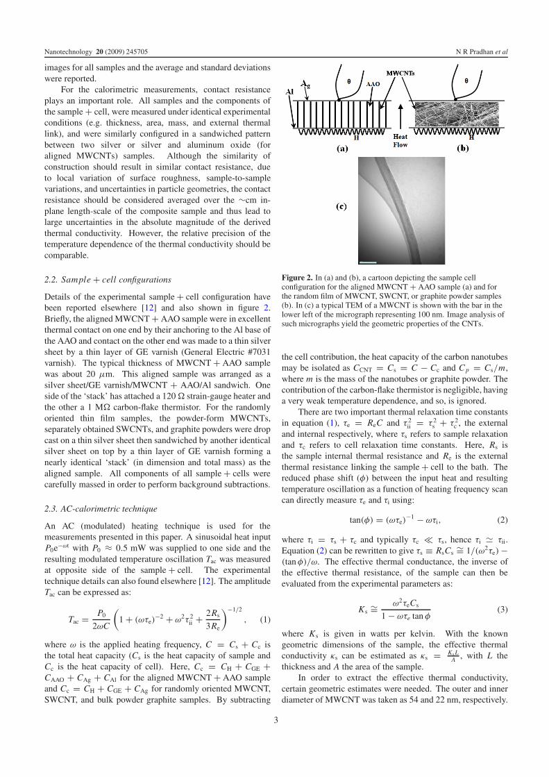
Nanotechnology 20 (2009) 245705 N R Pradhan et al
images for all samples and the average and standard deviationswere reported.
For the calorimetric measurements, contact resistanceplays an important role. All samples and the components ofthe sample + cell, were measured under identical experimentalconditions (e.g. thickness, area, mass, and external thermallink), and were similarly configured in a sandwiched patternbetween two silver or silver and aluminum oxide (foraligned MWCNTs) samples. Although the similarity ofconstruction should result in similar contact resistance, dueto local variation of surface roughness, sample-to-samplevariations, and uncertainties in particle geometries, the contactresistance should be considered averaged over the ∼cm in-plane length-scale of the composite sample and thus lead tolarge uncertainties in the absolute magnitude of the derivedthermal conductivity. However, the relative precision of thetemperature dependence of the thermal conductivity should becomparable.
2.2. Sample + cell configurations
Details of the experimental sample + cell configuration havebeen reported elsewhere [12] and also shown in figure 2.Briefly, the aligned MWCNT + AAO sample were in excellentthermal contact on one end by their anchoring to the Al base ofthe AAO and contact on the other end was made to a thin silversheet by a thin layer of GE varnish (General Electric #7031varnish). The typical thickness of MWCNT + AAO samplewas about 20 μm. This aligned sample was arranged as asilver sheet/GE varnish/MWCNT + AAO/Al sandwich. Oneside of the ‘stack’ has attached a 120 strain-gauge heater andthe other a 1 M carbon-flake thermistor. For the randomlyoriented thin film samples, the powder-form MWCNTs,separately obtained SWCNTs, and graphite powders were dropcast on a thin silver sheet then sandwiched by another identicalsilver sheet on top by a thin layer of GE varnish forming anearly identical ‘stack’ (in dimension and total mass) as thealigned sample. All components of all sample + cells werecarefully massed in order to perform background subtractions.
2.3. AC-calorimetric technique
An AC (modulated) heating technique is used for themeasurements presented in this paper. A sinusoidal heat inputP0e−ωt with P0 ≈ 0.5 mW was supplied to one side and theresulting modulated temperature oscillation Tac was measuredat opposite side of the sample + cell. The experimentaltechnique details can also found elsewhere [12]. The amplitudeTac can be expressed as:
Tac = P0
2ωC
(1 + (ωτe)
−2 + ω2τ 2ii + 2Rs
3Re
)−1/2
, (1)
where ω is the applied heating frequency, C = Cs + Cc isthe total heat capacity (Cs is the heat capacity of sample andCc is the heat capacity of cell). Here, Cc = CH + CGE +CAAO + CAg + CAl for the aligned MWCNT + AAO sampleand Cc = CH + CGE + CAg for randomly oriented MWCNT,SWCNT, and bulk powder graphite samples. By subtracting
Figure 2. In (a) and (b), a cartoon depicting the sample cellconfiguration for the aligned MWCNT + AAO sample (a) and forthe random film of MWCNT, SWCNT, or graphite powder samples(b). In (c) a typical TEM of a MWCNT is shown with the bar in thelower left of the micrograph representing 100 nm. Image analysis ofsuch micrographs yield the geometric properties of the CNTs.
the cell contribution, the heat capacity of the carbon nanotubesmay be isolated as CCNT = Cs = C − Cc and Cp = Cs/m,where m is the mass of the nanotubes or graphite powder. Thecontribution of the carbon-flake thermistor is negligible, havinga very weak temperature dependence, and so, is ignored.
There are two important thermal relaxation time constantsin equation (1), τe = ReC and τ 2
ii = τ 2s + τ 2
c , the externaland internal respectively, where τs refers to sample relaxationand τc refers to cell relaxation time constants. Here, Rs isthe sample internal thermal resistance and Re is the externalthermal resistance linking the sample + cell to the bath. Thereduced phase shift (φ) between the input heat and resultingtemperature oscillation as a function of heating frequency scancan directly measure τe and τi using:
tan(φ) = (ωτe)−1 − ωτi, (2)
where τi = τs + τc and typically τc τs, hence τi τii.Equation (2) can be rewritten to give τs ≡ RsCs
∼= 1/(ω2τe) −(tan φ)/ω. The effective thermal conductance, the inverse ofthe effective thermal resistance, of the sample can then beevaluated from the experimental parameters as:
Ks∼= ω2τeCs
1 − ωτe tan φ(3)
where Ks is given in watts per kelvin. With the knowngeometric dimensions of the sample, the effective thermalconductivity κs can be estimated as κs = KsL
A , with L thethickness and A the area of the sample.
In order to extract the effective thermal conductivity,certain geometric estimates were needed. The outer and innerdiameter of MWCNT was taken as 54 and 22 nm, respectively.
3

Nanotechnology 20 (2009) 245705 N R Pradhan et al
Figure 3. SEM micrographs of arrays of MWCNTs inside AAO template (a), released MWNTs from AAO template (b), SWCNTs (c), andgraphite powder (d). MWCNTs are 20 μm long with 60 nm outside and 25 nm outer diameter. The scale bar in (a)–(c) are 100 nm and in(d) is 1 μm.
See section 3.1 for details. By assuming the density ofnanotubes to be 1.3 g cm−3 and the interlayer separation ofgraphene sheets as 0.34 nm [29], the estimated mass is found tobe ∼30% higher than that determined by sample area and givesa conservative estimate of absolute uncertainty. To extractthe thermal conductivity, the whole area of the AAO pores isassumed to be filled by MWCNTs to determine the effectivethermal conductivity. By subtracting the inside hollow area ofeach nanotubes, the estimated value of thermal conductivity foranisotropic MWCNT could be two orders of magnitude larger.Thus, the absolute value of the conductivity is not well knownbut its temperature dependence should be well defined.
3. Results and discussion
3.1. Morphology study
Scanning electron microscope images were taken of thesamples studied and are shown in figure 3. For the alignedMWCNT embedded in the AAO channels, the cross-sectionSEM in figure 3(a) shows that each channel contains a well-confined MWCNT suggesting a very high filing fraction(essentially 1), with all the channels and MWCNTs parallel toeach other throughout the thickness of the MWCNT + AAOcomposite. As confirmed by previous studies [27, 26], theouter diameter of the MWCNTs were determined by the 60 nmpore size of the AAO template. The analyzed tunnelingelectron micrographs, an example shown in figure 2(c),indicate that the inner diameter of the synthesized MWCNT
was 22 ± 8 nm and the outer diameter 54 ± 5 nm. Asshown in figure 3(b), the liberated MWCNTs thin films arerandomly oriented, laying flat with one on top of the another.In figure 3(c), the randomly oriented SWCNT thin films appearto be highly entangled. Here, SWCNTs are approximately1.3 nm in diameter, 0.5–40 μm long, and 90% pure [28].The reference sample of graphite powder shown in figure 3(d)have a large particle size of ∼1 μm and a wide particle sizedistribution.
3.2. Specific heat of CNT composites
The anisotropic measurement of specific heat (c||p) and
randomly oriented specific heat (cMp ) for MWCNT, randomly
oriented specific heat (cSp) for SWCNT, and that of bulk
graphite powder (cBp ) are shown in figure 4. The specific heat
of all samples were determined as a function of temperaturefrom 300 to 400 K on heating. The bulk graphite powdersample yields a cB
p = 0.73 J g−1 K−1 at 300 K and a weak,nearly-linear, temperature dependence up to 360 K reaching0.80 J g−1 K−1. These values obtained from our experimentalarrangements are 2.1% higher and 5.5% lower, respectively,from literature values [30] and indicate in absolute valueuncertainty of about 5% (conservatively) and an uncertaintyin slope of about 7%.
For the aligned MWCNT composite sample c||p =
0.74 J g−1 K−1 while for the randomly oriented thin filmsample cM
p = 0.75 J g−1 K−1 at 300 K, very similar to bulkgraphite with similar temperature dependence. For randomly
4
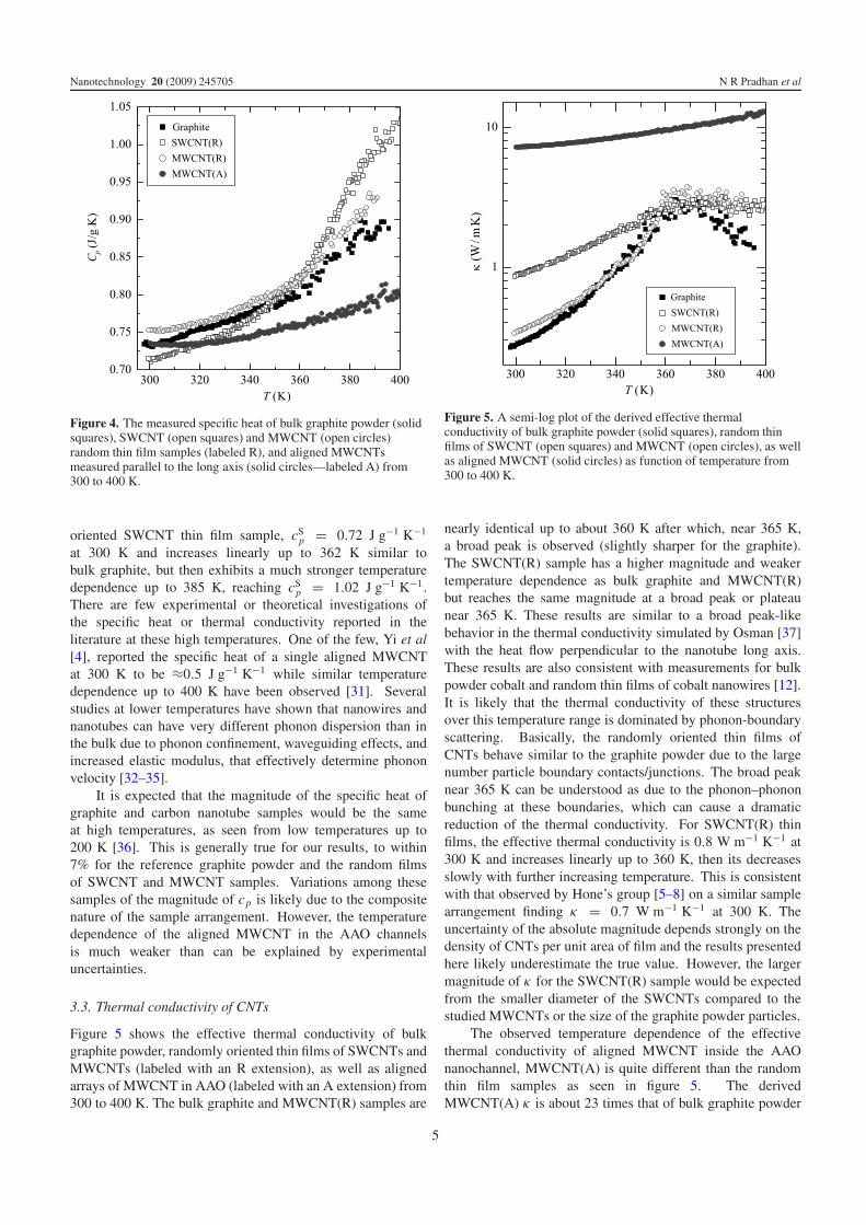
Nanotechnology 20 (2009) 245705 N R Pradhan et al
Figure 4. The measured specific heat of bulk graphite powder (solidsquares), SWCNT (open squares) and MWCNT (open circles)random thin film samples (labeled R), and aligned MWCNTsmeasured parallel to the long axis (solid circles—labeled A) from300 to 400 K.
oriented SWCNT thin film sample, cSp = 0.72 J g−1 K−1
at 300 K and increases linearly up to 362 K similar tobulk graphite, but then exhibits a much stronger temperaturedependence up to 385 K, reaching cS
p = 1.02 J g−1 K−1.There are few experimental or theoretical investigations ofthe specific heat or thermal conductivity reported in theliterature at these high temperatures. One of the few, Yi et al[4], reported the specific heat of a single aligned MWCNTat 300 K to be ≈0.5 J g−1 K−1 while similar temperaturedependence up to 400 K have been observed [31]. Severalstudies at lower temperatures have shown that nanowires andnanotubes can have very different phonon dispersion than inthe bulk due to phonon confinement, waveguiding effects, andincreased elastic modulus, that effectively determine phononvelocity [32–35].
It is expected that the magnitude of the specific heat ofgraphite and carbon nanotube samples would be the sameat high temperatures, as seen from low temperatures up to200 K [36]. This is generally true for our results, to within7% for the reference graphite powder and the random filmsof SWCNT and MWCNT samples. Variations among thesesamples of the magnitude of cp is likely due to the compositenature of the sample arrangement. However, the temperaturedependence of the aligned MWCNT in the AAO channelsis much weaker than can be explained by experimentaluncertainties.
3.3. Thermal conductivity of CNTs
Figure 5 shows the effective thermal conductivity of bulkgraphite powder, randomly oriented thin films of SWCNTs andMWCNTs (labeled with an R extension), as well as alignedarrays of MWCNT in AAO (labeled with an A extension) from300 to 400 K. The bulk graphite and MWCNT(R) samples are
Figure 5. A semi-log plot of the derived effective thermalconductivity of bulk graphite powder (solid squares), random thinfilms of SWCNT (open squares) and MWCNT (open circles), as wellas aligned MWCNT (solid circles) as function of temperature from300 to 400 K.
nearly identical up to about 360 K after which, near 365 K,a broad peak is observed (slightly sharper for the graphite).The SWCNT(R) sample has a higher magnitude and weakertemperature dependence as bulk graphite and MWCNT(R)but reaches the same magnitude at a broad peak or plateaunear 365 K. These results are similar to a broad peak-likebehavior in the thermal conductivity simulated by Osman [37]with the heat flow perpendicular to the nanotube long axis.These results are also consistent with measurements for bulkpowder cobalt and random thin films of cobalt nanowires [12].It is likely that the thermal conductivity of these structuresover this temperature range is dominated by phonon-boundaryscattering. Basically, the randomly oriented thin films ofCNTs behave similar to the graphite powder due to the largenumber particle boundary contacts/junctions. The broad peaknear 365 K can be understood as due to the phonon–phononbunching at these boundaries, which can cause a dramaticreduction of the thermal conductivity. For SWCNT(R) thinfilms, the effective thermal conductivity is 0.8 W m−1 K−1 at300 K and increases linearly up to 360 K, then its decreasesslowly with further increasing temperature. This is consistentwith that observed by Hone’s group [5–8] on a similar samplearrangement finding κ = 0.7 W m−1 K−1 at 300 K. Theuncertainty of the absolute magnitude depends strongly on thedensity of CNTs per unit area of film and the results presentedhere likely underestimate the true value. However, the largermagnitude of κ for the SWCNT(R) sample would be expectedfrom the smaller diameter of the SWCNTs compared to thestudied MWCNTs or the size of the graphite powder particles.
The observed temperature dependence of the effectivethermal conductivity of aligned MWCNT inside the AAOnanochannel, MWCNT(A) is quite different than the randomthin film samples as seen in figure 5. The derivedMWCNT(A) κ is about 23 times that of bulk graphite powder
5

Nanotechnology 20 (2009) 245705 N R Pradhan et al
Figure 6. A semi-log plot of the effective thermal conductivitynormalized to that determined for each sample at 300 K to reveal thefractional change as a function of temperature. Shown are the bulkgraphite powder (solid squares), random thin films of SWCNT (opensquares) and MWCNT (open circles), along with aligned MWCNT(solid circles) from 300 to 400 K.
or MWCNT(R) thin films and 8 times that of SWCNT(R)thin film at 300 K. Unlike the random thin film samples,κ of MWCNT(A) increases smoothly from 300 to 400 Kwithout any indications of a plateau or broad peak. Similarobservations of a smoothly increasing thermal conductivityhave been reported for CNTs aligned by a magnetic field [38]and supports the one-dimensional nature of the heat flow in oursample. From purely geometric considerations, the estimatedvalue of thermal conductivity for a single MWCNT along thelong axis at 300 K is approximately 700 W m−1 K−1. Whilethe uncertainty of the absolute magnitude of these measuredeffective κ are large, perhaps as large as an order of magnitude,it cannot explain the difference with that expected for a ‘scaled-up’ geometric estimate of κ along the long axis. Similarlyfor random thin film samples, an estimate assuming the wholesample area is filled completely by sample (a filling fractionof 1) yields a value at least two orders of magnitude orlarger than that derived here. Thus, the composite nature ofthese macroscopic samples must be intrinsically different thansimply scaling up the behavior of a single nanotube to thesedimensions.
To better compare the temperature dependence of theeffective thermal conductivity, normalized values (to thatobserved for each sample at 300 K, i.e. κ/κ300 K) of the bulkgraphite powder, the random thin films of SWCNT(R) andMWCNT(R), as well as aligned MWCNT(A) in AAO a shownin figure 6. This construction illustrates the fractional changeof the observed κ and indicate that the random thin filmsamples are all dominated by its granular nature while thealigned MWCNT sample, though higher in magnitude, has amuch small fractional change up to 400 K.
The effective thermal conductivity is greatly affected bythe interface contact resistance between surfaces and sample
as well as among the sample particles (nanotubes or graphitepowder) [39, 40]. The results presented in this work revealthat the heat transfer in aligned nanotubes is dominated bythe nanotube–nanotube interfacial resistance, nanotube length,diameter, and spacing. Paradoxically, the nanotube thermalresistance decreases with increasing nanotube length [39, 41].For aligned MWCNT + AAO, the heat flow is essentially one-dimensional across each single nanotube, but their couplingto the AAO matrix and the cell surfaces leads to increasedthermal resistance. However, in the case of a randomlyoriented thin film sample, the nanotube–nanotube resistancedecreases due to the proliferation of contacts among nanotubesimproving the heat exchange. In all samples, the interfacialresistance also depends upon the geometry of the contactingsurfaces through surface roughness [42]. Because anharmonicphonons can be created, destroyed or scattered from each otherleading to a finite mean-free-path and so, limiting the thermalconductivity [43].
The heat transfer across interfaces can be represented bya single parameter known as the thermal interfacial resistanceR [39] and is given by
R = AT/Q = t/(κ A); (4)
where A is the area of the interface contact, T is the steady-state temperature jump between two surfaces of contact, Q isthe rate of heat flow across the interface, t is the thickness ofsample, and κ is the thermal conductivity. Equation (4) appliesto one-dimensional heat flow through the area A across thethickness t .
Since the heat flow in these measurements across therandomly oriented and aligned samples are same, the thermalcontact resistance between nanotubes or powders (in randomlyoriented sample), nanotubes–matrix (in aligned sample), aswell as between contact areas plays an important role andinduces temperature gradients. Recently reported calculationsdescribe the effect of thermal contact resistance on a randomfilm sample of carbon nanotubes and obtained a very lowthermal conductivity as compared that along the long axis ofa single nanotube [44]. The energy transfer between carbonnanotubes in van der Waals contact is limited by a large contactresistance [39] arising from weak inter-particle bonding. Thecontact resistance for larger diameter CNT is smaller than thesmaller diameter CNT due to larger contact area, whereas thenumber of contacts per unit volume will be larger for smallernanotubes due to large aspect ratio.
4. Conclusions
In this work, experimental results of the specific heat andeffective thermal conductivity of a macroscopic compositecontaining randomly oriented single-wall and multi-wallcarbon nanotubes, graphite powder, and aligned multi-wallcarbon nanotube embedded in a porous aluminum matrix arereported from 300 to 400 K. The specific heat are generallyconsistent among all carbon samples with the graphite powderand random thin film of MWCNT being most similar. Therandom thin film of SWCNT has a stronger while the alignedMWCNT in AAO has a weaker temperature dependence
6

Nanotechnology 20 (2009) 245705 N R Pradhan et al
than the bulk behavior measured here. Though small, thesedifferences are due to the intrinsic properties of SWCNT forthe former and the macroscopic arrangement in the compositefor the latter sample. The effective thermal conductivityreveals the most striking effect of composite construction.In all the random thin film samples of SWCNT, MWCNT,and graphite powder, a broad peak-like feature is seen in κ
near 365 K, similar to that seen in a similar cobalt-basedcomposites [12]. The absolute value of effective thermalconductivity measured here of the single-wall and multi-wallCNTs are expected to be different because of their differencesin length, diameter, and overall purity. Given that all threerandom thin film sample + cell configuration of SWCNT(R),MWCNT(R), and graphite powder are nearly identical, thephonon-boundary scattering mechanism is the most likely andthe difference in absolute value is likely due to uncertainties inmass approximation and sample purity.
These results on how the thermal properties of carbonnanotube composites vary with construction can be combinedwith the recent work of Hone’s group [7, 8] on the thermalconductivity for an unaligned SWCNT sample in presenceof a magnetic field finding ≈25 W m−1 K−1 at 300 Kand increases with increasing temperature until saturating at≈35 W m−1 K−1 near 400 K. Thus, detailed engineeringof thermal properties is a strong possibility. Future workon more complex composite arrangements would furtherdetail the possible variations and should hopefully inspirecomplimentary theoretical or computational work to betterunderstand such systems.
Acknowledgment
G Iannacchione would like to thank the Department of Physicsat Worcester Polytechnic Institute for their support.
References
[1] Sumio I 1991 Nature 354 8[2] Olk C H and Heremans J P 1994 J. Mater. Res. 9 259[3] Dekker C 1999 Phys. Today 52 22[4] Yi W, Lu L, Dian-Lin Z, Pan Z W and Xie S S 1999 Phys. Rev.
B 59 R9015[5] Hone J, Whitney M, Piskoti C and Zettl A 1999 Phys. Rev. B
59 R2514[6] Hone J, Whitney M and Zettl A 1999 Synth. Met. 103 2498[7] Hone J, Batlogg B, Benes Z, Johnson A T and Fischer J E 2000
Science 289 1730[8] Hone J, Llaguno M C, Nemes N M, Johnson A T, Fisher J E,
Walters D A, Casavant M J, Schmidt J and Smalley R E2000 Appl. Phys. Lett. 77 666
[9] Hone J, Llaguno M C, Biercuk M J, Johnson A T, Batlogg B,Benes Z and Fisher J E 2002 Appl. Phys. A 74 339
[10] Yang D J, Zhang Q, Chen G, Yoon S F, Ahn J, Wang S G,Zhou Q, Wang Q and Li J Q 2002 Phys. Rev. B 66 165440
[11] Basu R and Iannacchione G S 2008 Appl. Phys. Lett.93 183105
[12] Pradhan N R, Huanan D, Liang J and Iannacchione G S 2008Nanotechnology 19 485712
[13] Tong T, Majumdar A, Zhao Y, Akashi A, Delzeit L andMeyapan M 2006 IEEE pp 1406–11
[14] Zhang K, Chai Y, Yuan M M F, Xio D G W and Chan P C H2008 Nanotechnology 19 215706
[15] Xu Y, Leong C and Chung D D L 2007 J. Electron. Mater.36 1181
[16] Park J-J and Taya M 2006 J. Electron. Packag. 128 46[17] Amama P B, Cola B A, Sands T D, Xu X and Fisher T S 2007
Nanotechnology 18 385303[18] Xu J and Fisher T S 2006 Int. J. Heat Mass Transfer 49 1658[19] Berber S, Kwon Y K and Tomanek D 2000 Phys. Rev. Lett.
84 4613–6[20] Kim P, Shi L, Majumdar A and McEuen P L 2001 Phys. Rev.
Lett. 87 215502[21] Shi L, Li D, Yu C, Jang W, Kim D, Yao Z, Kim P and
Majumdar A 2003 J. Heat Transfer 125 881[22] Zhang H-L, Li J-F, Zhang B-P, Yao K-F, Liu W-S and
Wang H 2007 Phys. Rev. B 75 205407[23] Xie S, Li W, Pan Z, Chang B and Sun L 2000 J. Phys. Chem.
Solids 61 1153[24] Lu L, Yi W and Zhang D L 2001 Rev. Sci. Instrum. 72 2996[25] Prasher R 2008 Phys. Rev. B 77 075424[26] Li J, Papadopoulos C, Xu J M and Moskovits M 1999 Appl.
Phys. Lett. 75 367[27] Liang J, Chik H, Yin A and Xu J M 2002 J. Appl. Phys.
91 2544[28] 2009 http://www.helixmaterial.com[29] Lavin J G, Subramoney S, Rouff R S, Berber S and
Tomanek D 2002 Carbon 40 1123[30] Nihira T and Iwata T 2003 Phys. Rev. B 68 134305[31] Xie H 2007 J. Mater. Sci. 42 3695[32] Dresselhaus M S, Lin Y-M, Cronin S B, Rabin O, Black M R,
Dresselhaus G and Koga T 2001 Semicond. Semimet. 71 1[33] Gu M X, Yeung T C, Tan C M and Nosik V 2006 J. Appl. Phys.
100 094304[34] Rego L G C and Kirczenow G 1998 Phys. Rev. Lett. 81 232[35] Mahan G 2002 Phys. Rev. B 65 235402[36] Mizel A, Benedict L X, Cohen M L, Louie S G, Zettl A,
Budraa N K and Beyermann W P 1999 Phys. Rev. B60 3264
[37] Osman M A and Srivastava D 2001 Nanotechnology 12 21[38] Fischer J E, Zhou W, Vavro J, Liaguno M C, Guthey C,
Haggenmuller R, Cassavant M J, Walters D E andSmalley R E 2003 J. Appl. Phys. 93 2157
[39] Zhong H and Lukes J R 2006 Phys. Rev. B 74 125403[40] Shenogin S, Xue L, Oziski R, Keblinski P and Cahill D G 2004
J. Appl. Phys. 95 8136–44[41] Huxtable S T et al 2003 Nat. Mater. 2 731[42] Pollack G L 1969 Rev. Mod. Phys. 41 48[43] Meng F Y, Ogata S, Xu D S, Shibutani Y and Shi S Q 2007
Phys. Rev. B 75 205403[44] Prasher R S, Hu X J, Chalopin Y, Mingo N, Lofgreen K,
Volz S, Cleri F and Keblinski P 2009 Phys. Rev. Lett.102 105902
7
IOP PUBLISHING JOURNAL OF PHYSICS D: APPLIED PHYSICS
J. Phys. D: Appl. Phys. 43 (2010) 105401 (7pp) doi:10.1088/0022-3727/43/10/105401
Relaxation dynamics of glass transition inPMMA + SWCNT composites bytemperature-modulated DSCN R Pradhan and G S Iannacchione
Department of Physics, Worcester Polytechnic Institute, Worcester, MA 01609, USA
Received 30 October 2009, in final form 25 December 2009Published 25 February 2010Online at stacks.iop.org/JPhysD/43/105401
AbstractThe experimental technique offered by temperature-modulated differential scanningcalorimeter (TMDSC) used to investigate the thermal relaxation dynamics through the glasstransition as a function of frequency was studied for pure PMMA and PMMA-single wallcarbon nanotubes (SWCNTs) composites. A strong dependence of the temperaturedependence peak in the imaginary part of complex heat capacity (Tmax) is found during thetransition from the glass-like to the liquid-like region. The frequency dependence of Tmax ofthe imaginary part of heat capacity (Cp) is described by Arrhenius law. The activation energyobtained from the fitting shows increases while the characteristic relaxation time decreaseswith increasing mass fraction (φm) of SWCNTs. The dynamics of the composites during glasstransition, at slow and high scan rates, are also the main focus of this experimental study. Thechange in enthalpy during heating and cooling is also reported as a function of scan rate andfrequency of temperature modulation. The glass transition temperature (Tg) shows increaseswith increasing frequency of temperature modulation and φm of SWCNTs inside the polymerhost. Experimental results show that Tg is higher at higher scan rates but as the frequency oftemperature modulation increases, the Tg values of different scan rates coincide with eachother and alter the scan rate dependence. From the imaginary part of heat capacity, it isobvious that Tmax is not the actual glass transition temperature of pure polymer but Tmax and Tg
values can be superimposed when φm increases in the polymer host or when the sampleundergoes a transition with a certain frequency of temperature modulation.
1. Introduction
Recently, the modulated differential scanning calorimetry(MDSC) [1–3] study has been widely used to investigatethe dynamics of glass transitions of polymer compositesand related materials. In MDSC analysis, the sample isdecomposed into reversing and non-reversing signals, iswidely used and appears to avoid the uncertain meaningof dynamic thermal analyses in analogy to, e.g., dynamicmechanical or dielectric spectroscopies. In recent studies ithas been commonly accepted to present the dynamic thermalproperties in terms of the complex, real (storage) and imaginary(loss) heat capacities (C∗
p, C ′p and C ′′
p). The concept offrequency-dependent specific heat C∗
p(ω, T ) (=C∗p(ω)) was
introduced and the first measurement was performed in the1980s [4–7] with an alternating current calorimeter technique.After that it has been widely used to study the dynamics of
glass transition of different polymer systems. From a statisticalpoint of view, C∗
p(ω) appears as a consequence of entropyfluctuations [8]. One advantage of dynamic heat capacity incomparison with other techniques is the fact that C∗
p(ω) reflectsthe contribution of all modes, orientational and translational,providing global and direct information of the slow dynamicsassociated with the glass transition. Thus MDSC is a widelyused technique to study the phase transition, glass transitionand specific heat measurement of widely available polymericsystems. But the concept of frequency-dependent specific heatis not widely used. It is specially the case in the applicationfields of polymers, food sciences, pharmaceuticals, etc. whereit could be of great interest to characterize the molecularmobility.
Carbon nanotubes (CNTs) have outstanding electrical,mechanical, optical and thermal properties. These propertieshave significant potential in a vast range of applications such
0022-3727/10/105401+07$30.00 1 © 2010 IOP Publishing Ltd Printed in the UK

J. Phys. D: Appl. Phys. 43 (2010) 105401 N R Pradhan and G S Iannacchione
as quantum wires [9], tips for scanning probe microscope [10]and molecular diodes [11]. Polymers play a very important rolein numerous fields of everyday life due to their advantages inlightness, ease of processing, resistance to corrosion and lowcost of production. To improve the performance of polymers,composites of polymers and a filler have been extensively usedand studied. The use of various nanofillers such as metals,semiconductors, organic and inorganic particles and fibres,especially carbon structures [12–15], is of particular interestand a subject of intense investigation. The unique properties ofCNTs such as extremely high strength, lightweight, elasticity,high thermal and air stability, high electric and thermalconductivity and high aspect ratio, offer crucial advantagesover other nanofillers.
The potential of using nanotubes as a filler in polymercomposites has not been fully realized because of processingdifficulties. Structural relaxation is the process by whichamorphous materials in the glassy state approach a stateof thermodynamic equilibrium. Calorimetry, such as DSC,has revealed enthalpic relaxations occurring near the glasstransition Tg in glassy polymers aged after a variety of heatingtreatments. It is well known that annealing or variationof heating and cooling rates leads to significant hysteresisin Tg because of these structural relaxations [16, 17]. Theintroduction of nanofillers is expected to interact stronglywith these short-range structural relaxations. However,the effective utilization of CNTs in polymer compositeapplications strongly depends on the quality/uniformity of thenanotubes and the ability to disperse them homogeneouslythroughout the polymer host [18, 19]. Our previous workwas to produce and investigate SWCNT-based nano-compositepolymer materials as candidates for the next generation ofhigh-strength, lightweight and enhanced thermal conductingmaterials [17]. Structural relaxation has been characterizedfor many polymers by the dielectric spectroscopy method,but this method is versatile, and widely used to study thedynamics of a sample at high frequencies, where it is foundthat the calorimetric results are the extension of dielectricresults. The calorimetric Tg includes total degree of freedomsuch as rotation, diffusion and vibration, while the dielectricTg originates only from the reorientation of molecules.
The main objective of this paper is to study the relaxationdynamics of the glass transition of PMMA + SWCNTscomposites at very low frequencies using MDSC and to presentthe details of frequency-dependent MDSC techniques. Manystudies have been done to describe the relaxation behaviourand glass transition for pure polymers in the frequencydomain but so far no results have been reported on CNTpolymer composites. The PMMA +SWCNT composites wereprepared by dispersing SWCNTs and PMMA in a chloroformsolution using sonication, and then slowly evaporating thesolvent leaving a homogeneous dispersion. The complexheat capacity was measured as a function of temperature anddifferent frequencies of temperature modulation from 0.0138to 0.0826 s−1. Then the real and imaginary parts of heatcapacity was estimated with the phase between input heatflow and heating rate. In all the samples, we observed thepeak maximum in the imaginary part of heat capacity. The
effective glass transition temperature, Tg, activation energyand dynamics observed in the real and imaginary parts aredependent on the applied modulated frequency of temperatureoscillation. The measurement was reported in the region ofglass transition of polymers and composites and other regionsare not of interest in this study as the dynamics do not changewith frequency.
Following this introduction, section 2 describes someof the basics of the experimental procedures for the MDSCand sample preparation. Section 3 presents the experimentalresults and discussion followed by a general conclusion withfuture directions presented in section 4.
2. Experimental
2.1. Modulated differential scanning calorimetry
Modulated (temperature) differential scanning calorimetry(MTDSC/MDSC) allows for the simultaneous measurementof the evolution of both heat flow and heat capacity. MDSCdiffers from conventional DSC where the sample is subjectedto a more complex heating program incorporating a sinusoidaltemperature modulation accompanied by an underlying linearheating ramp. Whereas DSC is only capable of measuringthe total heat flow, MDSC can simultaneously determine thenon-reversible (kinetic component) and the reversible (heatcapacity component) heat flows. A detailed description of theMDSC method can be found elsewhere [3, 20–25].
MDSC experiments were performed using a Model Q200from TA Instruments, USA. Prior to the experiment with oursample, temperature calibration was done with a sapphiredisc, under the same conditions of measurements we used forour studied sample. Q200 is an extension of the heat fluxtype of a conventional DSC. The method to obtain complexspecific heat has been proposed by Schawe based on the linearresponse theory [3, 21]. In general a temperature oscillation isdescribed as
T = T0 + q0t + AT sin(ωt), (1)
where T0 is the initial temperature at time t = 0, T is thetemperature at time t , q0 is the underlying scan rate, AT isthe temperature amplitude and ω (ω = 2πf ) is the angularfrequency of the temperature modulation. f = 1/τ is thefrequency in s−1 where τ was taken as the period of modulation.The results are plotted in the scale of frequency f instead of ω.The heating rate is given by
q = dT
dt= q0 + Aq cos(ωt), (2)
where Aq is the amplitude of heating rate (Aq = AT ω). Sincethe applied heating rate in MDSC consists of two components,q0 the underlying heating rate and Aq cos(ωt) the periodicheating rate, the measured heat flow can also be separated intotwo components, i.e. the response to the underlying heatingrate and response to the periodic heating rate. The latter canbe described by
HFperiod = AHF cos(ωt − φ), (3)
2

J. Phys. D: Appl. Phys. 43 (2010) 105401 N R Pradhan and G S Iannacchione
where HFperiod is the heat flow response to the periodic heatingrate, AHF is the amplitude of heat flow and φ is the phaseangle between heat flow and heating rate. An absolute valueof complex specific heat can be obtained by
∣∣C∗p
∣∣ = AHF
mAq
, (4)
where m is the mass of a sample.The data were analysed correcting the phase shift between
heating rate and heat flow rate signal. The imaginary part ofthe complex heat capacity was calculated by correcting thephase angle. The detailed correction procedure can be foundelsewhere [26]. By proper calibration for a raw phase angle,we can obtain real C ′
p and imaginary C ′′p parts by
C ′p = ∣∣C∗
p
∣∣ cos(φ), (5)
C ′′p = ∣∣C∗
p
∣∣ sin(φ). (6)
The measured phase angle was corrected using the reportedmethod [26]; then the real and imaginary parts of the complexheat capacity were estimated.
2.2. Preparation of PMMA + SWCNT composites
The required amounts of polymer PMMA (Mn =120 000 g mol−1, obtained from Aldrich) and SWCNTs(obtained from Helix Materials Solution, Texas, purity >
90%, ash 5%) were first dissolved in chloroform, in separatecontainers. Then the chloroform solution containing SWCNTwas sonicated for 8 h to separate the bundles of nanotubesinto individual particles. Then both PMMA dissolved inchloroform and SWCNT dispersed in chloroform were mixedtogether and again kept for 6 h in an ultrasonic bath. Scanningelectron micrographs of the SWCNTs used in this work weregiven in a previous paper [27]. After that the PMMA+SWCNTsolution was finally mixed in a touch mixer (Fisher Touch-Mixer model 12-810) for 10 min. Optical micrograph studieshave been done to clarify the good dispersion of SWCNTsinside host PMMA. The mass fraction was calculated using thefollowing formula from the mass of the CNTs and PMMA. Thevolume fraction was derived by taking the density of PMMAas 1.2 g cm−3 and assuming the density of CNTs as 1.4 g cm−3:
φm = Mf
Mf + Mp= Mf
MT
, (7)
φv = ρpMf
ρfMp + ρpMf, (8)
where φm is the mass fraction, Mf is the mass of the filler(SWCNTs), Mp is the mass of the polymer (PMMA), φv is thevolume fraction of SWCNTs, ρp is the density of PMMA andρf is the density of filler (SWCNTs).
Due to strong van der Waal attraction, CNTs bundletogether in high mass fraction, which reduces the dispersionquality of nanotubes inside a polymer matrix. In our case,after casting the required amount of sample on a silver sheet,the remaining solution of PMMA + SWCNT + choloform wasstored in a tightly capped bottle and no significant segregation
occurred over several days indicating the quality of dispersions.For the MDSC measurements, the samples were sealed insidea standard hermetically sealed pan.
Before sealing in the hermite pan, each sample washeated for 15 min at 127 C in vacuum to remove the trappedchloroform. The MDSC experiment was carried out withheating and cooling rates of 2.0, 0.4 and 0.1 K min−1 and dryultra pure nitrogen gas with a flow rate of 50 ml min−1 waspurged through the DSC cell. For accurate measurement ofspecific heat or to decrease the uncertainty, the reference andthe sample hermite pans were chosen carefully. The mass of thepan used was (0.0504 ± 0.0004) g; here 0.0004 is the standarddeviation of the pan for three different sample pans (threedifferent mass fractions of PMMA + SWCNT) and a referencepan used for this study. The mass of the three samples takenin all the measurements is ∼10 ± 0.2 mg. The temperaturemodulation amplitude was chosen to be 1.2 K. We have studiedthree distinct samples, pure PMMA, and 0.014 and 0.080 massfractions of SWCNTs dispersed in PMMA composites. Eachsample was scanned with the above-mentioned three differentscan rates and with modulation frequencies ranging from 1/160to 1/30 s−1.
3. Results and discussion
Figure 1 shows the real (up) and imaginary (bottom) partsof the complex specific heat capacity of 0.014 mass fractionSWCNTs inside PMMA matrix under heating (left panel) andcooling (right panel) rates of 0.4 K min−1 with frequency oftemperature modulation from 1/30 to 1/150 s−1. The realpart of specific heat (C ′
p) was normalized to zero far abovethe glass transition at 405 K and the imaginary part was alsonormalized by subtracting a base line. It is observed thatthe maximum rate of change of C ′
p occurs in the regionof glass transition and it depends on the applied frequencyof temperature modulation. Similar change in C ′
p wasobserved during heating and cooling of the real part of heatcapacity. The change in magnitude of the imaginary partof heat capacity, C ′′
p, shows a difference during heatingand cooling with frequency of temperature modulation. Thisexplains the difference in structural relaxation and mobilityof the sample during heating and cooling. There is nodifference in the real part of specific heat observed in theSWCNTs + PMMA composite samples during heating andcooling. The magnitude of C ′
p between the liquid andthe glass regions, i.e. C(L–G)
p = C ′p(405) − C ′
p(340) isshown in figure 2. This shows that C(L–G)
p increases withdecreasing frequency of temperature modulation. Figure 2shows C(L–G)
p for pure PMMA (upper), 0.014 (middle)and 0.080 (bottom) mass fractions of SWCNT in PPMAcomposites with frequency of temperature modulation. ForPMMA, C(L–G)
p increases with decreasing scan rate in theentire frequency range studied except at a higher frequencyof 0.035 s−1, where they seem to be equal. This changein C(L–G)
p with respect to scan rate disappears as the massfraction of SWCNT increases inside the host polymer. The0.080 mass fraction of SWCNT does not show any differencein C(L–G)
p with respect to scan rate in the entire frequency
3

J. Phys. D: Appl. Phys. 43 (2010) 105401 N R Pradhan and G S Iannacchione
Figure 1. The normalized real part of heat capacity C ′p(f ) (top panel) and imaginary heat capacity C ′′
p(f ) (bottom panel) of aPMMA + SWCNT composite (φm = 0.014 sample) from 340 to 405 K, for different applied heating frequencies from 1/30 to 1/150 s−1
(see legend). In the top panel, the difference between liquid and glass heat capacities CL–Gp is defined.
(This figure is in colour only in the electronic version)
range studied. The imaginary part of complex specific heatcapacity, during heating, C ′′
p(f ) (figure 1, bottom panel), ischaracterized by an asymmetric peak with a smaller slope at thelow temperature side than at the high temperature side, whichcan be characterized by the molecular distribution of intrinsicstructural relaxation and related to the dynamic glass transition.The slope increases with decreasing frequency of temperaturemodulation at low temperatures without changing the hightemperature slope during heating. The temperature wherethe imaginary specific heat shows the maximum value (Tmax)shifted towards a lower temperature with decreasing frequencyindicating the slowing down of the dynamics of the systems.The cooling C ′′
p shows a similar peak maximum shifted toa lower temperature from 1/30 to 1/70 s−1 and less change inmagnitude than the heating results. After 1/70 s−1, there is nosignificant change in peak maximum observed during coolingas compared with heating. The C ′′
p peak during cooling isvery symmetric without any change in slope in the high andlow temperature sides.
In our previous work [17], we studied the glass transitiontemperature, which showed that Tg increases with scanrate. Figure 3 shows the glass transition temperature forPMMA, 0.014 and 0.080 mass fractions of SWCNT + PMMAcomposites with frequency of temperature modulation. Inall these three samples, highly dependent Tg increases with
Figure 2. Semi-logarithmic plot of CL–Gp as a function of
temperature modulation frequency f for scan rates 2.0, 0.4 and0.1 K min−1, for PMMA (top), 0.014 (middle) and 0.080 (bottom)mass fractions of SWCNTs.
4

J. Phys. D: Appl. Phys. 43 (2010) 105401 N R Pradhan and G S Iannacchione
Figure 3. Semi-log plot of glass transition temperature (Tg) as afunction of temperature modulation frequency for pure PMMA(top), 0.014 (middle) and 0.080 (bottom) mass fractions ofSWCNTs at scan rates 2.0, 0.4 and 0.1 K min−1. Lines are guide tothe eye and arrows indicate the zero-frequency extrapolated Tg.
increasing frequency of temperature modulation and scan rate.But this shows that in all PMMA and SWCNT + PMMAcomposites, Tg of different scan rates approach the same valueas the frequency of temperature modulation increases, andafter a certain frequency of modulation, the Tg value of lowscan rate (0.1 K min−1) becomes greater than for the highscan rate (2 K min−1) (figure 3, bottom). This cross over ofTg between different scan rates with frequency of modulationshifts to a lower frequency as φm increases. This shows that thedynamics of the glass transition are highly dependent on thefrequency and the nanotube dispersion can significantly alterthese dynamics with modulated frequency.
Figure 4 shows the maximum peak temperature of theimaginary parts of complex specific heat (Tmax) and glasstransition temperature Tg, with frequency of temperaturemodulation, for PMMA, 0.014 and 0.080 mass fractions ofSWCNTs in host PMMA at 0.4 K min−1 scan rate. Tmax is thetemperature of peak value of the imaginary part of specific heatwhile heating and Tg obtained using DSC software from theheating run of reversible heat capacity during step like featureof transition. Tmax is the temperature where maximum lossappears. The glass transition where the polymer undergoeschange from the liquid-like phase to the glassy region andboth Tmax and Tg may not be the same. For pure PMMA and0.014 mass fraction of SWCNT + PMMA composites, Tmax ishigher than Tg, in the low frequency region and both Tmax andTg values approach each other as the frequency increases and ata particular frequency (0.029 s−1 for PMMA) they cross eachother and Tg becomes higher than Tmax. As the mass fractionof SWCNTs increases, for 0.080 mass fraction, Tmax and Tg
values overlap up to 0.17 s−1 and then cross each other to givea Tg value higher than the Tmax value. This indicates that the
Figure 4. Semi-log plot shows comparison of maximumtemperature in the imaginary part of complex heat capacity (Tmax)and glass transition temperature (Tg) with frequency of temperaturemodulation of PMMA (top), 0.014 (middle) and 0.080 (bottom)mass fractions of SWCNTs in PMMA.
Figure 5. Arrhenius plot of logarithm of time period of temperatureoscillation with inverse of the peak C ′′
p temperature obtained at rates2.0 and 0.4 K min−1 for PMMA, 0.014 and 0.080 mass fractions ofPMMA + SWCNTs composites.
cross over point between Tg and Tmax shifted towards the lowerfrequency as φm increases.
The frequency dependence of glass transition can also beinterpreted by Arrhenius law. Figure 5 shows the relaxationtime (τ in s−1: τ is the modulation time period) in logscale, versus inverse peak temperature of the imaginary partof complex heat capacity (1000/Tmax). Figure 5 shows two
5
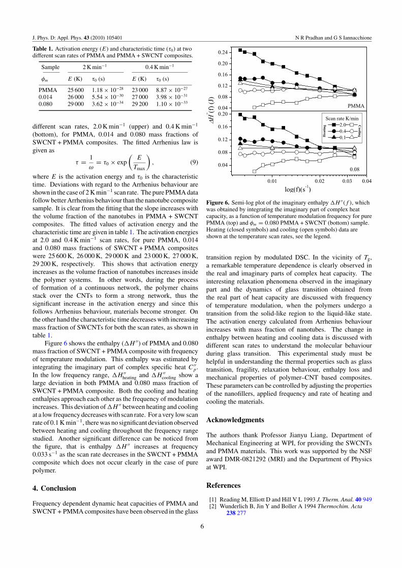
J. Phys. D: Appl. Phys. 43 (2010) 105401 N R Pradhan and G S Iannacchione
Table 1. Activation energy (E) and characteristic time (τ0) at twodifferent scan rates of PMMA and PMMA + SWCNT composites.
Sample 2 K min−1 0.4 K min−1
φm E (K) τ0 (s) E (K) τ0 (s)
PMMA 25 600 1.18 × 10⁻²⁸ 23 000 8.87 × 10⁻²⁷
0.014 26 000 5.54 × 10⁻³⁰ 27 000 3.98 × 10⁻³¹
0.080 29 000 3.62 × 10⁻³⁴ 29 200 1.10 × 10⁻³³
different scan rates, 2.0 K min−1 (upper) and 0.4 K min−1
(bottom), for PMMA, 0.014 and 0.080 mass fractions ofSWCNT + PMMA composites. The fitted Arrhenius law isgiven as
τ = 1
ω= τ0 × exp
(E
Tmax
), (9)
where E is the activation energy and τ0 is the characteristictime. Deviations with regard to the Arrhenius behaviour areshown in the case of 2 K min−1 scan rate. The pure PMMA datafollow better Arrhenius behaviour than the nanotube compositesample. It is clear from the fitting that the slope increases withthe volume fraction of the nanotubes in PMMA + SWCNTcomposites. The fitted values of activation energy and thecharacteristic time are given in table 1. The activation energiesat 2.0 and 0.4 K min−1 scan rates, for pure PMMA, 0.014and 0.080 mass fractions of SWCNT + PMMA compositeswere 25 600 K, 26 000 K, 29 000 K and 23 000 K, 27 000 K,29 200 K, respectively. This shows that activation energyincreases as the volume fraction of nanotubes increases insidethe polymer systems. In other words, during the processof formation of a continuous network, the polymer chainsstack over the CNTs to form a strong network, thus thesignificant increase in the activation energy and since thisfollows Arrhenius behaviour, materials become stronger. Onthe other hand the characteristic time decreases with increasingmass fraction of SWCNTs for both the scan rates, as shown intable 1.
Figure 6 shows the enthalpy (H ′′) of PMMA and 0.080mass fraction of SWCNT + PMMA composite with frequencyof temperature modulation. This enthalpy was estimated byintegrating the imaginary part of complex specific heat C ′′
p.In the low frequency range, H ′′
heating and H ′′cooling show a
large deviation in both PMMA and 0.080 mass fraction ofSWCNT + PMMA composite. Both the cooling and heatingenthalpies approach each other as the frequency of modulationincreases. This deviation of H ′′ between heating and coolingat a low frequency decreases with scan rate. For a very low scanrate of 0.1 K min−1, there was no significant deviation observedbetween heating and cooling throughout the frequency rangestudied. Another significant difference can be noticed fromthe figure, that is enthalpy H ′′ increases at frequency0.033 s−1 as the scan rate decreases in the SWCNT + PMMAcomposite which does not occur clearly in the case of purepolymer.
4. Conclusion
Frequency dependent dynamic heat capacities of PMMA andSWCNT + PMMA composites have been observed in the glass
Figure 6. Semi-log plot of the imaginary enthalpy H ′′(f ), whichwas obtained by integrating the imaginary part of complex heatcapacity, as a function of temperature modulation frequency for purePMMA (top) and φm = 0.080 PMMA + SWCNT (bottom) sample.Heating (closed symbols) and cooling (open symbols) data areshown at the temperature scan rates, see the legend.
transition region by modulated DSC. In the vicinity of Tg,a remarkable temperature dependence is clearly observed inthe real and imaginary parts of complex heat capacity. Theinteresting relaxation phenomena observed in the imaginarypart and the dynamics of glass transition obtained fromthe real part of heat capacity are discussed with frequencyof temperature modulation, when the polymers undergo atransition from the solid-like region to the liquid-like state.The activation energy calculated from Arrhenius behaviourincreases with mass fraction of nanotubes. The change inenthalpy between heating and cooling data is discussed withdifferent scan rates to understand the molecular behaviourduring glass transition. This experimental study must behelpful in understanding the thermal properties such as glasstransition, fragility, relaxation behaviour, enthalpy loss andmechanical properties of polymer–CNT based composites.These parameters can be controlled by adjusting the propertiesof the nanofillers, applied frequency and rate of heating andcooling the materials.
Acknowledgments
The authors thank Professor Jianyu Liang, Department ofMechanical Engineering at WPI, for providing the SWCNTsand PMMA materials. This work was supported by the NSFaward DMR-0821292 (MRI) and the Department of Physicsat WPI.
References
[1] Reading M, Elliott D and Hill V L 1993 J. Therm. Anal. 40 949[2] Wunderlich B, Jin Y and Boller A 1994 Thermochim. Acta
238 277
6
J. Phys. D: Appl. Phys. 43 (2010) 105401 N R Pradhan and G S Iannacchione
[3] Schawe J E K 1996 Thermochim. Acta 271 127[4] Birge N O and Nagel S R 1985 Phys. Rev. Lett. 54 2674[5] Birge N O 1986 Phys. Rev. B 34 1631[6] Dixon P K 1990 Phys. Rev. B 42 8179[7] Christensen T 1985 J. Phys. (Paris) Colloq. 46 C8 635–7[8] Birge N O, Dixon P and Menon N 1997 Thermochim. Acta
304/305 51–66[9] Tans S J, Devoret M F, Theses H D A and Smalley R E 1997
Nature 386 474[10] Dai H, Hafner J H, Rinzler A G, Colbert D T and Smalley R E
1996 Nature 384 147[11] Sander S J, Tans J, Verschueren A R M and Dekker C 1998
Nature 393 49[12] Glushanin S, Topolov V Y and Krivoruchko A V 2006
Mater. Chem. Phys. 97 357[13] Hine P, Broome V and Ward I 2005 Polymer 46 10936[14] Cioffi N, Torsi L, Ditaranto N, Tantillo G, Ghibelli L,
Sabbatini L, Bleve-Zacheo T, Alessio M D, Zambonin P Gand Traversa E 2005 Chem. Mater. 17 5255
[15] Pelaiz-Barranco A, Marin-Franch P 2005 J. Appl. Phys.97 034104
[16] Wunderlich B 1990 Thermal Analysis vol 135 (New York:Academic) p 205
[17] Pradhan N R and Iannacchione G S 2009 J. Appl. Phys.submitted
[18] Meyyappan M 2005 Carbon Nanotubes Science andApplications (Boca Raton, FL: CRC Press)
[19] Harris P J F 2001 Carbon Nanotubes and Related StructuresNew Materials for the Twenty-first Century (Cambridge:Cambridge University Press)
[20] Coleman N J and Craig D Q M 1996 Int. J. Pharmaceut.135 13
[21] Schawe J E K 1995 Thermochim. Acta 261 183[22] Hutchinson J M and Montserrat S 1996 J. Therm. Anal. 47 103[23] Hensel A, Dobbertin J, Boller A and Schawe J E K 1996
J. Therm. Anal. 46 935[24] Wunderlich B 1997 J. Therm. Anal. 48 207[25] Aubuchon S R and Gill P S 1997 J. Therm. Anal. 49 1039[26] Weyer S, Hensel A and Schick C 1997 Thermochim. Acta
304/305 267[27] Pradhan N R, Duan H, Liang J and Iannacchione G S 2009
Nanotechnology 20 245705
7

SPECIFIC HEAT AND THERMAL CONDUCTIVITY
MEASUREMENTS PARALLEL AND PERPENDICULAR TO
THE LONG-AXIS OF COBALT NANOWIRES
N. R. Pradhan1, H. Duan2, J. Liang2, G. S. Iannacchione1
1 Department of Physics and 2Department of Mechanical Engineering,Worcester Polytechnic Institute, Worcester, MA, 01605, USA
Keywords: specific heat, thermal conductivity, nanowires, Phonon scattering.
Abstract
This paper reports the synthesis and sample construction as well as measurements of thespecific heat and thermal conductivity of cobalt nanowires (CoNWs). Specific heat (cp)and thermal conductivity (κ) is measured by an AC calorimetric technique from 300 to400 K parallel and perpendicular to the CoNW long-axis. The specific heat both parallel(c||p) and perpendicular (c⊥p ) to the long-axis deviates strongly from the bulk amorphouspowder behavior above room temperature. The perpendicular thermal conductivity (κ⊥)of CoNWs follows a bulk-like behavior revealing a maximum value near 365 K, indicatingthe onset of boundary-phonon scattering. The parallel thermal conductivity (κ‖) increasessmoothly with the increase of temperature from 300 to 380 K and appears to be dominatedby phonon-phonon scattering.
Introduction
Recent advances in synthesis, processing, and microanalysis are enabling the promising ma-terials with structures that varies on the scale of several nanometers. Examples such assuper-lattices, nanotubes, nanowires, quantum dots, polymer nanocomposites, have advan-tages in optoelectronics, microelectronics, and micro-mechanical sensors. Many of thesenanostructures already have important useful commercial applications. Nanowires are espe-cially attractive for nanoscience studies as well as for nanotechnology applications. Becauseof their unique density of states, narrow cross-section, and large surface area, nanowires areexpected to have significantly different optical, electrical, and thermal properties comparedto the bulk. These characteristics may enhanced the exciton binding energy, induce diameterdependent band-gaps, and cause surface scattering of electrons and phonons to dominate thetransport properties. In most recent technological applications of nanostructures, thermalmanagement is an important issue in managing undesired heating. Such applications wouldrequire highly directional and tunable thermal conductivity and specific heats.
There have been several theoretical studies on the thermal conductivity (κ) of nanowires [1,2, 3, 4, 5, 6, 7, 8], which has shed light on the physics of their properties. It was found thatnanoscale porosity decreases the permittivity of amorphous dielectrics. But porosity also re-sults in a strongly decreased thermal conductivity [5, 9]. Theory suggests that for nanowireswith diameters smaller than the bulk phonon mean-free-path (λB
p ) the thermal conductivityof nanowires will be greatly reduced compared to the bulk [2, 4, 5, 6, 7, 8]. However, thereare no predictions regarding the influence of nano-confinement on the behavior of the specific
159
Supplemental Proceedings: Volume I: Materials Processing and Properties TMS (The Minerals, Metals & Materials Society), 2008

Figure 1: LEFT: SEM micrographs of (a) anodic aluminium oxide with 20 μm long and80 nm diameter parallel non-interconnected cylindrical cavities, (b) ”forest” of CoNWs afterremoval, and (c) expanded view of CoNWs. The scale bars are 500 nm (a), 5 μm (b),and 500 nm (c). RIGHT TOP: XRD pattern of CoNWs. RIGHT BOTTOM: Sample +Cell configuration for thermal study. (a) parallel alignment of CoNWs to heat flow. (b)Perpendicular alignment of CoNWs to heat flow.
heat (cp). Knowledge of both cp and κ is important in determining the thermal relaxationtime of materials. It is notable that there have been comparatively few experimental inves-tigations, especially at room temperature and above. The lack of experimental data is dueto the difficulty in preparing nanowire samples with the required specification as well as thechallenge of precise measurements on such delicate samples.
Synthesis of Cobalt Nanowires
CoNWs were synthesized by electrodeposition assisted by a homemade anodic aluminumoxide (AAO) template. The AAO templates were obtained by a well-established two-stepanodization process [10, 11]. Briefly, the first anodic oxidation of aluminum (99.999% pure,Electronic Space Products International) was carried out in a 0.3 M oxalic acid solution atan anodizing voltage of 40 V at 10 C for 16 − 20 hr. The porous alumina layer formedduring first anodization process is dissolved by chromic acid at 70 C. The treated samplesare subjected to the second anodization with the same conditions as the first. The thicknessof the anodic film was adjusted by appropriately setting the anodization time. The resultingAAO templates were then immersed in a 0.1 M phosphoric acid etching solution at roomtemperature for 30 min to widen the pores and thin the oxide barrier layer at the porebottom. Pore diameters were controlled to lie in the range of 80 − 120 nm by varying theanodizing voltage and etching times.
Cobalt nanowires were then electrochemically deposited by AC electrolysis from the bot-tom of the pores up using 14 V at 100 Hz for 150 mins in an electrolyte solution consistingof 240 g/L of CoSO4+7H2O, 40 g/L of HBO3, and 1 g/L of ascorbic acid [10, 11].
Structural characterization was performed by means of x-ray diffraction using a Rigaku
160

goniometer with Cu Kα radiation (λ = 0.15406 nm), operated routinely at 37.5 kV and 25 mAwith 0.5 divergent and anti-scattering slits coupled with 0.3 mm receiving slits. Diffractionpatterns were acquired at 2θ steps of 0.05 and 5 s/step exposures. The filling of the pores aswell as the morphology of the nanowire array before and after removing the alumina templatewas monitored with a JEOL 982 field-emission scanning electron microscopy (SEM).
For comparison, bulk cobalt was obtained from Aldrich Inc. in a fine powder form (99.9%pure) with particle size in the range of 2 to 10 μm. This bulk powder was used after degassingand drying in vacuum at ∼ 100 C for about 2 hr.
Sample Configuration
The CoNW samples were prepared for directional measurements of heat flow parallel and per-pendicular to the long-axis of the nanowires. The sample+cell configuration for the parallelmeasurement is shown in Fig. 1-RIGHT BOTTOM(a). The general sample+cell configura-tion consists of a sandwich (or stack) arrangement of heater, thin silver sheet (0.1 mm thickand 5 mm square), sample, thin silver sheet, and thermistor, all held together by a thinapplication of GE varnish.
For the parallel configuration, the CoNWs embedded in an AAO template were firstseparated from the Al substrate by a 0.1% HgCl2 solution, and the barrier layer was removedby wet etching in 0.5% H3PO4 for 30 mins. To ensure a good thermal contact between theCoNWs and the silver sheets, the AAO template is etched by 0.1 M NaOH solution toexpose the tips of the CoNWs from both ends. This 20 μm thick CoNW+AAO sampleis then carefully sandwiched between the two silver sheets and secured by a thin layer ofGE varnish. A 120 Ω strain-gauge heater is attached on one side of the stack and a 1 MΩcarbon-flake thermistor on the other side by GE varnish. In this arrangement, the appliedheat should transfer along the nanowires.
Measurements with the heat flow perpendicular to the long-axis of the nanowires wereconducted in a similar arrangement. The CoNW embedded AAO template was immersedin a 0.1 M NaOH solution to completely dissolve the AAO and release the nanowires. Thepowder form of CoNWs was then dispersed in a solvent and drop cast onto one of the cell’ssilver sheets. This deposition results in a mat-like arrangement of the CoNWs approximately0.1 mm thick and essentially perpendicular to the stack. The remaining components of thecell are attached again by a thin application of GE varnish. It is important to note thatalthough the geometry has the heat transfer perpendicular to the nanowire long-axis, thereare a large number of contacts between the sides of the nanowires in the layer of CoNWs.The bulk powder measurements were done in the same way with a similar film thickness.All sample+cell arrangements had essentially identical areas.
The AC calorimetric technique used to measure heat capacity and thermal conductivityis described elsewhere [12, 13]. Each component of the above described sample+cell arrange-ment was measured separately to determine the contribution of the thin silver sheets (Ag),heater (H), thermistor (θ), and GE varnish. In addition, an empty AAO template was alsomeasured. The specific heat (cp) is then calculated by subtracting these contributions fromthe total heat capacity and dividing by the cobalt mass. The thermal conductivity estima-tion for these macroscopic samples requires the assumption that the entire sample volumeof thickness L and area A is filled by the cobalt for the bulk powder and perpendicularconfiguration samples since the filling fraction is not known. For the parallel configuration,κ‖ of the nanowires is estimated by assuming that the AAO and CoNWs are in a parallelcircuit arrangement. Thus, it is expected that the thermal conductivity measured here is
161
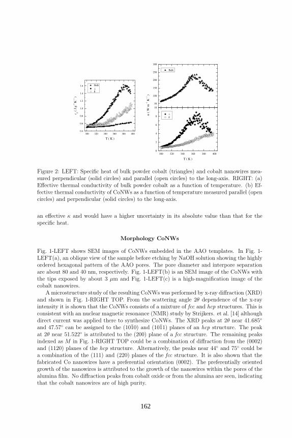
300 320 340 360 380 4000
2
4
6
8
10
50
100
150
200
250
300
⊥
||
κ (
W m
−1 K
−1 )
T ( K )
Bulk
300 320 340 360 380 4000.4
0.6
0.8
1.0
1.2
1.4
1.6
cp (
J g
−1 K
−1 )
T ( K )
Bulk
⊥
||
Figure 2: LEFT: Specific heat of bulk powder cobalt (triangles) and cobalt nanowires mea-sured perpendicular (solid circles) and parallel (open circles) to the long-axis. RIGHT: (a)Effective thermal conductivity of bulk powder cobalt as a function of temperature. (b) Ef-fective thermal conductivity of CoNWs as a function of temperature measured parallel (opencircles) and perpendicular (solid circles) to the long-axis.
an effective κ and would have a higher uncertainty in its absolute value than that for thespecific heat.
Morphology CoNWs
Fig. 1-LEFT shows SEM images of CoNWs embedded in the AAO templates. In Fig. 1-LEFT(a), an oblique view of the sample before etching by NaOH solution showing the highlyordered hexagonal pattern of the AAO pores. The pore diameter and interpore separationare about 80 and 40 nm, respectively. Fig. 1-LEFT(b) is an SEM image of the CoNWs withthe tips exposed by about 3 μm and Fig. 1-LEFT(c) is a high-magnification image of thecobalt nanowires.
A microstructure study of the resulting CoNWs was performed by x-ray diffraction (XRD)and shown in Fig. 1-RIGHT TOP. From the scattering angle 2θ dependence of the x-rayintensity it is shown that the CoNWs consists of a mixture of fcc and hcp structures. This isconsistent with an nuclear magnetic resonance (NMR) study by Strijkers. et al. [14] althoughdirect current was applied there to synthesize CoNWs. The XRD peaks at 2θ near 41.685
and 47.57 can be assigned to the (1010) and (1011) planes of an hcp structure. The peakat 2θ near 51.522 is attributed to the (200) plane of a fcc structure. The remaining peaksindexed as M in Fig. 1-RIGHT TOP could be a combination of diffraction from the (0002)and (1120) planes of the hcp structure. Alternatively, the peaks near 44 and 75 could bea combination of the (111) and (220) planes of the fcc structure. It is also shown that thefabricated Co nanowires have a preferential orientation (0002). The preferentially orientedgrowth of the nanowires is attributed to the growth of the nanowires within the pores of thealumina film. No diffraction peaks from cobalt oxide or from the alumina are seen, indicatingthat the cobalt nanowires are of high purity.
162

Specific Heat of CoNWs
The specific heats of bulk powder cobalt as well as CoNWs in parallel and perpendicular tothe long-axis configuration are shown in Fig. 2-LEFT. The specific heats of all samples weredetermined as a function of temperature from 300 to 400 K. The cobalt bulk powder sampleyields a cB
p = 0.49 J g−1 K−1 at 300 K and a weak, nearly-linear, temperature dependenceconsistent with the literature [15, 16]. The magnitude of the specific heat for the two CoNWsamples are c||p = 0.53 J g−1 K−1 and c⊥p = 0.50 J g−1 K−1 at 300 K. For the parallel CoNW
configuration, c||p increases linearly from room temperature to ∼ 320 K in a bulk-like fashion.
Above 320 K, c||p increases much more rapidly with temperature than the bulk. In the caseof perpendicular measurement, c⊥p increases more rapidly than either the parallel or the bulkbehavior from 318 to 370 K, above which it begins decreasing.
The differences in cp observed here are likely due to the composite nature of the sam-ple+cell configuration. The similarity, at least just above room temperature, between c||p andcBp is understandable as in this heat-flow configuration, the length of the CoNW is compa-
rable to the size of the bulk powder sample. The deviation beginning at ∼ 320 K may be aconsequence of the 1-D nature of the nanowires. As a result, one might expect ”bunching”of the phonons (or phonon-phonon scattering) to dominate at some elevated temperature.For the perpendicular arrangement and although laying flat to the silver sheets, the randomdeposition of CoNWs within the cell likely results in a very large number of contacts, on thenanometer scale, between individual CoNWs. Thus, the c⊥p measured is almost certainly aneffective result for the sample+cell composite.
Thermal Conductivity of CoNWs
Fig. 2-RIGHT(top panel) shows the effective thermal conductivity of bulk powder cobalt at300 K of κB ≈ 67 W m−1 K−1 with a strong temperature dependence reaching a maximumat ∼ 360 K. The the literature value for pure cobalt at 300 K is 90 W m−1 K−1 and displaysa weak temperature dependence [17]. As with c⊥p , the effective thermal conductivity ofbulk powder cobalt measured here is a consequence of the composite nature of micron sizedamorphous particles sandwiched in the cell ”stack”. As such, it seems likely that the observedmaximum is due to boundary-phonon scattering.
The derived thermal conductivity of the CoNWs for the two heat-flow configurations areshown in Fig. 2-RIGHT(bottom panel). Both κ‖ and κ⊥ have values 83 times less than thebulk at 300 K. However, for increasing temperatures, κ‖(T ) behaves quite differently fromthe observed bulk trend, increasing in a smooth manner up to ∼ 380 K at which a small”kink” is seen to a nearly constant value of κ‖ ≈ 4 W m−1 K−1. Although the uncertaintyin absolute values is higher for the measured κ compared to cp, the marked reduction ofmagnitude of κ in both configurations with respect to the bulk is consistent with the 1-Dnature and boundary scattering. However, for κ‖, the kink to a constant value at ∼ 380 Kmay be an indication of phonon-phonon and defect-phonon scattering. For the perpendicularheat-flow measurement of CoNWs, κ⊥ exhibits a similar temperature dependence as the bulk,although of greatly reduced magnitude. As with κB, the observed maximum for κ⊥ seen at∼ 360 K is again likely due to the composite nature of the sample+cell arrangement. Thejunctions between the nanowires dominant the heat transfer for κ⊥ as the contacts betweenbulk powder particles were for κB. The difference in temperature for the observed maximumis consistent with the bulk powder particles being much larger in size.
163
Conclusions
This paper reports measurements of the specific heat and effective thermal conductivityof a macroscopic arrangement of cobalt nanowires, CoNWs, with the orientation of thenanowire parallel and perpendicular to direction of the heat-flow and compared with resultsfor bulk-powder cobalt. The particle nature of the bulk-powder and random deposition of theCoNW(⊥) configuration, lead to strong deviations of both κ and cp from that expected forpure solid cobalt. Perpendicular heat-flow arrangement appears to be dominated by phonon-boundary scattering. Parallel heat-flow measurements appear dominated by phonon-phononor phonon-defect scattering. These results suggest the interesting possibility of engineeringboth the specific heat and thermal conductivity of nano-composite materials.
References
[1] S. Barman and G. P. Srivastava. Phys. Rev. B, 73:205308, 2006.
[2] K-Q. Chen, W-X. Li, W. Duan, Z. Shuai, and B-L. Gu. Phys. Rev. B, 72:045422, 2005.
[3] Y. Chen, D. Li, J. R. Lukes, and A. Majumdar. J. Heat Trans., 127:1129, October 2005.
[4] Y. Chena, D. Lib, J. Yangc, Y. Wuc, J. R. Lukes, and A. Majumdare. Physica B,349:270, 2004.
[5] D. Li, Y. Wu, P. Kim, L. Shi, P. Yang, and A. Majumdar. Appl. Phys. Lett., 14:2934,2003.
[6] R. Prasher. Phys. Rev. B, 74:165413, 2006.
[7] S. Volz and G. Chen. Appl. Phys. Lett., 75:2056, 1999.
[8] R. Yang, G. Chen, and M. S. Dresselhaus. Phys. Rev. B, 72:125418, 2005.
[9] T. M. Trit. Sci., 283:804, 1999.
[10] J. Li, C. Papadopoulos, J. M. Xu, and M. Moskovits. Appl. Phys. Lett., 75:367, 1999.
[11] J. Liang, H. Chik, A. Yin, and J. M. Xu. J. Appl. Physics, 91:2544, 2002.
[12] A. Roshi, G. S. Iannacchione, P. S. Clegg, and R. J. Birgeneau. Phys. Rev. E, 69:031703,2004.
[13] S. Sinha, S. Barjami, G. S. Iannacchione, A. Schwab, and G. Muench. J. Nanopart.
Res., 7(6):651, December 2005.
[14] G. J. Strijkers, J. H. J. Dalderop, M. A. A. Broeksteeg, H. J. M. Swagten, and W. J. M.de Jonge. J. Appl. Phys., 86(9):5141–5145, 1999.
[15] W. Bendick and W. J. Pepperhoff. J. Phys. F: Metal Phys., 11(11):2185, 1979.
[16] R. R. Rao and A. Ramanand. Phys. Rev. B, 19(4):1972, 1979.
[17] T. M. Tritt. Thermal conductivity: Theory Properties and Application. Number 4.Kluwer Academyc/Plenum Publishers, 2004.
164

Index
Index10CB, 148, 1545CB, 1488CB, 148, 154AAO, 40, 63, 84, 148AC Calorimeter, 46, 89, 104achiral, 2acoustic branch, 26agregation, 14Anisotropic, 68anisotropic, 17Arhenius, 137armchair, 4ballistic, 5buckyball, 1calorimetric, 17Calorimetry, 42chiral, 2chiral vector, 3CNPs, 144CNT-based composites, 12CNTs, 83, 102, 126, 144Co NWs, 17, 40, 62, 66coherence, 9CVD, 39, 85, 149defects, 28, 31density of states, 8diffusivity, 77dislocation, 31dislocations, 28dispersion, 26DOS, 37Dresselhaus, 5DSC, 49elastic scattering, 28electrical conductivity, 7Enthalpy, 138, 140filler, 13, 116fillers, 116filling, 151frequency, 137, 157fullerene, 1
GE varnish, 69, 104General Motors, 14Geometrical, 113Glass transition, 110GPIB, 49Hamilton-Crosser, 113Hermetic pan, 52hysteresis, 116imaginary, 132imaginary heat capacity, 125impurities, 28, 31inelsatic scattering, 29Isotropic, 152LBL, 16liquid crystals, 143lithography, 5Lorenz number, 7MDSC, iv, 106, 107, 116, 125, 148, 158mean free path, 8mean-free-path, 77mechanical properties, 13modulation, 157multi-wall CNTs, 84MWCNTs, 146nano-fillers, 11, 102, 126Nanowires, 37nanowires, 9, 62Nelsen, 113Nematic, 152non-reversing, 125Normal scattering, 29nylon 6, 14optical branch, 26optimizing, 6phonon, 6, 28, 75phonons, 25PID, 48plateau, 46PMMA, 116, 131PMMA+SWCNT, 106polymer, 18, 102polymers, 10
173

Chapter 10. APPENDIX 174
PRT, 48Q200, 50, 106quantum dots, 6quantum trasport, 5quantum wires, 6quantum-confinement, 7Random, 68real, 132real heat capacity, 125relaxation, 126reversing, 125Seebeck coefficient, 7SEM, 64, 86single-wall CNTs, 84Smectic-A, 152Specific heat, 71specific heat, 17, 109superlattice, 6, 8SWCNT, 86TE, 16TEM, 86, 148template-assited, 39thermal conductivity, 6, 17, 73, 93, 110,
119thermal model, 42thermoelectric, 6, 62thermoelectric figure, 7TIM, 16timing-belt, 14TMDSC, 52Toyota Motors, 14tunneling, 5Tzero press, 52Ultrasonic bath, 106ultrasonication, 14Umklap scattering, 29van der Waals, 14van der Wall, 131VLS, 40Wiedmann-Franz, 7XRD, 64, 70Xue, 113zigzag, 4ZT, 7, 28
Related Documents


![119 Nanowires 4. Nanowires - UFAMhome.ufam.edu.br/berti/nanomateriais/Nanowires.pdf · 119 Nanowires 4. Nanowires ... written about carbon nanotubes [4.57–59], which can be ...](https://static.cupdf.com/doc/110x72/5abfd11e7f8b9a5d718eba2b/119-nanowires-4-nanowires-nanowires-4-nanowires-written-about-carbon-nanotubes.jpg)


