Thermal Conductivity of Fiber-Reinforced Lightweight Cement Composites Daniel P. Hochstein Submitted in partial fulfillment of the requirements for the degree of Doctor of Philosophy in the Graduate School of Arts and Sciences COLUMBIA UNIVERSITY 2013

Welcome message from author
This document is posted to help you gain knowledge. Please leave a comment to let me know what you think about it! Share it to your friends and learn new things together.
Transcript

Thermal Conductivity of Fiber-Reinforced Lightweight Cement Composites
Daniel P. Hochstein
Submitted in partial fulfillment of the
requirements for the degree of
Doctor of Philosophy
in the Graduate School of Arts and Sciences
COLUMBIA UNIVERSITY
2013

© 2013
Daniel P. Hochstein
All rights reserved
ABSTRACT
Thermal Conductivity of Fiber-Reinforced Lightweight Cement Composites
Daniel P. Hochstein
This dissertation describes the development of a multiscale mathematical model to
predict the effective thermal conductivity (ETC) of fiber-reinforced lightweight cement
composites. At various stages in the development of the model, the results are compared to
experimental values and the model is calibrated when appropriate. Additionally at each stage the
proposed model and its results are compared to physical upper and lower bounds placed on the
ETC for the different types of structural models.
Fiber-reinforced lightweight cement mortar is a composite material that contains various
components at different scales. The model development begins with a study of neat cement
paste and is then extended to include normal weight fine aggregate, lightweight aggregate, and
reinforcing fibers. This is accomplished by first considering cement mortar, then models for
lightweight cement mortar and fiber-reinforced cement mortar are considered separately, and
finally these two are joined together to study fiber-reinforced lightweight cement mortar.
Two different experimental techniques are used to determine the ETC of the different
materials. The flash method is used to determine the ETC of the neat cement paste and cement
mortar samples, and a recently developed transient technique is used for the remainder of the
samples.
The model for the ETC of cement paste is derived from a lumped parameter model
considering the water-cement ratio and saturation of the paste. The results are calibrated using
experimental data generated during this project and are in good agreement with values found in
the literature. The models for the ETC of cement mortar, fiber-reinforced cement mortar,
lightweight cement mortar, and fiber-reinforced lightweight cement mortar are all based on a
differential multiphase model (DM model). This is capable of predicting the ETC of a composite
material with various ellipsoidal inclusion phases. It is shown how the DM model can be
modified to include information about the maximum volume fraction of the inclusions.
A linear packing model is introduced which allows the gradation of the different
inclusion phases to be considered. Additionally other factors that affect the ETC are discussed,
including the presence of an interfacial transition zone around the inclusions and the relative size
of the different constituent phases. The model developed in this report is not only able to predict
the effective thermal conductivity for a material, but it can also be used to minimize the effective
thermal conductivity by optimizing the structure of the composite. This is done through proper
selection of the types and amounts of the various constituents, along with their size, shape, and
gradation.

i
Table of Contents
Chapter 1. Introduction ........................................................................................................................... 1
1.1. Motivation ..................................................................................................................................... 1
1.1.1. Advantages of Lightweight Concrete.................................................................................... 2
1.1.2. Advantages of Fiber-Reinforced Concrete ............................................................................ 3
1.2. Goals, Objective, and Scope ......................................................................................................... 3
Chapter 2. Effective Thermal Conductivity of Composite Materials ..................................................... 7
2.1. Introduction ................................................................................................................................... 7
2.2. Conductive Heat Transfer in Homogeneous Media ...................................................................... 8
2.2.1. Fourier Equation and Steady State Heat Conduction ............................................................ 8
2.2.2. Transient Heat Conduction ................................................................................................... 8
2.3. Conductive Heat Transfer in Heterogeneous Media ..................................................................... 9
2.3.1. Parallel and Series Models .................................................................................................. 10
2.3.2. Hashin-Shtrikman Bounds .................................................................................................. 11
2.3.3. Maxwell Model and the Maxwell-Eucken Limits............................................................... 12
2.3.4. Effective Medium Theory ................................................................................................... 13
2.3.5. Internal and External Porosity ............................................................................................. 14
2.3.6. Unit Cell Conduction Models ............................................................................................. 15
2.3.7. Resistor Models................................................................................................................... 16
2.3.8. Lumped Parameter Models ................................................................................................. 19
2.3.9. Volume Averaging Techniques .......................................................................................... 20
2.4. Effects of Tortuosity ................................................................................................................... 21
2.5. Effect of the Thermal Conductivity Ratio ................................................................................... 22
Chapter 3. Experimental Methods to Measure the Effective Thermal Conductivity............................ 29
3.1. Overview of ASTM Methods ..................................................................................................... 29
3.1.1. Steady-State Methods ......................................................................................................... 29

ii
3.1.2. Transient Methods............................................................................................................... 31
3.1.3. Flash Method ...................................................................................................................... 32
3.2. Proposed Method ........................................................................................................................ 35
3.2.1. Theoretical Background ...................................................................................................... 35
3.2.2. Experimental Procedure ...................................................................................................... 37
Chapter 4. Effective Thermal Conductivity of Cement Pastes ............................................................. 45
4.1. Introduction ................................................................................................................................. 45
4.1.1. Cement Chemistry and Hydration ....................................................................................... 45
4.1.2. Cement Microstructure ....................................................................................................... 45
4.1.3. Volumetric Composition of Cement Paste .......................................................................... 46
4.1.4. Water Adsorption of Cement Paste ..................................................................................... 48
4.2. Factors that Affect the Effective Thermal Conductivity ............................................................. 51
4.3. Current Models ........................................................................................................................... 53
4.4. Proposed Model .......................................................................................................................... 55
4.4.1. Thermal Conductivity of Dry Cement Paste ....................................................................... 56
4.4.2. Thermal Conductivity of Saturated Cement Paste .............................................................. 57
4.4.3. ETC of Dry Cement Paste: Model Calibration .................................................................. 59
4.4.4. ETC of Dry Cement Paste: Model Validation .................................................................... 60
4.4.5. ETC of Fully Saturated Cement Paste: Model Calibration ................................................. 60
4.4.6. ETC of Cement Paste at Intermediate Saturations: Model Calibration .............................. 61
4.5. Summary ..................................................................................................................................... 62
Chapter 5. Effective Thermal Conductivity of Portland Cement Mortar ............................................. 73
5.1. Introduction ................................................................................................................................. 73
5.1.1. Types of Fine Aggregate ..................................................................................................... 73
5.1.2. Factors Affecting the Effective Thermal Conductivity of Fine Aggregate ......................... 74
5.1.3. Factors Affecting the Effective Thermal Conductivity of Cement Mortar ......................... 74
5.2. Effective Thermal Conductivity of Fine Aggregate .................................................................... 74
iii
5.3. ETC of Cement Mortar: Effect of Fine Aggregate Shape ........................................................... 75
5.3.1. Differential Multiphase Model ............................................................................................ 76
5.4. ETC of Cement Mortar: Effect of Maximum Volume Fraction ................................................. 77
5.4.1. Linear Packing Model ......................................................................................................... 78
5.4.2. The Modified Differential Multiphase Model ..................................................................... 79
5.5. ETC of Cement Mortar: Effect of the Interfacial Transition Zone (ITZ) ................................... 80
5.6. Equivalent Inhomogeneity/Finite Cluster Model ........................................................................ 84
5.7. Current Models for the ETC of Cement Mortar.......................................................................... 86
5.8. Experimental Results .................................................................................................................. 87
5.9. Proposed Model .......................................................................................................................... 88
5.10. Summary ................................................................................................................................. 89
Chapter 6. Effective Thermal Conductivity of Lightweight Cement Mortar ....................................... 99
6.1. Introduction ................................................................................................................................. 99
6.2. Differential Multiphase Model .................................................................................................. 100
6.2.1. Effect of Lightweight Aggregate Shape on the ETC ........................................................ 100
6.2.2. Effect of Lightweight Aggregate Gradation on the ETC .................................................. 101
6.2.3. Effect of Different Inclusion Scales on the ETC .............................................................. 101
6.3. Proposed Model for the ETC of Lightweight Cement Mortar .................................................. 104
6.4. Experimental Results ................................................................................................................ 106
6.5. Effect of the Relative Size of the Normal Weight and Lightweight Aggregate........................ 108
6.6. Summary ................................................................................................................................... 109
Chapter 7. Effective Thermal Conductivity of Fiber-Reinforced Cement Paste ................................ 119
7.1. Introduction ............................................................................................................................... 119
7.2. Types of Fibers ......................................................................................................................... 119
7.3. Maximum Volume Fraction ...................................................................................................... 120
7.4. Percolation ................................................................................................................................ 121
7.5. ETC of Fiber-Reinforced Composites at the Maximum Fiber Volume Fraction ..................... 123

iv
7.6. Bounds for the ETC of Fiber-Reinforced Composites .............................................................. 123
7.7. Differential Multiphase Model .................................................................................................. 124
7.8. Equivalent Inclusion Method .................................................................................................... 126
7.9. Proposed Model for the ETC of Fiber-Reinforced Cement Mortar .......................................... 127
7.10. ETC of Fiber-Reinforced Cement Paste: Experimental Results ........................................... 129
7.11. Summary ............................................................................................................................... 130
Chapter 8. Effective Thermal Conductivity of Fiber-Reinforced Lightweight Cement Mortar ......... 140
8.1. Introduction ............................................................................................................................... 140
8.2. Relative Size of the Inclusions (Fine Aggregate, Elemix, and Fibers) ..................................... 140
8.3. Proposed Model for the ETC of Fiber-Reinforced Lightweight Cement Paste ........................ 141
8.4. ETC of Fiber-Reinforced Lightweight Cement Mortar: Experimental Results ........................ 141
8.5. Effect of the Relative Size of the Lightweight Aggregate ........................................................ 142
8.6. Summary ................................................................................................................................... 143
Chapter 9. Conclusions and Future Work ........................................................................................... 146
9.1. Summary of Model ................................................................................................................... 146
9.2. Main Findings ........................................................................................................................... 148
9.3. Recommendations for Future Work .......................................................................................... 149
Bibliography ............................................................................................................................................. 150
Appendix ................................................................................................................................................... 159

v
List of Figures
Figure 2-1: One-Dimensional Conduction .................................................................................................. 24
Figure 2-2: Series Model ............................................................................................................................ 24
Figure 2-3: Parallel Model .......................................................................................................................... 24
Figure 2-4: Effective Medium Theory ........................................................................................................ 24
Figure 2-5: Maxwell-Eucken Model ........................................................................................................... 25
Figure 2-6: Comparison of the Various Models for ETC ........................................................................... 25
Figure 2-7: Bounds of the Internal and External Porosity Regions ............................................................ 26
Figure 2-8: Comparison of the CPS and CSP Models with the Hashin-Shtrikman Upper Bound ............. 26
Figure 2-9: Comparison of the CPS and CSP Models with the Hashin-Shtrikman Lower Bound ............. 27
Figure 2-10: Lumped Parameter Model ...................................................................................................... 27
Figure 2-11: Lumped Parameter Model ...................................................................................................... 27
Figure 2-12: Representative Elementary Volume (RVE) of a Composite Material ................................... 28
Figure 3-1: Guarded-Hot-Plate Apparatus .................................................................................................. 38
Figure 3-2: Heat Flow Meter Apparatus ..................................................................................................... 38
Figure 3-3: Guarded-Comparative-Longitudinal Heat Flow Apparatus ..................................................... 39
Figure 3-4: Transient Line-Source Technique ............................................................................................ 39
Figure 3-5: Dimensionless Plot of Rear Surface Temperature for Flash Method (Equation 3-2) .............. 40
Figure 3-6: Effect of Finite Pulse Time [51] ............................................................................................... 40
Figure 3-7: Effect of Radiant Heat Loss [51] ............................................................................................. 41
Figure 3-8: Idealized Pulse Shape [51] ....................................................................................................... 41
Figure 3-9: Netzsch LFA 447 Nano-Flash-Apparatus [57] ........................................................................ 42
Figure 3-10: Temperature in Semi-Infinite Solid using Equation 3-9 ........................................................ 42
Figure 3-11: Comparison of Actual and Calculated Thermal Diffusivity using Equations 3-12 and 3-13 43
Figure 3-12: Error Using Equation 3-13 for Different Number of Terms .................................................. 43
Figure 3-13: Test Setup ............................................................................................................................... 44
Figure 4-1: Volume Fraction of Hydration Products Using Powers and Brownyard’s [59] Model ........... 66
Figure 4-2: Water Adsorption for Fully Hydrated Type I Cement Paste [71] ............................................ 66
Figure 4-3: Water Adsorption for Fully Hydrated Cement Pastes (w/c = 0.4) ........................................... 67
Figure 4-4: Volume Fractions of Hydration Products for Different Cement Types (w/c = 0.5)................. 67
Figure 4-5: Thermal Conductivity of Water ............................................................................................... 68
Figure 4-6: Thermal Conductivity of Dry Air (ka) and Water Vapor (kv) .................................................. 68
Figure 4-7: Thermal Conductivity of Humid Air [70] ................................................................................ 69
Figure 4-8: Model of Kim et al. [71] for the Thermal Conductivity of Cement Paste ............................... 69
Figure 4-9: Model for the Thermal Conductivity of Air-Dry [32] & [72], Oven Dry, and Fully Saturated
Cement Paste [73] ....................................................................................................................................... 70
Figure 4-10: Model for ETC of Dry Cement Paste ..................................................................................... 70
Figure 4-11: Model for ETC of Cement Paste ............................................................................................ 70
Figure 4-12: Proposed Model for the ETC of Dry Cement Paste ............................................................... 71
Figure 4-13: Proposed Model for the ETC of Fully Saturated Cement Paste ............................................. 71
Figure 4-14: Proposed Model for the ETC of Cement Paste Using Lumped Parameter Model and
Equation 4-34 .............................................................................................................................................. 72
Figure 4-15: Proposed Model for the ETC of Cement Paste using Power Law Model (Equation 4-38) .... 72
vi
Figure 5-1: Fine Aggregate Grading Requirements [78] with Gradations that Produce Maximum and
Minimum Packing Density ......................................................................................................................... 93
Figure 5-2: Percent Difference between ETC of Composite with Nonspherical Aggregate with Respect to
Spherical Aggregate (km = 1 and kagg = 4) .................................................................................................. 93
Figure 5-3: Water-Cement Ratio through the ITZ (ca = 0.6, δ = 0.04 mm, ra = 1 mm, & w/co = 0.4) ........ 94
Figure 5-4: ETC of Cement Mortar Using the Differential Multiphase Model (kpaste = 0.5 W/m/K and
kaggregate = 3 W/m/K) .................................................................................................................................... 94
Figure 5-5: Reduction in the ETC of Cement Mortar Due to ITZ .............................................................. 95
Figure 5-6: ETC of Cement Mortar Using Finite Cluster Model (kpaste = 0.5 W/m/K and kaggregate = 3
W/m/K) ....................................................................................................................................................... 95
Figure 5-7: ETC of Cement Mortar Kim et. al............................................................................................ 96
Figure 5-8: ETC of Cement Mortar: Experimental Data (w/c = 0.5 and kpaste = 0.51 W/m/K) .................. 96
Figure 5-9: ETC of Cement Mortar: Comparison of Experimental Data with Physical Bounds (w/c = 0.5,
kpaste = 0.51 W/m/K, and kagg = 2.5 W/m/K) ............................................................................................... 97
Figure 5-10: ETC of Cement Mortar: Comparison of Experimental Data with Modified DM Model (w/c =
0.5, kpaste = 0.51 W/m/K, and kagg = 2.5 W/m/K) ........................................................................................ 97
Figure 5-11: Proposed Model for the ETC of Cement Mortar (kagg = 2.5 W/m/K) .................................... 98
Figure 6-1: Effect of the Shape of Perfectly Insulating Inclusions on the ETC (kmatrix = 1.0) .................. 111
Figure 6-2: Effect of the Maximum Volume Fraction of Perfectly Insulating Inclusions (kmatrix = 1.0) .. 112
Figure 6-3: Illustration of Different Inclusion Scales ............................................................................... 112
Figure 6-4: Effect of Different Inclusion Scales ....................................................................................... 113
Figure 6-5: Effect of Different Inclusion Scales (Close up on area of interest from Figure 6-4) ............. 113
Figure 6-6: Maximum Volume Fractions as a Function of the Relative Inclusion Size ........................... 114
Figure 6-7: Peak Maximum Volume Fraction as a Function of the Relative Inclusion Size .................... 114
Figure 6-8: ETC of Lightweight Cement Mortar – Aggregate is Smaller than Elemix ............................ 115
Figure 6-9: ETC of Lightweight Cement Mortar – Aggregate is Smaller than Elemix ............................ 115
Figure 6-10: ETC of Cement Paste and Elemix (Experimental Data and Theoretical Bounds) ............... 116
Figure 6-11: ETC of Cement Paste and Elemix (Experimental Data and Proposed Model) .................... 116
Figure 6-12: ETC of Lightweight Cement Mortar – Aggregate is Larger than Elemix ............................ 117
Figure 6-13: ETC of Lightweight Cement Mortar – Aggregate is Larger than Elemix ............................ 117
Figure 6-14: Bounds for the ETC of Lightweight Cement Mortar (From Figure 6-9 and Figure 6-13) ... 118
Figure 7-1: Maximum Packing Fraction for Fibers .................................................................................. 133
Figure 7-2: Effective Electrical Conductivity of Concrete Reinforced with Carbon Fibers
Reproduced from Xie and Gu [104] ......................................................................................................... 133
Figure 7-3: Bounds of the Internally Porous, Externally Porous, Conducting Fibers, and Insulating Fibers
Regions ..................................................................................................................................................... 134
Figure 7-4: Cylindrical Fiber and Equivalent Prolate Spheroid ................................................................ 134
Figure 7-5: Differential Multiphase Model for Fibrous Composite Containing Conducting Fibers (kfibers =
50, Solid Lines: kmatrix = 2 and Dotted Lines: kmatrix = 1)........................................................................... 135
Figure 7-6: Differential Multiphase Model for Fibrous Composite Containing Insulating Fibers (kfibers =
0.2, Solid Lines: kmatrix = 2 and Dotted Lines: kmatrix = 1).......................................................................... 135
Figure 7-7: DM Model for the Effective Electrical Conductivity of Fibrous Composite Containing
Conducting Fibers ..................................................................................................................................... 136

vii
Figure 7-8: Comparison of the Co-Continuous, EMT. and Differential Multiphase Models for a
Conducting Fibrous Composite (kmatrix = 2 and kfibers = 50) ...................................................................... 136
Figure 7-9: Comparison of the Co-Continuous, EMT, and Differential Multiphase Models for an
Insulating Fibrous Composite (kmatrix = 2 and kfibers = 0.2) ........................................................................ 137
Figure 7-10: Comparison of the Differential Multiphase Model and the Effective Inclusion Method for a
Conducting Fibrous Composite (kmatrix = 2 and kfibers = 50) ...................................................................... 137
Figure 7-11: Comparison of the Differential Multiphase Model and the Effective Inclusion Method for an
Insulating Fibrous Composite (kmatrix = 2 and kfibers = 0.2) ........................................................................ 138
Figure 7-12: Maximum Volume Fraction of Fibers vs. Actual Volume Fraction of Fine Aggregate in the
Mortar ....................................................................................................................................................... 138
Figure 7-13: ETC of Fiber-Reinforced Cement Mortar– Aggregate is Smaller than Fibers .................... 139
Figure 7-14: ETC of Cement Paste and Steel Fibers (Experimental Data and Theoretical Bounds) ........ 139
Figure 8-1: ETC of Fiber-Reinforced Lightweight Cement Mortar vs. Volume Fraction of Elemix ....... 145
Figure A-1: Thermal Conductivity of Dry Sandstone, Shale, and Granite ............................................... 162
Figure A-2: Thermal Conductivity of Saturated Sandstone, Shale, and Granite ...................................... 163
Figure A-3: Thermal Conductivity of Dry Basalt ..................................................................................... 163
Figure A-4: Thermal Conductivity of Saturated Basalt ............................................................................ 164
Figure A-5: Thermal Conductivity of Limestone ..................................................................................... 164
Figure A-6: Thermal Conductivity of Dolomite ....................................................................................... 165
Figure A-7: Effect of Temperature on the Thermal Conductivity of Rocks ............................................. 165
Figure A-8: Heat Flux Vectors through an Inclusion (ki/km = 1,000) ....................................................... 167
Figure A-9: Heat Flux Vectors around an Inclusion (ki/km = 0) ............................................................... 168
Figure A-10: Plate with a Circular Inclusion ............................................................................................ 168

viii
List of Tables
Table 1-1: Density and Thermal Conductivity of Various Types of Concrete ............................................. 5
Table 1-2: Thermal Conductivities of the Constituents of Concrete [8] ....................................................... 6
Table 3-1: Finite Pulse Time Factors [51] .................................................................................................. 38
Table 4-1: Typical Compositions of Cement Types ................................................................................... 64
Table 4-2: Constants Used in BSB Model [71] .......................................................................................... 64
Table 4-3: Thermal Properties of Cement Pastes [75] and [77] .................................................................. 65
Table 4-4: Nano-Flash Results for Dry Cement Paste ................................................................................ 65
Table 5-1: Minerals Found in Concrete Aggregate [95] & [96] ................................................................. 91
Table 5-2: Thermal Conductivity of Selected Minerals Found in Concrete Aggregate [79] ...................... 91
Table 5-3: Data Relating to Figure 5-2 ....................................................................................................... 92
Table 5-4: Experimental Results ................................................................................................................. 92
Table 6-1: Experimental Results ............................................................................................................... 111
Table 7-1: Properties of Fibers Used in Fiber-Reinforced Concrete from [110], [111], and [112] .......... 132
Table 7-2: Comparison of the ETC of Fiber-Reinforced Cement Paste Computed Two Ways (Assuming
that the Fibers are a Size Scale Larger than the Aggregate and Assuming that the Fibers and Aggregate
are of the Same Size Scale. ....................................................................................................................... 132
Table 7-3: Results for the Thermal Conductivity of Fiber-Reinforced Cement Paste .............................. 132
Table 8-1: ETC of Fiber-Reinforced Lightweight Cement Mortar ........................................................... 144
Table 8-2: ETC of Fiber-Reinforced Lightweight Cement Mortar (Comparison of Different Sizes of
Lightweight Aggregate) ............................................................................................................................ 144
Table A-1: Coefficients f and g in Equation 7-2 ....................................................................................... 166

ix
Acknowledgments
I would like to begin by thanking my advisor and mentor, Professor Christian Meyer,
who has guided me these last five years. Additionally I would like to thank the faculty of the Fu
Foundation School of Engineering and Applied Science and specifically those in the Department
of Civil Engineering and Engineering Mechanics (CEEM) who have contributed to my education
or aided me in my research. I am especially grateful to Professors Andrew Smyth, Huiming Yin,
Jeffrey Kysar, and Ismail Cevdet Noyan for their willingness to serve on my defense committee.
I am greatly appreciative of the assistance that I received from the staff of the Robert
A.W. Carleton Strength of Materials Laboratory. This includes Adrian Brügger, Dr. Liming Li,
and Travis Simmons. Without their support and technical knowledge, I would not have been
able to complete the experimental portion of my research. Additionally I would like to thank all
of the lab assistants who have helped me in any way.
During my first two years of doctoral study, I was involved with a research project
sponsored by the New York State Energy Research and Development Authority (NYSERDA).
Although my dissertation is not a direct result of the research sponsored by NYSERDA, it did
provide me with knowledge, experience, and financial support. I am grateful to everyone
involved in the project, especially Senior Project Manager Robert Carver from NYSERDA, Dr.
Semyon Shimanovich from Concrete Scientific, and Prof. Rimas Vaicaitis from CEEM.
For the last three years of my study, I have had the privilege of teaching courses in the
Department of Civil and Environmental Engineering (CEEN) at Manhattan College. For this

x
opportunity I am indebted to my friend and mentor, Dr. Moujalli Hourani. I would like to thank
him and all of my colleagues in the CEEN department for their encouragement and support.
I also must acknowledge my friends. This includes my colleagues at Columbia
University and also my 'brothers' in the Mount Kisco Fire Department, especially those in the
Union Hook and Ladder Company. Additionally I would like to thank Rich Cassidy, who has
been my best friend since I began my undergraduate study and always seemed to have a road trip
planned when I needed it the most.
Last, but certainly not least, I would like to thank my family for the love and support they
showed me along this journey. This includes my father, Harold, who pushed me the most and
always encouraged me to work harder when it got tough; my older brother, Joe, who has helped
me immensely by proofreading my dissertation; my younger brother, John, who was always
there when I needed some downtime; and especially my loving girlfriend Katy, who always
listened to me complain about my struggles along the way and who always knew what to say to
make the stress of a long day in the lab go away. I do not consider this achievement to be my
sole accomplishment but instead one that I share with them.

xi
In memory of my mother, Donna Michelle Hochstein

1
Chapter 1. Introduction
For thousands of years civilizations have used concrete as a material to create buildings,
bridges, dams, and other structures by incorporating numerous types of cement agents and also
various types of aggregate. Modern Portland cement was invented by Joseph Aspdin in 1824
and is the dominant type of cement used today. The traditional constituents of Portland cement
concrete (PCC) include: Portland cement, water, fine aggregate, and coarse aggregate. In
addition to traditional PCC, there exist numerous special types of PCC which include one or
more additional components and/or the omission of the aggregate phase. These special types of
concrete include among others: lightweight concrete, fiber-reinforced concrete, polymer
impregnated concrete, high-performance concrete, shotcrete, and heavyweight concrete.
1.1. Motivation
The driving principle behind these special types of PCC is to improve one or more
desirable properties over those of traditional PCC. For example, heavy weight concrete
improves upon traditional PCC by increasing the density and thus allowing PCC to be used as an
effective biological shield against radiation. High-performance concrete increases both the
strength and durability of traditional PCC for use in severe environments. However the
advantages of these specialty concretes also may come with some disadvantages, such as a high
initial cost or a decreased workability, as is the case with using heavyweight concrete. It is thus
the responsibility of researchers and engineers to optimize these special types of PCC to increase
the desirable properties while decreasing the undesirable ones.

2
1.1.1. Advantages of Lightweight Concrete
Lightweight concrete has been made since ancient times by such civilizations as the
Romans. The Romans finished construction of the Pantheon in 27 B.C. and incorporated
lightweight concrete in the dome, making it the dome with the largest diameter for almost two
thousand years. The lightweight concrete used for the Pantheon contained pumice stone which
replaced the normal weight coarse aggregate. Modern lightweight concretes include the use of
expanded perlite, slate, shale or clay aggregate, foamed slag or plastics, sintered pulverized-fuel
ash, exfoliated vermiculite, and the addition of air entraining or foaming admixtures.
While normal weight concrete has a unit weight of approximately 140 pcf (2243 kg/m3),
lightweight concrete can have a unit weight between 19 pcf and 138 pcf (304 kg/m3 and 2211
kg/m3) (Table 1.1). This difference between normal weight and lightweight concrete means that
the dead load of a lightweight concrete structure can be significantly less than that of a structure
constructed using normal weight concrete. The reduction in dead load can then lead to a
decrease in the size of supporting structural members and ultimately a reduction in the overall
cost of the structure.
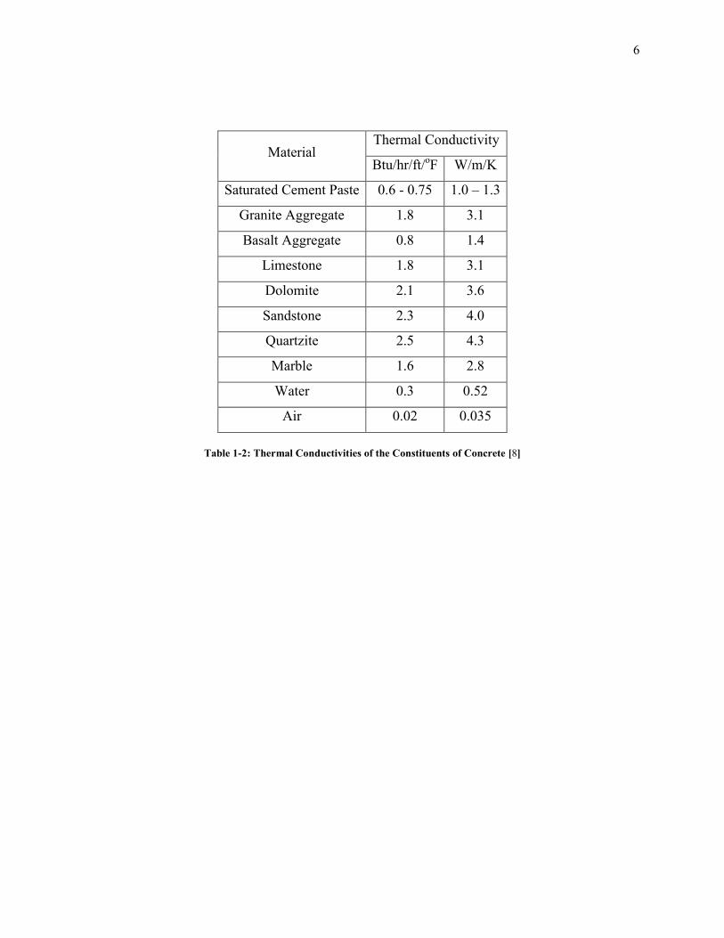
Another desirable property of lightweight concrete is that it has a lower thermal
conductivity than normal weight concrete (Table 1.1). This is due to the additional air voids,
which have a thermal conductivity that is much lower than that of both the hardened cement
paste and the common minerals found in normal weight fine and coarse aggregate (Table 1.2).
The lower thermal conductivity allows lightweight concrete wall panels to serve a dual purpose
as both load carrying structural elements and as thermal insulation.

3
1.1.2. Advantages of Fiber-Reinforced Concrete
Portland cement concrete is a brittle material with a tensile strength that is significantly
less than its compressive strength. Records of ancient civilizations show that brittle materials
such as brick and mud walls reinforced with straw and horse hair date back to the Egyptians and
Babylonians. Modern research into fiber-reinforced concrete did not begin until the 1960s with
the work of Romualdi, Batson, and Mandel [1] [2]. This early research focused mainly on the
use of steel fibers as the reinforcing material. However commonly used materials today include
glass, nylon, polypropylene, acrylic, and other synthetic as well as natural materials such as sisal.
The desirable properties of fiber-reinforced concrete include an increase in the tensile,
shear, and flexural strength, facture toughness, ductility, and performance under dynamic loads.
These properties come from the ability of the fibers to carry tensile stress across the microcracks
that form in the cement paste, which results from both the tensile strength of the fibers and the
bond between the fibers and the cement paste.
1.2. Goals, Objective, and Scope
When the primary objective of using lightweight concrete in a project is to reduce the
dead load of the building materials, it is straightforward to predict the unit weight of the resulting
concrete mix given the unit weights of the constituent materials and their proportions. This is
done based on simple laws of mixtures. On the other hand, the task of predicting the thermal
conductivity of a lightweight concrete to be used as an insulating material is much more difficult
because it depends on many other factors such as the shape, size, gradation, and distribution of
the lightweight aggregate and porosity.
4
The objective of this study was to develop a multiscale model that has the ability to
predict the thermal conductivity of a lightweight concrete. This model considers neat cement
paste on the smallest scale and accounts for the addition of normal weight and lightweight fine
aggregate on a larger scale. Furthermore the model can be expanded to include fiber
reinforcement.
Chapter 2 of this thesis introduces the phenomenon of heat transfer through composite
materials by reviewing the previous work in this field and discussing the applicability of various
methods. Chapter 3 discusses two methods used in this study to measure experimentally the
thermal conductivity of the concrete samples. The first method is the flash method which is
standardized by ASTM and as a result will only be briefly summarized [3] [4]. The second
method was developed in the course of this study and will be elaborated upon in greater detail.
In Chapter 4, a model for predicting the thermal conductivity of neat cement paste is developed.
This model is valid at room temperature for water-cement ratios between 0.4 and 0.80 and for
any degree of saturation. In Chapter 5 the model is expanded to include the effects of a fine
aggregate phase on the thermal conductivity. A model which considers the addition of a
lightweight aggregate phase is considered in Chapter 6. The effects of fiber reinforcement on the
thermal conductivity of cement mortar are discussed in Chapter 7, and Chapter 8 presents the
final model to determine the effective thermal conductivity of fiber-reinforced lightweight
cement mortar. Finally, Chapter 9 provides a summary of this study and suggests topics for
further study.

5
Type of Lightweight Concrete Density Thermal Conductivity
pcf kg/m3 Btu/hr/ft/
oF W/m/K
Normal Weight Concrete 140 - 145 2243 – 2323 0.9 – 2.0 1.56 – 3.46
EPS Concrete – Park et. al 1999 38 - 63 609 – 1009 0.077 – 0.24 0.13 – 0.42
EPS Concrete - Bouvard et. al [5] 27 – 60 432 – 961 0.077 – 0.18 0.13 – 0.31
Aerated Concrete 19 – 119 304 – 1906 0.029 – 0.75 0.50 – 1.30
Partially Compacted w/ Expanded
Vermiculite and Perlite 19 – 70 304 – 1121 0.040 – 0.058 0.07 – 0.10
Partially Compacted with Pumice 50 – 113 801 – 1810 0.087 – 0.17 0.15 – 0.29
Partially Compacted with Expanded
Slag 60 – 95 961 – 1522 0.093 – 0.24 0.16 – 0.42
Partially Compacted with Sintered PFA 70 – 80 1121 – 1281 0.099 – 0.17 0.17 – 0.73
Partially Compacted with Expanded
Clay, Slate, and Shale 60 – 95 961 – 1522 0.16 – 0.24 0.28 – 0.42
Partially Compacted with Clinker 70 – 80 1121 – 1281 0.12 – 0.24 0.21 – 0.42
Structural LWAC with Expanded Slag 100 – 125 1602 – 2002 0.12 – 0.43 0.21 – 0.74
Structural LWAC with PFA 55 – 85 881 – 1362 0.30 – 0.64 0.52 – 1.11
Structural LWAC with Expanded Clay,
Slate, and Shale 90 – 130 1442 – 2082 0.30 – 0.55 0.52 – 0.95
EPS Concrete with Silica Fume
Babu et. al [6] 94 – 124 1506 – 1986 - -
EPS Concrete with Fly Ash
Babu et. al [7] 36 - 138 577 – 2211 - -
Crumb Rubber Concrete
(Sukontasukkul 2008) 114 - 132 1826 – 2114 0.14 – 0.26 0.24 – 0.45
*1 W/m/K = 0.5782 Btu/hr/ft/oF 1 kg/m
3 = 0.06243 pcf Expanded Polystyrene (EPS)
**
Lightweight Aggregate Concrete (LWAC) Pulverised Fuel Ash (PFA)
Table 1-1: Density and Thermal Conductivity of Various Types of Concrete
(All from Mindess [8] unless otherwise noted.)
6
Material Thermal Conductivity
Btu/hr/ft/oF W/m/K
Saturated Cement Paste 0.6 - 0.75 1.0 – 1.3
Granite Aggregate 1.8 3.1
Basalt Aggregate 0.8 1.4
Limestone 1.8 3.1
Dolomite 2.1 3.6
Sandstone 2.3 4.0
Quartzite 2.5 4.3
Marble 1.6 2.8
Water 0.3 0.52
Air 0.02 0.035
Table 1-2: Thermal Conductivities of the Constituents of Concrete [8]

7
Chapter 2. Effective Thermal Conductivity of Composite Materials
2.1. Introduction
Before a model can be introduced to simulate heat transfer in a composite material such
as fiber-reinforced lightweight cement, the phenomenon of conductive heat transfer through a
homogeneous medium must be understood. Heat flows through a medium in three forms:
conduction, convection, and radiation. This study mainly considers the effect of conductive heat
transfer, while completely neglecting radiation and only considering convective transfer to a
limited extent.
Radiation is an electromagnetic phenomenon, which involves the transfer of heat between
objects not in physical contact. Normally the effects of radiation are considered only at high
temperatures or when the effects of conductive and convective heat transfer happen to be small.
This is due to the fourth order relationship involving the temperature difference between two
bodies and the quantity of heat transferred between them [9].
Convective heat transfer occurs when heat is transported through a medium due to the
movement of a fluid. When the medium under consideration is concrete, the fluids that
contribute to this transfer are free water (also called capillary water), dry air, and moist air; all of
which can be contained in the pore spaces of both the cement paste and the aggregate. All water
present in the cement paste contains ions of certain alkalis which precipitate out from the
hardened paste; however in this study the assumption will be made that the water is pure.

8
2.2. Conductive Heat Transfer in Homogeneous Media
2.2.1. Fourier Equation and Steady State Heat Conduction
Joseph Fourier, a French mathematical physicist developed the modern theory of
conductive heat transfer in 1822 [10]. His theory can easily be understood in one dimension by
considering a wall with different prescribed temperatures on the two faces (Figure 2-1). By
assuming that heat only travels perpendicular to the wall surface, the total quantity of heat
passing through the wall via conductive heat transfer can be expressed as:
2-1
where k is the thermal conductivity of the wall, Ax is the surface area of the wall perpendicular to
the direction of heat flow, T is the temperature, and x is the direction of heat flow. Equation 2-1
can also be presented in the following form:
2-2
where qx is the heat flux. When conductive heat transfer occurs in all three orthogonal directions
Fourier’s law can be expressed in its most general form:
2-3
2.2.2. Transient Heat Conduction
Fourier’s law of heat conduction is independent of time and applies to both steady state
and transient heat transfer. The partial differential equation which governs the change in

9
temperature of a homogenous and isotropic medium as a function of time is called the heat
diffusion equation:
2-4
where α is the thermal diffusivity of the material and t is time. The thermal diffusivity is the rate
at which the temperature of a material changes and is expressed as the ratio of the rate of heat
flow into a material to the ability of the material to store this energy:
2-5
where ρ is the density of the material and cp is its specific heat capacity. The product ρcp is
known as the heat storage capacity of the material, which is the amount of energy that the
material needs to absorb to increase the temperature of a unit volume of the material by one
degree.
2.3. Conductive Heat Transfer in Heterogeneous Media
When the medium under consideration is homogeneous, Fourier’s law can easily be
applied to determine the heat flux if both the temperature gradient and thermal conductivity are
known. Difficulties arise when the medium is heterogeneous and only the thermal conductivity
of each phase is known instead of the thermal conductivity of the medium as a whole. It is then
of great interest to be able to compute the thermal conductivity of a homogeneous medium that
would have the same macroscopic heat flux as the composite medium under the same overall
temperature gradient. The thermal conductivity which produces this is known as the effective
thermal conductivity (ETC) of the composite medium. There does not exist one universal

10
method to compute the ETC; however many researchers either have attempted to compute the
ETC for idealized media or have constructed upper and lower bounds under certain assumptions.
The equation which governs conductive heat transfer is known as the Laplace equation
(Equation 2-4). This same equation also describes other phenomena such as mass diffusion,
electrical conduction, and magnetism. Consequently many of the models proposed to compute
the ETC were first derived to simulate one of the other processes. The calculation of an effective
elastic modulus is part of a different class of problems which are governed by vector equilibrium
equations. Despite this difference Milton [11] and Torquato [12] have derived several interesting
cross-property relationships between the effective conductivity and stiffness properties of
composite media.
2.3.1. Parallel and Series Models
The most fundamental models for the ETC are the parallel and series models. These are
not only easy to visualize, but they provide absolute upper and lower limits on the ETC of any
composite medium. As a result they are also termed the Wiener bounds on the ETC [13].
The series model is constructed by considering a composite wall which consists of two
homogeneous wall panels placed in perfect contact with each other as shown in Figure 2-2. By
placing them in perfect contact with each other, the temperature is continuous at the interface. If
the temperature is prescribed on each free face, the heat must flow perpendicular to the face of
the wall and has the same value at every location. The ETC can be expressed as:
2-6

11
where φi and ki are the volume fraction and thermal conductivity of the two materials,
respectively. The series model can be applied to composites which are constructed by any
number of laminates of different materials and it is represented by the equation:
∑ ⁄
2-7
The parallel model is obtained by applying the temperature gradient along the plane of
contact between the two materials, instead of perpendicular to it (Figure 2-3). The ETC of a
composite medium made up of two materials using the parallel model is:
2-8
and for an arbitrary number of materials is:
∑ 2-9
It has been shown by Wiener [13] that the parallel model corresponds to the upper limit for the
thermal conductivity of composite media and the series model corresponds to the lower limit.
This is illustrated in Figure 2-6.
2.3.2. Hashin-Shtrikman Bounds
Models used to produce the Wiener limits do not originate from an isotropic medium that
is macroscopically homogeneous; thus they cannot be reliably used to calculate the upper and
lower limits on the ETC of composite materials which do. Using a variational approach, Hashin
and Shtrikman calculated the effective magnetic permeability of a multiphase material [14] and
so their results can easily be extended to the ETC. With this technique they were able to
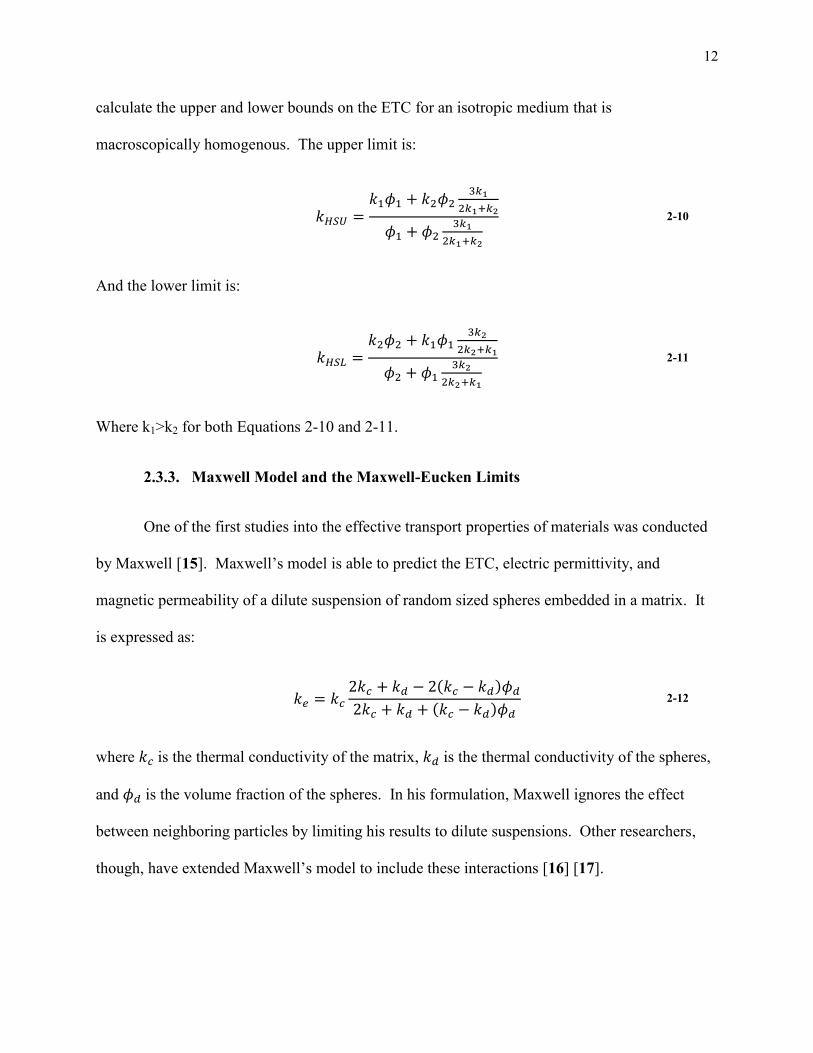
12
calculate the upper and lower bounds on the ETC for an isotropic medium that is
macroscopically homogenous. The upper limit is:
2-10
And the lower limit is:
2-11
Where k1>k2 for both Equations 2-10 and 2-11.
2.3.3. Maxwell Model and the Maxwell-Eucken Limits
One of the first studies into the effective transport properties of materials was conducted
by Maxwell [15]. Maxwell’s model is able to predict the ETC, electric permittivity, and
magnetic permeability of a dilute suspension of random sized spheres embedded in a matrix. It
is expressed as:
( ) ( )
2-12
where is the thermal conductivity of the matrix, is the thermal conductivity of the spheres,
and is the volume fraction of the spheres. In his formulation, Maxwell ignores the effect
between neighboring particles by limiting his results to dilute suspensions. Other researchers,
though, have extended Maxwell’s model to include these interactions [16] [17].

13
The Maxwell-Eucken Limits [18] are an extension of Maxwell’s model, which use it to
construct physical bounds on the ETC of a composite medium. This model assumes that an
isotropic and macroscopically homogenous composite medium is made up of two materials, with
the thermal conductivity of the first material being greater than that of the second material. The
ETC of the composite would have the largest possible value when the second phase is dispersed
in a continuum of the first phase and its smallest possible value when the first phase is dispersed
in a continuum of the second phase (Figure 2-5). There is no restriction on the shape of the
inclusions, but the neighboring inclusions cannot come into contact or interact with each other.
The upper limit is:
( ) ( )
2-13
And the lower limit is:
( ) ( )
2-14
Despite being expressed in different forms, the Maxwell-Eucken and the Hashin-Shtrikman
bounds are equivalent.
2.3.4. Effective Medium Theory
Effective medium theory (EMT) was first developed by Landauer [19] to compute the
electrical resistance of a composite medium composed of two phases; it is also used to compute
the ETC. The theory assumes that the distributions of the different phases within the composite
are completely random and that the phases are mutually dispersed (as shown in Figure 2-4). For

14
a composite with n phases, EMT can determine the ETC by solving the following implicit
equation [20]:
∑
2-15
When only two phases are present the solution for the ETC is:
,[ ] [ ]
√[( ) ( ) ] - 2-16
2.3.5. Internal and External Porosity
The Maxwell-Eucken Limits and EMT can be combined to introduce two types of
material models [21]. When all three equations are plotted, EMT will always be between the
Maxwell-Eucken limits (Figure 2-6). The region between the upper limit and the equation
corresponding to EMT is known as the internal porosity region and the region between the lower
limit and the EMT equation is known as the external porosity region, Figure 2-7. An internally
porous material consists of a continuous phase that has a higher thermal conductivity than that of
the dispersed phase (the dispersed phase does not necessarily need to be gaseous). The
continuous phase thus forms an uninterrupted conduction pathway through the material. When
the continuous phase has a lower thermal conductivity than the dispersed phase the material is
termed externally porous. In this case the heat does not have a continuous path through the more
conductive phase. Holding all other variables the same, a composite medium that is internally
porous always will have a higher thermal conductivity than if it were externally porous. Using
these concepts the bounds on the ETC of a composite medium can be further narrowed from the
Hashin-Shtrikman bounds when information is known about the material’s structure.

15
2.3.6. Unit Cell Conduction Models
If detailed information about the morphology of the composite is not known, it may be
practical to approximate it as a lattice structure. The ETC can then be calculated by assuming
the location of isotherms and analyzing the resulting unit cell. There exist many techniques that
use unit cell models and this section will mention several of them. Rayleigh [22] developed an
expression for the ETC of a cubical array of spherical particles of the form:
(
⁄ )
( ⁄ )
2-17
where phase 1 is the matrix phase, phase 2 is the dispersed phase, and AR and kR are parameters
of the form:
If the higher order terms are neglected ( ⁄ ) then this solution simplifies to the Hashin-
Shtrikman upper bound.
Another solution (Equation 2-18) for the same microstructure was developed by Deissler
and Eian [23] which is only valid when all of the spheres touch (φ2 = 0.524).
(
)
[ ( )
] (
) 2-18
Other researchers who have employed this technique are Schumann and Voss [24],
Deissler and Boegli [25], and Krupicska [26]. The shortcomings with this type of models are
that they ignore the bending of the heat-flow lines around the dispersed phase, the irregularities
16
in the arrangement of the dispersed phase, and also the possible contact between inclusions of the
dispersed phase.
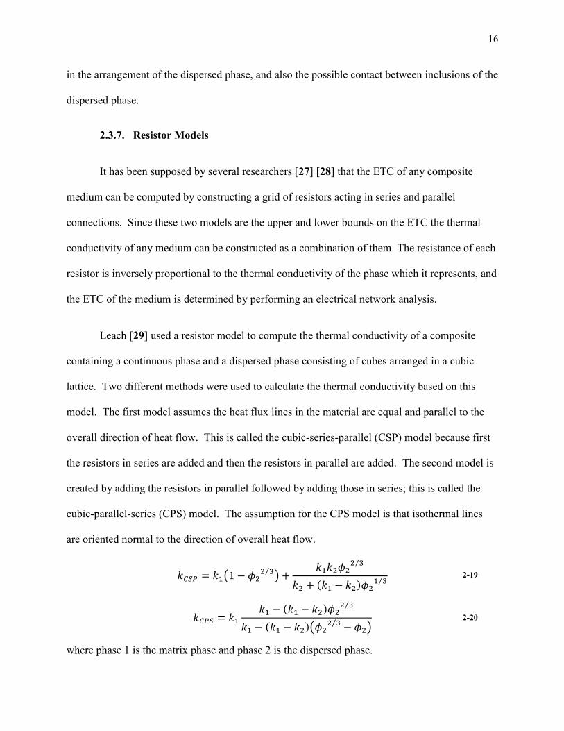
2.3.7. Resistor Models
It has been supposed by several researchers [27] [28] that the ETC of any composite
medium can be computed by constructing a grid of resistors acting in series and parallel
connections. Since these two models are the upper and lower bounds on the ETC the thermal
conductivity of any medium can be constructed as a combination of them. The resistance of each
resistor is inversely proportional to the thermal conductivity of the phase which it represents, and
the ETC of the medium is determined by performing an electrical network analysis.
Leach [29] used a resistor model to compute the thermal conductivity of a composite
containing a continuous phase and a dispersed phase consisting of cubes arranged in a cubic
lattice. Two different methods were used to calculate the thermal conductivity based on this
model. The first model assumes the heat flux lines in the material are equal and parallel to the
overall direction of heat flow. This is called the cubic-series-parallel (CSP) model because first
the resistors in series are added and then the resistors in parallel are added. The second model is
created by adding the resistors in parallel followed by adding those in series; this is called the
cubic-parallel-series (CPS) model. The assumption for the CPS model is that isothermal lines
are oriented normal to the direction of overall heat flow.
( ⁄ )
⁄
( ) ⁄
2-19
( )
⁄
( )( ⁄ )
2-20
where phase 1 is the matrix phase and phase 2 is the dispersed phase.

17
When the thermal conductivity of the matrix phase is greater than that of the dispersed
phase, the following observations are made by comparing the CPS and CSP models to the
Hashin-Shtrikman upper and lower bounds. The CPS model always predicts a value for the ETC
that is greater than the Hashin-Shtrikman upper bound, while the CSP model also will be greater
than the Hashin-Shtrikman upper bound when the thermal conductivities of the two phases are
close ( ⁄ ), and both models are always greater than the Hashin-Shtrikman lower bound.
When the thermal conductivity of the matrix phase is less than that of the dispersed phase the
following observations are made: the CSP model always predicts a value for the ETC that is less
than the Hashin-Shtrikman lower bound, while the CPS model always predicts a value greater
than the Hashin-Shtrikman lower bound, and the CPS will predict a value greater than the
Hashin-Shtrikman upper bound for certain porosities and when the thermal conductivities of the
two phases are similar ( ⁄ ). From these observations it can be concluded that the CPS
is more applicable to an externally porous material and the CSP model is more applicable to an
internally porous material.
In the past, certain researchers may have used an inappropriate model when analyzing the
ETC of materials. The CPS model has been alternately derived by Russell [30] and was used to
predict the ETC of bricks, even though brick is an internally porous material. Campbell-Allen
and Thorne [31] employed the CSP model to compute the ETC of cement mortar, even though
normal weight concrete is an externally porous material (the thermal conductivity of the
aggregate is generally slightly greater than that of the cement paste). These two observations are
illustrated in Figure 2-8 and Figure 2-9 using the following typical values for the thermal
conductivities of the different phases in units of W/m/K: solid portion of brick k = 2, air k =
0.025, cement paste k = 1, and aggregate k = 2. However, the report of ACI Committee 122 [32]

18
correctly uses the CPS model to compute the thermal conductivity of cement mortar containing
normal weight aggregate.
Babanov [33] developed a CPS model that is constructed using spherical inclusions and
the resulting ETC (Equation 2-21) only differs by the use of a constant. To obtain a more
realistic model that accounts for the deviations in the heat flux lines around the inclusions, a
porosity correction factor, Fp, was introduced by Tareev [34] which replaces φ2 in Equation
2-20. If the thermal conductivity of the dispersed phase is greater than that of the continuous
phase, the heat flux lines will bend in towards the inclusions, and if the thermal conductivity of
the dispersed phase is less, the heat flux lines will bend away from the inclusions. Also
parameter Fp can indirectly account for random deviations from the assumed cubic lattice
structure and non-uniform size and shape of the inclusions.
( )√
( ) .√
/
2-21
( )√
( ) .√
/
2-22
Singh et al. [35] recommend using the following equation for Fp:
(
( )) 2-23

19
2.3.8. Lumped Parameter Models
Lumped parameter models are similar to the resistor models in that the composite
medium is idealized as an electrical grid constructed out of individual resistors. However, unlike
resistor models, each resistor represents an entire phase or a heat transfer mechanism that occurs
within a phase or between several phases.
Kunni and Smith [36] developed a lumped parameter model to compute the ETC of
packed beds of unconsolidated material. In their model the two main modes of heat transfer
which act in parallel are one through the solid phase and another through the fluid occupying the
void space. The heat transfer through the solid phase is then broken down into two processes
that act in series: conduction through the solid phase and a parallel circuit which consists of
conduction through surface to surface contact, conduction through the stagnant fluid near the
contact points, and radiation between particle surfaces (Figure 2-10). This model only requires
two empirical parameters and it is formulated such that the resulting ETC will always lie
between the Hashin-Shtrikman bounds.
Another lumped parameter model has been developed by Tong, Jing, and Zimmerman
[37] which has been used to determine the ETC of geological porous media such as bentonite. In
their model they assumed that the four modes of heat transfer acting in parallel are: conduction
through a portion of the solid phase, conduction through a portion of the gas phase, conduction
through a portion of the liquid phase, and conduction through a series connection of the
remaining solid, liquid, and gas (Figure 2-11). It is this model that will be expanded on in this
study to model the ETC of cement paste. The rationale behind this will be discussed in Section
4.4.
20
2.3.9. Volume Averaging Techniques
If the morphology of the composite medium is known, then the principles of volume
averaging and thermodynamics can be used to analyze a composite medium as an effective
medium [38], [39], [40], [41], and [42]. The ETC of the composite can then be calculated once
the temperature gradient through the averaged medium is determined. The basis for using the
volume averaging technique is to first establish a representative volume element for the material
in question (Figure 2-12), where the characteristic length of the composite (Lm) is much greater
than the size of the RVE (ro) and the size of the RVE is much greater than the characteristic
length of each phase (li) (Equation 2-24).
2-24
Following the derivation of Hsu [39], the macroscopic transient heat conduction equation
for the ith
phase is:
( ) 2-25
with the following boundary conditions applied at the interface between the ith
and jth
phases:
By averaging the macroscopic heat equations for each phase over the RVE, applying the
boundary conditions, and invoking the assumption of local thermal equilibrium [43] the heat
conduction equation for the composite can be expressed as:
( )
[ ] 2-26

21
where ( ) is the heat capacity of the composite, is the ETC, is the macroscopic averaged
temperature, and is the macroscopic gradient operator. It should be noted that in the derivation
of Equation 2-26 it is assumed that effects of radiation, viscous dissipation, and the work done by
pressure changes are negligible [44].
Since mass and energy are extensive properties and independent of the morphology, the
effective heat capacity of the composite can be defined as the volume-fraction-weighted
arithmetic mean of the volumetric heat capacities of the constituent phases:
( ) ∑ ( ) 2-27
For a composite composed of only two phases the ETC of the medium can then be
expressed as:
( ) ( ) 2-28
where the first two terms on the right hand side correspond to the parallel model (Equation 2-8)
for the ETC, is the thermal conductivity ratio (k2/k1), and G is the tortuosity. It has already
been presented that the parallel model for the ETC is the upper limit and as a result of Equation
2-28 the tortuoisity parameter must always be greater than or equal to zero. For an isotropic
medium, the limits on the tortuosity parameter are obtained by considering the Hashin-Shtrikman
bounds.
2.4. Effects of Tortuosity
The value of the tortuosity parameter, G, has the effect of reducing the value for the ETC
of a composite medium from the maximum possible value. According to the previous derivation
it depends on both the geometry of the boundary between the different phases and the thermal
conducitivities of those phases [39]. The minimum value of G is zero, and this occurs when the

22
phases follow the parallel layer model since the easiest path for heat flow is straight through the
material with the highest thermal conductivity. Becasue of this, the parallel model can be
thought of as not being tortuous (i.e. G = 0). The value of G is at a maximum when the phases
follow the series layer model since heat is forced to flow equally through all phases and as a
result the material with the lower thermal conductivity slows down the rate at which the heat
flows. For all other possible arrangements the tortuosity parameter quantifies the degree at
which heat is forced to flow through the phases with the lower thermal conductivity.
2.5. Effect of the Thermal Conductivity Ratio
According to Aichlmayr and Kulacki [41], the thermal conductivity ratio plays an
important role in determining what method should be used to determine the ETC. The three
groups that they used to classify materials were media with small, intermediate, and large
conductivity ratios. They considered saturated porous media and defined the thermal
conductivity ratio as the ratio of the thermal conductivity of the solid phase to that of the fluid
phase. For the composites that they considered the thermal conductivity ratio was greater than
one. This is because generally the thermal conductivity of a solid is greater than that of a fluid.
A composite can be categorized as having a small conductivity ratio when σ < 10. For
these types of materials, the ETC is insensitive to the interfacial geometry between phases and
primarily depends on the volume fraction and the thermal conductivity of each phase. The
Maxwell model and mixture rule models, such as the series and parallel models, are most
applicable to these types of materials.
The range of values for which a composite is classified as an intermediate conductivity
ratio material is 10 ≤ σ < 103. The geometry of the interface does affect the effective thermal
23
conductivity for these types of materials. The types of models which can be applied to such
materials are conduction models, the resistor network technique, and lumped parameter models.
When σ ≥ 103, the ETC is highly dependent on the interfacial geometry of the composite,
and such materials are categorized as large thermal conductivity ratio materials. The volume
averaging technique gives the best results for materials in this category because it is able to
precisely consider the interface between the two phases without any of the assumptions that are
made when using the unit cell conduction, resistor network, and lumped parameter models.

24
Figure 2-4: Effective Medium Theory
Figure 2-3: Parallel Model
T1 T2
q
x
T1 T2
q
x
a) Isometric View b) Side View
Figure 2-2: Series Model
T1
T2
q
x T1 T2
q
x
a) Isometric view b) Side view
a) Isometric view of b) Side view
T1 T2
q
x T1 T2
q
x
Figure 2-1: One-Dimensional Conduction

25
Figure 2-6: Comparison of the Various Models for ETC
(k1 = 1.0 & k2 = 0.1)
0
0.25
0.5
0.75
1
0 0.2 0.4 0.6 0.8 1
k eff
φ1
Parallel Model H-S Upper Bound EMT
H-S Lower Bound Series Model
Figure 2-5: Maxwell-Eucken Model
(Phase 1 - Black & Phase 2 - White) a) Upper Bound b) Lower Bound

26
Figure 2-7: Bounds of the Internal and External Porosity Regions
Figure 2-8: Comparison of the CPS and CSP Models with the Hashin-Shtrikman Upper Bound
(k1= 2 and k2 = 0.025)
0
0.25
0.5
0.75
1
0 0.2 0.4 0.6 0.8 1
k eff
φ1
Parallel H-S Upper EMT (Random) H-S Lower Series
0.4
0.5
0.6
0.7
0.8
0.9
1
0 0.1 0.2 0.3 0.4 0.5
k eff/k
1
φ2
CPS HSU CSP
Internal Porosity Region
External Porosity
Region

27
Figure 2-9: Comparison of the CPS and CSP Models with the Hashin-Shtrikman Lower Bound
(k1= 1 and k2 = 2)
1
1.1
1.2
1.3
1.4
1.5
0 0.1 0.2 0.3 0.4 0.5
k eff/k
1
φ2
CPS HSL CSP
Surf
ace
Co
nta
ct
Flu
id C
on
du
ctio
n
Rad
iati
on
in t
he
Vo
id S
pac
e
Hea
t Tr
ansf
er t
hro
ugh
th
e Fl
uid
Occ
up
yin
g th
e V
oid
Sp
ace
Solid Conduction
Figure 2-10: Lumped Parameter Model
Kunni and Smith [36]
Solid
Gas
Liquid
Liq
uid
Gas
Solid
Figure 2-11: Lumped Parameter Model
Tong et al. [37]

28
l2
l1
Lm
ro
Figure 2-12: Representative Elementary Volume (RVE) of a Composite Material

29
Chapter 3. Experimental Methods to Measure the Effective Thermal Conductivity
There currently exist numerous standardized methods to measure the effective thermal
conductivity of a material. All of these methods are similar in that a system with a known
analytical solution is used to approximate the heat transfer through a sample. By measuring the
temperature and heat flow at various points in the material, the analytical solution can be used to
calculate the ETC. Both steady-state and transient systems are used and there are advantages
and disadvantages associated with both. In addition to methods standardized by ASTM
International there exist methods specific to concrete materials developed by the American
Society of Civil Engineers (ASCE) as well as methods developed by various researchers.
3.1. Overview of ASTM Methods
3.1.1. Steady-State Methods
The traditional procedure to measure the thermal conductivity of a material is to subject a
specimen to steady-state thermal conditions. The advantages of this method are that the various
fluid and solid phases within the specimen are in thermal equilibrium and the heat flux can be
measured directly. The disadvantages are that specimens, especially those with a large heat
capacity, may take a long time to reach steady-state and contact resistance between different
parts of the system interrupts the heat conduction. Additionally, heat loss from the system must
either be minimized to create an adiabatic system or measured and accounted for in the analytical
solution. The ASTM methods which employ this technique are: the guarded-hot-plate apparatus
[45], the heat flow meter apparatus [46], the thin heater apparatus [47], and the guarded-
comparative-longitudinal heat flow technique [48].

30
The guarded-hot-plate apparatus is shown in Figure 3-1. It consists of sandwiching a
guarded hot plate between two identical specimens and placing a cold surface assembly on the
other side of each specimen. The primary and secondary guards are then placed on the sides to
provide isothermal boundaries and the whole apparatus is surrounded by insulation. By
recording the temperature and heat supplied to the hot plate along with the temperature of the
cold surface assembly, the thermal conductivity of the specimens can be calculated.
The heat flow meter apparatus is similar to the guarded-hot-plate in that a specimen is
placed between two surfaces of different temperatures to approximate steady-state one-
dimensional heat flow. The difference is that in the heat flow meter method the heat flux is
measured via a heat flux transducer, whereas in the guarded-hot-plate method the heat flux is
measured by knowing the power of the hot plate. There are three standard configurations which
are shown in Figure 3-2.
The guarded-comparative-longitudinal heat flow technique also involves exposing a
specimen to a one-dimensional temperature gradient by placing a heat source and a heat sink on
either side of it (Figure 3-3). Metered bars are then sandwiched between the heat source and the
specimen and between the heat sink and the specimen. The metered bars are made of the same
material which has a known thermal conductivity. By measuring the temperature gradient on the
metered bars, the heat flux through the specimen can be calculated, which along with the
temperature gradient of the specimen can be used to determine the thermal conductivity.
Adiabatic conditions are maintained by surrounding the apparatus with insulation and also by
placing a guard shell around it. The guard is designed so that its temperature gradient closely
mimics that of the two meter bars and the specimen.

31
3.1.2. Transient Methods
Transient techniques to measure the ETC offer several advantages over steady-state
techniques. The duration of a transient test is relatively short because time does not have to
elapse for the specimen to reach steady-state. Additionally it can be assumed that the system is
semi-infinite, which eliminates the need to impose adiabatic conditions. Initially the specimen is
at a constant temperature and then a sudden heat flux is applied by either heating one of the
boundaries or by using a line heat source. The ASTM methods that employ a line heat source
are the transient line-source technique [49] and the hot wire technique [50]. The flash method
[51] is another ASTM method, which instead uses a short duration energy pulse to
instantaneously heat one side of a specimen. This method will be discussed in the greatest detail
because it was used in this study to calculate the thermal conductivity of cement paste and
cement mortar.
In the transient line-source technique, a line-source heater with a built-in thermocouple is
inserted into a specimen as shown in Figure 3-4. The specimen can be treated as a semi-infinite
domain which has radial symmetry and is initially at a constant temperature. Once the heater is
powered the temperature of the specimen will rise and the temperature is measured at the heater.
The thermal conductivity of the specimen can be determined from Equation 3-1, where Q is the
heat output per unit length, C is a calibration coefficient that depends on the dimensions of the
heater, and T1 and T2 are the temperature of the heater at times t1 and t2, where t2 > t1.
( ⁄ )
( ) 3-1
The hot wire technique is a variation on the transient line-source technique in which a
platinum wire is used to heat the material instead of a heater. The heat supplied to the medium is

32
determined by recording the current applied to the wire and the temperature of the wire is
calculated by measuring the resistance of the wire. The thermal conductivity of the medium is
also calculated according to Equation 3-1.
3.1.3. Flash Method
To perform the flash method, a thin disc specimen is exposed to a high-intensity radiant
energy pulse for a short period of time. The front face of the specimen absorbs the energy which
then heats up the rear face of the specimen through conduction. The thermal diffusivity of the
material is calculated based on the thickness of the sample and the time it takes for the rear face
to reach one-half of its maximum temperature; this is also known as the half-rise time (t1/2). The
thermal conductivity of the material can then be determined by also calculating the density and
specific heat of the material.
This method was developed in 1960 by Parker [3] and the theoretical basis can be found
in [52]. If a pulse of radiant energy, Q, is instantaneously and uniformly absorbed at the front
surface of a thermally insulated solid of uniform thickness, L, then the temperature at the rear
face is given by Equation 3-2:
( )
[ ∑( ) ( )
] 3-2
where ω is a dimensionless parameter:
3-3
Since the specimen is assumed to be fully insulated the maximum temperature occurs as
time approaches infinity, which is shown in Equation 3-4.

33
( )
3-4
If the dimensionless temperature ratio T/Tm is plotted against the dimensionless
parameter ω, it can be seen that the rear face of the sample will reach one-half of its maximum
temperature when ω = 1.38. This can be seen in the thermogram shown in Figure 3-5. Based on
the half-rise time, the thermal diffusivity of a specimen can be calculated using Equation 3-5.
⁄ 3-5
In practice it is very difficult to satisfy the conditions that lead to Equations 3-2 and 3-4.
The radiant energy pulse will always have some finite time length and heat will be lost from the
specimen due to radiation out of the rear face and conduction through the sample holder.
Examples of thermograms that show the effect of a finite pulse time and radiation heat loss are
shown in Figure 3-6 and Figure 3-7, respectively. The influence of the pulse length on the results
decreases as the sample thickness is increased and the influence of heat loss will decrease as the
sample thickness is reduced; thus by properly choosing the sample thickness these two effects
can be minimized. Additionally several correction methods have been developed which take
these phenomena into account.
The thermal diffusivity value corrected for the finite pulse time can be calculated from
Equation 3-6, where K1 and K2 are finite pulse time factors determined from Table 3-1 and τ is
the duration of the pulse. This equation assumes that the pulse is represented by a triangle with
the maximum intensity occurring at time βτ as shown in Figure 3-8. Additionally Cowan has
developed corrections to account for heat loss due to both conduction and radiation [53].
⁄ 3-6

34
Once the thermal diffusivity of the material is known, the density and specific heat must
also be determined before the thermal conductivity can be calculated using Equation 2-5. The
specific heat can be measured using various calorimetric methods, including differential
scanning calorimetry [54], and also by performing the flash test in calorimetric mode. The
specific heat of a material is determined using the flash method by first performing the test on a
material with a known specific heat and density. When the reference sample is tested, the
maximum temperature on the rear face is recorded and the energy of the pulse is calculated by
using Equation 3-4. Next the material with the unknown specific heat is tested and the
maximum temperature on the rear face is recorded. By knowing its density, the specific heat
capacity of the material can be determined using Equation 2-5. In order for this comparative
method to be valid, the following conditions must be satisfied: the energy of the pulse does not
change over time, the detector must maintain its sensitivity between the two tests, and the two
samples must be very similar in size, proportions, emissivity, and opacity.
In this study the Netzsch LFA 447 Nano-Flash-Apparatus (Figure 3-9) was used to
perform the flash method. The LFA 447 utilizes a xenon flash lamp to direct a radiant energy
pulse at a specimen and the temperature rise at the rear face of the specimen is then measured
using an infrared detector. The specimen is housed in a furnace that allows the test to occur
between ambient temperature and 300oC. The flash lamp has pulse energy of 10 Joules and a
pulse duration of 100, 250, or 450 μs. Both the Cowan and finite pulse corrections were applied
to the results.

35
3.2. Proposed Method
3.2.1. Theoretical Background
Consider a semi-infinite domain initially at a uniform temperature. If a uniform heat
flux, Q, is applied to the top surface, the system can be modeled as one-dimensional, with the
temperature only varying in a direction perpendicular to the surface. The heat diffusion equation
is expressed as:
( )
( )
3-7
The boundary conditions for the system are that the heat flux at the surface is equal to Q, the
initial temperature of the medium is equal to To, and the medium's temperature far away from the
surface remains unchanged:
|
| | 3-8
The solution for the temperature field is [55]:
( )
6 √
.
/ (
√ ) 7 3-9
If the temperatures T1 and T2 are observed at locations x1 and x2, the following equation can be
developed [56]:
√
(
) (
√ )
√
(
) (
√ )
3-10
36
If it is assumed that t 102s, α 10
-6m2 s, and 10
-2m⁄ , then
erfc (x
2√αt) 10-1
, exp (-x2
2
4αt) 100, 2√
αt
10
-2 and Equation 3-10 can be simplified to:
.
/ 3-11
The thermal diffusivity can then be solved for:
(
)
(
) 3-12
Figure 3-10 shows the temperature at two locations using Equation 3-9 with the following
parameters: α = 1×10⁻⁶
m/s2, k = 1 W/m/K, Q = 10 kW/m
2, x1 = 5 mm, x2 = 10 mm, and To =
10oC. It is seen in Figure 3-11 that the calculated thermal diffusivity using Equation 3-12 is not
accurate. A method has been developed to improve this approximation using an infinite power
series [56],
∑ ( )
3-13
where,
(
) 3-14
The coefficients ai are determined using a least-squares linear fit for the assumed range of
thermal diffusivity and the time interval. Using the temperature profiles shown in Figure 3-10
and assuming that the thermal diffusivity is between 5×10⁻⁵
and 5×10⁻⁷
m/s2, the first 5
coefficients for the power series are calculated as: a0 = -2.53×10⁻⁶
, a1 = 8.42×10⁻⁵
, a2 = 7.87×10⁻⁵
,
a3 = -1.24×10⁻⁸
, and a4 = 2.813×10⁻¹⁰
. The calculated thermal diffusivity using Equation 3-13 is

37
shown in Figure 3-11. The error using Equation 3-13 for a different number of terms is shown in
Figure 3-12. It is seen that even if only three terms are used (quadratic approximation) the error
after 100 seconds is close to 1%.
Once the thermal diffusivity is determined the thermal conductivity can be calculated by
rearranging the terms found in Equation 3-9:
6 √
.
/ (
√ ) 7
3-15
3.2.2. Experimental Procedure
The setup for this experiment consists of two 6"×6" cylindrical specimens, two aluminum
disks with a diameter of 6”, and one thin flexible heater arranged as shown in Figure 3-13. The
rationale behind sandwiching the heater between two specimens is that heat would be lost
through the top of the heater if only one specimen were used. Although it is possible to quantify
the amount that is lost, it is instead advantageous to use this heat to test another specimen
simultaneously. The surfaces of the specimens and aluminum that are in contact are to be
polished smooth and a thermal conductive paste is applied to eliminate any contact resistance
between them. Two thermocouples are placed at different locations within each specimen and
one thermocouple is placed at the center of each aluminum disk. The location of the
thermocouples in the specimens are at depths x1 and x2 from the surface that is in contact with
the aluminum disk (x2 < x1). The heater is a Kapton® Insulated Flexible Heater, which has a
diameter of 6", a maximum thickness of 0.010", and an output of 2.5 W/in2. A variable power
supply will be used to lower the power of the heater as necessary.
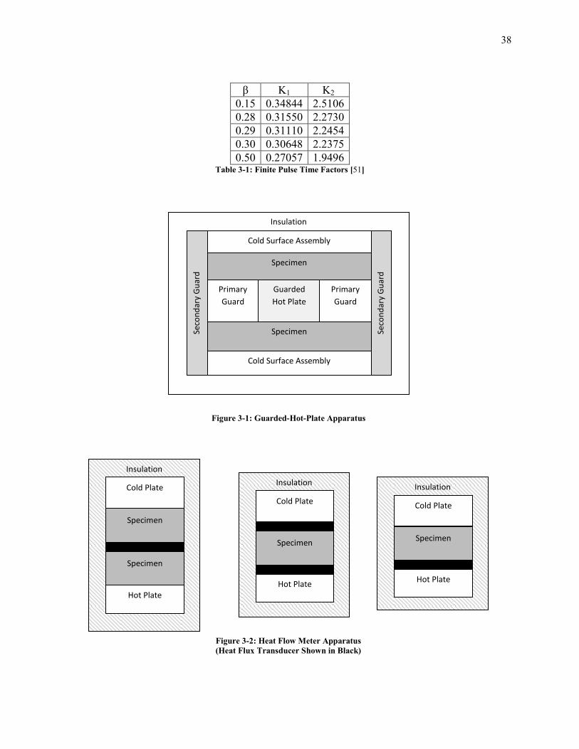
38
β K1 K2
0.15 0.34844 2.5106
0.28 0.31550 2.2730
0.29 0.31110 2.2454
0.30 0.30648 2.2375
0.50 0.27057 1.9496 Table 3-1: Finite Pulse Time Factors [51]
Insulation
Cold Surface Assembly
Specimen
Specimen
Primary
Guard
Guarded
Hot Plate
Seco
nd
ary
Gu
ard
Seco
nd
ary
Gu
ard
Cold Surface Assembly
Primary
Guard
Figure 3-1: Guarded-Hot-Plate Apparatus
Insulation
Cold Plate
Specimen
Hot Plate
Specimen
Specimen
Insulation
Cold Plate
Specimen
Hot Plate
Specimen
Specimen
Insulation
Cold Plate
Specimen
Hot Plate Specimen
Figure 3-2: Heat Flow Meter Apparatus
(Heat Flux Transducer Shown in Black)

39
Heater Section
Specimen
Heat Sink
Meter Bar
Meter Bar
Gu
ard
Sh
ell
Insu
lati
on
Gu
ard
Sh
ell
Insu
lati
on
Figure 3-3: Guarded-Comparative-Longitudinal Heat Flow Apparatus
Specimen
Hea
ter
Figure 3-4: Transient Line-Source Technique

40
Figure 3-5: Dimensionless Plot of Rear Surface Temperature for Flash Method (Equation 3-2)
Figure 3-6: Effect of Finite Pulse Time [51]
0
0.2
0.4
0.6
0.8
1
0 1 2 3 4 5 6
T/T
m
ω
0
0.2
0.4
0.6
0.8
1
0 1 2 3 4 5 6
T/T
m
ω
Instantaneous Pulse
Finite Pulse Time

41
Figure 3-7: Effect of Radiant Heat Loss [51]
Figure 3-8: Idealized Pulse Shape [51]
0
0.2
0.4
0.6
0.8
1
0 1 2 3 4 5 6
T/T
m
ω
No Heat Loss
Radiant Heat Loss
Inte
nsit
y
Time (s)
βτ τ

42
Figure 3-9: Netzsch LFA 447 Nano-Flash-Apparatus [57]
Figure 3-10: Temperature in Semi-Infinite Solid using Equation 3-9
0
50
100
150
200
0 100 200 300 400 500
Tem
pe
ratu
re (
oC
)
Time (seconds)
T₂
T₁
sample

43
Figure 3-11: Comparison of Actual and Calculated Thermal Diffusivity using Equations 3-12 and 3-13
Figure 3-12: Error Using Equation 3-13 for Different Number of Terms
0.0
0.2
0.4
0.6
0.8
1.0
1.2
0 20 40 60 80 100
The
rmal
Dif
fusi
vity
(m
/s2 )
x1
0-6
Time (seconds)
Actual Equation 3-12 Equation 3-13
0%
2%
4%
6%
8%
10%
0 20 40 60 80 100
Erro
r
Time (seconds)
5 Terms 4 Terms 3 Terms

44
Figure 3-13: Test Setup
Specimen
Specimen
Aluminum Disk
Thin Film Heater Thermocouple
Locations

45
Chapter 4. Effective Thermal Conductivity of Cement Pastes
4.1. Introduction
4.1.1. Cement Chemistry and Hydration
When Portland cement is mixed with water, a chemical reaction begins that results in the
formation of Portland cement paste. Table 4-1 gives the components of Portland cement along
with the oxide composition, cement chemistry notation, and approximate percentages by weight.
The hydration reaction results in the creation of calcium hydroxide, calcium silicate hydrate,
ettringite, monosulfoaluminate, and other products which exist in small amounts. Additionally
unhydrated grains of Portland cement may still exist if insufficient water was added to complete
the reaction.
4.1.2. Cement Microstructure
As the hydration reaction takes place, the unhydrated cement grains begin to react with
the mix water to form the various hydration products. The sum of these various products is
known as cement gel and the internal voids contained in the interstitial space of the cement gel
are known as the gel pores. Additionally there is void space between the layers of the calcium
silicate hydrate which is referred to as the interlayer space. This interlayer space contains water
that is chemically combined with the calcium silicate hydrate. The space occupied by neither
unhydrated cement grains nor the cement gel is known as the capillary void space. It is the water
contained in the capillary voids that is used for further hydration.
The size of the capillary pores range from 10 μm - 50 nm, and the water contained in
these pores is known as the capillary water or the free water. Gel pores range in size from 2.5 -
10 nm. The water present in these pores is termed the physically adsorbed water. This water is

46
adsorbed into the surface of pores as a result of the surface reactivity of the cement gel. Both the
water in the capillary voids and the gel pores can be removed by oven drying the cement paste at
105oC; therefore this water is termed the evaporable water. The water in the interlayer space is
known as nonevaporable water and can be removed by heating the cement paste to 1000oC. This
process is known as ignition.
It will be assumed that the amount of water contained in the interlayer space does not
change and that it is an integral part of the calcium silicate hydrate. The cement gel will then be
divided into the gel pores and the solid portion of the cement gel which itself is comprised of the
calcium silicate hydrate and the interlayer space. The porosity of the cement gel is 0.28 [58].
The total porosity of the cement paste is then the sum of the capillary pores and the gel pores.
The four relevant components are the unhydrated cement grains, the solid portion of the cement
gel, the gel pores, and the capillary pores.
4.1.3. Volumetric Composition of Cement Paste
Powers and Brownyard [59] developed a model of the microstructure of hardened cement
paste by studying the water vapor adsorption isotherms of the cement paste and using BET
theory (Section 4.1.4) [60] and capillary condensation theory. Powers' and Brownyard's model
does not differentiate between the compositions of the different types of cement and also only
predicts the amount of the total hydration product, not the individual products. Hansen [61]
expanded on Powers and Brownyard’s work and developed a set of equations that can be used to
predict the volume fractions of the different cement paste components. Later models, such as the
one proposed by Jennings [62], predict the volume fractions of the various hydration products

47
(calcium-silicate-hydrate, calcium hydroxide, and monosulfoaluminate) and also consider the
type of Portland cement used. According to Hansen's model:
Volume fraction of unhydrated Portland cement:
( )
4-1
Volume fraction of solid portion of cement gel:
4-2
Volume fraction of gel pores:
4-3
Volume fraction of capillary pores:
⁄
4-4
Volume fraction of total pores:
⁄
4-5
Volume fraction of cement gel:
4-6
where w/c is the water-cement-ratio and is the degree of hydration of the cement (0 ≤ ≤ 1).
When sufficient mixing water is not provided, the hydration reaction will stop
prematurely, leaving unhydrated cement grains in the microstructure. When the additional water
is made available to the cement paste from external sources, such as by continuously saturating
the sample during curing, the minimum water-cement-ratio to ensure full hydration is 0.36. If
additional water is not available from external sources (such as the sample being hermetically

48
sealed during curing) the minimum water-cement-ratio necessary for full hydration is 0.42.
Figure 4-1 shows schematically the volume fractions of the gel pores, the solid portion of the
cement gel, and the capillary pores. The sum of the volume fractions of these three components
equals unity.
4-7
4.1.4. Water Adsorption of Cement Paste
The water adsorption properties of cement paste are very complex due to the wide range
of pore sizes that are present. Additional complexities arise since the pore structure is constantly
changing during hydration. A well-known method used to study the adsorption of gas molecules
inside of pores is the BET model. It was developed in the 1930’s and is named after Stephen
Brunauer, P.H. Emmett, and Edward Teller. The BET model relates the water content of a
porous solid, W, to the relative humidity inside the pores, Rh. The additional parameters are the
monolayer capacity, Vm, and a constant, C, which is called the BET constant. One of the
inaccuracies inherent in the BET model is that it assumes the number of adsorbed layers to be
infinite at a pore relative humidity of 100%. This assumption leads to erroneous water content
values when the relative pore humidity is greater than about 35%.
Brunauer, Skalny, and Bodor [63] improved on the BET model by introducing a
parameter, n, which is equal to the number of adsorbed layers at the saturation state; their model
is referred to as the BSB model. According to the BSB model, the water content of a porous
solid can be expressed as:
( )[ ( ) ] 4-8
where
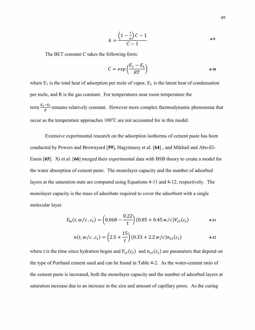
49
(
)
4-9
The BET constant C takes the following form:
(
) 4-10
where E1 is the total heat of adsorption per mole of vapor, EL is the latent heat of condensation
per mole, and R is the gas constant. For temperatures near room temperature the
term
remains relatively constant. However more complex thermodynamic phenomena that
occur as the temperature approaches 100oC are not accounted for in this model.
Extensive experimental research on the adsorption isotherms of cement paste has been
conducted by Powers and Brownyard [59], Hagymassy et al. [64] , and Mikhail and Abo-El-
Enein [65]. Xi et al. [66] merged their experimental data with BSB theory to create a model for
the water absorption of cement paste. The monolayer capacity and the number of adsorbed
layers at the saturation state are computed using Equations 4-11 and 4-12, respectively. The
monolayer capacity is the mass of adsorbate required to cover the adsorbent with a single
molecular layer.
( ⁄ ) (
) ( ⁄ ) ( ) 4-11
( ⁄ ) (
) ( ⁄ ) ( ) 4-12
where t is the time since hydration began and ( ) and ( ) are parameters that depend on
the type of Portland cement used and can be found in Table 4-2. As the water-cement ratio of
the cement paste is increased, both the monolayer capacity and the number of adsorbed layers at
saturation increase due to an increase in the size and amount of capillary pores. As the curing

50
time increases, the number of adsorbed layers at saturation decreases due to a decreasing average
pore radius and an increasing monolayer capacity.
The effect of the water-cement ratio on the adsorption isotherm is clearly seen in Figure
4-2. As the water-cement ratio increases, the water content also increases for all values of
relative humidity. This is due to the fact that both the monolayer capacity and the number of
adsorbed layers at saturation rise with an increase in the water-cement ratio. The relationship
between the type of Portland cement and the shape of the adsorption isotherm is unknown; this is
why no function is given to express the parameters ( ) and ( ). However it can be
observed from Figure 4-3 that the isotherms for cement types I, II, and III are very similar while
the isotherm for type IV is noticeably lower.
Once the water content of the cement paste is determined using Equation 4-8, the
equivalent saturation value is determined using the following linear equation:
( )
4-13
where Gs is the specific gravity of the solid portion of the cement paste and is the porosity. By
observing the above equation, it is noted that a specific value of Gs is not needed to convert the
water content to saturation. This is because the degree of saturation at the minimum and
maximum value of the water content is known. When the water content is equal to 0%, the
saturation is also equal to 0%, and when the water content is at its maximum, the saturation is
equal to 100%. Thus Equation 4-13 can be rewritten as:
4-14

51
where Wmax is the water content corresponding to a relative humidity of 100% as determined by
Equation 4-8.
4.2. Factors that Affect the Effective Thermal Conductivity
The variables that influence the effective thermal conductivity of any porous medium
such as cement paste must be determined first before a comprehensive model to predict its ETC
can be developed. The main variables that will be studied are the mineralogical composition of
the solid phase, the temperature, the porosity, and the saturation.
Table 4-1 contains the weight fractions of each of the main components that are found in
typical samples of the five types of Portland cement. Using this information and the
microstructural development theory of Jennings and Tennis [62], the volume fractions at full
hydration of the various hydration products are shown in Figure 4-4 for a water-cement ratio of
0.5. It is observed that the volume fractions of the hydration products in cement paste are
relatively independent of the type of Portland cement used. Since a detailed morphological
model of the microstructure of cement pastes formed from the different types of Portland cement
is not available, it will be assumed here, that at full hydration cement pastes formed by any of the
five types of Portland cement have the same volume fractions of the hydration products.
The principal mechanisms through which heat conduction can occur in solid materials are
molecular and lattice vibrations, and electron transport. For crystalline solids energy is
transported due to all three of these phenomena with the majority of the energy being transported
due to electron movement. In amorphous solids the main mode of heat movement is molecular
vibrations. This is the reason why metals have larger thermal conductivity than ceramic
materials. The vibrations and behavior of the electrons that occur on the atomic and molecular

52
scale are very complex and highly dependent on temperature. If the temperature range of interest
is relatively small, the relationship between the thermal conductivity of a solid and its
temperature can be approximated by using Equation 4-15:
( ) [ ( )] 4-15
where T0 is the reference temperature, k0 is the thermal conductivity at the reference temperature,
and γ is the temperature coefficient of thermal conductivity [67].
The thermal conductivity of liquids can be modeled similarly as that of amorphous solids.
The thermal conductivity of water has been studied extensively and can be modeled using
Equation A-1 [68], which is found in the appendix, and also shown in Figure 4-5. The
conduction of heat through gases and vapors can be understood using the kinetic theory of gases.
The thermal conductivity of dry air, , and water vapor, , are given in the appendix by
Equations A-2 and A-3 [69], respectively and are shown in Figure 4-6. The gaseous phase
present in cement paste will typically be humid air. An expression for the thermal conductivity
of humid air has been reported by Tsilingiris [70]:
( )
4-16
where xv is the molar fraction of vapor water given by the following equation:
( )
4-17
In Equation 4-17, Psv is the saturated vapor pressure, Po is the total pressure, and f(P,T) is
an enhancement factor that drops out of the above equation because, as shown in [70], it is very
close to unity for temperatures below 100oC. An equation for the saturated vapor pressure is
given in the appendix (Equation A-4) and Figure 4-7 illustrates the thermal conductivity of
humid air for different values of relative humidity at atmospheric pressure.

53
The porosity of cement paste is controlled primarily by the water-cement ratio of the mix
and the addition of entrained air. Figure 4-1 illustrates the volume fractions of the cement gel
solids, the cement gel pores, and the capillary pores for cement pastes having water-cement
ratios between 0.36 and 0.86 using Powers and Brownyard's model. As the water-cement ratio is
increased, the relative amount of the larger capillary pores also increases, while the relative
amount of the much smaller cement gel pores and cement gel solids decreases. Based on this
observation it is assumed that holding all other variables constant, the thermal conductivity of
fully hydrated cement paste must decrease as the water-cement ratio is increased. The effects of
air entrainment will not be discussed here.
The last variable that influences the thermal conductivity of cement paste is saturation.
By comparing Figure 4-5 and Figure 4-7, it is observed that the thermal conductivity of water is
approximately 20 times that of humid air for temperatures between 0oC and 100
oC. If all other
variables are held constant the thermal conductivity of cement paste will increase as the degree
of saturation is increased.
4.3. Current Models
Kim et al. [71] developed an empirical model to predict the thermal conductivity of
concrete. By setting the volume fraction of the aggregate and the percent fine aggregate to zero,
their model can be simplified to specifically deal with cement paste (Equation 4-18).
[ ( ⁄ ) ][ ] 4-18
where kcp is measured in W/m/K and the temperature, T, is measured in oC. Since this model
applies most generally to concrete, it has a large error if simplified for cement paste even when it
is compared to the authors’ own data. This is due to the fact that the model was calibrated

54
primarily for an aggregate volume ratio between 0.5 and 0.7. By performing a multivariate
linear regression analysis on their data for just cement paste, it is found that the leading
coefficient in Equation 4-18 changes from 0.62 to 0.80. Figure 4-8 compares this modified
model to the data from Kim et al. From the data it is observed that the thermal conductivity is
slightly lower at a water-cement ratio of 0.25 than it is at 0.3. This contradicts the requirement
that the thermal conductivity should decrease as the water-cement ratio increases. A possible
reason for this occurrence may be that at the water-cement ratios of 0.25 and 0.30 the cement
paste cannot fully hydrate, resulting in unhydrated cement grains embedded in the cement paste.
This phenomenon will not be discussed any further because the model developed in this report
applies only to fully hydrated cement paste.
Valore [72] and the report of ACI Committee 122 [32] both present a figure showing the
relationship between the water-cement ratio and the thermal conductivity of air-dried cement
paste. No raw data or equation was given for this data; however Equation 4-19 provides a good
empirical fit (Figure 4-9).
( ⁄ ) 4-19
Choktaweekarn et al. [73] developed a model to predict the thermal conductivity of
hydrating concrete with the addition of fly ash that is based on the parallel heat flow model.
Their model simplified for cement paste with no fly ash and assuming complete hydration is:
4-20
where the subscript, hp, stands for the hydration product. The various volume fractions can be
found by using the microstructural development theory of cement paste presented by Hansen
[61] along with knowledge of the degree of saturation. Using a regression analysis,
Choktaweekarn et al. determined the thermal conductivity of the hydration products to be 1.16

55
W/m/K. Figure 4-9 displays the thermal conductivity for cement pastes as a function of the
water-cement ratio for both oven dry and fully saturated samples using the model developed by
Choktaweekarn et al. It is observed from Figure 4-9 that this model predicts values for oven dry
cement paste that lie above those of an air-dry cement paste from ACI 122R-02. This violates the
principle that the thermal conductivity of a porous medium increases as the saturation increases.
The reason for this is that the model of Choktaweekarn et al. is based on the parallel heat flow
model, which gives the absolute upper bound for the ETC of a composite medium.
Other experimental values for the thermal conductivity of cement paste were reported by
Xu and Chung [74] and Fu and Chung [75]. The thermal properties of cement pastes were
measured by Fu and Chung for a water-cement ratio of 0.45 on air dry samples and by Xu and
Chung for a water-cement ratio of 0.35 (degree of saturation not known). Their results are
summarized in Table 4-3.
4.4. Proposed Model
The desired characteristics of a model to compute the effective thermal conductivity of
cement paste are that it: a) is based on thermodynamic and physical principles, b) provides
predictions lying between the established limits for isotropic materials, and c) considers
temperature and relative humidity along with the water-cement ratio and saturation of the cement
paste. The models previously discussed to compute the ETC fall short in several respects and
consequently prove inadequate. The model of Kim et al. and ACI 122R-02 are empirical in
nature, and since the model developed by Choktaweekarn et al. uses the parallel heat flow model,
it predicts values above the upper limit for isotropic materials. Additionally none of the models
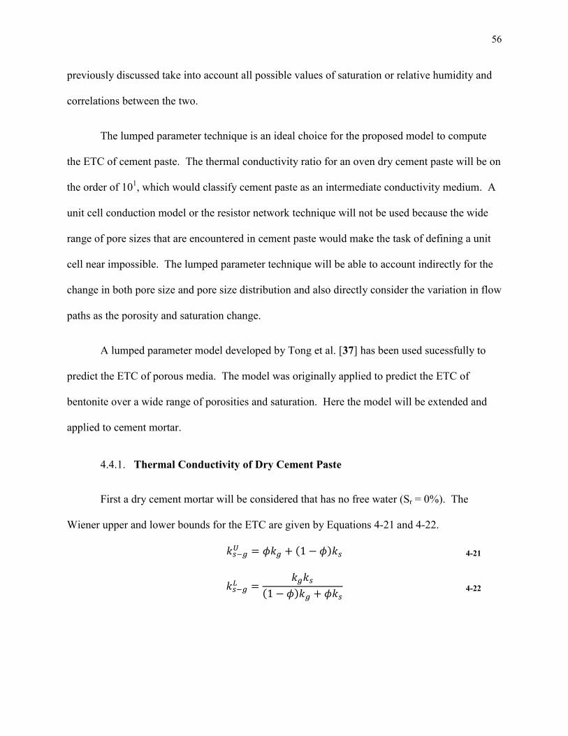
56
previously discussed take into account all possible values of saturation or relative humidity and
correlations between the two.
The lumped parameter technique is an ideal choice for the proposed model to compute
the ETC of cement paste. The thermal conductivity ratio for an oven dry cement paste will be on
the order of 101, which would classify cement paste as an intermediate conductivity medium. A
unit cell conduction model or the resistor network technique will not be used because the wide
range of pore sizes that are encountered in cement paste would make the task of defining a unit
cell near impossible. The lumped parameter technique will be able to account indirectly for the
change in both pore size and pore size distribution and also directly consider the variation in flow
paths as the porosity and saturation change.
A lumped parameter model developed by Tong et al. [37] has been used sucessfully to
predict the ETC of porous media. The model was originally applied to predict the ETC of
bentonite over a wide range of porosities and saturation. Here the model will be extended and
applied to cement mortar.
4.4.1. Thermal Conductivity of Dry Cement Paste
First a dry cement mortar will be considered that has no free water (Sr = 0%). The
Wiener upper and lower bounds for the ETC are given by Equations 4-21 and 4-22.
( ) 4-21
( )
4-22

57
where φ is the total porosity of the cement paste (the sum of the capillary and gel porosity). If
heat flow through cement paste is thought of as a combination of series and parallel paths, the
ETC of the dry cement paste can be expressed by the following equation:
( )
4-23
This is schematically shown in Figure 4-10. Equations 4-21 and 4-22 can be substituted into
Equation 4-23 and expressed as:
( ) ( )
( ) 4-24
The parameter η1 is dependent on the pore-structure of the cement paste and should vary
as a function of both the water-cement ratio and Portland cement type. For a general porous
medium the limits on its value are η For an isotropic porous medium the limits would
be more stringent so that the ETC lies between the Hashin-Shtrikman bounds. The bounds on η1
for cement paste can be further refined by characterizing it as an internally porous medium.
These bounds are shown in the appendix (Equation A-5). It is assumed that the following
functional relationship applies:
4-25
4.4.2. Thermal Conductivity of Saturated Cement Paste
The ETC of cement paste at any degree of saturation is computed by once again
considering the Wiener upper and lower bounds.
( ) ( )( ) ( ) 4-26
( )
[ ( )]
[( )( )
( )
]
4-27

58
If the flow of heat through cement paste is thought of as a combination of series and parallel
paths the ETC of the cement paste can be expressed by the following equation:
( )
4-28
This is schematically shown in Figure 4-11. Equations 4-26 and 4-27 can be substituted into
Equation 4-28 and expressed as:
( ) ( )[ ( )]
[( )( )
( )
]
[( )( ) ( )]
4-29
The parameter η2 is dependent on both the pore-structure and the degree of saturation of cement
paste. It should vary as a function of the water-cement ratio, Portland cement type, and relative
humidity. For a general porous medium the limits on its value are η . For an isotropic
porous medium the limits would be more stringent so that the ETC lies between the Hashin-
Shtrikman bounds. These bounds are shown in the appendix (Equation A-8). It is assumed in
Tong et al. that the following functional relationship applies:
4-30
The input parameters for the model are the ambient temperature, the relative humidity
inside the cement paste, the Portland cement type, and the water-cement ratio. The thermal
conductivity of the free water and air are determined using Equations A-1 and 4-16, respectively.
The porosity of the cement paste is calculated by using the microstructural development theory
of Powers and Brownyard (Section 4.1.3) and the saturation of the pore space is found using the
BSB model of water adsorption (Section 4.1.4).

59
4.4.3. ETC of Dry Cement Paste: Model Calibration
The test results for the thermal conductivity of the dry cement samples are shown in
Table 4-4. The value used for the specific heat capacity of dry cement paste was determined by
Fu and Chung [76] to be 0.703 J/g/K. This value was calculated for a paste with a water-cement
ratio of 0.4. If it is assumed that the specific heat capacity and density of air are negligible
compared to those of the solid portion of cement paste, then the value determined by Fu and
Chung is valid for all water-cement ratios where full hydration is possible. This is because,
regardless of the water-cement ratio, there is always 1 gram of solid cement gel in 1 gram of
cement paste. The density of dry cement paste was calculated using Hansen's model for the
microstructure of cement paste. By subtracting Equation 4-2 from Equation 4-6 and multiplying
the result by 2.51 cm3/g, which is the density of the solid cement gel [61], the density of fully
hydrated dry cement paste is given by:
4-31
The value for the thermal conductivity of the solid portion of the cement paste was
determined to be in the range of 1.05 – 1.18 W/m/K. This range was chosen so that the ETC of
the dry cement paste would lie between that of the Hashin-Shtrikman upper bound and the EMT
equation. The coefficients for Equation 4-25 were computed using a least squares fitting
method. Using a value of 1.12 W/m/K for ks, the coefficients c1 and c2 were determined to be
0.5631 and 0.3130, respectively. Figure 4-12 shows the results of the proposed model along with
the Hashin-Shtrikman upper bound, the EMT curve, and the ACI equation. The R2 coefficient for
the proposed model with respect to the experimental data is 0.98.

60
4.4.4. ETC of Dry Cement Paste: Model Validation
Figure 4-12 compares the proposed model for the ETC of dry cement paste to the ACI
equation [32]. The largest percent difference between the proposed model and the ACI equation
is 2.3%, which occurs at a water-cement ratio of 0.8. Additionally the experimentally
determined value for the thermal conductivity of the solid portion of the cement paste (1.12
W/m/K) is in good agreement with the value of 1.16 W/m/K, which was reported by
Choktaweekarn et al. [73].
4.4.5. ETC of Fully Saturated Cement Paste: Model Calibration
Since fully saturated cement paste will be modeled as an internally porous material, the
equation that describes its ETC must lie between the Hashin-Shtrikman upper bound and the
EMT line. As seen in Figure 4-13, the Hashin-Shtrikman upper bound and the EMT line are very
close for saturated cement paste; the difference between the two is of the order of 0.5%.
Therefore it will be assumed that the ETC of saturated cement paste is equal to the mean of the
Hashin-Shtrikman upper bound and the EMT equation.
If Equation 4-30 is used to describe the parameter η2, the coefficient c3 is calculated by
setting the saturation equal to one and performing a least squares fitting method. When cement
paste is fully saturated, Equation 4-30 simplifies to:
4-32
and the coefficient c3 is 0.21.
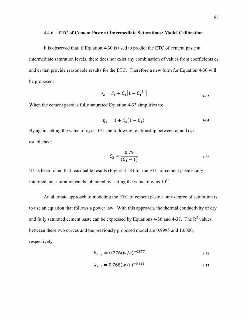
61
4.4.6. ETC of Cement Paste at Intermediate Saturations: Model Calibration
It is observed that, if Equation 4-30 is used to predict the ETC of cement paste at
intermediate saturation levels, there does not exist any combination of values from coefficients c4
and c5 that provide reasonable results for the ETC. Therefore a new form for Equation 4-30 will
be proposed:
[
] 4-33
When the cement paste is fully saturated Equation 4-33 simplifies to:
( ) 4-34
By again setting the value of η2 as 0.21 the following relationship between c3 and c4 is
established:
( ) 4-35
It has been found that reasonable results (Figure 4-14) for the ETC of cement paste at any
intermediate saturation can be obtained by setting the value of c4 as 1012
.
An alternate approach to modeling the ETC of cement paste at any degree of saturation is
to use an equation that follows a power law. With this approach, the thermal conductivity of dry
and fully saturated cement paste can be expressed by Equations 4-36 and 4-37. The R2 values
between these two curves and the previously proposed model are 0.9995 and 1.0000,
respectively.
( ⁄ ) 4-36
( ⁄ ) 4-37

62
If it is assumed that the two coefficients in the power law equation vary linearly with the degree
of saturation, the following equation can be used to compute the ETC of cement paste at any
saturation (Figure 4-15):
( )( ⁄ )( ) 4-38
4.5. Summary
This chapter outlines the various factors that affect the ETC of cement pastes and
proposes a lumped parameter model to predict their values. These factors include the volume
fraction of the different components of cement paste, the degree of saturation, and the
temperature. It assumes that the components consist of the solid portion of the cement gel, gel
pores, and capillary pores. No distinction is made between the gel and capillary pores, and the
sum of their volume fractions is termed the porosity of the cement paste. The microstructural
development theory of Powers and Brownyard is used to compute the porosity of the cement
paste in terms of the water-cement ratio, and the BSB model of water adsorption (developed by
Brunauer, Skalny, and Bodor) is used to determine the saturation of the pore space in terms of
the relative humidity. Existing models are also reviewed that determine the thermal conductivity
of the water or air occupying the pore space.
A lumped parameter model is proposed to compute the ETC of cement paste in terms of
the porosity and degree of saturation. This model does not include the influence of temperature.
This model was calibrated experimentally for dry cement paste by using the flash method to
measure the ETC. The proposed model is in good agreement with an empirical model proposed
by ACI. Additionally the thermal conductivity of the solid portion of the cement paste was
calculated as 1.12 W/m/K which is in good agreement with values found in the literature. The

63
proposed model was also calibrated for the case of fully saturated cement paste by fitting it
between the Hashin-Shtrikman upper bound and the EMT equation. The model also predicts the
ETC for intermediate degrees of saturation between 0% (oven dry) and 100% (fully saturated).
However due to a lack of data, it could not be calibrated or validated.
The following factors affect the ETC of cement paste:
When the paste is fully hydrated the ETC decreases with an increase in the water-cement
ratio due to an increase in the volume fraction of the gel pores and capillary pores.
The ETC increases as the degree of saturation increases, because as the saturation
increases, air in the pore space is replaced by water, which has a higher thermal
conductivity than air.

64
Name of
Compound
Oxide
Composition
Abbreviation Percent by Weight
Type I Type II Type III Type IV Type V
Tricalcium
Silicate 3CaO∙SiO2 C3S 55 51 57 28 38
Dicalcium
Silicate 2CaO∙SiO2 C2S 19 24 19 49 43
Tricalcium
Aluminate 3CaO∙Al2O3 C3A 10 6 10 4 4
Tetracalcium
Aluminoferrite
4CaO∙Al2O3∙
Fe2O3 C4AF 7 11 7 12 9
Table 4-1: Typical Compositions of Cement Types
Portland Cement Type Vct nct
I 0.9 1.1
II 1.0 1.0
III 0.85 1.15
IV 0.6 1.5
Table 4-2: Constants Used in BSB Model [71]
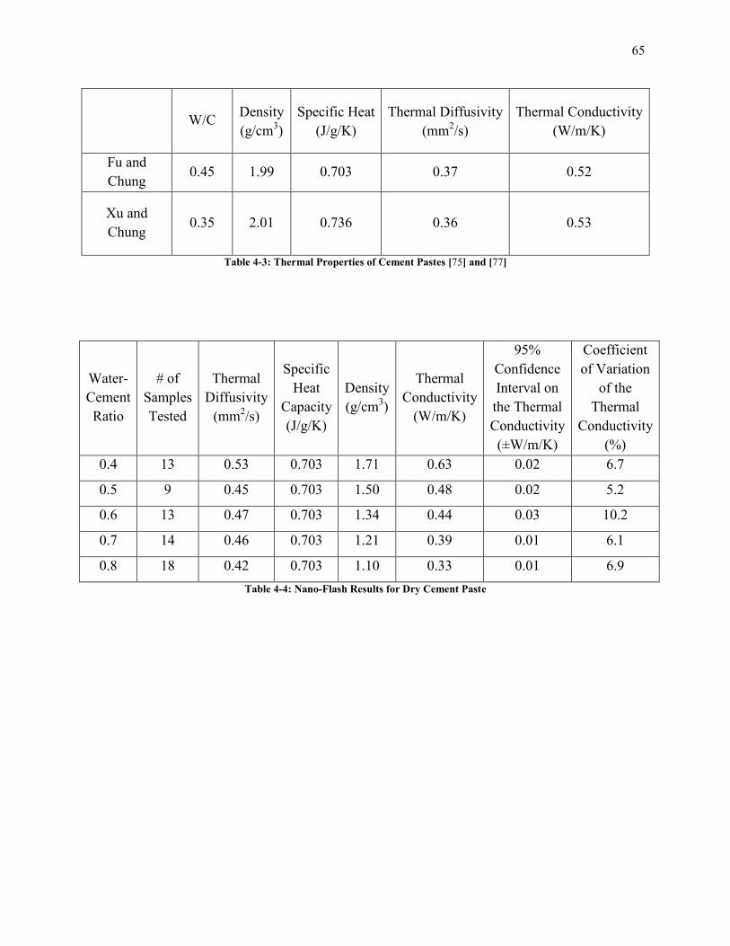
65
W/C Density
(g/cm3)
Specific Heat
(J/g/K)
Thermal Diffusivity
(mm2/s)
Thermal Conductivity
(W/m/K)
Fu and
Chung 0.45 1.99 0.703 0.37 0.52
Xu and
Chung 0.35 2.01 0.736 0.36 0.53
Table 4-3: Thermal Properties of Cement Pastes [75] and [77]
Water-
Cement
Ratio
# of
Samples
Tested
Thermal
Diffusivity
(mm2/s)
Specific
Heat
Capacity
(J/g/K)
Density
(g/cm3)
Thermal
Conductivity
(W/m/K)
95%
Confidence
Interval on
the Thermal
Conductivity
(±W/m/K)
Coefficient
of Variation
of the
Thermal
Conductivity
(%)
0.4 13 0.53 0.703 1.71 0.63 0.02 6.7
0.5 9 0.45 0.703 1.50 0.48 0.02 5.2
0.6 13 0.47 0.703 1.34 0.44 0.03 10.2
0.7 14 0.46 0.703 1.21 0.39 0.01 6.1
0.8 18 0.42 0.703 1.10 0.33 0.01 6.9
Table 4-4: Nano-Flash Results for Dry Cement Paste

66
Figure 4-1: Volume Fraction of Hydration Products Using Powers and Brownyard’s [59] Model
Figure 4-2: Water Adsorption for Fully Hydrated Type I Cement Paste [71]
0.0
0.2
0.4
0.6
0.8
1.0
0.36 0.46 0.56 0.66 0.76 0.86
Vo
lum
e F
ract
ion
Water-Cement Ratio
Solid Cement Gel Capillary Pores Gel Pores
0.00
0.10
0.20
0.30
0.40
0% 20% 40% 60% 80% 100%
Wat
er
Co
nte
nt
Relative Humidity
w/c = 0.8 w/c = 0.7 w/c = 0.6 w/c = 0.5 w/c = 0.4

67
Figure 4-3: Water Adsorption for Fully Hydrated Cement Pastes (w/c = 0.4)
Figure 4-4: Volume Fractions of Hydration Products for Different Cement Types (w/c = 0.5)
0.00
0.05
0.10
0.15
0.20
0% 20% 40% 60% 80% 100%
Wat
er
Co
nte
nt
Relative Humidity
Type I Type II Type III Type IV
0%
10%
20%
30%
40%
50%
CH AFm (C-S-H)solids (C-S-H)pores Capillary Pores
I
II
III
IV
V

68
Figure 4-5: Thermal Conductivity of Water
Figure 4-6: Thermal Conductivity of Dry Air (ka) and Water Vapor (kv)
0.55
0.60
0.65
0.70
0 10 20 30 40 50 60 70 80 90 100
The
rmal
Co
nd
uct
ivit
y (W
/mK
)
Temperature (oC)
0.015
0.020
0.025
0.030
0.035
0 20 40 60 80 100
The
rmal
Co
nd
uct
ivit
y (W
/mK
)
Temperature (oC)
ka
kv

69
Figure 4-7: Thermal Conductivity of Humid Air [70]
Figure 4-8: Model of Kim et al. [71] for the Thermal Conductivity of Cement Paste
(Lines represent the model and data points are the raw data)
0.020
0.025
0.030
0.035
0 20 40 60 80 100
The
rmal
Co
nd
uct
ivit
y (W
/mK
)
Temperature (oC)
Rh = 0%
Rh = 20%
Rh = 40%
Rh = 60%
Rh = 80%
Rh = 100%
0.50
0.60
0.70
0.80
0.90
1.00
0.25 0.3 0.35 0.4
The
rmal
Co
nd
uct
ivit
y (W
/mK
)
Water-Cement Ratio
Rh = 100% T = 20⁰C
Rh = 100% T = 60⁰C
Rh = 0% T = 20⁰C
Rh = 0% T = 60⁰C
Rh = 100% T = 20⁰C
Rh = 100% T = 60⁰C
Rh = 0% T = 20⁰C
Rh = 0% T = 60⁰C
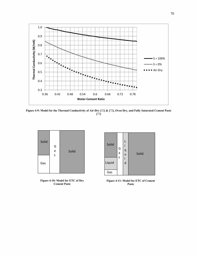
70
Figure 4-9: Model for the Thermal Conductivity of Air-Dry [32] & [72], Oven Dry, and Fully Saturated Cement Paste
[73]
0.3
0.4
0.5
0.6
0.7
0.8
0.9
1.0
0.36 0.42 0.48 0.54 0.6 0.66 0.72 0.78
The
rmal
Co
nd
uct
ivit
y (W
/mK
)
Water-Cement Ratio
S = 100%
S = 0%
Air-Dry
Figure 4-10: Model for ETC of Dry
Cement Paste Figure 4-11: Model for ETC of Cement
Paste
Solid
Solid
Gas
Gas
Solid
Solid
Liquid
Gas
Liquid
Gas

71
Figure 4-12: Proposed Model for the ETC of Dry Cement Paste
Figure 4-13: Proposed Model for the ETC of Fully Saturated Cement Paste
0.2
0.3
0.4
0.5
0.6
0.7
0.4 0.5 0.6 0.7 0.8
The
rmal
Co
nd
uct
ivit
y (W
/m/K
)
Water-Cement Ratio
HSU
Proposed
Data
ACI
EMT
0.80
0.82
0.84
0.86
0.88
0.90
0.92
0.94
0.4 0.5 0.6 0.7 0.8
The
rmal
Co
nd
uct
ivit
y (W
/m/K
)
Water-Cement Ratio
HSU
Proposed
EMT
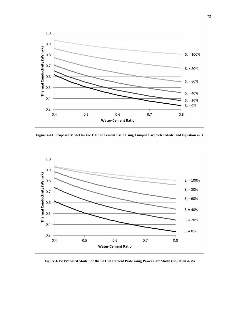
72
Figure 4-14: Proposed Model for the ETC of Cement Paste Using Lumped Parameter Model and Equation 4-34
Figure 4-15: Proposed Model for the ETC of Cement Paste using Power Law Model (Equation 4-38)
0.3
0.4
0.5
0.6
0.7
0.8
0.9
1.0
0.4 0.5 0.6 0.7 0.8
The
rmal
Co
nd
uct
ivit
y (W
/m/K
)
Water-Cement Ratio
Sr = 100%
Sr = 80%
Sr = 60%
Sr = 40%
Sr = 20%
Sr = 0%
0.3
0.4
0.5
0.6
0.7
0.8
0.9
1.0
0.4 0.5 0.6 0.7 0.8
The
rmal
Co
nd
uct
ivit
y (W
/m/K
)
Water-Cement Ratio
Sr = 100%
Sr = 80%
Sr = 60%
Sr = 40%
Sr = 20%
Sr = 0%
73
Chapter 5. Effective Thermal Conductivity of Portland Cement Mortar
5.1. Introduction
By itself cement paste has limited applications and is generally not thought of as an
engineering material. Cement mortar is created by adding fine aggregate to cement paste, which
lowers the overall cost and also transforms the paste to a useful engineering material. Normal
weight aggregate is generally cheaper than cement paste, thus cement mortar has a lower cost per
unit volume than cement paste. Also the addition of fine aggregate increases many desired
properties, including strength; durability; and resistance to shrinkage, creep, and wear. Typically
Portland cement mortar (PCM) consists of 50% fine aggregate by volume.
5.1.1. Types of Fine Aggregate
Generally the type of fine aggregate used will depend on the region where the concrete is
being placed. For typical applications most types of rock are suitable to produce fine aggregate
as long as it conforms to ASTM C 33 [78]. The presence of deleterious substances such as clay,
silt, friable particles, and organic matter will lower the quality of the mortar produced with the
aggregate. Also the aggregate should be chemically stable in concrete to avoid adverse
reactions, such as the well-studied alkali-silica reaction. The gradation of fine aggregate must
conform to the prescription of ASTM C 33 (Figure 5-1) with 100% of the aggregate passing the
3/8” sieve (9.5mm) and less than 10% passing the No. 100 sieve (150 μm). While there exist
many special types of fine aggregate, such as lightweight fine aggregate, this chapter will only
focus on normal weight fine aggregate.

74
5.1.2. Factors Affecting the Effective Thermal Conductivity of Fine Aggregate
The main factors that influence the ETC of both the parent rock and the aggregate are its
mineralogical composition, porosity, and degree of saturation. The two methods for obtaining
normal weight fine aggregate are to source natural deposits of sand or to crush gravel or larger
rock fragments. Since both the production and natural formation of fine aggregate are a
mechanical process and not a chemical one, it will be assumed that the mineralogical
composition of the aggregate is the same as that of the parent rock. During the crushing process
internal cracks may form within the aggregate which would increase its porosity.
5.1.3. Factors Affecting the Effective Thermal Conductivity of Cement Mortar
The ETC of cement mortar will be influenced by the following parameters: the thermal
conductivities of the fine aggregate and the cement paste; the shape, texture, and gradation of the
fine aggregate; the saturation of the cement paste and the fine aggregate; the temperature; and the
size and properties of the interfacial transition zone (ITZ) surrounding the fine aggregate.
5.2. Effective Thermal Conductivity of Fine Aggregate
Fine aggregate consists of three phases: a solid phase (consisting of various types of
minerals), air, and water. Minerals commonly found in concrete aggregate are summarized in
Table 5-1. The thermal conductivity of different rock-forming minerals has been determined by
Horai and Simmons [79] and a selection of their results for several different minerals that are
commonly found in aggregate used in concrete are shown in Table 5-2. Other sources of
information that are not included in this report are Diment and Pratt [80] and Dreyer [81]. There
are some discrepancies when these references are compared due to the fact that the measured

75
thermal conductivity of a specific mineral depends on its purity, the presence of imperfections,
the sample size, and anisotropy [82].
Figure A-1 through Figure A-6 in the appendix illustrate the thermal conductivities of
various dry and water saturated rocks as a function of their mineral content and porosity as
reported by Robertson [83]. The types of rocks included are: sandstone, shale, granite, basalt,
limestone, and dolomite. When these figures are compared to the results for the ETC of cement
paste it is seen that the ETC of the aggregate will generally be higher than that of the paste. As a
result the ETC of cement mortar will be greater than that of cement paste. The effect of
temperature on the thermal conductivity of select types of rocks is shown in Figure A-7 [84]. It
is observed that the temperature and the thermal conductivity of rocks are inversely related, as is
true for most solid materials.
5.3. ETC of Cement Mortar: Effect of Fine Aggregate Shape
The shape and texture of fine aggregate influence the ETC of cement mortar in two ways.
Firstly they affect how the heat flux lines behave when they encounter the aggregate, and
secondly they influence the packing density of the aggregate in the mortar. ASTM D4791 [85]
defines three types of aggregate based on their shape: elongated, flat, and flat and elongated.
While these definitions were developed primarily for coarse aggregate, in this study we will
apply them to fine aggregate as well. The criteria for a particle to be characterized as elongated,
flat, or elongated and flat are that: the ratio of its length to width exceeds 3:1, the ratio of the
width to thickness exceeds 3:1, and the ratio of its length to width exceeds 3:1 as well as the ratio
of the width to thickness exceeding 3:1, respectively. The length, width, and thickness are

76
defined, respectively as the largest, intermediate, and smallest dimension of a particle, where all
three are measured perpendicular to each other.
5.3.1. Differential Multiphase Model
A differential multiphase model (DM model) has been proposed by Phan-Thien and
Pham [86] to compute the ETC of a multiphase material which consists of n different types of
ellipsoidal inclusions distributed in a matrix. The differential equation for the ETC is:
∑4
∑
(
)
5
5-1
with the initial condition ( ) and where The terms (where j = 1, 2, or
3) are the solutions to the elliptic integrals (Equation A-18) based in the shape of the ith
inclusion, is the thermal conductivity of each type of inclusion, is the volume fraction of
each type of inclusion, and is the sum of the volume fractions of the various inclusion phases.
The effective thermal conductivity is the value of evaluated at . Generally Equation 5-1
has to be solved numerically; however for spherical inclusions it results in the following implicit
equation:
.
/ √
5-2
Figure 5-2 displays how the ETC varies with respect to the shape of the inclusion and
porosity. This figure was constructed using a thermal conductivity of the matrix phase of 1.0 and
a thermal conductivity of the inclusion phase of 4.0. When the thermal conductivity of the
inclusion phase is greater than that of the matrix phase, the computed ETC using spherical
inclusions is smaller than the computed ETC using any other particle shape. It is observed that

77
the ETC of the composite rises as the sphericity of the inclusions decreases. Sphericity, Ψ, is a
measure of how round a particle is and it is calculated as the ratio of the surface area of a sphere
with the same volume as the particle, to the actual surface area of the particle. The sphericity of
a perfect sphere is 1.0 and any other particle shape has a sphericity less than 1.0. Table 5-3
displays the sphericity of each type of inclusion along with its maximum percent difference from
Figure 5-2. The sphericity of a particle can be calculated using the following equation:
√
5-3
where is the volume of an inclusion and is the surface area of the inclusion.
It must be noted that this behavior becomes less noticeable as the ratio of the thermal
conductivity of the inclusions to that of the matrix increases. Also this behavior is not correct for
inclusions that have a thermal conductivity less than the matrix.
5.4. ETC of Cement Mortar: Effect of Maximum Volume Fraction
The maximum volume fraction is the largest volume fraction of the inclusion phase that
is possible. Gauss proved that for a system of uniform spheres arranged in a repeating lattice the
maximum volume fraction corresponds to the hexagonal close packing arrangement and is equal
to √ ⁄ . According to the famous Kepler conjecture, which was later proved by
Thomas Callister Hales, there does not exist any random packing of uniform spheres that results
in a maximum volume fraction greater than that of the hexagonal close packing.
The packing of fine aggregate in cement mortar is much more complicated than the
problem considered by Gauss. This is due to the fact that fine aggregate is not made up of

78
uniform spheres and also because the aggregate particles are not arranged in a lattice. In
actuality the aggregate consists of a random distribution of nonspherical particles.
5.4.1. Linear Packing Model
The linear packing model of Yu and Zou [87] is able to compute the maximum volume
fraction for a random arrangement of spherical particles given the relative volume fraction, Xi,
diameter, di, and individual maximum volume fraction of each type of particle, . The
relative volume fraction of each particle is the total volume of that type of particle divided by the
total volume of all of the particles. The maximum volume fraction for n types of particles
(where ) is given by:
.
/ 5-4
where
∑0
.
/ 1
∑
( )
5-5
and
.
/
.
/
5-6
.
/
.
/
5-7
The individual maximum volume fraction of each type of particle in the above equation is
the value that corresponds to its random close-packed (RCP) limit. For spheres this value is 0.64
as reported by Jaeger and Nagel [88] and Torquato et al. [89]. Using the above equations, and a
RCP of 0.64, the maximum packing density corresponding to the ASTM grading curves of

79
Figure 5-1 are given as 0.7717 and 0.7673 for the upper and lower curves, respectively.
Additionally the gradations that result in the highest and lowest maximum packing densities
falling between the maximum and minimum gradation curves were determined to be 0.8491 and
0.6984, respectively (Figure 5-1).
The use of a graded fine aggregate will result in a higher maximum packing fraction than
if monosized aggregate is used. Since the addition of fine aggregate generally increases the ETC
of the cement mortar, the higher maximum packing fraction of graded fine aggregate will allow
for the formation of cement mortar with a higher ETC than is possible with monosized
aggregate. This result is due to the addition of more aggregate particles.
5.4.2. The Modified Differential Multiphase Model
The DM model introduced in Section 5.3 can be extended to include the effect of the
maximum volume fraction. As it stands, when Equation 5-1 is solved it will predict an ETC for
any inclusion volume fraction, even a value of 1.0. In order to consider the effect of the
maximum volume fraction the composite will be modeled as a three phase system. The first
phase will be a part of the matrix phase; it has thermal conductivity and volume
fraction . The second phase is the aggregate phase with thermal conductivity and
volume fraction . The final phase is a fictitious spherical inclusion phase which is the
remainder of the mortar phase; it has thermal conductivity and volume
fraction . Since the sum of all the volume fractions must be equal to one:
5-8
and
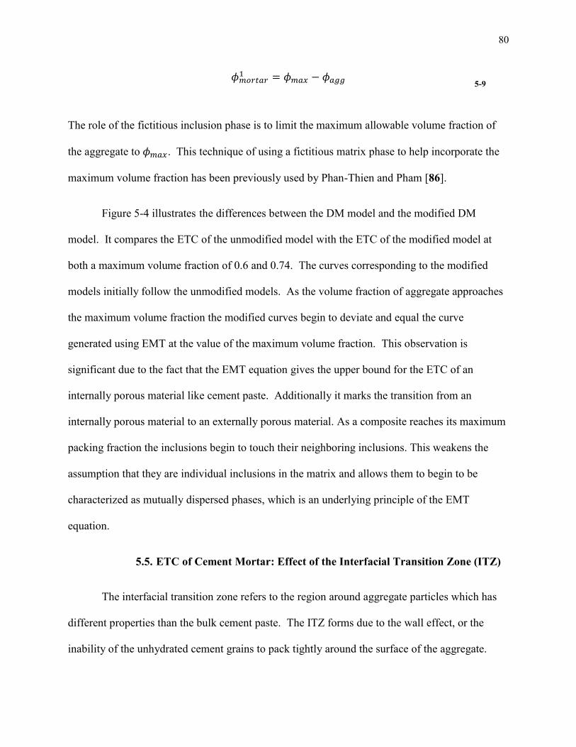
80
5-9
The role of the fictitious inclusion phase is to limit the maximum allowable volume fraction of
the aggregate to . This technique of using a fictitious matrix phase to help incorporate the
maximum volume fraction has been previously used by Phan-Thien and Pham [86].
Figure 5-4 illustrates the differences between the DM model and the modified DM
model. It compares the ETC of the unmodified model with the ETC of the modified model at
both a maximum volume fraction of 0.6 and 0.74. The curves corresponding to the modified
models initially follow the unmodified models. As the volume fraction of aggregate approaches
the maximum volume fraction the modified curves begin to deviate and equal the curve
generated using EMT at the value of the maximum volume fraction. This observation is
significant due to the fact that the EMT equation gives the upper bound for the ETC of an
internally porous material like cement paste. Additionally it marks the transition from an
internally porous material to an externally porous material. As a composite reaches its maximum
packing fraction the inclusions begin to touch their neighboring inclusions. This weakens the
assumption that they are individual inclusions in the matrix and allows them to begin to be
characterized as mutually dispersed phases, which is an underlying principle of the EMT
equation.
5.5. ETC of Cement Mortar: Effect of the Interfacial Transition Zone (ITZ)
The interfacial transition zone refers to the region around aggregate particles which has
different properties than the bulk cement paste. The ITZ forms due to the wall effect, or the
inability of the unhydrated cement grains to pack tightly around the surface of the aggregate.

81
The ITZ and the bulk cement paste have a different porosity and chemical makeup due to the
variation in the water-cement ratio as you go from the surface of the aggregate to the outer edge
of the ITZ. Numerous studies on the effective elastic properties of cementitious materials have
concluded that the presence of the ITZ needs to be considered in any subsequent model [90].
The properties of the ITZ are dependent on the size of the largest unhydrated cement grain, the
roughness of the aggregate, and the overall water-cement ratio of the cement mortar.
Nadeau [91] has developed a self-consistent model that predicts the water-cement ratio of
both the ITZ and the bulk cement paste. This model assumes the aggregate is spherical and
factors takes into account the size and volume fraction ( ) of the fine aggregate as well as the
overall water-cement ratio. However it does not consider the roughness of the aggregate. The
local cement volume fraction is expressed as a function of the distance, r, from the center of the
aggregate:
( ) 8 0 (
)
1
5-10
where ra is the radius of the aggregate, δ is the thickness of the ITZ, and is the cement content
of the bulk paste, which is computed using Equation 5-11.
( )
( ⁄ ) , ( ) *
+-
5-11
The local water-cement ratio in both the ITZ and the bulk paste is then determined based on the
specific gravity of the unhydrated cement grains, Gc, and the local cement volume fraction.
(
)
5-12

82
Figure 5-3 illustrates the local variation of the water-cement ratio through the ITZ of
cement mortar with an initial water-cement ratio of 0.4, an aggregate radius of 1mm, an
aggregate volume fraction of 0.6, and an ITZ thickness of 0.04mm. Using Equation 5-12, the
water-cement ratio at the aggregate surface increases to 1.12 and the water-cement ratio in the
bulk cement paste drops to 0.38. Since the thermal conductivity of cement paste is inversely
proportional to the water-cement ratio, the ITZ effectively creates a thermal insulating shell
around the aggregate particle.
Currently there is no model known to this author that is capable of determining the
ETC of composite spheres imbedded in the matrix where the cap of each sphere is a functionally
graded material (such as the ITZ). There is however a model developed by Felske [92] that
considers composite spheres with homogeneous caps. Each composite sphere consists of a core,
with radius, r3, and thermal conductivity, k3, and a shell with radius, r2, and thermal conductivity,
k2. The ETC of the system is given by equation:
5-13
where km is the thermal conductivity of the matrix and and are given by:
( ) [( ) ( ) ] ( ) [( )
( )
] 5-14
( ) [( ) ( ) ]
( ) [( ) ( )
]
5-15
and additionally:
( )
5-16

83
If each composite sphere is replaced with a homogeneous one (either r2 = r3 or k2 = k3) Felske's
solution reduces to the Maxwell model.
It is possible to predict the ETC of cement mortar composed of uniform sized spherical
aggregate particles by using a combination of Nadeau’s and Felske’s models. The thermal
conductivity of the shell in Felske’s model will be determined by calculating the average water-
cement ratio in the ITZ using Nadeau’s model, and then using the relationship developed in
Chapter 4 between the water-cement ratio and thermal conductivity of cement paste. By
integrating the first part of Equation 5-10 and dividing by the thickness of the ITZ, the average
water-cement ratio in the ITZ is:
⁄
5-17
The conductivity of the matrix phase in Felske’s model will be determined by calculating
the adjusted water-cement ratio in the bulk paste, using Nadeau’s model, and then again using
the relationship for the ETC of cement paste developed in Chapter 4. The adjusted water-cement
ratio in the bulk paste is equal to:
⁄
5-18
Figure 5-5 compares the ETC of cement mortar with an ITZ to cement mortar with no
ITZ. Since the ITZ can be thought of as an insulating shell, the presence of the ITZ decreases
the ETC of cement mortar when compared to the same mortar with no ITZ. As the radius of the
aggregate particle decreases, the ETC also decreases due to the fact that the ITZ occupies a
greater portion of the cement paste. Additionally an increase in the aggregate volume fraction
also decreases the ETC. The results shown in Figure 5-5 should not be interpreted as an exact
prediction, but instead they should be used only for comparative purposes to study the relative

84
effect of the ITZ. As stated before, the Felske model reduces to the Hashin-Shtrikman lower
bound when the composite sphere is replaced by a homogeneous one, and this means that the
model will still underestimate the actual ETC when the sphere is a composite.
5.6. Equivalent Inhomogeneity/Finite Cluster Model
The equivalent inhomogeneity/finite cluster model is a semi-analytical/multi-pole type
solution to the ETC of a suspension of N spherical particles, which was developed by
Mogilevskaya et al. [93]. It is able to precisely account for all of the interactions between
particles and it is applicable to suspensions with any particle size distribution and with interfacial
resistance between the particles and the matrix. This method assumes that both the original
cluster and an equivalent sphere, which has a thermal conductivity equal to the ETC of the
suspension, have the same effect on the temperature field a far distance away.
The ETC is equal to:
⟨
( )⟩
⟨ ( )⟩
5-19
where
⟨ ( )⟩
∑
( )
5-20
The total volume fraction of the spherical particles is and the coefficients ( ) are
determined by solving the following infinite series of equations:
( ) ( )
( ) ( ) ∑∑ ∑
( ) ( )
5-21
where , and
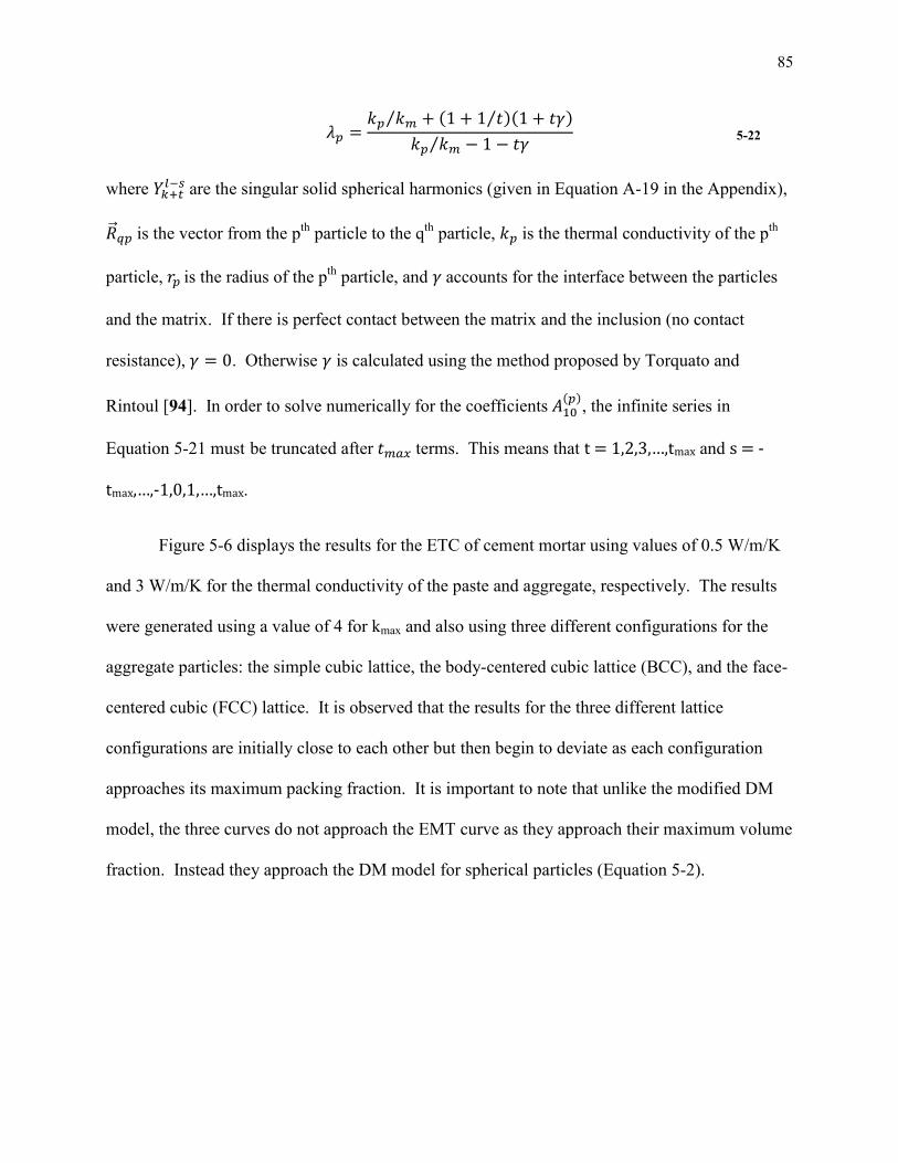
85
⁄ ( ⁄ )( )
⁄ 5-22
where are the singular solid spherical harmonics (given in Equation A-19 in the Appendix),
is the vector from the pth
particle to the qth
particle, is the thermal conductivity of the pth
particle, is the radius of the pth
particle, and accounts for the interface between the particles
and the matrix. If there is perfect contact between the matrix and the inclusion (no contact
resistance), . Otherwise is calculated using the method proposed by Torquato and
Rintoul [94]. In order to solve numerically for the coefficients ( )
, the infinite series in
Equation 5-21 must be truncated after terms. This means that t tmax and s = -
tmax -1,0,1, tmax.
Figure 5-6 displays the results for the ETC of cement mortar using values of 0.5 W/m/K
and 3 W/m/K for the thermal conductivity of the paste and aggregate, respectively. The results
were generated using a value of 4 for kmax and also using three different configurations for the
aggregate particles: the simple cubic lattice, the body-centered cubic lattice (BCC), and the face-
centered cubic (FCC) lattice. It is observed that the results for the three different lattice
configurations are initially close to each other but then begin to deviate as each configuration
approaches its maximum packing fraction. It is important to note that unlike the modified DM
model, the three curves do not approach the EMT curve as they approach their maximum volume
fraction. Instead they approach the DM model for spherical particles (Equation 5-2).

86
5.7. Current Models for the ETC of Cement Mortar
As discussed in Section 4.3 Kim et al. [71] developed an empirical model to predict the
thermal conductivity of concrete. By setting the percent fine aggregate to 100% their model can
be simplified to deal specifically with cement mortar:
[ ⁄ ][ ][ ] 5-23
where is the volume fraction of the aggregate and is the relative humidity.
The applicability of this model is questionable considering that it was calibrated
specifically for concrete and not cement mortar. Kim et al. did however test one mix that was
just cement mortar (no coarse aggregate) which is plotted on Figure 5-7 as a black data point.
This sample had a water-cement ratio, aggregate volume fraction, and relative humidity of 0.40,
0.42, and 100%, respectively. Equation 5-23 predicts an ETC of 2.17 W/m/K, while Kim et al.
measured a value of 2.07 W/m/K. Figure 5-7 displays Equation 5-23 for an aggregate volume
fraction of 0.25, 0.42, and 0.50 along with Kim et al.'s model for cement paste (Equation 4-18).
The fine aggregate used in this study was river sand from Keumkang Mountain, which
had a specific gravity of 2.55 and a fineness modulus of 2.95. Since the model proposed by Kim
et al. does not have an adjustable parameter which accounts for the thermal conductivity of the
aggregate, caution must be used if it is used to predict the ETC of concrete which contains a
different type of fine aggregate.
Also discussed in Section 4.3 was a method developed by Choktaweekarn et al. [73],
which was based on the parallel heat flow model to predict the thermal conductivity of hydrating
concrete with the addition of fly ash. Equation 2-24 presents a version of their model that is
simplified for cement mortar with no fly ash and assuming complete hydration is:
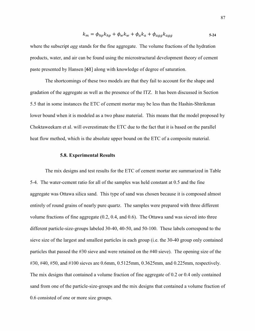
87
5-24
where the subscript agg stands for the fine aggregate. The volume fractions of the hydration
products, water, and air can be found using the microstructural development theory of cement
paste presented by Hansen [61] along with knowledge of degree of saturation.
The shortcomings of these two models are that they fail to account for the shape and
gradation of the aggregate as well as the presence of the ITZ. It has been discussed in Section
5.5 that in some instances the ETC of cement mortar may be less than the Hashin-Shtrikman
lower bound when it is modeled as a two phase material. This means that the model proposed by
Choktaweekarn et al. will overestimate the ETC due to the fact that it is based on the parallel
heat flow method, which is the absolute upper bound on the ETC of a composite material.
5.8. Experimental Results
The mix designs and test results for the ETC of cement mortar are summarized in Table
5-4. The water-cement ratio for all of the samples was held constant at 0.5 and the fine
aggregate was Ottawa silica sand. This type of sand was chosen because it is composed almost
entirely of round grains of nearly pure quartz. The samples were prepared with three different
volume fractions of fine aggregate (0.2, 0.4, and 0.6). The Ottawa sand was sieved into three
different particle-size-groups labeled 30-40, 40-50, and 50-100. These labels correspond to the
sieve size of the largest and smallest particles in each group (i.e. the 30-40 group only contained
particles that passed the #30 sieve and were retained on the #40 sieve). The opening size of the
#30, #40, #50, and #100 sieves are 0.6mm, 0.5125mm, 0.3625mm, and 0.225mm, respectively.
The mix designs that contained a volume fraction of fine aggregate of 0.2 or 0.4 only contained
sand from one of the particle-size-groups and the mix designs that contained a volume fraction of
0.6 consisted of one or more size groups.

88
All of the specimens were tested using the flash method described in Chapter 3. The
thermal conductivity of each mix design was calculated as the average of three identical samples
and each individual sample was tested three times. The tests results are shown in Figure 5-8. It
is observed that the ETC of the cement mortar increases as the aggregate volume fraction is
increased. Additionally, by comparing the first six mix designs, it is seen that, if the volume
fraction is held constant the mix with the smallest aggregate sizes has the lowest ETC. This
effect can be explained by considering the presence of the ITZ. As previously discussed in
Section 5.5, if the volume fraction of fine aggregate is held constant, a mix with smaller sized
aggregate particles will contain more cement paste that is part of the ITZ. Since the ITZ has a
lower thermal conductivity than the bulk paste, it lowers the ETC of the cement mortar. For the
mix designs that contained more than one particle-size-group, the relationship between the ETC
and the relative amounts and sizes of the different aggregate particles is less clear. Figure 5-9
displays the experimental results and compares them to the EMT curve and the Hashin-
Shtrikman Lower bound. These two curves were generated using values of 0.51 W/m/K and 2.5
W/m/K for the thermal conductivity of the cement paste and the aggregate, respectively.
5.9. Proposed Model
The differential multiphase model (DM model) modified to account for the maximum
volume fraction subsequently will be used to model the ETC of cement mortar. The model was
chosen because it can take into account both the maximum volume fraction and the shape of the
aggregate. Additionally it can indirectly model the effect of polydiversity in the aggregate size
by using the linear packing model to adjust the maximum volume fraction. Even though the
equivalent inhomogeneity/finite cluster model can take polydiversity directly into account, it was
not chosen due to the amount of computational resources that are needed to generate the finite

89
cluster of inclusions and also solve Equation 5-21. In contrast, the numerical implementation of
the linear packing model and the DM model are straightforward and computationally quicker.
The proposed model (φmax = 0.64, kpaste = 0.51 W/m/K, and kagg = 2.5 W/m/K) is compared to
the experimental results in Figure 5-10, and there is good agreement between the proposed
model and the experimental results. Figure 5-11 displays the ETC of cement mortar as a
function water-cement ratio for various volume fractions of fine aggregate.
5.10. Summary
The differential multiphase model is introduced in this chapter where it is used to predict
the ETC of cement mortar. The factors that influence the ETC are also discussed. These factors
include the thermal conductivities of the cement paste and aggregate, the shape and gradation of
the aggregate particles, and the presence of the ITZ on the surface of the aggregate. Finally the
results of the proposed model are compared to experimental data for cement mortar containing
Ottawa silica sand as the fine aggregate and there is good agreement between the results.
The elliptical integrals contained in the DM model account for the shape of the aggregate
particles. It is seen that particles with a higher sphericity have a smaller impact on the ETC, and
that nonspherical aggregate particles have a larger impact than spherical ones. The gradation of
the aggregate is included in the proposed model by using the linear packing model to determine
the maximum volume fraction of the aggregate in the cement mortar. It has been shown that a
graded particle size distribution will allow a higher volume fraction of aggregate in the cement
mortar. Once the maximum volume fraction is known, a fictitious inclusion phase with the same
thermal conductivity as the cement paste is included. This fictitious phase limits the amount of
aggregate that can be placed in the mortar and as the maximum volume fraction is approached,
this fictitious phase causes the ETC to be higher than if it were not present.
90
The ITZ is the region surrounding the aggregate particles that has a lower water-cement
ratio than the bulk cement paste. In effect this creates an insulating blanket around the aggregate
which lowers the ETC of the cement mortar. A model proposed by Nadeau is able to predict the
water-cement ratio in this region; however it cannot be integrated with the DM model. This is
because the DM model only considers homogeneous particles, whereas to include the ITZ, the
particles would be composite spheres surrounded by a functionally graded cap. Despite this
drawback, some additional observations concerning the effect of the ITZ on the ETC have been
made, namely that the effect of the ITZ is more pronounced for smaller sized particles. This
means that, holding all other parameters constant, the ETC of cement mortar with larger
aggregate particles will be greater than the ETC of cement mortar with smaller aggregate
particles. This is consistent with previous research [90] into the effective mechanical properties
of cement mortar which have concluded that it must be modeled as a three-phase material
(cement paste, aggregate, and ITZ) and not as a two-phase material (cement paste and
aggregate).

91
Mineral Group Examples
Silica Quartz, Opal, Chalcedony, Tridymite, & Cristobalite
Feldspar Potassium Feldspars, Sodium Feldspars, & Calcium Feldspars
Ferromagnesian Minerals Amphiboles, Pyroxenes, Olivines, and Dark Micas
Micaceous Minerals Muscovites, Biotites, Lepidolites, Chlorites, and Vermiculites
Clay Minerals Kaolinites, Illites, Chlorites, Smectites, & Montmorillonites
Zeolites Heulandite, Natrolite, & Laumonite
Carbonate Minerals Calcite & Dolomite
Sulphate Minerals Gypsum
Iron Sulphide Minerals Pyrite, Marcasite, & Pyrrhotite
Iron Oxides Magnetite, Haematite, Ilmenite, and Limonite
Table 5-1: Minerals Found in Concrete Aggregate [95] & [96]
Mineral Thermal Conductivity (W/m/K) Mineral Thermal Conductivity (W/m/K)
Quartz 18.37 Lepidolites 4.53 – 4.60
Fused Quartz 3.25 Calcite 8.58
Amphiboles 5.81 – 9.02 Dolomite 13.16
Pyroxenes 9.67 – 11.85 Pyrite 45.89
Olivines 7.55 – 12.32 Magnetite 12.18
Muscovites 5.29 – 5.96 Haematite 26.95
Biotites 4.06 – 5.59 Ilmenite 5.25
Table 5-2: Thermal Conductivity of Selected Minerals Found in Concrete Aggregate [79]

92
Type of Particle Aspect Ratio Sphericity Maximum Percent Difference (%)
Elongated (3:1:1) 0.846 1.8
Flat (3:3:1) 0.796 2.4
Elongated (9:1:1) 0.609 3.8
Elongated and Flat (9:3:1) 0.592 4.6
Flat (9:9:1) 0.446 6.6
Elongated and Flat (18:9:1) 0.358 7.5
Table 5-3: Data Relating to Figure 5-2
Mix
#
Volume Fraction of Fine
Aggregate
Aggregate Particle Size
Group*
Thermal Conductivity
(W/m/K)
1 0.2 40-50 0.71
2 0.2 50-100 0.67
3 0.4 40-50 1.16
4 0.4 50-100 1.11
5 0.6 40-50 1.41
6 0.6 50-100 1.36
7 0.6 40-50 (0.3)
50-100 (0.3) 1.49
8 0.6
30-40 (0.2)
40-50 (0.3)
50-100 (0.3)
1.47
9 0.6 40-50 (0.5)
50-100 (0.1) 1.40
10 0.6 30-40 (0.5)
40-50 (0.1) 1.45
*Individual volume fraction in parenthesis Table 5-4: Experimental Results
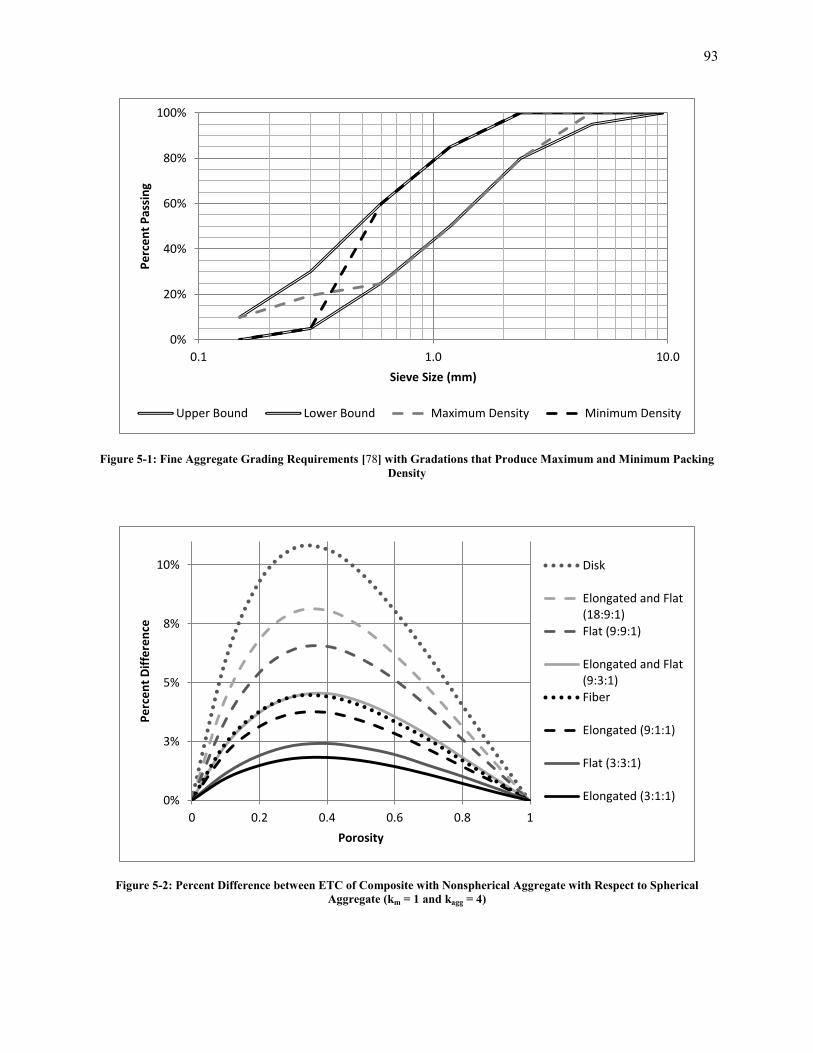
93
Figure 5-1: Fine Aggregate Grading Requirements [78] with Gradations that Produce Maximum and Minimum Packing
Density
Figure 5-2: Percent Difference between ETC of Composite with Nonspherical Aggregate with Respect to Spherical
Aggregate (km = 1 and kagg = 4)
0%
20%
40%
60%
80%
100%
0.1 1.0 10.0
Pe
rce
nt
Pas
sin
g
Sieve Size (mm)
Upper Bound Lower Bound Maximum Density Minimum Density
0%
3%
5%
8%
10%
0 0.2 0.4 0.6 0.8 1
Pe
rce
nt
Dif
fere
nce
Porosity
Disk
Elongated and Flat(18:9:1)
Flat (9:9:1)
Elongated and Flat(9:3:1)
Fiber
Elongated (9:1:1)
Flat (3:3:1)
Elongated (3:1:1)

94
Figure 5-3: Water-Cement Ratio through the ITZ (ca = 0.6, δ = 0.04 mm, ra = 1 mm, & w/co = 0.4)
Figure 5-4: ETC of Cement Mortar Using the Differential Multiphase Model (kpaste = 0.5 W/m/K and kaggregate = 3 W/m/K)
0.2
0.4
0.6
0.8
1.0
1.2
1.4
0.00 0.01 0.02 0.03 0.04 0.05
Loca
l Wat
er-
Ce
me
nt
Rat
io
Distance From Aggregate Surface (mm)
0.50
0.75
1.00
1.25
1.50
1.75
2.00
2.25
0 0.25 0.5 0.75
ETC
(W
/m/K
)
Aggregate Volume Fraction
HSL EMT DM Model (3.9) DM (φmax = 0.74) DM (φmax = 0.6)

95
Figure 5-5: Reduction in the ETC of Cement Mortar Due to ITZ
Figure 5-6: ETC of Cement Mortar Using Finite Cluster Model (kpaste = 0.5 W/m/K and kaggregate = 3 W/m/K)
0.4
0.6
0.8
1.0
1.2
1.4
1.6
0.40 0.45 0.50 0.55 0.60 0.65 0.70 0.75 0.80
Effe
ctiv
e T
he
rmal
Co
nd
uct
ivit
y (W
/m/K
)
Initial Water-Cement Ratio
φ = 0.6 (NO ITZ)
φ = 0.6 ra = 10
φ = 0.6 ra = 1
φ = 0.5 (NO ITZ)
φ = 0.5 ra = 10
φ = 0.5 ra = 1
φ = 0.5 ra = .1
φ = 0.4 (NO ITZ)
φ = 0.4 ra = 10
φ = 0.4 ra = 1
φ = 0.4 ra = .1
0.50
0.75
1.00
1.25
1.50
1.75
2.00
2.25
0 0.25 0.5 0.75
ETC
(W
/m/K
)
Aggregate Volume Fraction
EMT
Finite Cluster FCC 63Particles kmax = 4
Finite Cluster BCC 35Particles kmax = 4
Finite Cluster SimpleCubic 27 Particleskmax = 4
HSL
DM Model (3.9)

96
Figure 5-7: ETC of Cement Mortar Kim et al.
Figure 5-8: ETC of Cement Mortar: Experimental Data (w/c = 0.5 and kpaste = 0.51 W/m/K)
0.5
1.0
1.5
2.0
2.5
3.0
0.25 0.3 0.35 0.4
The
rmal
Co
nd
uct
ivit
y (W
/mK
)
Water-Cement Ratio
Rh = 100% φagg = 50%
RH = 0% φagg = 50%
Rh= 100% φagg = 42%
Rh = 0% φagg = 42%
Rh = 100% φagg = 25%
Rh= 0% φagg = 25%
Rh = 100% φagg = 0%
Rh = 0% φagg = 0%
Measured(S = 100% FA = 42%)
0.5
0.75
1
1.25
1.5
1.75
0 0.1 0.2 0.3 0.4 0.5 0.6
Effe
ctiv
e T
he
rmal
Co
nd
uct
ivit
y (W
/m/K
)
Volume Fraction of Aggregate
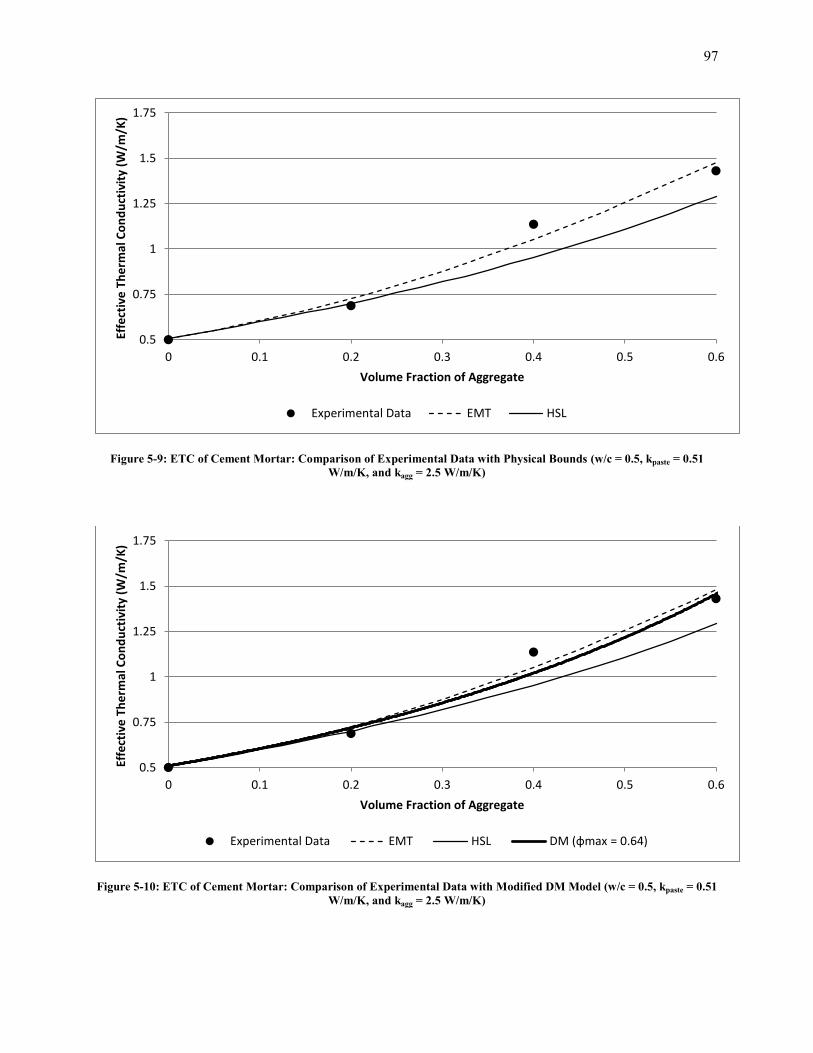
97
Figure 5-9: ETC of Cement Mortar: Comparison of Experimental Data with Physical Bounds (w/c = 0.5, kpaste = 0.51
W/m/K, and kagg = 2.5 W/m/K)
Figure 5-10: ETC of Cement Mortar: Comparison of Experimental Data with Modified DM Model (w/c = 0.5, kpaste = 0.51
W/m/K, and kagg = 2.5 W/m/K)
0.5
0.75
1
1.25
1.5
1.75
0 0.1 0.2 0.3 0.4 0.5 0.6
Effe
ctiv
e T
he
rmal
Co
nd
uct
ivit
y (W
/m/K
)
Volume Fraction of Aggregate
Experimental Data EMT HSL
0.5
0.75
1
1.25
1.5
1.75
0 0.1 0.2 0.3 0.4 0.5 0.6
Effe
ctiv
e T
he
rmal
Co
nd
uct
ivit
y (W
/m/K
)
Volume Fraction of Aggregate
Experimental Data EMT HSL DM (φmax = 0.64)

98
Figure 5-11: Proposed Model for the ETC of Cement Mortar (kagg = 2.5 W/m/K)
0.25
0.75
1.25
1.75
0 0.1 0.2 0.3 0.4 0.5 0.6
Effe
ctiv
e T
he
rmal
Co
nd
uct
ivit
y (W
/m/K
)
Volume Fraction of Aggregate
w/c = 0.4
w/c = 0.5
w/c = 0.6
w/c = 0.7
w/c = 0.8
99
Chapter 6. Effective Thermal Conductivity of Lightweight Cement Mortar
6.1. Introduction
As discussed in Section 1.1.1, there are many advantages of using lightweight concrete,
such as a reduction of the self-weight and thermal conductivity. This is accomplished by either
using lightweight aggregate or through the use of air entrainment. The lightweight aggregate
that is added to the cement mortar can be a combination of both lightweight fine and lightweight
coarse aggregate. While there exist numerous types of lightweight fine aggregate that have been
successfully incorporated into lightweight concrete, this report will focus on the use of expanded
polystyrene (EPS) beads as aggregate.
EPS is a closed cell synthetic polymer foam created by heating polystyrene with steam or
hot air. The closed cell nature of the beads means that the air inside the beads cannot escape and
also that water cannot be absorbed. Accepted vales for the density and thermal conductivity of
polystyrene are 1.06 g/cm3 (66.1 pcf) and 0.14 W/m/K, respectively [97], while for EPS the
accepted values are 0.01 - 0.045 g/cm3 (0.6 - 2.8 pcf) and 0.032 - 0.044 W/m/K, respectively
[98].
The EPS used in this study is a product called Elemix which is produced by the company
Syntheonic. Elemix is technically defined as a lightweight synthetic particle and in this study it
will be considered a lightweight aggregate. It can be used to replace a portion of or all of the
fine aggregate in a concrete mix to achieve a lightweight concrete with a density as low as 40
pcf. Each particle is a closed cell EPS sphere with a density of 0.042 g/cm3 (2.62 pcf) and a
diameter of 6.4 mm (0.25”) [99].
100
6.2. Differential Multiphase Model
The factors that affect the ETC of lightweight cement mortar are the thermal conductivity
of the constituents (cement paste, normal weight fine aggregate, and lightweight fine aggregate),
the shape of the aggregate, the gradation of the different types of aggregate, and the relative size
difference between the normal weight and the lightweight aggregate. The differential multiphase
model (DM model), which has been previously discussed in Section 5.3.1, will be used to study
each one of these factors and construct a model to predict the ETC of lightweight cement mortar.
6.2.1. Effect of Lightweight Aggregate Shape on the ETC
The effect of the shape of the aggregate on the ETC of the composite will be studied by
analyzing the case of a perfectly insulating inclusion, i.e. is one that has a thermal conductivity
of zero. The differential multiphase model (Equation 5-1) can be simplified to the following
expressions for perfectly insulating spheres, fibers, and disks:
( )
Sphere 6-1
( )
Fiber 6-2
( )
Disk 6-3
Figure 6-1 shows the computed ETC using the above equations and a value of kmatrix = 1. It is
seen from this figure that a disk is the most efficient shape at reducing the thermal conductivity,
while a sphere is the least efficient shape. Most manufactured synthetic lightweight particles,
such as Elemix, are produced as spherical beads. From a perspective of reducing the thermal
conductivity it appears more advantageous to use an irregularly shaped synthetic lightweight
101
particle. This can be accomplished by using aggregate produced by shredding recycled EPS
[100].
6.2.2. Effect of Lightweight Aggregate Gradation on the ETC
The effect of the gradation will be incorporated by modifying the maximum volume
fraction of the aggregate based on the linear packing model. As previously discussed in Section
5.4.2, the use of a graded aggregate will increase the maximum volume fraction. This increase
will subsequently allow more aggregate to be packed into the composite. When lightweight
aggregate is used it will decrease the lowest possible ETC of the composite. Figure 6-2 shows
the effect that different maximum volume fractions have on the ETC of a composite with
perfectly insulating spherical inclusions and kmatrix = 1. It is also noted that, at any given volume
fraction of lightweight aggregate, the microstructure with the lowest ETC is the one that is
closest to its maximum volume fraction. This means that changing the gradation to increase the
maximum volume fraction without increasing the actual volume fraction of the lightweight
aggregate will cause the ETC to increase.
6.2.3. Effect of Different Inclusion Scales on the ETC
Inclusions of different sizes will be categorized as belonging to a different scale if the
larger sized inclusions do not feel the effect of each individual smaller sized inclusion. Instead,
the larger inclusions see the original matrix material and the smaller inclusions as new
homogeneous effective matrix. In other words, the determination of the ETC can be broken
down into two steps. First a microstructure is considered which only contains the matrix
material and the smaller inclusions. The ETC of this microstructure is then computed using a
method such as the DM model. Second a system is created that considers the larger inclusions
102
and the new effective matrix, where the thermal conductivity of the effective matrix is equal to
the ETC of the first microstructure. The ETC of the entire composite is then computed by again
employing a method such as the DM model.
Even though this process was demonstrated for only two inclusion scales, the procedure
easily can be extended to a larger number of scales. Figure 6-3 illustrates how the smaller gray
inclusions in the microstructure on the left are combined with the white matrix phase to create an
effective matrix in the system on the right. The volume fraction of the smaller inclusions will be
computed without considering the larger particles and can be visualized as the volume fraction of
the smaller particles in the effective matrix:
6-4
The volume fraction of the larger inclusions is:
6-5
The total volume fraction of the inclusions is:
( ) 6-6
If both of the inclusion phases are randomly arranged spheres with an individual maximum
packing fraction of 0.64, then the total maximum packing fraction of both inclusions together is
0.8704. Figure 6-4 and Figure 6-5 display the ETC of the entire composite for a microstructure
with a matrix thermal conductivity of 1.0 and two perfectly insulating inclusion phases of
different scales. It is observed that up until a value of for , the composite with no small
inclusion phase has the lowest ETC. For larger values of
, the composite with the lowest
ETC is the one with the smallest value of
. This means that the substitution of small scale
insulating inclusions for an equal volume of large scale insulating inclusions will generally cause

103
the ETC to rise, especially if the first microstructure was near its maximum volume fraction of
inclusions. The only way that using small scale inclusions would cause the ETC to decrease is
by adding a larger volume of inclusions which increases and takes advantage of the larger
maximum volume fraction. This suggests that, in order to optimize a composite to produce the
lowest thermal conductivity, both the gradation and the total volume fraction of inclusions must
be considered. If the density of the composite is known, then the microstructure with the lowest
thermal conductivity can be determined by selecting a gradation that has a maximum volume
fraction closest to this target density.
Until now, it has not been considered how it is decided if two different sized inclusions
qualify as being of different scales. In theory this occurs when the actual size of the smaller
inclusion no longer affects the ETC of the composite. In this report, this determination will be
made by calculating when the size of the smaller inclusion no longer affects the packing of the
composite. This determination will be made through the use of the linear packing model. Figure
6-6 illustrates how the maximum volume fraction depends on the relative volume fraction of the
larger inclusions, Xlarge, and the relative size of the inclusions, R. The relative size of the
inclusions is expressed as the ratio of the diameter of the larger inclusions to that of the smaller
inclusions.
6-7
The peak maximum volume fraction of the composite increases as the relative size of the
inclusions increases. For the largest relative size shown in Figure 6-6 (R = 100), the peak
approaches a value of 0.8704, which is equal to the value of the maximum packing fraction if the
particles were of different size scales. The relative volume fraction of the larger inclusions,
which corresponds to the peak value of the maximum volume fraction, depends on the relative

104
size of the inclusions and lies in the range of 0.70 to 0.77. This means that to achieve the densest
packing the total volume of the larger particles needs to be roughly 2 to 3 times greater than the
volume of the smaller particles.
Figure 6-7 plots the peak maximum volume fraction as a function of the relative size of
the inclusions. The value of the peak maximum volume fraction is equal to 0.64 when the
inclusions are the same size and it asymptotically approaches a value of 0.8407 as the bigger
particles become much larger than the smaller particles. It will be proposed that two particles
belong to two different scales if the peak maximum volume fraction of those particles is within
95% of 0.8407, or in other words is greater than 0.8265. This corresponds to a relative size
difference of about 10.
6.3. Proposed Model for the ETC of Lightweight Cement Mortar
The addition of normal weight fine aggregate and lightweight aggregate to cement paste
creates a three-phase material. When the fine aggregate is sufficiently smaller than the
lightweight particles, the fine aggregate and cement paste can be treated as one equivalent matrix
phase and the composite becomes a two-phase material. As discussed in Section 6.2.3, this
would occur when the largest diameter of the fine aggregate is one tenth of the diameter of the
smallest lightweight particle. The average particle diameter of Elemix is 6.4 mm and the largest
fine aggregate particle size for the Ottawa sand used in Chapter 5 was 0.5125 mm.
The first step is to determine the volume fraction of the fine aggregate within the cement
mortar:

105
6-8
where is the volume fraction of the fine aggregate and is the volume fraction of the
lightweight aggregate. The modified differential multiphase model is then used twice, first to
determine the ETC of the cement mortar and then again to determine the ETC of the lightweight
cement mortar. In both stages the particle shape and the gradation can be taken into account.
The influence of the particle shape is determined by computing the ellipsoidal integrals
(Equation A-18) and the gradation is accounted for by modifying the maximum volume fraction
using the linear packing model. In the first stage the cement paste is the matrix phase and the
fine aggregate is the inclusion phase, and in the second stage the cement mortar is the effective
matrix phase and the lightweight aggregate is the inclusion phase. Figure 6-8 illustrates the
results of this model for various volume fractions of Elemix using the following parameters: the
cement paste has a water-cement ratio of 0.5 (k = 0.51 W/m/K); the thermal conductivity of the
fine aggregate, and lightweight aggregate are 2.5 W/m/K and 0.035 W/m/K, respectively; and
both the fine aggregate and lightweight aggregate have a maximum volume fraction of 0.64. The
horizontal axis of the figure is the volume fraction of the Elemix and the different data series that
are shown are the volume fraction of the fine aggregate in the cement mortar. It is observed that
the addition of Elemix decreases the ETC of the composite while the addition of fine aggregate
increases it. This is because Elemix has a thermal conductivity lower than that of the cement
paste and the fine aggregate has a thermal conductivity higher than that of the cement paste.
Additionally it is observed that effect of the Elemix is felt more when there is a higher volume
fraction of the fine aggregate in the cement paste while the effect of the fine aggregate is felt
more when there is less Elemix in the composite.

106
Figure 6-9 plots the ETC of lightweight cement mortar against its density. This figure
was generated from Figure 6-8 by using the following values for the density of the different
components: cement paste = 1.5 g/cm3, Elemix = 0.042 g/cm
3, and fine aggregate = 2.65 g/cm
3.
It is observed that the resulting ETC lies between 0.17 W/m/K and 1.45 W/m/K and these two
values occur at a density of 0.57 g/cm3 and 2.19 g/cm
3, respectively. Additionally the range of
possible values of the ETC is greatest for intermediate values of the density and is lower at the
extremes.
6.4. Experimental Results
Table 6-1 displays the experimental results for the ETC of twenty-seven lightweight
cement paste samples and five neat cement paste samples, all prepared with a water-cement ratio
of 0.6. None of the samples contained any normal weight fine aggregate. The ETC was
determined using the experimental method proposed in Section 3.2. The five neat cement paste
samples were tested in order to verify the proposed method. The average experimental ETC
value of these five samples was 0.38 W/m/K. The 95% confidence interval for the thermal
conductivity of dry cement paste with a water-cement ratio of 0.6 (Table 4-4) was determined
experimentally by the flash method to be 0.41-0.47 W/m/K (Section 4.4.3). The remaining
twenty-seven lightweight samples had a volume fraction of Elemix that varied between 8% and
69%. Additionally Table 6-1 contains the density for each of the samples.
Figure 6-10 compares the experimental results to the Hashin-Shtrikman upper and lower
bounds and EMT equation, using 0.38 W/m/K and 0.035 W/m/K as the thermal conductivity of
the cement paste and Elemix, respectively. As the percentage of Elemix increases the ETC of the
lightweight cement paste decreases. Since lightweight cement paste is an internally porous
107
material the results should fall between the Hashin-Shtrikman upper bound and the EMT
equation. It is observed that some of the experimental results fall outside of the internally porous
region and some are even below the Hashin-Shtrikman lower bound.
This scatter of the experimental results can be attributed to several factors. Firstly the
value used for the thermal conductivity of the Elemix was not determined experimentally but
instead was taken from literature. Secondly any cement composite is inherently a random and
variable material and so it can be expected that the results for its effective properties have some
scatter. Additionally the locations at which the temperature was recorded were at approximately
10mm and 20mm from the surface of the sample. It is unknown if these distances are large
enough to capture the effective properties of this heterogeneous material. Finally, the
experimental method that was used is only an approximate one and not standardized, and as a
result it is not expected to yield the same quality of results as techniques such as the flash
method.
Figure 6-11 compares the experimental results to the differential multiphase model and
also to the modified differential multiphase model with a maximum volume fraction of 0.69. A
value of 0.69 was used because this was the maximum volume fraction of the Elemix as seen in
Table 6-1. This value is greater than the accepted value for the maximum volume fraction of
random spheres (φmax = 0.64). The reason for this is that these samples were compacted as they
were cast, which increases the maximum volume fraction above that of a random arrangement.

108
6.5. Effect of the Relative Size of the Normal Weight and Lightweight
Aggregate
In the previous sections it was assumed that the lightweight aggregate belonged to a size
scale larger than that of the normal weight aggregate. Depending on the type of fine aggregate
and lightweight aggregate used, it can be the normal weight aggregate that is a size scale larger
than the lightweight aggregate. This would also be the case for a lightweight concrete composite
where normal weight coarse aggregate is present and the normal weight fine aggregate is
replaced entirely with lightweight fine aggregate. The only modification to the previous
procedure (Section 6.3) would be that the lightweight aggregate and the cement paste would
make up the effective matrix and the normal weight aggregate would be imbedded in this
effective matrix. Figure 6-12 displays the ETC of a lightweight cement composite in which the
normal weight aggregate is of a scale larger than the lightweight aggregate (the data series
represent different volume fractions of lightweight aggregate in the effective matrix).
Figure 6-13 plots the results for the ETC against the density of the composite and uses the
following values for the density of the different components: cement paste = 1.5 g/cm3, Elemix =
0.042 g/cm3, and normal weight aggregate = 2.65 g/cm
3. If the results from this figure are
compared to those from Figure 6-9 it is observed that for the same density, a cement composite
composed of large normal weight aggregate and small lightweight aggregate will generally have
a lower ETC than a composite made of large lightweight aggregate and small normal weight
aggregate. This is also illustrated in Figure 6-14, which shows the upper and lower bounds for
the ETC of each type of microstructure as a function of density (based on Figure 6-9 and Figure
6-13).

109
6.6. Summary
The use of lightweight cement mortar has become increasingly popular due to its low unit
weight and low thermal conductivity. Typically it is not possible to accurately predict the ETC
beforehand and it is determined by physically testing specimens, which is costly and time
consuming. A mathematical model is proposed in this chapter that is able to predict the value of
the ETC and it can also be used to optimize the structure of the composite in order to minimize
the ETC.
The proposed model is based on the DM model and makes use of the linear packing
model to include the effect of the gradation of the normal weight and lightweight aggregate.
Additionally the size difference between the normal weight and lightweight aggregate is
accounted for by combining the smaller of the two with the cement paste to create an effective
matrix. One effect that is not included in this model is the presence of an ITZ surrounding the
lightweight aggregate. It is unclear how much it would impact the ETC since the thermal
conductivity of the ITZ will be higher than that of the lightweight aggregate
The following observations have been made regarding the minimization of the ETC:
Flat or disk-shaped lightweight aggregate is more effective at reducing the ETC than
spherical lightweight aggregate.
The ETC can be lowered by using a graded lightweight aggregate to increase the
maximum volume fraction and also including more lightweight aggregate per unit
volume. However the ETC will increase if a monosized aggregate is replaced with a
graded aggregate and the volume fraction of the lightweight aggregate is not increased
to a value near the new maximum volume fraction.
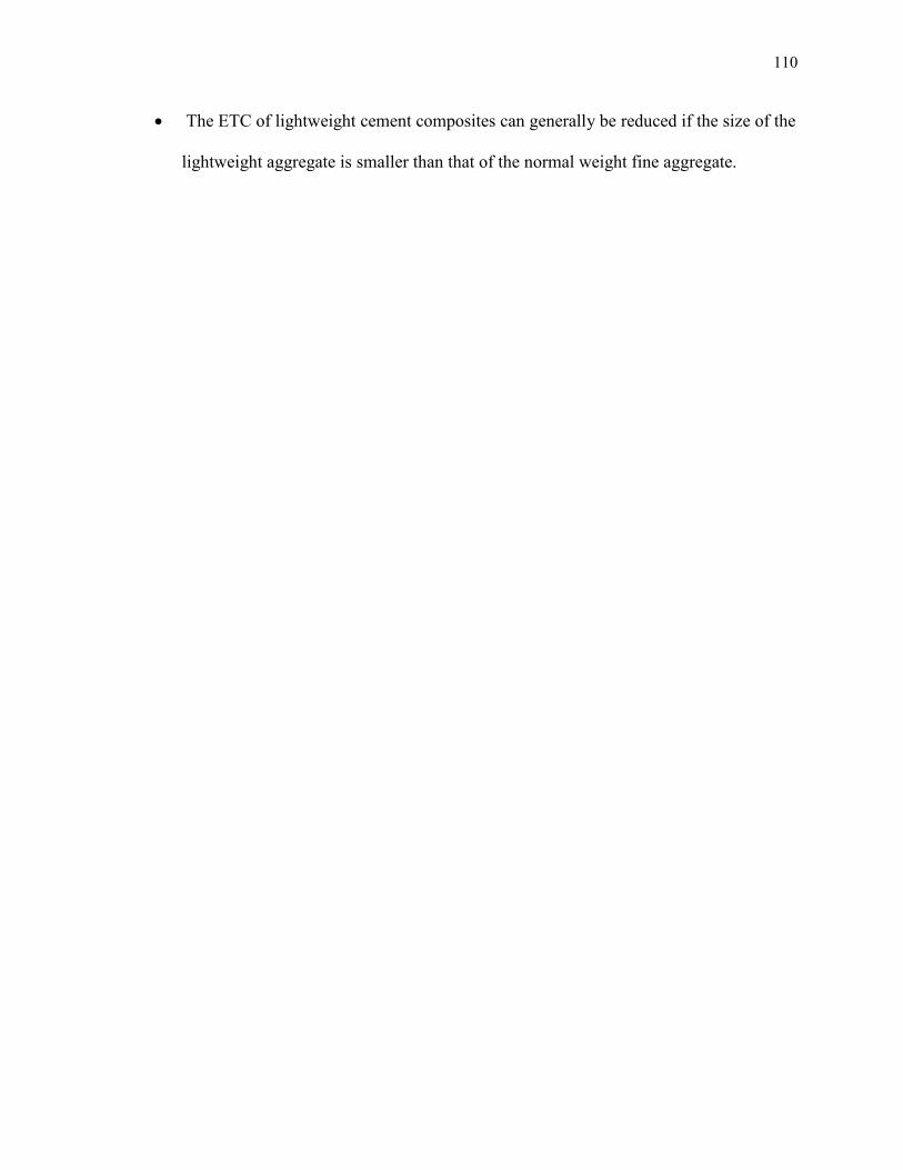
110
The ETC of lightweight cement composites can generally be reduced if the size of the
lightweight aggregate is smaller than that of the normal weight fine aggregate.
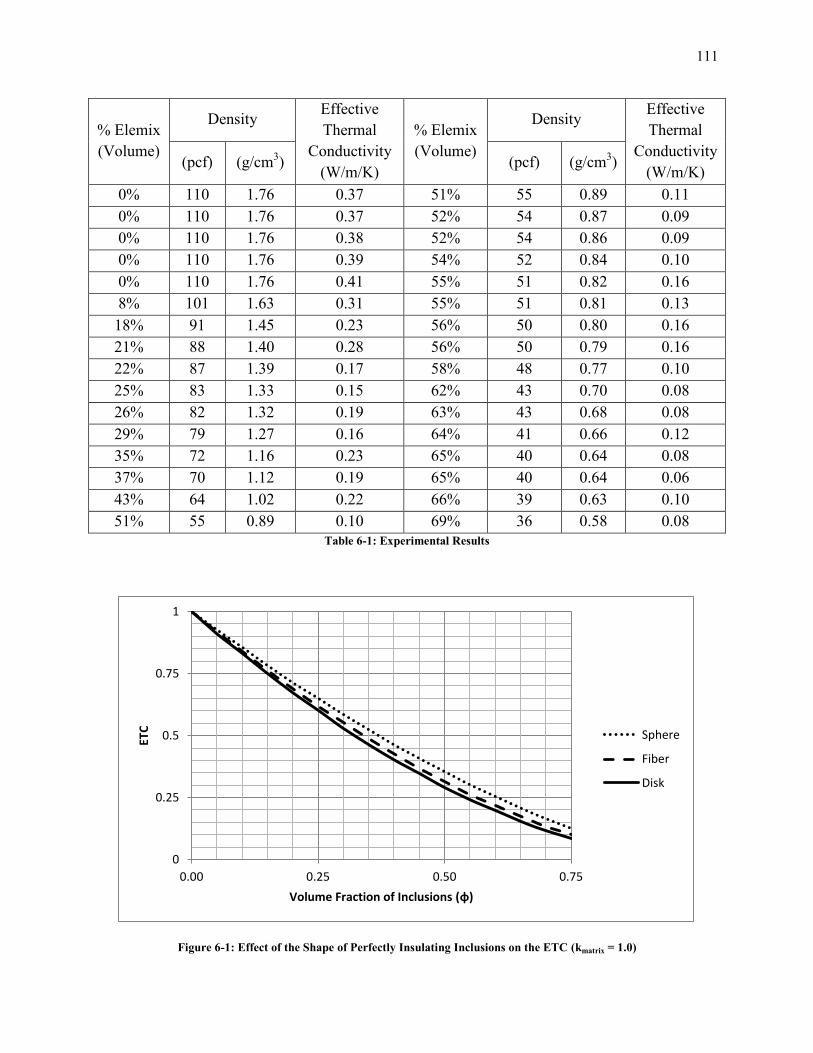
111
% Elemix
(Volume)
Density Effective
Thermal
Conductivity
(W/m/K)
% Elemix
(Volume)
Density Effective
Thermal
Conductivity
(W/m/K) (pcf) (g/cm
3) (pcf) (g/cm
3)
0% 110 1.76 0.37 51% 55 0.89 0.11
0% 110 1.76 0.37 52% 54 0.87 0.09
0% 110 1.76 0.38 52% 54 0.86 0.09
0% 110 1.76 0.39 54% 52 0.84 0.10
0% 110 1.76 0.41 55% 51 0.82 0.16
8% 101 1.63 0.31 55% 51 0.81 0.13
18% 91 1.45 0.23 56% 50 0.80 0.16
21% 88 1.40 0.28 56% 50 0.79 0.16
22% 87 1.39 0.17 58% 48 0.77 0.10
25% 83 1.33 0.15 62% 43 0.70 0.08
26% 82 1.32 0.19 63% 43 0.68 0.08
29% 79 1.27 0.16 64% 41 0.66 0.12
35% 72 1.16 0.23 65% 40 0.64 0.08
37% 70 1.12 0.19 65% 40 0.64 0.06
43% 64 1.02 0.22 66% 39 0.63 0.10
51% 55 0.89 0.10 69% 36 0.58 0.08
Table 6-1: Experimental Results
Figure 6-1: Effect of the Shape of Perfectly Insulating Inclusions on the ETC (kmatrix = 1.0)
0
0.25
0.5
0.75
1
0.00 0.25 0.50 0.75
ETC
Volume Fraction of Inclusions (φ)
Sphere
Fiber
Disk

112
Figure 6-2: Effect of the Maximum Volume Fraction of Perfectly Insulating Inclusions (kmatrix = 1.0)
0
0.05
0.1
0.15
0.2
0.25
0.60 0.65 0.70 0.75 0.80 0.85 0.90
ETC
Volume Fraction of Inclusions (φ)
φmax = 0.9
φmax = 0.85
φmax = 0.8
φmax = 0.75
φmax = 0.7
φmax = 0.64
Figure 6-3: Illustration of Different Inclusion Scales

113
Figure 6-4: Effect of Different Inclusion Scales
Figure 6-5: Effect of Different Inclusion Scales (Close up on area of interest from Figure 6-4)
0
0.2
0.4
0.6
0.8
1
0.0 0.2 0.4 0.6 0.8
ETC
φtotal
φsmall = 0
φsmall = 0.10
φsmall = 0.30
φsmall = 0.50
0
0.1
0.2
0.3
0.4
0.5 0.6 0.7 0.8
ETC
φtotal
φsmall = 0
φsmall = 0.10
φsmall = 0.30
φsmall = 0.50

114
Figure 6-6: Maximum Volume Fractions as a Function of the Relative Inclusion Size
Figure 6-7: Peak Maximum Volume Fraction as a Function of the Relative Inclusion Size
0.6
0.65
0.7
0.75
0.8
0.85
0.9
0 0.2 0.4 0.6 0.8 1
Max
imu
m V
olu
me
Fra
ctio
n
Relative Volume Fraction of the Larger Inclusions (Xlarger)
R = 100
R = 20
R = 10
R = 5
R = 2
R = 1.25
0.65
0.7
0.75
0.8
0.85
0.9
0 10 20 30 40 50 60 70 80 90 100
Pe
ak M
axim
um
Vo
lum
e F
ract
ion
Relative Inclusion Size
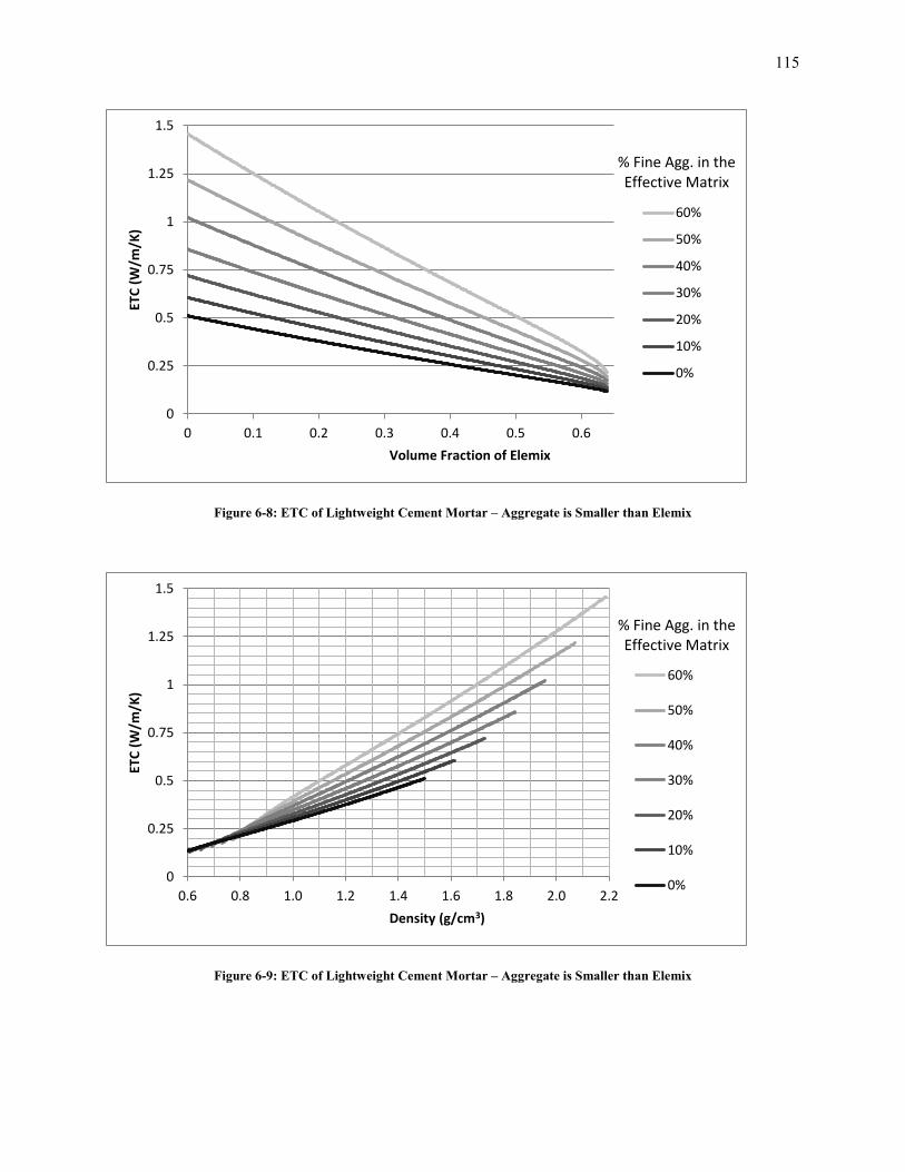
115
Figure 6-8: ETC of Lightweight Cement Mortar – Aggregate is Smaller than Elemix
Figure 6-9: ETC of Lightweight Cement Mortar – Aggregate is Smaller than Elemix
0
0.25
0.5
0.75
1
1.25
1.5
0 0.1 0.2 0.3 0.4 0.5 0.6
ETC
(W
/m/K
)
Volume Fraction of Elemix
60%
50%
40%
30%
20%
10%
0%
0
0.25
0.5
0.75
1
1.25
1.5
0.6 0.8 1.0 1.2 1.4 1.6 1.8 2.0 2.2
ETC
(W
/m/K
)
Density (g/cm3)
60%
50%
40%
30%
20%
10%
0%
% Fine Agg. in the Effective Matrix
% Fine Agg. in the Effective Matrix

116
Figure 6-10: ETC of Cement Paste and Elemix (Experimental Data and Theoretical Bounds)
Figure 6-11: ETC of Cement Paste and Elemix (Experimental Data and Proposed Model)
35455565758595105
0.05
0.15
0.25
0.35
0.45
0% 10% 20% 30% 40% 50% 60% 70%
Density (pcf) Th
erm
al C
on
du
ctiv
ity
(W/m
/K)
Percent Elemix HSU EMT HSL Data
35455565758595105
0.05
0.15
0.25
0.35
0.45
0% 10% 20% 30% 40% 50% 60% 70%
Density (pcf)
The
rmal
Co
nd
uct
ivit
y (W
/m/K
)
Percent Elemix
DM Model Modified DM Model Data
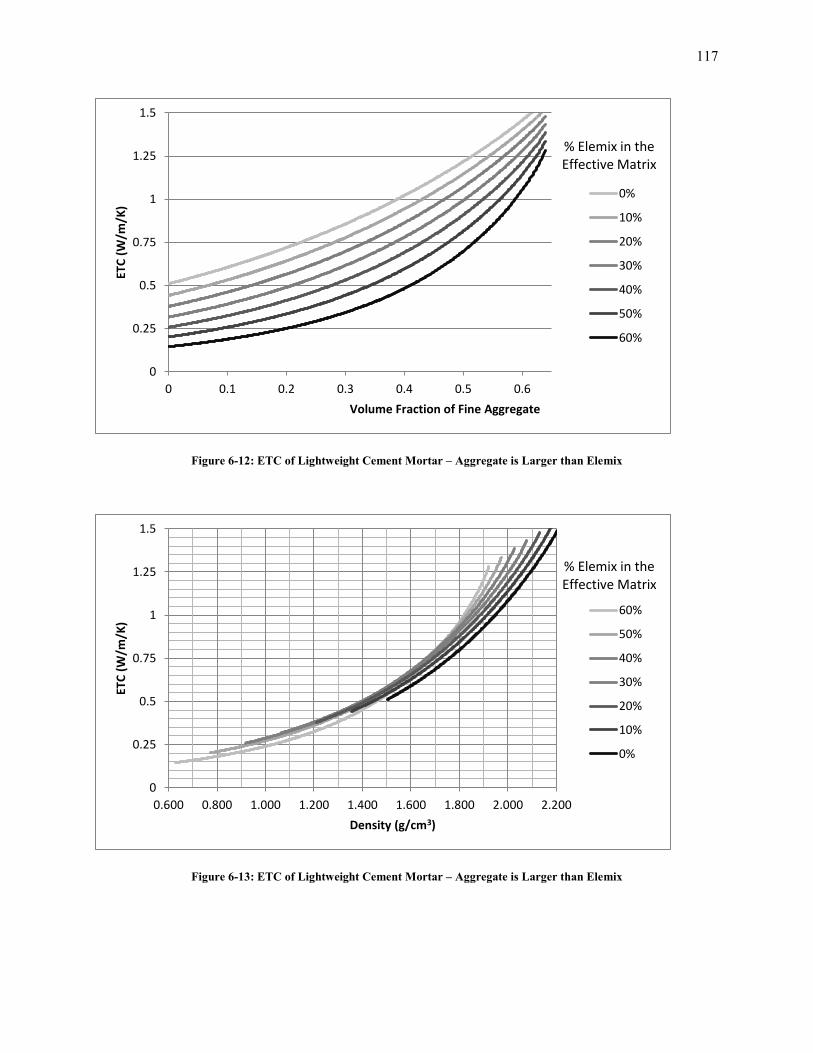
117
Figure 6-12: ETC of Lightweight Cement Mortar – Aggregate is Larger than Elemix
Figure 6-13: ETC of Lightweight Cement Mortar – Aggregate is Larger than Elemix
0
0.25
0.5
0.75
1
1.25
1.5
0 0.1 0.2 0.3 0.4 0.5 0.6
ETC
(W
/m/K
)
Volume Fraction of Fine Aggregate
0%
10%
20%
30%
40%
50%
60%
% Elemix in the Effective Matrix
0
0.25
0.5
0.75
1
1.25
1.5
0.600 0.800 1.000 1.200 1.400 1.600 1.800 2.000 2.200
ETC
(W
/m/K
)
Density (g/cm3)
60%
50%
40%
30%
20%
10%
0%
% Elemix in the Effective Matrix

118
Figure 6-14: Bounds for the ETC of Lightweight Cement Mortar (From Figure 6-9 and Figure 6-13)
0.1
0.3
0.5
0.7
0.9
1.1
1.3
1.5
0.6 0.8 1 1.2 1.4 1.6 1.8 2 2.2
ETC
(W
/m/K
)
Density (g/cm3)
Normal Weight Aggregate >> Elemix Elemix >> Normal Weight Aggregate
119
Chapter 7. Effective Thermal Conductivity of Fiber-Reinforced Cement Paste
7.1. Introduction
As stated in Section 1.1.2, fiber-reinforced concrete is used in a variety of applications to
increase properties such as tensile strength and fracture toughness. Typical materials used for
the fibers include steel, glass, nylon, polypropylene, polyvinyl alcohol (PVA), and carbon. Due
to their relatively low tensile strength compared to their compressive strength, cementitious
composites greatly benefit from the addition of reinforcing fibers. The types of fibers considered
here are relatively short (typically no longer than 25 or 50 mm), uniformly dispersed throughout
the cement matrix and randomly oriented.
7.2. Types of Fibers
Fibers can be either characterized as macrofibers or microfibers, depending on their size
and the types of cracks they are meant to restrain. Typically macrofibers have a diameter
between 0.2mm and 1mm. Most fibers have a circular cross-section which is uniform along the
length of the fiber. As a result these fibers can be thought of as long cylinders with a length, ,
and a diameter, . The aspect ratio of a fiber is defined as:
7-1
For practical applications the aspect ratio is generally in the range of 50 to 150 [8]. Additionally
steel fibers can be deformed or their surface can be roughened to increase their bond strength
with the cement matrix. In these cases an equivalent diameter and equivalent aspect ratio can be
determined. Table 7-1 contains a list of various materials used for fibers as well as their density,
thermal conductivity, and specific heat. Undeformed steel fibers will be used for the
experimental portion of this study.

120
7.3. Maximum Volume Fraction
While there has been an extensive amount of research conducted on the packing of
spherical particles, there is considerably less knowledge about the packing of highly
nonspherical particles such as fibers. However it can be reasoned that, due to their elongated
nature, a random mixture of fibers will have a much lower maximum volume fraction than a
random mixture of spheres.
Toll [101] developed an equation to compute the maximum unforced packing density of
fibers based on a statistical analysis of the distribution of fiber-fiber contact points.
⁄
⁄
7-2
where is the number of fiber-fiber contact points, which is assumed to be 8, and f and g are
constants that depend on the fiber orientation distribution (see Table A-1). For a random three-
dimensional arrangement of fibers Equation 7-3 becomes:
7-3
A similar expression has been developed by Evans and Gibson [102], using the free-volume
concept that previously has been applied to liquid crystals [103]:
7-4
Figure 7-1 displays Equations 7-3 and 7-4. The difference between the two equations is
only a few percent for the typical aspect ratios of reinforcing fibers. If the reinforcing fibers in a
mix design vary in size, the above methods can be combined with the linear packing model
(Section 5.4.1) to determine the overall maximum packing fraction. The only modification

121
needed is that the diameter terms in Equations 5-6 and 5-7 must be replaced with their equivalent
volume diameters. The equivalent volume diameter, , for a fiber is the diameter of a sphere
that will have the same volume as a single fiber. For cylindrical fibers:
√
7-5
7.4. Percolation
Percolation theory describes the effect that the physical contact between fibers has on the
ETC of the composite. The role of percolation can be understood by first considering a
composite that only consists of cement mortar and then fibers are gradually added randomly to
the composite. At first the distance between neighboring fibers is relatively large and contact
between two fibers is rare. As more fibers are added, several fibers may touch each other and
group together to form a cluster; however these clusters remain isolated. Eventually enough
fibers are added for the percolation threshold to be reached and the clusters join together so that
the fibers create a continuous network throughout the entire matrix. In the case of fibers that
have a thermal conductivity greater than that of the cement paste matrix, such as steel fibers,
once the percolation threshold is reached heat will have a continuous conduction pathway
through the composite. The volume fraction of fibers which corresponds to onset of percolation
is known as the critical volume fraction, . If the thermal conductivity of the fibers is greater
than that of the matrix, the critical volume fraction is determined by the sudden increase in the
ETC vs. volume fraction curve.
The theory of percolation has its roots in the determination of the effective electrical
conductivity of composites. As mentioned in Section 2.3, the underlying principles between the

122
conduction of electricity and heat are similar and this approach can be applied to heat transfer as
well. The electrical conductivity of fiber-reinforced cement composites has been studied by Xie
et al. [104] and Chen et al. [105]. Xie et al. used both carbon and steel fibers, while Chen et al.
only studied carbon fibers. Both researchers agree that as the aspect ratio of the fibers increases
the percolation threshold decreases. This occurs because there is a higher probability that a
longer fiber will touch one of its neighbors when compared to a shorter fiber with the same
diameter. Additionally both researchers observed that the effective electrical conductivity
remains relatively constant for volume fractions before and after the percolation threshold. The
only time that the effective electrical conductivity does change is in a small range of volume
fractions near the percolation threshold.
Data from Xie et al. for the electrical conductivity of fiber-reinforced concrete is
reproduced in Figure 7-2. The fibers used in their study were carbon fibers with a length of 3mm
and an electrical conductivity of 66.7 Ω-1cm
-1. Xie et al. did not report the electrical conductivity
of the cement mortar; however, based on Figure 7-2 it can be estimated to be 1x10⁻⁸
Ω-1cm
-1.
This results in the ratio of the electrical conductivity of the two materials to be around 1010
. If
the thermal conductivity of cement mortar is estimated to be 1 W/m/K and that of steel fibers is
52 W/m/K, then the ratio of the thermal conductivities of the two materials is of the order of 101.
Due to the large difference in the conductivity ratios the percolation phenomena will not impact
the ETC of fiber-reinforced concrete nearly as much as it does the effective electrical
conductivity.

123
7.5. ETC of Fiber-Reinforced Composites at the Maximum Fiber Volume
Fraction
Before the onset of percolation the cement mortar is the continuous phase and the fibers
are the dispersed phase. After the fibers percolate the cement mortar and a portion of the fibers
are continuous while the remainder of the fibers are dispersed. When the maximum volume
fraction is reached both phases act as a continuous phase and the structure is termed co-
continuous. The ETC of a co-continuous microstructure has been studied by Wang et al. [106]
as a function of the parallel and series models:
6√
7 7-6
Theoretically, if all of the fibers act as a continuous phase at the maximum volume fraction, then
the above equation will predict the ETC at the maximum volume fraction. In reality this will not
be true because it is believed that many of the fibers will not physically touch each other.
Instead, each fiber will have a thin layer of cement paste surrounding it that prevents it from
touching its neighboring fibers.
7.6. Bounds for the ETC of Fiber-Reinforced Composites
Once the ETC for a co-continuous composite is known, Equation 7-6 can be used to
construct two new types of material models and also modify the two previously discussed
models for the internally and externally porous materials (Section 2.3.5 and shown in Figure
2-7). As seen in Figure 7-3, the addition of the co-continuous model causes the internally porous
region to now be bounded from above by the Hashin-Shtrikman upper bound and from below by
the EMT equation and the co-continuous model. Additionally the externally porous region is
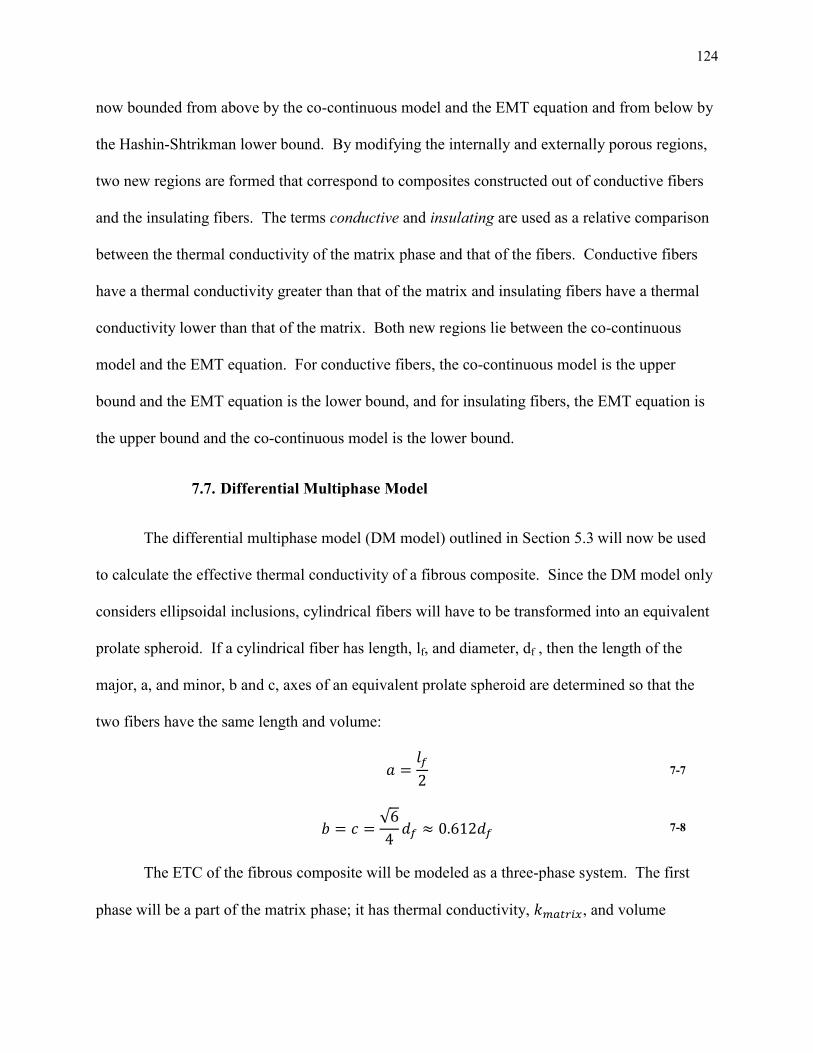
124
now bounded from above by the co-continuous model and the EMT equation and from below by
the Hashin-Shtrikman lower bound. By modifying the internally and externally porous regions,
two new regions are formed that correspond to composites constructed out of conductive fibers
and the insulating fibers. The terms conductive and insulating are used as a relative comparison
between the thermal conductivity of the matrix phase and that of the fibers. Conductive fibers
have a thermal conductivity greater than that of the matrix and insulating fibers have a thermal
conductivity lower than that of the matrix. Both new regions lie between the co-continuous
model and the EMT equation. For conductive fibers, the co-continuous model is the upper
bound and the EMT equation is the lower bound, and for insulating fibers, the EMT equation is
the upper bound and the co-continuous model is the lower bound.
7.7. Differential Multiphase Model
The differential multiphase model (DM model) outlined in Section 5.3 will now be used
to calculate the effective thermal conductivity of a fibrous composite. Since the DM model only
considers ellipsoidal inclusions, cylindrical fibers will have to be transformed into an equivalent
prolate spheroid. If a cylindrical fiber has length, lf, and diameter, df , then the length of the
major, a, and minor, b and c, axes of an equivalent prolate spheroid are determined so that the
two fibers have the same length and volume:
7-7
√
7-8
The ETC of the fibrous composite will be modeled as a three-phase system. The first
phase will be a part of the matrix phase; it has thermal conductivity, , and volume
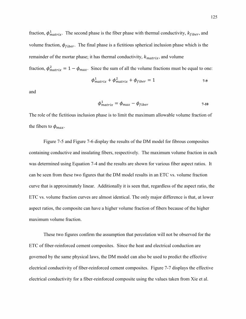
125
fraction, . The second phase is the fiber phase with thermal conductivity, and
volume fraction, . The final phase is a fictitious spherical inclusion phase which is the
remainder of the mortar phase; it has thermal conductivity, , and volume
fraction, . Since the sum of all the volume fractions must be equal to one:
7-9
and
7-10
The role of the fictitious inclusion phase is to limit the maximum allowable volume fraction of
the fibers to .
Figure 7-5 and Figure 7-6 display the results of the DM model for fibrous composites
containing conductive and insulating fibers, respectively. The maximum volume fraction in each
was determined using Equation 7-4 and the results are shown for various fiber aspect ratios. It
can be seen from these two figures that the DM model results in an ETC vs. volume fraction
curve that is approximately linear. Additionally it is seen that, regardless of the aspect ratio, the
ETC vs. volume fraction curves are almost identical. The only major difference is that, at lower
aspect ratios, the composite can have a higher volume fraction of fibers because of the higher
maximum volume fraction.
These two figures confirm the assumption that percolation will not be observed for the
ETC of fiber-reinforced cement composites. Since the heat and electrical conduction are
governed by the same physical laws, the DM model can also be used to predict the effective
electrical conductivity of fiber-reinforced cement composites. Figure 7-7 displays the effective
electrical conductivity for a fiber-reinforced composite using the values taken from Xie et al.

126
(electrical conductivity of the fibers is 66.7 Ω-1cm
-1 and electrical conductivity of the matrix is
1x10⁻⁸
Ω-1cm
-1). The effects of percolation are clearly seen in this figure with a sharp jump
occurring in each curve that corresponds to volume fraction where electrical percolation occurs.
Additionally it is observed that the aspect ratio of the fibers has more of an effect on the effective
electrical conductivity than the ETC. As previously reported by Xie et al. [104] and Chen et al.
[105], it is observed that the percolation threshold decreases as the aspect ratio increases.
Figure 7-8 and Figure 7-9 demonstrate that the DM model is able to predict an ETC for
conductive or insulating fibrous composites that fall within the bounded regions specified in
Section 7.6. Figure 7-8 shows that the DM model for a conducting fibrous composite fits within
the region bounded from above by the co-continuous model and from below by the EMT
equation, and Figure 7-9 shows that for an insulating fibrous composite the ETC computed using
the DM model is bounded from above by the EMT equation and from below by the co-
continuous. For the values showed in the figure (kf = 0.2 and km = 2) the ETC is very close to,
but still less than the EMT model.
7.8. Equivalent Inclusion Method
The equivalent inclusion method (EIM) used to determine the ETC was developed by
Hatta and Taya [107] and it is analogous to the Eshelby equivalent inclusion method in elasticity
[108]. This method is an improvement on other methods, such as volume averaging, because it
can better account for the interaction between inclusions [109]. For a completely random
distribution of inclusions the effective thermal conductivity is:
{ ( )[( )( ) ]
( ) ( ) ( )
} 7-11

127
where and are the elliptic integrals (Equation A-18) and:
( ) ( ) 7-12
For fibers with a large aspect ratio A1 ≈ 0.5, A3 ≈ 0, and Equation 7-11 reduces to:
2 ( )( )
( )( ) 3 7-13
Figure 7-10 and Figure 7-11 compare the results for the ETC using the DM model and
the EIM. It can be seen that these two models are close in their predictions of the ETC. The
advantages to using the EIM are that the method is computationally easier to use since Equation
7-11 is an explicit equation and Equation 5-1 is a differential equation that needs to be solved
numerically. However it is more desirable to use the DM model since it is capable of accounting
for both multiple inclusion phases and the maximum volume fraction of each phase, while the
EIM cannot.
7.9. Proposed Model for the ETC of Fiber-Reinforced Cement Mortar
When cement mortar is used as the matrix phase for a fibrous composite, a determination
must be made whether the mortar constitutes an effective matrix phase or not. If the aggregate is
a size scale smaller than the fibers, then the mortar is an effective matrix. However if the
aggregate and fibers are close in size, then both the aggregate and fibers must be considered at
the same scale. For fibers with an aspect ratio of 65 and a diameter of 0.2mm the equivalent
volume diameter (according to Equation 7-5) is 0.921mm and the maximum volume fraction is
6.1%. If the fine aggregate is Ottawa sand with a maximum particle diameter of 0.5125mm,
then the ratio of the equivalent diameter of the fibers to the diameter of the sand is not large
enough for the fibers to be of a larger size scale.

128
Using the linear packing model, Figure 7-12 displays the maximum volume fraction of
fibers that are allowed in the composite for different volume fractions of fine aggregate in the
mortar. It is clearly seen in this figure that the addition of fine aggregate reduces that quantity of
fibers that can be included in the composite. Figure 7-13 displays the ETC of fiber-reinforced
cement paste using the DM model and assuming that the fibers and the aggregate belong to
different size scales. This figure does account for the relative sizes of both the aggregate and
fibers by only displaying data for microstructures that fall below the maximum volume fraction
as shown in Figure 7-12.
Table 7-2 displays the results for the ETC of fiber-reinforced cement mortar computed
using the DM model two different ways. The first method considers that the aggregate and the
fibers belong to the same size scale and the second method assumes that the fibers are of a size
scale larger than the aggregate. When the fibers and aggregate are assumed to belong to the
same size scale, Equation 5-1 is only applied once with four different phases: the cement paste,
the fine aggregate, the fiber, and the fictitious inclusion phase. The fictitious inclusion phase
accounts for the effect of the maximum volume fraction, which is computed using the linear
packing model. When the fibers are assumed to belong to a size scale larger than the aggregate,
Equation 5-1 is applied twice. First the equation is used to compute the ETC of the cement
mortar, then the cement mortar is treated as an effective matrix and the ETC of the entire
composite is computed by calculating the ETC of the fibers in this effective matrix. It is
observed that the computed ETC is always greater when it is assumed that the fibers and
aggregate are of the same size scale opposed to when it is assumed that the fibers are of a larger
size scale. The maximum percent difference between these two methods is approximately 10%
with the difference increasing as the volume fraction of fibers increases.

129
For the type of fine aggregate and fibers used in this study it is not clear which one of
these methods is more appropriate. The true value for the ETC should lie somewhere between
the results for these two methods. It can be concluded that smaller sized conducting fibers
(closer to the size of the fine aggregate) have a greater impact on increasing the ETC of the
composite than larger fibers do.
7.10. ETC of Fiber-Reinforced Cement Paste: Experimental Results
Table 7-3 displays the results for the ETC of four fiber-reinforced cement paste mix
designs, which were all prepared at a water-cement ratio of 0.8. The fibers were SF Type I steel
fibers manufactured by Nycon Corp. Each has a length of 13mm and a diameter of 0.2mm (rf =
65). None of these samples contained any normal weight fine aggregate. The ETC was
determined using the experimental method proposed in Section 3.2 and each data point was
determined from the average of three samples. The four mix designs had the following fiber
volume fractions, 1.7%, 2.8%, 6.4%, and 7.8%. Additionally Table 7-3 contains the density for
each of the samples.
Figure 7-14 compares the experimental results to both the co-continuous model and the
EMT equation, using 0.33 W/m/K and 52 W/m/K as the thermal conductivity of the cement
paste and steel fibers, respectively. It is illustrated that as the percentage of steel fibers increased
the ETC of the fiber-reinforced cement paste increases. Since lightweight cement paste is a
conductive fibrous composite the results should be below the co-continuous model and above the
EMT equation. It is observed that the results generally fall in line with the EMT equation.
Additionally it is seen that the experimental data is much lower than the predicted vales
for the ETC using the DM model. There are several explanations for this large difference. The

130
DM model assumes perfect contact between the matrix phase and inclusion phase while in reality
this may not be the case due to: incomplete compaction and the existence of an ITZ around the
fibers. The presence of an ITZ on the surface of fine aggregate has previously been discussed in
Section 5.5 and it can be assumed that one also exists in the area surrounding each fiber.
Incomplete compaction will result in air voids being trapped on the surface of fibers. These air
voids will decrease the ETC because the thermal conductivity of air, ~0.025 W/m/K (Figure
4-7), is lower than that of both the steel fibers and cement paste. The ITZ will result in a layer of
cement paste surrounding the fiber that has a water-cement ratio higher than that of the bulk
cement paste. Since the ETC of cement paste decreases with an increasing water-cement ratio,
the presence of the ITZ will cause the ETC of the fiber-reinforced cement mortar to decrease.
7.11. Summary
This chapter accomplishes three main objectives. It discusses the factors that affect the
ETC of fiber-reinforced composites, describes the bounds for the ETC, and proposes a model
that can be used to predict the ETC. The two main factors that affect the ETC are the material
that the fibers are made of and the aspect ratio of the fibers. It has been shown that at low
volume fractions the aspect ratio does not affect the ETC to a great extent. However as the
aspect ratio decreases the maximum volume fraction of the fibers increases, which allows for a
greater percentage of fibers in the composite.
The introduction of the co-continuous model allows the formulation of two new types of
material models that apply to fibrous composites. Initially the Hashin-Shtrikman bounds and the
EMT equation produce the internal and external porosity regions. The addition of the co-
continuous model splits these regions and creates the conductive fibers region and the insulating

131
fibers region. Each of these new regions it bounded by the EMT equation and the co-continuous
model.
Building on previous chapters, the DM model is used to predict the ETC of fiber-
reinforced cement mortar. By comparison with experimental results it is shown that this model
overestimates the ETC for cement paste reinforced with steel fibers. It is hypothesized that this
occurs as a result of two factors. The first one is that there exists an ITZ around the fibers and
the second factor is that inadequate compaction leaves air voids on the surface of the fibers. The
current model is unable to account for either one of these issues. Additionally it is observed
from the DM model that the ETC of cement mortar reinforced with conductive fibers can be
minimized by using fibers which are much larger than the fine aggregate, rather than fibers
which are close in size to the fine aggregate.

132
Material Density
(g/cm3)
Thermal Conductivity
(W/m/K)
Specific Heat
(J/g/K)
Steel 7.84 52 0.44-0.49
Glass 2.5 0.8-1.4 0.75-0.84
PVA 1.27-1.31 0.20 1.50-1.67
Nylon 1.1 0.25 4.4
Acrylic 1.06 0.20 1.68-1.86
Polypropylene 0.91 0.25 1.93
Sisal 1.5 0.07 -
Carbon 1.9-2.3 1.7 0.52-0.71
Table 7-1: Properties of Fibers Used in Fiber-Reinforced Concrete from [110], [111], and [112]
%
Fibers
%
Aggregate
% Aggregate
in Mortar φmax
keff (W/m/K)
(Aggregate = Fibers)
keff (W/m/K)
(Aggregate << Fibers)
Percent
Difference
1 10 9.9 0.380 0.78 0.76 2.6%
1 50 49.5 0.556 1.41 1.39 1.4%
2 10 9.8 0.266 0.96 0.92 4.2%
2 30 29.4 0.434 1.26 1.19 5.6%
3 10 9.7 0.209 1.15 1.07 7.0%
3 30 29.1 0.377 1.46 1.35 7.5%
4 10 9.6 0.177 1.34 1.22 9.0%
4 20 19.2 0.263 1.50 1.35 10.0%
5 10 9.5 0.155 1.53 1.37 10.5%
Table 7-2: Comparison of the ETC of Fiber-Reinforced Cement Paste Computed Two Ways (Assuming that the Fibers
are a Size Scale Larger than the Aggregate and Assuming that the Fibers and Aggregate are of the Same Size Scale.
%
Fiber
Density
(pcf) Thermal Conductivity (W/m/K)
1.7 91 0.35
2.8 95 0.34
6.4 109 0.38
7.8 115 0.46
Table 7-3: Results for the Thermal Conductivity of Fiber-Reinforced Cement Paste

133
Figure 7-1: Maximum Packing Fraction for Fibers
Figure 7-2: Effective Electrical Conductivity of Concrete Reinforced with Carbon Fibers
Reproduced from Xie and Gu [104]
10
100
1000
0.0 0.1 0.2 0.3 0.4
Asp
ect
Rat
io, r
f
Maximum Packing Fraction, φmax
Toll Evans and Gibson
1.E-09
1.E-08
1.E-07
1.E-06
1.E-05
1.E-04
1.E-03
1.E-02
1.E-01
0 0.01 0.02 0.03 0.04 0.05 0.06 0.07
Ele
ctri
cal C
on
du
ctiv
ity
(Ω-1
cm-1 )
Volume Fraction of Fibers

134
Figure 7-3: Bounds of the Internally Porous, Externally Porous, Conducting Fibers, and Insulating Fibers Regions
0
0.25
0.5
0.75
1
0 0.1 0.2 0.3 0.4 0.5 0.6 0.7 0.8 0.9 1
k e/k
1
φ1
H-S Upper Bound EMT H-S Lower Bound Co-Continuous
Externally Porous
Conducting Fibers
Insulating Fibers
lf lf
√
df
Figure 7-4: Cylindrical Fiber and Equivalent Prolate Spheroid
Internally Porous

135
Figure 7-5: Differential Multiphase Model for Fibrous Composite Containing Conducting Fibers (kfibers = 50, Solid Lines:
kmatrix = 2 and Dotted Lines: kmatrix = 1)
Figure 7-6: Differential Multiphase Model for Fibrous Composite Containing Insulating Fibers (kfibers = 0.2, Solid Lines:
kmatrix = 2 and Dotted Lines: kmatrix = 1)
1
1.5
2
2.5
3
3.5
0% 1% 2% 3% 4% 5% 6% 7% 8%
Effe
ctiv
e T
he
rmal
Co
nd
uct
ivit
y
Volume Fraction of Fibers
Aspect Ratio = 50 Aspect Ratio = 100 Aspect Ratio = 150
0.75
1.00
1.25
1.50
1.75
2.00
2.25
0% 1% 2% 3% 4% 5% 6% 7% 8%
Effe
ctiv
e T
he
rmal
Co
nd
uct
ivit
y
Volume Fraction of Fibers
Aspect Ratio = 50 Aspect Ratio = 100 Aspect Ratio = 150

136
Figure 7-7: DM Model for the Effective Electrical Conductivity of Fibrous Composite Containing Conducting Fibers
Figure 7-8: Comparison of the Co-Continuous, EMT. and Differential Multiphase Models for a Conducting Fibrous
Composite (kmatrix = 2 and kfibers = 50)
1.E-08
1.E-07
1.E-06
1.E-05
1.E-04
1.E-03
1.E-02
1.E-01
1.E+00
1.E+01
0% 1% 2% 3% 4% 5% 6% 7% 8%
Effe
ctiv
e E
lect
rica
l Co
nd
uct
ivit
y
Volume Fraction of Fibers
Aspect Ratio = 50 Aspect Ratio = 100 Aspect Ratio = 150
2.00
2.25
2.50
2.75
3.00
3.25
3.50
0% 1% 2% 3% 4% 5% 6% 7% 8%
Effe
ctiv
e T
he
rmal
Co
nd
uct
ivit
y
Volume Fraction of Fibers Co-Continuous DM Model (Aspect Ratio = 50) DM Model (Aspect Ratio = 100)
DM Model (Aspect Ratio = 150) EMT

137
Figure 7-9: Comparison of the Co-Continuous, EMT, and Differential Multiphase Models for an Insulating Fibrous
Composite (kmatrix = 2 and kfibers = 0.2)
Figure 7-10: Comparison of the Differential Multiphase Model and the Effective Inclusion Method for a Conducting
Fibrous Composite (kmatrix = 2 and kfibers = 50)
1.80
1.85
1.90
1.95
2.00
0% 1% 2% 3% 4% 5% 6% 7% 8%
Effe
ctiv
e T
he
rmal
Co
nd
uct
ivit
y
Volume Fraction of Fibers
EMT DM Model (Aspect Ratio = 50) DM Model (Aspect Ratio = 100)
DM Model (Aspect Ratio = 150) Co-Continuous
2.00
2.25
2.50
2.75
3.00
3.25
3.50
0% 1% 2% 3% 4% 5% 6% 7% 8%
Effe
ctiv
e T
he
rmal
Co
nd
uct
ivit
y
Volume Fraction of Fibers EIM (Aspect Ratio = 50) EIM (Aspect Ratio = 100)
EIM (Aspect Ratio = 150) DM Model (Aspect Ratio = 50)
DM Model (Aspect Ratio = 100) DM Model (Aspect Ratio = 150)
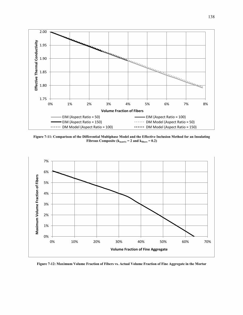
138
Figure 7-11: Comparison of the Differential Multiphase Model and the Effective Inclusion Method for an Insulating
Fibrous Composite (kmatrix = 2 and kfibers = 0.2)
Figure 7-12: Maximum Volume Fraction of Fibers vs. Actual Volume Fraction of Fine Aggregate in the Mortar
1.75
1.80
1.85
1.90
1.95
2.00
0% 1% 2% 3% 4% 5% 6% 7% 8%
Effe
ctiv
e T
he
rmal
Co
nd
uct
ivit
y
Volume Fraction of Fibers
EIM (Aspect Ratio = 50) EIM (Aspect Ratio = 100)
EIM (Aspect Ratio = 150) DM Model (Aspect Ratio = 50)
DM Model (Aspect Ratio = 100) DM Model (Aspect Ratio = 150)
0%
1%
2%
3%
4%
5%
6%
7%
0% 10% 20% 30% 40% 50% 60% 70%
Max
imu
m V
olu
me
Fra
ctio
n o
f Fi
be
rs
Volume Fraction of Fine Aggregate
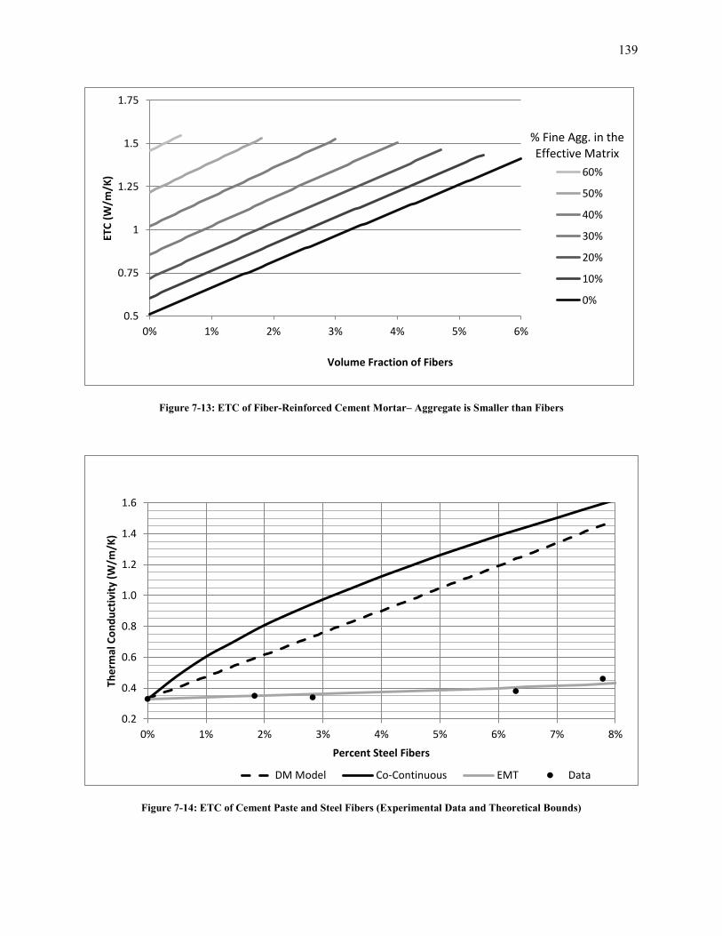
139
Figure 7-13: ETC of Fiber-Reinforced Cement Mortar– Aggregate is Smaller than Fibers
Figure 7-14: ETC of Cement Paste and Steel Fibers (Experimental Data and Theoretical Bounds)
0.5
0.75
1
1.25
1.5
1.75
0% 1% 2% 3% 4% 5% 6%
ETC
(W
/m/K
)
Volume Fraction of Fibers
60%
50%
40%
30%
20%
10%
0%
0.2
0.4
0.6
0.8
1.0
1.2
1.4
1.6
0% 1% 2% 3% 4% 5% 6% 7% 8%
The
rmal
Co
nd
uct
ivit
y (W
/m/K
)
Percent Steel Fibers
DM Model Co-Continuous EMT Data
% Fine Agg. in the Effective Matrix
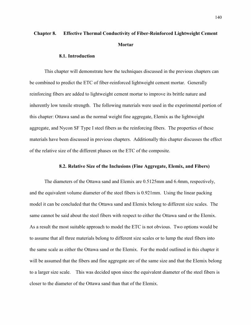
140
Chapter 8. Effective Thermal Conductivity of Fiber-Reinforced Lightweight Cement
Mortar
8.1. Introduction
This chapter will demonstrate how the techniques discussed in the previous chapters can
be combined to predict the ETC of fiber-reinforced lightweight cement mortar. Generally
reinforcing fibers are added to lightweight cement mortar to improve its brittle nature and
inherently low tensile strength. The following materials were used in the experimental portion of
this chapter: Ottawa sand as the normal weight fine aggregate, Elemix as the lightweight
aggregate, and Nycon SF Type I steel fibers as the reinforcing fibers. The properties of these
materials have been discussed in previous chapters. Additionally this chapter discusses the effect
of the relative size of the different phases on the ETC of the composite.
8.2. Relative Size of the Inclusions (Fine Aggregate, Elemix, and Fibers)
The diameters of the Ottawa sand and Elemix are 0.5125mm and 6.4mm, respectively,
and the equivalent volume diameter of the steel fibers is 0.921mm. Using the linear packing
model it can be concluded that the Ottawa sand and Elemix belong to different size scales. The
same cannot be said about the steel fibers with respect to either the Ottawa sand or the Elemix.
As a result the most suitable approach to model the ETC is not obvious. Two options would be
to assume that all three materials belong to different size scales or to lump the steel fibers into
the same scale as either the Ottawa sand or the Elemix. For the model outlined in this chapter it
will be assumed that the fibers and fine aggregate are of the same size and that the Elemix belong
to a larger size scale. This was decided upon since the equivalent diameter of the steel fibers is
closer to the diameter of the Ottawa sand than that of the Elemix.

141
8.3. Proposed Model for the ETC of Fiber-Reinforced Lightweight Cement
Paste
The ETC of the fiber-reinforced lightweight cement mortar will be computed in three
different stages (stage 1: cement paste, stage 2: fiber-reinforced cement mortar, and stage 3:
fiber-reinforced lightweight cement mortar). In the first stage the ETC of the cement paste is
computed according to the lumped parameter model outlined in Section 4.4. In the second stage
the ETC of the fiber-reinforced cement mortar is calculated using the procedure from Section
7.9, assuming that the fine aggregate and fibers are of the same size. In the third stage the ETC
of the entire composite is computed using the DM model with the ETC of the fiber-reinforced
cement mortar used as the thermal conductivity of the effective matrix. Figure 8-1 displays the
results from this model vs. the volume fraction of Elemix for various amounts of steel fibers and
Ottawa sand in the effective matrix.
8.4. ETC of Fiber-Reinforced Lightweight Cement Mortar: Experimental
Results
Table 8-1 summarizes the details of the four mix designs that were tested. Each
specimen had a water-cement ratio of 0.6 and a volume fraction of fine aggregate of 0.15. The
ETC for each mix design was taken as the average of 6 specimens that were tested using the
method discussed in Section 3.2. It is observed that the ETC decreased as the volume fraction
of Elemix was increased and the ETC increased as the volume fraction of steel fibers increased.
Additionally Table 8-1 contains the predicted values for the ETC based on the model developed
in the previous section. The predicted values are consistently higher than the experimental
values. It is believed that this difference is due to the same factors that affected the ETC of the

142
fiber-reinforced cement paste in Section 7.10 (the presence of an ITZ around the steel fibers and
inadequate compaction). However, given the wide disparity of thermal conductivities of the
various composite components, the agreement between predicted and measured results is
reasonable. Table 8-1 also includes the Hashin-Shtrikman bounds and the ETC determined from
the EMT model. It is observed that both the experimental data and the values from the proposed
model fall between the EMT value and the Hashin-Shtrikman upper bound. The Hashin-
Shtrikman bounds were determined using Equations A-26 and A-27 in the Appendix, which are
applicable to multiphase materials.
8.5. Effect of the Relative Size of the Lightweight Aggregate
If one of the principal reasons for selecting lightweight concrete for certain applications
is its low thermal conductivity, then it is undesirable for the various constituents of the concrete
to have a high thermal conductivity. Many times this is unavoidable since the majority of
normal weight aggregate and many types of reinforcing fibers do have a thermal conductivity
that is higher than both that of the cement paste and the lightweight aggregate. To overcome
this, the structure of the composite can be optimized by selecting the relative size of the various
constituents so as to minimize the ETC. For example, Table 8-2 displays the predicted results
for the ETC of two different types of fiber-reinforced lightweight cement mortar. For both the
reinforcing fibers and the normal weight aggregate are close in size. For the first type the
lightweight aggregate is much larger than both the normal weight aggregate and the reinforcing
fibers, and the second type contains lightweight aggregate that is much smaller than the other
constituents. It is seen that for most of the mix designs shown the ETC decreases when the large
lightweight aggregate is replaced with smaller sized lightweight aggregate. The results were
generated assuming that the water-cement ratio of the paste is 0.6, the normal weight aggregate

143
is Ottawa sand, the reinforcing fibers are steel, and Elemix is used as the lightweight aggregate.
The largest effect observed was for the eleventh mix design listed (φelemix = 0.5, φagg = 0.2, and
φfibers = 0.01), where the ETC decreases by 19.5% by using the smaller sized lightweight
aggregate.
8.6. Summary
It has been demonstrated in this chapter that an effective model to accurately predict the
ETC of fiber-reinforced cement mortar can be developed by combining the techniques
established in the previous chapters. This is accomplished by first grouping the different
constituents by their relative sizes and then through successive use of the DM model. Using this
model it has been shown that the ETC depends not only on the proportions and properties each
of the constituent materials, but also on their relative sizes. A consequence of this discovery is
that the ETC of a composite can then be optimized by varying the sizes of the various
constituents, e.g. large lightweight aggregate and small steel fibers or small lightweight
aggregate and large steel fibers.

144
φelemix
(%)
φagg
(%)
φfibers
(%)
HSL
(W/m/K)
Exp.
Data
(W/m/K)
EMT
(W/m/K)
HSU
(W/m/K)
Predicted
Value
(W/m/K)
30 15 1 0.15 0.47 0.38 0.85 0.55
30 15 2 0.15 0.51 0.39 1.16 0.72
20 15 2 0.20 0.75 0.49 1.20 0.82
20 15 3 0.20 0.87 0.50 1.46 1.00
Table 8-1: ETC of Fiber-Reinforced Lightweight Cement Mortar
φelemix φagg φfibers ETC (W/m/K)
Elemix is the Largest Phase
ETC (W/m/K)
Elemix is the Smallest Phase Percent Change
0.2 0.1 0.01 0.572 0.556 - 2.8%
0.4 0.1 0.01 0.437 0.417 - 4.6%
0.5 0.1 0.01 0.363 0.350 - 3.5%
0.2 0.1 0.02 0.733 0.730 - 0.4%
0.4 0.1 0.02 0.578 0.591 + 2.2%
0.5 0.1 0.02 0.493 0.517 + 4.9%
0.2 0.1 0.03 0.912 0.916 + 0.4%
0.4 0.1 0.03 0.732 0.772 + 5.5%
0.2 0.2 0.01 0.686 0.648 - 5.5%
0.4 0.2 0.01 0.546 0.475 - 13.0%
0.5 0.2 0.01 0.470 0.379 - 19.5%
0.2 0.2 0.02 0.861 0.840 - 2.5%
0.4 0.2 0.02 0.701 0.674 - 3.9%
0.2 0.2 0.03 1.054 1.041 - 1.2%
Table 8-2: ETC of Fiber-Reinforced Lightweight Cement Mortar (Comparison of Different Sizes of Lightweight
Aggregate)

145
Figure 8-1: ETC of Fiber-Reinforced Lightweight Cement Mortar vs. Volume Fraction of Elemix
0
0.3
0.6
0.9
1.2
1.5
0 0.2 0.4 0.6
ETC
(W
/m/K
)
Volume Fraction of Elemix
3% Fibers & 40%Fine Aggregate
2% Fibers & 40%Fine Aggregate
2% Fibers & 15%Fine Aggregate
1% Fibers & 15%Fine Aggregate
0.5% Fibers & 10%Fine Aggregate
% of Fibers and Fine Agg. in the Effective Matrix

146
Chapter 9. Conclusions and Future Work
This dissertation formulates a multiscale mathematical model to predict the effective
thermal conductivity of fiber-reinforced lightweight concrete composites. Additionally this
model is compared to experimental results at each developmental stage. This chapter
summarizes the proposed model along its main findings, and identifies areas for future research.
9.1. Summary of Model
The smallest scale considered in this model is that of the cement paste. Cement paste is
itself a composite material because it is composed of pore space (both gel pores and capillary
pores), the solid portion of the cement gel, and free water. A hydration model was used to
predict the volume fractions of these various components for fully hydrated cement paste based
on the water-cement ratio. Using this information a lumped parameter model was utilized to
predict the ETC of the cement paste. This model was calibrated using experimental data
obtained during this project and it was validated by comparing the results to values given in the
literature. Using the BSB adsorption model the amount of free water contained in the pore space
(degree of saturation) can be determined from the relative humidity.
The next composite studied was cement mortar. It is considered to exist at a larger scale
than cement paste because the largest capillary pores are about 50 nm and the smallest diameter
of fine aggregate is typically not much smaller than 150 μm. Next, fiber-reinforced cement
mortar and lightweight cement mortar were studied, and finally the techniques used to analyze
those two materials separately were combined to form a model that can predict the ETC of fiber-
reinforced lightweight cement mortar.

147
Due to its ability to incorporate the shape and packing characteristics of the inclusions,
the differential multiphase model (DM model) was chosen to predict the ETC of fiber-reinforced
lightweight cement mortar. Through use of the elliptic integrals, the DM model can be used to
study all types of inclusions from spheres to prolate or oblate ellipsoids. In the scope of this
study normal weight and lightweight aggregate were assumed to be perfect spheres and fibers
were assumed to be prolate ellipsoids. The DM model can also account for the packing of the
inclusions through the use of a fictitious inclusion phase that limits the volume fraction of the
actual inclusions to a previously determined maximum volume fraction. The values for the
maximum packing fractions can be found in the literature, such as for the random packing of
equal sized spheres or fibers, or they can be calculated using the linear packing model. The
linear packing model is able to compute the maximum volume fraction of inclusions of various
shapes and sizes, given the relative volume fractions of the different types of inclusions.
The next step in the determination of the ETC was to select which constituents belong to
the same size scale and which ones belong to different scales. This determination was made by
utilizing the linear packing model to observe the effect the smaller sized inclusions have on the
packing of the larger sized ones. At each scale the ETC was computed using the DM model.
This value was then used as the thermal conductivity of the effective matrix phase when the ETC
of the next scale was computed.
Throughout the report the predicted values for the ETC were compared to various bounds
that define the maximum and minimum ETC for different types of composite structures. The
first two structures were those of an internally and an externally porous material. Furthermore a
portion of the region which defines the internally porous material can be termed the insulating
fibers region and a portion of the region which defines the externally porous material can be

148
termed the conductive fibers region. These four regions are defined by the Hashin-Shtrikman
upper and lower bounds, the EMT equation, and the co-continuous model.
9.2. Main Findings
A lumped parameter model can be used to predict the ETC of cement paste for water-
cement ratios between 0.4 and 0.8 at all degrees of saturation. This model has been
validated for dry cement paste. The ETC decreases with an increase in the water-cement
ratio, while it increases with the degree of saturation.
The ITZ plays an important role in determining the ETC of a cementitious composite that
contains aggregate or fibers. The thermal conductivity of the ITZ is lower than that of
the cement paste due to its lower water-cement ratio. This causes the ETC of the
composite to be lowered and may drop it below the Hashin-Shtrikman lower bound.
The shape of the inclusions influences the ETC of a cementitious composite. This effect
is accounted for through the use of the elliptic integrals in the DM model.
The gradation of the inclusions also influences the ETC. The use of graded inclusions
increases the maximum volume fraction of the inclusions. To minimize the ETC, a
gradation of lightweight inclusions should be selected in which the actual volume fraction
of the inclusions is as close as possible to the maximum volume fraction of the
inclusions.
The relative sizes of the various inclusion phases are also a significant factor in
determining the ETC. It has been demonstrated that the ETC can be minimized by
altering the relative size of the insulating phase with respect to the conducting phase.
This shows that the model proposed in this report can be used to design the structure of
fiber-reinforced lightweight cement mortar to minimize the ETC.
149
9.3. Recommendations for Future Work
It has been shown that the composition of cement paste depends on the type of Portland
cement (i.e. I, II, III, IV, and V). Further research is needed to adjust the model for the
ETC of cement paste to include this information.
The model for the ETC of cement paste assumes complete hydration and the three phases
are pore space, solid cement gel, and free water. This model needs to be extended to
account for cement pastes that have not undergone complete hydration by including a
fourth phase: the unhydrated cement grains.
Further work is needed to study the effect of temperature on the ETC of cement paste.
The values for the ETC determined in this study are only valid at a temperature of 20oC
and it is desirable to extend this model to include the range of temperatures that are
normally encountered in construction practice. For the other materials considered in the
study (air, water, steel, normal weight aggregate, and EPS) the dependence of their
thermal conductivity on the temperature is already known.
It is known that the presence of the ITZ around the aggregate and fibers decreases the
ETC of fiber-reinforced cement mortar. The models developed in this report only
consider homogenous inclusions, and as a result they cannot incorporate the functionally
graded nature of the ITZ. Further study is needed to develop this model.
Finally more experimental data needs to be collected to fully verify some of the models
proposed in this study. Several significant conclusions were obtained from the proposed
model that were not included in the experimental portion of this study. This includes
both the effect of the gradation of the aggregate and the influence of the relative size of
the various inclusion phases on the ETC.

150
Bibliography
1 Romualdi, J. P. and Batson, G. B. Mechanics of Crack Arrest in Concrete. Proceedings,
ASCE Engineering Mechanics Journal, 89, 3 (1963), 147-168.
2 Romualdi, J. P. and Mandel, J. A. Tensile Strength of Concrete Affected by Uniformly
Distributed Closely Spaced Short Lenghts of Wire Reinforcement. Proceedings, ACI
Journal, 61, 6 (1964), 657-671.
3 Parker, W. J., Jenkins, R. J., Butler, C. P., and Abbott, G. L. Flash Method of Determining
the Thermal Diffusivity, Heat Capacity, and Thermal Conductivity. Journal of Applied
Physics, 32, 9 (1960), 1679-1684.
4 ASTM INTERNATIONAL. ASTM E 2585: Standard Practice for Thermal Diffusivity by
the Flash Method. West Conshohocken, PA, 2009.
5 Bouvard, D., Chaix, J. M., Dendievel, R., Fazekas, A., Letang, J. M., Peix, G., and Quenard
D. Characterization and Simulation of Microstructure and Properties of EPS Lightweight
Concrete. Cement and Concrete Research, 37, 12 (2007), 1666-1673.
6 Babu, K. G. and Babu, D. S. Behaviour of Lightweight Expanded Polystyrene Concretes
Containing Silica Fume. Cement and Concrete Research, 33 (2003), 755-762.
7 Babu, D. S., Babu, K. G., and Wee, T. H. Properties of Lightweight Expanded Polystyrene
Aggregate Concretes Containing Fly Ash. Cement and Concrete Research, 35 (2005), 1218-
1223.
8 Mindess, S., Young, J. F., and Darwin, D. Concrete. Prentice Hall, 2002.
9 White, Frank M. Heat Transfer. Addision-Wesley Publishing Company, Reading, 1984.
10 Fourier, J. B. Theorie Analytique de la Chaleur. Paris, 1822.
11 Milton, G. W. Correlation of the Electromagnetic and Elastic Properties of Composites and
Microgeometrics Corresponding with Effective Medium Approximations. In American
Institute of Physics (New York 1984).
12 Torquato, S. Connection Between the Morphology and Effective Properties of
Heterogeneous Materials. In Macroscopic Behavior of Heterogeneous Materials from the
Microstructure (Anaheim 1992), American Society of Mechanical Engineers.
13 Wiener, O. Die Theorie des Mischkörpers für das Feld der Stationären Strömung I. Die

151
Mittelwertsätze für Kraft, Polarisation und Energie, Der Abhandlungen der Mathematisch-
Physischen Klasse der Königl. Sächsischen Gesellschaft der Wissenschaften (1912), 509-
604.
14 Hashin, Z. and Shtrikman, S. A Variational Approach to the Theory of the Effective
Magnetic Permeability of Multiphase Materials. Journal of Applied Physics, 33, 10 (1962).
15 Maxwell, J. C. A Treastise on Electricity and Magnetism. Clarendon Press, Oxford, 1891.
16 Jeffrey, D. J. Conduction Through a Random Suspension of Spheres. Proceedings of the
Royal Society of London. Series A, Mathematical and Physical Sciences, 335, 1602 (1973),
355-367.
17 O'Brien, R. W. A Method for the Calculation of the Effective Transport Properties of
Suspensions of Interacting Particles. Journal of Fluid Mechanics, 91, 1 (1979), 17-39.
18 Eucken, A. Allgemeine Gesetzmässingkeiten für das Wärmeleitvermögen verschiedener
Stoffarten und Aggregatzustände. Forschung, 11, 1 (1940), 6-20.
19 Landauer, R. The Electrical Resistance of Binary Metallic Mixtures. Journal of Applied
Physics, 23, 7 (1952).
20 Davis, H. T., Valencourt, L. R., and Johnson, C. E. Transport Processes in Composite
Media. Journal of the American Ceramic Society, 58, 9-10 (1975), 446-452.
21 Carson, J. K., Lovatt, S. J., Tanner, D. J., and Cleland, A. C. Thermal Conductivity Bounds
for Isotropic, Porous Materials. International Journal of Heat and Mass Transfer, 48 (2005),
2150-2158.
22 Rayleigh, L. On the Influence of Obstacles Arranged in Rectangular Order Upon the
Properties of a Medium. Phil. Mag., 34 (1892), 481-492.
23 Deissler, R. G. and Eian, C. s. Investigation of Effective Thermal Conductivities of Powders.
National Advisory Committee for Aeronautics, 1952.
24 Schumann, T. and Voss, V. Heat Flow Through Granualr Material. Fuel in Science and
Practice, 13, 8 (1934), 249-256.
25 Deissler, R. G. and Boegli, J. S. An Investigation of Effective Thermal Conductivities of
Powders. ASME Transportation, 80, 7 (1958), 1417-1425.
26 Krupiczka, R. Analysis of Thermal Conductivity in Granular Materials. International

152
Journal of Chemical Engineering, 7, 1, 122-144.
27 Crane, R. A. and Vachon, R. I. A prediction of the bounds on the effective thermal
conductivity of granular materials. Journal of Heat and Mass Transfer, 20 (1977), 711-723.
28 Tsao, G. T. Thermal Conductivity of Two-Phase Materials. Industrial and Engineering
Chemistry (1961), 395-397.
29 Leach, A. G. The Thermal Conductivity of Foams. I. Models for Heat Conduction. Journal
of Physics D: Applied Physics (1993), 733-739.
30 Russell, H. W. Principle of Heat Flow in Porous Insulators. Journal of the American
Ceramic Society, 18 (1935), 1-5.
31 Campbell-Allen, D. and Thorne, C. P. The Thermal Conductivity of Concrete. Magazine of
Concrete Research, 15, 43 (1963).
32 ACI COMMITTE 122. Guide to Thermal Properties of Concrete and Masonary Systems.
ACI 122R-02, Farmington Hills, Michigan, 2002.
33 Babanov, B. B. Method of Calculation of Thermal Conduction Coefficient of Capillary
Porouse Media. Soviet Journal of Technical Physics, 2 (1957).
34 Tareev, B. Physics of Dielectric Materials. Moscow, 1975.
35 Singh, K. J., Singh, R., and Chaudhary, D. R. Heat Conduction and Porosity Correction
Term for Spherical and Cubic Particles in a Simple Cubic Packing. Journal of Physics D:
Applied Physics, 31 (1997), 1681-1687.
36 Kunii, D. and Smith, J. M. Heat Transfer Characteristics of Porous Rocks. American
Institute of Chemical Engineers Journal, 6, 1 (1963), 71-78.
37 Tong, F., Jing, L., and Zimmerman, R. W. An Effective Thermal Conductivity Model of
Geological Porous Media for Coupled Thermo-Hydro-Mechanical Systems with Multiphase
Flow. International Journal of Rock Mechanics and Mining Sciences, 46 (2009), 1358-1369.
38 Cheng, P. Heat Transfer in Geothermal Systems. In Advances in Heat Transfer. 1978.
39 Hsu, C. T. A Closure Model for Transient Conduction in Porous Media. Journal of Heat
Transfer (1999), 733-739.
40 Nakayama, A., Kuwahara, F., Sugiyama, M., and Xu, G. A Two-Energy Equation Model for
Conduction and Convection in Porous Media. International Journal of Heat and Mass

153
Transfer (2001), 4375-4379.
41 Aichlmayr, H. T. and Kulacki, F. A. The Effective Thermal Conductivity of Saturated
Porous Media. In Advances in Heat Transfer. Elsevier Inc., 2006.
42 Yang, C. and Nakayama, A. A Synthesis of Tortuosity and Dispersion in the Effective
Thermal Conductivity of Porous Media. International Journal of Heat and Mass Transfer
(2010), 3222-3230.
43 Quintard, M. and Whitaker, S. Local Thermal Equillibrium for Transient Heat Conduction:
Theory and Comparision with Numerical Experiments. International Journal of Heat and
Mass Transfer (1995), 2779-2796.
44 Nield, D. A. and Bejan, A. Convection in Porous Media. Springer Science+Business Media,
New York, 2006.
45 ASTM INTRENATIONAL. ASTM C 177: Standard Method for Steady-State Heat Flux
Measurements and Thermal Transmission Properties by Means of the Guarded-Hot-Plate
Apparatus. West Conshohocken, PA, 2004.
46 ASTM INTERNATIONAL. ASTM C 518: Standard Test Method for Steady-State
Transmission Properties by Means of the Heat Flow Meter Apparatus. West Conshohocken,
PA, 2004.
47 ASTM INTERNATIONAL. ASTM C 1114: Standard Method for Steady-State Thermal
Transmission Properties by Means of the Thin-Heater Apparatus. West Conshohocken, PA,
2006.
48 ASTM INTERNATIONAL. ASTM E 1225: Standard Test Method for Thermal Conductivity
of Solids by Means of the Guarded-Comparative-Longitudinal Heat Flow Technique. West
Conshohocken, PA, 2004.
49 ASTM INTERNATIONAL. ASTM D 5930: Standard Test Method for Thermal Conductivity
of Plastics by Means of a Transient Line-Source Technique. West Conshohocken, PA, 2009.
50 ASTM INTERNATIONAL. ASTM C 113: Standard Test Method for Thermal Conductivity
of Refractories by Hot Wire (Platinum Resistance Thermometer Technique). West
Conshohocken, PA, 2009.
51 ASTM INTERNATIONAL. ASTM E 1461: Standard Test Method for Thermal Diffusivity
by the Flash Method. West Conshohocken, PA, 2007.

154
52 Carslaw, H. S. Conduction of Heat in Solids. Clarendon Press, Oxford, 1947.
53 Cowan, R. D. Pulse Method of Measuring Thermal Diffusivity at High Temperatures.
Journal of Applied Physics, 34 (1963).
54 ASTM INTERNATIONAL. ASTM E 1269: Standard Test Method for Determining Specific
Heat Capacity by Differential Scanning Calorimetry. West Conshohocken, PA, 2011.
55 Lienhard, J. H. A Heat Transfer Textbook. Dover Publications, Englewood Cliffs, 2011.
56 Chang, R. and Modi, V. Portable Method of Measuring Thermal Properties of Ceramic
Bricks. New York.
57 NETZSCH. Operating Instructions: Nano-Flash-Apparatus LFA 447. 2009.
58 Neville, A. M. Properties of Concrete. Pearson Education Limited, England, 1995.
59 Powers, T. C. and Brownyard, T. L. Studies of the Physical Properties of Hardened
Portland Cement Paste. Detroit, 1948.
60 Bruanauer, S., Emmett, P. H., and Teller, E. Adsorption of Gases in Multimolecular Layers.
Journal of the American Chemical Society, 60, 2 (1938), 309.
61 Hansen, Torben C. Physical Structure of Hardened Cement Paste. A Classical Approach.
Materials and Structures, 19, 6 (1986), 423-436.
62 Jennings, H. M. and Tennis, P. D. Model for the Developing Microstructure in Portland
Cement Paste. Journal of the Americal Ceramic Society, 77, 12 (1994), 3161-3172.
63 Brunauer, S., Skalny, J., and Bodor, E. E. Adsorption on Nonporous Solids. Journal of
Colloid and Interface Sciences, 30, 4 (1969), 546-552.
64 Hagymassy, J., Odler, I., Yudenfreund, M., Skalny, J., and Brunauer, S. Pore Structure
Analysis by Water Vapor Adsorption. III. Analysis of Hydrated Calcium Silicates and
Portland Cements. Journal of Colloid and Interface Science, 38, 1 (1972), 20-34.
65 Mikhail, R. Sh. and Abo-El-Enein, S. A. Studies on Water and Nitrogen Adsorption on
Hardened Cement Pastes I: Development of Surface in Low Porosity Pastes. Cement and
Concrete Research, 2, 4 (1972), 401-414.
66 Xi, Y., Bažant, Z. P., and Jennings, H. M. Moisture Diffusion in Cementitious Materials:
Adsorption Iostherms. Advanced in Cement Based Materials, 1, 6 (1994), 248-257.

155
67 Kakaϛ, S. and Yener, Y. Heat Conduction. Taylor & Francis, Washington DC, 1993.
68 PURDUE UNIVERSITY. Thermophysical Properties of Matter: Thermal Conductivity;
Nonmetallic Liquids and Gases. New York, 1970.
69 Rohsenow, W. M., Hartnett, J. P., and Cho, Y. I. Handbook of Heat Transfer. McGraw-Hill,
New York, 1998.
70 Tsilingiris, P. T. Thermophysical and Transport Properties of Humid Air at Temperature
Range Between 0 and 100⁰C. Energy Conservation and Management, 49 (2007), 1098-
1110.
71 Kim, K., Jeon, S., Kim, J., and Yang, S. An Experimental Study on Thermal Conductivity of
Concrete. Cement and Concrete Research, 33 (2003), 363-371.
72 Valore, R. C. Calculation of U-Values of Hollow Concrete Masonary. Concrete
International, 2, 2 (1980), 41-63.
73 Choktaweekarn, P., Saengsoy, W., and Tangtermsirikul, S. A Model for Predicting the
Thermal Conductivity of Concrete. Magazine of Concrete Research, 61, 4 (2009), 1751-
1763.
74 Xu, Y. and Chung, D. D. L. Effect of Sand Addition on the Specific Heat and Thermal
Conductivity of Cement. Cement and Concrete Research, 30 (1999), 59-61.
75 Fu, X. and Chung, D. D. L. Effects of Silics Fume, Latex, Methylcellulose, and Carbon
Fibers on the Thermal Conductivity and Specific Heat of Cement Paste. Cement and
Concrete Research, 27, 12 (1997), 1799-1804.
76 Fu, X. and Chung, D. D. L. Effect of Admixtures on Thermal and Thermomechanical
Behavior of Cement Paste. ACI Materials Journal, 96, 4 (1999).
77 Xu, Y. and Chung, D. D. L. Increasing the Specific Heat of Cement Paste by Admixture
Surface Treatments. Cement and Concrete Research, 29 (1999), 1117-1121.
78 ASTM INTERNATIONAL. ASTM C 33: Standard Specification for Concrete Aggregates.
West Conshohocken, PA, 2008.
79 Horai, K. and Simmons, G. Thermal Conductivity of Rock-Forming Minerals. Earth and
Planetary Science Letters, 6 (1969), 359-368.
80 Diment, W. H. and Pratt, H. R. Thermal Conductivity of Some Rock Forming Minerals: A

156
Tabulation. Denver Co., 1988.
81 Dreyer, W. Properties of Anisotropic Solid-State Materials: Thermal and Electric
Properties. Springer, Wien, 1974.
82 Clauser, C. and Huenges, E. Thermal Conductivity of Rocks and Minerals. In Ahrens, T. J.,
ed., Rock Physics and Phase Relations: A Handbook of Physical Constants. American
Geophysical Union, 1995.
83 Robertson, E. C. Thermal Properties of Rocks. 1988.
84 Haenel, R. et al., eds. Handbook of Terrestrial Heat-Flow Density Determination. Kluwer
Academic Publishers, Boston, 1988.
85 ASTM INTERNATIONAL. ASTM D 4791: Standard Test Method for Flat Particles,
Elongated Particles, or Flat and Elongated Particles in Coarse Aggregate. West
Conshohocken, PA, 2010.
86 Phan-Thien, N. and Pham, D. C. Differential Multiphase Models for Polydispersed
Spheroidal Inclusions: Thermal Conductivity and Effective Viscosity. International Journal
of Engineering Science, 38 (2000), 73-88.
87 Yu, A. B. and Zou, R. P. Modifying the Linear Packing Model for Predicting the Porosity of
Nonspherical Particle Mixtures. Industrial & Engineering Chemistry Research, 35, 10
(1996), 3730-3741.
88 Jaegar, H. H. and Nagel, S. R. Physics of the Granular State. Science, 255, 5051 (1992),
1523-1531.
89 Torquato, S., Truskett, T. M., and Debenedetti, P. G. Is Random Close Packing of Spheres
Well Defined? Physics Review Letters, 84, 10 (2000), 2064-2067.
90 Nilsen, A. U. and Monteiro, P. J. Concrete: A Three Phase Material. Cement and Concrete
Research, 23, 1 (1993), 147-151.
91 Nadeau, J. C. Water-Cement Ratio Gradients in Mortars and Corresponding Effective
Elastic Properties. Cement and Concrete Research, 32 (2002), 481-490.
92 Felske, J. D. Effective Thermal Conductivity of Composite Spheres in a Continuous
Medium with Contact Resistance. International Journal of Heat and Mass Transfer, 47
(2004), 3453-3461.

157
93 Mogilevskaya, S. G., Kushch, V. I., Koroteeva, O., and Crouch, S. L. Equivalent
Inhomogeneity Method for Evaluating the Effective Conductivities of Isotropic Particulate
Composites. Journal of Mechanics of Materials and Structures, 7, 1 (2012).
94 Torquato and Rintoul. Effect of the Interface on the Properties of Composite Media.
Physical Review Letters, 75, 22 (1995), 4067-4070.
95 ASTM INTERNATIONAL. ASTM C 294: Standard Descriptive Nomenclature for
Constituents of Concrete Aggregate. West Conshohocken, PA, 2005.
96 Alexander, M. and Mindess, S. Aggregates in Concrete. Taylor & Francis Group, New
York, 2005.
97 Marcus, S. M. and Blaine, R. L. Thermal Conductivity of Polymers, Glasses, and Ceramics
by Modulated DSC.
98 Gnip, I., Vejelis, S., and Vaitkus, S. Thermal Conductivity of Expanded Polystyrene (EPS)
at 10ºC and its Conversion to Temperatures within the Interval from 0 to 50ºC. Energy and
Buildings, 52 (2012), 107-111.
99 ICC EVALUATION SERVICE. ICC-ES Evaluation Report. ESR-2574, 2012.
100 Meyer, C. and Hochstein, D. Lightweight Concrete Wall Panels for Building Envelope.
Report No. 11-14, 2011.
101 Toll, S. Packikng Mechanics of Fiber Reinforcements. Polymer Engineering and Science,
38, 8 (1998), 1337-1350.
102 Evans, K. E. and Gibson, A. G. Prediction of the Maximum Packing Fraction Achievable in
Randomly Oriented Short-Fibre Composites. Composites Science and Technology, 25
(1986), 149-162.
103 de Gennes, P. G. and Prost, J. The Physics of Liquid Crystals. Oxford University Press, New
York, 1995.
104 Xie, P., Gu, P., and Beaudoin, J. J. Electrical Percolation Phenomena in Cement Composites
Containing Conductive Fibers. Journal of Materials Science, 31 (1996), 4093-4097.
105 Chen, B., Wu, K., and Yao, W. Conductivity of Fiber Reinforced Cement-Based
Composites. Cement and Conctrete Composites, 26 (2004), 291-297.
106 Wang, J., Carson, J. K., North, M. F., and Cleland, D. J. A New Structural Model of
158
Effective Thermal Conductivity for Heterogeneous Materials with Co-Continuous Phases.
International Journal of Heat and Mass Transfer, 51 (2008), 2389-2397.
107 Hatta, H. and Taya, M. Effective Thermal Conductivity of a Misoriented Short Fiber
Composite. Journal of Applied Physics, 58, 7 (1985), 2378-2486.
108 Eshelby, J. D. The Determination of the Elastic Field of an Ellipsoidal Inclusion, and
Related Problems. Proceedings of the Royal Society of London, 241 (1957), 376-396.
109 Fricke, H. A Mathematical Treatment of the Electrical Conductivity and Capacity of
Disperse Sysrems I. The Electric Conductivity of a Suspension of Homogeneous Spheroids.
Physical Review, 24, 5 (1924), 575-587.
110 Nawy, Edward G. Fundamentals of High-Performance Concrete. John Wiley & Sons, Inc.,
New York, 2001.
111 CRC PRESS. POLYMERSnetBASE. Boca Raton, Fla, 2000.
112 CRC PRESS. Handbook of Chemistry and Physics.
113 Gordeliy, E., Crouch, S. L., and Mogilevskaya, S. G. Transient Heat Conduction in a
Medium with Multiple Spherical Cavities. International Journal for Numerical Methods in
Engineering, 77 (2009), 751-775.
114 Arfken, G. B., Weber, H. J., and Harris, F. E. Mathematical Methods for Physicists.
Academic Press, Orlando, FL, 2005.
115 McFall, A. L., Ariman, T., and Lee, L. H. N. Thermal Analysis of Plates with Circular
Inclusions. University of Notre Dame, Springfield VA, 1973.

159
Appendix
Thermal Conductivity of Water:
( )
A-1
where T [K], kw [W/m/K], and
Thermal Conductivity of Dry Air:
( )
A-2
where T [K], kw [W/m/K], and
Thermal Conductivity of Water Vapor:
( ) A-3
where T [K], kw [W/m/K], and
Saturated Vapor Pressure:
A-4
where T [oC], Psv [kPa], and

160
Limits on Parameter η1:
( )
[ ( ) ]
[( ) ][ ( ) ]
A-5
( )
[ ( ) ]
[( ) ][ ( ) ]
where ( )
is the ETC of the dry cement paste given by effective medium theory and
( )
is the Hashin-Shtrikman upper bound on the ETC of the dry cement paste.
( )
2[ ] [ ] √[( ) ( ) ]
3
A-6
( )
( )
( )
A-7
Limits on Parameter η2
( )
( ) [ ( )]
[ ( )]
A-8
( )
( ) [ ( )]
[ ( )]
where ( )
and ( )
are the Hashin-Shtrikman upper and lower bounds for cement paste
(Equations A-9 and A-10) and parameters A and B are computed using Equations A-11 and
A-12.
( )
[
]
( )
( )
A-9
( )
[
( )
]
( )
( )
A-10
161
with
( )( ) ( ) A-11
0( )( )
( )
1
A-12
Jennings and Tennis Model for the Developing Microstructure in Cement Pastes [62]:
If one gram of fresh cement paste is allowed to fully hydrate, the hydration products will form in
the following volumes (in cm3):
( ) A-13
( ) A-14
( ) A-15
( ) ( ) A-16
A-17
where c is the mass (in grams) of cement added and p1, p2, p3, and p4 are the percentages of C3S,
C2S, C3A, and C4AF in the Portland cement, respectively (Table 4-1).

162
Elliptic Integrals:
∫
( )√( )( )( )
A-18
∫
( )√( )( )( )
∫
( )√( )( )( )
where a:b:c is the aspect ratio of the ellipsoid.
Thermal Conductivity of Rock:
Figure A-1: Thermal Conductivity of Dry Sandstone, Shale, and Granite
0
1
2
3
4
5
6
0.0 0.1 0.2 0.3 0.4 0.5
The
rmal
Co
nd
uct
ivit
y (W
/mK
)
Porosity
100%
80%
60%
40%
20%
0%
% Quartz
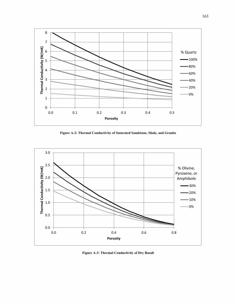
163
Figure A-2: Thermal Conductivity of Saturated Sandstone, Shale, and Granite
Figure A-3: Thermal Conductivity of Dry Basalt
0
1
2
3
4
5
6
7
8
0.0 0.1 0.2 0.3 0.4 0.5
The
rmal
Co
nd
uct
ivit
y (W
/mK
)
Porosity
100%
80%
60%
40%
20%
0%
0.0
0.5
1.0
1.5
2.0
2.5
3.0
0.0 0.2 0.4 0.6 0.8
The
rmal
Co
nd
uct
ivit
y (W
/mK
)
Porosity
30%
20%
10%
0%
% Quartz
% Olivine, Pyroxene, or Amphibole

164
Figure A-4: Thermal Conductivity of Saturated Basalt
Figure A-5: Thermal Conductivity of Limestone
0.5
1.0
1.5
2.0
2.5
3.0
3.5
0.0 0.2 0.4 0.6 0.8
The
rmal
Co
nd
uct
ivit
y (W
/mK
)
Porosity
30%
20%
10%
0%
0.0
0.5
1.0
1.5
2.0
2.5
3.0
0.0 0.1 0.2 0.3 0.4 0.5 0.6
The
rmal
Co
nd
uct
ivit
y (W
/mK
)
Porosity
Saturated
Dry
% Olivine, Pyroxene, or Amphibole

165
Figure A-6: Thermal Conductivity of Dolomite
Figure A-7: Effect of Temperature on the Thermal Conductivity of Rocks
1
2
3
4
5
0.0 0.1 0.2 0.3 0.4
The
rmal
Co
nd
uct
ivit
y (W
/mK
)
Porosity
Saturated
Dry
2.25
2.50
2.75
3.00
3.25
20 30 40 50 60 70 80
The
rmal
Co
nd
uct
ivit
y (W
/m/K
)
Temperature (oC)
Limestone
Acidic
Metamorphic
Basic

166
Singular Solid Spherical Harmonics [93]:
( )
( )
( ) A-19
where , , and define the vector in spherical coordinates and are the surface
spherical harmonics.
Surface Spherical Harmonics [113]:
( ) √
( )( )
( )
( ) A-20
where ( ) is the associated Legendre polynomial.
Associated Legendre Polynomials [114]:
( )
( )
( ) ⁄
( ) A-21
Coefficients f and g in Equation 7-2:
f g
Random 3D
Oriented 3D 0 1
Random 2D
Table A-1: Coefficients f and g in Equation 7-2
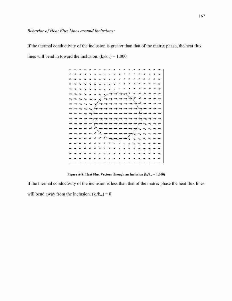
167
Behavior of Heat Flux Lines around Inclusions:
If the thermal conductivity of the inclusion is greater than that of the matrix phase, the heat flux
lines will bend in toward the inclusion. (ki/km) = 1,000
Figure A-8: Heat Flux Vectors through an Inclusion (ki/km = 1,000)
If the thermal conductivity of the inclusion is less than that of the matrix phase the heat flux lines
will bend away from the inclusion. (ki/km) = 0

168
Figure A-9: Heat Flux Vectors around an Inclusion (ki/km = 0)
Figure A-8 and Figure A-9 were developed using the solution of McFall et al. [115] for the
temperature distribution in a plate with a circular inclusion.
x
2a
2b R
r
y
θ
T= T2 T= T1
∂T/∂y = 0
∂T/∂y = 0
Figure A-10: Plate with a Circular Inclusion

169
The applied boundary conditions are:
|
A-22 |
|
The temperature distribution is:
{
∑ (
) ( )
∑ ( )
( )
A-23
And the heat flux components are:
{
∑
[ ( ) ( ) ( ) ( )]
∑( )
[ ( ) ( )]
A-24
{
∑
[ ( ) ( ) ( ) ( )]
∑( )
[ ( ) ( )]
A-25
The coefficients, , are determined by truncating the infinite series and numerically enforcing
the boundary conditions on the top, bottom, and sides of the plate.

170
Hashin-Shtrikman Bounds for Multiphase Materials:
For an isotropic mixture of N phases where , the Hashin-Shtrikman
upper and lower bounds are [37]:
∑
∑
A-26
∑
∑
A-27
where
A-28
A-29
Related Documents


