Theory of DP Flow

3 Theory of DP Flow

TO PIC PAGE

3.1 Introduction ............................................... 32

3.2 The Physics and Engineering of Fluids and Flow ..................................................... 32

3.3 Developed and Undeveloped Flow ............ 32

3.4 Reynolds Number ....................................... 33

3.5 The Bernoulli Principle................................ 35

3.6 The DP Flow Equation ................................. 40

3.7 Types of Area Meters .................................. 41

3.8 Averaging Pitot Tubes................................. 43

3.9 Things to Consider ...................................... 48

3.10 Summary .................................................... 48

3 – Theory of DP Flow

3.1 INTRODUCTIONChapter 3 covers the theoretical and computational details for DP Flow. Its purpose is two-fold:

• Introduce industry users to some of the general aspects of fluid flow and specifically DP Flow technologies • Explain the underlying assumptions and approaches behind the engineering of Rosemount DP Flow products

Note that an in-depth understanding of the physical relationships that affect DP Flow are useful in helping technical personnel cover all the aspects in the engineering of a specific application, but is not required for the installation and daily operation of DP flowmeters. What is important to understand is that there is a great deal of complexity that exists under the surface of even the simplest application.

3.1.1 Available Resources

There are many readily available resources that allow engineers to resolve complexities. Among these resources are the following:

• Application and sales engineering resources available from the vendor of a given product • Industry training and discussion by both experts and peers at user group and formal workshop sessions • Software toolboxes and utilities usually developed by vendors and designed to streamline the engineering of a given application • A large body of technical articles and books on the subject • Standards documents from standards organizations (ISO, ASME, AGA, etc)

The following chapters discuss the practical side of DP Flow — which technologies best serve a given class of application (gases, liquids, steam), insight into the hardware and software of available products (transmitters, primary elements), and considerations for installation and use.

3.2 THE PHYSICS AND ENGINEERING OF FLUIDS AND FLOWThe concepts used in DP Flow theory and calculations originate mainly in two areas of fluid mechanics: fluid kinematics, the study of fluids in motion; and fluid dynamics, the study of the effects of forces due to fluid motion. The DP Flow equation is based on the conservation of energy, and applies to the measurement of almost every type of fluid found in industrial or commercial use.

The advantages of using DP devices to measure flow rate include the simplicity of the sensing system, the availability of many types of primary devices, the ability to verify the measurement, and the wide range of applications that are suitable for DP Flow.

The challenges for using DP flowmeters are overcome by becoming familiar with the theory and operation of the devices used for DP Flow measurement.

3.3 DEVELOPED AND UNDEVELOPED FLOWWhen evaluating the performance of flowmeters and in assessing their use in a potential application, the condition of the velocity profile at the plane of measurement should be considered. A flow rate is considered “developed” when the velocity profile does not change significantly as it travels downstream. DP Flow calculations assume there is a developed flow. Achieving developed flow requires either a sufficient length of straight piping, or devices installed upstream that remove excessive turbulence or “straighten the flow.” Since most flow meters are primarily tested in developed flows, the potential effects on the performance of a meter must be considered separately if the flow at the measuring plane is not developed.

Different types of flow devices are affected differently by underdeveloped flows. Underdeveloped flow can result from additional turbulence in a pipe caused by piping fittings and types of valves installed upstream of the measurement location. Because of this, manufacturers usually provide a chart that shows how the flow meter device should be installed to achieve the stated performance.

32


(3.1)

3.4 REYNOLDS NUMBERReynolds Number, is an important non-dimensional parameter used in fluid mechanics. It is defined as the ratio of the inertial force of a fluid to the viscous force. The Reynolds number allows modeling of a fluid flow so that specific operational characteristics can be indexed to a common value. Aerodynamicists use the Reynolds number to allow the determination of how an aircraft will perform based on much smaller models used in wind tunnels. For flow metering, the Reynolds number is used to define a universal measuring range for all types of fluids. This ability greatly simplifies the evaluation, sizing, and use of flow meters.

For flow through a pipe the Reynolds number is given by:

Where:

ρ = Fluid density

D = Pipe diameter

= Average fluid velocity

μ = Absolute (dynamic) velocity of the fluid

The flow through a pipe is characterized by ranges of the Reynolds Number. The identification of these ranges, or regimes, is the result of extensive studies by scientists and engineers researching the theory that fluids flowing in pipes go through a transition between low and high velocities. This transition causes a change in the velocity profile in a pipe, which greatly affects the dynamics of the fluid and the ability accurately to measure the flow rate.

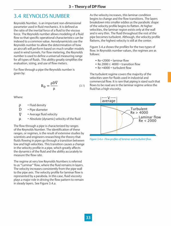
The regime at very low Reynolds Numbers is referred to as “Laminar” flow, where the fluid remains in layers. The velocity increases consistently from the pipe wall to the pipe axis. The velocity profile for laminar flow is represented by a parabola. In this case, fluid viscosity plays a major role in driving the flow pattern to remain in steady layers. See Figure 3.4.a.

As the velocity increases, this laminar condition begins to change and the flow transitions. The layers breakdown into smaller eddies as the parabolic shape of the velocity profile begins to flatten. At higher velocities, the laminar region exists only at the wall and is very thin. The fluid throughout the rest of the pipe becomes turbulent. Although, the velocity profile flattens, the highest velocity is still at the center.

Figure 3.4.a shows the profiles for the two types of flow. In Reynolds number values, the regimes are as follows:

• Re <2000 = laminar flow • Re 2000 ≤ 4000 = transition flow • Re >4000 = turbulent flow

The turbulent regime covers the majority of the velocities seen for fluids used in industrial and commercial flow. It is rare that piping is sized such that flows to be read are in the laminar regime unless the fluid has a high viscosity.

Figure 3.4.a - Flow profiles of laminar and turbulent flow.

33

TurbulentRe > 4000

Laminar flowRe < 2000

averageV


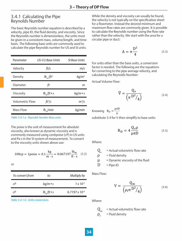
The poise is the unit of measurement for absolute viscosity, also known as dynamic viscosity and is commonly measured using centipoise (cP) in US units and Pa·s in the SI system of measurement. To convert to the viscosity units shown above use:

(3.2)

Table 3.4.1.b - Units conversions.

While the density and viscosity can usually be found, the velocity is not typically on the specification sheet for a flowmeter. Instead the desired minimum and maximum flow rates are commonly given. It is possible to calculate the Reynolds number using the flow rate rather than the velocity. We start with the area for a circular pipe or duct:

(3.3)

(3.4)

(3.5)

3.4.1 Calculating the Pipe Reynolds Number

The basic Reynolds number equation is described by a velocity, pipe ID, the fluid density, and viscosity. Since the Reynolds number is dimensionless, the units must be given in a consistent mass, volume/length, and time basis. The following base units are commonly used to calculate the pipe Reynolds number for US and SI units:

Table 3.4.1.a - Reynolds Number Base units.

Parameter US-CU Base Units SI Base Units

Velocity ft/s m/s

Density lbm /ft3 kg/m3

Diameter ft m

Viscosity lbm/ft•s kg/m•s

Volumetric Flow ft3/s m3/s

Mass Flow lbm/min kg/min

To convert from to Multiply by

cP kg/m•s 1 x 10-3

cP lbm/ft•s 6.7197 x 10-4

34

For units other than the base units, a conversion factor is needed. The following are the equations for converting to the pipe average velocity, and calculating the Reynolds Number:

Actual Volume Flow:

Where:

Qv = Actual volumetric flow rate

ρ = Fluid density

μ = Dynamic viscosity of the fluid

D = Pipe ID

Mass Flow:

Knowing

substitute 3.4 for V then simplify to base units:

Where:

Qm = Actual volumetric flow rate

ρf = Fluid density

(3.6)

or


Standard Volume Flow:

(3.7)

(3.8)

(3.9)

Figure 3.4.2.a - Rosemount Annubar™ primary element remote-mounted in a non-circular duct.

1 For introduction, see Chapter 1, “Bernoulli.”2 Swiss physicist and mathematician, 1707-1783. He created much of the mathematical terminology and notation used today in addition to his work in mechanics, fluid dynamics, astronomy, and optics.

3.5 THE BERNOULLI PRINCIPLE1 In fluid dynamics, the Bernoulli Principle and the equations derived from it are a special form of the conservation of energy equation first described mathematically by Leonhard Euler2 in 1757. This principle is a collection of related equations whose forms can differ for different kinds of flow. The basic Bernoulli Equation for steady, incompressible flow is:

(3.10)

(3.11)

35

Knowing


Knowing


Where:

DH = Hydraulic diameter

A = Duct wetted area

P = Duct wetted perimeter

H = Duct height (span)

W = Duct width

Where:

Qs = Standard volume flow rate

ρb = Density at standard conditions

3.4.2 Special Case: Non-Circular Ducts

For non-circular ducts (Figure 3.5.2.a), the hydraulic diameter is used in place of pipe diameter. This is defined as 4 times the cross-sectional area divided by the wetted perimeter. The equation is:

Where:

ρ = Density of the fluid

p = Pressure of the fluid

g = Local gravitational constant

z = Height above a datum

Vs = Velocity of the fluid in the streamline

This equation applies to a fluid that is moving along a “streamline” (denoted as “s”), a continuous path that is followed. All changes in the fluid will only occur along the streamline, and no fluid will flow out of or into the streamline. For the application of this concept to fluid meters, where the fluid is flowing in a conduit or pipe, the pipe is the streamline. For steady-state conditions with developed flow, this one-dimensional model is sufficient to describe the flow field in a pipe.


(3.11)

(3.12)

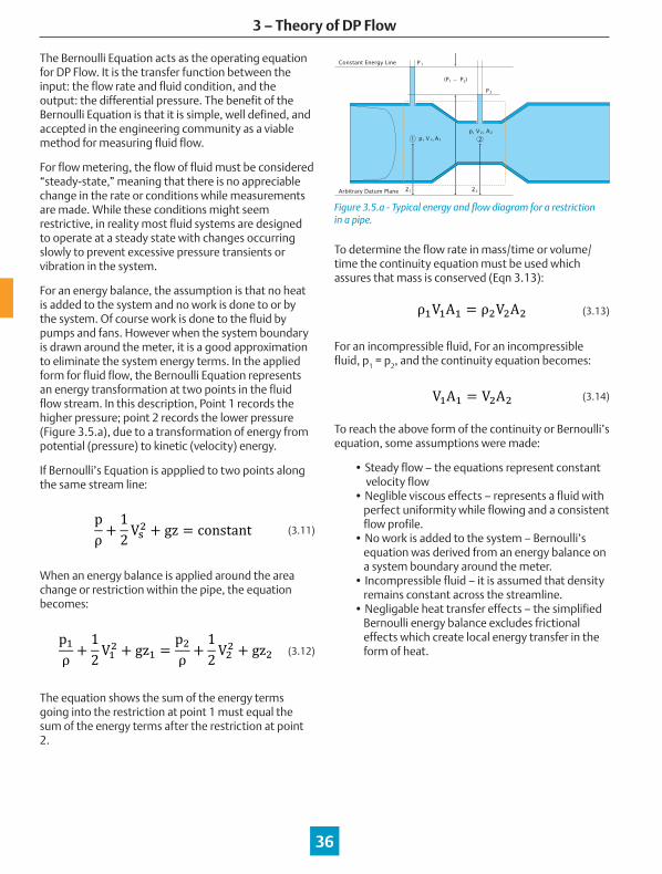
Figure 3.5.a - Typical energy and flow diagram for a restriction in a pipe.

To determine the flow rate in mass/time or volume/time the continuity equation must be used which assures that mass is conserved (Eqn 3.13):

For an incompressible fluid, For an incompressible fluid, p1 = p2, and the continuity equation becomes:

To reach the above form of the continuity or Bernoulli’s equation, some assumptions were made:

• Steady flow – the equations represent constant velocity flow • Neglible viscous effects – represents a fluid with perfect uniformity while flowing and a consistent flow profile. • No work is added to the system – Bernoulli’s equation was derived from an energy balance on a system boundary around the meter. • Incompressible fluid – it is assumed that density remains constant across the streamline. • Negligable heat transfer effects – the simplified Bernoulli energy balance excludes frictional effects which create local energy transfer in the form of heat.

(3.13)

(3.14)

The Bernoulli Equation acts as the operating equation for DP Flow. It is the transfer function between the input: the flow rate and fluid condition, and the output: the differential pressure. The benefit of the Bernoulli Equation is that it is simple, well defined, and accepted in the engineering community as a viable method for measuring fluid flow.

For flow metering, the flow of fluid must be considered “steady-state,” meaning that there is no appreciable change in the rate or conditions while measurements are made. While these conditions might seem restrictive, in reality most fluid systems are designed to operate at a steady state with changes occurring slowly to prevent excessive pressure transients or vibration in the system.

For an energy balance, the assumption is that no heat is added to the system and no work is done to or by the system. Of course work is done to the fluid by pumps and fans. However when the system boundary is drawn around the meter, it is a good approximation to eliminate the system energy terms. In the applied form for fluid flow, the Bernoulli Equation represents an energy transformation at two points in the fluid flow stream. In this description, Point 1 records the higher pressure; point 2 records the lower pressure (Figure 3.5.a), due to a transformation of energy from potential (pressure) to kinetic (velocity) energy.

If Bernoulli’s Equation is appplied to two points along the same stream line:

When an energy balance is applied around the area change or restriction within the pipe, the equation becomes:

The equation shows the sum of the energy terms going into the restriction at point 1 must equal the sum of the energy terms after the restriction at point 2.

36

21 p, V , A

Z

1

1 Z2

P2

P1

(P P )1 2

1

p, V , A2 2

Constant Energy Line

Arbitrary Datum Plane


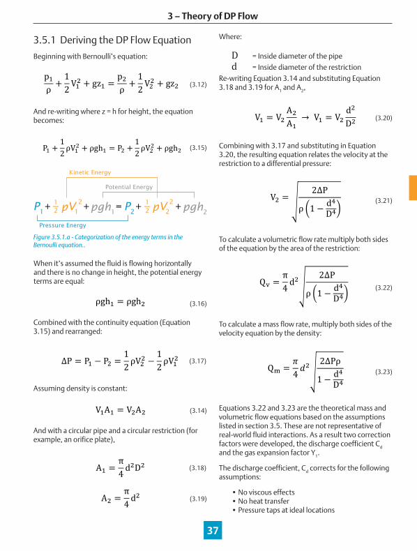
3.5.1 Deriving the DP Flow Equation

Beginning with Bernoulli’s equation:

And re-writing where z = h for height, the equation becomes:

(3.12)

(3.15)

Figure 3.5.1.a - Categorization of the energy terms in the Bernoulli equation..

(3.16)

(3.17)

(3.14)

(3.18)

(3.19)

Equations 3.22 and 3.23 are the theoretical mass and volumetric flow equations based on the assumptions listed in section 3.5. These are not representative of real-world fluid interactions. As a result two correction factors were developed, the discharge coefficient Cd and the gas expansion factor Y1.

The discharge coefficient, Cd corrects for the following assumptions:

• No viscous effects • No heat transfer • Pressure taps at ideal locations

(3.20)

(3.21)

(3.22)

(3.23)

37

When it’s assumed the fluid is flowing horizontally and there is no change in height, the potential energy terms are equal:

Combined with the continuity equation (Equation 3.15) and rearranged:

Assuming density is constant:

And with a circular pipe and a circular restriction (for example, an orifice plate),

To calculate a volumetric flow rate multiply both sides of the equation by the area of the restriction:

To calculate a mass flow rate, multiply both sides of the velocity equation by the density:

Re-writing Equation 3.14 and substituting Equation 3.18 and 3.19 for A1 and A2,

Combining with 3.17 and substituting in Equation 3.20, the resulting equation relates the velocity at the restriction to a differential pressure:

P1

P2

V1

+ + + +=12

12p pgh

1pgh

2

2 V2p2

Pressure Energy

Kinetic Energy

Potential Energy

Where:

D = Inside diameter of the pipe

d = Inside diameter of the restriction


38

The Gas Expansion Factor corrects for gas density changes as a gas flows through a restriction.

3.5.2 Beta Ratio

Instead of a “restriction,” this type of meter can be called an “area” meter, as the meter is based on a change in area. For convenience, the ratio “d/D” is called “Beta”, or “β.” The term “d4/D4” would then be β4. Area meters such as orifice plates or venturis are defined by Beta, and the result of calibrations is classified by the type of area meter. To further simplify the flow equation, the term for Beta replaces the diameter ratio:

(3.24)

(3.25)

The parameter: is defined as “E,” sometimes

called the velocity of approach, so that the equation simplifies to:

This is still the theoretical equation for incompressible flow, as it does not account for energy losses for a real fluid. When the discharge coefficient is added to the equation, it is called the “Actual Mass Flow Equation for an incompressible flow” and is:

(3.26)

3.5.3 The Discharge Coefficient (Cd)

The discharge coefficient is dependent on the Reynolds Number, and the value approaches a constant as the Reynolds number approaches infinity. A given meter type, Beta, and Reynolds number value will generate a unique discharge coefficient. Discharge coefficients are determined in the flow laboratory where an actual flow rate and the fluid conditions are known for a defined flow field. The following example illustrates how this factor is determined.

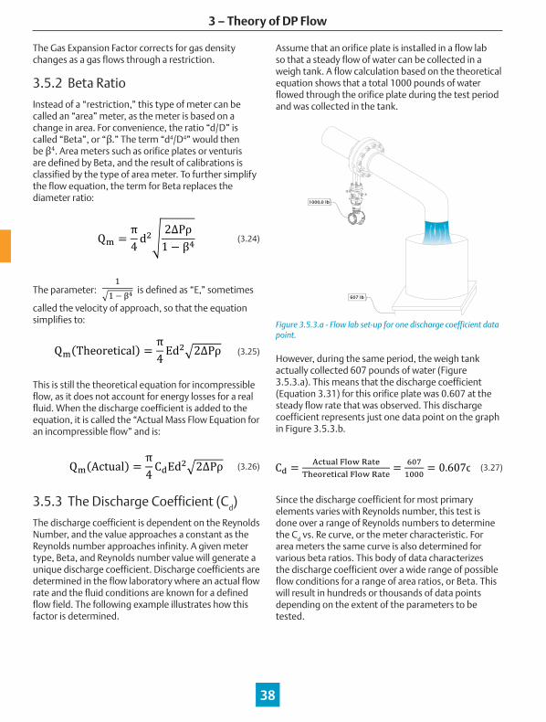
Figure 3.5.3.a - Flow lab set-up for one discharge coefficient data point.

However, during the same period, the weigh tank actually collected 607 pounds of water (Figure 3.5.3.a). This means that the discharge coefficient (Equation 3.31) for this orifice plate was 0.607 at the steady flow rate that was observed. This discharge coefficient represents just one data point on the graph in Figure 3.5.3.b.

(3.27)

Since the discharge coefficient for most primary elements varies with Reynolds number, this test is done over a range of Reynolds numbers to determine the Cd vs. Re curve, or the meter characteristic. For area meters the same curve is also determined for various beta ratios. This body of data characterizes the discharge coefficient over a wide range of possible flow conditions for a range of area ratios, or Beta. This will result in hundreds or thousands of data points depending on the extent of the parameters to be tested.

607 lb

1000.0 lb

Assume that an orifice plate is installed in a flow lab so that a steady flow of water can be collected in a weigh tank. A flow calculation based on the theoretical equation shows that a total 1000 pounds of water flowed through the orifice plate during the test period and was collected in the tank.

c


39

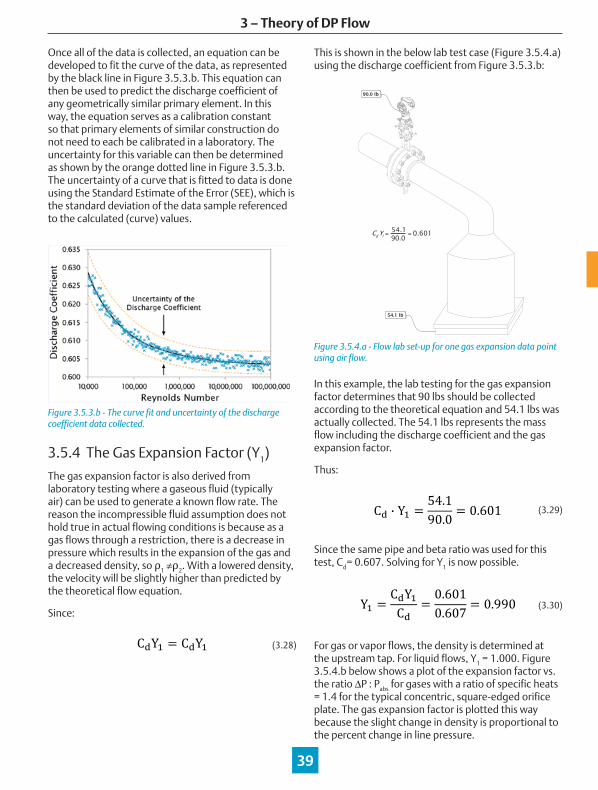
Once all of the data is collected, an equation can be developed to fit the curve of the data, as represented by the black line in Figure 3.5.3.b. This equation can then be used to predict the discharge coefficient of any geometrically similar primary element. In this way, the equation serves as a calibration constant so that primary elements of similar construction do not need to each be calibrated in a laboratory. The uncertainty for this variable can then be determined as shown by the orange dotted line in Figure 3.5.3.b. The uncertainty of a curve that is fitted to data is done using the Standard Estimate of the Error (SEE), which is the standard deviation of the data sample referenced to the calculated (curve) values.

Figure 3.5.3.b - The curve fit and uncertainty of the discharge coefficient data collected.

3.5.4 The Gas Expansion Factor (Y1)

The gas expansion factor is also derived from laboratory testing where a gaseous fluid (typically air) can be used to generate a known flow rate. The reason the incompressible fluid assumption does not hold true in actual flowing conditions is because as a gas flows through a restriction, there is a decrease in pressure which results in the expansion of the gas and a decreased density, so ρ1 ≠ρ2. With a lowered density, the velocity will be slightly higher than predicted by the theoretical flow equation.

Since:

(3.28)

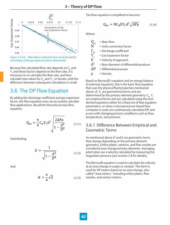
This is shown in the below lab test case (Figure 3.5.4.a) using the discharge coefficient from Figure 3.5.3.b:

Figure 3.5.4.a - Flow lab set-up for one gas expansion data point using air flow.

In this example, the lab testing for the gas expansion factor determines that 90 lbs should be collected according to the theoretical equation and 54.1 lbs was actually collected. The 54.1 lbs represents the mass flow including the discharge coefficient and the gas expansion factor.

Thus:

Since the same pipe and beta ratio was used for this test, Cd= 0.607. Solving for Y1 is now possible.

For gas or vapor flows, the density is determined at the upstream tap. For liquid flows, Y1 = 1.000. Figure 3.5.4.b below shows a plot of the expansion factor vs. the ratio ∆P : Pabs for gases with a ratio of specific heats = 1.4 for the typical concentric, square-edged orifice plate. The gas expansion factor is plotted this way because the slight change in density is proportional to the percent change in line pressure.

(3.30)

54.1 lb

90.0 lb

=Cd Y1 =54.190.0

0.601

(3.29)


40

Figure 3.5.4.b. - After data is collected a line can be fit and the uncertainty of the gas expansion factor determined.

Because the calculated flow rate depends on Cd and Y1 and these factors depend on the flow rate, it is necessary to re-calculate the flow rate, and then calculate new values for Cd and Y1, or iterate, until the difference between subsequent calculations is small.

3.6 The DP Flow EquationBy adding the discharge coefficient and gas expansion factor, the flow equation now can accurately calculate flow applications. Recall the theoretical mass flow equation:

Substituting:

And

Where:

Qm = Mass flow

N = Units conversion factor

CD = Discharge coefficient

Y1 = Gas Expansion Factor

E = Velocity of approach

d2 = Bore diameter of differential producer

ΔP = Differential pressure

ρ = Density

Based on Bernoulli’s equation and an energy balance (Continuity Equation), this is the basic flow equation that uses the physical fluid properties mentioned above. d2, E, are geometrical terms and are determined by the primary element geometry. Cd, Y1 are empirical terms and are calculated using the test-derived equations either for a fixed set of flow equation parameters, or when a microprocessor-based flow computer is used, are continuously calculated DP, and ρ vary with changing process conditions such as flow, temperature, and pressure.

3.6.1 Difference Between Empirical and Geometric Terms

As mentioned above d2 and E are geometric terms that change depending on the primary element geometry. Orifice plates, venturis, and flow nozzles are considered area-change primary elements. Averaging pitot tubes use a velocity calculated by measuring the stagnation pressure (see section 3.8 for details).

The Bernoulli equation is used to calculate the velocity at an area change in a pipe or conduit. This form is used for DP meters based on an area change, also called “area meters,” including orifice plates, flow nozzles, and venturi meters.

(3.31)

(3.32)

The flow equation is simplified to become:

(3.33)

(3.34)

Gas

Expan

sion F

acto

r

0

0.95

0.96

0.97

0.98

0.99

10.025 0.05 0.075 0.1 0.125 0.15

PΔPabs

Uncertainty of theGas Expansion Factor


41

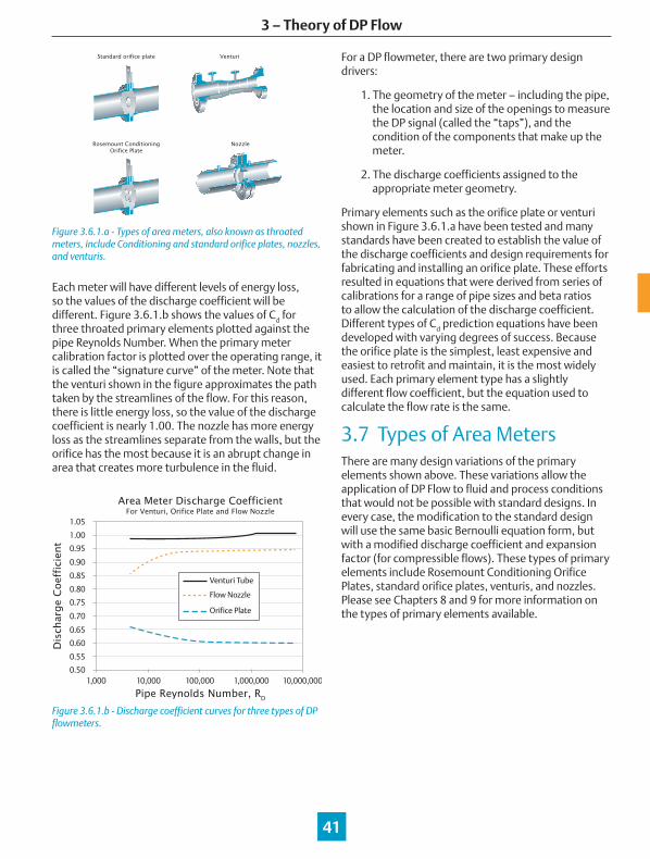
Figure 3.6.1.a - Types of area meters, also known as throated meters, include Conditioning and standard orifice plates, nozzles, and venturis.

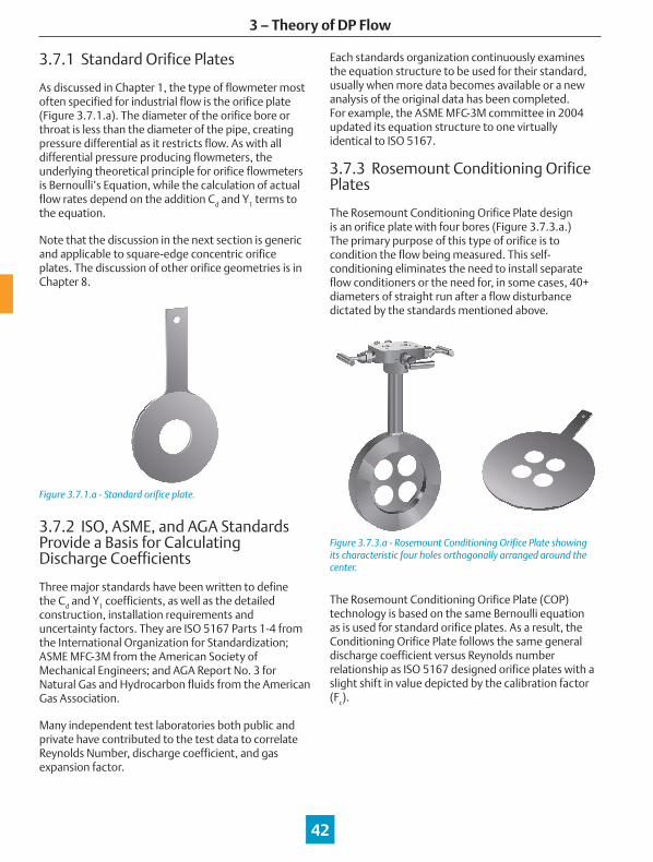
Each meter will have different levels of energy loss, so the values of the discharge coefficient will be different. Figure 3.6.1.b shows the values of Cd for three throated primary elements plotted against the pipe Reynolds Number. When the primary meter calibration factor is plotted over the operating range, it is called the “signature curve” of the meter. Note that the venturi shown in the figure approximates the path taken by the streamlines of the flow. For this reason, there is little energy loss, so the value of the discharge coefficient is nearly 1.00. The nozzle has more energy loss as the streamlines separate from the walls, but the orifice has the most because it is an abrupt change in area that creates more turbulence in the fluid.

Figure 3.6.1.b - Discharge coefficient curves for three types of DP flowmeters.

For a DP flowmeter, there are two primary design drivers:

1. The geometry of the meter – including the pipe, the location and size of the openings to measure the DP signal (called the “taps”), and the condition of the components that make up the meter.

2. The discharge coefficients assigned to the appropriate meter geometry.

Primary elements such as the orifice plate or venturi shown in Figure 3.6.1.a have been tested and many standards have been created to establish the value of the discharge coefficients and design requirements for fabricating and installing an orifice plate. These efforts resulted in equations that were derived from series of calibrations for a range of pipe sizes and beta ratios to allow the calculation of the discharge coefficient. Different types of Cd prediction equations have been developed with varying degrees of success. Because the orifice plate is the simplest, least expensive and easiest to retrofit and maintain, it is the most widely used. Each primary element type has a slightly different flow coefficient, but the equation used to calculate the flow rate is the same.

3.7 Types of Area MetersThere are many design variations of the primary elements shown above. These variations allow the application of DP Flow to fluid and process conditions that would not be possible with standard designs. In every case, the modification to the standard design will use the same basic Bernoulli equation form, but with a modified discharge coefficient and expansion factor (for compressible flows). These types of primary elements include Rosemount Conditioning Orifice Plates, standard orifice plates, venturis, and nozzles. Please see Chapters 8 and 9 for more information on the types of primary elements available.

Standard orifice plate

Rosemount ConditioningOrifice Plate

Nozzle

VenturiD

isch

arge

Coef

fici

ent

Pipe Reynolds Number, RD

Area Meter Discharge CoefficientFor Venturi, Orifice Plate and Flow Nozzle

1,000 10,000 100,000 1,000,000 10,000,0000.50

0.55

0.60

0.65

0.70

0.75

0.80

0.85

0.90

0.95

1.00

1.05

Venturi Tube

Orifice Plate

Flow NozzleOrifice Plate

Flow Nozzle

Venturi Tube


42

3.7.1 Standard Orifice Plates

As discussed in Chapter 1, the type of flowmeter most often specified for industrial flow is the orifice plate (Figure 3.7.1.a). The diameter of the orifice bore or throat is less than the diameter of the pipe, creating pressure differential as it restricts flow. As with all differential pressure producing flowmeters, the underlying theoretical principle for orifice flowmeters is Bernoulli’s Equation, while the calculation of actual flow rates depend on the addition Cd and Y1 terms to the equation.

Note that the discussion in the next section is generic and applicable to square-edge concentric orifice plates. The discussion of other orifice geometries is in Chapter 8.

Figure 3.7.1.a - Standard orifice plate.

3.7.2 ISO, ASME, and AGA Standards Provide a Basis for Calculating Discharge Coefficients

Three major standards have been written to define the Cd and Y1 coefficients, as well as the detailed construction, installation requirements and uncertainty factors. They are ISO 5167 Parts 1-4 from the International Organization for Standardization; ASME MFC-3M from the American Society of Mechanical Engineers; and AGA Report No. 3 for Natural Gas and Hydrocarbon fluids from the American Gas Association.

Many independent test laboratories both public and private have contributed to the test data to correlate Reynolds Number, discharge coefficient, and gas expansion factor.

Each standards organization continuously examines the equation structure to be used for their standard, usually when more data becomes available or a new analysis of the original data has been completed. For example, the ASME MFC-3M committee in 2004 updated its equation structure to one virtually identical to ISO 5167.

3.7.3 Rosemount Conditioning Orifice Plates

The Rosemount Conditioning Orifice Plate design is an orifice plate with four bores (Figure 3.7.3.a.) The primary purpose of this type of orifice is to condition the flow being measured. This self-conditioning eliminates the need to install separate flow conditioners or the need for, in some cases, 40+ diameters of straight run after a flow disturbance dictated by the standards mentioned above.

Figure 3.7.3.a - Rosemount Conditioning Orifice Plate showing its characteristic four holes orthogonally arranged around the center.

The Rosemount Conditioning Orifice Plate (COP) technology is based on the same Bernoulli equation as is used for standard orifice plates. As a result, the Conditioning Orifice Plate follows the same general discharge coefficient versus Reynolds number relationship as ISO 5167 designed orifice plates with a slight shift in value depicted by the calibration factor (Fc).


43

The four holes in the plate are placed equally around the plate center. When a kinetic energy balance is done at the conditioning orifice plate and the continuity equation is applied, the result requires the rate of the flow through the four holes to be the same. This pattern forces a distribution of the flow through the holes, creating a consistent downstream dynamic even when the upstream fluid velocity distribution is highly asymmetric or cyclonic. Since most of the orifice DP signal is created downstream, the COP provides equivalent results when installed in very close proximity to typical piping components or long runs of straight pipe. This removes the requirement for a flow conditioner to provide high performance in short straight pipe runs.

Figure 3.7.3.b - Illustration of how the four holes in the Rosemount Conditioning Orifice Plate conditions irregular flow profiles to provide accurate flow measurement with little straight run.

Total Straight Pipe Run Diameters Upstream (in Pipe Diameters) Downstream (in Pipe Diameters)

1595 and 405C 2 2

ASME MFC 3M Up to 54 Up to 5

AGA Report Number 3 Up to 95 Up to 4.2

ISO 5167 Up to 60

Up to 7

Flow Conditioners

Pressure Taps Flange Taps Corner Taps D and D/2

Not Reqired. All three standards sometimes require flow conditioners to shorten required straight pipe run.

Complies with all three standards Complies with ASME and ISO. Corner taps not included in AGA Report Number 3 In development

O-Plate Thickness 2’’ to 4’’ 6’’ 8’’ to 20’’

Complies with all three standards Complies with ASME and ISO. Thicker than AGA Report Number 3 Complies with all three standards

Beta Area of 4 holes = Area of same βfor standard oriface of all three standards.1

All other plate dimensions (including angle of bevel, bore thickness (e), etc.) Complies with all three standards

Surface Finish Complies with all three standards

Discharge Coefficient Uncertainty Follows ISO 5167.2

Expansion Factor Follows ISO 5167.

1 At Schedule Standard 2 Follows ISO 5167 with a bias shift – the bias is determined from previous test or is determined by lab calibration by request

Category 1595 and 405C Conditioning Orifice Plate Technology

Rosemount Conditioning Orifice flowmeters follows the intent of three main standards, ISO 5167/ASME MFC 3M and AGA Report Number 3. See Table 3.8.3.I for details of compliance and deviations from the standards.

3.8 Averaging Pitot TubesPitot tubes calculate velocity by measuring the pressure created by the fluid impact of the fluid on the pitot tubes. If the pressure at the low static pressure tap is considered to be the pipe or conduit static pressure, the DP is called the dynamic pressure of the fluid. This form is used for the pitot tube, invented and first used by Henri de Pitot in 1784. The modern incarnation of the pitot tube is the Averaging Pitot Tube, or APT. The purpose of the APT is to measure the flow rate in a pipe or duct by measuring the velocity pressure over the diameter of the pipe and average the results.

Table 3.7.3.1 – Comparison of the Rosemount Conditioning Orifice Plate to single-hole concentric orifice plates.

Even Profile

Even Profile


44

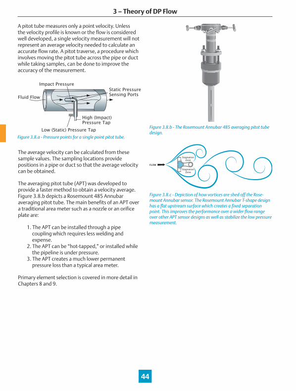
Figure 3.8.a - Pressure points for a single point pitot tube.

The average velocity can be calculated from these sample values. The sampling locations provide positions in a pipe or duct so that the average velocity can be obtained.

The averaging pitot tube (APT) was developed to provide a faster method to obtain a velocity average. Figure 3.8.b depicts a Rosemount 485 Annubar averaging pitot tube. The main benefits of an APT over a traditional area meter such as a nozzle or an orifice plate are:

1. The APT can be installed through a pipe coupling which requires less welding and expense. 2. The APT can be “hot-tapped,” or installed while the pipeline is under pressure. 3. The APT creates a much lower permanent pressure loss than a typical area meter.

Primary element selection is covered in more detail in Chapters 8 and 9.

Figure 3.8.b - The Rosemount Annubar 485 averaging pitot tube design.

Figure 3.8.c - Depiction of how vortices are shed off the Rose-mount Annubar sensor. The Rosemount Annubar T-shape design has a flat upstream surface which creates a fixed separation point. This improves the performance over a wider flow range over other APT sensor designs as well as stabilize the low pressure measurement.

A pitot tube measures only a point velocity. Unless the velocity profile is known or the flow is considered well developed, a single velocity measurement will not represent an average velocity needed to calculate an accurate flow rate. A pitot traverse, a procedure which involves moving the pitot tube across the pipe or duct while taking samples, can be done to improve the accuracy of the measurement.

StagnationZone

StagnationZone

FLOW

Impact Pressure

Fluid Flow

Low (Static) Pressure Tap

High (Impact)Pressure Tap

Static PressureSensing Ports


45

When compared to a single-point pitot tube, the following are the important distinctions for the Rosemount Annubar APT:

1. The velocity profile is sampled at the slots or holes in the front of the tube, which is installed across the pipe. This is equivalent to a “continuous pitot-traverse.” 2. The fluid that comes to rest (or stagnates) in front of each slot or hole creates a pressure that represents the velocity at that point in the velocity field. In addition, the opening at the front of the pitot tube must be perpendicular to the fluid velocity vector to achieve a proper stagnation pressure. 3. The pressure sensed at the top of the Annubar APT front chamber is the averaged stagnation pressure for the sampling slots or holes. 4. The rear chamber measures the pressure at the rear of the tube, or the suction pressure. This pressure will be below the pipe static pressure due to the fact that for real fluids in the turbulent flow regime, separation of the fluid from the element has occurred. This is advantageous because the DP signal is higher than that obtained with a standard pitot.

The pressure sensed at the top of the rear chamber is the average suction pressure. However in most cases, the pressure created behind the tube is nearly the same across the pipe diameter due to the span-wise vortex-shedding or separation of the flowing fluid from the element.

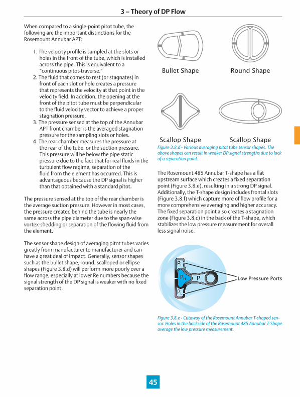
The sensor shape design of averaging pitot tubes varies greatly from manufacturer to manufacturer and can have a great deal of impact. Generally, sensor shapes such as the bullet shape, round, scalloped or ellipse shapes (Figure 3.8.d) will perform more poorly over a flow range, especially at lower Re numbers because the signal strength of the DP signal is weaker with no fixed separation point.

Figure 3.8.d - Various averaging pitot tube sensor shapes. The above shapes can result in weaker DP signal strengths due to lack of a separation point.

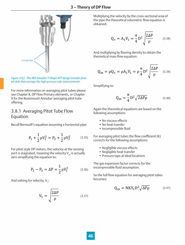
The Rosemount 485 Annubar T-shape has a flat upstream surface which creates a fixed separation point (Figure 3.8.e), resulting in a strong DP signal. Additionally, the T-shape design includes frontal slots (Figure 3.8.f) which capture more of flow profile for a more comprehensive averaging and higher accuracy. The fixed separation point also creates a stagnation zone (Figure 3.8.c) in the back of the T-shape, which stabilizes the low pressure measurement for overall less signal noise.

Figure 3.8.e - Cutaway of the Rosemount Annubar T-shaped sen-sor. Holes in the backside of the Rosemount 485 Annubar T-Shape average the low pressure measurement.

Low Pressure Ports

Bullet Shape Round Shape

Scallop Shape Scallop Shape


46

Figure 3.8.f - The 485 Annubar T-Shape APT design includes fron-tal slots that average the high pressure side measurements

For more information on averaging pitot tubes please see Chapter 8, DP Flow Primary elements, or Chapter 9 for the Rosemount Annubar averaging pitot tube offering.

3.8.1 Averaging Pitot Tube Flow Equation

Recall Bernoulli’s equation assuming a horizontal pipe:

(3.35)

For pitot style DP meters, the velocity at the sensing port is stagnated, meaning the velocity V2, is actually zero simplifying the equation to:

And solving for velocity, V1:

(3.36)

(3.37)

Mulitplying the velocity by the cross-sectional area of the pipe the theoretical volumetric flow equation is obtained:

(3.38)

And multiplying by flowing density to obtain the theoretical mass flow equation:

(3.39)

Simplifying to:

(3.40)

Again the theoretical equations are based on the following assumptions:

• No viscous effects • No heat transfer • Incompressible fluid

For averaging pitot tubes the flow coefficient (K) corrects for the following assumptions:

• Negligible viscous effects • Negligible heat transfer • Pressure taps at ideal locations

The gas expansion factor corrects for the incompressible fluid assumption.

So the full flow equation for averaging pitot tubes becomes:

(3.41)

Frontal Slot


47

Where:

N = Units conversion factor and

K = Averaging pitot tube flow coefficient

Y1 = Averaging pitot tube gas expansion factor

D = Pipe diameter


ρ = Density

3.8.2 Flow Coefficient, K, for Averaging Pitot Tubes

The K factor has to be determined by extensive laboratory testing, similar to that of the discharge coefficent for orifice plates. Empirical equations have been created to calculate the K factor based on the test data. To calculate the K factor for an averaging pitot tube, it is common to start from a function of blockage. Blockage is the ratio of the area of the averaging pitot tube to the area of the pipe.

And subsituting terms shown in figure 3.8.2.a (B is the blockage factor and is unitless)

(3.43)

(3.42)

Figure 3.8.2.a - Cross section of pipe with averaging pitot tube installed, showing terms of the blockage equation.

D

d

A A

Aπ

a

= x

4

a d D

= D2

Sensor Size Probe Width

1 0.59 in

2 1.06 in

3 1.935 in

Table 3.8.2.1 - Rosemount 485 Probe Widths for each available sensor size. Probe width is dimension d in Figure 3.8.2.a

Once the blockage is known, the K factor can be calculated.

For a blockage, B, ≤0.25 use the following K factor equation and C1 and C2 values from Table 3.8.2.2:

For a blockage, B >0.25 use equation 3.45 below and 3.8.2.2:

(3.45)

(3.44)

Table 3.8.2.2 - Constants for determining the flow coefficient for the Rosemount 485 Annubar primary element. Where C1, C2, and C3 are constants that are determined epirically based on the sensor width and shape. The values shown are applicable to the Roesmount 485 Annubar primary element.

Sensor Size C3

1 5.3955

2 —

3 —

C1

-1.515

-1.492

-1.5856

C2

1.4229

1.4179

1.3318


48

3.8.3 Gas Expansion Factor for Averaging Pitot Tubes

The gas expansion factor for averaging pitot tubes is calculated slightly differently than area meters such as orifice plates. It is a function of blockage, DP, static line pressure, and the ratio of specific heats. Again, this factor is determined by laboratory testing.

The equation for the gas expansion factor of the Rosemount Annubar primary elements is as follows – note this form requires the pressure and differential pressure to be in the same units:

(3.46)

Where:

Ya = Gas expansion factor for an averaging

pitot tube

Y1 = Adiabatic gas expansion factor

(0.3142329)

Y2 = Pressure ratio factor (0.09483556)

B = Blockage factor of averaging pitot tube


Pf = Static line pressure

γ = Ratio of specific heats

Note ∆P and Pf must be in the same units of measure for pressure so that Ya will be unitless.

3.9 THINGS TO CONSIDER 3.9.1 Computational Software

Flow computers are often used to calculate flow utilizing the variables from the DP Flow installation or other measurement points. Flow computers are configured to calculate the flow based on the fluid properties and installation specifics such as line size and process variables either from individual pressure and temperature measurements or a multivariable transmitter such as the Rosemount 4088 (see chapter 7 for details).

The other option is to utilize multivariable transmitters with the ability to calculate flow specifically the Rosemount 3051SMV. Rosemount Engineering Assistant is a PC-based software program used for configuring Rosemount MultiVariable™ devices with mass flow output. In addition to being able to configure and calibrate the device, Engineering Assistant also performs configuration of the mass flow equation inside the transmitter. This software makes setting up a compensated flow equation simpler than manually setting up the flow equation in the control system. This is because the configuration of the flow equation all happens within Engineering Assistant and the flow calculation is done with the transmitter. The user only needs to enter their basic flowmeter and process information to configure their transmitter for fully compensated mass or energy flow.

Engineering Assistant can be used as a “Stand-Alone” Windows based program, or as a SNAP-ON to AMS (covered in detail in Chapter 7). The SNAP-ON version runs within AMS, while the stand-alone version can be run without an AMS installation.

A common error in DP Flow installations is performing a double square root, or taking the square root of the Differential Pressure in the flow equation in both the transmitter and in the control system. The square root should only be taken once, either in the control system or in the transmitter.

3.10 SUMMARY Chapter 3 has focused on the theoretical and computational details for DP Flow, with a two-fold purpose:

1. Introduce industry users to some of the many aspects of fluid flow in general and of DP Flow technologies specifically 2. Explain the underlying assumptions and approaches behind the engineering of Rosemount DP Flow products


49

Note that an in-depth understanding of the physical relationships that affect DP Flow are useful to help technical personnel to cover all the bases in the engineering of a flow measurement, but is not required for the installation and daily operation of DP flowmeters. There are many readily available resources that allow engineers in charge of DP Flow projects to resolve complexities, including the following:

• Engineering expertise available from the vendor of a given product • Industry training and discussion by both experts and peers at user group and formal workshop sessions • Software toolboxes and utilities usually developed by vendors and designed to streamline the engineering of a given flow measurement • A large body of technical articles and books on the subject

3.10.1 The Physics and Engineering of Fluids and Flow

The concepts used in DP Flow theory and calculations originate mainly in two divisions of fluid mechanics: fluid kinematics, the study of fluids in motion; and fluid dynamics, the study of the effects of forces due to fluid motion. The basic DP Flow equation is based on the conservation of energy.

3.10.2 Developed and Undeveloped Flow

The condition of the velocity profile at the plane of measurement is necessary for the evaluation of flowmeters and their applications. A flow rate is considered “developed” when the velocity profile does not change significantly as it travels downstream. Achieving developed flow requires either a sufficient length of straight piping, or devices installed upstream that remove excessive turbulence or “straighten the flow.” Since most flow meters are primarily tested in developed flows, the potential effects on the performance of a meter must be considered separately if the flow at the measuring plane is not developed.

3.10.3 Reynolds Number

Reynolds number is an important non-dimensional parameter used in fluid mechanics. It is defined as the ratio of the inertial force of a fluid to the viscous force. The Reynolds number allows modeling of a fluid flow so that specific operational characteristics can be indexed to a common value.

3.10.4 The Bernoulli Principle

In fluid dynamics, the Bernoulli Principle and the equations derived from it is a form of the conservation of energy. It is in actuality a collection of related equations whose forms can differ for different kinds of flow.

The Bernoulli Equation acts as the operating equation for DP Flow — that is, the transfer function between the input: the flow rate and fluid condition, and the output: the differential pressure. The benefit of the Bernoulli Equation is that it is simple, well defined, and accepted in the engineering community as a viable method for measuring fluid flow.

3.10.5 Beta Ratio

Some DP flowmeters are called “area” meters, because the flow calculation is based on a change in area. For convenience, the ratio “d/D” is called “Beta,” or “β.” Area meters such as orifice plates or venturis are defined by Beta.

3.10.6 Discharge Coefficient

The discharge coefficient is dependent on the Reynolds number. A given primary element, Beta, and Reynolds number value will generate a unique discharge coefficient. Discharge coefficients are determined in the flow laboratory where an actual flow rate and the fluid conditions are known. Once all of the data is collected, an equation can be developed to fit the curve of the data. This equation can then be used to predict the discharge coefficient of any geometrically similar primary element.


50

3.10.7 Gas Expansion Factor

The gas expansion factor is also derived from laboratory testing where a gaseous fluid (typically air) can be used to generate a known flow rate. The reason the incompressible fluid assumption does not hold true in actual flowing conditions is because as a gas flows through a restriction, there is a decrease in pressure which results in the expansion of the gas and a decreased density, so ρ1 ≠ ρ2. With a lowered density, this means the velocity will be slightly higher than predicted by the theoretical flow equation.

3.10.8 The DP Flow Equation

By adding the discharge coefficient and gas expansion factor, the flow equation now can accurately calculate flow rate. Refer to section 3.7 above to see how this equation is simplified to become the following:

(3.34)

There have been standards created to establish the value of the discharge coefficients as well as the design requirements for fabricating and installing each type of meter.

3.10.9 Types of Area Meters

There are many variations of the basic types of DP area meters, venturi, orifice plate, and flow nozzle. These different designs offer flexibility to allow the use of DP flowmeters to various applications. In every case area meters will use the same basic Bernoulli equation form, but with a modified discharge coefficient, and expansion factor (for compressible flows). These types of primary elements include Rosemount Conditioning Orifice Plates, standard orifice plates, venturis, and nozzles. Please see Chapter 8 for more information on the available types of primary elements.

3.10.10 Standard Orifice Plates

The type of primary element most often specified in industry is the orifice plate. The diameter of the orifice bore is less than the diameter of the pipe, creating differential pressure as it restricts flow. As with all Bernoulli Principle-based differential pressure producing primary elements, the calculation of actual flow rates depends on Cd and Y1.

3.10.11 ISO, ASME and AGA Standards Provide the Means for Calculating Discharge Coefficients

Three major standards have been written to detail the Cd and Y1 coefficients, as well as the detailed construction, installation requirements and uncertainty factors. They are ISO 5167 Parts 1-4 from the International Organization for Standardization; ASME MFC-3M from the American Society of Mechanical Engineers; and AGA Report No. 3 for Natural Gas and Hydrocarbon fluids from the American Gas Association. Each standards organization continuously examines the equation structure to be used for their standard, usually when more data becomes available or a new analysis of the original data has been completed. For example, the ASME MFC-3M committee in 2004 updated its equation structure to one virtually identical to ISO 5167.

3.10.12 Rosemount Conditioning Orifice Plates

The Rosemount Conditioning Orifice Plate design is an orifice plate with four bores (refer to Figure 3.8.3.a). The primary purpose of this type of orifice is to condition the flow being measured within the area. This self-conditioning eliminates the need to install separate flow conditioners or the need for 40+ diameters of straight run after a flow disturbance. The Rosemount Conditioning Orifice Plate (COP) technology is based on the same Bernoulli equation as is used for standard orifice plates. As a result, the conditioning orifice plate follows the same general discharge coefficient versus Reynolds number relationship as standard orifice plates with a slight shift in value, depending on the Beta ratio.


51

3.10.13 Averaging Pitot Tubes

The purpose of the averaging pitot tube is to measure the flow rate in a pipe or duct by measuring the average differential pressure over the entire flow profile.

The Averaging Pitot Tube (APT) was developed to provide a faster method to obtain a velocity average. Figure 3.9.b depicts a Rosemount 485 averaging pitot tube. The main benefits of an APT are:

• The APT can be installed through a pipe coupling which requires less welding and material expense • The APT can be “hot-tapped,” or installed while the pipeline is under pressure • The APT creates a much lower permanent pressure loss than a typical area meter

3.10.14 Flow Coefficient K for Averaging Pitot Tubes

The K factor has been determined by extensive laboratory testing, similar to that of the discharge coefficient for orifice plates. Empirical equations have been created to calculate the K factor based on the test data. The K factor for an averaging pitot tube is a function of blockage and differs with differing types of meters. See Section 3.8.2 for full details.

3.10.15 Gas Expansion Factor for Averaging Pitot Tubes

The gas expansion factor for averaging pitot tubes is calculated slightly differently than area meters such as orifice plates. It is a function of blockage, DP, static line pressure, and the ratio of specific heats. Again, this factor is determined by laboratory testing. See Section 3.8.3 for details.

Standard Terms and Conditions of Sale can be found at: www.rosemount.com\terms_of_sale.The Emerson logo is a trademark and service mark of Emerson Electric Co.Rosemount and Rosemount logotype are registered trademarks of Rosemount Inc.All other marks are the property of their respective owners.

© 2015 Rosemount Inc. All rights reserved.

www.rosemount.com

Literature reference number: 00805-0100-1041 Rev AA March 2015


53

Theory of DP Flow

Documents

dp flow theory

dp flow measurement

dp flow technologies

dp flow equation

dp devices

flow rate

undeveloped flow

theory of dp flow3