Theory of computation: initial remarksddunham/cs3512s10/notes/l13.pdf · Theory of computation: initial remarks For many purposes, computation is elegantly modeled with simple mathematical

Theory of computation: initial remarksFor many purposes, computation is elegantly modeled with simplemathematical objects:

Turing machines, finite automata, pushdown automata, and such.

Turing machines (TMs) make precise the otherwise vague notion of an“algorithm”: no more powerful precise account of algorithms has been found.(Church-Turing Thesis)

An easy consequence of the definition of TMs: most functions (say, from Nto N ) are not computable (by TM-equivalent machines).

Why? There are more functions than there are TMs to compute them.

Remarkably, Turing machines also serve as a common platform forcharacterizing computational complexity, since the time cost, and space cost, ofworking with a TM is within a polynomial of the performance of conventionalcomputers.

So, for instance, the most famous open question in computer science theory —

P?= NP

— while formulated in terms of TMs, is important for practical computing.

Undergraduate study of the theory of computation typically starts with finiteautomata. They are simpler than TMs, and it is easier to prove main resultsabout them. They are also intuitively appealing. And automata theory haswide practical importance, in compiler theory and implementation, for instance.(lex – lexical analysis)

The typical next step is to study grammars, which are also nicely intuitive, andalready somewhat familiar to students. The theory of context-free grammars iscentral to compiler theory and implementation. (yacc – compiler generation)

Turing machines are only a little more complicated, but the theory ofcomputation based on them is quite sophisticated and extensive.

One thing all these models have in common is that they formulate computationin terms of questions about languages.

In fact, many of the central questions are formulated in terms oflanguage recognition: deciding whether a given string belongs to a givenlanguage.

Regular languages, regular expressionsand finite automata

“Regular” languages are relatively simple languages.

We’ll study means for “generating” regular languages and also for“recognizing” them.

All finite languages are regular.

Some infinite languages are regular.

Each regular language can be characterized by a (finite!) regular expression:which says how to generate the strings in the language.

It can also be characterized by a (finite!) finite state automaton: whichprovides a mechanism for recognizing the strings in the language.

Regular languages

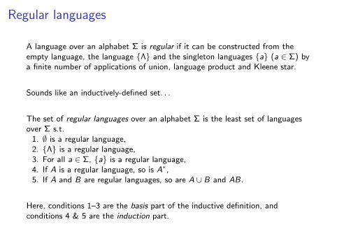
A language over an alphabet Σ is regular if it can be constructed from theempty language, the language {Λ} and the singleton languages {a} (a ∈ Σ) bya finite number of applications of union, language product and Kleene star.

Sounds like an inductively-defined set. . .

The set of regular languages over an alphabet Σ is the least set of languagesover Σ s.t.

1. ∅ is a regular language,2. {Λ} is a regular language,3. For all a ∈ Σ, {a} is a regular language,4. If A is a regular language, so is A∗,5. If A and B are regular languages, so are A ∪ B and AB.

Here, conditions 1–3 are the basis part of the inductive definition, andconditions 4 & 5 are the induction part.

The set of regular languages over an alphabet Σ is the least set of languagesover Σ s.t.

1. ∅ is a regular language,2. {Λ} is a regular language,3. For all a ∈ Σ, {a} is a regular language,4. If A is a regular language, so is A∗,5. If A and B are regular languages, so are A ∪ B and AB.

Example {00, 01, 10, 11}∗ is a regular language.

What is a “nice” description of this language?

Let’s check that it is regular:

L1 = {0} and L2 = {1} are regular.

Hence, L1L1 = {00}, L1L2 = {01}, L2L1 = {10} and L2L2 = {11} are regular.

It follows that {00} ∪ {01} = {00, 01} is regular,as are {00, 01} ∪ {10} = {00, 01, 10} and{00, 01, 10} ∪ {11} = {00, 01, 10, 11}.

So {00, 01, 10, 11}∗ is regular.

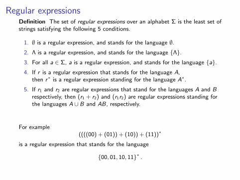
Regular expressionsDefinition The set of regular expressions over an alphabet Σ is the least set ofstrings satisfying the following 5 conditions.

1. ∅ is a regular expression, and stands for the language ∅.2. Λ is a regular expression, and stands for the language {Λ}.3. For all a ∈ Σ, a is a regular expression, and stands for the language {a}.4. If r is a regular expression that stands for the language A,

then r∗ is a regular expression standing for the language A∗.

5. If r1 and r2 are regular expressions that stand for the languages A and Brespectively, then (r1 + r2) and (r1r2) are regular expressions standing forthe languages A ∪ B and AB, respectively.

For example((((00) + (01)) + (10)) + (11))∗

is a regular expression that stands for the language

{00, 01, 10, 11}∗ .

We can omit many of the parentheses

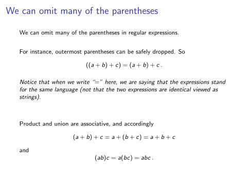
We can omit many of the parentheses in regular expressions.

For instance, outermost parentheses can be safely dropped. So

((a + b) + c) = (a + b) + c .

Notice that when we write “=” here, we are saying that the expressions standfor the same language (not that the two expressions are identical viewed asstrings).

Product and union are associative, and accordingly

(a + b) + c = a + (b + c) = a + b + c

and(ab)c = a(bc) = abc .

Precedence conventions help

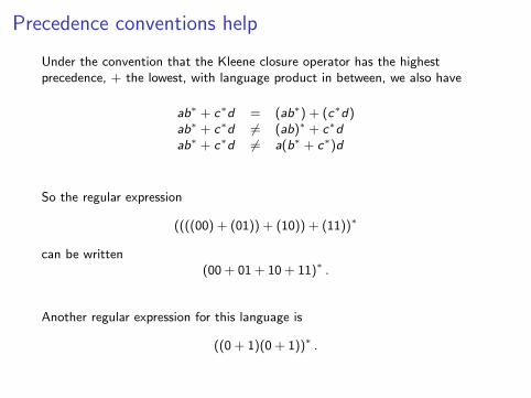
Under the convention that the Kleene closure operator has the highestprecedence, + the lowest, with language product in between, we also have

ab∗ + c∗d = (ab∗) + (c∗d)ab∗ + c∗d 6= (ab)∗ + c∗dab∗ + c∗d 6= a(b∗ + c∗)d

So the regular expression

((((00) + (01)) + (10)) + (11))∗

can be written(00 + 01 + 10 + 11)∗ .

Another regular expression for this language is

((0 + 1)(0 + 1))∗ .

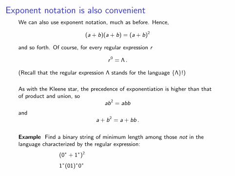
Exponent notation is also convenientWe can also use exponent notation, much as before. Hence,

(a + b)(a + b) = (a + b)2

and so forth. Of course, for every regular expression r

r 0 = Λ .

(Recall that the regular expression Λ stands for the language {Λ}!)

As with the Kleene star, the precedence of exponentiation is higher than thatof product and union, so

ab2 = abb

anda + b2 = a + bb .

Example Find a binary string of minimum length among those not in thelanguage characterized by the regular expression:

(0∗ + 1∗)2

1∗(01)∗0∗

Recognizing a regular languageFor regular languages, we address the language recognition problem roughly asfollows. To decide whether a given string is in the language of interest. . .

I Allow a single pass over the string, left to right.

I Rather than waiting until the end of the string to make a decision, wemake a tentative decision at each step. That is, for each prefix we decidewhether it is in the language.

Question: How much do we need to remember at each step about what wehave seen previously?

Everything? (If so we’re in trouble — our memory is finite, and strings can bearbitrarily long.)

Nothing? (Fine for ∅ and Σ∗.)

In general, we can expect there to be strings x , y s.t. x ∈ L and y /∈ L. As weread these strings from left to right, we will need to remember enough to allowus to distinguish x from y .

We’ll eventually give a “perfect” account of what must be remembered at eachstep — in terms of so-called “distinguishability”. First, let’s define finiteautomata and get a feeling for them. . .

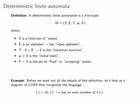
Deterministic finite automata

Definition A deterministic finite automaton is a five-tuple

M = (S , Σ, T , s0, F )

where

I S is a finite set of “states”,

I Σ is an alphabet — the “input alphabet”,

I T : S × Σ→ S is the “transition function”,

I s0 ∈ S is the “initial state”,

I F ⊂ S is the set of “final” or “accepting” states.

Example Before we work out all the details of this definition, let’s look at adiagram of a DFA that recognizes the language

{ x ∈ {0, 1}∗ | x has an even number of 1’s } .

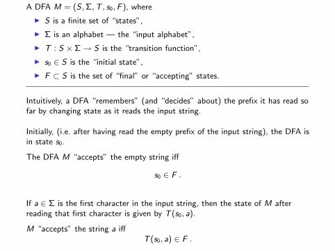
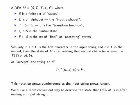
A DFA M = (S , Σ, T , s0, F ), where

I S is a finite set of “states”,

I Σ is an alphabet — the “input alphabet”,

I T : S × Σ→ S is the “transition function”,

I s0 ∈ S is the “initial state”,

I F ⊂ S is the set of “final” or “accepting” states.

Intuitively, a DFA “remembers” (and “decides” about) the prefix it has read sofar by changing state as it reads the input string.

Initially, (i.e. after having read the empty prefix of the input string), the DFA isin state s0.

The DFA M “accepts” the empty string iff

s0 ∈ F .

If a ∈ Σ is the first character in the input string, then the state of M afterreading that first character is given by T (s0, a).

M “accepts” the string a iffT (s0, a) ∈ F .

A DFA M = (S , Σ, T , s0, F ), where

I S is a finite set of “states”,

I Σ is an alphabet — the “input alphabet”,

I T : S × Σ→ S is the “transition function”,

I s0 ∈ S is the “initial state”,

I F ⊂ S is the set of “final” or “accepting” states.

Similarly, if a ∈ Σ is the first character in the input string and b ∈ Σ is thesecond, then the state of M after reading that second character is given byT (T (s0, a), b).

M “accepts” the string ab iff

T (T (s0, a), b) ∈ F .

This notation grows cumbersome as the input string grows longer.

We’d like a more convenient way to describe the state that DFA M is in afterreading an input string x . . .

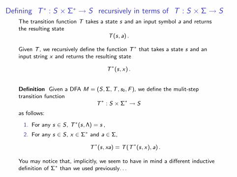
Defining T ∗ : S × Σ∗ → S recursively in terms of T : S × Σ→ S

The transition function T takes a state s and an input symbol a and returnsthe resulting state

T (s, a) .

Given T , we recursively define the function T ∗ that takes a state s and aninput string x and returns the resulting state

T ∗(s, x) .

Definition Given a DFA M = (S , Σ, T , s0, F ), we define the mulit-steptransition function

T ∗ : S × Σ∗ → S

as follows:

1. For any s ∈ S , T ∗(s, Λ) = s ,

2. For any s ∈ S , x ∈ Σ∗ and a ∈ Σ,

T ∗(s, xa) = T (T ∗(s, x), a) .

You may notice that, implicitly, we seem to have in mind a different inductivedefinition of Σ∗ than we used previously. . .

“Backwards” inductive definition of Σ∗

It turns out to be more convenient for our purposes to use the followingalternative inductive definition of Σ∗.

I Basis: Λ ∈ Σ∗.

I Induction: If x ∈ Σ∗ and a ∈ Σ, then xa ∈ Σ∗.

Previously we used an inductive definition of Σ∗ in which x and a were reversed(in the induction part).

That was in keeping with what is most convenient when working with lists.(Intuitively speaking, you build a list by adding elements to the front of thelist.)

From now on, we will use this new “backwards” definition.

It seems reasonably intuitive for strings. (You write a string from left to right,right?)

It is clearly equivalent to the other inductive definition.

It is much more convenient for proving things about finite automata!

First sanity check for recursive defn of T ∗Recall: For DFA M = (S , Σ, T , s0, F ), we define

T ∗ : S × Σ∗ → S

as follows:

1. For any s ∈ S , T ∗(s, Λ) = s ,

2. For any s ∈ S , x ∈ Σ∗ and a ∈ Σ,

T ∗(s, xa) = T (T ∗(s, x), a) .

Here’s a property T ∗ should have. . .

Claim For any DFA M = (S , Σ, T , s0, F ), and any s ∈ S and a ∈ Σ,

T ∗(s, a) = T (s, a) .

This is easy to check. . .

T ∗(s, a) = T ∗(s, Λa)= T (T ∗(s, Λ), a) (defn T ∗)= T (s, a) (defn T ∗)

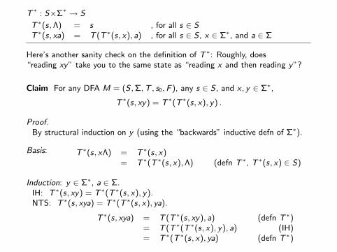
T ∗ : S×Σ∗ → S

T ∗(s, Λ) = s , for all s ∈ ST ∗(s, xa) = T (T ∗(s, x), a) , for all s ∈ S , x ∈ Σ∗, and a ∈ Σ

Here’s another sanity check on the definition of T ∗: Roughly, does“reading xy” take you to the same state as “reading x and then reading y”?

Claim For any DFA M = (S , Σ, T , s0, F ), any s ∈ S , and x , y ∈ Σ∗,

T ∗(s, xy) = T ∗(T ∗(s, x), y) .

Proof.By structural induction on y (using the “backwards” inductive defn of Σ∗).

Basis: T ∗(s, xΛ) = T ∗(s, x)= T ∗(T ∗(s, x), Λ) (defn T ∗, T ∗(s, x) ∈ S)

Induction: y ∈ Σ∗, a ∈ Σ.IH: T ∗(s, xy) = T ∗(T ∗(s, x), y).NTS: T ∗(s, xya) = T ∗(T ∗(s, x), ya).

T ∗(s, xya) = T (T ∗(s, xy), a) (defn T ∗)= T (T ∗(T ∗(s, x), y), a) (IH)= T ∗(T ∗(s, x), ya) (defn T ∗)

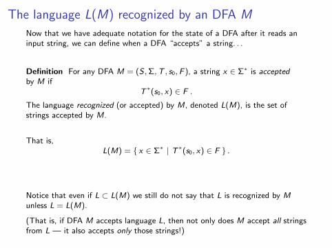
The language L(M) recognized by an DFA M

Now that we have adequate notation for the state of a DFA after it reads aninput string, we can define when a DFA “accepts” a string. . .

Definition For any DFA M = (S , Σ, T , s0, F ), a string x ∈ Σ∗ is acceptedby M if

T ∗(s0, x) ∈ F .

The language recognized (or accepted) by M, denoted L(M), is the set ofstrings accepted by M.

That is,L(M) = { x ∈ Σ∗ | T ∗(s0, x) ∈ F } .

Notice that even if L ⊂ L(M) we still do not say that L is recognized by Munless L = L(M).

(That is, if DFA M accepts language L, then not only does M accept all stringsfrom L — it also accepts only those strings!)

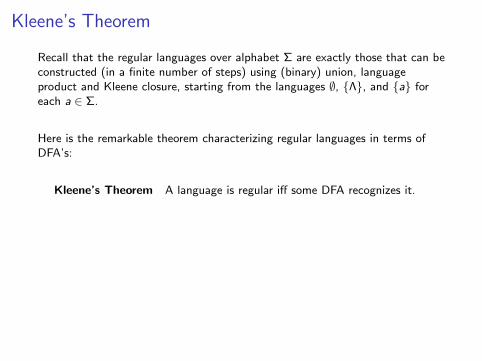
Kleene’s Theorem

Recall that the regular languages over alphabet Σ are exactly those that can beconstructed (in a finite number of steps) using (binary) union, languageproduct and Kleene closure, starting from the languages ∅, {Λ}, and {a} foreach a ∈ Σ.

Here is the remarkable theorem characterizing regular languages in terms ofDFA’s:

Kleene’s Theorem A language is regular iff some DFA recognizes it.

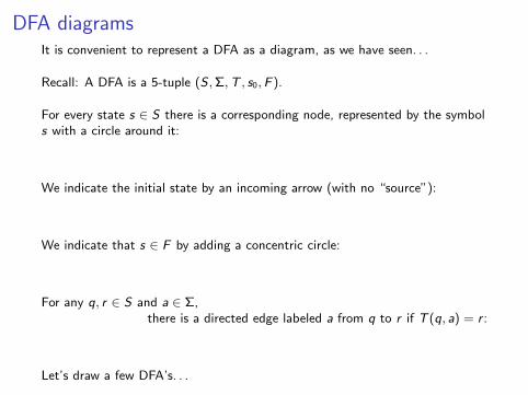
DFA diagramsIt is convenient to represent a DFA as a diagram, as we have seen. . .

Recall: A DFA is a 5-tuple (S , Σ, T , s0, F ).

For every state s ∈ S there is a corresponding node, represented by the symbols with a circle around it:

We indicate the initial state by an incoming arrow (with no “source”):

We indicate that s ∈ F by adding a concentric circle:

For any q, r ∈ S and a ∈ Σ,there is a directed edge labeled a from q to r if T (q, a) = r :

Let’s draw a few DFA’s. . .

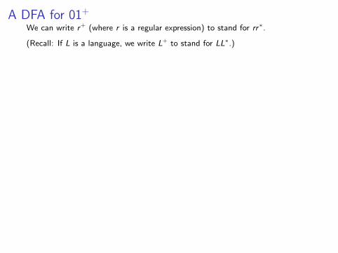
A DFA for 01+

We can write r+ (where r is a regular expression) to stand for rr∗.

(Recall: If L is a language, we write L+ to stand for LL∗.)

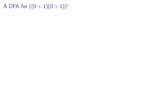
A DFA for ((0 + 1)(0 + 1))∗

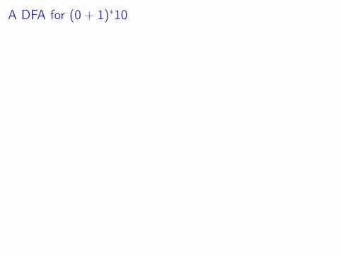
A DFA for (0 + 1)∗10

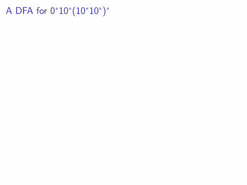
A DFA for 0∗10∗(10∗10∗)∗