Theory of Collective Intelligence - NASA · 4 Theory of Collective Intelligence David H. Wolpert NASA Ames Research Center, Moffett Field, CA 95033 http: //ic arc.nasa.gov/-&w June

4

Theory of Collective Intelligence

David H. Wolpert NASA Ames Research Center, Moffett Field, CA 95033

http: //ic arc.nasa.gov/-&w

June 21, 2003

Abstract In this chapter an analysis of the behavior of an a r b i t r q (perhaps

massive) collective of computationd processes in terms of an associated ’bvorld” utility function is presented We concentrate on the situation where each process in the collective can be viewed as though it were striving to maximix its own private utility function. For such situations the central design issue is how to initialize/update the collective’s structure, and in particular the private utility functions, so as to induce the overall collective to behave in a way that has large values of the world utility- Traditional ”team game* approaches to this problem simply set each private utility function equal to the world utility function. The “Col- lective Intelligence” (COIN) framework is a semi-formal set of heuristics that recently have been used to construct private utility. functions that in many experiments have resulted in world utility values up to orders of magnitude superior to that ensuing from use of the team game utility. In this paper we introduce a formal mathematics for analyzing and designing collectives. We also use this mathematics to suggest new private utilities that should outperform the COIN heuristics in certain kinds of domains. In accompanying work we use that mathematics to explain previous experimental results concerning the superiority of COIN heuristics. In that accompanying work we also use the mathematics to make numerical predictions, some of which we then test. In this way these two papers estabiish the study of collectives as a proper science, involving theory, explanation of old experiments, prediction concerning new experiments, and engineering insights.

Introduction This paper concerns distributed systems some of whose components can be viewed as though they were agents, adaptively “trying” to induce large values of their associated private utility functions. When combined with a world utility function that rates the possible behaviors of that system, the system is hown as a collective [17, 20, 23, 251.

I . ‘ I

I ~

1

https://ntrs.nasa.gov/search.jsp?R=20040084408 2018-09-12T07:19:59+00:00Z

J 1 #

L

Given a collective, there is an associated inverse design problem, of how to conjigure/modify the system so that in their pursuit of their private utilities the agents also maximizes the world utility. Solving this problem may involve determiningfmodifylng the number of agents, how they interact with each other, and what degrees of freedom of the overall system each of them controls (Le., the very definition of the agents). When the agents are machine learning algorithms overtly trying to maximize their private utilities, the inverse problem may also involve determining/modifying the algorithms that those agents use, as well as precisely what private utilities they are each trying to maximize.

This paper presents a mathematical framework for the investigation of collectives, and in particular the investigation of this design problem. A crucial feature of this framework is that it involves no modeling of the underlying system nor of the algorithms controlling the agents. For example, only the behavior of an agent (or more precisely, certain broad aspects of it) is formally related to what private utility that agent is “trying” to maximize; nothing of what goes on “under the hood” is assumed. This behaviorist approach is crucial since in the real world collectives are often so complicated that no tractable model can bear more than a cursory similarity with the system it is supposed to represent. More generally, this approach is crucial to have the framework be broad enough to encompass, for example, the collectives of spin glasses and of human economies.

In the next section we introduce generalized coordinates. These allow LIS to avoid any restrictions on the kinds of variables comprising the system-they can be uncountable, countable, or combinations thereof, with or without an underlying topology/metric, and except where explicitly indicated otherwise, all the results of the framework still apply. The underlying variables can either include time or not, and if they do, the associated underlying dynamics is arbitrary. The variables also can either be broken up explicitly into separate agents or not, and if they are, there can be arbitrary restrictions on which of the conceivable joint moves of the agents are physically allowed. In addition, how the variables are broken up into agents, and even the number of agents is arbitrary, and can be modified dynamically (if time is included in the underlying variables). More- over, if time is included as an underlying variable, then some of the agents can have their decision “simultaneously” fix the state of one or more variables of the system at distanct moments an time. (This is reminiscent of what is decided in settling on a contract in cooperative game theory.) Again, all of this can be

Using these generalized coordinates, a central equation can be derived that determines how well any of these kinds of systems perform. It does so by breaking performance down into three terms. These terms loosely reflect the concerns of the fields of high-dimensional search, economics, and machine learning; the central equation is the bridge that couples those fields.

independent) formalization of the assumption that a particular component of the system is a “utility-maximizing. . . agent”. That formalization is then used to derive the Aristocrat and Wonderful Life private utility functions, two utility functions previously intuited that have been found to result in far better world

-

varied in an arbitrary fashion. ..

The following section uses this mathematical framework to introduce a (model-

2

utility than conventional techniques. [17]. This derivation also uncovers (relatively rare) conditions under which those utilities should not perform very well. That section ends by deriving many new results, including the Collapsed private Utility, and ways to m o m other agents to help a particular agent, along with specification of the scenarios m which such techniques should result in good world utility.

An accompanying paper [22] presents this mathematical framework in a more pedagogical manner, including many examples, commentary and some discussion of related fields (e.g., mechanism design in game theory). That paper also discusses recent experiments involving a set of previous semi-formal heuristics (including the Aristocrat and Wonderful Life private utilities) that have been found to be very useful for the design of collectives. It uses the mathematical framework to explain the efficacy of those techniques. It then goes on to make numerical predictions based on that framework, and then presents some experimental tests of those predictions. It ends by making other (testable) predictions, and presents a sample of future research topics and open issues.

This paper instead exhaustively presents all of the currently elaborated mathematics of the framework, including the details omitted in [22]. In particular, this paper contains theorems not presented there, extensions of the theorems that are presented there, the proofs of all theorems, detailed application of the framework to multi-step games, and the important example of applying the framework to gradient ascent over categorical variables. (For pedagogical reasons, the latter two occur as appendices.) Combined, these two papers present a mathematical theory along with associated predictions/experiments and engineering recommendations. In this, they lay the foundation for a full-fledged science of collectives.

1 The Central Equation

(i) Generalized coordinates and intelligence We are interested in addressing optimization problems by decomposing them into many subproblems, each of which are solved separately. We will not try to choose such subproblems so that they are independent of one another, or iind a way to coordinate their solutions. Rather we wil l choose the subproblems so that each of them separately is relatively easy to solve, given the wntezt of a particular cumnt solution to the other subproblems, and then have them be

To formalize this, let C be an arbitrary space with elements z called worldpoints. Let C C < be the set of elements of < that are actually allowed, for example in that they are consistent with the laws of physics.l Define a generalized coordinate variable as a function from C to associated coordinate

solved in pardel.

'Whenever expressing a particular system as a mllective, it is a good rule to write out the functional dependencies presumed to specify C(.) as explicitly as one can, to check that what one has identified as the space C does indeed contain all the important variables.

3

I 1 4

R

values. (When the context makes the precise meaning clear, we will sometimes use the term “coordinate” to refer to a generalized coordinate variable, and sometimes to a value of that variable.) We will sometimes view a coordinate variable p as an exhaustive partition of C into non-empty subsets, with p(z) being the element of the partition that contains z. Accordingly we will sometimes write a coordinate value r = p(z) as “T E p” and a worldpoint z’ sharing that value as “z’ E T ” . ~ Intuitively, each ‘Lsub-problem’’ of our overall optimization problem will be formalized in terms of such a partition p, a s finding the optimal z within the r E p specified by the current solutions to the other subproblems.

Often we implicitly assume that the set of values that any coordinate variable we are discussing can take on forms a measurable set, as does the set of worldpoints having any such value. (All integrals are implicitly with respect to such measures.)

As an example, C might consist of the possible joint actions of a set of computational agents engaged in a non-cooperative game [7, 2 , 10. 3, 51. p(z E C) could then be the actions of all agents except some particular agent identified with p. In this case, by fixing all other degrees of freedom, the value of the coordinate p implicitly specifies the degrees of heedom that are still “available to be set” by the agent identified with p.

A frequently occurring type of coordinate variable is one whose values are contained in the real numbers. A particularly important example is a world utility function G : C -+ R that ranks the various possible worldpoints of the system. We are always provided a G; the goal in the problem of designing collectives is to maximize G.

Our mathematics does not concern G alone, but rather its relationship with some coordinate utilities g p : C -+ R3 Each coordinate utility ranks the possible values of those degrees of freedom still allowed once the worldpoint has been restricted to a set of worldpoints r E p. Given a set of coordinate variables, { p } , we are interested in inducing a z that each g p ranks highly (relative to the other worldpoints in the associated set r = p(z)), and in the relation between those rankings of z and G’s ranking of z . To analyze these issues we need to standardize utility functions so that the numeric value they assign to z only reflects their relative ranking of z (potentially just in comparison to the other worldpoints sharing some associated coordinate ~ a l u e ) . ~

Generically, we indicate such a standardization by N , and for any utility function U , coordinate p, and z E C, we write the associated value of such a standardization of the utility U as Np,u(z). Define “sgn[x]” to equal +l, 0, or -1 in the usual way. Then we only need to require of a standardization N that N P p ( z ) be a [0, 11-valued, pparameterized functional of the pair (U, U ( z ) ) , one that meets the following two conditions as we vary U and/or z:

~~ ~

21n general, we try to use lower-case greek letters for coordinates, and the associated lower-

31n previous work, roughly analogous utilities were called “personal utilities” [17]. 41t turns out that there never arises a reason to consider the relation between such a stan-

dardization and the axioms conventionally used to derive utility theory [lo], and in particular those axioms concerning behavior of expectation values of utility.

case roman letter for the value of that coordinate.

4

i) V z f C, if for apair of utilities V and W , sgn[W(z’)-W(z)] = sgn[V(z’)- V ( Z ) ] ‘d z’ E At.), then Np,w(z) = Np,v(z).

U(2)l- ii) With U and r E p fixed, V z, 2 E r , sgn[n$,u(z) -Np,u(z’}] = sgn[U(z) -

We call the value of Np,u at z the “intelligence of z (given p) with respect to U for coordinate pn.5 ,6 If p consists of a single set (all of C), we ”imply mi te Nu(z). An example of an intelligence operator based on percentiles is provided in App. A. Unless explicitly stated otherwise, whenever calculating intelligence values in any examples, we will use this choice of the intelligence operator.

Often there will be uncertainly in the worldpoint z , in particular on the part of the system designer (e.g., when worldpoints are worldlines of a physical system, such uncertainty arises if the designer is not able to calculate exactly how the system evolves). Such uncertainty is captured by a distribution P(z) that equals 0 off of C.7 Accordingly, coordinates p are not only partitions, but are also random variables, taken d u e s r E p.

All aspects of the designer’s ability to manipulate the system are encap siizted iii the se!ectim af az elexect s Zom s ~ m e desipA ccordfnate 6. h particular, since the (sub)problem of finding a z E r with maximal pintelligence will vary as r varies, it cannot be addressed with conventional algorithms for m a w & a static function. Instead, its solution requires techniques - like those in reinforcement learning - tailored for dynamically varying and/or un- certain functions. Accordingly, we will often consider the case where (among other things) s specifies which of a set of allowed private utility functions to associate with some coordinate p , ~ , ~ : z + 93. Such a function is one that we view intuitively as the ”payoff function” for a self-interested computational

5Note that for fixed U, the function Np,p(.) from C + W can be viewed as a utility function, and therefore as a coordinate. In particular, N p . ~ p , L T = Np,u. This follows from condition (i) in the definition of intelligence with V = U, W = N P , v , and the equality of sgn’s following from condition (i) in the definition of intelligence.

‘Although this p a p a concentrates on %valued utiIity functions, much of its analysis can be extended to functions having different ranges. Examples include vector-valued functions having range Rn - appropriate for analyzing intelligence with respect to several distinct U at once - and functions whose range is a set of non-overlapping contiguous subintervals of X In particular, given some such range Q, and any associated antisymmetric preference function F : Q x Q -t { - l , O , l}, we can replace the sgn function with F throughout (i) and (ii) when we specify our intelligence operator. Much of the sequel (e.g., Thm. 1) still holds under this modification. If in addition Q is a field over the reals, we can also form the average value of such an ixtdigence, and some of the theorems presented below concerning expected intelligence values will go through.

71f there is uncertainty m C itself we express that with a distribution P(C), to go with the distributions P(z I C). In particular, if probabilities reflect the system designer’s uncertainty about C, then P(z) may be non-zero even for points z off of the actual C. FLdng C exactly is analogous to iking the energy exactly in statistical physics (the microcanonid ensemble), with allowing C to vary being analogous to uncertainty in the energy (the canonical ensemble). Unless explicitly stated otherwise, in this paper we will consider C to be fixed. In a similar fashion, if probabilities reflect uncertainty in how a coordinate IS partitions C, then it could be that P(z 1 k) is non-zero even for points z where K ( Z ) f k. (For simplicity, we will usually assume this is not the case.)

5

” 1

*

agent, embodied in C, that uses a “learning algorithm”, to position within any particular element of p.s A pmori, a coordinate need not have an associated private utility; in particular, non-learning agents need not. Informally, when we have a “learning agent” associated with coordinate p we refer to p as either the agent coordinate or the agent’s context coordinate, with the value of that coordinate being the agent’s context. (These definitions are made more formal below.)

Properly interpreted, the rules of set theory hold when coordinate variables play the role of sets. Under this interpretation any coordinate variable R arising in a set-theeretic exupressim shcu!d be read as “every (subset of C that connti- tutes an) element of IC”. For example, R c X means “every element of IC is a proper subset of every element of A”, so that the value k fkes 1. See App. B.

As a notational matter, we adopt the usual convention that probability of a coordinate value is shorthand that the associated random variable takes on that value, e.g., P(u) means P(a = u) . As usual though, this convention is not propagated to expectation values: E(U(u , 0) I c) = s dbU(u, b)P(b 1 c). Delta functions are either Kronecker or Dirac as appropriate (although always written as arguments rather than as subscripts). Similarly, integrals are assumed to have a point-mass measure (i.e., reduce to a sum) as appropriate. For any function 4 : C -+ !3 and coordinate IC, with y E [0,1], we write CDF+(y 1 k ) to mean the cumulative distribution function P(4 5 y I k ) = s_”, dt s dz P ( z I k ) b(4(z ) -t), and just write CDF(4 I k ) to refer to the entire function over y. In addition, LLsupp’l is shorthand for the support operator, and “W’ indicates the Booleans. O ( A ) means the cardinality of the set A. For any two functions fi and f2 with the same domain x E X , “fl < f2” means that b’x fi(z) 5 f2(z), and 3a: such that fi(z) < fi(a:). All proofs that are not in the text are provided in App. C.

(ii) The Central Equation Our analysis revolves around the following central equat ion for P(U 1 s), which follows &om applying Bayes’ theorem twice in succession:

P(U I s) = J dflu P(V I Zu, s) J dfig ~ ( f i u I fig, s)p(Sg I s) (1)

where usually we are interested in having U = G. ‘Lg17 is the vector of the values of-a set of coordinate utilities, and L‘$gll is an associated vector of intelligences with respect to those coordinate utilities. Here we concentrate on the case where each of those intelligences is for the associated coordinaJe, i.e., for set of coordinates { p } it is the p-indexed vector with components {Np,g,(z)}. LLZu’l is also a coordinate-variable-indexed vector of intelligence values, only for utility U . We will concentrate on the case where flu is indexed with the same coordinates as fig. In this situation Gu has components @p,U(z) and is identical to gg except

aNote that, formally speaking, the learning algorithm itself is embodied in C. Hence the quotation marks around the term ‘control’.

6

in its choice of utility function^.^ If we can choose s so that term 3 in the integrand in Eq. 1 is peaked around

vectors sg all of whose components are close to 1, then we have likely induced large intelligences. If in addition to such a good term 3 we can have term 2 be peaked about l ? ~ equal to gg, then l ? ~ will also be large. If in addition term 1 in the integrand is peaked about high U when i?u is large, then our choice of s will likely result in high U, as desired.

In the next subsection we analyze what coordinate utilities give the desired form of term 2 in the central equation, for our choice of 3~ and fig. We then present examples illustrating such systems and more generdy illustrating generalized coordinates. We end this section with a brief discussion of term 1. Then in the next section we analyze what coordinate utilities give the desired form of term 3 in the central equation. It is only here that the use of agents to control some coordinate values becomes crucial. We end that section by combining these analyses to derive coordinate utilities that have the desired forms for both term 2 and term 3.

This formalism applies to many more scenarios than those that involve dy- 1 l d c 1 systeo;. +th d i x s z speciffig hehavior arms.. time. It also applies even in scenarios that are not conventionally viewed as instances of game theory- Nonetheless, as an example of the formalism, App. D is a detailed exposition of multistep games in terms of this formalism.

(iii) Term 2-Factoredness We say that Ul and Uz are (mutually) factored at a point z for coordinate p if Np,pl (2) = NP,u2 (2) V t' E p(z).l0 Note that factoredness is transitive. If we do not spec* U.2, it 1s taken to be Z, and we someximes say &ai ii "is 1ac;k~ied'' , or "is factored with respect to G" , when U and G are mutually factored. If V p in a set of coordinates that we are using to analyze a system, the utility gp is factored with respect to G for coordinate p at a point z, we simply say that the system is factored at z, or that the { g p } axe factored with respect to G there.

There is a very tight relation between factoredness and game theory. For example, consider the case where we have Pareto superiority of a point z' over some other point t with respect to the coordinate utility intelligences [7, 2, 10, 3, 51- Say that in addition those associated utilities form a factored system with respect to the world utility G. These together imply the Pareto superiority of z' over 2 with respect to world utility. The converse also holds. However th&e properties relating factoredness, coordinate and world utilities only hold for Pareto superiority for intelligences (rather than for raw coordinate utility values), in

gSince the distributions in F3q. 1 are conditioned on s, when we have a percentile-style intelligence, a naturd choice for the associated measure dp(z) is given by the values r = p(z) and s, as P(z I r)P(r I s) (see App. A). In other words, given that we are within a particular r, the measure extends across that entire context-including points inconsistent with s- according to the distribution P(z I r).

'Oh previous work we defined fadoredness only to mean that sgn[Ui(z') - S ( z ) ] = sgn[Uz(z') - U~(Z)] V z' E p(z). This is a necessary (but not sufficient) condition that Np,u1 (2) = Np,u2 (z') V z' E p(z); see Thm. 1 below and the definition of intelligence.

7

’, 1

general. In addition, by taking U2 = G, the following theorem provides the basis for relating game-theoretic concepts like Nash equilibria and non-rational behavior with world utility in factored systems:

Theorem 1 Ul and U2 are mutually factored at z E C for coordinate p i f f

Sgn[Ul(Z’) - Ul(Z”)] = Sgn[UZ(Z’) - Uz(Z”)J v ZI, z” E p ( 2 ) .

Note that ths holds regardless of the precise choice of N , so long as it meets the formal definition of an intelligence operator.

By Thm. 1, for a system whose coordinate utilities are factored with respect to G, the set of Nash equilibria of those coordinate utilities equals the set of points that are maxima of the world utility along each of the coordinates indi- viduaIly (which of course does not mean that they are maxlma along off-axis directions) .I1 In addition to this desirable equilibrium structure, factoredness ensures the appropriate off-equilibrium structure; so long as for each coordinate the associated intelligence is high (with respect to that coordinate’s utility), the system will be close to a local maximum of world utility. This is because, for each coordinate p , given a (fixed) associated coordinate value r , any change in z E r that decreases p’s coordinate utility-which is almost all changes if p’s intelligence is high-will assuredly decrease world utility. Note though that having gP factored with respect to G does not preclude deleterious side-effects on the other coordinate utilities of such a g,-improving change within r. All such factoredness tells us is whether world utility gets improved by such changes (see the end of App. D).12

“An immediate game-theoretic corollary is that any game whose utilities can be expressed as coordinate utilities of a system that is factored with respect to a world utility having critical points has at least one pure strategy Nash equilibrium. However consider an arbitrary vector Fall of whose components lie in [0,1]. Then it is not the case that every factored system has a pure strategy joint profile with each player’s intelligence given by the associated component of E: This is even true if every component of Fis either a 0 or a 1. As a simple example, choose g1 = gz = G, and have F = (0,l). Have G = 21 for z2 > 1/2, and equal 1 - z1 otherwise, where both z1 and z2 E [0,1]. Then if zz > 1/2, z1 = 1, since Nl = 1. However if zl = 1, then zz E [0,1/2] since N2 = 0. If 22 5 1/2 though, z1 = 0, which means that zz E (1/2,1]. QED.

”Factoredness is simply a bit; a system is factored or it isn’t. As such it cannot quantify situations in which term 2 has a good form although it is not exactly a delta function. Nor can it characterize “super-factored” situations in which that conditional distribution is better than a delta function, being biased towards NG values that exceed the Ng d u e s . One way to address t h s deficiency_ is to _define a “degree of factoredness” . One e.x_ample-of such a measure is 1 - dz P ( z I .)[Ne - NgI2 E [0,1]. Another is 1 d z P ( z I ~ ) [ N G - N,], which extends from “partially factored” systems (negative values), to perfectly factored systems (value 0), to super-factored systems (value greater than 0). Other definitions arise from consideration- of Thm. 1. For example, one might quantlfy factoredness for coordinate p as the probability that a random move within a context changes G and gP the same way:

/dzdz‘P(z I s)P(t’ I s)6(z‘ E p ( z ) ) @ ( [ G ( z ) - G(z’)l[gp(z) - gp(z’)I).

Especially when one has a percentile-type intelligence, all these possibilities suggest yet other variants in which the measure dp(z) replaces the distribution(s) P(z I s). Similarly, one can define “local” (degree of factoredness) about some point z” by introducing into the integrands of all these variants Heaviside functions restricting the worldpoint to be near 2”.

8

The following theorem gives the entire equivalence class of utilities that are mutudy factored at a point:

Theorem 2 171 and U2 are mutually factored ut z f o r coordinate p zff V z‘ E r E p(z), we can unite

for some r-indezed function 9, that i s a strictly increasing functaon of its argument acmss the set of all values U2 (z’ E r) . (The fo rm of lJ1 for other arguments is arbitrary.)

W.’> = @r(UZ(Z’))

Using some notational overloading of the “a” function, by Thm. 2 we can en-. sure that the system is factored by having each g,(z) = @,(G(z),p(z)) V z E [ for some functions a, whose first partial derivative is strictly increasing everywhere. Note that this factoredness holds regardless of C or P ( z I s)- The canonical example of such a case is a team game (also known as an ‘exact potential game‘ [6, 12, 41) where g, = G for d p. Alternatively, by only requiriig that b! z E C does g, take on such a form, we can access a broader class of factored utilities, a class that does depend on aspects of C.

As an example, define a difference utillty for coordrnate p with respect to utility D1 as a utility taking the form D p ( z ) = p(z)[D1(z) - D2(z)] for some - function 0 2 and positive function p(.), where both p(.) and D2(.) have the same value for any pair of points z and z’ f C for which p(z) = p ( 2 ) . (We will sometimes refer to D1 as the lead utility of such a dif€erence utility, with D2 being the secondary utility.) Since both p(z) and D2(z) can be written purely as a function of p(z), by Thm. 2, a difference utility is factored with respect to D1. As explicated in the next subsection, for such a utility with D1 = G, term 3 - +ha ”-.. m=nfral ---”-- qcztinr? c m he mdly superior tn that, of a team game: especially in large systems. In addition, as a practical matter, often D , can be evaluated much more easily than can D1.

(iv) Assuming term 3 results in a large value of having factoredness then ensures that we have a large value of l ? ~ as well. In this situation term 1 will determine how good G is. Intuitively, term 1 rdects how likely the system is to get caught near lo& maxima of G. If any maximum of G the system finds is likely to be the global maximum, then term 1 has a good form. (For factored systems, in such scenarios it is likely that a system near a Nash equilibrium it is near the highest possible G.)

So for factored systems, for our choice of l ? ~ and Gg, term 1 can be viewed as a formal encapsulation of the issue underpinning the much-studied exploration/exploitation trade-off of conventional search algorithms. That trade-off can manifest itself both within the learning algorithms of the individual agents as well as in a centralized process determining whether those agents are allowed to make proposed changes in their state ([26]). In this paper we will not consider such issues, but will instead concentrate on terms 2 and 3.

\

Term 1 and alternate forms of the central equation

9

I I

As mentioned, term 2 in the central equation is closely related to issues considered in economics and game theory (cf. Thm. 1 and note the relation between factoredness and the concept of incentive compatibility in mechanism design [7, 2,14, 2, 10, 16, 8, 27, 13, 151. On the other hand, as expounded below, term 3 is closely related to signal-noise issues often considered in machine learning (but essentially never considered in economics). Finally, as just mentioned, term 1 is related to issues considered by the search community. So the central equation can be viewed as a way of integrating the fields of economics, machine learning, and search.

investigated in t_hi paper is where it is the scalar N ~ J . In this situation, fiu is a monotonic transformation of U over all of C, rather than just within various partition elements of C. For this choice term 1 in the central equation becomes moot, and that equation effectively reduces to P(U I s ) = ! d g g P ( U I fig,s)P(i?g I s). The analysis presented below of the P ( z g I s) term in the central equation is unchanged by this change. However the analysis of the P(i?u I Sg, s) term is now replaced by analysis of P(U I Sg, s). For reasons of space, we do not investigate this alternative choice of i?~ in this paper.

- Finally, an important alternative to the Choice of

2 The Three Premises

(i) Coordinate complements, moves, and worldviews Since intelligence is bounded above by 1, we can roughly encapsulate the quality of term three in the central equation as the associated expected intelligence. Accordingly, our analysis of term 3 will be expressed in terms of expected intelligences.

We will consider only one coordinate at a time together with the associated expected coordinate intelligence. This simplifies the analysis to only concern one of the components of Fg together with the dependence of that component on associated variations in s, our choice of the element of the design coordinate. For now we further restrict attention to agent coordinate utilities, reserve “p”to refer only to siich an ageIit coordinate with same associated Iearning algorithm, and take gp = &,+.I3 The context will always make clear whether p specifies a coordinate (as when it subscripts a private utility), refers to the values the coordinate can assume (as in T E p ) , indicates the associated random variable (as in expressions like P(U(2, p ) ) =

As a notational matter, define two partitions of some T G C, 7r1 and 7r2, to be complements over T 2 < if z E T + (7r1(z),7rz(z)) is invertible, so that,

drP(r)U(z, r ) ) , etc.

I3Note that changing p’s coordinate utility while leaving s unchanged has no effect on the probability of a particular G value; gp is just an expansion variable in the central equation. Conversely, leaving p’s coordinate utility the same while making a change to its private utility (and therefore to s, and therefore in general to the associated distribution over C, P ( z I s)) changes the probability distribution across G values. Setting those two utilities equal is what allows the expansion of the central equation to be exploited to help determine s.

10

I I .

intuitively speaking, 7r1 and 7r2 jointly form a “Coordinate system” for T.14715 When discussing generalized coordinates, this nomenclature is used with T implicitly taken to be C. (XI and 7r2 are coordinate variables in the formal sense if T = C.) We adopt the convention that for any coordinate p, *p , having labels/values written *r , is shorthand for some coordinate that is complementary to p (the precise such coordinate will not matter) and that A p = p. We do not take the u^n operator to refer to values of a coordinate, only to coordinates as a whole. So for example, there is no a priori relationship implied between a particular element of - p that we write as ““r”, and some particular element of p that we write as “r”.

We always have E(N,,u I s) = 1 drd&P(r 1 s)P(n I r, s )P(x I n)N,,u(z, r) . Accordingly, if we h e w P(r I s), and also knew one of P(n I r, s) and P(z 1 n) but did not know the other, then we could in principle solve for that other distribution so as to optimize expected intelligence.16 Unfortunately, we usually do not know two of those three distributions, and so must take a more indirect approach.

The analysis presented here for agent coordinates revolves around the issue

between those elements of p- To conduct this analysis we will need to introduce two coordinates in addition to c and p: E and v.I7 Given some -p, rather than the precise element -r E -p, in general the agent associated with p can only control which of several sets of possible elements *r the system is in. This is formalized with the coordinate [ 2 * p . We refer to E as the move variable of the agent, and we refer to an 2 E [, and/or the set of z that that x speciiies, as the move value of the agent. For convenience we assume that for all such contexts r and moves x there exists at least one t E C such that p(z) = r and <(z) = x. Io general, what we identlfy as the 6 of a particular p need not be unique. Intuitively, such a partition < delineates a set of r -+ z maps, each such map giving a way that the agent associated with p is allowed to vary its behavior to reflect what context r it’s in. An agent’s move is a selection among such a set of allowed variations. An important example of move variables involving dynamic processes in presented in App. D.

We assume that <(z) and p(z> jointly set the value of G(z) and of any sP,+ we will consider.l* Accordingly, we write 3 when we mean the coordinate whose partition elements are identical to 0’s but whose values itre instead the private

14This characterization as a coordinate system is particularly apt if x i and 7r2 are minimal complements, by which is meant that there is neither a coarser padition d 2 xi such that d and 772 are complements, nor a coarser partition d’ 2 7r2 such that d’ and x i are complements.

I5Note that it is not assumed that T -+ @l,a) taking points z to partition element pairs is surjective.

16Formally, to implement this would require making an associated change to s, a change which in the case of solving for P(I I n) would have to be reflected in the value of n.

17Properly speaking, E and Y should be indexed by p, as should the coordinates a, - and u - ~ - introduced below; for reasons of clarity, here all such indices are implicit.

laphrased differently, given the utility function, and the associated E and p, the minimal choice for C is x p . Ifthevalue s is not fixed by I x r, i.e., if it is not the case that u 1 E n p , then u must also be contained in C, and similarly for v.

of hoTv seiiSitiv.2 i& 5 t o &mga Tith 2.a deme2t of r“ 2s opposed to changes

11

b I

utility functions of p : : s E u -+ G , ~ . Similarly, we will write Np when we mean the function (2, r, s ) -+ Np,gp,,(5,T).

We refer to u as the worldview variable of the agent, and we refer to a n E u, and/or the set of possible z that that u specifies, as the worldview value of the agent. Intuitively, n specifies all the information-all training data, all knowledge of how the training data is formed (including potentially knowledge of its own private utility), all observations, all external commands, all externally set prior biases-that p’s agent uses to determine its move, and nothing else. It is the centents of the (perhaps distorting) “window” through which the learnkg algorithm receives information from the emernai world.

Formally, there three properties a coordinate must possess for it to qualify as a worldview of an agent. First, if the agent does indeed use all the information in n, then the agent’s preference in moves must change in response to any change in the value of n. This means that V n l , n2 E u, for at least one of the x E E , P ( z 1 T Z ~ ) # P(x 1 n2).19 Second, if the worldview truly reflects everything the agent uses to make its move, then any change to any variable must be able to affect the distribution over moves only insofar as it affects n. This means that with R defined as the set of all non-( ccordinate we will consider in our analysis (e.g., u, p for some other agent, their intersection, etc.), P ( x 1 n, W ) = P ( z I n) V x E E , n E u and W E R such that P ( s , n , W ) # 0.20,21y22 Finally, of all coordinates obeying these two properties, the worldview must be among those whose information maximizes the expected performance of the associated Bayes-optimal guessing,23 i.e., V s E 0, p # u,

So P(n I s ) is how the worldview varies with s, and P ( x I n) is how the agent’s learning algorithm uses the resultant information. The P(x 1 s ) induced by these two distributions is how the move of the agent varies with s. Alternatively, P(r I s) is the distribution over contexts caused by our choice of design coordinate value, and the distribution P ( z I r, s ) = dnP(x 1 n)P(n I T , s) gives all salient aspects of the agent’s learning algorithm and technique for inferring information abou r ; the integral over r of the product of these two distributions says how choice of s determines the distribution over moves.

lgWhen worldviews are numeric-valued, we can modify this requirement to be that the distribution P(z 1 n) has to be sufficiently sensitive a function of n over aU of v.

20Note that if all W are allowed, then in general the only choice for v obeying this restriction is v = c.

21As a result of this requirement, P(r I z, n, W ) = P(r I n, W ) , P(z , r I n, W ) = P(z I n)P(r I n,W), etc.

22For any P(z ) and coordinates cy and ,f3 , one can always construct a coordinate 6 # a such that P ( a I b, d) varies with d. So our assumption about (, v and R constitutes a restriction on what coordinates we will consider in our analysis.

could double as the worldview, and often so could u. 231f it were not for this requirement,

12

We will h d it convenient to decompose (T = 0% n u - ~ , where uyp is a coordinate whose value gives %,,, and there is no coordinate w 3 C J ~ with this property. (Intuitively, u3's value is a component of s that specities %,+ and nothing more.) Also, from now on, we will often drop the p index whenever its implicit presence is clear. So for example, we will often write sg instead of s3. -

(5) Ambiguity Since we do not know P(x I n) in general, we cannot directly say how n sets the distribution over x. Fortunately we do not need such detailed information. We only need to know the effect that certain changes to n have on particular characteristics of the associated &ribution P(z I n) (e.g., the effect certain changes to n have on the "characteristic of P(x I n)" given by an n-conditioned expected intelligence E(Nu I n)).

Now if there were any universal rule for how such characteristics affect expected intelligence, then without m y assumptions we could use such a rule to deduce that some particular choices of n are superior to others. That has been proven to Le ;liiF'oskk ~ G F ~ W (18, 211. hccordkgIy, y e EYE& make some presumption about the nature of the learning algorithm, one that must be as conservative as possible if it is to apply to all reasonable algorithms.

To see what presumption we ca,n safely make concerning such effects, ikst note that the worldview n encapsdates all the information the agent might try to exploit concerning the z-dependence of the likely values of the private utility- That encapsulation given by n takes the form of the distribution over the Euclidean vector of private utility values (y', y2, ...) given by rdrds 6(qo <(xl ,r) - y1)6(g,.s(z2,r) - y2>-.. P(r,s I n). The agent works by 'tqmgn t Z L e this encapdation to appropriately set its move. our presump tion must concern aspects of how it does this. Furthermore, if that presumption is to apply to a wide variety of learning algorithms, it must only involve the encapsulated information, and not (for example) any characteristics of some class of learning algorithms to which the agent belongs.

For simplicity, consider the case where there are only two possible moves, x1 and x2. The encapsulated information provided by n induces a pair of distributions of likely utility values at those two x's, J drds b(&,+(xl, r ) - y) P(T: s I n) and l d r d s d(&,+(x2,r) - y) P(r,s 1 n), which we ct~n write in shorthand as P ( y ; ~ ; n , x I ) and P ( y ; 3 ; n , z 2 ) , respectively. (Note that unlike n, the zi value in this semicolon notation is a parameter to the random variable 3, not a conditioning event for that random variable.) By definition of Von Neu- mann utility functions, for worldview n, the optimal move is x1 if the expected d u e E ( y ; L; n, z') > E(y;&; n, z2), and x2 otherwise. h general though the learning algorithm of the agent will not (and often cannot) have its distribution over x set to a delta function this way. Other aspects of P(y;&;n,zl) and P(y; 3; n, 9) besides the difference in their iimt moments will affect how P(z I n) changes in going from the one n to the other. For example, it may be that if E(y;%; n , d ) > E ( y ; & ; n , x2), then if n is changed so that both the

13

probability of a relatively large y value at x2 and the probability of a relatively small y value at x1 shrinks, while the first moments of those distributions are unchanged, then the algorithm is more likely to choose x1 with the new n than with the original one.

In light of this, we want to err on the side of caution in presuming how changes to P(y; s; n, d) and P(y; 3; n, x2) induced by changing n affect the associated distribution P ( x I n) . The most unrestrictive such presumption we can make is that if the entire distributzons P(y; 3; n, d) and P(y;2;5; n, x 2 ) are “further separsltep from one another after the change in n, then P(x I n ) gets weighted more io the higiier of those two distributions. Such a presumption is the most conservative one we can make that holds for any learning algorithm, i.e., that is cast purely in terms of the set of posterior distributions {P(y; 3; n, x)} without any reference to attributes of the learning algorithm. This can be viewed as a first-principles justification that it applies to any learning algorithm not horribly mis-suited to the learning problem at hand.24

To formalize the foregoing, consider the quantity

which expands into the distribution

drl dr2 dsl ds2 6(gs1(x1, - rl) - y1)S(gS2(x2, r2) - y2)P(r1, s1 I n)P(r2, s2 I n).

This is the distribution generated by sampling P(r’, s’ I n) to get values of at xl, and then doing this again (in an ID manner) to get values at x 2 . This LLsemicolon” distribution is the most accurate possible distribution of private utilities values at z1 and x 2 that the agent could possibly employ to decide which x to adopt to optimize that private utility, based solely on n.

Now also fix a utility U that is a single-valued function of x. Our “most accurate distribution” induces the convolution distribution P ( y = y1 - y2; n, d. 2’).

The more weighted this convolution is towards values of y that are large and that have the same sign as U ( x l ) - V(x2), the less likely we expect the agent to be “led astray, as far as U(.) is concerned’’ in “deciding between x1 and x 2 ” , when the worldview is n. On the other hand, if the convolution distribution is heavily weighted around the value 0, then we expect the agent is more likely to be mistaken (again, as far as U is concerned) in its choice of x.

So consider changing na to nb in such a way that the associated convolution distribution, P([g1-g2] sgn[V(x1)-V(x2)]; nu, xl, x2) is more weighted upwards than is P( [gl - - -93 sG[U(zl) -U(x2)]; nb, xl, x 2 ) . Say this is the case for all pairs of x values (x1,z2), i.e., with worldview nu, the agent is less likely to be led astray for all decisions between a pair of x values than it is with worldview nb. 241f the learning algorithm and underlying distribution over utility values do not adhere to

this presumption, then in essence that underlying distribution IS “adversarially chosen” for the learning algorithm - that algorithm’s implicit assumptions concerning the learning problem are such a poor match to the actual ones - that the algorithm is likely t o perform badly for that underlying distribution no matter what one does to s, n, or the l i e .

14

Our assumption is that whenever such a situation arises, if we truly have an adaptive agent operating in a learnable environment, then the agent has higher intelligence with respect to U, on average, with worldview na.

Now in general we can encapsulate how much a stochastic process over C weights some random variable V upward, given some coordinate value Z E A, with CDFv (y 4 Z) - the smaller this cumulative distribution fundion, the larger the Z-conditioned values of V tend to be.25 Accordingly, we can use such a CDF to quantify how much more "weighted upward" our convolution distribution for nu is in comparison to the one for nb. (See App. A for how this CDF is related to intelligence.)

To formalize this we extend the semicolon notation introduced above. Given a coordinate x whose value c is a singlevalued function of (5, r, s), and arbitrary coordinate A, define the (zl, 9, I)-parameterized distribution over values cl. 2,

P ( x 1 , ~ ; Z , 5 1 , 5 2 ) = Px(cl,c2; I , 2 , 2 ) = / dr' dr2 ds' ds2 P(rl, s1 I I)P(r2, s2 I I)

""(X(.', 7-1, s') .'> 5(x,(.2, ?"2, 2) - 2) So in this expression x is a random variable that is (being treated as) parameterized by 5, and we are considering its Z-conditioned distributions at d and z2. This notation is sometimes s i m p E d when the meaning is clear, e.g., Px(2, 2; I , z1,2) is written as ~ ( 2 , 2 ; I , d, 2).

Expectations, variances, marginalizations, and CDF's of this distribution and of functionals of it are written with the obvious notation. In particular,

As another exampie, say char; x is &e ltd-dmi! ~ ~ ~ d . k ~ t z $ t&kg vdllpe $1'

at (xi, r', sa) . Then for any function f : !X2-+ R, for any I,

Px(c; I, 5) = P(x(z, p, CT) = c J I ) , so Px(cl, 2; E , z1,22) = Px(cl; I ; d)Px(C2; I , 2)

00

dyl dy2 W , y2; I, z', z2)e[~ - fb l , y2)J 1 2 L C D F f ( y ~ , y ~ ) (y; 1, z . z )

= J dr' dr2 dsl ds2P(r1, s1 I Z)P(r2, s2 I I) 2 2 2 eiv - f ( W , rl, sl), , f s )>I -

Using this notation, for any single-valued function U : 5 + %, we d&e the (ordered) ambiguity of U and +, for 1, xl, z2, as the CDF of the associated convolution distribution:

1 2 A b ; u, +; 1, Zl, z2) 3 CDF(,I-,Z) sgn[Lr(+)-U(zZ)] (y; I, 5 7 2 1 . Note that the argument of the s g n is just a constant as far as the integrations giving the CDF are concerned. That s g n term provides an ordering of the 5's;

25Let ii be a real-valued random variable, and F : 93 + TI a function such that F ( y ) > y; Vy E R. Then P(F(ii) < y) 5 P ( C < y) Vy, Le., the monotonically increasing function F applied to the underlying random variable pushes the CDF down. Conversely, if CDFi < CDF2, then the function F(u) = CDFT1(CDF2(u)) is a monotonically increasing function that transforms CDFl into CDF2.

15

1 a

ordered ambiguity says how separated our two y-distributions are “in the direction” given by that ordering. When U is not specified, the random variable in the CDF is understood to be ($1-$2) rather than sgn[U(x1)-U(z2)]. It is easy to verify that such unordered ambiguities are related to ordered ones by

where ttr(z1,z2) sgn[Ufz’) - U ( z 2 ) ] . We write just A(U, $; i, xl, z2) (or A($; 1, xi, x2)) when we want to refer to

the entire function over all y. If that entire function shrinks as we go from one n to another - if its value decreases for every value of the argument y - then intuitively, the function has been “pushed” towards more positive values of y . Taking X = v, such a change will serve as our formalization of the concept that the distributions over U at x’ and x 2 are “more separated” after that change in the value of u.

Expanding it in full we can write A(y; U, $; n, x1, x 2 ) as

Jdr’ dr2 dsl ds2 P(T’, si I i ) p ( r 2 , s2 1 I) 2 2 2 @[Y - ($(xl, 9, s’) - ,$(a: 1 7 - 1s 1) sgn[U(zl) - W2>1l1

or, by changing coordinates, as

SdZI’dy2~~(ZI’ ;z , s ’ )~~(y2; I , sZ)@iy - (Y’ - Y2)Sgn[U(Z1) - U(Z2)11,

and similarly for unordered ambiguities. So ambiguity is parameterized by the two distributions P($; 1, x’) as well as (for ordered ambiguities) U.26 As a final comment, it is worth noting that there is an alternative to A, A*, that also reflects the entire n-conditioned CDF of differences in utility values. It and our choice of A rather than A’ is discussed in App. G.

.

(iii) The first premise By considering ambiguity with $ = 3 and X = u, we can formalize our the conclusion of reasoning about how certain changes in n affect the probability of the agent’s “choosing” a particular x. We call this the first premise” -

CDF(U I na) 5 CDF(U I nb), 26Note that the ordered ambiguity does not change if we interchange I’ and z2, unlike

the unordered ambiguity. Note also that unless sgn[$(zl, r l , sl) - $(z2, r2 , s2)] is the same V (r1,.s1),(v2,s2) E suppP(.,. I n), the associated ordered ambiguity is non-zero for some y < 0. More generally, to have the ambiguity be strongly weighted towards positive values of y, we need that sgn to be the same for all (r’,s’) in a set with measure (according to P(+, s’ I n)) close to 1.

16

where U, n", and nb are arbitrary (up to the usual restrictions, that z E C, that U is a function of x, et^.)^^ In other words, we presume that when the condition in the first premise holds, the distribution P(z I n") must be so much better "aligned" with U ( z ) than P(z 1 nb) is that the implication in the first premise (concerning the two associated CDF's) holds. Note that that implication does not involve a specification of r; since in general the agent knows nothing about r , the first premise, which purely concerns P(z I n), cannot concern r.

Summarizing, U determines which of the two possible moves z1 and z2 by agent p are better; s,s is the (s-parameterized) private utility that agent p is trying to maximize, based exclusively on the d u e of the worldview, n (a worldview that may or may not provide the agent with the functional form of that private utility

The first premise is, at root, the following assumption: If every one of the ambiguities A(%; n", zl, z2) (one for each (d, s2) pair) is superior (as far as U is concerned) to the corresponding A(%; nb, d, z2), then if we replace nb with na, the effect on P(x I n) due to that superiority dominates any other characteristics of the two n's. In addition, that dominating effect pushes P(z I n) to favor x's having high values of U. As argued above, this is most broadly applicable rule relating certain changes to n and associated changes to an agent's choice of x. There is no alternative we could formulate that is more conservative, Le., that applies to more learning algorithms, while only involving the distributions of the problem at hand confronting the algorithm.

To explicitly relate the first, premise to intelligence, we start with the following result, which has n o w to do with learning algorithms, and which in particular holds regardless of the validity of the first premise. (Indeed, it can be seen as motivating the use of a CDF like ambiguity to analyze properties of ;nt011;rmn,-nc .-"Y-bv"uw.,

Theorem 3 Given any coordinates w, K and A, fized k E K , and two functions V" : (w, k) + % and Vb : (w, k) + !?I that are mutually factored for coordinate 6,

CDF(Vu 1 Z", k) < CDF(Vb I Z b , k)

E(NK,V. I Z",k) > E ( X , V b I Zb,k) _ _ _ _ and similarly when the inequalities QR both replaced by &aZzt&-

Now take w = V(., k) (so that U is a function of z). Then since P(z I n, k ) = P(z I n) (by definition of worldviews), assuming both P ( n a , k ) and P ( n b , k ) are nonzero, CDF(U I no) < CDF(U I nb) =+ CDF(U I na, k) < CDF(U I nb, k) CDF(V I n", k) < CDF(V I nb, k). So if we choose X = v in Thm. 3 and combine it with the first premise, we get

and for a fked k, define U(.)

27Note that the functional (sic) inequality in the first premise is equivalent to t~(z1,zZ)A(2p;na,z1,22) < t c r ( z1 ,12 )A(~;nb , ,1 , z2 ) . In turn, this inequality implies that U(z') # U ( z 2 ) , since otherwise tu(z1,z2) = 0.

17

the promised relation between ambiguities based on the 2-ordering V(zl k ) and expected /+intelligences of V conditioned on k and n. In turn, to relate the first premise to the problem of choosing s , use the fact that E(N, ,v I n, k, s ) = E(N, ,v (~ ,K) I n , k , s ) = E(N,,V 1 n , k ) to derive the equality E(N,,v I s) = .f dndkP(n, k I s ) E ( N K , v I 72, k ) .

(iv) Recasting the first premise

Below we will need to use a more general formulation of the first premise than that given above. To derive this more general form, start by defining a parameterized distribution H whose parameter has redundant variables:

P(x I n> H{A(y,;n,z1,z2).21,22EE},n(2)

Note that unordered ambiguity is used in this definition, and that H implicitly carries an index identifying the agent as p.

In general, the complexity of P ( z 1 n) can be daunting, especially if v is fine- grained enough to capture many different kinds of data that one might have the learning algorithm exploit. This complexity can make it essentially impossible to work with P(z I n) directly. However in many situations it is reasonable to suppose that the dependence of H on its v argument is small in comparison t o associated changes in the ambiguity arguments (e.g., n's value does not set a priori biases of the learning algorithm across El etc.). In such situations all aspects of P(z I n) get reduced to the dependence of H on ambiguities. In other words, in such situations the functional dependence of P (x I n) on the set of ambiguities can be seen as a low-dimensional parameterization of the set of all reasonable learning algorithms P(z I n). Accordingly, in these situations one can work with the ambiguities, and thereby circumvent the difficulties with working with P(x 1 n) directly.

Another advantage of reducing P ( x I n) to H is that often extremely general information concerning P ( 3 I n) allows us to identify ways to improve ambiguities] and therefore (by the first premise) improve intelligence. Reduction to HI with its explicit dependence on those ambiguities, facilitates the associated analysis.

In particular, say that the worldview coordinate value specifies the private utility (or at least that we can assume that augmenting the worldview to contain that information would not appreciably change P(z I n)). This means that P ( s I n), which arises in calculating ambiguities, can be replaced by P ( b , s I n), where hP,+ is the private utility specified by n. Say that in addition] P(x I n) not only is dominated by the the set of associated ambiguities (one ambiguity for each x pair), but can be written as a function exclusively of those ambiguities, a function whose domain is the set of all possible ambiguities. Under these two conditions we could consider the effects on P(z I n) of replacing the actual ambiguities {A(%; n, IC', zJ) : xtl xJ E (} = {A(%,+; n, x2, 2') : z', z3 E t } , with counterfactual ambiguities {A(~ , s , ; n , z ' l x3 ) : x2,xJ E (} that are based on the actual n at hand but are evaluated for some alternative candidate private utility

18

.

$,+,. Under certain circumstances, this approach could be used to determine what such candidate private utility to use, based on comparing the associated counterfactual ambiguities.

To use this approach in as broad a set of circumstances as possible, we must address the fact that P(z I n) may have some dependence on n not fully captured in the associated ambiguities, e.g., when n modifies the learning algorithm, for example by specifying biases for the learning algorithm to use. This means the definition given above for H will not in general extend to parameter values whose ambiguity set does not correspond to 71. Another hurdle is that often the domain of P(z I n) need not extend to all ambiguities of the form {A(&,+,; n, z’, zj) : x z , x j E t}. Finally, in general worldviews do not specify the private utility.

To circumvent these dif3culties we need to introduce new notation and recast the first premise accordingly. Start by extending the domain of definition of H to write it as H{A(+;~,~~~Z):~~,~Z~E},~(~), for any coordinate d u e 1 E X v. Here II, is an arbitrary real-valued function of x, r , and s, not necessarily related to L. So ~ ~ A ( + ; I , ~ ~ , ~ Z ) : ~ ~ , ~ Z ~ E } , * ( ~ ) is not necessarily related to the actua.l P(z I n). Despite these freedoms, we require that for any value of its parameters * ~ ~ ~ ~ ~ ; ~ , = ~ , = ~ j . ~ : , ~ ~ ~ ~ ~ , , ~ ( ~ ~ is a proper prohahi1it.y distribution over x. one that for Gxed $ and X = v is (like P(z I n)) parameterized by n. This extending of H’s domain is how we circumvent the fkst two of our difliculties.

Next we introduce some succinct notation. As in the definition of worldviews let W E 0 refer to the set of all non-5 coordinate we will consider in OUT analysis, and d&e the distribution PI$;’](z, I , W ) G H ~ A ( + ; ~ , ~ ~ , ~ Z ) ~ ~ , ~ ~ ~ E } , ~ ( Z ) P ( Z , W ) , where X 5 v. When $ = 3, we just write P[’l. So for example P[”](z I n) = PG;”](z I n) = P(z I n), Pi+;’I(x I I, W ) = PI+;’I(z I 1) = H{~(~~1,21,~z):~i,~~E€},~(z),

e+c. N5t.e isc? thzt P [ L ; ~ > “ ] ( ~ n 7 .<I = ~ ~ + ; ~ + 4 ~ z 1 n: sj. Intuitively, we view the learning algorithm as taking arbitrary sets ambiguities and worldviews as input and producing a distribution over z; P[+;’](z I I ) is the distribution over 3c that arises when the learning algorithm is fed the ambiguities {A($; I , zl, z”) : zl, z2 E <} and worldview n specif3ed by 1.

Now consider the following elementary result:

Lemma 1 Consider any two probability density functions over the reals, Pl and p2, where 40 PI(=,) > - 90 pz(u’) Vu,u‘ E 93 where u > u‘. Say we also have any 4 : % -+ % with nowhere negative derivative. Then CDFp, (4) _< CDFp2 (4)-

Combining this lemma with the first premise, and using our new notation, we arrive at the following version of the first premise, derived in the appendix:

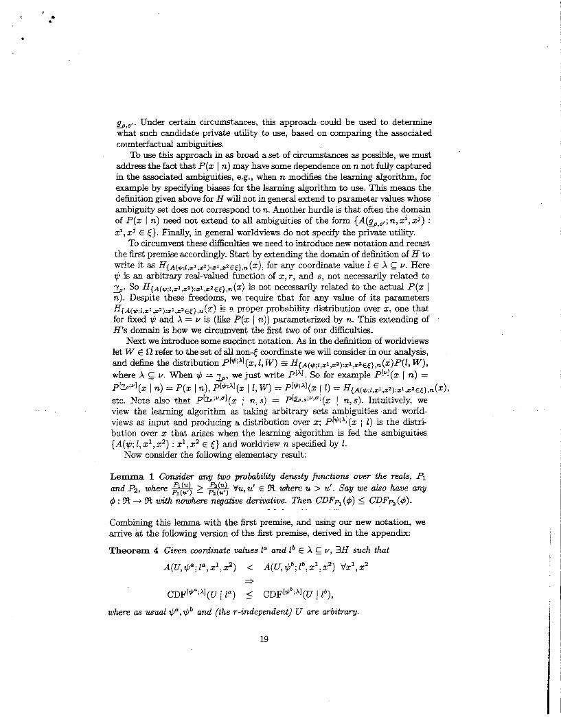
Theorem 4 Given coordinate values la and 1‘ E X C v, 3H such that

< A(U, +”; Z”, zl, z”) A(U, gb; Z b , zl, z”) Vz’, z2 =+

CDF[+~;’](U I za) I CDF[+*;’](U I z b ) ,

where as usual $a,$b and (the r-independent) U are arbitrary.

19

I I

/--- 1 -

.,............

Fi,m;.e I: The SCM h e depicts a ambiguity A(y; V; I, T I , r’) The dotted line depicts A(y; K V ; I , xl, 2’) = A(y/K; V ; 1, dl x2) for K > 1; the dashed line is A(KV; I , d, x’) for 0 < K < 1. Neither of those scaled-utility ambiguities lies entirely below the original one. Accordingly, neither of those scaled utilities is recommended by the first premise.

This theorem is illustrated geometrically in Fig. 1. Because it holds for any underlying distribution over I, Thm. 3 holds for

CDF’s and expectation values based on any P[+;’], not just Since for any $, P[+;’](x I I , W ) = P[+;’](x I I ) , the discussion following Thm. 3 holds for Pl*;’] conditioned on 1 just as well as for P conditioned on n. So Thm. 4 has the following corollary:

Corollary 1 Given any coordinates K and X 5 v, fixed k E K , and V : (x, k ) -+

R, 3H such that

A(V( . , k ) , Q”; I”, xl, x’) < A(V(., k), lClb; I b , xl, z’) V xl, z2 =+

E[+a’’l(N,,v I Z”,k) 2 E[$bJl(N,,V I P , k )

Summarizing, for a particular value of k , V determines which of the two possible moves x1 and x2 by agent p are better; G , ~ is the (s-parameterized) private utility that agent p is trying to maximize, based exclusively on the value of the worldview, n (a worldview that may or may not provide the agent with the functional form of that private utility); $I” and Qb are two real-vaiued functions of z, T and s that are used to evaluate ambiguities, and 1” and Z b are values of a conditioning variable for evaluating ambiguities, -a variable that specifies R at a minimum. In addition, H is a parametrized distribution over x that is defined for any parameter value that consists of O(<) CDF’s and a worldview, a distribution that equals P(x I n) when the its parameter value is the set {A(%; n)} together with n, and more generally for any X C v is expressed as P[$;’](x I Z) whenever the CDF’s are the ambiguities ( A ( @ ; I , xl, x’) : xl, x2 E 5)). From now on, unless explicitly stated otherwise, we will assume that we are restricting attention to an H for which Coroll. 1 holds.

20

(v) The second premise

Having rewritten the first premise this way, we can address the potential problem arising when the worldview does not specify the private utility. First consider any changes to s that modify the associated set of n for which P(n I s) is substantial. T y p i d y , any such change in the likely n fixes fairly precisely what the inducing changes in s are, as far as evaluation of ambiguities is concerned. Accordingly, when exploiting the 6rst premise we u s u d y restrict attention to scenarios in which 'dr E suppP(r I s) we can approximate

We refer to this approximation as the second premise. Note that it holds exactly if n contains a speci6cation of %+, and P(z I n) only depends on the associated ambiguities, {A(%; n, z', zJ)} = {A(&,+; n, xi, 2 3 ) ) . So if we can treat the system as though this were the case, on average, then the second premise holds 28 A *mi-formal example of a more general situation where the second premise holds is presented in App. F.29

The following corollary of the second premise is often useful:

Corollary 2 where V is any utility junction, h E any non-c coordinate,

any coordinate, and W E R

E(V 1 h, s) = /dndW P ( W I s)P(n I W, s) E ~ . * ; y 7 u ] ( V I n, s, h, W )

Often this result can be used in conjunction with CorolL 1 to analyze the impl- cations of various choices of s. As an example, in many situations (e-g., in very large systems) changes to p's private utility will have relatively little effect on the rest of the system, i.e., will have minimal effect on the distribution over T values. Accordingly consider sa and sb that vary only in that choice of p's private util- i@', in a situation where this implie that P(r I s") = P(r I sb) E P(r I sub).

%Conversely, if u is m c i o u s l y chosen" to &ways force n to equal nr for any s, where n' gives no information about the likely values that s is inducing of G,* at the various r , then J d n P ( n I s)PIvl(z I n) = P(z I n') and does not refiect the ambiguities determining J dnP(n I S ) P [ ~ - ~ I (z I n, s) = P['3u.] (z 1 n', s). In such a situation the second premise will not hold. This is similar to the situation with the first premise; in both an adversarially poor match between the learning algorithm and the learning problem at hand confounds our premise. "If it weren't for the second premise, we would have to work with P(r I n) rather than

P(r I n, s) in evaluating ambiguities. This would then require specifying a prior P ( S ) , refiecting %nor beliefs" of what the private utility is likely to be, among other aspects of s. Specifying a prior over such a space and then integrating against it can be a fraught exercise. In essence, the second premise allows us to circumvent this when averaging over n, by setting that prior to a delta function about the actual s. Nonetheless, it is important to note that we do not need a hypothesis as powerful as t he second premise to do this; the second premise is only used once, in the proof of Coroll. 3 below, and a significantly weaker version of it would suffice there. We present the "powerful" version instead for pedagogical clarity.

30F0rmaUy, our presumption is that V za E sa, zb E sb, B - ~ ( Z " ) - = B-~(Z~). -

21

. 1 , r.

Let V be a utility function, so that NP,v is as well. Then for both s = sa and s = sb, by using Coroll. 2 with R = p and q = 8, we establish that

So by Coroll. 1, taking X = Y n CT, tc = p, and $a = $‘ = 3, if separately for each T for which P ( r I sub) is substantial,

A(V(. , 4%; nu, sa, xl, z2) < A(V(., 4 y p ; nb, S b , & x 2 ) 7

(for all (d, z2) pairs, and for all (na, nb) such that both P(na I T , sa) and P(nb I T, sb) are substantial) we can conclude that E(N,,v I sa ) > E(N,,v I sb). This approach can be used even if the coordinate utility V is factored with respect to G but the private utility is not. Note also that if we take V = &+b

and have be factored with respect to & , S b , then our reasoning implies that

The kst two premises can also be used to analyze the effect on agent p of changes to the other agents. In addition they can be used to analyze changes that amount to a complete redefinition of the agent (which changes we can implement by inserting commands in the value of the agent‘s worldview that change how it behaves), or more generally, a coordinate transformation [22]. Indeed, by those premises, H , 3 and P(r I n , s ) parameterize P(z I n). In particular, say o = czp C Y, H has no direct dependence on n not arising in the ambiguities, and we take P(T 1 s) to be uniform. Then for k e d H , all aspects of the learning algorithm are set by 3, P(n I r, s ) , and the associated ambiguities.

More generally, once we specify P(r 1 s) in addtion to these quantities, we have made all the choices available to us as designers that affect term 3 of the central equation. In principle, this allows us to solve for the optimal one of those four quantities given the others. For example, for k e d 3, H , and P(r I s), we could solve for which P(n I T , S ) out of a class of candidate such likelihoods optimizes expected in te l l igen~e .~~

The rest of this paper presents a few preliminmy examples of such an approach, concentrating on changes to s that only alter one or more agents’ private utilities, where only very broad assumptions about P(n I T, s) are used. These are the scenarios in which the premises have been most thoroughly investigated, and therefore in which confidence that H etc. do indeed capture the totality of a learning algorithm is highest.

E ( N p > g o I sa> > E(NP,!7p , sb I sb)’

(vi) The third premise As just illustrated, for some differences in s (namely those that only modlfy private utilities), we can simplify the analysis to involve only a single s-induced

31More formally, where 0 C uv sets the likelihood P(n r , srhor s v ) , we could solve for the s y optimizing expected intelligence.

22

distribution over r’s (namely P(r I Pa)). The analysis still involved different distributions over n’s however, one each of the two s’s (in the guise of the two distributions P(n 1 r, s)). Moreover, t o calculate expected intelligence for a given s we must average over n, and usually changes to s change P(n I r, s) in a way diEcult to predict.32 Therefore to exploit the fkt two premises to determine which of the two s’s gave better expected intelligence, we had to have a desired difference in ambiguities hold for all pairs of n’s generated fkom the two s’s, an extremely restrictive condition.

One way around this would be to extend the analysis in a way that only involves a single s-induced distribution over n’s. To see how we might do this, ik r , xl, and 2, and consider a pair sa and sb that m e r only in the associated private utility for agent p, where those two utilities are mutually factored. Train on & b , thereby generating an n according to P(n I f , sb), and thence a distribution over r’, P(r‘ I n): which in turn gives an ambiguity between values of the private utility at z1 and z2 and therefore an expected intelligence. Our choice of private utility &ects this process in three ways:

1) By affecting the likely n, and therefore P(r’ 1 n). 2) By auneding how well distinguished utility values at zi and z2 are for m y

associated pair of r’ values generated from P(r’ I n). If P(r’ I n) is broad and/or the private utility is poor at distinguishing z1 and z2, then ambiguity will be poor.

3) By providing one of the arguments to H which (given the utility, and along with the ambiguities of (2)) fixes the distribution over intelligences.

In the guise of Coroll. 1 (with X = Y, IE = i-2 = p, $” = gsa = Va, and

with The second premise (in the guise of Coroll. 2, d t h 0 = p),. we see that the first two premises concern the last two effects of the choice of private utility on expected intelligence. They say nothing about the fist effect of the private utility choice though.

It is ty-pidy the case that the first effect will tend to work in a correlated manner with the last two ef€’ects. That is, if for some given n generated fiom %,sa the utility results in higher intelligences (e.g., because it is better able to distinguish utility values than is ~ , ~ 6 ) , it is typically also the case that if one had used to generate 12’s in the first place, it would have resulted in more informative n, and therefore P(r‘ I n) would have been crisper, leading to a better ambiguity and thence expected intelligence.

- rh = ysa = p j , the pie-e :hie szond ef&ct. If cG=3bb=e th&

We formalize this as the third premise.33 32F0r example, in a multi-stage game (see App. D), in general changing sp,s causes our agent

to take different actions at each stage of the game, which usually then causes the behavior of the other agents at later stages to change, which in turn changes p’s training data, contained in the d u e of n at those later stages.

33An alternative to the version of the third premise presented here that would serve our purposes just as well would have all distributions conditioned on some b E p u (e.g., (r, s)), rather than just on s. One could also modify the hypothesis condition of the thud premise by

23

Say that sa and sb differ only in their associated private utilities, and that those utilities are mutually factored. Then

/ d n P ( n I s ~ ) E [ ~ + ’ ; ~ ~ ~ ] ( N ~ I n , sb ) 2

/dnP(n 1 S”)E[~~~;~+’](N, 1 n, sa) _>

dnP(n I sb)E[~sb;v~r](Np I n,sb) J J

=+

dnP(n 1 S ~ ) E [ ~ S ~ ; ” ~ ~ ] ( N , 1 n, sb).

Together with Coroii. 2 th is resuits in the following:

Corollary 3 Say sa and sb differ only in the associated private utility for agent p, and that those utilitaes are mutually factored. Then

If, vr,A(&,sb(<,r),&,~b; n ,x1,z2,Sb) > A(&,Sb(6,r),&,sa; %x1,x2 , S b ) (for all (d, x 2 ) , and for all n such that P(n I T, sb) is substantid), then by Coroll. 1 the condition in Coroll. 3 is met (take X = v n and K = p, a s usual). So by Coroll. 3, in such a situation we can conclude that E(NP,g,n 1 sa) 2 E(Np,9sb 1 sb), i.e., that for k e d r, sa has better term 3 of the central equation than does sb. This is the process that will be the central concern of the rest of this paper: inducing improved ambiguity, and then plugging the first premise (in the guise of Coroll. 1) into the second and third premises (combined in Coroll. 3) to infer improved expected intelligence.

In particular, again consider the situation (chscussed in the subsection on the h s t premise) where P(r I sa ) = P(r I sb) = P(r I sub), and assume this also equals P(T I sb). If separately for each r for which P(r 1 sub) is substantia!, and for all associated n for which P(n 1 T , sub) is substantial,

1 2 b 1 2 b A(&,sb(.,f-),&,Sb;n,~ 72 ,SI > A(go,s4.7r)>&l,s’+,z ,2 , s > 7

then we can conclude that

E ( N P , g s a I ‘“1 2 E(NP,gJb I s b ) .

replacing sb throughout with some alternative s*, and our results would still hold under the substitution throughout of sb + s‘ . Similarly one could change the integration variable n E v to some other coordinate I E X C v. For all such changes the results presented below - and in particular Coroll. 3 - would still hold; the important thing for those results is that each ambiguity arising in the integrand of the left-hand-side of the hypothesis condition of the third premise IS evaluated with the same distribution over r1 and r2 a s the corresponding ambiguity in the right-hand-slde. For pedagogical clarity though, no such modification is considered here.

24

t I c

Of course, in practice this condition won’t hold for all such r and n. At the same time, Coroll. 3 makes clear that it doesn’t need to; we just need the associated integrals over r and n to favor sa over sb.

(vii) Example: The collapsed utility As an example of how to use Coroll. 3, consider the use of a Boltzmann learning algorithm for our agent [25], where sb is our original s value. With such an algorithm, constructing a new private utility by scaling the original one (i.e., changing s) is equivalent to modifying the learning algorithm’s temperature parameter. Now say that for any pair of moves, the ambiguity for sb and any probable associated worldview nb is zero for all negative y values. Then changing s by low- ering the temperature will monotonidy lower A(&,,b ((, r ) , &,,; nb, xl: x’). Ac- cordingly, doing this cannot lower expected intelligence, only increase it. (Note that the new private utility is factored with respect to the original one, so this effect of changing s also holds for expected intelligence with respect to the original private utility.)

hicw cmsider the f9nQvhg thexem:

Theorem 5 Fix n, sa,sb,r E suppP(. I sb) and a functzon U : z E ( -+ 57%- Stipulate that

i) v 2, E t, sp[u(z , r ) - u(z’, r ) ] = s@[gsb (x, r ) - - gsb (z’,

iz) V r’ E suppP(. 1 n), there exists two real numbers A,, and B,J 5 Art such that gsb (x, r’) takes on both values-but no others-as one varies the - 5 E t;

other- 9 b (&)-& iii) for all such r’ - g s a ( x , r ‘ ) = 0 i f A,, = B,,, and equals w e , and ‘d r’ suppP[. 1 n), is factored with respect to - g,b;

iu) for each pair of moues, for at least one moue of that paw, IC*, 3 y* such that P(g,a (x*, P ) = Y I n) = - Y*>.

Then V XI, x2, -4(U, - g,.; n, XI, 2) has purely non-negative support.

(An analogous version of this result holds if instead we take - gsa (x, r’) = 1 whenever A+ = E?,-,.)

Condition (i) of Thm. 5 can be viewed 2s a weakened form of requiring that u and gbb be factored. In particular, it trivially holds for u = gSb, or (due to the faccthat 9,. is a merence utfity with lead u t a @ gsb) u = - ca. COnditiOnS (ii) and (iii) mean that for each r’, the values of 9,. (G, r’) as one varies x are those of gSb “collapsed” to one of the two d u e s 3 or 1. However for h e d x, which of tha t pair of values equals gso(x , r’) can differ from one r’ to the next.

There are many situations in which condition {ii) of Thm. 5 holds with gSb = G. One example is a spin glass with G given by the Hamiltonian. Another E the simple spin system where G(z) = sin(7rn(z)/2), n(z) being dehed as the total number of spins in the up configuration.

25

Condition (iv) means that given worldview n, context r , and a pair of moves, there is no room for uncertainty in the value of the private utility at z*-it must equal (the typically unknown value) y* there. (Note that whch element of the pair of moves is this special x can vary with n and/or r.) This will often be the case if, for example, n was generated from g s a , and the agent’s (n-based) “prediction” for the utility value of the particuTar move it actually ends up making is both unambiguous and correct. In particular, such prediction accuracy often can be induced by having all the other agents readily “freeze” into a static background. In turn, as an example, those other agents are likely to freeze if they aii use Boitzmapn learning aigorithms with cheir temperatures set low enough, and with the windows they use to estimate the utilities of their possible moves short enough.

We call the difference utility gso in Thm. 5 the collapsed utility (CU), and say that it is formed by collapsing g S b , since for k e d T’ it is formed by collapsing all the values g S b (z, T’) takes on-as one varies z, to either 0 or 1.

Thm. 5 hold the ambiguity will shrink monotonically as the CU is scaled upwards. As an example, consider a Boltzmann learning algorit,hm in the scenzrio discussed at the end of the previous subsection, where in addition the conditions in Thm. 5 are met for private utility set to the CU. As the temperature parameter of that algorithm shrinks the associated expected intelligence cannot decrease, and should in particular eventually exceed that of - gsb.34 Therefore for the choice of g S b = G, the value of G induced by using cu as the private utility with a low enough temperature should be larger than that induced by using the team game at any temperature.

When the conditions

3 The Aristocrat and Wonderful Life Utilities In this section we illustrate a general set of techniques for changing the private utility so as to monotonically lower unordered ambiguity conditioned on a particular n. As discussed above, when plugged into Coroll. 3 such improved ambiguities can cause the new private utility to have better expected intelligence than the original one.

The analysis will be closely analogous to that behind the use of Fisher’s linear discriminant in statistics. We will start by restricting the analysis to distributions obeying a linearity condition. This is essentially an extended form of assuming Gaussian distributions - such an assumption being the starting point of the derivation of Fisher’s linear discriminant. We will then exploit Coroll. 3 to derive “learnability” as a measure of the quality of a private utility (as far as term 3 in the central equation is concerned). Formally, learnability

~~ ~~~ ~

34Formally, the fact that ambiguity for 9,. has purely non-negative support does not mean that the ambiguity for sSa has a support that extends to negative values. In practice though, that is the case for the vast majority of n E suppP(. I d‘). Even so, we cannot conclude that the ambiguity function for gsa, extending over all y, is less than that for Q s b . We can conclude that the reverse does not Eold though. And again, in practice, the discrepancy in supports usually does mean that the ambiguity function for ssa is less than that for g s b , so that we can apply the first two corollaries premises.

26

.

is identical to the Ftayleigh coefficient, just expressed in a Werent setting. Completing the analogy, whereas with the Fisher discriminant one strives for coordinate transformatiom of a data set giving a large value of the associated Rayleigh coefficient, at the end of this sedion we demonstrate transformations to the private utility giving a large value of the associated leamability.

(i) Learnability We begin by considering the first order expansion of the distribution of one utility in terms of the distribution of another utility:

Theorem 6 Fix 1, I' f X _C v, xl, x2, an x-orden'ng U , and two utilities V, and . vb, where 3 K E ZR+ and h : < -+ 93 such that

pv,(Y1,Y2;z',~1,~2) = PKVb+h(Y1,Y2;I,x1,x2).

Then V y,

So if in addition to the condition in Thm. 6, V y,

then it follows that A[U, V,; Z', xi, xzj < AjU, i4; i, d, x']. We will sometimes find it convenient to put subscripts on K and/or h explic-

itly giving the values of I f , V,, I, Vg, z1 and/or x2, in that order. For example, in Fig. 2 we refer to K v , ~ , to mean K when V, = V and V, = U.35

It is often the case that "to &st order", changing from v = vb to v = V, doesn't change the shapes of any of the associated distribution functions P(V(z) = v 1 Z) (one such distribution for each 5). Primarily, all the change does to those distributions is separately shift them, and/or contract them ad by the same f a c t ~ r . ~ ~ ? ~ ~ The condition in Thm. 6 is (a slightly weaker version

related: 35Note the following algebraic rules concerning such sets of distributions that are linearly

Kll ,VI 713 7 v3 = K l ~ , vl ,vZ Kh I v2 913, v3 ;

~ll,vl,12,v2 = ~/~12,v2,11,v1~

hll.VI,Z3.V3 = KIl,VI,I,,V2~l,,VZ,I3.V3 - hh.Vl.12,VZ; hl: ,VI ,IZ,VZ = -~12,v2,lI ,VI /~I2.v2,I1,V1-

36This is particularly common in situations where there are extremely many possible V

37Note that a linear relationship between utilities is a sficient but not necessary condition values, densely packed together.

for a linear relationship between the distributions of their values.

27

of) the requirement that this property holds exactly, even if we also switch from 1 to 1’ at the same time (and therefore change the underlying probability distribution over 2). The general effects of expansion or contraction of the utility on the associated ambiguity are illustrated in Fig. 2.

Thm. 6 tells us in particular that when its condition is met along with the one mentioned just following its presentation, then for K = 1 and tu(x1,x2)[h(x2) - h(s l ) ] negative, then changing from ( V b , I ) to (V,, 1’) improves ambiguity. More- over, the degree of that drop grows with increasing magnitude of {h(z2) - ~ ( Z ’ ) } / K . ~ ~ In the usual way, for 1 = 1’; X = vna , V, = Q, and Vb = g s i - where s a d s’ a&y di%r iE their privzte utilities, we cm. exploit this phe~omenoii iE concert with Coroll. 1 and then Coroll. 3 to improve term 3. To that end we start with the following:

Theorem 7 Say that the condation in Thm. 6 holds for the quadruple (l’, V,, 1 , V b )

with the same K , h Vxl, x2. Then

. .

a) where f is any dastrabutaon over x,

1” ) . Then

where the Va-independent proportionality constant is 4s dx f ( x ) Var(‘I/b; 1, x ) .

h(zZ)-h(s l ) We call the (ambiguity) shift and A f ( U ; 1, z1,z2) the learn- abiIity of U for zl, x2, and I .39 As a particular example, for f (.) = (1/2)[d(z- d) + S(S - 291,

Note that IAf(U; I“, d, x2) I is invariant under affine transformations of U . Typi- cally we are interested in the case where S ~ ~ [ E ( V , ~ -%2; I , zl, x2)] = sgn[E(V; -

38A similar result holds if we instead consider a fixed pair (z’, z2) and associated K,i ,=z,

39This latter is a slight modification from the definition used in our previous work. so that the expansion factor can vary with moves, just l i e the offset factor h.

28

I I

0

.

V:; 1, x l , x2)] = t v b ( X I , x2) , so that we can use learnability to evaluate the offset term in Thm. 6, tu(xl , x2) [ (

Intuitively, the learnability of U reflects its signal-tcmoise, as far as agent p is concerned, in that agent’s process of “choosing its move”. This is because the numerator term in the definition of learnability reflects how much (the expectation of) that utility varies as one changes the agent’s move x with the context held h e d . In contrast, the denominator term reflects the (average over x of) how much U varies due to uncertainty in the context while keeping the move x f k d 4 0

The following results provide a geometric perspective on the expressions in Thm. 7

h 2 ) - h 21 ( ’1.

Theorem 8 Say that the condition in Thm. 6 holds for the quadruple (Z’, Vu, 1, &).

i) If both v, and v b are di-ference utilities with the same lead utility and ,B = 1, while both P(.’;Z) = P(r’;Z‘) and A f ( K ; l , x 1 , x 2 ) < Af(Va;l f ,x1,x2) , then K < 1.

ii) Let {Va, 1’) be an equivalence class of (v, 1) pairs dl related to (vb, l j as in Thm. 6. Then the learnability of those pairs mdtiplied by tu(x1,x2) is a shrinking function of the value of the associated ambiguities at the origin. In addition, acmss all pairs in that class that share some particular learnability value, K is inversely proportional to the slope of the ambiguity of that pair at the origin.

iii) Say the condition (ii) aLso holds for the quadruple (,?*,Vu- = ,BV,,l,jlb) (though potentiallv for a different K and/or h), where P(r’; 1*) = P(r’; 1‘). ThenAf(Va.;1*,x1,x2) and -4f(Va;1’,x1,x2) are identicnlVxl, x2, as w e the associated shifts, whale Kp,va, ,I,& = PKp,v,,l,v,.

iv) IfK < 1 andAf(Va;1‘,x1,x2) >hf(jlb;1,x1,x2) (K > 1 andAf(Va;E‘,x1,x2) < A,(&; 1, X I , x2), respectively), then the maximal slope of A(Va; I f , x l , x ) is greater than (less than, respectively) the maximal slope of A ( K ; I, d,x2) .

41

To understand Thn. 7 in terns of ambiguities, for pedagogical SimpliciQ- consider making changes to a utility V without any corresponding changes to the value of X (and therefore none t o the underlying probability distribution over z>. First note that such a change applied to the scale of V doesn’t change how weighted the associated ambiguity is to positive y values. It doesn’t change “how far“ V ( x l ) - V ( 9 ) is kom zero, on average. This “weight to positive y values” is reflected in the value of /A,( (which is invariant with respect to such rescalings), and therefore (by Thm. 7(ii)) is also reflected in the value of 40L0w learnability is not only a problem for agents with poor learning algorithms. Even for a

Bayg-optimal learning algorithm, if the “signal to noise” of the private utility is poor, then the agent’s intelligence for the actual r at hand can readily be far less than 1. (Bayesoptimality only means that z is set to maximize E(gs I n,z), not to maximize g,(z,r).)

41Trivially, the condition in Thm. 6 holds for (l’, V,*, 1, Va) if it 20s for (l‘, V,, I , q). In addition, Af(Va-;1‘,z’,z2) = Aj(Va;1‘,z1,z2) while Kzt,va-,~,vb = ~KzJ,v,,~,v,.

29

Y FigLrc 2: The leftmcst s&d line shows an ambiguity A(y; ? f ; I , d l z2>. The dotted line shows A(y;V’;1,s1.s2) for V’ = aV, 0 < a < 1. KV/,V = a,

‘and learnability of V’ is the same as V’s. The dashed line shows the dotted line right-shifted by tU(x1 , s2 ) [h (d ) - h(x2)] > 0, i.e., the ambiguity A(y; U ; I , xl, x2) for U E aV + h. (Since we have not changed s, Thm. 6 must apply.) A, (U; 1 , s1 , x2) > A, (V’; 1, s1 , z2). Finally, the rightmost solid line depicts the dotted line expanded back to the scale of the leftmost solid line, i.e., the ambiguity of U‘ = PU where /3 = l/Kvl,v, so that K,yl,v = 1. As with the previous one, this rescaling &om W to T does not affect the learnability.

t u ( z l , x2) [ h ( z z ) & h ( z l ) ] . However such a rescaling can still be useful in how it “stretches” the CDF. To see how, note by Thm. 8(iii) that if V has better learnability than some other utility U , such stretching of V may provide a new utility V’ such that in addition K v , , ~ = 1, which means that V’ has better ambiguity than U (in light of Thm. 8(iii)).42 In other words, to change the learnability we must induce a rightward offset in the (potentially scaled) ambiguity of V. Having done that, a subsequent rescaling can give us an aggregate K equal to 1 (without changing learnability), and thereby provide a final utility whose ambiguity lies everywhere below that of U . The value of that offset is given by the (P-independent) ambiguity shift. (See Fig. 2.)

(ii) Learnability and term 3 Plug Thm. 7 into Thm. 6, with U in Thm. 6 set to the s-ordering given by &(., r). This shows that after appropriate rescaling of V,, the triple (Val Z’) has better ambiguity than does (Vb, I) if it has better l ea rnab i l i t~ .~~ If we plug that fact into Coroll. 1, we establish the following:

Corollary 4 Fix T , I, l’, V, and &, where X C v, as usual. Say 3K E %+, h : E + %, such that V xl, x2

2) p~(Y11Y2;~’1x1J2) = PKVb+h(y1,Y2;1,x1,x2);

and 42Note that such rescaling amounts to changing the temperature parameter in a Boltzmann

43Note that this rescaling is done before we invoke the third premise. In this way we will be learning algorithm.

able to exploit that premise to do rescaling without invoking the assumption in Thm. 8(iii).

30

L I

ii) t~+,(.,~)(x’,z~)Af(Va; l’,x1,x2) > t v , ( . , , ) ( ~ 1 , ~ 2 ) A ~ ( % ; 1,x1,r2)-

Then by appropriatdy rescaling Vu we can assure that

~[~a;~](i~,,v, I r, 1’) 2 E I ~ ~ ; ~ I ( N , , ~ ~ I r, 1).

Consider changing the private utility from V, to a V, which is factored with respect to V,. Then Coroll. 4 means that if this increases the learnability (in the x-ordering preferred by vb(-, r ) ) of one’s private utility, then t y p i d y it results in higher expected intelligence, for the optimal scaling of that private utility. More precisely, express Coroll. 4 for X = v n IS and 1 = 1’ (n, s) and then plug it into Coroll. 3 with sb = s,gsa = Vu and g s S = V,, where sa and sb differ only in the associated private ut&% for our agent, and V, and V, are mutually factored. Then we see that if learnability is higher with sa than with sb (in the z-ordering preferred by &(., T ) ) for enough of the n for which P(n 1 r, sb) is non-negligible, then s = sa gives a higher expected intelligence conditioned on r and s than does s = sb (each intelligence evaluated for the associated optimal scale of the private utility).

As an added bonus, often the higher the learnability of a private utility, the more “slack” there is in setting the parameters of the associated learning algorithm while still having an ambiguity that’s below that of some benchmark, low-learnability private utility. In other words, the higher the learnability, the less careful one must be in setting such parameters in order to achieve expected intelligence abave some threshold. In particular, the greater the ambiguity shift in Coroll. 4, the broader the range of scales ,B for which PV, has greater expected intelligence than does vb. So by using private utilities with increased learnability often it becomes less crucial that one exactly optimize the learning algorithm’s

mt;l;t.,

values. This phenomenon can be ampl&ed via “construction interference”, for example as in the following result.

Corollary 5 Fiz r and two sets of utilzty-(A-value) pairs, {G, 2,) and {V*, I t - ) , indexed by t and t*, respectively. Assume all quintuples (r, It- , V*, I t , &) obey Coroll. 4(i), (ii) with Vu = V*, vb = V,, etc. For pedagogical szmplicity, also take

ir,+rud p&-m&,zi s&$&g the s d e & -&.~& the d?g-ri;b

s g n [ ~ , ( s ’ , r ) - I+,(x2, r)] = sgn[~(z ’ , r ) - E(x2, r ) ] = m, sgn[E(xl - %2; 1, zl, x2)] = sgn[E(K’ - V,; l’, x’, z’)] 3 m’,

and m = m’.

i) Define

At,t-x~72 = {A, (V*; t t - , z’, z2) - A,(&; It , z’, z~)} dzf (z)Var(G; It, z), 0 ~~.+1,,2 E minty: A(y;Vt(.:r);VtIZt,x1,x2) = I), ~ ~ , ~ 1 , ~ 2 = max(y : ~ ( y ; v,(.,T), v,; zt,x1,z2) = 01,

where as wual f is a jixed but arbitrary distribution over x, and we assume At,,-,,1,x2 2 0 W , t*, z’, x2.

31

ii) Define Kt,t* = Kit. ,v-,lt,vt each ( t , zl, 9) triple)

Lt,t-,v*,x1,x2 = - Kt,t*

1 -

and then define the subintervals of 3 (one fo r

otherwise,

iii) Define Lt-,v* UtLt,t-,v--

Then for every t", Vp E Lt.,v.,

Note that Bt,,~,x2 2 0 always, since m = m' for ( I t , V,). Accordingly, Lt.,v- is never empty, always containing Uti- Kt.t- at Ieast.44>45

To help put Coroll. 5 in context, apply Coroll. 4 to the scenario of Coroll. 5. This establishes that for any t', 3/3 E Lt-,v. such that E[PV';X](Npv- I r , l t - ) 2 maqE[~; ' ] (Npv , I T, Z t ) . Note also,the immediate implication of Coroll. 5 that

mi~-E[~Bv*; ' ! (NVI I r , lt.) 2 mintE[G;AX](Nvt 1 r , I t ) .

As an example of Coroll. 5, take X = Y n c, have It* equal some fixed 1* Vt*, V* E gs., and V, 3 s,, Vt . Have real-valued t E [tl > 0, t 2 ] , where V, = I/'t.$. So assuming Af(V*;Z*,rc1,z2) 2 hf(Qlt,z1,rc2) Vz1,z2 as usual, the range in the logarithms of for which E[PV';'l(Nv* I T , E") 2 mintE[v~;'](Nv, I r , I t ) is greater than or equal to In(tz) - I n ( t ~ ) . ~ ~

VP E %Lt*,v* ,'

&If (unlike in Coroll. 4) the value of K can change with the (z1,s2) values, then those indices must be added to K's subscripts. In this case the conclusion of CoroU. 4 need not hold; Lt-,v. can be empty. 45A subtle point is that in situations where Dt , z i , z~ > 0, we can increase the scale of

Vt as many times as we want and assuredly improve its ambiguity each time. (This is not something we can do in the other situations.) Accordingly, if every instance going into Lt* ,v- is such a situation, then OUT conclusion that rescaling V* can assuredly give better expected intelligence than b$ is a bit irrelevant; in this scenario we can also rescale % to assuredly improve its expected intelligence. 46T0 see this, note that t sets the scale of G, just like p does for V*. Furthermore, Kt f

Kt,t- = if P(T/ ; 1* ) = P(#; I t ) V r l , t (cf. Thm. 8(iii)). So 1/Kt, which we know is contained in Lt,*. ,v- , equals Now apply Coroll. 5 .

t1Kt , t * t1

t iK t , .

32

As another example, choose { I t } = {Ii} = {n E supp P(Y I r, si), si)} for some set of D values {si}, with V, = Vn+i = gsi Vi. Also presume that Vl?, there is a design coordinate value sf such that gssa = gV*. If we now plug the conclu- sions of Coroll. 5 into Coroll. 3, we establish that Vi, P E nnEsupp P ( ~ ~ ~ , ~ ~ ) L , , , ; , V * ,

(iii) Aristocrat Utility In general, there is no utility that is both factored with respect to the world utility and has a t e iea~nabi l i ty .~~ The following result allows us to solve for the private utiIity that maximizes learnability, and thereby find the private utility for agent p that should give best performance under the &st three premises:

Theorem 9

i ) A utility UI is factored with respect to U.2 at z iff V z’ E p(z) r, with <(z’), Ul(z,r) = Fr(U2(z‘)) - D(r) , for some function D and some x

r-parameterized function Fr with positive derivative.

is the ( I , XI, z2)-independent quantity Ef(Z,(Fr(U2(<, r ) ) ) . ii) Forf ied 1 f X C u, r, XI, 2, and F , the D that maxzmizes A f (U1; I, XI, x2)

..., . . m,t Ti~r i G~ui 7 1 ~ u L ’ t i i i i - ‘ULLe - s & ~ ! d a;;,bzpkj s?$ b e t t ~ e ~ tT2 KX! U; IS

1 , xmnf [ Ef(Zl),f(ZZ){Var((F1 - F2)6(rl- r2); l,<1, ( 2 ) ) E f ( z ) { V 4 U 2 ; 40)

where the subscript on the denominator expectation indicates that both x ’s are averaged according to f , and the delta jknction there means that our two F’s (one for each x) are evaluated ut the same T.

A particularly important example of a function Fr meeting the condition in Thm. 9 is Fr(U2) = U2. This choice results in the difference utility U1 that takes z = (x, r ) 4 &(x, r ) - Ef (U2(e , r))- We call this the Aristocrat Utility (-4U) 47As an example of when having both conditions is impossible, take r E {r’,?}, z E

{z1,s2), and G{z1,6) > G(zZ,rl), while G ( z 2 , r 2 ) > G(s’,r2). Then by Thm. 1, we also must have %(sl , r ’ ) > 21p(z2,r1) and 3(z2,r2) > >(z1,r2). Also assume that P(r’;l) = d(r’ - r ) t/ r, s, so P(U = u; I , z) = 6(u - V ( z , r ) ) always.

and D dz f(s) Var(U; r, s,z) = [A” + B2]/4 , which by mnve3dty

- > [ ( A + B)/2)]’ = [(C + D)/2) ] . In tm, [E(U; 1 , ~ ’ ) - E(U; 1 , ~ ~ ) ] ~ = [ (D - C)/2l2 I ( (C+D)/2) l z . Combining, by the d a t i o n of learnability we see that it is bounded above by 1. QED.

Define A E %(z1,r2)-3(z1,r1), C E 3(zz,r2)->(z1,?), B ZE 3(z2: r’) -%(z 2 2 ,r ),

>(sl, r’) - s(z2, r’). So A + B + C + D = 0, and both C > 0 and D > 0. Take f(z) = 1 / 2 for both z, so

33

for U2 at z , AUUz,f(z), reflecting the fact that it is the difference between the value of Uz at the actual z and the average such utility.

Say a particular choice of f , f’, results in conditions (i) and (ii) of Coroll. 4 being met with V b = U2 and V, = AUu,,ft, for the choice of X etc. discussed just after the presentation of Coroll. 4. Then we know by that corollary that once it is appropriately rescaled, using the AU for Uz as p’s private utility results in an expected intelligence with that is larger than is the expected intelligence that arises from using U2 as the private utility. (Note that U2 and AUuz,f. are mutiially factored.) Moreover, by Thm. 9 any other difference utility that obeys Coio!!. 4(i)(ii) (iz coiicert with V..) must have wnse amhigli-ty t h m dnes AUuz,p, and therefore worse expected intel l igen~e.~~

To evaluate AU for some G at some z we must be able to list all z’ E p(z). This can be a major difficulty, for example if one cannot observe all degrees of freedom of the system. Even if we can list all such z’, we must also be able to calculate G for all those z’, an often daunting task which simple observation of the actual G(z) at hand cannot fulfiu (in contrast to the calculational needed with a team game, for example).

Even when we cannot calculate an AU exactly though, we can often use an approximate AU and thereby improve performance over a team game. For example, in an iterated game, at timestep t , r for a particular player i reflects the state of the other players it is confronting. In such a situation, by observing T , often we can approximate Ef(g,(<, r ) ) by an appropriate average of the value of gi over those preceding iterations when the state of the other players was T ,

wii% f being the frequency distribution of moves made by i in those iterations. In particular, consider a “bake-off” tournament of a 2-player game in which each player in the tournament plays one other player in each round, and keeps track of who it has played in the past and with what move and resultant outcome. In such a situation, the expectation value for player i confronting player j that gives AU, can often be approximated by the average payoff of player i over those previous runs where i’s opponent was 3 .

On the other hand, even when we can evaluate AU exactly, it may be that the conditions in Coroll. 4 are badly violated. In such situations increasing learnability by using AU will not necessarily improve expected intelligence, and accordingly AU may not induce optimal performance. Indeed, it may induce worse performance than the team game in such situations. On the other hand, there are other modifications to the private utility that (under the-first premise) may improve expected inteILigence in these sitcations. An exmple of such a utility is the CU, as illustrated in [22].

(iv) Wonderful Life Utility One technique that will often circumvent the difficulties in evaluating AU is to replace p with a coarser partition, having poorer resolution. While this replace-

48Note though that in general there may be a utility F,(U2) - D(r ) with better learnability than AU, for example if FT is non-linear. Note also that whether AUu2,f, obeys conditions 4(i)(ii) will depend on the choice off’ , in general.

34

ment usually decreases learnability below that of AU, it still results in utilities that are far more learnable than team game utilities, while (like team games) not requiring knowledge of the set of worldpoints p(z) in full. In this subsection we illustrate making such a replacement for difference utilities.

We concentrate on the case where the domain of the lead utility D1 is all of C, and the secondary utility D2 = Dl($(z)) for some function C$ : C j C where Vz E C, 4 depends only on T , i.e., V T , Vz', z" E r , $(z') = $(z"). So specifying the utility consists of choosing 4. While in general we can make the choice that best suits our purposes, here we will only consider a particular class of 4's. A more general approach might, for example, choose $ to maximize leamability. Intuitively, the resulting difference utility is equivalent to subtracting DI of a transformed z from the ori@ Dl(z) , with the transform chosen to maximize the signal-tenoise of the resultant function. See the discussion of Thm. 7.

Let 7r be a partition of <. Fix some subset of < called the clamping element CL-, such that V p E x,D1 is invariant across the (assumed non-empty) intersection of CL-, and ~4~ Define an associated projection operator CL-,(z) = CL-, n+), which for any p f T maps all worldpoints lying in p to the same I-LA- qihr+gn crf that clement, R srihregion having a constant DT value.50 Then the Wonderful Life Utility (WLU) of D1 and x is defined by

WLUD,,,(z) = Dl(z) - D1(CL-,(t)).51

To state our main theorem concerning WLU, for any partition of C, T, and any set B _C C, define B n x to be a partition of B with elements given by the intersections of B with the elements of T . Furthermore, recall from App. B that given two partitions x1 and x2, x1 C n-2 ifE each element of 7r1 is a subset of an -'----A -r - =-- +L.- r-11--;-- hnlrlc n x r a d 1 D p c what nihqpt of C forms C: Clcucul, Ul 112. I L L G U U L L C l"u"r*sug Y V l W L"bU\YI-.- -

Theorem 10 Let x and x' C x be two partitions of C. Then WLUD,,, is factored with respect t o D1 for coordinate C n d V z E C.

As an example, with p E C n x, WTUG,, is factored with respect to G for coordinate p.

Note that x' C x meam that x' is either identical to x or a ''her-resolution" version of x. So z + CL-, nT(z), by sending all points in ~ ( z ) to the same point, is a more severe operation, resulting in a greater loss of information, than is z -+ CL-,n,p(Z), which can map Herent points on x ( z ) differently. So Thm. 10 meam we can err on the side of being ova-severe in our choice of damping operator and the associated WLU is still factored.52

49Note that CL-, automatically has this propem, independent of D1, if its intersection

50K0te that both CL-, and CL-,(z) are implicitly parameterized by D1. jlNote that if there is some z' E 6 such that CL-,(z,r) = (z',~) V Z , T , then WLU is a

special type of AU, with a delta function f. 52Sometimes WLUG,~J(Z) will be factored with respect to G for coordinate C n x even

though d T- For example, this is the case if G is independent of precisely which of the elements of d contains z, so long as all of those elements are in ~ ( z ) . However in general

with each element of x consists of a single worldpoint.

35

There are other advantages to WLU that hold even when x = x’. For example, in general CL-,(z) need not lie on the set C (n.b., T and ^T are partitions of <, not C). In such a case the function G(CL-,(z)) : C --+ % is not specified by the function G(z) : C -+ E. In this situation we are free to choose the values G(CL-,(z)) to best suit our purposes, e.g., to maximize learnability.

An associated advantage is that to evaluate the WLU for coordinate C fl x, we do not need to know the detailed structure of C. This is what using WLU for the coarser partition x rather than the AU for the original coordinate C nx’ gains 11s- Given a choice of clamping element, so long a s we know G(z) and ~ ( z ) , bu5cbllGL ivlbll bllc FUlLblolldl luliri lul clLe ap~lupllabc 3Ub3cb~ o1 <, wc L U w

the value of VVLUG,,(Z). These advantages are borne out by the experiments reported in [17].

c-,-,-cLn- -:+h el. .--A: - - l C-- -S 0 C,, el, ,,,,,-:,e, ,-.. --e- S r --- _----.

(v) WLU in repeated games

As an example of WLU, say we have a deterministic and temporally invertible repeated game (see App. D). Let the {w1,w2, . . . , W J } and {el, 8 2 , . . . , e L } be two sets of generalized coordinates of CT (not necessarily repeating coordinates) Consider a particular player/agent, and presume that Yt’ there is a single-valued mapping from rt‘ + (wl, w2,. . . , W J ) , and one horn (zt’,+’) + (41. q 2 , . . . , qL) (both implicitly set by C). So the player’s context at time t’ fixes the values of the w, (defined for time T ) , and by adding in the player’s move at that time we also flx the values of the 8%. Say we also have a utility U that is a single-valued function of ( w l , w2,. . . , wJ, q1, qz , . . . , q L ) .

whose elements are specified by the joint values of the {w1,w2, . . . , w J } . Take CL-, to be a set of z sharing some fixed values of {el, 0 2 , . . . , eL}. Note that U is constant across the intersection of CL-, with any single element of x, as required for it to define a WLU.

Intuitively, CL-,(z) is formed by “clamping” the values of the {el, 82, . . . , 8 ~ ) to their fixed value while leaving the (w1, w2, . . . , WJ} values unchanged. More- over, since rt’ + ( ~ 1 , 2 0 2 , . . . , w J) is single-valued, we know that any dependency of the important aspects of z (as fa r as U is concerned) on our player’s move at time t: is given by (a subset of) the values (41, q2 , . . . , q ~ } . (Recall that all values zt are allowed to accompany a particular rt‘ .)

Now by Thm. 10, we know that WLUu,, is factored with respect to U for coordinate C n xf for any partition x‘ that is a refined version of x. In addition, p*’ C x. So TVLUv,, is factored with respect to U for the coordinate given by C n pt‘ = pt‘ , Le., it is factored for our player’s context coordinate at time t’.

When the {e,} are minimal in that none of them is a single-valued mapping of rt‘ (i.e., none can be transferred into the set of { w z } ) , we say they are OUT

Take x to be the partition of

such factoredness will not hold. Even if it doesn’t though, say G is relatzvely insensitive to which of the elements of ?yr contains z , over the set of all such elements that are in ~ ( 2 ) .

Then wLU~;:i.(z) will be quite close to factored for coordinate C fl x. This often allows us to be “sloppy in using WLU’s, by talung ?yr to be only those degrees of keedom C f l ~ with “significant impact” on the value of G.

36

player’s effect set [17].53 Often a player’s behavior can be modified to ensure that a particular set of {e*} contains its effect set for some particular time. When we can do this it will assure that some associated variables (wi} specify (a partition x that gives) a W L U G , ~ for our player’s move at that time that is factored with respect to G.

(vi) WLU in large systems Consider the case of very large systems, in which G typically depends significantly on many more degrees of freedom than can be varied within any single element of p (Le., depends more on the d u e of r than on where the system is within that r). So we can write G(z, r ) = Gl(z, r ) + Gz(r) where the d u e s of G2 in C are far greater than those of GI, and correspondingly the changes in the value of GI as one moves across C are far smaller than those of G2. In such cases, with p = C n T as usual: the learnability of G is far less than that of WLUG,,. This is due to the following slightly more general theorem:

Theorem 11 Let K and T

H~(K(z)) , where H is defined E E X E IJ, and define

and ,-

K be two partitions of I . W ~ t e H ( z ) = H I ( ~ ) + over di <, and consider the ageni p = C 17 n . F.iz

A~(WLUH,,; I , XI; x2) >- -& L hf(H;l,~l,~’) - 2M

Note that as K becomes progressively coarser and coarser, L shrinks. So such coarsening of the clamping element will t y p i d y lead to worse learnability- In fact, in the limit of K = 8, WLUH,, just equals H minus a constant. So in that

53Sometimes the (q l , a,. . . , q,,) value specifying the clamping element of an effect set can intuitively be viewed as a ”null action’’, so that clamping can be viewed as “removing agent p from the system”. Intuitively, in this case we can view WLU as a first order subtraction from G of the effects on it of specitjring those degree of freedom not contained in the effect set (hence the name “wonderful life” utilify-cf. the Frank Capra movie). More formally, in such circumstancg WLU can be viewed as an extension of the Groves mechanism of traditional mechanism design, generalized to concern arbitrary (potentially time-extended) world utility functions, and to concern situations having nothing to do with valuation functions, (quasi- linear) preferences, types, revelations, or the like. (See [7, 2, 14, 2, 10, 16, 8, 27, 131.) Due to its concern for signal-tenoise issues though, this extension relies crucially on r e - d i n g of G. (hdeed, if one just subtracts the clamped term without any such re-scaling, ambiguity can be badly distorted, so that performance can degrade substantially [23].) In addition, this extension allows alternative choices of the clamping operator, even clamping to illegal (i.e., not E C) worldpoints. This extension also can be used even in cases where there is no action that can be viewed as a “null action”, equivalent to “removing the agent from the system”.

37

limit, and H must have the exact same learnability - in agreement with Thm. 11 and the fact that L = 0 in that limit.

When L greatly exceeds M the bound in Thm. 11 is much greater than 1. So if we take H = G and K = 7r, Thm. 11 tells us that for very large systems, setting the private utility to G’s WLU rather than to G may result in an extreme growth in learnabi l i t~ .~~ In particular, for X = v n 0, in large systems it may be that L >> IM’d 1 such that P(l I s> is non-infinitesimal. Under the first three premises, assuming WLUG,, and G obey the conditions in Coroll. 4(i),(ii), this means that setting the private utility to WLU will result in larger expected ktelfigence of the agest than ml!! setting it to G. Moreover, since that WLU is factored with respect to G, this improvement in term 3 of the central equation will not be accompanied by a degradation in term 2. This ability to scale well to large systems is one of the major advantages of WLU and AU.

(vii) WLU in spin glasses

As a ha1 example, consider a spin glass with spins {b,}. For each spin z let h, be the set of spins other than i, and for each i let h, and F, be any two functions such that the Hamiltonian can be written as X ( g ) = h,(b,, g-,> + F,(g-%>. In particular, for X ( 6 ) = C J k F f J k b J b k + z , X , b , , we can have F,(b-,) =

Ff,z]b,b,/2. Since at equilibrium b minimizes X, and therefore given the equilibrium value of h,, at the 7f-minimizing point b, is set to the value that minimizes hz(bz,g-2).

We can view this as an instance of a collective where 7f is the (negative) world utility G for a system of “agents” p with move b,, and g, = h,. For all p, at the g that maximizes G, b, is set to the value that maximizes -h, given b-,. More generally, h,(b,, I!-,) = X($) - &(g-,) is factored with respect to G(g) (cf. Thm. 2), with the context for each agent p being g-, and C = C being the set of a11 vectors G. so any b‘ (locally) maximizing G also simdtaneously maximizes all of the -hz. Ffustration then is a state where all the agents’ intelligences equal 1, but the system is at a local rather than global maximum of G.

Consider a particular spin/agent, p. Embed C, the set of all possible g, in some larger space that allows the spin p to take on additional values, and redefine [ to be that larger space. Let 7r be an associated [-partition such that p C n 7r. Take CL-, to be some set off of C. Extend the domain of definition of h, by setting h,(CL-,(g) = 0 V G, # C. Then W L U G , ~ = -h,, i.e., WLU is the “local Hamiltonian” perceived by spin p, whereas G is the Hamiltonian of the entire system.

So by Thm. 11, if the number of nonzero coupling strengths between p and the other spins is much smaller than the total number of nonzero coupling strengths in the system, then the learnability of p’s local Hamiltonian far exceeds

- x 3 + , k + XJkbJbk c,+, X J ~ J , :nd hz(ba, 6-t) = Xzbz t Xzzb: C,+[%J +

...

54Trivially, since learnability of AU is bounded below by that of WLU, its learnability must exceed that of a team game at least as much as WLU’s does.

38

that of the global Hamiltonian. Accordingly, consider casting the evolution of the spin system as an iterated game, with each spin controlled by a learning algorithm, and each &,st set to either spin p’s local Hamiltonian at time t, or to the global Hamiltonian at that time. (See App. D.) Then since WLU is factored with respect to G, we would expect (under the first three premises, and assuming conditions 4.l(i)(ii) hold, etc.) that at any particular timestep of the game ;is closer to a local peak of the global Hamiltonian if the agents use the value at that timestep of their local Hamiltonians as their private utilities, rather than use the d u e of the global Hamiltonian at that timestep.

If we also incorporate techniques addressing term 1 in the central equation, then we can ensure that such local peaks are large compared to the global peak. Moreover, if we have the spins use a WLU with better learnability, we would expect faster convergence still. Similarly, if the spins use AU rather than their local Hamiltonians, then since this increases leamability, performance of the overall system should improve further still. (Roughly speaking, such a change in private utilities is equivalent to having the agents use mean-field approximations of their local Hamiltonians as their rewards rather than the actual values of their iocd E d t o n i m . j M u ~ e geiiedly, aiy i i i~di i icz t i~~ of t h e systc=: that induces higher learnability (while maintaining factoredness of the individual spins’ private utilities with respect to the original Hamiltonian) should result in faster convergence to the minimum of the original Hamiltonian. The foregoing is borne out in experiments reported in [24].

Acknowledgements I would like to thank Mike New, John Lawson, Joe Sill, Peter Stone, and especially Kagan Tumer and Mark Millonas for helpful discussion.

A Intelligence, Percentiles and Generalized CDF’s A useful example of intelligence is the following:

(A.l)

with the subscript on the (usually normalized) measure indicating it is restricted to z’ f p(z) (usually it is also nowhere-zero h that region). For consistency with its use in expansions of CDF’s, the Heaviside function is here taken to equal 0/1 depending on whether its argument is less than 0 or not. (Having 0(0) = 0 in l3q. A.l is also a valid intelligence operator.) Intuitively, this kind of intelligence quantifies the performance of z in terms of its percentile rank, exactly as is conventionally done in tests of human cognitive performance. Note that this type of intelligence is a model-kee quantification of performance quality; even if z is set by an agent that wants large Nf ,u and Np,u(z) turns out to be large “by luck”, we still give that agent credit. The analogous coordinateless expression is given by Nu(z) = J dp(z’) 0[U(z) - V(z’)] where p runs over all of C.

39

There is a close relationship between CDF’s and intelligence in general, not just percentile-based intelligence. Thm. 3 provides an example of that relationship. For percentile-based intelligence though the relationship is even deeper. In particular, coordinateless percentile-based intelligence can be viewed as a generalization of cumulative distribution functions (CDF’s). This generalization applies to arbitrary spaces serving as the argument of the underlying probability density function (not just !XI) and does not arbitrarily restrict the “sweep direction” (said direction being from --co to +a for the conventionaI case). In particular, for the special case of z E !Xn and invertible U(. ) where IV,U(z)I = 1 ax., /V,Xu(z)/ gives the pmbaK!it.; density p(z) and 0 5 ,Vv(z) 5 1 b’ z , just like with the conventional CDF for which the underlying space is 32’. (In fact, for U ( z E !XI) = z + constant, Nu(z) is identical to the conventional CDF of the underlying distribution p(z).) For the more general case, intuitively, U itself provides the flow lines of the sweep.

Percentile-type intelligence is arbitrary up to the choice of measure p, and in a certain sense essentially any intelligence (in the sense defined in the text) can be “expressed” as a percentile-type intelligence. As an alternative to these kinds of intelligences, one might consider standardzing a utility U by simply subtracting some canonical value (like the expected value of U) from U ( z ) . This operation doesn’t take into account the width of the distribution over U values however, and therefore doesn’t tell us how significant a particular value U(z)-E(U) is. To circumvent this difficulty one might “recalibrate” V(z) -E(U) by dividing it by the variance of the distribution, but this can be misleading for skewed distributions; higher-order moments may be important. Formally, even such a recalibrated functions runs afoul of condition (i) in the definition of intelligence.

One important property of percentile-type intelligence is that with uncountable [ and a utility U having no plateaus in [, if P(- r 1 r, s) = p,.(-r) and is independent of r , then P(Nu(z) 1 s) is constant, regardless of U and p. More formally,

Theorem A. l Assume that for all y in some subinterval of [0.0,1.0], for all r in suppP(. I s) there exists ^ r such that the intellagence N,,u(r, ^ r ) = y. Restrict attention to cases where the zntelligence measure pL,(^r) = F ( ^ r I r , s ) and is andependent of r. For all such cases, P(Nu(z) 1 s) is fiat with value 1.0, independent of both p and U .

Proof: We use the complement notation discussed in App. B. Write

P(N,,u(r, ̂ r ) = Y I s) = / d r d^r’P(r 1 s)P(^r’ I r, s)P(N,,u(r, “r’) = y I r, s )

Next write P(N,,u(r, ̂ r ) = y 1 r, s ) as the derivative of the CDF P(N,,u(r, ̂ r ) 5 y 1 r ,s) with respect to y. Now by assumption there exists a ^ r such that N,,u(r, ^ r ) = y. So we can rewrite that CDF as

P(Np,u(r, -7.’) 5 ”(r, -7.1 I r, SI,

40

.

where the probability is over -r‘, according to the distribution P(^T’ 1 T, s).

We can rewrite this CDF as

P(U(r, ̂ r‘) 5 U(r, -7.) I r, s),

by property (ii) of the general definition of intelligence. In turn we can write this as

= / d-T’p(-r’)@(U(r, - T ) - U(r, -r‘) (by assumption)

= NP,u(r, -T) = y.

(by dehition of intelligence)

Therefore the derivative of our CDF = 1. QED.

Intuitively, this theorem says that the probability that a randomly sampled point has a d u e of l7 5 the y‘th percentiie of ii is just y, su its deiii-ath-e = 1, independent of the underlying distributions. Note that both the assumption that P(”r 1 r, s) is independent of r and having P(~T) = P ( ^ r I s) is “naturaln in singlestage games-but not necessarily in multi-stage games (see App. D).

If the conditions in the theorem apply, then choice of U is irrelevant to term 3 in the central equation. If we choose a “reasonable” U this means that we cannot have P ( ^ T 1 s) = ,u(^T) if we want to have choice of coordinate utility make a difference.

Nete t h ~ g h that the nwimption about the subinterval of [0.0,1.0] will be violated if U has isoclines of E O E Z e i O probability. This will occur if p has delta functions, or if C is a Euclidean space and U has plateaus extending over the support of P(z 1 s). A particular example of the former is when C is a countable space-the theorem does not apply to categorical spaces.

B Theory of Generalized Coordinates It can be useful to view coordinates as L‘subscripts” on ‘bectors” z. Similarly, in light of their role as partitions of C, it can be useful to view separate coordinates as separate sets, complete with analogues of the conventional operations of set theory. As explicated in this appendix, these two perspectives are intimately related.

^p(z ) , so z - ~ = p( t ) . Typically we identify the elements of rP not by the sets making up -p(z), but rather by the labels of those sets. This notation is convenient when < is a multi-dimensional vector space, since it makes the natural identscation of contexts with vector components consistent with the conventional subscripting of vectors. For example, say C = !R3, with elements written (z, y, 2). Then a context for an “agent” making “move” z, pz, is most naturally taken to be the partition of !R3 that is indexed by the moves

Now define zp

41

of the other players, Le., the values of y and z . In other words, specifying y and z gives a line delineating the remaining degrees of freedom of setting z E !X3 that are available to agent z in determining its move, and each such line is an element of the partition p,. For this p,, we can take the complement *pz to be the partition of 2R3 whose elements are planes of constant 2, i.e., whose elements are labeled by the value of 5. We can then write ^ p Z ( z ) = zp, f z,. With t h s choice z, is just z’s z value (recall we identify an element of z, by its label). This is in accord with the usual notation for vector subscripts

TO formulate a set theory over coordinates, first note that coordinates are not just sets. but special kinds of sets-a coordinate’s elements are non-intersecting subsets of C whose union equals C. So for example to have p1 U p2 be a coordinate, it cannot be given by the set of all elements of p1 and p2, as it would under the conventional set theoretic definition of the union operator. (If the union operator were defined in that conventional manner, its elements would have non-zero intersection with one another.) This means that we cannot simply view coordinates as conventional sets and defme the set theory operators over coordinates accordingly; we need new definitions.

TO flesh out a full “set-theory” of coordinates, first note that the complement operation has already been dehed. (Note that unlike in conventional set theory, here the complement operator is not single-valued.) We can also define the null set coordinate 0 as the coordinate each of whose members is a single z E C. So 8 is bijectively related to <, and -8 can be taken to be the coordinate consisting of a single set: all of C.

To define the analogue of set inclusion, given two coordinates p1 and p2, we take p1 C p2 iff each element of p1 is a subset of an element of p2. Intuitively, p1 is a her-grained version of p2 if p1 _C p2, with p l ( z ) always providing at least as much information about z as does pz(z) . So p1 is a delineation of a set of degrees of heedom that includes those delineated by p2. Note that V p, 8 C p C -8, just as in conventional set theory.

One special case of having p1 G p2 is where every element of p1 occurs in p2, as in the traditional notion of set inclusion. (For our purposes we can broaden that special case, which is what we’ve done in our definition.) Note also that the 5 relation is transitive and that both p1 p2 and p2 _C p1 iff p1 = p2, and that p1 2 p2 means there are and ^p2 such that -p2 C ̂p1, jzst as in conventional set theory.

The other set-theory-like operations over coordinates can be defined by generalizing kom the special case of conventional vector subscripts. For example, p1 n p2 is shorthand for a coordinate whose members are given by the intersections of the members of p1 and pz. We make this definition to accord with the conventional vector subscript interpretation of Z , , ~ U , , ~ as having its elements be the surfaces in < of both constant zpl and constant zpz. (E.g., when < = !X3 and has elements written as (2, y, z ) , “z ,~ ,” meam z,,,, which is the set of points of constant z, and z,.) Given this interpretation, write zplUpZ = * (pl u p2) ^ p l n *p2. This then means that the elements of p1 n p2 = Z - , , ~ U - , , ~ should be surfaces of constant z- , ,~ = p l ( z ) and.constant z-pz = p2(z), exactly as our definition of the intersection operator stipulates.

42

Note that p1 np2 S p1, as one would like. Intuitively, the intersection operator is just the comma operator given by Cartesian products. (E-g., when C = !R3 and has elements written as (2, y), zz n zy is indexed by the vector (zz, zy ) . )

Findy, the intersection operator defines the union operator as p1 U p2 = n -p2) = *(zp, n zp,). To illustrate this, in the example of !=Ti3, where the

elements of pz are lines of constant (y,z), and the elements of py are lines of constant (5, z), the elements of pz U p , are planes of constant z. Similarly, when p1 C p2, p2\p1 is shorthand for a particular coordinate p C p2 that is disjoint from p1 (i.e., such that pl n p = 0) and such that p1 U p = p2. Both operations are not single-valued, in general.

Note that in analogy to set theory, any coordinate p1 such that there is no p2 C p1 is equal to the null set coordinate. The analogue of a “single-element set” is a coordinate p that contains only itself and the null set. This is any coordinate all of whose members but one consist of a single z E C, where that other member consists of two such z.

Proof of Thm. 1: Choose any z’,Y E p(z). s g n [ N p , ~ , ( z ‘ ) - Np,~,(z”>] = sgn[U~ (2‘) - U1 (z”)] for all such z‘ and z“, by definition of intelligence. Similarly, sgn[l\’,,v, (z’) - N,,U~(Z”)] = sgn[U2(z’) - U~(Z”)] for all such points. But by hy-

Np,~l (z”)] = sgn[N,,~,(Z/) - N f , ~ , ( z ” ) ] . Transitivity then establishes the forward direction of the theorem.

est&hh the reverse &rwtion; simply note that s p [ U ~ (2) - U1 (z”)] = sp[UZ((t’) - 7;i(z”)] V 2 f p(z), by hypothesis; and therefore by the first part of the defhition of intelligence, Ul and Uz have the same intelligence at z“. Since this is true for all z” E p(z ) , Ul and U2 have the same intelligence throughout

pothesi% Np,U2 (.”) = N p , U 1 (z”) and Np,U, (z’) = Np,U1 (9). so Sgn[Np,U, (4 -

4 ~ ) - QED.

Proof of Thm. 2: Consider any 2, z” E p(z). We can always writesgn[U2(z”)- U~(Z‘)] = sgn[@(U2(z”),p(z)) - @(V@),p(z))], due to the restriction on CP. Therefore U1 and U2 have the same intelligence at 2, by the first part of the definition of intelligence. Since this is true V z’ E p(z), U1 and U2 are factored at z. This establishes the backwards direction of the proof.

For the forward direction, use Thm. 1 and the fact that the system is factored to establish that V z in C, V z”,z’ E p(z), VI(.’) = Ul(z”) if€ U2(z’) = U2(z”). Therefore for all points in p(z), the value of U1 can be written as a single-valued function of the value of Uz. Since Thm. 1 also establishes that Ul(z’) > UI (2”)

iE U~(Z’) > Uz(z”), we know that that single-valued function must be strictly increasing. Identifymg that function with @ completes the proof. QED.

Proof of Thm. 3: CDF(V(w, k ) I P , k ) < CDF(V(w, k) I Z b , k) means that for any fixed z’, with y E V(z’),

P(w : V(w, k) 5 y 1 I”, k ) < P(w : V(w, k) 5 y I P, k).

43

This is equivalent to

P(z : V ( w ( z ) , .(z)) 5 y I I” , k )

P(z : V ( z ) I y I Z”, k )

< P(z : V ( W ( Z ) , .(z)) 5 y I zb, k ) , ‘

i.e., < P(z : V(2) 5 y I l b , k ) .

Since z E k in both of these probabilities, by the second part of the deiinition of intelligence we get

P(a : N,,V( , k ) ( Z ) < N,,V(. ,k)( .Z’) I la, k ) < p ( z : N,,V( ,k)(z) 5 N,,V( ,k)(z’) I l b , k) vz’ E k-

This in turn is equivalent to CDF(N,,v(.,k) 1 l a , k ) < CDF(N,,v(.,k) I l b , I C ) .

parts to get

1 Next write E(N,,v( ,k) I n, k ) = so dy y P(N,,v(.,k) = y I n, k ) . Integrate by

E(N,,V( ,k) I la, k ) - E(N,,V( ,k) 1 l b l k ) =

6’ dy [CDF(N~,V( ,k ) I I b , k , - CDF(Ntc,V( ,k) I la, k ) l -

Since Vy, CDF(N,,v( ,k) I I”, Ic)(y) < CDF(N,,v( ,k) I l b , Ic)(y), this last integral cannot be negative. The analog for equalities of CDF’s and expectations rather than inequalities follows similarly QED.

Proof of Lemma 1: Since both P, are normalized and they are distinct (if they aren’t distinct, we’re done), 3u* such that Pl(u*) > P2(u*). By our condition concerning the Pt, Pl(u) > P2(u) Vu > u*. Similarly there exists a u everywhere below which P2 exceeds Pl. Accordingly, there is a greatest lower bound on the u*’s, T. t7’ y _< T, PI(. _< y) _< P2(u _< y), and therefore by the non-negativity of Q,’, V y 5 4(T), PI(. : Q,(u) _< y) 5 P2(u : Q,(u) 5 y). So the CDF of 4 according to PI is less than that according to P2 everywhere below T. Therefore if there is to be any y value at which the CDF of Q, according to PI is greater than that according to P2, there must be a least such y value, and therefore a corresponding least such u, u’. We know that u’ > T. However for all u > T, Pl(u) > P2(u). Therefore Pl(u : #(u) 2 #(u’)) 2 Pz(u : Q,(u) 2 Q,(u’)). Summing the Pl probabilities of $(u) exceeding and being less than 4(u’), and doing the same for P2, we see that both P, cannot be normalized, which is impossible. QED.

Proof of Thm. 4: When the @s both equal 3 and X = u, by its definition H must be the actual associated n-conditioned distributions over z, P(s I nu) and P ( x I nb).

To complete the proof we must demonstrate that there is at least one parametric form for H that obeys the condition in the theorem when one of the +’s does not equal 2 and/or X # u. We do this by construction. First take the derivative of each ambiguity (one for each s) to get the convolutions j”dy1dy2P+(y1; Z,s1)P+(y2; I, s2)>a(y-(y1-y2)). Multiply each such convolution

44

.

by y and integrate the result over all y. This gives us the differences between the means of all the distributions P$(y; I,.) (one distribution for each z). Translate all those means, M($, I , z), by the same amount so that the lowest one has value 1. Then take P[+;xl(d I Z) 0: eM(+iz9z).

Use the relation between ordered and unordered ambiguity to rewrite the condition in the theorem as tu(&, z2)A(t ja; Z”, z’, 2) < tv(z’, z”)A($~; Z b , zl, z2). Consider some particular pair d, 2, where without loss of generality tu(zl, z”) = 1. Integrate A(y; $ I ” ; l a , z’, z2)--A(y; ib; Z b , zl, 2”) by parts. So long as y[A(y; ~ ” ; Z a , zl, 2”)-

A(y; ?,bb; Z b , z’, E”)] goes to 0 a s y goes to either positive or negative e t y , the result is

By hypothesis, tv(z’,s2) times this expression must be negative. Therefore

Proof of Coroll. 2: Expand E(U I r ,s) = jdn&P[n j T, s)U(zj rjF[‘*:(z i n). By the second premise we can write this integral as

/dndzP(n 1 r, s)U(z, r)P[”*ul(s I n, s) = JdndzP(n I r, s)U(z, r ) P [ ~ ~ ; Y 1 u l ( z I n, s)

QED.

Proof of Coroll. 3: For both $ = gsa and $ = g S b , expand - -

Rearranging tenns gives the hypothesis inequality of our corollary. Now apply Coroll. 2 to the consequent inequaliv of the third premise with i-2 = 7 = 0. QED.

Proof of Thm. 5: By condition (iv), the quantity y* defked there must equal - gsa(z*,r). Now fk z1 and 2”. By conditions (ii) and (iii), for both of those moves za, gso (z’, r’) has either the value 0 or 1 for all r’ arising in the expansion of A(g,,; < z’, z2)- Combining this with the value of y*, we see that for any r and G y pair (zl, z”), one of the following four cases must hold:

1) 9 s - (XI, r ) = 0, and P(g,a = y; n, d) is a delta function about 0, and P(gSa = y; n, z2) is an average of two delta functions, centered about 0 and about 1; I

45

11) gsn(zl,T) = 1, and P(g,a = y; n, d) is a delta function about 1, and P(g,, = y;n,x2) is an average of two delta functions, centered about 0 and about 1.

(Cases (III) and (rV) are the same as (I) and (11), just with z' and z2 inter- changed.)

Without loss of generality assume that we're in case (11). Then expand A(Y; U,g,a; n,x1,z2) as

dy' dy2P(g,, - = y'; n, z')P(g,, = y2; n, s2)O[y-(y1-y2) sgn[U(z', r)-U(z2, T ) ] ] .

This evaluates a s (C.2)

J /dy2 P(g,, = y2; R, z2)O[y - (1 - y2) sgn[U(zl, T ) - U ( z 2 , .)I].

Now sgn[g,, (d, 7-)-gsa - (z2, 7-)] equals 0 or 1 for case (11). So by condition (i), and the factor&ness of g,,, and g S b , ths must also be true for sgn[U(z', r)-u(z2, .)I. Given that y2 cannot exceed 1, this in turn means that the theta function is nonzero only for non-negative y. Accordingly, so is the ambiguity.

This character of the ambiguity holds for all four cases; for all of them the ambiguity A(y; gso, n, d, z2) is 0 up t o y = 0 where it may have a jump, and then is flat up to 1, where if the first jump did not go up to 1 it now has a second jump that gets it up to 1. So its support is assuredly non-negative. QED.

Proof of Thm. 6: Define m = tv(z ' , z2). Our condition means that

Jdyl dy2 O[y - (y l - y2)m]P(Va(s',p) = y1 I Z')P(Va(z2,p) = y2 1 Z') =

Jdy' dy2 O[y - (yl - y2)m] P(K&(z', p) + h ( d ) = y' 1 Z)P(KVb(z2, p) + h(z2) = y2 I l ) ,

i.e.,

1 dy' dy2 @[Y - (Y' - Y ~ ) ~ ] [ P ( V , ( ~ ~ , P ) = Y' I Z')P(Va(z2, P ) = y2 I 01

= /drl dr2@[y - rnK(&(zl, d ) - %(x2 , T ' ) ) - K(h(z l ) - h(x2))]P(7", r2; 1 )

= / d r l dr2 O[y/K - m(%(zl, T ' ) - % ( ~ ~ , 7 - ~ ) ) - m(h(rc') - h(z2)) /K]P(r1, r2; I )

= /dy' dy2 @[{y/K - m(h(z') - h(z2 ) ) /K} - (y' - y2)m]

P(&(& P ) = Y' I w v b ( x 2 , P ) = Y2 I 0. QED.

46

.

Proof of Thm. 7: To prove (i), first mare&alize out y2 from the equality relating PV, and PKVb+h, and then use the resultant equality between probability distributions to form an equality concerning the two associated variances of yl- The resultant formula for K holds for any d, and therefore it holds under arbitrary averaging over the 5’.

To prove (E), use the equality relating Pv, and P K V ~ + ~ to relate the expected values of the difference (y’ - y’), evaluated according to the two distributions Pv, and Pv,:

J d r l dr’ P(rl, r’; Z’, 2, z’)[Va(z1, r’) - v,(z’, r’)]

= h(zl) - h(2’) + K dr’ dr’ P(r’, r’; Z’, z’, s’))[&(z’, r’) - &(z2, .’)I. / Next collect terms to get an expression for [h(z2) -h(d)] /K in terms of expected d u e s of V, and v b . Findy plug in the definition of A, and evaluate K to verify our equation for [h(z2) - h(sl)]/K. QED.

Proof of Thm. 8: To prove (i), note that since P(r’; I ) = P(r’; l i j , and smce V, and V, have the same lead utility, E(V,; Z’,sl) -E(V,; Z’, 1.’) = E(&; I , d) - E(&; I, z’). Therefore the drop in learnability means that j- d s f(z) Var(Va; Z’, z) < da: f(s) Var(&; E , IC)- Plugging this into Thm. 7(i) gives the result claimed.

To prove the second part of (E), for pedagogical clarity define m tv, (d, 2’) and write the derivative as

/ dr’ dr2 P(rl , r2; Z’, sl, z2)6(m[V,(~’, r’) - Va(z’, .’)I) I

= I d ? dr2 P(?, r’; I , d , z2)6(m[K{V,(z1, r’) - &(z2, r’)} + h(rc’) - h(z2 ) ] )

where Thm. 7(E) was used in the last step. By hypothesis, the difference in learnabilities equals zero though. This establishes the result - claimed.

To prove the first part of (ii), use similar reasoning to write the value of the ambiguity at the origin as

/ d r ’ dr’ P(rl, r’; Z’, z’,z’)>e(m[V,(z’, r’) - V,(z2, r2 ) ] )

= / dr’ dr’ P(r’, r’; 2, zl, s2)

47

(iii) is immediate from Thm. 7(i).

Finally, to prove (iv), without loss of generality take K < 1, and use the trick in (ii) with s* = s to increase K to 1. Doing this reduces the maximal slope of the associated ambiguity. In addition, it results in a right-shifted version of the ambiguity A(Vb; 1, zl, z2). Therefore this reduced maximal slope is the same as the maximal slope of A(&; I, z’, z2). QED.

Proof of Coroll. 5: Due to their all obeying Coroll. 4(ii), all utilities share the same m, which equals all of their m”s. Write

A(y;V*(.,r),V*;Zt*,z1,z2)

= / dr’ dr2 P ( r l , r2; I t - , z1, z2))o[y - m(V*(zl, r’) - V*(z2 , r2))]

Jdr’ dr2 ~ ( r l , r2; l t , zl, z2) x =

@[({~/KZ,.,V*,Z,,V,} - At,t*,xl,z2) - m(%(zl, r’) - Vt(z2, .’))I. On the other hand,

A(y;Vt(.,r),Vt;ltI2’,z2) = dr1dr2P(r1,r2;lt,z1,~2)0[y-~(&(~1,~1)-~(~2,~2))] J By comparing our formulas for the two ambiguities, we see that as long as

it followsthat A(&(.,r),Vt;lt,z1,z2) 2 A(V*(.;r) ,V*; l t*,z1,z2). Furthermore, by our formulas for algebraic manipulation of K’s, we know that Kit* ,OK,,,. ,~,,v, = Kz,.,p~,,,,,z,.,v-K~,.,v-,i,,v,. BY Thm. 8(iii), this just equal PKz,. ,v-,z,,v, = PKt,t*.

Accordingly, Lt,t.,v.,z1,z2 is the set of values P by which one could multiply Kt,t= and still have the desired inequality hold, given the values of Dt,zi,zz and Bt,zl,zz. Lt,t* ,v- is then defined as the set of such multiples for which we can be assured that the inequality holds for every (d, z2) pair. So for every P in that set, we know that (PV*,Zt.) has better ambiguity than does (K,Zt), for every single (xl , z2) pair. Accordingiy, by Coroll. 1, it has better expected intelligence as well. That means that so long as p E UtLt,t-,v-, it follows that (W*, It-) has better expected intelligence than some (GI Zt). QED.

Proof of Thm. 9: By Thm. 2, a utility U1 is factored with respect to U2 for agent p at z if€ we can write it as Vl(z’) = @,.(Vz(z’)) for some r-parameterized function @ whose first partial derivative is positive across all z’ E p(z). Any such function can always be written as Fr(U2) - D for some function D only dependent on p(z) and some f-parameterized functionF, whose derivative is positive. This establishes (i).

!

48

To minimize the IeamabiLiQ of U1 given @, I, and U2, first note that since D is independent of z, the numerator in the dehition of Af(Ul;l,z’,x2), E(U1;l,xl) - E(Ul;l,x2), is independent of the choice of D. So we need only consider the denominator. Rewrite that denominator as

Ef (z) cv4G; I , 01 = (1/2)/dzf(z) Jdr”r”P(r’;Z)P(r’’; I)[Ul(z,r’) - U ~ ( Z , T ” ) ] ~

where we have used the fact that V a r { ~ ( ~ } = (1/2) J dtl dt2 P(tl)P(t2)[A(tl) - A(t2)I2 for any random variable 7 with distribution P.

Bring the integrd over z inside the other integrals, expand V I , and introduce the shorthand Dl(z, r ) = Fr(U2(z: r ) to get

(1/2) /dr’dr”P(r’; Z)P(r”; 1) dz f(z)[Dl(z, rf ) -Dl(z , r“)-(D(r’)-D(r’’))J2.

The innermost integral is minimized for each r’, and T” so long as for each r f and rN,

J q r ‘ ) - D(r“) = /dZf(z)[D1(z,r’) - D1(z , r f f ) ] .

This can be assured by picking D(r) = Ef(=) (Dl (e, r ) ) for all r. This establishes

Since E(U1;r,s,zl) - E(U1;r,s,z2) = E(U2;r,s,z1) - E(U2;r,s,z2), the (ii).

ambiguity shift in going from U2 to UI equals

E (Var(U2;I.C)) So what we need to do is minimixe Erf(var(u,;l,C)). Now for our choice of D, by the reasoning above,

Ef(Var(Ul; Z,c)) = (1/2) /dr’dr’‘P(r‘; 1,)P(rtf; I> Varf(,)(D1(J, r’)-l l~(<,~’’))-

Now again use the fact that Var{~(,) -= (1/2) J dtl dt, P(tl)P(t2)[A(tl)-A(t2)J2 for any random variable r with distnbution P and associated function A to expand the Varf into a double integral. Next rearrange terms, and again use that fact, this time to reduce the integral over r’ and r” into a single variance. QED.

Proof of Thm. 10: Any change to z that doesn’t move it out of the set B n d ( z ) doesn’t move it out of B f l ~ ( z ) , since all z in any element of T‘ lie in the same element of K. Therefore that change t o z doesn’t change a(z). That means in turn that it does not change DI(CL-,(z).) So DI(CL-,(z).) can be written as a function that depends only on B n 7rf (z) . Therefore it is of the form for the secondary utility required for the difference utility to be factored with respect to agent B n d(z) . QED.

49

i

.

Proof of Thm. 11: Note that H(CL-,(z)) can be written as a function of K(z), and therefore of p(z). Accordingly, expand the numerator term in the definition of learnability in terms of r to see that that it has the same value for H and WLUH,,.

Write out WLUH,,(Z) = H~(z) - HI(CL-,(z)) to see that the denominator term for A,(WLUH,,; 1, XI, z2 ) is bounded above by

/ dzf (z ) ] dr’P(r’;Z)[HI(z.r’) - H1(CL-,(z,r’))]2.

In turn, the greatest possible value of the term in square brackets is M . So that denominator term is bounded above by M .

Write the denominator term for A f ( H ; I , zl, z2) as

(1/2) 1 dz f(z) / dr’ dr” P(r’; I)P(r”; I ) x

[{H2(K(Tt)) - H2(+”))) + {~1(z,+) - H1(s,7-”))I2

= (1/2) 1 dz f(~) 1 d d dr” P(#; I ) P ( T ” ; I)

{ [ H 2 ( K ( T ’ ) ) - H2(n(r1’))I2 + [H&,r’) - &(z,r”)I2 + 2[Hz(n(r’)) - H2(47.’7)I[Hl(z,r’) - H1(z,r?l>.

The third of the integrals summed in this last expression is bounded below by

-V“Z d z f ( z ) dddr”P(r’ ; I )P(r”; I ) lHz (~ ( r ’ ) ) - H ~ ( K ( T ” ) ) / , I S which in turn is bounded below by -a, due to concavity of the squaring operator. The second of our integrals is bounded below by 0. Finally, the first of these integrals equals L/2 exactly. Combining, the denominator term for A f ( H ; 1, zl, x 2 ) is bounded below by L/2 - a. QED.

D Repeating Coordinates, Multi-Step Games, and Constrained Optimization

Say we have a set of coordinates of C, indicated by {[I, C 2 , . . . , CT}, with associated images of C written as {C1, C 2 , . . . , CT}. Conventionally the index t is called “time” or the “timestep”. An associated repeating coordinate is a set {X1,X2,. . . , A T } such that V t , At(.) = A(Ct(z)) for some function X whose domain is given by the union of the ranges of the coordinates {c), 2. For a deterministic set {?}, there is a set of single-valued functions {E’}, mapping 2 to 2, such that <‘+I = Ez((C“) ‘d i E (1,. . . , T-l}. The set is time-translation- invariant if Ez is the same for all i, and (temporally) invertible if the E* are all invertible.

50

# ’

.

In close analogy to conventional game theory nomenclature, we say that we have a set of players {i}, each consisting of a separate triple of repeating coordinates {ps}, {t i}, and {vt}, if for each t and i the triple (pr, t:, vz) act as the context, move, and worldview coordinates, respectively, of an agent. If in addition T > 1, we sometimes say we have a multi-step game, and identify each “step” with a Werent time.

Often we want to consider the intelligences of the players’ agents with respect to some associated sequences of private utilities. We can do this if in addition to the players we have a repeating coordinate {d}, s1 being the design coordinate value set by the designer of the collective, and git(z) = gi,nt(z)(z) being the private utility of player i at time In this wayeach player is identified with a sequence of agents.

A multi-stage game is one in which for every i, git is the same function of zT f 2. A normal-form (version of a multi-stage)game is the system C1 with associated coordinates and set of allowed points C1, where P(z1) is set by marginahzing P(z) . So in particular, P(g,, - (z1) = v) = dz P(zT I zl)b(v - - gi.(zT)). Intuitively, a normal form game is the underlying multi-stage game

the players. Iffor every i, git is the same function from zt E Z to the re&, then we say

we have an iterated game. More generally, if for each player i all of the {sit} are the same discounted sum over t‘ E (1,. . ~, T} of R,(zt’) for some real-valued reward function E. that has domain 2, then each player’s agents must try to predict the future, and we have a repeated game.

Note that conventional full rationality noncooperative game theory of normal form games, involving Nash equilibria of the private utilities, is simply the analysis of scenarios in which the ict.e&gence of z with respect to each player’s private utility, given the context set by the other players’ moves, equals 1. This fact suggests many extensions of conventional noncooperative game theory based on the formalism of this paper. For example, we can consider games in which C # C, Le., not al l joint-moves are possible. Another modifkation, applicable if we use the percentile-type of intelligence, is to restrict dpp to some limited LLset of moves that player p actively considers”. This provides us with the concept of an “effective Nash equilibrium” at the point z , in the sense that over the set of moves it has considered, each player has played a best possible move at such a point. In particular, for moves in a metric space, we could restrict each dp, 55An interesting topic is whether for a particular player there is a set of functions { v ‘ ( z t ) }

such that the values {d} induce large N P t , p (zt) , V t E {l, . . . , T } . When there is such a set, it would seem natural to interpret the player as a set of “agents” with associated private utilities { U t } . However unless we can vary the private utility that the time t “agent” is supposedly trying to maximize, we have no reason t o believe that the value zt really is set by a learning algorithm trying to maximize that private utility. (We might have a coordinate akin t o the explicitly non-learning spins in Ex. 1 of [22].) This means that for such an interpretation be

then induce associated changes in the moves consistent with the supposition that a learning algorithm is controlling those moves to try to maximize those values of the private utilities, as discussed in the subsection on the iirst premise.

“r~llec! ~ p ” i ~ t e a six& s t q e , th.+ e ~ g e behg set by the ;nit&! joint stat.+? of

-

tested, the-private utility must be part of some {at}, so we can set it. Our modifying it must - .

,

to some infhitesimal neighborhood about z , and thereby define a ‘‘local Nash equilibrium” by having p’s intelligence with respect to utility 3 equal 1 for each player p.

More generally, as an alternative to fully rational games, one can define a bounded rational game as one &I which the intelligences equal some vector E‘ whose components need not all equal 1. Many of the theorems of conventional game theory can be directly carried over to such bounded-rational games [19] by redefining the utility functions of the players. In other words, much of conventional full rationality game theory applies even to games with bounded rational- i ty under the appropriate transformation. This result has strong implications for the legitimacy of the common criticism of modern economic theory that its assumption of full rationality does not hold in the real world, implications that extend significantly beyond the Sonnenschein-Mantel-Debreu Theorem equilibrium aggregate demand theorem [ll].

Note also that at any point z that is a Nash equilibrium in the set of the player’s utilities, every player’s intelligence with respect to its utility must equal 1. Since that is the maximal value any intelligence can take on, a Nash equilibrium in those utilities is a Pareto optimal point in the values of the associated intelligences (for the simple reason that no deviation from such a z can raise any of the intelligences). Conversely, if there exists at least one Nash equilibrium in the player utilities, then there is not a Pareto optimal point in the values of the associated intelligences that is not a Nash equilibrium.

Note that the moves of some player i may directly set the private utility functions of the agent(s) of some other player i’ in a multi-step game. In particular, the private utilities of i’s agents might explicitly involve inferences about the effect on P(G I st) of various possible choices of go,) t . Loosely speaking, when an agent of player i changes the learning algorithm, move variable, worldview variable, and/or private utilities of (the agents of) other players, and does so gradually, based on considerations of how to improve P(G I st), we refer to its learning algorithm as engaging in macrolearning; that agent’s moves constitute on-line modification of s to try to improve G. We contrast this with microlearning, in which one agent’s moves are not viewed as directly setting other agents’ private utility functions, in loose analogy with the distinction between macroeconomics and microeconomics.56

In any kind of game, each agent only works to (try to) maximize its current private However gzt will not be mutually factored (with respect to moves d) with either the u&ties gZttZt or with G, in general. Intuitively, moves that improve the current private utility may hurt the future one, and may even

561n general, we wish to optimize G subject to the communicatzon restrictions at hand. When the nodes are agents, such restrictions apply to the argument lists of their private utilities. More generally though, the nodes can communicate with each other in ways other than via their private utilities. Indeed, part of macrolearning in the broadest sense of the term is modifying such extra-utility “signaling” and “bargaining” among the nodes, to try to improve performance of the overall system. None of these “low level” issues are addressed in this paper.

57Formally, the first premise applies to moves and private utilities that share the same time, since here the full agent is defined for a single time.

52

(due to those future effects) hurt G. (See 113 for an example of this). In repeated games where G is itself a discounted sum, appropriate coupling of the reward function of the player with that of G can ensure factoredness of those two reward functions. However in iterated games-which for example are those that arise with the Boltzmaan learning algorithms considered in [17]-there is no such assurance. And even for repeated games with discounted sum G’s, simply having each of the player’s rewards be factored with respect to the associated reward of G does not ensure that the player’s full private utility is factored with respect to G.38

Another subtlety arises if there is randomness in the dynamics of the system at times t’ > t , and we are considering a utility function at time t that depends on components of z other than zt (e.g., we have a multi-stage game). The problem is that in general we require utility functions to be expressible as a single-valued function of the move and context of any agent. So in particular our utility must be such a function of (zt, ~ f ) , despite the stochasticity at times t‘ > t.

One way around this problem is not to cast the problem as a multi-step game, and instead have contexts explicitly includes future states of the system. We can keep the game-theoretic strxture though if we have t specify the state bf the pseudo-random number generator underlying the stochasticity, and then have that state be included in ri. This encapsulates the stochastic dynamics within a deterministic system. Another approach is to recast utilities and associated intelligences in terms of partial worldpoints ti‘st rather than full worldpoints that include time to the future oft. As an example, starting with a conventional utility U , we could define a new utility O(z) = E(U I zt ’ l t ) . Since o(z’) = O(z) if ( z ’ ) ~ ‘ S ~ = zt‘st, Np,o(z) only judges z by the quality of its components for times previous KO t h e future.

There is another subtlety that can arise even in deterministic games, from the general requirement that any move can accompany any context. The problem is that this requirement is, on the face of it, incompatible with constrained optimization problems, in which typically for any moment t C forbids some of the potential joint-states of the agents at that time. The simplest way around this difficulty, when it is feasible, is simply to choose a H e r e n t set of move coordinates for the agents, one in which the constraints do not restrict the agent’s moves. Another way around this difficulty is to transform the problem by means of a function that maps any (unconstrained) pair (2, r ) to an allowed (col;strained) joint-state of all agents, which in turn is what i< used to deternhine

~~

‘*In practice factoredness of reward functions often results in approximate factoredness of associated utilities if t is large enough so that the system has stasted to settle toward a Nash equilibrium among the players’ reward functions. In turn, such settling toward a Nash equilibrium is expedited if we set s to give a good t e rn 3 in the “reward utility version” of the central equation, in which all utilities are replaced by the associated reward functions.

For the more general scenario where factoredness of reward functions does not suffice, one can guarantee factoredness of the utilities by using reward functions set via “effect sets”. As discussed in the discussion of the MTLU, such reward functions can ensure factoredness by (in essence) Overcompensating for all possible future effects on G of a player’s current action. A more nuanced approach is investigated in [20].

53

utility values. No such function is needed however if the constrained optimization problem

can be cast as traversing the nodes in a graph with fixed fan-out, so that the constraints don’t apply to the moves directly. To see this, first consider an iterated game with an “environment” repeating coordinate {e’}. Say that the game is a Markovian control problem with N players, Le., a multi-stage game where G(z) only depends on the value qT and

P(qt I qt--1,z;,z:, . . . ,%;-I, z;, . . . ,.;I) = P(qt I q t - 1 , z;-1, z;-1,. . . , zC1) ul/!qhf:-l. xi-’. . . . , z y ) =

where z1 is independent of t E (1,. . . , T - l}.59 For a graph-traversal version of this problem the dynamics is single-valued,

so we can write u(q’, q , z l , . . . , z”) = 6(q’ - x1x2. . . zN(q)) for some function of q and (d,. . . , zN) that is written a s z1z2.. . zN(q) . (For uncountable q. this is a continuum-limit graph.) So any constraints o on optimizing G--on finding the optimal node q in the graph-are reflected in the graph’s topology.

This kind of problem is a (fixed fan-out) undirected-graph-traversal problem if in addition the values of each Cz form a group, in the following sense:

i) V q E 8, 3!(Il , 12, . . . ,IN) E ( (x1,z2, . . . z?)} such that 1’12. . .I”(q) = q;

ii) v q E 8, \J (zi,zb,. . . xh) E {(z1,1c2,. . . P)}, 3!((z’)Fl, (2’)21’. . . , (z’);’) E z”)} such that (z’)T’(z’);’ . . . ( d ) S ; ’ z ~ z ~ . . . &(q) = q.

In practice, search across such a graph is easiest when the identity and inverse elements of each group of moves are independent of q, and G does not vary too quickly as one traverses the graph.

Finally, as an illustration of off-equilibrium benefits of factoredness, Eonsider the case where C is a Euclidean space with an iterated game structure where every pt((z) is a manifold and all of those manifolds are mutually orthogonal everywhere on C. Presume that all utilities are analytic. Then for small enough step sizes, having each player run a gradient ascent on its reward function must result in an increase in G, for a factored system. (However such a gradient ascent may progressively decrease the values of some players’ utilities.)

To see why G must increase under gradient ascent, first, as a notational matter, when M is a manifold embedded in C d e h e V M F ( Z ) to be the gradient of F in some coordinate system for M , expressed‘as a vector in C. Let J,t be the tangent plane to pt(z) at z. Then if G is factored with respect to Q, V T ~ (Q (2))

must be parallel to VT,~ (G(z)) . (If there were any discrepancy between the directions of those two gradients, there would be a direction within pt(z) in which one could move z and in so doing end up increasing Q but decreasing G.) SO the dot product between those gradients is non-negative, and therefore changing

5 9 N ~ t e that in this problem, G is not a direct function of the players’ joint-move at any time. Rather the joint-move specifies the incremental change to another var iab le the environment-which is what directly sets the value of G. See App. E on gradient ascent over categorical variables.

54

z -, z + V3pt (Q ( z ) ) for infinitesimal (Y cannot decrease G(z). Generalizing, note that for any utility U the gradients V3,: (V) (one for each pt) are mutually orthogonal, since the underlying manifolds are. Therefore having all those dot products be non-negative means that moving z an infinitesimal amount in C in the direction with components in each plane 3'p: given by V3,: (G ( z ) ) , cannot decrease G(z). So gradient ascent works for factored systems.

Similarly, lk t , and consider two worldpoints z' and z" that axe inbitesi- m d y close, but potentially differ for every player. Then it may be that for no player p does pt(z') = pt(z"); every player sees a different set of the moves of its opponents at z' and z". Nonetheless, again using non-negativity of the dot products, the system's being factored meam that there must be at least one player p for which sgn[Gt(z') - G ( z l ' ) ] = sgn[g,t(z') - gp:(z")]. (Compare to Thm. 1.)

E Example - gradient ascent for categorical variables

This example illustrates the many connections between traditional search techniques like gradient ascent and simulated annealing on the one hand, and the use of a collective of agents to maximize a world utility on the other.

M 1 x M 2 x . . M L , where each ME is a space of IM'I categorical (i.e., symbolic, non-numeric) variables. Write a generic element of M as m, having components q, i E (1,. . , L). Consider a function h(m) -+ R that we want to maximize. Because M is not a Euclidean spce, we t m n t iiw conventional gradient ascent to do this. However we can still use gradient %cent if we transform to a probability space.

To see how, take C to be the space of Euclidean vectors comprising the Carte- sian product Si''l x SIMZl x . . . SIML/, where each SI''I is the Ma-dimensional unit simplex. Define the function R ( z ) CmEM(n,=, z ~ , ~ , ) x h(m)- The product zp zz z ~ , ~ ) gives a (product) probability distribution over the space of possible m E M. (Intuitively, G , ~ = P(mE = j).) Accordingly, R(z ) is the expected value of h: evaluated according to the distribution zp.

Say we have a Cartesian product space M

L

L

Define m* = argmaq,, h(m). Then

=gmax,R(r) = I d ( Z l , l - 01, +1,2 - 01,. - . , - 11,. . - 1 S(Z1,IM'I - 0); . . ~, 6(z2,m; - l), . . .;

. . . , &(zL,*; - 11,. . . I 1

...

i.e., the z that maximizes R, z* , is a Kronecker delta function about the m that maximizes h. However unlike m, z lives in (a subset of) a Euclidean space. so if we make sure to always project V R ( ~ ) onto sIM'I x s@'I x . . ~ S M L I , the space of allowed z , we can use gradient ascent over z values to climb G- and thereby maximize h. Intuitively, as opposed to conventional gradient ascent

55

over the variable of direct interest (something that is meaningless for categorical variables), here we are performing gradient ascent over an auxiliary variable, and in that way maximizing the function of the variable of direct interest.60

Note that R is a multilinear function over the (sub)vector spaces {SIMa]}, and its maximum must lie at a vertex of that space. There are IM’I components of the gradient of R for each variable i, giving E,”=, lMzl components altogether. The value of the component corresponding to the j’ th possible value of M z is given by the expected value of h conditioned on m, = j . So calculating V R ( z ) means calculating Cf=, IMz I separate expectation values. Furthermore, at z*, every cocxponent of the gad imt h s the samc vahe, naiiely h(m), and at all other z the value of every component of the gradient is bounded above by h(m).61

Unfortunately, calculating V R ( z ) exactly is prohibitively difficult for large spaces. However we can readily estimate the components of the gradient instead by recasting it as a technique for improving world utility in a collective. Define G(z E C) E R(zT E cT) , where z is the history of joint states of a set of agents over a sequence of T steps in an iterated game, zt being the state at step t of the game (see App. D). Define z,” as the vector given by projecting zt onto the i’th simplex SIM’I, i.e., the time t-value of the vector ( z , , ~ , z,,2,. . . , E , , I M ~ I ) ,

Have all LT of the Cartesian product variables z: x zi x . . . zf-, x z;+, x . . . zt L be (the value of) a generalized agent coordinate p:, z: = 2,“ being the value of the associated move. So for every agent, G is a single-valued function of that agent’s move and its context, as required.62

The dynamical restrictions coupling all these distributions gives us C. TO design that dynamics, note that even though R(zt) is in no sense a stochastic function of zt , because of functional form of its dependence on the agents’ moves we can use Monte Carlo-like techniques to estimate various aspects of R(zt) . In particular, we can estimate its gradient this way, and then have the dynamics use that information to increase R’s value from one timestep to the next, hopefully

60By our choice of R, here we are only considering distributions over M that have all L of the variables statistically independent. Doing so exponentially reduces the dimension of the space over which we perform the gradient ascent, compared to allowing arbitrary distributions over M . However there may be other restrictions on the allowed distribution that results in even better performance. In the translation of the gradient ascent of R(z) into a coilective discussed below, such alternative stochastic forms of the distribution over m would correspond to having agents each of whose moves concerns more than one of the mi at once.

61To establish the first claim, simply note that Z* is a delta function, To establish the second, note that the grdient component E(R I mi = j ) is just the expected value of R under a different distribution, z’, where z’ and z are equal for all components not involving M i , but z’ has a delta function for those components. Since expected R under any distribution is bounded above by R(z*) , it must be for z’. Accordingly, each of the components of the gradient is bounded above by h(m), which establishes the claim.

62Strictly speaking, we need to encode in either ri or zf the other information specifying the full history, e.g., the values of zt‘ for t’ < t. Otherwise that pair of coordinates do not form a complement pair. For completeness, we can choose to encapsulate all such information in r:, as the current value of the seed of an invertible random-number generator used for the stochastic sampling that drives the dynamics (see below). None of the analysis presented here depends on this choice though.

, 56

reaching the maximum by time T (in which case we have ensured that G is m-ed).

More precisely, at the end of each step t, each agent (i,t) independently samples its distribution zf to choose one of its actions m, E M'. That set of L samples gives us a full vector mt. Next, we evaluate a function of mt, indexed by (i,t), whose expectation (according to z t ) is the private utility for that agent. (Note that the joint-action mt is not the joinbmove of the agents at time t. That is 2.)

Combining that function's value with other information (e.g., the similar values for i for some times t' < t ) provides us a training set for that agent controlling variable i. This training set constitutes the worldview for agent (i, t+ l), nz" E v;+l, and is used by the learning algorithm of agent (i, t+ 1) to form a new z:+'. This is done by all L agents, giving us a ztfl, and the process repeats.63

This dynamics produces a sequence of points {mt} in concert with a sequence of distributions {zt}, which (if we properly choose the private utilities, learning algorithms used to update the z,, etc.) will settle to m* and S(m - m*), respectively. As an example, for all z have the function evaluawd dt ? i X t LC h(mt), so that the private utility of each agent (i,t) is R(zt) . Have the associated training set for (i,t> be a set of averages of h(m), one average for each of the possible m. Have the average for choice j E M' be formed by summing the previously recorded h(m) values that accompanied each instance where m, equalled j, where the s u m is typically weighted to reflect how long ago each of those values was recorded. So each of the IM'( components of nt is nothing other than a (pseudo) Monte Carlo estimate of the components for variable M a

estimates of the components of the gradient of the private utility at the current joint-move.

Accordingly, let the learning algorithm for each agent (2, t + 1) be the following update rule:

VI b U C - & , I d G L I U -- :--+ "I -$ L(rjZ) W f 1 u v .,+ tho Y Y _ hemnning nf timestep t.64 In other words, they are

where the term in square brackets is the projection of vi,t onto its unit simplex SIM'I, the vector (1,1,. . .) being normal to that simplex. To keep z in its unit simplex, have (Y shrink the shorter the distance dong v+ &om zit to the edge of that associated simplex, Slwl. The result is that each variable in the collective performs a Monte Carlo version of gradient ascent on G and therefore on h. Moreover, the learning algorithm is a reasonable choice for an agent i trying to

~~

63A faster version of this process has all of the agents at a given time share the same m rather than each use a new sample of z'. This can introduce extra correlations between the moves of the agents though, which may violate o w assumption of statistical independence among the { M a } .

641t would be exactly Monte Carlo if not for the steps updating the { z * '<~ } . It is to account for that updating that the data going into the training set is aged.

57

modify its move z: to increase its private utility. Accordingly, we would expect it to obey the first premise.65

Note that maximizing G is just a problem in design of collectives. This suggests many modifications of the scheme outlined above. In particular, one might try many other learning algorithms besides Monte Carlo gradient ascent to try to find the z that maximizes G. For example, in a Boltzmann learning algorithm, each 2," is given by a Gibbs distribution over the lMa/ possible values of its variable, with the /Mzl "energies" going into that distribution given by the compcneEts of v,". TJsing the sarnpling scheme with this distribution may be better than gradient ascent if the tendency of the latter to get trapped circling local maxima is a concern (say due to the inaccuracy inherent in the Monte Carlo estimating of that gradient). Similarly, one can use many private utilities besides R, in particular ones that try to exploit the first premise. Moreover, all such approaches can be used even if the G and the z's are not an expected utility and associated probabilities over categorical spaces, respectively. The idea of inserting learning agents into a search problem to recast it as a problem in the design of collectives is much more general.

As an example, return to the gradient ascent Iearning algorithm, and consider replacing h(m) with some h*(m) that is factored with respect to h for variable i. This will result in a new R, R'. The partial derivatives of R* with respect to the lMzl components associated with the value of variable i equal the corresponding derivatives of R, up to an overall additive term that is independent of ma. Accordingly, if we set z, to maximize R* rather than R, while having all other coordinates still maximize R, we will arrive at the exact same optimizing distribution over m.

Extending this, we can have each coordinate use an associated R' based on an h* that is factored for that coordinate, and it will still be the case that if each z, is set to maximize the associated R" we end up with the same delta function over m as if all coordinates were set to maximize R. However there is one crucial way that use of R*'s differs uniform use of R. This arises from the fact that rather than ascending the exact gradient, we are ascending a Monte Carlo estimate of it. That estimation necessarily introduces noise into the ascent. If we can minimize that noise, the ascent should be much quicker. This in fact is exactly what is done when we chose the h"s to each have as small ambiguity as possible.66

65Note that the updates are invariant with respect to translations upward or downward of the function h, since such a translation of h induces an identical translation in R and therefore in n:. Similarly, so long as there are at least two 3 for which the associated n;:l have different values, z;" # z f ; the updating never halts. This reflects the fact that there are no local maxima.

66There are other ways of affecting ambiguity besides the choice of private utility of course, and they have to be traded off other factors in general. As an example, optimizing the step sizes of the agents depends on associated ambiguities. If the stepsizes used by agents other than i are too big, then the gradient estimate for coordinate a will be a poor approximation to the true direction of maximal ascent. To see this, note that if the stepsizes used by agents other than z are too big, then the actual context r for agent i at timestep t + 1 will difTer significantly from the r at the timestep t. However it is that latter T that determines the value

58

n o m this perspective, the idea of casting a search problem as a problem in design of collectives can be motivated as a way to extend gradient ascent so it can be used with categorical variables, by transforming the search to be over a numeric space. Furthermore, even if the underlying space is numeric, casting the search problem as a problem in design of collectives has the advantage over gradient ascent that it naturally allows for large jumps in that underlying space, whether the original space is categorical or numeric, the recasting has the advantage that it allows the search to be decomposed, into a set of parallel searches (one for each agent). If desired, those parallel search can then be implemented

More generally, there is nothing about this decomposition that restricts its use to cases where the original global search algorithm is gradient ascent. So in particular, the decomposition can be used directly over a categorical space, without kst transforming the search to a numeric space. Moreover, the search/learaing algorithms of the individual agents in the decomposition need not be direct analogues of the original global search procedure. So in particular, those individual algorithms need not restrict their agents to only change their

tra capabilities flow hom recasting the search problem as a design of collectives problem.

Another modification of vanilla gradient ascent dynamics follows from notic- ing we are only estimating the gradient of R, rather than evaluating it exactly, and that the estimation is a variant of Monte Carlo. These observations make it natural to m o w gradient ascent dynamics by inserting a simulated-aanealing- style keep/reject procedure at the end of every timestep. However we cannot do the naive thing, and run that keep/reject procedure on the pair of (the value of R(z,) before timestep t’s modification to zt ) , and (that value of R after the modification). This is because we can no more evaluate R exactly than we can its gradient. However we do know what the value of h is for the starting m of timestep t and for the new m generated in that timestep. So we can run the keep/reject procedure based on those two values of h.

procedure at the end of each timestep, regardless of the private utility function and/or learning algorithm. This is exactly what is done in the technique of Intelligent Coordinates (IC), sometimes called “Computational Corporations” [as]. From the perspective of design of collectives, IC was motivated as a way to improve techniques that focus exchsively on terms 2 and 3 in the central equation (e.g., by the setting of the private utility). By its insertion of a keep/reject procedure, IC boosts the performance of such techniques by leveraging term 1 in

on a parallel computer. :

~ & - by- a M t e s i m G y omd zz~i i&, ir: g f i cz t scezt. -AJ nf these ex-

In fact, we can we can always insert such a simulated-annealing-style keeplreject

n at timestep t + 1. So having those stepsizes too large means that P(r I n) will be broad. This in turn usually induces broad distributions over agent i’s private utility values for each of its candidate moves. Usually this means that the ambiguity is quite large.

Conversely, if the stepsize of agent i is too small, then it wiU be slow in increasing the value of its private utility. So while agent i benefits from having the stepsizes of other agents be as small as possible; its stepsize cannot be too small. Since this holds for all agents, we have to trade off the two effects when determining the optimal stepsize.

59

the central equation while not degrading terms 2 or 3. Another way of viewing IC is as a variant of a conventional simulated-annealing-style keep/reject search algorithm. In this variation each searched variable is made “smart”, its exploration values being the moves of game-playing computer algorithms (agents), rather than as in conventional algorithms, to random samples of a probability d i~ t r ibu t ion .~~

As a final example of an approach to optimization suggested by extending this gradient ascent example, consider replacing the gradient term with the move of a learning agent in the gradient update rule, rather than replacing the z,” term. There =e seyeral subtleties with implexeiiting such ari idea iii practice [9]. One is that typically the value of a utility will change with t even if all the agents freeze their moves with this new approach, since such freezing means that the agents are traversing the surface, only in a constant direction. This contrasts with the typical case where the learning agents set the {z,“} directly, and can often result in large ambiguities. Nonetheless, especially when in constrained optimization problems like graph traversal, this alternative might be the approach of choice. (See App. D.)

F General situation where the second premise holds

We will illustrate a case where J dnP(n 1 T , s)P[”](z 1 n) = 1 dnP(n I f , S ) P [ ” ~ ~ ] ( ~ I n, s), and therefore the second premise holds.

Consider the integral J dnP(n I T , s)P[”] (z I n) arising in the second premise. Expand the distribution in terms of H , and for simplicity say that H does not depend on n directly. Next suppose that P (n I T , s) is relatively peaked for fixed T and s. This provides a scale length of the ambiguity arguments of H, given by how much they vary as n moves across that peak. Say that H is a slowly varying function of its arguments on that scale length. (This is particularly reasonable if ambiguities vary little as one traverses the peak in P(n I T , s).) Under these circumstances we can p d the integral over n inside the H to operate directly on the vector of H’s n-dependent arguments, i.e., replace

/ dnP(n 1 T, s) I n)H{A(lp;n,zl,z3)) (3) H{s dnP(nlr , s )A(~;n ,z ’ ,=~)}

Next, consider each term .[ dnP(n 1 T , s)A(y,; n, xi, zj) appearing inside the H . If we expand that ambiguity and pull i n t h e integral over n, we get

67An analogue of IC is a well-run human corporation, with G the corporation’s profit, the players i identified with the employees, and the associated sit given by the employees’ compensation at time t. The corporation is factored if each employee’s compensation directly reflects its effect on G. If each compensation package also has good ambiguity, the employees can readily discern how their behavior affects their compensation. Finally, the exploration/exploitation process is analogous to management’s deciding whether to maintain or abandon a particular set of decisions by the employees. These similarities are the basis of the name “computational corporation”.

60

expressions of the form dnP(n I T, S ) P ( % , ~ ( ~ , p))P($,,(z2, p) ) . Now again assume P ( n I r, s) is relatively peaked, this time on the scale of variations in

Say that the first distribution in the integrand is peabed, in sb, about some h(n), and that the second one is peaked about the n lying in the preimage ,$-l(s). (T& ma&$ t ~ ~ e 3 72 s p ~ i f i e s pre&e!y ) Then we can replace

/dnb(g,(z,r‘) - Y ) W , s; I nP(n I 7-9 s>

We would have arrived at the exact same expression if we had made the --” s-lngxs ~ppr~xiha t iom in eymnding j” dnP(n 1 r. S ) P [ ” ~ ~ ] (z I n, s) instead. Hence these zpproximations justify the second prernise. However the second premise can hold even if not all of those approximations of peaked distributions are valid, so long as there is d c i e n t cancellation among the contributions from the wings of the distributions (e.g., it will hold if I/ E c regardless of such peakedness). So the second premise is weaker than these approximations. In fact, under those approximations, we could always replace the ambiguities arising in H with their averages accordkg to P(n I r, s), something which we do not do in the current analysis.

.

G An alternative definition of ambiguity Note that rather than P(yl , y2; $; I , zl, z2), the Merence of the distributions of utility values at x1 and x 2 , one could consider the distribution of differences,

P*(yl, y2; +; 1, zl, z ) = drdsP(r, s I Z)b(yl - +s(zl, r))b(y2 - ?js(z2, r)) , = - J and the associated ambi,dty A*. Now almost all of the theorems and corollaries presented below hold for ambiguities based on A* as well as A, so we could use A* rather than A if we wanted to. Moreover, P is P* modiiied to preserve the

61

marginals of the random variables q1 and q2 while making those variables be independent:

P(y1, y 2 ; q ; l , s l , z 2 ) = P*(yl;q;z,sl,s2)P*(y2;q;l,sl,~2).

So A* fixes (P* which fixes P which fixes) A, but not vice-versa, i.e., A contains less information than A*. Furthermore, of all ambiguities based on a distribution with the same marginals a s P*, A is the "widest", having the largest region in which it is neither 0 nor 1.

However all of this does not mean that we are just being more conservative by using A rather than A*, i.e., that we are discarding certain predictions concerning orderings of CDF's that we would make if we used A*, while keeping other such predictions. That's because in general A can shrink in going from one 1 to another (Le., its value can decrease for at least one y and not increase for any y) while A* does not, and vice-versa.68 So either choice of ambiguitj- may result in predictions that would not have been made with the other choice.

In t h s paper we restrict attention to learning algorithms whose behavior depends on increasing/decreasing ambiguities based on A rather than on A*. This seems to be the case for most real-world learning algorithms, and therefore A rather than A" seems to be the appropriate quantity to plug into our results. Only if the learning algorithm exploits information in n about the relation of utility values at the same T would changes in A* be a better predictor of associated changes in what move the algorithm is likely to make. This is rarely the case though. For example, training sets formed in the course of multi-step games (see App. D) contain information about utility values for move/context pairs (one such pair for each preceding timestep), rather than for multiple moves in a particular context.

Despite this though, since A* &xes A but not vice-versa, parameterizing H in terms of A* rather than A would make N more flexible. However since the premises only involve A, not A', to simply the exposition here we will write H in terms of A.

References

[l] N. I. Al-Najjar and R. Smorodinsky. Large nonanonymous repeated games. Game and Economic Behavior, 37(26-391, 2001.

[a] R.J. Aumann and S. Hart. Handbook of Game Theory with Economic Applications, Volumes 1 and 1% North-Holland Press, 1992.

[3] T. Basar and G.J. Olsder. Dynamic Noncooperative Game Theory. Siam, Philadelphia, PA, 1999. Second Edition.

68However it is not possible that A can shrink while A* increases, since if A shrink that means the difference in the expected values of yb at z1 and z2 decreases while if A* grows that difference must increase.

62

'71 ' f

. - -

[4J R.. H. Crites and A. G. Barto. Improving elevator performance wing reinforcement learning. In D. s. Touretzky, M. C. Mozer, and M. E. Has- selmo, kditors, Advances in Neural I n f o n a t i o n Processing Systems - 8, pages 1017-1023. MIT Press, 1996.

[5] J. Eatwell, Milgate M., and Newman P. The New Palgmve Game Theory. Macmillan Press, 1989.

[6] Y. M. Ermoliev and S. D. Flam. Learning in potential games. Technical Report IR-97-022, International Institute for Applied Systems Analysis, June 1997.

[7] D. Fudenberg and J. Tirole. Game Theory. MIT Press, Cambridge, MA, 1991.

[8] V. Krishna and P. Motty. Efficient mechanism design. (preprint), 1997.

[9] J. Lawson and D. Wolpert. The design of collectives of agents to control non-markovian systems. In of American Association of Artificial Intelli- gence Conference 2002, 2002.

[lo] R. D. Luce and H. Raiffa. Games and Decisions. Dover Press, 1985.

[ll] A. Mas-Cold, M. D. Whinston, and J. R. Green. Microeconomic Theorey. Oxford University Press, New York, 1995.

[12] D. Monderer and L. S. Sharpley. Potential games. Games and Economic Behavior, 14:124-143, 1996.

[13] N. Nisan and A. Ronen. Algorithmic mechanism design. =Games and Eco- nomic Behavior, 35:166-196, 2001.

1141 M. Osborne and A. Rubenstein. A Course in Game Theory. MIT Press, Cambridge, MA, 1994.

[15] D. C. Parka. Iterative Combinatorial Auctions: Theory and Practice. PhD thesis, University of Pennsylvania, 2001.

[16] P. Tucker and F. Berman. On market mechanisms as a sofware techniques. Technical Report CS96-513, University of California, San Diego, December 1996.

. .

[17] K. Tumer and D. H. Wolpert. Overview of collective intelligence. In D. H. Wolpert and K. Tumer, editors, The Design and Analysis of Collectives. Springer-Verlag, New York, 2002.

[18] D. H. Wolpert. The lack of a prior distinctions between learning algorithms and the existence of a priori distinctions between Iearning algorithms. Neu- ral Computation, 8:1341-1390,1391-1421, 1996.

63

' 8 .

[19] D. H. Wolpert. A mathematics of bounded rationality. (in preparation), 1999.

[20] D. H. Wolpert and J . Lawson. Designing agent collectives for systems with markovian dynamics. In Proceedings of the First International Joint Con- ference on Autonomous Agents and Multi-Agent Systems, Bologna, Italy, July 2002.

[21] D. H. Wolpert and W. G. Macready. No free lunch theorems for optimization. IEEE Transactions on Evolutionary Computatio.iL, 1(1):67-82, 1997. Best Paper Award.

[22] D. H. Wolpert and M. Millonas. Experimental tests of the theory of collectives. Available at http://ic.arc.nasa.gov/ dhw, 2003.

[23] D. H. Wolpert and K. Tumer. Optimal payoff functions for members of collectives. Advances in Complex Systems, 4(2/3):265-279, 2001.

[24] D. H. Wolpert and K. Tumer. Collective intelligence, data routing and braess' paradox. Journal of Artificial Intelligence Research, 2002. to appear.

[25] D. H. Wolpert, K. Turner, and 3. Frank. Using collective intelligence to route internet traffic. In Advances in Neural Information Processing Sys- tems - 11, pages 952-958. MIT Press, 1999.

[26] D.H. Wolpert, K. Tumer, and E. Bandari. Intelligent coordinates for search. 2002. submitted.

[27] G. Zlotkin and J. S. Rosenschein. Coalition, cryptography, and stability: Mechanisms for coalition formation in task orieuted'domains. (preprint), 1999.

64

Theory of Collective Intelligence - NASA · 4 Theory of Collective Intelligence David H. Wolpert NASA Ames Research Center, Moffett Field, CA 95033 http: //ic arc.nasa.gov/-&w June

Documents