Theory of Casimir-Polder forces

arX

iv:0

904.

4241

v3 [

quan

t-ph

] 5

Sep

200

9

On the Theory of Casimir-Polder Forces

Bo-Sture Skagerstam,1, ∗ Per Kristian Rekdal,1, † and Asle Heide Vaskinn1, ‡

1Department of Physics, The Norwegian University of Science and Technology, N-7491 Trondheim, Norway

We consider the energy shift for an atom close to a non-magnetic body with a magnetic momentcoupled to a quantized magnetic field. The corresponding repulsive Casimir-Polder force is obtainedfor a perfect conductor, a metal, a dielectric medium, with dielectric properties modeled by a Drudeformula, and a superconductor at zero temperature. The dielectric properties of the superconductoris obtained by making use of the Mattis-Bardeen linear response theory and we present some usefulexpressions for the low-frequency conductivity. The quantum dynamics with a given initial state isdiscussed in terms of the well-known Weisskopf-Wigner theory and is compared with correspondingresults for a electric dipole coupling. The results obtained are compatible with a conventional masterequation approach. In order to illustrate the dependence on geometry and material properties,numerical results are presented for the ground state using a two-level approximation.

PACS numbers: 34.35.+a, 03.65.Yz, 03.75.Be, 42.50.Ct

I. INTRODUCTION

In recent years [1], great advances in experimentaltechniques have stimulated an intense theoretical as wellas experimental activity on the Casimir effect [2]. Inparticular, the study of the force between an atom anda bulk material - the Casimir-Polder (CP) force [3, 4]- at finite temperature has recently become a popularsubject of research (see e.g. Refs.[5, 6, 7, 8] and refer-ences therein). The CP force on e.g. a Bose-Einsteincondensate is, in fact, not only of theoretical interestas the thermal corrections are measurable [9, 10]. CPforces play an important role in a variety of processes inphysical chemistry, atom optics, and cavity QED. Thisincludes e.g. nano-technological applications [11, 12], thepossibility of investigating fundamental forces at the sub-micrometer scale [13] and the effort to miniaturize atomchips [14, 20]. The CP force can, under some circum-stances, turn from an attractive character to a repulsiveone leading to a quantum levitation phenomena. Thiscan be achieved using left-handed meta-materials [15] orif the system under consideration is immersed in a suit-able fluid [16]. As we will argue in the present paper onecan easily obtain repulsive CP forces if one consider mag-netic moment transitions instead of electric dipole oneswithout the need of additional ingredients. Such repul-sive forces tend, however, to be very small as comparedto the conventional attractive electric dipole CP forces.

Experiments reveal that the proximity of atoms to thenon-magnetic body may introduce several surface-relateddecoherence effects (see e.g. Refs.[17, 18, 19]). Most im-portantly, atoms may be expelled from an atom trap dueto spin flip transitions induced by Johnson-noise currentsin the material. If the expelled atoms can not re-enter

∗Electronic address: [email protected]†Electronic address: [email protected]‡Electronic address: [email protected]

Atomz

h

V acuum

V acuum

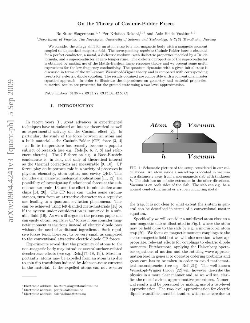
FIG. 1: Schematic picture of the setup considered in our cal-culations. An atom inside a microtrap is located in vacuumat a distance z away from a non-magnetic slab with thicknessh. The slab has an infinite extension in the other directions.Vacuum is on both sides of the slab. The slab can e.g. be anormal conducting metal or a superconducting metal.

the trap, it is not clear to what extent the system in gen-eral can be described in terms of a conventional masterequation.

Specifically we will consider a multilevel atom close to anon-magnetic slab as illustrated in Fig.1, where the atommay be held close to the slab by e.g. a microscopic atomtrap [20]. We focus on magnetic moment couplings to theelectromagnetic field but we will also mention, where ap-propriate, relevant effects for couplings to electric dipolemoments. Furthermore, applying the Heisenberg opera-tor equations of motion and the rotating-wave approxi-mation lead in general to operator ordering problems andgreat care has to be taken in order to avoid mathemat-ical inconsistencies (see e.g. Ref.[21]). The well-knownWeisskopf-Wigner theory [22] will, however, describe thephysics in a more clear manner and, as we will see, clari-fies the role of various approximative procedures. Numer-ical results will be presented by making use of a two-levelapproximation. The two-level approximation for electricdipole transitions must be handled with some care due to

2

the existence of sum rules [23]. For magnetic transitionswe will, however, not encounter such issues.

The paper is organized as follows. In the next sectionwe outline the theoretical framework. In order to ob-tain the energy shift for ground state atoms it is arguedthat one has to go beyond the conventional rotating-waveapproximation. In Section III we give explicit expres-sions for the appropriate Green’s functions in the caseof a semi-infinite slab and magnetic transitions. Ex-plicit expressions for the ground state energy shift arethen obtained for a zero temperature perfect conductor,a metallic slab with dielectric properties described by aDrude dispersion relation and extensions of it, a dielec-tric medium, and for a superconductor as described bya weakly coupled BCS superconductor. In the case ofa superconducting slab we have to reconsider the low-frequency dielectric properties in great detail includingthe presence of impurities. The short and long distancebehavior of the corresponding CP force, as induced bya magnetic moment, are considered in detail. Numericalresults are compared with the corresponding results forelectric dipole transitions. By defining a suitable rescaledand dimensionless CP force, we can easily compare someof our results with similar results for CP forces as in-duced by electric dipole transitions. In Section IV wegive some final remarks concerning electric dipole transi-tions. Technical details concerning the Green’s functionsused for magnetic transitions, their analytical continu-ation as well as various explicit expansion for a perfectconductor are presented in two appendices.

II. GENERAL THEORY

Let us consider a neutral atom at a fixed position rA.The magnetic moment of the atom interacts with thequantized magnetic field via a conventional Zeeman cou-pling. The total Hamiltonian is then

H =∑

α

Eα |α〉〈α|

+

∫

d3r

∫ ∞

0

dω hω f†(r, ω) · f (r, ω) + H ′ , (1)

where the effective interaction part is

H ′ = −∑

α

∑

β

|α〉〈β| µαβ ·B(rA) . (2)

Here f (r, ω) is an annihilation operator for the quantizedmagnetic field, |α〉 denotes the atomic state and Eα is thecorresponding energy. We assume non-degenerate states,i.e. Eα 6= Eβ for α 6= β. The magnetic moment of theatom is µαβ = 〈α|µ|β〉, where µ is the magnetic moment

operator. The magnetic field B(r) = B(+)(r) + B

(−)(r)is written B

(+)(r) = ∇ × A(+)(r), where B

(−)(r) =

(B(+)(r))† and where the vector potential is

A(+)(r) = µ0

∫ ∞

0

dω ′

∫

d3r′ ω′

√

hǫ0π

ǫ2(r′, ω′)

× G(r, r′, ω′) · f(r′, ω′) . (3)

Here the imaginary part of the complex permittivity isǫ2(r, ω). The dyadic Green’s tensor G(r, r ′, ω) is theunique solution to the Helmholtz equation. Because theHelmholtz equation is linear, the associated Green’s ten-sor can be written as a sum according to

G(r, r′, ω) = G0(r, r′, ω) + GS(r, r′, ω) , (4)

where G0(r, r′, ω) represents the contribution of the di-rect waves from the radiation sources in an unboundedmedium, which is vacuum in our case, and GS(r, r′, ω)describes the scattering contribution of multiple reflec-tion waves from the body under consideration. The pres-ence of the vacuum part G0(r, r′, ω) in Eq.(4) will in gen-eral give rise to divergences in the energy shifts to be cal-culated below. A renormalization prescription is there-fore required. We subtract the vacuum part G0(r, r′, ω),i.e. we neglect possible finite corrections due to this vac-uum subtraction like conventional vacuum-induced Lambshifts. Since we, in the end, are going to consider CPforces all additive coordinate independent corrections toenergy shifts will, anyway, not contribute. When we be-low refer to a renormalization prescription the procedureabove is what we then have in mind.

We now consider the Hamiltonian in Eq.(1) and applythe well-known Weisskopf-Wigner theory for the transi-tions α→ β, where Eα > Eβ . The solution to the time-dependent Schrodinger equation in the rotating-wave ap-proximation (RWA), i.e. applying H ′ ≈ HRWA, where

HRWA = −∑

β<α

|α〉〈β|µαβ ·B(+)(rA) + h.c. , (5)

is then (ωα ≡ Eα/h)

|ψ(t)〉 = cα(t) e− iωαt |α〉 ⊗ |0〉

+

∫

d3r

∫ ∞

0

dω

3∑

m=1

∑

β<α

× cmβ(r, ω, t) e− i(ω+ωβ)t|β〉 ⊗ |1m(r, ω)〉 . (6)

Here the initial state of the atom-field system is |α〉⊗|0〉,where |0〉 denotes the vacuum of the electromagnetic field

and |1m(r, ω)〉 = f †m(r, ω) |0〉 is a one photon state. We

also make use of the notation β < α in a β-sum to denotethe condition Eβ < Eα. The coefficient cα(t) is thendetermined by

dcα(t)

dt=

∫ t

0

∑

β<α

dt ′ KRαβ(t− t ′) cα(t ′) , (7)

where KRαβ(t) is the renormalized version of the kernel

Kαβ(t) = − 1

2 π

∫ ∞

0

dω e− i(ω−ωαβ)t Γαβ(rA, ω) . (8)

3

Here we have defined ωαβ ≡ (Eα − Eβ)/h > 0 as well as

Γαβ(r, ω) =

2µ0

hµαβ · Im[

−→∇ ×G(r, r, ω)×←−∇] · µβα , (9)

which is the spontaneous spin flip rate for the transitionα → β where Eα > Eβ . Assuming that the Markov ap-proximation holds, i.e. memory effects can be discarded,we can make the substitution cα(t′) → cα(t) in Eq.(7).By extending the remaining time integral to infinite timeand making use of the distributional identity

∫ ∞

0

dt e−i(ω−ωαβ)t = π δ(ω − ωαβ) + P i

ωαβ − ω, (10)

the solution to Eq.(7) is then of the form

cα(t) = cα(0) exp

{

− [1

2Γα(rA, ωα)

+ i δωα(rA, ωα) ] t

}

. (11)

The spontaneous spin flip rate for an atom initially inthe state |α〉 is

Γα(r, ωα) =∑

β<α

ΓRαβ(r, ωαβ) , (12)

where ΓRαβ(r, ωαβ) is the renormalized version of the

spontaneous spin flip rate in Eq.(9). In Eq.(11) we havealso defined the frequency shift δωα(r, ωα) by

δωα(r, ωα) =∑

β<α

δωRαβ(r, ωαβ) , (13)

where again δωRαβ(r, ω) is the renormalized version of

δωαβ(r, ω) =1

2 πP

∫ ∞

0

dω′

ω − ω′Γαβ(r, ω′) , (14)

where Γαβ(r, ω) is given in Eq.(9). Similar results toEqs.(9) and (14) are also derived in Ref.[24]. These lat-ter results can, of course, be obtained using conventionalperturbation theory (see e.g. Ref.[25]).

In passing we observe that Eq.(9), i.e. the spontaneousspin flip rate, has been derived using the Heisenbergequations of motion in Ref.[26]. Despite the fact thatsuch an approach leads to a well-known mathematicalinconsistencies due to operator ordering problems [21], itgives, nevertheless, the same result. Similar results forthe frequency shift for the more well-known case of anelectric dipole can e.g. be found in Refs.[27, 28].

The principal integral in Eq.(14) can be further evalu-ated by means of well-known contour integral techniquesdue to the absence of poles in the upper complex fre-quency plane (see e.g. Refs.[21, 27, 29]). For the transi-tions α→ β, where Eα > Eβ , we obtain

δωα(rA, ωα) = δω(1)α (rA, ωα) + δω(2)

α (rA, ωα) , (15)

×

×

×

×α

β

α

+

α

β

α

+

α

β

α

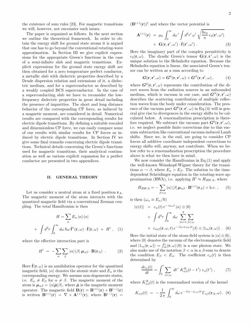
FIG. 2: Feynman diagrams. From left to right: the virtualprocess in vacuum, stimulated emission in the heath bath, andthe absorption-emission process in the heath bath, all leadingto the same final state α.

where δω(i)α (r, ωα) =

∑

β<α δω(i)αβ(r, ωαβ) (i = 1, 2). Here

we have defined the resonant contribution

δω(1)αβ (r, ω) =

− µ0

hµαβ ·Re[

−→∇ ×G(r, r, ω)×←−∇] · µβα , (16)

and the off-resonant contribution

δω(2)αβ (r, ω) =

ω

π

µ0

h

∫ ∞

0

dω′ µαβ · [−→∇ ×G(r, r, iω′)×←−∇] · µβα

ω2 + ω′2. (17)

In the RWA, the energy shift for the ground state inthe Weisskopf-Wigner approach is, however, vanishing inthe large time limit. On the other hand, applying theinteraction H ′ ≈ HAWR, where

HAWR = −∑

α>β

|α〉〈β|µαβ · B(−)(rA) + h.c. , (18)

rather than HRWA when considering the transitions β →α, where Eβ < Eα, i.e. ωβα < 0, the decay rate vanishesbut the energy shift is non-zero. It is given by

δωβ(rA, ωβ) =∑

α>β

δωRβα(rA, ωβα) , (19)

where again δωRβα(r, ω) is the renormalized version

Eq.(14). In the same fashion as above one may showthat for the state |β〉, the frequency shift is

δωβ(rA, ωβ) = δω(2)β (rA, ωβ) , (20)

where now δω(2)β (r, ωβ) =

∑

α>β δω(2)βα(r, ωβα). For states

such that ωβα < 0 there will be only off-resonant contri-butions when converting the ω-integration in Eq.(14) toimaginary frequencies.

From these discussions we now realize that, in general,it is not sufficient to make us of only the effective inter-action HRWA in the rotating-wave approximation. In-stead we must use the complete interaction Hamiltonian

4

H ′ as given by Eq.(2). This has the unfortunate conse-quence that an exact analysis is not any more possible.The Weisskopf-Wigner theory can, however, easily be ex-tended to a more general situation, at least when onelimit oneself to self-energy corrections to at most second-order in perturbation theory (see e.g. Ref.[25]). Theenergy shift for a given state of interest to us is then ob-tained by calculating the second-order energy shift usingthe complete interaction Hamiltonian Eq.(2). If we limitourselves to perturbation theory an alternative procedureis to consider the coordinate-dependent energy shift andmaking use of linear response theory in a standard man-ner (see e.g. Ref.[30]). We are then interested in findingan expression for 〈ψ(t)|H ′|ψ(t)〉 = I〈ψ(t)|H ′

I(t)|ψ(t)〉I ,where in the interaction picture and to lowest order inH ′,

|ψ(t)〉I = |ψ(t0)〉+1

ih

∫ t

t0

dt′H ′I(t

′)|ψ(t0)〉 . (21)

Here we eventually consider the limit t0 → −∞ for theinitial time t0. In terms of a retarded response functionDR(t, t′) we can therefore write

〈ψ(t)|H ′|ψ(t)〉 =1

h

∫ ∞

−∞

dt′DR(t, t′) , (22)

where

iDR(t, t′) = Θ(t− t′)〈ψ(t0)|[H ′I(t), H

′I(t

′)]|ψ(t0)〉 , (23)

and where we have assumed that 〈ψ(t0)|H ′|ψ(t0)〉 = 0.The retarded Green’s function Eq.(23) is then directlyrelated to the retarded Green’s functions for our basicquantum fields A

(+)(r), and its hermitian conjugatedfield, as given by Eq.(3), and can be calculated in a stan-dard manner with a knowledge about the initial state|ψ(t0)〉. The virtue of this formulation is that we now canallow for any quantum state of the radiation field, like athermal background, of photons by making use of a suit-able random phases for a pure state of the radiation field.One is then led to a consideration of so called real-timefinite temperature propagators which has been consid-ered elsewhere in great detail (see e.g. Refs.[31]). In thepresent paper we will, however, restrict us to an initialvacuum state of the radiation field and return to the caseof a background of thermal photons elsewhere Ref.[32].The energy shift then obtained will contain processes cor-responding to photon absorption and emission, as well asstimulated emission, with a thermal background of pho-tons. This physical picture is illustrated by means of theFeynman diagrams in Fig.2. The initial state of the atomis then assumed to be fixed which has been referred to asa constrained free energy of an atom immersed in heatbath Ref.[33].

For reasons of completeness we now write down theenergy shift for a background of thermal photons, ata temperature T , including finite temperature sponta-

neous emission and absorption processes, valid to second-order in perturbation theory using the Feynman dia-grams as indicated in Fig.2. We obtain δωα(r, ωα, T ) =∑

β δωRαβ(r, ωαβ , T ), where δωR

αβ(r, ω, T ) is the renormal-ized version of

δωαβ(r, ω, T ) =

1

2 πP

∫ ∞

0

dω′

ω − ω′(1 + n(ω′))Γαβ(r, ω′) +

1

2 πP

∫ ∞

0

dω′

ω + ω′n(ω′)Γαβ(r, ω′) , (24)

where Γαβ(r, ω) again is as given in Eq.(9) and n(ω) =1/(exp(hω/kBT )− 1) is the Planck black-body distribu-tion. As the temperature T → 0 in Eq.(24) we obviouslyhave a smooth limit (see in this context e.g. Ref. [8]).Similar results to Eqs. (9) and (14) are also derived inRef.[7, 24, 34, 35] for electric dipole transitions.

III. ATOM NEAR A NON-MAGNETIC SLAB

Let us now consider the geometry as shown in Fig. 1,i.e. a semi-infinite slab with finite thickness. The ana-lytical continuation of the equal position Green’s tensorEq.(A1) is then

−→∇ ×GS(r, r, iω)×←−∇ =

1

4π

I‖(ω) 0 00 I‖(ω) 00 0 I⊥(ω)

, (25)

where ω is real and

I‖(ω) =1

2

∫ ∞

0

dλλ

η0(λ, ω)e− 2 η0(λ,ω) z

×{

− ω2

c2CN(λ, ω) + η2

0(λ, ω) CM (λ, ω)

}

, (26)

I⊥(ω) =

∫ ∞

0

dλλ3

η0(λ, ω)e− 2 η0(λ,ω) z CM (λ, ω) . (27)

The scattering coefficients CN (λ, ω) and CM (λ, ω), whichare analytical continuations of Eqs. (A2) and (A3), aregiven by [36]

CN (λ, ω) = rp(λ, ω)1− e− 2 η(λ,ω) h

1− r2p(λ, ω) e− 2 η(λ,ω) h, (28)

CM (λ, ω) = rs(λ, ω)1− e− 2 η(λ,ω) h

1− r2s(λ, ω) e− 2 η(λ,ω) h, (29)

with the electromagnetic field polarization dependentFresnel coefficients

rs(λ, ω) =η0(λ, ω)− η(λ, ω)

η0(λ, ω) + η(λ, ω), (30)

rp(λ, ω) =ǫ(iω) η0(λ, ω)− η(λ, ω)

ǫ(iω) η0(λ, ω) + η(λ, ω), (31)

5

which are analytical continuations of Eqs. (A4) and

(A5). Here we have defined η(λ, ω) =√

k2ǫ(iω) + λ2,

η0(λ, ω) =√k2 + λ2 and k = ω/c. Below we will mostly

consider the large h limit, i.e. h is supposed to be largein comparison with any other length scale in the system.

Due to causality, the complex dielectric functionǫ(ω) = ǫ1(ω) + iǫ2(ω) will in general obey the Kramers-Kronig relations. Hence [37]

ǫ(iω) = 1 +2

π

∫ ∞

0

dxx ǫ2(x)

x2 + ω2, (32)

where ǫ(iω) is a real function. Due to physically neces-sary conditions, ǫ2(x) ≥ 0 for x ≥ 0 (see e.g. Ref.[37]).This guarantees, in general, that G

S(r, r′, iω) is real.The Casimir-Polder force obtained from any frequency

shift in δωβ(r, ωβ) is now given by

Fβ(r, ωβ) = −∇[ h δωβ(r, ωβ) ] , (33)

which actually is independent of the additive and di-vergent contribution due to the free Green’s functionG0(r, r, ω).

Let us also limit our attention to ground state transi-tions β → α, where Eβ ≤ Eα or ωβα ≤ 0, in which casewe may apply Eqs. (20) and (25). Only the off-resonantterm contribute in this case, i.e.

δωβ(z, ωβ) =µ0

4πh

∑

α

{

(|µβαx |2 + |µβα

y |2) i‖(z, ωβα)

+ |µβαz |2 i⊥(z, ωβα)

}

, (34)

where we have defined ( using ρ = ‖,⊥ )

iρ(z, ω) =ω

π

∫ ∞

0

dω′

ω2 + ω′2Iρ(ω

′) . (35)

In the numerical analysis we have found it useful tomake use of the following property of iρ(z, ω), i.e. wecan write

iρ(z, ω) =1

π

(∫ ǫ

0

dx

1 + x2Iρ(ωx)

+

∫ 1/ǫ

0

dx

1 + x2Iρ(ω/x)

)

, (36)

with a natural choice ǫ = 1. As a curiosity we remarkthat such a behavior of integrals under a modular trans-formation x→ 1/x has been noticed before and found tobe useful in e.g. quantum electrodynamics [38].

A. Perfect conductor

The integrals Eq.(35) can, in general, not be computedanalytically. For a perfect conductor CN (λ) = 1 andCM (λ) = −1 for any h. The corresponding integrals canthen be simplified. In this case, the integrals Eqs.(26)and (27) are related by

I‖(ω) =1

2I⊥(ω)− k2

2ze−2kz . (37)

For an atom in the state |β〉, where Eβ ≤ Eα, itis straight forward to show that the frequency shift is(kβα ≡ |ωβα/c| = kαβ):

δωβ(z, ωβ) =µ0

4πh

1

(2z)3

∑

α

{

(|µβαx |2 + |µβα

y |2 )i‖(kαβz)

+ |µβαz |2 i⊥(kαβz)

}

, (38)

where the dimensionless integrals are given by

i‖(x) =2x

π

∫ ∞

0

dξ

(2x)2 + ξ2e−ξ

(

ξ2 + ξ + 1

)

, (39)

i⊥(x) =4x

π

∫ ∞

0

dξ

(2x)2 + ξ2e−ξ

(

ξ + 1

)

. (40)

This result is analogous to Eq.(10.87) in Ref.[27], whichdescribes the attractive potential for an electric dipoleoutside a perfectly conducting plate. The magnetic fre-quency shift for the excited state is given in the AppendixA, see Eq.(B1). We observe that the energy shift corre-sponding to Eq.(38) is independent of h, i.e. it may bederived purely in classical manner.

For short distances (non-retarded limit), i.e. kαβz ≪1, one may easily show that i⊥(kαβz) ≈ 2 i‖(kαβz) ≈ 1,in which case Eq.(38) is reduced to

δωβ(z, ωβ) ≃ µ0

64π h

1

z3

×∑

α

{

|µβαx |2 + |µβα

y |2 + 2 |µβαz |2

}

=µ0

64π hz3〈β|µ · µ + µzµz|β〉 , (41)

due to completeness of states. Numerical studies showthat Eq.(41) actually a good approximation for kαβz <∼0.01. This result may also be obtained using a classi-cal approach, e.g. the method of images for a mag-netic moment (see e.g. Ref.[39]) . The frequency shiftin Eq.(41) corresponding to the repulsive Casimir-Polderforce Fβ(z, ωβ) as given by Eq.(33) i.e.

Fβ(z, ωβ) ≃ 3µ0

64πz4〈β|µ · µ + µzµz |β〉nz . (42)

Here nz is a unit vector in the z-direction, i.e. normaldirection to the plane of the conductor. With a = x, y, zand µαβ

a = gSehSαβa /2me, where Sαβ

a = 〈α|Sa|β〉 are

6

dimensionless, the frequency shift δωβ(z, ωβα) as givenby Eq.(41) can be re-written as

δωβ(z, ωβ) ≃ g2S

64π ǫ0hz3

( e

2λe

)2 〈β|S · S + SzSz|β〉 , (43)

where λe = h/mec is the Compton wavelength. Forelectric dipole transitions, the corresponding frequencyshift can be written in an analogous form where themagnetic dipole moment µαβ is replaced by the elec-tric dipole moment dαβ = e rαβ (see e.g. Ref.[27]),where rαβ = 〈α|r|β〉. Here r is the displacement vec-tor, whose order of magnitude is the Bohr radius a0. As(λe/a0)

2 ≈ 10−6 we realize that magnetic dipole transi-tion CP forces are in general weak as compared to thecorresponding electric dipole transitions CP forces.

In the long distance (i.e. retarded) limit, correspond-ing to kαβz ≫ 1, we realize that i⊥(kαβz) ≃ i‖(kαβz) ≃2/(π kαβz). Numerical studies show that this is a goodapproximation for kαβz >∼ 10. Eq.(38) is then reduced to

δωβ(z, ωβ) ≃ µ0

16π2 hz4

×∑

α6=β

1

kαβ

{

|µβαx |2 + |µβα

y |2 + |µβαz |2

}

, (44)

and the corresponding repulsive CP force will then havea 1/z5 dependence. Eq.(44) is an complete analogy withthe famous Casimir-Polder energy shift for electric dipoletransitions in the large distance limit [3]. The factorcontaining the sum over intermediate states in Eq.(44)is then related to the static polarizability of the atomconsidered. In our case the corresponding factor couldsimilarly be interpreted as a static magnetization of theatom.

B. Metal

In vacuum, the Drude dispersion relation may be writ-ten (see e.g. Ref. [40])

ǫ(iω) = 1 +ω2

p

ω (ω + ν ), (45)

where for gold the plasma frequency is ωp = 9.0 eV andthe relaxation frequency is ν = 35 meV.

Let us first consider the case ν = 0 and hence ǫ(iω) =1 + ω2

p/ω2. In order to present analytical as well as nu-

merical results we now consider a two-level approxima-tion (β = g and e = α) for an infinitely thick slab. Themagnitude of the ground state CP force is

Fg(z, ωA) = −dδωg(z, ωA)/dz , (46)

with ωA ≡ ωe−ωg. It is now convenient to explicitly per-form the spatial z−derivative in equations Eq.(26) and

(27). This enables us to define a rescaled and dimension-less force quantity FM (z, ωA) ≡ FM (kAz) for magneticmoment transitions as

FM (kAz) ≡ Fg(z, ωA)32πz4

µ0(µBgS)2

= (|Sx|2 + |Sy|2)i‖(kAz) + |Sz|2i⊥(kAz) , (47)

where Sa ≡ Sgea , a = x, y, x, and kA = ω/c. Here we

have defined the functions

iρ(kAz) =kAz

π

∫ ∞

0

dξ

(kAz)2 + ξ2Iρ(ξ, αkAz) , (48)

where ρ = ‖ or ⊥ and α ≡ ωp/ωA, in terms of

I⊥(ξ, γ) = 24

∫ ∞

0

dxx3e−2√

x2+ξ2

×√

γ2 + ξ2 + x2 −√

ξ2 + x2

√

γ2 + ξ2 + x2 +√

ξ2 + x2, (49)

as well as

I‖(ξ, γ) = 23

∫ ∞

0

dxxe−2√

x2+ξ2

×{

(ξ2 + x2)

√

γ2 + ξ2 + x2 −√

ξ2 + x2

√

γ2 + ξ2 + x2 +√

ξ2 + x2

+ ξ2(ξ2 + γ2)

√

ξ2 + x2 − ξ2√

γ2 + ξ2 + x2

(ξ2 + γ2)√

ξ2 + x2 + ξ2√

γ2 + ξ2 + x2

}

. (50)

Even though the Eqs.(49) and (50) appear complicatedtheir asymptotic expansions can, however, be obtained ina straightforward manner. If kAz <∼ 1 then, according toEq.(48), only small ξ contributes. If, in addition, αkAz <∼1 then

I⊥(ξ, αkAz) ≃ (αkAz)2 ,

I‖(ξ, αkAz) ≃ (αkAz)2

(

1

2+

2ξ2

(αkAz)2 + 2ξ2

)

, (51)

where we refrain from writing down the higher orderterms.

If, on the other hand, αkAz >∼ 1 we find thatIρ(ξ, αkAz), for a = ‖,⊥, does not depend on α, and

I⊥(ξ, αkAz) ≃ 2(3 + 6ξ + 4ξ2)e−2ξ , (52)

as well as

I‖(ξ, αkAz) ≃ (3 + 6ξ + 8ξ2 + 8ξ3)e−2ξ . (53)

Eqs.(47) and (48) then imply that if kAz and αkAz <∼ 1then

FM (kAz) ≃(

(|Sx|2 + |Sy|2){

1

2+

2

2 +√

2α

}

+|Sz|2)

(αkAz)2

2, (54)

7

ǫ(iω) = 1 +ω2

Aω2 α2

α = 1

kAz

101

10−1

10−3

10−5

10−7

10−9

10−4 10−3 10−2 10−1 1 10 102 103

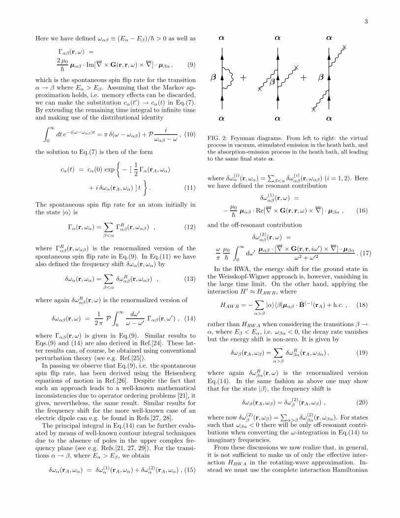
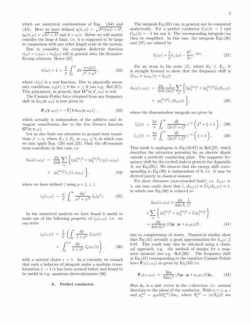
FIG. 3: The ground state dimensionless CP force FM (kAz),as defined in the main text Eq.(47), in the case of a dielectricconstant ǫ(iω) = 1+ω2

Aα2/ω2 with α ≡ ωp/ωA, as a functionof kAz = ωAz/c. For convenience we have chosen |Sx|

2 =|Sy |

2 = |Sz|2 = 1/4. The curves correspond to α = 1 (lower

solid curve), α = 10, 102, 103, 104, and α = ∞ (upper curve).

i.e. Fg(z, ωA) ∝ α2/(kAz)2. If, on the other hand,

αkAz >∼ 1 but kAz sufficiently small, then

FM (kAz) ≃3

2

(

|Sx|2 + |Sy|2 + 2|Sz|2)

, (55)

i.e. Fg(z, ωA) ∝ 1/(kAz)4. With αkAz ≫ 1 and kAz >∼

10, we obtain

FM (kAz) ≃(

|Sx|2 + |Sy|2 + |Sz |2) 8

πkAz, (56)

i.e. Fg(z, ωA) ∝ 1/(kAz)5. In Fig.3 the scaled and di-

mensionless CP force FM (kAz) is presented and the nu-merical calculations are in excellent agreement with theasymptotic expansions as given above. The choice forthe matrix elements |Sx|2 = |Sy|2 = |Sz |2 = 1/4 is notimportant and we do not in general find any essentialdifference with regards to r- and p-polarizations. We willtherefore, for convenience, make use of the same set ofmatrix elements in the numerical calculations throughoutthe present paper.

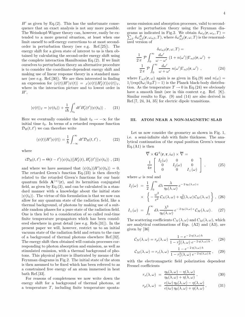
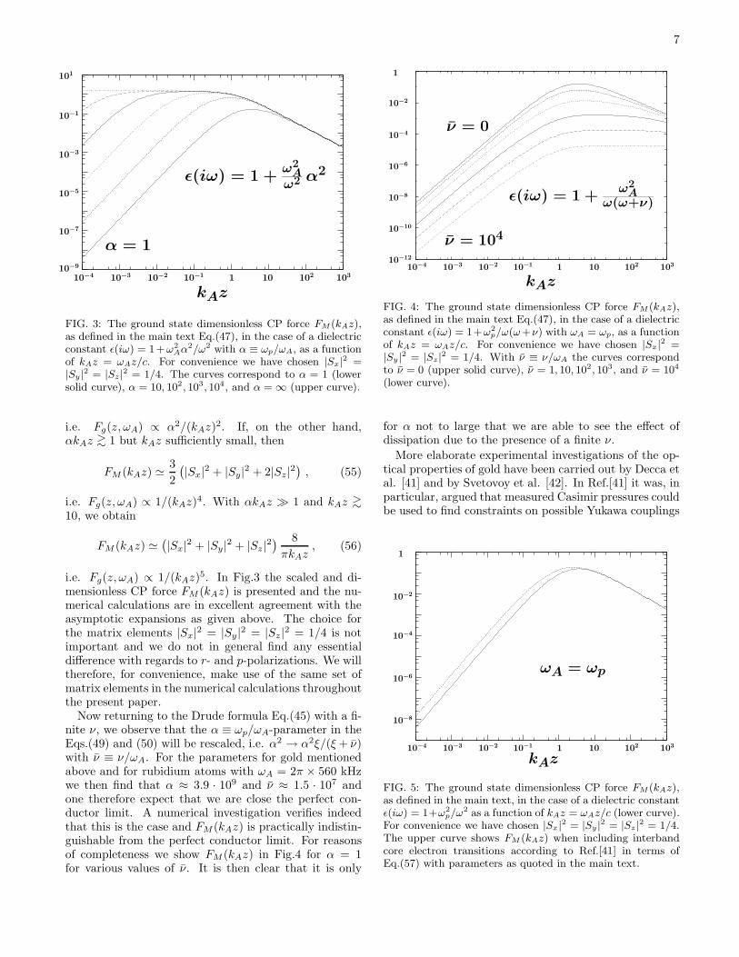
Now returning to the Drude formula Eq.(45) with a fi-nite ν, we observe that the α ≡ ωp/ωA-parameter in theEqs.(49) and (50) will be rescaled, i.e. α2 → α2ξ/(ξ+ ν)with ν ≡ ν/ωA. For the parameters for gold mentionedabove and for rubidium atoms with ωA = 2π × 560 kHzwe then find that α ≈ 3.9 · 109 and ν ≈ 1.5 · 107 andone therefore expect that we are close the perfect con-ductor limit. A numerical investigation verifies indeedthat this is the case and FM (kAz) is practically indistin-guishable from the perfect conductor limit. For reasonsof completeness we show FM (kAz) in Fig.4 for α = 1for various values of ν. It is then clear that it is only

ǫ(iω) = 1 +ω2

Aω(ω+ν)

ν = 0

ν = 104

kAz

1

10−2

10−4

10−6

10−8

10−10

10−12

10−4 10−3 10−2 10−1 1 10 102 103

FIG. 4: The ground state dimensionless CP force FM (kAz),as defined in the main text Eq.(47), in the case of a dielectricconstant ǫ(iω) = 1+ω2

p/ω(ω+ν) with ωA = ωp, as a functionof kAz = ωAz/c. For convenience we have chosen |Sx|

2 =|Sy |

2 = |Sz|2 = 1/4. With ν ≡ ν/ωA the curves correspond

to ν = 0 (upper solid curve), ν = 1, 10, 102, 103, and ν = 104

(lower curve).

for α not to large that we are able to see the effect ofdissipation due to the presence of a finite ν.

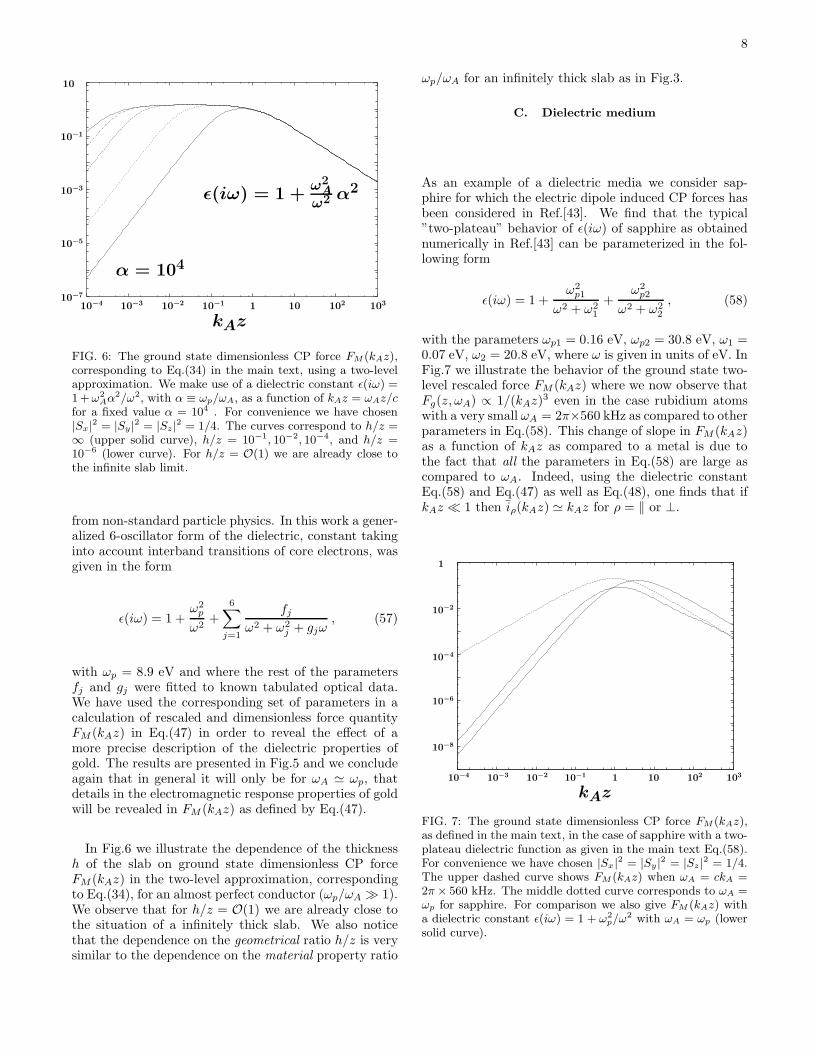
More elaborate experimental investigations of the op-tical properties of gold have been carried out by Decca etal. [41] and by Svetovoy et al. [42]. In Ref.[41] it was, inparticular, argued that measured Casimir pressures couldbe used to find constraints on possible Yukawa couplings

ωA = ωp

kAz

1

10−2

10−4

10−6

10−8

10−4 10−3 10−2 10−1 1 10 102 103

FIG. 5: The ground state dimensionless CP force FM (kAz),as defined in the main text, in the case of a dielectric constantǫ(iω) = 1+ω2

p/ω2 as a function of kAz = ωAz/c (lower curve).For convenience we have chosen |Sx|

2 = |Sy |2 = |Sz|

2 = 1/4.The upper curve shows FM (kAz) when including interbandcore electron transitions according to Ref.[41] in terms ofEq.(57) with parameters as quoted in the main text.

8

ǫ(iω) = 1 +ω2

Aω2 α2

α = 104

kAz

10

10−1

10−3

10−5

10−7

10−4 10−3 10−2 10−1 1 10 102 103

FIG. 6: The ground state dimensionless CP force FM (kAz),corresponding to Eq.(34) in the main text, using a two-levelapproximation. We make use of a dielectric constant ǫ(iω) =1+ ω2

Aα2/ω2, with α ≡ ωp/ωA, as a function of kAz = ωAz/cfor a fixed value α = 104 . For convenience we have chosen|Sx|

2 = |Sy |2 = |Sz|

2 = 1/4. The curves correspond to h/z =∞ (upper solid curve), h/z = 10−1, 10−2, 10−4, and h/z =10−6 (lower curve). For h/z = O(1) we are already close tothe infinite slab limit.

from non-standard particle physics. In this work a gener-alized 6-oscillator form of the dielectric, constant takinginto account interband transitions of core electrons, wasgiven in the form

ǫ(iω) = 1 +ω2

p

ω2+

6∑

j=1

fj

ω2 + ω2j + gjω

, (57)

with ωp = 8.9 eV and where the rest of the parametersfj and gj were fitted to known tabulated optical data.We have used the corresponding set of parameters in acalculation of rescaled and dimensionless force quantityFM (kAz) in Eq.(47) in order to reveal the effect of amore precise description of the dielectric properties ofgold. The results are presented in Fig.5 and we concludeagain that in general it will only be for ωA ≃ ωp, thatdetails in the electromagnetic response properties of goldwill be revealed in FM (kAz) as defined by Eq.(47).

In Fig.6 we illustrate the dependence of the thicknessh of the slab on ground state dimensionless CP forceFM (kAz) in the two-level approximation, correspondingto Eq.(34), for an almost perfect conductor (ωp/ωA ≫ 1).We observe that for h/z = O(1) we are already close tothe situation of a infinitely thick slab. We also noticethat the dependence on the geometrical ratio h/z is verysimilar to the dependence on the material property ratio

ωp/ωA for an infinitely thick slab as in Fig.3.

C. Dielectric medium

As an example of a dielectric media we consider sap-phire for which the electric dipole induced CP forces hasbeen considered in Ref.[43]. We find that the typical”two-plateau” behavior of ǫ(iω) of sapphire as obtainednumerically in Ref.[43] can be parameterized in the fol-lowing form

ǫ(iω) = 1 +ω2

p1

ω2 + ω21

+ω2

p2

ω2 + ω22

, (58)

with the parameters ωp1 = 0.16 eV, ωp2 = 30.8 eV, ω1 =0.07 eV, ω2 = 20.8 eV, where ω is given in units of eV. InFig.7 we illustrate the behavior of the ground state two-level rescaled force FM (kAz) where we now observe thatFg(z, ωA) ∝ 1/(kAz)

3 even in the case rubidium atomswith a very small ωA = 2π×560 kHz as compared to otherparameters in Eq.(58). This change of slope in FM (kAz)as a function of kAz as compared to a metal is due tothe fact that all the parameters in Eq.(58) are large ascompared to ωA. Indeed, using the dielectric constantEq.(58) and Eq.(47) as well as Eq.(48), one finds that ifkAz ≪ 1 then iρ(kAz) ≃ kAz for ρ = ‖ or ⊥.

kAz

1

10−2

10−4

10−6

10−8

10−4 10−3 10−2 10−1 1 10 102 103

FIG. 7: The ground state dimensionless CP force FM (kAz),as defined in the main text, in the case of sapphire with a two-plateau dielectric function as given in the main text Eq.(58).For convenience we have chosen |Sx|

2 = |Sy |2 = |Sz|

2 = 1/4.The upper dashed curve shows FM (kAz) when ωA = ckA =2π × 560 kHz. The middle dotted curve corresponds to ωA =ωp for sapphire. For comparison we also give FM (kAz) witha dielectric constant ǫ(iω) = 1 + ω2

p/ω2 with ωA = ωp (lowersolid curve).

9

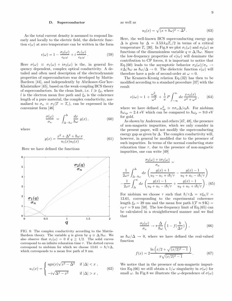
D. Superconductor

As the total current density is assumed to respond lin-early and locally to the electric field, the dielectric func-tion ǫ(ω) at zero temperature can be written in the form

ǫ(ω) = 1− σ2(ω)

ǫ0 ω+ i

σ1(ω)

ǫ0 ω. (59)

Here σ(ω) ≡ σ1(ω) + iσ2(ω) is the, in general fre-quency dependent, complex optical conductivity. A de-tailed and often used description of the electrodynamicproperties of superconductors was developed by Mattis-Bardeen [44], and independently by Abrikosov-Gor’kov-Khalatnikov [45], based on the weak-coupling BCS theoryof superconductors. In the clean limit, i.e. l ≫ ξ0, wherel is the electron mean free path and ξ0 is the coherencelength of a pure material, the complex conductivity, nor-malized to σn ≡ σ1(T = Tc), can be expressed in theconvenient form [46]

σ(ω)

σn=

∫ ∆

∆−hω

dx

hωg(x) , (60)

where

g(x) =x2 + ∆2 + hω x

u1(x)u2(x). (61)

Here we have defined the functions

σ1(q)σn

σ2(q)σn

q

6

5

4

3

2

1

00 0.5 1 1.5 2

FIG. 8: The complex conductivity according to the Mattis-Bardeen theory. The variable q is given by q ≡ ∆/hω. Wealso observe that σ1(ω) = 0 if q ≥ 1/2. The solid curvescorrespond to an infinite relaxation time τ . The dotted curvescorrespond to niobium for which we choose 13.61 = h/τ∆,which corresponds to a mean free path of 9 nm.

u1(x) =

sgn(x)√x2 −∆2 if |∆| < x ,

−i√

∆2 − x2 if |∆| > x ,(62)

as well as

u2(x) =√

(x + hω)2 −∆2 . (63)

Here, the well-known BCS superconducting energy gap∆ is given by ∆ = 3.53 kBTc/2 in terms of a criticaltemperature Tc [30]. In Fig.8 we plot σ1(ω) and σ2(ω) asfunctions of the dimensionless variable q ≡ ∆/hω. Sincethe low-frequency properties of ǫ(iω) will dominate thecontribution to CP forces, it is important to notice thatEq.(60) leads to the asymptotic behavior σ2(ω)/σn →π∆/hω as hω/∆ → 0. The dielectric function ǫ(ω) willtherefore have a pole of second-order at ω = 0.

The Kramers-Kronig relation Eq.(32) has then to bemodified according to a standard procedure [37] with theresult

ǫ(iω) = 1 +ω2

sp

ω2+

1

πP

∫ ∞

−∞

dxx ǫ2(x)

x2 + ω2, (64)

where we have defined ω2sp ≡ πσn∆/ǫ0h. For niobium

hωsp = 2.4 eV which can be compared to hωp = 9.0 eVfor gold.

As shown by Anderson and others [47, 48], the presenceof non-magnetic impurities, which we only consider inthe present paper, will not modify the superconductingenergy gap as given by ∆. The complex conductivity will,however, in general be modified due to the presence ofsuch impurities. In terms of the normal conducting staterelaxation time τ , due to the presence of non-magneticimpurities, one can write [49]

σ2(ω) + iσ1(ω)

σn=

1

2ωτ

∫ ∆

∆−hω

dx

(

g(x) + 1

u2 − u1 + ih/τ− g(x)− 1

u2 + u1 − ih/τ

)

− 1

2ωτ

∫ ∞

∆

dx

(

g(x)− 1

u2 + u1 − ih/τ+

g(x)− 1

u2 + u1 + ih/τ

)

. (65)

For niobium we choose τ such that h/τ∆ = πξ0/l =13.61, corresponding to the experimental coherencelength ξ0 = 39 nm and the mean free path l(T ≈ 9 K) =vF τ = 9 nm [50]. The low-frequency limit of Eq.(65) canbe calculated in a straightforward manner and we findthat

σ2(ω)

σn→ π

∆

hω

(

1− f(h

∆τ)

)

, (66)

as hω/∆ → 0, where we have defined the real-valuedfunction

f(x) = 2ln

(

x/2 +√

(x/2)2 − 1)

π√

(x/2)2 − 1. (67)

We notice that in the presence of non-magnetic impuri-ties Eq.(66) we still obtain a 1/ω singularity in σ(ω) forsmall ω. In Fig.8 we illustrate the ω-dependence of σ(ω)

10

in the clean limit (τ → ∞) as well as for niobium. Nu-merical investigations show that the asymptotic formulaEq.(66) actually describes σ2(ω) for a wide range of fre-quencies. We also notice that for any finite τ/h∆ 6= 0 wehave the asymptotic behavior σ(ω) → 0 as hω/∆→ ∞.The discussion in this Section reveals that for supercon-ductors, we are led back to the considerations for a metalas discussed in Section III B, apart from the continuumcontribution in Eq.(64). A closer of investigation showsthat its only for frequencies ωA

>∼ ∆/h that the CP forcewill be sensitive to this continuum contribution. For suchfrequencies, however, the Cooper pairs of the supercon-ductor start to break up and we are again led back to ametal.

ωA = ωp

kAz

1

10−1

10−3

10−5

10−7

10−9

10−4 10−3 10−2 10−1 1 10 102 103

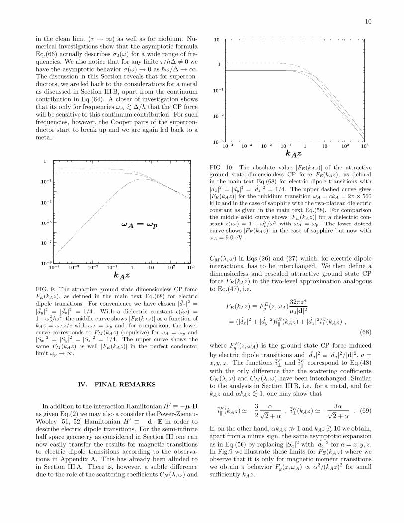
FIG. 9: The attractive ground state dimensionless CP forceFE(kAz), as defined in the main text Eq.(68) for electric

dipole transitions. For convenience we have chosen |dx|2 =

|dy |2 = |dz|

2 = 1/4. With a dielectric constant ǫ(iω) =1+ω2

p/ω2, the middle curve shows |FE(kAz)| as a function ofkAz = ωAz/c with ωA = ωp and, for comparison, the lowercurve corresponds to FM (kAz) (repulsive) for ωA = ωp and|Sx|

2 = |Sy|2 = |Sz|

2 = 1/4. The upper curve shows thesame FM (kAz) as well |FE(kAz)| in the perfect conductorlimit ωp → ∞.

IV. FINAL REMARKS

In addition to the interaction HamiltonianH ′ ≡ −µ·Bas given Eq.(2) we may also a consider the Power-Zienau-Wooley [51, 52] Hamiltonian H ′ ≡ −d · E in order todescribe electric dipole transitions. For the semi-infinitehalf space geometry as considered in Section III one cannow easily transfer the results for magnetic transitionsto electric dipole transitions according to the observa-tions in Appendix A. This has already been alluded toin Section III A. There is, however, a subtle differencedue to the role of the scattering coefficients CN (λ, ω) and

kAz

10

1

10−1

10−2

10−3

10−4 10−3 10−2 10−1 1 10 102 103

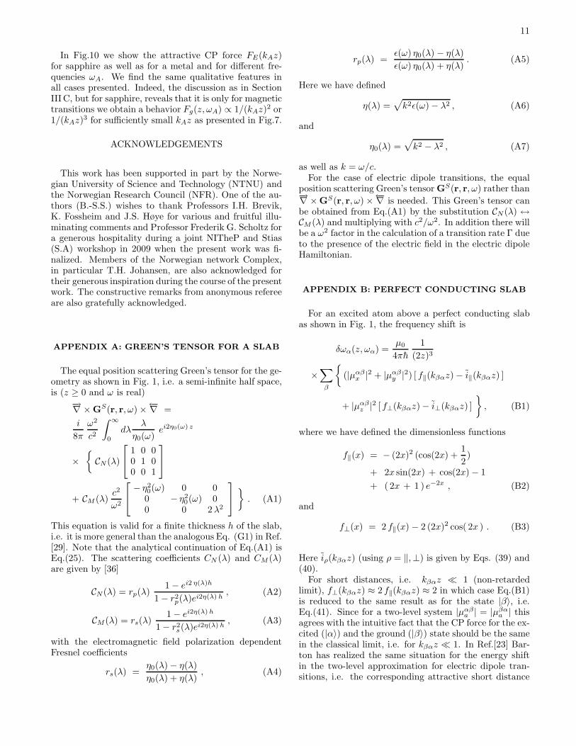
FIG. 10: The absolute value |FE(kAz)| of the attractiveground state dimensionless CP force FE(kAz), as definedin the main text Eq.(68) for electric dipole transitions with

|dx|2 = |dy|

2 = |dz|2 = 1/4. The upper dashed curve gives

|FE(kAz)| for the rubidium transition ωA = ckA = 2π × 560kHz and in the case of sapphire with the two-plateau dielectricconstant as given in the main text Eq.(58). For comparisonthe middle solid curve shows |FE(kAz)| for a dielectric con-stant ǫ(iω) = 1 + ω2

p/ω2 with ωA = ωp. The lower dottedcurve shows |FE(kAz)| in the case of sapphire but now withωA = 9.0 eV.

CM (λ, ω) in Eqs.(26) and (27) which, for electric dipoleinteractions, has to be interchanged. We then define adimensionless and rescaled attractive ground state CPforce FE(kAz) in the two-level approximation analogousto Eq.(47), i.e.

FE(kAz) ≡ FEg (z, ωA)

32πz4

µ0|d|2

= (|dx|2 + |dy|2 )iE‖ (kAz) + |dz |2iE⊥(kAz) ,

(68)

where FEg (z, ωA) is the ground state CP force induced

by electric dipole transitions and |da|2 ≡ |da|2/|d|2, a =x, y, z. The functions iE⊥ and iE‖ correspond to Eq.(48)

with the only difference that the scattering coefficientsCN (λ, ω) and CM (λ, ω) have been interchanged. Similarto the analysis in Section III B, i.e. for a metal, and forkAz and αkAz <∼ 1, one may show that

iE‖ (kAz) ≃ −3

2

α√2 + α

, iE⊥(kAz) ≃ −3α√2 + α

. (69)

If, on the other hand, αkAz ≫ 1 and kAz >∼ 10 we obtain,apart from a minus sign, the same asymptotic expansion

as in Eq.(56) by replacing |Sa|2 with |da|2 for a = x, y, z.In Fig.9 we illustrate these limits for FE(kAz) where weobserve that it is only for magnetic moment transitionswe obtain a behavior Fg(z, ωA) ∝ α2/(kAz)

2 for smallsufficiently kAz.

11

In Fig.10 we show the attractive CP force FE(kAz)for sapphire as well as for a metal and for different fre-quencies ωA. We find the same qualitative features inall cases presented. Indeed, the discussion as in SectionIII C, but for sapphire, reveals that it is only for magnetictransitions we obtain a behavior Fg(z, ωA) ∝ 1/(kAz)

2 or1/(kAz)

3 for sufficiently small kAz as presented in Fig.7.

ACKNOWLEDGEMENTS

This work has been supported in part by the Norwe-gian University of Science and Technology (NTNU) andthe Norwegian Research Council (NFR). One of the au-thors (B.-S.S.) wishes to thank Professors I.H. Brevik,K. Fossheim and J.S. Høye for various and fruitful illu-minating comments and Professor Frederik G. Scholtz fora generous hospitality during a joint NITheP and Stias(S.A) workshop in 2009 when the present work was fi-nalized. Members of the Norwegian network Complex,in particular T.H. Johansen, are also acknowledged fortheir generous inspiration during the course of the presentwork. The constructive remarks from anonymous refereeare also gratefully acknowledged.

APPENDIX A: GREEN’S TENSOR FOR A SLAB

The equal position scattering Green’s tensor for the ge-ometry as shown in Fig. 1, i.e. a semi-infinite half space,is (z ≥ 0 and ω is real)

−→∇ ×GS(r, r, ω)×←−∇ =

i

8π

ω2

c2

∫ ∞

0

dλλ

η0(ω)ei2η0(ω) z

×{

CN (λ)

1 0 00 1 00 0 1

+ CM (λ)c2

ω2

− η20(ω) 0 00 − η2

0(ω) 00 0 2λ2

}

. (A1)

This equation is valid for a finite thickness h of the slab,i.e. it is more general than the analogous Eq. (G1) in Ref.[29]. Note that the analytical continuation of Eq.(A1) isEq.(25). The scattering coefficients CN (λ) and CM (λ)are given by [36]

CN(λ) = rp(λ)1− ei2 η(λ)h

1− r2p(λ)ei2η(λ) h, (A2)

CM (λ) = rs(λ)1− ei2η(λ) h

1− r2s(λ)ei2η(λ) h, (A3)

with the electromagnetic field polarization dependentFresnel coefficients

rs(λ) =η0(λ)− η(λ)η0(λ) + η(λ)

, (A4)

rp(λ) =ǫ(ω) η0(λ) − η(λ)ǫ(ω) η0(λ) + η(λ)

. (A5)

Here we have defined

η(λ) =√

k2ǫ(ω)− λ2 , (A6)

and

η0(λ) =√

k2 − λ2 , (A7)

as well as k = ω/c.For the case of electric dipole transitions, the equal

position scattering Green’s tensor GS(r, r, ω) rather than−→∇ ×G

S(r, r, ω)×←−∇ is needed. This Green’s tensor canbe obtained from Eq.(A1) by the substitution CN (λ) ↔CM (λ) and multiplying with c2/ω2. In addition there willbe a ω2 factor in the calculation of a transition rate Γ dueto the presence of the electric field in the electric dipoleHamiltonian.

APPENDIX B: PERFECT CONDUCTING SLAB

For an excited atom above a perfect conducting slabas shown in Fig. 1, the frequency shift is

δωα(z, ωα) =µ0

4πh

1

(2z)3

×∑

β

{

(|µαβx |2 + |µαβ

y |2) [ f‖(kβαz)− i‖(kβαz) ]

+ |µαβz |2 [ f⊥(kβαz)− i⊥(kβαz) ]

}

, (B1)

where we have defined the dimensionless functions

f‖(x) = − (2x)2 (cos(2x) +1

2)

+ 2x sin(2x) + cos(2x)− 1

+ ( 2x + 1 ) e−2x , (B2)

and

f⊥(x) = 2 f‖(x) − 2 (2x)2 cos( 2x ) . (B3)

Here iρ(kβαz) (using ρ = ‖,⊥) is given by Eqs. (39) and(40).

For short distances, i.e. kβαz ≪ 1 (non-retardedlimit), f⊥(kβαz) ≈ 2 f‖(kβαz) ≈ 2 in which case Eq.(B1)is reduced to the same result as for the state |β〉, i.e.Eq.(41). Since for a two-level system |µαβ

a | = |µβαa | this

agrees with the intuitive fact that the CP force for the ex-cited (|α〉) and the ground (|β〉) state should be the samein the classical limit, i.e. for kβαz ≪ 1. In Ref.[23] Bar-ton has realized the same situation for the energy shiftin the two-level approximation for electric dipole tran-sitions, i.e. the corresponding attractive short distance

12

CP force is the same in the ground state and the excitedstate.

In the long distance retarded limit, i.e. kβαz ≫ 1, werealize that

f‖(kβαz) ≃ − (2 kβαz)2

(

cos(2 kβαz) +1

2

)

, (B4)

and

f⊥(kβαz) ≃ − (2kβαz)2

(

4 cos(2 kβαz) + 1

)

, (B5)

in which case Eq.(B1) is reduced to

δωα(z, ωβ) ≃ − µ0

32π h

k2βα

z

×∑

β

{

(|µαβx |2 + |µαβ

y |2) ( cos(2kβαz) +1

2)

+ |µαβz |2 ( 4 cos(2kβαz) + 1 )

}

. (B6)

[1] V.M. Mostepanenko, N.N. Trunov, The Casimir Effect

and its Applications, Clarendon Press, Oxford, 1997;V.A. Parsegian, Van der Waals Forces, Cambridge Uni-versity Press, Cambridge, 2005.

[2] H.B.G. Casimir, Proc. K. Ned. Akad. Wet. 51, 793(1948).

[3] H.B.G. Casimir, and D. Polder, Phys. Rev. 73, 360(1948).

[4] I.E. Dzyaloshinskii, E.M. Lifshitz, and L.P. Pitavskii,Adv. Phys. 10, 165 (1961).

[5] S.K. Lamoreaux, Physics Today, Feb. 2007, p. 40.[6] G.L. Klimchitskaya. U. Mohideen, and V.M. Mostepa-

nenko, arXiv:quant-ph/0902.4022 (2009) and Rev. Mod.Phys. (in press).

[7] S.Y. Buhmann, and S. Scheel, Phys. Rev. Lett. 100,253201 (2008).

[8] S.K. Lamoreaux, arXiv:quant-ph/0801.1283 (2008).[9] J.M. Obrecht, R.J. Wild, M. Antezza, L.P. Pitaevskii, S.

Stringari, and E.A. Cornell, Phys. Rev. Lett. 98, 063201(2007).

[10] C. Roux, A. Emmert, A. Lupascu, T. Nirrengarten, G.Nouges, M. Brune, J.-M. Raimond, and S. Haroche, EPL81, 56004 (2008).

[11] H.B. Chan, V.A. Aksyuk, R.N. Kleiman, D.J. Bishop,and F. Capasso, Phys. Rev. Lett. 87, 211801 (2001).

[12] V. Klimov, and A. Lambrecht, Plasmonics 4, 31 (2009).[13] S. Dimopoulos and A.A. Geraci, Phys. Rev. D 68, 124021

(2003).[14] D. Cano, B. Kasch, H. Hattermann, D. Koelle, R.

Kleiner, C. Zimmermann, and J. Fortagh, Phys. Rev.A 77, 063408 (2008).

[15] U. Leonhardt, and T.G. Philbin, New Journal of Physics9, 254 (2007).

[16] J.N. Munday, Federico Capasso, and V. AdrianParsegian, Nature 457, 170 (2009).

[17] M.P.A. Jones, C.J. Vale, D. Sahagun, B.V. Hall, and E.A.Hinds, Phys. Rev. Lett. 91, 080401 (2003).

[18] D.M. Harber, J.M. McGuirk, J.M. Obrecht, and E.A.Cornell, J. Low. Temp. Phys. 133, 229 (2003).

[19] Y.J. Lin, I. Teper, C. Chin, and V. Vuletic, Phys. Rev.Lett. 92, 050404 (2004).

[20] J. Fortagh, and C. Zimmermann, Rev. Mod. Phys. 79,235 (2007).

[21] S.M. Barnett and P.M. Radmore, “Methods in Theoret-

ical Quantum Optics”, Oxford University Press, Oxford(1997).

[22] V. Weisskopf, and E.P. Wigner, Zeitschrift fur Physik 63,54 (1930).

[23] G. Barton, J. Phys.B: Atom. Molec. Phys. 7, 2134 (1974).[24] R. Fermani, S. Scheel, and P.L. Knight, Phys. Rev. A 73,

032902 (2006).[25] E. Merzbacher, Quantum Mechanics; 2nd Edition, Wi-

ley, New York, 1970. For an extension using intermediateresonances, which is appropriate in our case in calculat-ing the rate for a transition, see J.W. Norbury, and P.A.Deutchman, Am. J. Phys. 52, 17 (1984).

[26] P.K. Rekdal, S. Scheel, P.L. Knight, and E.A. Hinds,Phys. Rev. A 70, 013811 (2004).

[27] W. Vogel, D.-G. Welsch, “Quantum Optics; 3:rd Edi-

tion”, Wiley-VCH, New York, 2006.[28] S. Scheel, L. Knoll, and D.-G. Welsch, Phys. Rev. A 60,

4094 (1999).[29] S.Y. Buhmann, L. Knoll, D.-G. Welsch, and H.T. Dung,

Phys. Rev. A 70, 052117 (2004).[30] A.L. Fetter, and J.D. Walecka “Quantum Theory of

Many-Particle Systems”, McGraw-Hill, New York, 1971.[31] L. Dolan, and R. Jackiw, Phys. Rev. D 9, 3320 (1974);

J.F. Donoghue, and B.R. Holstein, Phys. Rev. D 28, 340(1983) and (E) Phys. Rev. D 29, 3004 (1983); K. Taka-hashi, Phys. Rev. D 29, 632 (1984); A. E. I. Johans-son, G. Peressutti, and B.-S. Skagerstam, Nucl. Phys.B 278, 324 (1986); B.-S. Skagerstam, “Thermal Effects

in Particle and String Theories” in Workshop on Su-

perstrings and Particle Theory, Eds. L. Clavelli and B.Harms, World Scientific, Singapore, 1990.

[32] P.K. Rekdal, B.-S. Skagerstam, and A.H. Vaskinn, inpreparation.

[33] G. Barton, J. Phys. B: At. Mol. Phys. 20, 879 (1987).[34] C. Henkel, S.Potting, and W. Wilkens, Appl. Phys. B

69 379 (1999); C. Henkel, K. Joulain, J.-P. Mulet, andJ.-J. Greffet, J. Opt. A Appl. Opt. 4 S-109 (2002); C.Henkel, Eur. Phys. J. D. 35, 59 (2005); V. Dikovsky, Y.Japha, C. Henkel, and R. Folman, Eur. Phys. J D. 35,87 (2005); Bo Zhang, and C. Henkel, J. Appl. Phys. 102

084907 (2007).[35] M.-P. Gorza and M. Ducloy, Eur. Phys. J. D 40, 343

(2006).[36] L.W. Li, P.S. Kooi, M.S. Leong, and T.S. Yeo, J. of Elec-

tromag. Waves and Appl. 8, 663 (1994).[37] L.D. Landau, E.M. Lifshitz, and P.L. Pitaevskii, “Elec-

trodynamics of Continuous Media: Volume 8 of Course of

Theoretical Physics”, Pergamon Press, New York, 1984.[38] P. Elmfors, P. Liljenberg, D. Persson, and B.-S. Skager-

stam, Phys. Rev. D 51, 5885 (1995).[39] J.D. Jackson, “Classical Electrodynamics”, John Wiley&

Sons, New York, 1975.

13

[40] I. Brevik, J.B. Aarseth, J.S. Høye, and K.A. Milton,Phys. Rev. E 71, 056101 (2005).

[41] R.S. Decca, D.Lopez, E. Fischbach, G.L. Klimchitskaya,D. E. Krause, and V.M. Mosteepanenko, Eur. Phys. J. C51, 963 (2007).

[42] V.B. Svetovoy, P.J. van Zwol, G. Palasantzas, andJ.Th.M. De Hosson, Phys. Rev. B 77, 035439 (2008).

[43] M. Antezza, L.P. Pitaevskii, and S. Stringari, Phys. Rev.A 70, 053619 (2004).

[44] D.C. Mattis, and J. Bardeen, Phys. Rev. 111, 412 (1958).[45] A.A. Abrikosov, L.P. Gor’kov, and I.M. Khalatnikov, Zh.

Eksp. Teor. Fiz. 35, 365 (1958) [Sov. Phys. JETP 8, 182(1959)].

[46] O. Klein, E.J. Nicol, K. Holczer, and G. Gruner, Phys.Rev. B 50, 6307 (1994).

[47] P.W. Anderson, J. Phys. Chem. Solids 11, 26 (1959).[48] A.A. Abrikosov and L.P. Gor’kov, Zh. Eksp. Teor. Fiz

35, 1558 (1958); 36, 319 (1959) [Sov. Phys. JETP 8,1090 (1959); 9, 220 (1959)], and in Phys. Rev. 49, 12337(1994).

[49] G. Rickayzen, Theory of Superconductivity (Interscience,New York, 1965); J.-J. Chang, and D.J. Scalapino, Phys.Rev. B 40, 4299 (1989).

[50] A.V. Pronin, M. Dressel, A. Pimenov, A. Loidl, I.V.Roshchin, and L.H. Greene, Phys. Rev. B 57, 14416(1998).

[51] E.A. Power, and S. Zienau, Phil. Trans. R. Soc. Lond. A251, 427 (1959).

[52] R.G. Woolley, Proc. R. Soc. Lond. A 321, 557 (1971).