Theory of Bouguet's MatLab Camera Calibration …hvrl.ics.keio.ac.jp/charmie/doc/CameraCalibration/Bougu...Theory of Bouguet’s MatLab Camera Calibration Toolbox Yuji Oyamada 1HVRL,

Theory of Bouguet’s MatLab Camera CalibrationToolbox

Yuji Oyamada

1HVRL, University

2Chair for Computer Aided Medical Procedure (CAMP)Technische Universitat Munchen

June 26, 2012

Introduction Functions Theory

MatLab Camera Calibration Toolbox

• Calibration using a planar calibration object.

• Points correspondence requires manual click on object’scorners.

• Core calibration part is fully automatic.

• C implementation is included in OpenCV.

• Web

Introduction Functions Theory

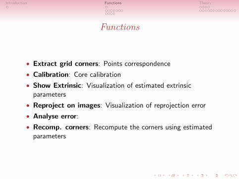
Functions

• Extract grid corners: Points correspondence

• Calibration: Core calibration

• Show Extrinsic: Visualization of estimated extrinsicparameters

• Reproject on images: Visualization of reprojection error

• Analyse error:

• Recomp. corners: Recompute the corners using estimatedparameters

Introduction Functions Theory

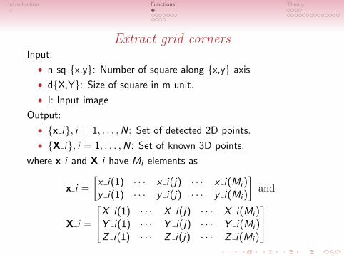
Extract grid cornersInput:

• n sq {x,y}: Number of square along {x,y} axis

• d{X,Y}: Size of square in m unit.

• I: Input image

Output:

• {x i}, i = 1, . . . ,N: Set of detected 2D points.

• {X i}, i = 1, . . . ,N: Set of known 3D points.

where x i and X i have Mi elements as

x i =

[x i(1) · · · x i(j) · · · x i(Mi )y i(1) · · · y i(j) · · · y i(Mi )

]and

X i =

X i(1) · · · X i(j) · · · X i(Mi )Y i(1) · · · Y i(j) · · · Y i(Mi )Z i(1) · · · Z i(j) · · · Z i(Mi )

Introduction Functions Theory

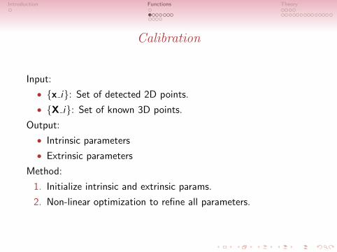
Calibration

Input:

• {x i}: Set of detected 2D points.

• {X i}: Set of known 3D points.

Output:

• Intrinsic parameters

• Extrinsic parameters

Method:

1. Initialize intrinsic and extrinsic params.

2. Non-linear optimization to refine all parameters.

Introduction Functions Theory

Camera parameters

Intrinsic parameters:

• fc ∈ R2: Camera focal length

• cc ∈ R2: Principal point coordinates

• alpha c ∈ R1: Skew coefficient

• kc ∈ R5: Distortion coefficients

• KK ∈ R3×3: The camera matrix (containing fc, cc, alpha c)

Extrinsic parameters for i-th image:

• omc i ∈ R3: Rotation angles

• Tc i ∈ R3: Translation vectors

• Rc i ∈ R3×3: Rotation matrix computed asRc i = rodrigues(omc i)

Introduction Functions Theory

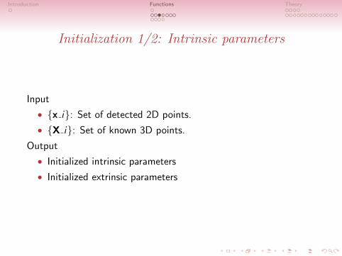
Initialization 1/2: Intrinsic parameters

Input

• {x i}: Set of detected 2D points.

• {X i}: Set of known 3D points.

Output

• Initialized intrinsic parameters

• Initialized extrinsic parameters

Introduction Functions Theory

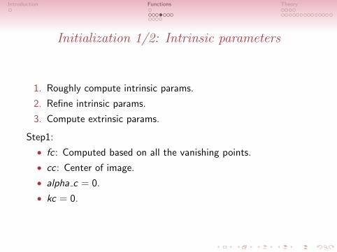
Initialization 1/2: Intrinsic parameters

1. Roughly compute intrinsic params.

2. Refine intrinsic params.

3. Compute extrinsic params.

Step1:

• fc : Computed based on all the vanishing points.

• cc : Center of image.

• alpha c = 0.

• kc = 0.

Introduction Functions Theory

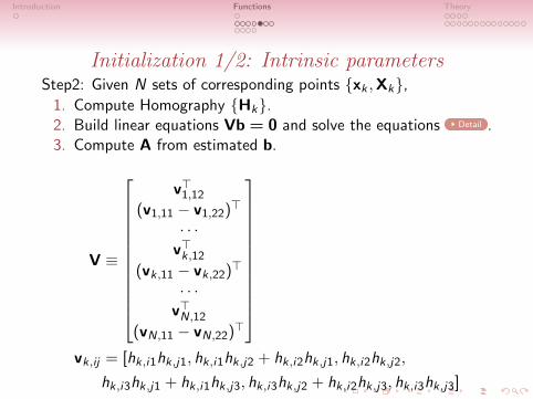
Initialization 1/2: Intrinsic parametersStep2: Given N sets of corresponding points {xk ,Xk},

1. Compute Homography {Hk}.2. Build linear equations Vb = 0 and solve the equations Detail .3. Compute A from estimated b.

V ≡

v>1,12

(v1,11 − v1,22)>

· · ·v>k,12

(vk,11 − vk,22)>

· · ·v>N,12

(vN,11 − vN,22)>

vk,ij = [hk,i1hk,j1, hk,i1hk,j2 + hk,i2hk,j1, hk,i2hk,j2,

hk,i3hk,j1 + hk,i1hk,j3, hk,i3hk,j2 + hk,i2hk,j3, hk,i3hk,j3]

Introduction Functions Theory

Initialization 2/2: Extrinsic parameters

Step3: Compute each extrinsic parameters from estimated A andpre-computed Hk as

rk,1 = λkA−1hk,1

rk,2 = λkA−1hk,2

rk,3 = rk,1 × rk,2

tk = λkA−1hk,3

where

λk =1

||A−1hk,1||=

1

||A−1hk,2||

Introduction Functions Theory

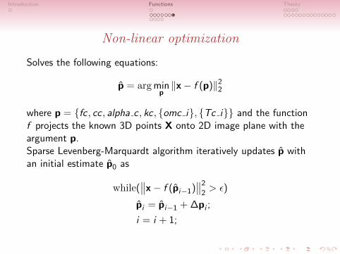
Non-linear optimization

Solves the following equations:

p = argminp‖x− f (p)‖2

2

where p = {fc, cc , alpha c , kc , {omc i}, {Tc i}} and the functionf projects the known 3D points X onto 2D image plane with theargument p.Sparse Levenberg-Marquardt algorithm iteratively updates p withan initial estimate p0 as

while(∥∥x− f (pi−1)

∥∥2

2> ε)

pi = pi−1 + ∆pi ;

i = i + 1;

Introduction Functions Theory

Image projectionGiven

• xp = (xp, yp, 1)>: Pixel coordinate of a point on the imageplane.

• xd = (xd , yd , 1)>: Normalized coordinate distorted by lens.

• xn = (xn, yn, 1)>: Normalized pinhole image projection.

• k ∈ R5: Lens distortion parameters.

• KK ∈ R3×3: Camera calibration matrix.

where

KK =

fc(1) alpha c(1) cc(1)0 fc(2) cc(2)0 0 1

xp = KKxd = KK(cdistxn + delta x)

Introduction Functions Theory

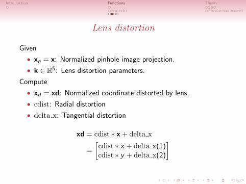
Lens distortion

Given

• xn = x: Normalized pinhole image projection.

• k ∈ R5: Lens distortion parameters.

Compute

• xd = xd: Normalized coordinate distorted by lens.

• cdist: Radial distortion

• delta x: Tangential distortion

xd = cdist ∗ x + delta x

=

[cdist ∗ x + delta x(1)cdist ∗ y + delta x(2)

]

Introduction Functions Theory

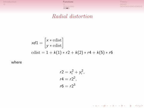
Radial distortion

xd1 =

[x ∗ cdisty ∗ cdist

]cdist = 1 + k(1) ∗ r2 + k(2) ∗ r4 + k(5) ∗ r6

where

r2 = x2i + y2

i ,

r4 = r22,

r6 = r23

Introduction Functions Theory

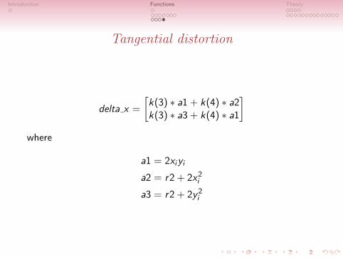
Tangential distortion

delta x =

[k(3) ∗ a1 + k(4) ∗ a2k(3) ∗ a3 + k(4) ∗ a1

]where

a1 = 2xiyi

a2 = r2 + 2x2i

a3 = r2 + 2y2i

Introduction Functions Theory

Closed form solution for initialization

s

uv1

= A[r1 r2 r3 t

] XY01

= A[r1 r2 t

] XY1

= H

XY1

Since r1 and r2 are orthonormal, we have following two constraints:

h>1 A−>A−1h2 = 0

h>1 A−>A−1h1 = h>2 A

−>A−1h2,

where A−>A−1 describes the image of the absolute conic.

Introduction Functions Theory

Closed form solution for initialization

Let

B = A−>A−1 ≡

B11 B21 B31

B12 B22 B32

B13 B23 B33

=

1α2 − γ

α2βv0γ−u0βα2β

− γα2β

γ2

α2β2 + 1β2 −γ(v0γ−u0β)

α2β2 − v0β2

v0γ−u0βα2β

−γ(v0γ−u0β)α2β2 − v0

β2(v0γ−u0β)2

α2β2 +v2

0β2 + 1

Note that B is symmetric, defined by a 6D vector

b ≡[B11,B12,B22,B13,B23,B3

]>

Introduction Functions Theory

Closed form solution for initialization

Let the i-th column vector of H be hi =[hi1, hi2, hi3

]>.

Then, we have following linear equation

h>i Bhj = v>ij b

where

vij = [hi1hj1, hi1hj2 + hi2hj1, hi2hj2

hi3hj1 + hi1hj3, hi3hj2 + hi2hj3, hi3hj3]

Introduction Functions Theory

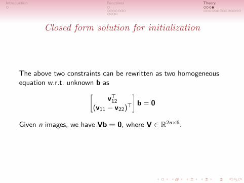
Closed form solution for initialization

The above two constraints can be rewritten as two homogeneousequation w.r.t. unknown b as[

v>12

(v11 − v22)>

]b = 0

Given n images, we have Vb = 0, where V ∈ R2n×6.

Introduction Functions Theory

Least Squares

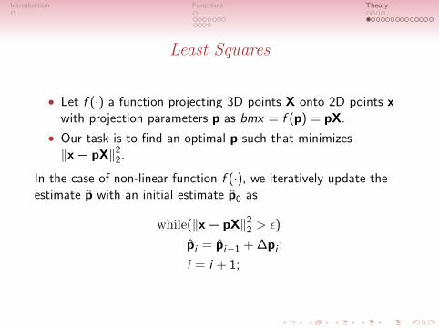
• Let f (·) a function projecting 3D points X onto 2D points xwith projection parameters p as bmx = f (p) = pX.

• Our task is to find an optimal p such that minimizes‖x− pX‖2

2.

In the case of non-linear function f (·), we iteratively update theestimate p with an initial estimate p0 as

while(‖x− pX‖22 > ε)

pi = pi−1 + ∆pi ;

i = i + 1;

Introduction Functions Theory

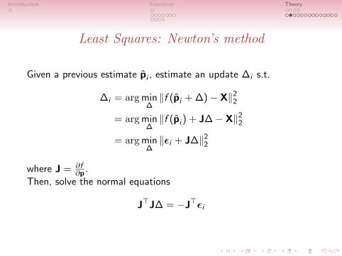
Least Squares: Newton’s method

Given a previous estimate pi , estimate an update ∆i s.t.

∆i = argmin∆‖f (pi + ∆)− X‖2

2

= argmin∆‖f (pi ) + J∆− X‖2

2

= argmin∆‖εi + J∆‖2

2

where J = ∂f∂p .

Then, solve the normal equations

J>J∆ = −J>εi

Introduction Functions Theory

Levenberg-Marquardt (LM) iteration

The normal equation is replaced by the augmented normalequations as

J>J∆ = −J>εi→ (J>J + λI)∆ = −J>εi

where I denotes the identity matrix.An initial value of λ is 10−3 times the average of the diagonalelements of N = J>J.

Introduction Functions Theory

Sparse LM

• LM is suitable for minimization w.r.t. a small number ofparameters.

• The central step of LM, solving the normal equations,• has complexity N3 in the number of parameters and• is repeated many times.

• The normal equation matrix has a certain sparse blockstructure.

Introduction Functions Theory

Sparse LM

• Let p ∈ RM be the parameter vector that is able to bepartitioned into parameter vectors as p = (a>,b>)>.

• Given a measurement vector x ∈ RN

• Let∑

x be the covariance matrix for the measurement vector.

• A general function f : RM → RN takes p to the estimatedmeasurement vector x = f (p).

• ε denotes the difference x− x between the measured and theestimated vectors.

Introduction Functions Theory

Sparse LM

The set of equations Jδ = ε solved as the central step in the LMhas the form

Jδ = [A|B]

(δaδb

)= ε.

Then, the normal equations J>∑∑∑−1

x Jδ = J>∑∑∑−1

x ε to be solvedat each step of LM are of the form[

A>∑∑∑−1

x A A>∑∑∑−1

x B

B>∑∑∑−1

x A B>∑∑∑−1

x B

](δaδb

)=

(A>∑∑∑−1

x ε

B>∑∑∑−1

x ε

)

Introduction Functions Theory

Sparse LM

Let

• U = A>∑∑∑−1

x A

• W = A>∑∑∑−1

x B

• V = B>∑∑∑−1

x B

and ·∗ denotes augmented matrix by λ.The normal equations are rewritten as[

U∗ WW> V∗

](δaδb

)=

(εAεB

)→[U∗ −WV∗−1W> 0

W> V∗

](δaδb

)=

(εA −WV∗−1εB

εB

)This results in the elimination of the top right hand block.

Introduction Functions Theory

Sparse LM

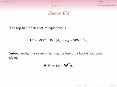
The top half of this set of equations is

(U∗ −WV∗−1W>)δa = εA −WV∗−1εB

Subsequently, the value of δa may be found by back-substitution,giving

V∗δb = εB −W>δa

Introduction Functions Theory

Sparse LM

p = (a>,b>)>, where a = (fc>, cc>, alpha c>, kc>)> andb = ({omc i> Tc i>})>The Jacobian matrix is

J =∂x

∂p=

[∂x

∂a,∂x

∂b

]= [A,B]

where

∂x

∂a=

[∂x

∂fc,∂x

∂cc,

∂x

∂alpha c,∂x

∂kc

]∂x

∂b=

[∂x

∂omc 1,

∂x

∂Tc 1, · · · , ∂x

∂omc i

∂x

∂Tc i· · · , ∂x

∂omc N

∂x

∂Tc N

]

Introduction Functions Theory

Sparse LM

The normal equation is rewritten as([A>

B>

] [A B

]+ λI

)∆p = −

[A>

B>

]εx

→

N∑i=1

A>i Ai

N∑i=1

A>i Bi

N∑i=1

B>i Ai

N∑i=1

B>i Bi

+ λI

∆p = −[A>εxB>εx

]

Introduction Functions Theory

Sparse LM

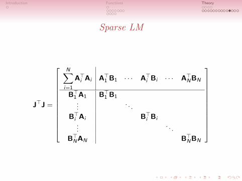
J>J =

N∑i=1

A>i Ai A>1 B1 · · · A>i Bi · · · A>NBN

B>1 A1 B>1 B1...

. . .

B>i Ai B>i Bi...

. . .

B>NAN B>NBN

Introduction Functions Theory

Sparse LM

J>εx =

N∑i=1

A>i εx

B>1 εx...

B>i εx...

B>Nεx

Introduction Functions Theory

Sparse LM

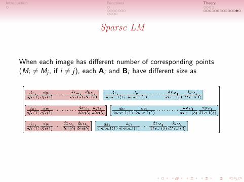
When each image has different number of corresponding points(Mi 6= Mj , if i 6= j), each Ai and Bi have different size as

Introduction Functions Theory

Sparse LM

However, the difference does not matter because

A>A ∈ Rdint×dint

A>B ∈ Rdint×dex

B>A ∈ Rdex×dint

B>B ∈ Rdex×dex

where dint denotes dimension of intrinsic params and dex denotesdimension of extrinsic params.