Theory IPhO 2019 Q1-1 S1-1 · Theory IPhO 2019 Q1-1 MS1-2 expressed 2 0 Mg dy ldl kL 0.2 pts used 0 0 0 2 0 L l Mg l kL ³ (if assumed l 0 0: 0.1 pts) 0.3 pts correct result expressed

Theory IPhO 2019 Q1-1

S1-1

Zero-length springs and slinky coils – Solution

Part A: Statics

A.1 The force 𝐹 causes the spring to change its length from 𝐿0 to 𝐿. Since equal parts of the

spring are extended to equal lengths, we get: Δ𝑦

Δ𝑙=

𝐿

𝐿0→ Δ𝑦 =

𝐿

𝐿0Δ𝑙.

Since 𝐿 = max {𝐹

𝑘, 𝐿0}, we get Δ𝑦 = max{

𝐹

𝑘𝐿0Δ𝑙, Δ𝑙}. From this result we see that any piece of

length Δ𝑙 the spring behaves as a ZLS with spring constant 𝑘∗ = 𝑘𝐿0

Δ𝑙.

A.2 Let us compute the work of the force. From Task A.1: 𝑑𝑊 = 𝐹(𝑥)𝑑𝑥 =𝑘𝐿0

Δ𝑙𝑥𝑑𝑥.

Hence, Δ𝑊 = ∫𝑘𝐿0

Δ𝑙𝑥𝑑𝑥

Δ𝑦

Δ𝑙=

𝑘𝐿0

Δ𝑙

𝑥2

2|Δ𝑙

Δ𝑦

=𝑘𝐿0

2Δ𝑙(Δ𝑦2 − Δ𝑙2).

A.3. At every point along the statically hanging spring the weight of the mass below is balanced

by the tension from above. This implies that at the bottom of the spring there is a section of

length 𝑙0 whose turns are still touching each other, as their weight is insufficient to exceed the

threshold force 𝑘𝐿0 to pull them apart. The length 𝑙0 can be derived from the equation: 𝑙0

𝐿0𝑀𝑔 = 𝑘𝐿0, hence 𝑙0 =

𝑘𝐿02

𝑀𝑔= 𝛼𝐿0.

For 𝑙 > 𝑙0, a segment of the unstretched spring between 𝑙 and 𝑙 + d𝑙 feels a weight of 𝑙

𝐿0𝑀𝑔

from beneath, which causes its length to stretch from d𝑙 to 𝑑𝑦 =𝐹

𝑘𝐿0𝑑𝑙 =

𝑙

𝐿0𝑀𝑔

𝑑𝑙

𝑘𝐿0=

𝑀𝑔

𝑘𝐿02 𝑙𝑑𝑙 =

𝑙

𝑙0𝑑𝑙 .

Integration of the last expression over the stretched region, up to the point 𝐿0, gives its height

when the spring is stretched

𝐻 = 𝑙0 + ∫𝑙

𝑙0𝑑𝑙

𝐿0

𝑙0

= 𝑙0 +𝑙2

2𝑙0|𝑙0

𝐿0

= 𝑙0 +1

2𝑙0(𝐿0

2 − 𝑙02) =

𝐿02

2𝑙0+𝑙02=𝐿02(𝛼 +

1

𝛼)


S1-2

Part B: Dynamics

B.1. From Task A.3 we have 𝐻(𝑙) =𝑙2

2𝑙0+

𝑙0

2. We now calculate the position of the center of

mass of the suspended spring. The contribution of the unstretched section of height 𝑙0 at the

bottom, having a mass of 𝑙0

𝐿0𝑀 = 𝛼𝑀, is 𝛼𝑀

𝑙0

2. The position of the center of mass is obtained by

summing the contributions of its elements:

𝐻𝑐𝑚 =1

𝑀[𝑙02𝛼𝑀 + ∫ 𝐻(𝑙)𝑑𝑚

𝐿0

𝑙0

] =1

𝑀[𝛼𝐿02

𝛼𝑀 + ∫ (𝑙2

2𝑙0+𝑙02)𝑀𝑑𝑙

𝐿0

𝐿0

𝑙0

]

=𝛼2𝐿02

+1

𝐿0[𝑙3

6𝑙0+𝑙02𝑙]𝑙0

𝐿0

=𝛼2𝐿02

+1

𝐿0[𝐿03 − 𝑙0

3

6𝑙0+𝑙02(𝐿0 − 𝑙0)]

Where we have used 𝑑𝑚 =𝑑𝑙

𝐿0𝑀. Substituting 𝑙0 = 𝛼𝐿0 yields

𝐻𝑐𝑚 = 𝐿0 [1

6𝛼−𝛼2

6+𝛼

2]

When the spring is contracted to its free length 𝐿0, its center of mass is located at 𝐿0

2. From the

falling of the center of mass at acceleration 𝑔 we get:

𝑔

2𝑡𝑐2 = 𝐻𝑐𝑚 −

𝐿02= 𝐿0 [

1

6𝛼−𝛼2

6+𝛼

2−1

2] =

𝐿06𝛼

(1 − 𝛼)3

Hence, 𝑡𝑐 = √𝐿0

3𝑔𝛼(1 − 𝛼)3.

For 𝑘 = 1.02 N/m, 𝐿0 = 0.055 m, 𝑀 = 0.201 kg, and 𝑔 = 9.80 m/s2, we have𝛼 = 0.0285, and

𝑡𝑐 = 0.245s.

B.2. The moving top section of the spring is pulled down by its own weight, 𝑚𝑡𝑜𝑝𝑔 = 𝑀𝑔(𝐿0−𝑙)

𝐿0

and also by the tension in the spring below, which is equal to the weight 𝑀𝑔𝑙/𝐿0 of the

stationary section of the spring. Thus, the moving top section experiences a constant force 𝐹 =

𝑀𝑔 throughout its whole fall. Another way to see that, is that a total force of 𝑀𝑔 is exerted on

the spring, but only the moving part experiences it. Let’s calculate the position of the center of

mass at equilibrium of the upper part, i.e., all points with 𝑙′ > 𝑙 for some 𝑙 > 𝑙0. From part A,


S1-3

the position of a small portion 'l with coordinate 'l is: 𝐻(𝑙′) =𝑙′2

2𝑙0+

𝑙0

2 and the center of

mass of this part is:

𝐻𝑐𝑚−𝑢𝑝𝑝𝑒𝑟−𝑖 =𝐿0

𝑀(𝐿0 − 𝑙)∫ 𝐻(𝑙′)𝑑𝑚

𝐿0

𝑙

=𝐿0

𝑀(𝐿0 − 𝑙)∫ (

𝑙′2

2𝑙0+𝑙02)𝑑𝑚

𝐿0

𝑙

=𝐿0

𝑀(𝐿0 − 𝑙)∫ (

𝑙′2

2𝑙0+𝑙02)𝑀𝑑𝑙′

𝐿0

𝐿0

𝑙

=1

(𝐿0 − 𝑙)∫ (

𝑙′2

2𝑙0+𝑙02)𝑑𝑙′

𝐿0

𝑙

=1

(𝐿0 − 𝑙)[𝑙′3

6𝑙0+𝑙0𝑙

′

2]𝑙

𝐿_0

=𝐿02 + 𝐿0𝑙 + 𝑙2

6𝑙0+𝑙02

The position of the upper part of CM when it contracts to a length 𝐿0 − 𝑙 is 𝐻𝑐𝑚−𝑢𝑝𝑝𝑒𝑟−𝑓 =𝑙2

2𝑙0+

𝑙0

2+

1

2(𝐿0 − 𝑙). The change in the CM during the contraction process is: Δ𝐻𝑐𝑚−𝑢𝑝𝑝𝑒𝑟 =

𝐻𝑐𝑚−𝑢𝑝𝑝𝑒𝑟−𝑖 − 𝐻𝑐𝑚−𝑢𝑝𝑝𝑒𝑟−𝑓 =𝐿02+𝐿0𝑙−2𝑙

2

6𝑙0−

1

2(𝐿0 − 𝑙) =

(𝐿0−𝑙)(𝐿0+2𝑙)

6𝑙0−

1

2(𝐿0 − 𝑙).

The acceleration of the CM of the upper part is 𝑎𝐶𝑀 =𝐹𝐿0

𝑀(𝐿0−𝑙)=

𝑔𝐿0

𝐿0−𝑙.

From the work energy theorem we get the equation 𝑣𝑢𝑝𝑝𝑒𝑟−𝑓2 = 2𝑎𝐶𝑀Δ𝐻𝑐𝑚−𝑢𝑝𝑝𝑒𝑟, hence

𝑣𝑢𝑝𝑝𝑒𝑟−𝑓2 = 2

𝑔𝐿0𝐿0 − 𝑙

[(𝐿0 − 𝑙)(𝐿0 + 2𝑙)

6𝛼𝐿0−1

2(𝐿0 − 𝑙)] = 2𝑔 [

𝐿0 + 2𝑙

6𝛼−1

2𝐿0]

=2𝑔

3𝛼𝑙 + (

1

3𝛼− 1)𝑔𝐿0

Therefore, 𝐴 =2𝑔

3𝛼 and 𝐵 = (

1

3𝛼− 1)𝑔𝐿0.

Note that for 𝑙 = 𝐿0, we have 𝑣𝑢𝑝𝑝𝑒𝑟−𝑓2 = 𝐿0𝑔

1−𝛼

𝛼 and for 𝑙 = 𝑙0 = 𝛼𝐿0, we get 𝑣𝑢𝑝𝑝𝑒𝑟−𝑓

2 =

𝐿0𝑔1−𝛼

3𝛼 , hence, the moment we release the spring its velocity is finite (not zero, the meaning is

that it accumulate this velocity in time that is much shorter than the contracting time ct ) and it

decreases to 1

√3 of the initial value when 𝑙 = 𝑙0.

B.3. Note that even though the center of mass of the spring accelerates downwards constantly,

the moving top section actually decelerates, while the position of the center of mass moves

down the spring. The speed of the top section 𝑣(𝑙), calculated in Task B2, decreases and


S1-4

approaches the value √𝐴𝛼𝐿0 + 𝐵 immediately before it attaches to the bottom section of

height 𝑙0 = 𝛼𝐿0, which was unstretched and at rest. Once the moving top section attaches to

the resting bottom section, its momentum is shared between both sections, so the speed

further decreases just before the whole spring starts accelerating downwards as a single mass.

Thus, the minimum speed is that of the whole spring immediately after its full collapse. From

momentum conservation, we have

𝑀𝑣𝑚𝑖𝑛 = 𝑚𝑡𝑜𝑝𝑣(𝑙0) = 𝑀 (1 −𝑙0𝐿0)√𝐴𝛼𝐿0 + 𝐵

𝑣𝑚𝑖𝑛 = (1 − 𝛼)√𝐴𝛼𝐿0 + 𝐵

Part C: Energetics

C.1. From the moment the spring is released, the acceleration of its center of mass is governed

by the external force 𝑀𝑔 and therefore the gravitational potential energy of the spring is fully

converted into the kinetic energy of the center of mass of the spring, which just before hitting

the ground is equal to the kinetic energy of the spring.

All that is left is the elastic energy stored in the spring, which is converted into heat, sound, etc.

To calculate it, we consider the elastic energy stored in a segment 𝑑ℎ of the stretched spring,

which when unstretched lies between 𝑙 and 𝑙 + d𝑙, using the result of Task A.2, Δ𝑊 =𝑘𝐿0

2Δ𝑙(Δ𝑙2

2 − Δ𝑙2), by choosing Δ𝑙 = 𝑑𝑙 and Δ𝑙2 = 𝑑𝑦, and using 𝑑𝑦 =𝑙

𝑙0𝑑𝑙 (which was obtained

in Task A.3), we get:

𝑑𝑊 =𝑘𝐿0

2(𝑙2

𝑙02 − 1)𝑑𝑙. Integrating from 𝑙0 to 𝐿0 we find

𝑊 = ∫𝑘𝐿02

(𝑙2

𝑙02 − 1)𝑑𝑙

𝐿0

𝑙0

=𝑘𝐿02

[𝑙3

3𝑙02 − 𝑙]

𝑙0

𝐿0

=𝑘𝐿02

(𝐿03 − 𝑙0

3

3𝑙02 − (𝐿0 − 𝑙0))

=𝑘𝐿0

2

2(1 − 𝛼3

3𝛼2− (1 − 𝛼)) =

𝑘𝐿02

6𝛼2(1 − 𝛼)2(2𝛼 + 1)

= 𝑀𝑔𝐿0(1 − 𝛼)2(2𝛼 + 1)

6𝛼


MS1-1

Zero-length springs and slinky coils – Marking Scheme

Part A: Statics

A.1 First method:

realized that

0

y L

l L

0.2 pts

realized that

FL

k

0.1 pts

mentioned that y l if 0F kL 0.1 pts

correct result 0.1 pts

Second method:

realized

* 0Lk k

l

0.2 pts

mentioned that y l if 0F kL 0.1 pts

used *

0 ( )F F k y l 0.1 pts


A.2 used 0( )

kLF x x

l

0.1 pts

used

2 0l

l

kLW xdx

l

(if Δ𝑊 =𝑘𝐿0

Δ𝑙(Δ𝑦 − Δ𝑙)2 – no pts.)

0.3 pts


A.3 calculating 0l , the length of the closed turns 0.2 pts

correct result for 0l 0.3 pts

realized

0

( )l

F l MgL

0.3 pts


MS1-2

expressed

2

0

Mgdy ldl

kL

0.2 pts

used

0

0

0 2

0

L

l

MgH l ldl

kL

(if assumed 0 0l : 0.1 pts)

0.3 pts

correct result expressed using the required variables


correct result but not expressed using the required variables


0.7 pts

0.4 pts

Part B: Dynamics

B.1 used

2

0

0

( )2 2

l lH l

l

0.3 pts

the contribution of element dl to the center of mass: 2

0

0 02 2

l l Mdl

l L

0.2 pts

0

0

0cm

1( )

2

L

l

lH M H l dm

M

(first term 0.3, second term 0.3)

0.6 pts

correct calculation of

2

cm 0

1

6 6 2H L


0.4 pts

found the displacement of the center of mass:

0cm

2

LH H

0.2 pts


MS1-3

used

2 0cm

2 2c

g Lt H

0.2 pts

correct result expressed using the required variables

correct result but not expressed using the required variables

0.5 pts

0.4 pts

numerical value of time 0.1 pts

B.2 Default method – work of external force equals the change in kinetic energy

calculated the position of the upper part ( 0'l l L ) before the

spring is released, used 2

0

0

'( ')

2 2

l lH l

l

0.2 pts

0 0 2

0 0 0

0 0 0 0

' '( ')

( ) ( ) 2 2

L L

cm upper

l l

L L l l MdlH H l dm

M L l M L l l L

if using 𝑀 instead of 𝑀(𝐿0−𝑙)

𝐿0: only 0.1 pts

0.3 pts

found

2 2

0 0 0

06 2cm upper

L L l l lH

l

0.5 pts

found the position of the center of mass of the moving part: 2

00

0

1( )

2 2 2cm upper f

l lH L l

l

(first two terms – 0.1 pts, third term – 0.2 pts)

0.3 pts

0 0

0

0

( )( 2 ) 1( )

6 2cm upper cm upper cm upper f

L l L lH H H L l

l

(finding the difference – 0.1 pts, result for the difference – 0.2 pts)

0.3 pts

understood that the external force is Mg

(any other expression – 0 pts)

0.3 pts

Using 𝑀𝑔Δ𝐻𝑐𝑚−𝑢𝑝𝑝𝑒𝑟 =𝑀(𝐿0−𝑙)

2𝐿0𝑣2 0.3 pts


MS1-4

obtained

2 00

2

3 3upper f

g L gv l L g

0.3 pts

Other methods: There are other ways to solve this part

Finding A and B without deriving I ( )v l Al B

1.3 pts

B.3 realized that the velocity decreases in time when a stationary part still exists

in case a student gets 𝐴 < 0: 0.1 pts for the opposite conclusion

0.1 pts

substituted 0l l to find I 0 0( )v l Al B 0.1 pts

used conservation of momentum (plastic collision) to find correct result

𝑣𝑚𝑖𝑛 =𝑚𝑡𝑜𝑝𝑣(𝑙0)

𝑀

0.3 pts

Part C: Energetics

C.1 an equation relating 𝑄 and 𝑊 (without gravitational energy) 0.4 pts

use

22

20 0

2

0 0

11

2 2

kL kL ldW ldl dl dl

dl l l

0.4 pts

calculated the elastic energy of the spring: 0

0

2

0

2

0

12

L

l

kL lW dl

l

0.4 pts

correct result

2

0

(1 ) (2 1)

6W MgL

0.3 pts


S2-1

The Physics of a Microwave Oven – Solution

Part A: The structure and operation of a magnetron

A.1. The frequency of an LC circuit is 𝑓 = 𝜔/2𝜋 = 1/(2𝜋√𝐿𝐶). If the total electric current

flowing along the boundary of the cavity is 𝐼, it generates a magnetic field whose magnitude (by

the assumptions of the question) is 0.6𝜇0𝐼/ℎ, and a total magnetic flux equal to 𝜋𝑅2 ×

0.6𝜇0𝐼/ℎ, hence the inductance of the resonator is 𝐿 = 0.6𝜋𝜇0𝑅2/ℎ. Approximating the

capacitor as a plate capacitor, its capacitance is 𝐶 = 휀0𝑙ℎ/𝑑. Putting everything together, we

find

89

2 3

0 0

1 1 1 1 1 3 10 12.0 10

2 2 0.6 2 0.6 2 7 10 3.6est

h d c df

R lh R lLC

Hz

A.2. Denoting the electron velocity by �⃗� (𝑡), in this case the total force applied on it is

𝐹 = −𝑒(−𝐸0�̂� + �⃗� (𝑡) × 𝐵0�̂�).

Let us write �⃗� (𝑡) = �⃗� 𝐷 + �⃗� ′(𝑡), with �⃗� 𝐷 = (−𝐸0/𝐵0)�̂�̂ being the drift velocity of a charged

particle in the crossed electric and magnetic fields (the velocity at which the electric and

magnetic forces cancel each other exactly). Then 𝐹 = −𝑒�⃗� ′(𝑡) × 𝐵0�̂�. Thus, in a frame moving

at the drift velocity �⃗� 𝐷, the electron trajectory is a circle with constant-magnitude velocity 𝑢′ =

|�⃗� ′(𝑡)|, and radius 𝑟 = 𝑚𝑢′/𝑒𝐵0. In the lab frame this circular motion is superimposed upon

the drift at the constant velocity �⃗� 𝐷. Hence:

1. For �⃗� (0) = (3𝐸0/𝐵0)�̂�̂ we find 𝑢′ = 4𝐸0/𝐵0 and 𝑟 = 4𝑚𝐸0/𝑒𝐵02.

2. For �⃗� (0) = −(3𝐸0/𝐵0)�̂�̂ we find 𝑢′ = 2𝐸0/𝐵0 and 𝑟 = 2𝑚𝐸0/𝑒𝐵02.

This information, together with the independence of the period of the circular motion on 𝑢′

allows us to plot the electron trajectory in both cases (green and red, for cases 1 and 2,

respectively):


S2-2

A.3. The velocity of the electron in a frame of reference where the motion is approximately

circular is 'u . From A.2 we get that max'Du u v and

min'Du u v , hence

max min max' ( ) / 2u v v v .

The radius of the circular motion of the electron in this frame is 0 max 0'/ /r mu eB mv eB . The

maximal velocity is that corresponding to a kinetic energy, 𝐾max = 𝑚𝑣max2 /2, of 800 eV.

Substituting we find 31

4

19

2 1 2 1 2 9.1 10 8003.18 10 m 0.3mm

0.3 1.6 10

m eV mVr

eB m B e

.

Since this maximal radius is much smaller than the distance between the anode and the

cathode, we may ignore the circular component of the electronic motion, and approximate it as

pure drift.

A.4. As just explained, we may approximate the electron motion as pure drift. In task A.2 we

have found that the direction of the drift

velocity �⃗� 𝐷 is in the direction of the vector �⃗� ×

�⃗� . Since we are interested in radial component

of the drift velocity, the only contribution is from

the azimuthal component of the electric field.

The static electric field has no azimuthal

component, hence the drift in the radial

direction results solely from the azimuthal

component of the alternating electric field.

What we have to check is if the azimuthal

component points clockwise or

counterclockwise. From the direction of the field

lines it is easy to see (attached figure) that in

points A and B the azimuthal component

pointing clockwise therefore the electrons there drift towards the cathode, while for points C, D

and E the azimuthal component points counterclockwise and the electrons there drift toward

the anode.

perpendicular to the radius

toward the cathode toward the anode

Point

X A

X B

A

B C D

E


S2-3

X C

X D

X E

A.5. In this task we need to consider the azimuthal component of the drift velocity, which

results from the radial component of the electric field. Since all points are at the same distance

from the anode, all electrons experience the same static electric field. Hence only the radial

component of the alternating field determines whether the angle between the electrons’

position vectors would increase or decrease: If the radial component of the alternating field

points inwards (towards the cathode), the azimuthal drift velocity will be positive

(counterclockwise) and vise versa. Hence the electrons at A, B and C drift closer to each other in

terms of angles, while those at D, E and F drift away from each other.

indeterminate angle increases angle decreases points

X AB

X BC

X CA

X DE

X EF

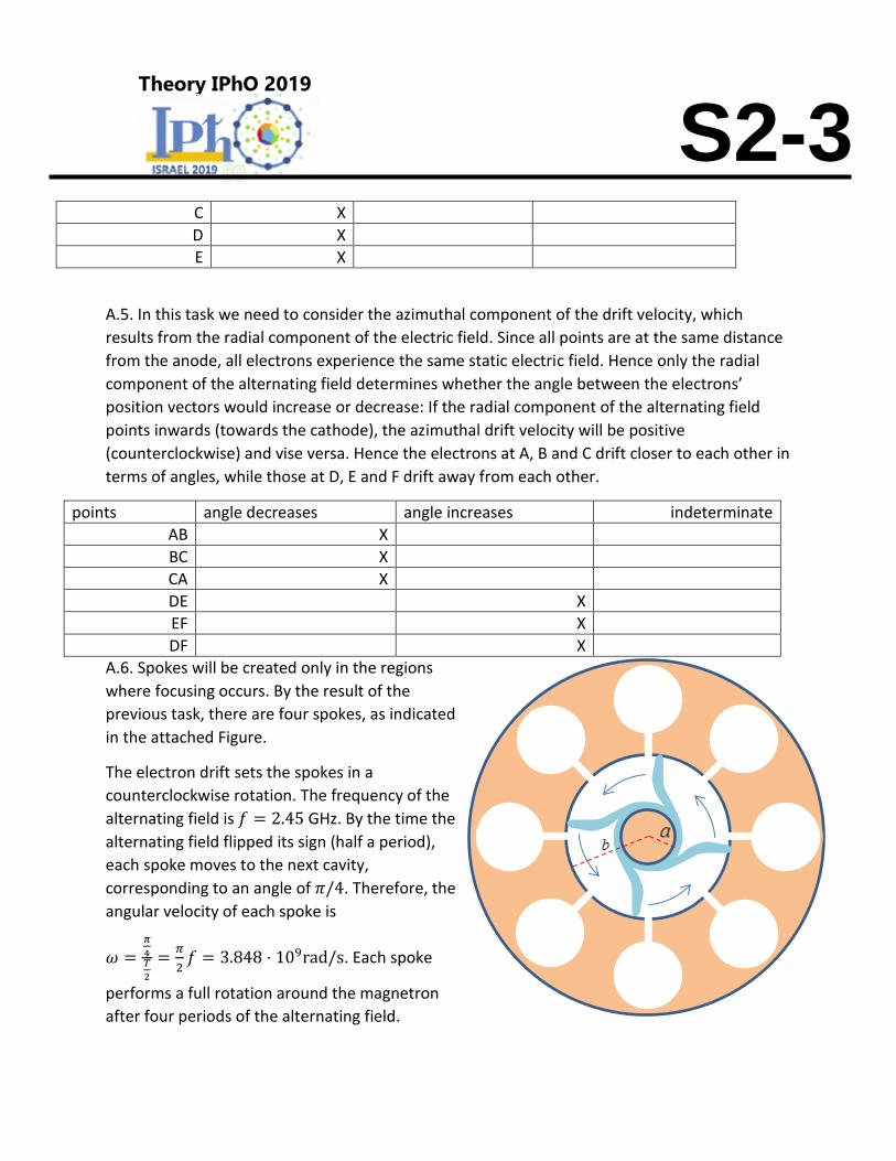
X DF A.6. Spokes will be created only in the regions

where focusing occurs. By the result of the

previous task, there are four spokes, as indicated

in the attached Figure.

The electron drift sets the spokes in a

counterclockwise rotation. The frequency of the

alternating field is 𝑓 = 2.45 GHz. By the time the

alternating field flipped its sign (half a period),

each spoke moves to the next cavity,

corresponding to an angle of 𝜋/4. Therefore, the

angular velocity of each spoke is

𝜔 =𝜋

4𝑇

2

=𝜋

2𝑓 = 3.848 ⋅ 109rad/s. Each spoke

performs a full rotation around the magnetron

after four periods of the alternating field.


S2-4

A.7. The magnitude of the electric field in the region considered, 𝑟 = (𝑏 + 𝑎)/2, is the

magnitude of the static field, that is, 𝐸 = 𝑉0/(𝑏 − 𝑎), giving rise to an azimuthal drift velocity of

magnitude 𝑢𝐷 = 𝐸/𝐵0 = 𝑉0/[𝐵0(𝑏 − 𝑎)]. Equating 𝑢𝐷/𝑟 with the angular velocity found in the

previous task we find 2 2

0 0( ) / 4V fB b a

Part B: The interaction of microwave radiation with water molecules

B.1. The torque at time 𝑡 is given by 𝜏(𝑡) = −𝑞𝑑sin[𝜃(𝑡)]𝐸(𝑡) = −𝑝0sin[𝜃(𝑡)]𝐸(𝑡), hence the

instantaneous power delivered to the dipole by the electric field is

0 0

( )( ) ( ) ( ) ( )sin ( ) ( ) ( ) cos ( ) ( ) x

i

d dp tH t t t p E t t t E t p t E t

dt dt

B.2. Since the average dipole density (hence the average of each molecular dipole) is parallel to

the field, the absorbed power density is (angular brackets, ⟨⋯ ⟩, denote average over time)

0 0 0 0

2 2 2

0 0 0 0 0 0

( ) sin( ) sin( ) sin( )

sin( )cos( ) 0.5 sin sin(2 ) 0.5 sin

xf f f

f f f f f f

dP dH t E t E t E t

dt dt

E t t E t E

B.3. The energy density of the electromagnetic field at penetration depth 𝑧, which is twice the

electric energy density, is 2 × 휀𝑟휀0⟨𝐸2(𝑧, 𝑡)⟩/2 = 휀𝑟휀0𝐸0

2(𝑧)⟨sin2(𝜔𝑡)⟩ = 휀𝑟휀0𝐸02(𝑧)/2.

Therefore, the time-averaged flux density at depth 𝑧 is:

𝐼(𝑧) =1

2휀𝑟휀0𝐸0

2(𝑧) ×𝑐

𝑛=

1

2√휀𝑟휀0𝑐𝐸0

2(𝑧),

where 𝑐 is the speed of light in vacuum. 𝐼 decreases with 𝑧 due to the absorbed power

calculated in the previous task we find

𝑑𝐼(𝑧)

𝑑𝑧= −

1

2𝛽휀0𝜔𝐸0

2(𝑧)sin𝛿 = −𝛽𝜔sin𝛿

𝑐√휀𝑟

𝐼(𝑧),

hence 𝐼(𝑧) = 𝐼(0) exp[−𝑧𝛽𝜔sin𝛿/(𝑐√휀𝑟)].

B.4. Similarly to the previous task, the energy flux corresponding to the given field is

𝐼(𝑧) = √휀𝑟휀0𝑐⟨𝐸2(𝑧, 𝑡)⟩ =

1

2√휀𝑟휀0𝑐𝐸0

2𝑒−𝑧𝜔√ 𝑟 tan𝛿/𝑐.

Equating the argument of the exponent in the last expression with the result of the previous

task, and using the given approximation tan 𝛿 ≈ sin 𝛿 leads to 𝛽 = 휀𝑟.


S2-5

B.5.

1. Using previous results, the radiation power per unit area is reduced to half of its 𝑧 = 0 value

at 𝑧1/2 = 𝑐 ln 2 /(𝜔√휀𝑟 tan 𝛿) = 𝑐√휀𝑟 ln 2 /(𝜔휀𝑙). From the given graph, at the given

frequency 휀𝑟 ≈ 78 and 휀𝑙 ≈ 10, hence 𝑧1/2 ≈ 12 mm.

We have just found that the penetration depth is proportional to √휀𝑟/휀𝑙. From the given graph

we thus find that:

2. Heating up pure water (continuous lines) decreases 휀𝑙 much more significantly than the

corresponding decrease of √휀𝑟 at the given frequency. Thus, the penetration depth of pure

water increases with temperature, allowing deeper penetration of the microwave radiation and

heating up the water inner regions.

3. On the contrary, for a soup (dilute salt solution, dashed lines) 휀𝑙 at the given frequency

increases with temperature while 휀𝑟 decreases. Thus, the absorption rate increases with

temperature, the penetration depth decreases, and less microwave radiation reaches its inner

regions.

material 𝑧1/2increases with

temp.

𝑧1/2 decreases with

temp.

𝑧1/2remains the same

water X

soup X


MS2-1

The Physics of a Microwave Oven – Marking Scheme

Part A: The structure and operation of a magnetron

A.1 realized 𝑓 =𝜔

2𝜋=

1

2𝜋√𝐿𝐶 0.1pts

found 𝐿 = 0.6𝜋𝜇0𝑅2/ℎ 0.2 pts

final result 0.1 pts

A.2 found �⃗� 𝐷 = (𝐸0/𝐵0)𝑥̂ 0.1 pts

found 𝑟 = 𝑚𝑢′/𝑒𝐵0 0.2 pts

For �⃗� (0) = (3𝐸0

𝐵0) �̂�̂:

found 𝑢′ =2𝐸0

𝐵0 0.1 pts

found 𝑟 = 2𝑚𝐸0/𝑒𝐵02 0.1 pts

For �⃗� (0) = −(3𝐸0/𝐵0)𝑥̂ :

found 𝑢′ = 4𝐸0/𝐵0 0.1 pts

found 𝑟 = 4𝑚𝐸0/𝑒𝐵02 0.1 pts

For each graph:

correct direction of drift (towards x̂ ) 0.1 pts

correct trajectory pitch ( 2

0 02 /mE eB ) 0.1 pts

correct y range 0.1 pts

correct graph shape 0.1 pts

A.3 realized 𝑢′ < 𝑣𝑚𝑎𝑥, hence 𝑟 <𝑚𝑣𝑚𝑎𝑥

𝑒𝐵0 0.2 pts

connection between velocity and energy 0.1 pts


A.4 drifts in all five points are correct 1.2 pts

only four are correct 0.6 pts

less than four are correct 0.0 pts

all five points are reversed 0.6 pts


MS2-2

A.5 all six pairs are correct 1.2 pts

only five pairs are correct 0.6 pts

less than five pairs are correct 0.0 pts

all six pairs are reversed 0.6 pts

A.6 direction of rotation 0.1 pts

four spokes 0.2 pts

spokes are symmetric under 90 rotation 0.1 pts

in half period the spoke rotates by 45 0.2 pts

correct result of angular velocity 0.2 pts

A.7 realized 0

( )D

Vu

b a B

0.3 pts

using ( ) / 4Du f b a 0.5 pts


Part B: The interaction of microwave radiation with water molecules

B.1 find 0( ) ( )sin ( )t p E t t 0.2 pts

find that

( )( ) ( ) x

i

dp tH t E t

dt

0.3 pts

B.2 realized polarization is along x axis 0.1 pts

0 0 0( ) sin( ) sin( )f f

dH t E t E t

dt

0.1 pts

used correct trigonometric averaging 0.1 pts


B.3 found the average electromagnetic energy density 20

0 ( )2

r E z

0.1 pts

the energy flux density is 20

0 ( )2

r

r

cE z

0.2 pts


MS2-3

used result of task B2 to get

0 0( ) ( ) 0.5 ( ) sinfI z dz I z E z dz

0.4 pts

get

sin( )( )

f

r

dI zI z

dz c

0.2 pts

final result

sin( ) (0)exp

f

r

I z I zc

0.2 pts

B.4 found the average energy density 0 tan20

02

k n zr E e

0.2 pts

found

tan

( ) (0)f r

zcI z I e

0.2 pts

final result 𝛽 = 𝜀𝑟 0.2 pts

B.5 used

tan

ln 2f r

zce e

0.1 pts

found correct numerical value of z 0.2 pts

for water penetration depth: increases with increasing temperature

0.2 pts

for soup penetration depth: decreases with increasing temperature

0.2 pts


S3-1

Thermoacoustic engine – Solution

Part A: Sound wave in a closed tube

A.1. The boundary conditions are: 𝑢(0, 𝑡) = 𝑢(𝐿, 𝑡) = 0. As a result, sin (2𝜋

𝜆𝐿) = 0, so we get

𝜆max = 2𝐿.

A.2. We get

𝑉(𝑥, 𝑡) = 𝑆 ⋅ (Δ𝑥 + 𝑢(𝑥 + Δ𝑥, 𝑡) − 𝑢(𝑥, 𝑡)) = 𝑆Δ𝑥 ⋅ (1 + 𝑢′) = 𝑉0 + 𝑉0𝑢′.

Thus,

𝑉(𝑥, 𝑡) = 𝑉0 + 𝑎𝑘𝑉0 cos(𝑘𝑥) cos(𝜔𝑡)

⇒ 𝑉1(𝑥) = 𝑎𝑘𝑉0 cos(𝑘𝑥).

A.3. We use Newton’s Second Law 𝜌0�̈� = −𝑝′ to deduce 𝑝′ = −𝜌0�̈� = 𝜌0𝑎𝜔2 sin(𝑘𝑥)cos (𝜔𝑡),

so that

𝑝(𝑥, 𝑡) = 𝑝0 − 𝑎𝜔2

𝑘𝜌0cos (𝑘𝑥)cos (𝜔𝑡)

⇒ 𝑝1(𝑥) = 𝑎

𝜔2

𝑘𝜌0cos (𝑘𝑥).

A.4. Using 𝑎 ≪ 𝐿, we obtain 𝑝1(𝑥)

𝑝0= 𝛾

𝑉1(𝑥)

𝑉0. As a result,

𝜌0

𝑝0

𝜔2

𝑘= 𝛾 ⋅ 𝑘, and 𝑐 = √

𝛾𝑝0

𝜌0.

A.5. The relative change in 𝑇(𝑥, 𝑡) is the sum of the relative changes in 𝑉(𝑥, 𝑡) and 𝑝(𝑥, 𝑡). As a

result,

𝑇1(𝑥) =𝑇0

𝑝0𝑝1(𝑥) −

𝑇0

𝑉0𝑉1(𝑥) = (𝛾 − 1)

𝑇0

𝑉0𝑉1(𝑥) = 𝑎𝑘(𝛾 − 1)𝑇0 cos(𝑘𝑥).

A.6. The movement of the gas parcels inside the tube conveys heat along its boundary. To

determine the direction of the convection, we combining the result of Task A.5 and the

expression (1) for 𝑢(𝑥, 𝑡). We see that when 0 < 𝑥 <𝐿

2, the gas is colder when the displacement

𝑢(𝑥, 𝑡) is positive. Likewise, when 𝐿

2< 𝑥 < 𝐿, the gas is colder when the displacement 𝑢(𝑥, 𝑡) is

negative. Hence, heat flows into the gas near the point B, cooling it down, and out of the gas near

the points A and C, heating them up.

Part B: Sound wave amplification induced by external thermal contact

B.1. We get

𝑇env(𝑡) = 𝑇plate(𝑥0 + 𝑢(𝑥0, 𝑡)) = 𝑇0 −𝜏

ℓ⋅ 𝑢(𝑥0, 𝑡),


S3-2

so that:

𝑇st =𝑎𝜏

ℓsin(𝑘𝑥0) =

𝑎𝜏

ℓ√2.

B.2. The gas will convey heat from the hot reservoir to the cold one if the parcels are colder than

the environment when 𝑢(𝑥0, 𝑡) < 0, and hotter when 𝑢(𝑥0, 𝑡) > 0. This occurs precisely if

𝑇st > 𝑇1.

Plugging in the results of Tasks A.5 and B.1, we get

𝑎𝜏cr

ℓsin(𝑘𝑥0) = 𝑎𝑘(𝛾 − 1)𝑇0 cos(𝑘𝑥0)

⇒ 𝜏cr = 𝑘ℓ(𝛾 − 1)𝑇0.

B.3. Using the first law of thermodynamics, we get

𝑑𝑄

𝑑𝑡=

𝑑𝐸

𝑑𝑡+ 𝑝

𝑑𝑉

𝑑𝑡.

Plugging in the relation 𝐸 =1

𝛾−1𝑝𝑉, we see that:

𝑑𝑄

𝑑𝑡=

1

𝛾−1

𝑑

𝑑𝑡(𝑝𝑉) + 𝑝

𝑑𝑉

𝑑𝑡=

1

𝛾−1𝑉

𝑑𝑝

𝑑𝑡+

𝛾

𝛾−1𝑝

𝑑𝑉

𝑑𝑡≈

1

𝛾−1𝑉0

𝑑𝑝

𝑑𝑡+

𝛾

𝛾−1𝑝0

𝑑𝑉

𝑑𝑡.

B.4. We plug the expression for 𝑑𝑄

𝑑𝑡 into the result of Task B.3. This gives:

1

𝛾−1𝑉0

𝑑𝑝

𝑑𝑡+

𝛾

𝛾−1𝑝0

𝑑𝑉

𝑑𝑡= 𝛽𝑉0(𝑇st − 𝑇1) ⋅ cos (𝜔𝑡).

We now plug in the data given in equation (6), and get (by considering terms with cos (𝜔𝑡) and

sin (𝜔𝑡) separately):

1

𝛾 − 1𝑉0𝑝𝑎𝜔 +

𝛾

𝛾 − 1𝑝0𝑉𝑎𝜔 = 𝛽𝑉0(𝑇st − 𝑇1)

1

𝛾 − 1𝑉0𝑝𝑏𝜔 −

𝛾

𝛾 − 1𝑝0𝑉𝑏𝜔 = 0

and thus, we can already express 𝑉𝑏 as

𝑉𝑏 =1

𝛾𝑝𝑏 ⋅

𝑉0

𝑝0.

For 𝑉𝑎, we plug in the results of Tasks B.1 and B.2,

𝑇st − 𝑇1 =𝑎

ℓ√2(𝜏 − 𝜏cr),


S3-3

giving:

𝑉𝑎 = (−1

𝛾𝑝𝑎 −

𝛾−1

𝛾

𝛽

𝜔

𝑎

ℓ√2(𝜏 − 𝜏cr)) ⋅

𝑉0

𝑝0.

B.5. We want to integrate the mechanical work generated, ∫ 𝑝𝑑𝑉, and averaging the result over

a long time. To do this, we substitute our expressions (6) for the perturbed 𝑝 and 𝑉. Since the

average of cos (𝜔𝑡)sin (𝜔𝑡) is 0, and that of sin2(𝜔𝑡) and cos2(𝜔𝑡) is 1

2, we get:

𝑉0

𝑆ℓ𝑊tot = −𝜋 ⋅ (𝑝𝑎𝑉𝑏 + 𝑝𝑏𝑉𝑎).

Using the result of B.4, we get

𝑉0

𝑆ℓ𝑊tot =

𝜋

𝜔⋅

𝛾−1

𝛾𝛽

𝑎

ℓ√2(𝜏 − 𝜏cr) ⋅ 𝑉0

𝑝𝑏

𝑝0.

To leading order, 𝑝𝑏 is the unperturbed wave 𝑝𝑏 ≈ 𝑝1(𝑥0) = 𝑎𝜔2

𝑘𝜌0 cos(𝑘𝑥0) = 𝑎𝑘𝛾𝑝0

1

√2.

Simplifying, we get

𝑊tot =𝜋

𝜔𝑆 ⋅

𝛾−1

𝛾𝛽

𝑎

√2(𝜏 − 𝜏cr) ⋅

𝑝𝑏

𝑝0=

𝜋

2𝜔(𝛾 − 1)𝛽(𝜏 − 𝜏cr)𝑘𝑎2𝑆.

B.6. We want to compute the amount of heat convection over one cycle. This means that we

need to take the amount of heat moving in or out of the parcel, and weigh it by the position of

the parcel at that time. Thus, the total heat conveyed by the parcel, integrated along a cycle, is:

𝑄tot =1

Δ𝑥∫

𝑑𝑄

𝑑𝑡𝑢 ⋅ 𝑑𝑡.

This expression can be computed to leading order using 𝑑𝑄

𝑑𝑡= 𝛽𝑉0(𝑇st − 𝑇1) ⋅ cos (𝜔𝑡) and the

unperturbed displacement 𝑢(𝑥0, 𝑡) =𝑎

√2cos (𝜔𝑡). This gives

𝑄tot =𝜋

𝜔𝛽𝑉0(𝑇st − 𝑇1)

𝑎

√2=

𝜋

𝜔𝛽𝑉0 ⋅

𝑎

ℓ√2(𝜏 − 𝜏cr) ⋅

𝑎

√2=

𝜋

2𝜔𝛽(𝜏 − 𝜏cr)

𝑎2𝑆

ℓ.

B.7. Dividing the results of Tasks B.5 and B.6, we obtain the expression:

𝜂 =𝑊tot

𝑄tot= (𝛾 − 1)𝑘ℓ =

𝜏cr

𝑇0=

𝜏cr

𝜏⋅

𝜏

𝑇0=

𝜏cr

𝜏⋅ 𝜂𝑐.


MS3-1

Thermoacoustic engine – Marking Scheme

Part A: Sound wave in a closed tube

A.1 boundary conditions 𝑢(𝐿, 𝑡) = 0 0.2pts

𝜆𝑚𝑎𝑥 = 2𝐿 0.1 pts

A.2 𝑉(𝑥, 𝑡) = 𝑆 ⋅ 𝛥𝑥𝑡(𝑡) 0.1 pts

comparing two sides 1

𝛥𝑥(𝑢(𝑥 + 𝛥𝑥, 𝑡) − 𝑢(𝑥, 𝑡)) =

𝑑𝑢

𝑑𝑥 0.2 pts


A.3 𝛥𝐹 = 𝑆 ⋅ 𝛥𝑝 0.1 pts

𝛥𝑝 ≈ −𝑑𝑝(𝑥,𝑡)

𝑑𝑥⋅ 𝛥𝑥 0.2 pts

Newton’s 2nd law 𝛥𝐹 = 𝑚𝑑2𝑢

𝑑𝑡2 ≈ 𝜌0 ⋅ 𝑆 ⋅ 𝛥𝑥𝑑2𝑢

𝑑𝑡2 0.2 pts


A.4 final result 0.3 pts

A.5 ideal gas 𝑝𝑉 = 𝑛𝑅𝑇 0.2 pts

𝑇 =𝑇0

𝑝0𝑉0(𝑝0 − 𝑝1 𝑐𝑜𝑠 (𝜔𝑡))(𝑉0 + 𝑉1 𝑐𝑜𝑠 (𝜔𝑡)) 0.1 pts

𝑇 = 𝑇0 + 𝑇0(𝑉1/𝑉0 − 𝑝1/𝑝0) 𝑐𝑜𝑠 (𝜔𝑡) 0.2 pts


A.6 Two correct sites 0.6 pts

All are correct 1.2 pts

Part B: Sound wave amplification induced by external thermal contact

B.1 𝑇𝑒𝑛𝑣(𝑡) = 𝑇0 −𝜏

𝑙⋅ (𝑢(𝐿/4, 𝑡)) 0.3 pts


B.2 𝑇𝑠𝑡 > 𝑇1 0.6 pts


B.3 use first law 𝛥𝑄 = 𝛥𝐸 + 𝑊 or 𝑑𝑄

𝑑𝑡=

𝑑𝐸

𝑑𝑡+

𝑑𝑊

𝑑𝑡 0.4 pts


MS3-2

understand energy of ideal gas 𝛥𝐸 = 𝑐𝑣𝑛𝛥𝑇 0.1 pts

𝑛𝑅𝛥𝑇 = 𝑝𝛥𝑉 + 𝛥𝑝 ⋅ 𝑉 0.2 pts


B.4 final result 𝑉𝑏 =1

𝛾𝑝𝑏

𝑉0

𝑝0 0.5 pts

𝑉𝑎 = [−𝛾−1

𝛾

𝛽

𝜔(𝑇𝑠𝑡 − 𝑇1) −

1

𝛾𝑝𝑎]

𝑉0

𝑝0 0.8 pts

𝑇𝑠𝑡 − 𝑇1 = (𝜏 − 𝜏𝑐𝑟)𝑎

𝑙√2 0.5 pts

final result 𝑉𝑎 = [−𝛾−1

𝛾

𝛽

𝜔(𝜏 − 𝜏𝑐𝑟)

𝑎

𝑙√2−

1

𝛾𝑝𝑎]

𝑉0

𝑝0 0.1 pts

B.5 𝑤 = ∫ 𝑝𝑑𝑉 = ∫ 𝑝𝑑𝑉

𝑑𝑡𝑑𝑡

𝛥𝑡𝑐

0 0.2 pts

∫ 𝑐𝑜𝑠 (𝜔𝑡)𝑑𝑡𝛥𝑡𝑐

0= ∫ 𝑠𝑖𝑛 (𝜔𝑡)𝑑𝑡

𝛥𝑡𝑐

0= ∫ 𝑠𝑖𝑛 (𝜔𝑡)

𝛥𝑡𝑐

0

𝑐𝑜𝑠 (𝜔𝑡)𝑑𝑡 = 0 (or equivalent)

0.2 pts

∫ 𝑐𝑜𝑠2 (𝜔𝑡)𝑑𝑡𝛥𝑡𝑐

0= ∫ 𝑠𝑖𝑛2 (𝜔𝑡)𝑑𝑡

𝛥𝑡𝑐

0=

𝛥𝑡𝑐

2 0.2 pts

𝑤 = −𝛥𝑡𝑐𝜔

2(𝑝𝑎𝑉𝑏 + 𝑝𝑏𝑉𝑎) = −𝜋(𝑝𝑎𝑉𝑏 + 𝑝𝑏𝑉𝑎) 0.1 pts

𝑊 =𝜋

2𝜔(𝛾 − 1)𝛽(𝜏 − 𝜏𝑐𝑟)𝑘𝑎2𝑆 0.1 pts

B.6 𝑄𝑡𝑜𝑡 = 𝑆 ∫ 𝑗 ⋅ 𝑑𝑡𝛥𝑡𝑐

0=

1

Δ𝑥∫ 𝑄

𝑑𝑢

𝑑𝑡⋅ 𝑑𝑡

𝛥𝑡𝑐

0 0.2 pts

𝑄 = −1

𝜔𝛽𝑉0(𝑇𝑠𝑡 − 𝑇1) 𝑠𝑖𝑛 (𝜔𝑡) + 𝑄0 0.1 pts

𝑑𝑢

𝑑𝑡(𝑥, 𝑡) = −𝑎𝜔 ⋅𝑠𝑖𝑛 (𝑘𝑥) 𝑠𝑖𝑛 (𝜔𝑡) 0.1 pts

𝑄𝑡𝑜𝑡 =1

𝜔𝜋𝑎𝛽𝑆(𝑇𝑠𝑡 − 𝑇1) 𝑠𝑖𝑛 (𝑘𝑥) 0.3 pts

𝑄𝑡𝑜𝑡 =1

𝜔

𝜋

2𝑎2𝛽

𝑠

𝑙(𝜏 − 𝜏𝑐𝑟) 0.1 pts

B.7 𝜂 = (𝛾 − 1)𝑘𝑙 0.2 pts

𝜂 =𝜏𝑐𝑟

𝑇0=

𝜏𝑐𝑟

𝜏

𝜏

𝑇0≈ 𝜂𝑐

𝜏𝑐𝑟

𝜏 0.4 pts

Note that some students may solve B.6 and B.7 using a different method. A student that solved

correctly B.7, and inferred incorrect answer for B.6 with correct units, will get full points for B.7

and ½ of the points for B.6.

Theory IPhO 2019 Q1-1 S1-1 · Theory IPhO 2019 Q1-1 MS1-2 expressed 2 0 Mg dy ldl kL 0.2 pts used 0 0 0 2 0 L l Mg l kL ³ (if assumed l 0 0: 0.1 pts) 0.3 pts correct result expressed

Documents