Theory and Design of Electrical and Electronic Circuits

THEORY AND DESIGN OF ELECTRONIC CIRCUITS

E. TAITFOR ELEKTRODA PEOPLE

Theory and Design of

Electrical and Electronic Circuits

Index

Introduction

Chap. 01 Generalities

Chap. 02 Polarization of components

Chap. 03 Dissipator of heat

Chap. 04 Inductors of small value

Chap. 05 Transformers of small value

Chap. 06 Inductors and Transformers of great value

Chap. 07 Power supply without stabilizing

Chap. 08 Power supply stabilized

Chap. 09 Amplification of Audiofrecuency in low level class A

Chap. 10 Amplification of Audiofrecuenciy on high level classes A and B

Chap. 11 Amplification of Radiofrecuency in low level class A

Chap. 12 Amplification of Radiofrecuency in low level class C

Chap. 13 Amplifiers of Continuous

Chap. 14 Harmonic oscillators

Chap. 15 Relaxation oscillators

Chap. 16 Makers of waves

Chap. 17 The Transistor in the commutation

Chap. 18 Multivibrators

Chap. 19 Combinationals and Sequentials

Chap. 20 Passive networks as adapters of impedance

Chap. 21 Passive networks as filters of frequency (I Part)

Chap. 22 Passive networks as filters of frequency (II Part)

Chap. 23 Active networks as filters of frequency and displaced of phase (I Part)

Chap. 24 Active networks as filters of frequency and displaced of phase (II Part)

Chap. 25 Amplitude Modulation

Chap. 26 Demodulación of Amplitude

Chap. 27 Modulation of Angle

Chap. 28 Demodulation of Angle

Chap. 29 Heterodyne receivers

Chap. 30 Lines of Transmission

Chap. 31 Antennas and Propagation

Chap. 32 Electric and Electromechanical installations

Chap. 33 Control of Power (I Part)

Chap. 34 Control of Power (II Part)

Chap. 35 Introduction to the Theory of the Control

Chap. 36 Discreet and Retained signals

Chap. 37 Variables of State in a System

Chap. 38 Stability in Systems

Chap. 39 Feedback of the State in a System

Chap. 40 Estimate of the State in a System

Chap. 41 Controllers of the State in a System

Bibliography

Theory and Design of

Electrical and Electronic Circuits

_________________________________________________________________________________

Introduction

Spent the years, the Electrical and Electronic technology has bloomed in white hairs; white technologically for much people and green socially for others. To who writes to them, it wants with this theoretical and practical book, to teach criteria of design with the experience of more than thirty years. I hope know to take advantage of it because, in

truth, I offer its content without interest, affection and love by the fellow.

Eugenio Máximo Tait

_________________________________________________________________________________

Chap. 01 Generalities

Introduction

System of units

Algebraic and graphical simbology

Nomenclature

Advice for the designer

_______________________________________________________________________________

Introduction

In this chapter generalizations of the work are explained.

Almost all the designs that appear have been experienced satisfactorily by who speaks to them.

But by the writing the equations can have some small errors that will be perfected with time.

The reading of the chapters must be ascending, because they will be occurred the subjects

being based on the previous ones.

System of units

Except the opposite clarifies itself, all the units are in M. K. S. They are the Volt, Ampere,

Ohm, Siemens, Newton, Kilogram, Second, Meter, Weber, Gaussian, etc.

The temperature preferably will treat it in degrees Celsius, or in Kelvin.

All the designs do not have units because incorporating each variable in M. K. S., will be

satisfactory its result.

Algebraic and graphical simbology

Often, to simplify, we will use certain symbols. For example:

— Parallel of components 1 / (1/X1 + 1/X2 + ...) like X1// X2//...

— Signs like " greater or smaller" (≥ ≤), "equal or different " (= ≠), etc., they are made of

form similar to the conventional one to have a limited typesetter source.

In the parameters (curves of level) of the graphs they will often appear small arrows that

indicate the increasing sense.

In the drawn circuits when two lines (conductors) are crossed, there will only be connection

between such if they are united with a point. If they are drawn with lines of points it indicates that

this conductor and what he connects is optative.

Nomenclature

A same nomenclature in all the work will be used. It will be:

— instantaneous (small) v

— continuous or average (great) V — effective (great) V or Vef — peak Vpico or vp — maximum Vmax — permissible (limit to the breakage) VADM

Advice for the designer

All the designs that become are not for arming them and that works in their beginning, but to only

have an approximated idea of the components to use. To remember here one of the laws of

Murphy: " If you make something and works, it is that it has omitted something by stop ".

The calculations have so much the heuristic form (test and error) like algoritmic (equations)

and, therefore, they will be only contingent; that is to say, that one must correct them until reaching

the finished result.

So that a component, signal or another thing is despicable front to another one, to choose among

them 10 times often is not sufficient. One advises at least 30 times as far as possible. But two

cases exist that are possible; and more still, up to 5 times, that is when he is geometric (52 = 25), that is to say, when the leg of a triangle rectangle respect to the other is of that greater magnitude

or. This is when we must simplify a component reactive of another pasive, or to move away to us of

pole or zero of a transference.

As far as simple constants of time, it is to say in those transferences of a single pole and that is

excited with steps being exponential a their exit, normally 5 constants are taken from time to arrive

in the end. But, in truth, this is unreal and little practical. One arrives at 98% just by 3 constants

from time and this magnitude will be sufficient.

As far as the calculations of the permissible regimes, adopted or calculated, always he is advisable

to sobredetermine the proportions them.

The losses in the condensers are important, for that reason he is advisable to choose of high value

of voltage the electrolytic ones and that are of recognized mark (v.g.: Siemens). With the ceramic

ones also always there are problems, because they have many losses (Q of less than 10 in many

applications) when also they are extremely variable with the temperature (v.g.: 10 [ºC] can change

in 10 [%] to it or more), thus is advised to use them solely as of it desacopled and, preferably,

always to avoid them. Those of poliester are something more stable. Those of mica and air or oil in

works of high voltage are always recommendable.

When oscillating or timers are designed that depend on capacitiva or inductive constant of times,

he is not prudent to approach periods demarcated over this constant of time, because small

variations of her due to the reactive devices (v.g.: time, temperature or bad manufacture, usually

changes a little the magnitude of a condenser) it will change to much the awaited result.

_______________________________________________________________________________

Chap. 02 Polarization of components

Bipolar transistor of junction (TBJ)Theory

Design

Fast design

Unipolar transistor of junction (JFET)

Theory

Design

Operational Amplifier of Voltage (AOV)

Theory

Design

_________________________________________________________________________________

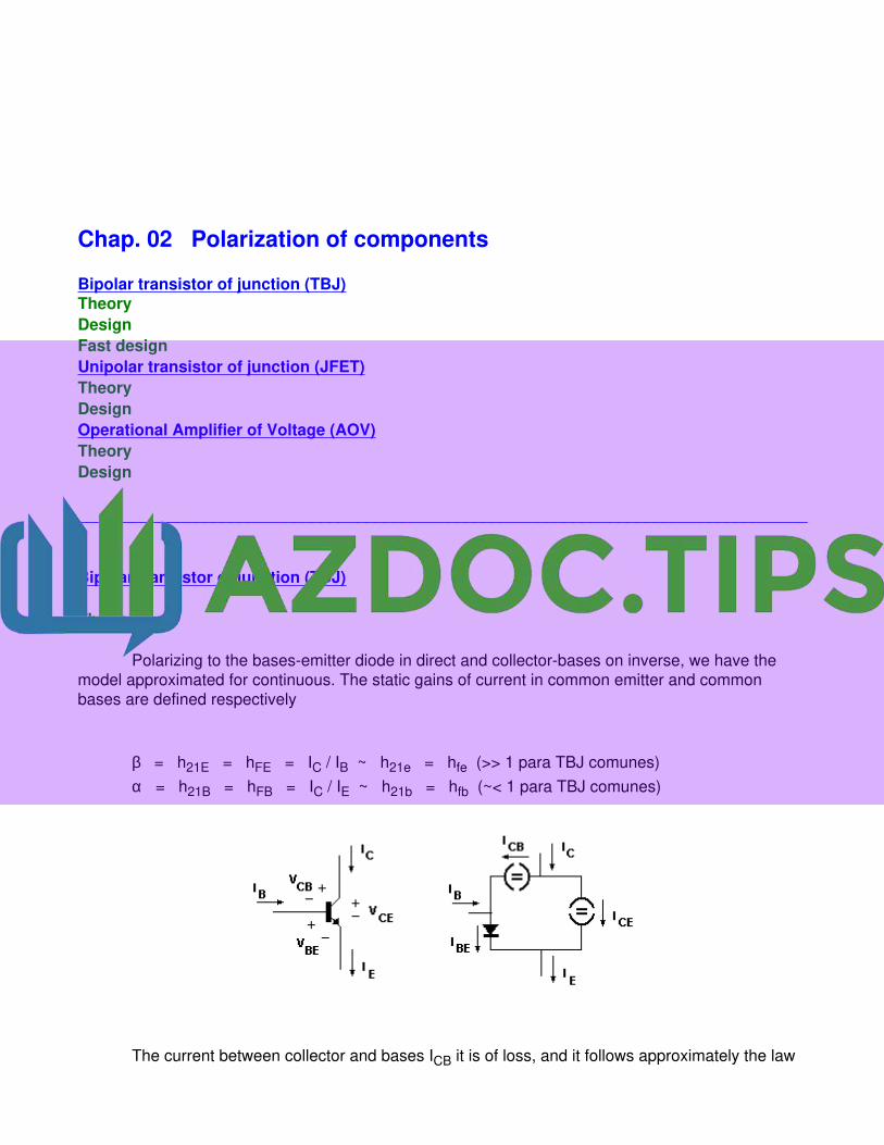
Bipolar transistor of junction (TBJ)

Theory

Polarizing to the bases-emitter diode in direct and collector-bases on inverse, we have the model approximated for continuous. The static gains of current in common emitter and common bases are defined respectively

β = h21E = hFE = IC / IB ~ h21e = hfe (>> 1 para TBJ comunes)

α = h21B = hFB = IC / IE ~ h21b = hfb (~< 1 para TBJ comunes)

The current between collector and bases ICB it is of loss, and it follows approximately the law

ICB = ICB0 (1 - eVCB/VT) ~ ICB0

where

VT = 0,000172 . ( T + 273 )

ICB = ICB0(25ºC) . 2 ∆T/10

with ∆T the temperature jump respect to the atmosphere 25 [ºC]. From this it is then

∆T = T - 25

∂ICB / ∂T = ∂ICB / ∂∆T ~ 0,07. ICB0(25ºC) . 2 ∆T/10

On the other hand, the dependency of the bases-emitter voltage respect to the temperature, to current of constant bases, we know that it is

∂VBE / ∂T ~ - 0,002 [V/ºC]

The existing relation between the previous current of collector and gains will be determined now

IC = ICE + ICB = α IE + ICB

IC = ICE + ICB = β IBE + ICB = β ( IBE + ICB ) + ICB ~ β ( IBE + ICB )

β = α / ( 1 - α )

α = β / ( 1 + β )

Next let us study the behavior of the collector current respect to the temperature and the voltages

∆IC = (∂IC/∂ICB) ∆ICB + (∂IC/∂VBE) ∆VBE + (∂IC/∂VCC) ∆VCC +

+ (∂IC/∂VBB) ∆VBB + (∂IC/∂VEE) ∆VEE

of where they are deduced of the previous expressions

∆ICB = 0,07. ICB0(25ºC) . 2 ∆T/10 ∆T

∆VBE = - 0,002 ∆T

VBB - VEE = IB (RBB + REE) + VBE + IC REE

IC = [ VBB - VEE - VBE + IB (RBB + REE) ] / [ RE + (RBB + REE) β-1 ]

SI = (∂IC/∂ICB) ~ (RBB + REE) / [ REE + RBB β-1 ]

SV = (∂IC/∂VBE) = (∂IC/∂VEE) = - (∂IC/∂VBB) = - 1 / ( RE + RBB β-1 )

(∂IC/∂VCC) = 0

being

∆IC = [ 0,07. 2 ∆T/10 (RBB + REE) ( REE + RBB β-1 )-1 ICB0(25ºC) +

+ 0,002 ( REE + RBB β-1 )-1 ] ∆T + ( RE + RBB β-1 )-1 (∆VBB - ∆VEE)

Design

Be the data

IC = ... VCE = ... ∆T = ... ICmax = ... RC = ...

From manual or the experimentation according to the graphs they are obtained

β = ... ICB0(25ºC) = ... VBE = ... ( ~ 0,6 [V] para TBJ de baja potencia)

and they are determined analyzing this circuit

RBB = RB // RS

VBB = VCC . RS (RB+RS)-1 = VCC . RBB / RB

∆VBB = ∆VCC . RBB / RS = 0

∆VEE = 0

REE = RE

RCC = RC

and if to simplify calculations we do

RE >> RBB / β

us it gives

SI = 1 + RBB / RE

SV = - 1 / RE

∆ICmax = ( SI . 0,07. 2 ∆T/10 ICB0(25ºC) - SV . 0,002 ) . ∆T

and if now we suppose by simplicity

∆ICmax >> SV . 0,002 . ∆T

are

RE = ... >> 0,002 . ∆T / ∆ICmax

RE [ ( ∆ICmax / 0,07. 2 ∆T/10 ICB0(25ºC) . ∆T ) - 1 ] = ... > RBB = ... << β RE = ...

being able to take a ∆IC smaller than ∆ICmax if it is desired.

Next, as it is understood that