Theoretically Based Algorithms for Robustly … Based Algorithms for Robustly Tracking Intersection Curves of ... their deformations to develop algorithms for ... not defined everywhere

Theoretically Based Algorithms for Robustly

Tracking Intersection Curves of Deforming

Surfaces ⋆

Xianming Chen a Richard F. Riesenfeld a Elaine Cohen a

James Damon b

aSchool of Computing, University of Utah, Salt Lake City, UT 84112

bDepartment of Mathematics, University of North Carolina, Chapel Hill, NC

27599

Abstract

This paper applies singularity theory of mappings of surfaces to 3-space and thegeneric transitions occurring in their deformations to develop algorithms for contin-uously and robustly tracking the intersection curves of two deforming parametricspline surfaces, when the deformation is represented as a family of generalized offsetsurfaces. The set of intersection curves of 2 deforming surfaces over all time is for-mulated as an implicit 2-manifold I in an augmented (by time domain) parametricspace R

5. Hyper-planes corresponding to some fixed time instants may touch I atsome isolated transition points, which delineate transition events, i.e., the topologi-cal changes to the intersection curves. These transition points are the 0-dimensionalsolution to a rational system of 5 constraints in 5 variables, and can be computedefficiently and robustly with a rational constraint solver using subdivision and hyper-tangent bounding cones. The actual transition events are computed by contouringthe local osculating paraboloids. Away from any transition points, the intersectioncurves do not change topology and evolve according to a simple evolution vectorfield that is constructed in the Euclidean space in which the surfaces are embedded.

Key words: Deforming Surface/Surface Intersection, Generalized Offset Surface,Evolution Vector Field, Topological Transition Event, Shape Computation ofImplicit 2-Manifold in 5-Space

⋆ This work is supported in part by NSF CCR-0310705, NSF IIS-0218809, NSFCCR-0310546, and NSF DMS-0405947. All opinions, findings, conclusions or rec-ommendations expressed in this document are those of the authors and do notnecessarily reflect the views of the sponsoring agencies.

Email address: [email protected] (Xianming Chen).URL: http://www.cs.utah.edu/∼xchen/ (Xianming Chen).

Preprint submitted to Elsevier 13 November 2006

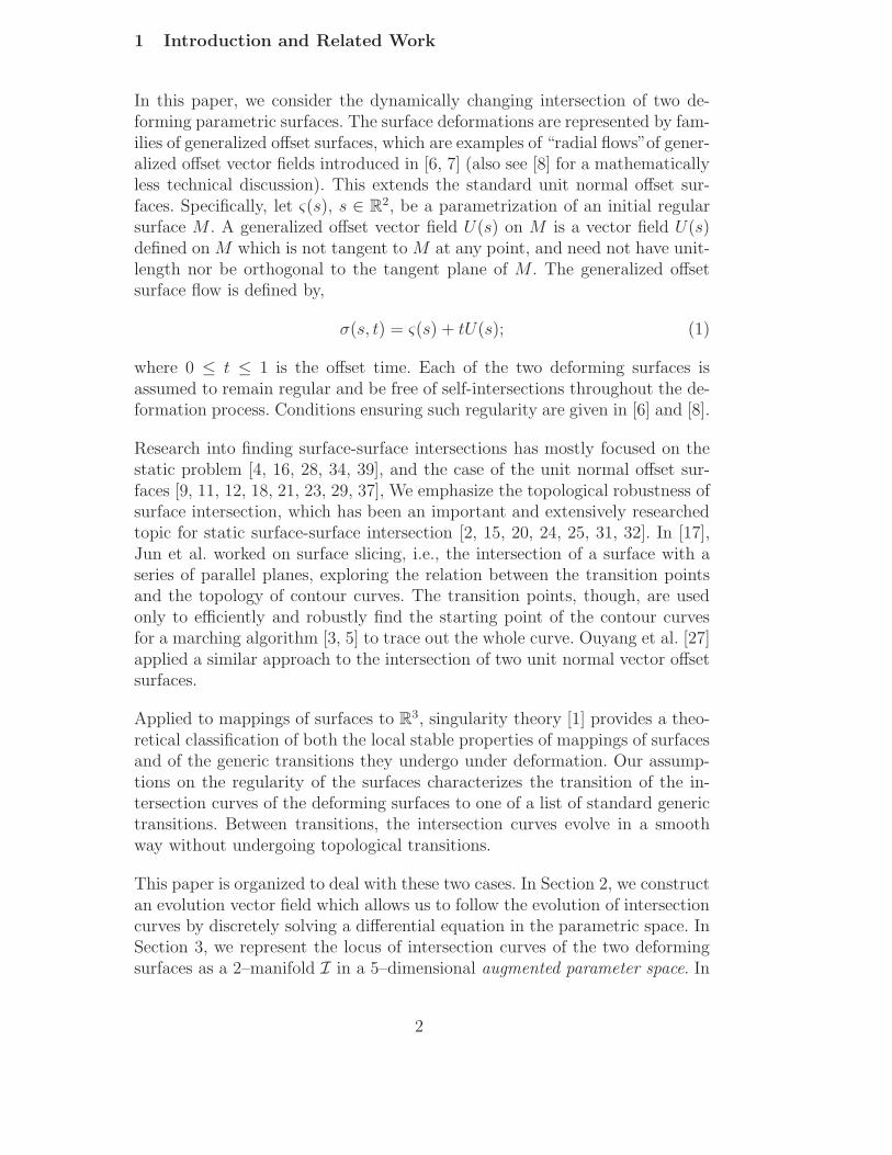
1 Introduction and Related Work

In this paper, we consider the dynamically changing intersection of two de-forming parametric surfaces. The surface deformations are represented by fam-ilies of generalized offset surfaces, which are examples of “radial flows”of gener-alized offset vector fields introduced in [6, 7] (also see [8] for a mathematicallyless technical discussion). This extends the standard unit normal offset sur-faces. Specifically, let ς(s), s ∈ R

2, be a parametrization of an initial regularsurface M . A generalized offset vector field U(s) on M is a vector field U(s)defined on M which is not tangent to M at any point, and need not have unit-length nor be orthogonal to the tangent plane of M . The generalized offsetsurface flow is defined by,

σ(s, t) = ς(s) + tU(s); (1)

where 0 ≤ t ≤ 1 is the offset time. Each of the two deforming surfaces isassumed to remain regular and be free of self-intersections throughout the de-formation process. Conditions ensuring such regularity are given in [6] and [8].

Research into finding surface-surface intersections has mostly focused on thestatic problem [4, 16, 28, 34, 39], and the case of the unit normal offset sur-faces [9, 11, 12, 18, 21, 23, 29, 37], We emphasize the topological robustness ofsurface intersection, which has been an important and extensively researchedtopic for static surface-surface intersection [2, 15, 20, 24, 25, 31, 32]. In [17],Jun et al. worked on surface slicing, i.e., the intersection of a surface with aseries of parallel planes, exploring the relation between the transition pointsand the topology of contour curves. The transition points, though, are usedonly to efficiently and robustly find the starting point of the contour curvesfor a marching algorithm [3, 5] to trace out the whole curve. Ouyang et al. [27]applied a similar approach to the intersection of two unit normal vector offsetsurfaces.

Applied to mappings of surfaces to R3, singularity theory [1] provides a theo-

retical classification of both the local stable properties of mappings of surfacesand of the generic transitions they undergo under deformation. Our assump-tions on the regularity of the surfaces characterizes the transition of the in-tersection curves of the deforming surfaces to one of a list of standard generictransitions. Between transitions, the intersection curves evolve in a smoothway without undergoing topological transitions.

This paper is organized to deal with these two cases. In Section 2, we constructan evolution vector field which allows us to follow the evolution of intersectioncurves by discretely solving a differential equation in the parametric space. InSection 3, we represent the locus of intersection curves of the two deformingsurfaces as a 2–manifold I in a 5–dimensional augmented parameter space. In

2

Section 4 we turn to the second problem of computing the transition events,and tracking the topological changes of the intersection curves occurring attransition points. In Section 4.1, we enumerate the generic transition pointsclassified by singularity theory and provide an alternative characterization ascritical points of a function on the implicit surface I. This provides the theo-retical basis to our algorithm that detects transition points as the simultaneous0-set of a rational system of 5 constraints in 5 variables. Then, in Section 4.2we compute the transitions in the intersection curves using contours on thelocal osculating quadric of the surface I at the critical points. A concludingdiscussion of the issues ensues in Section 5.

2 Evolution of Intersection Curves

Consider two deforming surfaces, σ and σ, represented as generalized offsetsurfaces,

σ(s, t) = ς(s) + t U(s),

σ(s, t) = ς(s) + t U(s),

where s = (s1, s2) ∈ R2 and s = (s1, s2) ∈ R

2 are the parameters of ς(s) andς(s), and their corresponding offset vector fields U(s) and U(s), respectively.We write the coordinate representation of the deforming surfaces by

σ(s, t) = (x(s, t), y(s, t), z(s, t)) and σ(s, t) = (x(s, t), y(s, t), z(s, t)).

We let L0 denote the set of the points in R3 which will lie on the intersection

of the two deforming surfaces for at least one time t. Consider a point P onan intersection curve of the two deforming surfaces at some time t. We firstassume that the tangent planes to the two offset surfaces at P are different;otherwise, we are in the singular case corresponding to a transition event,which we will discuss in section 4. We use the notation σi = (xi, yi, zi) todenote the partial derivative ∂σ

∂si

= ( ∂x∂si

, ∂y∂si

, ∂z∂si

) (i = 1, 2), and analogously forσi. Define

N = σ1 × σ2, N = σ1 × σ2

to be the 2 non-unit length normals to each of the two surfaces, respectively.Further let

N = (N × N) × N .

to be the tangent vector of σ at P that is perpendicular to the intersectioncurve.

3

σ2N×N

P

TSσ

NTSσ

σ1

Fig. 1. Local Basis {σ1, σ2, N}

Because the two tangent planes to the two surfaces at P are different, {σ1, σ2, N}is a basis of R

3 (Fig. 1). Decomposing δU = U − U in this basis gives,

δU = U − U = aσ1 + bσ2 + cN

Because the last term cN lives entirely in the tangent plane to the surface σ

at P , it has a decomposition relative to the basis {σ1, σ2},

−cN = aσ1 + bσ2,

Thus, we have

δU = U − U = aσ1 + bσ2 + (−aσ1 − bσ2),

or,U + (aσ1 + bσ2) = U + aσ1 + bσ2

Consequently, we have the evolution vector field with two equivalent rep-resentations (over two different basis of R

3),

η = U + aσ1 + bσ2 (2)

η = U + aσ1 + bσ2 (3)

This vector field is defined on a neighborhood of the point P in R3, rather

than just on the surfaces.

Next, for any point P which lies on a curve of intersection for the deformingsurfaces, we can define a scalar field φ in a neighborhood of P (in R

3). Bythe inverse function theorem, there is a neighborhood of P which is entirelycovered by each deforming family. For a point P ′ in this neighborhood, wedefine φ(P ′) = t − t, where t (resp. t) is the time when the surface σ(s, t)(resp. σ(s, t)) reaches P ′. Although φ is not defined everywhere on R

3, it isdefined on a neighborhood of L0.

The following properties involving φ, η, and L0 can be shown to hold:

(1) The directional derivative ∂φ∂η

= 0 identically wherever φ is defined. This

4

is readily verified by directly computing the directional derivative of φ

with respect to η.(2) The zero level set of φ is exactly L0.(3) Hence, η is tangent to L0 at all points.

Now suppose point P is on L0, and lies on an intersection curve at time t.The condition that η is tangent to L0 allows us to follow the evolution of P

on future intersection curves by solving the differential equation

dγ

dt= η(γ) with initial condition γ(0) = P

for γ(t) ∈ R3. The evolution vector field η is the image of the vector field

ξ = ∂∂t

+ a ∂∂s1

+ b ∂∂s2

under the parametrization map σ. Thus, the evolutioncould likewise be followed on the parameter space using instead the vectorfield ξ, and analogously for σ.

Then, we can use a discrete algorithm for solving the differential equationsto follow the evolution of the intersection curves over a time interval voidof transitions. Specifically, for small time dt, P moves to Q = P + dt (U +aσ1 + bσ2) on the physical surface, and if p = s ∈ R

2 corresponds to P ,then q = s + (a dt, b dt) will correspond to Q in the parameter space, andanalogously for σ. The first order marching algorithm accumulates error overtime, so point correction can be used to increase the quality. Various pointcorrection algorithms are discussed in [5] in the context of static surface-surfaceintersection. We have adopted the middle point algorithm as presented in [4] torelax the points onto the actual intersection curve. As the evolution proceeds,sample points for the intersection curves are adaptively inserted or deleted sothat the spacing of two consecutive sample points is neither too far away nortoo close, and so that the angle deviation of 3 consecutive sample points stayssmall.

3 Formulation in the Augmented Parametric Space

Define a vector distance mapping

d(s, s, t) = σ − σ : R5{s,s,t} −→ R

3 (4)

where R5{s,s,t}

1 is the combined parametric space of the two surfaces and thetime domain, and is thus called augmented parametric space. The canon-ical orthonormal basis R

5{s,s,t} is denoted as {es1

, es2, es1

, es2, et}. The 0-set of

1R

5{s,s,t} denotes R

5 with the five coordinates being s1, s2, s1, s2, t and analogously,

for R3{s,t}, etc.

5

this mapping, denoted I hereafter in this paper, gives the set of all intersectionpoints in R

5{s,s,t}. Note that d(s, s, t) concisely represents related equations for

three separate coordinate functions. Considering the x-component dx(s, s, t).dx(s, s, t) = 0 defines a hyper-surface in R

5{s,s,t}, with corresponding normal

Nx = ∇dx = (−x1, − x2, x1, x2, δUx) (5)

The component functions y and z define another two hyper-surfaces with anal-ogous expressions for their normals Ny and Nz. Geometrically, I is the locus ofintersection points of these three hyper-surfaces in R

5{s,s,t}. The Jacobian [22]

of the mapping d(s, s, t) : R5{s,s,t} −→ R

3 is,

J = (Nx Ny Nz)t =

−x1 −x2 x1 x2 δUx

−y1 −y2 y1 y2 δUy

−z1 −z2 z1 z2 δUz

= (−σ1 − σ2 σ1 σ2 δU). (6)

Remark 1 If the two tangent planes to the two deforming surfaces at theintersection point are not the same, then both of the triple scalar products(determinants) [σ1σ2σi]’s (i = 1, 2) can not simultaneously vanish, and so Jhas the full rank of 3. Otherwise, the two tangent planes must be the same.Assuming, at such a touching point, δU is not on the common tangent plane,i.e., [σ1σ2δU ] 6= 0 and [σ1σ2δU ] 6= 0, J again has the full rank. Therefore,the 0-set of the distance mapping d(s, s, t) = σ − σ : R

5{s,s,t} −→ R

3, is a welldefined implicit 2-manifold in the augmented parametric space.

4 Transition of Intersection Loops

In singularity theory, the situation we consider is considered generic. Thatis, except for a finite set of times, the two closed surfaces intersect trans-versely, that is, at each intersection point the tangent planes of the surfacesare different. Thus, the method presented in Section 2 can be applied to trackthe evolution of the curves. Over such time intervals topological changes areguaranteed not to occur.

At the remaining finite number of times, there will be intersection points atwhich the tangent planes coincide (non-transverse points). Again for genericdeformations, singularity theory describes exactly the transitions in intersec-tion curves that can occur as the evolution passes such times. These transi-tions can always be given (up to a change of coordinates) by standard modelequations, so there is essentially a unique way for each transition to occur.We shall refer to points (and times) at which transitions occur as transitionpoints. These transitions are classified as,

6

Fig. 2. Creation of Intersection Curve Component

Fig. 3. Exchange of Intersection Curve Components

(1) a creation event, when a new intersection loop is created (Fig. 2),(2) an annihilation event, when one of the current loops collapses and disap-

pears (Fig. 2 in the reverse direction),(3) an exchange event, when two branches of intersection curves meet and

exchange branches (Fig. 3).

The exchange event can have two different global consequences. If the twobranches are part of the same curve, an intersection loop is split into twoloops and we refer to this as a splitting event (Fig. 6). If the branches are fromdistinct intersection loops, a single loop is formed in a merge event (Fig. 6 inreverse order).

4.1 Detection of Transition Events

In this sub-section, we formulate the topological transition points as the 0-setof a rational system of 5 nonlinear constraints in 5 variables. The 0-set hasdimension 0, i.e., it is a discrete collection of points. It can be robustly and effi-ciently computed using a rational constraint solver [10, 33]. The robustness isachieved by bounding the subdivided implicit surface I with the correspond-ing hyper-tangent cone [10], an extension of the bounding tangent cones forexplicit plane curves and explicit surfaces [31, 32].

Let us recall that the implicit 2-manifold I in R5{s,s,t} is the locus of intersection

points of the two deforming surfaces, over the whole time period. Geometri-cally, the intersection curves, at some time point, are the corresponding heightcontour of I when the t is regarded as the vertical axis. By Remark 1, I is

7

a well-defined 2-manifold, and as a consequence of the generic forms for thetransition points, the height function t has only non-degenerate critical pointswhich are of the three types: upward elliptic points, downward elliptic points,and hyperbolic (saddle) points (cf. Fig. 4). Therefore, it is obvious that therewill be one of the three transition events listed earlier, if the tangent space toI at a point (s, s, t) is orthogonal to the t-axis. Since I and its tangent spacehave the same dimension, namely, 2, the orthogonality condition is tantamountto satisfying two equations,

T1 ··· et = 0, T2 ··· et = 0,

where T1 and T2 are any two vectors spanning the tangent space. A simpleand natural way to construct such a pair of tangent vectors is to let T1 bethe tangent to an s2-iso-curve on I with the extra constraint s2 = c2 for someconstant c2, and let T2 be the tangent to an s1-iso-curve on I with the extraconstant s1 = c1 for some constant c1. Noticing that an s2-iso-curve is theintersection of 4 hyper surfaces in R

5{s,s,t}, defined by s2 = c2, dx = 0, dy = 0,

and dz = 0,

T1 =

∣

∣

∣

∣

∣

∣

∣

∣

∣

∣

∣

∣

∣

∣

∣

∣

∣

∣

es1es2

es1es2

et

0 1 0 0 0

−x1 −x2 x1 x2 δUx

−y1 −y2 y1 y2 δUy

−z1 −z2 z1 z2 δUz

∣

∣

∣

∣

∣

∣

∣

∣

∣

∣

∣

∣

∣

∣

∣

∣

∣

∣

= (T 12δ, 0, T12δ, − T

11δ, T112),

where T ’ denotes the triple scalar product of its 3 corresponding vectorsindicated by the superscripts. Superscripts i and i represent σi and σi, respec-tively, while a superscript δ represents δU (e.g., T 12δ = [σ1 σ2 δU ]). A similarderivation exists for T2. Thus, we have in general

Ti = T12δ esi

+ Ti2δ es1

− Ti1δ es2

+ Ti12 et, i = 1, 2. (7)

At transition points, the last component of T1 and T2 vanishes, i.e.

T1 ··· et = T112 = [σ1 σ1 σ2] = 0, T2 ··· et = T

212 = [σ2 σ1 σ2] = 0, (8)

Remark 2 At a transition point, T1 and T2 are guaranteed to be independentof each other because, by Eq. (7), the s1 coordinate component of T2 vanisheswhile the corresponding component of T1 is non-zero (cf. Remark (1) as well).It is also easily seen that Eq. (8) simply requires the two tangents σ1 andσ2 to the first offset surface to be perpendicular to the normal of the secondoffset surface, i.e., the two tangent planes to the two deforming surfaces in theeuclidean space are coincident.

8

Finally, together with σ − σ = 0, Eq. (8) gives a rational system with 5constraints in 5 variables, whose 0-dimensional solution set contains all thetransition points we are seeking.

4.2 Compute the Structural Change at Transition Events

In this section, we perform the shape computation of the 2-manifold I at atransition point, and subsequently compute the corresponding transition eventby contouring the osculating paraboloid [19, 26] to the local shape (Fig. 4).

p

(a) elliptic

p

(b) hyperbolic

Fig. 4. Contour Osculating Paraboloid

The implicit surface I is a 2-manifold in a 5-space R5{s,s,t}. Shape computation

is difficult because it is an implicit surface, and also because its codimension6= 1.

Most recently, a comprehensive set of formulas for curvature computation onimplicit curves/surfaces with further references were presented in [13]. How-ever, it is limited to curves/surfaces embedded in 2D or 3D spaces. Thereexists some literature from the visualization community, e.g., [14, 36] andreferences therein, that develops second order derivative computation on iso-surfaces extracted from trivariate functions. Most of these approaches use dis-crete approximations. Recently, [35] developed B-spline representations for theGaussian curvature and squared mean curvature of the iso-surfaces extractedfrom volumetric data defined as a trivariate B-spline function, and subse-quently presented an exact curvature computation for every possible point ofthe 3D domain. While we seek an exact differential computation, the task heresignificantly differs from that in [35] and [14, 36] since the implicit 2-manifoldI has codimension 3. In [38], a set of formulas for computing Riemanniancurvature, mean curvature vector, and principal curvatures, specifically for a2-manifold, and with arbitrary codimension, is presented. The specific 2ndorder problem we seek to solve, namely initializing the newly created intersec-tion loop, or switching the two pairs of hyperbolic-like segments, is based onshape approximation. For a surface in 3-space, the local shape approximation is

9

simply the osculating quadric, expressed in the second fundamental form [26]as z = 1

2II(a, a) where a is any tangent vector, and z is the vertical distance

from the local surface point to the tangent plane. Observing that the secondorder shape approximation is best done if the codimension is 1, we do notcompute the second fundamental form directly on the 2-manifold in 5-space.Instead, we project the 2-manifold to a 3-space of either R

3{s,t} (our choice

in this paper) or R3{s,t}. The second fundamental form is then computed for

this projected 2-manifold, and shape approximation is achieved subsequently.Notice that the shape approximation in the projected 3-space gives only apartial answer to the transition event; the full solution is achieved by the tan-gential mapping between the projected 2-manifold and the original one (cf.Observation 1 below).

4.2.1 Projection of I to R3{s,t}

Near a critical point, T1 and T2 (cf. Eq. (7)) give two vectors spanning (cf.Remark 2) the tangent space to I. By projecting I onto R3

{s1,s2,t} and ignoring

the s1 and s2 components, we transform I, a 2-manifold in R5{s,s,t}, into a

surface in R3{s,t}, denoted as Is. Furthermore, T1 and T2 are projected to

T s1 = T

12δ es1+ T

112 et, T s2 = T

12δ es2+ T

212 et, (9)

where we have used the superscript s to distinguish the tangents from theircounterparts of I in the original augmented parametric space R

5{s,s,t}.

Exactly at the transition point where T 112 = T 212 = 0 (cf. Eq. (8)), we have,

T s1 = T

12δ es1, T s

2 = T12δ es2

.

Hereafter, a point in the tangent space TSIs is typically specified by its 2coordinates, say, a1 and a2, with respect to the basis {T s

1 , T s2}, the canonical

frame {es1, es2

} scaled by T 12δ.

Notice that, T1 and T2 span the tangent space to I in the 5-space R5{s1,s2,s1,s2,t},

while their projection T s1 and T s

2 span the tangent space to Is in the 3-spaceR3

{s1,s2,t}. Therefore, the projection, denoted as π hereafter, is a diffeomor-phism.

Observation 1 At a transition point, the inverse of the derivative of π maps(cf. Eqs. (7)),

(1, 0) 7→ (T 12δ, 0, T 12δ,−T11δ, 0), (0, 1) 7→ (0, T 12δ, T 22δ,−T

21δ, 0),

where (1, 0) and (0, 1) are the coordinates of two points in the local tangentspace TSIs with basis {T s

1 , T s2}.

10

4.2.2 The Shape Computation

The local shape of Is in R3{s,t} is determined from the second fundamental

form II.

Typically, II of any parameterized surface is represented in a matrix forminvolving the 2nd order partial derivatives of the surface with respect to itsparameters. Even though, the surface Is we are considering is implicitly de-fined rather than being given by a parametric representation, it does havetwo independent tangent vector fields, T s

1 and T s2 , on a neighborhood of any

transition point. Moreover, II can be computed by covariant derivatives [26]on the tangent vector fields; specifically, at a transition point, the matrix ofthe second fundamental form in the {T s

1 , T s2} basis, denoted as L, is

L =(

N s···∇T s

iT s

j

)

=(

∇T s

iT s

j ··· et

)

, (10)

and the local shape is approximated by the osculating quadric [26, 19],

δt =1

2II(a, a) =

1

2

(

a1 a2

)

L

a1

a2

, (11)

where a = (a1, a2) ∈ TSIs . Notice that we wrote the left hand side as δt,because, at a transition point, the tangent plane TSIs is horizontal, and thusthe local vertical height is exactly the time deviation from the consideredtransition point.

We compute the second fundamental form II for the surface Is in R3 at a

transition point by computing (for i, j = 1, 2)

∇T s

iT s

j ··· et =∂

∂T si

(

(Tj ··· et) ◦ π−1)

Since π is a local diffeomorphism, this directional derivative is the same as

∂(Tj ··· et)

∂Ti

◦ π−1

Hence, the second fundamental form of Is at the transitional point can becomputed instead by computing at the corresponding transition point in R

5

∇TiTj ··· et.

Therefore, by Eq. (7),

∇T s

iT s

j ··· et = ∇TiTj ··· et = ∇Ti

(Tj ··· et) = ∇TiT

j12

= T12δ ∂T j12

∂si

+ Ti2δ ∂T j12

∂s1− T

i1δ ∂T j12

∂s2.

11

Introducing the following notations (i, j, k ∈ {1, 2}),

Tji12 = [

∂σj

∂si

σ1 σ2], Ti1k2 = [σi

∂σ1

∂sk

σ2], Ti12k = [σi σ1

σ2

∂sk

]

yields,

∇T s

iT s

j ··· et = T12δ

Tji12 + T

i2δ (T j112 + Tj121) − T

i1δ (T j122 + Tj122).

Throughout this paper, we make the generic assumption that the transitionpoint is non-degenerate, i.e., det(L) 6= 0.

4.2.3 Heuristically Uniform Sampling of Local Height Contours

To compute various transition events, the height contour curves of the localosculating quadric needs to be uniformly sampled in the euclidean space R

3.

Suppose we are sampling the height contour with the time deviation δt. ByEq. (11), the sample point pv ∈ TSIs along a direction v ∈ TSIs , is pv =√

2δtII(v,v)

v. Therefore, given an initial list of sample directions, the following

algorithm generates a list of heuristically uniform sample points.

Algorithm 1 Heuristically Uniform Sampling

(1) Turn the given list of sample directions into a list of sample points by

scaling each element p by√

2δtII(p,p)

.

(2) In the current list, find a neighboring sample pair p, q ∈ TSIs with maxi-mal distance.

(3) Let m = p+q2

, scale m by√

2δtII(m,m)

, and insert it into the list in between

p and q.(4) If not enough sample points, or the distances are not approximately uni-

form, goto Step 2.

4.2.4 Compute Transition Events

4.2.4.1 Compute Creation Events: If det(L) > 0 (or equivalently, theGaussian curvature of Is is positive), the osculating quadric (Eq. (11)) is anelliptic paraboloid, and the transition point has elliptic type. See Fig. 4(a).

For an upward elliptic type and offset surfaces deforming forward, or for adownward elliptic type and offset surfaces deforming backward, a creation

12

event is occurring, i.e., an entirely new intersection loop is created from noth-ing. The following algorithm computes the intersection loop at the time devi-ation δt from the transition point.

Algorithm 2 Compute Ellipse Contour for a Creation Event

(1) Put directions (1, 0), (0, 1), (−1, 0) into the ordered list of directions V .(2) Apply Algorithm. 1 to transform V to a ordered list of uniform samples

in TSIs.(3) Except the first and the last ones, copy and negate in order all elements,

in V, and append to itself.(4) Map V to a ordered list of samples in R

4{s,s,t} (cf. Observation 1).

4.2.4.2 Compute Annihilation Events: At an upward elliptic transi-tion point when offset surfaces deform backward (in time), or at a downwardelliptic transition point when offset surfaces deforming forward, there is an an-nihilation event happening, i.e. an intersection loop collapses and disappears.See Fig. 4(a). The key issue here is to choose the right current intersectionloop to annihilate. If there is currently only one intersection loop, annihi-late it. Otherwise, we use an “evolve-to-annihilate” strategy as illustrated inFig. 5. First, evolve all intersection loops at time t1 to the time t′1 (i.e., thecontour position used for the pre-computation of the corresponding creationevent). Then, using the inclusion test [30], find the one that the critical pointp identifies to annihilate.

Fig. 5 illustrates why this “evolve-to-annihilate” strategy is necessary in thesimpler scenario of dynamic curve/curve intersection. Given the type of theelliptic critical point at p, we are sure that when deforming from the currenttime t1 to next sampling point of time t2, there must be a pair of intersectionpoints to annihilate. However, had the inclusion test been preformed at thecurrent time t1, the right side pair of intersection points (colored in cyan)would be wrongly reported to be surrounding the considered critical point p inthe corresponding tangent space (tangent line for the curve/curve intersectioncase) and thus would wrongly selected to annihilate. This error is due to thefact that at t1, the osculating paraboloid is not a good approximation to thelocal shape at p, and can be avoided if the inclusion test is applied at timet′1 where the approximation is quite good and consequently the left side pairof intersection points now surrounds p while the original right side pair hasevolved far away from p.

13

ptp

t2

t1

t′1

= tp + δtp

Fig. 5. Evolve to Annihilate

S41 H12

H34

S′21

S′43

S43

S21

S23

Fig. 6. Split/Merge

4.2.4.3 Compute Switch Events: If det(L) < 0 (or equivalently, theGaussian curvature of Is is negative), the osculating quadric (Eq. (11)) isa hyperbolic paraboloid, and the transition point has hyperbolic type. SeeFig. 4(b).

Deforming across a hyperbolic transition point is a quite different situationfrom an elliptic point inasmuch as there is a switch of two pairs of hyperbolic-like segments (cf. Fig. 3 in the euclidean space, and Fig. 4 of Is): 2 localsegments approach each other, say, from above the transition point p , touchat p, and then swap and depart into another two local segments below p. Ifthe approaching pair of segments is from one intersection loop (Fig. 6), wehave a split event; and if it is from 2 intersection loops (Fig. 6 in reverseorder), we have a merge event. Each segment is a height contour of the localshape approximated by the osculating hyperbolic paraboloid. The followingalgorithm computes one pair of such height contours.

Algorithm 3 Compute Hyperbolic Contours for a Switch Event

(1) Put directions u1 +(u2−u1)∗λ, u1 +u2, u2 +(u1−u2)∗λ into the orderedlist of directions V.

(2) Invoke Algorithm 1 to transform V to an ordered list of uniform samplesin TSIs.

(3) In order, copy and negate all elements into another list V ′.(4) Map V to an ordered list of samples in R

4{s,s,t} (cf. Observation 1). Do

the same for V ′.

In the algorithm, u1 and u2 are the two asymptotic directions, which can besolved (for u) from the equation II(u, u) = 0 using the second fundamentalform in Eq. (10). The algorithm also uses some coefficient λ that is close toyet less than 1.0 so that neither of the two asymptotic direction u1 and u2 aresampled, because, after all, the projection of any non-zero contour can intersectneither of the two asymptotic direction where II(u1, u1) = II(u1, u1) = 0 (cf.Eq. (11)). The other pair of contours, with the opposite height value, can besampled similarly, with one of the asymptotic directions reversed.

14

Fig. 7. A split event of 2 deforming torus-like surfaces

Based on the deforming direction we can determine which of the 2 princi-pal curvature directions is the approaching direction, and which is the de-parting direction. Then the approaching pair of segments of current inter-section curves is the one that is closest to the considered transition pointalong the approaching direction. Using Algorithm 3, the switch event can becomputed by cutting the two approach segments, evolving the rest across,say upward, p, and then pasting the other pair of contours to the depart-ing pair of segments (Illustrated Fig. 6). Finally, Fig. 7 gives an example ofsplit event of two deforming torus-like surfaces. The images in Fig. 8 provideseveral snapshots showing the topological changes which occur in the inter-section curves when deforming two initially flat surfaces. Fig. 8(2) shows therandomly chosen generalized offset vector field for one surface used in gener-ating the sequence. Notice that split events and merge events in the imagesare classified according to, respectively, the split and merge of intersectioncurves rather than the regions surrounded by them. For demo videos, seehttp://www.cs.utah.edu/∼xchen/papers/more.html

5 Conclusion

In this paper, we have applied a mathematical framework provided by singu-larity theory to develop algorithms for continuously and robustly tracking theintersection curves of two generically deforming surfaces, on the assumptionthat both the base surfaces and the deforming vectors have piecewise rationalrepresentation. The core idea is to divide the process into two steps depend-ing on when transition points occur. Away from any transition points, theintersection curves evolve without any structural change. We found a simpleand robust method which constructs an evolution vector field directly in theEuclidean space R

3 and evolves the intersection curves accordingly. A methodis developed for identifying transition points and following topological changesin the intersection curves by introducing an implicit 2-manifold I, formed bythe union of intersection curves in an augmented parameter space. The tran-sition points are identified as the points on I where the tangent spaces are

15

(9) a loop annihilated (10) a split event (11) another annihilation

(6) no transition event (7) a merge event (8) no transition event

(3) 4 loops created (4) 2 merge events (5) a split event

(1) initial flat surfaces (2) 1st surface offset vector

Fig. 8. Series of transitions for intersection curves of deforming surfaces

16

orthogonal to t-axis, and the topological change of the intersection curves issubsequently computed by 2nd order differential geometric computations onI.

Singularity theory, on which this approach is based, assumes the transitionpoints are generic; that is, they are isolated and satisfy robustness and stabilityconditions. Thus, a plane and a cylinder whose axis is parallel to the planetouch non-generically in a line of contact points before evolving into a welldefined intersection curve. Cases such as this are not covered by the presentedapproach.

There are also further transitions which can occur for deforming surfaces,including the surface developing singularities, self-intersections, and triple in-tersection points. We are now developing a similar formulation for trackingthe intersection curve end points that correspond to surface boundaries, andfor tracking triple intersection points.

References

[1] J. Mather Stability of C∞–mappings, I: The Division Theorem Ann. ofMath 89 (1969) 89–104; II. Infinitesimal stability implies stability, Ann.of Math. 89 (1969) 254–291; III. Finitely determined map germs , Inst.Hautes Etudes Sci. Publ. Math. 36 (1968) 127–156; IV. Classification ofstable germs by R–algebras , Inst. Hautes Etudes Sci. Publ. Math. 37 (1969)223–248; V. Transversality , Adv. in Math. 37 (1970) 301–336; VI. The nicedimensions , Liverpool Singularities Symposium I , Springer Lecture Notesin Math. 192 (1970) 207–253

[2] K. Abdel-Malek and H. Yeh, “Determining intersection curves betweensurfaces of two solids,” Computer-Aided Design, vol. 28, no. 6-7, June-July1996, pp. 539–549.

[3] C. L. Bajaj, C. M. Hoffmann, R. E. Lynch, and J. E. H. Hopcroft, “Tracingsurface intersections,” Computer Aided Geometric Design, vol. 5, no. 4,November 1988, pp. 285–307.

[4] R. E. Barnhill, G. Farin, M. Jordan, and B. R. Piper, “Surface/surfaceintersection,” Computer Aided Geometric Design, vol. 4, no. 1-2, July 1987,pp. 3–16.

[5] R. E. Barnhill and S. N. Kersey, “A marching method for parametricsurface/surface intersection,” Computer Aided Geometric Design, vol. 7,no. 1-4, June 1990, pp. 257–280.

[6] J. Damon, “On the Smoothness and Geometry of Boundaries Associatedto Skeletal Structures I: Sufficient Conditions for Smoothness,” AnnalesInst. Fourier, vol. 53, 2003, pp. 1941–1985.

[7] J. Damon, “On the Smoothness and Geometry of Boundaries Associated

17

to Skeletal Structures II: Geometry in the Blum Case,” Compositio Math-ematica, vol. 140, no. 6, 2004, pp. 1657–1674.

[8] J. Damon, “Determining the Geometry of Boundaries of Objects fromMedial Data,” Int. Jour. Comp. Vision, vol. 63, no. 1, 2005, pp. 45–64.

[9] G. Elber and E. Cohen, “Error bounded variable distance offset operatorfor free form curves and surfaces,” Int. J. Comput. Geometry Appl, vol. 1,no. 1, 1991, pp. 67–78.

[10] G. Elber and M.-S. Kim, “Geometric constraint solver using multivari-ate rational spline functions,” ACM Symposium on Solid Modeling andApplications, 2001, pp. 1–10.

[11] G. Elber, I.-K. Lee, and M.-S. Kim, “Comparing offset curve approxima-tion methods,” IEEE Computer Graphics and Applications, vol. 17, 1997,pp. 62–71.

[12] R. T. Farouki and C. A. Neff, “Analytic properties of plane offset curves,”Computer Aided Geometric Design, vol. 7, no. 1-4, 1990, pp. 83–99.

[13] R. Goldman, “Curvature formulas for implicit curves and surfaces,” Com-puter Aided Geometric Design, vol. 22, no. 7, 2005, pp. 632–658.

[14] B. Hamann, “Visualization and Modeling Contours of Trivariate Func-tions, Ph.D. thesis,” Computer Science Department, Arizona State Uni-veristy, 1991.

[15] M. E. Hohmeyer, “A surface intersection algorithm based on loop detec-tion,” Proceedings of the first ACM symposium on Solid modeling founda-tions and CAD/CAM applications. May 1991, pp. 197–207, ACM Press.

[16] C. Y. Hu, T. Maekawa, N. M. Patrikalakis, and X. Ye, “Robust IntervalAlgorithm for Surface Intersections,” Computer-Aided Design, vol. 29, no.9, September 1997, pp. 617–627.

[17] C.-S. Jun, D.-S. Kim, D.-S. Kim, H.-C. Lee, J. Hwang, and Tien-ChienChang, “Surface slicing algorithm based on topology transition,”Computer-Aided Design, vol. 33, no. 11, September 2001, pp. 825–838.

[18] R. Kimmel and A. M. Bruckstein, “Shape offsets via level sets,”Computer-Aided Design, vol. 25, no. 3, March 1993, pp. 154–162.

[19] J. J. Koenderink, Solid Shape, MIT press, 1990.[20] G. A. Kriezis, N. M. Patrikalakis, and F. E. Wolter, “Topological and

differential-equation methods for surface intersections,” Computer-AidedDesign, vol. 24, no. 1, January 1992, pp. 41–55.

[21] G. V. V. R. Kumar, K. G. Shastry, and B. G. Prakash, “Computingoffsets of trimmed NURBS surfaces,” Computer-Aided Design, vol. 35, no.5, April 2003, pp. 411–420.

[22] S. Lang, Undergraduate Analysis, 2 edition, Springer, 1997.[23] T. Maekawa, “An overview of offset curves and surfaces,” Computer-

Aided Design, vol. 31, no. 3, March 1999, pp. 165–173.[24] T. Maekawa and N. M. Patrikalakis, “Computation of singularities and

intersections of offsets of planar curves.,” Computer Aided Geometric De-sign, vol. 10, no. 5, 1993, pp. 407–429.

[25] R. P. Markot and R. L. Magedson, “Solutions of tangential surface and

18

curve intersections,” Computer-Aided Design, vol. 21, no. 7, September1989, pp. 421–427.

[26] B. O’Neill, Elementary Differential Geometry, 2 edition, Academic Press,1997.

[27] Y. Ouyang, M. Tang, J. Lin, and J. Dong, “Intersection of two offsetparametric surfaces based on topology analysis,” Journal of Zhejiang UnivSCI, vol. 5, no. 3, 2004, pp. 259–268.

[28] N. M. Patrikalakis, T. Maekawa, K. H. Ko, and H. Mukundan, “Surfaceto Surface Intersections,” Computer-Aided Design and Applications, vol. 1,no. 1-4, 2004, pp. 449–458.

[29] B. Pham, “Offset curves and surfaces: a brief survey,” Computer-AidedDesign, vol. 24, no. 4, April 1992, pp. 223–229.

[30] F. P. Preparata and M. I. Shamos, Computational geometry: an intro-duction, Springer-Verlag, 1985.

[31] T. W. Sederberg, H. N. Christiansen, and S. Katz, “Improved test forclosed loops in surface intersections,” Computer-Aided Design, vol. 21, no.8, October 1989, pp. 505–508.

[32] T. W. Sederberg and R. J. Meyers, “Loop detection in surface patchintersections,” Computer Aided Geometric Design, vol. 5, no. 2, July 1988,pp. 161–171.

[33] E. C. Sherbrooke and N. M. Patrikalakis, “Computation of the solutionsof nonlinear polynomial systems,” Computer Aided Geometric Design, vol.10, no. 5, 1993, pp. 379–405.

[34] T. S. Smith, R. T. Farouki, M. al Kandari, and H. Pottmann, “Optimalslicing of free-form surfaces,” Computer Aided Geometric Design, vol. 19,no. 1, Jan. 2002, pp. 43–64.

[35] O. Soldea, G. Elber, and E. Rivlin, “Global Curvature Analysis andSegmentation of Volumetric Data Sets using Trivariate B-spline Functions,”Geometric Modeling and Processing 2004, April 2004, pp. 217–226.

[36] J.-P. Thirion and A. Gourdon, “Computing the Differential Character-istics of Isointensity Surfaces,” Journal of Computer Vision and ImageUnderstanding, vol. 61, no. 2, March 1995, pp. 190–202.

[37] J. Wallner, T. Sakkalis, T. Maekawa, H. Pottmann, and G. Yu, “Self-Intersections of Offset Curves and Surfaces,” International Journal of ShapeModelling, vol. 7, no. 1, June 2001, pp. 1–21.

[38] G. Xu and C. L. Bajaj, “Curvature Computations of 2-Manifolds in Rk,”

J. Comp. Math., vol. 21, no. 5, 2003, pp. 681–688.[39] X. Ye and T. Maekawa, “Differential Geometry of Intersection Curves of

Two Surfaces,” Computer Aided Geometric Design, vol. 16, no. 8, Septem-ber 1999, pp. 767–788.

19